Architecture des arbres :Auto-similarité et auto-organisation

Christophe EloyAix-Marseille Université, IRPHE UMR 7342, CNRS, Marseille

Corrélation, causalité et régulation en Biologie – Berder 2013

Giuseppe Penone travaillant sur le Cèdre de Versailles, 2000

Croissance dendritique

John Machta (UMass Amherst)

BaileyBio.com

Grinberg et al. (TAAC, U. Texas)

EpicKittyness / DeviantArt (http://fav.me/d3dpj76)

Auto-similarité

• Règle de Léonard de Vinci- J. P. Richter, The Notebooks of Leonardo da Vinci (Dover, 1970).- C. Eloy, Phys. Rev. Lett. (2011)

• Loi de Murray- C.D. Murray, Proc. Natl. Acad. Sci. USA (1926)- K.A. McCulloh, J.S. Sperry, Ecol. Biomech. (2011)

• Ordre de Horton–Strahler- R.E. Horton, Bull. Geol. Soc. Am. (1945)- A.N. Strahler, Bull. Geol. Soc. Am. (1952)- P.S. Dodds, D.H. Rothman, Phys. Rev. E (1999)

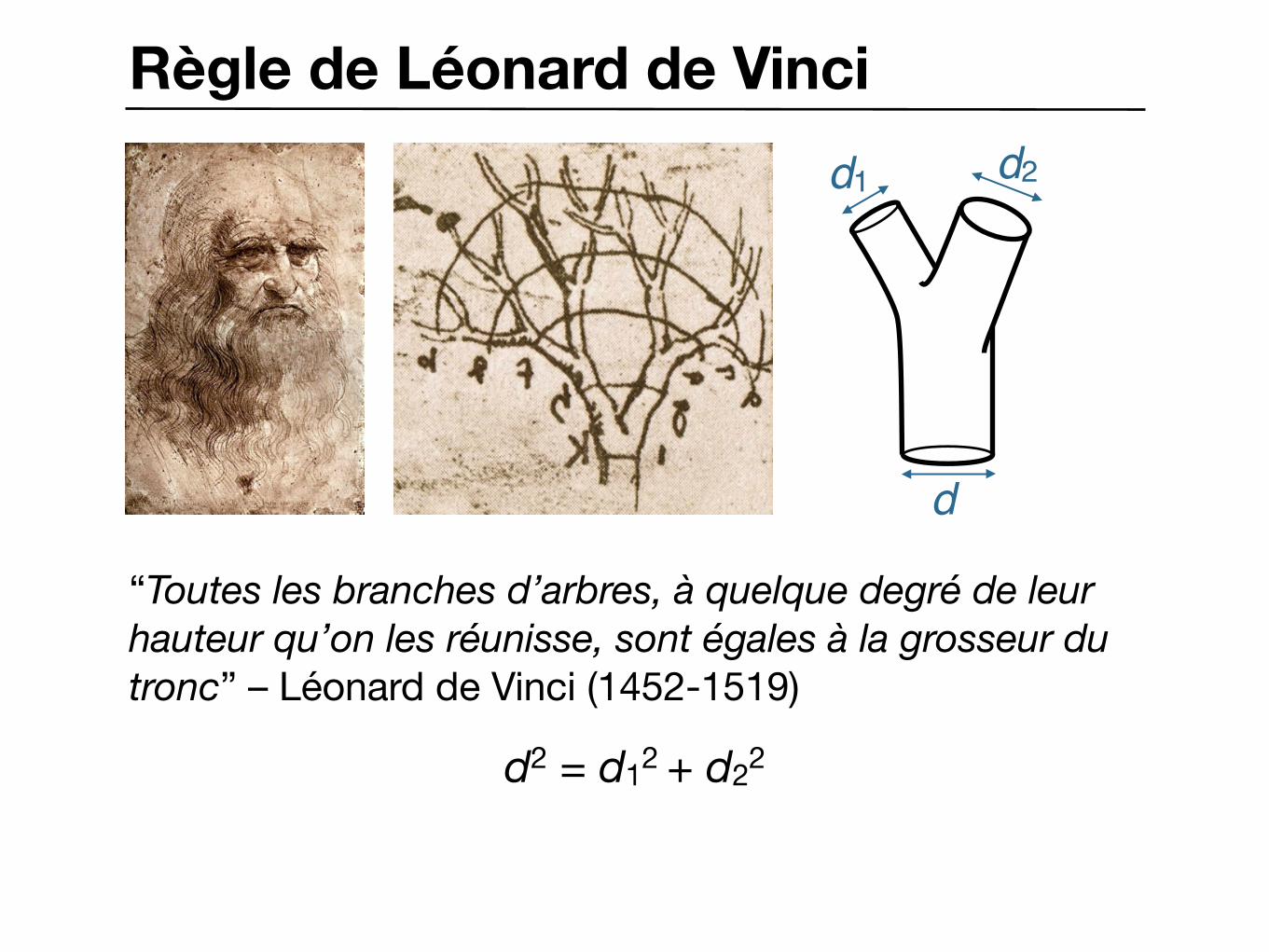
Règle de Léonard de Vinci

“Toutes les branches d’arbres, à quelque degré de leur hauteur qu’on les réunisse, sont égales à la grosseur du tronc” – Léonard de Vinci (1452-1519)

d2 = d12 + d22

d

d1 d2

Loi de Murray

“We see one of the simplest requirements for maximum efficiency in the circulation —namely that the flow of blood past any section shall everywhere bear the same relation to the cube of the radius of the vessel at that point.” – Cecil D. Murray

d3 = d13 + d23

d

d1 d2

Exposant de Léonard ∆

•Mandelbrot : ∆ ≈ 2 (3 essences)- B. Mandelbrot, The fractal geometry of nature, Freeman (1983)

• Aratsu : ∆ ≈ 2.2 (10 essences)- Aratsu, J. Young Invest. (1998)

• Sone et al. : ∆ = 2.0 (1 essence d’érable)- Sone et al., J. Plant Res. (2009)

Introduction Leonardo’s rule Beam model Current work

Measurements of Leonardo exponent

� = 1 � = 2 � = 3

• Mandelbrot: “� slightly smaller than 2” (3 species)McMahon, Kronauer, J. Theor. Biol. (1976)Mandelbrot, The fractal geometry of nature, Freeman (1983)

• Aratsu: � ⇡ 2.2 (10 species)Aratsu, J. Young Invest. (1998)

• Sone et al.: � = 2.0 (1 species: Redvein maple)Sone et al., J. Plant Res. (2009)

Un regard de physicien sur l’architecture des arbres C. Eloy, IRPHE, Aix-Marseille Université 14

d∆ = d1∆ + d2∆

Structure auto-affine

• Similitude des diamètres :

dk∆ = N dk+1∆

• Similitude des longueurs :

lkD = N lk+1D

Introduction Leonardo’s rule Beam model Current work

Self-affinity

• Self-similarity of the skeleton: lk/lk+1 = N1/D (with2 < D < 3)• Diameter ratio: dk/dk+1 = N1/�, (� 6= D Leonardo’s exponent)

• In practice, D ⇡ 2.5 and � ⇡ 2• It means that Sk ⇠ Nk lk dk ! 1 and Vk ⇠ Nk lk d2

k ! 0 as k ! 1• Possibility of a statistical definition of self-affinity

Un regard de physicien sur l’architecture des arbres C. Eloy, IRPHE, Aix-Marseille Université 6

Ordre de Horton–StrahlerGeneration:101 Nb branches:0436

1

23

4

5

Ordre de Horton–Strahler

EFFICIENCY OF B R A N C H I N G PATTERNS 343

TABLE I

data for Fig. 2 Number and average lengths of branches of various orders and other

Species : Fir (Abies concolor) Location: 10350 W. 13th PI., Denver, Colorado,

Size and age: Diameter breast high, 0.2 ft; 12 yrs

Needles or leaves:

August 1964

(est.); height 10 ft (est.)

Average 0.08 to 0.17 ft in length; needles solitary

Order of Number of Average length branch branches (ft)

1 88 0.27 2 21 -17 3 4 1.8 4 1 4.9

Main trunk estimated as fifth order.

Order Number

FIG. 2. Numbers and average lengths of branches of various orders. e, On a 10-ft high fir tree (Abies concolor); A, a pine 19-ft high (P. tuedu). In the left-hand plot, the branching ratio = 4.8; in the right-hand plot, the length ratio = 2 3 for the pine (- - -) and 2.7 for the fir (-). Open symbols marked E indicate estimated values. • Rapport des branches : Rn = ni+1 / ni

• Rapport des longueurs ratio : Rs = si / si+1

• Dimension fractale : D = ln Rn / ln Rs

- L.B. Leopold, J. Theor. Biol. (1971)

E F F I C I E N C Y O F B R A N C H I N G P A T T E R N S 351

The data plotted include one or several trials of each rule. It was found that successive trials under the same rules give very comparable results, for the data converge rapidly with replication.

Table 2 presents the average values of the bifurcation and length ratios for a variety of field examples and random models. The values of each ratio are quite comparable among the various types of examples. Bifurcation ratio averages about 3.8 which is only slightly larger than the value 3.5 for river networks for which a large number of data are available compared with a small number of examples of all other categories. The length ratio averages 2.6.

TABLE 2 Average values of branching characteristics of several field examples and

random models

Bifurcation Length ratio? ratio$

Average values Average values -_ ___- - - _. -

Two-dimensional River networks 3.5 2.3 Random models of

river networks 4.1 2.5 Theory5 2 to 4

Trees 5.1 3.4 Roots 3.2 2.4 Tinker-toy random

models 3.3 2.3

Three-dimensional

t Bifurcation ratio defined as the average number of branches of

$ Length ratio defined as ratio of average length of branches of a

8 Leopold & Langbein, 1962, p. A15.

a given order per branch of next higher order.

given order to average length of next higher order.

7. Area-hours Exposed to Direct Sunlight by a Simple Plant

In the preceding pages I have been concerned with the tendency for efficiency by the minimization of the total length of all the branches of a plant. Presumably there are opposing tendencies which constrain the branch- ing pattern. In a plant one tendency probably concerns both uniformity and maximization of the sunlight hours on each unit of leaf area. As a first rudimentary approach to this, a question was posed as follows.

Croissance d’un arbre

• L’architecture finale résulte d’un compromis entre croissance et élagage

• Question ouverte : Peut-on reproduire une architecture similaire à celles des arbres par des processus locaux ?

réalité

vision naïve

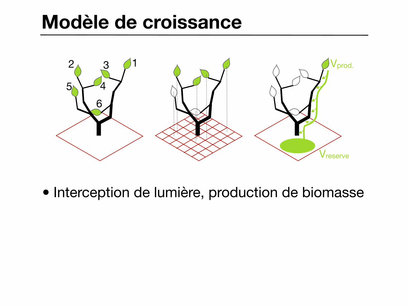
Modèle de croissance

• Interception de lumière, production de biomasse

12 3

456

Vprod.

Vreserve

Modèle de croissance

• Interception de lumière, production de biomasse

• Contraintes mécaniques, intensité des puits

12 3

456

Vprod.

Vreserve

Uσmax Vreq.

Vreq./2 Vreq./2

Vreq.

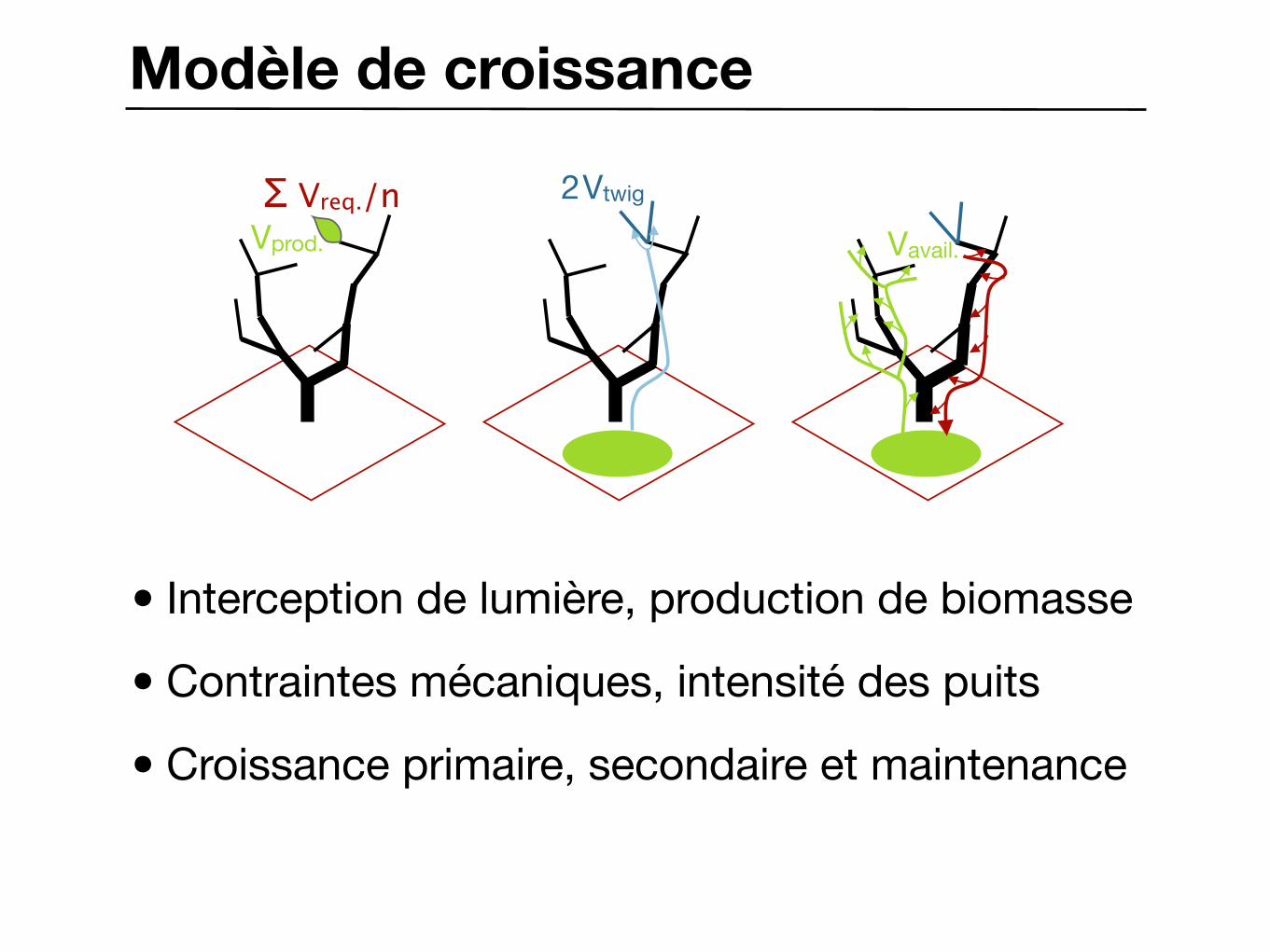
Modèle de croissance

• Interception de lumière, production de biomasse

• Contraintes mécaniques, intensité des puits

• Croissance primaire, secondaire et maintenance

12 3

456

Vprod.

Vreserve

Uσmax Vreq.

Vreq./2 Vreq./2

Vreq.

Σ Vreq./nVprod.

2 Vtwig

Vavail.

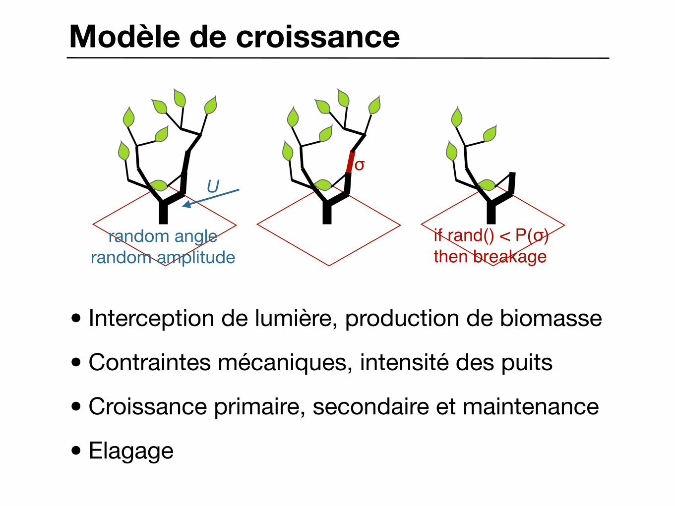
Modèle de croissance

• Interception de lumière, production de biomasse

• Contraintes mécaniques, intensité des puits

• Croissance primaire, secondaire et maintenance

• Elagage

12 3

456

Vprod.

Vreserve

Uσmax Vreq.

Vreq./2 Vreq./2

Vreq.

Σ Vreq./nVprod.

2 Vtwig

Vavail.

Uσ

if rand() < P(σ)then breakage

random anglerandom amplitude

Stratégies de croissance

lumièreVreq.

Vreq.Σ Vreq.

σmax

Nleaves

diamètre

newtwigs(Y/N)

• Stratégie de croissance = réponse aux stimuli

• Pas d’ansatz

Stratégies de croissance

lumièreVreq.

Vreq.Σ Vreq.

σmax

Nleaves

diamètre

newtwigs(Y/N)

j

Iij Ojk

entrées sorties

ik

Optimisation multi-objectifs

génome

angles

synapsesfeuilles

synapsesbranches

Generation:101 Nb branches:0713

Generation:101 Nb branches:0495

Generation:101 Nb branches:2065

Nbranches

Hlow resource

Nhigh wind

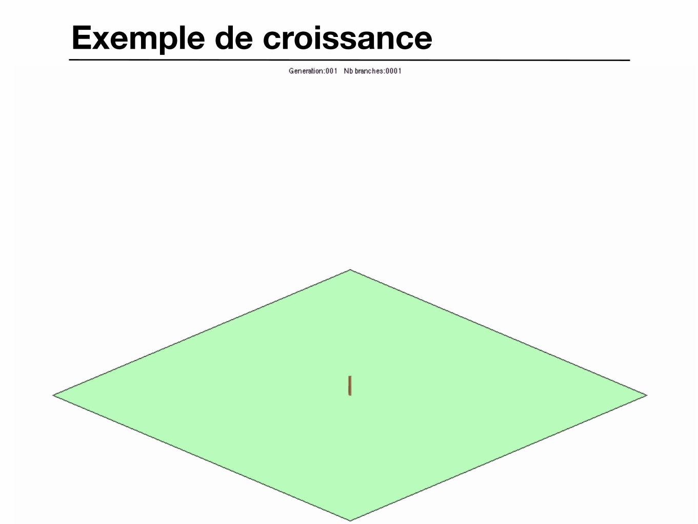
Exemple de croissance

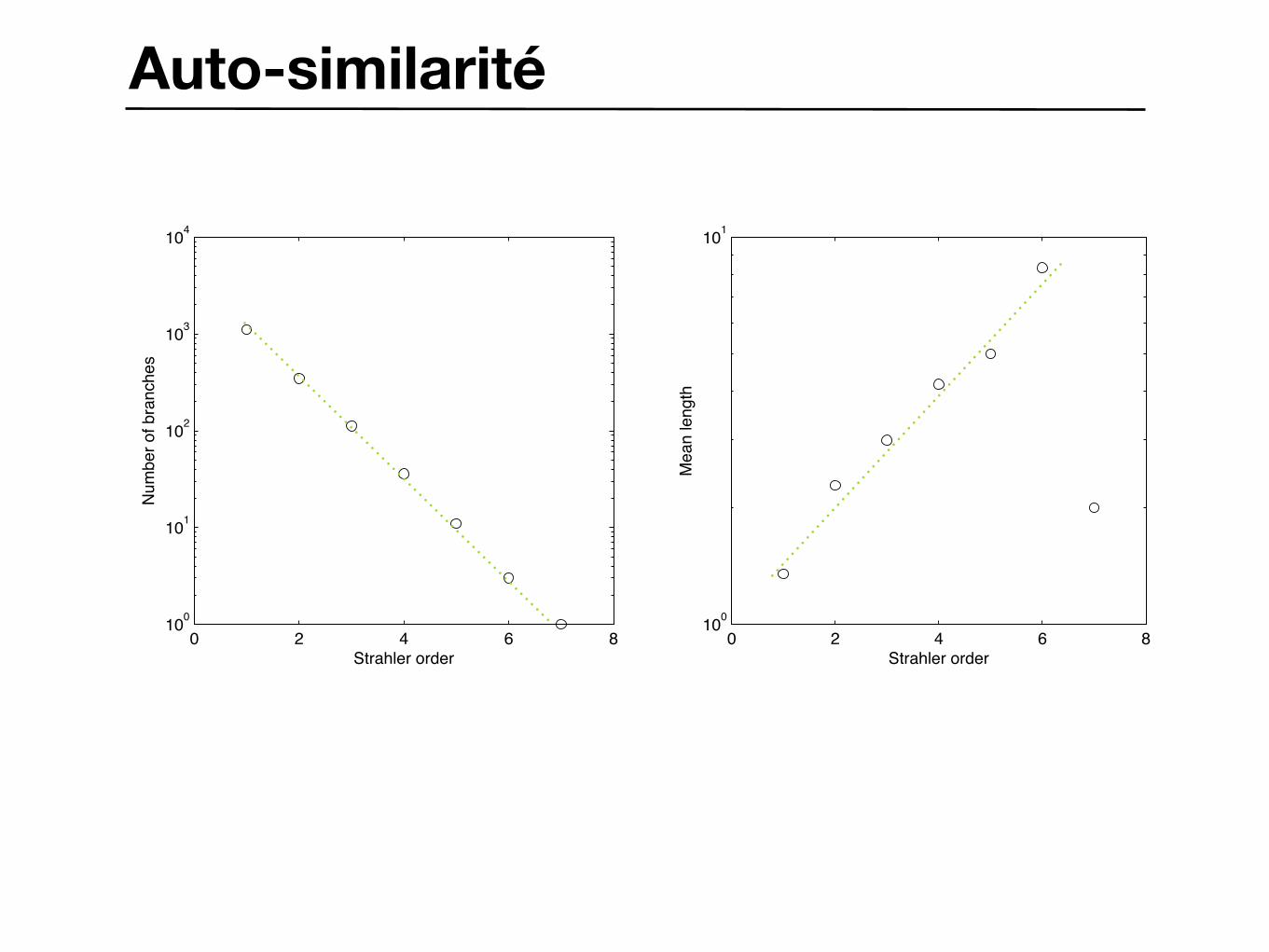
Auto-similarité

0 2 4 6 8100

101

Strahler orderM

ean

leng

th

0 2 4 6 8100

101

102

103

104

Strahler order

Num

ber o

f bra

nche

s

Discussion

• Ingénierie inverse de l’adaptation

• Optimisation multi-objectifs et diversité

• Acclimatation vs. adaptation