
A Reactive Decision Support System for Intermodal Freight ... · validate the decision support...
169
Thèse de doctorat A Reactive Decision Support System for Intermodal Freight Transportation Yunfei Wang July 2017 CIRRELT-2017-45
Transcript of A Reactive Decision Support System for Intermodal Freight ... · validate the decision support...
Thèse de doctorat
A Reactive Decision Support System for Intermodal Freight Transportation Yunfei Wang July 2017 CIRRELT-2017-45
A Reactive Decision Support System for Intermodal Freight Transportation
Yunfei Wang
Laboratoire d'Automatique, de Mécanique et d'Informatique industrielles et Humaines (LAMIH), Université de Valenciennes et du Hainaut-Cambrésis (UVHC), Batiment Malvache, Le Mont Houy, F59313 Valenciennes Cedex 9, France
Abstract. Barge transportation is an important research topic that started to draw increasing scientific attention in the recent decade. Considered as sustainable, environment-friendly and economical, barge transportation has been identified as a competitive alternative for freight transportation, complementing the traditional road and rail modes. However, contributions related to barge transportation, especially in the context of intermodal transportation, are still scarce. The objective of this thesis is to contribute to fill this gap by proposing a reactive decision support system for freight intermodal barge transportation from the perspective of the carriers. The proposed system incorporates resource and revenue management concepts and principles to build the optimal set of scheduled services plans at the tactical level. Carriers may thus benefit from transportation plans offering increased flexibility and reliability. They could thus serve more demands and better satisfy customers. One novelty of the approach is the application of revenue management considerations (e.g., market segmentation and price differentiation) at both operational and tactical planning levels. The optimization problems are mathematically formalized and mixed integer linear programming (MILP) models are proposed, implemented and tested against various network settings and demand scenarios, for each decision level. At the tactical level, a new solution approach, combining adaptive large neighborhood search (ALNS) and Tabu search is designed to solve large scale MILP problems. An integrated simulation framework, including the tactical and the operational levels jointly, is proposed to validate the decision support system in different settings, in terms of physical network topology, revenue management parameters and accuracy degree of demand forecasts. To analyze the numerical results corresponding to the solutions of the optimization problems, several categories of performance indicators are proposed and used. Keywords: Intermodal barge transportation, decision support system, revenue management, scheduled service network design, mixed integer linear programming, metaheuristics, network capacity allocation, discrete event simulation, performance indicators.
Results and views expressed in this publication are the sole responsibility of the authors and do not necessarily reflect those of CIRRELT.
Les résultats et opinions contenus dans cette publication ne reflètent pas nécessairement la position du CIRRELT et n'engagent pas sa responsabilité. _____________________________
* Corresponding author: [email protected]
Dépôt légal – Bibliothèque et Archives nationales du Québec Bibliothèque et Archives Canada, 2017
© Wang and CIRRELT, 2017

Thèse de doctorat
Pour obtenir le grade de Docteur de l’Université de
VALENCIENNES ET DU HAINAUT-CAMBRÉSIS
Spécialité: Informatique
présentée et soutenue par Yunfei, WANG.
Le 2 mars 2017, à Valenciennes
École doctorale:Sciences Pour l’Ingénieur (SPI)
Laboratoire:Laboratoire d’Automatique, de Mécanique et d’Informatique industrielles et Humaines(LAMIH UMR CNRS 8201)
Un Système Réactif d’Aide à la Décision pourle Transport Intermodal de Marchandises
JURYPrésident du jury:Pr. Teodor Gabriel Crainic (CIRRELT et UQAM, Montréal, Canada)Rapporteurs:Pr. Marcel Mongeau (ENAC, Toulouse, France)Pr. Tom van Woensel (TUE, Eindhoven, Pays-Bas)Examinateurs:Pr. Assoc. Guido Perboli (Politecnico, Torino, Italie)Directeurs de thèse:Pr. Abdelhakim Artiba (UVHC, LAMIH UMR CNRS 8201, France)MCF. Ioana Bilegan (UVHC, LAMIH UMR CNRS 8201, France)Invités:Mme. Anna Melsen (Coordinatrice de la plateforme d’innovation i-Fret, i-Trans, Dunkerque, France)M. Ludovic Vaillant (PhD, Directeur d’études, CEREMA, Lille, France)
A Reactive Decision Support System for Intermodal Freight Transportation
CIRRELT-2017-45

A Reactive Decision Support System for Intermodal Freight Transportation
CIRRELT-2017-45
Publications
Journals
• Wang Y., Bilegan I.C., Crainic T.G., Artiba A. (2016). A Revenue ManagementApproach for Network Capacity Allocation of an Intermodal Barge TransportationSystem. In: A. Paias et al. (Eds.) ICCL 2016. LNCS, vol. 9855, pp. 243-257.DOI: 10.1007/978-3-319-44896-1_16.
• Wang Y., Bilegan I.C., Crainic T.G., Artiba A. (2014). Performance Indicatorsfor Planning Intermodal Barge Transportation Systems. Transportation ResearchProcedia, 3, pp. 621-630. ISSN 2352-1465.
Working Papers
• Scheduled Service Network Design with Resource and Revenue Management Con-siderations for Intermodal Barge Transportation. Article manuscript in progress, tobe submitted to Transportation Science, 2017.
• A Metaheuristic for Service Network Design with Revenue Management for FreightIntermodal Transportation. Data collection and analysis in progress, to be submit-ted.
International Conferences
• Crainic T.G., Bilegan I.C., Wang Y. (2016). Barge Scheduled Service NetworkDesign with Resource and Revenue Management. INFORMS 2016 Annual Meeting,Nashville, United States, November.
• Crainic T.G., Bilegan I.C., Wang Y. (2016). Scheduled Service Network Designwith Revenue Management Considerations: An Intermodal Barge Transportation
A Reactive Decision Support System for Intermodal Freight Transportation
CIRRELT-2017-45

Application. Ninth Triennial Symposium on Transportation Analysis (TRISTANIX), Aruba, June.
• Wang Y., Crainic T.G., Bilegan I.C., Artiba A. (2015). A Metaheuristic for Ser-vice Network Design with Revenue Management for Freight Intermodal Transport.CORS/INFORMS International Conference, Montreal, Canada, June.
• Bilegan I.C., Crainic T.G., Wang Y. (2015). Revenue Management for ContainerTransportation Activities Optimization: from the Operational to the Tactical Level.17th British-French-German Conference on Optimization, London, UK, June.
• Wang Y., Bilegan I.C., Artiba A. (2015). A Reactive Decision Support System forFreight Intermodal Transportation Services (Poster). Matiné des Chercheurs 2015,Mons, Belgium, March.
A Reactive Decision Support System for Intermodal Freight Transportation
CIRRELT-2017-45

Acknowledgments
Pursuing the PhD is an amazing journey, in which there were full of difficulties and chal-lenges. It is impossible to imagine how I could finish this journey without the assistanceand inspiration of lots of people. Therefore, I would like to express my profound gratitudeto all of you.
First of all, I would like to express my appreciation to my supervisor, Professor Ab-delhakim Artiba, for the confidence he showed on me, for his valuable and constructivecomments, for his contributions and for his support throughout my three-year PhD re-search.
My greatest and most heartfelt gratitude goes to my supervisor, my tutor, even con-sidered as my family member, Professor Ioana Bilegan. Without her, I would not evenhave the chance to carry out my PhD research in LAMIH, University of Valenciennes.I would like to thank her for introducing me to Operations Research, for guiding mein all aspects with her deep suggestions, for her confidence in me when difficulties wereencountered, for her patience and for her constant availability. I have learned a lot fromher, e.g., how to strive for excellence details, how to tackle challenges and how to presentresearch problems from different perspectives, which are valuable and priceless, not onlyfor my research, but also for my life.
I would also like to thank Professor Teodor Gabriel Crainic. I am extremely gratefulfor the time he dedicated to me, for the chance he offered me conducting research inCIRRELT, Canada, under his supervision, for the efficient correction and improvement formy publications and thesis, and for his larger and higher perspective. His encouragementis like a spur to me so that I have the motivation to work harder and make further progress.I also appreciate the life experience he shared with me when we had the one-day trip inPairs. Sincerely, it is an honor to work with him.
Many thanks to Professor Marcel Mongeau, Professor Tom Van Woensel, ProfessorGuido Perboli and Doctor Ludovic Vaillant for being on my thesis committee. I appreciatetheir time spent on reading my thesis and their valuable feedbacks for my work.
It is impossible to carry out my PhD research without the financial support from i-Trans/i-Fret and Region Nord-Pas de Calais. Huge thanks go to Anna Melsen, who isthe coordinator of i-Fret, for her valuable support, constant confidence and constructive
A Reactive Decision Support System for Intermodal Freight Transportation
CIRRELT-2017-45

comments. I also want to extend my thanks to the Doctoral School of Lille and CNRSGDR RO for the scholarships they offered for my research in CIRRELT.
Next, I would like to express my gratitude for David, Abdessamad and other fellowresearchers from LAMIH. The discussions we had during the Doctor Days, seminars andmeetings are valuable. They helped me to formulate and formalize many views presentedin this thesis. I also appreciate their advices beyond research. It is a pleasure for me towork in LAMIH, University of Valenciennes.
Many thanks go to Dana, Elias, Souhir, Molly, Ben, Valerie, Marko, Zeineb, Ihsen,Karim, Guanwen, Hanane, Marie-France and so many others friends, officemates andcolleagues from LAMIH. It is not easy to live alone in a foreign country. But all themeetings, pleasant meals, countless coffee breaks and amazing parties, that we experiencedtogether, helped me to get used to and fit in this new place. Because of all my friends here,Valenciennes becomes my second hometown (even I still do not speak fluently French).
The same appreciations are expressed to Selene, Vinicius, Xiaolu, Slavic, Shahrouz andother friends who I met from CIRRELT. I am grateful for their constructive comments,selfless help, heartfelt company and especially for the trips we made together. All thosejoyful moments are the memories that I cherish. I am lucky to have supports from all ofyou.
I would also like to express my gratitude towards all secretaries of both LAMIH andCIRRELT, who took care the non-acdamic matters for me and gave me a hand wheneverI needed. My appreciations are also delivered to the technical staff of both CIRRELTand Calcul Quebec for their support.
Finally, special thanks fly to my beloved parents. It has been five years, in total, sinceI left China to pursue my study. I could not even imagine how it is possible for me tocomplete this thesis without your endless love, selfless sacrifice and infinite encouragement.Thank you a lot for your support. I love both of you so much.
In fact, my gratitude for all of you, whomever I mentioned or not, is beyond my abilityof expression. I just want to simply express my appreciation one more time. Thank youall for the appearance and participation in my past three years. Because of you, I amable to complete this thesis. Because of you, this journey becomes rich, colorful, specialand unforgettable.
Yunfei Wang
Valenciennes, May 2017
A Reactive Decision Support System for Intermodal Freight Transportation
CIRRELT-2017-45
List of Contents
List of Figures V
List of Tables VII
List of Algorithms X
General Introduction 1
I Introduction 5
I.1 Background, Motivation & Research Problems . . . . . . . . . . . . . . . . 6
I.2 Research Methodology . . . . . . . . . . . . . . . . . . . . . . . . . . . . . 13
I.3 Contributions of the Thesis . . . . . . . . . . . . . . . . . . . . . . . . . . 15
I.4 Structure of the Thesis . . . . . . . . . . . . . . . . . . . . . . . . . . . . . 18
II A Revenue Management Approach for Network Capacity Allocation ofan Intermodal Barge Transportation System 19
II.1 Introduction . . . . . . . . . . . . . . . . . . . . . . . . . . . . . . . . . . . 21
II.2 Problem Characterization . . . . . . . . . . . . . . . . . . . . . . . . . . . 23
II.2.1 Dynamic Capacity Allocation Problem . . . . . . . . . . . . . . . . 23
II.2.2 RM Policies . . . . . . . . . . . . . . . . . . . . . . . . . . . . . . . 25
II.3 DCA-RM Model Formulation . . . . . . . . . . . . . . . . . . . . . . . . . 26
I
A Reactive Decision Support System for Intermodal Freight Transportation
CIRRELT-2017-45
II.4 Simulation, Numerical Results and Analysis . . . . . . . . . . . . . . . . . 29
II.4.1 Scenario Settings . . . . . . . . . . . . . . . . . . . . . . . . . . . . 30
II.4.2 Numerical Results and Analysis . . . . . . . . . . . . . . . . . . . . 32
II.5 Extended DCA-RM Model . . . . . . . . . . . . . . . . . . . . . . . . . . . 37
II.6 Conclusions . . . . . . . . . . . . . . . . . . . . . . . . . . . . . . . . . . . 41
IIIScheduled Service Network Design with Revenue Management Consid-erations for Intermodal Barge Transportation 43
III.1 Introduction . . . . . . . . . . . . . . . . . . . . . . . . . . . . . . . . . . . 45
III.2 Literature Review . . . . . . . . . . . . . . . . . . . . . . . . . . . . . . . . 47
III.3 Problem Statement . . . . . . . . . . . . . . . . . . . . . . . . . . . . . . . 49
III.4 The SSND-RRM Formulation . . . . . . . . . . . . . . . . . . . . . . . . . 54
III.4.1 Revenue Management Modeling for the SSND-RRM . . . . . . . . . 54
III.4.2 Network Modeling . . . . . . . . . . . . . . . . . . . . . . . . . . . 55
III.4.3 SSND-RRM Model Formulation . . . . . . . . . . . . . . . . . . . . 59
III.5 Simulation and Numerical Results . . . . . . . . . . . . . . . . . . . . . . . 63
III.5.1 Test Instances Generation . . . . . . . . . . . . . . . . . . . . . . . 63
III.5.2 Experiment Plan . . . . . . . . . . . . . . . . . . . . . . . . . . . . 65
III.5.3 Experiment Results and Analysis: First Group . . . . . . . . . . . . 68
III.5.4 Experiment Results and Analysis: Second Group . . . . . . . . . . 71
III.5.5 Computational Time . . . . . . . . . . . . . . . . . . . . . . . . . . 74
III.6 Conclusions . . . . . . . . . . . . . . . . . . . . . . . . . . . . . . . . . . . 75
IVA Metaheuristic for Scheduled Service Network Design with Resourceand Revenue Management for Intermodal Barge Transportation 79
IV.1 Introduction . . . . . . . . . . . . . . . . . . . . . . . . . . . . . . . . . . . 81
II
A Reactive Decision Support System for Intermodal Freight Transportation
CIRRELT-2017-45

IV.2 Literature Review . . . . . . . . . . . . . . . . . . . . . . . . . . . . . . . . 82
IV.3 Problem Statement and Formulation of SSND-RRM . . . . . . . . . . . . . 84
IV.4 Solution Approach . . . . . . . . . . . . . . . . . . . . . . . . . . . . . . . 85
IV.4.1 Initialization . . . . . . . . . . . . . . . . . . . . . . . . . . . . . . . 88
IV.4.2 Improvement . . . . . . . . . . . . . . . . . . . . . . . . . . . . . . 89
IV.5 Computational Results and Analysis . . . . . . . . . . . . . . . . . . . . . 105
IV.5.1 Test Instance Generation . . . . . . . . . . . . . . . . . . . . . . . . 106
IV.5.2 Calibration . . . . . . . . . . . . . . . . . . . . . . . . . . . . . . . 107
IV.5.3 Benchmarking against an MILP Solver . . . . . . . . . . . . . . . . 108
IV.5.4 Analysis of the Impact of Each Algorithmic Component . . . . . . . 110
IV.6 Conclusions and Future Work . . . . . . . . . . . . . . . . . . . . . . . . . 110
V Performance Indicators for Planning Intermodal Barge TransportationSystems 113
V.1 Introduction . . . . . . . . . . . . . . . . . . . . . . . . . . . . . . . . . . . 115
V.2 Problem Characterization . . . . . . . . . . . . . . . . . . . . . . . . . . . 117
V.3 A First Step towards a Taxonomy of Performance Indicators . . . . . . . . 119
V.4 Test Instance Generation . . . . . . . . . . . . . . . . . . . . . . . . . . . . 122
V.5 Numerical Results and Analysis . . . . . . . . . . . . . . . . . . . . . . . . 123
V.6 R-DSS Assessment . . . . . . . . . . . . . . . . . . . . . . . . . . . . . . . 127
V.6.1 Simulation Framework . . . . . . . . . . . . . . . . . . . . . . . . . 128
V.6.2 Preliminary Assessment . . . . . . . . . . . . . . . . . . . . . . . . 129
V.7 Conclusions . . . . . . . . . . . . . . . . . . . . . . . . . . . . . . . . . . . 134
General Conclusions 137
III
A Reactive Decision Support System for Intermodal Freight Transportation
CIRRELT-2017-45

Bibliography 145
IV
A Reactive Decision Support System for Intermodal Freight Transportation
CIRRELT-2017-45
List of Figures
I.1 Inland waterway network of Northern France, Belgium, Netherlands . . . . 8
I.2 Structure of the proposed reactive decision support system; Both tacticaland operational planning levels are considered; Revenue Management (RM)policies are introduced . . . . . . . . . . . . . . . . . . . . . . . . . . . . . 9
I.3 a. An example of physical network of four terminals with three servicesdefined; b. The corresponding three services with schedules presented in atime-space network . . . . . . . . . . . . . . . . . . . . . . . . . . . . . . . 12
II.1 Procedure of the simulation . . . . . . . . . . . . . . . . . . . . . . . . . . 29
II.2 Effect of price differentiation on revenue (a) and on rejected requests (b) . 33
II.3 Procedure of the simulation combined with negotiation phase . . . . . . . . 36
II.4 Performance of the extended DCA-RM model; The accumulated total rev-enues of RM_ReRoute, RM and FCFS are presented . . . . . . . . . . . . 39
II.5 Examples of the three possible performance patterns of RM_ReRoute, RMand FCFS . . . . . . . . . . . . . . . . . . . . . . . . . . . . . . . . . . . . 41
III.1 Time-related attributes of service s . . . . . . . . . . . . . . . . . . . . . . 58
III.2 Time-space representation of the service network with two services . . . . . 59
III.3 Three physical network topologies considered for the SSND-RRM modelvalidation . . . . . . . . . . . . . . . . . . . . . . . . . . . . . . . . . . . . 64
III.4 Relative yield obtained in the second experiment group . . . . . . . . . . . 73
IV.1 An example of service cycles . . . . . . . . . . . . . . . . . . . . . . . . . . 91
V
A Reactive Decision Support System for Intermodal Freight Transportation
CIRRELT-2017-45
IV.2 Three considered physical network topologies . . . . . . . . . . . . . . . . . 106
IV.3 Calibration of parameter r . . . . . . . . . . . . . . . . . . . . . . . . . . . 108
V.1 A general physical network . . . . . . . . . . . . . . . . . . . . . . . . . . . 122
V.2 The value hierarchy of demand category ratios (R/P) for different perfor-mance indicators . . . . . . . . . . . . . . . . . . . . . . . . . . . . . . . . 125
V.3 The trends of total cost decrease and net profit increase when increasingthe ratio of punctual demands . . . . . . . . . . . . . . . . . . . . . . . . . 126
V.4 The trends of different cost component indicators when increasing the ratioof punctual demands . . . . . . . . . . . . . . . . . . . . . . . . . . . . . . 126
V.5 The trends of resource utilization and quality-of-service indicators whenincreasing the ratio of punctual demands . . . . . . . . . . . . . . . . . . . 127
V.6 An example of service deployment from tactical to operational level . . . . 128
VI
A Reactive Decision Support System for Intermodal Freight Transportation
CIRRELT-2017-45
List of Tables
II.1 Ratio of total revenue of RM/FCFS . . . . . . . . . . . . . . . . . . . . . . 34
II.2 Number of rejected demands of RM/FCFS . . . . . . . . . . . . . . . . . . 35
II.3 Effect of different negotiation strategies for rejected R customers . . . . . . 37
III.1 Characteristics of the two groups of experiments . . . . . . . . . . . . . . . 65
III.2 Topology n4 : Fast demands spread uniformly over the network, no faredifferentiation . . . . . . . . . . . . . . . . . . . . . . . . . . . . . . . . . . 68
III.3 Topology n4 : Fast demands concentrate at one port, no fare differentiation 68
III.4 Topology n6 : Fast demands spread uniformly over the network, no faredifferentiation . . . . . . . . . . . . . . . . . . . . . . . . . . . . . . . . . . 70
III.5 Topology n6 : All fast demands concentrate at one port, no fare differentiation 70
III.6 Topology n7 : Fast demands spread uniformly over the network, no faredifferentiation . . . . . . . . . . . . . . . . . . . . . . . . . . . . . . . . . . 71
III.7 Topology n7 : All fast demands concentrate at one port, no fare differentiation 71
III.8 Topology n4 : Experiment group 2 . . . . . . . . . . . . . . . . . . . . . . . 72
III.9 Topology n6 : Experiment group 2 . . . . . . . . . . . . . . . . . . . . . . . 74
III.10Topology n7 : Experiment group 2 . . . . . . . . . . . . . . . . . . . . . . . 74
III.11Statistics of computational time for 180 test instances in group 1 of topologyLinear n4 . . . . . . . . . . . . . . . . . . . . . . . . . . . . . . . . . . . . 75
VII
A Reactive Decision Support System for Intermodal Freight Transportation
CIRRELT-2017-45

III.12Computational time and size of large instances on topologies of Linear n4,Star n6 and General n7 . . . . . . . . . . . . . . . . . . . . . . . . . . . . 75
IV.1 Definition of estimated contribution of arcs to each Y-selection heuristic . 94
IV.2 Start arcs with interesting characteristics to each Y-selection heuristic . . . 95
IV.3 Association table of each F-selection heuristic with Y-selection heuristics . 102
IV.4 Details of the solutions to all test instances obtained by CPLEX after oneday . . . . . . . . . . . . . . . . . . . . . . . . . . . . . . . . . . . . . . . . 109
IV.5 Numerical results obtained by the proposed MH with CPLEX as comparison109
V.1 A first classification of performance indicators used for tactical planning ofintermodal barge transportation systems . . . . . . . . . . . . . . . . . . . 121
V.2 Performance indicators with fare ratio . . . . . . . . . . . . . . . . . . . . 125
V.3 Output of the tactical planning with different strategies . . . . . . . . . . . 131
V.4 Assessment of the proposed R-DSS: Group 1 . . . . . . . . . . . . . . . . . 132
V.5 Assessment of the proposed R-DSS: Group 2 . . . . . . . . . . . . . . . . . 134
VIII
A Reactive Decision Support System for Intermodal Freight Transportation
CIRRELT-2017-45
List of Algorithms
1 Overview of the proposed MH . . . . . . . . . . . . . . . . . . . . . . . . . . 87
2 Restore the feasibility of the limit on resources . . . . . . . . . . . . . . . . 89
3 Adapted labeling algorithm . . . . . . . . . . . . . . . . . . . . . . . . . . . 92
4 Identify a service cycle in time-space network . . . . . . . . . . . . . . . . . 94
5 Set up the candidate list of promising neighbors . . . . . . . . . . . . . . . . 95
6 Identify a set of neighbors for a given service cycle . . . . . . . . . . . . . . 96
7 Identify and evaluate neighbors (improve one service cycle) . . . . . . . . . 98
8 Basic greedy algorithm to select accepted F demands . . . . . . . . . . . . . 101
9 Score the chosen heuristics . . . . . . . . . . . . . . . . . . . . . . . . . . . 103
IX
A Reactive Decision Support System for Intermodal Freight Transportation
CIRRELT-2017-45

A Reactive Decision Support System for Intermodal Freight Transportation
CIRRELT-2017-45
General Introduction
Barge transportation is an important research topic that started to draw increasing sci-entific attention in the recent decade. Considered as sustainable, environment friendlyand economical, barge transportation has been identified as a competitive alternativefor freight transportation, complementing the traditional road and rail modes. However,contributions related to barge transportation, especially in the context of intermodaltransportation, are still scarce. The objective of this thesis is to contribute to fill this gapby proposing a Reactive Decision Support System (R-DSS) for freight intermodal bargetransportation from the perspective of the carriers. To achieve the R-DSS, four relatedresearch problems are proposed and addressed in this thesis.
In the first phase of the study, we propose a revenue management model (DCA-RM)for the network capacity allocation problem of an intermodal barge transportation system,at operational level. In the proposed DCA-RM model, two RM policies (i.e., customerclassification and price differentiation) are considered. In terms of customer classification,three categories of customers are identified according to their business relationships withthe carriers. Their transport requests, therefore, are accordingly treated differently. Theproposed DCA-RM model makes decisions to accept or reject a transport request bymaximizing the expected revenue of current demand and potential future demands overa given time horizon, taking into account several categories of customers. The consideredpotential future demands are characterized by probability distribution functions, withrespect to their volume. Sequential arrivals of transport requests are simulated to validateand assess the proposed DCA-RM model. A conventional model for dynamic capacityallocation considering only the feasibility, in terms of network capacity and delivery timeconstraints is used as alternative for comparison.
In the second part of the research, we propose what we believe to be, the first com-prehensive Scheduled Service Network Design model for freight carriers that integratesboth Resource and Revenue Management considerations (SSND-RRM). RM policies areequally considered in the proposed tactical planning model. To be more precise, cus-tomers are classified into several categories according to their business relationships with
1
A Reactive Decision Support System for Intermodal Freight Transportation
CIRRELT-2017-45
General Introduction
the carriers, and are dealt with following different (acceptance/denial) rules. In termsof resource management, design-balance constraints are considered to ensure the vehicleflow conservation at each terminal for each time instant. Vehicles repositioning is thusimplicitly considered as the SSND-RRM problems are formulated as a cyclic model. Inaddition, upper bounds on the quantity of the resource are also formulated. Freight trans-shipment between services and freight holding at terminals are also considered, with theircorresponding handling and holding costs. In order to validate RM policies considerationat tactical level for freight transportation and to assess the performances of the proposedmodel, we test the SSND-RRM model in various problem settings, in terms of demanddistribution, network topology, fare classes and quality-of-service (e.g., delivery time).The optimization problems are solved by feeding a commercial solver.
As the optimization problems addressed at tactical level are NP-hard, we propose ametaheuristic (MH) to produce high-quality solutions for the SSND-RRM problems inreasonable time, in a third part of the research study. The proposed solution approach iscomposed of four phases. In the first phase, a constructive heuristic is proposed to obtainan initial feasible solution. The solutions are then iteratively improved in the secondphase following a local search procedure. Adaptive large neighborhood search (ALNS)and tabu search are combined to guide the search. The other two phases: intensificationand diversification are also included to deeply explore a given region of the solution spaceand to direct the search towards non-thoroughly-explored regions of the solution space,respectively. Moreover, new neighborhood structures are proposed to accelerate the searchby ensuring the design-balance constraints and quick exploration simultaneously. Learningmechanisms are embedded into the proposed MH and used to guide the search. As noother solution approach to the proposed SSND-RRM problems exists in the literature,a commercial solver (IBM CPLEX) is used to compare with, in terms of computationaltime and solution quality.
The fourth research problem studied concerns a review of Performance Indicators(PIs) that could be used to evaluate the proposed R-DSS. PIs found in public sourcesand scientific literature are qualified with respect to their relevance to intermodal bargetransportation systems. The analysis is extended with consideration of revenue manage-ment policies, a topic generally neglected in freight transportation. We then make a firststep towards a taxonomy of PIs. Three categories of PIs, i.e., economic impact, resourceutilization and quality of service, are defined based on their relevance and meaning fromthe perspective of both carriers and customers. New PIs, considering both resource andrevenue management, in the context of freight transportation are also proposed for thethree categories. We also propose a methodology to generate test instances, methodologyadopted for the experiments throughout the whole thesis, and adequate for further studies
2
A Reactive Decision Support System for Intermodal Freight Transportation
CIRRELT-2017-45
General Introduction
of planning issues in a general context of freight barge transportation.
As a part of this fourth research question, we perform some validation tests of the pro-posed R-DSS, by designing an integrated simulation framework considering both tacticaland operational levels. Given the estimated demands, physical network and potentialservices, we first solve the service network design problems at tactical level for a givenschedule length. These selected services are then deployed repeatedly at the operationallevel during the planning horizon. Once the service plan is settled on space-time repre-sentation of the transportation network at the operational level, we simulate sequentialarrivals of transport requests as an iterative process at operational level. Different casesare designed and tested to evaluate the proposed R-DSS with specified PIs. The proposedR-DSS is thus compared against traditional decision support systems (with no consider-ation of RM at tactical level).
In summary, this thesis is devoted to contribute to the design of a reactive decisionsupport system, which deals with both tactical and operational levels of the transporta-tion activities planning. The optimization problems are mathematically formalized andmixed integer programming (MIP) models are proposed, implemented and tested againstvarious network settings and demand scenarios, for each decision level. RM policies areconsidered at both levels to enhance their interaction and information/knowledge ex-change. Consequently, this will generate more consistent and robust decisions, in termsof (scheduled) service plans, resource utilization, flow distribution, etc. At the tacticallevel, a new solution approach, combining adaptive large neighborhood search (ALNS)and tabu search is designed to solve large scale SSND-RRM problems. The proposed mod-els are validated and tested in different settings, in terms of physical network topology,revenue management parameters and accuracy degree of demand forecasts. To analyzethe numerical results a taxonomy and some new performance indicators are proposed andused.
3
A Reactive Decision Support System for Intermodal Freight Transportation
CIRRELT-2017-45

A Reactive Decision Support System for Intermodal Freight Transportation
CIRRELT-2017-45
Chapter I
Introduction
ContentsI.1 Background, Motivation & Research Problems . . . . . . . . 6
I.2 Research Methodology . . . . . . . . . . . . . . . . . . . . . . . 13
I.3 Contributions of the Thesis . . . . . . . . . . . . . . . . . . . . 15
I.4 Structure of the Thesis . . . . . . . . . . . . . . . . . . . . . . . 18
5
A Reactive Decision Support System for Intermodal Freight Transportation
CIRRELT-2017-45
Chapter I Introduction
I.1 Background, Motivation & Research Problems
Transportation, as one of the fundamental human activities, is vital to the development ofthe economy and society. In addition to providing the mobility of passengers and freights,it also affects our lives in various aspects, e.g., environment, land use, safety, healthand society equity. Freight transportation, in particular, contributes to the activities ofproduction, trade and consumption by ensuring the availability of raw materials and endproducts, in terms of required both physical movement and time condition [Crainic, 2000].In 2012, almost 2100 billion tonne-kilometres (tkm) of inland freight were transportedin the EU-28, and accounted for about 5% of gross domestic product (GDP) of EU-28 [Eurostat, 2015].
However, along with increased energy consumption and human intervention, the ex-pansion of transportation is considered as one of the three major contributions to theclimate change and arouses the awareness of human wellbeing and environment. The de-velopment of sustainable economy and the improvement of environment, therefore, drewthe global attention over the last few decades. [European Commission, 2011], in the whitepaper of transport, set up a goal to reduce the emissions of greenhouse gases and pollu-tants by 20% in 2020 and 40% in 2030, compared to the 1990 levels. To achieve that,increasing the use of more eco-friendly transport mode, among other measures, e.g., de-veloping renewable energy and increasing vehicle fuel efficiency, are encouraged by theEuropean Commission.
Compared to the traditional road and rail mode, barge transportation is more eco-friendly, in terms of both energy consumption and noise emissions. To be more precise,its energy consumption per tonne-kilometer of transported goods is approximately 17%of that of road transport and 50% of rail transport. In addition, barge transportationalso contributes to relieving the traffic congestion and reducing the number of accidentsof the road and rail transport networks. Therefore, it offers a competitive alternativefor the road and rail transport. However, according to [Eurostat, 2015], the majority ofthe EU-28 inland freight was transported by road (75.5%) in 2002. This share of inlandfreight transported by road was more than four times as high as the share transported byrail (18.3%), while only the remainder (6.2%) of the freight transported was carried bybarges. [European Commission, 2011], in the white paper of transport, targeted to shift30% of road freight over 300 km to either rail or barge by 2030, and more than 50% by2050. In 2012, the corresponding percentage of each transport mode changed slightly, andbecame 75.1% (road), 18.2% (rail) and 6.7% (barge). A general upward trend was found inthe share of inland freight transported along waterways during the period of 2002-2012 inthe EU-28, but still far away from the targets set by European Commission. Meanwhile,
6
A Reactive Decision Support System for Intermodal Freight Transportation
CIRRELT-2017-45
Chapter I Introduction
compared to the traditional road and rail modes, which have been intensively studied(e.g., [Lium et al., 2009,Cordeau et al., 1998,Moccia et al., 2011]), studies targeting bargetransportation are still scarce (e.g, [Sharypova, 2014,Fazi et al., 2015,Frémont and Franc,2010,Konings, 2007,Konings et al., 2013,Notteboom, 2012,Taylor et al., 2005,Caris et al.,2011]).
Therefore, in this thesis, we make contributions to building a competitive and effi-cient transport system by making greater use of more energy-efficient mode, i.e., bargetransportation, in the context of intermodal freight transportation. Generally defined asmoving cargo from its origin to its destination by a sequence of at least two transportmodes (e.g., [Crainic and Kim, 2007,Bektaş and Crainic, 2008,SteadieSeifi et al., 2014]),intermodal freight transportation performs the transfer of cargo from one mode to thenext at an intermodal terminal without handling the cargo directly. The reduced directhandling of cargo is accomplished by containerization, which means transporting cargoin the containers with standardized dimensions, e.g., twenty-foot equivalent unit (oftenTEU). As cargo is transported in containers for most of the journey, the safety of cargo isenhanced, e.g., reducing the loss and damage of cargo. Benefiting from the standardizedprocedure, containerized intermodal transportation also encourages consolidation, andconsequently produces economies of scale and generates less transport cost.
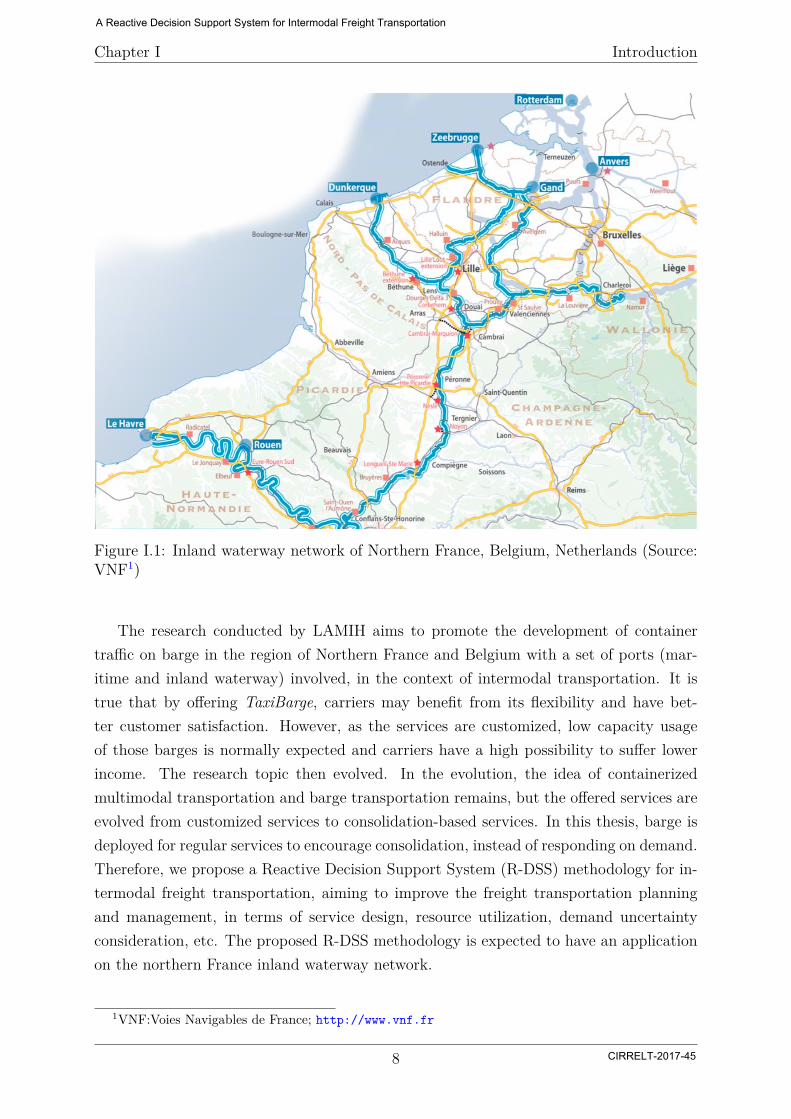
The original motivation of this thesis is the willingness of the inland waterway infras-tructure managers, e.g., VNF, to work together along the Nord-Pas-de-Calais - Wallonieinland waterway from Dunkirk, France to Liege, Belgium (as shown in Figure I.1), and tooffer TaxiBarge to the customers. The initial idea for TaxiBarge (as well as the name) hasbeen brought forward by the Port of Dunkirk (GPMD) and VNF, who were then linkedtogether in a contract for cooperation in order to better develop their traffics together. Asillustrated by the name of this project, barges are used to offer services as taxis, which re-sponding on demand (freight, not passenger) and often for a non-shared trip. To be moreprecise, a TaxiBarge responds to a particular customer and offers customized transportservice where the pick-up (origin) and drop-off (destination) terminals are determined bythe customer within the required delivery time. VNF and GPMD then invited the Belgianport of Liège (PAL) and the service publique de Wallonie (SPW) to join them, as theyimagined the TaxiBarge service on the inland waterway between Dunkirk and Liege. Aprotocol of understanding and cooperation was signed between them, and communicatedto the press. They then contacted i-Trans in order to find help for the realization andpossible additional funding for the project. In order to complete the project and facili-tate the progress (as well as finding of funding), the new innovation platform i-Fret thensuggested to add a research part in the project. The cooperation between i-Trans/i-Fretand LAMIH was then established.
7
A Reactive Decision Support System for Intermodal Freight Transportation
CIRRELT-2017-45
Chapter I Introduction
Figure I.1: Inland waterway network of Northern France, Belgium, Netherlands (Source:VNF1)
The research conducted by LAMIH aims to promote the development of containertraffic on barge in the region of Northern France and Belgium with a set of ports (mar-itime and inland waterway) involved, in the context of intermodal transportation. It istrue that by offering TaxiBarge, carriers may benefit from its flexibility and have bet-ter customer satisfaction. However, as the services are customized, low capacity usageof those barges is normally expected and carriers have a high possibility to suffer lowerincome. The research topic then evolved. In the evolution, the idea of containerizedmultimodal transportation and barge transportation remains, but the offered services areevolved from customized services to consolidation-based services. In this thesis, barge isdeployed for regular services to encourage consolidation, instead of responding on demand.Therefore, we propose a Reactive Decision Support System (R-DSS) methodology for in-termodal freight transportation, aiming to improve the freight transportation planningand management, in terms of service design, resource utilization, demand uncertaintyconsideration, etc. The proposed R-DSS methodology is expected to have an applicationon the northern France inland waterway network.
1VNF:Voies Navigables de France; http://www.vnf.fr
8
A Reactive Decision Support System for Intermodal Freight Transportation
CIRRELT-2017-45
Chapter I Introduction
A freight transportation system can be considered from two main perspectives: de-mand and supply. Demand comes from the shippers that need to move cargoes to differentlocations. These shippers are the purchasers of the freight transportation. Supply, on theother hand, is mainly provided by the infrastructures operators (e.g., intermodal termi-nals, locks and dams) and carriers, who move cargoes using resources (e.g., vessels andcrews). In this thesis, we limit the scope of our research and take the perspective of asingle carrier or a group of carriers cooperating with each other.
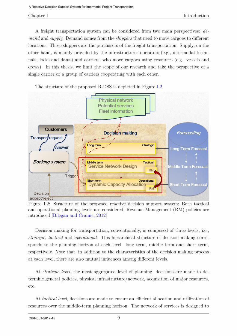
The structure of the proposed R-DSS is depicted in Figure I.2.
Figure I.2: Structure of the proposed reactive decision support system; Both tacticaland operational planning levels are considered; Revenue Management (RM) policies areintroduced [Bilegan and Crainic, 2012]
Decision making for transportation, conventionally, is composed of three levels, i.e.,strategic, tactical and operational. This hierarchical structure of decision making corre-sponds to the planning horizon at each level: long term, middle term and short term,respectively. Note that, in addition to the characteristics of the decision making processat each level, there are also mutual influences among different levels.
At strategic level, the most aggregated level of planning, decisions are made to de-termine general policies, physical infrastructure/network, acquisition of major resources,etc.
At tactical level, decisions are made to ensure an efficient allocation and utilization ofresources over the middle-term planning horizon. The network of services is designed to
9
A Reactive Decision Support System for Intermodal Freight Transportation
CIRRELT-2017-45

Chapter I Introduction
satisfy the forecasted demands, while minimizing total cost or maximizing the revenue.Typically, at tactical level, two types of major decisions, i.e., service selection and flowdistribution, are made. The first determines the itinerary of each service (if selected) andthe corresponding schedule. The second major type of decisions is the routing of demandsfrom their origin to destination within the required delivery time (if considered) and thecorresponding operations at terminals.
At operational level, decisions are made to allocate the network capacity, in a highlydynamic environment considering uncertainty of demands, damage or loss of cargo, delayof services, etc. In this planning level, the time factor plays an important role. The statesof the transport network, berthing capacity in the terminals, transport requests, etc., varythrough time. Therefore, the adjustment of routing is determined.
In addition, decision and information flows are also emphasized in the hierarchicalstructure. Decisions made at each level have influence on the lower level(s). For example,a solution to a strategic problem may determine the design and evolution of the physicalnetwork, e.g., where new terminals should be built, how big the berthing capacity shouldbe, how many equipments should be prepared and which terminals should serve as a hub.Based on the determined physical network from strategic level, decisions are made toselect which services to open with their corresponding schedule and itinerary at tacticallevel. At the middle-term planning level, the service network is build for a given schedulelength, e.g., a week, which is then operated repeatedly and proposed to shippers for theduration of the next planing horizon, e.g., six months. The decision made at tactical level,i.e., a set of selected services characterized by schedule, itinerary and capacity, is thenfed to the operational planning as input. Based on the determined service network, therouting of demands is decided and adjusted at operational level. The information flow,on the contrary, has influence upwards. Essential information, in terms of geographiclocation of terminals, customer definition, product definition, etc., at each level of thehierarchical structure is supplied to the higher level(s) for decision making processes.
As illustrated with the red rectangle in Figure I.2, the proposed R-DSS covers both thetactical and operational levels of the operations planning. To be more precise, given thephysical network, potential services and forecasted demands, decisions about the optimalscheduled service plan are made for the carriers at tactical level. Those selected servicesare then deployed at operational level to face transport requests from the shippers (orcustomers in this thesis). At operational level, decisions in terms of the acceptance/denialof each transport request and the corresponding routing (for accepted demands), are madewith the objective of revenue maximization. In order to limit the scope of this research,a set of assumptions are made as follows:
10
A Reactive Decision Support System for Intermodal Freight Transportation
CIRRELT-2017-45
Chapter I Introduction
• The scope of this research is limited to freight transportation, especially container-ized freight transportation;
• Demand forecasting is out of the scope of this thesis. Information related to demandforecasting is considered to be available for the decision making. Other requiredinformation, e.g., distance between terminals, speed of vehicles, handling time atterminals, fixed and variable costs, is also considered to be available for the scopeof the study;
• No traffic congestion, delay of services or damage/loss of cargo is considered; Notethat, the delay of services (here we are talking about short delays, not disasterones) could be claimed as considered as part of the time of operations consumed bya service at terminals;
• No other transport modes are considered explicitly in this thesis. To synchronize thebarge transport mode with other modes in the context of intermodal freight trans-portation, time dimension is considered. Both demands and services are representedwith time-related characteristics;
• At tactical level:
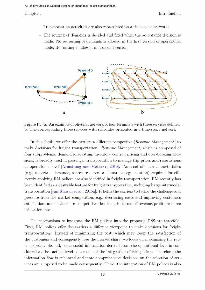
– To explicitly represent the movement of services and demands in time, andto synchronize the barge transport mode with other modes in the context ofintermodal transportation, the middle-term planning problems are formulatedon a time-space network. In Figure I.3, we present a physical network of fourterminals with three services (Figure I.3a) and the corresponding services withschedules in a time-space network (Figure I.3b);
– Different states of services and variety of demands are studied over the schedulelength, which is composed of a certain number of time periods in the time-spacenetwork;
– Operations at terminals, such as loading at origin, unloading at destination,and transshipment at intermediate stops of a demand, are considered withinthe time consumed by services and associated with corresponding costs;
• At operational level:
– Services, that have already been selected and scheduled at the tactical planninglevel, are not going to be rescheduled at the operational level;
– The capacities of scheduled services are also fixed since vehicles are alreadyassigned to services and no extra-vehicles are considered to be available uponrequest;
11
A Reactive Decision Support System for Intermodal Freight Transportation
CIRRELT-2017-45
Chapter I Introduction
– Transportation activities are also represented on a time-space network;
– The routing of demands is decided and fixed when the acceptance decision ismade. No re-routing of demands is allowed in the first version of operationalmode; Re-routing is allowed in a second version.
Figure I.3: a. An example of physical network of four terminals with three services defined;b. The corresponding three services with schedules presented in a time-space network
In this thesis, we offer the carriers a different perspective (Revenue Management) tomake decisions for freight transportation. Revenue Management, which is composed offour subproblems: demand forecasting, inventory control, pricing and over-booking deci-sions, is broadly used in passenger transportation to manage trip prices and reservationsat operational level [Armstrong and Meissner, 2010]. As a set of main characteristics(e.g., uncertain demands, scarce resources and market segmentation) required for effi-ciently applying RM polices are also identified in freight transportation, RM recently hasbeen identified as a desirable feature for freight transportation, including barge intermodaltransportation [van Riessen et al., 2015a]. It helps the carriers to tackle the challenge andpressure from the market competition, e.g., decreasing costs and improving customerssatisfaction, and make more competitive decisions, in terms of revenue/profit, resourceutilization, etc.
The motivations to integrate the RM polices into the proposed DSS are threefold.First, RM polices offer the carriers a different viewpoint to make decisions for freighttransportation. Instead of minimizing the cost, which may lower the satisfaction ofthe customers and consequently lose the market share, we focus on maximizing the rev-enue/profit. Second, some useful information derived from the operational level is con-sidered at the tactical level as a result of the integration of RM polices. Therefore, theinformation flow is enhanced and more comprehensive decisions on the selection of ser-vices are supposed to be made consequently. Third, the integration of RM polices is also
12
A Reactive Decision Support System for Intermodal Freight Transportation
CIRRELT-2017-45
Chapter I Introduction
expected to alleviate the negative influence of demand uncertainty and make more robustplans for the carriers. A better utilization of resource is also expected.
In this thesis, new models are proposed, at both tactical and operational levels toaddress the service network design (SND) and dynamic capacity allocation (DCA) prob-lems, respectively. In addition, a new solution technique is proposed to solve the servicenetwork design problems with consideration of resource and revenue management. Perfor-mance indicators (PIs) are studied and proposed to evaluate and analyze the the proposedmodels.
To build the R-DSS, a set of research questions have to be answered. Therefore, theR-DSS is decomposed into four main research topics as follows:
• How to integrate RM polices (which polices) with barge transportation at opera-tional level in order to dynamically allocate the capacity of transport network facingreal transport requests, in the context of intermodal freight transportation;
• How to integrate RM polices (which polices) and resource management considerationwith barge transportation for the service network design problems and how theselected services might be synchronized with other transport modes, in the contextof intermodal freight transportation;
• How to efficiently solve the scheduled service network design problems while simul-taneously considering resource and revenue management;
• How to validate and evaluate the decision support system of barge transportation,in terms of models, solution methods, corresponding results and strategies; are theresome indicators that give insight more than others;
To answer these questions, in the following of this chapter, we first present the re-search methodology in Section I.2; the detailed challenges of each research topic and thecontributions of the thesis are then discussed in Section I.3. Note that, the problem char-acterization and detailed literature review related to each research topic are introducedin each corresponding chapter.
I.2 Research Methodology
In this section, we present the research methodology used to address the reactive decisionsupport system introduced in the previous section. At the operational planning level,
13
A Reactive Decision Support System for Intermodal Freight Transportation
CIRRELT-2017-45
Chapter I Introduction
we propose a revenue management model (DCA-RM) for the network capacity allocationproblem, extended on [Bilegan et al., 2015]. In addition to the consideration of feasibility,i.e., available network capacity within the required delivery time, the proposed DCA-RM model makes decisions to accept or reject a transport request by maximizing theexpected revenue of current demand and potential future demands over a given time hori-zon, which is called the consideration of profitability. The sequential arrival of transportrequests is simulated as an iterative process, and the decision on each transport request ismade by solving the proposed DCA-RM model with a commercial solver. The total rev-enue obtained by applying the DCA-RM model through the simulation is calculated andcompared with the total revenue obtained by applying a conventional model consideringonly the feasibility. Different negotiation strategies, dealing with the rejected transportrequests, are also embedded in the DCA-RM model and discussed.
Aiming to improve the tactical planning for freight carriers in the context of intermodalbarge transportation, we propose a scheduled service network design with resource andrevenue management (SSND-RRM) model. By integrating the polices of RM, customersare classified into different categories according to their business relationships with thecarriers and their behaviors. Accordingly, different treatment of demands from differentcategories of customers are modeled. Moreover, various fare classes according to therequired delivery service types are also modeled as one of the characteristics of demands.Various problem settings, in terms of demand distribution, network topology, fare classand delivery service type, are tested to analyze the performance of the proposed SSND-RRM model. The optimization problems are also solved by feeding a commercial solver.
As the proposed SSND problems with the consideration of resource and revenue man-agement are NP-hard, we propose a metaheuristic (MH) to produce high-quality solutionsin reasonable time. The proposed solution approach is composed of four phases: a con-structive heuristic to obtain an initial feasible solution, a metaheuristic to iterativelyimprove the solutions, intensification and diversification. The proposed metaheuristic isbased on adaptive large neighborhood search [Ropke and Pisinger, 2006] and tabu search.Aiming to accelerate the search, new neighborhood structures considering design-balanceconstraints are proposed. Learning mechanisms are embedded in the whole algorithm toguide the search by identifying good characteristics/attributes of solutions. The obtainedstatistical information is also used to diversify and intensify the search when predefinedconditions are met. As no other solution approaches to the new SSND-RRM model exists,IBM CPLEX is used as comparison, in terms of computational time and solution quality.
In order to qualify the reactive decision support system and evaluate the performanceof the proposed models, performance indicators (PIs), which are broadly used in practiceand research of transportation, are studied, discussed, classified and applied. We first
14
A Reactive Decision Support System for Intermodal Freight Transportation
CIRRELT-2017-45
Chapter I Introduction
study and analyze some of the performance indicators generally used for validating andevaluating service network design models in the literature. A first classification of thesedifferent performance indicators based on their relevance and meaning from the serviceproviders’ perspective is then proposed. Furthermore, additional performance indicatorsfor the intermodal freight transportation problems with revenue management considera-tions are proposed. Some more representative performance indicators from each categoryare then selected and applied to assess the performance of the proposed reactive DSS.Insights into the generation of adequate test instances to study the planning issues in thegeneral context of freight transportation systems are also provided.
I.3 Contributions of the Thesis
The fundamental contribution (or the first group of contributions) of this thesis is theintegration of revenue management (RM) polices and the barge transportation system inthe context of the intermodal freight transportation. RM, conventionally applied for pas-senger transportation at operational planning level, is considered when making decisionson operations planning at both tactical and operational levels in our research.
At operational level, we propose a DCA-RM model for the network capacity alloca-tion problem of an intermodal barge transportation system in Chapter II. As RM policesare considered in the proposed DCA-RM model, one of the main challenges is to clas-sify the customers. According to the business relationship, customers are classified intothree categories: regular customers (R customers), who sign long-term contracts with thecarriers, and thus whose demands (R demands) have to be accepted; on the other hand,the so-called spot-market customers (P or F customers), who request transportation lessfrequently and on an irregular basis, and thus whose demands may be partially accepted(P demands) or fully accepted/denied (F demands). Another challenge is to differenti-ate the products. To achieve that, a transport request is characterized by three timecharacteristics:
• The reservation time of a transport request, when it is submitted to the bookingsystem;
• The available time of a transport request, when it is ready to be transported at itsorigin terminal on the carriers’ transportation network;
• The due time of a transport request, its maximization. delivery time to its destina-tion;
15
A Reactive Decision Support System for Intermodal Freight Transportation
CIRRELT-2017-45
Chapter I Introduction
among other characteristics. The difference between the available time and the reservationtime gives us the so-called booking anticipation of the transport request, and the deliverytype (slow/fast) depends on the required transport distance from origin to destinationand on the requested delivery time (the difference between the due time and the availabletime). A pricing policy, related to the booking anticipation and delivery type, is thenapplied to differentiate several product fares. The decision to accept or reject a transportrequest is made based on a probabilistic mixed integer optimization model maximizingthe expected revenue of the carrier over a given time horizon. To maximize the expectedrevenue of carriers, a set of future potential demands are considered and probabilitydistribution functions are used to account for their uncertainty of these future demands. Inaddition, a set of possible negotiation strategies for better satisfying the rejected customersare studied based on the proposed DCA-RM model.
In Chapter III, we propose, what we believe to be, the first comprehensive tacticalplanning model for freight carriers that integrates both revenue and resource manage-ment considerations. Customer classification and price differentiation, as considered RMpolices, are integrated into the proposed SSND-RRM model. Instead of accepting alltransport requests like most of the deterministic tactical planning models do, transportrequests from spot-market customers, in the proposed SSND-RRM model, are allowed tobe partially or fully rejected aiming to have better resource utilization and maximize thenet profit of the carriers. The different treatments of customers are decided according totheir corresponding customer categories. The same three customer categories as intro-duced at the operational level (Chapter II) apply. Different fare classes are also definedaccording to the required delivery types. Note that, at tactical level, the price policy isrelated to delivery type only. Booking anticipation is not considered because the reserva-tion time is not used to characterize a transport request at tactical level. With respect tothe resource management, design-balance constraints are considered to ensure the balanceof incoming and outgoing vehicles at each terminal for each time instant. Repositioningof vehicles is also considered implicitly as the SSND-RRM problems are formulated as acyclic model. In addition, the limits on the quantity of the resource is also formulated.Moreover, transshipment of the freight between different vehicles/services and holdingthem at terminals for given periods are considered, with corresponding handling andholding costs. The proposed SSND-RRM model is tested in various problem settings, interms of demand distribution, network topology, fare class and quality-of-service (e.g.,delivery time), to study and analyze its performance.
The next original contribution of this thesis is an efficient solution approach for solv-ing the proposed SSND-RRM model (discussed in Chapter III). The proposed four-phasemetaheuristic (MH) is introduced in Chapter IV. Design-balanced service network design
16
A Reactive Decision Support System for Intermodal Freight Transportation
CIRRELT-2017-45
Chapter I Introduction
problems, as shown in [Pedersen et al., 2009] and [Vu et al., 2013], are NP-hard. Fur-ther complexity to the SSND-RRM is added because of the additional demand selectionassociated to one of the customer categories defined in the SSND-RRM model (binarydecision variables), competition of different categories of customers for the network capac-ity with different fares and trade-offs between opening more services with higher revenueand rejecting more demands with lower total costs. There are challenges even just toobtain feasible solutions. We then propose a constructive heuristic in the first phase toobtain initial solutions to the SSND-RRM. Once an initial solution is obtained from thefirst phase, the algorithm tries to improve it in the second phase, by iteratively explor-ing the search space of service selection, demand selection and the combination of both.The selection of search space is based on a modified adaptive large neighborhood search(ALNS) inspired by [Ropke and Pisinger, 2006] and tabu search. To explore the searchspace of service selection, several heuristics are proposed based on a service cycle relatedneighborhood structure. A service cycle is a set of consecutive services using the sametype of vehicle back to the terminal where the sequence of service starts. Moves based onthe new neighborhood structure guarantee the design-balance constraints and diversifythe search simultaneously. To explore the search space of F-demand selection, severalF-selection heuristics are proposed and different strategies are considered to accept orreject F demands. Learning mechanisms are embedded into the proposed MH, and usedto guide the search and the other two phases (intensification and diversification).
Performance indicators (PIs) are broadly used to characterize the performance of trans-portation systems and to validate and evaluate models, solution methods, correspondingresults and strategies. Some of these are found in public documents, usually providingglobal measures such as total flow volumes, profits and share values. While of great in-terest, such measures are not sufficient to support a fine analysis of different operationstrategies, commercial policies and planning methods. Therefore, the contributions wemake in Chapter V are as follows. First, we make the first step towards a taxonomyof PIs. Three categories of PIs, i.e., economic impact, resource utilization and qualityof service, are classified based on their relevance and meaning from the perspective ofboth service provider and customer. Second, new PIs considering resource and revenuemanagement in the context of freight transportation are proposed for all three categories.In addition, we also provide procedure employed to generate test instances, which areadopted for the experiments throughout the whole thesis, and adequate for further stud-ies of the planning issues in a general context of freight barge transportation.
17
A Reactive Decision Support System for Intermodal Freight Transportation
CIRRELT-2017-45

Chapter I Introduction
I.4 Structure of the Thesis
The thesis is composed of five chapters and the remaining is organized as follows. ChapterII introduces the proposed revenue management approach for dynamic capacity alloca-tion of an intermodal barge transportation system. Chapter III presents the scheduledservice network design with resource and revenue management considerations model forintermodal barge transportation. A metaheuristic for the SSND-RRM is then introducedin Chapter IV. In Chapter V, we study and classify performance indicators for planningintermodal barge transportation systems and present test for the assessment of the R-DSSmethodology proposed.
18
A Reactive Decision Support System for Intermodal Freight Transportation
CIRRELT-2017-45
Chapter II
A Revenue Management Approachfor Network Capacity Allocation ofan Intermodal Barge TransportationSystem
ContentsII.1 Introduction . . . . . . . . . . . . . . . . . . . . . . . . . . . . . 21
II.2 Problem Characterization . . . . . . . . . . . . . . . . . . . . . 23
II.2.1 Dynamic Capacity Allocation Problem . . . . . . . . . . . . . . 23
II.2.2 RM Policies . . . . . . . . . . . . . . . . . . . . . . . . . . . . . 25
II.3 DCA-RM Model Formulation . . . . . . . . . . . . . . . . . . . 26
II.4 Simulation, Numerical Results and Analysis . . . . . . . . . . 29
II.4.1 Scenario Settings . . . . . . . . . . . . . . . . . . . . . . . . . . 30
II.4.2 Numerical Results and Analysis . . . . . . . . . . . . . . . . . . 32
II.5 Extended DCA-RM Model . . . . . . . . . . . . . . . . . . . . . 37
II.6 Conclusions . . . . . . . . . . . . . . . . . . . . . . . . . . . . . . 41
19
A Reactive Decision Support System for Intermodal Freight Transportation
CIRRELT-2017-45
This chapter is dedicated to the operational level of planning for the proposed R-DSS.In this chapter, we first propose a revenue management model (DCA-RM) for the networkcapacity allocation problem of an intermodal barge transportation system. Accept/rejectdecisions are made based on a probabilistic mixed integer optimization model maximizingthe expected revenue of the carrier over a given time horizon. Probability distributionfunctions are used to characterize future potential demands. The simulated bookingsystem solves, using a commercial software, the capacity allocation problem for each newtransportation request. A conventional model for dynamic capacity allocation consideringonly the available network capacity and the delivery time constraints is used as alternativewhen analyzing the results of the proposed model.
The first part of this chapter was published in Lecture Notes in Computer Sciencewith the following reference information:
Wang, Y., Bilegan, I.C., Crainic, T.G., Artiba, A.: A Revenue Management Approachfor Network Capacity Allocation of an Intermodal Barge Transportation System. In: A.Paias et al. (Eds.): ICCL 2016, LNCS, vol. 9855, pp. 243-257. Springer (2016). DOI:10.1007/978-3-319-44896-1_16.
Note that, in the proposed DCA-RMmodel, the routing of demand is decided and fixedwhen the corresponding acceptance decision is made. We then, in the second part of thischapter, extend the proposed DCA-RM model by integrating the re-routing of accepteddemands. Preliminary experiments are conducted to examine the extended DCA-RMmodel.
A Reactive Decision Support System for Intermodal Freight Transportation
CIRRELT-2017-45
Chapter II DCA-RM
II.1 Introduction
Barge transportation offers a competitive alternative for freight transportation, com-plementing the traditional road and rail modes. Moreover, considered as sustainable,environment-friendly and economical, barge transportation has been identified as in-strumental for modal shift and the increased use of intermodality in Europe [EuropeanCommission, 2011]. Yet, studies targeting barge transportation are scarce, (e.g., [Faziet al., 2015, Frémont and Franc, 2010, Konings, 2007, Konings et al., 2013, Notteboom,2012,Taylor et al., 2005]), the ones considering the intermodal context being even morerare (e.g., [Tavasszy et al., 2015, van Riessen et al., 2015a,Zuidwijk, 2015,Ypsilantis andZuidwijk, 2013]). An important and recent review of the scientific literature on multi-modal freight transportation planning can be found in [SteadieSeifi et al., 2014].
Revenue Management (RM ), broadly used in passenger transportation to managetrip prices and bookings (e.g., [Armstrong and Meissner, 2010]), has been identified asa desirable feature for freight transportation, including barge intermodal services [vanRiessen et al., 2015a]. RM is expected to provide freight carriers with tools to bettermanage revenues and enhance service by, in particular, tailoring the service levels andtariffs to particular classes of customers. In [van Riessen et al., 2015b], the authors studyrevenue management in synchromodal container transportation to increase the revenueof the transportation providers. In their study, several delivery types are provided bycarriers. Each type of delivery is associated with a fare class, characterized by a specificprice and a specific due time. In [Li et al., 2015], authors propose a cost-plus-pricingpolicy to determine the price of delivery types in the context of intermodal (truck, railand barge) freight transportation. The price associated with each delivery type is thesum of the operational cost and the targeted profit margin. The price of a delivery typedepends on its urgency as well. Different scenarios, i.e., self-transporting, subcontracting,and a mix of the two, are studied, with different operational costs and targeted profitmargins. However, in both [van Riessen et al., 2015b] and [Li et al., 2015], only one typeof customers, who sign long-term contracts with the carriers, is considered. Consequently,no accepting or rejecting decision is made during the operational phase. In [Liu and Yang,2015], customers are classified into two categories: contract sale (large shippers, whichmight be considered regular) customers, and free sale (scattered shippers) customers.A two-stage stochastic optimal model is then proposed to maximize the revenue. Inthe first stage, the revenue is maximized serving contract sale customers only. In thesecond stage, the slot capacity after serving contract sale customers is used to servethe scattered shippers customers through a dynamic pricing method for price settlingand an inventory control method for slot allocation applied jointly in each period offree sale. The exploration of RM-related issues in freight transportation is still at the
21
A Reactive Decision Support System for Intermodal Freight Transportation
CIRRELT-2017-45
Chapter II DCA-RM
very early stages, however, as illustrated by the reviews related to air cargo operations[Feng et al., 2015], railway transportation [Armstrong and Meissner, 2010], and containersynchromodal services [van Riessen et al., 2015a].
We aim to contribute to the field by proposing a DCA-RM model to address thenetwork capacity allocation problem of an intermodal barge transportation system. Asintermodal barge and rail systems share a number of characteristics, e.g., scheduled ser-vices, limited transport capacity (resource) and uncertain future demands, the approach isinspired by the work of [Bilegan et al., 2015] where the authors develop a model to dynam-ically allocate the rail capacity at operational level. In defining the revenue managementproblem for barge transportation we induce novel features to our modeling, however: weadapt it for the barge transportation space-time network, we enrich it by introducing dif-ferent categories of customers with the definition of specific treatment for each of them,including particular accept/reject rules. An important feature offered by the new model-ing lays in the proposal of a negotiation process based on the optimization model whendealing with rejected demands, as explained in more details further on. Customers areclassified into different categories as follows. Regular customers, who sign long-term con-tracts with the carriers/providers, must be satisfied and thus all these regular category ofdemands have to be accepted. On the other hand, the so-called spot-market customers,who request transportation less frequently and on an irregular basis, may be rejected ifneeded. The accept/reject mechanism is settled according to an estimation of the prof-itability of each new incoming demand, given the availability of service capacities at thetime of decision. In order to better consider customer behavior specificities, those spot-market customers are further classified into partially-spot customers, who would accepttheir requests to be partially accepted, and fully-spot customers, whose requests must beeither accepted as a whole or not accepted at all. These acceptance rules are introducedand used in the new DCA-RM model (through specific decision variables). Moreover,based on the customer differentiation, and on the associated acceptance rules, differentmechanisms are set out in a new negotiation process model which is implemented and usedwhen dealing with rejected demands. At the authors best knowledge, this is the first con-tribution proposing to introduce RM techniques, e.g., price differentiation and customerclassification, at the operational level planning of barge transportation activities.
The application of RM polices requires a booking system to manage transport requests,and the capability to forecast future demands. In our case, the simulated booking systemperforms an accept/reject decision for each new transport request, based on the resultsof the proposed optimization model maximizing the expected revenue of the carrier overa given time horizon. In case of acceptance, the corresponding optimal routing is alsoprovided by the optimization. Probability distribution functions are used to characterize
22
A Reactive Decision Support System for Intermodal Freight Transportation
CIRRELT-2017-45
Chapter II DCA-RM
future potential demands for transportation and, thus, the proposed optimization modeltakes the form of a probabilistic mixed integer program (MIP). A commercial solver is usedto address this model. Simulation is used to analyze the performance of the proposedoptimization model and RM polices, through comparisons with a conventional dynamiccapacity allocation model considering only the available network capacity and the deliverytime constraints.
The remainder of this chapter is organized as follows. In the first part, we brieflydescribe the network capacity allocation problem and the considered RM concepts andstrategies for intermodal barge transportation in Section II.2. The proposed DCA-RMmodel is introduced in Section II.3. Simulation and numerical results are discussed andanalyzed in Section II.4. In the second part of this chapter, the extended DCA-RM modelis presented in Section II.5 and validated with preliminary experiments. We conclude inSection II.6.
II.2 Problem Characterization
We first briefly present the general problem of dynamic capacity allocation for bargetransportation. The mechanisms of the booking system are then discussed, together withthe proposed RM polices. The associated notation is identified as well.
II.2.1 Dynamic Capacity Allocation Problem
Consolidation-based carriers, such as those operating barge services, plan and scheduletheir operations for the “next season” with the goal of jointly maximizing the revenue andsatisfying the forecast regular demand, through efficient resource utilization and opera-tions. Transport requests fluctuate greatly during actual operations, however, in terms oforigins, destinations, volumes, etc., not to speak of those unforeseen demands the carrierwill try to accommodate. The capability to answer customer expectations of the transportnetwork is consequently continuously changing as well, together with its efficiency andprofitability. Setting up some form of advanced booking system is the measure generallyadopted to handle this complex situation.
Transport booking requests are traditionally answered on a first-come first-serve (FCFS)basis. Moreover, a transport request is (almost) always accepted provided the networkcurrently has the capability to satisfy both the volume and the delivery time specifiedby the customer. This has the unwanted consequence that requests coming at a latter
23
A Reactive Decision Support System for Intermodal Freight Transportation
CIRRELT-2017-45
Chapter II DCA-RM
time might not be accepted, even though they present the potential to generate a higherrevenue, due to a lack of transport capacity, resulting in the loss of additional revenue forthe carrier.
RM-based booking systems operate according to different principles. The bookingsystem considered in this chapter manages the transport capacity, and the decision toaccept or reject a new demand, considering a set of potential future demands characterizedby different fare classes. To make the final decision, the acceptance and rejection of thecurrent demand are compared by optimizing the estimated total revenue of all demands,current and potential future ones. Therefore, in our model, a current transport requestmay be rejected if it appears less profitable compared with the estimated profit of futuredemands competing for the transport capacity. The resource is then reserved for thefuture demands, expecting a higher total revenue. On the other hand, when the bookingsystem accepts the current transport request and more than one possible routing exist,a “better” capacity allocation plan can be obtained by considering the future demands.That is, the capacity available in the future might more closely match future demands,increasing the possibility of acceptance and the generation of additional revenue.
We formulate the dynamic capacity allocation problem on a space-time network over atime interval composed of 1, ..., T time instants. The nodes of the G = (N ,A) network areobtained by duplicating the representation of the physical terminals at all time instants,i.e., a node n(i, t) ∈ N specifies the physical terminal i and the time instant t.
A set of already-selected services, each with given schedule, route and capacity, pro-vides transportation among the nodes in N . Note that, in this research, we assumethat services have already been scheduled at the tactical planning level (i.e., when theScheduled Service Network Design problem is solved) and are not to be rescheduled atthe operational level. The capacities of scheduled services are also fixed since vehiclesare already assigned to services and no extra-vehicles are considered to be available uponrequest. A service s ∈ S is characterized by its transport capacity cap(s) and set oflegs η(s). Leg ak(s) ∈ η(s) represents kth leg of service between two consecutive stops(i.e., ik(s) and ik+1(s)) of service s, and is characterized by its origin and destinationterminals, orig(ak(s)), dest(ak(s)) ∈ N , with the respective departure dep(ak(s)) and ar-rival arr(ak(s)) times. Let cap(ak(s)) = cap(s) identify the capacity of ak(s), and definecap_avl(ak(s)), the residual capacity of leg ak(s) after having routed the already accepteddemands.
The set of arcs A is then made up of the sets AK and AH representing the transportand holding arcs, respectively. Set AK is composed of all the defined service legs, whileAH arcs link two representations of the same terminal at two consecutive time periods.
24
A Reactive Decision Support System for Intermodal Freight Transportation
CIRRELT-2017-45
Chapter II DCA-RM
Holding arcs represent the possibility of demand flows to wait at their respective originsor at intermediate terminals during their journey, to be picked up by services passing byat later periods.
II.2.2 RM Policies
Revenue Management groups together a set of concepts and techniques aimed to betterintegrate customer behavior knowledge into the optimal capacity allocation models. Forinstance, different fares are applied to well-differentiated products/services, and differentmarket segments are identified and used with the overall objective to maximize expectedrevenue. To define RM polices for barge transportation systems, we introduce customerclassification and price differentiation.
Customers are classified into three categories according to the business relationship:regular customers (R), who sign long-term contracts with the carrier or whom the carriertrusts; partially-spot customers (P), who contact the carrier infrequently and do notrequire that all their demand be accepted; fully-spot customers (F), who also requireservice irregularly but their demand must be accepted as a whole or not at all.
Let d be the current booking request. Let D′d be the set of demands accepted beforethe arrival of d, and D′′d the set of forecasted future demands with direct interactionsin time with d. A transport request d ∈ D′d ∪ D′′d ∪ {d} is then characterized by thevolume to be transported in TEUs, vol(d); the origin and destination terminals, orig(d)and dest(d), respectively; the time res(d) it is submitted to the booking system; the timeavl(d) it becomes available at its origin terminal and the corresponding anticipation time,Θ(d) = avl(d) − res(d); the due time (latest delivery time) out(d) and the requesteddelivery time ∆(d) = out(d) − avl(d); the unit tariff f(d) according to the fare class ofthe demand (defined bellow); and the category cat(d) of customers (R, P or F). Note thata future demand d′′ is considered to be part of the set of potential future demands D′′dwhen it has “direct interactions” with the current booking request d, which is true whenthe two time conditions are satisfied:
• res(d′′) > res(d)
• [in(d′′), out(d′′)] ∩ [in(d), out(d)] 6= ∅.
Let VMAX(d′′) be the maximum volume a future demand request d′′ ∈ D′′d may take,and Pd′′(x) the discrete probability distribution function indicating the probability thata given value 0 ≤ x ≤ VMAX(d′′) occurs.
25
A Reactive Decision Support System for Intermodal Freight Transportation
CIRRELT-2017-45

Chapter II DCA-RM
We define four fare classes for any pair of terminals in the physical network (and thedistance separating them) as the combination of Θ(d), early or late booking, and ∆(d),slow or fast delivery requested. A demand with the highest fare class thus correspondsto a late booking and fast delivery request, while a demand with the lowest fare classcorresponds to an early booking and slow delivery request.
The proposed RM policy for barge transportation is then to examine each new trans-port request, d, and decide on its acceptance, and routing through the network for ac-cepted ones, by considering its feasibility and profitability, given the current status of thenetwork and an estimation of future demands. The former means that currently thereis sufficient capacity and time to satisfy d. The latter indicates that the expected totalrevenue given the acceptance of d is at least not worse than the one corresponding torejecting it, taking into account the potential future demands. The model of Section II.3is used to make these decisions.
A rejected request has no influence on the transport network. Similarly, the potentialfuture demands are only used to calculate the expected total revenue, and do not impactthe status of the network.
II.3 DCA-RM Model Formulation
We now present the Revenue Management decision model (DCA-RM) that is to be solvedfor every arriving request for transportation d. The decision variables are:
• ξ(d): accept or reject d, where ξ(d)
– equals 1 when cat(d) = R,
– varies within [0, 1] when cat(d) = P,
– takes the value 0 or 1 when cat(d) = F;
• x(d, ak(s)): volume of demand d on arc ak(s);
• maxvol(d′′): maximum volume available on the network (at the decision time) toserve the potential future demand d′′ ∈ D′′d ;
• x(d′′, ak(s)): volume of the potential future demand d′′ ∈ D′′d on arc ak(s).
Obviously, ξ(d′) and x(d′, ak(s)) variables are fixed on all arcs for the already accepteddemands, which we denote d′, d′ ∈ D′d.
26
A Reactive Decision Support System for Intermodal Freight Transportation
CIRRELT-2017-45
Chapter II DCA-RM
The objective function of the model with respect to the current demand d maximizesthe sum of its corresponding revenue and the expected revenue computed on the basis offuture demand forecasts:
max (f(d) · ξ(d) · vol(d) + φ) (II.1)
where
φ =∑
d′′∈D′′d
f(d′′)maxvol(d′′)∑
x=0xPd′′(x) (II.2)
Following [Bilegan et al., 2015], φ is linearized by introducing additional binary deci-sion variables yd′′j for each potential future demand d′′, where the integer-valued j takesall the values between 1 and VMAX(d′′). Note that VMAX(d′′) represents the maxi-mum possible volume of a booking request, which translates mathematically, in terms ofprobability distribution, as Pd′′(j) = 0 when j ≥ VMAX(d′′) + 1. The binary decisionvariables yd′′j are defined to be equal to 1, if no more than volume j of capacity is availableon the network to serve the potential future demand d′′ and 0 otherwise. In order to makethis definition consistent, for each future demand d′′, at most one of the variables yd′′jmay take the value 1 (since this will correspond to the maximum capacity available onthe network to serve that specific demand). Thus, the objective function becomes:
max (f(d) · ξ(d) · vol(d) +∑
d′′∈D′′d
f(d′′)∑
1≤j≤VMAX(d′′)yd′′j
j∑x=0
(xPd′′(x))) (II.3)
since maxvol(d′′) is defined as follows:
maxvol(d′′) =∑
1≤j≤VMAX(d′′)jyd′′j (II.4)
with ∑1≤j≤VMAX(d′′)
yd′′j ≤ 1 (II.5)
andyd′′j ∈ {0, 1}. (II.6)
Following this definition, note that the optimal value of maxvol(d′′) is computed (II.4)as a result of the optimization problem. Thus, this optimal value is obtained whenmaximizing the expected revenue corresponding to current demand d on the network,taking into account the entire remaining available capacity and the overall profitability ofthe whole set of potential future demands on that specific time window.
The constraints of the model are the usual flow conservation relations at nodes and
27
A Reactive Decision Support System for Intermodal Freight Transportation
CIRRELT-2017-45

Chapter II DCA-RM
the capacity restrictions imposed by the service network. The latter take the form definedby (II.7) for each service leg
∑d′′∈D′′
d
x(d′′, ak(s)) + v(d, ak(s)) ≤ cap_avl(ak(s)), ∀ak(s) ∈ AK (II.7)
while the flow conservation constraints for all nodes n(i, t) ∈ NIT are:
∑a∈A+(n(i,t))
x(d, a)−∑
a∈A−(n(i,t))x(d, a) =
ξ(d)vol(d) if i = orig(d)
−ξ(d)vol(d) if i = dest(d)
0 otherwise
(II.8)
and
∑a∈A+(n(i,t))
x(d′′, a)−∑
a∈A−(n(i,t))x(d′′, a) =
maxvol(d′′) if i = orig(d′′)
−maxvol(d′′) if i = dest(d′′), ∀d′′ ∈ D′′d0 otherwise
(II.9)
where A+(n(i, t)) and A−(n(i, t)) stand for the sets of outgoing and incoming arcs,respectively, of node n(i, t) ∈ N .
Finally, the constraints defining the range of the decision variables are:
ξ(d) =
1, if cat(d) = R
[0, 1], if cat(d) = P
{0, 1}, if cat(d) = F
(II.10)
x(d, a) ≥ 0, ∀a ∈ A (II.11)
28
A Reactive Decision Support System for Intermodal Freight Transportation
CIRRELT-2017-45
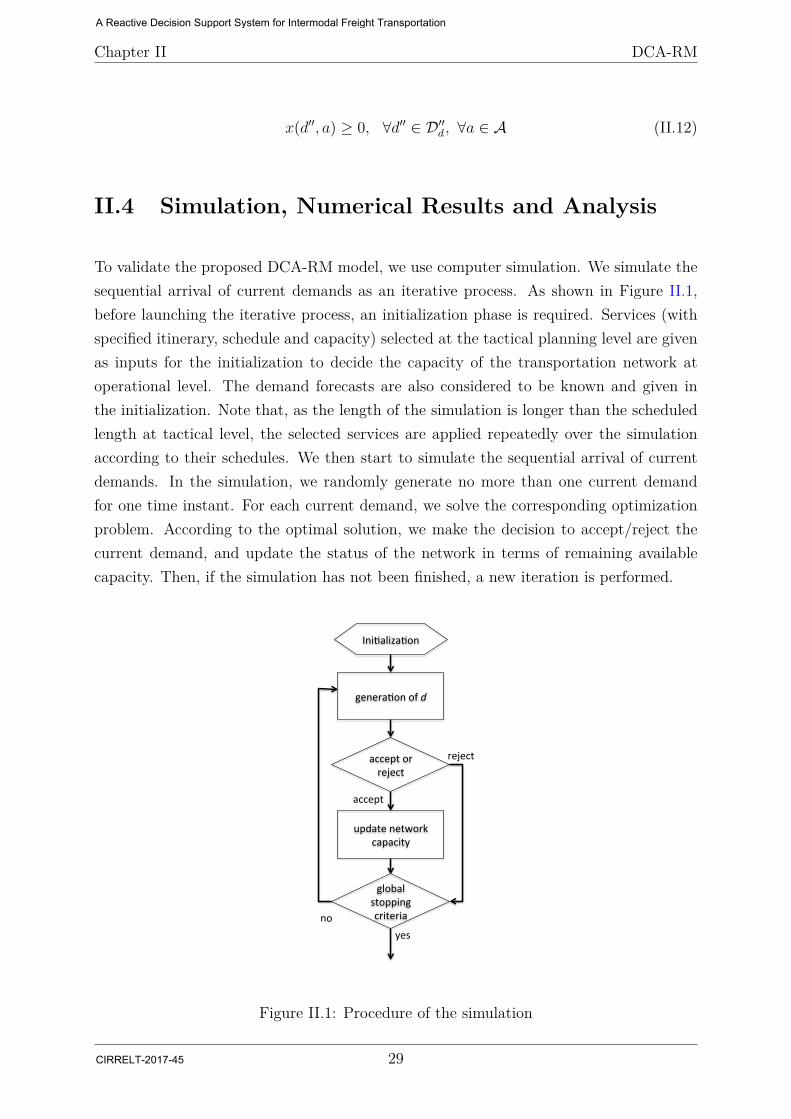
Chapter II DCA-RM
x(d′′, a) ≥ 0, ∀d′′ ∈ D′′d , ∀a ∈ A (II.12)
II.4 Simulation, Numerical Results and Analysis
To validate the proposed DCA-RM model, we use computer simulation. We simulate thesequential arrival of current demands as an iterative process. As shown in Figure II.1,before launching the iterative process, an initialization phase is required. Services (withspecified itinerary, schedule and capacity) selected at the tactical planning level are givenas inputs for the initialization to decide the capacity of the transportation network atoperational level. The demand forecasts are also considered to be known and given inthe initialization. Note that, as the length of the simulation is longer than the scheduledlength at tactical level, the selected services are applied repeatedly over the simulationaccording to their schedules. We then start to simulate the sequential arrival of currentdemands. In the simulation, we randomly generate no more than one current demandfor one time instant. For each current demand, we solve the corresponding optimizationproblem. According to the optimal solution, we make the decision to accept/reject thecurrent demand, and update the status of the network in terms of remaining availablecapacity. Then, if the simulation has not been finished, a new iteration is performed.
Ini$aliza$on�
genera$onofd�
acceptorreject�
updatenetworkcapacity�
globalstoppingcriteria�
yes�no�
accept�
reject�
Figure II.1: Procedure of the simulation
29
A Reactive Decision Support System for Intermodal Freight Transportation
CIRRELT-2017-45
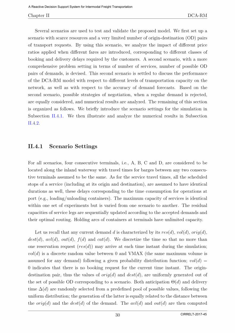
Chapter II DCA-RM
Several scenarios are used to test and validate the proposed model. We first set up ascenario with scarce resources and a very limited number of origin-destination (OD) pairsof transport requests. By using this scenario, we analyze the impact of different priceratios applied when different fares are introduced, corresponding to different classes ofbooking and delivery delays required by the customers. A second scenario, with a morecomprehensive problem setting in terms of number of services, number of possible ODpairs of demands, is devised. This second scenario is settled to discuss the performanceof the DCA-RM model with respect to different levels of transportation capacity on thenetwork, as well as with respect to the accuracy of demand forecasts. Based on thesecond scenario, possible strategies of negotiation, when a regular demand is rejected,are equally considered, and numerical results are analyzed. The remaining of this sectionis organized as follows. We briefly introduce the scenario settings for the simulation inSubsection II.4.1. We then illustrate and analyze the numerical results in SubsectionII.4.2.
II.4.1 Scenario Settings
For all scenarios, four consecutive terminals, i.e., A, B, C and D, are considered to belocated along the inland waterway with travel times for barges between any two consecu-tive terminals assumed to be the same. As for the service travel times, all the scheduledstops of a service (including at its origin and destination), are assumed to have identicaldurations as well, these delays corresponding to the time consumption for operations atport (e.g., loading/unloading containers). The maximum capacity of services is identicalwithin one set of experiments but is varied from one scenario to another. The residualcapacities of service legs are sequentially updated according to the accepted demands andtheir optimal routing. Holding arcs of containers at terminals have unlimited capacity.
Let us recall that any current demand d is characterized by its res(d), vol(d), orig(d),dest(d), avl(d), out(d), f(d) and cat(d). We discretize the time so that no more thanone reservation request (res(d)) may arrive at each time instant during the simulation;vol(d) is a discrete random value between 0 and VMAX (the same maximum volume isassumed for any demand) following a given probability distribution function; vol(d) =0 indicates that there is no booking request for the current time instant. The origin-destination pair, thus the values of orig(d) and dest(d), are uniformly generated out ofthe set of possible OD corresponding to a scenario. Both anticipation Θ(d) and deliverytime ∆(d) are randomly selected from a predefined pool of possible values, following theuniform distribution; the generation of the latter is equally related to the distance betweenthe orig(d) and the dest(d) of the demand. The avl(d) and out(d) are then computed
30
A Reactive Decision Support System for Intermodal Freight Transportation
CIRRELT-2017-45

Chapter II DCA-RM
accordingly. Thresholds for the anticipation and delivery time are predefined to splitthe demands into early/late reservation and slow/fast delivery types, respectively. Fora given distance of an OD, a basic fare p is predefined. The unit transportation price(per container) is then defined as f(d) = p · rΘ · r∆, where rΘ and r∆ are the anticipationratio and the delivery ratio respectively, and whose values will be set to define particularinstances. Their corresponding values for early reservation and slow delivery are bothset to 1, the others being integer values (factors) greater than one, corresponding tolarger fares charged on high contribution demands requesting higher quality-of-servicetransportation. Finally, cat(d) is randomly generated among R, P and F following theuniform distribution.
For each current demand d, the corresponding set of potential future demands isgenerated following the same generation procedure, except for its volume. Indeed, sincethe objective function is defined based on the mathematical expectation of the potentialrevenue of future demands, this computation is performed considering all the possiblevolumes (from 0 to VMAX), weighted by their probabilities. The summation is bounded,however, by the maximum available capacity (at decision time) on the network to satisfyeach specific future demand d′′ (maxvol(d′′)). Following the same idea, note that thecategories (i.e., R, P or F) of future demands are not needed either when generatingthe potential future demands. By doing so, an estimated value of the expected revenue isobtained by simulation and used to make the decision of accepting or rejecting the currentdemand d.
For all the scenarios in the simulation, a FCFS accept/reject policy is conducted ascomparison. No potential future demands are considered for the FCFS model. A currentdemand d is accepted when at least one feasible route exists in the space-time network,without considering the expected revenue and hence, without considering its profitability.
The characteristics of the first scenario are:
• Length of the simulated time horizon is 300 time instants;
• There are 15 identical services defined, starting every 20 time instants, from A toD with an intermediate stop at B;
• 3 different ODs are considered: AB, BD and AD;
• Different experiments are conducted, with different values of the anticipation ratio(rΘ) for late reservation and the values of the delivery ratio (r∆) for fast delivery:1, 2, 3 and 4.
31
A Reactive Decision Support System for Intermodal Freight Transportation
CIRRELT-2017-45
Chapter II DCA-RM
The characteristics of the second scenario are:
• Length of the simulated time horizon is 600 time instants;
• There is a total of 30 services running on the network, 15 in each direction: from Ato D and from D to A; they all stop at all terminals;
• All 12 possible ODs are considered;
• Different experiments are conducted, with different capacities of services: 5, 10 and20 TEUs;
• Different experiments are conducted, based on different forecast accuracies: goodaccuracy, underestimation, overestimation.
II.4.2 Numerical Results and Analysis
As described before, we vary the values of anticipation ratio (rΘ) for late reservation andthe values of the delivery ratio (r∆) for fast delivery in the first scenario. For example,when rΘ = r∆ = 2, the price ratio (r) of early reservation with slow delivery, earlyreservation with fast delivery, late reservation with slow delivery and late reservationwith fast delivery is denoted as r = 1 : 2 : 2 : 4. Experiments are also conductedwhen rΘ = r∆ = 1, 3 or 4. For each tested price ratio, the simulation was carried out20 times with random transport requests, which are generated following the proceduredescribed in the previous subsection. The total revenue obtained by the DCA-RM modeland by the FCFS policy is recorded for each simulation, and the ratio of total revenueof DCA-RM/FCFS is then calculated. In the simulation, we also counted the number ofrejected transport requests, which are denied according to the DCA-RM model due tounprofitability or infeasibility .
The average results obtained on the first scenario are illustrated in Figure II.2. FigureII.2 (a) presents the ratio between the total revenue obtained with the DCA-RM modeland the total revenue obtained with the FCFS policy, corresponding to different priceratios. Figure II.2 (b) presents the corresponding ratios of the number of nonprofitablerejected requests over the total number of rejected requests when applying the DCA-RM model. On the horizontal axis, r indicates the tested price ratios. As expected,better revenue is always obtained by applying the DCA-RM model when compared withthe FCFS policy. When we increase the price ratio r, the difference in profitability oflow-fare compared to high-fare demands grows as well. A low-fare demand, which has afeasible routing in the transport network, has then a higher chance to be less profitable
32
A Reactive Decision Support System for Intermodal Freight Transportation
CIRRELT-2017-45
Chapter II DCA-RM
Figure II.2: Effect of price differentiation on revenue (a) and on rejected requests (b)
compared to a potential future high-fare demand (even if its probability to occur is low)and consequently will be rejected or not fully accepted. Therefore, as shown in FigureII.2 (b), when we increase the price ratio r, more demands are rejected because of thiseconomic discrimination (unprofitability). Consequently, a boost in revenue, as illustratedin Figure II.2 (a), is obtained when we increase the values of anticipation and deliveryprice ratios. As the presented average values are calculated over 20 instances, an insightabout the consistency of the simulation (with the corresponding standard deviation in theparenthesis) is also given in Figure II.2 (a).
Note that, even without any price differentiation, the DCA-RM model still generatesbetter solutions in terms of total revenue (Figure II.2 (a), when r=1:1:1:1). In fact,the consideration of future demands equally aids in finding a better routing solutionwhen a demand is accepted. This better routing makes room in the space-time networkfor potentially infeasible future demands, and hence convert them to feasible, which istransformed accordingly into extra revenue.
The ratios between the total revenues generated when applying the DCA-RM model
33
A Reactive Decision Support System for Intermodal Freight Transportation
CIRRELT-2017-45
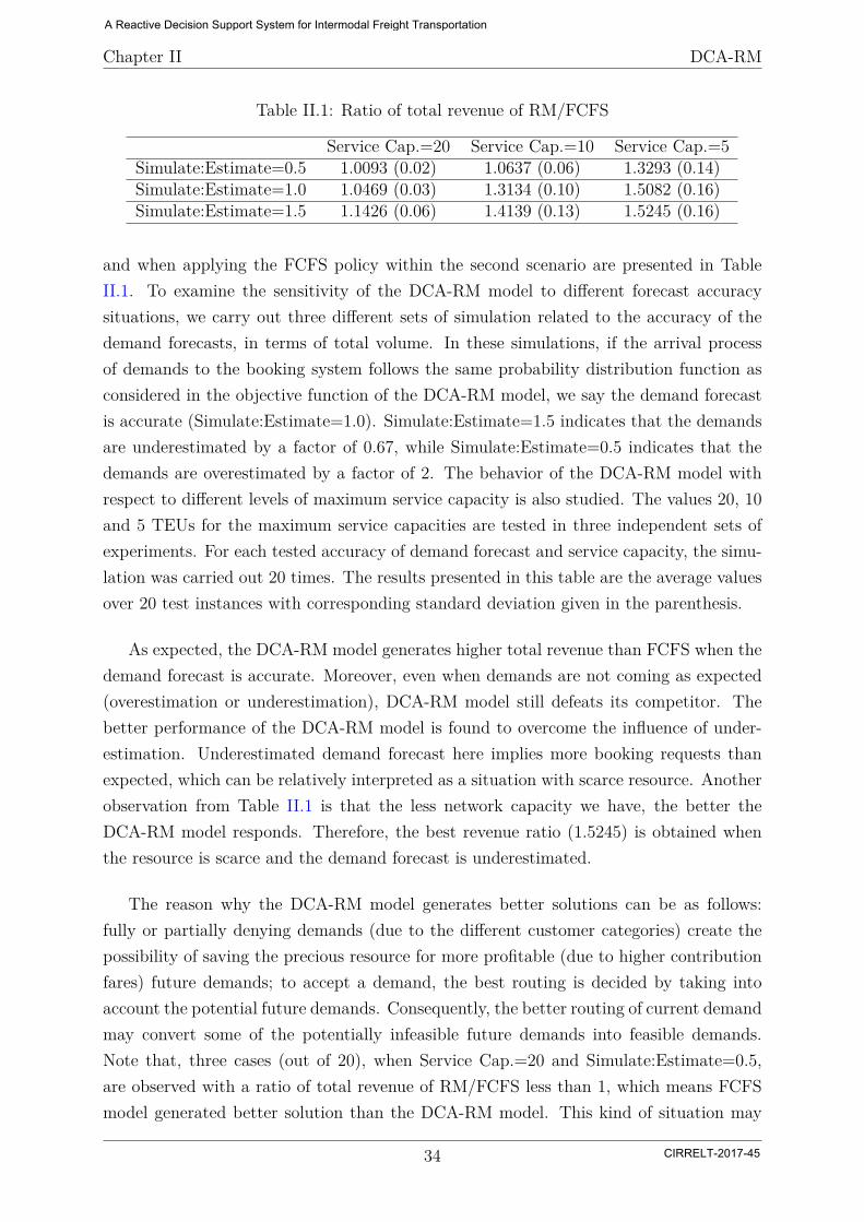
Chapter II DCA-RM
Table II.1: Ratio of total revenue of RM/FCFS
Service Cap.=20 Service Cap.=10 Service Cap.=5Simulate:Estimate=0.5 1.0093 (0.02) 1.0637 (0.06) 1.3293 (0.14)Simulate:Estimate=1.0 1.0469 (0.03) 1.3134 (0.10) 1.5082 (0.16)Simulate:Estimate=1.5 1.1426 (0.06) 1.4139 (0.13) 1.5245 (0.16)
and when applying the FCFS policy within the second scenario are presented in TableII.1. To examine the sensitivity of the DCA-RM model to different forecast accuracysituations, we carry out three different sets of simulation related to the accuracy of thedemand forecasts, in terms of total volume. In these simulations, if the arrival processof demands to the booking system follows the same probability distribution function asconsidered in the objective function of the DCA-RM model, we say the demand forecastis accurate (Simulate:Estimate=1.0). Simulate:Estimate=1.5 indicates that the demandsare underestimated by a factor of 0.67, while Simulate:Estimate=0.5 indicates that thedemands are overestimated by a factor of 2. The behavior of the DCA-RM model withrespect to different levels of maximum service capacity is also studied. The values 20, 10and 5 TEUs for the maximum service capacities are tested in three independent sets ofexperiments. For each tested accuracy of demand forecast and service capacity, the simu-lation was carried out 20 times. The results presented in this table are the average valuesover 20 test instances with corresponding standard deviation given in the parenthesis.
As expected, the DCA-RM model generates higher total revenue than FCFS when thedemand forecast is accurate. Moreover, even when demands are not coming as expected(overestimation or underestimation), DCA-RM model still defeats its competitor. Thebetter performance of the DCA-RM model is found to overcome the influence of under-estimation. Underestimated demand forecast here implies more booking requests thanexpected, which can be relatively interpreted as a situation with scarce resource. Anotherobservation from Table II.1 is that the less network capacity we have, the better theDCA-RM model responds. Therefore, the best revenue ratio (1.5245) is obtained whenthe resource is scarce and the demand forecast is underestimated.
The reason why the DCA-RM model generates better solutions can be as follows:fully or partially denying demands (due to the different customer categories) create thepossibility of saving the precious resource for more profitable (due to higher contributionfares) future demands; to accept a demand, the best routing is decided by taking intoaccount the potential future demands. Consequently, the better routing of current demandmay convert some of the potentially infeasible future demands into feasible demands.Note that, three cases (out of 20), when Service Cap.=20 and Simulate:Estimate=0.5,are observed with a ratio of total revenue of RM/FCFS less than 1, which means FCFSmodel generated better solution than the DCA-RM model. This kind of situation may
34
A Reactive Decision Support System for Intermodal Freight Transportation
CIRRELT-2017-45
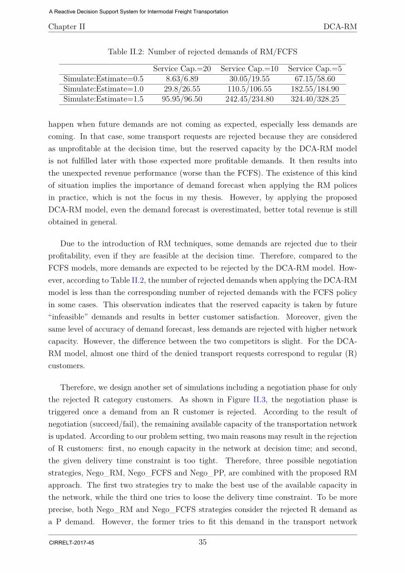
Chapter II DCA-RM
Table II.2: Number of rejected demands of RM/FCFS
Service Cap.=20 Service Cap.=10 Service Cap.=5Simulate:Estimate=0.5 8.63/6.89 30.05/19.55 67.15/58.60Simulate:Estimate=1.0 29.8/26.55 110.5/106.55 182.55/184.90Simulate:Estimate=1.5 95.95/96.50 242.45/234.80 324.40/328.25
happen when future demands are not coming as expected, especially less demands arecoming. In that case, some transport requests are rejected because they are consideredas unprofitable at the decision time, but the reserved capacity by the DCA-RM modelis not fulfilled later with those expected more profitable demands. It then results intothe unexpected revenue performance (worse than the FCFS). The existence of this kindof situation implies the importance of demand forecast when applying the RM policesin practice, which is not the focus in my thesis. However, by applying the proposedDCA-RM model, even the demand forecast is overestimated, better total revenue is stillobtained in general.
Due to the introduction of RM techniques, some demands are rejected due to theirprofitability, even if they are feasible at the decision time. Therefore, compared to theFCFS models, more demands are expected to be rejected by the DCA-RM model. How-ever, according to Table II.2, the number of rejected demands when applying the DCA-RMmodel is less than the corresponding number of rejected demands with the FCFS policyin some cases. This observation indicates that the reserved capacity is taken by future“infeasible” demands and results in better customer satisfaction. Moreover, given thesame level of accuracy of demand forecast, less demands are rejected with higher networkcapacity. However, the difference between the two competitors is slight. For the DCA-RM model, almost one third of the denied transport requests correspond to regular (R)customers.
Therefore, we design another set of simulations including a negotiation phase for onlythe rejected R category customers. As shown in Figure II.3, the negotiation phase istriggered once a demand from an R customer is rejected. According to the result ofnegotiation (succeed/fail), the remaining available capacity of the transportation networkis updated. According to our problem setting, two main reasons may result in the rejectionof R customers: first, no enough capacity in the network at decision time; and second,the given delivery time constraint is too tight. Therefore, three possible negotiationstrategies, Nego_RM, Nego_FCFS and Nego_PP, are combined with the proposed RMapproach. The first two strategies try to make the best use of the available capacity inthe network, while the third one tries to loose the delivery time constraint. To be moreprecise, both Nego_RM and Nego_FCFS strategies consider the rejected R demand asa P demand. However, the former tries to fit this demand in the transport network
35
A Reactive Decision Support System for Intermodal Freight Transportation
CIRRELT-2017-45
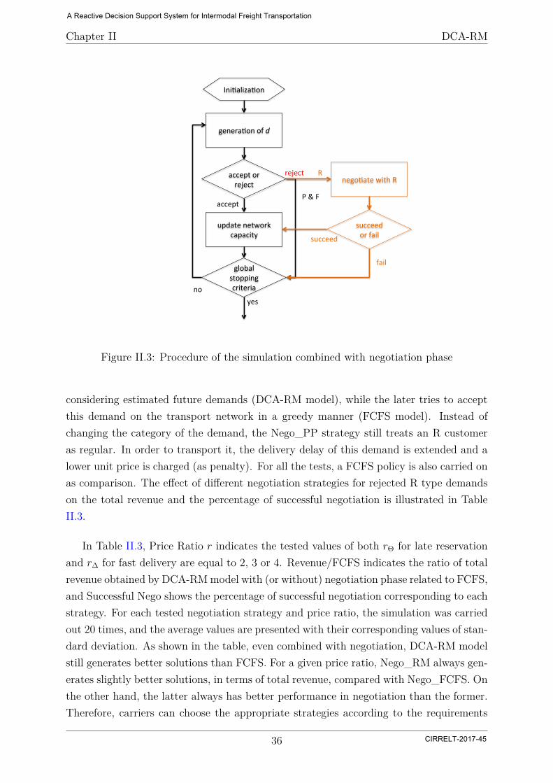
Chapter II DCA-RM
Ini$aliza$on�
genera$onofd�
acceptorreject�
updatenetworkcapacity�
globalstoppingcriteria�
nego$atewithR�
succeedorfail�
yes�no�
accept�
reject� R�
P&F�
succeed�
fail�
Figure II.3: Procedure of the simulation combined with negotiation phase
considering estimated future demands (DCA-RM model), while the later tries to acceptthis demand on the transport network in a greedy manner (FCFS model). Instead ofchanging the category of the demand, the Nego_PP strategy still treats an R customeras regular. In order to transport it, the delivery delay of this demand is extended and alower unit price is charged (as penalty). For all the tests, a FCFS policy is also carried onas comparison. The effect of different negotiation strategies for rejected R type demandson the total revenue and the percentage of successful negotiation is illustrated in TableII.3.
In Table II.3, Price Ratio r indicates the tested values of both rΘ for late reservationand r∆ for fast delivery are equal to 2, 3 or 4. Revenue/FCFS indicates the ratio of totalrevenue obtained by DCA-RMmodel with (or without) negotiation phase related to FCFS,and Successful Nego shows the percentage of successful negotiation corresponding to eachstrategy. For each tested negotiation strategy and price ratio, the simulation was carriedout 20 times, and the average values are presented with their corresponding values of stan-dard deviation. As shown in the table, even combined with negotiation, DCA-RM modelstill generates better solutions than FCFS. For a given price ratio, Nego_RM always gen-erates slightly better solutions, in terms of total revenue, compared with Nego_FCFS. Onthe other hand, the latter always has better performance in negotiation than the former.Therefore, carriers can choose the appropriate strategies according to the requirements
36
A Reactive Decision Support System for Intermodal Freight Transportation
CIRRELT-2017-45
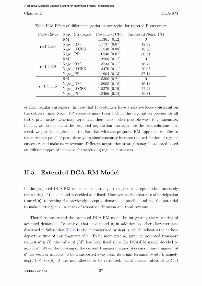
Chapter II DCA-RM
Table II.3: Effect of different negotiation strategies for rejected R customers
Price Ratio Nego. Strategies Revenue/FCFS Successful Nego. (%)
r=1:2:2:4
RM 1.1361 (0.12) 0Nego_RM 1.1737 (0.07) 12.82Nego_ FCFS 1.1540 (0.08) 18.36Nego_PP 1.0248 (0.07) 50.31
r=1:3:3:9
RM 1.3208 (0.17) 0Nego_RM 1.3733 (0.11) 16.42Nego_ FCFS 1.3476 (0.11) 20.67Nego_PP 1.1904 (0.13) 57.14
r=1:4:4:16
RM 1.5300 (0.21) 0Nego_RM 1.5905 (0.18) 16.14Nego_ FCFS 1.5379 (0.19) 22.44Nego_PP 1.3466 (0.14) 56.81
of their regular customers. In case that R customers have a relative loose constraint onthe delivery time, Nego_PP succeeds more than 50% in the negotiation process for alltested price ratios. One may argue that there exists other possible ways to compensate.In fact, we do not claim the proposed negotiation strategies are the best solutions. In-stead, we put the emphasis on the fact that with the proposed RM approach, we offer tothe carriers a panel of possible ways to simultaneously increase the satisfaction of regularcustomers and make more revenue. Different negotiation strategies may be adopted basedon different types of behavior characterizing regular customers.
II.5 Extended DCA-RM Model
In the proposed DCA-RM model, once a transport request is accepted, simultaneouslythe routing of this demand is decided and fixed. However, as the existence of anticipationtime Θ(d), re-routing the previously-accepted demands is possible and has the potentialto make better plans, in terms of resource utilization and total revenue.
Therefore, we extend the proposed DCA-RM model by integrating the re-routing ofaccepted demands. To achieve that, a demand d, in addition to other characteristicsdiscussed in Subsection II.2.2, is also characterized by dep(d), which indicates the earliestdeparture time of any fragment of d. To be more precise, given an accepted transportrequest d′ ∈ D′d, the value of ξ(d′) has been fixed since the DCA-RM model decided toaccept d′. When the booking of the current transport request d occurs, if any fragment ofd′ has been or is ready to be transported away from its origin terminal orig(d′), namelydep(d′) ≤ res(d), d′ are not allowed to be re-routed, which means values of x(d′, a)
37
A Reactive Decision Support System for Intermodal Freight Transportation
CIRRELT-2017-45
Chapter II DCA-RM
variables are fixed on all arcs; Otherwise (i.e., dep(d′) > res(d)), d′ will be re-routed whenthe DCA-RM model makes decision to accept or reject the current transport requestd, which means the values of x(d′, a) variables have to be computed again. We defineD̃(d) = {d′ | dep(d′) > res(d)} as a subset of D′d.
To consider those variables, the model presented in Section II.3 is then extended inthe following way. The constraints (II.7) should be replaced by:
∑d′∈D̃(d)
x(d′, ak(s)) +∑
d′′∈D′′d
x(d′′, ak(s)) + x(d, ak(s)) ≤ cap_avl(ak(s)), ∀ak(s) ∈ AK
(II.13)
Two more sets of constraints, with respect to flow conservation and range of decisionvariables, are added as well to the previous model.
∑a∈A+(n(i,t))
x(d′, a)−∑
a∈A−(n(i,t))x(d′, a) =
ξ(d′)vol(d′) if i = orig(d′)
−ξ(d′)vol(d′) if i = dest(d′), ∀d′ ∈ D̃(d)
0 otherwise
(II.14)
and
x(d′, a) ≥ 0, ∀d′ ∈ D̃(d), ∀a ∈ A. (II.15)
In order to examine the extended DCA-RM model, we conduct preliminary exper-iments. The same set of simulations described in Section II.4 is used here and a newscenario is designed and characterized as follows:
• Length of the simulated time horizon is 600 time instants;
• There is a total of 30 services running on the network, 15 in each direction: from Ato D and from D to A; they all stop at all terminals;
• All 12 possible ODs are considered;
• The value of anticipation ratio (rΘ) for late reservation and the value of the delivery
38
A Reactive Decision Support System for Intermodal Freight Transportation
CIRRELT-2017-45
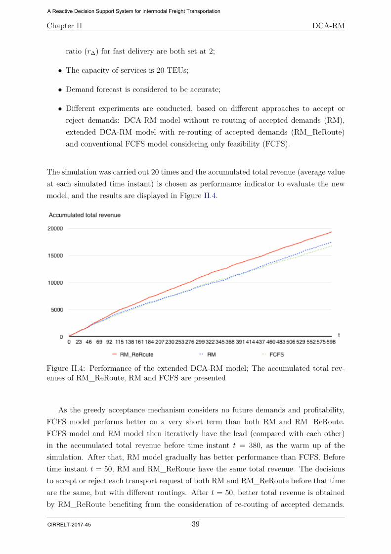
Chapter II DCA-RM
ratio (r∆) for fast delivery are both set at 2;
• The capacity of services is 20 TEUs;
• Demand forecast is considered to be accurate;
• Different experiments are conducted, based on different approaches to accept orreject demands: DCA-RM model without re-routing of accepted demands (RM),extended DCA-RM model with re-routing of accepted demands (RM_ReRoute)and conventional FCFS model considering only feasibility (FCFS).
The simulation was carried out 20 times and the accumulated total revenue (average valueat each simulated time instant) is chosen as performance indicator to evaluate the newmodel, and the results are displayed in Figure II.4.
Figure II.4: Performance of the extended DCA-RM model; The accumulated total rev-enues of RM_ReRoute, RM and FCFS are presented
As the greedy acceptance mechanism considers no future demands and profitability,FCFS model performs better on a very short term than both RM and RM_ReRoute.FCFS model and RM model then iteratively have the lead (compared with each other)in the accumulated total revenue before time instant t = 380, as the warm up of thesimulation. After that, RM model gradually has better performance than FCFS. Beforetime instant t = 50, RM and RM_ReRoute have the same total revenue. The decisionsto accept or reject each transport request of both RM and RM_ReRoute before that timeare the same, but with different routings. After t = 50, better total revenue is obtainedby RM_ReRoute benefiting from the consideration of re-routing of accepted demands.
39
A Reactive Decision Support System for Intermodal Freight Transportation
CIRRELT-2017-45

Chapter II DCA-RM
Following the time in the simulation, the difference between these three models, in termsof accumulated total revenue, is getting bigger.
Recall that the DCA-RM model decides the routing of a demand simultaneously whenthe acceptance decision of that demand is made. Once the routing of a demand is decided,it is then fixed. A set of related future demands are also considered, when making routingplans, so that an intelligent transport capacity allocation is expected with respect to betterresource utilization and profitability. We call a routing procedure like this: predictiverouting, as the decision is made based on a prediction of the future demands. However,the quality of predictive routing mainly depends on the accuracy of the forecast. Themore accurate the forecast is, the better the routing plan will be. To route demands,the extended DCA-RM model follows the predictive routing procedure, but allows there-routing of some accepted demands. From the perspective of those accepted demands,forecasts are regularly updated, as the information of some “future” demands is confirmed.The routing decisions of those accepted demands are then updated regularly correspondingto the confirmed information of “future” demands. An accepted demand keeps beingre-routed until the departure of its very first container. By taking into account there-routing of accepted demands (a more intelligent routing), better transport capacityallocation is expected. According to the results, it is obvious that the extended DCA-RMmodel (RM_ReRoute in Figure II.4) performs better and generates higher total revenuecompared with DCA-RM model (RM in Figure II.4) throughout the simulation.
As Figure II.4 presents the average accumulated total revenue of each model basedon 20 test instances, we then offer more insights of each test instance by presenting thepossible performance patterns of these three tested models in Figure II.5.
As shown in Figure II.5, there are three possible performance patterns: (a)RM_ReRoute >RM > FCFS, (b) RM > RM_ReRoute > FCFS and (c) RM_ReRoute > FCFS >
RM , in terms of total revenue when the simulation is finished. To be more precise, thesethree patterns happened 17 times, 2 times and 1 time, in turn, among the 20 test in-stances. In addition to the expected pattern (a), two more patterns (b) and (c) are alsoobserved. As shown in Figure II.5 (b), RM_ReRoute generates less total revenue thanRM after the simulation in this pattern. We notice that, after t = 514, the accumulatedtotal revenue of RM_ReRoute no more increases. This kind of situation happens, whencurrent demands in the simulation are encountered either infeasible or unprofitable con-secutively for the RM_ReRoute. The same reason also explains the flat segment of RMin Figure II.5 (c). However, as shown in Figure II.5 (c), after the abnormal situation, thecurve of the RM is gradually shrinking its difference compared to FCFS. If the simulationis carried out for longer, RM is expected to have a better total revenue than FCFS. Wealso have the same expectation for RM_ReReoute to obtain the best total revenue among
40
A Reactive Decision Support System for Intermodal Freight Transportation
CIRRELT-2017-45

Chapter II DCA-RM
Figure II.5: Examples of the three possible performance patterns of RM_ReRoute, RMand FCFS
these three models in Figure II.5 (b).
Note that, as more decision variables are considered, more computational time isconsumed to solve the extended DCA-RM model. Therefore, in the rest of the thesis,as the purpose is to validate the concept of RM introduction into the proposed reactivedecision support system, experiments are conducted based on the first version of theDCA-RM model.
II.6 Conclusions
In this chapter, we present a Revenue Management (RM) approach for dynamic capacityallocation of the intermodal barge transportation network. A new model is proposedconsidering the RM polices.
Customers in a deregulated market have different behaviors, requires and willingness topay. To model that, in our research, we classify the customer-demand from 2 dimensions.The first one is contractual category. According to their business relationships with thecarriers, in our research, we assume that customers are classified into two categories,Regular and Spot. Regular customers, are those customers who sign long-term contractswith carriers and whose demands must be accepted, if feasible; and Spot customers, are
41
A Reactive Decision Support System for Intermodal Freight Transportation
CIRRELT-2017-45

Chapter II DCA-RM
those customers who come to the carriers with transport requests from time to timeand consequently whose demands could be rejected. The Spot customers are furtherclassified into two categories, P and F: P stands for partially acceptance, which means tobe accepted as much as possible, and F stands for fully acceptance, which means to beeither fully accepted or rejected. The second dimension to classify customer-demand isits required service quality and booking anticipation, which means customers are askingfor normal/slow delivery or fast delivery, with early or late reservation. Note that, thiscustomer-demand classification is applied throughout the whole thesis.
We conduct a set of experiments to validate the RM approach. Compared with thefirst-come first-serve (FCFS) based booking strategy, the DCA-RM model always gen-erates better total revenue, even with inaccurate demand forecast. Another observa-tion is that facing scarce resource (small transport capacity), the DCA-RM model easilyoutscores its competitor, and this trend grows when resource levels decrease. We also dis-cuss a set of possible negotiation strategies combined with the proposed DCA-RM model,and conclude that with slightly lower total revenue the decision support still offers thepossibility to better satisfy loyal (regular) customers and generate more revenue comparedwith FCFS.
An extended DCA-RM model considering re-routing of accepted demands is thenproposed and studied. According to the numerical results, the extended DCA-RM modelgenerates better total revenue, compared to the first version of the DCA-RM model.Extensive experiments should be conducted to further study and validate this extendedDCA-RM model.
Encouraged by these preliminary results, we are also considering to study how thepenalty or compensation for those denied demands (R, P and F) should be further inte-grated into the new DCA-RM model proposed.
42
A Reactive Decision Support System for Intermodal Freight Transportation
CIRRELT-2017-45
Chapter III
Scheduled Service Network Designwith Revenue ManagementConsiderations for Intermodal BargeTransportation
ContentsIII.1 Introduction . . . . . . . . . . . . . . . . . . . . . . . . . . . . . 45
III.2 Literature Review . . . . . . . . . . . . . . . . . . . . . . . . . . 47
III.3 Problem Statement . . . . . . . . . . . . . . . . . . . . . . . . . 49
III.4 The SSND-RRM Formulation . . . . . . . . . . . . . . . . . . . 54
III.4.1 Revenue Management Modeling for the SSND-RRM . . . . . . 54
III.4.2 Network Modeling . . . . . . . . . . . . . . . . . . . . . . . . . 55
III.4.3 SSND-RRM Model Formulation . . . . . . . . . . . . . . . . . 59
III.5 Simulation and Numerical Results . . . . . . . . . . . . . . . . 63
III.5.1 Test Instances Generation . . . . . . . . . . . . . . . . . . . . . 63
III.5.2 Experiment Plan . . . . . . . . . . . . . . . . . . . . . . . . . . 65
III.5.3 Experiment Results and Analysis: First Group . . . . . . . . . 68
III.5.4 Experiment Results and Analysis: Second Group . . . . . . . . 71
III.5.5 Computational Time . . . . . . . . . . . . . . . . . . . . . . . . 74
III.6 Conclusions . . . . . . . . . . . . . . . . . . . . . . . . . . . . . . 75
43
A Reactive Decision Support System for Intermodal Freight Transportation
CIRRELT-2017-45
In this chapter, we consider the problem of container barge transportation in the con-text of intermodal freight transportation at the middle-term planning level. A new Sched-uled Service Network Design model with Resource and Revenue management (SSND-RRM) is proposed. The same RM policies applied at the operational level (i.e., customerclassification and fare differentiation) in Chapter II, are considered in this model. Giventhe information about the physical network, potential services and forecasted demands,the objective of the proposed SSND-RRM model is to build a scheduled service networkmaximizing the net profit of the carriers. The model is solved with a commercial solverand various problem settings, in terms of demand distribution, network topology, fareclass and quality-of-service (e.g., delivery time), are designed and tested to evaluate it.According to the results, it is promising to consider RM policies at tactical level.
Based on the material included in this chapter, a working paper is in preparation forsubmission to Transportation Science. Different parts of this research have been presentedat several international conferences.
A Reactive Decision Support System for Intermodal Freight Transportation
CIRRELT-2017-45
Chapter III SSND-RRM
III.1 Introduction
Intermodal freight transportation is generally defined as moving cargo by a series of atleast two transportation modes, being transferred from one mode to the next at intermodalterminals, e.g., ports and rail yards, without handling the cargo directly (e.g., [Bektaş andCrainic, 2008,Crainic and Kim, 2007,SteadieSeifi et al., 2014]). Intermodal cargo is thusgenerally loaded into containers for most of its journey.
Consolidation-based carriers perform the largest share of intermodal transportation,rail and navigation companies being particularly active in the long-distance segment. Car-riers aim to maximize net profits and meet shipper demand and requirements, by settingup a resource- and cost-efficient service network and schedule given the forecast demand.The so-called tactical operations planning process yields this network and schedule.
The scheduled service network design (SSND) problem class is the methodology ofchoice to build this tactical plan [Crainic and Kim, 2007]. It selects the transportationservices and schedule the carrier that will operate, and propose them to shippers for thenext season (e.g., six months). The schedule is built for a given schedule length (e.g.,a week), which is then operated repeatedly for the duration of the season. SSND withresource management models, SSND-RM, also include the determination of the resource(e.g., vessels, locomotives, etc.) routes supporting the selected services (e.g., [Andersenet al., 2009a,Crainic et al., 2014]).
Most service network design cases and models in the literature consider a single cat-egory of customers, making up what is generally identified as regular demand, which isexpected to represent most of what is serviced during any “normal” period. SSND modelsare thus set to minimize the cost of performing the service, which may account for bothoperations and the cost of time for resources and cargo. We take a different view andconsider several categories of customers, including regular and so-called spot demands, aswell as several tariffs and operation classes, aiming for the maximization of the net revenuethrough the possibility to capture more demand, or higher priced demand, by offering adifferent service network. We thus integrate revenue management (RM ) considerationsinto tactical planning SSND-RM models.
Although identified as a desirable feature for freight transportation [van Riessen et al.,2015a], RM is rather new to the freight transport planning literature, as illustrated bythe reviews related to air cargo operations [Feng et al., 2015], railway transportation[Armstrong and Meissner, 2010], and container synchromodal services [van Riessen et al.,2015a]. Moreover, the few contributions focusing on revenue management and freight
45
A Reactive Decision Support System for Intermodal Freight Transportation
CIRRELT-2017-45
Chapter III SSND-RRM
transportation [Bilegan et al., 2015,Wang et al., 2015] focus on the operational level, thetactical level being rarely envisaged [Crevier et al., 2012].
Our goal is to contribute closing this gap by studying the incorporation of RM con-siderations, usually tackled at the operational planning level, into tactical planning mod-els for consolidation-based freight transportation carriers. Our interest goes beyond themodeling and algorithmic challenges, to exploring the impact of this integration on thestructure of the service network (e.g., should the carrier increase the offer of service inorder to later be able to capture spot demand?) and the selection of customer demandsto service.
We perform this study within the context of intermodal barge transportation, a fieldrelatively neglected in the literature. We thus present a scheduled service network designwith resource and revenue management (SSND-RRM ) model for the tactical planning ofsuch carriers, and study its behavior and the structural characteristics of the solutionsobtained through an extensive experimentation campaign.
The contributions of the chapter are:
• Introduce what we believe to be the first comprehensive tactical planning model forfreight carriers that integrates revenue (and resource) management considerations;
• Provide a proof-of-concept by using an off-the-shelf software to solve the correspond-ing mixed-integer linear programming (MILP) formulation for realistically dimen-sioned barge intermodal transportation instances;
• Analyze the impact of various problem settings, in terms of, e.g., demand distri-bution, network topology, and fare and quality-of-service (e.g., delivery time, etc.)classes, on the structure of the scheduled service network and the carrier revenues.
The chapter is organized as follows. Section III.2 presents the relevant literaturereview on service network design and revenue management topics. Section III.3 describesthe problem setting and discusses issues related to combining tactical planning and RM.Section III.4 is dedicated to the revenue management modeling at the tactical level andthe proposed SSND-RRM formulation. The experimental plan and the analysis of thenumerical results are described in Section III.5, and we conclude in Section III.6.
46
A Reactive Decision Support System for Intermodal Freight Transportation
CIRRELT-2017-45
Chapter III SSND-RRM
III.2 Literature Review
The section is dedicated to a brief tour of the relevant literature with the goal of relatingour work to the field. We touch on barge transportation, service network design forconsolidation-based freight carriers, and revenue management. [Bontekoning et al., 2004,Macharis and Bontekoning, 2004,Bektaş and Crainic, 2008,SteadieSeifi et al., 2014] offergeneral reviews on planning intermodal freight transportation systems.
Barge transportation, or, more generally, river and canal freight navigation, is eco-nomical in terms of unit transportation cost and eco-friendly in terms of environmentalimpacts. Although slower than other land-based transportation modes, barges may thusplay an important role in intermodal transportation, both in exchanges between maritimeports and the hinterland and among river ports. This role is expanding in Europe, wherethe [European Commission, 2011] identifies barge transportation as the instrumental formodal shift and encouraged its use for intermodal freight transport, as well as elsewhere,most notably in China [Notteboom, 2012]. Yet, compared to other transportation modes,studies focusing on barge transportation, particularly in the context of intermodal trans-portation, are still very few. In most cases, one may class these contributions into one oftwo categories. The first category includes descriptive analyses of intermodal transporta-tion, including barge transport, within a territory or corridor (e.g., [Frémont and Franc,2010,Caris et al., 2012, Zuidwijk, 2015]). One may also mention within this group, thework of [Konings et al., 2013], who identify the need for a hub-and-spoke network struc-ture for intermodal barge transport linked to major sea ports, with the port of Rotterdamas illustration, and that of [van Riessen et al., 2015a], who examine the issues and researchopportunities related to synchromodal container assignment to available transportationmodes and carriers in the same context. The second group of contributions addressesmostly operational issues in ports (e.g., [Taylor et al., 2005,Konings, 2007,Douma et al.,2011]), and in routing and dispatching out of ports (e.g., [Fazi et al., 2015,Braekers et al.,2013]).
There is a rather rich literature on service network design for consolidation-basedfreight carriers [Crainic, 2000], reviewed by, e.g., [Crainic, 2003] for long-haul transporta-tion, [Cordeau et al., 1998] for rail, [Christiansen et al., 2004,Christiansen et al., 2007] formaritime, and [Crainic and Kim, 2007] for intermodal transportation. Scheduled servicenetwork design aims to generate the tactical operations plan for a consolidation-basedfreight carrier to, generally, minimize its costs or, more rarely, maximize revenues. Themain decisions making up the models address the selection of services and their schedules,the determination of the terminal policies such as classification and consolidation of cargoand vehicles and the formation of convoys (when relevant), and the optimization of the
47
A Reactive Decision Support System for Intermodal Freight Transportation
CIRRELT-2017-45

Chapter III SSND-RRM
cargo flow distribution on the resulting network to satisfy the multi-commodity demand.
SSND with resource management models include explicitly into the tactical planningmodels some high-level representation of the management of key resources, e.g., powerunits, vehicles or crews, necessary to operate the selected services. Encountered initiallyin articles targeting particular applications (e.g., [Lai, M.F. and Lo, H.K., 2004,Arma-cost et al., 2002, Smilowitz et al., 2003]), the SSND-RM problem is formally modeledby [Pedersen et al., 2009] as a network design problem with design-balance constrains, thelatter imposing that the numbers of services (or resources) entering and leaving terminal-representing nodes be balanced. Extensions are presented by [Andersen et al., 2009b,An-dersen et al., 2009a, Crainic et al., 2014] who, among other contributions, model thetime-dependency of decision through time-space networks, enrich the range of resourcemanagement concerns, and emphasize the circular nature of the routes resources mustfollow to support the selected services.
We found only one publication addressing the tactical planning of an intermodal bargefleet [Sharypova et al., 2012]. The authors propose a SSND-RM model for the particu-lar case of direct services (no intermediate stops), unique customer and service types, asingle container type, and two homogeneous vehicle fleets representing barges and trucks.The authors propose a continuous-time formulation with particular care being paid to themodeling of the terminal service synchronization and the associated load/unload/transferoperations. The numerical results obtained on very small instances are encouraging, par-ticularly in showing the interest of SSND-RM for planning barge transportation systems.The formulation we propose, based on a discrete-time representation, takes into accounta significantly richer set of problem characteristics, as well as explicitly including revenuemanagement aspects.
Indeed, none of these contributions found in the literature addressed the issue of rev-enue management. Revenue, or yield, management was initially developed for passengerair transportation, and was latter applied more broadly to passenger rail transporta-tion, hotel room management, etc. (e.g., [Kasilingam, 1997]).The benefits observed inthese domains appear promising for the freight transport industry as well. Yet, one can-not simply transpose the models and procedures from one industry to the other. Thus,e.g., [Kasilingam, 1997] present the characteristics and complexities of air cargo trans-portation (see for a review of air cargo operations [Feng et al., 2015]) from the perspectiveof RM by emphasizing the differences between air cargo and air passenger transportation.The author point out, in particular, that a correct and relevant model of RM for freighttransportation requires the comprehensive understanding of customers’ behavior, the con-secutive identification of customer categories, the so-called customer classification, andthe definition of different products and fares charged, i.e., the fare differentiation.
48
A Reactive Decision Support System for Intermodal Freight Transportation
CIRRELT-2017-45
Chapter III SSND-RRM
The contributions integrating RM and freight transportation of which we are awareaddress operational-level issues only. Thus, [Crevier et al., 2012] propose a bi-level mixed-integer formulation to jointly determine fares and the capacity utilization of a given set ofservices proposed by a rail freight carrier. [Bilegan et al., 2015] also present a RM modelapplied to rail freight transportation in which different fare classes are defined with respectto how early the booking is performed and how long the delivery time is. [Armstrong andMeissner, 2010] survey RM applied to railway transportation.
RM-related concepts are found in a number of tactical-planning studies for varioustransportation modes, e.g., the possibility not to service all the demand (e.g., [Braekerset al., 2013,Andersen and Christiansen, 2009,Thapalia et al., 2012]), the maximization ofthe net revenue, and the possibility for demands to be only partially accepted (e.g., [Tey-paz et al., 2010,Agarwal and Ergun, 2008,Gelareh and Pisinger, 2011]), and the segmen-tation of the transportation requests according the obligation to service them [Stålhaneet al., 2014].
We did not find, however, contributions integrating scheduled service network design,resource management and revenue management. We propose such an integrated modelin Section III.4 for the intermodal transportation problem described next.
III.3 Problem Statement
We address the problem of setting up the tactical plan of an intermodal freight trans-portation carrier to maximize its revenues, while satisfying the estimated demand andrequirements of its customers, and making the best use of its resources. The tactical planthus determines the transportation services and schedule, together with the assignmentof resources to the selected services, that the carrier will operate for the next cycle ofactivities, the next “season” (six months, for example), to answer this demand. Thetransportation plan actually specifies how operations are to be performed for a given timelength, e.g., a week, that we call schedule length. The plan is then operated repeatedlyfor the duration of the season.
We therefore describe the problem we address along three dimensions. For the firstdimension, we focus on the physical network and resources of a barge/coastal navigationcarrier performing intermodal transportation, including the port infrastructure and facil-ities, the containers that need to be moved and the vessels that transport them. For thesecond one, we describe the customers of the system, that is, the shippers generating thedemand for transportation of various types of containers, together with their requirements
49
A Reactive Decision Support System for Intermodal Freight Transportation
CIRRELT-2017-45
Chapter III SSND-RRM
and expectations in terms of cost and service quality. The last one considers the fares,services and schedule the carrier is setting up to satisfy this demand and address theserequirements over a medium-term, tactical planning horizon. The challenges and aimsrelated to the representation of RM activities into the scheduled service network designwith resource management formulation (detailed in Section III.4) are discussed at thesecond and third dimension, respectively.
Physical network and resources. A barge intermodal transportation system isdefined over a physical network of rivers and canals plus, eventually, coastal and short-sea-shipping navigation corridors. A number of physical characteristics often constrainnavigation on this network, e.g., the maximum draft of fully loaded vessels sailing on agiven part of a river or canal, and the number of vessels that may simultaneously navigate,in both directions, the same part of a river or canal during a given period of time.
A number of ports with container terminals are located along these rivers and canalsor on the sea shore. The layout and physical organization of a terminal, together withthe equipment available and the operation policies (as well as the conventions stating theworking rules for the personnel) constrain the activities that may be performed withinand influence the associated costs and performance measures. Prominent among theselimits and measures for the problem at hand are the maximum draft of fully loadedvessels berthing at the terminal, the number of vessels and associated length that maysimultaneously berth, the number of containers that may be stored within the terminalfor a given period of time, and the rate of vessel loading and unloading operations interms of containers per period of time. Costs are associated to terminal activities and arecharged to carriers using the port. Given the problem addressed in this chapter, we targetparticularly the cost of calling at the port, which varies by vessel type and the duration ofthe presence in the port, as well as the container loading/unloading (per container) andholding (per container and time period) costs.
The carrier operates a number of vessels to transport the containers shipped by itscustomers. Containers come in several types. They differ in terms of dimensions, 20and 40-foot long being the standard dimension for maritime and river navigation, whilelonger boxes are used within land-based intermodal transportation systems, such as the53-feet ones found in North America. Containers also differ in scope and requirements,e.g., insulated, refrigerated, bulk, tank, open top, high cube, and so on and so forth.For tactical planning purposes, the standard twenty-feet equivalent unit (TEU) measureis generally used, where 20-foot containers measure 1 TEU, while 40-foot ones accountfor 2 TEUs. Vessels also come in several types defined by their characteristics in termsof dimensions, draft, maximum number of TEUs carried, speed, etc., A limited numberof vessels of each type is available for the next season (vessels may be owned or rented,
50
A Reactive Decision Support System for Intermodal Freight Transportation
CIRRELT-2017-45
Chapter III SSND-RRM
but we will treat them in a similar way in this chapter). Operating a vessel incurs costs.Other than the port-related costs mentioned above, we consider in this chapter the travelcosts between particular pairs of ports, as well as the cost (maintenance, depreciation,etc.) associated with not using a vessel for the considered schedule length.
Customer demand. Customers ship loaded and empty containers of given typesamong particular pairs of terminals in the network. Shippers have quality and pricerequirements for each demand for transportation of a certain number of TEUs. “Quality”may involve the type of vehicle and handling equipment required for the particular typeof containers involved. It always involves, however, requirements in terms of travel timeand delivery date. In this chapter, we represent the quality requirements as the duedate associated to the demand, that is, the latest date containers have to be delivered atdestination. The price expectations of shippers are related to the value of the cargo andthe urgency of delivery. Obviously, they desire the lowest fare possible.
In traditional settings, including navigation-based intermodal transportation, a singleservice type (in terms of delivery time between two terminals in the network) is offered toshippers, the fare being determined mainly by the distance involved, and the cargo char-acteristics such as volume, weight, cargo type and handling requirements (e.g., dangerousgoods require special treatment), etc. On these bases, the final price paid by a givenshipper then results from the negotiations it and the carrier engage into, the existence oflong-term contracts or understandings with regular and trustworthy customers stronglyinfluencing the proceedings.
Following this commercial model, most service network design cases and models in theliterature consider a single category of customers, making up what is generally identifiedas regular demand. One generally finds in this category customers, or groups of customersin particular zones, that are strongly believed to bring business on a regular basis for thecoming season. This forecast (formal forecasting methods may or may not be involved)is based on a combination of signed long-term contracts, informal understanding withlong-standing, trustful customers, and market estimation by sales and customer-relationpersonnel. Regular demand is expected to make up a good part (a 80% figure is oftenmentioned) of what is serviced during any “normal” period.
When revenue management mechanisms are in place, or contemplated, the situation isdifferent. At a strategic level, one establishes a service and tariff policy, e.g., segmentingthe potential customers and defining a number of traffic/tariff classes and service levelsto attract the targeted customers and volume of demand. One also negotiates long-term contracts or understandings with important customers to ensure a good level ofregular business, which translates into regular levels of demand and traffic. During actual
51
A Reactive Decision Support System for Intermodal Freight Transportation
CIRRELT-2017-45
Chapter III SSND-RRM
operations, the revenue management mechanisms are used to determine the acceptanceand tariff of each request for transportation and, thus, to adjust the actual demand tothe offer of services with fixed capacities, regular schedules, and so on, which was plannedbased on demand forecasts. The questions then are, how to represent such mechanismswithin tactical planning models, and what is the benefit of using RM-based informationand knowledge when building the transportation plan.
Services and schedules. Each potential service is defined by an origin terminaland associated departure time within the schedule length, a destination terminal, a routethrough the physical network, a sequence of intermediary calls at ports along this route(the sequence is empty for direct services), and a schedule indicating the arrival and,for the intermediate stops, the departure times at ports. Without loss of generality,and because it reflects actual practice for the problem setting we examine, we assumethe longest service duration to be less than the schedule length. A vessel of particularcharacteristics is associated to each service. Each service is thus characterized by theattributes of its designated type of vessel, as well as by the costs to set up and operateon the links of its route.
Symmetrically, a vessel is assigned to a set of services during the schedule length.Without loss of generality, we assume vessels return to their home port. Consequently,each operated vessel supports a circular sequence of services starting and ending at thesame port. These cycling vessel routes, that we call service cycles in the following, ensurethat there are no empty-repositioning movements in the system we study.
The set of services selected by the carrier to efficiently and profitably satisfy theestimated demand, makes up the transportation plan and defines its service network andoperating schedule. Each customer demand is moved over this service network by oneof the possible itineraries for the particular demand. Remark that the same physicalcustomer may have several shipments over the schedule length, and that these shipmentsmay differ in volume, characteristics, and requested service level. We represent such casesas different customer demands. Remark also that, while demand estimations may be madeindividually for major and regular customers, most demands represent an aggregationof regular and potential customers within a given zone and with similar transportationrequests.
A demand itinerary is then defined by the origin terminal of the shipment and itsavailability period (i.e., the time it is supposed to arrive at the origin terminal), thesequence of services until the associated destination terminal, and the number and typeof containers moved. The sequence of services thus yields the schedule of the itinerary,i.e., the arrival and departure moments at each port terminal, together with the time
52
A Reactive Decision Support System for Intermodal Freight Transportation
CIRRELT-2017-45
Chapter III SSND-RRM
spent in the terminal to 1) unload the cargo from the incoming service, 2) wait in theterminal for the next service, and 3) load on that next service. We assume unloadingoperations take place immediately after the arrival of the service at the terminal, followedby loading operations taking place before leaving the terminal.
The SSND-RRM problem. As indicated earlier, the carrier aims to meet demandand the shipper requirements in the most resource- and cost-efficient way, through plannedoperations that maximize its net profit. The aim is thus to 1) select the services, out of aset of potential feasible ones, and, through their departure times, the schedule to operate,2) determine the circular asset routes, the service cycles, supporting the selected services,and 3) identify the demand itineraries. The combination of these three objectives alsoyields the loads of vessels during their movements from one stop of the correspondingservice to the next, and the amount of work to be performed on vessels and containers ateach port of call in the network.
The integration of revenue management considerations to tactical planning is per-formed through two major modifications to the traditional problem setting and modelingapproach.
First, we take the different view of explicitly considering several categories of cus-tomers, tariff and operation classes. The first category is the regular demand as discussedabove. Two other categories correspond to demand that is potentially there and that thecarrier could accept or not, given the estimated revenue and the capacity it plans to de-ploy. Such demand is usually explicitly accounted for in fleet [Crainic et al., 1993,Powell,W.B. and Topaloglu, H., 2005] and revenue management [Bilegan et al., 2015], but isnot normally included into tactical-planning formulations. The challenge of integratingit into an SSND-RRM formulation comes from the required qualitative and quantitativetranslation of the business relationship the carrier holds with its customers into a com-pact representation adequate for the aggregated tactical level. This translation is logicallyperformed in terms of demand characterization, starting with customer behavior (segmen-tation) considerations, but also including service-level (delivery delays) requirements.
Second, contrary to service network design literature, the goal here is the maximizationof the net revenue. The net revenue is computed as the difference between the estimatedprofit of servicing the regular and the accepted potential demand and the cost of per-forming the planned service. The cost accounts both for setting up the services and foroperating vessels and transporting containers. It is also generalized, accounting simul-taneously for operations and the cost of time for resources and cargo, given the latter’sservice and tariff class (remark that service differentiation was considered in a number ofearlier contributions, e.g., [Crainic et al., 1984,Crainic and Rousseau, 1986,Crainic and
53
A Reactive Decision Support System for Intermodal Freight Transportation
CIRRELT-2017-45
Chapter III SSND-RRM
Roy, 1988], without being contrasted to the revenues of the carrier).
The resulting SSND-RRM model may therefore be used both to plan the operationsfor the next season and as a tool to evaluate RM policies. It aims, in particular, to pro-vide the means to answer questions, e.g., is it profitable to increase the level of servicein terms of service frequencies or capacities, resulting in higher fixed and variable costs,in order to attract more, higher-priced, demand? Are the current or contemplated dif-ferentiated customer categories, and fare classes with their associated values adequate?Is the contemplated contract or business relationship for regular demand actually prof-itable? Which and how much of the potential demand should/could be serviced within apredefined schedule length, while optimally using the available resources?
We describe in the next section the methodology used to address these issues andformulate the planning problem at the tactical level.
III.4 The SSND-RRM Formulation
We present the formulation of the scheduled service network design with resource andrevenue management (SSND-RRM) model for the tactical planning of intermodal bargetransportation in three steps. We first discuss the representation of the revenue manage-ment considerations in terms of customer service and fare differentiation (Section III.4.1).We then introduce the time-space representation of operations, the demand, and the ser-vices one has to select in order to satisfy it (Section III.4.2). The formulation is presentednext (Section III.4.3).
III.4.1 Revenue Management Modeling for the SSND-RRM
Let D represent the set of regular and potential customer demands, and the notationd ∈ D will denote a particular demand. We model customer service and fare differentiationthrough a two-dimensional mechanism: business relationship and service requirement.
Business relationship addresses principally the contractual profile of customers, thatis, the commitment to work with the carrier: regular customers with long-term contractsor understandings, and customers present on the spot market that we may service or not.The latter correspond to a pool of irregular potential customers, who may arrive to thesystem as “short-notice” requests. Individually, these customers could be “small” in termsof volume and, even, not regularly present but, taken collectively, they form a significant
54
A Reactive Decision Support System for Intermodal Freight Transportation
CIRRELT-2017-45
Chapter III SSND-RRM
and consistent demand in terms of total volume per origin-to-destination pair; Identifiedwithin a given geographical zone - around a port that is the origin of their requests fortransportation - the decision to service them is to be made according to their particularrequirements and the available planned capacity on the transportation network.
We define three categories of business relationships (and customers), partitioning thecustomer set, D = DR ∪ DP ∪ DF, as follows:
• Regular customer demands, grouped within set DR, representing customers withlong-term contracts or understandings; This class corresponds to the regular demandin classical SSND formulations and must be always satisfied;
• Proportional-punctual customer demands, set DP, that may be fragmented and onlypartly satisfied, which means a fraction of it could be integrated in the demand tobe serviced by the planned services, the rest not being served at all by the carrier;We model this decision further down in this section through continuous decisionvariables yielding the percentage of the demand that is going to be serviced;
• Full-punctual demands, set DF, consisting of demands that may be either entirelyaccepted and serviced or not accepted at all; Binary selection variables are intro-duced in the formulation to represent these decisions.
Two service types are defined with respect to the service requirement dimension of theproposed mechanism, slow/normal and fast delivery reflecting the due times at destinationrequested by customers. Fares normally reflect service differentiation, e.g., fast deliveryrequests would be priced higher than slow delivery ones. We consequently introduce twofare classes:
• class(d): Fare class for demand d ∈ D, related to the type of delivery, slow/normalor fast requested;
• f(d): Unit fare value for demand d ∈ D with fare class class(d).
III.4.2 Network Modeling
Let the oriented graph Gph = (N ph,Aph) represent the physical network supporting theoperations of the carrier. The set N ph represents intermodal terminals. Each terminali ∈ N ph is characterized by a berthing capacity Qi in number of vessels per time period,and a container holding capacity Hi in number of TEUs per time period. The former is
55
A Reactive Decision Support System for Intermodal Freight Transportation
CIRRELT-2017-45
Chapter III SSND-RRM
defined with respect to the average length of the vessels used on the network, which isreasonable given the rather limited range of vessels used in such systems.
The set Aph groups the physical arcs of the network, each representing a possiblenavigation movement between two “consecutive” ports, that is, no intermediary portexists between the initial and final nodes of the arc. To simplify the presentation, butwithout loss of generality, we assume uncapacitated physical arcs.
Let the schedule length be discretized into T periods of equal length by T + 1 timeinstants t ∈ 0, ..., T . The period length is generally defined according to the particularoperational context of the application, e.g., average travel time along links or stoppingtime at ports, and the schedule length. For a week-long schedule on a river/coastal navi-gation network, a period length of a couple of hours appears appropriate. By convention,activities, e.g., demand arrival at terminals and vessel arrivals and departures at and fromports, occur at the beginning of a period.
Let Γ be the set of container types, and the notation γ ∈ Γ will denote a particularcontainer type. Then, as discussed above, each demand d ∈ D = DR ∪ DP ∪ DF ischaracterized by:
• vol(d): Volume in number of TEUs;
• γ(d): Container type, γ(d) ∈ Γ;
• orig(d): Origin node, orig(d) ∈ N ph;
• in(d): Period the demand d becomes available for transportation at orig(d);
• dest(d): Destination node, dest(d) ∈ N ph;
• out(d): Due date at destination, that is, the latest period the cargo may arrive atthe destination terminal;
• cat(d): Category of customer demand (R or P or F), according to whether d ∈ DR
or DP or DF;
• class(d): Fare class, slow/normal or fast;
• f(d): Unit fare value.
The carrier operates vessels of various types, that it owns or rents for the season,according to the scheduled set of services. The set of vessel types is noted L, each vesseltype l ∈ L being characterized by:
56
A Reactive Decision Support System for Intermodal Freight Transportation
CIRRELT-2017-45
Chapter III SSND-RRM
• cap(l): Capacity in TEUs;
• speed(l): Speed of vessel of type l ∈ L in normal operations, yielding δij(l), thenormal travel time of an l type vessel over arc (i, j) ∈ Aph;
• Bl: Maximum number of vessels of type l ∈ L available.
The formulation is defined on a circular time-space network capturing the time-dependency and repetitiveness of the demand and schedule (services and resource uti-lization), taking the form of an oriented graph G = (N ,A), with node and arc sets N andA, respectively. The network (and the the transportation plan and schedule) is circularover the schedule length, which means that any arc in A of length (duration) δ that startsat time t, arrives at destination at time (t+ δ) mod T .
The node set N is obtained by duplicating all physical nodes at all periods in theschedule length, so that node it ∈ N corresponds to the physical node i ∈ N ph at timeinstant t, t = 0, . . . , (T − 1). The set of arcs A is the union of the set of holding arcsat terminals, and the set of possible movements performed by services. A holding arc(it, i(t + 1)) captures a one time period waiting at terminal i at time t for vessels, cargoand services. Movements in the time-space network are performed by services travelingphysical paths between two consecutive stops on their respective routes. We call suchmovements service legs and these define the moving arcs of A.
A service s ∈ S is thus defined in the time-space network G by a number of physicaland time-related attributes, illustrated in Figures III.1 and III.2, and described as follows:
• orig(s): Physical origin terminal, orig(s) ∈ N ph;
• dest(s): Physical destination terminal, dest(s) ∈ N ph;
• η(s) = {ik(s) ∈ N ph, k = 0, . . . , (K − 1)}: Ordered set of consecutive stops of theservice, where K = |η(s)| and k indicates the kth stop of the service;
• ak(s) = (ik(s), ik+1(s)): kth leg of the service, k = 0, . . . , (K − 2);
• r(ak(s)) ⊆ Aph: Path of ak(s) in the physical network;
• δk(s): Travel time of leg ak(s);
• wk(s): Stopping time at terminal ik(s);
• αk(s): Arrival time of the service at its terminal ik(s); By convention:
57
A Reactive Decision Support System for Intermodal Freight Transportation
CIRRELT-2017-45
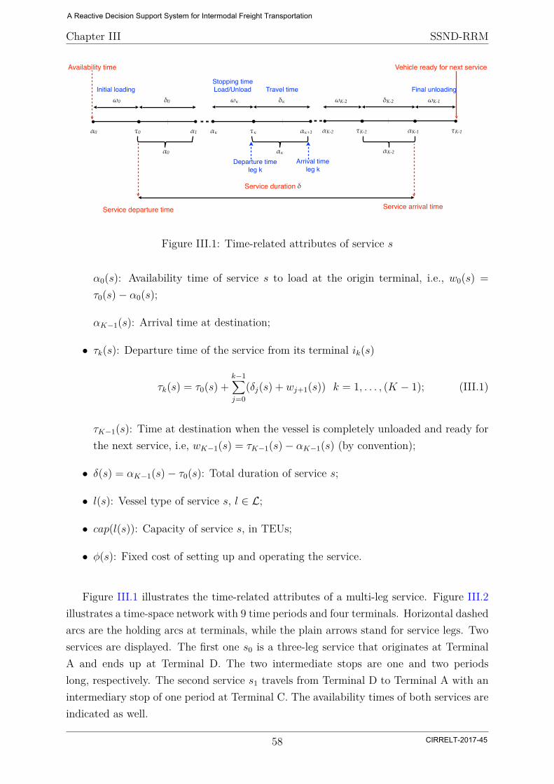
Chapter III SSND-RRM
Availability time
Initial loadingStopping timeLoad/Unload Travel time Final unloading
Vehicle ready for next service
ω0 δ0 ωκ δκ ωΚ-2 δΚ-2 ωΚ-1
Service duration
Service departure time Service arrival time
δ
α0 τ0
α0
α1 ακ τκ
ακ
ακ+1 αΚ-2 τΚ-2
αΚ-2
αΚ-1 τΚ-1
Departure timeleg k
Arrival timeleg k
Figure III.1: Time-related attributes of service s
α0(s): Availability time of service s to load at the origin terminal, i.e., w0(s) =τ0(s)− α0(s);
αK−1(s): Arrival time at destination;
• τk(s): Departure time of the service from its terminal ik(s)
τk(s) = τ0(s) +k−1∑j=0
(δj(s) + wj+1(s)) k = 1, . . . , (K − 1); (III.1)
τK−1(s): Time at destination when the vessel is completely unloaded and ready forthe next service, i.e, wK−1(s) = τK−1(s)− αK−1(s) (by convention);
• δ(s) = αK−1(s)− τ0(s): Total duration of service s;
• l(s): Vessel type of service s, l ∈ L;
• cap(l(s)): Capacity of service s, in TEUs;
• φ(s): Fixed cost of setting up and operating the service.
Figure III.1 illustrates the time-related attributes of a multi-leg service. Figure III.2illustrates a time-space network with 9 time periods and four terminals. Horizontal dashedarcs are the holding arcs at terminals, while the plain arrows stand for service legs. Twoservices are displayed. The first one s0 is a three-leg service that originates at TerminalA and ends up at Terminal D. The two intermediate stops are one and two periodslong, respectively. The second service s1 travels from Terminal D to Terminal A with anintermediary stop of one period at Terminal C. The availability times of both services areindicated as well.
58
A Reactive Decision Support System for Intermodal Freight Transportation
CIRRELT-2017-45
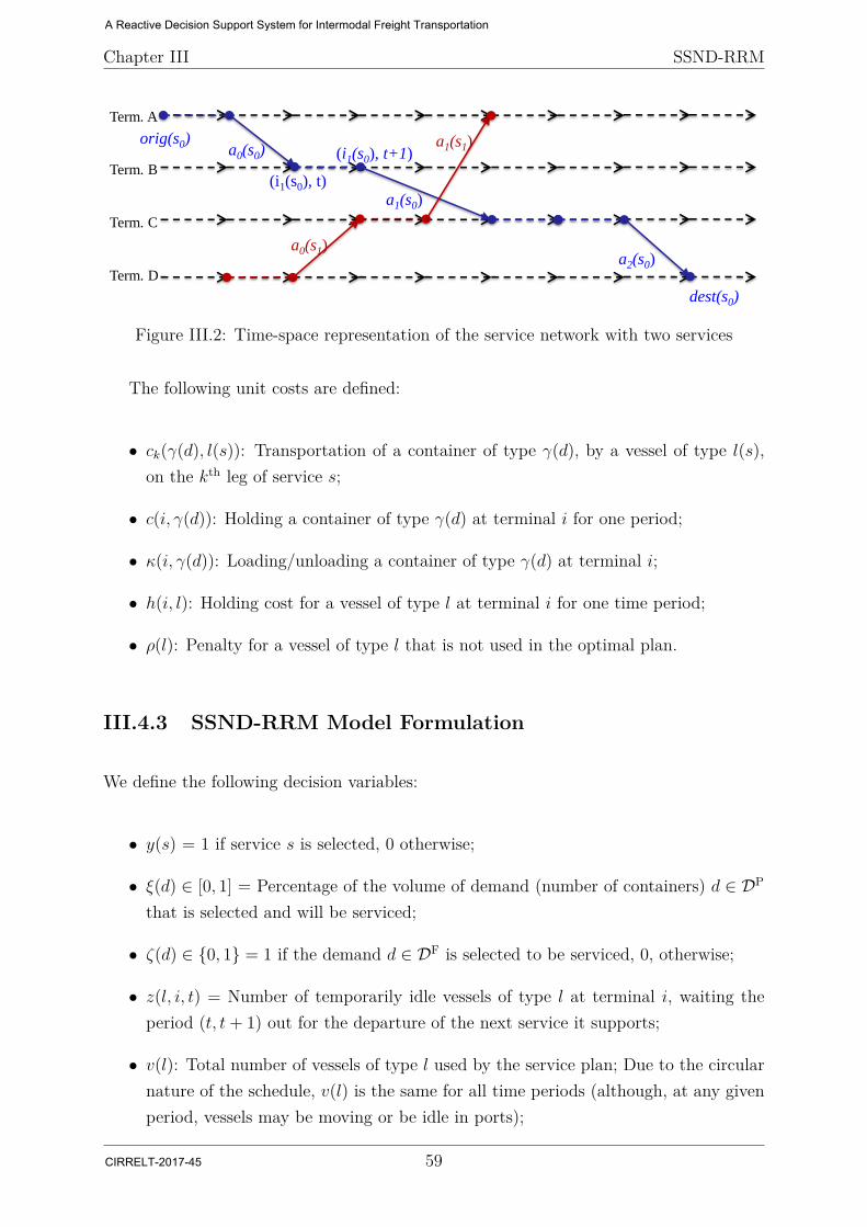
Chapter III SSND-RRM
© Teodor Gabriel Crainic 2016
Term. A
Term. B
Term. C
Term. D
a0(s0)
a1(s0)
a2(s0)a0(s1)
a1(s1)
(i1(s0), t)
(i1(s0), t+1)orig(s0)
dest(s0)
Figure III.2: Time-space representation of the service network with two services
The following unit costs are defined:
• ck(γ(d), l(s)): Transportation of a container of type γ(d), by a vessel of type l(s),on the kth leg of service s;
• c(i, γ(d)): Holding a container of type γ(d) at terminal i for one period;
• κ(i, γ(d)): Loading/unloading a container of type γ(d) at terminal i;
• h(i, l): Holding cost for a vessel of type l at terminal i for one time period;
• ρ(l): Penalty for a vessel of type l that is not used in the optimal plan.
III.4.3 SSND-RRM Model Formulation
We define the following decision variables:
• y(s) = 1 if service s is selected, 0 otherwise;
• ξ(d) ∈ [0, 1] = Percentage of the volume of demand (number of containers) d ∈ DP
that is selected and will be serviced;
• ζ(d) ∈ {0, 1} = 1 if the demand d ∈ DF is selected to be serviced, 0, otherwise;
• z(l, i, t) = Number of temporarily idle vessels of type l at terminal i, waiting theperiod (t, t+ 1) out for the departure of the next service it supports;
• v(l): Total number of vessels of type l used by the service plan; Due to the circularnature of the schedule, v(l) is the same for all time periods (although, at any givenperiod, vessels may be moving or be idle in ports);
59
A Reactive Decision Support System for Intermodal Freight Transportation
CIRRELT-2017-45
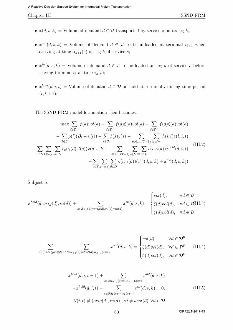
Chapter III SSND-RRM
• x(d, s, k) = Volume of demand d ∈ D transported by service s on its leg k;
• xout(d, s, k) = Volume of demand d ∈ D to be unloaded at terminal ik+1 whenarriving at time αk+1(s) on leg k of service s;
• xin(d, s, k) = Volume of demand d ∈ D to be loaded on leg k of service s beforeleaving terminal ik at time τk(s);
• xhold(d, i, t) = Volume of demand d ∈ D on hold at terminal i during time period(t, t+ 1);
The SSND-RRM model formulation then becomes:
max∑d∈DR
f(d)vol(d) +∑d∈DP
f(d)ξ(d)vol(d) +∑d∈DF
f(d)ζ(d)vol(d)
−∑l∈L
ρ(l)(Bl − v(l))−∑s∈S
φ(s)y(s)−∑
t∈0,...,(T−1)
∑i∈Nph
h(i, l)z(l, i, t)
−∑s∈S
∑k∈η(s)
∑d∈D
ck(γ(d), l(s))x(d, s, k)−∑
t∈0,...,(T−1)
∑i∈Nph
∑d∈D
c(i, γ(d))xhold(d, i, t)
−∑s∈S
∑k∈η(s)
∑d∈D
κ(i, γ(d))(xin(d, s, k) + xout(d, s, k))
(III.2)
Subject to
xhold(d, orig(d), in(d)) +∑
s∈S:ik(s)=orig(d),τk(s)=in(d)xin(d, s, k) =
vol(d), ∀d ∈ DR
ξ(d)vol(d), ∀d ∈ DP
ζ(d)vol(d), ∀d ∈ DF
(III.3)
∑in(d)<t≤out(d)
∑s∈S:ik+1(s)=dest(d),αk+1(s)=t
xout(d, s, k) =
vol(d), ∀d ∈ DR
ξ(d)vol(d), ∀d ∈ DP
ζ(d)vol(d), ∀d ∈ DF
(III.4)
xhold(d, i, t− 1) +∑
s∈S:ik+1(s)=i,αk+1(s)=txout(d, s, k)
−xhold(d, i, t)−∑
s∈S:ik(s)=i,τk(s)=txin(d, s, k) = 0,
∀(i, t) 6= (orig(d), in(d)),∀i 6= dest(d),∀d ∈ D
(III.5)
60
A Reactive Decision Support System for Intermodal Freight Transportation
CIRRELT-2017-45
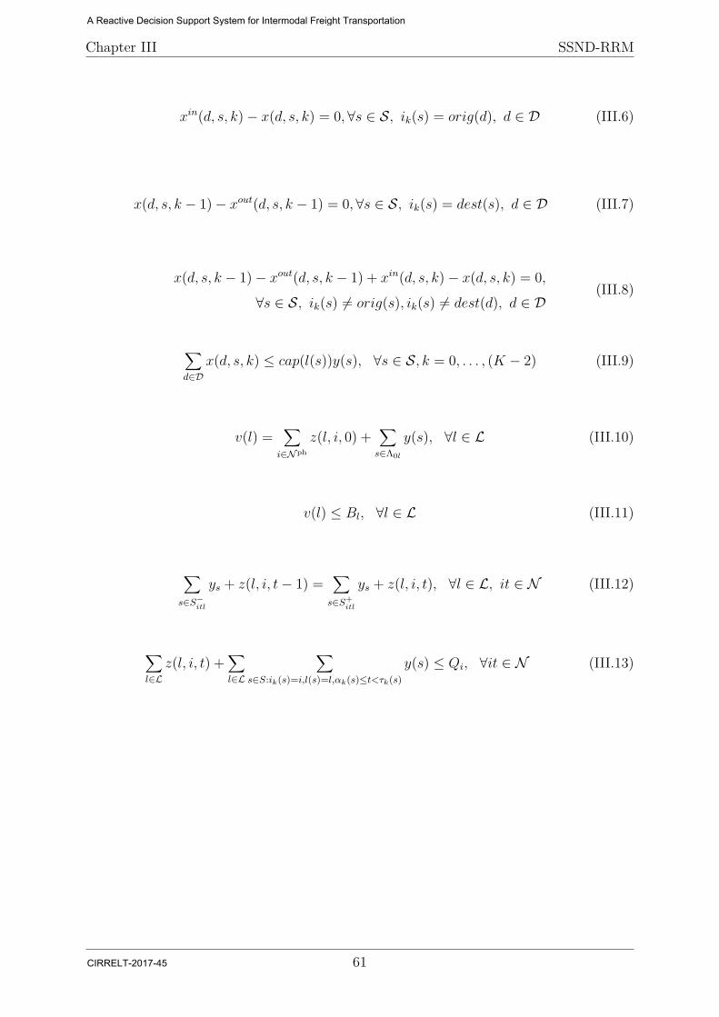
Chapter III SSND-RRM
xin(d, s, k)− x(d, s, k) = 0, ∀s ∈ S, ik(s) = orig(d), d ∈ D (III.6)
x(d, s, k − 1)− xout(d, s, k − 1) = 0, ∀s ∈ S, ik(s) = dest(s), d ∈ D (III.7)
x(d, s, k − 1)− xout(d, s, k − 1) + xin(d, s, k)− x(d, s, k) = 0,
∀s ∈ S, ik(s) 6= orig(s), ik(s) 6= dest(d), d ∈ D(III.8)
∑d∈D
x(d, s, k) ≤ cap(l(s))y(s), ∀s ∈ S, k = 0, . . . , (K − 2) (III.9)
v(l) =∑i∈Nph
z(l, i, 0) +∑s∈Λ0l
y(s), ∀l ∈ L (III.10)
v(l) ≤ Bl, ∀l ∈ L (III.11)
∑s∈S−
itl
ys + z(l, i, t− 1) =∑s∈S+
itl
ys + z(l, i, t), ∀l ∈ L, it ∈ N (III.12)
∑l∈L
z(l, i, t) +∑l∈L
∑s∈S:ik(s)=i,l(s)=l,αk(s)≤t<τk(s)
y(s) ≤ Qi, ∀it ∈ N (III.13)
61
A Reactive Decision Support System for Intermodal Freight Transportation
CIRRELT-2017-45
Chapter III SSND-RRM
y(s) ∈ {0, 1}, ∀s ∈ S
ξ(d) ∈ [0, 1], ∀d ∈ DP
ζ(d) ∈ {0, 1}, ∀d ∈ DF
z(l, i, t) ≥ 0, ∀l ∈ L, it ∈ N
v(l) ≥ 0, ∀l ∈ L
x(d, s, k) ≥ 0, ∀d ∈ D, s ∈ S, k = 0 . . . (K − 2)
xout(d, s, k) ≥ 0, ∀d ∈ D, s ∈ S, k = 0 . . . (K − 2)
xin(d, s, k) ≥ 0, ∀d ∈ D, s ∈ S, k = 0 . . . (K − 2)
xhold(d, i, t) ≥ 0, ∀d ∈ D, it ∈ N .
(III.14)
(III.15)
(III.16)
(III.17)
(III.18)
(III.19)
(III.20)
(III.21)
(III.22)
The objective function (III.2) maximizes the net profit, where the first three terms cor-respond to the revenue obtained by servicing the complete demand of regular customers,the selected proportion of demand of the proportional-punctual customers, and the com-plete demand of the selected and full-punctual customers respectively. Remark that, for agiven set of demands, the first term (revenue obtained by servicing the complete demandof regular customers) is a constant. It is kept to make the objective function homoge-neous. The following terms stand for the activity and time-related costs of operating theselected service network and resource routes, that is, the penalty cost of having but notusing vessels (never assigned to a service during the entire schedule length), the fixed costof setting up and operating services, the cost of the vessels idling at a port waiting fortheir next service departure, the cost of transporting containers on services, and the costof holding and handling containers in terminals.
Equations (III.3), (III.4) and (III.5) are flow-conservation constraints for containersof all customer types, at their particular origins, destinations, and intermediary nodes,respectively. Similarly, Equations (III.6), (III.7) and (III.8) enforce the conservation ofcontainer flows, for all customer types, on each service at its origin, destination andintermediary stops, respectively. Constraints (III.9) enforce the service capacity on eachleg.
Equation (III.10) computes the number of vessels used in the plan as the sum ofvessels idling in ports or moving between them performing services. Due to the resourcemanagement concerns and the resulting circular vessel routs, v(l) is the same at all periods,only the relative proportion of idle versus active vessels being different at different timeperiods. We therefore compute this number for the first period, i.e., t = 0, the setΛ0l = {s ∈ S, l(s) = l|(αK−1(s) mod T ) < τ0(s) and τ0(s) ≥ 0} ⊆ S containing allservices, of the appropriate vessel type, that operate one of its legs during the first period.
62
A Reactive Decision Support System for Intermodal Freight Transportation
CIRRELT-2017-45
Chapter III SSND-RRM
Constraints (III.11) enforce the fleet size for each vessel type, while Equations (III.12)are the so-called design-balance constraints, enforcing the vehicle-flow conservation atterminals (the number of services and vessels entering a node equals the number exitingthe node), where sets S−itl and S+
itl
S−itl = {s ∈ S | dest(s) = i, τK−1(s) = t, l(s) = l} (III.23)
S+itl = {s ∈ S | orig(s) = i, α0(s) = t, l(s) = l} (III.24)
group the services of type l that arrive at their destination or depart from their origin i attime t, respectively. Finally, Constraints (III.13) enforce the terminal berthing capacityat each time period, while decision-variable domains are defined by Constraints (III.14) -(III.22).
III.5 Simulation and Numerical Results
In this section, we design and conduct a set of experiments to validate the proposedScheduled Service Network Design with consideration of Resource and Revenue Manage-ment (SSND-RRM) model. Two research questions are discussed: first, the benefits ofdifferentiating products for decision making at tactical level; and second, the impactsof customer classification and fare differentiation on the scheduled service plan and theflow distribution. The rest of this section is organized as follows. We first describe theprocedure of test instance generations in Subsection III.5.1. Subsection III.5.2 briefly in-troduces the experiment plan. We then present and analyze the experiment results, withrespect to each research question, in Subsection III.5.3 and III.5.4, respectively. A briefanalysis relative to the computational times can be found in Subsection III.5.5.
III.5.1 Test Instances Generation
In this subsection, we present the procedure of test instance generation. Remark that, asone of the objectives of this chapter is to provide a proof-of-concept, we deliberately choosesmall test instances to better understand how the introduction of revenue managementcan affect the service network design. Without loss of generality, however, three differenttopologies, i.e., Linear 4 (n4): linear network of 4 terminals, Star 6 (n6): hub-and-spokenetwork of 6 terminals and General 7 (n7): general network (combination of linear andhub-and-spoke) of 7 terminals, as illustrated in Figure III.3, are studied to represent thereality of different physical networks.
63
A Reactive Decision Support System for Intermodal Freight Transportation
CIRRELT-2017-45
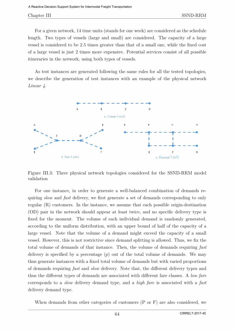
Chapter III SSND-RRM
For a given network, 14 time units (stands for one week) are considered as the schedulelength. Two types of vessels (large and small) are considered. The capacity of a largevessel is considered to be 2.5 times greater than that of a small one, while the fixed costof a large vessel is just 2 times more expensive. Potential services consist of all possibleitineraries in the network, using both types of vessels.
As test instances are generated following the same rules for all the tested topologies,we describe the generation of test instances with an example of the physical networkLinear 4.
Figure III.3: Three physical network topologies considered for the SSND-RRM modelvalidation
For one instance, in order to generate a well-balanced combination of demands re-quiring slow and fast delivery, we first generate a set of demands corresponding to onlyregular (R) customers. In the instance, we assume that each possible origin-destination(OD) pair in the network should appear at least twice, and no specific delivery type isfixed for the moment. The volume of each individual demand is randomly generated,according to the uniform distribution, with an upper bound of half of the capacity of alarge vessel. Note that the volume of a demand might exceed the capacity of a smallvessel. However, this is not restrictive since demand splitting is allowed. Thus, we fix thetotal volume of demands of that instance. Then, the volume of demands requiring fastdelivery is specified by a percentage (p) out of the total volume of demands. We maythus generate instances with a fixed total volume of demands but with varied proportionsof demands requiring fast and slow delivery. Note that, the different delivery types andthus the different types of demands are associated with different fare classes. A low farecorresponds to a slow delivery demand type, and a high fare is associated with a fastdelivery demand type.
When demands from other categories of customers (P or F) are also considered, we
64
A Reactive Decision Support System for Intermodal Freight Transportation
CIRRELT-2017-45

Chapter III SSND-RRM
simply “duplicate” the demands from R customers and change their customer category toP or F. Therefore, the total volume of a test instance considering R and P (or R and F)customers is twice that of its corresponding test instance considering only R customers.Furthermore, we assume that all demands from P customers require slow delivery, whereasall demands from F customers require fast delivery. For each given total volume, eachspecified percentage p and each particular customer category mix, 20 test instances arerandomly generated based on this procedure.
We solve all the optimization problems with the help of a commercial MILP solver(IBM CPLEX 12.5) on a multi-processor server running under Linux 64-bit with InterXeon X5675, 3GHz and 30 GB of RAM.
III.5.2 Experiment Plan
In this subsection, we introduce the experiment plan. Two groups of experiments areset up to study: first, the influences of having different delivery requirements (slow andfast) from customers on the decisions made at tactical level; and second, the benefits ofconsidering the customer classification and fare differentiation for the selection of servicesand the flow distribution, respectively.
The characteristics of the two groups of experiments are briefly displayed in TableIII.1. In the first group, to eliminate the influences of other parameters, only regular (R)customer demands are considered. Fare differentiation is not applied, even if fast and slowdelivery types are considered. Fast demands are considered to be distributed over the setof O-Ds in two different fashions: first, customers requiring fast delivery are distributedevenly, and second, fast delivery is required by customers concentrating at a single mainterminal (the one with the highest throughput), which is either the origin or destinationof a fast demand. The ratio of fast/slow demands (considered as Parameter 1) is varyingin the first group.
Table III.1: Characteristics of the two groups of experiments
Demand categories Fare differentiation Request for fast delivery Varied parametersGroup 1 only R no spread over the network or con-
centrated at a single terminal1
Group 2 R+P or R+F yes spread over the network 2+3
In the second group of experiments, partially spot (P) customer demands and fullyspot (F) customer demands are considered together with R. The total volume of P (or F)
65
A Reactive Decision Support System for Intermodal Freight Transportation
CIRRELT-2017-45
Chapter III SSND-RRM
is equal to the volume of R in each test instance. In addition, fare differentiation is alsoapplied, and transport requests for fast delivery appear all over the network.
In this second group of experiments, an important parameter (considered as Parameter2) is used: the degree of freedom of service selection. Three different cases are explored:fix all services, fix open services and fix no service. The difference among the three cases isthe restriction on the service selection once the initial optimization problem is solved for Rcustomers only. In the first two cases, we first solve the optimization problem consideringonly R demands and obtain a scheduled service plan. In the case of fix all services,we then fix all services (fix decision variables y(s) = 0 or y(s) = 1) according to theobtained assignment (for only R) and solve again the optimization problem consideringall demands (R, P and F). In the case of fix open services, we fix only the open services(fix decision variables y(s) = 1) according to the obtained assignment, and solve againthe optimization problem. Thus, more services might be open, considering all demands(R, P and F). The most flexible case is fix no service, in which no additional constraintis applied and the optimization model has the right to choose the best set of services,considering all demands from the beginning (no second solving is needed).
Another important parameter (Parameter 3) refers to the mix of customer categorieswithin the same test instance, with or without fare differentiation. Four different casesare compared in the second group of experiments:
• Case only R: only R demands with no fare differentiation;
• Case R+P: R and P demands with no fare differentiation;
• Case R+F no price: R and F demands with no fare differentiation;
• Case R+F with price: R and F demands with fare differentiation.
All R demands are identical in all four cases. The total volume of spot (P or F) demands isequal to the volume of R demands. Note that, throughout this whole group of experiments,all R and P demands ask for slow delivery, while all F demands ask for fast delivery. Faredifferentiation is applied only according to the delivery type, and the price ratio of slowdelivery to fast delivery is 1:1.5.
Performance indicators (PIs) used to analyze the solutions for both groups of experi-ments are:
• Total cost: Sum of all costs, i.e., fixed cost (opening services) and variable costs
66
A Reactive Decision Support System for Intermodal Freight Transportation
CIRRELT-2017-45

Chapter III SSND-RRM
(holding barges, holding non-used barges, holding containers, transportation andhandling containers);
• Opening services cost: Fixed cost alone corresponds to the maximum transporta-tion capacity made available in the optimal solution on the whole service network;
• # of open services (small): Number of open services with small vessel;
• # of open services (large): Number of open services with large vessel;
• Distance*Capacity usage: Indicator represents the degree of resource utilization;it is calculated as the ratio of used service distance*capacity over the maximumpossible service distance*capacity according to a given optimal solution; as shownin equation (III.25), used service distance*capacity is the sum of all service legs’used capacity multiplied by their corresponding transport distance, while maximumpossible service distance*capacity is the sum of all service legs’ capacity multipliedby their corresponding transport distance, for all open services;
Distance ∗ Capacityusage =
∑s
∑k
∑ddis(k) ∗ x(d, s, k)∑
s
∑kdis(k) ∗ cap(s) (III.25)
• Waiting at origin: Sum of waiting time of all regular demands at their origins,weighted by their volumes, which is an indicator of the flow congestion level on thenetwork;
• Transshipment: Sum of waiting time of all regular demands at their intermediatestops, weighted by their volumes, which is another indicator of the flow congestionlevel on the network;
• Slow splitting: When distributing the flow, some demands have to be split to fitin the residual capacity of services and to derive the optimal flow distribution; thisindicator is the ratio of split R demands (in TEUs) over all R demands, which mayalso give an idea about the flow congestion level on the network;
• Relative yield: Computed as the net profit divided by the total cost and used asan indicator of the profitability for accepted demands;
• Additional TEUs accepted: Total volume of P or F demands accepted by themodel.
67
A Reactive Decision Support System for Intermodal Freight Transportation
CIRRELT-2017-45
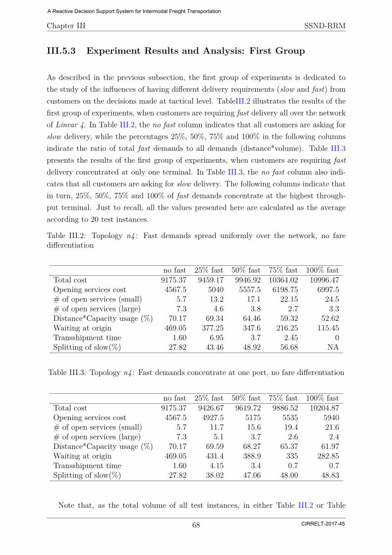
Chapter III SSND-RRM
III.5.3 Experiment Results and Analysis: First Group
As described in the previous subsection, the first group of experiments is dedicated tothe study of the influences of having different delivery requirements (slow and fast) fromcustomers on the decisions made at tactical level. TableIII.2 illustrates the results of thefirst group of experiments, when customers are requiring fast delivery all over the networkof Linear 4. In Table III.2, the no fast column indicates that all customers are asking forslow delivery, while the percentages 25%, 50%, 75% and 100% in the following columnsindicate the ratio of total fast demands to all demands (distance*volume). Table III.3presents the results of the first group of experiments, when customers are requiring fastdelivery concentrated at only one terminal. In Table III.3, the no fast column also indi-cates that all customers are asking for slow delivery. The following columns indicate thatin turn, 25%, 50%, 75% and 100% of fast demands concentrate at the highest through-put terminal. Just to recall, all the values presented here are calculated as the averageaccording to 20 test instances.
Table III.2: Topology n4 : Fast demands spread uniformly over the network, no faredifferentiation
no fast 25% fast 50% fast 75% fast 100% fastTotal cost 9175.37 9459.17 9946.92 10364.02 10996.47Opening services cost 4567.5 5040 5557.5 6198.75 6997.5# of open services (small) 5.7 13.2 17.1 22.15 24.5# of open services (large) 7.3 4.6 3.8 2.7 3.3Distance*Capacity usage (%) 70.17 69.34 64.46 59.32 52.62Waiting at origin 469.05 377.25 347.6 216.25 115.45Transshipment time 1.60 6.95 3.7 2.45 0Splitting of slow(%) 27.82 43.46 48.92 56.68 NA
Table III.3: Topology n4 : Fast demands concentrate at one port, no fare differentiation
no fast 25% fast 50% fast 75% fast 100% fastTotal cost 9175.37 9426.67 9619.72 9886.52 10204.87Opening services cost 4567.5 4927.5 5175 5535 5940# of open services (small) 5.7 11.7 15.6 19.4 21.6# of open services (large) 7.3 5.1 3.7 2.6 2.4Distance*Capacity usage (%) 70.17 69.59 68.27 65.37 61.97Waiting at origin 469.05 431.4 388.9 335 282.85Transshipment time 1.60 4.15 3.4 0.7 0.7Splitting of slow(%) 27.82 38.02 47.06 48.00 48.83
Note that, as the total volume of all test instances, in either Table III.2 or Table
68
A Reactive Decision Support System for Intermodal Freight Transportation
CIRRELT-2017-45
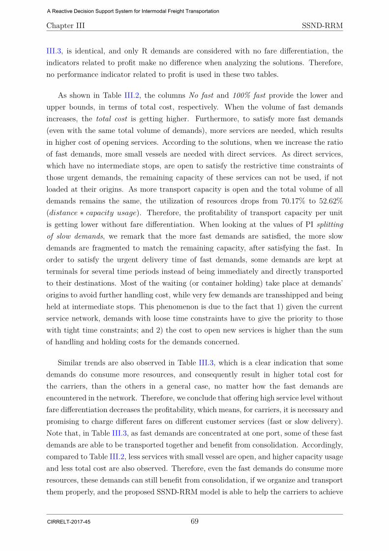
Chapter III SSND-RRM
III.3, is identical, and only R demands are considered with no fare differentiation, theindicators related to profit make no difference when analyzing the solutions. Therefore,no performance indicator related to profit is used in these two tables.
As shown in Table III.2, the columns No fast and 100% fast provide the lower andupper bounds, in terms of total cost, respectively. When the volume of fast demandsincreases, the total cost is getting higher. Furthermore, to satisfy more fast demands(even with the same total volume of demands), more services are needed, which resultsin higher cost of opening services. According to the solutions, when we increase the ratioof fast demands, more small vessels are needed with direct services. As direct services,which have no intermediate stops, are open to satisfy the restrictive time constraints ofthose urgent demands, the remaining capacity of these services can not be used, if notloaded at their origins. As more transport capacity is open and the total volume of alldemands remains the same, the utilization of resources drops from 70.17% to 52.62%(distance ∗ capacity usage). Therefore, the profitability of transport capacity per unitis getting lower without fare differentiation. When looking at the values of PI splittingof slow demands, we remark that the more fast demands are satisfied, the more slowdemands are fragmented to match the remaining capacity, after satisfying the fast. Inorder to satisfy the urgent delivery time of fast demands, some demands are kept atterminals for several time periods instead of being immediately and directly transportedto their destinations. Most of the waiting (or container holding) take place at demands’origins to avoid further handling cost, while very few demands are transshipped and beingheld at intermediate stops. This phenomenon is due to the fact that 1) given the currentservice network, demands with loose time constraints have to give the priority to thosewith tight time constraints; and 2) the cost to open new services is higher than the sumof handling and holding costs for the demands concerned.
Similar trends are also observed in Table III.3, which is a clear indication that somedemands do consume more resources, and consequently result in higher total cost forthe carriers, than the others in a general case, no matter how the fast demands areencountered in the network. Therefore, we conclude that offering high service level withoutfare differentiation decreases the profitability, which means, for carriers, it is necessary andpromising to charge different fares on different customer services (fast or slow delivery).Note that, in Table III.3, as fast demands are concentrated at one port, some of these fastdemands are able to be transported together and benefit from consolidation. Accordingly,compared to Table III.2, less services with small vessel are open, and higher capacity usageand less total cost are also observed. Therefore, even the fast demands do consume moreresources, these demands can still benefit from consolidation, if we organize and transportthem properly, and the proposed SSND-RRM model is able to help the carriers to achieve
69
A Reactive Decision Support System for Intermodal Freight Transportation
CIRRELT-2017-45
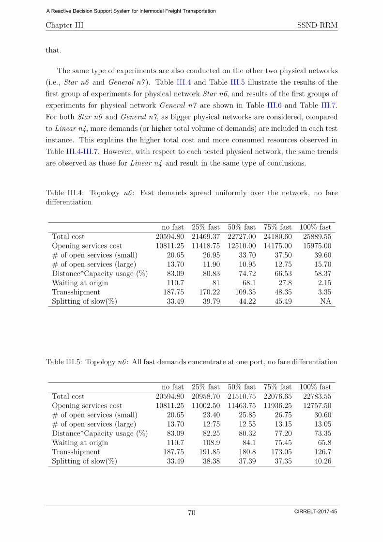
Chapter III SSND-RRM
that.
The same type of experiments are also conducted on the other two physical networks(i.e., Star n6 and General n7 ). Table III.4 and Table III.5 illustrate the results of thefirst group of experiments for physical network Star n6, and results of the first groups ofexperiments for physical network General n7 are shown in Table III.6 and Table III.7.For both Star n6 and General n7, as bigger physical networks are considered, comparedto Linear n4, more demands (or higher total volume of demands) are included in each testinstance. This explains the higher total cost and more consumed resources observed inTable III.4-III.7. However, with respect to each tested physical network, the same trendsare observed as those for Linear n4 and result in the same type of conclusions.
Table III.4: Topology n6 : Fast demands spread uniformly over the network, no faredifferentiation
no fast 25% fast 50% fast 75% fast 100% fastTotal cost 20594.80 21469.37 22727.00 24180.60 25889.55Opening services cost 10811.25 11418.75 12510.00 14175.00 15975.00# of open services (small) 20.65 26.95 33.70 37.50 39.60# of open services (large) 13.70 11.90 10.95 12.75 15.70Distance*Capacity usage (%) 83.09 80.83 74.72 66.53 58.37Waiting at origin 110.7 81 68.1 27.8 2.15Transshipment 187.75 170.22 109.35 48.35 3.35Splitting of slow(%) 33.49 39.79 44.22 45.49 NA
Table III.5: Topology n6 : All fast demands concentrate at one port, no fare differentiation
no fast 25% fast 50% fast 75% fast 100% fastTotal cost 20594.80 20958.70 21510.75 22076.65 22783.55Opening services cost 10811.25 11002.50 11463.75 11936.25 12757.50# of open services (small) 20.65 23.40 25.85 26.75 30.60# of open services (large) 13.70 12.75 12.55 13.15 13.05Distance*Capacity usage (%) 83.09 82.25 80.32 77.20 73.35Waiting at origin 110.7 108.9 84.1 75.45 65.8Transshipment 187.75 191.85 180.8 173.05 126.7Splitting of slow(%) 33.49 38.38 37.39 37.35 40.26
70
A Reactive Decision Support System for Intermodal Freight Transportation
CIRRELT-2017-45
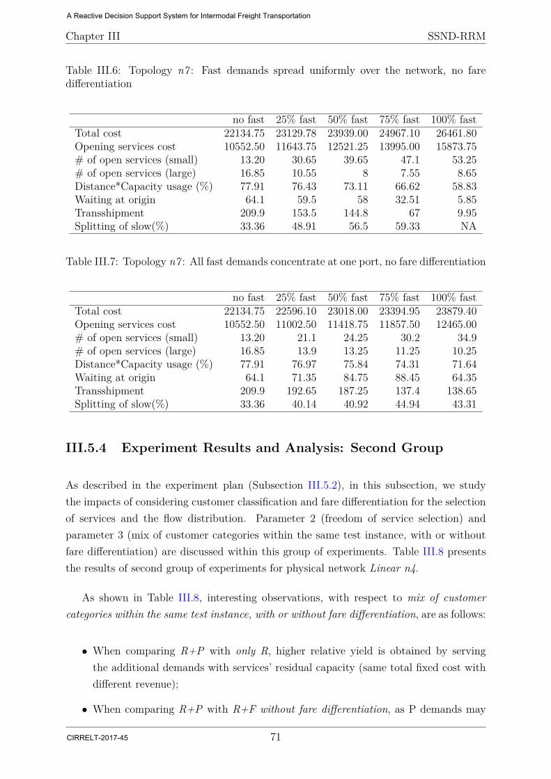
Chapter III SSND-RRM
Table III.6: Topology n7 : Fast demands spread uniformly over the network, no faredifferentiation
no fast 25% fast 50% fast 75% fast 100% fastTotal cost 22134.75 23129.78 23939.00 24967.10 26461.80Opening services cost 10552.50 11643.75 12521.25 13995.00 15873.75# of open services (small) 13.20 30.65 39.65 47.1 53.25# of open services (large) 16.85 10.55 8 7.55 8.65Distance*Capacity usage (%) 77.91 76.43 73.11 66.62 58.83Waiting at origin 64.1 59.5 58 32.51 5.85Transshipment 209.9 153.5 144.8 67 9.95Splitting of slow(%) 33.36 48.91 56.5 59.33 NA
Table III.7: Topology n7 : All fast demands concentrate at one port, no fare differentiation
no fast 25% fast 50% fast 75% fast 100% fastTotal cost 22134.75 22596.10 23018.00 23394.95 23879.40Opening services cost 10552.50 11002.50 11418.75 11857.50 12465.00# of open services (small) 13.20 21.1 24.25 30.2 34.9# of open services (large) 16.85 13.9 13.25 11.25 10.25Distance*Capacity usage (%) 77.91 76.97 75.84 74.31 71.64Waiting at origin 64.1 71.35 84.75 88.45 64.35Transshipment 209.9 192.65 187.25 137.4 138.65Splitting of slow(%) 33.36 40.14 40.92 44.94 43.31
III.5.4 Experiment Results and Analysis: Second Group
As described in the experiment plan (Subsection III.5.2), in this subsection, we studythe impacts of considering customer classification and fare differentiation for the selectionof services and the flow distribution. Parameter 2 (freedom of service selection) andparameter 3 (mix of customer categories within the same test instance, with or withoutfare differentiation) are discussed within this group of experiments. Table III.8 presentsthe results of second group of experiments for physical network Linear n4.
As shown in Table III.8, interesting observations, with respect to mix of customercategories within the same test instance, with or without fare differentiation, are as follows:
• When comparing R+P with only R, higher relative yield is obtained by servingthe additional demands with services’ residual capacity (same total fixed cost withdifferent revenue);
• When comparing R+P with R+F without fare differentiation, as P demands may
71
A Reactive Decision Support System for Intermodal Freight Transportation
CIRRELT-2017-45
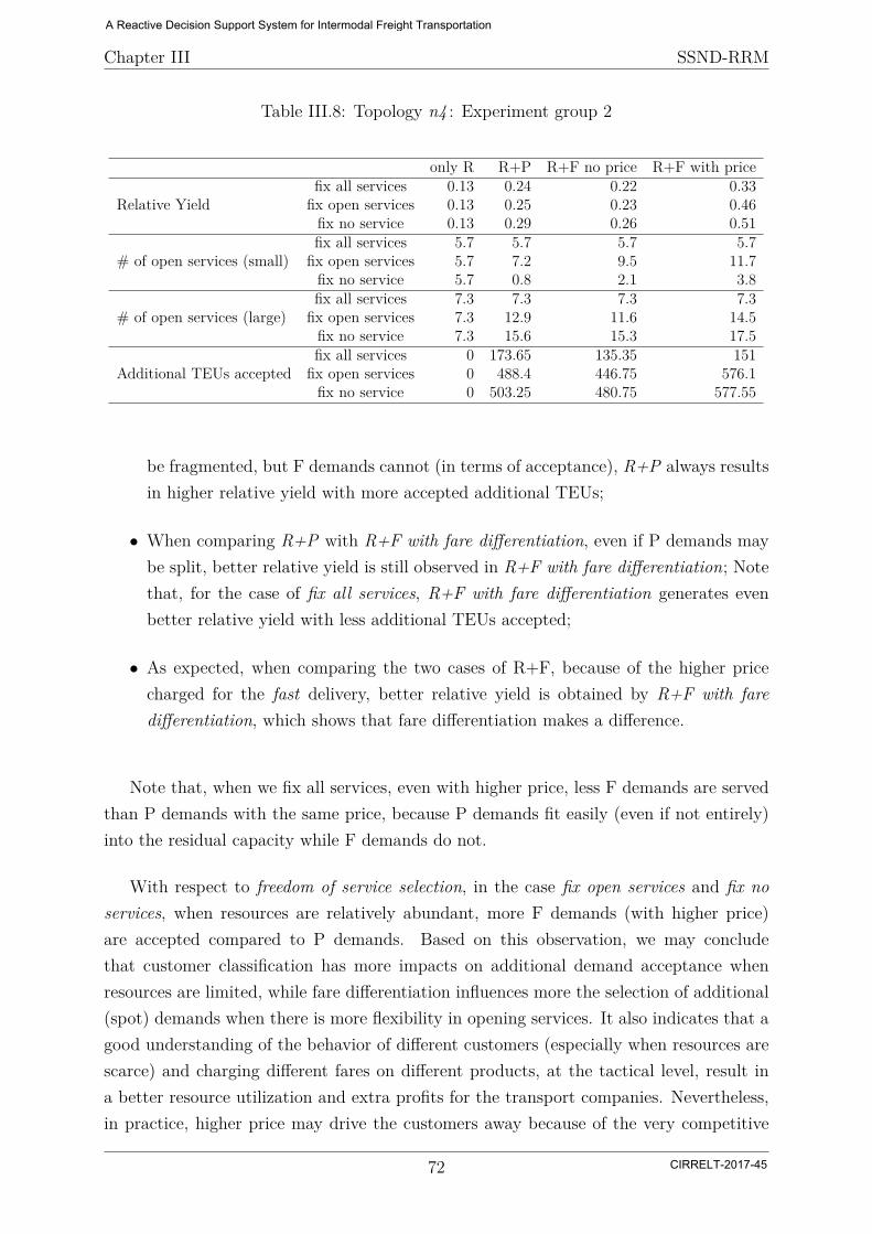
Chapter III SSND-RRM
Table III.8: Topology n4 : Experiment group 2
only R R+P R+F no price R+F with price
Relative Yieldfix all services 0.13 0.24 0.22 0.33
fix open services 0.13 0.25 0.23 0.46fix no service 0.13 0.29 0.26 0.51
# of open services (small)fix all services 5.7 5.7 5.7 5.7
fix open services 5.7 7.2 9.5 11.7fix no service 5.7 0.8 2.1 3.8
# of open services (large)fix all services 7.3 7.3 7.3 7.3
fix open services 7.3 12.9 11.6 14.5fix no service 7.3 15.6 15.3 17.5
Additional TEUs acceptedfix all services 0 173.65 135.35 151
fix open services 0 488.4 446.75 576.1fix no service 0 503.25 480.75 577.55
be fragmented, but F demands cannot (in terms of acceptance), R+P always resultsin higher relative yield with more accepted additional TEUs;
• When comparing R+P with R+F with fare differentiation, even if P demands maybe split, better relative yield is still observed in R+F with fare differentiation; Notethat, for the case of fix all services, R+F with fare differentiation generates evenbetter relative yield with less additional TEUs accepted;
• As expected, when comparing the two cases of R+F, because of the higher pricecharged for the fast delivery, better relative yield is obtained by R+F with faredifferentiation, which shows that fare differentiation makes a difference.
Note that, when we fix all services, even with higher price, less F demands are servedthan P demands with the same price, because P demands fit easily (even if not entirely)into the residual capacity while F demands do not.
With respect to freedom of service selection, in the case fix open services and fix noservices, when resources are relatively abundant, more F demands (with higher price)are accepted compared to P demands. Based on this observation, we may concludethat customer classification has more impacts on additional demand acceptance whenresources are limited, while fare differentiation influences more the selection of additional(spot) demands when there is more flexibility in opening services. It also indicates that agood understanding of the behavior of different customers (especially when resources arescarce) and charging different fares on different products, at the tactical level, result ina better resource utilization and extra profits for the transport companies. Nevertheless,in practice, higher price may drive the customers away because of the very competitive
72
A Reactive Decision Support System for Intermodal Freight Transportation
CIRRELT-2017-45

Chapter III SSND-RRM
environment of the market. Therefore, pricing should be done based on a deep analysisof customers behavior, which is not the focus of this chapter.
The relative yield obtained from the second group of experiments is also illustrated inFigure III.4, where the vertical axis stands for the relative yield. As shown in the figure, itis obvious that the consideration of a mix of regular and spot demands (R+P and R+F)results in better relative yield, compared with considering only the regular demands.Relative yield also grows when fare differentiation is introduced into the model. From theperspective of the freedom of service selection, it becomes clear that, in order to achievea better relative yield, no additional constraints should be taken into account and theSSND-RRM model should take the full responsibility for the decisions, in terms of serviceselection. Therefore, we conclude that it is profitable to include revenue managementconsideration into tactical SSND plan.
Figure III.4: Relative yield obtained in the second experiment group
As the experiments conducted on the other physical network topologies show the sametrends and consequently result in the same type of conclusions, numerical results for theother physical networks are presented in Table III.9 for Star n6 and Table III.10 forGeneral n7, respectively, without further analysis.
73
A Reactive Decision Support System for Intermodal Freight Transportation
CIRRELT-2017-45
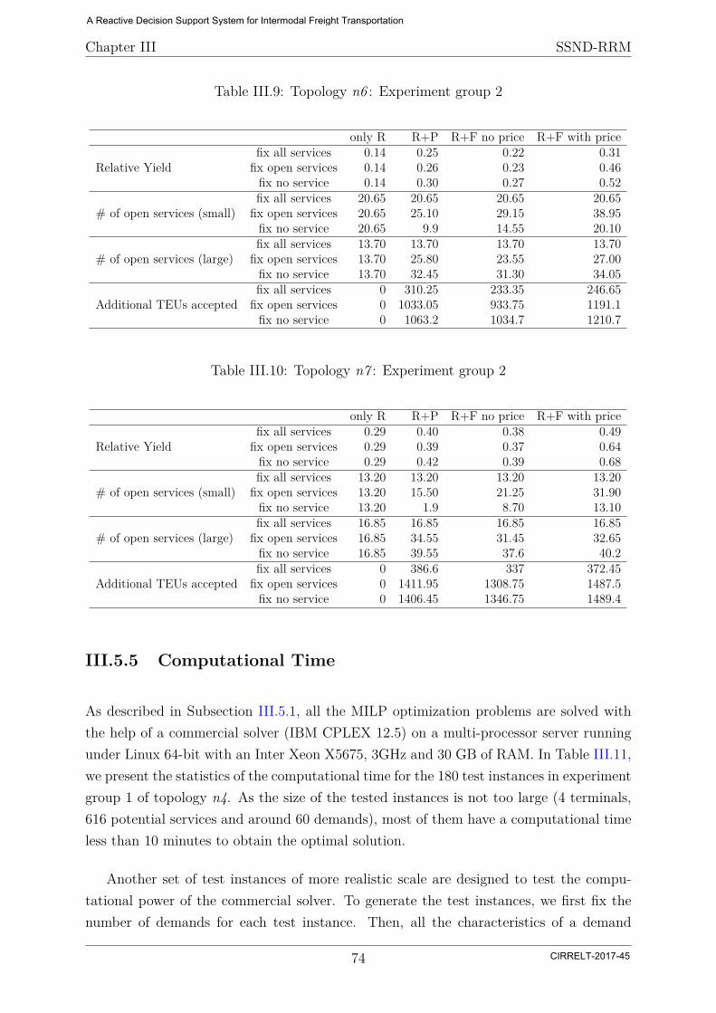
Chapter III SSND-RRM
Table III.9: Topology n6 : Experiment group 2
only R R+P R+F no price R+F with price
Relative Yieldfix all services 0.14 0.25 0.22 0.31
fix open services 0.14 0.26 0.23 0.46fix no service 0.14 0.30 0.27 0.52
# of open services (small)fix all services 20.65 20.65 20.65 20.65
fix open services 20.65 25.10 29.15 38.95fix no service 20.65 9.9 14.55 20.10
# of open services (large)fix all services 13.70 13.70 13.70 13.70
fix open services 13.70 25.80 23.55 27.00fix no service 13.70 32.45 31.30 34.05
Additional TEUs acceptedfix all services 0 310.25 233.35 246.65
fix open services 0 1033.05 933.75 1191.1fix no service 0 1063.2 1034.7 1210.7
Table III.10: Topology n7 : Experiment group 2
only R R+P R+F no price R+F with price
Relative Yieldfix all services 0.29 0.40 0.38 0.49
fix open services 0.29 0.39 0.37 0.64fix no service 0.29 0.42 0.39 0.68
# of open services (small)fix all services 13.20 13.20 13.20 13.20
fix open services 13.20 15.50 21.25 31.90fix no service 13.20 1.9 8.70 13.10
# of open services (large)fix all services 16.85 16.85 16.85 16.85
fix open services 16.85 34.55 31.45 32.65fix no service 16.85 39.55 37.6 40.2
Additional TEUs acceptedfix all services 0 386.6 337 372.45
fix open services 0 1411.95 1308.75 1487.5fix no service 0 1406.45 1346.75 1489.4
III.5.5 Computational Time
As described in Subsection III.5.1, all the MILP optimization problems are solved withthe help of a commercial solver (IBM CPLEX 12.5) on a multi-processor server runningunder Linux 64-bit with an Inter Xeon X5675, 3GHz and 30 GB of RAM. In Table III.11,we present the statistics of the computational time for the 180 test instances in experimentgroup 1 of topology n4. As the size of the tested instances is not too large (4 terminals,616 potential services and around 60 demands), most of them have a computational timeless than 10 minutes to obtain the optimal solution.
Another set of test instances of more realistic scale are designed to test the compu-tational power of the commercial solver. To generate the test instances, we first fix thenumber of demands for each test instance. Then, all the characteristics of a demand
74
A Reactive Decision Support System for Intermodal Freight Transportation
CIRRELT-2017-45

Chapter III SSND-RRM
Table III.11: Statistics of computational time for 180 test instances in group 1 of topologyLinear n4
Running time (s) 1 - 200 201 - 400 401 - 600 600+# of test instances 171 7 1 1
are generated randomly according to the uniform distribution. The commercial solver(CPLEX 12.5) is set with a maximum running time of 10 days. The size, the compu-tational time and the corresponding status of optimality of six particular test instancesare presented in Table III.12. In the table, |N ph|, |S|, |D| and |DF | indicate number ofphysical terminals, number of potential services, number of total demands and numberof F demands. respectively. Remark that, decisions with respect to service selection andF demand selection are formulated as binary decision variables, from where the compu-tational difficulties come. Numbers of decision variables and constraints generated foreach test instance according to the SSND-RRM model are also presented in column #DVs and column # Constraints, respectively. As shown in Table III.12, computationaldifficulties are encountered when solving the SSND-RRM problems of realistic scale. Forthe last three test instances, no optimal solution can be obtained after 10 days with thecommercial solver.
Table III.12: Computational time and size of large instances on topologies of Linear n4,Star n6 and General n7
Test instance |N ph| |S| |D| |DF | # DVs # Constraints Time consumption Optimality1 4 616 480 180 119858 104703 27.6 minutes yes2 4 616 960 307 230238 202045 36.7 minutes yes3 6 1848 150 66 77866 66225 26.8 hours yes4 6 1848 300 107 144686 122180 10 days no5 7 4200 210 79 265354 222719 10 days no6 7 4200 420 130 546397 450447 10 days no
III.6 Conclusions
In this chapter, we proposed what we believe to be the first comprehensive tactical plan-ning model for barge freight carriers that integrates both revenue and resource manage-ment considerations (SSND-RRM). In the proposed model, revenue management (RM)policies: customer classification and fare differentiation, are considered. In terms of re-source management, design-balance constraints and limits on the quantity of resources areformulated. To synchronize with other transport modes, scheduled services are planned
75
A Reactive Decision Support System for Intermodal Freight Transportation
CIRRELT-2017-45
Chapter III SSND-RRM
to answer to demands with time-delivery constraints.
We tested the model on various problem settings, in terms of network topologies,fare classes and quality-of-service (e.g., delivery time). According to results, when weincrease the ratio of fast demands for a given set of demands, more small vessels areneeded with lower capacity usage to satisfy those urgent demands. It also results in someslow traffic to be split. It is obvious that fast demands consume more resources andviolate the idea of consolidation-based service, which encourages demands from differentcustomers to be transported together. Therefore, those demands, which result in morecosts, should be discriminated by charging different prices. In addition, by classifyingcustomer into different categories and having different treatments accordingly, carriersmay benefit from consolidation, obtain a better resource utilization and consequentlygain better revenue. Our results indicate that, higher relative yield (or profitability) andbetter resource utilization for the carriers are always obtained, regardless of the physicalnetwork topology, by considering RM policies when designing the network of scheduledservices. It is thus promising to classify customers and differentiate fare-products attactical level.
Further research may be carried out to extend the proposed model. For example,different price policies could be applied. In the current SSND-RRM model, the pricepolicy is only related to the required delivery type. A different price policy can be alsoconsidered according to the customer categories. To be more precise, the unit pricecharged on the regular (R) customers should be lower than that charged on the spot(P and F) customers, with respect to the same delivery type. The lower price here,is applied to encourage the establishment of solid business relationship (or long-termcontract) between the carriers and customers. Even though the lower price seeminglydecreases the potential revenue of the carriers, it actually reduces the uncertainty ofdemands, in terms of volume, OD and even delivery time, due to the signed long-termcontract. Therefore, it may result in better service plans, in term of resource utilizationand relative yield (profitability). Furthermore, within the spot customers, as P customersfit in the residual capacity better, they should be charged with lower price, compared withF customers. Thus, more P customers could be attracted. Another interesting perspectiveis to formulate the stopping time of each service at each terminal as decisions in the SSND-RRM model. Facing the uncertain demands, in terms of available time, and/or delayedservices, better service plans are expected, if the stopping time of a service at each terminalis decided by the model, instead of fixed as a predefined value. Moreover, it is alsointeresting to explicitly consider the uncertainty of demands, based on their customercategories. For example, demands from regular customers are more predictable, whiledemands from spot customers are more uncertain, in terms of volume, available time, etc.
76
A Reactive Decision Support System for Intermodal Freight Transportation
CIRRELT-2017-45
Chapter III SSND-RRM
As one of the objectives of this chapter is to prove the concept of integration of revenue(and resource) management considerations into tactical planning model, no deep insightis offered with respect to the analysis of customer classification and fare differentiation.Therefore, it is more convincible, especially for the carriers, to validate the SSND-RRMmodel in case studies with real data and have a discussion on the market segmentation andservice qualification. In addition, the computational difficulties encountered when solvingthe proposed problems of large scale urges that efficient solution approaches should beproposed and developed.
77
A Reactive Decision Support System for Intermodal Freight Transportation
CIRRELT-2017-45

A Reactive Decision Support System for Intermodal Freight Transportation
CIRRELT-2017-45
Chapter IV
A Metaheuristic for ScheduledService Network Design withResource and Revenue Managementfor Intermodal Barge Transportation
ContentsIV.1 Introduction . . . . . . . . . . . . . . . . . . . . . . . . . . . . . 81
IV.2 Literature Review . . . . . . . . . . . . . . . . . . . . . . . . . . 82
IV.3 Problem Statement and Formulation of SSND-RRM . . . . . 84
IV.4 Solution Approach . . . . . . . . . . . . . . . . . . . . . . . . . . 85
IV.4.1 Initialization . . . . . . . . . . . . . . . . . . . . . . . . . . . . 88
IV.4.2 Improvement . . . . . . . . . . . . . . . . . . . . . . . . . . . . 89
IV.5 Computational Results and Analysis . . . . . . . . . . . . . . . 105
IV.5.1 Test Instance Generation . . . . . . . . . . . . . . . . . . . . . 106
IV.5.2 Calibration . . . . . . . . . . . . . . . . . . . . . . . . . . . . . 107
IV.5.3 Benchmarking against an MILP Solver . . . . . . . . . . . . . . 108
IV.5.4 Analysis of the Impact of Each Algorithmic Component . . . . 110
IV.6 Conclusions and Future Work . . . . . . . . . . . . . . . . . . . 110
79
A Reactive Decision Support System for Intermodal Freight Transportation
CIRRELT-2017-45
Revenue management is seldom considered when planning consolidation-based freighttransport services. In the previous chapter, we formalized and addressed the scheduledservice network design problems with resource management and revenue managementconsiderations (SSND-RRM). As the proposed SSND-RRM problems are NP-hard, inthis chapter, we propose a metaheuristic (MH), which is composed of four phases, toefficiently solve the SSND-RRM problems, especially for the large-scale instances. In thefirst phase, a constructive heuristic is proposed to obtain initial solutions, which are theniteratively improved in the following phases. Adaptive large neighborhood search (ALNS)and tabu search are combined to guide the iterative search in the second phase. Newneighborhood structures are proposed to explore in the search space of service selection,based on service-cycles, producing high-quality solutions quickly. The other two phasesconsidered are intensification and diversification. Given some interesting characteristicsof services, small regions of solution space are identified based on the global best solutionsand are deeply explored (intensification). Diversification, on the other hand, is called todirect the search towards non-thoroughly-explored regions of solution space.
A previous version of this research work has been presented at CORS/INFORMSInternational Conference, 2015 with the following reference information:
Wang Y., Crainic T.G., Bilegan I.C., Artiba A. (2015). A Metaheuristic for ServiceNetwork Design with Revenue Management for Freight Intermodal Transport. CORS/IN-FORMS International Conference, Montreal, Canada, June.
Based on the material included in this chapter, a working paper is in preparation forsubmission to an international journal.
A Reactive Decision Support System for Intermodal Freight Transportation
CIRRELT-2017-45

Chapter IV MH
IV.1 Introduction
Service network design (SND) is a core problem and is widely used as a generic modelto formulate network design problems faced in the fields of telecommunication, logistics,transportation, etc. In the field of freight transportation, SND models generally consist ofselection and scheduling of services, and routing demands with the selected services whileminimizing the total cost. [Crainic, 2000, Crainic, 2003] offer an introduction to servicenetwork design in freight transport. In addition to selection and scheduling of services, androuting demands, managing limited key resources (or assets), e.g., power units, vehicles,crews or containers, is also integrated within SND problems (e.g., [Pedersen et al., 2009,Andersen et al., 2009b,Andersen et al., 2009a,Crainic et al., 2014]). Due to the increasingcompetition (e.g., decreasing costs and improving customer satisfaction) on carriers fromthe market, different polices are taken in the literature to make “better” plans tackling thetactical planning problems. For example, maximizing the net profit (or revenue) instead ofminimizing the total costs (e.g., [Agarwal and Ergun, 2008,Teypaz et al., 2010,Gelareh andPisinger, 2011]), rejecting some demands instead of accepting all demands at tactical level(discrimination on customers/customer classification) (e.g., [Andersen and Christiansen,2009, Thapalia et al., 2012, Braekers et al., 2013, Stålhane et al., 2014]). Although notexplicitly identified, these different polices are Revenue Management (RM) related. RM,which was initially applied to passenger airline transportation, starts to draw attentionin research nowadays for freight transportation, as illustrated in the reviews related toair cargo operations [Feng et al., 2015], railway transportation [Armstrong and Meissner,2010], and container synchromodal services [van Riessen et al., 2015a]. However, the fewcontributions considering both RM and freight transportation [Bilegan et al., 2015,Wanget al., 2015] focus on the operational level, while the tactical level is rarely envisaged[Crevier et al., 2012].
Therefore, in the previous chapter, we proposed a Scheduled Service Network Designmodel with consideration of both Resource and Revenue Management (SSND-RRM) tosolve the tactical planning problems for freight carriers. To integrate resource managementinto the SSND-RRM, design-balance constraints, which ensure the balance of incomingand outgoing vehicles at each terminal for each time instant, and limits on the quantity ofresource (vehicles) are formulated. In terms of RM policies, various fare classes accordingto the required delivery types are modeled. Moreover, customers are classified into threecategories, i.e., Regular customers (R), Proportional-punctual customers (P ) and Full-punctual customers (F ). According to their business relationships with the carriers andtheir behaviors, demands from different customers are treated differently. To be moreprecise, demands from R must always be satisfied, while demands from P can be partiallyaccepted and demands from F may be either entirely accepted or not accepted at all.
81
A Reactive Decision Support System for Intermodal Freight Transportation
CIRRELT-2017-45
Chapter IV MH
Therefore, in addition to the selection of scheduled services and routing of demands,decisions related to the selection of demands to transport are also made in the proposedSSND-RRM. Further complexity to the SSND-RRM problems is added because of thecompetition of different categories of customers for the network capacity with differentfares and trade-offs between opening more services with higher revenue and rejecting moredemands with lower total costs.
As shown in Chapter III, introducing resource and revenue management considera-tions into the SND formulations poses great computational challenges. The goal of thischapter is to propose a solution approach to efficiently identify good-quality feasible so-lutions for the SSND-RRM problems of large scale. The contributions of this paper arethreefold: First, we propose a Metaheuristic (MH) that combines adaptive large neighbor-hood search (ALNS) and Tabu search, and utilizes long and short-term memory structuresfor addressing the SSND-RRM. Second, new neighborhood structures considering design-balance constraints are introduced to accelerate the search in the space of service selection.Third, we study the efficiency of the proposed solution approach through comprehensiveexperiments and benchmark against a state-of-the-art commercial solver.
The rest of this chapter is organized as follows. Following a brief literature reviewin Section IV.2, we recall the statement of the problem and present the model of SSND-RRM in Section IV.3. Section IV.4 is dedicated to introduce the solution approach, whilecomputational results are presented and analyzed in Section IV.5. We conclude withperspectives in Section IV.6.
IV.2 Literature Review
In SND problems, continuous and binary variables are used to represent commodity flowsthroughout the designed network and the selection of services, respectively. With twoof the most common constraints, i.e., network capacity constraints and flow conservationconstraints, SND problems are considered as a fixed-charge capacitated multicommoditynetwork design problem (CMND).
Considerable efforts directed towards investigating and developing effective solutiontechniques, in particular, metaheuristics and hybrid approaches, are proposed for theproblems of CMND/SND. [Crainic et al., 2000] propose a hybrid approach for CMND,combining a tabu search method with pivot-like neighborhood moves and column genera-tion. The work is continued by [Ghamlouche et al., 2003] and a more efficient cycle-basedneighborhood structure for CMND is proposed. In their study, two paths (sequence of
82
A Reactive Decision Support System for Intermodal Freight Transportation
CIRRELT-2017-45
Chapter IV MH
design arcs) connecting the same origin-destination nodes in the network constitute acycle. As no resource management is considered, a generated cycle is used to redirect flowfrom one path to another and contribute to the selection of design variables simultane-ously. Neighborhood moves proceed by redirecting flow around cycles, and closing andopening design arcs accordingly. [Ghamlouche et al., 2004] later enhance the approachof [Ghamlouche et al., 2003] by combining the cycle-based neighborhood structure andthe mechanism of path-relinking, introduced by [Glover, 1997]. Promising attributes of aset of elite solutions (called the reference set) are used to guide the local search (as wellas the intensification and diversification).
[Pedersen et al., 2009] study more generic service network design models in which theresource balance constraints are considered. A multi-start metaheuristic, based on tabusearch, is developed and tested. With respect to the resource balance constraints, infea-sible solutions (with unbalanced resource) are allowed in the exploration phase. Arc-addmoves are therefore included to restore the balance of resource and to lead the searchtowards feasible solutions. [Vu et al., 2013] and [Chouman and Crainic, 2014] in theirproposed solution approaches, also allow infeasible solution and have an additional pro-cedure to restore the feasibility with respect to the design-balance constraints. Variousmechanisms within a guided local search framework to solve the design-balanced SNDproblems are investigated by [Bai et al., 2012]. Compared with [Pedersen et al., 2009],the proposed tabu assisted local search approaches obtain solutions of the same qual-ity, with a reduction of 30% in the computational time. [Chouman and Crainic, 2014]propose a matheuristic for the design-balanced SND problems. In the proposed algo-rithm, a cutting-plane procedure is applied to compute the lower bounds. Memories oncharacteristics of promising solutions are built when tightening the lower bounds and areused in a variable-fixing heuristic to reduce the size of the problem by fixing a numberof design variables. After an extensive computational study, the authors point out thatappropriate learning mechanisms and variable-fixing techniques are able to identify highquality solutions rapidly. [Crainic et al., 2014] propose a solution approach that combinescolumn generation, meta-heuristic and exact optimization techniques to their new design-balanced SND model. In the proposed model, the limit on the resources at each terminalis considered.
Exact algorithms can also be found in the literature [Andersen et al., 2011, Menget al., 2012,Bektaş et al., 2010]. However, as the problems are NP-hard, exact methodsreach their limits rather rapidly as the size of the instances grows. It has been provedthat solving realistic instances of such planning problems are difficult. For example,[Andersen et al., 2011] study a branch and price method for the design-balance SNDproblems. Although the proposed algorithm finds solutions of higher quality than the
83
A Reactive Decision Support System for Intermodal Freight Transportation
CIRRELT-2017-45
Chapter IV MH
previous methods, the 10-hour computational time required by the algorithm indicates agreat challenge for its practical applications. Therefore, the focus of our research in thischapter is not on exact algorithms. For those who are interested in exact algorithms, werefer to [SteadieSeifi et al., 2014] as an overview.
Little effort has been dedicated, however, to solving scheduled service network designproblem while simultaneously considering resource management and revenue manage-ment. This chapter aims to help fill this gap.
This chapter is organized as follows. In Section IV.3, we recall the statement of theproblem and the model of SSND-RRM. Section IV.4 is dedicated to introduce the solutionapproach, while computational results are presented and analyzed in Section IV.5. Weconclude with perspectives in Section IV.6.
IV.3 Problem Statement and Formulation of SSND-RRM
In this section, we first briefly present the tactical planning problem with considerationof resource and revenue management. The formulation of SSND-RRM is then presented.
As described in Chapter III, we first assume the demands D = {d} from customersand services S = {s} offered by carriers follow a repetitive pattern during the middle-termplanning horizon (e.g., a season). A scheduled service plan is then built up for a givenschedule length (e.g., a week) and then repeatedly operated over the planning horizon tosatisfy demands.
We then formulate the SSND-RRM problem on a circular time-space network G =(N ,A). The node set N is obtained by duplicating all physical terminals (of rivers,canals, etc.) at all periods in the schedule length T , so that node it corresponds to thephysical terminal i at time instant t, t = 0, . . . , (T − 1). The set of arcs A is composedof two subsets of arcs: holding arcs at terminals and moving arcs performed by services.
Customers are classified, according to their business relationships with the carriers,into three categories, i.e., Regular customers (R), Proportional-punctual customers (P )and Full-punctual customers (F ). Accordingly, demands from different customers aretreated differently. Demands DR requested from regular customers R must always besatisfied, while demands DP from P can be partially accepted and demands DF from F
may either be entirely accepted or not accepted at all. Then, each demand d ∈ D =
84
A Reactive Decision Support System for Intermodal Freight Transportation
CIRRELT-2017-45

Chapter IV MH
DR ∪ DP ∪ DF is characterized by: the requested volume vol(d) in TEUs; the originand destination terminals, orig(d) and dest(d), respectively; the time in(d) it becomesavailable for transportation at its origin terminal; the last time out(d) it may arriveat its destination terminals; the category cat(d) of customers; the fare class class(d),slow/normal or fast; and unit fare value f(d).
Vessels L owned or rented by the carriers are operated for the scheduled services. Eachvessel type l ∈ L is characterized by: capacity cap(l) in TEUs; and maximum number Bl
of vessel type l.
A service s ∈ S is thus characterized by: the origin and destination terminals, orig(s)and dest(s), respectively; Ordered set of consecutive stops η(s) = {ik(s) ∈ N ph, k =0, . . . , (K−1)} of the service, where K = |η(s)| and k indicates the kth stop of the service;kth leg ak(s) = (ik(s), ik+1(s)) of the service; arrival and departure time at and from itsterminal ik(s), αk(s) and τk(s), respectively; vessel type l(s) of the service; capacitycap(l(s)) of the service; and fixed cost φ(s) of setting up and operating the service.
A set of unit costs are also defined: transportation cost ck(γ(d), l(s)) of a container oftype γ(d), by a vessel of type l(s), on the kth leg of service s; holding cost c(i, γ(d)) of acontainer of type γ(d) at terminal i for one period; Loading/unloading cost κ(i, γ(d)) of acontainer of type γ(d) at terminal i; Holding cost h(i, l) for a vessel of type l at terminali for one time period; and penalty ρ(l) for a vessel of type l that is not used in the plan.For an in-depth statement and detailed notation explanation of the problem, we refer toChapter III.
We now present the formulation of the scheduled service network design with resourceand revenue management (SSND-RRM) model for the tactical planning of intermodalbarge transportation. To avoid repetition, for decision variables defined for the SSND-RRM model and the SSND-RRM model formulation, we refer to Chapter III as well.
IV.4 Solution Approach
To solve the capacitied multicommodity network design (CMND) problems, a conven-tional methodology adopted in the literature is to consider a CMND problem as tworelated components: a). determine “optimal” design variables Y (selection of open arcs/ services); and then b). for a given feasible design variable vector Y , search the optimalflow distribution X (Y). Here, compared to the CMND problems, further complexity isadded to the SSND-RRM problem due to, among other factors, the additional decisions
85
A Reactive Decision Support System for Intermodal Freight Transportation
CIRRELT-2017-45
Chapter IV MH
on F-demand selection (which are binary decision variables) and resource management(design-balance constraints and limits on the quantity of resource).
As described in Section IV.3, a solution to the SSND-RRM is composed of ser-vice selection y(s), vehicle holding z(l, i, t), F-demand selection ζ(d) and P-demand se-lection ξ(d), flow distribution vector X , whose components are the decision vectorsx(d, s, k), xin(d, s, k), xout(d, s, k), xhold(d, i, t). According to the design-balance constraints(III.10), the decision variables z(l, i, t) are related to y(s) and their values can directly becalculated from the values of y(s). Moreover, the decision variables ξ(d) are continuousand can be determined when the flow distribution problem is solved. Therefore, a SSND-RRM problem can be considered as three components: a). identify promising F-demandselection variables F ; and then b). for a given vector F , search promising design vari-ables Y (service selection); and then c). for given vectors F and Y , determine the optimalflow distribution X (F ,Y). The motivation of considering SSND-RRM as a sequence ofthree successive components is that by fixing some parts of the solution, one may workon some other part of the solutions. As the service selection and F-demand selection areformulated as binary decision variables and the flow distribution as continuous variables,one of the most difficult challenges to obtain the optimal solution is to identify promisingF and Y .
Therefore, we propose a metaheuristic (MH) framework that combines adaptive largeneighborhood search (ALNS) and Tabu search, and utilizes long- and short-term memorystructures for addressing the SSND-RRM. The intuition of the proposed MH is to improvethe solutions by iteratively exploring the search space of F-demand selection, serviceselection or the combination of both. The mechanism of choosing the search space onwhich to concentrate is inspired by a modified ALNS strategy. To be more precise, toexplore the search space of service selection, a set of Y-selection heuristics are introduced.New neighborhood structures considering the design-balance constraints are proposed toaccelerate the search. The proposed neighborhood structures are based on a concept ofservice cycle, which is a set of consecutive services using the same type of resource/vehicle,and going back to the same terminal where the first service starts, with or without vehicleholding arcs. Meanwhile, to explore the search space of F-demand selection, a set of F-selection heuristics are introduced. Moreover, as the first two components of SSND-RRMare not independent, these two sets of heuristics are also able to be combined to explorethe integrated search space of both F-demand selection and service selection. Short-termmemory is maintained to record the performance of each heuristic, whereas long-termmemory (called trajectory lists in this chapter) is maintained to record the influence ofeach F demand and service on the solutions. Short-term memory tabu lists are alsomaintained to prevent repeatedly visiting a particular set of solutions.
86
A Reactive Decision Support System for Intermodal Freight Transportation
CIRRELT-2017-45
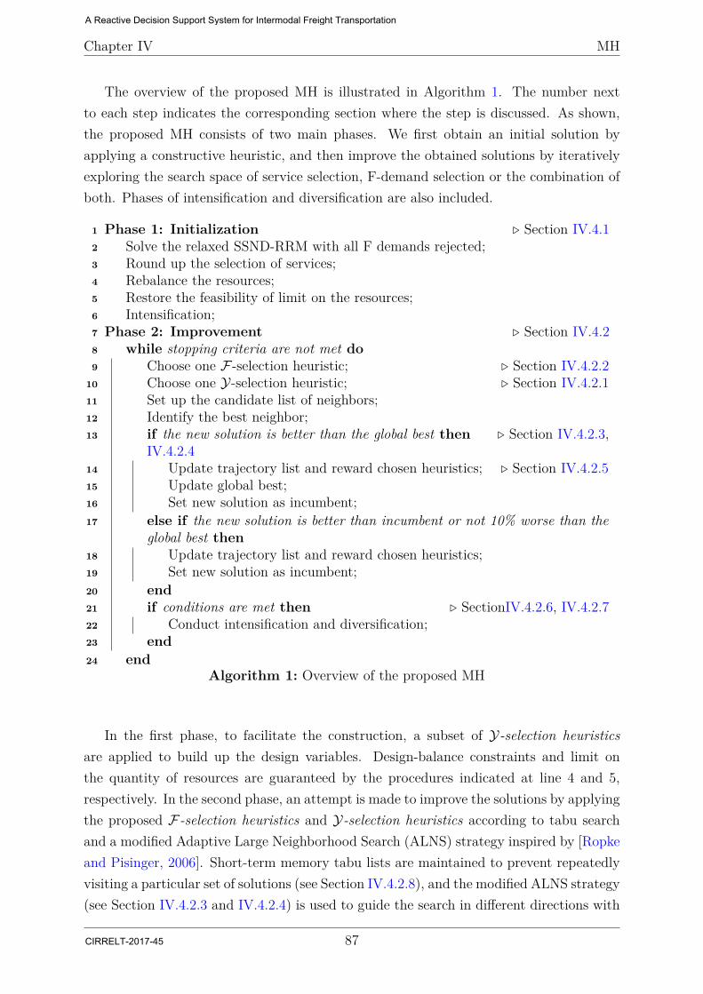
Chapter IV MH
The overview of the proposed MH is illustrated in Algorithm 1. The number nextto each step indicates the corresponding section where the step is discussed. As shown,the proposed MH consists of two main phases. We first obtain an initial solution byapplying a constructive heuristic, and then improve the obtained solutions by iterativelyexploring the search space of service selection, F-demand selection or the combination ofboth. Phases of intensification and diversification are also included.
1 Phase 1: Initialization . Section IV.4.12 Solve the relaxed SSND-RRM with all F demands rejected;3 Round up the selection of services;4 Rebalance the resources;5 Restore the feasibility of limit on the resources;6 Intensification;7 Phase 2: Improvement . Section IV.4.28 while stopping criteria are not met do9 Choose one F -selection heuristic; . Section IV.4.2.2
10 Choose one Y-selection heuristic; . Section IV.4.2.111 Set up the candidate list of neighbors;12 Identify the best neighbor;13 if the new solution is better than the global best then . Section IV.4.2.3,
IV.4.2.414 Update trajectory list and reward chosen heuristics; . Section IV.4.2.515 Update global best;16 Set new solution as incumbent;17 else if the new solution is better than incumbent or not 10% worse than the
global best then18 Update trajectory list and reward chosen heuristics;19 Set new solution as incumbent;20 end21 if conditions are met then . SectionIV.4.2.6, IV.4.2.722 Conduct intensification and diversification;23 end24 end
Algorithm 1: Overview of the proposed MH
In the first phase, to facilitate the construction, a subset of Y-selection heuristicsare applied to build up the design variables. Design-balance constraints and limit onthe quantity of resources are guaranteed by the procedures indicated at line 4 and 5,respectively. In the second phase, an attempt is made to improve the solutions by applyingthe proposed F-selection heuristics and Y-selection heuristics according to tabu searchand a modified Adaptive Large Neighborhood Search (ALNS) strategy inspired by [Ropkeand Pisinger, 2006]. Short-term memory tabu lists are maintained to prevent repeatedlyvisiting a particular set of solutions (see Section IV.4.2.8), and the modified ALNS strategy(see Section IV.4.2.3 and IV.4.2.4) is used to guide the search in different directions with
87
A Reactive Decision Support System for Intermodal Freight Transportation
CIRRELT-2017-45
Chapter IV MH
different neighborhoods. In each iteration, we first choose one F-selection heuristic, andthen one Y-selection heuristic. As the neighborhoods applied in this chapter are very large,a list of promising neighbors, called candidate list of neighbors, are generated to acceleratethe search. The iterative exploration continues until the global stopping criteria are met.As no infeasible solution is allowed in the second phase, to escape from a local optimal,moves that worsen the solutions are also accepted. A procedure is applied to diversify theincumbent solution when predefined number of consecutive no-feasible-neighbors situationis met (see Section IV.4.2.6). When predefined number of no-global-improvement situationis encountered, another procedure is applied to intensify the current global best solutionby addressing the corresponding reduced-size problems with a commercial MILP solver(see Section IV.4.2.7). Long-term memory, i.e., trajectory F list and trajectory service list(explained in Section IV.4.2.5), is maintained to record the influence of each F demandand service on the solutions, respectively
IV.4.1 Initialization
As the proposed SSND-RRM is NP-hard, we first propose an initialization phase to effi-ciently obtain an initial feasible solution sol, which will be used to start the improvementphase.
To obtain sol, the first step is to solve the relaxed SSND-RRM with all F demandsrejected. The reason to reject all F demands is that as ζ(d) are binary variables, fixingthe values of all ζ(d) can reduce the dimension of the optimization problem. Accordingto the solution to the relaxed SSND-RRM, in the second step, we round up the selectionof services. More precisely, if no flow is found on any leg of a service s, we set y(s) to0; otherwise, it is set to 1. In the third step, the indegree ∑
s∈S−itl
y(s) + z(l, i, t − 1) and
outdegree ∑s∈S+
itl
y(s) + z(l, i, t) of each node (i, t) in the time-space network for each type
of vehicle are calculated to verify the balance of resources. If unbalance is found, wefirst eliminate the unbalanced nodes among the same terminals by adding vehicle holdingarcs. If there are still some unbalanced nodes from different terminals, we then open extraservices to connect the unbalanced nodes until all nodes are balanced. Note that, after thesecond and third steps, constraints III.11 may be violated, which indicates that the limiton the quantity of resources may be exceeded. In such a case, a specific step, is conductedto restore the feasibility of the resource limit, as illustrated in Algorithm 2. Only threebasic Y-selection heuristics, i.e., drop one service cycle, replace large with small servicecycle and replace small with large service cycle, are applied in this algorithm. The firstheuristic is chosen to reduce the number of planned resources, while the last two are chosen
88
A Reactive Decision Support System for Intermodal Freight Transportation
CIRRELT-2017-45
Chapter IV MH
1 while constraints III.11 are still violated do2 Randomly choose one Y-selection heuristic;3 Modify Y accordingly;4 Fix Y and F0 (all ζ(d) = 0);5 Solve the flow distribution problem without constraint III.11;6 end
Algorithm 2: Restore the feasibility of the limit on resources
to balance the numbers of different kinds of resources and contribute to diversifying thesolution. The three heuristics are selected, from the proposed eight Y-selection heuristics,for this step in the interest of simple and fast reduction of the number of open designvariables. In addition, all the three heuristics have the same probabilities to be chosenin Algorithm 2. The detailed explanation of the three heuristics, among others, areintroduced in Section IV.4.2. A valid selection of design variables Y for the SSND-RRMis supposed to be obtained after this step.
IV.4.2 Improvement
Given an initial solution, in this phase, we try to iteratively improve the solutions byexploring in the search space of service selection, F-demand selection and the combinationof both, according to tabu search and a modified Adaptive Large Neighborhood Search(ALNS) strategy. To explore the search space of F-demand selection and service selection,seven F-selection heuristics and eight Y-selection heuristics are introduced, respectively.The iterative exploration continues until the global stopping criteria are met. In eachiteration, we first choose one F-selection heuristic. One Y-selection heuristic is thenchosen from a predefined associated set of Y-selection heuristics. To be more precise,the proposed F-selection heuristics can be briefly classified into two categories: rejectaccepted F demands and accept extra F demands. As the intuitions of reject accepted Fdemands and accept extra F demands are not the same, not all Y-selection heuristics are ofequal interest according to a given F-selection heuristic. The set of Y-selection heuristicsassociated to each F-selection heuristic is discussed later in this section and presentedin Table IV.3. According to the selected heuristics, if changes have to be made on bothF and Y , we explore the integrated search space of both F-demand selection and serviceselection. Otherwise, if the chosen F-selection heuristic is “change no F”, we explore thesearch space of service selection; or if the chosen Y-selection heuristic is “change no Y”,we explore the search space of F-demand selection. The selection among all heuristicsis guided by a modified ALNS strategy depending on the historical performance of eachheuristic.
89
A Reactive Decision Support System for Intermodal Freight Transportation
CIRRELT-2017-45

Chapter IV MH
As the applied neighborhoods are very large and not all neighbors are of equal interest,according to the chosen Y-selection heuristic, we generate a candidate list of neighborsby limiting the number of service cycles generated. Each neighbor in the list is thenevaluated by solving the corresponding flow distribution problem with fixed F and Y , andthe “best” neighbor is chosen as the new solution. In each iteration, if the new solutionis better than the global best, update the global best and set it as the incumbent; ifthe new solution is not better than the global best, but better than the incumbent ornot 10% worse than the global best, set it as the incumbent solution, then continue.Note that, it is possible that all neighbors in the list have no feasible solution during theprocedure. When this happens, we keep the incumbent solution and proceed to the nextiteration. As no infeasible solution is allowed in the this phase, to escape from a localoptimal, moves that worsen the solutions are also accepted and diversification is appliedwhen necessary (see Section IV.4.2.6). Learning mechanisms are embedded to guide thesearch by identifying good characteristics/attributes of solutions, i.e., promising serviceand F-demand selection. Intensification is also included by addressing the correspondingreduced-size problems with a commercial MILP solver (see Ssection IV.4.2.7).
In the following of Section IV.4.2, we first introduce the proposed F-selection heuristicsand Y-selection heuristics. Consequently, the modified ALNS is discussed, following withlearning mechanism. The diversification and intensification are then introduced.
IV.4.2.1 Y-selection Heuristics
The set of proposed Y-selection heuristics is composed of eight competing heuristics.Without considering the F-selection heuristics, all the Y-selection heuristics explore thesearch space of service selection. One basic neighborhood move to search the space of de-sign variables of CMND problems is defined by changing one, or sometimes two decisionvariables at a time. However, [Ghamlouche et al., 2003], in their study, point out thatthis conventional neighborhood move is not efficient to solve the CMND problems. Theyjustify that changing one arc in the network at a time has limited impact and generallyresults in equivalent solutions. Therefore, they propose cycle-based neighborhoods, inwhich a set of design variables are changed at a time to accelerate the search. However,design-balance constrains are not considered in their study and the cycle-based neigh-borhoods are proposed from the perspective of redirecting the flow, not resource manage-ment. [Pedersen et al., 2009], in their study, consider resource management by introducingthe design-balance constraints, and propose a tabu search metaheuristic framework forthe arc-based formulation. The proposed metaheuristic first explores the search space ofdesign variables by dropping or adding arcs. Infeasible solutions, with respect to design-
90
A Reactive Decision Support System for Intermodal Freight Transportation
CIRRELT-2017-45
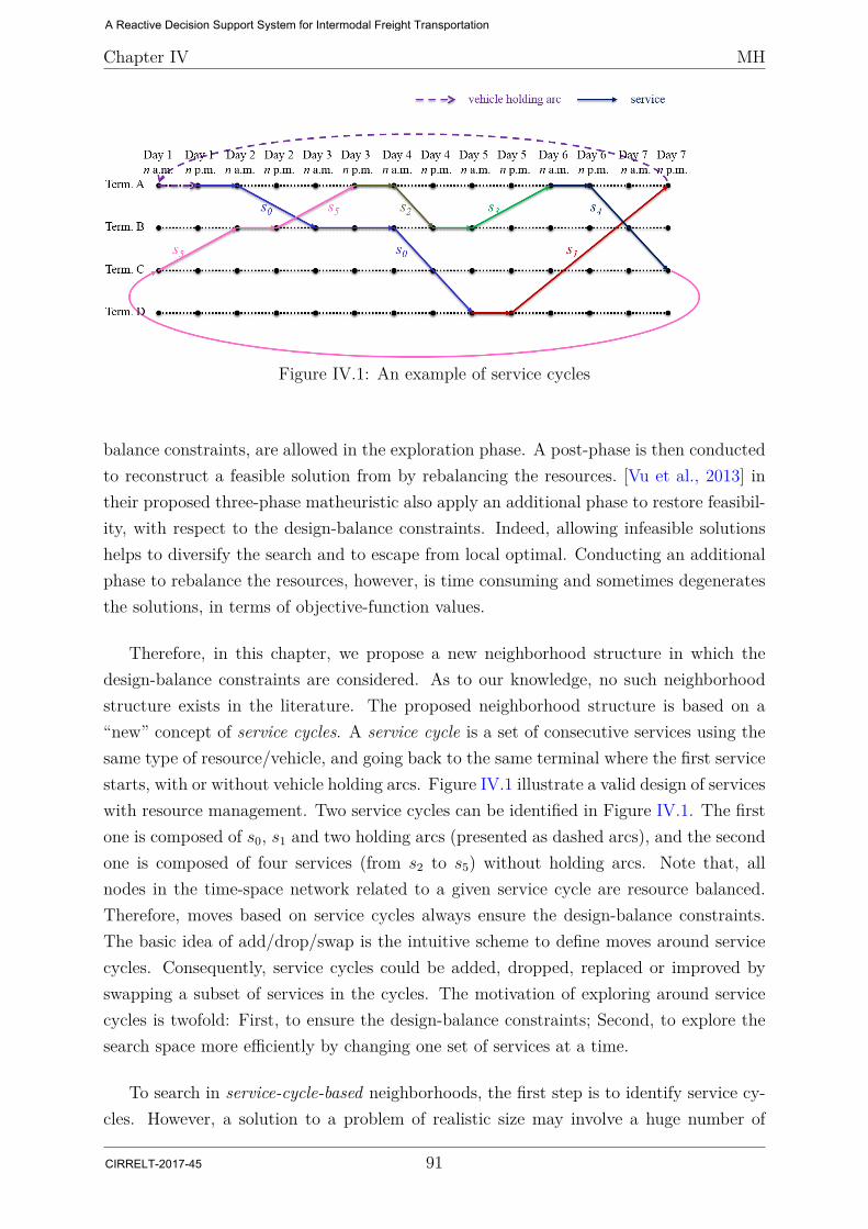
Chapter IV MH
Figure IV.1: An example of service cycles
balance constraints, are allowed in the exploration phase. A post-phase is then conductedto reconstruct a feasible solution from by rebalancing the resources. [Vu et al., 2013] intheir proposed three-phase matheuristic also apply an additional phase to restore feasibil-ity, with respect to the design-balance constraints. Indeed, allowing infeasible solutionshelps to diversify the search and to escape from local optimal. Conducting an additionalphase to rebalance the resources, however, is time consuming and sometimes degeneratesthe solutions, in terms of objective-function values.
Therefore, in this chapter, we propose a new neighborhood structure in which thedesign-balance constraints are considered. As to our knowledge, no such neighborhoodstructure exists in the literature. The proposed neighborhood structure is based on a“new” concept of service cycles. A service cycle is a set of consecutive services using thesame type of resource/vehicle, and going back to the same terminal where the first servicestarts, with or without vehicle holding arcs. Figure IV.1 illustrate a valid design of serviceswith resource management. Two service cycles can be identified in Figure IV.1. The firstone is composed of s0, s1 and two holding arcs (presented as dashed arcs), and the secondone is composed of four services (from s2 to s5) without holding arcs. Note that, allnodes in the time-space network related to a given service cycle are resource balanced.Therefore, moves based on service cycles always ensure the design-balance constraints.The basic idea of add/drop/swap is the intuitive scheme to define moves around servicecycles. Consequently, service cycles could be added, dropped, replaced or improved byswapping a subset of services in the cycles. The motivation of exploring around servicecycles is twofold: First, to ensure the design-balance constraints; Second, to explore thesearch space more efficiently by changing one set of services at a time.
To search in service-cycle-based neighborhoods, the first step is to identify service cy-cles. However, a solution to a problem of realistic size may involve a huge number of
91
A Reactive Decision Support System for Intermodal Freight Transportation
CIRRELT-2017-45
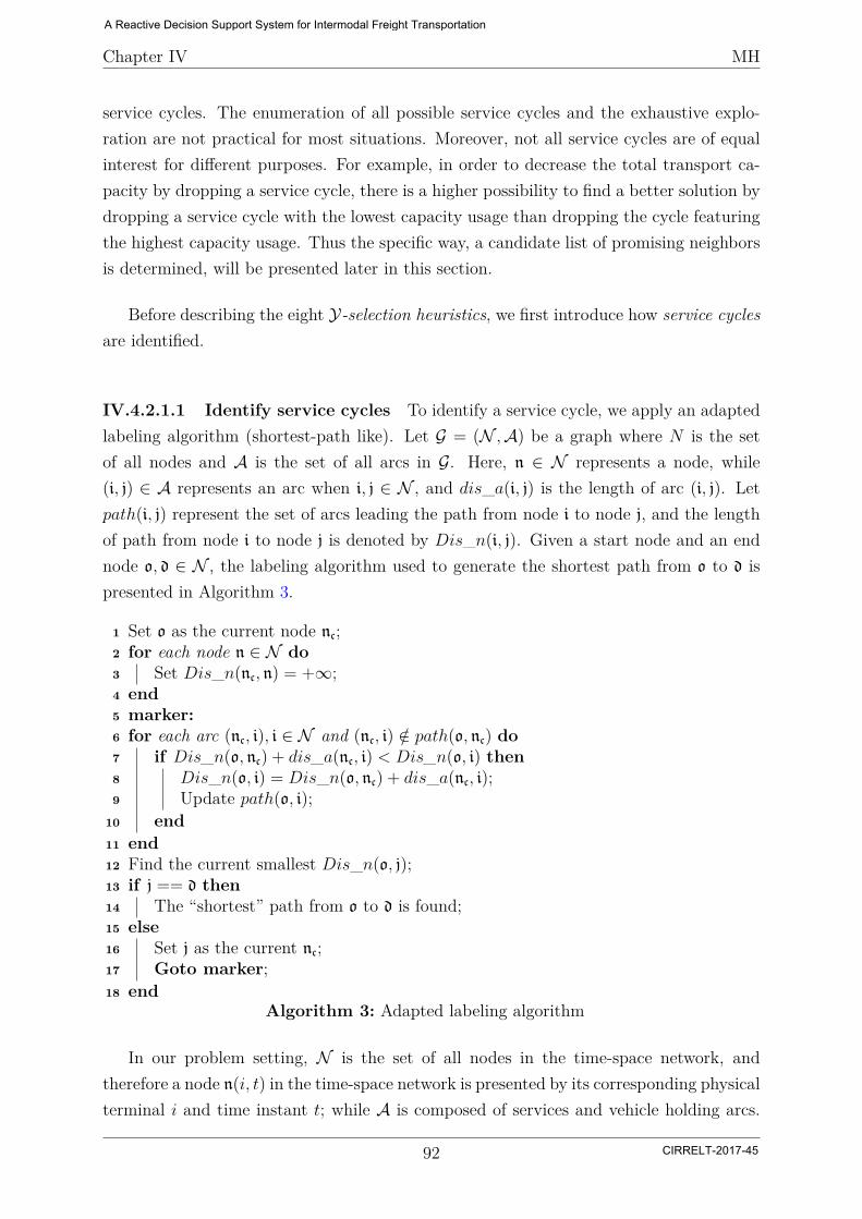
Chapter IV MH
service cycles. The enumeration of all possible service cycles and the exhaustive explo-ration are not practical for most situations. Moreover, not all service cycles are of equalinterest for different purposes. For example, in order to decrease the total transport ca-pacity by dropping a service cycle, there is a higher possibility to find a better solution bydropping a service cycle with the lowest capacity usage than dropping the cycle featuringthe highest capacity usage. Thus the specific way, a candidate list of promising neighborsis determined, will be presented later in this section.
Before describing the eight Y-selection heuristics, we first introduce how service cyclesare identified.
IV.4.2.1.1 Identify service cycles To identify a service cycle, we apply an adaptedlabeling algorithm (shortest-path like). Let G = (N ,A) be a graph where N is the setof all nodes and A is the set of all arcs in G. Here, n ∈ N represents a node, while(i, j) ∈ A represents an arc when i, j ∈ N , and dis_a(i, j) is the length of arc (i, j). Letpath(i, j) represent the set of arcs leading the path from node i to node j, and the lengthof path from node i to node j is denoted by Dis_n(i, j). Given a start node and an endnode o, d ∈ N , the labeling algorithm used to generate the shortest path from o to d ispresented in Algorithm 3.
1 Set o as the current node nc;2 for each node n ∈ N do3 Set Dis_n(nc, n) = +∞;4 end5 marker:6 for each arc (nc, i), i ∈ N and (nc, i) /∈ path(o, nc) do7 if Dis_n(o, nc) + dis_a(nc, i) < Dis_n(o, i) then8 Dis_n(o, i) = Dis_n(o, nc) + dis_a(nc, i);9 Update path(o, i);
10 end11 end12 Find the current smallest Dis_n(o, j);13 if j == d then14 The “shortest” path from o to d is found;15 else16 Set j as the current nc;17 Goto marker;18 end
Algorithm 3: Adapted labeling algorithm
In our problem setting, N is the set of all nodes in the time-space network, andtherefore a node n(i, t) in the time-space network is presented by its corresponding physicalterminal i and time instant t; while A is composed of services and vehicle holding arcs.
92
A Reactive Decision Support System for Intermodal Freight Transportation
CIRRELT-2017-45
Chapter IV MH
The “length” of each arc (a service or a vehicle holding arc) is defined by its correspondingestimated contribution, which is explained later in this section.
To identify a service cycle by applying the adapted labeling algorithm, we follow theprocedure illustrated in Algorithm 4. First, we define the “length” of each arc according tothe chosen Y-selection heuristic. As shown in Table IV.1, average capacity usage, averageresidual capacity or estimated profit is defined as the “length”, or estimated contribution,of each arc, according to the category of decrease capacity, increase capacity or other,respectively. Average capacity usage of a service s, cap_usage(s), is calculated accord-ing to equation (IV.7). For a vehicle holding arc decision variable z(l, i, t), the averagecapacity usage is 0, if z(l, i, t) > 0 according to the current solution; otherwise, it is 1.Furthermore, the average residual capacity residual_usage(s) is calculated according toequation (IV.1).
residual_usage(s) = 1− cap_usage(s); (IV.1)
The estimated profit of a service s, profit(s), is calculated according to equation (IV.2),in which the first term is the estimated revenue of s and the following three terms arefixed costs, transport costs and handling costs, respectively. Note that, to calculate theestimated revenue of s serving d, the transport volume of d and transport distance areconsidered. For a vehicle holding arc decision variable z(l, i, t), the estimated profit is−h(i, l), if z(l, i, t) > 0; otherwise, (T − 1)h(i, l). Further explanation can also be foundin the description of each neighborhood.
profit(s) =∑k∈η(s)
∑d∈D
f(d)x(d, s, k) dis(k)dis(orig(d), dest(d))
− φ(s)−∑k∈η(s)
∑d∈D
ck(γ(d), l(s))x(d, s, k)
−∑k∈η(s)
∑d∈D
κ(i, γ(d))(xin(d, s, k) + xout(d, s, k))
(IV.2)
After defining the length of each arc, we then identify a pair of o and d in the time-spacenetwork. These two nodes are identified by selecting a start arc, i.e., a service s. Accordingto the selected s, the end node (dest(s), τK−1(s)) and start node (orig(s), α0(s)) of s areset as o and d, respectively. After identifying o and d, we apply Algorithm 3 to identifythe shortest path from o to d. The start arc s and all arcs (services and holding arcs) ofthe shortest path(o, d) then constitute the service cycle.
An identified service cycle, consequently, is dropped, replaced or improved by swap-ping one or a subset of services in the cycle according to different Y-selection heuristics.For a given solution, the number of all possible service cycles is large, because the num-ber of services is large and one service can be used to construct different service cycles.
93
A Reactive Decision Support System for Intermodal Freight Transportation
CIRRELT-2017-45
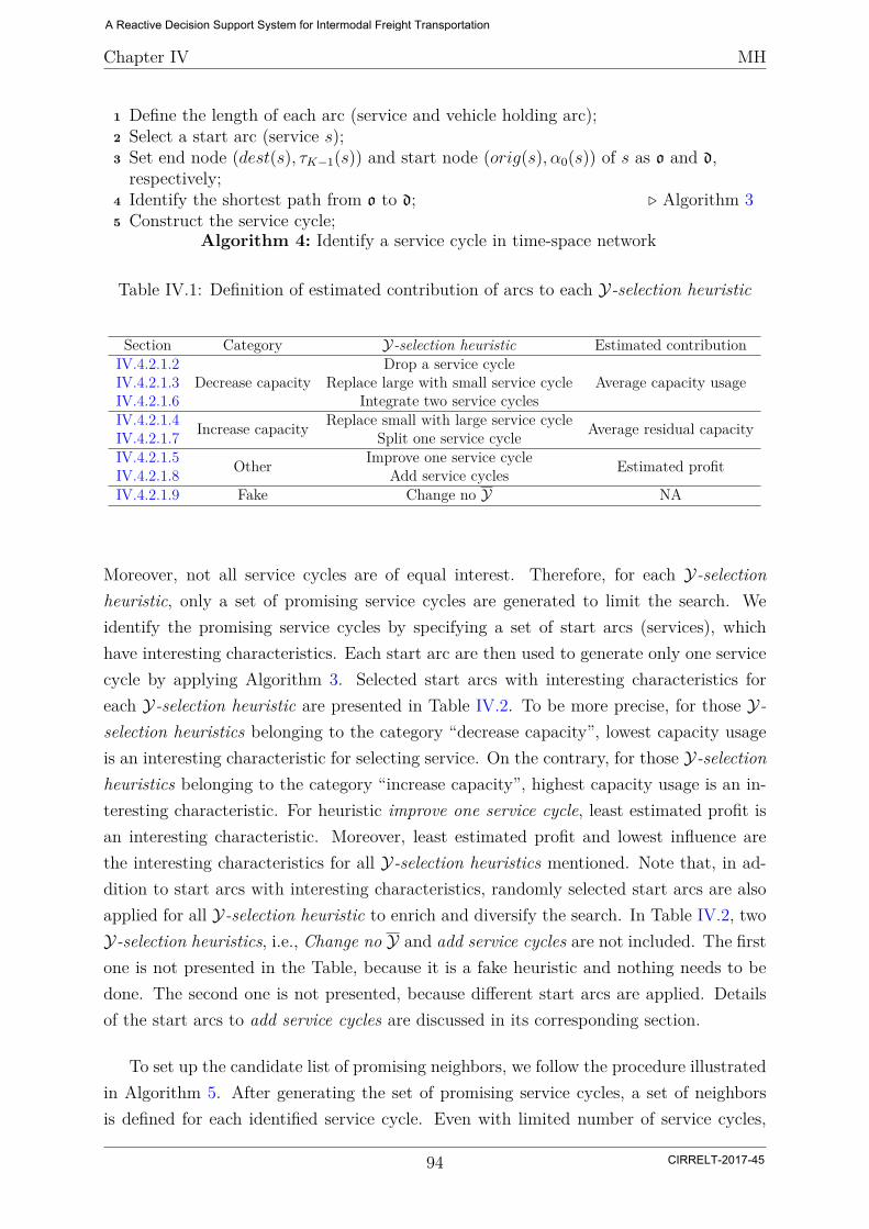
Chapter IV MH
1 Define the length of each arc (service and vehicle holding arc);2 Select a start arc (service s);3 Set end node (dest(s), τK−1(s)) and start node (orig(s), α0(s)) of s as o and d,respectively;
4 Identify the shortest path from o to d; . Algorithm 35 Construct the service cycle;
Algorithm 4: Identify a service cycle in time-space network
Table IV.1: Definition of estimated contribution of arcs to each Y-selection heuristic
Section Category Y-selection heuristic Estimated contributionIV.4.2.1.2
Decrease capacityDrop a service cycle
Average capacity usageIV.4.2.1.3 Replace large with small service cycleIV.4.2.1.6 Integrate two service cyclesIV.4.2.1.4 Increase capacity Replace small with large service cycle Average residual capacityIV.4.2.1.7 Split one service cycleIV.4.2.1.5 Other Improve one service cycle Estimated profitIV.4.2.1.8 Add service cyclesIV.4.2.1.9 Fake Change no Y NA
Moreover, not all service cycles are of equal interest. Therefore, for each Y-selectionheuristic, only a set of promising service cycles are generated to limit the search. Weidentify the promising service cycles by specifying a set of start arcs (services), whichhave interesting characteristics. Each start arc are then used to generate only one servicecycle by applying Algorithm 3. Selected start arcs with interesting characteristics foreach Y-selection heuristic are presented in Table IV.2. To be more precise, for those Y-selection heuristics belonging to the category “decrease capacity”, lowest capacity usageis an interesting characteristic for selecting service. On the contrary, for those Y-selectionheuristics belonging to the category “increase capacity”, highest capacity usage is an in-teresting characteristic. For heuristic improve one service cycle, least estimated profit isan interesting characteristic. Moreover, least estimated profit and lowest influence arethe interesting characteristics for all Y-selection heuristics mentioned. Note that, in ad-dition to start arcs with interesting characteristics, randomly selected start arcs are alsoapplied for all Y-selection heuristic to enrich and diversify the search. In Table IV.2, twoY-selection heuristics, i.e., Change no Y and add service cycles are not included. The firstone is not presented in the Table, because it is a fake heuristic and nothing needs to bedone. The second one is not presented, because different start arcs are applied. Detailsof the start arcs to add service cycles are discussed in its corresponding section.
To set up the candidate list of promising neighbors, we follow the procedure illustratedin Algorithm 5. After generating the set of promising service cycles, a set of neighborsis defined for each identified service cycle. Even with limited number of service cycles,
94
A Reactive Decision Support System for Intermodal Freight Transportation
CIRRELT-2017-45
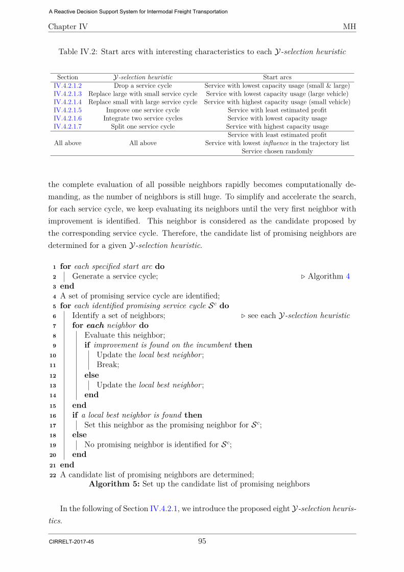
Chapter IV MH
Table IV.2: Start arcs with interesting characteristics to each Y-selection heuristic
Section Y-selection heuristic Start arcsIV.4.2.1.2 Drop a service cycle Service with lowest capacity usage (small & large)IV.4.2.1.3 Replace large with small service cycle Service with lowest capacity usage (large vehicle)IV.4.2.1.4 Replace small with large service cycle Service with highest capacity usage (small vehicle)IV.4.2.1.5 Improve one service cycle Service with least estimated profitIV.4.2.1.6 Integrate two service cycles Service with lowest capacity usageIV.4.2.1.7 Split one service cycle Service with highest capacity usage
All above All aboveService with least estimated profit
Service with lowest influence in the trajectory listService chosen randomly
the complete evaluation of all possible neighbors rapidly becomes computationally de-manding, as the number of neighbors is still huge. To simplify and accelerate the search,for each service cycle, we keep evaluating its neighbors until the very first neighbor withimprovement is identified. This neighbor is considered as the candidate proposed bythe corresponding service cycle. Therefore, the candidate list of promising neighbors aredetermined for a given Y-selection heuristic.
1 for each specified start arc do2 Generate a service cycle; . Algorithm 43 end4 A set of promising service cycle are identified;5 for each identified promising service cycle Sc do6 Identify a set of neighbors; . see each Y-selection heuristic7 for each neighbor do8 Evaluate this neighbor;9 if improvement is found on the incumbent then
10 Update the local best neighbor ;11 Break;12 else13 Update the local best neighbor ;14 end15 end16 if a local best neighbor is found then17 Set this neighbor as the promising neighbor for Sc;18 else19 No promising neighbor is identified for Sc;20 end21 end22 A candidate list of promising neighbors are determined;
Algorithm 5: Set up the candidate list of promising neighbors
In the following of Section IV.4.2.1, we introduce the proposed eight Y-selection heuris-tics.
95
A Reactive Decision Support System for Intermodal Freight Transportation
CIRRELT-2017-45

Chapter IV MH
IV.4.2.1.2 Drop one service cycle The move of this heuristic is defined by drop-ping a service cycle from the incumbent solution. It attempts to improve the solutionby reducing the total transport capacity. If dropping a service cycle could improve thesolutions, it implies that the total transport capacity is sufficient, or even more than nec-essary. Therefore, the low-capacity-usage service cycles are more interesting than others.As illustrated in Table IV.1, the estimated contribution of each arc is consequently definedas the average capacity usage. Promising service cycles are generated with specified startarcs, which are presented in Table IV.2. According to the definition of the neighborhoodmove, there is only one neighbor for each identified service cycle.
IV.4.2.1.3 Replace large with small service cycle The move of this heuristicis defined by replacing a large-vehicle service cycle S ′ with a small-vehicle service cycleS. In addition to reducing the total transport capacity, this heuristic also contributes todiversifying the search. According to Algorithm 5 (line 6), for a given large-vehicle servicecycle S ′, we identify a set of neighbors following the procedure illustrated in Algorithm6. To be more precise, for each service s′ in S ′, a corresponding alternative list S∗ isgenerated. A related s∗ of s′ is characterized from three aspects: first, s∗ is a service usingsmall vehicle; second, s∗ has the same start and end terminal as s′; last, both start timeand end time of s∗ are no more than ±1 time period away from those of s′. By choosingone service for each s′ ∈ S ′ from its corresponding alternative list, we obtain a possibleS. Therefore, all the possible S are generated by the enumeration of all service-selectingcombinations from the alternative lists. These possible S are then sorted decreasinglyaccording to the sum of influence of each s∗ ∈ S, according to the trajectory service list.To evaluate an S, we calculate the estimated revenue of it by restoring the flow of D′,
1 for each s′ ∈ S ′ do2 for each related s∗ of s′ do3 if s∗ 6= 1 in Y then4 s∗ is considered as a possible alternative of s′;5 end6 end7 end8 Enumerate all the possible S by choosing one service for each s′ ∈ S ′ from itscorresponding alternative list;
Algorithm 6: Identify a set of neighbors for a given S ′ (Replace large with small)
which is transported by S ′ in the current solution. A basic greedy algorithm is appliedto calculate the estimated revenue of S: sort all d ∈ D′ decreasingly according to theirrevenue; for each d ∈ D′, if S and the residual capacity of the network without S ′ is ableto serve it, update the flow distribution plan accordingly and the estimated revenue of S.
96
A Reactive Decision Support System for Intermodal Freight Transportation
CIRRELT-2017-45
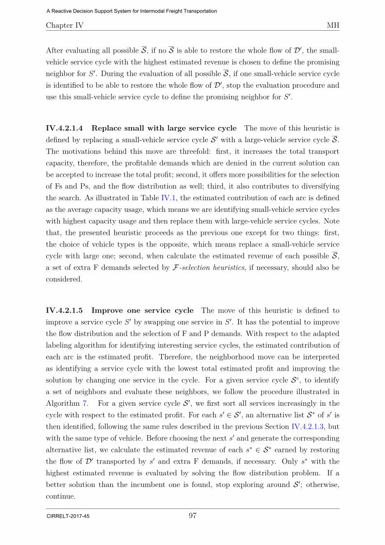
Chapter IV MH
After evaluating all possible S, if no S is able to restore the whole flow of D′, the small-vehicle service cycle with the highest estimated revenue is chosen to define the promisingneighbor for S ′. During the evaluation of all possible S, if one small-vehicle service cycleis identified to be able to restore the whole flow of D′, stop the evaluation procedure anduse this small-vehicle service cycle to define the promising neighbor for S ′.
IV.4.2.1.4 Replace small with large service cycle The move of this heuristic isdefined by replacing a small-vehicle service cycle S ′ with a large-vehicle service cycle S.The motivations behind this move are threefold: first, it increases the total transportcapacity, therefore, the profitable demands which are denied in the current solution canbe accepted to increase the total profit; second, it offers more possibilities for the selectionof Fs and Ps, and the flow distribution as well; third, it also contributes to diversifyingthe search. As illustrated in Table IV.1, the estimated contribution of each arc is definedas the average capacity usage, which means we are identifying small-vehicle service cycleswith highest capacity usage and then replace them with large-vehicle service cycles. Notethat, the presented heuristic proceeds as the previous one except for two things: first,the choice of vehicle types is the opposite, which means replace a small-vehicle servicecycle with large one; second, when calculate the estimated revenue of each possible S,a set of extra F demands selected by F-selection heuristics, if necessary, should also beconsidered.
IV.4.2.1.5 Improve one service cycle The move of this heuristic is defined toimprove a service cycle S ′ by swapping one service in S ′. It has the potential to improvethe flow distribution and the selection of F and P demands. With respect to the adaptedlabeling algorithm for identifying interesting service cycles, the estimated contribution ofeach arc is the estimated profit. Therefore, the neighborhood move can be interpretedas identifying a service cycle with the lowest total estimated profit and improving thesolution by changing one service in the cycle. For a given service cycle Sc, to identifya set of neighbors and evaluate these neighbors, we follow the procedure illustrated inAlgorithm 7. For a given service cycle S ′, we first sort all services increasingly in thecycle with respect to the estimated profit. For each s′ ∈ S ′, an alternative list S∗ of s′ isthen identified, following the same rules described in the previous Section IV.4.2.1.3, butwith the same type of vehicle. Before choosing the next s′ and generate the correspondingalternative list, we calculate the estimated revenue of each s∗ ∈ S∗ earned by restoringthe flow of D′ transported by s′ and extra F demands, if necessary. Only s∗ with thehighest estimated revenue is evaluated by solving the flow distribution problem. If abetter solution than the incumbent one is found, stop exploring around S ′; otherwise,continue.
97
A Reactive Decision Support System for Intermodal Freight Transportation
CIRRELT-2017-45
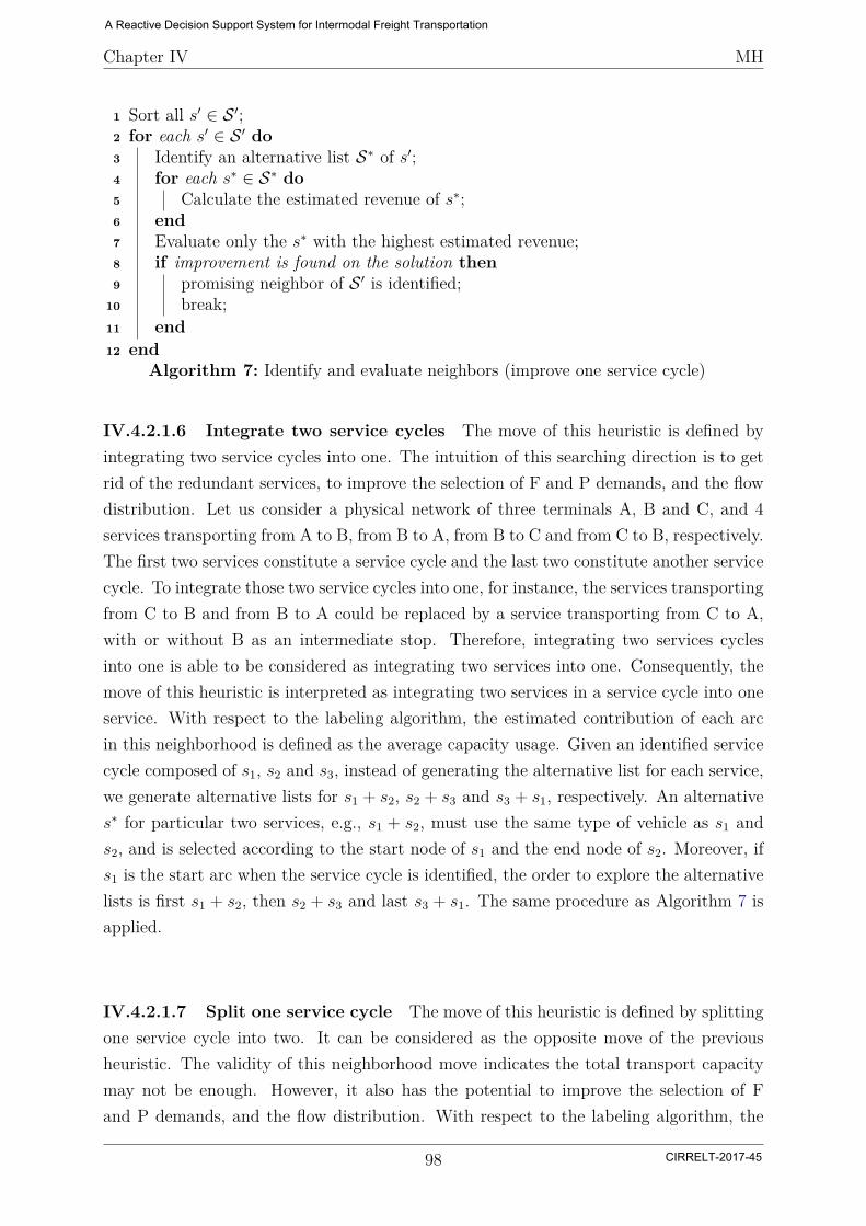
Chapter IV MH
1 Sort all s′ ∈ S ′;2 for each s′ ∈ S ′ do3 Identify an alternative list S∗ of s′;4 for each s∗ ∈ S∗ do5 Calculate the estimated revenue of s∗;6 end7 Evaluate only the s∗ with the highest estimated revenue;8 if improvement is found on the solution then9 promising neighbor of S ′ is identified;
10 break;11 end12 end
Algorithm 7: Identify and evaluate neighbors (improve one service cycle)
IV.4.2.1.6 Integrate two service cycles The move of this heuristic is defined byintegrating two service cycles into one. The intuition of this searching direction is to getrid of the redundant services, to improve the selection of F and P demands, and the flowdistribution. Let us consider a physical network of three terminals A, B and C, and 4services transporting from A to B, from B to A, from B to C and from C to B, respectively.The first two services constitute a service cycle and the last two constitute another servicecycle. To integrate those two service cycles into one, for instance, the services transportingfrom C to B and from B to A could be replaced by a service transporting from C to A,with or without B as an intermediate stop. Therefore, integrating two services cyclesinto one is able to be considered as integrating two services into one. Consequently, themove of this heuristic is interpreted as integrating two services in a service cycle into oneservice. With respect to the labeling algorithm, the estimated contribution of each arcin this neighborhood is defined as the average capacity usage. Given an identified servicecycle composed of s1, s2 and s3, instead of generating the alternative list for each service,we generate alternative lists for s1 + s2, s2 + s3 and s3 + s1, respectively. An alternatives∗ for particular two services, e.g., s1 + s2, must use the same type of vehicle as s1 ands2, and is selected according to the start node of s1 and the end node of s2. Moreover, ifs1 is the start arc when the service cycle is identified, the order to explore the alternativelists is first s1 + s2, then s2 + s3 and last s3 + s1. The same procedure as Algorithm 7 isapplied.
IV.4.2.1.7 Split one service cycle The move of this heuristic is defined by splittingone service cycle into two. It can be considered as the opposite move of the previousheuristic. The validity of this neighborhood move indicates the total transport capacitymay not be enough. However, it also has the potential to improve the selection of Fand P demands, and the flow distribution. With respect to the labeling algorithm, the
98
A Reactive Decision Support System for Intermodal Freight Transportation
CIRRELT-2017-45
Chapter IV MH
average residual capacity is defined as the estimated contribution of each arc. Withoutrepeating all the similarities, in this heuristic, the differences come from how to generatethe alternative list and how to identify the candidate for each service cycle. Given aservice cycle, we first sort all the services increasingly with respect to the influence intrajectory list. The exploration of alternative lists follows that increasing order. Foreach service in the cycle, to generate the alternative list, two types of replacement couldhappen: ABC replaced by AB+BC (opposite case of previous heuristic) or AB replacedby AC+CB with extra F demands related to C.
IV.4.2.1.8 Add service cycles The heuristic is defined by adding cycles. It is calledafter only “profitable acceptance” and “random acceptance” F -selection heuristic. Oneservice cycle, which is made of closed services according to the current Y , is generatedto transport the new accepted F demands by those two F -selection heuristics. Keepgenerating service cycles until all new accepted F demands are satisfied. Note that,without serving more new demands, this heuristic is going to degenerate the quality ofthe solution, in terms of objective value, and that is why this heuristic is only triggeredby the F-selection heuristics of profitable acceptance and random acceptance.
IV.4.2.1.9 Change no Y This is a fake Y-selection heuristic. When it is chosen, nochange is applied on the service selection. In other words, we only explore the searchspace of F-demand selection. Note that, this fake heuristic is not in the associated set ofchange no F heuristic.
IV.4.2.2 F-selection Heuristics
The proposed F-selection heuristics can be briefly classified into two categories: rejectaccepted F demands and accept extra F demands. In addition, a “fake” heuristic, changeno F , is also considered separately. In each iteration, if the change no F heuristic ischosen, we fix F and explore only in the search space of service selection.
To reject a set of accepted F demands, three heuristics are applied, i.e., random rejec-tion, minimal profit rejection and worst record rejection. All three reject heuristics needan integer p ∈ [1,MAX] as input, where p indicates the number of accepted F demandsto be rejected and MAX stands for the total number of accepted F demands accordingto the current F .
Random rejection: The random rejection heuristic simply selects p accepted F
99
A Reactive Decision Support System for Intermodal Freight Transportation
CIRRELT-2017-45
Chapter IV MH
demands at random and change their value from 1 to 0 in the current F .
Minimal profit rejection: Given a feasible solution to the SSND-RRM, we calculatethe estimated profit of each accepted demand d ∈ DF as follows:
profit(d) = revenue(d)− cost(d) (IV.3)
where revenue(d) is the revenue of accepting whole d, and cost(d) is the estimated totalcost of d:
revenue(d) = f(d)vol(d) (IV.4)
Calculated by equation (IV.5), cost(d) is the sum of transport costs, holding costs, han-dling costs and total estimated fixed costs, i.e., estimate(φ(d)), of d:
cost(d) =∑s∈S
∑k∈η(s)
ck(γ(d), l(s))x(d, s, k) +∑t∈T
∑i∈Nph
c(i, γ(d))xhold(d, i, t)
+∑s∈S
∑k∈η(s)
κ(i, γ(d))(xin(d, s, k) + xout(d, s, k)) + estimate(φ(d))(IV.5)
where estimate(φ(d)) = ∑s∈S estimate(φ(s(d))) is the total estimated fixed cost that d is
supposed to pay for all the services used for the routing of d. To calculate the estimatedfixed cost that d is supposed to pay for s, i.e., estimate(φ(s(d))), we take into accounttwo factors: a). for the used service s, the lower the capacity usage of s, the more d shouldshare the fixed cost; b). the more capacity of s used for transporting d, the more d shouldshare the fixed cost. Therefore, estimate(φ(s(d))) is calculated according:
estimate(φ(s(d))) = φ(s)cap_usage(s) ∗
∑k∈η(s)
x(d, s, k)∑k∈η(s)
cap(l(s)) (IV.6)
where capacity usage cap_usage(s) of s is calculated as the ratio of used distance ca-pacity over the maximum possible distance capacity according to the current solution,illustrated in equation (IV.7). Used distance capacity is the sum of all legs’ used capacitymultiplied by their corresponding transport distance dis(k), while maximum possible dis-tance capacity is the sum of all legs’ capacity multiplied by their corresponding transportdistance.
cap_usage(s) =
∑s∈S
∑k∈η(s)
∑d∈D
dis(k)x(d, s, k)∑s∈S
∑k∈η(s)
dis(k)cap(l(s)) (IV.7)
All accepted F demands are then sorted in ascending order according to their estimatedprofit. The first p demands in the list are then rejected and their corresponding values inthe F are changed.
100
A Reactive Decision Support System for Intermodal Freight Transportation
CIRRELT-2017-45
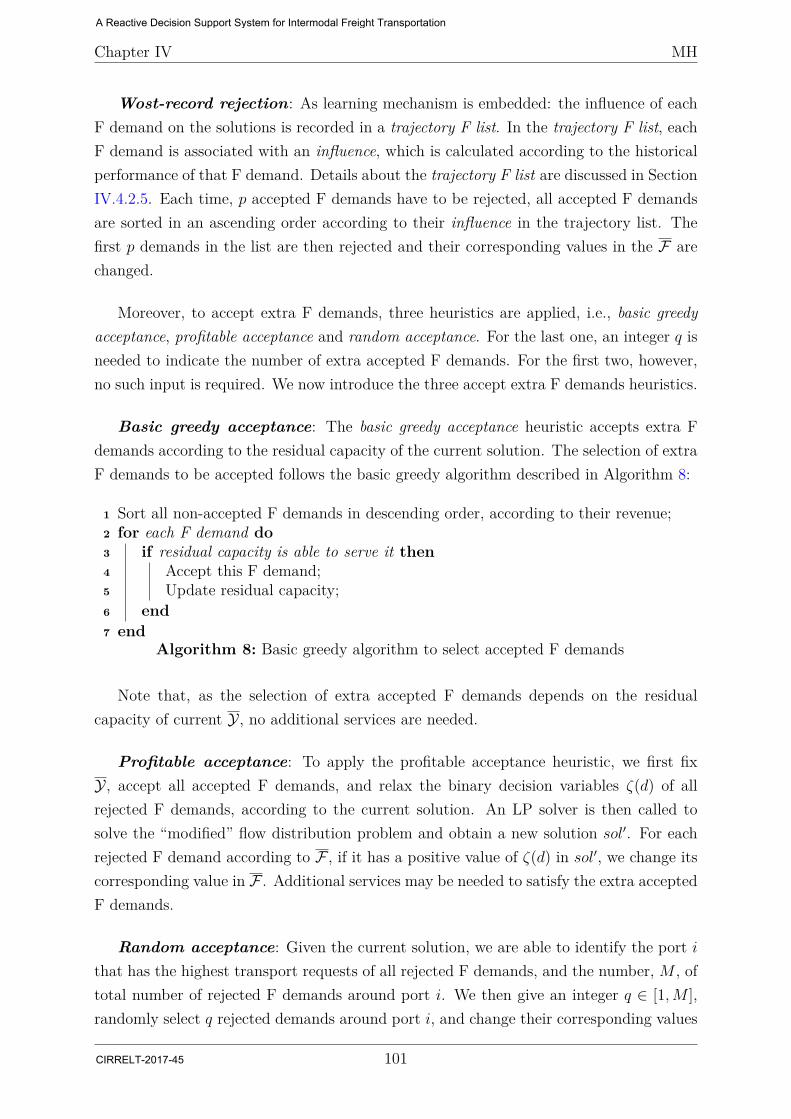
Chapter IV MH
Wost-record rejection: As learning mechanism is embedded: the influence of eachF demand on the solutions is recorded in a trajectory F list. In the trajectory F list, eachF demand is associated with an influence, which is calculated according to the historicalperformance of that F demand. Details about the trajectory F list are discussed in SectionIV.4.2.5. Each time, p accepted F demands have to be rejected, all accepted F demandsare sorted in an ascending order according to their influence in the trajectory list. Thefirst p demands in the list are then rejected and their corresponding values in the F arechanged.
Moreover, to accept extra F demands, three heuristics are applied, i.e., basic greedyacceptance, profitable acceptance and random acceptance. For the last one, an integer q isneeded to indicate the number of extra accepted F demands. For the first two, however,no such input is required. We now introduce the three accept extra F demands heuristics.
Basic greedy acceptance: The basic greedy acceptance heuristic accepts extra Fdemands according to the residual capacity of the current solution. The selection of extraF demands to be accepted follows the basic greedy algorithm described in Algorithm 8:
1 Sort all non-accepted F demands in descending order, according to their revenue;2 for each F demand do3 if residual capacity is able to serve it then4 Accept this F demand;5 Update residual capacity;6 end7 end
Algorithm 8: Basic greedy algorithm to select accepted F demands
Note that, as the selection of extra accepted F demands depends on the residualcapacity of current Y , no additional services are needed.
Profitable acceptance: To apply the profitable acceptance heuristic, we first fixY , accept all accepted F demands, and relax the binary decision variables ζ(d) of allrejected F demands, according to the current solution. An LP solver is then called tosolve the “modified” flow distribution problem and obtain a new solution sol′. For eachrejected F demand according to F , if it has a positive value of ζ(d) in sol′, we change itscorresponding value in F . Additional services may be needed to satisfy the extra acceptedF demands.
Random acceptance: Given the current solution, we are able to identify the port ithat has the highest transport requests of all rejected F demands, and the number, M , oftotal number of rejected F demands around port i. We then give an integer q ∈ [1,M ],randomly select q rejected demands around port i, and change their corresponding values
101
A Reactive Decision Support System for Intermodal Freight Transportation
CIRRELT-2017-45
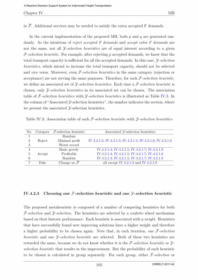
Chapter IV MH
in F . Additional services may be needed to satisfy the extra accepted F demands.
In the current implementation of the proposed MH, both p and q are generated ran-domly. As the intuitions of reject accepted F demands and accept extra F demands arenot the same, not all Y-selection heuristics are of equal interest according to a givenF-selection heuristic. For example, after rejecting p accepted demands, we know that thetotal transport capacity is sufficient for all the accepted demands. In this case, Y-selectionheuristics, which intend to increase the total transport capacity, should not be selectedand vice versa. Moreover, even F-selection heuristics in the same category (rejection oracceptance) are not serving the same purposes. Therefore, for each F-selection heuristic,we define an associated set of Y-selection heuristics. Each time a F-selection heuristic ischosen, only Y-selection heuristics in its associated set can be chosen. The associationtable of F-selection heuristics with Y-selection heuristics is illustrated as Table IV.3. Inthe column of “Associated Y-selection heuristics”, the number indicates the section, wherewe present the associated Y-selection heuristics.
Table IV.3: Association table of each F-selection heuristic with Y-selection heuristics
No. Category F -selection heuristic Associated Y-selection heuristics1
RejectRandom
IV.4.2.1.2; IV.4.2.1.3; IV.4.2.1.5; IV.4.2.1.6; IV.4.2.1.92 Minimal profit3 Worst record4
AcceptBasic greedy IV.4.2.1.4; IV.4.2.1.5; IV.4.2.1.7; IV.4.2.1.9
5 Profitable IV.4.2.1.4; IV.4.2.1.5; IV.4.2.1.7; IV.4.2.1.86 Random IV.4.2.1.4; IV.4.2.1.5; IV.4.2.1.7; IV.4.2.1.87 Fake Change no F all except IV.4.2.1.8 and IV.4.2.1.9
IV.4.2.3 Choosing one F-selection heuristic and one Y-selection heuristic
The proposed metaheuristic is composed of a number of competing heuristics for bothF-selection and Y-selection. The heuristics are selected by a roulette wheel mechanismbased on their historic performance. Each heuristic is associated with a weight. Heuristicsthat have successfully found new improving solutions have a higher weight and thereforea higher probability to be chosen again. Note that, in each iteration, one F-selectionheuristic and one Y-selection heuristic are selected. Both of these two heuristics arerewarded the same, because we do not know whether it is the F-selection heuristic or Y-selection heuristic that results in the improvement. But the probability of each heuristicto be chosen is calculated in group separately. For each group, either F-selection or
102
A Reactive Decision Support System for Intermodal Freight Transportation
CIRRELT-2017-45

Chapter IV MH
Y-selection, the probability of a heuristic to be chosen is calculated as follows:
pi = wi∑nwn
(IV.8)
In equation (IV.8), i indicates the selected heuristic and n indicates the total number ofheuristics in the given group.
IV.4.2.4 Adaptive weight and score adjustment
The probabilities of all heuristics to be chosen are the same in the beginning. Furthermore,the probabilities are recalculated after each m iterations according to the weight of eachheuristic, as illustrated in equation (IV.9).
wi = wi(1− r) + rscoreicounteri
(IV.9)
In equation (IV.9) [Ropke and Pisinger, 2006], scorei is the score of each heuristicand counteri is the number of times that the heuristic i is selected during the last miterations, and r is a number between 0 and 1. If r = 0, we do not change the weight ofi; if r = 1 the weight of i totally depends on its performance during the last m iterations.Otherwise, the weight of i depends on both its performance during the last m iterationsand the performance before.
The initial score for each heuristic is 0. Each time we get a new feasible solution,the score of the heuristic that results in the new feasible solution is updated as shown inAlgorithm 9, in which objs(opt), objs(incum) and objs(new) denotes the objective valueof the global best, the incumbent and the new feasible solution, respectively. Note that,each time after recalculating the weight of each heuristic, the score of each heuristic scoreiis reset as 0.
1 if objs(new) > objs(opt) then2 scorei = scorei + 2 ∗ objs(new)− objs(incum)− objs(opt);3 else if objs(new) > objs(incum) then4 scorei = scorei + objs(new)− objs(incum);5 end
Algorithm 9: Score the chosen heuristics
103
A Reactive Decision Support System for Intermodal Freight Transportation
CIRRELT-2017-45

Chapter IV MH
IV.4.2.5 Trajectory service list and F list
Trajectory service list and trajectory F list are the long-term memory learning mecha-nism for evaluating the influence of each service or each F demand on the quality of thesolutions, respectively. To be more precise, when a new solution sol is found better thanthen current global best solution sol′, we reward each open service and each accepted Fdemand in sol as
rewardi,j = diff(objs)card(sol) (IV.10)
where i is the index number of a service or an F demand accordingly, and j indicates theindex number of an improvement found on current global best, diff(objs) is the differencebetween the two objective values, namely sol− sol′, and card(sol) is the number of openservices for the service list and number of accepted F demands for the F list in sol,respectively. Besides that, the closed services and rejected F demands are rewarded with0. The influence of a service or an F demand, is then calculated as
influencei =J∑
j=J−crewardi,j
counteric
(IV.11)
where i is the index number of a service or an F demand; j is the index number of animprovement found on the current global best, and J is the total number of improvement;counteri is the number of ith service/F demand that appear in the last c times of currentglobal best. The influence of ith service/F demand is the sum of its rewards in the lastc times multiplied by the ratio of it that appears in the current global best in the last ctimes. Note that, a reward of a service/F demand is calculated and updated each timean improvement is found on the global best solution.
IV.4.2.6 Diversification
When a predefined number g of consecutive no-feasible-neighbor situation is met, a pro-cedure is conducted to diversify the incumbent solution. The basic idea of diversificationis to identify a set of closed “umpromising” services and force them to be open in thenew solution, aiming to escape from the current searching area. Based on the currentY , among all y(s) = 0, we choose the service with the lowest influence according to thetrajectory service list. The chosen service is then used as the start arc of the adapted label-ing algorithm to identify a service cycle to add in the incumbent solution. The estimatedcontribution (or length) of each arc to identify the shortest path is its corresponding in-fluence in the trajectory service list. After identifying the service cycle, we fix y(x) andζ(d), then solve the flow distribution problem and set the new solution as the incumbent
104
A Reactive Decision Support System for Intermodal Freight Transportation
CIRRELT-2017-45

Chapter IV MH
for the search procedure.
IV.4.2.7 Intensification
As the exploration in the search space of Y is around service cycles, a set of services aremodified in one move so that the optimal solution maybe missed. In addition, the paceof exploration in the search space of F is also big. Therefore, it is quite necessary to havethis intensification phase in the proposed MH. The goal of this phase is to find bettersolutions by intensifying the search in regions of the solution space, where interestingcharacteristics of services are identified.
Given a feasible solution (F ,Y ,X (F ,Y)), two types of intensification are applied inthis proposed solution approach. The first type of intensification calls the MILP solver tosolve a reduced SSND-RRM problem, in which only open services in Y can be chosen toserve all demands. This type of intensification is called right after the Initialization phasein order to feed the improvement phase with a promising start point. The second type ofintensification first identifies a promising service cycle from the closed services accordingto Y of current global best solution. Influence of closed services in the trajectory servicelist is considered to aid identifying the promising service cycle. The MILP solver is thencalled to choose the best design variables among the open services and the identified servicecycle, serving all demands. This type of intensification is called each time a consecutiveb times of no-global-improvement situation is encountered. The solution obtained by theintensification is then set as the incumbent for the search procedure.
IV.4.2.8 Tabu Lists
Three short-term memory tabu lists are maintained to record generated service cycles fordifferent purposes. The first one is used for the Y-selection heuristics, to avoid the sameservice cycle to be dropped or replaced. The second one and the third one, is used fordiversification and intensification to avoid adding back the same service cycle, respectively.The size of all three tabu lists are set as 30 for now.
IV.5 Computational Results and Analysis
The purpose of this section is to study the effectiveness of the proposed solution approach.After introducing the procedure of test instance generation in Subsection IV.5.1, we cal-
105
A Reactive Decision Support System for Intermodal Freight Transportation
CIRRELT-2017-45
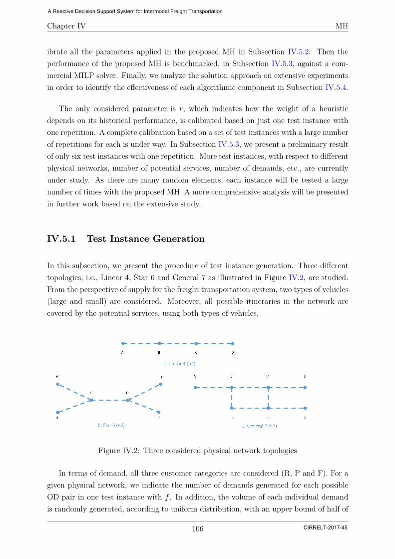
Chapter IV MH
ibrate all the parameters applied in the proposed MH in Subsection IV.5.2. Then theperformance of the proposed MH is benchmarked, in Subsection IV.5.3, against a com-mercial MILP solver. Finally, we analyze the solution approach on extensive experimentsin order to identify the effectiveness of each algorithmic component in Subsection IV.5.4.
The only considered parameter is r, which indicates how the weight of a heuristicdepends on its historical performance, is calibrated based on just one test instance withone repetition. A complete calibration based on a set of test instances with a large numberof repetitions for each is under way. In Subsection IV.5.3, we present a preliminary resultof only six test instances with one repetition. More test instances, with respect to differentphysical networks, number of potential services, number of demands, etc., are currentlyunder study. As there are many random elements, each instance will be tested a largenumber of times with the proposed MH. A more comprehensive analysis will be presentedin further work based on the extensive study.
IV.5.1 Test Instance Generation
In this subsection, we present the procedure of test instance generation. Three differenttopologies, i.e., Linear 4, Star 6 and General 7 as illustrated in Figure IV.2, are studied.From the perspective of supply for the freight transportation system, two types of vehicles(large and small) are considered. Moreover, all possible itineraries in the network arecovered by the potential services, using both types of vehicles.
Figure IV.2: Three considered physical network topologies
In terms of demand, all three customer categories are considered (R, P and F). For agiven physical network, we indicate the number of demands generated for each possibleOD pair in one test instance with f . In addition, the volume of each individual demandis randomly generated, according to uniform distribution, with an upper bound of half of
106
A Reactive Decision Support System for Intermodal Freight Transportation
CIRRELT-2017-45
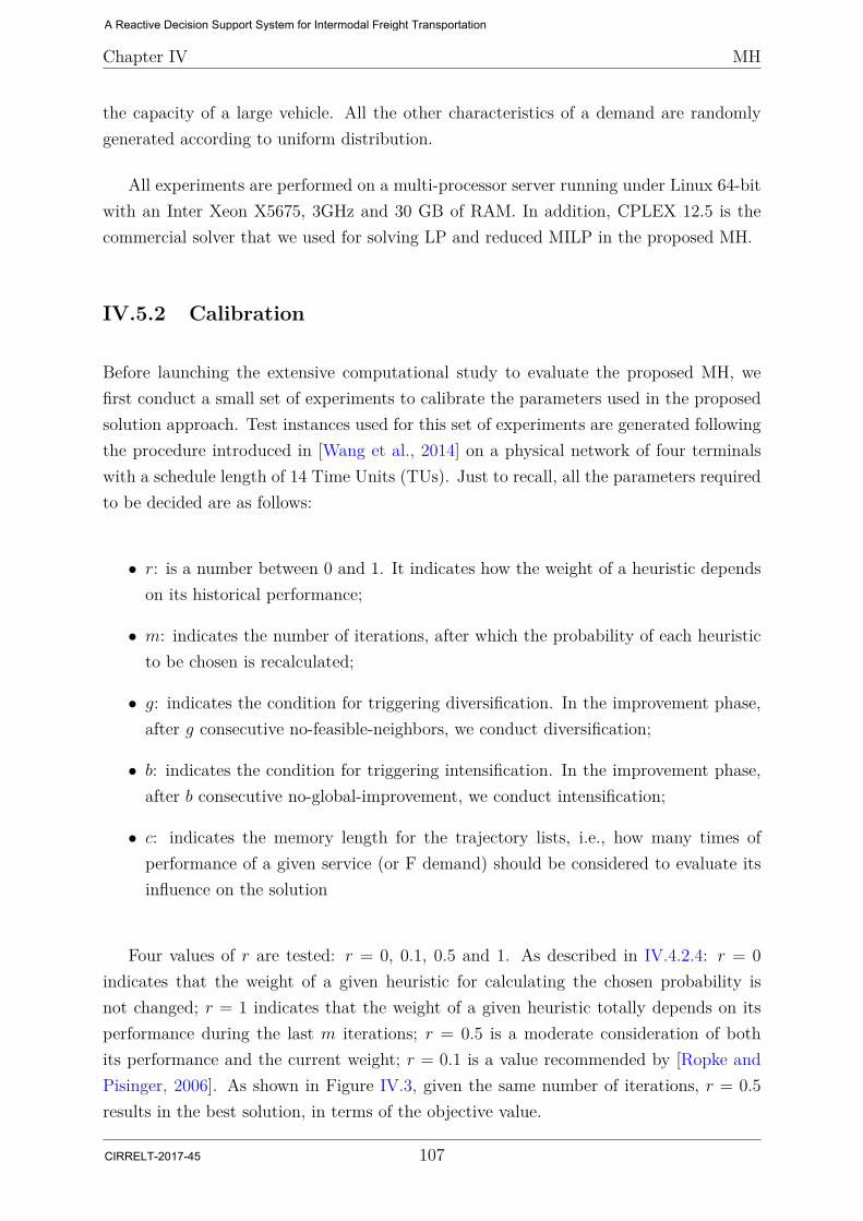
Chapter IV MH
the capacity of a large vehicle. All the other characteristics of a demand are randomlygenerated according to uniform distribution.
All experiments are performed on a multi-processor server running under Linux 64-bitwith an Inter Xeon X5675, 3GHz and 30 GB of RAM. In addition, CPLEX 12.5 is thecommercial solver that we used for solving LP and reduced MILP in the proposed MH.
IV.5.2 Calibration
Before launching the extensive computational study to evaluate the proposed MH, wefirst conduct a small set of experiments to calibrate the parameters used in the proposedsolution approach. Test instances used for this set of experiments are generated followingthe procedure introduced in [Wang et al., 2014] on a physical network of four terminalswith a schedule length of 14 Time Units (TUs). Just to recall, all the parameters requiredto be decided are as follows:
• r: is a number between 0 and 1. It indicates how the weight of a heuristic dependson its historical performance;
• m: indicates the number of iterations, after which the probability of each heuristicto be chosen is recalculated;
• g: indicates the condition for triggering diversification. In the improvement phase,after g consecutive no-feasible-neighbors, we conduct diversification;
• b: indicates the condition for triggering intensification. In the improvement phase,after b consecutive no-global-improvement, we conduct intensification;
• c: indicates the memory length for the trajectory lists, i.e., how many times ofperformance of a given service (or F demand) should be considered to evaluate itsinfluence on the solution
Four values of r are tested: r = 0, 0.1, 0.5 and 1. As described in IV.4.2.4: r = 0indicates that the weight of a given heuristic for calculating the chosen probability isnot changed; r = 1 indicates that the weight of a given heuristic totally depends on itsperformance during the last m iterations; r = 0.5 is a moderate consideration of bothits performance and the current weight; r = 0.1 is a value recommended by [Ropke andPisinger, 2006]. As shown in Figure IV.3, given the same number of iterations, r = 0.5results in the best solution, in terms of the objective value.
107
A Reactive Decision Support System for Intermodal Freight Transportation
CIRRELT-2017-45
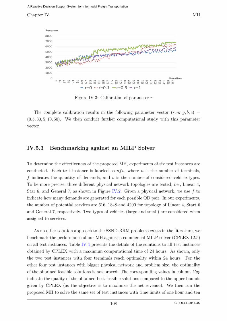
Chapter IV MH
0
1000
2000
3000
4000
5000
6000
7000
8000
1 19 37 55 73 91 109
127
145
163
181
199
217
235
253
271
289
307
325
343
361
379
397
415
433
451
469
487
r=0 r=0.1 r=0.5 r=1
Revenue
Iteration
Figure IV.3: Calibration of parameter r
The complete calibration results in the following parameter vector (r,m, g, b, c) =(0.5, 30, 5, 10, 50). We then conduct further computational study with this parametervector.
IV.5.3 Benchmarking against an MILP Solver
To determine the effectiveness of the proposed MH, experiments of six test instances areconducted. Each test instance is labeled as nfv, where n is the number of terminals,f indicates the quantity of demands, and v is the number of considered vehicle types.To be more precise, three different physical network topologies are tested, i.e., Linear 4,Star 6, and General 7, as shown in Figure IV.2. Given a physical network, we use f toindicate how many demands are generated for each possible OD pair. In our experiments,the number of potential services are 616, 1848 and 4200 for topology of Linear 4, Start 6and General 7, respectively. Two types of vehicles (large and small) are considered whenassigned to services.
As no other solution approach to the SSND-RRM problems exists in the literature, webenchmark the performance of our MH against a commercial MILP solver (CPLEX 12.5)on all test instances. Table IV.4 presents the details of the solutions to all test instancesobtained by CPLEX with a maximum computational time of 24 hours. As shown, onlythe two test instances with four terminals reach optimality within 24 hours. For theother four test instances with bigger physical network and problem size, the optimalityof the obtained feasible solutions is not proved. The corresponding values in column Gapindicate the quality of the obtained best feasible solutions compared to the upper boundsgiven by CPLEX (as the objective is to maximize the net revenue). We then run theproposed MH to solve the same set of test instances with time limits of one hour and ten
108
A Reactive Decision Support System for Intermodal Freight Transportation
CIRRELT-2017-45
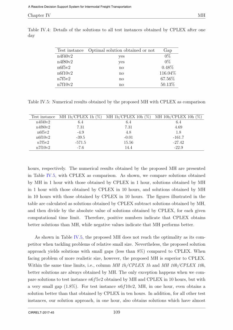
Chapter IV MH
Table IV.4: Details of the solutions to all test instances obtained by CPLEX after oneday
Test instance Optimal solution obtained or not Gapn4f40v2 yes 0%n4f80v2 yes 0%n6f5v2 no 0.48%n6f10v2 no 116.04%n7f5v2 no 67.56%n7f10v2 no 50.13%
Table IV.5: Numerical results obtained by the proposed MH with CPLEX as comparison
Test instance MH 1h/CPLEX 1h (%) MH 1h/CPLEX 10h (%) MH 10h/CPLEX 10h (%)n4f40v2 6.4 6.4 6.4n4f80v2 7.31 7.31 4.69n6f5v2 -4.9 4.8 1.8n6f10v2 -39.5 -0.01 -161.7n7f5v2 -571.5 15.56 -27.42n7f10v2 -7.6 14.4 -22.9
hours, respectively. The numerical results obtained by the proposed MH are presentedin Table IV.5, with CPLEX as comparison. As shown, we compare solutions obtainedby MH in 1 hour with those obtained by CPLEX in 1 hour, solutions obtained by MHin 1 hour with those obtained by CPLEX in 10 hours, and solutions obtained by MHin 10 hours with those obtained by CPLEX in 10 hours. The figures illustrated in thetable are calculated as solutions obtained by CPLEX subtract solutions obtained by MH,and then divide by the absolute value of solutions obtained by CPLEX, for each givencomputational time limit. Therefore, positive numbers indicate that CPLEX obtainsbetter solutions than MH, while negative values indicate that MH performs better.
As shown in Table IV.5, the proposed MH does not reach the optimality as its com-petitor when tackling problems of relative small size. Nevertheless, the proposed solutionapproach yields solutions with small gaps (less than 8%) compared to CPLEX. Whenfacing problem of more realistic size, however, the proposed MH is superior to CPLEX.Within the same time limits, i.e., column MH 1h/CPLEX 1h and MH 10h/CPLEX 10h,better solutions are always obtained by MH. The only exception happens when we com-pare solutions to test instance n6f5v2 obtained by MH and CPLEX in 10 hours, but witha very small gap (1.8%). For test instance n6f10v2, MH, in one hour, even obtains asolution better than that obtained by CPLEX in ten hours. In addition, for all other testinstances, our solution approach, in one hour, also obtains solutions which have almost
109
A Reactive Decision Support System for Intermodal Freight Transportation
CIRRELT-2017-45
Chapter IV MH
the same quality as those obtained by CPLEX in ten hours.
IV.5.4 Analysis of the Impact of Each Algorithmic Component
The promising performance of the proposed MH comes from the new service-cycle-basedneighborhood structures, especially when the size of the problem is large. As a set ofservices are changed in each iteration, searches are prevented from being stuck in a re-stricted neighborhood. Long-term learning mechanisms (i.e., trajectory service list andtrajectory F list) are applied to identify interesting characteristics of solution components(open services and accepted F demands). When combining this with a phase of inten-sification, solutions of good quality are then identified efficiently in the reduced regionof solution space. During the exploration around the service-cycle-based neighborhoods,short-term memory tabu lists are maintained to prevent searching in restricted neigh-borhoods. Moreover, given the fact that the SSND-RRM model takes into account theresource management, a separate phase aiming to repair the design-balance constraints isno more necessary benefiting from the service-cycle-based moves.
Note that, as one of the objective of this chapter is to offer the proof-of-concept forthe new service-cycle-based neighborhood structure, only low-level heuristics are used toexplore the search space of service selection and F-demand selection. In the future, moreadvanced heuristics and learning mechanism could be adopted to improve the performanceof the MH.
Further experiments should also be designed and tested to fine tune all the parametersand precisely identify the influence of each algorithmic component, on the behaviors,trajectories and the overall performance of the proposed MH.
IV.6 Conclusions and Future Work
In this chapter, we propose a new solution approach for the scheduled service networkdesign with resource management and revenue management problem. The proposed so-lution approach is composed of four phases. In the first phase, a constructive heuristicis proposed to obtain initial solutions to the SSND-RRM. Once an initial solution is ob-tained from the first phase, we then try to improve the solutions in the second phaseby iteratively exploring the search space of service selection, F-demand selection andthe combination of both. The selection of search space is based on a modified adaptivelarge neighborhood search (ALNS) inspired by [Ropke and Pisinger, 2006]. To explore
110
A Reactive Decision Support System for Intermodal Freight Transportation
CIRRELT-2017-45

Chapter IV MH
the search space of service selection, eight Y-selection heuristics are proposed based ona service-cycle related neighborhood structure. This service cycle based neighborhoodstructure allows the changes of a set of services in each iteration and guarantees thedesign-balance constraints simultaneously. Short-term memory tabu lists are maintainedto avoid searching in the same restricted neighborhoods. To explore the search space ofF-demand selection, seven F-selection heuristics are proposed and different strategies areconsidered to accept or reject F demands. Long-term memories are maintained to recordthe influence of each service and each F demand on the solution, and are then used toidentify interesting characteristics of the components of the solutions.
The performance of the metaheuristic is compared with a state-of-the-art solver bysolving a set of generated test instances. According to the numerical results, the proposedmetaheuristic does not guarantee to find global optimal solutions, however, it can oftenfind good solutions with less computational effort than its competitor, especially whenfacing problems of realistic scale.
However, research related to this chapter is still in progress. In our future research,a complete calibration of all the parameters will be done. Extensive experiments, interms of different physical networks, number of potential services, number of demands,etc., are going to be conducted. We shall also examine why the MH does not reachoptimality when applied on small problems and how to improve it. One of our guesses isthe existence of the symmetric structures in the solution, for example, different servicesor accepted demands which result in the same objective values. To address this challenge,the concept of column generation could be introduced.
111
A Reactive Decision Support System for Intermodal Freight Transportation
CIRRELT-2017-45

A Reactive Decision Support System for Intermodal Freight Transportation
CIRRELT-2017-45
Chapter V
Performance Indicators for PlanningIntermodal Barge TransportationSystems
ContentsV.1 Introduction . . . . . . . . . . . . . . . . . . . . . . . . . . . . . 115
V.2 Problem Characterization . . . . . . . . . . . . . . . . . . . . . 117
V.3 A First Step towards a Taxonomy of Performance Indicators 119
V.4 Test Instance Generation . . . . . . . . . . . . . . . . . . . . . . 122
V.5 Numerical Results and Analysis . . . . . . . . . . . . . . . . . 123
V.6 R-DSS Assessment . . . . . . . . . . . . . . . . . . . . . . . . . . 127
V.6.1 Simulation Framework . . . . . . . . . . . . . . . . . . . . . . . 128
V.6.2 Preliminary Assessment . . . . . . . . . . . . . . . . . . . . . . 129
V.7 Conclusions . . . . . . . . . . . . . . . . . . . . . . . . . . . . . . 134
113
A Reactive Decision Support System for Intermodal Freight Transportation
CIRRELT-2017-45
Various indicators are used to qualify the performance of intermodal transportationsystems. Some of these are found in public documents, e.g., annual company reports,usually providing global measures such as total flow volumes, profits, and share values.While of great interest, such measures are not sufficient to support a fine analysis ofdifferent operation strategies, commercial policies, and planning methods. A number ofadditional measures are therefore used in the scientific literature to address these issues.In this chapter, our first goal is to review the performance indicators (PIs) found in publicsources and scientific literature, and to qualify them with respect to tactical planning ofintermodal barge transportation systems. We extend this analysis to include revenuemanagement policies, e.g., market segmentation and differential pricing, a topic generallyneglected in freight transportation. A first classification of these different PIs is proposedand adequate PIs for analyzing the proposed R-DSS are identified for each category.We also discuss procedures to generate problem instances that provide the means toanalyze planning methods and system behavior based on these PIs. The proposed R-DSSmethodology is then assessed in an integrated simulation framework with the help of aset of PIs.
Material related to part of this chapter was published in Transportation ResearchProcedia with the following reference information:
Wang Y., Bilegan I.C., Crainic T.G., Artiba A. (2014). Performance Indicators forPlanning Intermodal Barge Transportation Systems. Transportation Research Procedia,3, pp. 621-630. ISSN 2352-1465.
A Reactive Decision Support System for Intermodal Freight Transportation
CIRRELT-2017-45
Chapter V PI
V.1 Introduction
Intermodal freight transportation is generally defined as moving cargo loaded into sometype of boxes, the well-known containers, by a series of at least two transportation modesor carriers, without handling the cargo, containers being moved from one mode (vehicle)to the next in intermodal terminals, e.g., ports and rail yards [Bektaş and Crainic, 2008,Crainic and Kim, 2007]. It is a core economic activity supporting for a large part nationaland international trade. As such, it is a well-known and intensely investigated applicationfield in operations research and transportation science. Planning and management ofactivities at the strategic (e.g., market development, and location and dimensioning offacilities), tactical (e.g., service and capacity planning) and operational (e.g., dispatchingand resource management) are both essential to the economic and operation efficiencyof intermodal transportation systems and stakeholders, and complex processes in theirown right. This resulted into a rather rich collection of models and methods aiming tooptimize operations, service and resource utilization for intermodal freight transportationcarriers. Not all components of the industry received equal treatment, however. Weare thus particularly interested in such a less-studied branch of the field, namely bargeintermodal freight transportation systems (river/in-land vessel transportation), which isgaining in interest as a component of environment-friendly modal shifts.
The study we undergo, and the results presented here, focus on the tactical leveldecision-making problems and concern, in particular, the scheduled service network de-sign (SSND) with asset management considerations. There are very few service networkdesign models and methods proposed for barge transportation yet, but one observes rais-ing interest for the topic, including within freight forwarders and carriers, mainly dueto modal-shift public policies and increasing concerns in the public and shippers alikewith respect to the environmental impact of other modes of freight transportation. Thistranslates for barge carriers into a new motivation and willingness to have a higher levelof competitiveness, to devise a different way of designing their services, and to explorenew customer-service strategies offered by the revenue-management concepts.
Many studies assess existing decision-support tools, policies and practice or proposedSND models and solution techniques, generally through comparison of optimization ornumerical simulation results. The transportation system is generally modeled throughnetwork-based formulations with assumptions regarding the underlying physical networkand infrastructure, characteristics of available assets (fleets of vehicles, terminal resources,capacities, etc.), and future demands (demand forecasts). Test instances are then gener-ated, hopefully with reference to actual practice, the corresponding SSND formulationsare solved, and solutions and characteristics of the corresponding operation plans are an-
115
A Reactive Decision Support System for Intermodal Freight Transportation
CIRRELT-2017-45

Chapter V PI
alyzed and performances are evaluated. Performance indicators thus play an importantrole in the analysis of models, methods, results, and corresponding policies.
Performance indicators are broadly used, in practice and research, to characterize theperformance of a given transportation system under current (e.g., the annual activityand financial reports of carriers) or proposed (e.g., optimization and simulation studies)operating conditions. They are, of course, also widely used to validate and evaluatemodels and solution methods, as well as the corresponding results and strategies. Manysuch indicators are found in official documents and the scientific literature, as shown inthe following. Yet, there is no general framework for analyzing the interest of particularperformance indicators in the context of specific problem settings, generating appropriateproblem instances, and choosing the most representative indicators. Nevertheless, it iscommonly accepted that, some indicators give more insights than others when evaluatingthe performances of a transportation system or methodology, and some critical ones maybe singled out. In the same time, the performance indicators can only be computed ifspecific information and data are collected for this purpose. Our goal is to contributetoward addressing this issue.
One of the contributions of the research presented here therefore is to propose a clas-sification and analysis of the performance indicators generally used to evaluate tacticalplanning solutions in freight transportation, aiming to identify adequate ones for SSNDwith revenue management considerations. The performance indicators analyzed hereinmay be applied to assess performances of different modes (maritime, rail, etc.) support-ing container transportation systems; we illustrate our study with an inland navigationsystem. We also give some insights in the way the necessary test instances are generatedfor a general network barge transportation system.
Another contribution of this chapter is the assessment of the proposed R-DSS method-ology. The two proposed Revenue Management (RM) model, i.e., DCA-RM (in ChapterII) and SSND-RRM (in Chapter III), are examined in an integrated simulation frame-work to study the influence of the introduction of RM policies in the intermodal freighttransportation.
The structure of the chapter is as follows. We give a brief description of the generalSSND problem in Section V.2, together with corresponding literature and specific issuesrelated to the introduction of revenue management considerations in the tactical planningproblem. Section V.3 gives the first steps toward a general classification of performanceindicators and identifies a number of particular ones related to the problem studied here.The description of a general procedure to generate problem instances for SSND modelsof general barge transportation networks is the focus of Section V.4, followed by Section
116
A Reactive Decision Support System for Intermodal Freight Transportation
CIRRELT-2017-45
Chapter V PI
V.5 where numerical results and an analysis of the different performance indicators arepresented. In Section V.6, we assess the proposed R-DSS with the help of a set of PIs.The chapter ends with conclusions about the presented study.
V.2 Problem Characterization
Service network design formulations [Crainic, 2000] are extensively used to address plan-ning issues within many application fields, in particular for the tactical planning of oper-ations of consolidation-based modal and multimodal carriers (e.g., [Bektaş and Crainic,2008,Christiansen et al., 2007,Cordeau et al., 1998,Crainic, 2003,Crainic and Kim, 2007]).Building such a plan involves principally selecting the services to operate and their sched-ules or frequencies, and routing the demand through the selected service network. Mostservice network design models proposed in the literature consider the resources requiredto perform the services (vehicles, power units, drivers, etc.) and the different types of cus-tomers only indirectly, however, which is increasingly inadequate to reflect the operationstrategies of a broad range of transportation systems.
One observes a recent trend in the field aiming to introduce more explicit resource-management considerations into tactical planning models (e.g., [Andersen et al., 2009b,Andersen et al., 2009a,Crainic et al., 2014,Agarwal and Ergun, 2008,Lai, M.F. and Lo,H.K., 2004,Pedersen et al., 2009, Sharypova et al., 2012, Smilowitz et al., 2003]). Theseso-called scheduled service network design with resource (or asset) management take theform of mixed-integer formulations defined on time-space networks (except [Sharypovaet al., 2012], working with continuous time). The schedule length (e.g., a week), whichwill be repeated during the planning horizon (e.g., the season), is divided into periods(e.g., the day), and the terminals are duplicated to have a time-labeled copy within eachsuch period. The set of time-labeled terminals makes up the set of nodes of the graph. Inthe basic problem setting, demand is then defined in terms of commodities, that is, givenquantity of freight available at an origin node at a given period to be moved to a givendestination node within some duration restrictions. Potential services (mode, speed, etc.,may further characterize the service) from a terminal at a given period (departure time)to a different terminal and time period are making up the set of design arcs of the model.Holding arcs, for freight and resources waiting at a given terminal for one period, areincluded between two consecutive copies of the same terminal. Service arcs are generallycharacterized by a capacity limiting the total quantity of flow transported (sometimes,commodity-specific capacities are also included), as well as by a fixed cost to be paid ifthe service is included in the final design (i.e., it will operate) and a unit commodity cost.
117
A Reactive Decision Support System for Intermodal Freight Transportation
CIRRELT-2017-45
Chapter V PI
Only the latter characterizes holding arcs. Resources, vehicles of a single or a low numberof types, support the operations of the services. In the current state-of-the-art, a unit ofresource is required to operate each selected service, and it may operate at most a serviceat each time period. Resources are allocated to terminals out of which they operate andwhere they return according to various rules and restrictions (e.g., the number of periodsthey may be out of their home terminal).
The scheduled service network design (SSND) with resource management formula-tion then includes three sets of variables representing decisions on service selection (arc,binary), demand transportation (arc-based continuous commodity-specific flows), andresource-to-service assignment (binary; path/cycle formulations have also been proposed,e.g., [Andersen et al., 2009a,Crainic, 2003,Pedersen et al., 2009]). The objective functiongenerally minimizes the total cost of the system made up of the total fixed cost of selectingservices, the total cost of flowing the demand, the total fixed cost of the used resources,and their respective operating costs. Other than the application-specific restrictions (e.g.,number of resources by terminal), the constraints making up the formulation are enforcingthe conservation of flow and the balance of services (number of services/resources incom-ing at a node equal the number departing the node) at nodes, the linking (and capacity)relations between flows and services, the assignment of a single resource to a service andof at most a service to each resource, the time limits on the route of a resource and thetransportation of demand.
To perform our experiments in the present study, we use the SSND-RRM model pro-posed in Chapter III. The model follows this general framework but also includes a rep-resentation of the revenue management strategy used by the firm. Revenue managementis a well-known set of concepts, strategies, and methods aiming to determine the mostappropriate fare for each customer at the moment the reservation is made [Talluri andvan Ryzin, 2004]. Used broadly for passenger transportation and in the tourism industry,its utilization within freight transportation is still in its infancy [Bilegan et al., 2015].Consequently, there is little expertise on how to include such concepts into the tactical-planning methodology. In Chapter III, we propose to proceed by including several typesof customers (on the demand side) and several levels of delivery service (on the providerside). Each level of delivery service (e.g., fast or slow delivery) is associated with a specificfare for each origin-destination pair of terminals in the system. The overall objective ofthe SSND model proposed is to maximize the net profit.
Therefore, two types of customers, and consequently two types of demand are consid-ered in the present study, regular – corresponding to the regular traffic on the network(following long-term contracts or advance bookings with customers); this demand has tobe always satisfied –, and punctual or “spot” demand. We stress here that the main
118
A Reactive Decision Support System for Intermodal Freight Transportation
CIRRELT-2017-45
Chapter V PI
difference between the two types of customers lays in the degree of confidence associatedto each. We consider the former, the regular customers, to be quite sure (this is the clas-sical assumption of most traditional SSND models); we consider the latter, the punctualor “spot” customers, to be associated to a higher degree of uncertainty (the values usedcould come from the aggregation of several small and sporadic customers using the trans-portation capacity of the network in place). Consequently, the solution of the model willnever deny regular demands but, in addition, will allow for part of the “spot” customersto be integrated at the tactical level, to offer more flexibility to the proposed solutions.Two types of “spot” demands are considered depending whether a punctual demand mustbe served in its entirety when accepted (full punctual demand) or whether only a frac-tion of the punctual demand could be accepted (partial punctual demand). The relativeratios of punctual to regular demand volumes, as well as the ratio of the fares (e.g., fastdelivery fare with respect to the slow delivery fare), are normally determining factors forthe profitability of the firm and they are addressed when analyzing numerical results inSection V.5.
V.3 A First Step towards a Taxonomy of Perfor-mance Indicators
In this section, we present an analysis of some of the performance indicators generallyused for validating and evaluating service network design models, and the correspondingresults and strategies. In order to keep the presentation short, only a few recent scientificpapers are cited. We select those with a high relevance to the present study, in particularthose developing models for intermodal barge transportation at the tactical level. Weconsider them to be quite representative of the existing literature in this field, althoughwe do not claim having performed an exhaustive search in this direction.
[Andersen and Christiansen, 2009] use a set of performance indicators to qualify railfreight services. The authors compute the number of contracts served and the numberof vehicles used. The total profit is also given, computed as total costs subtracted fromthe total revenue obtained from the served contracts. [Andersen et al., 2009b] also usethe number of vehicles in use, as well as the number of service departures per week andthe duration (number of hours or time periods) of service operations, repositioning moves,and holding vehicles at nodes. [Braekers et al., 2013] focused on the average cost reductionand vessel capacity utilization, as well as on weekly profit and cost, the weekly number oftransported containers, and the percentage of empty containers transported. It is worthnoticing that, in addition, they use a particular indicator giving the percentage of volume
119
A Reactive Decision Support System for Intermodal Freight Transportation
CIRRELT-2017-45
Chapter V PI
transported by barge out of the total volume of demand, since some of the demands couldbe transported by road in their setting. In [Caris et al., 2011], average and maximumwaiting times, and average turnaround time at the port of Antwerp are used as indicators.The authors also compute the average and maximum capacity utilization at the port ofAntwerp in terms of berthing capacity of the port. [Sharypova et al., 2012] calculatethe ratio between the number of vehicles used and the total number of vehicles in thefleet, the percentage of containers transshipped between vehicles with respect to the totalnumber of containers transported in the system, and the percentage of direct servicesout of the total number of services chosen as optimal solution of the SSND model. [Lai,M.F. and Lo, H.K., 2004] develop a two-phase stochastic program formulation for ferryservice network design with stochastic demand for passenger transportation. They usethe notion of service reliability to differentiate demands and introduce uncertainty intothe mathematical model. Total cost is used in comparing their new formulation with theconventional one. They also decompose it by different secondary indicators: ad hoc cost(cost of ad-hoc services added only when needed, subcontracted or outsourced to a thirdparty), waiting cost (passenger waiting time penalties), and regular services operationcosts.
We propose a first classification of these different performance indicators based on theirrelevance and meaning from the service providers’ perspective, as well as from the cus-tomers’ perspective. Thus, we consider that the first and most important category is theone grouping indicators directly giving information about the economic impact of the tac-tical planning decisions (e.g., costs, profits). The second one includes resource-utilizationperformance indicators, giving information particularly useful to service providers andother stakeholders directly involved in transportation and handling activities. Last butnot least, a third important category, especially from the customers’ point of view, isthe one concerning quality-of-service performance indicators. Inspired by the set of per-formance indicators cited above, we present a classification based on these three maincriteria in Table V.1. The performance indicators collected in the preliminary analysisare to be found in the upper part of the table, while the lower part displays additionalindicators responding to the need of evaluating SSND models with revenue managementconsiderations, as explained in more detail hereafter.
When differentiating types of customers and fares, we need to understand how thesystem behaves when different values of some key parameters are used (e.g., differentratios of Regular/Punctual customers, different ratios of slow/fast delivery type, etc.).This type of analysis also provides a better understanding of what are the most suitablecircumstances under which revenue management policies should be applied to obtain thebest results. This is why, when introducing revenue management concepts in service net-
120
A Reactive Decision Support System for Intermodal Freight Transportation
CIRRELT-2017-45
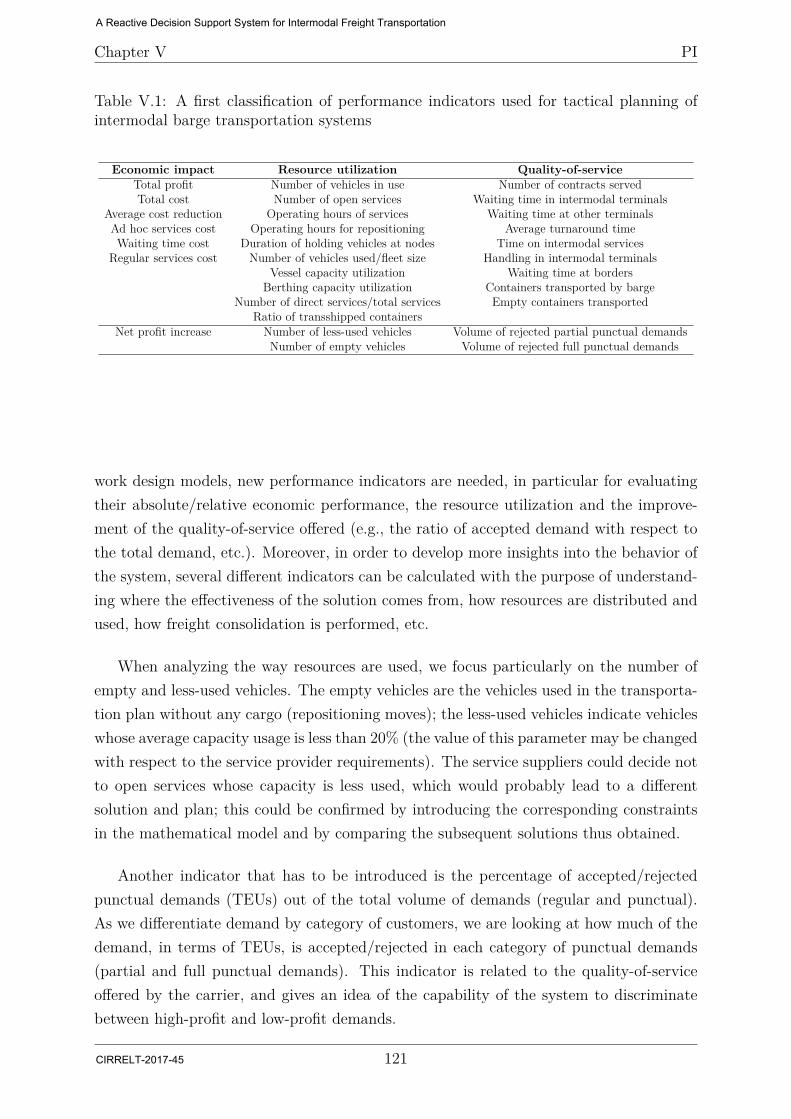
Chapter V PI
Table V.1: A first classification of performance indicators used for tactical planning ofintermodal barge transportation systems
Economic impact Resource utilization Quality-of-serviceTotal profit Number of vehicles in use Number of contracts servedTotal cost Number of open services Waiting time in intermodal terminals
Average cost reduction Operating hours of services Waiting time at other terminalsAd hoc services cost Operating hours for repositioning Average turnaround timeWaiting time cost Duration of holding vehicles at nodes Time on intermodal services
Regular services cost Number of vehicles used/fleet size Handling in intermodal terminalsVessel capacity utilization Waiting time at borders
Berthing capacity utilization Containers transported by bargeNumber of direct services/total services Empty containers transported
Ratio of transshipped containersNet profit increase Number of less-used vehicles Volume of rejected partial punctual demands
Number of empty vehicles Volume of rejected full punctual demands
work design models, new performance indicators are needed, in particular for evaluatingtheir absolute/relative economic performance, the resource utilization and the improve-ment of the quality-of-service offered (e.g., the ratio of accepted demand with respect tothe total demand, etc.). Moreover, in order to develop more insights into the behavior ofthe system, several different indicators can be calculated with the purpose of understand-ing where the effectiveness of the solution comes from, how resources are distributed andused, how freight consolidation is performed, etc.
When analyzing the way resources are used, we focus particularly on the number ofempty and less-used vehicles. The empty vehicles are the vehicles used in the transporta-tion plan without any cargo (repositioning moves); the less-used vehicles indicate vehicleswhose average capacity usage is less than 20% (the value of this parameter may be changedwith respect to the service provider requirements). The service suppliers could decide notto open services whose capacity is less used, which would probably lead to a differentsolution and plan; this could be confirmed by introducing the corresponding constraintsin the mathematical model and by comparing the subsequent solutions thus obtained.
Another indicator that has to be introduced is the percentage of accepted/rejectedpunctual demands (TEUs) out of the total volume of demands (regular and punctual).As we differentiate demand by category of customers, we are looking at how much of thedemand, in terms of TEUs, is accepted/rejected in each category of punctual demands(partial and full punctual demands). This indicator is related to the quality-of-serviceoffered by the carrier, and gives an idea of the capability of the system to discriminatebetween high-profit and low-profit demands.
121
A Reactive Decision Support System for Intermodal Freight Transportation
CIRRELT-2017-45
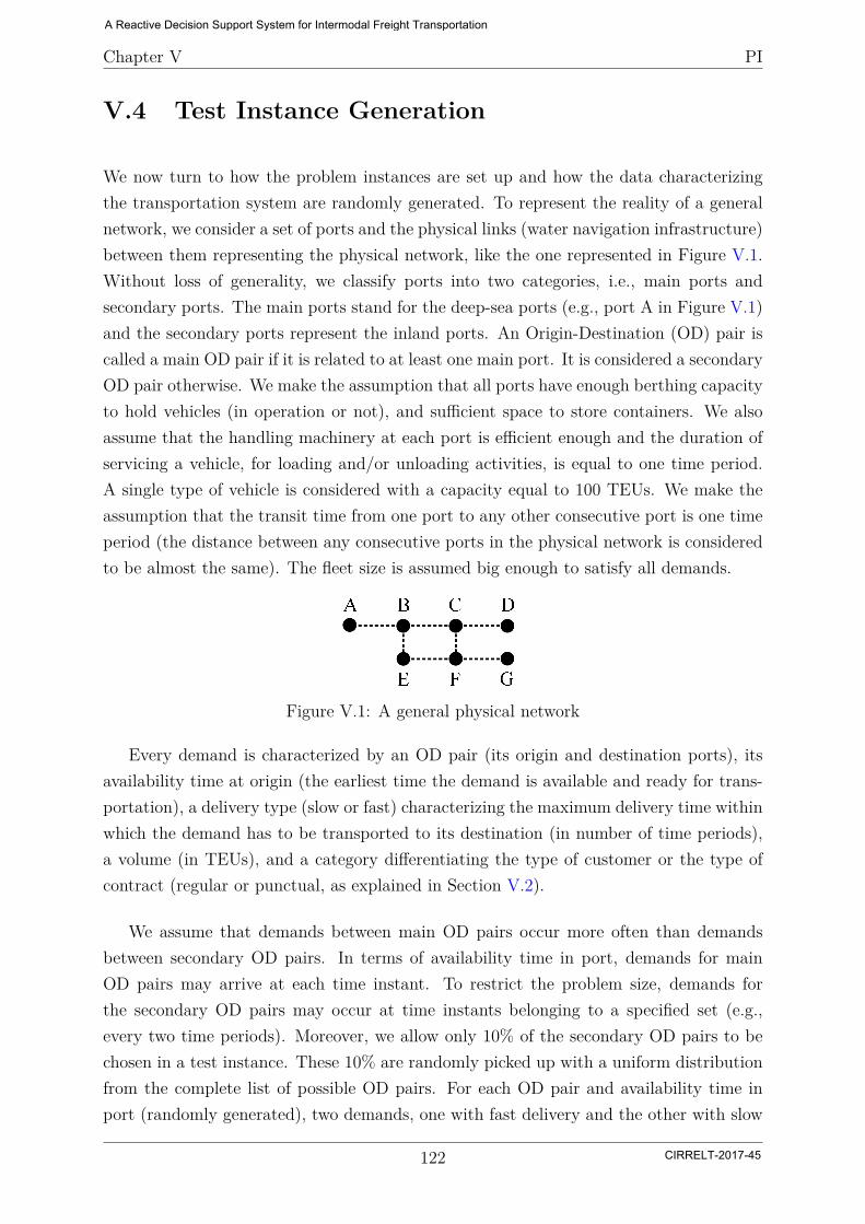
Chapter V PI
V.4 Test Instance Generation
We now turn to how the problem instances are set up and how the data characterizingthe transportation system are randomly generated. To represent the reality of a generalnetwork, we consider a set of ports and the physical links (water navigation infrastructure)between them representing the physical network, like the one represented in Figure V.1.Without loss of generality, we classify ports into two categories, i.e., main ports andsecondary ports. The main ports stand for the deep-sea ports (e.g., port A in Figure V.1)and the secondary ports represent the inland ports. An Origin-Destination (OD) pair iscalled a main OD pair if it is related to at least one main port. It is considered a secondaryOD pair otherwise. We make the assumption that all ports have enough berthing capacityto hold vehicles (in operation or not), and sufficient space to store containers. We alsoassume that the handling machinery at each port is efficient enough and the duration ofservicing a vehicle, for loading and/or unloading activities, is equal to one time period.A single type of vehicle is considered with a capacity equal to 100 TEUs. We make theassumption that the transit time from one port to any other consecutive port is one timeperiod (the distance between any consecutive ports in the physical network is consideredto be almost the same). The fleet size is assumed big enough to satisfy all demands.
Figure V.1: A general physical network
Every demand is characterized by an OD pair (its origin and destination ports), itsavailability time at origin (the earliest time the demand is available and ready for trans-portation), a delivery type (slow or fast) characterizing the maximum delivery time withinwhich the demand has to be transported to its destination (in number of time periods),a volume (in TEUs), and a category differentiating the type of customer or the type ofcontract (regular or punctual, as explained in Section V.2).
We assume that demands between main OD pairs occur more often than demandsbetween secondary OD pairs. In terms of availability time in port, demands for mainOD pairs may arrive at each time instant. To restrict the problem size, demands forthe secondary OD pairs may occur at time instants belonging to a specified set (e.g.,every two time periods). Moreover, we allow only 10% of the secondary OD pairs to bechosen in a test instance. These 10% are randomly picked up with a uniform distributionfrom the complete list of possible OD pairs. For each OD pair and availability time inport (randomly generated), two demands, one with fast delivery and the other with slow
122
A Reactive Decision Support System for Intermodal Freight Transportation
CIRRELT-2017-45

Chapter V PI
delivery type, are set. This results in a balanced number of demands requiring fast andslow deliveries within the same test instance.
The volume of each demand is randomly generated between 0 and a maximum value(usually less than the capacity of a vehicle) according to the uniform distribution. Inorder to generate a well-balanced combination of regular and punctual demands withina test instance, we generate first the set of demands to be used, without specifying theircategory. Thus, we fix the total volume of demand in the instance. Then, the volume ofpunctual demands is specified by a proportion (p) over the total volume of demand, theremaining proportion (1− p) corresponding to the total volume of regular demands. Wemay thus generate instances with a fixed total demand but with varying proportions ofmain to secondary and regular to punctual ratios.
The maximum delivery time for each demand is computed (in terms of time periods)according to the distance between the origin and destination of the demand and thecorresponding delivery type (fast or slow). As a general rule, we assume that a demandassociated to a slow delivery would accept to be delivered within a time twice longer thanthe delivery time required by a fast demand between the same origin and destination. Weset the fast delivery time by ensuring feasibility with respect to some of the less time-consuming potential services that could serve that demand. The different delivery typesand thus the different types of demands are associated to different fares classes. A lowfare corresponds to a slow delivery demand type, and a high fare is associated with a fastdelivery demand.
In the following section we give some numerical results obtained when solving theSSND problem for random test instances with data sets generated by this type of proce-dure.
V.5 Numerical Results and Analysis
We now illustrate how, using a set of problem instances generated as described above,the performance indicators may help analyze the output of an SSND model with assetand revenue management considerations. We compare two mathematical models, a tradi-tional one in which demands are not differentiated, called SSND in the following, and theproposed SSND-RRM in Chapter III, integrating revenue management concerns, namelydifferent categories of customers and different fare classes. The main difference betweenthe two models is that the first one deals with regular demands only (all the demand hasto be satisfied), while the second takes into account both regular and punctual demands,
123
A Reactive Decision Support System for Intermodal Freight Transportation
CIRRELT-2017-45

Chapter V PI
which allows potential performance increase by refusing partially or totally some of theless profitable demands. We follow the procedure described in Section V.1. The demandsare generated randomly for each test instance, and we run the program and solve theservice network design problem for 20 different instances.
The performance indicators used here are a selection of indicators from Table V.1,for each of the three main categories identified: economic impact, resource utilizationand quality of service. The main indicators used are the net profit and total cost. Forthe latter, we also identify and calculate some of its components. In terms of fixedservice operating costs, we use the cost of opening a service, called service-start cost. Interms of unit costs we use container-transportation, container-handling, container-holding(holding in the storage yard of a terminal), and in-port vehicle-holding costs. In termsof resource utilization, we compute the number of empty and less-used vehicles, as wellas classical indicators such as the number of open services, the number of vehicles usedby these services, and the average used capacity of those vehicles. Finally, we add twoparticular indicators required to study the incorporation of revenue management into theSSND related to the different categories of demands, which can be either partially or fullyaccepted or denied. The percentage of rejected volume of partial punctual demands andof full punctual demands out of the total volume of demands is denoted p/all and f/allrespectively.
The average values (over the 20 instances) are displayed in Table V.2. These relativevalues of the performance indicators denote an increase or a decrease of the correspondingabsolute value of an indicator when the solution of the SSND-RM problem is comparedwith that of the classical SSND.
The proportion of regular and punctual demands out of the total volume was variedin this set of instances. The five columns of the table correspond to five different ratiosfor the regular versus punctual demand categories. For example, “R=4P” indicates thatthe corresponding column displays the values of the performance indicators when in theSSND-RM setting the total volume of regular demands is 4 times as large as punctualdemands. In the same way, “R=P” means that the volume of regular demands is almostequal to the volume of punctual demands and, for the last column, “4R=P” means that wehave 4 times as large volume for the punctual demands as for the regular ones. Recall thatthe total volume of demands (regular plus punctual) is maintained equal, and that onlythe ratio between the two general categories is varied. As shown in the table, the SSND-RRM model always provides a better solution with respect to the performance indicatorscalculated here. This trend is even more accentuated when we increase the proportion ofpunctual demands. Figure V.2 shows that the same hierarchy in the value level of thedifferent measures is observed for the five different ratios of regular to punctual demands,
124
A Reactive Decision Support System for Intermodal Freight Transportation
CIRRELT-2017-45
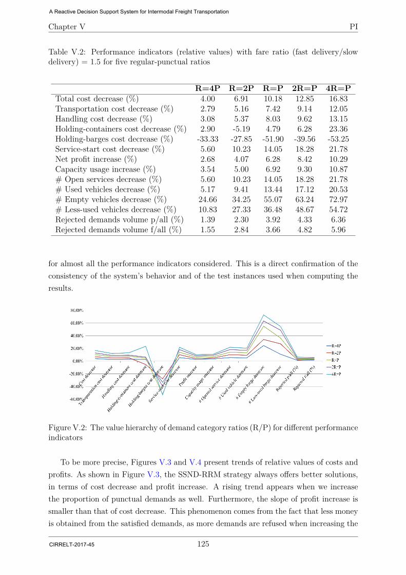
Chapter V PI
Table V.2: Performance indicators (relative values) with fare ratio (fast delivery/slowdelivery) = 1.5 for five regular-punctual ratios
R=4P R=2P R=P 2R=P 4R=PTotal cost decrease (%) 4.00 6.91 10.18 12.85 16.83Transportation cost decrease (%) 2.79 5.16 7.42 9.14 12.05Handling cost decrease (%) 3.08 5.37 8.03 9.62 13.15Holding-containers cost decrease (%) 2.90 -5.19 4.79 6.28 23.36Holding-barges cost decrease (%) -33.33 -27.85 -51.90 -39.56 -53.25Service-start cost decrease (%) 5.60 10.23 14.05 18.28 21.78Net profit increase (%) 2.68 4.07 6.28 8.42 10.29Capacity usage increase (%) 3.54 5.00 6.92 9.30 10.87# Open services decrease (%) 5.60 10.23 14.05 18.28 21.78# Used vehicles decrease (%) 5.17 9.41 13.44 17.12 20.53# Empty vehicles decrease (%) 24.66 34.25 55.07 63.24 72.97# Less-used vehicles decrease (%) 10.83 27.33 36.48 48.67 54.72Rejected demands volume p/all (%) 1.39 2.30 3.92 4.33 6.36Rejected demands volume f/all (%) 1.55 2.84 3.66 4.82 5.96
for almost all the performance indicators considered. This is a direct confirmation of theconsistency of the system’s behavior and of the test instances used when computing theresults.
Figure V.2: The value hierarchy of demand category ratios (R/P) for different performanceindicators
To be more precise, Figures V.3 and V.4 present trends of relative values of costs andprofits. As shown in Figure V.3, the SSND-RRM strategy always offers better solutions,in terms of cost decrease and profit increase. A rising trend appears when we increasethe proportion of punctual demands as well. Furthermore, the slope of profit increase issmaller than that of cost decrease. This phenomenon comes from the fact that less moneyis obtained from the satisfied demands, as more demands are refused when increasing the
125
A Reactive Decision Support System for Intermodal Freight Transportation
CIRRELT-2017-45
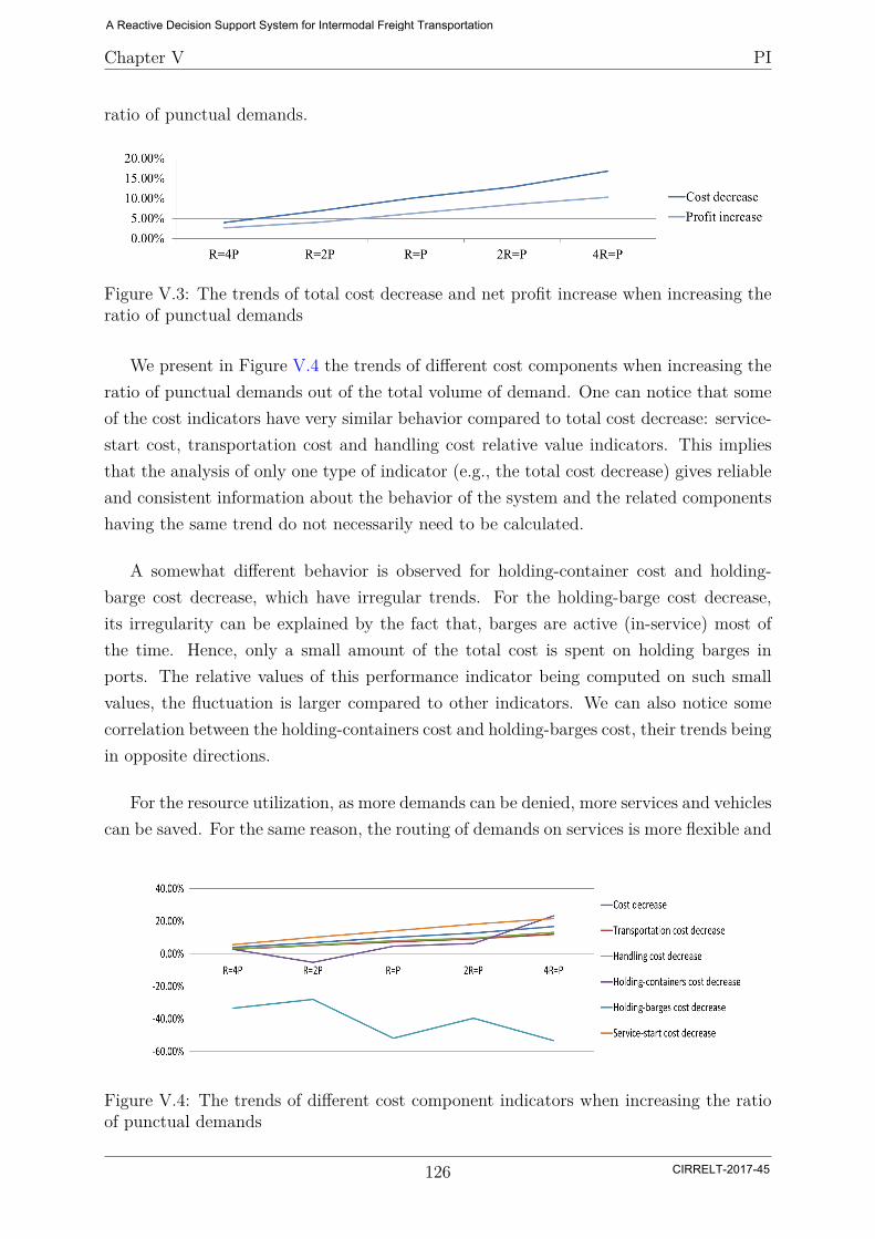
Chapter V PI
ratio of punctual demands.
Figure V.3: The trends of total cost decrease and net profit increase when increasing theratio of punctual demands
We present in Figure V.4 the trends of different cost components when increasing theratio of punctual demands out of the total volume of demand. One can notice that someof the cost indicators have very similar behavior compared to total cost decrease: service-start cost, transportation cost and handling cost relative value indicators. This impliesthat the analysis of only one type of indicator (e.g., the total cost decrease) gives reliableand consistent information about the behavior of the system and the related componentshaving the same trend do not necessarily need to be calculated.
A somewhat different behavior is observed for holding-container cost and holding-barge cost decrease, which have irregular trends. For the holding-barge cost decrease,its irregularity can be explained by the fact that, barges are active (in-service) most ofthe time. Hence, only a small amount of the total cost is spent on holding barges inports. The relative values of this performance indicator being computed on such smallvalues, the fluctuation is larger compared to other indicators. We can also notice somecorrelation between the holding-containers cost and holding-barges cost, their trends beingin opposite directions.
For the resource utilization, as more demands can be denied, more services and vehiclescan be saved. For the same reason, the routing of demands on services is more flexible and
Figure V.4: The trends of different cost component indicators when increasing the ratioof punctual demands
126
A Reactive Decision Support System for Intermodal Freight Transportation
CIRRELT-2017-45
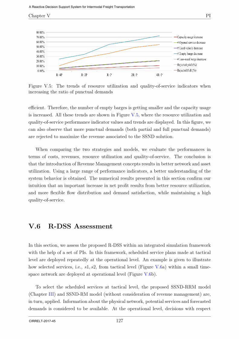
Chapter V PI
Figure V.5: The trends of resource utilization and quality-of-service indicators whenincreasing the ratio of punctual demands
efficient. Therefore, the number of empty barges is getting smaller and the capacity usageis increased. All these trends are shown in Figure V.5, where the resource utilization andquality-of-service performance indicator values and trends are displayed. In this figure, wecan also observe that more punctual demands (both partial and full punctual demands)are rejected to maximize the revenue associated to the SSND solution.
When comparing the two strategies and models, we evaluate the performances interms of costs, revenues, resource utilization and quality-of-service. The conclusion isthat the introduction of Revenue Management concepts results in better network and assetutilization. Using a large range of performance indicators, a better understanding of thesystem behavior is obtained. The numerical results presented in this section confirm ourintuition that an important increase in net profit results from better resource utilization,and more flexible flow distribution and demand satisfaction, while maintaining a highquality-of-service.
V.6 R-DSS Assessment
In this section, we assess the proposed R-DSS within an integrated simulation frameworkwith the help of a set of PIs. In this framework, scheduled service plans made at tacticallevel are deployed repeatedly at the operational level. An example is given to illustratehow selected services, i.e., s1, s2, from tactical level (Figure V.6a) within a small time-space network are deployed at operational level (Figure V.6b).
To select the scheduled services at tactical level, the proposed SSND-RRM model(Chapter III) and SSND-RM model (without consideration of revenue management) are,in turn, applied. Information about the physical network, potential services and forecasteddemands is considered to be available. At the operational level, decisions with respect
127
A Reactive Decision Support System for Intermodal Freight Transportation
CIRRELT-2017-45

Chapter V PI
Figure V.6: An example of service deployment from tactical to operational level
to the acceptance/denial of transport requests and the corresponding routing for thoseaccepted are made according to the proposed DCA-RM model (Chapter II). Sequentialarrivals of transport requests are simulated at the operational level as an iterative process.
In the rest of this section, we first introduce the procedures to generate test instancesfor the proposed simulation framework in Subsection V.6.1. Numerical results are thendisplayed and analyzed in Subsection V.6.2.
V.6.1 Simulation Framework
We now describe the simulation framework and introduce the procedure to generate testinstances used for the simulation.
In terms of physical network, four consecutive terminals located along the inlandwaterway are considered. As a similar topology is also studied in the previous chapters,the same assumptions related to the physical network and terminals as in Chapter II andChapter III are adopted here.
In terms of services, all possible itineraries with respect to the physical network areconsidered with two types of vehicles (large and small). The same assumptions related to
128
A Reactive Decision Support System for Intermodal Freight Transportation
CIRRELT-2017-45
Chapter V PI
services and vehicles as in Chapter II and Chapter III are also adopted here.
At tactical level, the schedule length is considered to be 14 time units long (e.g., oneweek). A test instance (a set of forecasted demands) is supposed to be composed of anequal number of transport requests from each of all the three customer categories (i.e.,R, P and F). In addition, each possible Origin-Destination (OD) pair is requested 4 timesby each category of customers. With respect to the other characteristics of demand, e.g.,volume, delivery type and available time at origin, the values are generated randomly(uniform distribution within predefined limits).
Time is discretized at the operational level into a number of time instants, so thatat each time instant there is no more than one transport request. At operational level,when we simulate the sequential arrivals of transport requests, at each time instant, onetransport request is generated randomly following the same procedure as that introducedin Chapter II. As analyzed in both Chapter II and Chapter III, the values of price ratiobetween fare classes have an important impact on the performance of RM models. Thehigher the price ratio is, the better the RM model performs. Therefore, in this exper-imentation, we set the values of the price ratios for both delivery type (fast/slow) andbooking anticipation (late/early reservation) to 1.5. In practice, better performance of theproposed R-DSS, in terms of the robustness of plans, is expected, when applying highervalues of price ratios than 1.5.
V.6.2 Preliminary Assessment
Two groups of experiments are conducted to assess the proposed R-DSS. The first groupof experiments is designed to study how the proposed R-DSS reacts, in terms of profit,resource utilization, etc., when facing inconsistent demand forecasts between tactical andoperational levels. A second group of experiments are then settled with the assumptionthat demand forecasts between tactical and operational levels are consistent, to evaluatethe performance of the proposed R-DSS with respect to different tactical strategies andaccuracy degree of demand forecasts at operational level.
As described previously, at tactical level, both SSND-RRM (with RM consideration)and SSND-RM (without RM consideration) are applied, in turn, to design the service net-work. When we make decisions to select open services, forecasted demands are required.Obviously, the accuracy of demand forecasts is important. However, it is a hard taskto obtain precise demand forecasts. Moreover, according to the business relationshipsbetween the carriers and customers (shippers), the behaviors of customers are different.
129
A Reactive Decision Support System for Intermodal Freight Transportation
CIRRELT-2017-45
Chapter V PI
Accuracies of demand forecasts, with respect to different categories of customers, arethus different. For example, as long-term contracts are signed with the regular customers(R), demands from R are predictable (or the demand forecasts could be considered asaccurate). On the contrary, demand forecasts, with respect to the spot customers, couldbe considered as less accurate. Freight carriers, normally, could make a choice betweenbeing greedy (to trust demand forecasts with respect to all customers and take the corre-sponding risks) and being protective (to trust only the demand forecasts with respect toregular customers and lose potential market), when making tactical plans. However, bytaking into account RM polices, carriers are offered with a different viewpoint, in whichcustomers are classified into different categories (in the decision making process) withdifferent treatments. Carriers, thus, are able to make decisions between being greedy andprotective, and consequently take less risks and win more potential market shares.
Therefore, when the SSND-RM model is applied, two different situations are consid-ered. Given a test instance defined for the SSND-RRM (i.e., considering three differentcustomer categories: R, P and F), either all demands are labeled as “R” (SSND-RM(AllR), being greedy), or only R demands are kept, the others (P and F) being discarded(SSND-RM(Only R), being protective). As stated before, at operational level, only DCA-RM is applied and solved. Selected Performance Indicators (PIs) used to analyze theperformance of the R-DSS are described as follows:
• # of TEUs: is the total number of containers requested to be transported;
• # of accepted TEUs: is the total number of accepted containers;
• # of open services: is the number of services selected at tactical level using smallor large vehicles;
• Capacity usage: is calculated as the ratio of used Distance*Capacity over themaximum possible Distance*Capacity according to the flow distribution plan; itindicates the resource utilization;
• Revenue: is the total revenue obtained;
• Estimated net profit: is calculated as Revenue subtracted by the fixed costs andvariable costs.
In Table V.3, we first briefly illustrate the output of the tactical planning in thesimulated framework. As shown in the table, SSND-RM(All R) generates a plan with thelargest number of open services (26) as all demands have to be satisfied. On the contrary,SSND-RM(Only R) generates the smallest service network (with 8 open services) as only R
130
A Reactive Decision Support System for Intermodal Freight Transportation
CIRRELT-2017-45

Chapter V PI
Table V.3: Output of the tactical planning with different strategies
SSND-RRM SSND-RMAll R Only R
# of TEUs 1847 1847 563# of accepted TEUs 1447 1847 563# of open services 16 (all large) 26 (2 small, 24 large) 8 (all large)Capacity usage (%) 91.75 82.38 78.17
demands are considered. Benefiting from the customer classification, SSND-RRM deniessome of the demands and consequently obtains a moderate service network with thehighest capacity usage. Services selected by those three strategies are applied in turn atthe operational level to evaluate the corresponding impact of each of them, when testedin similar operational conditions.
At operational level, in order to better understand the behavior of the proposed R-DSS, simulation was carried out 20 times for each tested demand accuracy and for eachtactical planning strategy. The procedure used to generate the sequential arrival of thecurrent transport requests here is the same as we introduced in Chapter II. Average valuesof the numerical results obtained from the simulation of the first group of experimentsare illustrated in Table V.4. Scale in the first column of the table indicates the numberof potential transport requests received at operational level during one time period of theschedule length (of the tactical level). As shown in Table V.4, when scale = 80 and 90,the total volume requested by the customers at operational level is 1655.45 and 1891.05,respectively. These values are within a close range of the total volume estimated at tacticallevel (1847). Therefore, when the value of scale is 80 or 90, we consider that the demandforecast at tactical level is accurate (or the demand forecasts between the two planninglevels are consistent). When the value of scale is less than 80, the demand forecast attactical level is considered to be overestimated, and on the contrary, the demand forecastat tactical level is considered to be underestimated (scale > 90). Both over- and under-estimation of demands at tactical level implies the inconsistency of demand forecastsbetween tactical and operational levels. Corresponding values for each PI obtained byapplying the three different tactical strategies are displayed in the last three columns.
As opening the largest number of services, SSND-RM(All R) always accepts the highestnumber of TEUs and consequently generates the highest revenue in all the test instances,compared to the other two planning strategies. However, as the open capacity is toolarge, even SSND-RM(All R) always accepts the most volume of demands, it still has thelowest capacity usage. In terms of estimated net profit, SSND-RM(All R) even earns theleast money, when the number of transport requests at operational level is low (scale =50 and 60), because of its high fixed cost. Compared to SSND-RM(All R), the SSND-
131
A Reactive Decision Support System for Intermodal Freight Transportation
CIRRELT-2017-45
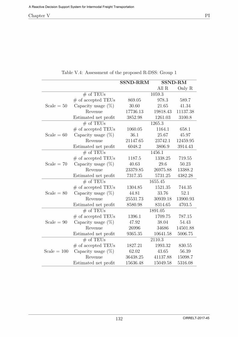
Chapter V PI
Table V.4: Assessment of the proposed R-DSS: Group 1
SSND-RRM SSND-RMAll R Only R
Scale = 50
# of TEUs 1059.3# of accepted TEUs 869.05 978.3 589.7Capacity usage (%) 30.60 21.65 41.34
Revenue 17736.13 19818.43 11137.38Estimated net profit 3852.98 1261.03 3100.8
Scale = 60
# of TEUs 1265.3# of accepted TEUs 1060.05 1164.1 658.1Capacity usage (%) 36.1 25.67 45.97
Revenue 21147.65 23742.1 12459.95Estimated net profit 6048.2 3806.9 3914.43
Scale = 70
# of TEUs 1456.1# of accepted TEUs 1187.5 1338.25 719.55Capacity usage (%) 40.63 29.6 50.23
Revenue 23379.85 26975.88 13388.2Estimated net profit 7317.35 5731.25 4382.28
Scale = 80
# of TEUs 1655.45# of accepted TEUs 1304.85 1521.35 744.35Capacity usage (%) 44.81 33.76 52.1
Revenue 25531.73 30939.18 13900.93Estimated net profit 8580.98 8314.65 4703.5
Scale = 90
# of TEUs 1891.05# of accepted TEUs 1396.1 1709.75 787.15Capacity usage (%) 47.92 38.04 54.43
Revenue 26996 34686 14501.88Estimated net profit 9365.35 10641.58 5006.75
Scale = 100
# of TEUs 2110.3# of accepted TEUs 1827.21 1993.32 830.55Capacity usage (%) 62.02 43.65 56.39
Revenue 36438.25 41137.88 15098.7Estimated net profit 15636.48 15049.58 5316.08
132
A Reactive Decision Support System for Intermodal Freight Transportation
CIRRELT-2017-45
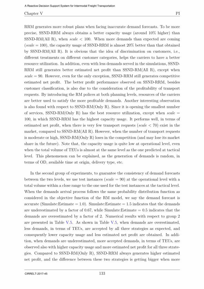
Chapter V PI
RRM generates more robust plans when facing inaccurate demand forecasts. To be moreprecise, SSND-RRM always obtains a better capacity usage (around 10% higher) thanSSND-RM(All R), when scale < 100. When more demands than expected are coming(scale = 100), the capacity usage of SSND-RRM is almost 20% better than that obtainedby SSND-RM(All R). It is obvious that the idea of discrimination on customers, i.e.,different treatments on different customer categories, helps the carriers to have a betterresource utilization. In addition, even with less demands served in the simulations, SSND-RRM still generates better estimated net profit than SSND-RM(All R), except whenscale = 90. However, even for the only exception, SSND-RRM still generates competitiveestimated net profit. The better profit performance observed on SSND-RRM, besidescustomer classification, is also due to the consideration of the profitability of transportrequests. By introducing the RM polices at both planning levels, resources of the carriersare better used to satisfy the more profitable demands. Another interesting observationis also found with respect to SSND-RM(Only R). Since it is opening the smallest numberof services, SSND-RM(Only R) has the best resource utilization, except when scale =100, in which SSND-RRM has the highest capacity usage. It performs well, in terms ofestimated net profit, when there is very few transport requests (scale < 70) exist in themarket, compared to SSND-RM(All R). However, when the number of transport requestsis moderate or high, SSND-RM(Only R) loses in the competition (and may lose its marketshare in the future). Note that, the capacity usage is quite low at operational level, evenwhen the total volume of TEUs is almost at the same level as the one predicted at tacticallevel. This phenomenon can be explained, as the generation of demands is random, interms of OD, available time at origin, delivery type, etc.
In the second group of experiments, to guarantee the consistency of demand forecastsbetween the two levels, we use test instances (scale = 90) at the operational level with atotal volume within a close range to the one used for the test instances at the tactical level.When the demands arrival process follows the same probability distribution function asconsidered in the objective function of the RM model, we say the demand forecast isaccurate (Simulate:Estimate = 1.0). Simulate:Estimate = 1.5 indicates that the demandsare underestimated by a factor of 0.67, while Simulate:Estimate = 0.5 indicates that thedemands are overestimated by a factor of 2. Numerical results with respect to group 2are presented in Table V.5. As shown in Table V.5, when demands are overestimated,less demands, in terms of TEUs, are accepted by all three strategies as expected, andconsequently lower capacity usage and less estimated net profit are obtained. In addi-tion, when demands are underestimated, more accepted demands, in terms of TEUs, areobserved also with higher capacity usage and more estimated net profit for all three strate-gies. Compared to SSND-RM(Only R), SSND-RRM always generates higher estimatednet profit, and the difference between these two strategies is getting bigger when more
133
A Reactive Decision Support System for Intermodal Freight Transportation
CIRRELT-2017-45
Chapter V PI
Table V.5: Assessment of the proposed R-DSS: Group 2
SSND-RRM SSND-RMAll R Only R
Simulate:Estimate=0.5
# of TEUs 900.5# of accepted TEUs 822.89 867.21 487.73Capacity usage (%) 28.25 19.3 33.72Estimated net profit 2563.98 -146.28 1732.87
Simulate:Estimate=1.0
# of TEUs 1891.05# of accepted TEUs 1396.1 1709.75 787.15Capacity usage (%) 47.92 38.04 54.43Estimated net profit 9365.35 10641.58 5006.75
Simulate:Estimate=1.5
# of TEUs 2760.93# of accepted TEUs 2158.7 2521.45 1145.28Capacity usage (%) 74.09 56.1 78.19Estimated net profit 18413.94 21034.55 8922.57
demands have to be satisfied. Compared to SSND-RM(All R), better resource utilizationis always observed by SSND-RRM. In terms of estimated net profit, SSND-RRM earnsmore than SSND-RM(All R) when demand forecast is overestimated. When demandforecast is considered to accurate or underestimated, SSND-RRM still generates compet-itive profit, compared to SSND-RM(All R), with almost 400 TEUs less accepted. Notethat, even SSND-RM(All R) has the best performance, in terms of net profit, when Sim-ulate:Estimate = 1 and Simulate:Estimate = 1.5, it actually loses money when transportrequests are overestimated. Therefore, we conclude that, in the simulated framework,compared to the other two planning strategies, SSND-RRM generates the most robustplans when facing different accuracies of demand forecasts.
V.7 Conclusions
Performance indicators are broadly used to characterize the performance of transportationsystems, and to validate and evaluate models and solution methods, corresponding resultsand strategies. It is also known that some indicators give more insight than others andone would like to single out the critical ones for particular problem settings. This isparticularly meaningful when new problem settings are analyzed, as are the emergingneeds for tactical planning for container barge transportation with revenue managementstrategies. Yet, there is no general framework for analyzing the interest of particularperformance indicators in the context of specific problem settings, generating appropriateproblem instances, and choosing the most representative indicators.
We proposed a first classification and analysis of performance indicators generally
134
A Reactive Decision Support System for Intermodal Freight Transportation
CIRRELT-2017-45
Chapter V PI
used to evaluate tactical planning solutions in freight transportation, and we identifieda number of adequate ones for scheduled service network design models with resourceand revenue management considerations. We also provided insights into the generation ofadequate test instances to study these planning issues in the general context of containerbarge transportation systems.
The numerical analysis of the results of comparing a classical SSND formulation and amodel integrating revenue management strategies has shown the interest of the instance-generation procedure and performance-indicator study in the context of SSND-RM forcontainer barge transportation. The initial insights provided by the study into the behav-ior of such systems under varying conditions of demand stratification and customer-servicestrategies (in terms of load acceptance) are a clear indication of this interest. They are alsoa first step towards more comprehensive studies of such intermodal systems and modelingapproaches, studies that we plan to undertake in the near future.
An integrated framework considering both the tactical and operational models is im-plemented to assess the R-DSS. In this framework, selected services at tactical level areapplied at the operational level and no extra-vehicles or rescheduling of services is consid-ered. Simulations at operational level are then conducted to evaluate the decisions madeat tactical level, and consequently validate the proposed Reactive Decision Support Sys-tem (R-DSS). Compared to the decision support systems with no revenue managementconsideration at tactical level, the proposed R-DSS generates more robust decisions, interms of net profit and resource utilization. The introduction of Revenue Managementstrategies at tactical level improves the interaction and information/knowledge exchangebetween tactical and operational levels of decision making for the intermodal barge trans-portation system studied.
135
A Reactive Decision Support System for Intermodal Freight Transportation
CIRRELT-2017-45

A Reactive Decision Support System for Intermodal Freight Transportation
CIRRELT-2017-45

General Conclusions
Barge transportation, in the recent years, has increasingly received global attention withthe intensified emphasis on the relationship between transportation and environmentalimpact. Compared to the other transport modes, e.g. road and rail, barge transportationis more environment-friendly, in terms of both energy consumption and noise emissions.In addition, it also contributes to relieving the traffic congestion and reducing the numberof accidents of the road and rail transport networks. Therefore, in Europe, the adoptionof barge transportation (or more generally, river and canal freight navigation) has beenencouraged by the [European Commission, 2011] in the context of intermodal freighttransportation. However, compared to other transport modes, contributions related tobarge, especially in the context of intermodal transportation, are still scarce.
This thesis, therefore, studies the freight intermodal barge transportation from a car-rier perspective. A reactive decision support system (R-DSS) covering both middle-termand short-term planning of operations is then proposed to make more robust decisions,in terms of scheduled services plan, resource management, flow distribution, etc. Fourrelated research problems are addressed to achieve the R-DSS: modeling the optimiza-tion problems for intermodal barge transportation activities at tactical planning level,at operational planning level, proposing a new solution approach to solve the large scaleMILP problems defined at tactical level, and classifying and introducing new performanceindicators, together with a methodology to generate test instances for the validation ofthe proposed R-DSS.
In addition, the fundamental contribution of this thesis is the introduction of RevenueManagement (RM) concept and polices into the freight intermodal barge transportationsystem. To be more precise, for both planning levels (tactical and operational), the bestdecisions (scheduled services and capacity allocation) are made with respect to the givenforecasted demands. However, in a deregulated market, customers have different be-haviors, different requires and different willingness to pay. These perspectives of demanduncertainty then challenge those best decisions in practice, and may endanger the benefitsof the carriers. Therefore, it is critical and stands for a great challenge to understand the
137
A Reactive Decision Support System for Intermodal Freight Transportation
CIRRELT-2017-45
General Conclusions
behaviors of customers and take this information into account when making decisions toalleviate the influence of demand uncertainty. RM, which is naturally used in marketingcompetition, offers us the techniques to tackle this challenge. By integrating the RM po-lices, e.g., customer classification and fare differentiation, carriers plan and offer differentservices, and charge different fares according to the behaviors, requires and willingness ofcustomers. As naturally used in practice at operational level for passenger transportation,RM is rather new to the freight transportation and very few contributions exist in theliterature. However, according to the numerical results, it is promising to consider RMpolices when making decision at each planning level for freight intermodal barge trans-portation system. Higher revenue and better resource utilization are obtained at eachplanning level when tested separately. Furthermore, by considering RM polices at bothlevels, more robust scheduled service plans are made, compared to those made withoutconsideration of RM at tactical level. To be more precise, when demand forecasts areaccurate, higher revenue and better resource utilization are observed. In addition, whendemand forecasts are inaccurate, the quality of solutions, in terms of income and resourceutilization, remains at a high level by considering RM polices, compared to those obtainedby the other tested planning strategies.
In the rest of this chapter, we first summarize the results of the thesis for each researchproblem, and then present future research perspectives.
Summary of the Results
In this subsection, we review the four research problems proposed in Chapter I. Theresults of each study is summarized accordingly, and an overall summary is also made.
Research topic 1: How to integrate RM policies (which policies) with barge transporta-tion at operational level and dynamically allocate the capacity of transport network facingtransport requests sequentially arriving in the system, in the context of intermodal freighttransportation.
In Chapter II, we first propose a Revenue Management model (DCA-RM) for dy-namically allocating the capacity of the intermodal barge transportation network. To bemore precise, according to the business relationship, customers are classified into threecategories, whose transport requests are accordingly treated differently. Different fareclasses are proposed to customers, in relation with their booking anticipation and re-quested delivery type (fast or slow), to differentiate the transportation solutions offeredby the carrier. In order to validate the DCA-RM model proposed, a set of experimentsare conducted. The obtained results show that the DCA-RM model always generates bet-
138
A Reactive Decision Support System for Intermodal Freight Transportation
CIRRELT-2017-45
General Conclusions
ter total revenue, when compared with the first-come first-serve (FCFS) based bookingstrategy, which has no consideration of profitability. This tendency of the results holdseven if demand forecasts are inaccurate (i.e., in case of under- or over-estimation of futuredemands).
A set of possible negotiation strategies for denied demands coming from regular cus-tomers are also studied within the proposed DCA-RM model. By considering the nego-tiation strategies, better satisfaction from the regular customers is achieved with slightlylower total revenue, which, however, is still higher than the revenue obtained when ap-plying the FCFS strategy.
The proposed DCA-RM model is then extended by integrating the re-routing of someof the accepted demands. Preliminary experiments are conducted to examine the ex-tended DCA-RM model. The obtained results indicate that it is interesting to take intoaccount re-routing of already accepted demands when making the operational plans, asthe extended DCA-RM model generates better total revenue, when compared with thebasic version.
Research topic 2: How to integrate RM and resource management concepts with bargetransportation for service network design problems and how to ensure synchronization withother transport modes, in the context of intermodal freight transportation.
In Chapter III, we propose a scheduled service network design model with consid-eration of both resource and revenue management (SSND-RRM) for intermodal bargetransportation. The same type of RM policies as those applied at the operational RMmodel (i.e., customer classification and price differentiation) are considered in this model.Note that, at tactical level, as no booking anticipation is considered, the price policy isonly related to the required delivery type, e.g., slow or fast delivery. In terms of resourcemanagement, design-balance constraints and upper bounds on the quantity of resource areformulated. To synchronize with other transport modes, scheduled services are proposedand time-related characteristics are explicitly associated with demands. Various problemsettings, in terms of demand distribution, network topology, fare classes and quality-of-service (e.g., delivery time), are designed and tested to evaluate the proposed SSND-RRMmodel. According to the results, we conclude that it is promising to consider RM poli-cies at tactical level. By classifying customers and differentiating product-fares, highernet profits and better resource utilization are observed, compared with the conventionalSSND-RM model without consideration of revenue management.
Research topic 3: How to efficiently solve the scheduled service network design problemswhile simultaneously considering resource and revenue management.
139
A Reactive Decision Support System for Intermodal Freight Transportation
CIRRELT-2017-45
General Conclusions
In Chapter IV, we propose a metaheuristic (MH) to efficiently solve large scale SSND-RRM problems (introduced in Chapter III). The new solution approach includes fourphases. In the first phase, a constructive heuristic is proposed to obtain initial solutions forthe SSND-RRM optimisation problem. In the second phase, starting from such an initialsolution, the algorithm tries to improve the solutions by iteratively exploring the searchspace of service selection, F-demand selection or the combination of both. The selectionof the search space is based on a modified adaptive large neighborhood search (ALNS). Toexplore the search space of service selection and F-demand selection, a set of Y-selectionheuristics and F-selection heuristics are designed, respectively. Historical performanceof these proposed heuristics is recorded to guide the search. Phases of intensificationand diversification are also included. Moreover, the proposed Y-selection heuristics arebased on service cycle related neighborhood structures, in which a service cycle is a set ofconsecutive services using the same type of vehicle back to the terminal where the sequenceof services starts. Moves based on the new neighborhood structures guarantee the design-balance constraints and diversify the search simultaneously. Long-term memory is usedto record the influence of each service and F demand on the solutions, and to identifypromising services and F demands. To avoid exploring repeatedly the same region ofsearch space, short-term memory tabu lists of service cycles are maintained. Compared toa commercial solver (CPLEX), the performance of the proposed MH is superior, in termsof both solution quality and time consumption, when dealing with large scale problems.
Research topic 4: How to validate and evaluate the decision support system of bargetransportation, in terms of models, solution methods, corresponding results and strategies;Are there some indicators that give more insights than others.
In Chapter V, we first review the Performance Indicators (PIs) found in public sourcesand scientific literature, and qualify them with respect to the intermodal barge transporta-tion. The analysis is then extended with RM considerations. Based on their relevanceand meaning, these PIs are classified into three categories, i.e., economic impact, resourceutilization and quality of service. All these PIs are applied and tested with respect tothe tactical planning of intermodal barge transportation system. New PIs consideringboth resource and revenue management, in the context of freight transportation, are alsoproposed for the three categories and tested. According to the results, for each category,some PIs do offer more insights than others. These PIs are thus identified to evaluatethe proposed R-DSS, and could be used for a more general evaluation of any intermodalfreight transportation system.
In addition, we also provide insights into the generation of adequate test instancesto study the planning issues in the general context of intermodal barge transportationsystems. The proposed R-DSS is then assessed within an integrated simulation framework
140
A Reactive Decision Support System for Intermodal Freight Transportation
CIRRELT-2017-45
General Conclusions
(both tactical and operational levels are considered) with specified PIs.
Overall, the consideration of RM policies for both middle-term and short-term plan-ning of intermodal barge transportation enhances the interaction and information / knowl-edge exchange between the two decision levels and consequently generates more consistentand robust decisions. More revenue (net profit) and better resource utilization are ob-served by applying the proposed R-DSS, compared with its competitors, which have noconsideration of RM at tactical level. Carriers, therefore, could benefit from the pro-posed R-DSS, in terms of net profit, resource utilization, customer satisfaction, etc., andconsequently obtain a better market share.
Perspectives
Given the limited time and the scope of the research carried out for this thesis, ex-tensive experiments have not been conducted for all the studies. For some of them, onlypreliminary results are presented. To thoroughly validate the proposed R-DSS, therefore,more work should and could be done. In this subsection, we discuss future research withrespect to each research study conducted in this thesis.
Operational Planning of Intermodal Barge Transportation System (DCA-RM): As dis-cussed in Chapter II, by introducing RM policies into operational planning for freighttransportation, carriers are able to obtain better total revenue. Considering both prof-itability of demands and feasibility with respect to the transportation network, decisionsmade for the capacity allocation are more robust. In addition, applying different treat-ments to different categories of customers also contributes to generating robust decisions.However, as the situation faced by carriers in practice is highly dynamic, it is possible (asillustrated in Chapter II) for some of the demands requested by regular customers to berejected. The rejection of regular (or even spot) customers may result in the decrease ofcustomer satisfaction and consequently loss of market share. Therefore, it is interesting,and also stands for a great challenge, to consider the uncertainty of demands. In theresearch study in Chapter II, we have already shown that it is possible and promising tohave a negotiation phase combined with the proposed DCA-RM model. A future researchpath could be the integration of different negotiation strategies into the proposed DCA-RM model to better satisfy the regular (or even the spot) customers. Moreover, proposingmore comprehensive models to implicitly reduce the degree of uncertainty of demands isalso a promising research topic. Two perspectives are then possible to achieve that: ro-bustness and flexibility. In terms of robustness, no further resource is available. Betterplans need to be made within the given transport capacity. As shown in the preliminaryexperiments on the extended DCA-RM model, re-routing some of the accepted demands
141
A Reactive Decision Support System for Intermodal Freight Transportation
CIRRELT-2017-45

General Conclusions
does result in better solutions, in terms of total revenue. Flow distribution is continuouslyimproved by making decisions based on regularly updated forecasts. In terms of flexibil-ity, outsourcing, paying penalty (could also be interpreted as outsourcing) or re-routingof services should be considered for these denied transport requests of all categories ofcustomers. It would also be interesting to consider the uncertainty of demands directlyinto the DCA-RM model, for example, flexible available time at origin or due time atdestination, or even a stochastic model to formulate all the situations mentioned above.As this thesis attempts to make contributions to the freight transportation on the North-ern France inland waterway, a real case study should be more convincible to validate theproposed new DCA-RM model with real carriers in practice. With real data, in terms ofunit costs, price, handling time, berthing capacity, etc., we could also better analyze theperformance of the proposed DCA-RM model and help carriers to win a better marketshare.
Tactical Planning of Intermodal Barge Transportation System (SSND-RRM): Exten-sive experiments have already been conducted in Chapter III. With respect to the numer-ical results, better solutions, in terms of net profit, resource utilization, etc., are obtainedby applying the SSND-RRM model at tactical level. Further studies are also carried out inChapter V to validate the service plan (made at tactical level) within an integrated frame-work for the proposed R-DSS. According to the results of simulations at operational level,more robust decisions are observed when applying SSND-RRM model at tactical level. Itis promising that without the explicit consideration of uncertainty of demands (demandsat tactical level are considered to be known), robust decisions are made by introducingRM policies. The aggregation of customer behavior (customer classification) does improvethe information/knowledge flow from operational level to tactical level. Meanwhile, it alsoreveals another set of research questions: what if we consider the RM policies for demandforecasting at tactical levels, what are the characteristics of demands to be consideredwith respect to the RM policies applied, etc. It would be also interesting to formulate thestopping time of each service at each terminal as decision variables in the SSND-RRMmodel. Better service plans are expected, in terms of flexibility and robustness, if thestopping time of a service at each terminal is decided by the model, instead of fixed asa predefined value. Those better plans are also expected to result in higher net profit,when facing the uncertain demands, in terms of available time. By making decisions onthe stopping time of each service at each terminal, the delay of services could also be for-mulated in the SSND-RRM model, which is another practice and interesting perspective.In addition, the research questions we had at operational level could also apply at tacticallevel.
Metaheuristics for the SSND-RRM Problems: As the research studies related to this
142
A Reactive Decision Support System for Intermodal Freight Transportation
CIRRELT-2017-45

General Conclusions
chapter are still in progress, several tasks should be conducted as follows:
• A complete calibration on all the parameters applied in the MH should be done,and an analysis of the impacts of each parameter on performance of the MH shouldbe made;
• Further experiments should be designed and tested to identify the influences of eachalgorithmic component;
• Extensive experiments should be conducted to study the performance of the MH.Test instances, with respect to different physical networks, number of potentialservices, number of demands, etc., are going to be examined;
• Further experiments can be designed to analyze the performance of the proposedMH, especially when solving problems of small scale. Improvement should be madeon the MH, so that the proposed solution approach could achieve the optimalityfaster. By now, one of our guesses for not obtaining the optimal solutions is theexistence of the symmetric structures in the solution. For example, different openservices or accepted demands which result in the same objective values. To addressthis challenge, the concept of column generation could be introduced;
• A more sophisticated algorithm should be designed to tune the values of all theparameters applied for the modified adaptive large neighborhood search (ALNS). Avery first attempt could be simulated annealing;
In addition, how the proposed MH could be modified and applied as a general algorithmsolving other related SSND problems also arises as a great challenge. As a set of servicesare changed in each iteration, the balance between continuously searching in differentneighborhoods (not “close” to each other) and exploring for optimal solutions within agiven neighborhood is hard to be measured. A more intelligent algorithm should make thechoices by considering the interesting characteristics of solution components and historicalperformance of all algorithmic components.
Performance Indicators (PIs): With respect to this research study, more comprehen-sive studies of PIs for general intermodal freight transportation systems are going to beundertaken. Another important and interesting category of PIs, i.e., Environment im-pact, should also be considered. CO2 emission, energy consumption and other indicatorsshould be classified into this category. Inspired by Environment impact, PIs belonging tothis category, e.g., CO2 emission, could be considered and formulated as one type of costswhen we are making decisions for the scheduled service network and capacity allocation.
143
A Reactive Decision Support System for Intermodal Freight Transportation
CIRRELT-2017-45

General Conclusions
According to the numerical results, the consideration of RM policies in the intermodalfreight transportation systems is able to make robust plans for the carriers, in terms ofscheduled service plan, resource utilization, flow distribution, etc., even when encounteringinaccurate demand forecasts. So far, the reactive decision support system is composed oftwo optimization models for tactical and operational level, respectively. It is an interestingtopic to propose a stochastic model at tactical level facing uncertain demands with thehelp of RM policy considerations, and the concept of outsourcing. More flexible androbust decisions, in terms of total revenue, resource utilization, etc. are expected. Wecould then study the importance of flexibility and robustness for barge transportationin different cases, in terms of physical network topologies, accuracy of demand forecasts,competitions from other carriers, and different pricing policies.
144
A Reactive Decision Support System for Intermodal Freight Transportation
CIRRELT-2017-45
Bibliography
[Agarwal and Ergun, 2008] Agarwal, R. and Ergun, O. (2008). Ship scheduling and net-work design for cargo routing in linear shipping. Transportation Science, 42(2):175–196.
[Andersen and Christiansen, 2009] Andersen, J. and Christiansen, M. (2009). Design-ing new European rail freight services. Journal of the Operational Research Society,60(March):348–360.
[Andersen et al., 2011] Andersen, J., Christiansen, M., Crainic, T., and Grønhaug, R.(2011). Branch-and-price for service network design with asset management constraints.Transportation Science, 46(1):33–49.
[Andersen et al., 2009a] Andersen, J., Crainic, T.G., and Christiansen, M. (2009a). Ser-vice network design with asset management: Formulations and comparative analyzes.Transportation Research Part C: New Technologies, 17(2):397–207.
[Andersen et al., 2009b] Andersen, J., Crainic, T.G., and Christiansen, M. (2009b). Ser-vice network design with management and coordination of multiple fleets. EuropeanJournal of Operational Research, 193(2):377–389.
[Armacost et al., 2002] Armacost, A.P., Barnhart, C., and Ware, K.A. (2002). Compos-ite variable formulations for express shipment service network design. TransportationScience, 36(1):1–20.
[Armstrong and Meissner, 2010] Armstrong, A. and Meissner, J. (2010). Railway revenuemanagement: Overview and models. Technical report, The Department of ManagementScience, Lancaster University.
[Bai et al., 2012] Bai, R., Kendall, G., Qu, R., and Atkin, J. (2012). Tabu assistedguided local search approaches for freight service network design. Information Sci-ences, 189:266–281.
[Bektaş and Crainic, 2008] Bektaş, T. and Crainic, T.G. (2008). A brief overview ofintermodal transportation. In Taylor, G.D., editor, Logistics Engineering Handbook,chapter 28, pages 1–16. Taylor and Francis Group, Boca Raton, FL, USA.
145
A Reactive Decision Support System for Intermodal Freight Transportation
CIRRELT-2017-45
Bibliography
[Bektaş et al., 2010] Bektaş, T., Chouman, M., and Crainic, T.G. (2010). Lagrangean-based decomposition algorithms for multicommodity network design problems withpenalized constraints. Networks, 55(3):171–180.
[Bilegan et al., 2015] Bilegan, I.C., Brotcorne, L., Feillet, D., and Hayel, Y. (2015). Rev-enue management for rail container transportation. EURO Journal on Transportationand Logistics, 4(2):261–283.
[Bilegan and Crainic, 2012] Bilegan, I.C. and Crainic, T.G. (2012). A decision supportsystem for intermodal barge transportation operations. VeRoLog 2012, First meetingof the EURO working group on Vehicle Routing and Logistics Optimization, bologna,Italy.
[Bontekoning et al., 2004] Bontekoning, Y., Macharis, C., and Trip, J. (2004). Is a newapplied transportation research field emerging? - A review of intermodal rail-truckfreight transport literature. Transportation Research Part A: Policy and Practice,38(1):1–34.
[Braekers et al., 2013] Braekers, K., Caris, A., and Janssens, G.K. (2013). Optimal ship-ping routes and vessel size for intermodal barge transport with empty container repo-sitioning. Computers in Industry, 64(2):155–164.
[Caris et al., 2011] Caris, A., Macharis, C., and Janssens, G.K. (2011). Network analysisof container barge transport in the port of Antwerp by means of simulation. Journalof Transport Geography, 19(1):125–133.
[Caris et al., 2012] Caris, A., Macharis, C., and Janssens, G.K. (2012). Corridor net-work design in hinterland transportation systems. Flexible Services and ManufacturingJournal, 24(3):294–391.
[Chouman and Crainic, 2014] Chouman, M. and Crainic, T.G. (2014). Cutting-planematheuristic for service network design with design-balanced requirements. Trans-portation Science, 49(1):99–113.
[Christiansen et al., 2007] Christiansen, M., Fagerholt, K., Nygreen, B., and Ronen, D.(2007). Maritime transportation. In Barnhart, C. and Laporte, G., editors, Transporta-tion, volume 14 of Handbooks in Operations Research and Management Science, pages189–284. North-Holland, Amsterdam.
[Christiansen et al., 2004] Christiansen, M., Fagerholt, K., and Ronen, D. (2004). Shiprouting and scheduling: Status and perspectives. Transportation Science, 38(1):1–18.
146
A Reactive Decision Support System for Intermodal Freight Transportation
CIRRELT-2017-45

Bibliography
[Cordeau et al., 1998] Cordeau, J.-F., Toth, P., and Vigo, D. (1998). A survey of opti-mization models for train routing and scheduling. Transportation Science, 32(4):380–404.
[Crainic, 2000] Crainic, T.G. (2000). Service network design in freight transportation.European Journal of Operational Research, 122(2):272–288.
[Crainic, 2003] Crainic, T.G. (2003). Long-haul freight transportation. In Hall, R.W., ed-itor, Handbook of Transportation Science, pages 451–516. Kluwer Academic Publishers,Norwell, MA, second edition.
[Crainic et al., 1984] Crainic, T.G., Ferland, J.-A., and Rousseau, J.-M. (1984). A tacticalplanning model for rail freight transportation. Transportation Science, 18(2):165–184.
[Crainic et al., 1993] Crainic, T.G., Gendreau, M., and Dejax, P.J. (1993). Dynamicstochastic models for the allocation of empty containers. Operations Research,41(1):102–126.
[Crainic et al., 2000] Crainic, T.G., Gendreau, M., and Farvolden, J. (2000). A simplex-based tabu search method for capacitated network design. INFORMS Journal onComputing, 12(3):223–236.
[Crainic et al., 2014] Crainic, T.G., Hewitt, M., Toulouse, M., and Vu, D.M. (2014). Ser-vice network design with resource constraints. Transportation Science, 50(4):1380–1393.
[Crainic and Kim, 2007] Crainic, T.G. and Kim, K.H. (2007). Intermodal transportation.In Barnhart, C. and Laporte, G., editors, Transportation, volume 14 of Handbooksin Operations Research and Management Science, chapter 8, pages 467–537. North-Holland, Amsterdam.
[Crainic and Rousseau, 1986] Crainic, T.G. and Rousseau, J.-M. (1986). Multicommod-ity, multimode freight transportation: A general modeling and algorithmic frameworkfor the service network design problem. Transportation Research Part B: Methodologi-cal, 20:225–242.
[Crainic and Roy, 1988] Crainic, T.G. and Roy, J. (1988). O.R. tools for tactical freighttransportation planning. European Journal of Operational Research, 33(3):290–297.
[Crevier et al., 2012] Crevier, B., Cordeau, J.-F., and Savard, G. (2012). Integrated oper-ations planning and revenue management for rail freight transportation. TransportationResearch Part B: Methodological, 46(1):100–119.
[Douma et al., 2011] Douma, A., Schuur, P., and Jage, R. (2011). Degrees of terminalcooperativeness and the efficiency of the barge handling process. Expert Systems withApplications, 38(4):3580–3589.
147
A Reactive Decision Support System for Intermodal Freight Transportation
CIRRELT-2017-45
Bibliography
[European Commission, 2011] European Commission (2011). White paper 2011:Roadmap to a single European transport area - Towards a competitive and resource-efficient transport system. Technical report, Directorate for Mobility and Transport,European Commission.
[Eurostat, 2015] Eurostat (2015). Energy, transport and environment indicators - 2015edition. Luxembourg: Publications Office of the European Union.
[Fazi et al., 2015] Fazi, S., Fransoo, J.C., and van Woensel, T. (2015). A decision supportsystem tool for the transportation by barge of import containers: A case study. DecisionSupport Systems, 79:33–45.
[Feng et al., 2015] Feng, B., Li, Y., and Shen, Z.-J. (2015). Air cargo operations: Litera-ture review and comparison with practices. Transportation Research Part C: EmergingTechnologies, 56:263–280.
[Frémont and Franc, 2010] Frémont, A. and Franc, P. (2010). Hinterland transportationin Europe: Combined transport versus road transport. Journal of Transport Geography,18(4):548–556.
[Gelareh and Pisinger, 2011] Gelareh, S. and Pisinger, D. (2011). Fleet deployment, net-work design and hub location of liner shipping companies. Transportation ResearchPart E: Logistics and Transportation Review, 47(6):947–964.
[Ghamlouche et al., 2003] Ghamlouche, I., Crainic, T.G., and Gendreau, M. (2003).Cycle-based neighbourhoods for fixed-charge capacitated multicommodity network de-sign. Operations research, 51(4):655–667.
[Ghamlouche et al., 2004] Ghamlouche, I., Crainic, T.G., and Gendreau, M. (2004). Pathrelinking, cycle-based neighbourhoods and capacitated multicommodity network de-sign. Annals of Operations research, 131(1-4):109–133.
[Glover, 1997] Glover, F. (1997). A template for scatter search and path relinking. InHao, J., Lutton, E., Ronald, E., Schoenauer, M., and Snyers, D., editors, ArtificialEvolution, volume 1363 of Lecture Notes in Computer Science, pages 13–54. Berlin:Springer.
[Kasilingam, 1997] Kasilingam, R. (1997). Air cargo revenue management: Characteris-tics and complexities. European Journal of Operational Research, 96(1):36–44.
[Konings, 2007] Konings, R. (2007). Opportunities to improve container barge handlingin the port of Rotterdam from a transport network perspective. Journal of TransportGeography, 15(6):443–454.
148
A Reactive Decision Support System for Intermodal Freight Transportation
CIRRELT-2017-45
Bibliography
[Konings et al., 2013] Konings, R., Kreutzberger, E., and Maraš, V. (2013). Major con-siderations in developing a hub-and-spoke network to improve the cost performance ofcontainer barge transport in the hinterland: The case of the port of Rotterdam. Journalof Transport Geography, 29:63–73.
[Lai, M.F. and Lo, H.K., 2004] Lai, M.F. and Lo, H.K. (2004). Ferry service networkdesign: Optimal fleet size, routing and scheduling. Transportation Research Part A:Policy and Practice, 38:305–328.
[Li et al., 2015] Li, L., Lin, X., Negenborn, R., and De Schutter, B. (2015). Pricingintermodal freight transport services: A cost-plus-pricing strategy. In F. Corman et al.,editor, Computational Logistics, volume 9355 of Lecture Notes in Computer Science,pages 541–556. Springer.
[Liu and Yang, 2015] Liu, D. and Yang, H. (2015). Joint slot allocation and dynamicpricing of container sea-rail multimodal transportation. Journal of Traffic and Trans-portation Engineering (English Edition), 2(3):198–208.
[Lium et al., 2009] Lium, A.-G., Crainic, T.G., and Wallace, S.W. (2009). A study ofdemand stochasticity in service network design. Transportation Science, 43(2):144–157.
[Macharis and Bontekoning, 2004] Macharis, C. and Bontekoning, Y.M. (2004). Oppor-tunities for OR in intermodal freight transport research: A review. European Journalof Operational Research, 153(2):400–416.
[Meng et al., 2012] Meng, Q., Wang, T., and Wang, S. (2012). Short-term liner shipfleet planning with container transshipment and uncertain container shipment demand.European Journal of Operational Research, 233(1):96–105.
[Moccia et al., 2011] Moccia, L., Cordeau, J.-F., Laporte, G., Ropke, S., and Valentini,M. (2011). Modeling and solving a multimodal transportation problem with flexible-time and scheduled services. Networks, 57(1):53–68.
[Notteboom, 2012] Notteboom, T. (2012). Challenges for container river services on theYangtze river: A case study for Chongqing. Research in Transportation Economics,35(1):41–49.
[Pedersen et al., 2009] Pedersen, M.B., Crainic, T.G., and Madsen, O.B.G. (2009). Mod-els and tabu search meta-heuristics for service network design with asset-balance re-quirements. Transportation Science, 43(2):158–177.
149
A Reactive Decision Support System for Intermodal Freight Transportation
CIRRELT-2017-45
Bibliography
[Powell, W.B. and Topaloglu, H., 2005] Powell, W.B. and Topaloglu, H. (2005). Fleetmanagement. In Wallace, S. and Ziemba, W., editors, Applications of Stochastic Pro-gramming, Math Programming Society - SIAM Series on Optimization, pages 185–216.SIAM, Philadelphia, PA.
[Ropke and Pisinger, 2006] Ropke, S. and Pisinger, D. (2006). An adaptive large neigh-borhood search heuristic for the pickup and delivery problem with time windows. Trans-portation science, 40(4):455–472.
[Sharypova, 2014] Sharypova, M.B. (2014). Optimization of hinterland intermodal con-tainer transportationl. PhD thesis, Technical University of Eindhoven, The Netherlands.
[Sharypova et al., 2012] Sharypova, M.B., Crainic, T.G., van Woensel, T., and J.C., F.(2012). Scheduled service network design with synchronization and transshipment con-straints for intermodal container transportation networks. Publication CIRRELT-2012-77, Centre interuniversitaire de recherche sur les réseaux d’entreprise, la logistique etle transport, Montréal, QC, Canada.
[Smilowitz et al., 2003] Smilowitz, K.R., Atamtürk, A., and Daganzo, C.F. (2003). De-ferred item and vehicle routing within integrated networks. Transportation ResearchPart E: Logistics and Transportation, 39:305–323.
[Stålhane et al., 2014] Stålhane, M., Andersson, H., Christiansen, M., and Fagerholt, K.(2014). Vendor managed inventory in tramp shipping. Omega, 47:60 –72.
[SteadieSeifi et al., 2014] SteadieSeifi, M., Dellaert, N., Nuijten, W., van Woensel, T.,and Raoufi, R. (2014). Multimodal freight transportation planning: A literature review.European Journal of Operational Research, 233(1):1–15.
[Talluri and van Ryzin, 2004] Talluri, K. T. and van Ryzin, G. J. (2004). The theory andpractice of revenue management.
[Tavasszy et al., 2015] Tavasszy, L., Behdani, B., and Konings, R. (2015). Intermodalityand synchromodality. Available at SSRN 2592888.
[Taylor et al., 2005] Taylor, G.D., Whyte, T.C., DePuy, G.W., and Drosos, D.J. (2005). Asimulation-based software system for barge dispatching and boat assignment in inlandwaterways. Simulation Modelling Practice and Theory, 13(7):550–565.
[Teypaz et al., 2010] Teypaz, N., Schrenk, S., and Cung, V.-D. (2010). A decompositionscheme for large-scale service network design with asset management. TransportationResearch Part E: Logistics and Transportation Review, 46(1):156–170.
150
A Reactive Decision Support System for Intermodal Freight Transportation
CIRRELT-2017-45
Bibliography
[Thapalia et al., 2012] Thapalia, B.K., Wallace, S.W., Kaut, M., and Crainic, T.G.(2012). Single source single-commodity stochastic network design. Computational Man-agement Science, 9(1):139–160.
[van Riessen et al., 2015a] van Riessen, B., Negenborn, R., and Dekker, R. (2015a). Syn-chromodal container transportation: An overview of current topics and research oppor-tunities. In Computational Logistics, pages 386–397. Springer.
[van Riessen et al., 2015b] van Riessen, B., Negenborn, R., and Dekker, R. (2015b). Thecargo fare class mix problem - Revenue management in synchromodal container trans-portation. Technical report.
[Vu et al., 2013] Vu, D.M., Crainic, T.G., and Toulouse, M. (2013). A three-phasematheuristic for the capacitated multi-commodity fixed-cost network design withdesign-balance constraints. Journal of Heuristics, 19(5):757–795.
[Wang et al., 2015] Wang, S., Wang, H., and Meng, Q. (2015). Itinerary provision andpricing in container liner shipping revenue management. Transportation Research PartE: Logistics and Transportation Review, 77:135–146.
[Wang et al., 2014] Wang, Y., Bilegan, I.C., Crainic, T.G., and Artiba, A. (2014). Perfor-mance indicators for planning intermodal barge transportation systems. TransportationResearch Procedia, 3(0):621–630.
[Ypsilantis and Zuidwijk, 2013] Ypsilantis, P. and Zuidwijk, R. (2013). Joint design andpricing of intermodal port-hinterland network services: Considering economies of scaleand service time constraints. ERIM Report Series Research in Management.
[Zuidwijk, 2015] Zuidwijk, R. (2015). Are we connected? ERIM Inaugural Address SeriesResearch in Management.
151
A Reactive Decision Support System for Intermodal Freight Transportation
CIRRELT-2017-45