Two-Scale Topology Optimization with Microstructures · topology optimization do not scale well and...
19
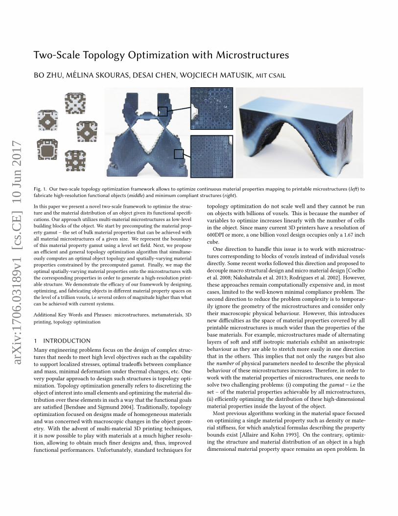
Two-Scale Topology Optimization with Microstructures BO ZHU, M ´ ELINA SKOURAS, DESAI CHEN, WOJCIECH MATUSIK, MIT CSAIL Fig. 1. Our two-scale topology optimization framework allows to optimize continuous material properties mapping to printable microstructures (le) to fabricate high-resolution functional objects (middle) and minimum compliant structures (right ). In this paper we present a novel two-scale framework to optimize the struc- ture and the material distribution of an object given its functional speci- cations. Our approach utilizes multi-material microstructures as low-level building blocks of the object. We start by precomputing the material prop- erty gamut – the set of bulk material properties that can be achieved with all material microstructures of a given size. We represent the boundary of this material property gamut using a level set eld. Next, we propose an ecient and general topology optimization algorithm that simultane- ously computes an optimal object topology and spatially-varying material properties constrained by the precomputed gamut. Finally, we map the optimal spatially-varying material properties onto the microstructures with the corresponding properties in order to generate a high-resolution print- able structure. We demonstrate the ecacy of our framework by designing, optimizing, and fabricating objects in dierent material property spaces on the level of a trillion voxels, i.e several orders of magnitude higher than what can be achieved with current systems. Additional Key Words and Phrases: microstructures, metamaterials, 3D printing, topology optimization 1 INTRODUCTION Many engineering problems focus on the design of complex struc- tures that needs to meet high level objectives such as the capability to support localized stresses, optimal tradeos between compliance and mass, minimal deformation under thermal changes, etc. One very popular approach to design such structures is topology opti- mization. Topology optimization generally refers to discretizing the object of interest into small elements and optimizing the material dis- tribution over these elements in such a way that the functional goals are satised [Bendsøe and Sigmund 2004]. Traditionally, topology optimization focused on designs made of homogeneous materials and was concerned with macroscopic changes in the object geom- etry. With the advent of multi-material 3D printing techniques, it is now possible to play with materials at a much higher resolu- tion, allowing to obtain much ner designs and, thus, improved functional performances. Unfortunately, standard techniques for topology optimization do not scale well and they cannot be run on objects with billions of voxels. is is because the number of variables to optimize increases linearly with the number of cells in the object. Since many current 3D printers have a resolution of 600DPI or more, a one billion voxel design occupies only a 1.67 inch cube. One direction to handle this issue is to work with microstruc- tures corresponding to blocks of voxels instead of individual voxels directly. Some recent works followed this direction and proposed to decouple macro structural design and micro material design [Coelho et al. 2008; Nakshatrala et al. 2013; Rodrigues et al. 2002]. However, these approaches remain computationally expensive and, in most cases, limited to the well-known minimal compliance problem. e second direction to reduce the problem complexity is to temporar- ily ignore the geometry of the microstructures and consider only their macroscopic physical behaviour. However, this introduces new diculties as the space of material properties covered by all printable microstructures is much wider than the properties of the base materials. For example, microstructures made of alternating layers of so and sti isotropic materials exhibit an anisotropic behaviour as they are able to stretch more easily in one direction that in the others. is implies that not only the ranges but also the number of physical parameters needed to describe the physical behaviour of these microstructures increases. erefore, in order to work with the material properties of microstructures, one needs to solve two challenging problems: (i) computing the gamut – i.e the set – of the material properties achievable by all microstructures, (ii) eciently optimizing the distribution of these high-dimensional material properties inside the layout of the object. Most previous algorithms working in the material space focused on optimizing a single material property such as density or mate- rial stiness, for which analytical formulas describing the property bounds exist [Allaire and Kohn 1993]. On the contrary, optimiz- ing the structure and material distribution of an object in a high dimensional material property space remains an open problem. In arXiv:1706.03189v1 [cs.CE] 10 Jun 2017
Transcript of Two-Scale Topology Optimization with Microstructures · topology optimization do not scale well and...
Two-Scale Topology Optimization with Microstructures
BO ZHU, MELINA SKOURAS, DESAI CHEN, WOJCIECH MATUSIK, MIT CSAIL
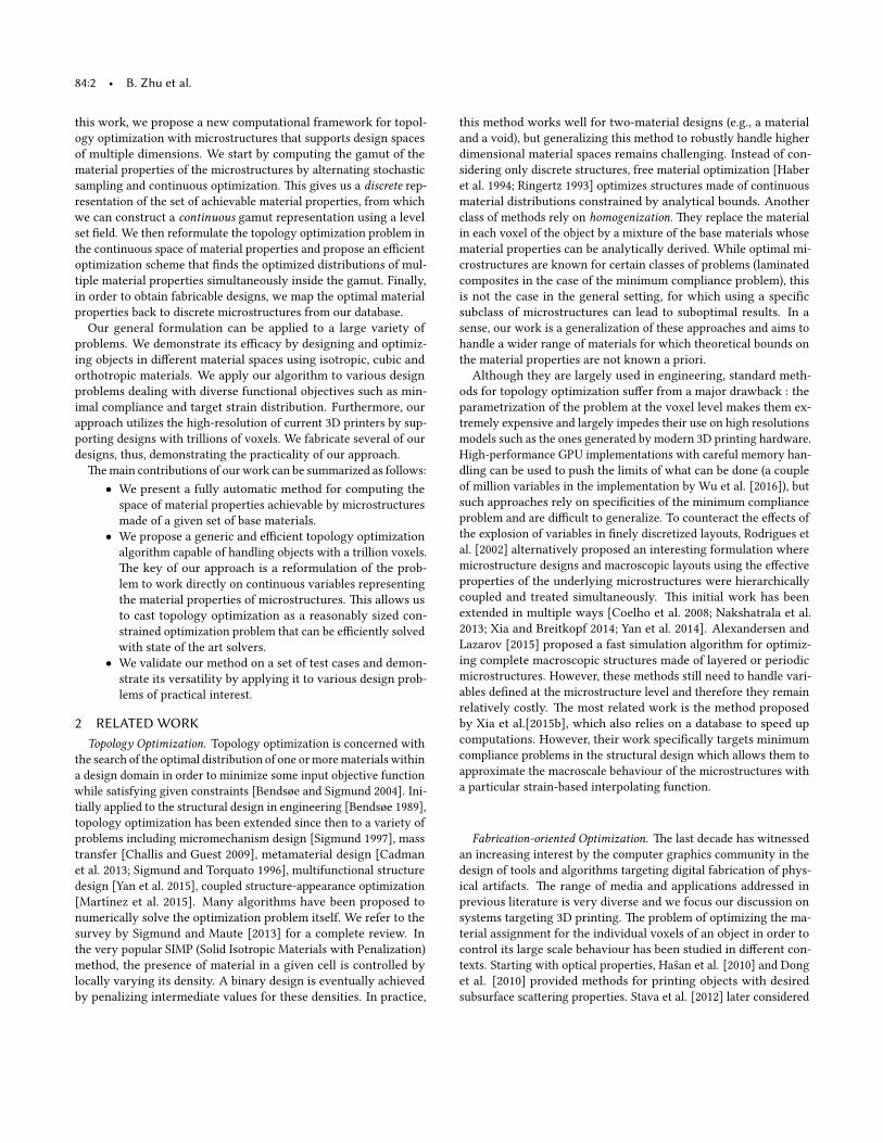
Fig. 1. Our two-scale topology optimization framework allows to optimize continuous material properties mapping to printable microstructures (le�) tofabricate high-resolution functional objects (middle) and minimum compliant structures (right).
In this paper we present a novel two-scale framework to optimize the struc-
ture and the material distribution of an object given its functional speci�-
cations. Our approach utilizes multi-material microstructures as low-level
building blocks of the object. We start by precomputing the material prop-
erty gamut – the set of bulk material properties that can be achieved with
all material microstructures of a given size. We represent the boundary
of this material property gamut using a level set �eld. Next, we propose
an e�cient and general topology optimization algorithm that simultane-
ously computes an optimal object topology and spatially-varying material
properties constrained by the precomputed gamut. Finally, we map the
optimal spatially-varying material properties onto the microstructures with
the corresponding properties in order to generate a high-resolution print-
able structure. We demonstrate the e�cacy of our framework by designing,
optimizing, and fabricating objects in di�erent material property spaces on
the level of a trillion voxels, i.e several orders of magnitude higher than what
can be achieved with current systems.
Additional Key Words and Phrases: microstructures, metamaterials, 3D
printing, topology optimization
1 INTRODUCTIONMany engineering problems focus on the design of complex struc-
tures that needs to meet high level objectives such as the capability
to support localized stresses, optimal tradeo�s between compliance
and mass, minimal deformation under thermal changes, etc. One
very popular approach to design such structures is topology opti-
mization. Topology optimization generally refers to discretizing the
object of interest into small elements and optimizing the material dis-
tribution over these elements in such a way that the functional goals
are satis�ed [Bendsøe and Sigmund 2004]. Traditionally, topology
optimization focused on designs made of homogeneous materials
and was concerned with macroscopic changes in the object geom-
etry. With the advent of multi-material 3D printing techniques,
it is now possible to play with materials at a much higher resolu-
tion, allowing to obtain much �ner designs and, thus, improved
functional performances. Unfortunately, standard techniques for
topology optimization do not scale well and they cannot be run
on objects with billions of voxels. �is is because the number of
variables to optimize increases linearly with the number of cells
in the object. Since many current 3D printers have a resolution of
600DPI or more, a one billion voxel design occupies only a 1.67 inch
cube.
One direction to handle this issue is to work with microstruc-
tures corresponding to blocks of voxels instead of individual voxels
directly. Some recent works followed this direction and proposed to
decouple macro structural design and micro material design [Coelho
et al. 2008; Nakshatrala et al. 2013; Rodrigues et al. 2002]. However,
these approaches remain computationally expensive and, in most
cases, limited to the well-known minimal compliance problem. �e
second direction to reduce the problem complexity is to temporar-
ily ignore the geometry of the microstructures and consider only
their macroscopic physical behaviour. However, this introduces
new di�culties as the space of material properties covered by all
printable microstructures is much wider than the properties of the
base materials. For example, microstructures made of alternating
layers of so� and sti� isotropic materials exhibit an anisotropic
behaviour as they are able to stretch more easily in one direction
that in the others. �is implies that not only the ranges but also
the number of physical parameters needed to describe the physical
behaviour of these microstructures increases. �erefore, in order to
work with the material properties of microstructures, one needs to
solve two challenging problems: (i) computing the gamut – i.e the
set – of the material properties achievable by all microstructures,
(ii) e�ciently optimizing the distribution of these high-dimensional
material properties inside the layout of the object.
Most previous algorithms working in the material space focused
on optimizing a single material property such as density or mate-
rial sti�ness, for which analytical formulas describing the property
bounds exist [Allaire and Kohn 1993]. On the contrary, optimiz-
ing the structure and material distribution of an object in a high
dimensional material property space remains an open problem. In
arX
iv:1
706.
0318
9v1
[cs
.CE
] 1
0 Ju
n 20
17
84:2 • B. Zhu et al.
this work, we propose a new computational framework for topol-
ogy optimization with microstructures that supports design spaces
of multiple dimensions. We start by computing the gamut of the
material properties of the microstructures by alternating stochastic
sampling and continuous optimization. �is gives us a discrete rep-
resentation of the set of achievable material properties, from which
we can construct a continuous gamut representation using a level
set �eld. We then reformulate the topology optimization problem in
the continuous space of material properties and propose an e�cient
optimization scheme that �nds the optimized distributions of mul-
tiple material properties simultaneously inside the gamut. Finally,
in order to obtain fabricable designs, we map the optimal material
properties back to discrete microstructures from our database.
Our general formulation can be applied to a large variety of
problems. We demonstrate its e�cacy by designing and optimiz-
ing objects in di�erent material spaces using isotropic, cubic and
orthotropic materials. We apply our algorithm to various design
problems dealing with diverse functional objectives such as min-
imal compliance and target strain distribution. Furthermore, our
approach utilizes the high-resolution of current 3D printers by sup-
porting designs with trillions of voxels. We fabricate several of our
designs, thus, demonstrating the practicality of our approach.
�e main contributions of our work can be summarized as follows:
• We present a fully automatic method for computing the
space of material properties achievable by microstructures
made of a given set of base materials.
• We propose a generic and e�cient topology optimization
algorithm capable of handling objects with a trillion voxels.
�e key of our approach is a reformulation of the prob-
lem to work directly on continuous variables representing
the material properties of microstructures. �is allows us
to cast topology optimization as a reasonably sized con-
strained optimization problem that can be e�ciently solved
with state of the art solvers.
• We validate our method on a set of test cases and demon-
strate its versatility by applying it to various design prob-
lems of practical interest.
2 RELATED WORKTopology Optimization. Topology optimization is concerned with
the search of the optimal distribution of one or more materials within
a design domain in order to minimize some input objective function
while satisfying given constraints [Bendsøe and Sigmund 2004]. Ini-
tially applied to the structural design in engineering [Bendsøe 1989],
topology optimization has been extended since then to a variety of
problems including micromechanism design [Sigmund 1997], mass
transfer [Challis and Guest 2009], metamaterial design [Cadman
et al. 2013; Sigmund and Torquato 1996], multifunctional structure
design [Yan et al. 2015], coupled structure-appearance optimization
[Martınez et al. 2015]. Many algorithms have been proposed to
numerically solve the optimization problem itself. We refer to the
survey by Sigmund and Maute [2013] for a complete review. In
the very popular SIMP (Solid Isotropic Materials with Penalization)
method, the presence of material in a given cell is controlled by
locally varying its density. A binary design is eventually achieved
by penalizing intermediate values for these densities. In practice,
this method works well for two-material designs (e.g., a material
and a void), but generalizing this method to robustly handle higher
dimensional material spaces remains challenging. Instead of con-
sidering only discrete structures, free material optimization [Haber
et al. 1994; Ringertz 1993] optimizes structures made of continuous
material distributions constrained by analytical bounds. Another
class of methods rely on homogenization. �ey replace the material
in each voxel of the object by a mixture of the base materials whose
material properties can be analytically derived. While optimal mi-
crostructures are known for certain classes of problems (laminated
composites in the case of the minimum compliance problem), this
is not the case in the general se�ing, for which using a speci�c
subclass of microstructures can lead to suboptimal results. In a
sense, our work is a generalization of these approaches and aims to
handle a wider range of materials for which theoretical bounds on
the material properties are not known a priori.
Although they are largely used in engineering, standard meth-
ods for topology optimization su�er from a major drawback : the
parametrization of the problem at the voxel level makes them ex-
tremely expensive and largely impedes their use on high resolutions
models such as the ones generated by modern 3D printing hardware.
High-performance GPU implementations with careful memory han-
dling can be used to push the limits of what can be done (a couple
of million variables in the implementation by Wu et al. [2016]), but
such approaches rely on speci�cities of the minimum compliance
problem and are di�cult to generalize. To counteract the e�ects of
the explosion of variables in �nely discretized layouts, Rodrigues et
al. [2002] alternatively proposed an interesting formulation where
microstructure designs and macroscopic layouts using the e�ective
properties of the underlying microstructures were hierarchically
coupled and treated simultaneously. �is initial work has been
extended in multiple ways [Coelho et al. 2008; Nakshatrala et al.
2013; Xia and Breitkopf 2014; Yan et al. 2014]. Alexandersen and
Lazarov [2015] proposed a fast simulation algorithm for optimiz-
ing complete macroscopic structures made of layered or periodic
microstructures. However, these methods still need to handle vari-
ables de�ned at the microstructure level and therefore they remain
relatively costly. �e most related work is the method proposed
by Xia et al.[2015b], which also relies on a database to speed up
computations. However, their work speci�cally targets minimum
compliance problems in the structural design which allows them to
approximate the macroscale behaviour of the microstructures with
a particular strain-based interpolating function.
Fabrication-oriented Optimization. �e last decade has witnessed
an increasing interest by the computer graphics community in the
design of tools and algorithms targeting digital fabrication of phys-
ical artifacts. �e range of media and applications addressed in
previous literature is very diverse and we focus our discussion on
systems targeting 3D printing. �e problem of optimizing the ma-
terial assignment for the individual voxels of an object in order to
control its large scale behaviour has been studied in di�erent con-
texts. Starting with optical properties, Hasan et al. [2010] and Dong
et al. [2010] provided methods for printing objects with desired
subsurface sca�ering properties. Stava et al. [2012] later considered
Two-Scale Topology Optimization with Microstructures • 84:3
Design goal
Target
deformation
Push
Topology optimization in
continuous material space
Rigid
Soft
Map to discrete microstructures
Base materials Microstructures
𝜈
Discrete point cloud Continuous level set
Fabrication
Material
Space
Sampling
Mapping Optimization
Microstructure
Database Generation
Multi-scale Topology
Optimization
𝜌
𝐸
𝜈
𝜌
𝐸
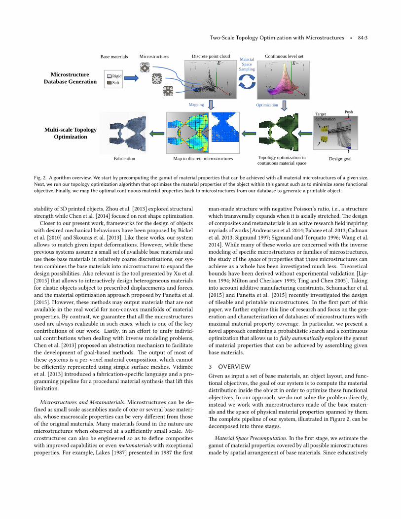
Fig. 2. Algorithm overview. We start by precomputing the gamut of material properties that can be achieved with all material microstructures of a given size.Next, we run our topology optimization algorithm that optimizes the material properties of the object within this gamut such as to minimize some functionalobjective. Finally, we map the optimal continuous material properties back to microstructures from our database to generate a printable object.
stability of 3D printed objects, Zhou et al. [2013] explored structural
strength while Chen et al. [2014] focused on rest shape optimization.
Closer to our present work, frameworks for the design of objects
with desired mechanical behaviours have been proposed by Bickel
et al. [2010] and Skouras et al. [2013]. Like these works, our system
allows to match given input deformations. However, while these
previous systems assume a small set of available base materials and
use these base materials in relatively coarse discretizations, our sys-
tem combines the base materials into microstructures to expand the
design possibilities. Also relevant is the tool presented by Xu et al.
[2015] that allows to interactively design heterogeneous materials
for elastic objects subject to prescribed displacements and forces,
and the material optimization approach proposed by Pane�a et al.
[2015]. However, these methods may output materials that are not
available in the real world for non-convex manifolds of material
properties. By contrast, we guarantee that all the microstructures
used are always realizable in such cases, which is one of the key
contributions of our work. Lastly, in an e�ort to unify individ-
ual contributions when dealing with inverse modeling problems,
Chen et al. [2013] proposed an abstraction mechanism to facilitate
the development of goal-based methods. �e output of most of
these systems is a per-voxel material composition, which cannot
be e�ciently represented using simple surface meshes. Vidimce
et al. [2013] introduced a fabrication-speci�c language and a pro-
gramming pipeline for a procedural material synthesis that li� this
limitation.
Microstructures and Metamaterials. Microstructures can be de-
�ned as small scale assemblies made of one or several base materi-
als, whose macroscale properties can be very di�erent from those
of the original materials. Many materials found in the nature are
microstructures when observed at a su�ciently small scale. Mi-
crostructures can also be engineered so as to de�ne composites
with improved capabilities or even metamaterials with exceptional
properties. For example, Lakes [1987] presented in 1987 the �rst
man-made structure with negative Poisson’s ratio, i.e., a structure
which transversally expands when it is axially stretched. �e design
of composites and metamaterials is an active research �eld inspiring
myriads of works [Andreassen et al. 2014; Babaee et al. 2013; Cadman
et al. 2013; Sigmund 1997; Sigmund and Torquato 1996; Wang et al.
2014]. While many of these works are concerned with the inverse
modeling of speci�c microstructures or families of microstructures,
the study of the space of properties that these microstructures can
achieve as a whole has been investigated much less. �eoretical
bounds have been derived without experimental validation [Lip-
ton 1994; Milton and Cherkaev 1995; Ting and Chen 2005]. Taking
into account additive manufacturing constraints, Schumacher et al.
[2015] and Pane�a et al. [2015] recently investigated the design
of tileable and printable microstructures. In the �rst part of this
paper, we further explore this line of research and focus on the gen-
eration and characterization of databases of microstructures with
maximal material property coverage. In particular, we present a
novel approach combining a probabilistic search and a continuous
optimization that allows us to fully automatically explore the gamut
of material properties that can be achieved by assembling given
base materials.
3 OVERVIEWGiven as input a set of base materials, an object layout, and func-
tional objectives, the goal of our system is to compute the material
distribution inside the object in order to optimize these functional
objectives. In our approach, we do not solve the problem directly,
instead we work with microstructures made of the base materi-
als and the space of physical material properties spanned by them.
�e complete pipeline of our system, illustrated in Figure 2, can be
decomposed into three stages.
Material Space Precomputation. In the �rst stage, we estimate the
gamut of material properties covered by all possible microstructures
made by spatial arrangement of base materials. Since exhaustively
84:4 • B. Zhu et al.
computing the properties of all these microstructures is, in practice,
intractable, we progressively increase the material space by alter-
nating a stochastic search and a continuous optimization. �e �rst
step introduces discrete changes in the materials of the microstruc-
tures and allows emergence of new types of microstructures. �e
second step allows to locally push the material space boundaries by
re�ning the microstructure shapes. A�er completing this stage, we
obtain a discrete representation of the space of material properties
and the mapping between these properties and the corresponding
microstructures.
Gamut-based Continuous Topology Optimization. In the second
stage, we construct a smooth continuous gamut representation of
the material property space by using a level set �eld. We de�ne our
topology optimization problem directly in this space. Our approach
minimizes the objective function over possible material parameters
while asking for strict satisfaction of the physics constraints – typ-
ically, the static equilibrium – as well as the strict satisfaction of
the physical parameter bounds. Taking advantage of our gamut
representation as a level set, we formulate this last constraint as
limiting the material properties to stay on the negative side of the
level set. �is guarantees that the material properties that we use
in the optimization are always physically realizable.
Fabrication-oriented Microstructure Mapping. In the last stage, we
generate a printable result by replacing each cell in the object layout
with a microstructure whose material properties are the closest to
the continuous material assignment resulting from the optimization.
We also take into account the boundary similarity across adjacent
cell interfaces to improve the connectivity between microstructures.
�is results in a complex, high-resolution, multi-material model
with optimized functional speci�cations.
4 MECHANICSIn this section, we brie�y introduce the background material for
simulating deformable objects. We will use these concepts when
computing the material properties of the microstructures (Section 5)
and in the topology optimization algorithm (Section 6). We refer to
the course by Sifakis and Barbic [2012] for a more comprehensive
exposition.
4.1 Material ModelMost available materials for 3D printers are elastic materials. As-
suming small deformations, we use linear elasticity to compute both
the mechanical behaviour of the entire object and the microstruc-
tures. In such a se�ing, the relation between the linear strain ϵ and
Cauchy stress σ at every material point is given by
σ = Cϵ , (1)
where C, the so-called elasticity tensor, can be described by 21
parameters [Bonet and Wood 1997].
Working in such a high dimensional space is prohibitive and
therefore we focus on materials having a certain numbers of sym-
metries, such as orthotropic materials for which the elasticity tensor
is de�ned by 12 parameters (4 parameters in 2D), cubic materials
de�ned by 3 parameters, and isotropic materials de�ned by 2 pa-
rameters. For example, the tensor for a 3D cubic structure can be
wri�en (using the Voigt notation) as
C =©«(1−ν )E ν E ν Eν E (1−ν )E ν Eν E ν E (1−ν )E
µµµ
ª®®®¬ (2)
with E = E/((1 − 2ν )(1 + ν )) and where E is the Young’s modulus of
the material, ν its Poisson’s ratio, and µ its shear modulus.
Alternatively, one can also use Lame’s parameters to de�ne the
tensor C, which simpli�es the derivation of the tensor with respect
to the elastic parameters. In this case, the tensor has the form
C =©«
2µ+λ λ λλ 2µ+λ λλ λ 2µ+λ
µµµ
ª®®®¬ . (3)
�e tensor for a 2D orthotropic structure can be wri�en as
C = c( Ex νyx ExνxyEy Ey
µ/c
)(4)
with c = 1/(1 − νxyνyx ), and where Ex and Ey are the Young’s
moduli along the two principal axes, µ is the shear modulus, νxy is
the Poisson’s ratio corresponding to a contraction in the direction
y when an extension is applied along the x axis, and νyx veri�es
νyxEx = νxyEy .
Le�ing Rn denote the space of n material properties, we then
write each point p ∈ Rn as p = [ρ, e], where ρ is the density of
the material and e are the other material parameters. Our gamut,
i.e. the setM ⊂ Rn of material properties corresponding to mi-
crostructures of a given resolution, is made of a �nite number of
points. However, by increasing the resolution of the microstructures
this gamut gets denser and denser so that we assume that it can be
approximated by the union of continuous n-dimensional manifolds
and can be represented using a distance �eld.
4.2 DiscretizationFollowing standard �nite element methodology, we discretize the
object in regular voxels and compute its deformed state when subject
to external forces fext using the well-known relation
Ku = fext, (5)
where K is the sti�ness matrix of the system, and u are the displace-
ments at the nodes of the voxels.
Note that we use the same approach to simulate both the mechan-
ical behaviour of the microstructures and the object macroscopic
behaviour. However, we work at two di�erent scales. To simulate
the microstructures, we assume that each of its voxels is made of an
homogeneous base material, whereas for determining the large scale
behaviour of the object, we assume that each of its cells corresponds
to a microstructure. �e properties of the individual microstructures
are determined from 6 harmonic displacements (or 2 displacements
in 2D) using numerical coarsening as described by Kharevych et al.
[2009].
We solve the static equilibrium Equation 5 using a fast multigrid
solver based on the implementation by Dick et al. [2011].
Two-Scale Topology Optimization with Microstructures • 84:5
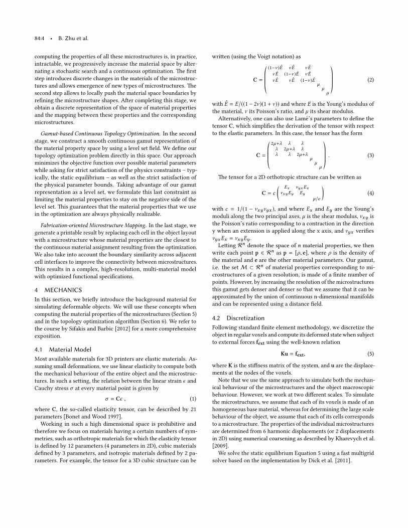
Fig. 3. Level set gamuts for two dimensional cubic microstructures (top row) and three dimensional cubic microstructures (bo�om row). The first columnshows the projection of the sample points in the space parametrized by the density ρ , the normalized Young’s modulus E and the Poisson’s ratio ν . Thesecond to the fourth columns show three slices of the four dimensional level sets corresponding to di�erent values for the shear modulus G .
Rigidmaterial
Softmaterial
Relative Young’s modulus
Po
isso
n’s
rat
io
Relative Young’s modulus
Pois
son
’s r
atio
Rigidmaterial
Softmaterial
Relative Young’s modulus
Po
isso
n’s
rat
io
Relative Young’s modulus
Pois
son
’s r
atio
Discrete Sampling Continuous Optimization
𝐩𝛻𝜑(𝐩)
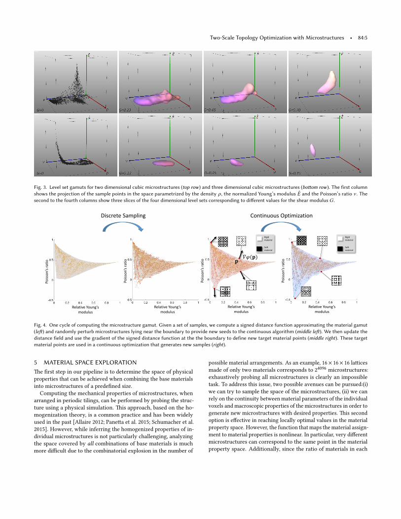
Fig. 4. One cycle of computing the microstructure gamut. Given a set of samples, we compute a signed distance function approximating the material gamut(le�) and randomly perturb microstructures lying near the boundary to provide new seeds to the continuous algorithm (middle le�). We then update thedistance field and use the gradient of the signed distance function at the the boundary to define new target material points (middle right). These targetmaterial points are used in a continuous optimization that generates new samples (right).
5 MATERIAL SPACE EXPLORATION�e �rst step in our pipeline is to determine the space of physical
properties that can be achieved when combining the base materials
into microstructures of a prede�ned size.
Computing the mechanical properties of microstructures, when
arranged in periodic tilings, can be performed by probing the struc-
ture using a physical simulation. �is approach, based on the ho-
mogenization theory, is a common practice and has been widely
used in the past [Allaire 2012; Pane�a et al. 2015; Schumacher et al.
2015]. However, while inferring the homogenized properties of in-
dividual microstructures is not particularly challenging, analyzing
the space covered by all combinations of base materials is much
more di�cult due to the combinatorial explosion in the number of
possible material arrangements. As an example, 16× 16× 16 la�ices
made of only two materials corresponds to 24096
microstructures:
exhaustively probing all microstructures is clearly an impossible
task. To address this issue, two possible avenues can be pursued:(i)
we can try to sample the space of the microstructures, (ii) we can
rely on the continuity between material parameters of the individual
voxels and macroscopic properties of the microstructures in order to
generate new microstructures with desired properties. �is second
option is e�ective in reaching locally optimal values in the material
property space. However, the function that maps the material assign-
ment to material properties is nonlinear. In particular, very di�erent
microstructures can correspond to the same point in the material
property space. Additionally, since the ratio of materials in each
84:6 • B. Zhu et al.
cell is bounded between zero and one, the continuous optimization
converges slowly or stops moving when material distributions in
many cells are at the lower or upper bound. Being able to jump out
of a local optimum and discovering di�erent variants is important
in order to provide new exploration regions. We leverage these two
approaches by combining them in a scheme that alternates between
a stochastic search and a continuous optimization. We provide the
technical details in the rest of this section.
5.1 Discrete Sampling of MicrostructuresWe aim at sampling the space of material assignments, i.e. mi-
crostructures, in such a way that we maximize the number of sam-
ples corresponding to microstructures whose material properties
lie in the vicinity of the material gamut boundaries. We do not
draw all samples at once but progressively enrich the database of
microstructures as we re�ne our estimation of the material gamut
boundaries. �is sampling strategy is motivated by the observation
that a small change in the material assignment of a microstructure
generally – but not always – translates to a small change of its
material properties. By modifying microstructures located near the
current boundaries of the material property gamut, we are likely to
generate more structures in this area, some of which will lie outside
of the current gamut.
Given a population of microstructures to evolve, we generate
new samples from each microstructure by changing its material at
random voxel locations. To rationalize computational resources,
we want to avoid revisiting the same voxel twice. But we do not
want to privilege any particular order either. Ritchie et al. [2015]
recently presented a Stochastically-Ordered Sequential Monte Carlo
(SOSMC) method that provides a suitable approach. In SOSMC, a
population of particles (here, our microstructures) corresponding to
instances of a procedural program (here, the sequential assignment
of materials to the voxels of the microstructures) are evolved so as to
represent a desired distribution. During this process, the programs
are executed in a random order and particles are regularly scored
and reallocated in regions of high probability. In our particular
se�ings, we use the scoring function
s(pi) =Φ(pi)D(pi)
× 1
D(pi), (6)
where Φ(pi) is the signed distance of the material properties of
particle i to the gamut boundary (see Section 5.3) and D(pi) is the
local sampling density at the location pi. We de�ne the sample
density as
D(pi) =∑k
ϕk(pi) , (7)
where ϕk (p) =(1 − | |p−pk | |
22
h2
)4are locally-supported kernel func-
tions that vanish beyond their support radius h, set to a tenth of
the size of the la�ice used for the continuous representation of the
material gamut (see Section 5.3).
�e �rst term in Equation 15 favors microstructures located near
the gamut boundary. �e normalization by D allows us to be less
sensitive to the local microstructures density and to hit any location
corresponding to the same level-set value with a more uniform
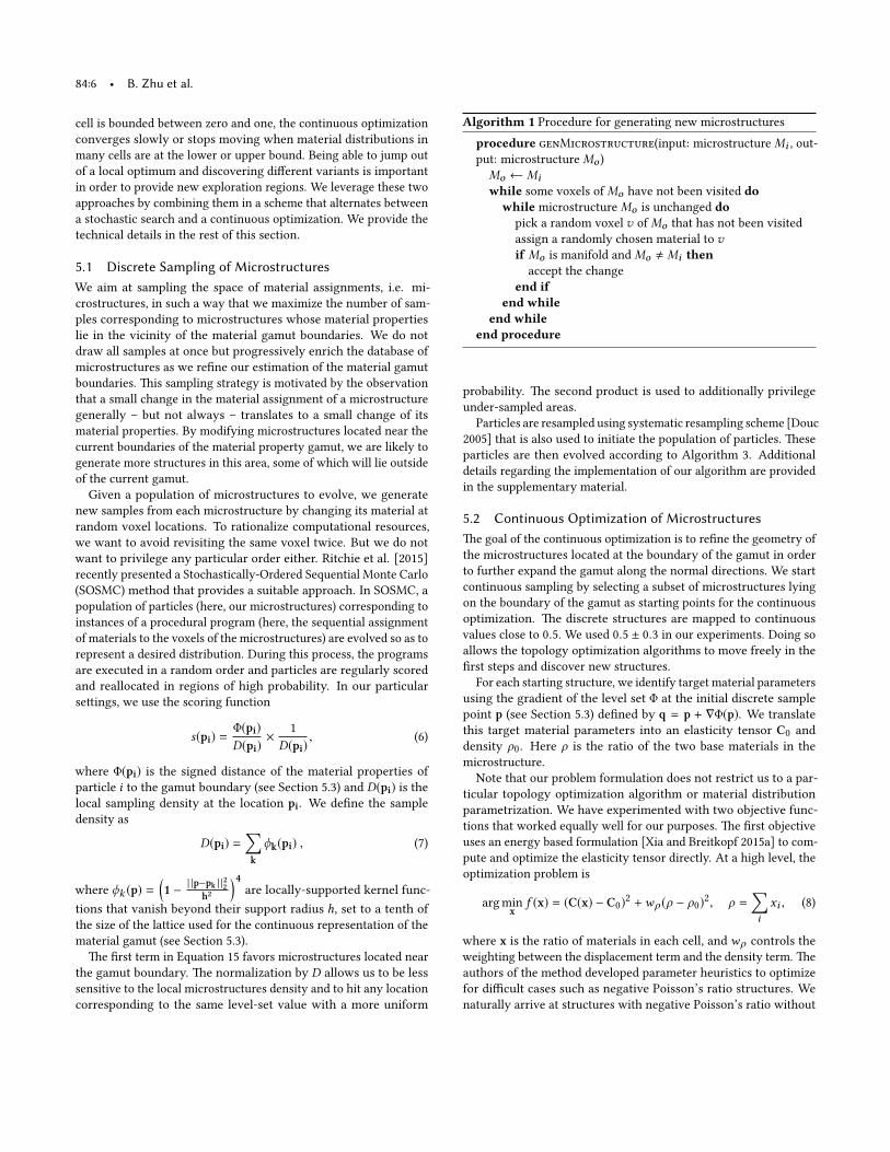
Algorithm 1 Procedure for generating new microstructures
procedure genMicrostructure(input: microstructure Mi , out-
put: microstructure Mo )
Mo ← Miwhile some voxels of Mo have not been visited do
while microstructure Mo is unchanged dopick a random voxel v of Mo that has not been visited
assign a randomly chosen material to vif Mo is manifold and Mo , Mi then
accept the change
end ifend while
end whileend procedure
probability. �e second product is used to additionally privilege
under-sampled areas.
Particles are resampled using systematic resampling scheme [Douc
2005] that is also used to initiate the population of particles. �ese
particles are then evolved according to Algorithm 3. Additional
details regarding the implementation of our algorithm are provided
in the supplementary material.
5.2 Continuous Optimization of Microstructures�e goal of the continuous optimization is to re�ne the geometry of
the microstructures located at the boundary of the gamut in order
to further expand the gamut along the normal directions. We start
continuous sampling by selecting a subset of microstructures lying
on the boundary of the gamut as starting points for the continuous
optimization. �e discrete structures are mapped to continuous
values close to 0.5. We used 0.5 ± 0.3 in our experiments. Doing so
allows the topology optimization algorithms to move freely in the
�rst steps and discover new structures.
For each starting structure, we identify target material parameters
using the gradient of the level set Φ at the initial discrete sample
point p (see Section 5.3) de�ned by q = p + ∇Φ(p). We translate
this target material parameters into an elasticity tensor C0 and
density ρ0. Here ρ is the ratio of the two base materials in the
microstructure.
Note that our problem formulation does not restrict us to a par-
ticular topology optimization algorithm or material distribution
parametrization. We have experimented with two objective func-
tions that worked equally well for our purposes. �e �rst objective
uses an energy based formulation [Xia and Breitkopf 2015a] to com-
pute and optimize the elasticity tensor directly. At a high level, the
optimization problem is
arg min
xf (x) = (C(x) − C0)2 +wρ (ρ − ρ0)2, ρ =
∑ixi , (8)
where x is the ratio of materials in each cell, and wρ controls the
weighting between the displacement term and the density term. �e
authors of the method developed parameter heuristics to optimize
for di�cult cases such as negative Poisson’s ratio structures. We
naturally arrive at structures with negative Poisson’s ratio without
Two-Scale Topology Optimization with Microstructures • 84:7
the parameter varying step in [Xia and Breitkopf 2015a] since our
discrete samples allow us to explore a wide variety of initial designs.
�e second objective is formulated using harmonic displace-
ments [Kharevych et al. 2009; Schumacher et al. 2015] G instead of
the elasticity tensor directly. G is a 6 × 6 symmetric matrix where
each row corresponds to a strain in vector form. We use the target
elasticity tensor C0 to compute the target harmonic displacements
matrix G0 and minimize the objective function:
f (x) = (G(x) − G0)2 +wρ (ρ − ρ0)2. (9)
�is objective matches so� structures more accurately since entries
of G are inversely proportional to material sti�ness.
Following the work by Andreassen et al. [2014], we use the
method of moving asymptotes (MMA) [Svanberg 1987]) to optimize
the objectives using an implementation provided in the NLOPT
package [Johnson 2014]. We run at most 50 iterations since it usually
converges to a solution within 20-30 steps. MMA makes large jumps
during the optimization while keeping track of the current best
solution, thus causing the oscillation of the objective value. To force
continuous material ratios towards discrete values, we experimented
with the SIMP model with the exponent set to 3 and the Hashin-
Shtrikman bound for isotropic materials described by Bendsøe and
Sigmund [1999].
Either interpolation allows us to threshold the �nal continuous
distribution and obtain a similar discrete sample. We tolerate small
deviations introduced by the thresholding since our goal is to obtain
a microstructure lying outside of the gamut rather than reaching a
particular target. In practice, we observed that the material proper-
ties of the �nal discrete structures o�en did not change signi�cantly
a�er the thresholding step.
5.3 Continuous Representation of the Material GamutWe represent the gamut of material properties using a signed dis-
tance �eld that is computed from the material points associated to
the sampled microstructures. First, we normalize each coordinate
pi of p to constrain the scope of the level set to an n-dimensional
unit cube. �en we compute the level set values on the cell cen-
ters of an n-dimensional Cartesian grid that encloses this unit cube.
We draw inspiration from the methods for surface reconstruction
used in particle �uid rendering [Ando et al. 2013; Bhatacharya et al.
2011; Zhu and Bridson 2005] and extend it to n dimensions. In this
case, a signed distance �eld is generated from a set of points by
evaluating an implicit distance function Φ at each point p ∈ M.
We initialize the signed distance �eld using the implicit function
Φ(p) = | |p − p| | − r from [Zhu and Bridson 2005] where | | · | | is the
Euclidean distance between two points inM, and p is the average
position of the neighboring points of p within a range of 2r . Note
that the signed distance is initially de�ned only near the boundary
of the gamut. In order to sample the distance on the entire domain,
we propagate the 0-level set surface using the fast marching algo-
rithm and solve an explicit mean curvature �ow problem de�ned as
∂Φ/∂t = ∆Φ [Osher and Fedkiw 2006] .
Having a continuous representation of the gamut of materials
achievable by the microstructures, we can now reformulate the
topology optimization problem directly in the material space.
6 TOPOLOGY OPTIMIZATIONA classic topology optimization problem consists of optimizing the
shape and structure of a given object de�ned by a prescribed domain
in order to minimize some cost function. For example, the standard
topology optimization minimizes the compliance of the object while
satisfying the static equilibrium and the total weight constraint.
Since the topology of the object is unknown a priori, a method
of choice is to de�ne the shape of the object through its material
distribution and to locally work with material densities. To this end,
the design layout is voxelized and a density variable is assigned to
every cell of the discretized domain. By penalizing intermediate
values for these densities, a binary distribution corresponding to
the object’s �nal layout can be eventually obtained.
In this work, we extend the traditional topology optimization
algorithm in multiple ways. First, we do not compute a binary ma-
terial distribution at the cell level as commonly done. Instead, we
leverage our database of microstructures and ask for each cell to be
�lled with one of the microstructures. By doing so we change the
topology of the object at a �ner scale, i.e. within each cell. �is is
done by working with the macro-scale material properties of the
microstructures instead of their geometry directly. �e second dif-
ference is that our algorithm can be used with parametrizations of
the material property space that are more complex than the single
density parameter per cell that is commonly used in the standard
topology optimization algorithm. Indeed, in our generalized topol-
ogy optimization problem, each cell ci contains an n-dimensional
material parameter pi ∈ Rn . We use p to denote the stacked vector
of material parameters in all cells. Given a signed distance func-
tion Φ(pi ) that de�nes the gamut, our new topology optimization
problem is then wri�en as
min
p: S(p, u)
s .t . : F (p, u) = 0
: Φ(pi ) ≤ 0, 1 ≤ i ≤ Nc
(10)
where S is a real-valued objective function that depends on the
material parameters and the displacement vector u of the entire
object at the elasticity equilibrium. �e equality constraint F = 0
requires u to satisfy the elasticity equilibrium and the inequality
constraint Φ ≤ 0 guarantees that the material properties of each
cell stay inside the precomputed gamut.
In our examples, the material parameter p consists of the density
ρ and the elasticity parameters e. We split our objective function
into an elasticity term C(e, u) that controls the deformation behavior
(see Section 6.1) and an optional density term V(ρ) that controls
the overall mass of the object.�e density term can be wri�en as
V(ρ) = (Nc∑i=1
ρiVi − M)2, (11)
where Vi is the cell volume and M is the target overall mass. When
one of the base material is void, the use of the density term allows
to modify the topology of the object at a larger scale than the one
of the microstructures, and thus to change the external shape of
the object. In fact, even for multi-material designs involving base
materials with similar mass densities, we noted that we could use
the density term to encourage the presence of so� material in the
84:8 • B. Zhu et al.
structure. By removing the external cells entirely made of the so�
material, we could then decrease the mass of the structure without
signi�cantly changing its mechanical behaviour. Alternatively, the
density term can also be used to control other quantities related to
the ratios of the di�erent materials such as the cost of the object.
For speci�c problems, we can also add spatially-varying weight
control terms to Equation 11. For example, we can control the target
weight of each individual cell by adding a local term (ρi − ρi )2Vi .Assuming static equilibrium, the elasticity constraint is wri�en
as
F (e, u) = K(e)u − fext = 0, (12)
where fext are the external loads applied to the object.
�e gamut constraint for a point pi in the material property space
is described by an n-dimensional level set function Φ(p). We have
Φ(pi ) < 0 for a point inside the gamut, Φ(pi ) > 0 for a point outside
the gamut, and Φ(pi ) = 0 for a point on the boundary of the gamut.
�e value of Φ represents the n-dimension Euclidean distance to
the level set boundary. �e gradient of Φ are evaluated by a �nite
di�erence operation on the signed distance �eld.
We used a standard gradient-based numerical optimizer (Ipopt
[Wachter and Biegler 2006] in our implementation) to solve Equa-
tion 10. We enforced the elasticity equilibrium constraint using
the adjoint method. �e optimizer only needs to take the function
values of S and Φ along with their gradients as input.
6.1 Elasticity ObjectivesWe used two di�erent types of objective functions for the elasticity
term in our topology optimization algorithm. �ese two types of
objectives allowed us to design a wide range of objects.
Target Deformation. Our algorithm takes a vector of nodal tar-
get displacements and boundary conditions (external forces, �xed
points, etc.) as input. �en, it automatically optimizes the material
distribution over the object domain to achieve the desired linear
deformation assuming a linear elastic behavior.
We de�ne the deformation objective as
Cd (e, u) = (u − u)TD(u − u), (13)
where u is the vector of the target displacements, D is a diagonal
matrix that determines the importance of each nodal displacement.
We use D to de�ne the subset of nodes that we are interested in.
For example, we can set most entries of D to zero and focus on a
portion of the domain (see Figure 12).
Minimum Compliance. We have experimented with the same
objective as the one used in the standard topology optimization
algorithm where the compliance Cc is de�ned as
Cc (e, u) = uTK(e)u. (14)
In the commonly used SIMP algorithm, the sti�ness matrix Ki of
each cell i depends on the arti�cial density value ρi through an
analytical formula such as Ki = ρ3
i K0 where K0 corresponds to the
sti�ness matrix of the base material. In contrast, the sti�ness matrix
in our objective function is directly computed from the material
parameters of the material space and forced to correspond to a
realizable material thanks to our gamut constraints.
Like in standard algorithms, we regularized the problem to avoid
checkerboard solutions by applying a smoothing kernel on the
material properties that favors smooth variations of the material
parameters over the object layout. Our optimizer supports multiple
objectives by linearly combining weighted objective functions.
7 MAPPING MATERIAL PROPERTIES TOMICROSTRUCTURES
A�er running the topology optimization
algorithm, we generate a printable result
by replacing each cell in the object la�ice
by a microstructure whose material prop-
erties match the optimal ones.
Material properties of the microstruc-
tures are computed using the homogeniza-
tion theory which is more accurate with
a smooth transition between the geome-
tries of neighboring cells. While smooth-
ness in the material parameters can be eas-
ily enforced, it does not imply topological
similarity of nearby microstructures. For
example, any translation of a given mi-
crostructure in a periodic tiling will result in a microstructure geo-
metrically di�erent but with exactly the same mechanical properties.
Fortunately, our database is very dense and multiple microstructures
generally map to similar points in the material property space, o�er-
ing several variants. To further increase the number of possibilities,
we also incorporate an additional exemplar for each microstruc-
ture by translating it by half its size, which preserves its cubic or
orthotropic symmetry without changing its properties (see inset
Figure). We then run a simple but e�ective algorithm that picks
the microstructure exemplars that minimize the boundary mate-
rial mismatch across adjacent cells. We quantify this mismatch by
I = ∑Nci=1Ii , where Ii is the contribution associated to the cell i and
corresponds to the number of boundary voxels �lled with materials
that are di�erent from the ones of the voxels’ immediate neighbours
across the interfaces.
Our algorithm proceeds as follows:
• For each cell, we de�ne a list of possible candidates by
picking all the microstructures mapping to material points
lying in the vicinity of the optimal material point and we
randomly initialize the cell with one of the candidates.
• We compute the mismatch energy Ii associated to each cell
i and sort the cells according to their energy.
• We pick the �rst cell in the sorted list, i.e. the one with the
highest energy and assign to it the microstructure candidate
that decreases the energy the most. If we cannot decrease
the cell energy, we move to the next cell in the list.
• We update the mismatch energies of all the impacted cells
and we update the priority list.
• We repeat the last two steps until the mismatch energy Icannot be decreased anymore.
Two-Scale Topology Optimization with Microstructures • 84:9
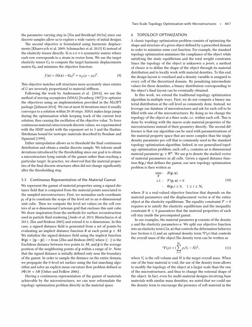
Fig. 5. Gamuts computed with our discrete-continuous sampling scheme for 2D cubic structures (le�) , 2D orthotropic structures (second from le�), 3D cubicstructures (second from right) and 3D cubic structures with 0.35 as Poisson’s ratio (right). The plots show the results for the projection of the gamuts onthe plane defined by the macroscale Young’s modulus along the x axis (normalized by the Young’s modulus of the sti�est base material) and the Poisson’sratio corresponding to a contraction along the y-direction when the material is stretched along the x-direction. The blue dots correspond to the generatedsamples,the orange dots correspond to the microstructures from Schumacher et al. [2015] and the yellow dots correspond to the microstructures from Pane�aet al. [2015].
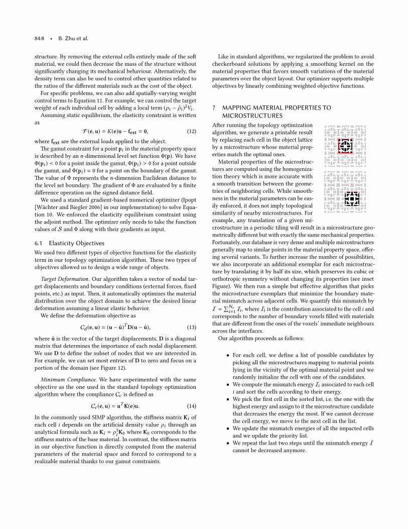
Fig. 6. Gamut corresponding to 2D cubic microstructures made of twomaterials and void. The Young’s modulus of the microstructures is plo�edusing a logarithmic scale. We show above some examples of microstructureslying near the estimated boundary of the gamut, i.e. with extreme materialproperties. The dark color corresponds to the so�er material, while the lightgrey color is used for the sti�er material.
8 RESULTSWe �rst analyzed our microstructure sampling algorithm for 2D
and 3D microstructure gamuts. �en we used these precomputed
gamuts and we designed and optimized a wide variety of objects
with our topology optimization algorithm.
8.1 Microstructure SamplingWe evaluated our method on two- and three-dimensional microstruc-
tures made of one or two materials. For the 2D case we consid-
ered pa�erns with cubic and orthotropic mechanical behaviors that
can be described with 4 parameters (3 elasticity parameters and
density) and 5 parameters (4 elasticity parameters and density) re-
spectively. In 3D we computed the gamut corresponding to cubic
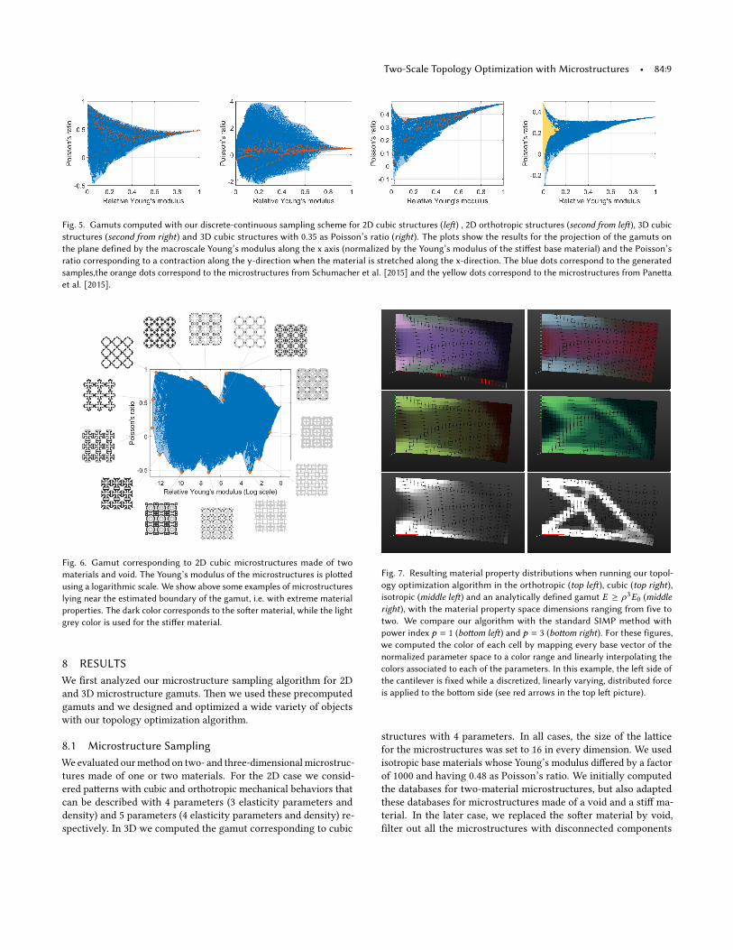
Fig. 7. Resulting material property distributions when running our topol-ogy optimization algorithm in the orthotropic (top le�), cubic (top right),isotropic (middle le�) and an analytically defined gamut E ≥ ρ3E0 (middleright), with the material property space dimensions ranging from five totwo. We compare our algorithm with the standard SIMP method withpower index p = 1 (bo�om le�) and p = 3 (bo�om right). For these figures,we computed the color of each cell by mapping every base vector of thenormalized parameter space to a color range and linearly interpolating thecolors associated to each of the parameters. In this example, the le� side ofthe cantilever is fixed while a discretized, linearly varying, distributed forceis applied to the bo�om side (see red arrows in the top le� picture).
structures with 4 parameters. In all cases, the size of the la�ice
for the microstructures was set to 16 in every dimension. We used
isotropic base materials whose Young’s modulus di�ered by a factor
of 1000 and having 0.48 as Poisson’s ratio. We initially computed
the databases for two-material microstructures, but also adapted
these databases for microstructures made of a void and a sti� ma-
terial. In the later case, we replaced the so�er material by void,
�lter out all the microstructures with disconnected components
84:10 • B. Zhu et al.
0 20 40 60
# iterations
0
5
10
15
Ob
jective
ene
rgy
×106
analytic
cubic
orthotropic
0 20 40 60
# iterations
5
10
15
20
25
30
Ela
stic e
ne
rgy
analytic
cubic
orthotropic
SIMP-3
SIMP-1
0 20 40 60 80
# iterations
0
1
2
3
Ob
jective
ene
rgy
×108
32
64
128
256
0 20 40 60 80
# iterations
8
10
12
14
16
18
20E
lastic e
nerg
y32
64
128
256
0 20 40 60
# iterations
0
2
4
6
8
Ob
jective
en
erg
y
×107
point 1
point 2
point 3
point 4
0 20 40 60
# iterations
10
20
30
40
Ela
stic e
ne
rgy
point 1
point 2
point 3
point 4
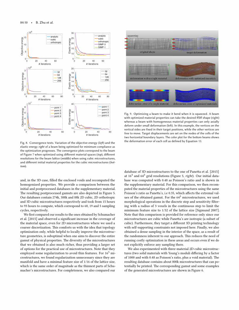
Fig. 8. Convergence tests. Variation of the objective energy (le�) and theelastic energy right of a beam being optimized for minimum compliance asthe optimization progresses. The convergence plots correspond to the beamof Figure 7 when optimized using di�erent material spaces (top), di�erentresolutions for the beam la�ice (middle) when using cubic microstructures,and di�erent initial material properties for the cubic microstructures (bot-tom).
and, in the 3D case, �lled the enclosed voids and recomputed the
homogenized properties. We provide a comparison between the
initial and postprocessed databases in the supplementary material.
�e resulting postprocessed gamuts are also depicted in Figure 5.
Our databases contain 274k, 388k and 88k 2D cubic, 2D orthotropic
and 3D cubic microstructures respectively and took from 15 hours
to 93 hours to compute, which correspond to 68, 19 and 5 sampling
cycles, respectively.
We �rst compared our results to the ones obtained by Schumacher
et al. [2015] and observed a signi�cant increase in the coverage of
the material space, even for 2D microstructures where we used a
coarser discretization. �is comforts us with the idea that topology
optimization only, while helpful to locally improve the microstruc-
ture geometries, is suboptimal when one aims to discover the entire
gamut of physical properties. �e diversity of the microstructures
that we obtained is also much richer, thus providing a larger set
of options for the practical use of microstructures. Note that they
employed some regularization to avoid thin features. For 163
mi-
crostructures, we found regularization unnecessary since they are
manifold and have a minimal feature size of 1/16 of the la�ice size,
which is the same order of magnitude as the thinnest parts of Schu-
macher’s microstructures. For completeness, we also compared our
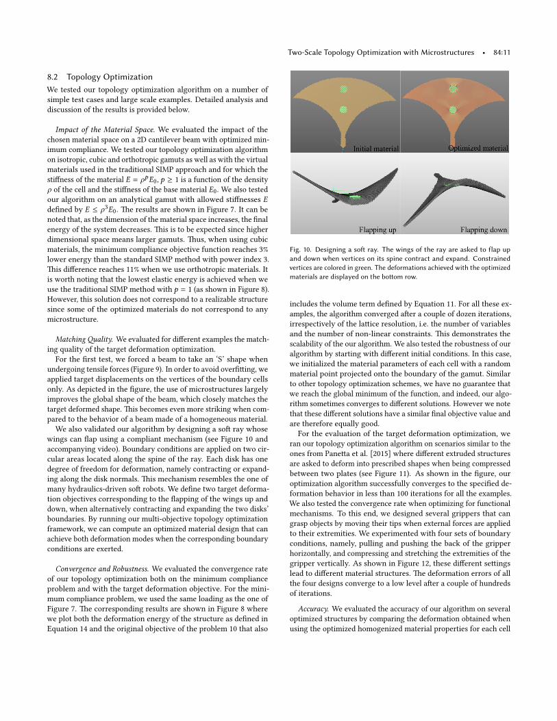
Fig. 9. Optimizing a beam to make it bend when it is squeezed. A beamwith optimized material properties can take the desired �S� shape (right)whereas a beam with homogeneous material properties can only axiallydeform under small deformation (le�). In this example, the vertices on thevertical sides are fixed in their target positions, while the other vertices arefree to move. Target displacements are set on the nodes of the cells of thetwo horizontal boundary layers. The color plot for the bo�om beams showsthe deformation error of each cell as defined by Equation 13.
database of 3D microstructures to the one of Pane�a et al. [2015]
at 163
and 643
grid resolutions (Figure 5, right). Our initial data-
base was computed with 0.48 as Poisson’s ratio and is shown in
the supplementary material. For this comparison, we then recom-
puted the material properties of the microstructures using the same
Poisson’s ratio as Pane�a’s, i.e 0.35, which a�ects the extremal val-
ues of the obtained gamut. For the 643
microstructures, we used
morphological operations in the discrete step and sensitivity �lter-
ing with a radius of 3 voxels in the continuous step to limit the
minimum feature size to 1/32 of the la�ice size [Sigmund 2007].
Note that this comparison is provided for reference only since our
microstructures are cubic while Pane�a’s are isotropic (a subset of
cubic). Furthermore, they target a di�erent 3D printing technology
with self-supporting constraints not imposed here. Finally, we also
obtained a dense sampling in the interior of the space, as a result of
the randomness inherent to our approach. �is reduces the need of
running costly optimization in these areas and occurs even if we do
not explicitly enforce any sampling there.
We also experimented with three-material 2D cubic microstruc-
tures (two solid materials with Young’s moduli di�ering by a factor
of 1000 and with 0.48 as Poisson’s ratio, plus a void material). �e
resulting database contains about 800k microstructures that can po-
tentially be printed. �e corresponding gamut and some examples
of the generated microstructures are shown in Figure 6.
Two-Scale Topology Optimization with Microstructures • 84:11
8.2 Topology OptimizationWe tested our topology optimization algorithm on a number of
simple test cases and large scale examples. Detailed analysis and
discussion of the results is provided below.
Impact of the Material Space. We evaluated the impact of the
chosen material space on a 2D cantilever beam with optimized min-
imum compliance. We tested our topology optimization algorithm
on isotropic, cubic and orthotropic gamuts as well as with the virtual
materials used in the traditional SIMP approach and for which the
sti�ness of the material E = ρpE0, p ≥ 1 is a function of the density
ρ of the cell and the sti�ness of the base material E0. We also tested
our algorithm on an analytical gamut with allowed sti�nesses Ede�ned by E ≤ ρ3E0. �e results are shown in Figure 7. It can be
noted that, as the dimension of the material space increases, the �nal
energy of the system decreases. �is is to be expected since higher
dimensional space means larger gamuts. �us, when using cubic
materials, the minimum compliance objective function reaches 3%
lower energy than the standard SIMP method with power index 3.
�is di�erence reaches 11% when we use orthotropic materials. It
is worth noting that the lowest elastic energy is achieved when we
use the traditional SIMP method with p = 1 (as shown in Figure 8).
However, this solution does not correspond to a realizable structure
since some of the optimized materials do not correspond to any
microstructure.
Matching�ality. We evaluated for di�erent examples the match-
ing quality of the target deformation optimization.
For the �rst test, we forced a beam to take an ‘S’ shape when
undergoing tensile forces (Figure 9). In order to avoid over��ing, we
applied target displacements on the vertices of the boundary cells
only. As depicted in the �gure, the use of microstructures largely
improves the global shape of the beam, which closely matches the
target deformed shape. �is becomes even more striking when com-
pared to the behavior of a beam made of a homogeneous material.
We also validated our algorithm by designing a so� ray whose
wings can �ap using a compliant mechanism (see Figure 10 and
accompanying video). Boundary conditions are applied on two cir-
cular areas located along the spine of the ray. Each disk has one
degree of freedom for deformation, namely contracting or expand-
ing along the disk normals. �is mechanism resembles the one of
many hydraulics-driven so� robots. We de�ne two target deforma-
tion objectives corresponding to the �apping of the wings up and
down, when alternatively contracting and expanding the two disks’
boundaries. By running our multi-objective topology optimization
framework, we can compute an optimized material design that can
achieve both deformation modes when the corresponding boundary
conditions are exerted.
Convergence and Robustness. We evaluated the convergence rate
of our topology optimization both on the minimum compliance
problem and with the target deformation objective. For the mini-
mum compliance problem, we used the same loading as the one of
Figure 7. �e corresponding results are shown in Figure 8 where
we plot both the deformation energy of the structure as de�ned in
Equation 14 and the original objective of the problem 10 that also
Fig. 10. Designing a so� ray. The wings of the ray are asked to flap upand down when vertices on its spine contract and expand. Constrainedvertices are colored in green. The deformations achieved with the optimizedmaterials are displayed on the bo�om row.
includes the volume term de�ned by Equation 11. For all these ex-
amples, the algorithm converged a�er a couple of dozen iterations,
irrespectively of the la�ice resolution, i.e. the number of variables
and the number of non-linear constraints. �is demonstrates the
scalability of the our algorithm. We also tested the robustness of our
algorithm by starting with di�erent initial conditions. In this case,
we initialized the material parameters of each cell with a random
material point projected onto the boundary of the gamut. Similar
to other topology optimization schemes, we have no guarantee that
we reach the global minimum of the function, and indeed, our algo-
rithm sometimes converges to di�erent solutions. However we note
that these di�erent solutions have a similar �nal objective value and
are therefore equally good.
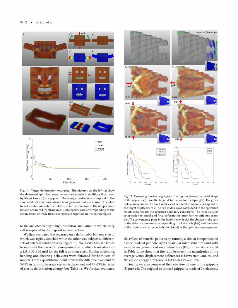
For the evaluation of the target deformation optimization, we
ran our topology optimization algorithm on scenarios similar to the
ones from Pane�a et al. [2015] where di�erent extruded structures
are asked to deform into prescribed shapes when being compressed
between two plates (see Figure 11). As shown in the �gure, our
optimization algorithm successfully converges to the speci�ed de-
formation behavior in less than 100 iterations for all the examples.
We also tested the convergence rate when optimizing for functional
mechanisms. To this end, we designed several grippers that can
grasp objects by moving their tips when external forces are applied
to their extremities. We experimented with four sets of boundary
conditions, namely, pulling and pushing the back of the gripper
horizontally, and compressing and stretching the extremities of the
gripper vertically. As shown in Figure 12, these di�erent se�ings
lead to di�erent material structures. �e deformation errors of all
the four designs converge to a low level a�er a couple of hundreds
of iterations.
Accuracy. We evaluated the accuracy of our algorithm on several
optimized structures by comparing the deformation obtained when
using the optimized homogenized material properties for each cell
84:12 • B. Zhu et al.
#iteration
0 50 100 150 200
obje
ctive e
nerg
y (
log)
-5
0
5
10
15arm
face
wave
Fig. 11. Target deformation examples. The pictures on the le� (a) showthe deformed optimized result when the boundary conditions illustratedby the pictures (b) are applied. The orange meshes (c) correspond to thesimulated deformations when a homogeneous material is used. The blue-to-red meshes indicate the relative deformation error of the unoptimized(d) and optimized (e) structures. Convergence rates corresponding to theoptimization of these three examples are reported on the bo�om figure.
to the one obtained by a high resolution simulation in which every
cell is replaced by its mapped microstructure.
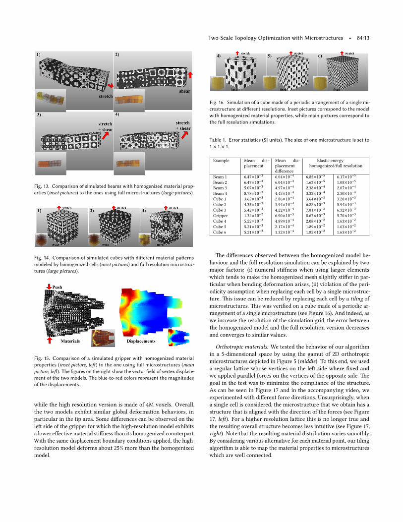
We �rst evaluated the accuracy on a deformable bar, one side of
which was rigidly a�ached while the other was subject to di�erent
sets of external conditions (see Figure 13). We used a 8× 2× 2 la�ice
to represent the bar with homogenized cells, which translates into
a 128 × 32 × 32 grid for the full resolution mesh. Similar stretching,
bending and shearing behaviors were obtained for both sets of
models. From a quantitative point of view, the di�erences amount to
5-10% in terms of average vertex displacement and 9%-33% in terms
of elastic deformation energy (see Table 1). We further evaluated
#iteration
0 50 100 150 200 250 300 350
de
form
atio
n e
ne
rgy (
L2
no
rm)
0
1
2
3
4
5
6push back
pull back
push side
pull side
#iteration
0 50 100 150 200 250 300 350
defo
rmation e
nerg
y (
Lin
f)
0
0.01
0.02
0.03
0.04
0.05
0.06
0.07
0.08push back
pull back
push side
pull side
Fig. 12. Designing functional grippers. The top row shows the initial shapeof the gripper (le�), and the target deformation for the tip (right). The greendots correspond to the fixed vertices while the blue arrows correspond tothe target displacements. The two middle rows correspond to the optimizedresults obtained for the specified boundary conditions. The inset picturescolor-code the initial and final deformation error for the di�erent exam-ples.The convergence plots in the bo�om row depict the change in the sumof the deformation errors corresponding to all the cells (le�) and the valueof the maximal cell error contribution (right) as the optimization progresses.
the e�ects of material pa�erns by running a similar comparison on
a cube made of periodic layers of similar microstructures and with
random assignments of microstructures (Figure 14). As reported
in Table 1, we show that the ratio between the magnitudes of the
average vertex displacement di�erences is between 4% and 7%, and
the elastic energy di�erence is between 10% and 19%.
Finally, we also compared the behaviors of one of the grippers
(Figure 15). �e original optimized gripper is made of 3k elements
Two-Scale Topology Optimization with Microstructures • 84:13
Fig. 13. Comparison of simulated beams with homogenized material prop-erties (inset pictures) to the ones using full microstructures (large pictures).
Fig. 14. Comparison of simulated cubes with di�erent material pa�ernsmodeled by homogenized cells (inset pictures) and full resolution microstruc-tures (large pictures).
Fig. 15. Comparison of a simulated gripper with homogenized materialproperties (inset picture, le�) to the one using full microstructures (mainpicture, le�). The figures on the right show the vector field of vertex displace-ment of the two models. The blue-to-red colors represent the magnitudesof the displacements.
while the high resolution version is made of 4M voxels. Overall,
the two models exhibit similar global deformation behaviors, in
particular in the tip area. Some di�erences can be observed on the
le� side of the gripper for which the high-resolution model exhibits
a lower e�ective material sti�ness than its homogenized counterpart.
With the same displacement boundary conditions applied, the high-
resolution model deforms about 25% more than the homogenized
model.
Fig. 16. Simulation of a cube made of a periodic arrangement of a single mi-crostructure at di�erent resolutions. Inset pictures correspond to the modelwith homogenized material properties, while main pictures correspond tothe full resolution simulations.
Table 1. Error statistics (SI units). The size of one microstructure is set to1 × 1 × 1.
Example Mean dis-
placement
Mean dis-
placement
di�erence
Elastic energy
homogenized/full resolution
Beam 1 6.47×10⁻³
6.04×10⁻⁴
6.85×10⁻⁵
6.17×10⁻⁵
Beam 2 6.47×10⁻³
6.04×10⁻⁴
1.63×10⁻⁵
1.08×10⁻⁵
Beam 3 5.07×10⁻³
4.97×10⁻⁴
2.38×10⁻⁴
2.07×10⁻⁴
Beam 4 8.78×10⁻³
4.45×10⁻⁴
3.33×10⁻⁴
2.30×10⁻⁴
Cube 1 3.62×10⁻³
2.86×10⁻⁴
3.64×10⁻³
3.20×10⁻³
Cube 2 4.35×10⁻³
1.94×10⁻⁴
6.82×10⁻³
5.94×10⁻³
Cube 3 5.42×10⁻³
4.22×10⁻⁴
7.81×10⁻³
6.32×10⁻³
Gripper 1.32×10⁻²
6.90×10⁻³
8.67×10⁻³
5.70×10⁻³
Cube 4 5.22×10⁻³
4.89×10⁻⁴
2.08×10⁻²
1.63×10⁻²
Cube 5 5.21×10⁻³
2.17×10⁻⁴
1.89×10⁻²
1.63×10⁻²
Cube 6 5.21×10⁻³
1.32×10⁻⁴
1.82×10⁻²
1.63×10⁻²
�e di�erences observed between the homogenized model be-
haviour and the full resolution simulation can be explained by two
major factors: (i) numeral sti�ness when using larger elements
which tends to make the homogenized mesh slightly sti�er in par-
ticular when bending deformation arises, (ii) violation of the peri-
odicity assumption when replacing each cell by a single microstruc-
ture. �is issue can be reduced by replacing each cell by a tiling of
microstructures. �is was veri�ed on a cube made of a periodic ar-
rangement of a single microstructure (see Figure 16). And indeed, as
we increase the resolution of the simulation grid, the error between
the homogenized model and the full resolution version decreases
and converges to similar values.
Orthotropic materials. We tested the behavior of our algorithm
in a 5-dimensional space by using the gamut of 2D orthotropic
microstructures depicted in Figure 5 (middle). To this end, we used
a regular la�ice whose vertices on the le� side where �xed and
we applied parallel forces on the vertices of the opposite side. �e
goal in the test was to minimize the compliance of the structure.
As can be seen in Figure 17 and in the accompanying video, we
experimented with di�erent force directions. Unsurprisingly, when
a single cell is considered, the microstructure that we obtain has a
structure that is aligned with the direction of the forces (see Figure
17, le�). For a higher resolution la�ice this is no longer true and
the resulting overall structure becomes less intuitive (see Figure 17,
right). Note that the resulting material distribution varies smoothly.
By considering various alternative for each material point, our tiling
algorithm is able to map the material properties to microstructures
which are well connected.
84:14 • B. Zhu et al.
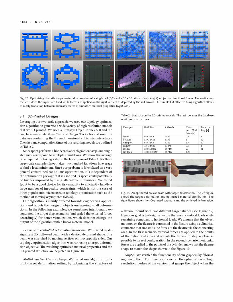
Fig. 17. Optimizing the orthotropic material parameters of a single cell (le�) and a 32 × 32 la�ice of cells (right) subject to directional forces. The vertices onthe le� side of the layout are fixed while forces are applied on the right vertices as depicted by the red arrows. Our simple but e�ective tiling algorithm allowsto nicely transition between microstructures of smoothly material properties (right, top).
8.3 3D-Printed DesignsLeveraging our two-scale approach, we used our topology optimiza-
tion algorithm to generate a wide variety of high resolution models
that we 3D-printed. We used a Stratasys Objet Connex 500 and the
two base materials Vero Clear and Tango Black Plus and used the
database containing the three-dimensional cubic microstructures.
�e sizes and computation times of the resulting models are outlined
in Table 2.
Since Ipopt performs a line search at each gradient step, one single
step may correspond to multiple simulations. We show the average
time required for taking a step in the last column of Table 2. For these
large scale examples, Ipopt takes two hundred iterations in average
to �nd a local minimum. Since our problem is formulated as a very
general constrained continuous optimization, it is independent of
the optimization package that is used and its speed could potentially
be further improved by using alternative minimizers. We found
Ipopt to be a good choice for its capability to e�ciently handle a
large number of inequality constraints, which is not the case of
other popular minimizers used in topology optimization such as the
method of moving asymptotes (MMA).
Our algorithm is mainly directed towards engineering applica-
tions and targets the design of objects undergoing small deforma-
tions. In the following examples, we sometimes intentionally ex-
aggerated the target displacements (and scaled the external forces
accordingly) for be�er visualization, which does not change the
output of the algorithm with a linear material model.
Beams with controlled deformation behaviour. We started by de-
signing a 3D hollowed beam with a desired deformed shape. �e
beam was stretched by moving vertices on two opposite sides. Our
topology optimization algorithm was run using a target deforma-
tion objective. �e resulting optimized material properties and the
3D-printed structure are depicted in Figure 18.
Multi-Objective Flexure Design. We tested our algorithm on a
multi-target deformation se�ing by optimizing the structure of
Table 2. Statistics on the 3D-printed models. The last row uses the databaseof 64
3 microstructures.
Example Grid Size # Voxels Time
per FEM
Solve [s]
Time per
Step [s]
Beam 96×24×4 38M 0.7 5
Flexure 32×32×16 67M 1 12
Gripper 64×32×8 67M 1.7 10
Bunny 32×32×32 134M 0.6 4
Bridge 128×64×32 1074M 27 81
Bridge 2 320×160×80 1074G 1.3k -
Fig. 18. An optimized hollow beam with target deformation. The le� figureshows the target deformation and optimized material distribution. Theright figure shows the 3D-printed structure and the achieved deformation.
a �exure mount with two di�erent target shapes (see Figure 19).
Here, our goal is to design a �exure that resists vertical loads while
remaining compliant to horizontal loads. We assume that the object
mounted on the �exure is connected to the �exure using a cylindrical
connector that transmits the forces to the �exure via the connecting
area. In the �rst scenario, vertical forces are applied to the points
of the cylindrical area and we ask the �exure to stay as close as
possible to its rest con�guration. In the second scenario, horizontal
forces are applied to the points of the cylinder and we ask the �exure
shape to match the shape shown in the Figure 19.
Gripper. We veri�ed the functionality of our grippers by fabricat-
ing two of them. For these results we ran the optimization on high
resolution meshes of the version that grasps the object when the
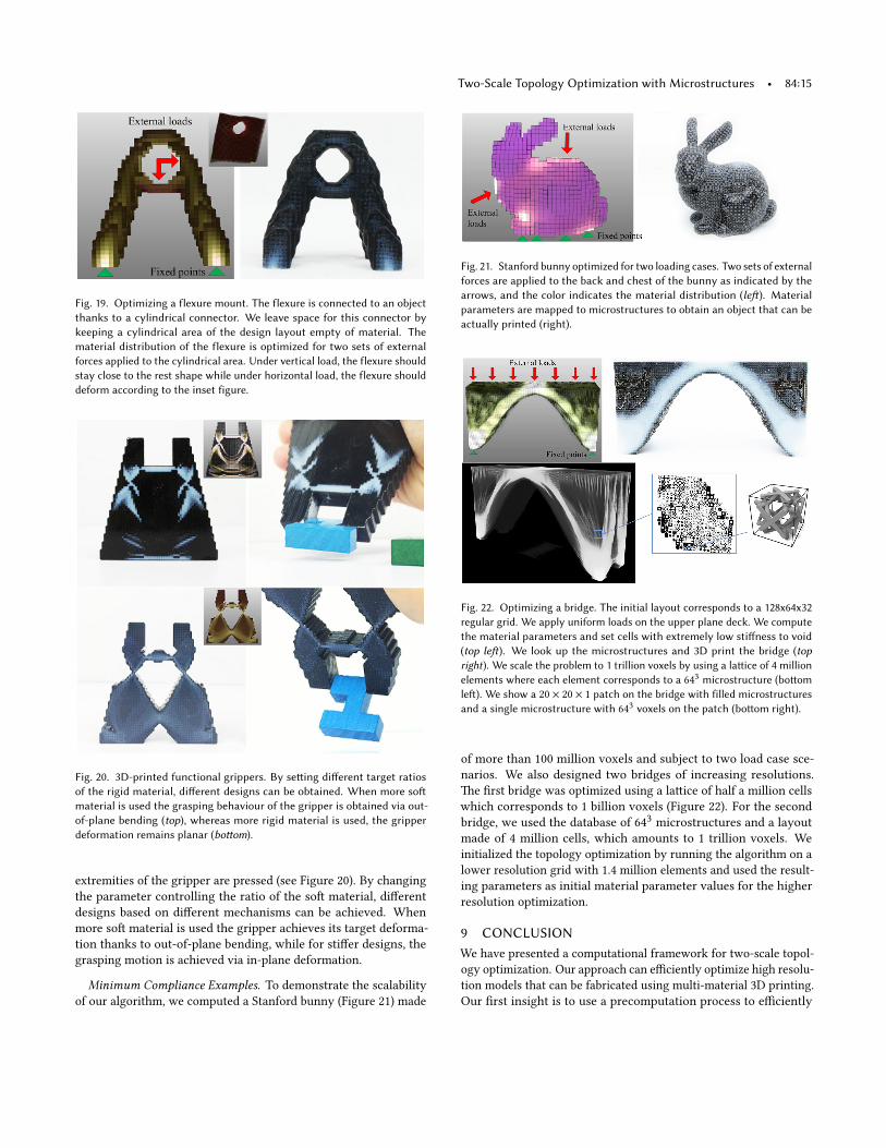
Two-Scale Topology Optimization with Microstructures • 84:15
Fig. 19. Optimizing a flexure mount. The flexure is connected to an objectthanks to a cylindrical connector. We leave space for this connector bykeeping a cylindrical area of the design layout empty of material. Thematerial distribution of the flexure is optimized for two sets of externalforces applied to the cylindrical area. Under vertical load, the flexure shouldstay close to the rest shape while under horizontal load, the flexure shoulddeform according to the inset figure.
Fig. 20. 3D-printed functional grippers. By se�ing di�erent target ratiosof the rigid material, di�erent designs can be obtained. When more so�material is used the grasping behaviour of the gripper is obtained via out-of-plane bending (top), whereas more rigid material is used, the gripperdeformation remains planar (bo�om).
extremities of the gripper are pressed (see Figure 20). By changing
the parameter controlling the ratio of the so� material, di�erent
designs based on di�erent mechanisms can be achieved. When
more so� material is used the gripper achieves its target deforma-
tion thanks to out-of-plane bending, while for sti�er designs, the
grasping motion is achieved via in-plane deformation.
Minimum Compliance Examples. To demonstrate the scalability
of our algorithm, we computed a Stanford bunny (Figure 21) made
Fig. 21. Stanford bunny optimized for two loading cases. Two sets of externalforces are applied to the back and chest of the bunny as indicated by thearrows, and the color indicates the material distribution (le�). Materialparameters are mapped to microstructures to obtain an object that can beactually printed (right).
Fig. 22. Optimizing a bridge. The initial layout corresponds to a 128x64x32regular grid. We apply uniform loads on the upper plane deck. We computethe material parameters and set cells with extremely low sti�ness to void(top le�). We look up the microstructures and 3D print the bridge (topright). We scale the problem to 1 trillion voxels by using a la�ice of 4 millionelements where each element corresponds to a 64
3 microstructure (bo�omle�). We show a 20 × 20 × 1 patch on the bridge with filled microstructuresand a single microstructure with 64
3 voxels on the patch (bo�om right).
of more than 100 million voxels and subject to two load case sce-
narios. We also designed two bridges of increasing resolutions.
�e �rst bridge was optimized using a la�ice of half a million cells
which corresponds to 1 billion voxels (Figure 22). For the second
bridge, we used the database of 643
microstructures and a layout
made of 4 million cells, which amounts to 1 trillion voxels. We
initialized the topology optimization by running the algorithm on a
lower resolution grid with 1.4 million elements and used the result-
ing parameters as initial material parameter values for the higher
resolution optimization.
9 CONCLUSIONWe have presented a computational framework for two-scale topol-
ogy optimization. Our approach can e�ciently optimize high resolu-
tion models that can be fabricated using multi-material 3D printing.
Our �rst insight is to use a precomputation process to e�ciently
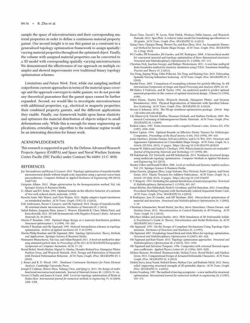
84:16 • B. Zhu et al.
sample the space of microstructures and their corresponding ma-
terial properties in order to de�ne a continuous material property
gamut. Our second insight is to use this gamut as a constraint in a
generalized topology optimization framework to assign spatially-
varying material properties throughout the optimized object. Finally,
the volume with assigned material properties can be converted to
a 3D model with corresponding spatially-varying microstructures.
We demonstrated the e�ectiveness of our approach on multiple ex-
amples and showed improvements over traditional binary topology
optimization schemes.
Limitations and Future Work. First, while our sampling method
outperforms current approaches in terms of the material space cover-
age and the approach converges to stable gamuts, we do not provide
any theoretical guarantees that the gamut space cannot be further
expanded. Second, we would like to investigate microstructures
with additional properties, e.g., electrical or magnetic properties,
their combined property gamuts, and the di�erent applications
they enable. Finally, our framework builds upon linear elasticity
and optimizes the material distribution of objects subject to small
deformations only. While this is enough for many engineering ap-
plications, extending our algorithm to the nonlinear regime would
be an interesting direction for future work.
ACKNOWLEDGEMENTS�is research is supported in part by the Defense Advanced Research
Projects Agency (DARPA) and Space and Naval Warfare Systems
Center Paci�c (SSC Paci�c) under Contract No 66001-15-C-4030.
REFERENCESJoe Alexandersen and Boyan S. Lazarov. 2015. Topology optimisation of manufacturable
microstructural details without length scale separation using a spectral coarse basis
preconditioner. Computer Methods in Applied Mechanics & Engineering 290 (2015),
156��182.
Gregoire Allaire. 2012. Shape optimization by the homogenization method. Vol. 146.
Springer Science & Business Media.
G. Allaire and R.V. Kohn. 1993. Optimal bounds on the e�ective behavior of a mixture
of two well-ordered elastic materials. (1993).
Ryoichi Ando, Nils �urey, and Chris Wojtan. 2013. Highly adaptive liquid simulations
on tetrahedral meshes. ACM Trans. Graph. (TOG) 32, 4 (2013).
Erik Andreassen, Boyan S. Lazarov, and Ole Sigmund. 2014. Design of manufacturable
3D extremal elastic microstructure. Mechanics of Materials 69, 1 (2014).
Sahab Babaee, Jongmin Shim, James C. Weaver, Elizabeth R. Chen, Nikita Patel, and
Katia Bertoldi. 2013. 3D So� Metamaterials with Negative Poisson’s Ratio. AdvancedMaterials 25, 36 (2013).
Martin P Bendsøe. 1989. Optimal shape design as a material distribution problem.
Structural optimization 1, 4 (1989), 193–202.
Martin P Bendsøe and Ole Sigmund. 1999. Material interpolation schemes in topology
optimization. Archive of applied mechanics 69, 9-10 (1999).
Martin Philip Bendsøe and Ole Sigmund. 2004. Topology Optimization: �eory, Methods,and Applications. Springer Science & Business Media.
Haimasree Bhatacharya, Yue Gao, and Adam Bargteil. 2011. A level-set method for skin-
ning animated particle data. In Proceedings of the 2011 ACM SIGGRAPH/EurographicsSymposium on Computer Animation. ACM, 17–24.
Bernd Bickel, Moritz Bacher, Miguel A. Otaduy, Hyunho Richard Lee, Hanspeter P�ster,
Markus Gross, and Wojciech Matusik. 2010. Design and Fabrication of Materials
with Desired Deformation Behavior. ACM Trans. Graph. (Proc. SIGGRAPH) 29, 4
(2010).
J. Bonet and R. D. Wood. 1997. Nonlinear Continuum Mechanics for Finite ElementAnalysis. Cambridge University Press.
Joseph E Cadman, Shiwei Zhou, Yuhang Chen, and Qing Li. 2013. On design of multi-
functional microstructural materials. Journal of Materials Science 48, 1 (2013), 51–66.
Vivien J Challis and James K Guest. 2009. Level set topology optimization of �uids in
Stokes �ow. International journal for numerical methods in engineering 79, 10 (2009),
1284–1308.
Desai Chen, David I. W. Levin, Piotr Didyk, Pitchaya Si�hi-Amorn, and Wojciech
Matusik. 2013. Spec2Fab: A reducer-tuner model for translating speci�cations to
3D prints. ACM Trans. Graph. (Proc. SIGGRAPH) 32, 4 (2013).
Xiang Chen, Changxi Zheng, Weiwei Xu, and Kun Zhou. 2014. An Asymptotic Numer-
ical Method for Inverse Elastic Shape Design. ACM Trans. Graph. (Proc. SIGGRAPH)33, 4 (Aug. 2014).
PG Coelho, PR Fernandes, JM Guedes, and HC Rodrigues. 2008. A hierarchical model
for concurrent material and topology optimisation of three-dimensional structures.
Structural and Multidisciplinary Optimization 35, 2 (2008), 107–115.
Christian Dick, Joachim Georgii, and Rudiger Westermann. 2011. A real-time multigrid
�nite hexahedra method for elasticity simulation using CUDA. Simulation ModellingPractice and �eory 19, 2 (2011).
Yue Dong, Jiaping Wang, Fabio Pellacini, Xin Tong, and Baining Guo. 2010. Fabricating
Spatially-Varying Subsurface Sca�ering. ACM Trans. Graph. (Proc. SIGGRAPH) 29, 4
(2010).
Randal Douc. 2005. Comparison of resampling schemes for particle �ltering. In 4thInternational Symposium on Image and Signal Processing and Analysis (ISPA. 64–69.
RB Haber, P Pedersen, and JE Taylor. 1994. An analytical model to predict optimal
material properties in the context of optimal structural design. Urbana 51 (1994),
61801.
Milos Hasan, Martin Fuchs, Wojciech Matusik, Hanspeter P�ster, and Szymon
Rusinkiewicz. 2010. Physical Reproduction of Materials with Speci�ed Subsur-
face Sca�ering. ACM Trans. Graph. (Proc. SIGGRAPH) 29, 4 (2010).
Steven G Johnson. 2014. �e NLopt nonlinear-optimization package. (2014). h�p:
//ab-initio.mit.edu/nlopt
Lily Kharevych, Patrick Mullen, Houman Owhadi, and Mathieu Desbrun. 2009. Nu-
merical Coarsening of Inhomogeneous Elastic Materials. ACM Trans. Graph. (Proc.SIGGRAPH) 28, 3 (2009).
Roderic Lakes. 1987. Foam structures with a negative Poisson’s ratio. Science 235, 4792
(1987), 1038–1040.
Robert Lipton. 1994. Optimal Bounds on E�ective Elastic Tensors for Orthotropic
Composites. Proceedings of the Royal Society A 444, 1921 (1994), 399–410.
Jonas Martınez, Jeremie Dumas, Sylvain Lefebvre, and Li-Yi Wei. 2015. Structure and
Appearance Optimization for Controllable Shape Design. ACM Trans. Graph. 34, 6,
Article 229 (Oct. 2015), 11 pages. h�ps://doi.org/10.1145/2816795.2818101
Graeme W. Milton and Andrej V. Cherkaev. 1995. Which elasticity tensors are realizable?
Journal of Engineering Materials and Technology 117 (1995), 483.
PB Nakshatrala, DA Tortorelli, and KB Nakshatrala. 2013. Nonlinear structural design
using multiscale topology optimization. Computer Methods in Applied Mechanicsand Engineering 261 (2013).
Stanley Osher and Ronald Fedkiw. 2006. Level set methods and dynamic implicit surfaces.Vol. 153. Springer Science & Business Media.
Julian Pane�a, Qingnan Zhou, Luigi Malomo, Nico Pietroni, Paolo Cignoni, and Denis
Zorin. 2015. Elastic Textures for Additive Fabrication. ACM Trans. Graph. 34, 4,
Article 135 (July 2015), 12 pages. h�ps://doi.org/10.1145/2766937
U. T. Ringertz. 1993. On �nding the optimal distribution of material properties. Structural& Multidisciplinary Optimization 5, 4 (1993), 265–267.
Daniel Ritchie, Ben Mildenhall, Noah D. Goodman, and Pat Hanrahan. 2015. Controlling
Procedural Modeling Programs with Stochastically-ordered Sequential Monte Carlo.
ACM Trans. Graph. (Proc. SIGGRAPH) 34, 4 (2015).
H Rodrigues, Jose M Guedes, and MP Bendsøe. 2002. Hierarchical optimization of
material and structure. Structural and Multidisciplinary Optimization 24, 1 (2002),
1–10.
Christian Schumacher, Bernd Bickel, Jan Rys, Steve Marschner, Chiara Daraio, and
Markus Gross. 2015. Microstructures to Control Elasticity in 3D Printing. ACMTrans. Graph. 34, 4 (2015).
E�ychios Sifakis and Jernej Barbic. 2012. FEM Simulation of 3D Deformable Solids:
A Practitioner’s Guide to �eory, Discretization and Model Reduction. In ACMSIGGRAPH 2012 Courses.
Ole Sigmund. 1997. On the Design of Compliant Mechanisms Using Topology Opti-
mization. Mechanics of Structures and Machines 25, 4 (1997).
Ole Sigmund. 2007. Morphology-based black and white �lters for topology optimization.
Structural and Multidisciplinary Optimization 33 (2007), 401–424.
Ole Sigmund and Kurt Maute. 2013. Topology optimization approaches. Structural andMultidisciplinary Optimization 48, 6 (2013), 1031–1055.
Ole Sigmund and Salvatore Torquato. 1996. Composites with extremal thermal expan-
sion coe�cients. Applied Physics Le�ers 69, 21 (1996), 3203–3205.
Melina Skouras, Bernhard �omaszewski, Stelian Coros, Bernd Bickel, and Markus
Gross. 2013. Computational Design of Actuated Deformable Characters. ACM Trans.Graph. (Proc. SIGGRAPH) 32, 4 (2013).
Ondrej Stava, Juraj Vanek, Bedrich Benes, Nathan Carr, and Radomır Mech. 2012. Stress
relief: improving structural strength of 3D printable objects. ACM Trans. Graph.(Proc. SIGGRAPH) 31, 4 (2012).
Krister Svanberg. 1987. �e method of moving asymptotes —a new method for structural
optimization. International journal for numerical methods in engineering 24, 2 (1987),
359–373.
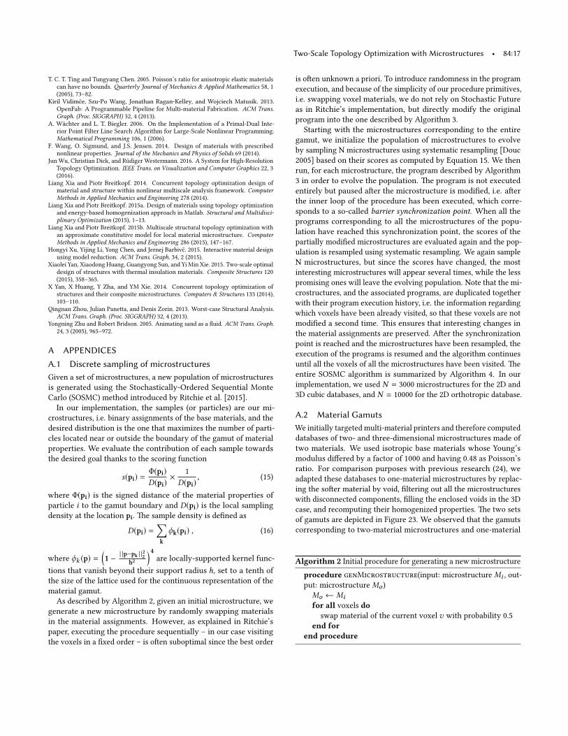
Two-Scale Topology Optimization with Microstructures • 84:17
T. C. T. Ting and Tungyang Chen. 2005. Poisson’s ratio for anisotropic elastic materials
can have no bounds. �arterly Journal of Mechanics & Applied Mathematics 58, 1
(2005), 73–82.
Kiril Vidimce, Szu-Po Wang, Jonathan Ragan-Kelley, and Wojciech Matusik. 2013.
OpenFab: A Programmable Pipeline for Multi-material Fabrication. ACM Trans.Graph. (Proc. SIGGRAPH) 32, 4 (2013).
A. Wachter and L. T. Biegler. 2006. On the Implementation of a Primal-Dual Inte-
rior Point Filter Line Search Algorithm for Large-Scale Nonlinear Programming.
Mathematical Programming 106, 1 (2006).
F. Wang, O. Sigmund, and J.S. Jensen. 2014. Design of materials with prescribed
nonlinear properties. Journal of the Mechanics and Physics of Solids 69 (2014).
Jun Wu, Christian Dick, and Rudiger Westermann. 2016. A System for High-Resolution
Topology Optimization. IEEE Trans. on Visualization and Computer Graphics 22, 3
(2016).
Liang Xia and Piotr Breitkopf. 2014. Concurrent topology optimization design of
material and structure within nonlinear multiscale analysis framework. ComputerMethods in Applied Mechanics and Engineering 278 (2014).
Liang Xia and Piotr Breitkopf. 2015a. Design of materials using topology optimization
and energy-based homogenization approach in Matlab. Structural and Multidisci-plinary Optimization (2015), 1–13.
Liang Xia and Piotr Breitkopf. 2015b. Multiscale structural topology optimization with
an approximate constitutive model for local material microstructure. ComputerMethods in Applied Mechanics and Engineering 286 (2015), 147–167.
Hongyi Xu, Yijing Li, Yong Chen, and Jernej Barbivc. 2015. Interactive material design
using model reduction. ACM Trans. Graph. 34, 2 (2015).
Xiaolei Yan, Xiaodong Huang, Guangyong Sun, and Yi Min Xie. 2015. Two-scale optimal
design of structures with thermal insulation materials. Composite Structures 120
(2015), 358–365.
X Yan, X Huang, Y Zha, and YM Xie. 2014. Concurrent topology optimization of
structures and their composite microstructures. Computers & Structures 133 (2014),
103–110.
Qingnan Zhou, Julian Pane�a, and Denis Zorin. 2013. Worst-case Structural Analysis.
ACM Trans. Graph. (Proc. SIGGRAPH) 32, 4 (2013).
Yongning Zhu and Robert Bridson. 2005. Animating sand as a �uid. ACM Trans. Graph.24, 3 (2005), 965–972.
A APPENDICES
A.1 Discrete sampling of microstructuresGiven a set of microstructures, a new population of microstructures
is generated using the Stochastically-Ordered Sequential Monte
Carlo (SOSMC) method introduced by Ritchie et al. [2015].
In our implementation, the samples (or particles) are our mi-
crostructures, i.e. binary assignments of the base materials, and the
desired distribution is the one that maximizes the number of parti-
cles located near or outside the boundary of the gamut of material
properties. We evaluate the contribution of each sample towards
the desired goal thanks to the scoring function
s(pi) =Φ(pi)D(pi)
× 1
D(pi), (15)
where Φ(pi) is the signed distance of the material properties of
particle i to the gamut boundary and D(pi) is the local sampling
density at the location pi. �e sample density is de�ned as
D(pi) =∑k
ϕk(pi) , (16)
where ϕk (p) =(1 − | |p−pk | |
22
h2
)4are locally-supported kernel func-
tions that vanish beyond their support radius h, set to a tenth of
the size of the la�ice used for the continuous representation of the
material gamut.
As described by Algorithm 2, given an initial microstructure, we
generate a new microstructure by randomly swapping materials
in the material assignments. However, as explained in Ritchie’s
paper, executing the procedure sequentially – in our case visiting
the voxels in a �xed order – is o�en suboptimal since the best order
is o�en unknown a priori. To introduce randomness in the program
execution, and because of the simplicity of our procedure primitives,
i.e. swapping voxel materials, we do not rely on Stochastic Future
as in Ritchie’s implementation, but directly modify the original
program into the one described by Algorithm 3.
Starting with the microstructures corresponding to the entire
gamut, we initialize the population of microstructures to evolve
by sampling N microstructures using systematic resampling [Douc
2005] based on their scores as computed by Equation 15. We then
run, for each microstructure, the program described by Algorithm
3 in order to evolve the population. �e program is not executed
entirely but paused a�er the microstructure is modi�ed, i.e. a�er
the inner loop of the procedure has been executed, which corre-
sponds to a so-called barrier synchronization point. When all the
programs corresponding to all the microstructures of the popu-
lation have reached this synchronization point, the scores of the
partially modi�ed microstructures are evaluated again and the pop-
ulation is resampled using systematic resampling. We again sample
N microstructures, but since the scores have changed, the most
interesting microstructures will appear several times, while the less
promising ones will leave the evolving population. Note that the mi-
crostructures, and the associated programs, are duplicated together
with their program execution history, i.e. the information regarding
which voxels have been already visited, so that these voxels are not
modi�ed a second time. �is ensures that interesting changes in
the material assignments are preserved. A�er the synchronization
point is reached and the microstructures have been resampled, the
execution of the programs is resumed and the algorithm continues
until all the voxels of all the microstructures have been visited. �e
entire SOSMC algorithm is summarized by Algorithm 4. In our
implementation, we used N = 3000 microstructures for the 2D and
3D cubic databases, and N = 10000 for the 2D orthotropic database.
A.2 Material GamutsWe initially targeted multi-material printers and therefore computed
databases of two- and three-dimensional microstructures made of
two materials. We used isotropic base materials whose Young’s
modulus di�ered by a factor of 1000 and having 0.48 as Poisson’s
ratio. For comparison purposes with previous research (24), we
adapted these databases to one-material microstructures by replac-
ing the so�er material by void, �ltering out all the microstructures
with disconnected components, �lling the enclosed voids in the 3D
case, and recomputing their homogenized properties. �e two sets
of gamuts are depicted in Figure 23. We observed that the gamuts
corresponding to two-material microstructures and one-material
Algorithm 2 Initial procedure for generating a new microstructure
procedure genMicrostructure(input: microstructure Mi , out-
put: microstructure Mo )
Mo ← Mifor all voxels do
swap material of the current voxel v with probability 0.5
end forend procedure
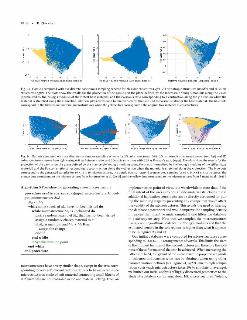
84:18 • B. Zhu et al.
Fig. 23. Gamuts computed with our discrete-continuous sampling scheme for 2D cubic structures (le�) , 2D orthotropic structures (middle) and 3D cubicstructures (right). The plots show the results for the projection of the gamuts on the plane defined by the macroscale Young’s modulus along the x axis(normalized by the Young’s modulus of the sti�est base material) and the Poisson’s ratio corresponding to a contraction along the y-direction when thematerial is stretched along the x-direction. All these plots correspond to microstructures that use 0.48 as Poisson’s ratio for the base material. The blue dotscorrespond to the filtered one-material microstructures while the yellow dots correspond to the original two-material microstructures.
Fig. 24. Gamuts computed with our discrete-continuous sampling scheme for 2D cubic structures (le�) , 2D orthotropic structures (second from le�) and 3Dcubic structures (second from right) using 0.48 as Poisson’s ratio, and 3D cubic structures with 0.35 as Poisson’s ratio (right). The plots show the results for theprojection of the gamuts on the plane defined by the macroscale Young’s modulus along the x axis (normalized by the Young’s modulus of the sti�est basematerial) and the Poisson’s ratio corresponding to a contraction along the y-direction when the material is stretched along the x-direction. The blue dotscorrespond to the generated samples for 16 × 16 × 16 microstructures, the purple dots correspond to generated samples for 64 × 64 × 64 microstructures, theorange dots correspond to the microstructures from Schumacher et al. [2015] and the yellow dots correspond to the microstructures from Pane�a et al. [2015].
Algorithm 3 Procedure for generating a new microstructure
procedure genMicrostructure(input: microstructure Mi , out-
put: microstructure Mo )
Mo ← Miwhile some voxels of Mo have not been visited do
while microstructure Mo is unchanged dopick a random voxel v of Mo that has not been visited
assign a randomly chosen material to vif Mo is manifold and Mo , Mi then
accept the change
end ifend while// Synchronization point
end whileend procedure
microstructures have a very similar shape, except in the area corre-
sponding to very so� microstructures. �is is to be expected since
microstructures made of so� material connecting small blocks of
sti� materials are not realizable in the one-material se�ing. From an
implementation point of view, it is worthwhile to note that, if the
�nal intent of the user is to design one-material structures, these
additional fabrication constraints can be directly accounted for dur-
ing the sampling stage by preventing any change that would a�ect
the validity of the microstructures. �is avoids the need of �ltering
the database a posteriori and would improve the sampling density
in regions that might be undersampled if one �lters the database
in a subsequent step. Note that we sampled the microstructures
using a non-logarithmic scale for the Young’s modulus and that the
estimated density in the so� regions is higher than what it appears
to be in Figures 23 and 24.
Our initial databases were computed for microstructures corre-
sponding to 16×16×16 arrangements of voxels. �is limits the sizes
of the thinnest features of the microstructures and therefore the so�-
ness of the so�er material that can be achieved. When increasing the
la�ice size to 64, the gamut of the microstructure properties expands
in this area and reaches what can be obtained when using other
parametrization methods (see Figure 24, right). Due to high compu-
tation costs (each microstructure takes 29s to simulate in average),
we limited our initial analysis of highly discretized geometries to the
study of a database comprising about 10k microstructures. Notably,
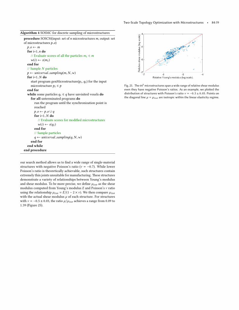
Two-Scale Topology Optimization with Microstructures • 84:19
Algorithm 4 SOSMC for discrete sampling of microstructures
procedure SOSCM(input: set of n microstructuresm, output: set
of microstructures p o)
p o ←mfor i=1..n do
// Evaluate scores of all the particlesmi ∈mw(i) ← s(mi )
end for// Sample N particles
p ← universal samplinд(m,N ,w)for i=1..N do
start program genMicrostructure(pi , qi ) for the input
microstructure pi ∈ pend forwhile some particles qi ∈ q have unvisited voxels do
for all unterminated programs dorun the program until the synchronization point is
reached
p o ← p o ∪ qfor i=1..N do
// Evaluate scores for modi�ed microstructures
w(i) ← s(qi )end for// Sample particles
q ← universal samplinд(q,N ,w)end for
end whileend procedure
our search method allows us to �nd a wide range of single-material
structures with negative Poisson’s ratio (ν = −0.7). While lower
Poisson’s ratio is theoretically achievable, such structures contain
extremely thin joints unsuitable for manufacturing. �ese structures
demonstrate a variety of relationships between Young’s modulus
and shear modulus. To be more precise, we de�ne µiso as the shear
modulus computed from Young’s modulus E and Poisson’s ν ratio
using the relationship µiso = E/(1 − 2 × ν ). We then compare µisowith the actual shear modulus µ of each structure. For structures
with ν = −0.5 ± 0.03, the ratio µ/µiso achieves a range from 0.09 to
1.39 (Figure 25).
Fig. 25. The 643 microstructures span a wide range of relative shear modulus
even they have negative Poisson’s ratios. As an example, we plo�ed thedistribution of structures with Poisson’s ratio ν = −0.5 ± 0.03. Points onthe diagonal line µ = µiso are isotropic within the linear elasticity regime.