


Langages
Pages
Légal

Imagerie SAR multi-modale pour la télédétection d'environnements
Laurent Ferro-Famil
Institut d’Electronique et de Télécommunications de Rennes – IETRUMR 6164
Université de Rennes 1
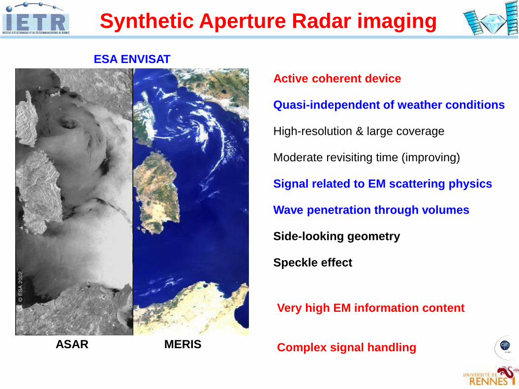
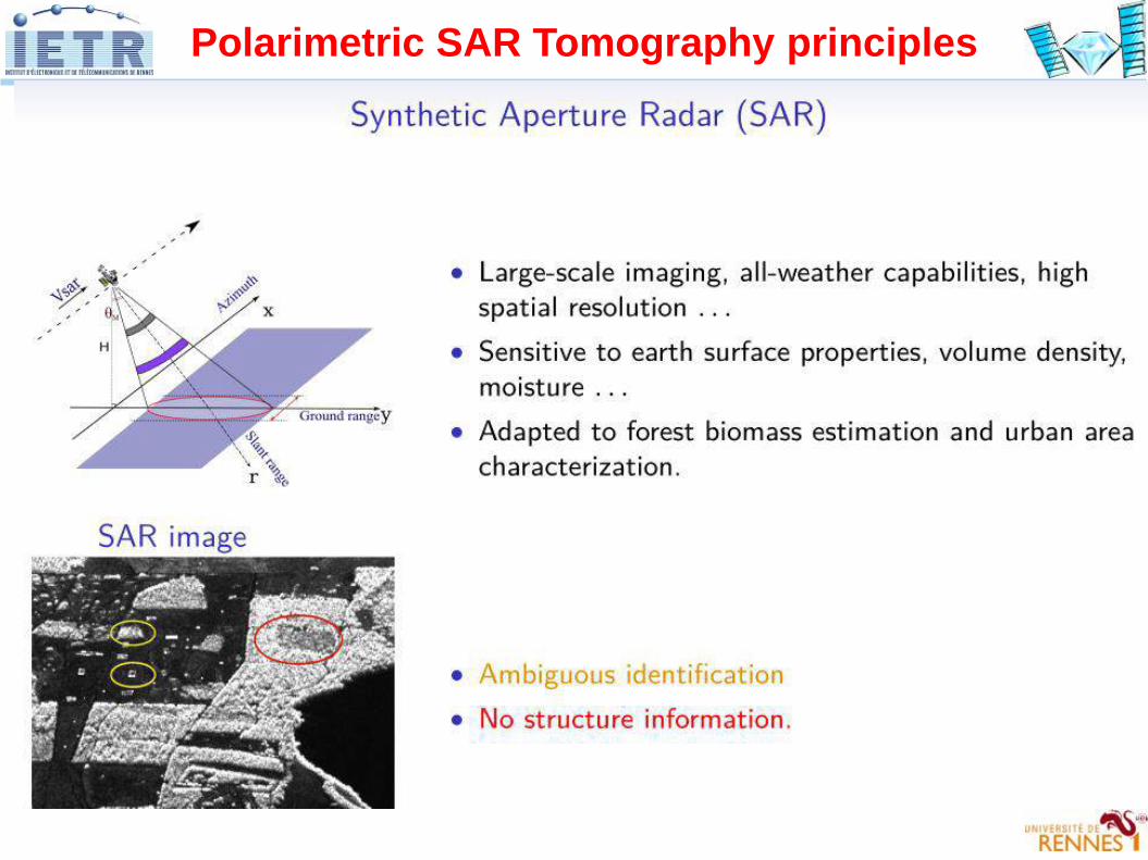
Synthetic Aperture Radar imaging
ESA ENVISAT
ASAR MERIS
Active coherent device
Quasi-independent of weather conditions
High-resolution & large coverage
Moderate revisiting time (improving)
Signal related to EM scattering physics
Wave penetration through volumes
Side-looking geometry
Speckle effect
Very high EM information content
Complex signal handling
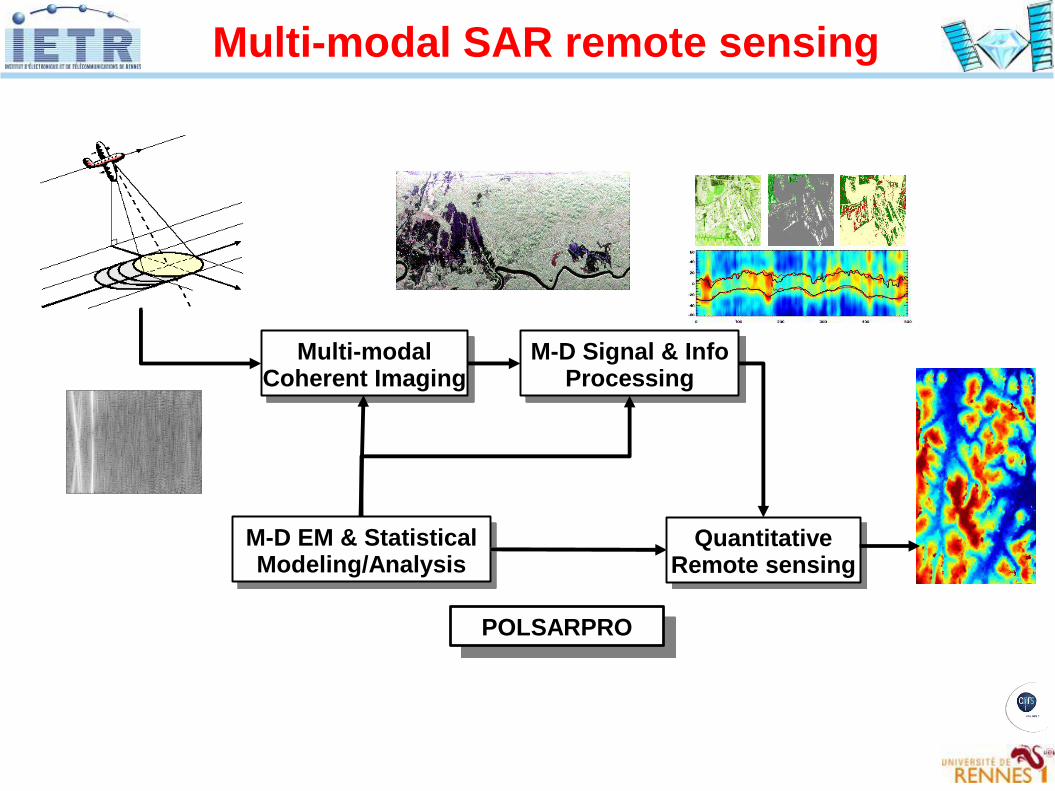
Multi-modalCoherent Imaging
M-D Signal & InfoProcessing
QuantitativeRemote sensing
M-D EM & StatisticalModeling/Analysis
Multi-modal SAR remote sensing
POLSARPRO
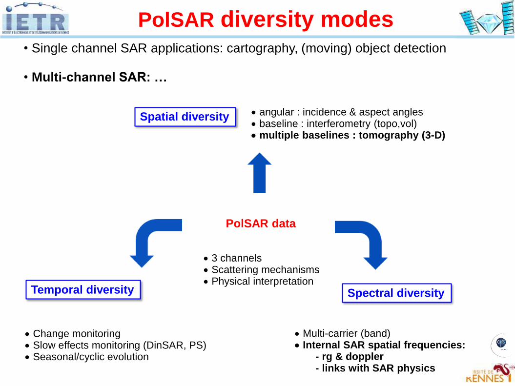
PolSAR data
Spatial diversity
Spectral diversityTemporal diversity
PolSAR diversity modes
angular : incidence & aspect angles baseline : interferometry (topo,vol) multiple baselines : tomography (3-D)
Change monitoring Slow effects monitoring (DinSAR, PS) Seasonal/cyclic evolution
Multi-carrier (band) Internal SAR spatial frequencies:
- rg & doppler- links with SAR physics
3 channels Scattering mechanisms Physical interpretation
• Single channel SAR applications: cartography, (moving) object detection
• Multi-channel SAR: …
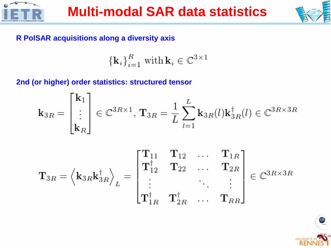
Multi-modal SAR data statistics
R PolSAR acquisitions along a diversity axis
2nd (or higher) order statistics: structured tensor
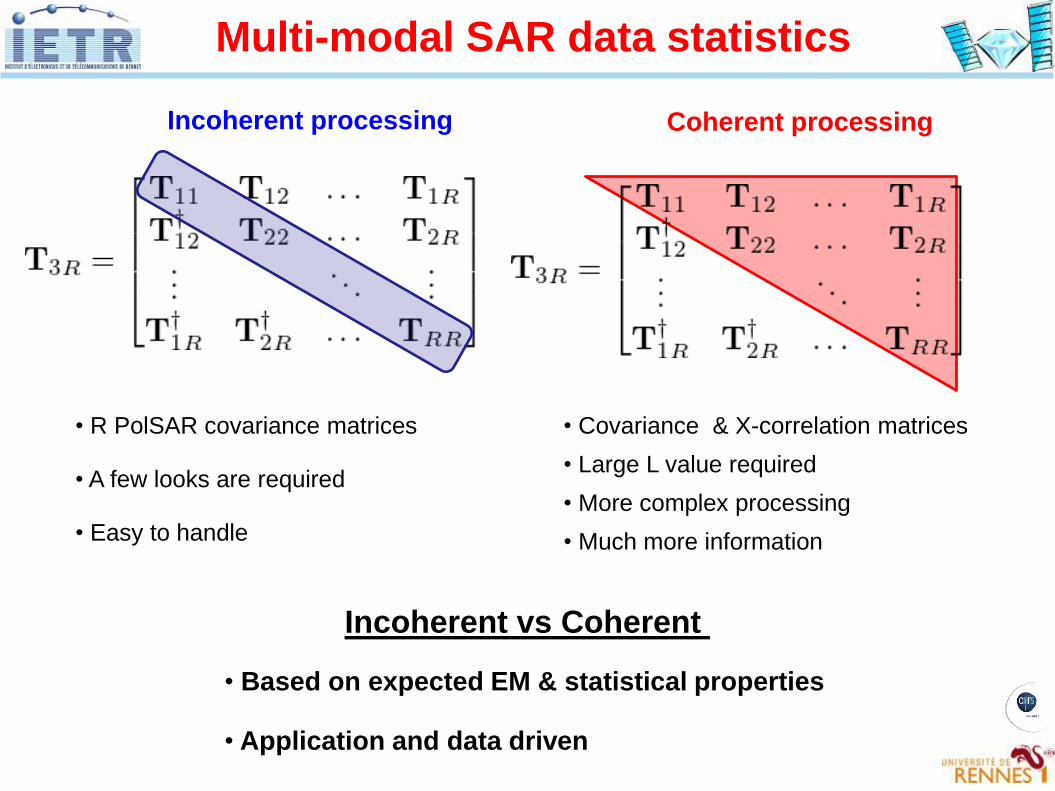
Multi-modal SAR data statistics
• R PolSAR covariance matrices
• A few looks are required
• Easy to handle
• Covariance & X-correlation matrices
• Large L value required
• More complex processing
• Much more information
Incoherent processing Coherent processing
Incoherent vs Coherent
• Based on expected EM & statistical properties
• Application and data driven
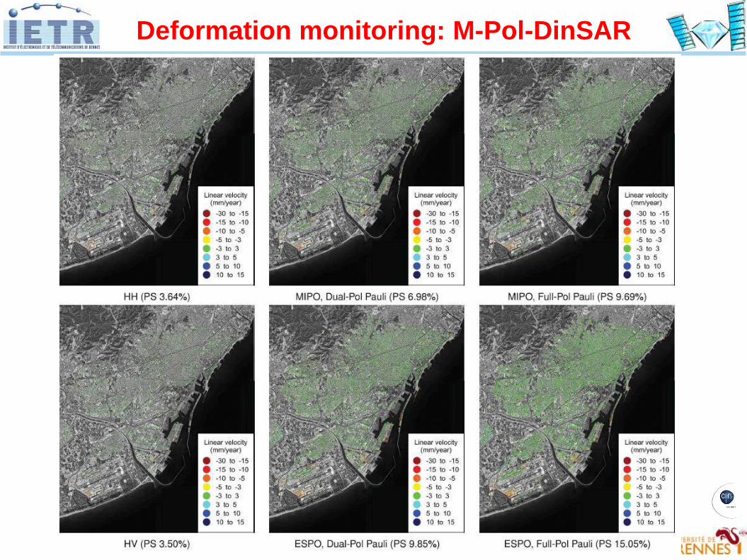
Deformation monitoring: M-Pol-DinSAR
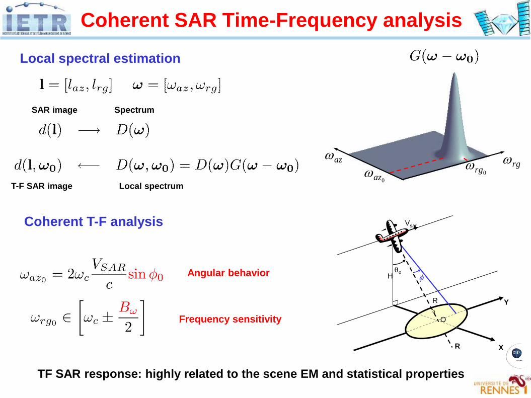
Coherent SAR Time-Frequency analysis
Vsar
Hqo
Ro
O
XR
Y
Coherent T-F analysis
0azaz
rg0rg
Angular behavior
Frequency sensitivity
Local spectral estimation
SAR image Spectrum
Local spectrumT-F SAR image
TF SAR response: highly related to the scene EM and statistical properties
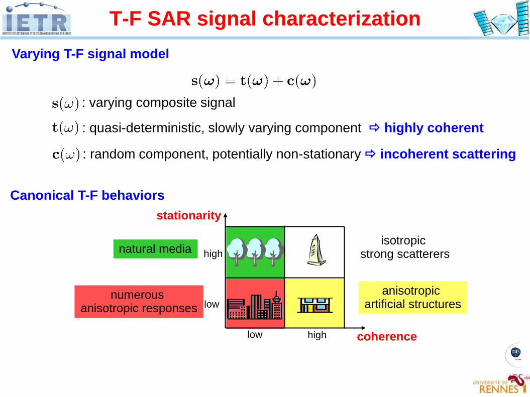
T-F SAR signal characterization
Varying T-F signal model
: varying composite signal
: quasi-deterministic, slowly varying component highly coherent
: random component, potentially non-stationary incoherent scattering
Canonical T-F behaviorsstationarity
coherencelow high
low
highnatural mediaisotropic
strong scatterers
anisotropic artificial structures
numerous anisotropic responses
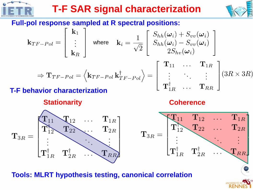
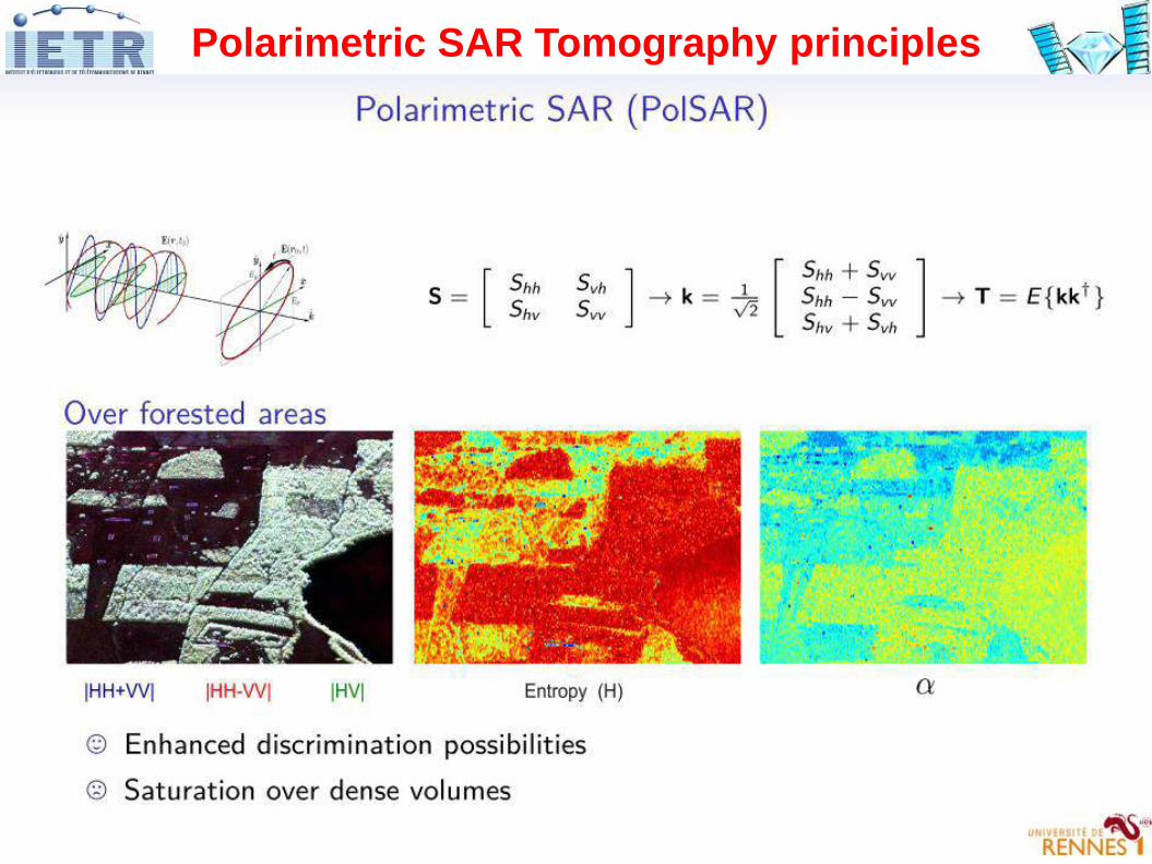
Full-pol response sampled at R spectral positions:
where
T-F behavior characterization
Stationarity Coherence
Tools: MLRT hypothesis testing, canonical correlation
T-F SAR signal characterization
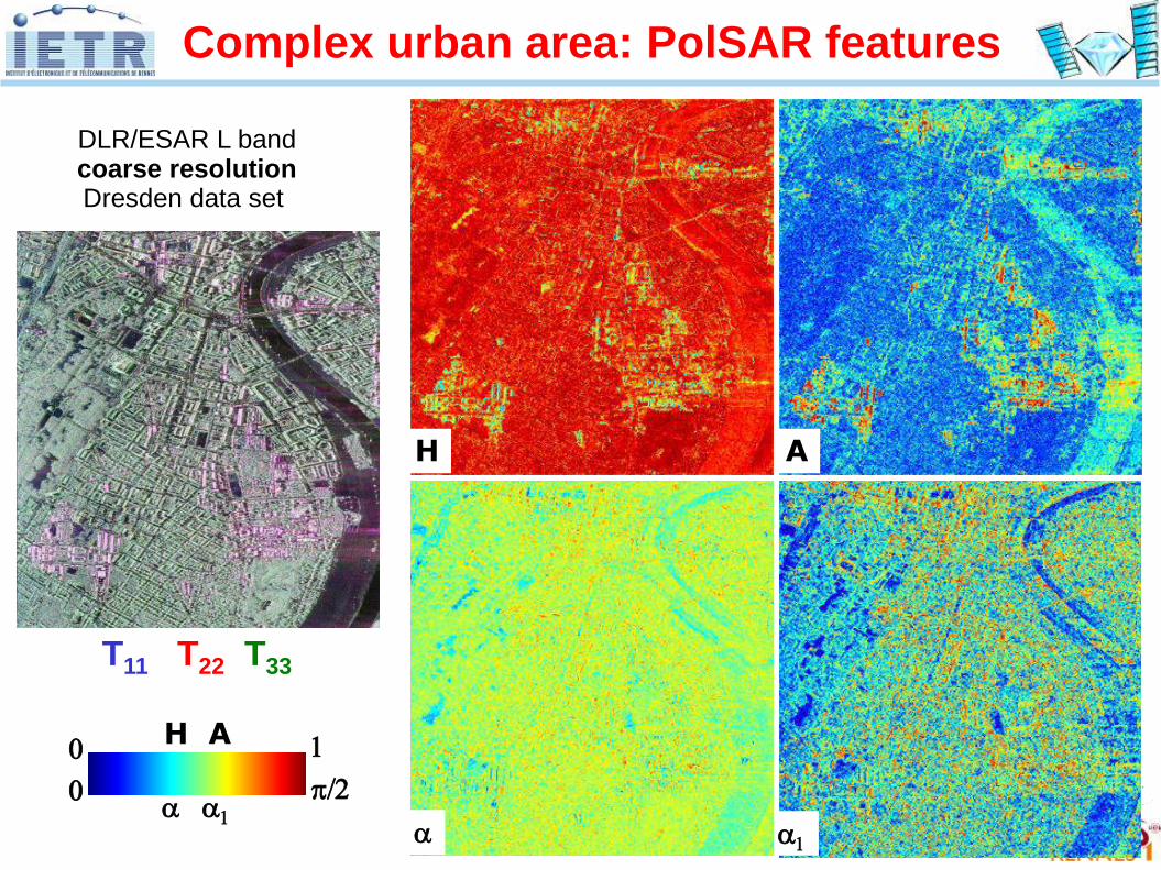
H A
a a1
0
0
1
p/2
T11 T22 T33
H A
a1a
Complex urban area: PolSAR features
DLR/ESAR L bandcoarse resolutionDresden data set
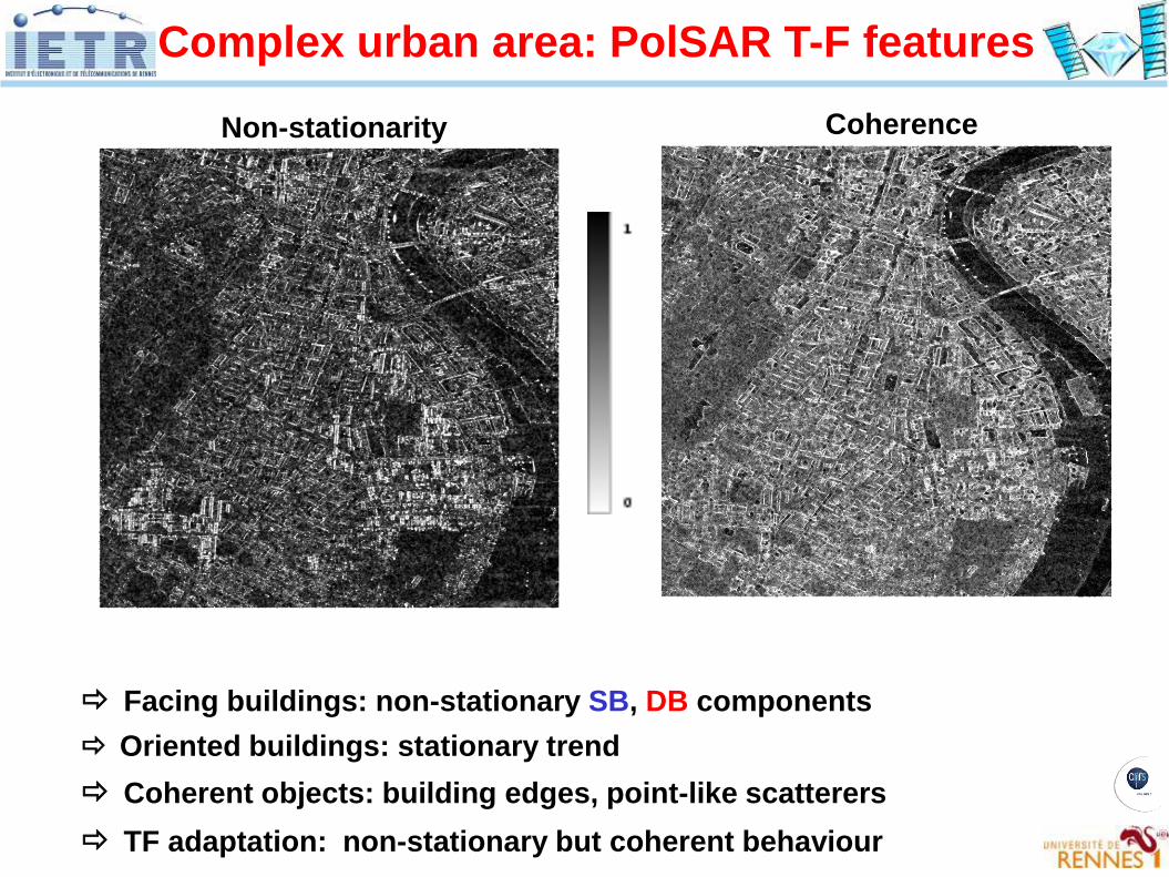
Non-stationarity
Facing buildings: non-stationary SB, DB components
Oriented buildings: stationary trend
Coherent objects: building edges, point-like scatterers
TF adaptation: non-stationary but coherent behaviour
Coherence
Complex urban area: PolSAR T-F features
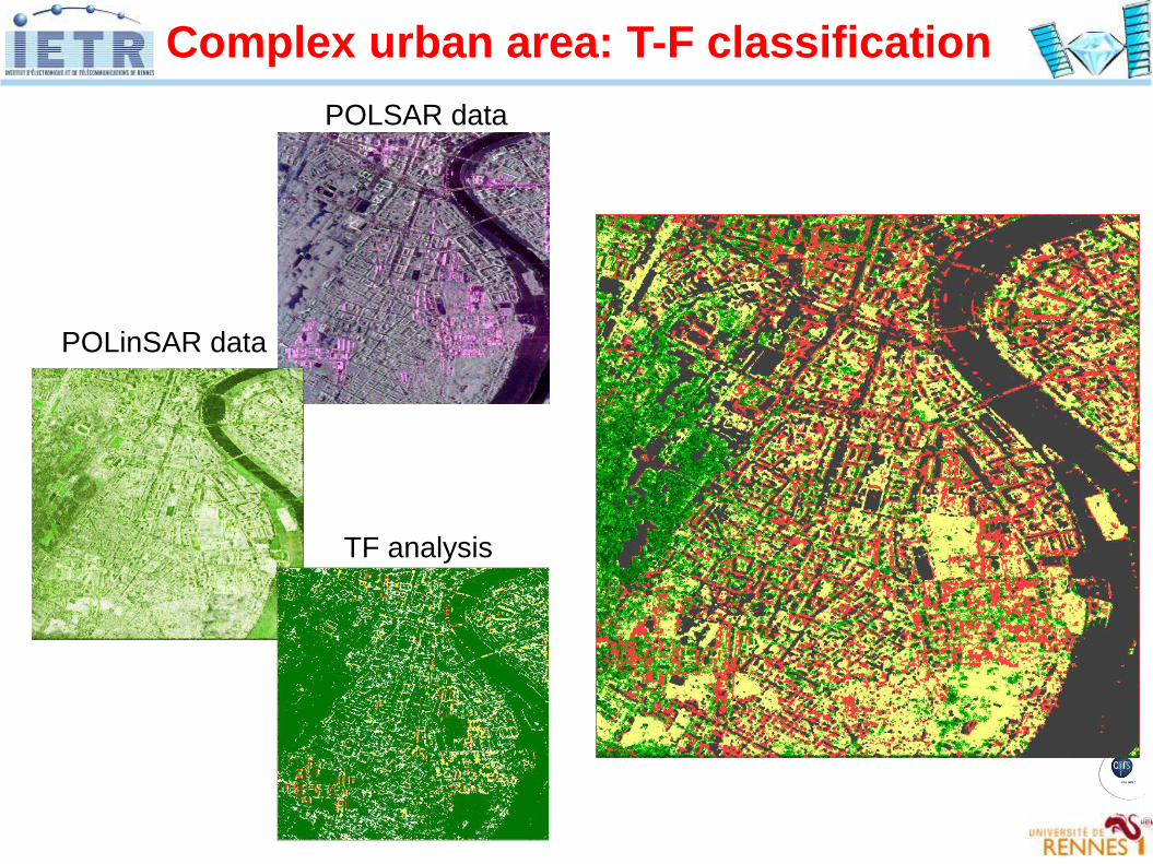
POLSAR data
POLinSAR data
TF analysis
Complex urban area: T-F classification
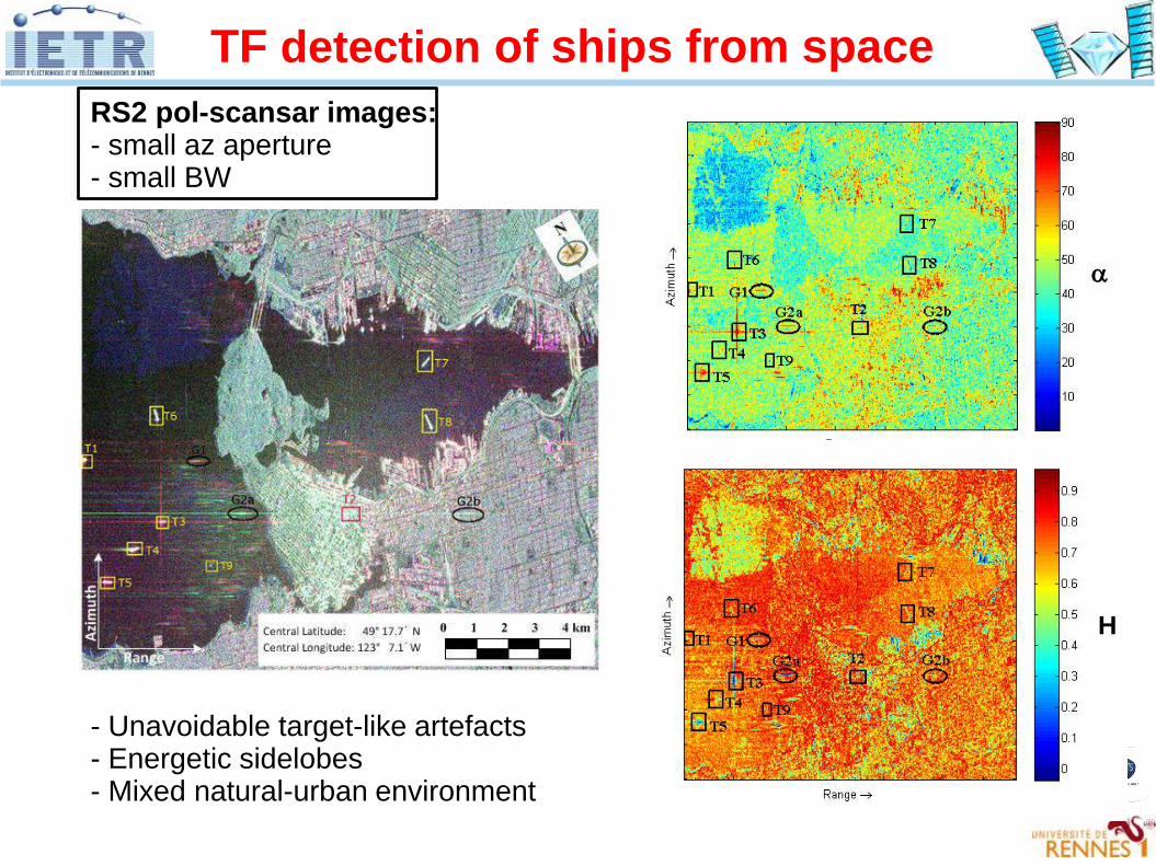
TF detection of ships from spaceRS2 pol-scansar images: - small az aperture- small BW
- Unavoidable target-like artefacts - Energetic sidelobes- Mixed natural-urban environment
H
a
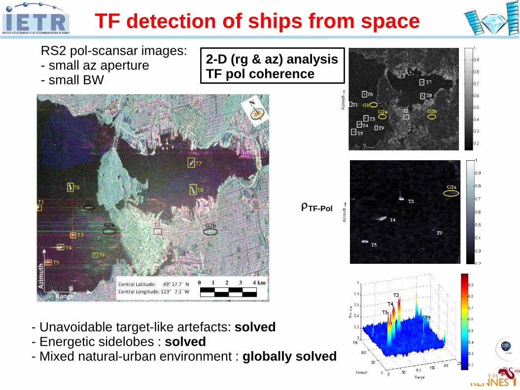
RS2 pol-scansar images: - small az aperture- small BW
- Unavoidable target-like artefacts: solved- Energetic sidelobes : solved- Mixed natural-urban environment : globally solved
2-D (rg & az) analysisTF pol coherence
TF detection of ships from space
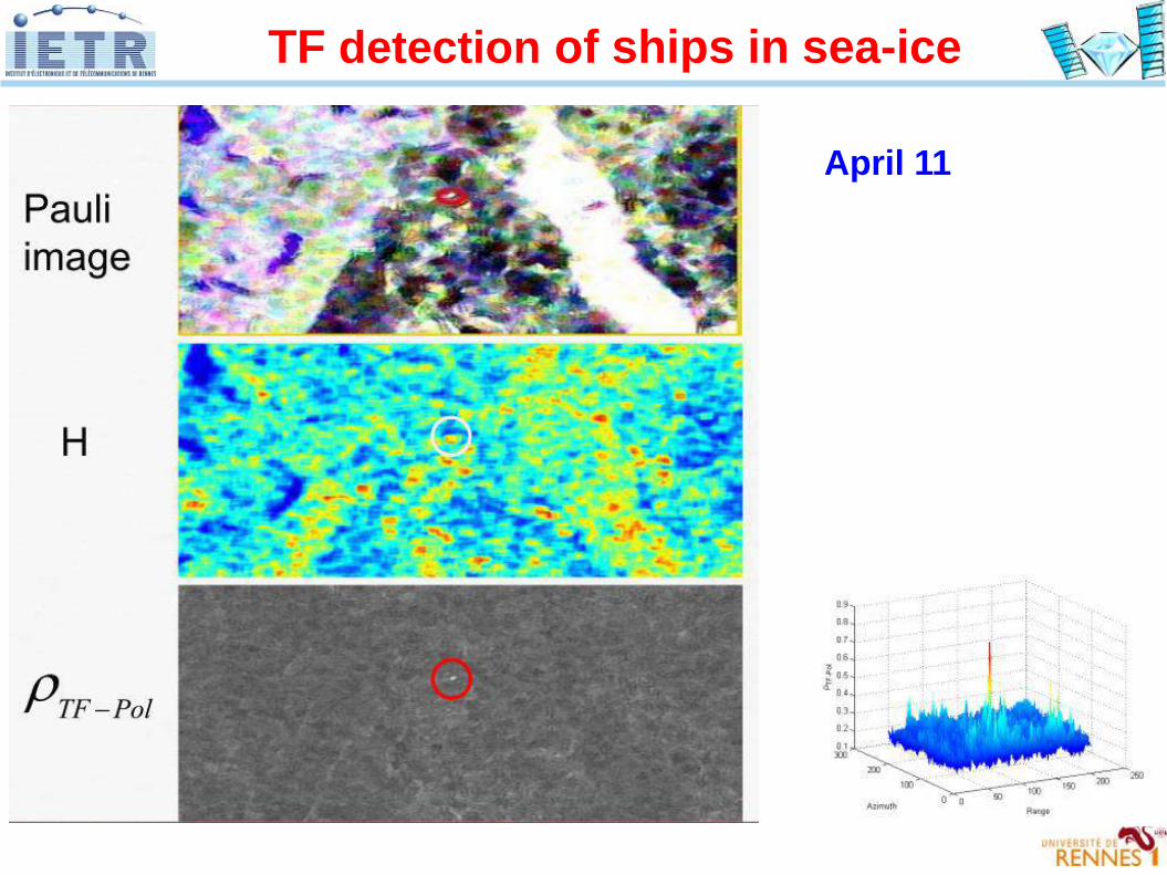
rTF-Pol
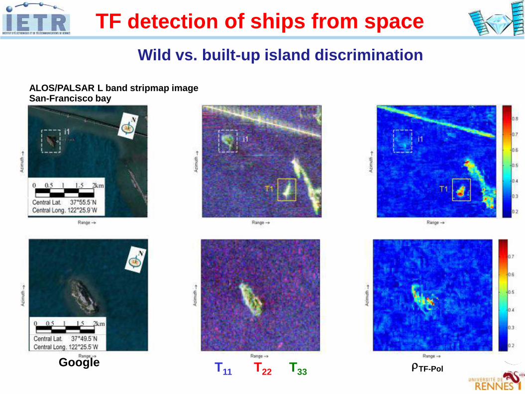
rTF-PolGoogle T11 T22 T33
Wild vs. built-up island discrimination
ALOS/PALSAR L band stripmap image San-Francisco bay
TF detection of ships from space
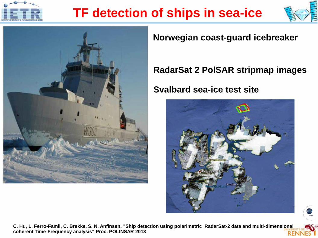
C. Hu, L. Ferro-Famil, C. Brekke, S. N. Anfinsen, "Ship detection using polarimetric RadarSat-2 data and multi-dimensional coherent Time-Frequency analysis" Proc. POLINSAR 2013
Norwegian coast-guard icebreaker
RadarSat 2 PolSAR stripmap images
Svalbard sea-ice test site
TF detection of ships in sea-ice
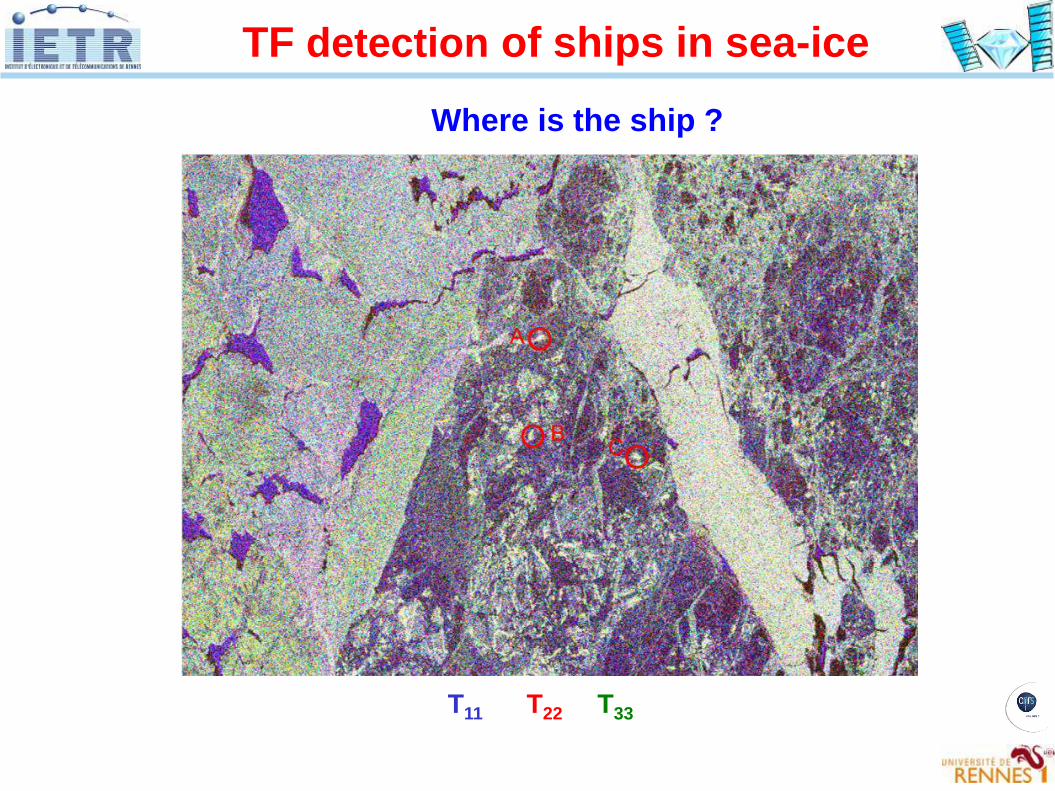
Where is the ship ?
T11 T22 T33
TF detection of ships in sea-ice
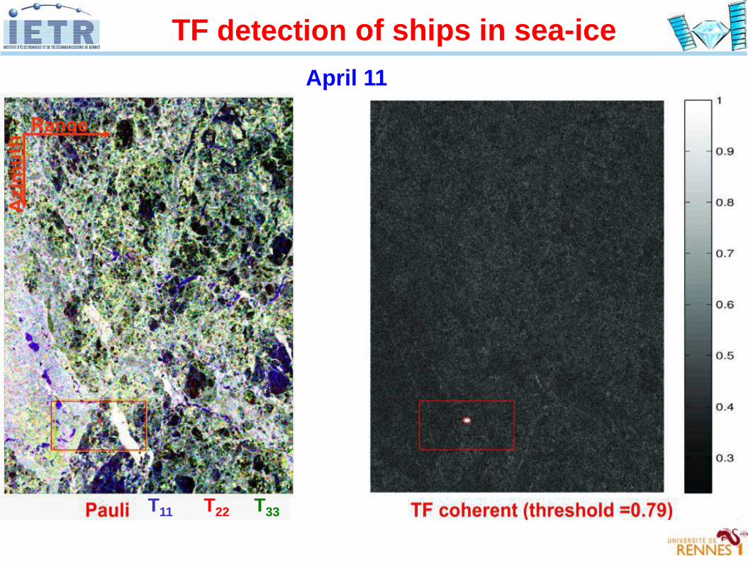
April 11
T11 T22 T33
TF detection of ships in sea-ice
April 11
TF detection of ships in sea-ice
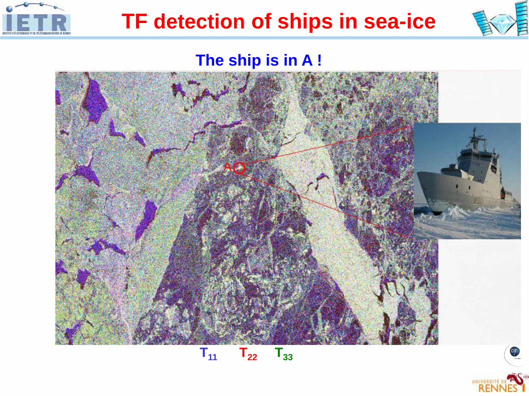
The ship is in A !
T11 T22 T33
TF detection of ships in sea-ice
Polarimetric SAR Tomography principles
Polarimetric SAR Tomography principles
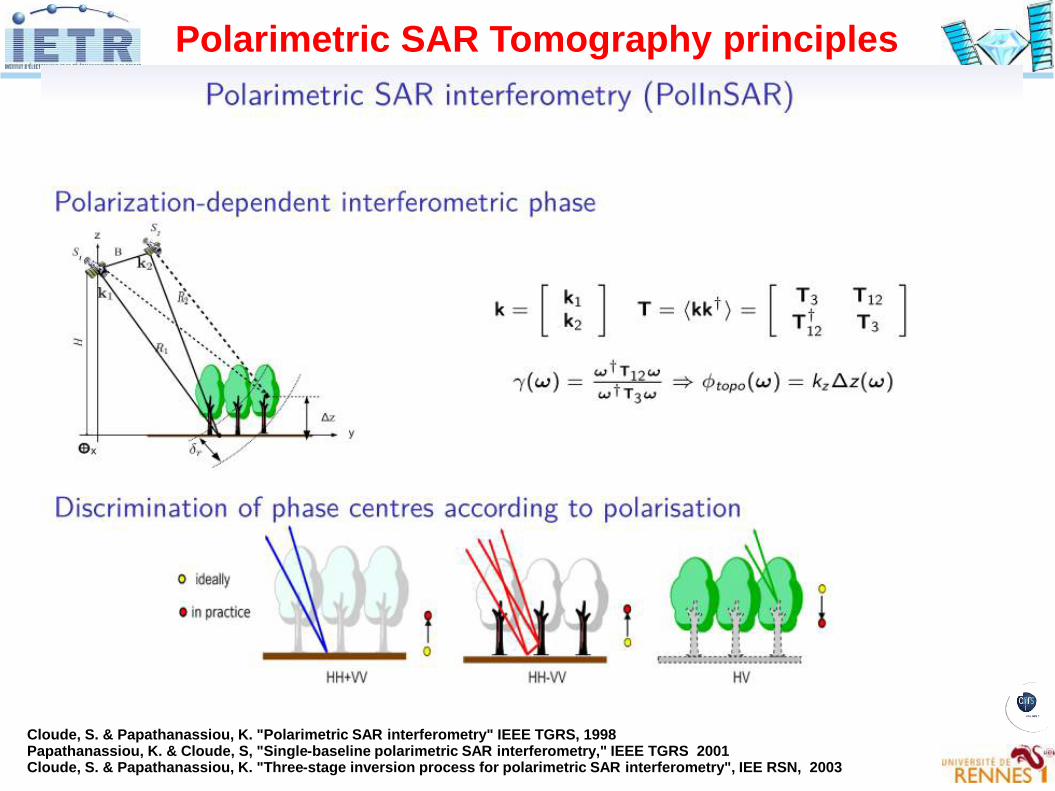
Cloude, S. & Papathanassiou, K. "Polarimetric SAR interferometry" IEEE TGRS, 1998Papathanassiou, K. & Cloude, S, "Single-baseline polarimetric SAR interferometry," IEEE TGRS 2001Cloude, S. & Papathanassiou, K. "Three-stage inversion process for polarimetric SAR interferometry", IEE RSN, 2003
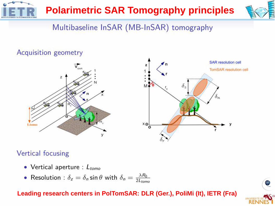
Polarimetric SAR Tomography principles
Polarimetric SAR Tomography principles
Leading research centers in PolTomSAR: DLR (Ger.), PoliMi (It), IETR (Fra)
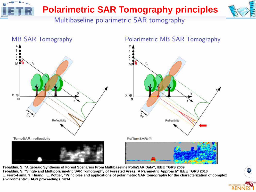
Tebaldini, S. "Algebraic Synthesis of Forest Scenarios From Multibaseline PolInSAR Data", IEEE TGRS 2009Tebaldini, S. "Single and Multipolarimetric SAR Tomography of Forested Areas: A Parametric Approach" IEEE TGRS 2010L. Ferro-Famil, Y. Huang, E. Pottier, “Principles and applications of polarimetric SAR tomography for the characterization of complex environments”, IAGS proceedings, 2014
Polarimetric SAR Tomography principles
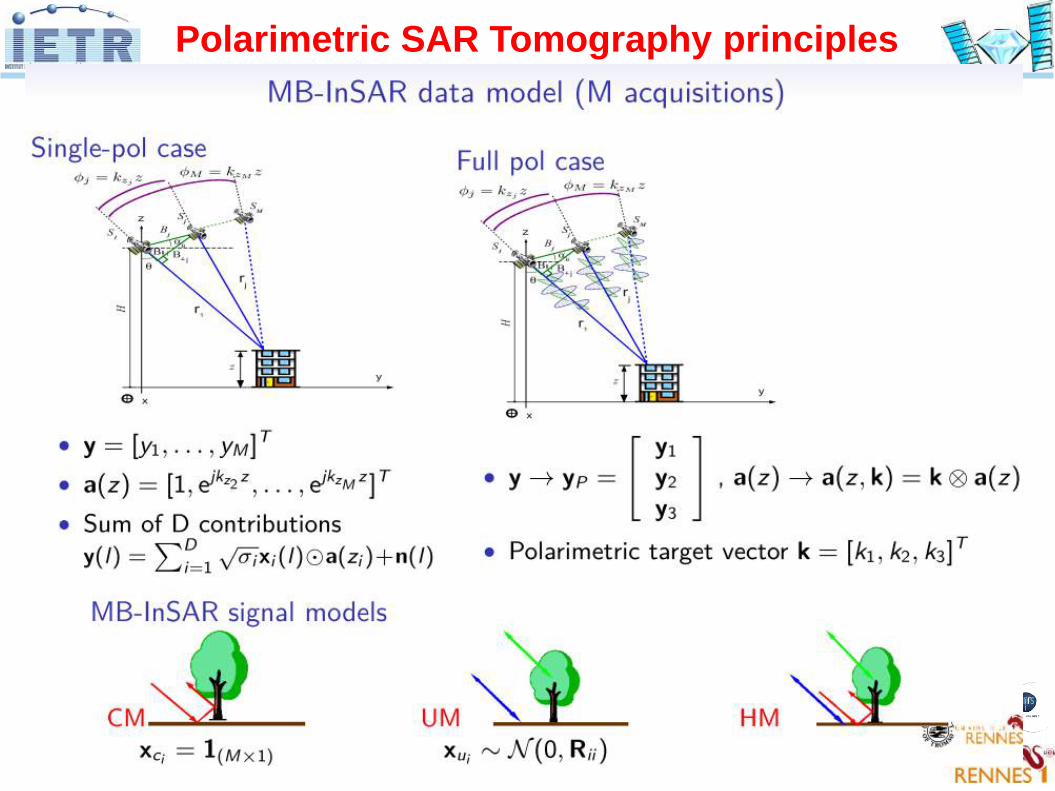
Polarimetric SAR Tomography principles
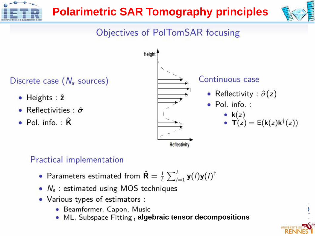
Polarimetric SAR Tomography principles
, algebraic tensor decompositions
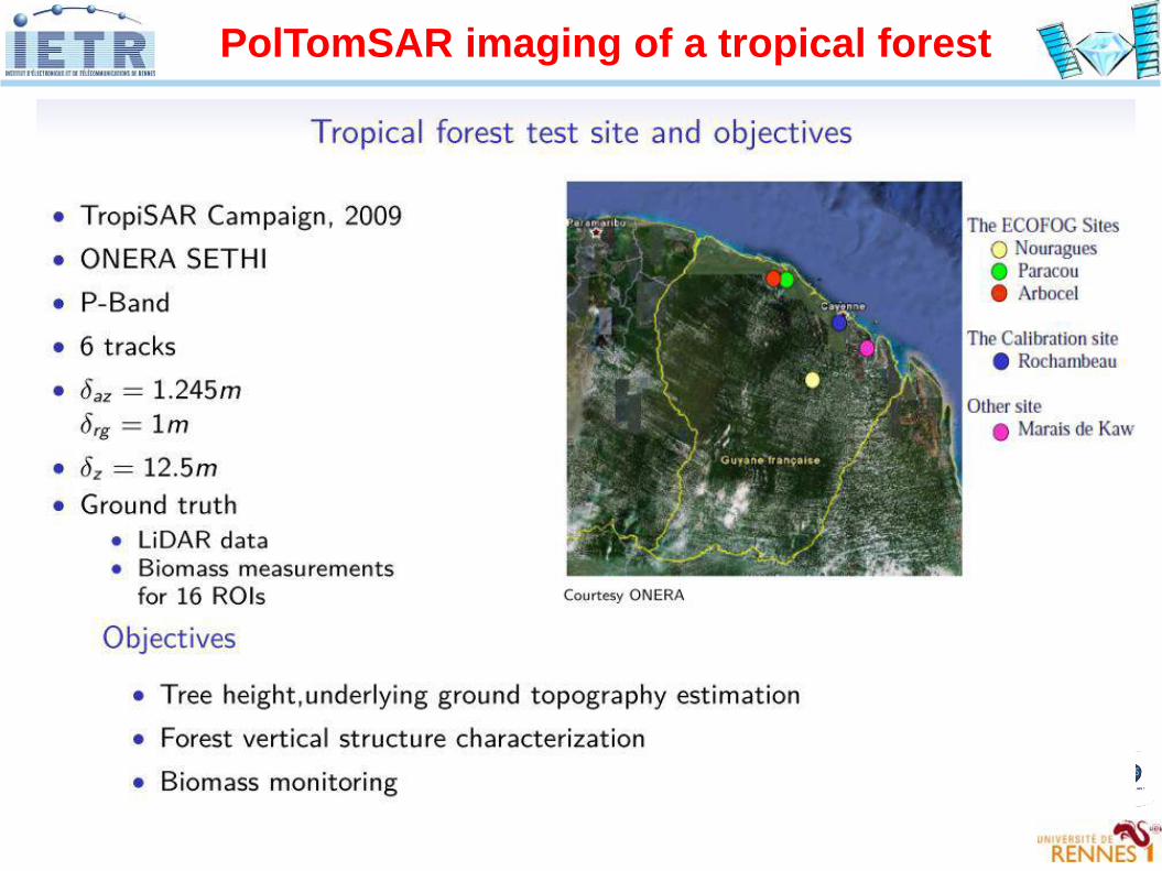
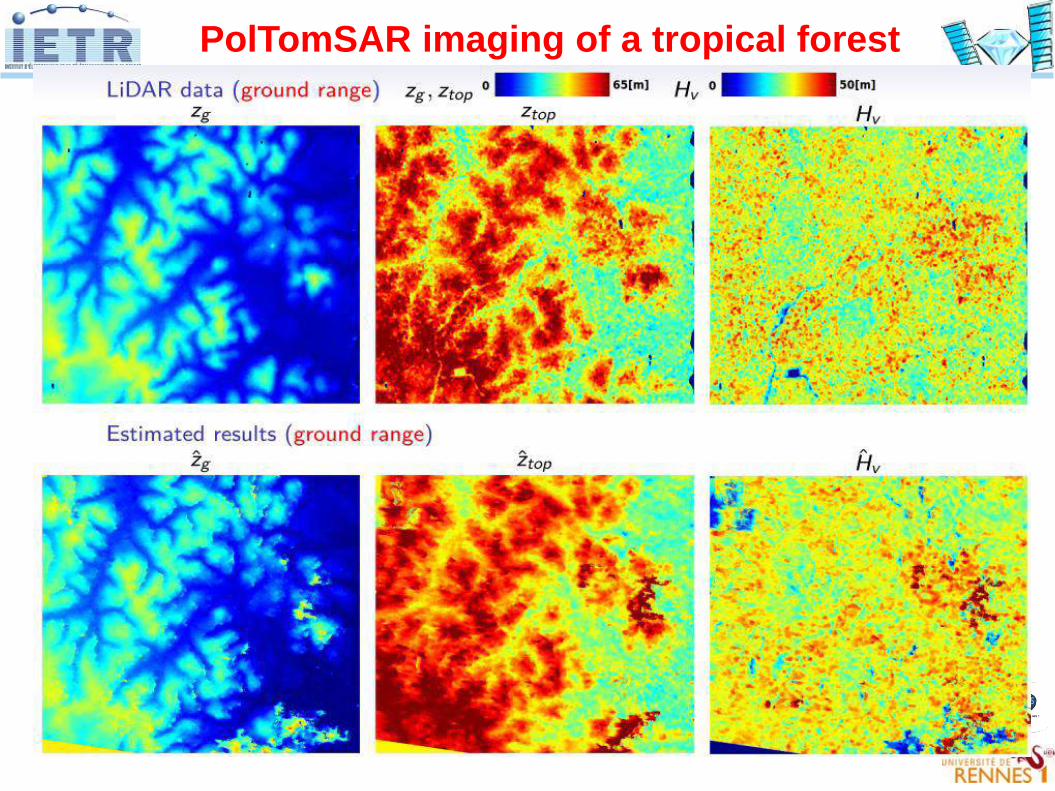
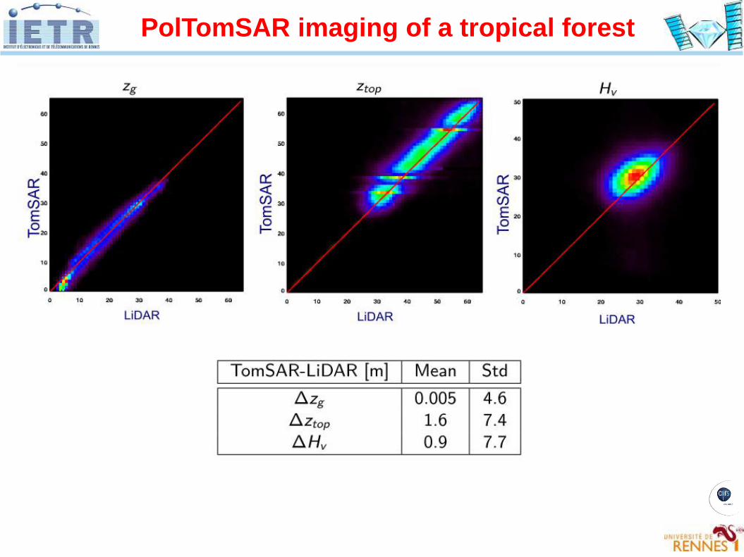
PolTomSAR imaging of a tropical forest
PolTomSAR imaging of a tropical forest
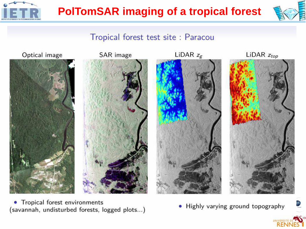
PolTomSAR imaging of a tropical forest
PolTomSAR imaging of a tropical forest
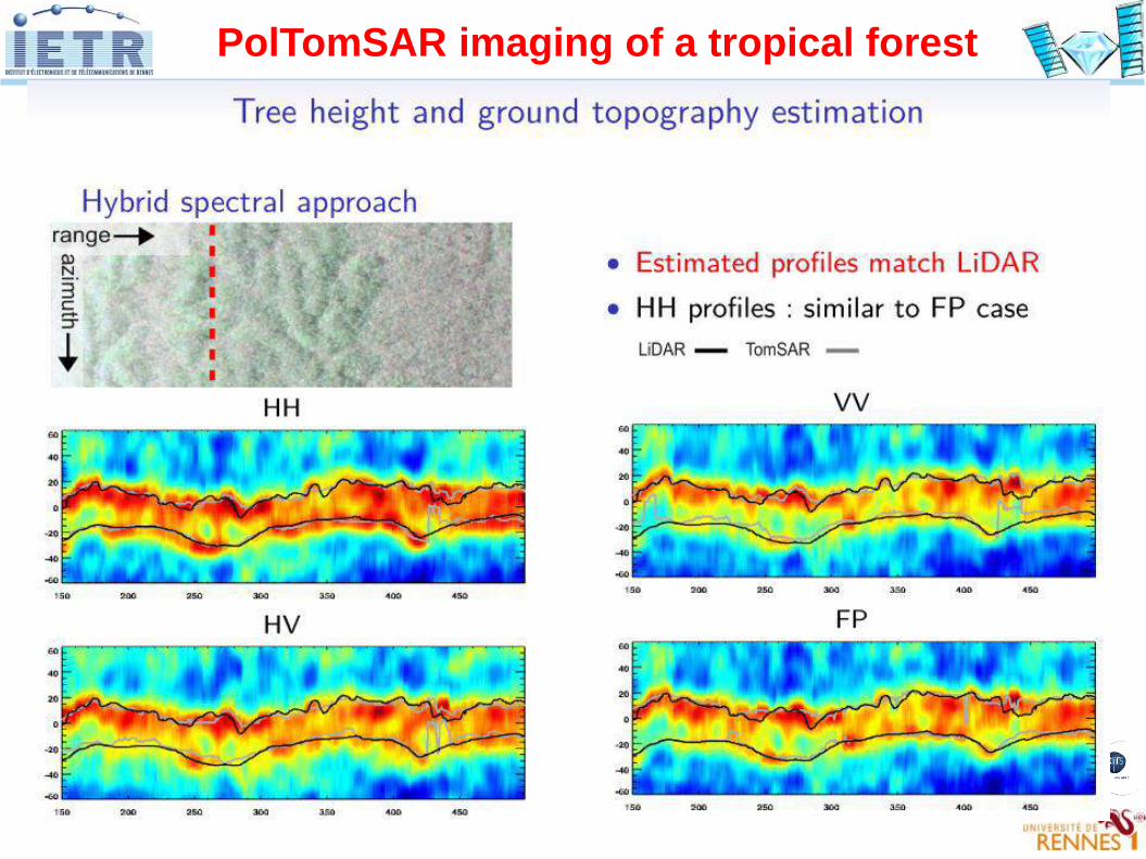
PolTomSAR imaging of a tropical forest
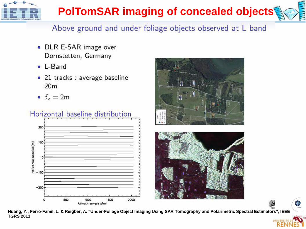
Huang, Y.; Ferro-Famil, L. & Reigber, A. "Under-Foliage Object Imaging Using SAR Tomography and Polarimetric Spectral Estimators", IEEE TGRS 2011
PolTomSAR imaging of concealed objects
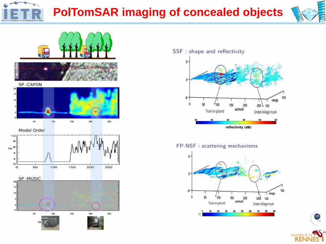
PolTomSAR imaging of concealed objects
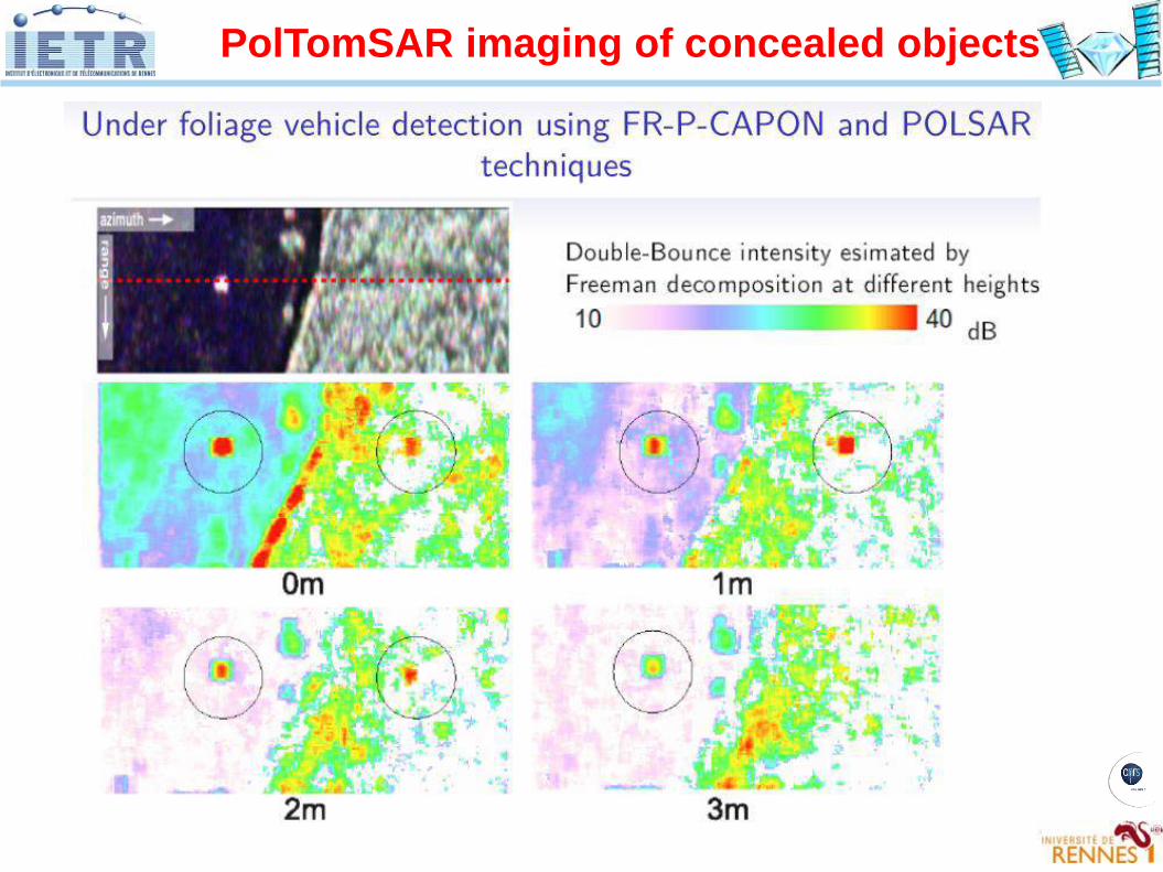
PolTomSAR imaging of concealed objects
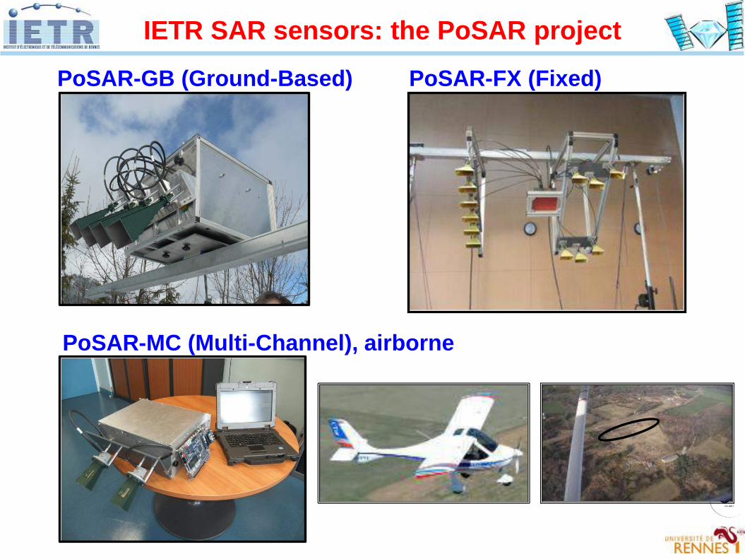
IETR SAR sensors: the PoSAR project
PoSAR-GB (Ground-Based) PoSAR-FX (Fixed)
PoSAR-MC (Multi-Channel), airborne
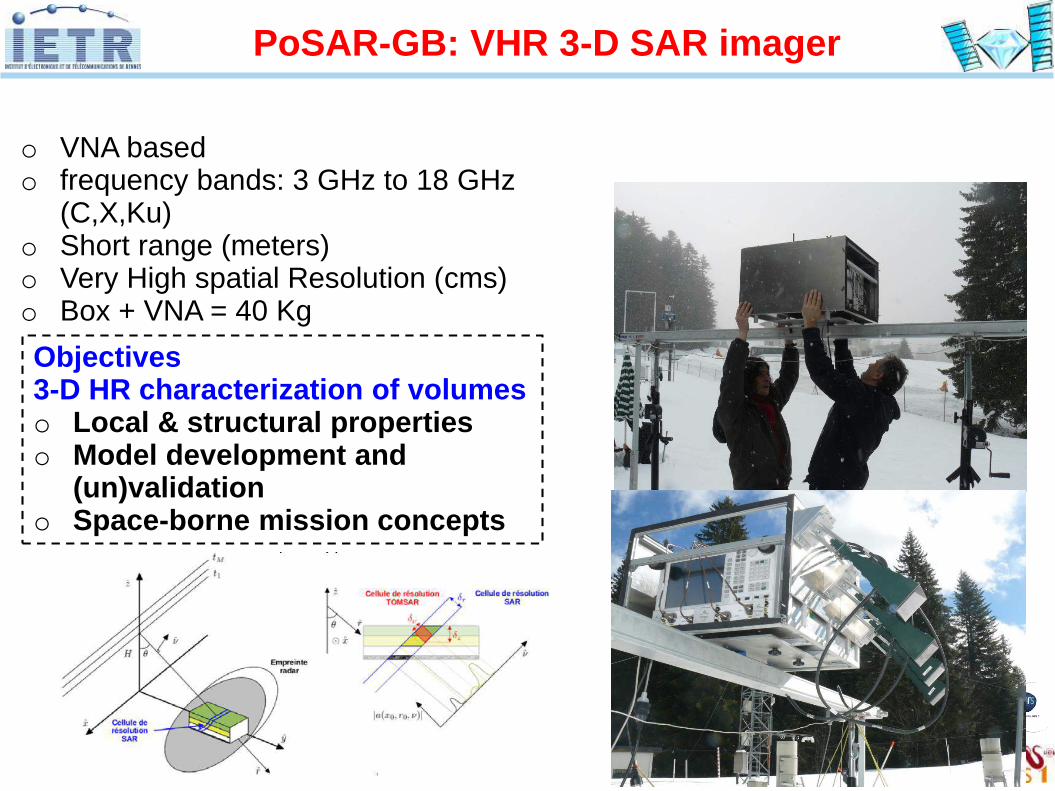
o VNA basedo frequency bands: 3 GHz to 18 GHz
(C,X,Ku) o Short range (meters)o Very High spatial Resolution (cms) o Box + VNA = 40 Kg
Objectives3-D HR characterization of volumeso Local & structural propertieso Model development and
(un)validationo Space-borne mission concepts
PoSAR-GB: VHR 3-D SAR imager
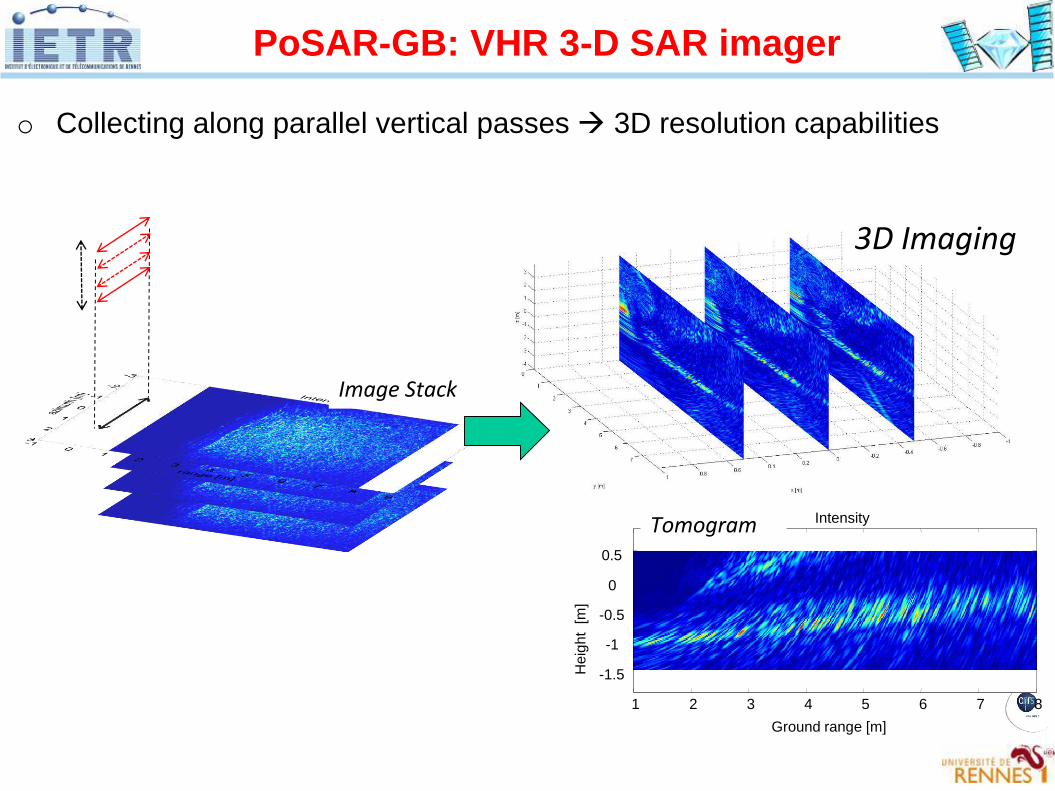
o Collecting along parallel vertical passes 3D resolution capabilities
3D Imaging
Image Stack
Ground range [m]
Hei
ght
[m]
Intensity
1 2 3 4 5 6 7 8
-1.5
-1
-0.5
0
0.5
Tomogram
PoSAR-GB: VHR 3-D SAR imager
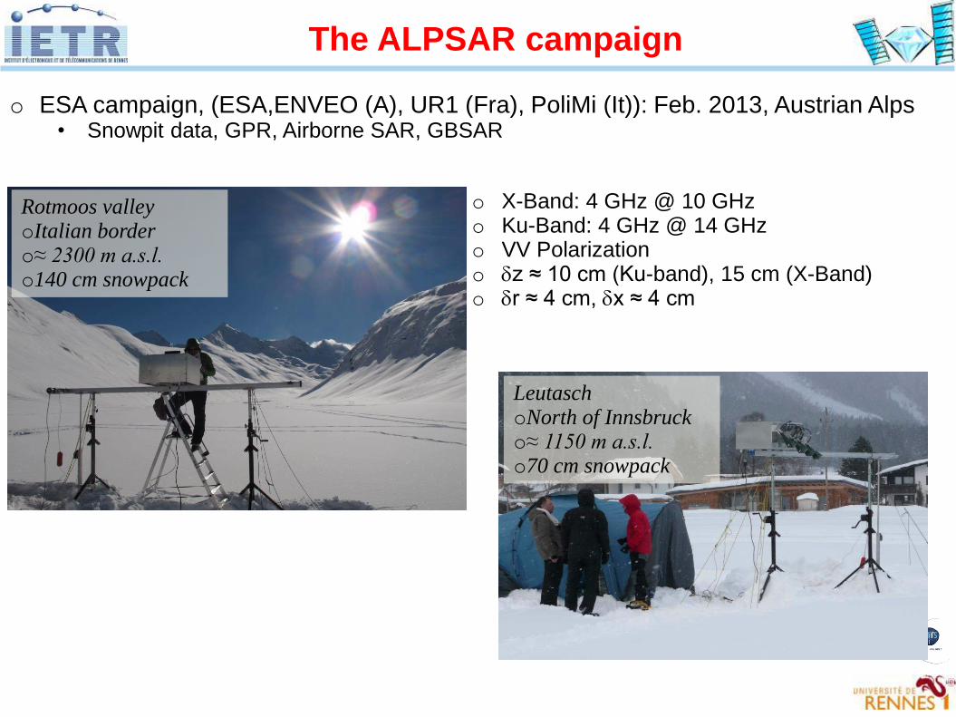
o ESA campaign, (ESA,ENVEO (A), UR1 (Fra), PoliMi (It)): Feb. 2013, Austrian Alps• Snowpit data, GPR, Airborne SAR, GBSAR
o X-Band: 4 GHz @ 10 GHzo Ku-Band: 4 GHz @ 14 GHzo VV Polarizationo dz ≈ 10 cm (Ku-band), 15 cm (X-Band) o dr ≈ 4 cm, dx ≈ 4 cm
LeutaschoNorth of Innsbrucko≈ 1150 m a.s.l.o70 cm snowpack
Rotmoos valleyoItalian bordero≈ 2300 m a.s.l. o140 cm snowpack
The ALPSAR campaign
y [m]
z [m
]
0 1 2 3 4 5 6 7-2
-1.5
-1
-0.5
0
0.5
y [m]
z [m
]
0 1 2 3 4 5 6 7-2
-1.5
-1
-0.5
0
0.5
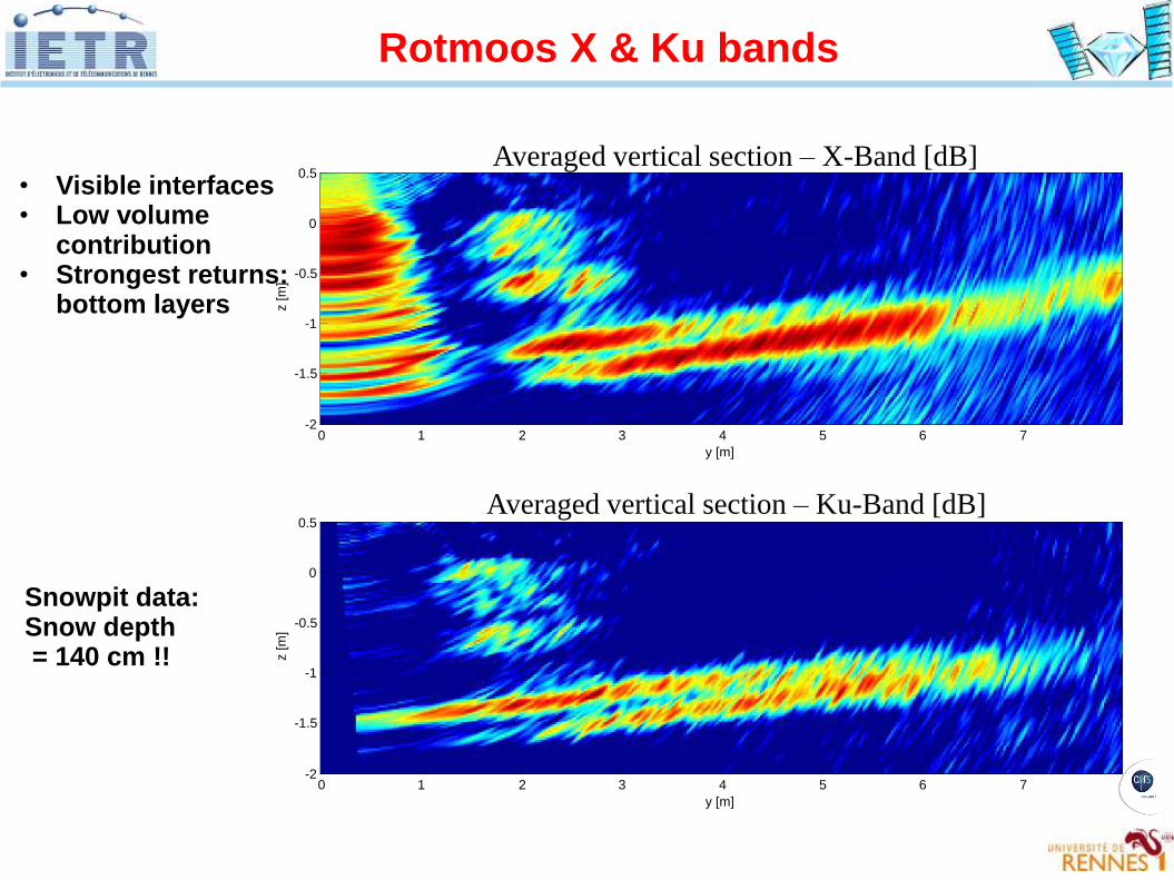
Averaged vertical section – X-Band [dB]
Averaged vertical section – Ku-Band [dB]
• Visible interfaces• Low volume
contribution • Strongest returns:
bottom layers
Snowpit data:Snow depth= 140 cm !!
Rotmoos X & Ku bands
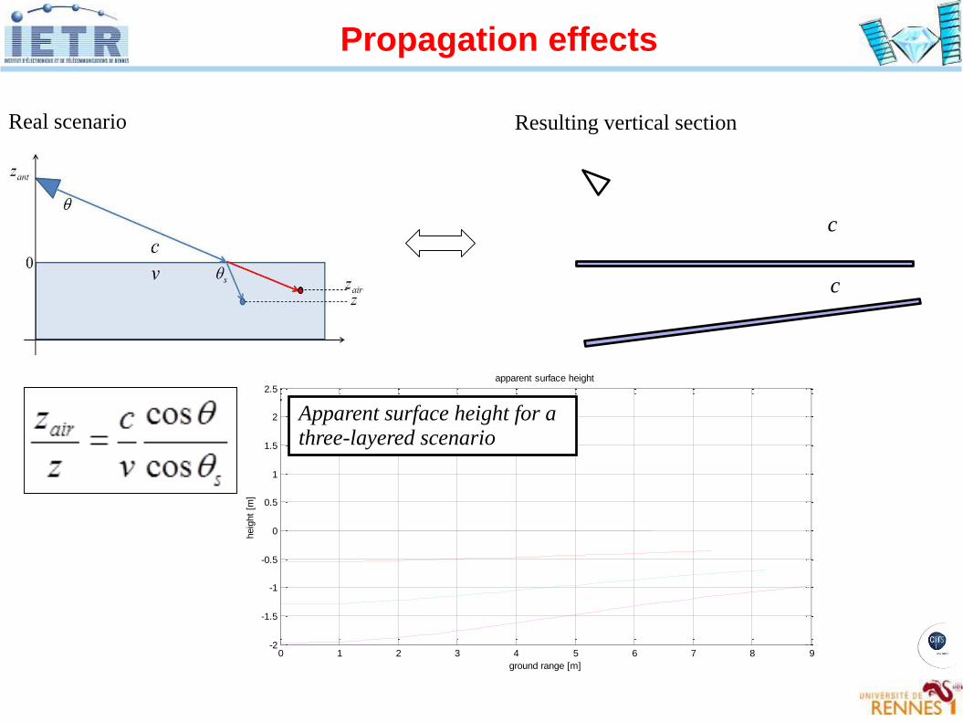
Real scenario
0 1 2 3 4 5 6 7 8 9-2
-1.5
-1
-0.5
0
0.5
1
1.5
2
2.5
ground range [m]
heig
ht [
m]
apparent surface height
c
Resulting vertical section
Apparent surface height for a three-layered scenario
c
Propagation effects
y [m]
z [m
]
0 1 2 3 4 5 6 7-2
-1.5
-1
-0.5
0
0.5
n = 1
0 m
-0.54 m
-1.03 m
-1.40 m
n = 1.25
n = 1.25
n = 1.25
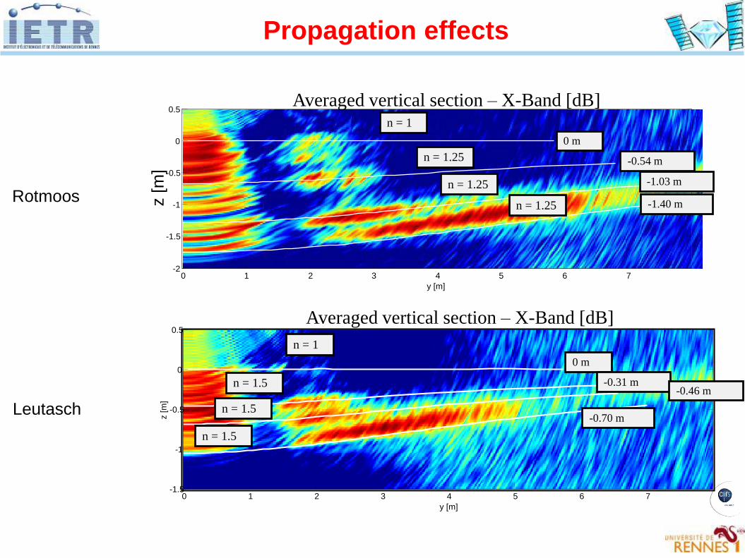
Averaged vertical section – X-Band [dB]
Rotmoos
y [m]
z [m
]
0 1 2 3 4 5 6 7-1.5
-1
-0.5
0
0.5
n = 1
0 m
-0.31 m-0.46 m
-0.70 m
n = 1.5
n = 1.5
n = 1.5
Averaged vertical section – X-Band [dB]
Leutasch
Propagation effects
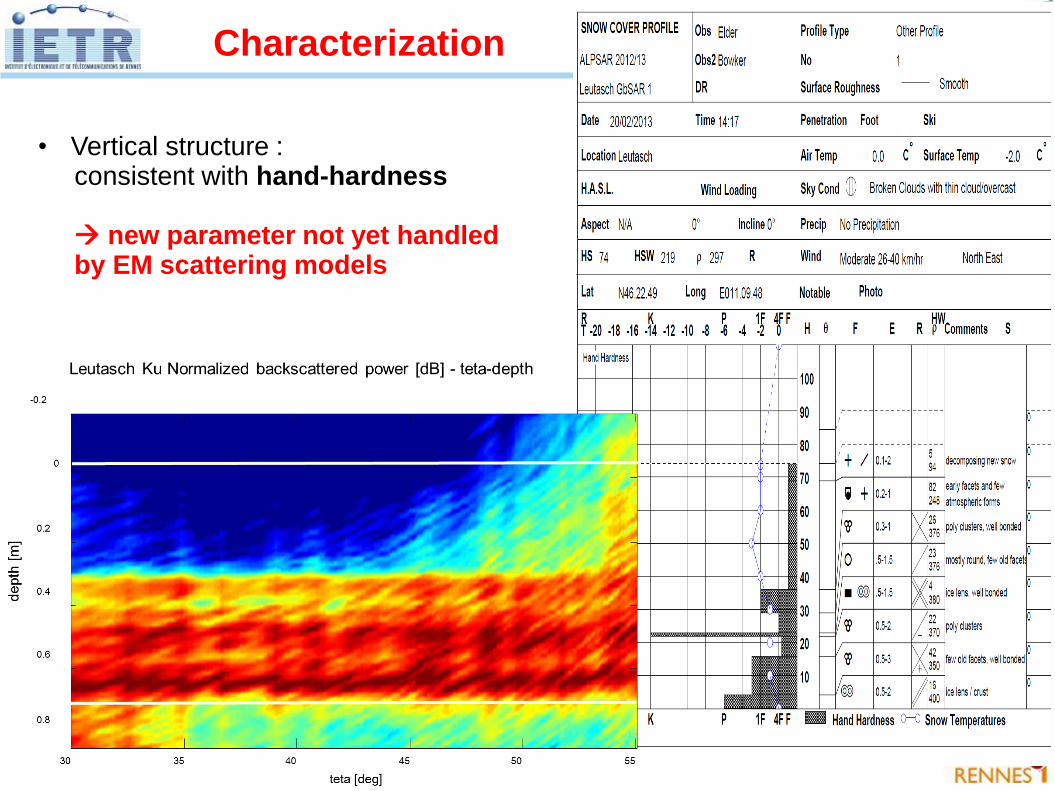
• Vertical structure : consistent with hand-hardness
new parameter not yet handled by EM scattering models
Characterization
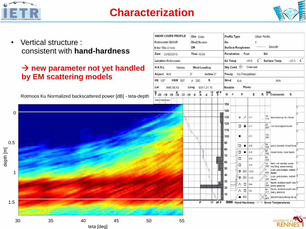
• Vertical structure : consistent with hand-hardness
teta [deg]
dept
h [m
]
Rotmoos Ku Normalized backscattered power [dB] - teta-depth
30 35 40 45 50 55
0
0.5
1
1.5
new parameter not yet handled by EM scattering models
Characterization
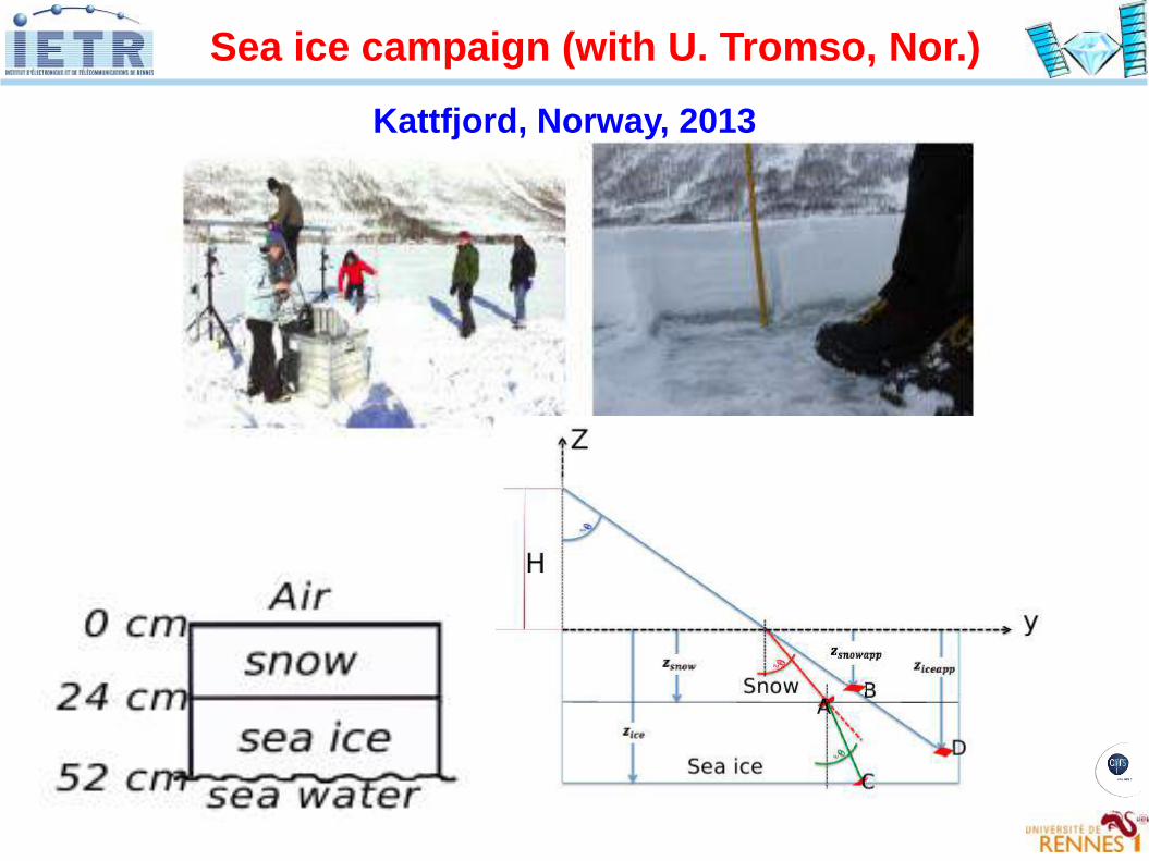
Sea ice campaign (with U. Tromso, Nor.)
Kattfjord, Norway, 2013
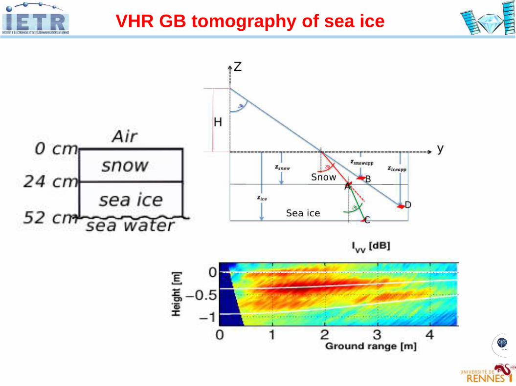
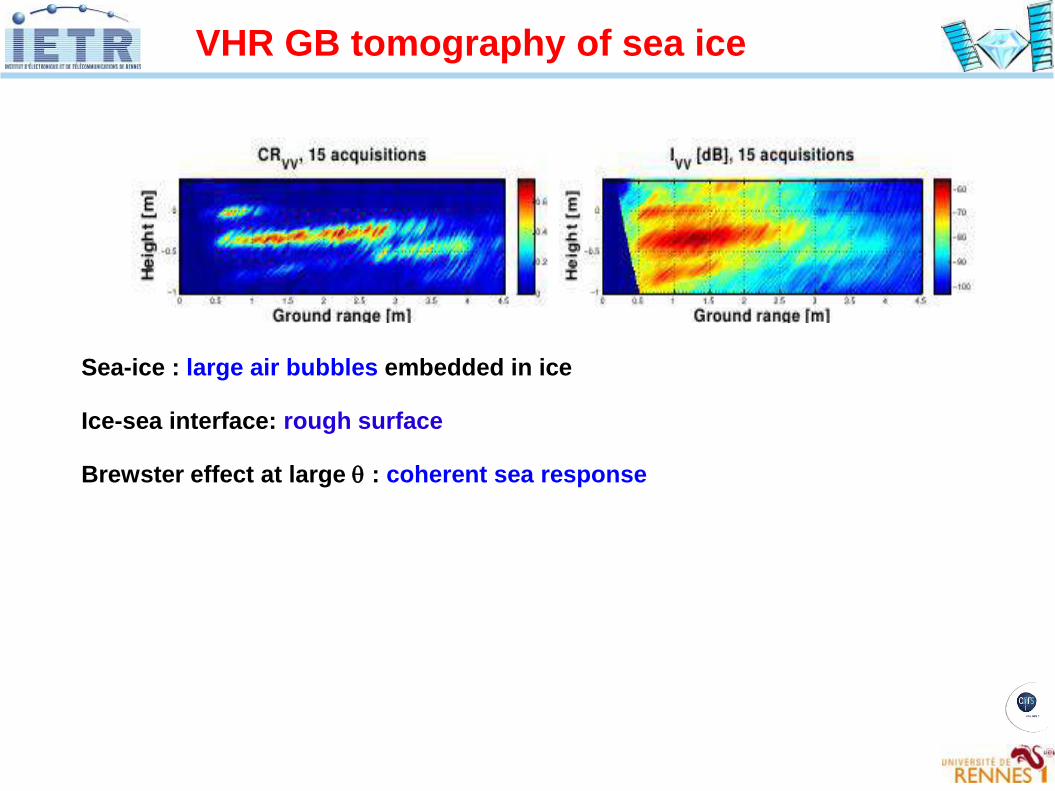
VHR GB tomography of sea ice
VHR GB tomography of sea ice
Sea-ice : large air bubbles embedded in ice
Ice-sea interface: rough surface
Brewster effect at large q : coherent sea response
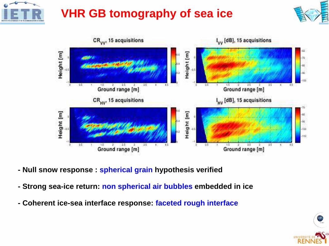
VHR GB tomography of sea ice
- Null snow response : spherical grain hypothesis verified
- Strong sea-ice return: non spherical air bubbles embedded in ice
- Coherent ice-sea interface response: faceted rough interface
Conclusions
Modern SAR remote sensing is multi-modal
Signal diversity:Application or medium adapted (a priori)Enhanced separationMost useful: space & time
Statistical signal processing:High dimensionalUses data structure (tensors)May use sparsity
EM model validation/correction: important potential
Top Related