XPS theory - California Institute of Technology Info/XPs Theory by R. Paynter.pdf · X-ray...

1

XPS Theory

Royston Paynter

INRS-ÉMT

Royston PaynterINRS-Énergie, Matériaux et Télécommunications1650 boul. Lionel-BouletVarennesQuébec J3X 1S2

(450) [email protected]

Division of surface science web site: http://goliath.inrs-emt.uquebec.ca/surfsci

Surface analysis laboratory web site:http://goliath.inrs-emt.uquebec.ca/commerce/

ARXPS web site:http://goliath.inrs-emt.uquebec.ca/surfsci/arxps/index.html

2

Emission

Photons Electrons Ions

Exc

itatio

n Photons Electrons Ions

XRF LOES EMP SEM-EDX TEM-EDX PIXE BLE

XPS (ESCA) P-AES E-AES TEELS I-AES

LAMMA, LMP EID SNMS SIMS LEIS (ISS) HEIS (RBS)

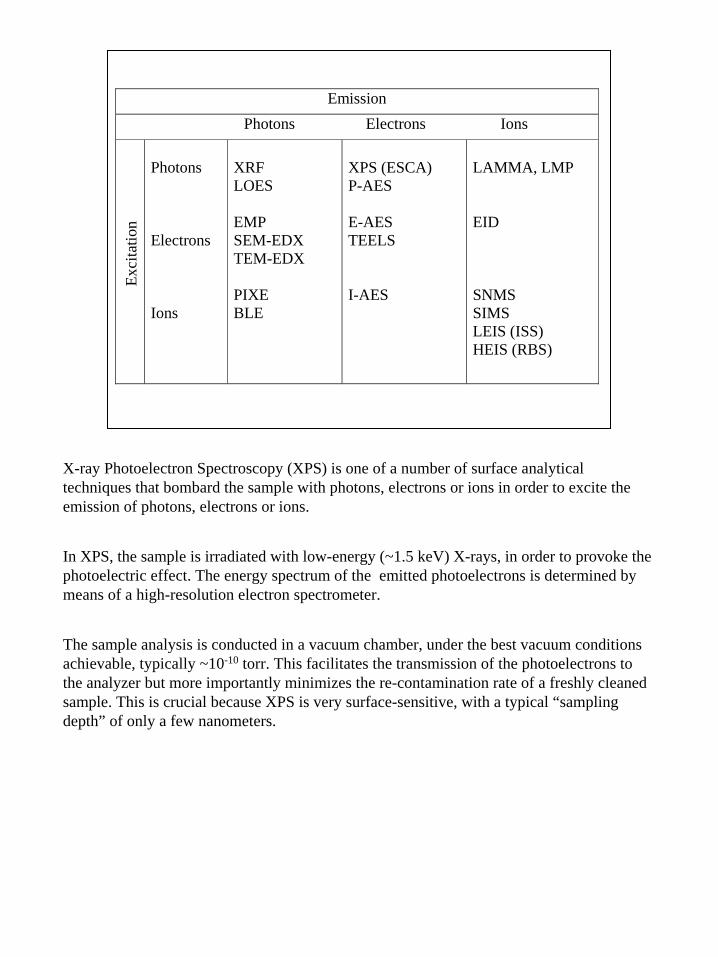
X-ray Photoelectron Spectroscopy (XPS) is one of a number of surface analytical techniques that bombard the sample with photons, electrons or ions in order to excite the emission of photons, electrons or ions.

In XPS, the sample is irradiated with low-energy (~1.5 keV) X-rays, in order to provoke the photoelectric effect. The energy spectrum of the emitted photoelectrons is determined by means of a high-resolution electron spectrometer.

The sample analysis is conducted in a vacuum chamber, under the best vacuum conditions achievable, typically ~10-10 torr. This facilitates the transmission of the photoelectrons to the analyzer but more importantly minimizes the re-contamination rate of a freshly cleaned sample. This is crucial because XPS is very surface-sensitive, with a typical “sampling depth” of only a few nanometers.

3

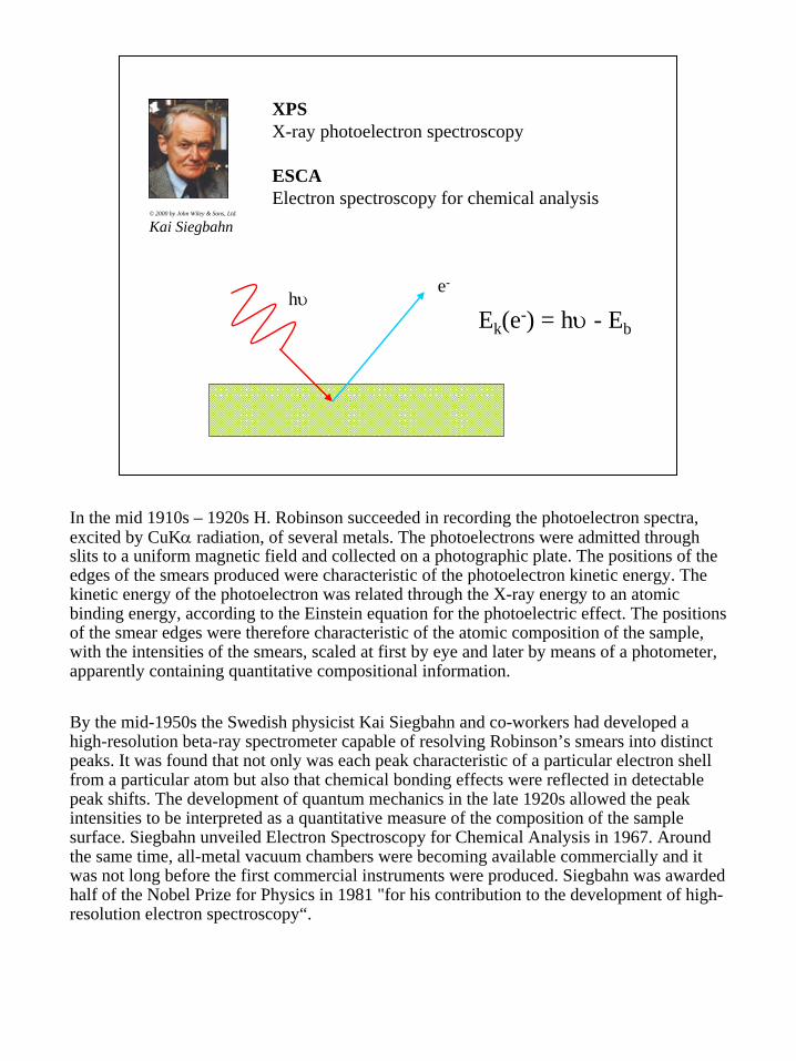
XPSX-ray photoelectron spectroscopy

ESCAElectron spectroscopy for chemical analysis

© 2000 by John Wiley & Sons, Ltd.

Kai Siegbahn

hυe-

Ek(e-) = hυ - Eb

In the mid 1910s – 1920s H. Robinson succeeded in recording the photoelectron spectra, excited by CuKα radiation, of several metals. The photoelectrons were admitted through slits to a uniform magnetic field and collected on a photographic plate. The positions of the edges of the smears produced were characteristic of the photoelectron kinetic energy. The kinetic energy of the photoelectron was related through the X-ray energy to an atomic binding energy, according to the Einstein equation for the photoelectric effect. The positions of the smear edges were therefore characteristic of the atomic composition of the sample, with the intensities of the smears, scaled at first by eye and later by means of a photometer, apparently containing quantitative compositional information.

By the mid-1950s the Swedish physicist Kai Siegbahn and co-workers had developed a high-resolution beta-ray spectrometer capable of resolving Robinson’s smears into distinct peaks. It was found that not only was each peak characteristic of a particular electron shell from a particular atom but also that chemical bonding effects were reflected in detectable peak shifts. The development of quantum mechanics in the late 1920s allowed the peak intensities to be interpreted as a quantitative measure of the composition of the sample surface. Siegbahn unveiled Electron Spectroscopy for Chemical Analysis in 1967. Around the same time, all-metal vacuum chambers were becoming available commercially and it was not long before the first commercial instruments were produced. Siegbahn was awarded half of the Nobel Prize for Physics in 1981 "for his contribution to the development of high-resolution electron spectroscopy“.

4

hυ

Ei Ef

Ek(e-)

hυ + Ei = Ek(e-) + Ef

hυ – Ek(e-) = Ef – Ei = Eb

atom ion

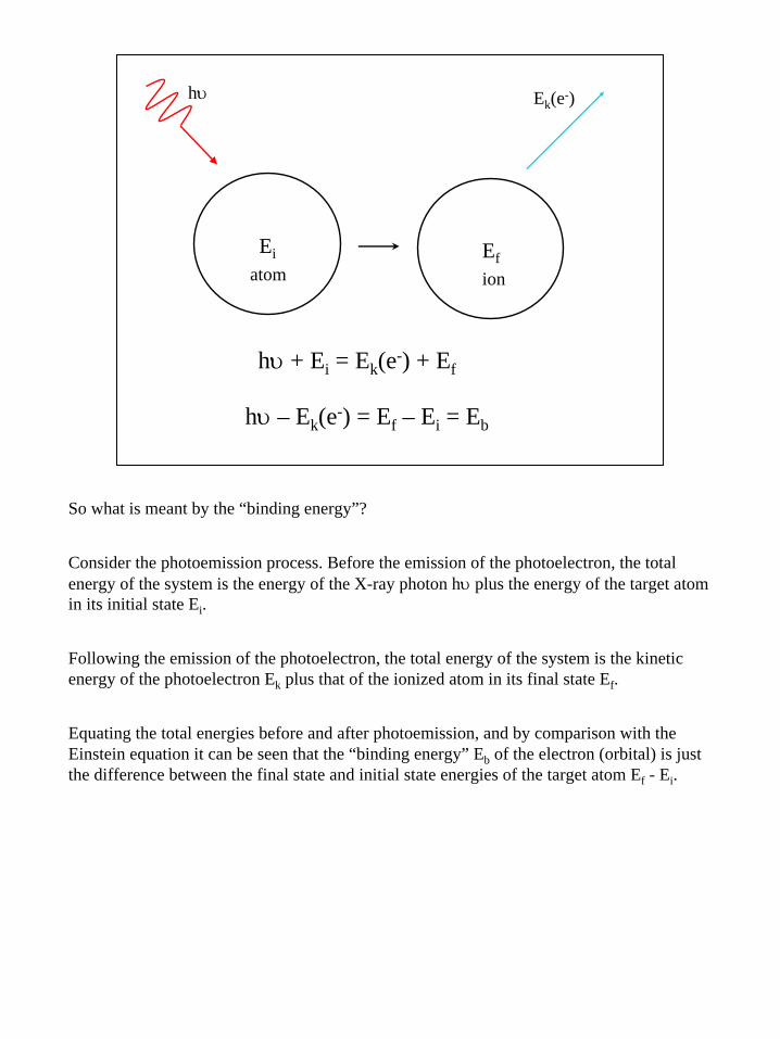
So what is meant by the “binding energy”?

Consider the photoemission process. Before the emission of the photoelectron, the total energy of the system is the energy of the X-ray photon hυ plus the energy of the target atom in its initial state Ei.

Following the emission of the photoelectron, the total energy of the system is the kinetic energy of the photoelectron Ek plus that of the ionized atom in its final state Ef.

Equating the total energies before and after photoemission, and by comparison with the Einstein equation it can be seen that the “binding energy” Eb of the electron (orbital) is just the difference between the final state and initial state energies of the target atom Ef - Ei.

5

Printed using CasaXPS

survey.dts

x 104

2

4

6

8

10

12

14

16

18

1000 800 600 400 200 0Binding Energy (eV)

C1s

N1s

O1s

O KLL

Photoelectron Kinetic Energy →

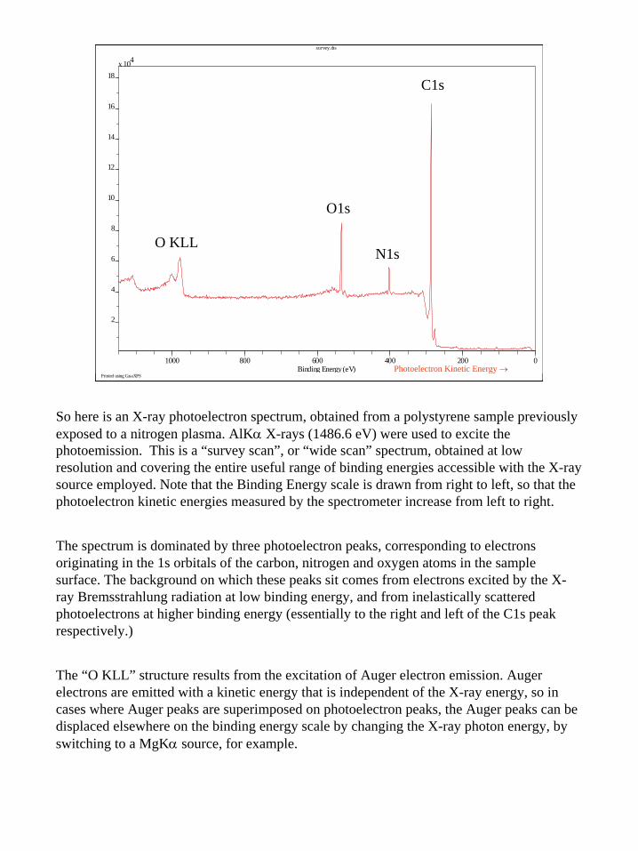
So here is an X-ray photoelectron spectrum, obtained from a polystyrene sample previously exposed to a nitrogen plasma. AlKα X-rays (1486.6 eV) were used to excite the photoemission. This is a “survey scan”, or “wide scan” spectrum, obtained at low resolution and covering the entire useful range of binding energies accessible with the X-ray source employed. Note that the Binding Energy scale is drawn from right to left, so that the photoelectron kinetic energies measured by the spectrometer increase from left to right.

The spectrum is dominated by three photoelectron peaks, corresponding to electrons originating in the 1s orbitals of the carbon, nitrogen and oxygen atoms in the sample surface. The background on which these peaks sit comes from electrons excited by the X-ray Bremsstrahlung radiation at low binding energy, and from inelastically scattered photoelectrons at higher binding energy (essentially to the right and left of the C1s peak respectively.)

The “O KLL” structure results from the excitation of Auger electron emission. Auger electrons are emitted with a kinetic energy that is independent of the X-ray energy, so in cases where Auger peaks are superimposed on photoelectron peaks, the Auger peaks can be displaced elsewhere on the binding energy scale by changing the X-ray photon energy, by switching to a MgKα source, for example.

6

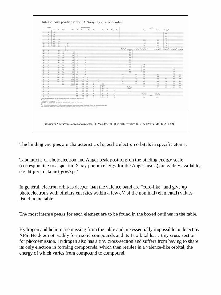
Handbook of X-ray Photoelectron Spectroscopy, J.F. Moulder et al., Physical Electronics, Inc., Eden Prairie, MN, USA (1992)

The binding energies are characteristic of specific electron orbitals in specific atoms.

Tabulations of photoelectron and Auger peak positions on the binding energy scale (corresponding to a specific X-ray photon energy for the Auger peaks) are widely available, e.g. http://srdata.nist.gov/xps/

In general, electron orbitals deeper than the valence band are “core-like” and give up photoelectrons with binding energies within a few eV of the nominal (elemental) values listed in the table.

The most intense peaks for each element are to be found in the boxed outlines in the table.

Hydrogen and helium are missing from the table and are essentially impossible to detect by XPS. He does not readily form solid compounds and its 1s orbital has a tiny cross-section for photoemission. Hydrogen also has a tiny cross-section and suffers from having to share its only electron in forming compounds, which then resides in a valence-like orbital, the energy of which varies from compound to compound.

7

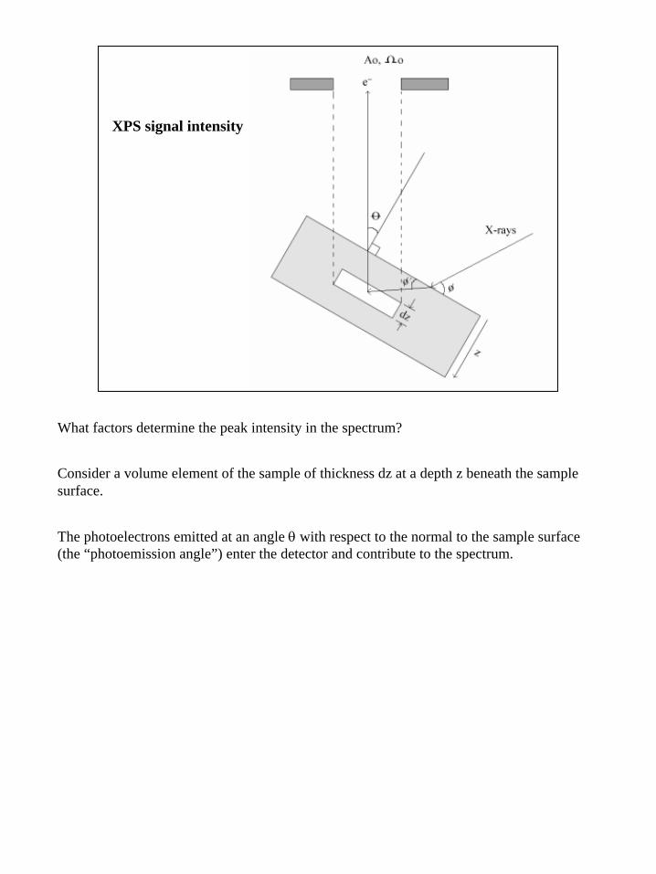
XPS signal intensity

What factors determine the peak intensity in the spectrum?

Consider a volume element of the sample of thickness dz at a depth z beneath the sample surface.

The photoelectrons emitted at an angle θ with respect to the normal to the sample surface (the “photoemission angle”) enter the detector and contribute to the spectrum.

8

1) The intensity of the x-rays at depth z

( ) 'sin

'sinsin1 φλ υ

φφγ h

z

er−

−

γ = incident X-ray fluxr = coefficient of reflectionλhν = attenuation length of X-ray photons

In practice, the reflection and refraction of the X-rays giving rise to the photoelectrons is only significant at a grazing angle φ of less than 5º, and can be ignored under normal circumstances.

In any case the X-ray flux will not normally be known, and it is therefore usual to eliminate this factor from consideration by taking peak intensity ratios or by calculating the composition of the sample in terms of atom percent, by taking into consideration one peak from each chemical element found.

9

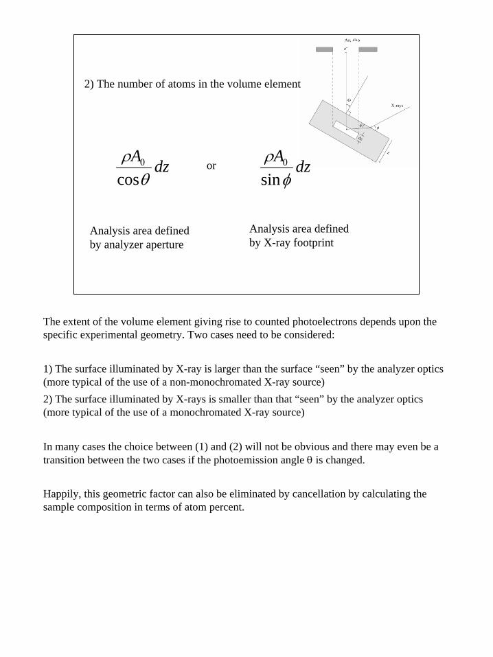
2) The number of atoms in the volume element

dzAθ

ρcos

0 dzAφ

ρsin

0or

Analysis area defined by analyzer aperture

Analysis area defined by X-ray footprint

The extent of the volume element giving rise to counted photoelectrons depends upon the specific experimental geometry. Two cases need to be considered:

1) The surface illuminated by X-ray is larger than the surface “seen” by the analyzer optics (more typical of the use of a non-monochromated X-ray source)2) The surface illuminated by X-rays is smaller than that “seen” by the analyzer optics (more typical of the use of a monochromated X-ray source)

In many cases the choice between (1) and (2) will not be obvious and there may even be a transition between the two cases if the photoemission angle θ is changed.

Happily, this geometric factor can also be eliminated by cancellation by calculating the sample composition in terms of atom percent.

10

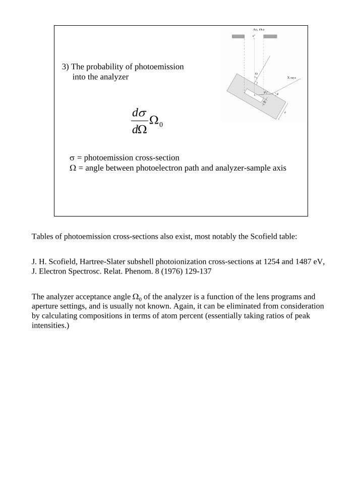
3) The probability of photoemission into the analyzer

0ΩΩd

dσ

σ = photoemission cross-sectionΩ = angle between photoelectron path and analyzer-sample axis

Tables of photoemission cross-sections also exist, most notably the Scofield table:

J. H. Scofield, Hartree-Slater subshell photoionization cross-sections at 1254 and 1487 eV, J. Electron Spectrosc. Relat. Phenom. 8 (1976) 129-137

The analyzer acceptance angle Ω0 of the analyzer is a function of the lens programs and aperture settings, and is usually not known. Again, it can be eliminated from consideration by calculating compositions in terms of atom percent (essentially taking ratios of peak intensities.)

11

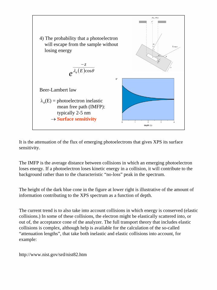
4) The probability that a photoelectronwill escape from the sample withoutlosing energy

( ) θλ cosEz

ee−

Beer-Lambert law

λe(E) = photoelectron inelastic mean free path (IMFP): typically 2-5 nm

→ Surface sensitivity

It is the attenuation of the flux of emerging photoelectrons that gives XPS its surface sensitivity.

The IMFP is the average distance between collisions in which an emerging photoelectron loses energy. If a photoelectron loses kinetic energy in a collision, it will contribute to the background rather than to the characteristic “no-loss” peak in the spectrum.

The height of the dark blue cone in the figure at lower right is illustrative of the amount of information contributing to the XPS spectrum as a function of depth.

The current trend is to also take into account collisions in which energy is conserved (elastic collisions.) In some of these collisions, the electron might be elastically scattered into, or out of, the acceptance cone of the analyzer. The full transport theory that includes elastic collisions is complex, although help is available for the calculation of the so-called “attenuation lengths”, that take both inelastic and elastic collisions into account, for example:

http://www.nist.gov/srd/nist82.htm

12

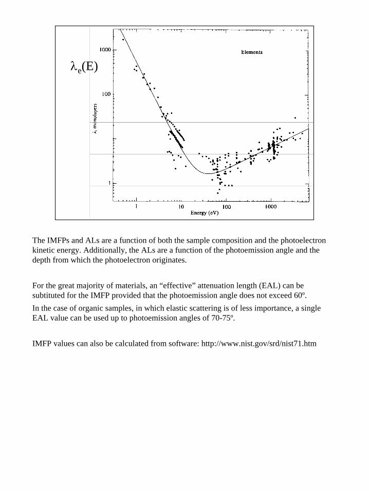
λe(E)

The IMFPs and ALs are a function of both the sample composition and the photoelectron kinetic energy. Additionally, the ALs are a function of the photoemission angle and the depth from which the photoelectron originates.

For the great majority of materials, an “effective” attenuation length (EAL) can be subtituted for the IMFP provided that the photoemission angle does not exceed 60º.In the case of organic samples, in which elastic scattering is of less importance, a single EAL value can be used up to photoemission angles of 70-75º.

IMFP values can also be calculated from software: http://www.nist.gov/srd/nist71.htm

13

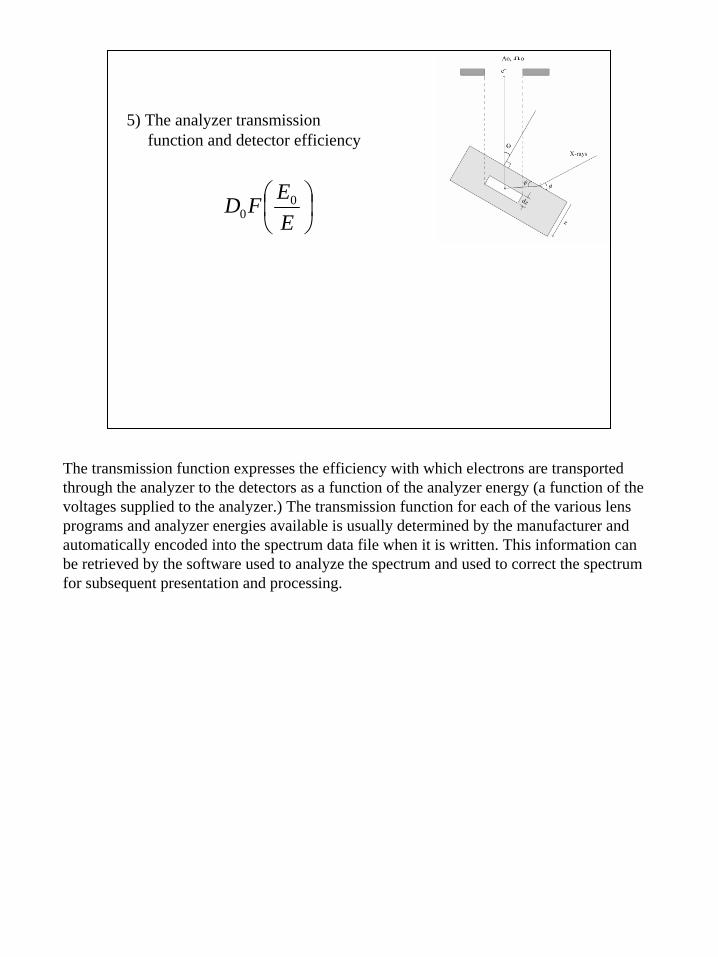
5) The analyzer transmission function and detector efficiency

EEFD 0

0

The transmission function expresses the efficiency with which electrons are transported through the analyzer to the detectors as a function of the analyzer energy (a function of the voltages supplied to the analyzer.) The transmission function for each of the various lens programs and analyzer energies available is usually determined by the manufacturer and automatically encoded into the spectrum data file when it is written. This information can be retrieved by the software used to analyze the spectrum and used to correct the spectrum for subsequent presentation and processing.

14

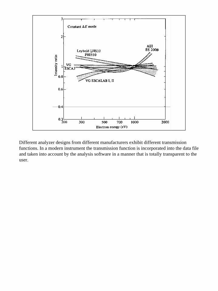
Different analyzer designs from different manufacturers exhibit different transmission functions. In a modern instrument the transmission function is incorporated into the data file and taken into account by the analysis software in a manner that is totally transparent to the user.

15

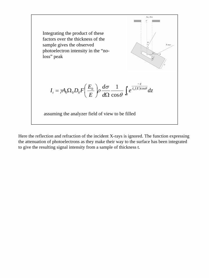
Integrating the product of these factors over the thickness of the sample gives the observed photoelectron intensity in the “no-loss” peak

( )∫−

Ω

Ω=

t Ez

t dzedd

EEFDAI e

0

cos0000 cos

1 θλ

θσργ

assuming the analyzer field of view to be filled

Here the reflection and refraction of the incident X-rays is ignored. The function expressing the attenuation of photoelectrons as they make their way to the surface has been integrated to give the resulting signal intensity from a sample of thickness t.

16

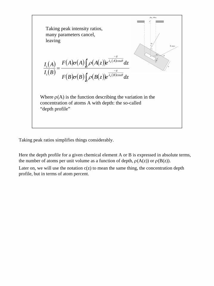
Taking peak intensity ratios, many parameters cancel, leaving

( )( )

( ) ( ) ( )( ) ( )

( ) ( ) ( )( ) ( )∫

∫−

−

=t B

z

t Az

t

t

dzezBBBF

dzezAAAF

BIAI

e

e

0

cos

0

cos

θλ

θλ

ρσ

ρσ

Where ρ(A) is the function describing the variation in the concentration of atoms A with depth: the so-called “depth profile”

Taking peak ratios simplifies things considerably.

Here the depth profile for a given chemical element A or B is expressed in absolute terms, the number of atoms per unit volume as a function of depth, ρ(A(z)) or ρ(B(z)).Later on, we will use the notation c(z) to mean the same thing, the concentration depth profile, but in terms of atom percent.

17

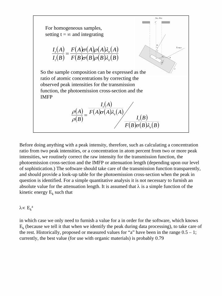
For homogeneous samples,setting t = ∞ and integrating

( )( )

( ) ( ) ( ) ( )( ) ( ) ( ) ( )BBBBF

AAAAFBIAI

e

e

t

t

λρσλρσ

=

So the sample composition can be expressed as the ratio of atomic concentrations by correcting the observed peak intensities for the transmission function, the photoemission cross-section and the IMFP

( )( )

( )( ) ( ) ( )

( )( ) ( ) ( )BBBF

BIAAAF

AI

BA

e

t

e

t

λσ

λσρρ

=

Before doing anything with a peak intensity, therefore, such as calculating a concentration ratio from two peak intensities, or a concentration in atom percent from two or more peak intensities, we routinely correct the raw intensity for the transmission function, the photoemission cross-section and the IMFP or attenuation length (depending upon our level of sophistication.) The software should take care of the transmission function transparently, and should provide a look-up table for the photoemission cross-section when the peak in question is identified. For a simple quantitative analysis it is not necessary to furnish an absolute value for the attenuation length. It is assumed that λ is a simple function of the kinetic energy Ek such that

λ∝ Eka

in which case we only need to furnish a value for a in order for the software, which knows Ek (because we tell it that when we identify the peak during data processing), to take care of the rest. Historically, proposed or measured values for “a” have been in the range 0.5 – 1; currently, the best value (for use with organic materials) is probably 0.79

18

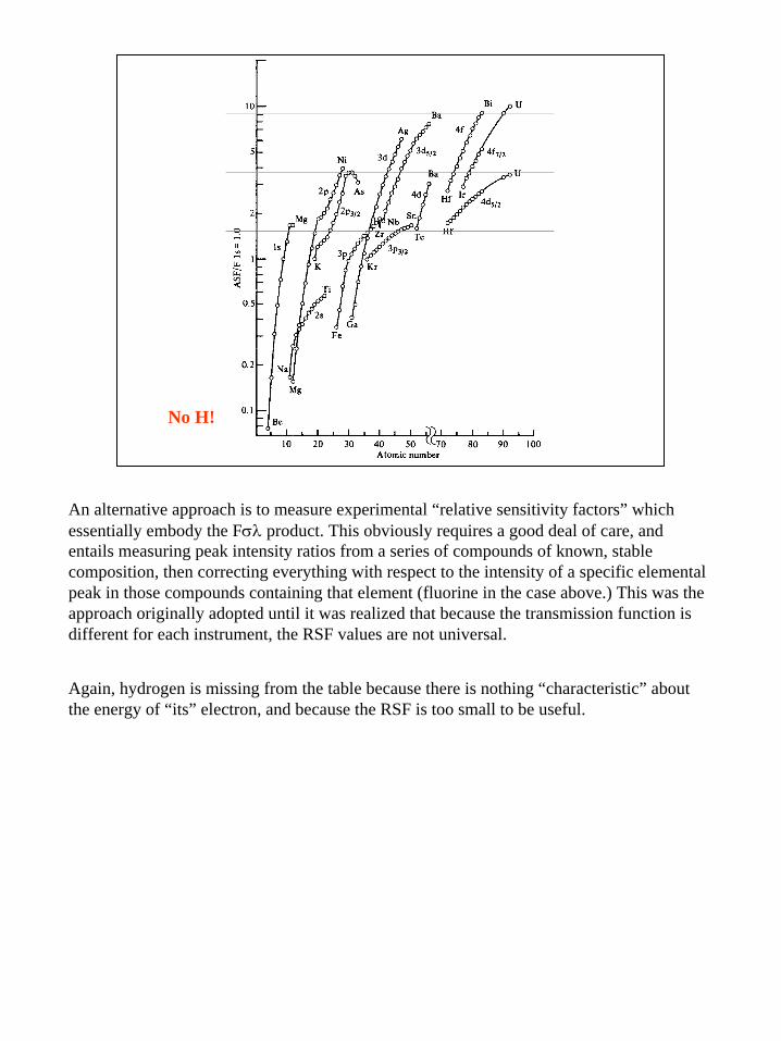
No H!

An alternative approach is to measure experimental “relative sensitivity factors” which essentially embody the Fσλ product. This obviously requires a good deal of care, and entails measuring peak intensity ratios from a series of compounds of known, stable composition, then correcting everything with respect to the intensity of a specific elemental peak in those compounds containing that element (fluorine in the case above.) This was the approach originally adopted until it was realized that because the transmission function is different for each instrument, the RSF values are not universal.

Again, hydrogen is missing from the table because there is nothing “characteristic” about the energy of “its” electron, and because the RSF is too small to be useful.

19


C 1s

x 102

5

10

15

20

25

300 298 296 294 292 290 288 286 284 282Binding energy (eV)

Chemical shifts in XPS

C C C CH

H

H

H

H

O

OF

F

FEthyl trifluoroacetate

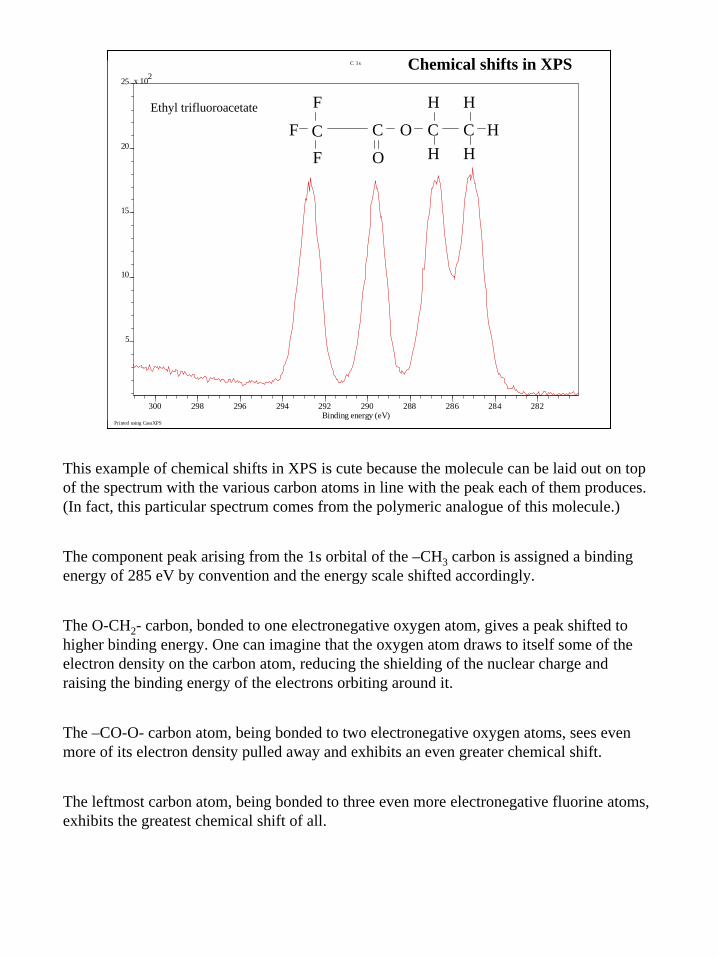
This example of chemical shifts in XPS is cute because the molecule can be laid out on top of the spectrum with the various carbon atoms in line with the peak each of them produces. (In fact, this particular spectrum comes from the polymeric analogue of this molecule.)

The component peak arising from the 1s orbital of the –CH3 carbon is assigned a binding energy of 285 eV by convention and the energy scale shifted accordingly.

The O-CH2- carbon, bonded to one electronegative oxygen atom, gives a peak shifted to higher binding energy. One can imagine that the oxygen atom draws to itself some of the electron density on the carbon atom, reducing the shielding of the nuclear charge and raising the binding energy of the electrons orbiting around it.

The –CO-O- carbon atom, being bonded to two electronegative oxygen atoms, sees even more of its electron density pulled away and exhibits an even greater chemical shift.

The leftmost carbon atom, being bonded to three even more electronegative fluorine atoms, exhibits the greatest chemical shift of all.

20

Ebv(j) = -εHF(j) – Ra(j)

“intra-atomic”relaxation energy

Koopman’s theorem:

Ebv(j) = -εHF(j)

Ebv(j) = -(εHF

atom(j) - Va)

change in εHF dueto valence charge

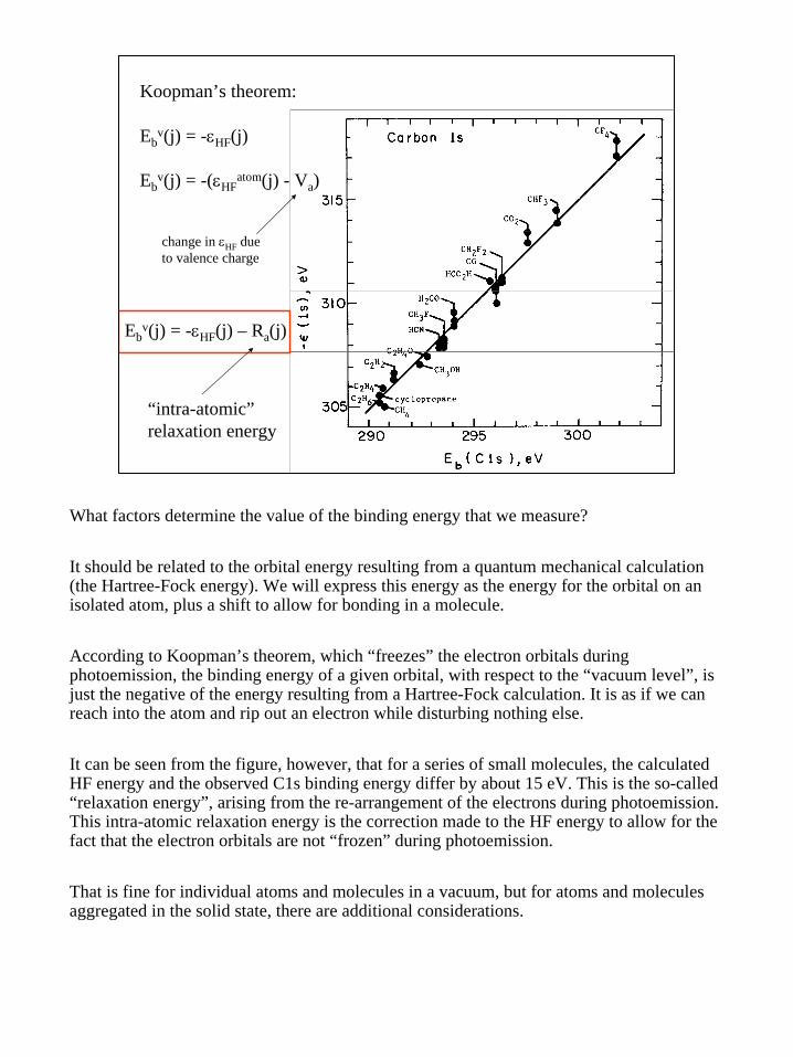
What factors determine the value of the binding energy that we measure?

It should be related to the orbital energy resulting from a quantum mechanical calculation (the Hartree-Fock energy). We will express this energy as the energy for the orbital on an isolated atom, plus a shift to allow for bonding in a molecule.

According to Koopman’s theorem, which “freezes” the electron orbitals during photoemission, the binding energy of a given orbital, with respect to the “vacuum level”, is just the negative of the energy resulting from a Hartree-Fock calculation. It is as if we can reach into the atom and rip out an electron while disturbing nothing else.

It can be seen from the figure, however, that for a series of small molecules, the calculated HF energy and the observed C1s binding energy differ by about 15 eV. This is the so-called “relaxation energy”, arising from the re-arrangement of the electrons during photoemission. This intra-atomic relaxation energy is the correction made to the HF energy to allow for the fact that the electron orbitals are not “frozen” during photoemission.

That is fine for individual atoms and molecules in a vacuum, but for atoms and molecules aggregated in the solid state, there are additional considerations.

21

In condensed phases

Eb(j) = -εHFatom + Va(j) – Ra(j) + Vea(j) – Rea(j) - φ

wrt Fermi level

shift in εHFfree atom → solid“Madelung potential”

“extra-atomic”relaxation energy

work function

Hartree-Fock orbital energy for free atom

shift in εHF due tovalence charge

“intra-atomic”relaxation energy

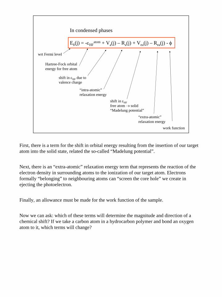
First, there is a term for the shift in orbital energy resulting from the insertion of our target atom into the solid state, related the so-called “Madelung potential”.

Next, there is an “extra-atomic” relaxation energy term that represents the reaction of the electron density in surrounding atoms to the ionization of our target atom. Electrons formally “belonging” to neighbouring atoms can “screen the core hole” we create in ejecting the photoelectron.

Finally, an allowance must be made for the work function of the sample.

Now we can ask: which of these terms will determine the magnitude and direction of a chemical shift? If we take a carbon atom in a hydrocarbon polymer and bond an oxygen atom to it, which terms will change?

22

Binding energy shifts (“chemical shifts”)

∆Eb ≅ ∆(Va + Vea) - ∆Rea

∝ ∆q/r

∆q = change in valence charger = valence shell radius

∝ -α∆q/r

α is related to Madelungconstant

reaction of atom’ssurroundings tocreation of core hole

electronegativity

polarizability

V’s and R can cancel out!

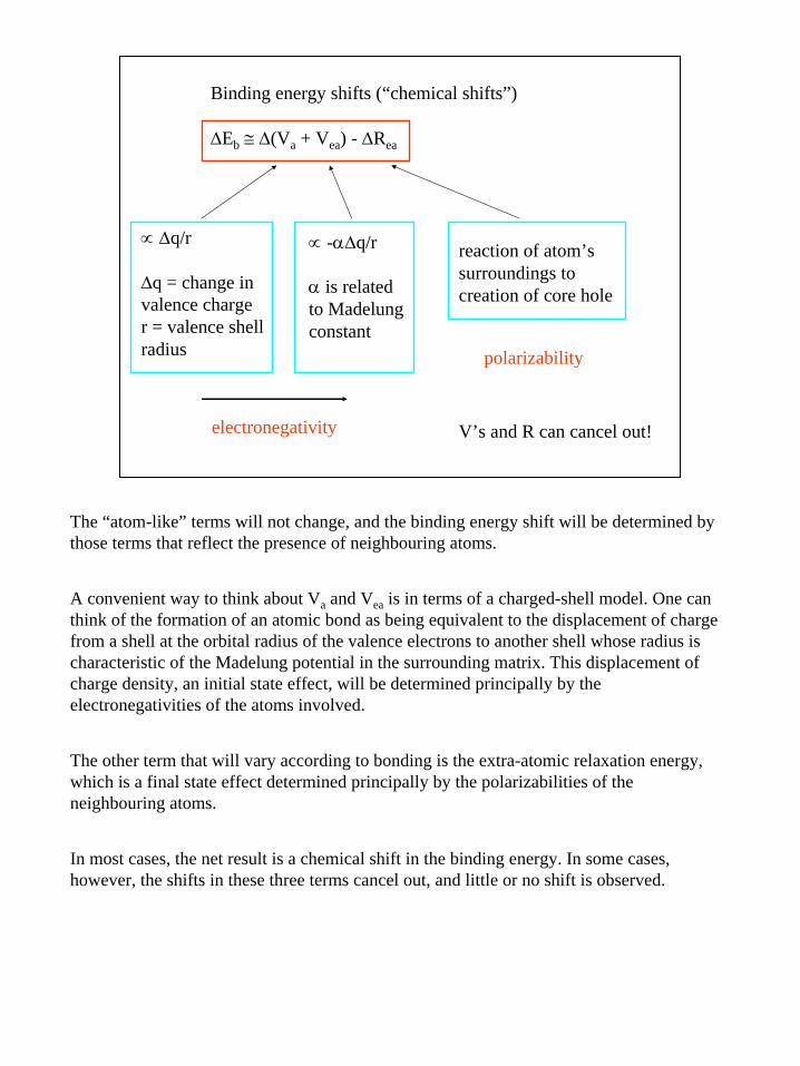
The “atom-like” terms will not change, and the binding energy shift will be determined by those terms that reflect the presence of neighbouring atoms.

A convenient way to think about Va and Vea is in terms of a charged-shell model. One can think of the formation of an atomic bond as being equivalent to the displacement of charge from a shell at the orbital radius of the valence electrons to another shell whose radius is characteristic of the Madelung potential in the surrounding matrix. This displacement of charge density, an initial state effect, will be determined principally by the electronegativities of the atoms involved.

The other term that will vary according to bonding is the extra-atomic relaxation energy, which is a final state effect determined principally by the polarizabilities of the neighbouring atoms.

In most cases, the net result is a chemical shift in the binding energy. In some cases, however, the shifts in these three terms cancel out, and little or no shift is observed.

23

C-CC-O-CC-OHC=O

COOHO-CO-O

C-NH2N-C=O

C=CC-SiC-ClC-F

-CF2-CF3

284 285 286 287 288 289 290 291 292 293

Binding Energy (eV)

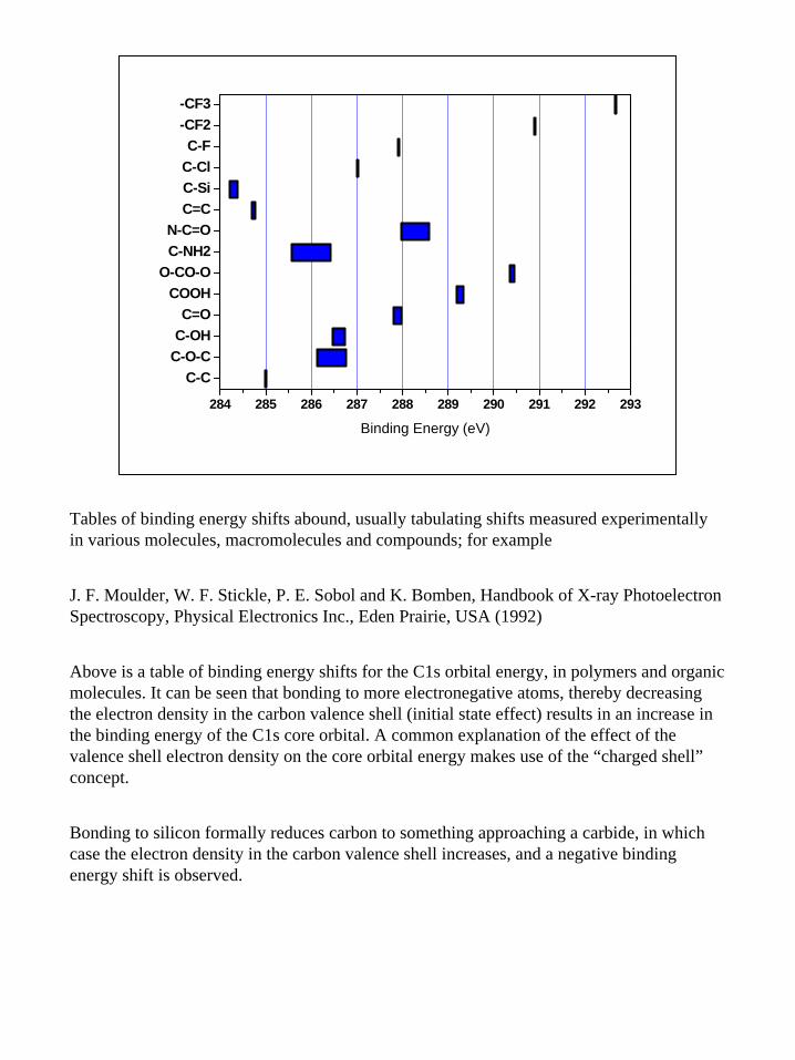
Tables of binding energy shifts abound, usually tabulating shifts measured experimentally in various molecules, macromolecules and compounds; for example

J. F. Moulder, W. F. Stickle, P. E. Sobol and K. Bomben, Handbook of X-ray Photoelectron Spectroscopy, Physical Electronics Inc., Eden Prairie, USA (1992)

Above is a table of binding energy shifts for the C1s orbital energy, in polymers and organic molecules. It can be seen that bonding to more electronegative atoms, thereby decreasing the electron density in the carbon valence shell (initial state effect) results in an increase in the binding energy of the C1s core orbital. A common explanation of the effect of the valence shell electron density on the core orbital energy makes use of the “charged shell”concept.

Bonding to silicon formally reduces carbon to something approaching a carbide, in which case the electron density in the carbon valence shell increases, and a negative binding energy shift is observed.

24

-0.2 -0.1 0.0 0.1 0.2 0.3 0.4 0.5

0

1

2

3

4

5

6

Et-O-(C=O)-O-Et

Et-COOHEt-(C=O)-O-Et

Et-(C=O)-Et

Et-CH2-OHEt-CH2-O-CH2-Et

Et-CH2-Et

C1s

Bin

ding

Ene

rgy

Shi

ft (e

V)

Mulliken charge on C at MNDO-PM3 geometry (e)

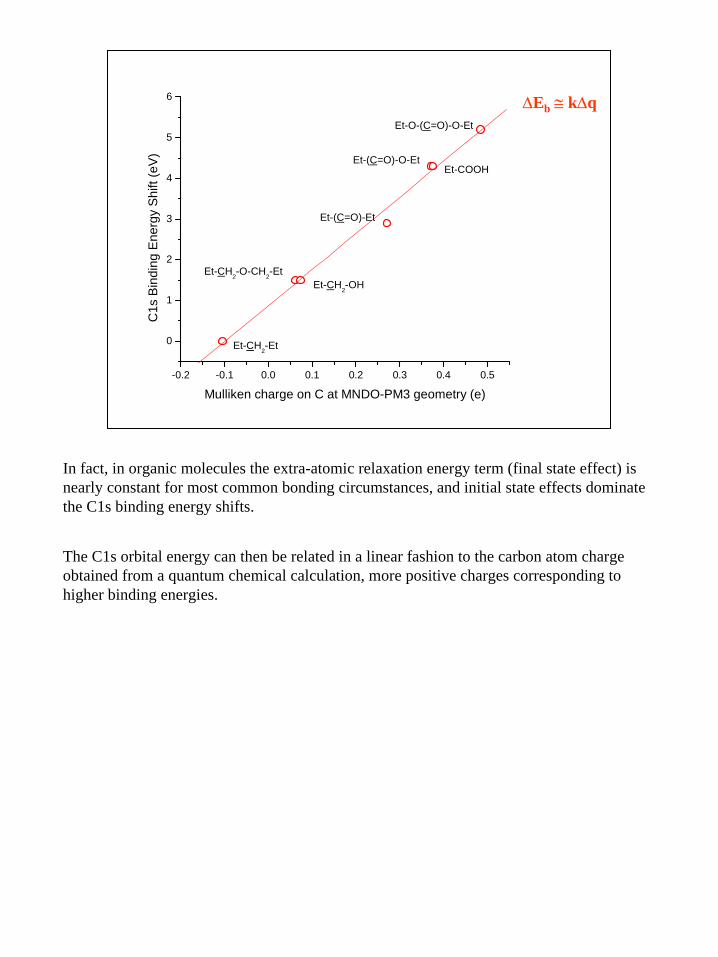
∆Eb ≅ k∆q

In fact, in organic molecules the extra-atomic relaxation energy term (final state effect) is nearly constant for most common bonding circumstances, and initial state effects dominate the C1s binding energy shifts.

The C1s orbital energy can then be related in a linear fashion to the carbon atom charge obtained from a quantum chemical calculation, more positive charges corresponding to higher binding energies.

25


survol.dts

x 104

5

10

15

20

25

30

35

40

45


CuInS2

photoelectron peaks

X-ray satellites

valence band

background = inelasticallyscattered electrons

Auger electron peaks

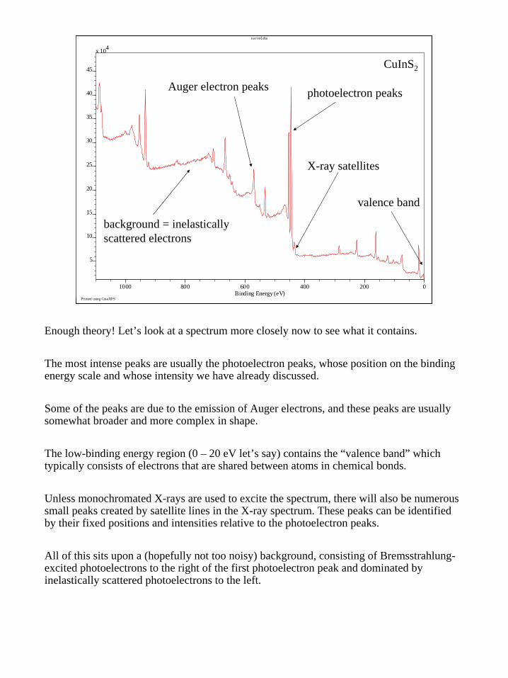
Enough theory! Let’s look at a spectrum more closely now to see what it contains.

The most intense peaks are usually the photoelectron peaks, whose position on the binding energy scale and whose intensity we have already discussed.

Some of the peaks are due to the emission of Auger electrons, and these peaks are usually somewhat broader and more complex in shape.

The low-binding energy region (0 – 20 eV let’s say) contains the “valence band” which typically consists of electrons that are shared between atoms in chemical bonds.

Unless monochromated X-rays are used to excite the spectrum, there will also be numerous small peaks created by satellite lines in the X-ray spectrum. These peaks can be identified by their fixed positions and intensities relative to the photoelectron peaks.

All of this sits upon a (hopefully not too noisy) background, consisting of Bremsstrahlung-excited photoelectrons to the right of the first photoelectron peak and dominated by inelastically scattered photoelectrons to the left.

26

http

://w

ww

.cem

.msu

.edu

/~ce

m92

4sg/

Topi

c09.

pdf

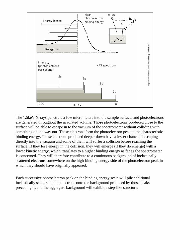
The 1.5keV X-rays penetrate a few micrometers into the sample surface, and photoelectrons are generated throughout the irradiated volume. Those photoelectrons produced close to the surface will be able to escape in to the vacuum of the spectrometer without colliding with something on the way out. These electrons form the photoelectron peak at the characteristic binding energy. Those electrons produced deeper down have a lesser chance of escaping directly into the vacuum and some of them will suffer a collision before reaching the surface. If they lose energy in the collision, they will emerge (if they do emerge) with a lower kinetic energy, which translates to a higher binding energy as far as the spectrometer is concerned. They will therefore contribute to a continuous background of inelasticallyscattered electrons somewhere on the high-binding energy side of the photoelectron peak in which they should have originally appeared.

Each successive photoelectron peak on the binding energy scale will pile additional inelastically scattered photoelectrons onto the background produced by those peaks preceding it, and the aggregate background will exhibit a step-like structure.

27

S. T

ouga

ard,

J. V

ac. S

ci. T

echn

ol. A

14

(199

6) 1

415

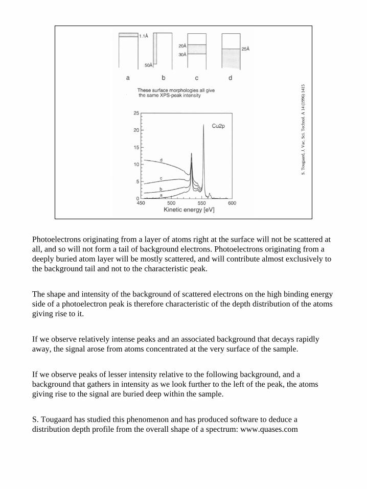
Photoelectrons originating from a layer of atoms right at the surface will not be scattered at all, and so will not form a tail of background electrons. Photoelectrons originating from a deeply buried atom layer will be mostly scattered, and will contribute almost exclusively to the background tail and not to the characteristic peak.

The shape and intensity of the background of scattered electrons on the high binding energy side of a photoelectron peak is therefore characteristic of the depth distribution of the atoms giving rise to it.

If we observe relatively intense peaks and an associated background that decays rapidly away, the signal arose from atoms concentrated at the very surface of the sample.

If we observe peaks of lesser intensity relative to the following background, and a background that gathers in intensity as we look further to the left of the peak, the atoms giving rise to the signal are buried deep within the sample.

S. Tougaard has studied this phenomenon and has produced software to deduce a distribution depth profile from the overall shape of a spectrum: www.quases.com

28


survey.dts

x 104

2

4

6

8

10

12

14

16

18


C1s

N1s

O1s

O KLL

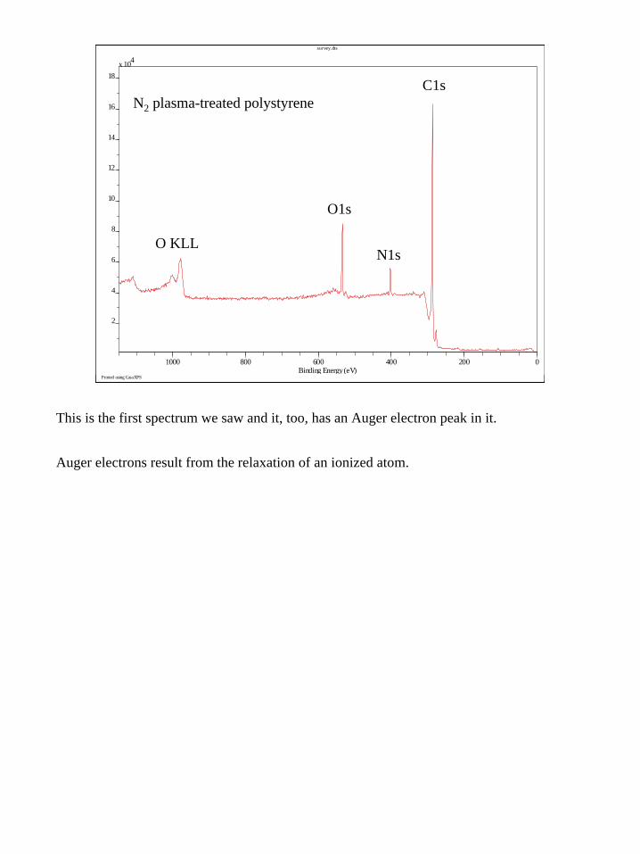
N2 plasma-treated polystyrene

This is the first spectrum we saw and it, too, has an Auger electron peak in it.

Auger electrons result from the relaxation of an ionized atom.

29

hυ photoelectron

KLL Auger electronK

L

Ek(KLL) = Eb(K) – Eb(L) – Eb’(L)

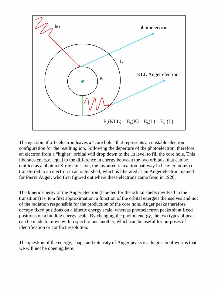
The ejection of a 1s electron leaves a “core hole” that represents an unstable electron configuration for the resulting ion. Following the departure of the photoelectron, therefore, an electron from a “higher” orbital will drop down to the 1s level to fill the core hole. This liberates energy, equal to the difference in energy between the two orbitals, that can be emitted as a photon (X-ray emission, the favoured relaxation pathway in heavier atoms) or transferred to an electron in an outer shell, which is liberated as an Auger electron, named for Pierre Auger, who first figured out where these electrons came from in 1926.

The kinetic energy of the Auger electron (labelled for the orbital shells involved in the transitions) is, to a first approximation, a function of the orbital energies themselves and not of the radiation responsible for the production of the core hole. Auger peaks therefore occupy fixed positions on a kinetic energy scale, whereas photoelectron peaks sit at fixed positions on a binding energy scale. By changing the photon energy, the two types of peak can be made to move with respect to one another, which can be useful for purposes of identification or conflict resolution.

The question of the energy, shape and intensity of Auger peaks is a huge can of worms that we will not be opening here.

30


survol.dts

x 104

5

10

15

20

25

30

35

40

45


Cu2p1/2 Cu2p3/2 Cu LMM

Cu3s

Cu3p

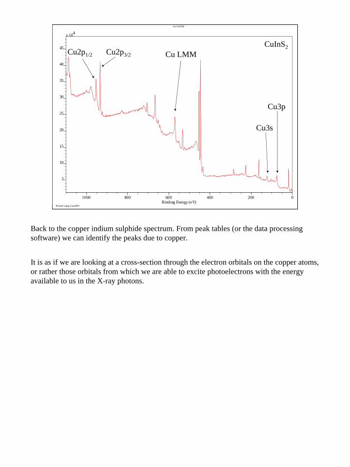
CuInS2

Back to the copper indium sulphide spectrum. From peak tables (or the data processing software) we can identify the peaks due to copper.

It is as if we are looking at a cross-section through the electron orbitals on the copper atoms, or rather those orbitals from which we are able to excite photoelectrons with the energy available to us in the X-ray photons.

31


survol.dts

x 104

5

10

15

20

25

30

35

40

45


In MNN

In3s

In3p1/2In3p3/2

In3d3/2 In3d5/2

In4s

In4p

In4d

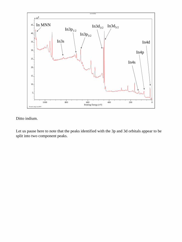
Ditto indium.

Let us pause here to note that the peaks identified with the 3p and 3d orbitals appear to be split into two component peaks.

32


in3d.dts

x 103

10

20

30

40

50

60

70

460 450 440Binding Energy (eV)

3 : 45/2, 7/2f

2 : 33/2, 5/2d

1 : 21/2, 3/2p

1/2s

Degeneraciesg = (2j + 1)

Total angular momentum j = (l + s)

Subshell Spin-orbit splitting

In3d3/2In3d5/2

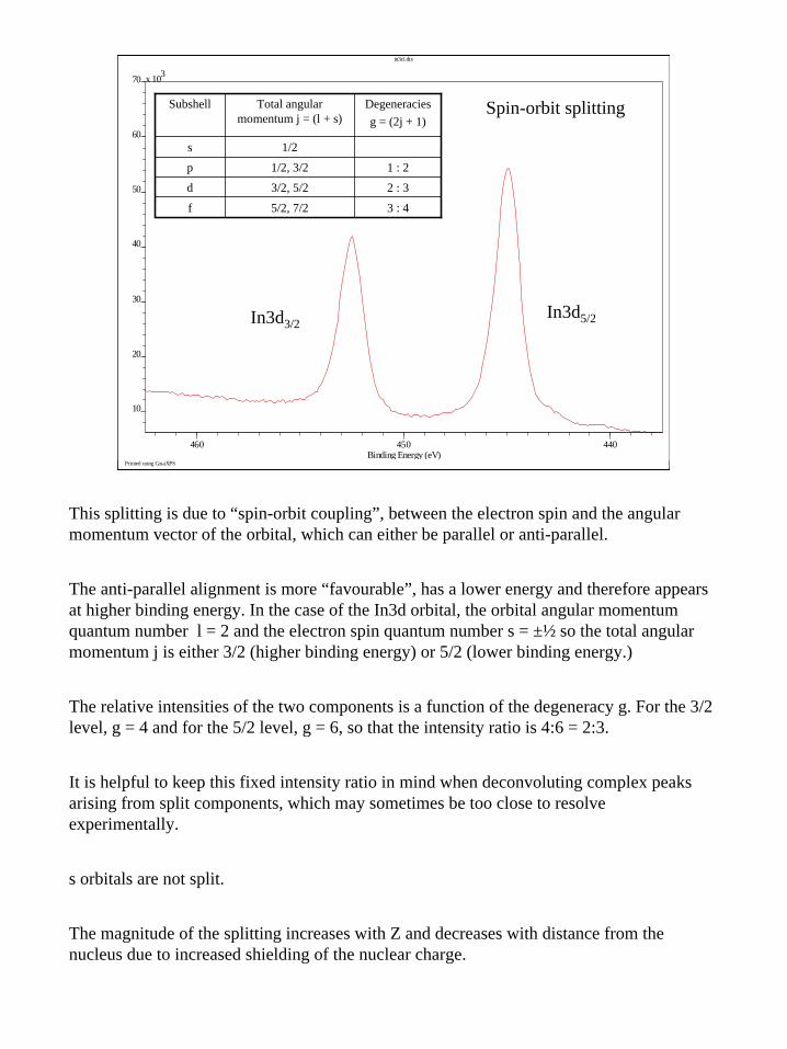
This splitting is due to “spin-orbit coupling”, between the electron spin and the angular momentum vector of the orbital, which can either be parallel or anti-parallel.

The anti-parallel alignment is more “favourable”, has a lower energy and therefore appears at higher binding energy. In the case of the In3d orbital, the orbital angular momentum quantum number l = 2 and the electron spin quantum number s = ±½ so the total angular momentum j is either 3/2 (higher binding energy) or 5/2 (lower binding energy.)

The relative intensities of the two components is a function of the degeneracy g. For the 3/2 level, g = 4 and for the 5/2 level, g = 6, so that the intensity ratio is 4:6 = 2:3.

It is helpful to keep this fixed intensity ratio in mind when deconvoluting complex peaks arising from split components, which may sometimes be too close to resolve experimentally.

s orbitals are not split.

The magnitude of the splitting increases with Z and decreases with distance from the nucleus due to increased shielding of the nuclear charge.

33


survol.dts

x 104

5

10

15

20

25

30

35

40

45


S2s S2p

CuInS2

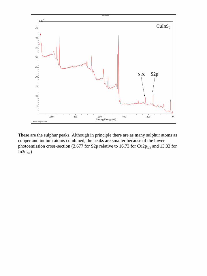
These are the sulphur peaks. Although in principle there are as many sulphur atoms as copper and indium atoms combined, the peaks are smaller because of the lower photoemission cross-section (2.677 for S2p relative to 16.73 for Cu2p3/2 and 13.32 for In3d5/2)

34


survol.dts

x 104

5

10

15

20

25

30

35

40

45


I3d O1sO KLL

C1s

Mn2p

Detection limit ~ 0.1%

CuInS2

Si2sSi2p

There are also peaks from elements that should not bet there, traces of contamination from the synthesis (Mn, Si, I), from oxidation of excess indium (O) and from the ubiquitous carbonaceous contamination observed on all but the most carefully prepared samples (C). Depending upon the photoemission cross-section and the noise in the data, the lower limit of concentration in the surface for detection by XPS is on the order of 0.1 at. %

35


ups6.dts

x 103

10

20

30

40

50

60



vb.dts

x 102

10

20

30

40

50

60

70

80

90


Valence bandUPSHeIIhυ = 40.8 eV

Valence bandXPSAlKαhυ = 1486.6 eV

In4d

In5pCu3d

S3p

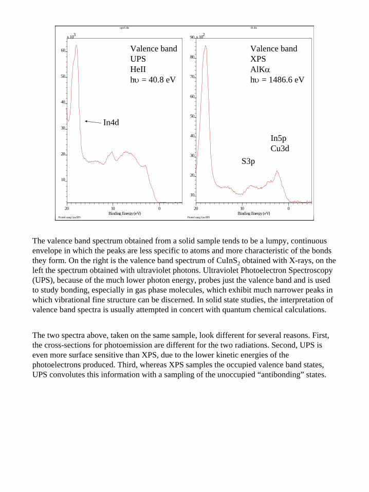
The valence band spectrum obtained from a solid sample tends to be a lumpy, continuous envelope in which the peaks are less specific to atoms and more characteristic of the bonds they form. On the right is the valence band spectrum of CuInS2 obtained with X-rays, on the left the spectrum obtained with ultraviolet photons. Ultraviolet Photoelectron Spectroscopy (UPS), because of the much lower photon energy, probes just the valence band and is used to study bonding, especially in gas phase molecules, which exhibit much narrower peaks in which vibrational fine structure can be discerned. In solid state studies, the interpretation of valence band spectra is usually attempted in concert with quantum chemical calculations.

The two spectra above, taken on the same sample, look different for several reasons. First, the cross-sections for photoemission are different for the two radiations. Second, UPS is even more surface sensitive than XPS, due to the lower kinetic energies of the photoelectrons produced. Third, whereas XPS samples the occupied valence band states, UPS convolutes this information with a sampling of the unoccupied “antibonding” states.

36

A.F

.Orc

hard

, in

Han

dboo

k of

X-R

ay a

nd U

ltrav

iole

t Pho

toel

ectr

on

Spec

tros

copy

, D.B

riggs

, Ed.

, Hey

don

and

Son,

Lon

don

(197

7)

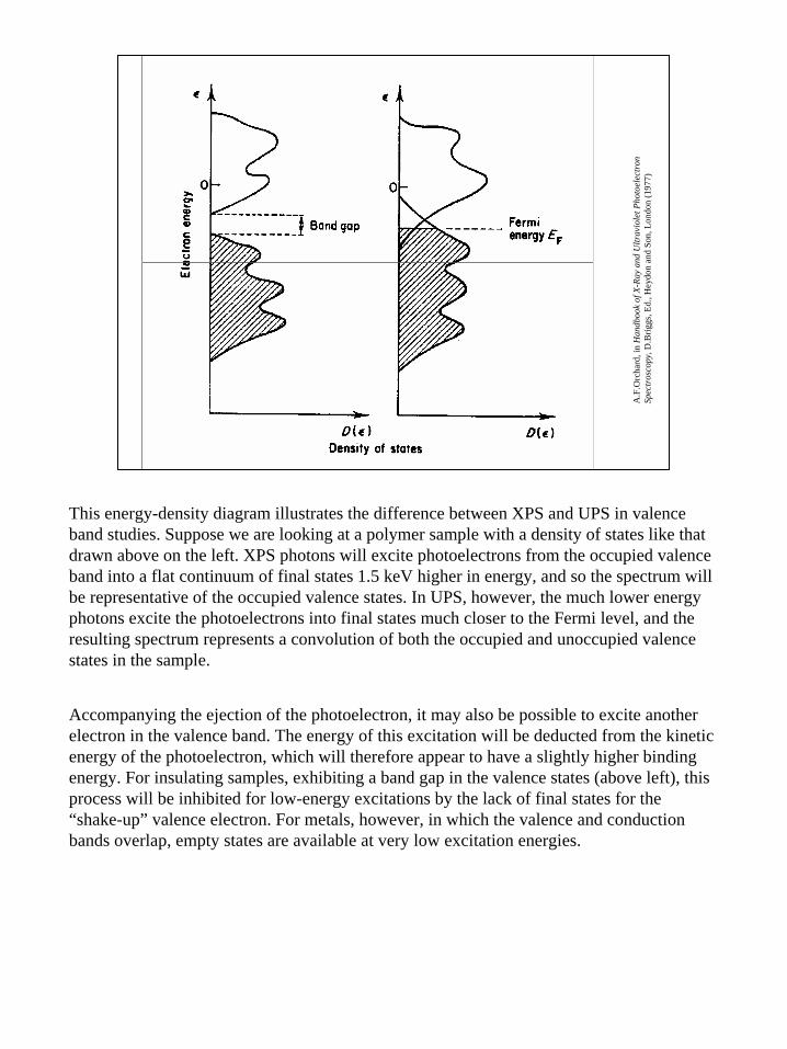
This energy-density diagram illustrates the difference between XPS and UPS in valence band studies. Suppose we are looking at a polymer sample with a density of states like that drawn above on the left. XPS photons will excite photoelectrons from the occupied valence band into a flat continuum of final states 1.5 keV higher in energy, and so the spectrum will be representative of the occupied valence states. In UPS, however, the much lower energy photons excite the photoelectrons into final states much closer to the Fermi level, and the resulting spectrum represents a convolution of both the occupied and unoccupied valence states in the sample.

Accompanying the ejection of the photoelectron, it may also be possible to excite another electron in the valence band. The energy of this excitation will be deducted from the kinetic energy of the photoelectron, which will therefore appear to have a slightly higher binding energy. For insulating samples, exhibiting a band gap in the valence states (above left), this process will be inhibited for low-energy excitations by the lack of final states for the “shake-up” valence electron. For metals, however, in which the valence and conduction bands overlap, empty states are available at very low excitation energies.

37

A.Barrie et al., Preprints, 27th Pittsburgh Conference on Analytical Chemistry and Applied Spectroscopy, Cleveland, USA (1976)

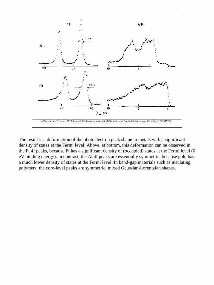
The result is a deformation of the photoelectron peak shape in metals with a significant density of states at the Fermi level. Above, at bottom, this deformation can be observed in the Pt 4f peaks, because Pt has a significant density of (occupied) states at the Fermi level (0 eV binding energy). In contrast, the Au4f peaks are essentially symmetric, because gold has a much lower density of states at the Fermi level. In band-gap materials such as insulating polymers, the core-level peaks are symmetric, mixed Gaussian-Lorentzian shapes.

38


Survol.dts

x 104

5

10

15

20


Si2p

Si2s

Plasmon satellites ħω = ~17eV

C1sO1sO KLL

Silicon wafer

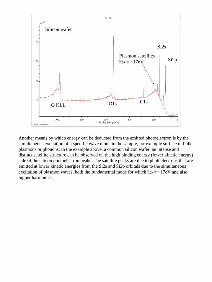
Another means by which energy can be deducted from the emitted photoelectron is by the simultaneous excitation of a specific wave mode in the sample, for example surface or bulk plasmons or phonons. In the example above, a common silicon wafer, an intense and distinct satellite structure can be observed on the high binding energy (lower kinetic energy) side of the silicon photoelectron peaks. The satellite peaks are due to photoelectrons that are emitted at lower kinetic energies from the Si2s and Si2p orbitals due to the simultaneous excitation of plasmon waves, both the fundamental mode for which ħω = ~17eV and also higher harmonics.

39

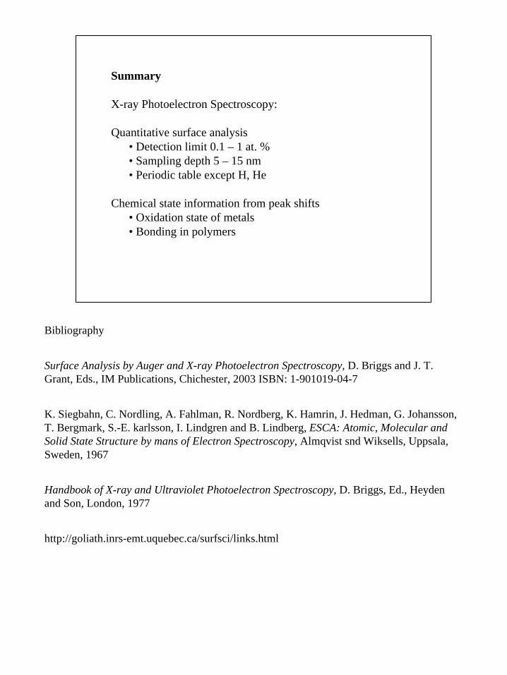
Summary

X-ray Photoelectron Spectroscopy:

Quantitative surface analysis• Detection limit 0.1 – 1 at. %• Sampling depth 5 – 15 nm• Periodic table except H, He

Chemical state information from peak shifts• Oxidation state of metals• Bonding in polymers

Bibliography

Surface Analysis by Auger and X-ray Photoelectron Spectroscopy, D. Briggs and J. T. Grant, Eds., IM Publications, Chichester, 2003 ISBN: 1-901019-04-7

K. Siegbahn, C. Nordling, A. Fahlman, R. Nordberg, K. Hamrin, J. Hedman, G. Johansson, T. Bergmark, S.-E. karlsson, I. Lindgren and B. Lindberg, ESCA: Atomic, Molecular and Solid State Structure by mans of Electron Spectroscopy, Almqvist snd Wiksells, Uppsala, Sweden, 1967

Handbook of X-ray and Ultraviolet Photoelectron Spectroscopy, D. Briggs, Ed., Heydenand Son, London, 1977

http://goliath.inrs-emt.uquebec.ca/surfsci/links.html

XPS theory - California Institute of Technology Info/XPs Theory by R. Paynter.pdf · X-ray...

Documents

Transcript of XPS theory - California Institute of Technology Info/XPs Theory by R. Paynter.pdf · X-ray...