Weak Gravitational Lensing Tables Rondes - … · Utilisez la charte graphique : elle pr sente...

Weak Gravitational LensingTables Rondes

Martin Kilbinger

CEA Saclay, Irfu/SAp - AIM; IAP

Euclid Summer School, FrejusJune/July 2017

[email protected]

www.cosmostat.org/kilbinger

Slides: http://www.cosmostat.org/ecole17

@energie sombre

COMMUNIQUE INTERNE

�

POUR INFORMATION, DIFFUSION ET AFFICHAGE

�

�Le 31 mai 2012

TÉLÉCHARGEZ LE LOGO DU CEA

Le nouveau logo du CEA et sa charte graphique sont téléchargeables sur l’intranet de la Direction de la communication : http://www-dcom.intra.cea.fr/ Énergie, cohésion et innovation

Présenté le 20 mars dernier à l’ensemble des salariés, le logo est le signe de la dynamique collective qui anime le CEA. La typographie des lettres CEA est unique : elle a été spécialement dessinée pour conférer à notre sigle modernité, mouvement et caractère. Le rouge, puissant, a été choisi pour exprimer l’énergie dans son sens le plus large, celui de la dynamique et de l’engagement collectif. Le rectangle et les lettres liées traduisent notre cohésion et la solidité de notre organisme. Enfin, ce logo réaffirme clairement notre mission. Il rappelle la richesse de nos champs d’action, reconnaît la solidité de notre socle de recherche fondamentale et concrétise notre engagement déterminé en faveur de l’industrie française. Bonnes pratiques � Utilisez la charte graphique : elle présente l’ensemble des éléments constitutifs

de la nouvelle identité graphique du CEA et ses règles d’applications.

� Ne créez pas vos propres supports : des modèles « prêts à l’emploi » sont téléchargeables sur l’intranet (notes, fax, présentation .ppt, ).

� Ne gaspillez pas de papier et épuisez vos stocks d’imprimés (cartes de visites, plaquettes ) avant d’en éditer de nouveaux intégrant la nouvelle charte.

Des questions ? Contactez le service Éditions-Évènements : 01 64 50 20 96 DIRECTION DE LA COMMUNICATION

Service Communication interne Tel. 01.64.50.10.72 Abonnez-vous et recevez par courrier électronique les communiqués internes. Pour cela connectez-vous à l’adresse : http://www-dcom.cea.fr

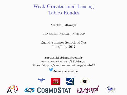
Outline

Weak-lensing tables rondes

Topic A: B-modes from varying z?

Topic B: Fisher matrix fit with CosmoSIS

Topic C: Peak counts and shear bias with camelus

Martin Kilbinger (CEA) Weak Gravitational Lensing Tables Rondes 2 / 23


B-modes from varying z?

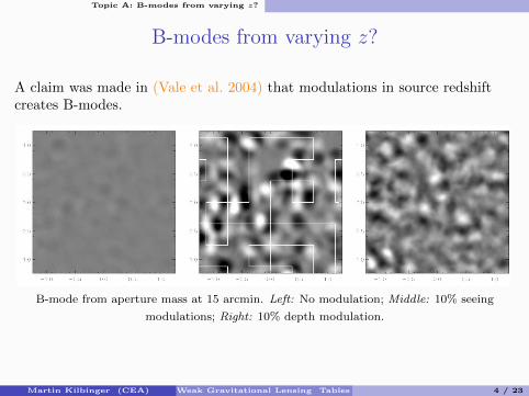
A claim was made in (Vale et al. 2004) that modulations in source redshiftcreates B-modes.L2 VALE ET AL. Vol. 613

Fig. 1.—B-mode aperture mass on a scale, for fields. The left panel is with no modulation, the center panel includes sharp 10% modulations in′15 2!.5# 2!.5the seeing correction on a scale (as detailed in the text and outlined by the solid lines), and the right panel is for 10% modulations in the source redshift′22relation at a scale of . The gray scale is linear and spans " .′ !48 5# 10

Fig. 2.—Variance in the aperture mass resulting from 10% modulations of the shear amplitude. Left: E-mode power (solid line) and the absolute value of thechange in the E-mode power resulting from modulations using a pixelized grid (dotted line) and a smooth gradient (dashed line) as described in the text. In bothcases the E-mode power is reduced on the largest scales for this particular realization. Right: B-mode power resulting from the same modulations.

3. SIMULATIONS

In order to assess the systematic errors induced by uncor-rected changes in the calibration or depth of the survey, wemake use of simulated weak lensing maps. These maps aregenerated by ray tracing through N-body simulations. We usethe methods described in detail in White & Vale (2003), pro-viding only a brief summary here.Our calculation is done within the context of a L cold dark

matter model (model 1 of White & Vale 2003) chosen to pro-vide a good fit to recent cosmic microwave background andlarge-scale structure data. The weak lensing maps are madefrom an N-body simulation using a multiplane ray tracing code,as described in Vale & White (2003). The code computes the

shear matrix A, which describes the distortion of an2# 2image due to lensing by a distribution of sources. The shearmatrix A is decomposed as

k " g g " q1 2A p , (1)( )g ! q k ! g2 1

where the are the shear components, k is the convergence,giand q is the rotation, which is generally small.We make maps of the shear and the convergence at a range

of source redshifts from to 3 in steps of Mpc.!1z ∼ 0 Dx p 50 hIn each case, a grid of rays subtending a field of view22048of is traced through the simulation. The two shear com-3!ponents and the convergence are output at each source planeand down-sampled to pixels. The final map is a21024weighted sum of the contributions from each source plane;for a distribution the weight given to source plane jdp/dzsis

dpw p H(z )Dx. (2)j jFdzs j

We use a source distribution of the form (Brainerd et al. 1996)

dp 2 3/2∝ z exp [!(z /z ) ]. (3)s s 0dzs

For this distribution . We use 2AzS p G(8/3)z ! 1.5z z p0 0 0 3for our base model and include fluctuations in wherez0appropriate.

B-mode from aperture mass at 15 arcmin. Left: No modulation; Middle: 10% seeing

modulations; Right: 10% depth modulation.



B-modes from varying z?

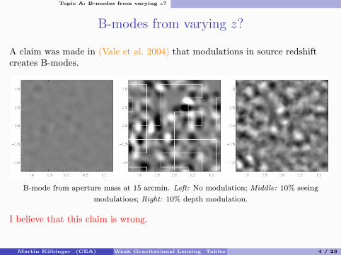
A claim was made in (Vale et al. 2004) that modulations in source redshiftcreates B-modes.L2 VALE ET AL. Vol. 613

Fig. 1.—B-mode aperture mass on a scale, for fields. The left panel is with no modulation, the center panel includes sharp 10% modulations in′15 2!.5# 2!.5the seeing correction on a scale (as detailed in the text and outlined by the solid lines), and the right panel is for 10% modulations in the source redshift′22relation at a scale of . The gray scale is linear and spans " .′ !48 5# 10

Fig. 2.—Variance in the aperture mass resulting from 10% modulations of the shear amplitude. Left: E-mode power (solid line) and the absolute value of thechange in the E-mode power resulting from modulations using a pixelized grid (dotted line) and a smooth gradient (dashed line) as described in the text. In bothcases the E-mode power is reduced on the largest scales for this particular realization. Right: B-mode power resulting from the same modulations.

3. SIMULATIONS

In order to assess the systematic errors induced by uncor-rected changes in the calibration or depth of the survey, wemake use of simulated weak lensing maps. These maps aregenerated by ray tracing through N-body simulations. We usethe methods described in detail in White & Vale (2003), pro-viding only a brief summary here.Our calculation is done within the context of a L cold dark

matter model (model 1 of White & Vale 2003) chosen to pro-vide a good fit to recent cosmic microwave background andlarge-scale structure data. The weak lensing maps are madefrom an N-body simulation using a multiplane ray tracing code,as described in Vale & White (2003). The code computes the

shear matrix A, which describes the distortion of an2# 2image due to lensing by a distribution of sources. The shearmatrix A is decomposed as

k " g g " q1 2A p , (1)( )g ! q k ! g2 1

where the are the shear components, k is the convergence,giand q is the rotation, which is generally small.We make maps of the shear and the convergence at a range

of source redshifts from to 3 in steps of Mpc.!1z ∼ 0 Dx p 50 hIn each case, a grid of rays subtending a field of view22048of is traced through the simulation. The two shear com-3!ponents and the convergence are output at each source planeand down-sampled to pixels. The final map is a21024weighted sum of the contributions from each source plane;for a distribution the weight given to source plane jdp/dzsis

dpw p H(z )Dx. (2)j jFdzs j

We use a source distribution of the form (Brainerd et al. 1996)

dp 2 3/2∝ z exp [!(z /z ) ]. (3)s s 0dzs

For this distribution . We use 2AzS p G(8/3)z ! 1.5z z p0 0 0 3for our base model and include fluctuations in wherez0appropriate.

B-mode from aperture mass at 15 arcmin. Left: No modulation; Middle: 10% seeing

modulations; Right: 10% depth modulation.

I believe that this claim is wrong.



Why do I have doubts about this claim?

Shear field at different depth still stays E-mode field.

Possible resons for the observed B-mode in (Vale et al. 2004):

• Artifact of the simulation. E.g. discontinuity in shear field.

• Artifact of measurement. E.g. problems with pixelisation, aperture-massestimator.

• Increased noise.



Possible aspects of study

Even if it is true, this is worth studying in more detail:

• Euclid will face problem of varying depth due to different qualityphoto-z’s from inhomogeneous ground-based data.

• Appearing B-mode means it is leaked from E-mode, so change incosmological weak-lensing signal. Important to quantify potentialsystematic.

• There is also information in the B-mode, e.g. induced by intrinsicalignment, higher-order effects, which might be exploited. Important toquantify systematic B-mode.

• We can study ways to reduce this B-mode. Smooth data across varyingz-regions? Use different aperture-mass estimator (integral over 2PCF, orother)?

• The authors did a purely numerical study. Worth to check analytically ifpossible.



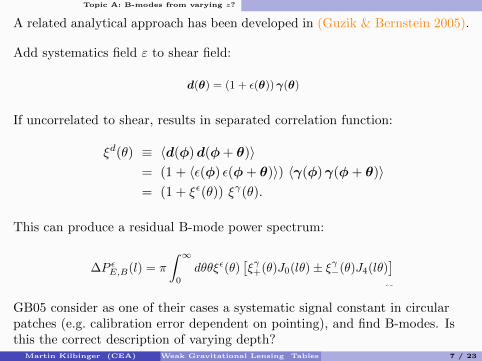
A related analytical approach has been developed in (Guzik & Bernstein 2005).

Add systematics field ε to shear field:

3

III. EFFECT OF SYSTEMATICS ON E/BPOWER SPECTRA

Ideally, we would like to measure the shear field γ(θ)directly. What we observe, however, is the coherent el-lipticity induced on an ensemble of galaxies, which (a)is defined by the distortion g = γ/(1 − κ); (b) is im-parted on galaxies that are not intrinsically circular, and(c) are viewed through a finite point-spread function(PSF). The measured shear field d(θ) will in practicebe modulated or contaminated by various observationaleffects [14]. Although techniques for shear extractionfrom galaxy images have been extensively developed andtested [5, 15, 19], there remain imperfections which canbe detrimental to precision cosmology.

Throughout the paper we assume that the observedfield is related to the true shear field by a position-dependent multiplicative scalar factor 1 + ϵ(θ) such aswill result from a misestimation of the “resolution” [5] or“shear polarizability” [19]. The systematic field ϵ(θ) is arandom field assumed to have zero mean and described tothe lowest interesting order by the two-point correlationfunction. Thus we express the observed field in terms ofthe shear and the systematics fields as

d(θ) = (1 + ϵ(θ))γ(θ). (4)

This relation is local in real space, so it is going to couplemodes of the shear field in the Fourier space, i.e. havesome non-local effect on the relevant power spectra. Weassume that the shear field γ due to massive structures inthe Universe is uncorrelated with systematics field ϵ(θ),which is a Galactic or instrumental foreground. The ob-served two-point correlation function ξd(θ) can in thiscase be written as

ξd(θ) ≡ ⟨d(φ)d(φ + θ)⟩ (5)

= (1 + ⟨ϵ(φ) ϵ(φ + θ)⟩) ⟨γ(φ)γ(φ + θ)⟩ (6)

= (1 + ξϵ(θ)) ξγ(θ). (7)

We have introduced two-point correlation functions ξγ(θ)for the shear field and ξϵ(θ) for the systematics field. Forsimplicity we will assume that the systematics field ϵ(θ)is homogeneous and isotropic. In practice the assump-tion of isoptropy is not restrictive, as the effects of ananisotropic systematic could be approximated to first or-der by considering the azimuthally averaged correlationfunction.

Correlation functions for the distortion field, ξd+(θ)

and ξd−(θ), may be expressed as products of the corre-

lation functions for the shear and systematics ξd±(θ) =

(1 + ξϵ(θ)) ξγ±(θ) which follow from eqs. (1) and (7).

We can rewrite eq. (3) in terms of the distortion in-stead of the shear and then account for systematic sig-nals ϵ(θ). We split the observed E and B mode powerspectra P d

E,B(l) into two contributions as follows

P dE,B(l) = P γ

E,B(l) + ∆P ϵE,B(l), (8)

where the term P γE,B(l) is E mode (B mode) power spec-

trum of the shear and ∆P ϵE,B(l) represents the contribu-

tions to the E mode (B mode) power due to systematicsignals. We focus on these error terms in the remainderof the paper. Using eqs. (3) and (8) they can be writtenas

∆P ϵE,B(l) = π

! ∞

0

dθθξϵ(θ)"ξγ+(θ)J0(lθ) ± ξγ

−(θ)J4(lθ)#.

(9)We assume that the shear correlation functions ξγ

± re-ceive contribution from E mode only, i.e. P γ

E(l) = Pκ(l),P γ

B(l) ≡ 0, since B-mode cosmological contributions areexpected to be a few orders of magnitude smaller onscales > 1′ [7]. The systematic errors ∆PE,B(l) to Eand B mode power spectra can be written as integralsover the convergence power spectrum Pκ(l) with a win-dow function WE,B(l, q):

∆PE,B(l) =

! ∞

0

dq q Pκ(q)WE,B(l, q), (10)

where the window function depends solely on the corre-lation function ξϵ of the systematic modulation, and isgiven by

WE,B =1

2

! ∞

0

dθθξϵ(θ) [J0(lθ)J0(qθ) ± J4(lθ)J4(qθ)] .

(11)In the limit of a systematic that is completely correlatedacross the entire observation, i.e. a constant calibra-tion error, we have ξϵ(θ) = Σ2, where Σ2 is the vari-ance of the calibration error. In this limit we obtainWE(l, q) = Σ2 q−1δD(l − q) and WB(l, q) ≡ 0, where wehave used an integral relation for the Bessel functions$∞0

dθ θ Jn(l θ)Jn(q θ) = q−1 δD(q − l) [20]. Thus the er-ror contributions to E/B power spectra are ∆PE(l) =Σ2Pκ(l) and ∆PB(l) = 0 in this case, and there is noconversion of E power to B power, as expected.

Numerical simulations of calibration inhomogeneity in[8] are presented in terms of the aperture mass statisticsMap(R) and M×(R) with compensated filter defined in[21, 22]. We produce analytic predictions for inhomoge-neous calibration errors for comparison with the numer-ical results of [8] using the same filter as they did.

IV. MODELING OF SYSTEMATICS

We consider several potentially useful models of thecorrelation function of the systematic signal ξϵ(θ) and weexamine the dependence of E and B mode power spectra(10) on the characteristics of ξϵ(θ). The correlation func-tions considered here are analytically tractable and ableto describe a wide variety of random processes leading tosystematic signals. Each correlation function consideredhere is assumed to describe a stationary, isotropic randomfield. We assume that the systematic field has a finitevariance Σ2. Equation (11) shows that ∆PE,B(l) ∝ Σ2

If uncorrelated to shear, results in separated correlation function:

3




d(θ) = (1 + ϵ(θ))γ(θ). (4)


ξd(θ) ≡ ⟨d(φ)d(φ + θ)⟩ (5)

= (1 + ⟨ϵ(φ) ϵ(φ + θ)⟩) ⟨γ(φ)γ(φ + θ)⟩ (6)

= (1 + ξϵ(θ)) ξγ(θ). (7)








P dE,B(l) = P γ

E,B(l) + ∆P ϵE,B(l), (8)




∆P ϵE,B(l) = π

! ∞

0


−(θ)J4(lθ)#.



E(l) = Pκ(l),P γ


∆PE,B(l) =

! ∞

0



WE,B =1

2

! ∞

0







This can produce a residual B-mode power spectrum:

3




d(θ) = (1 + ϵ(θ))γ(θ). (4)


ξd(θ) ≡ ⟨d(φ)d(φ + θ)⟩ (5)

= (1 + ⟨ϵ(φ) ϵ(φ + θ)⟩) ⟨γ(φ)γ(φ + θ)⟩ (6)

= (1 + ξϵ(θ)) ξγ(θ). (7)








P dE,B(l) = P γ

E,B(l) + ∆P ϵE,B(l), (8)




∆P ϵE,B(l) = π

! ∞

0


−(θ)J4(lθ)#.



E(l) = Pκ(l),P γ


∆PE,B(l) =

! ∞

0



WE,B =1

2

! ∞

0







GB05 consider as one of their cases a systematic signal constant in circularpatches (e.g. calibration error dependent on pointing), and find B-modes. Isthis the correct description of varying depth?



TasksA. Numerical study, redo (Vale et al. 2004) analysis.

1. Download (N -body +) ray-tracing/ray-shooting simulations. Needpositions x, y, shear γ (and/or convergence κ) and redshift z.

2. Produce E-/B-mode estimates: Compute the 2PCF, e.g. with athena,and 〈M2

ap,×〉 with pallas.py. Make sure there are no intrinsic significantB-modes.

3. Introduce redshift variations: Select galaxies at different z in patches.Redo step A.2, see whether B-modes are introduced.

B. Analytical study.

1. Use the (Guzik & Bernstein 2005) or a different approach to modelredshift variations over a field.

2. Compute the expected B-mode signal to see whether or not it is zero.

C. Advanced studies.

• Use realistic redshift variations on a large (Euclid-like?) field.

• Study other systematic effects, seeing variations, shear calibration,environment biases that correlated with density, . . .



Simulations to download

• Log-normal simulations, B. Joachimi, 08/2013, 25 fields, one z-bin, withmasks, used for code testing and validation in OU-LE3.www.astro.uni-bonn.de/~reiko/le3sim/simpublic/euclid_le3_

versim_v1.3.tar.gz

• Log-normal simulations, B. Joachimi, 04/2016, 1 field, two z-bins, withmasks, used for code testing and validation in OU-LE3.Get link from http://www.cosmostat.org/ecole17

• MICE v2.0 simulation, 5, 000 deg2, some issues with the lensing signal,fixed?https://cosmohub.pic.es/#/catalogs/1 (login required)

• Euclid Flagship v1.0 simulation, 5, 000 deg2, much deeper, to lower halomass, higher resolution than MICE.https://cosmohub.pic.es/#/catalogs/53 (login required)


www.astro.uni-bonn.de/~reiko/le3sim/simpublic/euclid_le3_versim_v1.3.tar.gz

www.astro.uni-bonn.de/~reiko/le3sim/simpublic/euclid_le3_versim_v1.3.tar.gz

http://www.cosmostat.org/ecole17

https://cosmohub.pic.es/#/catalogs/1

https://cosmohub.pic.es/#/catalogs/53


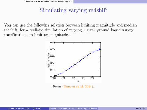
Simulating varying redshift

You can use the following relation between limiting magnitude and medianredshift, for a realistic simulation of varying z given ground-based surveyspecifications on limiting magnitude.

8 C. Duncan et al.

Figure 3. The top panel shows the effective number density of galaxies (ingalaxies/arcminute2) as a function of the faint limiting magnitude iAB forsources with valid shape measurement (dashed), and for all galaxies withphotometry (solid). The bottom panel shows the median redshift of sourcesas a function of the limiting magnitude. All data is taken from CFHTLenScatalogues. Crosses mark values taken for an S3 survey, whilst dots markvalues taken for an S4 survey.

redshift errors �Phot = 0.05(1 + zPhot). Unless otherwise stated,results hereafter are shown for an S4 survey.

Fig. 3 shows the median survey redshift, and effective num-ber density of galaxies as a function of faint limiting iAB mag-nitude taken from CFHTLenS catalogues for galaxies with validshape measurement (Heymans et al. 2012a) as well as for all galax-ies with photometry. As the galaxies broad size distributions areweakly redshift dependent, cuts on galaxy size such as those usedin a shape analysis do not significantly affect the measured medianredshift, but will cause a noticeable decrease in effective numberdensity of galaxies used. From Fig. 3 we choose for our S3 sur-vey a median redshift zmed = 0.66, and galaxy number densityof hni = 8.5 galaxies/arcminute2 and 18 gal/arcminute2 forshear and clustering analyses respectively. Similarly, we considerfor an S4 survey zmed = 0.7, and assume shapes can be mea-sured for every detected source. Therefore, we use the photometryline in deducing the number density of galaxies for S4, and takengal = 28 galaxies/arcminute2 for both shear and clusteringanalyses.

Figure 4. Galaxy redshift probability distribution functions as defined inSection 3.4, for an S3 ground–based (top) and S4 space–based (bottom)survey (defined in Section 3.3).

3.4 Galaxy redshift distributions

We model the distribution of galaxies with true redshift zt as

p(i)(zt) =

Z z(i)h

z(i)l

dzph p(zt|zph)p(zph), (38)

where p(zt|zph) is assumed to be a Gaussian with width �z =0.05(1 + zph), and zl and zh denote the lower and higher boundsof the redshift bin in photometric redshift. We model the galaxyphotometric redshift distribution, p(zph), as (Smail, Ellis & Fitch-ett 1994)

p(zph) /✓

zph

z0

◆2

e�⇣ zph

z0

⌘1.5

, (39)

with characteristic redshift z0 = zmed/1.412. The galaxy redshiftdistribution is subdivided into redshift bins with equal numbers ofgalaxies.

Fig. 4 shows the resultant galaxy distribution for 8 redshiftbins for survey types S3 and S4, with the number density contrastpower spectra given for three redshift bin combinations in Fig. 5,split by component. Noticeably, for closely–separated redshift bins,the intrinsic clustering term is non–vanishing due to the presenceof photometric redshift errors which cause some galaxies to be in-correctly assigned to a given redshift bin, and causes overlap be-tween the binned galaxy distributions. As we take redshift bins thatare more widely separated, the power from intrinsic clustering de-creases, so we see that for the most widely separated bins the totalpower is dominated by terms that include the magnification. It isfor this reason that van Waerbeke (2010) and Hildebrandt, Waer-beke & Erben (2009) take spatially disjoint redshift bins to isolatethe magnification contribution to the clustering power spectrum. Asthe cross power (mg+gm) is always dominant over the pure magni-fication (mm) power, frequently studies will ignore the pure mag-nification contribution to the overall clustering power, and insteadjust quote the cross contribution. In the situation where correla-tions are considered between distant foreground and backgrounds,the intrinsic clustering contribution is subdominant and may also beignored. In this analysis, we consider all contributions to the power,as given in Equation 11.

c� 2013 RAS, MNRAS 000, 1–18

From (Duncan et al. 2014).



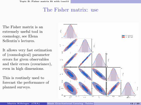
The Fisher matrix: use

The Fisher matrix is anextremely useful tool incosmology, see ElenaSellentin’s lectures.

It allows very fast estimationof (cosmological) parametererrors for given observablesand their errors (covariance),even in high dimensions.

This is routinely used toforecast the performance ofplanned surveys.



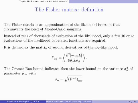
The Fisher matrix: definition

The Fisher matrix is an approximation of the likelihood function thatcircumvents the need of Monte-Carlo sampling.

Instead of tens of thousands of evaluation of the likelihood, only a few 10 or soevaluations of the likelihood or related functions are required.

It is defined as the matrix of second derivatives of the log-likelihood,

Fαβ =

⟨∂2[− lnL]

∂θα∂θβ

⟩.

The Cramer-Rao bound indicates then the lower bound on the variance σ2α of

parameter pα, with

σα =√

(F−1)αα.



The Fisher matrix: in practice IWeak lensingFor example, the Fisher matrix for the weak-lensing power spectrum can bewritten as

Fαβ =∑

`

∑

pq

∂Pp(`)

∂θα(C−1)pq(`)

∂Pq(`)

∂θβ,

where the indices p, q denote redshift bin combinations,p, q = 1 . . . nz(nz + 1)/2, and Pp is the tomographic weak-lensing powerspectrum.

Practical difficulties with the Fisher matrixComputing numerical derivations can be problematic, since often a very highprecision is required. Which is the case for the Fisher matrix, where smallerrors in the derivatives propagate in a non-linear way to the parameterconstraints due to the non-linear process of matrix inversion.

Such errors can be introduced by interpolation of cosmological quantities forspeed-up, insufficient accuracy of numerical integration, too largediscretisation steps etc.



The Fisher matrix: in practice II

Codes that compute theoretical models for Monte-Carlo sampling do not needto be as accurate as Fisher-matrix codes (Wolz et al. 2012).

Often the Fisher matrix changes substantially with small algorithmic changes,for example

• step size h of the numerical derivatives

• number of points n that are used (n-point stencil).

In addition the Fisher matrix is often ill conditioned in the presence ofparameter degeneracies, or badly constrained parameters. Inversion is thentricky; often a prior is added to “regularize” the Fisher matrix.



An alternative method to compute the Fisher matrix?

Instead of relying on derivatives, how about the following idea:

Around the maximum-likelihood (or posterior) point in parameter space p0,the likelihood for n points are computed, and a quadratic function is fitted tothose points.

This quadratic form is then an estimate of the Fisher matrix.

This circumvents the necessity for numerical derivatives.Questions:

• How many points are required? Does this number scale linearly with thedimension?

• How do we choose the step size? Adaptive if possible.

• Should the steps only vary one direction at a time, or be a combination ofparameters?

• How does the precision of this approach compare to the traditional Fishermatrix?



Tasks

A. ImplementationImplement this alternative Fisher matrix estimator in CosmoSIS.

Implementation of likelihood evaluation around fiducial point, fitting,convergence testing.

B. ComparisonCompare with the traditional Fisher matrix, that is already part of CosmoSIS.Play around with parameters, number of points, different probes, cosmologicalparameter, . . ..

C. Further studiesThis could also be implemented in nicaea, or MontePython, which computesdirectly the derivative of the likelihood for the Fisher matrix.

(From my obscure notes from recent IST Euclid meeting in Heidelberg):Eric Linder mentioned minuit minimizer and quadratic interpolation, seehttps://pypwa.jlab.org/mntutorial.pdf.


https://pypwa.jlab.org/mntutorial.pdf


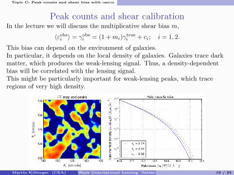
Peak counts and shear calibrationIn the lecture we will discuss the multiplicative shear bias m,

〈εobsi 〉 = γobsi = (1 +mi)γtruei + ci; i = 1, 2.

This bias can depend on the environment of galaxies.In particular, it depends on the local density of galaxies. Galaxies trace darkmatter, which produces the weak-lensing signal. Thus, a density-dependentbias will be correlated with the lensing signal.This might be particularly important for weak-lensing peaks, which traceregions of very high density.

Part I day 3+: Extra stu↵ Higher order statistics: peak counts

WL peak counts: Why do we want to study peaks?

[email protected] Chieh-An Lin (CEA/SAp)

What are peaks?

• Local maxima of the projected mass• Direct tracers of massive regions• Probe mass function

A fast stochastic approach for constraints using peaks Irfu — Jul 2nd, 2015 11Martin Kilbinger (CEA) WL Part I/II 121 / 135



The problem

This cannot easily be simulated and then calibrated, for example with simplegalaxy image simulations.

The correlation with the local desity means that the cosmological signal needsto be simulated as well.

This typically is an N -body simulation.

However, at least for a simple WL peak model (see lecture Part I day 3 [3/6]),this step can be replace by simple, fast simulations, implented in camelus (Lin& Kilbinger 2015).



Tasks IA. Run the C-code camelus

Download from https://github.com/Linc-tw/camelus.

Perform a few test runs and familiarize with the produced output.

B. Model and test density-dependent m

1. Simple modelFor the galaxies simulated by camelus, estimate local density δ(e.g. count in cells), and apply m(δ) with some fonctional dependence.See for example (Hoekstra et al. 2016).

2. More realistic modelThe galaxies should follow (trace) the halo distribution, this is not yetimplemented in camelus.

Relatively easy: Produce WL map with random galaxies from first run ofcamelus, re-distribute galaxies according to 2D density, re-run camelususing this new distribution, and some model m(δ).

Even better, the galaxies should follow the halo distribution in 3D. Thiscan be implemented by modifying the code, but might be quite involved.


https://github.com/Linc-tw/camelus


Tasks II

C. Quantify influence of mIn all of the above cases: Produce WL peak histograms with and withoutdensity-dependent m, compare using Euclid-like survey setting (area, depth,etc.).Compare these changes to the sensitivity of peak histograms from dark-energy.From this, actual requirements on m(δ) for WL peak counts could be derived.

D. Advanced studiesParametrize m(δ), add as sampling parameters to camelus.Perform joined analysis of cosmology and m(δ).Detailed analysis of influence of m on cosmological parameters, includingcorrelations and degeneracies.


Bibliography

Bibliography I

Duncan C A J, Joachimi B, Heavens A F, Heymans C & Hildebrandt H 2014MNRAS 437, 2471–2487.

Guzik J & Bernstein G 2005 Phys. Rev. D 72(4), 043503.

Hoekstra H, Viola M & Herbonnet R 2016 ArXiv e-prints .

Lin C A & Kilbinger M 2015 A&A 576, A24.

Vale C, Hoekstra H, van Waerbeke L & White M 2004 ApJ 613, L1–L4.

Wolz L, Kilbinger M, Weller J & Giannantonio T 2012 JCAP 9, 9.


Weak Gravitational Lensing Tables Rondes - … · Utilisez la charte graphique : elle pr sente...

Documents

Transcript of Weak Gravitational Lensing Tables Rondes - … · Utilisez la charte graphique : elle pr sente...