UNIVERSITÀ DI PAVIA UNIVERSITÉ DE STRASBOURG

UNIVERSITÀ DI PAVIA

UNIVERSITÉ DE STRASBOURG

DOTTORATO DI RICERCA IN MATEMATICA – XXXI ciclo

Dipartimento di Matematica «F. Casorati»

ÉCOLE DOCTORALE ED 269 «Mathématiques, Sciences de l'Information et del'Ingénieur»

Institut de recherche mathématique avancée (IRMA)

TESI/THÈSE presentata da / présentée par ::

Sonia CANNASsostenuta il/soutenue le : 27 Novembre 2018

per ottenere il titolo di : Dottore di Ricercapour obtenir le grade de : Docteur de l’université de Strasbourg

Disciplina / Discipline : Matematica / Mathématique

GEOMETRIC REPRESENTATION AND

ALGEBRAIC FORMALIZATION OF

MUSICAL STRUCTURES

RELATORI / THÈSE dirigée par :Prof. PAPADOPOULOS Athanase Directeur de Recherche, IRMA (Strasbourg) Prof. ANDREATTA Moreno Directeur de Recherche, IRCAM (Paris) Prof. PERNAZZA Ludovico Ricercatore, Università degli Studi di Pavia

ALTRI MEMBRI DELLA COMMISSIONE / AUTRES MEMBRES DU JURY :Prof. JEDRZEJEWSKI Franck Chargé de Recherches, CEA INISTN Prof. ACQUISTAPACE Francesca Professoressa, Università degli Studi di PisaProf. FERRARIO Davide Professor, Università Milano Bicocca

Università degli Studi di

Pavia e di Milano-Bicocca

Dottorato di Ricerca in Matematica

XXXI Ciclo

Université de Strasbourg

École doctorale de mathématiques,

sciences de l'information et de

l'ingénieur

Geometric representation and

algebraic formalization of

musical structures

Supervisors

Prof. Athanase Papadopoulos

Prof. Ludovico Pernazza

Co-supervisor

Prof. Moreno Andreatta

PhD candidate

Sonia Cannas

Acknowledgements

During my PhD, several people have contributed to make this work possible and made these three years a

wonderful experience.

Firstly, I would like to thank my supervisors Moreno Andreatta, Athanase Papadopoulos and Ludovico

Pernazza. The order chosen to thank them is only alphabetic and each of them gave me di�erent teachings.

A special thanks also for encouraging me to organize the co-tutorship between the University of Pavia and the

University of Strasbourg and for helping me in all bureaucratic di�culties. Spending half of my PhD in Pavia

and half in Strasbourg was a wonderful experience, extremely educational and exciting.

I would like to thank the universities of Pavia and Milano-Bicocca for giving me the opportunity to start my

research project. When I enrolled in the degree course of mathematics, I was also studying at the Conservatory.

I knew that studying at the same time both at the university and at the conservatory would not be easy, and

since my aim was to become a violist I thought I would end my studies in mathematics after my three-year

degree. As I had imagined, the �rst years were very hard, I had to make many sacri�ces. In addition, the eco-

nomic crisis threw my generation into fear of not being able to build a future; however, after all, I continued my

studies in mathematics with a master degree. It was right during the master that I discovered about a research

�eld that would satisfy my interdisciplinary curiosity as concerns the relationships between mathematics and

music: Mathematical Music Theory. My intent was to explore this innovative �eld and give my contribution,

therefore I decided to look for a PhD. I would like to thank prof. Cadeddu and prof. Polo of the University

of Cagliari for their support in the applications for PhD scholarships. I knew that it would have been hard to

get a PhD scholarship, especially for an interdisciplinary research project as mine, and I thank them for not

deceiving me. I would also like to thank Samuele Antonini for helping me at the beginning of the PhD.

I am thankful to the University of Pavia and to the SMIR project, �nanced by USIAS, for all fundings

that allowed me to live serenely the PhD. All over the world, more and more PhD students develop psychiatric

illnesses, especially anxiety and/or depression due to economic problems, the fear of not being able to �nd a

stable job, excessive competition in the research world and the lack of consideration by the supervisor. I was

very lucky from an economic viewpoint thanks to the fundings that allowed me to take part in many conferences

and to move freely between Pavia and Strasbourg. I was also very lucky with my three supervisors that followed

me and helped me, leaving a lot of freedom in the management of my work and supporting me in the choice of

the research topic.

I am grateful to Thomas Noll, Tom Fiore, Emmanuel Amiot, Franck Jedrzejewski, Giovanni Albini, Louis

Bigo, Alexandre Popo� and Andrée Ehresmann for their interest in my work and their suggestions. I would

also like to thank my colleagues Corentin Guichaoua, José-Luis Besada, Matteo Pennesi and Davide Stefani for

several interesting conversations about Mathematical Music Theory.

I am thankful to all my PhD and postdoc colleagues of the Universities of Pavia, Strasbourg and Milano-

Bicocca. Although I was far from my land, you helped in making the university a second home for me. A very

special thank to who in these years have been more than just colleagues: Marco, Francesco, Gioia, Barbara,

2

Monica, Alberto, Lorenzo and Lukas. I want to dedicate a heartfelt thanks to Salvatore, with which we have

become colleagues casually, who gave me the love for research and supported me so much during all my years

of study.

I would also like to thank my PDI colleagues. Joining the PDI program (Programme Doctoral International)

allowed me to know many other researches and many international students with whom it has been very inter-

esting to meet and discuss about our countries.

I am also thankful to all my colleagues of the University of Cagliari Marghe, Noe, Francesca and Federica.

A very special thank to the Cairoli College Choir for the beautiful musical experiences shared together. I

have always loved singing, and I really enjoyed it with you.

I would also like to thank the group of Italians in Strasbourg for helping me in many circumstances and for

sharing so many moments together.

A very special thanks to all the friends who have accompanied and supported me in this adventure. Many

thanks to Laura and Annamaria for giving me their friendship. One of the reasons why it was di�cult to leave

Pavia was because of you. Thank you so much to my historic friends Roby, Selly, Ale, Isa, Lau, Carlo e Mickey.

Although we have been away in these years, it has been a great help to know that I can always count on you.

Although she is no longer with us, I thank Giulia. I know if you had been there you would have been close to

me as always, and although you had a con�ictual relationship with math I am sure you would have liked this

interdisciplinary work.

Finally, a very heartfelt thanks to my family. My mother and father concluded what my grandparents could

not do: study with interests and improve their social condition. They taught me that love for studying and

dedication to work is important not only to avoid economic poverty, but also to improve oneself as people.

Together with my grandparents, who could not continue their studies as they would have liked, my parents

were a great model for me. Although younger than me, my brother was also a model that helped in showing

me the value of dedication and study. Maybe thirty years ago nobody would have imagined it, but now we are

going to have the �rst Doctor of Philosophy in our family. All this is thanks to you, that since I was a child

you have been a model for me and you have always supported me in all my studies: from the school, to the

Conservatory, up to the University. I know that in these years far from our island you missed me, but I thank

you for understanding how this experience was important for me.

3

Riassunto

Introduzione

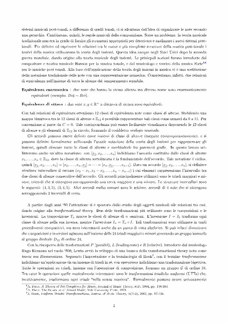
Nonostante la storia dei rapporti tra matematica e musica abbia radici nell'antichità, la ricerca in Mathemat-

ical Music Theory è molto recente. La matematica viene spesso considerata parte del mondo delle regole e

della razionalità, mentre la musica nel mondo della creatività e della libertà. Uno studio più approfondito di

entrambe le discipline mostra chiaramente che la matematica e la musica sono profondamente legate. Uno

dei legami più intuitivi e noti, soprattutto ai non esperti, riguarda gli aspetti �sici e acustici delle strutture

musicali. Un esempio noto è quello della scala pitagorici. Sulla base dei legami tra la lunghezza di una corda e

la frequenza della nota emessa quando la corda è in vibrazione, i pitagorici osservato l'esistenza di una relazione

tra numeri razionali e intervalli musicali. Sebbene sia semplice e intuitivo comprendere l'uso della matematica

per descrivere la musica da un punto di vista �sico-acustico, questo non è l'unica connessione tra queste due

discipline. Lasciando l'acustica, e guardando verso un livello più concettuale, che è il livello dell'atto compos-

itivo, si osserva che la musica è ricca di strutture e regole, ben rappresentate e formalizzate tramite strutture

matematiche. Il nuovo campo di ricerca, noto come Mathematical Music Theory, nasce per spiegare la teoria

musicale contemporanea, cercando di descriverne i diversi e nuovi oggetti musicali e, inoltre, le trasformazioni

fra loro attraverso formalizzazioni che possono essere utile per l'analisi musicale e la composizione.

Questo lavoro di tesi rientra nell'ambito della transformational theory, una branca della Mathematical Music

Theory nata con i lavori pioneristici di David Lewin12 e Guerino Mazzola34. L'idea principale è quella di

utilizzare la struttura matematica di gruppo per de�nire trasformazioni musicali. L'uso dell'utilizzo dell'algebra

in musica iniziò con diversi teorici della musica, ed è molto utile per descrivere e spiegare strutture musicali.

Introduzione alla Mathematical Music Theory

Nel primo capitolo presentiamo le principali de�nizioni e risultati della Mathematical Music Theory, in parti-

colare della transformational theory, necessari per la comprensione del lavoro sviluppato nella tesi.

Uno degli aspetti più importanti per la composizione risiede nell'abilità di rendere interessante l'interazione

tra le diverse linee melodiche che creano l'armonia, tradizionalmente conosciuta come voice leading. Si tratta

dell'interazione di due o più linee musicali, che realizza una progressione di accordi secondo i principi del

contrappunto. La maggior parte della musica occidentale dal XVII al XIX secolo è basata sull'armonia a

quattro parti, organizzata secondo determinate regole musicali, e una delle più importanti è quella di collegare

gli accordi cercando di compiere il minor movimento possibile, quindi lasciando ferme certe note e muoversi

possibilmente per moto congiunto.

Alla �ne del XIX secolo diversi compositori come Wagner, Debussy e Bartok cominciarono a cercare nuove

possibilità musicali abbandonando la musica tonale che aveva caratterizzato il XVII, XVII e XIX secolo. Nei

1D. Lewin, Transformational techniques in atonal and other music theories, Perspectives in New Music, n.21, 1982.2D. Lewin, Generalized Musical Intervals and Transformations, Yale University Press,1987.3G. Mazzola, Gruppen und Kategorien in der Musik: Entwurf einer mathematischen Musiktheorie, Heldermannr, Lemgo, 1985.4G. Mazzola, Geometrie der Tone, Birkhäuser, Basel, 1990.

4

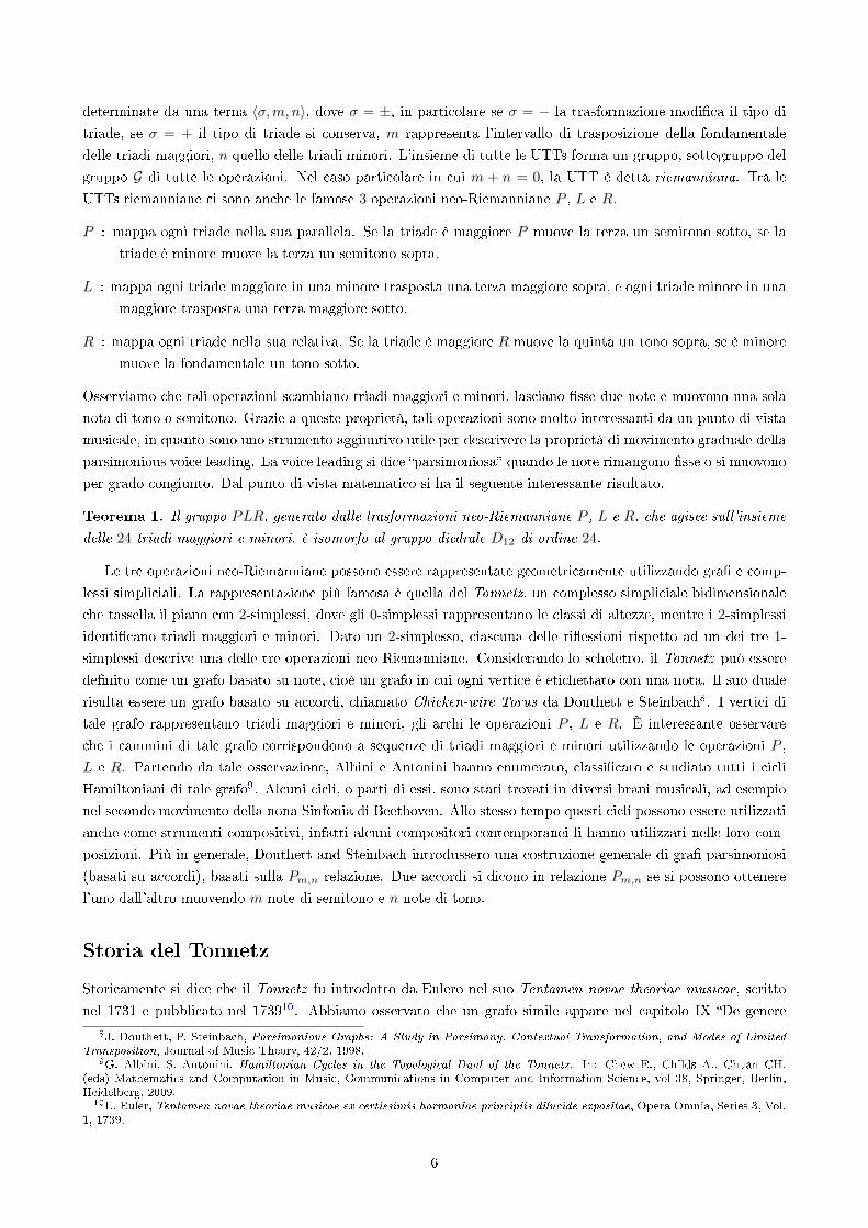
sistemi musicali post-tonali, a di�erenza di quelli tonali, ci si allontana dall'idea di organizzare le note secondo

una gerarchia. Cambiarono, quindi, le regole musicali della composizione. Sorse un problema: la teoria musicale

tradizionale non era in grado di fornire gli strumenti appropriati per descrivere e analizzare i nuovi sistemi post-

tonali. Per de�nire ed esprimere le relazioni tra le nuove e più complesse strutture della musica post-tonale i

teorici della musica utilizzarono la teoria degli insiemi. Questa idea nacque negli Stati Uniti dopo la seconda

guerra mondiale, dando origine alla teoria musicale degli insiemi. Le prinicpali nozioni furono introdotte dal

compositore e teorico musicale Hanson per la musica tonale, e dal musicologo e teorico della musica Forte56

per le musiche post-tonali. Alla base dell'applicazione della teoria degli insiemi in musica vi è una sostituzione

della notazione tradizionale delle note con una rappresentazione numerica. Consideriamo, infatti, due relazioni

di equivalenza nell'insieme di tutte le altezze del temperamento equabile.

Equivalenza enarmonica : due note che hanno la stessa altezza ma diverso nome sono enarmonicamente

equivalenti (esempio: Do] ∼ Re[).

Equivalenza di ottava : due note x, y ∈ R+ a distanza di ottava sono equivalenti.

Con tali relazioni di equivalenza otteniamo 12 classi di equivalenza note come classi di altezze. Stabilendo una

mappa biunivoca tra le 12 classi di altezze e Z12 è possibile rappresentare tali classi come numeri da 0 a 11. Per

convenzione si parte da C = 0. Tale corrispondenza può essere facilmente visualizzata disponendo le 12 classi

di altezze e gli elementi di Z12 in circolo, formando il cosiddetto orologio musicale.

Gli accordi possono essere de�niti come insiemi di classi di altezze (eseguite contemporaneamente), e si

possono de�nire formalmente utilizzando l'usuale notazione della teoria degli insiemi per rappresentare gli

insiemi, quindi elencare tutte le classi di altezze e racchiuderle fra parentesi gra�e. In questo lavoro uti-

lizzeremo anche un'altra notazione: con [x1, x2, . . . , xn] indichiamo l'accordo costituito dalle classi di altezze

x1, . . . , xn ∈ Z12, dove la classe di altezza sottolineata è la fondamentale dell'accordo. Tale notazione è ciclica,

quindi [x1, x2, . . . , xn] = [x2, . . . , xn, x1] = · · · = [xn, x1, . . . , xn−1]. Dato un accordo [x1, x2, . . . , xn], si de�nisce

struttura intervallare il vettore (x2 − x1, x3 − x2, . . . , xn − xn−1) i cui elementi rappresentano l'intervallo tra

due classi di altezze consecutive dell'accordo. Gli accordi principalmente utilizzati sono le triadi maggiori e mi-

nore, tricordi che si ottengono sovrapponendo una terza maggiore e una minore. Le strutture intervallari sono

le seguenti: (4, 3, 5), (3, 4, 5). Altri accordi molto comuni sono le settime, accordi di 4 note che si ottengono

sovrapponendo 3 intervalli di terza.

A partire dagli anni `80 l'attenzione si è spostata dallo studio degli oggetti musicali alle relazioni tra essi,

dando origine alla tranformational theory. Due delle trasformazioni più utilizzate sono le trasposizioni e le

inversioni. La trasposizione Tn muove le classi di altezze di n semitoni. L'inversione I = I0 trasforma ogni

classe di altezze nella sua inversa, mentre l'inversione In = Tn ◦ I. Tali trasformazioni sono utilizzate in tanti

procedimenti compositivi, ma sono interessanti anche da un punto di vista algebrico. Si può infatti dimostrare

che trasposizioni e inversioni agiscono sull'insieme delle 24 triadi maggiori e minori generando un gruppo isomorfo

al gruppo diedrale D12 di ordine 24.

Con la riscoperta delle trasformazioni P (parallel), L (leading-tone) e R (relative), introdotte dal musicologo

Hugo Riemann nel tardo `800, Lewin avviò lo sviluppo di una branca della transformational theory nota come

teoria neo-Riemanniana. Seguendo l'impostazione e la terminologia di Hook7, con il termine trasformazione

indichiamo un'applicazione da un insieme di triadi in sé, con operazione indichiamo una trasformazione bigettiva.

Tutte le operazioni su triadi, insieme con l'operazione di composizione, formano un gruppo G di ordine 24.

Tra tutte le operazioni quelle musicalmente interessanti sono le trasformazioni triadiche uniformi (UTTs) che,

intuitivamente, trasformano ogni triade �nella stessa maniera�. Formalmente possono essere univocamente

5A. Forte, A Theory of Set-Complexes for Music, Journal of Music Theory, 8(2), 1964, pp. 136-183.6A. Forte, The Structure of Atonal Music, Yale University Press, 1973.7J. Hook, Uniform Triadic Transformations, Journal of Music Theory, 46(1-2), 2002, pp. 57-126.

5

determinate da una terna 〈σ,m, n〉, dove σ = ±, in particolare se σ = − la trasformazione modi�ca il tipo di

triade, se σ = + il tipo di triade si conserva, m rappresenta l'intervallo di trasposizione della fondamentale

delle triadi maggiori, n quello delle triadi minori. L'insieme di tutte le UTTs forma un gruppo, sottogruppo del

gruppo G di tutte le operazioni. Nel caso particolare in cui m + n = 0, la UTT è detta riemanniana. Tra le

UTTs riemanniane ci sono anche le famose 3 operazioni neo-Riemanniane P , L e R.

P : mappa ogni triade nella sua parallela. Se la triade è maggiore P muove la terza un semitono sotto, se la

triade è minore muove la terza un semitono sopra.

L : mappa ogni triade maggiore in una minore trasposta una terza maggiore sopra, e ogni triade minore in una

maggiore trasposta una terza maggiore sotto.

R : mappa ogni triade nella sua relativa. Se la triade è maggiore R muove la quinta un tono sopra, se è minore

muove la fondamentale un tono sotto.

Osserviamo che tali operazioni scambiano triadi maggiori e minori, lasciano �sse due note e muovono una sola

nota di tono o semitono. Grazie a queste proprietà, tali operazioni sono molto interessanti da un punto di vista

musicale, in quanto sono uno strumento aggiuntivo utile per descrivere la proprietà di movimento graduale della

parsimonious voice leading. La voice leading si dice �parsimoniosa� quando le note rimangono �sse o si muovono

per grado congiunto. Dal punto di vista matematico si ha il seguente interessante risultato.

Teorema 1. Il gruppo PLR, generato dalle trasformazioni neo-Riemanniane P , L e R, che agisce sull'insieme

delle 24 triadi maggiori e minori, è isomorfo al gruppo diedrale D12 di ordine 24.

Le tre operazioni neo-Riemanniane possono essere rappresentate geometricamente utilizzando gra� e comp-

lessi simpliciali. La rappresentazione più famosa è quella del Tonnetz, un complesso simpliciale bidimensionale

che tassella il piano con 2-simplessi, dove gli 0-simplessi rappresentano le classi di altezze, mentre i 2-simplessi

identi�cano triadi maggiori e minori. Dato un 2-simplesso, ciascuna delle ri�essioni rispetto ad un dei tre 1-

simplessi descrive una delle tre operazioni neo-Riemanniane. Considerando lo scheletro, il Tonnetz può essere

de�nito come un grafo basato su note, cioè un grafo in cui ogni vertice è etichettato con una nota. Il suo duale

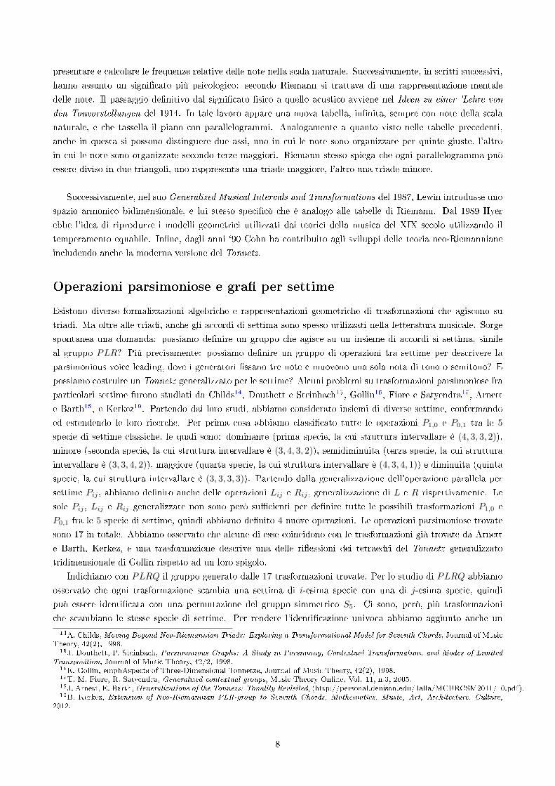
risulta essere un grafo basato su accordi, chiamato Chicken-wire Torus da Douthett e Steinbach8. I vertici di

tale grafo rappresentano triadi maggiori e minori, gli archi le operazioni P , L e R. È interessante osservare

che i cammini di tale grafo corrispondono a sequenze di triadi maggiori e minori utilizzando le operazioni P ,

L e R. Partendo da tale osservazione, Albini e Antonini hanno enumerato, classi�cato e studiato tutti i cicli

Hamiltoniani di tale grafo9. Alcuni cicli, o parti di essi, sono stati trovati in diversi brani musicali, ad esempio

nel secondo movimento della nona Sinfonia di Beethoven. Allo stesso tempo questi cicli possono essere utilizzati

anche come strumenti compositivi, infatti alcuni compositori contemporanei li hanno utilizzati nelle loro com-

posizioni. Più in generale, Douthett and Steinbach introdussero una costruzione generale di gra� parsimoniosi

(basati su accordi), basati sulla Pm,n relazione. Due accordi si dicono in relazione Pm,n se si possono ottenere

l'uno dall'altro muovendo m note di semitono e n note di tono.

Storia del Tonnetz

Storicamente si dice che il Tonnetz fu introdotto da Eulero nel suo Tentamen novae theoriae musicae, scritto

nel 1731 e pubblicato nel 173910. Abbiamo osservato che un grafo simile appare nel capitolo IX �De genere

8J. Douthett, P. Steinbach, Parsimonious Graphs: A Study in Parsimony, Contextual Transformation, and Modes of Limited

Transposition, Journal of Music Theory, 42/2, 1998.9G. Albini, S. Antonini, Hamiltonian Cycles in the Topological Dual of the Tonnetz. In: Chew E., Childs A., Chuan CH.

(eds) Mathematics and Computation in Music, Communications in Computer and Information Science, vol 38, Springer, Berlin,Heidelberg, 2009.

10L. Euler, Tentamen novae theoriae musicae ex certissimis harmoniae principiis dilucide expositae, Opera Omnia, Series 3, Vol.1, 1739.

6

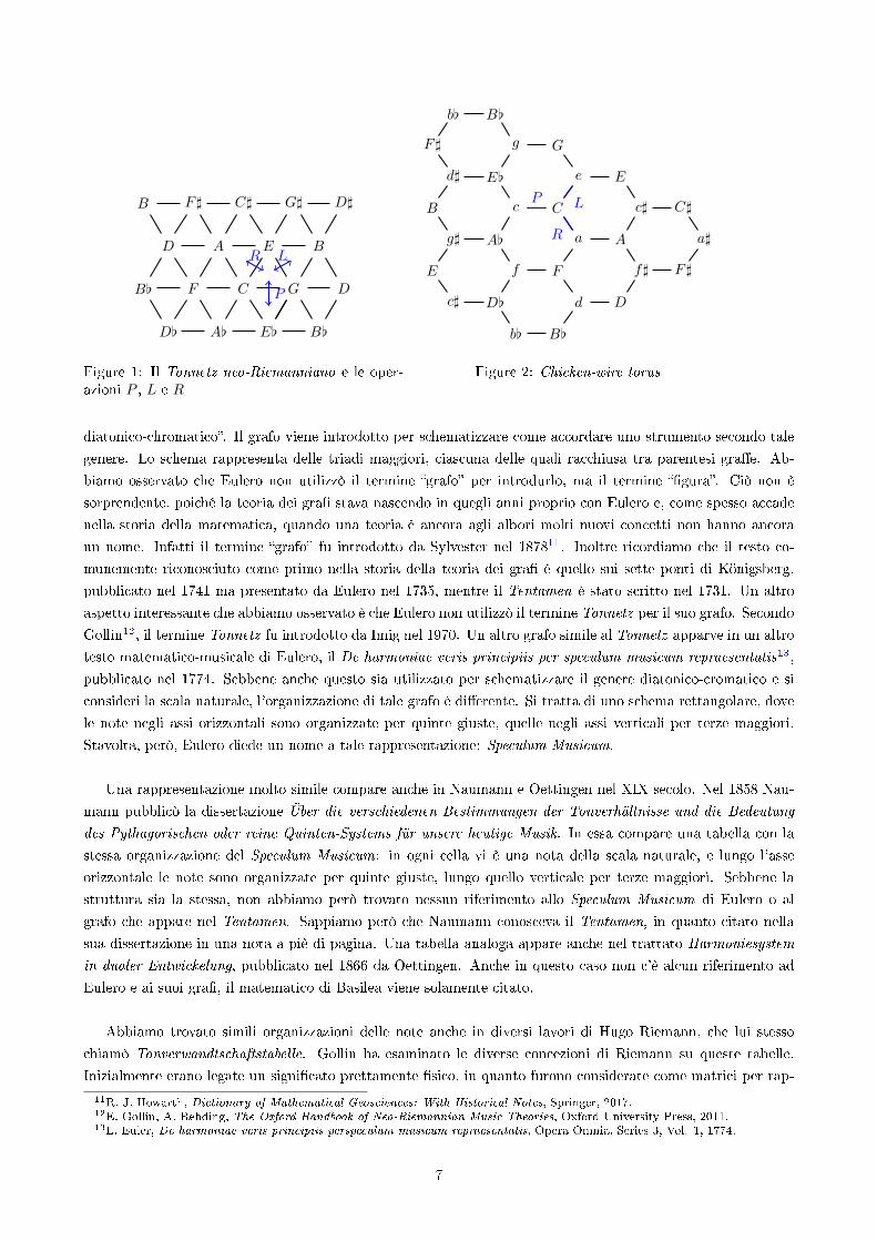
D[ A[ E[ B[

B[ F C G D

D A E B

B F] C] G] D]

P

R L

Figure 1: Il Tonnetz neo-Riemanniano e le oper-azioni P , L e R

b[ B[

d

Ff

D[c]

E

g] A[

B

F]

d] E[

c C

a A

f]

D

F]

a]

C]c]

Ee

Gg

B[b[

P

R

L

Figure 2: Chicken-wire torus

diatonico-chromatico�. Il grafo viene introdotto per schematizzare come accordare uno strumento secondo tale

genere. Lo schema rappresenta delle triadi maggiori, ciascuna delle quali racchiusa tra parentesi gra�e. Ab-

biamo osservato che Eulero non utilizzò il termine �grafo� per introdurlo, ma il termine ��gura�. Ciò non è

sorprendente, poiché la teoria dei gra� stava nascendo in quegli anni proprio con Eulero e, come spesso accade

nella storia della matematica, quando una teoria è ancora agli albori molti nuovi concetti non hanno ancora

un nome. Infatti il termine �grafo� fu introdotto da Sylvester nel 187811. Inoltre ricordiamo che il testo co-

munemente riconosciuto come primo nella storia della teoria dei gra� è quello sui sette ponti di Königsberg,

pubblicato nel 1741 ma presentato da Eulero nel 1735, mentre il Tentamen è stato scritto nel 1731. Un altro

aspetto interessante che abbiamo osservato è che Eulero non utilizzò il termine Tonnetz per il suo grafo. Secondo

Gollin12, il termine Tonnetz fu introdotto da Imig nel 1970. Un altro grafo simile al Tonnetz apparve in un altro

testo matematico-musicale di Eulero, il De harmoniae veris principiis per speculum musicum repraesentatis13,

pubblicato nel 1774. Sebbene anche questo sia utilizzato per schematizzare il genere diatonico-cromatico e si

consideri la scala naturale, l'organizzazione di tale grafo è di�erente. Si tratta di uno schema rettangolare, dove

le note negli assi orizzontali sono organizzate per quinte giuste, quelle negli assi verticali per terze maggiori.

Stavolta, però, Eulero diede un nome a tale rappresentazione: Speculum Musicum.

Una rappresentazione molto simile compare anche in Naumann e Oettingen nel XIX secolo. Nel 1858 Nau-

mann pubblicò la dissertazione Über die verschiedenen Bestimmungen der Tonverhältnisse und die Bedeutung

des Pythagorischen oder reine Quinten-Systems für unsere heutige Musik. In essa compare una tabella con la

stessa organizzazione del Speculum Musicum: in ogni cella vi è una nota della scala naturale, e lungo l'asse

orizzontale le note sono organizzate per quinte giuste, lungo quello verticale per terze maggiori. Sebbene la

struttura sia la stessa, non abbiamo però trovato nessun riferimento allo Speculum Musicum di Eulero o al

grafo che appare nel Tentamen. Sappiamo però che Naumann conosceva il Tentamen, in quanto citato nella

sua dissertazione in una nota a piè di pagina. Una tabella analoga appare anche nel trattato Harmoniesystem

in dualer Entwickelung, pubblicato nel 1866 da Oettingen. Anche in questo caso non c'è alcun riferimento ad

Eulero e ai suoi gra�, il matematico di Basilea viene solamente citato.

Abbiamo trovato simili organizzazioni delle note anche in diversi lavori di Hugo Riemann, che lui stesso

chiamò Tonverwandtschaftstabelle. Gollin ha esaminato le diverse concezioni di Riemann su queste tabelle.

Inizialmente erano legate un signi�cato prettamente �sico, in quanto furono considerate come matrici per rap-

11R. J. Howarth, Dictionary of Mathematical Geosciences: With Historical Notes, Springer, 2017.12E. Gollin, A. Rehding, The Oxford Handbook of Neo-Riemannian Music Theories, Oxford University Press, 2011.13L. Euler, De harmoniae veris principiis perspeculum musicum repraesentatis, Opera Omnia, Series 3, Vol. 1, 1774.

7

presentare e calcolare le frequenze relative delle note nella scala naturale. Successivamente, in scritti successivi,

hanno assunto un signi�cato più psicologico: secondo Riemann si trattava di una rappresentazione mentale

delle note. Il passaggio de�nitivo dal signi�cato �sico a quello acustico avviene nel Ideen zu einer 'Lehre von

den Tonvorstellungen del 1914. In tale lavoro appare una nuova tabella, in�nita, sempre con note della scala

naturale, e che tassella il piano con parallelogrammi. Analogamente a quanto visto nelle tabelle precedenti,

anche in questa si possono distinguere due assi, uno in cui le note sono organizzate per quinte giuste, l'altro

in cui le note sono organizzate secondo terze maggiori. Riemann stesso spiega che ogni parallelogramma può

essere diviso in due triangoli, uno rappresenta una triade maggiore, l'altro una triade minore.

Successivamente, nel suo Generalized Musical Intervals and Transformations del 1987, Lewin introdusse uno

spazio armonico bidimensionale, e lui stesso speci�cò che è analogo alle tabelle di Riemann. Dal 1989 Hyer

ebbe l'idea di riprodurre i modelli geometrici utilizzati dai teorici della musica del XIX secolo utilizzando il

temperamento equabile. In�ne, dagli anni `90 Cohn ha contribuito agli sviluppi delle teoria neo-Riemanniane

includendo anche la moderna versione del Tonnetz.

Operazioni parsimoniose e gra� per settime

Esistono diverse formalizzazioni algebriche e rappresentazioni geometriche di trasformazioni che agiscono su

triadi. Ma oltre alle triadi, anche gli accordi di settima sono spesso utilizzati nella letteratura musicale. Sorge

spontanea una domanda: possiamo de�nire un gruppo che agisce su un insieme di accordi si settima, simile

al gruppo PLR? Più precisamente: possiamo de�nire un gruppo di operazioni tra settime per descrivere la

parsimonious voice leading, dove i generatori �ssano tre note e muovono una sola nota di tono o semitono? E

possiamo costruire un Tonnetz generalizzato per le settime? Alcuni problemi su trasformazioni parsimoniose fra

particolari settime furono studiati da Childs14, Douthett e Steinbach15, Gollin16, Fiore e Satyendra17, Arnett

e Barth18, e Kerkez19. Partendo dai loro studi, abbiamo considerato insiemi di diverse settime, confermando

ed estendendo le loro ricerche. Per prima cosa abbiamo classi�cato tutte le operazioni P1,0 e P0,1 tra le 5

specie di settime classiche, le quali sono: dominante (prima specie, la cui struttura intervallare è (4, 3, 3, 2)),

minore (seconda specie, la cui struttura intervallare è (3, 4, 3, 2)), semidiminuita (terza specie, la cui struttura

intervallare è (3, 3, 4, 2)), maggiore (quarta specie, la cui struttura intervallare è (4, 3, 4, 1)) e diminuita (quinta

specie, la cui struttura intervallare è (3, 3, 3, 3)). Partendo dalla generalizzazione dell'operazione parallela per

settime Pij , abbiamo de�nito anche delle operazioni Lij e Rij , generalizzazione di L e R rispettivamente. Le

sole Pij , Lij e Rij generalizzate non sono però su�cienti per de�nire tutte le possibili trasformazioni P1,0 e

P0,1 fra le 5 specie di settime, quindi abbiamo de�nito 4 nuove operazioni. Le operazioni parsimoniose trovate

sono 17 in totale. Abbiamo osservato che alcune di esse coincidono con le trasformazioni già trovate da Arnett

e Barth, Kerkez, e una trasformazione descrive una delle ri�essioni dei tetraedri del Tonnetz generalizzato

tridimensionale di Gollin rispetto ad un loro spigolo.

Indichiamo con PLRQ il gruppo generato dalle 17 trasformazioni trovate. Per lo studio di PLRQ abbiamo

osservato che ogni trasformazione scambia una settima di i-esima specie con una di j-esima specie, quindi

può essere identi�cata con una permutazione del gruppo simmetrico S5. Ci sono, però, più trasformazioni

che scambiano le stesse specie di settime. Per rendere l'identi�cazione univoca abbiamo aggiunto anche un

14A. Childs, Moving Beyond Neo-Riemannian Triads: Exploring a Transformational Model for Seventh Chords, Journal of MusicTheory, 42(2), 1998.


Transposition, Journal of Music Theory, 42/2, 1998.16E. Gollin, emphAspects of Three-Dimensional Tonnetze, Journal of Music Theory, 42(2), 1998.17T. M. Fiore, R. Satyendra, Generalized contextual groups, Music Theory Online, Vol. 11, n.3, 2005.18J. Arnett, E. Barth, Generalizations of the Tonnetz: Tonality Revisited, (http://personal.denison.edu/ lalla/MCURCSM2011/10.pdf).19B. Kerkez, Extension of Neo-Riemannian PLR-group to Seventh Chords, Mathematics, Music, Art, Architecture, Culture,

2012.

8

vettore v ∈ Z512, dove ogni i-esima componente rappresenta il numero di semitoni di cui la fondamentale di un

accordo di tipo i deve essere mossa per diventare la fondamentale di un accordo di tipo j. In questo modo ogni

trasformazione può essere rappresentata come un elemento di S5 × V , dove V = {v ∈ Z512|∑5i=1 vi = 0}. La

mappa così de�nita diventa un omomor�smo di gruppi se de�niamo la seguente operazione di composizione:

(σk, vk) ◦ · · · ◦ (σ1, v1) =

=(σk · · ·σ1, v1 + σ−1

1 (v2) + (σ2σ1)−1(v3) + · · ·+ (σk−1 · · ·σ1)−1(vk))

= (1)

=(σk · · ·σ1, v1 + σ−1

1 (v2) + σ−11 σ−1

2 (v3) + · · ·+ σ−11 · · ·σ

−1k−1(vk)

).

In�ne, abbiamo dimostrato il seguente

Teorema 2. Il gruppo PLRQ è isomorfo a S5 n Z412.

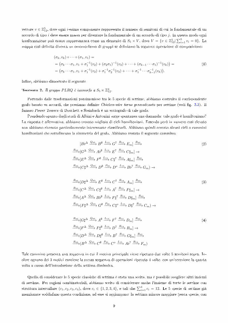
Partendo dalle trasformazioni parsimoniose tra le 5 specie di settime, abbiamo costruito il corrispondente

grafo basato su accordi, che possiamo de�nire Chicken-wire torus generalizzato per settime (vedi �g. 3.5). Il

famoso Power Towers di Douthett e Steinbach è un sottografo di tale grafo.

Prendendo spunto dagli studi di Albini e Antonini sorge spontanea una domanda: tale grafo è hamiltoniano?

La risposta è a�ermativa, abbiamo trovato migliaia di cicli hamiltoniani. Essendo però in numero così elevato

non abbiamo ritenuto particolarmente interessante classi�carli. Abbiamo quindi cercato alcuni cicli o cammini

hamiltoniani che sottolineano la simmetria del grafo. Abbiamo trovato il seguente cammino:

[B[∆Q43−−→ B∅

L13−−→ G7 R12−−→ Em]R42−−→ (2)

R42−−→[G∆ Q43−−→ A[∅L13−−→ E7 R12−−→ C]m] −→

R42−−→[E∆ Q43−−→ F ∅L13−−→ C]7

R12−−→ A]m]R42−−→

R42−−→(C]∆Q43−−→ D∅

P35−−→ Do L15−−→ B[7R12−−→ Gm) −→

R42−−→[D]∆Q43−−→ E∅

L13−−→ C7 R12−−→ Am]R42−−→ (3)

R42−−→[C∆ Q43−−→ C]∅L13−−→ A7 R12−−→ F]m] −→

R42−−→[A∆ Q43−−→ B[∅L13−−→ F]7

R12−−→ D]m]R42−−→

R42−−→(F]∆Q43−−→ G∅

P35−−→ C]oL15−−→ D]7

R12−−→ Cm) −→

R42−−→[G]∆Q43−−→ A∅

L13−−→ F 7 R12−−→ Dm]R42−−→ (4)

R42−−→[F∆ Q43−−→ F]∅L13−−→ D7 R12−−→ Bm] −→

R42−−→[D∆ Q43−−→ D]∅L13−−→ B7 R12−−→ G]m]

R42−−→R42−−→(B∆ Q43−−→ C∅

P35−−→ CoL15−−→ A[7

R12−−→ Fm)

Tale cammino presenta una sequenza in cui il motivo principale viene ripetuto due volte 5 semitoni sopra. In-

oltre ognuno dei 3 motivi contiene la stessa sequenza di operazioni ripetuta 4 volte, con un'eccezione la quarta

volta a causa dell'introduzione della settima diminuita.

Quella di considerare le 5 specie classiche di settima è stata una scelta, ma è possibile scegliere altri insiemi

di settime. Per ragioni combinatoriali, abbiamo scelto di considerare anche l'insieme di tutte le settime con

struttura intervallare (c1, c2, c3, c4), dove ci ∈ {1, 2, 3, 4}, e tali che∑4i=1 ci = 12. Le 5 specie di settime già

menzionate soddisfano questa condizione, ad esse si aggiungono: la settima minore maggiore (sesta specie, con

9

F

G]

B

D

C]

E

G

B[

A

C

D]

F]

D

F

G]

B

F]

A

C

D]

A]

C]

E

G

C]

E

G

B[

B[

C]

E

G

A C D] F]

F

A[

B

D

DFA[B

F]

A

C

D]

C

D C]

Figure 3: Il Chicken-wire torus generalizzato per accordi di settima. I vertici blu-pentagonali rappresentanole settime di dominante, quelli rossi-romboidali le settime minori, quelli verdi-circolari le semidiminuite, quelligialli-esagonali quelle maggiori e quelli arancioni-quadrangolari le settime diminuite.

10

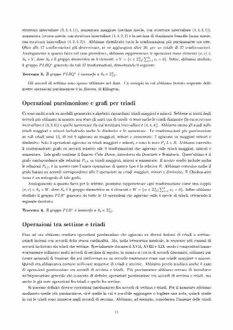
struttura intervallare (3, 4, 4, 1)), aumentata maggiore (settima specie, con struttura intervallare (4, 4, 3, 1)),

aumentata (ottava specie, con struttura intervallare (4, 4, 2, 2) e la settima di dominante bemolle (nona specie,

con struttura intervallare (4, 2, 4, 2)). Abbiamo classi�cato tutte le trasformazioni più parsimoniose tra esse.

Oltre alle 17 trasformazioni già determinate, se ne aggiungono altre 20, per un totale di 37 trasformazioni.

Analogamente a quanto fatto nel caso precedente, abbiamo rappresentato le operazioni come elementi (σ, v) ∈S9 × V , dove S9 è il gruppo simmetrico su 9 elementi, e V = {v ∈ Z9

12|∑9i=1 vi = 0}. In�ne, abbiamo studiato

il gruppo PLRQ∗ generato da tali 37 trasformazioni, dimostrando il seguente

Teorema 3. Il gruppo PLRQ∗ è isomorfo a S9 n Z812.

Gli accordi di settima sono spesso utilizzate nel Jazz. Un esempio in cui abbiamo trovato sequenze delle

nostre operazioni parsimoniose è in Heaven, di Ellington.

Operazioni parsimoniose e gra� per triadi

Ci sono molti studi su modelli geometrici e algebrici riguardanti triadi maggiori e minori. Sebbene si tratti degli

accordi più utilizzati in musica, non sono gli unici tipi di triadi: ci sono anche le triadi diminuite (la cui struttura

intervallare è (3, 3, 6)) e quelle aumentate (la cui struttura intervallare è (4, 4, 4)). Abbiamo esteso gli studi sulle

triadi maggiori e minori includendo anche le diminuite e le aumentate. Le trasformazioni più parsimoniose

su tali triadi sono 13, di cui 9 agiscono su maggiori, minori e aumentate, 7 agiscono su maggiori minori e

diminuite. Solo 3 operazioni agiscono su triadi maggiori e minori, e sono le note P , L e R. Abbiamo costruito

il corrispondente grafo su accordi relativo alle 9 trasformazioni che agiscono sulle triadi maggiori, minori e

aumentate. Tale grafo contiene il famoso Cube Dance, introdotto da Douthett e Steinbach. Quest'ultimo è il

grafo corrispondente alle relazioni P1,0 su triadi maggiori, minori e aumentate. Il nostro studio include anche

le relazioni P0,1, è in questo caso l'unica operazione di questo tipo è la relativa R. Abbiamo costruito anche il

grafo basato su accordi corrispondente alle 7 operazioni su triadi maggiori, minori e diminuite. Il Chicken-wire

torus è un sottografo di tale grafo.

Analogamente a quanto fatto per le settime, possiamo rappresentare ogni trasformazione come una coppia

(σ, v) ∈ S4 ×W , dove S4 è il gruppo simmetrico su 4 elementi e W = {w ∈ Z412|∑4i=1 wi = 0}. In�ne abbiamo

studiato il gruppo PLR∗ generato da tutte le 13 operazioni che agiscono sulle 4 specie di triadi, ottenendo il

seguente risultato.

Teorema 4. Il gruppo PLR∗ è isomorfo a S4 n Z312.

Operazioni tra settime e triadi

Fino ad ora abbiamo studiato operazioni parsimoniose che agiscono su diversi insiemi di triadi o settime,

quindi insiemi con accordi della stessa cardinalità. Ma, nella letteratura musicale, le sequenze più comuni di

accordi includono sia triadi che settime. Specialmente durante il XVII, XVIII e XIX secolo i compositori hanno

scarsamente utilizzato molti accordi di settima di seguito, in quanto si tratta di accordi dissonanti, utilizzati per

creare momenti di tensione che poi risolvevano su un accordo consonante come una triade maggiore o minore.

Quindi era abbastanza comune utilizzare sequenze di triadi e settime. Abbiamo perciò studiato anche il caso

di operazioni parsimoniose tra accordi di settima e triadi. Più precisamente abbiamo cercato di introdurre

un'impostazione generale che consenta di de�nire operazioni parsimoniose tra accordi di settima e triadi, ma

anche le già note operazioni fra triadi e quelle fra settime.

Si possono de�nire diverse operazioni parsimoniose fra accordi di settima e triadi. Per il momento abbiamo

analizzato quelle più parsimoniose, cioè quelle in cui è possibile aggiungere o togliere una nota, quindi quelle

in cui le triadi sono immerse negli accordi di settima. Abbiamo, ad esempio, considerato l'insieme delle triadi

11

maggiori e minori e le 5 specie classiche di settime. Su questo insieme agiscono 6 operazioni parsimoniose. Se,

invece, consideriamo l'insieme di tutte e 4 le triadi e le 5 specie classiche di settima le operazioni parsimoniose

che agiscono su di esso sono 12. Possiamo rappresentare ogni trasformazione come (θ, (v, w)), dove θ è una

permutazione che indica quali accordi vengono scambiati, v ∈ Z512 rappresenta il movimento delle fondamentali

delle settime, w ∈ Z412 rappresenta il movimento delle fondamentali delle triadi. Date due operazioni U1 =

(θ1, (v1, w1)), U2 = (θ2, (v2, w2)) fra settime, fra triadi, o fra settime e triadi, l'operazione di composizione è così

de�nita:

(θ2, (v2, w2)) ◦ (θ1, (v1, w1)) = (θ2 · θ1, (v1, w1) + θ−11 (v2, w2)) (5)

In�ne, abbiamo dimostrato il seguente

Teorema 5. Il gruppo ST generato dalle 17 operazioni parsimoniose fra le 5 specie di settima, le 13 operazioni

parsimoniose fra le 4 specie di triadi, e le 12 operazioni parsimoniose fra settime e triadi, è isomorfo a S9nZ812.

12

Résumé

Introduction

Nonobstant l'histoire de la relation entre les mathématiques et la musique plonge ses racines dans l'Antiquité, la

recherche en théorie mathématique de la musique est très récente. Les mathématiques sont souvent considérées

comme faisant partie du monde des règles et de la rationalité pure, tandis que la musique s'inscrit dans le monde

de la créativité et de la liberté. Cependant, une étude plus approfondie des deux disciplines montre clairement

que les mathématiques et la musique sont étroitement liées. L'un des liens les plus intuitifs et connus, en

particulier par les non-experts, concerne les aspects physiques et acoustiques des structures musicales. Un

exemple célèbre est celui de la gamme pythagoricienne. Sur la base des liens entre la longueur d'une corde et

la fréquence de la note émise lorsque la corde est en vibration, les pythagoriciens ont observé l'existence d'une

relation entre les nombres rationnels et les intervalles musicaux. Bien qu'il soit simple et intuitif de comprendre

l'utilisation des mathématiques pour décrire la musique d'un point de vue physique et acoustique, ce n'est pas

le seul lien entre ces deux disciplines. Mise à part l'acoustique, en allant vers un niveau plus conceptuel, et

plus spéci�quement celui de la composition, nous observons que la musique est riche en structures et en règles,

bien représentées et formalisées à travers des structures mathématiques. Le nouveau domaine de recherche,

connu sous le nom de théorie mathématique de la musique, a été créé pour expliquer la théorie de la musique

contemporaine, en essayant de décrire les di�érents objets musicaux et aussi les transformations par le bais de

formalisations utiles pour l'analyse musicale et la composition.

Ce travail de thèse fait partie de la théorie transformationnelle, une branche de la théorie mathématique de

la musique subséquente aux travaux des pionniers David Lewin2021 et Guerino Mazzola2223. L'idée principale

est d'utiliser la structure mathématique de groupe pour dé�nir des transformations musicales. L'utilisation

de l'algèbre en musique a commencé avec plusieurs théoriciens de la musique et est très utile pour décrire et

expliquer les structures musicales.

Introduction à la théorie mathématique de la musique

Dans le premier chapitre, nous présentons les principales dé�nitions et résultats de la théorie mathématique de

la musique, en particulier de la théorie transformationnelle, nécessaires à la compréhension du travail développé

dans la thèse.

L'un des aspects les plus importants de la composition réside dans la capacité à rendre intéressante l'interaction

entre les di�érentes lignes mélodiques qui créent l'harmonie, connue traditionnellement sous le nom de conduite

des voix. C'est l'interaction de deux ou plusieurs lignes musicales, qui réalisent une progression d'accords selon

les principes du contrepoint. La plupart des musiques occidentales du XVIIe au XIXe siècle sont basées sur une

harmonie à quatre voix, organisée selon certaines règles musicales dont l'une des plus importantes consiste à re-

20D. Lewin, Transformational techniques in atonal and other music theories, Perspectives in New Music, n.21, 1982.21D. Lewin, Generalized Musical Intervals and Transformations, Yale University Press,1987.22G. Mazzola, Gruppen und Kategorien in der Musik: Entwurf einer mathematischen Musiktheorie, Heldermannr, Lemgo, 1985.23G. Mazzola, Geometrie der Tone, Birkhäuser, Basel, 1990.

13

lier les accords en essayant de faire le moins de mouvement possible mais laissant la possibilité d'un mouvement

mélodique conjoint.

À la �n du XIXe siècle, plusieurs compositeurs tels que Wagner, Debussy et Bartok ont commencé à cherche

de nouveaux horizons musicaux en abandonnant la musique tonale propre au XVIIe et XIXe siècle. Dans

les systèmes de musique post-tonale, en contraposition aux systèmes tonals, on s'éloigne de l'idée d'organiser

les notes selon une hiérarchie. Ils ont donc changé les règles musicales de la composition. Un problème est

survenu: la théorie musicale traditionnelle était incapable de fournir les outils appropriés pour décrire et analyser

les nouveaux systèmes post-tonals. Pour dé�nir et exprimer les relations entre les nouvelles structures plus

complexes de la musique post tonale, les théoriciens de la musique ont utilisé la théorie des ensembles. Cette

idée, née aux États-Unis après la deuxième guerre mondiale, a donné lieu à la théorie musicale des ensembles

dont les notions principales ont été introduites par le compositeur et théoricien de la musique Hanson pour la

musique tonale et par le musicologue et théoricien de la musique Forte2425 pour la musique post-tonale. A la

base de l'application de la théorie des ensembles en musique, il y a une substitution de la notation traditionnelle

des notes par une représentation numérique. Nous considérons, en e�et, deux relations d'équivalence dans

l'ensemble de toutes les hauteurs de tempérament égal.

Équivalence Enharmonique : deux notes de même hauteur mais dissemblables sont en harmonie équivalente

(exemple: Do] ∼ Re[).

Équivalence d'octave : deux notes x, y ∈ R+ à une distance d'une octave sont équivalentes.

Avec ces relations d'équivalence, nous obtenons 12 classes d'équivalence appelées classes de hauteurs. En

établissant une carte biunivoque entre les 12 classes de hauteurs et Z12, il est possible de représenter ces classes

sous forme de nombres de 0 à 11. Par convention, nous partons de C = 0. Cette correspondance peut être

facilement visualisée en disposant les 12 classes de hauteurs et les éléments Z12 dans le cercle, formant ainsi

l'horloge dite musicale.

Les accords peuvent être dé�nis comme un ensemble de classes de hauteur (exécutées simultanément) et

peuvent être dé�nis formellement en utilisant la notation habituelle de la théorie des ensembles pour représen-

ter des ensembles donc liste toutes les classes de hauteurs et de les enfermer entre des accolades. Dans ce

travail, nous utiliserons également une autre notation: avec [x1, x2, . . . , xn] nous indiquons la disposition des

classes de hauteur x1, . . . , xn ∈ Z12, où la classe de hauteur soulignée est celle fondamentale de l'accord. Cette

notation est cyclique, donc [x1, x2, . . . , xn] = [x2, . . . , xn, x1] = · · · = [xn, x1, . . . , xn−1]. Étant donné un accord

[x1, x2, . . . , xn], nous dé�nissons comme structure de l'intervalle le vecteur (x2 − x1, x3 − x2, . . . , xn − xn−1)

dont les éléments représentent l'intervalle entre deux classes de hauteurs consécutives de l'accord. Les accords

principalement utilisés sont les triades majeures et mineures, accords de trois notes obtenus en superposant

un tierce majeur et un tierce mineur. Les structures d'intervalle sont les suivantes: (4, 3, 5), (3, 4, 5). Parmi

les autres accords très courants, citons les accords de septième soit des accords de quatre notes obtenus en

superposant des tierces.

Depuis les années 1980, l'étude des objets musicaux s'est déportée vers les relations existantes entre eux,

donnant ainsi naissance à la théorie transformationnelle. Deux parmi les transformations les plus utilisées sont les

transpositions et les inversions. La transposition Tn déplace les classes de hauteurs de n demi-tons. L'inversion

I = I0 transforme chaque classe de hauteur en son inverse, tandis qu'une inversion donne In = Tn ◦ I. Ces

transformations, utilisées dans nombreuses compositions, s'avèrent fort intéressantes du point de vue algébrique

car, en e�et, on peut démontrer que les transpositions et les inversions agissent sur l'ensemble des triades

majeures et mineures en générant un groupe isomorphe au groupe diédral D12 d'ordre 24.

24A. Forte, A Theory of Set-Complexes for Music, Journal of Music Theory, 8(2), 1964, pp. 136-183.25A. Forte, The Structure of Atonal Music, Yale University Press, 1973.

14

Avec la redécouverte des transformations P (parallel), L (leading-tone) et R (relative), introduites par

le musicologue Hugo Riemann à la �n du XIXe siècle, Lewin a commencé à développer une branche de la

théorie transformationnelle plus connue sous le nom de théorie néo-Riemannienne. Suivant la con�guration et

la terminologie de Hook26, avec le terme transformation, nous indiquons une application à partir d'un ensemble

de triades en soi et avec opération nous indiquons une transformation bijective. Toutes les opérations de triade,

ainsi que l'opération de composition, forment un groupe G d'ordre 24. Parmi toutes les opérations, celles

qui sont musicalement intéressantes sont les transformations triadiques uniformes (UTTs) qui transforment

intuitivement chaque triade �de la même manière�. Formellement, elles peuvent être déterminés de manière

unique par 〈σ,m, n〉, dove σ = ±, où σ = ±, en particulier si σ = − la transformation modi�e le type de triade,

si σ = + le type de triade est conservé, m représente l'intervalle de transposition de la fondamentale des triades

majeures, n celle des triades mineures. L'ensemble de toutes les UTTs forme un groupe, un sous-ensemble du

groupe G de toutes les opérations. Dans le cas particulier où m+ n = 0, l'UTT s'appelle riemannienne. Parmi

les UTTs riemanniens, il y a aussi les 3 opérations néo-riemanniennes P , L et R.

P : associe chaque triade à son parallèle. Si le triade est majeur, P déplace le tierce un demi-ton en dessous,

si le triade est mineur P déplace la tierce un demi-ton au-dessus.

L : associe chaque triade majeure avec une triade mineure et transpose une tierce majeure dessus tandis que

chaque triade mineure en majeur transpose une tierce majeure en dessous.

R : associe chaque triade dans sa relative. Si la triade est en majeur, R déplace la cinquième un ton plus haut,

si elle est est en mineur, R déplace la fondamentale un ton en dessous.

Nous observons que ces opérations changent des triades majeures et mineures tout en laissant deux notes �xes et

ne déplaçant qu'une seule note d'un ton ou d'un demi-ton. Grâce à ces propriétés, ces opérations s'avèrent très

intéressantes d'un point de vue musical car elles constituent un outil supplémentaire pour décrire la propriété

de mouvement progressif de la conduite des voix parcimonieuse. La conduite des voix est dite parcimonieuse

lorsque les notes restent �xes ou bougent par mouvement mélodique conjoint. Du point de vue mathématique,

nous avons le remarquable résultat ci-dessous.

Théorème 1. Le groupe PLR, généré par les transformations néo-riemanniennes P , L et R, agissant sur

l'ensemble des 24 triades majeures et mineures, est isomorphe au groupe diédral d'ordre 24.

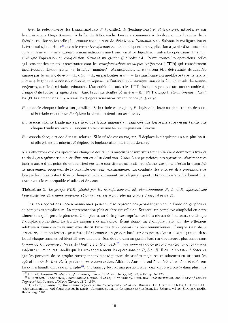
Les trois opérations néo-riemanniennes peuvent être représentées géométriquement à l'aide de graphes et

de complexes simpliciaux. La représentation plus célèbre est celle de Tonnetz : un complexe simplicial en deux

dimensions qu'il pave le plan avec 2-simplexes, où 0-simplexes représentent des classes de hauteurs, tandis que

2-simplexes identi�ent les triades majeures et mineures. Étant donné un 2-simplexe, chacune des ré�exions

relatives à l'une des trois simplexes décrit l'une des trois opérations néo-riemanniennes. Compte tenu de la

structure, le emphTonnetz peut être dé�ni comme un graphe basé sur des notes, c'est-à-dire un graphe dans

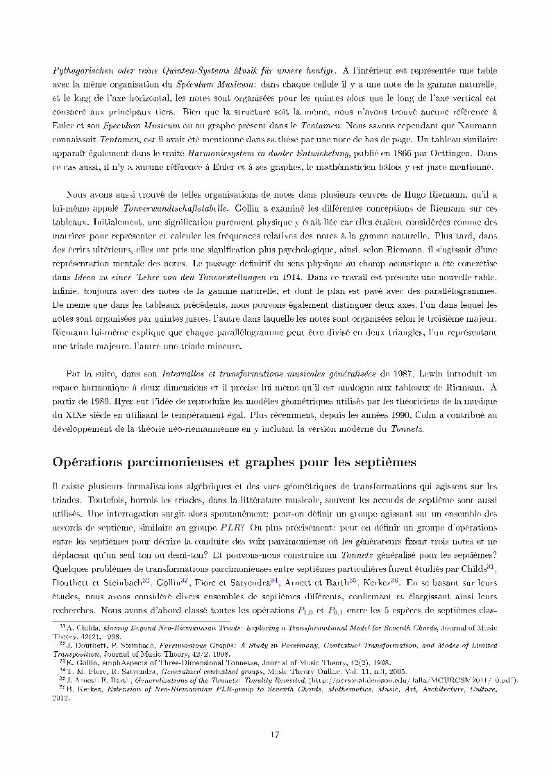
lequel chaque sommet est identi�é avec une note. Son double sera un graphe basé sur des accords plus connu sous

le nom de Chicken-wire Torus de Douthett et Steinbach27. Les sommets de ce graphe représentent les triades

majeures et mineures, tandis que les arcs représentent les opérations de P , L et R. Il est intéressant d'observer

que les parcours de ce graphe correspondent aux séquences de triades majeures et mineures en utilisant les

opérations de P , L et R. À partir de cette observation, Albini et Antonini ont énuméré, classi�é et étudié tous

les cycles hamiltoniens de ce graphe28. Certains cycles, ou une partie d'entre eux, ont été trouvés dans plusieurs

26J. Hook, Uniform Triadic Transformations, Journal of Music Theory, 46(1-2), 2002, pp. 57-126.27J. Douthett, P. Steinbach, Parsimonious Graphs: A Study in Parsimony, Contextual Transformation, and Modes of Limited

Transposition, Journal of Music Theory, 42/2, 1998.28G. Albini, S. Antonini, Hamiltonian Cycles in the Topological Dual of the Tonnetz. In: Chew E., Childs A., Chuan CH.

(eds) Mathematics and Computation in Music, Communications in Computer and Information Science, vol 38, Springer, Berlin,Heidelberg, 2009.

15

D[ A[ E[ B[

B[ F C G D

D A E B

B F] C] G] D]

P

R L

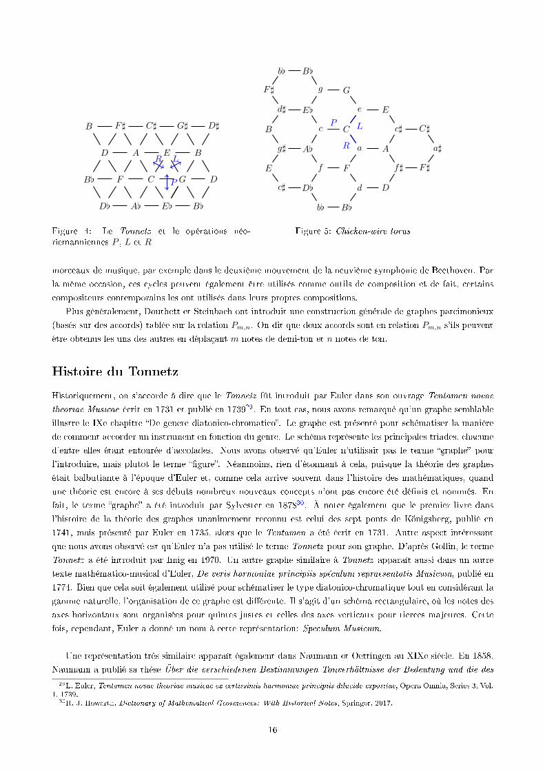
Figure 4: Le Tonnetz et le opérations néo-riemanniennes P , L et R

b[ B[

d

Ff

D[c]

E

g] A[

B

F]

d] E[

c C

a A

f]

D

F]

a]

C]c]

Ee

Gg

B[b[

P

R

L

Figure 5: Chicken-wire torus

morceaux de musique, par exemple dans le deuxième mouvement de la neuvième symphonie de Beethoven. Par

la même occasion, ces cycles peuvent également être utilisés comme outils de composition et de fait, certains

compositeurs contemporains les ont utilisés dans leurs propres compositions.

Plus généralement, Douthett et Steinbach ont introduit une construction générale de graphes parcimonieux

(basés sur des accords) tablée sur la relation Pm,n. On dit que deux accords sont en relation Pm,n s'ils peuvent

être obtenus les uns des autres en déplaçant m notes de demi-ton et n notes de ton.

Histoire du Tonnetz

Historiquement, on s'accorde à dire que le Tonnetz fût introduit par Euler dans son ouvrage Tentamen novae

theoriae Musicae écrit en 1731 et publié en 173929. En tout cas, nous avons remarqué qu'un graphe semblable

illustre le IXe chapitre �De genere diatonico-chromatico�. Le graphe est présenté pour schématiser la manière

de comment accorder un instrument en fonction du genre. Le schéma représente les principales triades, chacune

d'entre elles étant entourée d'accolades. Nous avons observé qu'Euler n'utilisait pas le terme �graphe� pour

l'introduire, mais plutôt le terme ��gure�. Néanmoins, rien d'étonnant à cela, puisque la théorie des graphes

était balbutiante à l'époque d'Euler et, comme cela arrive souvent dans l'histoire des mathématiques, quand

une théorie est encore à ses débuts nombreux nouveaux concepts n'ont pas encore été dé�nis et nommés. En

fait, le terme �graphe� a été introduit par Sylvester en 187830. À noter également que le premier livre dans

l'histoire de la théorie des graphes unanimement reconnu est celui des sept ponts de Königsberg, publié en

1741, mais présenté par Euler en 1735, alors que le Tentamen a été écrit en 1731. Autre aspect intéressant

que nous avons observé est qu'Euler n'a pas utilisé le terme Tonnetz pour son graphe. D'après Gollin, le terme

Tonnetz a été introduit par Imig en 1970. Un autre graphe similaire à Tonnetz apparaît aussi dans un autre

texte mathématico-musical d'Euler, De veris harmoniae principiis spéculum repraesentatis Musicum, publié en

1774. Bien que cela soit également utilisé pour schématiser le type diatonico-chromatique tout en considérant la

gamme naturelle, l'organisation de ce graphe est di�érente. Il s'agit d'un schéma rectangulaire, où les notes des

axes horizontaux sont organisées pour quintes justes et celles des axes verticaux pour tierces majeures. Cette

fois, cependant, Euler a donné un nom à cette représentation: Speculum Musicum.

Une représentation très similaire apparaît également dans Naumann et Oettingen au XIXe siècle. En 1858,

Naumann a publié sa thèse Über die verschiedenen Bestimmungen Tonverhältnisse der Bedeutung und die des

29L. Euler, Tentamen novae theoriae musicae ex certissimis harmoniae principiis dilucide expositae, Opera Omnia, Series 3, Vol.1, 1739.

30R. J. Howarth, Dictionary of Mathematical Geosciences: With Historical Notes, Springer, 2017.

16

Pythagorischen oder reine Quinten-Systems Musik für unsere heutige. A l'intérieur est représentée une table

avec la même organisation du Spéculum Musicum: dans chaque cellule il y a une note de la gamme naturelle,

et le long de l'axe horizontal, les notes sont organisées pour les quintes alors que le long de l'axe vertical est

consacré aux principaux tiers. Bien que la structure soit la même, nous n'avons trouvé aucune référence à

Euler et son Speculum Musicum ou au graphe présent dans le Tentamen. Nous savons cependant que Naumann

connaissait Tentamen, car il avait été mentionné dans sa thèse par une note de bas de page. Un tableau similaire

apparaît également dans le traité Harmoniesystem in dualer Entwickelung, publié en 1866 par Oettingen. Dans

ce cas aussi, il n'y a aucune référence à Euler et à ses graphes, le mathématicien bâlois y est juste mentionné.

Nous avons aussi trouvé de telles organisations de notes dans plusieurs ÷uvres de Hugo Riemann, qu'il a

lui-même appelé Tonverwandtschaftstabelle. Gollin a examiné les di�érentes conceptions de Riemann sur ces

tableaux. Initialement, une signi�cation purement physique y était liée car elles étaient considérées comme des

matrices pour représenter et calculer les fréquences relatives des notes à la gamme naturelle. Plus tard, dans

des écrits ultérieurs, elles ont pris une signi�cation plus psychologique, ainsi, selon Riemann, il s'agissait d'une

représentation mentale des notes. Le passage dé�nitif du sens physique au champ acoustique a été concrétisé

dans Ideen zu einer 'Lehre von den Tonvorstellungen en 1914. Dans ce travail est présente une nouvelle table,

in�nie, toujours avec des notes de la gamme naturelle, et dont le plan est pavé avec des parallélogrammes.

De même que dans les tableaux précédents, nous pouvons également distinguer deux axes, l'un dans lequel les

notes sont organisées par quintes justes, l'autre dans laquelle les notes sont organisées selon le troisième majeur.

Riemann lui-même explique que chaque parallélogramme peut être divisé en deux triangles, l'un représentant

une triade majeure, l'autre une triade mineure.

Par la suite, dans son Intervalles et transformations musicales généralisées de 1987, Lewin introduit un

espace harmonique à deux dimensions et il précise lui-même qu'il est analogue aux tableaux de Riemann. À

partir de 1989, Hyer eut l'idée de reproduire les modèles géométriques utilisés par les théoriciens de la musique

du XIXe siècle en utilisant le tempérament égal. Plus récemment, depuis les années 1990, Cohn a contribué au

développement de la théorie néo-riemannienne en y incluant la version moderne du Tonnetz.

Opérations parcimonieuses et graphes pour les septièmes

Il existe plusieurs formalisations algébriques et des vues géométriques de transformations qui agissent sur les

triades. Toutefois, hormis les triades, dans la littérature musicale, souvent les accords de septième sont aussi

utilisés. Une interrogation surgit alors spontanément: peut-on dé�nir un groupe agissant sur un ensemble des

accords de septième, similaire au groupe PLR? Ou plus précisément: peut-on dé�nir un groupe d'opérations

entre les septièmes pour décrire la conduite des voix parcimonieuse où les générateurs �xent trois notes et ne

déplacent qu'un seul ton ou demi-ton? Et pouvons-nous construire un Tonnetz généralisé pour les septièmes?

Quelques problèmes de transformations parcimonieuses entre septièmes particulières furent étudiés par Childs31,

Douthett et Steinbach32, Gollin33, Fiore et Satyendra34, Arnett et Barth35, Kerkez36. En se basant sur leurs

études, nous avons considéré divers ensembles de septièmes di�érents, con�rmant et élargissant ainsi leurs

recherches. Nous avons d'abord classé toutes les opérations P1,0 et P0,1 entre les 5 espèces de septièmes clas-

31A. Childs, Moving Beyond Neo-Riemannian Triads: Exploring a Transformational Model for Seventh Chords, Journal of MusicTheory, 42(2), 1998.


Transposition, Journal of Music Theory, 42/2, 1998.33E. Gollin, emphAspects of Three-Dimensional Tonnetze, Journal of Music Theory, 42(2), 1998.34T. M. Fiore, R. Satyendra, Generalized contextual groups, Music Theory Online, Vol. 11, n.3, 2005.35J. Arnett, E. Barth, Generalizations of the Tonnetz: Tonality Revisited, (http://personal.denison.edu/ lalla/MCURCSM2011/10.pdf).36B. Kerkez, Extension of Neo-Riemannian PLR-group to Seventh Chords, Mathematics, Music, Art, Architecture, Culture,

2012.

17

siques qui sont: dominantes (première espèce dont la structure des intervalles est (4, 3, 3, 2)), mineure (seconde

espèce dont la structure des intervalles est (3, 4, 3, 2)), semi-diminuée (troisième espèce dont la structure des

intervalles est (3, 3, 4, 2)), majeure (quatrième espèce dont la structure des intervalles est (4, 3, 4, 1)) et diminuée

(cinquième espèce, dont la structure des intervalles est (3, 3, 3, 3)). A partir de la généralisation de l'opération

parallèle pour la septième Pij , nous avons également dé�ni des opérations Lij et Rij , généralisation de L et

R respectivement. Les Pij , Lij et Rij généralisées ne su�sent pas à dé�nir toutes les transformations P1,0 e

P0,1 possibles parmi les 5 espèces des septièmes, nous avons donc dé�ni 4 nouvelles opérations. Les opérations

parcimonieuses recherchées sont au total 17. Nous avons constaté que certaines d'entre elles coïncident avec

les transformations déjà trouvées par Arnett, Barth et Kerkez, par ailleurs, une transformation décrit l'une des

ré�exions des tétraèdres du Tonnetz généralisé tri-dimensionnel de Gollin par rapport à une de leurs arêtes.

Soit PLRQ le groupe généré par les 17 transformations trouvées. Pour l'étude de la PLRQ, nous avons

observé que chaque transformation échange un septième de la i-ème espèce avec une de la j-ième espèce.

On peut donc l'identi�er avec une permutation du groupe symétrique S5. Cependant les transformations qui

échangent les mêmes espèces de septièmes restent les plus nombreuses. Pour rendre l'identi�cation unique,

nous avons également ajouté un vecteur v ∈ Z512, où chaque i-ème composant représente le nombre de demi-

tons dont le fondamental d'un accord de type i doit être déplacé pour devenir le fondamental d'un accord

de type j. De cette façon, chaque transformation peut être représentée comme un élément de S5 × V , doveV = {v ∈ Z5

12|∑5i=1 vi = 0}. La fonction ainsi dé�nie devient un homomorphisme de groupes si l'on dé�nit

l'opération de composition suivante:

(σk, vk) ◦ · · · ◦ (σ1, v1) =

=(σk · · ·σ1, v1 + σ−1

1 (v2) + (σ2σ1)−1(v3) + · · ·+ (σk−1 · · ·σ1)−1(vk))

= (6)

=(σk · · ·σ1, v1 + σ−1

1 (v2) + σ−11 σ−1

2 (v3) + · · ·+ σ−11 · · ·σ

−1k−1(vk)

).

En�n, nous avons démontré le théorème suivant.

Théorème 2. Le groupe PLRQ est isomorphe au S5 n Z412.

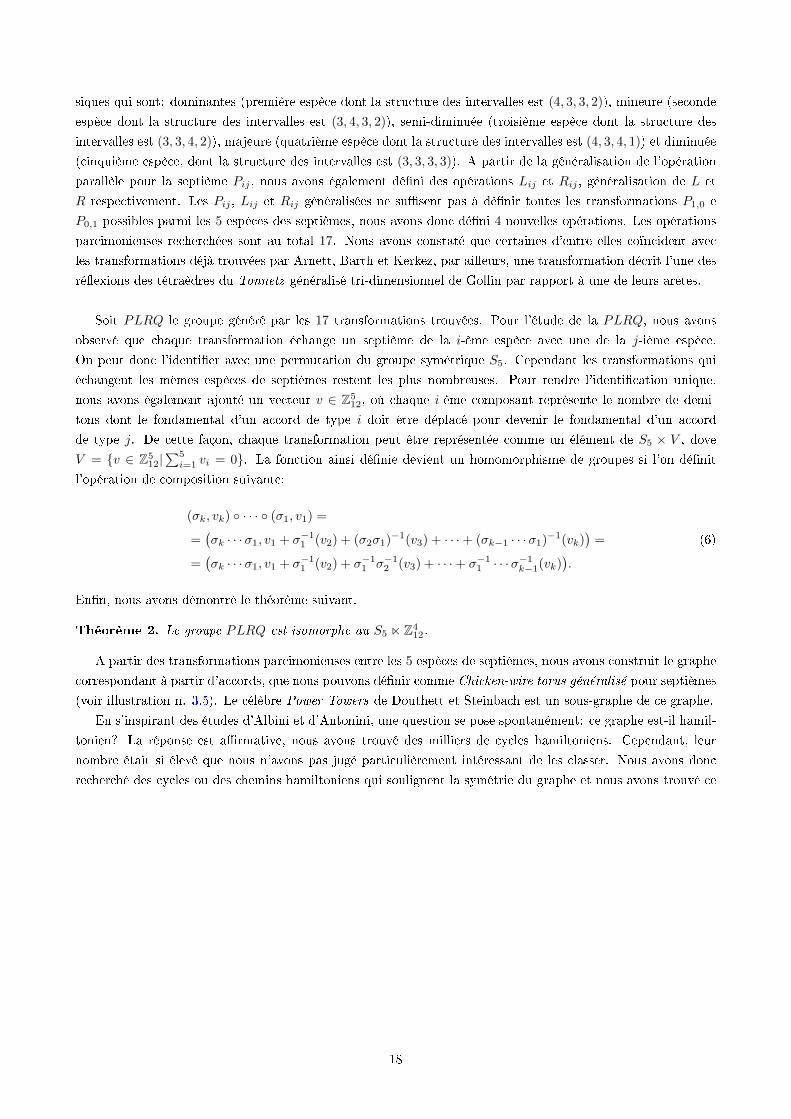
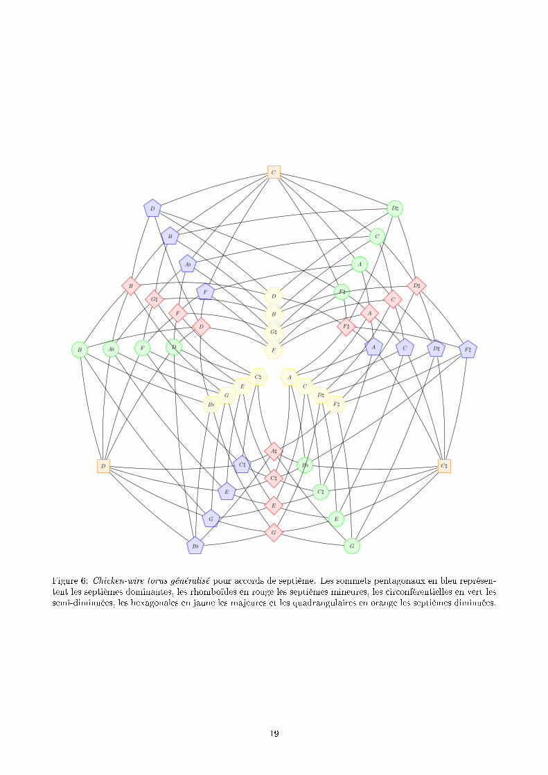
A partir des transformations parcimonieuses entre les 5 espèces de septièmes, nous avons construit le graphe

correspondant à partir d'accords, que nous pouvons dé�nir comme Chicken-wire torus généralisé pour septièmes

(voir illustration n. 3.5). Le célèbre Power Towers de Douthett et Steinbach est un sous-graphe de ce graphe.

En s'inspirant des études d'Albini et d'Antonini, une question se pose spontanément: ce graphe est-il hamil-

tonien? La réponse est a�rmative, nous avons trouvé des milliers de cycles hamiltoniens. Cependant, leur

nombre était si élevé que nous n'avons pas jugé particulièrement intéressant de les classer. Nous avons donc

recherché des cycles ou des chemins hamiltoniens qui soulignent la symétrie du graphe et nous avons trouvé ce

18

F

G]

B

D

C]

E

G

B[

A

C

D]

F]

D

F

G]

B

F]

A

C

D]

A]

C]

E

G

C]

E

G

B[

B[

C]

E

G

A C D] F]

F

A[

B

D

DFA[B

F]

A

C

D]

C

D C]

Figure 6: Chicken-wire torus généralisé pour accords de septième. Les sommets pentagonaux en bleu représen-tent les septièmes dominantes, les rhomboïdes en rouge les septièmes mineures, les circonférentielles en vert lessemi-diminuées, les hexagonales en jaune les majeures et les quadrangulaires en orange les septièmes diminuées.

19

qui suit:

[B[∆Q43−−→ B∅

L13−−→ G7 R12−−→ Em]R42−−→ (7)

R42−−→[G∆ Q43−−→ A[∅L13−−→ E7 R12−−→ C]m] −→

R42−−→[E∆ Q43−−→ F ∅L13−−→ C]7

R12−−→ A]m]R42−−→

R42−−→(C]∆Q43−−→ D∅

P35−−→ Do L15−−→ B[7R12−−→ Gm) −→

R42−−→[D]∆Q43−−→ E∅

L13−−→ C7 R12−−→ Am]R42−−→ (8)

R42−−→[C∆ Q43−−→ C]∅L13−−→ A7 R12−−→ F]m] −→

R42−−→[A∆ Q43−−→ B[∅L13−−→ F]7

R12−−→ D]m]R42−−→

R42−−→(F]∆Q43−−→ G∅

P35−−→ C]oL15−−→ D]7

R12−−→ Cm) −→

R42−−→[G]∆Q43−−→ A∅

L13−−→ F 7 R12−−→ Dm]R42−−→ (9)

R42−−→[F∆ Q43−−→ F]∅L13−−→ D7 R12−−→ Bm] −→

R42−−→[D∆ Q43−−→ D]∅L13−−→ B7 R12−−→ G]m]

R42−−→R42−−→(B∆ Q43−−→ C∅

P35−−→ CoL15−−→ A[7

R12−−→ Fm)

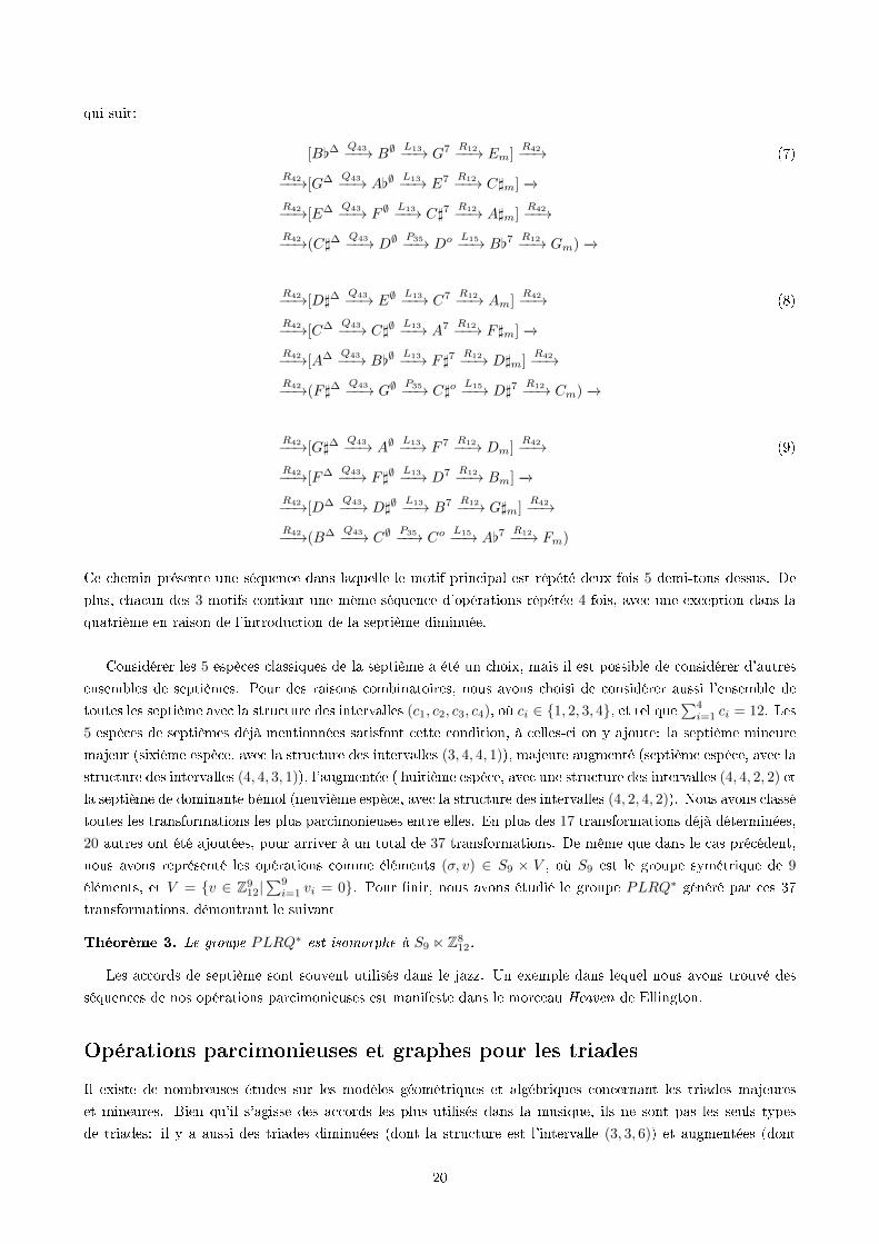
Ce chemin présente une séquence dans laquelle le motif principal est répété deux fois 5 demi-tons dessus. De

plus, chacun des 3 motifs contient une même séquence d'opérations répétée 4 fois, avec une exception dans la

quatrième en raison de l'introduction de la septième diminuée.

Considérer les 5 espèces classiques de la septième a été un choix, mais il est possible de considérer d'autres

ensembles de septièmes. Pour des raisons combinatoires, nous avons choisi de considérer aussi l'ensemble de

toutes les septième avec la structure des intervalles (c1, c2, c3, c4), où ci ∈ {1, 2, 3, 4}, et tel que∑4i=1 ci = 12. Les

5 espèces de septièmes déjà mentionnées satisfont cette condition, à celles-ci on y ajoute: la septième mineure

majeur (sixième espèce, avec la structure des intervalles (3, 4, 4, 1)), majeure augmenté (septième espèce, avec la

structure des intervalles (4, 4, 3, 1)), l'augmentée ( huitième espèce, avec une structure des intervalles (4, 4, 2, 2) et

la septième de dominante bémol (neuvième espèce, avec la structure des intervalles (4, 2, 4, 2)). Nous avons classé

toutes les transformations les plus parcimonieuses entre elles. En plus des 17 transformations déjà déterminées,

20 autres ont été ajoutées, pour arriver à un total de 37 transformations. De même que dans le cas précédent,

nous avons représenté les opérations comme éléments (σ, v) ∈ S9 × V , où S9 est le groupe symétrique de 9

éléments, et V = {v ∈ Z912|∑9i=1 vi = 0}. Pour �nir, nous avons étudié le groupe PLRQ∗ généré par ces 37

transformations, démontrant le suivant

Théorème 3. Le groupe PLRQ∗ est isomorphe à S9 n Z812.

Les accords de septième sont souvent utilisés dans le jazz. Un exemple dans lequel nous avons trouvé des

séquences de nos opérations parcimonieuses est manifeste dans le morceau Heaven de Ellington.

Opérations parcimonieuses et graphes pour les triades

Il existe de nombreuses études sur les modèles géométriques et algébriques concernant les triades majeures

et mineures. Bien qu'il s'agisse des accords les plus utilisés dans la musique, ils ne sont pas les seuls types

de triades: il y a aussi des triades diminuées (dont la structure est l'intervalle (3, 3, 6)) et augmentées (dont

20

la structure est l'intervalle (4, 4, 4)). Nous avons prolongé les études sur les triades majeures et mineures, y

compris les triades diminuées et les triades augmentées. Les transformations plus parcimonieuses sur ces triades

sont au nombre de 13, dont 9 agissent sur majeures, mineures et augmentées et les 7 restantes sur mineures

majeur et diminuées. Seulement 3 opérations agissent sur les triades majeures et mineures et ce sont P , L et

R. Nous avons réalisé le graphe correspondant sur les accords liés aux 9 transformations qui agissent sur les

triades majeures, mineures et augmentées. Ce graphe contient le célèbre Cube Dance, introduit par Douthett

et Steinbach. Ce dernier est le graphe correspondant aux relations P1,0 sur les triades majeures, mineures et

augmentées. Notre étude inclut également les relations P0,1. Dans ce cas, la seule opération de ce type est la

relation R. Le Chicken-wire Torus est un sous-graphe de ce graphe.

De manière similaire à ce que nous avons fait pour les septièmes, nous pouvons représenter chaque trans-

formation comme une paire (σ, v) ∈ S4 ×W , où S4 est le groupe symétrique des 4 éléments et W = {w ∈Z4

12|∑4i=1 wi = 0}. En dernier, nous avons étudié le groupe PLR∗ généré par les 13 opérations qui a�ectent les

4 espèces des triades, obtenant le résultat suivant.

Théorème 4. Le groupe PLR∗ est isomorphe à S4 n Z312.

Opérations entre septièmes et triades

Jusqu'à présent, nous avons étudié des opérations parcimonieuses qui agissent sur di�érents ensembles de triades

ou de septièmes, donc des ensembles avec des accords de même cardinalité. Mais, dans la littérature musicale,

les séquences d'accords les plus courantes comprennent les triades et les septièmes. En particulier aux XVIIe,

XVIIIe et XIXe siècles, les compositeurs ont rarement utilisé de longues séquences de septièmes, car ce sont des

accords dissonants, utilisés pour créer des moments de tension, mais qui se résolvent ensuite en triade majeur ou

mineu. Il était donc assez courant d'utiliser des séquences en triade et en septième. Nous avons donc également

étudié le cas d'opérations parcimonieuses entre les accords de septième et de triade. Plus précisément, nous

avons tenté d'introduire une approche générale permettant de dé�nir des opérations parcimonieuses entre les

accords de septième et de triade, mais aussi les opérations déjà connues entre triades et celles entre septièmes.

Plusieurs opérations parcimonieuses peuvent être dé�nies entre les accords de septième et de triade. Pour

le moment, nous avons analysé les plus parcimonieux, c'est-à-dire ceux dans lesquels il est possible d'ajouter ou

de supprimer une note, puis ceux dans lesquels les triades sont immergées dans les septièmes. Nous avons, par

exemple, considéré l'ensemble des triades majeures et mineures et les 5 espèces classiques des septièmes. Sur

cet ensemble agissent 6 opérations parcimonieuses. Si, cependant, nous considérons l'ensemble des 4 triades

et des 5 espèces classiques des septièmes, les opérations parcimonieuses qui agissent sur elle sont de 12. On

peut représenter chaque transformation comme (θ, (v, w)), où θ est une permutation représentant l'éventuel

échange de type entre les septièmes mineures et majeures, v ∈ Z512 r représente le mouvement des fondamentaux

des septièmes, w ∈ Z412 représente le mouvement des fondamentaux des triades. Soit deux opérations U1 =

(θ1, (v1, w1)), U2 = (θ2, (v2, w2)) entre les septièmes, entre les triades ou entre septièmes et triades, l'opération

de composition est ainsi dé�nie:

(θ2, (v2, w2)) ◦ (θ1, (v1, w1)) = (θ2 · θ1, (v1, w1) + θ−11 (v2, w2)) (10)

En�n, nous avons démontré le théorème suivant.

Théorème 5. Le groupe ST généré par les 17 opérations parcimonieuses parmi les 5 espèces des septièmes,

les 13 opérations parcimonieuses parmi les 4 espèces de triades et les 12 opérations parcimonieuses entre les

septièmes et les triades, est isomorphe à S9 n Z812.

21

Contents

Introduction 23

1 Introduction to Mathematical Music Theory 26

1.1 Musical set theory . . . . . . . . . . . . . . . . . . . . . . . . . . . . . . . . . . . . . . . . . . . . 26

1.2 Transformational theory . . . . . . . . . . . . . . . . . . . . . . . . . . . . . . . . . . . . . . . . . 31

1.3 Neo-Riemannian operations and the PLR-group . . . . . . . . . . . . . . . . . . . . . . . . . . . 36

1.4 Tonnetz, Chicken-wire Torus and other parsimonious graphs . . . . . . . . . . . . . . . . . . . . . 40

1.5 Hamiltonian cycles of musical graphs in music analysis and composition . . . . . . . . . . . . . . 44

1.6 Uniform Triadic Transformations . . . . . . . . . . . . . . . . . . . . . . . . . . . . . . . . . . . . 47

1.7 Computational approaches . . . . . . . . . . . . . . . . . . . . . . . . . . . . . . . . . . . . . . . . 51

2 History of the Tonnetz 54

2.1 Euler's Tonnetz . . . . . . . . . . . . . . . . . . . . . . . . . . . . . . . . . . . . . . . . . . . . . . 54

2.2 Naumann and Oettingen's tables . . . . . . . . . . . . . . . . . . . . . . . . . . . . . . . . . . . . 56

2.3 Riemann's tables and diagrams . . . . . . . . . . . . . . . . . . . . . . . . . . . . . . . . . . . . . 58

2.4 The Tonnetz in Mathematical Music Theory . . . . . . . . . . . . . . . . . . . . . . . . . . . . . 60

2.5 Generalized Tonnetze . . . . . . . . . . . . . . . . . . . . . . . . . . . . . . . . . . . . . . . . . . 62

3 Parsimonious operations and graphs for seventh chords 71

3.1 Previous works on transformations on seventh chords . . . . . . . . . . . . . . . . . . . . . . . . . 71

3.2 Parsimonious operations among seventh chords . . . . . . . . . . . . . . . . . . . . . . . . . . . . 73

3.3 The PLRQ group . . . . . . . . . . . . . . . . . . . . . . . . . . . . . . . . . . . . . . . . . . . . 79

3.4 The Clover graph: a generalized Chicken-wire Torus for sevenths . . . . . . . . . . . . . . . . . . 82

3.5 Extension of the PLRQ group . . . . . . . . . . . . . . . . . . . . . . . . . . . . . . . . . . . . . 87

4 Parsimonious operations and graphs for triads 93

4.1 Extension of the UTTs . . . . . . . . . . . . . . . . . . . . . . . . . . . . . . . . . . . . . . . . . . 94

4.2 Parsimonious operations among triads . . . . . . . . . . . . . . . . . . . . . . . . . . . . . . . . . 96

4.3 Generalized Cube Dance and Chicken-wire Torus . . . . . . . . . . . . . . . . . . . . . . . . . . . 97

4.4 The PLR∗-group . . . . . . . . . . . . . . . . . . . . . . . . . . . . . . . . . . . . . . . . . . . . . 99

5 Operations among sevenths and triads 101

5.1 Parsimonious operations among sevenths and triads . . . . . . . . . . . . . . . . . . . . . . . . . 101

5.2 The ST -group . . . . . . . . . . . . . . . . . . . . . . . . . . . . . . . . . . . . . . . . . . . . . . . 103

Conclusions and future perspectives 108

Bibliography 110

22

Introduction

Despite a long historical relationship between mathematics and music, the research in Mathematical Music

Theory is very recent. From a super�cial perspective, mathematics is considered the world of rules and ratio-

nality, while music is the world of creativity and freedom. Is it really the case? A look at the history of both

disciplines clearly shows that mathematics and music are deeply related and that the relationships between

these two disciplines goes back to ancient times. One way to approach the problem of possible connections

between mathematics and music is to look at the physical and acoustical aspects of musical structures, such

as the Pythagorean scale. Although Pythagoras' school role in the development of this scale is debatable, the

relations between the length of a string and the pitch of the note that is perceived when the string is played and

the subsequent link between rational numbers and consonant music intervals were certainly discovered already

in classical antiquity.

Although the use of mathematics to describe music from an acoustical point of view is simple and intuitive

to understand, this is not the only way to look for possible connections between these two �elds. By leaving the

acoustical domain and taking into account a more conceptual level, which is the level of the compositional act,

it appears that music is rich of rules and structures, which are well represented and formalized via mathematical

concepts. This is the aim of music theory, whose theoretical constructions are very much like the grammatical

rules that govern written language. The Mathematical Music Theory o�ers to the contemporary music theorist

and musicologist the way to properly de�ne and describe the di�erent musical objects as well as the transfor-

mations between them in a way that can be useful for musical analysis and composition.

More speci�cally, the problems studied in this thesis are part of transformational theory, an area of Math-

ematical Music Theory born in the 1980s with the pioneering works by David Lewin [52] [53] and Guerino

Mazzola [56] [57]. It is based on the use of mathematical group structure to de�ne musical transformations.

The use of algebra in music started with several music theorists because it provides a deeper insight into the

concept of musical structures and processes.

In Chapter 1 we will give an introduction to Mathematical Music Theory, in particular to transformational

theory. We will focus on one of the most important transformation groups, known as the neo-Riemannian

PLR-group. This group is generated by the three musical operations P , L and R, which exchange major and

minor triads moving a note by a semitone or a whole tone. These operations are interesting from a musical

point of view, because they are an additional tool useful to describe the property of stepwise motion in a single

voice known as parsimonious voice leading. Voice leading is the interplay of two or more musical lines that

realize chord progressions, according to the principles of the common-practice and counterpoint. It is organized

according to musical rules, and one of the most important in the common-practice period being to connect one

chord to another by parsimonious movements.

The PLR-group is also interesting from a mathematical point of view: it acts on the set of 24 major

and minor triads generating a group isomorphic to the dihedral group of order 24. Moreover, the three neo-

Riemannian operations have graphic representations in terms of graphs and simplicial complexes, the most

important of which is the Tonnetz : a 2-dimensional simplicial complex which tiles the Euclidean plane with

23

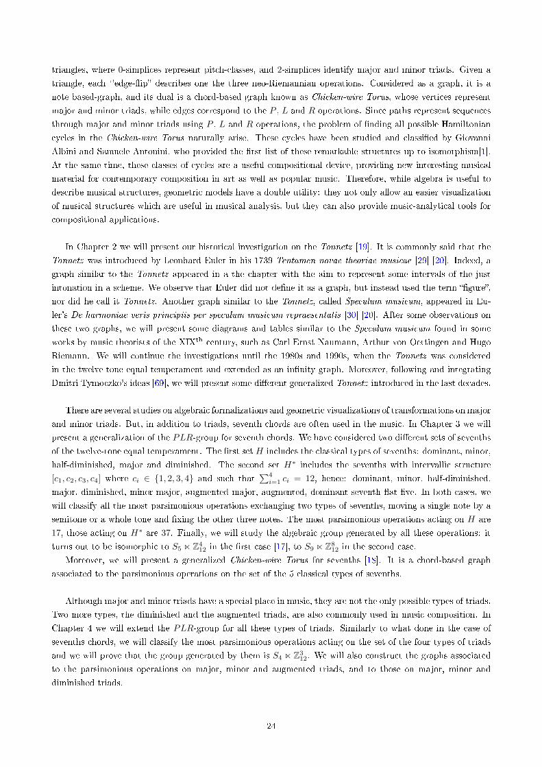
triangles, where 0-simplices represent pitch-classes, and 2-simplices identify major and minor triads. Given a

triangle, each `'edge-�ip� describes one the three neo-Riemannian operations. Considered as a graph, it is a

note based-graph, and its dual is a chord-based graph known as Chicken-wire Torus, whose vertices represent

major and minor triads, while edges correspond to the P , L and R operations. Since paths represent sequences

through major and minor triads using P , L and R operations, the problem of �nding all possible Hamiltonian

cycles in the Chicken-wire Torus naturally arise. These cycles have been studied and classi�ed by Giovanni

Albini and Samuele Antonini, who provided the �rst list of these remarkable structures up to isomorphism[1].

At the same time, these classes of cycles are a useful compositional device, providing new interesting musical

material for contemporary composition in art as well as popular music. Therefore, while algebra is useful to

describe musical structures, geometric models have a double utility: they not only allow an easier visualization

of musical structures which are useful in musical analysis, but they can also provide music-analytical tools for

compositional applications.

In Chapter 2 we will present our historical investigation on the Tonnetz [19]. It is commonly said that the

Tonnetz was introduced by Leonhard Euler in his 1739 Tentamen novae theoriae musicae [29] [20]. Indeed, a

graph similar to the Tonnetz appeared in a the chapter with the aim to represent some intervals of the just

intonation in a scheme. We observe that Euler did not de�ne it as a graph, but instead used the term ��gure�,

nor did he call it Tonnetz. Another graph similar to the Tonnetz, called Speculum musicum, appeared in Eu-

ler's De harmoniae veris principiis per speculum musicum repraesentatis [30] [20]. After some observations on

these two graphs, we will present some diagrams and tables similar to the Speculum musicum found in some

works by music theorists of the XIXth century, such as Carl Ernst Naumann, Arthur von Oettingen and Hugo

Riemann. We will continue the investigations until the 1980s and 1990s, when the Tonnetz was considered

in the twelve-tone equal temperament and extended as an in�nity graph. Moreover, following and integrating

Dmitri Tymoczko's ideas [69], we will present some di�erent generalized Tonnetz introduced in the last decades.

There are several studies on algebraic formalizations and geometric visualizations of transformations on major

and minor triads. But, in addition to triads, seventh chords are often used in the music. In Chapter 3 we will

present a generalization of the PLR-group for seventh chords. We have considered two di�erent sets of sevenths

of the twelve-tone equal temperament. The �rst set H includes the classical types of sevenths: dominant, minor,

half-diminished, major and diminished. The second set H∗ includes the sevenths with intervallic structure

[c1, c2, c3, c4] where ci ∈ {1, 2, 3, 4} and such that∑4i=1 ci = 12, hence: dominant, minor, half-diminished,

major, diminished, minor major, augmented major, augmented, dominant seventh �at �ve. In both cases, we

will classify all the most parsimonious operations exchanging two types of sevenths, moving a single note by a

semitone or a whole tone and �xing the other three notes. The most parsimonious operations acting on H are

17, those acting on H∗ are 37. Finally, we will study the algebraic group generated by all these operations: it

turns out to be isomorphic to S5 n Z412 in the �rst case [17], to S9 n Z8

12 in the second case.

Moreover, we will present a generalized Chicken-wire Torus for sevenths [18]. It is a chord-based graph

associated to the parsimonious operations on the set of the 5 classical types of sevenths.

Although major and minor triads have a special place in music, they are not the only possible types of triads.

Two more types, the diminished and the augmented triads, are also commonly used in music composition. In

Chapter 4 we will extend the PLR-group for all these types of triads. Similarly to what done in the case of

sevenths chords, we will classify the most parsimonious operations acting on the set of the four types of triads

and we will prove that the group generated by them is S4 n Z312. We will also construct the graphs associated

to the parsimonious operations on major, minor and augmented triads, and to those on major, minor and

diminished triads.

24

Finally, in the last chapter, we have studied operations among sevenths and triads, in which it is possible to

add a note (from a triad to a seventh) or to delete a note (from a seventh to a triad). We will introduce a general

framework in which to include the already known parsimonious operations among triads, the parsimonious

operations among sevenths, and also parsimonious operations among seventh and triads. As a special case, we

will consider the set of the 5 classical types of sevenths and the 4 types of triads. We prove that the ST -group,

generated by the 17 most parsimonious operations among sevenths, the 13 most operations among triads and

the new 12 operations among sevenths and triads, is isomorphic to S9 n Z812.

25

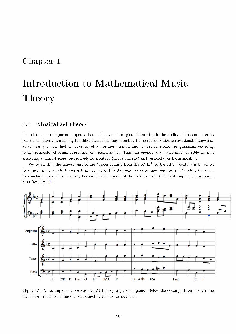
Chapter 1

Introduction to Mathematical Music

Theory

1.1 Musical set theory

One of the most important aspects that makes a musical piece interesting is the ability of the composer to

control the interaction among the di�erent melodic lines creating the harmony, which is traditionally known as

voice leading. It is in fact the interplay of two or more musical lines that realizes chord progressions, according

to the principles of common-practice and counterpoint. This corresponds to the two main possible ways of

analyzing a musical score, respectively horizontally (or melodically) and vertically (or harmonically).

We recall that the largest part of the Western music from the XVIIth to the XIXth century is based on

four-part harmony, which means that every chord in the progression contain four tones. Therefore there are

four melodic lines, conventionally known with the names of the four voices of the chant: soprano, alto, tenor,

bass (see Fig 1.1).

Figure 1.1: An example of voice leading. At the top a piece for piano. Below the decomposition of the same

piece into its 4 melodic lines accompanied by the chords notation.

26

Voice leading is organized according to musical rules, and music theory also deals with the study of these

compositional strategies. We might say that music theory is fundamental for composers as grammar is for poets.

The Western music of this era � also known as common practice period � was tonal. Music written within the

tonal system is generally analyzed by de�ning a certain note as the primary or �tonic�. The other notes are

subservient to the tonic and in a strict hierarchy: the �dominant� (or �fth degree), the �sub-dominant� (or

fourth degree) and so on.

In the late XIXth century composers began to investigate new musical possibilities abandoning tonal music

that had characterized the XVIIth, XVIIIth and XIXth century music. Unlike the tonal system, in post-tonal

music, composers moved away from a hierarchy among tones. This is impersonated by several composers such as

Richard Wagner (1813�1883), especially in his Tristan und Isolde, composed between 1857 and 1859. Another

important and famous example is La Fille aux cheveux de lin (1909�1910) by Claude Debussy (1862�1918).

The ways out were many. Some composers, such as Mussorgsky, Bartok, Debussy and Stravinsky, moved away

from the tonal system inspired by the music of their countries of origin. On the contrary, other composers such

as Schönberg, Webern and Berg, came to a complete break with the past and embraced complete atonality. In

atonal compositions, the hierarchy among tones focusing on a central tone is not used. All the notes of the

chromatic scale are used with functions that are independent from each other.

In tonal music, the properties of musical elements such as chords are fully described by the traditional music

theory. But the latter was not able to provide appropriate tools to analyze and describe new post-tonal musical

system. The role and the structural meaning of certain chords and chord sequences are di�erent; the harmonic

vocabulary of post-tonal music is much more varied and complex than that of tonal music. To de�ne the

rules and the signi�cant relationships between the complex and heterogeneous musical structures of post-tonal

music, music theorists used set theory, developed by Georg Cantor and others between 1874 and 1897, to extend

traditional music theory. This idea emerged in the United States, after World War II, allowing the birth of

musical set theory. This combination between the demands of compositional experimentation and the necessity

of analytic interpretation has decisively in�uenced both the birth and the developments of this type of music

theory.

The main concepts and notions of musical set theory were �rstly introduced around 1960 by the composer,

director and music theorist Howard Hanson (1896�1981) for tonal music and by the musicologist and music

theorist Allen Forte (1926�2014) in his articles A Theory of Set-Complexes for Music [32] and successively sys-

tematized in the book The Structure of Atonal Music [33] for atonal music. The concepts developed in musical

set theory are very general and are applied to tonal and atonal music in any equal temperament [4][46].

Pitch-class and pitch-class set

The application of set theory in music presupposes a substitution of the traditional music notation with a

numerical representation. The starting point is to consider two equivalence relations on the set of all possible

pitches.

Enharmonic equivalence : two tones are enharmonic equivalent if they have the same pitch, but named

di�erently. Example: C] ∼ D[.

Octave equivalence : two pitches x, y ∈ R+ are equivalent if their interval distance is an octave. We remind

the reader that if the frequency of a tone is f , the frequency of the tone one octave higher is 2f , while the

frequency of the tone one octave lower is 12f . Therefore octave equivalence is mathematically described

27

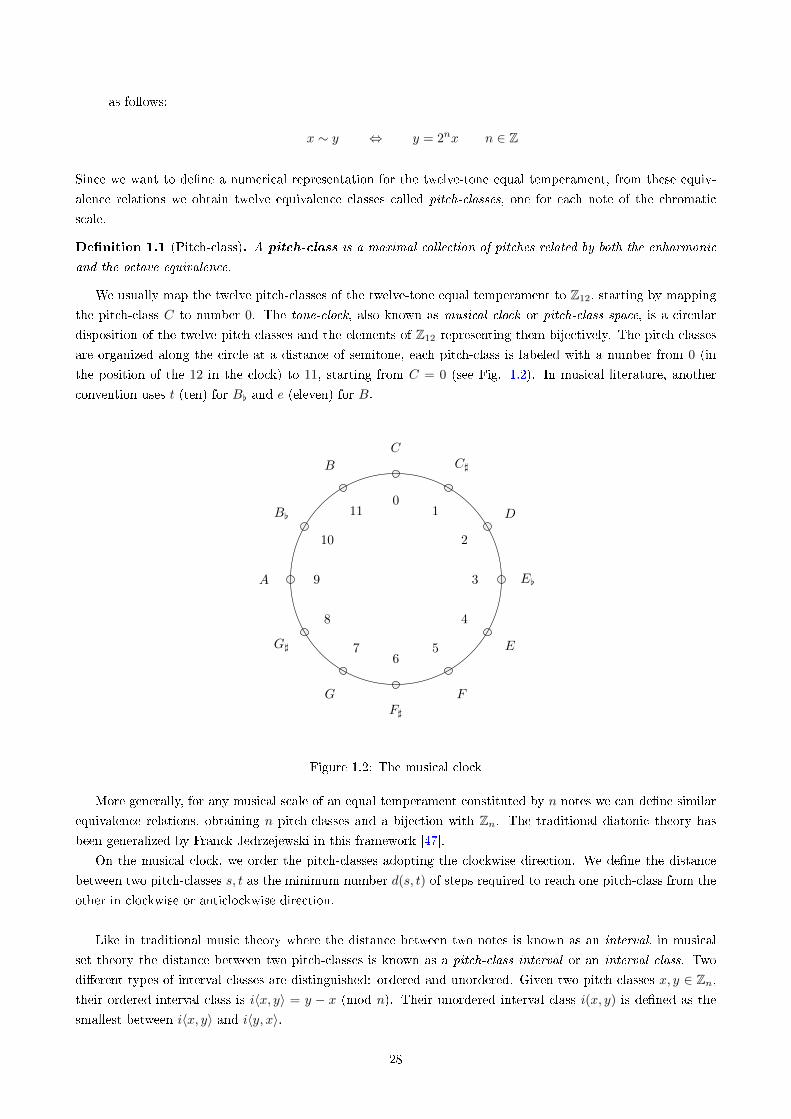
as follows:

x ∼ y ⇔ y = 2nx n ∈ Z

Since we want to de�ne a numerical representation for the twelve-tone equal temperament, from these equiv-

alence relations we obtain twelve equivalence classes called pitch-classes, one for each note of the chromatic

scale.

De�nition 1.1 (Pitch-class). A pitch-class is a maximal collection of pitches related by both the enharmonic

and the octave equivalence.

We usually map the twelve pitch-classes of the twelve-tone equal temperament to Z12, starting by mapping

the pitch-class C to number 0. The tone-clock, also known as musical clock or pitch-class space, is a circular

disposition of the twelve pitch-classes and the elements of Z12 representing them bijectively. The pitch-classes

are organized along the circle at a distance of semitone, each pitch-class is labeled with a number from 0 (in

the position of the 12 in the clock) to 11, starting from C = 0 (see Fig. 1.2). In musical literature, another

convention uses t (ten) for B[ and e (eleven) for B.

..

.

.

.

..

.

.

.

.

.

CC]

D

E[

E

FF]

G

G]

A

B[

B

01

2

3

4

56

7

8

9

10

11

Figure 1.2: The musical clock

More generally, for any musical scale of an equal temperament constituted by n notes we can de�ne similar

equivalence relations, obtaining n pitch-classes and a bijection with Zn. The traditional diatonic theory has

been generalized by Franck Jedrzejewski in this framework [47].

On the musical clock, we order the pitch-classes adopting the clockwise direction. We de�ne the distance

between two pitch-classes s, t as the minimum number d(s, t) of steps required to reach one pitch-class from the

other in clockwise or anticlockwise direction.

Like in traditional music theory where the distance between two notes is known as an interval, in musical

set theory the distance between two pitch-classes is known as a pitch-class interval or an interval class. Two

di�erent types of interval classes are distinguished: ordered and unordered. Given two pitch-classes x, y ∈ Zn,their ordered interval class is i〈x, y〉 = y − x (mod n). Their unordered interval class i(x, y) is de�ned as the

smallest between i〈x, y〉 and i〈y, x〉.

28

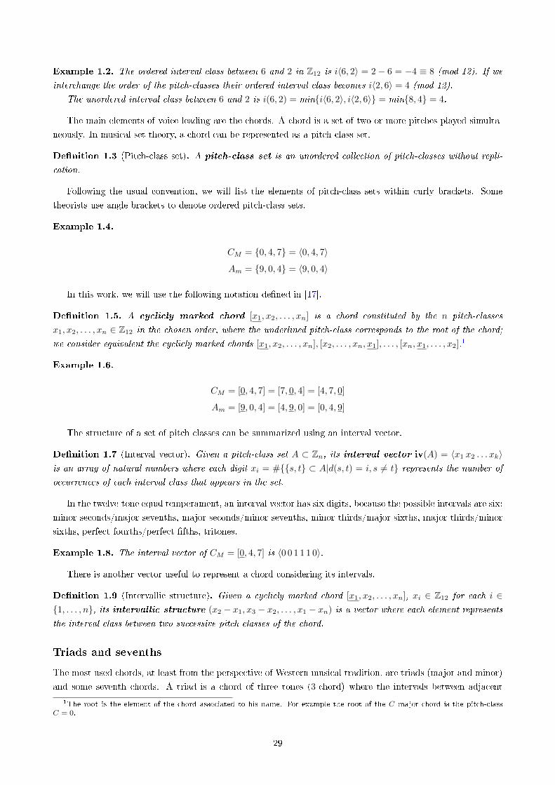
Example 1.2. The ordered interval class between 6 and 2 in Z12 is i〈6, 2〉 = 2− 6 = −4 ≡ 8 (mod 12). If we

interchange the order of the pitch-classes their ordered interval class becomes i〈2, 6〉 = 4 (mod 12).

The unordered interval class between 6 and 2 is i(6, 2) = min{i〈6, 2〉, i〈2, 6〉} = min{8, 4} = 4.

The main elements of voice leading are the chords. A chord is a set of two or more pitches played simulta-

neously. In musical set theory, a chord can be represented as a pitch-class set.

De�nition 1.3 (Pitch-class set). A pitch-class set is an unordered collection of pitch-classes without repli-

cation.

Following the usual convention, we will list the elements of pitch-class sets within curly brackets. Some

theorists use angle brackets to denote ordered pitch-class sets.

Example 1.4.

CM = {0, 4, 7} = 〈0, 4, 7〉

Am = {9, 0, 4} = 〈9, 0, 4〉

In this work, we will use the following notation de�ned in [17].

De�nition 1.5. A cyclicly marked chord [x1, x2, . . . , xn] is a chord constituted by the n pitch-classes

x1, x2, . . . , xn ∈ Z12 in the chosen order, where the underlined pitch-class corresponds to the root of the chord;

we consider equivalent the cyclicly marked chords [x1, x2, . . . , xn], [x2, . . . , xn, x1], . . . , [xn, x1, . . . , x2].1

Example 1.6.

CM = [0, 4, 7] = [7, 0, 4] = [4, 7, 0]

Am = [9, 0, 4] = [4, 9, 0] = [0, 4, 9]

The structure of a set of pitch classes can be summarized using an interval vector.

De�nition 1.7 (Interval vector). Given a pitch-class set A ⊂ Zn, its interval vector iv(A) = 〈x1 x2 . . . xk〉is an array of natural numbers where each digit xi = #{{s, t} ⊂ A|d(s, t) = i, s 6= t} represents the number of

occurrences of each interval class that appears in the set.

In the twelve-tone equal temperament, an interval vector has six digits, because the possible intervals are six:

minor seconds/major sevenths, major seconds/minor sevenths, minor thirds/major sixths, major thirds/minor

sixths, perfect fourths/perfect �fths, tritones.

Example 1.8. The interval vector of CM = [0, 4, 7] is 〈0 0 1 1 1 0〉.

There is another vector useful to represent a chord considering its intervals.

De�nition 1.9 (Intervallic structure). Given a cyclicly marked chord [x1, x2, . . . , xn], xi ∈ Z12 for each i ∈{1, . . . , n}, its intervallic structure (x2 − x1, x3 − x2, . . . , x1 − xn) is a vector where each element represents

the interval class between two successive pitch-classes of the chord.

Triads and sevenths

The most used chords, at least from the perspective of Western musical tradition, are triads (major and minor)

and some seventh chords. A triad is a chord of three tones (3-chord) where the intervals between adjacent

1The root is the element of the chord associated to his name. For example the root of the C major chord is the pitch-classC = 0.

29

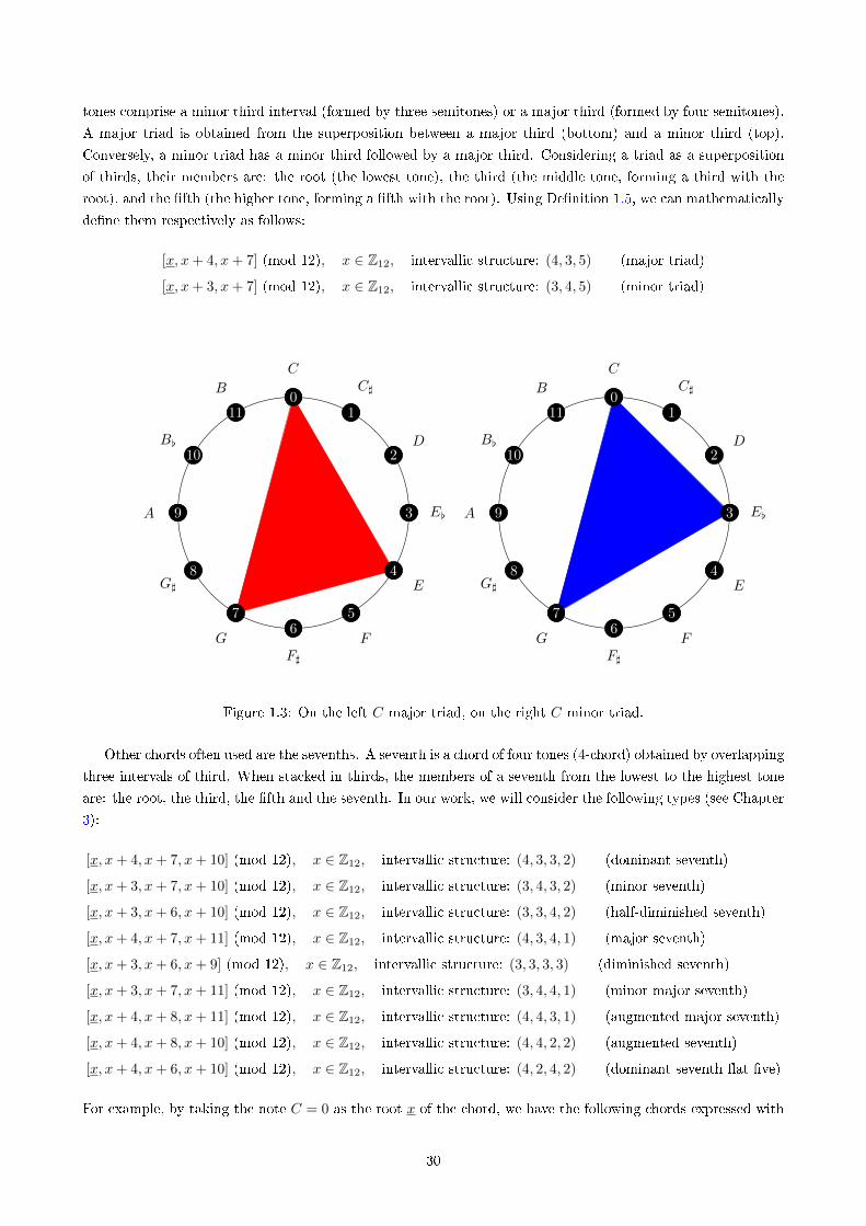
tones comprise a minor third interval (formed by three semitones) or a major third (formed by four semitones).

A major triad is obtained from the superposition between a major third (bottom) and a minor third (top).

Conversely, a minor triad has a minor third followed by a major third. Considering a triad as a superposition

of thirds, their members are: the root (the lowest tone), the third (the middle tone, forming a third with the

root), and the �fth (the higher tone, forming a �fth with the root). Using De�nition 1.5, we can mathematically

de�ne them respectively as follows:

[x, x+ 4, x+ 7] (mod 12), x ∈ Z12, intervallic structure: (4, 3, 5) (major triad)

[x, x+ 3, x+ 7] (mod 12), x ∈ Z12, intervallic structure: (3, 4, 5) (minor triad)

..

.

.

.

..

.

.

.

.

..

.

.

.

.

..

.

.

.

.

.

CC]

D

E[

E

FF]

G

G]

A

B[

B0

1

2

3

4

56

7

8

9

10

11

..

.

.

.

..

.

.

.

.

..

.

.

.

.

..

.

.

.

.

.

CC]

D

E[

E

FF]

G

G]

A

B[

B0

1

2

3

4

56

7

8

9

10

11

Figure 1.3: On the left C major triad, on the right C minor triad.

Other chords often used are the sevenths. A seventh is a chord of four tones (4-chord) obtained by overlapping

three intervals of third. When stacked in thirds, the members of a seventh from the lowest to the highest tone

are: the root, the third, the �fth and the seventh. In our work, we will consider the following types (see Chapter

3):

[x, x+ 4, x+ 7, x+ 10] (mod 12), x ∈ Z12, intervallic structure: (4, 3, 3, 2) (dominant seventh)

[x, x+ 3, x+ 7, x+ 10] (mod 12), x ∈ Z12, intervallic structure: (3, 4, 3, 2) (minor seventh)

[x, x+ 3, x+ 6, x+ 10] (mod 12), x ∈ Z12, intervallic structure: (3, 3, 4, 2) (half-diminished seventh)

[x, x+ 4, x+ 7, x+ 11] (mod 12), x ∈ Z12, intervallic structure: (4, 3, 4, 1) (major seventh)

[x, x+ 3, x+ 6, x+ 9] (mod 12), x ∈ Z12, intervallic structure: (3, 3, 3, 3) (diminished seventh)

[x, x+ 3, x+ 7, x+ 11] (mod 12), x ∈ Z12, intervallic structure: (3, 4, 4, 1) (minor major seventh)

[x, x+ 4, x+ 8, x+ 11] (mod 12), x ∈ Z12, intervallic structure: (4, 4, 3, 1) (augmented major seventh)

[x, x+ 4, x+ 8, x+ 10] (mod 12), x ∈ Z12, intervallic structure: (4, 4, 2, 2) (augmented seventh)

[x, x+ 4, x+ 6, x+ 10] (mod 12), x ∈ Z12, intervallic structure: (4, 2, 4, 2) (dominant seventh �at �ve)

For example, by taking the note C = 0 as the root x of the chord, we have the following chords expressed with

30

the usual music notation:

C7 = [0, 4, 7, 10] (C dominant seventh)

Cm = [0, 3, 7, 10] (C minor seventh)

Cø = [0, 3, 6, 10] (C half-diminished seventh)

C∆ = [0, 4, 7, 11] (C major seventh)

Co = [0, 3, 6, 9] (C diminished seventh)

C∆m = [0, 3, 7, 11] (C minor major seventh)

C∆+ = [0, 4, 8, 11] (C augmented major seventh)

C7+ = [0, 4, 8, 10] (C augmented seventh)

C7[5 = [0, 4, 6, 10] (C dominant seventh �at �ve)

1.2 Transformational theory

Changing the focus from musical objects to the relations between them, transformational theory was developed

since the 1980s. Its main idea is based on the use of group-theoretical concepts to de�ne musical objects and

transformations. Historically, this approach was introduced by the music theorist David Lewin in the late 1980s

and systematized in his book Generalized Musical Intervals and Transformations [53].

The GIS structure

One of the most important examples of transformational construction is the notion of GIS.

De�nition 1.10 (Generalized Interval System (GIS)). A Generalized Interval System (GIS) is an ordered

triplet (S, IV LS, int), where S is a set of musical elements, IV LS is a mathematical group called the interval

group, and int is a function int : S × S → IV LS, such that:

int(r, s)int(s, t) = int(r, t) ∀r, s, t ∈ S (1.1)

∀s ∈ S,∀i ∈ IV LS,∃!t ∈ S s.t. int(s, t) = i. (1.2)

Proposition 1.11. Let e ∈ IV LS be the neutral element. In any GIS, we have int(s, s) = e and int(t, s) =

int(s, t)−1 for every s, t ∈ S.

Proof. From 1.1 we have int(s, s)int(s, s) = int(s, s), hence int(s, s) = e. Moreover int(t, s)int(s, t) = int(t, t) =

e ⇒ int(t, s) = int(s, t)−1.

From the last proposition it is clear that GIS's are simply transitive group actions.

Example 1.12. (Z12, (Z12,+), int), where Z12 is the set of 12 pitch-classes, (Z12,+) is the interval group, and

int(s, t) := t− s, is a GIS. In fact, for every x, y, z ∈ Z12:

int(x, y) + int(y, z) = (y − x) + (z − y) = z − x = int(x, z),

hence 1.1 is satis�ed. Moreover given a pitch-class s ∈ Z12 and given an interval i ∈ Z12 there exists a unique

pitch-class t ∈ Z12 such that int(s, t) = i. In fact if there exists u ∈ S such that int(s, u) = i we would have

int(s, t) = int(s, u), then t− s = u− s ⇒ t = u.

31

..

.

.

.

..

.

.

.

.

..

.

.

.

.

..

.

.

.

.

.

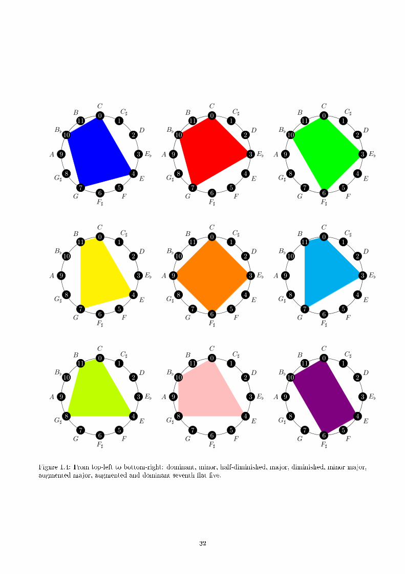
CC]

D

E[

E

FF]

G

G]

A

B[

B 01

2

3

4

56

7

8

9

10

11.

.

.

.

.

..

.

.

.

.

..

.

.

.

.

..

.

.

.

.

.

CC]

D

E[

E

FF]

G

G]

A

B[

B 01

2

3

4

56

7

8

9

10

11.

.

.

.

.

..

.

.

.

.

..

.

.

.

.

..

.

.

.

.

.

CC]

D

E[

E

FF]

G

G]

A

B[

B 01

2

3

4

56

7

8

9

10

11

..

.

.

.

..

.

.

.

.

..

.

.

.

.

..

.

.

.

.

.

CC]

D

E[

E

FF]

G

G]

A

B[

B 01

2

3

4

56

7

8

9

10

11.

.

.

.

.

..

.

.

.

.

..

.

.

.

.

..

.

.

.

.

.

CC]

D

E[

E

FF]

G

G]

A

B[

B 01

2

3

4

56

7

8

9

10

11.

.

.

.

.

..

.

.

.

.

..

.

.

.

.

..

.

.

.

.

.

CC]

D

E[

E

FF]

G

G]

A

B[

B 01

2

3

4

56

7

8

9

10

11

..

.

.

.

..

.

.

.

.

..

.

.

.

.

..

.

.

.

.

.

CC]

D

E[

E

FF]

G

G]

A

B[

B 01

2

3

4

56

7

8

9

10

11.

.

.

.

.

..

.

.

.

.

..

.

.

.

.

..

.

.

.

.

.

CC]

D

E[

E

FF]

G

G]

A

B[

B 01

2

3

4

56

7

8

9

10

11.

.

.

.

.

..

.

.

.

.

..

.

.

.

.

..

.

.

.

.

.

CC]

D

E[

E

FF]

G

G]

A

B[

B 01

2

3

4

56

7

8

9

10

11

Figure 1.4: From top-left to bottom-right: dominant, minor, half-diminished, major, diminished, minor major,augmented major, augmented and dominant seventh �at �ve.

32

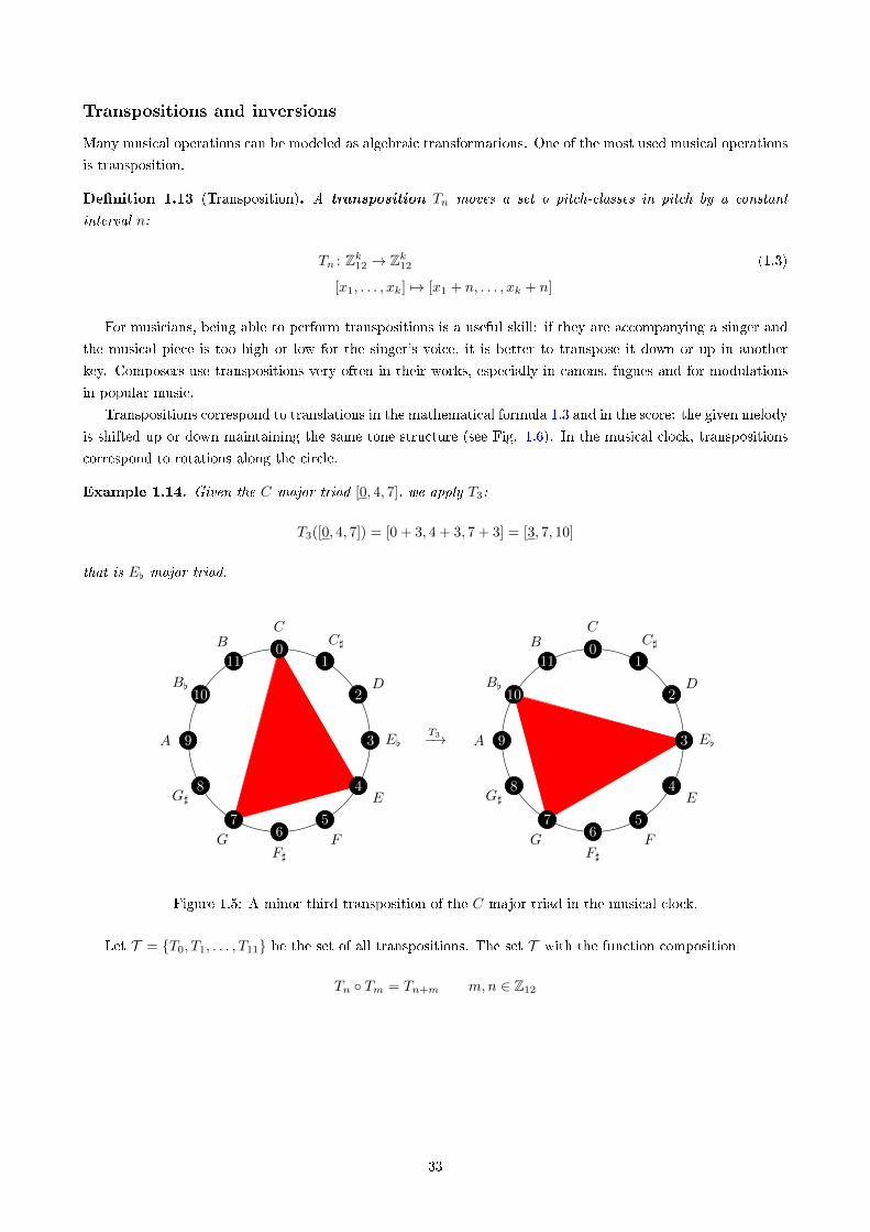
Transpositions and inversions

Many musical operations can be modeled as algebraic transformations. One of the most used musical operations

is transposition.

De�nition 1.13 (Transposition). A transposition Tn moves a set o pitch-classes in pitch by a constant

interval n:

Tn : Zk12 → Zk12 (1.3)

[x1, . . . , xk] 7→ [x1 + n, . . . , xk + n]

For musicians, being able to perform transpositions is a useful skill: if they are accompanying a singer and

the musical piece is too high or low for the singer's voice, it is better to transpose it down or up in another

key. Composers use transpositions very often in their works, especially in canons, fugues and for modulations

in popular music.

Transpositions correspond to translations in the mathematical formula 1.3 and in the score: the given melody

is shifted up or down maintaining the same tone structure (see Fig. 1.6). In the musical clock, transpositions

correspond to rotations along the circle.

Example 1.14. Given the C major triad [0, 4, 7], we apply T3:

T3([0, 4, 7]) = [0 + 3, 4 + 3, 7 + 3] = [3, 7, 10]

that is E[ major triad.

..

.

.

.

..

.

.

.

.

..

.

.

.

.

..

.

.

.

.

.

CC]

D

E[

E

FF]

G

G]

A

B[

B 01

2

3

4

56

7

8

9

10

11

T3−→

..

.

.

.

..

.

.

.

.

..

.

.

.

.

..

.

.

.

.

.

CC]

D

E[

E

FF]

G

G]

A

B[

B 01

2

3

4

56

7

8

9

10

11

Figure 1.5: A minor third transposition of the C major triad in the musical clock.

Let T = {T0, T1, . . . , T11} be the set of all transpositions. The set T with the function composition

Tn ◦ Tm = Tn+m m,n ∈ Z12

33

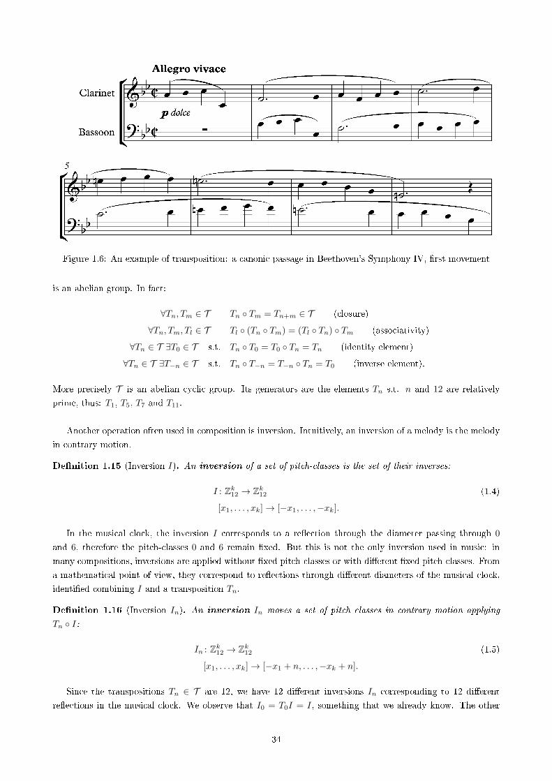
Figure 1.6: An example of transposition: a canonic passage in Beethoven's Symphony IV, �rst movement

is an abelian group. In fact:

∀Tn, Tm ∈ T Tn ◦ Tm = Tn+m ∈ T (closure)

∀Tn, Tm, Tl ∈ T Tl ◦ (Tn ◦ Tm) = (Tl ◦ Tn) ◦ Tm (associativity)

∀Tn ∈ T ∃T0 ∈ T s.t. Tn ◦ T0 = T0 ◦ Tn = Tn (identity element)

∀Tn ∈ T ∃T−n ∈ T s.t. Tn ◦ T−n = T−n ◦ Tn = T0 (inverse element).

More precisely T is an abelian cyclic group. Its generators are the elements Tn s.t. n and 12 are relatively

prime, thus: T1, T5, T7 and T11.

Another operation often used in composition is inversion. Intuitively, an inversion of a melody is the melody

in contrary motion.

De�nition 1.15 (Inversion I). An inversion of a set of pitch-classes is the set of their inverses:

I : Zk12 → Zk12 (1.4)

[x1, . . . , xk]→ [−x1, . . . ,−xk].

In the musical clock, the inversion I corresponds to a re�ection through the diameter passing through 0

and 6, therefore the pitch-classes 0 and 6 remain �xed. But this is not the only inversion used in music: in

many compositions, inversions are applied without �xed pitch-classes or with di�erent �xed pitch-classes. From

a mathematical point of view, they correspond to re�ections through di�erent diameters of the musical clock,

identi�ed combining I and a transposition Tn.

De�nition 1.16 (Inversion In). An inversion In moves a set of pitch classes in contrary motion applying

Tn ◦ I:

In : Zk12 → Zk12 (1.5)

[x1, . . . , xk]→ [−x1 + n, . . . ,−xk + n].

Since the transpositions Tn ∈ T are 12, we have 12 di�erent inversions In corresponding to 12 di�erent

re�ections in the musical clock. We observe that I0 = T0I = I, something that we already know. The other

34

inversions can be divided into two types. If n is even, In corresponds to a re�ection through the diameter

passing in n2 . If n is odd, In corresponds to a re�ection through the diameter passing in the middle between

n−12 and n+1

2 .

Example 1.17. Given the C major triad [0, 4, 7], we apply I3:

I3([0, 4, 7]) = T3I([0, 4, 7]) = [0 + 3,−4 + 3,−7 + 3] = [3, 11, 8] = [8, 11, 3],

that is, the G] minor triad.

..

.

.

.

..

.

.

.

.

..

.

.

.

.

..

.

.

.

.

.

CC]

D

E[

E

FF]

G

G]

A

B[

B 01

2

3

4

56

7

8

9

10

11

I3−→

..

.

.

.

..

.

.

.

.

..

.

.

.

.

..

.

.

.

.

.

CC]

D

E[

E

FF]

G

G]

A

B[

B 01

2

3

4

56

7

8

9

10

11

Remark 1.18. Some remarks on transpositions and inversions.

1. By applying a transposition to a chord, we obtain a chord with the same intervallic structure. On the

contrary, if we apply an inversion in general we obtain a chord whose intervallic structure is equal to the

retrogradation (up to cyclic permutation) of the intervallic structure of the initial chord.

2. The set T of transpositions is a group. Conversely inversions do not form a group because the composition

of two inversions is not an inversion.

3. Each inversion is an involution. Among transpositions, only T0 and T6 are involutions.

Transpositions and inversions satisfy the following properties:

Tm ◦ In = Im+n (mod 12)

Im ◦ Tn = Im−n (mod 12)

Im ◦ In = Tm−n (mod 12).

Theorem 1.19. Inversions and transpositions act on the set S of all 24 major and minor triads generating the

group T/I2 that is isomorphic to the dihedral group D12 of order 24.

Proof. We remind the reader that the dihedral group Dn of order 2n is the group of isometries of a regular

n-gon in the plane, including rotations and re�ections. Its representation is

〈s, t|sn = t2 = Id, tst = s−1〉.

2The notation does not represent the set-theoretical di�erence between T and I.

35

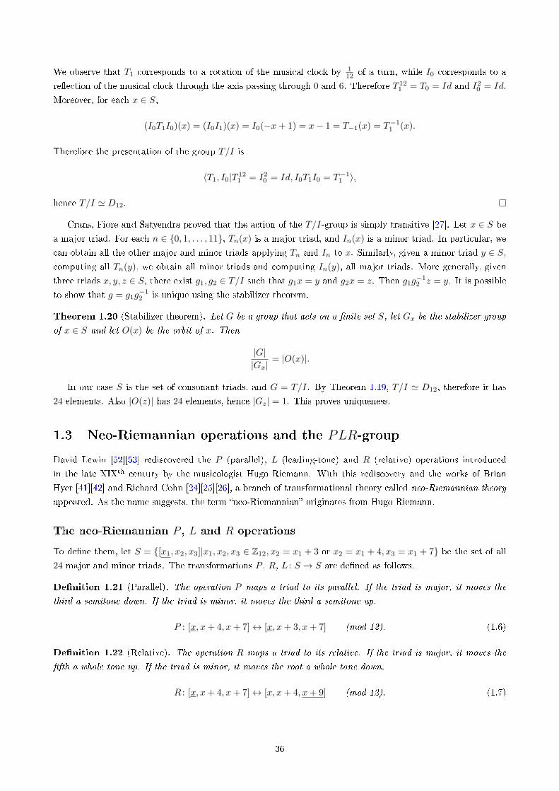
We observe that T1 corresponds to a rotation of the musical clock by 112 of a turn, while I0 corresponds to a

re�ection of the musical clock through the axis passing through 0 and 6. Therefore T 121 = T0 = Id and I2

0 = Id.

Moreover, for each x ∈ S,

(I0T1I0)(x) = (I0I1)(x) = I0(−x+ 1) = x− 1 = T−1(x) = T−11 (x).

Therefore the presentation of the group T/I is

〈T1, I0|T 121 = I2

0 = Id, I0T1I0 = T−11 〉,

hence T/I ' D12.

Crans, Fiore and Satyendra proved that the action of the T/I-group is simply transitive [27]. Let x ∈ S be

a major triad. For each n ∈ {0, 1, . . . , 11}, Tn(x) is a major triad, and In(x) is a minor triad. In particular, we

can obtain all the other major and minor triads applying Tn and In to x. Similarly, given a minor triad y ∈ S,computing all Tn(y), we obtain all minor triads and computing In(y), all major triads. More generally, given

three triads x, y, z ∈ S, there exist g1, g2 ∈ T/I such that g1x = y and g2x = z. Then g1g−12 z = y. It is possible

to show that g = g1g−12 is unique using the stabilizer theorem.

Theorem 1.20 (Stabilizer theorem). Let G be a group that acts on a �nite set S, let Gx be the stabilizer group

of x ∈ S and let O(x) be the orbit of x. Then

|G||Gx|

= |O(x)|.

In our case S is the set of consonant triads, and G = T/I. By Theorem 1.19, T/I ' D12, therefore it has

24 elements. Also |O(z)| has 24 elements, hence |Gz| = 1. This proves uniqueness.

1.3 Neo-Riemannian operations and the PLR-group

David Lewin [52][53] rediscovered the P (parallel), L (leading-tone) and R (relative) operations introduced

in the late XIXth century by the musicologist Hugo Riemann. With this rediscovery and the works of Brian

Hyer [41][42] and Richard Cohn [24][25][26], a branch of transformational theory called neo-Riemannian theory

appeared. As the name suggests, the term �neo-Riemannian� originates from Hugo Riemann.

The neo-Riemannian P , L and R operations

To de�ne them, let S = {[x1, x2, x3]|x1, x2, x3 ∈ Z12, x2 = x1 + 3 or x2 = x1 + 4, x3 = x1 + 7} be the set of all24 major and minor triads. The transformations P , R, L : S → S are de�ned as follows.

De�nition 1.21 (Parallel). The operation P maps a triad to its parallel. If the triad is major, it moves the

third a semitone down. If the triad is minor, it moves the third a semitone up.

P : [x, x+ 4, x+ 7]↔ [x, x+ 3, x+ 7] (mod 12). (1.6)

De�nition 1.22 (Relative). The operation R maps a triad to its relative. If the triad is major, it moves the

�fth a whole tone up. If the triad is minor, it moves the root a whole tone down.

R : [x, x+ 4, x+ 7]↔ [x, x+ 4, x+ 9] (mod 12). (1.7)

36

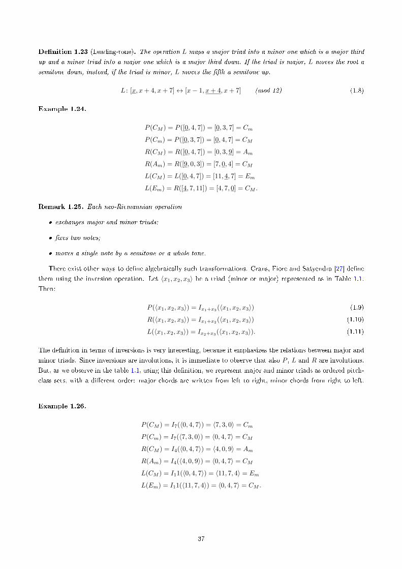
De�nition 1.23 (Leading-tone). The operation L maps a major triad into a minor one which is a major third

up and a minor triad into a major one which is a major third down. If the triad is major, L moves the root a

semitone down, instead, if the triad is minor, L moves the �fth a semitone up.

L : [x, x+ 4, x+ 7]↔ [x− 1, x+ 4, x+ 7] (mod 12) (1.8)

Example 1.24.

P (CM ) = P ([0, 4, 7]) = [0, 3, 7] = Cm

P (Cm) = P ([0, 3, 7]) = [0, 4, 7] = CM

R(CM ) = R([0, 4, 7]) = [0, 3, 9] = Am

R(Am) = R([9, 0, 3]) = [7, 0, 4] = CM

L(CM ) = L([0, 4, 7]) = [11, 4, 7] = Em

L(Em) = R([4, 7, 11]) = [4, 7, 0] = CM .

Remark 1.25. Each neo-Riemannian operation

� exchanges major and minor triads;

� �xes two notes;

� moves a single note by a semitone or a whole-tone.

There exist other ways to de�ne algebraically such transformations. Crans, Fiore and Satyendra [27] de�ne

them using the inversion operation. Let 〈x1, x2, x3〉 be a triad (minor or major) represented as in Table 1.1.

Then:

P (〈x1, x2, x3〉) = Ix1+x3(〈x1, x2, x3〉) (1.9)

R(〈x1, x2, x3〉) = Ix1+x2(〈x1, x2, x3〉) (1.10)

L(〈x1, x2, x3〉) = Ix2+x3(〈x1, x2, x3〉). (1.11)

The de�nition in terms of inversions is very interesting, because it emphasizes the relations between major and

minor triads. Since inversions are involutions, it is immediate to observe that also P , L and R are involutions.

But, as we observe in the table 1.1, using this de�nition, we represent major and minor triads as ordered pitch-

class sets, with a di�erent order: major chords are written from left to right, minor chords from right to left.

Example 1.26.

P (CM ) = I7(〈0, 4, 7〉) = 〈7, 3, 0〉 = Cm

P (Cm) = I7(〈7, 3, 0〉) = 〈0, 4, 7〉 = CM

R(CM ) = I4(〈0, 4, 7〉) = 〈4, 0, 9〉 = Am

R(Am) = I4(〈4, 0, 9〉) = 〈0, 4, 7〉 = CM

L(CM ) = I11(〈0, 4, 7〉) = 〈11, 7, 4〉 = Em

L(Em) = I11(〈11, 7, 4〉) = 〈0, 4, 7〉 = CM .

37

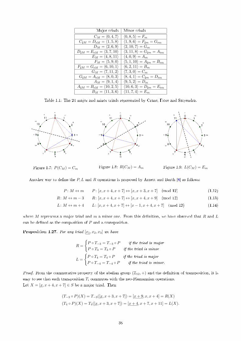
Major triads Minor triads

CM = 〈0, 4, 7〉〈0, 8, 5〉 = FmC]M = D[M = 〈1, 5, 8〉〈1, 9, 6〉 = F]m = G[m

DM = 〈2, 6, 9〉〈2, 10, 7〉 = GmD]M = E[M = 〈3, 7, 10〉〈3, 11, 8〉 = G]m = A[m

EM = 〈4, 8, 11〉〈4, 0, 9〉 = AmFM = 〈5, 9, 0〉〈5, 1, 10〉 = A]m = B[m

F]M = G[M = 〈6, 10, 1〉〈6, 2, 11〉 = BmGM = 〈7, 11, 2〉〈7, 3, 0〉 = Cm

G]M = A[M = 〈8, 0, 3〉〈8, 4, 1〉 = C]m = D[m

AM = 〈9, 1, 4〉〈9, 5, 2〉 = Dm

A]M = B[M = 〈10, 2, 5〉〈10, 6, 3〉 = D]m = E[mBM = 〈11, 3, 6〉〈11, 7, 4〉 = Em

Table 1.1: The 24 major and minor triads represented by Crans, Fiore and Satyendra.

Figure 1.7: P (CM ) = Cm Figure 1.8: R(CM ) = Am Figure 1.9: L(CM ) = Em

Another way to de�ne the P,L and R operations is proposed by Arnett and Barth [8] as follows:

P : M ↔ m P : [x, x+ 4, x+ 7]↔ [x, x+ 3, x+ 7] (mod 12) (1.12)

R : M ↔ m− 3 R : [x, x+ 4, x+ 7]↔ [x, x+ 4, x+ 9] (mod 12) (1.13)

L : M ↔ m+ 4 L : [x, x+ 4, x+ 7]↔ [x− 1, x+ 4, x+ 7] (mod 12) (1.14)

where M represents a major triad and m a minor one. From this de�nition, we have observed that R and L

can be de�ned as the composition of P and a transposition.

Proposition 1.27. For any triad [x1, x2, x3] we have

R =

{P ◦ T−3 = T−3 ◦ P if the triad is major

P ◦ T3 = T3 ◦ P if the triad is minor

L =

{P ◦ T4 = T4 ◦ P if the triad is major

P ◦ T−4 = T−4 ◦ P if the triad is minor.

Proof. From the commutative property of the abelian group (Z12,+) and the de�nition of transposition, it is

easy to see that each transposition Ti commutes with the neo-Riemannian operations.

Let X = [x, x+ 4, x+ 7] ∈ S be a major triad. Then

(T−3 ◦ P )(X) = T−3([x, x+ 3, x+ 7]) = [x+ 9, x, x+ 4] = R(X)

(T4 ◦ P )(X) = T4([x, x+ 3, x+ 7]) = [x+ 4, x+ 7, x+ 11] = L(X).

38

Let Y = [y, y + 3, y + 7] be a minor triad. Then

(T3 ◦ P )(Y ) = T3([y, y + 4, y + 7]) = [y + 3, y + 7, y + 10] = R(X)

(T−4 ◦ P )(Y ) = T−4([y, y + 4, y + 7]) = [y + 8, y, y + 3] = L(Y ).

PLR-group

The neo-Riemannian operations generate a group known as PLR-group or neo-Riemannian group.

Lemma 1.28. The neo-Riemannian operations L and R act on the set S of all 24 major and minor triads

generating a group.

Proof. First of all we observe that P = RLRLRLR. In fact, given a major triad [x, x+ 4, x+ 7] ∈ S we have

RLRLRLR([x, x+ 4, x+ 7]) = RLRLRL([x, x+ 4, x+ 9]) =

= RLRLR([x, x+ 5, x+ 9]) =

= RLRL([x+ 2, x+ 5, x+ 9]) =

= RLR([x+ 2, x+ 5, x+ 10]) =

= RL([x+ 2, x+ 7, x+ 10]) =

= R([x+ 3, x+ 7, x+ 10]) =

= ([x+ 3, x+ 7, x]) =

= P ([x, x+ 4, x+ 7]).

We get a similar result applying RLRLRLR to a minor triad.

Now we prove that L and R act on S generating a group. First of all, L,R : S → S and every operations

obtained as compositions of them is well de�ned on S. The composition of functions is always associative.

We remind the reader that for every triad X ∈ S the neo-Riemannian operations are involutions, therefore

we have an identity function Id.

Finally, since L and R are involutions, each transformation can be decomposed by alternating the generating

function L and R. To construct the inverse of each transformation de�ned as alternation of L and R, it is

su�cient to invert the order of composition.

Theorem 1.29. The PLR-group is isomorphic to the dihedral group D12 of order 24.

Proof. We observe that the elements of the PLR-group are described as R(LR)n or (LR)n, 0 ≤ n ≤ 11. In

fact, from Lemma 1.28 we know that each transformation of the PLR-group is constructed by alternating the

generating function L and R. Moreover the transformations described as (LR)kL are equivalent to R(LR)11−k.

Furthermore we observe that (LR)12 = Id, then we consider the transformations obtained by alternating L and

R whose length is lower than 24. Therefore we have twelve elements of type R(LR)n and other twelve of type

(LR)n, hence the PLR-group has 24 elements. Finally we observe that we can describe the group with the

following presentation

〈(LR), L|(LR)12 = L2 = Id, L(RL)L = RL〉

hence PLR ' D12.

Corollary 1.30. The PLR-group acts simply transitively on the set S of 24 major and minor triads.

39

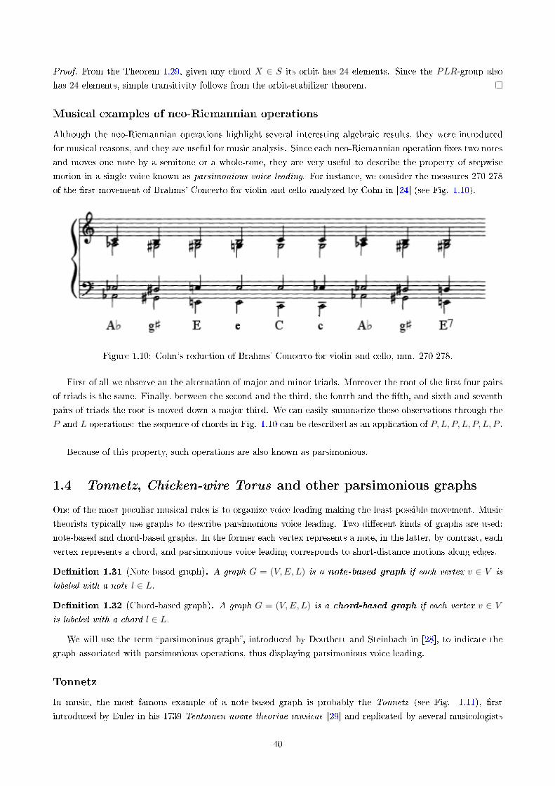
Proof. From the Theorem 1.29, given any chord X ∈ S its orbit has 24 elements. Since the PLR-group also

has 24 elements, simple transitivity follows from the orbit-stabilizer theorem.

Musical examples of neo-Riemannian operations

Although the neo-Riemannian operations highlight several interesting algebraic results, they were introduced

for musical reasons, and they are useful for music analysis. Since each neo-Riemannian operation �xes two notes

and moves one note by a semitone or a whole-tone, they are very useful to describe the property of stepwise

motion in a single voice known as parsimonious voice leading. For instance, we consider the measures 270-278

of the �rst movement of Brahms' Concerto for violin and cello analyzed by Cohn in [24] (see Fig. 1.10).

Figure 1.10: Cohn's reduction of Brahms' Concerto for violin and cello, mm. 270-278.

First of all we observe an the alternation of major and minor triads. Moreover the root of the �rst four pairs

of triads is the same. Finally, between the second and the third, the fourth and the �fth, and sixth and seventh

pairs of triads the root is moved down a major third. We can easily summarize these observations through the

P and L operations: the sequence of chords in Fig. 1.10 can be described as an application of P,L, P, L, P, L, P .

Because of this property, such operations are also known as parsimonious.

1.4 Tonnetz, Chicken-wire Torus and other parsimonious graphs

One of the most peculiar musical rules is to organize voice leading making the least possible movement. Music

theorists typically use graphs to describe parsimonious voice leading. Two di�erent kinds of graphs are used:

note-based and chord-based graphs. In the former each vertex represents a note, in the latter, by contrast, each

vertex represents a chord, and parsimonious voice leading corresponds to short-distance motions along edges.

De�nition 1.31 (Note-based graph). A graph G = (V,E, L) is a note-based graph if each vertex v ∈ V is

labeled with a note l ∈ L.

De�nition 1.32 (Chord-based graph). A graph G = (V,E,L) is a chord-based graph if each vertex v ∈ Vis labeled with a chord l ∈ L.

We will use the term �parsimonious graph�, introduced by Douthett and Steinbach in [28], to indicate the

graph associated with parsimonious operations, thus displaying parsimonious voice leading.

Tonnetz

In music, the most famous example of a note-based graph is probably the Tonnetz (see Fig. 1.11), �rst

introduced by Euler in his 1739 Tentamen novae theoriae musicae [29] and replicated by several musicologists

40

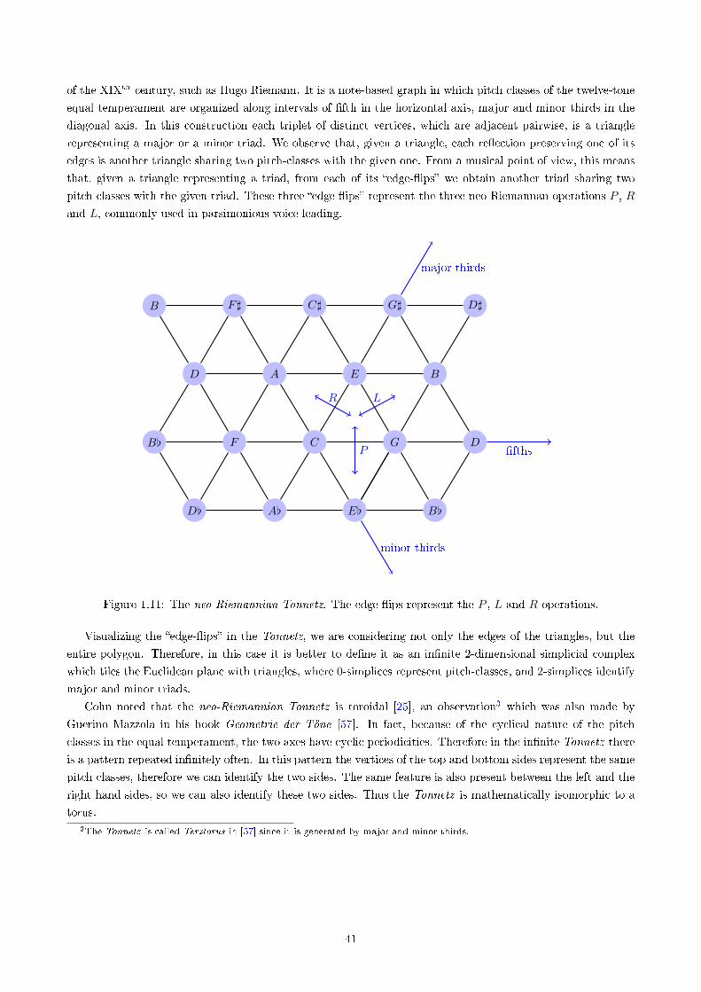
of the XIXth century, such as Hugo Riemann. It is a note-based graph in which pitch classes of the twelve-tone

equal temperament are organized along intervals of �fth in the horizontal axis, major and minor thirds in the

diagonal axis. In this construction each triplet of distinct vertices, which are adjacent pairwise, is a triangle

representing a major or a minor triad. We observe that, given a triangle, each re�ection preserving one of its

edges is another triangle sharing two pitch-classes with the given one. From a musical point of view, this means

that, given a triangle representing a triad, from each of its �edge-�ips� we obtain another triad sharing two

pitch-classes with the given triad. These three �edge-�ips� represent the three neo-Riemannan operations P , R

and L, commonly used in parsimonious voice leading.

D[ A[ E[ B[

B[ F C G D

D A E B

B F] C] G] D]

P

R L

�fths

major thirds

minor thirds

Figure 1.11: The neo-Riemannian Tonnetz. The edge-�ips represent the P , L and R operations.

Visualizing the �edge-�ips� in the Tonnetz, we are considering not only the edges of the triangles, but the

entire polygon. Therefore, in this case it is better to de�ne it as an in�nite 2-dimensional simplicial complex

which tiles the Euclidean plane with triangles, where 0-simplices represent pitch-classes, and 2-simplices identify

major and minor triads.

Cohn noted that the neo-Riemannian Tonnetz is toroidal [25], an observation3 which was also made by

Guerino Mazzola in his book Geometrie der Töne [57]. In fact, because of the cyclical nature of the pitch

classes in the equal temperament, the two axes have cyclic periodicities. Therefore in the in�nite Tonnetz there

is a pattern repeated in�nitely often. In this pattern the vertices of the top and bottom sides represent the same

pitch classes, therefore we can identify the two sides. The same feature is also present between the left and the

right hand sides, so we can also identify these two sides. Thus the Tonnetz is mathematically isomorphic to a

torus.3The Tonnetz is called Terztorus in [57] since it is generated by major and minor thirds.

41

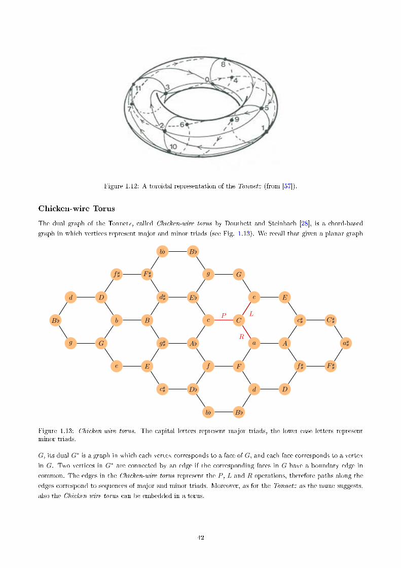
Figure 1.12: A toroidal representation of the Tonnetz (from [57]).

Chicken-wire Torus

The dual graph of the Tonnetz, called Chicken-wire torus by Douthett and Steinbach [28], is a chord-based

graph in which vertices represent major and minor triads (see Fig. 1.13). We recall that given a planar graph

b[ B[

d

Ff

D[c]

E

g] A[

e

G

b B

g

B[

d D

f] F]

d] E[

c C

a A

f]

D

F]

a]

C]c]

Ee

Gg

B[b[

P

R

L

Figure 1.13: Chicken-wire torus. The capital letters represent major triads, the lower-case letters representminor triads.

G, its dual G∗ is a graph in which each vertex corresponds to a face of G, and each face corresponds to a vertex

in G. Two vertices in G∗ are connected by an edge if the corresponding faces in G have a boundary edge in

common. The edges in the Chicken-wire torus represent the P , L and R operations, therefore paths along the

edges correspond to sequences of major and minor triads. Moreover, as for the Tonnetz as the name suggests,

also the Chicken-wire torus can be embedded in a torus.

42

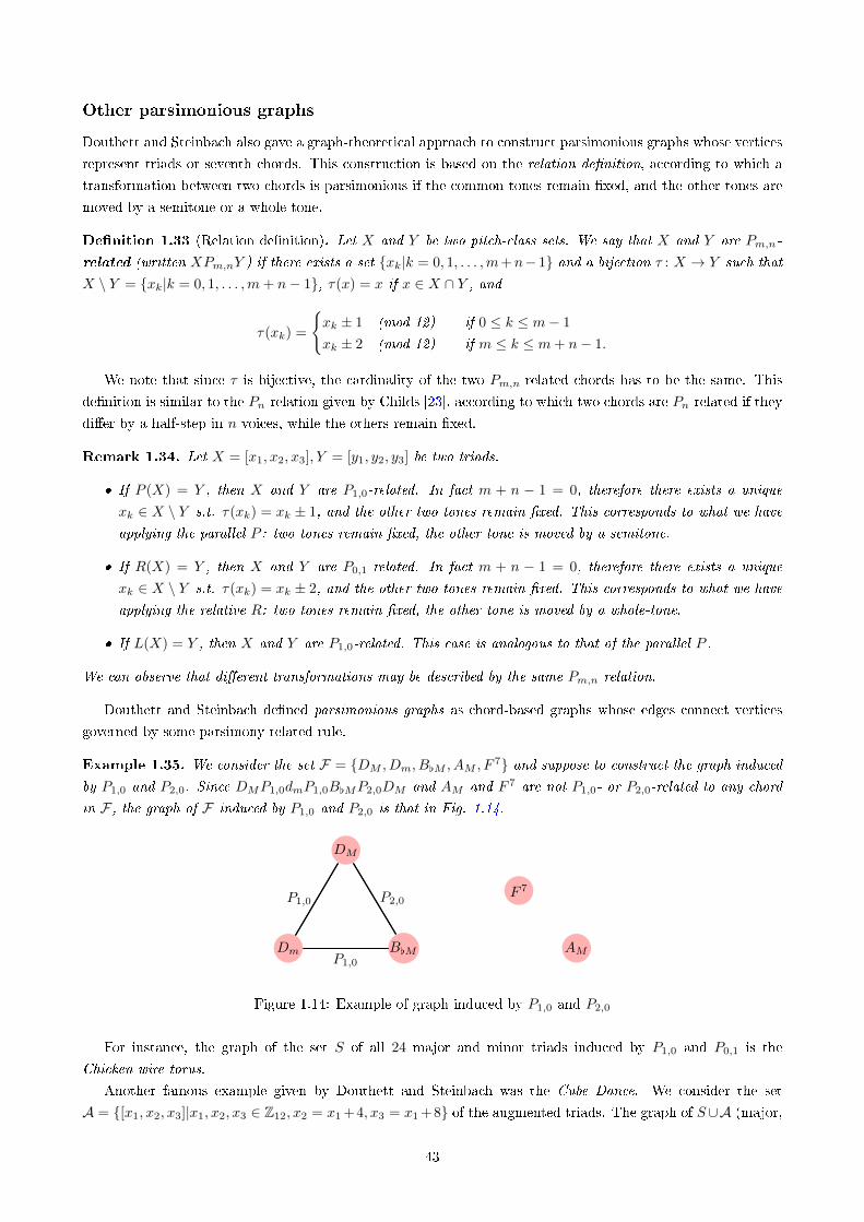
Other parsimonious graphs

Douthett and Steinbach also gave a graph-theoretical approach to construct parsimonious graphs whose vertices

represent triads or seventh chords. This construction is based on the relation de�nition, according to which a

transformation between two chords is parsimonious if the common tones remain �xed, and the other tones are

moved by a semitone or a whole tone.

De�nition 1.33 (Relation de�nition). Let X and Y be two pitch-class sets. We say that X and Y are Pm,n-

related (written XPm,nY ) if there exists a set {xk|k = 0, 1, . . . ,m+n− 1} and a bijection τ : X → Y such that

X \ Y = {xk|k = 0, 1, . . . ,m+ n− 1}, τ(x) = x if x ∈ X ∩ Y , and

τ(xk) =

{xk ± 1 (mod 12) if 0 ≤ k ≤ m− 1

xk ± 2 (mod 12) if m ≤ k ≤ m+ n− 1.

We note that since τ is bijective, the cardinality of the two Pm,n-related chords has to be the same. This

de�nition is similar to the Pn-relation given by Childs [23], according to which two chords are Pn-related if they

di�er by a half-step in n voices, while the others remain �xed.

Remark 1.34. Let X = [x1, x2, x3], Y = [y1, y2, y3] be two triads.

� If P (X) = Y , then X and Y are P1,0-related. In fact m + n − 1 = 0, therefore there exists a unique

xk ∈ X \ Y s.t. τ(xk) = xk ± 1, and the other two tones remain �xed. This corresponds to what we have

applying the parallel P : two tones remain �xed, the other tone is moved by a semitone.

� If R(X) = Y , then X and Y are P0,1-related. In fact m + n − 1 = 0, therefore there exists a unique

xk ∈ X \ Y s.t. τ(xk) = xk ± 2, and the other two tones remain �xed. This corresponds to what we have

applying the relative R: two tones remain �xed, the other tone is moved by a whole-tone.

� If L(X) = Y , then X and Y are P1,0-related. This case is analogous to that of the parallel P .

We can observe that di�erent transformations may be described by the same Pm,n relation.

Douthett and Steinbach de�ned parsimonious graphs as chord-based graphs whose edges connect vertices

governed by some parsimony-related rule.

Example 1.35. We consider the set F = {DM , Dm, B[M , AM , F7} and suppose to construct the graph induced

by P1,0 and P2,0. Since DMP1,0dmP1,0B[MP2,0DM and AM and F 7 are not P1,0- or P2,0-related to any chord

in F , the graph of F induced by P1,0 and P2,0 is that in Fig. 1.14.

Dm B[M

DM

AM

F 7

P1,0

P2,0P1,0

Figure 1.14: Example of graph induced by P1,0 and P2,0

For instance, the graph of the set S of all 24 major and minor triads induced by P1,0 and P0,1 is the

Chicken-wire torus.

Another famous example given by Douthett and Steinbach was the Cube Dance. We consider the set

A = {[x1, x2, x3]|x1, x2, x3 ∈ Z12, x2 = x1 +4, x3 = x1 +8} of the augmented triads. The graph of S∪A (major,

43

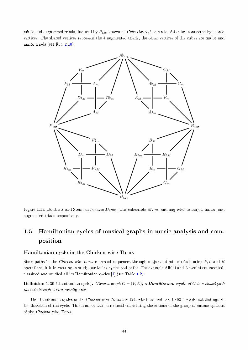
minor and augmented triads) induced by P1,0, known as Cube Dance, is a circle of 4 cubes connected by shared

vertices. The shared vertices represent the 4 augmented triads, the other vertices of the cubes are major and

minor triads (see Fig. 2.10).

CM

Cm

EmEM

A[m

A[M

Fm

FM

D[M D[m

AM

Am

B[M

B[m

Dm DM

F]m

F]M

Gm

GM

E[ME[m

BM

Bm

Faug Baug

A[aug

Daug

Figure 1.15: Douthett and Steinbach's Cube Dance. The subscripts M , m, and aug refer to major, minor, and

augmented triads respectively.

1.5 Hamiltonian cycles of musical graphs in music analysis and com-

position

Hamiltonian cycle in the Chicken-wire Torus

Since paths in the Chicken-wire torus represent sequences through major and minor triads using P,L and R

operations, it is interesting to study particular cycles and paths. For example Albini and Antonini enumerated,

classi�ed and studied all its Hamiltonian cycles [1] (see Table 1.2).

De�nition 1.36 (Hamiltonian cycle). Given a graph G = (V,E), a Hamiltonian cycle of G is a closed path

that visits each vertex exactly once.

The Hamiltonian cycles in the Chicken-wire Torus are 124, which are reduced to 62 if we do not distinguish

the direction of the cycle. This number can be reduced considering the actions of the group of automorphisms

of the Chicken-wire Torus.

44

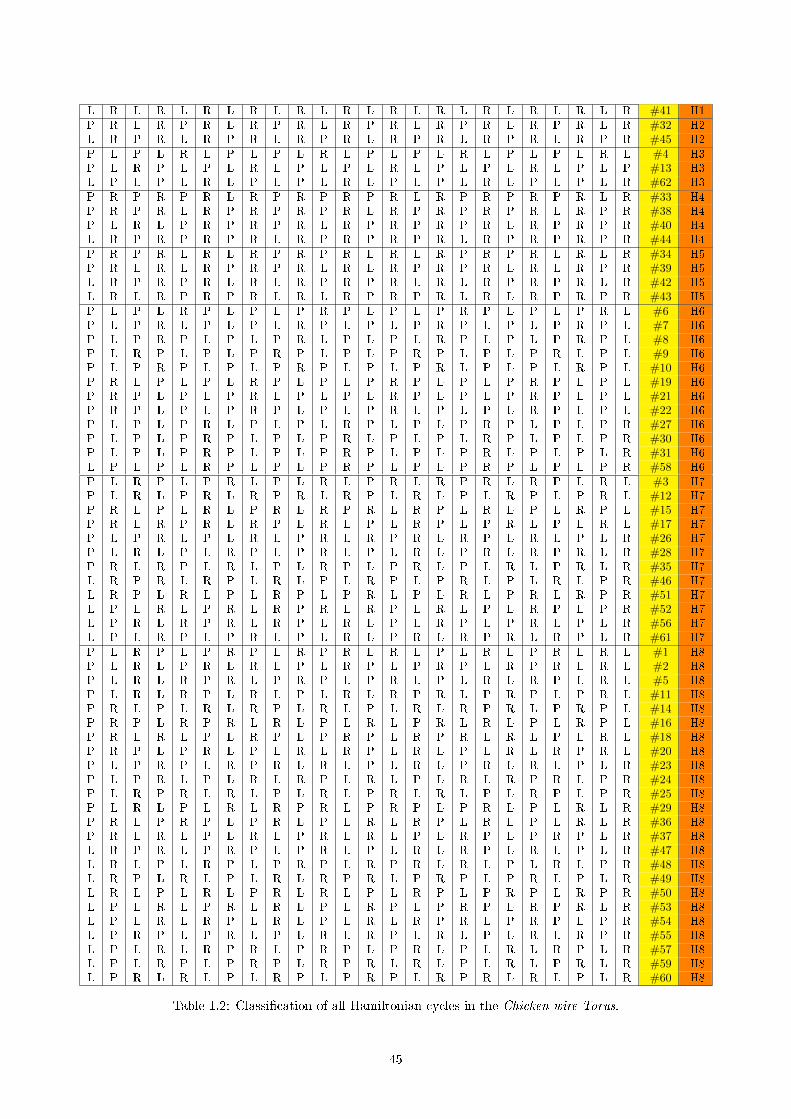
L R L R L R L R L R L R L R L R L R L R L R L R #41 H1P R L R P R L R P R L R P R L R P R L R P R L R #32 H2L R P R L R P R L R P R L R P R L R P R L R P R #45 H2P L P L R L P L P L R L P L P L R L P L P L R L #4 H3P L R P L P L R L P L P L R L P L P L R L P L P #13 H3L P L P L R L P L P L R L P L P L R L P L P L R #62 H3P R P R P R L R P R P R P R L R P R P R P R L R #33 H4P R P R L R P R P R P R L R P R P R P R L R P R #38 H4P L R L P R P R P R L R P R P R P R L R P R P R #40 H4L R P R P R P R L R P R P R P R L R P R P R P R #44 H4P R P R L R L R P R P R L R L R P R P R L R L R #34 H5P R L R L R P R P R L R L R P R P R L R L R P R #39 H5L R P R P R L R L R P R P R L R L R P R P R L R #42 H5L R L R P R P R L R L R P R P R L R L R P R P R #43 H5P L P L R P L P L P R P L P L P R P L P L P R L #6 H6P L P R L P L P L R P L P L P R P L P L P R P L #7 H6P L P R P L P L P R L P L P L R P L P L P R P L #8 H6P L R P L P L P R P L P L P R P L P L P R L P L #9 H6P L P R P L P L P R P L P L P R L P L P L R P L #10 H6P R L P L P L R P L P L P R P L P L P R P L P L #19 H6P R P L P L P R L P L P L R P L P L P R P L P L #21 H6P R P L P L P R P L P L P R L P L P L R P L P L #22 H6P L P L P R L P L P L R P L P L P R P L P L P R #27 H6P L P L P R P L P L P R L P L P L R P L P L P R #30 H6P L P L P R P L P L P R P L P L P R L P L P L R #31 H6L P L P L R P L P L P R P L P L P R P L P L P R #58 H6P L R P L P R L P L R L P R L R P R L R P L R L #3 H7P L R L P R L R P R L R P L R L P L R P L P R L #12 H7P R L P L R L P R L R P R L R P L R L P L R P L #15 H7P R L R P R L R P L R L P L R P L P R L P L R L #17 H7P L P R L P L R L P R L R P R L R P L R L P L R #26 H7P L R L P L R P L P R L P L R L P R L R P R L R #28 H7P R L R P L R L P L R P L P R L P L R L P R L R #35 H7L R P R L R P L R L P L R P L P R L P L R L P R #46 H7L R P L R L P L R P L P R L P L R L P R L R P R #51 H7L P L R L P R L R P R L R P L R L P L R P L P R #52 H7L P R L R P R L R P L R L P L R P L P R L P L R #56 H7L P L R P L P R L P L R L P R L R P R L R P L R #61 H7P L R P L P R P L R P R L R L P L R L P R L R L #1 H8P L R L P R L R L P L R P L P R P L R P R L R L #2 H8P L R L R P R L P R P L P R L P L R L R P L R L #5 H8P L R L R P L R L P L R L R P R L P R P L P R L #11 H8P R L P L R L R P L R L P L R L R P R L P R P L #14 H8P R P L R P R L R L P L R L P R L R L P L R P L #16 H8P R L R L P L R P L P R P L R P R L R L P L R L #18 H8P R P L P R L P L R L R P L R L P L R L R P R L #20 H8P L P R P L R P R L R L P L R L P R L R L P L R #23 H8P L P R L P L R L R P L R L P L R L R P R L P R #24 H8P L R P R L R L P L R L P R L R L P L R P L P R #25 H8P L R L P L R L R P R L P R P L P R L P L R L R #29 H8P R L P R P L P R L P L R L R P L R L P L R L R #36 H8P R L R L P L R L P R L R L P L R P L P R P L R #37 H8L R P R L P R P L P R L P L R L R P L R L P L R #47 H8L R L P L R P L P R P L R P R L R L P L R L P R #48 H8L R P L R L P L R L R P R L P R P L P R L P L R #49 H8L R L P L R L P R L R L P L R P L P R P L R P R #50 H8L P L R L P R L R L P L R P L P R P L R P R L R #53 H8L P L R L R P L R L P L R L R P R L P R P L P R #54 H8L P R P L P R L P L R L R P L R L P L R L R P R #55 H8L P L R L R P R L P R P L P R L P L R L R P L R #57 H8L P L R P L P R P L R P R L R L P L R L P R L R #59 H8L P R L R L P L R P L P R P L R P R L R L P L R #60 H8

Table 1.2: Classi�cation of all Hamiltonian cycles in the Chicken-wire Torus.

45

Theorem 1.37. The automorphism group of the Chicken-wire Torus is isomorphic to the dihedral group D12

of order 24.

Proof. First of all, we recall that for Theorem 1.19 the T/I-group acts on the 24 major and minor triads and

T/I ' D12. We will prove that the automorphism group of the Chicken-wire Torus is isomorphic to the T/I-

group. We will denote by CWT = (V,E) the Chicken-wire Torus. Since the labelling are 24, the automorphisms

of CWT are at least 24. Moreover, since given any two vertices v1, v2 ∈ V (CWT ) there exists an automorphism

f such that f(v1) = v2, the automorphism group is vertex transitive. To prove the theorem it is su�cient to

show that it has no more than 24 elements. Let v ∈ V (CWT ) be a vertex and let f be an automorphism such

that f(v) 6= v. We take g ∈ T/I such that (g ◦ f)(v) = v. Because of the structure of CWT this composition

can be only the identity, therefore f is the inverse of an element of T/I, thus it belongs to it itself.

We observe that given a Hamiltonian cycle, if n automorphisms of CWT transform it to itself, then there

are 24n di�erent Hamiltonian cycles sharing the model of transformation. In CWT we have 8 models.

H1 � cycle #41. It is characterized by the repetition of the model LR. All automorphisms map this cycle into

itself.

H2 � cycles #32 and #45. They are characterized by the repetition of the model PRLR. 12 automorphisms

map these cycles into themselves.

H3 � cycles #4, #13 and #62. They are characterized by the repetition of the model LPLPLR. 8 automor-

phisms map these cycles into themselves.

H4 � cycles #33, #38, #40 and #44. They are characterized by the repetition of the model PRPRPRLR. 6

automorphisms map these cycles into themselves.

H5 � cycles #34, #39, #42 and #43. They are characterized by the repetition of the model PRPRLRLR. 6

automorphisms map these cycles into themselves.

H6 � cycles #6, #7, #8, #9, #10, #19, #21, #27, #30 and #31. They are characterized by the repetition of

the model LPLPLR. 8 automorphisms map these cycles into themselves.

H7 � cycles #3, #12, #15, #17, #26, #28, #35, #46, #51, #51, #56 and #61. They are characterized by

the repetition of the model PLRPLPRLPLRLPRLRPRLRPLRL. 2 automorphisms map these cycles

into themselves.

H8 � the remaining 24 cycles. They are characterized by the model LRLPLRLPRLRLPLRPLPRPLRPR.

Only the identity automorphisms map these cycles into themselves.

Musical applications

From a musical point of view, each Hamiltonian cycle of the Chicken-wire Torus is a chord progression which

modulates to all 24 major and minor triads using the three neo-Riemannian operations P , L and R. Therefore,

it is not surprising to �nd Hamiltonian cycles, or part of them, in some musical pieces. A famous example is in

the second movement of Beethoven's Ninth Symphony, between measures 143 and 176. The German composer

covered 19 triads of the Hamiltonian cycle #41. Therefore, he did not make use of the entire cycle, but it is

interesting to observe that such type of cycle can be found in musical, independently from the knowledge on

graph theory by the composer. We observe that Beethoven lived between 1770 and 1827, graph theory was just

beginning and even if he had known Euler's Tonnetz he would not have thought of Hamiltonian cycles on its

dual and their use for composition.

46

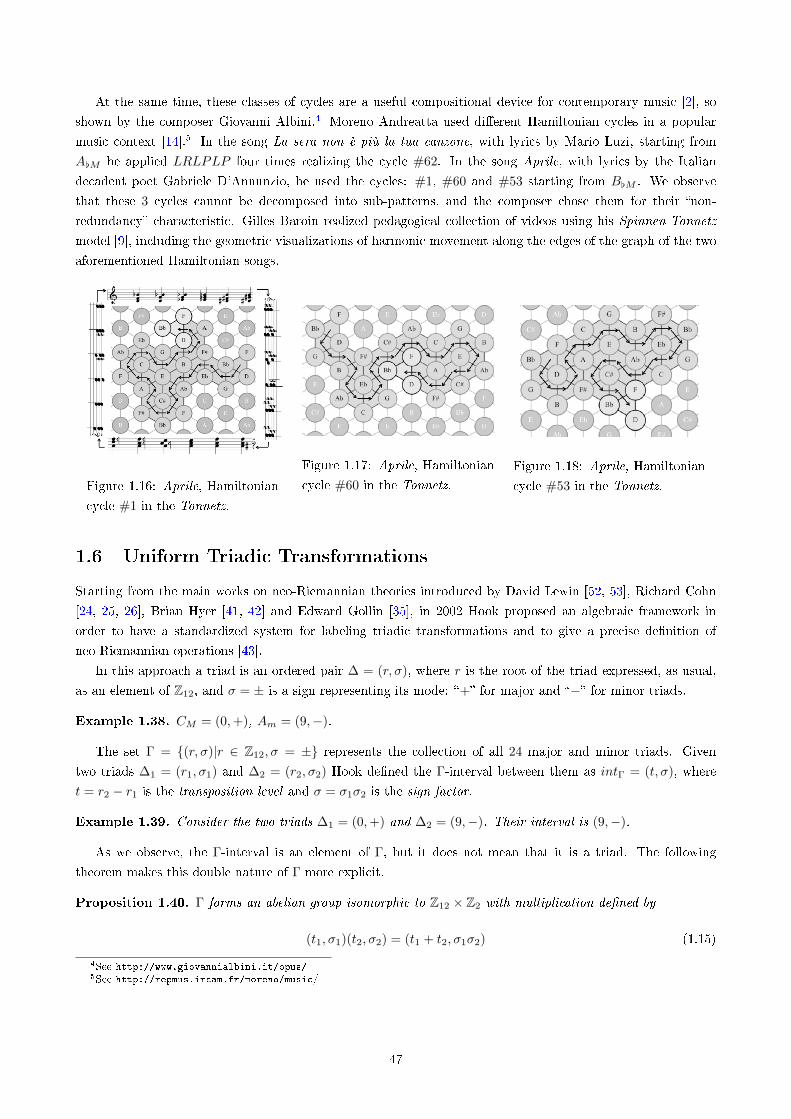
At the same time, these classes of cycles are a useful compositional device for contemporary music [2], so

shown by the composer Giovanni Albini.4 Moreno Andreatta used di�erent Hamiltonian cycles in a popular

music context [14].5 In the song La sera non è più la tua canzone, with lyrics by Mario Luzi, starting from

A[M he applied LRLPLP four times realizing the cycle #62. In the song Aprile, with lyrics by the Italian

decadent poet Gabriele D'Annunzio, he used the cycles: #1, #60 and #53 starting from B[M . We observe

that these 3 cycles cannot be decomposed into sub-patterns, and the composer chose them for their �non-

redundancy� characteristic. Gilles Baroin realized pedagogical collection of videos using his Spinnen-Tonnetz

model [9], including the geometric visualizations of harmonic movement along the edges of the graph of the two

aforementioned Hamiltonian songs.

Figure 1.16: Aprile, Hamiltonian

cycle #1 in the Tonnetz.





1.6 Uniform Triadic Transformations

Starting from the main works on neo-Riemannian theories introduced by David Lewin [52, 53], Richard Cohn

[24, 25, 26], Brian Hyer [41, 42] and Edward Gollin [35], in 2002 Hook proposed an algebraic framework in

order to have a standardized system for labeling triadic transformations and to give a precise de�nition of

neo-Riemannian operations [43].

In this approach a triad is an ordered pair ∆ = (r, σ), where r is the root of the triad expressed, as usual,

as an element of Z12, and σ = ± is a sign representing its mode: �+� for major and �−� for minor triads.

Example 1.38. CM = (0,+), Am = (9,−).

The set Γ = {(r, σ)|r ∈ Z12, σ = ±} represents the collection of all 24 major and minor triads. Given

two triads ∆1 = (r1, σ1) and ∆2 = (r2, σ2) Hook de�ned the Γ-interval between them as intΓ = (t, σ), where

t = r2 − r1 is the transposition level and σ = σ1σ2 is the sign factor.

Example 1.39. Consider the two triads ∆1 = (0,+) and ∆2 = (9,−). Their interval is (9,−).

As we observe, the Γ-interval is an element of Γ, but it does not mean that it is a triad. The following

theorem makes this double nature of Γ more explicit.

Proposition 1.40. Γ forms an abelian group isomorphic to Z12 × Z2 with multiplication de�ned by

(t1, σ1)(t2, σ2) = (t1 + t2, σ1σ2) (1.15)

4See http://www.giovannialbini.it/opus/5See http://repmus.ircam.fr/moreno/music/

47

http://www.giovannialbini.it/opus/

http://repmus.ircam.fr/moreno/music

Proof. From the Formula 1.15, it is clear that the multiplication of each pair of elements in Z12×Z2 is an element

in Z12 × Z2. Since (Z12,+) is an abelian group and σiσj = σjσi, commutativity is also satis�ed. Moreover

associativity is satis�ed, for every (t1, σ1), (t2, σ2), (t3, σ3)

(t1, σ1) ((t2, σ2), (t3, σ3)) = (t1, σ1)(t2 + t3, σ2σ3) =

=(t1 + t2 + t3, σ1σ2σ3) = (t1 + t2, σ1σ2)(t3, σ3) =

= ((t1, σ1)(t2, σ2)) (t3, σ3).

For every (t, σ) the identity element is (0,+) and the inverse is (−t, σ). In fact we have (0,+)(t, σ) = (t, σ) and

(t, σ)(−t, σ) = (0,+). Thus Γ is an abelian group. Finally, t ∈ Z12 and the set {+,−} form a group isomorphic

to Z2, hence Γ ' Z12 × Z2.

Hook observed that Γ as a set of triads with Γ as a group of intervals and the function intΓ form a GIS.

Hook's de�nitions of triadic transformation and operations are the same introduced by Lewin in [53].

De�nition 1.41 (Triadic transformation). A triadic transformation is a map Γ→ Γ.

De�nition 1.42 (Operation). An operation is a bijective transformation Γ→ Γ.

There are some important musical transformations that are not operations. For instance the transformation

mapping triads to its functional dominant: both major and minor triads with the same root are mapped to the

same triad.

The operations, together with the composition of maps form a group G of order 24!. Since the action of

a transformation on a given triad is not related to its action on any other triad, most of these operations are

not interesting from a musical point of view. Consequently, Hook focused on operations with a certain kind of

musical coherence, intuitively he studied those that transform each triad �in the same way�.

De�nition 1.43 (Uniform triadic transformation (UTT)). A uniform triadic transformation (UTT) U

is an operation satisfying the following uniformity condition: for every triad and every transposition level t, if

U transforms the triad (r, σ) into (r′, σ′), then U transforms (r + t, σ) into (r′ + t, σ′).

The behavior of a UTT is completely determined by three parameters: its sign σ = ±, the transposition

levels m = t+ (for major triads) and n = t− (for minor triads). Therefore a UTT can be represented as an

ordered triple 〈σ,m, n〉. If σ = + the UTT is called mode-preserving, otherwise it is called mode-reserving.

Many famous musical operations are UTTs.

Example 1.44.

Tn = 〈+, n, n〉

P = 〈−, 0, 0〉

L = 〈−, 4,−4〉

R = 〈−,−3, 3〉.

Including neo-Riemannian operations and many other operations, UTTs are very useful in the modelling

sequences of triads. Nevertheless, there are noteworthy operations that are not UTTs.

Remark 1.45. Inversions In are not UTTs.

Now we describe the actions of UTTs on triads. Let U = 〈σU , t+, t−〉 be a UTT and let ∆ = (r, σ∆) a triad.

U acts on ∆ transposing its root by t+ if σ∆ = + or by t− if σ∆ = −. Moreover, depending on the sign of σU ,

48

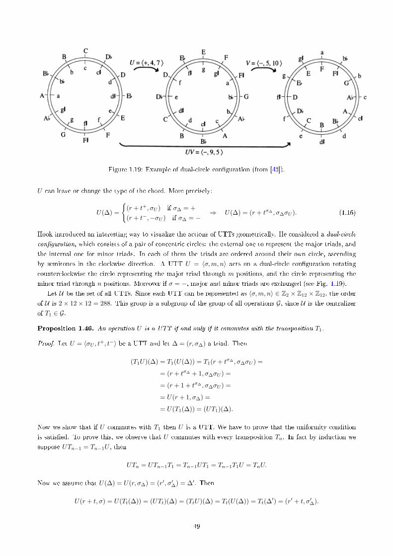
Figure 1.19: Example of dual-circle con�guration (from [43]).

U can leave or change the type of the chord. More precisely:

U(∆) =

{(r + t+, σU ) if σ∆ = +

(r + t−,−σU ) if σ∆ = −⇒ U(∆) = (r + tσ∆ , σ∆σU ). (1.16)

Hook introduced an interesting way to visualize the actions of UTTs geometrically. He considered a dual-circle

con�guration, which consists of a pair of concentric circles: the external one to represent the major triads, and

the internal one for minor triads. In each of them the triads are ordered around their own circle, ascending

by semitones in the clockwise direction. A UTT U = 〈σ,m, n〉 acts on a dual-circle con�guration rotating

counterclockwise the circle representing the major triad through m positions, and the circle representing the

minor triad through n positions. Moreover if σ = −, major and minor triads are exchanged (see Fig. 1.19).

Let U be the set of all UTTs. Since each UTT can be represented as 〈σ,m, n〉 ∈ Z2 × Z12 × Z12, the order

of U is 2× 12× 12 = 288. This group is a subgroup of the group of all operations G, since U is the centralizer

of T1 ∈ G.

Proposition 1.46. An operation U is a UTT if and only if it commutes with the transposition T1.

Proof. Let U = 〈σU , t+, t−〉 be a UTT and let ∆ = (r, σ∆) a triad. Then

(T1U)(∆) = T1(U(∆)) = T1(r + tσ∆ , σ∆σU ) =

= (r + tσ∆ + 1, σ∆σU ) =

= (r + 1 + tσ∆ , σ∆σU ) =

= U(r + 1, σ∆) =

= U(T1(∆)) = (UT1)(∆).

Now we show that if U commutes with T1 then U is a UTT. We have to prove that the uniformity condition

is satis�ed. To prove this, we observe that U commutes with every transposition Tn. In fact by induction we

suppose UTn−1 = Tn−1U , then

UTn = UTn−1T1 = Tn−1UT1 = Tn−1T1U = TnU.

Now we assume that U(∆) = U(r, σ∆) = (r′, σ′∆) = ∆′. Then

U(r + t, σ) = U(Tt(∆)) = (UTt)(∆) = (TtU)(∆) = Tt(U(∆)) = Tt(∆′) = (r′ + t, σ′∆).

49

Theorem 1.47. U is a subgroup of G.

Proof. By Proposition 1.46 U = CG(T1). Since the centralizer of an element of a group is its subgroup, U is a

subgroup of G.

The product formula of two UTTs U = 〈σU , t+U , t−U 〉, V = 〈σV , t+V , t

−V 〉 ∈ U is de�ned as6

V U = 〈σUV , t+U + tσU

V , t−U + t−σU

V 〉. (1.17)

Example 1.48. Let U = 〈+, 4, 7〉 and V = 〈−, 5, 10〉 be two UTTs. Their product UV is

V U = 〈−, 9, 5〉 ◦ 〈+, 4, 7〉 = 〈−, 4 + 5, 7 + 10〉 = 〈−, 9, 5〉.

We consider the major triad CM = (0,+) and the minor triad Cm = (0,−). We apply UV to them:

(V U)(0,+) = V (U(0,+)) = V (4,+) = (9,−)

(V U)(0,−) = V (U(0,−)) = V (7,−) = (5,+).

We obtain the same result applying directly V U = 〈−, 9, 5〉.

We observe that the group U is not abelian. In fact if we consider U, V ∈ U as in previous example, we have

UV = 〈+, 4, 7〉 ◦ 〈−, 5, 10〉 = 〈−, 5 + 7, 10 + 4〉 = 〈−, 0, 2〉 6= V U

Hook de�ned the Riemannian UTTs as UTTs in which the sum of the transposition levels is 0.

De�nition 1.49 (Riemannian UTT). A UTT 〈σ,m, n〉 is Riemannian if m+ n ≡ 0 (mod 12).

Example 1.50. Several UTTs are Riemannian. In addition to P = 〈−, 0, 0〉, L = 〈−, 4,−4〉 and R =

〈−,−3, 3〉, T0 = 〈+, 0, 0〉 and T6 = 〈+, 6, 6〉 are among the operations satisfying the Riemannian condition.

The Riemannian UTTs are 24: 12 mode-preserving UTTs of the form Sn = 〈+, n,−n〉 known as Schritte

and 12 mode-reversing of the form Wn = 〈−, n,−n〉 known as Wechsel. Therefore T0 = S0, T6 = S6, P = W0,

L = W4 and R = W9. The set of all 24 Riemannian UTTs is denoted by R and form a group known as the

Riemann group. This group is also known as the S/W -group.As it turns out, the PLR-group is isomorphic to

the Riemann group.

Theorem 1.51. The 24 Schritte Sn and Wechsel Wn form a group isomorphic to the PLR-group.

Proof. By using Formula 1.17, it is easy to see that Sn and Wn satisfy the following properties:

Sn ◦ Sm = Sm+n

Wn ◦ Sm = Wm+n

Sn ◦Wm = Wm−n

Wn ◦Wm = Sm−n

S−1n = S−n

W−1n = Wn.

Moreover S0 = T0 is the identity and the associativity is inherited from the group U of all UTTs.

6The product has to be read from right to left.

50

We denote by Q the operation S1 = 〈+, 1,−1〉. We observe that Sn = Qn and Wn = PQn. It su�ces to

prove that P and Q may be expressed as products of L and R. In Lemma 1.28 we have already proved that

P = RLRLRLR. Since

LR = 〈−, 4, 8〉 ◦ 〈−, 9, 3〉 = 〈+, 5, 7〉 = Q5

and since Q12 = T0, we have

(LR)5 = (Q5)5 = Q25 = (Q12)2Q = Q

Corollary 1.52. The Riemann group is isomorphic to the dihedral group of order 24.

1.7 Computational approaches

In the last decades, Computational Music Analysis has become increasingly widespread, due in part to the use

of di�erent mathematical areas7. The �rst academic computational projects started in the 1960s, providing

clari�cation of musical concepts, testing evolutionary hypotheses, contributing to music technology, creating

educational music tools [73]. These projects have contributed to many di�erent areas of music: historical

musicology [74], ethnomusicology [48], research in musical performance [34], cognitive musicology [72], music

theory, and music analysis [5].

It is evident that music contains many interesting structures, and music analysis is able to understand and to

study them. Traditional music analysis is usually applied directly to the score using Western musical notation.

But, historically, the musical language used in a score was developed according to the needs of the performer.

For the music theorist Tymoczko the use of geometric models can be a good tool to solve this problem. In fact,

it is a simple and immediate language to perform music, but it is less useful to study music from a theoretical

point of view:

Geometry can help to sensitize us to relationships that might not be immediately apparent in the

musical score. Ultimately, this is because conventional musical notation evolved to satisfy the needs

of the performer rather than the musical thinker: it is designed to facilitate the translation of musical

symbols into physical action, rather than to foment conceptual clarity.8

New technologies based on geometric models of musical objects provide further help.

HexaChord

There are several pieces of software in which musical graphs and other geometric models used in music are

integrated. One of them is HexaChord, a computer-aided music analysis environment based on spatial repre-

sentation of musical objects, developed by Louis Bigo [12] [13]. The geometric models integrated in it are: the

musical clock, the circle of �fths, the voice-leading space, the Tonnetz and other simplicial complexes isomorphic

to it.

Since the Tonnetz represents major and minor triads and their intervallic structure is [3, 4, 5], Bigo denoted

it by K[3, 4, 5]. The mathematical idea is to represent each chord as a simplex where each 0-simplex is labeled

by one note of the chord. Since card(σ) = dim(σ) + 1, a chord of n notes is represented by an (n− 1)-simplex.

Therefore a 0-simplex represents a single note, a 1-simplex a 2-chord, a 2-simplex a 3-chord, a 3-simplex a

7See [59] for a comprehensive perspective on Computational Music Analysis.8See [68], page 79.

51

4-chord, and so on. More generally, the building of a simplicial complex K[a1, . . . , ai] associated to chords

whose intervallic structure is [a1, . . . , ai] is described by Bigo as follows. We choose a chord with n notes

with intervallic structure [a1, . . . , an], and we consider the associated (n − 1)-simplex. As in the Tonnetz, the

1-simplices determine axes representing particular intervals, therefore simplices are replicated along these axes.

We note that 2-simplicial complexes associated with chords of the same size are isomorphic. Therefore,

from a geometrical point of view, all simplicial complexes representing trichords are isomorphic to the di�erent

Tonnetz : a 3-chord is a chord of 3 notes, then the associated simplex is a 2-simplex and the �nal simplicial

complex is a tiling of the 2-dimensional Euclidean space with 2-simplices. The only di�erences among them

are the labels. All simplicial complexes corresponding to the Tonnetz are integrated on HexaChord: K[1, 1, 10],

K[1, 2, 9], K[1, 3, 8], K[1, 4, 7], K[1, 5, 6], K[2, 2, 8], K[2, 3, 7], K[2, 4, 6], K[2, 5, 5], K[3, 3, 6], K[4, 4, 4], K[1, 1, 5],

K[1, 2, 4], K[1, 3, 3], K[2, 2, 3]. These simplicial complexes are not all isomorphic, as it has been pointed out in

a recent study [51]

Functionalities of HexaChord

Musical pieces are imported as MIDI �les. A MIDI (Musical Instrument Digital Interface) �le is a musical

�le with a speci�c protocol called MIDI, representing only player information. This is a protocol designed for

recording and playing back music on digital synthesizers that is supported by many makes of personal computer

sound cards.

Given a MIDI �le as an input, HexaChord is able to:

� visualize chords and chord sequences.

� Compute the compactness of the trajectory of the musical piece in each simplicial complex representing a

given Tonnetz.

� Modify the musical piece through a geometric transformation.

During the execution of the MIDI �le, it is possible to visualize in real time each chord in three di�erent geometric

models: the generalized Tonnetz, the musical clock and the circle of �fths. With the option �intervallic structure�

we can choose another simplicial complex, in which we can view the chords and the trace of the musical piece.

In these simplicial complexes it is also possible to visualize the trace in real time clicking on �trace on�. More

precisely, a temporal sequence of chords is represented by a static object, mathematically described as labeled

subgraph or sub-complex. Let S = [(S0, d0), (S1, d1), . . . , (Sn, dn)] be a chord sequence. It is represented by a

sequence of sub-complexes, called trajectory by Bigo and de�ned as follows

TK = [(K0, d0), (K1, d1), . . . , (Kn, dn)]

where each sub-complex Ki, i ∈ {1, . . . , n}, represents the chord Si and it is labeled with the corresponding

duration di in S. The simplicial complex

T =⋃

(Ki,di)∈TK

Ki

is the subcomplex of K representing the chords in the musical sequence S, and it is called trace.

Depending on the simplicial complex used, the trace of the musical piece is displayed di�erently. Clicking

on �compute compactness� the compactness of these traces is calculated, and the results are represented in a

histogram. The compactness of each trace gives us information on how much the geometric space used is suitable

to represent the chosen musical piece. High compactness of the trajectory in a particular complex might be

seen as a stylistic signature of the piece. Therefore, the computation of the compactness might be very helpful

in music analysis for music classi�cation.

52

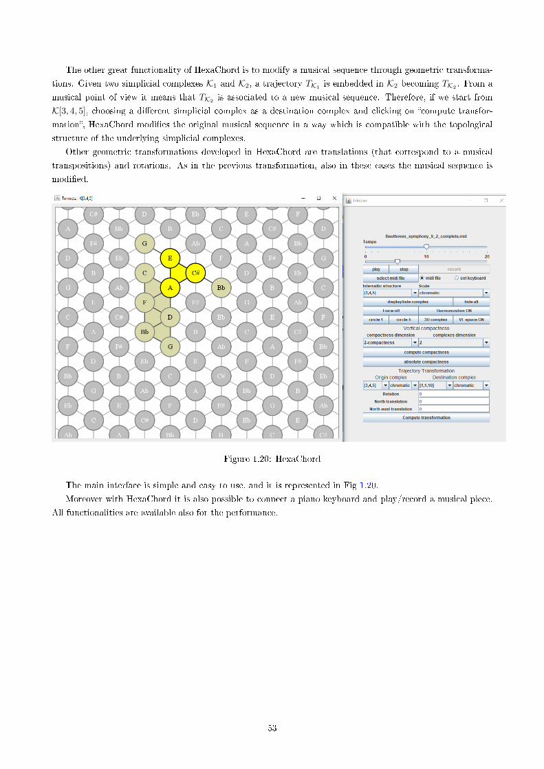
The other great functionality of HexaChord is to modify a musical sequence through geometric transforma-

tions. Given two simplicial complexes K1 and K2, a trajectory TK1is embedded in K2 becoming TK2

. From a

musical point of view it means that TK2is associated to a new musical sequence. Therefore, if we start from

K[3, 4, 5], choosing a di�erent simplicial complex as a destination complex and clicking on �compute transfor-

mation�, HexaChord modi�es the original musical sequence in a way which is compatible with the topological

structure of the underlying simplicial complexes.

Other geometric transformations developed in HexaChord are translations (that correspond to a musical

transpositions) and rotations. As in the previous transformation, also in these cases the musical sequence is

modi�ed.

Figure 1.20: HexaChord

The main interface is simple and easy to use, and it is represented in Fig 1.20.

Moreover with HexaChord it is also possible to connect a piano keyboard and play/record a musical piece.

All functionalities are available also for the performance.

53

Chapter 2

History of the Tonnetz1

2.1 Euler's Tonnetz

It is commonly said that the Tonnetz was originally introduced by Euler in 1739 in his Tentamen novae

theoriae musicae (Tentamen) [29] [20]. Indeed, a graph similar to the Tonnetz appeared in chapter IX, �De

genere diatonico-chromatico� (the diatonic-chromatic genus), to represent the scheme of a musical tuning. In

chapter VII, Euler wrote about musical tuning, in particular tuning systems, i.e. the theoretical study of various

systems of pitches used to tune an instrument. Starting from acoustical observations, he de�ned a musical genus

as a division of the octave, i.e. a collection of octave-equivalent tones, mathematically of the form 2ma, where

m ∈ Z, a ∈ N. Euler listed all genera up to the eighteenth, which is the one in use in his time: the diatonic-

chromatic genus, represented by 2m · 33 · 52. To determine the tones contained in this genus, he considered the

divisors of 33 · 52:

1, 3, 5, 32 = 9, 3 · 5 = 15, 52 = 25, 33 = 27, 32 · 5 = 45,

3 · 52 = 75, 33 · 5 = 135, 32 · 52 = 225, 33 · 52 = 675.(2.1)

The biggest is obviously 675: since we want 12 tones in the same octave, we �nd the biggest number 2x such that

2x < 675, that is 29 = 512, and multiply each divisor of 675 by a power of 2 until we �nd an octave-equivalent

tone in the octave range 512−−1024. In this way we obtain the following tones of the diatonic-chromatic genus:

512, 540, 576, 600, 640, 657, 720, 768, 800, 864, 900, 960, 1024. (2.2)

One would be tempted to say that this construction looks like an algorithm to build �arti�cial� musical scales

that do not correspond to the real ones. On the contrary, the distances between the numbers in (2.2) correspond,

with a good approximation, to the well-known intervallic ratios of the just intonation. A similar method was

known in Greek antiquity. In particular, it is explained in Plato's Timaeus, who learned it from the Pythagore-

ans [49].

After the theoretical construction of the diatonic-chromatic genus, Euler explained how to tune the instru-

ments with it:

1. �x the tone F , and from it get all the other F ;

2. from F get C and A by forming a (perfect) �fth and a major third respectively;

1To appear in [19].

54

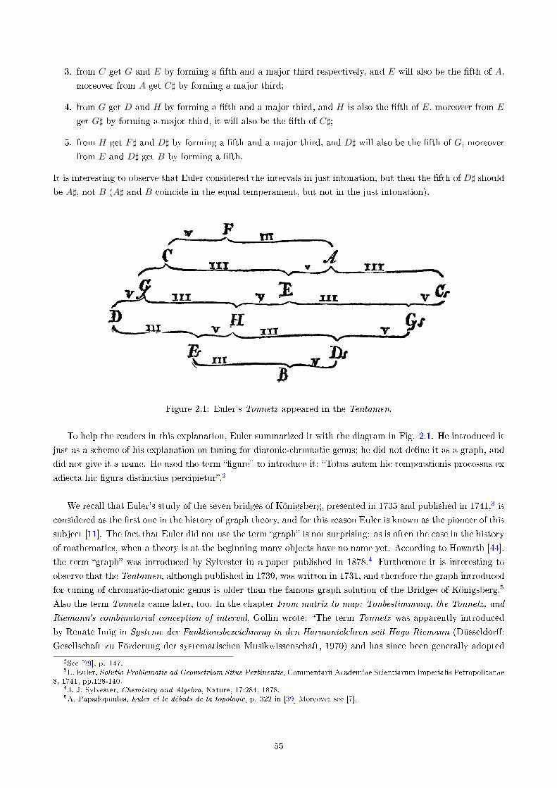
3. from C get G and E by forming a �fth and a major third respectively, and E will also be the �fth of A,

moreover from A get C] by forming a major third;

4. from G get D and H by forming a �fth and a major third, and H is also the �fth of E, moreover from E

get G] by forming a major third, it will also be the �fth of C];

5. from H get F] and D] by forming a �fth and a major third, and D] will also be the �fth of G, moreover

from E and D] get B by forming a �fth.

It is interesting to observe that Euler considered the intervals in just intonation, but then the �fth of D] should

be A], not B (A] and B coincide in the equal temperament, but not in the just intonation).

Figure 2.1: Euler's Tonnetz appeared in the Tentamen.

To help the readers in this explanation, Euler summarized it with the diagram in Fig. 2.1. He introduced it

just as a scheme of his explanation on tuning for diatonic-chromatic genus; he did not de�ne it as a graph, and

did not give it a name. He used the term ��gure� to introduce it: �Totus autem hic temperationis processus ex

adiecta hic �gura distinctius percipietur�.2

We recall that Euler's study of the seven bridges of Königsberg, presented in 1735 and published in 1741,3 is

considered as the �rst one in the history of graph theory, and for this reason Euler is known as the pioneer of this

subject [11]. The fact that Euler did not use the term �graph� is not surprising: as is often the case in the history

of mathematics, when a theory is at the beginning many objects have no name yet. According to Howarth [44],

the term �graph� was introduced by Sylvester in a paper published in 1878.4 Furthemore it is interesting to

observe that the Tentamen, although published in 1739, was written in 1731, and therefore the graph introduced

for tuning of chromatic-diatonic genus is older than the famous graph solution of the Bridges of Königsberg.5

Also the term Tonnetz came later, too. In the chapter From matrix to map: Tonbestimmung, the Tonnetz, and

Riemann's combinatorial conception of interval, Gollin wrote: �The term Tonnetz was apparently introduced

by Renate Imig in Systeme der Funktionsbezeichnung in den Harmonielehren seit Hugo Riemann (Düsseldor�:

Gesellschaft zu Förderung der systematischen Musikwissenschaft, 1970) and has since been generally adopted

2See [29], p. 147.3L. Euler, Solutio Problematis ad Geometriam Situs Pertinentis, Commentarii Academiae Scientiarum Imperialis Petropolitanae

8, 1741, pp.128-140.4J. J. Sylvester, Chemistry and Algebra, Nature, 17:284, 1878.5A. Papadopoulos, Euler et le débuts de la topologie, p. 322 in [39] Moreover see [7].

55

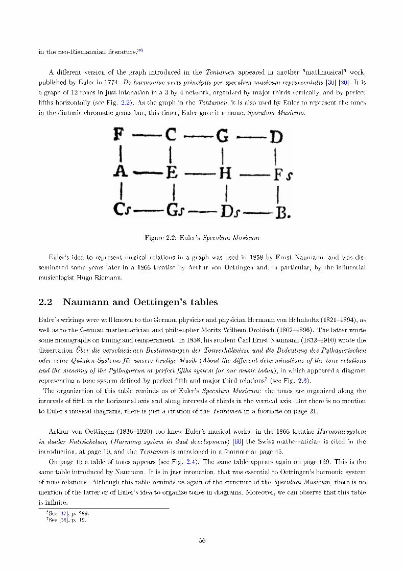
in the neo-Riemannian literature.�6

A di�erent version of the graph introduced in the Tentamen appeared in another "mathmusical" work,

published by Euler in 1774: De harmoniae veris principiis per speculum musicum repraesentatis [30] [20]. It is

a graph of 12 tones in just intonation in a 3 by 4 network, organized by major thirds vertically, and by perfect

�fths horizontally (see Fig. 2.2). As the graph in the Tentamen, it is also used by Euler to represent the tones

in the diatonic-chromatic genus but, this timer, Euler gave it a name, Speculum Musicum.

Figure 2.2: Euler's Speculum Musicum

Euler's idea to represent musical relations in a graph was used in 1858 by Ernst Naumann, and was dis-

seminated some years later in a 1866 treatise by Arthur von Oettingen and, in particular, by the in�uential

musicologist Hugo Riemann.

2.2 Naumann and Oettingen's tables

Euler's writings were well known to the German physicist and physician Hermann von Helmholtz (1821�1894), as

well as to the German mathematician and philosopher Moritz Wilhem Drobisch (1802�1896). The latter wrote

some monographs on tuning and temperament. In 1858, his student Carl Ernst Naumann (1832�1910) wrote the

dissertation Über die verschiedenen Bestimmungen der Tonverhältnisse und die Bedeutung des Pythagorischen

oder reine Quinten-Systems für unsere heutige Musik (About the di�erent determinations of the tone relations

and the meaning of the Pythagorean or perfect �fths system for our music today), in which appeared a diagram

representing a tone system de�ned by perfect �fth and major third relations7 (see Fig. 2.3).

The organization of this table reminds us of Euler's Speculum Musicum: the tones are organized along the

intervals of �fth in the horizontal axis and along intervals of thirds in the vertical axis. But there is no mention

to Euler's musical diagrams, there is just a citation of the Tentamen in a footnote on page 21.

Arthur von Oettingen (1836�1920) too knew Euler's musical works: in the 1866 treatise Harmoniesystem

in dualer Entwickelung (Harmony system in dual development) [60] the Swiss mathematician is cited in the

introduction, at page 19, and the Tentamen is mentioned in a footnote at page 45.

On page 15 a table of tones appears (see Fig. 2.4). The same table appears again on page 169. This is the

same table introduced by Naumann. It is in just intonation, that was essential to Oettingen's harmonic system

of tone relations. Although this table reminds us again of the structure of the Speculum Musicum, there is no

mention of the latter or of Euler's idea to organize tones in diagrams. Moreover, we can observe that this table

is in�nite.6See [37], p. 289.7See [58], p. 19.

56

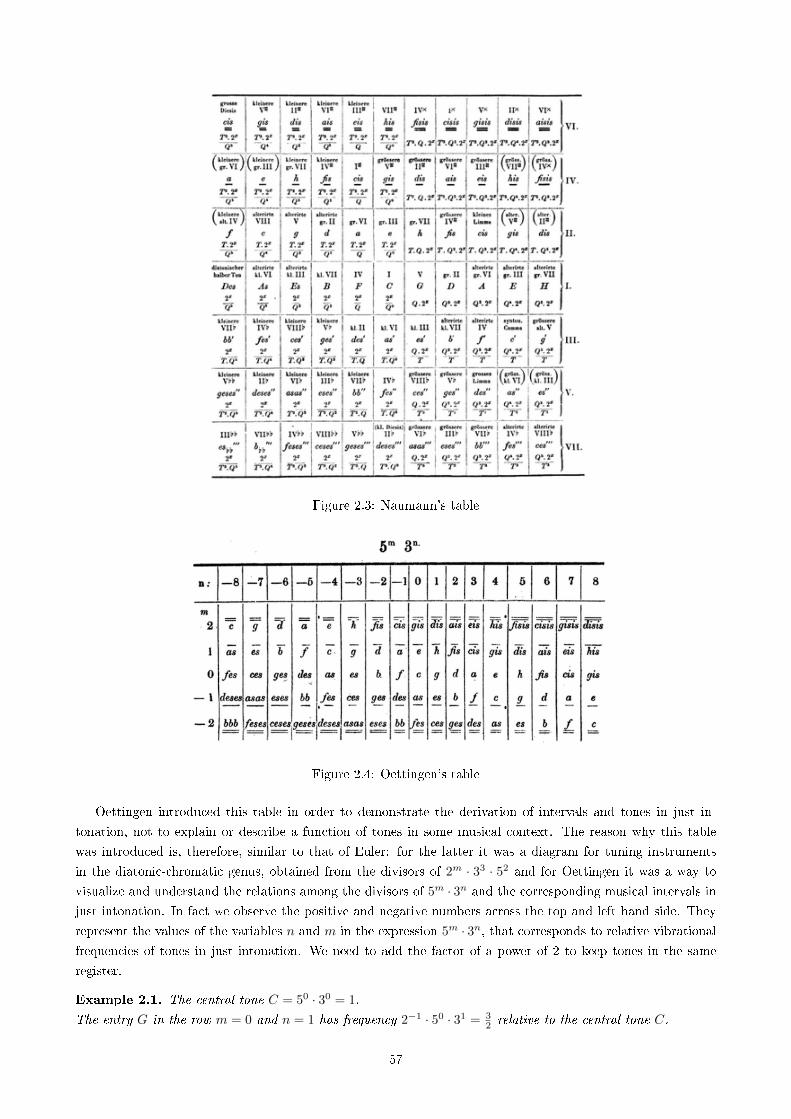
Figure 2.3: Naumann's table

Figure 2.4: Oettingen's table

Oettingen introduced this table in order to demonstrate the derivation of intervals and tones in just in-

tonation, not to explain or describe a function of tones in some musical context. The reason why this table

was introduced is, therefore, similar to that of Euler: for the latter it was a diagram for tuning instruments

in the diatonic-chromatic genus, obtained from the divisors of 2m · 33 · 52 and for Oettingen it was a way to

visualize and understand the relations among the divisors of 5m · 3n and the corresponding musical intervals in

just intonation. In fact we observe the positive and negative numbers across the top and left hand side. They

represent the values of the variables n and m in the expression 5m · 3n, that corresponds to relative vibrational

frequencies of tones in just intonation. We need to add the factor of a power of 2 to keep tones in the same

register.

Example 2.1. The central tone C = 50 · 30 = 1.

The entry G in the row m = 0 and n = 1 has frequency 2−1 · 50 · 31 = 32 relative to the central tone C.

57

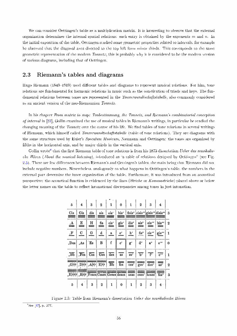
We can consider Oettingen's table as a multiplication matrix. It is interesting to observe that the external

organization determines the internal spatial relations: each entry is obtained by the exponents m and n. In

the initial exposition of the table, Oettingen studied some geometric properties related to intervals, for example

he observed that the diagonal axes directed to the top left form minor thirds. This corresponds to the same

geometric representation of the modern Tonnetz ; this is probably why it is considered to be the modern version

of various diagrams, including that of Oettingen.

2.3 Riemann's tables and diagrams

Hugo Riemann (1849�1919) used di�erent tables and diagrams to represent musical relations. For him, tone

relations are fundamental for harmonic relations in music such as the constitution of triads and keys. The fun-

damental relations between tones are represented in the Tonverwandtschaftstabelle, also commonly considered

as an ancient version of the neo-Riemannian Tonnetz.

In his chapter From matrix to map: Tonbestimmung, the Tonnetz, and Riemann's combinatorial conception

of interval in [37], Gollin examined the use of musical tables in Riemann's writings, in particular he studied the

changing meaning of the Tonnetz over the course of his life. We �nd tables of tone relations in several writings

of Riemann, which himself called Tonverwandtschaftstabelle (table of tone relations). They are diagrams with

the same structure used by Euler's Speculum Musicum, Naumann and Oettingen: the tones are organized by

�fths in the horizontal axis, and by major thirds in the vertical axis.

Gollin wrote8 that the �rst Riemann table of tone relations is from his 1873 dissertation Ueber das musikalis-

che Hören (About the musical listening), introduced as �a table of relations designed by Oettingen� (see Fig.

2.5). There are few di�erences between Riemann's and Oettingen's tables, the main being that Riemann did not

include negative numbers. Nevertheless, analogously to what happens in Oettingen's table, the numbers in the

external part determine the inner organization of the table. Furthemore, it was introduced from an acoustical

perspective: the acoustical function is evidenced by the lines (Striche or Kommastriche) placed above or below

the letter names on the table to re�ect intonational discrepancies among tones in just intonation.

Figure 2.5: Table from Riemann's dissertation Ueber das musikalische Hören

8See [37], p. 277.

58

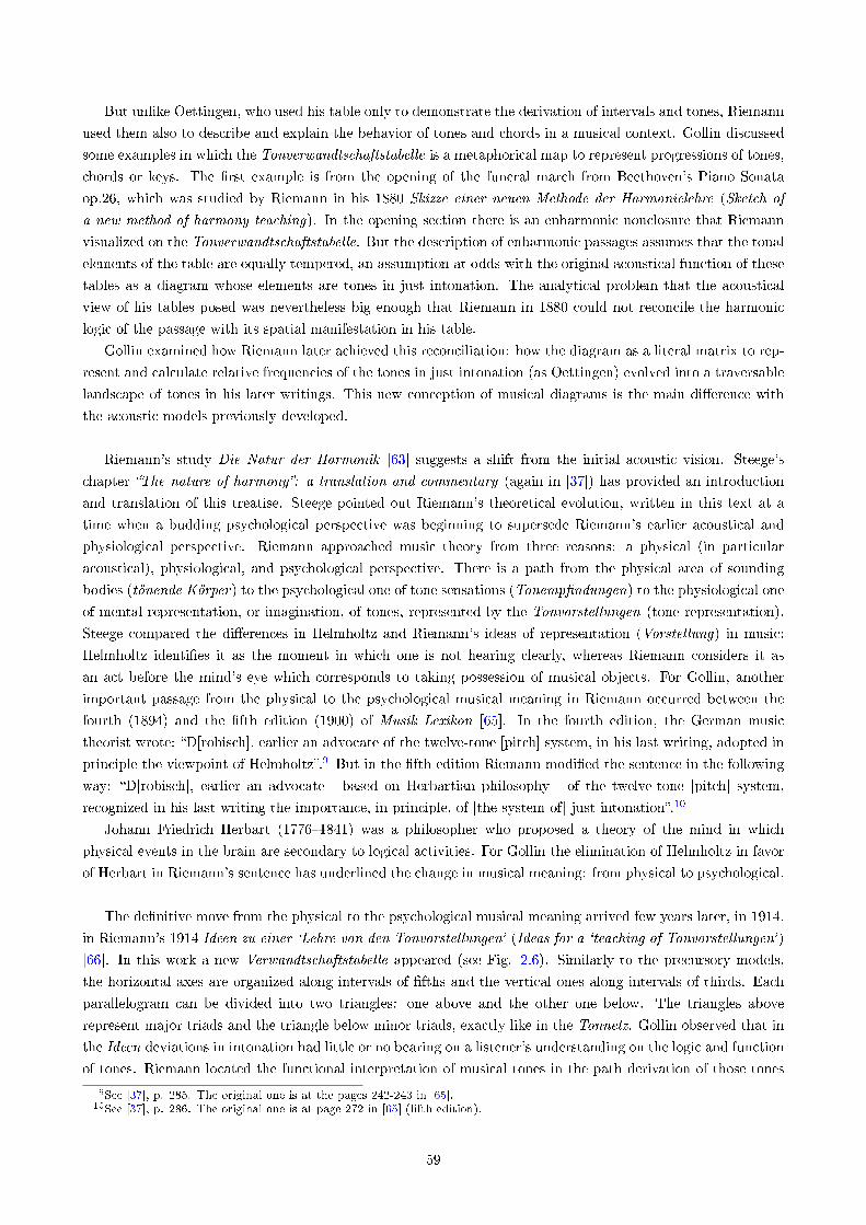
But unlike Oettingen, who used his table only to demonstrate the derivation of intervals and tones, Riemann

used them also to describe and explain the behavior of tones and chords in a musical context. Gollin discussed

some examples in which the Tonverwandtschaftstabelle is a metaphorical map to represent progressions of tones,

chords or keys. The �rst example is from the opening of the funeral march from Beethoven's Piano Sonata

op.26, which was studied by Riemann in his 1880 Skizze einer neuen Methode der Harmonielehre (Sketch of

a new method of harmony teaching). In the opening section there is an enharmonic nonclosure that Riemann

visualized on the Tonverwandtschaftstabelle. But the description of enharmonic passages assumes that the tonal

elements of the table are equally tempered, an assumption at odds with the original acoustical function of these

tables as a diagram whose elements are tones in just intonation. The analytical problem that the acoustical

view of his tables posed was nevertheless big enough that Riemann in 1880 could not reconcile the harmonic

logic of the passage with its spatial manifestation in his table.

Gollin examined how Riemann later achieved this reconciliation: how the diagram as a literal matrix to rep-

resent and calculate relative frequencies of the tones in just intonation (as Oettingen) evolved into a traversable

landscape of tones in his later writings. This new conception of musical diagrams is the main di�erence with

the acoustic models previously developed.

Riemann's study Die Natur der Harmonik [63] suggests a shift from the initial acoustic vision. Steege's

chapter �The nature of harmony�: a translation and commentary (again in [37]) has provided an introduction

and translation of this treatise. Steege pointed out Riemann's theoretical evolution, written in this text at a

time when a budding psychological perspective was beginning to supersede Riemann's earlier acoustical and

physiological perspective. Riemann approached music theory from three reasons: a physical (in particular

acoustical), physiological, and psychological perspective. There is a path from the physical area of sounding

bodies (tönende Körper) to the psychological one of tone sensations (Tonemp�ndungen) to the physiological one

of mental representation, or imagination, of tones, represented by the Tonvorstellungen (tone representation).

Steege compared the di�erences in Helmholtz and Riemann's ideas of representation (Vorstellung) in music:

Helmholtz identi�es it as the moment in which one is not hearing clearly, whereas Riemann considers it as

an act before the mind's eye which corresponds to taking possession of musical objects. For Gollin, another

important passage from the physical to the psychological musical meaning in Riemann occurred between the

fourth (1894) and the �fth edition (1900) of Musik Lexikon [65]. In the fourth edition, the German music

theorist wrote: �D[robisch], earlier an advocate of the twelve-tone [pitch] system, in his last writing, adopted in

principle the viewpoint of Helmholtz�.9 But in the �fth edition Riemann modi�ed the sentence in the following

way: �D[robisch], earlier an advocate - based on Herbartian philosophy - of the twelve-tone [pitch] system,

recognized in his last writing the importance, in principle, of [the system of] just intonation�.10

Johann Friedrich Herbart (1776�1841) was a philosopher who proposed a theory of the mind in which

physical events in the brain are secondary to logical activities. For Gollin the elimination of Helmholtz in favor

of Herbart in Riemann's sentence has underlined the change in musical meaning: from physical to psychological.

The de�nitive move from the physical to the psychological musical meaning arrived few years later, in 1914,

in Riemann's 1914 Ideen zu einer `Lehre von den Tonvorstellungen' (Ideas for a `teaching of Tonvorstellungen' )

[66]. In this work a new Verwandtschaftstabelle appeared (see Fig. 2.6). Similarly to the precursory models,

the horizontal axes are organized along intervals of �fths and the vertical ones along intervals of thirds. Each

parallelogram can be divided into two triangles: one above and the other one below. The triangles above

represent major triads and the triangle below minor triads, exactly like in the Tonnetz. Gollin observed that in

the Ideen deviations in intonation had little or no bearing on a listener's understanding on the logic and function

of tones. Riemann located the functional interpretation of musical tones in the path derivation of those tones

9See [37], p. 285. The original one is at the pages 242-243 in [65].10See [37], p. 286. The original one is at page 272 in [65] (�fth edition).

59

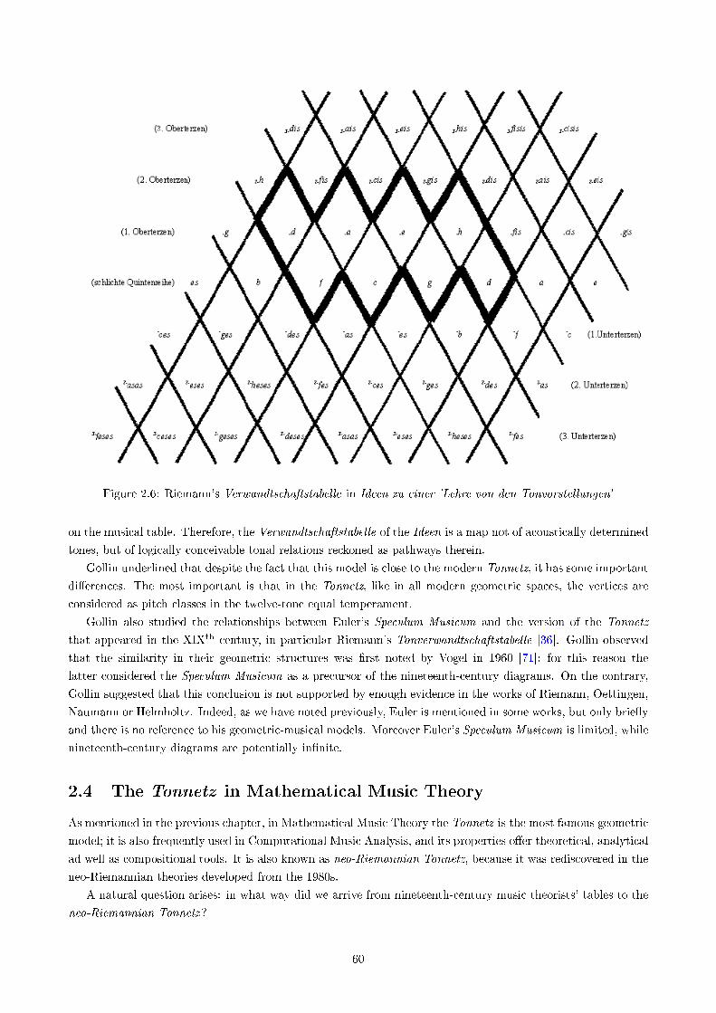
Figure 2.6: Riemann's Verwandtschaftstabelle in Ideen zu einer 'Lehre von den Tonvorstellungen'

on the musical table. Therefore, the Verwandtschaftstabelle of the Ideen is a map not of acoustically determined

tones, but of logically conceivable tonal relations reckoned as pathways therein.

Gollin underlined that despite the fact that this model is close to the modern Tonnetz, it has some important

di�erences. The most important is that in the Tonnetz, like in all modern geometric spaces, the vertices are

considered as pitch classes in the twelve-tone equal temperament.

Gollin also studied the relationships between Euler's Speculum Musicum and the version of the Tonnetz

that appeared in the XIXth century, in particular Riemann's Tonverwandtschaftstabelle [36]. Gollin observed

that the similarity in their geometric structures was �rst noted by Vogel in 1960 [71]; for this reason the

latter considered the Speculum Musicum as a precursor of the nineteenth-century diagrams. On the contrary,

Gollin suggested that this conclusion is not supported by enough evidence in the works of Riemann, Oettingen,

Naumann or Helmholtz. Indeed, as we have noted previously, Euler is mentioned in some works, but only brie�y

and there is no reference to his geometric-musical models. Moreover Euler's Speculum Musicum is limited, while

nineteenth-century diagrams are potentially in�nite.

2.4 The Tonnetz in Mathematical Music Theory

As mentioned in the previous chapter, in Mathematical Music Theory the Tonnetz is the most famous geometric

model; it is also frequently used in Computational Music Analysis, and its properties o�er theoretical, analytical

ad well as compositional tools. It is also known as neo-Riemannian Tonnetz, because it was rediscovered in the

neo-Riemannian theories developed from the 1980s.

A natural question arises: in what way did we arrive from nineteenth-century music theorists' tables to the

neo-Riemannian Tonnetz?

60

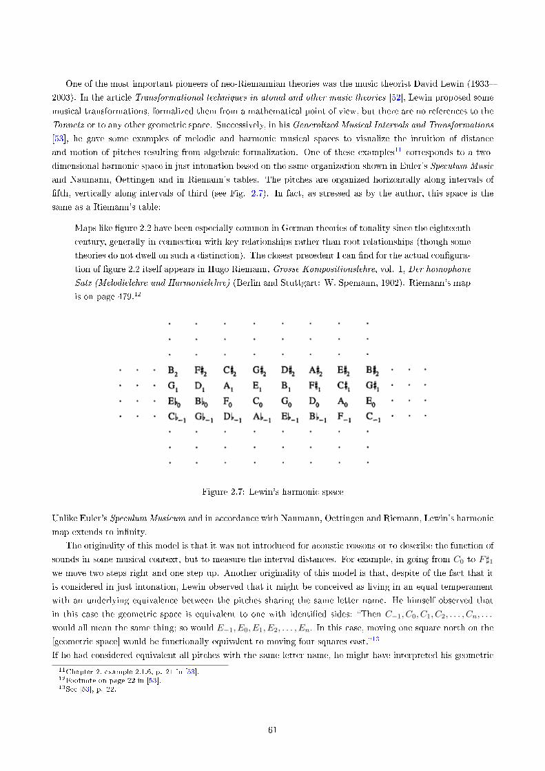
One of the most important pioneers of neo-Riemannian theories was the music theorist David Lewin (1933�

2003). In the article Transformational techniques in atonal and other music theories [52], Lewin proposed some

musical transformations, formalized them from a mathematical point of view, but there are no references to the

Tonnetz or to any other geometric space. Successively, in his Generalized Musical Intervals and Transformations

[53], he gave some examples of melodic and harmonic musical spaces to visualize the intuition of distance

and motion of pitches resulting from algebraic formalization. One of these examples11 corresponds to a two-

dimensional harmonic space in just intonation based on the same organization shown in Euler's Speculum Music

and Naumann, Oettingen and in Riemann's tables. The pitches are organized horizontally along intervals of

�fth, vertically along intervals of third (see Fig. 2.7). In fact, as stressed as by the author, this space is the

same as a Riemann's table:

Maps like �gure 2.2 have been especially common in German theories of tonality since the eighteenth

century, generally in connection with key relationships rather than root relationships (though some

theories do not dwell on such a distinction). The closest precedent I can �nd for the actual con�gura-

tion of �gure 2.2 itself appears in Hugo Riemann, Grosse Kompositionslehre, vol. 1, Der homophone

Satz (Melodielehre und Harmonielehre) (Berlin and Stuttgart: W. Spemann, 1902). Riemann's map

is on page 479.12

Figure 2.7: Lewin's harmonic space

Unlike Euler's Speculum Musicum and in accordance with Naumann, Oettingen and Riemann, Lewin's harmonic

map extends to in�nity.

The originality of this model is that it was not introduced for acoustic reasons or to describe the function of

sounds in some musical context, but to measure the interval distances. For example, in going from C0 to F]1we move two steps right and one step up. Another originality of this model is that, despite of the fact that it

is considered in just intonation, Lewin observed that it might be conceived as living in an equal temperament

with an underlying equivalence between the pitches sharing the same letter name. He himself observed that

in this case the geometric space is equivalent to one with identi�ed sides: �Then C−1, C0, C1, C2, . . . , Cn, . . .

would all mean the same thing; so would E−1, E0, E1, E2, . . . , En. In this case, moving one square north on the

[geometric space] would be functionally equivalent to moving four squares east.�13

If he had considered equivalent all pitches with the same letter name, he might have interpreted his geometric

11Chapter 2, example 2.1.6, p. 21 in [53].12Footnote on page 22 in [53].13See [53], p. 22.

61

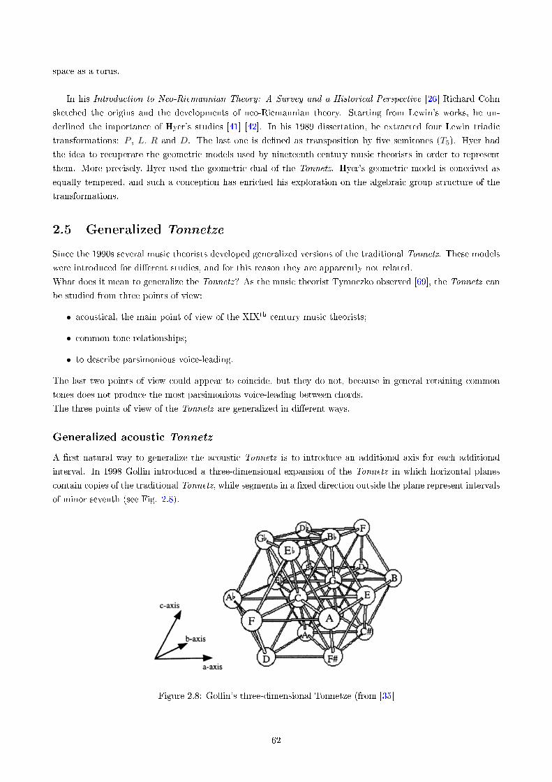
space as a torus.

In his Introduction to Neo-Riemannian Theory: A Survey and a Historical Perspective [26] Richard Cohn

sketched the origins and the developments of neo-Riemannian theory. Starting from Lewin's works, he un-

derlined the importance of Hyer's studies [41] [42]. In his 1989 dissertation, he extracted four Lewin triadic

transformations: P , L, R and D. The last one is de�ned as transposition by �ve semitones (T5). Hyer had

the idea to recuperate the geometric models used by nineteenth-century music theorists in order to represent

them. More precisely, Hyer used the geometric dual of the Tonnetz. Hyer's geometric model is conceived as

equally tempered, and such a conception has enriched his exploration on the algebraic group structure of the

transformations.

2.5 Generalized Tonnetze

Since the 1990s several music theorists developed generalized versions of the traditional Tonnetz. These models

were introduced for di�erent studies, and for this reason they are apparently not related.

What does it mean to generalize the Tonnetz? As the music theorist Tymoczko observed [69], the Tonnetz can

be studied from three points of view:

� acoustical, the main point of view of the XIXth century music theorists;

� common-tone relationships;

� to describe parsimonious voice-leading.

The last two points of view could appear to coincide, but they do not, because in general retaining common

tones does not produce the most parsimonious voice-leading between chords.

The three points of view of the Tonnetz are generalized in di�erent ways.

Generalized acoustic Tonnetz

A �rst natural way to generalize the acoustic Tonnetz is to introduce an additional axis for each additional

interval. In 1998 Gollin introduced a three-dimensional expansion of the Tonnetz in which horizontal planes

contain copies of the traditional Tonnetz, while segments in a �xed direction outside the plane represent intervals

of minor seventh (see Fig. 2.8).

Figure 2.8: Gollin's three-dimensional Tonnetze (from [35]

62

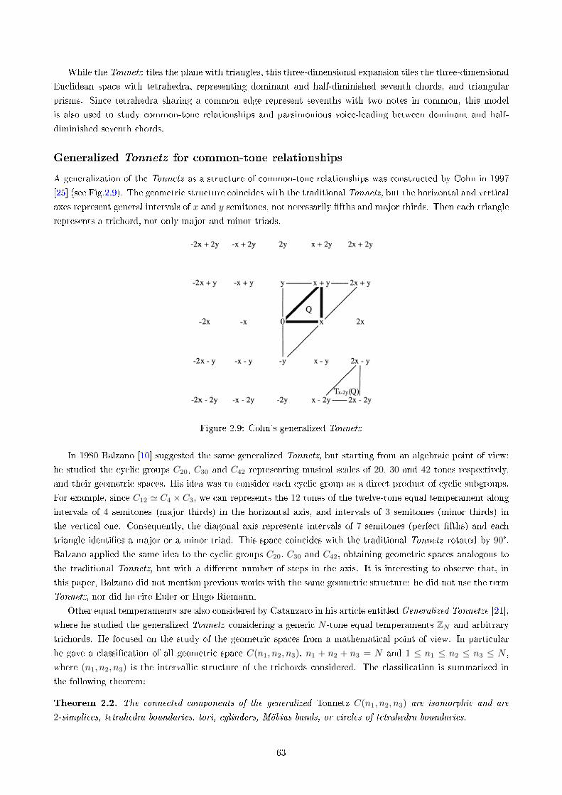
While the Tonnetz tiles the plane with triangles, this three-dimensional expansion tiles the three-dimensional

Euclidean space with tetrahedra, representing dominant and half-diminished seventh chords, and triangular

prisms. Since tetrahedra sharing a common edge represent sevenths with two notes in common, this model

is also used to study common-tone relationships and parsimonious voice-leading between dominant and half-

diminished seventh chords.

Generalized Tonnetz for common-tone relationships

A generalization of the Tonnetz as a structure of common-tone relationships was constructed by Cohn in 1997

[25] (see Fig.2.9). The geometric structure coincides with the traditional Tonnetz, but the horizontal and vertical

axes represent general intervals of x and y semitones, not necessarily �fths and major thirds. Then each triangle

represents a trichord, not only major and minor triads.

Figure 2.9: Cohn's generalized Tonnetz

In 1980 Balzano [10] suggested the same generalized Tonnetz, but starting from an algebraic point of view:

he studied the cyclic groups C20, C30 and C42 representing musical scales of 20, 30 and 42 tones respectively,

and their geometric spaces. His idea was to consider each cyclic group as a direct product of cyclic subgroups.

For example, since C12 ' C4 × C3, we can represents the 12 tones of the twelve-tone equal temperament along

intervals of 4 semitones (major thirds) in the horizontal axis, and intervals of 3 semitones (minor thirds) in

the vertical one. Consequently, the diagonal axis represents intervals of 7 semitones (perfect �fths) and each

triangle identi�es a major or a minor triad. This space coincides with the traditional Tonnetz rotated by 90°.

Balzano applied the same idea to the cyclic groups C20, C30 and C42, obtaining geometric spaces analogous to

the traditional Tonnetz, but with a di�erent number of steps in the axis. It is interesting to observe that, in

this paper, Balzano did not mention previous works with the same geometric structure: he did not use the term

Tonnetz, nor did he cite Euler or Hugo Riemann.

Other equal temperaments are also considered by Catanzaro in his article entitled Generalized Tonnetze [21],

where he studied the generalized Tonnetz considering a generic N -tone equal temperaments ZN and arbitrary

trichords. He focused on the study of the geometric spaces from a mathematical point of view. In particular

he gave a classi�cation of all geometric space C(n1, n2, n3), n1 + n2 + n3 = N and 1 ≤ n1 ≤ n2 ≤ n3 ≤ N ,

where (n1, n2, n3) is the intervallic structure of the trichords considered. The classi�cation is summarized in

the following theorem:

Theorem 2.2. The connected components of the generalized Tonnetz C(n1, n2, n3) are isomorphic and are

2-simplices, tetrahedra boundaries, tori, cylinders, Möbius bands, or circles of tetrahedra boundaries.

63

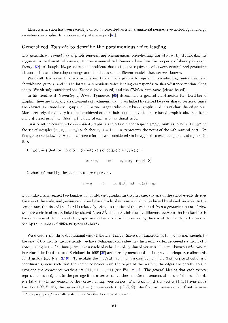
This classi�cation has been recently re�ned by Lascabettes from a simplicial perspectives including homology

èersistency as applied to automatic stylistic analysis [51].

Generalized Tonnetz to describe the parsimonious voice leading

The generalized Tonnetz as a graph representing parsimonious voice-leading was studied by Tymoczko: he

suggested a mathematical strategy to create generalized Tonnetze based on the property of duality in graph

theory [69]. Although this presents some problems due to the non-equivalence between musical and geometric

distance, it is an interesting strategy and it includes some di�erent models that are well known.

We recall that music theorists usually use two kinds of graphs to represent voice-leading: note-based and

chord-based graphs, and in the latter parsimonious voice leading corresponds to short-distance motion along

edges. We already considered the Tonnetz (note-based) and the Chicken-wire torus (chord-based).

In his treatise A Geometry of Music Tymoczko [68] determined a general construction for chord-based

graphs: these are typically arrangements of n-dimensional cubes linked by shared faces or shared vertices. Since

the Tonnetz is a note-based graph, his idea was to generalize note-based graphs as duals of chord-based graphs.

More precisely, the duality is to be considered among their components: the note-based graph is obtained from

a chord-based graph considering the dual of each n-dimensional cube.

First of all he considered chord-based graphs in the orbifold chord-space Tn/Sn built as follows. Let Rn be

the set of n-tuples (x1, x2, . . . , xn) such that xi, i = 1, . . . , n, represents the notes of the i-th musical part. On

this space the following two equivalence relations are considered (to be applied to each component of a point in

Rn):

1. two tones that form one or more intervals of octave are equivalent

xi ∼ xj ⇔ xi ≡ xj (mod 12)

2. chords formed by the same notes are equivalent

x ∼ y ⇔ ∃σ ∈ Sn s.t. σ(x) = y.

Tymoczko characterized two families of chord-based graphs. In the �rst one, the size of the chord evenly divides

the size of the scale, and geometrically we have a circle of n-dimensional cubes linked by shared vertices. In the

second one, the size of the chord is relatively prime to the size of the scale, and from a geometric point of view

we have a circle of cubes linked by shared facets.14. The most interesting di�erence between the two families is

the dimension of the cubes of the graph: in the �rst one it is determined by the size of the chords, in the second

one by the number of di�erent types of chords.

We consider the three-dimensional case of the �rst family. Since the dimension of the cubes corresponds to

the size of the chords, geometrically we have 3-dimensional cubes in which each vertex represents a chord of 3

notes. Being in the �rst family, we have a circle of cubes linked by shared vertices. The well-known Cube Dance,

introduced by Douthett and Steinbach in 1998 [28] and already mentioned in the previous chapter, realizes this

construction (see Fig. 2.10). To explain the musical meaning, we consider a single 3-dimensional cube in a

coordinate system such that the center coincides with the origin of the system, the edges are parallel to the

axes and the coordinate vertices are (±1,±1, . . . ,±1) (see Fig. 2.11). The general idea is that each vertex

represents a chord, and in the passage from a vertex to another one the movements of notes of the two chords

is related to the movement of the corresponding coordinates. For example, if the vertex (1, 1, 1) represents

the chord (C,E,A[), the vertex (1, 1,−1) corresponds to (C,E,G): the �rst two notes remain �xed because

14In a polytope a facet of dimension n is a face that has dimension n− 1.

64

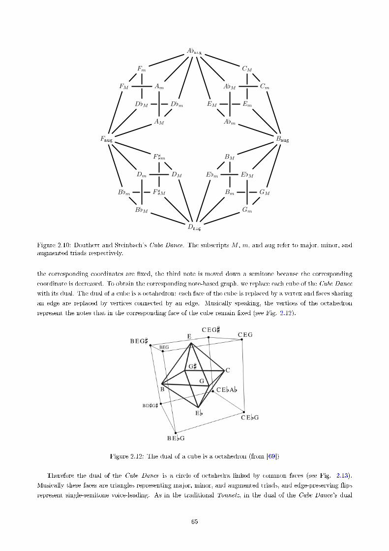
CM

Cm

EmEM

A[m

A[M

Fm

FM

D[M D[m

AM

Am

B[M

B[m

Dm DM

F]m

F]M

Gm

GM

E[ME[m

BM

Bm

Faug Baug

A[aug

Daug

Figure 2.10: Douthett and Steinbach's Cube Dance. The subscripts M , m, and aug refer to major, minor, andaugmented triads respectively.

the corresponding coordinates are �xed, the third note is moved down a semitone because the corresponding

coordinate is decreased. To obtain the corresponding note-based graph, we replace each cube of the Cube Dance

with its dual. The dual of a cube is a octahedron: each face of the cube is replaced by a vertex and faces sharing

an edge are replaced by vertices connected by an edge. Musically speaking, the vertices of the octahedron

represent the notes that in the corresponding face of the cube remain �xed (see Fig. 2.12).

Figure 2.12: The dual of a cube is a octahedron (from [69])

Therefore the dual of the Cube Dance is a circle of octahedra linked by common faces (see Fig. 2.13).

Musically these faces are triangles representing major, minor, and augmented triads, and edge-preserving �ips

represent single-semitone voice-leading. As in the traditional Tonnetz, in the dual of the Cube Dance's dual

65

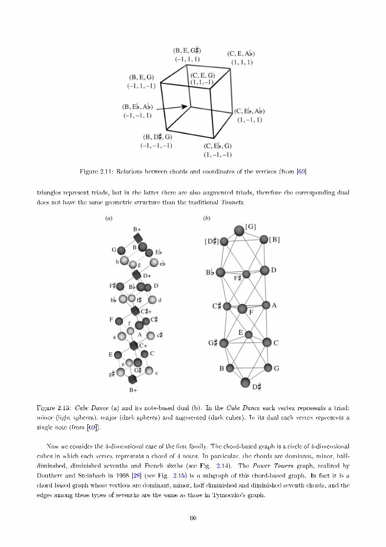
Figure 2.11: Relations between chords and coordinates of the vertices (from [69]

triangles represent triads, but in the latter there are also augmented triads, therefore the corresponding dual

does not have the same geometric structure than the traditional Tonnetz.

Figure 2.13: Cube Dance (a) and its note-based dual (b). In the Cube Dance each vertex represents a triad:

minor (light spheres), major (dark spheres) and augmented (dark cubes). In its dual each vertex represents a

single note (from [69]).

Now we consider the 4-dimensional case of the �rst family. The chord-based graph is a circle of 4-dimensional

cubes in which each vertex represents a chord of 4 notes. In particular, the chords are dominant, minor, half-

diminshed, diminished sevenths and French sixths (see Fig. 2.14). The Power Towers graph, realized by

Douthett and Steinbach in 1998 [28] (see Fig. 2.15) is a subgraph of this chord-based graph. In fact it is a

chord-based graph whose vertices are dominant, minor, half-diminished and diminished seventh chords, and the

edges among these types of sevenths are the same as those in Tymoczko's graph.

66

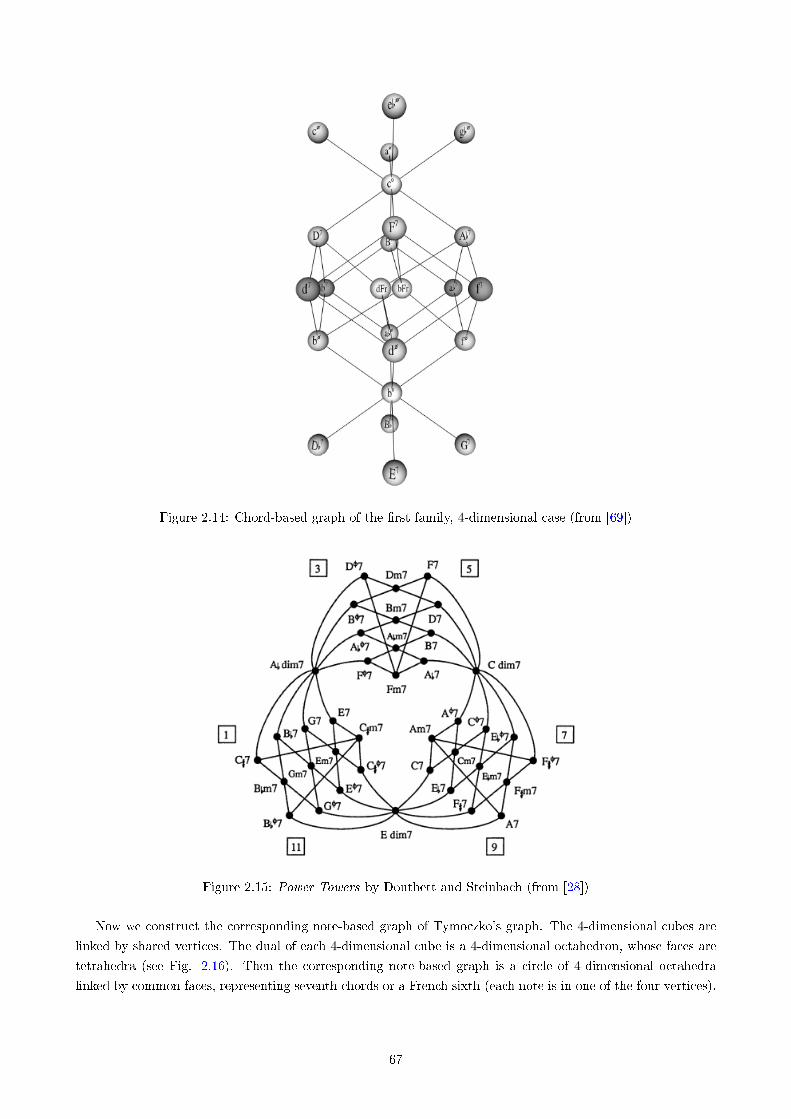
Figure 2.14: Chord-based graph of the �rst family, 4-dimensional case (from [69])

Figure 2.15: Power Towers by Douthett and Steinbach (from [28])

Now we construct the corresponding note-based graph of Tymoczko's graph. The 4-dimensional cubes are

linked by shared vertices. The dual of each 4-dimensional cube is a 4-dimensional octahedron, whose faces are

tetrahedra (see Fig. 2.16). Then the corresponding note-based graph is a circle of 4-dimensional octahedra

linked by common faces, representing seventh chords or a French sixth (each note is in one of the four vertices).

67

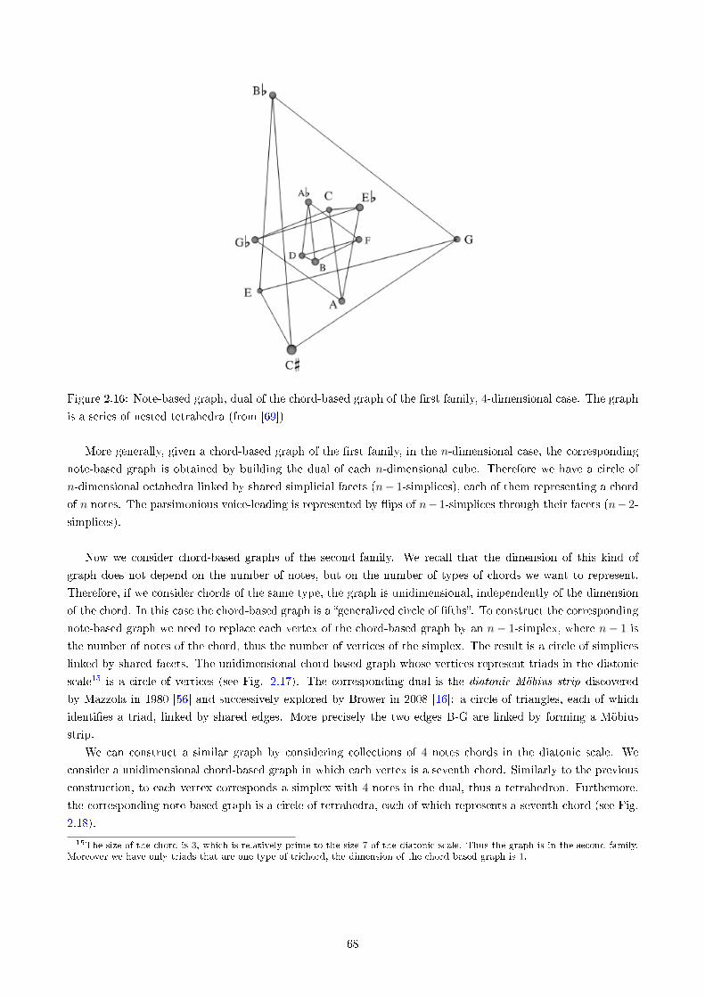
Figure 2.16: Note-based graph, dual of the chord-based graph of the �rst family, 4-dimensional case. The graph

is a series of nested tetrahedra (from [69])

More generally, given a chord-based graph of the �rst family, in the n-dimensional case, the corresponding

note-based graph is obtained by building the dual of each n-dimensional cube. Therefore we have a circle of

n-dimensional octahedra linked by shared simplicial facets (n− 1-simplices), each of them representing a chord

of n notes. The parsimonious voice-leading is represented by �ips of n− 1-simplices through their facets (n− 2-

simplices).

Now we consider chord-based graphs of the second family. We recall that the dimension of this kind of

graph does not depend on the number of notes, but on the number of types of chords we want to represent.

Therefore, if we consider chords of the same type, the graph is unidimensional, independently of the dimension

of the chord. In this case the chord-based graph is a �generalized circle of �fths�. To construct the corresponding

note-based graph we need to replace each vertex of the chord-based graph by an n− 1-simplex, where n− 1 is

the number of notes of the chord, thus the number of vertices of the simplex. The result is a circle of simplices

linked by shared facets. The unidimensional chord-based graph whose vertices represent triads in the diatonic

scale15 is a circle of vertices (see Fig. 2.17). The corresponding dual is the diatonic Möbius strip discovered

by Mazzola in 1980 [56] and successively explored by Brower in 2008 [16]: a circle of triangles, each of which

identi�es a triad, linked by shared edges. More precisely the two edges B-G are linked by forming a Möbius

strip.

We can construct a similar graph by considering collections of 4 notes chords in the diatonic scale. We

consider a unidimensional chord-based graph in which each vertex is a seventh chord. Similarly to the previous

construction, to each vertex corresponds a simplex with 4 notes in the dual, thus a tetrahedron. Furthemore,

the corresponding note-based graph is a circle of tetrahedra, each of which represents a seventh chord (see Fig.

2.18).

15The size of the chord is 3, which is relatively prime to the size 7 of the diatonic scale. Thus the graph is in the second family.Moreover we have only triads that are one type of trichord, the dimension of the chord-based graph is 1.

68

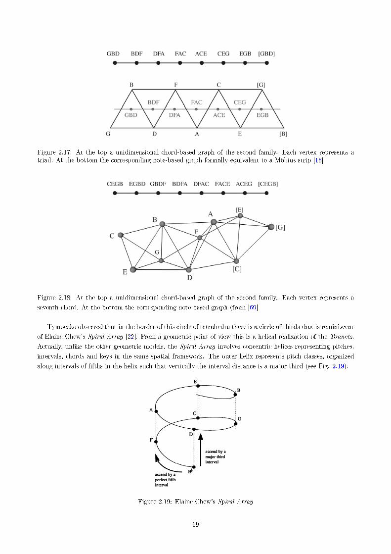
Figure 2.17: At the top a unidimensional chord-based graph of the second family. Each vertex represents atriad. At the bottom the corresponding note-based graph formally equivalent to a Möbius strip [16]

Figure 2.18: At the top a unidimensional chord-based graph of the second family. Each vertex represents a

seventh chord. At the bottom the corresponding note-based graph (from [69]

Tymoczko observed that in the border of this circle of tetrahedra there is a circle of thirds that is reminiscent

of Elaine Chew's Spiral Array [22]. From a geometric point of view this is a helical realization of the Tonnetz.

Actually, unlike the other geometric models, the Spiral Array involves concentric helices representing pitches,

intervals, chords and keys in the same spatial framework. The outer helix represents pitch classes, organized

along intervals of �fths in the helix such that vertically the interval distance is a major third (see Fig. 2.19).

Figure 2.19: Elaine Chew's Spiral Array

69

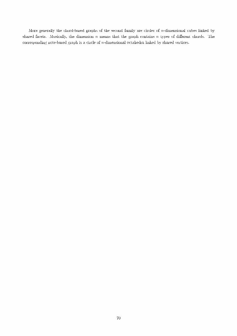
More generally the chord-based graphs of the second family are circles of n-dimensional cubes linked by

shared facets. Musically, the dimension n means that the graph contains n types of di�erent chords. The

corresponding note-based graph is a circle of n-dimensional octahedra linked by shared vertices.

70

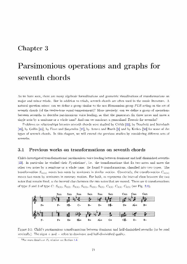
Chapter 3

Parsimonious operations and graphs for

seventh chords

As we have seen, there are many algebraic formalizations and geometric visualizations of transformations on

major and minor triads. But in addition to triads, seventh chords are often used in the music literature. A

natural question arises: can we de�ne a group similar to the neo-Riemannian group PLR acting on the set of

seventh chords (of the twelve-tone equal temperament)? More precisely: can we de�ne a group of operations

between sevenths to describe parsimonious voice leading, so that the generators �x three notes and move a

single note by a semitone or a whole tone? And can we construct a generalized Tonnetz for sevenths?

Problems on relationships between seventh chords were studied by Childs [23], by Douthett and Steinbach

[28], by Gollin [35], by Fiore and Satyendra [31], by Arnett and Barth [8] and by Kerkez [50] for some of the

types of seventh chords. In this chapter, we will extend the previous studies by considering di�erent sets of

sevenths.

3.1 Previous works on transformations on seventh chords

Childs investigated transformational parsimonious voice leading between dominant and half-diminished sevenths

[23]. In particular he studied their P2-relations1, i.e. the transformations that �x two notes and move the

other two notes by a semitone or a whole tone. He found 9 transformations, classi�ed into two types. The

transformation Sm(n) moves two notes by semitones in similar motion. Conversely, the transformation Cm(n)

moves two notes by semitones in contrary motion. For both, m represents the interval class between the two

notes that remain �xed, n the interval class between the two notes that are moved. There are 6 transformations

of type S and 3 of type C: S2(3), S3(2), S3(4), S4(3), S5(6), S6(5), C3(2), C3(4), C6(5) (see Fig. 3.1).

Figure 3.1: Child's parsimonious transformations between dominant and half-diminished sevenths (to be read

vertically). The signs + and − refers to dominant and half-diminished quality.

1For more details on Pn-relation see Section 1.4.

71

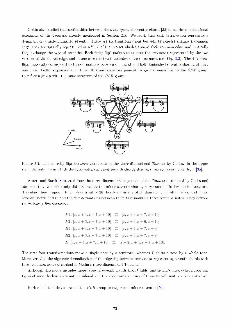
Gollin also studied the relationships between the same types of sevenths chords [35] in his three-dimensional

expansion of the Tonnetz, already mentioned in Section 2.5. We recall that each tetrahedron represents a

dominant or a half-diminished seventh. There are six transformations between tetrahedra sharing a common

edge: they are spatially represented as a ��ip� of the two tetrahedra around their common edge, and musically

they exchange the type of sevenths. Each �edge-�ip� maintains at least the two notes represented by the two

vertices of the shared edge, and in one case the two tetrahedra share three notes (see Fig. 3.2). The 4 �vertex-

�ips� musically correspond to transformations between dominant and half-diminished sevenths sharing at least

one note. Gollin explained that these 10 transformations generate a group isomorphic to the S/W -group,

therefore a group with the same structure of the PLR-group.

Figure 3.2: The six edge-�ips between tetrahedra in the three-dimensional Tonnetz by Gollin. In the upper

right the only �ip in which the tetrahedra represent seventh chords sharing three common notes (from [35].

Arnett and Barth [8] started from the three-dimensional expansion of the Tonnetz introduced by Gollin and

observed that Gollin's study did not include the minor seventh chords, very common in the music literature.

Therefore they proposed to consider a set of 36 chords consisting of all dominant, half-diminished and minor

seventh chords and to �nd the transformations between them that maintain three common notes. They de�ned

the following �ve operations:

P1: [x, x+ 4, x+ 7, x+ 10] 7→7→ [x, x+ 3, x+ 7, x+ 10]

P2: [x, x+ 3, x+ 7, x+ 10] 7→7→ [x, x+ 3, x+ 6, x+ 10]

R1: [x, x+ 4, x+ 7, x+ 10] 7→7→ [x, x+ 4, x+ 7, x+ 9]

R2: [x, x+ 3, x+ 7, x+ 10] 7→7→ [x, x+ 3, x+ 7, x+ 9]

L : [x, x+ 4, x+ 7, x+ 10] 7→7→ [x+ 2, x+ 4, x+ 7, x+ 10].

The �rst four transformations move a single note by a semitone, whereas L shifts a note by a whole tone.

Moreover, L is the algebraic formalization of the edge-�ip between tetrahedra representing seventh chords with

three common notes described in Gollin's three-dimensional Tonnetz.

Although this study includes more types of seventh chords than Childs' and Gollin's ones, other important

types of seventh chords are not considered and the algebraic structure of these transformations is not studied.

Kerkez had the idea to extend the PLR-group to major and minor sevenths [50].

72

Let H be the set of major and minor seventh chords, that is,

H = {〈x1, x2, x3, x4〉 |x1, x2, x3, x4 ∈ Z12, x2 = x1 + 4, x3 = x1 + 7, x4 = x1 + 11}∪

{〈x1, x2, x3, x4〉 |x1, x2, x3, x4 ∈ Z12, x3 = x4 + 3, x2 = x4 + 7, x1 = x4 + 10}.

Kerkez de�nes the following two maps P, S : H → H:

P 〈a, b, c, d〉 = 〈(type〈a, b, c, d〉) · 2 + d, a, b, c〉

S〈a, b, c, d〉 = 〈b, c, d, (−1) · (type〈a, b, c, d〉) · 2 + a〉

where

type(t) =

{1 if t is a minor seventh

−1 if t is a major seventh.

P maps each major seventh to its relative minor seventh moving the seventh down a whole tone. Conversely, it

maps each minor seventh to its relative major seventh moving the root up a whole tone.

S maps each major seventh to the minor seventh having root 4 semitones up, moving its root up a whole

tone. On the contrary, it maps each minor seventh to the major seventh having root 4 semitones down, moving

its seventh down a whole tone.

Example 3.1. We consider the major seventh chord C7 = 〈0, 4, 7, 11〉.

P 〈0, 4, 7, 11〉 = 〈7, 4, 0, (−1) · 2 + 11 (mod 12)〉 = 〈7, 4, 0, 9〉 = Am

S〈0, 4, 7, 11〉 = 〈(−1) · (−1) · 2 + 0 (mod 12), 11, 7, 4〉 = 〈2, 11, 7, 4〉 = Em.

We consider the minor seventh chord Cm = 〈10, 7, 3, 0〉.

P 〈10, 7, 3, 0〉 = 〈3, 7, 10, (+1) · 2 + 0 (mod 12)〉 = 〈3, 7, 10, 2〉 = E7[

S〈10, 7, 3, 0〉 = 〈(−1) · (+1) · 2 + 10 (mod 12), 0, 3, 7〉 = 〈8, 0, 3, 7〉 = A7[ .

Theorem 3.2. The transformations P and S act on H generating a group again isomorphic to the dihedral

group D12 of order 24.

Proof. We note that P 2 = S2 = 1, (PS)12 = 1 and (PS)P (PS) = (PS)(PP )S = (PS)S = P (SS) = P = P−1.

Therefore the group has the following presentation:

〈P, PS|P 2 = 1, (PS)12 = 1, (PS)P (PS) = P−1〉.

3.2 Parsimonious operations among seventh chords

Since seventh chords are often used in voice leading, our aim is to �nd all the most parsimonious operations

among seventh chords, similar to the P , L and R operations for triads. The most parsimonious operations �x

three notes and move only one note by a semitone or a whole tone. Equivalently: we want to determine all P1,0

and P0,1 relations among sevenths. We re�ne the de�nition of transformations and operations among sevenths,

extending in a natural way De�nitions 1.41 and 1.42 given by Hook for triads. We will denote the set of all

possible seventh chords with Σ.

73

De�nition 3.3 (Seventh chord transformation). A seventh chord transformation is a map Σ→ Σ.

De�nition 3.4 (Seventh chord operation). A seventh chord operation is a bijective transformation Σ→ Σ.

As for the triads, there are some musical transformations that are not operations. For instance there are

some di�erent chords with the same secondary dominant, therefore the transformation mapping each chord into

its secondary dominant is not an operation.

For our study we do not want to consider all types of sevenths in Σ. For the moment we consider the

following types of seventh chords: dominant (D), minor (m), half-diminished (hd), major (M) and diminished

(d), and let H ⊂ Σ be the set of all cyclicly marked seventh chords of these 5 types:

H ={[x1, x2, x3, x4] |x1, x2, x3, x4 ∈ Z12, x2 = x1 + 4, x3 = x1 + 7, x4 = x1 + 10}∪

{[x1, x2, x3, x4] |x1, x2, x3, x4 ∈ Z12, x2 = x1 + 3, x3 = x1 + 7, x4 = x1 + 10}∪



{[x1, x2, x3, x4] |x1, x2, x3, x4 ∈ Z12, x2 = x1 + 3, x3 = x1 + 6, x4 = x1 + 9}

As in Lewin and Hook's terminology, we de�ne a transformation among seventh as a map H → H, and an

operation as a bijective transformation H → H.

We �rst analyze all P1,0 relations, that is the transformations moving just one note by one semitone: let us

call Qi+ the map that sends each type of seventh chord to another type moving the i-th member up a semitone,

where i = R, T, F, S depending on whether the member is considered to be the root (R), the third (T), �fth (F)

or seventh (S), respectively. Analogously, let Qi− be the map that moves the i-th member down a semitone.

By overstriking the maps that do not produce any of the classical types of seventh chord, we have:

QR+(D) = d QR+(m) = D QR+(hd) = m QR+(M) = hd QR+(d) = hd

��QR−(D) ��

�QR−(m) QR−(hd) = M ��QR−(M) QR−(d) = D

��QT+(D) QT+(m) = D ��

��QT+(hd) ��QT+(M) QT+(d) = hd

QT−(D) = m ��QT−(m) ��

��QT−(hd) ��QT−(M) QT−(d) = D

��QF+(D) ��

��QF+(m) QF+(hd) = m ��QF+(M) QF+(d) = hd

��QF−(D) QF−(m) = hd ��

��QF−(hd) ��QF−(M) QF−(d) = D

QS+(D) = M ��QS+(m) ��

��QS+(hd) ��QS+(M) QS+(d) = hd

QS−(D) = m QS−(m) = hd QS−(hd) = d QS−(M) = D QS−(d) = D.

We observe that some transformations are inverse to each other:

QR+(M) = hd QR−(hd) = M

QR+(m) = D QS−(D) = m

QR+(hd) = m QS−(m) = hd

QS+(D) = M QS−(M) = D

QT+(m) = D QT−(D) = m

QF+(hd) = m QF−(m) = hd.

74

It remains to consider the following operations:

QR+(D) = d QR−(d) = D QT−(d) = D QF−(d) = D QS−(d) = D

QS−(hd) = d QS+(d) = hd QR+(d) = hd QT+(d) = hd QF+(d) = sd.

QR+ is the inverse of QR−, QT−, QF− and QS−. This is due to the particular symmetry of the intervallic

structure (3, 3, 3, 3) of diminished sevenths, in which the members of the chord play an identical role. From

an acoustical point of view we have only 3 diminished sevenths: Co = E[o = G[o = Ao = [0, 3, 6, 9], C]o =

Eo = Go = B[o = [1, 4, 7, 10], Do = F o = A[o = Bo = [2, 5, 8, 11]. Unlike the other four types, the diminished

sevenths would be only three (and not twelve), e.g. C,C],D, because the other nine chords are three by three

enharmonic to them. This explains why we have four transformations that have the same inverse. Since we are

considering cyclicly marked chords, the diminished sevenths count as 12 distinct chords, which means that our

set of transformations is well-de�ned. Hence we have 4 transformations between diminished and half-diminished

seventh chords and 4 transformations between diminished and dominant seventh chords

QS−(hd) = d QR−(d) = hd

QS−(hd) = d QT−(d) = hd

QS−(hd) = d QF−(d) = hd

QS−(hd) = d QS−(d) = hd

QR+(D) = d QR−(d) = D

QR+(D) = d QT−(d) = D

QR+(D) = d QF−(d) = D

QR+(D) = d QS−(d) = D.

Now we consider the P0,1 relations, i.e. the transformations that move a single note by a whole tone. Analogously

to what was done above, let us call Qi++ the map which sends each type of seventh chord in another type moving

the i-th member up a whole tone, and Qi−− the map which moves the i-th member down a whole tone. We

obtain another classical type of seventh chords only moving the root up a whole tone or the seventh down a

whole tone:

QR++(D) = hd QR++(m) = M ��QR++(hd) QR++(M) = m ��

��QR++(d)

��QS−−(D) QS−−(m) = M QS−−(hd) = D QS−−(M) = m ��

��QS−−(d).

Again, we �nd some transformations that are the inverse of each other:

QR++(D) = hd QS−−(hd) = D

QR++(m) = M QS−−(M) = m

QR++(M) = m QS−−(m) = M.

Overall we have 17 transformations corresponding to a parsimonious voice leading among our 5 types of seventh

chords.

We want to de�ne these transformations similarly to the neo-Riemannian operations. Let K be a set of

chords of di�erent types and of the same cardinality (in our case K = H). We start by de�ning a generalized

parallel operation P .

De�nition 3.5. Let Pij : K → K be the maps which send an i-th type of chord to a j-th type of chord with the

75

same root, i 6= j, and vice versa, and which are identity the other types.

In H the types of the seventh chords are 5, and we will denote them with the numbers from 1 to 5: �1� is

for dominant sevenths, �2� for minor sevenths, �3� for half-diminished sevenths, �4� for major sevenths and �5�

for diminished sevenths.

4 of the 17 transformations are parallel operations:

QT P12 : [x, x+ 4, x+ 7, x+ 10] 7→7→ [x, x+ 3, x+ 7, x+ 10]

QS P14 : [x, x+ 4, x+ 7, x+ 10] 7→7→ [x, x+ 4, x+ 7, x+ 11]

QF P23 : [x, x+ 3, x+ 7, x+ 10] 7→7→ [x, x+ 3, x+ 6, x+ 10]

QS P35 : [x, x+ 3, x+ 6, x+ 10] 7→7→ [x, x+ 3, x+ 6, x+ 9].

Remark 3.6. P12 and P23 coincide with P1 and P2 de�ned by Arnett and Barth.

Now we de�ne the generalized relative and leading-tone operations. We recall that, from Proposition 1.27,

if the triad is major R = P ◦ T−3 = T−3 ◦ P , if it is minor R = P ◦ T3 = T3 ◦ P .

De�nition 3.7. Let Rij : K → K be the maps which send an i-th type of chord to a j-th type chord whose root

is transposed 3 semitones down, a j-th type of chord to an i-th type of chord transposed 3 semitones up, and

which �x the other types:

Rij = T±3 ◦ Pij = Pij ◦ T±3. (3.1)

More precisely, we are using the usual symbol Tn, but it is not the usual transposition, because it is to be

considered applied only to the i-th and j-th types of sevenths. We will continue to use this notation also in the

other de�nitions and in the following chapters.

Now, 5 of the 17 transformations are generalized relative operations:

QR, QS R12 : [x, x+ 4, x+ 7, x+ 10] 7→7→ [x, x+ 4, x+ 7, x+ 9]

QR, QS R23 : [x, x+ 3, x+ 7, x+ 10] 7→7→ [x, x+ 3, x+ 7, x+ 9]

QR, QS R42 : [x, x+ 4, x+ 7, x+ 11] 7→7→ [x, x+ 4, x+ 7, x+ 9]

QR, QS R35 : [x, x+ 3, x+ 6, x+ 10] 7→7→ [x, x+ 3, x+ 6, x+ 9]

QF , QS R53 : [x, x+ 3, x+ 6, x+ 9] 7→7→ [x, x+ 3, x+ 7, x+ 9].

Remark 3.8. R12 and R23 coincide with R1 and R2 de�ned by Arnett and Barth. Moreover, R42 coincide with

the map P de�ned by Kerkez.

For the operation L we recall that, from Proposition 1.27, if the triad is major L = P ◦ T4 = T4 ◦ P , if it isminor L = P ◦ T−4 = T−4 ◦ P .

De�nition 3.9. Let Lij : H → H be the maps which send an i-th type of chord to a j-th type of chord whose

root is transposed 4 semitones up, a j-th type of chord to an i-th type of chord transposed 4 semitones down,

and which �x the other types:

Lij = T±4 ◦ Pij = Pij ◦ T±4 (3.2)

76

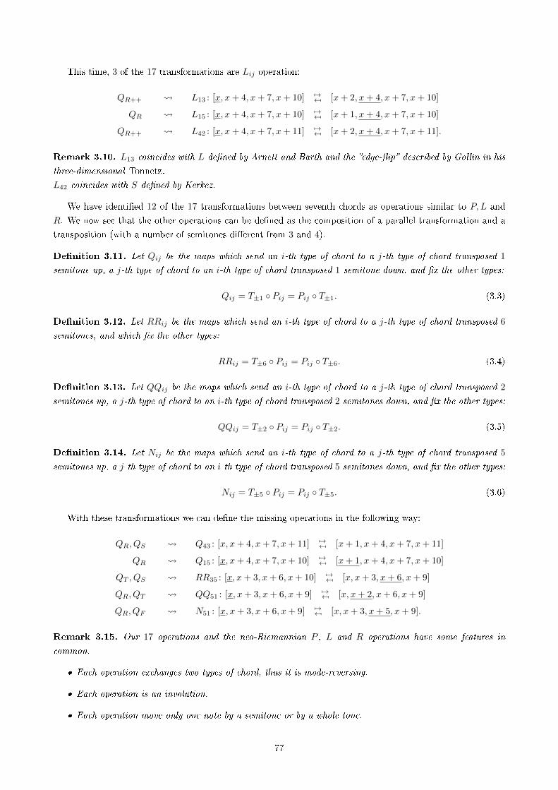
This time, 3 of the 17 transformations are Lij operation:

QR++ L13 : [x, x+ 4, x+ 7, x+ 10] 7→7→ [x+ 2, x+ 4, x+ 7, x+ 10]

QR L15 : [x, x+ 4, x+ 7, x+ 10] 7→7→ [x+ 1, x+ 4, x+ 7, x+ 10]

QR++ L42 : [x, x+ 4, x+ 7, x+ 11] 7→7→ [x+ 2, x+ 4, x+ 7, x+ 11].

Remark 3.10. L13 coincides with L de�ned by Arnett and Barth and the �edge-�ip� described by Gollin in his

three-dimensional Tonnetz.

L42 coincides with S de�ned by Kerkez.

We have identi�ed 12 of the 17 transformations between seventh chords as operations similar to P,L and

R. We now see that the other operations can be de�ned as the composition of a parallel transformation and a

transposition (with a number of semitones di�erent from 3 and 4).

De�nition 3.11. Let Qij be the maps which send an i-th type of chord to a j-th type of chord transposed 1

semitone up, a j-th type of chord to an i-th type of chord transposed 1 semitone down, and �x the other types:

Qij = T±1 ◦ Pij = Pij ◦ T±1. (3.3)

De�nition 3.12. Let RRij be the maps which send an i-th type of chord to a j-th type of chord transposed 6

semitones, and which �x the other types:

RRij = T±6 ◦ Pij = Pij ◦ T±6. (3.4)

De�nition 3.13. Let QQij be the maps which send an i-th type of chord to a j-th type of chord transposed 2

semitones up, a j-th type of chord to an i-th type of chord transposed 2 semitones down, and �x the other types:

QQij = T±2 ◦ Pij = Pij ◦ T±2. (3.5)

De�nition 3.14. Let Nij be the maps which send an i-th type of chord to a j-th type of chord transposed 5

semitones up, a j-th type of chord to an i-th type of chord transposed 5 semitones down, and �x the other types:

Nij = T±5 ◦ Pij = Pij ◦ T±5. (3.6)

With these transformations we can de�ne the missing operations in the following way:

QR, QS Q43 : [x, x+ 4, x+ 7, x+ 11] 7→7→ [x+ 1, x+ 4, x+ 7, x+ 11]

QR Q15 : [x, x+ 4, x+ 7, x+ 10] 7→7→ [x+ 1, x+ 4, x+ 7, x+ 10]

QT , QS RR35 : [x, x+ 3, x+ 6, x+ 10] 7→7→ [x, x+ 3, x+ 6, x+ 9]

QR, QT QQ51 : [x, x+ 3, x+ 6, x+ 9] 7→7→ [x, x+ 2, x+ 6, x+ 9]

QR, QF N51 : [x, x+ 3, x+ 6, x+ 9] 7→7→ [x, x+ 3, x+ 5, x+ 9].

Remark 3.15. Our 17 operations and the neo-Riemannian P , L and R operations have some features in

common.

� Each operation exchanges two types of chord, thus it is mode-reversing.

� Each operation is an involution.

� Each operation move only one note by a semitone or by a whole tone.

77

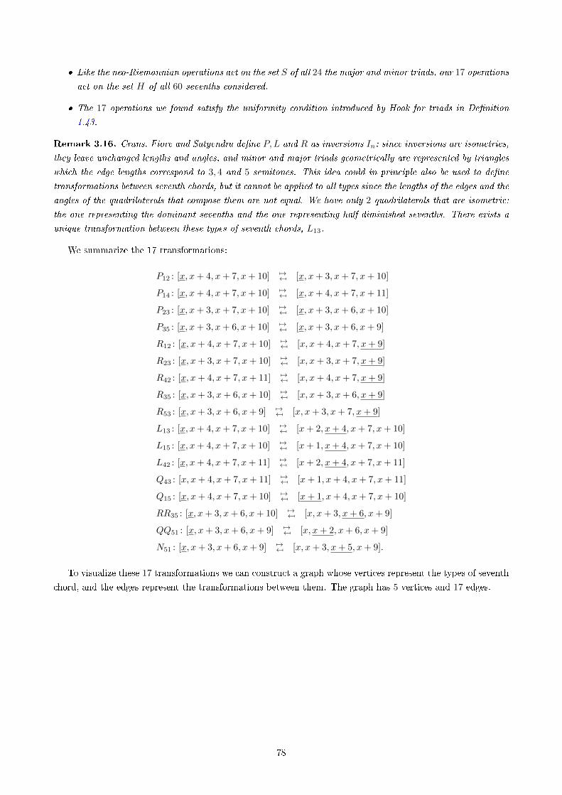
� Like the neo-Riemannian operations act on the set S of all 24 the major and minor triads, our 17 operations

act on the set H of all 60 sevenths considered.

� The 17 operations we found satisfy the uniformity condition introduced by Hook for triads in De�nition

1.43.

Remark 3.16. Crans, Fiore and Satyendra de�ne P,L and R as inversions In; since inversions are isometries,

they leave unchanged lengths and angles, and minor and major triads geometrically are represented by triangles

which the edge lengths correspond to 3, 4 and 5 semitones. This idea could in principle also be used to de�ne

transformations between seventh chords, but it cannot be applied to all types since the lengths of the edges and the

angles of the quadrilaterals that compose them are not equal. We have only 2 quadrilaterals that are isometric:

the one representing the dominant sevenths and the one representing half-diminished sevenths. There exists a

unique transformation between these types of seventh chords, L13.

We summarize the 17 transformations:

P12 : [x, x+ 4, x+ 7, x+ 10] 7→7→ [x, x+ 3, x+ 7, x+ 10]

P14 : [x, x+ 4, x+ 7, x+ 10] 7→7→ [x, x+ 4, x+ 7, x+ 11]

P23 : [x, x+ 3, x+ 7, x+ 10] 7→7→ [x, x+ 3, x+ 6, x+ 10]

P35 : [x, x+ 3, x+ 6, x+ 10] 7→7→ [x, x+ 3, x+ 6, x+ 9]

R12 : [x, x+ 4, x+ 7, x+ 10] 7→7→ [x, x+ 4, x+ 7, x+ 9]

R23 : [x, x+ 3, x+ 7, x+ 10] 7→7→ [x, x+ 3, x+ 7, x+ 9]

R42 : [x, x+ 4, x+ 7, x+ 11] 7→7→ [x, x+ 4, x+ 7, x+ 9]

R35 : [x, x+ 3, x+ 6, x+ 10] 7→7→ [x, x+ 3, x+ 6, x+ 9]

R53 : [x, x+ 3, x+ 6, x+ 9] 7→7→ [x, x+ 3, x+ 7, x+ 9]

L13 : [x, x+ 4, x+ 7, x+ 10] 7→7→ [x+ 2, x+ 4, x+ 7, x+ 10]

L15 : [x, x+ 4, x+ 7, x+ 10] 7→7→ [x+ 1, x+ 4, x+ 7, x+ 10]

L42 : [x, x+ 4, x+ 7, x+ 11] 7→7→ [x+ 2, x+ 4, x+ 7, x+ 11]

Q43 : [x, x+ 4, x+ 7, x+ 11] 7→7→ [x+ 1, x+ 4, x+ 7, x+ 11]

Q15 : [x, x+ 4, x+ 7, x+ 10] 7→7→ [x+ 1, x+ 4, x+ 7, x+ 10]

RR35 : [x, x+ 3, x+ 6, x+ 10] 7→7→ [x, x+ 3, x+ 6, x+ 9]

QQ51 : [x, x+ 3, x+ 6, x+ 9] 7→7→ [x, x+ 2, x+ 6, x+ 9]

N51 : [x, x+ 3, x+ 6, x+ 9] 7→7→ [x, x+ 3, x+ 5, x+ 9].

To visualize these 17 transformations we can construct a graph whose vertices represent the types of seventh

chord, and the edges represent the transformations between them. The graph has 5 vertices and 17 edges.

78

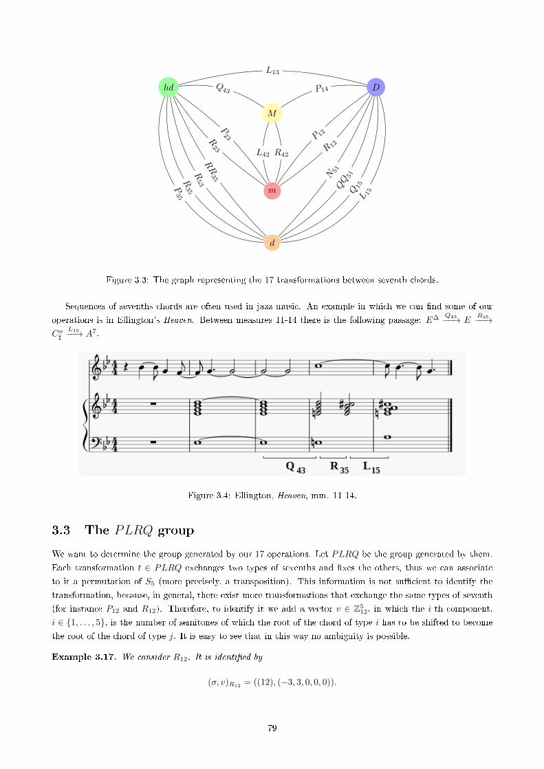
hd D

M

m

d

L13

R42L42

Q43 P14

P23R

23

RR

35

R53R

35P35

P 12

R 12

N51

QQ

51Q

15L 15

Figure 3.3: The graph representing the 17 transformations between seventh chords.

Sequences of sevenths chords are often used in jazz music. An example in which we can �nd some of our

operations is in Ellington's Heaven. Between measures 11-14 there is the following passage: E∆ Q43−−→ ER35−−→

Co]L15−−→ A7.

Figure 3.4: Ellington, Heaven, mm. 11-14.

3.3 The PLRQ group

We want to determine the group generated by our 17 operations. Let PLRQ be the group generated by them.

Each transformation t ∈ PLRQ exchanges two types of sevenths and �xes the others, thus we can associate

to it a permutation of S5 (more precisely, a transposition). This information is not su�cient to identify the

transformation, because, in general, there exist more transformations that exchange the same types of seventh

(for instance P12 and R12). Therefore, to identify it we add a vector v ∈ Z512, in which the i-th component,

i ∈ {1, . . . , 5}, is the number of semitones of which the root of the chord of type i has to be shifted to become

the root of the chord of type j. It is easy to see that in this way no ambiguity is possible.

Example 3.17. We consider R12. It is identi�ed by

(σ, v)R12 = ((12), (−3, 3, 0, 0, 0)).

79

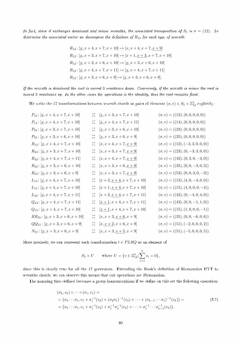
In fact, since it exchanges dominant and minor sevenths, the associated transposition of S5 is σ = (12). To

determine the associated vector we decompose the de�nition of R12 for each type of seventh:

R12 : [x, x+ 4, x+ 7, x+ 10] 7→ [x, x+ 4, x+ 7, x+ 9]

R12 : [x, x+ 3, x+ 7, x+ 10] 7→ [x+ 1, x+ 3, x+ 7, x+ 10]

R12 : [x, x+ 3, x+ 6, x+ 10] 7→ [x, x+ 3, x+ 6, x+ 10]

R12 : [x, x+ 4, x+ 7, x+ 11] 7→ [x, x+ 4, x+ 7, x+ 11]

R12 : [x, x+ 3, x+ 6, x+ 9] 7→ [x, x+ 3, x+ 6, x+ 9].

If the seventh is dominant the root is moved 3 semitones down. Conversely, if the seventh is minor the root is

moved 3 semitones up. In the other cases the operations is the identity, thus the root remains �xed.

We write the 17 transformations between seventh chords as pairs of elements (σ, v) ∈ S5 × Z512 explicitly:

P12 : [x, x+ 4, x+ 7, x+ 10] 7→7→ [x, x+ 3, x+ 7, x+ 10] (σ, v) = ((12), (0, 0, 0, 0, 0))

P14 : [x, x+ 4, x+ 7, x+ 10] 7→7→ [x, x+ 4, x+ 7, x+ 11] (σ, v) = ((14), (0, 0, 0, 0, 0))

P23 : [x, x+ 3, x+ 7, x+ 10] 7→7→ [x, x+ 3, x+ 6, x+ 10] (σ, v) = ((23), (0, 0, 0, 0, 0))

P35 : [x, x+ 3, x+ 6, x+ 10] 7→7→ [x, x+ 3, x+ 6, x+ 9] (σ, v) = ((35), (0, 0, 0, 0, 0))

R12 : [x, x+ 4, x+ 7, x+ 10] 7→7→ [x, x+ 4, x+ 7, x+ 9] (σ, v) = ((12), (−3, 3, 0, 0, 0))

R23 : [x, x+ 3, x+ 7, x+ 10] 7→7→ [x, x+ 3, x+ 7, x+ 9] (σ, v) = ((23), (0,−3, 3, 0, 0))

R42 : [x, x+ 4, x+ 7, x+ 11] 7→7→ [x, x+ 4, x+ 7, x+ 9] (σ, v) = ((42), (0, 3, 0,−3, 0))

R35 : [x, x+ 3, x+ 6, x+ 10] 7→7→ [x, x+ 3, x+ 6, x+ 9] (σ, v) = ((35), (0, 0,−3, 0, 3))

R53 : [x, x+ 3, x+ 6, x+ 9] 7→7→ [x, x+ 3, x+ 7, x+ 9] (σ, v) = ((53), (0, 0, 3, 0,−3))

L13 : [x, x+ 4, x+ 7, x+ 10] 7→7→ [x+ 2, x+ 4, x+ 7, x+ 10] (σ, v) = ((13), (4, 0,−4, 0, 0))

L15 : [x, x+ 4, x+ 7, x+ 10] 7→7→ [x+ 1, x+ 4, x+ 7, x+ 10] (σ, v) = ((15), (4, 0, 0, 0,−4))

L42 : [x, x+ 4, x+ 7, x+ 11] 7→7→ [x+ 2, x+ 4, x+ 7, x+ 11] (σ, v) = ((42), (0,−4, 0, 4, 0))

Q43 : [x, x+ 4, x+ 7, x+ 11] 7→7→ [x+ 1, x+ 4, x+ 7, x+ 11] (σ, v) = ((43), (0, 0,−1, 1, 0))

Q15 : [x, x+ 4, x+ 7, x+ 10] 7→7→ [x+ 1, x+ 4, x+ 7, x+ 10] (σ, v) = ((15), (1, 0, 0, 0,−1))

RR35 : [x, x+ 3, x+ 6, x+ 10] 7→7→ [x, x+ 3, x+ 6, x+ 9] (σ, v) = ((35), (0, 0,−6, 0, 6))

QQ51 : [x, x+ 3, x+ 6, x+ 9] 7→7→ [x, x+ 2, x+ 6, x+ 9] (σ, v) = ((51), (−2, 0, 0, 0, 2))

N51 : [x, x+ 3, x+ 6, x+ 9] 7→7→ [x, x+ 3, x+ 5, x+ 9] (σ, v) = ((51), (−5, 0, 0, 0, 5)).

More precisely, we can represent each transformation t ∈ PLRQ as an element of

S5 × V where V = {v ∈ Z512|

5∑i=1

vi = 0},

since this is clearly true for all the 17 generators. Extending the Hook's de�nition of Riemannian UTT to

sevenths chords, we can observe this means that our operations are Riemannian.

The mapping thus de�ned becomes a group homomorphism if we de�ne on this set the following operation:

(σk, vk) ◦ · · · ◦ (σ1, v1) =

=(σk · · ·σ1, v1 + σ−1

1 (v2) + (σ2σ1)−1(v3) + · · ·+ (σk−1 · · ·σ1)−1(vk))

= (3.7)

=(σk · · ·σ1, v1 + σ−1

1 (v2) + σ−11 σ−1

2 (v3) + · · ·+ σ−11 · · ·σ

−1k−1(vk)

).

80

Example 3.18.

Q43L13R12 = ((43), (0, 0,−1, 1, 0)) ◦ ((13), (4, 0,−4, 0, 0)) ◦ ((12), (−3, 3, 0, 0, 0)) =

= ((1243), (−3, 3, 0, 0, 0) + σ−11 (4, 0,−4, 0, 0) + σ−1

1 σ−12 (0, 0,−1, 1, 0)) =

= ((1243), (−3, 3, 0, 0, 0) + (0, 4,−4, 0, 0) + σ−11 (−1, 0, 0, 1, 0)) =

= ((1243), (−3, 3, 0, 0, 0) + (0, 4,−4, 0, 0) + (0,−1, 0, 1, 0)) =

= ((1243), (−3, 6,−4, 1, 0)).

We want to prove that PLRQ is isomorphic to S5 nV . We recall the de�nition of semidirect product of two

subgroups.

Let G be a group. If G contains two subgroups H and K such that

i) G = HK;

ii) K EG;

iii) H ∩K = 1;

G is the semidirect product of H and K. Conversely, given two groups H and K and a group homomorphism

φ : H → Aut(K), we can construct a new group H nK de�ning in the cartesian product H ×K the following

operation:

(h1, k1)(h2, k2) = (h1h2, φh2(k1) · k2).

Theorem 3.19. The group PLRQ is isomorphic to S5 n Z412.

Proof. First of all we prove that PLRQ is isomorphic to S5 n V .

We observe that the subgroup formed by the elements (Id, v) is normal. In fact, for all (σ, v) ∈ S5×V, (Id, v′) ∈{Id} × V , we have

(σ, v)(Id, v′)(σ, v)−1 = (σσ−1,−v + σ(v′) + σ(v)) = (Id, v′′) ∈ {Id} × Z.

On the other hand, since S5 is generated by transpositions, it is easy to see that, calling O the origin in Z512,

S5 × {O} < PLRQ, since we already have in it P12, P14, P23, P35.

It is clear that the two subgroups have trivial intersection. Thus, PLRQ ' S5 n V . Now we compute the

permutations and vectors associated to R42L42, P14L42P14R12, P12L13P12R23:

R42L42 = (σ′, v′)

σ′ =σ2σ1 = (42)(42) = Id

v′ =v1 + σ−11 (v2) =

=(0,−4, 0, 4, 0) + (0,−3, 0, 3, 0) =

=(0,−7, 0, 7, 0)

P14L42P14R12 = (σ′′, v′′)

σ′′ =σ4σ3σ2σ1 = (14)(42)(14)(12) = Id

v′′ =v1 + σ−11 (v2) + σ−1

1 σ−12 (v3) + σ−1

1 σ−12 σ−1

3 (v4) =

=(−3, 3, 0, 0, 0) + (0, 0, 0, 0, 0) + (−4, 4, 0, 0, 0) + (0, 0, 0, 0, 0) =

=(7,−7, 0, 0, 0)

81

P12L13P12R23 = (σ′′′, v′′′)

σ′′′ =σ4σ3σ2σ1 = (12)(13)(12)(23) = Id

v′′′ =v1 + σ−11 (v2) + σ−1

1 σ−12 (v3) + σ−1

1 σ−12 σ−1

3 (v4) =

=(0,−3, 3, 0, 0) + (0, 0, 0, 0, 0) + (0,−4, 4, 0, 0) + (0, 0, 0, 0, 0) =

=(0, 7,−7, 0, 0).

With the following elements just computed

R42L42 = (Id, (0,−7, 0, 7, 0)) (3.8)

P14L42P14R12 = (Id, (7,−7, 0, 0, 0))

P12L13P12R23 = (Id, (0, 7,−7, 0, 0))

we can generate each element (Id, (v1, v2, v3, v4, 0)), with (v1, v2, v3, v4, 0) ∈ Z512 such that

∑41 vi = 0. To see

this, taken a, b, c ∈ Z, we have to solve

a(0,−7, 0, 7, 0) + b(7,−7, 0, 0, 0) + c(0, 7,−7, 0, 0) ≡ (v1, v2, v3, v4, 0) (mod 12)

(−7b,−7a+ 7b− 7c, 7c, 7a) ≡ (v1, v2, v3, v4, 0) (mod 12)

−7b ≡ v1

−7a+ 7b− 7c ≡ v2

7c ≡ v3

7a ≡ v4

⇒

−7b ≡ v1

7b− 7c ≡ v2 + 7a

7c ≡ −v3

7a ≡ v4

⇒

7b ≡ −v1

−v1 − v3 ≡ v2 + v4

7c ≡ −v3

7a ≡ v4

which is solvable because 7 is coprime with 12.

To obtain all elements (Id, (v1, v2, v3, v4, v5)), with (v1, v2, v3, v4, v5) ∈ Z512 such that

∑51 vi = 0, it is su�cient

to add to the 3 generators listed in 3.8 the generator P12P35R23P12L15L13 = (Id, (7, 0, 0, 0,−7)).

From this, it is evident that V ' Z412, hence PLRQ ' S5 n Z4

12.

3.4 The Clover graph: a generalized Chicken-wire Torus for sevenths

Starting from the algebraic de�nition of the parsimonious operations among sevenths as pairs of elements

(σ, v) ∈ S5 n Z512, we can construct a generalized Chicken-wire torus for seventh chords. It is a chord-based

graph in which each vertex represents a seventh chord and each edge identi�es a parsimonious musical operation

(see Fig. 3.5).

For algebraic reasons we have considered 60 sevenths, 12 for each type, but we recall that some dimin-

ished sevenths are enharmonic equivalent. Similarly, some of the 17 transformations are di�erent from a

theoretical and mathematical point of view, but enharmonic equivalent from an acoustical point of view:

P35 ∼ R35 ∼ R53 ∼ RR35 and L15 ∼ Q15 ∼ QQ51 ∼ N51. Since our aim is to study paths in our graph

and their musical interpretation less than enharmonic equivalences, we identify vertices and edges enharmonic

equivalent. Therefore our graph has 12 · 4 + 3 = 51 vertices and 12 · 11 = 132 edges.

The Power Towers graph (see Fig. 2.15) realized by Douthett and Stainbach [28], that we mentioned in

Section 2.5, is a subgraph of our graph. The Power Towers is a chord-based graph representing dominant,

minor, major and diminished sevenths. These vertices and their edges are also in our graph. Our Clover graph

di�ers from the �rst one for twelve vertices representing major sevenths and the related edges.

If we observe the drawing of our graph, it is evident that a rotation of the plane by 2π3 induces automor-

82

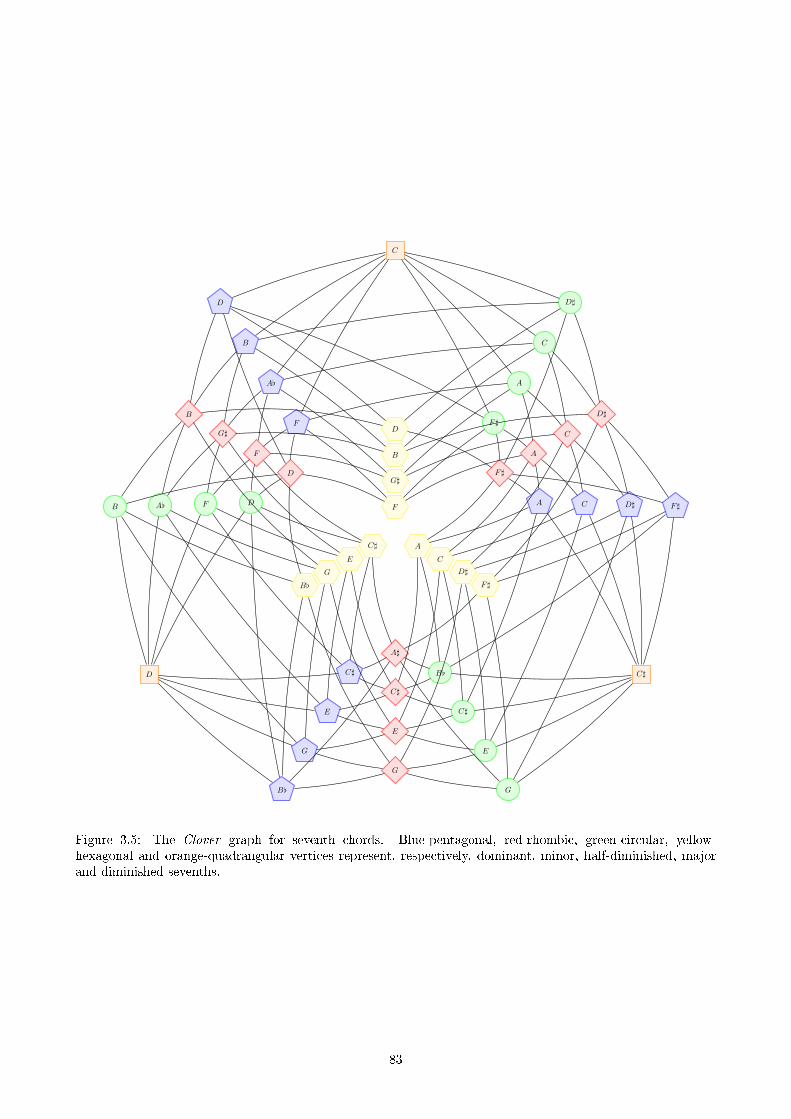
F

G]

B

D

C]

E

G

B[

A

C

D]

F]

D

F

G]

B

F]

A

C

D]

A]

C]

E

G

C]

E

G

B[

B[

C]

E

G

A C D] F]

F

A[

B

D

DFA[B

F]

A

C

D]

C

D C]

Figure 3.5: The Clover graph for seventh chords. Blue-pentagonal, red-rhombic, green-circular, yellow-hexagonal and orange-quadrangular vertices represent, respectively, dominant, minor, half-diminished, majorand diminished sevenths.

83

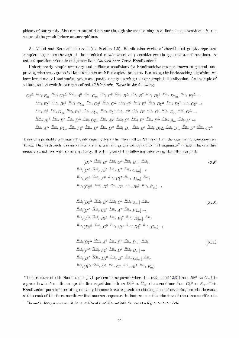
phisms of our graph. Also re�ections of the plane through the axis passing in a diminished seventh and in the

center of the graph induce automorphisms.

As Albini and Bernardi observed (see Section 1.5), Hamiltonian cycles of chord-based graphs represent

complete sequences through all the admitted chords which only consider certain types of transformations. A

natural question arises: is our generalized Chicken-wire Torus Hamiltonian?

Unfortunately simple necessary and su�cient conditions for Hamiltonicity are not known in general, and

proving whether a graph is Hamiltonian is an NP-complete problem. But using the backtracking algorithm we

have found many Hamiltonian cycles and paths, clearly showing that our graph is Hamiltonian. An example of

a Hamiltonian cycle in our generalized Chicken-wire Torus is the following:

C]∆L42−−→ Fm

R42−−→ G]∆Q43−−→ A∅

R23−−→ CmP23−−→ C∅

Q43−−→ B∆ P14−−→ B7 L13−−→ D]∅P23−−→ D]m

R42−−→ F]∆ −→P14−−→ F]7

L13−−→ B[∅R23−−→ C]m

P23−−→ C]∅Q43−−→ C∆ P14−−→ C7 L13−−→ E∅

Q43−−→ D]∆P14−−→ D]7

L15−−→ C]o −→P35−−→ G∅

P23−−→ GmR12−−→ B[7

P12−−→ A]mR12−−→ C]7

L13−−→ F ∅P35−−→ Do L15−−→ G7 R12−−→ Em

R42−−→ G∆ −→Q43−−→ A[∅

L13−−→ E7 P14−−→ E∆ L42−−→ G]mP12−−→ A[7

L15−−→ CoL15−−→ F 7 P14−−→ F∆ L42−−→ Am

P12−−→ A7 −→P14−−→ A∆ R42−−→ F]m

P23−−→ F]∅L13−−→ D7 P14−−→ D∆ R42−−→ Bm

P23−−→ B∅Q43−−→ B[∆

L42−−→ DmP23−−→ D∅

Q43−−→ C]∆

There are probably too many Hamiltonian cycles to list them all as Albini did for the traditional Chicken-wire

Torus. But with such a symmetrical structure in the graph we expect to �nd sequences2 of sevenths or other

musical structures with some regularity. It is the case of the following interesting Hamiltonian path:

[B[∆Q43−−→ B∅

L13−−→ G7 R12−−→ Em]R42−−→ (3.9)

R42−−→[G∆ Q43−−→ A[∅L13−−→ E7 R12−−→ C]m] −→

R42−−→[E∆ Q43−−→ F ∅L13−−→ C]7

R12−−→ A]m]R42−−→

R42−−→(C]∆Q43−−→ D∅

P35−−→ Do L15−−→ B[7R12−−→ Gm) −→

R42−−→[D]∆Q43−−→ E∅

L13−−→ C7 R12−−→ Am]R42−−→ (3.10)

R42−−→[C∆ Q43−−→ C]∅L13−−→ A7 R12−−→ F]m] −→

R42−−→[A∆ Q43−−→ B[∅L13−−→ F]7

R12−−→ D]m]R42−−→

R42−−→(F]∆Q43−−→ G∅

P35−−→ C]oL15−−→ D]7

R12−−→ Cm) −→

R42−−→[G]∆Q43−−→ A∅

L13−−→ F 7 R12−−→ Dm]R42−−→ (3.11)

R42−−→[F∆ Q43−−→ F]∅L13−−→ D7 R12−−→ Bm] −→

R42−−→[D∆ Q43−−→ D]∅L13−−→ B7 R12−−→ G]m]

R42−−→R42−−→(B∆ Q43−−→ C∅

P35−−→ CoL15−−→ A[7

R12−−→ Fm)

The structure of this Hamiltonian path presents a sequence where the main motif 3.9 (from B[∆ to Gm) is

repeated twice 5 semitones up: the �rst repetition is from D]∆ to Cm, the second one from G]∆ to Fm. This

Hamiltonian path is interesting not only because it corresponds to this sequence of sevenths, but also because

within each of the three motifs we �nd another sequence. In fact, we consider the �rst of the three motifs: the

2In music theory a sequence is the repetition of a motif or melodic element at a higher or lower pitch.

84

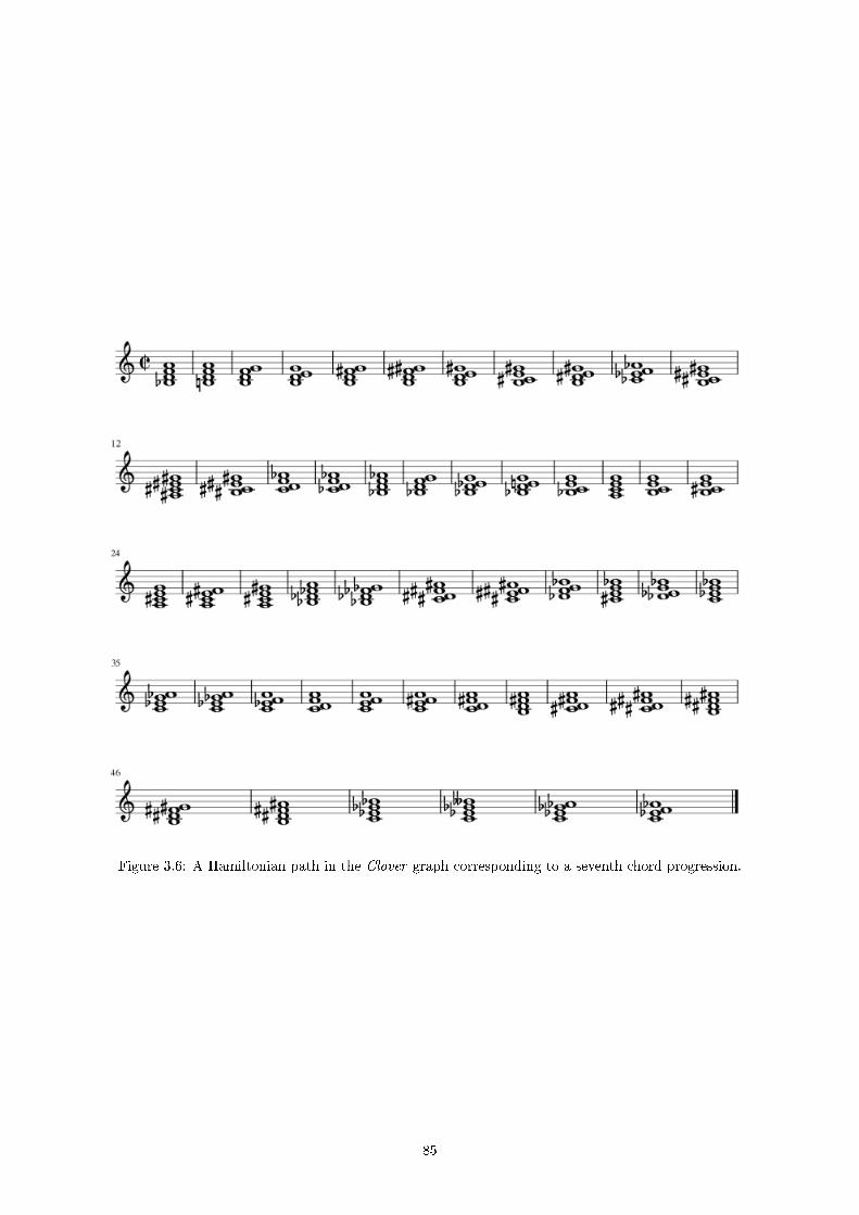
Figure 3.6: A Hamiltonian path in the Clover graph corresponding to a seventh chord progression.

85

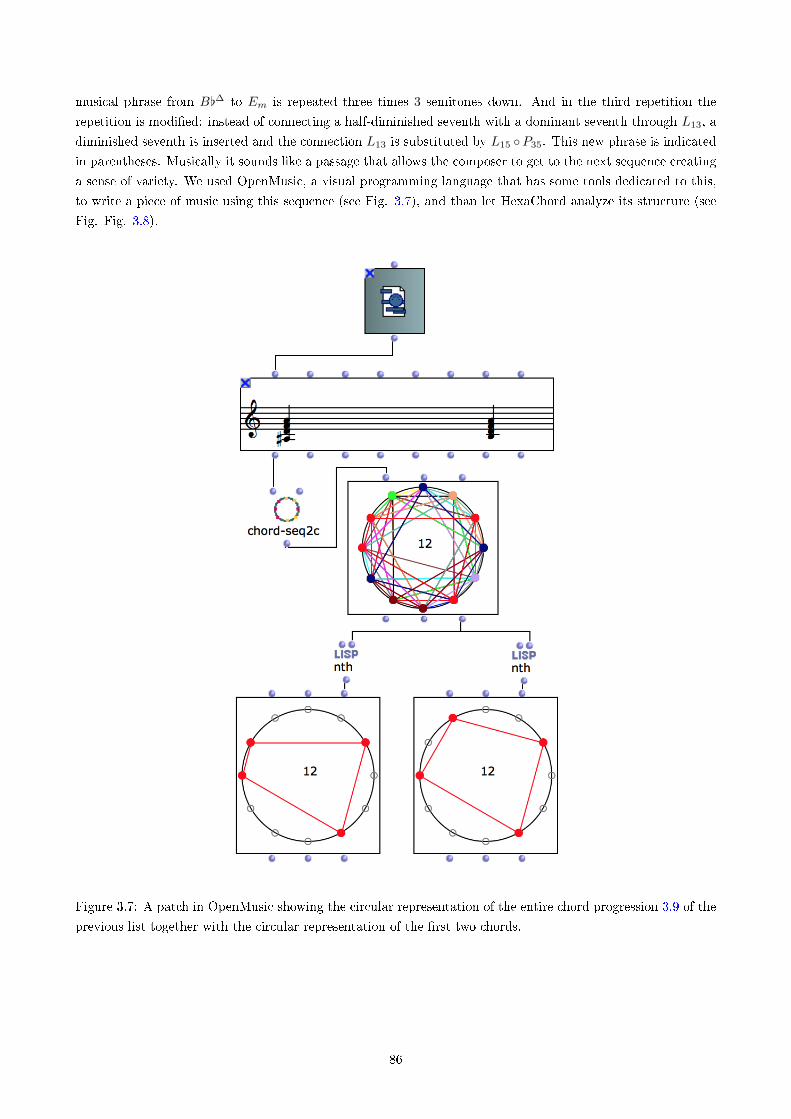
musical phrase from B[∆ to Em is repeated three times 3 semitones down. And in the third repetition the

repetition is modi�ed: instead of connecting a half-diminished seventh with a dominant seventh through L13, a

diminished seventh is inserted and the connection L13 is substituted by L15 ◦P35. This new phrase is indicated

in parentheses. Musically it sounds like a passage that allows the composer to get to the next sequence creating

a sense of variety. We used OpenMusic, a visual programming language that has some tools dedicated to this,

to write a piece of music using this sequence (see Fig. 3.7), and than let HexaChord analyze its structure (see

Fig. Fig. 3.8).

Figure 3.7: A patch in OpenMusic showing the circular representation of the entire chord progression 3.9 of the

previous list together with the circular representation of the �rst two chords.

86

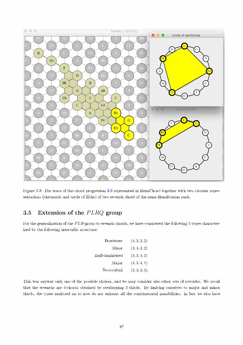
Figure 3.8: The trace of the chord progression 3.9 represented in HexaChord together with two circular repre-

sentations (chromatic and circle of �fths) of two seventh chord of the same Hamiltonian path.

3.5 Extension of the PLRQ group

For the generalization of the PLR-group to seventh chords, we have considered the following 5 types character-

ized by the following intervallic structure:

Dominant (4, 3, 3, 2)

Minor (3, 4, 3, 2)

Half-diminished (3, 3, 4, 2)

Major (4, 3, 4, 1)

Diminished (3, 3, 3, 3).

This was anyway only one of the possible choices, and we may consider also other sets of sevenths. We recall

that the sevenths are 4-chords obtained by overlapping 3 thirds. By limiting ourselves to major and minor

thirds, the types analyzed up to now do not exhaust all the combinatorial possibilities. In fact we also have

87

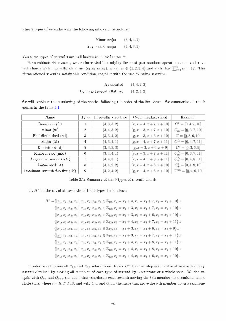
other 2 types of sevenths with the following intervallic structure:

Minor major (3, 4, 4, 1)

Augmented major (4, 4, 3, 1)

Also these types of sevenths are well known in music literature.

For combinatorial reasons, we are interested in studying the most parsimonious operations among all sev-

enth chords with intervallic structure (c1, c2, c3, c4), where ci ∈ {1, 2, 3, 4} and such that∑4i=1 ci = 12. The

aformentioned sevenths satisfy this condition, together with the two following sevenths:

Augmented (4, 4, 2, 2)

Dominant seventh �at �ve (4, 2, 4, 2)

We will continue the numbering of the species following the order of the list above. We summarize all the 9

species in the table 3.1.

Name Type Intervallic structure Cyclic marked chord Example

Dominant (D) 1 (4, 3, 3, 2) [x, x+ 4, x+ 7, x+ 10] C7 = [0, 4, 7, 10]

Minor (m) 2 (3, 4, 3, 2) [x, x+ 3, x+ 7, x+ 10] Cm = [0, 3, 7, 10]

Half-diminished (hd) 3 (3, 3, 4, 2) [x, x+ 3, x+ 6, x+ 10] C = [0, 3, 6, 10]

Major (M) 4 (4, 3, 4, 1) [x, x+ 4, x+ 7, x+ 11] C∆ = [0, 4, 7, 11]

Diminished (d) 5 (3, 3, 3, 3) [x, x+ 3, x+ 6, x+ 9] Co = [0, 3, 6, 9]

Minor major (mM) 6 (3, 4, 4, 1) [x, x+ 3, x+ 7, x+ 11] C∆m = [0, 3, 7, 11]

Augmented major (AM) 7 (4, 4, 3, 1) [x, x+ 4, x+ 8, x+ 11] C∆+ = [0, 4, 8, 11]

Augmented (A) 8 (4, 4, 2, 2) [x, x+ 4, x+ 8, x+ 10] C7+ = [0, 4, 8, 10]

Dominant seventh �at �ve (Df) 9 (4, 2, 4, 2) [x, x+ 4, x+ 6, x+ 10] C7[5 = [0, 4, 6, 10]

Table 3.1: Summary of the 9 types of seventh chords.

Let H∗ be the set of all sevenths of the 9 types listed above:

H∗ ={[x1, x2, x3, x4] |x1, x2, x3, x4 ∈ Z12, x2 = x1 + 4, x3 = x1 + 7, x4 = x1 + 10}∪








{[x1, x2, x3, x4] |x1, x2, x3, x4 ∈ Z12, x2 = x1 + 4, x3 = x1 + 6, x4 = x1 + 10}.

In order to determine all P1,0 and P0,1 relations on the set H∗, the �rst step is the exhaustive search of any

seventh obtained by moving all members of each type of seventh by a semitone or a whole tone. We denote

again with Qi+ and Qi++ the maps that transforms each seventh moving the i-th member up a semitone and a

whole tone, where i = R, T, F, S, and with Qi− and Qi−− the maps that move the i-th member down a semitone

88

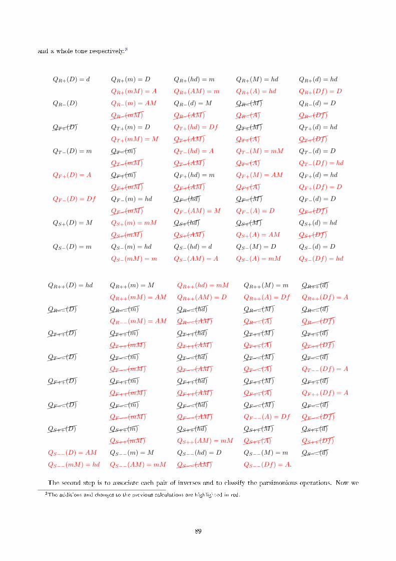
and a whole tone respectively.3

QR+(D) = d QR+(m) = D QR+(hd) = m QR+(M) = hd QR+(d) = hd

QR+(mM) = A QR+(AM) = m QR+(A) = hd QR+(Df) = D

QR−(D) QR−(m) = AM QR−(d) = M ��QR−(M) QR−(d) = D

��QR−(mM) ��

��QR−(AM) ��QR−(A) ��

��QR−(Df)

��QT+(D) QT+(m) = D QT+(hd) = Df ��

��QT+(M) QT+(d) = hd

QT+(mM) = M ��QT+(AM) ��

�QT+(A) ��QT+(Df)

QT−(D) = m ��QT−(m) QT−(hd) = A QT−(M) = mM QT−(d) = D

��QT−(mM) ��

��QT−(AM) ��QT−(A) QT−(Df) = hd

QF+(D) = A ��QF+(m) QF+(hd) = m QF+(M) = AM QF+(d) = hd

��QF+(mM) ��

��QF+(AM) ��QF+(A) QF+(Df) = D

QF−(D) = Df QF−(m) = hd ��QF−(hd) ��

��QF−(M) QF−(d) = D

��QF−(mM) QF−(AM) = M QF−(A) = D ��

��QF−(Df)

QS+(D) = M QS+(m) = mM ��QS+(hd) ��

��QS+(M) QS+(d) = hd

��QS+(mM) ��

��QS+(AM) QS+(A) = AM ��QS+(Df)

QS−(D) = m QS−(m) = hd QS−(hd) = d QS−(M) = D QS−(d) = D

QS−(mM) = m QS−(AM) = A QS−(A) = mM QS−(Df) = hd

QR++(D) = hd QR++(m) = M QR++(hd) = mM QR++(M) = m ��QR++(d)

QR++(mM) = AM QR++(AM) = D QR++(A) = Df QR++(Df) = A

��QR−−(D) ��

��QR−−(m) ��QR−−(hd) ��

��QR−−(M) ��QR−−(d)

QR−−(mM) = AM ((((((QR−−(AM) ��

��QR−−(A) ��

�QR−−(Df)

��QT++(D) ��

��QT++(m) ��QT++(hd) ��

��QT++(M) ��QT++(d)

((((((QT++(mM) ((((

((QT++(AM) ��QT++(A) ��

��QT++(Df)

��QT−−(D) ��

��QT−−(m) ��QT−−(hd) ��

��QT−−(M) ��QT−−(d)

((((((QT−−(mM) ((((

((QT−−(AM) ��QT−−(A) QT−−(Df) = A

��QF++(D) ��

��QF++(m) ��QF++(hd) ��

��QF++(M) ��QF++(d)

((((((QF++(mM) ((((

((QF++(AM) ��QF++(A) QF++(Df) = A

��QF−−(D) ��

��QF−−(m) ��QF−−(hd) ��

��QF−−(M) ��QF−−(d)

((((((QF−−(mM) ((((

((QF−−(AM) QF−−(A) = Df ��QF−−(Df)

��QS++(D) ��

��QS++(m) ��QS++(hd) ��

��QS++(M) ��QS++(d)

((((((QS++(mM) QS++(AM) = mM ��

��QS++(A) ��QS++(Df)

QS−−(D) = AM QS−−(m) = M QS−−(hd) = D QS−−(M) = m ��QS−−(d)

QS−−(mM) = hd QS−−(AM) = mM ((((((QS−−(AM) QS−−(Df) = A.

The second step is to associate each pair of inverses and to classify the parsimonious operations. Now we

3The additions and changes to the previous calculations are highlighted in red.

89

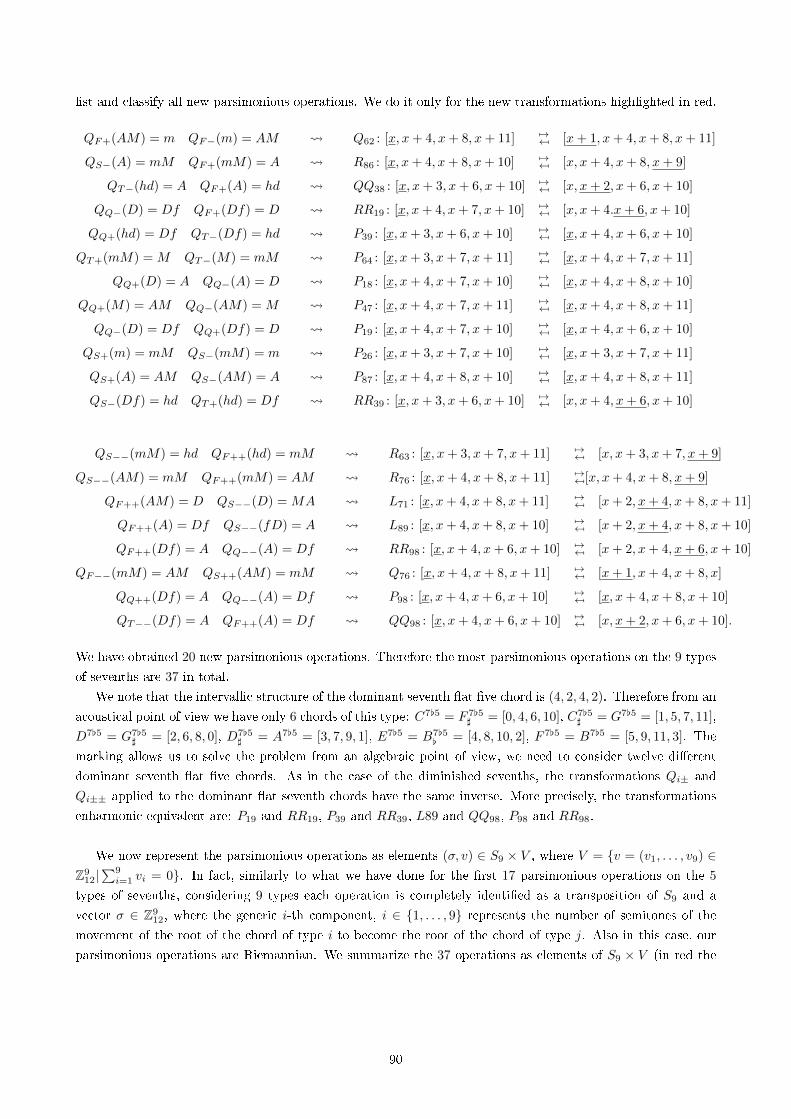
list and classify all new parsimonious operations. We do it only for the new transformations highlighted in red.

QF+(AM) = m QF−(m) = AM Q62 : [x, x+ 4, x+ 8, x+ 11] 7→7→ [x+ 1, x+ 4, x+ 8, x+ 11]

QS−(A) = mM QF+(mM) = A R86 : [x, x+ 4, x+ 8, x+ 10] 7→7→ [x, x+ 4, x+ 8, x+ 9]

QT−(hd) = A QF+(A) = hd QQ38 : [x, x+ 3, x+ 6, x+ 10] 7→7→ [x, x+ 2, x+ 6, x+ 10]

QQ−(D) = Df QF+(Df) = D RR19 : [x, x+ 4, x+ 7, x+ 10] 7→7→ [x, x+ 4.x+ 6, x+ 10]

QQ+(hd) = Df QT−(Df) = hd P39 : [x, x+ 3, x+ 6, x+ 10] 7→7→ [x, x+ 4, x+ 6, x+ 10]

QT+(mM) = M QT−(M) = mM P64 : [x, x+ 3, x+ 7, x+ 11] 7→7→ [x, x+ 4, x+ 7, x+ 11]

QQ+(D) = A QQ−(A) = D P18 : [x, x+ 4, x+ 7, x+ 10] 7→7→ [x, x+ 4, x+ 8, x+ 10]

QQ+(M) = AM QQ−(AM) = M P47 : [x, x+ 4, x+ 7, x+ 11] 7→7→ [x, x+ 4, x+ 8, x+ 11]

QQ−(D) = Df QQ+(Df) = D P19 : [x, x+ 4, x+ 7, x+ 10] 7→7→ [x, x+ 4, x+ 6, x+ 10]

QS+(m) = mM QS−(mM) = m P26 : [x, x+ 3, x+ 7, x+ 10] 7→7→ [x, x+ 3, x+ 7, x+ 11]

QS+(A) = AM QS−(AM) = A P87 : [x, x+ 4, x+ 8, x+ 10] 7→7→ [x, x+ 4, x+ 8, x+ 11]

QS−(Df) = hd QT+(hd) = Df RR39 : [x, x+ 3, x+ 6, x+ 10] 7→7→ [x, x+ 4, x+ 6, x+ 10]

QS−−(mM) = hd QF++(hd) = mM R63 : [x, x+ 3, x+ 7, x+ 11] 7→7→ [x, x+ 3, x+ 7, x+ 9]

QS−−(AM) = mM QF++(mM) = AM R76 : [x, x+ 4, x+ 8, x+ 11] 7→7→[x, x+ 4, x+ 8, x+ 9]

QF++(AM) = D QS−−(D) = MA L71 : [x, x+ 4, x+ 8, x+ 11] 7→7→ [x+ 2, x+ 4, x+ 8, x+ 11]

QF++(A) = Df QS−−(fD) = A L89 : [x, x+ 4, x+ 8, x+ 10] 7→7→ [x+ 2, x+ 4, x+ 8, x+ 10]

QF++(Df) = A QQ−−(A) = Df RR98 : [x, x+ 4, x+ 6, x+ 10] 7→7→ [x+ 2, x+ 4, x+ 6, x+ 10]

QF−−(mM) = AM QS++(AM) = mM Q76 : [x, x+ 4, x+ 8, x+ 11] 7→7→ [x+ 1, x+ 4, x+ 8, x]

QQ++(Df) = A QQ−−(A) = Df P98 : [x, x+ 4, x+ 6, x+ 10] 7→7→ [x, x+ 4, x+ 8, x+ 10]

QT−−(Df) = A QF++(A) = Df QQ98 : [x, x+ 4, x+ 6, x+ 10] 7→7→ [x, x+ 2, x+ 6, x+ 10].

We have obtained 20 new parsimonious operations. Therefore the most parsimonious operations on the 9 types

of sevenths are 37 in total.

We note that the intervallic structure of the dominant seventh �at �ve chord is (4, 2, 4, 2). Therefore from an

acoustical point of view we have only 6 chords of this type: C7[5 = F 7[5] = [0, 4, 6, 10], C7[5

] = G7[5 = [1, 5, 7, 11],

D7[5 = G7[5] = [2, 6, 8, 0], D7[5

] = A7[5 = [3, 7, 9, 1], E7[5 = B7[5[ = [4, 8, 10, 2], F 7[5 = B7[5 = [5, 9, 11, 3]. The

marking allows us to solve the problem from an algebraic point of view, we need to consider twelve di�erent

dominant seventh �at �ve chords. As in the case of the diminished sevenths, the transformations Qi± and

Qi±± applied to the dominant �at seventh chords have the same inverse. More precisely, the transformations

enharmonic equivalent are: P19 and RR19, P39 and RR39, L89 and QQ98, P98 and RR98.

We now represent the parsimonious operations as elements (σ, v) ∈ S9 × V , where V = {v = (v1, . . . , v9) ∈Z9

12|∑9i=1 vi = 0}. In fact, similarly to what we have done for the �rst 17 parsimonious operations on the 5

types of sevenths, considering 9 types each operation is completely identi�ed as a transposition of S9 and a

vector σ ∈ Z912, where the generic i-th component, i ∈ {1, . . . , 9} represents the number of semitones of the

movement of the root of the chord of type i to become the root of the chord of type j. Also in this case, our

parsimonious operations are Riemannian. We summarize the 37 operations as elements of S9 × V (in red the

90

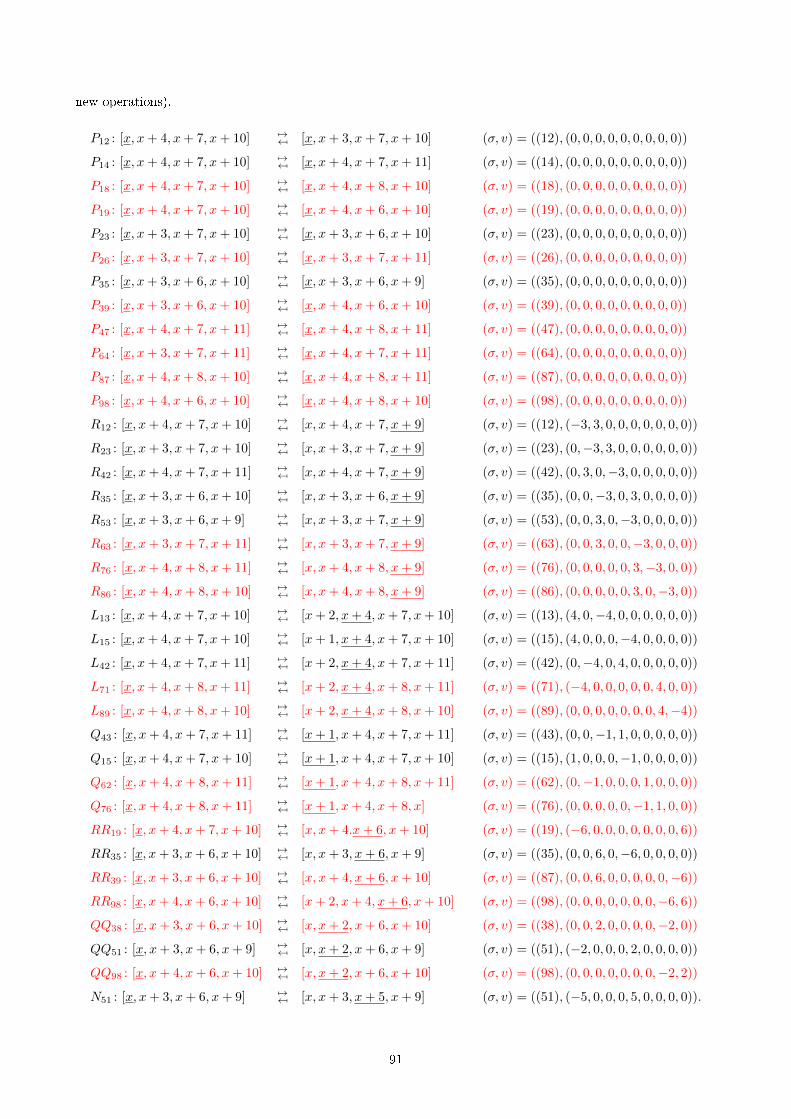
new operations).

P12 : [x, x+ 4, x+ 7, x+ 10] 7→7→ [x, x+ 3, x+ 7, x+ 10] (σ, v) = ((12), (0, 0, 0, 0, 0, 0, 0, 0, 0))

P14 : [x, x+ 4, x+ 7, x+ 10] 7→7→ [x, x+ 4, x+ 7, x+ 11] (σ, v) = ((14), (0, 0, 0, 0, 0, 0, 0, 0, 0))

P18 : [x, x+ 4, x+ 7, x+ 10] 7→7→ [x, x+ 4, x+ 8, x+ 10] (σ, v) = ((18), (0, 0, 0, 0, 0, 0, 0, 0, 0))

P19 : [x, x+ 4, x+ 7, x+ 10] 7→7→ [x, x+ 4, x+ 6, x+ 10] (σ, v) = ((19), (0, 0, 0, 0, 0, 0, 0, 0, 0))

P23 : [x, x+ 3, x+ 7, x+ 10] 7→7→ [x, x+ 3, x+ 6, x+ 10] (σ, v) = ((23), (0, 0, 0, 0, 0, 0, 0, 0, 0))

P26 : [x, x+ 3, x+ 7, x+ 10] 7→7→ [x, x+ 3, x+ 7, x+ 11] (σ, v) = ((26), (0, 0, 0, 0, 0, 0, 0, 0, 0))

P35 : [x, x+ 3, x+ 6, x+ 10] 7→7→ [x, x+ 3, x+ 6, x+ 9] (σ, v) = ((35), (0, 0, 0, 0, 0, 0, 0, 0, 0))

P39 : [x, x+ 3, x+ 6, x+ 10] 7→7→ [x, x+ 4, x+ 6, x+ 10] (σ, v) = ((39), (0, 0, 0, 0, 0, 0, 0, 0, 0))

P47 : [x, x+ 4, x+ 7, x+ 11] 7→7→ [x, x+ 4, x+ 8, x+ 11] (σ, v) = ((47), (0, 0, 0, 0, 0, 0, 0, 0, 0))

P64 : [x, x+ 3, x+ 7, x+ 11] 7→7→ [x, x+ 4, x+ 7, x+ 11] (σ, v) = ((64), (0, 0, 0, 0, 0, 0, 0, 0, 0))

P87 : [x, x+ 4, x+ 8, x+ 10] 7→7→ [x, x+ 4, x+ 8, x+ 11] (σ, v) = ((87), (0, 0, 0, 0, 0, 0, 0, 0, 0))

P98 : [x, x+ 4, x+ 6, x+ 10] 7→7→ [x, x+ 4, x+ 8, x+ 10] (σ, v) = ((98), (0, 0, 0, 0, 0, 0, 0, 0, 0))

R12 : [x, x+ 4, x+ 7, x+ 10] 7→7→ [x, x+ 4, x+ 7, x+ 9] (σ, v) = ((12), (−3, 3, 0, 0, 0, 0, 0, 0, 0))

R23 : [x, x+ 3, x+ 7, x+ 10] 7→7→ [x, x+ 3, x+ 7, x+ 9] (σ, v) = ((23), (0,−3, 3, 0, 0, 0, 0, 0, 0))

R42 : [x, x+ 4, x+ 7, x+ 11] 7→7→ [x, x+ 4, x+ 7, x+ 9] (σ, v) = ((42), (0, 3, 0,−3, 0, 0, 0, 0, 0))

R35 : [x, x+ 3, x+ 6, x+ 10] 7→7→ [x, x+ 3, x+ 6, x+ 9] (σ, v) = ((35), (0, 0,−3, 0, 3, 0, 0, 0, 0))

R53 : [x, x+ 3, x+ 6, x+ 9] 7→7→ [x, x+ 3, x+ 7, x+ 9] (σ, v) = ((53), (0, 0, 3, 0,−3, 0, 0, 0, 0))

R63 : [x, x+ 3, x+ 7, x+ 11] 7→7→ [x, x+ 3, x+ 7, x+ 9] (σ, v) = ((63), (0, 0, 3, 0, 0,−3, 0, 0, 0))

R76 : [x, x+ 4, x+ 8, x+ 11] 7→7→ [x, x+ 4, x+ 8, x+ 9] (σ, v) = ((76), (0, 0, 0, 0, 0, 3,−3, 0, 0))

R86 : [x, x+ 4, x+ 8, x+ 10] 7→7→ [x, x+ 4, x+ 8, x+ 9] (σ, v) = ((86), (0, 0, 0, 0, 0, 3, 0,−3, 0))

L13 : [x, x+ 4, x+ 7, x+ 10] 7→7→ [x+ 2, x+ 4, x+ 7, x+ 10] (σ, v) = ((13), (4, 0,−4, 0, 0, 0, 0, 0, 0))

L15 : [x, x+ 4, x+ 7, x+ 10] 7→7→ [x+ 1, x+ 4, x+ 7, x+ 10] (σ, v) = ((15), (4, 0, 0, 0,−4, 0, 0, 0, 0))

L42 : [x, x+ 4, x+ 7, x+ 11] 7→7→ [x+ 2, x+ 4, x+ 7, x+ 11] (σ, v) = ((42), (0,−4, 0, 4, 0, 0, 0, 0, 0))

L71 : [x, x+ 4, x+ 8, x+ 11] 7→7→ [x+ 2, x+ 4, x+ 8, x+ 11] (σ, v) = ((71), (−4, 0, 0, 0, 0, 0, 4, 0, 0))

L89 : [x, x+ 4, x+ 8, x+ 10] 7→7→ [x+ 2, x+ 4, x+ 8, x+ 10] (σ, v) = ((89), (0, 0, 0, 0, 0, 0, 0, 4,−4))

Q43 : [x, x+ 4, x+ 7, x+ 11] 7→7→ [x+ 1, x+ 4, x+ 7, x+ 11] (σ, v) = ((43), (0, 0,−1, 1, 0, 0, 0, 0, 0))

Q15 : [x, x+ 4, x+ 7, x+ 10] 7→7→ [x+ 1, x+ 4, x+ 7, x+ 10] (σ, v) = ((15), (1, 0, 0, 0,−1, 0, 0, 0, 0))

Q62 : [x, x+ 4, x+ 8, x+ 11] 7→7→ [x+ 1, x+ 4, x+ 8, x+ 11] (σ, v) = ((62), (0,−1, 0, 0, 0, 1, 0, 0, 0))

Q76 : [x, x+ 4, x+ 8, x+ 11] 7→7→ [x+ 1, x+ 4, x+ 8, x] (σ, v) = ((76), (0, 0, 0, 0, 0,−1, 1, 0, 0))

RR19 : [x, x+ 4, x+ 7, x+ 10] 7→7→ [x, x+ 4.x+ 6, x+ 10] (σ, v) = ((19), (−6, 0, 0, 0, 0, 0, 0, 0, 6))

RR35 : [x, x+ 3, x+ 6, x+ 10] 7→7→ [x, x+ 3, x+ 6, x+ 9] (σ, v) = ((35), (0, 0, 6, 0,−6, 0, 0, 0, 0))

RR39 : [x, x+ 3, x+ 6, x+ 10] 7→7→ [x, x+ 4, x+ 6, x+ 10] (σ, v) = ((87), (0, 0, 6, 0, 0, 0, 0, 0,−6))

RR98 : [x, x+ 4, x+ 6, x+ 10] 7→7→ [x+ 2, x+ 4, x+ 6, x+ 10] (σ, v) = ((98), (0, 0, 0, 0, 0, 0, 0,−6, 6))

QQ38 : [x, x+ 3, x+ 6, x+ 10] 7→7→ [x, x+ 2, x+ 6, x+ 10] (σ, v) = ((38), (0, 0, 2, 0, 0, 0, 0,−2, 0))

QQ51 : [x, x+ 3, x+ 6, x+ 9] 7→7→ [x, x+ 2, x+ 6, x+ 9] (σ, v) = ((51), (−2, 0, 0, 0, 2, 0, 0, 0, 0))

QQ98 : [x, x+ 4, x+ 6, x+ 10] 7→7→ [x, x+ 2, x+ 6, x+ 10] (σ, v) = ((98), (0, 0, 0, 0, 0, 0, 0,−2, 2))

N51 : [x, x+ 3, x+ 6, x+ 9] 7→7→ [x, x+ 3, x+ 5, x+ 9] (σ, v) = ((51), (−5, 0, 0, 0, 5, 0, 0, 0, 0)).

91

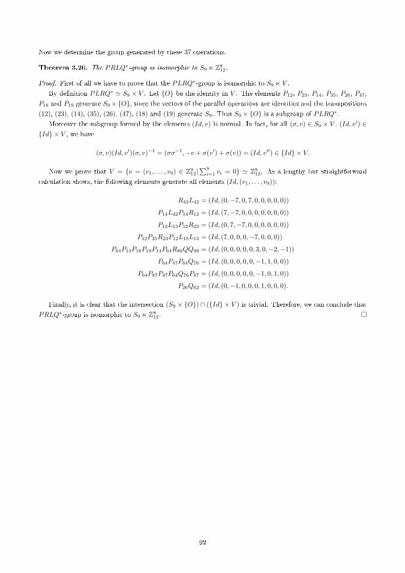
Now we determine the group generated by these 37 operations.

Theorem 3.20. The PRLQ∗-group is isomorphic to S9 n Z812.

Proof. First of all we have to prove that the PLRQ∗-group is isomorphic to S9 n V .

By de�nition PLRQ∗ ' S9 × V . Let {O} be the identity in V . The elements P12, P23, P14, P35, P26, P47,

P18 and P19 generate S9×{O}, since the vectors of the parallel operations are identities and the transpositions

(12), (23), (14), (35), (26), (47), (18) and (19) generate S9. Thus S9 × {O} is a subgroup of PLRQ∗.

Moreover the subgroup formed by the elements (Id, v) is normal. In fact, for all (σ, v) ∈ S9 × V , (Id, v′) ∈{Id} × V , we have

(σ, v)(Id, v′)(σ, v)−1 = (σσ−1,−v + σ(v′) + σ(v)) = (Id, v′′) ∈ {Id} × V.

Now we prove that V = {v = (v1, . . . , v9) ∈ Z912|∑9i=1 vi = 0} ' Z8

12. As a lengthy but straightforward

calculation shows, the following elements generate all elements (Id, (v1, . . . , v9)):

R42L42 = (Id, (0,−7, 0, 7, 0, 0, 0, 0, 0))

P14L42P14R12 = (Id, (7,−7, 0, 0, 0, 0, 0, 0, 0))

P12L13P12R23 = (Id, (0, 7,−7, 0, 0, 0, 0, 0, 0))

P12P35R23P12L15L13 = (Id, (7, 0, 0, 0,−7, 0, 0, 0))

P64P14P18P19P14P64R86QQ98 = (Id, (0, 0, 0, 0, 0, 3, 0,−2,−1))

P64P47P64Q76 = (Id, (0, 0, 0, 0, 0,−1, 1, 0, 0))

P64P87P47P64Q76P87 = (Id, (0, 0, 0, 0, 0,−1, 0, 1, 0))

P26Q62 = (Id, (0,−1, 0, 0, 0, 1, 0, 0, 0).

Finally, it is clear that the intersection (S9 × {O}) ∩ ({Id} × V ) is trivial. Therefore, we can conclude that

PRLQ∗-group is isomorphic to S9 n Z812.

92

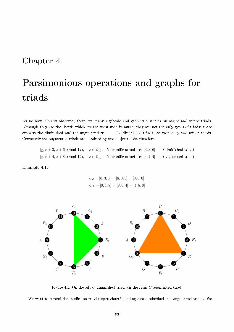
Chapter 4

Parsimonious operations and graphs for

triads

As we have already observed, there are many algebraic and geometric studies on major and minor triads.

Although they are the chords which are the most used in music, they are not the only types of triads: there

are also the diminished and the augmented triads. The diminished triads are formed by two minor thirds.

Conversely the augmented triads are obtained by two major thirds, therefore:

[x, x+ 3, x+ 6] (mod 12), x ∈ Z12, intervallic structure: [3, 3, 6] (diminished triad)

[x, x+ 4, x+ 8] (mod 12), x ∈ Z12, intervallic structure: [4, 4, 4] (augmented triad)

Example 4.1.

Cd = [0, 3, 6] = [6, 0, 3] = [3, 6, 0]

CA = [0, 4, 8] = [8, 0, 4] = [4, 8, 0]

..

.

.

.

..

.

.

.

.

..

.

.

.

.

..

.

.

.

.

.

CC]

D

E[

E

FF]

G

G]

A

B[

B0

1

2

3

4

56

7

8

9

10

11.

.

.

.

.

..

.

.

.

.

..

.

.

.

.

..

.

.

.

.

.

CC]

D

E[

E

FF]

G

G]

A

B[

B0

1

2

3

4

56

7

8

9

10

11

Figure 4.1: On the left C diminished triad, on the right C augmented triad.

We want to extend the studies on triadic operations including also diminished and augmented triads. We

93

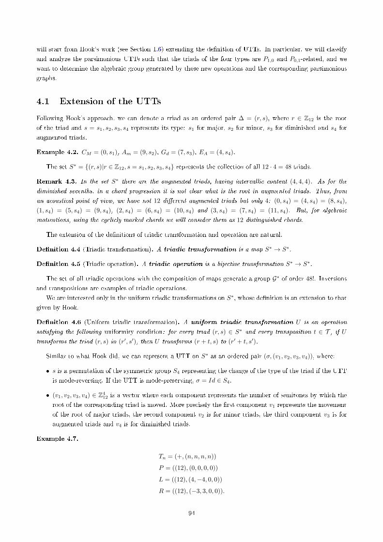
will start from Hook's work (see Section 1.6) extending the de�nition of UTTs. In particular, we will classify

and analyze the parsimonious UTTs such that the triads of the four types are P1,0 and P0,1-related, and we

want to determine the algebraic group generated by these new operations and the corresponding parsimonious

graphs.

4.1 Extension of the UTTs

Following Hook's approach, we can denote a triad as an ordered pair ∆ = (r, s), where r ∈ Z12 is the root

of the triad and s = s1, s2, s3, s4 represents its type: s1 for major, s2 for minor, s3 for diminished and s4 for

augmented triads.

Example 4.2. CM = (0, s1), Am = (9, s2), Gd = (7, s3), EA = (4, s4).

The set S∗ = {(r, s)|r ∈ Z12, s = s1, s2, s3, s4} represents the collection of all 12 · 4 = 48 triads.

Remark 4.3. In the set S∗ there are the augmented triads, having intervallic content (4, 4, 4). As for the

diminished sevenths, in a chord progression it is not clear what is the root in augmented triads. Thus, from

an acoustical point of view, we have not 12 di�erent augmented triads but only 4: (0, s4) = (4, s4) = (8, s4),

(1, s4) = (5, s4) = (9, s4), (2, s4) = (6, s4) = (10, s4) and (3, s4) = (7, s4) = (11, s4). But, for algebraic

motivations, using the cyclicly marked chords we will consider them as 12 distinguished chords.

The extension of the de�nitions of triadic transformation and operation are natural.

De�nition 4.4 (Triadic transformation). A triadic transformation is a map S∗ → S∗.

De�nition 4.5 (Triadic operation). A triadic operation is a bijective transformation S∗ → S∗.

The set of all triadic operations with the composition of maps generate a group G∗ of order 48!. Inversions

and transpositions are examples of triadic operations.

We are interested only in the uniform triadic transformations on S∗, whose de�nition is an extension to that

given by Hook.

De�nition 4.6 (Uniform triadic transformation). A uniform triadic transformation U is an operation

satisfying the following uniformity condition: for every triad (r, s) ∈ S∗ and every transposition t ∈ T , if Utransforms the triad (r, s) in (r′, s′), then U transforms (r + t, s) to (r′ + t, s′).

Similar to what Hook did, we can represent a UTT on S∗ as an ordered pair (σ, (v1, v2, v3, v4)), where:

� s is a permutation of the symmetric group S4 representing the change of the type of the triad if the UTT

is mode-reversing. If the UTT is mode-preserving, σ = Id ∈ S4.

� (v1, v2, v3, v4) ∈ Z412 is a vector where each component represents the number of semitones by which the

root of the corresponding triad is moved. More precisely the �rst component v1 represents the movement

of the root of major triads, the second component v2 is for minor triads, the third component v3 is for

augmented triads and v4 is for diminished triads.

Example 4.7.

Tn = (+, (n, n, n, n))

P = ((12), (0, 0, 0, 0))

L = ((12), (4,−4, 0, 0))

R = ((12), (−3, 3, 0, 0)).

94

We observe that we can extend the neo-Riemannian P , L and R operations to diminished and augmented triads

de�ning it as the identity on these two types of triads. In fact, for example

R : (s1, x) 7→ (s2, x− 3) if the triad is major

R : (s2, x) 7→ (s1, x+ 3) if the triad is minor

R : (s3, x) 7→ (s3, x) if the triad is diminished

R : (s4, x) 7→ (s4, x) if the triad is augmented.

Let U∗ be the set of all UTTs. Since each UTT can be represented as (σ, (v1, v2, v3, v4)) ∈ S5 × Z412, the

order of U∗ is 120× 124 = 2488320.

Now we describe the actions of UTTs on triads. Let U = (σ, (v1, v2, v3, v4)) be a UTT and let ∆ = (r, s)

be a triad. U acts on ∆ transposing its root by v1 if s = s1, by v2 if s = s2, by v3 if s = s3, by v4 if s = s4.

Moreover, depending on the permutation σ ∈ S4, U can leave or change the type of the chord. More precisely:

U(∆) = (r + vi, sσ(i)). (4.1)

Example 4.8. Let U = ((132), (2, 5, 4, 0)) be a UTT and let ∆ = Gd = (7, s3) be a diminished triad. We apply

U to ∆:

U(∆) = U(7, s3) = (7 + 4, sσ(3)) = (11, s2) = Bm.

The product formula for the UTTs on S∗ is the same de�ned in 3.7:

(σk, vk) ◦ · · · ◦ (σ1, v1) =

=(σk · · ·σ1, v1 + σ−1

1 (v2) + (σ2σ1)−1(v3) + · · ·+ (σk−1 · · ·σ1)−1(vk))

= (4.2)

=(σk · · ·σ1, v1 + σ−1

1 (v2) + σ−11 σ−1

2 (v3) + · · ·+ σ−11 · · · ) (4.3)

Example 4.9. Let U = (Id, (4, 7, 0, 0)), V = ((12), (5, 10, 0, 0)) and W = ((23, (0, 5, 4, 0)). Their product is

WV U = ((23), (0, 5, 4, 0)) ◦ ((12), (5, 10, 0, 0)) ◦ (Id, (4, 7, 0, 0)) =

= ((23) ◦ (12), (4, 7, 0, 0) + (5, 10, 0, 0) + (5, 0, 4, 0)) =

= ((132), (2, 5, 4, 0)).

In fact, if we consider DM = (2, s1), Em = (4, s2), Gd = (7, s3) and BA = (11, s4) and if we apply U , V and W

W (V (U(DM ))) = W (V (6, s1)) = W (11, s2) = (4, s3)

W (V (U(Em))) = W (V (11, s2)) = W (9, s1) = (9, s1)

W (V (U(Gd))) = W (V (7, s3)) = W (7, s3) = (11, s2)

W (V (U(BA))) = W (V (11, s4)) = W (11, s4) = (11, s4).

We obtain the same results applying directly WV U

(WV U)(DM ) = (4, s3)

(WV U)(Em) = (9, s1)

(WV U)(Gd) = (11, s2)

(WV U)(BA) = (11, s4).

95

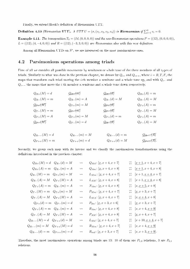
Finally, we extend Hook's de�nition of Riemannian UTT.

De�nition 4.10 (Riemannian UTT). A UTT U = (σ, (v1, v2, v3, v4)) is Riemannian if∑4i=1 vi = 0.

Example 4.11. The transposition T0 = (Id, (0, 0, 0, 0)) and the neo-Riemannian operations P = ((12), (0, 0, 0, 0)),

L = ((12), (4,−4, 0, 0)) and R = ((12), (−3, 3, 0, 0)) are Riemannian also with this new de�nition.

Among all Riemannian UTTs on S∗, we are interested on the most parsimonious ones.

4.2 Parsimonious operations among triads

First of all we consider all possible movements by semitones or whole tone of the three members of all types of

triads. Similarly to what was done in the previous chapter, we denote by Qi+ and Qi++, where i = R, T, F , the

maps that transform each triad moving the i-th member a semitone and a whole tone up, and with Qi− and

Qi−− the maps that move the i-th member a semitone and a whole tone down respectively.

QR+(M) = d ��QR+(m) ��

�QR+(d) QR+(A) = m

QR−(M) = m QR−(m) = A QR−(d) = M QR−(A) = M

��QT+(M) QT+(m) = M ��

�QT+(d) QT+(A) = m

QT−(M) = m ��QT−(m) ��

�QT−(d) QT−(A) = M

QF+(M) = A QF+(m) = M QF+(d) = m QF+(A) = m

��QF−(M) QF−(m) = d ��

��QR−(d) QF−(A) = M

QR−−(M) = d QR−−(m) = M QR−−(d) = m ��QR−−(A)

QF++(M) = m QF++(m) = d QF++(d) = M ��QF++(A).

Secondly, we group each map with its inverse and we classify the parsimonious transformations using the

de�nitions introduced in the previous chapter:

QR+(M) = d QR−(d) = M QMd : [x, x+ 4, x+ 7] 7→7→ [x+ 1, x+ 4, x+ 7]

QR+(A) = m QR−(m) = A QAm : [x, x+ 4, x+ 8] 7→7→ [x+ 1, x+ 4, x+ 8]

QR−(M) = m QF+(m) = M LMm : [x, x+ 4, x+ 7] 7→7→ [x+ 1, x+ 4, x+ 7]

QR−(A) = M QF+(M) = A LAM : [x, x+ 4, x+ 8] 7→7→ [x+ 1, x+ 4, x+ 8]

QT+(A) = m QR−(m) = A NAm : [x, x+ 4, x+ 8] 7→7→ [x, x+ 5, x+ 8]

QT−(M) = m QT+(m) = M PMm : [x, x+ 4, x+ 7] 7→7→ [x, x+ 3, x+ 7]

QT−(A) = M QF+(M) = A LMA : [x, x+ 4, x+ 7] 7→7→ [x, x+ 4, x+ 8]

QF+(d) = m QF−(m) = d Pdm : [x, x+ 3, x+ 6] 7→7→ [x, x+ 3, x+ 7]

QF+(A) = m QR−(m) = A RAm : [x, x+ 4, x+ 8] 7→7→ [x, x+ 4, x+ 9]

QF−(A) = M QF+(M) = A PAM : [x, x+ 4, x+ 8] 7→7→ [x, x+ 4, x+ 7]

QR−−(M) = d QF++(d) = M LMd : [x, x+ 4, x+ 7] 7→7→ [x+ 10, x+ 4, x+ 7]

QR−−(m) = M QF++(M) = d RMm : [x, x+ 4, x+ 7] 7→7→ [x, x+ 4, x+ 9]

QR−−(d) = m QF++(m) = d Rmd : [x, x+ 3, x+ 7] 7→7→ [x, x+ 3, x+ 9].

Therefore, the most parsimonious operations among triads are 13: 10 of them are P1,0 relations, 3 are P0,1

relations.

96

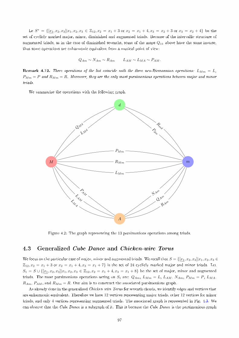
Le S∗ = {[x1, x2, x3]|x1, x2, x3 ∈ Z12, x2 = x1 + 3 or x2 = x1 + 4, x3 = x2 + 3 or x3 = x2 + 4} be the

set of cyclicly marked major, minor, diminished and augmented triads. Because of the intervallic structure of

augmented triads, as in the case of diminished sevenths, some of the maps Qi± above have the same inverse,

thus some operations are enharmonic equivalent from a musical point of view:

QAm ∼ NAm ∼ RAm LAM ∼ LMA ∼ PAM .

Remark 4.12. Three operations of the list coincide with the three neo-Riemannian operations: LMm = L,

PMm = P and RMm = R. Moreover, they are the only most parsimonious operations between major and minor

triads.

We summarize the operations with the following graph.

M m

d

A

PMm

RMm

LMm

PAML

AML

MA

NAm

QAm

RAm

Pdm

Rmd

LMd

QMd

Figure 4.2: The graph representing the 13 parsimonious operations among triads.

4.3 Generalized Cube Dance and Chicken-wire Torus

We focus on the particular case of major, minor and augmented triads. We recall that S = {[x1, x2, x3]|x1, x2, x3 ∈Z12, x2 = x1 + 3 or x2 = x1 + 4, x3 = x1 + 7} is the set of 24 cyclicly marked major and minor triads. Let

S1 = S ∪ {[x1, x2, x3]|x1, x2, x3 ∈ Z12, x2 = x1 + 4, x3 = x1 + 8} be the set of major, minor and augmented

triads. The most parsimonious operations acting on S1 are: QAm, LMm = L, LAM , NAm, PMm = P , LMA,

RAm, PAM , and RMm = R. Our aim is to construct the associated parsimonious graph.

As already done in the generalized Chicken-wire Torus for seventh chords, we identify edges and vertices that

are enharmonic equivalent. Therefore we have 12 vertices representing major triads, other 12 vertices for minor

triads, and only 4 vertices representing augmented triads. The associated graph is represented in Fig. 4.3. We

can observe that the Cube Dance is a subgraph of it. This is because the Cube Dance is the parsimonious graph

97

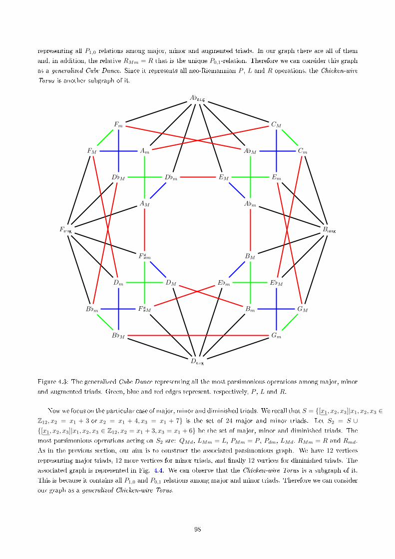
representing all P1,0 relations among major, minor and augmented triads. In our graph there are all of them

and, in addition, the relative RMm = R that is the unique P0,1-relation. Therefore we can consider this graph

as a generalized Cube Dance. Since it represents all neo-Riemannian P , L and R operations, the Chicken-wire

Torus is another subgraph of it.

CM

Cm

EmEM

A[m

A[M

Fm

FM

D[M D[m

AM

Am

B[M

B[m

Dm DM

F]m

F]M

Gm

GM

E[ME[m

BM

Bm

Faug Baug

A[aug

Daug

Figure 4.3: The generalized Cube Dance representing all the most parsimonious operations among major, minor

and augmented triads. Green, blue and red edges represent, respectively, P , L and R.

Now we focus on the particular case of major, minor and diminished triads. We recall that S = {[x1, x2, x3]|x1, x2, x3 ∈Z12, x2 = x1 + 3 or x2 = x1 + 4, x3 = x1 + 7} is the set of 24 major and minor triads. Let S2 = S ∪{[x1, x2, x3]|x1, x2, x3 ∈ Z12, x2 = x1 + 3, x3 = x1 + 6} be the set of major, minor and diminished triads. The

most parsimonious operations acting on S2 are: QMd, LMm = L, PMm = P , Pdm, LMd, RMm = R and Rmd.

As in the previous section, our aim is to construct the associated parsimonious graph. We have 12 vertices

representing major triads, 12 more vertices for minor triads, and �nally 12 vertices for diminished triads. The

associated graph is represented in Fig. 4.4. We can observe that the Chicken-wire Torus is a subgraph of it.

This is because it contains all P1,0 and P0,1 relations among major and minor triads. Therefore we can consider

our graph as a generalized Chicken-wire Torus.

98

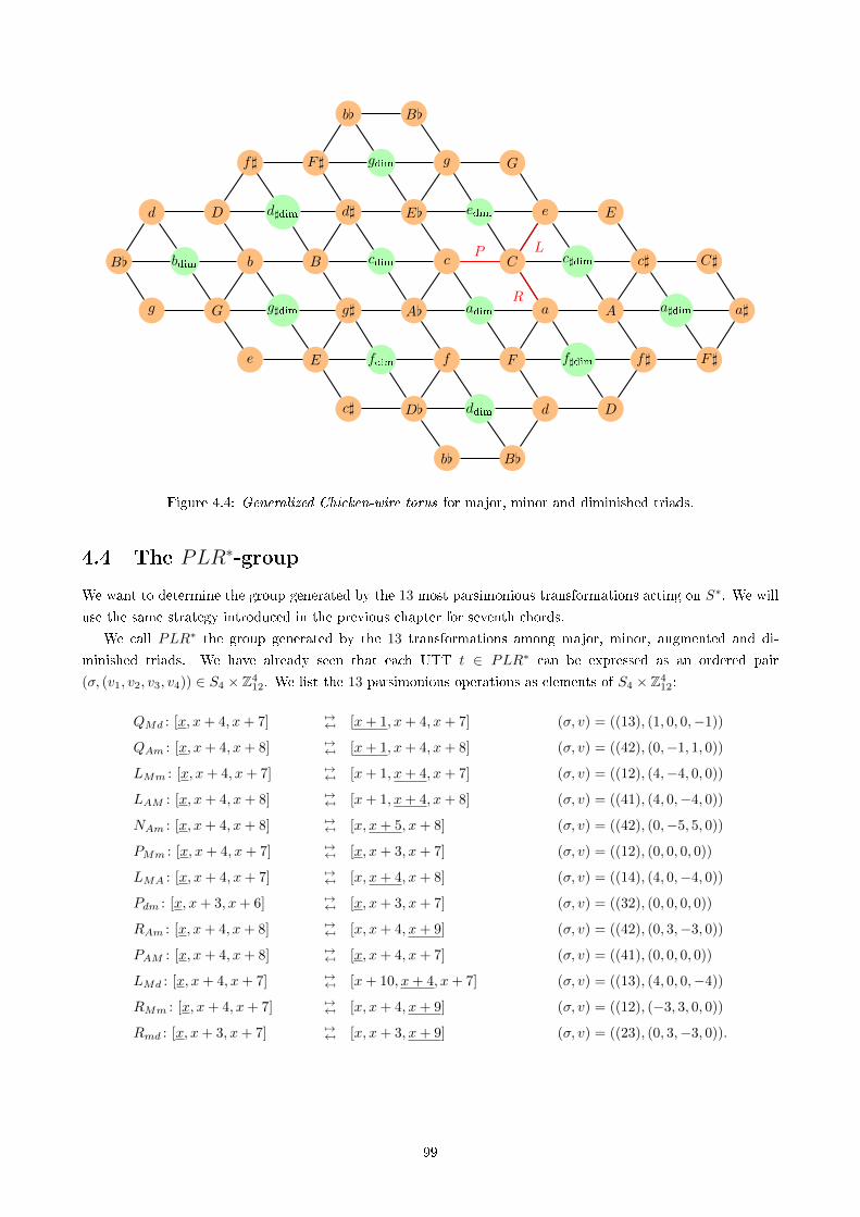
b[ B[

d

Ff

D[ ddimc]

E

g] A[

fdime

G

b B

g]dimg

B[

d D

bdim

f] F]

d]d]dim E[

ccdim C

aadim A

f]

D

f]dim F]

a]

C]c]

a]dim

Ee

c]dim

Gg

edim

B[b[

gdim

P

R

L

Figure 4.4: Generalized Chicken-wire torus for major, minor and diminished triads.

4.4 The PLR∗-group

We want to determine the group generated by the 13 most parsimonious transformations acting on S∗. We will

use the same strategy introduced in the previous chapter for seventh chords.

We call PLR∗ the group generated by the 13 transformations among major, minor, augmented and di-

minished triads. We have already seen that each UTT t ∈ PLR∗ can be expressed as an ordered pair

(σ, (v1, v2, v3, v4)) ∈ S4 × Z412. We list the 13 parsimonious operations as elements of S4 × Z4

12:

QMd : [x, x+ 4, x+ 7] 7→7→ [x+ 1, x+ 4, x+ 7] (σ, v) = ((13), (1, 0, 0,−1))

QAm : [x, x+ 4, x+ 8] 7→7→ [x+ 1, x+ 4, x+ 8] (σ, v) = ((42), (0,−1, 1, 0))

LMm : [x, x+ 4, x+ 7] 7→7→ [x+ 1, x+ 4, x+ 7] (σ, v) = ((12), (4,−4, 0, 0))

LAM : [x, x+ 4, x+ 8] 7→7→ [x+ 1, x+ 4, x+ 8] (σ, v) = ((41), (4, 0,−4, 0))

NAm : [x, x+ 4, x+ 8] 7→7→ [x, x+ 5, x+ 8] (σ, v) = ((42), (0,−5, 5, 0))

PMm : [x, x+ 4, x+ 7] 7→7→ [x, x+ 3, x+ 7] (σ, v) = ((12), (0, 0, 0, 0))

LMA : [x, x+ 4, x+ 7] 7→7→ [x, x+ 4, x+ 8] (σ, v) = ((14), (4, 0,−4, 0))

Pdm : [x, x+ 3, x+ 6] 7→7→ [x, x+ 3, x+ 7] (σ, v) = ((32), (0, 0, 0, 0))

RAm : [x, x+ 4, x+ 8] 7→7→ [x, x+ 4, x+ 9] (σ, v) = ((42), (0, 3,−3, 0))

PAM : [x, x+ 4, x+ 8] 7→7→ [x, x+ 4, x+ 7] (σ, v) = ((41), (0, 0, 0, 0))

LMd : [x, x+ 4, x+ 7] 7→7→ [x+ 10, x+ 4, x+ 7] (σ, v) = ((13), (4, 0, 0,−4))

RMm : [x, x+ 4, x+ 7] 7→7→ [x, x+ 4, x+ 9] (σ, v) = ((12), (−3, 3, 0, 0))

Rmd : [x, x+ 3, x+ 7] 7→7→ [x, x+ 3, x+ 9] (σ, v) = ((23), (0, 3,−3, 0)).

99

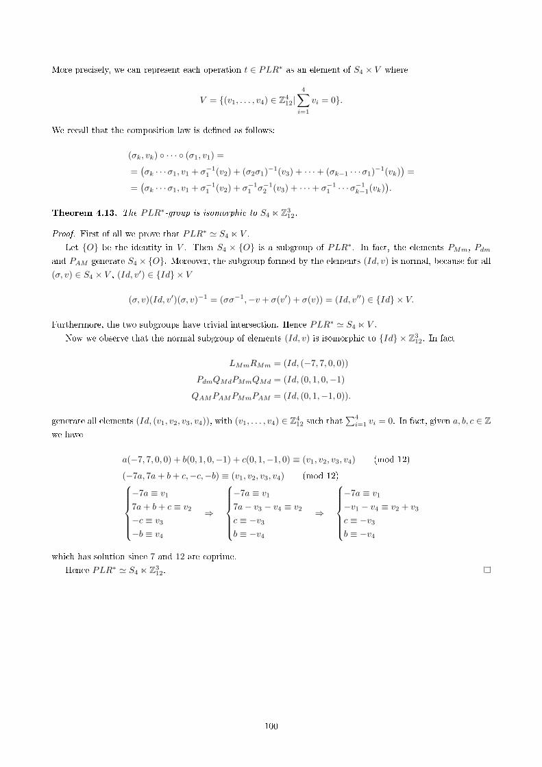
More precisely, we can represent each operation t ∈ PLR∗ as an element of S4 × V where

V = {(v1, . . . , v4) ∈ Z412|

4∑i=1

vi = 0}.

We recall that the composition law is de�ned as follows:

(σk, vk) ◦ · · · ◦ (σ1, v1) =

=(σk · · ·σ1, v1 + σ−1

1 (v2) + (σ2σ1)−1(v3) + · · ·+ (σk−1 · · ·σ1)−1(vk))

=

=(σk · · ·σ1, v1 + σ−1

1 (v2) + σ−11 σ−1

2 (v3) + · · ·+ σ−11 · · ·σ

−1k−1(vk)

).

Theorem 4.13. The PLR∗-group is isomorphic to S4 n Z312.

Proof. First of all we prove that PLR∗ ' S4 n V .

Let {O} be the identity in V . Then S4 × {O} is a subgroup of PLR∗. In fact, the elements PMm, Pdmand PAM generate S4 × {O}. Moreover, the subgroup formed by the elements (Id, v) is normal, because for all

(σ, v) ∈ S4 × V , (Id, v′) ∈ {Id} × V

(σ, v)(Id, v′)(σ, v)−1 = (σσ−1,−v + σ(v′) + σ(v)) = (Id, v′′) ∈ {Id} × V.

Furthermore, the two subgroups have trivial intersection. Hence PLR∗ ' S4 n V .

Now we observe that the normal subgroup of elements (Id, v) is isomorphic to {Id} × Z312. In fact

LMmRMm = (Id, (−7, 7, 0, 0))

PdmQMdPMmQMd = (Id, (0, 1, 0,−1)

QAMPAMPMmPAM = (Id, (0, 1,−1, 0)).

generate all elements (Id, (v1, v2, v3, v4)), with (v1, . . . , v4) ∈ Z412 such that

∑4i=1 vi = 0. In fact, given a, b, c ∈ Z

we have

a(−7, 7, 0, 0) + b(0, 1, 0,−1) + c(0, 1,−1, 0) ≡ (v1, v2, v3, v4) (mod 12)

(−7a, 7a+ b+ c,−c,−b) ≡ (v1, v2, v3, v4) (mod 12)−7a ≡ v1

7a+ b+ c ≡ v2

−c ≡ v3

−b ≡ v4

⇒

−7a ≡ v1

7a− v3 − v4 ≡ v2

c ≡ −v3

b ≡ −v4

⇒

−7a ≡ v1

−v1 − v4 ≡ v2 + v3

c ≡ −v3

b ≡ −v4

which has solution since 7 and 12 are coprime.

Hence PLR∗ ' S4 n Z312.

100

Chapter 5

Operations among sevenths and triads

In the previous chapters we have determined parsimonious operations acting on di�erent sets of triads or

sevenths. But in music literature the most common sequences of chords include both triads and sevenths.

With respect to common practice period in particular, there are not so many long sequences of seventh chords,

because they are dissonant in nature. But it is usual to �nd sequences of chords in which there are both sevenths

and triads. Therefore, we want to de�ne new musical operations among sevenths and triads. Our aim is to

�nd a general framework in which to include the already known parsimonious operations among triads, the

parsimonious operations among sevenths, and also parsimonious operations among seventh and triads.

5.1 Parsimonious operations among sevenths and triads

There are several possibilities to de�ne parsimonious operations among triads and sevenths. For the moment,

we will focus on very simple operations, that is those in which a single note is added or deleted, which is possible

since some triads are embedded in some sevenths.

Similarly to what we have done in previous chapters, we will de�ne some new parsimonious operations

capable of classifying our new operations among sevenths and triads. Let K be a set of sevenths and triads.

De�nition 5.1. Let Pij : K → K be the map which sends an i-th type of seventh to a j-th type of triad with

the same root, and which �xes the other types.

De�nition 5.2. Let Rij : K → K be the map which sends an i-th type of seventh to a j-th type of triad whose

root is transposed 3 semitones up, a j-th type of triad to an i-th type of seventh whose root is transposed 3

semitones down, and which �xes the other types:

Rij = T±3 ◦ Pij = Pij ◦ T±3.

De�nition 5.3. Let Lij : K → K be the map which sends an i-th type of seventh to a j-th type of triad whose

root is transposed 4 semitones up, a j-th type of triad to an i-th type of seventh whose root is transposed 4

semitones down, and which �xes the other types:

Lij = T±4 ◦ Pij = Pij ◦ T±4.

We will use the notation used in the previous chapters to represent the set of chords. For instance, we

consider K1 = H ∪ S be the set containing the 5 classical types of sevenths (dominant, minor, half-diminished,

major and diminished) and major and minor triads. The parsimonious operations among these sevenths and

101

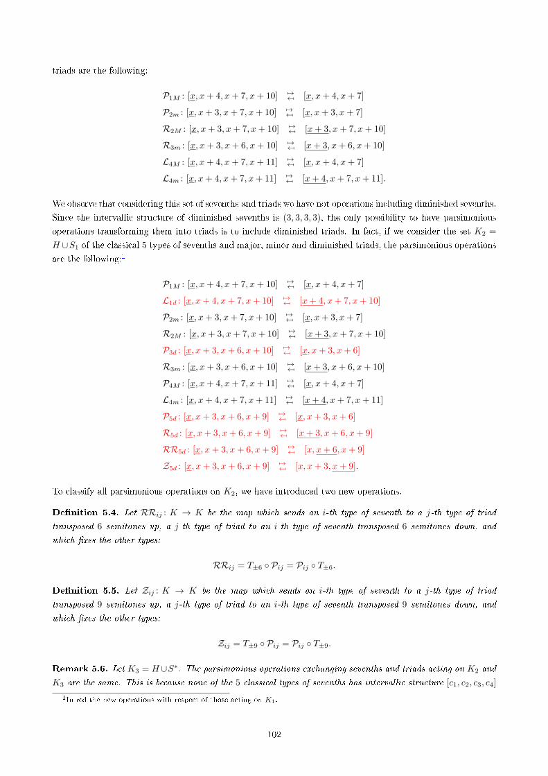
triads are the following:

P1M : [x, x+ 4, x+ 7, x+ 10] 7→7→ [x, x+ 4, x+ 7]

P2m : [x, x+ 3, x+ 7, x+ 10] 7→7→ [x, x+ 3, x+ 7]

R2M : [x, x+ 3, x+ 7, x+ 10] 7→7→ [x+ 3, x+ 7, x+ 10]

R3m : [x, x+ 3, x+ 6, x+ 10] 7→7→ [x+ 3, x+ 6, x+ 10]

L4M : [x, x+ 4, x+ 7, x+ 11] 7→7→ [x, x+ 4, x+ 7]

L4m : [x, x+ 4, x+ 7, x+ 11] 7→7→ [x+ 4, x+ 7, x+ 11].

We observe that considering this set of sevenths and triads we have not operations including diminished sevenths.

Since the intervallic structure of diminished sevenths is (3, 3, 3, 3), the only possibility to have parsimonious

operations transforming them into triads is to include diminished triads. In fact, if we consider the set K2 =

H ∪S1 of the classical 5 types of sevenths and major, minor and diminished triads, the parsimonious operations

are the following:1

P1M : [x, x+ 4, x+ 7, x+ 10] 7→7→ [x, x+ 4, x+ 7]

L1d : [x, x+ 4, x+ 7, x+ 10] 7→7→ [x+ 4, x+ 7, x+ 10]

P2m : [x, x+ 3, x+ 7, x+ 10] 7→7→ [x, x+ 3, x+ 7]

R2M : [x, x+ 3, x+ 7, x+ 10] 7→7→ [x+ 3, x+ 7, x+ 10]

P3d : [x, x+ 3, x+ 6, x+ 10] 7→7→ [x, x+ 3, x+ 6]

R3m : [x, x+ 3, x+ 6, x+ 10] 7→7→ [x+ 3, x+ 6, x+ 10]

P4M : [x, x+ 4, x+ 7, x+ 11] 7→7→ [x, x+ 4, x+ 7]

L4m : [x, x+ 4, x+ 7, x+ 11] 7→7→ [x+ 4, x+ 7, x+ 11]

P5d : [x, x+ 3, x+ 6, x+ 9] 7→7→ [x, x+ 3, x+ 6]

R5d : [x, x+ 3, x+ 6, x+ 9] 7→7→ [x+ 3, x+ 6, x+ 9]

RR5d : [x, x+ 3, x+ 6, x+ 9] 7→7→ [x, x+ 6, x+ 9]

Z5d : [x, x+ 3, x+ 6, x+ 9] 7→7→ [x, x+ 3, x+ 9].

To classify all parsimonious operations on K2, we have introduced two new operations.

De�nition 5.4. Let RRij : K → K be the map which sends an i-th type of seventh to a j-th type of triad

transposed 6 semitones up, a j-th type of triad to an i-th type of seventh transposed 6 semitones down, and

which �xes the other types:

RRij = T±6 ◦ Pij = Pij ◦ T±6.

De�nition 5.5. Let Zij : K → K be the map which sends an i-th type of seventh to a j-th type of triad

transposed 9 semitones up, a j-th type of triad to an i-th type of seventh transposed 9 semitones down, and

which �xes the other types:

Zij = T±9 ◦ Pij = Pij ◦ T±9.

Remark 5.6. Let K3 = H∪S∗. The parsimonious operations exchanging sevenths and triads acting on K2 and

K3 are the same. This is because none of the 5 classical types of sevenths has intervallic structure [c1, c2, c3, c4]

1In red the new operations with respect of those acting on K1.

102

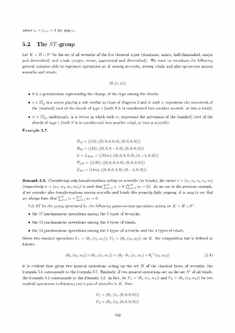
where ci = ci+1 = 4 for any ci.

5.2 The ST -group

Let K = H ∪ S∗ be the set of all sevenths of the �ve classical types (dominant, minor, half-diminished, major

and diminished) and triads (major, minor, augmented and diminished). We want to introduce the following

general notation able to represent operations on K among sevenths, among triads and also operations among

sevenths and triads:

(θ, (v, w))

� θ is a permutation representing the change of the type among the chords.

� v ∈ Z512 is a vector playing a role similar to those of chapters 3 and 4: each vi represents the movement of

the (marked) root of the chords of type i (both if it is transformed into another seventh, or into a triad);

� w ∈ Z412, analogously, is a vector in which each wi represents the movement of the (marked) root of the

chords of type i (both if it is transformed into another triad, or into a seventh).

Example 5.7.

P12 = ((12), ((0, 0, 0, 0, 0), (0, 0, 0, 0)))

R42 = ((42), ((0, 3, 0,−3, 0), (0, 0, 0, 0)))

L = LMm = ((Mm), ((0, 0, 0, 0, 0), (4,−4, 0, 0)))

P1M = ((1M), ((0, 0, 0, 0, 0), (0, 0, 0, 0)))

L4m = ((4m), ((0, 0, 0, 4, 0), (0,−4, 0, 0)))

Remark 5.8. Considering only transformations acting on sevenths (or triads), the vector v = (v1, v2, v3, v4, v5)

(respectively w = (w1, w2, w3, w4)) is such that∑5i=1 vi = 0 (

∑4i=1 wi = 0). As we see in the previous example,

if we consider also transformations among sevenths and triads this property fails; anyway, it is easy to see that

we always have that∑5i=1 vi +

∑4i=1 wi = 0.

Let ST be the group generated by the following parsimonious operations acting on K = H ∪ S∗:

� the 17 parsimonious operations among the 5 types of sevenths;

� the 13 parsimonious operations among the 4 types of triads;

� the 12 parsimonious operations among the 5 types of sevenths and the 4 types of triads.

Given two musical operations U1 = (θ1, (v1, w1)), U2 = (θ2, (v2, w2)) on K, the composition law is de�ned as

follows:

(θ2, (v2, w2)) ◦ (θ1, (v1, w1)) = (θ2 · θ1, (v1, w1) + θ−11 (v2, w2)) (5.1)

It is evident that given two musical operations acting on the set H of the classical types of sevenths, the

Formula 5.1 corresponds to the Formula 3.7. Similarly, if two musical operations act on the set S∗ of all triads,

the Formula 5.1 corresponds to the Formula 4.2. In fact, let U1 = (θ1, (v1, w1)) and U2 = (θ2, (v2, w2)) be two

musical operations exchanging two types of sevenths in K, then

U1 = (θ1, (v1, (0, 0, 0, 0)))

U2 = (θ2, (v2, (0, 0, 0, 0)))

103

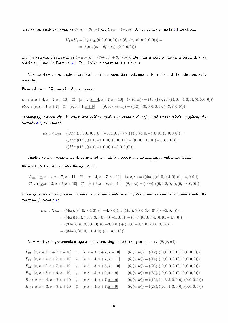
that we can easily represent as U1|H = (θ1, v1) and U2|H = (θ2, v2). Applying the Formula 5.1 we obtain

U2 ◦ U1 = (θ2, (v2, (0, 0, 0, 0, 0))) ◦ (θ1, (v1, (0, 0, 0, 0, 0))) =

= (θ2θ1, (v1 + θ−11 (v2), (0, 0, 0, 0)))

that we can easily represent as U2|HU1|H = (θ2θ1, v1 + θ−11 (v2)). But this is exactly the same result that we

obtain applying the Formula 3.7. For triads the argument is analogous.

Now we show an example of applications if one operation exchanges only triads and the other one only

sevenths.

Example 5.9. We consider the operations

L13 : [x, x+ 4, x+ 7, x+ 10] 7→7→ [x+ 2, x+ 4, x+ 7, x+ 10] (θ, (v, w)) = (Id, (13), Id, ((4, 0,−4, 0, 0), (0, 0, 0, 0)))

RMm : [x, x+ 4, x+ 7] 7→7→ [x, x+ 4, x+ 9] (θ, σ, τ, (v, w)) = ((12), ((0, 0, 0, 0, 0), (−3, 3, 0, 0)))

exchanging, respectively, dominant and half-diminished sevenths and major and minor triads. Applying the

formula 5.1, we obtain:

RMm ◦ L13 = ((Mm), ((0, 0, 0, 0, 0), (−3, 3, 0, 0))) ◦ ((13), ((4, 0,−4, 0, 0), (0, 0, 0, 0))) =

= ((Mm)(13), ((4, 0,−4, 0, 0), (0, 0, 0, 0) + ((0, 0, 0, 0, 0), (−3, 3, 0, 0))) =

= ((Mm)(13), ((4, 0,−4, 0, 0), (−3, 3, 0, 0))).

Finally, we show some example of application with two operations exchanging sevenths and triads.

Example 5.10. We consider the operations

L4m : [x, x+ 4, x+ 7, x+ 11] 7→7→ [x+ 4, x+ 7, x+ 11] (θ, v, w) = ((4m), ((0, 0, 0, 4, 0), (0,−4, 0, 0)))

R3m : [x, x+ 3, x+ 6, x+ 10] 7→7→ [x+ 3, x+ 6, x+ 10] (θ, v, w) = ((3m), ((0, 0, 3, 0, 0), (0,−3, 0, 0)))

exchanging, respectively, minor sevenths and minor triads, and half-diminished sevenths and minor triads. We

apply the formula 5.1:

L4m ◦ R3m = ((4m), ((0, 0, 0, 4, 0), (0,−4, 0, 0))) ◦ ((3m), ((0, 0, 3, 0, 0), (0,−3, 0, 0))) =

= ((4m)(3m), ((0, 0, 3, 0, 0), (0,−3, 0, 0)) + (3m)((0, 0, 0, 4, 0), (0,−4, 0, 0))) =

= ((34m), ((0, 0, 3, 0, 0), (0,−3, 0, 0)) + ((0, 0,−4, 4, 0), (0, 0, 0, 0))) =

= ((34m), ((0, 0,−1, 4, 0), (0,−3, 0, 0)))

Now we list the parsimonious operations generating the ST -group as elements (θ, (v, w)):

P12 : [x, x+ 4, x+ 7, x+ 10] 7→7→ [x, x+ 3, x+ 7, x+ 10] (θ, (v, w)) = ((12), ((0, 0, 0, 0, 0), (0, 0, 0, 0)))

P14 : [x, x+ 4, x+ 7, x+ 10] 7→7→ [x, x+ 4, x+ 7, x+ 11] (θ, (v, w)) = ((14), ((0, 0, 0, 0, 0), (0, 0, 0, 0)))

P23 : [x, x+ 3, x+ 7, x+ 10] 7→7→ [x, x+ 3, x+ 6, x+ 10] (θ, (v, w)) = ((23), ((0, 0, 0, 0, 0), (0, 0, 0, 0)))

P35 : [x, x+ 3, x+ 6, x+ 10] 7→7→ [x, x+ 3, x+ 6, x+ 9] (θ, (v, w)) = ((35), ((0, 0, 0, 0, 0), (0, 0, 0, 0)))

R12 : [x, x+ 4, x+ 7, x+ 10] 7→7→ [x, x+ 4, x+ 7, x+ 9] (θ, (v, w)) = ((12), ((−3, 3, 0, 0, 0), (0, 0, 0, 0)))

R23 : [x, x+ 3, x+ 7, x+ 10] 7→7→ [x, x+ 3, x+ 7, x+ 9] (θ, (v, w)) = ((23), ((0,−3, 3, 0, 0), (0, 0, 0, 0)))

104

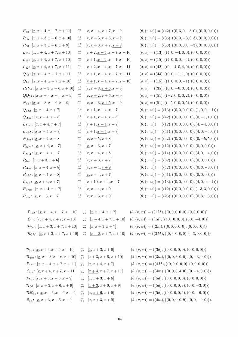
R42 : [x, x+ 4, x+ 7, x+ 11] 7→7→ [x, x+ 4, x+ 7, x+ 9] (θ, (v, w)) = ((42), ((0, 3, 0,−3, 0), (0, 0, 0, 0)))

R35 : [x, x+ 3, x+ 6, x+ 10] 7→7→ [x, x+ 3, x+ 6, x+ 9] (θ, (v, w)) = ((35), ((0, 0,−3, 0, 3), (0, 0, 0, 0)))

R53 : [x, x+ 3, x+ 6, x+ 9] 7→7→ [x, x+ 3, x+ 7, x+ 9] (θ, (v, w)) = ((53), ((0, 0, 3, 0,−3), (0, 0, 0, 0)))

L13 : [x, x+ 4, x+ 7, x+ 10] 7→7→ [x+ 2, x+ 4, x+ 7, x+ 10] (σ, v) = ((13), ((4, 0,−4, 0, 0), (0, 0, 0, 0)))

L15 : [x, x+ 4, x+ 7, x+ 10] 7→7→ [x+ 1, x+ 4, x+ 7, x+ 10] (σ, v) = ((15), ((4, 0, 0, 0,−4), (0, 0, 0, 0)))

L42 : [x, x+ 4, x+ 7, x+ 11] 7→7→ [x+ 2, x+ 4, x+ 7, x+ 11] (σ, v) = ((42), ((0,−4, 0, 4, 0), (0, 0, 0, 0)))

Q43 : [x, x+ 4, x+ 7, x+ 11] 7→7→ [x+ 1, x+ 4, x+ 7, x+ 11] (σ, v) = ((43), ((0, 0,−1, 1, 0), (0, 0, 0, 0)))

Q15 : [x, x+ 4, x+ 7, x+ 10] 7→7→ [x+ 1, x+ 4, x+ 7, x+ 10] (σ, v) = ((15), ((1, 0, 0, 0,−1), (0, 0, 0, 0)))

RR35 : [x, x+ 3, x+ 6, x+ 10] 7→7→ [x, x+ 3, x+ 6, x+ 9] (σ, v) = ((35), ((0, 0,−6, 0, 6), (0, 0, 0, 0)))

QQ51 : [x, x+ 3, x+ 6, x+ 9] 7→7→ [x, x+ 2, x+ 6, x+ 9] (σ, v) = ((51), ((−2, 0, 0, 0, 2), (0, 0, 0, 0))

N51 : [x, x+ 3, x+ 6, x+ 9] 7→7→ [x, x+ 3, x+ 5, x+ 9] (σ, v) = ((51), ((−5, 0, 0, 0, 5), (0, 0, 0, 0))

QMd : [x, x+ 4, x+ 7] 7→7→ [x+ 1, x+ 4, x+ 7] (θ, (v, w)) = ((13), ((0, 0, 0, 0, 0), (1, 0, 0,−1)))

QAm : [x, x+ 4, x+ 8] 7→7→ [x+ 1, x+ 4, x+ 8] (θ, (v, w)) = ((42), ((0, 0, 0, 0, 0), (0,−1, 1, 0)))

LMm : [x, x+ 4, x+ 7] 7→7→ [x+ 1, x+ 4, x+ 7] (θ, (v, w)) = ((12), ((0, 0, 0, 0, 0), (4,−4, 0, 0)))

LAM : [x, x+ 4, x+ 8] 7→7→ [x+ 1, x+ 4, x+ 8] (θ, (v, w)) = ((41), ((0, 0, 0, 0, 0), (4, 0,−4, 0)))

NAm : [x, x+ 4, x+ 8] 7→7→ [x, x+ 5, x+ 8] (θ, (v, w)) = ((42), ((0, 0, 0, 0, 0), (0,−5, 5, 0)))

PMm : [x, x+ 4, x+ 7] 7→7→ [x, x+ 3, x+ 7] (θ, (v, w)) = ((12), ((0, 0, 0, 0, 0), (0, 0, 0, 0)))

LMA : [x, x+ 4, x+ 7] 7→7→ [x, x+ 4, x+ 8] (θ, (v, w)) = ((14), ((0, 0, 0, 0, 0), (4, 0,−4, 0)))

Pdm : [x, x+ 3, x+ 6] 7→7→ [x, x+ 3, x+ 7] (θ, (v, w)) = ((32), ((0, 0, 0, 0, 0), (0, 0, 0, 0)))

RAm : [x, x+ 4, x+ 8] 7→7→ [x, x+ 4, x+ 9] (θ, (v, w)) = ((42), ((0, 0, 0, 0, 0), (0, 3,−3, 0)))

PAM : [x, x+ 4, x+ 8] 7→7→ [x, x+ 4, x+ 7] (θ, (v, w)) = ((41), ((0, 0, 0, 0, 0), (0, 0, 0, 0)))

LMd : [x, x+ 4, x+ 7] 7→7→ [x+ 10, x+ 4, x+ 7] (θ, (v, w)) = ((13), ((0, 0, 0, 0, 0), (4, 0, 0,−4)))

RMm : [x, x+ 4, x+ 7] 7→7→ [x, x+ 4, x+ 9] (θ, (v, w)) = ((12), ((0, 0, 0, 0, 0), (−3, 3, 0, 0)))

Rmd : [x, x+ 3, x+ 7] 7→7→ [x, x+ 3, x+ 9] (θ, (v, w)) = ((23), ((0, 0, 0, 0, 0), (0, 3,−3, 0)))

P1M : [x, x+ 4, x+ 7, x+ 10] 7→7→ [x, x+ 4, x+ 7] (θ, (v, w)) = ((1M), ((0, 0, 0, 0, 0), (0, 0, 0, 0)))

L1d : [x, x+ 4, x+ 7, x+ 10] 7→7→ [x+ 4, x+ 7, x+ 10] (θ, (v, w)) = ((1d), ((4, 0, 0, 0, 0), (0, 0,−4, 0)))

P2m : [x, x+ 3, x+ 7, x+ 10] 7→7→ [x, x+ 3, x+ 7] (θ, (v, w)) = ((2m), ((0, 0, 0, 0, 0), (0, 0, 0, 0)))

R2M : [x, x+ 3, x+ 7, x+ 10] 7→7→ [x+ 3, x+ 7, x+ 10] (θ, (v, w)) = ((2M), ((0, 3, 0, 0, 0), (−3, 0, 0, 0)))

P3d : [x, x+ 3, x+ 6, x+ 10] 7→7→ [x, x+ 3, x+ 6] (θ, (v, w)) = ((3d), ((0, 0, 0, 0, 0), (0, 0, 0, 0)))

R3m : [x, x+ 3, x+ 6, x+ 10] 7→7→ [x+ 3, x+ 6, x+ 10] (θ, (v, w)) = ((3m), ((0, 0, 3, 0, 0), (0,−3, 0, 0)))

P4M : [x, x+ 4, x+ 7, x+ 11] 7→7→ [x, x+ 4, x+ 7] (θ, (v, w)) = ((4M), ((0, 0, 0, 0, 0), (0, 0, 0, 0)))

L4m : [x, x+ 4, x+ 7, x+ 11] 7→7→ [x+ 4, x+ 7, x+ 11] (θ, (v, w)) = ((4m), ((0, 0, 0, 4, 0), (0,−4, 0, 0)))

P5d : [x, x+ 3, x+ 6, x+ 9] 7→7→ [x, x+ 3, x+ 6] (θ, (v, w)) = ((5d), ((0, 0, 0, 0, 0), (0, 0, 0, 0)))

R5d : [x, x+ 3, x+ 6, x+ 9] 7→7→ [x+ 3, x+ 6, x+ 9] (θ, (v, w)) = ((5d), ((0, 0, 0, 0, 3), (0, 0,−3, 0)))

RR5d : [x, x+ 3, x+ 6, x+ 9] 7→7→ [x, x+ 6, x+ 9] (θ, (v, w)) = ((5d), ((0, 0, 0, 0, 6), (0, 0,−6, 0)))

Z5d : [x, x+ 3, x+ 6, x+ 9] 7→7→ [x, x+ 3, x+ 9] (θ, (v, w)) = ((4m), ((0, 0, 0, 0, 9), (0, 0,−9, 0))).

105

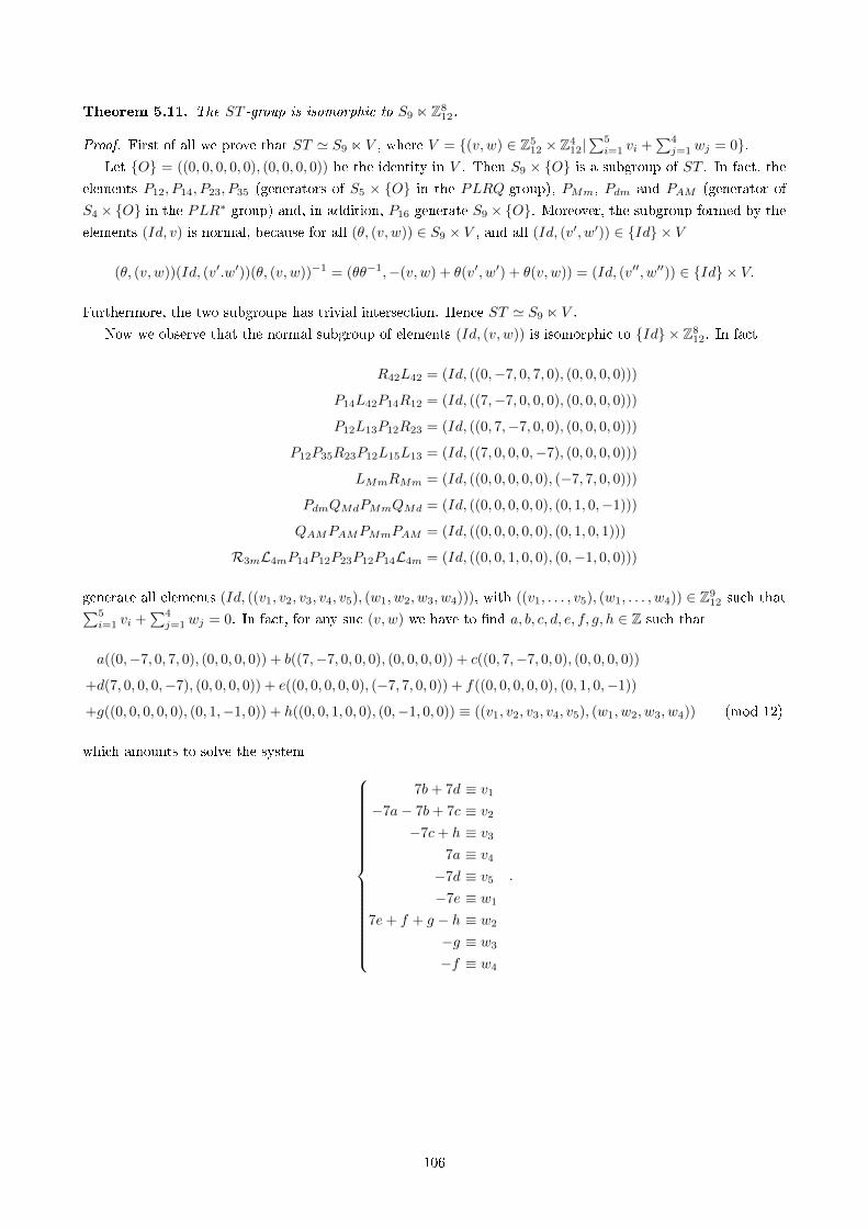
Theorem 5.11. The ST -group is isomorphic to S9 n Z812.

Proof. First of all we prove that ST ' S9 n V , where V = {(v, w) ∈ Z512 × Z4

12|∑5i=1 vi +

∑4j=1 wj = 0}.

Let {O} = ((0, 0, 0, 0, 0), (0, 0, 0, 0)) be the identity in V . Then S9 × {O} is a subgroup of ST . In fact, the

elements P12, P14, P23, P35 (generators of S5 × {O} in the PLRQ-group), PMm, Pdm and PAM (generator of

S4 × {O} in the PLR∗-group) and, in addition, P16 generate S9 × {O}. Moreover, the subgroup formed by the

elements (Id, v) is normal, because for all (θ, (v, w)) ∈ S9 × V , and all (Id, (v′, w′)) ∈ {Id} × V

(θ, (v, w))(Id, (v′.w′))(θ, (v, w))−1 = (θθ−1,−(v, w) + θ(v′, w′) + θ(v, w)) = (Id, (v′′, w′′)) ∈ {Id} × V.

Furthermore, the two subgroups has trivial intersection. Hence ST ' S9 n V .

Now we observe that the normal subgroup of elements (Id, (v, w)) is isomorphic to {Id} × Z812. In fact

R42L42 = (Id, ((0,−7, 0, 7, 0), (0, 0, 0, 0)))

P14L42P14R12 = (Id, ((7,−7, 0, 0, 0), (0, 0, 0, 0)))

P12L13P12R23 = (Id, ((0, 7,−7, 0, 0), (0, 0, 0, 0)))

P12P35R23P12L15L13 = (Id, ((7, 0, 0, 0,−7), (0, 0, 0, 0)))

LMmRMm = (Id, ((0, 0, 0, 0, 0), (−7, 7, 0, 0)))

PdmQMdPMmQMd = (Id, ((0, 0, 0, 0, 0), (0, 1, 0,−1)))

QAMPAMPMmPAM = (Id, ((0, 0, 0, 0, 0), (0, 1, 0, 1)))

R3mL4mP14P12P23P12P14L4m = (Id, ((0, 0, 1, 0, 0), (0,−1, 0, 0)))

generate all elements (Id, ((v1, v2, v3, v4, v5), (w1, w2, w3, w4))), with ((v1, . . . , v5), (w1, . . . , w4)) ∈ Z912 such that∑5

i=1 vi +∑4j=1 wj = 0. In fact, for any suc (v, w) we have to �nd a, b, c, d, e, f, g, h ∈ Z such that

a((0,−7, 0, 7, 0), (0, 0, 0, 0)) + b((7,−7, 0, 0, 0), (0, 0, 0, 0)) + c((0, 7,−7, 0, 0), (0, 0, 0, 0))

+d(7, 0, 0, 0,−7), (0, 0, 0, 0)) + e((0, 0, 0, 0, 0), (−7, 7, 0, 0)) + f((0, 0, 0, 0, 0), (0, 1, 0,−1))

+g((0, 0, 0, 0, 0), (0, 1,−1, 0)) + h((0, 0, 1, 0, 0), (0,−1, 0, 0)) ≡ ((v1, v2, v3, v4, v5), (w1, w2, w3, w4)) (mod 12)

which amounts to solve the system

7b+ 7d ≡ v1

−7a− 7b+ 7c ≡ v2

−7c+ h ≡ v3

7a ≡ v4

−7d ≡ v5

−7e ≡ w1

7e+ f + g − h ≡ w2

−g ≡ w3

−f ≡ w4

.

106

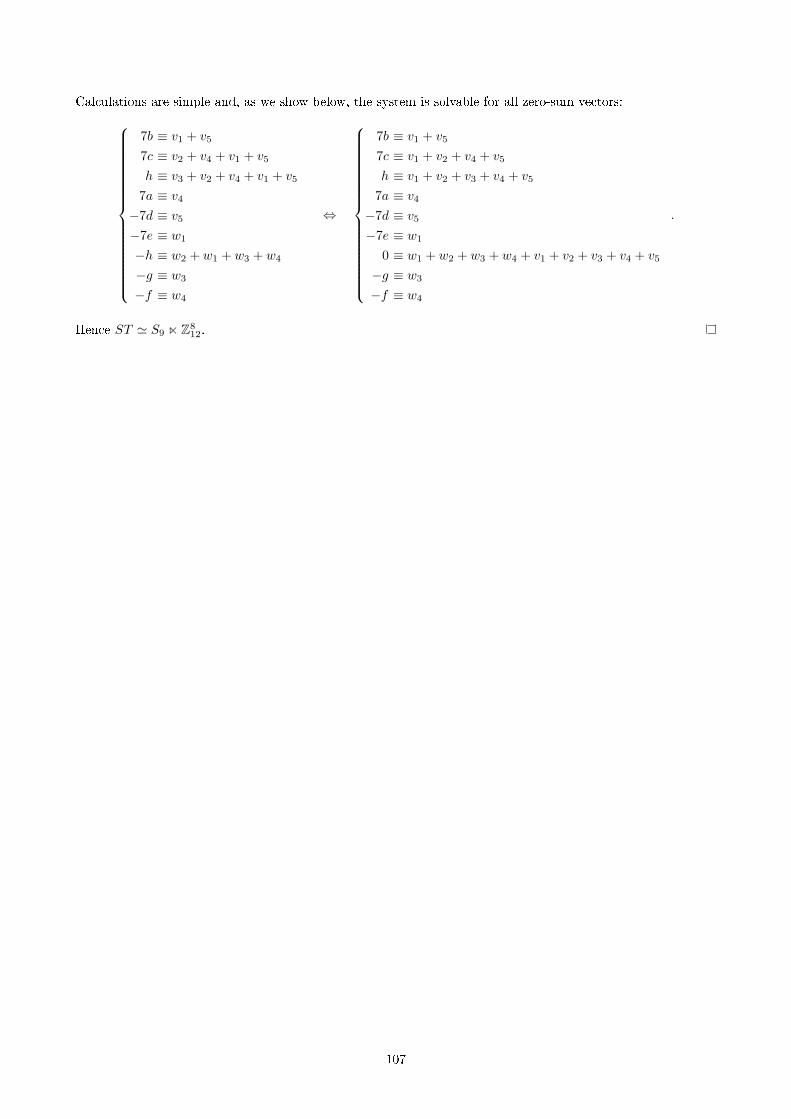
Calculations are simple and, as we show below, the system is solvable for all zero-sum vectors:

7b ≡ v1 + v5

7c ≡ v2 + v4 + v1 + v5

h ≡ v3 + v2 + v4 + v1 + v5

7a ≡ v4

−7d ≡ v5

−7e ≡ w1

−h ≡ w2 + w1 + w3 + w4

−g ≡ w3

−f ≡ w4

⇔

7b ≡ v1 + v5

7c ≡ v1 + v2 + v4 + v5

h ≡ v1 + v2 + v3 + v4 + v5

7a ≡ v4

−7d ≡ v5

−7e ≡ w1

0 ≡ w1 + w2 + w3 + w4 + v1 + v2 + v3 + v4 + v5

−g ≡ w3

−f ≡ w4

.

Hence ST ' S9 n Z812.

107

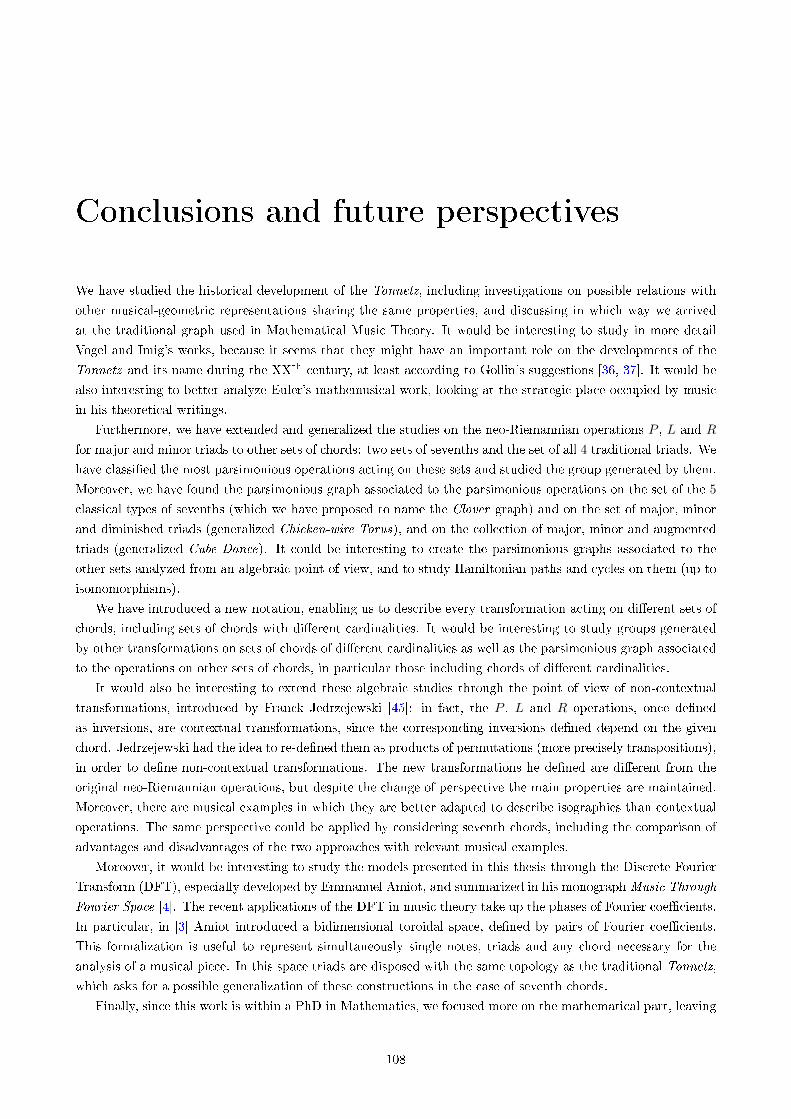
Conclusions and future perspectives

We have studied the historical development of the Tonnetz, including investigations on possible relations with

other musical-geometric representations sharing the same properties, and discussing in which way we arrived

at the traditional graph used in Mathematical Music Theory. It would be interesting to study in more detail

Vogel and Imig's works, because it seems that they might have an important role on the developments of the

Tonnetz and its name during the XXth century, at least according to Gollin's suggestions [36, 37]. It would be

also interesting to better analyze Euler's mathemusical work, looking at the strategic place occupied by music

in his theoretical writings.

Furthermore, we have extended and generalized the studies on the neo-Riemannian operations P , L and R

for major and minor triads to other sets of chords: two sets of sevenths and the set of all 4 traditional triads. We

have classi�ed the most parsimonious operations acting on these sets and studied the group generated by them.

Moreover, we have found the parsimonious graph associated to the parsimonious operations on the set of the 5

classical types of sevenths (which we have proposed to name the Clover graph) and on the set of major, minor

and diminished triads (generalized Chicken-wire Torus), and on the collection of major, minor and augmented

triads (generalized Cube Dance). It could be interesting to create the parsimonious graphs associated to the

other sets analyzed from an algebraic point of view, and to study Hamiltonian paths and cycles on them (up to

isomomorphisms).

We have introduced a new notation, enabling us to describe every transformation acting on di�erent sets of

chords, including sets of chords with di�erent cardinalities. It would be interesting to study groups generated

by other transformations on sets of chords of di�erent cardinalities as well as the parsimonious graph associated

to the operations on other sets of chords, in particular those including chords of di�erent cardinalities.

It would also be interesting to extend these algebraic studies through the point of view of non-contextual

transformations, introduced by Franck Jedrzejewski [45]: in fact, the P , L and R operations, once de�ned

as inversions, are contextual transformations, since the corresponding inversions de�ned depend on the given

chord. Jedrzejewski had the idea to re-de�ned them as products of permutations (more precisely transpositions),

in order to de�ne non-contextual transformations. The new transformations he de�ned are di�erent from the

original neo-Riemannian operations, but despite the change of perspective the main properties are maintained.

Moreover, there are musical examples in which they are better adapted to describe isographies than contextual

operations. The same perspective could be applied by considering seventh chords, including the comparison of

advantages and disadvantages of the two approaches with relevant musical examples.

Moreover, it would be interesting to study the models presented in this thesis through the Discrete Fourier

Transform (DFT), especially developed by Emmanuel Amiot, and summarized in his monographMusic Through

Fourier Space [4]. The recent applications of the DFT in music theory take up the phases of Fourier coe�cients.

In particular, in [3] Amiot introduced a bidimensional toroidal space, de�ned by pairs of Fourier coe�cients.

This formalization is useful to represent simultaneously single notes, triads and any chord necessary for the

analysis of a musical piece. In this space triads are disposed with the same topology as the traditional Tonnetz,

which asks for a possible generalization of these constructions in the case of seventh chords.

Finally, since this work is within a PhD in Mathematics, we focused more on the mathematical part, leaving

108

aside the musical application of all theoretical constructions we presented. We are aware there is still much work

to be done to show that the formal and theoretical aspects that have been discussed are not only interesting

from a mathematical point of view, but also as a way to suggest new original applications in music analysis and

composition.

109

Bibliography

[1] G. Albini, S. Antonini, Hamiltonian Cycles in the Topological Dual of the Tonnetz. In: Chew E., Childs A.,

Chuan CH. (eds) Mathematics and Computation in Music, Communications in Computer and Information

Science, vol 38, Springer, Berlin, Heidelberg, 2009.

[2] G. Albini, M. P. Bernardi, Hamiltonian Graphs as Harmonic Tools. In: Agustín-Aquino O., Lluis-Puebla E.,

Montiel M. (eds) Mathematics and Computation in Music. Lecture Notes in Computer Science, vol. 10527,

Springer, Mexico City, 2017.

[3] E. Amiot, The Torii of phases, Proceedings of SMCM, Springer, Montreal, 2013.

[4] E. Amiot,Music Through Fourier Space. Discrete Fourier Transform in Music Theory, Computational Music

Science, Springer, 2016.

[5] C. Anagnostopoulou, C. Buteau (Eds.), Special issue: Computational Music Analysis, Journal of Mathe-

matics and Music, Vol. 5, n. 2, 2010.

[6] M. Andreatta, C. Agon Amado, T. Noll, E. Amiot Towards Pedagogability of Mathematical Music The-

ory: Algebraic Models and Tiling Problems in computer-aided composition. Bridges Conference Proceedings,

London, 2006, pp. 277-284. http://archive.bridgesmathart.org/2006/bridges2006-277.html.

[7] M. Andreatta, Calcul algébrique et calcul catégoriel en musique: aspects théoriques et informatiques, Le

calcul de la musique, L. Pottier (éd.), Publications de l'université de Saint-Etienne, 2008, p. 429-477.

[8] J. Arnett, E. Barth, Generalizations of the Tonnetz: Tonality Revisited, (http://personal.denison.edu/

~lalla/MCURCSM2011/10.pdf).

[9] G. Baroin, The Spinnen-Tonnetz: New Musical Dimensions in the 2D Network for Tonal Music Analysis. In:

Collins T., Meredith V., Volk A. (eds) Mathematics and Computation in Music, Lectures Notes in Computer

Science, Springer, London, Heidelberg, 2015.

[10] G. J. Balzano, The Group-Theoretic Description of 12-Fold and Microtonal Pitch Systems, Computer Music

Journal, Vol. 4, n. 4, 1980.

[11] N. Biggs, E. Lloyd, R. Wilson. Graph Theory, 1736-1936, Oxford University Press, 1986.

[12] L. Bigo, M. Andreatta, J. L. Giavitto, O. Michel, A. Spicher, Computation and Visualization of Musical

Structures in Chord-Based Simplicial Complexes. In: Yust J., Wild J., Burgoyne J.A. (eds) Mathematics

and Computation in Music. MCM 2013. Lecture Notes in Computer Science, vol 7937. Springer, Berlin,

Heidelberg, 2013.

[13] L. Bigo, D, Ghisi, A. Spicher, M. Andreatta, Spatial transformations in simplicial chord spaces. In: Pro-

ceedings of the Joint International Computer Music Conference - Sound and Music Computing, Athens, 2014,

pp. 1112-1119.

110

http://archive.bridgesmathart.org/2006/bridges2006-277.html

http://personal.denison.edu/~lalla/MCURCSM2011/10.pdf

http://personal.denison.edu/~lalla/MCURCSM2011/10.pdf

[14] L. Bigo, M. Andreatta, A geometric model for the analysis of pop music, Sonus - special issue on modelling

in musical analysis, vol. 35, n. 1, 2014, p.36-48.

[15] L. Bigo, D. Ghisi, A. Spicher, M. Andreatta, Representation of Musical Structures and Processes in Sim-

plicial Chord Spaces, Computer Music Journal, vol. 39, n. 3, 2015.

[16] C. Brower, Paradoxes of Pitch Space, Music Analysis, 27(1), 2008, pp. 51-106.

[17] S. Cannas, S. Antonini, L. Pernazza, On the group of transformations of classical types of seventh chords.'

In: Agustín-Aquino O., Lluis-Puebla E., Montiel M. (eds) Mathematics and Computation in Music, Lecture

Notes in Computer Science, vol. 10527, Springer, Mexico City, 2017.

[18] S. Cannas, M. Andreatta, A Generalized Dual of the Tonnetz for Seventh Chords: Mathematical, Compu-

tational and Compositional Aspects, Bridges Conference Proceedings, Stockholm, 2018.

[19] S. Cannas, Towards the history of the Tonnetz: from Euler to Mathematical Music Theory, In: X. Hascher,

A. Papadopoulos (eds) �Mathematics and music, from the Greeks to Euler�, Hermann, Paris, 2019 (to appear).

[20] R. Caddeo, X. Hascher, P. Jehel, A. Papadopoulos, H. Papadopoulos, Leonhard Euler - Écrits sur la

musique, Paris, Hermann - Collection GREAM, 2015.

[21] M. J. Catanzaro, Generalized Tonnetze, Journal of Mathematics and Music, Vol. 5, n. 2, 2011.

[22] E. Chew, Towards a Mathematical Model of Tonality. Ph.D. diss., MIT, 2000.

[23] A. Childs, Moving Beyond Neo-Riemannian Triads: Exploring a Transformational Model for Seventh

Chords, Journal of Music Theory, 42(2), 1998.

[24] R. Cohn, Maximally Smooth Cycles, Hexatonic Systems, and the Analysis of Late-Romantic Triadic Pro-

gressions, Music Analysis, Vol. 15, n. 1 1996.

[25] R. Cohn, Neo-Riemannian Operations, Parsimonious Trichords, and their �Tonnetz� Representation, Jour-

nal of Music Theory, 1997.

[26] R. Cohn, Introduction to Neo-Riemannian Theory: A Survey and a Historical Perspective, Journal of Music

Theory, 42(2), 1998.

[27] A. Crans, T. M. Fiore, R. Satyendra,Musical Actions of Dihedral Groups, American Mathematical Monthly,

Vol. 116, n. 6, June-July 2009, pp. 479-495.

[28] J. Douthett, P. Steinbach, Parsimonious Graphs: A Study in Parsimony, Contextual Transformation, and

Modes of Limited Transposition, Journal of Music Theory, 42/2, 1998.

[29] L. Euler, Tentamen novae theoriae musicae ex certissimis harmoniae principiis dilucide expositae, Opera

Omnia, Series 3, Vol. 1, 1739.

[30] L. Euler, De harmoniae veris principiis perspeculum musicum repraesentatis, Opera Omnia, Series 3, Vol.

1, 1774.

[31] T. M. Fiore, R. Satyendra, Generalized contextual groups, Music Theory Online, Vol. 11, n.3, 2005.

[32] A. Forte, A Theory of Set-Complexes for Music, Journal of Music Theory, 8(2), 1964, pp. 136-183.

[33] A. Forte, The Structure of Atonal Music, Yale University Press, 1973.

111

[34] W. Goebl, G. Widmer, On the use of computational methods for expressive music performance, in Modern

Methods for Musicology: Prospects, Proposals, and Realities, T. Crawford and L. Gibson, eds., Ashgate

Publishing, Surrey, England, 2009, pp. 93-113.

[35] E. Gollin, Aspects of Three-Dimensional Tonnetze, Journal of Music Theory, 42(2), 1998.

[36] E. Gollin, Combinatorial and Transformational Aspects of Euler's Speculum Musicum, in: Klouche T., Noll

T. (eds) Mathematics and Computation in Music. MCM 2007. Communications in Computer and Information

Science, vol 37. Springer, Berlin, Heidelberg, 2009.

[37] E. Gollin, A. Rehding, The Oxford Handbook of Neo-Riemannian Music Theories, Oxford University Press,

2011.

[38] T. C. Hales, The Honeycomb Conjecture, Disc. Comp. Geom., v. 25, 2001.

[39] X. Hascher, A. Papadopoulos, Leonhard Euler: Mathématicien, physicien et théoricien de la musique, Paris,

CNRS editions, 2015.

[40] T. Heath, A History of Greek Mathematics, Oxford at the Clarendon press, Vol. 2, 1921.

[41] B. Hyer, Tonal Intuitions in �Tristan und Isolde�, Ph.D. diss., Yale University, 1989.

[42] B. Hyer, Reimag(in)ing Riemann, Journal of Music Theory, 39(1), 1995.

[43] J. Hook, Uniform Triadic Transformations, Journal of Music Theory, 46(1-2), 2002, pp. 57-126.

[44] R. J. Howarth, Dictionary of Mathematical Geosciences: With Historical Notes, Springer, 2017.

[45] F. Jedrzejewski, Permutation Groups and Chord Tessellations, ICMC Proceedings, Barcelona, 2005.

[46] F. Jedrzejewski, Mathematical Theory of Music, Collection Musique/sciences, IRCAM/Editions Delatour

France, 2006.

[47] F. Jedrzejewski, Generalized diatonic scales, Journal of Mathematics and Music, Vol. 2, n. 1, 2008.

[48] Z. Juhász, A systematic comparison of di�erent European folk music traditions using self-organizing maps,

J. New Music Res., n. 35, 2006 , pp. 95-112.

[49] G. J. Kayas, L'âme de l'univers et la musique dans le �Timée� de Platon (34 b et ss), Bulletin de

l'Association Guillame Budé, 1974, pp. 287-329.

[50] B. Kerkez, Extension of Neo-Riemannian PLR-group to Seventh Chords, Mathematics, Music, Art, Archi-

tecture, Culture, 2012.

[51] P. Lascabettes, Homologie Persistante Appliqué à la Reconnaissance des Genres Musicaux, Master disser-

tation, ENS Paris Saclay and Université de Strasbourg, 2018.

[52] D. Lewin, Transformational techniques in atonal and other music theories, Perspectives in New Music,

n.21, 1982.

[53] D. Lewin, Generalized Musical Intervals and Transformations, Yale University Press,1987.

[54] H. C. Longuet-Higgins, Letter to a Musical Friend, The Music Review, 23, 1962, 244-248.

[55] J. Mandereau, D. Ghisi, E. Amiot, M. Andreatta, C. Agon, Z-Relation and Homometry in Musical Distri-

butions, Journal of Mathematics and Music, vol. 5, 2011.

112

[56] G. Mazzola, Gruppen und Kategorien in der Musik: Entwurf einer mathematischen Musiktheorie, Helder-

mannr, Lemgo, 1985.

[57] G. Mazzola, Geometrie der Töne, Birkhäuser, Basel, 1990.

[58] K. E. Naumann, Über die verschiedenen Bestimmungen der Tonverhältnisse und die Bedeutung des

pythagoräischen oder reinen Quinten-Systems für unsere heutige Musik, Leipzig, 1858.

[59] D. Meredith. Computational Music Analysis, Springer, Berlin, Heidelberg, 2016.

[60] A. von Oettingen, Harmoniesystem in dualer Entwickelung, 1866.

[61] Pappus d'Alexandrie, La collection mathematique, tr. Paul Ver Eecke, Albert Blanchard, 1982.

[62] S. Pasticci, Teoria degli insiemi e analisi della musica post-tonale, Rivista di Analisi e Teoria musicale, n.1,

Bologna, 1985.

[63] H. Riemann, Die Natur der Harmonik, Leipzig, 1882.

[64] H. Riemann, Handbuch der Harmonielehre, Breitkopf und Härtel, Leipzig 1887.

[65] H. Riemann, Musik-Lexikon, IV edition, Leipzig, 1894.

[66] H. Riemann, Ideen zu einer 'Lehre von den Tonvorstellungen', 1914.

[67] J. J. Rotman, Advanced Modern Algebra, American Mathematical Society, 2010.

[68] D. Tymoczko, A Geometry of Music, Oxford University Press, 2011.

[69] D. Tymoczko, The Generalized Tonnetz, Journal of Music Theory, 56(1), 2012.

[70] M. T. Varro, On Agriculture, Loeb Classical Library, 1934.

[71] M. Vogel, Die Musikschriften Leonhard Eulers, In: Speiser, A. (ed.) Leonhardi Euleri Opera omnia sub

auspiciis Societas scientiarum naturalium Helveticae, Ser. 3, pp. 11�12. Orell Füssli, Zurich, 1960.

[72] A. Volk, F. Wiering, P. van Kranenburg, Unfolding the potential of computational musicology, in Proceed-

ings of ICISO, the Netherlands, 2011, pp. 137-144.

[73] A. Volk, A. Honingh, Mathematical and computational approaches to music: challenges in an interdisci-

plinary enterprise, Journal of Mathematics and Music, Vol. 6, n. 2, 2012, pp. 73-81.

[74] F. Wiering, Digital critical editions of music: A multidimensional model, in Modern Methods for Musi-

cology: Prospects, Proposals and Realities, T. Crawford and L. Gibson, eds., London, Ashgate, 2009, pp.

23-46

113

UNIVERSITÀ DI PAVIA UNIVERSITÉ DE STRASBOURG

Documents

Transcript of UNIVERSITÀ DI PAVIA UNIVERSITÉ DE STRASBOURG