Université de Montréal

Classification analytique de systèmes différentiels

linéaires déployant une singularité irrégulière de

rang de Poincaré 1

par

Caroline Lambert

Département de mathématiques et de statistique

Faculté des arts et des sciences

Thèse présentée à la Faculté des études supérieures et postdoctorales

en vue de l’obtention du grade de Philosophiæ Doctor (Ph.D.)

en mathématiques,

option mathématiques pures

Avril 2010

c© Caroline Lambert, 2010

Université de MontréalFaculté des études supérieures et postdoctorales

Cette thèse intitulée

Classification analytique de systèmes différentiels

linéaires déployant une singularité irrégulière de

rang de Poincaré 1

présentée par

Caroline Lambert

a été évaluée par un jury composé des personnes suivantes :

Pavel Winternitz

président-rapporteur

Christiane Rousseau

directrice de recherche

André Giroux

membre du jury

Claude Mitschi

examinatrice externe

Alain Vincent

représentant du doyen

iii

RÉSUMÉ

Cette thèse traite de la classification analytique du déploiement de systèmes

différentiels linéaires ayant une singularité irrégulière. Elle est composée de deux

articles sur le sujet : le premier présente des résultats obtenus lors de l’étude de la

confluence de l’équation hypergéométrique et peut être considéré comme un cas

particulier du second ; le deuxième contient les théorèmes et résultats principaux.

Dans les deux articles, nous considérons la confluence de deux points singu-

liers réguliers en un point singulier irrégulier et nous étudions les conséquences

de la divergence des solutions au point singulier irrégulier sur le comportement

des solutions du système déployé. Pour ce faire, nous recouvrons un voisinage

de l’origine (de manière ramifiée) dans l’espace du paramètre de déploiement ǫ.

La monodromie d’une base de solutions bien choisie est directement reliée aux

matrices de Stokes déployées. Ces dernières donnent une interprétation géomé-

trique aux matrices de Stokes, incluant le lien (existant au moins pour les cas

génériques) entre la divergence des solutions à ǫ = 0 et la présence de solutions

logarithmiques autour des points singuliers réguliers lors de la résonance. La mo-

nodromie d’intégrales premières de systèmes de Riccati correspondants est aussi

interprétée en fonction des éléments des matrices de Stokes déployées.

De plus, dans le second article, nous donnons le système complet d’invariants

analytiques pour le déploiement de systèmes différentiels linéaires x2y′ = A(x)y

ayant une singularité irrégulière de rang de Poincaré 1 à l’origine au-dessus d’un

voisinage fixé Dr dans la variable x. Ce système est constitué d’une partie for-

melle, donnée par des polynômes, et d’une partie analytique, donnée par une

classe d’équivalence de matrices de Stokes déployées. Pour chaque valeur du pa-

ramètre ǫ dans un secteur pointé à l’origine d’ouverture plus grande que 2π, nous

iv

recouvrons l’espace de la variable, Dr, avec deux secteurs et, au-dessus de cha-

cun, nous choisissons une base de solutions du système déployé. Cette base sert à

définir les matrices de Stokes déployées. Finalement, nous prouvons un théorème

de réalisation des invariants qui satisfont une condition nécessaire et suffisante,

identifiant ainsi l’ensemble des modules.

Mots-clés : phénomène de Stokes, systèmes differentiels linéaires, singu-

larité irrégulière, déploiement, monodromie, classification analytique,

réalisation, espace des modules, équation hypergéometrique, équation

différentielle matricielle de Riccati.

v

ABSTRACT

This thesis deals with the analytic classification of unfoldings of linear dif-

ferential systems with an irregular singularity. It contains two papers related to

this subject : the first paper presents results concerning the confluence of the

hypergeometric equation and may be viewed as a particular case of the second

one ; the second paper contains the main theorems and results.

In both papers, we study the confluence of two regular singular points into

an irregular one and we give consequences of the divergence of solutions at the

irregular singular point for the unfolded system. For this study, a full neighbo-

rhood of the origin is covered (in a ramified way) in the space of the unfolding

parameter ǫ. Monodromy of a well chosen basis of solutions around the regular

singular points is directly linked to the unfolded Stokes matrices. These matrices

give a complete geometric interpretation to the well-known Stokes matrices : this

includes the link (existing at least for the generic cases) between the divergence

of the solutions at ǫ = 0 and the presence of logarithmic terms in the solutions

for resonant values of ǫ. Monodromy of first integrals of related Riccati systems

are also interpreted in terms of the elements of the unfolded Stokes matrices.

The second paper goes further into the subject, giving the complete system

of analytic invariants for the unfoldings of nonresonant linear differential systems

x2y′ = A(x)y with an irregular singularity of Poincaré rank 1 at the origin over

a fixed neighborhood Dr in the space of the variable x. It consists of a formal

part, given by polynomials, and an analytic part, given by an equivalence class

of unfolded Stokes matrices. For each parameter value ǫ taken in a sector poin-

ted at the origin of opening larger than 2π, we cover the space of the variable,

Dr, with two sectors and, over each of them, we construct a well chosen basis

vi

of solutions of the unfolded differential system. This basis is used to define the

unfolded Stokes matrices. Finally, we give a realization theorem for the invariants

satisfying a necessary and sufficient condition, thus identifying the set of modules.

Key words : Stokes phenomenon, linear differential systems, irregu-

lar singularity, unfolding, monodromy, analytic classification, realiza-

tion, moduli space, hypergeometric equation, Riccati matrix differen-

tial equation.

vii

TABLE DES MATIÈRES

Résumé. . . . . . . . . . . . . . . . . . . . . . . . . . . . . . . . . . . . . . . . . . . . . . . . . . . . . . . . . . iii

Abstract . . . . . . . . . . . . . . . . . . . . . . . . . . . . . . . . . . . . . . . . . . . . . . . . . . . . . . . . . v

Liste des tableaux . . . . . . . . . . . . . . . . . . . . . . . . . . . . . . . . . . . . . . . . . . . . . . . xi

Liste des figures . . . . . . . . . . . . . . . . . . . . . . . . . . . . . . . . . . . . . . . . . . . . . . . . . xii

Liste des sigles et abréviations . . . . . . . . . . . . . . . . . . . . . . . . . . . . . . . . . . . xv

Remerciements . . . . . . . . . . . . . . . . . . . . . . . . . . . . . . . . . . . . . . . . . . . . . . . . . . xvi

Introduction . . . . . . . . . . . . . . . . . . . . . . . . . . . . . . . . . . . . . . . . . . . . . . . . . . . . . 1

0.1. Mise en contexte . . . . . . . . . . . . . . . . . . . . . . . . . . . . . . . . . . . . . . . . . . . . . . . . . . 1

0.2. But de la thèse . . . . . . . . . . . . . . . . . . . . . . . . . . . . . . . . . . . . . . . . . . . . . . . . . . . 2

0.3. Caractère distinctif de la thèse . . . . . . . . . . . . . . . . . . . . . . . . . . . . . . . . . . . . 3

0.4. Méthodologie . . . . . . . . . . . . . . . . . . . . . . . . . . . . . . . . . . . . . . . . . . . . . . . . . . . . . 4

0.5. Organisation de la thèse et contribution aux articles . . . . . . . . . . . . . . . 6

Chapitre 1. Présentation des principaux résultats . . . . . . . . . . . . . . . 8

1.1. Point de départ à la résolution du problème . . . . . . . . . . . . . . . . . . . . . . . 8

1.2. Forme prénormale analytique et invariants formels . . . . . . . . . . . . . . . . 9

1.3. Matrices de Stokes déployées . . . . . . . . . . . . . . . . . . . . . . . . . . . . . . . . . . . . . . 10

1.4. Matrices de Stokes déployées et monodromie de la base de solution

choisie . . . . . . . . . . . . . . . . . . . . . . . . . . . . . . . . . . . . . . . . . . . . . . . . . . . . . . . . . . . . 13

viii

1.5. Matrices de Stokes déployées et bases de solutions qui sont des

vecteurs propres de la monodromie . . . . . . . . . . . . . . . . . . . . . . . . . . . . . . . . 14

1.6. Systèmes de Riccati . . . . . . . . . . . . . . . . . . . . . . . . . . . . . . . . . . . . . . . . . . . . . . . 15

1.7. Relation d’auto-intersection . . . . . . . . . . . . . . . . . . . . . . . . . . . . . . . . . . . . . . . 16

1.8. Théorèmes de classification et de réalisation . . . . . . . . . . . . . . . . . . . . . . . 17

Chapitre 2. The Stokes Phenomenon in the Confluence of the

Hypergeometric Equation Using Riccati Equation . . 19

Abstract . . . . . . . . . . . . . . . . . . . . . . . . . . . . . . . . . . . . . . . . . . . . . . . . . . . . . . . . . . . . . . . . 19

2.1. Introduction . . . . . . . . . . . . . . . . . . . . . . . . . . . . . . . . . . . . . . . . . . . . . . . . . . . . . . 20

2.2. Solutions of the hypergeometric equation . . . . . . . . . . . . . . . . . . . . . . . . . . 22

2.2.1. Bases for the solutions of the hypergeometric equation (2.2.2) at

the regular singular points x = 0 and x = ǫ . . . . . . . . . . . . . . . . . 22

2.2.2. The confluent hypergeometric equation and its summable solutions

25

2.3. Divergence and Monodromy. . . . . . . . . . . . . . . . . . . . . . . . . . . . . . . . . . . . . . . 29

2.3.1. Divergence and ramification : first observations. . . . . . . . . . . . . . . . . 29

2.3.2. Limit of quotients of solutions on S± . . . . . . . . . . . . . . . . . . . . . . . . . . . 29

2.3.3. Divergence and nondiagonal form of the monodromy operator in

the basis B+ . . . . . . . . . . . . . . . . . . . . . . . . . . . . . . . . . . . . . . . . . . . . . . . 33

2.3.4. The wild and continous part of the monodromy operator . . . . . . . 39

2.4. A related Riccati system . . . . . . . . . . . . . . . . . . . . . . . . . . . . . . . . . . . . . . . . . . 41

2.4.1. First integrals of a Riccati system related to the hypergeometric

equation (2.2.2) . . . . . . . . . . . . . . . . . . . . . . . . . . . . . . . . . . . . . . . . . . . . 41

2.4.2. Divergence and unfolding of the saddle-nodes . . . . . . . . . . . . . . . . . . 43

2.4.3. Universal unfolding . . . . . . . . . . . . . . . . . . . . . . . . . . . . . . . . . . . . . . . . . . . . 46

ix

2.5. Directions for further research. . . . . . . . . . . . . . . . . . . . . . . . . . . . . . . . . . . . . 47

2.6. Acknowledgements . . . . . . . . . . . . . . . . . . . . . . . . . . . . . . . . . . . . . . . . . . . . . . . . 47

Chapitre 3. Complete system of analytic invariants for unfolded

differential linear systems with an irregular singularity

of Poincaré rank 1. . . . . . . . . . . . . . . . . . . . . . . . . . . . . . . . . . 48

Abstract . . . . . . . . . . . . . . . . . . . . . . . . . . . . . . . . . . . . . . . . . . . . . . . . . . . . . . . . . . . . . . . . 48

3.1. Introduction . . . . . . . . . . . . . . . . . . . . . . . . . . . . . . . . . . . . . . . . . . . . . . . . . . . . . . 49

3.2. The Stokes phenomenon and invariants, ǫ = 0 . . . . . . . . . . . . . . . . . . . . . 51

3.3. The prenormal form, k ∈ N∗ . . . . . . . . . . . . . . . . . . . . . . . . . . . . . . . . . . . . . . 54

3.3.1. Generic unfolding . . . . . . . . . . . . . . . . . . . . . . . . . . . . . . . . . . . . . . . . . . . . . . 54

3.3.2. Equivalence classes of generic families of linear systems unfolding

(3.1.1) . . . . . . . . . . . . . . . . . . . . . . . . . . . . . . . . . . . . . . . . . . . . . . . . . . . . . 56

3.3.3. Prenormal form . . . . . . . . . . . . . . . . . . . . . . . . . . . . . . . . . . . . . . . . . . . . . . . . 56

3.4. Complete system of invariants in the case k = 1 . . . . . . . . . . . . . . . . . . . 58

3.4.1. The projective space . . . . . . . . . . . . . . . . . . . . . . . . . . . . . . . . . . . . . . . . . . . 61

3.4.2. Radius of the sectors in the x-space when ǫ = 0 . . . . . . . . . . . . . . . . 62

3.4.3. Sector in the parameter space . . . . . . . . . . . . . . . . . . . . . . . . . . . . . . . . . . 64

3.4.4. Sectorial domains in x . . . . . . . . . . . . . . . . . . . . . . . . . . . . . . . . . . . . . . . . . 65

3.4.5. Invariant manifolds in the projective space . . . . . . . . . . . . . . . . . . . . . 70

3.4.6. Basis of the linear system (3.4.1) . . . . . . . . . . . . . . . . . . . . . . . . . . . . . . . 74

3.4.7. Definition of the unfolded Stokes matrices . . . . . . . . . . . . . . . . . . . . . . 77

3.4.8. Unfolded Stokes matrices and monodromy in the linear system . 79

3.4.9. Stokes matrices and monodromy in the Riccati systems . . . . . . . . 86

3.4.10. Auto-intersection relation and 12-summable representative of the

equivalence class of unfolded Stokes matrices . . . . . . . . . . . . . . . 89

3.4.11. Unfolded Stokes matrices reducible in block diagonal form . . . . 97

x

3.4.12. Unfolded Stokes matrices with trivial rows or column . . . . . . . . . 100

3.4.13. Analytic invariants. . . . . . . . . . . . . . . . . . . . . . . . . . . . . . . . . . . . . . . . . . . . 102

3.5. Realization of the analytic invariants . . . . . . . . . . . . . . . . . . . . . . . . . . . . . . 105

3.5.1. Introduction to the proof of Theorem 3.5.1 . . . . . . . . . . . . . . . . . . . . . 106

3.5.2. Choice of the radius r for the domains in the x-variable . . . . . . . . 108

3.5.3. Choice of radius ρ of S and sequence of spiraling domains . . . . . . 110

3.5.4. Construction of a specific sequence Zν , ZνU and Zν

D . . . . . . . . . . . . . 111

3.5.5. Construction of HD(ǫ, x) and HU(ǫ, x). . . . . . . . . . . . . . . . . . . . . . . . . . 113

3.5.6. Introduction to the proof of Theorem 3.5.2 . . . . . . . . . . . . . . . . . . . . . 115

3.5.7. The correction to a uniform family . . . . . . . . . . . . . . . . . . . . . . . . . . . . . 115

3.5.8. Properties of P (ǫ, x) near ǫ = 0 . . . . . . . . . . . . . . . . . . . . . . . . . . . . . . . . 117

3.5.8.1. Proof of (3.5.42) . . . . . . . . . . . . . . . . . . . . . . . . . . . . . . . . . . . . . . . . . . . 117

3.5.8.2. Property (3.5.50) of Zνs . . . . . . . . . . . . . . . . . . . . . . . . . . . . . . . . . . . . 118

3.5.9. Construction of J(ǫ, x) . . . . . . . . . . . . . . . . . . . . . . . . . . . . . . . . . . . . . . . . . 123

3.6. Discussion and directions for further research. . . . . . . . . . . . . . . . . . . . . . 125

Conclusion. . . . . . . . . . . . . . . . . . . . . . . . . . . . . . . . . . . . . . . . . . . . . . . . . . . . . . . 127

Bibliographie . . . . . . . . . . . . . . . . . . . . . . . . . . . . . . . . . . . . . . . . . . . . . . . . . . . . 129

xi

LISTE DES TABLEAUX

2.I Quotient of the eigenvalue in y by the eigenvalue in x of the Jacobian

for each singular point. . . . . . . . . . . . . . . . . . . . . . . . . . . . . . . . . . . . . . . . . . . . . . . 43

xii

LISTE DES FIGURES

1.1 Secteur S dans l’espace du paramètre ǫ. . . . . . . . . . . . . . . . . . . . . . . . . . . . . . . 11

1.2 Domaines sectoriels en x des transformations vers le modèle pour

quelques valeurs de ǫ ∈ S ∪ 0. . . . . . . . . . . . . . . . . . . . . . . . . . . . . . . . . . . . . . . 11

1.3 Exemple de valeurs ǫ et ǫ = ǫe2πi dans l’auto-intersection de S. . . . . . . . 12

1.4 Les composantes connexes de l’intersection des domaines sectoriels Ωǫb

et Ωǫh, cas

√ǫ ∈ R∗

−.. . . . . . . . . . . . . . . . . . . . . . . . . . . . . . . . . . . . . . . . . . . . . . . . . . 12

1.5 Domaine de H(ǫ, x), dénoté V ǫ, cas√

ǫ ∈ R∗−. . . . . . . . . . . . . . . . . . . . . . . . . 13

1.6 Illustration des lacets définissant les opérateurs de monodromie Mxg et

Mxd, cas xg =

√ǫ ∈ R∗

−. . . . . . . . . . . . . . . . . . . . . . . . . . . . . . . . . . . . . . . . . . . . . . 14

2.1 Domains of the Borel sums of the confluent series g(x) and h(x). . . . . . 26

2.2 Domains of H0(x) and H0′(x), with arbitrary radius. . . . . . . . . . . . . . . . . . 28

2.3 Link between ramification of the analytic continuation of the hypergeometric

series in the unfolded case and divergence (ramification) of the associated

confluent series. . . . . . . . . . . . . . . . . . . . . . . . . . . . . . . . . . . . . . . . . . . . . . . . . . . . . . . 30

2.4 Analytic continuation of κ+(ǫ)(

xǫ

) 1ǫ(1 − x

ǫ

)1− 1ǫ−a−b

for ǫ ∈ S+. . . . . . . . 31

2.5 Analytic continuation of κ−(ǫ)(

xǫ

) 1ǫ(1 − x

ǫ

)1− 1ǫ−a−b

for ǫ ∈ S−. . . . . . . . 31

2.6 Analytic continuation of w(x). . . . . . . . . . . . . . . . . . . . . . . . . . . . . . . . . . . . . . . . 34

2.7 Phase plane, ǫ = 0. . . . . . . . . . . . . . . . . . . . . . . . . . . . . . . . . . . . . . . . . . . . . . . . . . . 43

2.8 Phase plane if ǫ and 1ǫ+ a + b ∈ R, ǫ > 0. . . . . . . . . . . . . . . . . . . . . . . . . . . . . 44

2.9 Phase plane if ǫ and 1ǫ+ a + b ∈ R, ǫ < 0. . . . . . . . . . . . . . . . . . . . . . . . . . . . . 44

2.10 Invariant manifolds y = ρ2(x, ǫ) and y = ρ3(x, ǫ), case ǫ ∈ R∗+. . . . . . . . . 44

xiii

2.11 Analytic continuation of an invariant manifold of a saddle when the

corresponding analytic center manifold is divergent. . . . . . . . . . . . . . . . . . . 45

2.12 Analytic continuation of an invariant manifold of a saddle when the

corresponding analytic center manifold is convergent (this is the case

since a and b are fixed). . . . . . . . . . . . . . . . . . . . . . . . . . . . . . . . . . . . . . . . . . . . . . . 46

3.1 Sectors ΩD and ΩU and their intersection ΩL ∪ ΩR. . . . . . . . . . . . . . . . . . . 52

3.2 Sector S in terms of the parameters ǫ and√

ǫ. . . . . . . . . . . . . . . . . . . . . . . . 64

3.3 Example of values of ǫ and ǫ in S∩ (in terms of ǫ and√

ǫ). . . . . . . . . . . . 65

3.4 Sectorial domains in the x-variable when ǫ = 0. . . . . . . . . . . . . . . . . . . . . . . 66

3.5 Sectorial domains in the t-variable when ǫ = 0. . . . . . . . . . . . . . . . . . . . . . . . 66

3.6 Sectorial domains in the t-variable when√

ǫ ∈ R∗. . . . . . . . . . . . . . . . . . . . . 66

3.7 Incorrectly slanted sectorial domains in the t-variable. . . . . . . . . . . . . . . . . 67

3.8 Correctly slanted sectorial domains in the t-variable. . . . . . . . . . . . . . . . . . 67

3.9 Sectorial domains in the t-variable for some values of ǫ ∈ S ∪ 0, with

γ = π4. . . . . . . . . . . . . . . . . . . . . . . . . . . . . . . . . . . . . . . . . . . . . . . . . . . . . . . . . . . . . . . . 68

3.10 Sectorial domains in the x-variable for some values of ǫ ∈ S ∪ 0. . . . 68

3.11 The connected components of the intersection of the sectorial domains

ΩǫD and Ωǫ

U , case√

ǫ ∈ R∗−.. . . . . . . . . . . . . . . . . . . . . . . . . . . . . . . . . . . . . . . . . . . 69

3.12 Difference between the sectorial domains Ωǫs and Ω0

s mainly located

inside a small disk of radius c′√|ǫ|. . . . . . . . . . . . . . . . . . . . . . . . . . . . . . . . . . . 69

3.13 Domain of H(ǫ, x), denoted V ǫ, case√

ǫ ∈ R∗−. . . . . . . . . . . . . . . . . . . . . . . . 80

3.14 Illustration of the definition of the monodromy operators MxLand

MxR, case xL =

√ǫ ∈ R∗

−. . . . . . . . . . . . . . . . . . . . . . . . . . . . . . . . . . . . . . . . . . . . . 81

3.15 Sectorial domains in the x-variable for ǫ ∈ S∩. . . . . . . . . . . . . . . . . . . . . . . . 90

3.16 Illustration of the definition of the monodromy operators M∗xL

, M∗xR

,

M∗xL

and M∗xR

. . . . . . . . . . . . . . . . . . . . . . . . . . . . . . . . . . . . . . . . . . . . . . . . . . . . . . . . 90

xiv

3.17 Domains G ǫU and G ǫ

D and their intersection. . . . . . . . . . . . . . . . . . . . . . . . . . . 91

3.18 Sectorial domains ΩD, ΩD,β, Ω0D and Ω0

D,β. . . . . . . . . . . . . . . . . . . . . . . . . . . . 108

3.19 A neighborhood Γ0s(ν) of Γ0

s, s = D, U . . . . . . . . . . . . . . . . . . . . . . . . . . . . . . . . 109

3.20 Integration path γ0ν,s ⊂ ∂Ω0

s(ν), s = D, U . . . . . . . . . . . . . . . . . . . . . . . . . . . . . 109

3.21 Sectorial domains ΩǫD and Ωǫ

D,β, case√

ǫ ∈ R∗−. . . . . . . . . . . . . . . . . . . . . . . . 110

3.22 Integration path γ ǫν,s = γ ǫ

ν,s,L ∪ γ ǫν,s,R, s = D, U , case

√ǫ ∈ R∗

−. . . . . . . . . 110

3.23 Integration path γ ǫν−1, case

√ǫ ∈ R∗

−. . . . . . . . . . . . . . . . . . . . . . . . . . . . . . . . . 112

3.24 Integration paths iǫν,s, rǫν,s = rǫ

ν,s,L ∪ rǫν,s,R and rǫ

ν,s = rǫν,s,L ∪ rǫ

ν,s,R,

s = D, U . . . . . . . . . . . . . . . . . . . . . . . . . . . . . . . . . . . . . . . . . . . . . . . . . . . . . . . . . . . . . 119

3.25 Integration path tν,s = tν,s,L ∪ tν,s,R, s = D, U . . . . . . . . . . . . . . . . . . . . . . . . . 124

xv

LISTE DES SIGLES ET ABRÉVIATIONS

c.-à-d. : c’est-à-dire

cf. : confer

FIG. : figure (en français et en anglais)

i.e. : id est (en anglais)

TAB. : tableau (ou table, en anglais)

xvi

REMERCIEMENTS

Tout d’abord, j’aimerais remercier sincèrement ma directrice de recherche,

Christiane Rousseau. Le sujet original qu’elle m’a proposé a capté mon intérêt.

Les discussions que nous avons eues lors de nos rencontres hebdomadaires, sa

lecture attentive de mes écrits et ses recommandations m’ont permis d’en arriver

à ce point. Je la remercie aussi de m’avoir offert du financement en cette dernière

année de doctorat et de m’avoir donné l’opportunité de participer à des congrès

où j’ai présenté mes résultats.

Je remercie le Conseil de recherches en sciences naturelles et en génie du Ca-

nada (CRSNG) et le Fonds québécois de la recherche sur la nature et les technolo-

gies (FQRNT) pour le financement qu’ils m’ont accordé au niveau de la maîtrise

et du doctorat. Je remercie la Faculté des études supérieures et postdoctorales et

le Département de mathématiques et de statistique pour le soutien financier dont

j’ai bénéficié (bourse d’admission, bourse Banque Nationale, bourse de passage

accéléré au doctorat, bourse de fin d’études doctorales). Je suis également recon-

naissante au Département de mathématiques et de statistique de m’avoir permis

de donner des démonstrations et une charge de cours, ce qui fut une très belle

expérience d’enseignement.

Finalement, je remercie mon mari, ma famille et mes amis pour leur soutien

et leurs encouragements. Je remercie les chercheurs que j’ai rencontrés lors de

congrès et avec qui j’ai eu l’occasion de discuter. Je remercie également les pro-

fesseurs, le personnel et les collègues du Département de mathématiques et de

statistique de l’Université de Montréal qui rendent ce milieu agréable et propice

à la réussite.

INTRODUCTION

0.1. Mise en contexte

Les équations différentielles les plus simples ont des solutions formelles diver-

gentes au voisinage des singularités. Certaines séries divergentes ont été utilisées

par les anciens pour faire des calculs reliés à l’astronomie et à la physique. Les

approximations étaient très rapprochées des valeurs attendues ou expérimentales.

Maintenant, ces calculs peuvent être justifiés en associant des sommes aux séries

divergentes. Typiquement, ces sommes sont analytiques sur des secteurs dans le

plan complexe. Cependant, elles ne coïncident pas nécessairement sur l’intersec-

tion de deux d’entre eux. Ce défaut de recollement est appelé le phénomène de

Stokes.

Cette thèse par articles s’inscrit dans un programme de recherche qui consiste

à comprendre comment le phénomène de Stokes encode la géométrie complexe des

solutions de systèmes différentiels, en se concentrant sur les germes de systèmes

différentiels linéaires non résonants ayant une singularité irrégulière de rang de

Poincaré k. L’approche utilisée consiste à étudier les perturbations génériques qui

séparent le point singulier irrégulier en points singuliers réguliers. Ce processus

appelé déploiement est le processus inverse de la confluence. Les perturbations

s’effectuant à l’aide d’un paramètre ǫ prenant ses valeurs au voisinage de 0, nous

parlons de système confluent à la limite ǫ = 0 et de système déployé lorsque ǫ 6= 0.

Notre étude se concentre sur le déploiement de singularités de rang de Poincaré

k = 1. Comme point de départ, nous avons considéré la confluence de l’équation

hypergéométrique. Nous présentons une méthode permettant de considérer les

2

valeurs du paramètre pour lesquelles il y a résonance et de les inclure de ma-

nière continue dans l’étude. Le phénomène de Stokes (observé à la confluence)

s’interprète au niveau du comportement des solutions de l’équation déployée. En

particulier, le phénomène de Stokes gouverne la présence de solutions logarith-

miques au voisinage des singularités régulières lors de la résonance.

La mesure du phénomène de Stokes s’effectue à l’aide de matrices de Stokes

qui sont, à équivalence près, des invariants de classification analytique des sys-

tèmes considérés à ǫ = 0. Dans cette thèse, nous nous intéressons au système

complet d’invariants analytiques (c.-à-d. l’ensemble des invariants qui caracté-

risent complètement la relation d’équivalence analytique) des systèmes déployés.

Précisons que deux germes de systèmes y′1 = B1(ǫ, x)y1 et y′

2 = B2(ǫ, x)y2 sont lo-

calement analytiquement équivalents s’il existe une matrice inversible de germes

de fonctions analytiques en (ǫ, x) à l’origine, T (ǫ, x), telle que la substitution

y1 = T (ǫ, x)y2 transforme l’un en l’autre ; ils sont formellement équivalents si

T (ǫ, x) est une matrice inversible de séries formelles en (ǫ, x).

0.2. But de la thèse

On considère une famille de germes de systèmes différentiels linéaires s’écrivant

(x2 − ǫ)y′ = B(ǫ, x)y, (0.2.1)

avec

• B(ǫ, x) : matrice de germes de fonctions analytiques en (0, 0),

• B(0, 0) = diagλ1, ..., λn, avec ℜ(λ1) > ℜ(λ2) > ... > ℜ(λn),

• x ∈ (C, 0),

• y ∈ Cn.

La famille (0.2.1) correspond à un déploiement générique des germes de systèmes

x2y′ = B(0, x)y. (0.2.2)

Le but de la présente thèse est d’identifier le système complet d’invariants analy-

tiques des systèmes (0.2.1), de l’interpréter et d’en étudier la réalisation (c.-à-d. la

question d’existence, pour tout système complet d’invariants donné, d’un système

3

(0.2.1) caractérisé par ces invariants). Pour ce faire, nous prendrons le paramètre

de déploiement ǫ sur un secteur recouvrant tout un voisinage de l’origine dans le

plan complexe.

0.3. Caractère distinctif de la thèse

La présente thèse s’inscrit dans un plus grand projet d’étude des invariants

analytiques des déploiements des germes de systèmes ayant une singularité irré-

gulière de rang de Poincaré k à l’origine, s’écrivant

xk+1y′ = B(0, x)y, (0.3.1)

où k ∈ N∗, y ∈ Cn et B(0, x) est une matrice de germes de fonctions analytiques

en x = 0. Le cas non résonant considéré dans cette thèse correspond au fait

que les valeurs propres de B(0, 0) sont distinctes. Plusieurs mathématiciens ont

étudié les conditions d’existence d’une matrice de germes de fonctions analytiques

à l’origine Q(x) qui conjugue deux systèmes de la forme (0.3.1), via y1 = Q(x)y2.

Le système complet d’invariants analytiques des systèmes non résonants (0.3.1) se

retrouve dans l’article [1] de W. Balser, W.B. Jurkat et D.A. Lutz. Les invariants

formels sont ceux de la forme normale formelle, et les invariants analytiques sont

donnés par une classe d’équivalence de matrices de Stokes. Le système complet

d’invariants analytiques est réalisable. Une preuve par Y. Sibuya de la réalisation,

qui utilise une généralisation du Lemme de Cartan, est donnée dans [22] (p. 150).

Le phénomène de Stokes se produit dans le cas générique où les matrices de

Stokes sont différentes de l’identité. Dans un déploiement, l’interprétation géomé-

trique des invariants analytiques (dépendant du paramètre de déploiement) mène

aux conséquences du phénomène de Stokes dans les systèmes déployés. De nom-

breux mathématiciens, dont Arnold, Ramis et Bolibruch, ont conjecturé (avec

des énoncés qui diffèrent légèrement) que le phénomène de Stokes provient d’une

incompatibilité, entre des bases de solutions, qui persiste jusqu’à la confluence des

singularités. Des travaux ont permis de donner un sens aux matrices de Stokes

via la confluence de singularités. Dans le cas des systèmes (0.3.1) non résonants,

il s’agit de ceux de A. Glutsyuk [6] ; dans le cas de l’équation hypergéométrique,

ce sont ceux de J.-P. Ramis, [17], et de C. Zhang, [24] et [25]. Par le processus de

4

confluence, ils ont relié les matrices de Stokes aux opérateurs de transition entre

des bases de solutions particulières des systèmes perturbés. Des questions simi-

laires ont été étudiées par A. Duval ([4] et [5]) et R. Schäfke [21]. Dans toutes

ces études, lorsque le paramètre complexe est pris sur des secteurs, ceux-ci ne

recouvrent pas tout un voisinage de l’origine, empêchant que les solutions autour

des points singuliers réguliers (qui confluent) contiennent des termes logarith-

miques. Il est de tradition d’utiliser, au voisinage d’un point singulier régulier,

des bases de solutions qui sont des vecteurs propres de la monodromie (la mo-

nodromie autour d’un point singulier est un opérateur qui agit sur une solution

en lui associant son prolongement analytique le long d’un lacet faisant le tour de

ce point). Les solutions formant cette base peuvent ne plus exister lorsqu’il y a

résonance, c.-à-d. lorsque la matrice représentant l’opérateur de monodromie a

deux valeurs propres égales. Lorsqu’une telle solution n’existe plus, elle peut être

remplacée, dans la base de solutions autour du point singulier régulier, par une

solution contenant des termes logarithmiques.

La présente thèse se distingue des études précédentes (pour un rang de Poin-

caré k = 1) par le recouvrement, de manière ramifiée, de tout un voisinage de

ǫ = 0, permettant l’inclusion, dans un processus continu, des valeurs du paramètre

pour lesquelles il y a résonance. Pour k = 1 et en dimension n = 2 (seulement), la

base de solutions que nous choisissons à cet effet équivaut à une base mixte telle

que dans [24] et [25], une base composée de deux solutions qui sont des vecteurs

propres de la monodromie à des points singuliers différents.

0.4. Méthodologie

La méthodologie utilisée afin de résoudre le problème considéré repose sur une

construction de bases de solutions sur des domaines recouvrant un voisinage de

l’origine dans les espaces de la variable x et du paramètre ǫ.

Pour définir les domaines en (ǫ, x), nous considérerons d’abord les solutions

des systèmes linéaires dans l’espace projectif complexe. Nous prenons la variable x

sur un disque Dr dont le rayon r est choisi lorsque ǫ = 0 afin de s’assurer, dans les

cartes de l’espace projectif, du confinement de certaines solutions. Ensuite, dans

5

l’espace du paramètre ǫ, nous choisissons un secteur S, pointé à l’origine, dont

l’ouverture (plus grande que 2π) et le rayon sont déterminés par les invariants

formels. Le rayon pourra par la suite être restreint à quelques reprises, entre autres

pour construire deux domaines sectoriels en x recouvrant Dr et variant selon

ǫ ∈ S. Cette construction, détaillée dans [20], est la clé de la définition des bases

de solutions que nous utilisons. En effet, afin d’inclure, dans un processus continu,

les valeurs du paramètre de déploiement pour lesquelles il y a résonance, il est

nécessaire de choisir une base de solutions autrement qu’en prenant des vecteurs

propres de la monodromie autour des points singuliers réguliers. Sur l’intersection

des domaines sectoriels construits dans la variable x, la base de solutions de la

forme normale formelle en (ǫ, x), que nous appelons le modèle, a un comportement

bien spécifique (asymptotique) près des points singuliers (ce comportement est le

même lorsque ǫ = 0 et c’est ce qui motive la construction des domaines sectoriels

en x). Nous choisissons la base de solutions d’un système (0.2.1) comme étant

l’unique base de solutions (à normalisation près) qui a ce même comportement

spécifique près des points singuliers. Nous prouvons l’existence de cette base de

solutions en nous plaçant dans toutes les cartes de l’espace projectif. Dans chaque

carte, le système linéaire devient un système de Riccati. Nous considérons, dans

chaque système de Riccati ainsi obtenu, les variétés invariantes passant par les

points singuliers et leur prolongement analytique (nous utilisons ici le confinement

de ces variétés). Par exemple, en dimension n = 2, le portrait de phase, dans

chacun des deux systèmes de Riccati, est composé d’un col et d’un noeud (qui se

confondent en ǫ = 0). En ramenant, dans le système linéaire, la variété invariante

du col (dans un système de Riccati), nous obtenons une des deux solutions de

la base recherchée (ce procédé est répété avec l’autre système de Riccati afin de

compléter la base de solutions).

L’approche unifiée que nous adoptons, en recouvrant tout un voisinage de

ǫ = 0, mène à de plus amples informations sur les conséquences du phénomène

de Stokes au niveau du comportement des solutions dans un déploiement. Une

fois la base de solutions bien choisie, le calcul des invariants analytiques et son

6

interprétation en termes de monodromie en découlent. Afin d’interpréter le phé-

nomène de Stokes mesuré par les invariants analytiques en ǫ = 0, nous utilisons le

fait que ces derniers sont la limite, lorsque ǫ → 0 sur le secteur S, des invariants

analytiques en ǫ 6= 0.

Pour une valeur donnée du paramètre ǫ, la réalisation du système complet

d’invariants analytiques ne requiert aucune condition. Puisque les invariants sont

présentés sur un ouvert ramifié dans l’espace du paramètre, la construction pro-

duit une famille ramifiée. La stratégie utilisée afin de trouver une condition néces-

saire à la réalisation, soit la correction à une famille uniforme, consiste à comparer

les deux présentations de la même dynamique sur l’auto-intersection du secteur S

dans l’espace du paramètre. Nous obtenons ainsi une relation, appelée la relation

d’auto-intersection, qui doit être satisfaite par le système complet d’invariants

analytiques. Pour prouver que cette condition est aussi suffisante à la réalisa-

tion, nous généralisons le théorème de réalisation des invariants à ǫ = 0 à un

théorème de réalisation pour ǫ 6= 0. Ce dernier est obtenu par la construction

d’une base de solutions sur les domaines sectoriels en x et pour ǫ ∈ S. La relation

d’auto-intersection est ensuite utilisée afin de corriger la construction et d’obtenir

l’analyticité en ǫ.

0.5. Organisation de la thèse et contribution aux ar-

ticles

Les articles de la présente thèse sont précédés d’un chapitre de présentation

des principaux résultats et sont suivis d’une conclusion. Les deux articles, faisant

chacun l’objet d’un chapitre, sont :

• Article 1 : C. Lambert, C. Rousseau, The Stokes phenomenon in the

confluence of the hypergeometric equation using Riccati equation, Journal

of Differential Equations 244 (2008), no 10, 2641–2664 ;

• Article 2 : C. Lambert, C. Rousseau, Complete system of analytic inva-

riants for unfolded differential linear systems with an irregular singularity

of Poincaré rank 1, 55 pages.

7

J’ai écrit ces deux articles présentant les résultats de mon projet de recherche.

La contribution de Christiane Rousseau aux articles en est une de directrice de

recherche, ce qui comprend l’idée du sujet, l’aide à la résolution de problèmes

mathématiques ainsi que la lecture commentée de mes écrits. Son accord pour

que les articles soient inclus dans la thèse ainsi que l’autorisation des éditeurs se

retrouvent à l’annexe A.

Chapitre 1

PRÉSENTATION DES PRINCIPAUX

RÉSULTATS

Dans ce chapitre, nous présentons les principaux résultats des deux articles

constituant la thèse. Puisque les résultats du premier article peuvent être considé-

rés comme des cas particuliers de certains résultats du second, ils sont présentés

en adoptant le point de vue du second article. Nous introduirons et interpréterons

d’abord les invariants formels, puis analytiques. Nous terminerons ce chapitre avec

les théorèmes de classification analytique et de réalisation.

1.1. Point de départ à la résolution du problème

Justifions dans un premier temps le choix des équations hypergéométriques

confluentes comme point de départ à l’étude du déploiement de systèmes de la

forme (0.2.2). S’écrivant

x2w′′(x) + 1 + (1 + a + b)xw′(x) + abw(x) = 0, (1.1.1)

avec des paramètres complexes a et b, les équations hypergéométriques confluentes

correspondent à des cas particuliers de systèmes de la forme (0.2.2) avec n = 2.

En effet, une équation différentielle d’ordre 2 de la forme

p(x)w′′(x) + a1(x)w′(x) + a0(x)w(x) = 0, (1.1.2)

9

avec p(x), a1(x) et a0(x) des fonctions analytiques dans un voisinage de 0, se met

sous la forme d’un système

y′ =1

p(x)

0 1

−a0(x)p(x) p′(x) − a1(x)

y (1.1.3)

via le changement de variables

y =

y1

y2

=

w(x)

p(x)w′(x)

. (1.1.4)

Les solutions d’une équation hypergéométrique confluente et de la famille

d’équations hypergéométriques qui la déploie étant connues explicitement, ce cas

particulier a servi d’exemple de base aux développement des idées plus générales

et abstraites permettant de résoudre le problème considéré.

1.2. Forme prénormale analytique et invariants formels

Avant toute identification des invariants analytiques de la famille de systèmes

(0.2.1) qui déploie les systèmes (0.2.2) de manière générique (cf. section 3.3.1),

nous introduisons une forme prénormale à partir de laquelle les invariants formels

peuvent être calculés. Par le théorème 3.3.4, la famille de systèmes (0.2.1) est

analytiquement équivalente à la famille sous forme prénormale :

(x2 − ǫ)y′ =(Λ0(ǫ) + Λ1(ǫ)x + (x2 − ǫ)R(ǫ, x)

)y, (1.2.1)

avec

• Λ0(ǫ), Λ1(ǫ) des matrices diagonales de germes de fonctions analytiques

en ǫ = 0,

• R(ǫ, x) une matrice de germes de fonctions analytiques en (ǫ, x) = (0, 0),

• y ∈ Cn.

Le problème de classification analytique des systèmes (0.2.1) revient donc à celui

des systèmes ayant la forme prénormale (1.2.1).

Nous appelons le système

(x2 − ǫ)y′ = (Λ0(ǫ) + Λ1(ǫ)x) y (1.2.2)

10

le modèle associé au système (1.2.1). Le système complet d’invariants formels des

systèmes (1.2.1) est entièrement déterminé par Λ0(ǫ) et Λ1(ǫ) (cf. théorème 3.4.4).

Le modèle permet d’interpréter les invariants de la forme normale formelle des

systèmes (0.2.2) qui s’écrit

x2z′ = (Λ0(0) + Λ1(0)x) z. (1.2.3)

En effet, la matrice (Λ0(ǫ) + Λ1(ǫ)x) du modèle est complètement déterminée par

les valeurs propres de la matrice de la forme prénormale (1.2.1) aux deux points

singuliers x =√

ǫ et x = −√ǫ (pour ǫ 6= 0). Le modèle permet d’interpréter :

• Λ0(0), en tant que limite de la moyenne des valeurs propres en x = ±√ǫ ;

• Λ1(0), en tant que limite d’un décalage des valeurs propres en x = ±√ǫ.

Notons que le déploiement générique ainsi que la forme prénormale ont été

obtenus (cf. section 3.3) pour le déploiement de systèmes ayant une singularité

irrégulière de rang de Poincaré k, avec k ∈ N∗. La suite ne concerne que le cas

k = 1.

1.3. Matrices de Stokes déployées

Les invariants analytiques proviennent de la comparaison de transformations

vers le modèle sur l’intersection de leur domaine de définition. En effet, en choi-

sissant de manière adéquate (cf. sections 3.4.2, 3.4.3 et 3.4.4) le domaine S (figure

1.1) du paramètre de déploiement et les domaines sectoriels Ωǫb et Ωǫ

h (figure 1.2)

dans l’espace de la variable x, nous obtenons (cf. théorème 3.4.21) des transfor-

mations Hb(ǫ, x) et Hh(ǫ, x), définies respectivement au-dessus des domaines Ωǫb

et Ωǫh, qui

• ont une limite non singulière quand x s’approche des points singuliers

réguliers,

• conjuguent le système (1.2.1) à son modèle au-dessus de leur domaine de

définition,

• sont telles que, pour ǫ et ǫ = ǫe2πi appartenant à l’auto-intersection de S

(figure 1.3), |Hs(ǫ, 0) − Hs(ǫ, 0)| ≤ c|ǫ| pour un certain c ∈ R+, s = b, h,

11

• sont bornées et ont un inverse borné sur l’auto-intersection de S lors-

qu’elles sont évaluées en x = 0.

Quand ǫ → 0 et ǫ ∈ S, la transformation Hh(ǫ, x) (respectivement Hb(ǫ, x)) vers

le modèle converge uniformément sur les compacts de Ω0h (respectivement Ω0

b)

vers une transformation normalisante du système à ǫ = 0 (cf. corollaire 3.4.22 et

remarque 3.4.2).

ℜ(ǫ)

ℑ(ǫ)

S

Fig. 1.1. Secteur S dans l’espace du paramètre ǫ.

ℜ(ǫ)

ℑ(ǫ)

ΩǫbΩǫ

b

Ωǫb

ΩǫhΩǫ

h

Ωǫh

S

xgxg

xg

xd

xd

xd

Ω0b

Ω0h

Fig. 1.2. Domaines sectoriels en x des transformations vers le mo-

dèle pour quelques valeurs de ǫ ∈ S ∪ 0.

L’intersection des domaines sectoriels en x a trois composantes connexes (si-

tuées à droite, à gauche et au centre) notées Ωǫd, Ωǫ

g et Ωǫc (figure 1.4). Au-dessus

de chacune, Hb(ǫ, x)−1Hh(ǫ, x) est un automorphisme du modèle agissant sur une

matrice fondamentale de solutions Fb(ǫ, x) du modèle de la manière suivante (cf.

12

ℜ(ǫ)

ℑ(ǫ)

S

ǫ

ǫ

Fig. 1.3. Exemple de valeurs ǫ et ǫ = ǫe2πi dans l’auto-intersection

de S.

théorème 3.4.24) :

Hb(ǫ, x)−1Hh(ǫ, x)Fb(ǫ, x) =

Fb(ǫ, x)Cd(ǫ) sur Ωǫnd ,

Fb(ǫ, x)Cg(ǫ) sur Ωǫg,

Fb(ǫ, x) sur Ωǫc,

(1.3.1)

où Cd(ǫ) et Cg(ǫ) sont unipotentes, respectivement triangulaire supérieure et tri-

angulaire inférieure, dépendent analytiquement de ǫ ∈ S et tendent lorsque ǫ → 0

vers les matrices de Stokes. Nous appelons Cd(ǫ) et Cg(ǫ) les matrices de Stokes

déployées.

Ωǫg Ωǫ

d

Ωǫb

Ωǫh Ωǫ

c

xdxg

Fig. 1.4. Les composantes connexes de l’intersection des domaines

sectoriels Ωǫb et Ωǫ

h, cas√

ǫ ∈ R∗−.

Les transformations Hb(ǫ, x) et Hh(ǫ, x) vers le modèle sont uniques à mul-

tiplication près par la droite par une matrice diagonale et non singulière K(ǫ)

qui

• dépend analytiquement de ǫ ∈ S,

• a une limite non singulière à ǫ = 0,

13

• est telle que, pour ǫ et ǫ = ǫe2πi appartenant à l’auto-intersection de S

(figure 1.3), |K(ǫ) − K(ǫ)| ≤ c|ǫ| pour un certain c ∈ R+ (cf. proposition

3.4.26).

Ceci induit une équivalence sur les matrices de Stokes déployées : Cd(ǫ), Cg(ǫ)et C ′

d(ǫ), C′g(ǫ) sont équivalentes si

C ′l(ǫ) = K(ǫ)Cl(ǫ)K(ǫ)−1, l = g, d. (1.3.2)

On a prouvé qu’il existe un représentant Cd(ǫ), Cg(ǫ) de la classe d’équi-

valence de matrices de Stokes déployées qui est 12-sommable en ǫ (cf. théorème

3.4.53).

1.4. Matrices de Stokes déployées et monodromie de la

base de solution choisie

Étant donné que les transformations Hb(ǫ, x) et Hh(ǫ, x) vers le modèle sont

égales sur Ωǫc (voir (1.3.1)), nous pouvons définir

H(ǫ, x) =

Hb(ǫ, x), sur Ωǫb,

Hh(ǫ, x), sur Ωǫh,

(1.4.1)

une transformation d’un système (1.2.1) vers son modèle pour ǫ ∈ S et pour x

sur le domaine ramifié

V ǫ = Ωǫb ∪ Ωǫ

h (1.4.2)

illustré à la figure 1.5 (et pouvant avoir une forme spiralée autour des points

singuliers).

xRxL

V ǫ

Fig. 1.5. Domaine de H(ǫ, x), dénoté V ǫ, cas√

ǫ ∈ R∗−.

14

À partir de la transformation H(ǫ, x) vers le modèle et d’une matrice fon-

damentale de solutions FV (ǫ, x) du modèle sur V ǫ, nous obtenons une matrice

fondamentale de solutions du système (1.2.1) donnée par

WV (ǫ, x) = H(ǫ, x)FV (ǫ, x). (1.4.3)

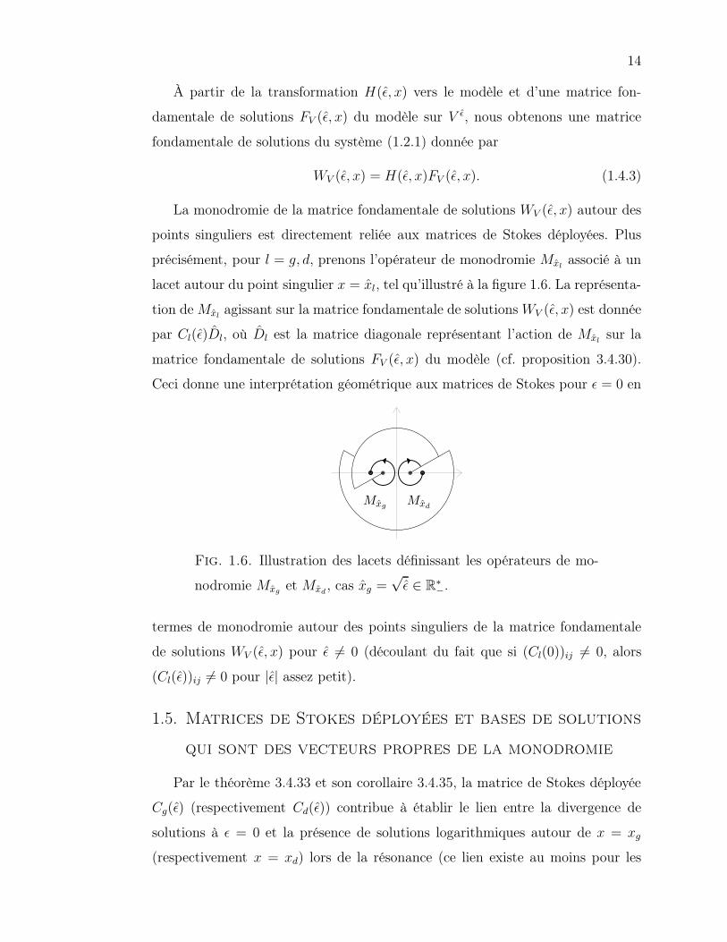
La monodromie de la matrice fondamentale de solutions WV (ǫ, x) autour des

points singuliers est directement reliée aux matrices de Stokes déployées. Plus

précisément, pour l = g, d, prenons l’opérateur de monodromie Mxlassocié à un

lacet autour du point singulier x = xl, tel qu’illustré à la figure 1.6. La représenta-

tion de Mxlagissant sur la matrice fondamentale de solutions WV (ǫ, x) est donnée

par Cl(ǫ)Dl, où Dl est la matrice diagonale représentant l’action de Mxlsur la

matrice fondamentale de solutions FV (ǫ, x) du modèle (cf. proposition 3.4.30).

Ceci donne une interprétation géométrique aux matrices de Stokes pour ǫ = 0 en

Mxg Mxd

Fig. 1.6. Illustration des lacets définissant les opérateurs de mo-

nodromie Mxg et Mxd, cas xg =

√ǫ ∈ R∗

−.

termes de monodromie autour des points singuliers de la matrice fondamentale

de solutions WV (ǫ, x) pour ǫ 6= 0 (découlant du fait que si (Cl(0))ij 6= 0, alors

(Cl(ǫ))ij 6= 0 pour |ǫ| assez petit).

1.5. Matrices de Stokes déployées et bases de solutions

qui sont des vecteurs propres de la monodromie

Par le théorème 3.4.33 et son corollaire 3.4.35, la matrice de Stokes déployée

Cg(ǫ) (respectivement Cd(ǫ)) contribue à établir le lien entre la divergence de

solutions à ǫ = 0 et la présence de solutions logarithmiques autour de x = xg

(respectivement x = xd) lors de la résonance (ce lien existe au moins pour les

15

cas génériques). En effet, le nombre de solutions qui sont des vecteurs propres de

l’opérateur de monodromie Mxl(pour l = g, d) est égal au nombre de vecteurs

propres de la matrice de Jordan associée à Cl(ǫ)Dl (qui est la représentation

de Mxlagissant sur WV (ǫ, x)). Les valeurs du paramètre de déploiement ǫ pour

lesquelles il y a résonance sont celles pour lesquelles une matrice Cl(ǫ)Dl pourrait

ne pas être diagonalisable (celles pour lesquelles la matrice Cl(ǫ)Dl a des valeurs

propres multiples). Voici les résultats selon qu’il y a résonance ou non.

• En considérant la matrice triangulaire unipotente Tl diagonalisant Cl(ǫ)Dl

dans le cas de non résonance, nous démontrons que WV (ǫ, x)Tl est une

matrice fondamentale de solutions qui sont des vecteurs propres de l’opé-

rateur de monodromie Mxl(cette matrice fondamentale de solutions est

unique à normalisation près) ;

• Lors de la résonance, la matrice Cl(ǫ)Dl n’est plus diagonalisable avec la

jième colonne de Tl n’existant plus si et seulement si la solution (vecteur

propre de la monodromie) correspondant à la jième colonne de WV (ǫ, x)Tl

n’existe plus. Dans ce cas de non-existence, cette solution doit être rempla-

cée, dans la base de solutions autour de x = xl, par une solution contenant

des termes logarithmiques. Les conditions pour lesquelles une colonne de

Tl n’existe plus à la résonance se traduisent par la non-annulation de po-

lynômes en termes des éléments de Dl et de Cl(ǫ). Dans les cas génériques

(où les lignes de Stokes sont distinctes), la non-annulation de ce polynôme

pour |ǫ| petit est assuré par la non-annulation du polynôme limite à ǫ = 0.

Ce dernier est un polynôme, à coefficients entiers, en les coefficients des

matrices de Stokes.

1.6. Systèmes de Riccati

En prenant des cartes dans l’espace projectif complexe, les systèmes déployés

s’écrivent comme des équations différentielles matricielles de Riccati, pour ǫ ∈S ∪ 0. En introduisant une variable temporelle, ces équations correspondent à

n systèmes différentiels non linéaires que nous avons appelés les n systèmes de

Riccati (cf. section 3.4.1).

16

Dans chaque système de Riccati, nous avons prouvé l’existence, pour x ∈ Ωǫs

et s = h, b, d’une variété invariante de dimension un qui est bornée près des

deux points singuliers. C’est en ramenant dans le système linéaire ces n variétés

invariantes (une pour chaque système de Riccati) que nous avons obtenu le théo-

rème d’existence des transformations vers le modèle ainsi que leur convergence

uniforme sur les compacts de Ω0s (cf. sections 3.4.5 et 3.4.6).

Les matrices de Stokes déployées s’interprètent en termes de monodromie d’in-

tégrales premières dans les systèmes de Riccati. Dans le jième système de Riccati,

nous donnons l’expression de n − 1 intégrales premières Hjq que nous indexons

par q ∈ 1, 2, ..., n\j. La monodromie d’une intégrale première Hjq autour des

points singuliers peut être écrite (cf. théorème 3.4.38) comme la composition

• d’une partie sauvage (c.-à-d. de la forme e2πiα avec α ∈ C, α → 0) et

linéaire, ne dépendant que du modèle (c.-à-d. que des invariants formels),

• d’une application dépendant des éléments des lignes q et j de l’inverse des

matrices de Stokes déployées et ayant une limite pour ǫ = 0.

On en déduit qu’une ligne j non triviale de l’inverse d’une matrice de Stokes

Cl(0) (l ∈ g, d) est une obstruction à ce que les intégrales premières Hjq du

jième système de Riccati soient des vecteurs propres de la monodromie autour

du point singulier x = xl, pour q = 1, 2, ..., j− 1, j +1, ..., n (cf. corollaire 3.4.39).

1.7. Relation d’auto-intersection

Les invariants formels, Λ0(ǫ) et Λ1(ǫ), et les matrices de Stokes déployées, Cd(ǫ)

et Cg(ǫ), satisfont une relation que nous nommons la relation d’auto-intersection.

Celle-ci provient (cf. section 3.4.10) de l’invariance (à normalisation près) sur

l’auto-intersection de S, des matrices de transition entre des bases de solutions

qui

• sont des vecteurs propres de la monodromie autour des points singuliers

réguliers,

• passent à la limite lorsque |ǫ| → 0.

17

En pratique, la relation d’auto-intersection s’écrit

Qb(ǫ)DdT−1d TgD

−1d = T−1

g TdQh(ǫ), (1.7.1)

où

• ǫ et ǫ = ǫe2πi appartiennent à l’auto-intersection de S (figure 1.3),

• la matrice diagonale Dd représente l’action de Mxdsur la matrice fonda-

mentale de solutions du modèle,

• Tl est la matrice triangulaire unipotente diagonalisant Cl(ǫ)Dl, l = g, d,

• Qh(ǫ) et Qb(ǫ) sont des matrices diagonales non singulières, dépendent

analytiquement de ǫ ∈ S∩, ont une limite non singulière lorsque ǫ tend

vers 0 et sont telles que

|Qi(ǫ) − I| < ci|ǫ|, ci ∈ R, ǫ ∈ S∩, i = b, h. (1.7.2)

1.8. Théorèmes de classification et de réalisation

Le système complet d’invariants analytiques des systèmes déployés (1.2.1) et

les conditions de sa réalisation s’obtiennent finalement des deux théorèmes sui-

vants (qui correspondent aux théorèmes 3.4.61 et 3.5.2).

Théorème de classification analytique

Deux systèmes (1.2.1) sont analytiquement équivalents si et seulement

si ils ont les mêmes invariants formels Λ0(ǫ), Λ1(ǫ) et des matrices de

Stokes déployées équivalentes.

Théorème de réalisation

Soit un système complet d’invariants composé

• d’un modèle (entièrement déterminé par les invariants formels

Λ0(ǫ), Λ1(ǫ)),

• d’une classe d’équivalence de matrices de Stokes déployées (le

secteur d’analyticité S de rayon ρ0 et d’ouverture plus grande

que 2π est choisi tel que dans la section 3.4.3, et son rayon ρ0 peut

18

être choisi plus petit afin d’assurer l’analyticité des éléments des

matrices de Stokes déployées sur S),

qui satisfont la relation d’auto-intersection. Alors il existe r > 0, un

rayon ρ < minρ0,r2

2 de S et un système (x2 − ǫ)y′ = B(ǫ, x) (y ∈ Cn)

caractérisé par ces invariants, où B(ǫ, x) est analytique sur Dρ × Dr.

Chapitre 2

THE STOKES PHENOMENON IN THE

CONFLUENCE OF THE HYPERGEOMETRIC

EQUATION USING RICCATI EQUATION

Caroline Lambert, Christiane Rousseau

Research supported by NSERC and FQRNT in Canada

Key words : hypergeometric equation, confluence, Stokes phenomenon,

divergent series, analytic continuation, summability, monodromy,

confluent hypergeometric equation, Riccati equation.

Submitted 8 June 2007 (revised 1 November 2007) and published in the

Journal of Differential Equations 244 (2008), no 10, 2641–2664

For the purpose of the thesis, this version includes slight modifications from the

published version.

Abstract

In this paper we study the confluence of two regular singular points of the

hypergeometric equation into an irregular one. We study the consequence of the

divergence of solutions at the irregular singular point for the unfolded system.

Our study covers a full neighborhood of the origin in the confluence parameter

space. In particular, we show how the divergence of solutions at the irregular

singular point explains the presence of logarithmic terms in the solutions at a

regular singular point of the unfolded system. For this study, we consider values

of the confluence parameter taken in two sectors covering the complex plane. In

20

each sector, we study the monodromy of a first integral of a Riccati system related

to the hypergeometric equation. Then, on each sector, we include the presence

of logarithmic terms into a continuous phenomenon and view a Stokes multiplier

related to a 1-summable solution as the limit of an obstruction that prevents a

pair of eigenvectors of the monodromy operators, one at each singular point, to

coincide.

2.1. Introduction

The hypergeometric differential equation arises in many problems of mathe-

matics and physics and is related to special functions. It is written

X(1 − X) v′′(X) + c − (a + b + 1)X v′(X) − ab v(X) = 0. (2.1.1)

More precisely, any linear equation of order two (y′′(z)+p(z)y′(z)+q(z)y(z) =

0) with three regular singular points can be transformed into the hypergeometric

equation by a change of variables of the form y = f(z)v and a new independant

variable X obtained from z by a Möbius transformation (see for example [16]

p. 164).

The confluent hypergeometric equation with a regular singular point at z = 0

and an irregular one at z = ∞ is often written in the form

zu′′(z) + (c′ − z)u′(z) − a′u(z) = 0. (2.1.2)

Solutions of this equation at the irregular point z = ∞ are in general divergent

and always 1-summable. C. Zhang ([24] and [25]) and J.-P. Ramis [17] showed

that the Stokes multipliers related to the confluent equation can be obtained from

the limits of the monodromy of the solutions of the nonconfluent equation (2.1.1).

They assumed that the bases of solutions of (2.1.1) around the merging singular

points (z = b and z = ∞) never contain logarithmic terms and they described the

phenomenon using two types of limits : first with ℑ(b) → ∞, then with ℜ(b) → ∞on the subset b = b0 + N for b0 ∈ C. They also proved the uniform convergence

of the solutions on all compact sets in the case ℑb → ∞. Related questions have

been considered by R. Schäfke [21].

21

In this paper, we propose a different approach : we describe the phenomenon

in a whole neighborhood of values of the confluence parameter, but we are forced

to cover the neighborhood with two sectors on which the presentations are dif-

ferent. We are then able to explain the presence of the logarithmic terms : they

occur precisely for discrete values of the confluence parameter when we unfold a

confluent equation with at least one divergent solution. On each sector, each di-

vergent solution explains the presence of logarithmic terms at one of the unfolded

singular points. The occurrence of logarithmic terms, a discrete phenomenon, is

embedded into a continuous phenomenon valid on the whole sector.

To help understanding the phenomenon, we give a translation of the hyper-

geometric equation in terms of a Riccati system in which two saddle-nodes are

unfolded with a parameter ǫ. The parameter space is again covered with two

sectors S±. For this Riccati system, we consider on each sector S± of the pa-

rameter space a first integral which has a limit when ǫ → 0, written in the

form Iǫ±(x, y) = Hǫ±(x)y−ρ1(x,ǫ)y−ρ2(x,ǫ)

where y = ρ1(x, ǫ) and y = ρ2(x, ǫ) are ana-

lytic invariant manifolds of singular points and, for ǫ = 0, center manifolds of

the saddle-nodes. Then, when we calculate the monodromy of one of these first

integrals, we can separate it into two parts : a continuous one which has a limit

when ǫ → 0 inside the sector S± and a wild one which has no limit but which is

linear. The wild part is independent of the divergence of the solutions and present

in all cases. The divergence of ρ1(x, 0) corresponds to the analytic invariant ma-

nifold of one singular point being ramified at the other in the unfolding of one

saddle-node. For particular values of ǫ for which one singular point is a resonant

node, this forces the node to be nonlinearisable (i.e. to have a nonzero resonant

monomial), in which case logarithmic terms appear in Iǫ±. This is called the pa-

rametric resurgence phenomenon in [19]. The divergence of ρ2(x, 0) corresponds

to a similar phenomenon with the pair of singular points coming from the unfol-

ding of the other saddle-node. Finally, we translate our results in the case of a

universal deformation.

22

2.2. Solutions of the hypergeometric equation

In this paper, we study the confluence of the singular points 0 and 1 ; the

confluent hypergeometric equation has an irregular singular point at the origin.

We make the change of variables X = xǫ

in (2.1.1) to bring the singular point at

X = 1 to a singular point at x = ǫ 6= 0. We consider small values of ǫ and we

limit the values of c to

c = 1 − 1

ǫ. (2.2.1)

Let v(xǫ) be denoted by w(x). Then (2.1.1) becomes

x(x − ǫ) w′′(x) + 1 − ǫ + (a + b + 1)xw′(x) + abw(x) = 0. (2.2.2)

We will then let ǫ → 0. We want to study what happens in a neighborhood of

ǫ = 0. The confluence parameter ǫ will be taken in two sectors, the union of which

is a small pointed neighborhood of the origin in the complex plane.

Remark 2.2.1. Although not explicitly written, our study is still valid if we let

a(ǫ) and b(ǫ) be analytic functions of ǫ.

Definition 2.2.2. Given γ ∈ (0, π2) fixed, we define

• S+ = ǫ ∈ C : 0 < |ǫ| < r(γ), arg(ǫ) ∈ (−π + γ, π − γ),

• S− = ǫ ∈ C : 0 < |ǫ| < r(γ), arg(ǫ) ∈ (−2π + γ,−γ).

Remark 2.2.3. γ can be chosen arbitrary small, but r(γ) will depend on γ and

r(γ) → 0 as γ → 0. In particular, we will ask a + b + 1ǫ

/∈ −N, a + 1ǫ

/∈ −N and

b + 1ǫ

/∈ −N on S+ and 2 − a − b − 1ǫ

/∈ −N, a − 1ǫ

/∈ −N and b − 1ǫ

/∈ −N on S−

(in this paper N = 0, 1, ...).

2.2.1. Bases for the solutions of the hypergeometric equation (2.2.2)

at the regular singular points x = 0 and x = ǫ

The fundamental group of C\0, ǫ based at an ordinary point acts on a

solution (valid at this base point) by giving its analytic continuation at the end

of a loop. In this way we have monodromy operators around each singular point.

We can extend it to act on any function of solutions.

Notation 2.2.4. The monodromy operator M0 (resp. Mǫ) is the one associated

to the loop which makes one turn around the singular point x = 0 (resp. x = ǫ) in

23

the positive direction (and which does not surround any other singular point). In

this paper, since we use bases of solutions whose Taylor series are convergent in

a disk of radius ǫ centered at a singular point, it will be useful to define M0 (resp.

Mǫ) with the fundamental group based at a point belonging to the line joining −ǫ

and 0 (resp. ǫ and 2ǫ).

As the hypergeometric equation is linear of second order, the space of solutions

is of dimension 2. Given a basis for the space of solutions, the monodromy operator

M0 (resp. Mǫ) acting on this basis is linear and is represented by a two-dimensional

matrix.

As elements of a basis B0 (resp. Bǫ) around the singular point x = 0 (resp.

x = ǫ), it is classical to use solutions which are eigenvectors of the monodromy

operator M0 (resp. Mǫ) whenever these solutions exist. However, none of these

bases is defined on the whole of a sector S+ or S−. This is why we later switch

to mixed bases. C. Zhang ([24] and [25]) also used mixed bases but he has not

pushed the study as far as we do.

Definition 2.2.5. The hypergeometric series kFj(a1, a2, ...ak, c1, c2, ..., cj ; x) is

defined by

kFj(a1, a2, ...ak, c1, c2, ..., cj; x) = 1 +

∞∑

n=1

(a1)n(a2)n...(ak)n

(c1)n(c2)n...(cj)nn!xn (2.2.3)

with

(a)0 = 1,

(a)n = a(a + 1)(a + 2)...(a + n − 1)(2.2.4)

and for c1, ..., cj /∈ −N.

A basis B0 = w1(x), w2(x) of solutions of (2.2.2) around the singular point

x = 0 is well known (see [14] pp. 67–71 for details) :

w1(x) = 2F1

(a, b, 1 − 1

ǫ; x

ǫ

)

=(1 − x

ǫ

)1− 1ǫ−a−b

2F1

(1 − 1

ǫ− a, 1 − 1

ǫ− b, 1 − 1

ǫ; x

ǫ

),

w2(x) =(

xǫ

) 1ǫ

2F1

(a + 1

ǫ, b + 1

ǫ, 1 + 1

ǫ; x

ǫ

)

=(

xǫ

) 1ǫ(1 − x

ǫ

)1− 1ǫ−a−b

2F1

(1 − a, 1 − b, 1 + 1

ǫ; x

ǫ

).

(2.2.5)

The solution w1(x) exists if 1 − 1ǫ

/∈ −N whereas w2(x) exists if 1 + 1ǫ

/∈ −N.

24

Similarly, a basis Bǫ = w3(x), w4(x) of solutions of (2.2.2) around the sin-

gular point x = ǫ is given by :

w3(x) = 2F1

(a, b, a + b + 1

ǫ; 1 − x

ǫ

),

w4(x) =(

xǫ

) 1ǫ(1 − x

ǫ

)1− 1ǫ−a−b

2F1

(1 − a, 1 − b, 2 − 1

ǫ− a − b; 1 − x

ǫ

).

(2.2.6)

The solution w3(x) exists if a+b+1ǫ

/∈ −N whereas w4(x) exists if 2−1ǫ−a−b /∈ −N.

In particular, w2(x) and w3(x) exist for all ǫ ∈ S+ and w1(x) and w4(x) exist

for all ǫ ∈ S−, provided r(γ) is sufficiently small.

Traditionally, in order to get a basis when 1 − 1ǫ∈ −N, a /∈ −N and b /∈ −N

(resp. 2− 1ǫ− a− b ∈ −N, 1− a /∈ −N and 1− b /∈ −N), the solution w1(x) in B0

(resp. w4(x) in Bǫ) is replaced by some other solution w1(x) (resp. w4(x)) which

contains logarithmic terms. Similarly, we have w2(x) and w3(x) for specific value

of ǫ in S− (see for example [7]).

The problem with this approach is that the basis B0 = w1(x), w2(x) (resp.

Bǫ = w3(x), w4(x)) does not have a limit when the parameter tends to a value

for which there are logarithmic terms at the origin (resp. at x = ǫ). For ǫ ∈ S+,

there are values of ǫ for which w1(x) or w4(x) may not be defined, whereas w2(x)

or w3(x) may not be defined for some values of ǫ in S−. This means that B0

and Bǫ are not optimal bases to describe the dynamics for all values of ǫ in the

sectors S±. We will rather consider the bases B+ = w2(x), w3(x) for ǫ ∈ S+ and

B− = w4(x), w1(x) for ǫ ∈ S−. With these bases we will explain the occurence

of logarithmic terms (a phenomenon occuring for discrete values of the confluence

parameter) in a continuous way. The following lemma will allow us to consider

only one of the bases, namely B+ with ǫ ∈ S+.

25

Lemma 2.2.6. The equation (2.2.2) is invariant under

c′ = 1 − c + a + b,

ǫ′ = 11−c′ ,

x′ = ǫ′(1 − x

ǫ

),

a′ = a,

b′ = b,

(2.2.7)

which transforms S+ into S− and B+ into B−.

2.2.2. The confluent hypergeometric equation and its summable so-

lutions

Taking the limit ǫ → 0 in (2.2.2), we obtain a confluent hypergeometric equa-

tion :

x2 w′′(x) + 1 + (1 + a + b)xw′(x) + abw(x) = 0. (2.2.8)

A basis of solutions around the origin is

g(x) = 2F0(a, b;−x),

k(x) = e1x x1−a−b

2F0(1 − a, 1 − b; x) = e1x x1−a−bh(x).

(2.2.9)

Remark 2.2.7. The confluent equation in the literature is often studied with the

irregular singular point at infinity :

zu′′(z) + (c′ − z)u′(z) − au(z) = 0. (2.2.10)

The following transformation applied to (2.2.10) yields the confluent equation

(2.2.8) :

z = 1x,

u(

1x

)= xaw(x),

c′ = a + 1 − b.

(2.2.11)

The following theorem is well-known, one can refer for instance to [15].

Theorem 2.2.8. The series g(x) is divergent if and only if a /∈ −N and b /∈ −N.

It is 1-summable in all directions except R−. The series h(x) is divergent if and

only if 1− a /∈ −N and 1− b /∈ −N. It is 1-summable in all directions except R+.

26

The Borel sums of these series, denoted g(x) and h(x), are thus defined in the

sectors illustrated in Figure 2.1.

g(x) h(x)

00

Fig. 2.1. Domains of the Borel sums of the confluent series g(x)

and h(x).

As illustrated in Figure 2.1, we have one Borel sum g(x) in the region ℜ(x) > 0.

When extending g(x) to the region ℜ(x) < 0 by turning around the origin in

the positive (resp. negative) direction, we get a sum g+(x) (resp. g−(x)). The

functions g+(x) and g−(x) are different in general and never coincide if the series

is divergent. Similarly, we consider h(x) defined in the region ℜ(x) < 0. When we

extend it by turning around the origin in the positive (resp. negative) direction,

we obtain the sum h+(x) (resp. h−(x)). We define

k+(x) = e1x x1−a−bh+(x),

k−(x) = e1x x1−a−bh−(x)

(2.2.12)

for ℜ(x) > 0, and

k(x) = e1x x1−a−bh(x) (2.2.13)

for ℜ(x) < 0.

Since g+(x) and g−(x) have the same asymptotic expansion g(x), their diffe-

rence is a solution of (2.2.8) which is asymptotic to 0 in the region ℜ(x) < 0, and

thus there exists λ ∈ C such that

g+(xe2πi) − g−(x) = λk(x) if arg(x) ∈(−3π

2,−π

2

). (2.2.14)

Similarly, there exists µ ∈ C such that

k+(x) − e2πi(1−a−b)k−(xe−2πi) = µg(x) if arg(x) ∈(−π

2,π

2

). (2.2.15)

27

Remark 2.2.9. For all n ∈ Z, it is possible to construct a function gn(x), cor-

responding to the Borel sum of the divergent series g(x) in the regions arg(x) ∈(−π

2+2πn, π

2+2πn). Then, g+

n (x) (resp. g−n (x)) denotes its analytic continuation

in the positive (resp. negative) direction around the origin, defined in the region

arg(x) ∈ (π2

+ 2πn, 3π2

+ 2πn) (resp. arg(x) ∈ (−3π2

+ 2πn, −π2

+ 2πn)). Since

g+n+1(xe2πi) = g+

n (x), g−n+1(xe2πi) = g−

n (x) and gn+1(xe2πi) = gn(x), the subscript

n is not necessary and the functions g(x), g+(x) and g−(x) are univalued. But

what is important is that, when considering g+(x), the + does not refer to the

values of arg(x), but to the fact that g+(x) has been obtained by analytic conti-

nuation of g(x) when turning in the positive direction. Similar relations for h+(x),

h−(x) and h(x) imply that these functions are also univalued. On the other hand,

x1−a−b is a multivalued function, which becomes univalued as soon as arg(x) is

determined.

Definition 2.2.10. In the relations (2.2.14) and (2.2.15), we call λ and µ the

Stokes multipliers associated respectively to the solutions g(x) and k(x).

Their values are calculated in [15]. Using the change of variable (2.2.11), we

have

λ = −2πieiπ(1−a−b)

Γ(a)Γ(b)(2.2.16)

and

µ = − 2iπ

Γ(1 − a)Γ(1 − b). (2.2.17)

Notation 2.2.11. Let us write

H0(x) =

k(x)g−(x)

if ℜ(x) < 0,

k+(x)g(x)

if ℜ(x) > 0(2.2.18)

and

H0′(x) =

k−(x)g(x)

if ℜ(x) > 0,

k(x)g+(x)

if ℜ(x) < 0(2.2.19)

with H0(x) (resp. H0′(x)) analytic in the complex plane minus a cut with values

in CP1, as illustrated in Figure 2.2. On purpose we leave the ambiguity in the

argument. In this form, H0(x) and H0′(x) are multivalued. They will become

univalued when arg(x) is specified.

28

H0′(x)H0(x)

0

0

Fig. 2.2. Domains of H0(x) and H0′(x), with arbitrary radius.

Proposition 2.2.12. The Stokes multiplier of g(x) is

λ = 1H0′(x)

− 1H0(x)

if arg(x) ∈(−3π

2, −π

2

), (2.2.20)

while the Stokes multiplier of k(x) is

µ = H0(x) − e2πi(1−a−b)H0′(xe−2πi) if arg(x) ∈(−π

2, π

2

). (2.2.21)

Proof. We have

λ = g+(xe2πi)k(x)

− g−(x)k(x)

= g+(x)k(x)

− g−(x)k(x)

= 1H0′(x)

− 1H0(x)

if arg(x) ∈(−3π

2, −π

2

)(2.2.22)

and

µ = k+(x)g(x)

− e2πi(1−a−b) k−(xe−2πi)g(x)

= k+(x)g(x)

− e2πi(1−a−b) k−(xe−2πi)g(xe−2πi)

= H0(x) − e2πi(1−a−b)H0′(xe−2πi) if arg(x) ∈(−π

2, π

2

).

(2.2.23)

In view of this proposition, it will seem natural in the next section to study

the monodromy of some quotient of solutions of the hypergeometric equation

(2.2.2). But before, let us explore the link between divergent series in particular

solutions of the confluent differential equation and analytic continuation of series

appearing in solutions of the nonconfluent equation.

29

2.3. Divergence and Monodromy

2.3.1. Divergence and ramification : first observations

Let us illustrate by an example the link between the divergence of a confluent

series and the ramification of its unfolded series.

Example 2.3.1. The series g(x) = 2F0(a, b;−x) is non-summable in the direc-

tion R−, i.e. on the left side. We unfold g(x) with a small ǫ ∈ R. Let us define

gǫ(x) =

w3(x) = 2F1

(a, b, a + b + 1

ǫ; 1 − x

ǫ

)if ǫ ∈ S+,

w1(x) = 2F1

(a, b, 1 − 1

ǫ; x

ǫ

)if ǫ ∈ S−.

(2.3.1)

By continuity, the analytic continuation of gǫ(x) will be ramified at the left sin-

gular point and regular at the right singular point (Figure 2.3). For the special

values of ǫ for which logarithmic terms may exist in the general solution at the

left singular point, this will force their existence. Indeed, for these special values

of ǫ, the general solution at the left singular point either has logarithmic terms or

is not ramified (for more details, refer to the proof of Theorem 2.3.5 (1)).

This example illustrates that a direction of non-summability for a confluent

series determines which merging singular point is "pathologic" (with ǫ in S±) for

an unfolded solution, as illustrated in Figure 2.3. Although subtleties are needed

to adapt Example 2.3.1 to the other solution k(x) = e1x x1−a−bh(x) because of

the ramification of x1−a−b, we have a similar phenomenon if we define adequately

the pathology. For example, if ǫ ∈ S+, the singular point x = 0 will be defined

pathologic for the solution w3(x) if the analytic continuation of this solution is

not an eigenvector of the monodromy operator M0. This will be studied more

precisely in Section 2.3.3 using the results we will obtain in the next two sections.

2.3.2. Limit of quotients of solutions on S±

We will later see that a divergent series in the basis of solutions at the

confluence necessarily implies the presence of an obstruction that prevents an

eigenvector of M0 to be an eigenvector of Mǫ. As a tool for our study, we will

consider the behavior of the analytic continuation of some functions of the particu-

lar solutions wi(x) ∈ B± when turning around singular points. A first motivation

30

0 0 ǫ

0 0 ǫ

ǫ 0

ǫ 0

2F0(a, b;−x) 2F1

(a, b, a + b + 1

ǫ; 1 − x

ǫ

)

2F0(1 − a, 1 − b; x) 2F1

(1 − a, 1 − b, 1 + 1

ǫ; x

ǫ

)

2F1

(a, b; 1 − 1

ǫ, x

ǫ

)

2F1

(1 − a, 1 − b; 2 − a − b − 1

ǫ, 1 − x

ǫ

)

⇐⇒

⇐⇒

or

or

∀ǫ ∈ S+ ∀ǫ ∈ S−

∀ǫ ∈ S+ ∀ǫ ∈ S−

Fig. 2.3. Link between ramification of the analytic continuation

of the hypergeometric series in the unfolded case and divergence

(ramification) of the associated confluent series.

for studying these functions comes from Proposition 2.2.12. We will also see in

Section 2.4 that these quantities have the same ramification as first integrals of a

Riccati system related to the hypergeometric equation, these first integrals having

a limit when ǫ → 0 on S±. The first integrals are defined by

Hǫ+(x) =κ+(ǫ)w2(x)

w3(x)if ǫ ∈ S+ (2.3.2)

and

Hǫ−(x) =κ−(ǫ)w4(x)

w1(x)if ǫ ∈ S− (2.3.3)

with

κ+(ǫ) = ǫ1−a−beπi(a+b−1+ 1ǫ), κ−(ǫ) = ǫ1−a−be−πi(a+b−1+ 1

ǫ). (2.3.4)

Hǫ±(x) are first defined in B(0, ǫ) ∩ B(ǫ, ǫ) and then analytically extended as

in Figures 2.4 and 2.5. The coefficients κ± in the functions Hǫ±(x) are chosen

so that Hǫ±(x) have the limit H0(x) when ǫ → 0 inside S±. More precisely, for

ǫ ∈ S+, we replace f(x) = (xǫ)

1ǫ (1 − x

ǫ)1− 1

ǫ−a−b by κ+(ǫ)f(x), so that the limit

when ǫ → 0 and ǫ ∈ S+ exists and corresponds to e1x x1−a−b. The limit is uniform

on any simply connected compact set which does not contain 0. The constant

31

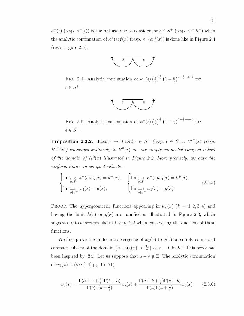
κ+(ǫ) (resp. κ−(ǫ)) is the natural one to consider for ǫ ∈ S+ (resp. ǫ ∈ S−) when

the analytic continuation of κ+(ǫ)f(x) (resp. κ−(ǫ)f(x)) is done like in Figure 2.4

(resp. Figure 2.5).

0 ǫ

Fig. 2.4. Analytic continuation of κ+(ǫ)(

xǫ

) 1ǫ(1 − x

ǫ

)1− 1ǫ−a−b

for

ǫ ∈ S+.

ǫ 0

Fig. 2.5. Analytic continuation of κ−(ǫ)(

xǫ

) 1ǫ(1 − x

ǫ

)1− 1ǫ−a−b

for

ǫ ∈ S−.

Proposition 2.3.2. When ǫ → 0 and ǫ ∈ S+ (resp. ǫ ∈ S−), Hǫ+(x) (resp.

Hǫ−(x)) converges uniformly to H0(x) on any simply connected compact subset

of the domain of H0(x) illustrated in Figure 2.2. More precisely, we have the

uniform limits on compact subsets :

limǫ→0ǫ∈S+

κ+(ǫ)w2(x) = k+(x),

limǫ→0ǫ∈S+

w3(x) = g(x),

limǫ→0ǫ∈S−

κ−(ǫ)w4(x) = k+(x),

limǫ→0ǫ∈S−

w1(x) = g(x).(2.3.5)

Proof. The hypergeometric functions appearing in wk(x) (k = 1, 2, 3, 4) and

having the limit h(x) or g(x) are ramified as illustrated in Figure 2.3, which

suggests to take sectors like in Figure 2.2 when considering the quotient of these

functions.

We first prove the uniform convergence of w3(x) to g(x) on simply connected

compact subsets of the domain x, | arg(x)| < 3π2 as ǫ → 0 in S+. This proof has

been inspired by [24]. Let us suppose that a − b /∈ Z. The analytic continuation

of w3(x) is (see [14] pp. 67–71)

w3(x) =Γ(a + b + 1

ǫ)Γ(b − a)

Γ(b)Γ(b + 1ǫ)

w5(x) +Γ(a + b + 1

ǫ)Γ(a − b)

Γ(a)Γ(a + 1ǫ)

w6(x) (2.3.6)

32

with

w5(x) =(

ǫx

)a2F1

(a, a + 1

ǫ, a + 1 − b; ǫ

x

),

w6(x) =(

ǫx

)b2F1

(b, b + 1

ǫ, b + 1 − a; ǫ

x

).

(2.3.7)

The function 2F1(a, a+ 1ǫ, a+1−b; ǫ

x) converges uniformly on simply connected

compact subsets to 1F1(a, a + 1 − b; 1x) and we have

limǫ→0ǫ∈S+

ǫaΓ(a+b+ 1ǫ)

Γ(b+ 1ǫ)

= 1. (2.3.8)

The same relations apply with a and b interchanged so w3(x) converges uniformly

on simply connected compact subsets to

g(x) =Γ(b − a)

Γ(b)x−a

1F1

(a, a + 1 − b;

1

x

)+

Γ(a − b)

Γ(a)x−b

1F1

(b, b + 1 − a;

1

x

).

(2.3.9)

Let us suppose now that a − b = −m with m ∈ N. We take t small, we let

a = b−m+t. We first show that limt→0 w3(x) exists with x on a simply connected

compact subset of the domain x, | arg(x)| < 3π2. We write w3(x) as

w3(x) = (a − b)Γ(b − a)Γ(a − b)Γ(a + b + 1ǫ)

×[

w5(x)

Γ(b)Γ(b+ 1ǫ)Γ(a−b+1)

− w6(x)

Γ(a)Γ(a+ 1ǫ)Γ(b−a+1)

] (2.3.10)

and take the limit t → 0 with a = b −m + t. The part inside brackets has a zero

at t = 0 since

limt→0w5(x)

Γ(a−b+1)=(

ǫx

)b (b−m)m(b−m+ 1ǫ)m

m! 2F1

(b, b + 1

ǫ, m + 1; ǫ

x

)

=Γ(b)Γ(b+ 1

ǫ)w6(x)

Γ(a)Γ(a+ 1ǫ)Γ(b−a+1)

.(2.3.11)

The left part of (2.3.10) has a simple pole at t = 0 so limt→0 w3(x) exists. Since

w3(x) is an analytic function of t on a punctured neighborhood of t = 0, we

have that w3(x) converges uniformly on simply connected compact subsets to

limt→0 w3(x) when t → 0. Similarly, g(x) converges uniformly on simply connected

compact subsets to limt→0 g(x) since

limt→01F1(a,a+1−b; 1

x)

xaΓ(a−b+1)=

Γ(b)1F1(b,b+1−a; 1x)

xbΓ(a)Γ(b−a+1). (2.3.12)

Hence, when ǫ → 0 in S+, limt→0 w3(x) converges uniformly on simply connected

compact subsets (of x, | arg(x)| < 3π2) to limt→0 g(x). Interchanging a and b

leads to the case b − a ∈ −N.

33

Now, w2(x) (as in (2.2.5)) converges uniformly to k(x) on simply connected

compact subsets of the domain x, | arg(−x)| < 3π2 to k(x). Indeed, we can

decompose κ+(ǫ)w2(x) as

(e

πiǫ

(x

ǫ

) 1ǫ(1 − x

ǫ

)− 1ǫ

)((x − ǫ)1−a−b

2F1

(1 − a, 1 − b, 1 +

1

ǫ;x

ǫ

)). (2.3.13)

The first part converges to e1x . The second part converges to x1−a−b

2F0(1 −a, 1 − b; x). The fact that 2F1(1 − a, 1 − b, 1 + 1

ǫ; x

ǫ) converges uniformly on sim-

ply connected compact subsets to 2F0(1 − a, 1 − b; x) can be obtained from the

convergence of w3(x) to g(x) by a change of coordinates. The case ǫ ∈ S− is

similar.

2.3.3. Divergence and nondiagonal form of the monodromy operator

in the basis B+

It is clear that w2(x) is an eigenvector of the monodromy operator M0 with

eigenvalue eiπǫ , and that w3(x) is an eigenvector of Mǫ with eigenvalue 1. In gene-

ral, eigenvectors of the monodromy operators M0 and Mǫ should not coincide. In

the generic case, the analytic continuation of an eigenvector of the monodromy

operator M0 is not an eigenvector of Mǫ. If we are in the generic case and this

persists to the limit ǫ = 0, then at the limit we have a nonzero Stokes multi-

plier. The results stated in the next theorem tell us whether or not the analytic

continuation of w3(x) (resp. w2(x)) is an eigenvector of M0 (resp. Mǫ). This is

done in the two covering sectors S± of a small neighborhood of ǫ, and it includes

the presence of logarithmic terms : we will detail this last part in Theorem 2.3.5

below.

Notation 2.3.3. Let w(δ,θ)(x) be the analytic continuation of w(x) when starting

on (0, ǫ) and turning of an angle θ around x = δ, with δ ∈ 0, ǫ (see Figure 2.6).

In short, w(δ,π)(x) can be obtained from the action of the monodromy operator

around x = δ applied on w(δ,−π)(x).

Theorem 2.3.4.

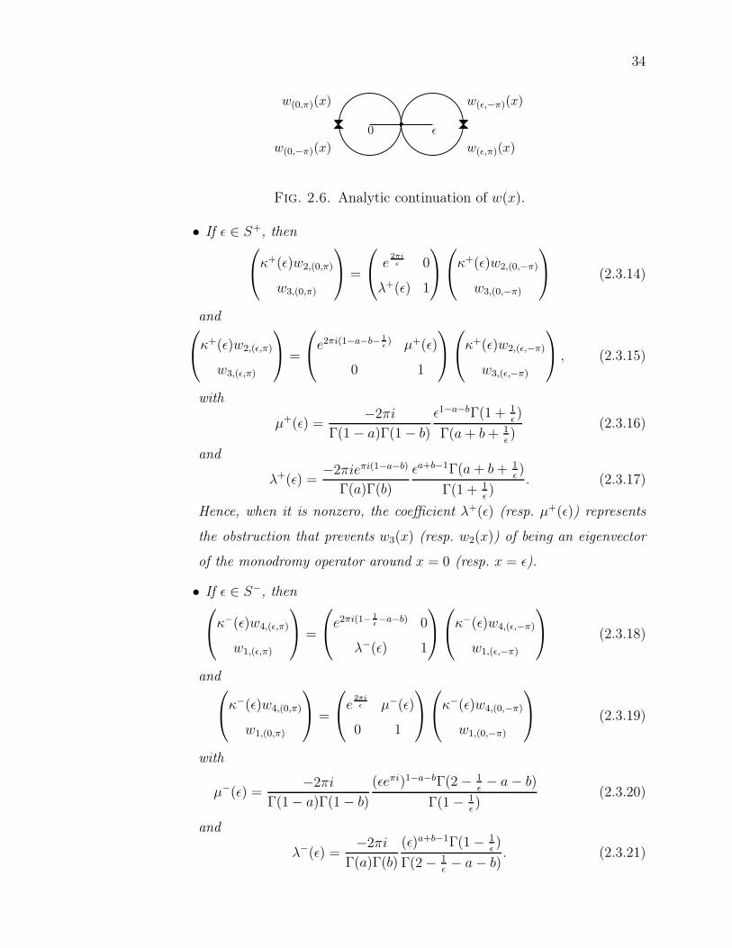
34

0 ǫ

w(0,π)(x)

w(0,−π)(x)

w(ǫ,−π)(x)

w(ǫ,π)(x)

Fig. 2.6. Analytic continuation of w(x).

• If ǫ ∈ S+, thenκ+(ǫ)w2,(0,π)

w3,(0,π)

=

e

2πiǫ 0

λ+(ǫ) 1

κ+(ǫ)w2,(0,−π)

w3,(0,−π)

(2.3.14)

andκ+(ǫ)w2,(ǫ,π)

w3,(ǫ,π)

=

e2πi(1−a−b− 1

ǫ) µ+(ǫ)

0 1

κ+(ǫ)w2,(ǫ,−π)

w3,(ǫ,−π)

, (2.3.15)

with

µ+(ǫ) =−2πi

Γ(1 − a)Γ(1 − b)

ǫ1−a−bΓ(1 + 1ǫ)

Γ(a + b + 1ǫ)

(2.3.16)

and

λ+(ǫ) =−2πieπi(1−a−b)

Γ(a)Γ(b)

ǫa+b−1Γ(a + b + 1ǫ)

Γ(1 + 1ǫ)

. (2.3.17)

Hence, when it is nonzero, the coefficient λ+(ǫ) (resp. µ+(ǫ)) represents

the obstruction that prevents w3(x) (resp. w2(x)) of being an eigenvector

of the monodromy operator around x = 0 (resp. x = ǫ).

• If ǫ ∈ S−, thenκ−(ǫ)w4,(ǫ,π)

w1,(ǫ,π)

=

e2πi(1− 1

ǫ−a−b) 0

λ−(ǫ) 1

κ−(ǫ)w4,(ǫ,−π)

w1,(ǫ,−π)

(2.3.18)

andκ−(ǫ)w4,(0,π)

w1,(0,π)

=

e

2πiǫ µ−(ǫ)

0 1

κ−(ǫ)w4,(0,−π)

w1,(0,−π)

(2.3.19)

with

µ−(ǫ) =−2πi

Γ(1 − a)Γ(1 − b)

(ǫeπi)1−a−bΓ(2 − 1ǫ− a − b)

Γ(1 − 1ǫ)

(2.3.20)

and

λ−(ǫ) =−2πi

Γ(a)Γ(b)

(ǫ)a+b−1Γ(1 − 1ǫ)

Γ(2 − 1ǫ− a − b)

. (2.3.21)

35

Hence, when it is nonzero, the coefficient λ−(ǫ) (resp. µ−(ǫ)) represents

the obstruction that prevents w1(x) (resp. w4(x)) of being an eigenvector

of the monodromy operator around x = ǫ (resp. x = 0).

Then, with the limit taken for any path in S+ or in S−, we have

limǫ→0

µ±(ǫ) = µ (2.3.22)

and

limǫ→0

λ±(ǫ) = λ, (2.3.23)

which are precisely the Stokes multipliers associated to the solutions k(x) and g(x)

and given by (2.2.16) and (2.2.17).

Proof. Let ǫ ∈ S+. To make analytic continuation of the solutions w2(x) and

w3(x), we need to make further restrictions on the values of ǫ, but we will shortly

show the validity of the result without these hypotheses. We have (see for example

[14] pp. 67–71)

• if 2 − 1ǫ− a − b /∈ −N,

w2(x) =Γ(1− 1

ǫ−a−b)Γ(1+ 1

ǫ)

Γ(1−a)Γ(1−b)w3(x) +

Γ(a+b−1+ 1ǫ)Γ(1+ 1

ǫ)

Γ(a+ 1ǫ)Γ(b+ 1

ǫ)

w4(x)

= D(ǫ)w3(x) + E(ǫ)w4(x);(2.3.24)

• if 1 − 1ǫ

/∈ −N,

w3(x) =Γ( 1

ǫ)Γ(a+b+ 1

ǫ)

Γ(b+ 1ǫ)Γ(a+ 1

ǫ)w1(x) +

Γ(a+b+ 1ǫ)Γ(− 1

ǫ)

Γ(a)Γ(b)w2(x)

= A(ǫ)w1(x) + B(ǫ)w2(x).(2.3.25)

These relations allow the calculation of the monodromy of w2(x) (resp. w3(x))

around x = ǫ (resp. x = 0). The explosion of the coefficients (coefficients becoming

infinite) for specific values of ǫ corresponds to the presence of logarithmic terms

in the general solution around the singular point x = ǫ (resp. x = 0). We have,

36

in the region B(0, ǫ) ∩ B(ǫ, ǫ) (with the hypothesis that 2 − 1ǫ− a − b /∈ −N),

κ+(ǫ)w2(x)

= κ+(ǫ)(D(ǫ)w3(x) + E(ǫ)w4(x))

= κ+(ǫ)(D(ǫ) 2F1(a, b, a + b + 1

ǫ; 1 − x

ǫ)

+E(ǫ)(xǫ)

1ǫ (1 − x

ǫ)1− 1

ǫ−a−b

2F1(1 − a, 1 − b,−1ǫ

+ 2 − a − b; 1 − xǫ))

.

(2.3.26)

Since w3,(ǫ,−π) = w3,(ǫ,π), we obtain

κ+(ǫ)w2,(ǫ,π) = e2πi(1−a−b− 1ǫ)κ+(ǫ)w2,(ǫ,−π) + µ+(ǫ)w3,(ǫ,−π) (2.3.27)

with

µ+(ǫ) = D(ǫ)ǫ1−a−beπi(a+b−1+ 1ǫ)(1 − e2πi(1−a−b− 1

ǫ))

= −D(ǫ)ǫ1−a−b(eπi(1−a−b− 1

ǫ) − e−πi(1−a−b− 1

ǫ))

.(2.3.28)

Since sin(z) = eiz−e−iz

2iand Γ(z) sin(πz) = π

Γ(1−z), we can simplify the latter

expression :

µ+(ǫ) = −2iD(ǫ)ǫ1−a−b sin(π(1 − a − b − 1

ǫ

))

= −2iΓ(1− 1

ǫ−a−b)Γ(1+ 1

ǫ)

Γ(1−a)Γ(1−b)ǫ1−a−b sin

(π(1 − a − b − 1

ǫ

))

= −2πiΓ(1+ 1

ǫ)

Γ(1−a)Γ(1−b)ǫ1−a−b 1

Γ(a+b+ 1ǫ).

(2.3.29)

Remark that this expression is defined even if 2− 1ǫ− a− b ∈ −N, so we have

removed the indeterminacy !

In the particular case a + b ∈ Z,

µ+(ǫ) =−2iπ

Γ(1 − a)Γ(1 − b)ǫ1−a−br(a + b) (2.3.30)

with

r(γ) =Γ(1+ 1

ǫ)

Γ(γ+ 1ǫ)

=

∏γ−1j=1

11ǫ+j

, γ > 1,

∏0j=γ(

1ǫ+ j), γ < 1,

1, γ = 1.

(2.3.31)

Finally,

limǫ→0ǫ∈S+

ǫ1−a−bΓ(1

ǫ+ 1)

Γ(1ǫ+ a + b)

= 1. (2.3.32)

37

Hence

limǫ→0ǫ∈S+

µ+(ǫ) = − 2iπ

Γ(1 − a)Γ(1 − b)= µ. (2.3.33)

Let ǫn such that 2 − 1ǫn

− a − b = −n, n ∈ N. Recall that we have supposed

ǫ 6= ǫn to obtain µ+(ǫ). Since µ+(ǫ) is analytic in a punctured disk B(ǫn, ρ)\ǫn(for some well chosen ρ ∈ R+), and limǫ→ǫn µ+(ǫ) exists, then µ+(ǫ) is analytic in

B(ǫn, ρ). Hence, the result obtained is valid without the restriction 2− 1ǫ−a−b /∈

−N.

A similar calculation gives, with w2,(0,π) = e2πiǫ w2,(0,−π),

w3,(0,π) = w3,(0,−π) + λ+(ǫ)κ+(ǫ)w2,(0,−π) (2.3.34)

with λ+(ǫ) = B(ǫ)e−πi(a+b−1+ 1ǫ)ǫa+b−1

(e

2πiǫ − 1

).

And then

λ+(ǫ) = −2πieπi(1−a−b) 1

Γ(a)Γ(b)ǫa+b−1 Γ(a + b + 1

ǫ)

Γ(1 + 1ǫ)

, (2.3.35)

which, for a + b ∈ Z, yields

λ+(ǫ) =−2πieπi(1−a−b)ǫa+b−1

Γ(a)Γ(b)

1

r(a + b). (2.3.36)

Hence,

limǫ→0ǫ∈S+

λ+(ǫ) =−2πieiπ(1−a−b)

Γ(a)Γ(b)= λ. (2.3.37)

Finally, Lemma 2.2.6 and equation (2.2.1) relates the case ǫ′ ∈ S− to the case

ǫ ∈ S+, and we have, denoting wi(x) by wi(x, ǫ),

κ+(ǫ) =(eπi ǫ′

ǫ

)a+b−1κ−(ǫ′),

w2(x, ǫ) = w4(x′, ǫ′),

w3(x, ǫ) = w1(x′, ǫ′).

(2.3.38)

Theorem 2.3.5.

(1) If the series g(x) is divergent, then, for all ǫ ∈ S+ (resp. for all ǫ ∈ S−),

w3(x) (resp. w1(x)) is not an eigenvector of the monodromy operator M0

(resp. Mǫ). In particular, this forces the existence of logarithmic terms at

38

x = 0 (resp. x = ǫ) for all special values of ǫ for which logarithmic terms

may exist.

(2) Conversely, for fixed a and b, if w3(x) (resp. w1(x)) is not an eigenvector

of the monodromy operator M0 (resp. Mǫ) for some ǫ ∈ S+ (resp. for

some ǫ ∈ S−), then the series g(x) is divergent.

(3) If the series h(x) is divergent, then, for all ǫ ∈ S+ (resp. for all ǫ ∈ S−),

w2(x) (resp. w4(x)) is not an eigenvector of the monodromy operator Mǫ

(resp. M0). In particular, this forces the existence of logarithmic terms at

x = ǫ (resp. x = 0) for all special values of ǫ for which logarithmic terms

may exist.

(4) Conversely, for fixed a and b, if w2(x) (resp. w4(x)) is not an eigenvector

of the monodromy operator Mǫ (resp. M0) for some ǫ ∈ S+ (resp. for

some ǫ ∈ S−), then the series h(x) is divergent.

Proof. Let ǫ ∈ S+ (the proof for ǫ ∈ S− is similar). With Theorem 2.2.8, we

have that g(x) is divergent if and only if λ 6= 0. Since limǫ→0 λ+(ǫ) = λ, we have

λ+(ǫ) 6= 0 for ǫ ∈ S+ provided the radius of S+ is sufficiently small. If w3(x) were

an eigenvector of the monodromy operator M0, then we would have λ+(ǫ) = 0

which is a contradiction. If λ+(ǫ) 6= 0, then the analytic continuation of w3(x) is

ramified around x = 0. When 1 − 1ǫ∈ −N, w2(x) is not ramified around x = 0

and either w1(x) is a polynomial or it has logarithmic terms. Since the analytic

continuation of w3(x) is ramified at x = 0 and since it is a linear combination

of w1(x) and w2(x), we are forced to have w1(x) with logarithmic terms. The

argument is similar for w2(x).

To prove the converse, we use the expressions (2.3.16) and (2.3.17) : for ǫ ∈ S+

and a and b fixed, we have λ+(ǫ) 6= 0 if and only if λ 6= 0 as well as µ+(ǫ) 6= 0 if

and only if µ 6= 0.

Hence, the singular direction R− (resp. R+) of the 1-summable series g(x)

(resp. h(x)) is directly related to the presence of logarithmic terms at the left

(resp. right) singular point for specific values of the confluence parameter.

39

Remark 2.3.6. The necessary condition (1) in Theorem 2.3.5 is still valid when

a and b are analytic functions a(ǫ) and b(ǫ). A counterexample to the converse

(2) when a(ǫ) and b(ǫ) are not constant, is given by

a(ǫ) = n + ǫ, n ∈ −N,

b(ǫ) = m + ǫ, m ∈ N∗.(2.3.39)

Looking at Theorem 2.3.4, it is clear that, even in the convergent case, there

is some wild behavior (e2πiǫ ) in the monodromy of the solutions which does not

go to the limit. Fortunately, this wild behavior is linear. In the next section, we

will separate it from the non linear part in order to get a limit for the latter.

2.3.4. The wild and continous part of the monodromy operator

In this section, we see that the monodromy of Hǫ±(x) can be separated in a

wild part (i.e. of the form e2πiα with α ∈ C, α → 0) and continuous part. This is

the advantage of studying the monodromy of Hǫ±(x) instead of the monodromy

of each solution. The wild part is present even in the case of convergence of the

confluent series g(x) and h(x) and is purely linear. The continous part leads us

to the Stokes coefficients. This is still done in the two covering sectors S± of a

small neighborhood of ǫ.

Theorem 2.3.7. Let Hǫ±i,(δ,θ)(x) be obtained from analytic continuation of Hǫ±(x)

as in notation 2.3.3. The relation between Hǫ±(ǫ,∓π) and Hǫ±

(ǫ,±π), as well as the

relation between Hǫ±(0,∓π) and Hǫ±

(0,±π) may be separated into

• a wild linear part with no limit at ǫ = 0,

• a continuous non linear part

on each of the sectors S±. More precisely,

• if ǫ ∈ S+,

Hǫ+

(ǫ,−π) = e2πi(a+b−1+ 1ǫ)(Hǫ+

(ǫ,π) − µ+(ǫ)) (2.3.40)

and1

Hǫ+

(0,π)

= e−2πi

ǫ

(1

Hǫ+

(0,−π)

+ λ+(ǫ)

)(2.3.41)

with µ+(ǫ) and λ+(ǫ) as in (2.3.16) and (2.3.17).

40

• if ǫ ∈ S−,

Hǫ−(0,−π) = e

−2πiǫ (Hǫ−

(0,π) − µ−(ǫ)) (2.3.42)

and1

Hǫ−(ǫ,π)

= e2πi(a+b−1+ 1ǫ)

(1

Hǫ−(ǫ,−π)

+ λ−(ǫ)

)(2.3.43)

with µ−(ǫ) and λ−(ǫ) as in (2.3.20) and (2.3.21).

Proof. The proof is a mere calculation using (2.3.14), (2.3.15), (2.3.18) and

(2.3.19).

Proposition 2.3.8. To know which invariants are realisable, it is sufficient to

look at the product λ+(ǫ)µ+(ǫ). If a and b are analytic functions of ǫ, this last

product is analytic in a neighborhood of ǫ = 0.

Proof. If µ+(ǫ) 6= 0, we can take µ+(ǫ)w3(x) instead of w3(x) in the expression

for Hǫ+(x). Then, µ+(ǫ) is replaced by 1 in equation (2.3.40) and λ+(ǫ) is replaced

by λ+(ǫ)µ+(ǫ) in equation (2.3.41). Similarly if λ+(ǫ) 6= 0. So we can regard our

invariants as 1 and λ+(ǫ)µ+(ǫ), instead of λ+(ǫ) and µ+(ǫ), in the case where one

of them is different from 0. We have

λ+(ǫ)µ+(ǫ) = − 4π2eπi(1−a−b)

Γ(1−a)Γ(1−b)Γ(a)Γ(b)

= −4eπi(1−a−b) sin(πa) sin(πb)

= −(1 − e−2πia)(1 − e−2πib)

= λ−(ǫ)µ−(ǫ).

(2.3.44)

Remark 2.3.9. If µ+(ǫ) 6= 0 (resp. λ+(ǫ) 6= 0), the product λ+(ǫ)µ+(ǫ) =

λ−(ǫ)µ−(ǫ) is zero precisely when a ∈ −N or b ∈ −N (resp. 1 − a ∈ −N or

1 − b ∈ −N), i.e. when g(x) (resp. k(x)) is a convergent solution.

Remark 2.3.10. When a + b = 1, we have µ+(ǫ) = λ+(ǫ) and µ−(ǫ) = λ−(ǫ)

(and µ = λ). We will see in Remark 2.4.4 of Section 2.4 that this is the particular

case when the formal invariants of the two saddle-nodes of the Riccati equation

(2.4.1) vanish.

41

2.4. A related Riccati system

2.4.1. First integrals of a Riccati system related to the hypergeo-

metric equation (2.2.2)

We studied the monodromy of

Hǫ±(x) =κ±(ǫ)wi(x)

wj(x)

with (i, j) =

(2, 3), ǫ ∈ S+,

(4, 1), ǫ ∈ S−

instead of the monodromy of each solution wk(x), for k = i, j. To justify this

choice, we transform the hypergeometric equation into a Riccati equation (see for

instance [9] p. 104) and find a first integral of the Riccati system.

Proposition 2.4.1. The Riccati system

x = x(x − ǫ),

y = abx(x − ǫ) + (−1 + (1 − a − b)x)y + y2

(2.4.1)

is related to the hypergeometric equation (2.2.2) with singular points at 0, ǫ,∞with the following change of variable :

y = −x(x − ǫ)w′(x)

w(x). (2.4.2)

The space of all nonzero solutions (Ciwi(x) + Cjwj(x)) of the hypergeometric

equation is the manifold CP1 × C∗. The next proposition gives the expression of

a first integral of the Riccati system which takes values in CP1. Up to a constant

(in C∗), this first integral is related to a general solution of the hypergeometric

equation.

Proposition 2.4.2. Let wj(X) et wi(X) be two linearly independent solutions of

the hypergeometric equation (2.2.2). In their shared region of validity we have the

following first integral of the Riccati system (2.4.1) :

Iǫ(i,j) =

wi(x)

wj(x)

(y − ρi(x, ǫ)

y − ρj(x, ǫ)

)(2.4.3)

where

ρi(x, ǫ) = −x(x − ǫ)w′

i(x)

wi(x). (2.4.4)

42

In order that the limit exists when ǫ ∈ S+ goes to zero, we consider the first

integral

Iǫ± =

κ+(ǫ)Iǫ(2,3) if ǫ ∈ S+,

κ−(ǫ)Iǫ(4,1) if ǫ ∈ S−

(2.4.5)

where κ±(ǫ) are defined in (2.3.4). Now let us see why we can work with a simpler

expression than this one to study its ramification.

Proposition 2.4.3. The quotient Hǫ± = κ±(ǫ)wi(x)wj(x)

has the same ramification

around x = 0 and x = ǫ as

Iǫ± = κ±(ǫ)wi(x)

wj(x)

(y − ρi(x, ǫ)

y − ρj(x, ǫ)

), (2.4.6)

namely we can replace Hǫ± by Iǫ± in the formulas (2.3.40)–(2.3.43).

Proof. Let us prove that Hǫ+ = κ+(ǫ)wi(x)wj(x)

has the same ramification as Iǫ+ in

the case ǫ ∈ S+. We start with the ramification around x = ǫ. We have, with

relation (2.3.15),

w′2,(ǫ,−π)

(x)

w2,(ǫ,−π)(x)=

κ+(ǫ)w′2,(ǫ,−π)

(x)

κ+(ǫ)w2,(ǫ,−π)(x)

=e2πi(a+b+ 1

ǫ −1)(κ+(ǫ)w′2,(ǫ,π)

(x)−µ+(ǫ)w′3,(ǫ,π)

(x))

e2πi(a+b+ 1ǫ −1)(κ+(ǫ)w2,(ǫ,π)(x)−µ+(ǫ)w3,(ǫ,π)(x))

= 1

κ+(ǫ)w2,(ǫ,π)(x)

w3,(ǫ,π)(x)−µ+(ǫ)

(κ+(ǫ)

w′2,(ǫ,π)

(x)

w3,(ǫ,π)(x)− µ+(ǫ)

w′3,(ǫ,π)

(x)

w3,(ǫ,π)(x)

)

= 1

Hǫ+

(ǫ,π)−µ+(ǫ)

(w′

2,(ǫ,π)(x)

w2,(ǫ,π)(x)Hǫ+

(ǫ,π) − µ+(ǫ)w′

3,(ǫ,π)(x)

w3,(ǫ,π)(x)

).

(2.4.7)

Using (2.4.4), (2.3.40) and (2.4.7), we have

Iǫ+

(ǫ,−π) = Hǫ+

(ǫ,−π)

(y−ρ2,(ǫ,−π)(x,ǫ)

y−ρ3,(ǫ,−π)(x,ǫ)

)

= e2πi(a+b−1+ 1ǫ)(Hǫ+

(ǫ,π) − µ+(ǫ))y+x(x−ǫ)

w′2,(ǫ,−π)

(x)

w2,(ǫ,−π)(x)

y+x(x−ǫ)w′

3,(ǫ,−π)(x)

w3,(ǫ,−π)(x)

= e2πi(a+b−1+ 1ǫ)

“

Hǫ+

(ǫ,π)−µ+(ǫ)

”

y+x(x−ǫ)

w′2,(ǫ,π)

(x)

w2,(ǫ,π)(x)Hǫ+

(ǫ,π)−µ+(ǫ)

w′3,(ǫ,π)

(x)

w3,(ǫ,π)(x)

!

y+x(x−ǫ)w′

3,(ǫ,π)(x)

w3,(ǫ,π)(x)

= e2πi(a+b−1+ 1ǫ)(Hǫ+

(ǫ,π)

y−ρ2,(ǫ,π)(x,ǫ)

y−ρ3,(ǫ,π)(x,ǫ)− µ+(ǫ)

)

= e2πi(a+b−1+ 1ǫ)(Iǫ+

(ǫ,π) − µ+(ǫ))

.

(2.4.8)

43

Singular point Quotient of eigenvalues

(0, 0) 1ǫ

(ǫ, 0) 1 − 1ǫ− a − b

(0, 1) −1ǫ

(ǫ, y1) −1 + 1ǫ+ a + b

Tab. 2.I. Quotient of the eigenvalue in y by the eigenvalue in x of

the Jacobian for each singular point.

The proofs for Iǫ+

(0,±π), Iǫ−(0,±π) and Iǫ−

(ǫ,±π) are similar to this one.

2.4.2. Divergence and unfolding of the saddle-nodes

Let us consider the Riccati system (2.4.1) with ǫ = 0. It has two saddle-nodes

located at (0, 0) and (0, 1) (see Figure 2.7). In the unfolding (with maybe a(ǫ)

y = 1

y = 0

x = 0

Fig. 2.7. Phase plane, ǫ = 0.

and b(ǫ)), this yields the Riccati system (2.4.1) with the four singular points

(0, 0), (ǫ, 0), (0, 1) and (ǫ, y1) as illustrated in Figures 2.8 and 2.9, with y1 =

1 + ǫ(a + b − 1).

The quotient of the eigenvalue in y by the eigenvalue in x of the Jacobian, for

each singular point, is given in Table 2.I.

Remark 2.4.4. By summing the quotient of the eigenvalues at the corresponding

saddle and node, we get the formal invariant of the saddle-node at (0, 0) (resp. at

(0, 1)), which is 1 − a − b (resp. a + b − 1).

The curves y − ρk(x, ǫ) = 0 for k = i, j appearing in the first integral (2.4.3)

are solution curves (trajectories) of the Riccati system, more precisely analytic

44

y = 1 y = y1

y = 0

x = 0 x = ǫ

Fig. 2.8. Phase plane if ǫ and 1ǫ+ a + b ∈ R, ǫ > 0.

y = y1y = 1

y = 0

x = ǫ x = 0

Fig. 2.9. Phase plane if ǫ and 1ǫ+ a + b ∈ R, ǫ < 0.

invariant manifolds of two of the singular points when ǫ ∈ S±. For example, for

ǫ ∈ S+, y = ρ2(x, ǫ) is the invariant manifold of the singular point (0, 1) and

y = ρ3(x, ǫ) is the invariant manifold of (ǫ, 0) (see Figure 2.10).

y = 1y = y1

y = 0

x = 0 x = ǫ

y = ρ2(x, ǫ)

y = ρ3(x, ǫ)

Fig. 2.10. Invariant manifolds y = ρ2(x, ǫ) and y = ρ3(x, ǫ), case

ǫ ∈ R∗+.

45

Indeed,

ρ2(x, ǫ) = −x(x − ǫ)w′

2(x)

w2(x)

= 1 − xǫ

+ ǫ(a + b − 1) + 1xǫ

+ x(1 − x

ǫ

) (1−a)(1−b)

1+ 1ǫ

2F1(2−a,2−b,2+ 1ǫ; xǫ)

2F1(1−a,1−b,1+ 1ǫ; xǫ)

(2.4.9)

and ρ2(0, ǫ) = 1. Similarly,

ρ3(x, ǫ) = −x(x − ǫ)w′

3(x)

w3(x)

= −x(x − ǫ) ab

a+b+ 1ǫ

2F1(1+a,1+b,1+a+b+ 1ǫ;1−x

ǫ)

2F1(a,b,a+b+ 1ǫ;1−x

ǫ)

(2.4.10)

and ρ3(ǫ, ǫ) = 0.

The divergence of g(x) corresponds to a nonanalytic center manifold at (0, 0)

for ǫ = 0. When we unfold on S+ (resp. S−), the invariant manifold of (ǫ, 0) (resp.

(0, 0)) is necessarily ramified at (0, 0) (resp. (ǫ, 0)) for small ǫ (see Figure 2.11).

In the particular case when 1− 1ǫ∈ −N (resp. a + b + 1

ǫ) with ǫ small, then (0, 0)

(resp. (ǫ, 0)) is a resonant node. Then necessarily in this case it is non linearisable

(the resonant monomial is nonzero) which in practice yields logarithmic terms in

the first integral.

Besides, if g(x) is convergent, the invariant manifold y = ρ3(x) (after unfolding

in S+, keeping a and b fixed) is not ramified at (0, 0) (recall that if a ∈ −N or

b ∈ −N, i.e. if g(x) is convergent, then w3(x) is a polynomial). This correspond

to Figure 2.12, an exceptional case.

Fig. 2.11. Analytic continuation of an invariant manifold of a

saddle when the corresponding analytic center manifold is di-

vergent.

The divergence of k(x) has a similar interpretation with the pair of singular

points coming from the unfolding of the saddle-node at (0, 1). If k(x) is divergent

then, when we unfold in S+ (resp. S−) the invariant manifold of (0, 1) (resp.

(ǫ, y1)) is necessarily ramified at (ǫ, y1) (resp. (0, 1)). As before, this implies that

(ǫ, y1) (resp. (0, 1)) is nonlinearisable as soon as it is a resonant node.

46

Fig. 2.12. Analytic continuation of an invariant manifold of

a saddle when the corresponding analytic center manifold is

convergent (this is the case since a and b are fixed).

The general description of this parametric resurgence phenomenon is described

in [19].

2.4.3. Universal unfolding

As the universal deformation of x2 is x2 − ǫ, let us translate the previous

results in the case of this deformation. When studying the universal unfolding

of the Riccati system (2.4.1) evaluated at ǫ = 0, the singular points to consider

would be at x = −√ǫ and x =

√ǫ (instead of x = 0 and x = ǫ).

Proposition 2.4.5. The unfolded Riccati system (with maybe a(ǫ) and b(ǫ))

x = x2 − ǫ,

y = a(ǫ)b(ǫ)(x2 − ǫ) + (1 + (1 − a(ǫ) − b(ǫ))x)y + y2

(2.4.11)

is related, with c = 12√

ǫ+ a+b+1

2, to the hypergeometric equation with singular

points (−√ǫ,√

ǫ,∞)

(x2 − ǫ) w′′(x) + −1 + (a + b + 1)xw′(x) + abw(x) = 0 (2.4.12)

with the change of variables

y = −(x2 − ǫ)w′(x)

w(x). (2.4.13)

The product λ+(√

ǫ)µ+(√

ǫ) is an analytic function of ǫ (and not of√

ǫ) :

Theorem 2.4.6. For the family of systems (2.4.11), in which a(ǫ) and b(ǫ) are

analytic functions of ǫ, the product L(ǫ) = λ+(√

ǫ)µ+(√

ǫ) is an analytic function

of ǫ.

Proof. Given γ ∈ (0, π2) fixed, we define

47

• S+ = ǫ ∈ C : 0 < |ǫ| < r(γ), arg(ǫ) ∈ (γ, 4π − γ).

The sector S+ is defined such as w2(x) and w3(x) always exist for these values

of ǫ. In particular, we ask − 12√

ǫ+ 3−a+b

2/∈ −N, − 1

2√

ǫ+ a+b+1

2/∈ −N, − 1

2√

ǫ+ a+1−b

2/∈

−N and − 12√

ǫ+ b+1−a

2/∈ −N.

Then, we define

Hǫ+ =κ+(

√ǫ)w2(x)

w3(x)(2.4.14)

with

κ+(√

ǫ) = (2√

ǫ)1−a−beπi( 1

2√

ǫ+ a+b+1

2). (2.4.15)

The functions µ+(√

ǫ) and λ+(√

ǫ) can be defined as before and the calcula-

tions give the same relation

L(ǫ) = λ+(√

ǫ)µ+(√

ǫ) = −(1 − e−2πia(ǫ))(1 − e−2πib(ǫ)). (2.4.16)

This product is thus analytic in ǫ if a(ǫ) and b(ǫ) are analytic functions of ǫ.

These results are used in [3] to characterize the moduli space of a Riccati

equation under orbital equivalence.

Remark 2.4.7. L(ǫ) is related to known invariants. Indeed, we have the relation

L(ǫ) = −4π2eπiα(ǫ)γ(ǫ)γ′(ǫ), where α(ǫ) = 1 − a(ǫ) − b(ǫ) is the formal invariant

of the saddle-node family (2.4.11), while γ(ǫ) and γ′(ǫ) are the unfolding of the

Jurkat-Lutz-Peyerimhoff invariants γ and γ′ (see [11]) obtained with the change

of variable (2.2.11) in the system associated to the differential equation (2.2.10).

2.5. Directions for further research

The hypergeometric equation corresponds to a particular Riccati system. The

study of this system allowed us to describe how divergence in the limit organizes

the system in the unfolding. Similar phenomena are expected to occur in the

more general cases where solutions at the confluence are 1-summable or even

k-summable.

2.6. Acknowledgements

We thank the reviewer for useful comments.

Chapitre 3

COMPLETE SYSTEM OF ANALYTIC

INVARIANTS FOR UNFOLDED

DIFFERENTIAL LINEAR SYSTEMS WITH AN

IRREGULAR SINGULARITY OF POINCARÉ

RANK 1

Caroline Lambert, Christiane Rousseau

Research supported by NSERC in Canada

Key words : Stokes phenomenon, irregular singularity, unfolding, confluence,

divergent series, summability, monodromy, analytic classification, realization,

Riccati matrix differential equation.

Abstract

In this, paper, we give a complete system of analytic invariants for the un-

foldings of nonresonant linear differential systems with an irregular singularity

of Poincaré rank 1 at the origin over a fixed neighborhood Dr. The unfolding

parameter ǫ is taken in a sector S pointed at the origin of opening larger than

2π in the complex plane, thus covering a whole neighborhood of the origin. For

each parameter value ǫ ∈ S, we cover Dr with two sectors and, over each sector,

we construct a well chosen basis of solutions of the unfolded linear differential

systems. This basis is used to find the analytic invariants linked to the mono-

dromy of the chosen basis around the singular points. The analytic invariants

49

give a complete geometric interpretation to the well-known Stokes matrices at

ǫ = 0 : this includes the link (existing at least for the generic cases) between

the divergence of the solutions at ǫ = 0 and the presence of logarithmic terms in

the solutions for resonance values of the unfolding parameter. Finally, we give a

realization theorem for a given complete system of analytic invariants satisfying

a necessary and sufficient condition, thus identifying the set of modules.

3.1. Introduction

In this paper, we are interested in the unfolding of linear differential systems

written as

y′ =A(x)

xk+1y, (3.1.1)

with A(x) a matrix of germs of analytic functions at the origin such that A(0)

has distinct eigenvalues (nonresonant case), x ∈ (C, 0), y ∈ Cn, and k is a strictly

positive integer called the Poincaré rank. We investigate the case of Poincaré rank

k = 1, but a prenormal form, from which formal invariants can be calculated, is

obtained in the general case k ∈ N∗ (Section 3.3).

Most of the time, the solutions of the differential systems (3.1.1) at the irre-

gular singular point x = 0 are divergent and the Stokes phenomenon is observed.

To understand this phenomenon, the irregular singular point can be split into

regular singular points by a deformation depending on a parameter ǫ. A. Glut-

syuk [6] showed that the Stokes multipliers related to the system (3.1.1) can be

obtained from the limits of transition operators of a perturbed system. In the

generic deformations of the system (3.1.1) he considered, the parameter ǫ is ta-

ken in sectors that do not cover a whole neighborhood of ǫ = 0. In particular,

he restricts his study to parameter values for which the bases of solutions of the

perturbed system around the regular singular points never contain logarithmic

terms. In our previous paper [12], we studied the confluence of two regular sin-

gular points of the hypergeometric equation into an irregular one. Our approach

allowed us to cover a full neighborhood of the origin in the parameter space, the

occurrence of logarithmic terms being embedded into a continuous phenomenon.

Our description of the geometry however was not uniform in the parameter space.

50

In this paper, we use the same approach for the unfolding of the systems (3.1.1) :

a whole neighborhood of ǫ = 0 is covered, in a ramified way.

One of the main questions of the field is the equivalence problem for sys-

tems of the form (3.1.1) : under which conditions does there exist an invertible

matrix of germs of analytic functions at the origin, T (x), giving an equivalence

between two arbitrary systems of the form (3.1.1) with y1 = T (x)y2 ? The com-

plete system of invariants for this equivalence relation contains formal invariants

and an equivalence class of Stokes matrices. Many people have worked on it,

and a final statement can be found in the paper of W. Balser, W.B. Jurkat and

D.A. Lutz [1]. In this paper, we give the analog of this complete system of in-

variants for 1-parameter families of systems that unfold generically the systems

(3.1.1), with k = 1. Over a fixed neighborhood Dr in x-space, the complete system

of invariants for the unfolded systems consists of formal and analytic invariants.

Formal invariants are obtained from the polynomial part of degree k of a pre-

normal form. The system composed of this polynomial part is a formal normal

form which we call the "model system". When ǫ tends to 0, it converges to the

usual polynomial formal normal form. Dr is covered with two sectorial domains

converging to sectors when ǫ → 0. These sectorial domains are chosen so that, on

their intersection, solutions of the model have the same behavior when x tends

to the singular points as solutions of the formal normal form at ǫ = 0. Analytic

invariants are given by an equivalence class of unfolded Stokes matrices (defined

in Section 3.4.7), obtained from the monodromy of a well chosen basis of solutions

that is the unique basis having the same asymptotic behavior, over the intersec-

tion of the sectorial domains and near the singular points, as the "diagonal" basis

of the model system. In dimension n = 2 and k = 1, the well chosen basis corres-

ponds to a "mixed basis" composed of two solutions that are eigenvectors of the

monodromy operator at the two different singular points.

Furthermore, we give a geometric interpretation to the Stokes matrices in the

unfolded systems : in particular, we link the Stokes matrices to the presence of

logarithmic terms in the general solution of the unfolded system for resonance va-

lues of the parameter. We also relate these analytic invariants to the monodromy

51

of first integrals of associated Riccati systems. Unfolded Stokes matrices depend

analytically on ǫ over a ramified sector around the origin and we show that there

exists a representative in their equivalence class which is 12-summable in ǫ.

Finally, we describe the moduli space. We give a necessary and sufficient

condition for a given set of invariants to be realizable as the modulus of an

equivalence class of differential systems.

3.2. The Stokes phenomenon and invariants, ǫ = 0

We consider the system (3.1.1) and we denote by λ1,0, ..., λn,0 the distinct

eigenvalues of the matrix A(0) that we can assume diagonal after a constant linear

change of coordinates in the y variable. There exists a formal transformation H(x)

such that H(0) = I and such that y = H(x)z conjugates (3.1.1) with its formal

normal form

z′ =Λ0 + Λ1x + ... + Λkx

k

xk+1z, (3.2.1)

with

Λq = diagλ1,q, ..., λn,q, q = 0, 1, ..., k. (3.2.2)

Generally, elements of the matrix H(x) are not analytic around x = 0. But, there

exists a covering of a punctured neighborhood of the origin in x-space by 2k

sectors Ωs such that on each of them there exists a unique invertible analytic

transformation Hs(x) conjugating (3.1.1) with (3.2.1) and having the asymptotic

series H(x) in Ωs. The comparison of these transformations on the intersections

of the sectors Ωs leads to the analytic invariants of the system (3.1.1). In this

section, we recall these known results (for instance [10] pp. 351–372) in the case

k = 1, since they will organize our study in the unfolding.

Let us take the system (3.1.1) and its formal normal form (3.2.1) which are

written in the case k = 1 as

y′ =A(x)

x2y (3.2.3)

and

z′ =Λ0 + Λ1x

x2z, (3.2.4)

52

with the above assumptions on A(0). We permute the coordinates of y ∈ Cn in

order to have

ℜ(λ1,0) > ℜ(λ2,0) > ... > ℜ(λn,0) (3.2.5)

and, if ℜ(λq,0) = ℜ(λj,0),

ℑ(λq,0) < ℑ(λj,0), q < j. (3.2.6)

Then, we have arg(λq,0 − λj,0) ∈]− π2, π

2] for q < j. We rotate slightly the x-plane

in the positive direction such that

ℜ(λq,0 − λj,0) > 0, q < j. (3.2.7)

From now on, the order of the coordinates of y and the x-coordinate (for ǫ = 0)

are fixed. We are now ready to choose the covering sectors in x using the notion

of separation rays.

Definition 3.2.1. When k = 1, the separation rays in the x-plane corresponding

to λq,0, λj,0 ∈ C, λq,0 6= λj,0, are the two rays such that

ℜ(

λq,0 − λj,0

x

)= 0. (3.2.8)

Definition 3.2.2. We define two open sectors ΩD and ΩU as

ΩD = x ∈ C : |x| < r,−(π + δ) < arg(x) < δ,ΩU = x ∈ C : |x| < r,−δ < arg(x) < π + δ,

(3.2.9)

with δ > 0 chosen sufficiently small so that the closure of ΩD (respectively ΩU )

does not contain any separation rays located in the upper (respectively lower) half

plane. Several restrictions on the radius of these sectors will be discussed later.

The sectors are illustrated in Figure 3.1 with their intersection ΩL ∩ ΩR.

ΩL ΩRΩU

ΩD

Fig. 3.1. Sectors ΩD and ΩU and their intersection ΩL ∪ ΩR.

53

By the sectorial normalization theorem of Y. Sibuya [22] (p. 144), if r is chosen

sufficiently small, there exists over each sector Ωs (s = D, U) a unique invertible

matrix of analytic functions Hs(x), asymptotic at the origin in Ωs to a power

series H(x) independent of s, such that y = Hs(x)z conjugates (3.2.3) with its

formal normal form (3.2.4).

The Stokes phenomenon appears when considering the intersection of the

sectors ΩU and ΩD. Let F (x) be the diagonal fundamental matrix solution of the

formal normal form (3.2.4) in the ramified domain x ∈ C : −(π + δ) < arg(x) <

π + δ given by

F (x) = xΛ1e−1xΛ0. (3.2.10)

Let Fs(x) be the restriction of F (x) to Ωs, s = D, U . On each connected com-

ponent of the intersection ΩD ∩ ΩU (Figure 3.1), we have two bases of solutions

of (3.2.3) given by HD(x)FD(x) and HU(x)FU (x), with

FU(x) =

FD(x), on ΩR,

FD(x)e2πiΛ1 , on ΩL.(3.2.11)

Each element of one basis may be expressed as a linear combination of elements

of the other basis, giving the existence of matrices CR and CL, such that

HD(x)−1HU(x) =

FD(x)CR(FD(x))−1, on ΩR,

FD(x)CL(FD(x))−1, on ΩL.(3.2.12)

The matrices CR and CL are unipotent, respectively upper and lower triangular,

and they are called the Stokes matrices. The Stokes phenomenon occurs when

at least one of these Stokes matrices is different from the identity matrix and it

reflects the divergence of the formal transformation H(x).

As F (x)K is also a fundamental matrix of the normal system (3.2.4) for any

nonsingular constant diagonal matrix K, two Stokes collections CR, CL and

C ′R, C ′

L are said to be equivalent if there exists a nonsingular constant diagonal

matrix K such that

C ′l = KClK

−1, l = L, R. (3.2.13)

54

The equivalence classes of Stokes collections are analytic invariants for the clas-

sification of the systems (3.2.3). The next two theorems are now standard in the

literature.

Definition 3.2.3. Two systems are locally analytically equivalent if there exists

an invertible matrix of germs of analytic functions at the origin H(x) such that the

substitution y1 = H(x)y2 transforms the system y′1 = A1(x)y1 into y′

2 = A2(x)y2.

Theorem 3.2.4. Two systems (3.2.3) with the same formal normal form (3.2.4)

are locally analytically equivalent if and only if their Stokes collections are equi-

valent in the sense (3.2.13).

Related to a system (3.2.3), we thus have formal invariants, which are the

coefficients of the matrices Λ0 and Λ1 in the formal normal form (3.2.4), and

analytic invariants, given by the equivalence class of the Stokes collections. The

moduli space corresponding to these invariants has been completely described :

Theorem 3.2.5. Any collection consisting of two unipotent matrices, an upper

triangular one and a lower triangular one, can be realized as the Stokes collection

of a nonresonant irregular singularity with a preassigned formal normal form.

Where do these invariants come from? What do they mean ? The answer

appears when unfolding.

3.3. The prenormal form, k ∈ N∗

In this section, we unfold the systems (3.1.1), with k ∈ N∗, and introduce a

prenormal form in which formal invariants can be calculated from a polynomial

part. The transformation from a system (3.1.1) to its prenormal form is analytic.

3.3.1. Generic unfolding

We consider an unfolding of a system (3.1.1) of the form

f(η, x)y′ = A(η, x)y, (3.3.1)

where η = (η0, ..., ηk−1) ∈ Ck, f(η, x) are germs of analytic functions at the origin

such that f(0, x) = xk+1 and A(η, x) is a matrix of germs of analytic functions at

the origin satisfying A(0, x) = A(x). We will restrict ourselves to functions f(η, x)

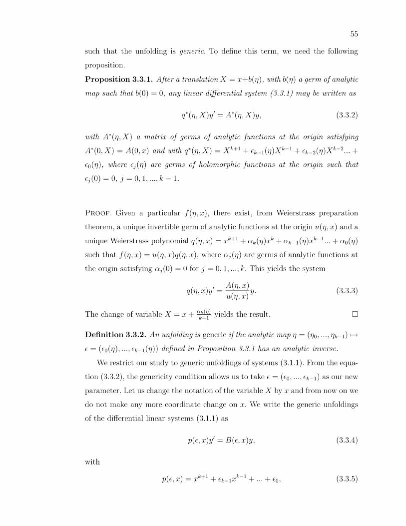
55

such that the unfolding is generic. To define this term, we need the following

proposition.

Proposition 3.3.1. After a translation X = x+b(η), with b(η) a germ of analytic

map such that b(0) = 0, any linear differential system (3.3.1) may be written as

q∗(η, X)y′ = A∗(η, X)y, (3.3.2)

with A∗(η, X) a matrix of germs of analytic functions at the origin satisfying

A∗(0, X) = A(0, x) and with q∗(η, X) = Xk+1 + ǫk−1(η)Xk−1 + ǫk−2(η)Xk−2... +

ǫ0(η), where ǫj(η) are germs of holomorphic functions at the origin such that

ǫj(0) = 0, j = 0, 1, ..., k − 1.

Proof. Given a particular f(η, x), there exist, from Weierstrass preparation

theorem, a unique invertible germ of analytic functions at the origin u(η, x) and a

unique Weierstrass polynomial q(η, x) = xk+1 + αk(η)xk + αk−1(η)xk−1... + α0(η)

such that f(η, x) = u(η, x)q(η, x), where αj(η) are germs of analytic functions at

the origin satisfying αj(0) = 0 for j = 0, 1, ..., k. This yields the system

q(η, x)y′ =A(η, x)

u(η, x)y. (3.3.3)

The change of variable X = x + αk(η)k+1

yields the result.

Definition 3.3.2. An unfolding is generic if the analytic map η = (η0, ..., ηk−1) 7→ǫ = (ǫ0(η), ..., ǫk−1(η)) defined in Proposition 3.3.1 has an analytic inverse.

We restrict our study to generic unfoldings of systems (3.1.1). From the equa-

tion (3.3.2), the genericity condition allows us to take ǫ = (ǫ0, ..., ǫk−1) as our new

parameter. Let us change the notation of the variable X by x and from now on we

do not make any more coordinate change on x. We write the generic unfoldings

of the differential linear systems (3.1.1) as

p(ǫ, x)y′ = B(ǫ, x)y, (3.3.4)

with

p(ǫ, x) = xk+1 + ǫk−1xk−1 + ... + ǫ0, (3.3.5)

56

ǫ = (ǫ0, ..., ǫk−1) ∈ Ck and B(ǫ, x) a matrix of germs of analytic functions at the

origin satisfying B(0, x) = A(x) as in (3.1.1).

3.3.2. Equivalence classes of generic families of linear systems un-

folding (3.1.1)

In this paper, we are interested in equivalence classes of systems (3.3.4). We

use the same terminology as the one used for the classification of the systems

(3.1.1), since it agrees with it when ǫ = 0 :

Definition 3.3.3. Two systems y′ = A(ǫ, x)y and z′ = B(ǫ, x)z are locally ana-

lytically equivalent (respectively formally equivalent) if there exists an invertible

matrix of germs of analytic functions of (ǫ, x) at the origin (respectively an inver-

tible matrix of formal series in (ǫ, x)) denoted T (ǫ, x) such that the substitution

y = T (ǫ, x)z transforms one system into the other.

We search for a complete system of analytic invariants for the systems (3.3.4)

under analytic equivalence. First, we choose a representative of each equivalence

class called the prenormal form.

3.3.3. Prenormal form

The families of systems (3.3.4) have singularities at x = xl, for xl such that

p(ǫ, xl) = 0. When looking at solutions around these singularities, we need to

evaluate the eigenvalues of B(ǫ, xl). With the next theorem, we express them as

the values at xl of polynomials of degree less than or equal to k.

Theorem 3.3.4. The family of systems (3.3.4) is analytically equivalent to a

family in the prenormal form

p(ǫ, x)y′ = B(ǫ, x)y, (3.3.6)

where

B(ǫ, x) = Λ(ǫ, x) + p(ǫ, x)R(ǫ, x), (3.3.7)

Λ(ǫ, x) = diagλ1(ǫ, x), ..., λn(ǫ, x), (3.3.8)

λi(ǫ, x) = λi,0(ǫ) + λi,1(ǫ)x + ... + λi,k(ǫ)xk, (3.3.9)

57

λj,q(ǫ) are germs of analytic functions at the origin, p(ǫ, x) is given by (3.3.5) and

R(ǫ, x) is a matrix of germs of analytic functions at the origin.

Proof. As A(0) in (3.1.1) is a diagonal matrix, B(0, 0) = A(0) is also diagonal

with distinct eigenvalues. We take x in a neighborhood Dr of the origin such that

the eigenvalues of A(x) are distinct. Let us prove that there exists P (ǫ, x) a matrix

of germs of analytic functions at the origin that diagonalizes B(ǫ, x) for x ∈ Dr

and for ǫ sufficiently small. P (0, 0) can be any nonsingular diagonal matrix, let us

take P (0, 0) = I. For ǫ small and x ∈ Dr, the eigenvalues of B(ǫ, x) are distinct

and are analytic functions νi(ǫ, x) of (ǫ, x) by the implicit function theorem. Also,

there exists a unique analytic eigenvector vi(ǫ, x) relative to the eigenvalue νi(ǫ, x)

having the ith component equal to one (this is obtained with the implicit function

theorem, taking Fi(w, ǫ, x) = 0, where Fi(w, ǫ, x) = Bi(ǫ, x)vi, w = (w1, ..., wn−1),

vi = (w1, ..., wi−1, 1, wi, ..., wn−1) and where Bi(ǫ, x) is the matrix obtained by

removing the ith line of (B(ǫ, x) − νi(ǫ, x)I)). We then take the ith column of

P (ǫ, x) equal to vi(ǫ, x).

Finally, by taking z = P (ǫ, x)−1y, the new system p(ǫ, x)z′ = B∗(ǫ, x)z satisfies

B∗(ǫ, x) = diagν1(ǫ, x), ..., νn(ǫ, x) + p(ǫ, x)P (ǫ, x)−1 ∂P (ǫ,x)∂x

and is analytically

equivalent to the original system. Dividing νi(ǫ, x) by p(ǫ, x), we get νi(ǫ, x) =

ci(ǫ, x)p(ǫ, x)+λi,0(ǫ)+λi,1(ǫ)x+ ...+λi,k(ǫ)xk, from which the result follows.

Remark 3.3.5. The polynomial part Λ(ǫ, x) of the prenormal form is completely

characterized by n(k+1) quantities λj,q(ǫ) (with q = 0, 1, ..., k and j = 1, 2, ..., n).

For ǫ fixed such that the singular points are nonresonant, the collection of the well-

known formal invariants at all singular points contains also n(k+1) elements (for

instance the collection of the eigenvalues of the residue matrices if the singular

points are all distinct).

For the rest of the paper, we only discuss systems in prenormal form (3.3.6).

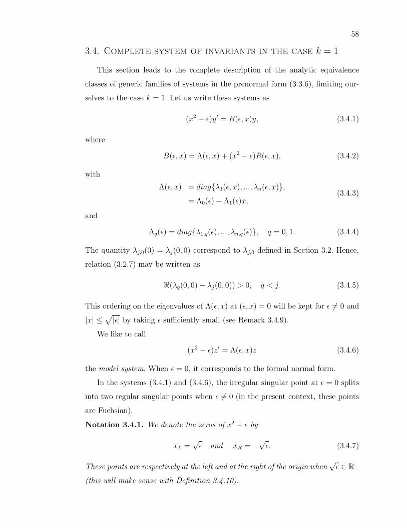
58

3.4. Complete system of invariants in the case k = 1

This section leads to the complete description of the analytic equivalence

classes of generic families of systems in the prenormal form (3.3.6), limiting our-

selves to the case k = 1. Let us write these systems as

(x2 − ǫ)y′ = B(ǫ, x)y, (3.4.1)

where

B(ǫ, x) = Λ(ǫ, x) + (x2 − ǫ)R(ǫ, x), (3.4.2)

with

Λ(ǫ, x) = diagλ1(ǫ, x), ..., λn(ǫ, x),= Λ0(ǫ) + Λ1(ǫ)x,

(3.4.3)

and

Λq(ǫ) = diagλ1,q(ǫ), ..., λn,q(ǫ), q = 0, 1. (3.4.4)

The quantity λj,0(0) = λj(0, 0) correspond to λj,0 defined in Section 3.2. Hence,

relation (3.2.7) may be written as

ℜ(λq(0, 0) − λj(0, 0)) > 0, q < j. (3.4.5)

This ordering on the eigenvalues of Λ(ǫ, x) at (ǫ, x) = 0 will be kept for ǫ 6= 0 and

|x| ≤√|ǫ| by taking ǫ sufficiently small (see Remark 3.4.9).

We like to call

(x2 − ǫ)z′ = Λ(ǫ, x)z (3.4.6)

the model system. When ǫ = 0, it corresponds to the formal normal form.

In the systems (3.4.1) and (3.4.6), the irregular singular point at ǫ = 0 splits

into two regular singular points when ǫ 6= 0 (in the present context, these points

are Fuchsian).

Notation 3.4.1. We denote the zeros of x2 − ǫ by

xL =√

ǫ and xR = −√

ǫ. (3.4.7)

These points are respectively at the left and at the right of the origin when√

ǫ ∈ R−

(this will make sense with Definition 3.4.10).

59

The model system has a fundamental matrix of solutions given by

F (ǫ, x) = diagf1(ǫ, x), ..., fn(ǫ, x) =

(x − xR)UR(x − xL)UL, ǫ 6= 0,

xΛ1(0) exp (−Λ0(0)x

), ǫ = 0,

(3.4.8)

with

Ul =1

2xl

Λ(ǫ, xl) =1

2xl

Λ0(ǫ) +1

2Λ1(ǫ) = diagµ1,l, ..., µn,l, l = L, R. (3.4.9)

The functions fj(ǫ, x) will be at the core of the construction of the sectorial

domains in the x-space done in Section 3.4.4.

Remark 3.4.2. The solutions fj(ǫ, x) of the model system given by (3.4.8) are

analytic in (ǫ, x) for ǫ in a punctured neighborhood of ǫ = 0 and for x in a simply

connected domain that does not contain any singular point x = xl, for l = L, R.

These functions converge uniformly on compact sets to fj(0, x) when ǫ → 0.

Let us immediately state notations related to formal invariants that we will

frequently use in this paper.

Notation 3.4.3. We define

DR = e−2πiUR , DL = e2πiUL . (3.4.10)

and

∆sj,l = (Dl)ss(D−1l )jj, l = L, R,

=

e2πi(µs,l−µj,l), l = L,

e2πi(µj,l−µs,l), l = R,

(3.4.11)

with Ul and µj,l given by (3.4.9). We have

D−1R DL = e2πiΛ1(ǫ), (3.4.12)

with Λ1(ǫ) given by (3.4.4). We will see that DL (respectively DR) is the matrix

representing the monodromy around x = xL in the positive direction (respectively

around x = xR in the negative direction) when acting on the fundamental ma-

trix of solutions (3.4.8) of the model system. e2πiΛ1(ǫ) represents the monodromy

around both singular points, in the positive direction.

The model system (3.4.6) corresponding to a system (3.4.1) contains all the

information on the formal invariants :

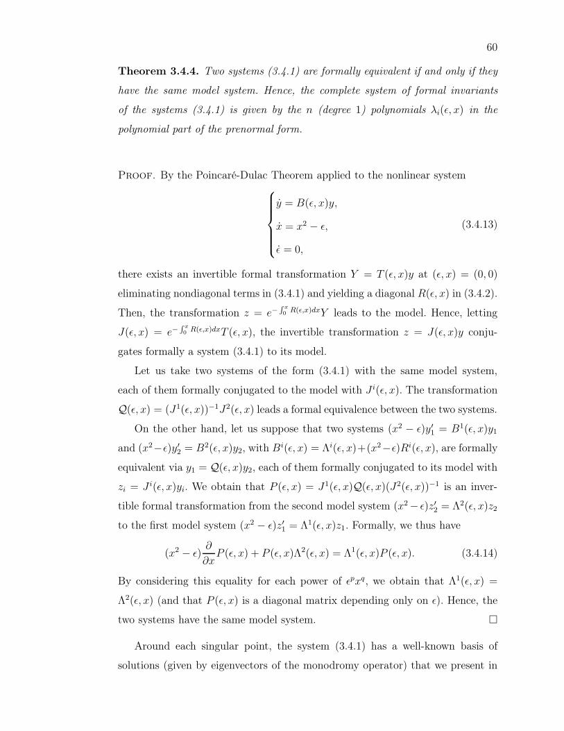
60

Theorem 3.4.4. Two systems (3.4.1) are formally equivalent if and only if they

have the same model system. Hence, the complete system of formal invariants

of the systems (3.4.1) is given by the n (degree 1) polynomials λi(ǫ, x) in the

polynomial part of the prenormal form.

Proof. By the Poincaré-Dulac Theorem applied to the nonlinear system

y = B(ǫ, x)y,

x = x2 − ǫ,

ǫ = 0,

(3.4.13)

there exists an invertible formal transformation Y = T (ǫ, x)y at (ǫ, x) = (0, 0)

eliminating nondiagonal terms in (3.4.1) and yielding a diagonal R(ǫ, x) in (3.4.2).

Then, the transformation z = e−R x0 R(ǫ,x)dxY leads to the model. Hence, letting

J(ǫ, x) = e−R x0 R(ǫ,x)dxT (ǫ, x), the invertible transformation z = J(ǫ, x)y conju-

gates formally a system (3.4.1) to its model.

Let us take two systems of the form (3.4.1) with the same model system,

each of them formally conjugated to the model with J i(ǫ, x). The transformation

Q(ǫ, x) = (J1(ǫ, x))−1J2(ǫ, x) leads a formal equivalence between the two systems.

On the other hand, let us suppose that two systems (x2 − ǫ)y′1 = B1(ǫ, x)y1

and (x2−ǫ)y′2 = B2(ǫ, x)y2, with Bi(ǫ, x) = Λi(ǫ, x)+(x2−ǫ)Ri(ǫ, x), are formally

equivalent via y1 = Q(ǫ, x)y2, each of them formally conjugated to its model with

zi = J i(ǫ, x)yi. We obtain that P (ǫ, x) = J1(ǫ, x)Q(ǫ, x)(J2(ǫ, x))−1 is an inver-

tible formal transformation from the second model system (x2 − ǫ)z′2 = Λ2(ǫ, x)z2

to the first model system (x2 − ǫ)z′1 = Λ1(ǫ, x)z1. Formally, we thus have

(x2 − ǫ)∂

∂xP (ǫ, x) + P (ǫ, x)Λ2(ǫ, x) = Λ1(ǫ, x)P (ǫ, x). (3.4.14)

By considering this equality for each power of ǫpxq, we obtain that Λ1(ǫ, x) =

Λ2(ǫ, x) (and that P (ǫ, x) is a diagonal matrix depending only on ǫ). Hence, the

two systems have the same model system.

Around each singular point, the system (3.4.1) has a well-known basis of

solutions (given by eigenvectors of the monodromy operator) that we present in

61

Theorem 3.4.33, but the problem with this basis is that it is not defined for an

infinite set of resonance values of ǫ which accumulate at ǫ = 0. We want to give a

unified treatment which highlights the fact that the Stokes phenomenon at ǫ = 0

organizes, in the unfolding, the form of solutions at the resonance values of the

parameter. Thus, we rather use a new basis that is defined for all parameter

values in a sector of opening greater than 2π in the universal covering of the

ǫ-space punctured at ǫ = 0. To find this particular basis, we choose to consider

the solutions of the linear systems in the complex projective space.

3.4.1. The projective space

The system (3.4.1) is invariant under y → cy, with c ∈ C∗. Taking charts

in the complex projective space, it gives n particular Riccati matrix differential

equations. We introduce t by dxdt

= x = x2 − ǫ and replace them by n systems of

ordinary differential equations (indexed by j)

dxdt

= x2 − ǫ,

ddt

(y)q

(y)j= (λq(ǫ, x) − λj(ǫ, x)) (y)q

(y)j

+(x2 − ǫ)∑n

i=1(y)i

(y)j

((R(ǫ, x))qi − (R(ǫ, x))ji

(y)q

(y)j

), q 6= j,

(3.4.15)

that we call the Riccati systems.

Notation 3.4.5. Let v be a n-dimensional column vector. We define

[v]j =

(−(v)1

(v)j

, ...,−(v)j−1

(v)j

,− (v)j

(v)j

,−(v)j+1

(v)j

, ...,−(v)n

(v)j

)T

, (3.4.16)

where (v)i is the ith component of the column vector v and where the hat denotes

omission.

Remark 3.4.6. Following Notation 3.4.5, the jth Riccati system associated to

the linear system (3.4.1) may be written as

ddt

x = x2 − ǫ,

ddt

[y]j = −T 0j (ǫ, x) + T 1

j (ǫ, x)[y]j +(T 2

j (ǫ, x)[y]j)[y]j,

(3.4.17)

62

with, denoting I the (n − 1) × (n − 1) identity matrix,

T 0j (ǫ, x) : jth column of B(ǫ, x) except (B(ǫ, x))jj ;

T 1j (ǫ, x) :

(B(ǫ, x) without jth column and jth line

)− (B(ǫ, x))jj I;

T 2j (ǫ, x) : jth line of B(ǫ, x) except (B(ǫ, x))jj .

(3.4.18)

3.4.2. Radius of the sectors in the x-space when ǫ = 0

In order to obtain a basis of solutions of the linear system (3.4.1), we will find

in Section 3.4.5 particular solutions (defined for ǫ in a ramified sector and for x in

sectorial domains) of the Riccati systems (3.4.17). To ensure that these solutions

will converge uniformly on compact sets to solutions [y]j = Gj,s(0, x) (defined

over the sectors Ωs given by (3.2.9) for s = D, U), we choose in this section the

radius of Ωs.

Let us first define the solution [y]j = Gj,s(0, x). When ǫ = 0, if the radius

r of Ωs is chosen sufficiently small, there exists a unique fundamental matrix of

solutions of the system (3.4.1) that can be written as

Ws(0, x) = Hs(0, x)Fs(0, x), on Ωs, s = D, U, (3.4.19)

where Fs(0, x) is the restriction of F (0, x) given by (3.4.8) to the sectorial domain

Ωs, and where Hs(0, x) is an invertible matrix of functions which are analytic on

Ωs and continuous on its closure, satisfying Hs(0, 0) = I. Hs(0, x) links the system

to its formal normal form and is obtained by the sectorial normalization theorem

of Y. Sibuya [22] (p. 144), as mentioned in Section 3.2.

Notation 3.4.7. The solution corresponding to the jth column of Ws(0, x) in

the jth Riccati system passes through (x, [y]j) = (0, 0) and is tangent to the x

direction, we denote it as [y]j = Gj,s(0, x).

Let us now specify how we restrict the radius of Ωs.

Proposition 3.4.8. Let us define the region

Vj =

(x, [y]j) ∈ C × CP

n−1 :

∣∣∣∣(y)i

(y)j

∣∣∣∣ ≤ |x|, ∀i ∈ 1, ..., n\j

. (3.4.20)

63

The boundary of Vj is⋃n

i=1i6=j

Vji , with

Vji =

(x, [y]j) ∈ C × CP

n−1 :

∣∣∣∣(y)i

(y)j

∣∣∣∣ = |x|,∣∣∣∣(y)k

(y)j

∣∣∣∣ ≤ |x| if k 6= i, j

, i 6= j.

(3.4.21)

The radius r of Ωs, s = D, U , can be chosen sufficiently small so that the graph

[y]j = Gj,s(0, x) is confined inside Vj, for all j ∈ 1, ..., n.

Proof. We consider (3.4.15) for ǫ = 0. We have∣∣∣∣d

dt|x|∣∣∣∣ =

|ℜ(xx)||x| =

|ℜ(xx2)||x| ≤ |x|2 (3.4.22)

and1

|x|

∣∣∣∣d

dt

∣∣∣∣(y)i

(y)j

∣∣∣∣∣∣∣∣ ≥ |ℜ(λi,0(0) − λj,0(0))| − vij(x), (3.4.23)

with

vij(x) = |λi,1(0) − λj,1(0)||x| + |x|2∑n

k=1k 6=j

|(R(0, x))ik|

+|x| (|(R(0, x))ij| +∑n

k=1 |(R(0, x))jk|) .(3.4.24)

Let us choose 0 < η < 1. As |ℜ(λi,0(0) − λj,0(0))|>0, we can take the radius r of

ΩD and ΩU sufficiently small so that

vij(x) + |x| < (1 − η)|ℜ(λi,0(0) − λj,0(0))|, x ∈ ΩD ∪ ΩU , i, j ∈ 1, ..., n, i 6= j.

(3.4.25)

This implies

∣∣∣∣d

dt|x|∣∣∣∣ <

∣∣∣∣d

dt

∣∣∣∣(y)i

(y)j

∣∣∣∣∣∣∣∣ , for

(x, [y]j) ∈ Vji ,

x ∈ Ωs, s = D, U,

i, j ∈ 1, ..., n, i 6= j.

(3.4.26)

Since the graph [y]j = Gj,s(0, x) contains the point (x, [y]j) = (0, 0) and is tangent

to the x-plane, it is confined inside Vj (if a solution parametrized by a curve in

complex time living on the graph [y]j = Gj,s(0, x) were to intersect a boundary

component of Vj, then (3.4.26) would not be satisfied). We introduced the pa-

rameter η in order to have in the unfolding a similar property (see Proposition

3.4.15).

64

3.4.3. Sector in the parameter space

Let us specify the sector on the universal covering of the ǫ-space punctured

at the origin with which we will work.

Remark 3.4.9. We take ǫ sufficiently small in order to have :

ℜ((λq(ǫ, x) − λj(ǫ, x)) > 0, |x| ≤√

|ǫ|, q < j, l = L, R. (3.4.27)

Hence, we have the same ordering of the eigenvalues of Λ(ǫ, xl) as the one for

Λ(0, 0) given by (3.4.5).

Definition 3.4.10. We define the sector S, of opening larger than 2π and cove-

ring completely a punctured neighborhood of ǫ = 0, as

S = ǫ ∈ C : 0 < |ǫ| < ρ, arg(ǫ) ∈ (π − 2γ, 3π + 2γ) (3.4.28)

(see Figure 3.2). In (3.4.28), any γ > 0 such that γ(1 + 2 γ

π) < θ0 can be chosen,

ℜ(√

ǫ)

ℑ(√

ǫ)

ℜ(ǫ)

ℑ(ǫ)

SS

Fig. 3.2. Sector S in terms of the parameters ǫ and√

ǫ.

with θ0 the maximum angle in (0, π2) such that

ℜ(e±iθ0(λq(0, 0) − λj(0, 0))) ≥ 0, q < j, (3.4.29)

with λj(ǫ, x) as in (3.4.3) (θ0 exists because of (3.4.5)). Once γ is chosen, the

radius ρ is chosen to ensure that there exists C > 0 for which

ℜ(e±iγ(1+2 γπ

)(λq(ǫ, xl) − λj(ǫ, xl))) > C > 0, q < j, l = L, R, ǫ ∈ S.

(3.4.30)

We will restrict a few other times the value of ρ (in particular, to construct the

sectorial domains in the x-variable in Section 3.4.4 and to ensure that Proposition

3.4.15 is true).

65

Notation 3.4.11. We denote the auto-intersection of S as S∩. For values of the

parameter in S∩, we denote

ǫ = ǫe2πi ∈ S∩ (3.4.31)

(see Figure 3.3).

ℜ(ǫ)

ℑ(ǫ)

S

ǫ

ǫ

ℜ(√

ǫ)

ℑ(√

ǫ)

√ǫ

√ǫ

S

Fig. 3.3. Example of values of ǫ and ǫ in S∩ (in terms of ǫ and√

ǫ).

Notation 3.4.12. We frequently write the hat symbol over some quantities to

recall the dependence on ǫ ∈ S (for example xL). When we use the hat symbol for

values of the parameter in S∩, we mean that ǫ could either be ǫ or ǫ.

3.4.4. Sectorial domains in x

For the rest of Section 3.4, x belongs to a disk of radius r determined by

Proposition 3.4.8. Let us now explain the construction of the sectorial domains

in the complex plane for the x-variable. The boundary of these domains will be

defined from solutions of the equation

x = (x2 − ǫ), (3.4.32)

allowing complex time. More precisely, passing to the t-variable, we have

t(x) =

12√

ǫln(

x−√ǫ

x+√

ǫ

), ǫ 6= 0,

− 1x, ǫ = 0.

(3.4.33)

For ǫ = 0, we cover the disk of radius r with two sectorial domains Ω0D and Ω0

U (see

Figure 3.4) included respectively inside the sectors ΩD and ΩU defined by (3.2.9).

The sectorial domains Ω0D and Ω0

U correspond respectively, in the t-variable, to

the sectorial domains Γ0D and Γ0

U illustrated in Figure 3.5.

When ǫ 6= 0, as the function t(x) given by (3.4.33) is multivalued, its inverse

function x(t) is periodic of period T = πi√ǫ. Hence, the disk of radius r is sent

66

Ω0L Ω0

R

Ω0D

Ω0U

Fig. 3.4. Sectorial domains in the x-variable when ǫ = 0.

Γ0D

Γ0U

Γ0LΓ0

R

Fig. 3.5. Sectorial domains in the t-variable when ǫ = 0.

to the exterior of a sequence of deformed circles (of initial radius r−1 for ǫ = 0)

repeated with period T . To cover the disk, we take two strips (ΓǫD and Γǫ

U , see

Figure 3.6) in the direction of T of width larger than T2, such that their union

is a strip (with a hole) of width w, T < w < 2T , containing ±πi2√

ǫ. The singular

points in the t-variable are located at infinity in the direction perpendicular to

the line of holes. The intersection of the two domains ΓǫD and Γǫ

U consists of three

connected sets : ΓǫL and Γǫ

R linking a part of the boundary to a singular point,

and ΓǫC linking the two singular points (coming from the periodicity).

ΓǫD

ΓǫU

ΓǫLΓǫ

R

ΓǫC

Fig. 3.6. Sectorial domains in the t-variable when√

ǫ ∈ R∗.

For most values of ǫ ∈ S, the line of holes is slanted and we need to slant

the strips. If we take pure slanted strips as in Figure 3.7, we get domains that do

67

not converge when ǫ → 0 to the sectorial domains at ǫ = 0 (Figure 3.5). Hence,

we take a part of the boundary horizontal on a length c√|ǫ|

for some fixed c > 0

independent of ǫ, as illustrated in Figure 3.8.

Fig. 3.7. Incorrectly slanted sectorial domains in the t-variable.

ΓǫD

ΓǫU

c√|ǫ|

T = πi√|ǫ|

Fig. 3.8. Correctly slanted sectorial domains in the t-variable.

Then, we define the sectorial domain Ωǫs in the x-variable as the one correspon-

ding, via (3.4.33), to the sectorial domain in the t-variable Γǫs, s ∈ U, D, L, R, C

(Figures 3.10 and 3.11). The points xR and xL are not in the sectorial domains

Ωǫs but in their closure. The region Ωǫ

L (respectively ΩǫR) has the singular point

xL (respectively xR) in its closure and ΩǫC has both (Figure 3.11). Note that the

point x = 0 belongs to ΩǫC .

In the x-variable, the difference between Ωǫs and Ω0

s (s = D, U) is mainly

located inside a disk of radius c′√|ǫ| (Figure 3.12), due to the non-horizontal

part of the boundary of the sectorial domains in the t-variable. Quantitative

details and proofs can be found in [20]. The construction is possible for all ǫ ∈ S,

provided the radius ρ of S is sufficiently small. Indeed, reducing ρ amounts to

increase the distance between the holes.

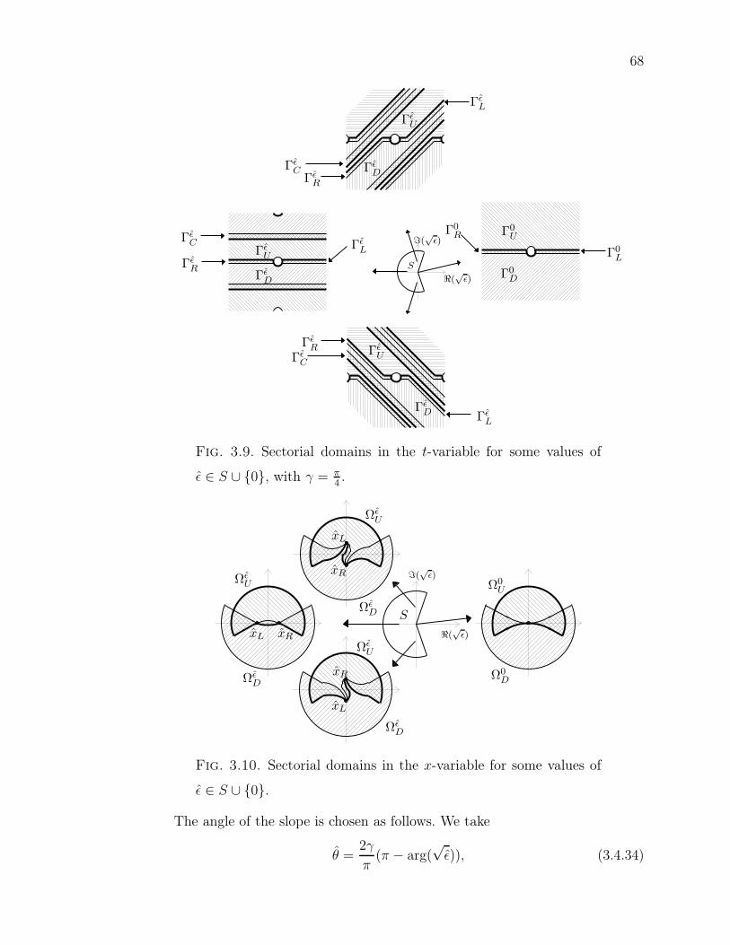
68

ℜ(√

ǫ)

ℑ(√

ǫ)

ΓǫD

ΓǫD

ΓǫD

ΓǫU

ΓǫU

ΓǫU

Γ0D

Γ0U

ΓǫL

ΓǫL

ΓǫL

ΓǫR

ΓǫR

ΓǫR

Γ0L

Γ0R

ΓǫC

ΓǫC

ΓǫC

S

Fig. 3.9. Sectorial domains in the t-variable for some values of

ǫ ∈ S ∪ 0, with γ = π4.

ℜ(√

ǫ)

ℑ(√

ǫ)

ΩǫD

ΩǫD

ΩǫD

ΩǫU

ΩǫU

ΩǫU

S

xL

xL

xL

xR

xR

xR Ω0D

Ω0U

Fig. 3.10. Sectorial domains in the x-variable for some values of

ǫ ∈ S ∪ 0.

The angle of the slope is chosen as follows. We take

θ =2γ

π(π − arg(

√ǫ)), (3.4.34)

69

ΩǫL Ωǫ

R

ΩǫD

ΩǫU

ΩǫC

xRxL

Fig. 3.11. The connected components of the intersection of the

sectorial domains ΩǫD and Ωǫ

U , case√

ǫ ∈ R∗−.

Fig. 3.12. Difference between the sectorial domains Ωǫs and Ω0

s

mainly located inside a small disk of radius c′√

|ǫ|.

with γ as chosen in Definition 3.4.10. Then, on the trajectories in the x-plane

corresponding to t = Ceiθ + C ′ near the singular points, with C ′ ∈ C fixed for

each trajectory and C ∈ R, we have

limx(t)→xl

t=Ceiθ+C′

(x − xR)µj,R−µq,R(x − xL)µj,L−µq,L = 0, for

q > j, if l = R,

q < j, if l = L,

(3.4.35)

(this is obtained from the fact that ℜ(eiθ√

ǫ) < 0 and that |θ| < γ(1 + 2 γ

π) with

γ satisfying (3.4.30)). The limits (3.4.35) yield, with fj(ǫ, x) given by (3.4.8),

limx→xl

x∈Ωǫs

fj(ǫ, x)

fq(ǫ, x)= 0, for

q > j, if l = R,

q < j, if l = L.(3.4.36)

70

Note that we have the same behavior when ǫ = 0 :

limx→0x∈Ω0

s

fj(0, x)

fq(0, x)= 0, for

q > j, if l = R,

q < j, if l = L.(3.4.37)

3.4.5. Invariant manifolds in the projective space

In this section, we find an invariant manifold [y]j = Gj,s(ǫ, x) of the jth Riccati

system (3.4.17) that converges when ǫ → 0 (in S) to the invariant manifold

[y]j = Gj,s(0, x) (Notation 3.4.7).

The Jacobian of the jth Riccati system at the singular point (xl, 0), l = L, R,

has eigenvalues

2xl; λ1(ǫ, xl) − λj(ǫ, xl); ... ; (λj(ǫ, xl) − λj(ǫ, xl)); ... ; λn(ǫ, xl) − λj(ǫ, xl).

(3.4.38)

For q 6= j, the quotient of the eigenvalue in − (y)q

(y)j(see Notation 3.4.5) over the

one in x gives µq,l − µj,l, with µj,l given by (3.4.9).

Definition 3.4.13. We define the resonant values of ǫ as those for which µq,l −µj,l ∈ N∗ for q 6= j, l = L, R. These are true resonances of the nonlinear Riccati

system : they are exactly the values for which there is an obstruction to eliminate

the terms (y)j(x − xl)m ∂

∂(y)qin (3.4.1) when localizing the system at x = xl. The

parameter ǫ has been taken inside a sector which avoids half of these resonances.

Remark 3.4.14. All resonance values of the unfolding parameter ǫ can be inte-

grated in a continuous study : the consideration of half of them on the sector S

is sufficient since the change of parameter ε = ǫe2πi, under which the unfolded

systems are invariant, gives the new parameter ε in a sector including the other

half of the resonance values.

When ǫ ∈ S, the eigenvalues of the Jacobian, listed in (3.4.38), are separated

in two distinct groups by a real line passing through the origin. It gives, locally,

the existence of invariant manifolds that are tangent to the invariant subspaces

of the linearization operator of the vector field at the singular points (xl, 0). We

will need the following proposition to extend these local invariant manifolds.

71

Proposition 3.4.15. For ǫ ∈ S, let us define the region

Vjǫ = Vj

ǫ,+ ∩ Vjǫ,−, (3.4.39)

with

Vjǫ,± =

(x, [y]j) ∈ C × CP

n−1 :

∣∣∣∣(y)i

(y)j

∣∣∣∣ ≤ |x ±√

ǫ|, i ∈ 1, 2, ..., n\j

.

(3.4.40)

The boundary of Vjǫ,± is

⋃ni=1i6=j

Vjǫ,±,i, with, for i 6= j,

Vjǫ,±,i = (x, [y]j) ∈ C × CP

n−1 :

∣∣∣∣(y)i

(y)j

∣∣∣∣ = |x ±√

ǫ|,∣∣∣∣(y)k

(y)j

∣∣∣∣ ≤ |x ±√

ǫ| if k 6= i, j.(3.4.41)

We can take the radius of S sufficiently small so that

∣∣∣∣d

dt|x ±

√ǫ|2∣∣∣∣ <

∣∣∣∣∣d

dt

∣∣∣∣(y)i

(y)j

∣∣∣∣2∣∣∣∣∣ , for

(x, [y]j) ∈ Vjǫ,±,i,

x ∈ Ωǫs, s = D, U,

ǫ ∈ S,

i, j ∈ 1, ..., n, i 6= j.

(3.4.42)

Proof. Similarly to the proof of Proposition 3.4.8, we consider (3.4.15) and we

have, either with the upper or the lower sign,∣∣∣∣1

2

d

dt|x ±

√ǫ|2∣∣∣∣ ≤ |x ±

√ǫ|2|x ∓

√ǫ|. (3.4.43)

On Vjǫ,±,i, we have

1

2|x ±√

ǫ|2

∣∣∣∣∣d

dt

∣∣∣∣(y)i

(y)j

∣∣∣∣2∣∣∣∣∣ ≥ |ℜ(λi,0(ǫ) − λj,0(ǫ))| − v±

ij(ǫ, x), (3.4.44)

with

v±ij(ǫ, x) = |λi,1(ǫ) − λj,1(ǫ)||x| + |x ±

√ǫ|2∑n

k=1k 6=j

|(R(ǫ, x))ik|

+|x ∓√

ǫ| (|(R(ǫ, x))ij| +∑n

k=1 |(R(ǫ, x))jk|) .(3.4.45)

Let us take α such that

α ≤ η|ℜ(λi,0(0) − λj,0(0))|, ∀i 6= j, (3.4.46)

72

with η as chosen in Proposition 3.4.8. We restrict the radius of S to ρ > 0 such

that∣∣|ℜ(λi,0(ǫ) − λj,0(ǫ))| − |ℜ(λi,0(0) − λj,0(0))|

∣∣ < α

2(3.4.47)

and such that

∣∣v±ij(ǫ, x) + |x ∓

√ǫ| − |x| − vij(0, x)

∣∣ < α

2, ∀i 6= j, (3.4.48)

implying

v±ij(ǫ, x) + |x ∓

√ǫ| < |ℜ(λi,0(ǫ) − λj,0(ǫ))|, ∀ǫ ∈ S, ∀i 6= j. (3.4.49)

This yields (3.4.42).

Using Proposition 3.4.15, we now define the graph [y]j = Gj,s(ǫ, x) as consis-

ting of the union of all solutions, parametrized by curves in complex time of the

jth Riccati system, that are confined inside the region Vjǫ when restricted to the

sectors Ωǫs :

Theorem 3.4.16. In the jth Riccati system, there exists, over Ωǫs, a one-dimensional

invariant manifold given as a graph [y]j = Gj,s(ǫ, x), passing through the two sin-

gular points (x, [y]j) = (xl, 0), l = L, R, and located inside the region Vjǫ over the

sector Ωǫs. Gj,s(ǫ, x) depends analytically on (ǫ, x) for ǫ ∈ S and x ∈ Ωǫ

s.

Proof. We always take x inside the sectorial domain Ωǫs and we omit the lower

index s within the proof : we write simply Gj(ǫ, x).

Let us take the first Riccati system and fix ǫ0 ∈ S. The choice of S allows

to separate, by a real line passing through the origin, the eigenvalue 2xR from

the other eigenvalues at (xR, 0) given by (3.4.38). From the Hadamard-Perron

theorem for holomorphic flows (see [10] p. 106), there exist holomorphic invariant

manifolds W+xR,1 and W−

xR,1 tangent to the invariant subspaces of the linearization

operator of the vector field at (xR, 0). We denote by [y]1 = G1(ǫ0, x) the unique

one-dimensional invariant manifold W+xR,1. Near x = xR, it is the unique invariant

manifold contained inside the region Vjǫ0

(defined by (3.4.39)) and its extension

cannot escape from Vjǫ0

, by Proposition 3.4.15.

73

Similarly, in the nth Riccati system, we take [y]n = Gn(ǫ0, x) as the exten-

sion of the unique holomorphic one-dimensional invariant manifold W−xL,n passing

through (xL, 0).

Now, let us take the jth Riccati system, with 1 < j < n. Around x = xR

(respectively x = xL), we have two invariant manifolds W+xR,j and W−

xR,j of di-

mension j and n−j (respectively W+xL,j and W−

xL,j of dimension j−1 and n−j+1)

tangent to the corresponding invariant subspaces of the linearization operator of

the vector field. We analytically extend the invariant manifold W+xR,j tangent to

(x, (y)1(y)j

, ...,(y)j−1

(y)j) at (xR, 0) towards the singular point x = xL. Proposition 3.4.15

implies that any solution (with complex time) of this extended invariant manifold

cannot exit Vjǫ0

by its part of the boundary consisting of the Vjǫ0,±,i for i ≥ j + 1.

Near x = xL, the extension of W+xR,j must then intersect the invariant mani-

fold W−xL,j, which is tangent to (x,

(y)j+1

(y)j, ..., (y)n

(y)j), along a unique one-dimensional

invariant manifold denoted [y]j = Gj(ǫ0, x).

In each Riccati system, we thus have one-dimensional invariant manifolds

[y]j = Gj(ǫ0, x) confined inside Vjǫ0

. Near ǫ0 6= 0, W±xl,j

depends analytically on ǫ,

implying that the unique solution [y]j = Gj(ǫ, x) is analytic in ǫ for ǫ ∈ S.

Remark 3.4.17. The invariant manifolds [y]1 = G1,s(ǫ, x) and [y]n = Gn,s(ǫ, x)

are uniform respectively near xR and near xL, whereas [y]j = Gj,s(ǫ, x) is rami-

fied at the two singular points. More precisely, Gj,U(ǫ, x) = Gj,D(ǫ, x) over ΩǫC

(Figure 3.11) for j = 1, 2, ..., n, G1,U(ǫ, x) = G1,D(ǫ, x) over ΩǫR and Gn,U(ǫ, x) =

Gn,D(ǫ, x) over ΩǫL.

Solutions in the invariant manifold [y]j = Gj,s(ǫ, x) behave differently from

the other solutions of the jth Riccati system, since they are the only ones that are

bounded when x → xR and x → xL over Ωǫs. The fact that an invariant manifold

[y]j = Gj,s(ǫ, x) is bounded over the region Vjǫ leads to its uniform convergence

on compact sets of Ω0s :

Theorem 3.4.18. The invariant manifold [y]j = Gj,s(ǫ, x) converges uniformly

on compact subsets of Ω0s, when ǫ → 0, ǫ ∈ S, to the invariant manifold at ǫ = 0

[y]j = Gj,s(0, x) (see Notation 3.4.7), for s = D, U .

74

Proof. Let us take a simply connected compact subset of Ω0s. For |ǫ| sufficiently

small, it does not contain neither xR nor xL, nor the spiraling part of Ωǫs. Propo-

sition 3.4.15 implies that the invariant manifold [y]j = Gj,s(ǫ, x) satisfies

|(Gj,s(ǫ, x))i| < min|x− xR|, |x− xL|, with

x ∈ Ωǫs, s = D, U,

ǫ ∈ S,

i = 1, 2, ..., n − 1.

(3.4.50)

This implies the desired convergence to a bounded solution of the system for ǫ = 0

that can only be [y]j = Gj,s(x, 0).

3.4.6. Basis of the linear system (3.4.1)

In this section, we establish the correspondence between the invariant manifold

[y]j = Gj,s(ǫ, x) of the jth Riccati system (3.4.17) and multiples (by a complex

constant) of a particular solution of the linear system (3.4.1). We show that these

n particular solutions form a basis of solutions of the linear system which is valid

for all values of ǫ ∈ S and x ∈ Ωǫs.

Notation 3.4.19. Let FD(ǫ, x) be the restriction to ΩǫD of the fundamental matrix

of solutions of the model system F (ǫ, x) (given by (3.4.8)), and let FU(ǫ, x) be its

analytic continuation to ΩǫU , passing through Ωǫ

R.

Remark 3.4.20. The solution Fs(ǫ, x) is uniform over Ωǫs, s = D, U , and accor-

ding to Notation 3.4.19, we have

FU(ǫ, x) =

FD(ǫ, x), on ΩǫR,

FD(ǫ, x)e2πiΛ1(ǫ), on ΩǫL,

FD(ǫ, x)D−1R , on Ωǫ

C ,

(3.4.51)

with DR given by (3.4.10) and Λ1(ǫ) by (3.4.4), satisfying (3.4.12).

Theorem 3.4.21. Let s = D, U . There exists a fundamental matrix of solutions

of (3.4.1) that can be written as

Ws(ǫ, x) = Hs(ǫ, x)Fs(ǫ, x), (ǫ, x) ∈ S × Ωǫs, (3.4.52)

75

with Hs(ǫ, x) analytic on S × Ωǫs, satisfying

|Hs(ǫ, 0)−Hs(ǫ, 0)| ≤ c|ǫ|, for some c ∈ R+, ǫ, ǫ = ǫe2πi ∈ S∩∪0, (3.4.53)

|Hs(ǫ, 0)| and |Hs(ǫ, 0)−1| are bounded, ǫ ∈ S∩, (3.4.54)

and

limx→xl

x∈Ωǫs

Hs(x, ǫ) = Kl(ǫ), ǫ ∈ S, l = L, R, (3.4.55)

where Kl(ǫ) is an invertible diagonal matrix depending analytically on ǫ ∈ S with

a nonsingular limit at ǫ = 0 (independent of s).

Proof. The proof is valid for s = D or s = U . For our needs, we write [y]j =

Gj,s(ǫ, x) on Ωǫs as

−(y)k

(y)j= gkj,s(ǫ, x),

−1 = gjj,s(ǫ, x).(3.4.56)

With (3.4.1), we can write

(y′)j =λj(ǫ, x)

x2 − ǫ(y)j +

n∑

k=1

(R(ǫ, x))jk(y)k. (3.4.57)

Dividing by (y)j, the known solutions of the jth Riccati system appear in the

right hand side :

(y′)j

(y)j

= −λj(ǫ, x)

x2 − ǫgjj,s(ǫ, x) −

n∑

k=1

(R(ǫ, x))jkgkj,s(ǫ, x). (3.4.58)

The integration of equation (3.4.58) allows to recover (y)j and relation (3.4.56)

leads to the other (y)k, thus yielding a solution wj,s(ǫ, x) of the linear system

(3.4.1) (and all its multiples by a complex constant) that can be written as

wj,s(ǫ, x) = fj,s(ǫ, x)hj,s(ǫ, x), (3.4.59)

with fj,s(ǫ, x) the jth diagonal element of Fs(ǫ, x) (see Notation 3.4.19), and with

(hj,s(ǫ, x))k = −e−R x

0

Pnp=1(R(ǫ,x))jpgpj,s(ǫ,x)dxgkj,s(ǫ, x), (3.4.60)

where the integration path is taken inside Ωǫs. Such a path can be found in the

t-variable (see Section 3.4.4) since t(0) ∈ ΓǫC . With the n Riccati systems, we

76

obtain in this way n solutions wj,s(ǫ, x) of the linear system (3.4.1) defined for

ǫ ∈ S and x ∈ Ωǫs. We take

Ws(ǫ, x) = [w1,s(ǫ, x) ...wn,s(ǫ, x)] (3.4.61)

and

Hs(ǫ, x) = [h1,s(ǫ, x) ...hn,s(ǫ, x)] (3.4.62)

to obtain (3.4.52) from (3.4.59). The limit (3.4.55) follows from

limx→xl

x∈Ωǫs

gkj,s(x, ǫ) = 0, k 6= j, l = L, R, (3.4.63)

and

(Kl(ǫ))jj = limx→xl

(hj,s(ǫ, x))j = e−R xl0

Pnp=1(R(ǫ,x))jpgpj,s(ǫ,x)dx, (3.4.64)

which is independent of s since the integration path in (3.4.64) may be taken

inside ΩǫC (see Remark 3.4.17).

The solutions w1,s(ǫ, x), ..., wn,s(ǫ, x) form a basis of solutions since the co-

lumns of Fs(ǫ, x) are linearly independent and since Kl(ǫ) in (3.4.55) is invertible.

The property (3.4.54) comes from (3.4.50). Let us now prove (3.4.53). From

its definition, Hs(ǫ, 0)Fs(ǫ, 0) is a solution of (3.4.1) at x = 0, so

Λ(ǫ, 0)Hs(ǫ, 0) − Hs(ǫ, 0)Λ(ǫ, 0) = ǫ (H ′s(ǫ, 0) − R(ǫ, 0)Hs(ǫ, 0)) . (3.4.65)

With ǫ and ǫ in S∩ (see Notation 3.4.11), we thus have

Λ(ǫ, 0)(Hs(ǫ, 0) − Hs(ǫ, 0)) − (Hs(ǫ, 0) − Hs(ǫ, 0))Λ(ǫ, 0)

= ǫ (H ′s(ǫ, 0) − H ′

s(ǫ, 0) − R(ǫ, 0)(Hs(ǫ, 0) − Hs(ǫ, 0))) ,(3.4.66)

yielding, for some k ∈ R+,

| (Hs(ǫ, 0) − Hs(ǫ, 0))jq | ≤ k|ǫ|, j 6= q, ǫ ∈ S∩ ∪ 0, i = 1, 2, (3.4.67)

by the boundedness of |H ′s(ǫ, 0)−H ′

s(ǫ, 0)|, |R(ǫ, 0)| and |Hs(ǫ, 0)−Hs(ǫ, 0)| over

S∩ ∪ 0 (recall that Λ(ǫ, 0) has distinct eigenvalues for ǫ ∈ S ∪ 0). Relation

(3.4.53) comes from (3.4.67) and from the fact that the diagonal elements of

Hs(ǫ, 0) − Hs(ǫ, 0) are zeros (since (Hs(ǫ, 0))jj = 1).

77

We have seen that the solutions in the invariant manifold [y]j = Gj,s(ǫ, x)

converge uniformly on compact sets of Ω0s. This property remains for the corres-

ponding solutions of the linear system :

Corollary 3.4.22 (of Theorem 3.4.18). The fundamental matrix Ws(ǫ, x) converges

(uniformly on compact sets of Ω0s) to the fundamental matrix Ws(0, x) defined in

(3.4.19), s = D, U .

Proof. From (3.4.52) and the convergence of F (ǫ, x) to F (0, x), it suffices to

prove the desired convergence of Hs(ǫ, x). This is immediate, since each column

has an expression in terms of the solution [y]j = Gj,s(ǫ, x) as in (3.4.60), using

the notation (3.4.56).

Remark 3.4.23. The transformation y = Hs(ǫ, x)z (with Hs(ǫ, x) given by Theo-

rem 3.4.21) conjugates the system (3.4.1) to its model (3.4.6) over Ωǫs, for ǫ ∈

S ∪ 0.The bases WD(ǫ, x) and WU(ǫ, x) defined respectively on Ωǫ

D and ΩǫU will allow

the calculation of the analytic invariants of the linear system.

3.4.7. Definition of the unfolded Stokes matrices

In this section, we define the unfolded Stokes matrices by comparing the funda-

mental matrices of solutions WD(ǫ, x) and WU(ǫ, x) on the connected components

of the intersection of ΩǫD and Ωǫ

U (Figure 3.11).

Theorem 3.4.24. There exist matrices CR(ǫ) and CL(ǫ) such that

HD(ǫ, x)−1HU(ǫ, x) =

FD(ǫ, x)CR(ǫ)(FD(ǫ, x))−1, on ΩǫR,

FD(ǫ, x)CL(ǫ)(FD(ǫ, x))−1, on ΩǫL,

I, on ΩǫC .

(3.4.68)

CR(ǫ) and CL(ǫ) are respectively an upper triangular and a lower triangular uni-

potent matrix. They depend analytically on ǫ ∈ S and converge when ǫ → 0

(ǫ ∈ S) to the Stokes matrices defined by (3.2.12).

78

Proof. As WD(ǫ, x) and WU(ǫ, x) are two fundamental matrices of solutions

on the intersection of ΩǫD and Ωǫ

U (see Theorem 3.4.21), there exist matrices

expressing the fact that columns of WU(ǫ, x) are linear combinations of columns

of WD(ǫ, x) on the intersection parts ΩǫL, Ωǫ

R and ΩǫC . With (3.4.51) and (3.4.52),

these relations become equivalent to

HD(ǫ, x)−1HU(ǫ, x) =

FD(ǫ, x)CR(ǫ)(FD(ǫ, x))−1 on ΩǫR

FD(ǫ, x)CL(ǫ)(FD(ǫ, x))−1 on ΩǫL

FD(ǫ, x)C0(ǫ)(FD(ǫ, x))−1 on ΩǫC .

(3.4.69)

Then, taking the limit x → xL on ΩǫL, x → xR on Ωǫ

R and both limits on ΩǫC leads,

with (3.4.36) and (3.4.55), to C0(ǫ) = I and to the unipotent triangular form of

the matrices CR(ǫ) and CL(ǫ). Since Ws(ǫ, x) and Fs(ǫ, x) converge uniformly on

compact sets of Ω0s (see Corollary 3.4.18 and Remark 3.4.2), so does Hs(ǫ, x) .

Then, the matrices CR(ǫ) and CL(ǫ) must converge to the Stokes matrices when

ǫ → 0, ǫ ∈ S.

Definition 3.4.25. We call CR(ǫ) and CL(ǫ) (defined by (3.4.68)) the unfolded

Stokes matrices and CR(ǫ), CL(ǫ) an unfolded Stokes collection.

Proposition 3.4.26. A fundamental matrix of solutions of (3.4.1) that can be

written as (3.4.52), with Hs(ǫ, x) analytic on S×Ωǫs, satisfying (3.4.53), (3.4.54)

and with a limit when x → xl, x ∈ Ωǫs that is bounded, invertible and independent

of s, is unique up to right multiplication by any nonsingular diagonal matrix K(ǫ)

depending analytically on ǫ ∈ S with a nonsingular limit at ǫ = 0 and such that

|K(ǫ) − K(ǫ)| ≤ c|ǫ| over S∩, for some c ∈ R+. (3.4.70)

Proof. Let us suppose that we have two fundamental matrices of solutions that

can be written as Hs(ǫ, x)Fs(ǫ, x) and H∗s (ǫ, x)Fs(ǫ, x) with properties listed in

the proposition. Having two bases of solutions over ΩǫC , there exists a matrix K(ǫ)

such that

H∗s (ǫ, x)Fs(ǫ, x) = Hs(ǫ, x)Fs(ǫ, x)K(ǫ), x ∈ Ωǫ

C . (3.4.71)

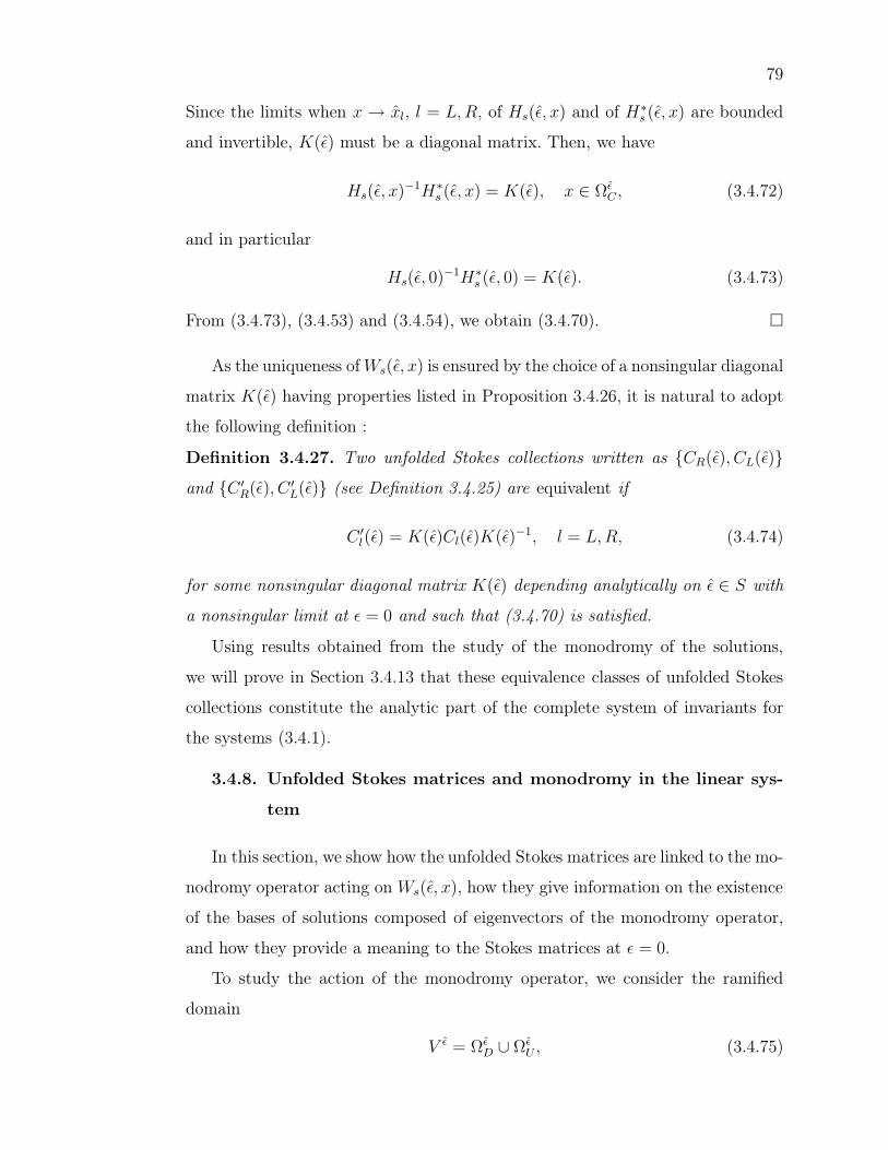
79

Since the limits when x → xl, l = L, R, of Hs(ǫ, x) and of H∗s (ǫ, x) are bounded

and invertible, K(ǫ) must be a diagonal matrix. Then, we have

Hs(ǫ, x)−1H∗s (ǫ, x) = K(ǫ), x ∈ Ωǫ

C , (3.4.72)

and in particular

Hs(ǫ, 0)−1H∗s (ǫ, 0) = K(ǫ). (3.4.73)

From (3.4.73), (3.4.53) and (3.4.54), we obtain (3.4.70).

As the uniqueness of Ws(ǫ, x) is ensured by the choice of a nonsingular diagonal

matrix K(ǫ) having properties listed in Proposition 3.4.26, it is natural to adopt

the following definition :

Definition 3.4.27. Two unfolded Stokes collections written as CR(ǫ), CL(ǫ)and C ′

R(ǫ), C ′L(ǫ) (see Definition 3.4.25) are equivalent if

C ′l(ǫ) = K(ǫ)Cl(ǫ)K(ǫ)−1, l = L, R, (3.4.74)

for some nonsingular diagonal matrix K(ǫ) depending analytically on ǫ ∈ S with

a nonsingular limit at ǫ = 0 and such that (3.4.70) is satisfied.

Using results obtained from the study of the monodromy of the solutions,

we will prove in Section 3.4.13 that these equivalence classes of unfolded Stokes

collections constitute the analytic part of the complete system of invariants for

the systems (3.4.1).

3.4.8. Unfolded Stokes matrices and monodromy in the linear sys-

tem

In this section, we show how the unfolded Stokes matrices are linked to the mo-

nodromy operator acting on Ws(ǫ, x), how they give information on the existence

of the bases of solutions composed of eigenvectors of the monodromy operator,

and how they provide a meaning to the Stokes matrices at ǫ = 0.

To study the action of the monodromy operator, we consider the ramified

domain

V ǫ = ΩǫD ∪ Ωǫ

U , (3.4.75)

80

illustrated in Figure 3.13, which could have a (non illustrated) spiraling part

around xR and xL.

xRxL

V ǫ

Fig. 3.13. Domain of H(ǫ, x), denoted V ǫ, case√

ǫ ∈ R∗−.

Notation 3.4.28. Let FV (ǫ, x) be the analytic continuation of FD(ǫ, x) from ΩǫD

to V ǫ (through ΩǫC).

The well chosen basis of solutions we consider on this domain is the analytic

continuation of WD(ǫ, x) from ΩǫD to V ǫ, that we write as

WV (ǫ, x) = [w1(ǫ, x) ... wn(ǫ, x)] = H(ǫ, x)FV (ǫ, x), (3.4.76)

where

H(ǫ, x) =

HD(ǫ, x), on ΩǫD,

HU(ǫ, x), on ΩǫU ,

(3.4.77)

which is well-defined because of (3.4.68).

The fundamental group of C\xR, xL based at a nonsingular point acts on a

solution (valid at this base point) by giving its analytic continuation at the end

of a loop. In this way we have monodromy operators around each singular point

x = xl. We can extend this action of the fundamental group to any function of

the solutions. When the monodromy operator acts on a fundamental matrix of

solutions W , its is represented by a matrix acting by right multiplication on W .

Notation 3.4.29. We denote MxR(respectively MxL

) the monodromy operator

associated to the loop which makes one turn around the singular point x = xR

(respectively x = xL) in the negative (respectively positive) direction and which

does not surround any other singular point, with the fundamental group based,

independently of ǫ ∈ S, at a point belonging to ΩǫR (respectively Ωǫ

L) and taken on

ΩǫD (see Figure 3.14).

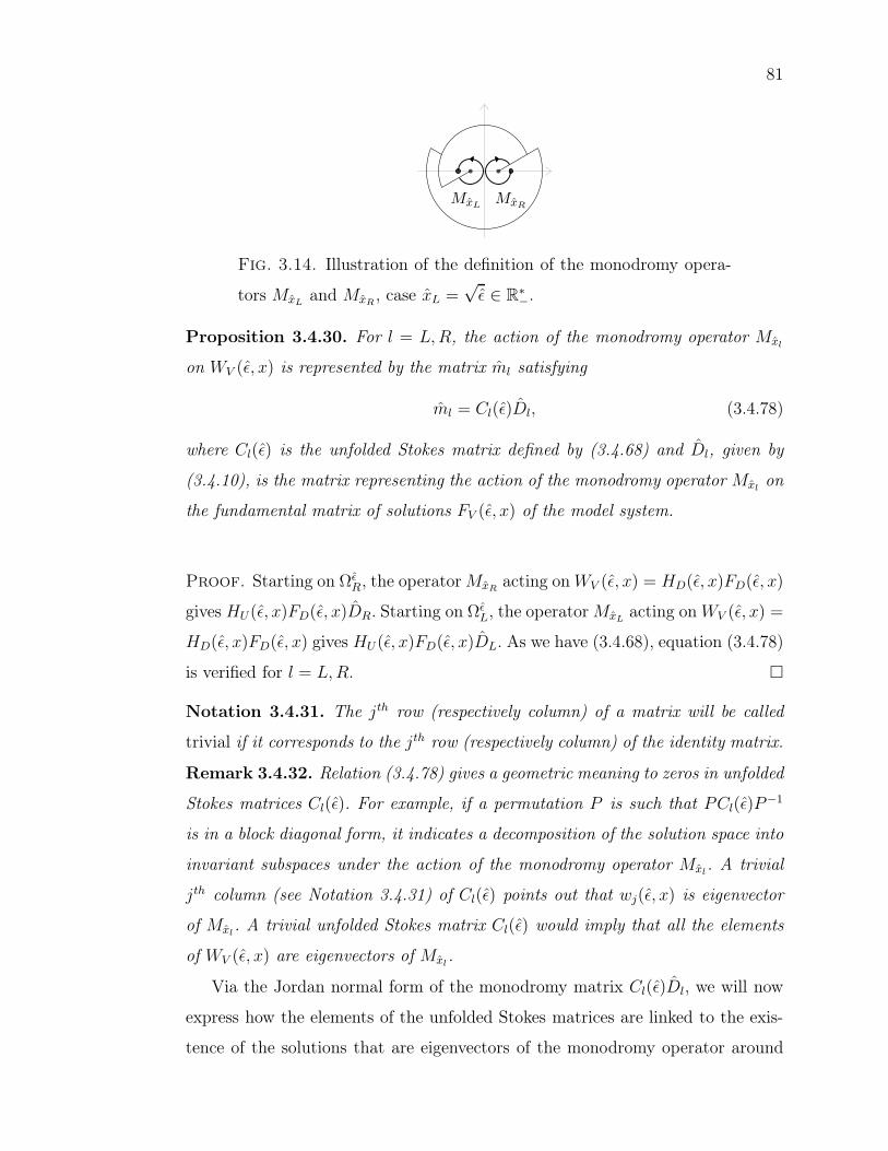
81

MxLMxR

Fig. 3.14. Illustration of the definition of the monodromy opera-

tors MxLand MxR

, case xL =√

ǫ ∈ R∗−.

Proposition 3.4.30. For l = L, R, the action of the monodromy operator Mxl

on WV (ǫ, x) is represented by the matrix ml satisfying

ml = Cl(ǫ)Dl, (3.4.78)

where Cl(ǫ) is the unfolded Stokes matrix defined by (3.4.68) and Dl, given by

(3.4.10), is the matrix representing the action of the monodromy operator Mxlon

the fundamental matrix of solutions FV (ǫ, x) of the model system.

Proof. Starting on ΩǫR, the operator MxR

acting on WV (ǫ, x) = HD(ǫ, x)FD(ǫ, x)

gives HU(ǫ, x)FD(ǫ, x)DR. Starting on ΩǫL, the operator MxL

acting on WV (ǫ, x) =

HD(ǫ, x)FD(ǫ, x) gives HU(ǫ, x)FD(ǫ, x)DL. As we have (3.4.68), equation (3.4.78)

is verified for l = L, R.

Notation 3.4.31. The jth row (respectively column) of a matrix will be called

trivial if it corresponds to the jth row (respectively column) of the identity matrix.

Remark 3.4.32. Relation (3.4.78) gives a geometric meaning to zeros in unfolded

Stokes matrices Cl(ǫ). For example, if a permutation P is such that PCl(ǫ)P−1

is in a block diagonal form, it indicates a decomposition of the solution space into

invariant subspaces under the action of the monodromy operator Mxl. A trivial

jth column (see Notation 3.4.31) of Cl(ǫ) points out that wj(ǫ, x) is eigenvector

of Mxl. A trivial unfolded Stokes matrix Cl(ǫ) would imply that all the elements

of WV (ǫ, x) are eigenvectors of Mxl.

Via the Jordan normal form of the monodromy matrix Cl(ǫ)Dl, we will now

express how the elements of the unfolded Stokes matrices are linked to the exis-

tence of the solutions that are eigenvectors of the monodromy operator around

82

the singular points. This will give a geometric interpretation to the elements of

Cl(ǫ) and, in particular, of their limits, the elements of Cl(0).

Theorem 3.4.33. t ∈ Cn is an eigenvector of the monodromy matrix ml if and

only if WV (ǫ, x)t is a solution eigenvector of the monodromy operator Mxlwith the

same eigenvalue. Hence, for l = L, R, the number of independent solutions which

are eigenvectors of Mxlis equal to the number of Jordan blocks in the Jordan

matrix associated to ml = Cl(ǫ)Dl. The values for which the monodromy matrix

ml may not be diagonalizable, are the resonance values of ǫ specified in Definition

3.4.13 (which exactly correspond to multiple eigenvalues of ml).

For nonresonance values of ǫ, let Tl be the unipotent triangular matrix diago-

nalizing the monodromy matrix ml = Cl(ǫ)Dl :

(Tl)−1mlTl = Dl. (3.4.79)

The fundamental matrix of solutions

Wxl(x) = WV (ǫ, x)Tl (3.4.80)

is composed of eigenvectors of the monodromy operator around x = xl. A fun-

damental matrix having this property is unique up to its normalization : the jth

column of Wxlis a nonzero multiple of the Floquet solution (for example [23]

p. 25) given by

wj,l(x) = (x − xl)µj,l gj,l(x), (3.4.81)

with µj,l given by (3.4.9) and gj,l(x) = ej + O(|x− xl|) an analytic function of x

in a region containing x = xl but no other singular point.

When ǫ is a resonance value, the matrix ml = Cl(ǫ)Dl is no more diagona-

lizable with no jth eigenvector if and only it the jth Floquet solution wj,l(x) does

not exist and has to be replaced, in the basis of solutions around x = xl, by a

solution containing logarithmic terms.

83

Proof. By Proposition 3.4.30, we have MxlWV (ǫ, x) = WV (ǫ, x)ml. Let t ∈ Cn

and β ∈ C. The first assertion of the theorem is obtained from

mlt = βt ⇐⇒ WV (ǫ, x)mlt = βWV (ǫ, x)t

⇐⇒ MxlWV (ǫ, x)t = βWV (ǫ, x)t.

(3.4.82)

To prove the uniqueness (up to normalization) of Wxl(x), let us suppose that

W ∗ is such that MxlW ∗ = W ∗Dl. Since we have two bases of solutions, there

exists a nonsingular matrix K such that Wxl(x) = W ∗K. Since Mxl

Wxl= Wxl

Dl,

we must have DlK = KDl. Since ǫ is not a resonance value, the eigenvalues of

Dl are distinct and K can only be diagonal.

Remark 3.4.34. For nonresonance values of ǫ, (3.4.79) implies that the unfolded

Stokes matrices are equal to the multiplicative commutator of the matrices Tl and

Dl :

Cl(ǫ) = TlDlT−1l D−1

l = [Tl, Dl]. (3.4.83)

The unfolded Stokes matrix CR(ǫ) (respectively CL(ǫ)) is linked to the pre-

sence of logarithmic terms in solutions around x = xR (respectively x = xL) :

Corollary 3.4.35. There exist polynomials in terms of the elements of the un-

folded Stokes matrices Cl(ǫ) and the elements of Dl indicating, when they are

nonzero at a resonance value, the nonexistence of a Floquet solution wj,l(x) at the

resonance.

In generic cases, the obstruction to the existence of Floquet solutions can be

forced by the special form of the Stokes matrix Cl = Cl(0). This is the case when

• (CR)12 6= 0 : w2,R(x) does not exist at the resonance µ1,R − µ2,R ∈ N∗ ;

• (CL)n(n−1) 6= 0 : wn−1,L(x) does not exist at the resonance µn,L−µn−1,L ∈N∗ ;

• arg(λs,0 − λj,0) are distinct for all s 6= j : a nonvanishing sth polynomial

in terms of the elements of the Stokes matrices Cl with integer coefficients

yields an obstruction to the existence of wj,l(x) at the resonance µs,l−µj,l ∈N∗, with s > j if l = L and s < j if l = R.

84

Proof. The polynomials of the corollary could be obtained by analytic or alge-

braic arguments, by counting the number of eigenvectors of Cl(ǫ)Dl. We present

the proof in the analytic way. Recall that the matrices Tl are triangular and uni-

potent. Since Tl = Cl(ǫ)DlTlD−1l (see (3.4.83)), elements (Tl)ij, for i 6= j, can be

calculated from the recurrent equations

(Tl)ij(1 − ∆ij,l) = (Cl(ǫ))ij +∑

i<k<j, l=Rj<k<i, l=L

(Cl(ǫ))ik(Tl)kj∆kj,l, (3.4.84)

with ∆sj,l given by (3.4.11). At the resonance, ∆sj,l = 1 for some s, j, l. Conditions

to the nonexistence of the jth column of Tl at the resonance can be calculated

from (3.4.84) : they are given by polynomials in terms of elements of Dl and of

elements of the unfolded Stokes matrices. For generic cases, these polynomials

have a limit at ǫ = 0 and the conditions can be formulated with polynomials in

the elements of the Stokes matrices at ǫ = 0 : the nonvanishing of the polynomials

for small ǫ is ensured by the nonvanishing of the limit polynomial at ǫ = 0 which

depends on Cl. This is the case for the conditions to the existence of

• the second column of TR ;

• the (n − 1)th column of TL ;

• all columns if the Stokes lines are distinct (i.e. arg(λs,0−λj,0) are distinct

for all s 6= j). In that case, the resonance ∆ij,l = 1 is distinct from the

resonance ∆kj,l = 1 for k 6= i. On the sequence ǫn → 0 corresponding

to the resonance ∆ij,l = 1, the limit of(

∆kj,l

1−∆kj,l

)is 0 or −1, hence the

polynomials at the limit have integer coefficients (independent of ǫ).

85

Example 3.4.36. Let us consider the case n = 3, with distinct arguments of

λ2 − λ3, λ1 − λ2 and λ1 − λ3. Equation (3.4.84) gives

(TR)12(1 − ∆12,R) = (CR(ǫ))12,

(TR)13(1 − ∆13,R) = (CR(ǫ))13 + (CR(ǫ))12(CR(ǫ))23

(∆23,R

1−∆23,R

),

(TR)23(1 − ∆23,R) = (CR(ǫ))23,

(TL)21(1 − ∆21,L) = (CL(ǫ))21,

(TL)31(1 − ∆31,L) = (CL(ǫ))31 + (CL(ǫ))21(CL(ǫ))32

(∆21,L

1−∆21,L

),

(TL)32(1 − ∆32,L) = (CL(ǫ))32.

(3.4.85)

Decreasing values of ǫ such that µ1,R − µ3,R ∈ N∗ and µ3,L − µ1,L ∈ N∗ are

approaching the ray arg(√

ǫ) = arg(λ3,0 − λ1,0). The following comes from the

inequalities arg(λ1,0 − λ2,0) < arg(λ1,0 − λ3,0) < arg(λ2,0 − λ3,0). When ǫ → 0 on

resonance values

• µ1,R − µ3,R ∈ N∗ making ∆13,R = 1, we have ℑ(µ2,R − µ3,R) > 0 and then(∆23,R

1−∆23,R

)=(

1∆32,R−1

)tends to −1, since ∆32,R → 0 ;

• µ3,L − ˆµ1,L ∈ N∗ making ∆31,L = 1, we have ℑ(µ1,L − µ2,L) > 0 and then(∆21,L

1−∆21,L

)=(

1

∆12,L−1

)tends to −1, since ∆12,L → 0.

These limits imply that the right hand side of the equations (3.4.85) at the re-

sonance is minus an element of the inverse of the unfolded Stokes matrices. We

immediately see that

• if (CR)12 6= 0, (TR)12 (and hence w2,R(x)) does not have a limit at the

resonances µ1,R − µ2,R ∈ N∗ making ∆12,R = 1 ;

• if (CR)23 6= 0, (TR)23 (and hence w3,R(x)) does not have a limit at the

resonances µ2,R − µ3,R ∈ N∗ making ∆23,R = 1 ;

• if (CR)13 − (CR)12(CR)23 6= 0, (TR)13 (and hence w3,R(x)) does not have

a limit at the resonances µ1,R − µ3,R ∈ N∗ making ∆13,R = 1 ;

• if (CL)21 6= 0, (TL)21 (and hence w1,L(x)) does not have a limit at the

resonances µ2,L − µ1,L ∈ N∗ making ∆21,L = 1 ;

• if (CL)32 6= 0, (TL)32 (and hence w2,L(x)) does not have a limit at the

resonances µ3,L − µ2,L ∈ N∗ making ∆32,L = 1 ;

86

• if (CL)31 − (CL)21(CL)32 6= 0, (TL)31 (and hence w1,L(x)) does not have

a limit at the resonances µ3,L − µ1,L ∈ N∗ making ∆31,L = 1.

3.4.9. Stokes matrices and monodromy in the Riccati systems

In this section, we give a meaning to the unfolded Stokes matrices in the cor-

responding Riccati systems. This allows an interpretation of the Stokes matrices

at ǫ = 0. This section is not prerequisite to state the complete system of analytic

invariants of the systems (3.4.1) .

We will look at the monodromy of first integrals in the Riccati systems. These

first integrals are obtained from the basis of the linear system.

Proposition 3.4.37. For x ∈ V ǫ, the jth Riccati system has first integrals Hjq,

for q ∈ 1, 2, ..., n\j, that can be written as

Hjq = (−1)q−j

∣∣∣bj1(ǫ, x, [y]j) ... bj

q(ǫ, x, [y]j) ... bjn(ǫ, x, [y]j)

∣∣∣∣∣∣bj

1(ǫ, x, [y]j) ... bjj(ǫ, x, [y]j) ... bj

n(ǫ, x, [y]j)

∣∣∣, (3.4.86)

with

bji (ǫ, x, [y]j) = (−1)i−j(wi(ǫ, x))j ([y]j − [wi]j) , (3.4.87)

and wi(ǫ, x) the ith column of the fundamental matrix of solutions WV (ǫ, x) given

by (3.4.76) (for [wi]j, see Notation 3.4.5). (Hj)q has values in (CP1) for q 6= j.

Proof. Let wi(ǫ, x) be the columns of the fundamental matrix of solutions

WV (ǫ, x) given by (3.4.76). The general solution of a linear system (3.4.1) may be

expressed as a linear combination y =∑n

q=1 kqwq(ǫ, x) of the particular solution

wq(ǫ, x), with kq ∈ C. In particular, the jth component of this general solution y

satisfies

(y)j =n∑

q=1

kq(wq(ǫ, x))j, (3.4.88)

son∑

q=1

kq(wq(ǫ, x))j

y

(y)j

=n∑

q=1

kqwq(ǫ, x), (3.4.89)

andn∑

q=1

kq

kj

(wq(ǫ, x) − (wq(ǫ, x))j

y

(y)j

)= 0. (3.4.90)

87

Solving for kq

kj, q 6= j, and using Notation 3.4.5 and (3.4.87) gives (3.4.86).

As detailed in the next theorem, elements of the inverse of the unfolded Stokes

matrices appear in the expression of the monodromy of the first integrals Hjq

around x = xl.

Theorem 3.4.38. The monodromy of a first integral Hjq around x = xl may be

written as the composition of

• a wild part (i.e. of the form e2πiα with α ∈ C, α → 0) depending on the

formal invariants,

• a map depending on the elements of the inverse of the unfolded Stokes

matrices and having a limit for ǫ = 0.

More precisely, with Hjj = 1, the monodromy of the first integrals may be expressed

as

MxR(Hj

q) = ∆jq,R

Hjq +

∑np=q+1(CR(ǫ)−1)qpHj

p

1 +∑n

p=j+1(CR(ǫ)−1)jpHjp

, (3.4.91)

and

MxL(Hj

q) = ∆jq,L

Hjq +

∑q−1p=1(CL(ǫ)−1)qpHj

p

1 +∑j−1

p=1(CL(ǫ)−1)jpHjp

. (3.4.92)

Denoting

Hj = (Hj1, ...,Hj

n)T , (3.4.93)

this is equivalent to

Mxl(Hj) = diag∆j1,l, ..., ∆jn,l

Cl(ǫ)−1Hj

[(Cl(ǫ)−1)j1, ..., (Cl(ǫ)−1)jn]Hj, (3.4.94)

with ∆jq,l as defined by (3.4.11).

Proof. In order to calculate the monodromy of the first integrals given by

(3.4.86), we need to compute the monodromy of

Bj(ǫ, x, [y]j) = [bj1(ǫ, x, [y]j) ... bj

n(ǫ, x, [y]j)], (3.4.95)

with bji (ǫ, x, [y]j) given by (3.4.87). Since the monodromy of wq(ǫ, x) is given by

Proposition 3.4.30, we have

Mxl(Bj(ǫ, x, [y]j)) = Bj(ǫ, x, [y]j)ml, (3.4.96)

88

with ml given by (3.4.78). With Hj defined in (3.4.93), relation (3.4.90) implies

Bj(ǫ, x, [y]j)Hj = 0, (3.4.97)

and thus, using (3.4.96),

Bj(ǫ, x, [y]j)mlMxl(Hj) = 0. (3.4.98)

Equations (3.4.97) and (3.4.98) imply that

Mxl(Hj

q) =(m−1

l Hj)q

(m−1l Hj)j

, (3.4.99)

leading to the equations of the theorem, using (3.4.78).

Theorem 3.4.38 yields the following interpretation of the Stokes matrices at

ǫ = 0 :

Corollary 3.4.39. The first integral Hjq is an eigenvector of the monodromy

operator around a singular point x = xl (by this we means MxlHj

q = ∆jq,lHjq ) if

and only if the rows j and q in the inverse of the unfolded Stokes matrix Cl(ǫ) are

trivial (see Notation 3.4.31). Hence, a nontrivial ith row in the inverse of the right

(respectively left) Stokes matrix at ǫ = 0 is an obstruction for the first integrals

Hik to be eigenvectors of the monodromy operator around the right (respectively

left) singular point, for k ∈ 1, ..., n\i.

Proof. This is immediate from equations (3.4.91) and (3.4.92).

The wild part in the monodromy of the first integrals of the Riccati system is

due to the definition of the fundamental matrix of solutions of the model system

over the considered domain and is not a consequence of the Stokes phenomenon :

Remark 3.4.40. If we compare first integrals over the intersections of the secto-

rial domains ΩǫU and Ωǫ

D instead of over the auto-intersection of V ǫ (thus taking

Notation 3.4.19 for Fs(ǫ, x) over Ωǫs instead of Notation 3.4.28 for FV (ǫ, x) over

V ǫ), the wild part is only present in the comparison over ΩǫC (which does not exist

at ǫ = 0). When we compare the first integrals over ΩǫR and Ωǫ

L, there is no wild

part in equations corresponding to (3.4.91), (3.4.92) and (3.4.94).

89

3.4.10. Auto-intersection relation and 12-summable representative of

the equivalence class of unfolded Stokes matrices

In this section, we compare the two points of view that we have on S∩, the

auto-intersection of S. This will yield a relation that is satisfied for all ǫ ∈ S∩.

We call it the auto-intersection relation. It allows to prove the existence of a

representative of the equivalence class of unfolded Stokes matrices which is 12-

summable in ǫ. Further, it will be a necessary and sufficient condition for the

realization of the complete system of analytic invariants.

For ǫ and ǫ = ǫe2πi in S∩ (Figure 3.3), we have two different presentations

of the dynamics of the same linear differential system. On S∩, since there is no

resonance value, there always exists transition matrices between fundamental ma-

trices of solutions composed of eigenvectors of the monodromy operators around

the singular points. We will use these transition matrices to compare the two pre-

sentations on S∩. First, let us take the monodromy operators with the base point

taken on the upper (respectively lower) sectorial domain when the corresponding

loop surrounds the upper (respectively lower) singular point.

Notation 3.4.41. In Notation 3.4.29, we defined the monodromy operators MxR

and MxL, for ǫ ∈ S. Over S∩, let us denote

• M∗xL

= MxL,

• M∗xR

= MxR,

• M∗xL

= M−1xL

,

• M∗xR

= M−1xR

.

Hence, the base points of M∗xL

and M∗xR

belongs to ΩǫD ∩ Ωǫ

D, whereas the base

points of M∗xL

(respectively M∗xR

) are taken on ΩǫU ∩Ωǫ

U (Figures 3.15 and 3.16).

Definition 3.4.42. For l = L, R, let us take Wxl(x) a fundamental matrix of

solutions of (3.4.1) composed of eigenvectors of the monodromy operator M∗xl,

depending analytically on ǫ ∈ S∩ and converging uniformly over compact sets of

Ω0s when ǫ → 0 (and ǫ ∈ S∩) to Ws(0, x) defined by (3.4.19), with s = D if

ℑ(xl) < 0 and s = U otherwise. Let EL,xL→xRbe the matrix such that, over a

90

ΩǫD

ΩǫU

xL

xR

ǫ ∈ S∩ ǫ ∈ S∩

ΩǫD

ΩǫU

xL

xR

Fig. 3.15. Sectorial domains in the x-variable for ǫ ∈ S∩.

M∗xL

M∗xR

ǫ ∈ S∩ ǫ ∈ S∩

M∗xL

M∗xR

Fig. 3.16. Illustration of the definition of the monodromy opera-

tors M∗xL

, M∗xR

, M∗xL

and M∗xR

.

fixed compact set of Ω0L sufficiently far from the singular points,

EL,xL→xR= (WxL

(x))−1WxR(x). (3.4.100)

Let ExL→xRbe the matrix such that, over a fixed compact set of Ω0

R sufficiently

far from the singular points,

ER,xL→xR= (WxL

(x))−1WxR(x). (3.4.101)

We call EL,xL→xR(respectively ExL→xR

) the left (respectively right) transition

matrix from xL to xR. These transition matrices are unique up to multiplication

on each side by nonsingular diagonal matrices depending analytically on ǫ ∈ S∩,

with a nonsingular limit at ǫ = 0 (coming from the normalization of the chosen

fundamental matrices of solutions).

The following proposition is implicit from the paper [6] of A. Glutsyuk. The

proof will be useful later.

91

Proposition 3.4.43. Let us take two families of systems

(x2 − ǫ)y′i = Bi(ǫ, x)yi, i = 1, 2, (3.4.102)

having the form (3.4.1) with the same model system and depending on ǫ ∈ S∩.

Let

xU = xL = xR, xD = xR = xL. (3.4.103)

Let us take for each family of systems a right transition matrix from xD to xU ,

i.e. EiR,xD→xU

(Definition 3.4.42). The two family of systems (3.4.102) are analy-

tically equivalent, the equivalence depending analytically on (ǫ, x) ∈ S∩ × Dr and

converging uniformly on compact sets of Dr when ǫ → 0, if and only if there exist

QU(ǫ) and QD(ǫ) nonsingular diagonal matrices depending analytically on ǫ ∈ S∩,

with a nonsingular limit at ǫ = 0, and such that

E1R,xD→xU

QU(ǫ) = QD(ǫ)E2R,xD→xU

. (3.4.104)

Proof. Let us denote by W ixl

(x), l = L, R, the fundamental matrix of solutions

taken to calculate the right transition matrices EiR,xD→xU

, i = 1, 2. Let us take

two domains G ǫU and G ǫ

D covering Dr (Figure 3.17), such that G ǫU (respectively

G ǫD) contains xU but not xD (respectively xD but not xU) and has the limit Ω0

U

(respectively Ω0D) when ǫ → 0 in S∩.

xD

xU

G ǫU

G ǫD

Fig. 3.17. Domains G ǫU and G ǫ

D and their intersection.

92

Let us suppose that (3.4.104) is satisfied. The transformation y1 = Pǫ(x)y2,

with

Pǫ(x) =

W 1xU

(x)QU(ǫ)(W 2xU

(x))−1, on G ǫU ,

W 1xD

(x)QD(ǫ)(W 2xD

(x))−1, on G ǫD,

(3.4.105)

is well-defined on Dr because of (3.4.104), for any ǫ ∈ S∩ ∪ 0. It conjugates the

two systems, depends analytically on (ǫ, x) ∈ S∩ × Dr and converges uniformly

on compact sets of Dr when ǫ → 0.

On the other hand, let us suppose that the change y1 = Pǫ(x)y2 yields an

analytic equivalence (as in the statement of the proposition) between the two

systems. Then, by uniqueness (up to normalization) of W ixL

(x) and W ixR

(x), we

must have

Pǫ(x)W 2xU

(x) = W 1xU

(x)QU (ǫ), over G ǫU , (3.4.106)

and

Pǫ(x)W 2xD

(x) = W 1xD

(x)QD(ǫ), over G ǫD, (3.4.107)

with QU(ǫ) and QD(ǫ) nonsingular diagonal matrices depending analytically on

ǫ ∈ S∩ and having a nonsingular limit at ǫ = 0. Isolating Pǫ(x) in (3.4.106) and

(3.4.107), we get, over a compact in Ω0R and for ǫ sufficiently small,

W 1xD

(x)QD(ǫ)(W 2xD

(x))−1 = W 1xU

(x)QU (ǫ)(W 2xU

(x))−1, (3.4.108)

which is equivalent to (3.4.104), using (3.4.101).

Remark 3.4.44. Taking the left transition matrices instead of the right transition

matrices in Proposition 3.4.43 (and taking in the proof a compact set on Ω0L

instead of Ω0R) yields similar result.

When taking a system of the form (3.4.1), the right transition matrices ER,xL→xR

and ER,xR→xLboth correspond to the transition from the lower point to the upper

point. By Proposition 3.4.43, we know they satisfy a relation like (3.4.104). We

formulate it more precisely in Proposition 3.4.52.

Definition 3.4.45. For r(ǫ) analytic in ǫ ∈ S∩, we say that r(ǫ) is exponentially

close to 0 in√

ǫ if it satisfies |r(ǫ)| < be− a√

|ǫ| for some a, b ∈ R∗+.

93

Lemma 3.4.46. Following its definition given by (3.4.11),

∆sj,l = (Dl)ss(D−1l )jj, s < j, l = L, R (3.4.109)

is exponentially close to 0 in√

ǫ (to prove it, use (3.4.30)). We also have

(∆sj,l)−1 = ∆js,l (3.4.110)

and

∆sj,l∆ji,l = ∆si,l. (3.4.111)

By (3.4.7), (3.4.10) and (3.4.31), we obtain

DL = D−1R , DR = D−1

L (3.4.112)

and, by (3.4.11),

∆sj,R = ∆js,L,

∆sj,L = ∆js,R.(3.4.113)

Hence, ∆sj,l is exponentially close to 0 in√

ǫ for s > j and l = L, R.

Lemma 3.4.47. On S∩, elements from the following matrices are exponentially

close to 0 in√

ǫ in the sense of Definition 3.4.45 :

CL(ǫ) − TL, I − TL,

CR(ǫ) − TR, I − TR.(3.4.114)

CL(ǫ)−1 − T−1L , I − T−1

L ,

CR(ǫ)−1 − T−1R , I − T−1

R ,(3.4.115)

CL(ǫ) − DLT−1L D−1

L ,

CR(ǫ) − DRT−1R D−1

R ,(3.4.116)

and

I − DRTLD−1R , I − DLTLD−1

L , I − DRT−1L D−1

R

I − DRTRD−1R I − DLTRD−1

L I − DLT−1R D−1

L .(3.4.117)

94

Proof. The proof follows from Lemma 3.4.46 and (3.4.83). Relation (3.4.84) is

used to obtain (3.4.114). Since T−1l = DlT

−1l D−1

l Cl(ǫ)−1, we have, for i 6= j,

(T−1l )ij(1 − ∆ij,l) = (Cl(ǫ)

−1)ij +∑

i<k<j, l=Rj<k<i, l=L

(T−1l )ik(Cl(ǫ)

−1)kj∆ik,l, (3.4.118)

Relation (3.4.118) leads to (3.4.115). Since DlT−1l D−1

l = T−1l Cl(ǫ), we have, for

i 6= j,

(T−1l )ij(∆ij,l − 1) = (Cl(ǫ))ij +

∑

i<k<j, l=Rj<k<i, l=L

(T−1l )ik(Cl(ǫ))kj, (3.4.119)

Relations (3.4.119) and (3.4.115) yield (3.4.116). Finally, (3.4.117) follows from

(3.4.114) and (3.4.115), using (3.4.12) if necessary.

Definition 3.4.48. Let the unfolded Stokes matrices and the formal invariants

be given, and let Tl be obtained by (3.4.79) from them. Let

NL = DLT−1L TRD−1

L , NR = T−1L TR,

NL = T−1R TL, NR = DRT−1

R TLD−1R .

(3.4.120)

We call the matrix NL (respectively NR) the left (respectively right) transition

invariant. Note that the equivalence classes of unfolded Stokes matrices induce an

equivalence class on the transition invariants.

Corollary 3.4.49 (of Lemma 3.4.47). On S∩, the difference between a left (res-

pectively right) transition invariants and a left (respectively right) unfolded Stokes

matrix is exponentially close to 0 in√

ǫ in the sense of Definition 3.4.45, i.e.

NR − CR(ǫ), NL − CL(ǫ), NL − CL(ǫ), NR − CR(ǫ). (3.4.121)

Remark 3.4.50. From Corollary 3.4.49, the diagonal entries of the transition

invariants Nl, l = L, R, tend to 1 when ǫ → 0 in S∩. They are thus always

different from zero if the radius ρ of the sector S is sufficiently small.

Definition 3.4.51. Let the unfolded Stokes matrices and the formal invariants be

given. Let Tl as obtained by (3.4.79). We say that the auto-intersection relation is

satisfied if there exist QU (ǫ) and QD(ǫ) nonsingular diagonal matrices depending

analytically on ǫ ∈ S∩, with a nonsingular limit at ǫ = 0, such that

|Qi(ǫ) − I| < ci|ǫ|, ci ∈ R, ǫ ∈ S∩, i = U, D, (3.4.122)

95

and

QD(ǫ)DRT−1R TLD−1

R = T−1L TRQU (ǫ), (3.4.123)

which is equivalent to

QD(ǫ)Nl = NlQU(ǫ), l = L, R. (3.4.124)

because of (3.4.112) and Definition 3.4.48.

Proposition 3.4.52. The auto-intersection relation (3.4.124) for the family (3.4.1)

is satisfied.

Proof. We proceed similarly as the proof of Proposition 3.4.43, taking

(a) WU (ǫ, x)DRTLD−1R and WU(ǫ, x)DRTRD−1

R as the fundamental matrices of

solutions composed of eigenvectors of M∗xL

(to verify, use (3.4.51), (3.4.68)

and (3.4.83)),

(b) WD(ǫ, x)TR and WD(ǫ, x)TL as the fundamental matrices of solutions com-

posed of eigenvectors of M∗xR

,

with Ws(ǫ, x) given by (3.4.52). By Lemma 3.4.47 and Corollary 3.4.22, these

solutions converge uniformly to Ws(0, x) (defined by (3.4.19)) on compact sets

of Ω0s when ǫ → 0, ǫ ∈ S∩, for s = D or s = U . The corresponding transition

matrices are here given by

EL,xL→xR= NLe2πiΛ1(ǫ), ER,xL→xR

= NR, (3.4.125)

EL,xR→xL= NLe2πiΛ1(ǫ), ER,xR→xL

= NR, (3.4.126)

leading to (3.4.124).

Let us now prove (3.4.122) for i = D (the case i = U is similar). We have ob-

tained the existence of nonsingular diagonal matrices QU(ǫ) and QD(ǫ) depending

analytically on ǫ ∈ S∩, with a nonsingular limit at ǫ = 0, such that

WU(ǫ, x)DRTLD−1R = WU (ǫ, x)DRTRD−1

R QU(ǫ) (3.4.127)

and

WD(ǫ, x)TR = WD(ǫ, x)TLQD(ǫ). (3.4.128)

96

Extending the solution WD(ǫ, x)TR (respectively WD(ǫ, x)TL) to x = 0 along a

path in ΩǫD (respectively Ωǫ

D), we obtain

WD(ǫ, 0)TR = WD(ǫ, 0)TLQD(ǫ)DR (3.4.129)

or equivalently, because of (3.4.52),

HD(ǫ, 0)FD(ǫ, 0)TR = HD(ǫ, 0)FD(ǫ, 0)TLQD(ǫ)DR. (3.4.130)

Since FD(ǫ, 0) = FD(ǫ, 0)DR, we have

HD(ǫ, 0)FD(ǫ, 0)TRFD(ǫ, 0)−1 = HD(ǫ, 0)FD(ǫ, 0)TLFD(ǫ, 0)−1QD(ǫ). (3.4.131)

FD(ǫ, 0)TRFD(ǫ, 0)−1 and FD(ǫ, 0)TLFD(ǫ, 0)−1 are exponentially close in√

ǫ to I.

We use (3.4.53) and (3.4.54) in order to obtain (3.4.122) for i = D.

We now show that the auto-intersection relation implies that there exists a

representative of the equivalence class of unfolded Stokes matrices which is 12-

summable in ǫ.

Theorem 3.4.53. There exists a representative of the equivalence class of unfol-

ded Stokes matrices which is 12-summable in ǫ.

Proof. The strategy consists in using the Ramis-Sibuya Theorem (see for ins-

tance [18]) : if C(ǫ) depends analytically on ǫ on a ramified sector around the

origin and if the difference on the auto-intersection of the sector is exponentially

close to 0 in√

ǫ, i.e. |C(ǫ) − C(ǫ)| < Be− A√

|ǫ| for some positive A and B, then

C(ǫ) is 12-summable in ǫ.

By Proposition 3.4.52, the auto-intersection relation (3.4.124) is satisfied.

Hence,

QD(ǫ)Nl = NlQD(ǫ)Q(ǫ), (3.4.132)

with Q(ǫ) = QD(ǫ)−1QU(ǫ). We then have

(Nl)ii = (Nl)ii(Q(ǫ))ii, (3.4.133)

Corollary 3.4.49 says that Nl (respectively Nl) is exponentially close in√

ǫ to Cl(ǫ)

(respectively Cl(ǫ)). Since the unfolded Stokes matrices has 1’s on the diagonal,

relation (3.4.133) implies that Q(ǫ) is exponentially close (in√

ǫ) to I. Let K(ǫ) be

97

a nonsingular diagonal matrix depending analytically on ǫ ∈ S, with a nonsingular

limit at ǫ = 0, such that K(ǫ)−1K(ǫ) = QD(ǫ) (recall that (3.4.122) is satisfied).

Relation (3.4.132) becomes

K(ǫ)NlK(ǫ)−1 = K(ǫ)NlK(ǫ)−1Q(ǫ), (3.4.134)

since Q(ǫ) is diagonal, and hence commutes with K(ǫ). Let us take the representa-

tive of the equivalence class of unfolded Stokes matrices C ′l(ǫ) = K(ǫ)Cl(ǫ)K

−1(ǫ).

Using Corollary 3.4.49 with

N ′l (ǫ) = K(ǫ)Nl(ǫ)K

−1(ǫ), (3.4.135)

we obtain that N ′l (respectively N ′

l ) is exponentially close to C ′l(ǫ) (respectively

C ′l(ǫ)). On the other hand, relation (3.4.134) implies

N ′l = N ′

lQ(ǫ) (3.4.136)

with Q(ǫ) exponentially close in√

ǫ to I. The difference between the representa-

tives C ′l(ǫ) and C ′

l(ǫ) is hence exponentially close to 0 in√

ǫ, for l = L, R.

Remark 3.4.54. In dimension n = 2, it is always possible to choose an analy-

tic representative of the equivalence classes of unfolded Stokes matrices. All the

cases have been enumerated in [3]. Indeed, in the case of nonvanishing elements

(CL(ǫ))21 and (CR(ǫ))12, the auto-intersection relation is equivalent to the ana-

lyticity of the product (CL(ǫ))21(CR(ǫ))12. Preliminary investigation in the case

n = 3 shows that this could not be the case generically. We study this in more

details in [13].

3.4.11. Unfolded Stokes matrices reducible in block diagonal form

We will now state a sufficient condition for the decomposition of a system

(3.4.1) in dimension n as the direct product of irreducible systems of lower di-

mension (this may require a permutation), using the following lemma.

Lemma 3.4.55. For ǫ ∈ S∩, the matrix P−1CL(ǫ)P (respectively P−1CR(ǫ)P ),

with a permutation matrix P , is lower (respectively upper) triangular, unipotent

and in a block diagonal form if and only if P−1TLP (respectively P−1TRP ) has

the same form.

98

CR(ǫ) and CL(ǫ) have a common block diagonal form with the same permuta-

tion matrix P (when staying triangular) if and only if CR(ǫ) and CL(ǫ) have the

same block diagonal form with the same permutation matrix P (and stay trian-

gular).

Proof. The first assertion comes from the fact that columns of P−1TlP are ei-

genvectors of P−1Cl(ǫ)DlP (note that there are no resonances for ǫ in S∩). Let

us prove the converse. P−1TlP is unipotent, triangular and in a block diagonal

form if and only if P−1DlTlD−1l P has the same structure with the same permuta-

tion matrix P . Then, the product (P−1TlP )(P−1DlTlD−1l P )−1 = P−1Cl(ǫ)P (by

(3.4.83)) has the desired property.

The second assertion follows directly from (3.4.123) and from the first asser-

tion.

Theorem 3.4.56. Let us take any family of systems (3.4.1) with both unfolded

Stokes matrices admitting, after conjugation (if necessary) by the same permuta-

tion matrix P preserving their triangular form, the same decomposition in diago-

nal blocks for all ǫ ∈ S (i.e. P−1Cl(ǫ)P = cln1

⊕ cln2

⊕ ... ⊕ clnk

for l = L, R, with

n1 + n2 + ... + nk = n). This family of systems is analytically equivalent (with

permutation P ) to the direct product of families of systems.

Proof. First, let us take a system (3.4.1) which has unfolded Stokes matrices

in block diagonal form with the same positions of the blocks : Cl(ǫ) = cln1

(ǫ) ⊕cln2

(ǫ) ⊕ ... ⊕ clnk

(ǫ) for l = L, R, with n1 + n2 + ... + nk = n. We will prove that

this system is analytically equivalent to a direct product of smaller systems of

dimensions n1, ..., nk. Looking at (3.4.68), we notice that these relations would

still hold if we replace by zero each element (Hs(ǫ, x))ij such that the position

(i, j) is outside the diagonal blocks of Cl(ǫ). This leads us to define Js(ǫ, x), for

99

x ∈ Ωǫs, by

(Js(ǫ, x))ij =

0, if (Cl(ǫ))ij is outside the diagonal blocks,

(Hs(ǫ, x))ij, otherwise.

(3.4.137)

Js(ǫ, x) is in block diagonal form Js,n1(ǫ, x) ⊕ Js,n2(ǫ, x) ⊕ ... ⊕ Js,nk(ǫ, x) and it

follows from (3.4.55) that it is invertible. From (3.4.68), we have

JD(ǫ, x)−1JU(ǫ, x) =

FD(ǫ, x)CR(ǫ)(FD(ǫ, x))−1, on ΩǫR,

FD(ǫ, x)CL(ǫ)(FD(ǫ, x))−1, on ΩǫL,

I, on ΩǫC .

(3.4.138)

These relations imply that the transformation

Q(ǫ, x) =

JD(ǫ, x)HD(ǫ, x)−1, x ∈ ΩǫD,

JU(ǫ, x)HU(ǫ, x)−1, x ∈ ΩǫU ,

(3.4.139)

is well-defined on the intersections of the domains and is an analytic function of

x in a whole neighborhood of x = 0, including the points xR and xL. We will now

prove that Q(ǫ, x) is unramified in ǫ. Since it is bounded at ǫ = 0, this will imply

the analyticity of Q(ǫ, x) at ǫ = 0. To prove that

Q(ǫ, x) = Q(ǫ, x), (3.4.140)

i.e.

Js(ǫ, x)−1Js(ǫ, x) = Hs(ǫ, x)−1Hs(ǫ, x), s ∈ 1, 2, (3.4.141)

we will consider x ∈ ΩǫC ∩ Ωǫ

C . In this region, we have JU(ǫ, x) = JD(ǫ, x) and

HU(ǫ, x) = HD(ǫ, x). By uniqueness of the Floquet solutions (Theorem 3.4.33),

we have

HD(ǫ, x)FD(ǫ, x)TRK = HD(ǫ, x)FD(ǫ, x)TL (3.4.142)

with K a nonsingular diagonal matrix. Hence,

HD(ǫ, x)FD(ǫ, x) = HD(ǫ, x)FD(ǫ, x)Z, (3.4.143)

100

with Z = TLK−1T−1R . By Lemma 3.4.55, Z is in the block diagonal form Zn1 ⊕

Zn2 ⊕ ... ⊕ Znk. By definition of JD(ǫ, x), we have

JD(ǫ, x)FD(ǫ, x) = JD(ǫ, x)FD(ǫ, x)Z. (3.4.144)

Relations (3.4.143) and (3.4.144) yield (3.4.141). Finally, limǫ→0 Q(ǫ, x) is boun-

ded, so Q(ǫ, x) is an analytic function of (ǫ, x) in a whole neighborhood of (0, 0).

The transformation v = Q(ǫ, x)y gives a system with the fundamental matrix of

solutions Js(ǫ, x)Fs(ǫ, x) on Ωǫs, and hence with the matrix in block diagonal form

B(ǫ, x) = Bn1(ǫ, x) ⊕ Bn2(ǫ, x) ⊕ ... ⊕ Bnk(ǫ, x).

Finally, let us take a system (3.4.1) in which the unfolded Stokes matrices

conjugated by a permutation matrix have the same decomposition in diagonal

blocks. We apply the previous result to the system transformed by y 7→ Py.

3.4.12. Unfolded Stokes matrices with trivial rows or column

We include here the study of the cases when both unfolded Stokes matrices

have a trivial row or column (see Notation 3.4.31). When this happens, the system

is analytically equivalent to a simpler one. This section is not a prerequisite to

obtain the complete system of invariants of the systems (3.4.1).

Lemma 3.4.57. For ǫ in S∩ and j ∈ 1, 2, ..., n, the following properties are

equivalent, and they are satisfied for ǫ if and only if they are satisfied for ǫ :

(1) the jth solution that is eigenvector of the monodromy operator around x =

xR is a multiple of the jth solution that is eigenvector of the monodromy

operator around x = xL ;

(2) the jth column of the transition invariants NL and NR (Definition 3.4.48)

is trivial ;

(3) the jth columns of TR and TL are trivial ;

(4) the jth columns of CR(ǫ) and CL(ǫ) are trivial ;

(5) the solution wj(ǫ, x), corresponding to the jth column of WV (ǫ, x) given by

(3.4.76), is eigenvector of the monodromy around both singular points.

101

Proof. It follows from (3.4.124).

Theorem 3.4.58. A family of systems (3.4.1) with both unfolded Stokes matrices

having the jth column trivial for all ǫ ∈ S is analytically equivalent to a family

of system (3.4.1) with an invariant subsystem formed by the equations i 6= j (i.e.

the (i, j) entries are null for all i 6= j).

Proof. We follow the same steps as in the proof of Theorem 3.4.56, considering

the jth column with nondiagonal elements null (instead of null elements outside

diagonal blocks in Theorem 3.4.56), and taking a different definition of Js(ǫ, x).

We take Js(ǫ, x) = Qs(ǫ, x)Hs(ǫ, x), with

(Qs(ǫ, x))ik =

1, if i = k,

−(Hs(ǫ,x))ij

(Hs(ǫ,x))jj, if k = j, i 6= k,

0, otherwise.

(3.4.145)

The jth column of Js(ǫ, x) then has zero nondiagonal elements. The rest follows

as in the proof of Theorem 3.4.56, using Lemma 3.4.57 instead of Lemma 3.4.55

(and forgetting about the last part of the proof about the permutation of the

y-coordinates).

Lemma 3.4.59. For ǫ in S∩ and j ∈ 1, 2, ..., n, the following properties are

equivalent, and they are satisfied for ǫ if and only if they are also for ǫ :

(1) the jth row of the transition invariants NL and NR is trivial ;

(2) the jth rows of TR and TL are trivial ;

(3) the jth rows of CR(ǫ) and CL(ǫ) are trivial.

Hence, in the jth Riccati system, the property of a first integral Hjq to be an

eigenvector of the monodromy around both singular points is conserved in both

points of view ǫ and ǫ.

Proof. The first part follows from (3.4.124). The last part comes from Corollary

3.4.39 : a first integral Hjq is eigenvector of the monodromy around both singular

102

points if and only if rows q and j of the inverse of two unfolded Stokes matrices

are trivial.

Theorem 3.4.60. A family of systems (3.4.1) with both unfolded Stokes matrices

having the jth row trivial for all ǫ ∈ S is analytically equivalent to a family of

system (3.4.1) where the jth equation is independent of the others, hence integrable

(i.e. the (j, i) entries are null for all i 6= j).

Proof. The proof of the analytic equivalence (to a system having (j, i) entries

null for all i 6= j with j fixed) is very similar to the proof of Theorem 3.4.56,

considering the jth row with nondiagonal elements null (instead of null elements

outside diagonal blocks in Theorem 3.4.56), and taking a different definition of

Js(ǫ, x), namely

(Js(ǫ, x))ik =

(Hs(ǫ, x))ik, i 6= j,

0, i = j, 6= j

1, i = j = k.

(3.4.146)

We then follow the proof of Theorem 3.4.56, using Lemma 3.4.59 instead of

Lemma 3.4.55 and forgetting about the last section of the proof that concerns

permutation.

3.4.13. Analytic invariants

We now have the tools to prove that the equivalent unfolded Stokes collections

are analytic invariants for the classification of the systems (3.4.1).

Theorem 3.4.61. Two families of systems of the form (3.4.1) with the same

model system (3.4.6) are analytically equivalent if and only if their unfolded Stokes

collections are equivalent. In particular, a family (3.4.1) is analytically equivalent

to its model if and only if the unfolded Stokes collection is trivial.

Proof. We consider two systems of the form (3.4.1) :

(x2 − ǫ)y′i = Bi(ǫ, x)yi, (3.4.147)

103

with

Bi(ǫ, x) = Λ(ǫ, x) + (x2 − ǫ)Ri(ǫ, x), i = 1, 2, (3.4.148)

and Λ(ǫ, x) given by (3.4.3). We choose a neighborhood of the origin Dr common

to the two systems for which the modulus is defined. We denote the fundamental

matrix of solutions of (3.4.147) given by Theorem 3.4.21 as Hi,s(ǫ, x)Fs(ǫ, x) (for

(ǫ, x) ∈ S × Ωǫs, s = D, U).

Let us suppose that these two systems are analytically equivalent via a trans-

formation y2 = Q(ǫ, x)y1. By Proposition 3.4.26, we must have

H2,s(ǫ, x) = Q(ǫ, x)H1,s(ǫ, x)K(ǫ) on Ωǫs, s = D, U, (3.4.149)

with K(ǫ) a nonsingular diagonal matrix depending analytically on ǫ ∈ S with

a nonsingular limit at ǫ = 0 and such that (3.4.70) is satisfied. Then, on the

intersections of ΩǫD and Ωǫ

U , we have

(H2,D(ǫ, x))−1H2,U(ǫ, x) = K(ǫ)−1(H1,D(ǫ, x))−1H1,U(ǫ, x)K(ǫ). (3.4.150)

This implies that the unfolded Stokes collections given by (3.4.68) are equivalent.

Let us prove the other direction. Let us suppose that the two systems above

have equivalent Stokes collections CiR(ǫ), Ci

L(ǫ) with a matrix K(ǫ) as in Defi-

nition 3.4.27, i.e.

C2l (ǫ) = K(ǫ)C1

l (ǫ)K(ǫ)−1, l = L, R. (3.4.151)

By taking, for the second system, an adequate normalization of the fundamental

matrix of solutions (namely changing from H2,s(ǫ, x)Fs(ǫ, x) to H2,s(ǫ, x)Fs(ǫ, x)K(ǫ),

s = D, U), we can, without loss of generality, suppose that

C2l (ǫ) = C1

l (ǫ), l = L, R. (3.4.152)

First, let us suppose that the unfolded Stokes matrices CiR(ǫ) and Ci

L(ǫ) cannot

have a block diagonal form (for all ǫ ∈ S) with the same positions of the blocks,

neither after conjugation of each of them by the same permutation matrix (that

keeps their triangular form). We take

Q(ǫ, x) =

H2,D(ǫ, x)(H1,D(ǫ, x))−1, on ΩǫD,

H2,U(ǫ, x)(H1,U(ǫ, x))−1, on ΩǫU ,

(3.4.153)

104

which is well-defined because of (3.4.152). Since limx→xlQ(ǫ, x) is bounded, in-

vertible and independent of s for l = L, R (see (3.4.55)), Q(ǫ, x) is an analytic

function of x on the whole neighborhood Dr of x = 0 which includes the points

xR and xL, for ǫ ∈ S. We will now choose carefully η(ǫ) such that η(ǫ)Q(ǫ, x)

becomes analytic at ǫ = 0. We will prove that η(ǫ)Q(ǫ, x) is uniform in ǫ and

bounded near ǫ = 0. The transformation Q(ǫ, x)Q(ǫ, x)−1 is an automorphism of

the second family of systems (3.4.147). Hence, over each domain Ωǫs, s = D, U ,

we have the following automorphism of the model

(H2,s(ǫ, x))−1Q(ǫ, x)Q(ǫ, x)−1H2,s(ǫ, x) = Ds(ǫ), (3.4.154)

giving Ds(ǫ) a diagonal matrix depending on ǫ. With relations (3.4.68) applied

to the second system, (3.4.154) leads to

C2l (ǫ)DU(ǫ) = DD(ǫ)C2

l (ǫ), l ∈ R, L. (3.4.155)

As the diagonal entries of Cl(ǫ) are 1’s, we have DU(ǫ) = DD(ǫ). The hypothesis

that the Stokes matrices have no common reduction to block diagonal form (nei-

ther after conjugation by a permutation matrix that keeps their triangular form)

implies that this relation can only be satisfied for DU(ǫ) = µ(ǫ)I for some µ(ǫ)

analytic function over S∩. Relation (3.4.154) becomes

Q(ǫ, x)Q(ǫ, x)−1 = µ(ǫ)I. (3.4.156)

In particular,

Q(ǫ, 0)Q(ǫ, 0)−1 = µ(ǫ)I. (3.4.157)

Using properties (3.4.53) and (3.4.54)(which remained valid when we modified

H2,s(ǫ, x) to H2,s(ǫ, x)K(ǫ), s = D, U), the definition (3.4.153) implies there exists

C ∈ R+ such that

|Q(ǫ, 0)Q(ǫ, 0)−1 − I| ≤ C|ǫ|, ǫ ∈ S∩. (3.4.158)

Relation (3.4.157) and (3.4.158) imply there exists c ∈ R+ such that

|µ(ǫ) − 1| ≤ c|ǫ|, ǫ ∈ S∩. (3.4.159)

105

Reducing slightly the radius ρ of S and its opening, let η(ǫ) be an analytic function

of ǫ on S satisfying

η(ǫ)−1η(ǫ) = µ(ǫ). (3.4.160)

Of course, such a function can be found with limǫ→0 η(ǫ) = 1. Let Q∗(ǫ, x) =

η(ǫ)Q(ǫ, x). From (3.4.156) and (3.4.160), we get

Q∗(ǫ, x) = Q∗(ǫ, x). (3.4.161)

Then,

limǫ→0

Q∗(ǫ, x) = H2,s(0, x)(H1,s(0, x))−1, x ∈ Ω0s, s = D, U, (3.4.162)

which is finite, so Q∗(ǫ, x) is analytic in ǫ at ǫ = 0. Hence, Q∗(ǫ, x) analytically

conjugates the two systems.

Finally, let us suppose that both unfolded Stokes matrices of each system ad-

mit, after conjugation if necessary by the same permutation matrix that keeps

their triangular form, the same maximal decomposition in diagonal blocks for

all ǫ ∈ S. By Theorem 3.4.56, each system is analytically equivalent (with per-

mutation P ) to a system decomposed in smaller indecomposable systems. The

decomposed systems have equivalent unfolded Stokes collections and the smaller

indecomposable systems too. By applying the former argument to each pair of

indecomposable systems, we find that they are analytically equivalent. Hence,

the two decomposed systems are analytically equivalent, and so are the initial

systems.

3.5. Realization of the analytic invariants

By Section 3.4, the complete system of analytic invariants for the systems

(3.4.1) consists of the formal invariants (the model system) and an equivalence

class of unfolded Stokes matrices. In this section, we give the realization theo-

rem for these invariants by proceeding in two steps. First, we consider the local

realization :

Theorem 3.5.1. Let a complete system of analytic invariants be given :

• a model system (i.e. formal invariants λj,q(ǫ), j = 1, 2, ..., n, q = 0, 1,

depending analytically on ǫ at the origin),

106

• an equivalence class (see Definition 3.4.27) of unfolded Stokes matrices

CR(ǫ) and CL(ǫ), which are respectively an upper triangular and a lower

triangular unipotent matrix depending analytically on ǫ ∈ S and having a

bounded limit when ǫ → 0 on S (the sector S of radius ρ0 and of opening

2π + γ0 is chosen from the formal invariants as in Section 3.4.3, and ρ0

can obviously be chosen smaller to ensure the analyticity, over S, of the

entries of CR(ǫ) and CL(ǫ)).

Then, there exist r > 0, a radius ρ < minρ0,r2

2 of S and a system (x2 − ǫ)y′ =

A(ǫ, x)y (y ∈ Cn) characterized by these analytic invariants, with A(ǫ, x) analytic

over S × Dr. The limit of A(ǫ, x) when ǫ → 0 (ǫ ∈ S) is analytic in x over Dr.

We prove Theorem 3.5.1 from Sections 3.5.1 to 3.5.5. Then, we show that the

auto-intersection relation (3.4.123) is sufficient for the global realization of the

analytic invariants, i.e. :

Theorem 3.5.2. Let a complete system of analytic invariants as described in

Theorem 3.5.1 be given and satisfying the auto-intersection relation (3.4.123).

Then, there exist r > 0, a radius ρ < minρ0,r2

2 of S and a system (x2 − ǫ)y′ =

B(ǫ, x)y (y ∈ Cn) characterized by these analytic invariants, with B(ǫ, x) analytic

over Dρ × Dr.

The proof of Theorem 3.5.2 is presented from Sections 3.5.6 to 3.5.9. It uses the

ramified system constructed in the proof of Theorem 3.5.1. The auto-intersection

relation (3.4.123) will be the key ingredient to prove Theorem 3.5.2, namely to

correct the family to a uniform family. It will guarantee the triviality of the

abstract vector bundle realizing the family of Stokes matrices.

3.5.1. Introduction to the proof of Theorem 3.5.1

Considering ǫ fixed, we realize the invariants on an abstract vector bundle

which we then show to be trivial. For this, using ideas from the proof of the

realization theorem at ǫ = 0 in [22] (p. 150) and from the proof of Cartan’s

Lemma in [8] (p. 199), we will prove that, for s = D, U and sufficiently small

radii ρ of S and r of Ωǫs, there exist matrices Hs(ǫ, x) depending analytically on

(ǫ, x) ∈ S ×Ωǫs, having a limit when ǫ → 0 in S that is analytic in x over Ω0

s, and

107

such that, for ǫ ∈ S ∪ 0,

HD(ǫ, x)−1HU(ǫ, x) = I + Z(ǫ, x), x ∈ ΩǫU ∩ Ωǫ

D, (3.5.1)

where

Z(ǫ, x) =

FD(ǫ, x)CR(ǫ)FD(ǫ, x)−1 − I on ΩǫR,

FD(ǫ, x)CL(ǫ)FD(ǫ, x)−1 − I on ΩǫL,

0 on ΩǫC ,

(3.5.2)

with Fs(ǫ, x) a fundamental matrix of solutions of the model system (as in Nota-

tion 3.4.19) which is completely determined by the given formal invariants.

Then, we consider

Ws(ǫ, x) = Hs(ǫ, x)Fs(ǫ, x), (ǫ, x) ∈ (S ∪ 0) × Ωǫs, s = D, U. (3.5.3)

Relations (3.5.1) implies that

W ′D(ǫ, x)WD(ǫ, x)−1 = W ′

U(ǫ, x)WU (ǫ, x)−1, on Ωǫ∩, ǫ ∈ (S ∪ 0), (3.5.4)

so that

A(ǫ, x) =

(x2 − ǫ)W ′D(ǫ, x)WD(ǫ, x)−1, on Ωǫ

D,

(x2 − ǫ)W ′U(ǫ, x)WU(ǫ, x)−1, on Ωǫ

U ,(3.5.5)

is well-defined and hence analytic over (Dr\xR, xL) × (S ∪ 0).We will prove the boundedness of Hs(ǫ, x), Hs(ǫ, x)−1 and H ′

s(ǫ, x) near x = xl,

for ǫ ∈ (S ∪ 0), s = D, U and l = L, R. This implies that A(ǫ, x) is analytic

over S × Dr and has a limit when ǫ → 0 (with ǫ ∈ S) that is analytic in x over

Dr, since

(x2 − ǫ)W ′s(ǫ, x)Ws(ǫ, x)−1

= (x2 − ǫ)H ′s(ǫ, x)Hs(ǫ, x)−1 + Hs(ǫ, x)Λ(ǫ, x)Hs(ǫ, x)−1.

(3.5.6)

Hs(ǫ, x) will be obtained in Section 3.5.5 from a specific sequence of matrices

constructed in Section 3.5.4. This proof needs adequate choice of radii r of Ωǫs

and ρ of S.

108

3.5.2. Choice of the radius r for the domains in the x-variable

First, we choose r by considering the case ǫ = 0. For r > 0, let us take ΩD

and ΩU as in Definition 3.2.2 (Figure 3.1) and let

ΩD,β = x ∈ C : |x| < r,−(π + δ + β) < arg(x) < δ + β,ΩU,β = x ∈ C : |x| < r,−(δ + β) < arg(x) < π + δ + β,

(3.5.7)

with β > 0 sufficiently small so that the closure of Ωs,β does not contain more

separation rays (Definition 3.2.1) than Ωs, s = D, U (Figure 3.18). From these

domains, we define domains having their part of the boundary other than the

part |x| = r included in some solution curves of the system x = x2 − ǫ allowing

complex time. The procedure explained in Section 3.4.4 yields Ω0s (respectively

Ω0s,β) included in Ωs (respectively Ωs,β), for s = D, U (Figure 3.18). In the course

of the proof, for domains denoted by the letter Ω, we use the notation

Ω∩ = ΩU ∩ ΩD = ΩL ∪ ΩC ∪ ΩR. (3.5.8)

ΩD

ΩD,β

Ω0D

Ω0D,β

Fig. 3.18. Sectorial domains ΩD, ΩD,β , Ω0D and Ω0

D,β.

We now define domains Ω0s(ν) included in Ω0

s,β and converging when ν → ∞to Ω0

s. In the t-variable (see Section 3.4.4), let us define the neighborhoods Γ0s(ν)

(Figure 3.19) of Γ0s (which is the domain corresponding to Ω0

s in the t-variable) :

Γ0s(ν) = z : ∃t ∈ Γ0

s s.t. |z − t| |z||t| < 2−νθ, ν ≥ 1, s = D, U. (3.5.9)

We choose θ > 0 such that Γ0s(1) is included in Γ0

s,β (which is the domain

corresponding to Ω0s,β in the t-variable). In the x-variable, the domains Γ0

s(ν)

109

Γ0D

Γ0U

Γ0D(ν)

Γ0U(ν)

Fig. 3.19. A neighborhood Γ0s(ν) of Γ0

s, s = D, U .

correspond to

Ω0s(ν) = y : ∃x ∈ Ω0

s s.t. |y − x| < 2−νθ|y|2, ν ≥ 0, s = D, U. (3.5.10)

As illustrated in Figure 3.20, we write the boundary of Ω0∩(ν) = Ω0

U(ν)∩Ω0D(ν)

as

∂Ω0∩(ν) = γ0

ν,U ∪ γ0ν,D, (3.5.11)

denoting γ0ν,s ⊂ ∂Ω0

∩(ν) the path included in the boundary of Ω0s(ν), s = D, U

starting at x = −r and ending at x = r.

γ0ν,D

γ0ν,U Ω0

D(ν)

Ω0U(ν)

Fig. 3.20. Integration path γ0ν,s ⊂ ∂Ω0

s(ν), s = D, U .

Asymptotic properties of Z(0, x) imply that ∀N ∈ N∗ there exists K0N ∈ R+

such that

|Z(0, x)| ≤ K0N |x|N , x ∈ Ω0

l (θ), l = L, R. (3.5.12)

We take r sufficiently small so that the length of each path γ0ν,s is bounded by a

constant c0s such that∫

γ0ν,s

|dh| < c0s < min

πθ

24K02

,π

K01

, ν ≥ 1, s = D, U. (3.5.13)

110

3.5.3. Choice of radius ρ of S and sequence of spiraling domains

First, let us take the radius ρ > 0 for S such that ρ < minρ0,r2

2. Restricting

ρ if necessary, we construct, as in Section 3.4.4, sectorial domains Ωǫs (respectively

Ωǫs,β) that differ from Ω0

s (respectively Ω0s,β) mainly inside a small disk. Ωǫ

s,β is a

neighborhood of Ωǫs (see Figure 3.21). As in Figure 3.10, these sectorial domains

may spiral around the singular points, depending on the value of ǫ. Nevertheless,

Ωǫs always stay inside Ωǫ

s,β.

ΩǫD

ΩǫD,β

xRxL

Fig. 3.21. Sectorial domains ΩǫD and Ωǫ

D,β, case√

ǫ ∈ R∗−.

For ν ≥ 1, we define the spiraling domains Ωǫs(ν) which converge when ν → ∞

to Ωǫs and are included in Ωǫ

s,β for ρ sufficiently small :

Ωǫs(ν) = Ωǫ

s∪l=L,Ry : ∃x ∈ Ωǫl s.t. |y−x| < 2−νθ|y−xl|2, ǫ ∈ S∪0, s = D, U.

(3.5.14)

The spirals of Ωǫs(ν) near x = xl are approximately logarithmic.

As illustrated in Figure 3.22, we denote as γ ǫν,s = γ ǫ

ν,s,L∪γ ǫν,s,R the broken path

included in the boundary of Ωǫs(ν), s = D, U . The path γ ǫ

ν,s,L starts at x = −r

and ends at x = xL, whereas γ ǫν,s,R starts at x = xR and ends at x = r. Remember

that they may spiral near the singular points.

γ ǫν,U,L

γ ǫν,D,L

γ ǫν,D,R

γ ǫν,U,R Ωǫ

D(ν)

ΩǫU (ν)

xL

xL

xR

xR

Fig. 3.22. Integration path γ ǫν,s = γ ǫ

ν,s,L ∪ γ ǫν,s,R, s = D, U , case

√ǫ ∈ R∗

−.

111

Reducing ρ if necessary, properties of Z(ǫ, x) (from (3.5.2)) on ΩǫL,β and Ωǫ

R,β

imply that, for N = 1, 2, 3, 4, there exists KN ∈ R+ (KN ≥ K0N ) such that

|Z(ǫ, x)| ≤ KN |x − xl|N , (ǫ, x) ∈ (S ∪ 0) × Ωǫl (1), l = L, R. (3.5.15)

Also,

Z(ǫ, x) = 0 (ǫ, x) ∈ S × ΩǫC(1). (3.5.16)

We reduce ρ in order to have∫

γǫν,s

|dh| = cs ≤ min

πθ

24K2

,π

22K1

, ν ≥ 1, ǫ ∈ S ∪ 0, s = D, U, (3.5.17)

(since the spirals are logarithmic, they have finite length).

3.5.4. Construction of a specific sequence Zν, ZνU and Zν

D

In this section, starting from Z1 = Z(ǫ, x), we construct, for ν = 2, 3, ..., a

sequence of matrices Zν , ZνU and Zν

D such that the following four conditions are

satisfied :

(I) Zν−1 = ZνU − Zν

D, for (ǫ, x) ∈ (S ∪ 0) × Ωǫ∩(ν − 1) ;

(II) for s = D, U ,

• Zνs (ǫ, x) is analytic on S × Ωǫ

s(ν − 1),

• Zνs (0, x) is analytic for x ∈ Ω0

s(ν − 1),

• |Zνs | ≤ 2−(ν+1) for (ǫ, x) ∈ (S ∪ 0) × Ωǫ

s(ν)

(III) I + Zν = (I + ZνD)(I + Zν−1)(I + Zν

U)−1, (ǫ, x) ∈ (S ∪ 0) × Ωǫ∩(ν − δ)

for some 0 < δ < 1 ;

(IV) • Zν(0, x) is analytic over Ω0∩(ν − δ),

• Zν(ǫ, x) = 0 on S × ΩǫC(ν − δ),

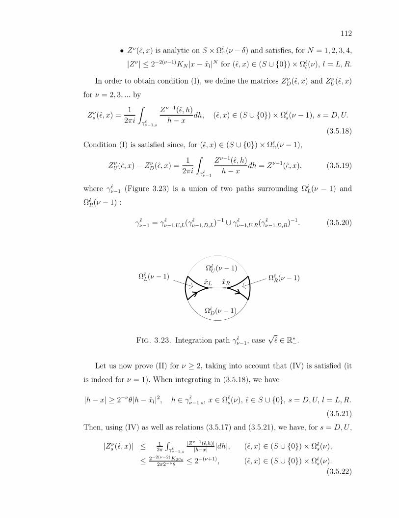
112

• Zν(ǫ, x) is analytic on S ×Ωǫ∩(ν − δ) and satisfies, for N = 1, 2, 3, 4,

|Zν | ≤ 2−2(ν−1)KN |x − xl|N for (ǫ, x) ∈ (S ∪ 0) × Ωǫl (ν), l = L, R.

In order to obtain condition (I), we define the matrices ZνD(ǫ, x) and Zν

U(ǫ, x)

for ν = 2, 3, ... by

Zνs (ǫ, x) =

1

2πi

∫

γǫν−1,s

Zν−1(ǫ, h)

h − xdh, (ǫ, x) ∈ (S ∪ 0) × Ωǫ

s(ν − 1), s = D, U.

(3.5.18)

Condition (I) is satisfied since, for (ǫ, x) ∈ (S ∪ 0) × Ωǫ∩(ν − 1),

ZνU(ǫ, x) − Zν

D(ǫ, x) =1

2πi

∫

γǫν−1

Zν−1(ǫ, h)

h − xdh = Zν−1(ǫ, x), (3.5.19)

where γ ǫν−1 (Figure 3.23) is a union of two paths surrounding Ωǫ

L(ν − 1) and

ΩǫR(ν − 1) :

γ ǫν−1 = γ ǫ

ν−1,U,L(γ ǫν−1,D,L)−1 ∪ γ ǫ

ν−1,U,R(γ ǫν−1,D,R)−1. (3.5.20)

ΩǫD(ν − 1)

ΩǫU(ν − 1)

ΩǫL(ν − 1) Ωǫ

R(ν − 1)xL xR

Fig. 3.23. Integration path γ ǫν−1, case

√ǫ ∈ R∗

−.

Let us now prove (II) for ν ≥ 2, taking into account that (IV) is satisfied (it

is indeed for ν = 1). When integrating in (3.5.18), we have

|h − x| ≥ 2−νθ|h − xl|2, h ∈ γ ǫν−1,s, x ∈ Ωǫ

s(ν), ǫ ∈ S ∪ 0, s = D, U, l = L, R.

(3.5.21)

Then, using (IV) as well as relations (3.5.17) and (3.5.21), we have, for s = D, U ,

|Zνs (ǫ, x)| ≤ 1

2π

∫γǫ

ν−1,s

|Zν−1(ǫ,h)||h−x| |dh|, (ǫ, x) ∈ (S ∪ 0) × Ωǫ

s(ν),

≤ 2−2(ν−2)K2cs

2π2−νθ≤ 2−(ν+1), (ǫ, x) ∈ (S ∪ 0) × Ωǫ

s(ν).

(3.5.22)

113

Let us now prove condition (IV), taking Zν defined by relation (III) (there

exists some 0 < δ < 1 such that (I + ZνU) is invertible for (ǫ, x) ∈ (S ∪ 0) ×

Ωǫ∩(ν − δ)). On each side of (III), multiplying by (I + Zν

U) on the right yields

ZνU + Zν(I + Zν

U) = Zν−1 + ZνD + Zν

DZν−1, (ǫ, x) ∈ (S ∪0)×Ωǫ∩(ν). (3.5.23)

Using condition (I), it yields

Zν(I + ZνU) = Zν

DZν−1, (ǫ, x) ∈ (S ∪ 0) × Ωǫ∩(ν). (3.5.24)

Hence,

|Zν | ≤ |ZνD||Zν−1||(I + Zν

U)−1| (ǫ, x) ∈ (S ∪ 0) × Ωǫ∩(ν)

≤ |ZνD||Zν−1| 1

1−|ZνU | (ǫ, x) ∈ (S ∪ 0) × Ωǫ

∩(ν),(3.5.25)

the last inequality obtained since |ZνU | < 1

2. Because of (3.5.16), we have

Zν(ǫ, x) = 0 on S × ΩǫC(ν). (3.5.26)

Finally, we finish the proof of (IV) from condition (II) and the induction hypo-

thesis into (3.5.25) : for N ≤ 4 and l = L, R, we have

|Zν | ≤ 2−(ν+1)(2−2(ν−2)KN |x − xl|N)( 11−2−(ν+1) ), (ǫ, x) ∈ (S ∪ 0) × Ωǫ

l (ν),

≤ 2−2(ν−1)KN |x − xl|N , (ǫ, x) ∈ (S ∪ 0) × Ωǫl (ν).

(3.5.27)

3.5.5. Construction of HD(ǫ, x) and HU(ǫ, x)

The sequence of matrices Zν , ZνU and Zν

D constructed in Section 3.5.4 satisfies

condition (III) and hence, for (ǫ, x) ∈ (S ∪ 0) × Ωǫ∩(ν),

I + Z(ǫ, x) = I + Z1 =

[(I + ZνD)...(I + Z3

D)(I + Z2D)]

−1(I + Zν) [(I + Zν

U)...(I + Z3U)(I + Z2

U)] .

(3.5.28)

Since

limν→∞

Zν = 0, (ǫ, x) ∈ (S ∪ 0) × Ωǫ∩(ν), (3.5.29)

and∞∏

ν=2

|1 + Zνs | ≤

∞∏

ν=2

(1 + 2−(ν+1)), (ǫ, x) ∈ (S ∪ 0) × Ωǫs(ν), s = D, U, (3.5.30)

114

the products in brackets are convergent in (3.5.28) when ν → ∞ and we are led to

matrices satisfying (3.5.1) (details in Lemma 4 from the proof of Cartan’s Lemma

in [8] p. 195) :

Hs(ǫ, x) = limν→∞

(I +Zνs )...(I +Z3

s )(I +Z2s ), (ǫ, x) ∈ (S ∪0)×Ωǫ

s(ν), s = D, U.

(3.5.31)

The boundedness of Hs(ǫ, x) and Hs(ǫ, x)−1 when x → xl, x ∈ Ωǫs, ǫ ∈ S∪0,

s = D, U , l = L, R, is obtained from (IV) and from the fact that the limit of the

products in brackets in (3.5.28) are invertible and convergent when ν → ∞.

Let us now prove that H ′s(ǫ, x) = ∂Hs(ǫ,x)

∂xis bounded when x → xl, x ∈ Ωǫ

s,

ǫ ∈ S ∪ 0, l = L, R and s = D, U , by proving there exists K ∈ R+ such that

|Hs(ǫ, xl + t) − Hs(ǫ, xl)| ≤ K|t|, xl + t ∈ Ωǫs. (3.5.32)

First, let us prove there exists k ∈ R+ such that

|Zνs (ǫ, xl + t) − Zν

s (ǫ, xl)| ≤ 2−νk|t|, xl + t ∈ Ωǫs(ν). (3.5.33)

Using (3.5.18), (IV), (3.5.21) and (3.5.17), we have, for t such that xl + t ∈ Ωǫs(ν),

|Zνs (ǫ, xl + t) − Zν

s (ǫ, xl)| = 12π

∣∣∣∫

γǫν−1,s

Zν−1(ǫ, h)(

1h−(xl+t)

− 1h−xl

)dh∣∣∣

≤ |t|2π

∣∣∣∫

γǫν−1,s

|Zν−1(ǫ,h)||h−(xl+t)||h−xl| |dh|

∣∣∣≤ |t|

2πK32νcs

22(ν−2)θ

≤ |t| K3

2ν+1K2,

(3.5.34)

thus proving (3.5.33) with k = K3

2K2. To obtain (3.5.32) from (3.5.33), let us denote

shortly

Zνs (ǫ, xl) = Zν

s,l, Zνs (ǫ, xl + t) = Zν

s,t. (3.5.35)

From (3.5.31), we have

|Hs(ǫ, xl + t) − Hs(ǫ, xl)|= limν→∞ |(I + Zν

s,t)...(I + Z3s,t)(I + Z2

s,t) − (I + Zνs,l)...(I + Z3

s,l)(I + Z2s,l)|.

(3.5.36)

115

Using (3.5.33) and (II), we can bound (3.5.36) and obtain (3.5.32) from :

|Hs(ǫ, xl + t) − Hs(ǫ, xl)|≤ limν→∞

∑ν

i=2 |Z is,t − Z i

s,l|∏i−1

q=2 |I + Zqs,t|∏ν

p=i+1 |I + Zps,l|

≤ limν→∞∑ν

i=2

|I+Zis,l|

1−2−(i+1) |Z is,t − Z i

s,l|∏i−1

q=2 |I + Zqs,t|∏ν

p=i+1 |I + Zps,l|

≤ limν→∞∑ν

i=2

|Zis,t−Zi

s,l|1−2−(i+1)

∏ν

p=2(1 + 2−(p+1))

≤ limν→∞∑ν

i=2k|t|

2i(1−2−(i+1))

∏νp=2(1 + 2−(p+1))

≤ limν→∞ k|t|∑ν

i=2 2−(i−1)∏ν

p=2(1 + 2−(p+1)).

(3.5.37)

This section concludes the proof of Theorem 3.5.1. 2

3.5.6. Introduction to the proof of Theorem 3.5.2

From now on and until the end of Section 3.5, we present the proof of Theorem

3.5.2, using the proof of Theorem 3.5.1.

Since the given system of invariants satisfy the auto-intersection relation

(3.4.123), Theorem 3.4.53 allows us to take, without loss of generality, the unfol-

ded Stokes matrices as 12-summable in ǫ and then, by (3.4.136), the corresponding

matrices NR and NR (Definition 3.4.48) satisfy

NR = NRQ(ǫ), (3.5.38)

with Q(ǫ) a nonsingular diagonal matrix exponentially close to I in√

ǫ. Let

(x2 − ǫ)v′ = A(ǫ, x)v (3.5.39)

be the system constructed in the proof of Theorem 3.5.1 by using the 12-summable

unfolded Stokes matrices. We will correct the system (3.5.39) by a transformation

y = J(ǫ, x)v (defined for (ǫ, x) ∈ S ×Dr) to obtain a system (x2 − ǫ)y′ = B(ǫ, x)y

with B(ǫ, x) analytic in ǫ at ǫ = 0. The condition (3.5.38) will be used in the

correction of the family.

3.5.7. The correction to a uniform family

Let ǫ and ǫ = ǫe2πi in S∩. Similarly as in Proposition 3.4.52, NR (respec-

tively NR) is the transition matrix ER,xR→xL(respectively ER,xL→xR

) between

HD(ǫ, x)FD(ǫ, x)TR and HU(ǫ, x)FU(ǫ, x)DRTLD−1R (respectively HD(ǫ, x)FD(ǫ, x)TL

116

and HU(ǫ, x)FU(ǫ, x)DRTRD−1R ). Because the transition matrices satisfy (3.5.38),

Proposition 3.4.43 implies that there exists an invertible transformation P (ǫ, x)

analytic in (ǫ, x) ∈ S∩ × Dr and conjugating the systems (x2 − ǫ)v′ = A(ǫ, x)v

and (x2 − ǫ)v′ = A(ǫ, x)v, i.e.

A(ǫ, x) = P (ǫ, x)A(ǫ, x)P (ǫ, x)−1 + (x2 − ǫ)P (ǫ, x)′P (ǫ, x)−1. (3.5.40)

We need to go inside the details of the construction of P (ǫ, x) to estimate its

growth. P (ǫ, x) is as follows :

P (ǫ, x) =

HU(ǫ, x)FU(ǫ, x)DRTRD−1R Q(ǫ)

×(HU(ǫ, x)FU(ǫ, x)[DRTLD−1

R ])−1

, x ∈ ΩǫU ∩ Ωǫ

U ,

HD(ǫ, x)FD(ǫ, x)TL

(HD(ǫ, x)FD(ǫ, x)TR

)−1, x ∈ Ωǫ

D ∩ ΩǫD.

(3.5.41)

P (ǫ, x) is well-defined (to verify, use (3.5.1), (3.4.51) and (3.4.83)) and can be

analytically extended to Dr. It satisfies P (0, x) = I (see Lemma 3.4.47).

In Section 3.5.8, we will show that there exists K1 ∈ R+ such that

|P (ǫ, x) − I| ≤ K1|ǫ|, (ǫ, x) ∈ (S∩ ∪ 0) × Dr. (3.5.42)

This leads to the proof, sketched in Section 3.5.9, of the existence of J(ǫ, x), a

nonsingular matrix depending analytically on (ǫ, x) ∈ S × Br such that

J(ǫ, x)−1J(ǫ, x) = P (ǫ, x) (3.5.43)

on S∩ and such that J(ǫ, x), J ′(ǫ, x) and J(ǫ, x)−1 have a bounded limit at ǫ = 0

(this proof requires slight reductions of the radius and opening of S).

Let (x2 − ǫ)y′ = B(ǫ, x)y be the system obtained by the change y = J(ǫ, x)v

into (3.5.39). We have

B(ǫ, x) = J(ǫ, x)A(ǫ, x)J(ǫ, x)−1 + (x2 − ǫ)J(ǫ, x)′J(ǫ, x)−1. (3.5.44)

Replacing (3.5.43) into (3.5.40), we get

J(ǫ, x)A(ǫ, x)J(ǫ, x)−1 + (x2 − ǫ)J(ǫ, x)′J(ǫ, x)−1

= J(ǫ, x)A(ǫ, x)J(ǫ, x)−1 + (x2 − ǫ)J(ǫ, x)′J(ǫ, x)−1,(3.5.45)

117

and hence we will have B(ǫ, x) = B(ǫ, x) on S∩ (for x fixed). B(ǫ, x) will be

analytic in ǫ because it will be unramified and because limǫ→0 B(ǫ, x) will exist.

In conclusion, once (3.5.42) and the existence of the desired J(ǫ, x) will be

proved (in Sections 3.5.8 and 3.5.9), we will have constructed an analytic family

of systems with the given complete system of analytic invariants.

3.5.8. Properties of P (ǫ, x) near ǫ = 0

In this section, we show that the conjugating transformation P (ǫ, x) satisfies

(3.5.42).

3.5.8.1. Proof of (3.5.42)

Let us detail how to obtain (3.5.42) for ǫ 6= 0 from the construction of P (ǫ, x)

given by (3.5.41). We will prove that (3.5.42) is satisfied for x ∈ (ΩǫU ∩Ωǫ

U )∪(ΩǫD∩

ΩǫD). By the Maximum Modulus Theorem, this implies that (3.5.42) is satisfied

for x ∈ Dr.

With the shorter notations

HD = HD(ǫ, x) and FD = FD(ǫ, x), (3.5.46)

we have, for x ∈ ΩǫD ∩ Ωǫ

D,

|P (ǫ, x) − I| = |HDFDTLT−1R F−1

D H−1D − I|

= |HDFD(TLT−1R − I)F−1

D H−1D + (HDH−1

D − I)|≤ |H−1

D ||HD||FD||F−1D ||TLT−1

R − I| + |H−1D ||HD − HD|

≤ |H−1D ||HD||FD||F−1

D |(|TL − I| + |T−1R − I| + |TL − I||T−1

R − I|)+|H−1

D ||HD − HD|,(3.5.47)

as well as a similar relation on ΩǫU ∩Ωǫ

U . From Lemma 3.4.47 (and using (3.4.12)),

the following matrices appearing in (3.5.47) and in the similar relation on ΩǫU ∩Ωǫ

U

are exponentially close in√

ǫ to I :

DRTRD−1R , DRT−1

L D−1R , TL, T−1

R . (3.5.48)

118

Hence, in order to obtain the relation (3.5.42) for x ∈ (ΩǫU ∩Ωǫ

U) ∪ (ΩǫD ∩Ωǫ

D), it

suffices to bound |Hs(ǫ, x) − Hs(ǫ, x)| . From (3.5.31), we have

|Hs(ǫ, x) − Hs(ǫ, x)|= limν→∞ |(I + Zν

s )...(I + Z3s )(I + Z2

s ) − (I + Zνs )...(I + Z3

s )(I + Z2s )|.(3.5.49)

We will prove in Section 3.5.8.2 that there exists k1 ∈ R+ such that, for ν ≥ 2,

|Zνs − Zν

s | ≤ 2−νk1|ǫ|, (ǫ, x) ∈ S∩ × (Ωǫs(ν) ∩ Ωǫ

s)(ν), s = D, U. (3.5.50)

Using (3.5.49), (3.5.50) and condition (II) in Section 3.5.4, we then have

|Hs(ǫ, x) − Hs(ǫ, x)|≤ limν→∞

∑νi=2 |Z i

s − Z is|∏i−1

q=2 |I + Zqs |∏ν

p=i+1 |I + Zps |

≤ limν→∞∑ν

i=2 |Z is − Z i

s|∏i−1

q=2 |I + Zqs |∏ν

p=i+1 |I + Zps | |I+Zi

s|1−2−(i+1)

≤ limν→∞∏ν

p=2(1 + 2−(p+1))∑ν

i=2|Zi

s−Zis|

1−2−(i+1)

≤ limν→∞∏ν

p=2(1 + 2−(p+1))∑ν

i=2k1|ǫ|

2i(1−2−(i+1))

≤ limν→∞ k1|ǫ|∏ν

p=2(1 + 2−(p+1))∑ν

i=2 2−(i−1),

(3.5.51)

yielding the existence of K∗1 ∈ R+ such that

|Hs(ǫ, x) − Hs(ǫ, x)| ≤ K∗1|ǫ|, (ǫ, x) ∈ S∩ × (Ωǫ

s ∩ Ωǫs), s = D, U. (3.5.52)

3.5.8.2. Property (3.5.50) of Zνs

Let us now prove (3.5.50), the remaining ingredient of the proof of (3.5.42)

for x ∈ (ΩǫU ∩ Ωǫ

U ) ∪ (ΩǫD ∩ Ωǫ

D). From the definition of Zνs in (3.5.18), we have,

for (ǫ, x) ∈ S × Ωǫs(ν) ∩ Ωǫ

s(ν) and s = D, U ,

∣∣∣Zνs − Zν

s

∣∣∣ =

∣∣∣∣∣1

2πi

∫

γǫν−1,s

Zν−1(ǫ, h)

h − xdh − 1

2πi

∫

γǫν−1,s

Zν−1(ǫ, h)

h − xdh

∣∣∣∣∣ (3.5.53)

The integration paths in (3.5.53) differ near the singular points but have a nonvoid

common part. For s = D, U , we denote by iǫν,s the common part of γ ǫν,s and

γ ǫν,s, and by rǫ

ν,s and rǫν,s their respective remaining broken paths (i.e. we have

γ ǫν,s = iǫν,s + rǫ

ν,s). Finally, as illustrated in Figure 3.24, we separate the left and

right parts of rǫν,s, denoting rǫ

ν,s = rǫν,s,L ∪ rǫ

ν,s,R. With these notations, we can

119

rǫν,U,L

rǫν,U,L rǫ

ν,U,R

rǫν,U,R

iν,U

rǫν,D,R

rǫν,D,R

rǫν,D,L

rǫν,D,L

iν,D

xRxR

xLxL

Fig. 3.24. Integration paths iǫν,s, rǫν,s = rǫ

ν,s,L ∪ rǫν,s,R and rǫ

ν,s =

rǫν,s,L ∪ rǫ

ν,s,R, s = D, U .

write (3.5.53) as

∣∣∣Zνs − Zν

s

∣∣∣ =∣∣∣ 12πi

∫iǫν−1,s

Zν−1(ǫ,h)−Zν−1(ǫ,h)h−x

dh

+ 12πi

∫rǫν−1,s

Zν−1(ǫ,h)h−x

dh − 12πi

∫rǫν−1,s

Zν−1(ǫ,h)h−x

dh∣∣∣ ,

(3.5.54)

and hence∣∣∣Zν

s − Zνs

∣∣∣ ≤ 12π

∫iǫν−1,s

|Zν−1(ǫ,h)−Zν−1(ǫ,h)||h−x| |dh|

+ 12π

∣∣∣∫

rǫν−1,s

Zν−1(ǫ,h)h−x

dh∣∣∣ + 1

2π

∣∣∣∫

rǫν−1,s

Zν−1(ǫ,h)h−x

dh∣∣∣ .

(3.5.55)

In order to prove (3.5.50) from (3.5.55), we will bound its last row, and then use

induction.

By condition (IV) in Section 3.5.4, we have

|Zν−1(ǫ, h)| ≤ 2−2(ν−2)K4|h − xl|4, (ǫ, x) ∈ (S ∪ 0) × Ωǫl (ν). (3.5.56)

Using (3.5.21), we thus have, for x ∈ Ωǫl (ν) ∩ Ωǫ

l (ν) s = D, U , l = L, R and

ǫ ∈ ǫ, ǫ,∣∣∣∫

rǫν−1,s,l

Zν−1(ǫ,h)h−x

dh∣∣∣ ≤

∫rǫν−1,s,l

|Zν−1(ǫ,h)||h−x| |dh|

≤∫

rǫν−1,s,l

2−2(ν−2)K4|h−xl|22−νθ

|dh|.(3.5.57)

The integration paths rǫν,s are located inside a disk of radius c

√|ǫ| for some c ∈ R∗

+

(Section 3.4.4), yielding

∣∣∣∫

rǫν−1,s,l

Zν−1(ǫ,h)h−x

dh∣∣∣ ≤

∫rǫν−1,s,l

θ−124−νK4(|h| +√

|ǫ|)2|dh|

≤∫

rǫν−1,s,l

θ−124−νK4|ǫ|(c + 1)2|dh|

= θ−124−νK4|ǫ|(c + 1)2∫

rǫν−1,s,l

|dh|.

(3.5.58)

120

Thus, a bound for the last row of (3.5.55) is, using (3.5.17) and the fact that the

length of the path rǫν−1,s is smaller than the length of the path γ ǫ

ν−1,s,

12π

(∣∣∣∫

rǫν−1,s

Zν−1(ǫ,h)h−x

dh∣∣∣+∣∣∣∫

rǫν−1,s

Zν−1(ǫ,h)h−x

dh∣∣∣)

≤ (2πθ)−124−νK4|ǫ|(c + 1)2(∫

rǫν−1,s

|dh| +∫

rǫν−1,s

|dh|)

≤ (2πθ)−124−νK4|ǫ|(c + 1)2(∫

γǫν−1,s

|dh| +∫

γǫν−1,s

|dh|)

≤ (2πθ)−124−νK4|ǫ|(c + 1)22cs

=k∗1

2ν+5 |ǫ|,

(3.5.59)

where

k∗1 =

25K4(c + 1)2

K2. (3.5.60)

Hence, (3.5.55) becomes

∣∣∣Zνs − Zν

s

∣∣∣ ≤ 12π

∫iǫν−1,s

|Zν−1(ǫ,h)−Zν−1(ǫ,h)||h−x| |dh| + k∗

1

2ν+5 |ǫ|,

(ǫ, x) ∈ S∩ × (Ωǫl (ν) ∩ Ωǫ

l (ν)).(3.5.61)

From (3.5.61), we will prove (3.5.50) for ν = 2, ν = 3 and ν > 3.

Beginning with ν = 2, we have, from

Fs(ǫ, x) = Fs(ǫ, x), x ∈ Ωǫs ∩ Ωǫ

s, s = D, U, (3.5.62)

and from (3.5.2),

|Z1 − Z1| ≤

|FD(ǫ, x) (CR(ǫ) − CR(ǫ))FD(ǫ, x)−1|, on Ωǫ

R ∩ ΩǫR,

|FD(ǫ, x) (CL(ǫ) − CL(ǫ))FD(ǫ, x)−1|, on ΩǫL ∩ Ωǫ

L.(3.5.63)

By the 12-summability of the unfolded Stokes matrices, |Cl(ǫ) − Cl(ǫ)| is expo-

nentially close to 0 in√

ǫ. Then, (3.5.63) implies that there exists w1 ∈ R+ such

that

|Z1 − Z1| ≤ w1

24K2|ǫ||x− xl|2, l = L, R, (ǫ, x) ∈ S∩ × (Ωǫ

l (ν)∩Ωǫl (ν)), (3.5.64)

with K2 given by (3.5.15). Using relations (3.5.17) and (3.5.21) and the fact that

the length of the path iǫν,s is smaller than the length of the path γ ǫν,s, the integral

121

in (3.5.61) for ν = 2 is bounded by

12π

∫i1,s

|Z1(ǫ,h)−Z1(ǫ,h)||h−x| |dh| ≤ 1

2π

∫i1,s

w1K2|ǫ||h−xl|224|h−x| |dh|

≤ 12π

∫i1,s

w1K2|ǫ||h−xl|2242−2θ|h−xl|2 |dh|

≤ w1|ǫ| K2

23θπ

∫i1,s

|dh|≤ w1|ǫ|K2cs

23θπ

≤ 127 w1|ǫ|.

(3.5.65)

From (3.5.61) and (3.5.65), we have

|Z2s − Z2

s | ≤1

26k1|ǫ|, (ǫ, x) ∈ S∩ × (Ωǫ

s(2) ∩ Ωǫs)(2), s = D, U, (3.5.66)

with

k1 = maxk∗1, w1. (3.5.67)

Relation (3.5.50) is thus satisfied for ν = 2.

Now, let us study |Zν−1 − Zν−1| in order to bound (3.5.61) for ν ≥ 3. From

the equality

ABC−1 − ABC−1 =((A − A)B + A(B − B) + ABC−1(C − C)

)C−1, (3.5.68)

applied to relation Zν−1 = Zν−1D Zν−2(I + Zν−1

U )−1 coming from (3.5.24), we have

(taking Zν−1 = ABC−1, Zν−1D = A, Zν−2 = B and (I + Zν−1

U ) = C)

|Zν−1 − Zν−1|≤(|Zν−1

D − Zν−1D ||Zν−2| + |Zν−1

D ||Zν−2 − Zν−2| + |Zν−1||Zν−1U − Zν−1

U |)

×|(I + Zν−1U )−1|.

(3.5.69)

Let us remark that, because of (3.5.62), we have

|Zν | ≤ 2−2(ν−1)K1|x − xl|, (ǫ, x) ∈ S∩ × Ωǫl (ν) ∩ Ωǫ

l (ν), l = L, R, (3.5.70)

coming from condition (IV) of Section 3.5.4.

For ν = 3, equation (3.5.69) yields, with the use of (3.5.64), (3.5.66), (3.5.67),

(3.5.70) and |Zν−1s | ≤ 2−ν (from (II) ),

|Z2 − Z2| ≤ k1|ǫ|K2|x − xl|2(

126 + 1

2324 + 12226

) (1

1−2−3

), l = L, R,

≤ k1|ǫ|K2|x − xl|2 124 , l = L, R,

(3.5.71)

122

for (ǫ, x) ∈ S∩ × (Ωǫs(2) ∩ Ωǫ

s)(2). In the same way as when we bounded (3.5.65),

we use (3.5.71) to bound the integral in (3.5.61) for ν = 3 :

12π

∫i2,s

|Z2(ǫ,h)−Z2(ǫ,h)||h−x| |dh| ≤ 1

2π

∫i2,s

k1|ǫ|K2|h−xl|2242−3θ|h−xl|2 |dh|

≤ k1|ǫ|K2

22πθ

∫i2,s

|dh|≤ k1|ǫ|K2

22πθ

∫γǫ2,s

|dh|

≤ 122 k1|ǫ|K2cs

πθ

≤ 126 k1|ǫ|.

(3.5.72)

Then, (3.5.72) into (3.5.61) gives

|Z3s − Z3

s | ≤1

25k1|ǫ|, (ǫ, x) ∈ S∩ × (Ωǫ

s(3) ∩ Ωǫs(3)), s = D, U. (3.5.73)

Relation (3.5.50) is hence satisfied for ν = 3.

We are now ready to prove (3.5.50) for ν > 3 by induction on ν. Let us suppose

that we have

|Zν−2 − Zν−2| ≤ k1

22(ν−3) |ǫ|K2|x − xl|2,(ǫ, x) ∈ S∩ × (Ωǫ

s(ν − 2) ∩ Ωǫs(ν − 2)), l = L, R,

(3.5.74)

and

|Zν−1s − Zν−1

s | ≤ 1

2ν−1k1|ǫ|, (ǫ, x) ∈ S∩ × (Ωǫ

s(ν − 1) ∩ Ωǫs(ν − 1)), s = D, U,

(3.5.75)

(this is indeed satisfied for ν = 4 because of (3.5.71) and (3.5.73)). For ν > 3,

relation (3.5.69) yields, using (3.5.74), (3.5.75), (3.5.70) and |Zν−1s | ≤ 2−ν (from

(II)),

|Zν−1 − Zν−1| ≤ k1|ǫ|K2|x − xl|2(

12ν−122(ν−3) + 1

2ν22(ν−3) + 122(ν−2)2ν−1

)

×(

11−2−ν

),

(3.5.76)

and thus, for (ǫ, x) ∈ S∩ × (Ωǫs(ν − 1) ∩ Ωǫ

s(ν − 1)) and l = L, R,

|Zν−1 − Zν−1| ≤ k1

22(ν−2) |ǫ|K2|x − xl|2. (3.5.77)

123

In the same way as when we bounded (3.5.65) and (3.5.72), we use (3.5.77) to

bound the integral in (3.5.61) for ν > 3 :

12π

∫iǫν−1,s

|Zν−1(ǫ,h)−Zν−1(ǫ,h)||h−x| |dh| ≤ 1

2π

∫iǫν−1,s

k1K2|ǫ||h−xl|222(ν−2) |h−x| |dh|

≤ 12π

∫iǫν−1,s

k1K2|ǫ||h−xl|222(ν−2)2−νθ|h−xl|2

|dh|

≤ k1K2|ǫ|π2ν−3θ

∫iǫν−1,s

|dh|

≤ k1K2|ǫ|π2ν−3θ

∫γǫ

ν−1,s|dh|

≤ 12ν−3 k1|ǫ|K2cs

πθ

≤ 12ν+1 k1|ǫ|.

(3.5.78)

Then, (3.5.78) and (3.5.61) gives (3.5.50) for ν > 3 (using (3.5.67)).

3.5.9. Construction of J(ǫ, x)

For fixed x, the existence of J(ǫ, x) follows from the triviality of the vector

bundle on the punctured disk in ǫ-space. But, we need to show that J(ǫ, x) de-

pends analytically on the "parameter" x ∈ Dr and also that we can fill the hole at

ǫ = 0. So we need to go into the details of the construction of J(ǫ, x). We do this

in a sketchy way since the details are completely similar (and simpler) to those

we have done in Sections 3.5.1 to 3.5.5.

S has been taken previously with an opening 2π + γ0. We reduce slightly the

opening of S to 2π + γ with 0 < γ < γ0, denoting the sector with the previous

opening Sprev, such that, for some α > 0,

S(1) = S ∪ ǫ : ∃ǫ ∈ S∩ s.t. |ǫ − ǫ| < 2−1α|ǫ| ⊂ Sprev. (3.5.79)

We write S as the union of two sectors VU and VD

VD = ǫ ∈ C : 0 < |ǫ| < ρ, arg(ǫ) ∈ (π − γ, 2π + γ),VU = ǫ ∈ C : 0 < |ǫ| < ρ, arg(ǫ) ∈ (2π − γ, 3π + γ).

(3.5.80)

We take the following domains converging when ν → ∞ to Vs and included into

Sprev :

Vs(ν) = Vs ∪ǫ : ∃ǫ ∈ VU ∩VD s.t. |ǫ− ǫ| < 2−να|ǫ|, ν ≥ 1, s = D, U. (3.5.81)

We separate the intersection of VU(ν) and VD(ν) into a left and a right domain :

V∩(ν) = VU(ν) ∩ VD(ν) = VL(ν) ∪ VR(ν). (3.5.82)

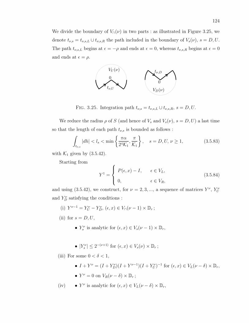
124

We divide the boundary of V∩(ν) in two parts : as illustrated in Figure 3.25, we

denote tν,s = tν,s,L ∪ tν,s,R the path included in the boundary of Vs(ν), s = D, U .

The path tν,s,L begins at ǫ = −ρ and ends at ǫ = 0, whereas tν,s,R begins at ǫ = 0

and ends at ǫ = ρ.

tν,U

tν,D

VD(ν)

VU (ν)

00

Fig. 3.25. Integration path tν,s = tν,s,L ∪ tν,s,R, s = D, U .

We reduce the radius ρ of S (and hence of Vs and Vs(ν), s = D, U) a last time

so that the length of each path tν,s is bounded as follows :∫

tν,s

|dh| < ls < min

πα

24K1,

π

K1

, s = D, U, ν ≥ 1, (3.5.83)

with K1 given by (3.5.42).

Starting from

Y 1 =

P (ǫ, x) − I, ǫ ∈ VL,

0, ǫ ∈ VR,(3.5.84)

and using (3.5.42), we construct, for ν = 2, 3, ..., a sequence of matrices Y ν , Y νU

and Y νD satisfying the conditions :

(i) Y ν−1 = Y νU − Y ν

D, (ǫ, x) ∈ V∩(ν − 1) × Dr ;

(ii) for s = D, U ,

• Y νs is analytic for (ǫ, x) ∈ Vs(ν − 1) × Dr,

• |Y νs | ≤ 2−(ν+1) for (ǫ, x) ∈ Vs(ν) × Dr ;

(iii) For some 0 < δ < 1,

• I + Y ν = (I + Y νD)(I + Y ν−1)(I + Y ν

U )−1 for (ǫ, x) ∈ VL(ν − δ)× Dr,

• Y ν = 0 on VR(ν − δ) × Dr ;

(iv) • Y ν is analytic for (ǫ, x) ∈ VL(ν − δ) × Dr,

125

• Y ν(0, x) = 0,

• Y ν satisfies, with K1 given by (3.5.42),

|Y ν | ≤ 2−2(ν−1)K1|ǫ| for (ǫ, x) ∈ VL(ν) × Dr.

We can prove that the properties (i) to (iv) are satisfied in a similar (and

simpler) way as in Section 3.5.4, by defining the matrices Y νD(ǫ, x) and Y ν

U (ǫ, x),

for ν = 2, 3, ..., by

Y νs (ǫ, x) =

1

2πi

∫

tν−1,s

Y ν−1(h, x)

h − ǫdh, (ǫ, x) ∈ Vs(ν−1)×Dr, s = D, U. (3.5.85)

As in Section 3.5.5, the desired J(ǫ, x) is given by

J(ǫ, x) =

JD(ǫ, x), ǫ ∈ VD,

JU(ǫ, x), ǫ ∈ VU ,(3.5.86)

with

Js(ǫ, x) = limν→∞

(I + Y νs )...(I + Y 3

s )(I + Y 2s ), s = D, U. (3.5.87)

By (ii), J(ǫ, x)−1 has a bounded limit at ǫ = 0. Since the familyJ ′(ǫ, x)ǫ∈(S∪0)

is bounded, J ′(ǫ, x) has a bounded limit at ǫ = 0. This concludes the proof of

Theorem 3.5.2. 2

3.6. Discussion and directions for further research

The work presented in this paper brings a new light on the divergence of formal

solutions near an irregular singular point of Poincaré rank 1. It gives new pers-

pectives, including a unified point of view in the understanding of the dynamics

of the singularities by deformation. We have identified, interpreted and studied

the realization of the complete system of analytic invariants of unfolded differen-

tial linear systems with an irregular singularity of Poincaré rank 1 (nonresonant

case). The meaning of the auto-intersection relation (which is the necessary and

sufficient condition for the realization) is still obscure (in dimension n ≥ 3). We

will investigate it in more details in [13].

One of the next steps in the large program of understanding singularities

by unfolding is the study of analytic invariants of nonresonant linear differential

126

equations with singularities of Poincaré rank k higher than 1. One difference is

that there is no more a bijection between the 2k Stokes matrices and the k + 1

singular points in the unfolded systems.

Another direction of research is the existence of universal families. Can we

identify canonical representatives of the analytic equivalence classes of unfolded

systems ?

CONCLUSION

La présente thèse, concernant la classification analytique des déploiements de

systèmes différentiels linéaires ayant une singularité irrégulière (non résonante) de

rang de Poincaré k = 1, donne un système d’invariants complet, son interprétation

ainsi que les conditions nécessaires et suffisantes à sa réalisation.

Le but de la thèse a été atteint par les résultats des articles. Le système

complet d’invariants analytiques a été identifié par des invariants formels et ana-

lytiques. La partie formelle a été déterminée à partir d’une forme prénormale et se

retrouve dans un modèle polynomial qui devient, lorsque ǫ → 0, la forme normale

formelle du système confluent. Le modèle nous a permis alors d’interpréter tous

les invariants formels au point singulier irrégulier. Nous avons montré que la partie

analytique du système d’invariants compte des classes d’équivalence de matrices

de Stokes déployées, dont les représentants peuvent être choisis 12-sommables en

ǫ. De plus, nous avons interprété les matrices de Stokes déployées en termes de

monodromie d’une base de solutions particulières dans le système linéaire (et

d’intégrales premières dans les systèmes de Riccati correspondants). Ceci nous a

mené aux conséquences du phénomène de Stokes dans les déploiements, ce qui

comprend le lien avec la présence de solutions logarithmiques aux points singu-

liers réguliers lors de la résonance. Finalement, nous avons résolu la question de

la réalisation des invariants. Tout système complet d’invariants analytiques peut

être réalisé si et seulement si la relation d’auto-intersection est satisfaite.

Notons que la notion de sommabilité n’est pas disparue par le processus de

déploiement. En effet, afin d’expliquer le phénomène de Stokes dans la variable

x, nous avons déployé la singularité irrégulière et recherché les invariants analy-

tiques des systèmes déployés. Alors que les invariants formels ont une dépendance

128

analytique en ǫ, les représentants des invariants analytiques peuvent être choisis12-sommable en ǫ. On a donc introduit de la 1

2-sommabilité dans le paramètre afin

de comprendre la 1-sommabilité dans la variable x.

Sur l’auto-intersection du secteur S dans l’espace du paramètre, les deux

points de vue se recollent par une relation que nous avons appelée la relation

d’auto-intersection. Elle dépend indirectement des matrices de Stokes déployées

et reste alors un peu mystérieuse. Cependant, quelle que soit la dimension n, la

relation d’auto-intersection peut être interprétée en termes d’invariance (lors de

l’adoption de deux points de vue différents sur l’auto-intersection du secteur S)

des matrices de transition entre des bases de solutions particulières qui sont des

vecteurs propres de la monodromie autour des points singuliers réguliers. La re-

lation d’auto-intersection peut s’énoncer facilement en fonction des matrices de

Stokes déployées en dimension n = 2. Ceci vient du fait que les éléments des

matrices diagonalisant la monodromie sont dans ce cas des multiples (bien pré-

cis) des éléments des matrices de Stokes déployées (ceci est généralement faux en

dimension supérieure). L’étude du cas n = 3 devrait s’avérer fructueuse afin de

dégager des résultats généraux pour toute dimension n.

L’approche utilisée apporte une nouvelle lumière sur le phénomène de Stokes

et mérite d’être généralisée à des systèmes déployant une singularité irrégulière

(non résonante) de rang de Poincaré k ∈ N∗, avec k > 1. Cette généralisation n’est

pas immédiate, nous pouvons déjà y voir une différence notable avec les travaux

de cette thèse. En effet, lorsque k = 1, nous avons deux matrices de Stokes et

chacune est associée à un point singulier régulier des systèmes déployés. Dans le

cas général, nous devrons faire le lien entre 2k matrices de Stokes et k + 1 points

singuliers réguliers dans le déploiement. La théorie sera forcément plus élaborée

et nous en apprendra davantage sur la dynamique en jeu. Près de 150 ans après sa

découverte, le phénomène de Stokes a encore des subtilités à nous faire découvrir.

BIBLIOGRAPHIE

[1] W. Balser, W. B. Jurkat, D. A. Lutz, Birkhoff invariants and Stokes’ multi-

pliers for meromorphic linear differential equations, J. Math. Anal. Appl. 71

(1979), no 1, 48–94.

[2] C. Christopher, C. Rousseau, The moduli space of germs of generic families of

analytic diffeomorphims unfolding a parabolic fixed point, prépublication CRM,

2008.

[3] C. Christopher, C. Rousseau, The moduli space of germs of generic families

of analytic diffeomorphisms unfolding a parabolic fixed point, C.R. Acad. Sci.

Paris, Ser. I 345 (2007) 695–698.

[4] A. Duval, Biconfluence et groupe de Galois, J. Fac. Sci. Univ. Tokyo Sect. IA

Math. 38 (1991), no 2, 211–223.

[5] A. Duval, Confluence procedures in the generalized hypergeometric family, J.

Math. Sci. Univ. Tokyo 5 (1998), no 4, 597–625.

[6] A. Glutsyuk, Stokes operators via limit monodromy of generic perturbation, J.

Dynam. Control Systems 5 (1999), no 1, 101–135.

[7] É. Goursat, Leçons sur les séries hypergéométriques et sur quelques fonctions

qui s’y rattachent, propriétés générales de l’équation d’Euler et de Gauss, Ac-

tualités scientifiques et industrielles, vol. 333, Hermann, Paris, 1936.

[8] R. C. Gunning, H. Rossi, Analytic functions of several complex variables,

Prentice-Hall Inc., Englewood Cliffs, N.J., 1965.

[9] E. Hille, Ordinary Differential Equations in the Complex Domain, A Wiley-

Interscience publication, John Wiley and Sons, New York, 1976.

[10] Y. Ilyashenko, S. Yakovenko, Lectures on Analytic Differential Equations, Gra-

duate Studies in Mathematics, 86, American Mathematical Society, Provi-

dence, RI, 2008.

130

[11] W. Jurkat, D. A. Lutz, A. Peyerimhoff, Birkhoff invariants and effective cal-

culations for meromorphic linear differential equations I, J. Math. Anal. Appl.

53 (1976) 438–470.

[12] C. Lambert, C. Rousseau, The Stokes phenomenon in the confluence of the

hypergeometric equation using Riccati equation, J. Differential Equations 244

(2008), no 10, 2641–2664.

[13] C. Lambert, C.Rousseau, Compatibility conditions for the realization of the

analytic invariants of unfolded differential linear systems with an irregular sin-

gularity of Poincaré rank 1, en préparation.

[14] Y.L. Luke, The special functions and their approximations, Math. Sci. Eng.,

vol. 53-1, Academic Press, New York, 1969.

[15] J. Martinet, J.-P. Ramis, Théorie de Galois différentielle et resommation,

Computer Algebra and Differential Equations, 117–214, E. Tournier, Acade-

mic Press, New York, 1989.

[16] E.D. Rainville, Intermediate differential equations, Macmillan Company, New

York, 1964.

[17] J.-P. Ramis, Confluence et résurgence, J. Fac. Sci. Univ. Tokyo Sect. IA Math.

36 (1989) 703–716.

[18] J.-P. Ramis. Gevrey asymptotics and applications to holomorphic ordinary dif-

ferential equations, Differential equations and asymptotic theory in mathema-

tical physics, 44–99, Ser. Anal., 2, World Sci. Publ., Hackensack, NJ, 2004.

[19] C. Rousseau, Modulus of orbital analytic classification for a family unfolding

a saddle-node, Mosc. Math. J. 5 (2005), no 1, 245–268.

[20] C. Rousseau, L. Teyssier, Analytical moduli for unfoldings of saddle-node

vector-fields, Mosc. Math. J. 8 (2008), no 3, 547–614.

[21] R. Schäfke, Confluence of several regular singular points into an irregular one,

J. Dynam. Control Systems 4 (1998), no 3, 401–424.

[22] Y. Sibuya, Linear differential equations in the complex domain : problems of

analytic continuation. Translations of Mathematical Monographs, 82, Ameri-

can Mathematical Society, Providence, RI, 1990.

[23] W. Wasow, Asymptotic expansions for ordinary differential equations, Dover

Publications Inc., New York, 1987.

131

[24] C. Zhang, Quelques études en théorie des équations fonctionnelles et en analyse

combinatoire, thèse de doctorat, Université Louis Pasteur, 1994.

[25] C. Zhang, Confluence et phénomène de Stokes, J. Math. Sci. Univ. Tokyo 3

(1996), no 1, 91–107.