
Título do Projeto - Thèses en ligne de l'Université...
199
Université de Toulouse ' THESE En vue de l'obtention du DOCTORAT DE L'UNIVERSITÉ DE TOULOUSE Délivré par : Université Toulouse 3 Paul Sabatier (UT3 Paul Sabatier) Cotutelle internationale avec : lnstituto Nacional de Pesquisas da Amazônia -INPA Présentée et soutenue par : Elisa Natalia ARMIJOS CARDENAS le mercredi 10 novembre 2015 Titre: Propagation des flux de sédiments en suspension sur l'Amazone de Tamsh iyacu (Pérou) à Obidos(Brésii)-Variabilité spatio-temporelle École doctorale et discipline ou spécialité ED SDU2E : Hydrologie, Hydrochimie, Sol, Environnement Unité de recherche: UMR Géosciences Environnement Toulouse (GET) Directeur(s) de Thèse : Dr. Jean Loup GUYOT Dr. Naziano Pantoja FILIZOLA Jr. Rapporteurs : Dr. Gustavo Henrique MERTEN Dr. José Cândido STEVAUX Autre(s) membre(s) du jury: Dr. Luiz Antonio CÀNDIDO Dr. Jean Michel MARTiNEZ
Transcript of Título do Projeto - Thèses en ligne de l'Université...
Université de Toulouse
' THESE En vue de l'obtention du
DOCTORAT DE L'UNIVERSITÉ DE TOULOUSE Délivré par :
Université Toulouse 3 Paul Sabatier (UT3 Paul Sabatier)
Cotutelle internationale avec :
lnstituto Nacional de Pesquisas da Amazônia -INPA
Présentée et soutenue par : Elisa Natalia ARMIJOS CARDENAS
le mercredi 10 novembre 2015
Titre: Propagation des flux de sédiments en suspension sur l'Amazone de
Tamshiyacu (Pérou) à Obidos(Brésii)-Variabilité spatio-temporelle
École doctorale et discipline ou spécialité ED SDU2E : Hydrologie, Hydrochimie, Sol, Environnement
Unité de recherche: UMR Géosciences Environnement Toulouse (GET)
Directeur(s) de Thèse : Dr. Jean Loup GUYOT
Dr. Naziano Pantoja FILIZOLA Jr.
Rapporteurs : Dr. Gustavo Henrique MERTEN
Dr. José Cândido STEVAUX
Autre(s) membre(s) du jury:
Dr. Luiz Antonio CÀNDIDO Dr. Jean Michel MARTiNEZ
INSTITUTO NACIONAL DE PESQUISAS DA AMAZÔNIA - INPA -MANAUS-BRASIL
PROGRAMA DE PÓS-GRADUAÇÃO EM CLIMA E AMBIENTE - CLIAMB
TESE EM COTUTELA COM AUNIVERSITÉ PAUL SABATIER- UPS- TOULOUSE-FRANÇA
Propagação dos Fluxos de Sedimentos em suspensão do RioAmazonas- Trecho Tamshiyacu (Peru) até
Óbidos(Brasil)-Variabilidade Espacial e Temporal
Elisa Natalia Armijos Cárdenas
Manaus, AmazonasNovembro, 2015
Elisa Natalia Armijos Cárdenas
Propagação dos Fluxos de Sedimentos em suspensão do RioAmazonas- Trecho Tamshiyacu (Peru) até
Óbidos(Brasil)-Variabilidade Espacial e Temporal
Orientadores:Naziano Pantoja Filizola Jr.e Jean Loup Guyot.
Fonte Financiadora: Capes
Tese apresentada ao Instituto Nacional de Pes-quisas da Amazônia - INPA em cotutela com aUniversidade de Toulouse Paul Sabatier comorequisito para a obtenção do Título de Doutoraem Clima e Ambiente e em Ciências da Terra.
Manaus, AmazonasNovembro, 2015
A729p Armijos Cárdenas,Elisa Natalia.
Propagação dos fluxos de sedimentos em suspensão do Rio Amazonas.Trecho Tamshiyacu (Peru) ate Óbidos (Brasil)-Variabilidade Espacial eTemporal./Elisa Natalia Armijos Cárdenas.−−− Manaus: [s.n.], 2016.177 f. : il., color.
Tese de Doutorado em cotutela INPA e UPS, Manaus, 2015Orientadores: Naziano Pantoja Filizola Jr e
Jean Loup Guyot
Área de concentração : Clima e Ambiente.
1.Sedimentação, 2.Iteração biosfera-atmosfera, 3. Hidrologia, 4. BaciaAmazônica. I. Titulo
CDD 551.354
Sipnose:Estudou-se a distribuição espacial e temporal dos sedimentos em suspen-são no Rio Amazonas, se quantificou o fluxo sedimentar na bacia Amazô-nica Peruana e no Brasil na estação de Óbidos. Implantou-se uma novametodologia para predizer modelos de concentração em base na turbidez.Palavras chave: sedimentos em suspensão,Bacia Amazônica,turbidez,granulometria, sub-bacias Andinas, Amazônia.
Comissão Julgadora:
Revisores/ Rapporteurs:
Dr. Gustavo Henrique MERTEN University Minnesota Duluth- Department of Ci-vil Engenniering.
Dr.José Cândido STEVAUX Instituto de Geociências e Ciências Exatas-Universidade Estadual Paulista Rio Claro
Miembros da banca/ Examinateurs:
Dr.Jean Michel MARTÍNEZ Laboratoire Géosciences Environnement Tou-louse Université de Toulouse Paul Sabatier.
Dr. Luiz CÂNDIDO CLIAMB- Instituto de Pesquisas daAmazônia(INPA)-Universidade do Estadode Amazonas (UEA).
Orientadores/Directeurs:
Dr. Naziano FILIZOLA CLIAMB- Universidade Federal do Amazonas.Dr. Jean Loup GUYOT Laboratoire Géosciences Environnement Tou-
louse Université de Toulouse Paul Sabatier.
Agradecimentos
Este estudo faz parte do projeto de pesquisa do Observatório SO-HYBAM que envolveos Países da bacia Amazônica e que com ajuda de Instituições interessadas no desen-volvimento da pesquisa tem apoiado na realização deste estudo como são, ao ServiçoNacional de Meteorologia e Hidrologia do Peru (SENAMHI), a Agencia Nacional deÁguas do Brasil (ANA), o Serviço Geológico do Brasil (CPRM) e a Laborátorio dePotamologia da Amazônia (LAPA) e ao Institut de Recherche pour le Devéloppementda França (IRD).
Tenho que dar meu infinito agradecimento ao Brasil por estender as fronteiras doconhecimento e apoiar a estrangeiros como eu a realizar estudos de post-graduação. AsInstituições de ensino Universidade Agraria La Molina do Peru, a Universidade Esta-tal do Amazonas UEA, a Universidade Paul Sabatier de Toulouse-França e ao InstitutoNacional de Pesquisas da Amazônia (INPA) onde literalmente fez com agrado minha se-gunda moradia. Aos professores do programa Clima e Ambiente (CLIAMB) em especiala Dra. Rita Andreoli, Dr. Antônio Manzi, Dr. Luiz Cândido e Dr. Alberto Quezada.Igualmente agradeço as secretárias Priscylla, Rita e Mme. Cathala que sempre tentamajudar aos alunos com um sorriso.
Agradeço a meus Orientadores Dr. Naziano Filizola e a Dr.Jean Loup Guyot queme deram sua confiança para realizar este trabalho e caminharam comigo esses quatrosanos. Tenho que agradecer ao Dr. Alain Crave, quem me ensino o prazer de fazerpesquisa, as largas horas de skype e de campo deram como fruto este trabalho, aoCoordenador do Observatório SO-HYBAM, Dr. Jean Michel Martínez pela ajuda ecolaboração durante estes anos.
Agradeço aos co-autores dos artigos, por suas valiosas contribuições na elaboraçãodos artigos. Tenho que dar meus agradecimentos a Pascal Fraizy e Phillipe Vauchel porseus aportes nestes trabalho, grandes professores no campo.
Fico grata com os revisores/rapporteurs que deram importantes aportes no textofinal Dr. Gustavo Merten, Dr. José Stevaux.
Um muito obrigado a meus amigos e grandes pesquisadores Jean Sebastién Moquet,Jhan Carlo Espinoza, Raúl Espinoza e Jamesito, Isa, eles traçaram meu caminho e sem-pre es um prazer trabalhar juntos. Aos amigos da Casita Verde que cada vez que voltopara Peru fazem que seja como voltar a casa Hector, el Gato, Elmo, Margot.
Tenho que dar meu agradecimento ao equipe do IRSTEA, Jérôme Le Coz, BenoîtCamene e Guillaume Damaris, que me ajudaram durante minha estadia em Lyon.
Tenho que agradecer a Manaus, uma cidade que depois que a conheces impossívelde deixar lhe, aqui meus colegas de trabalho se transformaram em grandes amigos,Nilda, Eurides, Marco, Luna, Daniel, Paulo, Alice, Bosco, Menino Lindo, os meninosdo LAPA, ao Capitão Zé e Baixinho.
Graças Taty e o Zé, por ser um exemplo de vida e por sua acolhida, obrigada pelasrisadas e os dias de música junto Newton e Marluce com os integrantes de EletricidadeMambembe.
Ao amigos do CLIAMB que me deram força no caminho, Cléo, Raoni, Paulo, outroPaulo, Aline, Claudia, Lore, Bruna, Stephan e a Rosy. A Sylvain, minha voz em Tou-louse. Também as funcionários do LBA sempre ajudando a gente.
A Marcela, Polly, Paula minhas amigas que ficam pendentes de mim e são minhasprofes de português, francês e inglês.
A o maître que desde o primeiro dia virou um grande amigo.
Agradeço a minha família, meus padres Dina e Alberto minha irmã Nadia e minhatia Luz que me apoiaram a pesar da ausência. A mi outra família que me quere tanto eque também suporto minhas ausências Merci Marie, Fernand, Michel, Pascal, Françoise,Helene, Marie e Martin. Graças pelo apoio Pierric, Doriam e Pat. A meus amigos davida um grand merci Brigitte, Jacky, Dennis, Lyka, Françoise e Tony.
E finalmente a meu esposo, o homem que levo a parte difícil nestes anos, obrigadapela compreensão e amor Pascal Fraizy, je t’aime.
Resumo
Na bacia Amazônica, os fluxos de sedimentos em suspensão têm um papel importante nabiodiversidade aquática e na riqueza das zonas inundadas, pois, os nutrientes e matériaorgânica que estão aderidos aos sedimentos são depositados nestas zonas. Os sedimen-tos influenciam na geomorfologia do curso do rio Amazonas ao serem depositados emzonas de menor velocidade, criando novas ilhas. O fluxo sedimentar tem a capacidadede influir na movimentação dos meandros e em certos casos até no desligamento destes,formando assim novos lagos. Estas mudanças e riquezas, têm influência direita nas po-pulações que moram na Amazônia.
A bacia Amazônica é considerada como uma das principais fontes de sedimentospara o Oceano Atlântico em termos mundiais, porém, os Andes e as zonas sub-Andinasproduzem aproximadamente o 90% desses sedimentos para a bacia Amazônica.
Entender o a distribuição espacial e temporal dos fluxos sedimentários é o objetivodeste estudo, no qual foram escolhidas quatro estações de monitoramento de água esedimento ao longo do rio Amazonas, desde o Peru até o Brasil. Para cumprir com esteobjetivo, foram feitas coletas superficiais a cada 10 dias em cada estação e amostragensdistribuídos na seção em diferentes épocas do ano. Perfis de turbidez e amostragempara granulometria ao longo da seção também formaram parte do monitoramento.
Na zona Andina, os fluxos de sedimentos em suspensão têm uma relação direitacom os fluxos de água, no entanto, está relação se transforma em uma histereses aose aproximar da planície, tornando-se bem marcada em Óbidos, localizada a 870 kmantes da desembocadura. Atribui-se este resultado à contribuição de fluxos de água detributários pobres em sedimentos provenientes principalmente dos Escudos Brasileiro eGuianês.
Tanto na planície peruana quanto na planície brasileira, em aproximadamente umalongitude de 3000 km, observa-se que a concentração de sedimentos em suspensão estácomposta de dois tipos de granulometrias bem definidos: sedimentos finos (10-20 µm)e sedimentos grosseiros de tipo areias (100-250 µm). A porcentagem de cada tipo desedimentos presente no curso principal está em função do regime hidrológico. Picosde concentração de sedimentos finos são presenciados nas épocas de máximas chuvas(Dezembro a Março) e picos de areias em época de cheia (Maio a Julho).
Nas estações Andinas e sub-Andinas, a turbulência junto com as baixas profundi-dades permitem a ascensão de sedimentos grosseiros à superfície. Consequentemente,
observa-se uma relação direita entre concentração de sedimentos em suspensão na su-perfície com a concentração de sedimentos média da seção, o que permite o cálculode fluxos sedimentários, sendo que, a bacia peruana contribui com 540 Mt ano−1. Naplanície brasileira o contexto muda, onde as profundidades atingem de 40 á 100 m,tornando quase nula a presencia de areias na superfície. Está é, por tanto, a maiorincerteza ao utilizar a relação da concentração de superfície com a média da secção.Analisando a estação de Óbidos constatou-se que existe uma relação direita entre aconcentração de sedimentos da superfície e a concentração média de sedimentos finosda seção. Observou-se também que, a concentração média de sedimentos grosseiros daseção têm relação direita com a vazão. Esta diferenciação dos tipos de sedimentos per-mite o cálculo de fluxos do rio Amazonas, concluindo que 1100 Mt ano−1 de sedimentossão transportados para el Oceano Atlântico na estação de Óbidos, sendo que 60% cor-responde ao fluxo de sedimentos finos e 40% ao fluxo de areias. Observou-se que ossedimentos são sensíveis à variabilidade climática, em geral eventos El Niño estão rela-cionados com maiores quantidades de sedimentos finos e eventos La Niña incrementama porcentagem de sedimentos grosseiros no rio Amazonas.
Utilizou-se a turbidez para obter dados de concentração por ser uma medida dealta frequência, na qual, foram feitas curvas de calibração em função do diâmetro dapartícula. Observou-se que o sinal de turbidez é uma adição do sinal emitido pelaspartículas presentes em uma amostra, com esta premissa utilizou-se o modelo de Rousepara separar o sinal de concentração obtido pela turbidez dos tipos de sedimentos pre-sentes no rio Amazonas, partículas finas e areias. Deste modo conseguiu-se perfis deconcentração para sedimentos finos e perfis de concentração para as areias. Observa-seque na época de enchente os perfis de concentração tem um gradiente bem marcadopara os sedimentos finos, no entanto, em épocas de cheia o gradiente é governado pelasareias e os perfis de finos são verticais e constantes em toda a seção. Estes resultadosindicam que, pode-se predizer perfis de concentração com base na turbidez em rios daAmazônia.
Palavras-chave: sedimentos em suspensão, Bacia Amazônica, turbidez, granulometria,sub-bacias Andinas.
Résumé
Dans le bassin amazonien, les flux de sédiments en suspension jouent un rôle im-portant pour la biodiversité aquatique et pour la richesse des zones inondées car lesnutriments et la matière organique adhérants aux sédiments sont déposés dans ces zo-nes. Les sédiments influencent également la géomorphologie du cours de l’Amazone ense déposant aux endroits de plus faible vitesse et en créant des îles. Le flux sédimen-taire influe sur le déplacement progressif des méandres et dans certains cas peut allerjusqu’à couper le méandre du fleuve créant ainsi de nouvelles lagunes. Cette dynami-que sédimentaire a donc un impact direct sur la vie des populations vivant en Amazonie.
Le bassin amazonien est considéré au niveau mondial comme l’un des principauxapports de sédiments à l’Océan Atlantique, cependant approximativement 90% des sé-diments du bassin proviennent des Andes et des zones sub-andines.
Comprendre la distribution spatiale et temporelle des flux sédimentaires est l’objectifde cette étude pour laquelle on a choisi quatre stations hydrométriques de suivi répartiestout au long de l’Amazone depuis sa formation au Pérou jusqu´à environ 800 km deson embouchure au Brésil. Pour atteindre cet objectif, on a mis en place pour chaquestation un échantillonnage décadaire en surface et une exploration totale de leur sectionà différentes périodes de l’année. Des profils de turbidité et des échantillons pour lagranulométrie sur toute la section faisaient également partie de ce suivi.
Dans la zone andine, les flux de sédiments en suspension sont en relation directeavec les débits liquides mais cette relation laisse peu à peu apparaître un hystérésis aufur et à mesure que l’on pénètre dans la plaine et celui-ci est alors nettement marquéà Óbidos, 870 km avant l´embouchure. On attribue cet effet d’hystérésis aux apportsen eaux peu chargées de sédiments de tributaires en provenance, pour la plupart, desboucliers Brésiliens et Guyanais.
Sur une distance d’environ 3000 km , tant sur la plaine péruvienne que brésilienne,on a pu observer que le matériel en suspension se compose en fait de deux types desédiments bien définis : des sédiments fins (10-20 µm) et des sédiments grossiers, dessables(100-250 µm). La quantité de chaque type de sédiment présent dans le cours prin-cipal du fleuve est fonction de son régime hydrologique annuel. On relève des pics deconcentration en sédiments fins aux époques de plus grandes précipitations (décembreà mars) alors que ceux des sables apparraissent pendant la période de crue (mai à juillet).
Sur les stations andines et sub-andines, la turbulence de l’écoulement jointe auxfaibles profondeurs permet l’ascension de sédiments grossiers vers la surface. Par con-séquent, on observe une relation directe entre la concentration de sédiments en suspen-sion de surface et la concentration moyenne dans la section, ce qui permet un calculsimple des flux sédimentaires et d’arriver à une valeur de 540 Mt an−1 pour qui con-cerne l’apport du bassin péruvien de l’Amazone. Dans la plaine brésilienne, le contextechange, les profondeurs moyennes se situent entre 40 et 100 m de telle sorte que laprésence de sable en surface est quasi nulle. D’où une incertitude plus grande à vouloirutiliser une relation entre concentration de surface et concentration moyenne dans lasection. Cependant, l’analyse des résultats à la station d’Óbidos montre qu’il existeencore une relation directe entre la concentration de sédiments de surface et la concen-tration moyenne de sédiments fins dans la section alors que la concentration moyennede sédiments grossiers dans la section est, elle, en relation directe avec le débit liquide.En différenciant ainsi le calcul suivant ces deux types de sédiments, on arrive pourl’Amazone à une valeur de flux de 1100 Mt an−1 transitant par Óbidos, dont 60% cor-respond au flux des sédiments fins et 40% respectivement aux grossiers.
On a utilisé la turbidité car c’est une mesure à haute fréquence et pour parveniraux valeurs de concentration à partir de celles-ci, on a dû établir différentes courbes decalibration en fonction du diamétre des particules. On a pu observer que le signal deturbidité est le résultat de l’addition des signaux émis par les particules de différentsdiamètres présentes dans l’échantillon et avec cette prémisse, on a utilisé le modèle deRouse pour différencier le signal de concentration obtenu avec la turbidité. On a constatéque les granulométries en présence sont les mêmes tout au long du régime hydrologiquemais que ce sont les proportions de chacune d’entre elles qui varient. Aussi a-t-on aboutià des profils de concentration pour sédiments fins et des profils pour sédiments grossiers.En montée de crue, les profils de concentration présentent un gradient bien marqué pourles sédiments fins, alors qu’en période de crue ce gradient est contrôlé par les sables etles profils de fines sont alors verticaux et constants sur toute la section. Ces résultatsmontrent qu’il est possible de prédire, en Amazonie, les profils de concentration à partirde la turbidité.
Mots clés: sédiments en suspension, Basin Amazonian, turbidité, granulométrie, sub-basin Andean.
Abstract
The sediments flux in Amazon Basin have an important role on the aquatic biodiver-sity and richness in the floodplains because the nutrients and organic matter attachedon suspended sediments are deposited in these zones. The suspended sediments haveinfluence in the geomorphology of Amazon River too, because where they are depositedin zone of low turbulence new isle are create. The sediments flux have influence inthe meandering movement and sometimes this movement can cause meanders to cutoffand create new lakes. These changes and richeness have influence in the Amazonianpopulation.
The Amazon Basin is considered in global terms as one of main source of suspendedsediments of Atlantic Ocean, but the Andean region and foreland provide 90% of sedi-ments at the Amazon Basin.
The aim of this study is to understand the spatial and temporal distribution ofsediments flux in the Amazon River, therefore were select four gauging station locatedalong of Amazon Riven from Peru to Brazil. In each gauging station was make superfi-cial samples each ten days and samples in the section in different times of hydrologicalperiod. Turbidity profiles and granulometry measuring were made too in each gaugingstation.
In the Andean region, it is observed a relationship between the suspended sedimentsconcentration and discharge, however, this relationship become a hysteresis in the plainespecially in the Óbidos gauging station located at 870 km before of mouth. This resultcan be by the contribution of influx poor in suspended sediments from Guyanese andBrazilian shields.
In 3000 km of long from Peru to Brazil plain, the suspended sediments is composedby two well defined types of suspended sediments: fine sediments (10-20 µm) and coarsesediments (100-250 µm). The percentage of each type of sediments in the main river isdifferent during the hydrologic regime. Peak of fine sediments is observed in the sameperiod of peak of rainfall (December to March) and peak of coarse sediments is observedin flood period (May to July).
The Andean and sub-Andean basin gauging station show the coarse sediments insurface due to great turbulence and low depths. Therefore, this gauging station showa relationship between the suspended sediments concentration in surface and average
suspended sediments concentration in section, with this relation is possible to calcu-late the suspended sediments flux. Hence the Peruvian basin provide 540 Mt year−1.However in the Brazilian plain the context is different, the depth is from 40 to 100 m,becoming almost null the presence of coarse sediments in the surface. Therefore, cannotuse the relationship between suspended sediments concentration in surface and averagesuspended sediments concentration in section. When the Óbidos gauging station isanalysed, it found there is a relationship between suspended sediments concentrationin surface and average of fine suspended sediments concentration. It is observed too,that there is the relationship between coarse suspended sediments concentration anddischarge. Therefore, it is possible to calculate of suspended sediments flux using thistwo relationships. The Amazon River export 1100 Mt year−1 of suspended sedimentsat Óbidos gauging station, of which 60% correspond at fine sediments flux and 40% tocoarse sediments flux. It is observed that the suspended sediments are sensitivity ofclimate variability, generally El Niño events is associate with increase of fine suspendedsediments and La Niña events increase a percentage of coarse sediments in AmazonRiver.
It is using the turbidity for determinate of suspended sediments concentration, weuse this technique due the high frequency in acquisition of data. However for usethe turbidity is necessary the previous calibration. It was observed that the turbiditysignal is an addition to the signal emitted by the particles in one sample and with thisassumption the Rose model was used to separate the concentration signal obtained bythe turbidity of these two types of sediments present in the Amazon River, fine particlesand sand. Therefore, it was obtained the concentration profiles to fine sediments and theconcentration profiles to the sand. It is observed during the rising period that the finesediments profiles show a strong gradient, however in the flood periods this gradientreduce come a constant in all section. These results show that turbidity and Rousemodel can be used for prediction of suspended concentration in Amazon River.
Keywords: suspended sediments, Amazon Basin, turbidity, granulometry, sub-basinAndean.

Lista de Figuras
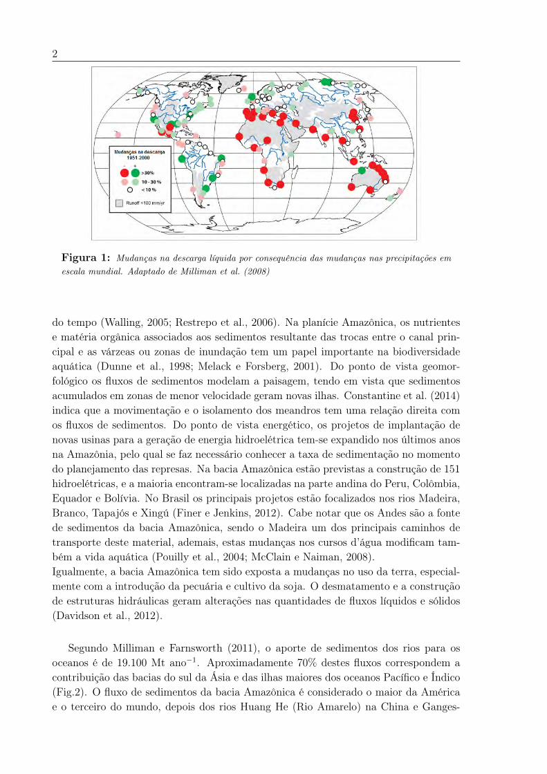
1 Mudanças na descarga líquida por consequência das mudanças nas precipitações emescala mundial. Adaptado de Milliman et al. (2008) . . . . . . . . . . . . . . . . 2
2 Fluxos de sedimentos em suspensão para os oceanos. Adaptado de: Milliman e Farnsworth(2011) . . . . . . . . . . . . . . . . . . . . . . . . . . . . . . . . . . . . . . 3
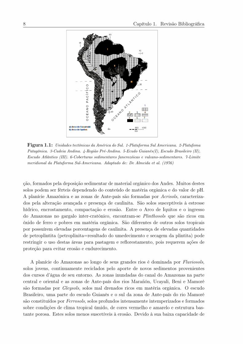
1.1 Unidades tectônicas da América do Sul. 1-Plataforma Sul Americana. 2-PlatafomaPatagônica. 3-Cadeia Andina. 4-Região Pré-Andina. 5-Ecudo Guianês(I), EscudoBrasileiro (II), Escudo Atlântico (III). 6-Coberturas sedimentares fanerozóicas e vulcano-sedimentares. 7-Limite meridional da Plataforma Sul-Americana. Adaptado de: De Al-meida et al. (1976) . . . . . . . . . . . . . . . . . . . . . . . . . . . . . . . . 8
1.2 Mapa de solos Fonte: Atlas de Solos 2014 (Gardi et al., 2014) . . . . . . 91.3 A) Precipitação média (𝑚𝑚.𝑎𝑛𝑜−1). B) Porcentagens de precipitação trimestral a)
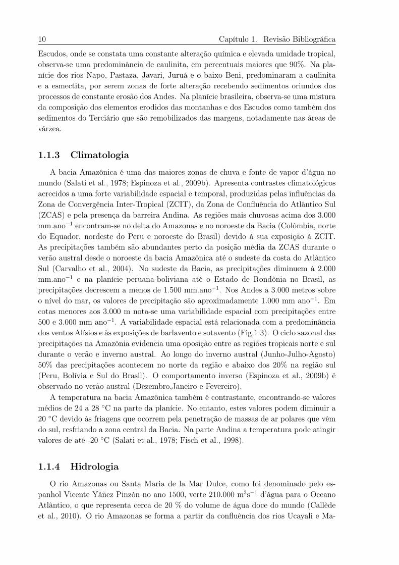
Dezembro-Janeiro-Fevereiro (DJF), b) Março-Abril-Maio (MAM), c) Junho-Julho-Agosto (JJA) e d) Setembro-Outubro-Novembro (SON). A região Andina acima dos500 m é limitada com uma linha preta e branca Adaptado de: Espinoza et al. (2009b) 11
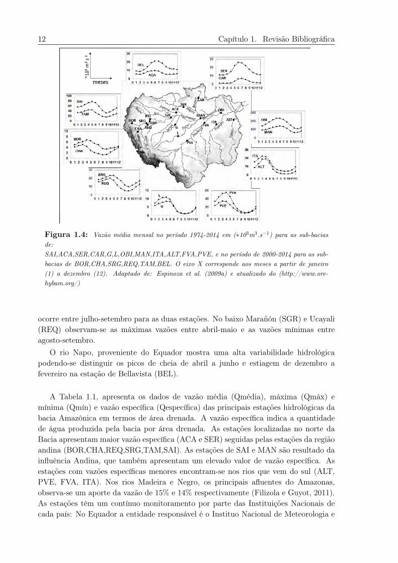
1.4 Vazão média mensal no período 1974-2014 em (*103m3.s−1) para as sub-bacias de:SAI,ACA,SER,CAR,G,L,OBI,MAN,ITA,ALT,FVA,PVE, e no período de 2000-2014para as sub-bacias de BOR,CHA,SRG,REQ,TAM,BEL. O eixo X corresponde aosmeses a partir de janeiro (1) a dezembro (12). Adaptado de: Espinoza et al. (2009a)e atualizado do (http://www.ore-hybam.org/) . . . . . . . . . . . . . . . . . . . 12
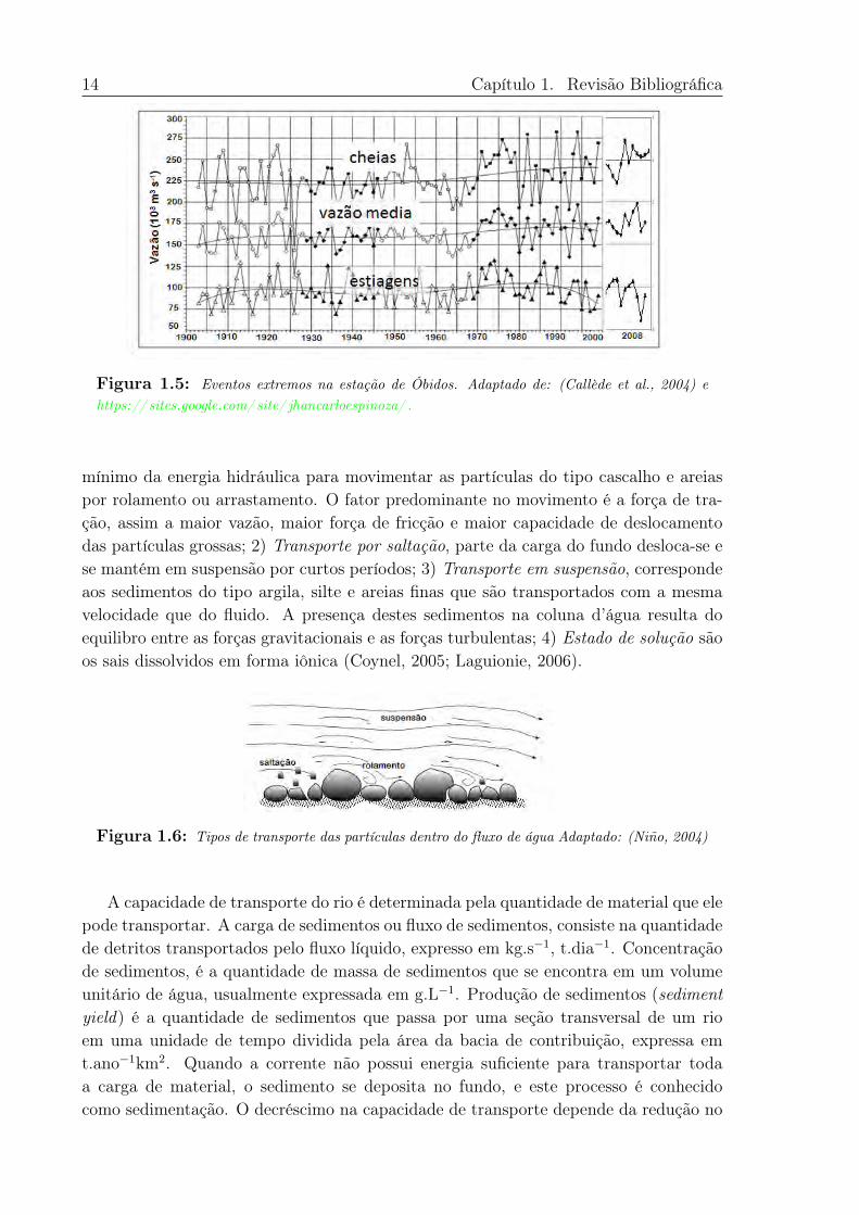
1.5 Eventos extremos na estação de Óbidos. Adaptado de: (Callède et al., 2004) e https:// sites.google.com/ site/ jhancarloespinoza/ . . . . . . . . . . . . . . . . . . . . . 14
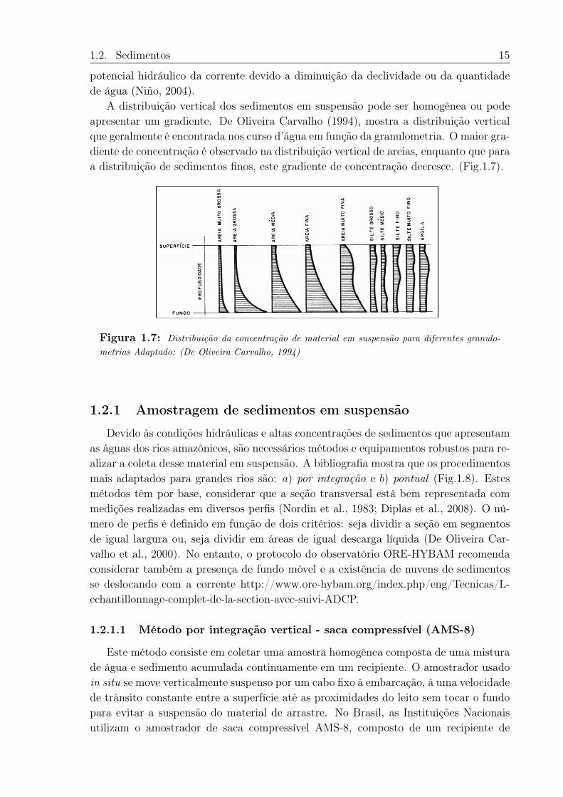
1.6 Tipos de transporte das partículas dentro do fluxo de água Adaptado: (Niño, 2004) . 141.7 Distribuição da concentração de material em suspensão para diferentes granulometrias
Adaptado: (De Oliveira Carvalho, 1994) . . . . . . . . . . . . . . . . . . . . . . 151.8 𝑎) amostrador AMS-8 de saca compressível, 𝑏) Componentes do amostrador AMS-
8, 𝑐) amostrador pontual horizontal ”𝐶𝑎𝑙𝑙𝑒𝑑𝑒𝐼𝐼”- Programa ORE-HYBAM Fonte:(De Oliveira Carvalho, 1994) . . . . . . . . . . . . . . . . . . . . . . . . . . . 16
1.9 𝑎) Efeitos da incidência da luz em uma partícula; 𝑏) padrões de difração para partículas< 20 𝜇𝑚 e partículas > 20 𝜇𝑚; 𝑐) esquema do funcionamento do granulômetro àlaser. Fonte:https://www.sympatec.com . . . . . . . . . . . . . . . . . . . . . . 18
1.10 𝑎) Partículas de tamanho 1/10 do comprimento de onda com espalhamento simétrico.Partículas maiores do comprimento de onda com espalhamento para a frente; 𝑏) es-quema do funcionamento do tubidímetro com um angulo de 90 graus; 𝑐) esquema dosensor de turbidez Fonte: http://www.vliz.be/wiki/Turbidity/ sensors . . . . . . . . 19
1.11 curvas chaves em função das diferentes condições hidráulicas Fonte: (Herschy, 1995) 20
xiii
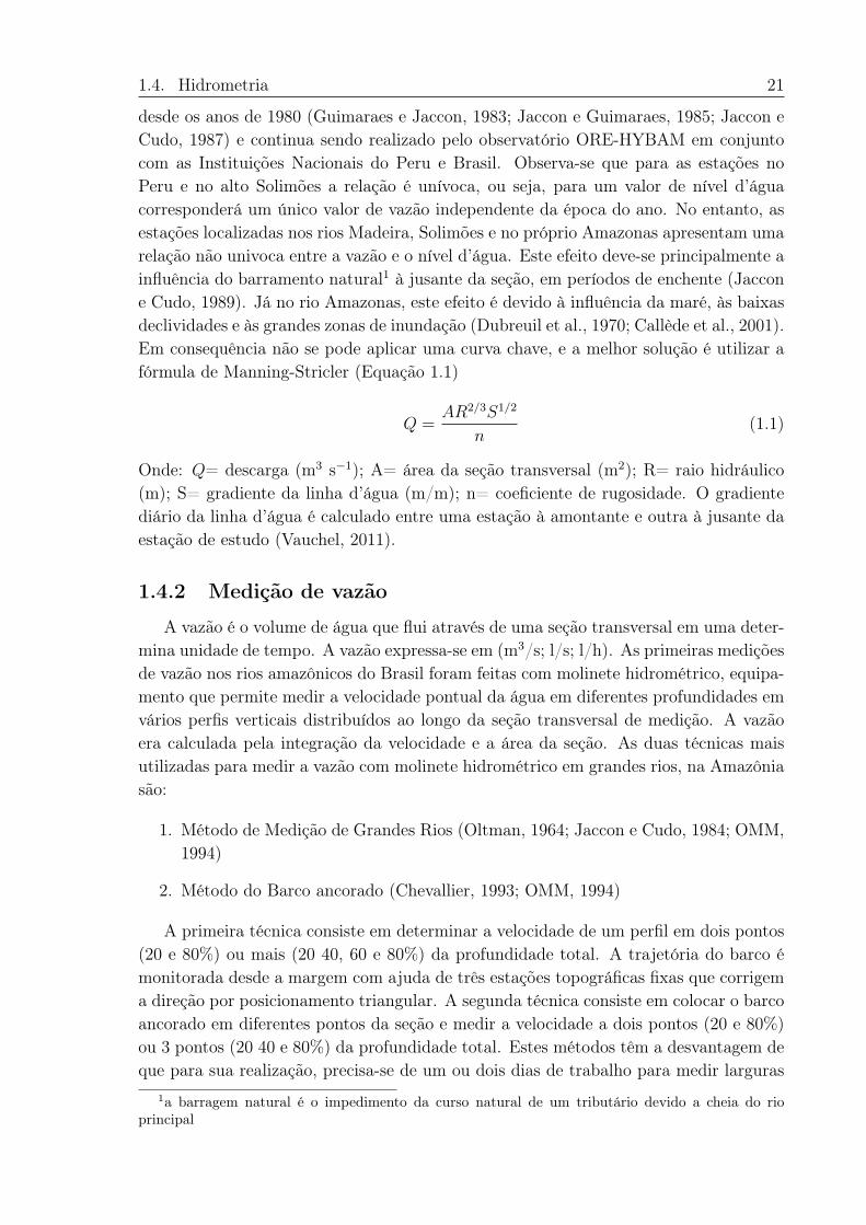
1.12 𝑎) Esquema de medição com ADCP (Gotvald e Oberg, 2009), 𝑏) Montagem do ADCPno rio Amazonas Fonte: Observatório ORE-HYBAM, 𝑐) Representação dos feixesacústicos e zonas de medição com o ADCP. Adaptado de: http://www.wmo.int . . . 22
1.13 Representação gráfica de um perfil de concentração [C], velocidade média (U) e es-forço de fricção (𝜏) , z= eixo vertical, 𝑧𝑜= camada de atrito, 𝛿𝑣/𝛿𝑧= gradiente develocidade em direção do fluxo, 𝜏𝐿= esforço de cisalhamento laminar, 𝜏𝑇= esforço decisalhamento turbulento, 𝜏𝑜=esforço de corte no fundo e 𝑢*= velocidade de corte . . 24
1.14 Esquema dos diferentes tipos de Perfil de Rouse em função do Número de RouseAdaptado: (ASCE, 1977) . . . . . . . . . . . . . . . . . . . . . . . . . . . . . 26
2.1 Esquema da metodolgia . . . . . . . . . . . . . . . . . . . . . . . . . . . . . . 302.2 Estações de estudo: Peru: BOR= Borja, CHA=Chazuta, LAG=Lagarto, SRG=
San Regis, REQ= Requena,TAM= Tamshiyacu, BEL= Bellavita, TAB= Tabatinga,SPO= São Paulo de Olivença, FBO= Fonte Boa, TEF= Tefé, MAN= Manacapuru,ITA= Itacoatiara e OBI=Óbidos . . . . . . . . . . . . . . . . . . . . . . . . . 31
2.3 Esquema da troca de referência com respeito ao fundo . . . . . . . . . . . . . . . 342.4 Perfil logarítmico de velocidade,Vertical 2 estação de Óbidos em 09/06/2013 varia-
ção temporal 𝑎) barco em ponto fixo; 𝑏) barco a deriva e 𝑐) Estação Itacoatiara em10/12/2012-variação espacial . . . . . . . . . . . . . . . . . . . . . . . . . . 35
2.5 𝑎) Cálculo de incerteza do coeficiente a,𝑏) Flutuação do coeficiente 𝑎 nas 4 diferentesverticais distanciadas en referencia na margem esquerda da estação de Óbidos 18-12-2011, (av1= 590 m, av2= 1130 m, av3= 1670 m e av4 = 2200 m distancia da margemesquerda), 𝑐) tração da regressão, Óbidos vertical 4 de 18-12-2011 . . . . . . . . . 35
2.6 esquematização do processo de coleta e filtração em campo e amostragem superficiala cada dez dias . . . . . . . . . . . . . . . . . . . . . . . . . . . . . . . . . 36
2.7 𝑎) sistema de calibração da turbidez, 𝑏) curvas de calibração para finos e areias . . . 382.8 Teste de separação do sinal de turbidez para finos e areias. . . . . . . . . . . . . 382.9 𝑎) Instalação da sonda de turbidez no dispositivo de amostragem,𝑏) Exemplo da aqui-
sição de perfis para cada ponto de amostragem Exemplo vertical 3 em Óbidos no17-12-2005, 𝑐) Perfil médio da vertical 3. . . . . . . . . . . . . . . . . . . . . . 39
2.10 Perfil granulométrico e descomposição da distribuição normal de cada moda presenteem cada ponto medido- Estação de Itacoatiara- maio 2012 . . . . . . . . . . . . . 40
2.11 Esquema gráfico da medição de vazão dada pelo ADCP na seção de Tamshiyacu- Perue método de ponderação para determinar a concentração média da seção . . . . . . 40
A.1 Sonda de turbidez 6820 V2 . . . . . . . . . . . . . . . . . . . . . . . . . . . . 131A.2 Resposta do sensor de turbidez, 𝑖) Sondas 2 e 3 com seus próprios sensores, 𝑖𝑖) troca
de sensores . . . . . . . . . . . . . . . . . . . . . . . . . . . . . . . . . . . 132A.3 Teste de luz 𝑎) no exterior, 𝑏) luz artificial- laboratório, 𝑐) escuro . . . . . . . . . . 133A.4 Sinal de turbidez da sonda 2 com e sem proteção no exterior . . . . . . . . . . . . 133A.5 𝑎) Sinal de turbidez da sonda 2 𝑏) com e 𝑐)s em proteção . . . . . . . . . . . . . . 134A.6 Sinal de turbidez da sonda com e sem proteção no escuro . . . . . . . . . . . . . . 134A.7 Dispositivo para a calibração do leite e teste de linearidade para as 3 sondas . . . . . 135
B.1 Tecnica de medição do granulométro laser. Fonte: ℎ𝑡𝑡𝑝 : //𝑤𝑤𝑤.𝑐𝑖𝑙𝑎𝑠.𝑐𝑜𝑚/𝑙𝑎𝑠𝑒𝑟 −𝑑𝑖𝑓𝑓𝑟𝑎𝑐𝑡𝑖𝑜𝑛− 𝑝𝑎𝑟𝑡𝑖𝑐𝑙𝑒− 𝑠𝑖𝑧𝑒− 𝑎𝑛𝑎𝑙𝑦𝑠𝑖𝑠− 𝑝𝑟𝑖𝑛𝑐𝑖𝑝𝑙𝑒𝑠.ℎ𝑡𝑚 . . . . . . . . . . . . . 138
B.2 𝑎) teoria do Fraunhofer, 𝑏) teoria de Mie . . . . . . . . . . . . . . . . . . . . . 138

B.3 Amostra de Manacapuru- 16-02-2011. Amostra em pó- utilizando diferentes cenários:A1.- velocidade da bomba 2300 rpm. A2. Adicionando ultrasson 400 rpm por 60segundos. A3.- Mistura por 60 segundos mais ultrasson por 30 segundos. A4. Analisesrealizado na França . . . . . . . . . . . . . . . . . . . . . . . . . . . . . . . 140
B.4 Amostra superficial de Manacapuru- 25-07-2011. Amostra em fase aquosa- utilizandodiferentes quantidades de amostra: A1=20 𝑚𝑙 e A2=30 𝑚𝑙 . . . . . . . . . . . . . 141
B.5 Amostra superficial de Itacoatiara- 20-02-2011. Amostra em fase líquida- utilizandodiferentes volumeis de diluição . . . . . . . . . . . . . . . . . . . . . . . . . . 142

Lista de Tabelas
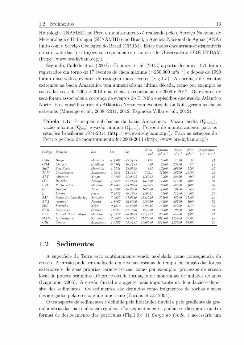
1.1 Principais sub-bacias da bacia Amazônica. Vazão média (Q𝑚𝑑𝑖𝑎), vazãomáxima (Q𝑚𝑥) e vazão mínima (Q𝑚𝑚). Período de monitoramento paraas estações brasileiras 1974-2014 (http://www.ore-hybam.org/). Para asestações do Peru o período de monitoramento foi 2000-2014 (http://www.ore-hybam.org/) . . . . . . . . . . . . . . . . . . . . . . . . . . . . . . . . . . 13
1.2 Propriedades das águas naturais, os efeitos sobre a medição da turbideze as características dos instrumentos para contornar o problema. IR=infravermelho. Adaptado de Anderson (2005) . . . . . . . . . . . . . . . 19
1.3 Valores dos coeficientes A,B e m da equação de Camenen (2007), csf eP correspondem aos fatores da forma das partículas, cfs= forma plana eP= forma aredondada . . . . . . . . . . . . . . . . . . . . . . . . . . . . 27
2.1 Lista das estações monitoradas, dados de localização,medição de vazãodas estações de estudo e período de dados de vazão . . . . . . . . . . . . 32
2.2 Quantidade de dados utilizados neste estudo . . . . . . . . . . . . . . . . 32
A.1 Características técnicas das sondas . . . . . . . . . . . . . . . . . . . . . 132A.2 Impacto da luz sobre a turbidez registrada . . . . . . . . . . . . . . . . . 133
B.1 Resultado das análises com amostra em pó- Volume 5L . . . . . . . . . . 139B.2 Resultado das análises com amostra em solução aquosa provenientes do
Volume 5L . . . . . . . . . . . . . . . . . . . . . . . . . . . . . . . . . . . 140B.3 Resultado das análises com amostra em fase líquida . . . . . . . . . . . . 142
xvii

Sumário
Introdução Geral 1
1 Revisão Bibliográfica 71.1 A bacia Amazônica . . . . . . . . . . . . . . . . . . . . . . . . . . . . . . 7
1.1.1 Solos . . . . . . . . . . . . . . . . . . . . . . . . . . . . . . . . . . 71.1.2 Natureza dos sedimentos em suspensão . . . . . . . . . . . . . . . 91.1.3 Climatologia . . . . . . . . . . . . . . . . . . . . . . . . . . . . . . 101.1.4 Hidrologia . . . . . . . . . . . . . . . . . . . . . . . . . . . . . . . 10
1.2 Sedimentos . . . . . . . . . . . . . . . . . . . . . . . . . . . . . . . . . . 131.2.1 Amostragem de sedimentos em suspensão . . . . . . . . . . . . . . 15
1.3 Técnicas Óticas . . . . . . . . . . . . . . . . . . . . . . . . . . . . . . . . 161.3.1 Granulometria . . . . . . . . . . . . . . . . . . . . . . . . . . . . . 171.3.2 Turbidez . . . . . . . . . . . . . . . . . . . . . . . . . . . . . . . . 17
1.4 Hidrometria . . . . . . . . . . . . . . . . . . . . . . . . . . . . . . . . . . 201.4.1 Nível d’água . . . . . . . . . . . . . . . . . . . . . . . . . . . . . . 201.4.2 Medição de vazão . . . . . . . . . . . . . . . . . . . . . . . . . . . 21
1.5 Perfil de velocidade e concentração de sedimentos em suspensão . . . . . 231.5.1 Camada laminar . . . . . . . . . . . . . . . . . . . . . . . . . . . 241.5.2 Camada turbulenta . . . . . . . . . . . . . . . . . . . . . . . . . . 241.5.3 Repartição da concentração de sedimentos na coluna de água-
Perfil de Rouse . . . . . . . . . . . . . . . . . . . . . . . . . . . . 261.5.4 Velocidade de sedimentação . . . . . . . . . . . . . . . . . . . . . 27
2 Materiais e Métodos 292.1 Área de Estudo . . . . . . . . . . . . . . . . . . . . . . . . . . . . . . . . 302.2 Dados . . . . . . . . . . . . . . . . . . . . . . . . . . . . . . . . . . . . . 322.3 Coleta de dados . . . . . . . . . . . . . . . . . . . . . . . . . . . . . . . . 33
2.3.1 Nível d’água e Medição de vazão . . . . . . . . . . . . . . . . . . 332.3.2 Perfil de velocidade média . . . . . . . . . . . . . . . . . . . . . . 332.3.3 Amostragem de água e sedimentos em suspensão . . . . . . . . . 352.3.4 Medição de turbidez . . . . . . . . . . . . . . . . . . . . . . . . . 362.3.5 Medição da granulometria . . . . . . . . . . . . . . . . . . . . . . 38
2.4 Cálculo de vazão sólida . . . . . . . . . . . . . . . . . . . . . . . . . . . . 40
3 Dinâmica dos sedimentos em suspensão do rio Amazonas no Peru 41
4 Nova estimação do fluxo sedimentário no rio Amazonas 65
xix
5 Estudo do gradiente vertical do sedimentos 81
6 Conclusões 115
Referências Bibliográficas 117
A Calibração Turbidez 131A.1 Características das sondas de turbidez . . . . . . . . . . . . . . . . . . . 131
A.1.1 Princípio do funcionamento do equipamento . . . . . . . . . . . . 131A.1.2 Impactos do meio exterior sobre a medida . . . . . . . . . . . . . 132A.1.3 Teste de linearidade do sinal de turbidez . . . . . . . . . . . . . . 135
B Granulometria 137B.1 Determinação granulométrica em amostras dos Rios da bacia Amazônica 137B.2 Fundamentos da Granulometria Laser . . . . . . . . . . . . . . . . . . . . 137B.3 Metodologia-Técnica de medição . . . . . . . . . . . . . . . . . . . . . . . 138
B.3.1 Amostras de 5 L em fase seca . . . . . . . . . . . . . . . . . . . . 139B.3.2 Amostras de 5 L em fase aquosa . . . . . . . . . . . . . . . . . . . 140B.3.3 Amostras menores a 1000 ml em fase líquida . . . . . . . . . . . . 141B.3.4 Conclusões . . . . . . . . . . . . . . . . . . . . . . . . . . . . . . . 142
C Sedimentos em suspensão e material dissolvido dos Andes do Equador143
D Propiedades óticas das águas do rio e da várzeas na Bacia Amazônica:Implicações baseadas em medidas do satélite e medidas de partículasem suspensão 163
Introdução Geral
Considera-se a teoria de feedback da erosão junto com os efeitos do clima, como a ex-plicação para formação de montanhas (Pinter e Brandon, 2002). Quando as montanhase a crosta se erodem, os sedimentos são depositados no sopé causando a subsidênciadesta zona. Para compensar o material perdido e manter o equilíbrio produz-se o so-erguimento da cadeia montanhosa. Esta hipótese é complementada com a teoria dasplacas, que estabelece à Terra como um sistema dinâmico, com movimentos e interaçõesentre placas, provocando alterações e deformações na crosta e litosfera e dando lugar asgrandes cadeias montanhosas. Assim, os Andes são consequência da subducção ocasio-nada pela colisão de duas placas: a placa Oceânica do Pacífico com a placa Continentalda América do Sul (Paleogéno 65-34 Ma). A placa Oceânica, que é mais densa, afundousobre a continental, criando o levantamento da Cordilheira Andina. O norte Andino éproduto da colisão da placa Sul-Americana e a placa do Caribe (Mioceno 23 Ma). Moraet al. (2010) indicaram que a formação do rio Amazonas com o fluxo no sentido parao Atlântico, aconteceu no final do Mioceno-Pleistoceno (11 Ma), resultado do desnuda-mento dos Andes e da precipitação orográfica.
A água cumpre um papel fundamental no ciclo dos sedimentos por ser um dosprincipais fatores que causam a denudação do solo. Também é um dos agentes maisimportantes no transporte e deposição de sedimentos através dos sistemas fluviais. Anível mundial, nestas últimas décadas, observaram-se mudanças nas descargas líquidasque correspondem às modificações nas precipitações (Fig.1). Os rios da Ásia, África eAustrália têm sofrido um decréscimo de 50% nas descargas médias. Em contrapartida,rios da América do Norte (exceto o Canadá) apresentam aumento médio de 30%. Os riosda América do Sul (Amazonas, Orinoco, Magdalena) em termos de média mantêm-seem situação de estabilidade (Milliman et al., 2008). No entanto, no caso do rio Amazo-nas, Espinoza et al. (2009a) mostraram um aumento significativo nos valores máximosde precipitação e uma diminuição nos valores mínimos. Estas alterações influem nosfluxos de sedimentos e materiais dissolvidos, como exemplo o aumento significativo daconcentração de sedimentos em suspensão depois de uma mudança abrupta de umaseca extrema (2010) para uma cheia (2011) no rio Amazonas no Peru observado porEspinoza et al. (2011).
A importância de estimar a carga de sedimentos nos rios reside em: desde o pontode vista ambiental, na quantidade de nutrientes e contaminantes transportados pelossistemas fluviais, até o impacto que causaria as mudanças dessas concentrações ao longo
1
2
Figura 1: Mudanças na descarga líquida por consequência das mudanças nas precipitações emescala mundial. Adaptado de Milliman et al. (2008)
do tempo (Walling, 2005; Restrepo et al., 2006). Na planície Amazônica, os nutrientese matéria orgânica associados aos sedimentos resultante das trocas entre o canal prin-cipal e as várzeas ou zonas de inundação tem um papel importante na biodiversidadeaquática (Dunne et al., 1998; Melack e Forsberg, 2001). Do ponto de vista geomor-fológico os fluxos de sedimentos modelam a paisagem, tendo em vista que sedimentosacumulados em zonas de menor velocidade geram novas ilhas. Constantine et al. (2014)indica que a movimentação e o isolamento dos meandros tem uma relação direita comos fluxos de sedimentos. Do ponto de vista energético, os projetos de implantação denovas usinas para a geração de energia hidroelétrica tem-se expandido nos últimos anosna Amazônia, pelo qual se faz necessário conhecer a taxa de sedimentação no momentodo planejamento das represas. Na bacia Amazônica estão previstas a construção de 151hidroelétricas, e a maioria encontram-se localizadas na parte andina do Peru, Colômbia,Equador e Bolívia. No Brasil os principais projetos estão focalizados nos rios Madeira,Branco, Tapajós e Xingú (Finer e Jenkins, 2012). Cabe notar que os Andes são a fontede sedimentos da bacia Amazônica, sendo o Madeira um dos principais caminhos detransporte deste material, ademais, estas mudanças nos cursos d’água modificam tam-bém a vida aquática (Pouilly et al., 2004; McClain e Naiman, 2008).Igualmente, a bacia Amazônica tem sido exposta a mudanças no uso da terra, especial-mente com a introdução da pecuária e cultivo da soja. O desmatamento e a construçãode estruturas hidráulicas geram alterações nas quantidades de fluxos líquidos e sólidos(Davidson et al., 2012).
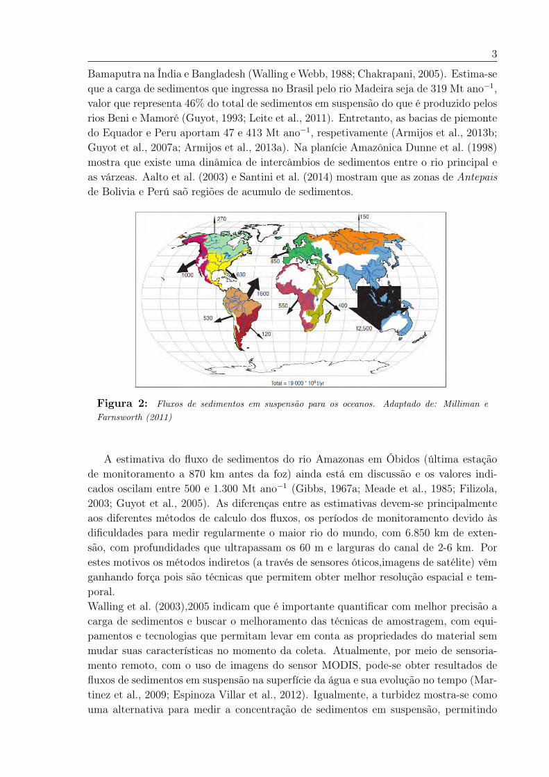
Segundo Milliman e Farnsworth (2011), o aporte de sedimentos dos rios para osoceanos é de 19.100 Mt ano−1. Aproximadamente 70% destes fluxos correspondem acontribuição das bacias do sul da Ásia e das ilhas maiores dos oceanos Pacífico e Índico(Fig.2). O fluxo de sedimentos da bacia Amazônica é considerado o maior da Américae o terceiro do mundo, depois dos rios Huang He (Rio Amarelo) na China e Ganges-
3
Bamaputra na Índia e Bangladesh (Walling e Webb, 1988; Chakrapani, 2005). Estima-seque a carga de sedimentos que ingressa no Brasil pelo rio Madeira seja de 319 Mt ano−1,valor que representa 46% do total de sedimentos em suspensão do que é produzido pelosrios Beni e Mamoré (Guyot, 1993; Leite et al., 2011). Entretanto, as bacias de piemontedo Equador e Peru aportam 47 e 413 Mt ano−1, respetivamente (Armijos et al., 2013b;Guyot et al., 2007a; Armijos et al., 2013a). Na planície Amazônica Dunne et al. (1998)mostra que existe uma dinâmica de intercâmbios de sedimentos entre o rio principal eas várzeas. Aalto et al. (2003) e Santini et al. (2014) mostram que as zonas de Antepaisde Bolivia e Perú saõ regiões de acumulo de sedimentos.
Figura 2: Fluxos de sedimentos em suspensão para os oceanos. Adaptado de: Milliman eFarnsworth (2011)
A estimativa do fluxo de sedimentos do rio Amazonas em Óbidos (última estaçãode monitoramento a 870 km antes da foz) ainda está em discussão e os valores indi-cados oscilam entre 500 e 1.300 Mt ano−1 (Gibbs, 1967a; Meade et al., 1985; Filizola,2003; Guyot et al., 2005). As diferenças entre as estimativas devem-se principalmenteaos diferentes métodos de calculo dos fluxos, os períodos de monitoramento devido àsdificuldades para medir regularmente o maior rio do mundo, com 6.850 km de exten-são, com profundidades que ultrapassam os 60 m e larguras do canal de 2-6 km. Porestes motivos os métodos indiretos (a través de sensores óticos,imagens de satélite) vêmganhando força pois são técnicas que permitem obter melhor resolução espacial e tem-poral.Walling et al. (2003),2005 indicam que é importante quantificar com melhor precisão acarga de sedimentos e buscar o melhoramento das técnicas de amostragem, com equi-pamentos e tecnologias que permitam levar em conta as propriedades do material semmudar suas características no momento da coleta. Atualmente, por meio de sensoria-mento remoto, com o uso de imagens do sensor MODIS, pode-se obter resultados defluxos de sedimentos em suspensão na superfície da água e sua evolução no tempo (Mar-tinez et al., 2009; Espinoza Villar et al., 2012). Igualmente, a turbidez mostra-se comouma alternativa para medir a concentração de sedimentos em suspensão, permitindo
4
um maior número de medidas com um equipamento mais versátil (Tessier, 2006; Res-trepo e Pierini, 2012). A utilização de modelos verticais também tem sido testados parapredizer o fluxo de sedimentos nos rios Solimões e Amazonas (Bouchez et al., 2011b),no entanto, tem-se encontrado dificuldade para gerar um modelo geral no espaço e notempo. Guyot et al. (2005) mostraram que não existe uma relação direita entre vazãoe concentração de sedimentos em suspensão, pelo que recomendam realizar um monito-ramento contínuo para determinar o fluxo de sedimentos em suspensão.
O objetivo deste trabalho é estudar a distribuição espacial e temporal dos sedimen-tos em suspensão ao longo do rio Amazonas no trecho Tamshiyacu (Peru) até Óbidos(Brasil). Este trabalho propõe uma estimativa do fluxo de sedimentos na zona Andinae sub-Andina do Peru. Estuda a distribuição espacial e temporal dos sedimentos emsuspensão e seu comportamento, durante o regime hidrológico nas estações andinas eda planície peruana logo depois da saída dos Andes (Capitulo 3). Apresenta uma novaestimativa de fluxos na estação de Óbidos baseado em 19 anos de monitoramento e ainfluência da variabilidade climática nos fluxos sedimentares na bacia Amazônica (Capí-tulo 4), e finalmente este estudo propõe uma metodologia para caracterizar o gradientevertical e horizontal dos sedimentos em suspensão baseada na turbidez e no modelo deRouse (Capítulo 5).
O estudo se apoia nos dados de estações do observatório ORE-HYBAM (www.ore-hybam.org) estabelecido no contexto de convênios bilaterais entre o IRD (Institut deRecherche pour le Dévelopement) da França e instituições interessadas na hidrologiae geodinâmica da Bacia Amazônica. No Brasil, as Instituições parceiras são a Uni-versidade Federal do Amazonas (UFAM), a Agência Nacional de Águas (ANA) e aCompanhia de Pesquisa de Recursos Mineiros (CPRM). Além disso, esta tese está inse-rida escopo do Projeto IHESA (Iniciativa de Hidrologia Espacial na Amazônia) da Redede Hidrologia Amazônica (Projeto FINEP) do qual participam a UFAM, CPRM, ANA,IRD, INPA (Instituto de Pesquisa da Amazônia), UEA (Universidade do Estado deAmazonas), UFPA (Universidade Federal do Pará), UFRGS (Universidade Federal doRio Grande do Sul), SIPAM (Sistema de Proteção da Amazônia), UNIR (UniversidadeFederal de Rondonia) e The University of Texas at Austin.
A tese está escrita no formato de artigos, composta por 6 Capítulos:
Capítulo 1 : Revisão Bibliográfica;
Capítulo 2 : Metodologia- Área de Estudo
Capítulo 3 : Suspended sediment dynamics in the Amazon River of Peru. Publicadono Journal South American Earth Sciences.
Capítulo 4 : New estimation of suspended sediments yields of the Amazon River andits sensitivity to climate variability. Artigo submetido para o Science.
5
Capítulo 5 : Measuring and modelling vertical gradients of suspended sediments inthe Amazon River. Artigo submetido ao Hydrological Processes.
Capitulo 6 : Conclusões
Apendice :
• Características das sondas de turbidez.
• Determinação granulométrica em amostras dos Rios da bacia Amazônica.
• Yields of suspended sediment and dissolved solids from the Andean basinsof Ecuador. Artigo publicado no Hydrological Sciences Journal durante operíodo de doutorado como primeira autora.
• The optical properties of river and floodplain waters in the Amazon River Ba-sin: Implications for satellite-based measurements of suspended particulatematter. Artigo publicado Journal of Geophysical Research: Earth Surface,como colaboradora

6
Capítulo 1
Revisão Bibliográfica
1.1 A bacia Amazônica
A bacia Amazônica localiza-se na América do Sul entre as latitudes 5𝑜N (rio Co-tingo no Brasil) e 20𝑜S (rio Parapeti na Bolívia) e as longitudes 50𝑜E (rio Pará no Bra-sil) e 80𝑜W (rio Chamaya no Peru). Drena uma superfície de 5.961.000 km2 (Callèdeet al., 2010) que abrange os países do Brasil (62,61%), Peru (16,61%), Bolívia (11,67%),Colômbia(6,02%), Equador (2,35%), Venezuela (0,60%) e Guiana (0,1%) (Wolf et al.,1999). Estruturalmente a bacia Amazônica é formada por quatro zonas geomorfológicas(De Almeida et al., 1976; Roddaz et al., 2005): 1) Os Andes que incluem a zonasub-andina , caracterizada por forte declividade e submetida a uma forte erosão; 2) Azona de Ante-país ou região Pré-Andina , é a zona de transição entre os Andes ea planície, formada pela erosão recente dos Andes de idade Quaternária ou Terciária.Atualmente esta região tem áreas receptoras de sedimentos que proveem da erosão dosAndes e outras áreas que fornecem sedimentos. Inclui-se nesta zona o Arco de Fitz-carraldo, este arco constitui a linha divisória das águas entre o alto Solimões e o altoMadeira (Espurt et al., 2008), e o Arco de Iquitos, divisor das águas do Marañón e altoSolimões (Bernal e Tavera, 2002); 3) A planície Amazônica , que atua como umadepressão, acumula o material sedimentar resultante da erosão dos Andes desde que foiformada no Mioceno médio e 4) Os escudos Guianês e Brasileiro, localizados res-pectivamente ao norte e sul da bacia Amazônica, correspondem a porções do continenteSul-Americano da idade do Pré-cambriano já bastante erodidos (Fig.1.1).
1.1.1 Solos
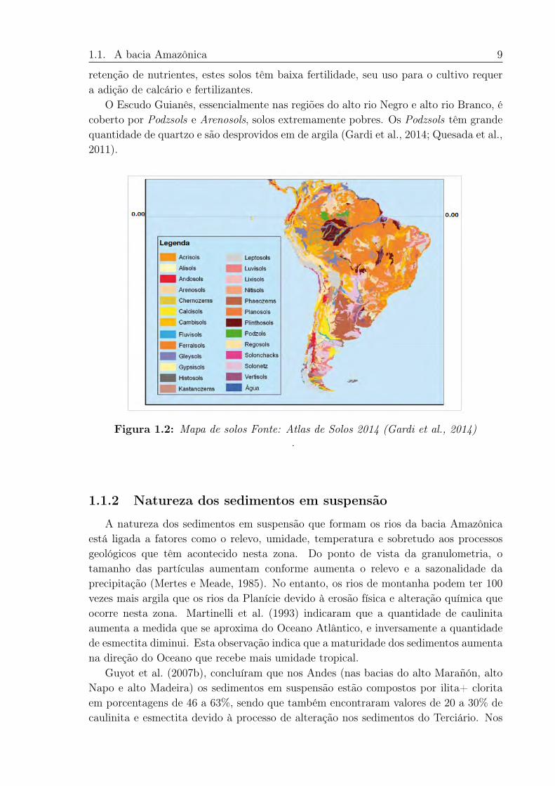
Os solos que estão presentes na Amazônia, segundo Gardi et al. (2014) são o re-sultado dos processos de formação da Bacia (Fig.1.2). Na parte Andina e piemonteencontram-se Regosols e Leptosols, solos pouco alterados que recebem e exportam con-tinuamente a matéria da cadeia Andina, caracterizados por serem rasos e armazenarempouca água, tendem a ser utilizados para pastagens e floresta. Estes tipos de solosencontram-se também de forma pontual nos escudos Brasileiro e Guianês.
A zona sub-Andina é formada por Cambisols, solos com moderado grau de altera-
7
8 Capítulo 1. Revisão Bibliográfica
Figura 1.1: Unidades tectônicas da América do Sul. 1-Plataforma Sul Americana. 2-PlatafomaPatagônica. 3-Cadeia Andina. 4-Região Pré-Andina. 5-Ecudo Guianês(I), Escudo Brasileiro (II),Escudo Atlântico (III). 6-Coberturas sedimentares fanerozóicas e vulcano-sedimentares. 7-Limitemeridional da Plataforma Sul-Americana. Adaptado de: De Almeida et al. (1976)
ção, formados pela deposição sedimentar de material orgânico dos Andes. Muitos destessolos podem ser férteis dependendo do conteúdo de matéria orgânica e do valor de pH.A planície Amazônica e as zonas de Ante-país são formadas por Acrisols, caracteriza-dos pela alteração avançada e presença de caulinita. São solos susceptíveis à estressehídrico, encrostamento, compactação e erosão. Entre o Arco de Iquitos e o ingressodo Amazonas no gargalo inter-cratônico, encontram-se Plinthosols que são ricos emóxido de ferro e pobres em matéria orgânica. São diferentes de outros solos tropicaispor possuírem elevadas porcentagens de caulinita. A presença de elevadas quantidadesde petroplintita (petroplinita=resultado do umedecimento e secagem da plintita) poderestringir o uso destas áreas para pastagem e reflorestamento, pois requerem ações deproteção para evitar erosão e endurecimento.
A planície do Amazonas ao longo de seus grandes rios é dominada por Fluviosols,solos jovens, continuamente reciclados pelo aporte de novos sedimentos provenientesdos cursos d’água de seu entorno. As zonas inundadas do canal do Amazonas na partecentral e oriental e as zonas de Ante-país dos rios Marañón, Ucayali, Beni e Mamorésão formadas por Gleysols, solos mal drenados ricos em matéria orgânica. O escudoBrasileiro, uma parte do escudo Guianês e o sul da zona de Ante-país do rio Mamorésão constituídos por Ferrosols, solos profundos intensamente intemperizados e formadossobre condições de clima tropical úmido, de cores vermelho e amarelo e estrutura bas-tante porosa. Estes solos menos suscetíveis à erosão. Devido à sua baixa capacidade de
1.1. A bacia Amazônica 9
retenção de nutrientes, estes solos têm baixa fertilidade, seu uso para o cultivo requera adição de calcário e fertilizantes.
O Escudo Guianês, essencialmente nas regiões do alto rio Negro e alto rio Branco, écoberto por Podzsols e Arenosols, solos extremamente pobres. Os Podzsols têm grandequantidade de quartzo e são desprovidos em de argila (Gardi et al., 2014; Quesada et al.,2011).
Figura 1.2: Mapa de solos Fonte: Atlas de Solos 2014 (Gardi et al., 2014).
1.1.2 Natureza dos sedimentos em suspensão
A natureza dos sedimentos em suspensão que formam os rios da bacia Amazônicaestá ligada a fatores como o relevo, umidade, temperatura e sobretudo aos processosgeológicos que têm acontecido nesta zona. Do ponto de vista da granulometria, otamanho das partículas aumentam conforme aumenta o relevo e a sazonalidade daprecipitação (Mertes e Meade, 1985). No entanto, os rios de montanha podem ter 100vezes mais argila que os rios da Planície devido à erosão física e alteração química queocorre nesta zona. Martinelli et al. (1993) indicaram que a quantidade de caulinitaaumenta a medida que se aproxima do Oceano Atlântico, e inversamente a quantidadede esmectita diminui. Esta observação indica que a maturidade dos sedimentos aumentana direção do Oceano que recebe mais umidade tropical.
Guyot et al. (2007b), concluíram que nos Andes (nas bacias do alto Marañón, altoNapo e alto Madeira) os sedimentos em suspensão estão compostos por ilita+ cloritaem porcentagens de 46 a 63%, sendo que também encontraram valores de 20 a 30% decaulinita e esmectita devido à processo de alteração nos sedimentos do Terciário. Nos
10 Capítulo 1. Revisão Bibliográfica
Escudos, onde se constata uma constante alteração química e elevada umidade tropical,observa-se uma predominância de caulinita, em percentuais maiores que 90%. Na pla-nície dos rios Napo, Pastaza, Javari, Juruá e o baixo Beni, predominaram a caulinitae a esmectita, por serem zonas de forte alteração recebendo sedimentos oriundos dosprocessos de constante erosão dos Andes. Na planície brasileira, observa-se uma misturada composição dos elementos erodidos das montanhas e dos Escudos como também dossedimentos do Terciário que são remobilizados das margens, notadamente nas áreas devárzea.
1.1.3 Climatologia
A bacia Amazônica é uma das maiores zonas de chuva e fonte de vapor d’água nomundo (Salati et al., 1978; Espinoza et al., 2009b). Apresenta contrastes climatológicosacrecidos a uma forte variabilidade espacial e temporal, produzidas pelas influências daZona de Convergência Inter-Tropical (ZCIT), da Zona de Confluência do Atlântico Sul(ZCAS) e pela presença da barreira Andina. As regiões mais chuvosas acima dos 3.000mm.ano−1 encontram-se no delta do Amazonas e no noroeste da Bacia (Colômbia, nortedo Equador, nordeste do Peru e noroeste do Brasil) devido à sua exposição à ZCIT.As precipitações também são abundantes perto da posição média da ZCAS durante overão austral desde o noroeste da bacia Amazônica até o sudeste da costa do AtlânticoSul (Carvalho et al., 2004). No sudeste da Bacia, as precipitações diminuem à 2.000mm.ano−1 e na planície peruana-boliviana até o Estado de Rondônia no Brasil, asprecipitações decrescem a menos de 1.500 mm.ano−1. Nos Andes a 3.000 metros sobreo nível do mar, os valores de precipitação são aproximadamente 1.000 mm ano−1. Emcotas menores aos 3.000 m nota-se uma variabilidade espacial com precipitações entre500 e 3.000 mm ano−1. A variabilidade espacial está relacionada com a predominânciados ventos Alísios e às exposições de barlavento e sotavento (Fig.1.3). O ciclo sazonal dasprecipitações na Amazônia evidencia uma oposição entre as regiões tropicais norte e suldurante o verão e inverno austral. Ao longo do inverno austral (Junho-Julho-Agosto)50% das precipitações acontecem no norte da região e abaixo dos 20% na região sul(Peru, Bolívia e Sul do Brasil). O comportamento inverso (Espinoza et al., 2009b) éobservado no verão austral (Dezembro,Janeiro e Fevereiro).
A temperatura na bacia Amazônica também é contrastante, encontrando-se valoresmédios de 24 a 28 ∘C na parte da planície. No entanto, estes valores podem diminuir a20 ∘C devido às friagens que ocorrem pela penetração de massas de ar polares que vêmdo sul, resfriando a zona central da Bacia. Na parte Andina a temperatura pode atingirvalores de até -20 ∘C (Salati et al., 1978; Fisch et al., 1998).
1.1.4 Hidrologia
O rio Amazonas ou Santa Maria de la Mar Dulce, como foi denominado pelo es-panhol Vicente Yáñez Pinzón no ano 1500, verte 210.000 m3s−1 d’água para o OceanoAtlântico, o que representa cerca de 20 % do volume de água doce do mundo (Callèdeet al., 2010). O rio Amazonas se forma a partir da confluência dos rios Ucayali e Ma-
1.1. A bacia Amazônica 11
Figura 1.3: A) Precipitação média (𝑚𝑚.𝑎𝑛𝑜−1). B) Porcentagens de precipitação trimestral a)Dezembro-Janeiro-Fevereiro (DJF), b) Março-Abril-Maio (MAM), c) Junho-Julho-Agosto (JJA)e d) Setembro-Outubro-Novembro (SON). A região Andina acima dos 500 m é limitada com umalinha preta e branca Adaptado de: Espinoza et al. (2009b)
.
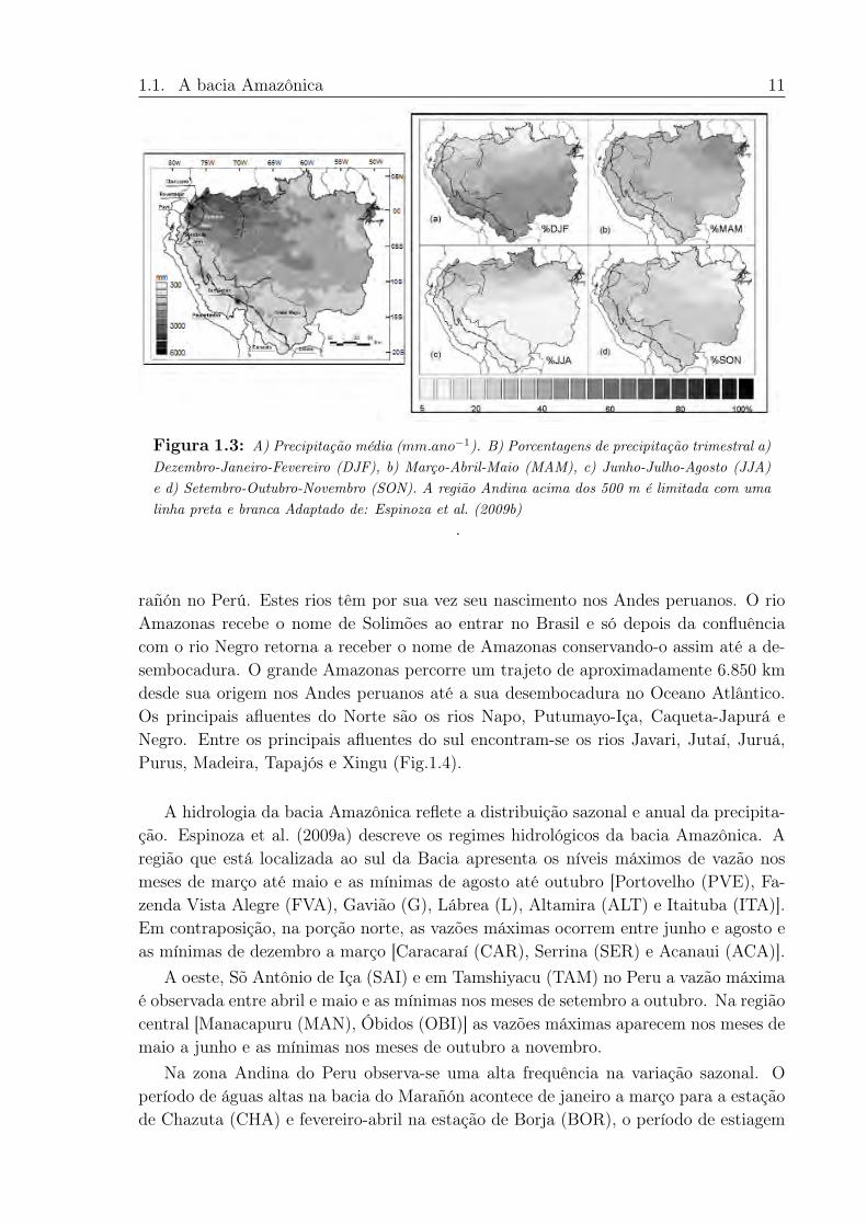
rañón no Perú. Estes rios têm por sua vez seu nascimento nos Andes peruanos. O rioAmazonas recebe o nome de Solimões ao entrar no Brasil e só depois da confluênciacom o rio Negro retorna a receber o nome de Amazonas conservando-o assim até a de-sembocadura. O grande Amazonas percorre um trajeto de aproximadamente 6.850 kmdesde sua origem nos Andes peruanos até a sua desembocadura no Oceano Atlântico.Os principais afluentes do Norte são os rios Napo, Putumayo-Iça, Caqueta-Japurá eNegro. Entre os principais afluentes do sul encontram-se os rios Javari, Jutaí, Juruá,Purus, Madeira, Tapajós e Xingu (Fig.1.4).
A hidrologia da bacia Amazônica reflete a distribuição sazonal e anual da precipita-ção. Espinoza et al. (2009a) descreve os regimes hidrológicos da bacia Amazônica. Aregião que está localizada ao sul da Bacia apresenta os níveis máximos de vazão nosmeses de março até maio e as mínimas de agosto até outubro [Portovelho (PVE), Fa-zenda Vista Alegre (FVA), Gavião (G), Lábrea (L), Altamira (ALT) e Itaituba (ITA)].Em contraposição, na porção norte, as vazões máximas ocorrem entre junho e agosto eas mínimas de dezembro a março [Caracaraí (CAR), Serrina (SER) e Acanaui (ACA)].
A oeste, Sõ Antônio de Iça (SAI) e em Tamshiyacu (TAM) no Peru a vazão máximaé observada entre abril e maio e as mínimas nos meses de setembro a outubro. Na regiãocentral [Manacapuru (MAN), Óbidos (OBI)] as vazões máximas aparecem nos meses demaio a junho e as mínimas nos meses de outubro a novembro.
Na zona Andina do Peru observa-se uma alta frequência na variação sazonal. Operíodo de águas altas na bacia do Marañón acontece de janeiro a março para a estaçãode Chazuta (CHA) e fevereiro-abril na estação de Borja (BOR), o período de estiagem
12 Capítulo 1. Revisão Bibliográfica
Figura 1.4: Vazão média mensal no período 1974-2014 em (*103m3.s−1) para as sub-baciasde:SAI,ACA,SER,CAR,G,L,OBI,MAN,ITA,ALT,FVA,PVE, e no período de 2000-2014 para as sub-bacias de BOR,CHA,SRG,REQ,TAM,BEL. O eixo X corresponde aos meses a partir de janeiro(1) a dezembro (12). Adaptado de: Espinoza et al. (2009a) e atualizado do (http://www.ore-hybam.org/)
ocorre entre julho-setembro para as duas estações. No baixo Marañón (SGR) e Ucayali(REQ) observam-se as máximas vazões entre abril-maio e as vazões mínimas entreagosto-setembro.
O rio Napo, proveniente do Equador mostra uma alta variabilidade hidrológicapodendo-se distinguir os picos de cheia de abril a junho e estiagem de dezembro afevereiro na estação de Bellavista (BEL).
A Tabela 1.1, apresenta os dados de vazão média (Qmédia), máxima (Qmáx) emínima (Qmín) e vazão específica (Qespecífica) das principais estações hidrológicas dabacia Amazônica em termos de área drenada. A vazão específica indica a quantidadede água produzida pela bacia por área drenada. As estações localizadas no norte daBacia apresentam maior vazão específica (ACA e SER) seguidas pelas estações da regiãoandina (BOR,CHA,REQ,SRG,TAM,SAI). As estações de SAI e MAN são resultado dainfluência Andina, que também apresentam um elevado valor de vazão específica. Asestações com vazões específicas menores encontram-se nos rios que vem do sul (ALT,PVE, FVA, ITA). Nos rios Madeira e Negro, os principais afluentes do Amazonas,observa-se um aporte da vazão de 15% e 14% respectivamente (Filizola e Guyot, 2011).As estações têm um contínuo monitoramento por parte das Instituições Nacionais decada país: No Equador a entidade responsável é o Instituo Nacional de Meteorologia e
1.2. Sedimentos 13
Hidrologia (INAMHI), no Peru o monitoramento é realizado pelo o Serviço Nacional deMeteorologia e Hidrologia (SENAMHI) e no Brasil, a Agência Nacional de Águas (ANA)junto com o Serviço Geológico do Brasil (CPRM). Estes dados encontram-se disponíveisno site web das Instituções correspondentes e no site do Observatório ORE-HYBAM(http://www.ore-hybam.org/).
Segundo, Callède et al. (2004) e Espinoza et al. (2013) a partir dos anos 1970 foramregistrados em torno de 17 eventos de cheia máxima (>250.000 m3s−1) e depois de 1990foram observados, eventos de estiagem mais severos (Fig.1.5). A corrença de eventosextremos na bacia Amazônica tem aumentado na ultima década, como por exemplo oscasos das seca de 2005 e 2010 e as cheias excepcionais de 2009 e 2012. Os eventos deseca foram associados a corrença de eventos do El Niño e episódios quentes do AtlânticoNorte. E os episódios frios do Atlântico Norte com eventos de La Niña geram as cheiasextremas (Marengo et al., 2008, 2011, 2012; Espinoza Villar et al., 2012).
Tabela 1.1: Principais sub-bacias da bacia Amazônica. Vazão média (Q𝑚𝑑𝑖𝑎),vazão máxima (Q𝑚𝑥) e vazão mínima (Q𝑚𝑚). Período de monitoramento para asestações brasileiras 1974-2014 (http://www.ore-hybam.org/). Para as estações doPeru o período de monitoramento foi 2000-2014 (http://www.ore-hybam.org/)
Codigo Estação Rio Lat. Log. Area Qmédia Qmáx Qmín Qespecíficokm2 m3 s−1 m3s−1 m3s−1 l s−1 km−2
BOR Borja Marañón -4.4702 -77.5483 114 5000 1550 60 44CHA Chazuta Huallaga -6.5704 -76.1193 69 2980 13200 220 43SRG San Regis Marañón -4.5134 -73.9068 362 16200 26870 5400 45TAM Tamshiyacu Amazonas -4.0034 -73.1161 726.4 31700 46700 16400 44ALT Altamira Xingu -3.2122 -54.0008 446203 7900 22670 960 18ITA Itaituba Tapajós -4.2833 -57.5833 451600 11700 24900 3000 26PVE Porto Velho Madeira -8.7367 -63.9203 954285 18800 38800 4000 20G Gavião Juruá -4.8392 -66.8500 162000 4700 9100 850 29L Lábrea Purus -7.2522 -66.1833 220351 5500 11200 900 25SAI Santo Antônio do Iça Solimões -3.0850 -67.9320 1134540 55700 78500 25800 49ACA Acanaui Japurá -1.8167 -66.6000 242259 13400 20700 5600 56SER Serrinha Negro -0.4819 -64.8289 279945 16700 28500 6470 60CAR Caracaraí Branco 1.8214 -61.1236 124980 3000 9800 600 24FVA Fazenda Vista Alegre Madeira -4.8972 -60.0253 1324727 27800 55700 4900 21MAN Manacapuru Solimões -3.3083 -60.6094 2147736 104000 145200 56300 48OBI Óbidos Amazonas -1.9197 -55.5134 4680000 181700 248600 97500 39
1.2 Sedimentos
A superfície da Terra está continuamente sendo modelada como consequência daerosão. A erosão pode ser analisada em diversas escalas de tempo em função das forçasexteriores e de suas próprias características, como por exemplo: processos de erosãolocal de poucos segundos até processos de formação de montanhas de milhões de anos(Laguionie, 2006). A erosão fluvial é o agente mais importante na denudação e depó-sito dos sedimentos. Os sedimentos são definidos como fragmentos de rochas e solosdesagregados pela erosão e intemperismo (Bordas et al., 2004).
O transporte de sedimentos é definido pela hidráulica fluvial e pelo gradiente da gra-nulometria das partículas carregadas. Consequentemente, podem-se distinguir quatroformas de deslocamento das partículas (Fig.1.6): 1) Carga do fundo, é necessário um
14 Capítulo 1. Revisão Bibliográfica
Figura 1.5: Eventos extremos na estação de Óbidos. Adaptado de: (Callède et al., 2004) ehttps:// sites.google.com/ site/ jhancarloespinoza/ .
mínimo da energia hidráulica para movimentar as partículas do tipo cascalho e areiaspor rolamento ou arrastamento. O fator predominante no movimento é a força de tra-ção, assim a maior vazão, maior força de fricção e maior capacidade de deslocamentodas partículas grossas; 2) Transporte por saltação, parte da carga do fundo desloca-se ese mantém em suspensão por curtos períodos; 3) Transporte em suspensão, correspondeaos sedimentos do tipo argila, silte e areias finas que são transportados com a mesmavelocidade que do fluido. A presença destes sedimentos na coluna d’água resulta doequilibro entre as forças gravitacionais e as forças turbulentas; 4) Estado de solução sãoos sais dissolvidos em forma iônica (Coynel, 2005; Laguionie, 2006).
Figura 1.6: Tipos de transporte das partículas dentro do fluxo de água Adaptado: (Niño, 2004)
A capacidade de transporte do rio é determinada pela quantidade de material que elepode transportar. A carga de sedimentos ou fluxo de sedimentos, consiste na quantidadede detritos transportados pelo fluxo líquido, expresso em kg.s−1, t.dia−1. Concentraçãode sedimentos, é a quantidade de massa de sedimentos que se encontra em um volumeunitário de água, usualmente expressada em g.L−1. Produção de sedimentos (sedimentyield) é a quantidade de sedimentos que passa por uma seção transversal de um rioem uma unidade de tempo dividida pela área da bacia de contribuição, expressa emt.ano−1km2. Quando a corrente não possui energia suficiente para transportar todaa carga de material, o sedimento se deposita no fundo, e este processo é conhecidocomo sedimentação. O decréscimo na capacidade de transporte depende da redução no
1.2. Sedimentos 15
potencial hidráulico da corrente devido a diminuição da declividade ou da quantidadede água (Niño, 2004).
A distribuição vertical dos sedimentos em suspensão pode ser homogênea ou podeapresentar um gradiente. De Oliveira Carvalho (1994), mostra a distribuição verticalque geralmente é encontrada nos curso d’água em função da granulometria. O maior gra-diente de concentração é observado na distribuição vertical de areias, enquanto que paraa distribuição de sedimentos finos, este gradiente de concentração decresce. (Fig.1.7).
Figura 1.7: Distribuição da concentração de material em suspensão para diferentes granulo-metrias Adaptado: (De Oliveira Carvalho, 1994)
1.2.1 Amostragem de sedimentos em suspensão
Devido às condições hidráulicas e altas concentrações de sedimentos que apresentamas águas dos rios amazônicos, são necessários métodos e equipamentos robustos para re-alizar a coleta desse material em suspensão. A bibliografia mostra que os procedimentosmais adaptados para grandes rios são: 𝑎) por integração e 𝑏) pontual (Fig.1.8). Estesmétodos têm por base, considerar que a seção transversal está bem representada commedições realizadas em diversos perfis (Nordin et al., 1983; Diplas et al., 2008). O nú-mero de perfis é definido em função de dois critérios: seja dividir a seção em segmentosde igual largura ou, seja dividir em áreas de igual descarga líquida (De Oliveira Car-valho et al., 2000). No entanto, o protocolo do observatório ORE-HYBAM recomendaconsiderar também a presença de fundo móvel e a existência de nuvens de sedimentosse deslocando com a corrente http://www.ore-hybam.org/index.php/eng/Tecnicas/L-echantillonnage-complet-de-la-section-avec-suivi-ADCP.
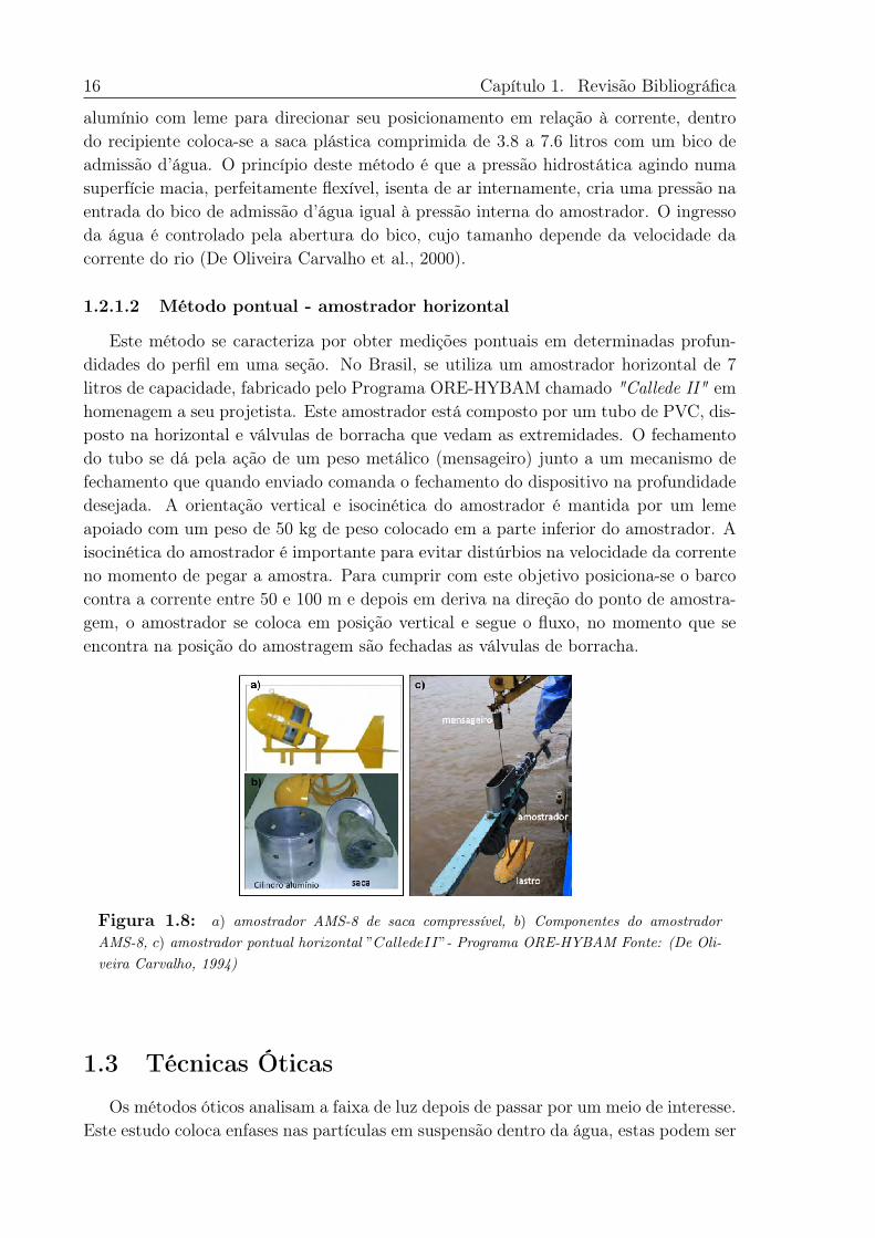
1.2.1.1 Método por integração vertical - saca compressível (AMS-8)
Este método consiste em coletar uma amostra homogênea composta de uma misturade água e sedimento acumulada continuamente em um recipiente. O amostrador usadoin situ se move verticalmente suspenso por um cabo fixo à embarcação, à uma velocidadede trânsito constante entre a superfície até as proximidades do leito sem tocar o fundopara evitar a suspensão do material de arrastre. No Brasil, as Instituições Nacionaisutilizam o amostrador de saca compressível AMS-8, composto de um recipiente de
16 Capítulo 1. Revisão Bibliográfica
alumínio com leme para direcionar seu posicionamento em relação à corrente, dentrodo recipiente coloca-se a saca plástica comprimida de 3.8 a 7.6 litros com um bico deadmissão d’água. O princípio deste método é que a pressão hidrostática agindo numasuperfície macia, perfeitamente flexível, isenta de ar internamente, cria uma pressão naentrada do bico de admissão d’água igual à pressão interna do amostrador. O ingressoda água é controlado pela abertura do bico, cujo tamanho depende da velocidade dacorrente do rio (De Oliveira Carvalho et al., 2000).
1.2.1.2 Método pontual - amostrador horizontal
Este método se caracteriza por obter medições pontuais em determinadas profun-didades do perfil em uma seção. No Brasil, se utiliza um amostrador horizontal de 7litros de capacidade, fabricado pelo Programa ORE-HYBAM chamado "Callede II" emhomenagem a seu projetista. Este amostrador está composto por um tubo de PVC, dis-posto na horizontal e válvulas de borracha que vedam as extremidades. O fechamentodo tubo se dá pela ação de um peso metálico (mensageiro) junto a um mecanismo defechamento que quando enviado comanda o fechamento do dispositivo na profundidadedesejada. A orientação vertical e isocinética do amostrador é mantida por um lemeapoiado com um peso de 50 kg de peso colocado em a parte inferior do amostrador. Aisocinética do amostrador é importante para evitar distúrbios na velocidade da correnteno momento de pegar a amostra. Para cumprir com este objetivo posiciona-se o barcocontra a corrente entre 50 e 100 m e depois em deriva na direção do ponto de amostra-gem, o amostrador se coloca em posição vertical e segue o fluxo, no momento que seencontra na posição do amostragem são fechadas as válvulas de borracha.
Figura 1.8: 𝑎) amostrador AMS-8 de saca compressível, 𝑏) Componentes do amostradorAMS-8, 𝑐) amostrador pontual horizontal ”𝐶𝑎𝑙𝑙𝑒𝑑𝑒𝐼𝐼”- Programa ORE-HYBAM Fonte: (De Oli-veira Carvalho, 1994)
1.3 Técnicas Óticas
Os métodos óticos analisam a faixa de luz depois de passar por um meio de interesse.Este estudo coloca enfases nas partículas em suspensão dentro da água, estas podem ser
1.3. Técnicas Óticas 17
detectadas por difusão ou absorção da faixa de luz incidente, dependendo do sistema demedida de cada aparelho. Dentro destes métodos, temos a Granulometria e a Turbidez(Maréchal, 2000).
1.3.1 Granulometria
O tamanho da partícula pode ser considerado como a característica física mais im-portante no controle do transporte e da dinâmica geoquímica dos sedimentos, e comotal é incluído direta o indiretamente na maioria dos modelos em termos da velocidadede sedimentação (Phillips e Walling, 1995). A medição in situ é a mais adequada paradeterminar as características dos sedimentos sem ter que modificar o tamanho natu-ral da partícula e seu equilíbrio com o regime turbulento da coluna d’água. Mas essetipo de equipamento tem custo elevado e precisa de dispositivos adaptados para rios degrande porte (Gibbs, 1981). No entanto, os equipamentos de laboratório têm evoluído,permitindo a obtenção de bons resultados se comparados à distribuição dos tamanhosdas partículas presentes no ambiente natural.
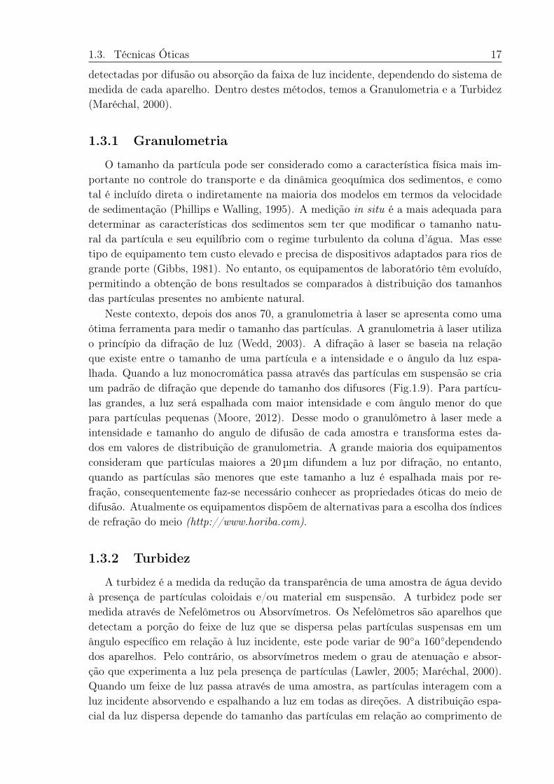
Neste contexto, depois dos anos 70, a granulometria à laser se apresenta como umaótima ferramenta para medir o tamanho das partículas. A granulometria à laser utilizao princípio da difração de luz (Wedd, 2003). A difração à laser se baseia na relaçãoque existe entre o tamanho de uma partícula e a intensidade e o ângulo da luz espa-lhada. Quando a luz monocromática passa através das partículas em suspensão se criaum padrão de difração que depende do tamanho dos difusores (Fig.1.9). Para partícu-las grandes, a luz será espalhada com maior intensidade e com ângulo menor do quepara partículas pequenas (Moore, 2012). Desse modo o granulômetro à laser mede aintensidade e tamanho do angulo de difusão de cada amostra e transforma estes da-dos em valores de distribuição de granulometria. A grande maioria dos equipamentosconsideram que partículas maiores a 20 µm difundem a luz por difração, no entanto,quando as partículas são menores que este tamanho a luz é espalhada mais por re-fração, consequentemente faz-se necessário conhecer as propriedades óticas do meio dedifusão. Atualmente os equipamentos dispõem de alternativas para a escolha dos índicesde refração do meio (http://www.horiba.com).
1.3.2 Turbidez
A turbidez é a medida da redução da transparência de uma amostra de água devidoà presença de partículas coloidais e/ou material em suspensão. A turbidez pode sermedida através de Nefelômetros ou Absorvímetros. Os Nefelômetros são aparelhos quedetectam a porção do feixe de luz que se dispersa pelas partículas suspensas em umângulo específico em relação à luz incidente, este pode variar de 90∘a 160∘dependendodos aparelhos. Pelo contrário, os absorvímetros medem o grau de atenuação e absor-ção que experimenta a luz pela presença de partículas (Lawler, 2005; Maréchal, 2000).Quando um feixe de luz passa através de uma amostra, as partículas interagem com aluz incidente absorvendo e espalhando a luz em todas as direções. A distribuição espa-cial da luz dispersa depende do tamanho das partículas em relação ao comprimento de
18 Capítulo 1. Revisão Bibliográfica
Figura 1.9: 𝑎) Efeitos da incidência da luz em uma partícula; 𝑏) padrões de difração parapartículas < 20 𝜇𝑚 e partículas > 20 𝜇𝑚; 𝑐) esquema do funcionamento do granulômetro àlaser. Fonte:https://www.sympatec.com
onda da luz incidente. Partículas muito menores do que o comprimento de onda da luzincidente, exibem uma distribuição de dispersão bastante simétrica com quantidadesiguais de luz difundida, tanto para a frente quanto para trás. Quando o tamanho daspartículas aumenta em relação ao comprimento de onda, a luz dispersa se espalha nafrente com uma intensidade maior do que em outras direções (Fig.1.10). Além disso,as partículas menores espalham mais intensamente em curtos comprimentos de onda(azul) e têm pouco efeito sobre comprimentos de onda mais longos (vermelho). Poroutro lado, as partículas maiores dispersam mais facilmente em longos comprimentosde onda do que em curtos comprimentos de onda. A forma das partículas e o índice derefração também afetam na distribuição de dispersão e intensidade da luz. A dispersãode luz intensifica-se quando a concentração de partículas aumenta. Se a concentraçãofor superior a um certo ponto, maior aos níveis detectáveis, a luz difundida e transmitidadiminuem rapidamente, marcando o limite superior de turbidez mensurável. Para dimi-nuir este efeito deve-se reduzir o comprimento do percurso da luz através da amostra, oque reduz o número de partículas entre a fonte de luz e o detector de luz, estendendo-seassim, o limite superior da medição de turbidez (http://www.omega.com).
Anderson (2005) indica como mostrado na Tabela 1.2 as características necessáriasque teria que ter um turbidímetro em função das condições naturais dos cursos d’água.A medição da turbidez fornece uma leitura da quantidade de luz dispersa e não podeser diretamente relacionada com um equivalente gravimétrico, a menos que uma curvade calibração seja criada (Minella et al., 2008).
O uso da turbidez no contexto aqui referenciado por ser uma ferramenta que per-mite determinar a concentração de sedimentos em suspensão em eventos pontuais queocorrem em curto espaço de tempo sem interferir com a dinâmica hidro-sedimentar(Restrepo e Pierini, 2012). Esta ferramenta soluciona problemas associados com a ex-trapolação de dados, principalmente quando se tem uma curta série de dados da relaçãoentre a concentração de sedimentos em função da descarga líquida, ou em estações queapresentam histereses (Walling e Collins, 2000). A turbidez também pode ajudar aresolver os problemas relacionados ao custo econômico elevado à longo prazo, de coletas
1.3. Técnicas Óticas 19
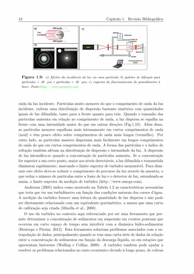
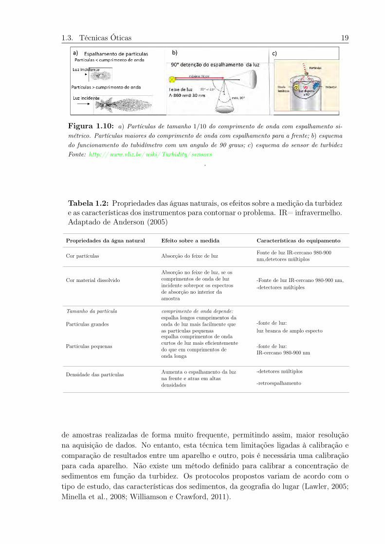
Figura 1.10: 𝑎) Partículas de tamanho 1/10 do comprimento de onda com espalhamento si-métrico. Partículas maiores do comprimento de onda com espalhamento para a frente; 𝑏) esquemado funcionamento do tubidímetro com um angulo de 90 graus; 𝑐) esquema do sensor de turbidezFonte: http://www.vliz.be/wiki/Turbidity/ sensors
.
Tabela 1.2: Propriedades das águas naturais, os efeitos sobre a medição da turbideze as características dos instrumentos para contornar o problema. IR= infravermelho.Adaptado de Anderson (2005)
Propriedades da água natural Efeito sobre a medida Características do equipamento
Cor partículas Absorção do feixe de luz Fonte de luz IR-cercano 980-900nm,detetores múltiplos
Cor material dissolvidoAbsorção no feixe de luz, se oscomprimentos de onda de luzincidente sobrepor os espectrosde absorção no interior daamostra
-Fonte de luz IR-cercano 980-900 nm,-detectores múltiples
Tamanho da partícula comprimento de onda depende:
Partículas grandesespalha longos cumprimentos daonda de luz mais facilmente queas partículas pequenas
-fonte de luz:luz branca de amplo especto
Partículas pequenas
espalha comprimentos de ondacurtos de luz mais eficientementedo que em comprimentos deonda longa
-fonte de luz:IR-cercano 980-900 nm
Densidade das partículas Aumenta o espalhamento da luzna frente e atras em altasdensidades
-detetores múltiplos
-retroespalhamento
de amostras realizadas de forma muito frequente, permitindo assim, maior resoluçãona aquisição de dados. No entanto, esta técnica tem limitações ligadas à calibração ecomparação de resultados entre um aparelho e outro, pois é necessária uma calibraçãopara cada aparelho. Não existe um método definido para calibrar a concentração desedimentos em função da turbidez. Os protocolos propostos variam de acordo com otipo de estudo, das características dos sedimentos, da geografia do lugar (Lawler, 2005;Minella et al., 2008; Williamson e Crawford, 2011).
20 Capítulo 1. Revisão Bibliográfica
1.4 Hidrometria
1.4.1 Nível d’água
A determinação do regime hidrológico de um rio refere-se às variações estacionaise cíclicas do nível e volume d’água de uma determinada estação. Para realizar o mo-nitoramento do nível do rio utiliza-se um jogo de réguas referenciadas localmente edeve-se realizar um mínimo de duas leituras diárias a cada 12 horas (padrão da OMM-Organização Mundial de Meteorologia (OMM, 1994)). As leituras das cotas dos riossão transformadas em vazão através do uso da relação cota (vs) vazão, conhecida comocurva chave. A curva chave obtém-se das medições conjuntas do nível d’água e vazãoem diferentes períodos, onde se busca cobrir todo o período/ciclo hidrológico.
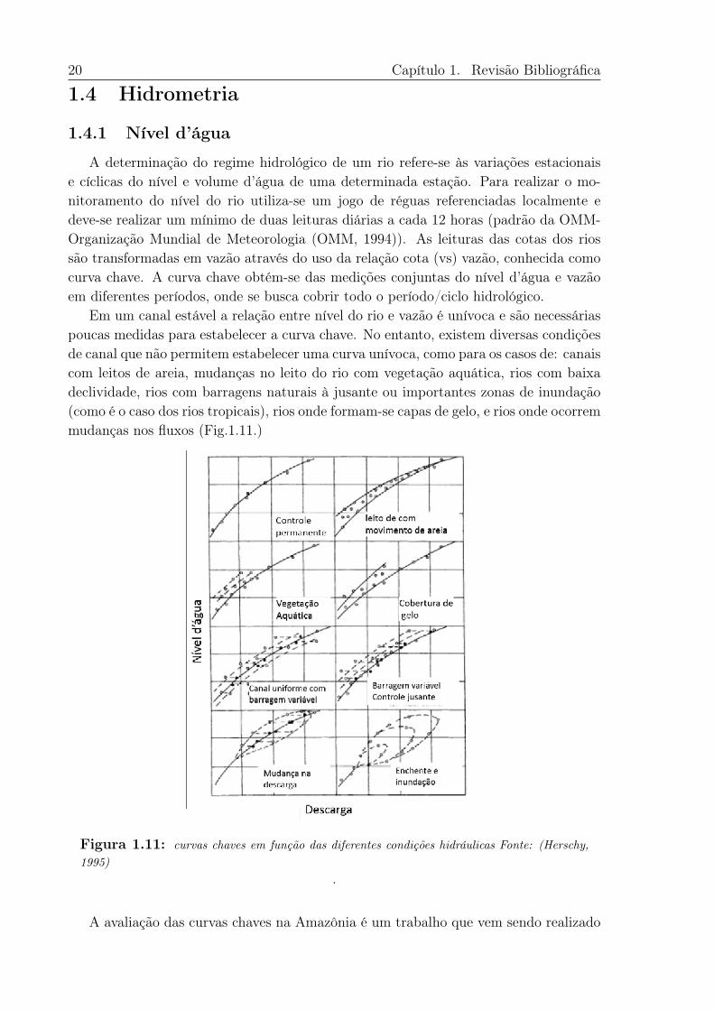
Em um canal estável a relação entre nível do rio e vazão é unívoca e são necessáriaspoucas medidas para estabelecer a curva chave. No entanto, existem diversas condiçõesde canal que não permitem estabelecer uma curva unívoca, como para os casos de: canaiscom leitos de areia, mudanças no leito do rio com vegetação aquática, rios com baixadeclividade, rios com barragens naturais à jusante ou importantes zonas de inundação(como é o caso dos rios tropicais), rios onde formam-se capas de gelo, e rios onde ocorremmudanças nos fluxos (Fig.1.11.)
Figura 1.11: curvas chaves em função das diferentes condições hidráulicas Fonte: (Herschy,1995)
.
A avaliação das curvas chaves na Amazônia é um trabalho que vem sendo realizado
1.4. Hidrometria 21
desde os anos de 1980 (Guimaraes e Jaccon, 1983; Jaccon e Guimaraes, 1985; Jaccon eCudo, 1987) e continua sendo realizado pelo observatório ORE-HYBAM em conjuntocom as Instituições Nacionais do Peru e Brasil. Observa-se que para as estações noPeru e no alto Solimões a relação é unívoca, ou seja, para um valor de nível d’águacorresponderá um único valor de vazão independente da época do ano. No entanto, asestações localizadas nos rios Madeira, Solimões e no próprio Amazonas apresentam umarelação não univoca entre a vazão e o nível d’água. Este efeito deve-se principalmente ainfluência do barramento natural1 à jusante da seção, em períodos de enchente (Jaccone Cudo, 1989). Já no rio Amazonas, este efeito é devido à influência da maré, às baixasdeclividades e às grandes zonas de inundação (Dubreuil et al., 1970; Callède et al., 2001).Em consequência não se pode aplicar uma curva chave, e a melhor solução é utilizar afórmula de Manning-Stricler (Equação 1.1)
𝑄 =𝐴𝑅2/3𝑆1/2
𝑛(1.1)
Onde: 𝑄= descarga (m3 s−1); A= área da seção transversal (m2); R= raio hidráulico(m); S= gradiente da linha d’água (m/m); n= coeficiente de rugosidade. O gradientediário da linha d’água é calculado entre uma estação à amontante e outra à jusante daestação de estudo (Vauchel, 2011).
1.4.2 Medição de vazão
A vazão é o volume de água que flui através de uma seção transversal em uma deter-mina unidade de tempo. A vazão expressa-se em (m3/s; l/s; l/h). As primeiras mediçõesde vazão nos rios amazônicos do Brasil foram feitas com molinete hidrométrico, equipa-mento que permite medir a velocidade pontual da água em diferentes profundidades emvários perfis verticais distribuídos ao longo da seção transversal de medição. A vazãoera calculada pela integração da velocidade e a área da seção. As duas técnicas maisutilizadas para medir a vazão com molinete hidrométrico em grandes rios, na Amazôniasão:
1. Método de Medição de Grandes Rios (Oltman, 1964; Jaccon e Cudo, 1984; OMM,1994)
2. Método do Barco ancorado (Chevallier, 1993; OMM, 1994)
A primeira técnica consiste em determinar a velocidade de um perfil em dois pontos(20 e 80%) ou mais (20 40, 60 e 80%) da profundidade total. A trajetória do barco émonitorada desde a margem com ajuda de três estações topográficas fixas que corrigema direção por posicionamento triangular. A segunda técnica consiste em colocar o barcoancorado em diferentes pontos da seção e medir a velocidade a dois pontos (20 e 80%)ou 3 pontos (20 40 e 80%) da profundidade total. Estes métodos têm a desvantagem deque para sua realização, precisa-se de um ou dois dias de trabalho para medir larguras
1a barragem natural é o impedimento da curso natural de um tributário devido a cheia do rioprincipal
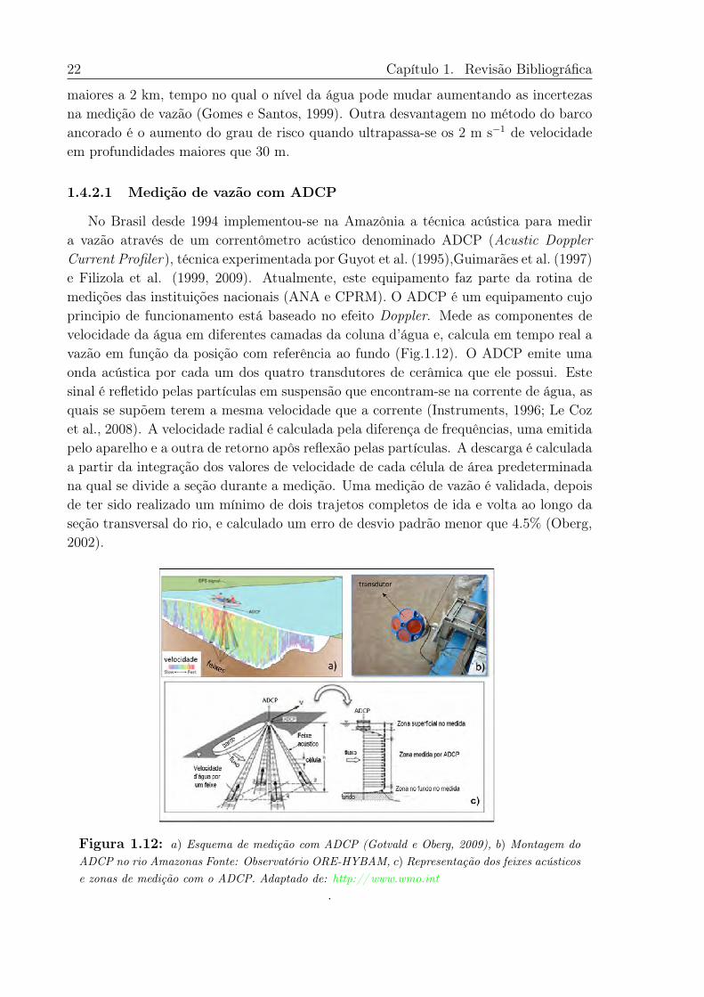
22 Capítulo 1. Revisão Bibliográfica
maiores a 2 km, tempo no qual o nível da água pode mudar aumentando as incertezasna medição de vazão (Gomes e Santos, 1999). Outra desvantagem no método do barcoancorado é o aumento do grau de risco quando ultrapassa-se os 2 m s−1 de velocidadeem profundidades maiores que 30 m.
1.4.2.1 Medição de vazão com ADCP
No Brasil desde 1994 implementou-se na Amazônia a técnica acústica para medira vazão através de um correntômetro acústico denominado ADCP (Acustic DopplerCurrent Profiler), técnica experimentada por Guyot et al. (1995),Guimarães et al. (1997)e Filizola et al. (1999, 2009). Atualmente, este equipamento faz parte da rotina demedições das instituições nacionais (ANA e CPRM). O ADCP é um equipamento cujoprincipio de funcionamento está baseado no efeito Doppler. Mede as componentes develocidade da água em diferentes camadas da coluna d’água e, calcula em tempo real avazão em função da posição com referência ao fundo (Fig.1.12). O ADCP emite umaonda acústica por cada um dos quatro transdutores de cerâmica que ele possui. Estesinal é refletido pelas partículas em suspensão que encontram-se na corrente de água, asquais se supõem terem a mesma velocidade que a corrente (Instruments, 1996; Le Cozet al., 2008). A velocidade radial é calculada pela diferença de frequências, uma emitidapelo aparelho e a outra de retorno apôs reflexão pelas partículas. A descarga é calculadaa partir da integração dos valores de velocidade de cada célula de área predeterminadana qual se divide a seção durante a medição. Uma medição de vazão é validada, depoisde ter sido realizado um mínimo de dois trajetos completos de ida e volta ao longo daseção transversal do rio, e calculado um erro de desvio padrão menor que 4.5% (Oberg,2002).
Figura 1.12: 𝑎) Esquema de medição com ADCP (Gotvald e Oberg, 2009), 𝑏) Montagem doADCP no rio Amazonas Fonte: Observatório ORE-HYBAM, 𝑐) Representação dos feixes acústicose zonas de medição com o ADCP. Adaptado de: http://www.wmo.int
.
1.5. Perfil de velocidade e concentração de sedimentos em suspensão 23
Embora a utilização de ADCP tenha sido um avanço nas medições de vazão, so-bre tudo na Amazônia, exitem problemas e limitações: 𝑖) O ADCP não realiza umamedida pontual de velocidade, o valor da velocidade é o resultado da média das velo-cidades projetadas por 3 dos 4 feixes. Este resultado é válido se as velocidades foremhomogêneas. 𝑖𝑖) A configuração dos feixes (ângulo de 20∘) faz com que a superfície demedida se incremente com a profundidade, o que significa que à grandes profundidadestambém haverão grandes zonas de medida, por exemplo em um profundidade de 20m a superfície de medida no fundo é de 100 m2. Deve-se considerar que existe umasuperposição de áreas a cada segundo de medida ja que o barco esta em movimento.𝑖𝑖𝑖) Outra limitação corresponde às zonas que não são medidas pelo ADCP, uma destaszonas são as células do fundo, o que limita o cálculo da velocidade de cisalhamento. Ovalor desta zona é obtido por regressão de um perfil de velocidades em uma extensãode 6% da profundidade total ao fundo.
1.5 Perfil de velocidade e concentração de sedimentosem suspensão
O transporte de sedimentos no curso de água depende das características: do fluido(velocidade e viscosidade), do escoamento (declividade e profundidade) e proprieda-des dos sedimentos (granulometria, densidade e composição). O esforço tangencial(força/área), resultado da interação entre as camadas do fluido e estas com as paredesdo leito, se conhece como tensão de corte ou cisalhamento. Segundo a lei de Rey-nolds, no fluido permanente, uniforme e bidimensional (planos x-horizontal, z-vertical),a expressão de tensão de cisalhamento em toda a coluna d’água é o resultado de doiscomponentes: 𝑖) um esforço de corte turbulento e, 𝑖𝑖) um esforço de corte laminar(Equação 1.2). A suspensão das partículas é causada pelo cisalhamento turbulento eo movimento da matéria no fundo se deve ao cisalhamento laminar ou turbulento. Nacamada laminar a tensão de corte é originada pela existência de um gradiente de velo-cidade e pela viscosidade do fluido. A camada turbulenta é caracterizada por vórticesonde o cisalhamento laminar é nulo. Entre estas duas camadas existe uma zona de tran-sição onde ocorre a combinação das duas forças (Laguionie, 2006). Nas proximidadesdo fundo, a camada gerada puramente por forças viscosas em escoamento laminar éconhecida como camada limite, mas se o escoamento for turbulento a camada laminar,é na verdade, uma subcamada da camada limite(Fig.1.13).
𝜏(𝑧) = −𝜌𝑤 * (𝑢′)(𝑧) * 𝑤
′
(𝑧)⏟ ⏞ Cisalhamento turbulento
+ 𝜇 * 𝛿𝑢𝛿𝑧⏟ ⏞
Cisalhamento laminar
(1.2)
onde:𝜏(𝑧)= força de cisalhamento no nível z,𝜌𝑤= massa por unidade de volume d’água (kg.m−3),𝑢
′ = componente de velocidade horizontal instantânea no nível z,𝑤
′
(𝑧)= componente de velocidade vertical instantânea no nível z,
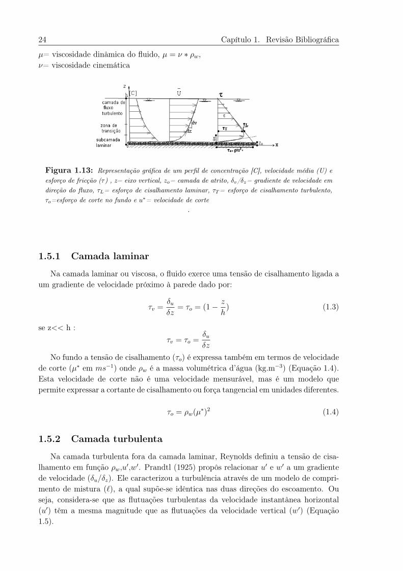
24 Capítulo 1. Revisão Bibliográfica
𝜇= viscosidade dinâmica do fluido, 𝜇 = 𝜈 * 𝜌𝑤,𝜈= viscosidade cinemática
Figura 1.13: Representação gráfica de um perfil de concentração [C], velocidade média (U) eesforço de fricção (𝜏) , z= eixo vertical, 𝑧𝑜= camada de atrito, 𝛿𝑣/𝛿𝑧= gradiente de velocidade emdireção do fluxo, 𝜏𝐿= esforço de cisalhamento laminar, 𝜏𝑇= esforço de cisalhamento turbulento,𝜏𝑜=esforço de corte no fundo e 𝑢*= velocidade de corte
.
1.5.1 Camada laminar
Na camada laminar ou viscosa, o fluido exerce uma tensão de cisalhamento ligada aum gradiente de velocidade próximo à parede dado por:
𝜏𝑣 =𝛿𝑢𝛿𝑧
= 𝜏𝑜 = (1 − 𝑧
ℎ) (1.3)
se z<< h :𝜏𝑣 = 𝜏𝑜 =
𝛿𝑢𝛿𝑧
No fundo a tensão de cisalhamento (𝜏𝑜) é expressa também em termos de velocidadede corte (𝜇* em 𝑚𝑠−1) onde 𝜌𝑤 é a massa volumétrica d’água (kg.m−3) (Equação 1.4).Esta velocidade de corte não é uma velocidade mensurável, mas é um modelo quepermite expressar a cortante de cisalhamento ou força tangencial em unidades diferentes.
𝜏𝑜 = 𝜌𝑤(𝜇*)2 (1.4)
1.5.2 Camada turbulenta
Na camada turbulenta fora da camada laminar, Reynolds definiu a tensão de cisa-lhamento em função 𝜌𝑤,𝑢′,𝑤′. Prandtl (1925) propôs relacionar 𝑢′ e 𝑤′ a um gradientede velocidade (𝛿𝑢/𝛿𝑧). Ele caracterizou a turbulência através de um modelo de compri-mento de mistura (ℓ), a qual supõe-se idêntica nas duas direções do escoamento. Ouseja, considera-se que as flutuações turbulentas da velocidade instantânea horizontal(𝑢′) têm a mesma magnitude que as flutuações da velocidade vertical (𝑤′) (Equação1.5).
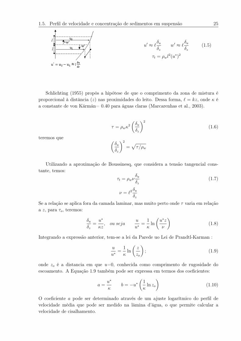
1.5. Perfil de velocidade e concentração de sedimentos em suspensão 25
𝑢′ ≈ ℓ𝛿𝑢𝛿𝑧
𝑤′ ≈ ℓ𝛿𝑢𝛿𝑧
(1.5)
𝜏𝑡 = 𝜌𝑤𝑙2(𝑢*)2
Schlichting (1955) propôs a hipótese de que o comprimento da zona de mistura éproporcional à distância (𝑧) nas proximidades do leito. Dessa forma, ℓ = 𝑘𝑧, onde 𝜅 éa constante de von Kármán= 0.40 para águas claras (Marcarenhas et al., 2003).
𝜏 = 𝜌𝑤𝜅2
(︂𝛿𝑢𝛿𝑧
)︂2
(1.6)
teremos que (︂𝛿𝑢𝛿𝑧
)︂2
=√︀
𝜏/𝜌𝑤
Utilizando a aproximação de Boussinesq, que considera a tensão tangencial cons-tante, temos:
𝜏𝑡 = 𝜌𝑤𝜈𝛿𝑢𝛿𝑧
(1.7)
𝜈 = ℓ2𝛿𝑢𝛿𝑧
Se a relação se aplica fora da camada laminar, mas muito perto onde 𝜏 varia em relaçãoa 𝑧, para 𝜏𝑜, teremos:
𝛿𝑢𝛿𝑧
=𝑢*
𝜅𝑧, 𝑜𝑢 𝑠𝑒𝑗𝑎
𝑢
𝑢* =1
𝜅ln
(︂𝑢*𝑧
𝜈
)︂(1.8)
Integrando a expressão anterior, tem-se a lei da Parede uo Lei de Prandtl-Karman :
𝑢
𝑢* =1
𝜅ln
(︂𝑧
𝑧𝑜
)︂; (1.9)
onde 𝑧𝑜 é a distancia em que u=0, conhecida como comprimento de rugosidade doescoamento. A Equação 1.9 também pode ser expressa em termos dos coeficientes:
𝑎 =𝑢*
𝜅𝑏 = −𝑢*
(︂1
𝜅ln 𝑧𝑜
)︂(1.10)
O coeficiente 𝑎 pode ser determinado através de um ajuste logarítmico do perfil develocidade média que pode ser medido na lâmina d’água, o que permite calcular avelocidade de cisalhamento.
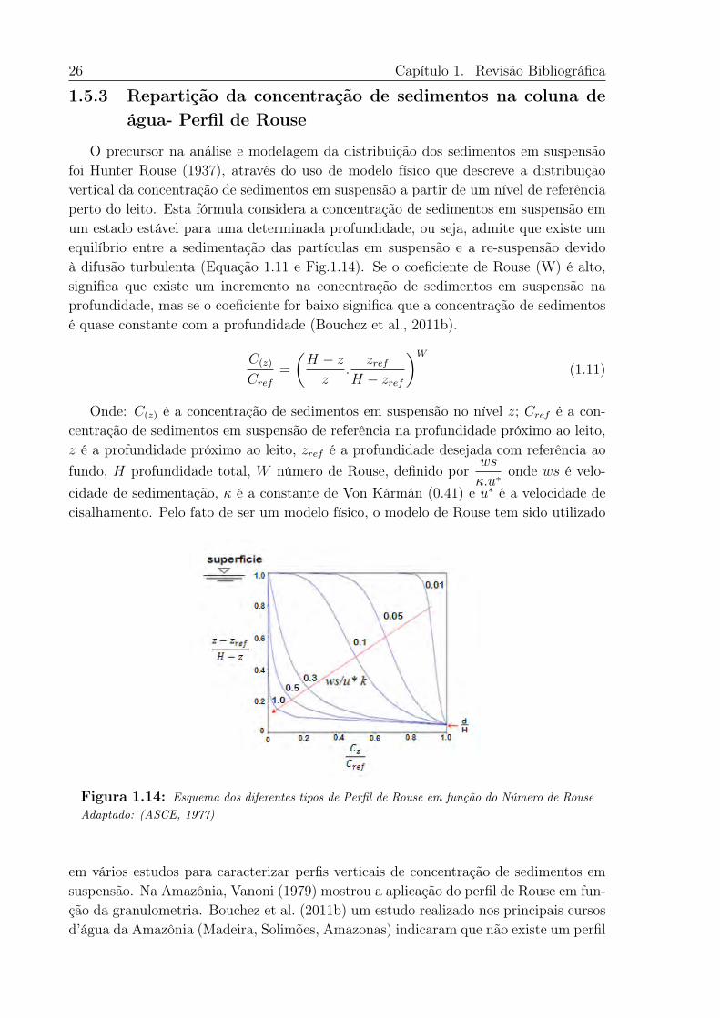
26 Capítulo 1. Revisão Bibliográfica
1.5.3 Repartição da concentração de sedimentos na coluna deágua- Perfil de Rouse
O precursor na análise e modelagem da distribuição dos sedimentos em suspensãofoi Hunter Rouse (1937), através do uso de modelo físico que descreve a distribuiçãovertical da concentração de sedimentos em suspensão a partir de um nível de referênciaperto do leito. Esta fórmula considera a concentração de sedimentos em suspensão emum estado estável para uma determinada profundidade, ou seja, admite que existe umequilíbrio entre a sedimentação das partículas em suspensão e a re-suspensão devidoà difusão turbulenta (Equação 1.11 e Fig.1.14). Se o coeficiente de Rouse (W) é alto,significa que existe um incremento na concentração de sedimentos em suspensão naprofundidade, mas se o coeficiente for baixo significa que a concentração de sedimentosé quase constante com a profundidade (Bouchez et al., 2011b).
𝐶(𝑧)
𝐶𝑟𝑒𝑓
=
(︂𝐻 − 𝑧
𝑧.
𝑧𝑟𝑒𝑓𝐻 − 𝑧𝑟𝑒𝑓
)︂𝑊
(1.11)
Onde: 𝐶(𝑧) é a concentração de sedimentos em suspensão no nível 𝑧; 𝐶𝑟𝑒𝑓 é a con-centração de sedimentos em suspensão de referência na profundidade próximo ao leito,𝑧 é a profundidade próximo ao leito, 𝑧𝑟𝑒𝑓 é a profundidade desejada com referência aofundo, 𝐻 profundidade total, 𝑊 número de Rouse, definido por
𝑤𝑠
𝜅.𝑢* onde 𝑤𝑠 é velo-cidade de sedimentação, 𝜅 é a constante de Von Kármán (0.41) e 𝑢* é a velocidade decisalhamento. Pelo fato de ser um modelo físico, o modelo de Rouse tem sido utilizado
Figura 1.14: Esquema dos diferentes tipos de Perfil de Rouse em função do Número de RouseAdaptado: (ASCE, 1977)
em vários estudos para caracterizar perfis verticais de concentração de sedimentos emsuspensão. Na Amazônia, Vanoni (1979) mostrou a aplicação do perfil de Rouse em fun-ção da granulometria. Bouchez et al. (2011b) um estudo realizado nos principais cursosd’água da Amazônia (Madeira, Solimões, Amazonas) indicaram que não existe um perfil
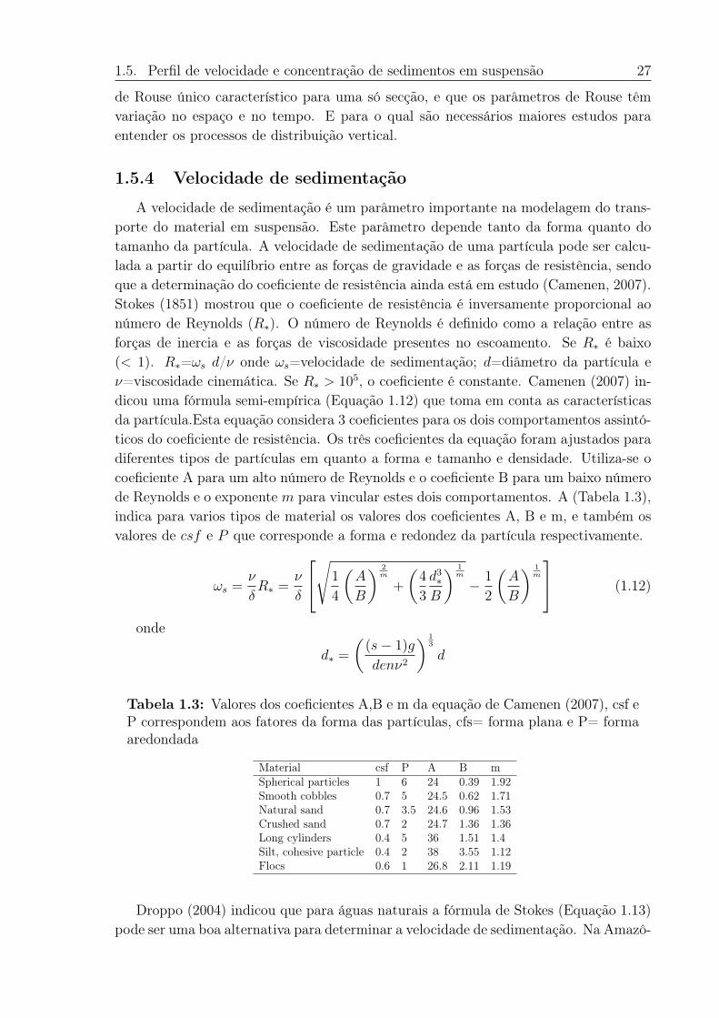
1.5. Perfil de velocidade e concentração de sedimentos em suspensão 27
de Rouse único característico para uma só secção, e que os parâmetros de Rouse têmvariação no espaço e no tempo. E para o qual são necessários maiores estudos paraentender os processos de distribuição vertical.
1.5.4 Velocidade de sedimentação
A velocidade de sedimentação é um parâmetro importante na modelagem do trans-porte do material em suspensão. Este parâmetro depende tanto da forma quanto dotamanho da partícula. A velocidade de sedimentação de uma partícula pode ser calcu-lada a partir do equilíbrio entre as forças de gravidade e as forças de resistência, sendoque a determinação do coeficiente de resistência ainda está em estudo (Camenen, 2007).Stokes (1851) mostrou que o coeficiente de resistência é inversamente proporcional aonúmero de Reynolds (𝑅*). O número de Reynolds é definido como a relação entre asforças de inercia e as forças de viscosidade presentes no escoamento. Se 𝑅* é baixo(< 1). 𝑅*=𝜔𝑠 𝑑/𝜈 onde 𝜔𝑠=velocidade de sedimentação; 𝑑=diâmetro da partícula e𝜈=viscosidade cinemática. Se 𝑅* > 105, o coeficiente é constante. Camenen (2007) in-dicou uma fórmula semi-empírica (Equação 1.12) que toma em conta as característicasda partícula.Esta equação considera 3 coeficientes para os dois comportamentos assintó-ticos do coeficiente de resistência. Os três coeficientes da equação foram ajustados paradiferentes tipos de partículas em quanto a forma e tamanho e densidade. Utiliza-se ocoeficiente A para um alto número de Reynolds e o coeficiente B para um baixo númerode Reynolds e o exponente 𝑚 para vincular estes dois comportamentos. A (Tabela 1.3),indica para varios tipos de material os valores dos coeficientes A, B e m, e também osvalores de 𝑐𝑠𝑓 e 𝑃 que corresponde a forma e redondez da partícula respectivamente.
𝜔𝑠 =𝜈
𝛿𝑅* =
𝜈
𝛿
⎡⎣√︃1
4
(︂𝐴
𝐵
)︂ 2𝑚
+
(︂4
3
𝑑3*𝐵
)︂ 1𝑚
− 1
2
(︂𝐴
𝐵
)︂ 1𝑚
⎤⎦ (1.12)
onde
𝑑* =
(︂(𝑠− 1)𝑔
𝑑𝑒𝑛𝜈2
)︂ 13
𝑑
Tabela 1.3: Valores dos coeficientes A,B e m da equação de Camenen (2007), csf eP correspondem aos fatores da forma das partículas, cfs= forma plana e P= formaaredondada
Material csf P A B mSpherical particles 1 6 24 0.39 1.92Smooth cobbles 0.7 5 24.5 0.62 1.71Natural sand 0.7 3.5 24.6 0.96 1.53Crushed sand 0.7 2 24.7 1.36 1.36Long cylinders 0.4 5 36 1.51 1.4Silt, cohesive particle 0.4 2 38 3.55 1.12Flocs 0.6 1 26.8 2.11 1.19
Droppo (2004) indicou que para águas naturais a fórmula de Stokes (Equação 1.13)pode ser uma boa alternativa para determinar a velocidade de sedimentação. Na Amazô-
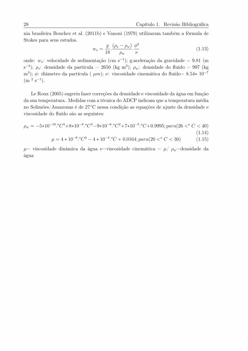
28 Capítulo 1. Revisão Bibliográfica
nia brasileira Bouchez et al. (2011b) e Vanoni (1979) utilizaram também a fórmula deStokes para seus estudos.
𝑤𝑠 =𝑔
18.(𝜌𝑠 − 𝜌𝑤)
𝜌𝑤.𝜑2
𝜈(1.13)
onde: 𝑤𝑠: velocidade de sedimentação (cm s−1); g:aceleração da gravidade = 9.81 (ms−2); 𝜌𝑠: densidade da partícula = 2650 (kg m3); 𝜌𝑤: densidade do fluido = 997 (kgm3); 𝜑: diâmetro da partícula ( 𝜇𝑚); 𝜈: viscosidade cinemática do fluído= 8.54* 10−7
(m 2 s−1).
Le Roux (2005) sugeriu fazer correções da densidade e viscosidade da água em funçãoda sua temperatura. Medidas com a técnica do ADCP indicam que a temperatura médiano Solimões/Amazonas é de 27∘C nessa condição as equações de ajuste da densidade eviscosidade do fluído são as seguintes:
𝜌𝑤 = −5*10−10.𝑜𝐶4+8*10−8.𝑜𝐶3−9*10−6.𝑜𝐶2+7*10−5.𝑜𝐶+0.9995; 𝑝𝑎𝑟𝑎(26 <𝑜 𝐶 < 40)
(1.14)𝜇 = 4 * 10−6.𝑜𝐶2 − 4 * 10−4.𝑜𝐶 + 0.0164; 𝑝𝑎𝑟𝑎(20 <𝑜 𝐶 < 30) (1.15)
𝜇= viscosidade dinâmica da água 𝜈=viscosidade cinemática = 𝜇/ 𝜌𝑤=densidade daágua
Capítulo 2
Materiais e Métodos
A metodologia deste trabalho baseou-se em amostragens pontuais que complementa-ram a base de dados já constituída e, que serve para determinar os fluxos de sedimentosnas estações de Tamshiyacu no Peru e de Óbidos no Brasil. Além das coletas estetrabalho coloca em evidencia a utilização de métodos indiretos, como a turbidez, paradeterminar a concentração de sedimentos em suspensão. Escolheu-se a turbidez, faceao fato de a sonda medição ser de alta frequência quanto à adquisição de dados, oque permite caracterizar melhor a distribuição espacial e temporal dos sedimentos emsuspensão na seção.
A (Fig.2.1) esquematiza a metodologia seguida neste trabalho, onde pode-se des-tacar três etapas: 𝑖) a primeira etapa que corresponde as amostragens. Este trabalhose apoia em coletas de amostras, medições de turbidez e granulometria nas estaçõesescolhidas (no apêndice mostra-se como realizar a calibração da turbidez e o processopara determinar a granulometria); 𝑖𝑖) a segunda etapa corresponde a analises de dadoscoletados nas medições de campo e no laboratório, onde se fez a separação de sedimentosfinos [𝐶𝑓 ] e areias [𝐶𝑐]. Esta distinção foi feita para poder identificar as diferenças entrea distribuição vertical e horizontal destes dois tipos de sedimentos durante o períodohidrológico. Igualmente, foi feito no laboratório a calibração da turbidez também emfunção da granulometria. foram traçadas curvas de calibração para sedimentos finos eareias. Também é mostrado o processo para utilizar a turbidez e determinar a concen-tração de sedimentos baseada na granulometria. Este método utiliza o Modelo de Rousepara separar o sinal dos sedimentos finos das areias; 𝑖𝑖𝑖) os resultados correspondem aquantificação dos fluxos sedimentários no rio Amazonas, na saída do Peru e na estaçãode Óbidos a 870 km antes da desembocadura.
Tem-se ressaltar que uma grade parte do tempo durante o doutorado foi dedicado acoleta, testes no campo para consolidar a base de dados, além dos testes no laboratório.Como o projeto faz parte do Observatório ORE-Hybam foi dedicado um tempo nomonitoramento regular das estações que formam parte do programa, com capacitaçãoaos observadores e estudantes.
29
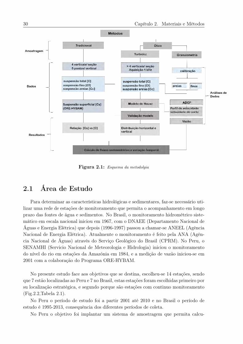
30 Capítulo 2. Materiais e Métodos
Figura 2.1: Esquema da metodolgia
2.1 Área de Estudo
Para determinar as características hidrológicas e sedimentares, faz-se necessário uti-lizar uma rede de estações de monitoramento que permita o acompanhamento em longoprazo das fontes de água e sedimentos. No Brasil, o monitoramento hidrométrico siste-mático em escala nacional iniciou em 1967, com o DNAEE (Departamento Nacional deÁguas e Energia Elétrica) que depois (1996-1997) passou a chamar-se ANEEL (AgênciaNacional de Energia Elétrica). Atualmente o monitoramento é feito pela ANA (Agên-cia Nacional de Águas) através do Serviço Geológico do Brasil (CPRM). No Peru, oSENAMHI (Servicio Nacional de Meteorologia e Hidrologia) iniciou o monitoramentodo nível do rio em estações da Amazônia em 1984, e a medição de vazão iniciou-se em2001 com a colaboração do Programa ORE-HYBAM.
No presente estudo face aos objetivos que se destina, escolheu-se 14 estações, sendoque 7 estão localizadas ao Peru e 7 no Brasil, estas estações foram escolhidas primeiro porsu localização estratégica, e segundo porque são estações com continuo monitoramento(Fig.2.2,Tabela 2.1).
No Peru o período de estudo foi a partir 2001 até 2010 e no Brasil o período deestudo é 1995-2013, consequência dos diferentes períodos de coleta.
No Peru o objetivo foi implantar um sistema de amostragem que permita calcu-
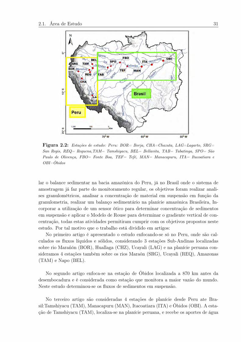
2.1. Área de Estudo 31
Figura 2.2: Estações de estudo: Peru: BOR= Borja, CHA=Chazuta, LAG=Lagarto, SRG=San Regis, REQ= Requena,TAM= Tamshiyacu, BEL= Bellavita, TAB= Tabatinga, SPO= SãoPaulo de Olivença, FBO= Fonte Boa, TEF= Tefé, MAN= Manacapuru, ITA= Itacoatiara eOBI=Óbidos
lar o balance sedimentar na bacia amazônica do Peru, já no Brasil onde o sistema deamostragem já faz parte do monitoramento regular, os objetivos foram realizar anali-ses granulométricos, analisar a concentração de material em suspensão em função dagranulometria, realizar um balanço sedimentário na planície amazônica Brasileira, In-corporar a utilização de um sensor ótico para determinar concentração de sedimentosem suspensão e aplicar o Modelo de Rouse para determinar o gradiente vertical de con-centração, todas estas atividades permitiram cumprir com os objetivos propostos nesteestudo. Por tal motivo que o trabalho está dividido em artigos:
No primeiro artigo é apresentado o estudo enfocando-se só no Peru, onde são cal-culados os fluxos líquidos e sólidos, considerando 3 estações Sub-Andinas localizadassobre rio Marañón (BOR), Huallaga (CHZ), Ucayali (LAG) e na planície peruana con-sideramos 4 estações também sobre os rios Maraón (SRG), Ucayali (REQ), Amazonas(TAM) e Napo (BEL).
No segundo artigo enfoca-se na estação de Óbidos localizada a 870 km antes dadesembocadura e é considerada como estação que monitora a maior vazão do mundo.Neste estudo determinou-se os fluxos de sedimentos em suspensão.
No terceiro artigo são consideradas 4 estações de planície desde Peru ate Bra-sil:Tamshiyacu (TAM), Manacapuru (MAN), Itacoatiara (ITA) e Óbidos (OBI). A esta-ção de Tamshiyacu (TAM), localiza-se na planície peruana, e recebe os aportes de água
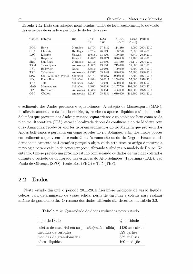
32 Capítulo 2. Materiais e Métodos
Tabela 2.1: Lista das estações monitoradas, dados de localização,medição de vazãodas estações de estudo e período de dados de vazão
Código Estação Rio LAT LON AREA Vazão Período° S ° W Km2 (m3 s-1)
BOR Borja Marañón 4.4704 77.5482 114,280 5,000 2004-2010CHA Chazuta Huallaga 6.5704 76.1193 68,720 2,980 2004-2010LAG Lagarto Ucayali 10.6081 73.8709 190,810 6,540 2009-2010REQ Requena Ucayali 4.9027 73.6721 346,600 11,400 2004-2010SRG San Regis Marañón 4.5100 73.9500 361,880 16,170 2004-2010TAM Tamshiyacu Amazonas 4.0033 73.1600 719,640 28,000 2001-2010BEL Bellavista Napo 3.4800 73.0800 100,030 6,600 2004-2010TAB Tabatinga Amazonas 4.2347 69.9447 890,000 37,900 1990-2014SPO Saõ Paulo de Olivença Solimões 3.5167 69.0167 940,000 47,600 1974-2014FBO Fonte Boa Solimões 2.4914 66.0617 1,159,000 57,000 1978-2014TFE Tefé Solimões 3.7667 64.9500 1,500,000 84,600 1996-2010MAN Manacapuru Solimões 3.3083 60.6094 2,147,730 104,000 1963-2014ITA Itacotiara Amazonas 4.0333 58.4833 435,000 150,300 1978-2014OBI Óbidos Amazonas 1.9187 55.5134 4,680,000 181,700 1968-2014
e sedimento dos Andes peruanos e equatorianos. A estação de Manacapuru (MAN),localizada amontante da foz do rio Negro, recebe os aportes líquidos e sólidos do altoSolimões que proveem dos Andes peruanos, equatorianos e colombianos bem como os daplanície. Itacoatiara (ITA), estação localizada depois da confluência do rio Madeira como rio Amazonas, recebe os aportes ricos em sedimentos do rio Madeira que proveem dosAndes bolivianos e peruanos em como aqueles do rio Solimões, além dos fluxos pobresem sedimentos que veem do escudo Guianês como são os do rio Negro. Foram consi-deradas unicamente as 4 estações porque o objetivo de este terceiro artigo é mostrar ametologia para o cálculo de concentrações utilizando turbidez e o modelo de Rouse. Noentanto, tem-se previso um próximo estudo comiserando os dados de turbidez coletadosdurante o período de doutorado nas estações do Alto Solimões: Tabatinga (TAB), SaõPaulo de Olivença (SPO), Fonte Boa (FBO) e Tefé (TEF).
2.2 Dados
Neste estudo durante o período 2011-2014 fizeram-se medições de vazão líquida,coletas para determinação de vazão sólida, perfis de turbidez e coletas para realizaranálise de granulometria. O resumo dos dados utilizado são descritos na Tabela 2.2.
Tabela 2.2: Quantidade de dados utilizados neste estudo
Tipo de Dado Quantidade
coletas de material em suspensão(vazão sólida) 1480 amostrasmedidas de turbidez 329 perfiesmedidas de granulometria 352 análisesaforos líquidos 160 medições
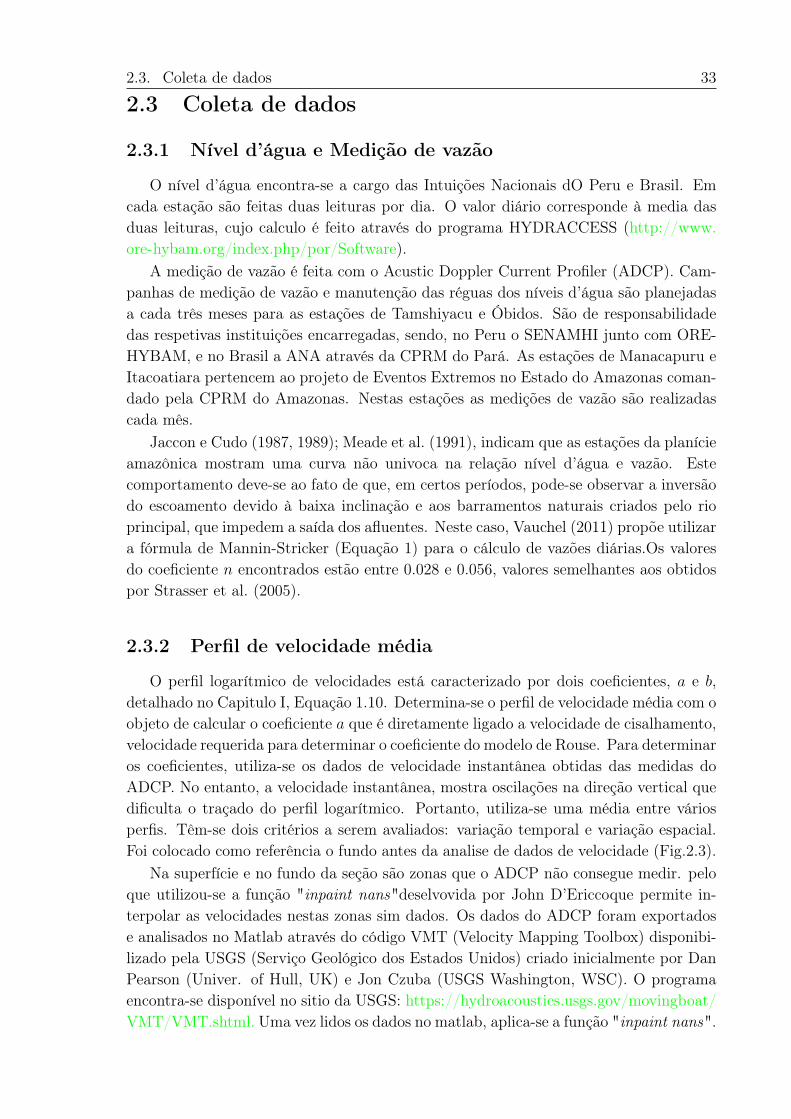
2.3. Coleta de dados 33
2.3 Coleta de dados
2.3.1 Nível d’água e Medição de vazão
O nível d’água encontra-se a cargo das Intuições Nacionais dO Peru e Brasil. Emcada estação são feitas duas leituras por dia. O valor diário corresponde à media dasduas leituras, cujo calculo é feito através do programa HYDRACCESS (http://www.ore-hybam.org/index.php/por/Software).
A medição de vazão é feita com o Acustic Doppler Current Profiler (ADCP). Cam-panhas de medição de vazão e manutenção das réguas dos níveis d’água são planejadasa cada três meses para as estações de Tamshiyacu e Óbidos. São de responsabilidadedas respetivas instituições encarregadas, sendo, no Peru o SENAMHI junto com ORE-HYBAM, e no Brasil a ANA através da CPRM do Pará. As estações de Manacapuru eItacoatiara pertencem ao projeto de Eventos Extremos no Estado do Amazonas coman-dado pela CPRM do Amazonas. Nestas estações as medições de vazão são realizadascada mês.
Jaccon e Cudo (1987, 1989); Meade et al. (1991), indicam que as estações da planícieamazônica mostram uma curva não univoca na relação nível d’água e vazão. Estecomportamento deve-se ao fato de que, em certos períodos, pode-se observar a inversãodo escoamento devido à baixa inclinação e aos barramentos naturais criados pelo rioprincipal, que impedem a saída dos afluentes. Neste caso, Vauchel (2011) propõe utilizara fórmula de Mannin-Stricker (Equação 1) para o cálculo de vazões diárias.Os valoresdo coeficiente 𝑛 encontrados estão entre 0.028 e 0.056, valores semelhantes aos obtidospor Strasser et al. (2005).
2.3.2 Perfil de velocidade média
O perfil logarítmico de velocidades está caracterizado por dois coeficientes, 𝑎 e 𝑏,detalhado no Capitulo I, Equação 1.10. Determina-se o perfil de velocidade média com oobjeto de calcular o coeficiente 𝑎 que é diretamente ligado a velocidade de cisalhamento,velocidade requerida para determinar o coeficiente do modelo de Rouse. Para determinaros coeficientes, utiliza-se os dados de velocidade instantânea obtidas das medidas doADCP. No entanto, a velocidade instantânea, mostra oscilações na direção vertical quedificulta o traçado do perfil logarítmico. Portanto, utiliza-se uma média entre váriosperfis. Têm-se dois critérios a serem avaliados: variação temporal e variação espacial.Foi colocado como referência o fundo antes da analise de dados de velocidade (Fig.2.3).
Na superfície e no fundo da seção são zonas que o ADCP não consegue medir. peloque utilizou-se a função "inpaint nans"deselvovida por John D’Ericcoque permite in-terpolar as velocidades nestas zonas sim dados. Os dados do ADCP foram exportadose analisados no Matlab através do código VMT (Velocity Mapping Toolbox) disponibi-lizado pela USGS (Serviço Geológico dos Estados Unidos) criado inicialmente por DanPearson (Univer. of Hull, UK) e Jon Czuba (USGS Washington, WSC). O programaencontra-se disponível no sitio da USGS: https://hydroacoustics.usgs.gov/movingboat/VMT/VMT.shtml. Uma vez lidos os dados no matlab, aplica-se a função "inpaint nans".
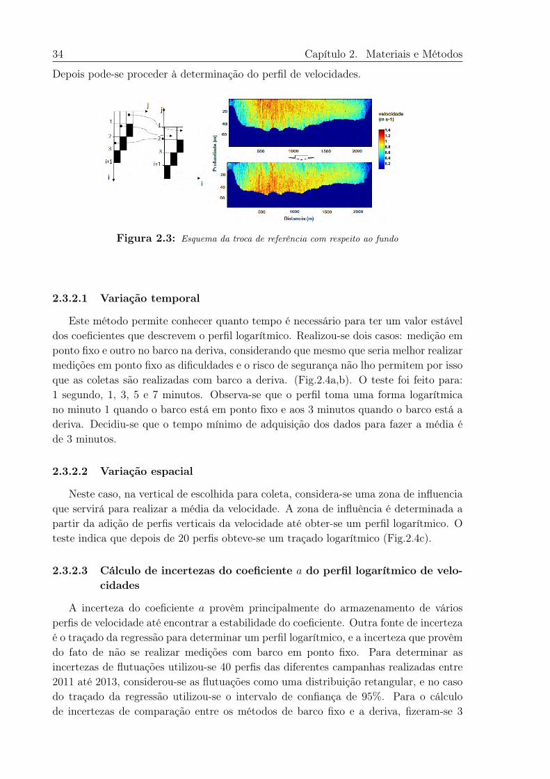
34 Capítulo 2. Materiais e Métodos
Depois pode-se proceder à determinação do perfil de velocidades.
Figura 2.3: Esquema da troca de referência com respeito ao fundo
2.3.2.1 Variação temporal
Este método permite conhecer quanto tempo é necessário para ter um valor estáveldos coeficientes que descrevem o perfil logarítmico. Realizou-se dois casos: medição emponto fixo e outro no barco na deriva, considerando que mesmo que seria melhor realizarmedições em ponto fixo as dificuldades e o risco de segurança não lho permitem por issoque as coletas são realizadas com barco a deriva. (Fig.2.4a,b). O teste foi feito para:1 segundo, 1, 3, 5 e 7 minutos. Observa-se que o perfil toma uma forma logarítmicano minuto 1 quando o barco está em ponto fixo e aos 3 minutos quando o barco está aderiva. Decidiu-se que o tempo mínimo de adquisição dos dados para fazer a média éde 3 minutos.
2.3.2.2 Variação espacial
Neste caso, na vertical de escolhida para coleta, considera-se uma zona de influenciaque servirá para realizar a média da velocidade. A zona de influência é determinada apartir da adição de perfis verticais da velocidade até obter-se um perfil logarítmico. Oteste indica que depois de 20 perfis obteve-se um traçado logarítmico (Fig.2.4c).
2.3.2.3 Cálculo de incertezas do coeficiente 𝑎 do perfil logarítmico de velo-cidades
A incerteza do coeficiente 𝑎 provêm principalmente do armazenamento de váriosperfis de velocidade até encontrar a estabilidade do coeficiente. Outra fonte de incertezaé o traçado da regressão para determinar um perfil logarítmico, e a incerteza que provêmdo fato de não se realizar medições com barco em ponto fixo. Para determinar asincertezas de flutuações utilizou-se 40 perfis das diferentes campanhas realizadas entre2011 até 2013, considerou-se as flutuações como uma distribuição retangular, e no casodo traçado da regressão utilizou-se o intervalo de confiança de 95%. Para o cálculode incertezas de comparação entre os métodos de barco fixo e a deriva, fizeram-se 3
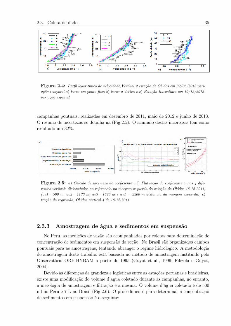
2.3. Coleta de dados 35
Figura 2.4: Perfil logarítmico de velocidade,Vertical 2 estação de Óbidos em 09/06/2013 vari-ação temporal 𝑎) barco em ponto fixo; 𝑏) barco a deriva e 𝑐) Estação Itacoatiara em 10/12/2012-variação espacial
campanhas pontuais, realizadas em dezembro de 2011, maio de 2012 e junho de 2013.O resumo de incertezas se detalha na (Fig.2.5). O acumulo destas incertezas tem comoresultado um 32%.
Figura 2.5: 𝑎) Cálculo de incerteza do coeficiente a,𝑏) Flutuação do coeficiente 𝑎 nas 4 dife-rentes verticais distanciadas en referencia na margem esquerda da estação de Óbidos 18-12-2011,(av1= 590 m, av2= 1130 m, av3= 1670 m e av4 = 2200 m distancia da margem esquerda), 𝑐)
tração da regressão, Óbidos vertical 4 de 18-12-2011
2.3.3 Amostragem de água e sedimentos em suspensão
No Peru, as medições de vazão são acompanhadas por coletas para determinação deconcentração de sedimentos em suspensão da seção. No Brasil são organizados campospontuais para as amostragens, tentando abranger o regime hidrológico. A metodologiade amostragem deste trabalho está baseada no método de amostragem instituído peloObservatório ORE-HYBAM a partir de 1995 (Guyot et al., 1999; Filizola e Guyot,2004).
Devido às diferenças de grandeza e logísticas entre as estações peruanas e brasileiras,existe uma modificação do volume d’água coletado durante as campanhas, no entanto,a metologia de amostragem e filtração é a mesma. O volume d’água coletado é de 500ml no Peru e 7 L no Brasil (Fig.2.6). O procedimento para determinar a concentraçãode sedimentos em suspensão é o seguinte:
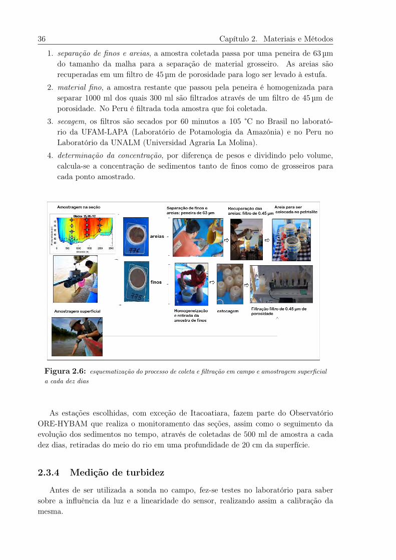
36 Capítulo 2. Materiais e Métodos
1. separação de finos e areias, a amostra coletada passa por uma peneira de 63 µm
do tamanho da malha para a separação de material grosseiro. As areias sãorecuperadas em um filtro de 45 µm de porosidade para logo ser levado à estufa.
2. material fino, a amostra restante que passou pela peneira é homogenizada paraseparar 1000 ml dos quais 300 ml são filtrados através de um filtro de 45 µm deporosidade. No Peru é filtrada toda amostra que foi coletada.
3. secagem, os filtros são secados por 60 minutos a 105 °C no Brasil no laborató-rio da UFAM-LAPA (Laboratório de Potamologia da Amazônia) e no Peru noLaboratório da UNALM (Universidad Agraria La Molina).
4. determinação da concentração, por diferença de pesos e dividindo pelo volume,calcula-se a concentração de sedimentos tanto de finos como de grosseiros paracada ponto amostrado.
Figura 2.6: esquematização do processo de coleta e filtração em campo e amostragem superficiala cada dez dias
As estações escolhidas, com exceção de Itacoatiara, fazem parte do ObservatórioORE-HYBAM que realiza o monitoramento das seções, assim como o seguimento daevolução dos sedimentos no tempo, através de coletadas de 500 ml de amostra a cadadez dias, retiradas do meio do rio em uma profundidade de 20 cm da superfície.
2.3.4 Medição de turbidez
Antes de ser utilizada a sonda no campo, fez-se testes no laboratório para sabersobre a influência da luz e a linearidade do sensor, realizando assim a calibração damesma.
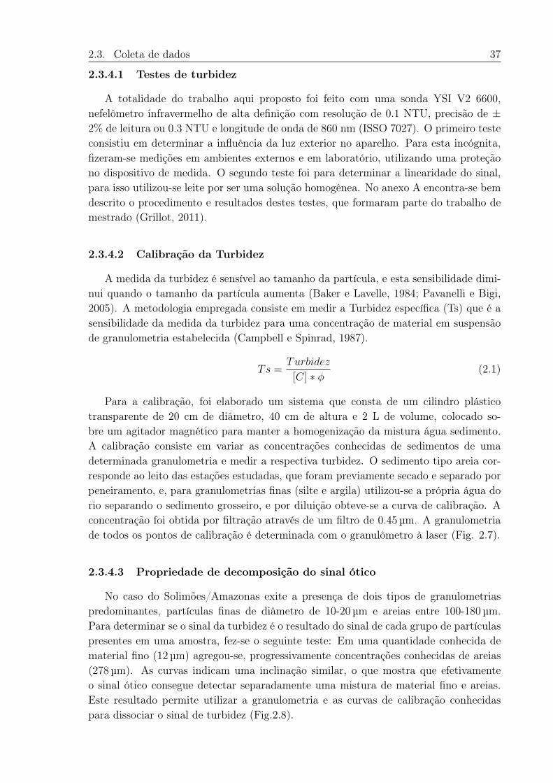
2.3. Coleta de dados 37
2.3.4.1 Testes de turbidez
A totalidade do trabalho aqui proposto foi feito com uma sonda YSI V2 6600,nefelômetro infravermelho de alta definição com resolução de 0.1 NTU, precisão de ±2% de leitura ou 0.3 NTU e longitude de onda de 860 nm (ISSO 7027). O primeiro testeconsistiu em determinar a influência da luz exterior no aparelho. Para esta incógnita,fizeram-se medições em ambientes externos e em laboratório, utilizando uma proteçãono dispositivo de medida. O segundo teste foi para determinar a linearidade do sinal,para isso utilizou-se leite por ser uma solução homogênea. No anexo A encontra-se bemdescrito o procedimento e resultados destes testes, que formaram parte do trabalho demestrado (Grillot, 2011).
2.3.4.2 Calibração da Turbidez
A medida da turbidez é sensível ao tamanho da partícula, e esta sensibilidade dimi-nui quando o tamanho da partícula aumenta (Baker e Lavelle, 1984; Pavanelli e Bigi,2005). A metodologia empregada consiste em medir a Turbidez específica (Ts) que é asensibilidade da medida da turbidez para uma concentração de material em suspensãode granulometria estabelecida (Campbell e Spinrad, 1987).
𝑇𝑠 =𝑇𝑢𝑟𝑏𝑖𝑑𝑒𝑧
[𝐶] * 𝜑(2.1)
Para a calibração, foi elaborado um sistema que consta de um cilindro plásticotransparente de 20 cm de diâmetro, 40 cm de altura e 2 L de volume, colocado so-bre um agitador magnético para manter a homogenização da mistura água sedimento.A calibração consiste em variar as concentrações conhecidas de sedimentos de umadeterminada granulometria e medir a respectiva turbidez. O sedimento tipo areia cor-responde ao leito das estações estudadas, que foram previamente secado e separado porpeneiramento, e, para granulometrias finas (silte e argila) utilizou-se a própria água dorio separando o sedimento grosseiro, e por diluição obteve-se a curva de calibração. Aconcentração foi obtida por filtração através de um filtro de 0.45 µm. A granulometriade todos os pontos de calibração é determinada com o granulômetro à laser (Fig. 2.7).
2.3.4.3 Propriedade de decomposição do sinal ótico
No caso do Solimões/Amazonas exite a presença de dois tipos de granulometriaspredominantes, partículas finas de diâmetro de 10-20 µm e areias entre 100-180 µm.Para determinar se o sinal da turbidez é o resultado do sinal de cada grupo de partículaspresentes em uma amostra, fez-se o seguinte teste: Em uma quantidade conhecida dematerial fino (12 µm) agregou-se, progressivamente concentrações conhecidas de areias(278 µm). As curvas indicam uma inclinação similar, o que mostra que efetivamenteo sinal ótico consegue detectar separadamente uma mistura de material fino e areias.Este resultado permite utilizar a granulometria e as curvas de calibração conhecidaspara dissociar o sinal de turbidez (Fig.2.8).
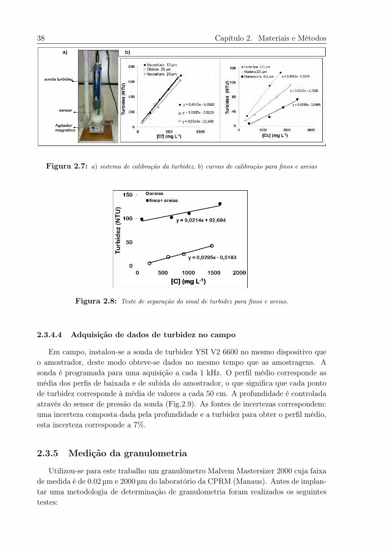
38 Capítulo 2. Materiais e Métodos
Figura 2.7: 𝑎) sistema de calibração da turbidez, 𝑏) curvas de calibração para finos e areias
Figura 2.8: Teste de separação do sinal de turbidez para finos e areias.
2.3.4.4 Adquisição de dados de turbidez no campo
Em campo, instalou-se a sonda de turbidez YSI V2 6600 no mesmo dispositivo queo amostrador, deste modo obteve-se dados no mesmo tempo que as amostragens. Asonda é programada para uma aquisição a cada 1 kHz. O perfil médio corresponde asmédia dos perfis de baixada e de subida do amostrador, o que significa que cada pontode turbidez corresponde à média de valores a cada 50 cm. A profundidade é controladaatravés do sensor de pressão da sonda (Fig.2.9). As fontes de incertezas correspondem:uma incerteza composta dada pela profundidade e a turbidez para obter o perfil médio,esta incerteza corresponde a 7%.
2.3.5 Medição da granulometria
Utilizou-se para este trabalho um granulômetro Malvem Mastersizer 2000 cuja faixade medida é de 0.02 µm e 2000 µm do laboratório da CPRM (Manaus). Antes de implan-tar uma metodologia de determinação de granulometria foram realizados os seguintestestes:
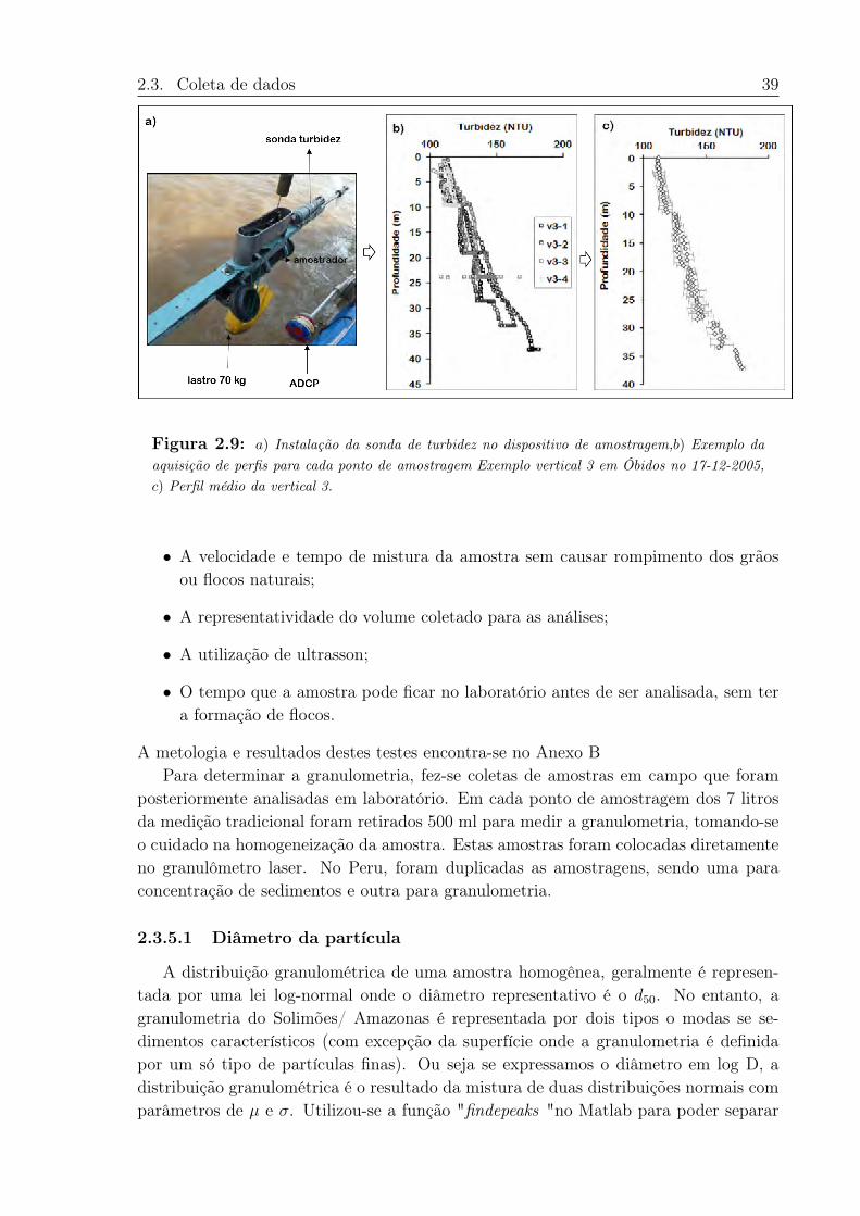
2.3. Coleta de dados 39
Figura 2.9: 𝑎) Instalação da sonda de turbidez no dispositivo de amostragem,𝑏) Exemplo daaquisição de perfis para cada ponto de amostragem Exemplo vertical 3 em Óbidos no 17-12-2005,𝑐) Perfil médio da vertical 3.
• A velocidade e tempo de mistura da amostra sem causar rompimento dos grãosou flocos naturais;
• A representatividade do volume coletado para as análises;
• A utilização de ultrasson;
• O tempo que a amostra pode ficar no laboratório antes de ser analisada, sem tera formação de flocos.
A metologia e resultados destes testes encontra-se no Anexo BPara determinar a granulometria, fez-se coletas de amostras em campo que foram
posteriormente analisadas em laboratório. Em cada ponto de amostragem dos 7 litrosda medição tradicional foram retirados 500 ml para medir a granulometria, tomando-seo cuidado na homogeneização da amostra. Estas amostras foram colocadas diretamenteno granulômetro laser. No Peru, foram duplicadas as amostragens, sendo uma paraconcentração de sedimentos e outra para granulometria.
2.3.5.1 Diâmetro da partícula
A distribuição granulométrica de uma amostra homogênea, geralmente é represen-tada por uma lei log-normal onde o diâmetro representativo é o 𝑑50. No entanto, agranulometria do Solimões/ Amazonas é representada por dois tipos o modas se se-dimentos característicos (com excepção da superfície onde a granulometria é definidapor um só tipo de partículas finas). Ou seja se expressamos o diâmetro em log D, adistribuição granulométrica é o resultado da mistura de duas distribuições normais comparâmetros de 𝜇 e 𝜎. Utilizou-se a função "findepeaks "no Matlab para poder separar
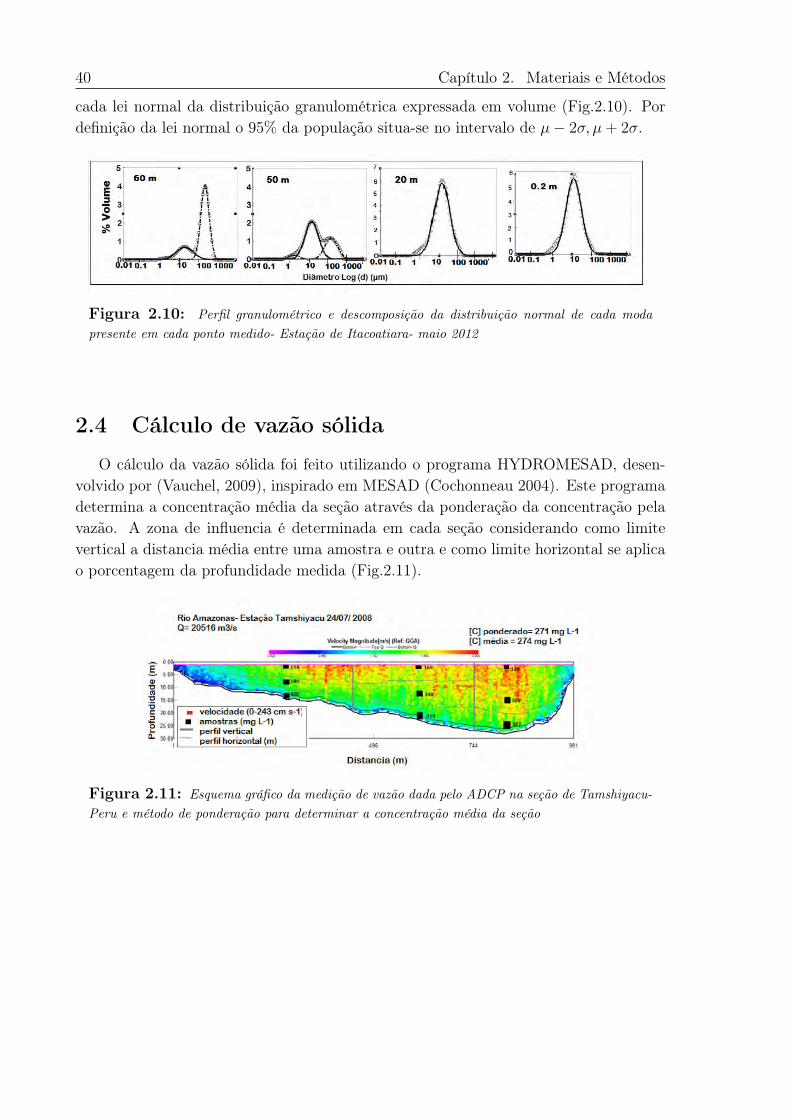
40 Capítulo 2. Materiais e Métodos
cada lei normal da distribuição granulométrica expressada em volume (Fig.2.10). Pordefinição da lei normal o 95% da população situa-se no intervalo de 𝜇− 2𝜎, 𝜇 + 2𝜎.
Figura 2.10: Perfil granulométrico e descomposição da distribuição normal de cada modapresente em cada ponto medido- Estação de Itacoatiara- maio 2012
2.4 Cálculo de vazão sólida
O cálculo da vazão sólida foi feito utilizando o programa HYDROMESAD, desen-volvido por (Vauchel, 2009), inspirado em MESAD (Cochonneau 2004). Este programadetermina a concentração média da seção através da ponderação da concentração pelavazão. A zona de influencia é determinada em cada seção considerando como limitevertical a distancia média entre uma amostra e outra e como limite horizontal se aplicao porcentagem da profundidade medida (Fig.2.11).
Figura 2.11: Esquema gráfico da medição de vazão dada pelo ADCP na seção de Tamshiyacu-Peru e método de ponderação para determinar a concentração média da seção
Capítulo 3
Dinâmica dos sedimentos emsuspensão do rio Amazonas no Peru
41
42 Capítulo 3. Dinâmica dos sedimentos em suspensão do rio Amazonas no Peru
ResumoNo Peru a bacia Amazônica abrange uma área de 977.920 km2, se entende desde
os Andes (≈ 6000 m.s.n.m) até a planície (≈ 100 m.sn.m). Está composta por duasprincipais sub-bacias, a bacia do rio Marañón composta principalmente por afluentesdo norte e a bacia do rio Ucayali com afluentes do sul. A confluência entre estes doisrios forma o Amazonas cujo monitoramento é realizado na estação de Tamshiyacu.
A bacia amazônica peruana apresenta contrastes fisiográficos e climáticos entre osAndes que inclui as sub-bacias Andinas e a planície. No entanto, estes contrastes tam-bém são observados entre o norte e sul da Bacia. Estes contrastes tem influência nosfluxos sedimentares. Neste contexto, o objetivo deste estudo foi determinar a variabili-dade temporal do fluxos de água e sedimentos em suspensão nas sub-bacias andinas ena planície amazônica peruana.
A partir de 2003 o Observatório ORE-HYBAM (IRD-SENAMHI-UNALM) inicia omonitoramento de água e sedimentos nas estações peruanas. Neste estudo foram consi-deradas 8 estações localizadas nos principais rios amazônicos. Três estações localizadasna parte sub-Andina e cinco estações na planície peruana. No período 2003-2010, emcada uma das estações, foram feitas coletas de sedimentos em suspensão a cada dez diase as medições de vazão líquida e sólida a cada três meses.
Na parte Andina observam-se altas variações de descarga como resposta instantâneada precipitação, enquanto que na planície estas variações são de baixa frequência. Osmeses de cheia nas sub-bacias Andinas são de dezembro até maio e os meses de estiagemencontram-se entre julho e setembro. Já na planície os meses de cheia acontecem emabril e maio e de estiagem entre julho e setembro. Ao se comparar as bacias do Marañóne Ucayali, a bacia do Marañón (16.175 m3 s−1 bacia do norte) tem maior aporte dedescarga líquida quanto a comparamos com a bacia do Ucayali (11.415 m3 s−1 bacia dosul).
Os rios Andinos apresentam uma relação entre concentração de sedimentos em sus-pensão e vazão, no entanto, quanto mais nos aproximamos na planície, esta relação tomauma configuração de loop, o que impede sua utilização. Este fenômeno de histerese podeser causado pela diferença entre o regime sedimentar e a vazão. Para contornar esteproblema de variabilidade temporal realizou-se coletas regulares de água e sedimentodurante o regime hidrológico. O fato que a concentração de sedimentos superficiais acada dez dias apresentam uma boa relação com a concentração média de sedimentos daseção (r2=0.72), é possível quantificar o fluxo de sedimentos a partir desta relação. Naregião Andina observa-se uma alta variação dos sedimentos em suspensão en quanto naplanície o regime estacional é mais marcado. Em contrapartida a sub-bacia do Ucayalitem um maior aporte de fluxo de sedimentos aproximadamente 360 Mt year−1, enantoa bacia do Marañón tem um aporte de 144 Mt year−1. O que significa que o fluxo queingressa no Brasil é aproximandamente 540 Mt year−1.
43
RésuméAu Pérou le bassin Amazonien représente une superficie de 977.920 km2 qui s’étend
depuis les Andes (≈ 6000 m.s.n.m) jusqu’à la plaine du même nom (≈ 100 m.s.n.m). Ilcomprend deux sous-bassins principaux, le bassin du Marañon constitué principalementpar des affluents venus du nord et du bassin de l’Ucayali issu de formateurs venant dusud. La confluence de ces deux fleuves forme l’Amazone dont la station de Tamshiyacuassure le suivi.
Le bassin Amazonien au Pérou présente des contrastes physiographiques et clima-tiques entre les sous bassins andins et la plaine. Mais l’on observe également de telscontrastes entre le sud et le nord du bassin. Ces contrastes vont influencer fortement lesflux sédimentaires. L’objectif de cette étude sera de déterminer la variabilité temporelledans un tel contexe des flux d’eau et de sédiments en suspension dans les sous bassinsandins ainsi que dans la plaine amazonienne péruvienne.
A partir de 2003 l’Observatoire ORE-HYBAM (IRD-SENAMHI-UNALM) a iniciéle suivi hydrologique et sédimentaire des stations péruviennes. On a considéré danscette étude 8 stations situées sur les principaux fleuves Amazoniens dont trois dans lapartie sub-andine et cinq dans la plaine. Sur la période 2003-2010, et sur chacune deces stations, on a prélevé tous les dix jours des échantillons en surface de sédiments ensuspension et réalisé tous les trois mois des mesures de débit liquide et solide sur lasection totale.
Dans la partie andine, on observe de fortes variations de débit en réponse instantanéeaux précipitations alors que dans la plaine ces variations s’atténuent. Dans les sousbassins Andins les crues ont lieu de décembre à mai et l´étiage de juillet à septembre.Dans la plaine la période de crue arrive en avril-mai, celle d’étiage s’étalant aussi dejuillet á septembre. On remarquera que le bassin du Marañon apporte un débit liquidesupérieur á celui de l’Ucayali, 16,175 m3 s−1 pour le Marañon contre 11,415 m3 s−1 pourl’Ucayali.
Dans les cours d’eau Andins on peut établir une relation directe entre concentrationde sédiments en suspension et débit liquide alors qu’au fur et à mesure que l’on avancedans la plaine cette relation tend à prendre une forme de loop qui empêche un calculdirect du flux solide. Ce phénomène d’hystérésis peut provenir du déphasage entre lesflux sédimentaires et liquides et l’on doit donc contourner ce problème de variationtemporelle en réalisant un échantillonnage continu tout au long du cycle hydrologique.
En effet, la concentration de sédiments de superficie des échantillons présente unebonne relation avec la concentration moyenne dans la section (r2=0.72) et l’on peutarriver á calculer le flux solide en se basant sur cette relation.
Dans la partie andine on observe comme pour les débits une très forte variation des

44 Capítulo 3. Dinâmica dos sedimentos em suspensão do rio Amazonas no Peru
valeurs de concentration en materiel en suspension alors que dans la plaine le régimesaisonnier est plus marqué. En revanche, c´est cette fois le bassin de l´Ucayali quiamène le plus gros flux sédimentaire avec approximativement 360 Mt an−1 quand dansle même temps on obtient 144 Mt an−1 pour le Marañon. Au final se sont 540 Mt an−1
qui transitent par l’Amazone à la frontière péruano-brésilienne.
45
Suspended sediment dynamics in the Amazon River of Peru
Elisa Armijos1, Alain Crave2,3, Philippe Vauchel4, Pascal Fraizy4, William Santini4, JeanSebastian Moquet5, Nore Arevalo6, Jorge Carranza7,Jean Loup Guyot8.
1 − LBA, Instituto Nacional de Pesquisas da Amazônia (INPA)- Universidade do Estado doAmazonas (UEA). Av. André Araújo, 2936, Aleixo, CEP 69060-001, Manaus- Brazil .2 − Géoscience Rennes, CNRS/INSU UMR 6118, Campus de Beaulieu, 35042 Rennes, France.3 − Université de Rennes 1, Campus de Beaulieu, 35042 Rennes, France.4 − GET (CNRS, IRD, OMP, Université de Toulouse), 14 Avenue Edouard Belin, 31400 Toulouse,France.5 − Universidade de São Paulo -Instituto de Geociencias Rua do lago, 562 - cidade Universitária SãoPaulo, São Paulo – Brazil.6 − UNALM, Universidad Nacional Agraria La Molina – Facultad de Ingeniería Agrícola, AvenidaLa Molina s/n, Lima 12, Perú.7 − SENAMHI – DGH Servicio Nacional de Meteorología e Hidrología – Dirección General deHidrología, Casilla 11-1308, Lima 11, Perú− GET (CNRS, IRD, OMP, Université de Toulouse), IRD, CP 7091 Lago Sul, CEP 71635-971Brasília, DF, Brazil.
Abstract
The erosion and transport of sediments allow us to understand many activities ofsignificance such, as crust evolution, climate change, uplift rates, continental processes,the biogeochemical cycling of pollutants and nutrients. The Amazon basin of Peru hascontrasting physiographic and climatic characteristics between the Andean piedmontand the plains and between the north and south of the basin which is why there arewhy 8 gauging stations located along the principal rivers of the Andean piedmont (Ma-rañón, Huallaga, Ucayali) and the plain (Marañón, Tigre, Napo, Ucayali and Amazonrivers). Since 2003, the ORE-Hybam (IRD-SENAMHI-UNALM) observatory has per-formed regular measurements at strategic points of the Amazon basin to understandand model the systems behavior and their long-term dynamics. On the Andean pied-mont, the suspended yields are governed by a simple model with a relationship betweenthe river discharge and the sediment concentration. In the plain, the dilution effect ofthe concentrations can create hysteresis in this relationship on a monthly basis. TheAmazon basin of Peru has sediments yield of 541 * 106 t year −1, 70% of which comesfrom the southern basin.KEY WORDS: hydrology, sedimentation, erosion, Andes, sediment transport, Andeanpiedmont.
Introduction
Erosion and transport processes are key factors for understanding the dynamicsof natural systems of different scales. Among other factors, the influence of erosionprocesses on mountain range dynamics is one of the crucial points for understanding
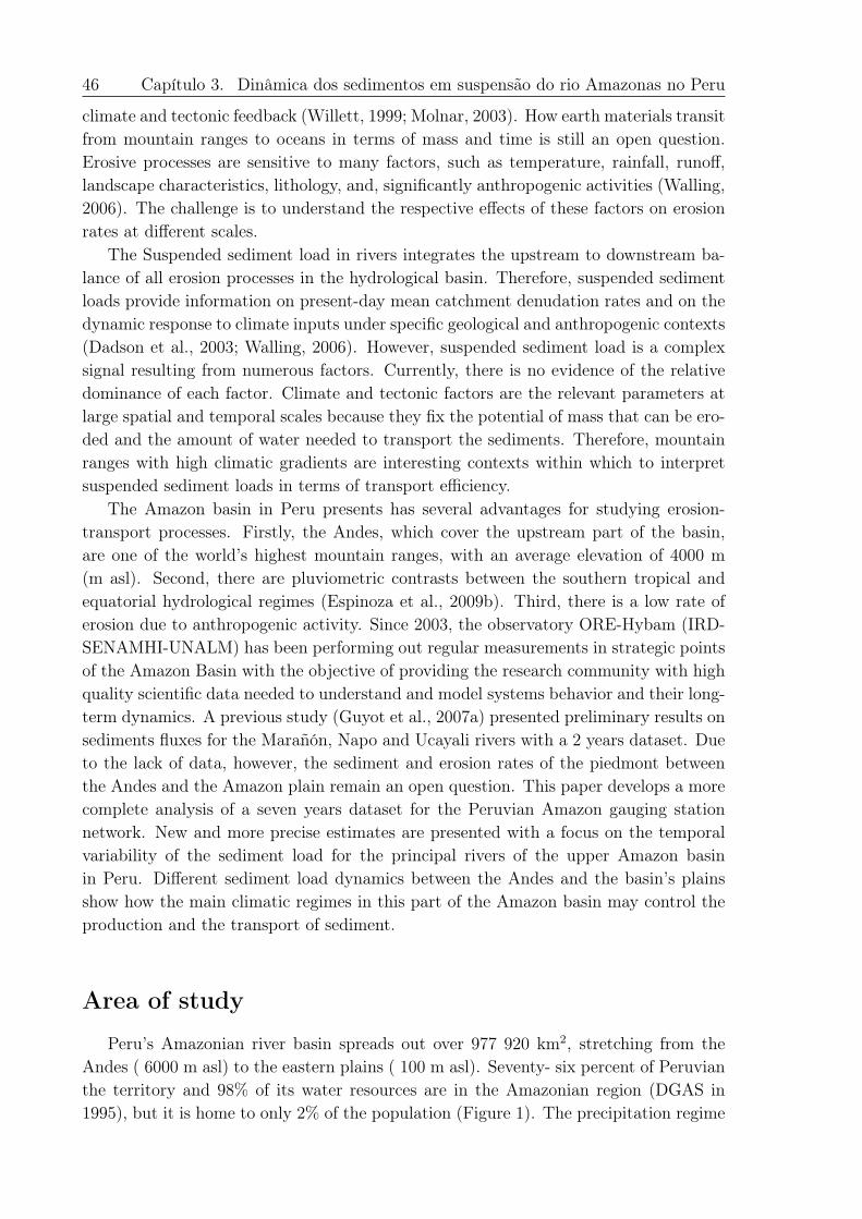
46 Capítulo 3. Dinâmica dos sedimentos em suspensão do rio Amazonas no Peru
climate and tectonic feedback (Willett, 1999; Molnar, 2003). How earth materials transitfrom mountain ranges to oceans in terms of mass and time is still an open question.Erosive processes are sensitive to many factors, such as temperature, rainfall, runoff,landscape characteristics, lithology, and, significantly anthropogenic activities (Walling,2006). The challenge is to understand the respective effects of these factors on erosionrates at different scales.
The Suspended sediment load in rivers integrates the upstream to downstream ba-lance of all erosion processes in the hydrological basin. Therefore, suspended sedimentloads provide information on present-day mean catchment denudation rates and on thedynamic response to climate inputs under specific geological and anthropogenic contexts(Dadson et al., 2003; Walling, 2006). However, suspended sediment load is a complexsignal resulting from numerous factors. Currently, there is no evidence of the relativedominance of each factor. Climate and tectonic factors are the relevant parameters atlarge spatial and temporal scales because they fix the potential of mass that can be ero-ded and the amount of water needed to transport the sediments. Therefore, mountainranges with high climatic gradients are interesting contexts within which to interpretsuspended sediment loads in terms of transport efficiency.
The Amazon basin in Peru presents has several advantages for studying erosion-transport processes. Firstly, the Andes, which cover the upstream part of the basin,are one of the world’s highest mountain ranges, with an average elevation of 4000 m(m asl). Second, there are pluviometric contrasts between the southern tropical andequatorial hydrological regimes (Espinoza et al., 2009b). Third, there is a low rate oferosion due to anthropogenic activity. Since 2003, the observatory ORE-Hybam (IRD-SENAMHI-UNALM) has been performing out regular measurements in strategic pointsof the Amazon Basin with the objective of providing the research community with highquality scientific data needed to understand and model systems behavior and their long-term dynamics. A previous study (Guyot et al., 2007a) presented preliminary results onsediments fluxes for the Marañón, Napo and Ucayali rivers with a 2 years dataset. Dueto the lack of data, however, the sediment and erosion rates of the piedmont betweenthe Andes and the Amazon plain remain an open question. This paper develops a morecomplete analysis of a seven years dataset for the Peruvian Amazon gauging stationnetwork. New and more precise estimates are presented with a focus on the temporalvariability of the sediment load for the principal rivers of the upper Amazon basinin Peru. Different sediment load dynamics between the Andes and the basin’s plainsshow how the main climatic regimes in this part of the Amazon basin may control theproduction and the transport of sediment.
Area of study
Peru’s Amazonian river basin spreads out over 977 920 km2, stretching from theAndes ( 6000 m asl) to the eastern plains ( 100 m asl). Seventy- six percent of Peruvianthe territory and 98% of its water resources are in the Amazonian region (DGAS in1995), but it is home to only 2% of the population (Figure 1). The precipitation regime
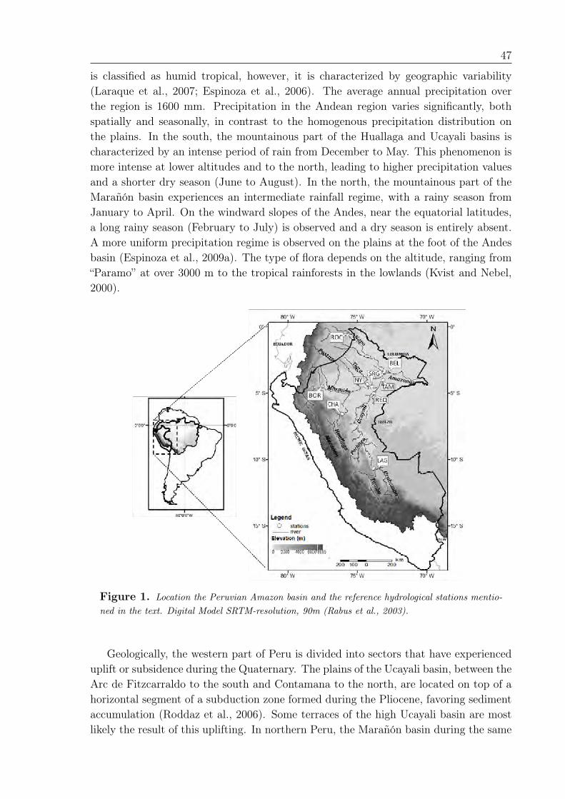
47
is classified as humid tropical, however, it is characterized by geographic variability(Laraque et al., 2007; Espinoza et al., 2006). The average annual precipitation overthe region is 1600 mm. Precipitation in the Andean region varies significantly, bothspatially and seasonally, in contrast to the homogenous precipitation distribution onthe plains. In the south, the mountainous part of the Huallaga and Ucayali basins ischaracterized by an intense period of rain from December to May. This phenomenon ismore intense at lower altitudes and to the north, leading to higher precipitation valuesand a shorter dry season (June to August). In the north, the mountainous part of theMarañón basin experiences an intermediate rainfall regime, with a rainy season fromJanuary to April. On the windward slopes of the Andes, near the equatorial latitudes,a long rainy season (February to July) is observed and a dry season is entirely absent.A more uniform precipitation regime is observed on the plains at the foot of the Andesbasin (Espinoza et al., 2009a). The type of flora depends on the altitude, ranging from“Paramo” at over 3000 m to the tropical rainforests in the lowlands (Kvist and Nebel,2000).
Figure 1. Location the Peruvian Amazon basin and the reference hydrological stations mentio-ned in the text. Digital Model SRTM-resolution, 90m (Rabus et al., 2003).
Geologically, the western part of Peru is divided into sectors that have experienceduplift or subsidence during the Quaternary. The plains of the Ucayali basin, between theArc de Fitzcarraldo to the south and Contamana to the north, are located on top of ahorizontal segment of a subduction zone formed during the Pliocene, favoring sedimentaccumulation (Roddaz et al., 2006). Some terraces of the high Ucayali basin are mostlikely the result of this uplifting. In northern Peru, the Marañón basin during the same
48 Capítulo 3. Dinâmica dos sedimentos em suspensão do rio Amazonas no Peru
period suffered subsidence that continues in the Pastaza River depression and in theinter-river zones of the Marañón and Ucayali Rivers (Dumont et al., 1992). The Arc deFitzcarraldo, perpendicular to the Andes’ axis, is the result of the horizontal subductionof the Nazca fault. The Pastaza alluvial cone, one of the world’s largest, is describedas an extremely active zone in terms of erosion dynamics (Bernal et al., 2011).
Data and methods
Data collection
Hydrological data from nine gauging stations (Table 1, Figure 1) are presented:three Hybam stations located in Peru (CHA, LAG, NY), one Hybam station locatedin Ecuador (Rocafuerte) and five SENAMHI gauging stations in Peru (BEL, BOR,SRG, REQ, TAM). ROC, BOR, CHA and LAG monitor the outlet of the Andeanpart of the Napo, Marañón, Huallaga and Ucayali rivers, respectively. The total waterbalance and sediment discharge are monitored for the Napo (BEL), Marañón (SRG) andUcayali (REQ) rivers. TAM is the first gauging station of the Amazon River mainstreamafter the confluence of the Marañón and Ucayali rivers. Note that the Amazon Riverat TAM collects inputs from both Marañón and Ucayali with few transversal inputsat the confluence (Figure1). The starting date of the regular water discharge andsediment concentration monitoring depends on the specific station (Table 1). This studyconcerns only the period during which regular monitoring for both water discharge andconcentration are available. The LAG gauging station is relatively new with two yearsof measurements.
Table 1.The network of gauging stations in the Amazon basin of Peru. Superficialsampling= samples made by one person every 10 days (observer samples). Sedimentsamples = mean concentrations of the cross section (sampling of the different depths)
STATION GAUGING RIVER LAT (deg.) LON (deg.) AREA NUMBER SEDIMENT SURFACIALPERIODCODE STATION S W Km2 OF SAMPLES SAMPLES
GAUGING
BOR Borja Marañón 4.47 77.55 114 280 20 119 305 2004-2010CHA Chazuta Huallaga 6.57 76.12 68 720 12 70 249 2004-2010NY Nva. York El Tigre 4.32 74.29 42 170 10 74 122 2006-20009LAG Lagarto Ucayali 10.61 73.87 190 810 30 256 197 2009-2010REQ Requena Ucayali 4.9 73.67 346 600 40 283 80 2006-2010SRG San Regis Marañón 4.51 73.95 361 880 36 245 191 2004-2010TAM Tamshiyacu Amazonas 4 73.16 719 640 58 441 191 2004-2010ROC* Nvo.Rocafuerte Napo 0.92 75.39 27 390 32 207 291 2001-2010BEL Bellavista Napo 3.48 73.08 100 030 20 96 168 2004-2010
*Armijos et al.,2013
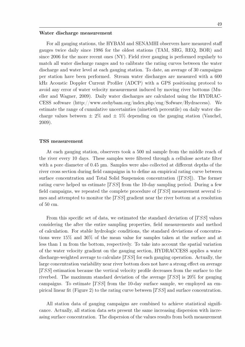
49
Water discharge measurement
For all gauging stations, the HYBAM and SENAMHI observers have measured staffgauges twice daily since 1986 for the oldest stations (TAM, SRG, REQ, BOR) andsince 2006 for the more recent ones (NY). Field river gauging is performed regularly tomatch all water discharge ranges and to calibrate the rating curves between the waterdischarge and water level at each gauging station. To date, an average of 30 campaignsper station have been performed. Stream water discharges are measured with a 600kHz Acoustic Doppler Current Profiler (ADCP) with a GPS positioning protocol toavoid any error of water velocity measurement induced by moving river bottoms (Mu-eller and Wagner, 2009). Daily water discharges are calculated using the HYDRAC-CESS software (http://www.orehybam.org/index.php/eng/Sofware/Hydraccess). Weestimate the range of cumulative uncertainties (ninetieth percentile) on daily water dis-charge values between ± 2% and ± 5% depending on the gauging station (Vauchel,2009).
TSS measurement
At each gauging station, observers took a 500 ml sample from the middle reach ofthe river every 10 days. These samples were filtered through a cellulose acetate filterwith a pore diameter of 0.45 µm. Samples were also collected at different depths of theriver cross section during field campaigns in to define an empirical rating curve betweensurface concentration and Total Solid Suspension concentration ([𝑇𝑆𝑆]). The formerrating curve helped us estimate [𝑇𝑆𝑆] from the 10-day sampling period. During a fewfield campaigns, we repeated the complete procedure of [𝑇𝑆𝑆] measurement several ti-mes and attempted to monitor the [𝑇𝑆𝑆] gradient near the river bottom at a resolutionof 50 cm.
From this specific set of data, we estimated the standard deviation of [𝑇𝑆𝑆] valuesconsidering the after the entire sampling properties, field measurements and methodof calculation. For stable hydrologic conditions, the standard deviations of concentra-tions were 15% and 36% of the mean value for samples taken at the surface and atless than 1 m from the bottom, respectively. To take into account the spatial variationof the water velocity gradient on the gauging section, HYDRACCESS applies a waterdischarge-weighted average to calculate [𝑇𝑆𝑆] for each gauging operation. Actually, thelarge concentration variability near river bottom does not have a strong effect on average[𝑇𝑆𝑆] estimation because the vertical velocity profile decreases from the surface to theriverbed. The maximum standard deviation of the average [𝑇𝑆𝑆] is 20% for gaugingcampaigns. To estimate [𝑇𝑆𝑆] from the 10-day surface sample, we employed an em-pirical linear fit (Figure 2) to the rating curve between [𝑇𝑆𝑆] and surface concentration.
All station data of gauging campaigns are combined to achieve statistical signifi-cance. Actually, all station data sets present the same increasing dispersion with incre-asing surface concentration. The dispersion of the values results from both measurement
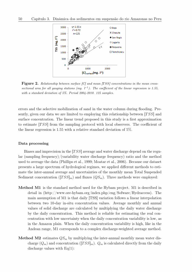
50 Capítulo 3. Dinâmica dos sedimentos em suspensão do rio Amazonas no Peru
Figure 2. Relationship between surface [C] and mean [𝑇𝑆𝑆] concentrations in the mean cross-sectional area for all gauging stations (mg. l−1). The coefficient of the linear regression is 1.55,with a standard deviation of 5%. Period 2004-2010. 125 samples.
errors and the selective mobilization of sand in the water column during flooding. Pre-sently, given our data we are limited to employing this relationship between [𝑇𝑆𝑆] andsurface concentration. The linear trend proposed in this study is a first approximationto estimate [𝑇𝑆𝑆] from the sampling protocol with local observers. The coefficient ofthe linear regression is 1.55 with a relative standard deviation of 5%.
Data processing
Biases and imprecision in the [𝑇𝑆𝑆] average and water discharge depend on the regu-lar (sampling frequency)/(variability water discharge frequency) ratio and the methodused to average the data (Phillips et al., 1999; Moatar et al., 2006). Because our datasetpresents a large spectrum of hydrological regimes, we applied different methods to esti-mate the inter-annual average and uncertainties of the monthly mean Total SuspendedSediment concentration ([𝑇𝑆𝑆]𝑚) and fluxes (𝑄𝑆𝑚). Three methods were employed:
Method M1 is the standard method used for the Hybam project. M1 is described indetail in (http://www.ore-hybam.org/index.php/eng/Sofware/Hydraccess). Themain assumption of M1 is that daily [TSS] variation follows a linear interpolationbetween two 10-day in-situ concentration values. Average monthly and annualvalues of solid discharge are calculated by multiplying the daily water dischargeby the daily concentration. This method is reliable for estimating the real con-centration with low uncertainty when the daily concentration variability is low, asin the Amazon plain. When the daily concentration variability is high, like in theAndean range, M1 corresponds to a complex discharge-weighted average method.
Method M2 estimates 𝑄𝑆𝑚 by multiplying the inter-annual monthly mean water dis-charge (𝑄𝑚) and concentration ([𝑇𝑆𝑆]𝑚). 𝑄𝑚 is calculated directly from the dailydischarge values with Eq(1):
51
𝑄𝑚 =1
𝑛
∑︁𝑄𝑚𝑖
where 𝑄𝑚𝑖 is the water discharge for the mith observation and 𝑛 is the totalnumber of observations for the month m for the entire dataset range. [𝑇𝑆𝑆]𝑚 iscalculated with a discharge-weighted mean concentration method, Eq(2):
𝑇𝑆𝑆𝑀 =
∑︀𝑇𝑆𝑆𝑚𝑖 *𝑄𝑚𝑖
𝑄𝑚𝑖
where [𝑇𝑆𝑆]𝑚𝑖 is the total suspended sediment concentration for the mith obser-vation for month 𝑚 for the entire dataset range. For each month, we suppose thatthe density distribution probability of gauging water discharges and daily waterdischarge are the same which is a necessary condition to obtain significant means
Method M3 is a rating curve method applied to derive [𝑇𝑆𝑆]𝑚 with 𝑄𝑚 when thesevariables present a univocal trend. For this study, M3 is used mainly to calculateannual water and sediment fluxes. All methods only estimate the true values of[𝑇𝑆𝑆] with uncertainty related to the in-situ measurement protocol, daily hydro-logical variability and calculation method. We assumed there is no systematic biasof concentration value in our dataset. The confidence intervals in the followingtext integrate all uncertainties of all steps of the process. To test the reliabilityof M1 and M2, we controlled the sediment mass balance budget at the confluencebetween the Marañón and Ucayali rivers with time-series of SRG, REQ and TAM.Note that this test corresponds only to a hydrologic regime with low daily waterdischarge variability
Results
All figures with monthly mean water discharge, concentrations and sediment fluxespresent values calculated with the M2 method because this method is the most widelyused in the literature and does not introduce any assumptions. However, M1 givessimilar results at monthly and annual scales.
Hydrology
In what follows, we present the principle results on the hydrology regime characte-ristics of the study region. For a more complete analysis of the hydrology of Peruvianrivers see, Espinoza et al.,(2006,2011). and . Daily water discharges (Q) are displayedin Figure 3 for the 2006-2010 series. The Andean stations (BOR, CHA, ROC) demons-trate high frequency variability superimposed on a low frequency annual cycle. Onthe plains, the hydrologic regime at SRG, REQ, TAM, and BEL reveals only a lowfrequency annual cycle. Several factors may act as low-pass filters for the hydrologicsignal. First, diffusive processes on flood wave propagation over more than 1000 km
52 Capítulo 3. Dinâmica dos sedimentos em suspensão do rio Amazonas no Peru
decrease water level fluctuations downstream (Trigg et al., 2009). Second, the shallowtopographic slope of the Amazon plain decreases the contribution of the short-termhydrologic response to river water discharge (Beighley et al., 2009).
Figure 3. Daily discharge period 2006-2010 for all gauging stations (m3 s−1).𝑎) MarañónRiver-BOR, 𝑏) Huallaga River-CHA, 𝑐) Ucayali River-LAG, 𝑑) Napo River- ROC, 𝑒) UcayaliRiver- REQ, 𝑓) Marañón River-SRG, 𝑔) Amazon River-TAM, ℎ) Napo River-BEL.
The flood amplitude at the Andean stations is equivalent to the amplitude of theannual low frequency fluctuation. The 𝑄𝑚 annual fluctuations (Figure 4) reflect theclimatic context of the southern tropical regime for the Ucayali River and the equatorialregime for the Marañón and Napo rivers (Espinoza et al., 2006; Espinoza et al., 2009a;Espinoza et al., 2011;). High water discharges occur from December to February inthe southern part of the Ucayali River (LAG), from January to March in the southernregion of the Marañón River (CHA), and from May to July in the Napo River (ROC andBEL). At BOR, the Marañón River drains an area from 2∘S to 7∘S latitude therefore,𝑄𝑚 experiences smooth annual variability as a combination of the southern tropical and
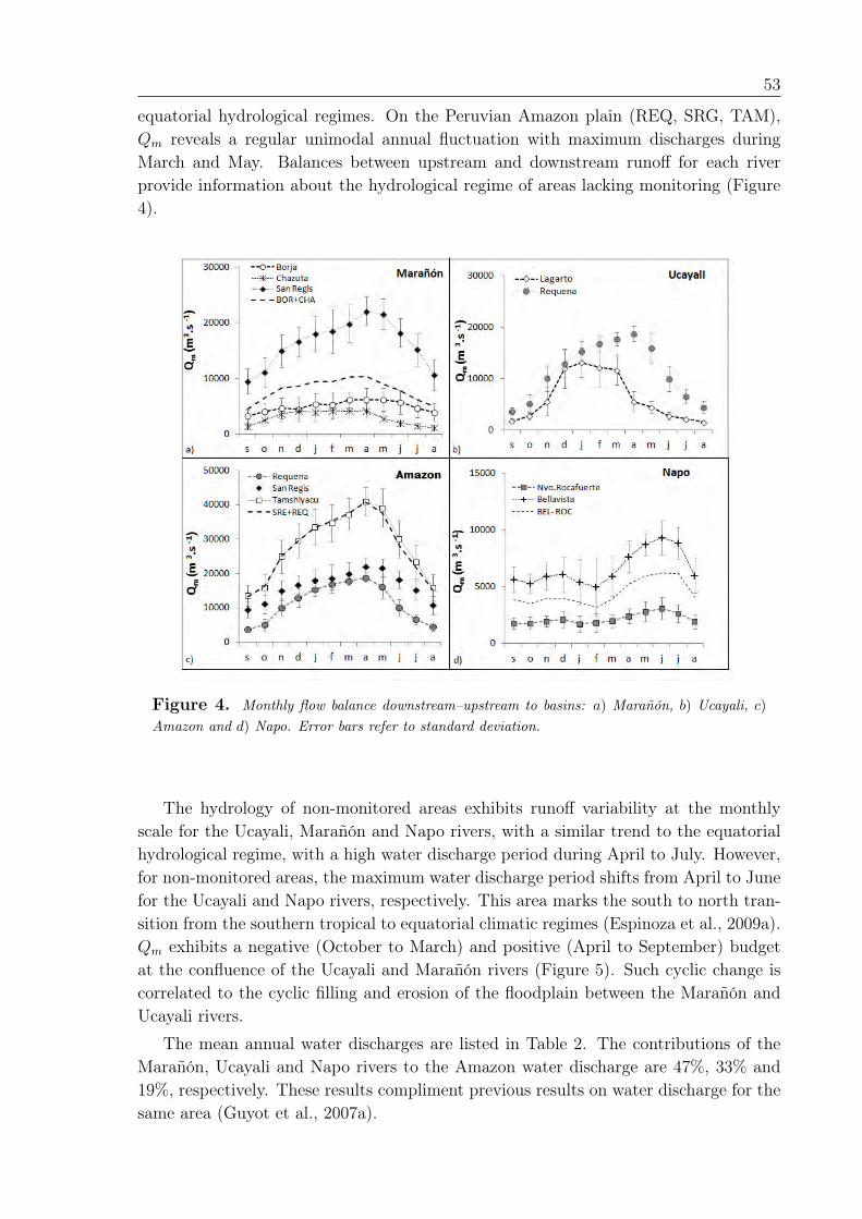
53
equatorial hydrological regimes. On the Peruvian Amazon plain (REQ, SRG, TAM),𝑄𝑚 reveals a regular unimodal annual fluctuation with maximum discharges duringMarch and May. Balances between upstream and downstream runoff for each riverprovide information about the hydrological regime of areas lacking monitoring (Figure4).
Figure 4. Monthly flow balance downstream–upstream to basins: 𝑎) Marañón, 𝑏) Ucayali, 𝑐)
Amazon and 𝑑) Napo. Error bars refer to standard deviation.
The hydrology of non-monitored areas exhibits runoff variability at the monthlyscale for the Ucayali, Marañón and Napo rivers, with a similar trend to the equatorialhydrological regime, with a high water discharge period during April to July. However,for non-monitored areas, the maximum water discharge period shifts from April to Junefor the Ucayali and Napo rivers, respectively. This area marks the south to north tran-sition from the southern tropical to equatorial climatic regimes (Espinoza et al., 2009a).𝑄𝑚 exhibits a negative (October to March) and positive (April to September) budgetat the confluence of the Ucayali and Marañón rivers (Figure 5). Such cyclic change iscorrelated to the cyclic filling and erosion of the floodplain between the Marañón andUcayali rivers.
The mean annual water discharges are listed in Table 2. The contributions of theMarañón, Ucayali and Napo rivers to the Amazon water discharge are 47%, 33% and19%, respectively. These results compliment previous results on water discharge for thesame area (Guyot et al., 2007a).
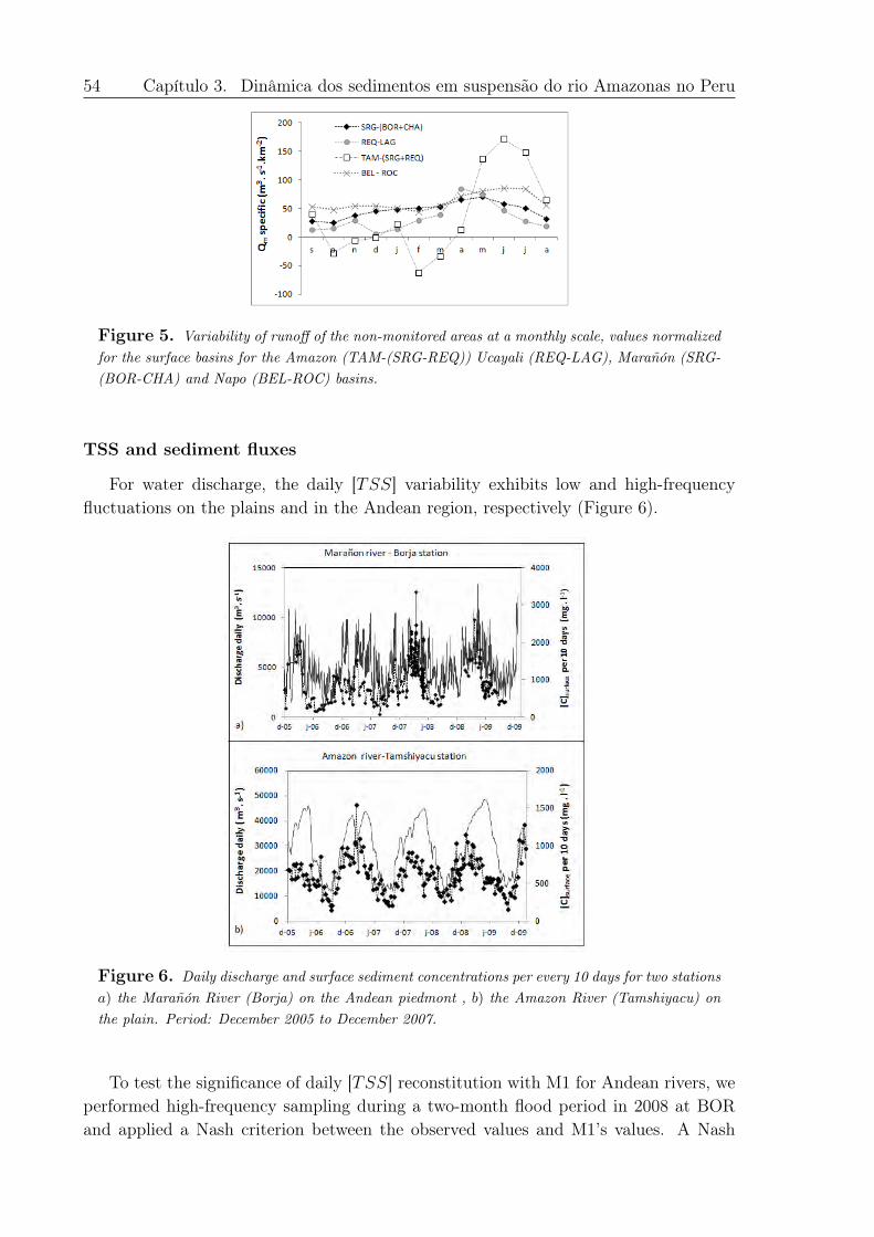
54 Capítulo 3. Dinâmica dos sedimentos em suspensão do rio Amazonas no Peru
Figure 5. Variability of runoff of the non-monitored areas at a monthly scale, values normalizedfor the surface basins for the Amazon (TAM-(SRG-REQ)) Ucayali (REQ-LAG), Marañón (SRG-(BOR-CHA) and Napo (BEL-ROC) basins.
TSS and sediment fluxes
For water discharge, the daily [𝑇𝑆𝑆] variability exhibits low and high-frequencyfluctuations on the plains and in the Andean region, respectively (Figure 6).
Figure 6. Daily discharge and surface sediment concentrations per every 10 days for two stations𝑎) the Marañón River (Borja) on the Andean piedmont , 𝑏) the Amazon River (Tamshiyacu) onthe plain. Period: December 2005 to December 2007.
To test the significance of daily [𝑇𝑆𝑆] reconstitution with M1 for Andean rivers, weperformed high-frequency sampling during a two-month flood period in 2008 at BORand applied a Nash criterion between the observed values and M1’s values. A Nash
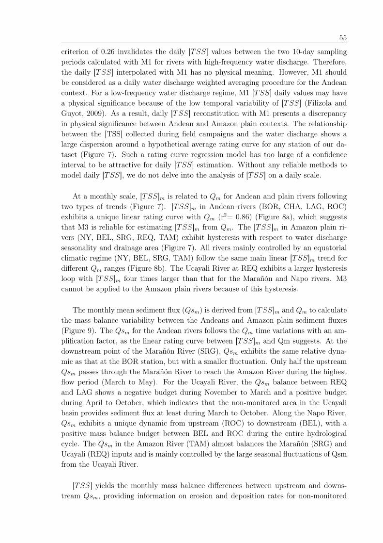
55
criterion of 0.26 invalidates the daily [𝑇𝑆𝑆] values between the two 10-day samplingperiods calculated with M1 for rivers with high-frequency water discharge. Therefore,the daily [𝑇𝑆𝑆] interpolated with M1 has no physical meaning. However, M1 shouldbe considered as a daily water discharge weighted averaging procedure for the Andeancontext. For a low-frequency water discharge regime, M1 [𝑇𝑆𝑆] daily values may havea physical significance because of the low temporal variability of [𝑇𝑆𝑆] (Filizola andGuyot, 2009). As a result, daily [𝑇𝑆𝑆] reconstitution with M1 presents a discrepancyin physical significance between Andean and Amazon plain contexts. The relationshipbetween the [TSS] collected during field campaigns and the water discharge shows alarge dispersion around a hypothetical average rating curve for any station of our da-taset (Figure 7). Such a rating curve regression model has too large of a confidenceinterval to be attractive for daily [𝑇𝑆𝑆] estimation. Without any reliable methods tomodel daily [𝑇𝑆𝑆], we do not delve into the analysis of [𝑇𝑆𝑆] on a daily scale.
At a monthly scale, [𝑇𝑆𝑆]𝑚 is related to 𝑄𝑚 for Andean and plain rivers followingtwo types of trends (Figure 7). [𝑇𝑆𝑆]𝑚 in Andean rivers (BOR, CHA, LAG, ROC)exhibits a unique linear rating curve with 𝑄𝑚 (r2= 0.86) (Figure 8a), which suggeststhat M3 is reliable for estimating [𝑇𝑆𝑆]𝑚 from 𝑄𝑚. The [𝑇𝑆𝑆]𝑚 in Amazon plain ri-vers (NY, BEL, SRG, REQ, TAM) exhibit hysteresis with respect to water dischargeseasonality and drainage area (Figure 7). All rivers mainly controlled by an equatorialclimatic regime (NY, BEL, SRG, TAM) follow the same main linear [𝑇𝑆𝑆]𝑚 trend fordifferent 𝑄𝑚 ranges (Figure 8b). The Ucayali River at REQ exhibits a larger hysteresisloop with [𝑇𝑆𝑆]𝑚 four times larger than that for the Marañón and Napo rivers. M3cannot be applied to the Amazon plain rivers because of this hysteresis.
The monthly mean sediment flux (𝑄𝑠𝑚) is derived from [𝑇𝑆𝑆]𝑚 and 𝑄𝑚 to calculatethe mass balance variability between the Andeans and Amazon plain sediment fluxes(Figure 9). The 𝑄𝑠𝑚 for the Andean rivers follows the 𝑄𝑚 time variations with an am-plification factor, as the linear rating curve between [𝑇𝑆𝑆]𝑚 and Qm suggests. At thedownstream point of the Marañón River (SRG), 𝑄𝑠𝑚 exhibits the same relative dyna-mic as that at the BOR station, but with a smaller fluctuation. Only half the upstream𝑄𝑠𝑚 passes through the Marañón River to reach the Amazon River during the highestflow period (March to May). For the Ucayali River, the 𝑄𝑠𝑚 balance between REQand LAG shows a negative budget during November to March and a positive budgetduring April to October, which indicates that the non-monitored area in the Ucayalibasin provides sediment flux at least during March to October. Along the Napo River,𝑄𝑠𝑚 exhibits a unique dynamic from upstream (ROC) to downstream (BEL), with apositive mass balance budget between BEL and ROC during the entire hydrologicalcycle. The 𝑄𝑠𝑚 in the Amazon River (TAM) almost balances the Marañón (SRG) andUcayali (REQ) inputs and is mainly controlled by the large seasonal fluctuations of Qsmfrom the Ucayali River.
[𝑇𝑆𝑆] yields the monthly mass balance differences between upstream and downs-tream 𝑄𝑠𝑚, providing information on erosion and deposition rates for non-monitored
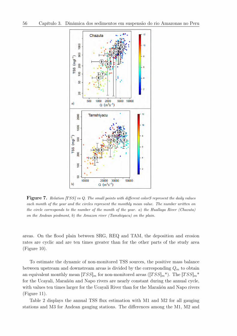
56 Capítulo 3. Dinâmica dos sedimentos em suspensão do rio Amazonas no Peru
Figure 7. Relation [𝑇𝑆𝑆] vs Q. The small points with different colorS represent the daily valueseach month of the year and the circles represent the monthly mean value. The number written onthe circle corresponds to the number of the month of the year. 𝑎) the Huallaga River (Chazuta)on the Andean piedmont, 𝑏) the Amazon river (Tamshiyacu) on the plain.
areas. On the flood plain between SRG, REQ and TAM, the deposition and erosionrates are cyclic and are ten times greater than for the other parts of the study area(Figure 10).
To estimate the dynamic of non-monitored TSS sources, the positive mass balancebetween upstream and downstream areas is divided by the corresponding 𝑄𝑚 to obtainan equivalent monthly mean [𝑇𝑆𝑆]𝑚 for non-monitored areas ([𝑇𝑆𝑆]𝑚*). The [𝑇𝑆𝑆]𝑚*for the Ucayali, Marañón and Napo rivers are nearly constant during the annual cycle,with values ten times larger for the Ucayali River than for the Marañón and Napo rivers(Figure 11).
Table 2 displays the annual TSS flux estimation with M1 and M2 for all gaugingstations and M3 for Andean gauging stations. The differences among the M1, M2 and
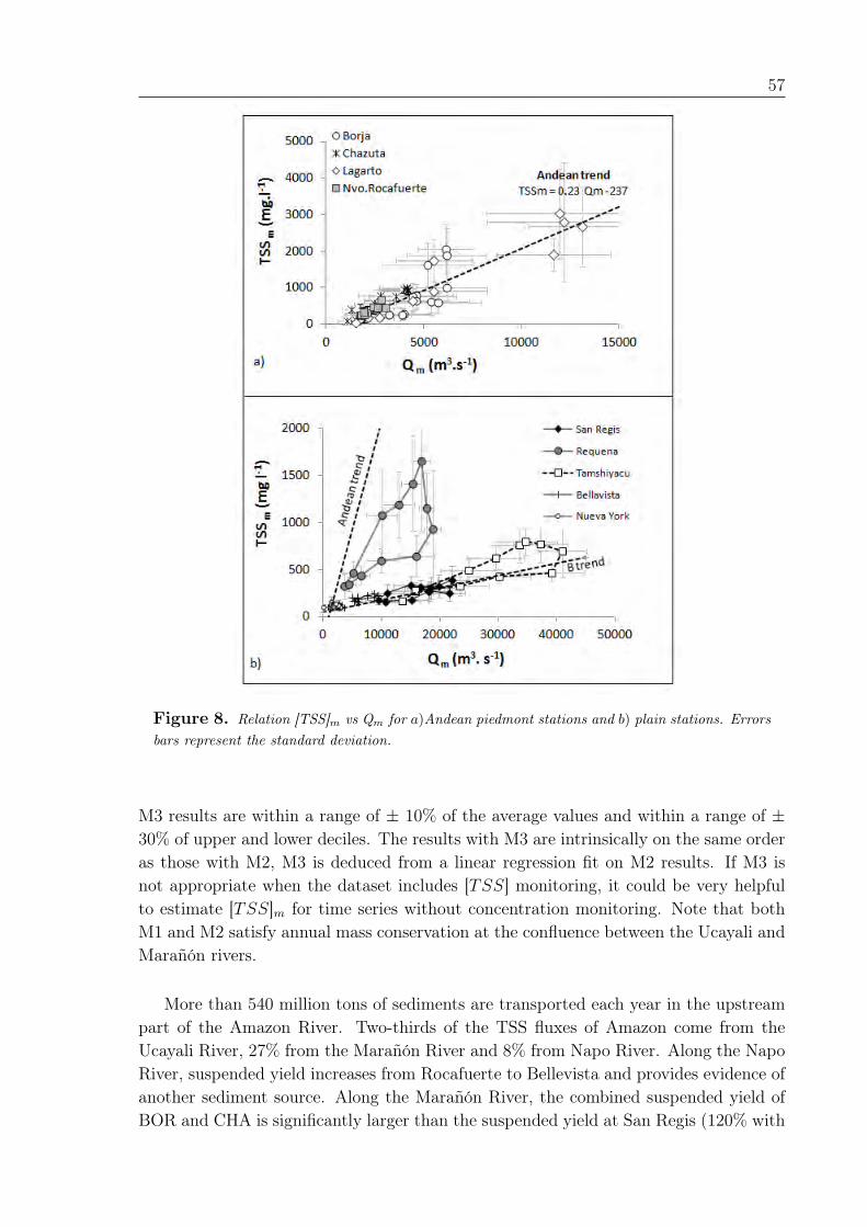
57
Figure 8. Relation [TSS]𝑚 vs Q𝑚 for 𝑎)Andean piedmont stations and 𝑏) plain stations. Errorsbars represent the standard deviation.
M3 results are within a range of ± 10% of the average values and within a range of ±30% of upper and lower deciles. The results with M3 are intrinsically on the same orderas those with M2, M3 is deduced from a linear regression fit on M2 results. If M3 isnot appropriate when the dataset includes [𝑇𝑆𝑆] monitoring, it could be very helpfulto estimate [𝑇𝑆𝑆]𝑚 for time series without concentration monitoring. Note that bothM1 and M2 satisfy annual mass conservation at the confluence between the Ucayali andMarañón rivers.
More than 540 million tons of sediments are transported each year in the upstreampart of the Amazon River. Two-thirds of the TSS fluxes of Amazon come from theUcayali River, 27% from the Marañón River and 8% from Napo River. Along the NapoRiver, suspended yield increases from Rocafuerte to Bellevista and provides evidence ofanother sediment source. Along the Marañón River, the combined suspended yield ofBOR and CHA is significantly larger than the suspended yield at San Regis (120% with
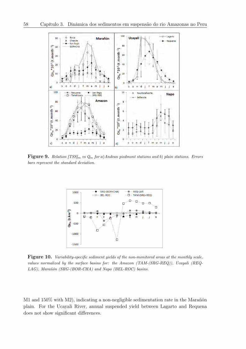
58 Capítulo 3. Dinâmica dos sedimentos em suspensão do rio Amazonas no Peru
Figure 9. Relation [TSS]𝑚 vs Q𝑚 for 𝑎)Andean piedmont stations and 𝑏) plain stations. Errorsbars represent the standard deviation.
Figure 10. Variability-specific sediment yields of the non-monitored areas at the monthly scale,values normalized by the surface basins for: the Amazon (TAM-(SRG-REQ)), Ucayali (REQ-LAG), Marañón (SRG-(BOR-CHA) and Napo (BEL-ROC) basins.
M1 and 150% with M2), indicating a non-negligible sedimentation rate in the Marañónplain. For the Ucayali River, annual suspended yield between Lagarto and Requenadoes not show significant differences.
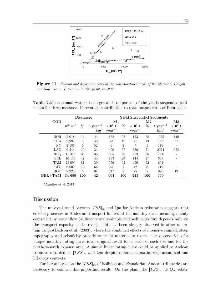
59
Figure 11. Erosion and deposition rates of the non-monitored areas of the Marañón, Ucayaliand Napo rivers. B trend = 0.013+48.62, r2=0.88.
Table 2.Mean annual water discharges and comparison of the yields suspended sedi-ments for three methods. Percentage contribution to total output ratio of Peru basin.
Discharge Yield Suspended SedimentsCOD M1 M2 M3
m3 s−1 % l year−1 *106 t % *106 t % t year−1 *106 tkm2 year−1 year−1 km2 year−1
BOR 5 018 14 44 132 22 153 28 1335 149CHA 2 984 9 43 73 12 71 13 1037 51
NY 2 187 6 52 9 2 7 1 176 -LAG 6 544 19 34 400 67 386 71 2024 378REQ 11 415 33 33 395 66 359 66 1036 -SRE 16 175 47 45 173 29 144 27 399 -TAM 28 090 81 39 556 93 499 92 694 -BEL 6 609 19 66 45 7 42 8 419 -ROC 2 226 6 81 21* 3 25 5 920 19
BEL+TAM 34 699 100 42 601 100 541 100 660
*Armijos et al.,2013
Discussion
The univocal trend between [𝑇𝑆𝑆]𝑚 and Qm for Andean tributaries suggests thaterosion processes in Andes are transport limited at the monthly scale, meaning mainlycontrolled by water flow (sediments are available and sediments flux depends only onthe transport capacity of the river). This has been already observed in other moun-tain ranges(Dadson et al., 2003), where the combined effects of intensive rainfall, steeptopography and seismicity provide sufficient material to rivers. The observation of aunique monthly rating curve is an original result for a basin of such size and for thenorth-to-south expanse area. A simple linear rating curve could be applied to Andeantributaries to deduce [𝑇𝑆𝑆]𝑚 and Qm despite different climatic, vegetation, soil andlithology contexts.
Further analysis on the [𝑇𝑆𝑆]𝑚 of Bolivian and Ecuadorian Andean tributaries arenecessary to confirm this important result. On the plain, the [𝑇𝑆𝑆]𝑚 vs 𝑄𝑚 relati-
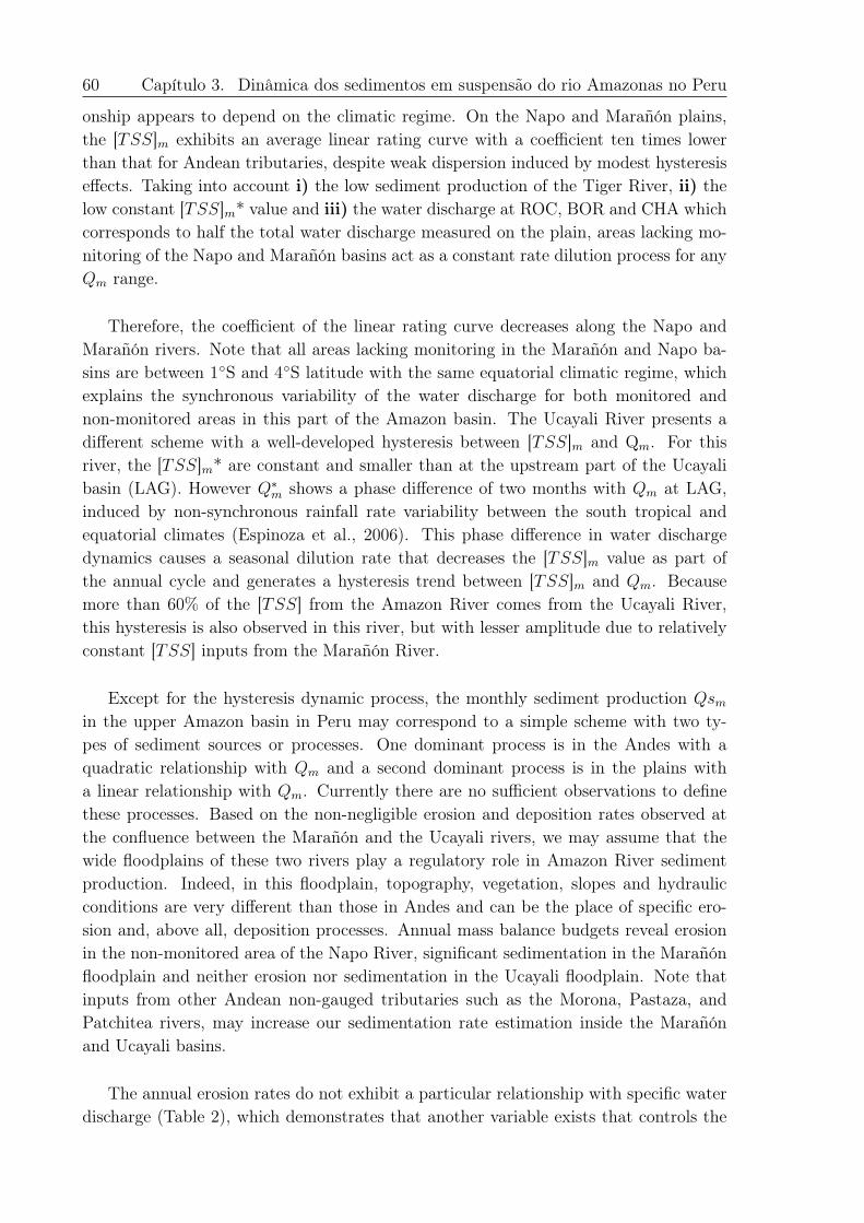
60 Capítulo 3. Dinâmica dos sedimentos em suspensão do rio Amazonas no Peru
onship appears to depend on the climatic regime. On the Napo and Marañón plains,the [𝑇𝑆𝑆]𝑚 exhibits an average linear rating curve with a coefficient ten times lowerthan that for Andean tributaries, despite weak dispersion induced by modest hysteresiseffects. Taking into account i) the low sediment production of the Tiger River, ii) thelow constant [𝑇𝑆𝑆]𝑚* value and iii) the water discharge at ROC, BOR and CHA whichcorresponds to half the total water discharge measured on the plain, areas lacking mo-nitoring of the Napo and Marañón basins act as a constant rate dilution process for any𝑄𝑚 range.
Therefore, the coefficient of the linear rating curve decreases along the Napo andMarañón rivers. Note that all areas lacking monitoring in the Marañón and Napo ba-sins are between 1∘S and 4∘S latitude with the same equatorial climatic regime, whichexplains the synchronous variability of the water discharge for both monitored andnon-monitored areas in this part of the Amazon basin. The Ucayali River presents adifferent scheme with a well-developed hysteresis between [𝑇𝑆𝑆]𝑚 and Q𝑚. For thisriver, the [𝑇𝑆𝑆]𝑚* are constant and smaller than at the upstream part of the Ucayalibasin (LAG). However 𝑄*
𝑚 shows a phase difference of two months with 𝑄𝑚 at LAG,induced by non-synchronous rainfall rate variability between the south tropical andequatorial climates (Espinoza et al., 2006). This phase difference in water dischargedynamics causes a seasonal dilution rate that decreases the [𝑇𝑆𝑆]𝑚 value as part ofthe annual cycle and generates a hysteresis trend between [𝑇𝑆𝑆]𝑚 and 𝑄𝑚. Becausemore than 60% of the [𝑇𝑆𝑆] from the Amazon River comes from the Ucayali River,this hysteresis is also observed in this river, but with lesser amplitude due to relativelyconstant [𝑇𝑆𝑆] inputs from the Marañón River.
Except for the hysteresis dynamic process, the monthly sediment production 𝑄𝑠𝑚in the upper Amazon basin in Peru may correspond to a simple scheme with two ty-pes of sediment sources or processes. One dominant process is in the Andes with aquadratic relationship with 𝑄𝑚 and a second dominant process is in the plains witha linear relationship with 𝑄𝑚. Currently there are no sufficient observations to definethese processes. Based on the non-negligible erosion and deposition rates observed atthe confluence between the Marañón and the Ucayali rivers, we may assume that thewide floodplains of these two rivers play a regulatory role in Amazon River sedimentproduction. Indeed, in this floodplain, topography, vegetation, slopes and hydraulicconditions are very different than those in Andes and can be the place of specific ero-sion and, above all, deposition processes. Annual mass balance budgets reveal erosionin the non-monitored area of the Napo River, significant sedimentation in the Marañónfloodplain and neither erosion nor sedimentation in the Ucayali floodplain. Note thatinputs from other Andean non-gauged tributaries such as the Morona, Pastaza, andPatchitea rivers, may increase our sedimentation rate estimation inside the Marañónand Ucayali basins.
The annual erosion rates do not exhibit a particular relationship with specific waterdischarge (Table 2), which demonstrates that another variable exists that controls the
61
rate of erosion apart from the variable annual flow. Presently, there are no data thatallow us to understand this observation. A greater spatial and temporal resolutionprecipitation data set (including rainfall intensity) in addition to a more detailed analysisof the local topography and seismicity would be necessary.
Conclusion
The data collected by the Hybam project have allowed this study to be realized,which is a contribution to the scientific knowledge of the Amazonian Peruvian basin,where few studies have been conducted on sediment yields. A quantification of the dis-charge and sediment yields has been performed out on a monthly and yearly basis forthe upper and lower basins of the Peruvian Amazonian region. A contribution of thiswork has is the demonstration of a simple relationship between [𝑇𝑆𝑆] and discharge forthe stations in the Andean region. On the plains, the dilution effect of the concentra-tions can create hysteresis in this relationship on a monthly basis, which means that agap exists between the discharge sources and sediment yields for the same basin.
The major part of the sediment yield is from the Andes, and the plain can act as adiffuse source or, more importantly, as a zone of sedimentation of approximately 20 to50% of the charge coming from the Andes. The same figures were found by Guyot et al.(1994) in the high basin of the Mamore River in Bolivia. Comparing the results foundin a first estimation in 2007 by Guyot et al., we can say with more confidence that theMarañón Plain is a zone of sedimentation rather than an erosion plain. To estimate thereal sedimentation rate, the suspended sediment yield coming through the Pastaza andMorona rivers needs to be quantified.
The annual rate of sedimentary flux that comes from the Peruvian basin is 541 *106
t year −1 which corresponds to 660 t year−1 km−2 ; with 70% coming from the southernregion of the basin.
Acknowledgements This study was performed with support from the Servicio Naci-onal de Meteorología e Hidrología del Perú (SENAMHI) and the Institut de Recherchepour le Dèveloppement (IRD). We would like to thank participants in the ORE-HYBAMproject from Peru (UNALM) and each of the observers of the gauging stations for hisdaily work and France (GET Toulouse).
Bibliography
Armijos, E., Laraque, A., Barba, S., Bourrel, L.,Ceron, C., Lagane, C., Magat, P.,Moquet, J.S., Pombosa, R., Sondag, F., Vera, A. Guyot , J.L. submitted. Yields of sus-pended sediment and dissolved solids from the Andean basins of Ecuador. HydrologicalSciences Journal HSJ-2011-0219.
62 Capítulo 3. Dinâmica dos sedimentos em suspensão do rio Amazonas no Peru
Beighley, R. E., Eggert, K. G., Dunne, T., He, Y., Gummadi, V., Verdin, K. L.Simulating hydrologic and hydraulic processes throughout the Amazon River Basin.Hydrological Processes.Vol.23, Issue 8, pages 1221–1235, 15 April 2009.
Bernal, C., Christophoul, F., Darrozes, J., Soula, J.C., Baby, P., Burgos, J. LateGlacial and Holocene avulsions of the Rio Pastaza Megafan (Ecuador–Peru): frequencyand controlling factors. International Journal of Earth Sciences. Geol Rundsch .2011.100:1759–1782.DOI 10.1007/s00531-010-0555-9.
Dadson, S., Hovius, N.,Chen, H., Dade, W., Hsieh, M.L.,Willett, S., Hu, J.C., Horng,M.J., Chen, M.C., Stark,C., Laguel, D., Lin, J-C. 2003. Links between erosion, runoffvariability and seismicity in the Taiwan orogen. Nature. Vol. 426. 6967.pag. 648-51.
DGAS (Dirección General de Aguas y Suelos).1995 Hacia una gestión integrada delos recursos hídricos en el Perú. Ministerio de Agricultura, Perú.
Dumont, J.F., Garcia, F., Fournier, M., 1992. Registros de cambios climáticos porlos depósitos y morfologías fluviales en la Amazonia occidental. Paleo ENSO Records.Internalcional Symposium. Lima March 1992. In Ortlieb Macharé (Eds). Orstom-Concytec. Lima 1992, p. 87-92.
Espinoza, J.C., Fraizy, P., Guyot, J.L., Ordoñez, J., Pombosa, R., Ronchail, J. 2006.La variabilité des débits du rio Amazonas au Pérou. In: IAHS (Editor), Fifth FRIENDWorld Conference held Climate Variability and Change–Hydrological Impacts. Vol 308,La Havana, Cuba, pp. 424-429.
Espinoza, J.C., Ronchail, J., Guyot, J.L., Cocheneau, G., Filizola, N., Lavado, W.,De Oliveira, E., Pombosa, R., Vauchel, P. 2009a. Spatio-temporal rainfall variability inthe Amazon Basin Countries (Brazil, Peru, Bolivia, Colombia and Ecuador). Interna-tional Journal of Climatology, 29, 1574-1594.
Espinoza, J.C., Guyot, J.L., Ronchail, J., Cochonneau, G., Filizola, N., Fraizy, P.,De Oliveira, E., Ordoñez, J., Vauchel, P. 2009b.Contrasting regional discharge evoluti-ons in the Amazon Basin (1974–2004). J Hydrol 375:297–311.
Espinoza, J.C ., Lengaigne, M., Ronchail, J., Janicot, S. 2011. Large-scale circula-tion patterns and related rainfall in the Amazon Basin: a neuronal networks approach.Earth and Environmental Science. Climate Dynamics. DOI 10.1007/s00382-011-1010-8.
Filizola, N., Guyot, J.L. 2009. Suspended sediment yields in the Amazon basin: anassessment using the Brazilian national data set. Hydrological Processes 23, 3207–3215.DOI: 10.1002/hyp.7394
Guyot, J.L., Bourges J., Cortez J., 1994. Sediment transport in the Rio Grande, anAndean river of the Bolivian Amazon drainage basin. IAHS Publ n° 224 (Proceedingsof the Camberra Symposium).
63
Guyot, J.L., Bazan, H., Fraizy, P., Ordonez, J., Armijos. E., Laraque. A. 2007.Suspended sediment yields in the Amazon basin of Peru, a first estimation.. HS2005-Water quality and sediment behaviour of the future: Predictions.
Kvist, L.P.,Nebel, G. 2000.Bosque de la llanura aluvial del Perú: Ecosistemas, habi-tantes y uso de los recursos. Folia Amazónica. Vol 10. Instituto de Investigaciones dela Amazonia Peruana.
Laraque, A., Ronchail, J., Cochonneau, G., Pombosa, R., Guyot, J.L. 2007.Hetero-geneous distribution of rainfall and discharge regimes in the Ecuadorian Amazon basin.Journal of Hydrometeorology 8:1364–1381.
Molnar, P. 2003. Nature, nurture and landscape Geomorphology.Nature.Vol 426 .11December 2003.
Moatar, F., Person, G., Meybeck, M., Coynel, A., Etcheber, H., Crouzet, P.H. 2006.The influence of contrasting suspended particulate matter transport regimes on the biasand precision of flux estimates . Science of the Total Environment .370 : 515-531.
Mueller, D.S., Wagner, C.R. 2009. Measuring Discharge with Acoustic Doppler Cur-rent Profilers from a Moving Boat. USGS Techniques and Methods 3- A22.
Phillips, J.M., Webb, B.W., Walling, D.E., Leeks, G.J.L.1999. Estimating the sus-pended sediment loads of rivers in the LOIS study area using infrequent samples. Hy-drological Processes. Special Issue: River Basin Sediment Dynamics.Vol. 13, Issue 7,pages 1035–1050. May 1999.
Rabus, B., Eineder, M., Roth, A., Bamler, R. 2003. The Shuttle Radar TopographyMission a new class of digital elevation models acquired by spaceborne radar. Photoand Rem. Sen. 57, 241-262.
Roddaz, M., Brusset, S., Baby, P.,Hérail, G., 2006. Miocene tidal-influenced sedi-mentation to continental Pliocene sedimentation in the forebulge-backbulge depozonesof the Beni-Mamore foreland Basin (northern Bolivia). Journal of South 1290 AmericanEarth Sciences, 20(4), 351-368.
Trigg, M., Wilson, M.D., Batesa, P.D., Horritt, M.S., Alsdorf, D.E., Forsberg, B.R.,Vega, M.C. 2009. Amazon flood wave hydraulics. Journal of Hydrology. Vol. 374,Issues 1-2, 30 July 2009, Pages 92-105 doi:10.1016/j.jhydrol.2009.06.
Vauchel, P. 2009. Hidromesad: Logiciel de gestión y tratamiento de datos hidroló-gicos y de sedimentos. Informe Técnico Proyecto Hybam Lima-Perú.
Walling, D. E. 2006. Human impact on land–ocean sediment transfer by the world’srivers. Geomorphology. Vol.79, Issues 3-4, 30 September 2006, Pages 192-216.37thBinghamton Geomorphology Symposium.

64 Capítulo 3. Dinâmica dos sedimentos em suspensão do rio Amazonas no Peru
Willet, S. 1999. Orogeny and orography: The effects of erosion on the structure ofmountain belts. Journal of Geophysical Research. Vol 104.No.B12 pages 28,957-28981,December 10, 1999.
Capítulo 4
Nova estimação do fluxo sedimentáriono rio Amazonas
New estimates of suspended sediment flux inthe Amazon River link coarse sediment flux toclimate variability
ResumoA biodiversidade e produtividade ecológica e da floresta das várzeas na bacia Amazô-
nica esta baseada em nutrientes e matéria orgânica associada aos sedimentos em suspen-são. Neste contexto, destaca-se a importância de quantificar os sedimentos em suspensãono rio Amazonas. As analises de 586 amostras obtidas durante o período 1995-2013 in-dicam que os sedimentos em suspensão do baixo Amazonas estão compostos de doistipos de sedimentos em função de sua granulometria: sedimentos finos (15 µm) e sedi-mentos grosseiros de (150 µm), e cada tipo de sedimento apresenta uma diferente taxade transporte durante o ano hidrológico. O fluxo de sedimentos no baixo Amazonas éde 1100 Mt ano−1 ± 25%, dos quais 60% correspondem ao fluxo de sedimentos finos e40% correspondem ao fluxo de sedimentos grosseiros. Existem evidencias da sensibili-dade dos sedimentos frente a variabilidade climática, mas esta depende da distribuiçãoespacial e sazonal das precipitações. Pode-se observar que existe um incremento dos se-dimentos finos durante os anos El Niño assim como também um aumento de sedimentosgrosseiros durante os anos La Niña e em episodios do dipolo do Altlântico Tropical.
65
66 Capítulo 4. Nova estimação do fluxo sedimentário no rio Amazonas
RésuméLa biodiversité et la productivité de la forêt amazonienne dans la plaine d’inondation
est basée sur les nutriments et la matière organique associés aux sédiments en suspen-sion. Dans ce contexte, nous mettons en lumiére l’importance d’une quantification dessédiments en suspension de l’Amazone. L’analyse de 586 échantillons collectés entre1995 et 2013 montre que la concentration de sédiments en suspension sur la basse Ama-zone est composée de deux populations de sédiments de tailles différentes : sédimentsfins (10 µm) et grossiers (250 µm). Chaque population présente un taux de transportdifférent tout au long de l’année hydrologique. Le flux de sédiments en suspension dela basse Amazone est estimé à 1100 Mt an−1 ± 25%, dont 60% est constitué du flux desédiments fins et 40% de celui des grossiers. Nous mettons en évidence la sensibilité duflux sédimentaire à la variabilité climatique quoique cette sensibilité dépende du type desédiment, et de la distribution spatiale des précipitations sur le bassin et de leur saison-nalité. De fait, le flux de sédiments grossiers augmente lors des années caractérisées pardes épisodes froids dans la zone du Pacifique central équatorien (La Niña) et pendantles annés do dipole do Atlantique Tropical.
67
New estimates of suspended sediment flux in the Amazon Riverlink coarse sediment flux to climate variability
E. Armijos1,2*, N. Filizola3, A. Crave4, J.C. Espinoza5, P. Fraizy6, P. Vauchel,6, R.Espinoza7, J.M. Martinez6, P. Ribeiro 1, R.A. Dos Santos 3,8, G. Cochonneau 6, P.Fonseca1, E. De Oliveira9, W. Santini6 and J.L. Guyot6.
1 − Programa de Pós-graduação CLIAMB, Instituto Nacional de Pesquisas da Amazônia (INPA),Universidade do Estado do Amazonas (UEA), Manaus, Brasil.2 − Université Paul Sabatier, Toulouse, France.3 − Universidade Federal do Amazonas (UFAM), Manaus, Brasil.4 − Géoscience Rennes, CNRS UMR 6118, Rennes, France.5 − Subdirección de ciencias de la atmósfera e hidrósfera-Instituto Geofísico del Perú (IGP), Lima,Perú.6 − Géoscience Environnement Toulouse (GET- CNRS, IRD, Université de Toulouse),Toulouse,France.7 − Géoscience Environnement Toulouse (IRD/GET), Toulouse, France.8 − Universidad Nacional Mayor de San Marcos, Lima, Perú.9 − Serviço Geológico do Brasil (CPRM), Manaus,Brasil.10 − Agência Nacional da Agua (ANA), Brasília, Brasil.
Abstract
The biodiversity and productivity of the Amazon floodplain depend on nutrients andorganic matter transported with suspended sediments (1). However, there are still fun-damental unknowns about how hydrological and climatic variability influence sedimentflux in the Amazon River. To address this gap we analyzed sediment samples collectedevery ten days from 1995-2014. We found a bimodal distribution of sediment sizes, withdistinct fine (15 µm) and coarse sediments (150 µm), which followed contrasting seaso-nal and long-term patterns. By taking these dynamics into account, we estimate thesuspended sediment flux of the lower Amazon River is 1100 Mt year−1 ±25%, of which60% is fine and flux and 40% is coarse suspended flux. We establish that suspendedsediment flux is linked to climate, with higher coarse suspended sediment flux duringcool episodes in the central equatorial Pacific (La Niña) and the warm phase of theTropical South Atlantic.
The Amazon River accounts for almost of fifth of global freshwater discharge (2)
and supplies the majority of the Atlantic Ocean’s sediment (3, 4). The water and se-
diment flowing through Amazon carry carbon and nutrients that fuel productivity on
the immense Amazon floodplain resulting in globally relevant fluxes of organic carbon
(5), water vapor (6, 7), and CO2 (8). The expansion of hydropower and agriculture
has put severe pressure on the Amazon basin, altering discharge and sediment flux (9,
10). Indeed, 151 new dams are currently planned on five major Andean tributaries (11).
As such, the Amazon Basin is a critical and strategic zone for studying the effects of
climate change and direct human disturbance on water, sediment, and biogeochemical
68 Capítulo 4. Nova estimação do fluxo sedimentário no rio Amazonas
fluxes.
The Amazon Basin includes regions with contrasting topography, climate, and hy-
drology, sediment flux depends on the timing and amount of regional discharge and the
availability of sediment sources. Tributaries from the Andes supply the majority of sedi-
ments, nutrients, and organic matter to the main stem of the Amazon (1 and 12-16). As
the Amazon nears the ocean, it receives influx from the Peruvian, Colombian and Ecu-
adorian Andes in the Solimões River (contributing 60% of annual average discharge),
the Peruvian and Bolivian Andes in the Madeira River (15% of discharge), and the
Guyana shield in the Negro River (14% of discharge; 17 ). The Solimões and Madeira
rivers are rich in suspended sediment, while the Negro River is largely sediment-free.
Peak rainfall occurs from March to May in the northern region (the Negro basin), and
from December to February in the southern and western regions (7). These differences
in rainfall produce a flood period on the main stem from May to June, and a low water
period from September to November.
Previous studies have shown that Amazon River discharge is related to climate varia-
bility (18-19), however, the relationship between the interannual climate variability and
sediment flux in the Amazon is unknown. There has been an intensification of extreme
hydrological events in the Amazon basin during the last decades linked to anomalies in
the surface temperature of the Pacific and Atlantic Oceans. El Niño conditions (1998,
2003) or warm episodes in the Tropical North Atlantic (2005, 2010) have been associ-
ated with extreme droughts, while La Niña or warm conditions in the Tropical South
Atlantic (1999, 2009, 2012) are related to extreme floods (20-29).
Sediment flux in the Amazon is poorly constrained with current estimates of sedi-
ment flux varying by a factor of two (600 to 1300 Mt year−1) at the most downstream
Óbidos gauging station (30-34). The difference in the estimates is the difficulty in per-
forming measurements with the traditional methods due to the large scale of the cross
section and also high cost for monitoring in long-term. To explore the possible link
between climate and sediment flux, we used samples obtained every ten days during
twenty years of sediment monitoring at the Óbidos gauging station from 1995 to 2014
(Fig 1A,1C). This dataset of 622 samples provides unprecedented temporal resolution
and enables improved estimates of sediment load and the identification of climatic con-
trols. One of our main findings is that the suspended sediment at Óbidos has two
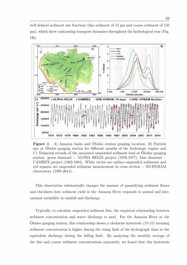
69
well-defined sediment size fractions (fine sediment of 15 µm and coarse sediment of 150
µm), which show contrasting transport dynamics throughout the hydrological year (Fig.
1B).
Figure 1. 𝐴) Amazon basin and Óbidos station gauging location; 𝐵) Particlesize at Óbidos gauging station for different months of the hydrologic regime and𝐶) Temporal records of the measured suspended sediment load at Óbidos gaugingstation: green diamond = ALPHA HELIX project (1976-1977); blue diamond =CAMREX project (1982-1984). White circles are surface suspended sediments andred squares are suspended sediment measurement in cross section = SO-HYBAMobservatory (1995-2014). .
This observation substantially changes the manner of quantifying sediment fluxes
and elucidates how sediment yield in the Amazon River responds to annual and inte-
rannual variability in rainfall and discharge.
Typically, to calculate suspended sediment flux, the empirical relationship between
sediment concentration and water discharge is used. For the Amazon River at the
Óbidos gauging station, this relationship shows a clockwise hysteresis (33-35) meaning
sediment concentration is higher during the rising limb of the hydrograph than at the
equivalent discharge during the falling limb. By analyzing the monthly average of
the fine and coarse sediment concentrations separately, we found that this hysteresis
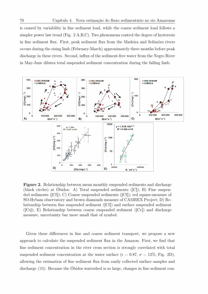
70 Capítulo 4. Nova estimação do fluxo sedimentário no rio Amazonas
is caused by variability in fine sediment load, while the coarse sediment load follows a
simpler power law trend (Fig. 2 A,B,C). Two phenomena control the degree of hysteresis
in fine sediment flux. First, peak sediment flux from the Madeira and Solimões rivers
occurs during the rising limb (February-March) approximately three months before peak
discharge in these rivers. Second, influx of the sediment-free water from the Negro River
in May-June dilutes total suspended sediment concentration during the falling limb.
Figure 2. Relationship between mean monthly suspended sediments and discharge(black circles) at Óbidos: A) Total suspended sediments ([C]); B) Fine suspen-ded sediments ([Cf]); C) Coarse suspended sediments ([Cf]); red square-measure ofSO-Hybam observatory and brown diamonds measure of CAMREX Project; D) Re-lationship between fine suspended sediment ([Cf]) and surface suspended sediment([Cs]); E) Relationship between coarse suspended sediment ([Cc]) and dischargemeasure, uncertainty bar more small that of symbol.
Given these differences in fine and coarse sediment transport, we propose a new
approach to calculate the suspended sediment flux in the Amazon. First, we find that
fine sediment concentration in the river cross section is strongly correlated with total
suspended sediment concentration at the water surface (r = 0.87, 𝜎 = 12%; Fig. 2D),
allowing the estimation of fine sediment flux from easily collected surface samples and
discharge (33). Because the Óbidos watershed is so large, changes in fine sediment con-
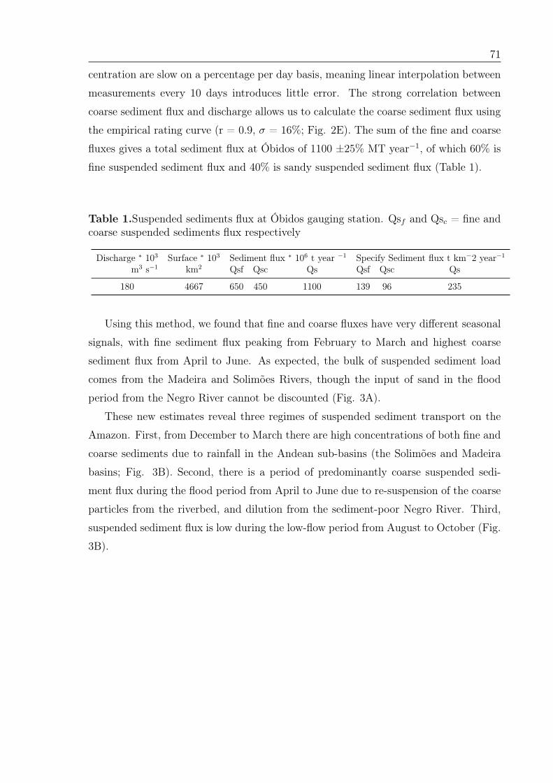
71
centration are slow on a percentage per day basis, meaning linear interpolation between
measurements every 10 days introduces little error. The strong correlation between
coarse sediment flux and discharge allows us to calculate the coarse sediment flux using
the empirical rating curve (r = 0.9, 𝜎 = 16%; Fig. 2E). The sum of the fine and coarse
fluxes gives a total sediment flux at Óbidos of 1100 ±25% MT year−1, of which 60% is
fine suspended sediment flux and 40% is sandy suspended sediment flux (Table 1).
Table 1.Suspended sediments flux at Óbidos gauging station. Qs𝑓 and Qs𝑐 = fine andcoarse suspended sediments flux respectively
Discharge * 103 Surface * 103 Sediment flux * 106 t year −1 Specify Sediment flux t km−2 year−1
m3 s−1 km2 Qsf Qsc Qs Qsf Qsc Qs
180 4667 650 450 1100 139 96 235
Using this method, we found that fine and coarse fluxes have very different seasonal
signals, with fine sediment flux peaking from February to March and highest coarse
sediment flux from April to June. As expected, the bulk of suspended sediment load
comes from the Madeira and Solimões Rivers, though the input of sand in the flood
period from the Negro River cannot be discounted (Fig. 3A).
These new estimates reveal three regimes of suspended sediment transport on the
Amazon. First, from December to March there are high concentrations of both fine and
coarse sediments due to rainfall in the Andean sub-basins (the Solimões and Madeira
basins; Fig. 3B). Second, there is a period of predominantly coarse suspended sedi-
ment flux during the flood period from April to June due to re-suspension of the coarse
particles from the riverbed, and dilution from the sediment-poor Negro River. Third,
suspended sediment flux is low during the low-flow period from August to October (Fig.
3B).
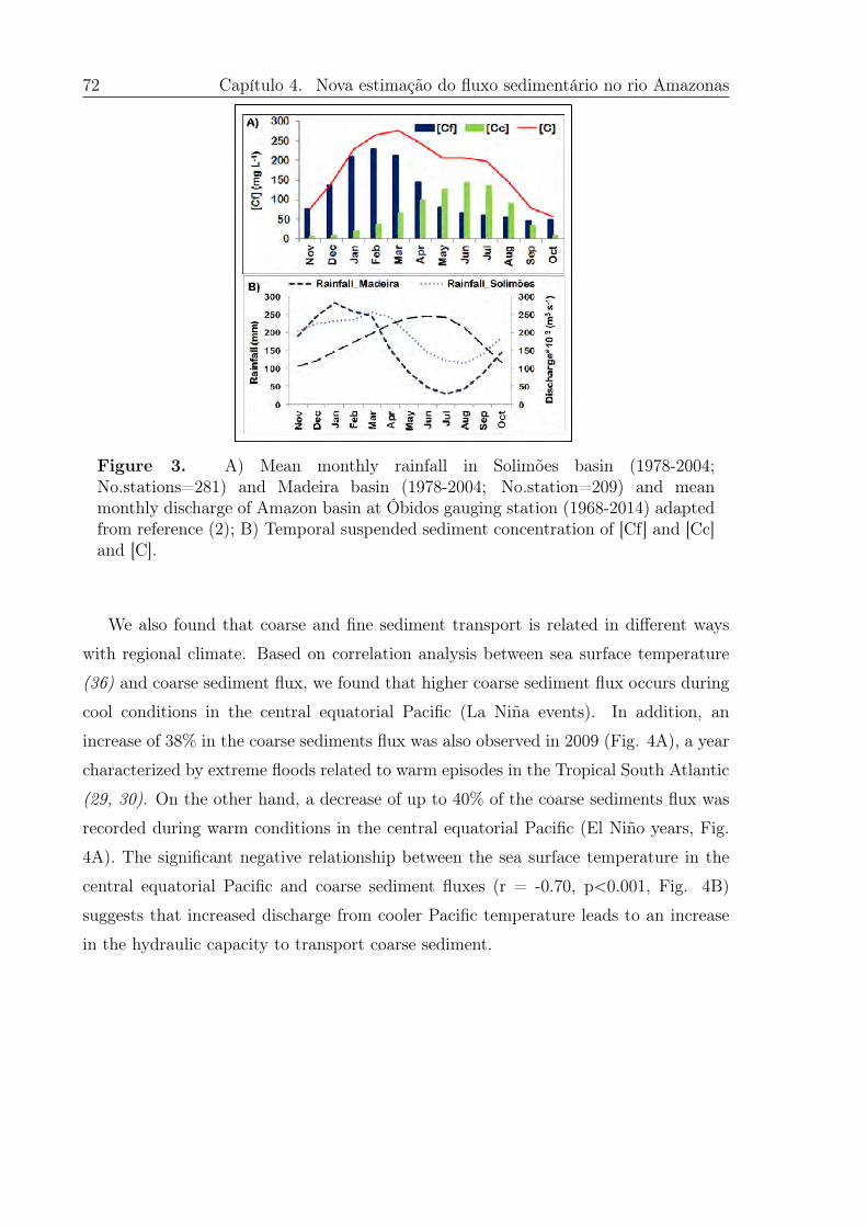
72 Capítulo 4. Nova estimação do fluxo sedimentário no rio Amazonas
Figure 3. A) Mean monthly rainfall in Solimões basin (1978-2004;No.stations=281) and Madeira basin (1978-2004; No.station=209) and meanmonthly discharge of Amazon basin at Óbidos gauging station (1968-2014) adaptedfrom reference (2); B) Temporal suspended sediment concentration of [Cf] and [Cc]and [C].
We also found that coarse and fine sediment transport is related in different ways
with regional climate. Based on correlation analysis between sea surface temperature
(36) and coarse sediment flux, we found that higher coarse sediment flux occurs during
cool conditions in the central equatorial Pacific (La Niña events). In addition, an
increase of 38% in the coarse sediments flux was also observed in 2009 (Fig. 4A), a year
characterized by extreme floods related to warm episodes in the Tropical South Atlantic
(29, 30). On the other hand, a decrease of up to 40% of the coarse sediments flux was
recorded during warm conditions in the central equatorial Pacific (El Niño years, Fig.
4A). The significant negative relationship between the sea surface temperature in the
central equatorial Pacific and coarse sediment fluxes (r = -0.70, p<0.001, Fig. 4B)
suggests that increased discharge from cooler Pacific temperature leads to an increase
in the hydraulic capacity to transport coarse sediment.
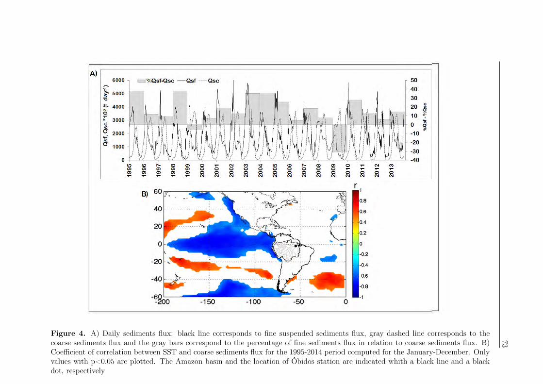
73
Figure 4. A) Daily sediments flux: black line corresponds to fine suspended sediments flux, gray dashed line corresponds to thecoarse sediments flux and the gray bars correspond to the percentage of fine sediments flux in relation to coarse sediments flux. B)Coefficient of correlation between SST and coarse sediments flux for the 1995-2014 period computed for the January-December. Onlyvalues with p<0.05 are plotted. The Amazon basin and the location of Óbidos station are indicated whith a black line and a blackdot, respectively
74 Capítulo 4. Nova estimação do fluxo sedimentário no rio Amazonas
Based on our dataset (1995-2014), we found no relationship between the maximum
and minimum fine sediments flux and the extreme hydrological events (r = 0.11 and
0.02). This results could be due to differences in rainfall regime and the different
forcing act separately in the main tributaries of Amazon River (Solimões, Madeira and
Negro Rives). Indeed, 2005 and 2010 droughts had different effects, while 2005 was
more intense in southwestern Amazonia while 2010 was stronger in central and eastern
Amazonia (37). However in locale scale e.g. in the Bolivian Amazon, for instance (Beni
and Mamoré rivers), it is observed the accumulation of fine sediments during the floods
associated with La Niña events (38).
In summary, the suspended sediment flux in the Amazon River at Óbidos shows a
bimodal size distribution, with fine sediments near 15 µm accounting for 60% of annual
sediment load and coarse sediments of 150 µm accounting for 40%. Coarse sediment
flux was strongly related with discharge, meaning that this part of the sediment flux
is correlated with the climatic oceanic indices that control Amazon basin hydrology.
The relationship between the fine sediment flux sediment and discharge presents a more
complex hysteresis trend related to the different production phases of the main fine
sediment sources over the Amazon basin. To answer the question of what controls
fine sediment flux in the Amazon, accurate time and spatial monitoring of the fine
sediment on the Amazon mainstem and major sub-basins are required. We suggest
that the methodology from this study be applied in the Andean rivers of the Amazon
basin, namely the separation of the granulometric mode to explore the relationships
with hydrology and climatic indices.
75
References and Notes1. M. McClain, R. Naiman., Andean influences on the biogeochemistry and ecology
of the Amazon River.BioScience. 58, 325-338 (2008).
2. J. Callède, et al., Les apports en eau de l’Amazone à l’Océan Atlantique. Revuedes sciences de l’eau/Journal of Water Science. 23, 247-273 (2010).
3. J. P. Syvitski, S. D. Peckham, R. Hilberman, T. Mulder, Predicting the terres-trial flux of sediment to the global ocean: a planetary perspective. SedimentaryGeology. 162, 5-24 (2003).
4. J. D. Milliman, K. L. Farnsworth, River discharge to the coastal ocean: a globalsynthesis (Cambridge University Press, 2011).
5. P. Moreira ˘ Turcq, et al., Exportation of organic carbon from the Amazon Riverand its main tributaries. Hydrological Processes. 17, 1329-1344. (2003).
6. E. Salati, P. B. Vose, Amazon basin: a system in equilibrium. Science. 225(1984).
7. J.C. Espinoza, et al., Spatio temporal rainfall variability in the Amazon basincountries (Brazil, Peru, Bolivia, Colombia, and Ecuador). International Journalof Climatology. 29, 1574-1594 (2009).
8. G. Abril, et al., Amazon River carbon dioxide outgassing fuelled by wetlands.Nature. 505, 395-398 (2013).
9. E. A. Davidson, et al., The Amazon basin in transition, Nature. 481, 321-328(2012).
10. J. Ferreira, et al., Brazil’s environmental leadership at risk, Science. 346, 706-707(2014).
11. M. Finer, C. Jenkis, Proliferation of hydroelectric dams in the Andean Amazonand implications for Andes-Amazon connectivity, Plos one. 7, e35126 (2012).
12. E. Armijos, et al., Suspended sediment dynamics in the Amazon River of Peru.Journalof South American Earth Sciences. 44, 75-84 (2013).
13. E. Armijos, et al., Yields of suspended sediment and dissolved solids from theAndean basins of Ecuador. Hydrological Sciences Journal. 58, 1478-1494 (2013).
14. R. Espinoza Villar, et al., A study of sediment transport in the Madeira River,Brazil, using MODIS remote-sensing images. Journal of South American EarthSciences. 44, 45-54 (2013).
15. J. S. Moquet, et al., Cl and Na Fluxes in an Andean Foreland Basin of the PeruvianAmazon: An Anthropogenic Impact Evidence. Aquatic Geochemistry. 20, 613-637 (2014).
16. W. Santini et al., Sediment budget in the Ucayali River basin, an Andean tributaryof the Amazon River. IAHS Publ. 367 (2014).
17. N. Filizola, J.L. Guyot, Suspended sediment yields in the Amazon basin: anassessment using the Brazilian national data set. Hydrological Processes. 23,3207-3215 (2009).
18. J. C. Espinoza, et al., Contrasting regional discharge evolutions in the Amazonbasin (1974–2004). Journal of Hydrology. 375, 297-311 (2009).
76 Capítulo 4. Nova estimação do fluxo sedimentário no rio Amazonas
19. J. Callède, et al., Evolution du débit de l’Amazone à Óbidos de 1903 à 1999.Hydrological Sciences Journal.49, 85-97 (2004).
20. J. C. Espinoza, et al., Climate variability and extreme drought in the upperSolimões River (western Amazon Basin): Understanding the exceptional 2010drought. Geophysical Research Letters. 38 (2011).
21. M. Gloor, et al., Intensification of the Amazon hydrological cycle over the last twodecades. Geophysical Research Letters. 40, 1729-1733 (2013).
22. J. A. Marengo, J. A, et al. Two Contrasting Severe Seasonal Extremes in TropicalSouth America in 2012: Flood in Amazonia and Drought in Northeast Brazil.Journal of Climate. 26, 9137-9154 (2013).
23. J.C. Espinoza, et al., From drought to flooding: understanding the abrupt 2010-11hydrological annual cycle in the Amazonas River and tributaries. EnvironmentalResearch Letters. 7, 024008 (2012).
24. J. A. Marengo, J. Tomasella, W. R. Soares, L. M. Alves, C. A. Nobre, Extremeclimatic events in the Amazon basin. Theoretical and Applied Climatology. 107,73-85 (2012).
25. J.A. Marengo, J.C.Espinoza, Extreme seasonal droughts and floods in Amazonia:causes, trends and impacts. International Journal of Climatology. 1097, (2015).
26. J. A. Marengo, et al., The drought of Amazonia in 2005. Journal of Climate. 21,495-516 (2008).
27. J. A. Marengo, et al., The drought of 2010 in the context of historical droughtsin the Amazon region. Geophysical Research Letters. 38, L12703 (2011).
28. J. C. Espinoza, et al., Climate variability and extreme drought in the upperSolimões River (western Amazon Basin): Understanding the exceptional 2010drought. Geophysical Research Letters. 38 (2011).
29. J. A. Marengo, J. Tomasella, W. R. Soares, L. M. Alves, C. A. Nobre, Extremeclimatic events in the Amazon basin. Theoretical and Applied Climatology. 107,73-85 (2012).
30. J.A. Marengo, J.C. Espinoza, Extreme seasonal droughts and floods in Amazonia:causes, trends and impacts. International Journal of Climatology. 1097, (2015).
31. R. J. Gibbs, Amazon River: Environmental factors that control its dissolved andsuspended load. Science. 156, 1734-1737 (1967).
32. R. H. Meade, et al., Sediment loads in the Amazon River. Nature. 278, 161-163(1979).
33. R. H. Meade, T. Dune, J.E. Richey, U. Santos, E. Salati, Storage and remobiliza-tion of suspended sediment in the lower Amazon River of Brazil. Science. 228,488-490 (1985).
34. J. L. Guyot, N. Filizola, A. Laraque, Régime et bilan du flux sédimentaire del’Amazone à Óbidos (Pará, Brésil) de 1995 à 2003. Sediments Budgets 1. IAHSPubl. 291, 347-354 (2005).
35. J.M. Martinez, et al., Increase in suspended sediment discharge of the AmazonRiver assessed by monitoring network and satellite data. Catena. 79, 257-264(2009).
77
36. T. Dunne et al., Exchanges of sediment between the flood plain and channel ofthe Amazon River in Brazil. Geological Society of America Bulletin. 110, 450-467(1998). 37. T.M. Smith, R.W. Reynolds, Extended Reconstruction of Global SeaSurface Temperatures Based on COADS Data (1854-1997). Journal of Climate.16, 1495-1510 (2003).
37. J.A. Marengo, J.C. Espinoza. Extreme seasonal droughts and floods in Amazonia:causes, trends and impacts. International Journal of Climatology. (2015).
38. R. Aalto, et al., Episodic sediment accumulation on Amazonian flood plains in-fluenced by El Nino/Southern Oscillation.Nature. 425, 493-497 (2003).
AcknowledgementThe SO-HYBAM (The Observation Service geodynamical, hydrological and bioge-
ochemical control of erosion/alteration and material transport in the Amazon basin,supported by IRD- Institute for Research and Development, France) together the Nati-onal Water Agency (ANA) and Geological Survey of Brazil (CPRM) and the AmazonPotamology Laboratory of Amazon Federal University (UFAM), Brazil. We tanks ofBosco Alfenas. The especially reconnaissance to Pascal Fraizy and Philippe Vauchel.We tanks of National Institute of Amazonian Research (INPA) and Estate Universityof Amazon (UEA) and the Climate and Environmental Program (CLIAM), especiallyDr. Luis Cândido and Dra. Rita Valeria Andreoli.
78 Capítulo 4. Nova estimação do fluxo sedimentário no rio Amazonas
Supplementary Materials
Since 1995, in the context of the SO-HYBAM program, 548 measures of discharge
were made using a Rio Grande 600 kHz RDI Acoustic Doppler Current Profiler (ADCP)
monitored by a global positioning system (GPS) to account for the river’s moving bed.
The Óbidos gauging station presents non-unique rating curve between the stage and
discharge. Continuous measurement during 36 hours has showed that the non-unique
rating curve is due to the influence of the tide, as well as the low slope and floodplains
with regular hydrological regimes, flood and low flood period. For this case, the option
is to calculate the daily discharge from the Manning-Strickler formula(1). The daily sur-
face water slope is calculated between the Óbidos and Santarém downstream gauging
station. Manning’s roughness coefficient is between 0.028 and 0.052, where high values
correspond to low levels of the main channel and low values include the flood plains
channel control. The calculated discharge is overestimated by 4% compared with the
measured discharge. From 1995-2013, we made 26 measurements of the Óbidos cross
section with 586 samples during different periods of the annual hydrological cycle. At
the beginning of the project, there was no separation of fine and coarse sediments, there-
fore, there were fewer samples for the coarse sediments. To collect suspended sediment,
we use the same sampling protocol used by the SO-HYBAM observatory (2-6). Discrete
water samples of 7 L were collected at different depths for several profiles with samples
at less than 1m from the riverbed. The spatial location of the profiles in the cross sec-
tion depends on the acoustic backscatter signal of the ADCP and the moving bottom
estimation. For each sample, the coarse and fine sediments are separated using a 63 µm
sieve. A 300 mL sample of the fine sediments is filtered through a 0.45 µm cellulose fil-
ter. Repeated measurements revealed an uncertainty of 10% for surface concentrations
and 25% for the concentrations near the river bottom. The dates of both the discharge
and the suspended sediments are stored and processed by the software HYDRACCESS
(http://www.ore-hybam.org/index.php/eng/Software/Hydraccess). The grain size dis-
tributions were defined using a Malvern Mastersizer 2000 laser granulometer at the
CPRM Laboratory in Manaus. The laser diffraction results are reported on a volume
basis. Eighty-six samples were made in different periods of the hydrologic year and
at several points of cross-section for measurements of the particle size. The particle
size obtained in this study is similar to that found by (6). These authors show that
the source of the fine and coarse sediments are the Andean Chain. In this study, the
oceanic features were analyzed using NOAA Extended Reconstructed SST V3b data
available at 2° resolution from the NOAA-CPC (7). This information is freely available
79
at: http://www.esrl.noaa.gov/psd/data/gridded/data.noaa.ersst.html.
References1. P. Kosuth, et al., Sea tide effects on flows in the lower reaches of the Amazon
River. Hydrol. Process. 23 , 3141-3150 (2009).
2. J. L. Guyot, N. Filizola, A. Laraque, Régime et bilan du flux sédimentaire del’Amazone à Óbidos (Pará, Brésil) de 1995 à 2003. Sediments Budgets 1. IAHSPubl. 291, 347-354 (2005).
3. N. Filizola, J.L. Guyot, Suspended sediment yields in the Amazon basin: anassessment using the Brazilian national data set. Hydrological Processes.23, 3207-3215 (2009).
4. N. Filizola, J. L Guyot, The use of Doppler technology for suspended sedimentdischarge determination in the River Amazon. Hydrological Sciences Journal. 49,143-153 (2004).
5. J.M. Martinez, et al., Increase in suspended sediment discharge of the AmazonRiver assessed by monitoring network and satellite data. Catena . 79, 257-264(2009).
6. T.M. Smith, and R.W. Reynolds, Extended Reconstruction of Global Sea SurfaceTemperatures Based on COADS Data (1854-1997). Journal of Climate. 16, 1495-1510 (2003).

Capítulo 5
Estudo do gradiente vertical do
sedimentos
Measuring and modeling vertical gradients inthe suspended sediments in the Amazon River
Resumo
Estimar a denudação dos continentes para os oceanos é um dos desafios nas últimas
décadas. A bacia Amazônica é uma das principais fontes de sedimentos no mundo. As
primeiras estimativas do fluxo de sedimentos no rio Solimões/Amazonas data do final
da década de sessenta. Desde então, baseados em amostragens tradicionais vários são
os trabalhos que apresentaram diferentes resultados. Se bem a amostragem é uma me-
dida direita da concentração de sedimentos em suspensão, porém tem um alto custo
econômico e limitações em termos de resolução espacial e temporal, devido a que estas
técnicas precisam de 4-6 de horas de trabalho para poder realizar entre 4 ao 9 perfis
em seções de 2 a 4 km entre uma margem e outra, com profundidades de 20 a 60 m.
Outra das desvantagem dos métodos tradicionais em rios de grande porte é o alto grau
de perigo que se apresenta ao realizar as coletas no caso do uso de um barco ancorado.
Desde alguns anos observa-se o aumento na utilização de métodos indiretos para
determinar a concentração de sedimentos em suspensão ([𝐶]), este aumento deve-se à
técnicas indiretas que permitem caracterizar a variabilidade espacial e temporal da [𝐶]
com menor custo e tempo. A turbidez é uma medida indireta da [𝐶] em função da gra-
nulometria e precisa de calibração previa. Para o rio Solimões/Amazonas a calibração
81
82 Capítulo 5. Estudo do gradiente vertical do sedimentos
foi feita para os dois tipos preponderantes de granulometria: partículas finas 10-20 µm
e areias 100-200 µm.
Este trabalho descreve um método para realizar medidas de sedimentos em suspensão
no rio Solimões/Amazonas utilizando a turbidez. Este método baseia-se na aplicação do
modelo de Rouse para predizer perfies de [𝐶] ao longo da seção transversal em função
da granulometria e finalmente calcular o fluxo de sedimentos em suspensão com uma
melhor resolução. Para cumprir os objetivos propostos fizeram-se medições em dois
períodos hidrológicos (enchente e cheia) em quatro estações hidrológicas distribuídas ao
longo do rio Solimões/Amazonas localizadas entre as planícies amazônicas peruana e
brasileira. Em cada uma das seções de medição fizeram-se 3 a 4 perfies e em cada perfil
coletou-se amostras concentração de sedimentos finos [𝐶𝑓 ] concentração de areias [𝐶𝑐],
granulometria e medições de turbidez.
Ensaios no laboratório indicam que o sinal resultante da turbidez em uma amostra
é o resultado da soma dos sinais de turbidez de cada uma das partículas presentes nessa
amostra. Utilizou-se o modelo de Rouse para separar o sinal de turbidez, resultado
das dois classificações de sedimentos. O modelo de Rouse é definido por dois parâme-
tros, um coeficiente (que corresponde à concentração de sedimentos de referencia com
respeito ao fundo) e um exponente (que relaciona a velocidade de sedimentação com
a velocidade de cisalhamento). Observações no campo mostram que sedimentos finos
são predominantes no primeiro terço superior de cada perfil. Baseando-se na calibração
feita no laboratório para sedimentos finos, transforma-se este primeiro terço em [𝐶𝑓 ]
para logo ajustar o perfil de Rouse nesta fração do perfil e este resultado é estendido
em toda a profundidade. Conhecida a [𝐶𝑓 ] pode-se conhecer a turbidez das areias por
subtração da turbidez total e utilizando a curva de calibração das areias feita no labo-
ratório converte-se em [𝐶𝑐]. A soma de [𝐶𝑓 ] e [𝐶𝑐] corresponde a [𝐶].
A validação do método foi feita a partir da comparação do diâmetro da partícula
medido no laboratório e o diâmetro modelado no perfil de Rouse. Os resultados indi-
cam que o tamanho da partícula é duas vezes maior que o medido no granulômetro à
laser. Acredita-se que esta diferença deve-se as incertezas introduzidas no cálculo do
exponente de Rouse: O fato de utilizar a fórmula de sedimentação de Stocks que calcula
o diâmetro considerando que as partículas são esféricas e também o fato de considerar
a densidade da sílica como a densidade das partículas. Outra fonte de incerteza decorre
83
da determinação na velocidade de cisalhamento a qual obtêm-se à partir da média de
vários perfis de velocidade até obter um perfil logarítmico. Outra hipóteses para a dife-
rença entre os resultados é o fracionamento da partícula no momento da medição com
o granulômetro à laser, onde a velocidade de mistura difere das condições naturais.
Observa-se que em uma mesma seção, os perfis de Rouse para sedimentos finos têm os
mesmos parâmetros. Não entanto, os perfis de Rouse para areias mostram variações no
coeficiente de um perfil para outro, isso deve-se à heterogeneidade nas condições hidráu-
licas em uma mesma seção. Utilizar um mesmo coeficiente para toda a seção implica
em uma sensibilidade de até o ± 29% no fluxo de areias. O analise temporal mostra
a variação dos coeficientes de Rouse. Na época da enchente é predominante [𝐶𝑓 ] e na
época de cheia a [𝐶𝑐] joga um papel preponderante. Consequentemente, o coeficiente
de Rouse de finos é maior na época da enchente que na época de cheia e vice-versa para
o coeficiente de Rouse das areias.
As concentrações calculadas com o método de separação do sinal de turbidez são
comparáveis com as concentrações medidas o que indica que a aplicação do modelo de
Rouse em função da turbidez e granulometria é uma opção para determinar a concen-
tração de sedimentos em suspensão.
84 Capítulo 5. Estudo do gradiente vertical do sedimentos
Résumé
Estimer les apports de l’érosion des continents à l’océan est un des défis de ces dix
dernières années. Le bassin Amazonien est l’une des principales sources de sédiments au
monde. Les premières estimations du flux de sédiments du Solimões/Amazone datent de
la fin des années soixante-dix. Depuis lors, basées sur des échantillonnages traditionnels,
de nombreuses études ont donné des résultats différents. Bien que l’échantillonnage soit
une mesure directe de la concentration de sédiments en suspension, il reste d’un coût
élevé et présente des limitations en terme de résolution spatio-temporelle dues à ce que
ces techniques demandent 4 à 6 heures de travail pour pouvoir réaliser entre 4 et 9
profils sur des sections de 2 à 4 km de large et de 20 à 60 m de profondeur. Un autre
désavantage de ces méthodes traditionnelles appliquées aux grands fleuves réside dans
les risques importants encourus à devoir échantillonner à partir d’un bateau á l’ancre.
Depuis quelques années on voit augmenter le nombre de méthodes indirectes pour
déterminer la concentration de sédiments en suspension ([𝐶]), permettant, outre une
économie de temps et de moyens, une meilleure caractérisation de la variabilité spatio
temporelle de [𝐶]. L’une d’entre elles utilise la turbidité en fonction de la granulométrie
et requiert une calibration préalable. Cette calibration a été réalisée pour les deux types
de granulométrie prépondérantes dans le Río Solimoes/Amazone : les particules fines
(10-20 µm) et les sables (100-200 µm).
Cette étude décrit une méthode basée sur l’application du modèle de Rouse per-
mettant de prédire des profils de [𝐶] dans une section transversale en fonction de la
granulométrie et finalement de calculer le flux de sédiment avec une meilleure résolu-
tion. Pour atteindre ces objectifs, les mesures ont été réalisées à deux periodes du cycle
hydrologique (montée de crue et pic de crue) sur quatre stations hydrométriques distri-
buées le long du Rio Solimões/Amazone entre les plaines Amazoniennes du Pérou et du
Brésil. Sur chacune de ces sections ont été réalisé 3 à 4 profils verticaux et sur chacun
d’entre eux on a échantillonné la concentration de sédiments fins [𝐶𝑓 ], la concentration
en sable [𝐶𝑐], déterminé la granulométrie et mesuré en continu la turbidité. Des essais
en laboratoire ont montré que le signal de turbidité pour un échantillon est le résultat
de la somme des signaux de turbidité de chacun des deux types de particules présentes
dans cet échantillon.
On a utilisé le modèle de Rouse pour différencier le signal de turbidité résultant des
85
deux classes de sédiments en présence. Ce modèle requiert la détermination de deux
paramétres, un coefficient (la concentration de sédiments prise comme référence pour le
fond) et un exposant qui relie la vitesse de sédimentation à la vitesse de cisaillement.
Les observations de terrain montrent que les sédiments fins prédominent dans le premier
tiers supérieur de chaque profil. En se basant sur une calibration faite en laboratoire
pour les sédiments fins, on transforme en [𝐶𝑓 ] ce premier tiers avant que d’ajuster
le profil de Rouse á cette fraction du profil, pour ensuite étendre le résultat obtenu
à la profondeur totale. Connaissant [𝐶𝑓 ] et la turbidité totale, on peut déduire par
soustraction la turbidité due aux sables et, en utilisant cette fois une calibration pour
les sables faite en laboratoire, on la traduit en [𝐶𝑐]. La somme de [𝐶𝑓 ] et [𝐶𝑐] correspond
alors à [𝐶].
La validation de la méthode a été faite á partir de la comparaison du diamétre des
particules mesuré en laboratoire avec le diamétre modélisé par le profil de Rouse. Les
résultats indiquent que la taille de la particule obtenue est deux fois plus grande que
celle mesurée au granulomètre laser. Nous pensons que cette différence est due aux
incertitudes introduites par le calcul de l’exposant de Rouse : En effet, celui-ci fait
intervenir la formule de sédimentation de Stocks qui calcule le diamètre en assimilant
la particules á une sphère et utilise comme valeur de densité celle couramment admise
pour la silice. Enfin, dans ce calcul, la vitesse de cisaillement a été obtenue en prenant
la moyenne de plusieurs profils de vitesse jusqu’ à obtenir un profil logarithmique. Au-
tre hypothèse pouvant expliquer cette différence: un fractionnement des particules au
moment de la mesure au granulomètre laser car la vitesse de mélange dans l’appareil
diffère des conditions naturelles.
Nous avons observé que dans une même section, les profils de Rouse pour les sédi-
ments fins ont les mêmes paramètres. Cependant, les profils de Rouse pour les sables
montrent des variations du coefficient d’un profil à l’autre dues pet être à l’hétérogénéité
des conditions hydrauliques dans une même section. Utiliser un même coefficient pour
toute la section entraine une sensibilité pouvant affecter jusqu’à ± 29% le flux de gros-
siéres. L’analyse dans le temps montre des variations des coefficients de Rouse, car
pendant la période de montée de crue c’est la concentration de fines qui prédomine,
mais durant la crue les sables deviennent prépondérants. D’où un coefficient pour les
fines plus fort en montée de crue qu’en pic de crue, respectivement plus faible pour les
sables.
Les concentrations calculées en scindant en deux le signal de turbidité sont néan-
moins comparables aux concentration mesurées, montrant ainsi que l’application du

86 Capítulo 5. Estudo do gradiente vertical do sedimentos
modèle de Rouse en fonction de la turbidité et de la granulométrie reste une bonne
option pour la détermination des flux de sédiments.
87
Measuring and modeling vertical gradients in the suspended
sediments in the Amazon River
E. Armijos1,2*, A. Crave3,4, J.L. Guyot5, A.L.M.R. Dos Santos6,9, F. Sampaio1,
P. Fraizy5 E. De Oliveira7, R. Espinoza8, , W. Santini5, J.M. Martinez5, P. Autin5,9,
N.Pantoja6, M.Oliveira6 and N. Filizola9.
1 − CLIAMB, Instituto Nacional de Pesquisas da Amazônia (INPA), Universidade do Estado doAmazonas (UEA), Av. André Araújo, 2936, Aleixo, CEP 69060-001, Manaus, Brasil.2 − Université de Toulouse 3 Paul Sabatier, 118 Route de Narbonne, 31062 Toulouse, France.3 − Géoscience Rennes, CNRS/INSU UMR 6118, Campus de Beaulieu, 35042 Rennes, France.4 − Université de Rennes 1, Campus de Beaulieu, 35042 Rennes, France.5 − Géoscience Environnement Toulouse (CNRS, IRD, OMP, Université de Toulouse),14 Av.Edouard Belin, 31400 Toulouse, France.6 − Servicio Geológico do Brasil (CPRM), Av. André Araújo, 2160, CEP: 69060-000 Manaus-Brasil.7 − Agência Nacional da Agua (ANA), Setor Policial, área 5, Quadra 3, Blocos "B","L","M"e "T".8 − Universidad Nacional Mayor de San Marcos, Calle Germán Amézaga N° 375 Lima, Perú..9 − Universidade Federal do Amazonas (UFAM), Av. General Rodrigo Octávio, 6200, CoroadoI,CEP: 69077-000, Manaus, Brasil.
*Corresponding author. Tel:+55 92 931 64734-Fax:+55 92 364 3625. E-mail:
Abstract
Accurately measuring sediment flux in large rivers remains a challenge due to the
cross-sectional spatial and temporal variability of suspended sediment concentration
in conjunction with sampling procedures that fail accurately quantify those differences.
This study presents a better protocol for field campaign can be proposed to improve the
measurement of suspended sediment concentration field of the Amazon River or similar
large river using of a turbidimeter and Rouse model. Profiles of vertical concentrations of
fine (9-24 µm) and coarse (65-326 µm) sediment are defined separately at a high spatial
resolution using a careful calibration procedure for turbidity. In situ measurements
of suspended-sediment concentration profiles at gauging stations over 3,000-km during
low water and flood periods indicate that the Rouse model and its underlying theory
are relevant to modeling concentration variability with depth in the Amazon River.
Sediment flux of fine and coarse are calculated separately by combining the ADCP
velocity field and the concentration field derived from the calibrated Rouse models.
keywords
suspended sediments, turbidity, Rouse model, Amazon River, in situ concentration
measurement, sediment flux monitoring.
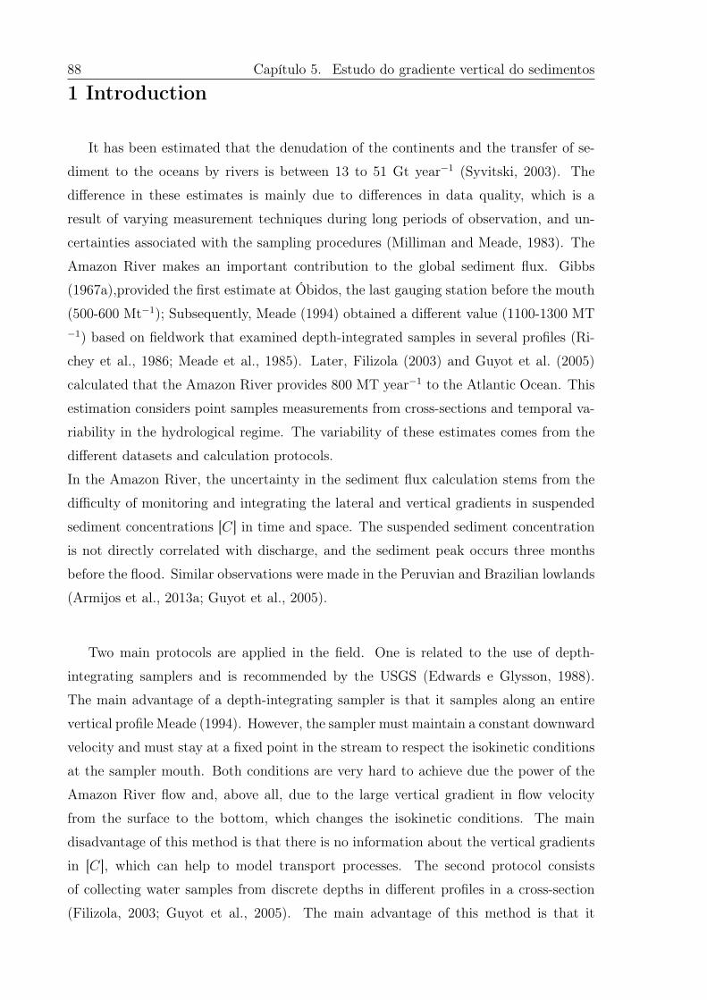
88 Capítulo 5. Estudo do gradiente vertical do sedimentos
1 Introduction
It has been estimated that the denudation of the continents and the transfer of se-
diment to the oceans by rivers is between 13 to 51 Gt year−1 (Syvitski, 2003). The
difference in these estimates is mainly due to differences in data quality, which is a
result of varying measurement techniques during long periods of observation, and un-
certainties associated with the sampling procedures (Milliman and Meade, 1983). The
Amazon River makes an important contribution to the global sediment flux. Gibbs
(1967a),provided the first estimate at Óbidos, the last gauging station before the mouth
(500-600 Mt−1); Subsequently, Meade (1994) obtained a different value (1100-1300 MT−1) based on fieldwork that examined depth-integrated samples in several profiles (Ri-
chey et al., 1986; Meade et al., 1985). Later, Filizola (2003) and Guyot et al. (2005)
calculated that the Amazon River provides 800 MT year−1 to the Atlantic Ocean. This
estimation considers point samples measurements from cross-sections and temporal va-
riability in the hydrological regime. The variability of these estimates comes from the
different datasets and calculation protocols.
In the Amazon River, the uncertainty in the sediment flux calculation stems from the
difficulty of monitoring and integrating the lateral and vertical gradients in suspended
sediment concentrations [𝐶] in time and space. The suspended sediment concentration
is not directly correlated with discharge, and the sediment peak occurs three months
before the flood. Similar observations were made in the Peruvian and Brazilian lowlands
(Armijos et al., 2013a; Guyot et al., 2005).
Two main protocols are applied in the field. One is related to the use of depth-
integrating samplers and is recommended by the USGS (Edwards e Glysson, 1988).
The main advantage of a depth-integrating sampler is that it samples along an entire
vertical profile Meade (1994). However, the sampler must maintain a constant downward
velocity and must stay at a fixed point in the stream to respect the isokinetic conditions
at the sampler mouth. Both conditions are very hard to achieve due the power of the
Amazon River flow and, above all, due to the large vertical gradient in flow velocity
from the surface to the bottom, which changes the isokinetic conditions. The main
disadvantage of this method is that there is no information about the vertical gradients
in [𝐶], which can help to model transport processes. The second protocol consists
of collecting water samples from discrete depths in different profiles in a cross-section
(Filizola, 2003; Guyot et al., 2005). The main advantage of this method is that it
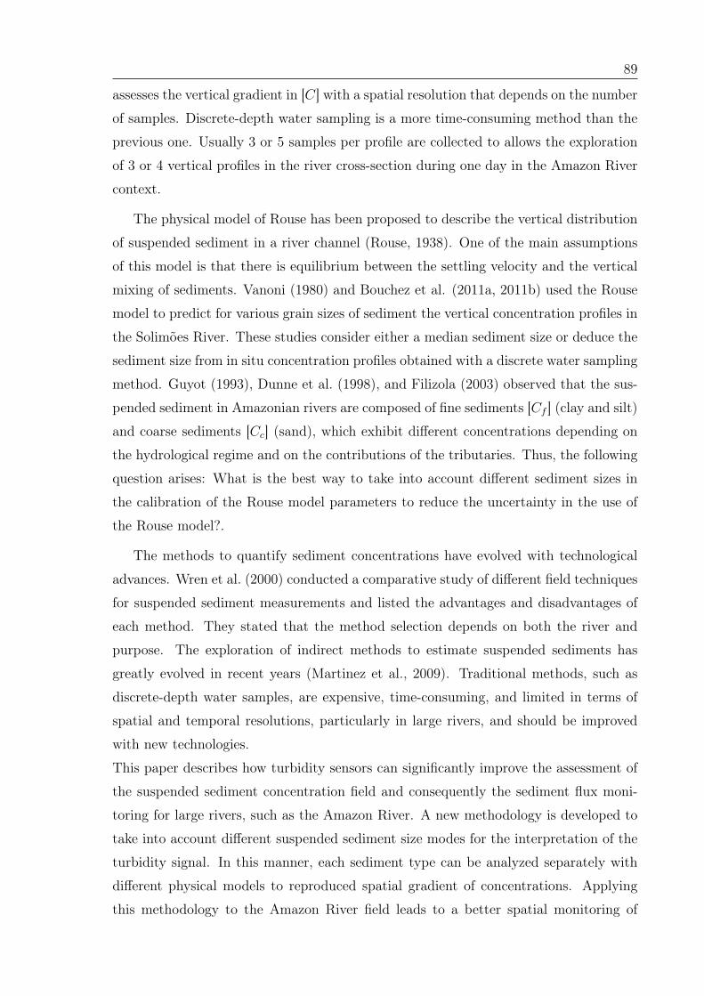
89
assesses the vertical gradient in [𝐶] with a spatial resolution that depends on the number
of samples. Discrete-depth water sampling is a more time-consuming method than the
previous one. Usually 3 or 5 samples per profile are collected to allows the exploration
of 3 or 4 vertical profiles in the river cross-section during one day in the Amazon River
context.
The physical model of Rouse has been proposed to describe the vertical distribution
of suspended sediment in a river channel (Rouse, 1938). One of the main assumptions
of this model is that there is equilibrium between the settling velocity and the vertical
mixing of sediments. Vanoni (1980) and Bouchez et al. (2011a, 2011b) used the Rouse
model to predict for various grain sizes of sediment the vertical concentration profiles in
the Solimões River. These studies consider either a median sediment size or deduce the
sediment size from in situ concentration profiles obtained with a discrete water sampling
method. Guyot (1993), Dunne et al. (1998), and Filizola (2003) observed that the sus-
pended sediment in Amazonian rivers are composed of fine sediments [𝐶𝑓 ] (clay and silt)
and coarse sediments [𝐶𝑐] (sand), which exhibit different concentrations depending on
the hydrological regime and on the contributions of the tributaries. Thus, the following
question arises: What is the best way to take into account different sediment sizes in
the calibration of the Rouse model parameters to reduce the uncertainty in the use of
the Rouse model?.
The methods to quantify sediment concentrations have evolved with technological
advances. Wren et al. (2000) conducted a comparative study of different field techniques
for suspended sediment measurements and listed the advantages and disadvantages of
each method. They stated that the method selection depends on both the river and
purpose. The exploration of indirect methods to estimate suspended sediments has
greatly evolved in recent years (Martinez et al., 2009). Traditional methods, such as
discrete-depth water samples, are expensive, time-consuming, and limited in terms of
spatial and temporal resolutions, particularly in large rivers, and should be improved
with new technologies.
This paper describes how turbidity sensors can significantly improve the assessment of
the suspended sediment concentration field and consequently the sediment flux moni-
toring for large rivers, such as the Amazon River. A new methodology is developed to
take into account different suspended sediment size modes for the interpretation of the
turbidity signal. In this manner, each sediment type can be analyzed separately with
different physical models to reproduced spatial gradient of concentrations. Applying
this methodology to the Amazon River field leads to a better spatial monitoring of
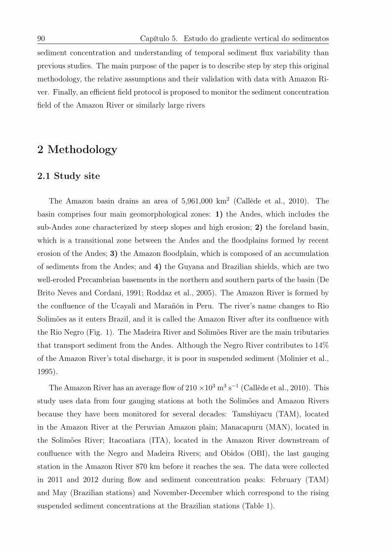
90 Capítulo 5. Estudo do gradiente vertical do sedimentos
sediment concentration and understanding of temporal sediment flux variability than
previous studies. The main purpose of the paper is to describe step by step this original
methodology, the relative assumptions and their validation with data with Amazon Ri-
ver. Finally, an efficient field protocol is proposed to monitor the sediment concentration
field of the Amazon River or similarly large rivers
2 Methodology
2.1 Study site
The Amazon basin drains an area of 5,961,000 km2 (Callède et al., 2010). The
basin comprises four main geomorphological zones: 1) the Andes, which includes the
sub-Andes zone characterized by steep slopes and high erosion; 2) the foreland basin,
which is a transitional zone between the Andes and the floodplains formed by recent
erosion of the Andes; 3) the Amazon floodplain, which is composed of an accumulation
of sediments from the Andes; and 4) the Guyana and Brazilian shields, which are two
well-eroded Precambrian basements in the northern and southern parts of the basin (De
Brito Neves and Cordani, 1991; Roddaz et al., 2005). The Amazon River is formed by
the confluence of the Ucayali and Marañón in Peru. The river’s name changes to Rio
Solimões as it enters Brazil, and it is called the Amazon River after its confluence with
the Rio Negro (Fig. 1). The Madeira River and Solimões River are the main tributaries
that transport sediment from the Andes. Although the Negro River contributes to 14%
of the Amazon River’s total discharge, it is poor in suspended sediment (Molinier et al.,
1995).
The Amazon River has an average flow of 210 ×103 m3 s−1 (Callède et al., 2010). This
study uses data from four gauging stations at both the Solimões and Amazon Rivers
because they have been monitored for several decades: Tamshiyacu (TAM), located
in the Amazon River at the Peruvian Amazon plain; Manacapuru (MAN), located in
the Solimões River; Itacoatiara (ITA), located in the Amazon River downstream of
confluence with the Negro and Madeira Rivers; and Obidos (OBI), the last gauging
station in the Amazon River 870 km before it reaches the sea. The data were collected
in 2011 and 2012 during flow and sediment concentration peaks: February (TAM)
and May (Brazilian stations) and November-December which correspond to the rising
suspended sediment concentrations at the Brazilian stations (Table 1).
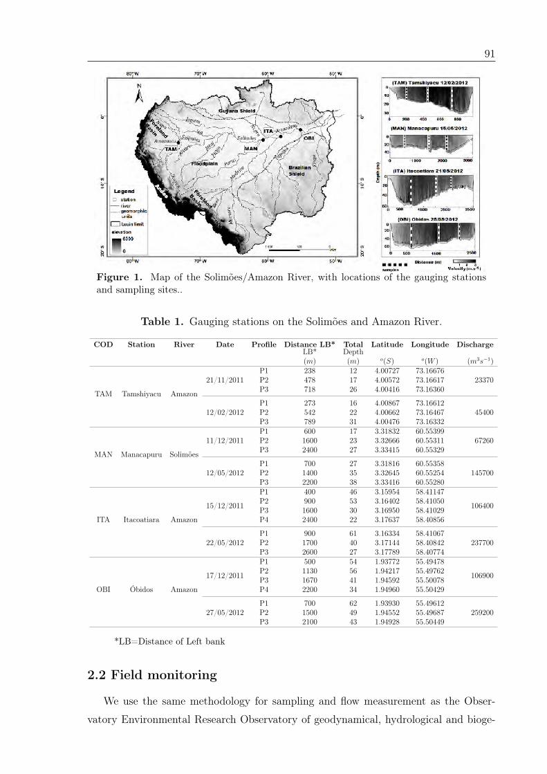
91
Figure 1. Map of the Solimões/Amazon River, with locations of the gauging stationsand sampling sites..
Table 1. Gauging stations on the Solimões and Amazon River.
COD Station River Date Profile Distance LB* Total Latitude Longitude DischargeLB* Depth(𝑚) (𝑚) 𝑜(𝑆) 𝑜(𝑊 ) (𝑚3𝑠−1)
TAM Tamshiyacu Amazon
21/11/2011P1 238 12 4.00727 73.16676
23370P2 478 17 4.00572 73.16617P3 718 26 4.00416 73.16360
12/02/2012P1 273 16 4.00867 73.16612
45400P2 542 22 4.00662 73.16467P3 789 31 4.00476 73.16332
MAN Manacapuru Solimões
11/12/2011P1 600 17 3.31832 60.55399
67260P2 1600 23 3.32666 60.55311P3 2400 27 3.33415 60.55329
12/05/2012P1 700 27 3.31816 60.55358
145700P2 1400 35 3.32645 60.55254P3 2200 38 3.33416 60.55280
ITA Itacoatiara Amazon
15/12/2011
P1 400 46 3.15954 58.41147
106400P2 900 53 3.16402 58.41050P3 1600 30 3.16950 58.41029P4 2400 22 3.17637 58.40856
22/05/2012P1 900 61 3.16334 58.41067
237700P2 1700 40 3.17144 58.40842P3 2600 27 3.17789 58.40774
OBI Óbidos Amazon
17/12/2011
P1 500 54 1.93772 55.49478
106900P2 1130 56 1.94217 55.49762P3 1670 41 1.94592 55.50078P4 2200 34 1.94960 55.50429
27/05/2012P1 700 62 1.93930 55.49612
259200P2 1500 49 1.94552 55.49687P3 2100 43 1.94928 55.50449
*LB=Distance of Left bank
2.2 Field monitoring
We use the same methodology for sampling and flow measurement as the Obser-
vatory Environmental Research Observatory of geodynamical, hydrological and bioge-
92 Capítulo 5. Estudo do gradiente vertical do sedimentos
ochemical control of erosion/alteration and material transport in the Amazon, Orinoco
and Congo basins (SO-HYBAM). The flow at each of the gauging stations is measured
using a Rio Grande 600 kHz RDI Acoustic Doppler Current Profiler (ADCP) monitored
by a global positioning system (GPS).
Along with the flow measurements, 7-L discrete water samples are collected with a
horizontal water sampler at different depths along selected profiles across the section.
To ensure that the sample is obtained at a given vertical profile, the sampler is tied
to a 70-kg weight. The location of the profile is chosen by considering two criteria:
the spatial distribution of the acoustic backscatter signal of the ADCP and a moving-
bottom estimation. For each sample, the coarse and fine sediments is separated using
a 63 µm sieve. A 300 mL sample of fine sediments is filtered through a 0.45 µm cel-
lulose filter. The samples of fine and coarse sediments are then taken to the Amazon
Potamology Laboratory (LAPA−UFAM) to be dried at a 100𝑜𝐶 for an hour. Repeat
measurements revealed an uncertainty of ± 10% for surface concentrations and ±25%
for concentrations near the river bottom.
A high-definition YSI V2 6600 infrared (860-nm wavelength) nephelometer (0.1 NTU
resolution, 2% accuracy, and 90º angle detection) turbidity sensor, coupled with a pres-
sure detector is attached to the sampler and records turbidity during sampler lowering,
with a data acquisition frequency of 1 Hz. Thus, a high-resolution turbidity profile is
captured along a given vertical profile. Each value of turbidity (𝑇 ) corresponds to the
average signal over a height of 50 cm, and the maximum uncertainty of this measurement
is ± 7%.
2.3 Determination of suspended sediment concentration profileusing turbidity measurements
Turbidity represents the transparency reduction of water due to the presence of
suspended matter, such as sand, clay, or organic matter (ASTM, 2003). Turbidity can be
measured by a turbidity-meter, whose sensor detects the portion of light that is scattered
by suspended particles (Anderson, 2004). Turbidity is an optical measurement technique
to estimate [𝐶] without interfering the sediment (Bunt et al., 1999; Pavanelli e Bigi, 2005;
Restrepo e Pierini, 2012; Landers, 2011). One of its main advantages is that it provides
the opportunity to obtain values at high frequency with portable probes. However, this
procedure requires calibration to account for sediment granulometry, nature and color
(Ludwig e Hanes, 1990; Butt et al., 2002; Minella et al., 2008; Thollet et al., 2013).
For example, the assumption of a single representative diameter is not appropriate
93
and can leads to large uncertainty in the calculation of [𝐶]. Indeed, turbidity is the
addition of the turbidity signal relative to each granulometric mode and depends on
the sediment concentration in each mode (see section 2.3.1). Interpreting turbidity as
a concentration requires identifying the turbidity intensity relative to each mode and
applying appropriate calibration curves relative to each mode.
The 65 samples collected during the field campaigns show that the sediment particle
sizes at the four gauging stations are between 9 and 24 µm for fine sediments and between
65 and 156 µm for coarse sediments (Table 2). Note the exception for coarse sediments
at MAN during the high water period (326 µm on average). This simple configuration
of granulometry over thousands of kilometers from Tamshiyacu to Óbidos offers the
opportunity to use turbidity as an efficient signal to measure the concentration of both
sediment modes. However, this requires developing a new methodology to analyze
turbidity data. The main difficulty is taking into account the mass partition between
the two modes, which may vary vertically with the river depth. To develop an adequate
methodology, we first evaluate several properties of turbidity in the laboratory using
suspended Amazon River sediment to define specific calibration curves. Second, we
develop a sequential method to extract the concentration profiles of both modes from
in situ turbidity profiles knowing the size modes of the suspended sediment.
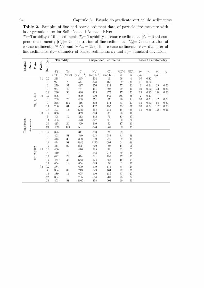
94 Capítulo 5. Estudo do gradiente vertical do sedimentos
Table 2. Samples of fine and coarse sediment data of particle size measure withlaser granulometer for Solimões and Amazon River.𝑇𝑓=Turbidity of fine sediment; 𝑇𝑐= Turbidity of coarse sediments; [𝐶]=Total sus-pended sediments; [𝐶𝑓 ]= Concentration of fine sediments; [𝐶𝑐]= Concentration ofcoarse sediments; %[𝐶𝑓 ] and %[𝐶𝑐]= % of fine coarse sediments; 𝜑𝑓= diameter offine sediments; 𝜑𝑐= diameter of coarse sediments; 𝜎𝑓 and 𝜎𝑐= standard deviation.
Sta
tion
Riv
er
Dat
e
Pro
file (m
) Turbidity Suspended Sediments Laser Granulometry
Dep
th
𝑇𝑓 Tc [C] [𝐶𝑓 ] [𝐶𝑐] %[𝐶𝑓 ] %[𝐶𝑐] 𝜑𝑓 𝜎𝑓 𝜑𝑐 𝜎𝑐
(NTU) (NTU) (mg L−1) (mg L−1) (mg L−1) % % (𝜇m) (𝜇m)
Tam
shiy
acu
Am
azon
as
21/1
1/20
11
P1 0.2 218 245 234 11 96 4 10 0.823 271 8 544 378 166 69 31 11 0.826 279 37 487 376 112 77 23 9 0.34 35 0.509 287 42 784 461 323 59 41 10 0.52 73 0.3111 296 34 886 413 473 47 53 15 0.80 126 0.30
P2 0.2 206 200 200 0.3 100 0 7 0.474 268 23 408 351 57 86 14 10 0.54 47 0.549 278 103 416 302 114 73 27 13 0.60 65 0.3713 286 61 589 432 157 73 27 10 0.54 107 0.2817 303 83 1236 555 681 45 55 13 0.56 125 0.26
P3 0.2 356 359 323 36 90 107 398 39 412 342 71 83 1713 405 10 470 377 93 80 2020 415 20 390 340 50 87 1324 432 130 604 373 231 62 38
12/0
2/20
12
P1 0.2 325 311 310 2 99 14 403 51 870 618 252 71 298 415 38 898 619 279 69 3111 424 51 1919 1225 694 64 3615 444 82 1645 722 923 44 56
P2 0.2 400 416 385 31 93 75 410 18 791 548 243 69 3110 422 29 674 521 153 77 2315 435 33 1261 574 686 46 5419 454 18 854 523 330 61 39
P3 0.2 384 690 519 171 75 257 384 68 713 549 164 77 2315 389 17 695 510 186 73 2722 394 16 735 534 201 73 2726 403 51 1000 498 502 50 50
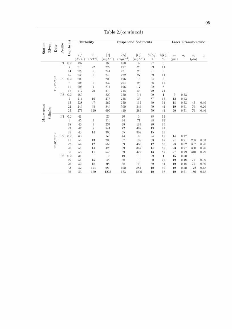
95
Table 2.(continued)
Sta
tion
Riv
er
Dat
e
Pro
file (m
) Turbidity Suspended Sediments Laser Granulometrie
Dep
th
𝑇𝑓 Tc [C] [𝐶𝑓 ] [𝐶𝑐] %[𝐶𝑓 ] %[𝐶𝑐] 𝜑𝑓 𝜎𝑓 𝜑𝑐 𝜎𝑐
(𝑁𝑇𝑈) (𝑁𝑇𝑈) (𝑚𝑔𝐿−1) (𝑚𝑔𝐿−1) (𝑚𝑔𝐿−1) % % (𝜇m) (𝜇m)
Man
acap
uru
Solim
ões
11/1
2/20
11
P1 0.2 197 166 160 6 97 37 216 22 222 197 25 89 1114 229 6 244 221 23 91 915 236 6 249 222 27 89 11
P2 0.2 200 209 196 13 94 66 203 5 232 204 28 88 1211 205 4 214 196 17 92 817 212 20 270 215 56 79 21
P3 0.2 180 220 220 0.4 99 1 7 0.537 214 16 273 238 35 87 13 12 0.5315 228 47 362 250 112 69 31 18 0.53 45 0.4922 246 65 846 500 346 59 41 19 0.51 76 0.2625 273 120 699 410 289 59 41 20 0.51 76 0.46
12/0
5/20
12
P1 0.2 41 23 20 3 88 129 45 4 116 44 71 38 6218 46 9 237 48 189 20 8023 47 8 541 72 468 13 8725 48 14 363 55 308 15 85
P2 0.2 60 52 44 9 84 16 14 0.7711 54 13 205 67 138 33 67 21 0.71 258 0.3322 54 12 555 69 486 12 88 28 0.82 307 0.2828 54 14 426 59 367 14 86 23 0.77 330 0.2831 55 11 548 69 479 13 87 27 0.79 310 0.29
P3 0.2 31 19 19 0.1 99 1 15 0.5019 51 15 48 38 10 80 20 19 0.48 77 0.3926 52 18 98 58 40 59 41 19 0.48 77 0.3933 52 124 980 100 881 10 90 19 0.50 172 0.1836 53 169 1223 123 1200 10 98 19 0.51 186 0.18
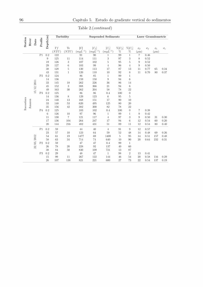
96 Capítulo 5. Estudo do gradiente vertical do sedimentos
Table 2.(continued)Sta
tion
Riv
er
Dat
e
Pro
file (m
) Turbidity Suspended Sediments Laser Granulometrie
Dep
th𝑇𝑓 Tc [C] [𝐶𝑓 ] [𝐶𝑐] %[𝐶𝑓 ] %[𝐶𝑐] 𝜑𝑓 𝜎𝑓 𝜑𝑐 𝜎𝑐
(𝑁𝑇𝑈) (𝑁𝑇𝑈) (𝑚𝑔𝐿−1) (𝑚𝑔𝐿−1) (𝑚𝑔𝐿−1) % % (𝜇m) (𝜇m)
Itac
oati
ara
Am
azon
15/1
2/20
11
P1 0.2 122 91 90 1 99 1 7 0.469 125 11 114 111 3 97 3 8 0.5219 126 3 107 102 5 95 5 9 0.5229 127 6 103 99 4 96 4 9 0.5038 128 5 130 113 17 87 13 11 0.77 65 0.3443 131 1 120 110 10 92 8 11 0.70 80 0.37
P2 0.2 124 86 85 1 99 114 136 159 150 9 94 633 145 18 262 226 36 86 1445 152 3 388 366 21 94 649 163 30 262 204 58 78 22
P3 0.2 125 86 86 0.4 100 014 136 8 129 123 6 95 524 140 13 168 151 17 90 1033 148 53 620 495 125 80 2035 156 42 382 300 82 78 22
P4 0.2 125 103 102 0.4 100 0 7 0.386 126 10 97 96 1 99 1 9 0.4211 130 7 121 117 4 97 3 9 0.50 31 0.3017 136 104 264 247 17 94 6 12 0.54 60 0.2020 144 216 482 431 51 89 11 12 0.54 80 0.40
22/0
5/20
12
P1 0.2 59 44 40 4 91 9 12 0.5723 57 10 123 64 59 52 48 14 0.48 69 0.2654 61 19 1477 69 1408 5 95 14 0.51 157 0.4858 63 34 714 74 640 10 90 20 0.64 232 0.31
P2 0.2 59 47 47 0.4 99 126 78 20 228 92 137 40 6038 84 50 830 109 721 13 87
P3 0.2 29 48 47 1 98 2 13 0.4115 99 11 267 122 144 46 54 20 0.58 116 0.2926 107 138 821 221 600 27 73 22 0.54 137 0.19
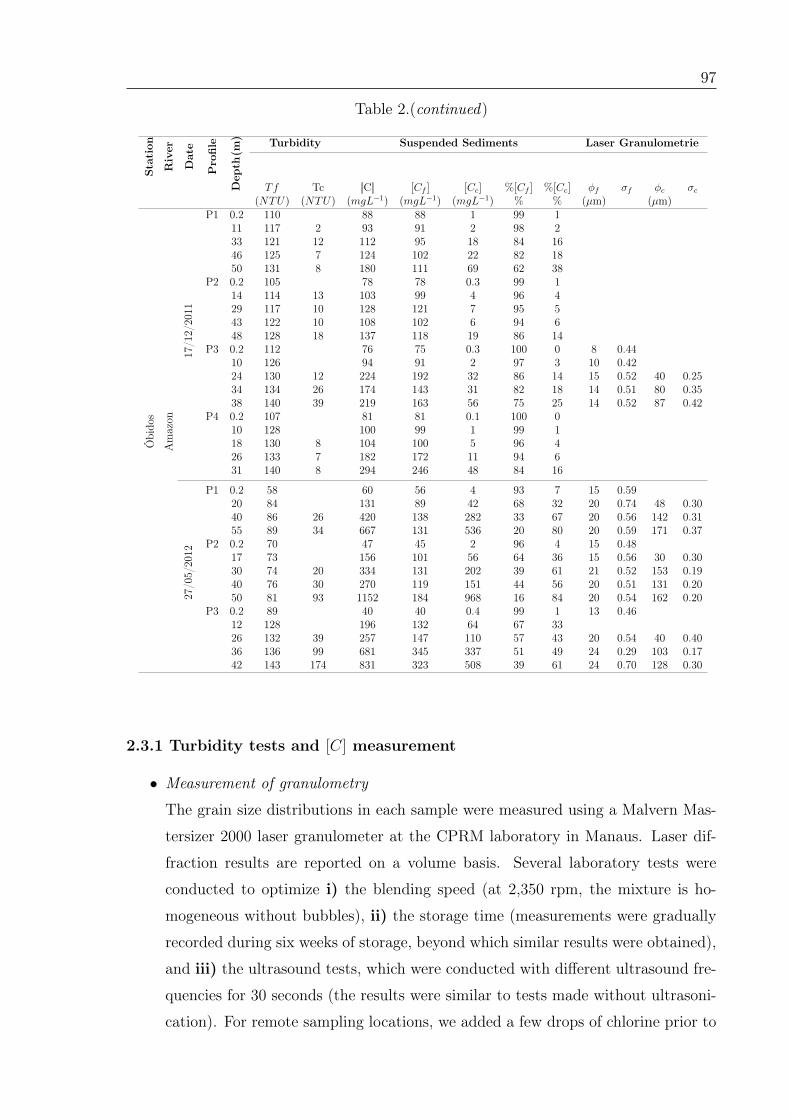
97
Table 2.(continued)
Sta
tion
Riv
er
Dat
e
Pro
file
(m) Turbidity Suspended Sediments Laser Granulometrie
Dep
th
𝑇𝑓 Tc [C] [𝐶𝑓 ] [𝐶𝑐] %[𝐶𝑓 ] %[𝐶𝑐] 𝜑𝑓 𝜎𝑓 𝜑𝑐 𝜎𝑐
(𝑁𝑇𝑈) (𝑁𝑇𝑈) (𝑚𝑔𝐿−1) (𝑚𝑔𝐿−1) (𝑚𝑔𝐿−1) % % (𝜇m) (𝜇m)
Óbi
dos
Am
azon
17/1
2/20
11
P1 0.2 110 88 88 1 99 111 117 2 93 91 2 98 233 121 12 112 95 18 84 1646 125 7 124 102 22 82 1850 131 8 180 111 69 62 38
P2 0.2 105 78 78 0.3 99 114 114 13 103 99 4 96 429 117 10 128 121 7 95 543 122 10 108 102 6 94 648 128 18 137 118 19 86 14
P3 0.2 112 76 75 0.3 100 0 8 0.4410 126 94 91 2 97 3 10 0.4224 130 12 224 192 32 86 14 15 0.52 40 0.2534 134 26 174 143 31 82 18 14 0.51 80 0.3538 140 39 219 163 56 75 25 14 0.52 87 0.42
P4 0.2 107 81 81 0.1 100 010 128 100 99 1 99 118 130 8 104 100 5 96 426 133 7 182 172 11 94 631 140 8 294 246 48 84 16
27/0
5/20
12
P1 0.2 58 60 56 4 93 7 15 0.5920 84 131 89 42 68 32 20 0.74 48 0.3040 86 26 420 138 282 33 67 20 0.56 142 0.3155 89 34 667 131 536 20 80 20 0.59 171 0.37
P2 0.2 70 47 45 2 96 4 15 0.4817 73 156 101 56 64 36 15 0.56 30 0.3030 74 20 334 131 202 39 61 21 0.52 153 0.1940 76 30 270 119 151 44 56 20 0.51 131 0.2050 81 93 1152 184 968 16 84 20 0.54 162 0.20
P3 0.2 89 40 40 0.4 99 1 13 0.4612 128 196 132 64 67 3326 132 39 257 147 110 57 43 20 0.54 40 0.4036 136 99 681 345 337 51 49 24 0.29 103 0.1742 143 174 831 323 508 39 61 24 0.70 128 0.30
2.3.1 Turbidity tests and [𝐶] measurement
• Measurement of granulometry
The grain size distributions in each sample were measured using a Malvern Mas-
tersizer 2000 laser granulometer at the CPRM laboratory in Manaus. Laser dif-
fraction results are reported on a volume basis. Several laboratory tests were
conducted to optimize i) the blending speed (at 2,350 rpm, the mixture is ho-
mogeneous without bubbles), ii) the storage time (measurements were gradually
recorded during six weeks of storage, beyond which similar results were obtained),
and iii) the ultrasound tests, which were conducted with different ultrasound fre-
quencies for 30 seconds (the results were similar to tests made without ultrasoni-
cation). For remote sampling locations, we added a few drops of chlorine prior to
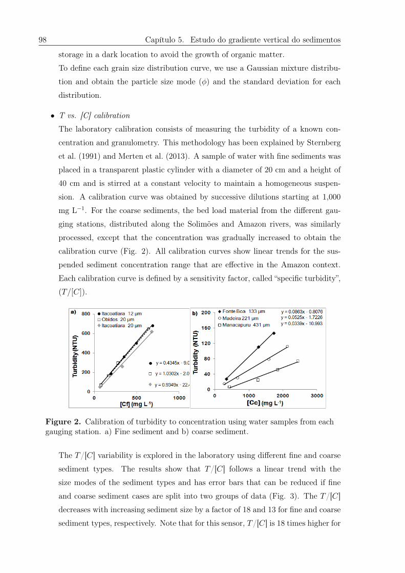
98 Capítulo 5. Estudo do gradiente vertical do sedimentos
storage in a dark location to avoid the growth of organic matter.
To define each grain size distribution curve, we use a Gaussian mixture distribu-
tion and obtain the particle size mode (𝜑) and the standard deviation for each
distribution.
• T vs. [C] calibration
The laboratory calibration consists of measuring the turbidity of a known con-
centration and granulometry. This methodology has been explained by Sternberg
et al. (1991) and Merten et al. (2013). A sample of water with fine sediments was
placed in a transparent plastic cylinder with a diameter of 20 cm and a height of
40 cm and is stirred at a constant velocity to maintain a homogeneous suspen-
sion. A calibration curve was obtained by successive dilutions starting at 1,000
mg L−1. For the coarse sediments, the bed load material from the different gau-
ging stations, distributed along the Solimões and Amazon rivers, was similarly
processed, except that the concentration was gradually increased to obtain the
calibration curve (Fig. 2). All calibration curves show linear trends for the sus-
pended sediment concentration range that are effective in the Amazon context.
Each calibration curve is defined by a sensitivity factor, called “specific turbidity”,
(𝑇/[𝐶]).
Figure 2. Calibration of turbidity to concentration using water samples from eachgauging station. a) Fine sediment and b) coarse sediment.
The 𝑇/[𝐶] variability is explored in the laboratory using different fine and coarse
sediment types. The results show that 𝑇/[𝐶] follows a linear trend with the
size modes of the sediment types and has error bars that can be reduced if fine
and coarse sediment cases are split into two groups of data (Fig. 3). The 𝑇/[𝐶]
decreases with increasing sediment size by a factor of 18 and 13 for fine and coarse
sediment types, respectively. Note that for this sensor, 𝑇/[𝐶] is 18 times higher for
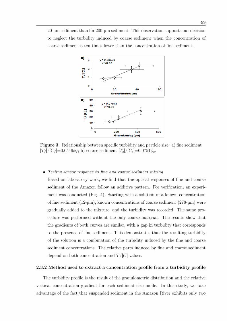
99
20-µm sediment than for 200-µm sediment. This observation supports our decision
to neglect the turbidity induced by coarse sediment when the concentration of
coarse sediment is ten times lower than the concentration of fine sediment.
Figure 3. Relationship between specific turbidity and particle size: a) fine sediment[𝑇𝑓 ]/[𝐶𝑓 ]=0.0549𝜑𝑓 ; b) coarse sediment [𝑇𝑐]/[𝐶𝑐]=0.0751𝜑𝑐.
• Testing sensor response to fine and coarse sediment mixing
Based on laboratory work, we find that the optical responses of fine and coarse
sediment of the Amazon follow an additive pattern. For verification, an experi-
ment was conducted (Fig. 4). Starting with a solution of a known concentration
of fine sediment (12-µm), known concentrations of coarse sediment (278-µm) were
gradually added to the mixture, and the turbidity was recorded. The same pro-
cedure was performed without the only coarse material. The results show that
the gradients of both curves are similar, with a gap in turbidity that corresponds
to the presence of fine sediment. This demonstrates that the resulting turbidity
of the solution is a combination of the turbidity induced by the fine and coarse
sediment concentrations. The relative parts induced by fine and coarse sediment
depend on both concentration and 𝑇/[𝐶] values.
2.3.2 Method used to extract a concentration profile from a turbidity profile
The turbidity profile is the result of the granulometric distribution and the relative
vertical concentration gradient for each sediment size mode. In this study, we take
advantage of the fact that suspended sediment in the Amazon River exhibits only two
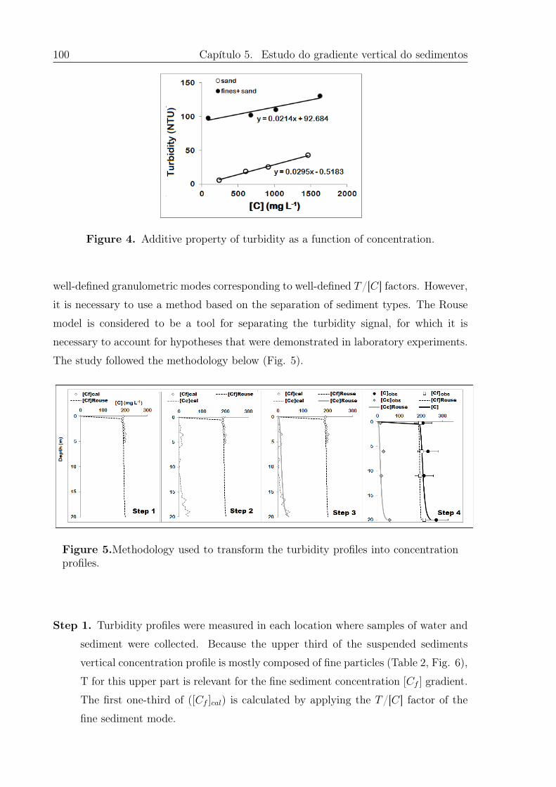
100 Capítulo 5. Estudo do gradiente vertical do sedimentos
Figure 4. Additive property of turbidity as a function of concentration.
well-defined granulometric modes corresponding to well-defined 𝑇/[𝐶] factors. However,
it is necessary to use a method based on the separation of sediment types. The Rouse
model is considered to be a tool for separating the turbidity signal, for which it is
necessary to account for hypotheses that were demonstrated in laboratory experiments.
The study followed the methodology below (Fig. 5).
Figure 5.Methodology used to transform the turbidity profiles into concentrationprofiles.
Step 1. Turbidity profiles were measured in each location where samples of water and
sediment were collected. Because the upper third of the suspended sediments
vertical concentration profile is mostly composed of fine particles (Table 2, Fig. 6),
T for this upper part is relevant for the fine sediment concentration [𝐶𝑓 ] gradient.
The first one-third of ([𝐶𝑓 ]𝑐𝑎𝑙) is calculated by applying the 𝑇/[𝐶] factor of the
fine sediment mode.
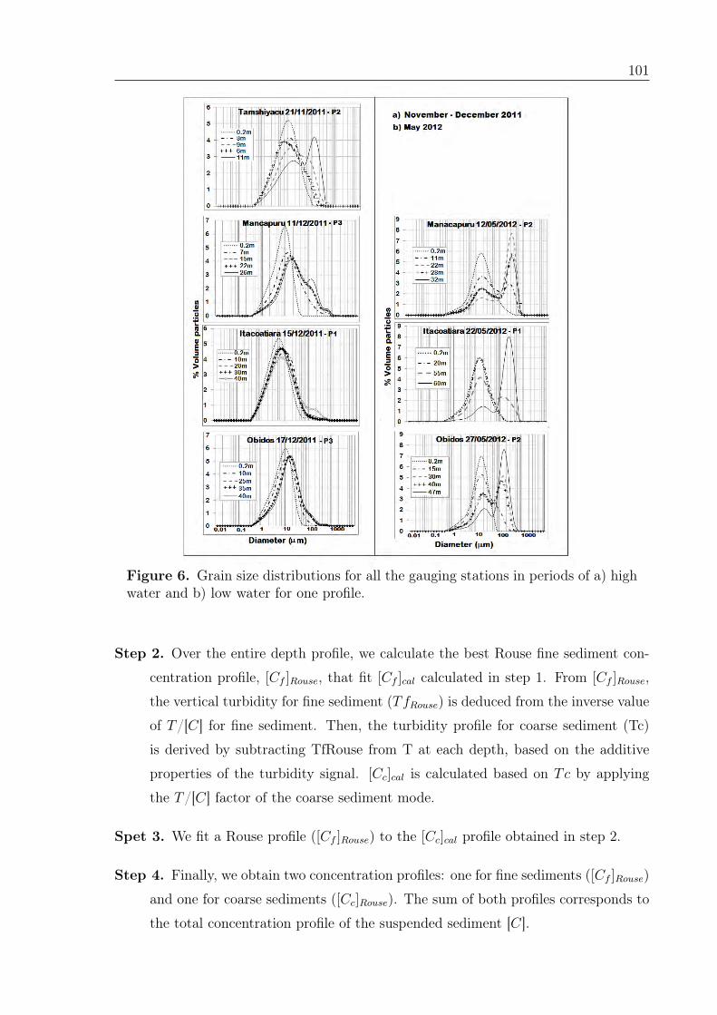
101
Figure 6. Grain size distributions for all the gauging stations in periods of a) highwater and b) low water for one profile.
Step 2. Over the entire depth profile, we calculate the best Rouse fine sediment con-
centration profile, [𝐶𝑓 ]𝑅𝑜𝑢𝑠𝑒, that fit [𝐶𝑓 ]𝑐𝑎𝑙 calculated in step 1. From [𝐶𝑓 ]𝑅𝑜𝑢𝑠𝑒,
the vertical turbidity for fine sediment (𝑇𝑓𝑅𝑜𝑢𝑠𝑒) is deduced from the inverse value
of 𝑇/[𝐶] for fine sediment. Then, the turbidity profile for coarse sediment (Tc)
is derived by subtracting TfRouse from T at each depth, based on the additive
properties of the turbidity signal. [𝐶𝑐]𝑐𝑎𝑙 is calculated based on 𝑇𝑐 by applying
the 𝑇/[𝐶] factor of the coarse sediment mode.
Spet 3. We fit a Rouse profile ([𝐶𝑓 ]𝑅𝑜𝑢𝑠𝑒) to the [𝐶𝑐]𝑐𝑎𝑙 profile obtained in step 2.
Step 4. Finally, we obtain two concentration profiles: one for fine sediments ([𝐶𝑓 ]𝑅𝑜𝑢𝑠𝑒)
and one for coarse sediments ([𝐶𝑐]𝑅𝑜𝑢𝑠𝑒). The sum of both profiles corresponds to
the total concentration profile of the suspended sediment [𝐶].
102 Capítulo 5. Estudo do gradiente vertical do sedimentos
2.4 Rouse profile calibration and validation
The Rouse profile aims to describe the vertical distribution of suspended sediment
under steady state conditions when downward settling is balanced by upward transport
processes of sediment. It predicts that the suspended sediment concentration follows
the following equation:
𝐶(𝑧)
𝐶(𝑟𝑒𝑓)
=
(︂𝐻 − 𝑑
𝑑.
𝑧
𝐻 − 𝑧
)︂𝑊
(5.1)
where: [𝐶(𝑧)] is the sediment concentration at level 𝑧, [𝐶(𝑟𝑒𝑓)] is the reference concen-
tration at distance 𝑧 = 𝑑 (𝑑 = 0.03*𝐻, which corresponds to the minimum distance
between the turbidity sensor and bed), 𝐻 is the total depth, 𝑊 is the Rouse number,
which is defined as𝑤𝑠
𝜅.𝑢* where 𝑤𝑠 is the settling velocity, 𝜅 is the Von Kármán constant
(0.41) and 𝑢* is the shear velocity.In a steady, turbulent and uniform flow, the velocity
distribution is well represented by the law of the wall:
�̄�
𝑢* =1
𝜅. ln
(︂𝑧
𝑧𝑜
)︂(5.2)
Where �̄� is the time-averaged flow velocity at a distance 𝑧; 𝑧𝑜 is the bed roughness
length. Equation 2 can also be written as follows:
�̄� = 𝑎. ln (𝑧) + 𝑏 (5.3)
where: 𝑢*= 𝑎 × 𝜅 ; 𝑧𝑜= exp(︀−𝑏
𝑎
)︀.
The coefficients of 𝑎 and 𝑏 were estimated by fitting the average of various ADCP
velocity profiles. Because data are collected using an ADCP in motion, it is necessary to
obtain the average of various profiles to correctly describe a logarithmic profile. Nystrom
et al. (2007) conducted laboratory experiments showing that ADCPs are capable of
correctly reproducing the logarithmic profile of velocity predicted by the law of the wall.
However, during field measurements, it is necessary to average several vertical profiles to
obtain such logarithmic profiles of velocity Stone e Hotchkiss (2007). We found that with
the high velocities (>2 m s−1) and large width (>2 km) of the Solimões/Amazon River,
the number of velocity profiles needed to obtain a significant 𝑢* value depends on the
stability of the coefficient a. Generally, stable values were reached using approximately
50 to 60 ADCP velocity profiles, corresponding to a spatial average of 150 m (i.e., 10%
of the total width of the section) in the cross-section direction. The uncertainty of 𝑢*
is ± 33%. This uncertainty includes the fact that velocity profiles are registered during
the drift of the boat instead of the fixed-point protocol.
103
To validate the application of the Rouse model theory to the vertical concentration
profile for fine and coarse sediment, two criteria are checked. The first one is the
coherency between the sample concentrations and concentrations calculated from the
Rouse profiles. The second criterion is the coherency between the sediment size mode
calculated from the 𝑊 and ws values and the particle size mode measured with the laser
granulometer. The settling velocity (𝑤𝑠) is a function of particle size following Stoke’s
law.
2.5 Estimation of suspended sediment flux
The instantaneous suspended-sediment flux (𝑄𝑠𝑖) in each ADCP cell is calculated
as:
𝑄𝑠𝑖 = 𝑄𝑖 * [𝐶𝑖] (5.4)
where 𝑄𝑖 is the instantaneous water discharge of the ADCP cell in m3 s−1 and [𝐶𝑖] is
the suspended sediment concentration ([𝐶𝑓 ] + [𝐶𝑐]) in mg L−1. The total sediment flux
is calculated by summing all Qsi values in the section in kg s−1. To test the sensitivity
of 𝑄𝑠𝑖 to each parameter of the Rouse model, 𝑊 is fixed and [𝐶](𝑟𝑒𝑓) is varied, and vice
versa, for both fine and coarse sediment cases.
3. Results
Fig. 7 shows a good coherence between the fine and coarse concentrations obtained
from turbidity and the discrete fine and coarse samples, with r2 = 0.71. The main
disparities depend on the coarse sediment concentration near the river bottom.
The 𝑊𝑓 (fine-sediment Rouse number) and 𝑊𝑐 (coarse-sediment Rouse number) va-
lues are in range of 0.01 to 0.03 and 0.25 to 0.60, respectively (Table 3). For a single
cross-section 𝑊𝑓 , 𝑊𝑐 and the coefficient [𝐶𝑓 ]𝑟𝑒𝑓 show a lateral variation that is within
the range of the uncertainties, and [𝐶𝑐]𝑟𝑒𝑓 varies with the vertical location. Again, ca-
reful calculation or measurement of [𝐶𝑐]𝑟𝑒𝑓 must be performed to significantly reduce
uncertainty in the concentration prediction. For flux estimations of fine sediments, a
linear interpolation is valid to fix the Rouse model for unmeasured vertical profiles. For
coarse sediments, the variation in [𝐶𝑐]𝑟𝑒𝑓 from one vertical profile to another is signi-
ficant, suggesting the importance of the local hydraulic conditions. This variation can
present an uncertainty of up to ±36% in the estimates of the solid coarse sediment flux.
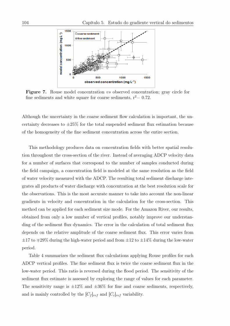
104 Capítulo 5. Estudo do gradiente vertical do sedimentos
Figure 7. Rouse model concentration 𝑣𝑠 observed concentration; gray circle forfine sediments and white square for coarse sediments, r2= 0.72.
Although the uncertainty in the coarse sediment flow calculation is important, the un-
certainty decreases to ±25% for the total suspended sediment flux estimation because
of the homogeneity of the fine sediment concentration across the entire section.
This methodology produces data on concentration fields with better spatial resolu-
tion throughout the cross-section of the river. Instead of averaging ADCP velocity data
for a number of surfaces that correspond to the number of samples conducted during
the field campaign, a concentration field is modeled at the same resolution as the field
of water velocity measured with the ADCP. The resulting total sediment discharge inte-
grates all products of water discharge with concentration at the best resolution scale for
the observations. This is the most accurate manner to take into account the non-linear
gradients in velocity and concentration in the calculation for the cross-section. This
method can be applied for each sediment size mode. For the Amazon River, our results,
obtained from only a low number of vertical profiles, notably improve our understan-
ding of the sediment flux dynamics. The error in the calculation of total sediment flux
depends on the relative amplitude of the coarse sediment flux. This error varies from
±17 to ∓29% during the high-water period and from ±12 to ±14% during the low-water
period.
Table 4 summarizes the sediment flux calculations applying Rouse profiles for each
ADCP vertical profiles. The fine sediment flux is twice the coarse sediment flux in the
low-water period. This ratio is reversed during the flood period. The sensitivity of the
sediment flux estimate is assessed by exploring the range of values for each parameter.
The sensitivity range is ±12% and ±36% for fine and coarse sediments, respectively,
and is mainly controlled by the [𝐶𝑓 ]𝑟𝑒𝑓 and [𝐶𝑐]𝑟𝑒𝑓 variability.
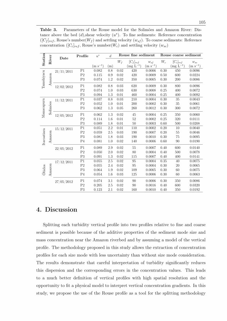
105
Table 3. Parameters of the Rouse model for the Solimões and Amazon River: Dis-tance above the bed (𝑑),shear velocity (𝑢*). To fine sediments: Reference concentration([𝐶𝑓 ]𝑟𝑒𝑓 , Rouse’s number(𝑊𝑓 ) and settling velocity (𝑤𝑠𝑓 ). To coarse sediments: Referenceconcentration ([𝐶𝑐]𝑟𝑒𝑓 , Rouse’s number(𝑊𝑐) and settling velocity (𝑤𝑠𝑐)
Sta
tion
Riv
er Date Profile 𝑢* 𝑑 Rouse fine sediment Rouse coarse sediment
𝑊𝑓 [𝐶𝑓 ]𝑟𝑒𝑓 𝑤𝑠𝑓 𝑊𝑐 [𝐶𝑐]𝑟𝑒𝑓 𝑤𝑠𝑐
(m s−1) (m) (mg L−1) (m s−1) (mg L−1) (m s−1)
Tam
shiy
acu
Am
azon
21/11/2011 P1 0.082 0.8 0.02 420 0.0006 0.30 450 0.0096P2 0.115 0.9 0.02 420 0.0009 0.50 600 0.0224P3 0.074 1.2 0.02 350 0.0005 0.30 200 0.0086
12/02/2012 P1 0.082 0.8 0.03 620 0.0009 0.30 800 0.0096P2 0.074 1.0 0.03 630 0.0008 0.25 400 0.0072P3 0.094 1.3 0.01 460 0.0004 0.25 400 0.0092
Man
acap
uru
Solim
ões 11/12/2011 P1 0.037 0.8 0.03 210 0.0004 0.30 35 0.0043
P2 0.052 1.0 0.01 200 0.0002 0.30 35 0.0061P3 0.062 1.3 0.05 260 0.0012 0.30 300 0.0072
12/05/2012 P1 0.062 1.3 0.02 45 0.0004 0.25 350 0.0060P2 0.114 1.6 0.01 52 0.0002 0.25 320 0.0111P3 0.089 1.8 0.01 50 0.0003 0.60 500 0.0208
Itac
oati
ara
Am
azon
15/12/2011 P1 0.051 2.2 0.01 110 0.0002 0.20 10 0.0040P2 0.059 2.5 0.03 190 0.0007 0.20 55 0.0046P3 0.081 1.8 0.03 190 0.0010 0.30 75 0.0095P4 0.081 1.0 0.02 140 0.0006 0.60 90 0.0190
22/05/2012 P1 0.089 2.9 0.02 55 0.0007 0.40 600 0.0140P2 0.050 2.0 0.02 80 0.0004 0.40 500 0.0078P3 0.091 1.3 0.02 115 0.0007 0.40 400 0.0141
Óbi
dos
Am
azon
17/12/2011 P1 0.055 2.5 0.02 95 0.0004 0.35 40 0.0075P2 0.055 2.4 0.02 95 0.0004 0.30 20 0.0065P3 0.064 1.9 0.02 109 0.0005 0.30 60 0.0075P4 0.054 1.6 0.03 125 0.0006 0.30 60 0.0063
27/05/2012 P1 0.074 3.1 0.02 90 0.0006 0.30 350 0.0086P2 0.205 2.5 0.02 90 0.0016 0.40 600 0.0320P3 0.123 2.1 0.02 160 0.0010 0.40 350 0.0192
4. Discussion
Splitting each turbidity vertical profile into two profiles relative to fine and coarse
sediment is possible because of the additive properties of the sediment mode size and
mass concentration near the Amazon riverbed and by assuming a model of the vertical
profile. The methodology proposed in this study allows the extraction of concentration
profiles for each size mode with less uncertainty than without size mode consideration.
The results demonstrate that careful interpretation of turbidity significantly reduces
this dispersion and the corresponding errors in the concentration values. This leads
to a much better definition of vertical profiles with high spatial resolution and the
opportunity to fit a physical model to interpret vertical concentration gradients. In this
study, we propose the use of the Rouse profile as a tool for the splitting methodology
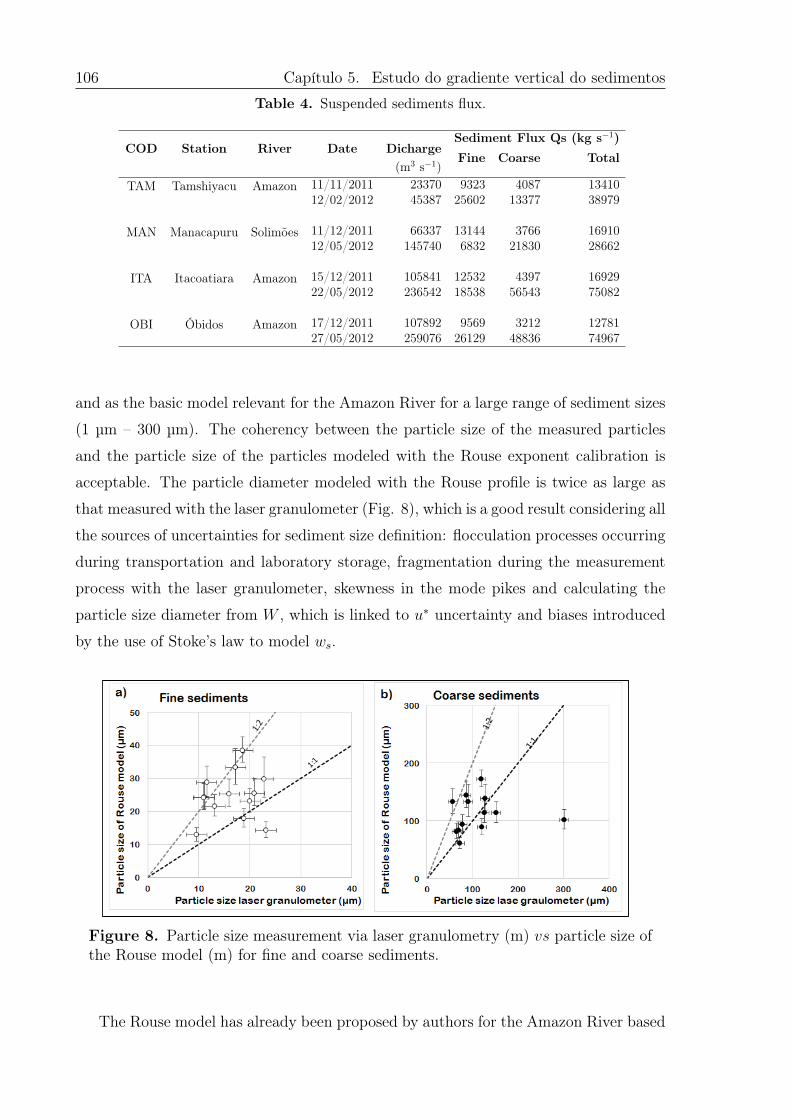
106 Capítulo 5. Estudo do gradiente vertical do sedimentos
Table 4. Suspended sediments flux.
COD Station River Date DichargeSediment Flux Qs (kg s−1)
(m3 s−1)Fine Coarse Total
TAM Tamshiyacu Amazon 11/11/2011 23370 9323 4087 1341012/02/2012 45387 25602 13377 38979
MAN Manacapuru Solimões 11/12/2011 66337 13144 3766 1691012/05/2012 145740 6832 21830 28662
ITA Itacoatiara Amazon 15/12/2011 105841 12532 4397 1692922/05/2012 236542 18538 56543 75082
OBI Óbidos Amazon 17/12/2011 107892 9569 3212 1278127/05/2012 259076 26129 48836 74967
and as the basic model relevant for the Amazon River for a large range of sediment sizes
(1 µm – 300 µm). The coherency between the particle size of the measured particles
and the particle size of the particles modeled with the Rouse exponent calibration is
acceptable. The particle diameter modeled with the Rouse profile is twice as large as
that measured with the laser granulometer (Fig. 8), which is a good result considering all
the sources of uncertainties for sediment size definition: flocculation processes occurring
during transportation and laboratory storage, fragmentation during the measurement
process with the laser granulometer, skewness in the mode pikes and calculating the
particle size diameter from 𝑊 , which is linked to 𝑢* uncertainty and biases introduced
by the use of Stoke’s law to model 𝑤𝑠.
Figure 8. Particle size measurement via laser granulometry (m) 𝑣𝑠 particle size ofthe Rouse model (m) for fine and coarse sediments.
The Rouse model has already been proposed by authors for the Amazon River based
107
on in situ data (Vanoni, 1979, Bouchez et al., 2011a). However, the previous studies
consider one sediment size mode per vertical profile of samples or for the entire gauging
station. Our results show that the Rouse profile theory can be defined per sediment
size mode when a combination of different size modes is present. This notably improves
the use of the Rouse model to predict vertical concentration gradients and defines the
main source of uncertainty as the calibration of [𝐶𝑐]𝑟𝑒𝑓 .
5. Conclusion
This study demonstrates that turbidity sensors can greatly enhance suspended se-
diment monitoring of large rivers. Consequently, it can reduce logistical constraints
and significantly improve the accuracy of the results. The methodology proposed in
this study leads to a much better definition of the concentration gradients in the river
section because it considers a mix of particle sizes. Each mode can be modeled inde-
pendently from one another to fit a Rouse model, which is relevant for every suspended
sediment size mode.
Therefore, traditional methods of sediment flux monitoring along the Amazon River can
be updated using optical technologies and an adapted sampling strategy. Fine sediment
concentration profiles can be simply monitored using samples from the surface and/or
MODIS satellite images (Martinez et al., 2009). Then, from these data on the fine
sediment concentration at the surface of the stream, we can apply a Rouse model with
an average exponent of 0.02. Coarse sediment concentration profile monitoring requires
determining the concentration gradient near the river bottom. For this, one profile with
a turbidimeter probe and one sample, preferably at less than 1 m from the bottom, are
enough to fit a Rouse model. This protocol notably improves 1) the accuracy of the
concentration profile that is multiplied by the ADCP velocity field and consequently the
sediment flux assessment and 2) the efficiency of the field campaign in terms of time
and logistics.
The Rouse model helps to describe vertical gradients in the suspended sediment concen-
tration. It reduces the problematic aspects of vertical concentration profile prediction
by calculating the two main parameters of this model for each sediment size mode. If
the sediment size modes are known, the Rouse exponents can be calculated directly
using the ADCP data. The main difficulty remains obtaining samples near the bedform
for each vertical profile to calibrate [𝐶𝑐]𝑟𝑒𝑓 because the lateral gradient of [𝐶𝑐]𝑟𝑒𝑓 along
the river cross-section is the main source of uncertainty in the sediment flux profile
108 Capítulo 5. Estudo do gradiente vertical do sedimentos
calculation. Collecting samples near the bottom of large rivers is sometimes a challenge
and requires a good knowledge of the bottom and synchronization between the team
members in the Amazon context. If the sediment size modes are unknown, this protocol
must be adapted to capture the gradient of concentration where the values are larger,
meaning the bottom third of the river. Finally, three samples are needed to describe the
trend of concentration near the river bottom, and we recommend sampling at 𝑧 equal
to 5, 10, and 20 percent of the total depth 𝐻.
One of the main findings of this study is that a field campaign protocol has been pro-
posed to improve the measurement of suspended.
Acknowledgement
This study was conducted with support from the Agencia Nacional de Aguas (ANA),
Serviço Geológico do Brasil (CPRM), the Institut de Recherche pour le Dèveloppement
(IRD), and Servicio Nacional de Meterología e Hidrología (SENAMHI-Perú). We would
like to thank the participants in the Laboratorio de Potamologia da Amazônia (LAPA)
and the entire crew of Janes Jose IV, especially Captains Jose and Baxinho and Bosco
Alfanes for all the support during the field days. We also thank the Laboratory of
CPRM, especially Paulo Melo and Magda Ferreira. The authors of this article are
listed sequentially according to their contribution to this work. The last author is the
coordinator, who is responsible for the publication. The authors would like to thank J.
Bouchez and an anonymous reviewer for their critical comments, which greatly improved
the manuscript.
109
I Appendice-Notacion
[𝐶] total suspended sediment concentration (mg L−1)
[𝐶𝑓 ] fine suspended sediment concentration (mg L−1)
[𝐶𝑐] coarse suspended sediment concentration (mg L−1)
[𝐶𝑓 ]𝑐𝑎𝑙 fine suspended sediment concentration using a fine calibration curve (mg L−1)
[𝐶𝑐]𝑐𝑎𝑙 coarse suspended sediment concentration using a coarse calibration curve (mg L−1)
[𝐶𝑓 ]𝑅𝑜𝑢𝑠𝑒 fine suspended sediment concentration modeled by Rouse model (mg L−1)
[𝐶𝑐]𝑅𝑜𝑢𝑠𝑒 coarse suspended sediment concentration modeled by Rouse model (mg L−1)
[𝐶𝑧] suspended sediment concentration at level z (mg L−1)
[𝐶]𝑟𝑒𝑓 reference suspended sediment concentration a above the bed (mgL−1)
[𝐶𝑓 ]𝑟𝑒𝑓 fine reference suspended sediment concentration a above the bed (mg L−1)
[𝐶𝑐]𝑟𝑒𝑓 coarse reference suspended sediment concentration a above the bed (mg L−1)
𝑊 Rouse number
𝑊𝑓 fine Rouse number
𝑊𝑐 coarse Rouse number
𝑢* shear velocity (m s−1)
𝑤𝑠 settling velocity (m s−1)
𝑇 turbidity (𝑁𝑇𝑈)
𝑇/[𝐶] specific turbidity
𝑇𝑓𝑅𝑜𝑢𝑠𝑒 fine sediments turbidity obtained by Rouse model (NTU)
𝑇𝑐 coarse sediments turbidity (NTU)
𝜑𝑓 fine size particle (𝜇m)
𝜑𝑐 coarse size particle (𝜇m)
110 Capítulo 5. Estudo do gradiente vertical do sedimentos
Bibliography
Anderson, C.,2004. Turbidity,(version 2): Us geological survey techniques of water-resources investigations, book 9, chap, A6, section 6.
Armijos, E., Crave, A., Vauchel, P., Fraizy, P., Santini, W., Moquet, J.-S., Arevalo,N., Carranza, J. and Guyot, J.-L.,2013. Suspended sediment dynamics in the AmazonRiver of Peru, Journal of South American Earth Sciences 44, 75–84.
ASTM International, a.,2003. D1889–00-Standard test method for turbidity of wa-ter, Annual Book of ASTM Standards,Water and Environmental Technology.
Bouchez, J., Metivier, F., Lupker, M., Maurice, L., Perez, M., Gaillardet, J. andFrance-Lanord, C.,2011. Prediction of depth-integrated fluxes of suspended sedimentin the Amazon River: Particle aggregation as a complicating factor, Hydrological pro-cesses 25(5), 778–794.
Bouchez, J., Lupker, M., Gaillardet, J., France-Lanord, C. and Maurice, L., 2011b.How important is it to integrate riverine suspended sediment chemical compositionwith depth? clues from amazon river depth-profiles, Geochimica et Cosmochimica Acta75(22), 6955–6970.
Bunt, J. A., Larcombe, P. and Jago, C. F.,1999. Quantifying the response of opticalbackscatter devices and transmissometers to variations in suspended particulate matter,Continental shelf research 19(9), 1199–1220.
Butt, T., Miles, J., Ganderton, P. and Russell, P.,2002. A simple method for ca-librating optical backscatter sensors in high concentrations of non-cohesive sediments,Marine Geology 192(4), 419–424.
Callède, J., Cochonneau, G., Alves, F.V., Guyot, J.-L., Guimaraes, V. S. and DeOliveira, E.,2010. Les apports en eau de l’Amazone à l’Océan Atlantique, Revue dessciences de l’eau/Journal of Water Science 23(3), 247–273.
De Brito Neves, B. B. and Cordani, U. G.,1991. Tectonic evolution of South Ame-rica during the late proterozoic, Precambrian Research 53(1), 23–40.
Dunne, T., Mertes, L. A., Meade, R. H., Richey, J. E. and Forsberg, B. R.,1998.Exchanges of sediment between the flood plain and channel of the amazon river in bra-zil, Geological Society of America Bulletin 110(4), 450–467.
Edwards, T. K., Glysson, G. D. 1988. Field methods for measurement of fluvialsediment (pp. 9-32). Department of the Interior, US Geological Survey.
Filizola, N.,2003. Transfert sédimentaire actuel par les fleuves Amazoniens, PhDthesis, Université Paul Sabatier.
111
Filizola, N. and Guyot, J.L.,2004. The use of doppler technology for suspended sedi-ment discharge determination in the river Amazon/l’utilisation des techniques dopplerpour la détermination du transport solide de l’Amazone, Hydrological Sciences Journal49(1), 143–153.
García, M.,2008. Sediment Transport and Morphodynamics. In Sedimentation En-gineering: Pro- cesses, Measurements, Modeling and Practice, chapter 2, pp. 21–163.
Gibbs, R.J.,1967. Amazon rivers: Environmental factors that control its dissolvedand suspended load, Science 156, 3.
Guyot, J.-L.,1993. Hydrogéochimie des fleuves de l’Amazonie Bolivienne, PhD the-sis, Université de Bordeaux 1, Talence,France.
Guyot, J.-L. and Called, H.,1990. Utilisation de mesures journalières de la turbiditépour l’estimation des flux de matières en suspension. l’exemple des fleuves Andins deBolivie, in ‘Proceeding of two Lausanne Symposia”, August 1990, IAHS Publ. No 193,1990. Disponible en la Biblioteca del IRD en La Paz, Bolivia’.
Guyot, J.L., Filizola, N. and Laraque, A., 2005. Régime et bilan du flux sédimen-taire de l’Amazone à Obidos (Pará, Brésil) de 1995 à 2003, Sediments Budgets 1. IAHSPubl (291), 347.
Landers, M. N.,2011. Fluvial suspended sediment characteristics by high-resolution,surrogate metrics of turbidity, laser-diffraction, acoustic backscatter, and acoustic atte-nuation, PhD thesis, Georgia Institute of Technology.
Le Roux, J.,2005. Grains in motion: A review, Sedimentary Geology 178(3), 285–313.
Ludwig, K. A. and Hanes, D. M.,1990. A laboratory evaluation of optical backscat-terance suspended solids sensors exposed to sand-mud mixtures, Marine Geology 94(1),173–179.
Martinez, J.-M., Guyot, J.-L., Filizola, N. and Sondag, F.,2009. Increase in sus-pended sediment discharge of the Amazon River assessed by monitoring network andsatellite data, Catena 79(3), 257–264.
Meade, R. H.,1994. Suspended sediments of the modern Amazon and Orinoco ri-vers, Quaternary International 21, 29–39.
Meade, R. H., Dunne, T., Richey, J. E., Santos, U. d. M. and Salati, E.,1985. Sto-rage and remobilization of suspended sediment in the lower Amazon River of Brazil,Science 228(4698), 488–490.
Merten, G. H., Capel, P. D. and Minella, J. P.,2013. Effects of suspended sedimentconcentration and grain size on three optical turbidity sensors, Journal of Soils andSediments pp. 1–7.
112 Capítulo 5. Estudo do gradiente vertical do sedimentos
Milliman, J. D. and Meade, R. H.,1983. World-wide delivery of river sediment tothe oceans, The Journal of Geology pp. 1–21.
Minella, J. P., Merten, G. H., Reichert, J. M. and Clarke, R. T.,2008. Estimatingsuspended sediment concentrations from turbidity measurements and the calibrationproblem, Hydrological processes 22(12), 1819–1830.
Molinier, M., Guyot, J.-L., De Oliveira, E., Guimaraes, V., Chaves, A., Olivry, J.and Boulègue, J.,1995. Hydrologie du bassin de l’Amazone, Proc. Grands Bassins Flu-viaux P´eri-atlantiques 1, 335–344.
Nystrom, E. A., Rehmann, C. R. and Oberg, K. A.,2007. Evaluation of mean velo-city and turbulence measurements with adcps, Journal of hydraulic engineering 133(12),1310–1318.
Pavanelli, D. and Bigi, A.,2005. Indirect methods to estimate suspended sedimentconcentration: Reliability and relationship of turbidity and settleable solids, Biosystemsengineering 90(1), 75–83.
Phillips, J. and Walling, D.,1995. An assessment of the effects of sample collection,storage and resuspension on the representativeness of measurements of the effective par-ticle size distribution of fluvial suspended sediment, Water Research 29(11), 2498–2508.
Restrepo, J.C. and Pierini, J. O.,2012. Medición de la concentración de sedimentosen suspension mediante dispositivos opticos y acústicos: aplicación en sistemas tropica-les (delta del Río Mira, Colombia), Latin American Journal of Aquatic Research 40(1),153–168.
Richey, J. E., Meade, R. H., Salati, E., Devol, A. H., Nordin, C. F. and Santos, U.D.,1986. Water discharge and suspended sediment concentrations in the Amazon River:1982–1984, Water Resources Research 22(5), 756–764.
Roddaz, M., Viers, J., Brusset, S., Baby, P. and Hérail, G.,2005. Sediment pro-venances and drainage evolution of the neogene Amazonian foreland basin, Earth andPlanetary Science Letters 239(1), 57–78.
Rouse, H.,1938. Nomogram for the settling velocity of spheres, National ResearchCouncil, Division of Geology and Geography.
Sternberg, R., Kineke, G. and Johnson, R.,1991. An instrument system for profilingsuspended sediment, fluid, and flow conditions in shallow marine environments, Conti-nental Shelf Re- search 11(2), 109–122.
Stone, M. C. and Hotchkiss, R. H.,2007. Evaluating velocity measurement techni-ques in shallow streams, Journal of Hydraulic Research 45(6), 752–762.
113
Syvitski, J. P., Peckham, S. D., Hilberman, R. and Mulder, T.,2003. Predicting theterrestrial flux of sediment to the global ocean: a planetary perspective, SedimentaryGeology 162(1), 5-24.
Thollet, F., Le Coz, J., Antoine, G., Fran¸cois, P., Saguintaah, L., Launay, M. andCamenen, B.,2013. Influence de la granulométrie des particules sur la mesure par tur-bidimétrie des flux de mati‘eres en suspension dans les cours d’eau, La Houille Blanche(4), 50–56.
Vanoni, V. A., 1979. Sediment studies in the Brazilian Amazon River basin.
Vanoni, V. A., 1980. Sediment studies in the Brazilian Amazon River basin, ReportKH-P-168, W.M. Keck Laboratory of Hydraulic and Water Resources.
Wren, D., Barkdoll, B., Kuhnle, R. and Derrow, R.,2000. Field techniques forsuspended- sediment measurement, Journal of Hydraulic Engineering 126(2), 97–104.

Capítulo 6
Conclusões
O contínuo monitoramento feito por o Observatório SO-HYBAM junto com a par-ceria das Instituições Nacionais, SENAMHI no Peru e ANA-CPRM no Brasil, permitiudeterminar os fluxos de sedimentos em suspensão nos principais rios da bacia amazô-nica peruana (Marañón, Huayllaga, Ucayali e Amazonas) e no Amazonas na estação deÓbidos. Além este estudo mostra a distribuição vertical dos sedimentos em suspensãona seção na calha principal do Rio Solimões/Amazonas.
As bacias sub-Andinas apresentam uma variabilidade hidrológica de alta frequênciaacompanhada pelos fluxos de sedimentos em suspensão, no entanto, esta variabilidadediminui em frequência na planície e os fluxos sedimentários tem um adianto no picode sedimentos de até 3 meses em comparação com o pico da cheia. Atribuímoseste comportamento às diferenças entre os regimes do norte e sul da Bacia, além doingresso das águas pretas que são pobres em sedimentos. No entanto, ainda restam osquestionamentos sobre a compreensão da histerese, que deve ser entendida.
A distinção dos dois tipos de sedimentos presentes no rio Solimões/Amazonas e suadiferenciada presença durante o regime hidrológico é um passo a mais na compreensãodos processos de transporte no rio Amazonas.Graças a este analise foi possível de calcular os fluxos de sedimentos na estação deÓbidos, considerada como a estação que monitora a maior bacia do mundo e ate agorafoi motivo de discussão en quanto as diferencias nas estimativas.
Este estudo deu uma pauta na sensibilidade dos fluxos sedimentários frente àsvariabilidades climáticas, colocando em evidência que em anos El Niño a porcentagemde fluxos de sedimentos grosseiros tem um decréscimo, e em de eventos La Niñasão observados altas porcentagens de fluxos de areias. A positiva correlação entreo resfriamento da temperatura da superfície de mar do Pacífico com os fluxos desedimentos de areias, coloca aos fluxos de sedimentos como indicadores da variabilidadeclimática, no entanto, ainda precisa-se aprofundar-se no tema e continuar com asanálises, já que a bacia Amazônica é a maior do mundo com características continentais.
A utilização de técnicas indiretas com é a turbidez, pode ser utilizada no rio Soli-mões/Amazonas, este estudo descreve a metodologia a ser empregada para o uso emgrandes rios. Apresenta-se uma calibração em função da granulometria, permitindo teruma calibração para material fino e outra para areias. Mostrou-se que medições de altafrequência descrevem melhor a distribuição espacial na seção.
115
116 Capítulo 6. Conclusões
Mostrou-se também que não existe um perfil característico de concentração emcada seção, no entanto, a distribuição de sedimentos finos é mais homogênea na seção,tendo sempre um gradiente vertical na época de enchente e este gradiente decrescena época de cheia. Já para as areias o comportamento é contrário, em que perfisverticais são observados na época de enchente e gradientes marcados na época de cheia.A forma dos perfis verticais tem variação espacial para as areias, e a distribuição éheterogênea, indicando que são as condições hidráulicas que regem este comportamento.
Este estudo mostra que no rio Amazonas é factível a utilização de um modelo deconcentração como é o modelo de Rouse junto com a turbidez, sempre e quando sefaça a distinção dos tipos de sedimentos, finos e areias. Este é um passo também napredição de perfis de concentração com um equipamento mas versátil.
Um dos próximos passos é entender variabilidade espacial a nivel da bacia no AltoSolimões utilizando ferramentas como imagens MODIS acoplados aos resultado obtidosneste estudo, achamos que esta junção de ferramentas pode ser utilizado também nacompreensão das histereses.
Finalmente, podemos concluir que cada inovação ao estudo feito na maior Bacia domundo é um passo na compressão de processos de erosão e transporte de sedimentos,no entanto, faz-se necessário um monitoramento contínuo.
Referências Bibliográficas
Aalto, R., Maurice-Bourgoin, L., Dunne, T., Montgomery, D. R., Nittrouer, C. A.,e Guyot, J.-L. (2003). Episodic sediment accumulation on Amazonian flood plainsinfluenced by El Nino/Southern Oscillation. Nature, 425(6957):493–497.
Abril, G., Martinez, J.-M., Artigas, L. F., Moreira-Turcq, P., Benedetti, M. F., Vidal,L., Meziane, T., Kim, J.-H., Bernardes, M. C., Savoye, N., et al. (2014). Amazonriver carbon dioxide outgassing fuelled by wetlands. Nature, 505(7483):395–398.
Anderson, C. (2004). Turbidity,(version 2): US Geological Survey techniques of Water-resources Investigations, book 9, chap. A6, section, 6.
Anderson, C. (2005). Turbidity. . S. Geological Survey Techniques of Water ResourcesInvestigations Book, Chapter A6, Section 6.7, 9.
Armijos, E., Crave, A., Vauchel, P., Fraizy, P., Santini, W., Moquet, J.-S., Arevalo, N.,Carranza, J., e Guyot, J.-L. (2013a). Suspended sediment dynamics in the AmazonRiver of Peru. Journal of South American Earth Sciences, 44:75–84.
Armijos, E., Laraque, A., Barba, S., Bourrel, L., Ceron, C., Lagane, C., Magat, P.,Moquet, J. S., Pombosa, R., Sondag, F., et al. (2013b). Yields of suspended sedi-ment and dissolved solids from the Andean basins of Ecuador. Hydrological SciencesJournal, 58(7):1478–1494.
ASCE (1977). American Society of Civil Engineer, Manual Sedimentation Engineering,volume 54. 10017, New York, n.y.10017.
ASTM, S. (2003). Standard test method for dynamic young’s modulus, shear modulus,and poisson’s ratio by impulse excitation of vibration. West Conshohocken: ASTMInternational, pgs. 1876–1878.
Baker, E. T. e Lavelle, J. W. (1984). The effect of particle size on the light attenuationcoefficient of natural suspensions. Journal of Geophysical Research: Oceans (1978–2012), 89(C5):8197–8203.
Beighley, R., Eggert, K., Dunne, T., He, Y., Gummadi, V., e Verdin, K. (2009). Simu-lating hydrologic and hydraulic processes throughout the amazon river basin. Hydro-logical Processes, 23(8):1221–1235.
Bernal, C., Christophoul, F., Darrozes, J., Soula, J.-C., Baby, P., e Burgos, J. (2011).Late glacial and holocene avulsions of the rio pastaza megafan (ecuador–peru): fre-quency and controlling factors. International Journal of Earth Sciences, 100(7):1759–1782.
117
118 Referências Bibliográficas
Bernal, I. e Tavera, H. (2002). Geodinámica, sismicidad y energía sísmica en Perú.Monografía, IGP, Lima-Perú.
Bordas, M., Semmelmann, F., e TUCCI, C. (2004). Elementos de engenharia de sedi-mentos. Hidrologia. Ciência e Aplicação. Porto Alegre: Editora da UFRGS/ABRH,.
Bouchez, J., Lupker, M., Gaillardet, J., France-Lanord, C., e Maurice, L. (2011a). Howimportant is it to integrate riverine suspended sediment chemical composition withdepth? clues from amazon river depth-profiles. Geochimica et Cosmochimica Acta,75(22):6955–6970.
Bouchez, J., Metivier, F., Lupker, M., Maurice, L., Perez, M., Gaillardet, J., e France-Lanord, C. (2011b). Prediction of depth-integrated fluxes of suspended sedimentin the Amazon River: Particle aggregation as a complicating factor. Hydrologicalprocesses, 25(5):778–794.
Bunt, J. A., Larcombe, P., e Jago, C. F. (1999). Quantifying the response of opti-cal backscatter devices and transmissometers to variations in suspended particulatematter. Continental shelf research, 19(9):1199–1220.
Butt, T., Miles, J., Ganderton, P., e Russell, P. (2002). A simple method for calibratingoptical backscatter sensors in high concentrations of non-cohesive sediments. MarineGeology, 192(4):419–424.
Callède, J., Cochonneau, G., Alves, F. V., Guyot, J.-L., Guimarães, V. S., e De Oliveira,E. (2010). Les apports en eau de l’Amazone à l’océan Atlantique. Revue des sciencesde l’eau/Journal of Water Science, 23(3):247–273.
Callède, J., Guyot, J. L., Ronchail, J., L’Hôte, Y., Niel, H., e de Oliveira, E. (2004).Evolution du débit de l’Amazone à óbidos de 1903 à 1999/Evolution of the RiverAmazon’s discharge at óbidos from 1903 to 1999. Hydrological Sciences Journal,49(1):85–97.
Callède, J., Kosuth, P., e DE OLIVEIRA, E. (2001). Etablissement de la relationhauteur-débit de l’Amazone à óbidos: méthode de la dénivelée normale à “géométrievariable”. Hydrological sciences journal, 46(3):451–463.
Camenen, B. (2007). Simple and general formula for the settling velocity of particles.Journal of Hydraulic Engineering, 133(2):229–233.
Campbell, D. E. e Spinrad, R. W. (1987). The relationship between light attenuationand particle characteristics in a turbid estuary. Estuarine, Coastal and Shelf Science,25(1):53–65.
Carvalho, L. M., Jones, C., e Liebmann, B. (2004). The South Atlantic convergencezone: Intensity, form, persistence, and relationships with intraseasonal to interannualactivity and extreme rainfall. Journal of Climate, 17(1):88–108.
Chakrapani, G. (2005). Factors controlling variations in river. Current Science, 88(4).
Chevallier, P. (1993). Aquisição e processamento de dados. Hidrologia (Org. Tucci,CEM), 2.
Referências Bibliográficas 119
Constantine, J. A., Dunne, T., Ahmed, J., Legleiter, C., e Lazarus, E. D. (2014). Sedi-ment supply as a driver of river meandering and floodplain evolution in the AmazonBasin. Nature Geoscience, 7(12):899–903.
Coynel, A. (2005). Erosion mécanique des sols et transferts géochimiques dans le bassinAdour-Garonne. PhD thesis, Université de Bordeaux 1.
Dadson, S. J., Hovius, N., Chen, H., Dade, W. B., Hsieh, M.-L., Willett, S. D., Hu,J.-C., Horng, M.-J., Chen, M.-C., Stark, C. P., et al. (2003). Links between erosion,runoff variability and seismicity in the taiwan orogen. Nature, 426(6967):648–651.
Davidson, E. A., de Araújo, A. C., Artaxo, P., Balch, J. K., Brown, I. F., Bustamante,M. M., Coe, M. T., DeFries, R. S., Keller, M., Longo, M., et al. (2012). The Amazonbasin in transition. Nature, 481(7381):321–328.
De Almeida, F. F., Hasui, Y., e Neves, B. B. d. B. (1976). The upper Precambrian ofSouth America. Boletim IG-USP, 7:45–80.
De Brito Neves, B. B. e Cordani, U. G. (1991). Tectonic evolution of South Americaduring the late Proterozoic. Precambrian Research, 53(1):23–40.
De Oliveira Carvalho, N. (1994). Hidrossedimentologia prática. CPRM.
De Oliveira Carvalho, N., Filizola Pantoja, Júnior, N., Dos Santos Coutinho, P. M., eLima, Furquim Werneck, J. E. (2000). Guia de práticas sedimentométricas. Aneel.
Diplas, P., Kuhnle, R., Gray, J., Glysson, D., e Edwards, T. (2008). Sediment transportmeasurements. Sedimentation Engineering: Theories, Measurements, Modeling, andPractice. ASCE Manuals and Reports on Engineering Practice, (110):165–252.
Droppo, I. G. (2004). Structural controls on floc strength and transport. CanadianJournal of Civil Engineering, 31(4):569–578.
Dubreuil, P., Lamagat, J., e Vuillaume, G. (1970). Tarage et calcul des débits desstations hydrométriqu non univoque.
Dumont, J.-F., Garcia, F., e Fournier, M. (1992). Registros de cambios climaticos porlos depositos y morfologias fluviales en la amazonia occidental. Em InternationalSymposium on Former ENSO Phenomena in Western South America: Records ofEl Niño Events. Paleo-ENSO records international symposium. Extended abstracts.Lima, pgs. 87–92.
Dunne, T., Mertes, L. A., Meade, R. H., Richey, J. E., e Forsberg, B. R. (1998).Exchanges of sediment between the flood plain and channel of the Amazon River inBrazil. Geological Society of America Bulletin, 110(4):450–467.
Edwards, T. K. e Glysson, G. D. (1988). Field methods for measurement of fluvialsediment. Department of the Interior, US Geological Survey.
Espinoza, J., Fraizy, P., Guyot, J., Ordoñez, J., Pombosa, R., e Ronchail, J. (2006). Lavariabilité des débits du rio amazonas au pérou. IAHS publication, pgs. 424–429.
120 Referências Bibliográficas
Espinoza, J. C., Guyot, J. L., Ronchail, J., Cochonneau, G., Filizola, N., Fraizy, P.,Labat, D., de Oliveira, E., Ordoñez, J. J., e Vauchel, P. (2009a). Contrasting regi-onal discharge evolutions in the Amazon basin (1974–2004). Journal of Hydrology,375(3):297–311.
Espinoza, J. C., Ronchail, J., Frappart, F., Lavado, W., Santini, W., e Guyot, J. L.(2013). The Major Floods in the Amazonas River and Tributaries (Western Ama-zon Basin) during the 1970–2012 period: A Focus on the 2012 Flood. Journal ofHydrometeorology, 14(3):1000–1008.
Espinoza, J. C., Ronchail, J., Guyot, J. L., Cochonneau, G., Filizola, N., Lavado, W.,De Oliveira, E., Pombosa, R., e Vauchel, P. (2009b). Spatio-temporal rainfall varia-bility in the Amazon basin countries (Brazil, Peru, Bolivia, Colombia, and Ecuador).International Journal of Climatology, 29(11):1574–1594.
Espinoza, J. C., Ronchail, J., Guyot, J. L., Junquas, C., Drapeau, G., Martinez, J. M.,Santini, W., Vauchel, P., Lavado, W., Ordoñez, J., et al. (2012). From drought to flo-oding: understanding the abrupt 2010–11 hydrological annual cycle in the amazonasriver and tributaries. Environmental Research Letters, 7(2):024008.
Espinoza, J. C., Ronchail, J., Guyot, J. L., Junquas, C., Vauchel, P., Lavado, W.,Drapeau, G., e Pombosa, R. (2011). Climate variability and extreme drought in theupper Solimões River (western Amazon Basin): Understanding the exceptional 2010drought. Geophysical Research Letters, 38(13).
Espinoza Villar, R., Martinez, J.-M., Guyot, J.-L., Fraizy, P., Armijos, E., Crave, A.,Bazán, H., Vauchel, P., e Lavado, W. (2012). The integration of field measurementsand satellite observations to determine river solid loads in poorly monitored basins.Journal of Hydrology, 444:221–228.
Espurt, N., Brusset, S., Baby, P., Hermoza, W., Bolaños, R., Uyen, D., e Déramond, J.(2008). Paleozoic structural controls on shortening transfer in the Subandean forelandthrust system, and southern Ucayali basins, Peru. Tectonics, 27(3).
Ferreira, J., Aragão, L., Barlow, J., Barreto, P., Berenguer, E., Bustamante, M., Gard-ner, T., Lees, A., Lima, A., Louzada, J., et al. (2014). Brazil’s environmental lea-dership at risk. Science, 346(6210):706–707.
Filizola, N. (2003). Transfert sédimentaire actuel par les fleuves Amazoniens. PhDthesis, Université Paul Sabatier.
Filizola, N., Guimarães, V., e Guyot, J. L. (1999). Medição de vazão em grandes rioscom o uso do perfilador doppleracustico de corrente. Em Manaus’ 99 internationalsymposium-Hydrological and Geochemical processes in large scale river basins. Ma-naus, Brasil.
Filizola, N. e Guyot, J. L. (2004). The use of Doppler technology for suspended sedimentdischarge determination in the River Amazon. L’utilisation des techniques Dopplerpour la détermination du transport solide de l’ Amazone. Hydrological Sciences Jour-nal, 49(1):143–153.
Referências Bibliográficas 121
Filizola, N. e Guyot, J. L. (2009). Suspended sediment yields in the Amazon basin: anassessment using the Brazilian national data set. Hydrological Processes, 23(22):3207–3215.
Filizola, N. e Guyot, J. L. (2011). Fluxo de sedimentos em suspensão nos rios daAmazônia. Revista Brasileira de Geociências, 41(4):566–576.
Filizola, N., Guyot, J. L., e Guimarães, V. (2009). Measuring the discharge of the Ama-zon river using doppler technology (Manacapuru, Amazonas, Brazil). Hydrologicalprocesses, 23(22):3151–3156.
Finer, M. e Jenkins, C. N. (2012). Proliferation of hydroelectric dams in the AndeanAmazon and implications for Andes-Amazon connectivity. Plos one, 7(4):e35126.
Fisch, G., Marengo, J. A., e Nobre, C. A. (1998). The climate of amazonia-a review.Acta Amazonica, 28(2):101–101.
Florencio, R. e Selmo, S. (2006). Estudo comparativo de granulometria a laser parafinos da reciclagem de resíduos de construção e demolição. 17 CBECIMat-CongressoBrasileiro deEngenharia e Ciência dos Materiais, 15.
Fu, R., Yin, L., Li, W., Arias, P. A., Dickinson, R. E., Huang, L., Chakraborty, S., Fer-nandes, K., Liebmann, B., Fisher, R., et al. (2013). Increased dry-season length oversouthern amazonia in recent decades and its implication for future climate projection.Proceedings of the National Academy of Sciences, 110(45):18110–18115.
Gardi, C., Angelini, M., Barceló, S., Comerma, J., Cruz Gaistardo, C., Encina Ro-jas, A., Jones, A., Krasilnikov, P., Mendonça Santos Brefin, M., Montanarella, L.,Muñiz Ugarte, O., Schad, P., Vara Rodríguez, M., e Vargas, R. e. (2014). Atlas desuelos de América Latina y el Caribe. Comisión Europea - Oficina de Publicacionesde la Unión Europea, L-2995 Luxembourg, 176 pp.
Gibbs, R. J. (1967a). Amazon River: Environmental factors that control its dissolvedand suspended load. Science, 156(3783):1734–1737.
Gibbs, R. J. (1967b). Amazon River: Environmental factors that control its dissolvedand suspended load. Science, 156(3783):1734–1737.
Gibbs, R. J. (1981). Sites of river-derived sedimentation in the ocean. Geology, 9(2):77–80.
Gloor, M., Brienen, R., Galbraith, D., Feldpausch, T., Schöngart, J., Guyot, J.-L., Es-pinoza, J., Lloyd, J., e Phillips, O. (2013). Intensification of the amazon hydrologicalcycle over the last two decades. Geophysical Research Letters, 40(9):1729–1733.
Gomes, J. e Santos, I. d. (1999). Análise comparativa de campanhas de medição de des-carga líquida pelos métodos convencional e acústico. Simpósio Brasileiro de RecursosHídricos, 13.
Gotvald, A. J. e Oberg, K. A. (2009). Acoustic Doppler Current Profiler Applicationsused in Rivers and Estuaries by the US Geological Survey.
122 Referências Bibliográficas
Grillot, N. (2011). Flux solides sur le bassin amazonien. Master 2, UM2. Université deMontpellier 2.
Guimarães, V., Guyot, J., Filizola, N., e Oliveira, E. (1997). O uso do ADCP (correntô-metro de perfilagem acústico por efeito Doppler) para medição de vazão e estimativado fluxo de sedimentos nos grandes rios da bacia Amazônica (l’emploi de l’ADCPpour la mesure du débit et l’estimation du flux de sédiments dans les grands fleuvesdu bassin amazonien). XII Simpósio Brasileiro de Recursos Hídricos, 1:545–552.
Guimaraes, V. e Jaccon, G. (1983). Calibragem em estações fluviométricas da baciaamazônica. aplicação do método gradiente linimétrico. 5to Simpósio Brasileiro deHidrologia e Recursos Hídricos,, (1).
Guimberteau, M., Ronchail, J., Espinoza, J., Lengaigne, M., Sultan, B., Polcher, J.,Drapeau, G., Guyot, J.-L., Ducharne, A., e Ciais, P. (2013). Future changes inprecipitation and impacts on extreme streamflow over amazonian sub-basins. Envi-ronmental Research Letters, 8(1):014035.
Guyot, J. (1993). Hydrogéochimie des fleuves de l’Amazonie bolivienne. PhD thesis,Université de Bordeaux 1, Talence, FRANCE.
Guyot, J., Conceiçô, S., Guimarâes, V., Dos Santos, J., e Longuinhos, R. (1995). Medi-çâo de vazâo com adcp—primeiros resultados na bacia amazônica (mesures de débitsavec l’adcp—premiers résultats dans le bassin amazonien, en portugais). A Âgua emRevista, 3(4):26–30.
Guyot, J. L., Bazan, H., Fraizy, P., Ordonez, J. J., Armijos, E., e Laraque, A. (2007a).Suspended sediment yields in the Amazon basin of Peru: a first estimation. IAHSpublication, 314:3.
Guyot, J. L., Bourges, J., e Cortez, J. (1994). Sediment transport in the rio grande,an andean river of the bolivian amazon drainage basin. IAHS Publications-Series ofProceedings and Reports-Intern Assoc Hydrological Sciences, 224:223–232.
Guyot, J. L., Filizola, N., e Laraque, A. (2005). Régime et bilan du flux sédimentairede l’Amazone à óbidos (Pará, Brésil) de 1995 à 2003. Sediments Budgets 1. IAHSPubl, (291):347.
Guyot, J. L., Filizola, N., Laraque, A., e Seyler, P. (1999). La variabilité saisonnièredes flux sédimentaires dans le bassin de l’Amazone. Em Conference on Hydrologicaland Geochemical Processes in Large-scale River Basins, Manaus, Brazil.
Guyot, J.-L., Jouanneau, J., Soares, L., Boaventura, G., Maillet, N., e Lagane, C.(2007b). Clay mineral composition of river sediments in the amazon basin. Catena,71(2):340–356.
Herschy, R. W. (1995). Streamflow measurement. CRCPress.
Instruments, R. D. (1996). Acoustic doppler current profilers principles of operation: Apractical primer. RD Instruments, San Diego, 36.
Referências Bibliográficas 123
Jaccon, G. e Cudo, K. (1984). Curso sobre tecnicas de mediçao de descarga liquida emgrandes rios: Manaus, 04 a 09 de junho de 1984.
Jaccon, G. e Cudo, K. (1987). Calibragem de posto fluviométrico : roteiro, cuidados erecomendações. 7to Simpósio Brasileiro de Hidrologia e Recursos Hídricos,, (1).
Jaccon, G. e Cudo, K. (1989). Hidrologia : Curva-chave, análise e traçado. DNAEE-ORSTOM., (1).
Jaccon, G. e Guimaraes, V. (1985). Pesquisas hidrológicas no rio solimões. 6to SimpósioBrasileiro de Hidrologia e Recursos Hídricos,, (1).
Kvist, L. P. e Nebel, G. (2000). Bosque de la llanura aluvial del perú: Ecosistemas,habitantes y uso de los recursos. Folia Amazónica, 10(1-2):5–56.
Laguionie, P. (2006). Mesures in situ et modelisation du transport des sediments enriviere. Applicacation au bssin versant de la Velaine. PhD thesis, Université de Rennes1.
Landers, M. N. (2011). Fluvial suspended sediment characteristics by high-resolution,surrogate metrics of turbidity, laser-diffraction, acoustic backscatter, and acousticattenuation. PhD thesis, Georgia Institute of Technology.
Laraque, A., Ronchail, J., Cochonneau, G., Pombosa, R., e Guyot, J. L. (2007). He-terogeneous distribution of rainfall and discharge regimes in the ecuadorian amazonbasin. Journal of hydrometeorology, 8(6):1364–1381.
Lawler, D. M. (2005). Spectrophotometry: turbidimetry and nephelometry. Em Ency-clopedia of Analytical Science, Elsevier, 2nd ed, 10 volumes, 343-351., pgs. 343–351.
Le Coz, J., Marchand, P., Brochot, J.-F., Pierrefeu, G., Le Coz, J., e Saysset, G. (2008).Mesures hydrologiques par profileur Doppler. Editions Quae.
Le Roux, J. (2005). Grains in motion: A review. Sedimentary Geology, 178(3):285–313.
Leite, N. K., Krusche, A. V., Ballester, M. V., Victoria, R. L., Richey, J. E., e Gomes,B. M. (2011). Intra and interannual variability in the madeira river water chemistryand sediment load. Biogeochemistry, 105(1-3):37–51.
Ludwig, K. A. e Hanes, D. M. (1990). A laboratory evaluation of optical backscatterancesuspended solids sensors exposed to sand-mud mixtures. Marine Geology, 94(1):173–179.
Marcarenhas, F., Miguez, M., e Silva, R. (2003). Hidráulica fluvial, volume 1. Rio deJaneiro: COPPE/UFRJ.
Maréchal, A. (2000). Relations entre caractéristiques de la pollution particulaire etparamètres optiques dans les eaux résiduaires urbaines. PhD thesis.
Marengo, J. A., Alves, L. M., Soares, W. R., Rodriguez, D. A., Camargo, H., Riveros,M. P., e Pabló, A. D. (2013). Two contrasting severe seasonal extremes in tropicalsouth america in 2012: flood in amazonia and drought in northeast brazil. Journalof Climate, 26(22):9137–9154.
124 Referências Bibliográficas
Marengo, J. A., Nobre, C. A., Tomasella, J., Oyama, M. D., Sampaio de Oliveira, G.,De Oliveira, R., Camargo, H., Alves, L. M., e Brown, I. F. (2008). The drought ofAmazonia in 2005. Journal of Climate, 21(3):495–516.
Marengo, J. A., Tomasella, J., Alves, L. M., Soares, W. R., e Rodriguez, D. A. (2011).The drought of 2010 in the context of historical droughts in the Amazon region.Geophysical Research Letters, 38(12).
Marengo, J. A., Tomasella, J., Soares, W. R., Alves, L. M., e Nobre, C. A. (2012).Extreme climatic events in the Amazon basin. Theoretical and Applied Climatology,107(1-2):73–85.
Martinelli, L. A., Victoria, R. L., Dematte, J. L. I., Richey, J., e Devol, A. (1993). Che-mical and mineralogical composition of Amazon River floodplain sediments, Brazil.Applied Geochemistry, 8(4):391–402.
Martinez, J.-M., Guyot, J.-L., Filizola, N., e Sondag, F. (2009). Increase in suspendedsediment discharge of the Amazon River assessed by monitoring network and satellitedata. Catena, 79(3):257–264.
McClain, M. E. e Naiman, R. J. (2008). Andean influences on the biogeochemistry andecology of the Amazon River. BioScience, 58(4):325–338.
Meade, R. H. (1994). Suspended sediments of the modern Amazon and Orinoco rivers.Quaternary International, 21:29–39.
Meade, R. H., Dunne, T., Richey, J. E., Santos, U. d. M., e Salati, E. (1985). Storage andremobilization of suspended sediment in the lower Amazon River of Brazil. Science,228(4698):488–490.
Meade, R. H., Nordin, C. F., Curtis, W. F., RODRIGUES, F. M. C., DO VALE, C. M.,e EDMOND, J. M. (1979). Sediment loads in the amazon river.
Meade, R. H., Rayol, J. M., Da Conceicão, S. C., e Natividade, J. R. (1991). Backwatereffects in the amazon river basin of brazil. Environmental Geology and Water Sciences,18(2):105–114.
Melack, J. e Forsberg, B. (2001). Biogeochemistry of amazon floodplain lakes andassociated wetlands. The biogeochemistry of the Amazon basin and its role in achanging world, pgs. 235–276.
Merten, G. H., Capel, P. D., e Minella, J. P. (2013). Effects of suspended sedimentconcentration and grain size on three optical turbidity sensors. Journal of Soils andSediments, pgs. 1–7.
Mertes, L. A. e Meade, R. H. (1985). Particle sizes of sands collected from the bed ofthe Amazon River and its tributaries in Brazil during 1982-84. US Department ofthe Interior, Geological Survey.
Milliman, J., Farnsworth, K., Jones, P., Xu, K., e Smith, L. (2008). Climatic andanthropogenic factors affecting river discharge to the global ocean, 1951–2000. Globaland planetary change, 62(3):187–194.
Referências Bibliográficas 125
Milliman, J. D. e Farnsworth, K. L. (2011). River discharge to the coastal ocean: aglobal synthesis. Cambridge University Press.
Milliman, J. D. e Meade, R. H. (1983). World-wide delivery of river sediment to theoceans. The Journal of Geology, pgs. 1–21.
Minella, J. P., Merten, G. H., Reichert, J. M., e Clarke, R. T. (2008). Estimatingsuspended sediment concentrations from turbidity measurements and the calibrationproblem. Hydrological processes, 22(12):1819–1830.
Moatar, F., Person, G., Meybeck, M., Coynel, A., Etcheber, H., e Crouzet, P. (2006).The influence of contrasting suspended particulate matter transport regimes on thebias and precision of flux estimates. Science of the Total Environment, 370(2):515–531.
Molinier, M., Guyot, J.-L., De Oliveira, E., Guimarães, V., Chaves, A., Olivry, J.,e Boulègue, J. (1995). Hydrologie du bassin de l’Amazone. Proc. Grands BassinsFluviaux Péri-atlantiques, 1:335–344.
Molnar, P. (2003). Geomorphology: Nature, nurture and landscape. Nature,426(6967):612–614.
Moore, S. (2012). Monitoring flow and fluxes of suspended sediment in rivers usingside-looking acoustic Doppler current profilers. University of Grenoble, Grenoble.
Moquet, J.-S., Maurice, L., Crave, A., Viers, J., Arevalo, N., Lagane, C., Lavado-Casimiro, W., e Guyot, J.-L. (2014). Cl and na fluxes in an andean foreland basinof the peruvian amazon: An anthropogenic impact evidence. Aquatic Geochemistry,20(6):613–637.
Mora, A., Baby, P., Roddaz, M., Parra, M., Brusset, S., Hermoza, W., e Espurt, N.(2010). Tectonic history of the Andes and sub-Andean zones: implications for thedevelopment of the Amazon drainage basin. Amazonia, Landscape and Species Evo-lution, a Look into the Past (Hoorn, C.
Moreira-Turcq, P., Seyler, P., Guyot, J. L., e Etcheber, H. (2003). Exportation oforganic carbon from the amazon river and its main tributaries. Hydrological Processes,17(7):1329–1344.
Mueller, D. S., Wagner, C. R., Rehmel, M. S., Oberg, K. A., e Rainville, F. (2009).Measuring discharge with acoustic Doppler current profilers from a moving boat. USDepartment of the Interior, US Geological Survey.
Niño, Y. (2004). Hidráulica Fluvial y Transporte de Sedimentos. Universidad de Chile.
Nordin, C., Cranston, C., e Mjia, A. (1983). New technology for measuring waterand suspended-sediment discharge of Large Rivers. Em Proceedings of the SecondInternational Symposium on River Sedimentation, pgs. 1145–1158. Water Resourcesand Electric Power Press Beijing.
Nystrom, E. A., Rehmann, C. R., e Oberg, K. A. (2007). Evaluation of mean velocityand turbulence measurements with adcps. Journal of hydraulic engineering.
126 Referências Bibliográficas
Oberg, K. (2002). In search of easy-to-use methods for calibrating ADCPs for velocityand discharge methods in Conference of Hydraulic Measurements and Experimen-tal Methods, Estes Park, Colorado, 2002. Proceedings: Environmental and WaterResources Institute of the American Society of Civil Engineers.
Oltman, R. E. (1964). Amazon River Investigations: Reconnaissance Measurements ofJuly, 1963. Geological Survey.
OMM, O. M. M. (1994). Guia de prácticas hidrológicas- adquisición y proceso de datos,análisis, medición y otras aplicaciones.
Pavanelli, D. e Bigi, A. (2005). Indirect methods to estimate suspended sediment con-centration: reliability and relationship of turbidity and settleable solids. Biosystemsengineering, 90(1):75–83.
Phillips, J. e Walling, D. (1995). An assessment of the effects of sample collection,storage and resuspension on the representativeness of measurements of the effectiveparticle size distribution of fluvial suspended sediment. Water Research, 29(11):2498–2508.
Phillips, J., Webb, B., Walling, D., e Leeks, G. (1999). Estimating the suspendedsediment loads of rivers in the lois study area using infrequent samples. Hydrologicalprocesses, 13(7):1035–1050.
Pinter, N. e Brandon, M. (2002). Como a Erosão constrói montanhas. In: ScientificAmerican Brasil,São Paulo, Duetto, edição especial. 20.
Pouilly, M., Beck, S., Moraes, R., Ibanez, C., et al. (2004). Diversidad biológica en lallanura de inundación del Río Mamoré: importancia ecológica de la dinámica fluvial.
Quesada, C., Lloyd, J., Anderson, L., Fyllas, N., Schwarz, M., e Czimczik, C. (2011).Soils of Amazonia with particular reference to the RAINFOR sites. Biogeosciences,8(6).
Restrepo, J. C. e Pierini, J. O. (2012). Medición de la concentración de sedimentos ensuspensión mediante dispositivos ópticos y acústicos: aplicación en sistemas tropi-cales (delta del río Mira, Colombia). Latin American Journal of Aquatic Research,40(1):153–168.
Restrepo, J. D., Kjerfve, B., Hermelin, M., e Restrepo, J. C. (2006). Factors controllingsediment yield in a major South American drainage basin: the Magdalena River,Colombia. Journal of Hydrology, 316(1):213–232.
Richey, J. E., Meade, R. H., Salati, E., Devol, A. H., Nordin, C. F., e Santos, U. D.(1986). Water discharge and suspended sediment concentrations in the Amazon River:1982–1984. Water Resources Research, 22(5):756–764.
Roddaz, M., Brusset, S., Baby, P., e Hérail, G. (2006). Miocene tidal-influenced sedimen-tation to continental pliocene sedimentation in the forebulge–backbulge depozones ofthe beni–mamore foreland basin (northern bolivia). Journal of South American EarthSciences, 20(4):351–368.
Referências Bibliográficas 127
Roddaz, M., Viers, J., Brusset, S., Baby, P., e Hérail, G. (2005). Sediment provenancesand drainage evolution of the neogene Amazonian foreland basin. Earth and PlanetaryScience Letters, 239(1):57–78.
Rouse, H. (1938). Nomogram for the settling velocity of spheres. National ResearchCouncil, Division of Geology and Geography.
Salati, E., Marques, J., e Molion, L. (1978). Origem e distribuição das chuvas naAmazônia. Interciencia.
Santini, W., Martínez, J.-M., Espinoza-Villar, R., Cochonneu, G., Vauchel, P., Moquet,J.-S., Baby, P., Espinoza, J.-C., Lavado, W., Carranza, J., et al. (2014). Sedimentbudget in the Ucayali River basin, an Andean tributary of the Amazon River.
Smith, T. M. e Reynolds, R. W. (2003). Extended reconstruction of global sea surfacetemperatures based on coads data (1854-1997). Journal of Climate, 16(10):1495–1510.
Sternberg, R., Kineke, G., e Johnson, R. (1991). An instrument system for profilingsuspended sediment, fluid, and flow conditions in shallow marine environments. Con-tinental Shelf Research, 11(2):109–122.
Stone, M. C. e Hotchkiss, R. H. (2007). Evaluating velocity measurement techniques inshallow streams. Journal of Hydraulic Research, 45(6):752–762.
Strasser, M. A., Ribeiro Neto, A., Silva, R., e Mascarnhas, F. (2005). Estudo da variaçãodo coeficiente de rugosidade de Manning em rios da Bacia Amazônica por meio demodelagem hidrodinâmica. XVI Simpósio Brasileiro de Recursos Hídricos.
Syvitski, J. P. (2003). Supply and flux of sediment along hydrological pathways: researchfor the 21st century. Global and Planetary Change, 39(1):1–11.
Syvitski, J. P., Peckham, S. D., Hilberman, R., e Mulder, T. (2003). Predicting theterrestrial flux of sediment to the global ocean: a planetary perspective. SedimentaryGeology, 162(1):5–24.
Tessier, C. (2006). Caractérisation et dynamique des turbidités en zone côtière:l’exemple de la région marine Bretagne Sud. PhD thesis, Université de Bordeaux1.
Thollet, F., Le Coz, J., Antoine, G., François, P., Saguintaah, L., Launay, M., e Ca-menen, B. (2013). Influence de la granulométrie des particules sur la mesure parturbidimétrie des flux de matières en suspension dans les cours d’eau. La HouilleBlanche, (4):50–56.
Trigg, M. A., Wilson, M. D., Bates, P. D., Horritt, M. S., Alsdorf, D. E., Forsberg,B. R., e Vega, M. C. (2009). Amazon flood wave hydraulics. Journal of Hydrology,374(1):92–105.
Vanoni, V. A. (1979). Sediment studies in the Brazilian Amazon River basin. WorldMeteorological Organization.
128 Referências Bibliográficas
Vanoni, V. A. (1980). Sediment studies in the Brazilian Amazon River basin. ReportKH-P-168, W.M. Keck Laboratory of Hydraulic and Water Resources.
Vauchel, P. (2009). Hidromesad,logiciel de gestión y tratamiento de datos hidrológicos yde sedimentos. Informe Técnico. Technical report, IRD-GET- France, Hybam Lima-Peru.
Vauchel, P. (2011). Première analyse des données- Internal Report. Technical report,IRD-GET- France.
Villar, R. E., Martinez, J.-M., Le Texier, M., Guyot, J.-L., Fraizy, P., Meneses, P. R.,e de Oliveira, E. (2013). A study of sediment transport in the madeira river, bra-zil, using modis remote-sensing images. Journal of South American Earth Sciences,44:45–54.
Walling, D. (2005). Tracing suspended sediment sources in catchments and river sys-tems. Science of the total environment, 344(1):159–184.
Walling, D. (2006). Human impact on land–ocean sediment transfer by the world’srivers. Geomorphology, 79(3):192–216.
Walling, D. e Collins, A. (2000). Integrated assessment of catchment sediment budgets:A technical manual. School of Geography and Archaeology, University of Exeter.
Walling, D., Owens, P., Carter, J., Leeks, G., Lewis, S., Meharg, A., e Wright, J.(2003). Storage of sediment-associated nutrients and contaminants in river channeland floodplain systems. Applied Geochemistry, 18(2):195–220.
Walling, D. e Webb, B. (1987). Suspended load in gravel-bed rivers: Uk experience.Sediment Transfer in Gravel-Bed Rivers. John Wiley & Sons New York. 1987. p 691-723, 8 tab, 11 fig, 54 ref.
Walling, D. e Webb, B. (1988). The reliability of rating curve estimates of suspendedsediment yield: some further comments. IN: Sediment Budgets. IAHS Publication,(174).
Wedd, M. W. (2003). Determination of particle size distributions using laser diffraction.Educational Resources for Particle Technology, 4(1):1–4.
Willett, S. D. (1999). Orogeny and orography: The effects of erosion on the struc-ture of mountain belts. Journal of Geophysical Research: Solid Earth (1978–2012),104(B12):28957–28981.
Williamson, T. N. e Crawford, C. G. (2011). Estimation of suspended-sediment con-centration from total suspended solids and turbidity data for Kentucky, 1978-19951.JAWRA Journal of the American Water Resources Association, 47(4):739–749.
Wittmann, H. (2008). New applications to in situ-produced cosmogenic nuclides in riversediment: High mountain belt denudation in the Swiss Alps and Bolivian Andes andsediment transfer and storage in the Amazon basin. PhD thesis.

Referências Bibliográficas 129
Wolf, A. T., Natharius, J. A., Danielson, J. J., Ward, B. S., e Pender, J. K. (1999).International river basins of the world. International Journal of Water ResourcesDevelopment, 15(4):387–427.
Wren, D., Barkdoll, B., Kuhnle, R., e Derrow, R. (2000). Field techniques for suspended-sediment measurement. Journal of Hydraulic Engineering, 126(2):97–104.

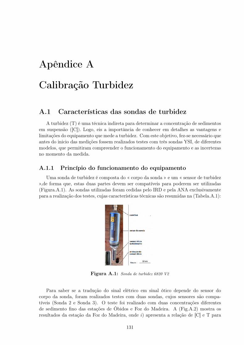
Apêndice A
Calibração Turbidez
A.1 Características das sondas de turbidez
A turbidez (T) é uma técnica indireta para determinar a concentração de sedimentosem suspensão ([C]). Logo, eis a importância de conhecer em detalhes as vantagens elimitações do equipamento que mede a turbidez. Com este objetivo, fez-se necessário queantes do inicio das medições fossem realizados testes com três sondas YSI, de diferentesmodelos, que permitiram compreender o funcionamento do equipamento e as incertezasno momento da medida.
A.1.1 Princípio do funcionamento do equipamento
Uma sonda de turbidez é composta do « corpo da sonda » e um « sensor de turbidez»,de forma que, estas duas partes devem ser compatíveis para poderem ser utilizadas(Figura.A.1). As sondas utilizadas foram cedidas pelo IRD e pela ANA exclusivamentepara a realização dos testes, cujas características técnicas são resumidas na (Tabela.A.1):
Figura A.1: Sonda de turbidez 6820 V2
Para saber se a tradução do sinal elétrico em sinal ótico depende do sensor docorpo da sonda, foram realizados testes com duas sondas, cujos sensores são compa-tíveis (Sonda 2 e Sonda 3). O teste foi realizado com duas concentrações diferentesde sedimento fino das estações de Óbidos e Foz do Madeira. A (Fig.A.2) mostra osresultados da estação da Foz do Madeira, onde 𝑖) apresenta a relação de [C] e T para
131
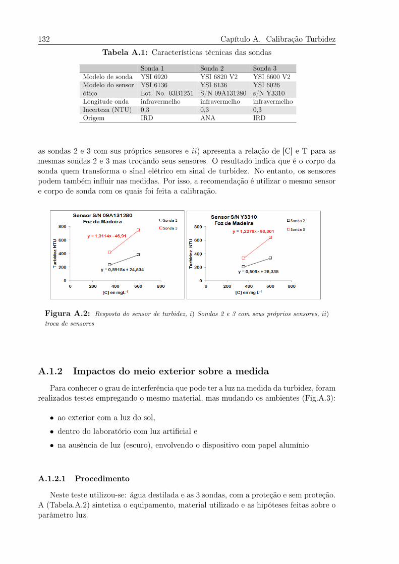
132 Capítulo A. Calibração Turbidez
Tabela A.1: Características técnicas das sondas
Sonda 1 Sonda 2 Sonda 3Modelo de sonda YSI 6920 YSI 6820 V2 YSI 6600 V2Modelo do sensor YSI 6136 YSI 6136 YSI 6026ótico Lot. No. 03B1251 S/N 09A131280 s/N Y3310Longitude onda infravermelho infravermelho infravermelhoIncerteza (NTU) 0,3 0,3 0,3Origem IRD ANA IRD
as sondas 2 e 3 com sus próprios sensores e 𝑖𝑖) apresenta a relação de [C] e T para asmesmas sondas 2 e 3 mas trocando seus sensores. O resultado indica que é o corpo dasonda quem transforma o sinal elétrico em sinal de turbidez. No entanto, os sensorespodem também influir nas medidas. Por isso, a recomendação é utilizar o mesmo sensore corpo de sonda com os quais foi feita a calibração.
Figura A.2: Resposta do sensor de turbidez, 𝑖) Sondas 2 e 3 com seus próprios sensores, 𝑖𝑖)troca de sensores
A.1.2 Impactos do meio exterior sobre a medida
Para conhecer o grau de interferência que pode ter a luz na medida da turbidez, foramrealizados testes empregando o mesmo material, mas mudando os ambientes (Fig.A.3):
• ao exterior com a luz do sol,
• dentro do laboratório com luz artificial e
• na ausência de luz (escuro), envolvendo o dispositivo com papel alumínio
A.1.2.1 Procedimento
Neste teste utilizou-se: água destilada e as 3 sondas, com a proteção e sem proteção.A (Tabela.A.2) sintetiza o equipamento, material utilizado e as hipóteses feitas sobre oparâmetro luz.
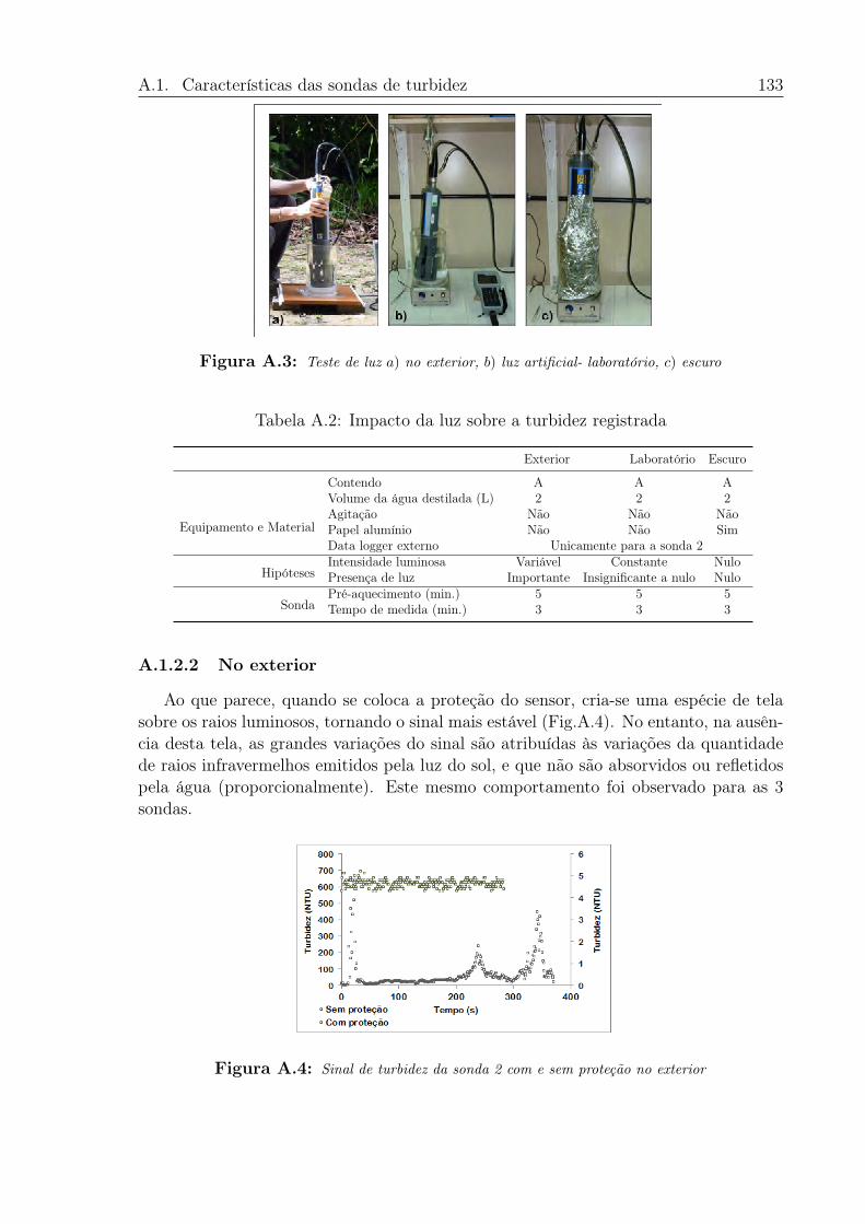
A.1. Características das sondas de turbidez 133
Figura A.3: Teste de luz 𝑎) no exterior, 𝑏) luz artificial- laboratório, 𝑐) escuro
Tabela A.2: Impacto da luz sobre a turbidez registrada
Exterior Laboratório Escuro
Equipamento e Material
Contendo A A AVolume da água destilada (L) 2 2 2Agitação Não Não NãoPapel alumínio Não Não SimData logger externo Unicamente para a sonda 2
HipótesesIntensidade luminosa Variável Constante NuloPresença de luz Importante Insignificante a nulo Nulo
SondaPré-aquecimento (min.) 5 5 5Tempo de medida (min.) 3 3 3
A.1.2.2 No exterior
Ao que parece, quando se coloca a proteção do sensor, cria-se uma espécie de telasobre os raios luminosos, tornando o sinal mais estável (Fig.A.4). No entanto, na ausên-cia desta tela, as grandes variações do sinal são atribuídas às variações da quantidadede raios infravermelhos emitidos pela luz do sol, e que não são absorvidos ou refletidospela água (proporcionalmente). Este mesmo comportamento foi observado para as 3sondas.
Figura A.4: Sinal de turbidez da sonda 2 com e sem proteção no exterior
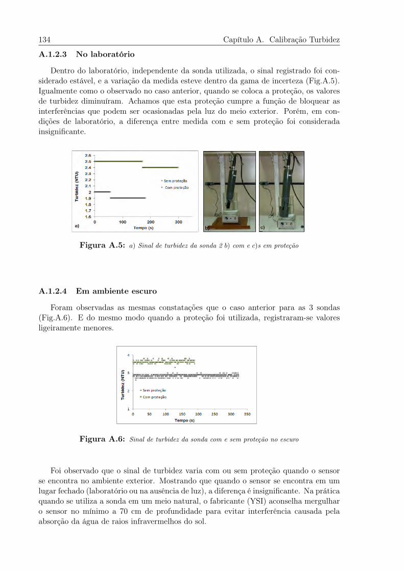
134 Capítulo A. Calibração Turbidez
A.1.2.3 No laboratório
Dentro do laboratório, independente da sonda utilizada, o sinal registrado foi con-siderado estável, e a variação da medida esteve dentro da gama de incerteza (Fig.A.5).Igualmente como o observado no caso anterior, quando se coloca a proteção, os valoresde turbidez diminuíram. Achamos que esta proteção cumpre a função de bloquear asinterferências que podem ser ocasionadas pela luz do meio exterior. Porém, em con-dições de laboratório, a diferença entre medida com e sem proteção foi consideradainsignificante.
Figura A.5: 𝑎) Sinal de turbidez da sonda 2 𝑏) com e 𝑐)s em proteção
A.1.2.4 Em ambiente escuro
Foram observadas as mesmas constatações que o caso anterior para as 3 sondas(Fig.A.6). E do mesmo modo quando a proteção foi utilizada, registraram-se valoresligeiramente menores.
Figura A.6: Sinal de turbidez da sonda com e sem proteção no escuro
Foi observado que o sinal de turbidez varia com ou sem proteção quando o sensorse encontra no ambiente exterior. Mostrando que quando o sensor se encontra em umlugar fechado (laboratório ou na ausência de luz), a diferença é insignificante. Na práticaquando se utiliza a sonda em um meio natural, o fabricante (YSI) aconselha mergulharo sensor no mínimo a 70 cm de profundidade para evitar interferência causada pelaabsorção da água de raios infravermelhos do sol.
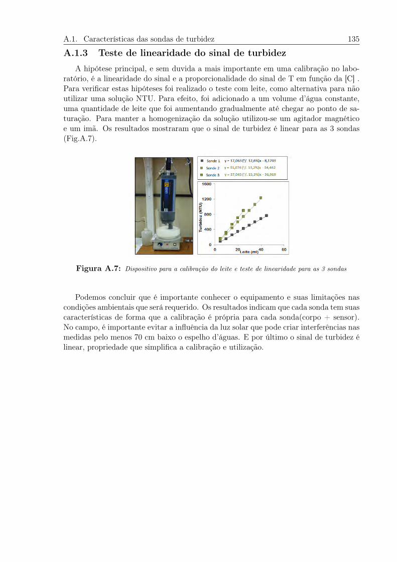
A.1. Características das sondas de turbidez 135
A.1.3 Teste de linearidade do sinal de turbidez
A hipótese principal, e sem duvida a mais importante em uma calibração no labo-ratório, é a linearidade do sinal e a proporcionalidade do sinal de T em função da [C] .Para verificar estas hipóteses foi realizado o teste com leite, como alternativa para nãoutilizar uma solução NTU. Para efeito, foi adicionado a um volume d’água constante,uma quantidade de leite que foi aumentando gradualmente até chegar ao ponto de sa-turação. Para manter a homogenização da solução utilizou-se um agitador magnéticoe um imã. Os resultados mostraram que o sinal de turbidez é linear para as 3 sondas(Fig.A.7).
Figura A.7: Dispositivo para a calibração do leite e teste de linearidade para as 3 sondas
Podemos concluir que é importante conhecer o equipamento e suas limitações nascondições ambientais que será requerido. Os resultados indicam que cada sonda tem suascaracterísticas de forma que a calibração é própria para cada sonda(corpo + sensor).No campo, é importante evitar a influência da luz solar que pode criar interferências nasmedidas pelo menos 70 cm baixo o espelho d’águas. E por último o sinal de turbidez élinear, propriedade que simplifica a calibração e utilização.

136 Capítulo A. Calibração Turbidez
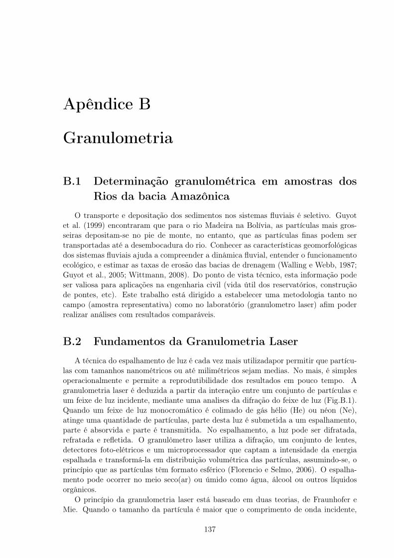
Apêndice B
Granulometria
B.1 Determinação granulométrica em amostras dosRios da bacia Amazônica
O transporte e depositação dos sedimentos nos sistemas fluviais é seletivo. Guyotet al. (1999) encontraram que para o rio Madeira na Bolívia, as partículas mais gros-seiras depositam-se no pie de monte, no entanto, que as partículas finas podem sertransportadas até a desembocadura do rio. Conhecer as características geomorfológicasdos sistemas fluviais ajuda a compreender a dinâmica fluvial, entender o funcionamentoecológico, e estimar as taxas de erosão das bacias de drenagem (Walling e Webb, 1987;Guyot et al., 2005; Wittmann, 2008). Do ponto de vista técnico, esta informação podeser valiosa para aplicações na engenharia civil (vida útil dos reservatórios, construçãode pontes, etc). Este trabalho está dirigido a estabelecer uma metodologia tanto nocampo (amostra representativa) como no laboratório (granulometro laser) afim poderrealizar análises com resultados comparáveis.
B.2 Fundamentos da Granulometria Laser
A técnica do espalhamento de luz é cada vez mais utilizadapor permitir que partícu-las com tamanhos nanométricos ou até milimétricos sejam medias. No mais, é simplesoperacionalmente e permite a reprodutibilidade dos resultados em pouco tempo. Agranulometria laser é deduzida a partir da interação entre um conjunto de partículas eum feixe de luz incidente, mediante uma analises da difração do feixe de luz (Fig.B.1).Quando um feixe de luz monocromático é colimado de gás hélio (He) ou néon (Ne),atinge uma quantidade de partículas, parte desta luz é submetida a um espalhamento,parte é absorvida e parte é transmitida. No espalhamento, a luz pode ser difratada,refratada e refletida. O granulômetro laser utiliza a difração, um conjunto de lentes,detectores foto-elétricos e um microprocessador que captam a intensidade da energiaespalhada e transformá-la em distribuição volumétrica das partículas, assumindo-se, oprincípio que as partículas têm formato esférico (Florencio e Selmo, 2006). O espalha-mento pode ocorrer no meio seco(ar) ou úmido como água, álcool ou outros líquidosorgânicos.
O princípio da granulometria laser está baseado em duas teorias, de Fraunhofer eMie. Quando o tamanho da partícula é maior que o comprimento de onda incidente,
137
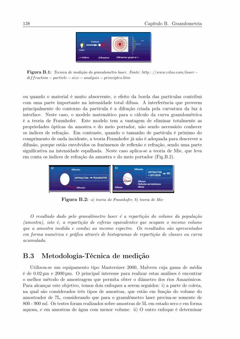
138 Capítulo B. Granulometria
Figura B.1: Tecnica de medição do granulométro laser. Fonte: ℎ𝑡𝑡𝑝 : //𝑤𝑤𝑤.𝑐𝑖𝑙𝑎𝑠.𝑐𝑜𝑚/𝑙𝑎𝑠𝑒𝑟−𝑑𝑖𝑓𝑓𝑟𝑎𝑐𝑡𝑖𝑜𝑛− 𝑝𝑎𝑟𝑡𝑖𝑐𝑙𝑒− 𝑠𝑖𝑧𝑒− 𝑎𝑛𝑎𝑙𝑦𝑠𝑖𝑠− 𝑝𝑟𝑖𝑛𝑐𝑖𝑝𝑙𝑒𝑠.ℎ𝑡𝑚
ou quando o material é muito absorvente, o efeito da borda das partículas contribuicom uma parte importante na intensidade total difusa. A interferência que proveemprincipalmente do contorno da partícula é a difração criada pela curvatura da luz àinterface. Neste caso, o modelo matemático para o cálculo da curva granulométricaé a teoria de Fraunhofer. Este modelo tem a vantagem de eliminar totalmente aspropriedades ópticas da amostra e do meio portador, não sendo necessário conheceros índices de refração. Em contraste, quando o tamanho de partícula é próximo docomprimento de onda incidente, a teoria Fraunhofer já não é adequada para descrever adifusão, porque estão envolvidos os fenômenos de reflexão e refração, sendo uma partesignificativa na intensidade espalhada. Neste caso aplica-se a teoria de Mie, que levaem conta os índices de refração da amostra e do meio portador (Fig.B.2).
Figura B.2: 𝑎) teoria do Fraunhofer, 𝑏) teoria de Mie
O resultado dado pelo granulômetro laser é a repartição do volume da população(amostra), isto é, a repartição de esferas equivalentes que ocupam o mesmo volumeque a amostra medida e conduz ao mesmo espectro. Os resultados são apresentadosem forma numérica e gráfica através de histogramas de repartição de classes ou curvaacumulada.
B.3 Metodologia-Técnica de medição
Utilizou-se um equipamento tipo Mastersizer 2000, Malvern cuja gama de médiaé de 0.02 µm e 2000 µm. O principal interesse para realizar estas análises é encontraro melhor método de amostragem que permita obter o diâmetro dos rios Amazônicos.Para alcançar este objetivo, temos dois enfoques a serem seguidos: i) a parte de coleta,na qual são considerados três tipos de amostras, que estão em função do volume doamostrador de 7L, considerando que para o granulômetro laser precisa-se somente de800 - 900 ml. Os testes foram realizados sobre amostras de 5L em estado seco e em formaaquosa, e em amostras de água com menor volume. ii) O outro enfoque é determinar
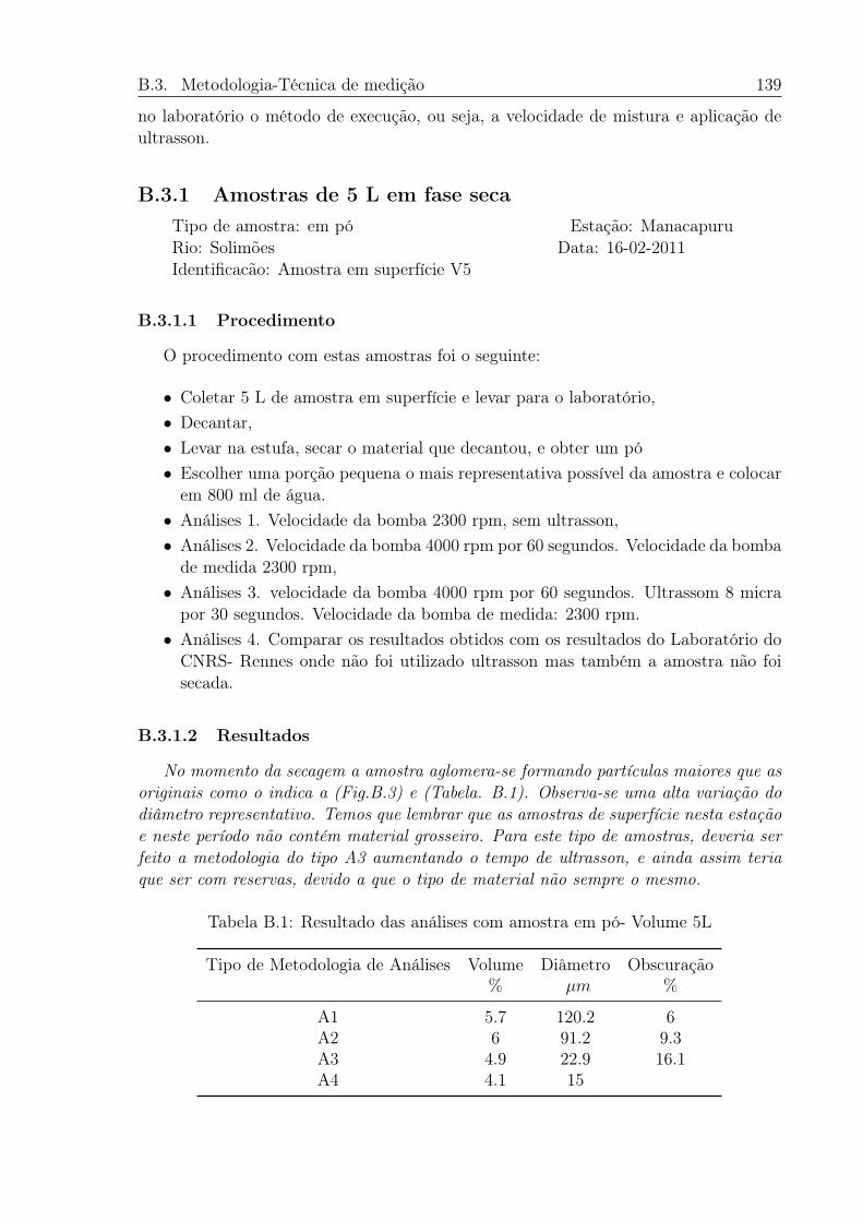
B.3. Metodologia-Técnica de medição 139
no laboratório o método de execução, ou seja, a velocidade de mistura e aplicação deultrasson.
B.3.1 Amostras de 5 L em fase secaTipo de amostra: em pó Estação: ManacapuruRio: Solimões Data: 16-02-2011Identificacão: Amostra em superfície V5
B.3.1.1 Procedimento
O procedimento com estas amostras foi o seguinte:
• Coletar 5 L de amostra em superfície e levar para o laboratório,• Decantar,• Levar na estufa, secar o material que decantou, e obter um pó• Escolher uma porção pequena o mais representativa possível da amostra e colocar
em 800 ml de água.• Análises 1. Velocidade da bomba 2300 rpm, sem ultrasson,• Análises 2. Velocidade da bomba 4000 rpm por 60 segundos. Velocidade da bomba
de medida 2300 rpm,• Análises 3. velocidade da bomba 4000 rpm por 60 segundos. Ultrassom 8 micra
por 30 segundos. Velocidade da bomba de medida: 2300 rpm.• Análises 4. Comparar os resultados obtidos com os resultados do Laboratório do
CNRS- Rennes onde não foi utilizado ultrasson mas também a amostra não foisecada.
B.3.1.2 Resultados
No momento da secagem a amostra aglomera-se formando partículas maiores que asoriginais como o indica a (Fig.B.3) e (Tabela. B.1). Observa-se uma alta variação dodiâmetro representativo. Temos que lembrar que as amostras de superfície nesta estaçãoe neste período não contém material grosseiro. Para este tipo de amostras, deveria serfeito a metodologia do tipo A3 aumentando o tempo de ultrasson, e ainda assim teriaque ser com reservas, devido a que o tipo de material não sempre o mesmo.
Tabela B.1: Resultado das análises com amostra em pó- Volume 5L
Tipo de Metodologia de Análises Volume Diâmetro Obscuração% 𝜇𝑚 %
A1 5.7 120.2 6A2 6 91.2 9.3A3 4.9 22.9 16.1A4 4.1 15
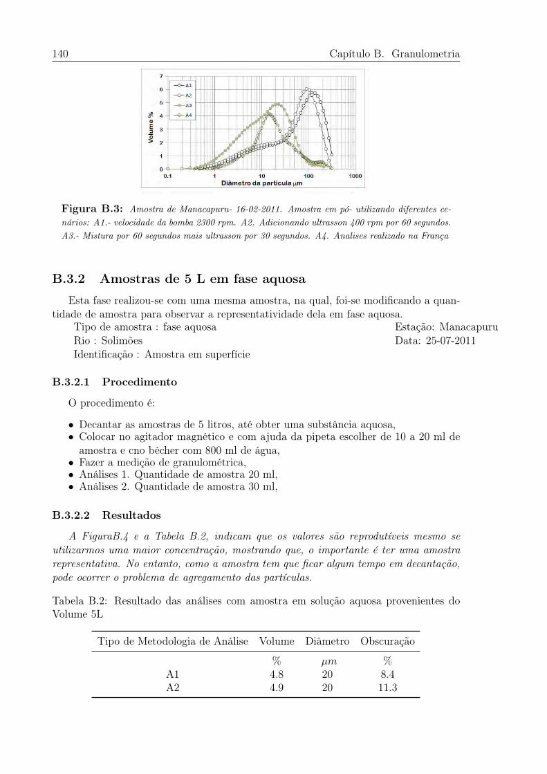
140 Capítulo B. Granulometria
Figura B.3: Amostra de Manacapuru- 16-02-2011. Amostra em pó- utilizando diferentes ce-nários: A1.- velocidade da bomba 2300 rpm. A2. Adicionando ultrasson 400 rpm por 60 segundos.A3.- Mistura por 60 segundos mais ultrasson por 30 segundos. A4. Analises realizado na França
B.3.2 Amostras de 5 L em fase aquosa
Esta fase realizou-se com uma mesma amostra, na qual, foi-se modificando a quan-tidade de amostra para observar a representatividade dela em fase aquosa.
Tipo de amostra : fase aquosa Estação: ManacapuruRio : Solimões Data: 25-07-2011Identificação : Amostra em superfície
B.3.2.1 Procedimento
O procedimento é:
• Decantar as amostras de 5 litros, até obter uma substância aquosa,• Colocar no agitador magnético e com ajuda da pipeta escolher de 10 a 20 ml de
amostra e cno bécher com 800 ml de água,• Fazer a medição de granulométrica,• Análises 1. Quantidade de amostra 20 ml,• Análises 2. Quantidade de amostra 30 ml,
B.3.2.2 Resultados
A FiguraB.4 e a Tabela B.2, indicam que os valores são reprodutíveis mesmo seutilizarmos uma maior concentração, mostrando que, o importante é ter uma amostrarepresentativa. No entanto, como a amostra tem que ficar algum tempo em decantação,pode ocorrer o problema de agregamento das partículas.
Tabela B.2: Resultado das análises com amostra em solução aquosa provenientes doVolume 5L
Tipo de Metodologia de Análise Volume Diâmetro Obscuração
% 𝜇𝑚 %A1 4.8 20 8.4A2 4.9 20 11.3
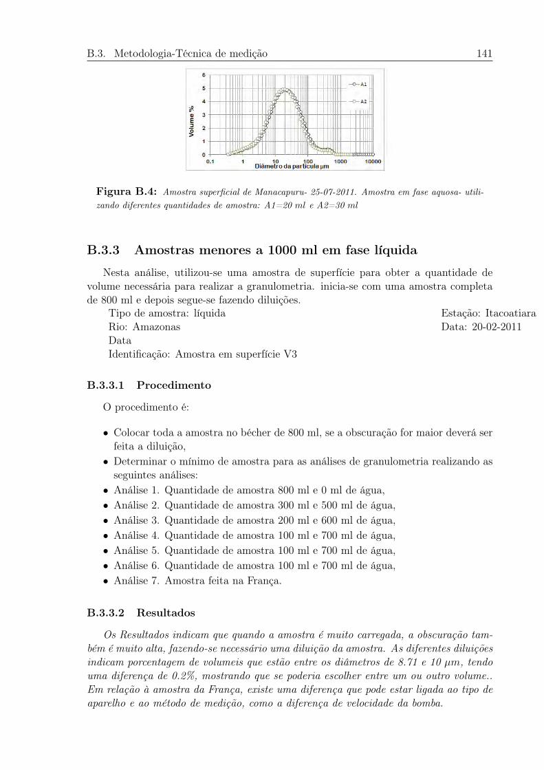
B.3. Metodologia-Técnica de medição 141
Figura B.4: Amostra superficial de Manacapuru- 25-07-2011. Amostra em fase aquosa- utili-zando diferentes quantidades de amostra: A1=20 𝑚𝑙 e A2=30 𝑚𝑙
B.3.3 Amostras menores a 1000 ml em fase líquida
Nesta análise, utilizou-se uma amostra de superfície para obter a quantidade devolume necessária para realizar a granulometria. inicia-se com uma amostra completade 800 ml e depois segue-se fazendo diluições.
Tipo de amostra: líquida Estação: ItacoatiaraRio: Amazonas Data: 20-02-2011DataIdentificação: Amostra em superfície V3
B.3.3.1 Procedimento
O procedimento é:
• Colocar toda a amostra no bécher de 800 ml, se a obscuração for maior deverá serfeita a diluição,
• Determinar o mínimo de amostra para as análises de granulometria realizando asseguintes análises:
• Análise 1. Quantidade de amostra 800 ml e 0 ml de água,• Análise 2. Quantidade de amostra 300 ml e 500 ml de água,• Análise 3. Quantidade de amostra 200 ml e 600 ml de água,• Análise 4. Quantidade de amostra 100 ml e 700 ml de água,• Análise 5. Quantidade de amostra 100 ml e 700 ml de água,• Análise 6. Quantidade de amostra 100 ml e 700 ml de água,• Análise 7. Amostra feita na França.
B.3.3.2 Resultados
Os Resultados indicam que quando a amostra é muito carregada, a obscuração tam-bém é muito alta, fazendo-se necessário uma diluição da amostra. As diferentes diluiçõesindicam porcentagem de volumeis que estão entre os diâmetros de 8.71 e 10 𝜇𝑚, tendouma diferença de 0.2%, mostrando que se poderia escolher entre um ou outro volume..Em relação à amostra da França, existe uma diferença que pode estar ligada ao tipo deaparelho e ao método de medição, como a diferença de velocidade da bomba.
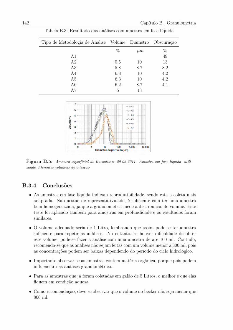
142 Capítulo B. Granulometria
Tabela B.3: Resultado das análises com amostra em fase líquida
Tipo de Metodologia de Análise Volume Diâmetro Obscuração
% 𝜇𝑚 %A1 49A2 5.5 10 13A3 5.8 8.7 8.2A4 6.3 10 4.2A5 6.3 10 4.2A6 6.2 8.7 4.1A7 5 13
Figura B.5: Amostra superficial de Itacoatiara- 20-02-2011. Amostra em fase líquida- utili-zando diferentes volumeis de diluição
B.3.4 Conclusões
• As amostras em fase líquida indicam reprodutibilidade, sendo esta a coleta maisadaptada. Na questão de representatividade, é suficiente com ter uma amostrabem homogeneizada, ja que a granulometria mede a distribuição de volume. Esteteste foi aplicado também para amostras em profundidade e os resultados foramsimilares.
• O volume adequado seria de 1 Litro, lembrando que assim pode-se ter amostrasuficiente para repetir as análises. No entanto, se houver dificuldade de obtereste volume, pode-se fazer a análise com uma amostra de até 100 ml. Contudo,recomenda-se que as análises não sejam feitas com um volume menor a 300 ml, poisas concentrações podem ser baixas dependendo do período do ciclo hidrológico.
• Importante observar se as amostras contem matéria orgânica, porque pois podeminfluenciar nas análises granulométrico..
• Para as amostras que já foram coletadas em galão de 5 Litros, o melhor é que elasfiquem em condição aquosa.
• Como recomendação, deve-se observar que o volume no becker não seja menor que800 ml.
Apêndice C
Sedimentos em suspensão e materialdissolvido dos Andes do Equador
Yields of suspended sediments and dissolvedsolids from the Andean basins of Ecuador
143
This article was downloaded by: [Elisa Armijos]On: 16 October 2013, At: 08:00Publisher: Taylor & FrancisInforma Ltd Registered in England and Wales Registered Number: 1072954 Registered office: Mortimer House,37-41 Mortimer Street, London W1T 3JH, UK
Hydrological Sciences JournalPublication details, including instructions for authors and subscription information:http://www.tandfonline.com/loi/thsj20
Yields of suspended sediment and dissolved solids fromthe Andean basins of EcuadorElisa Armijosab, Alain Laraquec, Sonia Barbad, Luc Bourrelc, Catalina Cerone, ChristelleLaganec, Philippe Magatc, Jean Sebastien Moquetc, Rodrigo Pombosaa, Francis Sondagcf,Philippe Vauchelc, Andrea Verae & Jean Loup Guyotcf
a Instituto Nacional de Meteorología e Hidrología (INAMHI), Iñaquito N36-14 y Correa, Quito,Ecuadorb Instituto Nacional de Pesquisas da Amazônia (INPA), LBA-CLIAMB, Universidade do Estadodo Amazonas, 2936 Aleixo, CEP 69060-001, Manaus, Brazilc GET (CNRS, IRD, OMP, Université de Toulouse), 14 Avenue Edouard Belin, F-31400,Toulouse, Franced Universidad Politécnica Nacional (EPN), Ladrón de Guevara E11, 253, Quito, Ecuadore Universidad Central del Ecuador (UCE), Ciudadela Universitaria, Avenida América, Quito,Ecuadorf IRD,Published online: 15 Oct 2013.
To cite this article: Elisa Armijos, Alain Laraque, Sonia Barba, Luc Bourrel, Catalina Ceron, Christelle Lagane, PhilippeMagat, Jean Sebastien Moquet, Rodrigo Pombosa, Francis Sondag, Philippe Vauchel, Andrea Vera & Jean Loup Guyot (2013)Yields of suspended sediment and dissolved solids from the Andean basins of Ecuador, Hydrological Sciences Journal, 58:7,1478-1494, DOI: 10.1080/02626667.2013.826359
To link to this article: http://dx.doi.org/10.1080/02626667.2013.826359
PLEASE SCROLL DOWN FOR ARTICLE
Taylor & Francis makes every effort to ensure the accuracy of all the information (the “Content”) containedin the publications on our platform. However, Taylor & Francis, our agents, and our licensors make norepresentations or warranties whatsoever as to the accuracy, completeness, or suitability for any purpose of theContent. Any opinions and views expressed in this publication are the opinions and views of the authors, andare not the views of or endorsed by Taylor & Francis. The accuracy of the Content should not be relied upon andshould be independently verified with primary sources of information. Taylor and Francis shall not be liable forany losses, actions, claims, proceedings, demands, costs, expenses, damages, and other liabilities whatsoeveror howsoever caused arising directly or indirectly in connection with, in relation to or arising out of the use ofthe Content.
This article may be used for research, teaching, and private study purposes. Any substantial or systematicreproduction, redistribution, reselling, loan, sub-licensing, systematic supply, or distribution in anyform to anyone is expressly forbidden. Terms & Conditions of access and use can be found at http://www.tandfonline.com/page/terms-and-conditions
1478 Hydrological Sciences Journal – Journal des Sciences Hydrologiques, 58 (7) 2013http://dx.doi.org/10.1080/02626667.2013.826359
Yields of suspended sediment and dissolved solids from the Andeanbasins of Ecuador
Elisa Armijos1,2 , Alain Laraque3, Sonia Barba4, Luc Bourrel3, Catalina Ceron5, Christelle Lagane3,Philippe Magat3, Jean Sebastien Moquet3, Rodrigo Pombosa1, Francis Sondag3,6, Philippe Vauchel3,Andrea Vera5 and Jean Loup Guyot3,6
1Instituto Nacional de Meteorología e Hidrología (INAMHI), Iñaquito N36-14 y Correa, Quito, [email protected] Nacional de Pesquisas da Amazônia (INPA), LBA-CLIAMB, Universidade do Estado do Amazonas, 2936 Aleixo, CEP69060-001, Manaus, Brazil3GET (CNRS, IRD, OMP, Université de Toulouse), 14 Avenue Edouard Belin, F-31400 Toulouse, France4Universidad Politécnica Nacional (EPN), Ladrón de Guevara E11, 253 Quito, Ecuador5Universidad Central del Ecuador (UCE), Ciudadela Universitaria, Avenida América, Quito, Ecuador6IRD, CP 7091 Lago Sul, CEP 71635-971 Brasília, DF, Brazil
Received 9 July 2012; accepted 10 January 2013; open for discussion until 1 April 2014
Editor Z.W. Kundzewicz
Citation Armijos, E., Laraque, A., Barba, S., Bourrel, L., Ceron, C., Lagane, C., Magat, P., Moquet, J.-S., Pombosa, R., Sondag, F.,Vauchel, P., Vera, A., and Guyot, J.L., 2013. Yields of suspended sediment and dissolved solids from the Andean basins of Ecuador.Hydrological Sciences Journal, 58 (7), 1478–1494.
Abstract Water discharge and suspended and dissolved sediment data from three rivers (Napo, Pastaza andSantiago) in the Ecuadorian Amazon basin and a river in the Pacific basin (Esmeraldas) over a 9-year period, arepresented. This data set allows us to present: (a) the chemical weathering rates; (b) the erosion rates, calculatedfrom the suspended sediment from the Andean basin; (c) the spatio-temporal variability of the two regions; and(d) the relationship between this variability and the precipitation, topography, lithology and seismic activity of thearea. The dissolved solids load from the Esmeraldas basin was 2 × 10⁶ t year-1, whereas for the Napo, Pastaza andSantiago basins, it was 4, 2 and 3 × 10⁶ t year-1, respectively. For stations in the Andean piedmont of Ecuador, therelationship between surface sediment and the total sediment concentration was found to be close to one. This isdue to minimal stratification of the suspended sediment in the vertical profile, which is attributed to turbulence andhigh vertical water speeds. However, during the dry season, when the water speed decreases, sediment stratificationappears, but this effect can be neglected in the sediment flux calculations due to low concentration rates. Thesuspended sediment load in the Pacific basin was 6 × 10⁶ t year-1, and the total for the three Amazon basins was47 × 106 t year-1. The difference between these contributions of the suspended sediment load is likely due to thetectonic uplift and the seismic and volcanic dynamics that occur on the Amazon side.
Key words hydrology; erosion; Andes; chemical weathering; Amazon basin; Pacific basin
Apports de matières en suspension et de solides dissous des les bassins andins de l’EquateurRésumé Cet article présente un ensemble de données concernant l’exportation d’eau et de matières en suspen-sion et dissoutes de trois rivières (Napo, Pastaza et Santiago) du bassin de l’Amazonie équatorienne et d’unerivière du bassin du Pacifique (Esmeraldas) sur une période de neuf ans. Cet ensemble de données nous permetde d’appréhender : (a) le taux d’altération chimique; (b) les taux d’érosion, calculés à partir des sédiments ensuspension dans le bassin andin; (c) la variabilité spatio-temporelle des deux régions; et (d) les relations entre lavariabilité et l’activité des précipitations, la topographie, la lithologie et l’activité sismique de la zone. La chargede solides dissous dans le bassin Esmeraldas était de 2 × 10⁶ t an-1, alors que pour le bassin du Napo, Pastaza etde Santiago, elle était respectivement de 4, 2 et 3 × 10⁶ t an-1 Pour les stations du piémont andin de l’Equateur,
© 2013 IAHS Press
Dow
nloa
ded
by [
Elis
a A
rmijo
s] a
t 08:
00 1
6 O
ctob
er 2
013
Yields of suspended sediment and dissolved solids from the Andean basins of Ecuador 1479
le rapport entre la concentration des sédiments en surface et la concentration totale de sédiments a été trouvéproche de 1. Cela est dû à la stratification minimale des sédiments en suspension selon le profil vertical, qui estattribuée à la turbulence et à des vitesses élevées de déplacement vertical de l’eau. Cependant, pendant la saisonsèche, lorsque la vitesse de l’eau diminue, la stratification des sédiments apparaît mais cet effet peut être négligédans les calculs de flux de sédiments en raison des faibles taux de concentration. La charge sédimentaire dans lebassin du Pacifique était de 6 × 10⁶ t an-1, et le total pour les trois bassins de l’Amazone était de 47 × 106 t an-1.La différence entre ces apports de sédiments en suspension est probablement due à la surrection tectonique et à ladynamique sismique et volcanique qui se produisent sur le versant amazonien.
Mots clefs hydrologie; érosion; Andes; altération chimique; bassin de l’Amazone; bassin du Pacifique
INTRODUCTION
The Andes represent 11% of the 6.1 × 10⁶ km2
Amazon Basin (Goulding et al. 2003), and are themost important source of sediment from the SouthAmerican continent and the third largest source ofsediment in the world, after the Ganges-Brahmaputraand Yellow rivers (Degens et al. 1991). The AmazonRiver discharges 6500 × 109 m3 year-1 of water(Callède et al. 2010), approx. 800 × 106 t year-1 ofsuspended sediments (Guyot et al. 2005, Martinezet al. 2009) and approx. 270 × 106 t year-1 of dis-solved elements (Mortatti and Probst 2003, Moquet2011) into the Atlantic Ocean.
Research on the processes of erosion and weath-ering and the spatio-temporal variability of theAmazon Basin has been ongoing for several decades(Gibbs 1967, Meade et al. 1979, 1985, Dunneet al. 1998, Filizola and Guyot 2004, 2009, Guyotet al. 1996, 2005, 2007, Moquet et al. 2011). TheAndean drainage basins of Bolivia produce dissolvedsediment load of 10 × 106 t year-1 as they leave theAndes (Beni River at Angosto del Bala and GrandeRiver at Abapo) because of the high solubility of therocks (Guyot 1993, Moquet et al. 2011), which givesa chemical weathering rate of 44 t year-1 km-2. At thesame stations, the mechanical erosion rates are 3140 tyear-1 km-2 for the Beni River and 2130 t year-1 km-2
for the Grande River (Guyot et al. 1996). In Peru,76% of the total area of the country is in the Amazonbasin (977 900 km2), and 53% of that is Andean. Theresults presented by Guyot et al. (2007) and Armijos(2010) demonstrate that the sediment flux through theAmazon River in Peru is 570 × 106 t year-1 (approx.550 t year-1 km-2).
Geologically, Ecuador is located in a transi-tion zone of the subducting Nazca Plate and is alsoaffected by the Carnegie Ridge collision. This posi-tion is responsible for the high volcanic and seismicactivity (Legrand et al. 2005). Furthermore, Ecuadorhas a spatially variable rainfall distribution (Laraque
et al. 2007, Espinoza et al. 2009), which directlyinfluences the quality and quantity of the dissolvedand suspended sediments.
Few studies have been performed on the quantifi-cation of fluxes in Ecuador due to the difficulty andcost of data collection; most have concentrated on theNapo River basin. Armijos (2002), Cerón (2004) andLaraque et al. (2004) presented the first data on waterdischarge and sediment fluxes in Amazon basins.Vanacker et al. (2007) worked in mountain basins inthe Upper Santiago basin (Paute basin) and showedthat small basins have high values of sediment con-centration mainly due to landslides and not becauseof human influence. However, Molina et al. (2008)found basins in the Andean Páramo (Upper Santiagobasin) where human activity can be an indirect causeof erosion in the sense of opening roads that leave thesoil exposed. Hence the importance of regular moni-toring of sediment concentration, especially in smallbasins that have quick response to changes in envi-ronment. Melo (2010) mapped risk areas for erosionin the Esmeraldas and Guyas basins. Narvaez andVera (2007) and Galeas and Melo (2007) performeda comparative characterization of the major dissolvedelements and suspended sediment yields in both theeastern and western basins (Napo and Esmeraldas)and showed that the waters of Ecuador are calciumbicarbonate type with a predominance of Na2+, Mg2+and K+. Moquet (2011) presented factors that influ-ence weathering in the Andean region of the Amazonbasin. Laraque et al. (2009) identified significant ero-sive processes in the Andes and the plains of theNapo basin in Ecuador and Peru, for 2001–2005 and2004–2005, respectively.
We complement this work by providing a dataset for the Ecuadorian Andean basins and new esti-mates for: (a) chemical weathering rates; (b) ero-sion rates calculated from suspended sediments;(c) the spatio-temporal variability of the two regions;and (d) the relationships between this variabilityand precipitation, topography, lithology and seismic
Dow
nloa
ded
by [
Elis
a A
rmijo
s] a
t 08:
00 1
6 O
ctob
er 2
013
1480 Elisa Armijos et al.
activity. The sediment load data set was collectedover nine years (2001–2009), and the dissolvedsolids data set ranges over eight years (2001–2008).The study area covers six gauging stations inAmazonian basins (Napo, Pastaza and Santiago) andtwo gauging stations in the Esmeraldas basin in thePacific region. These stations were monitored bythe ORE (Environmental Research Observatory) ofthe HYBAM (Geodynamical, hydrological and bio-geochemical control of erosion/alteration and mate-rial transport in the Amazon basin) programme inEcuador (INAMHI–IRD collaboration).
STUDY AREA
Ecuador is located in South America and extendsalong both sides of the Equator (La Condamine 1751)between latitudes 1◦30′ N and 5◦00′ S and longi-tudes 75◦20′ E and 81◦0′ W, occupying an area of248 406 km2. The Andes comprise the central third ofEcuador, stretching from north to south and formingtwo belts approximately 645 km long and 15–65 kmwide (DINAGE 1997). There are about 50 volcanoes,25% of which are still active (Monzier and Robin1995). The Cordillera, which is covered by glaciers,has peaks of 4000 to 6000 m (Aspiazu and Luna1993), divides Ecuador into two regions (west andeast) and forms the water divide between basins. Mostof the rivers have their origin in the Andean glaciers,from where they flow west to the Pacific Ocean, oreast to become part of the Amazon basin.
This study covers the three major basins in theAmazonian region—from north to south, the Napo,Pastaza and Santiago rivers—and the EsmeraldasRiver basin, whose waters flow to the Pacific Ocean(Fig. 1 and Table 1).
The eastern or Amazonian region accounts for50% of the total area of Ecuador and includes athird, non-continuous, 50-km-wide cordillera formedby the Galeras (Napo basin), Cutucú and Condor(Santiago basin) mountain ranges, where volcanoes,such as Reventador (3485 m) and Sumaco (3900 m),are located. This landscape is known as the UpperEast, whereas the Lower East is characterized byflat topography (ECORAE 2002). The topography ofboth the Pacific and Atlantic basins includes steepslopes of 40 to 70% in the Andes that graduallybecome plains at lower elevations (Winckell 1997).Ecuador is an area with much seismic activity dueto its location in a subduction zone, i.e. where theNazca oceanic plate is beneath the continental plateof South America (Gutscher et al. 1999, Legrand
et al. 2005), the presence of geological faults thatcross the territory, and the associated volcanic activ-ity (Servicio Nacional de Sismologia y Vulcanoligia;http://www.igepn.edu.ec). In the Amazon region, theAndean foothills present two areas of uplift, Santiagoand Napo, separated by a deep depression known asthe Cone of Pastaza (Bès de Berc et al. 2005). A sum-mary of the lithology and seismic activity is providedin Table 2.
The vegetation in the Pacific and Amazonianregions is diverse and depends on the orography,changing from “wastelands” above 3000 m altitude tomarshes of humid, natural forest in the lowlands. Thetwo zones have a human presence with cultivation ofshort-cycle crops; greater human impacts are seen inthe Pacific region where the agriculture is more indus-trialized (Neil 1997). Information on land use andcover was taken from the map data of the MAG IICACLIRSEN Project, updated in 2001, scale 1:25 000.The coverage and land use in the Esmeraldas basinshowed higher incidence of cropping (27% of cocoa,coffee, banana and African oil palm plantations, 18%of cultivated pasture and 11% of the short-cyclecrops). The Napo, Pastaza and Santiago basins areless disturbed, but the human presence has begun toexpand. The areas of cultivated pasture are 18, 15 and12% respectively, and of natural forest 55, 13 and46%. In the Pastaza basin, 17% of the area is used forshort-cycle crops. In the Santiago basin, 20% of thearea is under logged forest. In the Esmeraldas basin,urban area covers 1% the total basin area.
Ecuador has contrasting climates in the Andesand the plains. In the Amazon region, annual precip-itation ranges from 500 to 4000 mm year-1, varyingprimarily with altitude (Heredia and Pombosa 1999).The upper part of the eastern basins receives intenserainfall, both unimodal and bimodal, with maximumvalues in March–April and in October, and a min-imum in June–August (Laraque et al. 2007). Therainfall decreases from north to south (Moreno andTapia 2001) without clear seasonality, and rains arepersistent throughout the year (Fig. 1). Accordingto Laraque et al. (2007), the annual precipitation isapprox. 3100 mm year-1 in the Napo basin, 2300 mmyear-1 in the Pastaza basin and 2000 mm year-1 in theSantiago basin.
The western basin also has a complex spatialrainfall distribution and precipitation ranges from300 to 6000 mm year-1; the highest recorded annualprecipitation is in the Cordillera foothills, whichare characterized by a warm, humid climate. Long-duration, low-intensity rainfall occurs in the upper
Dow
nloa
ded
by [
Elis
a A
rmijo
s] a
t 08:
00 1
6 O
ctob
er 2
013
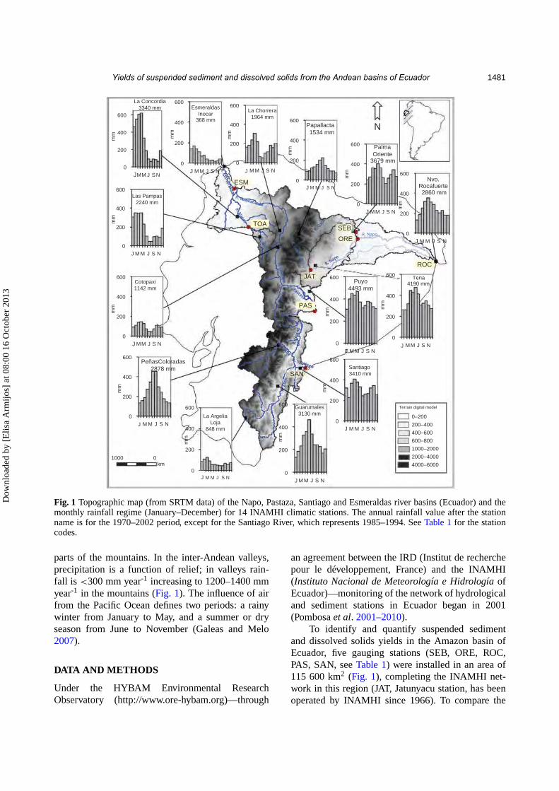
Yields of suspended sediment and dissolved solids from the Andean basins of Ecuador 1481
R.P
atat
e
R. Napo
0
200
400
600
mm
Cotopaxi1142 mm
0
200
400
600
mm
Papallacta1534 mm
0
200
400
600
mm
Nvo. Rocafuerte2860 mm
0
200
400
600
mm
Tena4190 mm
0
200
400
600
mm
Guarumales3130 mm
0
200
400
600
mm
Santiago 3410 mm
0
200
400
600
mm
La ArgeliaLoja
848 mm
0
200
400
600
mm
PeñasColoradas2878 mm
0
200
400
600
mm
Puyo4493 mm
0
200
400
600
mm
Las Pampas2240 mm 0
200
400
600
mm
Palma Oriente
3679 mm
1000 0km
Terrain digital model
0–200
200–400
400–600
600–800
1000–2000
2000–4000
4000–6000
ESM
TOA
SAN
PAS
JAT
ROC
SEB
ORE
0
200
400
600
mm
EsmeraldasInocar
368 mm
0
200
400
600
mm
La Chorrera1964 mm
0
200
400
600
MM J S N
M M J S N
M M J S N
MM J S N
M M J S N
M M J S N
M M J S N
M M J S N
E M M J S N
J M M J S N
MM J S N
M M J S N M M J S NMM J SN
mm
La Concordia3340 mm
JJ J
J
J
J
J
J
J
J
J
J
J
N
Fig. 1 Topographic map (from SRTM data) of the Napo, Pastaza, Santiago and Esmeraldas river basins (Ecuador) and themonthly rainfall regime (January–December) for 14 INAMHI climatic stations. The annual rainfall value after the stationname is for the 1970–2002 period, except for the Santiago River, which represents 1985–1994. See Table 1 for the stationcodes.
parts of the mountains. In the inter-Andean valleys,precipitation is a function of relief; in valleys rain-fall is <300 mm year-1 increasing to 1200–1400 mmyear-1 in the mountains (Fig. 1). The influence of airfrom the Pacific Ocean defines two periods: a rainywinter from January to May, and a summer or dryseason from June to November (Galeas and Melo2007).
DATA AND METHODS
Under the HYBAM Environmental ResearchObservatory (http://www.ore-hybam.org)—through
an agreement between the IRD (Institut de recherchepour le développement, France) and the INAMHI(Instituto Nacional de Meteorología e Hidrología ofEcuador)—monitoring of the network of hydrologicaland sediment stations in Ecuador began in 2001(Pombosa et al. 2001–2010).
To identify and quantify suspended sedimentand dissolved solids yields in the Amazon basin ofEcuador, five gauging stations (SEB, ORE, ROC,PAS, SAN, see Table 1) were installed in an area of115 600 km2 (Fig. 1), completing the INAMHI net-work in this region (JAT, Jatunyacu station, has beenoperated by INAMHI since 1966). To compare the
Dow
nloa
ded
by [
Elis
a A
rmijo
s] a
t 08:
00 1
6 O
ctob
er 2
013
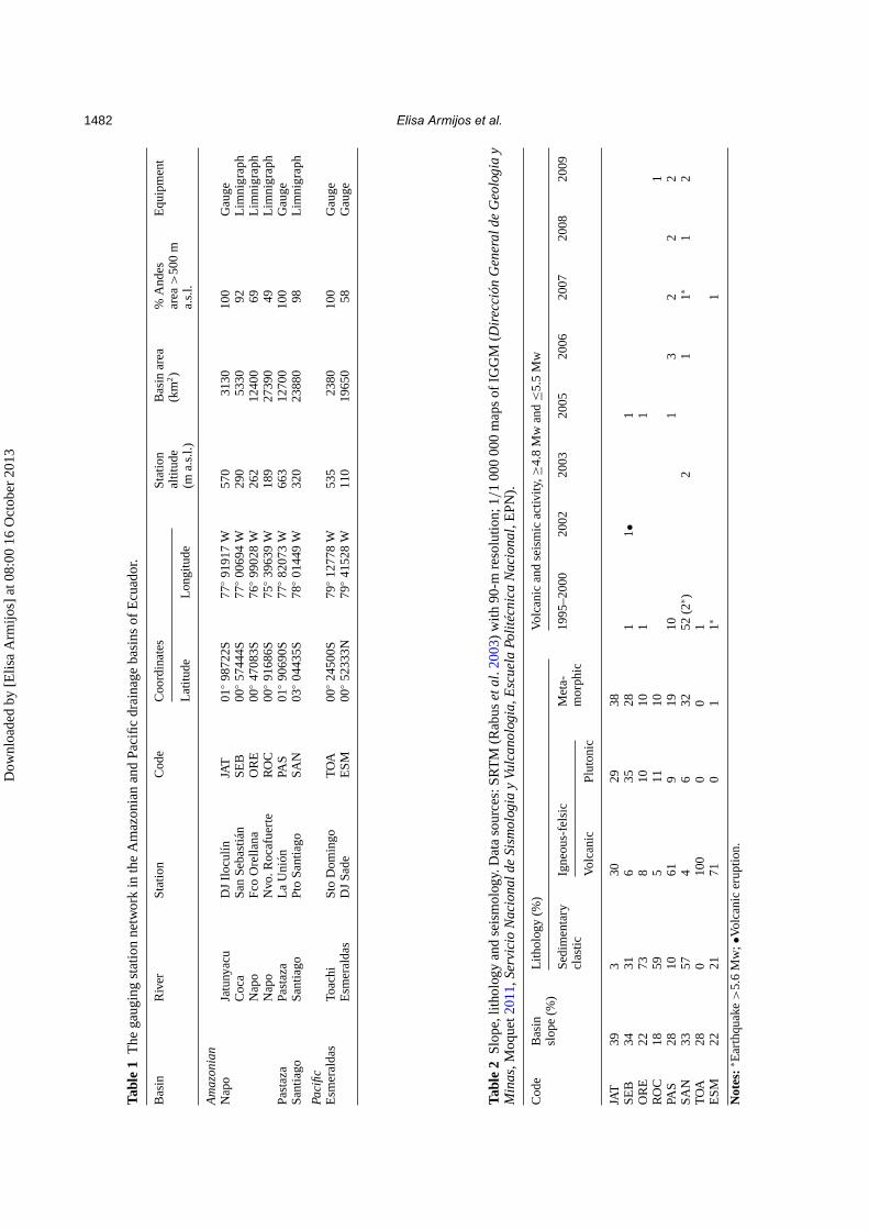
1482 Elisa Armijos et al.T
able
1T
hega
ugin
gst
atio
nne
twor
kin
the
Am
azon
ian
and
Paci
fic
drai
nage
basi
nsof
Ecu
ador
.
Bas
inR
iver
Sta
tion
Cod
eC
oord
inat
esS
tati
onal
titu
de(m
a.s.
l.)
Bas
inar
ea(k
m2)
%A
ndes
area
>50
0m
a.s.
l.
Equ
ipm
ent
Lat
itud
eL
ongi
tude
Am
azon
ian
Nap
oJa
tuny
acu
DJ
Iloc
ulín
JAT
01◦
9872
2S77
◦91
917
W57
031
3010
0G
auge
Coc
aS
anS
ebas
tián
SE
B00
◦57
444S
77◦
0069
4W
290
5330
92L
imni
grap
hN
apo
Fco
Ore
llan
aO
RE
00◦
4708
3S76
◦99
028
W26
212
400
69L
imni
grap
hN
apo
Nvo
.Roc
afue
rte
RO
C00
◦91
686S
75◦
3963
9W
189
2739
049
Lim
nigr
aph
Past
aza
Past
aza
La
Uni
ónPA
S01
◦90
690S
77◦
8207
3W
663
1270
010
0G
auge
San
tiag
oS
anti
ago
Pto
San
tiag
oS
AN
03◦
0443
5S78
◦01
449
W32
023
880
98L
imni
grap
h
Paci
ficE
smer
alda
sTo
achi
Sto
Dom
ingo
TO
A00
◦24
500S
79◦
1277
8W
535
2380
100
Gau
geE
smer
alda
sD
JS
ade
ES
M00
◦52
333N
79◦
4152
8W
110
1965
058
Gau
ge
Tab
le2
Slo
pe,l
itho
logy
and
seis
mol
ogy.
Dat
aso
urce
s:S
RT
M(R
abus
etal
.200
3)w
ith
90-m
reso
luti
on;1
/1
000
000
map
sof
IGG
M(D
irec
ción
Gen
eral
deG
eolo
gia
yM
inas
,Moq
uet2
011,
Serv
icio
Nac
iona
lde
Sism
olog
iay
Vulc
anol
ogia
,Esc
uela
Polité
cnic
aN
acio
nal,
EPN
).
Cod
eB
asin
slop
e(%
)L
itho
logy
(%)
Vol
cani
can
dse
ism
icac
tivit
y,≥4
.8M
wan
d≤5
.5M
w
Sed
imen
tary
clas
tic
Igne
ous-
fels
icM
eta-
mor
phic
1995
–200
020
0220
0320
0520
0620
0720
0820
09
Vol
cani
cP
luto
nic
JAT
393
3029
38S
EB
3431
635
281
1•1
OR
E22
738
1010
11
RO
C18
595
1110
1PA
S28
1061
919
101
32
22
SA
N33
574
632
52(2
∗ )2
11∗
12
TO
A28
010
00
01
ES
M22
2171
01
1∗1
Not
es:
∗ Ear
thqu
ake
>5.
6M
w;•
Vol
cani
cer
upti
on.
Dow
nloa
ded
by [
Elis
a A
rmijo
s] a
t 08:
00 1
6 O
ctob
er 2
013
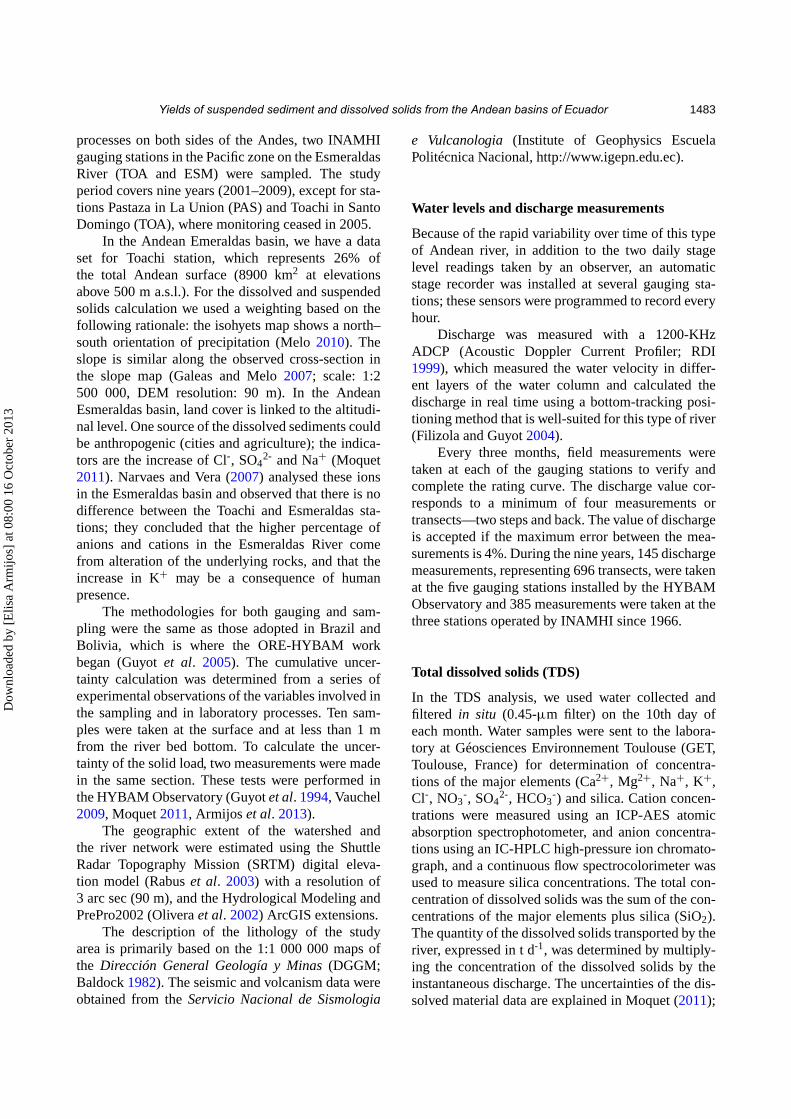
Yields of suspended sediment and dissolved solids from the Andean basins of Ecuador 1483
processes on both sides of the Andes, two INAMHIgauging stations in the Pacific zone on the EsmeraldasRiver (TOA and ESM) were sampled. The studyperiod covers nine years (2001–2009), except for sta-tions Pastaza in La Union (PAS) and Toachi in SantoDomingo (TOA), where monitoring ceased in 2005.
In the Andean Emeraldas basin, we have a dataset for Toachi station, which represents 26% ofthe total Andean surface (8900 km2 at elevationsabove 500 m a.s.l.). For the dissolved and suspendedsolids calculation we used a weighting based on thefollowing rationale: the isohyets map shows a north–south orientation of precipitation (Melo 2010). Theslope is similar along the observed cross-section inthe slope map (Galeas and Melo 2007; scale: 1:2500 000, DEM resolution: 90 m). In the AndeanEsmeraldas basin, land cover is linked to the altitudi-nal level. One source of the dissolved sediments couldbe anthropogenic (cities and agriculture); the indica-tors are the increase of Cl-, SO4
2- and Na+ (Moquet2011). Narvaes and Vera (2007) analysed these ionsin the Esmeraldas basin and observed that there is nodifference between the Toachi and Esmeraldas sta-tions; they concluded that the higher percentage ofanions and cations in the Esmeraldas River comefrom alteration of the underlying rocks, and that theincrease in K+ may be a consequence of humanpresence.
The methodologies for both gauging and sam-pling were the same as those adopted in Brazil andBolivia, which is where the ORE-HYBAM workbegan (Guyot et al. 2005). The cumulative uncer-tainty calculation was determined from a series ofexperimental observations of the variables involved inthe sampling and in laboratory processes. Ten sam-ples were taken at the surface and at less than 1 mfrom the river bed bottom. To calculate the uncer-tainty of the solid load, two measurements were madein the same section. These tests were performed inthe HYBAM Observatory (Guyot et al. 1994, Vauchel2009, Moquet 2011, Armijos et al. 2013).
The geographic extent of the watershed andthe river network were estimated using the ShuttleRadar Topography Mission (SRTM) digital eleva-tion model (Rabus et al. 2003) with a resolution of3 arc sec (90 m), and the Hydrological Modeling andPrePro2002 (Olivera et al. 2002) ArcGIS extensions.
The description of the lithology of the studyarea is primarily based on the 1:1 000 000 maps ofthe Dirección General Geología y Minas (DGGM;Baldock 1982). The seismic and volcanism data wereobtained from the Servicio Nacional de Sismologia
e Vulcanologia (Institute of Geophysics EscuelaPolitécnica Nacional, http://www.igepn.edu.ec).
Water levels and discharge measurements
Because of the rapid variability over time of this typeof Andean river, in addition to the two daily stagelevel readings taken by an observer, an automaticstage recorder was installed at several gauging sta-tions; these sensors were programmed to record everyhour.
Discharge was measured with a 1200-KHzADCP (Acoustic Doppler Current Profiler; RDI1999), which measured the water velocity in differ-ent layers of the water column and calculated thedischarge in real time using a bottom-tracking posi-tioning method that is well-suited for this type of river(Filizola and Guyot 2004).
Every three months, field measurements weretaken at each of the gauging stations to verify andcomplete the rating curve. The discharge value cor-responds to a minimum of four measurements ortransects—two steps and back. The value of dischargeis accepted if the maximum error between the mea-surements is 4%. During the nine years, 145 dischargemeasurements, representing 696 transects, were takenat the five gauging stations installed by the HYBAMObservatory and 385 measurements were taken at thethree stations operated by INAMHI since 1966.
Total dissolved solids (TDS)
In the TDS analysis, we used water collected andfiltered in situ (0.45-µm filter) on the 10th day ofeach month. Water samples were sent to the labora-tory at Géosciences Environnement Toulouse (GET,Toulouse, France) for determination of concentra-tions of the major elements (Ca2+, Mg2+, Na+, K+,Cl-, NO3
-, SO42-, HCO3
-) and silica. Cation concen-trations were measured using an ICP-AES atomicabsorption spectrophotometer, and anion concentra-tions using an IC-HPLC high-pressure ion chromato-graph, and a continuous flow spectrocolorimeter wasused to measure silica concentrations. The total con-centration of dissolved solids was the sum of the con-centrations of the major elements plus silica (SiO2).The quantity of the dissolved solids transported by theriver, expressed in t d-1, was determined by multiply-ing the concentration of the dissolved solids by theinstantaneous discharge. The uncertainties of the dis-solved material data are explained in Moquet (2011);
Dow
nloa
ded
by [
Elis
a A
rmijo
s] a
t 08:
00 1
6 O
ctob
er 2
013
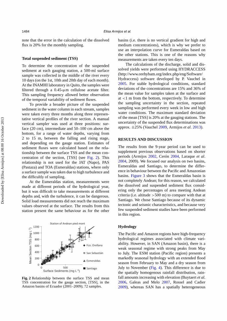
1484 Elisa Armijos et al.
note that the error in the calculation of the dissolvedflux is 20% for the monthly sampling.
Total suspended sediment (TSS)
To determine the concentration of the suspendedsediment at each gauging station, a 500-ml surfacesample was collected in the middle of the river every10 days (on the 1st, 10th and 20th day of each month).At the INAMHI laboratory in Quito, the samples werefiltered through a 0.45-µm cellulose acetate filter.This sampling frequency allowed better observationof the temporal variability of sediment fluxes.
To provide a broader picture of the suspendedsediment in the water column in each stream, sampleswere taken every three months along three represen-tative vertical profiles of the river section. A manualvertical sampler was used at three positions: sur-face (20 cm), intermediate and 50–100 cm above thebottom, for a range of water depths, varying from2 to 15 m, between the falling and rising stage,and depending on the gauge station. Estimates ofsediment fluxes were calculated based on the rela-tionship between the surface TSS and the mean con-centration of the section, [TSS] (see Fig. 2). Thisrelationship is not used for the JAT (Napo), PAS(Pastaza) and TOA (Esmeraldas) stations, where onlya surface sample was taken due to high turbulence andthe difficultly of sampling.
At the Esmeraldas station, measurements weremade at different periods of the hydrological year,but it was difficult to take measurements at differentdepths and, with the turbulence, it can be dangerous.Solid load measurements did not reach the maximumvalues observed at the surface. The results from thisstation present the same behaviour as for the other
0
200
400
600
800
1000
1200
0 500
Surface Sediments (mg L-1)
Mea
n S
ectio
n T
SS
(m
g L-1
)
Station of Andean pied mont
Fco. Orellana
San Sebastián
Esmeraldas
Santiago
Fig. 2 Relationship between the surface TSS and meanTSS concentration for the gauge section, [TSS], in theAmazon basins of Ecuador (2001–2009); 72 samples.
basins (i.e. there is no vertical gradient for high andmedium concentrations), which is why we prefer touse an interpolation curve for Esmeraldas based onthe other stations. This is one of the reasons whymeasurements are taken every ten days.
The calculations of the discharge, solid and dis-solved yields were performed using HYDRACCESS(http://www.orehybam.org/index.php/eng/Software/Hydraccess) software developed by P. Vauchel in2005. For stable hydrological conditions, standarddeviations of the concentrations are 15% and 36% ofthe mean value for samples taken at the surface andat <1 m from the bottom, respectively. To determinethe sampling uncertainty in the section, repeatedsampling was performed every week in low and highwater conditions. The maximum standard deviationof the mean [TSS] is 20% at the gauging stations. Theuncertainty of the suspended flux determinations wasapprox. ±25% (Vauchel 2009, Armijos et al. 2013).
RESULTS AND DISCUSSION
The results from the 9-year period can be used tosupplement previous observations based on shorterperiods (Armijos 2002, Cerón 2004, Laraque et al.2004, 2009). We focused our analysis on two basins,Esmeraldas and Santiago, to determine the differ-ence in behaviour between the Pacific and Amazonianbasins. Figure 3 shows that the Esmeraldas basin isnot completely Andean; for this reason, we calculatedthe dissolved and suspended sediment flux consid-ering only the percentages of area meeting Andeancriteria (i.e. altitude >500 m) to compare with that atSantiago. We chose Santiago because of its dynamictectonic and seismic characteristics, and because veryfew suspended sediment studies have been performedin this region.
Hydrology
The Pacific and Amazon regions have high-frequencyhydrological regimes associated with climate vari-ability. However, in SAN (Amazon basin), there is aweak seasonal regime with strong peaks from Mayto July. The ESM station (Pacific region) presents amarkedly seasonal hydrology with an extended floodseason from February to May and a dry season fromJuly to November (Fig. 4). This difference is due tothe spatially homogenous rainfall distribution, rain-fall amounts increasing with elevation (Buytaert et al.2006, Galeas and Melo 2007, Rossel and Cadier2009), whereas SAN has a spatially heterogeneous
Dow
nloa
ded
by [
Elis
a A
rmijo
s] a
t 08:
00 1
6 O
ctob
er 2
013
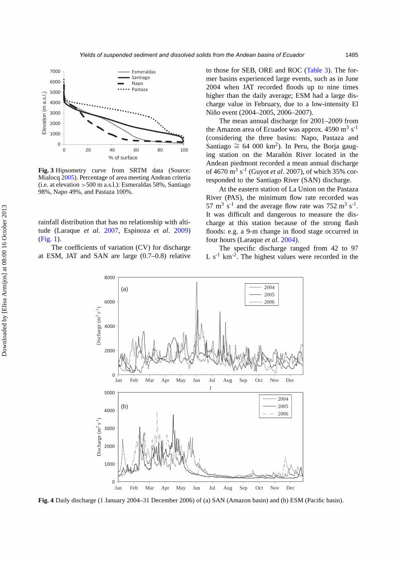
Yields of suspended sediment and dissolved solids from the Andean basins of Ecuador 1485
0
1000
2000
3000
4000
5000
6000
7000
0 20 40 60 80 100
Esmeraldas
Santiago
Napo
Pastaza
Ele
vatio
n (m
a.s
.l.)
% of surface
Fig. 3 Hipsometry curve from SRTM data (Source:Mialocq 2005). Percentage of area meeting Andean criteria(i.e. at elevation >500 m a.s.l.): Esmeraldas 58%, Santiago98%, Napo 49%, and Pastaza 100%.
rainfall distribution that has no relationship with alti-tude (Laraque et al. 2007, Espinoza et al. 2009)(Fig. 1).
The coefficients of variation (CV) for dischargeat ESM, JAT and SAN are large (0.7–0.8) relative
to those for SEB, ORE and ROC (Table 3). The for-mer basins experienced large events, such as in June2004 when JAT recorded floods up to nine timeshigher than the daily average; ESM had a large dis-charge value in February, due to a low-intensity ElNiño event (2004–2005, 2006–2007).
The mean annual discharge for 2001–2009 fromthe Amazon area of Ecuador was approx. 4590 m3 s-1
(considering the three basins: Napo, Pastaza andSantiago ∼= 64 000 km2). In Peru, the Borja gaug-ing station on the Marañón River located in theAndean piedmont recorded a mean annual dischargeof 4670 m3 s-1 (Guyot et al. 2007), of which 35% cor-responded to the Santiago River (SAN) discharge.
At the eastern station of La Union on the PastazaRiver (PAS), the minimum flow rate recorded was57 m3 s-1 and the average flow rate was 752 m3 s-1.It was difficult and dangerous to measure the dis-charge at this station because of the strong flashfloods: e.g. a 9-m change in flood stage occurred infour hours (Laraque et al. 2004).
The specific discharge ranged from 42 to 97L s-1 km-2. The highest values were recorded in the
0
2000
4000
6000
8000
Dis
char
ge (
m3 s
-1)
Dis
char
ge (
m3 s
-1)
2004
2005
2006
0
1000
2000
3000
4000
5000
Jan Feb Mar Apr May Jun Jul Aug Sep Oct Nov Dec
Jan Feb Mar Apr May Jun Jul Aug Sep Oct Nov Dec
J
2004
2005
2006(b)
(a)
Fig. 4 Daily discharge (1 January 2004–31 December 2006) of (a) SAN (Amazon basin) and (b) ESM (Pacific basin).
Dow
nloa
ded
by [
Elis
a A
rmijo
s] a
t 08:
00 1
6 O
ctob
er 2
013
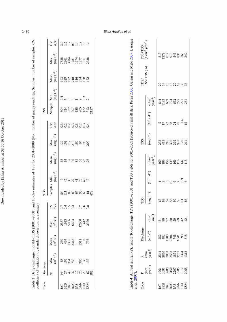
1486 Elisa Armijos et al.T
able
3D
aily
disc
harg
e,m
onth
lyT
DS
(200
1–20
08),
and
10-d
ayes
tim
ates
ofT
SS
for
2001
–200
9(N
o.:
num
ber
ofga
uge
read
ings
;S
ampl
es:
num
ber
ofsa
mpl
es;
CV
:co
effi
cien
tof
vari
atio
n;σ
:sta
ndar
dde
viat
ion;
x:av
erag
e).
Cod
eD
isch
arge
TD
ST
SS
No.
Min
.M
ean
Max
.C
VS
ampl
esM
in.
Mea
nM
ax.
CV
Sam
ples
Min
.M
ean
Max
.C
V(m
3s-1
)(m
3s-1
)(m
3s-1
)σ/x
(mg
L-1
)(m
gL
-1)
(mg
L-1
)σ/x
(mg
L-1
)(m
gL
-1)
(mg
L-1
)σ/x
JAT
144
6326
025
570.
710
47
6812
20.
330
40.
419
373
383.
0S
EB
2716
348
419
230.
411
145
9116
20.
232
47
329
2961
1.5
OR
E43
351
1335
5036
0.5
8638
5711
70.
233
73
192
3684
1.7
RO
C32
758
2313
6664
0.3
8922
5921
60.
330
75
218
1481
0.9
PAS
17−
−−
−67
4189
160
0.3
125
131
619
741.
4S
AN
2638
513
1112
960
0.7
9628
5594
0.2
285
229
419
771.
2T
OA
2933
103
412
0.6
6946
122
196
0.3
132
0.3
128
1811
1.8
ES
M67
156
798
3360
0.8
8119
103
200
0.4
313
216
226
281.
438
567
921
17
Tab
le4
Ann
ualr
ainf
all(
P),
runo
ff(R
),di
scha
rge,
TD
S(2
001–
2008
)and
TS
Syi
elds
for2
001–
2009
(Sou
rce
ofra
infa
llda
ta:P
erez
2000
,Gal
eas
and
Mel
o20
07,L
araq
ueet
al.2
007)
.
Cod
eP (m
mye
ar-1
)
R (mm
year
-1)
Dis
char
geT
DS
TS
ST
DS/
TS
S+
TD
S(%
)T
SS
+T
DS
(tkm
-2ye
ar-1
)(m
3s-1
)(L
s-1
km-2
)(m
gL
-1)
(103
td-1
)(t
km-2
year
-1)
(mg
L-1
)(1
03td
-1)
(tkm
-2
year
-1)
JAT
1961
2544
252
8166
116
925
35
644
2081
3S
EB
2691
2850
482
9069
319
641
517
1183
1413
79O
RE
3209
3053
1200
9752
515
821
622
659
1981
7R
OC
3150
2538
2204
8055
1013
930
558
774
1591
3PA
S22
0718
5174
859
906
166
369
2468
220
848
SA
N23
0521
6716
4169
567
110
335
4772
513
836
TO
A15
1213
2498
4211
10.
914
717
01.
422
139
368
ES
M20
6513
1381
842
886
115
214
1528
133
342
Dow
nloa
ded
by [
Elis
a A
rmijo
s] a
t 08:
00 1
6 O
ctob
er 2
013
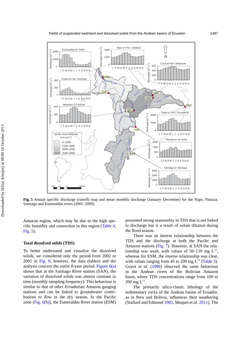
Yields of suspended sediment and dissolved solids from the Andean basins of Ecuador 1487
R.Pau
te
R. Napo
R. Napo
era
R.U
pano
R.Z
amor
a
R.T
oachi
R.Blanco
R. S
anP
edro
R. C
ham
o
R. Guayllabamba
R.Santiago
R.P
atat
e
R.Pastaza
R.Coc
a
R.Jatunya
R.Tiputini
100 0 10050 km
Specific annual discharge
(mm year-1
)
0–1500
1500–2000
2000–2500
2500–3000
ESM
J
TOA
SAN
PAS
S
ORE
ROC
J
N
0
200
400
J F M A M J J A S O N D
Jatunyacu DJ Iloculín
0
200
400
600
J F M A M J J A S O N D
Coca en San Sebastian 0
1000
2000
J F M A M J J A S O N D
Napo en Fco. Orellana
0
2000
4000
J F M A M J J A S O N D
Napo en Nvo. Rocafuerte
0
200
400
J F M A M J J A S O N D
Toachi en Sto. Domingo
0
1000
2000
J F M A M J J A S O N D
Esmeraldas DJ Sade
0
1000
2000
3000
J F M A M J J A S O N D
Dis
char
ge (
m3 s
-1)
Dis
char
ge (
m3 s
-1)
Dis
char
ge (
m3 s
-1)
Dis
char
ge (
m3 s
-1)
Dis
char
ge (
m3
s-1)
Dis
char
ge (
m3 s
-1)
Dis
char
ge (
m3 s
-1)
Dis
char
ge (
m3 s
-1)
Santiago en Santiago
0
500
1000
1500
J F M A M J J A S O N D
Pastaza en la Unión
Fig. 5 Annual specific discharge (runoff) map and mean monthly discharge (January–December) for the Napo, Pastaza,Santiago and Esmeraldas rivers (2001–2009).
Amazon region, which may be due to the high spe-cific humidity and convection in this region (Table 4,Fig. 5).
Total dissolved solids (TDS)
To better understand and visualize the dissolvedsolids, we considered only the period from 2002 to2005 in Fig. 6; however, the data (tables) and theanalysis concern the entire 8-year period. Figure 6(a)shows that at the Santiago River station (SAN), thevariation of dissolved solids was almost constant intime (monthly sampling frequency). This behaviour issimilar to that of other Ecuadorian Amazon gaugingstations and can be linked to groundwater contri-butions to flow in the dry season. In the Pacificzone (Fig. 6(b)), the Esmeraldas River station (ESM)
presented strong seasonality in TDS that is not linkedto discharge but is a result of solute dilution duringthe flood season.
There was an inverse relationship between theTDS and the discharge at both the Pacific andAmazon stations (Fig. 7). However, at SAN the rela-tionship was weak, with values of 50–110 mg L-1,whereas for ESM, the inverse relationship was clear,with values ranging from 45 to 200 mg L-1 (Table 3).Guyot et al. (1996) observed the same behaviourin the Andean rivers of the Bolivian Amazonbasin, where TDS concentrations range from 100 to200 mg L-1.
The primarily silico-clastic lithology of thesedimentary rocks of the Andean basins of Ecuador,as in Peru and Bolivia, influences their weathering(Stallard and Edmond 1983, Moquet et al. 2011). The
Dow
nloa
ded
by [
Elis
a A
rmijo
s] a
t 08:
00 1
6 O
ctob
er 2
013
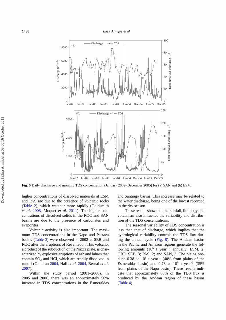
1488 Elisa Armijos et al.
0
20
40
60
80
100
0
2000
4000
6000
8000
Jan-02 Jul-02 Jan-03 Jul-03 Jan-04 Jun-04 Dec-04 Jun-05 Dec-05
Tot
al d
isso
lved
sol
ids
(mg
L-1
)
Dis
char
ge (
m3
s-1)
Dis
char
ge (
m3
s-1)
Discharge TDS
0
50
100
150
200
250
0
1000
2000
3000
Jan-02 Jul-02 Jan-03 Jul-03 Jan-04 Jun-04 Dec-04 Jun-05 Dec-05
Tot
al d
isso
lved
sol
ids
(mg
L-1
)
Discharge TDS(b)
(a)
Fig. 6 Daily discharge and monthly TDS concentration (January 2002–December 2005) for (a) SAN and (b) ESM.
higher concentrations of dissolved materials at ESMand PAS are due to the presence of volcanic rocks(Table 2), which weather more rapidly (Goldsmithet al. 2008, Moquet et al. 2011). The higher con-centrations of dissolved solids in the ROC and SANbasins are due to the presence of carbonates andevaporites.
Volcanic activity is also important. The maxi-mum TDS concentrations in the Napo and Pastazabasins (Table 3) were observed in 2002 at SEB andROC after the eruptions of Reventador. This volcano,a product of the subduction of the Nazca plate, is char-acterized by explosive eruptions of ash and lahars thatcontain SO2 and HCl, which are readily dissolved inrunoff (Gondran 2004, Hall et al. 2004, Bernal et al.2007).
Within the study period (2001–2008), in2005 and 2006, there was an approximately 50%increase in TDS concentrations in the Esmeraldas
and Santiago basins. This increase may be related tothe water discharge, being one of the lowest recordedin the dry season.
These results show that the rainfall, lithology andvolcanism also influence the variability and distribu-tion of the TDS concentrations.
The seasonal variability of TDS concentration isless than that of discharge, which implies that thehydrological variability controls the TDS flux dur-ing the annual cycle (Fig. 8). The Andean basinsin the Pacific and Amazon regions generate the fol-lowing amounts (106 t year-1) annually: ESM, 2;ORE+SEB, 3; PAS, 2; and SAN, 3. The plains pro-duce 0.38 × 10⁶ t year-1 (40% from plains of theEsmeraldas basin) and 0.73 × 10⁶ t year-1 (35%from plains of the Napo basin). These results indi-cate that approximately 80% of the TDS flux isproduced by the Andean region of these basins(Table 4).
Dow
nloa
ded
by [
Elis
a A
rmijo
s] a
t 08:
00 1
6 O
ctob
er 2
013
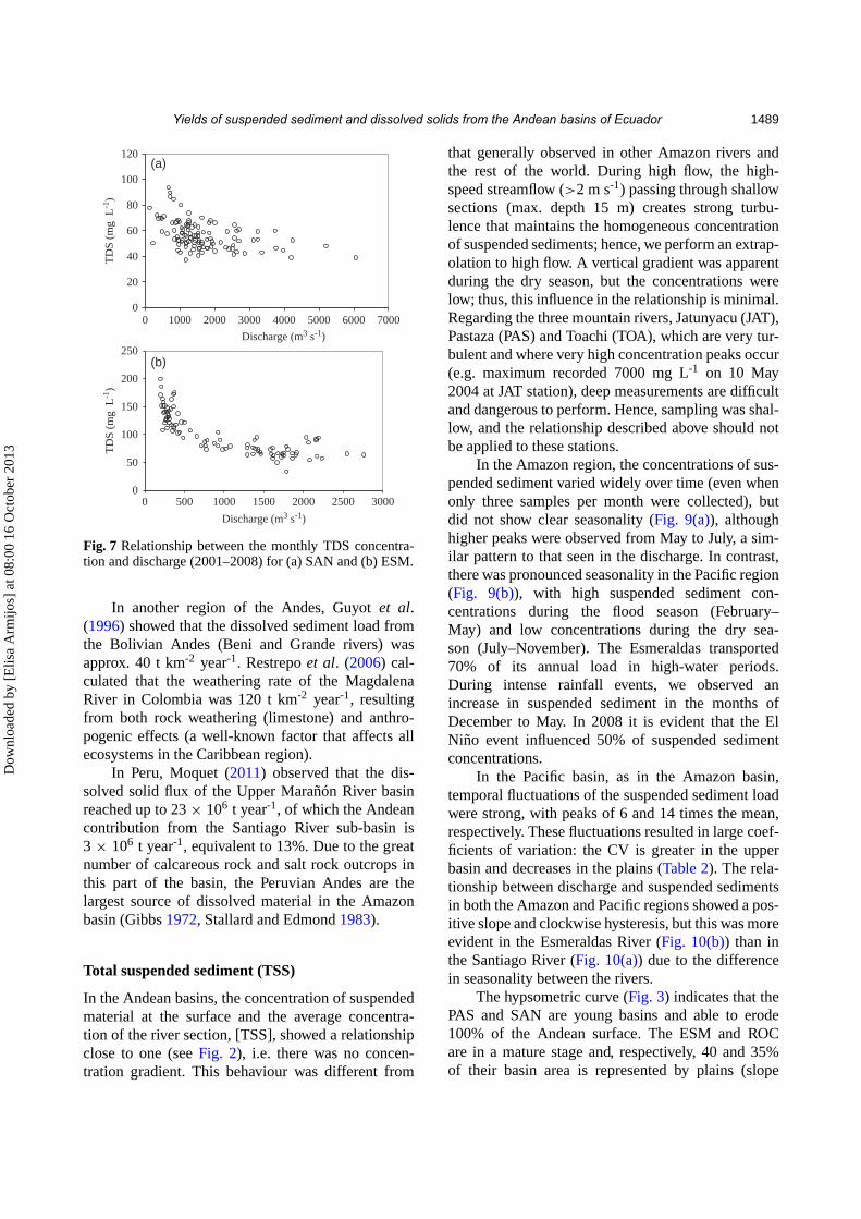
Yields of suspended sediment and dissolved solids from the Andean basins of Ecuador 1489
0
20
40
60
80
100
120
0 1000 2000 3000 4000 5000 6000 7000
TD
S (m
g L
-1)
Discharge (m3 s-1)
TD
S (m
g L
-1)
Discharge (m3 s-1)
0
50
100
150
200
250
0 500 1000 1500 2000 2500 3000
(b)
(a)
Fig. 7 Relationship between the monthly TDS concentra-tion and discharge (2001–2008) for (a) SAN and (b) ESM.
In another region of the Andes, Guyot et al.(1996) showed that the dissolved sediment load fromthe Bolivian Andes (Beni and Grande rivers) wasapprox. 40 t km-2 year-1. Restrepo et al. (2006) cal-culated that the weathering rate of the MagdalenaRiver in Colombia was 120 t km-2 year-1, resultingfrom both rock weathering (limestone) and anthro-pogenic effects (a well-known factor that affects allecosystems in the Caribbean region).
In Peru, Moquet (2011) observed that the dis-solved solid flux of the Upper Marañón River basinreached up to 23 × 106 t year-1, of which the Andeancontribution from the Santiago River sub-basin is3 × 106 t year-1, equivalent to 13%. Due to the greatnumber of calcareous rock and salt rock outcrops inthis part of the basin, the Peruvian Andes are thelargest source of dissolved material in the Amazonbasin (Gibbs 1972, Stallard and Edmond 1983).
Total suspended sediment (TSS)
In the Andean basins, the concentration of suspendedmaterial at the surface and the average concentra-tion of the river section, [TSS], showed a relationshipclose to one (see Fig. 2), i.e. there was no concen-tration gradient. This behaviour was different from
that generally observed in other Amazon rivers andthe rest of the world. During high flow, the high-speed streamflow (>2 m s-1) passing through shallowsections (max. depth 15 m) creates strong turbu-lence that maintains the homogeneous concentrationof suspended sediments; hence, we perform an extrap-olation to high flow. A vertical gradient was apparentduring the dry season, but the concentrations werelow; thus, this influence in the relationship is minimal.Regarding the three mountain rivers, Jatunyacu (JAT),Pastaza (PAS) and Toachi (TOA), which are very tur-bulent and where very high concentration peaks occur(e.g. maximum recorded 7000 mg L-1 on 10 May2004 at JAT station), deep measurements are difficultand dangerous to perform. Hence, sampling was shal-low, and the relationship described above should notbe applied to these stations.
In the Amazon region, the concentrations of sus-pended sediment varied widely over time (even whenonly three samples per month were collected), butdid not show clear seasonality (Fig. 9(a)), althoughhigher peaks were observed from May to July, a sim-ilar pattern to that seen in the discharge. In contrast,there was pronounced seasonality in the Pacific region(Fig. 9(b)), with high suspended sediment con-centrations during the flood season (February–May) and low concentrations during the dry sea-son (July–November). The Esmeraldas transported70% of its annual load in high-water periods.During intense rainfall events, we observed anincrease in suspended sediment in the months ofDecember to May. In 2008 it is evident that the ElNiño event influenced 50% of suspended sedimentconcentrations.
In the Pacific basin, as in the Amazon basin,temporal fluctuations of the suspended sediment loadwere strong, with peaks of 6 and 14 times the mean,respectively. These fluctuations resulted in large coef-ficients of variation: the CV is greater in the upperbasin and decreases in the plains (Table 2). The rela-tionship between discharge and suspended sedimentsin both the Amazon and Pacific regions showed a pos-itive slope and clockwise hysteresis, but this was moreevident in the Esmeraldas River (Fig. 10(b)) than inthe Santiago River (Fig. 10(a)) due to the differencein seasonality between the rivers.
The hypsometric curve (Fig. 3) indicates that thePAS and SAN are young basins and able to erode100% of the Andean surface. The ESM and ROCare in a mature stage and, respectively, 40 and 35%of their basin area is represented by plains (slope
Dow
nloa
ded
by [
Elis
a A
rmijo
s] a
t 08:
00 1
6 O
ctob
er 2
013
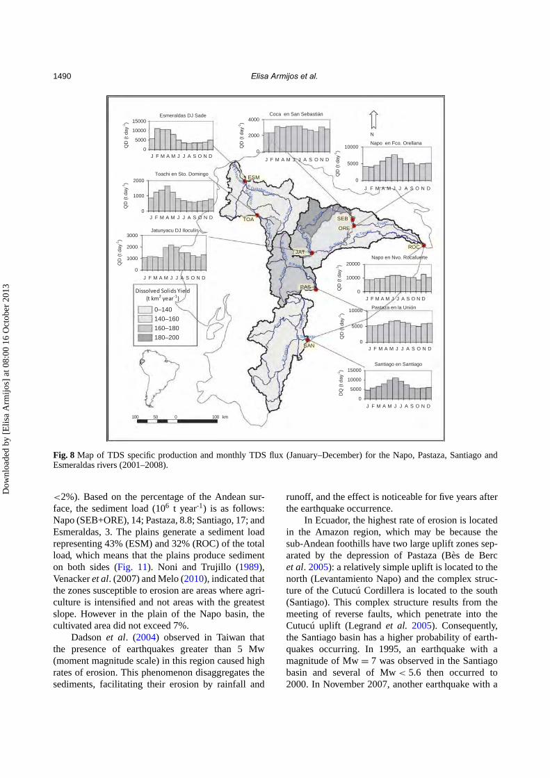
1490 Elisa Armijos et al.
100 0 10050 km
R.Pau
te
R. Napo
R. Napo
R.Esm
eraldas
R.U
pano
R.Z
amor
aR
.To
achi
R.Blanco
R. S
anP
edro
R. C
ham
bo
R. Guayllabamba
R.Santiago
R.P
atat
e
R.Pastaza
R.Coc
a
R.JatunyacuR.Tiputini
Dissolved Solids Yield
(t km2 year
-1)
0–140
140–160
160–180
180–200
ESM
TOA
SAN
PAS
JAT
SEB
ORE
ROC
N
0
5000
10000
15000
J F M A M J J A S O N D
QD
(t d
ay-1
)
QD
(t d
ay-1
)
QD
(t d
ay-1
)Q
D (
t day
-1)
QD
(t d
ay-1
)D
Q (
t day
-1)
QD
(t d
ay-1
)Q
D (
t day
-1)
Esmeraldas DJ Sade
0
1000
2000
J F M A M J J A S O N D
Toachi en Sto. Domingo
0
1000
2000
3000
J F M A M J J A S O N D
Jatunyacu DJ Iloculín
0
2000
4000
J F M A M J J A S O N D
Coca en San Sebastián
0
5000
10000
J F M A M J J A S O N D
Napo en Fco. Orellana
0
10000
20000
J F M A M J J A S O N D
Napo en Nvo. Rocafuerte
0
5000
10000
J F M A M J J A S O N D
Pastaza en la Unión
0
5000
10000
15000
J F M A M J J A S O N D
Santiago en Santiago
Fig. 8 Map of TDS specific production and monthly TDS flux (January–December) for the Napo, Pastaza, Santiago andEsmeraldas rivers (2001–2008).
<2%). Based on the percentage of the Andean sur-face, the sediment load (106 t year-1) is as follows:Napo (SEB+ORE), 14; Pastaza, 8.8; Santiago, 17; andEsmeraldas, 3. The plains generate a sediment loadrepresenting 43% (ESM) and 32% (ROC) of the totalload, which means that the plains produce sedimenton both sides (Fig. 11). Noni and Trujillo (1989),Venacker et al. (2007) and Melo (2010), indicated thatthe zones susceptible to erosion are areas where agri-culture is intensified and not areas with the greatestslope. However in the plain of the Napo basin, thecultivated area did not exceed 7%.
Dadson et al. (2004) observed in Taiwan thatthe presence of earthquakes greater than 5 Mw(moment magnitude scale) in this region caused highrates of erosion. This phenomenon disaggregates thesediments, facilitating their erosion by rainfall and
runoff, and the effect is noticeable for five years afterthe earthquake occurrence.
In Ecuador, the highest rate of erosion is locatedin the Amazon region, which may be because thesub-Andean foothills have two large uplift zones sep-arated by the depression of Pastaza (Bès de Bercet al. 2005): a relatively simple uplift is located to thenorth (Levantamiento Napo) and the complex struc-ture of the Cutucú Cordillera is located to the south(Santiago). This complex structure results from themeeting of reverse faults, which penetrate into theCutucú uplift (Legrand et al. 2005). Consequently,the Santiago basin has a higher probability of earth-quakes occurring. In 1995, an earthquake with amagnitude of Mw = 7 was observed in the Santiagobasin and several of Mw < 5.6 then occurred to2000. In November 2007, another earthquake with a
Dow
nloa
ded
by [
Elis
a A
rmijo
s] a
t 08:
00 1
6 O
ctob
er 2
013
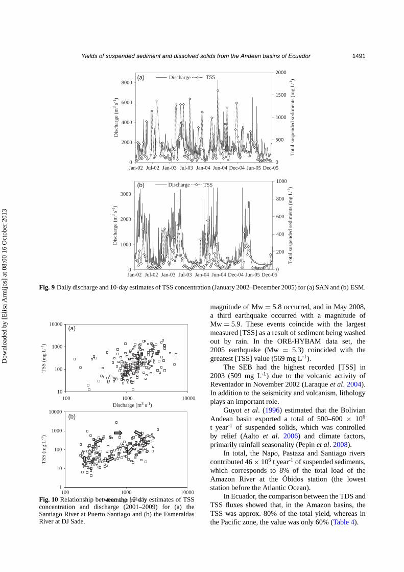
Yields of suspended sediment and dissolved solids from the Andean basins of Ecuador 1491
0
500
1000
1500
2000
0
2000
4000
6000
8000
Jan-02 Jul-02 Jan-03 Jul-03 Jan-04 Jun-04 Dec-04 Jun-05 Dec-05
Jan-02 Jul-02 Jan-03 Jul-03 Jan-04 Jun-04 Dec-04 Jun-05 Dec-05
Dis
char
ge (
m3 s
-1)
Dis
char
ge (
m3 s
-1)
Discharge TSS
0
200
400
600
800
1000
0
1000
2000
3000
Tot
al s
uspe
nded
sed
imen
ts (
mg
L-1
)T
otal
sus
pend
ed s
edim
ents
(m
g L
-1)
Discharge TSS(b)
(a)
Fig. 9 Daily discharge and 10-day estimates of TSS concentration (January 2002–December 2005) for (a) SAN and (b) ESM.
10
100
1000
10000
100 1000 10000
TSS
(m
g L
-1)
TSS
(m
g L
-1)
Discharge (m3 s-1)
Discharge (m3 s-1)
1
10
100
1000
10000
100 1000 10000
(b)
(a)
Fig. 10 Relationship between the 10-day estimates of TSSconcentration and discharge (2001–2009) for (a) theSantiago River at Puerto Santiago and (b) the EsmeraldasRiver at DJ Sade.
magnitude of Mw = 5.8 occurred, and in May 2008,a third earthquake occurred with a magnitude ofMw = 5.9. These events coincide with the largestmeasured [TSS] as a result of sediment being washedout by rain. In the ORE-HYBAM data set, the2005 earthquake (Mw = 5.3) coincided with thegreatest [TSS] value (569 mg L-1).
The SEB had the highest recorded [TSS] in2003 (509 mg L-1) due to the volcanic activity ofReventador in November 2002 (Laraque et al. 2004).In addition to the seismicity and volcanism, lithologyplays an important role.
Guyot et al. (1996) estimated that the BolivianAndean basin exported a total of 500–600 × 106
t year-1 of suspended solids, which was controlledby relief (Aalto et al. 2006) and climate factors,primarily rainfall seasonality (Pepin et al. 2008).
In total, the Napo, Pastaza and Santiago riverscontributed 46 × 106 t year-1 of suspended sediments,which corresponds to 8% of the total load of theAmazon River at the Óbidos station (the loweststation before the Atlantic Ocean).
In Ecuador, the comparison between the TDS andTSS fluxes showed that, in the Amazon basins, theTSS was approx. 80% of the total yield, whereas inthe Pacific zone, the value was only 60% (Table 4).
Dow
nloa
ded
by [
Elis
a A
rmijo
s] a
t 08:
00 1
6 O
ctob
er 2
013
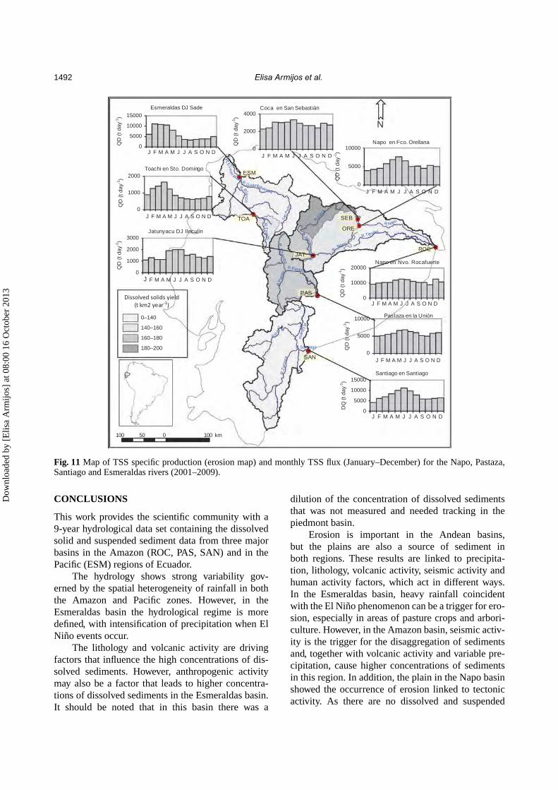
1492 Elisa Armijos et al.
100 0 10050 km
R.Pau
te
R. Napo
R. Napo
R.Esm
er aldas
R.U
pano
R.Z
amor
a
R.T
oachi
R.Blanco
R. S
anP
edro
R. C
ham
bo
R. Guayllabamba
R.Santiago
R.P
atat
e
R.Pastaza
R.Coc
a
R.Jatunyacu
R.Tiputini
0
1000
2000
3000
F M A M J J A S O N D
Jatunyacu DJ Iloculín
0
5000
10000
F M A M J J A S O N D
Napo en Fco. Orellana 0
2000
4000
F M A M J J A S O N D
Coca en San Sebastián
0
10000
20000
F M A M J J A S O N D
Napo en Nvo. Rocafuerte
0
5000
10000
F M A M J J A S O N D
Pastaza en la Unión
0
5000
10000
15000
F M A M J J A S O N D
Santiago en Santiago
0
5000
10000
15000
F M A M J J A S O N D
QD
(t d
ay-1
)Q
D (t
day
-1)
QD
(t d
ay-1
)
QD
(t d
ay-1
)
QD
(t d
ay-1
)Q
D (t
day
-1)
QD
(t d
ay-1
)D
Q (t
day
-1)
Esmeraldas DJ Sade
0
1000
2000
F M A M J J A S O N D
Toachi en Sto. Domingo
Dissolved solids yield
(t km2 year-1
)
0–140
140–160
160–180
180–200
ESM
TOA
SAN
PAS
JAT
SEB
ORE
ROC
JJ
J
J
J
J
J
J
N
Fig. 11 Map of TSS specific production (erosion map) and monthly TSS flux (January–December) for the Napo, Pastaza,Santiago and Esmeraldas rivers (2001–2009).
CONCLUSIONS
This work provides the scientific community with a9-year hydrological data set containing the dissolvedsolid and suspended sediment data from three majorbasins in the Amazon (ROC, PAS, SAN) and in thePacific (ESM) regions of Ecuador.
The hydrology shows strong variability gov-erned by the spatial heterogeneity of rainfall in boththe Amazon and Pacific zones. However, in theEsmeraldas basin the hydrological regime is moredefined, with intensification of precipitation when ElNiño events occur.
The lithology and volcanic activity are drivingfactors that influence the high concentrations of dis-solved sediments. However, anthropogenic activitymay also be a factor that leads to higher concentra-tions of dissolved sediments in the Esmeraldas basin.It should be noted that in this basin there was a
dilution of the concentration of dissolved sedimentsthat was not measured and needed tracking in thepiedmont basin.
Erosion is important in the Andean basins,but the plains are also a source of sediment inboth regions. These results are linked to precipita-tion, lithology, volcanic activity, seismic activity andhuman activity factors, which act in different ways.In the Esmeraldas basin, heavy rainfall coincidentwith the El Niño phenomenon can be a trigger for ero-sion, especially in areas of pasture crops and arbori-culture. However, in the Amazon basin, seismic activ-ity is the trigger for the disaggregation of sedimentsand, together with volcanic activity and variable pre-cipitation, cause higher concentrations of sedimentsin this region. In addition, the plain in the Napo basinshowed the occurrence of erosion linked to tectonicactivity. As there are no dissolved and suspended
Dow
nloa
ded
by [
Elis
a A
rmijo
s] a
t 08:
00 1
6 O
ctob
er 2
013

Yields of suspended sediment and dissolved solids from the Andean basins of Ecuador 1493
sediment concentration measurements for the AndeanEsmeraldas basin, we present a first estimate of thefluxes.
No sedimentation was observed along the riverprofile in the Bolivian, Peruvian or Brazilian Amazonbasin. The lithology and volcanic activity are driv-ing factors that influence the high concentrations ofdissolved and suspended sediments. Seismic activitycontributes to increases in the concentration of sus-pended sediments, particularly in the Santiago basin.The annual dissolved and sedimentary fluxes fromthe Ecuadorian Amazonian basin are 9 and 47 × 106
t year-1, respectively (3 and 6% of the total Amazonyield), which corresponds to a yield of 131 and736 t year-1 km-2, respectively. In the Pacific region(Esmeraldas basin), the dissolved and sedimentaryfluxes are 2 and 5 × 10⁶ t year-1, respectively, whichare equivalent to 111 and 279 t year-1 km-2.
Acknowledgements This study was performed withsupport from the Instituto Nacional de Meteorologíae Hidrología of Ecuador (SENAMHI) and theInstitut de recherche pour le développement (IRD),France. We would like to thank participants in theORE-HYBAM Observatory from Ecuador, and theobservers at the different gauging stations.
REFERENCES
Aalto, R., Dunne, T., and Guyot, J.L., 2006. Geomorphic controls onAndean denudation rates. Journal of Geology, 114 (1), 85–99.
Armijos, E., 2002. Estudio hidrofísico de las cuencas de los ríosNapo, Pastaza y Santiago dentro del proyecto Hybam. Thesis(Tesis de graduación), Universidad Central de Ecuador, Quito,Ecuador.
Armijos, E., 2010. Cuantificación de flujos sedimentarios de las cuen-cas Amazónicas del Perú. Thesis (Tesis para la obtención deltítulo de Máster en Recursos Hidricos), Universidad NacionalAgraria La Molina, Lima, Perú.
Armijos, E., et al., 2013. Suspended sediment dynamic in the AmazonRiver of Peru. Journal of South American Earth Sciences,doi:10.1016/j.jsames.2012.09.002.
Aspiazu, P. and Luna, M., 1993. Geografía e historia del Ecuador.Madrid, Spain: Cultural.
Baldock, J.W., 1982. Geología del Ecuador. Quito, Ecuador:Dirección General de Geología y Minas.
Bernal, C., et al., 2007. Influence de l’activité volcanique dans lachimie du Rio Napo: affluent de l’Amazone venant des Andeséquatoriennes. Poster presented at: Water quality and sedimentbehaviour of the future, July 2007. Perugia, Italy: IAHS.
Bès de Berc, S., et al., 2005. Geomorphic evidence ofactive deformation and uplift in a modern continentalwedge-top–foredeep transition: example of the east-ern Ecuadorian Andes. Tectonophysics, 399, 351–380,doi:10.1016/J.TECTO.2004.12.030.
Buytaert, W.. et al., 2006. Spatial and temporal rainfall vari-ability in mountainous areas: a case study from the south
Ecuadorian Andes. Journal of Hydrology, 329 (3–4), 413–421,doi:10.1016/j.jhydrol.2006.02.031.
Callède, J., et al., 2010. Les apports en eau de l’Amazone à l’OcéanAtlantique. Revue des Sciences de l’Eau, 23 (3), 247–273.
Cerón, C., 2004. Flux sédimentaires des basins amazoniensd’Equateur. Mémoire de DEA, Université Paul Sabatier,Toulouse, France.
CLIRSEN (Centro de Levantamientos Integrados de RecursosNaturales por Sensores Remotos), 2003. Análisis de cobertura.Quito, Ecuador: Boscosa del Ecuador.
Dadson, S., et al., 2004. Earthquake-triggered increase in sedimentdelivery from an active mountain belt. Geology, 32, 733–736.
Degens, E.T., Kempe, S., and Richey, J.E., 1991. Summary:biogeochemistry of major world rivers. In: E.T. Degens, S.Kempe, and J.E. Richey, eds. Biogeochemistry of major worldrivers. Chichester, UK: John Wiley & Sons Ltd., Scope 42,323–347.
DINAGE (Dirección Nacional de Geologia), 1997. Primer catálogode información técnica. Quito, Ecuador: Ministerio de Energíay Minas.
Dunne, T., et al., 1998. Exchanges of sediment between the floodplain and channel of the Amazon River in Brazil. GeologicalSociety of America Bulletin, 110, 450–467.
ECORAE (Instituto para el Ecodesarrollo Regional Amazónico),2002. Zonificación Ecológica–Económica de la AmazoníaEcuatoriana. Quito, Ecuador: ECORAE.
Espinoza, J.C., et al., 2009. Spatio-temporal rainfall variabil-ity in the Amazon Basin Countries (Brazil, Peru, Bolivia,Colombia and Ecuador). International Journal of Climatology,29, 1574–1594.
Filizola, N. and Guyot, J.L., 2004. The use of Doppler technologyfor suspended sediment discharge determinations in the RiverAmazon. Hydrological Sciences Journal, 49 (1), 143–153.
Filizola, N. and Guyot, J.L., 2009. Suspended sediment yieldsin the Amazon basin: an assessment using the Braziliannational data set. Hydrological Processes, 23, 3207–3215,doi:10.1002.hyp.7394
Galeas, R. and Melo, P., 2007. Estudio comparativo del compor-tamiento hidro-sedimentológico de las cuencas del río Napo(vertiente amazónica) y del río Esmeraldas (vertiente pací-fica). Influencia de la morfometría y del fenómeno del Niño.Thesis (Tesis de graduación), Pontificia Universidad Católicadel Ecuador, Quito, Ecuador.
Gibbs, R.J., 1967. The Geochemistry of the Amazon River System.Part I. The factors that control the salinity and the compositionand concentration of the suspended solids. Geological Societyof America Bulletin, 78, 1203–1232.
Gibbs, R.J., 1972. Water chemistry of the Arnazon River. Geochimicaet Cosmochimica Acta, 36, 1061–1066.
Goldsmith, S.T., et al., 2008. Geochemical fluxes and weatheringon high standing islands: Taranaki and Manawatu-WanganuiRegions, New Zealand. Geochimica et Cosmochimica Acta, 72(9), 2248–2267.
Gondran, R., 2004. Impact de l’éruption du Reventador sur la chimiede la phase dissoute du Rio Coca. Rapport de Stage, UniversitéPaul Sabatier, Toulouse, France.
Goulding, M., Barthem, R., and Ferreira, E., 2003. The SmithsonianAtlas of the Amazon. Washington, DC: Smithsonian InstitutionPress.
Gutscher, M.A., et al., 1999. Tectonic segmentation of the NorthAndean margin: impact of the Carnegie Ridge collision. Earthand Planetary Science Letters, 168, 255–270.
Guyot, J.L., 1993. Hydrogéochimie des fleuves de l’Amazonie bolivi-enne. Thèse de doctorat, Université de Bordeux. Paris, France.ORSTOM.
Guyot, J.L., Bourges, J., and Cortez, J., 1994. Sediment trans-port in the Rio Grande, an Andean river of the Bolivian
Dow
nloa
ded
by [
Elis
a A
rmijo
s] a
t 08:
00 1
6 O
ctob
er 2
013
1494 Elisa Armijos et al.
Amazon drainage basin. In: L.J. Olive, R.J. Loughran, and J.A.Kesby, eds. Variability in stream erosion and sediment trans-port. Wallingford, UK: IAHS Press, IAHS Publ. 224, 223–231.Available from: http://iahs.info/redbooks/224.htm [Accessed 15July 2013].
Guyot, J.L., Filizola, N., and Laraque, A., 2005. Régime et bilandu flux sédimentaire de l’Amazone à Óbidos (Pará, Brésil),de 1995 à 2003. In: D.E. Walling and A.J. Horowitz, eds.Sediment budgets. Wallingford, UK: IAHS Press, IAHS Publ.291, 347–356. Available from: http://iahs.info/redbooks/291.htm [Accessed 15 July 2013].
Guyot, J.L., et al., 1996. Dissolved solids and suspended sedimentyields in the Rio Madeira basin, from the Bolivian Andes tothe Amazon. In: D.E. Walling and B.W. Webb, eds. Erosion andsediment yield: Global and regional perspectives. Wallingford,UK: IAHS Press, IAHS Publ. 236, 55–63. Available from:http://iahs.info/redbooks/236.htm [Accessed 15 July 2013].
Guyot, J.L., et al., 2007. Suspended sediment yields in the Amazonbasin of Peru, a first estimation. In: B.W. Webb and D.De Boer, eds. Water quality and sediment behaviour of thefuture: Predictions for the 21st century. Wallingford, UK: IAHSPress, IAHS Publ. 314, 3–10. Available from: http://iahs.info/redbooks/314.htm [Accessed 15 July 2013].
Hall, M., et al., 2004. Volcanic eruptions with little warning: the caseof Volcán Reventador’s surprise November 3, 2002 eruption,Ecuador. Revista Geologica de Chile, 31 (2), 349–358.
Heredia, E. and Pombosa, R., 1999. Influencia del ENSO sobre loscaudales mensuales de las grandes cuencas hidrográficas delEcuador. In: Hydrological and geochemical processes in largescale river basins. Manaus, Brazil: HYBAM 11/1999.
La Condamine, C.M., 1751. Mesure des trois premiers degrés duméridien dans l’Hémisphère Austral. Paris: Académie Royalede Sciences.
Laraque, A., et al., 2004. Sediments yields and erosion rates in theNapo River Basin: an Ecuadorian Andean Amazon tributary. In:V. Golosov, V. Belyaev, and D.E. Walling, eds. Sediment trans-fer through the fluvial system. Wallingford, UK: IAHS Press,IAHS Publ. 288, 220–225.
Laraque, A., et al., 2007. Heterogeneous distribution of rainfall anddischarge regimes in the Ecuadorian Amazon basin. Journal ofHydrometeorology, 8 (6), 1364–1381.
Laraque, A., et al., 2009. Sediment budget of the Napo River, Amazonbasin, Ecuador and Peru. Hydrological Processes, 23 (25),3509–3524.
Legrand, D., et al., 2005. The 1999–2000 seismic experiment ofMacas swarm (Ecuador) in relation with rift inversion inSubandean foothills. Tectonophysics, 395, 67–80.
Martinez, J.M., et al., 2009. Increase in suspended sediment yield ofthe Amazon River assessed by monitoring network and satellitedata. CATENA, 79, 257–264.
Meade, R.H., et al., 1979. Sediment loads in the Amazon River.Nature, 278, 161–163.
Meade, R.H., et al., 1985. Storage and remobilization of suspendedsediment in the lower Amazon River of Brazil. Science, 228,488–490.
Melo, P., 2010. Estudio de los riesgos potenciales de erosión en doscuencas de la vertiente pacífica ecuatoriana bajo la influenciadel fenómeno ENSO. Los casos de la cuenca del Rio Guayasy Esmeraldas. Thesis (Master 2 SGT), Prefalc. Ciencias yGestión de la Tierra, Geologia, riesgos y gestión del territorio,Université Nice Sophia Antipolis, Nice, France.
Mialocq, L., 2005. Délimitation des bassins versants à l’aided’ArcGis8. Lima, Peru: HYBAM.
Molina, A., et al., 2008. Environmental factors controlling spatialvariation in sediment yield in central Andean mountain area.Geomorphology, 98, 178–186.
Monzier, M. and Robin, C., 1995. Volcans à risques du Vanuatu àl’Équateur. ORSTOM Actualités, 45, 13–20.
Moquet, J., et al., 2011. Chemical weathering and atmospheric/soilCO2 uptake in the Andean and foreland amazon basins.Chemical Geology, 287, 1–26.
Moquet, J.S., 2011. Caractérisation des flux hydrogéochimiques desbassins andins de l’Amazone. Thèse de doctorat, UniversitéPaul Sabatier, Toulouse, France.
Moreno, F. and Tapia, A., 2001. Regionalización hidrometeorológ-ica de las cuencas amazónicas. Thesis (Tesis de graduación),Universidad Central de Ecuador, Quito, Ecuador.
Mortatti, J. and Probst, J.L., 2003. Silicate rock weathering andatmospheric/soil CO2 uptake in the Amazon basin estimatedfrom river water geochemistry: seasonal and spatial variations.Chemical Geology, 197, 177–196.
Narvaéz, P. and Vera, A., 2007. Estudio comparativo del compor-tamiento geoquímico de las aguas superficiales de las cuencasdel río Napo en el oriente y del río Esmeraldas en la costaecuatoriana e identificación de factores naturales y antrópicosque determinan sus diferencias. Thesis (Tesis de graduación),Universidad Central del Ecuador, Quito, Ecuador.
Noni, G. and Trujillo, G., 1986. La Erosión en el Ecuador. Quito,Ecuador: Centro Ecuatoriano de Investigación Geográfica.
Neil, D.A., 1997. Ecuadorian Pacific coast mesic forest. In: A guideand strategy for their Conservation. The Americas, Vol. 3.Cambridge, MA: UICN, 508–518.
Olivera, F., Dodson, B., and Bristow, E., 2002. PrePro2002 User’sManual. Houston: Texas University and Dodson Associates,Inc.
Pepin, E., et al., 2008. Tectonic or climate control on mod-ern catchment-scale erosion rates. In: 4th Alexander vonHumboldt International Conference – The Andes: Challenge forGeosciences. Santiago, Chili, 12/2008, EGU.
Pérez, V., 2000. Balance hídrico superficial de la cuenca delRío Napo. Thesis, Universidad Central del Ecuador, Quito,Ecuador.
Pombosa, R., INAMHI- ORE .2001–2010-Informes de campo.Available from: http://www.ore-hybam.org
Rabus, B., et al., 2003. The Shuttle Radar Topography Mission a newclass of digital elevation models acquired by spaceborne radar.Photogrammetry and Remote Sensing, 57, 241–262.
RDI (RD Instruments), 1999. Acoustic Doppler Current Profilers –Principles of Operation: A Practical Primer. Second Edition forbroadband ADCPs. San Diego, CA: RD Instruments.
Restrepo, J.D., et al., 2006. Fluvial fluxes into the Caribbean Seaand their impact on coastal ecosystems: The Magdalena River,Colombia. Global and Planetary Change, 50, 33–49.
Rivadeneira, M. and Baby, P., 1999. La Cuenca Oriente: Estilo tec-tónico, etapas de deformación y características geológicas delos principales campos de Petro-producción. Quito, Ecuador:IRD, Publ. Petroproducción.
Rossel, F. and Cadier, E., 2009. El Nino and prediction of anomalousmonthly rainfalls in Ecuador. Hydrological Processes, 23 (22),3253–3260.
Stallard, R.F. and Edmond, J.M., 1983. Geochemistry of the Amazon.The influence of geology and weathering environment onthe dissolved load. Journal of Geophysical Research, 88,9671–9688.
Vanacker, V., et al., 2007. Spatial variation of suspended sedimentsconcentration in tropical Andean river system: The Paute River,southern Ecuador. Geomrophology, 87, 53–67.
Vauchel, P., 2005. Hydraccess : Logiciel de gestion et traitement dedonnées hydro-météorologiques, version 2.1.4. Téléchargeablesur. Available from: http://www.orehybam.org.
Vauchel, P., 2009. Tratamiento de datos hidrológicos y de sedimentoscon Hydromesad. Informe interno técnico, Observatório ORE-Hybam, Lima-Perú.
Winckell, A., 1997. Los paisajes naturales del Ecuador. CentroEcuatoriano de Investigación Geográfica, IPGH-ORSTOM,Quito, Ecuador.
Dow
nloa
ded
by [
Elis
a A
rmijo
s] a
t 08:
00 1
6 O
ctob
er 2
013

162Capítulo C. Sedimentos em suspensão e material dissolvido dos Andes do Equador
Apêndice D
Propiedades óticas das águas do rio eda várzeas na Bacia Amazônica:Implicações baseadas em medidas dosatélite e medidas de partículas emsuspensão
The optical properties of river and floodplainwaters in the Amazon River Basin: Implica-tions for satellite-based measurements of sus-pended particulate matter
163
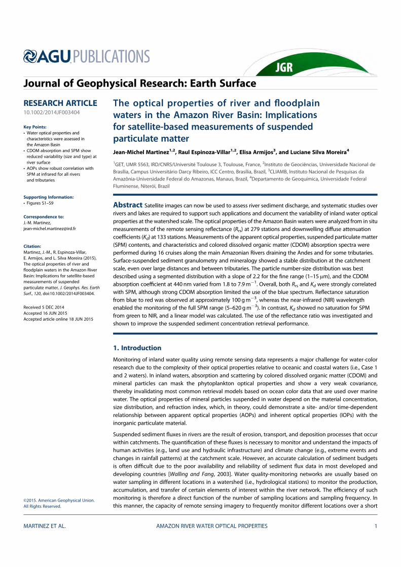
The optical properties of river and floodplainwaters in the Amazon River Basin: Implicationsfor satellite-based measurements of suspendedparticulate matterJean-Michel Martinez1,2, Raul Espinoza-Villar1,2, Elisa Armijos3, and Luciane Silva Moreira4
1GET, UMR 5563, IRD/CNRS/Université Toulouse 3, Toulouse, France, 2Instituto de Geociências, Universidade Nacional deBrasília, Campus Universitário Darcy Ribeiro, ICC Centro, Brasília, Brazil, 3CLIAMB, Instituto Nacional de Pesquisas daAmazônia-Universidade Federal do Amazonas, Manaus, Brazil, 4Departamento de Geoquímica, Universidade FederalFluminense, Niterói, Brazil
Abstract Satellite images can now be used to assess river sediment discharge, and systematic studies overrivers and lakes are required to support such applications and document the variability of inland water opticalproperties at the watershed scale. The optical properties of the Amazon Basin waters were analyzed from in situmeasurements of the remote sensing reflectance (Rrs) at 279 stations and downwelling diffuse attenuationcoefficients (Kd) at 133 stations. Measurements of the apparent optical properties, suspended particulatematter(SPM) contents, and characteristics and colored dissolved organic matter (CDOM) absorption spectra wereperformed during 16 cruises along the main Amazonian Rivers draining the Andes and for some tributaries.Surface-suspended sediment granulometry and mineralogy showed a stable distribution at the catchmentscale, even over large distances and between tributaries. The particle number-size distribution was bestdescribed using a segmented distribution with a slope of 2.2 for the fine range (1–15μm), and the CDOMabsorption coefficient at 440 nm varied from 1.8 to 7.9m�1. Overall, both Rrs and Kd were strongly correlatedwith SPM, although strong CDOM absorption limited the use of the blue spectrum. Reflectance saturationfrom blue to red was observed at approximately 100 gm�3, whereas the near-infrared (NIR) wavelengthenabled the monitoring of the full SPM range (5–620gm�3). In contrast, Kd showed no saturation for SPMfrom green to NIR, and a linear model was calculated. The use of the reflectance ratio was investigated andshown to improve the suspended sediment concentration retrieval performance.
1. Introduction
Monitoring of inland water quality using remote sensing data represents a major challenge for water-colorresearch due to the complexity of their optical properties relative to oceanic and coastal waters (i.e., Case 1and 2 waters). In inland waters, absorption and scattering by colored dissolved organic matter (CDOM) andmineral particles can mask the phytoplankton optical properties and show a very weak covariance,thereby invalidating most common retrieval models based on ocean color data that are used over marinewater. The optical properties of mineral particles suspended in water depend on the material concentration,size distribution, and refraction index, which, in theory, could demonstrate a site- and/or time-dependentrelationship between apparent optical properties (AOPs) and inherent optical properties (IOPs) with theinorganic particulate material.
Suspended sediment fluxes in rivers are the result of erosion, transport, and deposition processes that occurwithin catchments. The quantification of these fluxes is necessary to monitor and understand the impacts ofhuman activities (e.g., land use and hydraulic infrastructure) and climate change (e.g., extreme events andchanges in rainfall patterns) at the catchment scale. However, an accurate calculation of sediment budgetsis often difficult due to the poor availability and reliability of sediment flux data in most developed anddeveloping countries [Walling and Fang, 2003]. Water quality-monitoring networks are usually based onwater sampling in different locations in a watershed (i.e., hydrological stations) to monitor the production,accumulation, and transfer of certain elements of interest within the river network. The efficiency of suchmonitoring is therefore a direct function of the number of sampling locations and sampling frequency. Inthis manner, the capacity of remote sensing imagery to frequently monitor different locations over a short
MARTINEZ ET AL. AMAZON RIVER WATER OPTICAL PROPERTIES 1
PUBLICATIONSJournal of Geophysical Research: Earth Surface
RESEARCH ARTICLE10.1002/2014JF003404
Key Points:• Water optical properties andcharacteristics were assessed inthe Amazon Basin
• CDOM absorption and SPM showreduced variability (size and type) atriver surface
• AOPs show robust correlation withSPM at infrared for all riversand tributaries
Supporting Information:• Figures S1–S9
Correspondence to:J.-M. Martinez,[email protected]
Citation:Martinez, J.-M., R. Espinoza-Villar,E. Armijos, and L. Silva Moreira (2015),The optical properties of river andfloodplain waters in the Amazon RiverBasin: Implications for satellite-basedmeasurements of suspendedparticulate matter, J. Geophys. Res. EarthSurf., 120, doi:10.1002/2014JF003404.
Received 5 DEC 2014Accepted 16 JUN 2015Accepted article online 18 JUN 2015
©2015. American Geophysical Union.All Rights Reserved.
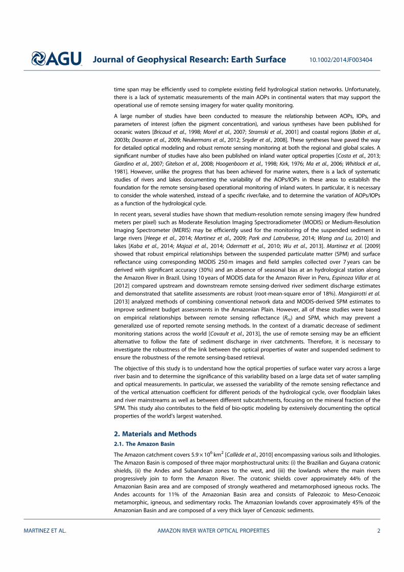
time span may be efficiently used to complete existing field hydrological station networks. Unfortunately,there is a lack of systematic measurements of the main AOPs in continental waters that may support theoperational use of remote sensing imagery for water quality monitoring.
A large number of studies have been conducted to measure the relationship between AOPs, IOPs, andparameters of interest (often the pigment concentration), and various syntheses have been published foroceanic waters [Bricaud et al., 1998; Morel et al., 2007; Stramski et al., 2001] and coastal regions [Babin et al.,2003b; Doxaran et al., 2009; Neukermans et al., 2012; Snyder et al., 2008]. These syntheses have paved the wayfor detailed optical modeling and robust remote sensing monitoring at both the regional and global scales. Asignificant number of studies have also been published on inland water optical properties [Costa et al., 2013;Giardino et al., 2007; Gitelson et al., 2008; Hoogenboom et al., 1998; Kirk, 1976; Ma et al., 2006; Whitlock et al.,1981]. However, unlike the progress that has been achieved for marine waters, there is a lack of systematicstudies of rivers and lakes documenting the variability of the AOPs/IOPs in these areas to establish thefoundation for the remote sensing-based operational monitoring of inland waters. In particular, it is necessaryto consider the whole watershed, instead of a specific river/lake, and to determine the variation of AOPs/IOPsas a function of the hydrological cycle.
In recent years, several studies have shown that medium-resolution remote sensing imagery (few hundredmeters per pixel) such as Moderate Resolution Imaging Spectroradiometer (MODIS) or Medium-ResolutionImaging Spectrometer (MERIS) may be efficiently used for the monitoring of the suspended sediment inlarge rivers [Heege et al., 2014; Martinez et al., 2009; Park and Latrubesse, 2014; Wang and Lu, 2010] andlakes [Kaba et al., 2014; Majozi et al., 2014; Odermatt et al., 2010; Wu et al., 2013]. Martinez et al. [2009]showed that robust empirical relationships between the suspended particulate matter (SPM) and surfacereflectance using corresponding MODIS 250m images and field samples collected over 7 years can bederived with significant accuracy (30%) and an absence of seasonal bias at an hydrological station alongthe Amazon River in Brazil. Using 10 years of MODIS data for the Amazon River in Peru, Espinoza Villar et al.[2012] compared upstream and downstream remote sensing-derived river sediment discharge estimatesand demonstrated that satellite assessments are robust (root-mean-square error of 18%). Mangiarotti et al.[2013] analyzed methods of combining conventional network data and MODIS-derived SPM estimates toimprove sediment budget assessments in the Amazonian Plain. However, all of these studies were basedon empirical relationships between remote sensing reflectance (Rrs) and SPM, which may prevent ageneralized use of reported remote sensing methods. In the context of a dramatic decrease of sedimentmonitoring stations across the world [Covault et al., 2013], the use of remote sensing may be an efficientalternative to follow the fate of sediment discharge in river catchments. Therefore, it is necessary toinvestigate the robustness of the link between the optical properties of water and suspended sediment toensure the robustness of the remote sensing-based retrieval.
The objective of this study is to understand how the optical properties of surface water vary across a largeriver basin and to determine the significance of this variability based on a large data set of water samplingand optical measurements. In particular, we assessed the variability of the remote sensing reflectance andof the vertical attenuation coefficient for different periods of the hydrological cycle, over floodplain lakesand river mainstreams as well as between different subcatchments, focusing on the mineral fraction of theSPM. This study also contributes to the field of bio-optic modeling by extensively documenting the opticalproperties of the world’s largest watershed.
2. Materials and Methods2.1. The Amazon Basin
The Amazon catchment covers 5.9 × 10⁶ km2 [Callède et al., 2010] encompassing various soils and lithologies.The Amazon Basin is composed of three major morphostructural units: (i) the Brazilian and Guyana cratonicshields, (ii) the Andes and Subandean zones to the west, and (iii) the lowlands where the main riversprogressively join to form the Amazon River. The cratonic shields cover approximately 44% of theAmazonian Basin area and are composed of strongly weathered and metamorphosed igneous rocks. TheAndes accounts for 11% of the Amazonian Basin area and consists of Paleozoic to Meso-Cenozoicmetamorphic, igneous, and sedimentary rocks. The Amazonian lowlands cover approximately 45% of theAmazonian Basin and are composed of a very thick layer of Cenozoic sediments.
Journal of Geophysical Research: Earth Surface 10.1002/2014JF003404
MARTINEZ ET AL. AMAZON RIVER WATER OPTICAL PROPERTIES 2
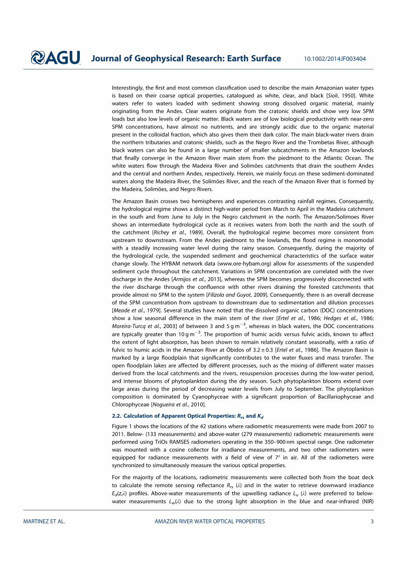
Interestingly, the first and most common classification used to describe the main Amazonian water typesis based on their coarse optical properties, catalogued as white, clear, and black [Sioli, 1950]. Whitewaters refer to waters loaded with sediment showing strong dissolved organic material, mainlyoriginating from the Andes. Clear waters originate from the cratonic shields and show very low SPMloads but also low levels of organic matter. Black waters are of low biological productivity with near-zeroSPM concentrations, have almost no nutrients, and are strongly acidic due to the organic materialpresent in the colloidal fraction, which also gives them their dark color. The main black-water rivers drainthe northern tributaries and cratonic shields, such as the Negro River and the Trombetas River, althoughblack waters can also be found in a large number of smaller subcatchments in the Amazon lowlandsthat finally converge in the Amazon River main stem from the piedmont to the Atlantic Ocean. Thewhite waters flow through the Madeira River and Solimões catchments that drain the southern Andesand the central and northern Andes, respectively. Herein, we mainly focus on these sediment-dominatedwaters along the Madeira River, the Solimões River, and the reach of the Amazon River that is formed bythe Madeira, Solimões, and Negro Rivers.
The Amazon Basin crosses two hemispheres and experiences contrasting rainfall regimes. Consequently,the hydrological regime shows a distinct high-water period from March to April in the Madeira catchmentin the south and from June to July in the Negro catchment in the north. The Amazon/Solimoes Rivershows an intermediate hydrological cycle as it receives waters from both the north and the south ofthe catchment [Richey et al., 1989]. Overall, the hydrological regime becomes more consistent fromupstream to downstream. From the Andes piedmont to the lowlands, the flood regime is monomodalwith a steadily increasing water level during the rainy season. Consequently, during the majority ofthe hydrological cycle, the suspended sediment and geochemical characteristics of the surface waterchange slowly. The HYBAM network data (www.ore-hybam.org) allow for assessments of the suspendedsediment cycle throughout the catchment. Variations in SPM concentration are correlated with the riverdischarge in the Andes [Armijos et al., 2013], whereas the SPM becomes progressively disconnected withthe river discharge through the confluence with other rivers draining the forested catchments thatprovide almost no SPM to the system [Filizola and Guyot, 2009]. Consequently, there is an overall decreaseof the SPM concentration from upstream to downstream due to sedimentation and dilution processes[Meade et al., 1979]. Several studies have noted that the dissolved organic carbon (DOC) concentrationsshow a low seasonal difference in the main stem of the river [Ertel et al., 1986; Hedges et al., 1986;Moreira-Turcq et al., 2003] of between 3 and 5 gm�3, whereas in black waters, the DOC concentrationsare typically greater than 10 gm�3. The proportion of humic acids versus fulvic acids, known to affectthe extent of light absorption, has been shown to remain relatively constant seasonally, with a ratio offulvic to humic acids in the Amazon River at Óbidos of 3.2 ± 0.3 [Ertel et al., 1986]. The Amazon Basin ismarked by a large floodplain that significantly contributes to the water fluxes and mass transfer. Theopen floodplain lakes are affected by different processes, such as the mixing of different water massesderived from the local catchments and the rivers, resuspension processes during the low-water period,and intense blooms of phytoplankton during the dry season. Such phytoplankton blooms extend overlarge areas during the period of decreasing water levels from July to September. The phytoplanktoncomposition is dominated by Cyanophyceae with a significant proportion of Bacillariophyceae andChlorophyceae [Nogueira et al., 2010].
2.2. Calculation of Apparent Optical Properties: Rrs and Kd
Figure 1 shows the locations of the 42 stations where radiometric measurements were made from 2007 to2011. Below- (133 measurements) and above-water (279 measurements) radiometric measurements wereperformed using TriOs RAMSES radiometers operating in the 350–900 nm spectral range. One radiometerwas mounted with a cosine collector for irradiance measurements, and two other radiometers wereequipped for radiance measurements with a field of view of 7° in air. All of the radiometers weresynchronized to simultaneously measure the various optical properties.
For the majority of the locations, radiometric measurements were collected both from the boat deckto calculate the remote sensing reflectance Rrs (λ) and in the water to retrieve downward irradianceEd(z,λ) profiles. Above-water measurements of the upwelling radiance Lu (λ) were preferred to below-water measurements Lw(λ) due to the strong light absorption in the blue and near-infrared (NIR)
Journal of Geophysical Research: Earth Surface 10.1002/2014JF003404
MARTINEZ ET AL. AMAZON RIVER WATER OPTICAL PROPERTIES 3
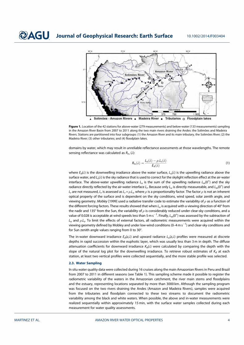
domains by water, which may result in unreliable reflectance assessments at those wavelengths. The remotesensing reflectance was calculated as Rrs (λ):
Rrs λð Þ ¼ Lu λð Þ � ρ:Ls λð ÞEd λð Þ (1)
where Ed(λ) is the downwelling irradiance above the water surface, Lu(λ) is the upwelling radiance above thesurface water, and Ls(λ) is the sky radiance that is used to correct for the skylight reflection effect at the air-waterinterface. The above-water upwelling radiance Lu is the sum of the upwelling radiance Lw(0
+) and the skyradiance directly reflected by the air-water interface Lr. Because only Lu is directly measureable, and Lw(0
+) andLr are not measured, Lr is assessed as Lr= ρ.Ls, where ρ is a proportionality factor. The factor ρ is not an inherentoptical property of the surface and is dependent on the sky conditions, wind speed, solar zenith angle, andviewing geometry. Mobley [1999] used a radiative transfer code to estimate the variability of ρ as a function ofthe different forcing factors. These results showed that when Lu is acquired with a viewing direction of 40° fromthe nadir and 135° from the Sun, the variability of ρ is considerably reduced under clear-sky conditions, and avalue of 0.028 is acceptable at wind speeds less than 5ms�1. Finally, Lw(0
+) was assessed by the subtraction ofLu and ρ.Ls. To limit the effects of external factors, all radiometric measurements were acquired within theviewing geometry defined by Mobley and under low-wind conditions (0–4m s�1) and clear-sky conditions andfor Sun zenith angle values ranging from 0 to 30°.
The in-water downward irradiance Ed(z,λ) and upward radiance Lu(z,λ) profiles were measured at discretedepths in rapid succession within the euphotic layer, which was usually less than 3m in depth. The diffuseattenuation coefficients for downward irradiance Kd(λ) were calculated by comparing the depth with theslope of the natural log plot for the downwelling irradiance. To retrieve robust estimates of Kd at eachstation, at least two vertical profiles were collected sequentially, and the more stable profile was selected.
2.3. Water Sampling
In situ water quality data were collected during 16 cruises along themain Amazonian Rivers in Peru and Brazilfrom 2007 to 2011 in different seasons (see Table 1). This sampling scheme made it possible to register theradiometric variability of the waters in the Amazonian catchment, the river main stems and floodplainsand the estuary, representing locations separated by more than 3000 km. Although the sampling programwas focused on the two rivers draining the Andes (Amazon and Madeira Rivers), samples were acquiredfrom the tributaries and floodplain connected to these two streams to document the radiometricvariability among the black and white waters. When possible, the above and in-water measurements wererealized sequentially within approximately 15min, with the surface water samples collected during eachmeasurement for water quality assessments.
Figure 1. Location of the 42 stations for above-water (279 measurements) and below-water (133 measurements) samplingin the Amazon River Basin from 2007 to 2011 along the two main rivers draining the Andes: the Solimões and MadeiraRivers. Stations are partitioned into four subgroups: (1) the Amazon River and its main tributary, the Solimões River; (2) theMadeira River; (3) other tributaries; and (4) floodplain lakes.
Journal of Geophysical Research: Earth Surface 10.1002/2014JF003404
MARTINEZ ET AL. AMAZON RIVER WATER OPTICAL PROPERTIES 4
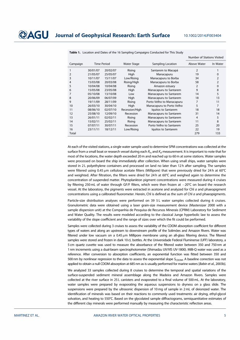
At each of the visited stations, a single water sample used to determine SPM concentrations was collected at thesurface from a small boat or research vessel during each Rrs and Kdmeasurement. It is important to note that formost of the locations, the water depth exceeded 20m and reached up to 60m at some stations. Water sampleswere processed on board the ship immediately after collection. When using small ships, water samples werestored in 2 L polyethylene containers and processed on land no later than 12h after sampling. The sampleswere filtered using 0.45μm cellulose acetate filters (Millipore) that were previously dried for 24 h at 60°Cand weighted. After filtration, the filters were dried for 24 h at 60°C and weighed again to determine theconcentration of suspended matter. Phytoplankton pigment concentrations were measured during 4 cruisesby filtering 250mL of water through GF/F filters, which were then frozen at �20°C on board the researchvessel. At the laboratory, the pigments were extracted in acetone and analyzed for Chl a and phaeopigmentconcentrations using a calibrated fluorometer. Herein, Chl is defined as the sum of Chl a and phaeopigments.
Particle-size distribution analyses were performed on 39 5 L water samples collected during 6 cruises.Granulometric data were obtained using a laser grain-size measurement device (Mastersizer 2000 with asample dispersion unit) at the Companhia de Pesquisa de Recursos Minerais (CPRM) Laboratory for Sedimentand Water Quality. The results were modeled according to the classical Junge hyperbolic law to assess thevariability of the slope coefficient and the range of sizes over which the fit could be performed.
Samples were collected during 3 cruises to assess the variability of the CDOM absorption coefficient for differenttypes of waters and along an upstream to downstream profile of the Solimões and Amazon Rivers. Water wasfiltered under low vacuum on a 0.45μm Millipore membrane using an all-glass filtering device. The filteredsamples were stored and frozen in dark 10cL bottles. At the Universidade Federal Fluminense (UFF) laboratory, a5 cm quartz cuvette was used to measure the absorbance of the filtered water between 350 and 750nm at1nm increments using a dual-beam spectrophotometer (Shimadzu UV/VIS UV-1800). Milli-Q water was used as areference. After conversion to absorption coefficients, an exponential function was fitted between 350 and500nm by nonlinear regression to the data to assess the exponential slope SCDOM. A baseline correction was notapplied to obtain a null CDOM absorption at 685nm as is usually performed for marine waters [Babin et al., 2003b].
We analyzed 33 samples collected during 8 cruises to determine the temporal and spatial variations of thesurface-suspended sediment mineral assemblage along the Madeira and Amazon Rivers. Samples werecollected at the river surface in 25 L canisters and evaporated to a final volume of 500mL. At the laboratory,water samples were prepared by evaporating the aqueous suspensions to dryness on a glass slide. Thesuspensions were prepared by the ultrasonic dispersion of 10mg of sample in 2mL of deionized water. Theidentification of minerals was based on their reactions to commonly used treatments: air drying, ethyl-glycolsolvation, and heating to 550°C. Based on the glycolated sample diffractograms, semiquantitative estimates ofthe different clay minerals were performed manually by measuring the characteristic reflection areas.
Table 1. Location and Dates of the 16 Sampling Campaigns Conducted for This Study
Campaign Time Period Water Stage Sampling Location
Number of Stations Visited
Above Water In Water
1 30/01/07 20/02/07 Rising Santarem to Macapá 2 12 21/05/07 25/05/07 High Manacapuru 19 03 10/11/07 15/11/07 Low/Rising Manacapuru to Borba 34 24 15/03/08 20/03/08 Rising/High Manacapuru to Borba 58 25 10/04/08 10/04/08 Rising Amazon estuary 2 06 15/05/08 23/05/08 High Manacapuru to Santarem 9 87 05/10/08 13/10/08 Low Manacapuru to Santarem 14 58 20/06/09 06/07/09 High Manacapuru to Santarem 18 139 19/11/09 28/11/09 Rising Porto Velho to Manacapuru 7 1110 26/03/10 30/04/10 High Manacapuru to Porto Velho 5 711 08/06/10 02/07/10 Recession/High Iquitos to Santarem 18 1812 25/08/10 12/09/10 Recession Manacapuru to Santarem 31 1413 26/01/11 02/02/11 Rising Manacapuru to Santarem 4 514 15/02/11 25/02/11 Rising Manacapuru to Santarem 11 815 07/07/11 30/07/11 Recession Porto Velho to Santarem 25 2016 23/11/11 18/12/11 Low/Rising Iquitos to Santarem 22 19Total 279 133
Journal of Geophysical Research: Earth Surface 10.1002/2014JF003404
MARTINEZ ET AL. AMAZON RIVER WATER OPTICAL PROPERTIES 5
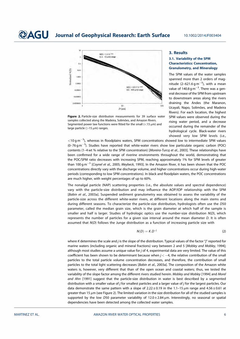
3. Results3.1. Variability of the SPMCharacteristics: Concentration,Granulometry, and Mineralogy
The SPM values of the water samplesspanned more than 2 orders of mag-nitude (2–621.6 gm�3), with a meanvalue of 140.8 gm�3. There was a gen-eral decrease of the SPM from upstreamto downstream areas along the riversdraining the Andes (the Maranon,Ucayali, Napo, Solimões, and MadeiraRivers). For each location, the highestSPM values were observed during therising water period, and a decreaseoccurred during the remainder of thehydrological cycle. Black-water riversshowed very low SPM levels (i.e.,
<10 gm�3), whereas in floodplains waters, SPM concentrations showed low to intermediate SPM values(0–76 gm�3). Studies have reported that white-water rivers show low particulate organic carbon (POC)contents (1–4wt % relative to the SPM concentration) [Moreira-Turcq et al., 2003]. These relationships havebeen confirmed for a wide range of riverine environments throughout the world, demonstrating thatthe POC/SPM ratio decreases with increasing SPM, reaching approximately 1% for SPM levels of greaterthan 100 gm�3 [Coynel et al., 2005; Meybeck, 1993]. In the Amazon River, it has been shown that the POCconcentrations directly vary with the discharge volume, and higher concentrations occur during high-waterperiods (corresponding to low SPM concentrations). In black and floodplain waters, the POC concentrationsare much higher, with weight percentages of up to 60%.
The nonalgal particle (NAP) scattering properties (i.e., the absolute values and spectral dependence)vary with the particle-size distribution and may influence the AOP/IOP relationship with the SPM[Babin et al., 2003a]. Suspended sediment granulometry was obtained to assess the variability of theparticle-size across the different white-water rivers, at different locations along the main stems andduring different seasons. To characterize the particle-size distribution, hydrologists often use the D50parameter, called the median grain size, which is the grain diameter at which half of the sample issmaller and half is larger. Studies of hydrologic optics use the number-size distribution N(D), whichrepresents the number of particles for a given size interval around the mean diameter D. It is oftenassumed that N(D) follows the Junge distribution as a function of increasing particle size with
N Dð Þ ¼ K :D�j (2)
where K determines the scale and j is the slope of the distribution. Typical values of the factor “j” reported formarine waters (including organic and mineral fractions) vary between 2 and 5 [Mobley and Mobley, 1994];although most studies assume a unique value for j of 4, experimental data are very limited. The value of thiscoefficient has been shown to be determinant because when j<�4, the relative contribution of the smallparticles to the total particle volume concentration decreases, and therefore, the contribution of smallparticles to the total light scattering decreases [Babin et al., 2003a]. The composition of the Amazon whitewaters is, however, very different that than of the open ocean and coastal waters; thus, we tested thevariability of the slope factor among the different rivers studied herein. Mobley and Mobley [1994] and Moreland Ahn [1991] suggest that the particle-size distribution in water is best described by a segmenteddistribution with a smaller value of j for smallest particles and a larger value of j for the largest particles. Ourdata demonstrate the same pattern with a slope of 2.22 ± 0.19 in the 1.1–15μm range and 4.56 ± 0.61 atgreater than 15μm (see Figure 2). The limited variation in the size distribution for all of the studied samples issupported by the low D50 parameter variability of 12.0 ± 2.84μm. Interestingly, no seasonal or spatialdependencies have been detected among the collected water samples.
Figure 2. Particle-size distribution measurements for 39 surface watersamples collected along the Madeira, Solimões, and Amazon Rivers.Segmented power law functions were fitted for the small (<15 μm) andlarge particle (>15 μm) ranges.
Journal of Geophysical Research: Earth Surface 10.1002/2014JF003404
MARTINEZ ET AL. AMAZON RIVER WATER OPTICAL PROPERTIES 6
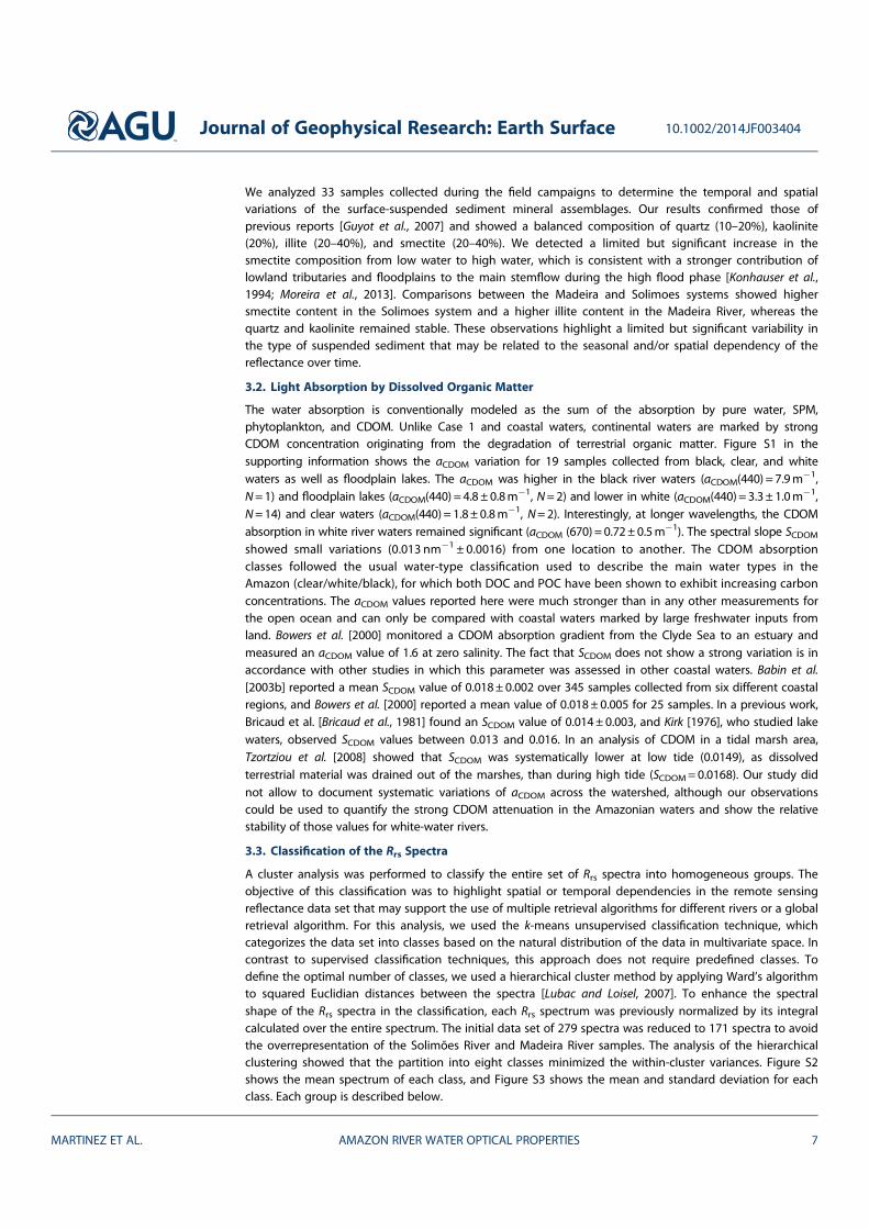
We analyzed 33 samples collected during the field campaigns to determine the temporal and spatialvariations of the surface-suspended sediment mineral assemblages. Our results confirmed those ofprevious reports [Guyot et al., 2007] and showed a balanced composition of quartz (10–20%), kaolinite(20%), illite (20–40%), and smectite (20–40%). We detected a limited but significant increase in thesmectite composition from low water to high water, which is consistent with a stronger contribution oflowland tributaries and floodplains to the main stemflow during the high flood phase [Konhauser et al.,1994; Moreira et al., 2013]. Comparisons between the Madeira and Solimoes systems showed highersmectite content in the Solimoes system and a higher illite content in the Madeira River, whereas thequartz and kaolinite remained stable. These observations highlight a limited but significant variability inthe type of suspended sediment that may be related to the seasonal and/or spatial dependency of thereflectance over time.
3.2. Light Absorption by Dissolved Organic Matter
The water absorption is conventionally modeled as the sum of the absorption by pure water, SPM,phytoplankton, and CDOM. Unlike Case 1 and coastal waters, continental waters are marked by strongCDOM concentration originating from the degradation of terrestrial organic matter. Figure S1 in thesupporting information shows the aCDOM variation for 19 samples collected from black, clear, and whitewaters as well as floodplain lakes. The aCDOM was higher in the black river waters (aCDOM(440) = 7.9m
�1,N=1) and floodplain lakes (aCDOM(440) = 4.8 ± 0.8m�1, N=2) and lower in white (aCDOM(440) = 3.3± 1.0m
�1,N=14) and clear waters (aCDOM(440) = 1.8± 0.8m
�1, N=2). Interestingly, at longer wavelengths, the CDOMabsorption in white river waters remained significant (aCDOM (670) = 0.72± 0.5m�1). The spectral slope SCDOMshowed small variations (0.013 nm�1 ± 0.0016) from one location to another. The CDOM absorptionclasses followed the usual water-type classification used to describe the main water types in theAmazon (clear/white/black), for which both DOC and POC have been shown to exhibit increasing carbonconcentrations. The aCDOM values reported here were much stronger than in any other measurements forthe open ocean and can only be compared with coastal waters marked by large freshwater inputs fromland. Bowers et al. [2000] monitored a CDOM absorption gradient from the Clyde Sea to an estuary andmeasured an aCDOM value of 1.6 at zero salinity. The fact that SCDOM does not show a strong variation is inaccordance with other studies in which this parameter was assessed in other coastal waters. Babin et al.[2003b] reported a mean SCDOM value of 0.018± 0.002 over 345 samples collected from six different coastalregions, and Bowers et al. [2000] reported a mean value of 0.018± 0.005 for 25 samples. In a previous work,Bricaud et al. [Bricaud et al., 1981] found an SCDOM value of 0.014± 0.003, and Kirk [1976], who studied lakewaters, observed SCDOM values between 0.013 and 0.016. In an analysis of CDOM in a tidal marsh area,Tzortziou et al. [2008] showed that SCDOM was systematically lower at low tide (0.0149), as dissolvedterrestrial material was drained out of the marshes, than during high tide (SCDOM=0.0168). Our study didnot allow to document systematic variations of aCDOM across the watershed, although our observationscould be used to quantify the strong CDOM attenuation in the Amazonian waters and show the relativestability of those values for white-water rivers.
3.3. Classification of the Rrs Spectra
A cluster analysis was performed to classify the entire set of Rrs spectra into homogeneous groups. Theobjective of this classification was to highlight spatial or temporal dependencies in the remote sensingreflectance data set that may support the use of multiple retrieval algorithms for different rivers or a globalretrieval algorithm. For this analysis, we used the k-means unsupervised classification technique, whichcategorizes the data set into classes based on the natural distribution of the data in multivariate space. Incontrast to supervised classification techniques, this approach does not require predefined classes. Todefine the optimal number of classes, we used a hierarchical cluster method by applying Ward’s algorithmto squared Euclidian distances between the spectra [Lubac and Loisel, 2007]. To enhance the spectralshape of the Rrs spectra in the classification, each Rrs spectrum was previously normalized by its integralcalculated over the entire spectrum. The initial data set of 279 spectra was reduced to 171 spectra to avoidthe overrepresentation of the Solimões River and Madeira River samples. The analysis of the hierarchicalclustering showed that the partition into eight classes minimized the within-cluster variances. Figure S2shows the mean spectrum of each class, and Figure S3 shows the mean and standard deviation for eachclass. Each group is described below.
Journal of Geophysical Research: Earth Surface 10.1002/2014JF003404
MARTINEZ ET AL. AMAZON RIVER WATER OPTICAL PROPERTIES 7
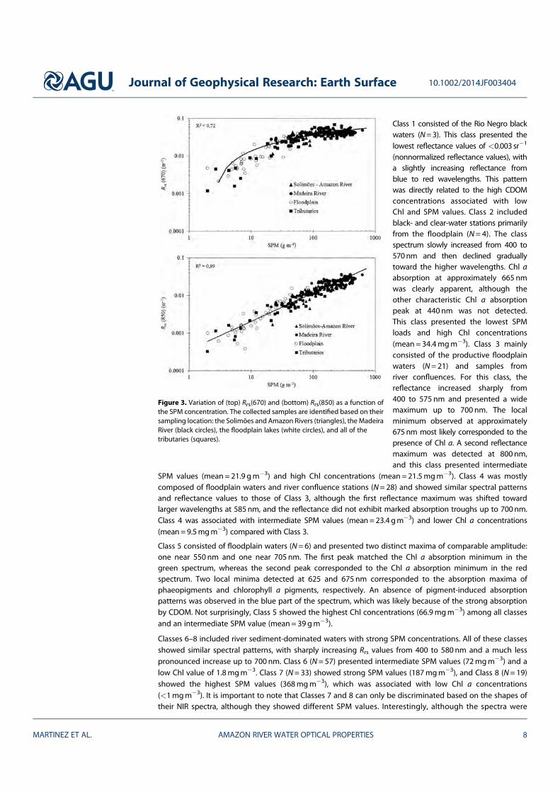
Class 1 consisted of the Rio Negro blackwaters (N=3). This class presented thelowest reflectance values of <0.003 sr�1
(nonnormalized reflectance values), witha slightly increasing reflectance fromblue to red wavelengths. This patternwas directly related to the high CDOMconcentrations associated with lowChl and SPM values. Class 2 includedblack- and clear-water stations primarilyfrom the floodplain (N= 4). The classspectrum slowly increased from 400 to570nm and then declined graduallytoward the higher wavelengths. Chl aabsorption at approximately 665 nmwas clearly apparent, although theother characteristic Chl a absorptionpeak at 440 nm was not detected.This class presented the lowest SPMloads and high Chl concentrations(mean = 34.4mgm�3). Class 3 mainlyconsisted of the productive floodplainwaters (N= 21) and samples fromriver confluences. For this class, thereflectance increased sharply from400 to 575 nm and presented a widemaximum up to 700 nm. The localminimum observed at approximately675nm most likely corresponded to thepresence of Chl a. A second reflectancemaximum was detected at 800 nm,and this class presented intermediate
SPM values (mean= 21.9 gm�3) and high Chl concentrations (mean= 21.5mgm�3). Class 4 was mostlycomposed of floodplain waters and river confluence stations (N= 28) and showed similar spectral patternsand reflectance values to those of Class 3, although the first reflectance maximum was shifted towardlarger wavelengths at 585nm, and the reflectance did not exhibit marked absorption troughs up to 700nm.Class 4 was associated with intermediate SPM values (mean=23.4 gm�3) and lower Chl a concentrations(mean=9.5mgm�3) compared with Class 3.
Class 5 consisted of floodplain waters (N= 6) and presented two distinct maxima of comparable amplitude:one near 550 nm and one near 705 nm. The first peak matched the Chl a absorption minimum in thegreen spectrum, whereas the second peak corresponded to the Chl a absorption minimum in the redspectrum. Two local minima detected at 625 and 675 nm corresponded to the absorption maxima ofphaeopigments and chlorophyll a pigments, respectively. An absence of pigment-induced absorptionpatterns was observed in the blue part of the spectrum, which was likely because of the strong absorptionby CDOM. Not surprisingly, Class 5 showed the highest Chl concentrations (66.9mgm�3) among all classesand an intermediate SPM value (mean= 39 gm�3).
Classes 6–8 included river sediment-dominated waters with strong SPM concentrations. All of these classesshowed similar spectral patterns, with sharply increasing Rrs values from 400 to 580 nm and a much lesspronounced increase up to 700 nm. Class 6 (N= 57) presented intermediate SPM values (72mgm�3) and alow Chl value of 1.8mgm�3. Class 7 (N= 33) showed strong SPM values (187mgm�3), and Class 8 (N=19)showed the highest SPM values (368mgm�3), which was associated with low Chl a concentrations(<1mgm�3). It is important to note that Classes 7 and 8 can only be discriminated based on the shapes oftheir NIR spectra, although they showed different SPM values. Interestingly, although the spectra were
Figure 3. Variation of (top) Rrs(670) and (bottom) Rrs(850) as a function ofthe SPM concentration. The collected samples are identified based on theirsampling location: the Solimões and Amazon Rivers (triangles), the MadeiraRiver (black circles), the floodplain lakes (white circles), and all of thetributaries (squares).
Journal of Geophysical Research: Earth Surface 10.1002/2014JF003404
MARTINEZ ET AL. AMAZON RIVER WATER OPTICAL PROPERTIES 8
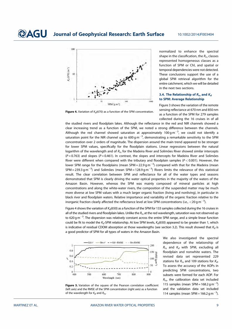
normalized to enhance the spectralshape in the classification, the Rrs classesrepresented homogeneous classes as afunction of SPM or Chl, and spatial ortemporal dependencies were not detected.These conclusions support the use of aglobal SPM retrieval algorithm for theentire catchment, whichwewill be detailedin the next two sections.
3.4. The Relationship of Rrs and Kdto SPM: Average Relationship
Figure 3 shows the variation of the remotesensing reflectance at 670 nm and 850 nmas a function of the SPM for 279 samplescollected during the 16 cruises in of all
the studied rivers and floodplain lakes. Although the reflectance in the red and NIR channels showed aclear increasing trend as a function of the SPM, we noted a strong difference between the channels.Although the red channel showed saturation at approximately 100 gm�3, we could not identify asaturation point for the NIR channel up to 600 gm�3, demonstrating a remarkable sensitivity to the SPMconcentration over 2 orders of magnitude. The dispersion around the main trend appeared to be strongerfor lower SPM values, specifically for the floodplain stations. Linear regressions between the naturallogarithm of the wavelength and of Rrs for the Madeira River and Solimões River showed similar intercepts(P= 0.763) and slopes (P=0.461). In contrast, the slopes and intercepts for Madeira River and SolimõesRiver were different when compared with the tributary and floodplain samples (P< 0.001). However, thelower SPM range for the floodplains (mean SPM=22.9 gm�3) compared with that for the Madeira (meanSPM=239.3 gm�3) and Solimões (mean SPM=128.9 gm�3) Rivers limits the relevance of this statisticalresult. The clear correlation between SPM and reflectance for all of the water types and seasonsdemonstrated that SPM is clearly driving the water optical properties in the majority of the waters of theAmazon Basin. However, whereas the SPM was mainly composed of mineral particles at highconcentrations and along the white-water rivers, the composition of the suspended matter may be muchmore diverse at low SPM values with a much larger organic fraction (living and nonliving), in particular inblack river and floodplain waters. Relative importance and variability of the organic fraction relative to theinorganic fraction clearly affected the reflectance level at low SPM concentrations (i.e., <20 gm�3).
Figure 4 shows the variation of Kd(650) as a function of the SPM for 133 samples collected during the 16 cruises inall of the studied rivers and floodplain lakes. Unlike the Rrs at the red wavelength, saturationwas not observed upto 620gm�3. The dispersion was relatively constant across the entire SPM range, and a simple linear functioncould be fit to model the Kd-SPM relationship. At low SPM levels, Kd(650) appeared to be greater than 1, whichis indicative of residual CDOM absorption at those wavelengths (see section 3.2). This result showed that Kd isa good predictor of SPM for all types of waters in the Amazon Basin.
We also investigated the spectraldependence of the relationship ofRrs and Kd with SPM, excluding allfloodplain and nonwhite waters. Therevised data set represented 229stations for Rrs and 109 stations for Kd.To assess the accuracy of the AOPs inpredicting SPM concentrations, twosubsets were formed for each AOP. ForRrs, the calibration data set included115 samples (mean SPM=168.2 gm�3)and the validation data set included114 samples (mean SPM=166.2gm�3).
Figure 4. Variation of Kd(670) as a function of the SPM concentration.
Figure 5. Variation of the square of the Pearson correlation coefficient(left axis) and the RMSE of the SPM concentration (right axis) as a functionof the wavelength for Kd and Rrs.
Journal of Geophysical Research: Earth Surface 10.1002/2014JF003404
MARTINEZ ET AL. AMAZON RIVER WATER OPTICAL PROPERTIES 9
For Kd, the calibration data set included 56 samples (mean SPM=128.1gm�3) and the validation data setincluded 53 samples (mean SPM=138.9 gm�3).
Figure 5 presents the model-fitting and SPM retrieval performances for Rrs and Kd as a function of thewavelength. For Rrs, there was a clear increasing relationship with SPM from the blue to NIR wavelengths,with a square Pearson correlation factor of greater than 0.75 beyond 730 nm and an optimal range of840–900 nm (r2 of approximately 0.81). A lower correlation in the visible spectrum (400 to 700 nm) wasinduced by the rapid saturation of the Rrs as a function of the SPM at low concentrations. The least squaresregression showed that a power law model a.Rrs(λ)
b provides the best fit values. The model factors andperformance were calculated based on the linear regression between the natural logarithm of thewavelength and of Rrs. The root-mean-square error (RMSE) of the retrieval model decreased as a functionof increasing wavelength starting at 114.1 gm�3 (400 nm) down to 61 gm�3 (820–900 nm). The optimalwavelength occurred at 860 nm, and the corresponding model is as follows:
SPM ¼ 20:41 Rrs 860ð Þ½ �1:173 (3)
Figure S4 shows the model performance over the validation data set. For Kd, there was a strong and robustcorrelation with SPM (see Figure 5) over a wide range of wavelengths in both the visible and NIR spectrafrom 495 to 860 nm (r2> 0.90). The lower Pearson correlation at short wavelengths and beyond 890 nmmay have been induced by the strong absorption of light that makes it difficult to accurately assess thedownwelling irradiance distant from the water surface. Accordingly, a linear best fit model between SPMand Kd performed better than for Rrs with an RMSE of better than 30 gm�3 from 500 to 870 nm.
SPM ¼ 20:5 :Kd 650ð Þ � 22:94 (4)
Figure S5 shows themodel performance for the validation data set. These observationsmay be related to the linkbetween the AOPs and IOPs (the absorption and scattering coefficients); i.e., whereas Rrs is related to theabsorption to scattering ratio, Kd is assumed to vary as the sum of absorption and scattering. With increasingSPM, coefficients a and b will increase, meaning that Kd will increase indefinitely as a function of thesuspended sediment concentration, whereas Rrs may reach a saturation point. Not surprisingly, Kd andRrs were well correlated at 730 nm up to 900 nm (r2> 0.80). At 850 nm, we observed the followingrelationship (r2> 0.85):
Kd 850ð Þ ¼ 559:17Rrs 850ð Þ þ 3:98 (5)
3.5. Improvement of SPM Retrieval Using the Rrs Ratio at Two Wavelengths
It has been shown that the ratio between Rrs at two wavelengths may lessen the dependence on the SPM typeand thus is more robustly linked to the SPM concentration [Doxaran et al., 2002; Moore et al., 1999]. Irradiancereflectance is generally modeled as R= f ·bb/(a+bb), where bb is the backscattering coefficient and f is a factordetermined by the incident light field and often assumed to be invariant as a function of the wavelength.Doxaran et al. [2002] analyzed the variation of the bb/(a+bb) ratio for highly turbid waters in the Girondeestuary. These authors showed that when the contributions of pure water, algal pigments, and CDOM to lightabsorption can be neglected, the bb/(a+bb) ratio becomes independent of the SPM concentrations, leading tothe saturation phenomenon observed for Rrs. The total absorption by pure water is high at NIR, and thus, thissimple model predicts that saturation will occur for higher SPM concentrations at infrared relatively to visiblewavelengths. Interestingly, the same authors reported that the bb/(a+bb) ratio at two wavelengths will be lesssensitive to the refraction index and grain-size variation than to the SPM concentration at high SPM loads.Indeed, by assuming that the spectral variations of bb are weak [Moore et al., 1999; Whitlock et al., 1981], it canbe shown that the ratio is much more dependent on the absorption than on the backscattering, which, inturn, may limit the influence of the refraction indices and granulometry. This simple ratio model will performbetter using wavelengths at which SPM absorption shows a strong variation and, together with the purewater absorption, dominates the total absorption. It can be deduced from our previous observations that theRrs ratio should make use of the red and NIR wavelengths.
We investigated whether the use of the reflectance ratio Rrs(λ1)/Rrs(λ2) improved the SPM-Rrs relationship inthe river sediment-dominated waters. To determine the optimal position of λ1, we selected an initial value ofλ2 = 670 nm within the range of the minimum total absorption in the red spectrum. We performed a
Journal of Geophysical Research: Earth Surface 10.1002/2014JF003404
MARTINEZ ET AL. AMAZON RIVER WATER OPTICAL PROPERTIES 10
regression of the model [Rrs(λ1)/Rrs(670)] versus SPM for the range of 730 to 900 nm; the RMSE of the SPMestimation showed minimal values over a wide range of λ1 between 760 and 820 nm (see Figure S6a). Inthe second iteration, we determined λ2 after fixing λ1 at 805 nm and regressing the model [Rrs(805)/Rrs(λ2)]versus SPM. Again, the RMSE was minimal over a wide range of λ2 between 650 and 700 nm, with the bestresult obtained at λ2 = 680 (see Figure S6b). Interestingly, the ratio model performed significantly betterthan with the use of a unique wavelength with an RMSE of approximately 38 gm�3 (Figures S7 and S8). Inaddition, the spectral bands showing a minimal RMSE at both the red and NIR regions of the spectrumincluded the spectral bands of commonly used water-color sensors, such as MERIS and MODIS, and futureplatforms, such as Sentinel-3, NPP/VIIRS, and JPSS.
We further investigated whether the efficiency of the Rrs ratio was global or varied from one river to another.For the Solimões River, the use of the ratio compared with that of a single-wavelengthmodel at NIR increasedslightly the model accuracy (r2 = 0.83 versus 0.73, N= 76). For the Madeira River, the use of the ratio showed astrong improvement of the retrieval accuracy (r2 = 0.93 versus 0.62, N=102) (see Figure S9). However, whenthe regression lines assessed for both rivers were compared, the data supported the hypothesis that theslope (P=0.108) and intercept (P= 0.225) are equal. From our data set, we concluded that the use of theRrs ratio may not show an increased SPM retrieval efficiency globally, although it may be used as a generaltool to homogenize a data set across a watershed.
4. Discusion and Conclusions
The Amazon Basin presents Case 2 waters with an absorption budget dominated by CDOM and SPM in riversbut with a significant contribution from Chl a in floodplains. A simple unsupervised classification of Rrsspectra made it possible to discriminate several classes: (1) one class presenting very low Rrs valuescorresponding to the so-called black waters with strong CDOM absorption and very low SPMconcentrations; (2) four groups of floodplain lakes and river confluences, where a reduced water velocityallows the development of phytoplankton at high concentrations; and (3) three classes of sediment-dominated waters with relatively high SPM concentrations. Rrs shows saturation, with SPM atapproximately 100 gm�3 in the green and red spectra. However, the use of Rrs in the infrared spectrummakes it possible to monitor the SPM range without saturation. Interestingly, the three main AmazonianRivers having sediment-dominated water (the Madeira, Solimões, and Amazon Rivers) showed a similarbehavior as a function of SPM, even though the samples were collected at stations that in some caseswere separated by more than 3000 km. Kd proved to be a very robust predictor (r2> 0.9) of SPM through asimple linear relationship for a very wide range of SPM values (up to 622 gm�3) and wavelengths.
The use of reflectance ratios has been previously presented as a means to reduce the sensitivity of Rrs to thesediment type or size distribution in sediment-dominated waters [Doxaran et al., 2002; Moore et al., 1999]. Inour data set, we observed that the use of a ratio model does not improve the results uniformly for all ofthe studied water bodies. For example, although the retrieval model accuracy was slightly improved for theSolimões River when using a reflectance ratio instead of one wavelength, for the Madeira River, theimprovement is much stronger. In an analysis of 11 years of MODIS red and infrared surface reflectance dataand of SPM data acquired at two hydrological stations along the Madeira River in Brazil, Espinoza Villar et al.[2013] showed that the NIR reflectance does not exhibit a simple relationship with SPM. The authors detecteda hysteresis effect in which for the same SPM concentration, the reflectance during rising water is higher thanat the flood peak. It is important to note that using the same method, Espinoza Villar et al. [2012] did notdetect such a seasonal variation for the Solimões River or its main tributaries (Marañon and Ucayali) in Peru.
For such sediment-dominated waters, it is expected that the AOP/IOP variations may be strongly impacted byspatial and seasonal changes in sediment type and particle-size distribution. However, our results showedthat at the Amazon catchment scale, Rrs exhibits a relationship with SPM that is sufficiently robust to beused for the accurate monitoring of surface-suspended sediment discharge in the largest river of theworld. Regarding the particle-size distribution, our granulometric results showed a relatively consistentgrain-size distribution among different rivers and hydrological periods. The segmented grain-sizedistribution showed a more even distribution (slope 2.22) for the 1 to 15μm diameter range than is usuallypredicted in optical modeling (approximately 4), which implies that the contribution of very fine particles
Journal of Geophysical Research: Earth Surface 10.1002/2014JF003404
MARTINEZ ET AL. AMAZON RIVER WATER OPTICAL PROPERTIES 11
(<1μm) to NAP scattering is limited. These observations agree with the classical results of sediment transportdynamics in a turbulent flow system that predict a relatively constant distribution of the fine-grained sizefraction in the water column in which the coarse-grained size fraction increases from the surface to theriver bottom [Rouse, 1938], resulting in an almost pure fine sediment composition at the river surface.Furthermore, most large rivers, such as the main rivers of the Amazon Basin, have been shown to displayreduced grain-size range in the bed load and suspended sediment mainly because they flow across vastplains for a major part of their course with very low topographic gradient causing strong sedimentation inthe foothills and floodplains [Latrubesse, 2008].
Our study did not allow for a detailed assessment of the variability of the mineral particle types, but it didconfirm the results of previous studies in the Amazonian Plain showing a relatively consistent pattern ofmineral compositions. Guyot et al. [2007] analyzed 229 sediment samples from throughout the entireAmazon Basin to document the spatial variability of the mineral assemblages. These authors reportedthat the sediment clay phase from the rivers draining the Andes contains a dominant illite + chloriteassemblage that is enriched in smectite during transport through the lowlands. The main minerals foundin the SPM showed a limited refraction index range relative to water of 1.16–1.18. Furthermore, previousmodeling studies [Babin et al., 2003a; Doxaran et al., 2009; Wozniak and Stramski, 2004] showed that evengrain-size distribution (i.e., slope below 4) limited the impact of the variability of the refraction index. Ourresults demonstrated that the sediment-size distribution and mineralogy may present limited variations atthe scale of a large river basin, thus supporting the development of robust SPM retrieval methods frommain AOPs.
Although the Rrs seasonal variation as a function of SPM for the Madeira River case can be efficiently correctedusing a simple reflectance ratio model, the cause of the Rrs variability remains unclear because the deviationmay originate from variations of the physical properties of the inorganic SPM or variation in the organicfraction. Viers et al. [2008] analyzed the variations in the geochemical and physical properties of SPM from theSolimões River and Madeira River during one hydrological cycle. These authors showed that both rivers exhibitdistinct suspended sediment chemical compositions but that these characteristics do not vary significantlyover time except for in the Madeira River, where the strontium (Sr) isotopic composition showed clearvariations between the high-water period and the remainder of the year. Santos et al. [2014] published a moreexhaustive monitoring of the dissolved Sr isotopes for the main Amazonian Rivers based on the HYBAMwater database. These authors confirm that only the Madeira River catchment waters exhibited a seasonaldependence in the dissolved strontium isotopic composition that can be tracked from the Andean piedmontdownstream to the Amazon River confluence. This seasonal variability is attributed to increasing rates oferosion of Precambrian rocks during the rainy season in the upstream catchments (Beni River). This seasonalcontrol of the Sr isotopic composition highlights the limited but significant variability in suspended sedimenttypes in the Madeira River. This variability may be used to explain the seasonal dependency of the reflectancein this subcatchment and the lower Rrs values observed during high-water periods in particular.
This work is one of the first studies to assess the variation of the AOP of river waters across a large river basinand for all hydrological periods. The SPM retrieval performance assessed based on the AOPs varied from 37%(Rrs at a single wavelength in the NIR) to 23% (Rrs ratio at two wavelengths) to 18% (Kd in the visible spectrum)relative RMSE. These performances are consistent with the operational monitoring of suspended sediment inrivers. Uncertainties regarding both the sampling and calculation methods are known to affect the accuracyof in situ SPM concentration assessments in rivers by approximately 10 to 20% [Cheviron et al., 2011; Horowitz,2003]. In recent years, we have published several studies that usedMODIS satellite imagery to retrieve surfaceSPM values for the Amazon Basin using correlations between Rrs and SPM data obtained from field samples.Martinez et al. [2009] found a 36% relative difference when comparing 7 years of MODIS-derived surface SPMestimates and 10 day surface field samples acquired at one station in Brazil. At two stations in Peru (Solimõesand Marañon Rivers), Espinoza Villar et al. [2012] reported a 27% and 45% relative RMSE when comparing4 years of MODIS-derived surface SPM estimates and 10 day surface field samples. The retrieval accuracyassessed based on the satellite data is consistent with the Rrs-based model performance we analyzed anddemonstrates that significant improvement may be achieved using an appropriate reflectance model. Theoptical properties presented in this study cannot be extrapolated for global use over all the continentalwaters. However, considering the size of the catchment, our results support the notion that remotesensing monitoring may be used efficiently for sediment discharge monitoring in large river basins.
Journal of Geophysical Research: Earth Surface 10.1002/2014JF003404
MARTINEZ ET AL. AMAZON RIVER WATER OPTICAL PROPERTIES 12
ReferencesArmijos, E., A. Crave, P. Vauchel, P. Fraizy, W. Santini, J.-S. Moquet, N. Arevalo, J. Carranza, and J.-L. Guyot (2013), Suspended sediment
dynamics in the Amazon River of Peru, J. South Am. Earth Sci., 44, 75–84.Babin, M., A. Morel, V. Fournier-Sicre, F. Fell, and D. Stramski (2003a), Light scattering properties of marine particles in coastal and open ocean
waters as related to the particle mass concentration, Limnol. Oceanogr., 48(2), 843–859.Babin, M., D. Stramski, G. M. Ferrari, H. Claustre, A. Bricaud, G. Obolensky, and N. Hoepffner (2003b), Variations in the light absorption
coefficients of phytoplankton, nonalgal particles, and dissolved organic matter in coastal waters around Europe, J. Geophys. Res., 108(C7),3211, doi:10.1029/2001JC000882.
Bowers, D. G., G. E. L. Harker, P. S. D. Smith, and P. Tett (2000), Optical properties of a region of freshwater influence (the Clyde Sea), EstuarineCoastal Shelf Sci., 50(5), 717–726.
Bricaud, A., A. Morel, and L. Prieur (1981), Absorption by dissolved organic matter of the sea (yellow substance) in the UV and visible domains,Limnol. Oceanogr., 26(1), 43–53.
Bricaud, A., A. Morel, M. Babin, K. Allali, and H. Claustre (1998), Variations of light absorption by suspended particles with chlorophyll aconcentration in oceanic (case 1) waters: Analysis and implications for bio-optical models, J. Geophys. Res., 103(C13), 31,033–31,044,doi:10.1029/98JC02712.
Callède, J., G. Cochonneau, F. V. Alves, J.-L. Guyot, V. S. Guimaraes, and E. De Oliveira (2010), Les apports en eau de l’Amazone à l’OcéanAtlantique, Rev. Sci. Eau, 23(3), 247–273.
Cheviron, B., M. Delmas, O. Cerdan, and J. M. Mouchel (2011), Parameter uncertainty and sensitivity analysis in sediment flux calculation,Hydrol. Earth Syst. Sci. Discuss., 8(1), 1469–1506.
Costa, M. P. F., E. Novo, and K. H. Telmer (2013), Spatial and temporal variability of light attenuation in large rivers of the Amazon,Hydrobiologia, 702(1), 171–190.
Covault, J. A., W. H. Craddock, B. W. Romans, A. Fildani, and M. Gosai (2013), Spatial and temporal variations in landscape evolution: Historicand longer-term sediment flux through global catchments, J. Geol., 121(1), 35–56.
Coynel, A., P. Seyler, H. Etcheber, M. Meybeck, and D. Orange (2005), Spatial and seasonal dynamics of total suspended sediment and organiccarbon species in the Congo River, Global Biogeochem. Cycles, 19, GB4019, doi:10.1029/2004GB002335.
Doxaran, D., J. M. Froidefond, S. Lavender, and P. Castaing (2002), Spectral signature of highly turbid waters. Application with SPOT data toquantify suspended particulate matter concentrations, Remote Sens. Environ., 81, 149–161.
Doxaran, D., K. Ruddick, D. McKee, B. Gentili, D. Tailliez, M. Chami, and M. Babin (2009), Spectral variations of light scattering by marineparticles in coastal waters, from visible to near infrared, Limnol. Oceanogr., 54(4), 1257.
Ertel, J. R., J. I. Hedges, A. H. Devol, J. E. Richey, and M. N. G. Ribeiro (1986), Dissolved humic substances of the Amazon River system, Limnol.Oceanogr., 31(4), 739–754.
Espinoza Villar, R., J.-M. Martinez, J.-L. Guyot, P. Fraizy, E. Armijos, A. Crave, H. Bazan, P. Vauchel, and W. Lavado (2012), The integration of fieldmeasurements and satellite observations to determine river solid loads in poorly monitored basins, J. Hydrol., 444, 221–228.
Espinoza Villar, R., J.-M. Martinez, M. Le Texier, J.-L. Guyot, P. Fraizy, P. R. Meneses, and E. d. Oliveira (2013), A study of sediment transport inthe Madeira River, Brazil, using MODIS remote-sensing images, J. South Am. Earth Sci., 44, 45–54.
Filizola, N., and J. L. Guyot (2009), Suspended sediment yields in the Amazon basin: An assessment using the Brazilian national data set,Hydrol. Processes, 23(22), 3207–3215.
Giardino, C., V. E. Brando, A. G. Dekker, N. Strambeck, and G. Candiani (2007), Assessment of water quality in Lake Garda (Italy) usingHyperion, Remote Sens. Environ., 109(2), 183–195.
Gitelson, A. A., G. Dall’Olmo, W. Moses, D. C. Rundquist, T. Barrow, T. R. Fisher, D. Gurlin, and J. Holz (2008), A simple semi-analytical model forremote estimation of chlorophyll-a in turbid waters: Validation, Remote Sens. Environ., 112(9), 3582–3593.
Guyot, J. L., J. M. Jouanneau, L. Soares, G. R. Boaventura, N. Maillet, and C. Lagane (2007), Clay mineral composition of river sediments in theAmazon Basin, Catena, 71, 340–356.
Hedges, J. I., J. R. Ertel, P. D. Quay, P. M. Grootes, J. E. Richey, A. H. Devol, G. W. Farwell, F. W. Schmidt, and E. Salati (1986), Organic carbon-14 inthe Amazon River system, Science, 231, 1129–1131.
Heege, T., V. Kiselev, M. Wettle, and N. N. Hung (2014), Operational multi-sensor monitoring of turbidity for the entire Mekong Delta, Int. J.Remote Sens., 35(8), 2910–2926.
Hoogenboom, H. J., A. G. Dekker, and I. A. Althuis (1998), Simulation of AVIRIS sensitivity for detecting chlorophyll over coastal and inlandwaters, Remote Sens. Environ., 65(3), 333–340.
Horowitz, A. J. (2003), An evaluation of sediment rating curves for estimating suspended sediment concentrations for subsequent fluxcalculations, Hydrol. Processes, 17(17), 3387–3409.
Kaba, E., W. Philpot, and T. Steenhuis (2014), Evaluating suitability of MODIS-Terra images for reproducing historic sediment concentrationsin water bodies: Lake Tana, Ethiopia, Int. J. Appl. Earth Observ. Geoinform., 26, 286–297.
Kirk, J. T. O. (1976), Yellow substance (gelbstoff) and its contribution to the attenuation of photosynthetically active radiation in some inlandand coastal south-eastern Australian waters, Mar. Freshwater Res., 27(1), 61–71.
Konhauser, K. O., W. S. Fyfe, and B. I. Kronberg (1994), Multi-element chemistry of some Amazonian waters and soils, Chem. Geol., 111, 155–175.Latrubesse, E. M. (2008), Patterns of anabranching channels: The ultimate end-member adjustment of mega rivers, Geomorphology, 101(1),
130–145.Lubac, B., and H. Loisel (2007), Variability and classification of remote sensing reflectance spectra in the eastern English Channel and
southern North Sea, Remote Sens. Environ., 110(1), 45–58.Ma, R.-H., J.-W. Tang, and J.-F. Dai (2006), Bio-optical model with optimal parameter suitable for Taihu Lake in water colour remote sensing,
Int. J. Remote Sens., 27(19), 4305–4328.Majozi, N. P., M. S. Salama, S. Bernard, D. M. Harper, and M. G. Habte (2014), Remote sensing of euphotic depth in shallow tropical inland
waters of Lake Naivasha using MERIS data, Remote Sens. Environ., 148, 178–189.Mangiarotti, S., J. M. Martinez, M. P. Bonnet, D. C. Buarque, N. Filizola, and P. Mazzega (2013), Discharge and suspended sediment flux
estimated along the mainstream of the Amazon and the Madeira Rivers (from in situ and MODIS satellite data), Int. J. Appl. Earth Observ.Geoinform., 21, 341–355.
Martinez, J. M., J. L. Guyot, N. Filizola, and F. Sondag (2009), Increase in suspended sediment discharge of the Amazon River assessed bymonitoring network and satellite data, Catena, 79, 257–264.
Meade, R. H., C. F. Nordin, W. F. Curtis, F. M. Costa Rodrigues, C. M. Do Vale, and J. M. Edmond (1979), Sediment loads in the Amazon River,Nature, 278, 161–163.
Journal of Geophysical Research: Earth Surface 10.1002/2014JF003404
MARTINEZ ET AL. AMAZON RIVER WATER OPTICAL PROPERTIES 13
AcknowledgmentsThis work has been supported by theBrazilian Water Agency (ANA), CNPq,Ministry of Science and Technologies,and Program for Graduate Students-Agreement (PEC-PG) program in Brazil;IRD, Joint International Laboratory“Environmental Changes Observatory inAmazon Region,” INSU “Reliefs,” INSU“Syster,” ANR “CARBAMA,” andCNES/TOSCA programs in France. Ourthanks also go to all the HYBAM pro-gram partners in Brazil and Peru: theUniversity of Brasilia, the AmazonasState Federal University (UFAM), theFluminense State University (UFF), theBrazilian Mineral Resources ResearchCompany (CPRM), and the PeruvianHydrologic and Meteorology Service(SENAMHI). The authors are grateful tothe ship crews who accompanied themduring the surveys. The data for thispaper are available by contacting thecorresponding author.
Meybeck, M. (1993), Riverine transport of atmospheric carbon: Sources, global typology and budget, Water Air Soil Pollut., 70, 443–463.Mobley, C. D. (1999), Estimation of the remote-sensing reflectance from above-surface measurements, Appl. Opt., 38(36), 7442–7455.Mobley, C. D., and C. D. Mobley (1994), Light and Water: Radiative Transfer in Natural Waters, Academic Press, San Diego, Calif.Moore, G. F., J. Aiken, and S. J. Lavender (1999), The atmospheric correction of water colour and the quantitative retrieval of suspended
particulate matter in Case II waters: Application to MERIS, Int. J. Remote Sens., 20(9), 1713–1733.Moreira, L. S., P. Moreira-Turcq, R. C. Cordeiro, B. Turcq, S. Caquineau, J. C. C. Viana, and N. Brandini (2013), Holocene paleoenvironmental
reconstruction in the eastern Amazonian Basin: Comprido Lake, J. South Am. Earth Sci., 44, 55–62.Moreira-Turcq, P., P. Seyler, J. L. Guyot, and H. Etcheber (2003), Exportation of organic carbon from the Amazon River and its main tributaries,
Hydrol. Processes, 17(7), 1329–1344.Morel, A., and Y.-H. Ahn (1991), Optics of heterotrophic nanoflagellates and ciliates: A tentative assessment of their scattering role in oceanic
waters compared to those of bacterial and algal cells, J. Mar. Res., 49(1), 177–202.Morel, A., B. Gentili, H. Claustre, M. Babin, A. Bricaud, J. P. Ras, and F. Tieche (2007), Optical properties of the “clearest” natural waters, Limnol.
Oceanogr., 52(1), 217–229.Neukermans, G., H. Loisel, X. Mériaux, R. Astoreca, and D. McKee (2012), In situ variability of mass-specific beam attenuation and
backscattering of marine particles with respect to particle size, density, and composition, Limnol. Oceanogr., 57(1), 124.Nogueira, I. D. S., J. C. Nabout, M. D. S. R. Ibanez, and L. M. Bourgoin (2010), Determinants of beta diversity: The relative importance of
environmental and spatial processes in structuring phytoplankton communities in an Amazonian floodplain, Acta Limnol. Bras., 22(3),247–256.
Odermatt, D., C. Giardino, and T. Heege (2010), Chlorophyll retrieval with MERIS Case-2-regional in perialpine lakes, Remote Sens. Environ.,114(3), 607–617.
Park, E., and E. M. Latrubesse (2014), Modeling suspended sediment distribution patterns of the Amazon River using MODIS data, RemoteSens. Environ., 147, 232–242.
Richey, J. E., L. A. K. Mertes, T. Dunne, R. Victoria, B. R. Forsberg, A. C. F. N. S. Tancredi, and E. Oliveira (1989), Source and routing of the AmazonRiver flood wave, Global Biogeochem. Cycles, 3(3), 191–204, doi:10.1029/GB003i003p00191.
Rouse, H. (1938), Experiments on the Mechanics of Sediment Suspension, paper presented at Fifth International Congress for AppliedMechanics, Wiley, Cambridge.
Santos, R. V., F. Sondag, G. Cochonneau, C. Lagane, P. Brunet, K. Hattingh, and J. G. S. Chaves (2014), Source area and seasonal87Sr/
86Sr
variations in rivers of the Amazon Basin, Hydrol. Processes, 29, 187–197, doi:10.1002/hyp.10131.Sioli, H. (1950), Das Wasser im Amazonasgebiet, Forsch. Fortschr., 26(21/22), 274–279.Snyder, W. A., R. A. Arnone, C. O. Davis, W. Goode, R. W. Gould, S. Ladner, G. Lamela, W. J. Rhea, R. Stavn, andM. Sydor (2008), Optical scattering and
backscattering by organic and inorganic particulates in U.S. coastal waters, Appl. Opt., 47(5), 666–677.Stramski, D., A. Bricaud, and A. Morel (2001), Modeling the inherent optical properties of the ocean based on the detailed composition of the
planktonic community, Appl. Opt., 40(18), 2929–2945.Tzortziou, M., P. J. Neale, C. L. Osburn, J. P. Megonigal, N. Maie, and R. Jaffe (2008), Tidal marshes as a source of optically and chemically
distinctive colored dissolved organic matter in the Chesapeake Bay, Limnol. Oceanogr., 53(1), 148.Viers, J., M. Roddaz, N. Filizola, J.-L. Guyot, F. Sondag, P. Brunet, C. Zouiten, C. Boucayrand, F. Martin, and G. R. Boaventura (2008), Seasonal and
provenance controls on Nd/Sr isotopic compositions of Amazon Rivers suspended sediments and implications for Nd and Sr fluxesexported to the Atlantic Ocean, Earth Planet. Sci. Lett., 274(3), 511–523.
Walling, D. E., and D. Fang (2003), Recent trends in the suspended sediment loads of the world’s rivers, Global Planet. Change, 39(1), 111–126.Wang, J. J., and X. X. Lu (2010), Estimation of suspended sediment concentrations using Terra MODIS: An example from the Lower Yangtze
River, China, Sci. Total Environ., 408(5), 1131–1138.Whitlock, C. H., L. R. Poole, J. W. Usry, W. M. Houghton, W. G. Witte, W. D. Morris, and E. A. Gurganus (1981), Comparison of reflectance with
backscatter and absorption parameters for turbid waters, Appl. Opt., 20(3), 517–522.Wozniak, S. B., and D. Stramski (2004), Modeling the optical properties of mineral particles suspended in seawater and their influence on
ocean reflectance and chlorophyll estimation from remote sensing algorithms, Appl. Opt., 43(17), 3489–3503.Wu, G., L. Cui, J. He, H. Duan, T. Fei, and Y. Liu (2013), Comparison of MODIS-based models for retrieving suspended particulate matter
concentrations in Poyang Lake, China, Int. J. Appl. Earth Observ. Geoinform., 24, 63–72.
Journal of Geophysical Research: Earth Surface 10.1002/2014JF003404
MARTINEZ ET AL. AMAZON RIVER WATER OPTICAL PROPERTIES 14