thèse finale vs110609 - u-bordeaux.frori-oai.u-bordeaux1.fr/pdf/2008/LACOSTE_MARIE_2008.pdf ·...
398
N° d’ordre : 3929 THESE Présentée à L’UNIVERSITE BORDEAUX 1 ECOLE DOCTORALE DES SCIENCES CHIMIQUES Par Marie LE DÛ-LACOSTE POUR OBTENIR LE GRADE DE DOCTEUR SPECIALITE CHIMIE ANALYTIQUE DE L’ENVIRONNEMENT *********** ETUDE DES PHENOMENES DE BIOTRANSFORMATION DES HYDROCARBURES AROMATIQUES POLYCYCLIQUES (HAP) PAR LES ORGANISMES AQUATIQUES (POISSONS). RELATION EXPOSITION – GENOTOXICITE *********** Soutenue le : 12 décembre 2008 Après avis de : M me PICHON Valérie Maître de Conférences (HDR), CNRS, Paris Rapporteur M r BURGEOT Thierry Chercheur (HDR), IFREMER, Nantes Rapporteur Devant la commission d’examen composée de : M r CACHOT Jérôme Professeur, Université Bordeaux 1 Président M me PICHON Valérie Maître de Conférences (HDR), CNRS, Paris Rapporteur M r BURGEOT Thierry Chercheur (HDR), IFREMER, Nantes Rapporteur M r LE BIZEC Bruno Professeur, ENVN, Nantes Invité M me BUDZINSKI Hélène Directeur de recherche, CNRS, Bordeaux Directeur de thèse
Transcript of thèse finale vs110609 - u-bordeaux.frori-oai.u-bordeaux1.fr/pdf/2008/LACOSTE_MARIE_2008.pdf ·...

N° d’ordre : 3929
THESE
Présentée à
L’UNIVERSITE BORDEAUX 1
ECOLE DOCTORALE DES SCIENCES CHIMIQUES
Par Marie LE DÛ-LACOSTE
POUR OBTENIR LE GRADE DE
DOCTEUR
SPECIALITE CHIMIE ANALYTIQUE DE L’ENVIRONNEMENT
*********** ETUDE DES PHENOMENES DE BIOTRANSFORMATION DES HYDROCARBURES
AROMATIQUES POLYCYCLIQUES (HAP) PAR LES ORGANISMES AQUATIQUES (POISSONS).
RELATION EXPOSITION – GENOTOXICITE
***********
Soutenue le : 12 décembre 2008 Après avis de : Mme PICHON Valérie Maître de Conférences (HDR), CNRS, Paris Rapporteur Mr BURGEOT Thierry Chercheur (HDR), IFREMER, Nantes Rapporteur Devant la commission d’examen composée de : Mr CACHOT Jérôme Professeur, Université Bordeaux 1 Président Mme PICHON Valérie Maître de Conférences (HDR), CNRS, Paris Rapporteur Mr BURGEOT Thierry Chercheur (HDR), IFREMER, Nantes Rapporteur Mr LE BIZEC Bruno Professeur, ENVN, Nantes Invité Mme BUDZINSKI Hélène Directeur de recherche, CNRS, Bordeaux Directeur de thèse


Remerciements
Ce manuscrit est le résultat de mon travail de thèse, réalisé au laboratoire de Physico- et Toxico-Chimie (LPTC) des systèmes naturels de l’université Bordeaux I. En avant-propos, je souhaiterais remercier les personnes ayant participé de près ou de loin à la bonne réalisation de ces travaux de recherche.
Je voudrais tout d’abord remercier Hélène Budzinski, directrice du groupe LPTC, d’avoir dirigé ma thèse.
Je remercie également Madame Valérie Pichon, Maître de Conférences au Laboratoire Environnement et Chimie Analytique (LECA) de l’Ecole Supérieure de Physique et Chimie Industrielles (ESPCI) de Paris, et Monsieur Thierry Burgeot, chercheur au Laboratoire d’Ecotoxicologie (DEL-PC) de l’Ifremer de Nantes, de m’avoir fait l’honneur d’évaluer mon travail en tant que rapporteurs de thèse et d’avoir apporté leurs observations avisées à ce manuscrit.
Je souhaite également exprimer ma gratitude à Monsieur Jérôme Cachot, enseignant-chercheur au LPTC et à Monsieur Bruno Le Bizec, Directeur du Laboratoire d’Etude des Résidus et Contaminants dans les Aliments (LABERCA) de l’Ecole Nationale Vétérinaire de Nantes (ENVN), pour avoir accepté de faire partie de mon jury de thèse.
Je remercie Philippe Garrigues de m’avoir accueillie au sein de son Institut des Sciences Moléculaire (ISM) et de m’avoir ainsi permis de découvrir le travail de recherche dans lequel j’ai pu m’épanouir.
Je voudrais d’autre part réaffirmer toute ma gratitude à Hélène Budzinski pour m’avoir proposé de réaliser ce doctorat dans son groupe et d’avoir mis en œuvre tous les moyens nécessaires à la réalisation de ces travaux. Elle a su me faire confiance tant sur le plan scientifique que sur le plan personnel. Ces trois années passées au sein de son laboratoire ont été scientifiquement très enrichissantes grâce à la diversité et à l’originalité des outils analytiques que j’ai été amenés à utiliser, grâce à la pluridisciplinarité des thématiques abordées et grâce à mes nombreuses participations à des congrès nationaux et internationaux.
A travers Hélène, je souhaiterais bien sûr remercier toutes les personnes que j’ai côtoyées au LPTC pendant ce doctorat. Je pense bien évidemment dans un premier lieu à Karyn Le Menach, pour son aide et ses nombreux conseils, notamment en chromatographie en phase gazeuse. Sa grande disponibilité et sa gentillesse ont vraiment facilité mon travail au laboratoire et au cours des campagnes de terrain. Je veux également remercier Sylvie Augagneur, Marie-Hélène Devier Patrick Pardon et Laurent Peluhet, les encadrants du groupe, mais également à Anne Togola, Sophie Lardy, Nathalie Tapie, Alexia Crespo, Mathieu Cazaunau, Kilian Miet, Marion-Justine Capdeville, Nathalie Bodin et tous les étudiants côtoyés au laboratoire qui ont, dans le cadre de manipulations ou de missions de terrain, participé à ma thèse (et à son ambiance).

Je voudrais de plus ré-exprimer toute mon amitié à Thierry Burgeot ainsi qu’à Farida Akcha et Nathalie Wessel, du DEL-PC de Nantes, qui ont collaboré de près à ma thèse durant les campagnes en Estuaire de Seine et les expérimentations en laboratoire. Merci également pour tous les conseils scientifiques lors de la rédaction de ces travaux de recherche.
J’ai eu la chance de participer à plusieurs campagnes de prélèvements sur le chalutier océanographique de l’Ifremer, le Gwen Drez, où j’ai passé de très bons moments. Je remercie en particulier Thierry, Farida et Sabrina pour les dissections sur les pontons du Havre, les pesées « sportives » à quai (un vrai bizutage !!!) et les tris de poissons à la remontée du chalut. Je garderai de très bons souvenirs de ces semaines passées ensemble et, incontestablement, une dextérité à la dissection et à la levée de filets de poissons plats.
Enfin, plus personnellement, je tenais à remercier mes proches sans qui, je ne serais pas arrivée jusqu’ici aujourd’hui.
Tout d’abord merci à Anne pour son soutien durant les années passées ensemble au laboratoire (et ailleurs) et pour son soutien lors des moments difficiles et heureux qui ont jalonnés cette thèse.
Merci à ma famille pour leur soutien et leurs encouragements. Neuf ans, c’est long ; mais c’est enfin fini.
Enfin, mon plus profond « merci » va à Thomas qui m’a accompagnée, soutenue et supportée durant ces trois longues années « dans la joie comme dans la douleur ». Ton soutien et ton amour sans faille ont été pour moi d’un grand réconfort.
La persévérance est la noblesse de l'obstination.
Adrien Decourcelle

Sommaire
Sommaire
INTRODUCTION GENERALE........................................................................................................ 1
CHAPITRE I : SYNTHESE BIBLIOGRAPHIQUE........................................................................ 5
1 LES HYDROCARBURES AROMATIQUES POLYCYCLIQUES........................................................ 7 1.1 Les composés .............................................................................................................................................. 7 1.2 Les origines des HAP................................................................................................................................. 7 1.3 Caractérisation des sources de HAP........................................................................................................ 8 1.4 Comportement et devenir des HAP dans les écosystèmes aquatiques .............................................. 9 1.4.1 Propriétés physico-chimiques................................................................................................................ 9 1.4.2 Cycle biogéochimique des HAP dans l’environnement .................................................................. 11 1.4.3 Biodisponibilté des HAP chez les poissons ....................................................................................... 13 1.4.4 Processus de bioaccumulation des HAP chez les poissons ............................................................. 13
À partir du sédiment ..................................................................................................................... 14 À partir de l’eau ou bioconcentration ......................................................................................... 14 Importance de la chaîne trophique.............................................................................................. 14
2 BIOTRANSFORMATION ET TOXICITE DE HAP DANS LE MILIEU AQUATIQUE............... 15 2.1 Les mécanismes de biotransformation des HAP chez les poissons .................................................. 15 2.1.1 La phase de fonctionnalisation ............................................................................................................ 16 2.1.2 La phase de conjugaison....................................................................................................................... 16 2.2 Toxicité des HAP...................................................................................................................................... 18 2.2.1 Mécanismes de génotoxicité et de cancérogénicité........................................................................... 18
Les bases oxydées .......................................................................................................................... 18 Les adduits d’ADN........................................................................................................................ 19 Les cassures de brins ..................................................................................................................... 19
2.2.2 Données toxicologiques........................................................................................................................ 20 Toxicité aiguë.................................................................................................................................. 20 Toxicité chronique ......................................................................................................................... 20 Classement des HAP en fonction de leur toxicité et valeurs guides ...................................... 20
2.2.3 Données écotoxicologiques .................................................................................................................. 23
3 LES METABOLITES DE HAP ................................................................................................................. 25 3.1 Techniques analytiques ........................................................................................................................... 25 3.1.1 Screening et techniques semi-quantitative......................................................................................... 25
La chromatographie en phase liquide haute performance associée à la fluorimétrie (HPLC/F) ............................................................................................................................................................ 25
La Fluorescence Fixe (FF).............................................................................................................. 28 La Spectrométrie à Fluorescence Synchrone (SFS) .................................................................... 28
3.1.2 Dosage quantitatif des métabolites individuels ................................................................................ 29 Préparation des échantillons ........................................................................................................ 30 Techniques de séparation et de détection................................................................................... 34 Note particulière : la dérivation................................................................................................... 35 Note particulière : UPLC™-MS/MS ........................................................................................... 37
3.1.3 Les différentes approches de normalisation des résultats ............................................................... 38 3.2 Etudes du métabolisme ........................................................................................................................... 39

Sommaire
3.2.1 Localisation de métabolites chez les organismes aquatiques.......................................................... 40 3.2.2 Identification des métabolites et étude cinétique du métabolisme ................................................ 40
Phénanthrène.................................................................................................................................. 41 Pyrène.............................................................................................................................................. 42 Chrysène ......................................................................................................................................... 43 Benzo[a]pyrène .............................................................................................................................. 43
3.2.3 Facteurs influençant la formation des métabolites ........................................................................... 45 Le sexe ............................................................................................................................................. 45 L’âge ................................................................................................................................................ 45 La température du milieu............................................................................................................. 45 L’état de jeûne des poissons ......................................................................................................... 45 Les interactions avec d’autres contaminants présents.............................................................. 46 Les espèces de poissons ................................................................................................................ 46
4 LA SURVEILLANCE ENVIRONNEMENTALE : AVENIR DES METABOLITES ....................... 47 4.1 Notion de biosurveillance ....................................................................................................................... 47 4.2 L’intérêt de l’étude des métabolites dans le cadre d’une surveillance environnementale............. 48
CHAPITRE II : MATERIEL ET METHODES .............................................................................. 53
1 LE CHOIX DES COMPOSES ETUDIES................................................................................................ 55 1.1 Les composés mono-hydroxylés ............................................................................................................ 55 1.2 Les métabolites primaires........................................................................................................................ 56
2 SITES D’ETUDES ET EXPERIMENTATIONS .................................................................................... 57 2.1 Le Programme National d’Ecotoxicologie ............................................................................................ 57 2.2 Les modèles d’étude................................................................................................................................. 59 2.2.1 Le modèle d’étude des campagnes de terrain : la limande (Limanda limanda).............................. 59 2.2.2 Le modèle d’étude des expérimentations en laboratoire : le turbot (Scophtalmus maximus) ....... 59 2.3 Les expérimentations en laboratoire...................................................................................................... 60 2.3.1 Expérimentations préliminaires sur des turbots juvéniles .............................................................. 60 2.3.2 Expérimentation multi-sources sur des turbots juvéniles : Expérience : Juillet 2006................... 64 2.4 Etudes en milieu naturel ......................................................................................................................... 69 2.4.1 Suivi de la contamination chez la limande en Estuaire de Seine (Programme PNETOX GENOTOX) ......................................................................................................................................................... 69
Le site d’échantillonnage .............................................................................................................. 69 Le plan d’échantillonnage............................................................................................................. 70
2.4.2 La Baie de Guanabara au Brésil : Collaboration avec PETROBRAS............................................... 71 Objet de la collaboration ............................................................................................................... 71 Contexte et sites d’échantillonnage ............................................................................................. 71
2.4.3 Programme MEDICIS-MERLUMED .................................................................................................. 73 Objectif général .............................................................................................................................. 73 Modèle d’étude .............................................................................................................................. 73 Sites et plan d’échantillonnage..................................................................................................... 73
3 DOSAGE DES HYDROCARBURES AROMATIQUES POLYCYCLIQUES (HAP) ..................... 75 3.1 Préparation des échantillons................................................................................................................... 75 3.1.1 Introduction des étalons internes........................................................................................................ 75 3.1.2 Extraction................................................................................................................................................ 76
Extraction des HAP dissous dans l’eau ..................................................................................... 76 Extraction micro-ondes des matrices solides ............................................................................. 77
3.1.3 Concentration......................................................................................................................................... 77 3.1.4 Purification par chromatographie en phase liquide ......................................................................... 77
Sommaire
3.2 Analyse par couplage GC/MS ............................................................................................................... 77 3.2.1 Méthode de quantification ................................................................................................................... 77 3.2.2 Validation des analyses ........................................................................................................................ 78
4 DOSAGE DES METABOLITES DE HAP MONO-HYDROXYLES ................................................. 79 4.1 Protocoles de préparation des échantillons .......................................................................................... 79 4.1.1 Dosage total des formes libres et conjuguées : Protocole n°1 (Publication n°1) ........................... 79
Ajout des étalons internes et déconjugaison enzymatique ...................................................... 79 Extraction sur phase solide des métabolites de HAP ............................................................... 80 Purification sur phase solide ........................................................................................................ 81
4.1.2 Fractionnement formes libres / formes conjuguées : Protocole n°2.............................................. 81 4.2 Analyse et Détection des métabolites de HAP (Publications n°1, 2 et 3).......................................... 84 4.2.1 Détection par GC/MS (Publication n°1) ............................................................................................ 84
Le principe ...................................................................................................................................... 84 La dérivation................................................................................................................................... 84 Les conditions d’analyse............................................................................................................... 85
4.2.2 Détection par GC-MS/MS (Publication n°2) ..................................................................................... 88 Le principe ...................................................................................................................................... 88 La dérivation................................................................................................................................... 89 Les conditions d’analyse............................................................................................................... 90
4.2.3 Analyse par UPLC-MS/MS ................................................................................................................. 92 Principe de l’UPLC-MS/MS......................................................................................................... 93 Choix du mode d’ionisation......................................................................................................... 94 Conditions d‘analyse..................................................................................................................... 94
4.3 Validation des procédures d’extraction et de quantification ............................................................. 97 4.3.1 Les rendements d’extraction/purification : dosage des métabolites totaux (protocole n°1) ...... 97 4.3.2 Validation du protocole de fractionnement des métabolites conjugués (protocole n°2)............. 98 4.3.3 Limites de détection ............................................................................................................................ 102
5 DOSAGE DES METABOLITES DE HAP PRIMAIRES PAR UPLC-MS/MS (PUBLICATION N° 4) 105 5.1 La séparation et l’analyse des métabolites primaires (Publication n°4).......................................... 105 5.2 Préparation des échantillons................................................................................................................. 108 5.3 Validation de la méthode de dosage et limites de détection ............................................................ 109
CHAPITRE III : EXPERIMENTATIONS EN LABORATOIRE.............................................. 111
1 EXPERIMENTATIONS PRELIMINAIRES......................................................................................... 113 1.1 Expérimentation de mai 2005 ............................................................................................................... 113 1.1.1 Analyses chimiques............................................................................................................................. 113
Teneurs en HAP dans les muscles de turbots juvéniles ......................................................... 113 Teneurs en métabolites de HAP dans la bile des turbots juvéniles ...................................... 114 Influence du sexe sur le devenir des HAP chez les poissons................................................. 117
1.1.2 Analyse biologique : Mesures des cassures de brins de l’ADN par le test des comètes............ 117 1.2 Expérimentation de janvier 2006.......................................................................................................... 118 1.2.1 Analyse chimique : Teneurs en métabolites de HAP dans la bile de turbots juvéniles............. 118 1.2.2 Analyse biologique : Mesures des cassures de brins de l’ADN par le test des comètes............ 120
2 EXPERIMENTATION MULTI-SOURCES (PUBLICATION N°7) ................................................. 123
CHAPITRE IV : LE MILIEU NATUREL ..................................................................................... 125

Sommaire
1 EXPOSITION ET EFFETS CHEZ LA LIMANDE (LIMANDA LIMANDA) DE BAIE DE SEINE (PUBLICATION N°8) ..................................................................................................................................... 127
2 ETUDE PRELIMINAIRE DE LA CONTAMINATION EN HAP DANS LA BAIE DE GUANABARA (BRESIL) VIA LA DETERMINATION DES METABOLITES BILIAIRES (PUBLICATION N°9) ..................................................................................................................................... 129
3 ETUDE DES METABOLITES DE HAP CHEZ LES MERLUS (MERLUCCIUS MERLUCCIUS) DE MEDITERRANEE. ................................................................................................................................... 131 3.1 Introduction ............................................................................................................................................ 131 3.2 Campagne de mai 2005.......................................................................................................................... 131 3.3 Spéciation des métabolites de HAP biliaires ...................................................................................... 133 3.4 Conclusions ............................................................................................................................................. 134
CHAPITRE V : SYNTHESE........................................................................................................... 135
1 MISE AU POINT D’UNE METHODE DE DOSAGE DES METABOLITES DE HAP DANS LES FLUIDES BIOLOGIQUES............................................................................................................................. 136
2 EXPERIMENTATIONS EN LABORATOIRE (PUBLICATION N°7) ............................................ 136
3 ETUDES EN MILIEU NATUREL (PUBLICATIONS N°8 ET 9) ...................................................... 138
CONCLUSION GENERALE......................................................................................................... 141
RÉFÉRENCES BIBLIOGRAPHIQUES ....................................................................................... 145
PUBLICATIONS ............................................................................................................................. 171
ANNEXES ......................................................................................................................................... 343

Sommaire
Liste des Figures
Figure 1: Structures chimiques des HAP définis comme polluants prioritaires par l’US EPA. 7 Figure 2: Cycle biogéochimique en milieu océanique des HAP (d’après [1])............................ 12 Figure 3: Schéma général de biotransformation des HAP............................................................ 15 Figure 4: Formules des principaux conjugués formés chez les poissons ................................... 17 Figure 5: Régions structurales du benzo(a)pyrène ........................................................................ 17 Figure 6 : Voies de métabolisation du BaP chez les vertébrés (d’après [126]) ........................... 17 Figure 7: Formule semi-développée du phénanthrène................................................................. 41 Figure 8: Formule semi-developpée du chrysène.......................................................................... 43 Figure 9: Formule semi-developpée du BaP................................................................................... 44 Figure 10: Formules semi-développées de métabolites de HAP choisis pour l'étude. Seul un des isomères du phénanthrène est ici représenté, en position 9.................................................. 55
Figure 11: Formules semi-développées des métabolites primaires de HAP choisis pour l’étude................................................................................................................................................... 57
Figure 12: La limande (Limanda limanda)......................................................................................... 59 Figure 13: Le turbot (Scophtalmus maximus) .................................................................................... 60 Figure 14: Dispositif expérimental pour d’exposition les expérimentations préliminaires de mai 2005 et janvier 2006..................................................................................................................... 62 Figure 15: Dispositif expérimental mis en œuvre pour l’expérimentation sur les turbots juvéniles (Juillet 2006). ....................................................................................................................... 65 Figure 16: Localisation du site de prélèvement du sédiment utilisé dans l’expérimentation de juillet 2006............................................................................................................................................ 67 Figure 17: Concentrations en fluoranthène et benzo(a)pyrène particulaire (ng.l-1) et valeurs seuils OSPAR (D’après [401]) ........................................................................................................... 70 Figure 18: Zones d’échantillonnages des campagnes effectuées dans le cadre du programme PNETOX GENOTOX. ........................................................................................................................ 70 Figure 19: Sites d’échantillonnage et espèces de poissons échantillonnés, en février, mars et avril 2006.............................................................................................................................................. 72 Figure 20 : Le merlu Merluccius merluccius...................................................................................... 73 Figure 21: Zones d’échantillonnages des campagnes effectuées dans le cadre du programme MERLUMED. Seules les zones entourées (I, III, IV, V) ont été étudiées au cours de cette thèse................................................................................................................................................................ 74 Figure 22: Protocole de dosage des HAP dans les eaux et les matrices biologiques. ............... 75
Figure 23: Protocole de dosage des métabolites totaux (libres + conjugués) dans les fluides biologiques .......................................................................................................................................... 80 Figure 24: Phase co-polymérique de la cartouche SPE Oasis MAX (Waters) Où AX = N+(CH3)2C4H9 Cl-. .............................................................................................................................. 81 Figure 25: Protocole de dosage combiné des différentes formes des métabolites (conjugués et libres).................................................................................................................................................... 83

Sommaire
Figure 26: Chromatogramme obtenu en GC/MS par injection d’un mélange contenant les métabolites étudiés après dérivation. (1) 1-OHN, (2) 2-OHN, (3) 2-OHBi, (4) 9-OHFe, (5) 4-OHPhe, (6) 9-OHPhe, (7) Pyr d10, (8) 3-OHPhe, (9) 1-OHPhe, (10) 2-OHPhe, (11) 1-OHP d9, (12) 1-OHP, (13) 1-OHC, (14) 3-OHBaP........................................................................................... 85
Figure 27: Principe de fonctionnent de la spectrométrie de masse en tandem ......................... 88 Figure 28: Chromatogramme obtenu en GC-MS/MS par injection d’un mélange contenant les métabolites étudiés après dérivation. 2-OHN, 1-OHPhe, 1-OHP d9, 1-OHP, 1-OHC, 3-OHBaP.................................................................................................................................................. 90 Figure 29: Chromatogramme obtenu en UPLC-ESI-MS/MS (débit de 0,45 ml.min-1) par injection d’un mélange contenant les métabolites étudiés. 2-OHN, 1-OHPhe, 1-OHP d9, 1-OHP, 1-OHC, 3-OHBaP..................................................................................................................... 95 Figure 30: Comparaison entre la somme des métabolites obtenus dans les différentes fractions (F1+ F2 + F3) (protocole n°2) et le dosage des métabolites totaux (protocole n°1). Concentrations exrpimées en ng.g-1 de bile. Moyenne ± écartype, n = 3. .................................. 99 Figure 31: Comparaison entre les résultats obtenus pour les métabolites de la fraction libre (F1) (protocole n°2) et le dosage des métabolites libre (protocole n°1 sans la déconjugaison enzymatique). Concentrations exrpimées en ng.g-1 de bile. Moyenne ± écartype, n = 3. ...... 100 Figure 32 : Concentrations en métabolites obtenues dans les différentes fractions selon le protocole n°2. F1 : fraction libre, F2 : fraction des glucuronides, F3 : fraction des sulfates. Concentrations exrpimées en ng.g-1 de bile. Moyenne ± écartype, n = 3. ................................ 100
Figure 33 : Chromatogramme d’un mélange étalon de métabolites primaires obtenu UPLC-MS/MS (temps exprimé en minutes) ............................................................................................ 106 Figure 34: Protocole simplifié de dosage (sans déconjugaison) des métabolites primaires dans les fluides biologiques (microsome, bile …) par UPLC-MS/MS............................................... 109
Figure 35: Concentrations en HAP dans les muscles des turbots exposés à un mélange de HAP (ng.g-1 de poids sec) ................................................................................................................ 113 Figure 36: Influence de la lipophilie sur la bioconcentration des HAP dans les tissus musculaires........................................................................................................................................ 114 Figure 37: Concentrations en métabolites biliaires (ng.g-1 de bile) mesurées chez les turbots exposés à un mélange de HAP (analyses effectuées en triplicat) .............................................. 115 Figure 38: Absence d’effet génotoxique chez le turbot après exposition au mélange de HAP dans les conditions d’expérimentation.......................................................................................... 118 Figure 39: Evolution de la concentration en métabolites de HAP (ng.g-1 de bile) dans la bile de turbots juvéniles exposés à un mélange de 7 HAPs............................................................... 119 Figure 40: Effet génotoxique de l’exposition chez le turbot au cours de l’expérimentation préliminaire de Janvier 2006 ........................................................................................................... 121 Figure 41: Interaction significative des facteurs « temps » et « traitement » sur le niveau de dommage à l’ADN des érythrocytes de turbot. ........................................................................... 121 Figure 42: Concentrations en métabolites de HAP dans la bile de merlus (ng.g-1 de bile) échantillonnés en mai 2005 dans le Golfe du Lion sur les Station I (à proximité de l’embouchure du Rhône), Station III et IV (partie centrale du Golfe) et Station V (dans les plus hauts fonds) (moyenne, n=3). ................................................................................................ 133
Sommaire
Liste des Tableaux
Tableau 1: Valeurs de quelques indices moléculaires caractérisant l’origine des HAP ............. 9 Tableau 2: Propriétés physico-chimiques des HAP....................................................................... 10 Tableau 3: Classement des HAP en fonction de leur génotoxicité et de leur cancérogénicité 21 Tableau 4: Récapitulatif des facteurs équivalent toxique au benzo(a)pyrène [41].................... 22 Tableau 5: Récapitulatif des critères d’évaluation écotoxicologique applicables aux HAP. Commission Oslo-Paris (OSPAR) .................................................................................................... 24 Tableau 6 : Préparation de l’échantillon et analyse HPLC de métabolites de HAP hydroxylés............................................................................................................................................................... 27 Tableau 7: Principales études utilisant la SFS et la FF pour l’analyse des métabolites de HAP dans la bile de poissons ..................................................................................................................... 29 Tableau 8 : Travaux mettant en œuvre une extraction liquide des métabolites de HAP......... 32
Tableau 9 : Principaux protocoles mettant en œuvre une extraction sur phase solide C18 des métabolites de HAP ........................................................................................................................... 33
Tableau 10 : Principaux travaux mettant en œuvre la GC/MS pour la détection des métabolites de HAP ........................................................................................................................... 36 Tableau 11: Principaux travaux étudiant le métabolisme du phénanthrène chez les organismes marins. ............................................................................................................................ 42 Tableau 12: Principaux travaux étudiant le métabolisme du pyrène chez les organismes marins................................................................................................................................................... 42 Tableau 13: Proportions des principales classes de métabolites conjugués dans la bile de poissons exposés à du BaP radioactif. ............................................................................................. 44 Tableau 14: HAP parents et métabolites de HAP associés, choisis pour l'étude....................... 55 Tableau 15: HAP parents et métabolites de HAP associés, choisis pour l'étude....................... 56 Tableau 16 : Concentration en HAP dans la solution mère éthanolique et dans la solution d’eau de mère distribuée dans les aquariums – Expérimentation de mai 2005 ........................ 63 Tableau 17 : Concentration en HAP dans la solution mère éthanolique et dans la solution d’eau de mère distribuée dans les aquariums – Expérimentation de janvier 2006................... 64 Tableau 18: Concentrations en HAP de la solution utilisée pour l’exposition par la voie dissoute. Les concentrations sont exprimées en quantité de HAP (mg) par litre d’eau de mer................................................................................................................................................................ 66 Tableau 19 : Concentrations en HAP dans le sédiment utilisé pour l’exposition par la voie sédimentaire. Les concentrations sont exprimées en quantité de HAP (µg) par kg de sédiment sec. ....................................................................................................................................... 67 Tableau 20: Concentrations en HAP dans le pétrole utilisé et dans la solution des élutriats de pétrole distribuée dans les aquariums des turbots juvéniles en juillet 2006. Les concentrations sont exprimées en quantité de HAP (µg et mg) par gramme de fioul lourd et par litre d’eau de mer. ................................................................................................................................................. 69 Tableau 21: Echantillonnage effectué pour 2006............................................................................ 72 Tableau 22: Liste des composés aromatiques étudiés, de leurs étalons internes de quantification et des rapports masse sur charge (m/z) utilisés pour leur détection en GC/MS................................................................................................................................................. 76

Sommaire
Tableau 23: Récapitulatif des composés utilisés ............................................................................ 79 Tableau 24: Principaux ions (m/z) caractéristiques des spectres de masse obtenus par GC/MS avec et sans dérivation. Le nombre entre parenthèse est l’abondance de chaque ion par rapport au premier fixé à 100 %. ............................................................................................... 86
Tableau 25: Linéarité des composés étudiés analysés en GC/MS (n=6). Les quantités injectées sont fixées à 1 µl. ................................................................................................................................. 86 Tableau 26: Quantification des métabolites de HAP en fonction de la quantité injectée. Les résultats sont exprimés en pourcentage de la quantité théorique (n =3, moyenne ± écartype)................................................................................................................................................................ 87 Tableau 27: Limites de détection instrumentales (LDI) exprimées en pg injectés (1 µl injecté) et calculées pour un rapport signal / bruit (S/N) = 3................................................................... 87 Tableau 28: Conditions MRM (transitions et énergie de collision) obtenues pour les métabolites hydroxylés dérivés........................................................................................................ 91 Tableau 29: Linéarité des composés étudiés analysés en GC-MS/MS (n=6) ............................. 91
Tableau 30: Quantification des métabolites de HAP en fonction de la quantité injectée. Les résultats sont exprimés en pourcentage de la quantité théorique (n =6, moyenne ± écartype)................................................................................................................................................................ 91 Tableau 31: Précision de la méthode : Répétabilité et reproductibilité obtenues (n = 6) ......... 92
Tableau 32: Limites de détection instrumentales (LDI) exprimées en pg injectés (1 µl injecté) et calculées pour un rapport signal / bruit (S/N) = 3................................................................... 92 Tableau 33: Principaux ions (m/z) et conditions MRM (transitions, tension de cône et énergie de collision) obtenus pour les métabolites hydroxylés. ................................................................ 95 Tableau 34: Linéarité des composés étudiés analysés en UPLC-MS/MS (n=3) ........................ 95
Tableau 35: Quantification des métabolites de HAP en fonction de la quantité injectée (10 µl injectés). Les résultats sont exprimés en pourcentage de la quantité théorique (n = 3, moyenne ± écartype). ......................................................................................................................... 96 Tableau 36: Limites de détection instrumentales (LDI) exprimées en pg injectés (10 µl injectés) et calculées pour un rapport signal / bruit (S/N) = 3. .................................................. 96
Tableau 37: Limites de détection instrumentales (LDI) exprimées en pg injectés, calculées pour un rapport signal / bruit (S/N) = 3, selon les différentes méthodologies GC/MS, GC-MS/MS et UPLC-MS/MS. ................................................................................................................ 96
Tableau 38: Rendement moyen du dosage total des métabolites de HAP dans des eaux supplémentées, à différentes concentrations (moyenne ± écartype, n = 3)................................ 97 Tableau 39: Rendement moyen du dosage total des métabolites de HAP dans des biles supplémentées, à différentes concentrations (moyenne ± écartype, n = 3)................................ 98 Tableau 40: Rendement moyen du dosage total des métabolites de HAP dans des plasmas supplémentés, à différentes concentrations (moyenne ± écartype, n = 3).................................. 98 Tableau 41: Teneurs en métabolites biliaires (ng.g-1 de bile) obtenues lors du dosage de bile de merlu selon les protocoles 1 (avec et sans déconjugaison) et 2. Moyenne ± écartype, n = 3................................................................................................................................................................ 99 Tableau 42: Distribution relative des différentes formes des métabolites dans la bile de merlu (100 % représentant la somme des métabolites détectés, toute forme confondue)................. 101

Sommaire
Tableau 43: Limites de détection (LOD) selon la méthodologie utilisant la GC/MS pour différentes matrices. LOD exprimées en ng.l-1 d’eau et ng.g-1 de bile. LOD calculées pour un rapport signal / bruit (S/N) = 3. .................................................................................................... 102 Tableau 44: Limites de détection (LOD) selon la méthodologie utilisant la GC-MS/MS pour la matrice biliaire. LOD exprimées en ng.g-1 de bile. LOD calculées pour un rapport signal / bruit (S/N) = 3. ................................................................................................................................. 102 Tableau 45: Limites de détection (LOD) selon la méthodologie utilisant l’UPLC-MS/MS pour différentes matrices. LOD exprimées en ng.l-1 d’eau et ng.g-1 de bile. LOD calculées pour un rapport signal / bruit (S/N) = 3. .................................................................................................... 102 Tableau 46: Principaux ions (m/z) et conditions MRM (transitions, tension de cône et énergie de collision) obtenus pour les métabolites hydroxylés. .............................................................. 106 Tableau 47: Linéarité des composés étudiés analysés en UPLC-MS/MS (n=3) ...................... 107 Tableau 48: Quantification des métabolites de HAP en fonction de la quantité injectée (10 µl injectés). Les résultats sont exprimés en pourcentage de la quantité théorique (n = 3, moyenne ± écartype). ....................................................................................................................... 107 Tableau 49: Limites de détection instrumentales (LDI) exprimées en pg injectés (10 µl injectés) et en pg.µl-1. LDI calculées pour un rapport signal / bruit (S/N) = 3. ...................... 108
Tableau 50: Rendement moyen du dosage des métabolites primaires de HAP dans des biles supplémentées, à différentes concentrations (moyenne ± écartype, n = 3).............................. 109 Tableau 51: Limites de détection (LOD) dans la matrice biliaire, exprimées en ng.g-1 de bile. LOD calculées pour un rapport signal / bruit (S/N) = 3. .......................................................... 110 Tableau 52: Concentrations en métabolites de HAP dans la bile de merlus échantillonnés dans le Golfe du Lion au cours des campagnes MERLUMED 3 en mai 2005. Concentrations moyennes exprimées en ng.g-1 de bile (n=3). Stations I et III : à proximité de l’embouchure du Rhône. Stations IV et V : partie centrale du Golfe. nd : non détectés (< LOD, publication n°1)............................................................................................................................................................. 132

Sommaire

Abbréviations
Liste des Abréviations
ADEME : Agence pour le Développement et la Maîtrise de l’Energie
ADN : Acide Désoxyribonucléique
AET : Apparent Effect Threshold
AFNOR : Agence Française de Normalisation
AFSSA : Agence Française Sanitaire et de Santé Alimentaire
AHH : Aryl Hydrocarbon Hydroxylase
AhR : Aryl hydrocarbon Receptor
APCI : Ionisation Chimique à Pression Atmosphérique
BAF : Facteur de Bioaccumulation
BCF : Facteur de Bioconcentration
BCR : Bureau Communautaire de Référence de l’Union Européenne
BEH : Bridged Ethyl-siloxane/silica Hybrid
BPDE : benzo(a)pyrène 7,8-dihydrodiol-9,10-époxide
BPH : Benzo(a)pyrène Hydroxylase
BSTFA : Bis(triméthylsylil)-trifluoroacétamide
[14C] : Isotope 14 du carbone
C18 : Octadécyl
CAT : Catalases
CEDRE : Centre de Documentation, de Recherche et d’expérimentations sur les pollutions accidentelles des eaux
CEMP : Coordinated Environnemental Monitoring Programme
CL50 : Concentration Léthale à 50%
CLHP : Chromatographie Liquide Haute Performance
CLHP/F : Chromatographie en phase Liquide Haute Performance couplée à la spectrofluorimétrie
CLHP/SM : Chromatographie en phase Liquide Haute Performance couplée à la Spectrométrie de Masse
CPG/SM : Chromatographie en Phase Gazeuse couplée à la Spectrométrie de Masse
CPG : Chromatographie en Phase Gazeuse
CREMA : Centre de Recherche sur les Ecosystèmes Marins et Aquacoles
CSHPF : Conseil de Sécurité et d’Hygiène Publique Française
CYP1A1 : Enzymes dépendantes du cytochrome P-450 1A1
DD : Dihydrodiol Déshydrogénases
DD : Enzymes Dihydrodiol-Déshydrogénases
DDD : Dichlorodiphényltrichloroéthane
DDE : Dichlorodiphényléthylène

Abbréviations
DDT : Dichlorodiphényltrichloroéthane
DHD : Dihydrodiol
DMSO : Diméthylsulfoxyde
DPMA : Direction des Pêches Maritimes et de l’Aquaculture
EDF : Electricité De France
EH : Epoxydes Hydrolases
ELISA : Enzyme-Linked Immunosorbent Assay
ER-L : Effect Range low
ER-M : Effect Range Medium
ERO : Espèces Réactives de l’Oxygène
EROD : Ethoxyrésorufin-O-Dééthylase
ESI : Ionisation Electrospray
FAC : Composés Aromatiques Fluorescents
FET : Facteur d’Equivalent Toxique
FF : Fluorescence Fixe
GC/MS : Chromatographie en phase gazeuse couplée à la spectrométrie de masse simple
GC : Chromatographie en phase Gazeuse
GC-MS/MS : Chromatographie en phase gazeuse couplée à la spectrométrie de masse en tandem
GESAMP: Joint Group of Experts on the Scientific Aspects of Marine Environmental Protection
GSH : Glutathion
GST : Glutathion S-Transférases
[3H] : Isotope 3 de l’hydrogène
H2O2 : Hydropéroxyde d’hydrogène
HAP : Hydrocarbures Aromatiques Polycycliques
HPLC /F : Chromatographie en phase Liquide Haute Performance couplée à la Fluorimétrie
HPLC/MS : Chromatographie liquide haute performance couplée à la spectrométrie de masse simple
HPLC : Chromatographie en phase Liquide Haute Performance
HPLC-MS/MS : Chromatographie liquide haute performance couplée à la spectrométrie de masse en tandem
IARC : International Agency for Research on Cancer
ICES : International Conference on Environmental Systems
IFREMER : Institut Français de Recherche pour l’Exploitation de la Mer
INERIS : Institut National de l’Environnement industriel et des Risques
IPCS : Programme International de Sécurité Chimique
ITOPF : International Tanker Owners Pollution Federation
JAMP : Programme conjoint d’évaluation et de surveillance continue (Réalisé par l’ OSPAR)
Abbréviations
JOCE : Journal Officiel des Communautés Européennes
Kd ou Kp: coefficient de partage sédiment/eau
Kd : coefficient de partage sédiment/eau
kDa : Kilodaltons
Kea : Coefficient de partage eau/air
Koc : coefficient de partage carbone organique/eau
Kow : coefficient de partage n-octanol/eau
Ksa : Coefficient de partage sol/air
LC/MS : Chromatographie en phase Liquide couplée à la Spectrométrie de Masse
LC : Chromatographie en phase Liquide
LDI : Limites de Détection Instrumentales
LIF : Fluorescence Induite par Laser
LOD : Limites de Détection
LOEC : Lowest Observed Effect Concentration
LPTC : Laboratoire de Physico- et Toxico-Chimie des systèmes naturels
MATE : Ministère de l’Aménagement du Territoire et de l’Environnement
MEKC/F : Chromatographie Electrocinétique Micellaire couplée à la Fluorimétrie
MFO : Mixed Function Oxygenases
MRM Multiple Reaction Monitoring
MS : Détection par Spectrométrie de Masse
MTBE : Méthyl t-butyl éther : (CH3)3C(OCH3)
NADH : Nicotinamide Adénine Dinucléotide Hydrogéné
NADPH : Nicotinamide Adénine Dinucléotide Phosphate Hydrogéné
NaOH : Hydroxyde de sodium, soude
NOAA : National Oceanic and Atmospheric Administration (USA)
NOEC : No Observed Effect Concentration
NRC : National Research Council
NRCC : National Research Council of Canada
NTP: National Toxicologic Program
O2•- : Anion superoxyde
OH : Hydroxy
OMS : Organisation Mondiale de la Santé
OSPAR : Oslo – Paris
OSPARCOM : Commission Oslo - Paris
PCB : Polychlorobiphényles
PEC: Probable Environnemental Concentration
PEL: Probable Effect Level

Abbréviations
PNEC: Probable No Effect Concentration
PNEC: Programme National Environnement Côtier
PNETOX: Programme National d’Ecotoxicologie
ppm : Partie par million
PSWQAT : Puget Sound Water Quality Action Team
Q : Quinone
REBENT : Réseau Benthique
REMI : Réseau de contrôle Microbiologique
REPHY : Réseau de surveillance du Phytoplancton et des Phycotoxines
RNO : Réseau National d’Observation de la qualité du milieu marin
SFS : Spectrométrie de Fluorescence Synchrone
SIM : Single Ion Monitoring
SOD : Superoxydes Dismutases
SPE : Extraction sur Phase Solide
SPME : Micro-Extraction sur Phase Solide
SRM : Standard Reference Matrix
SRM : Single Reaction Monitoring
TBT: Tributylétain
TEL: Threshold Effect Level
UDPGT : Uridine-Diphosphate-Glucuronyltransférases
UPLC™-MS/MS : l’Ultra Performance Chromatographie en phase Liquide couplée à une détection par spectrométrie de masse en tandem (marque déposée de Waters corporation)
US-EPA : Agence américaine de Protection de l'Environnement

Introduction générale
1
INTRODUCTION GENERALE

Introduction générale
2
Depuis l’accélération de l’industrialisation des pays européens et nord américains au cours du XIXème siècle, l’environnement est soumis à une forte pression anthropique (surexploitation des ressources naturelles, contamination chimique et modification physique du milieu naturel …). Les activités liées à cette révolution industrielle (production d’énergie, métallurgie, chimie de synthèse, agriculture, traitements des déchets, …) ont engendré l’introduction en grandes quantités de divers contaminants dans l’environnement (hydrocarbures, substances radioactives, métaux, dioxines, solvants, polychlorobiphényles, alkylphénols, pesticides, engrais …). Le milieu marin côtier, largement exploité pour ses richesses économiques (pêche, mariculture) et touristiques, subit de nombreuses pollutions provenant de rejets directs (effluents urbains et industriels, déversements de pétrole...) et indirects (apports fluviaux et atmosphériques) [1, 2]. La forte exploitation du charbon puis du pétrole s’est ainsi ajoutée à l’utilisation du bois pour le chauffage ainsi qu’aux phénomènes naturels (feux de forêts, volcanisme, fuite de réservoirs naturels de pétrole) comme sources naturelles d’hydrocarbures. Ces contaminants sont rejetés dans l’atmosphère, l’eau et les sols, et rejoignent in fine les océans selon divers processus de transport [3 , 4 , 5 , 6 ].
Au sein de cette famille chimique, les hydrocarbures aromatiques polycycliques (HAP) sont notamment considérés comme des contaminants prioritaires des écosystèmes tant terrestres que marins du fait de leur activité mutagène et cancérigène [7 , 8]. L’expression des effets toxiques des HAP dépend non seulement de l’absorption de ces composés par les organismes exposés mais également de leur biotransformation. Si les processus cellulaires de biotransformation sont censés constituer des mécanismes de détoxication, ils peuvent également mener à la formation de métabolites qui s’avèrent parfois plus toxiques que les composés de départ. La présence de HAP peut nuire à la faune et à la flore et par voie de conséquence à l'homme. Seize de ces composés ont été retenus par l'EPA (Environment Protection Agency) comme polluants prioritaires à rechercher dans les eaux, les sols et l'atmosphère. Les HAP sont aussi inscrits sur la liste des substances dangereuses prioritaires de la Directive Cadre sur l’Eau (Directive 2000/60/CE).
Pour connaître le niveau de pollution en HAP du milieu marin, la mesure de la concentration en HAP dans l’eau et le sédiment est généralement réalisée. Ces études ont permis de progresser dans la compréhension des phénomènes gouvernant leurs flux et leur devenir dans ce milieu ainsi que leur impact toxique [1, 9-14]. Néanmoins, ces travaux ne reflètent pas nécessairement la biodisponibilité de ces contaminants vis-à-vis des organismes marins. Pour pouvoir étudier la santé d'un écosystème marin et le potentiel toxique d'une pollution telle que celle liée à la présence de HAP, il est nécessaire de pouvoir accéder à la fraction des composés disponibles pour les organismes aquatiques et de connaître les effets toxiques des contaminants incriminés (effets toxiques qui dépendent généralement de la capacité de biotransformation des espèces). Dans le cas des organismes supérieurs tels que les poissons, cette approche est d’autant plus importante qu’ils présentent des capacités de biotransformation qui leur permettent d’éliminer ces composés [15-17]. Par conséquent, les concentrations tissulaires en HAP ne reflètent pas le niveau réel d’exposition des poissons.
L’étude des poissons présente un intérêt particulier en raison de leur importance économique et de la fragilisation généralisée des stocks de poissons notamment observée en Atlantique nord-est [18]. A l’échelle de la France, quelques études recensent les niveaux de contamination en HAP dans des organismes marins [19 , 20, 21]. Seules les données du RNO (Réseau National d’Observation, Ifremer) offrent un vision globale de la contamination du littoral français à travers l’analyse des différents composés minéraux et organiques dont les HAP, accumulés par deux organismes modèles, l’huître creuse (Crassostrea gigas) et la moule (Mytilus sp.).

Introduction générale
3
Néanmoins, là encore, les données disponibles ne sont pas complètes puisque seuls les résultats des mesures se rapportant à un composé aromatique polycyclique, le fluoranthène, sont présentés malgré la mesure des seize HAP prioritaires. De plus, seules les analyses des HAP tissulaires chez les bivalves sont effectuées. Ces données qui portent principalement sur les bivalves ne traduisent pas les réelles contaminations subies par les organismes supérieurs, qui comme le poisson biotransforment plus efficacement les HAP. En outre, ces organismes ne sont pas forcément exposés via les mêmes voies ni les mêmes mécanismes que les organismes supérieurs. Quelques travaux ont été conduits ponctuellement dans le cadre du RNO sur le flet en estuaire de Seine et dans le cadre du programme Seine Aval [22 , 23]. En conséquent, la connaissance de l’état actuel de la contamination en HAP des organismes supérieurs et en particulier des poissons est insuffisante sur le littoral français. Les informations existantes reposent sur des études ponctuelles n’intégrant que rarement les niveaux de contamination chimique et les effets biologiques. Un effort de validation des biomarqueurs pertinents pour évaluer la génotoxicité des HAP en lien avec la contamination chimique des tissus et la production de métabolites est nécessaire. Le Joint Assessment Monitoring (JAMP 2007) qui rédige les recommandations de surveillance pour le programme intégré de chimie biologie (CEMP : coordinated environemental monitoring programme) de surveillance des substances dangereuses en Atlantique Nord a ainsi identifié quelques biomarqueurs pertinents (Ethoxyrésorufin-O-Dééthylase, adduits à l’ADN, métabolites, micronoyaux et test des comètes après validation) pour évaluer les effets génotoxiques sur des sites fortement contaminés par les HAP (plate formes pétrolières en mer du Nord). L’enjeu d’un positionnement français de biosurveillance sur la base d’une expérience acquise dans un site atelier français comme l’estuaire de Seine est donc de première importance sur le plan national et international.
Ce manuscrit présente l’étude des phénomènes de biotransformation des HAP chez des poissons marins et en particulier l’évaluation de l'exposition des poissons aux HAP via la détermination des métabolites produits. De manière plus générale, la biosurveillance de l’environnement marin a été envisagée par une étude multi-biomarqueurs couplant les données chimiques et biologiques, correspondant à différents niveaux de réponse de l’organisme face à une contamination aux HAP.
Le premier axe d’investigation de ces travaux de thèse s’est donc porté sur l’étude des phénomènes de biodisponibilité, de bioaccumulation et de biotransformation des HAP chez des poissons marins et en particulier l’évaluation de l'exposition des poissons benthiques aux HAP via la détermination des métabolites produits. Pour cela, une méthode de dosage des métabolites de HAP biliaires a tout d’abord été mise au point.
Par la suite ce protocole analytique a été appliqué dans le cadre d’expérimentations en laboratoire et de campagnes de terrain qui avaient pour but principal la compréhension plus globale des mécanismes de génotoxicité de ces contaminants. Plus particulièrement il s’agissait de comprendre la relation entre présence des HAP dans le milieu, exposition des organismes à ces HAP, biotransformation et expression d’effets génotoxiques.
L’exposé de cette étude s’articule en différents chapitres. Le Chapitre I est consacré à une synthèse bibliographique sur les hydrocarbures aromatiques polycycliques, leurs origines, ainsi que leur comportement et leur devenir dans l’environnement. Les phénomènes de biotransformation et les facteurs qui les régulent y sont décrits. Les outils disponibles pour la détermination et l’analyse des métabolites de HAP sont présentés. L’enjeu du suivi des métabolites dans la surveillance environnementale ainsi que leur intérêt dans l’évaluation du risque sont exposés.

Introduction générale
4
Le Chapitre II regroupe les méthodologies analytiques mises en œuvre ainsi que les différentes études réalisées lors de ces travaux de recherche.
Dans une troisième partie (Chapitre III) l’ensemble des résultats, détaillés dans les chapitres suivants, est présenté sous forme de synthèse.
Le chapitre suivant (Chapitre IV) est consacré aux études en laboratoire sur des turbots (Scophtalmus maximus) exposés aux HAP selon différentes voies de contamination. En parallèle aux études en laboratoires, des études de terrain ont été menées afin de valider les outils développés en laboratoire (Chapitre V).
Enfin une Conclusion Générale ainsi que des Perspectives de recherche finalisent ce manuscrit. Les valorisations présentes et futures témoignent de l’intérêt à poursuivre les recherches initiées.

Chapitre I : Synthèse bibliographique
5
CHAPITRE I : SYNTHESE BIBLIOGRAPHIQUE
Ce chapitre expose le contexte scientifique de l’étude en établissant un état des lieux des connaissances actuelles sur l’étude des métabolites de HAP chez les organismes marins.
Résumé du chapitre :
Ce chapitre présente le contexte scientifique de l’étude en établissant un état des lieux des connaissances actuelles concernant la problématique des métabolites de HAP chez les organismes marins et plus particulièrement chez les poissons.
Après une présentation générale des composés parents, les hydrocarbures aromatiques polycycliques (HAP), de leurs origines et de leur devenir dans l’environnement aquatique, la synthèse s’attarde sur les divers processus de biotransformation de ces HAP observés chez les poissons, conduisant à la formation de métabolites de HAP. De nombreuses études ont montré que ces composés intermédiaires et très réactifs, se sont révélés être capables de former des liaisons covalentes avec des constituants cellulaires comme l’ADN ou les protéines, induisant alors des caractères cancérigènes et mutagènes.
Dans les années 70 et 80, des travaux ont été réalisés afin d’étudier le métabolisme des HAP par les poissons, de comprendre les mécanismes de toxicité, de localiser et d’identifier les métabolites produits. Ces recherches ont abouti à une localisation du principal lieu de stockage des métabolites, la vésicule biliaire. A partir des années 80, des études se sont intéressées aux métabolites de HAP comme biomarqueurs d’exposition des poissons aux HAP dans l’environnement afin d’évaluer le niveau de contamination du milieu et de mettre en évidence la biodisponibilité de ces contaminants vis-à-vis des organismes, de manière à prédire, in fine, les effets d’une telle contamination. La grande majorité de ces études ne vise qu’à évaluer une quantité globale de métabolites (ou classes de métabolites) produits dans la vésicule biliaire. Dans la plupart des cas, les méthodes utilisées sont des méthodes semi-quantitatives de détection, utilisant la fluorescence. Cependant, depuis les années 90, un nombre croissant de travaux quantifie des métabolites biliaires individuels. Les avancées technologiques, en particulier celles liées aux techniques de préparation des échantillons biologiques complexes et celles liées aux développements de la spectrométrie de masse, ont permis l’identification et la quantification d’un plus grand nombre de métabolites. Ceci a donc permis de mieux documenter les mécanismes de biotransformation et d’essayer de lier ces composés aux effets biologiques observés. Néanmoins, de grandes lacunes existent encore dans la compréhension des phénomènes de biotransformation des HAP chez les organismes supérieurs, pour lesquels la biodisponibilité de ces contaminants et leurs processus de métabolisation sont complexes.

Chapitre I : Synthèse bibliographique
6

Chapitre I : Synthèse bibliographique
7
Chapitre I : Synthèse bibliographique
1 Les hydrocarbures aromatiques polycycliques
1.1 Les composés
Les HAP représentent une classe de contaminants organiques relativement stables comportant au minimum deux noyaux aromatiques accolés et constitués essentiellement d’atomes de carbone et d’hydrogène (Figure 1). Dans l’environnement, les HAP composés de 2 à 7 noyaux aromatiques sont les plus présents et les plus mobiles [2].
Naphtalène Anthracène
Benz(a)anthracène
Acénaphtène Fluorène
Phénanthrène Fluoranthène Pyrène
Benzo(b)fluoranthène Benzo(k)fluoranthène Benzo(a)pyrène Indéno(1,2,3-cd)pyrène
Dibenz(a,h)anthracène
Acénaphtylène
Chrysène
Benzo(g,h,i)pérylène Figure 1: Structures chimiques des HAP définis comme polluants prioritaires par l’US EPA
1.2 Les origines des HAP
Plusieurs processus introduisent les HAP dans l’environnement [1, 2]. Les HAP sont principalement générés par combustion incomplète de la matière organique (origine pyrolytique), et par la lente maturation de la matière organique sous le gradient géothermique lors de la diagenèse dans le milieu sédimentaire profond (hydrocarbures pétroliers). Cependant, des hydrocarbures peuvent aussi être formés lors de la diagenèse précoce et, de façon plus controversée, par biosynthèse [2]. Deux grandes classes de sources doivent être considérées. La formation de HAP peut résulter de processus naturels, mais l’activité anthropique est généralement considérée comme la source majeure d’introduction de HAP dans l’environnement. En ce qui concerne les sources naturelles, des HAP pyrolytiques peuvent être générés par des feux de forêt ou de prairie ou lors d’éruptions volcaniques. Des fuites de réservoirs naturels de pétrole peuvent introduire des HAP pétroliers dans la mer et finalement des composés naturels peuvent dériver de précurseurs naturels. En ce qui concerne la pollution liée à l’activité anthropique, les HAP sont principalement générés par combustion incomplète de la matière organique à haute

Chapitre I : Synthèse bibliographique
8
température due à l’activité industrielle (source pyrolytique). Des hydrocarbures pétroliers peuvent être introduits dans l’environnement principalement au sein de plates-formes pétrolières ou lors du transport du carburant (source dite pétrogénique).
1.3 Caractérisation des sources de HAP
Trois grandes classes de HAP peuvent être considérées : les composés pyrolytiques, diagénétiques et pétroliers. Chaque source génère des HAP avec une empreinte caractéristique et il est ainsi possible de déterminer le processus par lequel ces composés ont été générés.
Les profils des HAP générés par combustion de la matière organique sont très complexes et caractérisés par une forte abondance de composés parents sans discrimination de masse, alors que les hydrocarbures pétroliers forment aussi un mélange très complexe [24], mais leur profil est dominé par les HAP de plus petite masse moléculaire (nombre de cycles aromatiques généralement inférieurs à 4). Les composés penta- et hexa-aromatiques sont seulement présents à l’état de traces [2]. Plusieurs facteurs tels que la composition chimique de la matière organique ou la température de combustion affectent les rendements et la distribution des HAP générés durant la maturation thermique. L’abondance des HAP substitués avec des fonctions alkyle dépend de la température de combustion [25]. La gamme de température de formation thermique des HAP est très grande. A faible température (T < 200°C), la distribution des composés est gouvernée par leur stabilité thermodynamique et les composés les plus stables sont formés, alors qu’à haute température des composés de plus grande enthalpie de formation peuvent être générés. En effet, à de très hautes températures (≈ 2000°C), certaines énergies d’activation peuvent être atteintes et certains composés sont alors formés dans ces conditions. A très haute température, les composés pyrolytiques sont principalement constitués d’un mélange de molécules non substitués. Si la température de pyrolyse diminue (400-800°C), une proportion significative de composés substitués peut être générée. La formation du pétrole, dont la maturation thermique se produit à température généralement inférieure à 150°C, génère des HAP dont le profil est dominé par les HAP alkylés, qui sont plus abondants que les composés parents. L’étude de la distribution des séries de composés alkylés peut alors donner des informations sur les processus de formation. Les indices ΣC1-HAP/HAP (somme des concentrations des composés méthylés divisée par la concentration du composé parent) sont discriminants. Ils sont plus grands pour les HAP dérivés du pétrole que pour les HAP produits par combustion de la matière organique à haute et très haute température (Tableau 1).
Afin de mieux caractériser la distribution des HAP en fonction du processus qui les a générés, d’autres indices moléculaires basés sur les concentrations en HAP parents ou en HAP alkylés ont été développés. Les mêmes considérations de stabilité thermodynamique ont été appliquées à plusieurs couples d’isomères. Le phénanthrène est l’isomère tri-aromatique le plus thermodynamiquement stable. Des calculs thermodynamiques ont montré que le rapport Phe/Ant (concentration du phénanthrène divisée par la concentration de l’anthracène) est thermo-dépendant [26]. A hautes températures, comme celles atteintes lors de la combustion de la matière organique, des HAP caractérisés par un rapport faible Phe/Ant faible (< 10) sont générés alors que la lente maturation de la matière organique pendant la catagénèse conduit à des rapports beaucoup plus élevés (> 15) [27, 28], Tableau 1). Les mêmes considérations peuvent être appliquées au rapport d’isomères Fluo/Pyr (concentration en fluoranthène divisée par la concentration en pyrène). Les valeurs supérieures à 1 caractérisent une pollution d’origine pyrolytique [28, 29 ] alors que des valeurs inférieures à 1 sont associées à des hydrocarbures pétroliers (Tableau 1). Cependant, les limites entre les deux domaines ne sont pas si précise [21] et les différents indices doivent être considérés simultanément afin d’obtenir une bonne estimation des différentes sources de

Chapitre I : Synthèse bibliographique
9
HAP. Le 4,5 méthyl-phénanthrène est un produit typique absent des pétroles mais présent dans les sédiments localisés près des zones urbaines et /ou industrialisées [30 , 31, 32]. L’indice moléculaire 4,5MP/ΣMP (concentration du 4,5 méthyl-phénanthrène divisée par la somme des concentrations des méthyl-phénanthrènes) est très discriminant. Une absence de 4,5MP caractérise des HAP d’origine pétrogénique ou diagénétique. Dans le cas d’un mélange de pollutions, plus l’indice est grand, plus la proportion de la pollution d’origine pyrolytique est grande (Tableau 1).
Tableau 1: Valeurs de quelques indices moléculaires caractérisant l’origine des HAP
Indices 4,5MP/ΣMP Phe/Ant Fluo/Pyr ΣMPhe/Phe Chrys/BaA BeP/BaP Produits pétroliers 0 > 25 < 1 > 2 > 1 > 5
Aérosols 0,1 - 0,2 10 - 25 > 1 < 1 - - Produits de
pyrolyse 0,04 - 0,4 1 - 10 > 1 < 1 < 1 < 2
Références [31] [27] [28, 29 ] [31] [33] [34]
Quelques composés peuvent être reliés à une origine diagénétique. Ainsi, le pérylène pourrait dériver de précurseurs biogéniques par des processus diagénétiques assez rapides [35]. L’origine de ce composé est assez souvent controversée. Des concentrations relativement grandes de pérylène ont été observées dans des sédiments anoxiques recevant un apport important de matière organique terrestre [10, 36 , 37, 38]. Cependant, des études ont montré que le pérylène peut aussi dériver de matériel aquatique ou de diatomées [35]. Dans le cas de processus diagénétiques, un cortège assez simple de composés est formé, en comparaison avec les mélanges complexes générés par les autres sources.
1.4 Comportement et devenir des HAP dans les écosystèmes aquatiques
La distribution des HAP dans les différents compartiments de l’environnement est directement régie par leurs propriétés physico-chimiques.
1.4.1 Propriétés physico-chimiques
Les HAP purs sont des solides habituellement colorés, cristallins à la température ambiante. Les propriétés physiques des HAP varient selon leur masse moléculaire et leur structure (tableau 2). Sauf dans le cas du naphtalène, leurs solubilités dans l’eau vont de très faibles à faibles et leurs tensions de vapeur, de faibles à modérément élevées. Leurs coefficients de partage octanol/eau (Kow) sont relativement élevés, ce qui dénote un important potentiel d’adsorption sur les matières particulaires en suspension dans l’air et dans l’eau, ainsi qu’un fort potentiel de bioconcentration dans les organismes [39]. Par ailleurs, les composés alkylés sont plus hydrophobes que les composés parents. Les HAP sont des composés aromatiques, leur réactivité sera donc relativement faible. Ils sont stables chimiquement et auront tendance à être rémanents. Ils sont néanmoins sensibles pour certains (anthracène, benzo(a)pyrène) à l’oxydation chimique, photochimique et biologique [39].

Chapitre I : Synthèse bibliographique
10
Tableau 2: Propriétés physico-chimiques des HAP
Composés Masse
moléculaire (g .mol-1) (5)
Point de
fusion (°C) (5)
Pression de vapeur saturante
à 25°C (Pa) (1)
Solubilité dans
l’eau à 25°C
(mg.l-1)
Log Kow (4)
Log Koc (2)
Log Kp ou Kd (5)
Log Kea
(1)
Cste de henry à
25°C (atm.m3.mol-
1) (2)
Naphtalène 128 80,5 10,5 (2) 31,8 (2) 3,4 (2) 3,0 1,7 (4) 1,7 483 (2)
Acénaphtène 154 95 0,356 (2) 3,7 (2) 3,9 (2) 3,7 - - 145
Fluorène 166 116,5 0,09 (2) 1,98 (2) 4,2 (2) 3,9 - - 91
Phénanthrène 178 101 0,018 1,2 (2) 4,6 (2) 4,2 2,73 2,8 39,3
Anthracène 178 216 7,5.10-4 1,29 (2) 4,6 4,4 2,73 - 49,7
C1-Phe 192 - - 1,53 (6) - - - - -
Fluoranthène 202 111 1,2.10-3 (2) 0,26 (2) 5,1 (2) 4,9 3,7 (3) 3,5 11,6-16,1 (2)
Pyrène 202 156 8,86.10-4 0,15 5,2 (4) - 3,7 (3) 3,7 5 (3)
Benzo(a)anthracène 228 162 7,3.10-6 0,011 5,84 - 4,19 - -
Chrysène 228 5,7.10-7 0,003 5,84 - 4,19 - -
Benzo(b)fuoranthène 252 168 - 0,001 (4) 6,6 (2) 5,2-5,8 5,0 (3) 3,3 12 (3)
Benzo(k)fuoranthène 252 217 6.10-7 7,6.10-4 (2) 6,8 (2) 5,9 4,88 - 0,68
Benzo(j)fluoanthène 252 166 - 0,0025 6,44 - 4,88 - -
Benzo(e)pyrène 252 - 6,3.10-3 6,44 - 4,88 - -
Benzo(a)pyrène 252 179 7,3.10-7 (2) 0,003 (2) 6,0 (2) 6,0 4,88 4,2 0,4
Indéno(1,2,3-cd)pyrène 276 164 - 1,9.10-4 6,0 (2) 6,8 5,57 - 0,29
Références : (1) [40] ; (2) [41]; (3) [42]; (4) [43]; (5) Merck Index, 1989 ; (6) [44]
Kow : coefficient de partage n-octanol/eau
Koc : coefficient de partage carbone organique/eau
Kd : coefficient de partage sédiment/eau
Kea : coefficient de partage eau/air

Chapitre I : Synthèse bibliographique
11
1.4.2 Cycle biogéochimique des HAP dans l’environnement
La conjonction des diverses causes de pollution décrites dans les paragraphes précédents se traduit par une contamination étendue de l’hydrosphère par les HAP. Celle-ci résulte soit des rejets directs d’effluents domestiques et industriels pollués par ces composés, soit par les apports dus aux précipitations qui, par action conjointe du dépôt sur le sol et du ruissellement, transfèrent ces molécules de l’atmosphère vers les eaux superficielles continentales et marines. Ceci explique leur présence même dans des zones littorales reculées telles que les côtes du Groenland ou la péninsule Antarctique (Figure 2.).
Par suite de leur faible solubilité dans l’eau et de leur faible pression de vapeur, les HAP sont adsorbés par la matière organique particulaire et colloïdale et incorporés dans les sédiments dans lesquels ils peuvent s’accumuler pour donner de très fortes concentrations [39, 45]. En 1997, une étude de Lipiatou et al. [6], concernant la zone ouest de la Méditerranée a estimé que 50 % des HAP introduits dans cette zone finissent incorporés dans les sédiments côtiers (0-200m de profondeur) et près de 13 % dans les sédiments compris entre 1000 et 2000m de profondeur. Les phénomènes de bioturbation, de resuspension et de diffusion les remettent ensuite en circulation dans les eaux marines. Ils peuvent être absorbés (ou ingérés) par les organismes dits « filtreurs » [46 , 47]. Ces composés passent ensuite dans les réseaux trophiques océaniques où ils présentent divers processus de bioaccumulation voire de bioamplification., surtout chez les invertébrés [48 , 49]. Cependant chez les vertébrés marins, les HAP ne s’accumulent que faiblement dans les tissus, empêchant la bioamplification au niveau supérieur de la chaîne alimentaire [17, 47].
Bien que les HAP puissent être partiellement métabolisés par les animaux aquatiques, ils sont en grande partie rejetés dans les excrétas et les matières fécales (Figure 2) ou encore libérés par la décomposition des organismes morts et recyclés à nouveau dans les sédiments. La connaissance des phénomènes de métabolisation et de détoxication chez les organismes marins est essentielle à la compréhension des effets toxiques et à leur prédiction. Dans le cas d’une pollution, il est nécessaire de distinguer les fractions de contaminant auxquelles les organismes sont exposés (biodisponibilité) et les fractions accumulées par ces mêmes organismes (bioaccumulation).

Chapitre I : Synthèse bibliographique
Figure 2: Cycle biogéochimique en milieu océanique des HAP (d’après [1]).
Dépots
Rejets urbains
Suintement naturel
Gisement pétrolier
Feux de forêts
Sédimentation
Rejets liés au transport
Photo-oxydation
Bioaccumulation Biomagnification
Marées noires
Devenir et transport des HAP
Origines des HAP
Diagénèse de la matière organique
Rejets lies aux activités pétrolières
Rejets industriels
Transport atmosphérique
Transport fluvial
Lessivage des sols
Remise en suspension
Dégradation bactérienne
Dégradation bactérienne

Chapitre I : Synthèse bibliographique
13
1.4.3 Biodisponibilté des HAP chez les poissons
La biodisponibilité d’un contaminant pour un organisme est définie comme la fraction du contaminant présent dans un (ou des) compartiment(s) de l’environnement et qui est susceptible de subir des modifications liées à des processus physiques, chimiques et/ou biologiques [50-55].
En général, on observe une partition du contaminant entre les 4 phases du milieu aquatique : la phase sédimentaire, particulaire, dissoute et le biota. Les sédiments jouent un rôle majeur dans la biodisponibilité des HAP dans l’environnement aquatique. En effet, ils agissent comme des puits mais aussi comme des sources permanentes de contamination aux HAP à cause des phénomènes de resuspension et de bioturbation. Les différences physico-chimiques qui caractérisent les sédiments, comme la taille et la forme des grains et leur composition organique, peuvent influencer profondément la biodisponibilité et le degré de toxicité des contaminants associés aux sédiments.
Le facteur majeur régissant la bioaccumulation d’un contaminant dans le sédiment est son caractère hydrophobe mesuré par le coefficient de partage eau/octanol (Kow). Ainsi, du fait de leur caractère hydrophobe, les HAP ont tendance à s’accumuler facilement dans les sédiments où ils peuvent atteindre des concentrations 3 à 4 fois plus élevées que dans les eaux surnageantes [39 , 56]. La biodisponibilité de ces contaminants diminue avec l’augmentation du Kow. Les composés de faible masse moléculaire se retrouvent plutôt en phase dissoute et ceux de haut poids moléculaire sont préférentiellement adsorbés sur la phase particulaire réduisant ainsi leur disponibilité envers les organismes. Une dynamique de piégeage et de relargage du contaminant s’instaure donc avec ces phénomènes d’adsorption et de désorption en phase particulaire. Cette dynamique est liée aux taux de matière organique, i.e. au taux de carbone organique, présent dans le sédiment, à la taille des particules et au temps de contact sédiment-contaminant [57]. Dans l’eau, les contaminants aromatiques hydrophobes sont donc présents : sous forme dissoute, sous forme adsorbée et/ou complexée sur la matière organique dissoute et sous forme adsorbée sur les particules en suspension. L’eau interstitielle joue également un rôle important pour le partage des composés entre le sédiment et l’eau et donc pour leur biodisponibilté. Les colloïdes présents dans les eaux interstitielles peuvent stabiliser les HAP hydrophobes et de ce fait augmenter leur concentration dans ces eaux, la rendant supérieure à la solubilité du contaminant en phase dissoute [58]. Enfin la granulométrie peut également influencer les phénomènes d’adsorption des HAP sur le sédiment et donc influencer leur distribution relative. Les particules les plus fines sont généralement enrichies en HAP de plus grande masse moléculaire relativement aux fractions de sédiment plus grossières enrichies en HAP de plus faible masse moléculaire [59, 60].
1.4.4 Processus de bioaccumulation des HAP chez les poissons
Le terme bioaccumulation désigne la capacité des organismes à concentrer et à accumuler des substances chimiques à des concentrations bien supérieures à celles où ces substances se trouvent présentes dans l’eau qui les environne.
La bioaccumulation considère deux principales voies d’entrée des substances chimiques dans l’organisme : l’eau par le biais de la respiration et la consommation d’aliments eux-mêmes contaminés. Les substances ingérées sont susceptibles d’être éliminées de diverses façons. Il y a bioaccumulation lorsque les quantités de substances apportées à l’individu dépassent les quantités éliminées. Les substances bioaccumulées doivent d’abord être bioconcentrées, stockées dans les graisses et ne pas être biotransformées. Pour les HAP, cette bioaccumulation, chez les organismes vertébrés supérieurs, est très minoritaire en comparaison aux phénomènes de biotransformation [61, 62 , 63 , 64-66]. Néanmoins, différents processus d’accumulation peuvent être distingués :

Chapitre I : Synthèse bibliographique
14
À partir du sédiment
Le facteur de bioaccumulation (BAF) est calculé pour estimer la fraction d’un contaminant issu du sédiment accumulé par un organisme (rapport entre la concentration du contaminant dans l’organisme et la concentration du contaminant dans le sédiment).
Dans le cas des contaminations en HAP, les particules les plus fines sont les plus enrichies en HAP de haut poids moléculaire. Par conséquent, les organismes proches du fond, où les sédiments peuvent être remis en suspension, et ceux situés dans une colonne d’eau ayant une turbidité élevée seront exposés à un milieu enrichi en HAP de plus haut poids moléculaire et en HAP les moins solubles [67].
À partir de l’eau ou bioconcentration
La bioconcentration signifie l’accumulation par les organismes aquatiques de substances à une concentration supérieure à celle mesurée dans l’eau. Le facteur de bioconcentration (BCF) est le rapport entre la concentration du contaminant dans l’organisme et la concentration du contaminant dans l’eau. Il dépend de la nature des contaminants et particulièrement de leur caractère hydrophobe. Des corrélations entre le facteur de bioconcentration et le coefficient de partage octanol-eau ont pu être établies [67, 68].
Importance de la chaîne trophique
La bioamplification (ou bioaccumulation écologique) traduit l’augmentation des concentrations des contaminants tout au long des chaînes alimentaires. Il y a passage des substances chimiques de la forme dissoute à l’état particulaire, associées à des matières en suspension vivantes ou détritiques. C’est une première étape de bioconcentration. Ensuite, par la consommation de ce matériel, phytoplancton ou particules détritiques, les contaminants vont progresser dans le réseau trophique par consommation de proies contaminées. Dans le cas des HAP, la grande capacité des organismes à métaboliser ces composés ne permet pas la bioamplification. Néanmoins on assiste à une bioaccumulation via la chaîne trophique [55, 69-72] (Figure 3).

Chapitre I : Synthèse bibliographique
15
2 Biotransformation et toxicité de HAP dans le milieu aquatique
Les HAP sont considérés comme des contaminants importants de l’environnement du fait de leur ubiquité. Ainsi en 1976, l’US-EPA a classé seize d’entre eux comme contaminants prioritaires (figure 1) en raison de leur abondance dans l’environnement et/ou de leur toxicité [73]. En 1983, l’IARC [74] a également donné une liste de HAP classés comme cancérigènes.
De nombreuses études ont montré que des organismes aquatiques marins collectés dans des zones fortement polluées aux HAP ne présentaient que de faibles teneurs en contaminants [16 , 68, 69 ] alors qu’une forte corrélation entre le degré de contamination du milieu et la présence de lésions hépatiques, notamment de nature cancéreuse, a été démontrée [75 , 76].
Ces observations traduisent le fait que, d’une part des phénomènes de biotransformation occurrent chez les organismes aquatiques exposés et d’autre part, que ces HAP ont une faible toxicité aiguë mais une forte toxicité chronique. Leur toxicité semble augmenter après avoir subi une étape de biotransformation. De nombreuses études ont ainsi été menées afin de mieux comprendre le devenir de ces HAP dans les organismes aquatiques, notamment chez les poissons, et afin de mieux connaître les mécanismes de transformation et de toxicité de ces composés.
2.1 Les mécanismes de biotransformation des HAP chez les poissons
La métabolisation des HAP s’effectue en deux phases que sont la fonctionnalisation (phase I) et la conjugaison (phase II) (Figure 3). La plupart des mécanismes impliqués dans ces étapes sont de type enzymatique.
Figure 3: Schéma général de biotransformation des HAP
Plusieurs auteurs ont étudié le métabolisme des HAP chez les poissons depuis les années 1980 [77-83].
Les différentes études de la métabolisation des HAP chez les poissons, ont montré une forte accumulation de métabolites dans la vésicule biliaire [82, 84]. Viennent ensuite le foie, principal organe de biotransformation, puis la peau et d’autres organes comme les branchies, les gonades, les reins, les intestins, la vessie, le cerveau, le sang et la rate avec des ordres variables selon les études. En effet, une fois absorbés, les HAP sont principalement acheminés jusqu’au foie (pour les poissons) où ils se fixent sur les membranes des cellules en raison de leur hydrophobicité. Ces cellules hépatiques vont ensuite mettre en œuvre les processus de biotransformation afin de pouvoir excréter les HAP sous forme de métabolites via les reins et la vessie (urine) ou, majoritairement, via la vésicule biliaire puis les intestins (excréments). La bile apparaît donc comme le fluide biologique de choix pour étudier les phénomènes de biotransformation.
HAP
hydrophobes
METABOLITES
électrophiles
METABOLITES
hydrophiles
Phase I
Fonctionnalisation
Phase II
Conjugaison
Toxicité Excrétion

Chapitre I : Synthèse bibliographique
16
2.1.1 La phase de fonctionnalisation
La phase I du processus de biotransformation est appelée phase de fonctionnalisation et a pour but de former des métabolites électrophiles plus enclins que les composés parents à se lier à des groupements hydrophiles lors de la phase II.
Au cours de la phase de fonctionnalisation, les HAP sont métabolisés par les enzymes du système mono-oxygénase (MFO: mixed function oxygenases) du cytochrome P450, en composés plus hydrophiles comme les phénols et les époxydes. Ces enzymes sont essentiellement localisées dans les microsomes (fraction sub-cellulaire du réticulum endoplasmique lisse) des cellules de foie des poissons mais également dans les mitochondries et le cytosol des cellules hépatiques ainsi que dans les branchies, les intestins, la peau, les reins, les gonades, le placenta, le sérum, les glandes surrénales, etc. … [85, 86].
Le cytochrome P-450 a notamment été étudié chez les poissons [85, 87-97], chez les invertébrés [45 , 49, 62 , 98, 99 , 100-104]. Ces études montrent que de grandes capacités de biotransformation existent entre ces différents organismes. Ainsi un classement de ces organismes en terme de capacité de biotransformation a pu être réalisé : Mammifères > Poissons > Crustacés > Mollusques
Cette première étape de biotransformation aboutit en général à la formation d’époxydes et de phénols qui peuvent ensuite être pris en charge par les enzymes de phase II. En outre, les époxydes formés peuvent aussi être hydratés par des enzymes microsomales non dépendantes du système cytochrome P450, appelées époxydes hydrolases (EH), pour former des dihydrodiols. Ces molécules peuvent à nouveau être prises en charge par le cytochrome P450 conduisant alors à la formation de diols-époxydes. Les dihydrodiols peuvent également être transformés en quinone ou en diols (catéchols) par des enzymes dihydrodiol-déshydrogénases (DD) [105-108].
D’une manière générale, les HAP sont principalement transformés en époxydes, phénols, phénols-oxydes, dihydrodiols, dihydrodiols-époxydes, quinones, diols, triols et tétrols [61, 109].
De plus, lors de l’oxydation des HAP par les enzymes mono-oxygénases du cytochrome P450, les transferts d’électrons réalisés peuvent provoquer un stress oxydatif par la production de formes très instables et très réactives de l’oxygène tel que l’anion superoxyde (O2
•-), le radical hydroxyle (•OH) et l’hydropéroxyde d’hydrogène (H2O2). Ces radicaux peuvent aussi réagir avec les HAP et leurs métabolites pour former notamment des péroxydes [110].
2.1.2 La phase de conjugaison
En phase II, phase de conjugaison, la plupart des métabolites issus de la phase I est prise en charge par les enzymes dites de phase II [88, 98, 111 , 112-114]. Les molécules oxydées vont alors se lier à des groupements hydrophiles dans le but de favoriser leur excrétion [115-118]. Ces molécules hydrophiles peuvent être l’acide glucuronique, l’acide sulfurique, le glutathion, des acides aminés. Les principaux conjugués produits sont représentés dans la Figure 4. Chez les poissons, la sulfoconjugaison est en général bien moins importante que la glucuronidation ou que la conjugaison au glutathion [88, 98, 101, 111-116, 119, 120].

Chapitre I : Synthèse bibliographique
17
O
O
OOH
OHCOOH
SO 3- Na +
Conjugué au glucuronide Conjugué au sulfate Conjugué au glutathion
OH
SCH 2CH
CONHCH 2COOH
NHCOCH 2CH 2CH
NH 2
COOH
Figure 4: Formules des principaux conjugués formés chez les poissons
Des différences de régiosélectivités des cytochromes P450 de poissons conduisent à des oxydations préférentielles dans certaines régions structurales des HAP (Figure 5) produisant ainsi des métabolites préférentiels différents d’une espèce animale à l’autre [81, 82, 121, 122, 123 , 124, 125].
Bay region
K region Figure 5: Régions structurales du benzo(a)pyrène
Ainsi chez les poissons, l’oxydation préférentielle dans la « Bay Region » conduit à la formation de diol-époxides qui sont des molécules cancérigènes [124].
CYP1A : enzymes mono-oxygénases du cytochrome P-450 1A
Figure 6 : Voies de métabolisation du BaP chez les vertébrés (d’après [126])

Chapitre I : Synthèse bibliographique
18
Dans l’organisme, les métabolites formés se trouvent sous forme libre (métabolites Iaires) ou sous forme conjuguée (métabolites IIaires) (Figure 6). Dans la bile, la forme conjuguée est prépondérante même si le pourcentage de conjugaison est variable d’un métabolite à l’autre [127 , 128]. Ainsi des études portant sur la biotransformation du BaP chez le carlottin anglais (Parophrys vetulus) ont montré que les principaux métabolites du BaP mesurés dans la bile sont des conjugués glucuronidés (entre 32 et 56%) tandis que les conjugués sulfatés sont en très faibles proportions (entre 2 et 16%) [81, 82, 121].
De manière générale, on note que, chez les poissons :
• les conjugués sulfatés des HAP sont en quantité moins importante que les glucuronidés [81, 127, 129]
• les conjugués sulfatés sont majoritairement éliminés via l’urine [130]
• les glucuronidés sont majoritairement excrétés dans la bile [127, 129 ]
2.2 Toxicité des HAP
La toxicité est la capacité inhérente à une substance de produire des effets délétères sur un organisme. Les HAP n’ont pas tous les mêmes propriétés toxiques ni les mêmes effets toxiques. De nombreuses études ont évalué les toxicités aiguë et chronique des HAP sur différents organismes aquatiques. Le benzo(a)pyrène est le HAP le plus étudié en raison des importantes propriétés toxiques de ses métabolites. La génotoxicité, la cancérogénicité, l’effet sur la reproduction et le développement [49, 131-137, 138 , 139 ] et l’immunotoxicité des HAP [140] ont été principalement mis en évidence à des degrés divers selon les HAP.
Dans cette synthèse bibliographique, ne seront abordés que les caractères génotoxiques et cancérogénes des HAP, qui sont les aspects les plus étudiés à ce jour du fait de l’importance sur les organismes des effets associés.
2.2.1 Mécanismes de génotoxicité et de cancérogénicité
L’exposition des organismes aquatiques aux HAP peut entraîner une interaction de ces polluants par le biais de leurs métabolites avec l’ensemble des constituants de l’organisme. Cette perspective revêt un aspect particulièrement critique pour l’ADN, compte tenu du rôle clé de cette macromolécule dans l’expression et la transmission de l’information génétique. Ainsi, la mesure des modifications induites sur l’ADN par les HAP peut être reliée au niveau d’exposition d’un vertébré aquatique à un polluant génotoxique [141]. Ces altérations de l’ADN induites par les HAP après biotransformation peuvent être utilisées comme biomarqueurs de génotoxicité [142].
Deux altérations sont fréquemment rencontrées dans les études des contaminations aux HAP. La première, d’ordre chimique, correspond à la formation de produits d’addition entre le xénobiotique et les nucléotides, appelés adduits. La seconde, d’ordre physique, correspond à la cassure au niveau d’un seul brin, ou des deux brins, d’ADN conduisant, dans ce dernier cas, à la formation de petites entités qui peuvent s’individualiser sous la forme de micronoyaux.
Les bases oxydées
L’ADN est une macromolécule constituée d’un squelette de phospho-désoxyriboses sur lequel sont greffées, suivant des séquences bien déterminées, des bases puriques (A :

Chapitre I : Synthèse bibliographique
19
adénine, G : guanine) et pyrimidiques (T : thymine, C : cytosine). Ces bases azotées constitutives de l’ADN représentent des cibles privilégiées pour les métabolites électrophiles réactifs issus de la biotransformation des HAP. Ainsi des lésions primaires de l’ADN de type bases oxydées sont formées au cours de la réaction entre l’ADN et les métabolites. Ces derniers sont soit des métabolites électrophiles susceptibles de se lier à l’ADN ; soit des métabolites pro-oxydants (quinone, o-quinone) qui résultent de l’activation métabolique des HAP par les monooxygénases du cytochrome P450.
Une des lésions de l’ADN les plus représentées est la 8-oxo-7,8-dihydro-2’-désoxyguanosine (8-oxodG). Sa présence sur l’ADN provoque des erreurs de lecture lors de la réplication de l’ADN [143] et des mutations par substitutions GC → TA apparaissent alors sur le brin d’ADN répliqué [144].
Bien que la 8-oxodG soit très utilisée comme biomarqueur de contamination aux HAP chez les organismes vertébrés supérieurs, peu d’études ont été menées sur les organismes aquatiques in vitro ou in vivo. Quelques travaux ont été réalisés sur la moule [145, 146] et sur certaines espèces de poissons [145 , 147 , 148].
Les adduits d’ADN
Différents travaux réalisés en milieu naturel ont montré l’intérêt de l’emploi de la détection des adduits d’ADN comme biomarqueur d’exposition et de génotoxicité des HAP chez les poissons. Ainsi, la présence d’adduits a été démontrée dès 1987 par Dunn et al. [149] dans le foie des poissons-chats (Ictalurus nebulosus) capturés dans des effluents contaminés. En 1989, Varanasi et al. [123, 150] ont observé une excellente corrélation entre le niveau d’adduits à l’ADN hépatique chez une sole, le niveau de composés aromatiques fluorescents dans la bile des individus capturés et le niveau de contamination par les HAP des sédiments des lieux de capture. Plus récemment, une étude [148, 151] sur des limandes prélevées en Baie de Seine a mis en évidence la présence d’adduits HAP dans l’ADN. Au cours de cette étude, des différences qualitatives dans les profils d’adduits obtenus ont été observées en fonction de l’âge et du sexe des individus analysés.
Les voies métaboliques d’activation des HAP, responsables de la formation d’adduits à l’ADN font intervenir des cytochromes P450. Après oxydation par le cytochrome P450 et hydratation catalysée par l’époxyde hydrolase (EH), des métabolites dihydrodiol sont formés et oxydés en Région Bay (Figure 6) en métabolites diol-époxydes. Ces derniers vont alors se lier de manière covalente avec une base de l’ADN pour former des adduits dits stables.
Dans l’exemple du benzo(a)pyrène, le HAP le plus étudié en termes de toxicité, il a été montré que la régiosélectivité des enzymes de biotransformation était cruciale en termes de toxicité. Ainsi, la biotransformation du benzo(a)pyrène peut aboutir à la formation du composé anti- ou syn-7,8-dihydrodiol-9,10-époxyde benzo(a)pyrène (anti- ou syn-BPDE) où l’époxyde positionné en « Région Bay » (Figure 5) lui confère une forte capacité à se lier avec l’ADN [105, 108, 152-154]. Le principal adduit détecté dans le foie de poissons ou des microsomes hépatiques exposés à du benzo(a)pyrène est l’anti-BPDE-deoxyguanosine [150, 155 , 156 , 157].
Les cassures de brins
Les cassures de brins de l’ADN ont également été très mesurées chez les poissons grâce au test des comètes [87, 148, 158, 159]. Dans le cas d’une exposition aux HAP, la réparation incomplète des adduits stables et dépurinables de l’ADN par les systèmes de réparation semble être à l’origine d’une grande partie des cassures de brins de l’ADN. Outre la formation de métabolites électrophiles réactifs pour l’ADN, l’activation métabolique des HAP par les monooxygénases du cytochrome P450 produit également des quinones et o-

Chapitre I : Synthèse bibliographique
20
quinones dont l’entrée dans le cycle redox génère des espèces réactives de l’oxygène (ERO) [160]. Ces ERO peuvent ainsi fragmenter les brins de l’ADN soit directement (cas de H2O2 et de OH ) ou indirectement via la réparation incomplète des bases oxydées de l’ADN [161].
2.2.2 Données toxicologiques
Des tests en laboratoire ont été réalisés afin d’évaluer la toxicité aiguë et chronique des HAP sur les organismes aquatiques. La toxicité dépend de plusieurs facteurs environnementaux (température, lumière) mais aussi de paramètres propres à l’organisme (espèce, stade de développement, voie de contamination). Ainsi il a été observé une toxicité plus importante des HAP pour les organismes à leurs premiers stades de développement et en présence de lumière [162].
Toxicité aiguë
La toxicité aiguë est évaluée par une brève exposition d’un organisme à une substance chimique à forte dose. Ces tests permettent d’établir des valeurs de CL50 (concentration létale). La CL50 est la concentration d'une substance déduite statistiquement qui devrait provoquer au cours d'une exposition ou, après celle-ci, pendant une période définie, la mort de 50% des animaux exposés pendant une durée déterminée (JOCE (Journal Officiel des Communautés Européennes) n° L383A).
La toxicité aiguë des HAP est faible à modérée (valeur de CL50). Différentes études réalisées sur des poissons sont résumées dans en Annexe 1 et montrent une toxicité généralement plus forte des HAP de plus haut poids moléculaire [163]. Ainsi des tests réalisés sur Pimephales promelas (cyprinidé, poisson d’eau douce) ont montré des valeurs de CL50 de 7900 µg.l-1 pour le naphtalène et de 1,8 µg.l-1 pour le benzo(a)anthracène. De plus, il a été observé que la toxicité aiguë des HAP variait peu d’une espèce de poisson à une autre [101, 164-174].
Toxicité chronique
La toxicité chronique est évaluée par une exposition faible d’un organisme à une substance chimique sur une longue durée. Ces tests permettent d’établir des valeurs de NOEC (No Observed Effect Concentration) et LOEC (Lowest Observed Effect Concentration). La NOEC correspond à la plus forte concentration testée n'entraînant pas d'effet statistiquement significatif par rapport au témoin. La LOEC correspond à la plus faible concentration testée entraînant un effet statistiquement significatif par rapport au témoin. Différentes études réalisées sur des organismes marins sont résumées dans l’Annexe 1. Comme pour la toxicité aiguë, les HAP de plus haut poids moléculaire présentent une toxicité chronique plus forte : valeur de NOEC de 450 µg.l-1 pour le naphtalène et de 5,4 µg.l-
1 pour l’anthracène [163].
Classement des HAP en fonction de leur toxicité et valeurs guides
Certains organismes internationaux comme l’IPCS (Programme International de Sécurité Chimique) ont classé les HAP en fonction de leur potentiel mutagène et cancérigène envers les mammifères (Tableau 3). L’US-EPA a retenu 16 HAP (Figure 1) comme polluants prioritaires à rechercher dans les eaux, les sols et l’atmosphère. Le benz(a)anthracène, le benzo(a)pyrène et le dibenz(a,h)anthracène sont généralement considérés comme les HAP les plus toxiques. On trouve ensuite principalement le chrysène, les benzofluoranthènes ainsi que l’indéno(1,2,3-cd)pyrène.

Chapitre I : Synthèse bibliographique
21
Le CSHPF (Conseil de Sécurité et d’Hygiène Publique Française) a quant à lui désigné 7 HAP à suivre dans les aliments : le benz(a)anthracène, les benzo(b+j)fluoranthènes, le benzo(k)fluoranthène, le benzo(a)pyrène, le dibenz(a,h)anthracène et l’indéno(1,2,3,cd)pyrène. Le dibenz(a,c)anthracène coéluant avec le dibenz(a,h)anthracène en GC/MS, on quantifie en fait 8 HAP.
Le concept de facteur d’équivalent toxique (FET) a également été développé afin d’établir une valeur toxicologique pour des effets cancérigènes induits par un mélange de composés chimiquement proches et ayant le même d’action. Ce concept suppose que l’organe ciblé ainsi que l’activité toxique soient identiques pour chaque molécule apparentée. L’étape essentielle dans l’approche FET consiste à estimer le potentiel toxique d’un HAP qui servira de référence à partir de laquelle le potentiel toxique des autres HAP sera établi. Un facteur d’équivalence toxique (FET) de 1 est arbitrairement donné à la substance de référence. Dans la plupart des cas, le benzo(a)pyrène est choisi comme substance de référence car c’est le HAP le plus étudié et en conséquence le mieux connu. De plus, il est souvent présent dans les mélanges de HAP. Une échelle de toxicité a donc été réalisée par différents organismes en calculant un FET au benzo(a)pyrène.
Ces données sont récapitulées dans le Tableau 4. L’US-EPA ne fournit de FET que pour les 7 HAP les plus toxiques (classés B2).
Tableau 3: Classement des HAP en fonction de leur génotoxicité et de leur cancérogénicité
Composé Génotoxicité Cancérogénicité
IPCS [162] a IPCS [162] a US-EPA [175] b IARC [74] c
Naphtalène - (?) C 2B (2002) Acénaphtylène (?) D Acénaphtène (?) ?
Fluorène - - D 3 Phénanthrène ? (?) D 3
Anthracène - - D 3 Fluoranthène + (+) D 3
Pyrène (?) (?) D 3 Benzo(a)Anthracène + + B2 2A
Chrysène + + B2 3 1-,2-,3-,4- et 6-C1Chrysène 3
5-C1Chrysène 2B Thiophène 3
Benzo(b)Fluoranthène + + B2 2B Benzo(j)Fluoranthène + + 2B Benzo(k)Fluoranthène + + B2 2B
Benzo(a)Pyrène + + B2 2A Indeno(1,2,3-c,d)Pyrène + + B2 2B Dibenzo(a,h)Anthracène + + B2 2A Dibenzo(a,c)Anthracène 3
Benzo(g,h,i)Perylène D 3

Chapitre I : Synthèse bibliographique
22
a Classification IPCS :
+ : effet positif - : effet négatif
? : incertain ( ) : résultats dérivant d’un faible nombre de données
b Classification US-EPA :
A : cancérogène pour l’homme B1 et B2 : cancérogène probable pour l’homme
C : cancérogène possible pour l’homme D : inclassable E : probablement non cancérogène
c Classification IARC :
1 : cancérogène pour l’homme 2A : probablement cancérogène pour l’homme
2B : possiblement cancérogène pour l’homme 3 : inclassable
Tableau 4: Récapitulatif des facteurs équivalent toxique au benzo(a)pyrène [41]
Composé US-EPA [175]
Kalberlah et al. [176]
Nisbet et Lagoy [177] Baars [178] INERIS [41]
Acénaphtène - 0,001 0,001 0,010 0,001
Anthracène - - 0,010 - 0,010
Benzo(a)anthracène 0,100 0,100 0,100 0,100 0,100
Benzo(a)pyrène 1,000 1,000 1,000 1,000 1,000
Benzo(b)pyrène 0,100 0,100 0,100 0,100 0,100
Benzo(g,h,i)perylène - - 0,010 - 0,010
Benzo(j)fluoranthène - 0,100 - - -
Benzo(k)fluoranthène 0,010 0,010 0,100 0,100 0,100
Chrysène 0,001 0,010 0,010 0,010 0,010
Dibenzo(a,h)anthracène 1,000 1,000 5,000 1,000 1,000
Fluoranthène - 0,010 0,001 0,010 0,001
Fluorène - - 0,001 - 0,001
Indeno(1,2,3-c,d)pyrène 0,100 0,100 0,100 0,100 0,100
Naphtalène - - 0,001 - 0,001
Phénanthrène - < 0,001 0,001 0,001 0,001
Pyrène - 0,001 0,001 0,001 0,001
US-EPA: Agence américaine de protection de l'environnement;
INERIS: Institut National de l'Environnement Industriel et des Risques

Chapitre I : Synthèse bibliographique
23
2.2.3 Données écotoxicologiques
Les sédiments marins et estuariens sont un réservoir pour de nombreux polluants, et particulièrement pour les HAP hydrophobes. L’impact des contaminants sédimentaires sur les organismes aquatiques est aujourd’hui bien connu. Aux Etats-Unis, les autorités estiment que 10 % des rivières, lacs et baies sont contaminés par des composés toxiques qui peuvent avoir des effets néfastes sur les organismes aquatiques mais aussi affecter la santé des personnes qui consomment poissons et crustacés de ces milieux [179 , 180]. La gestion de la qualité des milieux aquatiques et en particulier de leur phase sédimentaire est donc devenue une priorité pour de nombreux pays.
La toxicité potentielle de ces sédiments est évaluée à l'aide de bioessais et d'études sur la biodisponibilité des hydrocarbures aromatiques polycycliques (HAP). Il est recommandé d’utiliser plusieurs tests biologiques faisant appel à plusieurs organismes (bactéries, algues bivalves, amphipodes, polychètes, poissons). Ceci permet de prendre en compte la différence de sensibilité des espèces vis à vis des différents contaminants et d’évaluer l’impact des sédiments sur des organismes occupant différents niveaux des chaînes trophiques.
Toutes ces approches intégrées ont été utilisées afin de développer des seuils de toxicité pour les sédiments. Les premiers seuils de toxicité ont été initialement développés par Long et Morgan [181], suite à de nombreuses études sur la baie du Puget Sound (Etat de Washington, USA). A partir des niveaux de contamination des sédiments, des résultats des bioessais et d’études de la structure des communautés benthiques, ils ont défini des seuils de qualité (AET : Apparent Effect Threshold, concentrations les plus fortes pour lesquelles aucun effet biologique n’est observé) pour de nombreux contaminants.
En France, il existe une approche similaire, permettant d’évaluer le risque toxique que représente un sédiment. Elle consiste à déterminer pour chaque contaminant une PEC (Probable Environnemental Concentration) qui est obtenue soit par dosage, soit déterminée à l’aide de la PEC dans l’eau multiplié par le coefficient de partage du composé (Kp) étudié et par 1000. On détermine également une PNEC (Probable No Effect Concentration) qui correspond à la concentration la plus forte d’un composé sans effets biologiques observés. La PNEC est déterminée à l’aide de bioessais ou à partir de modèle similaire à ceux développés par Di Toro et al. [182, 183]. Les rapports entre les PEC et les PNEC des différents contaminants présents dans un sédiment permettent de caractériser le risque toxique de ce dernier.
Plus récemment Long et al. [13] et MacDonalds et al. [63] ont respectivement défini des seuils de toxicité et déterminé des valeurs ER-L (Effect Range low) et ER-M (Effect Range Medium) dans le premier cas et TEL (Threshold Effect Level) et PEL (Probable Effect Level) dans le second. Ces seuils ou critères de toxicité ont été obtenus de manière empirique, c’est à dire en compilant les résultats de nombreuses études réalisées soit au laboratoire, soit en milieu naturel et pour lesquelles, le niveau de contamination et de toxicité des sédiments étaient disponibles. A partir de cette banque de données, ces auteurs ont défini pour chaque contaminant les concentrations pour lesquelles des effets biologiques sont rarement (en dessous des ERL et TEL), occasionnellement (entre les ER-L et ERM ou entre TEL et PEL) ou fréquemment rencontrés (au dessus des ER-M ou PEL). De cette façon, les seuils de toxicité développés prennent en compte les effets dus au mélange de contaminants ainsi que de nombreuses caractéristiques du sédiment.
Ces seuils de toxicité permettent de classer les sédiments en fonction de leur toxicité potentielle [180, 184 ], d’identifier les contaminants les plus problématiques, ainsi que les zones méritant être étudiées et/ou restaurées [185], de corréler des effets biologiques observés au niveau de contamination des sédiments [186] et d’interpréter des résultats analytiques obtenus lors de programmes de surveillance sur le plan du risque environnemental [187]. Cependant, ils ne sont pas à l’heure actuelle reconnus par la législation et ne peuvent en aucun cas remplacer les tests de toxicité, d’accumulation ou les

Chapitre I : Synthèse bibliographique
24
études sur les communautés benthiques [179] dans l’évaluation de la qualité d’un sédiment. En effet, le détermination de valeurs seuils de tous les composés toxiques n’est pas possible, de plus leur utilisation est souvent plus coûteuse que celle des bio-essais. Plusieurs limites existent, notamment avec les sédiments présentant des contaminations intermédiaires (entre ER-L et ER-M). La biodisponibilité des contaminants, ainsi que la présence d’un composé non déterminé ou pour lequel il n’existe pas de valeur guide peuvent avoir un impact important sur la toxicité du sédiment. De plus, ils ne tiennent pas compte des produits de dégradation des composés organiques (comme les métabolites de HAP) qui peuvent être plus toxiques que les composés parents. Enfin lors des études écotoxicologiques, les corrélations entre les effets biologiques et la qualité des sédiments définie à l’aide de ces seuils de toxicité ne permettent pas d’en déduire des relations de causes à effets et par conséquent d’identifier avec justesse les contaminants responsables des effets observés.
Ces critères de toxicité n’ont pas pour but d’évaluer avec exactitude la qualité d’un sédiment ou de remplacer la réalisation de tests biologiques. Ils ont été développés pour donner un outil pratique et relativement fiable aux gestionnaires afin qu’ils puissent déterminer quelles sont les zones côtières, estuariennes et portuaires les plus impactées par une pollution, les classer en fonction de leur contamination, identifier celles qui doivent être restaurées en priorité et supporter ou recommander le développement de programme de surveillance de la qualité des sédiments (Tableau 5). L’utilisation de ces seuils de toxicité constitue des outils puissant pour évaluer la qualité d’un milieu lorsqu’ils sont couplés à des tests de toxicité, d’accumulation ou des études sur les communautés benthiques [63].
Tableau 5: Récapitulatif des critères d’évaluation écotoxicologique applicables aux HAP. Commission Oslo-Paris (OSPAR)
Composés Eau
(µg.l-1) Sédiment
(mg.kg-1 poids sec) Moule
(mg.kg-1 poids sec) Naphtalène 5 – 50 * 0,05 – 0,5 * 0,5 – 5 **
Phénanthrène 0,5 – 5 ** 0,1 – 1 * 5 – 50 ** Anthracène 0,001 – 0,01 ** 0,05 – 0,5 * 0,005 – 0,05 **
Fluoranthène 0,01 – 0,1 ** 0,5 – 5 ** 1 – 10 ** Pyrène 0,05 – 0,5 ** 0,05 – 0,5 ** 1 – 10 **
Benzo(a)anthracène nd 0,1 – 1 ** nd Chrysène nd 0,1 – 1 ** nd
Benzo(a)pyrène 0,01 – 0,1 ** 0,1 – 1 ** 5 – 50 **
D’après (http://www.ospar.org/fr/html/qsr2000/qfc4.htm, le 29/09/08). Les données des sédiments sont basées sur une teneur de référence de 1% de carbone organique. * données fermes ; ** données provisoires ; nd : aucune donnée n’est disponible ou les données disponibles sont insuffisantes.

Chapitre I : Synthèse bibliographique
25
3 Les métabolites de HAP
3.1 Techniques analytiques
En raison de la faible accumulation des HAP dans les organismes supérieurs et de la toxicité des métabolites, il est apparu nécessaire de rechercher les métabolites de HAP dans les organismes de manière à établir des relations entre l’exposition aux HAP et la toxicité observée [64]. Des protocoles analytiques ont donc été développés afin d’identifier et de quantifier ces métabolites.
Le dosage des métabolites de HAP nécessite la mise au point de techniques analytiques applicables aux matrices biologiques.
Le caractère complexe des échantillons de bile de poisson exposé aux HAP est un défi pour le chimiste analyticien, et la méthode analytique choisie dépendra des questions à résoudre. Différentes techniques existent pour caractériser les métabolites dans les fluides biologiques des poissons. Elles peuvent être distinguées en deux grandes catégories : les méthodes dites de screening ou semi-quantitatives estimant la totalité des métabolites et les méthodes quantitatives permettant de déterminer individuellement les composés.
3.1.1 Screening et techniques semi-quantitative
Les techniques de screening ou semi-quantitatives sont fondées sur une détection spectrofluorimétrique. Celle-ci repose sur la propriété qu’ont les composés aromatiques d’émettre une fluorescence lorsqu’ils sont soumis à une excitation, du fait de la présence d’électrons délocalisés sur leurs noyaux aromatiques.
De nombreuses techniques spectrofluorimétriques ont été utilisées pour déterminer les composés aromatiques fluorescents (FAC) dans la bile de poissons. Krahn et al. [188] ont introduit la chromatographie en phase liquide haute performance couplée à la fluorimétrie (HPLC/F) pour la quantification ; Lin et al. [189] ont présenté une méthode basée sur la fluorescence synchrone (SFS) et Aas et al. [190] décrivent une méthode fondée sur la fluorescence fixe (FF). Ces trois techniques étant les plus couramment utilisées, elles sont détaillées dans les paragraphes suivants. Néanmoins, d’autres méthodes peuvent également être envisagées comme le balayage des longueurs d’onde d’émissions à une longueur d’onde d’excitation fixée à 254 nm [191] ou la fluorescence induite par laser (LIF) [192, 193, 194 , 195, 196 , 197] ou encore la chromatographie électrocinétique micellaire couplée à la fluorimétrie (MEKC/F) [198 , 199].
La chromatographie en phase liquide haute performance associée à la fluorimétrie (HPLC/F)
Dans la plupart des techniques utilisant la HPLC/F, les métabolites de HAP sont séparés par chromatographie de partage utilisant des phases stationnaires inversées (reversed phase) avec des colonnes de type octadécyle (C18). Le tableau 5 établit une liste des méthodes les plus fréquemment rencontrées dans la littérature. Elles sont principalement dérivées de la méthode de Krahn et al. [200-202]. Des techniques utilisant des phases stationnaires normales sont également rencontrées, notamment pour séparer les métabolites de types diols du BaP dans la bile de poissons [203].
Le principal avantage de cette technique HPLC/F réside dans l’absence d’étape de préparation d’échantillon. En effet, les échantillons de bile non hydrolysés, regroupant donc les métabolites libres (de phase I) et les métabolites conjugués (de phase II), sont directement injectés dans le système chromatographiques et la fluorescence émise par les composés est mesurée à de longueurs d’ondes d’excitation et d’émission fixes. Cette technique est semi

Chapitre I : Synthèse bibliographique
26
quantitative puisque les métabolites ne sont pas quantifiés individuellement mais évalués par intégration du massif non résolu représentant les composés aromatiques fluorescents globaux (FACs). Les mesures sont effectuées à 290/335 nm pour les métabolites de type naphtaléniques (généralement, indicateurs d’une contamination pétrolière), à 260/380 nm pour les métabolites du phénanthrène et à 380/430 nm pour ceux du BaP (généralement indicateurs d’une source pyrolytique). En outre, des métabolites du pyrène sont également quantifiés à 340/384 nm [204] et ceux du chrysène à 290/390 nm [205]. Dans ces conditions, la contribution de composés interférents au signal global est considérée comme faible. Cependant, la présence d’interférents dans les chromatogrammes HPLC est parfois notée dans la bile de poissons aux longueurs d’onde des métabolites du naphtalène et du phénanthrène [206]. Les concentrations sont exprimées en équivalents naphtalène, phénanthrène, pyrène et benzo(a)pyrène, utilisés comme étalons externes. Néanmoins, certains métabolites du phénanthrène répondent aux longueurs d’onde du naphtalène et inversement, et ceux du fluoranthène et du pyrène peuvent également répondre à celles du benzo(a)pyrène [206]. Ainsi, certaines études utilisent les mono-hydroxy HAP, comme le 1-hydroxypyrène (1-OHP) ou le 3-hydroxybenzo(a)pyrène (3-OHBaP) comme étalons externes à la place des composés parents pour quantifier, en autres, les métabolites du benzo(a)pyrène [207, 208]. De ce fait, la quantification est effectuée grâce à des composés ayant une structure moléculaire la plus proche de celles de composés présents dans l’échantillon. On peut également noter l’utilisation du tétrahydrotétrolbenzo(a)pyrène comme étalon interne [209].
Enfin, il faut noter que certains travaux rapportent l’utilisation d’une déconjugaison enzymatique des échantillons de bile avant quantification globale des métabolites [202 , 210 , 211-213]. En effet, les métabolites se trouvant sous différentes formes conjuguées dans l’organisme, il est possible de recourir à une étape de déconjugaison afin de quantifier les métabolites sous forme libre (non conjuguée). Pour cela, une technique faisant appel à des enzymes est principalement utilisée [81 , 201 , 214 , 215 , 216]. Ces enzymes, β-glucuronidase et aryl-sulfatase, sont généralement utilisées en mélange afin de libérer les métabolites conjugués à l’acide glucuronique et aux sulfates. Elles peuvent être également être utilisées individuellement, notamment par l’inhibition de l’une ou de l’autre forme [81 , 82 , 84, 217].
Certaines études ont également recours à une attaque acide avec de l’acide chlorhydrique [83 , 211, 218 ] ou avec de l’acide sulfurique [217] afin de libérer des métabolites conjugués au glutathion. Steward et al. [84 , 203] ont montré la possible utilisation d’une autre enzyme, appelée gamma-glutamyltransférase, afin de libérer les conjugués au glutathion.
Les principaux avantages de la méthodologie HPLC/F sont les suivants : elle est disponible dans beaucoup de laboratoires de part son faible coût à l’achat et en fonctionnement. La détection par fluorescence est très sensible et la spécificité est relativement bonne mais très dépendante de la matrice de l’échantillon.
En revanche la technique HPLC/F souffre de plusieurs désavantages comme la nécessité d’avoir une grande quantité d’échantillon si les concentrations recherchées sont faibles.

Chapitre I : Synthèse bibliographique
27
Tableau 6 : Préparation de l’échantillon et analyse HPLC de métabolites de HAP hydroxylés Préparation de l’échantillon Analyse HPLC
Composés Traitement enzymatique Incubation Solvant d’extraction Etalon interne Colonne Phase mobile Détecteur Référence
Métabolites du BaP β-glucuronidase ou sulfatase 37 °C, 6 h. Ethylacétate et
acétone Zorbax ODS 5 μm; 4.6 mm × 250 mm
Gradient: eau, acétonitrile et
méthanol
Compteur à scintillation [84]
1-OHP β-glucuronidase et sulfatase 37 °C, 2 h. Ethanol, ≈ 50 ou 100 % Rosil C-18 HL; 3.1 mm
× 200 mm Acétonitrile:eau
(70:30 v/v) Fluorescence [210]
Métabolites du pyrène
Pas de traitement ou d’hydrolyse acide
Hydrolyse acide à 80 °C,
3 h.
Méthanol ou méthylène
chloride
Marck® LiChroCART®
RP-18 5 μm; 4.0 mm × 125 mm
Gradient: tampon acétate
d’ammonium, 10 mM, et
acétonitrile
LC-APCI-MS/MS [217]
Métabolites du BaP
β-glucuronidase, sulfatase ou γ-glutamyltranspeptidase 37 °C, 6 h. Ethylacétate et
acétone
6-OHC, Benzanthracène-
7,12-dione
S80A C-18 ECQ 5 μm; 4.6 mm × 250 mm
Gradient: eau et méthanol LC-APCI-MS [113, 114]
Composés hydroxylés de 2- à 5-noyaux aromatiques
β-glucuronidase sulfatase Ethanol Anthracène-d10
Xterra RP-18
Gradient: eau contenant 1 mg
l−1 d’acide ascorbique et acétonitrile
Fluorescence [219]
Composés hydroxylés de 2- à 5-noyaux aromatiques
β-glucuronidase sulfatase Ethanol RP silica C-18 Gradient: eau et acétonitrile Fluorescence [219]
BaP metabolites β-glucuronidase et sulfatase ou HCl, pH 0
37 °C, 1 h. ou 30 °C, 30 min.
Méthanol (50 %) Vydac 201TP54 C-18;
4.6 mm × 250 mm Gradient: eau et
méthanol Fluorescence [220]
Composés hydroxylés de 2- à 4-noyaux aromatiques
β-glucuronidase sulfatase 37 °C, 1 h. Ethanol (84 %) Vydac 201TP54 C-18; 4.6 mm × 250 mm
Gradient: eau acidifiée à pH 4 et acétonitrile
Fluorescence [221]
Composés hydroxylés de 3- à 5-noyaux aromatiques
β-glucuronidase sulfatase 37 °C, 45 min. Methanol (50 %) Vydac 201TP54 C-18;
4.6 mm × 250 mm Gradient: eau et
méthanol Fluorescence [222, 223]
Composés hydroxylés de 2- à 5-noyaux aromatiques
β-glucuronidase sulfatase 40 °C, 2 h. Acétonitrile (80%) Triphénylamine Vydac 201TP52 C-18 5
μm; 2.1 mm × 250 mm
Gradient: tampon acétate
d’ammonium,à pH 4 et
acétonitrile
Fluorescence [208]
Métabolites du chrysène β-glucuronidase sulfatase 40 °C, 2 h. Acétonitrile
(70%) Pérylène Vydac 201TP52 C-18 5 μm; 2.1 mm × 250 mm
Gradient: tampon acétate
d’ammonium,à pH 4 et
acétonitrile
Fluorescence [205, 224]

Chapitre I : Synthèse bibliographique
28
La Fluorescence Fixe (FF)
La fluorescence fixe (F) est considérée comme la méthode fluorimétrique la plus simple pour l’étude semi-quantitative des métabolites de HAP. En effet, elle consiste en une mesure directe de la fluorescence des échantillons de bile dilués, à des longueurs d’onde d’excitation et d’émission fixées. La plupart des travaux publiés sont fondés sur les études de Lin et al. [225], Beyer et al. [226] et Aas et al. [95, 190]. La quantification se fait par étalonnage externe soit par rapport aux composés étalons phénoliques disponibles (équivalents 1-hydroxynaphtalène, 9-hydroxyphénanthrène, 1-hydroxypyrène ou 3-hydroxybenzopyrène), soit par rapport aux HAP parents. Les couples de longueurs d’onde d’excitation et d’émission sont globalement les mêmes que ceux utilisés pour la HPLC/F. Cependant, on peut noter que Beyer et al. [226] ont réalisé un dosage combiné des métabolites du naphtalène et du phénanthrène à 275/383 nm, alors que Lin et al. [225] ont mesuré les métabolites du naphtalène à 290/335 nm et ceux du benzo[a]pyrene à 380/430 nm et que Fillman et al. [227] ont dosé ceux du phénanthrène seul à 252/357 nm. Le Tableau 7 récapitule les études de détection par la fluorescence fixe.
Comparé à la HPLC/F, la détection par FF donne des valeurs en unités relatives équivalentes [225]. Néanmoins, on peut noter que les valeurs obtenues pour les métabolites du benzo(a)pyrène par HPLC/F sont toujours supérieures à celles obtenues par FF alors que ce n’est pas le cas pour les métabolites du naphtalène où le rapport entre les deux méthodes est beaucoup plus variable [225].
Le principal inconvénient de cette technique est qu’elle ne permet pas de différentier, pour une paire spécifique de longueurs d’onde, les différents composés qui fluorescent, incluant alors les composés parents, leurs métabolites et les dérivés alkylés parents ainsi que leurs métabolites [201]. Cependant, les rapports des intensités des signaux pour les trois paires 290/350, 341/383 et 380/430 nm, peuvent fournir des informations sur les origines des sources de HAP [228, 229]. Ainsi une forte intensité de fluorescence à 290/335 nm peut être l’empreinte d’un mélange complexe de métabolites naphtaléniques non alkylés et alkylés, qui sont typiquement trouvés chez les poissons exposés à une contamination pétrogénique. Par ailleurs, les sources de type combustion (transports, chauffages domestiques, effluents industriels) conduisent à des signaux de fluorescence fixe plus importants à 341/383 et 380/430 nm en raison de la présence de composés comportant 4 et 5 cycles [228, 229].
La Spectrométrie à Fluorescence Synchrone (SFS)
Afin de diminuer le temps d’analyse, de simplifier le protocole expérimental et de réduire les coûts de l’analyse, la SFS peut être considérée comme une méthode alternative à la FF et à la HPLC/F. Cette technique consiste à balayer les longueurs d’onde d’excitation et d’émission monochromatiques des échantillons dilués avec une différence de longueurs d’onde constante. Dans la littérature, la majorité des études traitant de la SFS sont basées sur les travaux d’Ariese et al. [210], Lin et al. [189] et van der Oost et al. [230] pour le dosage des métabolites globaux du pyrène (Tableau 6). En effet, bien que le benzo(a)pyrène soit l’un des HAP les plus étudiés pour son caractère fortement cancérigène, le pyrène et ses métabolites semblent être de plus sensibles indicateurs d’une exposition aux HAP. Ainsi trois raisons principales ont justifié leur choix lors des développements de méthode SFS [189]. Tout d’abord, le pyrène est toujours présent dans les mélanges environnementaux de HAP et il est souvent le constituent majoritaire [74]. Deuxièmement, le pyrène a un schéma de biotransformation beaucoup moins complexe que le benzo(a)pyrène, puisque le 1-hydroxypyrène est le seul métabolite prépondérant du pyrène alors que le benzo(a)pyrène est métabolisé en plus de 20 métabolites différents [74]. Enfin il a été démontré que 1-hydroxypyrène était fortement présent dans la bile de poisson alors que les métabolites du benzo(a)pyrène ne contribuait que faiblement à la fluorescence globale mesurée [188 , 210].
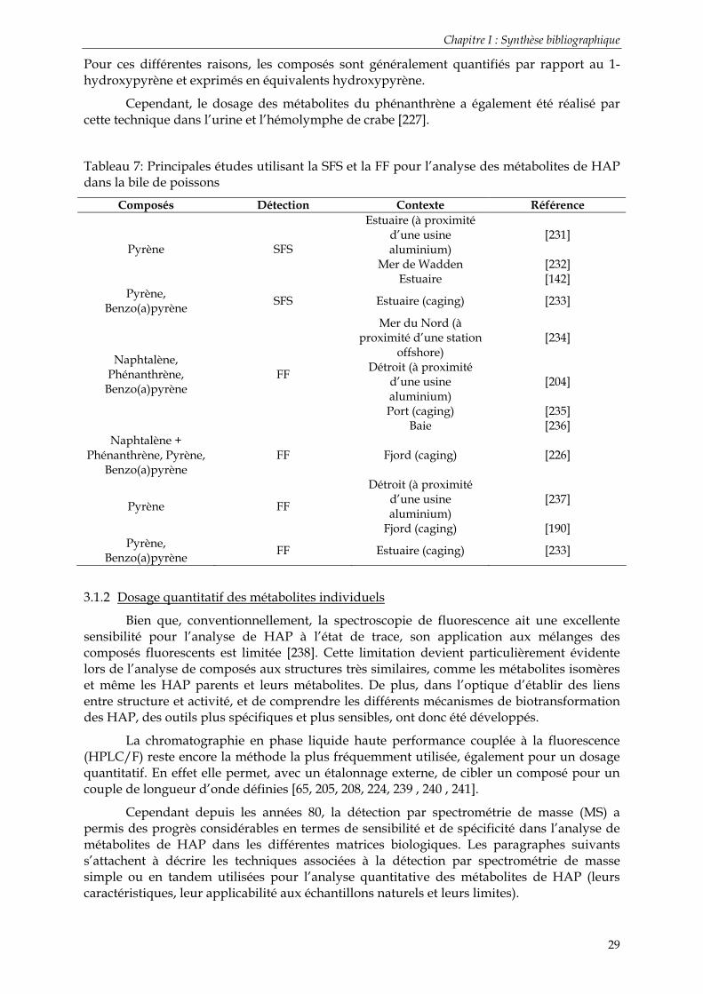
Chapitre I : Synthèse bibliographique
29
Pour ces différentes raisons, les composés sont généralement quantifiés par rapport au 1-hydroxypyrène et exprimés en équivalents hydroxypyrène.
Cependant, le dosage des métabolites du phénanthrène a également été réalisé par cette technique dans l’urine et l’hémolymphe de crabe [227].
Tableau 7: Principales études utilisant la SFS et la FF pour l’analyse des métabolites de HAP dans la bile de poissons
Composés Détection Contexte Référence Estuaire (à proximité
d’une usine aluminium)
[231]
Mer de Wadden [232] Pyrène SFS
Estuaire [142] Pyrène,
Benzo(a)pyrène SFS Estuaire (caging) [233]
Mer du Nord (à proximité d’une station
offshore) [234]
Détroit (à proximité d’une usine aluminium)
[204]
Port (caging) [235]
Naphtalène, Phénanthrène,
Benzo(a)pyrène FF
Baie [236] Naphtalène +
Phénanthrène, Pyrène, Benzo(a)pyrène
FF Fjord (caging) [226]
Détroit (à proximité d’une usine aluminium)
[237] Pyrène FF
Fjord (caging) [190] Pyrène,
Benzo(a)pyrène FF Estuaire (caging) [233]
3.1.2 Dosage quantitatif des métabolites individuels
Bien que, conventionnellement, la spectroscopie de fluorescence ait une excellente sensibilité pour l’analyse de HAP à l’état de trace, son application aux mélanges des composés fluorescents est limitée [238]. Cette limitation devient particulièrement évidente lors de l’analyse de composés aux structures très similaires, comme les métabolites isomères et même les HAP parents et leurs métabolites. De plus, dans l’optique d’établir des liens entre structure et activité, et de comprendre les différents mécanismes de biotransformation des HAP, des outils plus spécifiques et plus sensibles, ont donc été développés.
La chromatographie en phase liquide haute performance couplée à la fluorescence (HPLC/F) reste encore la méthode la plus fréquemment utilisée, également pour un dosage quantitatif. En effet elle permet, avec un étalonnage externe, de cibler un composé pour un couple de longueur d’onde définies [65, 205, 208, 224, 239 , 240 , 241].
Cependant depuis les années 80, la détection par spectrométrie de masse (MS) a permis des progrès considérables en termes de sensibilité et de spécificité dans l’analyse de métabolites de HAP dans les différentes matrices biologiques. Les paragraphes suivants s’attachent à décrire les techniques associées à la détection par spectrométrie de masse simple ou en tandem utilisées pour l’analyse quantitative des métabolites de HAP (leurs caractéristiques, leur applicabilité aux échantillons naturels et leurs limites).

Chapitre I : Synthèse bibliographique
30
Ces techniques de séparation et de détection très sensibles qui permettent de doser les métabolites dans les matrices biologiques, doivent obligatoirement être associées à une préparation préalable des échantillons. En effet, le caractère complexe des matrices biologiques, la multiplicité des sources d’interférents et la nécessité fréquente de concentrer les échantillons naturels, ont rendu indispensable la mise en œuvre de protocole de préparation des échantillons, comportant plusieurs étapes : de l’extraction à la séparation et la détection des composés.
Préparation des échantillons
La déconjugaison
Comme décrit précédemment, les métabolites se trouvent, principalement, sous la forme conjuguée (glucuronide, sulfate, glutathion) dans l’organisme et en particulier dans la bile de poisson (Chapitre I, § 2.1.2). Pour quantifier la totalité des métabolites individuels formés (sous forme libre et conjuguée), il est judicieux de recourir à une étape de déconjugaison au cours de laquelle, les métabolites conjugués sont hydrolysés et ainsi libérés sous forme de métabolites hydroxylés.
Différentes raisons justifient cette étape de déconjugaison. Premièrement, dans le cas de quantifications individuelles totales, très peu de standards conjugués sont accessibles pour effectuer une calibration, alors que de nombreux métabolites de type I sont commercialisés. De plus, les composés conjugués ne peuvent pas être analysés avec une technique de chromatographie en phase gazeuse couplée à une détection par spectrométrie de masse (GC/MS) en raison des problèmes de volatilisation de ces composés. Enfin, dans le cadre d’un diagnostic d’une exposition, la conversion des différents conjugués sous une forme unique de type I, augmente l’intensité du signal pour une meilleure détection. Par ailleurs, d’un point de vue toxicologique, il serait plus intéressant de quantifier uniquement les métabolites formés exclusivement durant la phase I, car ce sont eux qui engendrent les propriétés toxiques.
La technique la fréquemment plus utilisée est celle faisant appel à un mélange d’enzymes, β-glucuronidase et arylsulfatase, ajouté directement à l’échantillon de bile dilué et homogénéisé (Tableau 6). Les temps d’incubation vont de 2 à 24 heures [81, 82 , 84, 201, 210, 211, 214, 216, 217, 222, 242 , 243]. Ainsi les conjugués glucuronidés et sulfates peuvent être simultanément hydrolysés par ajout de β-glucuronidase contenant une activité arylsulfatase dans un échantillon dilué par à un tampon acétate au pH compris entre 4,8 et 5,0 et suivi d’une incubation allant de 1 à 24 heures à 37-40°C [84, 188 , 203 , 208 , 220, 244 ].
La majorité des publications concernant l’analyse des métabolites de HAP dans la bile de poisson se concentre sur la détermination des glucuronides et des sulfates. Cependant une partie non négligeable des métabolites conjugués est représentée par les conjugués liés au glutathion [156]. A la différence des glucuronidés et des sulfates, ces métabolites conjugués sont plus facilement retenus dans le foie [156]. Ainsi l’emploi de γ-glutamyltransférase, pour déconjuguer les métabolites associés au glutathion, est mentionné dans la littérature [203]. Enfin, certaines études mentionnent également l’utilisation d’une attaque acide avec de l’acide chlorhydrique [83 , 212 , 218] ou de l’acide sulfurique [217, 243] pour libérer les métabolites conjugués au glutathion.
Afin de prévenir toute oxydation des métabolites hydrolysés, Ariese et al. [219] et Richardson et al. [221] préconisent l’ajout de 0,5 et 4 % d’acide ascorbique, respectivement, au mélange de bile et d’enzymes de déconjugaison. Mazéas et Budzinski [245] ont, pour leur part, ajouté du β-mercaptoéthanol, un anti-oxydant, à l’échantillon de bile en début de protocole avant les étapes de déconjugaison et d’extraction.

Chapitre I : Synthèse bibliographique
31
L’extraction
Cette étape permet d’extraire les composés de leur matrice biologique. Les techniques utilisées dépendent de la matrice dans laquelle se trouve l’échantillon.
Ainsi pour des matrices aqueuses, la technique de choix se révèle être l’extraction liquide-liquide. Elle est la plus utilisée pour extraire les métabolites de HAP (avec ou sans déconjugaison) provenant des milieux aquatiques [242, 246-248]. Différentes combinaisons de solvants sont rapportées dans la littérature (Tableau 8). L’acétate d’éthyle [84, 208, 212, 214], le dichlorométhane en mélange avec le méthanol [216, 246] et le mélange hexane et méthyl-t-butyl éther (2/1, v /v) [242] ne sont que des exemples.
D’autres techniques sont également utilisées. C’est le cas de l’extraction sur phase solide (SPE) qui permet d’extraire des métabolites des matrices liquides par adsorption des composés sur une phase solide [94, 217]. Une fois déposés, les composés sont récupérés par élution avec un solvant organique dont l’affinité avec les molécules adsorbées est suffisante pour les décrocher de la phase et ainsi les éluer. La technique SPE offre de nombreux avantages en comparaison à l’extraction liquide-liquide comme une capacité d’automatisation, un temps d’analyse réduit, une quantité réduite de solvants permettant une reconcentration des échantillons.
La SPE a été largement développée pour l’étude des métabolites de HAP, et en particulier des métabolites du pyrène, dans l’urine humaine [249-253]. Cependant, très peu de travaux ont rapporté son emploi dans l’environnement marin [48, 94, 217, 245, 254 ]. La plupart des études faisant appel à cette technique d’extraction utilisent des cartouches remplies de phase octadécyle (C18) ou plus rarement, des disques en fibre de verre greffées C18.
Le Tableau 8 regroupe les principaux protocoles mettant en œuvre une extraction sur phase solide des métabolites de HAP. Un protocole pour l’extraction du 1-hydroxypyrène a été décrit par Jongeneelen et al. [255, 256] puis utilisé par différentes équipes [257 , 258]. Le passage de l’échantillon à la cartouche se fait après l’hydrolyse enzymatique et centrifugation. Après une étape de rinçage de la phase, les composés sont extraits de la phase par élution de méthanol. Les rendements varient de 81 à 91%.
Au cours des dernières années, un certain nombre de compagnies ont développé les sorbents polymériques bi-fonctionnels spécifiques, basés sur un squelette de polymère de styrène-divinylbenzène, fonctionnalisés par des groupements polaires, synthétisés de manière à améliorer le contact avec l’échantillon aqueux pendant la percolation en mettant en oeuvre des caractéristiques mixtes hydrophiles et hydrophobes, démontrant une meilleure mouillabilité et une plus grande sélectivité [252]. Ainsi des protocoles de dosage des métabolites de HAP, utilisant ces nouvelles phases polymériques ont vu le jour [250, 252].
La sélectivité peut de plus être optimisée par exemple en jouant sur le pH de l’échantillon et la nature et le pH des solvants. L’ajout d’étapes de rinçage des cartouches et d’élution des interférents permet d’augmenter la spécificité et par la même, la sensibilité de cette technique d’extraction.

Chapitre I : Synthèse bibliographique
32
Tableau 8 : Travaux mettant en œuvre une extraction liquide des métabolites de HAP
Matrice Exposition Solvant d’extraction Référence
Foie et peau Naphtalène C6H14 et NaOH [259]
Bile Ports C6H14 / (CH3)C(OCH3) (2:1, v:v) [242]
Bile Sédiment contaminé C6H14 [210, 260]
Microsomes hépatiques Sédiment contaminé CH3COOC2H5 [261, 262]
Foie Benzo(a)pyrène CH3COOC2H5 [122]
Foie Benzo(a)pyrène CH3COOC2H5 [263]
Muscle, foie et bile Benzo(a)pyrène CH3COOC2H5 [77]
Fraction hépato-pancréas de crabe Fluorène et Benzo(a)pyrène CH3COOC2H5 [218]
Bile Naphtalène et Benzo(a)pyrène CH3COOC2H5 [81]
Bile Naphtalène CH3COOC2H5 [214]
Foie Phénanthrène CH3COOC2H5 [264]
Microsomes Phénanthrène CH3COOC2H5 [125]
Bile Chrysène CH3COOC2H5 [205, 208]
Microsomes Dibenzo(a,l)pyrène CH3COOC2H5 [124]
Bile Milieu aquatique CH3COOC2H5 [211, 212, 248, 265]
Bile Benzo(a)pyrène CH3COOC2H5 / (CH3) 2CO puis CH3COOC2H5
[84]
Bile Pyrène CH2Cl2 [217]
Crabe entier Pyrène CH2Cl2 [266]
Bile Pétrole CH2Cl2 / CH3OH puis CH2Cl2
[213, 216]
Bile Milieu marin CH2Cl2 / CH3OH (10:1, v:v) puis CH2Cl2
[246, 247]
Bile Pétrole CH2Cl2 / CH3OH (10:1, v:v) puis CH2Cl2
[83]
Bile Milieu marin CH2Cl2 / CH3OH [206]
Micro-crustacé entier Benzo(a)pyrène et Fluoranthène CH2Cl2 / CH3OH / H2O [191]
Néréis Pyrène marqué CHCl3 / CH3OH / H2O [267]
Bile Benzo(a)pyrène CH3OH / CHCl3, BHT [82]
Bile, foie Phénanthrène et rétène CH3OH [94]
Poisson entier Benzo(a)pyrène CH3CN [268]
Poisson entier Pyrène CH3CN [254]
C6H14 : hexane ; NaOH : soude ; (CH3)C(OCH3) : méthyl t-butyl éther (MTBE) ; CH3COOC2H5 : acétate d’éthyle ; (CH3) 2CO : acétone ; CH2Cl2 : dichlorométhane ; CH3OH : méthanol ; H2O : eau ; CHCl3 : chloroforme ; CH3C6H2OH(C(CH3)3)2 : 2,6-di-tert-butyl-p-crésol (BHT) ; CH3CN : acétonitrile

Chapitre I : Synthèse bibliographique
33
Tableau 9 : Principaux protocoles mettant en œuvre une extraction sur phase solide C18 des métabolites de HAP
Métabolite Matrice Rinçage Elution Référence
1-OHP urine H2O CH3OH [256, 258, 269]
1-OHPG urine H2O / CH3OH (70:30, v:v)
H2O / CH3OH (20:80, v:v)
[270]
OHN et conjugués urine H2O CH3OH acidifié [271]
1-OHP urine H2O puis C6H14 CH2Cl2 [239]
3-OHBaP et 3-OHBaA urine H2O C2H5OC2H5 [272]
Métabolites du Benzo(a)anthracène Eau H2O CH3CN [48]
Métabolites du Pyrène Eau H2O
CH3CN / H2O puis CH3CN
[254]
Métabolites du Pyrène Bile de poisson H2O / CH3OH
(70:30, v:v) CH3OH [217]
Métabolites du Phénanthrène et
rétène
Bile et foie de poisson Non précisé Non précisé [94]
Enfin on peut également noter l’utilisation de la micro-extraction sur phase solide (SPME). La SPME est une technique qui a les avantages de ne pas utiliser de solvant organique et d’être très facilement coupable avec une analyse par chromatographie en phase gazeuse [273]. Elle consiste en l’adsorption des composés sur une fibre. Les composés sont généralement désorbés thermiquement directement dans l’injecteur du système chromatographique en phase gazeuse. Comme pour la SPE, cette technique n’a essentiellement été appliquée qu’aux échantillons d’urine humaine. Gmeiner et al. [273] préconisent l’emploi d’une fibre polyacrylate plongée pendant 45 minutes dans l’échantillon d’urine préalablement hydrolysé, pour l’analyse des hydroxypyrènes (1-, 2-, 4-hydroxypyrène), des hydroxynaphtalènes (1- et 2-hydroxynaphtalène) et des hydroxyphénanthrènes (1-, 2-, 3-, 4- et 9-hydroxyphénanthrène). La méthode a été modifiée en 2002 [274] afin d’extraire les métabolites hydroxylés du fluorène (1-, 2-, 4- et 9-hydroxyfluorène). La fibre reste lors immergée dans l’échantillon toute une nuit, sous agitation et à 35°C.
La purification
Les matrices biologiques étant composées d’un mélange complexe de molécules, certains constituants peuvent interférer avec les métabolites à doser et polluer les appareils d’analyse. Une étape de purification est donc souvent envisagée pour éliminer certains constituants de la matrice. Les techniques utilisées sont fondées sur les affinités relatives des composés pour une phase stationnaire solide et pour une phase mobile liquide. Ainsi, des protocoles mettant en œuvre la chromatographie en phase liquide haute performance (HPLC), en phase inverse et en phase normale, sont fréquemment utilisés [80, 82, 83, 127, 254].
L’utilisation de l’extraction en phase solide (SPE) permet également de purifier les échantillons. Ainsi une étude récente [245] propose un protocole basé sur la SPE pour la détermination quantitative de métabolites individuels de HAP dans des échantillons biologiques. Elle montre que l’utilisation d’une cartouche NH2 est essentielle pour purifier

Chapitre I : Synthèse bibliographique
34
les échantillons de bile avant une injection en chromatographie en phase gazeuse couplée à la spectrométrie de masse (GC/MS). Les rendements (protocole entier) obtenus pour la majorité des métabolites étudiés oscillent entre 70 et 96 %.
Techniques de séparation et de détection
Associés à la chromatographie en phase gazeuse (GC) ou à la chromatographie en phase liquide haute performance (HPLC) en tant que techniques de séparation, il existe de nombreux types de détecteurs pouvant permettre la détection des hydrocarbures aromatiques polycycliques et de leurs métabolites dans les échantillons environnementaux. Nous avons précédemmment exposé les techniques de screening ainsi que les dosages semi-quantitatifs des métabolites de HAP.
Dans le cas de dosages quantitatifs, les techniques de spectrométrie de masse (simple ou en tandem), couplées à la chromatographie en phase gazeuse ou en phase liquide et actuellement en plein essor, se sont révélées être des techniques de choix pour l’analyse des métabolites de HAP dans les matrices environnementales. Elles sont décrites dans le chapitre suivant.
Chromatographie en phase gazeuse couplée à la spectrométrie de masse simple ou en tandem (GC/MS ou GC-MS/MS)
Le rôle du chromatographe est de séparer les constituants d’un mélange. Le chromatographe en phase gazeuse est constitué de trois modules : un injecteur, une colonne capillaire dans un four et un détecteur. Il existe différents types de détecteurs mais le spectromètre de masse tend aujourd’hui à supplanter tous les autres car il est le seul à fournir des informations structurales sur les composés séparés par chromatographie. Les principes et caractéristiques techniques de cet outil sont présentés en Annexe 2.
Concernant l’étude des métabolites de HAP, la GC/MS est une technique utilisée d’une part pour l’identification des métabolites en laboratoire et d’autre part lors des dosages de ces composés dans le milieu marin. Cette technique permet, à la différence de l’HPLC/F, de pouvoir obtenir une meilleure résolution lors de la séparation des métabolites isomères.
Après une série d’étapes de préparation de l’échantillon, la quantification finale des métabolites individuels se fait par GC/MS en mode d’impact électronique (EI). Une étape de dérivation (cf paragraphe suivant) est souvent ajoutée avant l’injection. Le Tableau 10 regroupe les différentes études utilisant la GC/MS pour détecter les métabolites de HAP dans les organismes marins.
Les métabolites sont identifiés en comparant leur temps de rétention et leur spectre de masse à ceux des standards de référence. Chaque spectre de masse est caractérisé par la présence d’un ion moléculaire et des ions spécifiques de fragmentation qui dépendent de
l’agent de dérivation utilisé. Ainsi, pour les métabolites dérivés (e.g. TMS-éthers), les ions de fragmentation les plus abondants sont [M-15]+ et [M-31]+, et une forte abondance de l’ion [M-
89]+, ion [-O-Si(CH3)3] indique la présence du groupement hydroxyle [83]. Pour les métabolites non dérivés, l’ion de fragmentation majoritaire est l’ion [M-29]+ [92, 211, 246].
Les limites de la GC/MS sont celles de la chromatographie en phase gazeuse. Le facteur limitant étant la volatilité des analytes, cette technique est réservée à l’analyse de molécules aisément vaporisables et thermiquement stables, c’est à dire, en première approximation, de composés de poids moléculaire faible à moyen (inférieur à 700 Da). Une

Chapitre I : Synthèse bibliographique
35
seconde limitation, non négligeable, reste le coût plus excessif d’un couple GC/MS en comparaison à un couplage HPLC/F.
Ces limites admises, la GC/MS est un formidable outil d’analyse. La diversité des modes d’injection et des colonnes capillaires (géométrie, nature de la phase stationnaire) autorise la séparation de mélanges extrêmement complexes. Contrairement aux autres détecteurs, le spectromètre de masse fournit des informations structurales sur les analytes étudiés et peut permettre leur identification instantanée si ceux-ci sont répertoriés dans des bibliothèques de spectres. Le spectromètre de masse permet également de quantifier les analytes, même co-élués, à des concentrations inférieures au ng.l-1. C’est sa capacité à détecter spécifiquement une ou plusieurs molécules au sein d’un échantillon très complexe qui en fait un détecteur idéal pour l’analyse de traces. Cette grande sensibilité et cette haute spécificité sont davantage accrues avec l’utilisation d’un spectromètre de masse haute résolution (HRMS), au coût d’achat et de fonctionnement également très supérieurs à la GC/MS conventionnelle.
Note particulière : la dérivation
Les métabolites de HAP ne sont pas des candidats idéaux pour une analyse par chromatographie en phase gazeuse couplée à une détection par spectrométrie de masse (GC/MS) en raison de leur très faible volatilité. Ainsi l’ajout d’un agent dérivant va rendre possible l’analyse en GC/MS, en modifiant la fonctionnalité de la molécule. La dérivation permet également de réduire l’adsorption de l’analyte sur le système GC et d’augmenter la réponse du détecteur, d’améliorer la séparation des pics, la symétrie des pics et ainsi, améliorer la séparation et les limites de détection [208, 275]. Enfin, la dérivation empêche la déshydratation des dihydrodiols dans le système chromatographique [188, 201 , 275].
En général, l’acylation et la sylilation sont les techniques utilisées pour les métabolites biliaires hydrolysés avant injection en GC/MS. Différents réactifs de dérivation sont commercialisés. L’un des plus fréquemment utilisés est le N,O-bis-(triméthylsilyl)trifluoroacétamide (BSTFA), agent de sylilation. Il forme facilement des TMS-éthers avec les groupements alcools [276]. Après ajout de 100-200 µl de BSTFA dans un extrait reconcentré [208] ou dans un extrait évaporé à sec [188], la dérivation est finalisée par incubation du mélange à 60°C pendant 2 heures. Mazéas et Budzinski [245] recommandent également l’emploi de 30 µl de BSTFA suivi d’une incubation de 30 minutes à 65°C. Le triméthylsilylimidazole (TMSI) dans la pyridine (1:4, v:v) forme également des TMS-éthers avec les groupements phénoliques des métabolites ainsi qu’avec les diols et les tétrols, lors d’une dérivation à température ambiante durant 15 min [224, 277]. En outre, on note également l’emploi du 1,1,1,3,3,3-hexaméthyldisilazane (SYLON TP) [214] et du N,O-bis(trisméthylsislyl)acétamide (BSA) [217] comme agents de sylilation des métabolites. Enfin l’acylation est rapportée par Hellou et Payne [216, 244] au moyen de diazométhane éther.
Néanmoins, même si la dérivation facilite l’analyse des métabolites de HAP en GC/MS, son utilisation présente plusieurs inconvénients. Des études ont souligné la perte de sensibilité induite par l’étape de dérivation [201, 211, 213]. Il a été montré que le rendement de la dérivation diminuait avec l’augmentation du nombre de noyaux aromatiques du composé, conduisant ainsi à des rendements plus faibles et à une sensibilité réduite pour les métabolites de plus haut poids moléculaire. De plus, la réaction de dérivation est parfois difficile à stabiliser. Pour une seule molécule, plusieurs formes dérivées peuvent coexister diminuant ainsi la sensibilité de la technique lors de la recherche d’un ion spécifique. Enfin, les composés présents dans les matrices complexes peuvent interférer sur la dérivation et l’identification des spectres obtenus est rendue plus difficile.

Chapitre I : Synthèse bibliographique
Tableau 10 : Principaux travaux mettant en œuvre la GC/MS pour la détection des métabolites de HAP
Préparation des échantillons Analyse GC/SM Composés étudiés Traitement
enzymatique Incubation Solvant d’extraction Dérivant Etalon interne Colonne Détection
Référence
Métabolites du phénanthrène
β-glucuronidase sulfatase 37 °C, 10 h. Acétate d’éthyle TMS-éthers α-naphtol SE-54 5% phenyl; 20
m × 0.33 mm MS EI, 70
eV [214]
Composés hydroxylés de 2- à 4-noyaux aromatiques
β-glucuronidase sulfatase 40 °C, 4 h. Dichlorométhane
et isopropanol TMS-éthers hexaméthylbenzène J & W DB5 MS 5% phenyl;30 m × 0.25
mm
MS EI, 70 eV [188, 201]
Composés hydroxylés de 2- à 3-noyaux aromatiques
alkylés et non-alkylés
β-glucuronidase 37 °C, 24 h. Dichlorométhane et méthanol TMS-éthers n-pentadécane SE-30 MS EI, 70
eV [216]
Composés hydroxylés de 2- à 4-noyaux aromatiques
alkylés et non-alkylés
β-glucuronidase sulfatase 40 °C, 3 h. Dichlorométhane
et méthanol 2,6-dibromophénol J & W DB5 MS 5% phenyl;30 m × 0.25
mm
MS EI, 70 eV [246]
Composés hydroxylés de 2- à 5-noyaux aromatiques
alkylés et non-alkylés
β-glucuronidase sulfatase 40 °C, 2 h. Dichlorométhane
et méthanol TMS-éthers
2,6-dibromophénol, 1-naphtol-d8, phen-d10, chry-d12, flu-d10
et BaP-d12
J & W DB5 MS 5% phenyl;30 m × 0.25
mm
MS EI, 70 eV [83]
Composés hydroxylés de 2- à 4-noyaux aromatiques
β-glucuronidase sulfatase 40 °C, 2 h. Acétate d’éthyle 2,6-dibromophénol
hexamethylbenzène HP-5 MS 5% phenyl;
30 m × 0.25 mm MS EI, 70
eV [211, 212]
Composés hydroxylés de 1- à 4-noyaux aromatiques
β-glucuronidase sulfatase
37 °C toute la nuit
Hexane : méthyl-t-butyl éther (2:1) octadécane MSBP5 5% phenyl; 30
m × 0.25 mm MS EI, 70
eV [242]
Composés hydroxylés de 2- à 4-noyaux aromatiques
β-glucuronidase sulfatase TMS-éthers décachlorobiphényle GC separation MS EI, 70
eV [219]
Composés hydroxylés de 2- à 4-noyaux aromatiques
β-glucuronidase sulfatase 40 °C, 2 h. Acétate d’éthyle TMS-éthers 2,6-dibromophénol CP-Sil 8 5% phenyl;
50 m × 0.25 MS EI, 70
eV [208]
Métabolites du chrysène
β-glucuronidase sulfatase 40 °C, 2 h. Acétate d’éthyle TMS-éthers 4-Cl-naphtol
pérylène CP-Sil 8 5% phenyl;
50 m × 0.25 MS EI, 70
eV [205, 224]

Chapitre I : Synthèse bibliographique
37
Chromatographie liquide haute performance couplée à la spectrométrie de masse simple ou en tandem (HPLC/MS ou HPLC-MS/MS)
La combinaison du pouvoir de séparation de l’HPLC et de la sélectivité de la détection par spectrométrie de masse constitue un outil puissant pour l’analyse des composés polaires et réactifs que sont les métabolites conjugués [217, 254, 271, 278] et les métabolites hydroxylés des HAP [113, 279]. Les principes et caractéristiques techniques de cet outil sont présentés en Annexe 3.
La possibilité de détection des composés glucuronidés et des sulfates permet une simplification des protocoles (plus d’étape de déconjugaison) et fournit des informations essentielles sur la spéciation des différents composés (formes libres, formes conjuguées) dans l’organisme. Ces informations sont très utiles dans l’étude de la toxicité des HAP. La HPLC/MS a particulièrement été utilisée pour la quantification des métabolites de HAP chez les mammifères terrestres et très peu chez les organismes marins [127, 217, 254]. La plupart de travaux en HPLC/MS cités dans la littérature traitent de l’analyse des métabolites de HAP dans l’urine humaine [279, 280 , 281 ].
Les sources d’ionisation dites APCI (Ionisation Chimique à Pression Atmosphérique) et ESI (Ionisation Electrospray), ont toutes deux été utilisées dans les modes positif et négatif [158]. Dans l’étude des métabolites biliaires chez le poisson, cette technique n’a pas été établie en dosage de routine car elle souffre de problèmes liés à l’adsorption, la contamination, les réactions de surface et autres interférences, rendant impossibles les analyses aux concentrations inférieures au ng.g-1 [282]. Cependant quelques essais ont été tentés. Law et al. [217] ont utilisé l’analyse HPLC/MS pour caractériser les métabolites dans la bile et dans l’urine de truites (Oncorhynchus mykiss) exposées au pyrène. Après une première séparation des composés libres et des conjugués par une colonne HPLC en phase inversée, chaque fraction était identifiée en HPLC/APCI/MS. Dans une autre étude, Willet et al. [113] ont été capables de mesurer le 3-hydroxybenzo(a)pyrène, deux BaP-dihydrodiols et trois BaP-diones dans la bile déconjuguée de poisson grâce à la HPLC/APCI/MS. Les limites de détection (LOD) étaient excellentes pour les diones (1 ng injecté) et très bonnes pour les dihydrodiols et le 3-OHBaP (2,5-25 ng injectés) [113].
Plus récemment des travaux mettant en œuvre la spectrométrie de masse en tandem (HPLC-MS/MS) ont fait leur apparition [239 , 253]. Le mode de transitions sélectionnées ou mode MRM « Multiple Reactions Mode », utilisé en spectrométrie de masse en tandem, est un outil très puissant pour l’analyse quantitative [283 , 284 , 285] en raison de sa haute sensibilité, spécificité et sélectivité, rendant alors inutiles les longues et fastidieuses procédures de nettoyage de l’échantillon.
Note particulière : UPLC™-MS/MS
Au cours des dernières années, une nouvelle technique a vu le jour : l’Ultra Performance Chromatographie en phase Liquide couplée à une détection par spectrométrie de masse en tandem. L'UPLC est une marque déposée de Waters corporation qui désigne ses systèmes de chromatographie en phase liquide à très haute pression.
Introduite en 2004, l'UPLC apporte un progrès majeur dans trois domaines : résolution chromatographique, vitesse d'analyse et sensibilité.
L'emploi dans la phase stationnaire de particules de 1,7 micromètres (alors que les colonnes HPLC utilisent des particules de 5 à 3 micromètres) est à l'origine de l'UPLC. La courbe de Van Deemter, régie par une équation à trois composantes, montre que la gamme de débit utilisable avec un tel diamètre de particules est bien plus large que pour des

Chapitre I : Synthèse bibliographique
38
diamètres supérieurs. De ce fait il est possible d'augmenter le débit, et donc la vitesse d'analyse, sans altérer les performances chromatographiques. L'avènement de l'UPLC a toutefois nécessité le développement instrumental d'un nouveau système de chromatographie en phase liquide, pouvant tirer avantage des performances de séparation et compatible avec les pressions générées (de l'ordre de 8 000 à 15 000 PSI, à comparer avec 2 500 à 5 000 PSI en HPLC).
Les chromatographistes sont habitués aux compromis ; le plus fréquent d’entre-eux consiste à sacrifier la résolution au détriment de la vitesse. La technologie UPLC permet d’éviter de telles démarches.
En revanche, pour bénéficier des atouts analytiques de la technologie UPLC, les détecteurs associés doivent fonctionner avec une vitesse d’acquisition très rapide. C’est pourquoi, les spectromètres de masse sont privilégiés par rapport aux autres types de détecteurs (Fluorescence ou barrettes à diodes). En outre la spectrométrie de masse en tandem est, à son tour, privilégiée par rapport à la spectrométrie de masse simple, permettant ainsi d’associer la spécificité à la sensibilité de la méthode d’analyse.
Ainsi couplée à la spectrométrie de masse en tandem (exemple : un triple quadripôle Quattro Premier™, Micromass, USA) ce couplage intègre les technologies les plus récentes et les plus innovantes permettant l’identification et le dosage simultané d’un grand nombre de composés. L’utilisation de différents modes d’ionisation (APCI, ESI) au cours de la même analyse devient possible tout en maintenant les performances tant au niveau de la sensibilité et de la sélectivité qu’au niveau de la résolution spectrale et chromatographique.
La technologie UPLC augmente la concentration des pics en réduisant la dispersion chromatographique et en améliorant l’efficacité de la source ce qui implique des gains conséquents en sensibilité et en qualité spectrale. Grâce à l’obtention de pics plus fins et à l’augmentation de la résolution chromatographique, la technologie UPLC renforce les performances et la productivité de toute analyse en LC/MS et LC-MS/MS.
A l’heure actuelle, seuls les travaux de Zhu et al. (2008) ont montré l’utilisation de la technologie UPLC couplée à la spectrométrie de masse simple dans l’analyse des métabolites de HAP, en particulier les métabolites polaires du BaP. Des limites de détection de l’ordre de 10 pg.µl-1 de bile étaient atteintes. Les travaux en UPLC-MS/MS effectués au cours de cette thèse ont permis d’établir des limites de détection inférieures à 0,1 pg.µl-1 de bile pour les métabolites mono-hydroxylés étudiés [286]. Enfin si on compare ces résultats à ceux obtenus dans une méthode d’analyse plus conventionnelle, la GC/MS, les limites de détection atteintes sont comprises entre 4 et 21 pg.µl-1 pour les métabolites étudiés [287] avec une moins bonne sensibilité obtenue pour les métabolites de plus haut poids moléculaires (métabolites du chrysène et du BaP)
De manière plus générale, l’intérêt de l’UPLC-MS/MS, technologie innovante et très sensible, est largement démontré dans des études récentes s’intéressant à des composés plus polaires comme les substances pharmaceutiques, certains produits phytosanitaires ou encore des substances destinées à l’usage thérapeutique [288-297].
3.1.3 Les différentes approches de normalisation des résultats
La mesure de la fluorescence biliaire est devenue un biomarqueur très utilisé pour démontrer l’exposition des poissons aux HAP. Des résultats conflictuels ont été publiés sur

Chapitre I : Synthèse bibliographique
39
les méthodes de normalisation à appliquer à ces mesures de fluorescence [95 ]. Trois méthodes ont été proposées et testées :
Unités de fluorescence par volume de bile ou masse de bile ;
Unités de fluorescence par mg de protéines dans la bile ;
Unités de fluorescence par quantité de biliverdine dans la bile.
La première méthode semble être la plus simple et directe, mais le volume de bile est extrêmement variable et il dépend des fréquences d’alimentation des poissons. Sous des conditions de restriction alimentaire, les concentrations semblent suivre les volumes de bile produite [298]. Ceci rend l’expression de la fluorescence par rapport aux volumes de bile très aléatoire et variable. L’expression de la fluorescence par rapport à la quantité de biliverdine a été examinée mais là encore, a conduit à des résultats contradictoires [95, 223, 228]. Dans ces études, les conclusions données pour la normalisation ont été fondées sur la réduction de la variabilité des données et non sur les mécanismes biologiques. La biliverdine est le produit de décomposition de l’hème, partie contenant l’atome de fer dans les molécules d’hémoglobine et dans les enzymes des cytochromes. L’hème s’inscrit dans le cycle physiologique continuel du cytochrome et l’excès de cette molécule est métabolisé dans le foie, par les enzymes oxygénases qui catalysent sa conversion en biliverdine [299]. Ainsi l’excrétion de la biliverdine dans la bile est modulée par l’activité de l’hème oxygénase. Des études ont par ailleurs montré une modification de cette activité enzymatique en relation avec les polluants de l’environnement, en particulier chez les poissons [300, 301]. L’induction de l’activité de l’hème oxygénase par l’exposition aux polluants environnementaux conduit à l’hypothèse que l’excrétion de la biliverdine est également reliée au stress chimique et que par conséquent, la méthode qui relie la fluorescence à la quantité de biliverdine dans la bile d’animaux exposés à un mélange de HAP et de contaminants de l’environnement, ne constitue pas une méthode fiable. Dans une étude récente, Van den Hurk [302] a cherché à savoir si la méthode de normalisation par la biliverdine était une méthode appropriée et il a ainsi mis en place des expériences visant à comprendre la mécanistique de l’excrétion de la biliverdine chez les poissons soumis à des stress chimiques différents. Les résultats ont montré des relations linéaires entre les protéines biliaires et la biliverdine pour chaque type de stress. Mais la corrélation semble augmenter significativement pour les poissons ayant subi un stress chimique plus important. Une forte corrélation a par ailleurs été montrée entre l’activité de l’hème oxygénase et la concentration de la biliverdine dans la bile. Ceci permet de conclure que le stress chimique induit une augmentation de l’excrétion de la biliverdine. L’élucidation de cette mécanistique justifie que les mesures de fluorescence biliaire ne devraient plus être exprimées par rapport à l’absorption de la biliverdine et que l’expression de ces résultats en fonction de la quantité totale de protéines biliaires serait une méthode plus sûre.
3.2 Etudes du métabolisme
Dans le cadre des recherches sur les phénomènes de bioaccumulation et de biotransformation des HAP, de nombreuses espèces animales, vertébrées et invertébrées, ont été étudiées.
Dans la recherche de la localisation des métabolites dans l’organisme, différents organes ont été étudiés et principalement le foie, la vésicule biliaire, le plasma et l’urine.

Chapitre I : Synthèse bibliographique
40
Concernant l’étude du métabolisme en général et la caractérisation des cinétiques de formation et des chemins de métabolisation, des approches utilisant des microsomes hépatiques ont été préférées que se soient dans les études sur les rongeurs [82 , 117, 124 , 141, 303-312, 313 , 314 , 315-317] mais également pour les études sur les organismes aquatiques [100 , 113, 114, 117 , 125 , 315, 318, 319, 320 , 321 , 322, 323, 324 , 325].
3.2.1 Localisation de métabolites chez les organismes aquatiques
Parmi les organismes aquatiques, les poissons ont été les plus étudiés. Les recherches ont été fréquemment menées au moyen de composés radiomarqués qui sont plus facilement détectables à très faibles concentrations dans les tissus [80, 81, 214, 259 , 326-332]. Les chemins métaboliques et les organes d’accumulation des métabolites produits ont ainsi pu être mis en évidence. En général, bien que des différences existent entre les espèces, il a été montré une forte accumulation des métabolites dans la vésicule biliaire après une exposition des organismes à des HAP. Vient ensuite généralement le foie, principal organe de biotransformation, puis la peau et d’autres organes comme les branchies, les gonades, les reins, les intestins, la vessie, le sang, le cerveau et la rate avec des ordres variables selon les études. Les muscles quant à eux, ne présentent en général que des concentrations très faibles [17].
3.2.2 Identification des métabolites et étude cinétique du métabolisme
Différentes études ont montré que les poissons transformaient les HAP en métabolites de structures comparables à ceux produits par les rongeurs, en majorité des composés hydroxylés [82, 124, 125, 157, 263, 333]. Chez les mollusques, il a été montré que les quinones représentaient la majorité des métabolites produits, laissant ainsi supposer un mécanisme de biotransformation majoritairement radicalaire associée à une faible activité enzymatique du cytochrome P450 [62].
De manière générale, le temps de résidence des métabolites dans les tissus et dans les fluides est plus long que celui des composés parents chez les différents organismes marins [81, 123, 150, 156, 259, 334-336]. Il a été montré dans les paragraphes précédents que les métabolites peuvent se retrouver sous une forme libre mais également sous des formes conjuguées dans l’organisme. Dans la bile, les formes conjuguées sont généralement prépondérantes même si d’un composé à l’autre, le pourcentage de conjugaison reste très variable [127, 214, 259, 326, 329, 337]. Si on prend l’exemple des métabolites du benzo(a)pyrène, il apparaît qu’une proportion importante des métabolites biliaires du benzo(a)pyrène est constituée de 42 à 70% de thio-éthers (conjugués au glutathion) les glucuronides et les sulfates représentant de 23 à 58% des métabolites (Tableau 12). De plus, le 7,8-diol-9,10-epoxyde- 7,8,9,10-tétrahydrobenzo(a)pyrène-glutathion (BPDE-GSH) a été identifié comme étant le principal thio-éther présent dans la bile [123, 338 ]. Néanmoins, il a été montré que, en général, les composés sulfatés sont moins abondants que les glucuronides chez les poissons [81, 84, 127, 129, 157, 203] et majoritairement éliminés via l’urine [130], alors que les conjugués glucuronidés sont majoritairement excrétés dans la bile [127, 129].
Dans cette synthèse bibliographique, il a été choisi quatre composés parents pour traiter en détail de l’identification des métabolites chez les organismes marins exposés individuellement à ces HAP. Ce sont le phénanthrène, le pyrène, le chrysène et le benzo(a)pyrène.
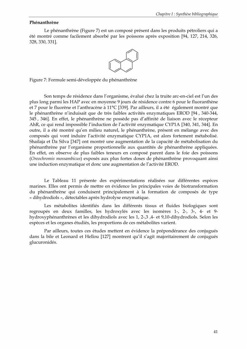
Chapitre I : Synthèse bibliographique
41
Phénanthrène
Le phénanthrène (Figure 7) est un composé présent dans les produits pétroliers qui a été montré comme facilement absorbé par les poissons après exposition [94, 127, 214, 326, 328, 330, 331].
Figure 7: Formule semi-développée du phénanthrène
Son temps de résidence dans l’organisme, évalué chez la truite arc-en-ciel est l’un des plus long parmi les HAP avec en moyenne 9 jours de résidence contre 6 pour le fluoranthène et 7 pour le fluorène et l’anthracène à 11°C [339]. Par ailleurs, il a été également montré que le phénanthrène n’induisait que de très faibles activités enzymatiques EROD [94 , 340-344, 345 , 346]. En effet, le phénanthrène ne possède pas d’affinité de liaison avec le récepteur AhR, ce qui rend impossible l’induction de l’activité enzymatique CYP1A [340, 341, 344]. En outre, il a été montré qu’en milieu naturel, le phénanthrène, présent en mélange avec des composés qui vont induire l’activité enzymatique CYP1A, est alors fortement métabolisé. Shailaja et Da Silva [347] ont montré une augmentation de la capacité de métabolisation du phénanthrène par l’organisme proportionnelle aux quantités de phénanthrène appliquées. En effet, on observe de plus faibles teneurs en composé parent dans le foie des poissons (Oreochromis mossambicus) exposés aux plus fortes doses de phénanthrène provoquant ainsi une induction enzymatique et donc une augmentation de l’activité EROD.
Le Tableau 11 présente des expérimentations réalisées sur différentes espèces marines. Elles ont permis de mettre en évidence les principales voies de biotransformation du phénanthrène qui conduisent principalement à la formation de composés de type « dihydrodiols », détectables après hydrolyse enzymatique.
Les métabolites identifiés dans les différents tissus et fluides biologiques sont regroupés en deux familles, les hydroxylés avec les isomères 1-, 2-, 3-, 4- et 9-hydroxyphénanthrènes et les dihydrodiols avec les 1, 2-,3 ,4- et 9,10-dihydrodiols. Selon les espèces et les organes étudiés, les proportions de ces métabolites varient.
Par ailleurs, toutes ces études mettent en évidence la prépondérance des conjugués dans la bile et Leonard et Hellou [127] montrent qu’il s’agit majoritairement de conjugués glucuronidés.

Chapitre I : Synthèse bibliographique
42
Tableau 11: Principaux travaux étudiant le métabolisme du phénanthrène chez les organismes marins.
Espèce Matrice Référence
Oncorhynchus mykiss Bile, microsome hépatique [127]
Oncorhynchus mykiss Bile, microsome hépatique [94]
Oncorhynchus mykiss Bile, microsome hépatique [346]
Oncorhynchus mykiss Bile, microsome hépatique [343, 344, 348]
Oreochromis mossambicus Bile, foie [347]
Squalus acanthis Bile [326, 329]
Pollachius virens Urine, bile [214, 327]
Platichthys flesus Estomac, intestin, bile, urine [328]
Oncorhynchus mykiss Intestin, bile [326, 329]
Gadus morhua Bile, microsome hépatique [264, 332]
Gadus morhua & Oncorhynchus mykiss Microsome hépatique [349]
Ameriurus nebulosus Microsome hépatique [125]
Pyrène
A la différence des autres HAP, le pyrène semble avoir un schéma de métabolisation moins complexe, conduisant à la détection d’un seul métabolite de phase I, le 1-hydroxypyrène. Le Tableau 12 présente les principaux travaux sur le métabolisme du pyrène chez les organismes aquatiques. Néanmoins il faut noter que Krahn et al. [200, 201, 350] ainsi que Law et al. [217] ont pu mettre en évidence à très faibles quantités d’autres phénols et des dihydrodiols dans la bile de carlottin anglais et de truite arc-en-ciel après déconjugaison enzymatique.
Concernant la spéciation de formes conjuguées, les glucuronides sont là encore majoritaires dans la bile de poisson alors que les glucosides et les sulfates sont majoritaires chez des organismes moins évolués comme les crustacées et les mollusques.
Tableau 12: Principaux travaux étudiant le métabolisme du pyrène chez les organismes marins.
Espèce Matrice Référence Parophrys vetulus Bile [200, 201, 350]
Oncorhynchus mykiss Bile, urine [217] Salvelinus fontinalis Bile [127]
Platichthys flesus Bile [325] Porcellio scaber Hépatopancréas et intestins [325, 351] Cancer magister Hémolymphe [352]
Mya arenaria Organisme entier [254] Protothaca staminea Organisme entier [254]

Chapitre I : Synthèse bibliographique
43
Chrysène
Le chrysène, présent à des concentrations importantes dans les produits pétroliers [71, 72, 74, 353 ] mais également dans les résidus de combustion de fioul fossile et de tout autre procédé industriel de combustion, est constitué de quatre noyaux aromatiques organisés en une structure à deux régions Bay (Figure 8). En règle générale, ce composé est rapidement adsorbé sur la matière organique et inorganique en raison de sa faible solubilité et il devient donc peu biodisponible pour le biota aquatique, excepté pour les poissons benthiques. Cependant, sur des zones proches des relargages d’effluents industriels, le chrysène peut être présent dans la colonne d’eau [354] et ainsi être plus biodisponible pour les poissons via une absorption au travers des branchies [237].
10
7
9
86
5
1112
43
12Bay - Region
Bay - Region
Figure 8: Formule semi-developpée du chrysène.
Le chrysène possède un faible pouvoir carcinogène après une activation métabolique via les dihydrodiols et les dihydrodiol-époxides [355-358, 359 , 360]. Le chrysène a été identifié comme un précurseur de la formation de l’ultime métabolite carcinogène du chrysène, le 1,2-dihydroxy-3,4-époxy-1,2,3,4-tétrahydrochrysène (un diol-époxide en région Bay) [361]. Pangrekar et al. [125, 362] ont étudié in vitro le métabolisme du chrysène dans les microsomes hépatiques de la barbotte (Ameriurus nebulosus). Plus récemment, Jonsonn et al. [205, 224] ont exposé in vivo des cabillauds (Gadus morhua) au chrysène par voie intra-péritonéale et intra-musculaire. Les oxydations sur les positions 1,2- et 3,4- résultant dans la formation de deux dihydrodiols, 1,2-dihydroxy-1,2-dihydro et 3,4-dihydroxy-3,4-dihydrochrysène et de quatre phénols, 1-, 2-, 3- et 4-hydroxychrysène ont été identifiées comme les principaux chemins de métabolisation. L’oxydation sur la position 5,6- (K-region) semble être la voie la moins favorable [361]. De manière générale, le principal métabolite formé est le 1,2-dihydroxy-1,2-dihydrochrysène. Puis sont formés dans de plus faibles quantités le 3,4-dihydroxy-3,4-dihydrochrysène, les hydroxychrysènes et le 5,6-dihydroxy-5,6-dihydrochrysène.
Benzo[a]pyrène
Le schéma métabolique du BaP chez les poissons est aujourd’hui bien connu grâce aux très nombreuses études in vitro et in vivo effectuées sur ce composé (Tableau 13). En raison de la lipophilie élevée du BaP (Figure 9) et de ses métabolites, l’extraction de ces composés des tissus riches en lipides (foie, muscle, gonades) pose un problème. C’est pourquoi, dans la plupart des études recensées, l’identification des métabolites du BaP est limitée aux composés hydrosolubles présents dans la bile.

Chapitre I : Synthèse bibliographique
44
10
7
9
86
1112
3
12
45
Bay - Region
K - Region Figure 9: Formule semi-developpée du BaP.
Concernant la spéciation des formes conjuguées (Tableau 13), il apparaît qu’une proportion importante des métabolites biliaires est constituée de 42 à 70 % de thio-éthers (conjugués du glutathion), les glucuronides et les sulfates ne représentant que 23 à 58 % des métabolites. Le composé prépondérant dans la bile a été identifié comme étant le 7,8-diol-9,10-époxyde-7,8,9,10-tétrahydrobenzo(a)pyrène-glutathion (BPDE-GSH) [81, 121-123, 150, 338, 363-366, 367 ].
Dans la bile de nombreuses espèces de poissons, les principaux métabolites détectés sont des conjugués glucuronidés de phénols et de 7,8-dihydrodiol tandis que les conjugués sulfatés sont en très faibles proportions [81, 82, 84, 121]. Après déconjugaison enzymatique, les métabolites biliaires de phase I détectés sont principalement le 1- et le 3-hydroxybenzo(a)pyrène et le 7,8-dihydrodiolbenzo(a)pyrène [77, 368, 369]. Selon les espèces de poissons, des différences dans la distribution de ces métabolites biliaires sont constatées. Néanmoins le composé le plus abondant reste le 3-hydroxybenzo(a)pyrène, représentant 18 à 46 % des métabolites identifiés.
Tableau 13: Proportions des principales classes de métabolites conjugués dans la bile de poissons exposés à du BaP radioactif.
Espèce % de glucuronides et de sulfates % de thio-éthers Référence
Parophrys vetulus (adulte) 32 68 [370] Parophrys vetulus
(juvénile) 43 57 [370]
Parophrys vetulus (adulte) 53 47 [82] Parophrys vetulus
(juvénile) 56 44 [82]
Platichthys stellatus (adulte) 58 42 [82]
Platichthys stellatus (juvénile) 43 57 [82]
Oncorhynchus mykiss 54 46 [371]

Chapitre I : Synthèse bibliographique
45
3.2.3 Facteurs influençant la formation des métabolites
Plusieurs facteurs sont à prendre en compte lors de la formation des métabolites et sont donc très importants à connaître lors de l’étude de métabolites des HAP chez les poissons.
Le sexe
Plusieurs études ont montré que des niveaux de métabolites biliaires similaires étaient obtenus chez des individus de sexe opposés de différentes espèces de poissons [77, 128, 371, 372]. Cependant il a été également démontré qu’au cours des périodes de reproduction, des différences de métabolisme et de bioaccumulation des composés parents étaient notables [373]. Ainsi le sexe ne semble pas être un facteur influençant les phénomènes de biotransformation excepté lorsque les poissons sont en période de reproduction.
L’âge
Des expérimentations ont été effectuées in vitro sur des juvéniles et des adultes de soles [374] et sur des carlottins anglais [82], montrant une formation d’adduits à l’ADN bien plus élevée chez les juvéniles que chez les adultes ainsi qu’une production de métabolites plus importante chez les juvéniles que chez les adultes.
La température du milieu
Chez les poissons, des études ont montré que quel que soit le mode de contamination, une diminution de l’adsorption des HAP est constatée lors d’une diminution de la température du milieu [375]. En revanche Collier et Varanasi [376] ont rapporté une augmentation de l’accumulation des HAP légers dans les tissus de poissons à basse température alors que les niveaux de métabolites biliaires restent constants. Ceci confirme les résultats obtenus par d’autres équipes [81, 128]. Dans le cadre d’exposition de microsomes hépatiques de truite arc-en-ciel, Egaas et Varanasi [263] ont montré une production de métabolites plus importantes à 7°C qu’à 16°C, d’une part, et une plus grande proportion de métabolites non conjugués à 7°C qu’à 16°C, d’autre part. Cette augmentation de la quantité de métabolites est expliquée par l’augmentation de acides gras polyinsaturés au niveau des membranes hépatiques à 7°C, qui favoriseraient alors l’oxydation des HAP [263].
Enfin des différences, selon la température du milieu, entre les temps de résidence des composés ont été observées. La tendance était à une augmentation du métabolisme et du temps de résidence des métabolites liée à une diminution des températures du milieu [78, 128, 216, 337].
L’état de jeûne des poissons
Jimenez et al. [375] ont montré que l’état de jeûne du poisson était très important dans l’étude du métabolisme. En effet, chez le crapet arlequin, l’absorption du benzo(a)pyrène est deux fois plus rapide, son taux de métabolisation accéléré et son excrétion dix fois plus importante lorsque le poisson est nourri. En outre, dans le cas des métabolites biliaires, l’état de jeûne du poisson au moment de la dissection est très important car il a une influence sur les concentrations mesurées. En effet, juste après s’être alimentés, la vésicule biliaire des poissons se vide et contient donc une plus faible quantité de métabolites [210, 219, 376].

Chapitre I : Synthèse bibliographique
46
Les interactions avec d’autres contaminants présents
Une étude réalisée par James et al. [377] a montré une synergie des actions des HAP et des PCB induisant une augmentation du pourvoir carcinogène du 7,8-dihydrodiolbenzo(a)pyrène sur des microsomes hépatiques. Une formation plus importante d’adduits à l’ADN a été observée lorsque les microsomes était exposés à un mélange de BaP et de PCB par rapport à une exposition au BaP seul (5 fois plus élevée). Eggas et Varanasi [263] ont également montré des résultats similaires sur des microsomes hépatiques de truite arc-en-ciel, traités avec un mélange de PCB (l’Arochlor) et exposés à du BaP.
Une activité antagoniste au métabolisme du BaP a été démontrée lors de l’exposition de saumon à du TBT (tributylétain), induisant une diminution de la production de métabolites [378].
Enfin, la présence de nitrites lors d’une exposition aux HAP, peut induire la formation de composés très réactifs et cancérigènes, les nitro-HAP ainsi que leurs métabolites [379].
Les espèces de poissons
Dans les paragraphes précédents, il a été montré que des différences notables existaient entre les différentes espèces de poissons lorsqu’il s’agissait d’identifier et de localiser les métabolites dans les organes. Ces différences sont d’ordres qualitatifs mais également quantitatifs.
D’un point de vue quantitatif, l’étude de la métabolisation du benzo(a)pyrène par des microsomes de truites de lac (Salmo trutta lacustris), de gardons (Rutilus rutilus) et de rats a permis de mettre en évidence des différences très nettes entre les trois espèces. Les microsomes de gardon biotransforment ainsi très faiblement le benzo(a)pyrène alors qu’une très forte activation métabolique est constatée chez la truite, environ 3 à 4 fois supérieure à celle du rat [155]. Une autre étude comparant la métabolisation du benzo(a)pyrène par des microsomes de carlottins anglais, de plies étoilées et de rats concluant à des taux de transformation environ trois fois plus faibles chez les deux espèces de poisson par rapport au rat [82], on peut en déduire que la truite biotransforme le benzo(a)pyrène en proportion beaucoup plus importante que les deux autres espèces de poisson.
D’un point de vue qualitatif, une étude consistant à étudier la métabolisation du benzo(a)pyrène par des carlottins anglais et des plies étoilées exposés à du benzo(a)pyrène a tout d’abord permis de montrer que ce HAP était biotransformé à des vitesses similaires par les microsomes des deux espèces de poisson et que la vitesse de formation du 7,8-dihydrodiolbenzo(a)pyrène était la même chez les deux espèces [82]. Pourtant une plus grande quantité de 7,8-dihydrodiol était mesurée dans la bile de soles. La plie étoilée avait par contre une activité GST environ 3 fois plus forte. La faible proportion de benzo(a)pyrènediolépoxyde (BPDE) constatée chez la plie étoilée s’expliquerait donc par la forte conjugaison des premiers métabolites formés, époxydes et phénols, avec le glutathion. De cette manière, une part moins importante de BPDE se forme chez la plie étoilée, ce qui se traduit par l’observation d’adduits à l’ADN hépatique plus nombreux chez le carlottin anglais.

Chapitre I : Synthèse bibliographique
47
4 La surveillance environnementale : Avenir des métabolites
4.1 Notion de biosurveillance
La biosurveillance repose sur l’étude de la réponse biologique des organismes vivants aux polluants. Ainsi le concept de « biomarqueurs » retient depuis ces dernières années l’attention croissante des écotoxicologues. Un biomarqueur est défini comme « un changement observable et/ou mesurable au niveau moléculaire, biochimique, cellulaire, physiologique ou comportemental, qui révèle l’exposition présente ou passée d’un individu à au moins une substance chimique à caractère polluant ». Un biomarqueur mesuré au niveau individuel ne trouve sa signification écotoxicologique que lorsqu’il permet de décrire, d’expliquer, voire même éventuellement de prédire, les effets des polluants sur les populations et communautés évoluant dans leur environnement naturel.
On distingue trois types de biomarqueurs (NAS/NRC, 1989) : les biomarqueurs d’exposition à un xénobiotique, les biomarqueurs d’effets de l’exposition et les biomarqueurs de sensibilité aux effets provoqués par l’exposition. Les biomarqueurs d’exposition indiquent que le polluant présent dans le milieu a pénétré dans l’organisme.
L’utilisation des biomarqueurs d’effets permet de montrer que le xénobiotique est entré dans l’organisme et qu’après avoir été distribué entre les différents tissus, il a exercé un effet, toxique ou non, sur une cible critique. Dans l’étude de la contamination aux HAP, la formation d’adduits à l’ADN est couramment utilisée [150, 230] comme biomarqueurs d’effet à ces molécules cancérigènes et génotoxiques.
Enfin les biomarqueurs de sensibilité aux effets provoqués par l’exposition sont reliés aux variations d’origine génétique entraînant une variation de la sensibilité (résistance par exemple) de l’organisme après une exposition au xénobiotique.
La commission Oslo-Paris (OSPAR) pour la protection du milieu marin de l’Atlantique du Nord-Est a mis en place un Programme conjoint d’évaluation et de surveillance continue (JAMP) (OSPAR, 2004). Dans les stratégies définies en 2003 et révisées en 2004 (numéro de référence 2004/17), une stratégie spécifique visant les substances dangereuses et incluant de ce fait les HAP a été établie. Une des lignes directrices JAMP est la surveillance continue des effets biologiques et de l’intégration à la surveillance continue chimique des substances dangereuses. Il est prévu depuis 2005 de mettre en place un système de collecte des informations portant sur les résultats de la surveillance continue des effets biologiques dans les zones où ces effets peuvent se produire en raison des niveaux potentiels de contamination.
Dans le cadre de la surveillance des effets biologiques des composés HAP et du risque d’exposition dans le milieu aquatique, des biomarqueurs sont aujourd’hui recommandés par la littérature [64] et soutenus par l’OSPAR (SIME, 2001). Il s’agit pour les poissons de l’activité EROD (éthoxyrésorufine-O-déethylase), des métabolites de HAP, des adduits à l’ADN et du test des comètes (test d’électrophorèse en gel d’agarose sur des cellules isolées qui permet de mesurer les cassures induites directement par un agent génotoxique, indirectement lors des processus enzymatiques de réparation des dommages et enfin lors de processus secondaire de fragmentations de l’ADN tel que l’apoptose). Dans cette perspective, l’utilisation des métabolites des HAP est très prometteuse (publication OSPAR 2005/235; www.ospar.org/fr/html/welcome.html). A l’heure actuelle, un nombre croissant de programme combinant l’étude des données obtenues avec ces différents biomarqueurs, essayent de mettre en évidence et de comprendre les relations entre présence des HAP dans le milieu, exposition des organismes à ces HAP, biotransformation et expression d’effets génotoxiques.

Chapitre I : Synthèse bibliographique
48
4.2 L’intérêt de l’étude des métabolites dans le cadre d’une surveillance environnementale
Suite à l’identification des composés issus de la biotransformation des HAP et à la compréhension des mécanismes gouvernant leur production, des études ont cherché à appliquer le dosage de ces molécules en milieu naturel afin de disposer d’un outil de diagnostic de l’exposition des organismes aux HAP dans l’environnement.
La quasi-totalité des travaux consistant à évaluer la biodisponibilité des HAP chez les animaux aquatiques étudient les métabolites dans la bile de poissons. Quelques travaux se sont intéressés au dosage des métabolites dans l’hémolymphe [231 , 352, 380] ou l’urine de crabe [227]. Une étude plus récente a montré l’application du dosage combiné des HAP parents et des métabolites dans le foie de guillemots exposés lors de marées noires [381].
En outre, la plupart de ces études s’attachent à effectuer des campagnes de prélèvements d’organismes résidents et seule une minorité de travaux utilisent la méthode dite du « caging », consistant à placer des organismes non contaminés dans des cages sur des sites choisis [226 , 233, 234 , 235, 237, 382 , 383]. Afin d’évaluer la biodisponibilité des HAP provenant d’un compartiment isolé du milieu d’étude, certaines équipes réalisent des prélèvements de sédiments ou d’eau sur le terrain afin d’exposer des organismes non contaminés en mésocosmes [210 , 233 , 364 , 373 , 384 , 385 , 386 , 387].
L’évaluation de l’exposition des organismes est généralement effectuée par un suivi de l’environnement (sédiment/sol, eau, et l’air). Cependant, la biosurveillance peut fournir une évaluation de la quantité totale assimilée par l’organisme selon toutes les voies d'exposition. Ce concept est très important puisque seule, la quantité biodisponible du contaminant peut être assimilé et concentré dans les tissus, les fluides et les excréments. Cependant, en raison de la complexité des échantillons biologiques, des protocoles analytiques longs et complexes doivent être mis en œuvre. C’est pourquoi les méthodes conventionnellement utilisées en biosurveillance, dans le cas des HAP, sont souvent grandes consommatrices de temps, de travail et d’argent. Actuellement, le 1-OHP est testé comme biomarqueur pour l’évaluation d’une exposition à faible dose en HAP chez une population d’organismes. Des études effectuées par Vyskocil et al. [388], Zhao et al. [389] Kanoh et al. [390] et Jongeneelen [391] ont suggéré que les niveaux en 1-OHP mesurés reflétaient les niveaux d’exposition environnementaux en HAP, via différentes sources comme l’air, la nourriture ou le sédiment sur lequel l’organisme évolue. Cependant dans son étude, [388] a montré que d’autres facteurs contribuaient de manière substantielle à l’exposition globale de l’organisme, en particulier le régime alimentaire. Ainsi dans une étude menée récemment au Chili, des niveaux les plus élevés en 1-OHP et en métabolites du BaP ont été trouvés dans la bile de poissons-chats collectés dans une zone de gros transports maritimes et à fortes pressions industrielles. Alors que d’un autre côté, les métabolites de HAP plus légers (type naphtalène) ont été mesurés dans tous les échantillons de bile prélevés, quel que soit le site, incluant le site de référence.
Ces métabolites de HAP plus légers, plus solubles et donc plus biodisponibles semblent montrer qu’une partie des HAP d’origine pétrogénique sont ubiquistes [392]. De manière similaire, [393], ont montré des résultats semblables sur une étude effectuée aux Etats-Unis, en Ohio, où là encore, les métabolites des HAP plus légers et plus biodisponibles étaient mesurés quelques soient le site choisi. L’origine pétrogénique de la contamination ne semble pourtant pas être totalement certifiée car seul le dosage de métabolites de composés alkylés pourrait corroborer l’origine de la contamination.
Il apparaît donc nécessaire et urgent de mettre en place des outils d’évaluation du risque environnemental. La plupart des données actuellement disponibles se réfèrent aux teneurs en xénobiotiques dans le biota, comme les métaux, les HAP, les pesticides ou les composés organocholorés [21, 394 , 395 , 396 ]. Cependant, les informations sur le devenir et la toxicité de ces composés, rejetés dans l’environnement marin, sont rares. Très peu de programmes de suivi définissent comme prérogative l’utilisation intégrée des analyses

Chapitre I : Synthèse bibliographique
49
chimiques et des réponses biochimiques et cellulaires de l’organisme [397 , 398]. C’est dans cette direction et via l’analyse des métabolites de HAP, que les programmes de suivi de la contamination en HAP de l’environnement marin se mettent en place et tendent à répondre aux nombreuses questions en suspens.

Chapitre I : Synthèse bibliographique
50

Chapitre I : Synthèse bibliographique
51
BUT DES TRAVAUX
Afin d’évaluer l’état de santé d’un écosystème marin du point de vue de la contamination en hydrocarbures aromatiques polycycliques, il apparaît essentiel de connaître la biodisponibilité de ces composés vis-àvis des organismes. Afin d’élucider le comportement des contaminants dans l’environnement aquatique et d’évaluer l’exposition des organismes aquatiques, les marqueurs de bioaccumulation (en particulier les mesures des concentrations tissulaires en HAP) sont fréquemment utilisés chez les poissons. Or il est impossible de prédire le devenir des contaminants par des simples modèles de partition. Lorsque l’évaluation du risque environnemental est effectuée au seul moyen des facteurs de bioconcentration et de bioaccumulation, la démarche est insuffisante et peut être complètement faussée par d’autres processus comme la biotransformation et d’autres phénomènes de dégradation. C’est pourquoi la complexité des phénomènes de bioaccumulation/biotransformation doit pris en compte ce qui sous-entend l’évaluation du processus global de bioaccumulation, incluant la toxicocinétique, le métabolisme et les facteurs de bioconcentration et de bioaccumulation dans les tissus.
Les travaux de cette thèse ont consisté dans un premier temps à développer un outil de dosage de certains produits de biotransformation des HAP chez les poissons. Il s’agissait de mettre au point un protocole analytique permettant de quantifier les métabolites de HAP individuellement dans différentes matrices complexes et plus particulièrement dans la bile, grâce à l’utilisation de techniques analytiques sensibles et spécifiques. L’étude de la relation entre exposition et génotoxicité des HAP chez les poissons a également influencé l’orientation des travaux de recherche vers l’analyse de classes de composés plus réactifs, responsables de dommages génotoxiques graves et irréversibles.
Le développement de nouveaux outils analytiques innovants, sensibles et spécifiques avait pour but de combler les manques et les faiblesses des méthodes existantes, conventionnellement utilisées pour l’analyse des métabolites de HAP chez les organismes marins.
Les outils ainsi développés ont par la suite été appliqués dans le cadre de programmes environnementaux de suivi de la contamination des organismes marins aux HAP. Un programme pilote de cette thèse, Programme National d’Ecotoxicologie volet Génotoxicité (PNETOX-GENOTOX), a permis l’application des outils de biosurveillance sur des limandes (Limanda limanda) échantillonnées dans une zone côtière connue pour être contaminée en HAP, l’Estuaire de la Seine. En parallèle aux campagnes de terrain effectuées en Mars et Septembre 2005 et 2006, des expérimentations en laboratoire effectuées sur des turbots juvéniles (Scophtalmus maximus) ont permis d’évaluer l’influence de différents facteurs sur le comportement, la biotransformation et la génotoxicité des HAP (sexe, voie de contamination).
Le dosage des métabolites de HAP a également été effectué chez des merlus échantillonnés en Méditerranée. Au travers de cette étude, il s’agissait de comparer la contamination en HAP des merlus de Méditerranée avec celle des limandes de la baie de Seine, via la détermination des métabolites de HAP. Enfin, dans le cadre de l’évaluation de la qualité de milieu à très forte pression anthropique, la biotransformation des HAP a été évaluée chez différentes espèces de poissons de la Baie de Guanabara au Brésil, polluée par les rejets industriels chroniques et accidentels.

Chapitre I : Synthèse bibliographique
52

Chapitre II : Matériels et Méthodes
53
CHAPITRE II : MATERIEL ET METHODES
Ce chapitre recense les techniques employées pour l’étude des métabolites de HAP dans les matrices environnementales sélectionnées. Les schémas expérimentaux, les sites et la méthodologie d’échantillonnage, ainsi que les procédures analytiques développées sont décrits.
Résumé du chapitre :
Dans une première partie, les différentes études réalisées dans ce travail sont présentées. Le chapitre précédent a montré le caractère ubiquiste des HAP. Ainsi, aucun écosystème n’échappe à la pollution par les HAP et de nombreux programmes de recherche sur l’étude des HAP et de leurs métabolites, ont vu le jour depuis une quinzaine d’années en France, en Europe et dans le mode entier, avec comme enjeux une connaissance des répercussions finales sur les écosystèmes mais aussi sur la santé humaine. La diversité des enjeux des programmes décrits dans ce chapitre en est le reflet. Premièrement, le Programme National d’Ecotoxicologie « PNETOX » (volet génotoxicité) est présenté. Il comporte deux approches complémentaires : une approche in vivo avec des campagnes en Estuaire de Seine sur un modèle de référence qu’est la limande (Limanda limanda) et une approche en laboratoire avec des expérimentations en aquariums sur des turbots (Scophtalmus maximus).
Une seconde étude a également été menée durant ces travaux. Elle résulte d’une collaboration avec F. Meniconi de PETROBRAS, groupe pétrolier brésilien. Le but était l’évaluation des impacts sur l’écosystème aquatique de la Baie de Guanabara (Brésil) d’une usine pétrolière et en particulier de ses rejets chroniques ou accidentels dans le milieu. Dans chacune de ces études, l’utilisation des métabolites de HAP comme biomarqueurs d’une contamination aux HAP a été réalisée afin d’établir un outil de surveillance validé et applicable dans diverses problématiques.
Enfin une évaluation de l’exposition de merlus (Merluccius merluccius) de Méditerranée occidentale aux HAP a été effectuée via la détermination des métabolites de HAP. Situés au large de la ville de Marseilles et dans le panache du Rhône, les sites d’étude ont été choisis en raison de leur caractère potentiellement contaminé en HAP.
Dans une seconde partie, les différentes techniques analytiques utilisées au cours de ces études sont décrites. Les protocoles de dosage des HAP et de leurs métabolites (sous formes libres et conjuguées) dans les matrices environnementales et biologiques y sont détaillés. Les développements analytiques conduisant à des méthodologiques innovantes sont présentés sous la forme de six publications scientifiques.

Chapitre II : Matériels et Méthodes
54

Chapitre II : Matériels et Méthodes
55
Chapitre II : Matériel et Méthodes
1 Le choix des composés étudiés 1.1 Les composés mono-hydroxylés
Compte tenu de la complexité des processus de métabolisation des HAP chez les poissons, il a fallu établir une liste des composés à étudier. Concernant le choix des composés parents, la variété des HAP associée à la variété des sources de HAP a conduit à un choix de 7 HAP parents, reflets de la diversité de cette famille de composés (Tableau 14). Par ailleurs, la rareté des métabolites de HAP disponibles dans le commerce a orienté les recherches majoritairement vers les composés mono-hydroxylés associés à ces HAP parents (Figure 10).
Néanmoins, le choix de ces composés a également été mué par leurs représentativités concernant les origines des contaminations en HAP. La synthèse bibliographique (Chapitre I) reprend les principales origines des HAP et métabolites cités ci-dessous.
Tableau 14: HAP parents et métabolites de HAP associés, choisis pour l'étude
HAP PARENT METABOLITE ASSOCIE Nom usuel Abréviation Nom usuel Abréviation
1-hydroxynaphtalène 1-OHN Naphtalène N
2-hydroxynaphtalène 2-OHN Biphényle Bi 2-hydroxybiphényle 2-OHBi Fluorène Fe 9-hydroxyfluorène 9-OHFe
1-hydroxyphénanthrène 1-OHPhe 2-hydroxyphénanthrène 2-OHPhe 3-hydroxyphénanthrène 3-OHPhe 4-hydroxyphénanthrène 4-OHPhe
Phénanthrène Phe
9-hydroxyphénanthrène 9-OHPhe Pyrène P 1-hydroxypyrène 1-OHP
Chrysène C 1-hydroxychrysène 1-OHC Benzo(a)pyrène BaP 3-hydroxybenzo(a)pyrène 3-OHBaP
OHOH
OH OH
OH OH OH
OH
1-hydroxynaphtalène 9-hydroxyfluorène2-hydroxybiphényle
1-hydroxypyrène
2-hydroxynaphtalène
9-hydroxyphénanthrène 1-hydroxychrysène 3-hydroxybenzo(a)pyrène
Figure 10: Formules semi-développées de métabolites de HAP choisis pour l'étude. Seul un des isomères du phénanthrène est ici représenté, en position 9.

Chapitre II : Matériels et Méthodes
56
Les travaux de cette thèse portent donc essentiellement sur l’analyse de ces composés dans les organismes aquatiques. Par ailleurs, afin mieux documenter les phénomènes de biotransformation et le lien qu’il peut exister entre exposition et génotoxicité, d’autres classes de métabolites ont été l’objet de développements analytiques annexes. Il s’agit de métabolites réactifs et électrophiles (diols, di-hydrodiols, époxyde, quinones), qui sont des précurseurs des composés mono-hydroxylés et qui sont directement responsables de la formation d’adduits à l’ADN. Ces métabolites sont dits métabolites primaires.
1.2 Les métabolites primaires
De même que pour les composés hydroxylés, le choix s’est tourné vers les métabolites du benzo(a)pyrène, fréquemment étudiés pour leur génotoxicité et pour lesquels le choix des composés est assez important. De plus, faisant l’objet d’un programme de recherche développé conjointement avec le laboratoire d’Ecotoxicologie de l’Ifremer de Nantes, les métabolites du fluoranthène ont également été étudiés. Au total neuf métabolites supplémentaires ont été introduits dans ces travaux de recherche (Tableau 15 et Figure 11) et ont été l’objet d’un développement analytique en UPLC-MS/MS ainsi qu’à une application en laboratoire (Publications n° 3 et 4).
Tableau 15: HAP parents et métabolites de HAP associés, choisis pour l'étude
Métabolites de HAP HAP Parent
Nom usuel Abréviation
Benzo(a)pyrène-trans-4,5-dihydrodiol (+/-) 4,5-DHDBaP
Benzo(a)pyrène-trans-7,8-dihydrodiol (+/-) 7,8-DHDBaP
Benzo(a)pyrène-1,6-dione 1,6-dioneBaP
Benzo(a)pyrène-3,6-dione 3,6-dioneBaP
Benzo(a)pyrène
9-hydroxybenzo(a)pyrène 9-OHBaP
Fluoranthène-trans-2,3-dihydrodiol 2,3-DHDFluo
Fluoranthène-2,3-dione 2,3-dioneFluo Fluoranthène
3-hydroxyfluoranthène 3-OHFluo

Chapitre II : Matériels et Méthodes
57
OH
OH OHOH
O
O
O
O
OH
OHOH
O
O OH
3-hydroxyfluoranthene (3-OHFluo)Fluoranthene-2,3-dione (2,3-DioneFluo)
Fluoranthene-2,3-dihydrodiol (2,3-DHDFluo)
Benzo(a)pyrene-7,8-dihydrodiol (7,8-DHDBaP)Benzo(a)pyrene-4,5-dihydrodiol (4,5-DHDBaP)
Benzo(a)pyrene-3,6-dione (3,6-DioneBaP)Benzo(a)pyrene-1,6-dione (1,6-DioneBaP)
9-Hydroxybenzo(a)pyrene (9-OHBaP)
Figure 11: Formules semi-développées des métabolites primaires de HAP choisis pour l’étude
2 Sites d’études et expérimentations 2.1 Le Programme National d’Ecotoxicologie
Ce travail de thèse prend place dans le cadre d’un projet national mené par le Laboratoire de Physico- et Toxico-Chimie des Systèmes Naturels (LPTC) de l’Université Bordeaux 1 , dirigé par Hélène Budzinski, consistant à utiliser les métabolites de HAP comme bioamrqueurs d’exposition des organismes marins aux HAP. Ce projet intitulé « Étude des phénomènes de bioaccumulation/biotransformation des Hydrocarbures Aromatiques Polycycliques (HAP) par les organismes aquatiques (poissons) - Relation exposition-génotoxicité » fait partie intégrante du Programme National d’Ecotoxicologie (PNETOX) (http://www.ecologie.gouv.fr/ecologie/Etude-des-phenomenes-de.html, le 25/09/08), financé par le Ministère de l’Ecologie et du Développement Durable.
Chapitre II : Matériels et Méthodes
58
Les thèmes fondateurs du PNETOX sont les suivants :
la connaissance des effets toxiques : développement et validation d’outils de diagnostic et de prédiction d’effets sur les individus ; développement de biomarqueurs moléculaires dans la mesure où ils débouchent sur des outils de diagnostic et de compréhension utilisables.
la caractérisation des expositions : développement d’outils visant à améliorer le volet « exposition » des procédures d’évaluation des risques.
la caractérisation des risques : intégration des différents outils de caractérisation des expositions et d’évaluation des effets dans un système cohérent.
L'objectif général du projet PNETOX GENOTOX est de développer des outils utiles à la surveillance des effets biologiques des contaminants chimiques dans une zone de surveillance définie : la Baie de Seine. Les paramètres étudiés sont les indicateurs biologiques préconisés par le programme de surveillance international de coordination et surveillance de la Commission d’Oslo-Paris (OSPAR) : le « Co-ordinated Environmental Monitoring Program » (CEMP). Trois objectifs sont identifiés pour le volet GENOTOX :
Etudier les phénomènes de biodisponibilité, bioaccumulation et biotransformation des HAP chez la limande (Limanda Limanda) par mesure des HAP dans les tissus, de l'activité enzymatique de biotransformation dans le foie et des métabolites d'HAP dans la bile.
Evaluer les effets génotoxiques des HAP dans les foies de limandes par mesure des altérations primaires de l'ADN (le test des comètes et les adduits à l'ADN) issues pour partie de la production de métabolites de HAP.
Optimiser la stratégie d'échantillonnage pour l'interprétation des effets génotoxiques sur les populations de limandes.
Deux volets ont été menés en parallèle au cours de ce projet. Le premier volet consistait à une approche expérimentale en laboratoire afin d’étudier les phénomènes de bioaccumulation et de biotransformation des HAP chez les poissons en milieux simplifiés et contrôlés. Les expérimentations ont été menées au LPTC sur des turbots juvéniles (Scophtalmus maximus). Des mesures de génotoxicité ont également été faites sur les organismes exposés afin de mieux comprendre la relation entre exposition et génotoxicité.
Le second volet a été une approche de terrain, qui avait pour but de confronter les profils obtenus dans le cas d’une exposition chimique diffuse de populations de limandes (âge, sexe) au sein d’un des estuaires les plus contaminés d’Europe par les HAP et de valider les méthodes obtenues en laboratoire sur les juvéniles de turbots pour la surveillance et l’évaluation du risque chimique. Pour des raisons techniques et des contraintes de captures, des juvéniles de turbots ont été préférés aux juvéniles de limandes plus difficiles à maintenir en aquarium.
Sur la base de travaux menés en estuaire de Seine depuis une quinzaine d’années [399], la finalité de cette étude était d’évaluer les effets génotoxiques des HAP sur la base d’une batterie de biomarqueurs reflétant à la fois les recommandations méthodologiques du JAMP pour les adduits à l’ADN, l’activité enzymatique du cytochrome P450 et les métabolites et notre expérience française sur des biomarqueurs prometteurs mais qui demandent à être approfondis dans le cadre d’une application in situ, comme les cassures de brins de l’ADN et la base oxydée 8oxodG. Une surveillance intégrée chimie et biologie a été initiée sur deux années consécutives, suivant une démarche de cartographie spatiale et temporelles des effets de la contamination en HAP chez une espèce de référence des

Chapitre II : Matériels et Méthodes
59
programmes de surveillance de la mer du Nord : la limande (Limanda limanda) et dans un estuaire à forte pression anthropique et économique : l’Estuaire de la Seine.
2.2 Les modèles d’étude
2.2.1 Le modèle d’étude des campagnes de terrain : la limande (Limanda limanda)
Le modèle d’étude pour les campagnes terrain défini dans le cadre de ce programme est la limande, Limanda limanda (Figure 12).
Figure 12: La limande (Limanda limanda)
Depuis environ 35 ans, le Conseil International d'Exploitation de la Mer entretient, à des fins halieutiques, des programmes d'études sur des espèces d'intérêt commercial, notamment sur la limande. Cette espèce benthique est une espèce de référence des programmes de surveillance de la Mer du Nord (JAMP, 2007). En effet, c’est une des espèces Pleuronectiformes les plus communes en Mer du Nord et une des plus exploitées en Atlantique Nord-Est. La Limande commune est bien implantée du nord de la Norvège à l'Islande jusqu'au Golfe de Gascogne. Selon certaines estimations, son stock est particulièrement important en mer du Nord (environ 1,5 million de tonne) et fait dire que la Limande est le poisson plat le plus présent en nombre d'individus. Ce poisson vit sur des fonds sableux et vaseux et à des profondeurs comprises entre 5 et 150 mètres. La limande dont la couleur lui permet de se confondre avec les fonds, est peu méfiante et peut être approchée sans grande difficulté. La limande se situe au milieu du réseau trophique. Elle se nourrit essentiellement de vers et de crustacés et accessoirement de petits poissons.
Si la période de frai peut paraître très étendue (janvier à août), c'est que la limande se reproduit en fait plus tardivement quand on remonte vers le nord de sa zone d'implantation. La maturité sexuelle du mâle intervient vers l'age de 2 ans, tandis que celle de la femelle intervient plus tardivement vers la 4ème année. Elle pond entre 50 000 et 150 000 oeufs dans des profondeurs comprises entre 20 et 40 mètres. En fonction de la température ceux-ci éclosent en moyenne après une semaine. Leur croissance est lente.
Toutes ces caractéristiques propres au mode de vie et au cycle de reproduction de la limande ont conditionné le plan d’échantillonnage des campagnes de terrain. Celui-ci sera détaillé dans les paragraphes suivants (Chapitre II, § 2.4.1).
2.2.2 Le modèle d’étude des expérimentations en laboratoire : le turbot (Scophtalmus maximus)
Le turbot (Scophtalmus maximus) a été choisi pour les expérimentations en laboratoire car son élevage aquacole est bien maîtrisé et disponible en France. Pour les expérimentations en laboratoire, les approvisionnements en turbots ont été effectués, d’une part à la « Ferme Aquacole de l’Ile de RÉ » (Loix en Ré, France) et d’autre part, chez « France Turbot », filiale du Groupe Adrien, (Ile de Noirmoutier, France).

Chapitre II : Matériels et Méthodes
60
Figure 13: Le turbot (Scophtalmus maximus)
Le turbot vit à des profondeurs moyennes comprises entre 20 et 100 mètres, sur des fonds de sables et graviers, voire de roches. Ce poisson plat se nourrit très souvent de poissons de fond, de lançons et de petites morues ainsi que de gros crustacés ou de certains coquillages. Si on estime que les mâles vivent environ 17 ans et les femelles jusqu'à 27 ans, il est à noter que les mâles sont en surnombre et sont plus petits que les femelles. La maturité sexuelle du Turbot est atteinte vers l'age de 3 à 5 ans. A des profondeurs faibles (10 à 40 m), la ponte du turbot est importante. Une femelle peut pondre jusqu'à 15 millions d’œufs pélagiques qui éclosent après une bonne semaine. Dès que les larves atteindront la taille de 25 mm, elles rejoindront les hauts fonds et resteront près des côtes. La croissance est variable suivant son implantation. Ainsi il est constaté qu'en Mer du Nord le Turbot mesure 30 à 35 cm à l'age de 3 ans, tandis que dans la Baltique il ne fera pas plus de 15 à 20 cm au même age.
Les turbots sont présents, sans être très nombreux, de la Norvège et l'Islande jusqu'au Maroc ainsi qu'en Méditerranée et en Mer Noire. Il a été introduit avec un certain succès dans les eaux de Nouvelle-Zélande. Il s’agit enfin d’un poisson aux intérêts économiques et commerciaux importants en raison de sa chair réputée.
2.3 Les expérimentations en laboratoire
Trois expositions en laboratoire ont été effectuées en mai 2005, janvier 2006 et juillet 2006. Les deux premières expériences étaient des expérimentations préliminaires. Elles étaient nécessaires afin de mettre en place un système expérimental suffisamment fiable et robuste pour être reproduit et dans lequel les poissons étaient en bonne condition pour l’exposition. De plus, comme peu de données existent dans la littérature sur des contaminations en HAP par voie dissoute sur des turbots et en particulier sur les doses nécessaires pour obtenir des effets génotoxiques (type dommages à l’ADN), il semblait nécessaire de faire des essais préliminaires pour évaluer des niveaux de contamination (par la voie dissoute) suffisant pour induire des effets génotoxiques sur des turbots juvéniles à cours terme (5 ou 7 jours).
La troisième expérimentation réalisée en juillet 2006 a mis en œuvre différentes voies de contamination (phase dissoute, sédiment, élutriats de pétrole) de manière à évaluer les différences dans les processus de biotransformation (nature et vitesse des métabolites produits) et dans les réponses génotoxiques associées.
2.3.1 Expérimentations préliminaires sur des turbots juvéniles
Dans le cas des deux expérimentations préliminaires, des turbots juvéniles (~ 50 g) provenant de la Ferme Aquacole de l’Ile de Ré. Les tailles et masses des poissons ont été mesurées à leur mise en place dans les aquariums. La taille moyenne est de 112 mm ± 4 et la masse moyenne est de 51 g ± 1.

Chapitre II : Matériels et Méthodes
61
Plan expérimental et plan de prélèvement des échantillons Le but des expérimentations préliminaires est de contaminer les poissons par la voie
dissoute. Ils ont donc été placés dans des bacs de 100L et contaminés en continu pendant la phase de contamination par un mélange de HAP dissous. La contamination en continu s’est faite au moyen d’une pompe péristaltique fonctionnant en débit continu moyen de 1 ml.min-
1 (Pompe ANALOG REGLO 4/8, ISMATEC, France). Pour chaque expérimentation, les solutions distribuées dans les aquariums sont présentées dans les paragraphes suivants (fabrication et teneurs en HAP dans les solutions).
Pendant toute la durée de l’expérimentation, à intervalle régulier, cinq individus ont été prélevés. Individuellement, des prélèvements de sang sont effectués pour le dosage des dommages à l’ADN et placés dans l’azote liquide à -170°C. La bile de chaque poisson est récoltée et regroupée par lot (n=5) pour l’analyse des métabolites de HAP et placée dans un cryotube à -80°C. Un morceau de foie est prélevé individuellement pour le dosage de la 8-oxodG et placé également à -80°C. Un bout de foie est aussi récolté pour chaque individu et regroupé en lot pour les individus d’un même bac pour le dosage des adduits à l’ADN (n=5). Ces lots sont alors conservés dans l’azote liquide. Enfin, des lots de muscles et de foies restants (n=5) sont constitués pour les individus d’un même bac et placés à -20°C pour le dosage des HAP.
Descriptif du dispositif expérimental commun pour les deux expérimentations Deux expérimentations préliminaires différentes ont été réalisées dans des aquariums
de 100L en verre. Les poissons ont été acclimatés dans de l’eau salée synthétique (30 psu) fabriquée sur place à partir d’eau osmosée et de sel synthétique (Instant Ocean, Aquarium systems, Sarrebourg, France). Chaque aquarium est équipé d’un système de filtration d’eau, d’oxygénation (bulleur) et d’un éclairage permettant d’ajuster la photopériode (6 heures de luminosité, 18 heures d’obscurité). La salle d’expérimentation était climatisée assurant ainsi la stabilisation de la température de l’air (16°C) et par conséquent celle de l’eau (Figure 14). La filtration des unités expérimentales est à la fois biologique et mécanique ; des tubes en céramique et des mousses synthétiques jouent le rôle de nids à bactéries, acteurs primordiaux de la dégradation de la matière organique. Du sable de corail a été utilisé pour stabiliser le pH entre 7,5 et 8,0. Avant et après expérimentation, l’aquarium a été nettoyé de toute trace de contaminants par l’utilisation de charbon actif dans le système de filtration.
Au cours de l’acclimatation et de l’expérimentation, les poissons sont maintenus à l’état de jeûne, afin de simuler une accumulation de la bile dans la vésicule biliaire.

Chapitre II : Matériels et Méthodes
62
Figure 14: Dispositif expérimental pour d’exposition les expérimentations préliminaires de mai 2005 et janvier 2006.
Expérience : Mai 2005
Des turbots mâles et femelles ont été exposés durant 5 jours à un mélange de 9 HAP parents : phénanthrène (Phe), fluoranthène (Fluo), pyrène (Pyr), anthracène (Ant), benzo(a)anthracène (BaA), chrysène (Chrys), benzo(a)pyrène (BaP), benzo(e)pyrène (BeP), 2-méthylphénanthrène (2-MPhe). Afin d’être disponibles pour les organismes dans l’eau des aquariums, les HAP ont été dissous dans une première solution mère éthanolique. Puis cette solution dans l’éthanol a été diluée dans de l’eau de mer (1% d’éthanol pour 99% d’eau de mer) et distribuée dans les bacs au moyen d’une pompe péristaltique avec un débit de 1 ml.min-1 (Pompe ANALOG REGLO 4/8, ISMATEC, France). Afin de contrôler un effet éventuel de l’éthanol sur les organismes, une solution d’éthanol diluée dans de l’eau de mer a été distribuée aux organismes des bacs de témoin de contrôle. Les teneurs en HAP dans les deux solutions préparées (solution mère dans l’éthanol et solution fille diluée dans l’eau de mer, distribuée dans les aquariums) sont résumées dans le Tableau 16.
6 heures jour – 18 heures nuit
Système de
filtration
Bac des témoins
Eau de mer à 30‰. T°C : 16°C
6 heures jour – 18 heures nuit
Système de
filtration
Pompe péristaltique
(débit 1 ml.min-1)
Eau de mer à 30‰. T°C : 16°C
Bac des organismes exposés

Chapitre II : Matériels et Méthodes
63
Tableau 16 : Concentration en HAP dans la solution mère éthanolique et dans la solution d’eau de mère distribuée dans les aquariums – Expérimentation de mai 2005
Composés Concentration dans la solution éthanolique (mg.g-1 d'éthanol)
Concentration dans la solution distribuée dans les aquariums
(µg.l-1 d’eau de mer)
2-MPhe 0,4 25,6 Phe 0,4 25,6 Ant 0,4 25,2 Fluo 0,3 22,5 Pyr 0,4 25,6
Chrys 0,3 19,4 BaA 0,3 23,0 BaP 0,3 24,7 BeP 0,3 23,4
Puis les poissons exposés ont subi une phase de décontamination de 5 jours. Les aquariums ont été intégralement nettoyés, l’eau entièrement changée et du charbon actif a été introduit dans la filtration afin de piéger les éventuels résidus de contaminants présents dans le système. Conjointement, le dosage des teneurs en HAP dans l’eau des aquariums a été réalisé chaque jour afin de suivre la contamination du milieu. Parallèlement aux bacs contaminés, un bac témoin dans lesquels les turbots évoluaient dans de l’eau de mer non contaminée, a servi de contrôle.
Il faut ici préciser que la différenciation mâle/femelle a été faite visuellement. A ce stade de développement, les individus ne sont pas totalement différentiés et des incertitudes persistent sur la détermination du sexe
Expérience : Janvier 2006 Des turbots juvéniles, non différenciés sexuellement, ont été exposés durant 7 jours à
un mélange de 7 HAP parents (phénanthrène, fluoranthène, pyrène, anthracène, benzo(b)fluoranthène, chrysène, benzo(a)pyrène). De manière identique à l’expérimentation de mai 2005, les HAP ont été tout d’abord dissous dans de l’éthanol. Puis cette solution éthanolique de HAP dissous a été diluée dans de l’eau de mer et distribuée dans les aquariums (1% d’éthanol pour 99% d’eau de mer). Le Tableau 17 résume les teneurs en HAP dans les différentes solutions de l’expérimentation de Janvier 2006.

Chapitre II : Matériels et Méthodes
64
Tableau 17 : Concentration en HAP dans la solution mère éthanolique et dans la solution d’eau de mère distribuée dans les aquariums – Expérimentation de janvier 2006
Composés Concentration dans la solution éthanolique (mg.g-1 d'éthanol)
Concentration dans la solution distribuée dans les aquariums
(mg.l-1 d’eau de mer) Phe 2,8 159,6 Ant 3,7 210,9 Fluo 2,0 111,2 Pyr 3,5 199,5
Chrys 2,6 145,4 B(b)F 0,4 20,0 BaP 1,9 108,3
2.3.2 Expérimentation multi-sources sur des turbots juvéniles : Expérience : Juillet 2006
Pour les besoins de cette expérimentation, les turbots ont été fournis par un autre fournisseur (France Turbot, Groupe Adrien, Ile de Noirmoutier). Ils ont été acheminés par container réfrigéré et oxygéné. Les turbots juvéniles (~ 100 g), non différenciables sexuellement. Les tailles et masses des poissons ont été mesurées à leur mise en place dans les aquariums. La taille moyenne est de 152 mm ± 4 et la masse moyenne est de 101 g ± 1.
Plan expérimental et plan de prélèvement des échantillons Le but des expérimentations préliminaires est de contaminer les poissons selon
différentes voies de contamination : la voie dissoute, sédimentaire et par les élutriats de pétrole.
A leur arrivée en container réfrigéré et oxygéné, 255 poissons ont été placés dans des bacs d’acclimatation. Après une période d’acclimatation de 26 jours, 30 poissons ont été placés dans des aquariums de 100 L. Les poissons ont été exposés durant 4 jours et ont subi une période de décontamination de 6 jours.
A l’issu de la période de contamination, les poissons restants dans les aquariums contaminés ont été placés dans des aquariums non contaminés (identiques aux aquariums des témoins de contrôle) et soumis à une période de décontamination de 6 jours consécutifs.
Pendant toute la durée de l’expérimentation et à l’issu de la période de décontamination, à intervalle régulier, cinq individus ont été prélevés dans chaque aquarium. Individuellement, des prélèvements de sang sont effectués pour le dosage des dommages à l’ADN et placés dans l’azote liquide à -170°C. La bile de chaque poisson est récoltée et regroupée par lot (n=5) pour l’analyse des métabolites de HAP et placée dans un cryotube à -80°C. Un morceau de foie est prélevé individuellement pour le dosage de la 8-oxodG et placé également à -80°C. Un bout de foie est aussi récolté pour chaque individu et regroupé en lot pour les individus d’un même bac pour le dosage des adduits à l’ADN (n=5). Ces lots sont alors conservés dans l’azote liquide. Enfin, des lots de muscles et de foies restants (n=5) sont constitués pour les individus d’un même bac et placés à -20°C pour le dosage des HAP.

Chapitre II : Matériels et Méthodes
65
Descriptif du dispositif expérimental Les expérimentations ont été réalisées dans les aquariums de 100L en verre similaires
à ceux utilisés pour les expérimentations préliminaires (Chapitre II, § 2.3.1). Chaque aquarium est équipé d’un système de filtration d’eau, d’oxygénation (bulleur) et d’un éclairage permettant d’ajuster la photopériode (6 heures de luminosité, 18 heures d’obscurité). La salle d’expérimentation était climatisée assurant ainsi la stabilisation de la température de l’air (16°C) et par conséquent celle de l’eau. La filtration des unités expérimentales est à la fois biologique et mécanique ; des tubes en céramique et des mousses synthétiques jouent le rôle de nids à bactéries, acteurs primordiaux de la dégradation de la matière organique. Du sable de corail a été utilisé pour stabiliser le pH entre 7,5 et 8,0. Une modification a été néanmoins apportée pour l’exposition au sédiment. La filtration de l’aquarium a été arrêtée durant la période d’exposition (4 jours) afin de ne pas transférer le sédiment contaminé vers le système de filtration. Ceci a permis d’éviter d’une part la diminution de la quantité de sédiment disponible pour les organismes et d’autre part l’encombrement du système de filtration par le sédiment.
Avant et après expérimentation, tous les aquariums ont été nettoyés de toute trace de contaminants par l’utilisation de charbon actif dans le système de filtration.
Au cours de l’acclimatation et de l’expérimentation, les poissons sont maintenus à l’état de jeûne, afin de simuler une accumulation de la bile dans la vésicule biliaire.
Dans les paragraphes suivants, les différentes voies d’exposition sont décrites. Les concentrations en HAP distribués dans les aquariums, les teneurs en HAP dans le sédiment ainsi que les niveaux d’exposition sont détaillés. La Figure 15 résume schématiquement le dispositif expérimental mis en œuvre durant cette expérimentation.
Figure 15: Dispositif expérimental mis en œuvre pour l’expérimentation sur les turbots juvéniles (Juillet 2006).
6 heures jour – 18 heures nuit
Système de
filtration
Contamination par les élutriat de pétrole
Eau de mer à 30‰. T°C : 16°C
6 heures jour – 18 heures nuit
Système de
filtration
Contamination par voie dissoute
Eau de mer à 30‰. T°C : 16°C
6 heures jour – 18 heures nuit
Système de
filtration
Témoins non contaminés
Eau de mer à 30‰. T°C : 16°C
6 heures jour – 18 heures nuit
Contamination sédimentaire
Eau de mer à 30‰. T°C : 16°C

Chapitre II : Matériels et Méthodes
66
En outre les paramètres physico-chimiques (taux de nitrites, taux de nitrates, pH, salinité et température) des aquariums sont suivis quotidiennement et des prélèvements d’eau (100 ml) sont effectués tous les jours et dans chaque bac afin de quantifier la contamination en HAP du milieu au cours du temps.
Contamination par voie dissoute : témoin positif Un mélange de 7 HAP est dissous dans une solution d’éthanol et puis cette solution
est à nouveau diluée dans l’eau de mer de manière à être distribuée dans les aquariums (1% d’éthanol pour 99% d’eau de mer). Le Tableau 18 résume les teneurs dans les deux solutions de HAP préparées. Les 7 HAP choisis sont le naphtalène, le phénanthrène, l’anthracène, le pyrène, le fluoranthène, le chrysène et le benzo(a)pyrène. Cette solution est apportée en flux continu au moyen d’une pompe péristaltique (Pompe ANALOG REGLO® 4/8 de chez ISMATEC, Fisher BioBlock, France) durant les 4 jours de contamination. Le débit de la pompe est contrôlé périodiquement (1 ml.min-1).
Tableau 18: Concentrations en HAP de la solution utilisée pour l’exposition par la voie dissoute. Les concentrations sont exprimées en quantité de HAP (mg) par litre d’eau de mer.
Composés Concentration dans la solution de HAP distribuée dans le bac (mg.l-1)
Naphtalène 10,6
Anthracène 10,2
Phénanthrène 7,5
Fluoranthène 15,3
Pyrène 3,3
Chrysène 15,5
Benzo(a)pyrène 5,2
Somme des HAP 67,5
Les mesures des concentrations en HAP dissous dans l’eau des aquariums au cours de l’expérimentation sont présentées dans l’Annexe 11.

Chapitre II : Matériels et Méthodes
67
Contamination par le sédiment Le sédiment utilisé provient du port d’Arcachon en Gironde (Figure 16).
Figure 16: Localisation du site de prélèvement du sédiment utilisé dans l’expérimentation de juillet 2006.
Le choix de la zone de prélèvement du sédiment a été justifié par la connaissance de la contamination sur ce site et la proximité des activités nautiques et portuaires, laissant à penser des concentrations non négligeables en HAP d’origine pyrolytique mais également d’origine pétrogénique.
Après quantification des HAP dans le sédiment (Tableau 19), il est apparu que bien que prélevé dans l’enceinte portuaire, ce sédiment ne présentait pas de fortes teneurs en HAP. Néanmoins, il restait très utile à cette expérimentation car il reflétait un niveau de contamination environnemental.
Tableau 19 : Concentrations en HAP dans le sédiment utilisé pour l’exposition par la voie sédimentaire. Les concentrations sont exprimées en quantité de HAP (µg) par kg de sédiment sec.
Composés Concentration en µg.kg-1 de poids sec de sédiment
Naphtalène 2
Phénanthrène 96
Acénaphthylène 8
Acénaphtène 3
Fluorène 10
Anthracène 18
Fluoranthène 362
Pyrène 281
Benzo[a]anthracène 193
Chrysène 201
Benzo[b]fluoranthène + Benzo[k]fluoranthène + Benzo[j]fluoranthène 465
Benzo[e]pyrène 145
Benzo(a)pyrène 190
Point de prélèvement du sédiment

Chapitre II : Matériels et Méthodes
68
Perylène 87
Indeno[1,2,3-cd]pyrène 306
Dibenzo[a,c]anthracène + Dibenzo[a,h]anthracène 35
Benzo[ghi]pérylène 159
Somme HAP 2561
Les sédiments ont été prélevés au mois de juin 2006. Seule la surface du sédiment (1er cm : fraction oxique) a été prélevée à l’aide de cuillères préalablement lavées (détergent RBS) et pyrolysées. Les sédiments ont ensuite été acheminés au laboratoire dans une glacière, puis ont été congelés, lyophilisés et stockés dans des bouteilles hermétiques à l’abri de la lumière.
La technique d’exposition utilisée ici est appelée sédiment contact. Les poissons sont exposés directement à du sédiment décanté. Le sédiment contact est préparé en mélangeant du sédiment réhydraté (adjonction au sédiment lyophilisé de la quantité d’eau Milli-Q nécessaire pour retrouver sa teneur en eau initiale) et de l’eau de mer naturelle filtrée à 0,2 μm à une salinité de 30 ‰. Les suspensions de sédiments sont laissées décanter 2 heures avant de placer les organismes tests, ceci afin d’éliminer tout risque d’effets mécaniques des particules sédimentaires sur les individus [400]. Par ailleurs, durant les phases de préparation des suspensions et de décantation, les teneurs en ammoniaque et en ammonium ont été mesurées. Tant que celles-ci n’étaient pas nulles, des changements d’eau et des remises en suspension ont été effectuées, limitant ainsi l’impact toxique sur les poissons.
Les mesures des concentrations en HAP dissous dans l’eau des aquariums au cours de l’expérimentation sont présentées dans l’Annexe 11.
Contamination par le pétrole Cette expérimentation consiste à exposer les turbots juvéniles à un fuel lourd n°2 de
l’ERIKA, introduit sous forme dispersée dans la colonne d’eau. Le fuel lourd n°2 de l’ERIKA est un produit utilisé pour deux types d’applications : la combustion industrielle (centrales thermiques, fours, cimenteries, etc) et l’alimentation des navires propulsés par des moteurs diesels lents et de grosse puissance. Les fuels lourds sont les résidus de la distillation des pétroles bruts. Le fuel utilisé ici provient de la raffinerie de Donges (provenance CEDRE, ERIKA-O).
La forme dispersée, ou élutriat de pétrole, est obtenue en dissolvant 60 g de fuel lourd dans 2 litres d’acétone. Cette solution est alors homogénéisée sous agitation magnétique pendant une nuit. Puis elle est diluée à nouveau dans 2 litres d’eau de mer (16°C, 30‰). Cette solution finale est apportée en flux continu au moyen d’une pompe péristaltique (Pompe ANALOG REGLO® 4/8 de chez ISMATEC, Fisher BioBlock, France) durant les 4 jours de contamination. Le débit de la pompe est contrôlé périodiquement (1 ml.min-1). Le Tableau 20 récapitule les niveaux de contamination atteints lors de l’exposition à l’élutriat de pétrole.

Chapitre II : Matériels et Méthodes
69
Tableau 20: Concentrations en HAP dans le pétrole utilisé et dans la solution des élutriats de pétrole distribuée dans les aquariums des turbots juvéniles en juillet 2006. Les concentrations sont exprimées en quantité de HAP (µg et mg) par gramme de fioul lourd et par litre d’eau de mer.
Composés Concentration dans le fuel lourd n°2 ERIKA (µg.g-1)
Concentration dans la solution d’élutriat de pétrole distribuée
dans le bac (mg.l-1)
Phénanthrène 614 5,5
Anthracène 90 0,8
Fluoranthène 46 0,4
Pyrène 218 2,0
Chrysène 324 2,9
Benzo(a)pyrène 96 0,9
Les mesures des concentrations en HAP dissous dans l’eau des aquariums au cours de l’expérimentation sont présentées dans l’Annexe 11.
2.4 Etudes en milieu naturel
2.4.1 Suivi de la contamination chez la limande en Estuaire de Seine (Programme PNETOX GENOTOX)
Le volet terrain du projet PNETOX GENOTOX consistait en un suivi sur deux années (2005-2006) de la contamination en HAP des limandes (Limanda limanda) de la Baie de Seine.
Le site d’échantillonnage
L’estuaire de la Seine est un milieu complexe soumis à des facteurs environnementaux multiples auxquels viennent s’ajouter de nombreux aménagements et de flux de contaminants d’origine diverses. L’estuaire de Seine recouvre une notion plus large que celle « d’embouchure ». La fonction de navigabilité du fleuve a largement été privilégiée depuis plus d’un siècle conduisant à une chenalisation extrême de l’estuaire (digues, dragages, infrastructures portuaires, barrages …) et a favorisé le comblement progressif de l’estuaire et la dégradation de la qualité des eaux. La présence de la région parisienne à l’amont, la densité de population du bassin versant, où vit un tiers de la population française et où 40% de l’activité économique nationale est présente, conduit à une contamination généralisée de l’estuaire. La contamination microbiologique et chimique est importante, liée en partie à la présence des hydrocarbures aromatiques polycycliques (HAP). On peut retrouver des teneurs en HAP importantes dans la phase particulaire supérieures à 100 ng.l-1 pour des composés tels que le fluoranthène ou le benzo(a)pyrène (Figure 17). Ces valeurs sont bien au dessus de celles fixées par la commission OSPAR (SIME, 2001). Ainsi à la vue de ces résultats, l’évaluation de l’impact de ces contaminants sur les poissons peuplant l’estuaire de Seine est apparue essentielle.

Chapitre II : Matériels et Méthodes
70
Figure 17: Concentrations en fluoranthène et benzo(a)pyrène particulaire (ng.l-1) et valeurs seuils OSPAR (D’après [401])
Le plan d’échantillonnage
Quatre campagnes d’échantillonnage ont été menées avec l’IFREMER en mars 2005, septembre 2005, mars 2006 et septembre 2006 sur deux stations. La première se situe dans le panache de la Seine à la sortie de l’estuaire et la seconde est dans la zone centrale de la Baie de Seine (zone à granulats) (Figure 18).
Figure 18: Zones d’échantillonnages des campagnes effectuées dans le cadre du programme PNETOX GENOTOX.
Les traits avaient déjà été identifiés dans les deux zones lors de précédentes campagnes de surveillance réalisées dans le cadre d’un programme financé par l’Ifremer et l’Agence de l’Eau Seine-Normandie. Les moyens nautiques sont fournis par l’Ifremer (Navire océanographique Gwendrez).
Pour chaque sexe, deux classes de taille ont été sélectionnées correspondant pour la première à des individus juvéniles et pour la seconde à des individus adultes. Pour chaque poisson, la bile, le foie, les muscles et une petite quantité de sang sont prélevés. Les biles, les morceaux de foie réservés pour les analyses des métabolites de HAP, de la 8-oxodG, des adduits à l’ADN et de l’activité EROD ainsi que les prélèvements sanguins sont stockés individuellement à -180°C dans l’azote liquide. Les muscles et les foies sont stockés en lots (n = 10) à -20°C dans des congélateurs à bord du navire.

Chapitre II : Matériels et Méthodes
71
2.4.2 La Baie de Guanabara au Brésil : Collaboration avec PETROBRAS
Objet de la collaboration
Cette collaboration résulte des échanges scientifiques antérieurs qui se sont tenus entre H. Budzinski et F. Meniconi. Petrobras est une entreprise brésilienne de recherche, d'extraction, de raffinage, de transport et de vente de pétrole.
Au sein de cette compagnie multinationale pétrolière, une cellule environnementale a vu le jour. Des chercheurs travaillent sur l’évaluation et la surveillance de la contamination de la zone géographique située autour de Rio de Janéro, la Baie de Guanabara. En particulier, les programmes de recherche déployés visent à étudier l’impact des implantations pétrolières de Petrobras dans cette zone fortement anthropisée. Ainsi les contaminations en divers polluants organiques dont les HAP font l’objet d’un monitoring au sein des différents compartiments abiotiques et biotiques. Dans le cadre de collaborations scientifiques sur l’étude des HAP, l’analyse des métabolites de HAP s’est montrée être une ouverture intéressante. Ainsi des échantillons de bile de poissons collectés dans cette baie ont été analysés au sein du LPTC afin d’obtenir une première évaluation de la faisabilité de l’analyse sur des échantillons de très petites tailles (poissons tropicaux).
Contexte et sites d’échantillonnage
En portugais, « Baía da Guanabara » est une baie océanique située au sud-est du Brésil dans l’état de Rio de Janeiro. Elle est bordée sur sa partie sud-ouest, par la ville de Rio de Janeiro et sur sa partie sud-est par la ville de Niterói. Cinq autres municipalités entourent les autres côtes. En termes d’étendue, la Baie de Guanabara occupe la seconde place au Brésil avec 412 km², et un périmètre de 143 km. Considérée comme l’un des endroits les plus beaux au monde par les touristes (forêts tropicales luxuriantes, des plages de sable fin, un arrière-pays constitué des hautes montagnes de Serra do Mar), cette baie souffre malheureusement de l’urbanisation, de la déforestation intensive et de la pollution chronique de ses eaux par les effluents industriels et domestiques, les décharges à ciel ouvert, les déversements de produits pétroliers … Son écosystème, qui fut extrêmement riche et diversifié dans le passé, souffre énormément de ces dégradations et en particulier, la mangrove, connue pour être rare et très fragile.
Une prise de conscience est aujourd’hui engagée et la première industrie du pays, PETROBRAS, a pris part dans un plan d’urgence mis en place en 1991 après la marée noire (en avril 1990), provoquée par une rupture d’un pipeline à l’intérieur de la baie et entraînant ainsi un déversement massif dans cet écosystème déjà fragilisé. Le « Guanabara Bay Emergency Plan » consiste à tenter de résoudre les problèmes liés aux déversements de produits ou de sous-produits pétroliers dans la baie.
A l’heure actuelle, très peu d’études documentent la contamination en HAP de cette baie et les effets sur les organismes [402-406]. Il semble donc nécessaire de faire un état des lieux de l’exposition des poissons aux HAP. C’est dans ce contexte que des campagnes de prélèvement d’eaux, de sédiments et d’organismes ont été effectuées depuis 1998. Concernant la collaboration avec le LPTC, seuls des échantillons biologiques (biles de poissons) provenant des campagnes de 2006 ont été analysés. Les campagnes ont été menées sous la direction de F. Meniconi (PETROBRAS). Un suivi sur trois mois (février, mars et avril 2006) dans la baie a été effectué. Au cours de ces campagnes, différentes espèces de poissons (Figure 19) ont été prélevées et ceci sur quatre sites, d’impact anthropique et industriels différents (Figure 19).

Chapitre II : Matériels et Méthodes
72
Figure 19: Sites d’échantillonnage et espèces de poissons échantillonnés, en février, mars et avril 2006.
Les différents sites retenus pour l’échantillonnage sont les suivants :
- le site de Dentro situé proche de la mangrove (Dentro M). Ceci correspond donc à des eaux saumâtres, en théorie moins impactées par les implantations pétrolières et humaines.
- le site de Dentro situé proche de la raffinerie Petrobras (Dentro P). Il est en outre proche de Rio de Janeiro et se situe au fond de la vallée également urbanisée. Ce site est donc en théorie fortement impacté.
- le site de Boa Viagem situé à la sortie sud-est de la baie. Cette zone est moins urbanisée et industrialisée que le reste du littoral. De forts courants la traversent et les eaux y sont perpétuellement renouvelées.
- le site de Botafogo situé proche à la sortie sud-ouest de la baie. Cette zone semble contaminée. En effet, elle est fortement anthropisée et industrialisée. En outre, elle constitue le chenal de sortie de navires rentrés dans la baie. Néanmoins les eaux y sont fortement oxygénées et en mouvement.
Le Tableau 21 présente les échantillonnages effectués pour les trois campagnes de 2006.
Tableau 21: Echantillonnage effectué pour 2006.
Espèces Dentro M Dentro P Botofago Boa Viagem
Genidens genidens Février, Mars, Avril 2006 - - -
Micropogonias funieri - Mars 2006 - Avril 2006
Cyclichthys spinosus - Mars 2006 - Avril 2006
Ctenoscianea gracilicirrhus - - Avril 2006 -
Ctenosciaena gracilicirrhus Cyclichthys spilostylus
Genidens genidens Micropogonias furnieri
Dentro M Dentro P

Chapitre II : Matériels et Méthodes
73
2.4.3 Programme MEDICIS-MERLUMED
Objectif général
Rattaché au projet de recherche intégré Medicis (http://www.ifremer.fr/medicis/, le 08/10/08), l’objectif principal de ce programme est de construire un modèle prédictif de la contamination et la décontamination d'une espèce représentative de la Méditerranée nord occidentale, le merlu, soumise à un apport chronique de contaminants. Pour ce faire, la contamination chimique dans le réseau trophique doit être connue. L’action de MERLUMED se situe donc à deux niveaux; d’une part dans la détermination et le suivi de la contamination chimique dans les différents compartiments du réseau trophique du merlu et d’autre part dans l’identification des processus clés (alimentation, croissance, reproduction) qui agissent sur le devenir (assimilation, élimination) des contaminants.
Ce programme, rattaché à différents programmes nationaux (PNEC, ECCO) est pluridisciplinaires (techniques de pêche, réseau trophique, contaminants, paramètres biologiques) et multi-organismes (CNRS, IFREMER).
Modèle d’étude
Le merlu (Merluccius merluccius) est un poisson à forte valeur économique et qui bénéficie d’une large distribution dans le Golfe du Lion. En outre cette espèce à la fois benthique et pélagique est un organisme bien étudié dans l’Atlantique en raison, notamment, de son niveau trophique élevé. Des comparaisons peuvent ainsi être faites entre les différentes zones géographiques.
Figure 20 : Le merlu Merluccius merluccius
Sites et plan d’échantillonnage
Le Rhône joue un rôle majeur dans le fonctionnement des écosystèmes et du cycle du carbone dans le golfe du Lion en apportant nutriments et matière organique d’origine terrestre sous forme dissoute et particulaire. Mais il véhicule également différents types de contaminants (polluants organiques, métaux lourds, et radionucléides) qui proviennent des activités anthropiques. La matière organique particulaire (MOP) sédimente en majeure partie sur le plateau continental où elle influence fortement la composition et l’abondance des communautés benthiques situées à la base des réseaux trophiques marins.

Chapitre II : Matériels et Méthodes
74
Figure 21: Zones d’échantillonnages des campagnes effectuées dans le cadre du programme MERLUMED. Seules les zones entourées (I, III, IV, V) ont été étudiées au cours de cette thèse.
Des captures de merlus et de ses proies ont été réalisées à l’aide d’un chalut lors d’opérations de pêche réalisées dans 4 stations du golfe du Lion (I, III, IV et V). Deux d’entre elles se situaient à proximité de l’embouchure du Rhône (I et IV) et les deux autres dans la partie centrale du golfe (III et V). Dans les deux sites, deux sondes ont été prospectées, l’une entre 30 et 50 m et l’autre entre 80 et 100 m.
Des merlus de taille supérieure à 25 cm ont été disséqués. Sur chaque individu, ont été opérés des prélèvements de muscle, foie, bile, gonade, otolithes, et réalisé des mensurations (longueur totale) et des pesées individuelles (poids total, poids éviscérés, poids éviscéré sans tête, poids du foie, poids des gonades, poids du muscle prélevé). Des petits merlus ont été également prélevés. Une partie d’entre eux a été mesurée et des prélèvements ont été réalisés pour l’étude du réseau trophique et des contaminants organiques, métaux et radionucléides. Les prélèvements de muscle, foie et gonade sont utilisés pour l’étude des contaminants organiques et métaux.

Chapitre II : Matériels et Méthodes
75
3 Dosage des hydrocarbures aromatiques polycycliques (HAP) Les protocoles de dosage des HAP dans les eaux et les tissus biologiques suivent ceux
développés dans le laboratoire au cours de travaux précédents [10, 407, 408]. Ils consistent en une succession d’étapes de préparation des échantillons avant une injection en GC/MS (Figure 22). Les premières étapes du protocole sont communes aux différentes matrices.
Figure 22: Protocole de dosage des HAP dans les eaux et les matrices biologiques.
3.1 Préparation des échantillons
Les tissus biologiques utilisés (foie et muscles) subissent une première étape de lyophilisation afin de les déshydrater (lyophilisation RP2V, CIRP, Argenteuil, France). Ils sont ensuite broyés au mortier pour les foies et au broyeur électrique pour les muscles.
3.1.1 Introduction des étalons internes
Les étalons internes choisis sont des HAP perdeutérés (Tableau 22), choisis en raison de leurs propriétés physico-chimiques, proches de celles des HAP natifs [407]. Le volume des étalons internes est contrôlé par gravimétrie de manière à avoir la meilleure précision quant à la quantité d’étalon introduite. Les solutions d’étalons internes sont préparées dans de l’isooctane. En outre, afin de contrôler le rendement des étalons internes, deux étalons dits de contrôle (par comparaison aux étalons de quantification) sont ajoutés juste avant l’analyse. Il s’agit du pyrène-d10 et du benzo[b]fluoranthène-d12.
Ajout des étalons internes Etalons de quantification
Concentration des extraits organiques
PURIFICATION sur micro-colonne d’alumine et silice
Ajout des étalons seringue Etalons de contrôle
Analyse GC/MS
Concentration des extraits organiques
Tissu biologique : EXTRACTION micro-onde
Eau : EXTRACTION sur disque (Speedisk expanded extraction station C18)

Chapitre II : Matériels et Méthodes
76
Tableau 22: Liste des composés aromatiques étudiés, de leurs étalons internes de quantification et des rapports masse sur charge (m/z) utilisés pour leur détection en GC/MS.
Composé m/z Etalon interne m/z Naphtalène 128 Naphtalène-d8 136
2-méthylnaphtalène 142 Naphtalène 136 1-méthylnaphtalène 142 Naphtalène 136
Acénaphtylène 152 Naphtalène 136 Acénaphtène 154 Naphtalène 136
Fluorène 166 Naphtalène 136 Phénanthrène 178 Phénanthrène-d10 188
Anthracène 178 Phénanthrène 188 3-méthylphénanthrène 192 Phénanthrène 188 2-méthylphénanthrène 192 Phénanthrène 188
9+4--méthylphénanthrène 192 Phénanthrène 188 1-méthylphénanthrène 192 Phénanthrène 188
2-méthylanthracène 192 Phénanthrène 188 Fluoranthène 202 Fluoranthène-d10 212
Pyrène 202 Fluoranthène-d10 212 Chrysène + Triphénylène 228 Chrysène-d12 240
Benz(a)anthracène 228 Chrysène-d12 240 Benzofluoranthènes 252 Benzo(e)pyrène-d12 264
Benzo(e)pyrène 252 Benzo(e)pyrène-d12 264 Benzo(a)pyrène 252 Benzo(a)pyrène-d12 264
Pérylène 252 Benzo(e)pyrène-d12 264
Indéno(1,2,3-cd)pyrène 276 Benzo(g,h,i)pérylène-d12 288
Benzo(g,h,i)pérylène 276 Benzo(g,h,i)pérylène-d12 288
Dibenz(a,h)anthracène + dibenz(a,c)anthracène 278 Benzo(g,h,i)pérylène-
d12 288
3.1.2 Extraction
Extraction des HAP dissous dans l’eau
Le principe repose sur l’extraction sur phase solide (SPE). Les HAP dissous dans l’eau sont retenus sur un disque greffé de molécules apolaires de type octadécyle (Speedisk expanded extraction station C18, Baker, Atlantic Labo, Floirac, France). Le disque est d’abord conditionné par 60 ml de dichlorométhane (Ultra Resi-analysed, Atlantic Labo, Floirac, France) puis par 60 ml de méthanol (Suprasolv, VWR, Strasbourg, France), 10 ml d’acétate d’éthyle Multisolvent Scharlau (ICS Nationale, Belin Beliet, France), 10 ml de méthanol et enfin 10 ml d’eau ultra-pure MilliQ (Millipore, Saint-Quentin-en-Yvelines, France). Après percolation de l’échantillon, le disque est séché sous vide durant 5 minutes. Les HAP sont élués par du dichlorométhane (2 x 5 ml), un mélange dichlorométhane/acétate d’éthyle 50/50, v/v (3 x 3 ml) et à nouveau du dichlorométhane (3 x 5 ml). Enfin l’extrait est séché par filtration sur Na2SO4 anhydre (Sigma Aldrich, Saint Quentin Falavier, France).

Chapitre II : Matériels et Méthodes
77
Extraction micro-ondes des matrices solides
Les HAP contenus dans les tissus biologiques sont extraits par application d’un champ micro-ondes en présence de dichlorométhane (40 ml) [409, 410 , 411]. L’extracteur micro-ondes (Prolabo, Fontenay-sous-bois, France) est programmé pour produire un champ d’ondes de puissance de 30 W pendant 10 min. Les HAP sont ainsi transférés de la matrice au solvant et l’extrait organique est définitivement séparé de la matrice par filtration sur coton de verre (VWR International, Strasbourg, France).
3.1.3 Concentration
Les extraits organiques obtenus sont ensuite concentrés au RapidVap® puis sous flux d’azote de manière à obtenir un volume final d’environ 300 μl.
3.1.4 Purification par chromatographie en phase liquide
La purification met en œuvre des micro-colonnes ouvertes d’alumine et de silice [412]. Deux étapes sont nécessaires ; la première utilisant l’alumine et la seconde, la silice. L’alumine (aluminium oxide 150 basic type T, VWR, Strasbourg, France) est introduite dans une micro-colonne de verre puis conditionnée par 4 ml de dichlorométhane. L’échantillon (300 μl) est ensuite déposé en tête de colonne et élué à l’aide de dichlorométhane (3 x 4 ml). Les HAP sont alors récupéré dans l’éluat et reconcentrés sous flux d’azote. Puis après remplacement du dichlorométhane par de l’isooctane, une seconde purification utilisant la silice est menée. La silice (Silica gel 60, VWR International, Strasbourg, France) est conditionnée par du n-pentane (4 ml) et l’extrait reconcentré est déposé en tête de colonne. Les hydrocarbures saturés, interférant avec les HAP en GC/MS [413], sont éliminés par rinçage au n-pentane (2 ml). Les HAP à doser sont ensuite élués avec un mélange de n-pentane/dichlorométhane (65/35, v/v ; 3 x 4 ml). Finalement, l’extrait recueilli est reconcentré sous flux d’azote jusqu’à obtenir une quantité équivalente à 100 μl.
3.2 Analyse par couplage GC/MS
Après la reconcentration, les étalons perdeutérés de contrôle du rendement de dosage des étalons internes sont ajoutés par gravimétrie. Les extraits sont alors analysés par GC/MS afin de doser les HAP. Les conditions d’analyse GC/MS sont données en Annexe 4.
3.2.1 Méthode de quantification
La méthode de quantification retenue est celle de l’étalonnage interne.
Dans cette méthode, on compare individuellement chacun des pics à évaluer au pic d’une substance étalon E, convenablement choisie, introduite en proportion connue dans le mélange à analyser en début de protocole (Figure 16). Il convient évidemment que le pic étalon ne soit confondu avec aucun des pics du chromatogramme.
On peut écrire : me = Ke.Ae
Soit mi / me = (Ki / Ke) x (Ai / Ae)
On définit alors : K i/e = Ki / Ke
On calculera donc la réponse de chaque soluté concerné par rapport à l’étalon. La méthode est générale. Elle est précise et reproductible.

Chapitre II : Matériels et Méthodes
78
Elle suppose néanmoins le choix d’un étalon qui, outre la nécessité de ne pas interférer avec les autres solutés, doit donner un pic de valeur de rétention proche de celle du pic à mesurer. L’étalon doit avoir également une aire approximativement égale à celle du pic du soluté, et enfin sa réponse doit se situer dans la zone de linéarité du détecteur utilisé. Ainsi, les étalons doivent avoir des propriétés physico-chimiques proches des composés à doser afin de compenser au mieux les pertes absolues intervenant au cours des différentes étapes de préparation des échantillons. De plus, ces composés doivent être chimiquement stables et ne pas être naturellement présents dans les échantillons à analyser. Les homologues deutérés des HAP remplissent tous ces critères et ont donc été utilisés (Tableau 22) dans les protocoles d’analyse des HAP. Par ailleurs, il faut noter que pour obtenir la meilleure quantification, un HAP deutéré doit être utilisé pour chaque classe d’aromaticité [20, 414].
Enfin, puisque la réponse du soluté par rapport à son étalon interne est extrêmement dépendante de la qualité du système chromatographique mais aussi de celle du système de détection par spectrométrie de masse, il est nécessaire d’injecter un mélange constitué d’une solution de composés non deutérés en concentrations connues et de la solution d’étalons internes utilisée. Cette injection doit être effectuée avant et après chaque série d’analyse d’environ 10 échantillons.
3.2.2 Validation des analyses
Afin de valider les analyses réalisées, un blanc de manipulation est effectué à chaque série d’analyse afin de tenir compte d’éventuelles contaminations lors du protocole. De plus les étalons internes (appelés étalons seringue ou étalons de contrôle) ajoutés en fin de protocole permettent de vérifier le rendement de récupération des étalons internes (appelés étalons de quantification) ajoutés en début de manipulation.

Chapitre II : Matériels et Méthodes
79
4 Dosage des métabolites de HAP mono-hydroxylés
Les composés présentés au début de ce chapitre ont été obtenus chez différents fournisseurs mais exclusivement sous forme cristalline. Le Tableau 23 résume les provenances des composés natifs et deutérés utilisés.
Tableau 23: Récapitulatif des composés utilisés
Composé Fournisseur Abréviation 1-hydroxynaphtalène Lancaster 1-OHN 2-hydroxynaphtalène Lancaster 2-OHN 2-hydroxybiphényle Sigma Aldrich 2-OHBi 9-hydroxyfluorène Sigma Aldrich 9-OHFe
1-hydroxyphénanthrène Promochem 1-OHPhe 2-hydroxyphénanthrène Promochem 2-OHPhe 3-hydroxyphénanthrène Promochem 3-OHPhe 4-hydroxyphénanthrène Promochem 4-OHPhe 9-hydroxyphénanthrène Promochem 9-OHPhe
1-hydroxypyrène Sigma Aldrich 1-OHP 1-hydroxypyrène d9 Cambridge Isotope Laboratories 1-OHP d9 1-hydroxychrysène Promochem 1-OHC
3-hydroxybenzo(a)pyrène Promochem 3-OHBaP Pyrène d10 Cambridge Isotope Laboratories Pyr d10
4.1 Protocoles de préparation des échantillons
4.1.1 Dosage total des formes libres et conjuguées : Protocole n°1 (Publication n°1)
Le protocole de dosage de la totalité des formes libres des métabolites de HAP dans la bile a adapté du protocole développé par O. Mazéas [245]. Durant ces travaux, il a été optimisé et validé sur différents fluides biologiques (bile, plasma, urine). La Figure 23 présente de manière schématique, la procédure générale mise en œuvre.
Le schéma général d’analyse est identique pour tous les types d’échantillons, seule la quantité d’étalon interne ajoutée en début de protocole change. Pour chaque série d’analyse, un échantillon dit « blanc » est mis en œuvre et analysé parallèlement aux échantillons à doser, afin d’estimer les contaminations pouvant survenir au cours du protocole.
Ajout des étalons internes et déconjugaison enzymatique
Après décongélation à température ambiante, les échantillons individuels sont supplémentés avec une solution d’étalon interne de 1-hydroxypyrénol-d9 (1-OHPd9). La solution mère d’étalon interne est préparée dans du méthanol et une solution fille diluée dans un tampon acétate de sodium (pH 5,0 ; 10-2 M) est utilisée pour l’étalonnage interne. Les échantillons sont alors dilués dans 2 ml d’eau acidifiée à pH 5,0 avec de l’acide acétique. Les quantités exactes sont déterminées par gravimétrie.
Les métabolites de HAP étant présents essentiellement sous leurs formes conjuguées dans les fluides biologiques, les échantillons doivent tout d’abord subir une étape de déconjugaison qui a pour but de tous les transformer en métabolites libres. Des enzymes sont ajoutés à l’échantillon afin de convertir les métabolites conjugués en métabolites de HAP

Chapitre II : Matériels et Méthodes
80
hydroxylés. 30 µl d’un mélange enzymatique (enzymes issues du suc digestif de Helix pomatia, activité arylsulfatase ≤ 75 00 unités.ml-1 et activité β-glucuronidase ≥ 100 000 unités.ml-1, Sigma Aldrich, France) ainsi que 30 µl d’antioxydant, le β-mercaptoéthanol (Sigma Aldrich, France) sont ajoutés. Les échantillons sont alors placés dans un incubateur à 37,5°C durant 18 heures [81 , 201, 211, 214 ]. Après déconjugaison, les échantillons (matrices + enzymes + tampon) sont centrifugés (5 min, 5 000 tr.min-1, 20°C) et les surnageants sont déposés sur les cartouches utilisées pour l’extraction des composés.
Figure 23: Protocole de dosage des métabolites totaux (libres + conjugués) dans les fluides biologiques
Extraction sur phase solide des métabolites de HAP
Une étape d’extraction sur phase solide est mise en œuvre après la centrifugation. Différentes cartouches SPE ont été testées. Le protocole retenu met en œuvre une phase polymérique (Strata X, 200 mg, 3cc, Phenomenex, Le Pecq, France), au préalable conditionnée par passage successif de 2 ml de méthanol et 4 ml d’eau acidifiée à pH 5 avec de l’acide acétique. Les surnageants sont déposés sur la cartouche. Les métabolites sont retenus sur la phase et la matrice est éliminée. La cartouche est alors rincée premièrement avec 2 ml d’eau (qualité Milli-Q, pH 6), puis avec 2 ml d’un mélange d’eau acidifiée (pH 5) et de méthanol (70/30, v/v). La phase stationnaire est ensuite séchée durant 45 min sous pression. Enfin les composés sont élués avec 5 ml de méthanol et évaporés à sec (40°C sous flux d’azote).
Ajout de l’étalon interne (1-Hydroxypyrène d9 ou 1-OHP d9)
Déconjugaison enzymatique (37,5°C, pH 5,0, 18h)
EXTRACTION sur phase solide (SPE)
Phase polymérique STRATA X Conditionnement : MeOH, H2O
Rinçage : H2O, H2O /MeOH (70:30, v/v) Elution : MeOH
PURIFICATION sur phase solide
Phase polymérique HF PSA Conditionnement : MeOH/DCM (20/80, v/v)
Elution : MeOH/DCM (20/80, v/v)
Dérivation (BSTFA, 30 min, 65°C)
Ajout de l’étalon seringue (Pyrène d10 ou Pyr d10)
Analyse GC/MS
Matrice aqueuse (fluide biologique)

Chapitre II : Matériels et Méthodes
81
Purification sur phase solide
Après évaporation sous flux d’azote, les extraits sont repris dans 1 ml de mélange de dichlorométhane/méthanol (80 /20, v/v) et déposés en tête de colonne sur une cartouche à phase polymérique HF PSA (500 mg, 3 cc, Varian, France), conditionnée au préalable par 4 ml du mélange dichlorométhane/méthanol (80 /20, v/v).
Après le dépôt, l’éluat est directement récupéré et la cartouche est rincée avec 5 ml du mélange dichlorométhane/méthanol (80 /20, v/v). Les métabolites hydroxylés sont élués alors que les composés plus polaires sont retenus sur la phase. L’extrait obtenu est ensuite évaporé à sec sous flux d’azote, repris dans 50 µl de dichlorométhane et transféré dans des flacons d’injection GC/MS.
A NOTER :
Le protocole a été développé pour un dosage des métabolites par GC/MS. Le solvant, dans lequel les extraits finaux sont repris et dans lequel ils sont injectés, est du dichlorométhane, compatible avec une analyse par chromatographie en phase gazeuse.
Dans le cas d’une analyse par chromatographie en phase liquide (HPLC/MS), le solvant d’injection et dans lequel les extraits sont repris, est du méthanol. Ce solvant est un solvant de choix pour les analyses en phase liquide et est proscrit dans le cas d’une analyse en phase gazeuse.
4.1.2 Fractionnement formes libres / formes conjuguées : Protocole n°2
Un second protocole (Figure 25) a été développé au cours de ces travaux. Il conduit au dosage combiné des métabolites sous leurs formes conjuguées et sous leurs formes libres dans les fluides biologiques. Une spéciation est alors possible au sein de l’échantillon. Les prises d’essai et les quantités d’étalons interne et seringue sont identiques à celles utilisées dans le protocole de dosage total précédemment décrit. Les procédures de préparation des échantillons telles que l’extraction sur cartouche Strata X, la déconjugaison enzymatique et la purification sur cartouche HF PSA, sont également identiques. L’étape-clé qui diffère et sur laquelle repose le fractionnement entre les formes libres et conjuguées, est l’étape de fractionnement sur cartouche de type Oasis MAX (60 mg, 3cc, Varian, France) qui possède une phase co-polymérique m-divinylbenzène et N-vinylpyrrolidone greffée avec des groupements d’amines quaternaires (Figure 24). Elle permet de fractionner via différentes élutions les formes conjuguées aux sulfates, de celles conjuguées au glutathion ou à l’acide glucuronique.
Figure 24: Phase co-polymérique de la cartouche SPE Oasis MAX (Waters) Où AX = N+(CH3)2C4H9 Cl-.
Le pH des échantillons est en premier lieu ajusté à 5,0 à l’aide d’une solution d’eau Milli-Q acidifiée avec de l’acide acétique. Une première extraction est nécessaire sur

Chapitre II : Matériels et Méthodes
82
cartouche Strata X (200 mg, 3 cc, Phenomenex, Le Pecq, France). Les cartouches sont conditionnées par passage de 2 ml de méthanol et de 2 ml d’eau Milli-Q, avant dépôt des échantillons et rinçage à l’eau Milli-Q (1,5 ml). L’élution des composés est effectué par passage de 2 ml de méthanol.
Le fractionnement entre les formes libres et les différentes formes conjuguées des métabolites a lieu au moyen d’une cartouche polymérique greffée de groupement d’amines quaternaires (OASIS MAX, 60 mg, 3cc, Waters, St Quentin le Fallavier, France). Le conditionnement s’effectue par passage successif de méthanol (1,5 ml), d’eau Milli-Q (1,5 ml), d’acide acétique à 3 % dans de l’eau Milli-Q (4 ml) et enfin d’eau Milli-Q (4 ml) et de méthanol (1,5 ml). Les extraits sont déposés en tête de cartouches et les fractions sont séparées par différents élutions.
La première fraction (F1), contenant les formes libres, est éluée avec 2 ml de méthanol. Les extraits sont ensuite évaporés à sec sous flux d’azote et repris dans 1 ml d’un mélange de dichlorométhane/méthanol (80/20, v/v). Ils sont alors purifiés par passage sur cartouches polymériques HF PSA (500 mg, 3 cc, Varian, St Quentin le Fallavier, France) conditionnées au préalable par 4 ml du mélange dichlorométhane/méthanol (80/20, v/v). L’élution s’effectue par passage de 5 ml de mélange de dichlorométhane/méthanol (80/20, v/v). L’éluat est évaporé à sec sous flux d’azote, repris dans 50 µl de dichlorométhane et transféré dans les flacons d’injection.
La seconde fraction (F2), contenant les formes conjuguées glucuronidées, est éluée avec 2,5 ml d’acide formique à 3,4 % dans du méthanol. L’étalon interne (1-OHPd9) est alors ajouté, puis les échantillons sont évaporés à sec, repris dans 2 ml d’eau Milli-Q acidifiée pour subir une déconjugaison enzymatique (Chapitre II, § 4.1.1.). L’extrait obtenu est alors en phase aqueuse. Il faut donc l’extraire par passage sur une cartouche polymérique Strata X (200 mg, 3cc, Phenomenex, Le Pecq, France) et ainsi passer en milieu organique, condition nécessaire pour la purification sur HF PSA. Le protocole est identique à celui utilisé pour le dosage total des formes libres et conjugués (Chapitre II, § 4.1.1.). L’élution s’effectue par passage de 5 ml de mélange de dichlorométhane/méthanol (80/20, v/v). L’éluat est évaporé à sec sous flux d’azote, repris dans 50 µl de dichlorométhane et transféré dans les flacons d’injection.
La troisième et dernière fraction (F3), contenant les formes conjuguées sulfatées, est éluée avec 4 ml de NaOH à 1M ajusté à pH 5,0 par de l’acide acétique. L’étalon interne (1-OHPd9) est alors ajouté, puis les échantillons sont évaporés à sec, repris dans 2 ml d’eau Milli-Q acidifiée pour subir une déconjugaison enzymatique (Chapitre II, § 4.1.1.). L’extrait obtenu est alors en phase aqueuse. Il faut donc l’extraire par passage sur une cartouche polymérique Strata X (200 mg, 3cc, Phenomenex, Le Pecq, France) et ainsi passer en milieu organique, condition nécessaire pour la purification sur HF PSA. Le protocole est identique à celui utilisé pour le dosage total des formes libres et conjugués (Chapitre II, § 4.1.1.). L’élution s’effectue par passage de 5 ml de mélange de dichlorométhane/méthanol (80/20, v/v). L’éluat est évaporé à sec sous flux d’azote, repris dans 50 µl de dichlorométhane et transféré dans les flacons d’injection.
A NOTER :
La remarque est identique que dans le cas du protocole de dosage des métabolites totaux (Chapitre II, § 4.1.1). Le solvant d’injection varie selon le type d’analyse chromatographique effectuée en suivant (en phase gazeuse ou en phase liquide). Le dichlorométhane est utilisé dans le cas d’une analyse par chromatographie en phase gazeuse et le méthanol est choisi dans le cas d’une analyse en phase liquide.
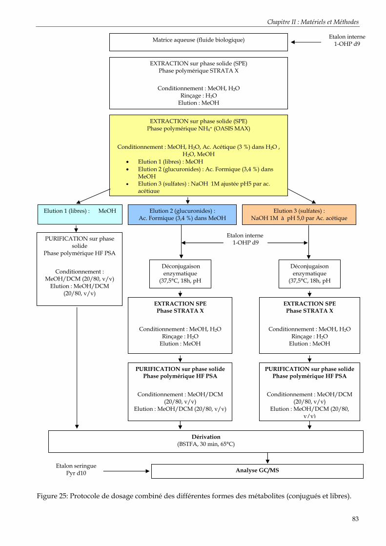
Chapitre II : Matériels et Méthodes
83
Figure 25: Protocole de dosage combiné des différentes formes des métabolites (conjugués et libres).
EXTRACTION sur phase solide (SPE) Phase polymérique STRATA X
Conditionnement : MeOH, H2O
Rinçage : H2O Elution : MeOH
EXTRACTION sur phase solide (SPE) Phase polymérique NH4+ (OASIS MAX)
Conditionnement : MeOH, H2O, Ac. Acétique (3 %) dans H2O ,
H2O, MeOH • Elution 1 (libres) : MeOH • Elution 2 (glucuronides) : Ac. Formique (3,4 %) dans
MeOH • Elution 3 (sulfates) : NaOH 1M ajustée pH5 par ac.
acétique
Elution 1 (libres) : MeOH
Elution 2 (glucuronides) : Ac. Formique (3,4 %) dans MeOH
Elution 3 (sulfates) : NaOH 1M à pH 5,0 par Ac. acétique
Etalon interne 1-OHP d9
PURIFICATION sur phase solide
Phase polymérique HF PSA
Conditionnement :
MeOH/DCM (20/80, v/v) Elution : MeOH/DCM
(20/80, v/v)
Déconjugaison enzymatique
(37,5°C, 18h, pH )
Déconjugaison enzymatique
(37,5°C, 18h, pH )
EXTRACTION SPE Phase STRATA X
Conditionnement : MeOH, H2O
Rinçage : H2O Elution : MeOH
EXTRACTION SPE Phase STRATA X
Conditionnement : MeOH, H2O
Rinçage : H2O Elution : MeOH
Analyse GC/MS
Etalon seringue Pyr d10
Matrice aqueuse (fluide biologique)
Etalon interne 1-OHP d9
PURIFICATION sur phase solide Phase polymérique HF PSA
Conditionnement : MeOH/DCM
(20/80, v/v) Elution : MeOH/DCM (20/80, v/v)
PURIFICATION sur phase solide Phase polymérique HF PSA
Conditionnement : MeOH/DCM
(20/80, v/v) Elution : MeOH/DCM (20/80,
v/v)
Dérivation (BSTFA, 30 min, 65°C)

Chapitre II : Matériels et Méthodes
84
4.2 Analyse et Détection des métabolites de HAP (Publications n°1, 2 et 3)
Les axes de développement analytique suivis durant ces travaux de recherche ont été définis en fonction des acquisitions technologiques du laboratoire. Trois technologies ont été mises en œuvre :
- la chromatographie en phase gazeuse couplée à la spectrométrie de masse simple (GC/MS),
- la chromatographie en phase gazeuse couplée à la spectrométrie de masse en tandem (GC-MS/MS),
- la chromatographie en phase liquide couplée à la spectrométrie de masse en tandem (UPLC-MS/MS)
4.2.1 Détection par GC/MS (Publication n°1)
Le principe
Le couplage de la chromatographie en phase gazeuse et de la spectrométrie de masse permet la séparation et la détection des composés ainsi que leur identification grâce aux spectres de fragmentation. En effet, après avoir été séparés par chromatographie en phase gazeuse, les composés sont introduits directement dans la source du spectromètre de masse où ils sont ionisés, dans notre cas, par impact électronique. L’ion moléculaire ainsi obtenu est ensuite plus ou moins fragmenté en fonction de sa stabilité. Les ions obtenus sont séparés d’après leurs rapports masse sur charge (m/z) et détectés en proportion de leur nombre (abondance). On obtient ainsi le spectre de masse de chaque composé présent dans le mélange de départ.
Dans le cas des analyses quantitatives de composés préalablement identifiés, le mode SIM (single ion monitoring) est privilégié. Il permet de ne détecter que certains ions particuliers. Ainsi il engendre une meilleure sensibilité que le mode qui effectue en continu un balayage des ions (le mode SCAN)
La dérivation
Comme il a été montré dans la synthèse bibliographique (Chapitre I, § 3.1.2), les métabolites de HAP ne sont pas des candidats idéaux pour une analyse en chromatographie en phase gazeuse couplée une détection par spectrométrie de masse (GC/MS) en raison de leur très faible volatilité. Ainsi l’ajout d’un agent dérivant va rendre possible l’analyse en GC/MS, en modifiant la fonctionnalité de la molécule.
Ainsi, préalablement à leur injection, les extraits subissent une étape de dérivation afin d’améliorer la séparation et la détection des composés. Le protocole conventionnel développé au laboratoire utilise comme agent de dérivation le N,O-bis-(trimethylsilyl)trifluoroacétamide (BSTFA, pureté > 98,5%) obtenu chez Sigma Aldrich (Saint Quentin Falavier, France). 30 µl de cet agent de sylilation sont ajoutés à l’extrait reconcentré et mis à incuber à 65°C pendant 30 minutes.
La dérivation est un procédé qui va entraîner un conditionnement spécifique de la colonne chromatographique et un encrassement particulier du détecteur. Ainsi pour éviter tout excès de ce composé, la quantité de BSTFA introduite dans l’extrait devrait être dans les proportions stœchiométriques (1: 1) avec les groupements hydroxylés. Or les quantités sont trop infimes pour pouvoir être mesurées avec précision. De plus, il existe dans l’extrait d’autres molécules susceptibles de réagir avec le dérivant qui vont donc consommer de manière non contrôlée une partie du produit de dérivation. Le BSTFA est donc introduit en

Chapitre II : Matériels et Méthodes
85
excès par rapport aux métabolites présents. Il induit donc un encrassement dans le temps du détecteur et de la colonne.
Les conditions d’analyse
Comme pour les HAP, un composé deutéré est ensuite ajouté afin de déterminer le rendement de dosage de l’étalon interne (le 1-OHPd9). Ce composé ajouté en fin de protocole est appelé « étalon seringue » ou « étalon de contrôle ». Ici, il s’agit du pyrène d10 (Pyr d10).
Les analyses ont été réalisées avec un chromatographe Agilent Technologies 6890, équipé d’une colonne capillaire HP5-MS Agilent Technologies dont la phase est constituée à 5% de diphényl- et 95% de diméthyl-polysiloxane et couplé à un spectromètre de masse Agilent Technologies 5973. Les métabolites sont séparés suivant un gradient de température allant de 70 à 290°C, avec une rampe de 15°C.min-1. Les conditions d’analyse (paramètres de la séparation et de la détection) sont détaillées dans l’Annexe 5.
Le chromatogramme obtenu après extraction d’ion (analyse en mode SIM) pour le mélange des métabolites est représenté sur la Figure 26. Les composés sont généralement détectés sous la forme HAP-O-Si(CH3)3+ à la valeur m/z = « masse moléculaire + 72 », à l’exception du 1-hydroxynaphtalène, du 2-hydroxybiphényle et du 9-hydroxyfluorène. L’ion [HAP-H]+ détecté pour le 9-hydroxyfluorène correspond à la molécule ayant perdue une molécule d’H2O. Pour le 1-hydroxynaphtalène, la perte d’un groupement CH3 provenant de la sylilation Si(CH3)3 semble être la plus probable explication à l’ion majoritaire formé. Pour le 2-hydroxybiphényle, l’ion majoritaire formé correspond à l’ion HAP-O-Si(CH3)2+. Les principaux ions des spectres de masse obtenus avec et sans dérivation, ainsi que leurs abondances relatives sont présentés dans le Tableau 24.
Figure 26: Chromatogramme obtenu en GC/MS par injection d’un mélange contenant les métabolites étudiés après dérivation. (1) 1-OHN, (2) 2-OHN, (3) 2-OHBi, (4) 9-OHFe, (5) 4-OHPhe, (6) 9-OHPhe, (7) Pyr d10, (8) 3-OHPhe, (9) 1-OHPhe, (10) 2-OHPhe, (11) 1-OHP d9, (12) 1-OHP, (13) 1-OHC, (14) 3-OHBaP.
13,5 13,7 13,9 14,1 14,3 14,5
4-OHPhe9-OHPhe 3-OHPhe
1-OHPhe 2-OHPhe
P-d10
0
5000
10000
15000
20000
25000
30000
35000
40000
45000
50000
9 11 13 15 17 19 21Temps de rétention (minutes)
Abondance
1
2
3
4
56
7
8
9
10
12
14
11
13

Chapitre II : Matériels et Méthodes
86
Tableau 24: Principaux ions (m/z) caractéristiques des spectres de masse obtenus par GC/MS avec et sans dérivation. Le nombre entre parenthèse est l’abondance de chaque ion par rapport au premier fixé à 100 %.
Composés M (g.mol-1) m/z sans dérivation m/z avec dérivation 1-OHN 144 144 (100), 115 (85) 201(100), 216 (90) 2-OHN 144 144 (100), 115 (60) 216 (100), 201 (65) 2-OHBi 170 170 (100), 169 (75), 141 (32) 211 (100), 227 (60), 242 (40) 9-OHFe 182 181 (100), 182 (77), 152 (38) 165 (100), 254 (25), 73 (25),
180 (10) OHPhe (5 isomères) 194 194 (100), 165 (100) 266 (100), 251 (63)
1-OHP 218 218 (100), 189 (77) 290 (100), 275 (25), 291 (20) 1-OHP d9 227 227 (100) 299 (100)
1-OHC 244 244 (100), 215 (75) 316 (100), 301 (70), 285 (15) 3-OHBaP 268 268 (100), 239 (68) 340 (100), 341 (30) Pyr d10 212 212 (100) 212 (100)
Tous les composés présentent une réponse linéaire sur une gamme du pg au ng injecté (1 µl injecté). Cet intervalle couvre la gamme des concentrations observées dans les échantillons environnementaux (Tableau 25).
Tableau 25: Linéarité des composés étudiés analysés en GC/MS (n=6). Les quantités injectées sont fixées à 1 µl.
Analytes m/z Gamme de concentrations Régression linéaire R2 RSD (%)
1-OHN 201 3 ng.g-1 – 30 µg.g-1 y = 23838x - 26571 0,9893 5,6 2-OHN 216 3 ng.g-1 – 30 µg.g-1 y = 14942x - 16013 0,9918 5,3 2-OHBi 211 3 ng.g-1 – 30 µg.g-1 y = 22817x - 23468 0,9913 4,6 9-OHFe 165 3 ng.g-1 – 30 µg.g-1 y = 26284x - 31325 0,9878 4,5
4-OHPhe 266 3 ng.g-1 – 30 µg.g-1 y = 12151x - 13319 0,9858 4,5 9-OHPhe 266 3 ng.g-1 – 30 µg.g-1 y = 12916x - 14529 0,9891 4,3 3-OHPhe 266 3 ng.g-1 – 30 µg.g-1 y = 15309x - 18395 0,9829 4,6 1-OHPhe 266 3 ng.g-1 – 30 µg.g-1 y = 30562x - 34723 0,9935 3,9 2-OHPhe 266 3 ng.g-1 – 30 µg.g-1 y = 17012x - 20177 0,9864 3,9
1-OHP 290 3 ng.g-1 – 30 µg.g-1 y = 22224x - 25699 0,9978 3,7 1-OHP d9 299 3 ng.g-1 – 30 µg.g-1 y = 24142x - 26655 0,9955 3,5
1-OHC 316 3 ng.g-1 – 30 µg.g-1 y = 4679,7x - 5469,7 0,9843 6,1 3-OHBaP 340 7 ng.g-1 – 40 µg.g-1 y = 3266,5x - 4258,8 0,9255 10,5 Pyr d10 212 3 ng.g-1 – 30 µg.g-1 y = 25253x - 26139 0,9821 5,6

Chapitre II : Matériels et Méthodes
87
Le choix d’étudier la linéarité de la méthode sur une large gamme de concentrations justifie l’obtention de coefficients de corrélation de la régression linéaire (R²) un peu plus faibles que sur des gammes de linéarité plus restreintes. Néanmoins, ce choix se justifiait par la taille de la gamme des concentrations en métabolites mesurés dans l’environnement. Afin de pouvoir valider notre méthode sur toutes les gammes de concentrations en OHHAP mesurées dans les organismes, nous avons conservé ces résultats.
Le protocole de quantification a été validé au moyen de solutions étalons contenant les métabolites natifs et le métabolite deutéré (1-OHP d9) en quantités connues. La quantification a été vérifiée pour des quantités injectées variant de 3 pg à 30 ng (sauf pour le 3-OHBaP, gamme de 7 pg à 40 ng). Cet intervalle a été ainsi choisi car il couvre la gamme des concentrations observées dans les échantillons environnementaux (Tableau 26). Les limites de détection instrumentales sont présentées dans le Tableau 27. Les limites de détection du protocole global sont présentées dans le paragraphe suivant.
Tableau 26: Quantification des métabolites de HAP en fonction de la quantité injectée. Les résultats sont exprimés en pourcentage de la quantité théorique (n =3, moyenne ± écartype).
Composés 3 pg
(7 pg pour 3-OHBaP)
30 pg (70 pg pour 3-
OHBaP)
0.3 ng (0,7 ng pour 3-
OHBaP)
3 ng (7 ng pour 3-
OHBaP)
30 ng (40 ng pour 3-
OHBaP) 1-OHN 106 ± 6 105 ± 6 97 ± 5 109 ± 9 96 ± 7 2-OHN 101 ± 10 100 ± 7 92 ± 7 103 ± 9 92 ± 6 2-OHBi 98 ± 8 98 ± 9 90 ± 6 100 ± 6 91 ± 8 9-OHFe 96 ± 9 96 ± 9 88 ± 5 98 ± 5 90 ± 9
4-OHPhe 103 ± 12 106 ± 9 97 ± 7 108 ± 6 99 ± 8 9-OHPhe 98 ± 9 100 ± 8 92 ± 8 103 ± 5 94 ± 5 3-OHPhe 105 ± 11 108 ± 11 99 ± 8 110 ± 5 101 ± 5 1-OHPhe 106 ± 10 109 ± 9 100 ± 5 109 ± 8 102 ± 7 2-OHPhe 105 ± 8 108 ± 7 99 ± 5 108 ± 5 101 ± 6
1-OHP 100 ± 4 103 ± 2 94 ± 1 102 ± 1 96 ± 3 1-OHC 99 ± 6 101 ± 5 93 ± 5 101 ± 8 95 ± 8
3-OHBaP 95 ± 10 97 ± 9 90 ± 9 92 ± 11 91 ± 11 1-OHP d9 105 ± 4 108 ± 3 99 ± 1 101 ± 1 101 ± 2
Tableau 27: Limites de détection instrumentales (LDI) exprimées en pg injectés (1 µl injecté) et calculées pour un rapport signal / bruit (S/N) = 3.
Composés LDI Composés LDI 1-OHN 0,2 1-OHPhe 0,1 2-OHN 0,3 2-OHPhe 0,2 2-OHBi 0,2 1-OHP 0,3 9-OHFe 0,1 1-OHC 2,5
4-OHPhe 0,3 3-OHBaP 8,1 9-OHPhe 0,4 1-OHP d9 0,5 3-OHPhe 0,2 Pyr d10 0,3

Chapitre II : Matériels et Méthodes
88
4.2.2 Détection par GC-MS/MS (Publication n°2)
Le second axe de ces travaux a été orienté vers une analyse en chromatographie en phase gazeuse couplée à la spectrométrie de masse en tandem (GC-MS/MS). Menés conjointement avec Justyna Sekula, étudiante étrangère en thèse au LPTC (Echange dans le cadre du programme Marie Curie), ces travaux ont pour but d’établir un protocole de dosage des métabolites plus spécifique et plus sensible que celui utilisant la GC/MS, permettant ainsi de diminuer les limites de détection et les quantités de matrice utilisées. Les développements effectués ainsi que la validation de l’analyse par GC-MS/MS ont fait l’objet d’une publication soumise à « Journal of Chromatography B » (Publication n°2).
Le principe
Les spectromètres de masse en tandem sont conçus de la manière suivante : une première étape consistant à sélectionner un ion stable particulier issu de la source d’ions (appelé « parent » ou « précurseur ») et une seconde qui représente l’analyse des ions issus de sa décomposition (ions « fils » ou « produits »). Dans l’intermédiaire se situe la phase d’activation de l’ion précurseur qui conduit à son excitation (i.e. l’augmentation de son énergie interne) et à sa fragmentation. La Figure 27 résume le principe de fonctionnement de la spectrométrie de masse en tandem.
Figure 27: Principe de fonctionnent de la spectrométrie de masse en tandem
Source d’ions
Analyseur 1 (MS 1)
Analyseur 2 (MS 2)
Cellule de collision
Détecteur

Chapitre II : Matériels et Méthodes
89
Les principaux avantages de cette technologie sont la précision et la reproductibilité des analyses quantitatives de composés présents à l’état de traces. La sensibilité, la sélectivité et la gamme dynamique de l’appareil sont parfaitement adaptées aux analyses environnementales, toxicologiques, agroalimentaires et toutes les analyses de traces, notamment dans les matrices complexes [415-423].
Comme pour l’analyse en GC/MS, différents modes d’acquisition sont possibles :
- Balayage complet pour la confirmation de la masse (SCAN)
- Détection sélective des ions pour le suivi d’un ou plusieurs composés (SRM, Single Reaction Monitoring)
- Balayage des ions produits pour des élucidations structurales
- Balayage des ions précurseurs pour rechercher des classes spécifiques de composés à l’aide de fragments communs
- Perte de neutre constante pour rechercher des classes spécifiques de composés
- Suivi des chromatogrammes en mode MRM (Multiple Reaction Monitoring) pour la quantification sélective des composés à l’état de traces.
Au cours de ces travaux, les développements analytiques ont été effectués sur un spectromètre de masse dont le principe de fonctionnement repose sur l’utilisation de deux analyseurs de type quadripolaire (MS1 et MS2). L’utilisation de deux analyseurs quadripolaires fournit des données de meilleure qualité pour un grand nombre d’applications :
- Sélectivité élevée pour réduire, voire éliminer les interférences dues à la matrice
- Sensibilité élevée, avec limites de quantification basses, pour les composés à l’état de traces
- Précision quantitative due à une excellente reproductibilité, stabilité, large gamme dynamique et à la possibilité de quantifier de manière exacte les composés en faible concentration.
Comme pour l’analyse par GC/MS le spectromètre de masse en tandem opère, dans le cas de cette étude, en mode d’impact électronique (EI) à 70 eV.
La dérivation
De manière similaire à la détection par GC/MS, il est nécessaire de dériver les métabolites de HAP pour pouvoir les détecter en GC-MS/MS. Néanmoins, dans le cas du spectromètre de masse en tandem, l’encrassement du système s’est avéré plus important que dans le cas du GC/MS. Le protocole de dérivation a donc été modifié par rapport à celui présenté dans le paragraphe précédent. 30 µl de N,O-bis-(trimethylsilyl)trifluoroacétamide (BSTFA, pureté > 98,5%, Sigma Aldrich, Saint Quentin Falavier, France) sont ajoutés à l’extrait reconcentré et mis à incuber à 65°C pendant 30 minutes.
Afin de minimiser l’impact du BSTFA dans le spectromètre de masse en tandem, 50 µl d’isooctane sont ajoutés à l’extrait dérivé et le BSTFA est évaporé sous flux d’azote. L’isooctane est un solvant moins volatil que le dichlorométhane. Il est ainsi ajouté à l’extrait afin que sous l’évaporation, le BSTFA s’évapore mais que les molécules de HAP hydroxylés les plus volatiles soient piégées dans l’extrait.

Chapitre II : Matériels et Méthodes
90
Les conditions d’analyse
Le principe du double-étalonnage interne n’a pas été mis en place dans le cas de l’analyse par GC-MS/MS. L’utilisation du pyrène d10 s’est montrée impossible du fait de la difficulté de décomposition de l’ion parent en ions fils stables. Le pyrène d10 est une molécule très stable. La formation d’ion parents est possible mais le passage dans la cellule de collision et la décomposition en ions fils nécessitent de grandes énergies de collision. L’application de telles énergies résulte en la fragmentation trop importante des ions parents et donc il est impossible d’obtenir des transitions spécifiques et sensibles pour le pyrène d10.
Les développements et les analyses ont été effectués au laboratoire sur un chromatographe Waters G1540N, équipé d’une colonne capillaire HP5-MS Ageilent Technologies et couplé à un spectromètre de masse Quattro Micro (Waters, UK). Les métabolites sont séparés selon un gradient de température de 70°C à 310°C, avec une rampe de température de 10°C par minute. Les conditions d’analyse et de détection sont détaillées dans l’Annexe 6.
Au cours de ces travaux, les développements et optimisations des méthodes d’analyses ont été uniquement menés pour 5 molécules hydroxylées : le 2-OHN, le 1-OHPhe, le 1-OHP, le 1-OHC et le 3-OHBaP. Ces 5 molécules sont représentatives de la famille des métabolites mono-hydroxylés. Elles sont plus ou moins aromatiques et donc plus ou moins volatiles. Les analyses sont effectuées en mode MRM (multiple reactions monitoring). Les transitions des ions « parents » aux ions « fils » ont été déterminées et optimisées. Le choix des produits de fragmentations pour chaque analyte et les énergies de collision associées ainsi que tous les autres paramètres instrumentaux à déterminer, ont été obtenus en travaillant avec des solutions de composés étalons aux concentrations allant de 7 à 10 µg.g-1.
La Figure 28 présente les chromatogrammes pour chaque ion acquis dans le mode MRM. Les transitions obtenues ainsi que les conditions MRM pour l’analyse de composés dérivés sont résumées dans le Tableau 28.
%
0
10025.12
27073
%
0
100
%
0
10022.43
4463
19.8616406
10 12 14 16 18 20 22 24 26 28
%
0
100
%
0
16.985975
11.032098
2-naphtol
1-phenanthrol
1-pyrenol
1-chrysenol
3 OHBaP
100
%
0
10025.12
27073
%
0
100
%
0
10022.43
4463
19.8616406
10 12 14 16 18 20 22 24 26 28
%
0
100
%
0
16.985975
11.032098
2-naphtol
1-phenanthrol
1-pyrenol
1-chrysenol
3 OHBaP
100
Figure 28: Chromatogramme obtenu en GC-MS/MS par injection d’un mélange contenant les métabolites étudiés après dérivation. 2-OHN, 1-OHPhe, 1-OHP d9, 1-OHP, 1-OHC, 3-OHBaP.

Chapitre II : Matériels et Méthodes
91
Tableau 28: Conditions MRM (transitions et énergie de collision) obtenues pour les métabolites hydroxylés dérivés.
Analytes Transition 1 (m/z)
Energie de
collision T1 (eV)
Transition 2 (m/z)
Energie de
collision T2 (eV)
Ion de quantification
Ion de qualification
Concentration injectée [μg.g-1]
2-OHN 216-201 8 216-73 20 73 201 6,87 1-
OHPhe 266-251 10 266-73 22 73 259 6,62
1-OHP 290-275 10 290-73 22 73 275 6,63 1-OHC 316-301 10 316-73 20 73 301 9,53
3-OHBaP 340-325 16 340-73 28 73 325 7,74
Tous les composés présentent une réponse linéaire sur les gammes des concentrations testées et variables selon les composés (1 µl injecté). Le Tableau 29 présente les domaines de linéarité ainsi que les performances obtenues pour chaque composé dans les conditions d’analyse optimisées.
Tableau 29: Linéarité des composés étudiés analysés en GC-MS/MS (n=6)
Analytes Transition (m/z)
Gamme de concentrations
[ng.g-1]
Régression linéaire R2 RSD (%)
2-OHN 216-201 0,1 – 441 y = 49x - 10 0,9999 4,3 1-OHPhe 266-251 0,2 – 440 y = 102x - 103 0,9986 3,9
1-OHP 290-275 0,2 – 502 y = 100x - 714 0,9910 5,0 1-OHC 316-301 0,4 – 490 y = 17x - 126 0,9903 3,6
3-OHBaP 340-325 1,7 - 1850 y = 17x - 460 0,9903 5,9
Le protocole de quantification a été validé au moyen de solutions étalons contenant les métabolites natifs et le métabolite deutéré (1-OHP d9) en quantités connues (Tableau 30). La répétabilité (intra-jour) ainsi que la reproductibilité (inter-jour) ont été mesurées pour des quantités injectées de l’ordre de 13 à 42 ng (Tableau 31).
Les limites de détection instrumentales sont présentées dans le Tableau 32.
Tableau 30: Quantification des métabolites de HAP en fonction de la quantité injectée. Les résultats sont exprimés en pourcentage de la quantité théorique (n =6, moyenne ± écartype).
Composés Pourcentage de la quantité théorique Quantité injectée (ng)
2-OHN 103 ± 9 9 1-OHPhe 100 ± 3 12
1-OHP 97 ± 1 6 1-OHC 100 ± 8 4
3-OHBaP 97 ± 14 11

Chapitre II : Matériels et Méthodes
92
Tableau 31: Précision de la méthode : Répétabilité et reproductibilité obtenues (n = 6)
Analytes Quantités injectées (ng) Répétabilité RSD % Reproductibilité RSD
% 2-OHN 13 11 11
1-OHPhe 16 9 10 1-OHP 16 11 13 1-OHC 16 8 14
3-OHBaP 42 10 11
Tableau 32: Limites de détection instrumentales (LDI) exprimées en pg injectés (1 µl injecté) et calculées pour un rapport signal / bruit (S/N) = 3.
Composés LDI 2-OHN 0,1
1-OHPhe 0,1 1-OHP 0,3 1-OHC 0,2
3-OHBaP 2,8
Si on compare ces limites de détection obtenues en GC-MS/MS avec celles obtenues en GC/MS pour les mêmes composés, on constate qu’une différence significative en termes de performance et de limites de détection existe entre ces deux techniques pour les composés de plus haut poids moléculaires (1-OHC et 3-OHBaP). Ces composés ont des chemins de fragmentations complexes qui génèrent un plus grand nombre d’ions et donc une plus faible quantité d’ion majoritaire. Ceci nécessite donc une spécificité plus importante lors de leur détection. Ainsi le choix de la spectrométrie de masse en tandem est judicieux afin d’obtenir des transitions spécifiques à chaque composé et ainsi de pouvoir abaisser les limites de détection en diminuant également le bruit de fond de la matrice.
Ces gains en sensibilité et en spécificité sont des atouts dans la recherche des métabolites dans les matrices environnementales complexes dans lesquelles les teneurs en composé recherché sont parfois très proches des limites de détection des outils analytiques. Ces avantages analytiques sont d’autant plus importants qu’ils concernent des molécules très importantes dans le suivi environnemental de la contamination en HAP : le 1-pyrénol, considéré comme marqueur d’exposition et le 3-OHBaP, considéré comme responsable en partie des dommages génotoxiques chez les organismes exposés.
4.2.3 Analyse par UPLC-MS/MS
L’inconvénient majeur des techniques d’analyse des métabolites par chromatographie en phase gazeuse est l’utilisation de produit de dérivation, nécessaire à la volatilisation des composés. Comme noté dans les paragraphes précédents, l’utilisation du BSTFA entraîne un encrassement de l’appareillage non négligeable qui induit un surcoût en termes de temps de nettoyage des appareillages, mais aussi en termes d’usure prématurée des colonnes chromatographiques et également un surplus de temps de préparation des échantillons. En effet, à la fin de l’étape de purification, l’extrait à analyser est dissous dans un solvant polaire (Méthanol). Il faut donc pourvoir le transférer dans un solvant apolaire afin de l’injecter en chromatographie en phase gazeuse. Cette étape est source possible de perte de composés. Enfin, il faut donc dériver l’échantillon en ajoutant un surplus de BSTFA et attendre 30

Chapitre II : Matériels et Méthodes
93
minutes durant la réaction de dérivation. Toutes ces étapes sont donc consommatrices de temps et sources d’erreur. Dans un souci de rentabilité et dans le cadre d’analyses en routine d’un très grand nombre d’échantillons, le choix de s’orienter vers la chromatographie en phase liquide était judicieux.
Des travaux précédents [424] avaient montré néanmoins que la chromatographie en phase liquide couplée à la spectrométrie de masse (LC/MS) donnait des rendements inférieurs ainsi que de moins bonnes performances analytiques par rapport à l’utilisation de la GC/MS avec dérivation.
Cependant, des avancées technologiques significatives ont été réalisées récemment dans le domaine des phases stationnaires et l’optimisation des systèmes chromatographiques. Mises en commun, ces innovations contribuent à une amélioration croissante des performances analytiques. Ainsi Waters Corporation a récemment développé une nouvelle technologie, la chromatographie liquide ultra-performante (UPLC), permettant d’allier toutes les qualités de la chromatographie en phase liquide, tout en diminuant ses inconvénients. La technologie UPLC respecte les principes de la chromatographie liquide classique tout en améliorant la résolution, la vitesse et la sensibilité des analyses.
Ainsi, suite à l’acquisition de cette technologie au sein du LPTC, les travaux se sont naturellement orientés vers le transfert technologique de la méthode HPLC/MS vers l’UPLC-MS/MS afin de pallier aux inconvénients des techniques de chromatographie en phase gazeuse et afin d’améliorer davantage les performances analytiques des outils de quantification des métabolites de HAP.
Principe de l’UPLC-MS/MS
L’UPLC est une technologie développée par WATERS Corporation qui s’appuie sur les principes de la chromatographie en phase liquide mais à laquelle s’ajoutent des innovations en termes de sensibilité, de résolution chromatographique et de vitesse d'analyse. L’utilisation de colonnes, capables de résister à de très grandes pressions de fonctionnement, est une des clés de cette innovation technologique. Ces colonnes contiennent des phases stationnaires composées de petites particules de 1,7 µm de diamètre (entre 3 et 5 µm pour l’HPLC classique).
A l’heure actuelle, trois types de colonnes de type BEH (Bridged Ethyl-siloxane/silica Hybrid) sont commercialisés :
- ACQUITY UPLC BEH C8 et C18 (greffons de chaînes linéaires d’alcanes),
- ACQUITY UPLC BEH Shield RP18 (greffons de groupements apolaires),
- ACQUITY UPLC BEH Phenyl (greffons de groupements phényle).
Dans le cas de l’analyse des métabolites de HAP, la colonne ACQUITY UPLC BEH C18 a été préférée du fait du caractère très polaire des métabolites primaires à faiblement polaire des composés hydroxylés.
Concernant le spectromètre de masse en tandem, la technologie du double quadripôle a également été utilisée (Chapitre II, § IV.2.2). Utilisée en couplage avec la chromatographie en phase gazeuse, elle avait démontré le gain substantiel acquis en termes de limites de détection, de sensibilité et de spécificité. C’est pourquoi lors des développements analytiques en chromatographie en phase liquide, ce type de détection a été conservé afin d’optimiser davantage les outils de quantification.

Chapitre II : Matériels et Méthodes
94
Le transfert de la méthodologie HPLC/MS existante au laboratoire [424] s’est donc déroulé en deux temps :
1) Le transfert de l’HPLC vers l’UPLC : optimisation des solvants, du gradient d’élution, des températures …
2) Le transfert de la MS simple à la MS/MS : choix dans le mode d’ionisation entre la technologie APCI (Atmospheric Pressure Chemical Ionization) et l’ESI (Electrospray Ionization), recherche des transitions (parents → fils), optimisation des conditions MRM (énergies de collision, tension de cône, tension du capillaire).
Choix du mode d’ionisation
La méthode d’analyse des OH-HAP par HPLC/MS, déjà développée au laboratoire, utilisait le mode d’ionisation par électrospray (ESI). En effet, les limites de détection atteintes en mode d’ionisation chimique à pression atmosphérique (APCI) étaient dix fois supérieures à celles obtenues avec le mode ESI.
De plus, dans la littérature, on observe que l’analyse des métabolites de HAP par HPLC-MS/MS et HPLC/MS utilise plus fréquemment le mode d’ionisation ESI en particulier lorsque les concentrations en métabolites sont faibles. Néanmoins les deux modes d’ionisation sont possibles [253, 280 , 425 , 426 , 427 ]
Le mode d’ionisation a été examiné dans les deux modes positif et négatif. Cependant, les métabolites mono-hydroxylés choisis dans cette étude ne produisent des signaux qu’uniquement dans le mode négatif. En effet, le groupement hydroxyle de ces molécules a tendance à perdre un hydrogène du groupement phényle et donc à générer des ions [M-H]-. Les ions fils sont issus des fragmentations des ions parents. Dans le cas des métabolites mono-hydroxylés étudiés, la fragmentation résulte de la perte d’un groupement –CO et donc de la recombinaison de la structure moléculaire.
Conditions d‘analyse
Les développements et les analyses ont été effectués au laboratoire sur un chromatographe Waters ACQUITY UPLC system (Milford, MA, USA), équipé d’une colonne ACQUITY UPLC BEH C18 (1,7 µm ; 2,1 mm x 150 mm) et couplé à un spectromètre de masse en tandem Quattro Premier™ (Micromass Ltd, Manchester, UK). Le système HPLC-MS/MS est contrôlé par l’application MassLynx™ 4.0 et QuanLynx™ 4.0.
Les paramètres utilisés pour la séparation des métabolites et leur détection sont détaillés dans l’Annexe 7. Au cours de ces travaux, les développements et optimisations des méthodes d’analyses ont été uniquement menés pour 5 molécules hydroxylées : le 2-OHN, le 1-OHPhe, le 1-OHP, le 1-OHC et le 3-OHBaP.
Le chromatogramme du mélange de métabolites obtenu après extraction d’ions en mode MRM est représenté sur la Figure 29. Les principaux ions des spectres de masse obtenus en ESI négatif sont présentés dans le Tableau 33.

Chapitre II : Matériels et Méthodes
95
0 1 2 3 4 5 6 7 8
Temps (min)
Abon
danc
e
2-OHN
1-OHPhe
1-OHP
1-OHP d9
1-OHC3-OHBaP
Figure 29: Chromatogramme obtenu en UPLC-ESI-MS/MS (débit de 0,45 ml.min-1) par injection d’un mélange contenant les métabolites étudiés. 2-OHN, 1-OHPhe, 1-OHP d9, 1-OHP, 1-OHC, 3-OHBaP.
Tableau 33: Principaux ions (m/z) et conditions MRM (transitions, tension de cône et énergie de collision) obtenus pour les métabolites hydroxylés.
Analytes Ion parents (m/z) Ion fils (m/z) Tension de
cône (V) Energie de
collision (eV) Dwell time
(ms) 2-OHN 143 [M-H]- 115 32 40 32 50
1-OHPhe 193 [M-H]- 165 30 50 30 50 1-OHP 217 [M-H]- 189 30 60 30 50 1-OHC 243 [M-H]- 215 32 60 32 50
3-OHBaP 267 [M-H]- 239 40 60 40 50
Tous les composés présentent une réponse linéaire sur les gammes des concentrations testées et variables selon les composés (10 µl injectés). Les solutions étalons ont été préparées dans de l’acétonitrile. Le Tableau 34 présente les domaines de linéarité ainsi que les performances obtenues pour chaque composé dans les conditions d’analyse optimisées.
Tableau 34: Linéarité des composés étudiés analysés en UPLC-MS/MS (n=3)
Analytes Transition (m/z)
Gamme de concentrations
Régression linéaire R2 RSD (%)
2-OHN 143 – 115 1 ng.g-1 – 8 µg.g-1 y = 1,46x + 0,024 0,9961 2,3
1-OHPhe 193 – 165 1 ng.g-1 – 8 µg.g-1 y = 144,45x - 2,99 0,9990 2,4
1-OHP 218 – 189 1 ng.g-1 – 9 µg.g-1 y = 358,03x + 21,36 0,9987 1,3
1-OHC 243 – 215 1 ng.g-1 – 8 µg.g-1 y = 50,87x + 2,87 0,9982 2,9
3-OHBaP 267 – 239 2 ng.g-1 – 13 µg.g-1 y = 12,70x + 0,9954 2,4

Chapitre II : Matériels et Méthodes
96
1,41 Le protocole de quantification a été validé au moyen de solutions étalons contenant
les métabolites natifs et le métabolite deutéré (1-OHP d9) en quantités connues. La quantification a été vérifiée pour des quantités injectées variant de 1 pg à 30 ng. Cet intervalle a été ainsi choisi car il couvre la gamme des concentrations observées dans les échantillons environnementaux (Tableau 35). Les limites de détection instrumentales sont présentées dans le Tableau 36. Les limites de détection du protocole global sont présentées dans le paragraphe suivant.
Tableau 35: Quantification des métabolites de HAP en fonction de la quantité injectée (10 µl injectés). Les résultats sont exprimés en pourcentage de la quantité théorique (n = 3, moyenne ± écartype).
Composés 1 pg 10 pg 0,1 ng 10 ng 30 ng 2-OHN 101 ± 10 97 ± 7 100 ± 7 96 ± 5 101 ± 10
1-OHPhe 94 ± 9 95 ± 9 96 ± 3 94 ± 4 96 ± 6 1-OHP 97 ± 7 104 ± 2 99 ± 4 98 ± 3 100 ± 5 1-OHC 93 ± 6 94 ± 7 92 ± 7 92 ± 8 96 ± 7
3-OHBaP 95 ± 8 101 ± 7 98 ± 5 98 ± 8 97 ± 7
Tableau 36: Limites de détection instrumentales (LDI) exprimées en pg injectés (10 µl injectés) et calculées pour un rapport signal / bruit (S/N) = 3.
Composés LDI en pg (10 µl injectés) 2-OHN 0,1
1-OHPhe 0,1 1-OHP 0,1 1-OHC 0,1
3-OHBaP 0,4
Tableau 37: Limites de détection instrumentales (LDI) exprimées en pg injectés, calculées pour un rapport signal / bruit (S/N) = 3, selon les différentes méthodologies GC/MS, GC-MS/MS et UPLC-MS/MS.
Composés GC-MS :
LDI en pg (1 µl injecté)
GC-MS/MS : LDI en pg
(1 µl injecté)
UPLC-MS/MS : LDI en pg
(10 µl injectés) 2-OHN 0,3 0,1 0,1
1-OHPhe 0,1 0,1 0,1 1-OHP 0,3 0,3 0,1 1-OHC 2,5 0,2 0,1
3-OHBaP 8,1 2,8 0,4
Si on compare ces résultats à ceux obtenus en GC/MS et en GC-MS/MS, on note que le gain en sensibilité devient notable pour les composés de plus haut poids moléculaires (1-OHC et 3-OHBaP) (Tableau 37). Comme précédemment discuté (Chapitre II, § IV.2.2), ces gains en sensibilité et en spécificité sont essentiels à l’analyse environnementale

Chapitre II : Matériels et Méthodes
97
d’échantillons complexes. Les avantages de la spectrométrie de masse en tandem sont donc couplés à l’utilisation de la chromatographie en phase liquide qui ne nécessite pas de dérivation, ni de préparation d’échantillons trop laborieuse.
Les avantages de la chromatographie en phase liquide ultra-rapide (UPLC) permettent de diminuer les temps d’analyse de manière très significative. Avec l’UPLC moins de 10 minutes sont nécessaires pour analyser tous les composés recherchés alors que 40 minutes étaient nécessaires en HPLC conventionnelle. La technologie UPLC permet également l’obtention de pics chromatographiques mieux résolus et plus fins qu’en HPLC conventionnelle, augmentant ainsi la sensibilité de la méthode analytique.
4.3 Validation des procédures d’extraction et de quantification
Les procédures de déconjugaison, d’extraction, de purification et de quantification ont été validées au moyen de différents types d’échantillons (eau, bile, plasma, urine) dans lesquels une quantité connue de métabolites de HAP a été introduite (après détermination préalable des teneurs initiales en analytes dans les échantillons naturels). Néanmoins à l’heure actuelle, il ne nous a pas été possible d’obtenir des matrices de référence certifiées par le Bureau Communautaire de Référence (BCR) de l’Union Européenne.
4.3.1 Les rendements d’extraction/purification : dosage des métabolites totaux (protocole n°1)
Afin de proposer une validation des procédures de préparation des échantillons, les rendements d’extraction/purification ont été déterminés pour des échantillons d’eaux, de biles et de plasma supplémentés en métabolites de HAP. Le protocole utilisé dans ces validations de préparation des échantillons mettait en œuvre une analyse des métabolites de HAP par GC/MS. Les résultats pour les différentes matrices sont présentés dans les Tableaux 38, 39 et 40.
De manière à pouvoir comparer les différentes techniques analytiques, seules les données inhérentes aux 5 métabolites étudiés dans les trois méthodologies analytiques sont ici présentées. L’ensemble des données obtenues dans le cadre de l’optimisation et de la validation de l’analyse par GC/MS est traité dans la Publication n°1.
Tableau 38: Rendement moyen du dosage total des métabolites de HAP dans des eaux supplémentées, à différentes concentrations (moyenne ± écartype, n = 3)
15 ng.g-1 1,5 ng.g-1 150 pg.g-1 15 pg.g-1
2-OHN 91 ± 8 88 ± 7 88 ± 8 74 ± 10 1-OHPhe 95 ± 7 96 ± 7 92 ± 9 83 ± 8
1-OHP 90 ± 3 90 ± 5 87 ± 8 78 ± 7 1-OHC 89 ± 6 89 ± 8 86 ± 8 77 ± 9
3-OHBaP 86 ± 8 86 ± 9 78 ± 8 74 ± 10

Chapitre II : Matériels et Méthodes
98
Tableau 39: Rendement moyen du dosage total des métabolites de HAP dans des biles supplémentées, à différentes concentrations (moyenne ± écartype, n = 3)
15 ng.g-1 1,5 ng.g-1 150 pg.g-1 15 pg.g-1
2-OHN 90 ± 7 75 ± 9 81 ± 10 68 ± 8 1-OHPhe 94 ± 8 81 ± 6 85 ± 8 76 ± 9
1-OHP 89 ± 2 76 ± 5 80 ± 6 72 ± 8 1-OHC 88 ± 6 75 ± 9 79 ± 6 71 ± 8
3-OHBaP 85 ± 9 72 ± 10 72 ± 9 68 ± 11
Tableau 40: Rendement moyen du dosage total des métabolites de HAP dans des plasmas supplémentés, à différentes concentrations (moyenne ± écartype, n = 3)
50 ng.g-1 5 ng.g-1 500 pg.g-1
2-OHN 98 ± 5 93 ± 8 88 ± 13 1-OHPhe 99 ± 2 98 ± 8 104 ± 6
1-OHP 96 ± 2 82 ± 7 86 ± 3 1-OHC 77 ± 5 74 ± 8 69 ± 4
3-OHBaP 71 ± 6 69 ± 7 65 ± 9
4.3.2 Validation du protocole de fractionnement des métabolites conjugués (protocole n°2)
Afin de valider le protocole de fractionnement des métabolites conjugués, il est nécessaire de connaître la quantité exacte de chaque composé initialement présent dans l’échantillon à doser. Deux techniques sont alors possibles. La première, et la plus juste, est de supplémenter, comme il a été fait précédemment, l’échantillon avec des composés commerciaux et de déterminer le rendement du protocole de dosage. La seconde option est de déterminer, d’une part, les teneurs en composés selon une méthodologie validée et d’autre part, selon la méthodologie à valider. La différence entre les résultats obtenus permet de conclure sur la validité du protocole à valider. Cependant dans cette seconde option, les résultats sont soumis à de plus grandes variabilités humaines et analytiques et à de plus grandes sources d’erreur.
En outre, pour l’étude des métabolites conjugués, il n’existe à l’heure actuelle, qu’un seul métabolite conjugué disponible commercialement, le 1-OHP-glucuronide. Ainsi, pour déterminer la part de chaque métabolite dans les différentes fractions (libre, sulfate, glucuronidé), il est impossible d’utiliser la technique de la supplémentation de l’échantillon.
Pour valider le protocole de fractionnement des métabolites biliaires, des échantillons de biles naturelles (merlus pêchés en Méditerranée) ont donc été dosés selon les deux protocoles.
Les résultats de dosage obtenus avec les deux protocoles (déconjugaison totale et fractionnement) ont ainsi été comparés (Tableau 41 et Figures 30, 31 et 32). L’analyse par GC/MS a été utilisée pour le dosage des extraits finaux pour les deux protocoles.

Chapitre II : Matériels et Méthodes
99
Tableau 41: Teneurs en métabolites biliaires (ng.g-1 de bile) obtenues lors du dosage de bile de merlu selon les protocoles 1 (avec et sans déconjugaison) et 2. Moyenne ± écartype, n = 3.
Protocole n°1
Protocole n°1 sans déconjugaison Protocole n°2
Composé Dosage
total Dosage des
composés libres
Fraction 1 composés
libres
Fraction 2 conjugués
glucuronidés
Fraction 3 conjugués sulfatés
Somme des 3 fractions totalité des métabolites
1-OHN 215,5 ± 48,0 20,0 ± 5,1 36,1 ± 7,1 181,7 ± 13,0 15,0 ± 11,0 232,8 ± 90,8
2-OHN 144,3 ± 58,0 15,0 ± 6,0 13,0 ± 1,0 96,5 ± 14,5 44,1 ± 17,4 153,6 ± 42,2
4-OHPhe 9,6 ± 8,0 0,9 ± 0,4 0,7 ± 0,1 5,6 ± 0,4 3,2 ± 0,4 9,5 ± 2,4 9-OHPhe 20,4 ± 14,4 0,9 ± 0,2 2,3 ± 0,6 20,0 ± 9,2 25,5 ± 14,8 47,8 ± 12,1 3-OHPhe 77,7 ± 29,1 0,6 ± 0,3 2,1 ± 0,7 6,4 ± 2,0 49,0 ± 3,2 57,5 ± 25,9
1-OHPhe 138,9 ± 35,0 6,1 ± 4,4 5,1 ± 3,3 17,7 ± 2,4 52,0 ± 3,8 74,8 ± 24,3
2-OHPhe 39,9 ± 16,0 2,0 ± 0,2 1,6 ± 0,4 43,6 ± 0,3 10,5 ± 9,0 55,7 ± 22,1
1-OHP 272,2 ± 44,0 41,4 ± 11,6 28,5 ± 17,9 157,5 ± 22,0 21,1 ± 14,0 207,2 ± 76,7
0
50
100
150
200
250
300
350
1-OHN 2-OHN 4-OHPhe 9-OHPhe 3-OHPhe 1-OHPhe 2-OHPhe 1-OHP
Conc
entra
tion
en O
HHAP
(ng/
g de
bile
)
F1 + F2 + F3Total deconjugaison
Figure 30: Comparaison entre la somme des métabolites obtenus dans les différentes fractions (F1+ F2 + F3) (protocole n°2) et le dosage des métabolites totaux (protocole n°1). Concentrations exrpimées en ng.g-1 de bile. Moyenne ± écartype, n = 3.
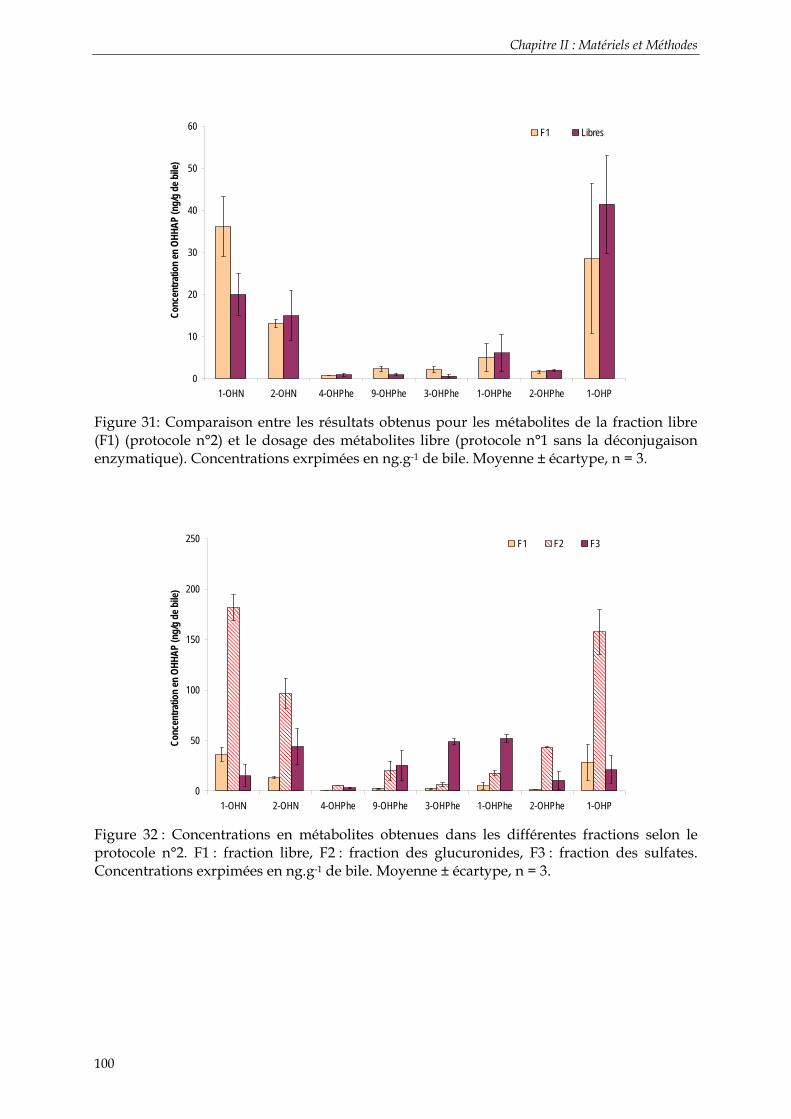
Chapitre II : Matériels et Méthodes
100
0
10
20
30
40
50
60
1-OHN 2-OHN 4-OHPhe 9-OHPhe 3-OHPhe 1-OHPhe 2-OHPhe 1-OHP
Conc
entra
tion
en O
HHAP
(ng/
g de
bile
)
F1 Libres
Figure 31: Comparaison entre les résultats obtenus pour les métabolites de la fraction libre (F1) (protocole n°2) et le dosage des métabolites libre (protocole n°1 sans la déconjugaison enzymatique). Concentrations exrpimées en ng.g-1 de bile. Moyenne ± écartype, n = 3.
0
50
100
150
200
250
1-OHN 2-OHN 4-OHPhe 9-OHPhe 3-OHPhe 1-OHPhe 2-OHPhe 1-OHP
Conc
entra
tion
en O
HHAP
(ng/
g de
bile
)
F1 F2 F3
Figure 32 : Concentrations en métabolites obtenues dans les différentes fractions selon le protocole n°2. F1 : fraction libre, F2 : fraction des glucuronides, F3 : fraction des sulfates. Concentrations exrpimées en ng.g-1 de bile. Moyenne ± écartype, n = 3.

Chapitre II : Matériels et Méthodes
101
Concernant la spéciation des différentes formes des métabolites, on observe que les formes conjuguées sont majoritaires pour tous les métabolites recherchés. En pourcentage relatif à la totalité des métabolites dosés, on obtient les résultats suivants (Tableau 42).
Tableau 42: Distribution relative des différentes formes des métabolites dans la bile de merlu (100 % représentant la somme des métabolites détectés, toute forme confondue)
Composés % de la forme libre (F1)
% de la forme glucuronide (F2)
% de la forme sulfate (F3)
1-OHN 15 78 6 2-OHN 8 63 29
4-OHPhe 8 59 34 9-OHPhe 5 42 53 3-OHPhe 4 11 85 1-OHPhe 7 24 70 2-OHPhe 3 78 19
1-OHP 14 76 10
On remarque que pour les métabolites isomères du phénanthrène, la fraction des conjugués sulfates est plus importante que celle des composés glucuronides. Pour les métabolites du pyrène et du naphtalène, cette distribution est inversée. Ces résultats sont en correspondance avec ceux que l’on peut trouver dans la littérature (Chapitre I, § 2.2.2).
Si on prend l’exemple du naphtalène, les conjugués glucuronides dans la bile sont largement majoritaires par rapport aux sulfates [81, 259, 337 ]. Les conjugués sulfatés des HAP sont d’une manière générale moins abondamment produits que les glucuronides chez différentes espèces de poissons [81 , 428 , 429]. Il a été également constaté sur des HAP phénoliques que les conjugués sulfatés étaient majoritairement éliminés via l’urine [430] alors que les glucuronides l’étaient principalement par la bile [430]. Dans cette dernière étude où douze espèces de poisson sont exposées au 1-hydroxynaphtalène, entre 77 et 93% des métabolites biliaires sont conjugués à l’acide glucuronique et entre 4 et 12% aux sulfates. Toutes ces données bibliographiques sont en accord avec les résultats obtenus dans cette étude.
Ces travaux de recherche portant sur la spéciation des métabolites ont ouvert de nouvelles perspectives sur l’étude des phénomènes de biodisponibilité et de biotransformation des HAP chez les organismes supérieurs. En revanche, l’outil analytique développé n’a pas été utilisé en routine sur des programmes de surveillance car il était consommateur de temps et de moyens. C’est pourquoi ces recherches doivent être poursuivies dans ce sens et la méthodologie doit être optimisée afin d’obtenir une méthode analytique rapide et performante, nécessaire à la compréhension du devenir des HAP chez les poissons exposés.

Chapitre II : Matériels et Méthodes
102
4.3.3 Limites de détection
Les limites de détection ont été établies dans les matrices aqueuses et dans la bile. Pour chaque méthode de séparation et d’analyse (GC-MS, GC-MS/MS et UPLC-MS/MS), ces limites sont calculées selon le rapport « signal / bruit = 3 ». Elles sont présentées dans les Tableaux 43, 44 et 45.
Les prises d’essai sont de 3 ml pour les eaux supplémentées et de 100 µl pour la bile.
Tableau 43: Limites de détection (LOD) selon la méthodologie utilisant la GC/MS pour différentes matrices. LOD exprimées en ng.l-1 d’eau et ng.g-1 de bile. LOD calculées pour un rapport signal / bruit (S/N) = 3.
Composés LOD – EAU
(ng.l-1) LOD – BILE
(ng.g-1) 2-OHN 1,6 3,9
1-OHPhe 0,4 0,9 1-OHP 0,6 0,1 1-OHC 4,5 6,6
3-OHBaP 13,6 20,6
Tableau 44: Limites de détection (LOD) selon la méthodologie utilisant la GC-MS/MS pour la matrice biliaire. LOD exprimées en ng.g-1 de bile. LOD calculées pour un rapport signal / bruit (S/N) = 3.
Composés LOD – EAU
(ng.l-1) LOD – BILE
(ng.g-1) 2-OHN 0,2 0,7
1-OHPhe 0,1 0,5 1-OHP 0,7 0,3 1-OHC 0,6 1,4
3-OHBaP 4,9 8,5
Tableau 45: Limites de détection (LOD) selon la méthodologie utilisant l’UPLC-MS/MS pour différentes matrices. LOD exprimées en ng.l-1 d’eau et ng.g-1 de bile. LOD calculées pour un rapport signal / bruit (S/N) = 3.
Composés LOD – EAU
(ng.l-1) LOD – BILE
(ng.g-1) 2-OHN 0,03 0,10
1-OHPhe 0,01 0,03 1-OHP 0,01 0,02 1-OHC 0,01 0,03
3-OHBaP 0,02 0,10
Ces LOD ont été déterminées pour un certain type de matrice. Pour les matrices
aqueuses, il s’agit d’eau Milli-Q fortifée en métabolites, via une solution de métabolites dissous dans de l’éthanol. Pour les biles, des biles de truites ont été utilisées comme matrice

Chapitre II : Matériels et Méthodes
103
de référence. Après vérification de l’absence de métabolites dans la matrice initiale, elle a été supplémentée en métabolites via une solution de métabolites dissous dans de l’éthanol.
Néanmoins, la variabilité « naturelle » de la composition des matrices biologiques (bile) et en particulier la nature et la quantité des protéines et des lipides les composant, entraîne une forte variabilité des limites de détection entre deux échantillons (peut atteindre 25% pour le 3-OHBaP). Ceci est dû principalement aux fluctuations importantes du bruit de fond et des interférences matricielles. Il convient donc de calculer les LOD pour chaque série d’analyse et parfois pour chaque type d’échantillon, en particulier lorsqu’on s’intéresse à différentes espèces animales. De plus des variabilités sur les machines peuvent également influencer la détermination des limites de détection. Un encrassement du système provoquera des interférences matricielles visibles par une augmentation du bruit de fond et donc par une augmentation des limites de détection établies par la méthode du rapport Signal/Bruit.
Après comparaison avec les LOD recueillies dans la littérature, on constate que les performances obtenues avec les protocoles développés au cours de cette thèse sont globalement plus sensibles, quels que soient les modes de séparation et de détection considérés.
Avec une méthodologie utilisant la GC/MS et la dilution isotopique, Smith et al. [431, 432] ont montré, sur des échantillons d’urine, des LOD comprises entre 1 et 16 ng.l-1 d’urine pour les métabolites mono-hydroxylés du phénanthrène. Dans les travaux de recherche ici présentés, la LOD obtenue sur des échantillons de bile pour le 1-hydroxyphénanthrène est de 0,9 ng.g-1 de bile avec la méthode GC/MS. Jongeneelen et al. [433] ont mis en œuvre une méthode GC/MS pour laquelle la LOD du 1-hydroxypyrène était 170 pg.g-1 de bile. Dans la méthode présentée dans ces travaux de recherche (Publication n°1), la limite de détection du 1-hydroxypyrène est calculée à 100 pg.g-1 de bile.
Enfin, Romanoff et al. [434] ont développé une méthodologie utilisant la GC/HRMS combinée à la dilution isotopique pour quantifier les métabolites de HAP dans l’urine. Les LOD obtenues avec la spectrométrie haute résolution étaient comprises entre 2 et 10 ng.l-1 d’urine. Pour la matrice aqueuse, les LOD obtenues avec le protocole GC/MS (Tableau 43) sont du même ordre de grandeur que celles obetnues en GC/HRMS. En revanche pour la matrice biliaire, les limites de détection restent inférieures à celles obtenues en GC/HRMS. Les différences sont d’autant plus importantes que les composés ont un plus haut poids moléculaire (1-OHC et 3-OHBaP). Pour le 1-OHPhe et le 1-OHP, les différences sont de l’ordre de 5 et 8 fois plus importantes en GC/MS par rapport à la GC/HRMS, respectivement. Néanmoins, il faut tenir compte dans ces comparaisons des différences matricielles (urine et bile) qui peuvent beaucoup influencer la détermination des LODs.
Si on considère les autres méthodologies développées au cours de cette thèse (protocoles utilisant GC-MS/MS et UPLC-MS/MS), très peu de comparaisons sont possibles avec la littérature. En effet, à l’heure actuelle, aucun travail n’a présenté une analyse des métabolites de HAP dans la bile par GC-MS/MS ou par UPLC-MS/MS. Seuls des travaux utilisant la méthodologie par HPLC-MS/MS peuvent être recensés. Xu et al. [425] ont proposé une méthode LC-MS/MS pour laquelle les limites de détection instrumentales pour le 2-hydroxynaphtalène, le 1-hydroxyphénanthrène, le 1-hydroxypyrène et le 3-hydroxybenzo(a)pyrène étaient de 1,1, 0,8, 0,1 et 0,1 pg injectés (10 µl injectés), respectivement. Si on compare ces valeurs à celles obtenues pour les protocoles utilisant la GC-MS/MS et l’UPLC-MS/MS, on note que les valeurs sont globalement similaires à celles obtenues en UPLC-MS/MS mais supérieures à celles obtenues en GC-MS/MS. Néanmoins,
Chapitre II : Matériels et Méthodes
104
la comparaison ne peut pas être étendue aux limites de détection du protocole global car l’influence matricielle de la bile ne peut pas être extrapolée à partir de valeurs instrumentales uniquement. Pigini et al. [426] ont montré sur des échantillons d’urine une LOD pour le 1-hydroxypyrène de 0,01 ng.l-1 d’urine en HPLC-MS/MS. Dans cette étude, l’importance de l’étalonnage interne a été démontrée lors de l’application de cette méthodologie pour le dosage d’échantillons complexes tels que l’urine. L’influence de la matrice dans les interférences matricielles et donc dans le dosage des métabolites a été prouvée.
Une seule étude, à l’heure actuelle, rapporte le développement d’une méthode d’analyse par UPLC/MS pour la quantification des métabolites du BaP dans la bile de poissons [435]. Les LOD des métabolites du BaP sont données pour inférieures à 10 ng.g-1 de bile. Si on compare ces données avec celles obtenues par le protocole UPLC-MS/MS développé au cours de cette thèse, on se rend compte qu’un facteur 100 à 500 sépare les LOD des deux protocoles. La spécificité et la sensibilité de la spectrométrie de masse en tandem ainsi que l’optimisation de la séparation par chromatographie en phase liquide ultra-performante sont ainsi démontrées.

Chapitre II : Matériels et Méthodes
105
5 Dosage des métabolites de HAP primaires par UPLC-MS/MS (Publication n° 4)
Le dosage de ces métabolites plus réactifs (Tableau 15) et moins stables que les composés mono-hydroxylés (dits métabolites primaires) a été développé à partir du protocole de dosage des métabolites totaux, validé au laboratoire (Chapitre II, § 4.1.1). Seule la méthode d’analyse a différé et la technologie UPLC-MS/MS a été mise en œuvre.
5.1 La séparation et l’analyse des métabolites primaires (Publication n°4)
Dans un premier temps, le développement s’est porté sur la détection de ces composés en spectrométrie de masse en tandem. Les deux techniques d’ionisation (ESI et APCI) ont été testées dans les deux modes. Des tests préliminaires ont rapidement montré que la sensibilité de la méthode APCI était nettement plus faible que celle de la méthode ESI (environ 4 fois plus faible). Dès lors, l’optimisation des paramètres d’ionisation a été conduite uniquement pour l’ESI. Un plan expérimental a permis d’obtenir la meilleure combinaison pour les facteurs suivants : pression de nébulisation, température et débit de gaz desséchant, différence de potentiel appliquée au capillaire, différence de potentiel utilisée pour la fragmentation des ions parents, énergie appliquée à la cellule de collision, vitesse du gaz de collision. L’optimisation de ces paramètres a permis l’obtention d’un signal maximal avec une fragmentation minimale pour la plupart des analytes.
La quasi-totalité des métabolites a été analysée en mode positif (ions [M+H]+) à l’exception des métabolites mono-hydroxylés, le 9-OHBaP et le 3-OHFluo, analysés en mode négatif (ions [M-H]-). L’Annexe 8 résume les paramètres d’analyse optimisés.
Un compromis a dû être fait afin de pouvoir doser la totalité des composés en une seule analyse. En effet, les métabolites de type diol, dione et époxyde sont analysés en mode positif. Or l’unique étalon interne disponible pour les métabolites de HAP est le 1-OHPd9 pour lequel l’optimisation de l’ionisation donne une analyse en mode négatif. Par ailleurs, afin d’ioniser les métabolites primaires en mode positif, un acide organique doit être ajouté à la phase mobile. Or, l’ajout de cet acide, même à faible quantité dans la phase mobile, entraîne une moins bonne détection en mode négatif car il augmente légèrement le bruit de fond. Le compromis a donc été fait quant à la composition de la phase mobile supplémentée en acide organique et la détection un peu moins bonne de l’étalon interne en mode négatif.
L’acquisition des données par le spectromètre de masse se fait donc simultanément en mode positif et en mode négatif. La phase mobile a été supplémentée avec de l’acide acétique à 0,1%. La sensibilité se trouve donc être un peu moins bonne pour les composés analysés en mode négatif mais très suffisante pour une analyse quantitative de composés présents à l’état d’ultra-trace dans les matrices naturelles. La Figure 33 présente un chromatogramme obtenu en UPLC-MS/MS pour un mélange étalons de métabolites de type diole, dione et époxyde.

Chapitre II : Matériels et Méthodes
106
Figure 33 : Chromatogramme d’un mélange étalon de métabolites primaires obtenu UPLC-MS/MS (temps exprimé en minutes)
Les principaux ions des spectres de masse obtenus en ESI positif et négatif ainsi que les paramètres MRM sont présentés dans le Tableau 46.
Tableau 46: Principaux ions (m/z) et conditions MRM (transitions, tension de cône et énergie de collision) obtenus pour les métabolites hydroxylés.
Analytes Ion parents (m/z) Ion fils (m/z) Tension de
cône (V)
Energie de collision
(eV)
Dwell time (ms)
4,5-DHDBaP 268 239 60 40 50 7,8-DHDBaP 268 239 60 40 50
7,8-DHepoxideBaP 268 239 60 40 50 1,6-dioneBaP 283 226 60 42 50 3,6-dioneBaP 283 226 60 42 50
9-OHBaP 267 239 60 40 50 2,3-DHDFluo 218 189 60 38 50 2,3-dioneFluo 233 176 60 40 50
3-OHFluo 217 189 60 30 50
Tous les composés présentent une réponse linéaire sur les gammes des concentrations testées et variables selon les composés (10 µl injectés). Les solutions étalons ont été préparées dans de l’acétonitrile. Le Tableau 47 présente les domaines de linéarité ainsi que les performances obtenues pour chaque composé dans les conditions d’analyse optimisées.
Time0.50 1.00 1.50 2.00 2.50 3.00 3.50 4.00 4.50 5.00 5.50 6.00 6.50 7.00 7.50 8.00 8.50 9.00 9.50 10.00
%
0
100283 > 226.22
5.00e66.20
6.09
2,3-DHDFluo
2,3-DioneFluo
4,5-DHDBaP 7,8-DHEpoxide BaP
1-OHPd9 :
étalon interne
3,6-DioneBaP
7,8-DHDBaP
1,6-DioneBaP

Chapitre II : Matériels et Méthodes
107
Tableau 47: Linéarité des composés étudiés analysés en UPLC-MS/MS (n=3)
Analytes Transition (m/z)
Gamme de concentrations
Régression linéaire R2 RSD (%)
4,5-DHDBaP 268 – 239 8 ng.g-1 – 34 µg.g-1 y = 712,9x + 33,9 0,9983 4 7,8-DHDBaP 268 – 239 8 ng.g-1 – 34 µg.g-1 y = 689,9x + 47,5 0,9976 4
7,8-DHepoxideBaP 268 – 239 8 ng.g-1 – 30 µg.g-1 y = 210,9x + 5,7 0,9942 11 1,6-dioneBaP 283 – 226 8 ng.g-1 – 33 µg.g-1 y = 262,9x + 12,6 0,9971 10 3,6-dioneBaP 283 – 226 8 ng.g-1 – 33 µg.g-1 y = 282,3x + 9,4 0,9975 9
9-OHBaP 267 – 239 8 ng.g-1 – 32 µg.g-1 y = 908,6x + 1,4 0,9995 5 2,3-DHDFluo 218 – 189 17 ng.g-1 – 70 µg.g-1 y = 1185,9x + 83,8 0,9980 4 2,3-dioneFluo 233 – 176 11 ng.g-1 – 44 µg.g-1 y = 297,6x + 19,9 0,9994 5
3-OHFluo 217 – 189 12 ng.g-1 – 48 µg.g-1 y = 1921,4x + 18,9 0,9996 5
Le protocole de quantification a été validé au moyen de solutions étalons contenant les métabolites natifs et le métabolite deutéré (1-OHP d9) en quantités connues. La quantification a été vérifiée pour des quantités injectées variant de 10 pg à 10 ng (Tableau 48). Les limites de détection instrumentales sont présentées dans le Tableau 49.
Tableau 48: Quantification des métabolites de HAP en fonction de la quantité injectée (10 µl injectés). Les résultats sont exprimés en pourcentage de la quantité théorique (n = 3, moyenne ± écartype).
Composés 10 pg 0,1 ng 10 ng 4,5-DHDBaP 90 ± 8 86 ± 8 91 ± 9 7,8-DHDBaP 86 ± 8 85 ± 9 89 ± 8
7,8-DHepoxideBaP 61 ± 6 63 ± 6 66 ± 6 1,6-dioneBaP 75 ± 7 73 ± 7 77 ± 7 3,6-dioneBaP 75 ± 7 74 ± 9 75 ± 9
9-OHBaP 89 ± 8 91 ± 9 95 ± 9 2,3-DHDFluo 82 ± 8 84 ± 8 89 ± 8 2,3-dioneFluo 78 ± 7 78 ± 7 82 ± 8
3-OHFluo 88 ± 8 91 ± 9 95 ± 9

Chapitre II : Matériels et Méthodes
108
Tableau 49: Limites de détection instrumentales (LDI) exprimées en pg injectés (10 µl injectés) et en pg.µl-1. LDI calculées pour un rapport signal / bruit (S/N) = 3.
Composés LDI (pg) LDI (pg.µl-1)
4,5-DHDBaP 15,0 1,5 7,8-DHDBaP 16,8 1,7
7,8-DHepoxideBaP 21,4 2,1 1,6-dioneBaP 11,7 1,2 3,6-dioneBaP 16,9 1,7
9-OHBaP 1,0 0,1 2,3-DHDFluo 11,2 1,1 2,3-dioneFluo 24,2 2,4
3-OHFluo 0,6 0,1
A l’heure actuelle, aucune étude ne rapporte l’utilisation de l’UPLC-MS/MS pour l’analyse des métabolites primaires de HAP. Quelques études mettant en œuvre l’HPLC/F [436], la LC/MS [437] et une seule utilisant l’UPLC/MS [435] on été publiées. Des études ont été menées en LC-Q-TOFMS [438] pour l’identification des métabolites polaires du benzo(a)pyrène , mais elles ne présentaient pas d’application sur des échantillons naturels (urine, bile, plasma). Seules des identifications des composés ont été présentées.
Si on compare les limites de détection instrumentales obtenues dans ces travaux de thèse (Pulication n°4) avec la littérature, on note qu’elles sont comparables à celles rapportées dans les autres études. Ainsi en LC-APCI-MS, Koeber et al. [437] ont montré des limites de détection pour des métabolites polaires du BaP comprises entre 2 et 25 pg injectés (10 µl injectés) soit entre 0,2 et 2,5 pg.µl-1. Wang et al. [438] ont utilisé la technique LC-Q-TOFMS pour identifier les métabolites polaires du BaP et ont montré des limites de détection comprises entre 40 et 60 pg (10 µl injectés), soit entre 4 et 6 pg.µl-1. Enfin, Zhu et al. [435] présente des limites de détection en UPLC/MS inférieures à 10 pg.µl-1. Ces limites restent très supérieures à celles obtenues en UPLC-MS/MS au cours de ces travaux de recherche.
5.2 Préparation des échantillons
Dans ce développement analytique, le protocole de préparation des échantillons optimisé et validé pour le dosage total des métabolites de HAP a été utilisé intégralement. Aucun nouveau développement n’a été mis en œuvre.
Les métabolites réactifs ici considérés sont des métabolites primaires, très vite produits par l’organisme suite à une exposition aux HAP. En revanche, ils sont également très vite métabolisés et associés aux molécules endogènes ou transformés en molécules plus stables (comme les métabolites mono-hydoxylés). C’est pourquoi, dans les organismes vivants, il est très difficile de pouvoir doser ces molécules dans la bile ou dans les différents organes de détoxification. Ils sont présents principalement dans les cellules hépatiques, cellules de métabolisation de l’organisme.
Des études précédentes [113, 124, 125, 315, 319, 321, 439, 440] ont pu mettre en évidence certains de ces métabolites primaires et les doser dans le cas d’exposition in vitro en laboratoire sur des microsomes hépatiques. En revanche, les méthodologies employées utilisent principalement une analyse par HPLC/F. Très peu d’études s’attachent à déterminer quantitativement ces composés et la techniques alors employée est l’HPLC/MS.

Chapitre II : Matériels et Méthodes
109
Le mode de traitement de l’échantillon microsome est identique à un échantillon biliaire à l’exception de l’étape de déconjugaison (métabolites de phase I non conjugués). En effet, ces molécules sont des métabolites primaires, non conjugués. L’étape de déconjugaison est ainsi supprimée du protocole. Un protocole simplifié est donc mis en œuvre pour cette analyse (Figure 34). Les différentes étapes sont présentées précédemment dans le Chapitre II (§ 4.1.1.).
Figure 34: Protocole simplifié de dosage (sans déconjugaison) des métabolites primaires dans les fluides biologiques (microsome, bile …) par UPLC-MS/MS.
5.3 Validation de la méthode de dosage et limites de détection
Des dosages sur des biles supplémentées en métabolites à 3 niveaux de concentrations et immédiatement analysés selon le protocole simplifié, ont permis de valider le protocole de dosage de ces composés dans une matrice biologique. Les rendements du dosage ont été déterminés et les résultats sont présentés dans le Tableau 50.
Tableau 50: Rendement moyen du dosage des métabolites primaires de HAP dans des biles supplémentées, à différentes concentrations (moyenne ± écartype, n = 3)
Composés 10 ng.g-1 100 ng.g-1 1 µg.g-1 4,5-DHDBaP 75 ± 10 78 ± 9 79 ± 8 7,8-DHDBaP 71 ± 11 70 ± 10 75 ± 8
7,8-DHepoxideBaP 43± 9 40 ± 9 45 ± 7 1,6-dioneBaP 65 ± 10 64 ± 9 69 ± 9
Ajout de l’étalon interne (Pyrénol d9 ou 1-OHP d9)
EXTRACTION sur phase solide (SPE) Phase polymérique STRATA X
Conditionnement : MeOH, H2O
Rinçage: H2O, H2O /MeOH (70:30, v/v) Elution : MeOH
PURIFICATION sur phase solide Phase polymérique HF PSA
Conditionnement : MeOH/DCM (20/80, v/v)
Elution : MeOH/DCM (20/80, v/v)
Analyse UPLC™-MS/MS
Matrice biologique (microsome hépatique, bile …)

Chapitre II : Matériels et Méthodes
110
3,6-dioneBaP 69 ± 11 70 ± 10 65 ± 10 9-OHBaP 77 ± 7 76 ± 6 77 ± 6
2,3-DHDFluo 71 ± 11 68 ± 9 75 ± 10 2,3-dioneFluo 64 ± 11 64 ± 9 70 ± 9
3-OHFluo 87 ± 9 84 ± 7 88 ± 6
Les limites de détection ont été établies dans la bile. Elles sont calculées selon le rapport « signal / bruit = 3 ». Elles sont présentées dans le Tableau 51. La prise d’essai est de 0,1 g de bile.
Tableau 51: Limites de détection (LOD) dans la matrice biliaire, exprimées en ng.g-1 de bile. LOD calculées pour un rapport signal / bruit (S/N) = 3.
Composés LOD (ng.g-1) 4,5-DHDBaP 0,15 7,8-DHDBaP 0,20
7,8-DHepoxideBaP 0,50 1,6-dioneBaP 0,30 3,6-dioneBaP 0,30
9-OHBaP 0,03 2,3-DHDFluo 0,26 2,3-dioneFluo 0,36
3-OHFluo 0,01
Au regard de la littérature, très peu d’études rapportent des mesures de métabolites polaires de HAP dans une matrice biologiques. Il existe donc très peu de points de comparaison possibles. Une étude réalisée en HPLC/F sur des échantillons de plasma et d’urine de rat a permis le dosage des métabolites polaires du BaP (mono-hydroxyBaP et diols). Dans cette étude, Won et al. [436] présentent des limites de détection comprises entre 0,04 et 0,1 ng.ml-1 dans l’urine et 0,2 et 0,4 ng.ml-1 dans le plasma.
En revanche aucune étude ne présente des résultats de dosage de ces métabolites dans la bile. Les résultats présentés dans ces travaux de recherche sont donc innovants et justifiés par l’absence de données dans la littérature.
Une expérimentation en laboratoire sur des microsomes hépatiques de limandes et de soles exposés directement à des HAP a permis de valider sur des échantillons naturels la méthodologie développée au laboratoire (Publications n° 4). En revanche des tests de dosage effectués sur des biles de poissons, échantillonnés en milieu naturel, n’ont pas permis de détecter et de doser ces composés. Une oxydation de l’échantillon, une absence des métabolites primaires dans la bile ou une dégradation des composés durant le stockage à -80°C pourraient expliquer l’absence de signaux obtenus au cours de l’analyse.

Chapitre III : Expérimentations en Laboratoire
111
CHAPITRE III : EXPERIMENTATIONS EN LABORATOIRE
Ce chapitre présente les résultats obtenus au cours des expérimentations en laboratoire sur des turbots juvéniles exposés aux HAP au cours de ces travaux de thèse.
Ces expérimentations consistant à exposer des poissons aux HAP en laboratoire ont été réalisées afin d’étudier le comportement de ces contaminants dans un milieu simplifié et de mieux comprendre leur devenir dans les organismes marins et en particulier les processus de biotransformation et de génotoxicité.

Chapitre III : Expérimentations en Laboratoire
112

Chapitre III : Expérimentations en Laboratoire
113
1 Expérimentations préliminaires
1.1 Expérimentation de mai 2005
Les résultats bruts de cette première expérimentation préliminaire sont présentés en Annexe 9.
1.1.1 Analyses chimiques
Teneurs en HAP dans les muscles de turbots juvéniles
Concernant le devenir des différents HAP dans l'organisme, les turbots échantillonnés ne présentent aucune bioaccumulation significative dans les muscles, au cours de l'exposition (Figure 39). On note la forte présence des HAP dans les tissus dés 12 heures après l'exposition. Cependant, les concentrations commencent à décroître au bout de 24 heures malgré les apports journaliers de HAP dans la phase dissoute durant les 5 premiers jours d’expérimentation. La diminution des concentrations en HAP dans les muscles permet en fin de période de dépuration un retour à des taux de contamination équivalents à ceux des individus du groupe contrôle. On peut donc penser que les niveaux de contamination choisis pour cette expérimentation n'ont pas été suffisants pour permettre une accumulation dans les réserves lipidiques.
0
200
400
600
TO H12 J1 J3 J5 J8 J10
Conc (ng/g) BaPtriph+chrysBaABePpyr2MPfluoantphe
Figure 35: Concentrations en HAP dans les muscles des turbots exposés à un mélange de HAP (ng.g-1 de poids sec)
La bioconcentration des HAP dans les muscles peut être évaluée par le calcul du facteur de bioconcentration (BCF). Il représente le rapport entre la concentration mesurée dans les organismes et celle mesurée dans l'eau et est exprimé en l.g-1. Dans les muscles, les BCF des HAP parents de plus haut poids moléculaires (BaP, BeP, BaA, Chrys) calculés au temps J1, varient de 0,01 à 0,15 l.g-1 et celui des composés de plus faible poids moléculaires de 3,6 à 23,3 l.g-1. Après 24h d’exposition (temps où l'accumulation dans les muscles est la plus importante), une bonne corrélation (R² de 93 %) (Figure 36) est obtenue entre le facteur de bioconcentration des molécules de HAP et leur caractère lipophile (exprimé par la valeur du log Kow).

Chapitre III : Expérimentations en Laboratoire
114
Cependant, cette proportionnalité entre la lipophilie des HAP et la bioconcentration dans les muscles n’est plus vérifiée en cours d’expérimentation du fait de la diminution observée des concentrations en HAP dans les muscles. Ainsi à la fin de la période de contamination (J5), ces deux propriétés ne sont plus corrélées. Ceci traduit l’insuffisance du seul concept de bioaccumulation pour expliquer la complexité du devenir des HAP chez les poissons. A l’évidence, les phénomènes de biotransformation jouent un rôle important dans le cycle des HAP chez les organismes aquatiques.
R2 = 0,9361
R2 = 0,5675
R2 = 0,5809
0
5
10
15
20
25
0,0E+00 5,0E-06 1,0E-05 1,5E-05 2,0E-05 2,5E-05 3,0E-05
Kow
BCF (l/g) J1J5J10
Figure 36: Influence de la lipophilie sur la bioconcentration des HAP dans les tissus musculaires
Teneurs en métabolites de HAP dans la bile des turbots juvéniles
Les métabolites recherchés ont tous pu être détectés à chacun des temps de prélèvement. Ceci s'explique d'une part par la concentration relativement importante en HAP introduits dans le milieu à chaque exposition et d'autre part par la sensibilité et la spécificité de la méthode développée pour le dosage des métabolites. Alors que le 3-OHBaP est connu pour être un métabolite difficilement détectable car présent en très faible concentration et au rendement d'extraction plus faible que les autres composés, l'évolution de sa concentration dans la bile a pu être suivie au cours du temps. On peut donc conclure que les démarches expérimentales et analytiques mises en œuvre au cours de cette expérimentation sont suffisantes pour mettre en évidence une exposition des turbots à tous les composés étudiés. On notera que les concentrations en métabolites dans les individus de contrôle vont de 1 à 16 ng.g-1 pour les métabolites étudiés (hydroxyphénanthrènes, 1-hydroxychrysène, 1-hydroxypyrène et 3-hydroxy-BaP). La mesure des HAP hydroxylés dans la bile des turbots échantillonnés a permis de montrer deux tendances concernant la production de métabolites (Figure 37) :
une augmentation durant l’exposition suivie d’une baisse des concentrations en métabolites durant la dépuration (cas du 1-OHP, du 1-OHC et du 3-OHBaP)
une augmentation durant l’exposition, non suivie d’une diminution des concentrations durant la dépuration (cas des métabolites du phénanthrène).

Chapitre III : Expérimentations en Laboratoire
115
Figure 37: Concentrations en métabolites biliaires (ng.g-1 de bile) mesurées chez les turbots exposés à un mélange de HAP (analyses effectuées en triplicat)
Suivi du 1-hydroxypyrénol (1-OHP)
La mesure du 1-OHP dans la bile permet de mettre clairement en évidence l'exposition au pyrène. Comme il avait été observé chez la sole [91] ou chez le flet Platichthys flesus [325], la biotransformation du pyrène en 1-OHP est pour ainsi dire exclusive, puisque aucun autre métabolite monohydroxylé n'est détecté dans la bile.
Après seulement 12 heures d'exposition (H12), une forte augmentation de la concentration biliaire est visible (figure 41A). Cette augmentation est d’un facteur 200 entre T0 et H12 (16 et 3110 ng.g-1, respectivement, moyenne des teneurs mesurées chez les mâles et chez les femelles). On note que cette augmentation est quasiment linéaire jusqu'aux derniers jours de contamination (linéarité entre T0 et J4). Ceci s'explique par l'apport journalier et à concentration constante de pyrène dans le milieu et par la quasi-totale disparition de celui-ci de la phase dissoute. Comme on ne le détecte pas lors du suivi de la bioaccumulation dans les muscles, on suppose une complète métabolisation de ce composé dans la bile.
Un ralentissement de la métabolisation du pyrène entre J4 et J5 est observé. Il peut s'expliquer par l’absence d’excrétion de la bile vers les intestins en raison du jeûne des poissons (dilution possible de la bile).
Au cours de la décontamination, la diminution de la concentration est incontestable, traduisant l'arrêt de l'apport du pyrène ainsi que l'élimination de la bile (poissons nourris à J5 et J6). Le niveau atteint après décontamination reste, cependant, très élevé. La concentration atteinte après 5 jours de décontamination (à J10, 16 434 ng.g-1) est équivalente à celle atteinte entre J2 et J3 (12 378 et 20 774 ng.g-1 respectivement) et reste bien supérieure à la concentration des contrôles (16 ng.g-1). Au total, la concentration en 1-OHP a augmenté d'un facteur 1000 dans la bile entre T0 (contrôle) et J10 (respectivement 16 et 16 434 ng.g-1) alors que la concentration en pyrène dissous montre une augmentation maximale mesurée d'un facteur 354 après 50 minutes. Ces observations montrent la sensibilité du suivi du métabolite
0
10000
20000
30000
40000
50000
T0 H12 J1 J2 J3 J4 J5 J8 J10
conc (ng/g) 1-OHP
0
200
400
600
800
1000
T0 H12 J1 J2 J3 J4 J5 J8 J10
conc (ng/g) 1-OHC
620
1000
2000
3000
4000
T0 H12 J1 J2 J3 J4 J5 J8 J10
conc (ng/g) 1-OHPhe 3-OHPhe2-OHPhe 9-OHPhe4-OHPhe
0
2000
4000
6000
8000
10000
T0 H12 J1 J2 J3 J4 J5 J8 J10
conc (ng/g) 3-OHBaP
A B
C D

Chapitre III : Expérimentations en Laboratoire
116
du pyrène (1-OHP) produits chez les organismes aquatiques comme marqueur de contamination de la phase dissoute par un mélange de HAP.
Suivi des autres métabolites
En ce qui concerne les autres métabolites suivis, on note une différence dans l'évolution des concentrations. Deux cas s'opposent :
le premier correspondant à une évolution similaire à celle du 1-OHP : augmentation des concentrations durant la contamination et diminution au cours de la décontamination ; c'est le cas des métabolites du chrysène et du benzo(a)pyrène.
le second correspondant à une augmentation continue des concentrations au cours de la contamination et de la décontamination ; c'est le cas des hydroxyphénanthrènes.
En ce qui concerne la biotransformation du chrysène, la présence d'un seul composé hydroxylé, le 1-hydroxychrysène (1-OHC), a été mise en évidence dans la bile du turbot. Comme pour le 1-OHP, une augmentation est constatée durant la période de contamination avec une croissance d'un facteur 140 entre T0 et J5 (Figure 37B). Cependant, on constate que cette augmentation est bien moins rapide et bien moins importante que celle observée avec le 1-OHP. Au bout de 12 heures, les concentrations n'ont augmenté que d'un facteur 3 (3 et 9 ng/g respectivement) alors que pour le 1-OHP, cette augmentation est déjà d’un facteur 200. Pourtant, la concentration de ces deux HAP dans la phase dissoute est équivalente et aucune bioaccumulation n'a été observée quel que soit le composé. La différence de niveau de concentration pourrait être expliquée par l'existence de processus de biotransformation plus complexes pour le chrysène, qui produirait un profil métabolique plus riche. La formation de métabolites dihydrodiols y serait majoritaire. Des études chez la morue [205] ont montré la prédominance du 1,2-dihydrodiol dans la bile après déconjugaison. Par ailleurs, après 10 jours d'expérimentation, les concentrations en métabolites restent très supérieures au niveau initial avec un facteur 66 entre T0 (contrôle, 3 ng.g-1) et J10 (198 ng.g-1).
Concernant l'exposition au benzo(a)pyrène, là encore, le profil des concentrations en métabolite (Figure 37C) est identique à celui du 1-OHP. Une augmentation d'un facteur 19 entre T0 (contrôle, 2 ng.g-1) et H12 (38 ng.g-1) et d'un facteur 2 252 entre T0 et J5 (4 504 ng.g-1) est observée. Cependant, les concentrations mesurées restent inférieures à celles observées pour le 1-OHP, supposant une biotransformation plus complexe du BaP conduisant à la formation d'autres métabolites. À la fin de l'expérimentation, le niveau de contamination reste là encore supérieur au niveau de départ avec un facteur 622 entre T0 et J10 (1244 ng.g-1).
Pour les 5 hydroxyphénanthrènes recherchés, les profils d'évolution des concentrations (Figure 37D) diffèrent de ceux observés pour le 1-OHP, le 1-OHC et le 3-OHBaP. Les teneurs en métabolites mesurées sont inférieures à celles observées pour le pyrène (facteur 80 à H12, facteur 40 à J5 et facteur 10 à J10). Pourtant, l'exposition au phénanthrène dans la phase dissoute est plus importante que celle du pyrène. On peut donc en déduire, tout comme pour les autres HAP étudiés, que les voies de métabolisation du phénanthrène sont plus complexes que celles du pyrène. Des études ont montré que les principaux produits de biotransformation du phénanthrène dans la bile des poissons sont les dihydrodiols [125, 264].
Concernant l'évolution globale des concentrations en métabolites des hydroxyphénanthrènes, elle diffère de celle des métabolites du pyrène, du chrysène et du BaP. On note une augmentation des teneurs en métabolites qui n’est pas suivie d'une diminution au cours de la période de décontamination, hormis pour les isomères 4 et 9-

Chapitre III : Expérimentations en Laboratoire
117
hydroxyphénanthrène, pour lesquels les concentrations n'évoluent pas au cours du temps. Ce phénomène est difficilement explicable. Déjà observé lors de travaux chez la sole Solea solea [424], il avait été expliqué par un possible apport de phénanthrène par les eaux de pluie et les eaux de décontamination (eaux de marais). Lors de ces études, les expériences avaient été faites à l'extérieur et l'eau des bassins n'avait pas été changée entre la période de contamination et celle de décontamination. Dans le cas de notre étude, aucun apport extérieur de phénanthrène n’a été possible. Néanmoins, un relargage de phénanthrène adsorbé sur les parois de l'aquarium au cours du temps ne peut être exclu. Par ailleurs, il a été montré que ce composé pouvait s'accumuler de manière non négligeable dans les tissus et notamment dans le foie [94, 127]. Bien que le dosage du phénanthrène dans les muscles ne laisse pas supposer une bioaccumulation significative de ce composé, l'accumulation dans le foie pourrait entraîner une re-mobilisation de ce composé au cours du temps, expliquant ainsi une augmentation des teneurs en métabolites produits.
D'autre part on peut remarquer que les isomères 3, 1 et 2 sont prédominants par rapport aux isomères 4 et 9. La prédominance de ces isomères avait déjà été observée au cours d’études précédentes dans la bile de poisson [264]. Entre T0 (1 ng.g-1 pour l'isomère 3) et H12 (22 ng.g-1, moyenne des teneurs mesurées chez les mâles et chez les femelles), l'augmentation des concentrations est plus lente (facteur 22) que pour les métabolites du chrysène (facteur 140) mais équivalente à celle du BaP (facteur 19).
A la fin de la période de décontamination les niveaux ont augmenté d'un facteur 1000, 214, 200 et 60 pour les isomères 3-, 1-, 2- et 9-hydroxyphénanthrène, respectivement. L'isomère 4 n'ayant pas pu être détecté à T0, le calcul du facteur d'augmentation relative des teneurs à J10 est impossible.
A la vue de ces résultats, le 1-hydroxypyrène s'avére être un bon indicateur d'exposition aux HAP en raison du mécanisme de biotransformation simple et rapide du pyrène (12 heures suffisent pour observer la contamination) et de son excrétion rapide dans la vésicule biliaire. Les écarts types obtenus lors du calcul des teneurs moyennes en 1-OHP sont faibles, entre 3 et 9 % seulement (n=3).
Influence du sexe sur le devenir des HAP chez les poissons
Au cours de cette expérimentation, aucune différence significative de biotransformation des HAP entre les mâles et les femelles n’a été observée. Cependant, compte tenu du jeune âge des poissons, il est possible que des erreurs soient survenues lors du sexage des poissons. En outre, l’influence du sexe sur la biotransformation ne semble effective que lorsque les poissons ont atteint leur maturité sexuelle [372, 373]. Ces résultats nécessiteraient donc d’être confirmés.
1.1.2 Analyse biologique : Mesures des cassures de brins de l’ADN par le test des comètes
Les données brutes ont été mathématiquement transformées (racine carrée) de manière à normaliser la distribution des paramètres mesurés. Les données ont ensuite été analysées grâce à la réalisation d’une Analyse de la Variance (ANOVA, modèle mixte) (Statistica Soft. 6.0). Les facteurs « Individus » (5 modalités) et « Temps » (2 modalités) ont été considérés comme des facteurs aléatoires. Le facteur «Traitement » (2 modalités) a été considéré comme un facteur fixe.
Les résultats de cette analyse montrent l’existence de différences significatives entre individus dans le niveau de cassures de brins de l’ADN de turbot (p < 0,01). Cette variabilité

Chapitre III : Expérimentations en Laboratoire
118
inter-individuelle peut être attribuée à l’existence de différences individuelles dans (1) les niveaux d’activité des enzymes impliquées dans l’activation et la détoxication des composés pro-génotoxiques, (2) les contenus en défenses pro-oxydantes et (3) les niveaux d’activités des systèmes de réparation de l’ADN. Cette variabilité biologique est donc le résultat de l’expression du polymorphisme génétique. A noter qu’avec le test des comètes, il a été démontré chez la limande que la variabilité inter-cellulaire était plus importante que la variabilité inter-individuelle [148]. Les cellules issues d’une même population d’érythrocytes présentent généralement des niveaux de cassures hétérogènes du fait de différences dans les processus d’activation, de détoxication et de réparation mais également de différences dans le cycle cellulaire.
Malgré l’absorption et la biotransformation des HAP (détection de métabolites de HAP dans la bile), aucun effet toxique génotoxique du mélange n’est mis en évidence chez le turbot pour la durée et la concentration d’exposition testées ceci quel que soit le paramètre comète mesuré (OTM, % ADN queue) (p > 0,05) (Figure 38). Au cours de cette expérimentation, le niveau d’exposition des turbots n’a donc pas été suffisant pour l’induction significative de dommage à l’ADN.
Moyenne ±SE ±0,95 Conf. Interval
Témoins Exposés
Traitement
4,20
4,22
4,24
4,26
4,28
4,30
4,32
4,34
4,36
4,38
4,40
Rac
ine
du %
d'A
DN
dan
s la
que
ue
Figure 38: Absence d’effet génotoxique chez le turbot après exposition au mélange de HAP dans les conditions d’expérimentation
1.2 Expérimentation de janvier 2006
Les résultats bruts de cette expérimentation sont présentés en Annexe 10.
1.2.1 Analyse chimique : Teneurs en métabolites de HAP dans la bile de turbots juvéniles
Durant la seconde expérimentation de janvier 2006, aucune mesure de bioaccumulation n’a été effectuée. En effet, cette expérience avait pour but de déterminer une concentration minimum d’exposition en HAP parents pour laquelle il était possible d’induire un niveau détectable de dommages à l’ADN.

Chapitre III : Expérimentations en Laboratoire
119
Les biles des turbots exposés ont été prélevées aux temps T0, T3 et T7, soit après 7 jours de contamination par voie dissoute à un mélange de 7 HAP standards. Les résultats sont présentés dans la Figure 39.
9865
3152
254020961770
4262870
2000
4000
6000
8000
10000
12000
T0 T3 T7
conc (ng/g)
1-OHPhe3-OHPhe3-OHBaP2-OHPhe9-OHPhe1-OHC4-OHPhe
208 880
154 758
160
0
50000
100000150000
200000
250000
T0 T3 T7
conc (ng/g)
1-OHP
Figure 39: Evolution de la concentration en métabolites de HAP (ng.g-1 de bile) dans la bile de turbots juvéniles exposés à un mélange de 7 HAPs.
Les résultats obtenus mettent en évidence l’exposition des poissons aux différents HAP. Pour chaque HAP introduit dans le système par voie dissoute, des métabolites hydroxylés sont détectés. Néanmoins, on observe des différences dans les cinétiques de biotransformation.
De même que lors de la première expérimentation en laboratoire, les 5 isomères de l’hydroxyphénanthrène sont détectés mais dans des proportions différentes. Les isomères 1- et 3-OHPhe sont majoritaires, puis les isomères 2-, 9- et enfin le 4-OHPhe. Par ailleurs, on note également des différences dans les cinétiques de production de métabolites entre T0 et T3 et entre T3 et T7. Entre T0 et T3, l’isomère 1-OHPhe montre une cinétique plus rapide (91 ng.g-1.h-1) que celle des autres isomères (20, 19, 2 et 9 ng.g-1.h-1 pour les isomères 3-OHPhe, 2-OHPhe, 4-OHPhe et 9-OHPhe, respectivement). Entre T3 et T7, on observe un ralentissement des vitesses de formation pour les isomères 1-, 3- et 2-OHPhe (34, 17 et 7 ng.g-1.h-1, respectivement) et le nombre de métabolites produits diminue. Pour les autres isomères, on remarque que la vitesse de production des métabolites reste constante (1 ng.g-1.h-1 pour le 4-OHPhe) voire même augmente légèrement (12 ng.g-1.h-1) pour le 9-OHPhe.
Pour les autres HAP, les résultats montrent une importante différence entre la production de 1-OHP, et les autres quantités de métabolites produits pour tous les autres HAP. Entre T0 et T3, la vitesse de production des métabolites est très élevée (2 147 ng.g-1.h-1) puis entre T3 et T7, elle diminue très fortement (564 ng.g-1.h-1). Ces concentrations sont très élevées du fait des fortes concentrations en HAP dans la phase dissoute.
Concernant les métabolites du B[a]P, seul le 3-OHBaP a été quantifié. Un autre métabolite est également détecté dans des proportions non négligeables mais en l’absence de standards il n’a pas été possible de l’identifier et de le quantifier avec précision. Bien que les

Chapitre III : Expérimentations en Laboratoire
120
concentrations initiales en HAP parents aient été similaires, les quantités en 3-OHBaP sont plus faibles que celles en 1-OHP et en 1- et 3-OHPhe. Ceci s’explique par les différents phénomènes d’absorption et d’adsorption de ce composé dans le système expérimental qui sont plus importants pour le BaP que pour les autres HAP du fait de son caractère lipophile plus important. Malgré cette hydrophobicité plus importante, les concentrations en BaP sont suffisantes pour conduire l’expérimentation et sont plus représentatives d’une contamination de l’environnement. En outre, les concentrations mesurées sont non négligeables et témoignent d’une activité métabolique pour ce composé. Concernant les vitesses de formation du 3-OHBaP, on note une différence entre les temps T0 et T3 (24 ng.g-1.h-1) et entre les temps T3 et T7 (8 ng.g-1.h-1). Ceci peut être dû à un ralentissement de l’activité de métabolisation de l’organisme et/ou à des modifications dans les voies de métabolisation.
Enfin pour l’exposition au chrysène, on note que les concentrations en 1-hydroxychrysène obtenues sont moins élevées que celles de tous les autres métabolites détectés. Les vitesses de formation sont faibles et différentes entre T0 et T3 (4 ng.g-1.h-1) et entre T3 et T7 (1 ng.g-1.h-1). Notre méthode analytique permet de détecter d’autres métabolites hydroxylés du chrysène mais pour lesquels nous ne disposons d’aucun standard.
En conclusion, ces résultats nous permettent de corroborer les résultats obtenus au cours de la première expérimentation et ainsi de mettre en évidence la simplicité du schéma de biotransformation du pyrène et la rapidité de son excrétion dans la vésicule biliaire. Par ailleurs, la formation également rapide et en quantité suffisamment importante des métabolites du phénanthrène et en particulier des isomères 1- et 3-OHPhe, nous permettent également de proposer ces molécules comme indicateur général d’exposition aux HAP. La possibilité de combiner les deux indicateurs (1-OHP et les OHPhe) pourrait s’avérer intéressante pour une différentiation des sources de HAP. Le phénanthrène est majoritairement présent dans les pollutions de type pétrogéniques alors que le pyrène est présent en quantité importante dans tous les types de pollutions (pétrogéniques et pyrolytiques).
1.2.2 Analyse biologique : Mesures des cassures de brins de l’ADN par le test des comètes
Pour le groupe témoin, la réalisation d’une ANOVA (facteur aléatoire : individu, facteur fixe : temps d’expérimentation) a permis de confirmer une variabilité inter-individuelle dans les niveaux de dommage à l’ADN (p < 0,001) et une diminution significative du nombre de dommage avec le temps d’expérimentation (p < 0,05), témoignant ainsi de la qualité des conditions d’expérimentation en aquariums.
L’ensemble des données obtenues a par la suite été normalisé par transformation mathématique et analysé grâce à la réalisation d’une ANOVA (facteurs : « individus », « temps », « traitement »). Les résultats de cette analyse montrent un effet significatif de chacun des trois facteurs étudiés (p < 0,001).
Une augmentation significative du nombre de cassures de brins de l’ADN est notamment observée après exposition au mélange de HAP confirmant ainsi la génotoxicité de ces composés chez le turbot pour les conditions d’exposition testées (Figure 40).

Chapitre III : Expérimentations en Laboratoire
121
Moyenne Mean±SE Mean±0,95 Conf. Interval
Témoins Exposés
Traitement
3,85
3,90
3,95
4,00
4,05
4,10
4,15
4,20
4,25
Rac
ine
du %
d'A
DN
dan
s la
que
ue d
e la
com
ète
Figure 40: Effet génotoxique de l’exposition chez le turbot au cours de l’expérimentation préliminaire de Janvier 2006
De manière à compléter ce résultat, l’interaction entre les facteurs « temps » et « traitement » a été testée dans un second temps. Le résultat obtenu a montré que l’interaction entre ces deux facteurs était hautement significative (p < 0,001) et que sa prise en compte annulait l’effet du facteur « traitement ». Ce résultat montre que le taux de dommage à l’ADN évolue différemment au cours du temps en fonction du groupe expérimental (Figure 41). Pour le groupe témoin, la réalisation d’un test a posteriori (test de Tukey) montre une diminution significative et continue du niveau de dommage à l’ADN au cours du temps (T0 < T3 < T7, p < 0,001). Pour le groupe exposé, le nombre de dommage à l’ADN tend à augmenter entre T0 et T3 mais cette hausse n’est pas significative (p > 0,05) et est suivie d’une baisse significative à T7 (p < 0,001).
0 3 7
Temps d'expérimentation (jour)
3,6
3,7
3,8
3,9
4,0
4,1
4,2
4,3
4,4
4,5
4,6
4,7
Rac
ine
du %
d'A
DN
pré
sent
dan
s la
que
ue
Témoins Exposés
moyennes +/- IC 95%
Figure 41: Interaction significative des facteurs « temps » et « traitement » sur le niveau de dommage à l’ADN des érythrocytes de turbot.

Chapitre III : Expérimentations en Laboratoire
122

Chapitre III : Expérimentations en Laboratoire
123
2 Expérimentation multi-sources (Publication n°7)
Les résultats de cette étude sont présentés dans la Publication n°7. Les données brutes afférantes sont résumées dans l’Annexe 11.
Une étude multi-marqueurs couplant les données chimiques et biologiques a été envisagée. Les variations de la réponse des différents biomarqueurs ont été mesurées en laboratoire sur les turbots exposés aux HAP selon différentes voies de contamination (sédimentaire, dissoute, élutriat de pétrole). Les marqueurs étudiés (HAP parents dans les tissus, métabolites biliaires, activité EROD, cassures de brins à l’ADN) correspondent ux différents niveaux de réponse de l’organisme face à une contamination en HAP.
En laboratoire, les résultats ont montré que les niveaux de métabolites quantifiés dans la bile des poissons corrélaient avec les niveaux de contamination du milieu, même si des différences de nature et de quantité de métabolites formés existaient. Une rapide production de métabolites était également observable quelques soient les niveaux d’exposition du milieu, et en particulier pour le 1-hydroxypyrène (1-OHP), métabolite majoritaire du pyrène. Ces observations corroborent l’hypothèse que les métabolites de HAP et en particulier le 1-OHP peuvent être utilisés comme biomarqueur d’exposition précoce aux HAP, même à faible dose de contamination. A l’inverse aucune bioaccumulation dans les tissus n’a été démontrée au cours de l’exposition. Ainsi la seule caractérisation chimique des HAP parents dans les muscles et le foie n’est pas suffisante pour démontrer une exposition de l’organisme. D’autres marqueurs doivent être utilisés conjointement.
Concernant les biomarqueurs biologiques, l’analyse des cassures de brins de l’ADN a montré un effet significatif du temps d’expérimentation et de l’exposition aux HAP. Les taux de cassures pour les limandes des différents groupes d’exposition sont différents de celles du groupe de témoins. En revanche, après 4 jours de contamination, on ne peut pas faire de différence entre les effets des 3 modalités d’exposition : sédimentaire, dissoute et élutriat de pétrole. Concernant l’activité EROD, seul le groupe exposé au mélange de HAP dissous présente une activité EROD moyenne significativement différente de celle du groupe témoin. Le groupe exposé au sédiment montre également une induction significative de l’activité EROD au 3ième jour d’exposition. Enfin pour le dosage de la base oxydée 8-oxodG, les résultats sont similaires à ceux de l’activité EROD avec des groupes exposés au mélange de HAP dissous et au sédiment qui présentent une augmentation significative du taux de 8-oxodG montrant ainsi la génotoxicité des HAP pour deux modes de contamination différents.

Chapitre III : Expérimentations en Laboratoire
124

Chpaitre IV : Le millieu Naturel
125
CHAPITRE IV : LE MILIEU NATUREL
L’application des protocoles issus des développements analytiques lors d’études de terrain a permis d’évaluer l’exposition des organismes aux HAP dans le milieu naturel et de valider l’utilisation des métabolites de HAP biliaires comme outil de diagnostique précoce d’une contamination en HAP.
Ce chapitre regroupe quatre études montrant l’application du dosage des métabolites de HAP. Ces travaux ont donné lieu à deux publications. La diversité des espèces de poissons ainsi que celle des zones géographiques étudiées permettent de documenter davantage les phénomènes de biodisponibilité, de bioaccumulation et de biotransformation des HAP chez les organismes aquatiques. L’utilisation combinée de différents biomarqueurs au cours de ces études conduit également à une meilleure compréhension de la relation entre l’exposition aux HAP subie par les organismes et les effets génotoxiques de ces composés observés sur les poissons. Ces suivis environnementaux effectués sur différents sites permettent de définir des valeurs indicatives en métabolites justifiant d’une exposition à court terme en HAP. Ils valident ainsi les métabolites de HAP comme biomarqueurs d’exposition précoce aux HAP chez les poissons.
Dans la première publication, la biosurveillance de l’environnement marin a été envisagée par une approche multi-biomarqueurs couplant les données biologiques et chimiques, chez une espèce de poisson benthique, la limande (Limanda limanda). L’étude a été menée en Estuaire de Seine sur deux années consécutives. La mesure des niveaux de métabolites a permis de confirmer la présence de HAP dans les zones étudiées et leur biodisponibilité pour les organismes vivants. Associée aux indications données par les biomarqueurs biologiques (EROD, cassures de brins), une cartographie spatiale et temporelle de la zone étudiée a pu être mise en place.
La seconde publication porte sur la mesure des métabolites de HAP dans une zone fortement polluée mais faiblement étudiée : la Baie de Guanabara au Brésil. Les niveaux en métabolites mesurés ont permis, pour la première fois, de témoigner de la présence de HAP dans les différentes zones étudiées. L’étude de la distribution relative des métabolites de HAP a également permis la discrimination des sources de HAP. Ainsi des valeurs de référence pour le rapport entre les teneurs en 1-OHP et en métabolites du phénanthrène ont pu être définies, permettant la discrimination entre les origines pétrogéniques et pyrolytiques de la contamination en HAP entre les sites étudiés.
Enfin un paragraphe est consacré à une étude en milieu naturel qui n’a pas donnée lieu à l’heure actuelle à une publication soumise. Elle porte sur l’étude de la contamination en HAP des merlus (Merluccius merluccius) de Méditerrannée. Les niveaux en métabolites de HAP ont été mesurés sur des poissons échantillonnés sur différentes zones côtières et hauturières afin de déterminer l’impact des HAP sur ces organismes, à grande valeur économiquement. Au cours de cette étude, une attention particulière a été portée sur l’étude des métabolites conjugués de HAP et de leur répartition dans la quantité totale de métabolites produits.

Chpaitre IV : Le millieu Naturel
126

Chpaitre IV : Le millieu Naturel
127
1 Exposition et Effets chez la limande (Limanda limanda) de Baie de Seine (Publication n°8)
Cette étude de terrain avait pour but de confronter les profils obtenus dans le cas d’une exposition chimique diffuse de population de limandes (âge et sexe) au sein d’un des estuaires les plus contaminés d’Europe par les HAP et de valider les méthodes obtenues en laboratoire sur les juvéniles de turbots (Publication n°7) pour la surveillance et l’évaluation du risque chimique. Sur la base des recommandations méthodologiques de la Commission d’Oslo-Paris (JAMP), une sélection de biomarqueurs a été définie pour cette étude : les adduits à l’ADN, l’activité enzymatique EROD et les métabolites de HAP. Une surveillance intégrée chimie et biologie a été initiée sur deux années consécutives, suivant une démarche de cartographie spatiale et temporelle des effets de la contamination en HAP chez une espèce de référence des programmes de surveillance de la Mer du Nord, la limande et dans un estuaire à forte pression anthropique et économique, l’estuaire de Seine.
Les niveaux en métabolites ont permis de confirmer la présence de HAP dans les zones étudiées et leur biodisponibilité pour les organismes vivants. Grâce à l’analyse des métabolites biliaires, des différences dans les niveaux de contamination chimique ont été observées avec la période et le site d’échantillonnage. Au cours de cette étude, l’influence de facteurs biotiques (âge, sexe) et abiotiques (site, saison d’échantillonnage) sur le niveau de cassures de brins de l’ADN de limande a été mise en évidence. Les effets de l’âge et du sexe de la limande ainsi que leur interaction significative semblent indiquer l’influence d’autres facteurs physiologiques tels que vraisemblablement le cycle de reproduction de la limande.
Grâce aux données chimiques obtenues sur les deux années consécutives, des niveaux de base en métabolites biliaires ont pu être définis pour les deux sites d’études. Associés aux indications données par les biomarqueurs biologiques, une cartographie spatiale et temporelle de la zone étudiée a pu êre mise en place. C’est sur la base de ces travaux qu’un programme européen (ICON) mené conjointement par l’ICES (International Conference on Environmental Systems) et par l’OSPAR a vu le jour en 2008. Il a pour but d’évaluer l’état de santé des écosystèmes de la mer du Nord face aux contaminants anthropogéniques en considérant les effets biologiques, dans le cadre d’une approche intégrée.
L’ensemble des données brutes de cette étude sont présentées dans l’Annexe 12.

Chpaitre IV : Le millieu Naturel
128

Chpaitre IV : Le millieu Naturel
129
2 Etude préliminaire de la contamination en HAP dans la Baie de Guanabara (Brésil) via la détermination des métabolites biliaires (Publication n°9)
Une étude préliminaire a été menée dans la Baie de Guanabara (Brésil) sur différentes espèces de poissons collectés sur des sites aux typologies et impacts anthropiques différents. Les teneurs en métabolites mesurées sont très supérieures à celles communément mesurées dans les poissons échantillonnés le long des côtes françaises. Les différences mesurées pour les niveaux de métabolites totaux, compris entre 15 et 76 µg.g-1 de bile, ont permis la discrimination des sites étudiés face à une contamination en HAP des organismes. L’étude de la distribution des métabolites individuels par rapport à la somme des métabolites totaux a montré une forte prédominance du métabolite du pyrène (1-OHP) et des métabolites du phénanthrène (OHPhe) mais en des proportions différente selon les sites. L’utilisation du rapport de valeurs des concentrations en 1-OHP et OHPhe a permis d’établir une discrimination des origines de la contamination (pétrogénique et pyrolytique) pour les sites étudiés.
Cette étude est la première qui met en œuvre l’utilisation des métabolites biliaires de HAP chez les poissons de la Baie de Guanabara dans le suivi environnemental de la contamination en HAP.
L’ensemble des données brutes de cette étude sont présentées dans l’Annexe 13.

Chpaitre IV : Le millieu Naturel
130

Chpaitre IV : Le millieu Naturel
131
3 Etude des métabolites de HAP chez les merlus (Merluccius merluccius) de Méditerranée.
3.1 Introduction
La présence de contaminants organiques dans l’environnement marin pose la question importante de leur devenir dans les réseaux trophiques et, finalement, celle de l’exposition des consommateurs finaux, y compris l’homme, à de telles substances potentiellement toxiques. Dans le projet MERLUMED, il s’agit de comprendre le transfert et la bioaccumulation des contaminants dans le merlu (Merluccius merluccius) du golfe du Lion en Méditerranée Nord Occidentale et dans les espèces principales de son réseau trophique. Le merlu a été choisi comme modèle d’étude car il est un poisson à forte valeur économique et qui bénéficie d’une large distribution dans le Golfe du Lion. Cette espèce, à la fois benthique et pélagique, est un organisme très étudié dans l’Atlantique en raison, notamment, de son niveau trophique élevé.
Comme décrit dans le chapitre « Matériels et Méthodes », des merlus ont été échantillonnés dans quatre sites du Golfe du Lion. Deux sites se situaient à proximité de l’embouchure du Rhône et deux autres dans la partie centrale du Golfe du Lion, aux profondeurs plus importantes.
Les résultats présentés ci-après concernent les dosages des métabolites de HAP effectués dans la bile des individus étudiés. L’objectif principal de cette étude était de documenter les teneurs en métabolites chez cette espèce et sur ces zones géographiques, suspectées d’être contaminer en HAP du fait des activités anthropiques.
3.2 Campagne de mai 2005
Le Tableau 52 présente les concentrations en métabolites mesurées dans la bile des merlus provenant du Golfe de Lion. Les résultats correspondent à des mesures en triplicats sur des échantillons préparés en individuel.
Les teneurs en métabolites mesurées dans la bile de merlu de Méditerranée se sont révélées être relativement constantes d’un site à l’autre. En effet, la somme des métabolites mesurée varie entre 86 et 116 ng.g-1 de bile. Aucune discrimination n’a pu être faite tant par la quantité que par distribution des métabolites d’un site à l’autre. Dans les quatre cas, une forte prédominance des métabolites du phénanthrène est observée (entre 30 et 48%) alors que la contribution du 1-OHP à l’ensemble reste faible (entre 7 et 11%). Ces résultats orientent les conclusions vers une contamination majoritairement d’origine pétrogénique et dans une moindre mesure d’origine pyrolytique. En revanche la présence de métabolites du benzo(a)pyrène est une empreinte d’une ocontamination pyrolytique. Mais les quantités détectées sont infimes.
C’est pourquoi ces résultats semblent supposer une origine diverse de la contamination (pyrolitique et pétrogénique) avec une légère prédominance pour une contamination d’origine pétrotrogénique.

Chpaitre IV : Le millieu Naturel
132
Tableau 52: Concentrations en métabolites de HAP dans la bile de merlus échantillonnés dans le Golfe du Lion au cours des campagnes MERLUMED 3 en mai 2005. Concentrations moyennes exprimées en ng.g-1 de bile (n=3). Stations I et III : à proximité de l’embouchure du Rhône. Stations IV et V : partie centrale du Golfe. nd : non détectés (< LOD, publication n°1)
Station I Station III Station IV Station V
Composés Moyenne ± Ecartype
Moyenne ± Ecartype
Moyenne ± Ecartype
Moyenne ± Ecartype
1-OHN 11,4 ± 1,7 9,9 ± 2,1 17,5 ± 2,3 11,4 ± 1,1
2-OHN 4,3 ± 1,2 4,7 ± 1,2 2,4 ± 1,4 2,6 ± 0,6
2-OHBi 17,2 ± 0,5 15,8 ± 6,4 17,9 ± 0,9 14,7 ± 6,8
9-OHFe 1,8 ± 1,5 13,6 ± 7,4 5,4 ± 3,4 10,6 ± 6,1
4-OHPhe 1,8 ± 1,5 2,2 ± 1,6 2,6 ± 1,6 2,5 ± 0,5
9-OHPhe 19,9 ± 3,4 16,8 ± 7,7 19,8 ± 6,4 26,2 ± 11,0
3-OHPhe 3,0 ± 0,3 3,3 ± 2,2 1,6 ± 1,1 1,4 ± 1,0
1-OHPhe 5,5 ± 1,4 9,0 ± 4,2 12,1 ± 2,8 7,7 ± 5,1
2-OHPhe 4,4 ± 0,5 5,4 ± 3,2 5,9 ± 1,0 3,7 ± 1,8
1-OHP 12,7 ± 9,1 12,0 ± 2,9 8,5 ± 2,0 5,6 ± 0,4
1-OHC 11,3 ± 9,0 13,0 ± 8,5 nd nd
3-OHBaP 15,5 ± 6,5 nd 2,9 ± 5,0 nd
Somme OHPhe 34,6 ± 5,0 36,6 ± 15,7 41,9 ± 4,5 41,5 ± 15,3
Somme OHHAP 108,8 ± 26,1 105,7 ± 24,6 96,4 ± 1,0 86,4 ± 20,1

Chpaitre IV : Le millieu Naturel
133
0
20
40
60
80
100
120
140
160
Station I Station III Station IV TEC PEC V
conc (ng/g bile) 1-OHN2-OHN2-OHBi9-OHFe4-OHPhe9-OHPhe3-OHPhe1-OHPhe2-OHPhe1-OHP1-OHC3-OHBaPsom OHPhesom OHHAP
Figure 42: Concentrations en métabolites de HAP dans la bile de merlus (ng.g-1 de bile) échantillonnés en mai 2005 dans le Golfe du Lion sur les Station I (à proximité de l’embouchure du Rhône), Station III et IV (partie centrale du Golfe) et Station V (dans les plus hauts fonds) (moyenne, n=3).
Les concentrations en métabolites mesurées chez les merlus ont été comparées à celles obtenues chez les limandes de l’Estuaire de Seine en 2005 et en 2006 (Publication n°8). La somme des métabolites mesurée dans la bile de merlus semble être inférieure à celle trouvée dans les biles de limandes prélevées dans l’estuaire de Seine, quel que soit le site, l’année, l’âge ou le sexe des poissons considérés.
Plus particulièrement, les teneurs en 1-OHP trouvées en Méditerranée (entre 6 et 13 ng.g-1) sont légèrement inférieures à celles trouvées dans les biles de limandes du site Granulats de Baie de Seine en 2005 (entre 21 et 34 ng.g-1) et très inférieures à celles trouvées dans les bile de limandes de l’estuaire de Seine sur le site ES en 2005 (entre 88 et 90 ng.g-1), connu pour être plus impacté.
Cependant, il faut rester très prudent dans les comparaisons et les conclusions sur les niveaux de métabolites entre deux espèces aux comportements alimentaires et aux modes de vie très différents.
3.3 Spéciation des métabolites de HAP biliaires
Cette étude avait également pour but de valider le développement méthodologique présenté dans le Chapitre II, § 4.1.2. Ce développement analytique a permis de mettre au point un protocole de préparation des échantillons de bile conduisant au fractionnement des métabolites de HAP conjugués.
Les échantillons de bile de merlus ont été soumis aux deux protocoles de préparation des échantillons : le protocole n°1 (Chapitre II, § 4.1.1) qui permet le dosage de métabolites totaux de HAP après avoir subi une déconjugaison enzymatique et le protocole n°2 qui permet de fractionner les métabolites conjugués en trois fractions analysées individuellement

Chpaitre IV : Le millieu Naturel
134
(F1, F2 et F3) correspondant aux métabolites libres (F1), aux glucuronides (F2) et aux sulfates (F3). Les résultats sont présentés dans les Tableaux 41 et 42 et dans les Figures 30, 31 et 32.
On note que les formes conjuguées sont majoritaires (entre 84% et 97%) quel que soit le métabolite considéré. De plus, les formes glucuronides sont globalement prépondérantes par rapport aux formes sulfates, à l’exception des métabolites du phénanthrène. Cette majorité varie selon les composés (entre 78 et 11% de glucuronides et entre 6 et 85% de sulfates). Tous ces résultats sont en accord avec la littérature (Chapitre I, §2.2.2.).
Cette étude a permis de valider le protocole d’analyse développé pour étudier le fractionnement des métabolites biliaires. Les résultats sont très prometteurs pour une utilisation dans des études de biotransformation et de lien entre exposition et génotoxicité.
Ce protocole de fractionnement est une première étape dans le développement d’une méthodologie d’analyse utilisant l’extraction SPE pour séparer les différentes formes de métabolites conjugués. Des études précédentes ont mesuré les fractions des différentes formes de conjugués en HPLC/F mais aucune en GC/MS. Ce protocole reste à être optimisé mais il représente une avancée de taille dans l’étude des métabolites de HAP biliaires et plus généralement, dans l’étude des phénomènes de biotransformation.
3.4 Conclusions
Cette étude a permis d’obtenir une première documentation des teneurs en métabolites de HAP présents dans les merlus de Méditerranée. Avec ces données aucune discrimination du niveau d’exposition aux HAPs entre les sites n’a pu être effectuée. En revanche, une origine pétrogénique des HAP semble être majoritaire.
Ces conclusions ne sont que fondées sur une seule campagne de prélèvement. Afin de mieux documenter les résultats et de poursuivre dans la connaissance du degré d’exposition de ces organismes aux HAP, il faut s’intéresser à davantage de campagnes permettant ainsi de documenter l’influence de la période d’échantillonnage (liée à la période de reproduction), du sexe ou de l’âge des poissons. Il faut également mettre en relation ces données sur les métabolites de HAP aux autres données chimiques telles que la teneur en HAP dans les tissues, dans les eaux et les sédiments prélevés sur les sites d’échantillonnage.

Chpaitre V : Synthèse
135
CHAPITRE V : SYNTHESE
Le but de ce chapitre est de récapituler les principaux résultats obtenus dans le cadre de cette thèse et d’en présenter une synthèse.
L’objet initial de ces travaux était, d’une part l’étude des phénomènes de biodisponibilité, de bioaccumulation et de biotransformation des HAP chez les poissons marins et d’autre part, la proposition de nouveaux outils de biosurveillance dans le cadre de pollutions par les hydrocarbures en milieu marin.
Tout d’abord, il s’agissait de développer des outils analytiques sensibles et spécifiques pour l’analyse des métabolites de HAP mono-hydroxylés dans différents fluides biologiques.
Par la suite, afin de démontrer l’applicabilité de ses méthodes d’analyse des métabolites de HAP chez des organismes marins exposés, deux approches ont été mises en œuvre. Une approche expérimentale, portant sur l’étude de la biodisponibilité et de la biotransformation des HAP chez le turbot (Scophtalmus maximus) a été menée en mésocosmes en laboratoire. Complétée par l’étude des effets génotoxiques induits par l’exposition aux HAP, ce volet expérimental a servi à la mise en place d’outils de biosurveillance. L’analyse des métabolites de HAP et leur défintion comme biomarqueurs d’exposition aux HAP a été le moteur des développements et travaux initiés au cours de cette thèse.
Ces outils, une fois développés et validés, ont été appliqués à différentes études de suivi environnemental des organismes exposés à une contamination en HAP. Intégrée à des programmes aux objectifs variés, l’analyse des métabolites de HAP a permis de dresser des états des lieux de la contamination en HAP des organimses marins ciblés dans des écosystèmes variés et de relier les effets génotoxiques observés aux niveaux d’exposition en HAP mesurés.

Chpaitre V : Synthèse
136
1 Mise au point d’une méthode de dosage des métabolites de HAP dans les fluides biologiques
La plupart des études réalisées sur les métabolites de HAP mettent en œuvre un dosage semi-quantitatif global de ces composés. Les protocoles mis au point lors de ces travaux permettent de réaliser des dosages quantitatifs des métabolites individuellement. Les études ont été orientées vers trois méthodologies analytiques aux avantages et inconvénients différents : la GC/MS, la GC-MS/MS et l’UPLC-MS/MS.
Les développements analytiques présentés dans cette thèse ont permis de mettre au point des méthodologies analytiques sensibles et spécifiques. L’absence ou la rareté de travaux utilisant ces techniques pour l’analyse des métabolites de HAP biliaires justifient et appuient les développements mis en œuvre au cours de cette thèse. Ces méthodes d’analyse des métabolites ont été appliquées avec succés lors de travaux en laboratoire et d’études de terrain.
Quatre publications portant sur les développements analytiques réalisés dans le cadre de cette thèse pour l’étude des métabolites d’hydrocarbures aromatiques polycycliques biliaires dans les organismes aquatiques, ainsi que l’application de ces protocoles de dosage aux matrices environnementales, ont été soumises. Les optimisations et la validation du protocole de préparation des échantillons suivi d’une analyse par GC/MS fait l’objet d’une première publication. L’utilisation de la GC-MS/MS puis de l’UPLC-MS/MS afin d’améliorer la sensibilité et la spécificité de l’analyse, a conduit à l’écriture des publications n°2 et 3, respectivement. Enfin une méthode d’analyse des métabolites primaires réactifs en UPLC-MS/MS est présentée dans la publication n°4.
Par ailleurs, deux autres publications scientifiques écrites sur la base de ces travaux de thèse ont également fait l’objet d’une attention particulière. La première correspond à un état de l’art concernant l’analyse des métabolites de HAP biliaires chez les poissons et leur utilisation comme outil de diagnostique d’une exposition aux HAP de ces organismes (Publication n°5). Ce travail de bibliographie et de synthèse est nécessaire pour définir les axes et les stratégies de développement analytique à mettre en œuvre. La seconde publication est une note d’application, concise et technique traitant de l’analyse de métabolites de HAP en UPLC-MS/MS. Soumise pour une publication au sein de Waters Corporation, elle apparaît sous la forme d’une note technique (Publication n°6).
2 Expérimentations en laboratoire (Publication n°7)
Afin d’élucider le comportement des contaminants dans l’environnement aquatique et d’évaluer l’exposition des organismes aquatiques, les marqueurs de bioaccumulation (en particulier les mesures des concentrations tissulaires en HAP) sont fréquemment utilisés chez les poissons. Or il est impossible de prédire le devenir des contaminants par des simples modèles de partition. Lorsque l’évaluation du risque environnemental est effectuée au seul moyen des facteurs de bioconcentration et de bioaccumulation, la démarche est insuffisante et peut être complètement faussée par d’autres processus comme la biotransformation et d’autres phénomènes de dégradation. C’est pourquoi la complexité des phénomènes de
Chpaitre V : Synthèse
137
bioaccumulation/biotransformation doit être prise en compte ce qui sous-entend l’évaluation du processus global de bioaccumulation, incluant la toxicocinétique, le métabolisme et les facteurs de bioconcentration et de bioaccumulation dans les tissus.
Au cours des expérimentations en laboratoire, les mesures de bioaccumulation dans les tissus n’ont pas permis de relier l’exposition aux effets biologiques observés. Des niveaux d’exposition ont été investis, via différentes voies d’exposition (dissous, sédimentaire et élutriat de pétrole). Chacune d’elles engendrait une biodisponibilité différente des HAP vis-à-vis de l’organisme. Des teneurs et des profils différents en HAP n’ont pas permis de conclure sur les liens entre biodisponibilité et bioaccumulation des HAP dans les muscles et les foies des poissons.
Concernant l’analyse des métabolites de HAP, le volet expérimental de cette étude a permis de montrer que les niveaux de métabolites quantifiés dans la bile des poissons corrélaient avec les niveaux de contamination du milieu, même si des différences de nature et de quantité de métabolites formés existaient. Une rapide production de métabolites était également observable pour tous les niveaux d’exposition du milieu, en particulier pour le 1-hydroxypyrène (1-OHP), métabolite majoritaire du pyrène. Ces observations corroborent l’hypothèse que les métabolites de HAP et en particulier le 1-OHP peuvent être utilisés comme biomarqueur d’exposition précoce aux HAP, même à faible dose de contamination. L’utilisation des métabolites du phénanthrène semble être également un bon indicateur d’exposition des organismes aux HAP. Un rapport liant ces deux paramètres reste à définir afin de pouvoir déterminer l’origine d’une contamination en HAP.
La mesure de l’activité EROD et des métabolites de HAP présentent de nombreux avantages comme outils d’évaluation d’une exposition aux HAP. On peut ainsi citer la fiabilité et la facilité des analyses, la sensibilité de la réponse face à une contamination en HAP, les niveaux de bases de l’EROD connus dans la littérature et les informations mécanistiques apportées par ces mesures. En revanche, l’EROD peut être influencée par divers facteurs intrinsèques et extrinsèques. Néanmoins les liens entre l’EROD et les métabolites de HAP sont connus et directs puisque l’activation du CYP450 engendre la formation de métabolites de HAP. C’est pourquoi, la mesure des métabolites de HAP est essentielle afin de relier HAP assimilés par l’organisme et effets génotoxiques. Mais elle doit se faire conjointement avec la mesure de l’activité EROD. Ainsi cela permet de faire le trait d’union entre les HAP assimilés par l’organisme (mesures chimiques) et les réponses génotoxiques (mesures biologiques) associées à l’activation du CYP450 et à la production des métabolites. Dans notre étude, aucune corrélation significative n’a été clairement établie entre l’activité EROD et les métabolites majoritaires, le 1-OHP et les OHPhe. Van Schanke et al. [220] a montré que la corrélation entre ces deux biomarqueurs n’était effective que si on s’intéressait aux métabolites primaires des HAP (dihydrodiols) et en particulier à ceux du BaP, connu pour son pouvoir génotoxique. Dans notre étude, nous ne nous intéressons qu’aux métabolites secondaires, excrétables par l’organisme et pas responsables directement de l’activation du CYP450.
Les métabolites peuvent apporter des informatiques supplémentaires si on s’intéresse à certaines classes de métabolites, les métabolites de phase I, réactifs. Ces métabolites primaires (diols, diols-époxyde, dihydrodiols) sont directement responsables des dommages à l’ADN. Néanmoins, il reste des développements méthodologiques à effectuer afin d’analyser ces métabolites, selon une méthodologie rapide et fiable permettant l’intégration à un programme de surveillance. Une partie des travaux de développements analytiques effectués au cours de cette thèse s’est portée sur l’étude des ces métabolites primaires et leur dosage par UPLC-MS/MS (Publication n°4). Même si des optimisations restent à faire, cette méthode d’analyse très sensible et innovante a ouvert la voie à de nouvelles perspectives d’études en offrant un outil analytique performant.

Chpaitre V : Synthèse
138
3 Etudes en milieu naturel (Publications n°8 et 9)
Les conclusions empiriques obtenues au cours des expérimentations en laboratoire ont pu être vérifiées au cours des études de terrain. Trois études menées sur des zones géographiques différentes ont été réalisées au cours de cette thèse.
Le principal résultat est que, quel que soit l’organisme ou la zone géographique considéré, les métabolites majoritaires quantifiés dans la bile des limandes sont le 1-OHP et les métabolites du phénanthrène. Les niveaux en métabolites biliaires mesurés ont permis de confirmer la présence de HAP dans les zones étudiées et leur biodisponibilité pour les organismes vivants.
Concernant l’étude en Estuaire de Seine (Publication n°8), des mesures de bioaccumulation dans les tissus ont complété l’étude des métabolites de HAP. Après exposition, ces composés ont été absorbés par l’organisme, bioaccumulés dans ses différents tissus (foie, muscle), puis biotransformés et stockés dans la bile. Les résultats obtenus ont montré des niveaux de contamination en HAP plus élevés dans la zone de l’estuaire de la Seine par rapport à la zone centrale de la Baie de Seine. Du fait de la biotransformation, les concentrations en HAP dans les muscles sont proches de la limite de quantification dans les limandes des deux zones et ne permettent pas de différencier les niveaux d’exposition. Cependant, grâce à l’analyse des métabolites biliaires, des différences dans les niveaux de contamination chimique ont été observées avec la période et le site d’échantillonnage. Néanmoins, aucune différence selon l’âge ou le sexe de la limande dans les niveaux ou dans le profil de contamination n’a pu être établi avec certitude.
Issus de la biotransformation des HAP, les teneurs en métabolites mesurées chez les limandes de l’Estuaire de Seine ont montré une corrélation avec les altérations à l’ADN mesurés par le test des comètes. Ce niveau cellulaire de l’information mécanistique permet ainsi d’accéder à l’effet génotoxique et de relier ainsi l’exposition à la génotoxicité.
En revanche, le marqueur biologique étudié (test des comètes) n’est pas spécifique des polluants chimiques, et en particulier des HAP. Les cassures de brins de l’ADN peuvent résulter de la production endogène d’espèces réactives de l’oxygène : cette production d’oxyradicaux fait notamment partie intégrante de la réponse immunitaire à une infection bactérienne. De la même façon, il a été démontré que le métabolisme des oestrogènes pouvait également conduire à la formation endogène d’adduits à l’ADN. Malgré ce manque de spécificité, des corrélations ont été observées in situ entre le niveau de cassures de brins de l’ADN et le niveau de certains des métabolites biliaires de HAP. Ces corrélations semblent donc indiquer un rôle pour la contamination chimique du milieu notamment par les HAP dans les effets génotoxiques mesurés chez la limande.
Au cours de cette étude in situ en Estuaire de Seine, l’influence de facteurs biotiques (age, sexe) et abiotiques (site et saison d’échantillonnage) sur le niveau de cassures de brins de l’ADN de limande a été mis en évidence. Les effets de l’âge et du sexe de la limande ainsi que leur interaction significative semblent indiquer l’influence d’autres facteurs physiologiques tels que vraisemblablement le cycle de reproduction de la limande. La ponte peut en effet constituer chez les limandes femelles un moyen indirect d’éliminer une partie des polluants chimiques absorbés au cours de son existence. La connaissance de l’influence de ces facteurs permettra d’améliorer la stratégie d’échantillonnage à adopter pour les études de biosurveillance.

Chpaitre V : Synthèse
139
Afin d’évaluer l’exposition aux HAP des poissons de la Baie de Guanabara au Brésil, une première étude basée sur la mesure des métabolites de HAP dans la bile a été mise en œuvre sur quelques sites plus ou moins soumis à la pression anthropique (Publication n°9). Compte-tenu du caractère préliminaire de cette étude, les échantillonnages n’ont pas été nombreux et aucune mesure du niveau de HAP dans le milieu n’a été faite en parallèle pour étudier la bioaccumulation des contaminants chez les organismes ciblés.
Néanmoins, les teneurs en métabolites mesurées sur tous les sites considérés se sont trouvées être en quantités très supérieures à celles générallement mesurées chez les poissons évoluant le long des côtes françaises (hors épisodes exceptionnels de marées noires ou d’accidents pétroliers). Une discrimination des sites et des niveaux d’exposition des organismes aux HAP a pu être effectuée par la mesure des métabolites.
Des différences spatiales dans les concentrations en 1-OHP et en métabolites du phénanthrène ont pu être mises en évidence. Les différences spatiales en métabolites concourent avec les différences d’origines des HAP dans la Baie. L’étude du rapport entre le 1-OHP et les métabolites du phénanthrène permet de proposer un indice de caractérisation de l’origine des HAP. Deux valeurs pour ce rapport ont pu être définies. La première, OHPhe/1-OHP > 2, tend vers une origine pétrogénique de la contamination en HAP alors qu’un rapport correspondant à OHPhe/1-OHP < 1, tend plutôt vers une origine pyrolytique. Ces indices d’origine de sources des HAP ne sont qu’une première approche et doivent être documentés par de plus amples données et suivis environnementaux dans cette zone géographique et sur ces espèces, en particulier. Néanmoins, ces conclusions ouvrent la voie à de nouveaux suivis environnementaux dans la Baie de Guanabara pour lesquels les stratégies de biosurveillance et d’échantillonnage devront tenir compte de ces indices d’origines de sources et des niveaux importants en métabolites biliaires mesurés.
Enfin, une étude menée dans le Golfe du Lion au large de Marseille a permis l’évaluation de l’exposition aux HAP de merlus au moyen de l’analyse des métabolites de HAP biliaires. Le but principal de cette étude était de valider une méthodologie d’analyse des métabolites conjugués sur des échantillons naturels, disponibles en quantités suffisantes et pour lesquels le niveau de métabolites supposés serait relativement élevé. Ainsi une campagne d’échantillonnage, faisant partie intégrante d’un long programme de biosurveillance des merlus en Méditerranée, a été considérée. Les résultats obtenus au demeurant, compte tenu du faible nombre d’échantillons, n’ont pas fait l’objet d’une publication.
Néanmoins, ils se sont révélés être très intéressants pour les travaux de cette thèse. En effet, l’analyse des métabolites de HAP conjugués a pu être validée. Ce protocole est le premier protocole de fractionnement des conjugués au moyen d’une extraction SPE. L’analyse par GC/MS des fractions obtenues (métabolites libres, glucuronides et sulfates) permet d’ouvrir les portes à de nouvelles perspectives d’études tant du point de vue analytique que du point de vue mécanistique et de la compréhension plus globale des processus de biotransformation.
Concernant l’étude de la contamination en HAP des merlus de Méditerranée, les résultats obtenus pour l’analyse des métabolites biliaires se sont avérés être un peu surprenants. En effet, les niveaux en métabolites mesurés sont très inférieurs à ceux escomptés compte tenu de la pression anthropique exercée sur cette partie de la Méditerranée. L’embouchure du Rhône et son panache dans la mer sont connus pour être impactés par les polluants organiques, et plus particulièrement par les HAP. Les teneurs en HAP totaux comprises entre 1 ng.g-1 et 20,8 µg.g-1 ont été rencontrées dans les sédiments de
Chpaitre V : Synthèse
140
la Méditerranée occidentale1. Dans les zones portuaires, les concentrations sont fréquemment supérieures au µg.g-1. Dans la plupart des cas, la contamination est attribuée à une origine pyrolitique.
Dans cette campagne, les teneurs en métabolites totaux mesurées sont compris entre 86 et 109 ng.g-1. Comparées aux limandes de Baie de Seine, ces valeurs sont très inférieures. La différence entre les espèces étudiées peut expliquer en partie la différence de niveaux de concentrations en métabolites ; chaque espèce ayant un métabolisme différent qualitativement et quantitativement.
De plus, la prédominance des métabolites du phénanthrène, laissant supposer une origine pétrogénique de la contamination, contredit les origines majoritairement pyrolytiques des HAP sédimentaires. De manière à pouvoir réellement conclure sur ces résultats, les questions en suspens devront être approfondies par des études supplémentaires, intégrant un plus grand nombre d’échantillons.
1 http://www.ifremer.fr/envlit/documentation/dossiers/dragages/drag-c3311.htm, le 15/10/08

Conclusion Générale
141
CONCLUSION GENERALE

Conclusion Générale
142
Le but de cette thèse, fondée principalement sur la méthodologie anlytique, était de mettre au point un outil de biosurveillance des organismes marins, en particulier des poissons, exposés aux HAP. La possibilité d’utiliser cet outil, basé sur les produits de biotransformation des HAP, dans l’étude de la relation entre l’exposition des organismes et la génotoxocité de HAP a été étudiée afin de répondre à l’objectif de cette thèse.
Dans un premier temps, les travaux ont donc porté sur le développement de procédures permettant l’analyse quantitative des métabolites biliaires. Une sélection de métabolites mono-hydroxylés ont été choisis pour cette étude en raison de la représentativité des HAP parents correspondants. Trois méthodologies aux performances analytiques différentes ont été développées : GC/MS, GC-MS/MS et UPLC-MS/MS. Toutes se sont montrées adaptées au dosage des métabolites dans la bile de poisson. L’optimisation des procédures analytiques, associant extraction sur phase solide et analyse par chromatographie liquide ou gazeuse couplée à la spectrométrie de masse simple ou en tandem, a permis d’obtenir des limites de détection compatibles avec les exigences requises pour l’analyse des métabolites biliaires, quelle que soit la méthodologie considérée.
Des études en laboratoire ont ensuite permis d’évaluer l’applicabilité de l’outil analytique développé et son utilité dans la compréhension des phénomènes de biodisponibilité et de biotransformation des HAP chez le turbot (Scophtalmus maximus). Associé à l’étude des effets génotoxiques, l’étude des métabolites de HAP, niveau cellulaire de l’information mécanistique, permet d’accéder à l’effet génotoxique et de relier ainsi l’exposition à la génotoxicité. L’utilisation conjointe des compétences des chimistes et biologistes a été la force majeure de ces travaux de recherche permettant ainsi la compréhension globale des mécanismes de biotransformation et de génotoxicité des HAP chez les poissons.
Appliqués lors d’études de terrain, les outils de dosage des métabolites de HAP ont permis l’évaluation de l’exposition des organismes aux HAP dans le milieu naturel. Le potentiel particulier de certains métabolites comme le 1-hydroxypyrène et les métabolites du phénanthrène a ainsi été mis en évidence. Utilisés comme biomarqueurs d’exposition potentiels des poissons aux HAP dans le milieu naturel, des précautions sont néanmoins à prendre afin de comparer les niveaux de métabolites en fonction de l’âge et du sexe des poissons. Corrélée à la mesure des dommages à l’ADN induits par l’exposition aux HAP, la mesure des métabolites de HAP s’avère être un bon outil de biosurveillance et de compréhension du lien existant entre l’exposition et la génotoxicité.
Cette étude a permis de cibler les marqueurs chimiques et biologiques les plus appropriés pour la surveillance environnementale. Les différents biomarqueurs proposés ont été retenus et validés par les études en laboratoire et les campagnes en estuaire de Seine.
Le point fort de cette étude est l’intégration des données chimiques et biologiques, en particulier au niveau de l’analyse de l’EROD et des métabolites de HAP. Cette approche n’a pas été souvent étudiée. Ainsi c’est via la détermination conjointe des HAP parents, des métabolites de HAP, de l’activité EROD et des dommages à l’ADN, que la relation entre exposition et génotoxicité peut être établie. Cette approche permet de suivre le devenir des HAP depuis la mesure dans le milieu jusqu’aux effets sur l’organisme.

Conclusion Générale
143
Néanmoins, les résultats de ces travaux laissent encore des questions en suspens. Afin d’y répondre, il faudrait étoffer le volet en laboratoire par des expérimentations plus longues afin de saturer la capacité métabolique des organismes et d’observer les effets de cette saturation. Du point de vue de la surveillance environnementale, de nouvelles campagnes sur plusieurs saisons devraient renforcer les données existantes afin de conforter ou non les résultats obtenus sur deux années, et en particulier « les niveaux de base » obtenus au cours des campagnes en estuaire de Seine et en Méditerranée occidentale sur des sites régionaux.
D’un point de vue méthodologique, il serait intéressant d’orienter les développements vers l’analyse des métabolites dans les matrices solides (foie, muscle, poisson entier). La distribution dans les organes des composés pendant les processus de biotransformation pourrait ainsi être suivie et des informations supplémentaires pourraient ainsi être obtenues sur les aspects mécanistiques des phénomènes.
Les développements analytiques initiés au cours de ces travaux de thèse concernant l’étude des métabolites primaires et des métabolites conjugués de HAP doivent être poursuivis. En effet, les métabolites primaires peuvent apporter des informations supplémentaires car ils sont directement responsables des dommages à l’ADN. Les développements méthodologiques doivent donc être poursuivis en UPLC et en particulier en UPLC-MS/MS. Cette étude des métabolites primaires pourrait ainsi étendue aux métabolites d’un plus grand nombre de HAP, aux processus de métabolisation complexes (benzofluoranthène, benzoanthracène …).
Les développements analytiques portant sur l’analyse des métabolites conjugués doivent également être poursuivis. En effet ces composés peuvent permettre d’établir un lien entre exposition et biodisponibilité car ils peuvent être les traceurs de la fraction disponible et toxique des métabolites de HAP au niveau cellulaire. Les développements analytiques doivent se focaliser en premier lieu sur la préparation des échantillons et la bonne séparation des différentes fractions (sulphate, glucuronide et libre) au moyen des systèmes d’extraction solide-liquide (cartouches SPE). D’autre part, une optimisation des méthodes d’analyse (séparation et détection) de ces composés, et en particulier une analyse en UPLC-MS/MS, permettrait de s’affranchir d’une préparation de l’échantillon coûteuse en temps et en rendement d’extraction. Sans déconjugaison préalable, les métabolites conjugués pourraient être séparés directement par chomatographie en phase liquide.
Toutes ces perspectives de développement d’outils analytiques sont prometteuses et les méthodologies investies doivent être optimisées et validées pour une utilisation dans des études en milieu contrôlé et naturel.
L’expérience acquise lors de l’étude de suivi environnemental en estuaire de Seine a été valorisée sous forme de transfert méthodologique dans le cadre du programme de surveillance de la zone Manche Mer du Nord mené par OSPAR. Les données recueillies pendant deux ans ont été compilées sur une matrice et seront transmises sur la base de données internationale gérée par le CIEM. Les variations spatiales et temporelles des concentrations en HAP dans les muscles et foies et les biomarqueurs EROD, métabolites HAP, et comète ont été interprétées et utilisées pour la rédaction d’une proposition de biosurveillance en estuaire de Seine [441]. Cette proposition intègre les recommandations du JAMP (2007) concernant la stratégie d’échantillonnage et les méthodes d’analyses pour conduire un suivi des effets biologiques sur les côtes françaises sur une espèce de référence : la limande. Cette étude propose également des « niveaux de base » pour chacun des biomarqueurs. Ces niveaux de base seront utilisés par OSPAR pour la validation et l’interprétation régionale des biomarqueurs dans la rédaction du rapport de qualité de la mer du Nord qui sera publié en 2010.

Conclusion Générale
144
Références Bibliographiques
145
RÉFÉRENCES BIBLIOGRAPHIQUES
1. McElroy, A. E., Farrington, J. W., Teal, J. M., and Varanasi, U., Metabolism of Polycyclic Aromatic Hydrocarbons in the Aquatic Environment, Pp 1-40. 1989, Boca Raton: CRC Press.
2. Neff, J. M., Polycyclic Aromatic Hydrocarbons in the Aquatic Environment: Sources, Fates and Biological Effects. 1979, London: Applied Science Publishers Ltd. 262.
3. Cossa, D., Meybeck, M., Idlafkih, Z., and Bombled, B., Etude Pilote Des Apports En Contaminants Par La Seine. Rapport Ifremer, Agence De L’eau Seine-Normandie Et Ministère De L’environnement, in Nantes, R. Int. DEL, Editor. 1994.
4. La Rocca, C., Conti, L., Crebelli, R., Crochi, B., Lacovella, N., Rodriguez, F., Turrio-Baldassarri, L., and Di Domenico, A. 1996. Ecotoxicol. Environ. Safety 33: p. 236-245.
5. Botello, A. V., Villanueva, F. S., and Diaz, G. G. 1997. Rev. Sea. Environ. Contam. Toxicol. 153: p. 91-118.
6. Lipiatou, E., Tolosa, I., Simo, R., Bouloubassi, I., Dachs, J., Marti, S., Sicre, M. A., Bayona, J. M., Grimalt, J. O., Saliot, A., and Albaige?s, J. 1997. Deep-Sea Research Part II: Topical Studies in Oceanography 44(3-4): p. 881-905.
7. White, K. L. 1986. Envir. Carcino. Revs C4,: p. 163-202.
8. Belkin, S., Stieber, M., Tiehm, A., Frimmel, F. H., Abeliovich, A., Ulitzur, S., and Werner, P. 1994. Environmental Toxicology and Water Quality: An International Journal 9: p. 303-309.
9. Ashley, J. F. T. and Baker, J. E. 1999. Environmental Toxicology and Chemistry 18: p. 838-849.
10. Baumard, P., Biogéochimie Des Composés Aromatiques Dans L'environnement Marin, in Chemistry. 1997, Université Bordeaux I: Bordeaux.
11. Devier, M. H., Etude Intégrée Sur L’impact Des Différentes Classes De Contaminants (Composés Organostanniques, Métaux, Hap, Pcb) Sur Les Moules ; Bioaccumulation Et Réponses Biochimiques. , in Chemistry. 2003, Université Bordeaux I,: Bordeaux. p. 344 pp.
12. Fernandes, M. B., Sicre, M. A., Boireau, A., and Tronczynski, J. 1997. Marine Pollution Bulletin 34(11): p. 857-867.
13. Long, E. R., MacDonald, D. D., Smith, S. L., and Calder, F. D. 1995. Environmental management 19: p. 81-97.
14. McCready, S., Slee, D. J., Birch, G. F., and Taylor, S. E. 2000. Mar. Poll. Bull. 40: p. 999-1006.
15. Altenburger, R. and Schmitt-Jansen, M., Chapter 5: Predicting Toxic Effects of Contaminants in Ecosystems Using Single Species Investigations from Trace Metals and Other Contaminants in the Environment. ,ed. 6, V. 2003.

Références Bibliographiques
146
16. Varanasi, U., Chan, S. L., McLeod, W. D., Stein, J. E., Brown, D. W., Burrows, D. G., Tilbury, K. L., Landahl, J. T., Wigren, C. A., Hom, T., and Pierce, S. M., Noaa Technical Memorandum: Survey of Subsistence Fish and Shellfish for Exposure to Oil Spilled from the Exxon Valdez : First Year, 1989., US Department of Commerce, S., Editor. 1990.
17. Varanasi, U. and Stein, J. E. 1991. Environmental Health Perspectives 90: p. 93-100.
18. OSPAR, Jamp: Guidelines for Contaminant-Specific Biological Effect Monitoring., Commission, O.O.a.P., Editor. 2005: London, UK.
19. Ribeiro C.A. 2005. Aquatic Toxicology 74: p. 53-69.
20. Baumard, P., Budzinski, H., and Garrigues, P. 1998. Marine Pollution Bulletin 36(8): p. 577-586.
21. Baumard, P., Budzinski, H., Michon, Q., Garrigues, P., Burgeot, T., and Bellocq, J. 1998. Estuarine, Coastal and Shelf Science 47(1): p. 77-90.
22. Burgeot T, Bocquené G, His E, Vincent F, Geffard O, Beiras R, Goraguer H, and Galgani F, Microplate Method for Measurement of Ethoxyresorufin-O-Deethylase (Erod) in Fish. In: Biomarkers in Marine Organisms; a Practical Approach, ed. Elsevier. 2001.
23. Abarnou, A., Loizeau, V., Cugier, P., Le Guellec, A. M., and Ménesguen, A. Modélisation De La Bioaccumulation: L'exemple Des Pcb Dans Le Réseau Trophique Du Bar En Estuaire De Seine. in Modelisation en écologie, Actes Colloque PNETOX. 2000. Paris.
24. Mille, G., El Jammal, T., Doumenq, P., and Bertrand, J. C. 1992. The Science of The Total Environment 113(3): p. 209-228.
25. Youngblood, W. W. and Blummer, M. 1975. Geochim. Cosmchim. Acta 39: p. 1303-1314.
26. Alberty R.A. and I., O. 1986. J. Chem. Phys. 84(2): p. 917-920.
27. Soclo, H. H., Etude De La Distribution Des Hydrocarbures Aromatiques Polycycliques Dans Les Sédiments Récents. Identification Des Sources., in Sciences Chimiques. 1986, Université Bordeaux1: Bordeaux. p. 158 pp.
28. Raoux, C. Y., Modélisation Des Mécanismes De Contamination Par Les Hydrocarbures Aromatiques Polycycliques (Hap) Des Sédiments Marins Côtiers De Méditerranée: Conséquences Sur La Biodisponibilité Des Hap Dans Le Milieu Marin., in Thèse de Doctorat. 1991, Université Bordeaux 1: Bordeaux. p. 136 pp.
29. Sicre, M. A., Marty, J. C., Saliot, A., Aparicio, X., Grimalt, J., and Albaigès, J. 1987. Atmospheric Environment 21: p. 2247-2259.
30. Lee, C., Gagosian, R. B., and Farrington, J. W. 1977. Geochimica et Cosmochimica Acta 41: p. 985-992.
31. Garrigues, P., Budzinski, H., Manitz, M. P., and Wise, S. 1995. Polycycl. Aromat. Compd. 7: p. 275-284.
32. Garrigues, P. and Ewald, M. 1987. Chemosphere 16(2-3): p. 485-494.

Références Bibliographiques
147
33. Parlanti, E., Belin, C., Texier, H., Ewald, M., and Lamotte, M. 1997Interpretation of the Fluorescence Signature of the Marine and Continental Waters in the Gironde and Seine Estuaries, in The Role of Humic Substances in the Ecosystems and in Environmental Protection, Drozd, J., et al., Editors. p. 603-609.
34. Broyelle, I., Contribution À L'étude De La Biochimie De La Matière Organique En Milieu Estuarien: Cas Des Deltas Du Rhône Et De La Léna., in Thèse de l'Université de Paris 6. 1997: Paris. p. 256 pp.
35. Venkatesan, M. O. 1988. Marine Chemistry 25(1): p. 1-27.
36. Laflamme, R. E. and Hites, R. A. 1978. Geochim. Cosmochim. Acta 42(3): p. 289-303.
37. Baumard, P., Budzinski, H., and Garrigues, P. 1998. Environmental Toxicology and Chemistry 17(5): p. 765-776.
38. Baumard, P., Budzinski, H., Garrigues, P., Dizer, H., and Hansen, P. D. 1999. Marine Environmental Research 47(1): p. 17-47.
39. McElroy, A. E. and Sisson, J. D. 1989. Marine Environmental Research 28(1-4): p. 265-269.
40. De Kruif, C. G., Spectral Atlas of Polycyclic Aromatic Compounds - Vol 2. Kluwer Acad. Publishers, ed. W., K. 1988, Dordrecht, Les Pays Bas.
41. INERIS, Hydrocarbures Aromatiques Polycycliques (Haps). Evaluation De La Relation Dose-Réponse Pour Des Effets Cancérigènes: Approches Substance Par Substance Et Approche Par Mélange - Evaluation De La Relation Dose-Réponse Pour Des Effets Non Cancérigènes: Valeurs Toxiques De Référence. Rapport Final (Doornaert B. Et Pichard A.). 2003.
42. ADEME, Agence De L'environnement Et De La Maitrise De L'energie. Fiche N°4, Concention Ademe/ Irh Environnement, Contrat N°275008. 1995.
43. Karcher, W., Ellison, S., Ewald, M., Garrigues, P., Gevers, E., and Jacob, J., Spectral Atlas of Polycyclic Aromatic Compounds - Including Data on Physico-Chemical Properties, Occurrence and Biological Activity. Vol. 2. 1988, Dordrecht: Kluwer Academic Publishers. 864.
44. Govers, H. C., Ruepert, C., and Aiking, H. 1984. Chemosphere 13: p. 227-236.
45. James, M. O. 1989Biotransformation and Disposition of Pah in Aquatic Invertebrates, P 69-92, in Metabolism Fo Polycyclic Aromatic Hydrocarbons in the Aquatic Environment, Varanasi, U., Editor CRC Press: Boca Raton. p. 341.
46. Meador, J. P., Stein, J. E., Reichert, W. L., and Varanasi, U. 1995. Reviews of environmental contamination and toxicology 143: p. 79-165.
47. Meador, M. R., Brown, L. R., and Short, T. 2003. Ecological Indicators 3(2): p. 81-92.
48. McElroy, A. E., Farrington, J. W., and Teal, J. M. 1990. Environ Sci Technol 24: p. 1648-1655.
49. Rice, C. A., Myers, M. S., Willis, M. L., French, B. L., and Casillas, E. 2000. Marine Environmental Research 50(1-5): p. 527-533.

Références Bibliographiques
148
50. Kukkonen, J. and Landrum, P. F. 1996. Chemosphere 32(6): p. 1063-1076.
51. Kukkonen, J. V. K., Landrum, P. F., Mitra, S., Gossiaux, D. C., Gunnarsson, J., and Weston, D. 2003. Environmental Science and Technology 37(20): p. 4656-4663.
52. Landrum, P. F., Eadie, B. J., and Faust, W. R. 1991. Environmental Toxicology and Chemistry 10(1): p. 35-46.
53. Landrum, P. F. and Faust, W. R. Effect of Variation in Sediment Composition on the Uptake Rate Coefficient for Selected Pcb and Pah Congeners by the Amphipod, Diporeia Sp. in ASTM Special Technical Publication. 1991. San Francisco, CA, USA: Publ by ASTM.
54. Landrum, P. F., Gossiaux, D. C., and Kukkonen, J. 1997. Chemical Speciation and Bioavailability 9(2): p. 43-55.
55. Landrum, P. F., Lotufo, G. R., Gossiaux, D. C., Gedeon, M. L., and Lee, J. H. 2003. Chemosphere 51(6): p. 481-489.
56. Notar, M., Leskovs?ek, H., and Faganeli, J. 2001. Marine Pollution Bulletin 42(1): p. 36-44.
57. Conrad, A. U., Comber, S. D., and Simkiss, K. 2002. Chemosphere 49(5): p. 447-454.
58. Harkey, G. A., Van Hoof, P. L., and Landrum, P. F. 1995. Environmental Toxicology and Chemistry 14(9): p. 1551-1560.
59. Raoux, C., Boyona, J. M., Miquel, J. C., Teyssie, J. L., Fowler, S. W., and Albaiges, J. 1999. Estuarine, Coastal and Shelf Science 48(5): p. 605-616.
60. Dachs, J., Bayona, J. M., Raoux, C., and Albaiges, J. 1997. Environmental Science and Technology 31(3): p. 682-688.
61. Buhler, D. R. and Williams, D. E. 1989Enzymes Involved in Metabolism of Pah by Fishes and Other Aquatic Animal: Oxidatives Enzymes (or Phase I Enzymes). in Metabolism of Pah in the Aquatic Environment, Varanasi, U., Editor CRC: Boca Raton, FL, USA. p. 151-184.
62. Stegeman, J. J. and Lech, J. J. 1991. Environmental Health Perspectives 90: p. 101-109.
63. MacDonald R W, Barrie LA, Bidleman TF, Diamond ML, Gregor DJ, Semkin RG, Strachan WMJ, Li YF, Wania F, Alaee M, Alexeeva LB, Backus SM, Bailey, R., Bewers, J., Gobeil, C., Halsall, C. J., Harner, T., Hoff, J. T., Jantunen, L. M. M., Lockhart, W. L., Mackay, D., Muir, D. C. G., Pudykiewicz, J., Reimer, K. J., Smith, J. N., Stern, G. A., Schroeder, W. H., Wagemann, R., and Yunker, M. B. 2000. Science of the Total Environment 254(2-3): p. 93-234.
64. van der Oost, R., Beyer, J., and Vermeulen, N. P. E. 2003. Environmental Toxicology and Pharmacology 13(2): p. 57-149.
65. Hellou, J. and Leonard, J. 2004. Polycyclic Aromatic Compounds 24(4-5): p. 697-712.
66. Law, R. J., Kelly, C. A., Graham, K. L., Woodhead, R. J., Dyrynda, P. E. J., and Dyrynda, E. A. Hydrocarbons and Pah in Fish and Shellfish from Southwest Wales Following the Sea Empress Oil Spill in 1996. in 2005 International Oil Spill Conference, IOSC 2005. 2005. Miami Beach, FL.

Références Bibliographiques
149
67. Baumard, P., Budzinski, H., Garrigues, P., Narbonne, J. F., Burgeot, T., Michel, X., and Bellocq, J. 1999. Marine Environmental Research 47(5): p. 415-439.
68. Baumard, P., Budzinski, H., Garrigues, P., Sorbe, J. C., Burgeot, T., and Bellocq, J. 1998. Marine Pollution Bulletin 36(12): p. 951-960.
69. Nakata, H., Sakai, Y., Miyawaki, T., and Takemura, A. 2003. Environmental science & technology 37(16): p. 3513-3521.
70. Lotufo, G. R. and Landrum, P. F. 2002. Aquatic Toxicology 58(3-4): p. 137-149.
71. Baussant, T., Sanni, S., Skadsheim, A., Jonsson, G., Børseth, J. F., and Gaudebert, B. 2001. Environmental Toxicology and Chemistry 20(6): p. 1185-1195.
72. Baussant, T., Sanni, S., Jonsson, G., Skadsheim, A., and Børseth, J. F. 2001. Environmental Toxicology and Chemistry 20(6): p. 1175-1184.
73. Keith, L. H. and Telliard, W. A. 1979. Environ Sci Technol 13: p. 416-423.
74. IARC, Monographs on the Evaluation of the Carcinogenic Risk of Chemicals to Human. Vol 32. 1983, International Agency for Research on Cancer: Lyon, France. p. 57-61.
75. Landahl, J. T., McCain, B. B., Myers, M. S., Rhodes, L. D., and Brown, D. W. 1990. Environmental health perspectives 89: p. 195-203.
76. PSWQAT. 2000.
77. Gmur, D. J. and Varanasi, U. 1982. Carcinogenesis 3(12): p. 1397-1403.
78. Hellou, J., Leonard, J., Meade, J., Sharpe, S., Banoub, J. H., Papiernik, S., Eglington, L., and Whelan, J. 1999. Polycyclic Aomatic Compounds 14/15: p. 221-230.
79. Krahn, M. M., Brown, D. W., Collier, T. K., Firedman, A. J., Jenkins, R. G., and Malins, D. C. 1980. Journal of Biochemical and Biophysical Methods 2(4): p. 233-246.
80. Krahn, M. M. and Malins, D. C. 1982. Journal of Chromatography A 248(1): p. 99-107.
81. Varanasi, U. and Gmur, D. J. 1981. Aquatic Toxicology 1(1): p. 49-67.
82. Varanasi, U., Nishimoto, M., Reichert, W. L., and Le Eberhart, B. T. 1986. Cancer Research 46(8): p. 3817-3824.
83. Yu, Y., Wade, T. L., Fang, J., McDonald, S., and Brooks, J. M. 1995. Archives of Environmental Contamination and Toxicology 29(2): p. 241-246.
84. Steward, A. R., Kandaswami, C., Chidambaram, S., Ziper, C., Rutkowski, J. P., and Sikka, H. C. 1990. Environmental Toxicology and Chemistry 9: p. 1503-1512.
85. Van der Weiden, M. E. J., Hanegraaf, F. H. M., Eggens, M. L., Celander, M., Seinen, W., and Van den Berg, M. 1994. Environmental Toxicology and Chemistry 13(5): p. 797-802.
86. Celander, M., Naf, C., Broman, D., and Forlin, L. 1994. Aquatic Toxicology 29(3-4): p. 183-196.

Références Bibliographiques
150
87. Inzunza, B., Orrego, R., Penalosa, M., Gavilan, J. F., and Barra, R. 2006. Ecotoxicology and Environmental Safety 65(2): p. 242-251.
88. Ferreira, M., Moradas-Ferreira, P., and Reis-Henriques, M. A. 2006. Marine Environmental Research 61(3): p. 326-338.
89. Ortiz-Delgado, J. B. and Sarasquete, C. 2004. Journal of Molecular Histology 35(1): p. 29-45.
90. Gorbi, S. and Regoli, F. 2004. Marine Environmental Research 58(2-5): p. 511-515.
91. Budzinski, H., Maze?as, O., Tronczynski, J., De?saunay, Y., Bocquene, G., and Claireaux, G. 2004. Aquatic Living Resources 17(3 SPEC. ISS.): p. 329-334.
92. Stephensen, E., Adolfsson-Erici, M., Celander, M., Hulander, M., Parkkonen, J., Hegelund, T., Sturve, J., Hasselberg, L., Bengtsson, M., and Förlin, L. 2003. Environmental toxicology and chemistry / SETAC 22(12): p. 2926-2931.
93. Jewett, S. C., Dean, T. A., Woodin, B. R., Hoberg, M. K., and Stegeman, J. J. 2002. Marine Environmental Research 54(1): p. 21-48.
94. Hawkins, S. A., Billiard, S. M., Tabash, S. P., Brown, R. S., and Hodson, P. V. 2002. Environmental Toxicology and Chemistry 21(9): p. 1845-1853.
95. Aas, E., Baussant, T., Balk, L., Liewenborg, B., and Andersen, O. K. 2000. Aquatic Toxicology 51(2): p. 241-258.
96. Collier, T. K., Anulacion, B. F., Stein, J. E., Goksoyr, A., and Varanasi, U. 1995. Environmental Toxicology and Chemistry 14(1): p. 143-152.
97. Collier, T. K., Anulacion, B. F., Goksoyr, A., Grunwald, C., Wirgin, I., and Varanasi, U. 1995. Marine Environmental Research 39(1): p. 348-348.
98. Livingstone, D. R. 1998. Comparative Biochemistry and Physiology - Part A: Molecular & Integrative Physiology 120(1): p. 43-49.
99. Lee, J. H. and Landrum, P. F. 2006. Environmental Science and Technology 40(4): p. 1350-1357.
100. Rewitz, K. F., Styrishave, B., Løbner-Olesen, A., and Andersen, O. 2006. Comparative Biochemistry and Physiology - C Toxicology and Pharmacology 143(4): p. 363-381.
101. Fragoso, N. M., Hodson, P. V., and Zambon, S. 2006. Environmental Monitoring and Assessment 116(1-3): p. 481-511.
102. Li, B., Bisgaard, H. C., and Forbes, V. E. 2004. Biochemical and Biophysical Research Communications 325(2): p. 510-517.
103. Sparagano, O., Sage, T., Fossi, M. C., Lari, L., Child, P., Savva, D., Depledge, M., Bamber, S., and Walker, C. 1999. Biomarkers 4(3): p. 203-213.
104. Vasguez, M., Heffernan, L. M., Zinn, R. R., Mayeaux, M. H., and Winston, G. W. 1996. FASEB Journal 10(6).

Références Bibliographiques
151
105. Harvey, R. G., Dai, Q., Ran, C., Lim, K., Blair, I., and Penning, T. M. 2005. Polycyclic Aromatic Compounds 25(5): p. 371-391.
106. Harvey, R. G., Dai, Q., Ran, C., and Penning, T. M. 2004. Journal of Organic Chemistry 69(6): p. 2024-2032.
107. Penning, T. M., Palackal, N. T., Blair, I. A., and Harvey, R. G. 2002. Polycyclic Aromatic Compounds 22(3-4): p. 791-800.
108. Harvey, R. G., Penning, T. M., Jarabak, J., and Zhang, F. J. 1999. Polycyclic Aromatic Compounds 16(1-4): p. 13-20.
109. Bucheli, T. D. and Fent, K. 1995. Crit. Rev. Environ. Sci. Technol. 25: p. 201-268.
110. Narbonne, J. F., Garrigues, P., Ribera, D., Raoux, C., Mathieu, A., Lemaire, P., Salaun, J. P., and Lafaurie, M. 1991. Comparative Biochemistry and Physiology - C Pharmacology Toxicology and Endocrinology 100(1-2): p. 37-42.
111. Stroomberg, G. J., Zappey, H., Steen, R. J. C. A., van Gestel, C. A. M., Ariese, F., Velthorst, N. H., and van Straalen, N. M. 2004. Comparative Biochemistry and Physiology, Part C 138(2): p. 129-137.
112. Stephensen, E., Adolfsson-erici, M., and Forlin, L. 1998. Marine Environmental Research 46(1): p. 395-396.
113. Willett, K. L., Gardinali, P. R., Lienesch, L. A., and Di Giulio, R. T. 2000. Toxicological sciences : an official journal of the Society of Toxicology 58(1): p. 68-76.
114. Willett, K., Rogers, J., and Di Giulio, R. 2000. Marine Environmental Research 50(1): p. 67-68.
115. Van der Oost, R., Van Gastel, L., Worst, D., Hanraads, M., Satumalay, K., Van Schooten, F. J., Heida, H., and Vermeulen, N. P. E. 1994. Chemosphere 29(4): p. 801-817.
116. Van Der Oost, R., Goksøyr, A., Celander, M., Heida, H., and Vermeulen, N. P. E. 1996. Aquatic Toxicology 36(3-4): p. 189-222.
117. Van Lipzig, M. M. H., Vermeulen, N. P. E., Gusinu, R., Legler, J., Frank, H., Seidel, A., and Meerman, J. H. N. 2005. Environmental Toxicology and Pharmacology 19(1): p. 41-55.
118. Van Der Oost, R., Heida, H., Opperhuizen, A., and Vermeulen, N. P. E. 1991. Comparative Biochemistry and Physiology - C Pharmacology Toxicology and Endocrinology 100(1-2): p. 43-47.
119. Yunker, M. B., Macdonald, R. W., Vingarzan, R., Mitchell, R. H., Goyette, D., and Sylvestre, S. 2002. Organic Geochemistry 33(4): p. 489-515.
120. Van Der Oost, R., Vindimian, E., Van Den Brink, P. J., Satumalay, K., Heida, H., and Vermeulen, N. P. E. 1997. Aquatic Toxicology 39(1): p. 45-75.
121. Varanasi, U., Collier, T. K., Williams, D. E., and Buhler, D. R. 1986. Biochemical Pharmacology 35(17): p. 2967-2971.
122. Varanasi, U. and Gmur, D. J. 1980. Biochemical Pharmacology 29(5): p. 753-761.

Références Bibliographiques
152
123. Varanasi, U., Reichert, W. L., and Stein, J. E. 1989. Cancer Research 49(5): p. 1171-1177.
124. Yuan, Z.-X., Honey, S. A., Kumar, S., and Sikka, H. C. 1999. Aquatic Toxicology 45(1): p. 1-8.
125. Pangrekar, J., Kole, P. L., Honey, S. A., Kumar, S., and Sikka, H. C. 2003. Aquatic Toxicology 64(4): p. 407-418.
126. Kleinow, K. M., James, M. O., Tong, Z., and Venugopalan, C. S. 1998. Environmental Health Perspectives 106(3): p. 155-166.
127. Leonard, J. D. and Hellou, J. 2001. Environmental Toxicology and Chemistry 20(3): p. 618-623.
128. Varanasi, U., Stein, J. E., and Hom, T. 1981. Biochemical And Biophysical Research Communications 103(2): p. 780-787.
129. Hellou, J., Banoub, J. H., and Payne, J. F. 1986. Chemosphere 15(6): p. 787-793.
130. Pritchard, J. B. and Renfro, J. L. 1984Interactions of Xenobiotics with Teleost Renal Function., in Aquatic Toxicology, LJ, W., Editor Raven Press: New York. p. 51.
131. Johnson, L., Casillas, E., Sol, S., Collier, T., Stein, J., and Varanasi, U. 1993. Marine Environmental Research 35(1): p. 165-170.
132. Johnson, L. L., Landahl, J. T., Kubin, L. A., Horness, B. H., Myers, M. S., Collier, T. K., and Stein, J. E. 1998. Journal of Sea Research 39(1): p. 125-137.
133. Johnson, L. L., Stein, J. E., Collier, T. K., Casillas, E., and Varanasi, U. 1994. The Science of the Total Environment 141(1): p. 241-260.
134. Johnson, L. L., Collier, T. K., and Stein, J. E. 2002. Aquatic Conservation: Marine and Freshwater Ecosystems 12(5): p. 517-538.
135. Arkoosh, M., Casillas, E., Clemons, E., Huffman, P., Kagley, A., Collier, T., and Stein, J. 2000. Marine Environmental Research 50(1-5): p. 470-471.
136. Myers, M. S., French, B. L., Reichert, W. L., Willis, M. L., Anulacion, B. F., Collier, T. K., and Stein, J. E. 1998. Marine Environmental Research 46(1-5): p. 197-202.
137. Arkoosh, M. R., Clemons, E., Huffman, P., Sanborn, H. R., Casillas, E., and Stein, J. E. 1996. Environmental Toxicology and Chemistry 15(7): p. 1154-1162.
138. Stein, J. E., Reichert, W. L., Nishimoto, M., and Varanasi, U. 32p-Postlabeling of DNA: A Sensitive Method for Assessing Environmentally Induced Genotoxicity. 1989. Seattle, WA, USA: Publ by IEEE.
139. Casillas, E., Misitano, D., Johnson, L. L., Rhodes, L. D., Collier, T. K., Stein, J. E., McCain, B. B., and Varanasi, U. 1991. Marine Environmental Research 31(2): p. 99-122.
140. Reynaud, S. and Deschaux, P. 2006. Aquatic Toxicology 77(2): p. 229-238.
141. Wang, X., Mu, J., Wang, S., Lin, J., and Hong, H. 2006. Aquatic Ecosystem Health and Management 9(1): p. 49-53.

Références Bibliographiques
153
142. Lyons, B. P., Stewart, C., and Kirby, M. F. 1999. Mutation Research/Genetic Toxicology and Environmental Mutagenesis 446(1): p. 111-119.
143. Kuchino, Y., Mori, F., Kasai, H., Inoue, H., Iwai, S., Miura, K., Ohtsuka, E., and Nishimura, S. 1987. Nature 327(1): p. 77-79.
144. Cheng, K. C., Cahill, D. S., Kasai, H., Nishimura, S., and Loeb, L. A. 1992. J. Biol. Chem. 267(1): p. 166-172.
145. Akcha, F., Burgeot, T., Budzinski, H., Pfohl-Leszkowicz, A., and Narbonne, J. F. 2000. Marine Ecology Progress Series 205: p. 195-206.
146. Akcha, F., Izuel, C., Venier, P., Budzinski, H., Burgeot, T., and Narbonne, J. F. 2000. Aquatic Toxicology 49(4): p. 269-287.
147. Malins, D. C., Anderson, K. M., Stegeman, J. J., Jaruga, P., Green, V. M., Gilman, N. K., and Dizdaroglu, M. 2006. Environmental health Perspectives 114(6): p. 823-829.
148. Akcha, F., Vincent Hubert, F., and Pfhol-Leszkowicz, A. 2003. Mutation Research/Genetic Toxicology and Environmental Mutagenesis 534(1-2): p. 21-32.
149. Dunn, B. P., Black, J. J., and Maccubbin, A. 1987. Cancer Res 47(24_Part_1): p. 6543-6548.
150. Varanasi, U., Reichert, W. L., Le Eberhart, B. T., and Stein, J. E. 1989. Chemico-Biological Interactions 69(2-3): p. 203-216.
151. Akcha, F., Leday, G., and Pfohl-Leszkowicz, A. 2004. Mutation Research/Fundamental and Molecular Mechanisms of Mutagenesis 552(1-2): p. 197-207.
152. Phillips, D. H., Schoket, B., Hewer, A., and Grover, P. L. 1990. IARC scientific publications(104): p. 223-229.
153. Hall, M. and Grover, P. L. 1988. Chemico-Biological Interactions 64(3): p. 281-296.
154. Camus, A. M., Pyerin, W. G., and Grover, P. L. 1980. Chemico-Biological Interactions 32(3): p. 257-265.
155. Ahokas J T and Pelkonen O. 1984. Marine Environmental Research 14(1-4): p. 59-69.
156. Varanasi, U., Stein, J., Nishimoto, M., Reichert, W., and Collier, T. 1987. Environ Health Perspective 71: p. 155-170.
157. Sikka, H. C., Steward, A. R., Kandaswami, C., Rutkowski, J. P., Zaleski, J., Kumar, S., Earley, K., and Gupta, R. C. 1991. Comparative Biochemistry and Physiology Part C: Comparative Pharmacology 100(1-2): p. 25-28.
158. Frenzilli, G., Scarcelli, V., Barga, I. D., Nigro, M., Forlin, L., Bolognesi, C., and Sturve, J. 2004. Mutation Research/Fundamental and Molecular Mechanisms of Mutagenesis 552(1-2): p. 187-195.
159. Brown, J. S. and Steinert, S. A. 2004. Ecological Indicators 3(4): p. 263-274.
160. Bolton, J. L., Trush, M. A., Penning, T. M., Dryhurst, G., and Monks, T. J. 2000. Chemical Research in Toxicology 13(3): p. 135-160.

Références Bibliographiques
154
161. Memisoglu, A. and Samson, L. 2000. Mutation Research - Fundamental and Molecular Mechanisms of Mutagenesis 451(1-2): p. 39-51.
162. IPCS. Selected Non-Heterocyclic Polycyclic Aromatic Hydrocarbons. in International Programme on Chemical Safety. 1998. World Health Organization, Geneva, Switzerland.
163. Oris, J. T. and Giesy Jr, J. P. 1987. Chemosphere 16(7): p. 1395-1404.
164. Kennedy, C. J. and Farrell, A. P. 2005. Journal of Experimental Marine Biology and Ecology 323(1): p. 43-56.
165. Ha?kkinen, J., Vehnia?inen, E., and Oikari, A. 2004. Aquatic Toxicology 66(4): p. 393-404.
166. Vehnia?inen, E. R., Ha?kkinen, J., and Oikari, A. 2003. Environmental Toxicology and Chemistry 22(12): p. 2995-3000.
167. Luckenbach, T., Ferling, H., Gernho?fer, M., Ko?hler, H. R., Negele, R. D., Pfefferle, E., and Triebskorn, R. 2003. Aquatic Toxicology 65(1): p. 39-54.
168. Wernersson, A. S. 2003. Ecotoxicology and Environmental Safety 54(3): p. 355-365.
169. Wertheimer, A. C., Heintz, R. A., Thedinga, J. F., Maselko, J. M., Celewycz, A., Bradshaw, R. F., and Rice, S. D. 1999. Exxon Valdez Oil Spill Restoration Project Final Report(REPORT98076).
170. Spehar, R. L., Poucher, S., Brooke, L. T., Hansen, D. J., Champlin, D., and Cox, D. A. 1999. Archives of Environmental Contamination and Toxicology 37(4): p. 496-502.
171. Holladay, S. D., Hart, L. J., Smith, S. A., Besteman, E. G., Deyab, A., Gogal, R. M., Hrubec, T., and Ahmed, S. A. 1996. Fundamental and Applied Toxicology 30(1): p. 342.
172. Sved, D. W. and Roberts Jr, M. H. 1995. Water Research 29(4): p. 1169-1177.
173. McCloskey, J. T. and Oris, J. T. 1993. Aquatic Toxicology 24(3-4): p. 207-218.
174. Roberts Jr, M. H., Hargis Jr, W. J., Strobel, C. J., and De Lisle, P. F. 1989. Bulletin of Environmental Contamination and Toxicology 42(1): p. 142-149.
175. US-EPA, Provisional Guidance for Quantitative Risk Assessment of Polycyclic Aromatic Hydrocarbons. Epa/600/R-93/089, in Office of Health and Environmental Assessment, Environmental Criteria and Assessment Office. 1993, Environmental Protection Agency: Cincinnatti, Ohio, USA.
176. Kalberlah F, Frijus-Plessen N, and Hassauer M. 1995. Atlasten-Spektrum 5: p. 231-237.
177. Nisbet ICT and LaGoy PK. 1992. Regulatory Toxicology and Pharmacology 16: p. 290-300.
178. Baars AJ, Update of the Human Health-Based Maximum Permissible Risk (Mpr) for Polycyclic Aromatic Hydrocarbons., n°7059A00., R.-C.a.r., Editor. 2000, National Institute of Public Health and the Environment: Bilthoven, the Netherlands.
179. McCauley DJ, DeGraeve GM, and Linton TK. 2000. Environmental Science & Policy 3: p. 133-144.

Références Bibliographiques
155
180. Long ER, MacDonald DD, Severn CG, and Hong CB. 2000. Environmental Toxicological Chemistry 19(10): p. 2598-2601.
181. Long ER and Morgan LG, Potential for Biological Effects of Sediment-Sorbed Contaminants Tested in the National Status and Trends Program. , in National Oceanic and
Atmospheric Administration, NOAA/TM/NOS/OMA-52., Editor. 1990: Springfield, USA. p. 232p.
182. Di Toro DM, Mahony JD, Hansen DJ, Scott KJ, Carlson AR, and Ankley GT. 1992. Environ Sci Technol 26: p. 96-101.
183. Di Toro DM, Zarba CS, Hansen DJ, Berry WJ, Swartz RC, Cowan CE, Pavlou SP, Allen HE, Thomas NA, and Paquin PR. 1991. Environ Toxicol Chem. 10: p. 1541-1583.
184. Long ER, Field LJ, and MacDonald DD. 1998. Environmental Toxicological Chemistry 17(4): p. 714-727.
185. Chapman PM, Wang F, Janssen C, Persoone G, and Allen HE. 1998. Canadian Journal of fish Aquatic Science 55: p. 2212-2243.
186. Miller BS, Pine DJ, and Redshaw CJ. 2000. Marine Pollution Bulletin 40: p. 22-34.
187. Woodhead RJ, Law R, and Matthiessen J. 1999. Marine Pollution Bulletin 38(9): p. 773-790.
188. Krahn, M. M., Burrows, D. G., MacLeod, W. D., and Malins, D. 1987. Archives of Environmental Contamination and Toxicology 16(5): p. 511-522.
189. Lin, E. L. C., Cormier, S. M., and Racine, R. N. 1994. Environmental Toxicology and Chemistry 13(5): p. 707-715.
190. Aas, E., Beyer, J., and Goksoyr, A. 1998. Marine Environmental Research 46(1-5): p. 225-228.
191. Gourlay, C., Miege, C., Garric, J., Tusseau-Vuillemin, M.-H., and Mouchel, J.-M. 2002. Polycyclic Aomatic Compounds 22: p. 501-516.
192. Weeks, S., Gilles, S., Dobson, R., Senne, S., and D'Silva, A. P. 1990. Analytical chemistry 62(14): p. 1472-1477.
193. Ariese, F., Gooijer, C., Velthorst, N. H., and Hofstraat, J. W. 1990. Analytica Chimica Acta 232: p. 245-251.
194. Ariese, F., Kok, S. J., Verkaik, M., Hoornweg, G. P., Gooijer, C., Velthorst, N. H., and Hofstraat, J. W. 1993. Anal. Chem. 65(8): p. 1100-1106.
195. Kozin, I., Gooijer, C., Velthorst, N. H., Hellou, J., and Zitko, V. 1996. Chemosphere 33(8): p. 1435-1447.
196. Kozin, I. S., Gooijer, C., and Velthorst, N. H. 1996. Analytica Chimica Acta 333(3): p. 193-204.
197. Kuijt, J., Garcia-Ruiz, C., Stroomberg, G. J., Marina, M. L., Ariese, F., Brinkman, U. A. T., and Gooijer, C. 2001. Journal of Chromatography A 907(1-2): p. 291-299.
Références Bibliographiques
156
198. Smith, C. J., Grainger, J., and Patterson, D. G. 1998. Journal of Chromatography A 803(1): p. 241-247.
199. Kodama, S., Yamamoto, A., Matsunaga, A., Toriba, A., and Hayakawa, K. 2000. Analyst 125: p. 1555-1559.
200. Krahn, M. M., Moore, L. K., and McLeod, W. D., Standard Analytical Procedures of the Noaa National Analytical Facility, 1986 : Metabolites of Aromatic Compounds in Fish Bile., US Department of Commerce, S., Editor. 1986, NOAA Technical Memorandum NMFS F/NWC-102.
201. Krahn, M. M., Myers, M. S., Burrows, D. G., and Malins, D. C. 1984. Xenobiotica 14(8): p. 633-646.
202. Krahn, M. M., Rhodes, L. D., Myers, M. S., Moore, L. K., MacLeod, W. D., and Malins, D. C. 1986. Archives of environmental contamination and toxicology 15(1): p. 61-67.
203. Steward, A. R., Zaleski, J., and Sikka, H. C. 1990. Chemico-Biological Interactions 74(1-2): p. 119-138.
204. Aas, E., Beyer, J., Jonsson, G., Reichert, W. L., and Andersen, O. K. 2001. Marine Environmental Research 52(3): p. 213-229.
205. Jonsson, G., Sundt, R. C., Aas, E., and Beyer, J. 2004. Chemosphere 56(1): p. 81-90.
206. McDonald, S. J., Kennicutt Ii, M. C., and Brooks, J. M. 1992. Marine Pollution Bulletin 25(9-12): p. 313-317.
207. Gagnon, M. M. and Holdway, D. A. 2000. Archives of Environmental Contamination and Toxicology 38(1): p. 70-77.
208. Jonsson, G., Beyer, J., Wells, D., and Ariese, F. 2003. J. Environ. Monit. 5: p. 513-520.
209. Deshpande, A. D. 1989. Archives of environmental contamination and toxicology 18(6): p. 900-907.
210. Ariese, F., Kok, S. J., Verkaik, M., Gooijer, C., Velthorst, N. H., and Hofstraat, J. W. 1993. Aquatic Toxicology 26(3-4): p. 273-286.
211. Escartin, E. and Porte, C. 1999. Environ Sci Technol 33: p. 2710-2714.
212. Escartin, E. and Porte, C. 1999. Eviron. Sci. Technol. 33: p. 406-409.
213. Upshall, C., Payne, J. F., and Hellou, J. 1993. Environmental Toxicology and Chemistry 12: p. 2105-2112.
214. Solbakken, J. E., Palmork, K. H., Neppelberg, T., and Scheline, R. R. 1980. acta pharmacol. et toxicol. 46: p. 127-132.
215. Stein, J. E., Hom, T., and Varanasi, U. 1984. Marine Environmental Research 13(2): p. 97-119.
216. Hellou, J. and Payne, J. F. 1987. Environmental Toxicology and Chemistry 6: p. 857-862.

Références Bibliographiques
157
217. Law, F. C. P., Meng, J. X., He, Y. T., and Chui, Y. C. 1994. Xenobiotica 24(3): p. 221-229.
218. Lee, R. F. 1989. Marine Environmental Research 28(1-4): p. 93-97.
219. Ariese, F., Beyer, J., and Wells, D., Preparation and Certification of Fish Bile Reference Materials for Exposure Monitoring of Pahs in the Aquatic Environment, 2nd Progress Report, W-00/07, R., Editor. 2000, Institute for Environmental Studies/IVM: Amsterdam, the Netherlands.
220. Schanke, A. v., Holtz, F., der Meer, J. v., Boon, J. P., Ariese, F., Stroomberg, G., den Berg, M. v., and Everaarts, J. M. 2001. Environmental Toxicology and Chemistry 20(8): p. 1641-1647.
221. Richardson, D. M., Davies, I. M., Moffat, C. F., Pollard, P., and Stag, R. M. 2001. J Environ Monit 3(6): p. 610-615.
222. Ruddock, P. J., Bird, D. J., and McCalley, D. V. 2002. Ecotoxicology and Environmental Safety 51(2): p. 97-105.
223. Ruddock, P. J., Bird, D. J., McEvoy, J., and Peters, L. D. 2003. The Science of The Total Environment 301(1-3): p. 105-117.
224. Jonsson, G., Taban, I. C., Jorgensen, K. B., and Sundt, R. C. 2004. Chemosphere 54(8): p. 1085-1097.
225. EPA Method 3545, Pressurized Fluid Extraction, Test Methods for Evaluating Solid Waste. July 1995, US EPA: Washington, DC.
226. Beyer, J., Sandvik, M., Hylland, K., Fjeld, E., Egaas, E., Aas, E., Skare, J. U., and Goksoyr, A. 1996. Aquatic Toxicology 36(1-2): p. 75-98.
227. Fillmann, G., Watson, G. M., Francioni, E., Readman, J. W., and Depledge, M. H. 2002. Marine Environmental Research 54(3-5): p. 823-828.
228. Aas, E., Beyer, J., and Goksoyr, A. 2000. Biomarkers 5(1): p. 9-23.
229. Lin, E. L. C., Cormier, S. M., and Torsella, J. A. 1996. Ecotoxicology and Environmental Safety 35(1): p. 16-23.
230. Van der Oost, R., Van Schooten, F.-J., Ariese, F., Heida, H., Satumalay, K., and Vermeulen, N. P. E. 1994. Environmental Toxicology and Chemistry 13(6): p. 859-870.
231. Paine, M. D., Chapman, P. M., Allard, P. J., Murdoch, M. H., and Minifie, D. 1996. Environmental Toxicology and Chemistry 15(11): p. 2003-2018.
232. Eggens, M. L., Opperhuizen, A., and Boon, J. P. 1996. Chemosphere 33(8): p. 1579-1596.
233. Barra, R., Sanchez-Hernandez, J. C., Orrego, R., Parra, O., and Gavilan, J. F. 2001. Chemosphere 45(4-5): p. 439-444.
234. Aas, E. and Klungsoyr, J. 1998. Marine Environmental Research 46(1-5): p. 229-232.
235. Ahmad, I., Pacheco, M., and Santos, M. A. 2004. Ecotoxicology and Environmental Safety 57(3): p. 290-302.

Références Bibliographiques
158
236. Gagnon, M. M. and Holdway, D. A. 2002. Marine Pollution Bulletin 44(3): p. 230-237.
237. Beyer, J., Aas, E., Borgenvik, H. K., and Ravn, P. 1998. Marine Environmental Research 46(1-5): p. 233-236.
238. Santana Rodriguez, J. J. and Miller, J. N. 1998. Analyst 123(11).
239. Ferrari, S., Mandel, F., and Berset, J. D. 2002. Chemosphere 47(2): p. 173-182.
240. Elovaara, E., Mikkola, J., Makela, M., Paldanius, B., and Priha, E. 2006. Toxicology Letters 162: p. 158-163.
241. Vuontisjärvi, H., Keinänen, M., Vuorinen, P. J., and Peltonen, K. 2004. Polycycl. Aromat. Compd. 24: p. 333-342.
242. Stephensen, E., Svavarsson, J., Sturve, J., Ericson, G., Adolfsson-Erici, M., and Forlin, L. 2000. Marine Environmental Research 50(1): p. 439-439.
243. Seubert, J. M. and Kennedy, C. J. 2000. Archives of environmental contamination and toxicology 38(3): p. 342-349.
244. Hellou, J. and Payne, J. F. 1986. Comparative Biochemistry and Physiology. Part C: Comparative Pharmacology and Toxicology 84(2): p. 257-261.
245. Mazéas, O. and Budzinski, H. 2005. Analytical and bioanalytical chemistry 383(6): p. 985-990.
246. Krahn, M. M., Burrows, D. G., Ylitalo, G. M., Brown, D. W., Wigren, C. A., Collier, T. K., Chan, S.-L., and Varanasi, U. 1992. Environ Sci Technol 26: p. 116-126.
247. Krahn, M. M., Ylitalo, G. M., Buzitis, J., Chan, S.-L., and Varanasi, U. 1993. Journal of Chromatography A 642(1-2): p. 15-32.
248. Porte, C., Escarti?n, E., Garci?a de la Parra, L. M., Biosca, X., and Albaige?s, J. 2002. Marine Ecology Progress Series 235: p. 205-216.
249. Grova, N., Monteau, F., Le Bizec, B., Feidt, C., Andre, F., and Rychen, G. 2005. Journal of analytical toxicology 29(3): p. 175-181.
250. Maisonnette, C., Simon, P., Hennion, M. C., and Pichon, V. 2006. Journal of Chromatography A 1120(1): p. 185-193.
251. Munoz-Olivas, R. 2004. TrAC Trends in Analytical Chemistry 23(3): p. 203-216.
252. Romanoff, L. C., Li, Z., Young, K. J., Blakely Iii, N. C., Patterson, J. D. G., and Sandau, C. D. 2006. Journal of Chromatography B 835(1-2): p. 47-54.
253. Van de Wiele, T. R., Peru, K. M., Verstraete, W., Siciliano, S. D., and Headley, J. V. 2004. Journal of Chromatography B 806(2): p. 245-253.
254. Simpson, C. D., Cullen, W. R., He, T. Y. T., Ikonomou, M., and Reimer, K. J. 2002. Chemosphere 49(3): p. 315-322.

Références Bibliographiques
159
255. Clonfero, E., Jongeneelen, F., Zordan, M., and Levis, A. G. 1990. IARC scientific publications(104): p. 215-222.
256. Jongeneelen, F. J., Bos, R. P., and Anzion, R. B. M. 1986. Scandinavian Journal of Work, Environment and Health 12(2): p. 137-143.
257. Siwin?ska, E., Mielzyn?ska, D., Bubak, A., and Smolik, E. 1999. Mutation Research - Genetic Toxicology and Environmental Mutagenesis 445(2): p. 147-153.
258. Li, K., Woodward, L. A., Karu, A. E., and Li, Q. X. 2000. Analytica Chimica Acta 419(1): p. 1-8.
259. Varanasi, U., Uhler, M., and Stranahan, S. I. 1978. Toxicology and Applied Pharmacology 44(2): p. 277-289.
260. Hyötyläinen, T. and Oikari, A. 1999. Ecotoxicology and environmental safety 44(3): p. 253-258.
261. Ahokas, J. T., Pelkonen, O., and Karki, N. T. 1977. Cancer Research 37(10): p. 3737-3743.
262. Ahokas, J. T., Saarni, H., Nebert, D. W., and Pelkonen, O. 1979. Chemico-Biological Interactions 25(1): p. 103-111.
263. Egaas, E. and Varanasi, U. 1982. Biochemical Pharmacology 31(4): p. 561-566.
264. Goksoyr, A., Solbakken, J. E., and Klungsoyr, J. 1986. Chemico-Biological Interactions 60(3): p. 247-263.
265. Fernandes, D., Potrykus, J., Morsiani, C., Raldua, D., Lavado, R., and Porte, C. 2002. Environmental Research 90(2): p. 169-178.
266. Stroomberg, G. J., Reuther, C., Kozin, I., van Brummelen, T. C., van Gestel, C. A. M., Gooijer, C., and Cofino, W. P. 1996. Chemosphere 33(10): p. 1905-1914.
267. Christensen, M., Andersen, O., and Banta, G. T. 2002. Aquatic Toxicology 58(1-2): p. 15-25.
268. Kolok, A. S., Huckins, J. N., Petty, J. D., and Oris, J. T. 1996. Environmental Toxicology and Chemistry 15(10): p. 1752-1759.
269. Siwinska, E., Mielzynska, D., Bubak, A., and Smolik, E. 1999. Mutation Research - Genetic Toxicology and Environmental Mutagenesis 445(2): p. 147-153.
270. Lee, C.-K., Cho, S.-H., Kang, J.-W., Lee, S.-J., Ju, Y.-S., Sung, J., Strickland, P. T., and Kang, D. 1999. Toxicology Letters 108(2-3): p. 209-215.
271. Andreoli, R., Manini, P., Bergamaschi, E., Mutti, A., Franchini, I., and Niessen, W. M. A. 1999. Journal of Chromatography A 847(1): p. 9-17.
272. Gündel, J. and Angerer, J. 2000. Journal of Chromatography B: Biomedical Sciences and Applications 738(1): p. 47-55.
273. Gmeiner, G., Krassnig, C., Schmid, E., and Tausch, H. 1998. Journal of Chromatography B: Biomedical Sciences and Applications 705(1): p. 132-138.

Références Bibliographiques
160
274. Gmeiner, G., Gartner, P., Krassnig, C., and Tausch, H. 2002. Journal of Chromatography B: Analytical Technologies in the Biomedical and Life Sciences 766(2): p. 209-218.
275. Jacob, J. and Grimmer, G. 1988. Review of Analytical Chemistry 9: p. 49-89.
276. Evershed, R. P. 1993Advances in Silylation, in Handbook of Derivatives for Chromatography, Blau, K. and Halket, J., Editors John Wiley & Sons Ltd: Chichester, UK. p. 51-108.
277. Day, B. W., Naylor, S., Gan, L. S., Sahali, Y., Nguyen, T. T., Skipper, P. L., Wishnok, J. S., and Tannenbaum, S. R. 1991. Journal of Chromatography B: Biomedical Sciences and Applications 562(1): p. 563-571.
278. Capotorti, G., Digianvincenzo, P., Cesti, P., Bernardi, A., and Guglielmetti, G. 2004. Biodegradation 15(2): p. 79-85.
279. Galceran, M. T. and Moyano, E. 1996. Journal of Chromatography A 731(1-2): p. 75-84.
280. Fan, R., Dong, Y., Zhang, W., Wang, Y., Yu, Z., Sheng, G., and Fu, J. 2006. Journal of Chromatography B 836(1-2): p. 92-97.
281. Galceran, M. T. and Moyano, E. 1994. Journal of Chromatography A 683(1): p. 9-19.
282. Oehme, M., Berger, U., Brombacher, S., Kuhn, F., and Kolliker, S. 2002. TrAC Trends in Analytical Chemistry 21(5): p. 322-331.
283. Ramakrishna, N. V. S., Vishwottam, K. N., Puran, S., Manoj, S., Santosh, M., Wishu, S., Koteshwara, M., Chidambara, J., Gopinadh, B., and Sumatha, B. 2004. Journal of Chromatography B 805(1): p. 13-20.
284. Pommier, F. and Frigola, R. 2003. Journal of Chromatography B 784(2): p. 301-313.
285. Constanzer, M. L., Chavez, C. M., and Matuszewski, B. K. 1997. Journal of Pharmaceutical and Biomedical Analysis 15(7): p. 1001-1008.
286. Le Dû - Lacoste M, Wessel N, Augagneur S, Le Menach K, Pardon P, Akcha F, and Budzinski H. Submitted. Rapid Communication in Mass Spectrometry.
287. Le Dû - Lacoste M and Budzinski H. Submitted. Anal Bioanal Chem.
288. Zhang, Y., Jiao, J., Cai, Z., Zhang, Y., and Ren, Y. 2007. Journal of Chromatography A 1142(2): p. 194-198.
289. Yu, K., Di, L., Kerns, E., Li, S. Q., Alden, P., and Plumb, R. S. 2007. Rapid Communications in Mass Spectrometry 21(6): p. 893-902.
290. Wang, X., Zhao, T., Gao, X., Dan, M., Zhou, M., and Jia, W. 2007. Analytica Chimica Acta 594(2): p. 265-273.
291. Wang, J., Pang, X., Ge, F., and Ma, Z. 2007. Toxicon 49(8): p. 1120-1128.
292. Stephanson, N., Helander, A., and Beck, O. 2007. Journal of Mass Spectrometry 42(7): p. 940-949.

Références Bibliographiques
161
293. Pedraglio, S., Rozio, M. G., Misiano, P., Reali, V., Dondio, G., and Bigogno, C. 2007. Journal of Pharmaceutical and Biomedical Analysis 44(3 SPEC. ISS.): p. 665-673.
294. Liu, M., Li, Y., Chou, G., Cheng, X., Zhang, M., and Wang, Z. 2007. Journal of Chromatography A 1157(1-2): p. 51-55.
295. Kaufmann, A. 2007. Rapid Communications in Mass Spectrometry 21(13): p. 2003-2013.
296. Kasprzyk-Hordern, B., Dinsdale, R. M., and Guwy, A. J. 2007. Journal of Chromatography A 1161(1-2): p. 132-145.
297. Hsieh, Y., Duncan, C. J. G., Lee, S., and Liu, M. 2007. Journal of Pharmaceutical and Biomedical Analysis 44(2): p. 492-497.
298. Richardson, D. M., Gubbins, M. J., Davies, I. M., Moffat, C. F., and Pollard, P. M. 2004. Environmental Toxicology and Pharmacology 17(2): p. 79-85.
299. Dennery, P. A. 2004. Antioxidants and Redox Signaling 6(1): p. 147-153.
300. Wolkers, J., Jørgensen, E. H., Nijmeijer, S. M., and Witkamp, R. F. 1998. Marine Environmental Research 46(1-5): p. 117-120.
301. Jørgensen, E. H., Burkow, I. C., Foshaug, H., Killie, B., and Ingebrigtsen, K. 1997. Comparative Biochemistry and Physiology - C Pharmacology Toxicology and Endocrinology 118(3): p. 311-318.
302. van den Hurk, P. 2006. Aquatic Toxicology 77(2): p. 202-209.
303. Schober, W., Luch, A., Soballa, V. J., Raab, G., Stegeman, J. J., Doehmer, J., Jacob, J., and Seidel, A. 2006. Chemico-Biological Interactions 161(1): p. 37-48.
304. Jacob, J., Schmoldt, A., and Grimmer, G. 1982. Archives of Toxicology 51(3): p. 255-265.
305. Jacob, J., Schmoldt, A., and Grimmer, G. 1982. Toxicology 25(4): p. 333-343.
306. Jacob, J., Grimmer, G., Raab, G., and Schmoldt, A. 1982. Xenobiotica 12(1): p. 45-53.
307. Jacob, J., Schmoldt, A., and Grimmer, G. 1981. Hoppe-Seyler's Zeitschrift fur Physiologische Chemie 362(8): p. 1021-1030.
308. Grimmer, G., Jacob, J., Naujack, K. W., and Dettbarn, G. 1981. Fresenius Zeitschrift fur Analytische Chemie Labor und Betriebsverfahren 309(1): p. 13-19.
309. Schmoldt, A., Jacob, J., and Grimmer, G. 1981. Cancer Letters 13(3): p. 249-257.
310. Jacob, J., Schmoldt, A., and Grimmer, G. 1981. Carcinogenesis 2(5): p. 395-401.
311. Jacob, J., Grimmer, G., and Schmoldt, A. 1981. Cancer Letters 14(2): p. 175-185.
312. Schmoldt, A., Jacob, J., and Grimmer, G. 1981. Journal of Cancer Research and Clinical Oncology 99(3).
313. Schmoldt, A., Jacob, J., Rossbach, R., and Grimmer, G. 1981. Naunyn-Schmiedeberg's Archives of Pharmacology 316(Suppl.): p. 68.

Références Bibliographiques
162
314. Thakker, D. R., Yagi, H., and Sayer, J. M. 1984. Journal of Biological Chemistry 259(18): p. 11249-11256.
315. Walker, S. A., Whitten, L. B., Seals, G. B., Lee, W. E., Archibong, A. E., and Ramesh, A. 2006. Food and Chemical Toxicology 44(3): p. 380-387.
316. Shen, Y. M., Troxel, A. B., Vedantam, S., Penning, T. M., and Field, J. 2006. Chemical Research in Toxicology 19(11): p. 1441-1450.
317. Harrigan, J. A., Vezina, C. M., McGarrigle, B. P., Ersing, N., Box, H. C., Maccubbin, A. E., and Olson, J. R. 2004. Toxicological Sciences 77(2): p. 307-314.
318. Dam, E., Styrishave, B., Rewitz, K. F., and Andersen, O. 2006. Aquatic Toxicology 80(3): p. 290-297.
319. Miranda, C. L., Chung, W. G., Wang-Buhler, J. L., Musafia-Jeknic, T., Baird, W. M., and Buhler, D. R. 2006. Aquatic Toxicology 80(2): p. 101-108.
320. Mdegela, R., Myburgh, J., Correia, D., Braathen, M., Ejobi, F., Botha, C., Sandvik, M., and Skaare, J. U. 2006. Ecotoxicology 15(1): p. 51-59.
321. Platt, K. L. and Grupe, S. 2005. Chemical Research in Toxicology 18(4): p. 700-710.
322. Willett, K., Steinberg, M., Thomsen, J., Narasimhan, T. R., Safe, S., McDonald, S., Beatty, K., and Kennicutt, M. C. 1995. Comparative Biochemistry and Physiology Part B: Biochemistry and Molecular Biology 112(1): p. 93-103.
323. Willett, K. L., Wassenberg, D., Lienesch, L., Reichert, W., and Di Giulio, R. T. 2001. Toxicology and Applied Pharmacology 177(3): p. 264-271.
324. Winter, M. J., Verweij, F., Garofalo, E., Ceradini, S., McKenzie, D. J., Williams, M. A., Taylor, E. W., Butler, P. J., van der Oost, R., and Kevin Chipman, J. 2005. Aquatic Toxicology 73(4): p. 394-405.
325. Luthe, G., Stroomberg, G. J., Ariese, F., Brinkman, U. A. T., and van Straalen, N. M. 2002. Environmental Toxicology and Pharmacology 12(4): p. 221-229.
326. Solbakken, J. E. and Palmork, K. H. 1981. Comparative Biochemistry And Physiology. C: Comparative Pharmacology 70(1): p. 21-26.
327. Solbakken, J. E., Palmork, K. H., Neppelberg, T., and Scheline, R. R. 1979. Bulletin of Environmental Contamination and Toxicology 23(1-2): p. 100-103.
328. Solbakken, J. E., Palmork, K. H., and Ingebrigtsen, K. 1984. Marine Environmental Research 14(1-4): p. 446-447.
329. Solbakken, J. E. and Palmork, K. H. 1980. Bulletin of Environmental Contamination and Toxicology 25(6): p. 902-908.
330. Solbakken, J. E., Knap, A. H., and Palmork, K. H. 1982. Bulletin of Environmental Contamination and Toxicology 28(3): p. 285-289.
331. Solbakken, J. E., Ingebrigtsen, K., and Palmork, K. H. 1984. Marine Biology 83(3): p. 239-246.

Références Bibliographiques
163
332. Goksoyr, A., Klungsoyr, J., and Solbakken, J. E. 1985. Marine Environmental Research 17(2-4): p. 87-90.
333. Swain, L. and Melius, P. 1984. Comparative Biochemistry And Physiology. C, Comparative Pharmacology And Toxicology 79(1): p. 151-158.
334. Malins, D. C. 1980. Environ Sci Technol 14(1): p. 32-37.
335. Malins, D. C. and Hodgins, H. O. 1981. Environ Sci Technol (Feature) 15(11): p. 1273-1280.
336. Statham, C., Melancon, M. J., and Lech, J. J. 1976. Nature 193: p. 680-681.
337. Collier, T. K., Thomas, L. C., and Donald C. Malins. 1978. Comparative Biochemistry and Physiology Part C: Comparative Pharmacology 61(1): p. 23-28.
338. Varanasi, U., Stein, J. E., Nishimoto, M., and Hom, T. Benzo(a)Pyrene Metabolites in Liver, Muscle, Gonads and Bile of Adult English Sole (Parophrys Vetulus). in Polynuclear Aromatic Hydrocarbons, International Symposium. 1983. Columbus, OH, USA: Battelle Press.
339. Niimi, A. J. and Palazzo, V. 1986. Water Research 20(4): p. 503-507.
340. Billiard, S. M., Bols, N. C., and Hodson, P. V. 2004. Ecotoxicology and Environmental Safety 59(3): p. 292-299.
341. Billiard, S. M., Hahn, M. E., Franks, D. G., Peterson, R. E., Bols, N. C., and Hodson, P. V. 2002. Comparative Biochemistry and Physiology - B Biochemistry and Molecular Biology 133(1): p. 55-68.
342. Behrens, A., Schirmer, K., Bols, N. C., and Segner, H. 2001. Environmental Toxicology and Chemistry 20(3): p. 632-643.
343. Whyte, J. J., Karrow, N. A., Boermans, H. J., Dixon, D. G., and Bols, N. C. 2000. Polycyclic Aromatic Compounds 18(1): p. 71-98.
344. Billiard, S. M., Hodson, P. V., and Bols, N. C. 2000. Marine Environmental Research 50(1-5): p. 308-309.
345. Schirmer, K., Dixon, D. G., Greenberg, B. M., and Bols, N. C. 1998. Toxicology 127(1-3): p. 129-141.
346. Basu, N., Billiard, S., Fragoso, N., Omoike, A., Tabash, S., Brown, S., and Hodson, P. 2001. Environmental Toxicology and Chemistry 20(6): p. 1244-1251.
347. Shailaja, M. S. and D'Silva, C. 2003. Chemosphere 53(8): p. 835-841.
348. Karrow, N. A., Boermans, H. J., Dixon, D. G., Hontella, A., Solomon, K. R., Whyte, J. J., and Bols, N. C. 1999. Aquatic Toxicology 45(4): p. 223-239.
349. Goksoyr, A., Husoy, A. M., Larsen, H. E., Klungsoyr, J., Wilhelmsen, S., Maage, A., Brevik, E. M., Andersson, T., Celander, M., Pesonen, M., and Forlin, L. 1991. Archives of Environmental Contamination and Toxicology 21(4): p. 486-496.

Références Bibliographiques
164
350. Krahn, M. M., Kittle, J. L. J., and MacLeod, J. W. D. 1986. Marine Environmental Research 20(4): p. 291-298.
351. Stroomberg, G. J., de Knecht, J. A., Ariese, F., Van Gestel, C. A. M., and Velhorst, N. H. 1999. Environmental Toxicology and Chemistry 18(10): p. 2217-2224.
352. Eickhoff, C. V., Gobas, F., and Law, F. 2003. Environmental Toxicology and Chemistry 22(1): p. 59-66.
353. Neff, J. M. 1985Polycyclic Aromatic Hydrocarbons, in Fundamentals of Aquatic Toxicology, Methods and Applications, Pp. 416-454, Rand, G.M. and Petrocelli, S.R., Editors Hemisphere: New York. p. 666
354. Law, R. J., Dawes, V. J., Woodhead, R. J., and Matthiessen, P. 1997. Marine Pollution Bulletin 34(5): p. 306-322.
355. Wenzel-Hartung, R., Brune, H., Grimmer, G., Germann, P., Timm, J., and Wosniok, W. 1990. Experimental Pathology 40(4): p. 221-227.
356. Harvey, R. G. 1996. Polycyclic Aromatic Compounds 9(1-4): p. 1-23.
357. Afshar, C. E., Carrell, C. J., Carrell, H. L., Harvey, R. G., Kiselyov, A. S., Amin, S., and Glusker, J. P. 1996. Carcinogenesis 17(11): p. 2507-2511.
358. Kiselyov, A. S., Lee, H., and Harvey, R. G. 1995. Journal of Organic Chemistry 60(19): p. 6123-6128.
359. Tang, X. Q. and Harvey, R. G. 1995. Tetrahedron Letters 36(34): p. 6037-6038.
360. Glatt, H., Wameling, C., Elsberg, S., Thomas, H., Marquardt, H., Hewer, A., Phillips, D. H., Oesch, F., and Seidel, A. 1993. Carcinogenesis 14(1): p. 11-19.
361. Grimmer, G., Brune, H., Dettbarn, G., Naujack, K. W., Mohr, U., and Wenzel-Hartung, R. 1988. Cancer Letters 43(3): p. 173-177.
362. Pangrekar, J., Kandaswami, C., Kole, P., Kumar, S., and Sikka, H. C. 1995. Marine Environmental Research 39(1-4): p. 51-55.
363. Nishimoto, M. and Varanasi, U. 1985. Biochemical Pharmacology 34(2): p. 263-268.
364. Varanasi, U., Reichert, W. L., Stein, J. E., Brown, D. W., and Sanborn, H. R. 1985. Eviron. Sci. Technol. 19: p. 836-841.
365. Varanasi, U., Nishimoto, M., and Stein, J. E. 1984. Federation Proceedings 43(6).
366. Varanasi, U. and Gmur, D. J. 1981. Aquatic Toxicology 1: p. 49-67.
367. Collier T. K., Anulacion B. F., Stein J. E., GoksØyr A., and Varanasi U. 1995. Environmental Toxicology and Chemistry 14(1): p. 143-152.
368. Krahn, M. M., Collier, T. K., and Malins, D. C. 1982. Journal of Chromatography A 236(2): p. 429-440.

Références Bibliographiques
165
369. Krahn, M. M., Schnell, J. V., Uyeda, M. Y., and MacLeod, J. W. D. 1981. Analytical Biochemistry 113(1): p. 27-33.
370. Mannervik, B. 1985. Advances in enzymology and related areas of molecular biology 57: p. 357-417.
371. Varanasi, U., Eberhart, B. T., Nishimoto, M., and Reichert, W. 1985. Proceedings of the American Association for Cancer Research VOL. 26.
372. Spies, R. B., Stegeman, J. J., Hinton, D. E., Woodin, B., Smolowitz, R., Okihiro, M., and Shea, D. 1996. Aquatic Toxicology 34(3): p. 195-219.
373. Eggens, M. L., Vethaak, A. D., Leaverz, M. J., Jean Horbach, G. J. M., Boon, J. P., and Seinen, W. 1996. Chemosphere 32(7): p. 1357-1380.
374. Mazéas, O., Budzinski, H., and Tronczynski, J. Submitted. Marine Pollution Bulletin.
375. Jimenez, B. D., Cirmo, C. P., and McCarthy, J. F. 1987. Aquatic Toxicology 10(1): p. 41-57.
376. Collier, T. K. and Varanasi, U. 1991. Archives of environmental contamination and toxicology 20(4): p. 462-473.
377. James, M. O., Kleinow, K. M., Zhang, Y., Zheng, R., Wang, L., and Faux, L. R. 2004. Marine Environmental Research 58(2-5): p. 343-346.
378. Padros, J. and Pelletier, E. 2000. Marine Environmental Research 50(1-5): p. 347-351.
379. Shailaja, M. S., Rajamanickam, R., and Wahidulla, S. 2006. Environmental Pollution 143(1): p. 174-177.
380. Eickhoff, C. V., He, S. X., Gobas, F. A. P. C., and Law, F. C. P. 2003. Environmental Toxicology and Chemistry 22(1): p. 50-58.
381. Troisi, G. M., Bexton, S., and Robinson, I. 2006. Environmental Science and Technology 40(24): p. 7938-7943.
382. Leadly, T. A., Arcand-Hoy, L. D., Haffner, G. D., and Metcalfe, C. D. 1999. Environmental Toxicology and Chemistry 18(4): p. 750-755.
383. Van Der Oost, R., Iero, A., Satumalay, K., and Vermeulen, N. P. E. 2000. Marine Environmental Research 50(1-5): p. 431-432.
384. Stein, J. E., Hom, T., Casillas, E., Friedman, A., and Varanasi, U. 1987. Marine Environmental Research 22(2): p. 123-149.
385. Britvic, S., Lucic, D., and Kurelec, B. 1993. Environmental Toxicology and Chemistry 12: p. 765-773.
386. Roy, L. A., Steinert, S., Bay, S. M., Greenstein, D., Sapozhnikova, Y., Bawardi, O., Leifer, I., and Schlenk, D. 2003. Aquatic Toxicology 65(2): p. 159-169.
387. Vethaak, A. D., Jol, J. G., Meijboom, A., Eggens, M. L., Rheinallt, T., Wester, P. W., van de Zande, T., Bergman, A., Dankers, N., and Ariese et, a. 1996. Environmental Health Perspectives 104(11): p. 1218-1229.

Références Bibliographiques
166
388. Vyskocil A, Drolet D, Viau C, Brodeur J, Tardif R, Gérin M, Baril M, Truchon G, and Lapointe G. 2004. Environmental Toxicology and Pharmacology 18(3): p. 235-242.
389. Zhao ZH, Quan WY, and Tian DH. 1992. J. Environ. Sci. Health 27(7): p. 1949-1966.
390. Kanoh T, Fukuda M, Onozuka H, Kinouchi T, and Ohnishi Y. 1993. Environmental Research 62(2): p. 230-241.
391. Jongeneelen FJ. 2001. Ann. occup. Hyg. 45(1): p. 3-13.
392. Fuentes-Rios, D., Orrego, R., Rudolph, A., Mendoza, G., Gaviln, J. F., and Barra, R. 2005. Chemosphere 61(2): p. 192-199.
393. Cormier, S. M., Lin, E. L. C., Fulk, F., and Subramanian, B. 2000. Environmental Toxicology and Chemistry 19(4(2)): p. 1120-1126.
394. Albaigés, J., Environmental Analytical Chemistry of Pcbs. Current Topics in Environmental and Toxicological Chemistry, ed. Hutzinger, O. and Albaiges, J. Vol. 16. 1993, Amsterdam: Gordon and Breach Science Publishers. 409.
395. Porte C and Albaigés J. 1993. The Science of the Total Environment: p. 171-176.
396. Pastor, D., Boix, J., Fernandez, V., and Albaiges, J. 1996. Marine Pollution Bulletin 32: p. 257-262.
397. Burgeot T, Bocquené G, Porte C, Dimeet J, Santelle RM, Garcia de la Parra LM, Pfohl-Leszkowicz A, Raoux C, and Galgani F. 1996. Mar Ecol. Prog. Ser 131: p. 125-141.
398. Porte C., Biosca X., Solé M., and J., A. 2001. Environmental Pollution 112: p. 261-268.
399. Burgeot T and Galgani F, eds. Application De L’erod Chez Les Poissons Marins Dans Un Programme Pluridisciplinaire De Surveillance De La Mer Du Nord. Utilisation Des Biomarqueurs Pour La Surveillance De La Qualité De L’environnement,, ed. Lagadic, T.C., J.C. Amiard et F. Ramade. 1998, Tec & Doc Lavoisier: Paris. 24.
400. Geffard O., Geffard A., His E, and H., B. 2003. Marine Pollution Bulletin 46(4): p. 481-490.
401. Tronczynski, J., Munschy, C., and Moisan, C. 1999. Fascicule Seine-Aval 12.
402. Azevedo, L. A., Bruning, I. M. R. D. A., and Moreira, I. 2004. Marine Pollution Bulletin 49: p. 1109-1126.
403. Meniconi, M. F. G., Massone, C. G., and Scofield, A. D. L. Distribution and Sources of Polycyclic Aromatic Hydrocarbons in Sediments of Guanabara Bay, Brazil. in Proceedings of the 26th Artic and Marine Oil Spill Program (AMOP). 2003.
404. Gabardo, I. T., Meniconi, M. F. G., Falcao, L. V., Vital, N. A. A., and Pereira, R. C. L. Hydrocarbon and Ecotoxicity in Seawater and Sediment Samples of Guanabara Bay after the Oil Spill in January 2000. in 2001 International Oil Spill Conference. 2001.
405. FEEMA, Qualidade De Agua Da Baia De Guanabara. , in Programa de Despoluiçao da Baia de Guanabara - Programas Ambientais Complementares. 1998.

Références Bibliographiques
167
406. Kjerfve, B., Ribeiro, C. H. A., Dias, G. T. M., Filippo, A. M., and Quaresma, V. D. S. 1997. Continental Shelf Research. 17(13): p. 1609-1643.
407. Baumard, P. and Budzinski, H. 1997. Analusis 25: p. 246-252.
408. Baumard, P., Budzinski, H., and Garrigues, P. 1997. Fresenius J Anal Chem 359(6): p. 502-509.
409. Budzinski, H., Garrigues, P., Connan, J., Devillers, J., Domine, D., Radke, M., and Oudin, J. L. 1995. Geochimica et Cosmochimica Acta 59(10): p. 2043-2056.
410. Budzinski, H., Letellier, M., Garrigues, P., and Le Ménach, K. 1999. J. Chromatogr. A 837(1-2): p. 187-200.
411. Letellier, M., Budzinski, H., and Garrigues, P. 1999. LC-GC Europe 12(4): p. 222-225.
412. Mazeas, L. and Budzinski, H. 2002. International Journal of Environmental Analytical Chemistry 82(3): p. 157-173.
413. Huynh CK and Vu Duc T. 1984. J. High Resol. Chromatogr. and Chromatogr. Communication 7: p. 270-273.
414. Baumard, P., Biogéochimie Des Composés Aromatiques Dans L'environnement Marin. 1997.
415. Fatta, D., Achilleos, A., Nikolaou, A., and Meric, S. 2007. TrAC Trends in Analytical Chemistry 26(6): p. 515-533.
416. Fine, D. D., Breidenbach, G. P., Price, T. L., and Hutchins, S. R. 2003. Journal of Chromatography A 1017(1-2): p. 167-185.
417. Gaillard, Y., Vayssette, F., Balland, A., and Pepin, G. 1999. Journal of Chromatography B 735: p. 189-205.
418. Impens, S., De Wasch, K., Cornelis, M., and De Brabander, H. F. 2002. Journal of Chromatography A 970(1-2): p. 235-247.
419. Kelly, C. 2000. Journal of Chromatography A 872: p. 309-314.
420. Louter, A. J. H., Van Doornmalen, J., Vreuls, J. J., and Brinkman, U. A. T. 1996. Journal of High Resolution Chromatography 19(12): p. 679-685.
421. Metcalfe, Koenig, B. G., Bennie, D. T., Servos M. , Ternes T. A. , and Hirsch R. 2003. Environmental Toxicology and Chemistry 22(12): p. 2872-2880.
422. Rosen, R. 2007. Current Opinion in Biotechnology 18(3): p. 246-251.
423. Rossi, S.-A., Johnson, J. V., and Yost, R. A. 1994. Biological Mass Spectrometry 23(3): p. 131-139.
424. Mazéas O, Evaluation De L'exposition Des Organismes Aux Hydrocarbures Aromatiques Polycycliques (Hap) Dans Le Milieu Marin Par Le Dosage Des Métabolites De Hap., in Chemistry. 2005, Université Bordeaux 1: Bordeaux. p. 456 pp.

Références Bibliographiques
168
425. Xu, X., Zhang, J., Zhang, L., Liu, W., and Weisel, C. P. 2004. Rapid Communication in Mass Spectrometry 18: p. 2299-2308.
426. Pigini, D., Cialdella, A. M., Faranda, P., and Tranfo, G. 2006. Rapid Communication in Mass Spectrometry 20: p. 1013-1018.
427. Holm A, Molander P, Lundanes E, Øvrebø S, and Greibrokk T. 2003. Journal of Chromatography B 794(1): p. 175-183.
428. Morrison H, Young P, and Georges S. 1985. Biochem. Pharmacology 34.
429. Plakunov I, Smolarek TA, Fisher DL, Wiley JC, and Baird WM. 1987. Carcinogenesis 8.
430. Layiwola PJ, Linnecar DFC, and Knights B. 1983. Xenobiotica 13.
431. Smith, C. J., Huang, W., Walcott, C. J., Turner, W., Grainger, J., and Patterson, D. G. 2002. Anal. Bioanal.Chem 372: p. 216-220.
432. Smith, C. J., Walcott, C. J., Huang, W., Maggio, V., Grainger, J., and Patterson, J., Donald G. 2002. Journal of Chromatography B 778(1-2): p. 157-164.
433. Jongeneelen, F. J. and R.B.M. Anzion, P. T. J. S., R.P. Bos, P.Th. Henderson, E.H. Nijenhuis, S.J. Veenstra, R.M.E. Brouns and A. WinkesEditor. 1997. The Science of the Total Environment 199: p. 141-149.
434. Romanoff L.C, Li Z, Young K.J, Blakely N.C, Patterson Jr D.G, and Sandau C.D. 2006. Journal of Chromatography B: Analytical Technologies in the Biomedical and Life Sciences 835(1-2): p. 47-54.
435. Zhu, S., Li, L., Thornton, C., Carvalho, P., Avery, B. A., and Willett, K. 2008. Journal of chromatography B 863(1): p. 141-149.
436. Won L, Shin H.S, Hong J.E, Pyo H, and Kim Y. 2003.
437. Koeber R, R., N., and Bayona J.M. 1997. Fresenius J Anal Chem 359: p. 267-273.
438. Wang, J. J., Frazer, D. G., Law, B., and Lewis, D. M. 2003. Analyst 128(7): p. 864-870.
439. Aina, R., Palin, L., and Citterio, S. 2006. Chemosphere 65(4): p. 666-673.
440. Jewell C.S.E., Mayeaux M.H., and G.W., W. 1997. Comparative Biochemistry and Physiology 118C(3): p. 369-374.
441. Burgeot T., Akcha F., Minier C., Cachot J., and Budzinski H., Position Française Sur Le Développement De Bioessais Et Biomarqueurs En Biosurveillance (Ospar), in R.INT.DCN-BE-EX/2006.11/Nantes. 2006. p. 10.
442. Millemann RE, Birge WJ, Black JA, Cushman RM, Daniels KL, Franco PJ, Giddings JM, MacCarthy JF, and Steward AJ. 1984. Transactions of the American Fisheries Society 113: p. 73-85.
443. De Graeve GM, Elder RG, Woods DC, and Bergman HL. 1982. Arch. Environ. Contam. Toxicol 11: p. 487-490.

Références Bibliographiques
169
444. Rice SD and Thomas RE. 1989. Comparative Biochemistry and Physiology 94: p. 289-293.
445. Anderson JW, Neff JM, Cox BA, Tatem HE, and High Tower GM. 1974. Pollution and Physiology of marine organisms: p. 285-310.
446. Holcombe GW, Phipps GL, and Fiandt JT. 1983. Ecotoxicol. Environ. Safety 7: p. 400-409.
447. Black, M. C. and McCarthy, J. F. 1988. Environmental Toxicology and Chemistry 7: p. 593-600.
448. Hall AT and Oris JT. 1991. Aquatic Toxicology 19(3): p. 249-264.
449. Hooftman RJ and Evers-de Ruiter A, Early Stage Tests with Brachydanio Rerio and Several Polycyclic Aromatic Hydrocarbons Using an Intermittent Flow-through System., in TBO Institute of Environmental Sciences. 1992b: Delft.
450. Hooftman RJ and Evers-de Ruiter A, Investigations into Aquatic Toxicity of Phenanthrene (Cover-Report for Reproduction Tests with the Waterflea Daphnia Magna and an Early Life Stage Test with the Zebra Fish Brachdanio Rerio), in TNO Institute of Environmental Sciences. 1992a: Delft, The Netherlands.
451. Hannah JB, Hose JE, Landolt ML, Miller BS, Felton SP, and Iwaoka WT. 1982. Arch. Environ. Contam. Toxicol 11: p. 727-734.

Références Bibliographiques
170

Publications
171
PUBLICATIONS

Publications
172

Publications
173
Publication n°1
Selective detection of monohydroxylated metabolites of polycyclic aromatic hydrocarbons (OH-PAH) in fish bile using solid-phase extraction coupled to gas chromatography/mass spectrometry (SPE-GC/MS).
Marie Le Dû-Lacoste and Hélène Budzinski*
ISM-LPTC, UMR 5255 CNRS, University of Bordeaux 1, 351 cours de la Libération, 33405 TALENCE, FRANCE
* Corresponding author: [email protected]
Tel: + 33 540 006 998
Fax: + 33 540 002 267
Abstract
Polycyclic aromatic hydrocarbons (PAH) are ubiquitously present in the environment and associated with a variety of adverse health effects on aquatic organisms. Monohydroxylated PAHs (OH-PAH), metabolites of PAH, have been employed as biomarkers for fish exposure assessment of PAH. This manuscript describes an analytical procedure for the determination of 12 PAH metabolites in fish bile by solid-phase extraction (SPE) and gas chromatography/mass spectrometry (GC/MS). After deconjugaison, samples were extracted and concentrated using STRATA X cartridges. Purification processes and sample storage conditions have been optimized. For most of the compounds monitored, recoveries were in the range of 73 to 99%, and the variability was below 15% for the complete procedure. The developed method was successfully applied to the monitoring of biliary PAH metabolites in the Seine estuary.
Keywords: PAH metabolites, fish bile, SPE, GC/MS
Submitted to Analytical Bioanalytical Chemistry

Publications
174
1 Introduction
Polycyclic aromatic hydrocarbons (PAHs) are a group of hydrophobic organic compounds that are ubiquitous pollutants derived from pyrogenic and petrogenic sources. PAHs have been shown to be toxic to marine life [1-3]. Certain PAHs (e.g. benzo(a)anthracene and benzo(a)pyrene) are metabolically activated in vertebrates to form carcinogens [4-11]. Levels of PAHs in the marine environment have been monitored in many areas from the time that these compounds were recognized as a serious environmental concern [12]. Furthermore, the feasibility of measuring tissue concentrations of PAHs in marine species to monitor for exposure depends on rates of uptake, biotransformation, and excretion. Although the ability of invertebrates to take up and eliminate PAHs has been well documented [13, 14], biotransformation rates in invertebrates are highly species dependent. However, biotransformation processes are considered to be low in many invertebrates [13]. In contrast, fish and other marine vertebrates rapidly biotransform PAHs to form epoxy and hydroxyl derivatives during phase I metabolism. Subsequently, during phase II metabolism, the phase I metabolites are converted into highly water-soluble conjugates (e.g., glucuronides or sulfates) that accumulate in the bile [15-17]. Therefore, measuring PAH metabolites in bile provides a means for determining exposure [18-26].
Analysis for metabolites in fish bile has been used to monitor for PAH exposure in a number of studies [27-30]. The complex nature of PAH metabolites in bile of fish exposed to oil or other environmental pollution makes analysis challenging. As a result, selecting the best analytical method will depend upon the questions that need to be answered. The concentration of PAH metabolites is usually determined semi-quantitatively as global fluorescent aromatic compound equivalents (FACs). Several analytical techniques have been used to estimate FACs in fish bile, such as high-performance liquid chromatography coupled to fluorescence (HPLC/F) [23, 31-39], synchronous fluorescence spectrometry (SFS) [40, 41] or fixed fluorescence (FF) [42]. A limited degree of compound specificity has been achieved by optimization of fluorescence wavelength pairs for analysis of naphthalene-, phenanthrene-, pyrene- and benzo(a)pyrene-like metabolites [43-45]. These screening methods have been successfully used in a large number of PAH monitoring studies [23-26, 46-53]. FF and SFS methods are both very rapid; because the preparation is simple (i.e. only dilution) and the fluorescence analysis takes just a few minutes per sample. Fields studies have shown that FF and SFS normally are sufficiently sensitive to discriminate between control and impacted sites and that interference from non-PAH compounds are limited [45]. However fluorescence spectroscopy is known to be highly sensitive for PAH analysis at trace levels, its use seems to be limited when applied to complex mixtures of fluorescent aromatic compounds [54]. This limitation becomes evident when compounds have similar structures such as isomeric metabolites, PAH parent compounds and its metabolites. They do not provide sufficient information on the fingerprint of the contamination. Moreover in order to link the activity and the structure of a compound and to understand the PAHs biotransformation processes, more specific and more sensible analytical tools have been developed.
High performance liquid chromatography coupled to fluorescence (HPLC/F) still remains the most frequently used methodology in the laboratories, also for quantitative analysis. Indeed, it allows to target a compound with a couple of wavelengths, via an external standard calibration method [32-34, 35 , 55, 56 , 57]. However since the 80’s, the mass spectrometric detection (MS) allowed considerable progresses in terms of sensitivity and specificity for the PAH metabolites analysis, especially in complex biological matrices. Separation by HPLC or gas chromatography (GC) prior to mass spectrometry (MS) detection are the most frequently used methods for identification and quantification of individual metabolites [58-64]. Few studies deal with quantitative determination of specific metabolites [33, 65-69].

Publications
175
These separation and detection techniques which are very sensible even in biological tissues have to be compulsory associated with preliminary sample preparation techniques. Indeed the complexity of biological samples (e.g. multiple interference sources) and the common need to concentrate the sample for a sufficient detection level made essential the implementation of sample preparation protocol. These protocols often compromise several steps: from the extraction to the separation and the detection of selected compounds.
Table 1 presents an overview of limits of detection obtained with several analytical techniques commonly used for PAH metabolites analysis. GC/MS technique coupled to efficient sample preparation proves to be sufficient in terms of sensitivity and selectivity, especially for complex chromatograms. With the help of derivatization, the sensitivity for larger PAH metabolites is enhanced [70].
Major studies dealing with HPLC analysis of hydrolyzed bile for individual quantification describe simple sample preparation without any extraction step involved [34, 71, 72]. One of principal aim of extraction is usually to transfer hydroxylated PAH into a volatile organic solvent compatible with gas chromatography analysis [27]. Liquid-liquid extraction (LLE) and solid-phase extraction (SPE) are the two major techniques currently reported. Liquid-liquid extraction is the most widely used technique to extract PAH metabolites. [60, 73, 74]
Solid phase extraction (SPE) offers different advantages compared to liquid-liquid extraction such as automation, reduced analytical time, smaller amount of solvent. SPE was widely developed for the study of PAH metabolites, and especially of pyrene metabolites, in human urine [75-79]. However, only few studies have reported the application of this technique to the marine environment. McElroy et al. [80] and Simpson et al. [81] developed a method using octadecyle (C18) disks to quantify pyrene or benzo(a)anthracene metabolites in water from laboratory experiments. Law et al. [82] as well as Mazéas and Budzinski [83] used a chromatographic extraction step (C18-sorbent SPE cartridge) to separate hydrolyzed PAH metabolites from the bile matrice. Very few studies reported the use of polymeric sorbents. In one of the very first studies published on PAH metabolites in fish, Statham et al. used a polymeric XAD-2 phase to extract naphthalene and methylnaphthalene metabolites from trout biles [84].
Most of the techniques used for extraction can also be used for purification and clean up. The major aims of this step are to remove most of protein and lipid contents and in a general way to remove most of the impurities that are responsible of the complex structure of bile samples. Natural matrices and especially biological ones are complex mixtures made of constituents, which can interfere with compounds of interest and affect analytical systems. However, only a few marine studies report the use of such a step for the analysis of PAH metabolites. One of the strategies is to fraction the sample by HPLC in order to isolate the different kind of constituents (e.g. lipids, proteins, metabolites, pigments).
However mass spectrometric detection methods are more quantitative than fluorescence methodologies, there is still a need to develop a straightforward method that can monitor exposure to different PAH at very low level with a stronger sensitivity and specificity, without instrumental change or investment. The driving force of new analytical developments has to enhance methodological performances by the way of sample preparation and especially throughout the extraction and purification of PAH metabolites from biological matrices. This works presents a sensitive and efficient solid-phase extraction (SPE)-based protocol for the quantitative determination of individual PAH metabolites in biological fluids. A previous work [70] based on a SPE-based GC/MS methodology already improved the detection limits and the applicability of GC/MS analysis for PAH metabolites. However limits of detection and recoveries obtained for BaP metabolites were not satisfying. This is one of key points in PAH metabolites quantification: BaP metabolites because their role in carcinogens formation [85-87].

Publications
176
The present protocol was focused on the improvement of sensitivity for mono-hydroxylated PAH metabolites detection. Their developed chemical structure is presented in Figure 1. The studied metabolites are known to be some of the major products of biotransformation in fish, which are present in their free form or more commonly conjugated with endogenous molecules [3, 73, 82, 88]. Such compounds are extensively excreted into the bile. Potential metabolites of priority PAH listed by the US-EPA (United States Environmental Protection Agency) have been chosen for their interest in environmental surveys [89]. Thus, the developed methodology was finally applied to fish bile samples to evaluate the applicability of this method to natural samples.
OHOH
OH OH
OH OH OH
OH
1-hydroxynaphtalene 9-hydroxyfluorene2-hydroxybiphenyl
1-hydroxypyrene
2-hydroxynaphtalene
9-hydroxyphenanthrene 1-hydroxychrysene 3-hydroxybenzo(a)pyrene
Figure 1: The studied hydroxylated polycyclic aromatic hydrocarbon metabolites (OH-PAH)
2 Materials and Methods
2.1 Chemicals, solvents and reagents
1-hydroxynaphthalene (1-OHN) and 2-hydroxynaphthalene (2-OHN) were purchased from Lancaster (Bischeim, France); 2-hydroxybiphenyl (2-OHBi), 9-hydroxyfluorene (9-OHFe) and 1-hydroxypyrene (1-OHP) from Sigma-Aldrich (Saint Quentin Falavier, France) and 9-hydroxyphenanthrene (9-OHPhe), 1-hydroxychrysene (1-OHC) and 3-hydroxybenzo(a)pyrene (3-OHBaP) from Promochem (Molsheim, France). 1-hydroxypyrene-d9 (1-OHPd9) and pyrene-d10 (Pd10) were obtained from Cambridge Isotope Laboratories (Cluzeau Info Labo, Ste Foy La Grande, France). All the standards were of analytical grade (purity > 98%). Stock standard solutions were prepared, on the one hand in dichloromethane (DCM) (stored at -20°C) and on the other hand in methanol (MeOH) (stored at 4°C). All the solvents used were of analytical grade. Dichloromethane was provided by Acros Organics (Noisy-Le-Grand, France). Methanol Supersolv was provided by Merck and acetic acid 100% Normapur (analytical reagent grade, Scharlau) was obtained from ICS (Belin-Beliet, France).
Sodium acetate trihydrate 99% (purity > 99%) and β-glucuronidase-aryl-sulfatase mixture from Helix pomatia (100,000 and 7,500 units/ml respectively) were provided by Sigma Aldrich (St Quentin Falavier, France). Trifluoroacetic acid (Reagent grade, purity > 99%) was obtained from Fischer chemicals (Fischer Scientific Labo, Elancourt, France). 2-mercaptoethanol and bis(trimethylsylil)-trifluoroacetamide (BSTFA) were purchased from Acros Organics (Noisy-Le-Grand, France). Deionised water was obtained with a Milli-Q system (Millipore, Molsheim, France).

Publications
177
Table 1: Overview of limits of detection of PAH metabolites according to various analytical methodologies. Instrumental: only instrumental limits of detection are investigated.
References Analytical methods Compounds Sensitivity
[90] FF 1OHP 500 ng 1OHP-eq/ml of
bile
[34] GC/MS 1-OHP 6 pg injected
(instrumental)
[33] GC/MS OHC isomers 50-120 ng.g-1 bile
[91] GC/MS (SPME) 1-OHP 1.6 ng.l-1 of urine
[91] GC/MS (SPME) 1-OHC 1.68 ng.l-1 of urine
[41] HPLC/F 1-OHP 20.2 ng.g-1 of bile
[41] HPLC/F 3-OHBaP 41.5 ng.g-1 of bile
[34] HPLC/F 1-OHP 6 pg injected
(instrumental)
[34] HPLC/F 3-OHBaP 3 ng injected
(instrumental)
[55] HPLC/F OHC 5-60 ng.g-1 of bile
[92] LC-APCI-MS OHPAH 0.3-50 µg.ml-1 (instrumental)
[93] LC-APCI-MS BaP Metabolites 0.002-0.2 ng injected
(instrumental)
[78] LC/MS OHPAH 0.36-14.09 µg.l-1 of
gastrointestinal fluid
[78] LC/MS 1-OHP 0.6 µg.l-1 of
gastrointestinal fluid
[94] LC-MS/MS OHPAH 0.1-5 pg injected (instrumental)
[95] LC-MS/MS 1-OHP 0.01 ng.l-1 of urine
[95] LC-ESI-MS/MS 1OHP 0.5 ng.l-1 of urine
[96] LC-QTOFMS BaP metabolites 40-60 pg injected
(instrumental)
[97] UPLC-ESI-MS BaP metabolites < 0.01 ng.µl-1
(instrumental)

Publications
178
First the extraction step was optimized. Three polymeric sorbents and two C18 silica-based ones were compared to the control C18 silica-based sorbent. The control sorbent was BakerBond Elut C18 (3 cc, 500 mg) from J.T Baker provided by Atlantic Labo (Eysines, France) which originally was used to perform extraction on a vacuum manifold [83]. The two other C18 silica-based sorbent were C18-S and C18-U Interchrom (3 cc, 200 mg) provided by Interchim (Montluçon, France). The three polymeric sorbents used were Oasis HLB (3 cc, 60 mg) from Waters (St Quentin Falavier, France), STRATA-X (3 cc, 200 mg) and STRATA-XC (3 cc, 200 mg) both from Phenomenex (Le Pecq, France).
With an aim to optimize the purification step three different sorbents have been tested. Two silica-based sorbents, Bond Elut-PSA and HF Bond Elut-PSA (3 cc, 500 mg) from Varian and provided by Atlantic Labo (Eysines, France) were investigated. They have been compared with the control silica-based cartridge Supelclean LC-NH2 (3 cc, 500 mg) from Sigma-Aldrich (Saint Quentin Falavier, France) [83].
2.2 Optimisation of the Solid-Phase Extraction protocol
2.2.1 Solvolysis and enzymatic hydrolysis
In order to perform recovery tests, spiked samples were used since no certified matrice was available at that time. Spiked bile was prepared to mimic natural liquid sample. It consisted of a mixture of hydroxylated PAHs prepared in methanol added to 100 µl of non contaminated trout bile (obtained from the fishing farm “Ferme aquacole Le Moulin de la Cassadote”, Biganos, France) and diluted in acidified water (deionized water at pH 5.0 with acetic acid). The internal standard (1-hydroxypyrene-d9) was added to the bile samples. Then a deconjugaison step was needed because of the predominance of the conjugate forms of metabolites in bile [3, 73, 82, 88]. Conjugated metabolites are not readily analysed by GC/MS, because of both their low volatility and their high polarity. In this work the possible use of chemical solvolysis prior the enzymatic deconjugaison has been investigated. The samples have been evaporated to dryness under nitrogen stream. Then they have been resolubilised in 600 µl of a mixture of methanol, tetrahydrofuran and trifluoroacetic acid (20/80/1 respectively, v/v). An incubation time was needed at 45°C during 30 minutes. After the completion of the solvolysis 240 µl of sodium carbonate (0.2 M) was added to neutralise the acidic attack. Finally all the solvents were evaporated under nitrogen stream prior the addition of enzymes (β-glucuronidase/arylsulfatase, 20 µl) and of the antioxidant (2-mercaptoethanol, 20 µl). After dilution in acidified water (2 ml, pH 5.0) the samples were further incubated at 55°C for 4 hours. By comparison to solvolysis, classical enzymatic deconjugaison has been used. After dilution in acidified water (2 ml, pH 5.0), 20 µl of enzymes (β-glucuronidase/arylsulfatase) and 20 µl of antioxidant (2-mercaptoethanol) were added to the samples, prior to be incubated at 37.5°C for 18 hours. Glass vials were used for the deconjugaison step to avoid adsorption phenomena on inner surfaces. After the completion of deconjugaison, samples, containing only unconjugated metabolites were ultra-sonicated, centrifugated (10 min, 5,000 rpm, 20°C) and extracted using SPE cartridges.
2.2.2 Solid-Phase Extraction on polymeric sorbent
With the aim of improving the selective extraction of PAH metabolites from the bile samples different types of cartridges with different functionalities and compositions have been compared with Bond Elut® C18, which is a silica-based C18 sorbent used in our reference method [83]. Three polymeric sorbents (Oasis HLB, STRATA-X and STRATA-XC) were tested according to each manufacturers recommended method by loading spiked samples and calculating recovery of each metabolite. Moreover two other silica-based C18 sorbents, Interchrom® C18-S, C18-U, have been investigated to test the influence of surface chemistry

Publications
179
variables of sorbents such as the end-capping, the particle size and the surface area. All sorbents were compared using the same conditioning, washing and eluting protocols.
After centrifugation, extraction of the analytes was performed using 200 mg STRATA X cartridges (flow rate10 ml.min-1) previously conditioned with 2 mL of methanol and 2 x 2 mL of acidified water pH 5.0 (3 ml.min-1). The cartridges were washed with 2 ml of acidified water pH 5.0 and then dried under vacuum during 45 min (5 bars) to evaporate solvents. The metabolites were then eluted with 2 x 2.5 mL of methanol and the extracts were evaporated at 50°C under nitrogen stream. The residues were resuspended in 1 mL of a mixture of dichloromethane/methanol (80/20, v/v) prior to purification.
2.2.3 Purification on silica-based sorbent
The purification step aims to remove the most part of interfering compounds prior the GC/MS analysis. The major problems come from the lipid and protein contents of bile samples. This step was investigated by examining several different factors: type of sorbent, sorbent volume and elution solvent/volume.
Two polymeric-based cartridges (PSA and HF-PSA) were tested and compared with a silica-based cartridge (SupelClean) LC-NH2 used as a reference. They were tested according to the conventional method used in the laboratory [83] by loading spiked samples and calculating recovery for each metabolite.
Extracts in mixture of dichloromethane/methanol (80/20, v/v) were finally cleaned using silica-based 500 mg HF PSA cartridges conditioned with 2 mL of dichloromethane/methanol (80/20, v/v). The extracts were eluted through the cartridges and the analytes passed unretained through the sorbent. The eluates were directly collected and the cartridges were further rinsed with 2 x 2 mL of the solvent mixture. The final extracts were taken to dryness at 50°C under nitrogen stream and resuspended in 50 µl of dichloromethane prior to silylation (final volume of 80 µl).
2.3 Analysis and quantification of the target metabolites by GC/MS
Because of their low volatility PAH metabolites have to be derivatized in order to be analyzed by GC/MS. 30 µl of the silylation reagent (BSTFA) were added to the extracts. The derivatization step was completed after keeping the solutions 30 min in an oven at 65°C. After adding pyrene-d10, standard solution prepared in dichloromethane, for recovery control, analysis of the derivatized metabolites contained in the SPE extracts were achieved using an HP GC 6890A gas chromatograph Agilent Technologies coupled to an HP MSD 5973 Network mass selective detector Agilent Technologies. The separation was performed on an Agilent Technologies HP5-MS capillary column (length: 30 m; internal diameter: 250 µm; stationary phase thickness: 0.25 µm; phase: 5% diphenyl-, 95% dimethyl-siloxane), with the following oven parameters: from 70°C (2 min) to 180 °C (1 min) at 5°C.min-1 from 180°C to 290°C (1 min) at 10°C.min-1. The injection volume was set at 1 µl (automated PTV pulsed splitless injection (25 psi, 1.5 min)), while the injector temperature was set at 250°C and the interface temperature at 280°C. The purge flow was set at 60 ml/min during 1.5 min and helium 6.0 (Linde, Bassens, France) was used as the carrier gas (constant flow: 1 ml.min-1). Acquisition was performed in selected ion monitoring mode (SIM), with 1.53 scan/s and a dwell time of 50 ms for each ion. The source temperature was 150°C and the electron multiplier voltage 2,000 V.
The compounds were quantified in SIM mode using the following ions: 1-hydroxynaphthalene (m/z=201), 2-hydroxynaphthalene (m/z=216), 2-hydroxybiphenyl (m/z=211), 9-hydroxyfluorene (m/z=165), 9-hydroxyphenanthrene and isomers (m/z=266), 1-hydroxypyrene (m/z=290), 1-hydroxychrysene (m/z=316) 3-hydroxybenzo(a)pyrene

Publications
180
(m/z=340) and 1-hydroxypyrene-d9 (m/z=299), pyrene-d10 (m/z=212). Generally the ions selected for quantification and identification purposes were the molecular ions M+ [83].
A mixture of the standard metabolites, 1-hydroxypyrene-d9, and pyrene-d10 in dichloromethane was injected, after derivatization, at the beginning and at the end of each sequence for the determination of response factors. For each series of analyses, a manipulation blank was performed with samples to control potential contamination.
2.4 Natural samples
Dab (Limanda limanda) were collected in September 2006 by trawling at two sites in Seine Estuary mouth (France): Seine Estuary (ES) and Granulats (G) (Figure 2). Location ES is the mouth of the estuary impacted by important industrial and transport activities whereas the (G) site is a located, considering as a less impacted area.
At each site, female and male dab of two size classes (14–18 and 22–26 cm) were collected from several trawl nets (4<n<12, standard haul duration of 20 min) for biliary PAH metabolites measurement. These fish were considered, respectively, as juveniles (≤ 2-year-old) and adults (≈ 2.5 to < 4-year-old). Fish were kept alive on board in a fish well and were dissected once back to the dock. Gall bladders were stored at -80°C.
Figure 2: Sampling sites for dab (Limanda limanda) during September 2006 in the Seine Estuary mouth, France.
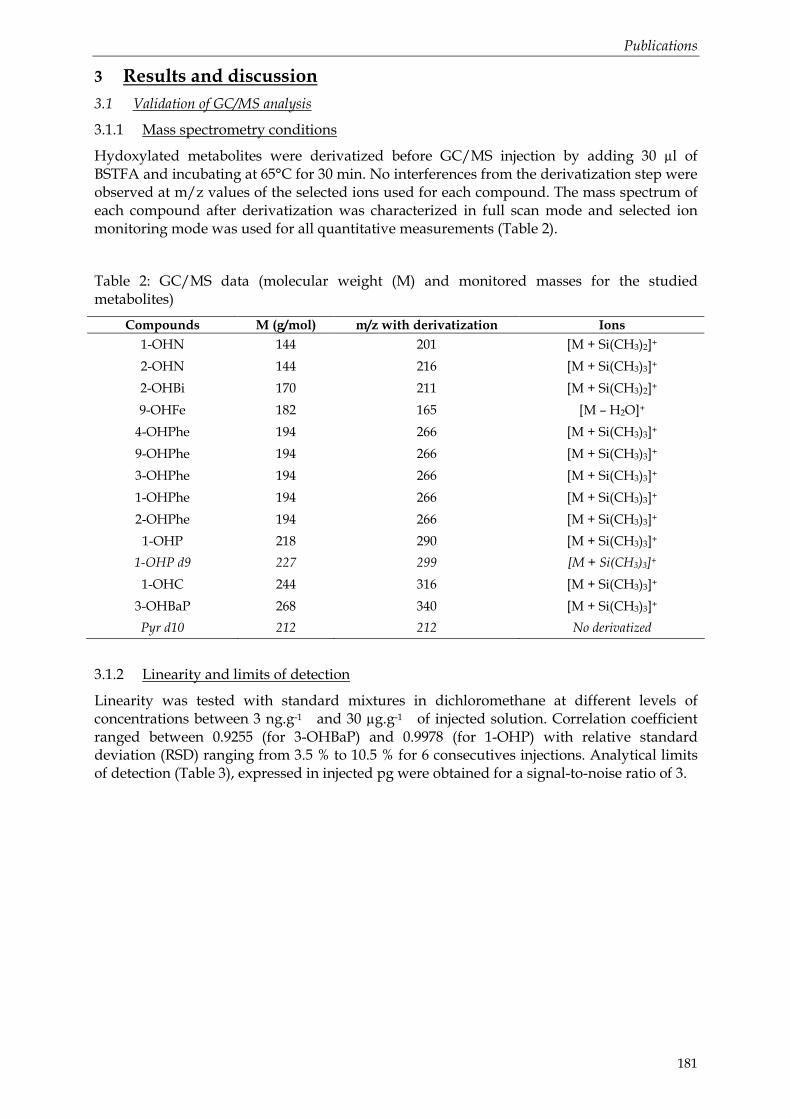
Publications
181
3 Results and discussion
3.1 Validation of GC/MS analysis
3.1.1 Mass spectrometry conditions
Hydoxylated metabolites were derivatized before GC/MS injection by adding 30 µl of BSTFA and incubating at 65°C for 30 min. No interferences from the derivatization step were observed at m/z values of the selected ions used for each compound. The mass spectrum of each compound after derivatization was characterized in full scan mode and selected ion monitoring mode was used for all quantitative measurements (Table 2).
Table 2: GC/MS data (molecular weight (M) and monitored masses for the studied metabolites)
Compounds M (g/mol) m/z with derivatization Ions
1-OHN 144 201 [M + Si(CH3)2]+
2-OHN 144 216 [M + Si(CH3)3]+
2-OHBi 170 211 [M + Si(CH3)2]+
9-OHFe 182 165 [M – H2O]+
4-OHPhe 194 266 [M + Si(CH3)3]+
9-OHPhe 194 266 [M + Si(CH3)3]+
3-OHPhe 194 266 [M + Si(CH3)3]+
1-OHPhe 194 266 [M + Si(CH3)3]+
2-OHPhe 194 266 [M + Si(CH3)3]+
1-OHP 218 290 [M + Si(CH3)3]+
1-OHP d9 227 299 [M + Si(CH3)3]+
1-OHC 244 316 [M + Si(CH3)3]+
3-OHBaP 268 340 [M + Si(CH3)3]+
Pyr d10 212 212 No derivatized
3.1.2 Linearity and limits of detection
Linearity was tested with standard mixtures in dichloromethane at different levels of concentrations between 3 ng.g-1 and 30 µg.g-1 of injected solution. Correlation coefficient ranged between 0.9255 (for 3-OHBaP) and 0.9978 (for 1-OHP) with relative standard deviation (RSD) ranging from 3.5 % to 10.5 % for 6 consecutives injections. Analytical limits of detection (Table 3), expressed in injected pg were obtained for a signal-to-noise ratio of 3.

Publications
182
Table 3: Linearity and Instrumental Detection Limit (IDL) expressed in pg injected (1 µl injected, solvent: dichloromethane)
Analytes m/z Range of
concentrations Linearity R²
RSD (%)
IDL
1-OHN 201 3 ng.g-1 – 30 µg.g-1 y = 23838x - 765 0.9893 5.6 0.17
2-OHN 216 3 ng.g-1 – 30 µg.g-1 y = 14942x - 601 0.9918 5.3 0.28
2-OHBi 211 3 ng.g-1 – 30 µg.g-1 y = 22817x - 234 0.9913 4.6 0.20
9-OHFe 165 3 ng.g-1 – 30 µg.g-1 y = 26284x - 313 0.9878 4.5 0.12
4-OHPhe 266 3 ng.g-1 – 30 µg.g-1 y = 12151x - 133 0.9858 4.5 0.27
9-OHPhe 266 3 ng.g-1 – 30 µg.g-1 y = 12916x - 145 0.9891 4.3 0.43
3-OHPhe 266 3 ng.g-1 – 30 µg.g-1 y = 15309x - 183 0.9829 4.6 0.22
1-OHPhe 266 3 ng.g-1 – 30 µg.g-1 y = 30562x - 347 0.9935 3.9 0.11
2-OHPhe 266 3 ng.g-1 – 30 µg.g-1 y = 17012x - 201 0.9864 3.9 0.22
1-OHP 290 3 ng.g-1 – 30 µg.g-1 y = 22224x - 256 0.9978 3.7 0.28
1-OHP d9 299 3 ng.g-1 – 30 µg.g-1 y = 24142x - 266 0.9955 3.5 0.54
1-OHC 316 3 ng.g-1 – 30 µg.g-1 y = 4679x – 550 0.9843 6.1 2.51
3-OHBaP 340 7 ng.g-1 – 40 µg.g-1 y = 3266x - 4259 0.9255 10.5 8.08
Pyr d10 212 3 ng.g-1 – 30 µg.g-1 y = 25253x - 261 0.9821 5.6 0.27
3.1.3 Quantification
Five calibration solutions were prepared by mixing the internal standard used for quantification (1-hydroxypyrene-d9) and the metabolites of interest. The different solutions were gravimetrically controlled during the preparation. These calibration solutions were injected to calculate response factors of each compound in reference to the internal standard compound. These response factors were then applied to other independent solutions in order to validate the quantitative approach. 6 replicates have been implemented and results are shown in Table 4. The mean recovery ranged between 90 % for 9-OHFe and 110 % for 3-OHPhe with RSD between 1 and 11 %. This allowed the use of 1-hydroxypyrene-d9 as internal standard for the quantification of the 12 studied metabolites.
Table 4: Mean recoveries for the standard solutions of metabolites at different levels (n =6,
mean ± standard deviation).
Compound
3 pg injected
(7 pg for 3-OHBaP)
30 pg injected
(70 pg for 3-OHBaP)
0.3 ng injected
(0,7 ng for 3-OHBaP)
3 ng injected
(7 ng for 3-OHBaP)
30 ng injected
(40 ng for 3-OHBaP)
1-OHN 106 ± 6 105 ± 6 97 ± 5 109 ± 9 96 ± 7
2-OHN 101 ± 10 100 ± 7 92 ± 7 103 ± 9 92 ± 6
2-OHBi 98 ± 8 98 ± 9 90 ± 6 100 ± 6 91 ± 8
9-OHFe 96 ± 9 96 ± 9 88 ± 5 98 ± 5 90 ± 9
4-OHPhe 103 ± 12 106 ± 9 97 ± 7 108 ± 6 99 ± 8
9-OHPhe 98 ± 9 100 ± 8 92 ± 8 103 ± 5 94 ± 5
3-OHPhe 105 ± 11 108 ± 11 99 ± 8 110 ± 5 101 ± 5
1-OHPhe 106 ± 10 109 ± 9 100 ± 5 109 ± 8 102 ± 7
2-OHPhe 105 ± 8 108 ± 7 99 ± 5 108 ± 5 101 ± 6

Publications
183
1-OHP 100 ± 4 103 ± 2 94 ± 1 102 ± 1 96 ± 3
1-OHC 99 ± 6 101 ± 5 93 ± 5 101 ± 8 95 ± 8
3-OHBaP 95 ± 10 97 ± 9 90 ± 9 92 ± 11 91 ± 11
1-OHP d9 105 ± 4 108 ± 3 99 ± 1 101 ± 1 101 ± 2
3.2 Optimisation of the sample preparation protocol
3.2.1 Deconjugation
The efficiency of deconjugation was found to be dependant on the time of the incubation (Figure 3) whatever the protocol tested (solvolysis + enzymes or only enzymes). The normalized concentrations were calculated. The 18 hours-concentrations were set to 100 % for each compound. Two sets of experiments were done. The first one considered only the enzymatic deconjugation. The second one dealt with the combined protocol using solvolysis and enzymatic deconjugation (data not shown). For the enzymatic deconjugation only, some compounds (3-OHBaP and 3-OHPhe) showed increasing concentrations up to 24h, and others showed a decrease after 18h (1-OHC, 9-, 1-, 2-, 4-OHPhe). Most compounds reached a maximum at 18h followed by a subsequent and gradual decrease. When considering the use of solvolysis prior to enzymatic deconjugation, most compounds reached a maximum at 8h. But, no compound reached the maximum concentration obtained with the enzymatic deconjugation (between 25% for 4-OHPhe and 82% for 1–OHP). Therefore the enzymatic deconjugation only with an incubation time of 18h was chosen as the optimum protocol.
3.2.2 Solid-phase extraction
In comparison with reversed phase silica based octadecyle adsorbent (C18) widely used for PAH metabolites extraction [83], three polymeric phases were evaluated: Oasis HLB sorbent, STRATA X sorbent, and STRATA XC sorbent.
Recoveries for the six different sorbents are indicated in Table 5. Results showed a lot of variations from one sorbent to another and for one compound to another. Recoveries ranged between 40 and 89% pour 1-OHN; between 50 to 105 % for 9-OHPhe; between 78 and 105% for 1-OHP; between 63 and 99% for 1-OHC and between 20 and 89% for 3-OHBaP. Recoveries obtained for the internal standard 1-OHP-d9, quantified in comparison with pyrene-d10 used as syringe standard, were between 74 and 98%.
C18-U and C18-S cartridges were obviously not appropriate for the extraction of these compounds due to their lower capacity factor. Oasis HLB phase was able to extract satisfactorily most of the compounds with the exception of 3-OHBaP. The results suggested either a too important elution by water during the rinsing step or a too strong absorption on the cartridge phase of this compound to be eluted with the conditions that were used. STRATA X and STRATA XC phase showed acceptable recoveries for all compounds and especially with the STRATA X phase. When compared to C18 Bakerbond which was used in the reference protocol, a gain in recoveries extraction was observed for all compounds and better standard deviations were obtained. Generally speaking relative standard deviations were lower than 15% for the six sorbents tested.

Publications
Figure 3: Enzymatic deconjugation time optimization, results are normalized using concentrations at 18 hours as reference value.
0
20
40
60
80
100
120
0 6 12 18 24Time (hours)
Nor
mal
ized
con
c. (
18 H
ours
is s
et to
100
%)
1-OHC
0
20
40
60
80
100
120
0 6 12 18 24Time (Hours)
Nor
mal
ized
con
c. (
18 H
ours
is s
et to
100
%)
1-OHP
0
20
40
60
80
100
120
0 6 12 18 24Time (hours)
Nor
mal
ized
con
c. (
18 H
ours
is s
et to
100
%)
4-OHPhe9-OHPhe3-OHPhe1-OHPhe2-OHPhe
0
20
40
60
80
100
120
0 6 12 18 24Time (hours)
Nor
mal
ized
con
c. (
18 H
ours
is s
et to
100
%)
3-OHBaP

Publications
185
Table 5: Comparison of the recovery percentages obtained for the analysis (mean value ± standard deviation, n=3) of bile samples spiked at 10 ng.g-1 for each compound and extracted with six different sorbents.
Compounds C18
Bakerbond JT Baker
C18-S Interchim
C18-U Interchim
OASIS HLB Waters
Strata XC Phenomenex
Strata X Phenomenex
1-OHN 78 ± 8 40 ± 12 55 ± 16 72 ± 10 74 ± 10 89 ± 8
9-OHPhe 83 ± 6 77 ± 11 69 ± 8 98 ± 6 50 ± 6 105 ± 4
1-OHP 90 ± 5 78 ± 9 79 ± 9 102 ± 4 81 ± 6 105 ± 3
1-OHC 82 ± 8 63 ± 9 71 ± 10 79 ± 9 81 ± 9 99 ± 8
3-OHBaP 78 ± 9 57 ± 15 68 ± 11 20 ± 12 75 ± 12 89 ± 9
1-OHP-d9 87 ± 6 75 ± 9 74 ± 9 87 ± 6 94 ± 6 98 ± 6
3.2.3 SPE purification
In order to decrease the limits of detection and to insure a better reliability of the determination, clean-up step of natural samples has been optimized. Results are presented in the Table 6. The use of silica-based PSA and HF PSA cartridges decreased significantly the noise and allowed to lower the limits of detection without significant losses of compounds. The Figure 5 presents a chromatogram obtained in natural fish bile sample. Global recoveries concerning solid-phase extraction on C18 Bakerbond cartridge followed by solid-phase purification on LC-NH2, PSA and HF PSA cartridges ranged from 81% to 105% with RSDs (n = 3) from 0 to 10% for all metabolites.
HF-PSA cartridge was chosen as SPE purification cartridge because of the better recoveries obtained compared to other sorbents and because of the reduction of the baseline noise, which was a significant advantage for polymeric sorbent compared to aminopropyl cartridge.
Table 6: Comparison of the recovery percentages obtained for the analysis (mean value ± standard deviation, n=3) of bile samples spiked at 10 ng.g-1 for each compound, extracted with a silica-based C18 Bakerbond cartridge and purified with three different sorbents.
Compounds LC-NH2 Supelco Bond Elut PSA Varian Bond Elut HF PSA
Varian
1-OHN 78 ± 8 89 ± 6 105 ± 4
9-OHPhe 83 ± 5 90 ± 4 102 ± 6
1-OHP 90 ± 6 90 ± 2 97 ± 2
1-OHC 82 ± 8 88 ± 6 103 ± 5
3-OHBaP 78 ± 10 81 ± 9 97 ± 8
1-OHP-d9 87 ± 6 85 ± 6 94 ± 7
3.2.4 Performances of the methodology
The performance of the methodology (extraction with STRATA X and purification by HF-PSA cartridges) was evaluated estimating the recoveries in spiked water and spiked bile samples at different concentration levels (Table 7). They varied from 67 to 96 % for all compounds. RSD were < 11% in all cases.

Publications
186
Table 7: Mean recoveries for the entire protocol and standard deviations for three replicates at different concentration levels in spiked water and spiked bile samples.
15 ng.g-1 1.5 ng.g-1 0.15 ng.g-1 0.015 ng.g-1 Compounds
Water Bile Water Bile Water Bile Water Bile
1-OHN 93 ± 9 88 ± 9 82 ± 8 78 ± 9 92 ± 10 77 ± 7 78 ± 9 72 ±11
2-OHN 91 ± 8 90 ± 7 88 ± 7 75 ± 9 88 ± 8 81 ± 10 74 ± 10 68 ± 8
2-OHBi 86 ± 10 82 ± 9 76 ± 9 72 ± 10 85 ± 9 78 ± 9 74 ± 10 68 ± 11
9-OHFe 84 ± 9 80 ± 8 75 ± 8 71 ± 11 84 ± 5 77 ± 8 73 ± 9 67 ± 10
4OHPhe 93 ± 8 88 ± 6 83 ± 6 78 ± 9 92 ± 5 85 ± 6 80 ± 9 74 ± 9
9-OHPhe 88 ± 6 84 ± 7 79 ± 9 75 ± 6 87 ± 7 80 ± 5 76 ± 7 70 ± 8
3-OHPhe 95 ± 5 90 ± 8 84 ± 6 80 ± 9 94 ± 8 86 ± 8 82 ± 8 75 ± 6
1-OHPhe 95 ± 7 94 ± 8 96 ± 7 81 ± 6 92 ± 9 85 ± 8 83 ± 8 76 ± 9
2-OHPhe 95 ± 6 90 ± 7 84 ± 8 80 ± 9 91 ± 6 84 ± 9 82 ± 6 75 ± 10
1-OHP 90 ± 3 99 ± 2 90 ± 5 96 ± 5 87 ± 8 97 ± 6 78 ± 7 92 ± 8
1-OHC 89 ± 6 88 ± 6 89 ± 8 75 ± 9 86 ± 8 79 ± 6 77 ± 9 71 ± 8
3-OHBaP 86 ± 8 85 ± 9 86 ± 9 72 ± 10 78 ± 8 72 ± 9 74 ± 10 68 ± 11
LODs were quite similar for all compounds (Table 8) ranging from 1 to 21 ng.g-1. By comparison, Jonsson et al. [98] gave LODs between 1 and 75 ng injected for the same compounds by GC/MS. Romanoff et al. [76] gave LODs between 2 and 10 pg.ml-1 for OH-PAH in urine. The present limits of detection were higher for bile sample. For 1-OHPhe and 1-OHP, differences between GC/MS and GC/HRMS performance were of 5 and 8 times more important, respectively. However one must take into account the matrix differences (urine and bile) which influence the determination of limits of detection. As a result of sample preparation protocol optimization, the present methodology nearly reached analytical performance commonly obtained with high resolution instrument (HRMS). Mazeas and Budzinski [70] already reached instrumental detection limits in the range of 1 injected pg (for 2-OHBi) and 130 injected pg (for 3-OHBaP). The usefulness of sample preparation optimization was thus demonstrated to reach enough sensitivity for its applicability in environmental surveys. However 3-OHBaP recovery and limits of detection were not satisfying. This metabolite of interest could not be quantified in biological fluids of fish collected from the Seine Bay (France).

Publications
187
Table 8: Overall limits of detection (LOD) for OH-PAH in bile (100 µl) and water (3 ml) matrices. Signal-to-noise ratio is 3:1 for LOD.
LOD Compounds
Water (ng.l-1) Bile (ng.g-1 of bile)
1-OHN 0.9 0.9
2-OHN 1.6 3.9
2-OHBi 0.6 1.4
9-OHFe 0.4 1.1
4OPhe 1.0 2.5
9-OHPhe 1.0 2.5
3-OHPhe 0.9 2.3
1-OHPhe 0.4 0.9
2-OHPhe 0.8 1.9
1-OHP 0.6 1.3
1-OHC 4.5 6.6
3-OHBaP 13.6 20.6
The present protocol pushed forward the optimization of the sample preparation protocol and divided by more than 16 times the instrumental limits of detection of 3-OHBaP allowing a greater applicability of the protocol.
3.3 Storage parameters
In order to evaluate the stability of metabolites in biological fluid samples between sampling, extraction and analysis steps, different experiments have been carried out. Trout bile was spiked with a solution of standard in methanol (around 1 µg.g-1, gravimetrically checked) and stored at 4°C, -20°C and -80°C, in darkness. Samples were characterized each month during 6 months. All results dealing with the storage experiments are presented in Figure 4. The three storages gave widely different results. When stored at 4°C, significant losses were measured for all compounds (Mann-Whitney test, p < 0.05). The recoveries ranged between 58% for 3-OHBaP and 77% for 4-OHPhe and the relative standard deviation (RSD) ranged from 14% and 22%. Such high variability in the recoveries rates at 4°C proved the non-suitability of this storage.
When stored at -20°C and -80°C, results showed no significant losses (measured mean concentrations were statistically the same in both experiments at a probability level of 95 % (Mann-Whitney test)). The recoveries range from 71% for 3-OHBaP and 98% for 4- and 9-OHPhe. The RSD vary between 4% and 14% for the storage at -20°C and between 4% and 10% for the storage at -80°C.
Therefore, it has been chosen to store the bile sample at -80°C just after sampling, particularly when analysis is not performed in the month. Considering the results of the storage study, they can ensure compound conservation and analysis validity over six months storage.

Publications
188
Figure 4: Effect of temperature on storage stability of PAH metabolites in spiked biles after six months. Results are expressed as mean percentage of the initial concentration (standard deviation, n = 6).
3.4 Application to the Seine Estuary samples
To assess the exposure of fish to PAH in the Seine estuary and to evaluate the optimized procedure for bile samples, sampling was conducted at different sites of the Seine estuary mouth in September 2006. The sensitivity of the analytical procedure was sufficient to detect most of the studied compounds. The entire protocol was applied to ten bile samples for each group of dabs collected from the Seine Bay (Adult males and females, juvenile males and females). 100 µl (0.1 g) of bile samples were analyzed. After the sample loading on the STRATA X cartridge, the rinsing step with water and more particularly with water/methanol showed the removal of matrix constituents, which resulted in a clearer extract being obtained and a slower clogging of the GC/MS than with water rinsing alone. However, the obtained extract remained strongly concentrated in bile pigments. The HF PSA purification step with methanol/methylene chloride elution (20:80, v/v) proved to be efficient, ensuring a strongly selective elution of the metabolites with retention of most of the bile pigments in the first millimeters of the phase. The resulting extracts were completely colourless and transparent.
After GC/MS analysis, different metabolites could be detected and quantified in the bile (Figure 6). 1- and 2-hydroxynaphthalene, 2-hydroxybiphenyl, 9-hydroxyfluorene and 1-hydroxypyrene were identified. 4-hydroxy and 9-hydroxyphenanthrene isomers were not detected but three other isomers (1-, 2- and 3-hydroxyphenanthrene) could be quantified. 1-hydroxychrysene and 3-hydroxybenzo(a)pyrene were not detected in any sample either. Major metabolites were found to be 1-OHP, the hydroxyphenanthrene isomers (OHPhe) and the 2-OHBi. The average concentrations and standard deviations obtained for the samples are presented in Table 9.
0
20
40
60
80
100
1-OHN
2-OHN
2-OHBi
9-OHFe
4-OHPhe
9-OHPhe
3-OHPhe
1-OHPhe
2-OHPhe
1-OHP
1-OHC
3-OHBaP
1-OHP d
9
Rec
over
y R
ate
(%)
4°C' -20°C' -80°C'

Publications
189
8 10 12 14 16 18
Retention time (min)
Ab
un
dan
ce
2-OHN
OHPhe
1-OHPd9
1-OHP1-OHN
2-OHBi
9-OHFe
Pyr d10
Figure 5: Chromatogram obtained for a fish bile sample analysed by GC/MS in SIM mode.
0
100
200
300
400
500
600
700
800
Con
c. O
HP
AH
in b
ile (
ng/g
of b
ile)
FJ G MJ G FA G MA G FJ ES MJ ES FA ES MA ES
1-OHP
OHPhe
9-OHFe
2-OHBi
2-OHN
1-OHN
GRANULATS
ESTUARY (ES)
Figure 6: Mean concentrations of the different metabolites detected in the bile of dabs collected from two locations of the Seine Bay (Estuary and Granulats). Concentrations expressed in ng.g-1 of bile. ES: estuary, G: granulats, F: female, M: male, J: juvenile, A: adult.
The results suggest a stronger exposure to PAHs of dabs for the Seine mouth (Seine Estuary) (global concentration of 580 ± 68 ng.g-1) than for dabs from Seine Bay (Granulats) (global concentration of 267 ± 33 ng.g-1). No significant difference has been found between juveniles and adults (Mann-Whitney test, p < 0.05). This result does not agree with previous studies

Publications
190
[99] in which juvenile soles exhibited higher metabolite concentrations in bile than adults. However one should not forget that only one campaign has been taken into account in this study. More samplings have to be done to ensure conclusions. Indeed, metabolism processes are known to be affected by biotic and abiotic factors [100]. Temperature, sex and sexual maturity are predominant factors in the temporal and spatial variations of PAH biotransformation in fish. In general biotransformation processes and rates are correlated to gonads maturity [11] and thus the cycle of reproduction of dabs has to be taken into account when discussing of PAH metabolites concentrations during September 2006.
4 Conclusions
We have developed and validated an analytical method for the quantitative analysis of 12 OH-PAH metabolites in bile by GC/MS analysis. We have optimized each step in the method which has resulted in a sensitive and precise analytical method that only requires a small bile volume (100 µl). The major goal of the work was to develop a simple SPE-GC method is by optimizing the extraction process, by maximizing the recovery of the target analytes and minimizing the amount of co-eluted impurities, under conditions which provide efficient and reproducible GC separation and detection. This work has provided a high-throughput, precise and low cost method based on GC/MS detection, which has been proved ideal for analyzing samples for environmental surveys. Preliminary results demonstrated the applicability of the method which was applied to natural fish bile samples. PAH metabolites were quantified in the range of few ng.g-1 to more than 100 ng.g-1, demonstrating the interest to monitor PAH metabolites to assess PAH marine organisms exposure. The develop protocol is simple and robust and should enable more frequent and less expansive environmental surveys.
Acknowledgements: The authors wish to thank the National Program of Ecotoxicology (PNETOX program1), the French National Research Agency (ANR) and the research team IMOPHYS for research funding. They want also to acknowledge the “Region Aquitaine” and the French National Council for Scientific Research (CNRS) for providing the PhD grant of M. Le Dû-Lacoste.
1 http://www.ecologie.gouv.fr/-PNETOX-.html, 10/10/08.
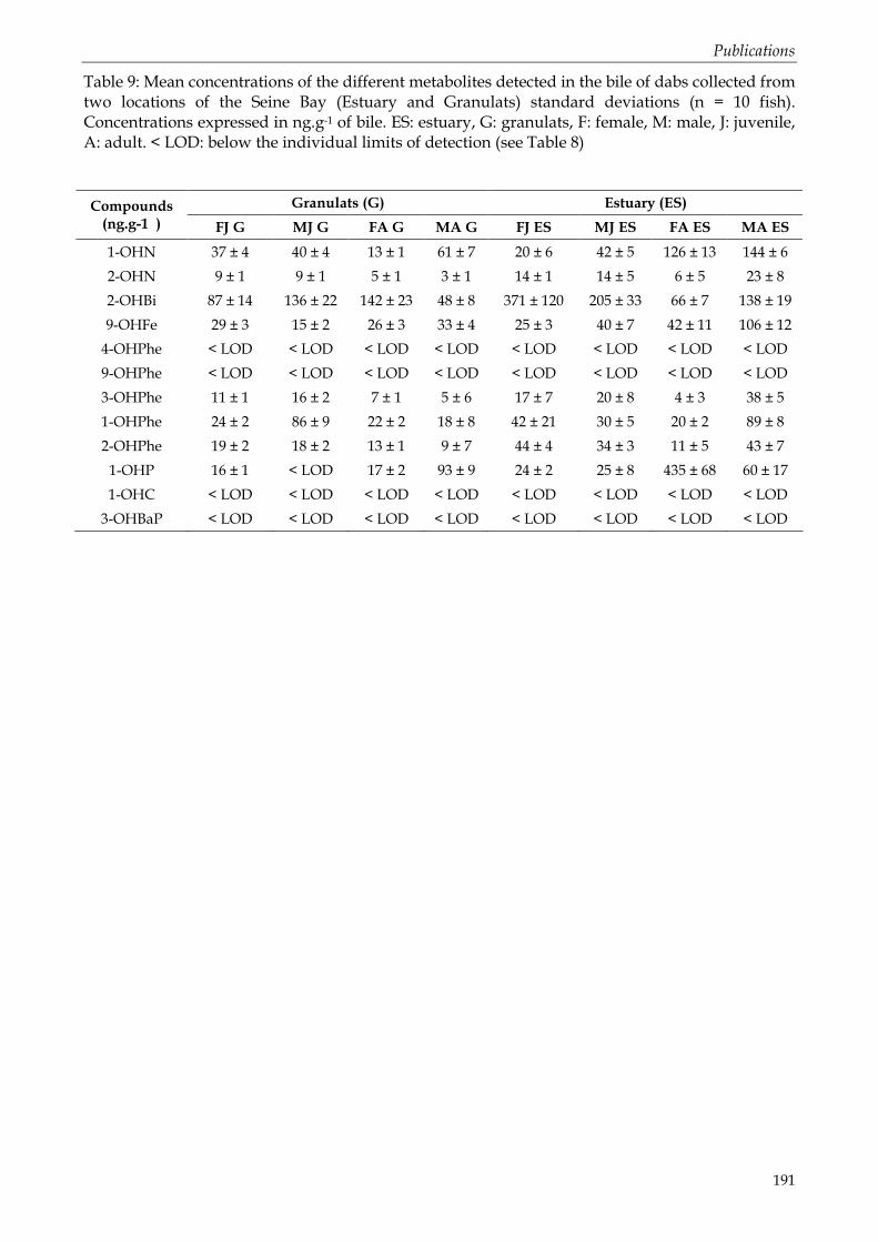
Publications
191
Table 9: Mean concentrations of the different metabolites detected in the bile of dabs collected from two locations of the Seine Bay (Estuary and Granulats) standard deviations (n = 10 fish). Concentrations expressed in ng.g-1 of bile. ES: estuary, G: granulats, F: female, M: male, J: juvenile, A: adult. < LOD: below the individual limits of detection (see Table 8)
Granulats (G) Estuary (ES) Compounds (ng.g-1 ) FJ G MJ G FA G MA G FJ ES MJ ES FA ES MA ES
1-OHN 37 ± 4 40 ± 4 13 ± 1 61 ± 7 20 ± 6 42 ± 5 126 ± 13 144 ± 6
2-OHN 9 ± 1 9 ± 1 5 ± 1 3 ± 1 14 ± 1 14 ± 5 6 ± 5 23 ± 8
2-OHBi 87 ± 14 136 ± 22 142 ± 23 48 ± 8 371 ± 120 205 ± 33 66 ± 7 138 ± 19
9-OHFe 29 ± 3 15 ± 2 26 ± 3 33 ± 4 25 ± 3 40 ± 7 42 ± 11 106 ± 12
4-OHPhe < LOD < LOD < LOD < LOD < LOD < LOD < LOD < LOD
9-OHPhe < LOD < LOD < LOD < LOD < LOD < LOD < LOD < LOD
3-OHPhe 11 ± 1 16 ± 2 7 ± 1 5 ± 6 17 ± 7 20 ± 8 4 ± 3 38 ± 5
1-OHPhe 24 ± 2 86 ± 9 22 ± 2 18 ± 8 42 ± 21 30 ± 5 20 ± 2 89 ± 8
2-OHPhe 19 ± 2 18 ± 2 13 ± 1 9 ± 7 44 ± 4 34 ± 3 11 ± 5 43 ± 7
1-OHP 16 ± 1 < LOD 17 ± 2 93 ± 9 24 ± 2 25 ± 8 435 ± 68 60 ± 17
1-OHC < LOD < LOD < LOD < LOD < LOD < LOD < LOD < LOD
3-OHBaP < LOD < LOD < LOD < LOD < LOD < LOD < LOD < LOD
Publications
192
References
1. Malins, D. C., McCain, B. B., Myers, M. S., Brown, D. W., Krahn, M. M., Roubal, W. T., Schiewe, M. H., Landahl, J. T., and Chan, S. L. 1987. Environmental health perspectives 71: p. 5-16.
2. Myers, M. S., Landahl, J. T., Krahn, M. M., and McCain, B. B. 1991. Environmental Health Perspectives 90: p. 7-15.
3. Varanasi, U. and Stein, J. E. 1991. Environmental Health Perspectives 90: p. 93-100.
4. IARC, Monographs on the Evaluation of the Carcinogenic Risk of Chemicals to Human. Vol 32. 1983, International Agency for Research on Cancer: Lyon, France. p. 57-61.
5. Zhang, W., Xu, D., Zhuang, G., Ding, C., Wang, G., Chang, J., and Ren, G. 2007. Environmental Monitoring and Assessment 131(1-3): p. 387-394.
6. Ruchirawat, M., Settachan, D., Navasumrit, P., Tuntawiroon, J., and Autrup, H. 2007. Toxicology Letters 168(3): p. 200-209.
7. Palmqvist, A., Rasmussen, L. J., and Forbes, V. E. 2006. Aquatic Toxicology 80(3): p. 309-319.
8. Inzunza, B., Orrego, R., Penalosa, M., Gavilan, J. F., and Barra, R. 2006. Ecotoxicology and Environmental Safety 65(2): p. 242-251.
9. Fragoso, N. M., Hodson, P. V., and Zambon, S. 2006. Environmental Monitoring and Assessment 116(1-3): p. 481-511.
10. Aina, R., Palin, L., and Citterio, S. 2006. Chemosphere 65(4): p. 666-673.
11. van der Oost, R., Beyer, J., and Vermeulen, N. P. E. 2003. Environmental Toxicology and Pharmacology 13(2): p. 57-149.
12. Robertson, A. 1998Petroleum Hydrocarbons, in Amap Assessment Report: Arctic Pollution Issues, Wilson, S.J., Murray, J.L., and Hungtington, H.P., Editors: Oslo. p. 859
13. James, M. O. 1989Biotransformation and Disposition of Pah in Aquatic Invertebrates, P 69-92, in Metabolism Fo Polycyclic Aromatic Hydrocarbons in the Aquatic Environment, Varanasi, U., Editor CRC Press: Boca Raton. p. 341.
14. Neff, J. M., Polycyclic Aromatic Hydrocarbons in the Aquatic Environment: Sources, Fates and Biological Effects. 1979, London: Applied Science Publishers Ltd. 262.
15. Lee, R. F., Sauerheber, R., and Dobbs, G. H. 1972. Marine Biology 17: p. 201-208.
16. Varanasi, U. and Gmur, D. J. 1981. Aquatic Toxicology 1(1): p. 49-67.
17. Varanasi, U., Reichert, W. L., Stein, J. E., Brown, D. W., and Sanborn, H. R. 1985. Eviron. Sci. Technol. 19: p. 836-841.
18. Varanasi, U., Chan, S. L., McLeod, W. D., Stein, J. E., Brown, D. W., Burrows, D. G., Tilbury, K. L., Landahl, J. T., Wigren, C. A., Hom, T., and Pierce, S. M., Noaa Technical

Publications
193
Memorandum: Survey of Subsistence Fish and Shellfish for Exposure to Oil Spilled from the Exxon Valdez : First Year, 1989., US Department of Commerce, S., Editor. 1990.
19. Tuvikene, A. 1995. Ann. Zool. Fenn. 32: p. 295-309.
20. Baumard, P., Budzinski, H., Garrigues, P., Sorbe, J. C., Burgeot, T., and Bellocq, J. 1998. Marine Pollution Bulletin 36(12): p. 951-960.
21. Nakata, H., Sakai, Y., Miyawaki, T., and Takemura, A. 2003. Environmental science & technology 37(16): p. 3513-3521.
22. Meador, M. R., Brown, L. R., and Short, T. 2003. Ecological Indicators 3(2): p. 81-92.
23. Kammann, U. 2007. Environmental Science and Pollution Research 14(2): p. 102-108.
24. Johnson, L. L., Ylitalo, G. M., Arkoosh, M. R., Kagley, A. N., Stafford, C., Bolton, J. L., Buzitis, J., Anulacion, B. F., and Collier, T. K. 2007. Environmental Monitoring and Assessment 124(1-3): p. 167-194.
25. Vuorinen, P. J., Keinanen, M., Vuontisjarvi, H., Barsiene, J., Broeg, K., Forlin, L., Gercken, J., Kopecka, J., Kohler, A., Parkkonen, J., Pempkowiak, J., and Schiedek, D. 2006. Marine Pollution Bulletin 53(8-9): p. 479-487.
26. Pikkarainen, A. L. 2006. Chemosphere 65(10): p. 1888-1897.
27. Krahn, M. M., Burrows, D. G., MacLeod, W. D., and Malins, D. 1987. Archives of Environmental Contamination and Toxicology 16(5): p. 511-522.
28. Krahn, M. M., Kittle, J., Lewey J., and MacLeod, J., William D. 1986. Marine Environmental Research 20(4): p. 291-298.
29. McDonald, S. J., Kennicutt II, M. C., Liu, H., and Safe, S. H. 1995. Arch. Environ. Contam. Toxicol. 29: p. 232-240.
30. Van der Oost, R., Van Schooten, F.-J., Ariese, F., Heida, H., Satumalay, K., and Vermeulen, N. P. E. 1994. Environmental Toxicology and Chemistry 13(6): p. 859-870.
31. Krahn, M. M., Moore, L. K., and McLeod, W. D., Standard Analytical Procedures of the Noaa National Analytical Facility, 1986 : Metabolites of Aromatic Compounds in Fish Bile., US Department of Commerce, S., Editor. 1986, NOAA Technical Memorandum NMFS F/NWC-102.
32. Vuontisjärvi, H., Keinänen, M., Vuorinen, P. J., and Peltonen, K. 2004. Polycycl. Aromat. Compd. 24: p. 333-342.
33. Jonsson, G., Taban, I. C., Jorgensen, K. B., and Sundt, R. C. 2004. Chemosphere 54(8): p. 1085-1097.
34. Jonsson, G., Beyer, J., Wells, D., and Ariese, F. 2003. J. Environ. Monit. 5: p. 513-520.
35. Ferrari, S., Mandel, F., and Berset, J. D. 2002. Chemosphere 47(2): p. 173-182.
36. Gündel, J. and Angerer, J. 2000. Journal of Chromatography B: Biomedical Sciences and Applications 738(1): p. 47-55.

Publications
194
37. Lee, C.-K., Cho, S.-H., Kang, J.-W., Lee, S.-J., Ju, Y.-S., Sung, J., Strickland, P. T., and Kang, D. 1999. Toxicology Letters 108(2-3): p. 209-215.
38. Galceran, M. T. and Moyano, E. 1994. Journal of Chromatography A 683(1): p. 9-19.
39. Mastenbroek, J. W. G., Ariese, F., Gooijer, C., Velthorst, N. H., Hofstraat, J. W., and van Zeijl, W. J. M. 1990. Chemosphere 21(3): p. 377-386.
40. Lin, E. L. C., Cormier, S. M., and Racine, R. N. 1994. Environmental Toxicology and Chemistry 13(5): p. 707-715.
41. Ariese, F., Burgers, I., Oudhoff, K., Rutten, T., Stroomberg, G., and Vethaak, D. 1997.
42. Aas, E. and Klungsoyr, J. 1998. Marine Environmental Research 46(1-5): p. 229-232.
43. Ariese, F., Kok, S. J., Verkaik, M., Gooijer, C., Velthorst, N. H., and Hofstraat, J. W. 1993. Aquatic Toxicology 26(3-4): p. 273-286.
44. Lin, E. L. C., Cormier, S. M., and Torsella, J. A. 1996. Ecotoxicology and Environmental Safety 35(1): p. 16-23.
45. Aas, E., Beyer, J., and Goksoyr, A. 2000. Biomarkers 5(1): p. 9-23.
46. Yang, X. and Baumann, P. C. 2006. Ecological Indicators 6(3): p. 567-574.
47. Schiedek, D., Broeg, K., Bars?iene, J., Lehtonen, K. K., Gercken, J., Pfeifer, S., Vuontisja?rvi, H., Vuorinen, P. J., Dedonyte, V., Koehler, A., Balk, L., and Schneider, R. 2006. Marine Pollution Bulletin 53(8-9): p. 387-405.
48. Mdegela, R., Myburgh, J., Correia, D., Braathen, M., Ejobi, F., Botha, C., Sandvik, M., and Skaare, J. U. 2006. Ecotoxicology 15(1): p. 51-59.
49. Martinez-Gomez, C., Campillo, J. A., Benedicto, J., Fernandez, B., Valdes, J., Garcia, I., and Sanchez, F. 2006. Marine Pollution Bulletin 53(5-7): p. 305-314.
50. Malins, D. C., Anderson, K. M., Stegeman, J. J., Jaruga, P., Green, V. M., Gilman, N. K., and Dizdaroglu, M. 2006. Environmental health Perspectives 114(6): p. 823-829.
51. Da Silva, D. A. M., Buzitis, J., Krahn, M. M., Bicego, M. C., and Pires-Vanin, A. M. S. 2006. Marine Pollution Bulletin 52(2): p. 175-183.
52. Barsiene, J., Lehtonen, K. K., Koehler, A., Broeg, K., Vuorinen, P. J., Lang, T., Pempkowiak, J., Syvokiene, J., Dedonyte, V., and Rybakovas, A. 2006. Marine Pollution Bulletin Volume 53(Issues 8-9): p. Pages 422-436.
53. Fuentes-Rios, D., Orrego, R., Rudolph, A., Mendoza, G., Gaviln, J. F., and Barra, R. 2005. Chemosphere 61(2): p. 192-199.
54. Santana Rodriguez, J. J. and Miller, J. N. 1998. Analyst 123(11).
55. Jonsson, G., Sundt, R. C., Aas, E., and Beyer, J. 2004. Chemosphere 56(1): p. 81-90.
56. Elovaara, E., Mikkola, J., Makela, M., Paldanius, B., and Priha, E. 2006. Toxicology Letters 162: p. 158-163.
57. Hellou, J. and Leonard, J. 2004. Polycyclic Aromatic Compounds 24(4-5): p. 697-712.

Publications
195
58. Solbakken, J. E., Palmork, K. H., Neppelberg, T., and Scheline, R. R. 1980. acta pharmacol. et toxicol. 46: p. 127-132.
59. Krahn, M. M., Ylitalo, G. M., Buzitis, J., Chan, S.-L., and Varanasi, U. 1993. Journal of Chromatography A 642(1-2): p. 15-32.
60. Hellou, J. and Payne, J. F. 1987. Environmental Toxicology and Chemistry 6: p. 857-862.
61. Deshpande, A. D. 1988. Marine Environmental Research 24(1): p. 119-120.
62. Deshpande, A. D. 1989. Archives of environmental contamination and toxicology 18(6): p. 900-907.
63. Yu, Y., Wade, T. L., Fang, J., McDonald, S., and Brooks, J. M. 1995. Archives of Environmental Contamination and Toxicology 29(2): p. 241-246.
64. Escartin, E. and Porte, C. 1999. Environ Sci Technol 33: p. 2710-2714.
65. Troisi, G. M., Bexton, S., and Robinson, I. 2006. Environmental Science and Technology 40(24): p. 7938-7943.
66. Romanoff, L., Li, Z., Young, K., Blakely, N., Patterson Jr, D., and Sandau, C. 2006. Journal of Chromatography B: Analytical Technologies in the Biomedical and Life Sciences 835(1-2): p. 47-54.
67. Luan, T. G., Yu, K. S. H., Zhong, Y., Zhou, H. W., Lan, C. Y., and Tam, N. F. Y. 2006. Chemosphere 65(11): p. 2289-2296.
68. Gmeiner, G., Gartner, P., Krassnig, C., and Tausch, H. 2002. Journal of Chromatography B: Analytical Technologies in the Biomedical and Life Sciences 766(2): p. 209-218.
69. Gmeiner, G., Krassnig, C., Schmid, E., and Tausch, H. 1998. Journal of Chromatography B: Biomedical Sciences and Applications 705(1): p. 132-138.
70. Mazéas O and Budzinski H. 2005. Anal. Bioanal.Chem 383: p. 985-990.
71. Richardson, D. M., Davies, I. M., Moffat, C. F., Pollard, P., and Stag, R. M. 2001. J Environ Monit 3(6): p. 610-615.
72. Schanke, A. v., Holtz, F., der Meer, J. v., Boon, J. P., Ariese, F., Stroomberg, G., den Berg, M. v., and Everaarts, J. M. 2001. Environmental Toxicology and Chemistry 20(8): p. 1641-1647.
73. Steward, A. R., Kandaswami, C., Chidambaram, S., Ziper, C., Rutkowski, J. P., and Sikka, H. C. 1990. Environmental Toxicology and Chemistry 9: p. 1503-1512.
74. Krahn, M. M., Burrows, D. G., Ylitalo, G. M., Brown, D. W., Wigren, C. A., Collier, T. K., Chan, S.-L., and Varanasi, U. 1992. Environ Sci Technol 26: p. 116-126.
75. Maisonnette, C., Simon, P., Hennion, M. C., and Pichon, V. 2006. Journal of Chromatography A 1120(1): p. 185-193.
76. Romanoff L.C, Li Z, Young K.J, Blakely N.C, Patterson Jr D.G, and Sandau C.D. 2006. Journal of Chromatography B: Analytical Technologies in the Biomedical and Life Sciences 835(1-2): p. 47-54.

Publications
196
77. Grova, N., Monteau, F., Le Bizec, B., Feidt, C., Andre, F., and Rychen, G. 2005. Journal of analytical toxicology 29(3): p. 175-181.
78. Van de Wiele, T. R., Peru, K. M., Verstraete, W., Siciliano, S. D., and Headley, J. V. 2004. Journal of Chromatography B 806(2): p. 245-253.
79. Munoz-Olivas, R. 2004. TrAC Trends in Analytical Chemistry 23(3): p. 203-216.
80. McElroy, A. E., Farrington, J. W., and Teal, J. M. 1990. Environ Sci Technol 24: p. 1648-1655.
81. Simpson, C. D., Cullen, W. R., He, T. Y. T., Ikonomou, M., and Reimer, K. J. 2002. Chemosphere 49(3): p. 315-322.
82. Law, F. C. P., Meng, J. X., He, Y. T., and Chui, Y. C. 1994. Xenobiotica 24(3): p. 221-229.
83. Mazéas, O. and Budzinski, H. 2005. Analytical and bioanalytical chemistry 383(6): p. 985-990.
84. Statham, C., Melancon, M. J., and Lech, J. J. 1976. Nature 193: p. 680-681.
85. Varanasi, U., Eberhart, B. T., Nishimoto, M., and Reichert, W. 1985. Proceedings of the American Association for Cancer Research VOL. 26.
86. Varanasi, U., Nishimoto, M., Reichert, W. L., and Le Eberhart, B. T. 1986. Cancer Research 46(8): p. 3817-3824.
87. Varanasi, U., Reichert, W. L., Le Eberhart, B. T., and Stein, J. E. 1989. Chemico-Biological Interactions 69(2-3): p. 203-216.
88. Leonard, J. D. and J., H. 2001. Environmental Toxicology and Chemistry 20(3): p. 618-623.
89. Keith, L. H. and Telliard, W. A. 1979. Environ Sci Technol 13: p. 416-423.
90. Aas, E., Beyer, J., and Goksoyr, A. 1998. Marine Environmental Research 46(1-5): p. 225-228.
91. Smith, C. J., Walcott, C. J., Huang, W., Maggio, V., Grainger, J., and Patterson, J., Donald G. 2002. Journal of Chromatography B 778(1-2): p. 157-164.
92. Galceran, M. T. and Moyano, E. 1996. Journal of Chromatography A 731(1-2): p. 75-84.
93. Koeber, R., Niessner, R., and Bayona, J. M. 1997. Fresenius J Anal Chem 359: p. 267-273.
94. Xu, X., Zhang, J., Zhang, L., Liu, W., and Weisel, C. P. 2004. Rapid Communication in Mass Spectrometry 18: p. 2299-2308.
95. Pigini, D., Cialdella, A. M., Faranda, P., and Tranfo, G. 2006. Rapid Communication in Mass Spectrometry 20: p. 1013-1018.
96. Wang, J. J., Frazer, D. G., Law, B., and Lewis, D. M. 2003. Analyst 128(7): p. 864-870.
97. Zhu, S., Li, L., Thornton, C., Carvalho, P., Avery, B. A., and Willett, K. 2008. Journal of chromatography B 863(1): p. 141-149.

Publications
197
98. Jonsson, G., Beyer, J., Wells, D., and Ariese, F. 2003. Journal of Environmental Monitoring 5: p. 513-520.
99. Budzinski, H., Mazéas, O., Tronczynski, J., Desaunay, Y., Bocquene, G., and Claireaux, G. 2004. Aquat. Living Resour. 17: p. 329-334.
100. Kopecka, J., Lehtonen, K. K., Barsiene, J., Broeg, K., Vuorinen, P. J., Gercken, J., and Pempkowiak, J. Marine Pollution Bulletin In Press, Corrected Proof.

Publications
198

Publications
199
Publication n°2
Quantification of biliary polycyclic aromatic hydrocarbon metabolites by gas chromatography coupled to tandem mass spectrometry with comparison to conventional gas chromatography.
Justyna Sekula1,2, Marie Le Dû-Lacoste2, Karyn Le Menach2, Luc Nagels1, Hélène Budzinski2*
1 Antwerp University, Chemistry Department, Groenenborgerlaan 171, B-2020 Antwerp,
Belgium
2 Universite de Bordeaux ISM-LPTC UMR 5255 CNRS, 351 Cours de La Liberation, 33405
Talence, France
* Corresponding author: [email protected]
Tel: + 33 540 006 998
Fax: + 33 540 002 267
Abstract
An analytical procedure for the determination of five polycyclic aromatic hydrocarbon metabolites (2-hydroxynaphtalene, 1-hydroxyphenanthrene, 1-hydroxypyrene, 1-hydroxychrysene and 3-hydroxybenzo(a)pyrene) in fish bile has been developed. For this purpose the use of gas chromatography coupled with MS/MS detection was examined. The limits of detection for spiked bile samples were less than or equal to 2.8 pg injected for each metabolite. The method demonstrated good recoveries (79-102 %) for all the analytes, excluding 3-hydroxybenzo(a)pyrene (63 %) and good precision (3-11 %). The entire protocol was applied to the analysis of several bile samples from hake fish (Merluccius merluccius).
Keywords: PAH metabolites, fish bile, GC-MS/MS, 3-hydroxybenzo(a)pyrene.
Submitted to Journal of Chromatography B

Publications
200
1 Introduction
Polycyclic aromatic hydrocarbons (PAHs) are a group of over 100 different chemicals, typically formed during incomplete combustion [1, 2, 3] of materials such as coal [4], oil [5], garbage or other organic substances like tobacco or charbroiled meat [6, 7]. PAHs can also enter the air as releases from volcanoes [8], forest fires [9], and car exhausts. Fires can form fine PAH particles [10, 11]. They bind to ash particles and can move over a long distance through the air [12, 13, 14]. High exposure to PAHs occurs in several industries and occupations: aluminium production, chimney sweeping, iron and steel foundries. As well as in shale oil extraction, wood impregnation, road paving, carbon black production, carbon electrode and calcium carbide production [15]. Many of these compounds are mutagenic [16, 17, 18], and carcinogenic [19, 20, 21] and some have been reported to cause reproductive toxicity in both aquatic [22, 23], and non-aquatic animals [24, 25]. PAHs can enter into the groundwater from ash, tar or creosote that is improperly disposed on landfills. They enter the aquatic environment [26] from a variety of sources, for example, municipal and industrial waste effluents, atmospheric fallout of airborne particles, oil spills and surface runoff from land [27, 28, 29].
Elevated concentrations of PAHs in the air and water can lead to significant environmental effects in both marine and fresh water systems. PAH concentrations are rarely high enough to kill aquatic organisms outright. Physical and biochemical changes often result from prolonged exposure to low levels of these compounds [30]. Once in the aquatic systems, most PAHs are associated with the particulate phase due to their hydrophobic properties giving rise to accumulation in sediments [31, 32, 33]. PAHs present in sediments can be rapidly absorbed by fish via the gills and body surface what have resulted in liver damage and tumors in flatfish (which live on or near the bottom), and affect reproduction [34, 35]. The exposure and contamination of aquatic organisms to PAHs have generally been evaluated by the quantification of bioaccumulated PAHs in tissues.
However, this approach is open to criticism when taking into account the biotransformation abilities of biological organisms such as vertebrates and the toxic properties of such biotransformation products. Monohydroxylated PAHs are known to be some of the major metabolites excreted in the gall bladder, either present in their free form but mainly conjugated with glucuronide, glutathione and sulphate groups [36, 37, 38]. These more soluble conjugated metabolites are formed in the liver, concentrated in the bile and are ultimately excreted [39, 40, 41, 42, 43]. As a consequence, tissue levels of parent PAHs do not usually provide an adequate assessment of the exposure level [44, 45]. In this sense, the aim of this study was to evaluate the impact of PAH metabolites in order to study the exposure and contamination of organisms to PAHs in the marine environment [46, 47, 48]. The presence of PAH metabolites in fish bile has been used as an indicator of exposure to PAH [49, 50].
For this purpose, we considered two chromatographic methods: liquid and gas phase chromatography coupled with mass spectrometry (LC/MS and GC/MS). Several groups have worked on the analysis of OH-PAH using HPLC or gas chromatography (GC) prior to mass spectrometry (MS) detection [51, 52, 53]. Both methods were tested and compared in the past by our group [54] for the detection of selected hydroxyl-metabolites of PAHs. LC/MS provided lower detection limits but only with GC/MS whole sets of compounds were detected. Moreover good separation was only achieved by gas chromatography. LC/MS is to some extent a less mature technique and there are no spectral libraries available for compound identification as there are with GC instruments. However, due to limitations of volatility it is necessary to perform derivatization steps before sample injections to the GC/MS. The sample size used for gas chromatography is usually between 1 and 5 µl, which was important in this study as we normally have only small amounts of natural samples. It is also necessary to monitor the contamination at very low levels.
An alternative approach for GC/MS is tandem mass spectrometry (MS/MS), where a target compound ion is isolated from matrix and then fragmented to generate very unique spectra. In

Publications
201
GC/MS the sample is usually ionised directly (EI), or indirectly (CI) by an electron beam. The high-energy electrons cause the formation of free radical ions. In fact the electron beam is often energetic enough to cause substantial fragmentation. The fragments are also free radicals, and form the "fingerprint" that is used in confirmation of identity. This fingerprint is compared with library fingerprints; NIST is probably the most widely used library.
There is an obvious need for test procedures that provide unambiguous results in the low concentrations range for PAH metabolites. The selectivity advantage of GC-MS/MS allows an analyst to quantify and identify components on very low levels in the most difficult matrices. GC-MS/MS provides extreme selectivity against matrix interferences through few separation mechanisms: chromatographic separation on GC column with accompanying knowledge of the retention time, isolation of a characteristic ion, fragmentation of the isolated ion to a unique set of product ions which unambiguously identifies the presence or absence of the targets.
To this end, an analytical methodology to quantify PAH metabolites by GC-MS/MS in biological matrices (bile) was developed as coupling GC with MS/MS became a new powerful and very sensitive method. The following compounds (Figure 1) known to be some of the major metabolites produced by fish were chosen: 2-naphtol, 1-phenanthrol, 1-pyrenol, 1-chrysenol and 3-benzo(a)pyrenol .
OH
OHOH
OH
1-hydroxypyrene
2-hydroxynaphtalene 1-hydroxyphenanthrene
1-hydroxychrysene 3-hydroxybenzo(a)pyrene
OH
Figure 1: The five studied hydroxylated polycyclic aromatic hydrocarbons metabolites (OH-PAHs).
2 Materials and Methods
2.1 Chemical and reagents
All reagents and solvents were of analytical or HPLC grade quality (> 98%). 2-hydroxynaphtalene (2-OHN) was purchased from Lancaster (Bischeim, France), 1-hydroxyphenanthrene (1-OHPhe), 1-hydroxychrysene (1-OHC) and 3-hydroxybenzo(a)pyrene (3-OHBaP) were from Promochem (Molsheim, France). 1-hydroxypyrene (1-OHP) was from Sigma-Aldrich (Saint Quentin Falavier, France); 1-hydroxypyrene-d9 (1-OHPd9) and pyrene-d10 (Pd10) were obtained from Cambridge Isotope Laboratories (Cluzeau Info Labo, Ste Foy La Grande, France). Dichloromethane was supplied by Acros Organics (Noisy-Le-Grand, France). Methanol Supersolv was provided by Merck, acetic acid 100% Normapur (analytical reagent
grade, Scharlau) was obtained from ICS (Belin-Beliet, France). β-glucuronidase-aryl-sulfatase mixture from Helix pomatia (100,000 and 7,500 units/ml respectively) and sodium acetate trihydrate 99% (purity > 99%) were provided by Sigma Aldrich (St Quentin Falavier, France). Trifluoroacetic acid (Reagent grade, purity > 99%) was obtained from Fischer chemicals (Fischer Scientific Labo, Elancourt, France). 2-mercaptoethanol and bis(trimethylsylil)-trifluoroacetamide (BSTFA) were purchased from Acros Organics (Noisy-Le-Grand, France).

Publications
202
Deionised water was obtained with a Milli-Q system (Millipore, Molsheim, France). The cartridges used for solid phase extraction (SPE) were silica-based cartridges, BakerBond Elut C18 (3 ml, 500 mg) from J.T Baker provided by Atlantic Labo (Eysines, France). The purification step was performed on a silica-based cartridge Supelclean LC-NH2 (3 ml, 500 mg) from Sigma-Aldrich (Saint Quentin Falavier, France).
Individual stock standard solutions of 2-naphtol, 1-phenanthrol, 1-pyrenol, 1-chrysenol, 3-benzo(a)pyrenol, 1-pyrenol d9 and pyrene d10 at concentrations varying between 6.5 and 9.5 µg.g-1, were prepared in dichloromethane. A second set of stock solutions (for spiking samples) at concentration around 70 µg.g-1, were prepared in methanol. Stock solutions of individual analytes were then combined before being used in further analysis. All the solutions were stored in the freezer.
2.2 Sample preparation
Bile samples were prepared according to the protocol described by Le Dû-Lacoste and Budzinski [55].
The weighted whole bile were thawed and then homogenized in precooled buffered water (sodium acetate buffer at pH 5.0 with acetic acid) (100 µl of bile: 2 ml buffer). The internal standard, 1-hydroxypyrene-d9, 20 µl of mercaptoethanol, used as an antioxidant, and 20 µl of β-glucuronidase and arylsulfatase mixture were added to the samples. They were then placed at 37°C in an oven during 18 hours for hydrolysis. After deconjugation, bile samples were ultrasonicated and centrifuged (10 min, 5 000 rpm, 20°C). Solid-phase Strata X cartridges were preconditioned with 2 ml methanol and 4 ml buffered water. The supernatants were loaded on cartridges and washed with 2 ml buffered water and 2 ml water/methanol (70/30, v/v). Water traces were then removed by applying vacuum on the cartridges during 45 min. Metabolites were then eluted with 5 ml of methanol. Extracts were reduced to dryness under nitrogen stream and redissolved in 1 ml methanol/methylene chloride (20/80, v/v) before purification made on solid-phase HF PSA Varian cartridges. Before loading the extracts redissolved in methanol/methylene chloride (20/80, v/v), the purification cartridges were first preconditioned with 2.5 ml methanol/methylene chloride (20/80, v/v). The elution of the compounds was then performed with 6 ml of the same mixture. Extracts were reduced to dryness under a nitrogen stream, redissolved in 50 µl dichloromethane and 30 µl of a derivatizing agent (BSTFA) were finally added. The derivatization was then completed by incubation at 65°C during 30 min. After derivatization and before GC-MS analysis, a solution of deuterated internal standard (pyrene-d10, 20 µl) was added to the sample for recovery determination. The whole procedure for the sample preparation is shown in Figure 2.
2.3 GC-MS Conditions
The analysis of the PAH metabolites were performed on HP GC 6890A gas chromatograph Agilent Technologies coupled to an HP MSD 5973 Network mass selective detector Agilent Technologies both purchased from BIOS Analytique (I’Union, France). The separation was performed on an Agilent Technologies HP5-MS capillary (length: 30 m; internal diameter: 250 µm; stationary phase thickness: 0.25 µm; phase: 5% diphenyl-, 95% dimethyl-siloxane), with the following oven parameters: from 70°C (2 min) to 180°C (1 min) at 5°C/min from 180°C to 290°C (1 min) at 10°C/min. The injection volume was set at 1 µl (automated Programmed Temperature Vaporization (PTV) pulsed splitless injection (25 psi, 1.5 min)), while the injector temperature was set at 250°C and the interface temperature at 280°C. The purge flow was set at 60 ml/min during 1.5 min and helium 6.0 (Linde, Bassens, France) was used as the carrier gas (constant flow: 1 ml/min). Acquisition was performed in selected ion monitoring mode (SIM), with 1.53 scan/s and a dwell time of 50 ms for each ion. The source temperature was set at

Publications
203
150°C, and the electron mulitiplier voltage set at 2,000 V. Quantitation ions were as follows: 2-naphtol (216), 1-phenanthrol (266), 1-pyrenol (290), 1-chrysenol (316), 3-benzo(a)pyrenol (340).
Figure 2: General procedure for PAH metabolites analysis in fish bile samples.
2.4 GC-MS/MS method
The analysis was performed with a GC-MS/MS system comprising a GC6890 gas chromatograph Agilent Technologies (BIOS Analytique, I’Union, France) with a RAB051 Waters Micromass® Quattro Micro™ tandem quadrupole mass spectrometer (Manchester, UK) equipped with an electron impact ionization (EI) source. Two autosamplers were employed, the first an Agilent Technologies 7683 Series injector subsequently replaced by a CTC Analytics PAL System. Data acquisition and processing were performed using Mass Lynx software (version 4.0). Chromatographic separation was obtained using an Agilent Technologies HP5-MS capillary column (length: 30 m; internal diameter: 250 µm; stationary phase thickness: 0.25 µm; phase: 5% diphenyl-, 95% dimethyl-siloxane). The sample injection volume was 1 µl. The samples were injected in Splitless and in Programmed Temperature Vaporization (PTV) mode for comparison. PTV mode was chosen for further analysis because of its better reproducibility. The oven temperature was increased from 70°C (held for 1 min.) to 310°C (held for 5 min.) at 10°C/min. The total GC run time was 34 minutes. Helium (6.0 purity; Linde, Bassens, France) was used as a carrier gas at a flow rate of 1.3 ml/min. Argon was used as a collision gas, at collision gas pressure of 3.00 x 10⁻³ Bar. The tandem quadrupole mass spectrometer was operated in electron impact (EI) mode. The MS/MS detector interface temperature was set at 250°C, the source temperature at 150°C, electron energy at 70 eV and filament current at 200 µA.
Internal standard (1-OHPd9) introduction
Enzymatic deconjugation (37°C, pH 5, 20h)
Solid Phase Extraction STRATA X Phenomenex
Rinsing : water and water/methanol (70/30, v/v) Elution: methanol
Solid Phase Purification HF PSA Varian
Elution : methanol/methylene chloride (20/80, v/v)
Derivatization (30 min, 65°C)
Pyrene d10 addition
GC-MS/MS analysis

Publications
204
The solvent delay time was 9 min. Perfluorotributylamine (heptacosa) from Waters UK Ltd., Manchester, was used for tuning the mass spectrometer. Mass spectrometry analyses were done in the multiple reaction monitoring (MRM) mode, measuring the fragmentation products of the molecular ions of each metabolite and internal standard. The choice of fragmentation products for each analyte and the optimization of energy collisions and other instrument parameters were carried out using standard solutions at concentrations of 6.6-9.5 µg.g-1 in dichloromethane. The multiple reaction monitoring (MRM) conditions for the analytes are given in Tables 1 and 2 for non derivatized and derivatized samples respectively.
The parent ion of OH-HAP presented in Table 2 corresponds to the molecular ion obtained after derivatization ([M+ Si(CH3)3]+]. These ions deliver daughter ions, which were indicative of the structure of the analyte, being adequate for an accurate identification. In the case of OH-PAHs the major daughter ion corresponded to the loss of a methyl group from the parent ion ([M+ Si(CH3)3]+ -15]. The second transition (used for confirmation) corresponds to ion 73 which is obtained as a result of BSTFA fragmentation ([Si(CH3)3]+).
Table 1: The multiple reaction monitoring (MRM) conditions for non derivatized analytes. Tested standard solutions at concentrations of 6.6-9.5 µg.g-1 were prepared in dichloromethane.
Analytes Transition
(m/z) Collision energy
(eV)
Injected concentration
[µg.g-1]
2-naphtol 144-115 18 6.9
1-phenanthrol 194-165 20 6.6
1-pyrenol 218-189 30 6.6
1-chrysenol 244-215 30 9.5
3-benzo(a)pyrenol 268-239 26 7.7
Table 2: The multiple reaction monitoring (MRM) conditions for derivatized analytes. Tested standard solutions at concentrations of 6.6-9.5 µg.g-1 were prepared in dichloromethane.
Analytes Transition
1 (m/z)
Collision energy T1 (eV)
Transition 2 (m/z)
Collision energy T2 (eV)
Quantifying ion
Qualifying ion
Injected concentration
[µg.g-1]
2-naphtol 216-201 8 216-73 20 73 201 6.9
1-phenanthrol 266-251 10 266-73 22 73 259 6.6
1-pyrenol 290-275 10 290-73 22 73 275 6.6
1-chrysenol 316-301 10 316-73 20 73 301 9.5
3- benzo(a)pyrenol
340-325 16 340-73 28 73 325 7.7
3 Results and discussion
3.1 Method optimization
First all compounds were characterized individually in Full SCAN mode with electron impact ionization for further identification by retention time and mass spectrum. The suite of compounds was detected with this method. The most intense, highest mass precursor ions were
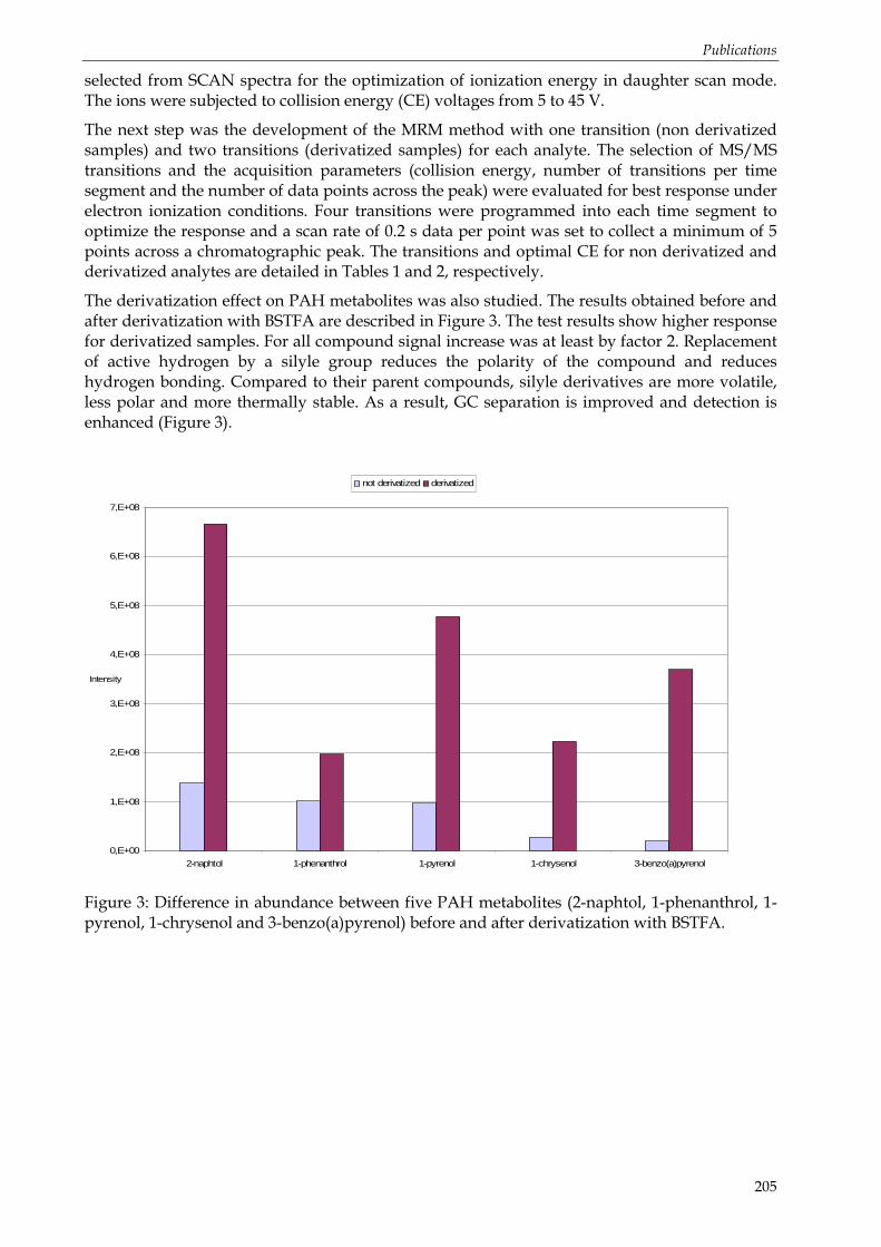
Publications
205
selected from SCAN spectra for the optimization of ionization energy in daughter scan mode. The ions were subjected to collision energy (CE) voltages from 5 to 45 V.
The next step was the development of the MRM method with one transition (non derivatized samples) and two transitions (derivatized samples) for each analyte. The selection of MS/MS transitions and the acquisition parameters (collision energy, number of transitions per time segment and the number of data points across the peak) were evaluated for best response under electron ionization conditions. Four transitions were programmed into each time segment to optimize the response and a scan rate of 0.2 s data per point was set to collect a minimum of 5 points across a chromatographic peak. The transitions and optimal CE for non derivatized and derivatized analytes are detailed in Tables 1 and 2, respectively.
The derivatization effect on PAH metabolites was also studied. The results obtained before and after derivatization with BSTFA are described in Figure 3. The test results show higher response for derivatized samples. For all compound signal increase was at least by factor 2. Replacement of active hydrogen by a silyle group reduces the polarity of the compound and reduces hydrogen bonding. Compared to their parent compounds, silyle derivatives are more volatile, less polar and more thermally stable. As a result, GC separation is improved and detection is enhanced (Figure 3).
0,E+00
1,E+08
2,E+08
3,E+08
4,E+08
5,E+08
6,E+08
7,E+08
2-naphtol 1-phenanthrol 1-pyrenol 1-chrysenol 3-benzo(a)pyrenol
Intensity
not derivatized derivatized
Figure 3: Difference in abundance between five PAH metabolites (2-naphtol, 1-phenanthrol, 1-pyrenol, 1-chrysenol and 3-benzo(a)pyrenol) before and after derivatization with BSTFA.

Publications
206
3.2 Method validation
In order to choose between PTV and Splitless injection mode, standard solutions (prepared in dichloromethane) were tested with results summarized in Table 3. The mean recoveries ranged between 92 and 109% for all compounds in Splitless mode and between 99 and 101% in PTV mode, with relative standard deviations from 4 to 10% in Splitless mode, and from 2 to 7% in PTV mode.
Table 3: Recovery (R %) for standard solutions measured in PTV and Splitless mode n=5, 1 µl injected. Tested standard solutions at concentrations between 20 ng.g-1-1.9 µg.g-1 were prepared in dichloromethane.
Analytes R % Splitless
mode
RSD% Splitless
mode
R % PTV mode
RSD% PTV
mode
Concentration
2-naphtol 98 4 99 3 20 ng.g-1-1.4 µg.g-1
1-phenanthrol 100 4 100 4 30 ng.g-1-1.9 µg.g-1
1-pyrenol 97 5 100 2 30 ng.g-1-0.9 µg.g-1
1-chrysenol 109 6 100 3 30 ng.g-1-0.7 µg.g-1
3- benzo(a)pyrenol 92 10 99 7 70 ng.g-1-1.8 µg.g-1
Then, spiked water samples were prepared to compare the method in both modes. The obtained data are given in Table 4. The mean recoveries ranged between 84 and 112% for all compounds in Splitless mode and between 79 and 99% in PTV mode, with relative standard deviations from 4 to 11% in Splitless mode, and from 2 to 8% in PTV mode. PTV mode, being more precise, was chosen for following tests for spiked bile samples.
Table 4: Recovery (R%) of spiked water samples. n=3, 1 µl injected.
Analytes R% Splitless
mode RSD %
R% PTV mode
RSD % Water concentration
[µg.g-1]
2-naphtol 84 4 88 8 0.17
1-phenanthrol 100 7 94 7 0.16
1-pyrenol 92 8 92 3 0.16
1-chrysenol 112 6 99 2 0.16
3- benzo(a)pyrenol 84 11 79 7 0.48
The analytical performance of the GC/MS and GC-MS/MS methods was evaluated by testing the linearity, accuracy, precision and sensitivity. Linearity was tested with standard mixtures in dichloromethane in the range presented in Table 5. Obtained correlation coefficients were higher for GC-MS/MS and ranged between 0.9903 (1-chrysenol; 3-benzo(a)pyrenol) and 0.9999 (2-naphtol). The intra-day and inter-day precisions for GC-MS/MS ranged between 4 and 6% and between 10 and 14 %, respectively and they were comparable with results obtained by GC-MS (4-11% and 7-11% respectively). Methodological limits of detection (LOD Table 6) as well as instrumental limits of detection (IDL Table 5) were obtained for a signal-to-noise ratio of 3 and were much lower for GC-MS/MS, this is especially evident for 2-naphtol and 3-benzo(a)pyrenol where IDLs were from 4 to 16 times lower than for GC/MS. Comparing those two methods GC-MS/MS is more sensitive, specific and has lower limits of detection.

Publications
207
Table 5: Method performance parameters for standard solutions (prepared in dichloromethane) measured in PTV mode n=5, 1 µl injected, IDL instrumental limit of detection.
Range of linearity
R² Repeatability
(RSD %) Reproducibility
(RSD %) IDL (pg injected)
Analytes
GC/MS GC-
MS/MS GC/MS
GC-MS/MS
GC/MS GC-
MS/MS GC/MS
GC-MS/MS
GC/MS GC-
MS/MS
2-OHN 3 ng.g-1
- 30 µg.g-1
0.1-441 ng.g-1
0.9918 0.9999 5 4 9 11 0.3 0.08
1-OHPhe
3 ng.g-1
-30 µg.g-1
0.2-440 ng.g-1
0.9935 0.9986 4 4 10 10 0.1 0.07
1-OHP 3 ng.g-1
- 30 µg.g-1
0.2-502 ng.g-1
0.9978 0.9910 4 5 7 13 0.3 0.25
1-OHC 3 ng.g-1
- 30 µg.g-1
0.4-490 ng.g-1
0.9843 0.9903 6 4 8 14 2.5 0.16
3-OHBaP
7 ng.g-1
- 40 µg.g-1
1.7-1,850 ng.g-1
0.9255 0.9903 11 6 11 11 8.1 2.79
Table 6: Methodological limits of detection (LOD) measured by GC-MS/MS for spiked water and spiked bile samples with comparison to GC/MS , PTV mode, 1 µl injected, n=4.
Spiked water Spiked bile
Analytes LOD (ng.l-1 of water)
GC/MS
LOD (ng.l-1 of water)
GC-MS/MS
LOD (ng.l-1 of bile)
GC/MS
LOD (ng.l-1 of bile)
GC-MS/MS
2-naphtol 1.6 0.2 3.9 0.7
1-phenanthrol 0.4 0.1 0.9 0.5
1-pyrenol 0.6 0.7 1.3 0.3
1-chrysenol 4.5 0.6 6.6 1.4
3- benzo(a)pyrenol 13.6 4.9 20.6 8.5

Publications
208
3.3 Spiked bile samples
For spiked bile samples turbots (scophtalmus maximus) from the Aquacole Farm in the city of Re (50 g weight and 13 cm length) were caught and transported to the lab. Afterwards, the fish were kept for 40 days in a large 760 litres aquarium for acclimatization. 10 fish were subsequently used and bile was harvested from the gall bladder and the collected bile was used for spiking.
Figure 4 shows chromatograms for spiked bile samples analyzed with the above described procedure. The absence of interfering peaks around the retention times of analytes in chromatograms demonstrates that the clean-up procedure fitted the purpose. Recoveries obtained in PTV mode were between 79% and 102% for all metabolites excluding 2-naphtol (63%), the precision of the experimental procedure was evaluated by calculating the relative standard deviation (RSD) from three different extractions of the spiked sample. Values ranged from 3% to 11% for all analytes (Table 7), which indicates good repeatability of the method.
Table 7: Recovery (R %) of spiked bile samples n=3.
Analytes R % Concentration in the
bile [µg.g-1] RSD %
2-naphtol 63 1.0 4
1-phenanthrol 80 2.1 11
1-pyrenol 98 1.4 3
1-chrysenol 102 0.9 11
3- benzo(a)pyrenol 79 2.8 3
The limits of detection (LODs), defined as the amount injected which gave a signal equivalent to three times the baseline noise, was determined experimentally for the spiked water and spiked bile samples. The LODs based on areas of the optimized transition ions are presented in Table 6 with comparison to GC/MS. Detection limits obtained for GC-MS/MS method are much lower than those for single GC/MS method. These LOD values illustrate the high sensitivity of the proposed method in the determination of the target compounds in fish bile.
To illustrate sensitivity of GC-MS/MS method, two chromatograms obtained for spiked water (Figure 5) and spiked bile (Figure 4) samples are presented. As it can bee seen there is no significant matrix effect even on chromatogram presented for spike bile sample. The chromatograms are devoid of interfering ions.

Publications
209
Figure 4: Efficiency of spiked bile sample preparation for 5 metabolites. MRM acquisition mode. Ion chromatogram corresponding to areas of spiked bile sample in which quantity of metabolites were around: 30 ng.g-1 of bile for 2-naphtol, 1-phenanthrol, 1-pyrenol, 1-chrysenol and 98 ng.g-1 of bile for 3-benzo(a)pyrenol.
Figure 5: Efficiency of spiked water sample preparation for 5 metabolites. MRM acquisition mode. Ion chromatogram corresponding to areas of spiked water sample in which quantity of metabolites were around: 15 ng.g-1 of water for 2-naphtol, 1-phenanthrol, 1-pyrenol, 1-chrysenol and 45 ng.g-1 of water for 3-benzo(a)pyrenol.

Publications
210
3.4 Environmental samples
The entire protocol was applied to the analysis of several bile samples from hake fish (Merluccius merluccius) which were caught in the Mediterranean Sea (Figure 6).
Figure 6: Sampling sites for hake fish (Merluccius merluccius) during October 2006 in the Mediterranean Sea, France.
Three individual bile samples (coming from individual fish) were pooled (in order to have a homogenous sample) and three replicates of each pool of biles were analysed. The volume of samples was approximately 100 µl. The samples were analyzed by GC-MS/MS and GC/MS for comparison. The results are presented in Tables 8 and 9 respectively. The sensitivity of the analytical procedure was sufficient to detect most of the studied compounds. Figure 7 shows an example of a natural bile chromatogram.
Four metabolites (2-naphtol, 1-pyrenol, 1-chrysenol and 3-benzo(a)pyrenol) were detected in natural samples by the GC-MS/MS method. 1-phenanthrol was not found. However, another product, 9-phenanthrol, was present in all the samples. 1-chrysenol and 3-benzo(a)pyrenol were below detection limit for GC/MS (34 and 107 ng.g-1, respectively) and could be only detected by GC-MS/MS. This result is very important because 3-benzo(a)pyrenol is one of the most significant mono-hydroxylated PAH metabolites and is known to play major role in the genotoxic and mutagenic processes in organisms [16,17,18]. To evaluate the potential effect of such compounds as well as to study the mechanic aspect of benzo(a)pyrene metabolism in organisms it is essential to quantify 3-benzo(a)pyrene at very low levels. In such case GC-MS/MS methodology offers several advantages in comparison with conventional GC/MS methods. As it can be seen, 1-pyrenol was the dominant contaminant in all the samples, with concentrations varying from 18 to 27 ng.g-1 and an average contribution of 47%. The difference in contamination levels between fish could be caused by different ability for PAHs accumulation varying from fish to fish (age, sex, size).

Publications
211
Table 8: Levels of contaminations in natural bile samples (ng.g-1 of bile) obtained by GC-MS/MS.
Analytes Bile 1 Bile 2 Bile 3
2-naphtol 0.7 2.7 1.0
9-phenanthrol 2.3 0.9 2.5
1-pyrenol 23.4 27.4 17.7
1-chrysenol 5.5 8.4 2.0
3- benzo(a)pyrenol 19.3 22.4 10.7
Table 9: Levels of contaminations in natural bile samples (ng.g-1 of bile) obtained by GC/MS.
Analytes Bile 1 Bile 2 Bile 3
2-naphtol 1.0 1.9 0.9
9-phenanthrol 2.5 nd 2.8
1-pyrenol 27.7 24.9 6.7
1-chrysenol nd nd nd
3- benzo(a)pyrenol nd nd nd
nd= non detected
Figure 7: Identification of five PAH metabolites (2-naphtol, 1-phenanthrol, 1-pyrenol, 1-chrysenol and 3-benzo(a)pyrenol) in the bile of hake fish (Merluccius merluccius) which were caught in the Mediterranean Sea. MRM acquisition mode. Transitions from derivatized products to [M+ Si(CH3)3]+ -15] (the loss of a methyl group from the parent ion).

Publications
212
4 Conclusions
The assessment of the potential health hazard has been of great concern in recent years. A new, rapid and specific multicomponent procedure for determining PAH metabolites in complex environmental matrices is needed. Some sources of PAH contamination have been recognized as marine oil spills and discharges from refineries into estuarine waters. The potential health hazard associated with the consumption of commercial species of shellfish (oysters, mussels, and clams) contaminated by petroleum products must be assessed for the presence of PAH compounds which are carcinogenic [19, 20, 21]. By detecting PAH metabolites (which are sometimes even more dangerous than PAHs) in the environment we can follow the level and pattern of PAH contamination.
GC-MS/MS analysis of PAH metabolites was studied in an attempt to achieve better sensitivity, precision and repeatability than in currently available methods that use single quadrupole GC-MS. Using MRM mode we were able to eliminate the matrix effect from the quantification of the target compounds at a 0.3 ng.g-1 level in bile. Both instruments were evaluated in terms of sensitivity. If GC-MS/MS is used the detection limit is sometimes even 25 times lower (ranged from 0.3 to 0.8 ng.g-1 of bile) than with single MS. The precision was satisfying (3-11%) for spiked bile samples. The spectral quality of spiked samples is excellent due to the ion isolation step and selectivity of GC-MS/MS.
Several bile samples were analysed by the developed method and 4 of 5 investigated metabolites were detected in all tested samples, which shows the objectives of an improved method were achieved. The single quadrupole in Selected Ion Monitoring (SIM) mode was not able to detect some of the PAH metabolites (1-chrysenol, 3-benzo(a)pyrenol) in environmental samples.
GC-MS/MS is a more powerful analytical technique that provides a method for detecting target compounds in complex matrices at trace levels. This method is designed to provide a better analysis for environmental samples. The resulted methodology was proved to be sensitive, reliable, reproducible and precise.
Acknowledgements: The authors wish to thank the “ORQUE” program (Observatoire Régional de la Qualité de l'Environnement) and the French Minister of Environment for research fundings. Justyna Sekula would like to thank EC for Marie-Curie grant and LPTC for all support. The authors want also to acknowledge the “Region Aquitaine” and the French National Council for Scientific Research (CNRS) for providing the PhD grant of M. Le Dû-Lacoste.

Publications
213
References
[1] D.M. Jauhiainen, R. Berg, G.F. Grinstead, J. R. Kruse, Journal of Analytical and Applied Pyrolysis 74 (2005) 512.
[2] M.H. Topal, J. Wang, Y.A. Levenolis, J.B. Carlson, J. Jordan, Fuel, 83 (2004) 2357.
[3] P. Fernandez, R.M. Vilanova, J.O. Grimalt, Environmental Science & Technology 33 (1999) 3716.
[4] K. Liu, W. Han, W-P. Pan, J.T. Riley, Journal of Hazardous Materials, 84 (2001) 175.
[5] N. Yassaa, A. Cecinato, Chemosphere 60 (2005) 1660.
[6] J. Djinovic, A. Popovic, W. Jira, Meat Science 80 (2008) 449.
[7] R. Hurt, Spitzer Science Center, June 27 (2005).
[8] A.P. Ilnitsky, V.S. Mischenko, L.M. Shabad, Cancer Letters, 3 (1977) 227.
[9] E. Terzi, C. Samara, Atmospheric Environment, 39 (2005) 6261.
[10] M. Kalaitzoglou, E. Terzi, C. Samara, Atmospheric Environment 38 (2004) 2545.
[11] J.O. Allen, N.M. Dookeran, K.A. Smith, A.F. Sarofim, K. Taghizadeh, A.L. Lafleur, Environmental Science & Technology 30 (1996) 1023.
[12] C. J. Halsall, A.J. Sweetman, L.A. Barrie, K.C. Jones, Atmospheric Environment, 35 (2001) 255.
[13] D.L. Leister, J.E. Baker, Atmospheric Environment, 28 (1994) 1499.
[14] R.M. Harrison, D.J.T. Smith, L. Luhana, Environmental Science & Technology 30 (1996) 825.
[15] P. Boffetta, N. Jourenkova, P. Gustavson, Cancer Causes and Cintrol, 8 (1997) 444.
[16] D. Chakravarti, D. Venugopal, P.C. Mailander, J.L. Meza, S. Higginbottam, E.L. Cavalieri, E.G. Rogan, Mutation Research, 649 (2008) 161.
[17] V.A. Du Four, C.R. Janssen, E. Brits, N. Van Larebeke, Mutation Research 588 (2005) 106.
[18] L. Flowers, S.H. Rieth, V.J. Coliano, G.L. Foureman, R. Hertzberg, E.L. Hofmann, D.L. Murphy, S. Nesnow, R.S. Schoeny, Polycyclic Aromatic Compounds, 22 (2002) 811.
[19] G. Grimmer, H. Brune, G. Dettbarn, J. Jacob, J. Misfeld, U. Mohr, K.W. Naujack, J. Timm, R. Wenzel-Hartung, Journal of Analytical Chemistry, 339 (1991) 792.
[20] T.L. Shchekaturina, A.L. Khesina, O.G. Mironov, L.G. Krivosheeva Marine Pollution Bulletin, 30 (1995) 38.
[21] R. Singh, B. Kaur, I. Kalina, T.A. Popov, T. Georgieva, S. Garte, B. Binkova, R.J. Sram, E. Taioli, P.B. Farmer, Mutation Research, 602 (2007) 71.
[22] U. Varanasi, M. Nishimoto, W.L. Reichert, J.E. Stein, Xenobiotica, 12 (1982) 417.
[23] S. Reynaud, P. Deschaux, Aquatic Toxicology, 77 (2006) 229.
[24] D.R. Mattison, K. Shiromizu, M.S. Nightingale, American Journal of Industrial Medicine, 4 (1983) 191.
[25] B. Mahadevan, A. Luch, C.F. Bravo, J. Atkin, L.B. Steppan, C. Pereira, N.I. Kerkvliet, W.M. Baird, Cancer Letters, 227 (2005) 25.
[26] R.J. Law, V.J. Dawes, R.J. Woodhead, P. Matthiessen, Marine Pollution Bulletin, 34 (1997) 306.
[27] A.R. Steward, Ch. Kandaswami, S. Chidambaram, C. Ziper, J.P. Rutkowski, H.C. Sikka, Environmental Toxicology and Chemistry, 9 (1990) 1503.
[28] G. Witt, Marine Pollution Bulletin, 31 (1995) 237.

Publications
214
[29] G. Witt, H. Siegel, Marine Pollution Bulletin, 40 (2000) 1124.
[30] G. Claireaux, Y. Desaunay, F. Akcha, B. Auperin, G. Bocquene, H. Budzinski, J.C. Cravedi, F. Davoodi, R. Galois, C. Gilliers, Ch. Goanvec, D. Guerault, N. Imbert, O. Mazeas, G. Nonnotte, L. Nonnotte, P. Prunet, P. Sebert, A. Vettier, Aquatic Living Resources, 17 (2004) 335.
[31] R.J. Law, J.L. Biscaya, Marine Pollution Bulletin, 29 (1994) 235.
[32] P.M. Gschwend, R.A. Hites, Geocimica et Cosmochimica Acta, 45 (1981) 2359.
[33] Y. Liang, M.F. Tse, L. Young, M.H. Wong, Water Research, 41 (2007) 1303.
[34] M.S. Shailaja, C. D’Silva, Chemosphere, 53 (2003) 835.
[35] Environment Canada Toxic chemicals in Atlantic Canada-PAHs (2001).
[36] U. Varanasi, J.E. Stein, M. Nishimoto, Biotransformation and disposition of polycyclic aromatic hydrocarbons (PAH) in fish, In U. Varanasi (editor), Metabolism of polycyclic aromatic hydrocarbons in the aquatic environment, p. 93-149. CRC Press, Inc., Boca Raton, FL. 1989.
[37] G. Luthe, G.J. Stroomberg, F. Ariese, U.A.T. Brinkman, N.M. Straalen, Environmental Toxicology and Pharmacology, 12 (2001) 221.
[38] G.J. Stroomberg, Comparative Biochemistry and Physiology, 138 (2004) 129.
[39] J. Hellou, J.H. Banoub, A. Ryan, Environmental Toxicology and Chemistry, 8 (1989) 871.
[40] P. van den Hurk, Marine Environmental Research, 62 (2006) 16.
[41] W. Zhang, D. X. G. Zhuang, C. Ding, G. Wang, J. Chang, G. Ren, Environmental Monitoring and Assesment 131 (2007) 387.
[42] A. Palmqvist, L.J. Rasmussen, V.E. Forbes, Aquatic Toxicology, 80 (2006) 309.
[43] R. Aina, L. Palin, S. Citterio, Chemosphere 60 (2006) 666.
[44] P.Baumard, H. Budzinski, P. Garrigues, J.C. Sorbe, T. Burgeot, J. Bellocq, Marine Pollution Bulletin 36 (1998) 951.
[45] H. Nakata, Y. Sakai, T. Miyawaki, A. Takemura, Environmental Science and Technology 37 (2003) 3513.
[46] U. Kammann, Environmental Science and Pollution Research 14 (2007) 102.
[47] L.L. Johnson, G.M. Ylitalo, M.R. Arkoosh, A.N. Kagley, C. Stafford, J.L. Bolton, J. Buzitis, B.F. Anulacion, T.K. Collier, Environmental Monitoring and Assessment 124 (2007) 167.
[48] A.L. Pikkarainen Chemosphere 65 (2006) 1888.
[49] J.D. Leonard, J. Hellou, Environmental Toxicology and Chemistry, 20 (2001) 618.
[50] S. Gorbi, F. Regoli, Marine Environmental Research, 58 (2004) 511.
[51] J. Lintelmann, K. Fischer, G. Matuschek, Journal of Chromatography A, 1133 (2006) 241.
[52] M.M. Krahn, G.M. Ylitalo, J. Buzitis, S.L. Chan, U. Varanasi, Journal of Chromatography A (1993) 15.
[53] G.M. Troisi, S. Bexton, I. Robinson, Environmental Science and Technology 40 (2006) 7938.
[54] O. Mazéas (2004) Thèse n° 2945. Université Bordeaux 1, France.
[55] Le Dû - Lacoste M and Budzinski H. Anal Bioanal Chem. (Submitted)
Publications
215
Publication n°3
Selective and sensitive determination of polycyclic aromatic hydrocarbon metabolites (OH-PAH) in fish bile using a new ultra-performance liquid chromatography-tandem mass spectrometry method (UPLC™-MS/MS).
Marie Le Dû-Lacoste and Hélène Budzinski*
ISM-LPTC, UMR 5255 CNRS, University of Bordeaux 1, 351 cours de la Libération, 33405 TALENCE, FRANCE
* Corresponding author: [email protected]
Tel: + 33 540 006 998
Fax: + 33 540 002 267
Abstract
A sensitive and fast method was developed to quantify selected mono-hydroxylated PAH metabolites by Ultra-Performance Liquid Chromatography (UPLC™) coupled to tandem mass spectrometry (MS/MS). The UPLC method, using an acetonitrile:water gradient as a mobile phase, provided baseline separation of the selected metabolites during a run time shorter than 10 min. The excellent linearity (4 orders of magnitude) and the signal-to-noise performance provided by the MRM method allowed the development of a sensitive and specific UPLC-MS/MS methodology. The limits of detection ranged from 0.1 to 0.4 pg on column. Applied to chub bile samples, this methodology has proved to be suitable for environmental survey study.
Keywords: PAH metabolites, UPLC, tandem mass spectrometry, fish bile.
Submitted to Journal of Chromatography B

Publications
216
1 Introduction Polycyclic aromatic hydrocarbons (PAHs) are a group of hydrophobic organic compounds that are ubiquitous pollutants derived from pyrogenic and petrogenic sources [1]. PAHs have been shown to be toxic to marine life [2-4]. Some PAHs (e.g. benzo(a)anthracene and benzo(a)pyrene) are metabolically activated in vertebrates to form carcinogens [5-12]. Thus, the quantification of PAHs in tissues of marine organisms is usually carried out to evaluate the impact of such a contaminant on these organisms [13]. The feasibility of measuring tissue concentrations of PAHs in marine species to monitor for exposure depends on rates of uptake, biotransformation, and excretion. However, biotransformation processes are considered to be low in many invertebrates [14]. In contrast, fish and other marine vertebrates rapidly biotransform PAHs to form epoxy and hydroxyl derivatives during phase I metabolism. Subsequently, during phase II metabolism, the phase I metabolites are converted into highly water-soluble conjugates (e.g., glucuronides or sulfates) that accumulate in the bile [15-17]. Therefore, measuring PAH metabolites in bile provides a means for determining exposure [18-26].
Analysis for metabolites in fish bile has been used to monitor for PAH exposure in a number of studies [27-30]. The complex nature of PAH metabolites in bile of fish exposed to oil or other environmental pollution makes analysis challenging. As a result, selecting the best analytical method will depend upon the questions that need to be answered. The concentration of PAH metabolites is usually determined semi-quantitatively as global fluorescent aromatic compound equivalents (FACs). Several analytical techniques have been used to estimate FACs in fish bile, such as high-performance liquid chromatography coupled to fluorescence (HPLC/F) [23, 31-39], synchronous fluorescence spectrometry (SFS) [40, 41] or fixed fluorescence (FF) [42]. A limited degree of compound specificity has been achieved by optimization of fluorescence wavelength pairs for analysis of naphthalene-, phenanthrene-, pyrene- and benzo(a)pyrene-like metabolites [43-45]. These screening methods have been successfully used in a large number of PAH monitoring studies [23-26, 46-53], but their use seems to be limited when applied to complex mixtures of fluorescent aromatic compounds [54]. This limitation becomes evident when compounds have similar structures such as isomeric metabolites, PAH parent compounds and its metabolites.
Since the 80’s, the mass spectrometric detection (MS) allowed considerable progresses in terms of sensitivity and specificity for the PAH metabolites analysis, especially in complex biological matrices. In recent years liquid chromatography coupled to mass spectrometry (LC-MS) instruments has become available in many laboratories, a major driving force being their widespread use in drug discovery and development. With LC coupled to triple-stage quadrupole tandem mass spectrometers (LC-MS/MS), a wide range of substances in complex biological matrixes can be quantified at low levels and with high specificity. Despite this advantage, relatively few LC-MS methods have been reported for the determination of PAH metabolites. Van de Wiele et al.[55] have developed an LC-MS method that utilized a single quadrupole instrument with electrospray ionization in negative mode (ESI-) for the determination of phenolic metabolites of PAHs from in vitro metabolism studies. Several LC/MS methods using atmospheric pressure chemical ionization (APCI) or ESI, both in positive and negative mode, for determination of various hydroxylated PAH metabolites have been reported but not applied to biological samples[38, 56-58]. More recently, LC-MS/MS methods for selective detection and quantification of selected monohydroxy PAH metabolites in human urine were reported [59-62]. Recently, ultra-performance liquid chromatography (UPLC) with < 2 µm particle size column was introduced for rapid and efficient compound separation over traditional HPLC [63]. UPLC coupled with mass spectrometry is increasingly being used for rapid multiple component quantitation for in vitro and in vivo BaP metabolite characterization [64].
The present protocol was focused on the development of a new specific and sensitive UPLC™-MS/MS method to separate and simultaneously quantify five mono-hydroxylated

Publications
217
PAH metabolites in fish bile. Their developed chemical structure is presented in Figure 1. The studied metabolites are known to be some of the major products of biotransformation in fish, which are present in their free form or more commonly conjugated with endogenous molecules [4, 65-67]. Such compounds are extensively excreted into the bile. Potential metabolites of priority PAH listed by the US-EPA (United States Environmental Protection Agency) have been chosen for their interest in environmental surveys [68]. Thus, the developed methodology was finally applied to fish bile samples to evaluate the applicability of this method to natural samples.
OH
OHOH
OH
1-hydroxypyrene
2-hydroxynaphtalene 1-hydroxyphenanthrene
1-hydroxychrysene 3-hydroxybenzo(a)pyrene
OH
Figure 1: Chemical structures of OH-PAH analysed by UPLC-MS/MS
2 Experimental 2.1 Materials and reagents
1-hydroxynaphthalene (1-OHN) and 2-hydroxynaphthalene (2-OHN) were purchased from Lancaster (Bischeim, France); 2-hydroxybiphenyl (2-OHBi), 9-hydroxyfluorene (9-OHFe) and 1-hydroxypyrene (1-OHP) from Sigma-Aldrich (Saint Quentin Falavier, France) and 9-hydroxyphenanthrene (9-OHPhe), 1-hydroxychrysene (1-OHC) and 3-hydroxybenzo(a)pyrene (3-OHBaP) from Promochem (Molsheim, France). 1-hydroxypyrene-d9 (1-OHPd9) and pyrene-d10 (Pd10) were obtained from Cambridge Isotope Laboratories (Cluzeau Info Labo, Ste Foy La Grande, France). All the standards were of analytical grade (purity > 98%). All the solvents used were of analytical grade (purity > 98%). Ultra gradient HPLC grade acetonitrile was obtained from J.T Baker (VWR International, Strasbourg, France). Methanol Supersolv was provided by Merck. Formic acid and acetic acid 100% Normapur (analytical reagent grade, Scharlau) were obtained from ICS (Belin-Beliet, France). Sodium acetate trihydrate 99% (purity > 99%) was purchased from Acros Organics (Noisy-Le-Grand, France). Deionised water was obtained with a Milli-Q system (Millipore, Molsheim, France). Two solid-phase extraction (SPE) cartridges were used: Strata-X cartridge (3 cc, 200 mg) was from Phenomenex (Le Pecq, France) and HF Bond Elut-PSA cartridge (3 cc, 500 mg) from Varian (Atlantic Labo, Eysines, France).
2.2 UPLC™ instrument and chromatographic conditions
The Ultra Performance™ Liquid Chromatography (UPLC) was performed on a Waters ACQUITY UPLC™ system (Milford, MA, USA), equipped with a binary solvent delivery manager, and a sample manager. The UPLC separation was performed on a Waters

Publications
218
ACQUITY BEH™ C18 column (1.7 µm, 2.1 mm x 150 mm) maintained at 30°C. A 0.2 µm precolumn filter (ACQUITY UPLC™ stainless steel in-line filter) was used to protect the analytical column. 10 µl sample, dissolved in acetonitrile, was injected for UPLC analysis. The mobile phase used was a mixture of acetonitrile (A) and Milli-Q water (B) with the following multi-step gradient: 0-2 min: 60/40 (A/B, v/v); 2-4 min: 60/40 (A/B, v/v) to 80/20 (A/B, v/v); 4-6 min: 80/20 (A/B, v/v) to 60/40 (A/B, v/v); 6-8 min: 60/40 (A/B, v/v) at a flow rate of 0.45 ml.min-1. Total run time was 8 min per sample.
2.3 Mass Spectrometric conditions
Mass spectrometric (MS) measument was performed on a Waters Micromass® Quattro Premier™ tandem quadrupole mass spectrometer (Manchester, UK) equipped with an electrospray ionization (ESI) source. The MS system was controlled by MassLynx™ 4.0 Software. All MS optimization experiments were performed in Scan mode and in product scan mode. All quantifications were performed in multiple reaction monitoring (MRM) mode. The cone voltage and collision energies for each of the MRM transitions were optimized by infusing the individual neat standard solution into the mass spectrometer at 2 µg.ml-1. To ensure that the ionisation source parameters were compatible with the mobile phase flow during the tuning, a flow of 0.6 ml.min-1 at 60% A was introduced into the mass spectrometer at the same time by using a PEEK T connector. MRM data collection during the chromatographic experiments were performed in both negative and positive mode with the capillary voltage fixed at 3.5 kV, the source temperature at 90°C, the desolvatation temperature at 400°C, the desolvatation gas flow at 1,000 l.h-1, and the cone gas flow at 90 l.h-
1. Inter-scan delay for the polarity switching, inter-channel delay and dwell time for each MRM channel were set at 20, 5 and 50 ms, respectively. This allowed a sufficient cycle time to collect at least 15 data points per peak.
2.4 Standard and working solutions
Individual stock solutions of hydroxylated metabolites (100 ng.µl-1) and internal standard (50 ng.µl-1) were prepared in acetonitrile. Working standard solutions for linear calibration were prepared by mixing and diluting in acetonitrile the individual stock solutions of metabolites and internal standard. The final concentrations of compounds in the working solutions ranged from 1 pg.µl-1 to 8 ng.µl-1 of solvent (ACN). Both the stock and working solutions were stored at -20°C until use. The samples were then extracted as described in section 2.5. Quality control (QC) samples were prepared at five different concentrations (0.1, 1, 10, 1,000 and 3,000 pg.µl-1 of bile), by adding working standard solutions in 100 µl of bile. They were used to assess accuracy and precision.
2.5 Sample preparation
Samples were prepared according to a protocol developed by Le Dû-Lacoste and Budzinski [69].
The weighted samples (100 µl of bile sample) were homogenized in 2 ml precooled buffered water (sodium acetate buffer at pH 5.0 with acetic acid). The internal standard, 1-hydroxypyrene-d9 was added to the samples (20 µl of a diluted solution at 0.5 ng.µl-1 of solvent). Glass vials were used to avoid adsorption phenomena on inner surface. Following centrifugation (10 min, 5,000 rpm, 20°C), samples were extracted on solid-phase Strata X cartridges which were preconditioned with 2 ml methanol and 4 ml buffered water. The supernatants were loaded on cartridges and washed with 2 ml buffered water and 2 ml water/methanol (70/30, v/v). Water traces were then removed by applying vacuum on the cartridges during 45 min. Metabolites were then eluted with 5 ml of methanol. Extracts were

Publications
219
reduced to dryness under nitrogen stream and redissolved in 1 ml methanol/methylene chloride mixture (20/80, v/v) before purification. Solid-phase HF PSA Varian cartridges were used for the purification step. Before loading the extracts redissolved in methanol/methylene chloride (20/80, v/v), the cartridges were first preconditioned with 2.5 ml methanol/methylene chloride (20/80, v/v). The elution of the compounds was then performed with 6 ml of the same mixture. Extracts were finally reduced to dryness under a nitrogen stream and redissolved in 100 µl acetonitrile. Finally the extracts were stored at -20°C until injection.
2.6 Method validation
This UPLC™-MS/MS method was validated considering different criteria, including linearity, inter- and intra-day precision, intra-day accuracy and recovery. The method was then applied for the analysis of PAH metabolites produced by chub (Leuciscus cephalus) caught in the Drôme River (city of Saillans, France) in September 2006 and 2007.
2.6.1 Linearity and limits of detection
The calibration curves for metabolites were constructed by plotting measured peak ratios of analyte to internal standard (IS) against nominal OH-PAH concentrations in bile using a 1/x weighted linear least-squares regression model. The minimally acceptable correlation coefficient (r²) for the calibration curve was 0.99 or greater. The only use of one IS is a limitation of the method due to the variability of chemical structure/properties between compound studied and the chosen internal standard. The choice of only one IS is explained by the very high cost of isotope labelled compounds and by the lack of adequate labelled metabolites. Detection limits were determined using a signal-to-noise approach (3:1). Standard solutions were used for the determination of instrumental detection limits (IDL). Bile samples spiked before extraction were used for method detection limits determination (MDL).
2.6.2 Precision and accuracy
In order to assess the intra- and inter-batch precision and accuracy, QC samples at three concentrations were prepared. The intra- and inter-batch precisions of the assay were assessed by calculating the relative standard deviation (RSD) for the analysis of QC samples in three replicates. Accuracy was presented as the percent bias of the calculated concentration in comparison to the nominal concentration. The criterion for acceptability of precision was that RSD for each concentration level should not exceed ± 15% with the exception of the low level, for which it should not exceed ± 20%. Similarly, the averaged value for accuracy should be in the range of ± 15% of the nominal concentration except for the lowest level (± 20%)[70].
2.6.3 Extraction recoveries
The recoveries of PAH metabolites have been determined in triplicates using metabolite-free bile samples spiked with standard solutions of metabolites prepared in aetonitrile. Final concentrations of metabolites in bile were 0.1, 1, 10, 1,000 and 3,000 pg.µl-1 of bile. The spiked samples were then extracted as described in Section 2.5. The extraction recoveries were calculated according to the internal standard methodology.

Publications
220
2.6.4 Natural sample
Chub (Leuciscus cephalus) were collected in the Drôme River (near the city of Saillans, France) in September 2007. This location is known to have a good chemical and biological quality of water, because it is not directly impacted by human activities and industrial discharges. 10 chubs were collected each year. Bile samples were removed from gall bladders and stored at -80°C. Samples were prepared for analysis by UPLC-MS/MS as indicated in section 2.5.
3 Results and discussion 3.1 Mass spectrometry
For quantitative analysis, peak integration with high precision and reproducibility is critical for the final results. No less than 15 data points are generally recommended to defined chromatographic peaks [70]. As peaks become narrower, the mass spectrometer is required to acquire data faster. Such considerations make essential the use of tandem mass spectrometry, especially when UPLC technology is used for the chromatographic separation of compounds.
When optimizing an analytical method, it is desirable to produce an intense ion signal that is characteristic of the target compound. Using tandem mass spectrometry, selectivity and sensitivity are increased by almost suppressing the noise level. Thus mass spectrometric parameters were optimized to achieve maximum abundance of the product and fragmented ions of PAH metabolites. Acquisition parameters were determined by direct infusion into the tandem mass spectrometer of 2 µl.ml-1 solutions (in mobile phase) of each compound at a flow rate of 20 µl.ml-1. Full scan and product ion mass spectra of each compound were obtained in negative ESI mode for IS and mono-hydroxylated metabolites. In the negative mode, OH-PAHs gave a precursor ion which corresponded to [M–H]-. The isolation time was set at 20 ms and the isolation window was fixed at 5 ms in all cases, in order to get good sensitivity and selectivity. The collision energies applied to the fragmentation of the parent ion was adjusted in order to avoid its complete disappearance. Fragmented ions under collision-induced decomposition were chosen upon the criterion of abundance in order to enhance the sensitivity of the analysis. The chosen m/z values for daughter ions were as follows: m/z 115 for 2-OHN, m/z 165 for 1-OHPhe, m/z 189 for 1-OHP, m/z 215 for 1-OHC and m/z 239 for 3-OHBaP. The MRM transition of m/z 226 -> 198 was chosen for the quantification of the IS (1-OHPd9). The use of internal standard allows a more reliable and rapid analysis when compared to external calibration. The optimum mass spectrometric conditions along with mass transitions in MRM are presented in Table 1.
Table 1: The MRM transitions
Compounds Mode Precursor Ion (m/z)
Product Ion (m/z)
Cone tension
(V)
Collision Energy (eV)
Dwell time (ms)
2-OHN ESI - 143 115 40 32 50
1-OHPhe ESI - 193 165 50 30 50
1-OHP ESI - 217 189 60 30 50
1-OHC ESI - 243 215 60 32 50
3-OHBaP ESI - 267 239 60 40 50
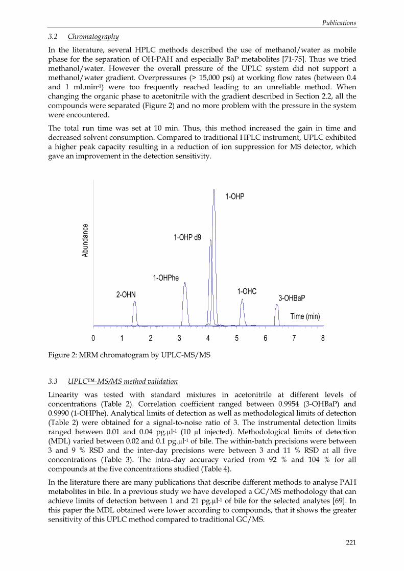
Publications
221
3.2 Chromatography
In the literature, several HPLC methods described the use of methanol/water as mobile phase for the separation of OH-PAH and especially BaP metabolites [71-75]. Thus we tried methanol/water. However the overall pressure of the UPLC system did not support a methanol/water gradient. Overpressures (> 15,000 psi) at working flow rates (between 0.4 and 1 ml.min-1) were too frequently reached leading to an unreliable method. When changing the organic phase to acetonitrile with the gradient described in Section 2.2, all the compounds were separated (Figure 2) and no more problem with the pressure in the system were encountered.
The total run time was set at 10 min. Thus, this method increased the gain in time and decreased solvent consumption. Compared to traditional HPLC instrument, UPLC exhibited a higher peak capacity resulting in a reduction of ion suppression for MS detector, which gave an improvement in the detection sensitivity.
0 1 2 3 4 5 6 7 8
Time (min)
Abundance
2-OHN
1-OHPhe
1-OHP
1-OHP d9
1-OHC3-OHBaP
Figure 2: MRM chromatogram by UPLC-MS/MS
3.3 UPLC™-MS/MS method validation
Linearity was tested with standard mixtures in acetonitrile at different levels of concentrations (Table 2). Correlation coefficient ranged between 0.9954 (3-OHBaP) and 0.9990 (1-OHPhe). Analytical limits of detection as well as methodological limits of detection (Table 2) were obtained for a signal-to-noise ratio of 3. The instrumental detection limits ranged between 0.01 and 0.04 pg.µl-1 (10 µl injected). Methodological limits of detection (MDL) varied between 0.02 and 0.1 pg.µl-1 of bile. The within-batch precisions were between 3 and 9 % RSD and the inter-day precisions were between 3 and 11 % RSD at all five concentrations (Table 3). The intra-day accuracy varied from 92 % and 104 % for all compounds at the five concentrations studied (Table 4).
In the literature there are many publications that describe different methods to analyse PAH metabolites in bile. In a previous study we have developed a GC/MS methodology that can achieve limits of detection between 1 and 21 pg.µl-1 of bile for the selected analytes [69]. In this paper the MDL obtained were lower according to compounds, that it shows the greater sensitivity of this UPLC method compared to traditional GC/MS.

Publications
222
Table 2: Linearity and limit of detection of the methodology. IDL: instrumental limit of detection expressed in pg.µl-1 of solvent. MDL: methodological limit of detection expressed in pg.µl-1 of bile.
Compounds Range of
concentrations Linearity R²
IDL
(pg.µl-1)
LOD
(pg.µl-1 of bile)
2-OHN 1 ng/g – 8 µg/g y = 1,46x + 0,024 0.9961 0.01 0.01
1-OHPhe 1 ng/g – 8 µg/g y = 144,45x - 2,99 0.9990 0.01 0.03
1-OHP 1 ng/g – 9 µg/g y = 358,03x + 21,36 0.9987 0.01 0.02
1-OHC 1 ng/g – 8 µg/g y = 50,87x + 2,87 0.9982 0.01 0.03
3-OHBaP 2ng/g – 13 µg/g y = 12,70x + 1,41 0.9954 0.04 0.1
Table 3: Intra- and inter-precision data of OH-PAH at five different concentrations (expressed in pg.µl-1 of bile).
Intra-day precision
(RSD %, n=6 injections)
Inter-day precision
(RSD %, n=3 injections)
Compound 0.1
pg.µl-1 1
pg.µl-1 10
pg.µl-1 1,000
pg.µl-1 3,000
pg.µl-1 0.1
pg.µl-1 1
pg.µl-1 10
pg.µl-1 1,000
pg.µl-1 3,000
pg.µl-1
2-OHN 9 8 6 6 8 9 8 6 6 9
1-OHPhe 4 7 5 4 5 7 7 5 4 6
1-OHP 4 6 5 3 3 8 6 6 3 5
1-OHC 6 6 7 6 5 9 10 7 6 7
3-OHBaP 7 8 7 9 7 11 10 8 8 10
Table 4: Accuracy data of OH-PAH at five different concentrations expressed in pg.µl-1 of bile (mean ± SD).
Accuracy
(RSD %, n=3 injections)
Compound 0.1 pg.µl-1 1 pg.µl-1 10 pg.µl-1 1,000 pg.µl-1 3,000 pg.µl-1
2-OHN 101 ± 10 97 ± 7 100 ± 7 96 ± 5 101 ± 10
1-OHPhe 94 ± 9 95 ± 9 96 ± 3 94 ± 4 96 ± 6
1-OHP 97 ± 7 104 ± 2 99 ± 4 98 ± 3 100 ± 5
1-OHC 93 ± 6 94 ± 7 92 ± 7 92 ± 8 96 ± 7
3-OHBaP 95 ± 8 101 ± 7 98 ± 5 98 ± 8 97 ± 7
Besides, the use of UPLC-MS/MS technology in the MRM mode allows us to obtain better chromatograms which are cleaner and with less interference than those obtained with GC-MS (Data not shown). This is especially true for the largest OHPAH (1-OHC and 3-OHBaP). Recently Zhu et al. [64] have developed a UPLC-MS methodology for PAH metabolites analysis in fish bile. Limits of detection obtained were closed to 10 pg.µl-1 of bile. When comparing these detection limits with those obtained by the present methodology they were found to be more than 100 times higher for 3-OHBaP. This result showed the greater sensitivity of UPLC-MS/MS method compared to UPLC-MS. Currently no comparison can be done with other UPLC-MS/MS methodology since no previous work has been published yet.

Publications
223
The very good precisions and accuracy results over the five concentrations allow us to present the usefulness of this method to quantify selected mono-hydroxylated PAH metabolites in biological samples.
3.4 Application to fish bile
This method has been satisfactorily applied for detection of biliary metabolites from fish caught in the Drôme River (France) in September 2007. Sampled in a site considered as a non-polluted area, fish were supposed to be poorly impacted by PAHs. Thus the presumed PAH metabolites concentrations could be in the lower range. Therefore the application of the sensitive UPLC-MS/MS methodology developed in this work was justified. As with any biological sample, potential matrix interference by endogenous compounds present in bile must be considered. For all samples, no interfering peak was observed leading to accurate quantitation of the targeted compounds. All compounds have been detected and quantified in all samples (Table 5). Moreover isomeric metabolites of 1-OHPhe (2-, 3-, 4-, 9-OHPhe) have been also detected and quantified in the fish samples. Relative standard deviation (RSD) and coefficients of variation (CV) have been calculated.
Table 5: Mean concentrations of the different metabolites detected in the bile of chubs (n=10) collected in the Drôme River (Saillans, France) for three replicates, coefficients of variation (CV, n=10) and relative standard deviation (RSD %, n=3). Concentrations are expressed in ng.g-1.
Mean concentration CV RSD %
2-OHN 6 13 5
3-OHPhe 1 23 8
1-OHPhe 14 7 4
9-OHPhe 9 7 4
4-OHPhe 6 8 4
1-OHP 167 7 4
1-OHC 20 18 7
3-OHBaP 13 14 6
sum OH-PAH 236 4 4
1-OHP was found to be the major metabolite detected in all bile samples. The mean concentration was determined at 167 ng.g-1 of bile. This corroborated previous studies in which 1-OHP was considered as a reliable PAH exposure biomarker [23, 25, 26, 46, 51, 76-81]. Chrysene and phenanthrene metabolites and 3-OHbaP were measured at 18, 30 and 13 ng.g-1 of bile, respectively. When looking at the metabolites distribution, one could notice that 1-OHP represented more than 70% and phenanthrene metabolites at least 13%. These results suggest that the origin of PAH contamination is more pyrolytic than petrogenic since the proportion of phenanthrene is minor. The presence of BaP metabolite also suggests the predominance of a pyrolytic origin. A general transportation of industrial and traffic discharges by sewage and aerosol deposition to the river could explain the origins of PAH in the Drôme River.

Publications
224
4 Conclusions This paper represents the first developments and validation of an UPLC™-MS/MS method for the detection of PAH metabolites at low levels. Thanks to the UPLC technology coupled to the tandem mass spectrometry, this methodology allows to separate and analyze PAH metabolites with an increase in resolution, sensitivity, and specificity when compared to traditional methods. New developments could be considered to enhance the number of metabolites that can be separated and quantified. As a tool for biomonitoring and risk assessment studies, PAH metabolites analysis has to be increasingly more sensitive because of ultra-trace concentrations of these compounds in organisms. The use of UPLC-MS/MS enhances the analytical performances of the method and the limits of detection at pg level appear suitable to extend the window of detection.
Furthermore this method has been applied to natural fish bile samples and has proved its efficiency and performance. The sensitivity and the specificity of the method were sufficient to identify and quantify PAH metabolites in a complex biological sample.
Acknowledgements: The authors wish to thank the National Program for Ecotoxicology (PNETOX), the French Minister of Environment and the research team IMOPHYS (Integration of molecular and physiologic responses to organic contaminants in coastal area) for research fundings. They want also to acknowledge the “Region Aquitaine” and the French National Council for Scientific Research (CNRS) for providing the PhD grant of M. Le Dû-Lacoste.

Publications
225
References
1. Neff, J. M., Polycyclic Aromatic Hydrocarbons in the Aquatic Environment: Sources, Fates and Biological Effects. 1979, London: Applied Science Publishers Ltd. 262.
2. Malins, D. C., McCain, B. B., Myers, M. S., Brown, D. W., Krahn, M. M., Roubal, W. T., Schiewe, M. H., Landahl, J. T., and Chan, S. L. 1987. Environmental health perspectives 71: p. 5-16.
3. Myers, M. S., Landahl, J. T., Krahn, M. M., and McCain, B. B. 1991. Environmental Health Perspectives 90: p. 7-15.
4. Varanasi, U. and Stein, J. E. 1991. Environmental Health Perspectives 90: p. 93-100.
5. IARC, Monographs on the Evaluation of the Carcinogenic Risk of Chemicals to Human. Vol 32. 1983, International Agency for Research on Cancer: Lyon, France. p. 57-61.
6. Zhang, W., Xu, D., Zhuang, G., Ding, C., Wang, G., Chang, J., and Ren, G. 2007. Environmental Monitoring and Assessment 131(1-3): p. 387-394.
7. Ruchirawat, M., Settachan, D., Navasumrit, P., Tuntawiroon, J., and Autrup, H. 2007. Toxicology Letters 168(3): p. 200-209.
8. Palmqvist, A., Rasmussen, L. J., and Forbes, V. E. 2006. Aquatic Toxicology 80(3): p. 309-319.
9. Inzunza, B., Orrego, R., Penalosa, M., Gavilan, J. F., and Barra, R. 2006. Ecotoxicology and Environmental Safety 65(2): p. 242-251.
10. Fragoso, N. M., Hodson, P. V., and Zambon, S. 2006. Environmental Monitoring and Assessment 116(1-3): p. 481-511.
11. Aina, R., Palin, L., and Citterio, S. 2006. Chemosphere 65(4): p. 666-673.
12. van der Oost, R., Beyer, J., and Vermeulen, N. P. E. 2003. Environmental Toxicology and Pharmacology 13(2): p. 57-149.
13. Robertson, A. 1998Petroleum Hydrocarbons, in Amap Assessment Report: Arctic Pollution Issues, Wilson, S.J., Murray, J.L., and Hungtington, H.P., Editors: Oslo. p. 859
14. James, M. O. 1989Biotransformation and Disposition of Pah in Aquatic Invertebrates, P 69-92, in Metabolism Fo Polycyclic Aromatic Hydrocarbons in the Aquatic Environment, Varanasi, U., Editor CRC Press: Boca Raton. p. 341.
15. Lee, R. F., Sauerheber, R., and Dobbs, G. H. 1972. Marine Biology 17: p. 201-208.
16. Varanasi, U. and Gmur, D. J. 1981. Aquatic Toxicology 1(1): p. 49-67.
17. Varanasi, U., Reichert, W. L., Stein, J. E., Brown, D. W., and Sanborn, H. R. 1985. Eviron. Sci. Technol. 19: p. 836-841.
18. Varanasi, U., Chan, S. L., McLeod, W. D., Stein, J. E., Brown, D. W., Burrows, D. G., Tilbury, K. L., Landahl, J. T., Wigren, C. A., Hom, T., and Pierce, S. M., Noaa Technical Memorandum: Survey of Subsistence Fish and Shellfish for Exposure to Oil Spilled from the Exxon Valdez : First Year, 1989., US Department of Commerce, S., Editor. 1990.

Publications
226
19. Tuvikene, A. 1995. Ann. Zool. Fenn. 32: p. 295-309.
20. Baumard, P., Budzinski, H., Garrigues, P., Sorbe, J. C., Burgeot, T., and Bellocq, J. 1998. Marine Pollution Bulletin 36(12): p. 951-960.
21. Nakata, H., Sakai, Y., Miyawaki, T., and Takemura, A. 2003. Environmental science & technology 37(16): p. 3513-3521.
22. Meador, M. R., Brown, L. R., and Short, T. 2003. Ecological Indicators 3(2): p. 81-92.
23. Kammann, U. 2007. Environmental Science and Pollution Research 14(2): p. 102-108.
24. Johnson, L. L., Ylitalo, G. M., Arkoosh, M. R., Kagley, A. N., Stafford, C., Bolton, J. L., Buzitis, J., Anulacion, B. F., and Collier, T. K. 2007. Environmental Monitoring and Assessment 124(1-3): p. 167-194.
25. Vuorinen, P. J., Keinanen, M., Vuontisjarvi, H., Barsiene, J., Broeg, K., Forlin, L., Gercken, J., Kopecka, J., Kohler, A., Parkkonen, J., Pempkowiak, J., and Schiedek, D. 2006. Marine Pollution Bulletin 53(8-9): p. 479-487.
26. Pikkarainen, A. L. 2006. Chemosphere 65(10): p. 1888-1897.
27. Krahn, M. M., Burrows, D. G., MacLeod, W. D., and Malins, D. 1987. Archives of Environmental Contamination and Toxicology 16(5): p. 511-522.
28. Krahn, M. M., Kittle, J., Lewey J., and MacLeod, J., William D. 1986. Marine Environmental Research 20(4): p. 291-298.
29. McDonald, S. J., Kennicutt II, M. C., Liu, H., and Safe, S. H. 1995. Arch. Environ. Contam. Toxicol. 29: p. 232-240.
30. Van der Oost, R., Van Schooten, F.-J., Ariese, F., Heida, H., Satumalay, K., and Vermeulen, N. P. E. 1994. Environmental Toxicology and Chemistry 13(6): p. 859-870.
31. Krahn, M. M., Moore, L. K., and McLeod, W. D., Standard Analytical Procedures of the Noaa National Analytical Facility, 1986 : Metabolites of Aromatic Compounds in Fish Bile., US Department of Commerce, S., Editor. 1986, NOAA Technical Memorandum NMFS F/NWC-102.
32. Vuontisjärvi, H., Keinänen, M., Vuorinen, P. J., and Peltonen, K. 2004. Polycycl. Aromat. Compd. 24: p. 333-342.
33. Jonsson, G., Taban, I. C., Jorgensen, K. B., and Sundt, R. C. 2004. Chemosphere 54(8): p. 1085-1097.
34. Jonsson, G., Beyer, J., Wells, D., and Ariese, F. 2003. J. Environ. Monit. 5: p. 513-520.
35. Ferrari, S., Mandel, F., and Berset, J. D. 2002. Chemosphere 47(2): p. 173-182.
36. Gündel, J. and Angerer, J. 2000. Journal of Chromatography B: Biomedical Sciences and Applications 738(1): p. 47-55.
37. Lee, C.-K., Cho, S.-H., Kang, J.-W., Lee, S.-J., Ju, Y.-S., Sung, J., Strickland, P. T., and Kang, D. 1999. Toxicology Letters 108(2-3): p. 209-215.
38. Galceran, M. T. and Moyano, E. 1994. Journal of Chromatography A 683(1): p. 9-19.

Publications
227
39. Mastenbroek, J. W. G., Ariese, F., Gooijer, C., Velthorst, N. H., Hofstraat, J. W., and van Zeijl, W. J. M. 1990. Chemosphere 21(3): p. 377-386.
40. Lin, E. L. C., Cormier, S. M., and Racine, R. N. 1994. Environmental Toxicology and Chemistry 13(5): p. 707-715.
41. Ariese, F., Burgers, I., Oudhoff, K., Rutten, T., Stroomberg, G., and Vethaak, D. 1997.
42. Aas, E. and Klungsoyr, J. 1998. Marine Environmental Research 46(1-5): p. 229-232.
43. Ariese, F., Kok, S. J., Verkaik, M., Gooijer, C., Velthorst, N. H., and Hofstraat, J. W. 1993. Aquatic Toxicology 26(3-4): p. 273-286.
44. Lin, E. L. C., Cormier, S. M., and Torsella, J. A. 1996. Ecotoxicology and Environmental Safety 35(1): p. 16-23.
45. Aas, E., Beyer, J., and Goksoyr, A. 2000. Biomarkers 5(1): p. 9-23.
46. Yang, X. and Baumann, P. C. 2006. Ecological Indicators 6(3): p. 567-574.
47. Schiedek, D., Broeg, K., Barsiene, J., Lehtonen, K. K., Gercken, J., Pfeifer, S., Vuontisjarvi, H., Vuorinen, P. J., Dedonyte, V., Koehler, A., Balk, L., and Schneider, R. 2006. Marine Pollution Bulletin 53(8-9): p. 387-405.
48. Mdegela, R., Myburgh, J., Correia, D., Braathen, M., Ejobi, F., Botha, C., Sandvik, M., and Skaare, J. U. 2006. Ecotoxicology 15(1): p. 51-59.
49. Martinez-Gomez, C., Campillo, J. A., Benedicto, J., Fernandez, B., Valdes, J., Garcia, I., and Sanchez, F. 2006. Marine Pollution Bulletin 53(5-7): p. 305-314.
50. Malins, D. C., Anderson, K. M., Stegeman, J. J., Jaruga, P., Green, V. M., Gilman, N. K., and Dizdaroglu, M. 2006. Environmental health Perspectives 114(6): p. 823-829.
51. Da Silva, D. A. M., Buzitis, J., Krahn, M. M., Bicego, M. C., and Pires-Vanin, A. M. S. 2006. Marine Pollution Bulletin 52(2): p. 175-183.
52. Barsiene, J., Lehtonen, K. K., Koehler, A., Broeg, K., Vuorinen, P. J., Lang, T., Pempkowiak, J., Syvokiene, J., Dedonyte, V., and Rybakovas, A. 2006. Marine Pollution Bulletin Volume 53(Issues 8-9): p. Pages 422-436.
53. Fuentes-Rios, D., Orrego, R., Rudolph, A., Mendoza, G., Gaviln, J. F., and Barra, R. 2005. Chemosphere 61(2): p. 192-199.
54. Santana Rodriguez, J. J. and Miller, J. N. 1998. Analyst 123(11).
55. Van de Wiele, T. R., Peru, K. M., Verstraete, W., Siciliano, S. D., and Headley, J. V. 2004. Journal of Chromatography B 806(2): p. 245-253.
56. Galceran, M. T. and Moyano, E. 1996. Journal of Chromatography A 731(1-2): p. 75-84.
57. Letzel, T., Poschl, U., Wissiack, R., Rosenberg, E., Grasserbauer, M., and Niessner, R. 2001. Analytical Chemistry 73(7): p. 1634-1645.
58. Letzel, T., Rosenberg, E., Wissiack, R., Grasserbauer, M., and Niessner, R. 1999. Journal of Chromatography A 855(2): p. 501-514.

Publications
228
59. Fan, R., Dong, Y., Zhang, W., Wang, Y., Yu, Z., Sheng, G., and Fu, J. 2006. Journal of Chromatography B 836(1-2): p. 92-97.
60. Jacob, P., Wilson, M., and Benowitz, N. L. 2007. Analytical Chemistry 79(2): p. 587-598.
61. Pigini, D., Cialdella, A. M., Faranda, P., and Tranfo, G. 2006. Rapid Communication in Mass Spectrometry 20: p. 1013-1018.
62. Xu, X., Zhang, J., Zhang, L., Liu, W., and Weisel, C. P. 2004. Rapid Communication in Mass Spectrometry 18: p. 2299-2308.
63. Sherma, J. 2005. J. AOAC Int 88(3): p. 63-67.
64. Zhu, S., Li, L., Thornton, C., Carvalho, P., Avery, B. A., and Willett, K. 2008. Journal of chromatography B 863(1): p. 141-149.
65. Steward, A. R., Kandaswami, C., Chidambaram, S., Ziper, C., Rutkowski, J. P., and Sikka, H. C. 1990. Environmental Toxicology and Chemistry 9: p. 1503-1512.
66. Law, F. C. P., Meng, J. X., He, Y. T., and Chui, Y. C. 1994. Xenobiotica 24(3): p. 221-229.
67. Leonard, J. D. and J., H. 2001. Environmental Toxicology and Chemistry 20(3): p. 618-623.
68. Keith, L. H. and Telliard, W. A. 1979. Environ Sci Technol 13: p. 416-423.
69. Le Dû - Lacoste, M. and Budzinski, H. Submitted. Anal Bioanal Chem.
70. Waters. 2004. Waters Application Note 720000917EN.
71. James, M. O., Kleinow, K. M., Zhang, Y., Zheng, R., Wang, L., and Faux, L. R. 2004. Marine Environmental Research 58(2-5): p. 343-346.
72. Ruddock, P. J., Bird, D. J., McEvoy, J., and Peters, L. D. 2003. The Science of The Total Environment 301(1-3): p. 105-117.
73. Schanke, A. v., Holtz, F., der Meer, J. v., Boon, J. P., Ariese, F., Stroomberg, G., den Berg, M. v., and Everaarts, J. M. 2001. Environmental Toxicology and Chemistry 20(8): p. 1641-1647.
74. Varanasi, U., Nishimoto, M., Reichert, W. L., and Le Eberhart, B. T. 1986. Cancer Research 46(8): p. 3817-3824.
75. Willett, K. L., Gardinali, P. R., Lienesch, L. A., and Di Giulio, R. T. 2000. Toxicological sciences : an official journal of the Society of Toxicology 58(1): p. 68-76.
76. Gold-Bouchot, G., Zapata-Perez, O., Rodriguez-Fuentes, G., Ceja-Moreno, V., Del Rio-Garcia, M., and Chan-Cocom, E. 2006. International Journal of Environment and Pollution 26(1-3): p. 129-141.
77. Cormier, S. M. and Lin, E. L. C. 2006. Ecotoxicology 15(2): p. 111-120.
78. Casini, S., Marsili, L., Fossi, M. C., Mori, G., Bucalossi, D., Porcelloni, S., Caliani, I., Stefanini, G., Ferraro, M., and di Catenaja, C. A. 2006. Marine Environmental Research 62(SUPPL. 1).

Publications
229
79. Winter, M. J., Verweij, F., Garofalo, E., Ceradini, S., McKenzie, D. J., Williams, M. A., Taylor, E. W., Butler, P. J., van der Oost, R., and Kevin Chipman, J. 2005. Aquatic Toxicology 73(4): p. 394-405.
80. Le Dû - Lacoste M, Morin B, Akcha F, Burgeot T, and Budzinski H. Submitted. Aquatic Toxicology.
81. Le Dû - Lacoste, M., Akcha, F., Peluhet, L., Le Menach, K., Burgeot, T., and Budzinski, H. Submitted. Environmental Science & Technologies.

Publications
230

Publications
231
Publication n°4
Development and validation of a sensitive ultra-performance liquid chromatography-tandem mass spectrometry method (UPLC™-MS/MS) for the determination of polycyclic aromatic hydrocarbon metabolites.
Marie Le Dû-Lacoste, Nathalie Wesselb, Karyn Le Menacha, Patrick Pardona, Farida Akchab, Hélène Budzinskia*
aISM-LPTC, UMR 5255 CNRS, University of Bordeaux 1, FRANCE
bLaboratoire d’Ecotoxicologie, Ifremer, Nantes, FRANCE
* Corresponding author: [email protected]
Tel: + 33 540 006 998
Fax: + 33 540 002 267
Abstract
A rapid and reliable method was developed to analyze selected benzo(a)pyrene (BaP) and fluoranthene (Fluo) metabolites by Ultra-Performance Liquid Chromatography (UPLC™) coupled to tandem mass spectrometry (MS/MS). Electrospray ionization was operated in both negative and positive ion mode to detect a selection of BaP-diols, BaP-diones, Fluo-diol, Fluo-dione and mono-hydroxylated Fluo and BaP metabolites. The excellent linearity (4 orders of magnitude) and the signal-to-noise performance provided by the MRM method allowed the development of a sensitive and specific UPLC-MS/MS methodology. The limits of detection ranged from 11 to 24 pg on column for diol and dione metabolites and varied from 0.6 and 0.9 pg on column for monohydroxylated metabolites tested in this study. Applied to liver microsomes from soles exposed to BaP and Fluo, this methodology has proved to be suitable for metabolism study.
Keywords: PAH metabolites, UPLC, tandem mass spectrometry, fish.
Submitted to Rapid Communication in Mass Spectrometry (RCM)
Publications
232
1 Introduction Many classes of chemicals are thought to be genotoxic or/and carcinogenic. Among these, polycyclic aromatic hydrocarbons (PAHs) are one of the most significant priority pollutants based upon their toxic properties and the amounts produced by combustion of biogenic and anthropogenic materials [1]. As major pollutants in the marine environment, PAH toxicity is well investigated in marine organisms. The expression of PAH toxicity requires a biotransformation process. In fish and bivalves, similarities were reported with higher vertebrates in the biotransformation of the model PAH, benzo[a]pyrene (BaP) [2-7]. In most cases, oxidation of PAHs by P450 enzymes is an initial step in the activation process producing major metabolites such as phenols, dihydrodiols and diones. These metabolites can be conjugated to glucuronic acid, sulphate and glutathione to become more water-soluble facilitating their excretion. The biotransformations of PAHs produce also polar biochemically reactive electrophilic species (ultimate carcinogenic metabolites) capable of interacting with cellular macromolecules, particularly nucleic acids and proteins. Bioactivation to reactive metabolites for the DNA is known as a key event in the initiation of carcinogenesis, aging and in some pathologies including those related to the reproduction process. The identification and characterization of ultimate metabolites and of DNA/protein adducts contribute to the elucidation of the mechanisms involved in the metabolic activation of PAHs and in chemical carcinogenesis[8]. PAHs are known as pro-carcinogens due to the metabolic activation requires for the expression of their genotoxicity and cancerogenicity [4-6, 9]. For other major PAH compounds like fluoranthene (Fluo), there are still some uncertainties concerning their bioactivation pathways and their genotoxic potential. Fluoranthene is one of the PAHs the most abundant in the different compartments of the marine environment. Its genotoxic properties are well controversed [10]. Therefore our goal was to develop a sensitive and reliable method to quantify BaP and Fluo metabolism in fish.
High Performance Liquid Chromatography (HPLC) methods with Ultra-Violet (UV) detection were originally used to quantify PAH metabolites[11-18]. In recent years liquid chromatography coupled to mass spectrometry (LC-MS) instruments has become available in many laboratories, a major driving force being their widespread use in drug discovery and development. With LC coupled to triple-stage quadrupole tandem mass spectrometers (LC-MS/MS), a wide range of substances in complex biological matrixes can be quantified at low levels and with high specificity. Despite this advantage, relatively few LC-MS methods have been reported for the determination of PAH metabolites. Van de Wiele et al.[19] have developed an LC-MS method that utilized a single quadrupole instrument with electrospray ionization in negative mode (ESI-) for the determination of phenolic metabolites of PAHs from in vitro metabolism studies. Several LC/MS methods using atmospheric pressure chemical ionization (APCI) or ESI, both in positive and negative mode, for determination of various hydroxylated PAH metabolites have been reported but not applied to biological samples [20-23]. More recently, LC-MS/MS methods for selective detection and quantification of selected monohydroxy PAH metabolites in human urine were reported [24-27]. However none of these methods were dedicated to the study of pro-carcinogen metabolites which are more reactive and sensible to degradation. One additional difficulty is that BaP metabolites share mostly the same parent and product ion patterns making impossible the use of mass spectrometry to distinguish them without good chromatographic separation.
Recently, ultra-performance liquid chromatography (UPLC) with < 2 µm particle size column was introduced for rapid and efficient compound separation over traditional HPLC [28]. UPLC coupled with mass spectrometry is increasingly being used for rapid multiple component quantitation for in vitro and in vivo BaP metabolite characterization [29].

Publications
233
The objective of this study was to develop a new specific and sensitive UPLC™-MS/MS method to separate and simultaneously quantify eight BaP and Fluo metabolites. This development showed overall improvement compared to currently used methods, and provided the methodological support to study the role of biotransformation enzymes (e.g. CYP1A1) in BaP and Fluo metabolism.
OH
OH OHOH
O
O
O
O
OH
OH
OH
O
O OH
3-hydroxyfluoranthene (3-OHFluo)Fluoranthene-2,3-dione (2,3-DioneFluo)
Fluoranthene-2,3-dihydrodiol (2,3-DHDFluo)
Benzo(a)pyrene-7,8-dihydrodiol (7,8-DHDBaP)Benzo(a)pyrene-4,5-dihydrodiol (4,5-DHDBaP)
Benzo(a)pyrene-3,6-dione (3,6-DioneBaP)Benzo(a)pyrene-1,6-dione (1,6-DioneBaP)
9-Hydroxybenzo(a)pyrene (9-OHBaP)
Figure 1: Chemical structures of investigated PAH metabolites
2 Experimental 2.1 Materials and reagents
Benzo[a]pyrene (CAS No 50-32-8) and Fluoranthene (CAS No 206-44-0) were purchased from Sigma Aldrich Chemicals (St Quentin Falavier, France). BaP-4,5-dihydrodiol, BaP-7,8-dihydrodiol, BaP-1,6-dione, BaP-3,6-dione, 9-hydroxy BaP, Fluo-2,3-dihydrodiol, Fluo-2,3-dione and 3-hydroxy Fluo were purchased from National Cancer Institute Chemical Carcinogen Reference Standard Repository (Kansas City, MO, USA). 1-hydroxy pyrene-d9 was obtained from Cambridge Isotope Laboratories (Cluzeau Info Labo, Sainte Foy la Grande, France). The structures of studied metabolites are shown in Figure 1. All the standards were of analytical grade (> 98%).

Publications
234
All the solvents used were of analytical grade (purity > 98%). Ultra gradient HPLC grade acetonitrile was obtained from J.T Baker (VWR International, Strasbourg, France). Methanol Supersolv was provided by Merck. Formic acid and acetic acid 100% Normapur (analytical reagent grade, Scharlau) were obtained from ICS (Belin-Beliet, France). Sodium acetate trihydrate 99% (purity > 99%) was purchased from Acros Organics (Noisy-Le-Grand, France). Deionised water was obtained with a Milli-Q system (Millipore, Molsheim, France). Two solid-phase extraction (SPE) cartridges were used: Strata-X cartridge (3 cc, 200 mg) was from Phenomenex (Le Pecq, France) and HF Bond Elut-PSA cartridge (3 cc, 500 mg) from Varian (Atlantic Labo, Eysines, France).
2.2 UPLC™ instrument and chromatographic conditions
The Ultra Performance™ Liquid Chromatography (UPLC) was performed on a Waters ACQUITY UPLC™ system (Milford, MA, USA), equipped with a binary solvent delivery manager, and a sample manager. The UPLC separation was performed on a Waters ACQUITY BEH™ C18 column (1.7 µm, 2.1 mm x 150 mm) maintained at 30°C. A 0.2 µm precolumn filter (ACQUITY UPLC™ stainless steel in-line filter) was used to protect the analytical column. 10 µl sample, dissolved in acetonitrile, was injected for UPLC analysis. The mobile phase used was a mixture of 0.1 % of formic acid in acetonitrile (A) and 0.1 % of formic acid in Milli-Q water (B) with the following multi-step gradient: 0-2 min: 40/60 (A/B, v/v); 2-6 min: 40/60 (A/B, v/v) to 80/20 (A/B, v/v); 6-8 min: 80/20 (A/B, v/v) to 40/60 (A/B, v/v); 8-10 min: 40/60 (A/B, v/v) at a flow rate of 0.40 ml.min-1. Total run time was 10 min per sample.
2.3 Mass Spectrometric conditions
Mass spectrometric (MS) measument was performed on a Waters Micromass® Quattro Premier™ tandem quadrupole mass spectrometer (Manchester, UK) equipped with an electrospray ionization (ESI) source. The MS system was controlled by MassLynx™ 4.0 Software. All MS optimization experiments were performed in Scan mode and in product scan mode. All quantifications were performed in multiple reaction monitoring (MRM) mode. The cone voltage and collision energies for each of the MRM transitions were optimized by infusing the individual neat standard solution into the mass spectrometer at 2 µg.ml-1. To ensure that the ionisation source parameters were compatible with the mobile phase flow during the tuning, a flow of 0.6 ml.min-1 at 40% A was introduced into the mass spectrometer at the same time by using a PEEK T connector. MRM data collection during the chromatographic experiments were performed in both negative and positive mode with the capillary voltage fixed at 3.5 kV, the source temperature at 90°C, the desolvatation temperature at 350°C, the desolvatation gas flow at 900 l.h-1, and the cone gas flow at 80 l.h-1. Inter-scan delay for the polarity switching, inter-channel delay and dwell time for each MRM channel were set at 20, 5 and 50 ms, respectively. This allowed a sufficient cycle time to collect at least 15 data points per peak.
2.4 Standard and working solutions
Individual stock solutions of hydroxylated metabolites (100 ng.µl-1) and internal standard (50 ng.µl-1) were prepared in acetonitrile. Working standard solutions for linear calibration were prepared by mixing and diluting in acetonitrile the individual stock solutions of metabolites and internal standard. The final concentrations of compounds in the working solutions ranged from 1 pg.µl-1 to 8 ng.µl-1 of solvent (ACN). Both the stock and working solutions were stored at -20°C until use. The samples were then extracted as described in section 2.5. Quality control (QC) samples were prepared at three different concentrations (10 pg.µl-1, 0.1

Publications
235
and 1 ng.µl-1 of bile), by adding working standard solutions in 100 µl bile. They were used to assess accuracy and precision.
2.5 Sample preparation
Samples were prepared according to a protocol developed by Le Dû-Lacoste and Budzinski [30].
The weighted samples (100 µl of microsome and bile sample) were homogenized in 2 ml precooled buffered water (sodium acetate buffer at pH 5.0 with acetic acid). The internal standard, 1-hydroxypyrene-d9 was added to the samples (20 µl of a diluted solution at 0.5 ng.µl-1 of solvent). Glass vials were used to avoid adsorption phenomena on inner surface. Following centrifugation (10 min, 5,000 rpm, 20°C), samples were extracted on solid-phase Strata X cartridges which were preconditioned with 2 ml methanol and 4 ml buffered water. The supernatants were loaded on cartridges and washed with 2 ml buffered water and 2 ml water/methanol (70/30, v/v). Water traces were then removed by applying vacuum on the cartridges during 45 min. Metabolites were then eluted with 5 ml of methanol. Extracts were reduced to dryness under nitrogen stream and redissolved in 1 ml methanol/methylene chloride mixture (20/80, v/v) before purification. Solid-phase HF PSA Varian cartridges were used for the purification step. Before loading the extracts redissolved in methanol/methylene chloride (20/80, v/v), the cartridges were first preconditioned with 2.5 ml methanol/methylene chloride (20/80, v/v). The elution of the compounds was then performed with 6 ml of the same mixture. Extracts were finally reduced to dryness under a nitrogen stream and redissolved in 100 µl acetonitrile. Finally the extracts were stored at -20°C until injection.
2.6 Method validation
This UPLC™-MS/MS method was validated considering different criteria, including linearity, inter- and intra-day precision, intra-day accuracy and recovery. The method was then applied for the analysis of PAH metabolites produced by sole (Solea solea) following microsomal incubation.
2.6.1 Linearity and limits of detection
The calibration curves for metabolites were constructed by plotting measured peak ratios of analyte to internal standard (IS) against nominal OH-PAH concentrations in bile using a 1/x weighted linear least-squares regression model. The minimally acceptable correlation coefficient (r²) for the calibration curve was 0.99 or greater. The only use of one IS is a limitation of the method due to the variability of chemical structure/properties between compound studied and the chosen internal standard. The choice of only one IS is explained by the very high cost of isotope labelled compounds and by the lack of adequate labelled metabolites. Detection limits were determined using a signal-to-noise approach (3:1). Standard solutions were used for the determination of instrumental detection limits (IDL). Bile samples spiked before extraction were used for method detection limits determination (MDL).
2.6.2 Precision and accuracy
In order to assess the intra- and inter-batch precision and accuracy, QC samples at three concentrations were prepared. The intra- and inter-batch precisions of the assay were assessed by calculating the relative standard deviation (RSD) for the analysis of QC samples

Publications
236
in three replicates. Accuracy was presented as the percent bias of the calculated concentration in comparison to the nominal concentration. The criterion for acceptability of precision was that RSD for each concentration level should not exceed ± 15% with the exception of the low level, for which it should not exceed ± 20%. Similarly, the averaged value for accuracy should be in the range of ± 15% of the nominal concentration except for the lowest level (± 20%) [31].
2.6.3 Extraction recoveries
The recoveries of PAH metabolites have been determined in triplicates using metabolite-free bile samples spiked with standard solutions of metabolites prepared in acetonitrile. Final concentrations of metabolites in bile were 10, 100 and 1,000 pg.µl-1 of bile. The spiked samples were then extracted as described in Section 2.5. The extraction recoveries were calculated according to the internal standard methodology.
2.6.4 Microsomal incubation
Microsomes of sole liver were prepared and used for in vitro bioactivation of BaP and Fluo as described in a complementary study on PAH metabolism in fish by Wessel et al. [32]. Following exposure to 20 and 40 µM of each PAH, samples were prepared for analysis by UPLC-MS/MS as indicated in section 2.5.
3 Results and discussion 3.1 Mass spectrometry
For quantitative analysis, peak integration with high precision and reproducibility is critical for the final results. No less than 15 data points are generally recommended to defined chromatographic peaks [31]. As peaks become narrower, the mass spectrometer is required to acquire data faster. Such considerations make essential the use of tandem mass spectrometry, especially when UPLC technology is used for the chromatographic separation of compounds.
When optimizing an analytical method, it is desirable to produce an intense ion signal that is characteristic of the target compound. Using tandem mass spectrometry, selectivity and sensitivity are increased by almost suppressing the noise level. Thus mass spectrometric parameters were optimized to achieve maximum abundance of the product and fragmented ions of PAH metabolites. Acquisition parameters were determined by direct infusion into the tandem mass spectrometer of 2 µl.ml-1 solutions (in mobile phase) of each compound at a flow rate of 20 µl.ml-1. Full scan and product ion mass spectra of each compound were obtained in positive ESI mode for dione and diol compounds and in negative ESI mode for IS and monohydroxylated metabolites. BaP-diols gave a precursor ion which corresponded to [M–18]+. For Fluo-diol, it corresponded to [M–15]+. For both BaP-dione and Fluo-dione, the precursor ion chosen was [M+H]+. Finally in the negative mode, 3-OHFluo and 9-OHBaP gave a [M–H]- as precursor ion. The isolation time was set at 20 ms and the isolation window was fixed at 5 ms in all cases, in order to get good sensitivity and selectivity. The collision energies applied to the fragmentation of the parent ion was adjusted in order to avoid its complete disappearance. Fragmented ions under collision-induced decomposition were chosen upon the criterion of abundance in order to enhance the sensitivity of the analysis. The chosen m/z values for daughter ions were as follows: m/z 189 for 3-OHFluo and Fluo-2,3-diol, m/z 176 for Fluo-2,3-dione, m/z 239 for 9-OHBaP and BaP-diols and m/z 226 for

Publications
237
BaP-diones. The MRM transition of m/z 226 -> 198 was chosen for the quantification of the IS (1-OHPd9). The optimum mass spectrometric conditions along with mass transitions in MRM are presented in Table 1.
The use of internal standard allows a more reliable and rapid analysis when compared to external calibration. However for the analysis of PAH metabolites, the use of internal standard was commercially limited. The use of 1-OHPd9 as internal standard has led to choose the ESI negative mode analysis. But the majority of the metabolites of interest could only be analysed in the ESI positive mode. That is why a compromise was done. For each LC injection, the mass spectrometer was set to collect data in MRM mode using ESI, both in negative and positive ion modes.
Table 1: MRM parameters for selected PAH metabolites
Compound Mode MRM Cone Voltage / Collision energy
(V / eV) Dwell time (s)
2,3-DHD-Fluo ESI+ 219 -> 189 60/38 0.050
2,3-Dione-Fluo ESI+ 233 -> 176 60/40 0.050
4,5-DHD-BaP ESI+ 268 -> 239 60/40 0.050
7,8-DHD-BaP ESI+ 268 -> 239 60/40 0.050
1,6-Dione-BaP ESI+ 283 -> 226 60/42 0.050
3,6-Dione-BaP ESI+ 283 -> 226 60/42 0.050
3-OHFluo ESI - 217 -> 189 60/30 0.050
9-OHBaP ESI - 267 -> 239 60/40 0.050
1-OHP d9 ESI- 226 -> 198 60/32 0.050
3.2 Chromatography
In the literature, several HPLC methods described the use of methanol/water as mobile phase for the separation of OH-PAH and especially BaP metabolites [33-37]. Thus we tried methanol/water. However, even after optimization, we did not achieve accurate separation of the BaP diones and the overall pressure of the UPLC system did not support a methanol/water gradient. Overpressures (> 15,000 psi) at working flow rates (between 0.4 and 1 ml.min-1) were too frequently reached leading to an unreliable method. When changing the organic phase to acetonitrile with the gradient described in Section 2.2, all the compounds were separated (Figure 2) and no more problem with the pressure in the system were encountered. Moreover when looking at the storage of stock solutions and samples, labile compounds such as diones and epoxides demonstrated better stability in acetonitrile than in methanol (data not shown).
Various combinations of acetonitrile and water and a number of acidic modifiers (trifluoroacetic acid, formic acid and glacial acetic acid) were investigated to identify the optimal mobile phase composition that produced the best sensitivity and peak shape for the analyte. It was found that the use of formic acid as an acidic modifier in the mobile phase gave excellent positive ESI response for metabolites analysed in the positive mode. An increase in the acetonitrile content could improve the peak shape whereas an increase in water content broadened the peak. However an increase in acetonitrile content could lead to an overpressure in the column that could only be avoided by a decrease in the mobile phase flow rate. So a compromise was done between all factors taking a mobile phase made of 40% acetonitrile in water containing 0.1% formic acid at 0.4 ml/min (Pressure ~ 10,000 psi).

Publications
238
Figure 2: UPLC™-MS/MS chromatogram of the PAH metabolites mixtures. Retention time in min.
The total run time was set at 10 min. Thus, this method increased the gain in time and decreased solvent consumption. Compared to traditional HPLC instrument, UPLC exhibited a higher peak capacity resulting in a reduction of ion suppression for MS detector, which gave an improvement in the detection sensitivity.
3.3 UPLC™-MS/MS method validation
Linearity was tested with standard mixtures in acetonitrile at different levels of concentrations (Table 2). Correlation coefficient ranged between 0.9971 (BaP-1,6-dione) and 0.9996 (3-OHFluo). Analytical limits of detection as well as methodological limits of detection (Table 2) were obtained for a signal-to-noise ratio of 3. The instrumental detection limits ranged between 1.1 and 2.4 pg.µl-1 for metabolites analyzed in the positive mode (10 µl injected). For mono-hydroxylated PAHs they were lower with values of 0.06 and 0.09 pg.µl-1 for 3-OHFluo and 9-OHBaP, respectively. When comparing these detection limits with those obtained by UPLC-MS [29], they were found to be more than 10 times lower for the same studied metabolites. This result showed the greater sensitivity of UPLC-MS/MS method compared to UPLC-MS. Methodological limits of detection (MDL) varied between 30 and 73 pg.µl-1 of bile for diol and dione compounds. For 3-OHFluo and 9-OHBaP, MDL were 2 and 6 pg.µl-1 of bile, respectively.
At all three concentrations, intra-day and inter-day precisions were below 9 % RSD (Table 3). The intra-day accuracy ranged between 64 % and 88 % for all compounds at the three concentrations (Table 4). The lower recoveries for diol and dione compounds (between 64 and 79%) compared to mono-hydroxylated metabolites (more than 76%) may be explained

Publications
239
by the loss of these more hydrophilic compounds during sample preparation steps. Compared to 3-OHFluo or 9-OHBaP, diol and dione compounds would bind more weakly to the SPE-cartridge and would be partly removed during the purification step on SPE-cartridge. Moreover diols and diones are more reactive compounds than mono-hydroxylated ones. They can react easily with light and air which can result in degradation into more stable compounds. Despite lower recoveries for some compounds reproducibility was acceptable at all three concentrations. This allows us to present the usefulness of this method to quantify selected BaP and Fluo metabolites in biological samples.
Table 2: Linearity and limits of detection of the UPLC-MS/MS method. IDL: instrumental limit of detection (10 µl injected). MDL: methodological limit of detection.
Compounds Range of
concentrations Linearity R²
IDL (pg/µl of solvent)
MDL (pg/µl of
bile)
4,5-DHDBaP 8 ng.g-1 – 34 µg.g-1 y = 712,9x + 33,9 0,9983 1.5 30.2
7,8-DHDBaP 8 ng.g-1 – 34 µg.g-1 y = 689,9x + 47,5 0,9976 1.7 39.1
1,6-dioneBaP 8 ng.g-1 – 33 µg.g-1 y = 262,9x + 12,6 0,9971 1.2 58.0
3,6-dioneBaP 8 ng.g-1 – 33 µg.g-1 y = 282,3x + 9,4 0,9975 1.7 60.1
9-OHBaP 8 ng.g-1 – 32 µg.g-1 y = 908,6x + 1,4 0,9995 0.09 5.6
2,3-DHDFluo 17 ng.g-1 – 70 µg.g-1 y = 1185,9x + 83,8 0,9980 1.1 51.8
2,3-dioneFluo 11 ng.g-1 – 44 µg.g-1 y = 297,6x + 19,9 0,9994 2.4 72.8
3-OHFluo 12 ng.g-1 – 48 µg.g-1 y = 1921,4x + 18,9 0,9996 0.06 2.2
Table 3: Intra- and inter-precision data of PAH metabolites at three different concentrations
Intra-day precision
(RSD %, n=3 injections)
Inter-day precision
(RSD %, n=3 injections)
Compound 1 pg.µl-1 10 pg.µl-1 1 ng.µl-1 1 pg.µl-1 10 pg.µl-1 1 ng.µl-1
4,5-DHDBaP 4 5 3 8 8 9
7,8-DHDBaP 4 4 2 8 9 8
1,6-dioneBaP 5 4 5 7 7 7
3,6-dioneBaP 9 4 4 7 9 9
9-OHBaP 5 2 2 8 9 9
2,3-DHDFluo 4 5 4 8 8 8
2,3-dioneFluo 5 6 5 7 7 8
3-OHFluo 5 3 2 8 9 9

Publications
240
Table 4: Accuracy data of PAH metabolites at three different concentrations (mean ± SD)
Accuracy
(RSD %, n=3 injections)
Compound 10 pg.µl-1 100 pg.µl-1 1 ng.µl-1
4,5-DHDBaP 75 ± 10 78 ± 9 79 ± 8
7,8-DHDBaP 71 ± 11 70 ± 10 75 ± 8
1,6-dioneBaP 65 ± 10 64 ± 9 69 ± 9
3,6-dioneBaP 69 ± 11 70 ± 10 65 ± 10
9-OHBaP 77 ± 7 76 ± 6 77 ± 6
2,3-DHDFluo 71 ± 11 68 ± 9 75 ± 10
2,3-dioneFluo 64 ± 11 64 ± 9 70 ± 9
3-OHFluo 87 ± 9 84 ± 7 88 ± 6
3.4 Application to hepatic microsomes of flatfish: In vitro study
For all samples, no interfering peak was observed leading to accurate quantitation of the targeted compounds. Concerning BaP exposure, BaP-diols, BaP-dione and OH-BaP metabolites were identified and quantified. Results are presented in Table 5. Bap-diols and OH-BaP were produced at higher levels than BaP-diones. A few amount of 9-OHBaP was measured but one isomer was predominant (3-OHBaP). This preferred metabolism pathway for BaP is corroborated by previous studies [5, 9, 38-40]. Concerning fluoranthene exposure, the same trend was observed. Fluo-2,3-diol and 3-OHFluo were found to be major metabolites measured in the liver microsomes. Lower amount of Fluo-2,3-dione was quantified. There are very poor data concerning the metabolism pathways of fluoranthene. Having regards to these preliminary results, the metabolism of fluoranthene seems to follow the same patterns as those of BaP. To go further in our investigations, a complementary study using our UPLC-MS/MS analytical method for metabolite identification was conducted [32].
Table 5: BaP and Fluo metabolites detected in sole liver microsome samples after exposure to parent compounds. Concentrations are expressed in ng.g-1 microsomes (mean ± SD, n = 3).
Compound PAH concentration (µM)
20 40
Sum of DHDBaP 1,791 ± 186 9,245 ± 960
Sum of dioneBaP 409 ± 33 2,946 ± 138
9-OHBaP 259 ± 15 1,508 ± 59
OHBaP isomer 1,883 ± 196 11,084 ± 960
2,3-DHDFluo 3,319 ± 410 5,442 ± 672
2,3-dioneFluo 116 ± 13 334 ± 78
3-OHFluo 8,319 ± 1,325 8,388 ± 1,804

Publications
241
4 Conclusions This paper represents the first developments and validation of an UPLC™-MS/MS method for the detection of PAH metabolites at low levels. Thanks to the UPLC technology coupled to the tandem mass spectrometry, this methodology allows to separate and analyze PAH metabolites with an increase in resolution, sensitivity, and specificity when compared to traditional HPLC methods. New developments could be considered to enhance the number of metabolites that can be separated and quantified.
Furthermore this method has been applied to in vitro metabolism studies and has proved its efficiency and performance. The sensitivity and the specificity of the method were sufficient to identify and quantify PAH metabolites in a complex biological sample.
Acknowledgements: The authors wish to thank the National Program for Ecotoxicology (PNETOX), the French Minister of Environment and the research team IMOPHYS (Integration of molecular and physiologic responses to organic contaminants in coastal area) for research fundings. They want also to acknowledge the “Region Aquitaine” and the French National Council for Scientific Research (CNRS) for providing the PhD grant of M. Le Dû-Lacoste.

Publications
242
References
1. IARC, Monographs on the Evaluation of the Carcinogenic Risk of Chemicals to Human. Vol 32. 1983, International Agency for Research on Cancer: Lyon, France. p. 57-61.
2. Johnson, L. L., Ylitalo, G. M., Arkoosh, M. R., Kagley, A. N., Stafford, C., Bolton, J. L., Buzitis, J., Anulacion, B. F., and Collier, T. K. 2007. Environmental Monitoring and Assessment 124(1-3): p. 167-194.
3. Rewitz, K. F., Styrishave, B., Løbner-Olesen, A., and Andersen, O. 2006. Comparative Biochemistry and Physiology - C Toxicology and Pharmacology 143(4): p. 363-381.
4. Patel, M. R., Scheffler, B. E., Wang, L., and Willett, K. L. 2006. Aquatic Toxicology 77(3): p. 267-278.
5. Miranda, C. L., Chung, W. G., Wang-Buhler, J. L., Musafia-Jeknic, T., Baird, W. M., and Buhler, D. R. 2006. Aquatic Toxicology 80(2): p. 101-108.
6. Aina, R., Palin, L., and Citterio, S. 2006. Chemosphere 65(4): p. 666-673.
7. Platt, K. L. and Grupe, S. 2005. Chemical Research in Toxicology 18(4): p. 700-710.
8. Pitot, H. 1995. Mutation Research/Fundamental and Molecular Mechanisms of Mutagenesis 333(1-2): p. 3-14.
9. Harrigan, J. A., Vezina, C. M., McGarrigle, B. P., Ersing, N., Box, H. C., Maccubbin, A. E., and Olson, J. R. 2004. Toxicological Sciences 77(2): p. 307-314.
10. Palmqvist, A., Rasmussen, L. J., and Forbes, V. E. 2006. Aquatic Toxicology 80(3): p. 309-319.
11. Kammann, U. 2007. Environmental Science and Pollution Research 14(2): p. 102-108.
12. Buratti, M., Campo, L., Fustinoni, S., Cirla, P. E., Martinotti, I., Cavallo, D., and Foa, V. 2007. Biomarkers 12(3): p. 221-239.
13. Walker, S. A., Whitten, L. B., Seals, G. B., Lee, W. E., Archibong, A. E., and Ramesh, A. 2006. Food and Chemical Toxicology 44(3): p. 380-387.
14. Vuorinen, P. J., Keinanen, M., Vuontisjarvi, H., Barsiene, J., Broeg, K., Forlin, L., Gercken, J., Kopecka, J., Kohler, A., Parkkonen, J., Pempkowiak, J., and Schiedek, D. 2006. Marine Pollution Bulletin 53(8-9): p. 479-487.
15. van den Hurk, P. 2006. Marine Environmental Research 62(SUPPL. 1).
16. van den Hurk, P. 2006. Aquatic Toxicology 77(2): p. 202-209.
17. Shailaja, M. S., Rajamanickam, R., and Wahidulla, S. 2006. Environmental Pollution 143(1): p. 174-177.
18. Pikkarainen, A. L. 2006. Chemosphere 65(10): p. 1888-1897.

Publications
243
19. Van de Wiele, T. R., Peru, K. M., Verstraete, W., Siciliano, S. D., and Headley, J. V. 2004. Journal of Chromatography B 806(2): p. 245-253.
20. Galceran, M. T. and Moyano, E. 1994. Journal of Chromatography A 683(1): p. 9-19.
21. Galceran, M. T. and Moyano, E. 1996. Journal of Chromatography A 731(1-2): p. 75-84.
22. Letzel, T., Poschl, U., Wissiack, R., Rosenberg, E., Grasserbauer, M., and Niessner, R. 2001. Analytical Chemistry 73(7): p. 1634-1645.
23. Letzel, T., Rosenberg, E., Wissiack, R., Grasserbauer, M., and Niessner, R. 1999. Journal of Chromatography A 855(2): p. 501-514.
24. Fan, R., Dong, Y., Zhang, W., Wang, Y., Yu, Z., Sheng, G., and Fu, J. 2006. Journal of Chromatography B 836(1-2): p. 92-97.
25. Jacob, P., Wilson, M., and Benowitz, N. L. 2007. Analytical Chemistry 79(2): p. 587-598.
26. Pigini, D., Cialdella, A. M., Faranda, P., and Tranfo, G. 2006. Rapid Communication in Mass Spectrometry 20: p. 1013-1018.
27. Xu, X., Zhang, J., Zhang, L., Liu, W., and Weisel, C. P. 2004. Rapid Communication in Mass Spectrometry 18: p. 2299-2308.
28. Sherma, J. 2005. J. AOAC Int 88(3): p. 63-67.
29. Zhu, S., Li, L., Thornton, C., Carvalho, P., Avery, B. A., and Willett, K. 2008. Journal of chromatography B 863(1): p. 141-149.
30. Le Dû - Lacoste, M. and Budzinski, H. Submitted. Anal Bioanal Chem.
31. Waters. 2004. Waters Application Note 720000917EN.
32. Wessel, N., Le Dû - Lacoste, M., Budzinski, H., Perdu-Durand, E., Burgeot, T., and Akcha, F. Submitted. Aquatic Toxicology.
33. James, M. O., Kleinow, K. M., Zhang, Y., Zheng, R., Wang, L., and Faux, L. R. 2004. Marine Environmental Research 58(2-5): p. 343-346.
34. Ruddock, P. J., Bird, D. J., McEvoy, J., and Peters, L. D. 2003. The Science of The Total Environment 301(1-3): p. 105-117.
35. Schanke, A. v., Holtz, F., der Meer, J. v., Boon, J. P., Ariese, F., Stroomberg, G., den Berg, M. v., and Everaarts, J. M. 2001. Environmental Toxicology and Chemistry 20(8): p. 1641-1647.
36. Varanasi, U., Nishimoto, M., Reichert, W. L., and Le Eberhart, B. T. 1986. Cancer Research 46(8): p. 3817-3824.
37. Willett, K. L., Gardinali, P. R., Lienesch, L. A., and Di Giulio, R. T. 2000. Toxicological sciences : an official journal of the Society of Toxicology 58(1): p. 68-76.
38. Willett, K. L., Wassenberg, D., Lienesch, L., Reichert, W., and Di Giulio, R. T. 2001. Toxicology and Applied Pharmacology 177(3): p. 264-271.

Publications
244
39. Padros, J. and Pelletier, E. 2000. Marine Environmental Research 50(1-5): p. 347-351.
40. Stein, J. E., Hom, T., and Varanasi, U. 1984. Marine Environmental Research 13(2): p. 97-119.

Publications
245
Publication n°5
PAH biliary metabolites as exposure diagnostic tool in fish: A review of analytical approaches
Marie Le Dû-Lacoste , Olivier Mazéas and Hélène Budzinski*
ISM-LPTC, UMR 5255 CNRS, University of Bordeaux 1, 351 cours de la Libération, 33405 TALENCE, FRANCE
* Corresponding author: [email protected]
Tel: + 33 540 006 998
Fax: + 33 540 002 267
Abstract
Polycyclic aromatic hydrocarbons (PAHs) constitute a major environmental threat due to their carcinogenic properties. The need for monitoring such biological effects is now fully recognised by several international programmes and committees. Monitoring for PAH exposure can involve analysing the exposure media or the exposed organisms for PAHs and/or their biotransformation products and biochemical and/or biological endpoints. As a biomarker of exposure, the determination of PAH metabolite in fish bile has several advantages over other assessment techniques. One of them is the strong fluorescence emitted by the compounds leading to the use of straightforward fluorescence detection techniques. These methods are excellent for rapid screening of overall PAH exposure levels, but less suitable for the absolute quantification of individual compounds. To reach this objective, mass spectrometric detection is needed and particularly gas chromatography separation coupled to a mass spectrometric detection (GC/MS). However in such a case, sample pre-treatment steps are required (deconjugaison, extraction, purification, derivation). Analysis of individual compounds can also be achieved with high-performance liquid chromatographic separation coupled to fluorescence detection (HPLC/F). In the present review, the state-of-art for the main analytical methods is described. The advantages and limitations of each approach are discussed. The scope is illustrated with some relevant applications in environmental monitoring highlighting the efficiency of the PAH metabolites analysis in fish bile as a diagnostic tool of short-term PAH exposure.
Keywords: PAH, bile metabolites, fish, analytical methods, diagnostic tool, biomarkers.
Submitted to Analytical Bioanalytical Chemistry
Publications
246
1 Introduction
1.1 PAH in the marine environment
Polycyclic aromatic hydrocarbons (PAHs) are ubiquitous and persistent environmental contaminants. This class of compounds can be found in fossil fuels or as by-products of combustion of organic matter. Primary sources of PAHs are anthropogenic (e.g., road and river transport, industrial effluents, extraction and transport of oil, heating) [1]. Natural sources (e.g., forest fires, volcanism, and crude oil leaking from natural stocks) contribute to a minor degree to the overall PAH burden in the environment as compared to anthropogenic ones [2, 3]. The most significant sources of petrogenic PAH in the marine environment are petroleum spills and by-products released from offshore drilling installations (e.g., released water) [4] whereas the primary source of pyrogenic PAHs is combustion of fossil fuels and transportation [1]. Three sources for PAHs can be distinguished by order of importance: pyrolytic sources, petrogenic sources then in very minority quantity diagenetic sources. The relative distribution of these sources varies with the localizations (regional, urban, or rural space, streets public parks) and seasons. Each source generates PAHs with a characteristic fingerprint and it is thus possible to determine the process by which these compounds were generated by studying the distribution of these compounds. Thus the pyrolytic source (incomplete combustion of organic matter at high temperature) is known to produce rich mixtures in high molecular-weight compounds (more than 3 rings) and with a low proportion of alkylated ones. On the contrary the petrogenic and diagenetic sources lead to rich mixtures of alkylated PAH and low molecular-weight compounds (2 or 3 rings). Though it is the various sources have as a common point to produce complex mixtures of compounds. The physical properties of PAHs vary according to their molecular mass and their structure. Generally their solubilities in water are very low and their octanol/water coefficients (log Kow) are high that indicates an important potential of adsorption on the particulate matters suspended in water, as well as a strong potential of bioconcentration in the organisms [5]. In addition, the alkylated compounds are more hydrophobic than the parent compounds. Numerous works studied the PAH contamination of the different compartments of the marine environment allowing a better understanding of contaminant fluxes and fate. However, due to availability and transformation phenomena, this approach does not allow to access the actual exposure level of organisms in order to evaluate the health state of the environment and the toxic potential of the observed pollution [6-9]. Nevertheless strong correlations between the degree of contamination of the medium and the presence of hepatic lesions, in particular of cancerous nature, were shown [10-17]. These observations highlight that PAH have a low acute toxicity but a strong chronic toxicity. Their toxicity seems to increase after having undergone a stage of biotransformation. Many studies were thus undertaken in order to better understand the mechanisms of biotransformation and toxicity of these compounds, especially in fish.
The present review will only deal with the biotransformation of PAH in fish and the analysis of metabolites in fish. Several works have shown the capability of other organisms such as bacteria or copepods to biotransform PAH and to produce metabolites [18]. And although this point remains important, it will not be approach in the present work.

Publications
24
7
Figure 1: PAH Biotransformation processes in fish, according to [7]
Toxicity Excretion
Phase II : Conjugation
Phase I : Functionalisation
Hydrophobic PAH Primary electrophilic Metabolites Secondary hydrophilic Metabolites
B[a]P
O
O OH
OH
COOH
Glucuronide conjugate
Sulfate conjugate
Glutathion conjugate
O SO 3
- Na
+
OH
SCH2CH
CONHCH2COOH
NHCOCH2CH2CH
NH2
COOH
3-OHB[a]P OH
HO
OH
HO
O
7,8-diol-9,10-oxide B[a]P
9-OHB[a]P

Publications
248
1.2 Biotransformation of PAHs in fish
The metabolisation of the PAHs is carried out in two phases which are the functionalisation (phase I) and the conjugation (phase II) (Figure 1). The majority of the mechanisms implied in these stages are of enzymatic type. Several authors studied the metabolism of PAH in fish since the 80’s [19-26] and they have showed a strong accumulation of metabolites in the gall bladder [27, 28]. Then the liver comes, as the principal body of biotransformation, then skin and other tissues like the gills, gonads, kidneys, intestines, the bladder, the brain, blood, and the plasma with variable orders according to studies. The hepatic cells will implement the processes of biotransformation in order to be able to excrete PAHs as metabolites via the kidneys and the bladder (urine) or, mainly, via the gall bladder then the intestines (excrements). The bile seems the biological fluid of choice to study the phenomena of biotransformation. Each PAH has its own biotransformation pathway according to its chemical structure. Thus the metabolisation process can lead to more or less complex phenomena producing various kinds of metabolites (quinones, diols, epoxydes, mono- or polyhydroxylated compounds …). Into the liver, PAHs are the target of oxidative metabolism by cytochrome P-450 monooxygenase enzymes (also called mixed-function oxidase or CYP1A1) and epoxide hydrolases into liver microsoms leading to the formation of epoxides, phenols, diols and dihydrodiol-epoxides (Figure 2). In the case of benzo(a)pyrene (BaP), those processes end up producing different isomers of BaP dihydrodiol-epoxides, among them +(anti) 7,8-diol-9,10-oxide benzo(a)pyrene which is known to be one of the most potent PAH carcinogen (Figure 2). Concerning pyrene, the metabolisation process is really easier, leading predominantly to a single, strongly fluorescent metabolite (1-hydroxypyrene). This specificity led to a massive use of this compound as a target molecule. The main forms of PAH metabolites in fish are hydroxy–PAH and their conjugates (Figure 1). They can be detected either as conjugates or after hydrolysis as free metabolites. Both approaches have their specific advantages as well as drawbacks: the analysis of conjugates may lead to extra complicated metabolite patterns and also complexify the analysis itself (lack of standards, need to use special analytical methods …). It is also important to notice that metabolites of alkylated PAH are also formed. Their presence can therefore indicate the origin and the fingerprint of the organism exposure. Nevertheless it is important to print out the lack of the marketable choices of PAH metabolites. Only the hydroxylated metabolites are manufactured and no conjugated one is sold. This reduces considerably the field of investigation of the techniques of analysis.
1.3 Interest in using PAH metabolites
Levels of PAHs in the marine environment have been monitored in many areas from the time that these compounds were recognized as a serious environmental concern [1]. Because of the weak accumulation of PAH in the higher organisms and the toxicity of this metabolites, it appeared necessary to seek out PAH metabolites in the organisms so as to establish relations between exposures to PAHs and observed toxicity [17]. Analytical protocols were thus developed in order to identify and to quantify these compounds. In the long term, environmental surveys using the metabolites as indicators of contamination and bioavailability of PAHs in the aquatic environment will have to be developed. The OSPAR commission (Oslo-Paris) for the North-East Atlantic marine environment protection set up the Joint Assessment and Monitoring Programme (JAMP) (OSPAR, 2005). Monitoring in the past has been based mostly on chemical measurements, but biological effect techniques have become increasingly important over recent years. As such, they have become part of the OSPAR Joint Assessment and Monitoring Programme (JAMP) and, more recently, also of the OSPAR coordinated Environmental Monitoring Programme (CEMP) (publication OSPAR 2005/235; www.ospar.org/fr/html/welcome.html).

Publications
249
Figure 2: Metabolic cascade for benzo(a)pyrene (BaP) via the cytochrome P4501A (CYP1A) in fish [29].
One of hot lines of JAMP is the continuous monitoring of biological effects and the integration within the continuous chemical monitoring of dangerous substances. It has been envisaged from 2005 to set up a system of collection of information related to the results of the continuous monitoring of the biological effects in the zones where these effects can occur because of the potential levels of contamination. From this point of view, the use of PAH metabolites is very promising. Some studies showed the interest of the follow-up of the metabolites in natural environment as a tool for diagnosis of the exposure of the aquatic organisms to PAHs and in particular, their exposure following the oil slick of Exxon Valdez in 1989 [30-33]. Analysis of fluorescent aromatic compounds (FACs) in fish bile has been used as a monitoring parameter of PAH exposure in many studies [34-37] and the determined concentrations were found to be correlated with the PAH exposure levels [30, 38-40]. They made it possible to show the bioavailability of the PAH contained in the oil with respect to various fish and geographically to delimit the zone impacted by the oil slick. Lastly, work, realized within the framework of the impact study of the oil slick of Erika on the French Atlantic coast (1999), clearly showed an exposure of the targeted organism (Solea solea) by the means of the study of the biliary metabolites. Moreover, this exposure had not been highlighted by traditional measurements of accumulation in tissues [41].
1.4 The aim of the present work
The complex nature of bile sampled from a fish exposed to PAHs is a challenge for the analytical chemist, and the analytical method of choice will depend upon the questions to be answered.
This paper will present an overview of the various techniques used to characterize PAH metabolites in fish bile. However it will not be only one list of successive standard operating

Publications
250
procedures, but it will provide sufficient information including advantages and drawbacks of each, to enable a judicious choice according to cases.
In a first part screening and semi-quantitative techniques based on spectrofluorimetric detection will be presented (liquid chromatography coupled to fluorimetry, fixed fluorescence and synchronous fluorescence spectrometry). In a second part quantitative techniques will be detailed. An overview of sample preparation methodologies will precede a presentation of separation and detection techniques mainly based on mass spectrometric detection (gas phase chromatography and liquid phase chromatography coupled to mass spectrometry).
The paper will also demonstrate the applicability of PAH metabolites in the case of monitoring pollution from hydrocarbons. This discussion will be illustrated with some relevant applications in environmental monitoring.
2 Total metabolites estimation (screening) and semi-quantitative techniques
Various analytical techniques have been used to determine fluorescent aromatic compounds (FAC) in fish bile. Krahn et al. [42] introduced a high-performance liquid chromatography (HPLC) method for quantification and Lin et al. [43] presented a method based on synchronous fluorescence spectrometry (SFS). Ariese et al. [44] compared the SFS and HPLC methods with bile samples from flounders (Platichthys flesus) exposed to contaminated sediments in a mesocosm study. Lin et al. [45] made a comparison between HPLC and a fixed wavelength fluorescence (FF) method for benzo[a]pyrene- and naphthalene-type metabolites; Vuontisjärvi et al. [46] compared a HPLC method with an FF method for pyrene-type metabolites. Aas et al. [47] used the FF method for detecting FACs in fish bile.
Screening or semi-quantitative techniques are based on spectrofluorimetric detection. This one is founded on the property which has the aromatic compounds to emit fluorescence when they are excited, due to the delocalized electrons on their aromatic rings. Most of the larger PAH molecules in the bile of exposed fish are present in the form of hydrophilic conjugates such as glucuronides (Figure 1). One of the attractive features of these rapid techniques is that the time-consuming hydrolysis step can be left out and the conjugated species can be measured directly by fluorescence. However, for quantification one should be aware of the fact that their fluorescence intensities are usually enhanced relative to the hydroxy PAH and the optimal excitation and emission wavelengths are slightly shifted to shorter wavelengths (i.e., higher energy levels). Therefore, when the conjugated species is not available, as it is most often the case, the corresponding free hydroxy PAH cannot be used for calibration without caution [48]. In general, these three bile screening methods all represent tools for easy, rapid, and semi-quantitative assessment of PAH metabolites in fish. A brief review of each method is provided below.
2.1 High Pressure Liquid Chromatography coupled to Fluorescence (HPLC/F)
In the great majority of HPLC/F screening methods, PAH metabolites in fish are separated by reversed phase chromatography (Table 1) using octadecyl columns. It can be noticed that normal phase chromatography was also used to separate benzo(a)pyrene diols in the bile of fish [23]. Most of the studies using reversed phase chromatography are based on the protocol set up by Krahn et al. [35, 39, 49] (Table 1). Non-hydrolyzed bile samples are directly injected in HPLC and fluorescence is measured at fixed excitation and emission wavelength. It is a semi-quantitative method where metabolites are not quantified individually but by integrating unresolved group of peaks corresponding to global fluorescent aromatic

Publications
251
compounds (FACs). Their concentrations are expressed in external standard equivalents. Measures are conducted at 290/335 nm (excitation/emission wavelengths) to detect naphtalenic metabolites (generally indicators of petroleum contamination), at 260/380 nm for phenanthrenic metabolites and at 380/430 nm for benzo(a)pyrene ones (generally indicators of pyrolytic contamination). It can be noticed that pyrene metabolites were also quantified at 340/384 nm [40] and chrysene ones at 270/390 nm [50]. Concentrations are respectively expressed in naphthalene, phenanthrene, pyrene and benzo(a)pyrene equivalents which are the compounds used as external standards. Some studies use monohydroxy-PAH, such as 1-OHP or 3-OHBaP, as external standards instead of parent PAH to quantify metabolites [51, 52]. In this way, the quantification is performed with compounds structurally closer to the ones present in the samples. Tetrahydrotetrolbenzo(a)pyrene was also used as an internal standard [53]. With the wavelength parameters indicated above, the contribution of interfering compounds is considered as low. However, the existence of interferences in HPLC/F chromatograms is sometimes noted [54, 55]. McDonald et al. [55] additionally specify that some phenanthrene metabolites respond to naphthalene metabolite wavelength and reversely, and that fluoranthene and pyrene metabolites can also respond to benzo(a)pyrene metabolite wavelength. Some works also describe the enzymatic deconjugation of bile samples before performing the analysis [35, 56-59]. In a survey dealing with the Exxon Valdez oil spill Krahn et al. [30] analyzed PAH metabolites both in HPLC/F and GC/MS. They precised that, in spite of a very good global correlation between the two techniques (both efficient to discriminate uncontaminated and contaminated sites), the fingerprint obtained by HPLC/F (naphtalene, phenanthrene and benzo(a)pyrene metabolites) is highly variable. Thus the source identification is very difficult with HPLC/F while GC/MS analysis allows a very accurate diagnosis. Other studies successfully used HPLC/F to evaluate fish exposure to PAH during the Exxon Valdez oil spill [30, 32, 33, 60, 61]. It can be noticed that Varanasi et al. [60] selected, among fish collected in 1989, the ones exhibiting the highest levels of metabolites in the bile in order to look for PAH metabolites in their muscles by HPLC/F and identify possible sanitary risks for human consumption. The whole analyses showed FAC levels under detection limits. Furthermore, HPLC/F was revealed efficient to demonstrate the exposure of fish to PAH during a natural petroleum seep in the Santa Barbara Channel [62]. FAC levels were higher in the bile of fish collected in the vicinity of the leak than in a reference site. Other studies, especially recent ones, use HPLC/F after enzymatic deconjugation to quantify metabolites individually [42, 51, 60, 63-68]. Among the compounds detected in those studies, they found 2-hydroxynaphthalene, 1-hydroxyphenanthrene, 1-hydroxypyrene, as well as several chrysene and BaP metabolites (monohydroxy-PAH and dihydrodiols). However, Jonsson et al. [51] underline the lack of selectivity and separation abilities of HPLC/F for 2-hydroxynaphthalene and 1-hydroxyphenanthrene, which are thus likely to suffer from chromatographic overlap. Using this method to study the PAH exposure of eels from several English estuaries, Ruddock et al. observed important differences of global metabolite levels between estuaries [68]. Moreover, fish presented relative compositions of bile metabolites characteristic of each estuary. 1-hydroxypyrene is however always prominent (from 57 to 94 % of the studied metabolites) whatever the estuary [68] and the studied species (eel, flounder and conger) [63].

Publications
Table 1: Sample preparation and HPLC analysis of hydrolyzed PAH metabolites
Target compounds Separation Detection LOD Reference
BaP metabolites HPLC Scintillation counting not given [28]
Pyrene metabolites HPLC Fluorescence not given [56]
Pyrene metabolites HPLC/APCI Tandem mass spectrometry not given [69]
BaP metabolites HPLC/APCI Mass Spectrometry not given [70, 71]
2- to 5-ring PAC metabolites HPLC Fluorescence not given [72]
2- to 5-ring PAC metabolites HPLC Fluorescence not given [72]
BaP metabolites HPLC Fluorescence not given [65]
2- to 4-ring PAC metabolites HPLC Fluorescence not given [66]
3- to 5-ring PAC metabolites HPLC Fluorescence not given [63, 68]
BaP metabolites HPLC Fluorescence 0.02 ng/mL of urine for OHBaP and 0.04-0.1 ng/ml of urine for
diols BaP [73]
2- to 5-ring PAC metabolites HPLC Fluorescence 24, 20, 14 and14 ng/g of bile for 2-OHN, 1-OHPhe, 1-OHP and
3-OHBaP [51]
Chrysene metabolites HPLC Fluorescence 5-60 ng/g of bile for OHChrys isomers and 12-50 ng/g of bile
for diols-chrysene isomers [50, 64]
2- to 5-ring PAC metabolites HPLC Fluorescence Between 20.2 and 477.3 ng/g of
bile OH-PAH [46]
2- to 5-ring PAC metabolites HPLC/ESI Mass Spectrometry Between 0.6 and 31.3 µ/l of
intestinal OH-PAH [74]
2- to 5-ring PAC metabolites HPLC/ESI Tandem mass spectrometry Instrumental LOD: between 0.08
and 5.0 pg injected (10 µl injected)
[75]
Pyrene metabolites HPLC/ESI Tandem mass spectrometry 0.01 ng/l of urine [76]
BaP metabolites UPLC/ESI Mass Spectrometry < 0.01 ng/µl for BaP metabolites [77]

Publications
253
2.2 Fixed Fluorescence (FF)
Fixed fluorescence (FF) is the simplest fluorescent method for the semi-quantification of PAH metabolites, consisting in directly measuring fluorescence at fixed excitation and emission wavelengths in diluted bile samples. Most of the published works are based on the studies of Lin et al. [45], Beyer et al. [78] and Aas et al. [47, 79] (Table 2). Standard solutions of hydroxy PAHs and bile sample from fish exposed to single compounds of PAH have both been used to establish optimal wavelength pairs for different classes of PAH metabolites. The latter approach is preferred because the optimal excitation/emission wavelengths of free hydroxy metabolites will not be exactly the same as those of the conjugated species that can be found in natural bile samples. Quantification is achieved thanks to external standards such as hydroxylated PAHs (1-OHN, 9-OHPhe, 1-OHP, 3-OHBaP equivalents) or parent PAH. The wavelengths used vary from a study to another but are globally closed to the ones reported for HPLC/F. In the literature, certain excitation/emission wavelength have been suggested for FF detection of different PAH metabolites, such as 290/335 nm and 380/430 nm for naphthalene and benzo[a]pyrene type metabolites, respectively [45]. It can be noticed that Beyer et al. [78] performed a combined quantification of naphthalene and phenanthrene metabolites at 275/383 nm, while Lin et al. [45] measured naphthalene metabolites at 290/335 nm and Fillmann et al. [80] phenanthrene ones at 252/357 nm. The main studies using FF are summarized in Table 2. FF is a technique that does not differentiate PAH metabolites from other compounds due to the fluorescence overlap contributed by different PAH compounds, which may occur in field situations. At specified wavelength pairs, the fluorescence measured included the parent compound, its metabolites and the alkylated derivatives of the parent and its subsequent metabolites [39]. FF analysis is regarded as a qualitative measure of exposure to various PAH groups [81]. Nevertheless signal intensity ratios at the three wavelength pairs 290/335, 341/383, and 380/430 nm may also provide information about the dominant PAH source [45, 81]. On the one hand, strong FF fluorescence intensity at 290/335 nm can be the fingerprint of a complex mixture of non-alkylated and alkylated naphthalene metabolites which is typically found in fish exposed to petrogenic contamination. On the other hand combustion-type sources (traffic, domestic heating) yield a stronger FF signal at 341/383 and 380/430 nm because of 4- to 5-ring PAH [45, 81]. Because of a lack of glucuronidated hydroxy PAH standards, FF data are often expressed in arbitrary fluorescence units, which may be considered as acceptable within the framework of a screening tool (e.g., in discriminating exposed samples from non-exposed ones), as long as all samples are analyzed with the same instrument under identical conditions. The FF signal may also be expressed as equivalents of a PAC standard, such as pyrene [81]. As an application to field studies, Beyer et al. [82] used FF measurements of pyrene metabolites to investigate the exposure of caged cods to PAHs in the vicinity of an aluminium plant (South-West of Norway). Levels of pyrene metabolites up to 37 times higher were detected in the bile of fish collected near the aluminium plant compared to the ones measured in a reference site while pyrene concentrations were similar in the sediment of the two locations. This result suggests a contamination of the fish by the water column. For each caging location of this study, two cages were installed: one in contact with sediment and one 2 meters under the surface water. The higher levels of pyrene equivalents measured in the bile of fish from the cages located in the water column confirm this hypothesis. Finally, though a good correlation is generally observed between FF and HPLC results, Lin et al. [45], comparing HPLC/F and FF, put in evidence the always higher results obtained for benzo(a)pyrene metabolites in HPLC/F with respect to FF while not such a trend is observed for naphthalene metabolites.
2.3 Synchronous Fluorescence Spectrometry (SFS)
SFS can also be alternative method to FF or HPLC/F in order to decrease the time of analysis, to simplify protocols and to perform low cost analyses. It consists in scanning
Publications
254
monochromatic excitation and emission wavelengths of diluted samples with a constant wavelength difference. SFS may also encounter less interference from other compounds and therefore be more discriminatory than conventional FF. Although conventional excitation and emission spectra are often complicated with many peaks, a simpler spectrum can be obtained using SFS. By scanning excitation and emission synchronously with a fixed
wavelength difference (∆λ), fewer peaks emerge, in some cases only one, because signal is
only seen when ∆λ matches the interval between on excitation and one emission band. By comparison to HPLC/F, SFS is more sensitive in detecting three-and four-ring chromophores, and excitation/emission at 380/430 nm is more sensitive in detecting five-ring chromophores. Therefore the SFS method preferentially detects hydroxylated pyrene chromophores (pyrene-type metabolites) more strongly than other chromophores or parent pyrene. Method neither distinguishes specific compounds but indicates in relative terms that PAH metabolites are present. SFS methods are mainly based on the work of Ariese et al. [56], Lin et al. [43] and van der Oost et al. [83] for the semi-quantification of the global metabolites of pyrene (Table 2). Among the PAH, B[a]P is the most studied compound and one of the most potent carcinogens. However, pyrene and its metabolites may be more sensitive indicators of PAH exposure and were therefore chosen to develop the SFS method [43]. Compounds are generally quantified in comparison to 1-hydroxypyrene and expressed as hydroxypyrene equivalents. The quasi-totality of the published works is focused on pyrene metabolites due to three reasons. At first, pyrene is always present in environmental mixtures of PAH and is often one of the more abundant constituents [84]. Secondly, pyrene has a less complicated metabolite pattern than B[a]P. Pyrenols are the only major metabolites of pyrene, whereas B[a]P is metabolized to more than 20 different metabolites [84]. Finally, even though 380/430 nm is optimal for detecting phenolic-type metabolites of B[a]P, pyrenols have been reported to be major contributors to fluorescence in HPLC/F at 380/430 nm of bile of English sole from polluted sites, whereas metabolites of B[a]P contributed only to a minor extent [42]. Other PAH metabolites have been also investigated. Chrysene metabolites have been quantified in bile of various fish species [50] and global quantification of phenanthrene metabolites was also realized in the urine and haemolymph of crabs [80]. To finish, applied to environmental field [43, 85], SFS analysis of non-hydrolyzed bile samples is a very rapid and non-expansive method. Both non-hydrolyzed and hydrolyzed bile samples can be used. However, in order to save time, and because the conjugated PAH metabolites typically display enhanced fluorescence compared to their hydrolyzed counterparts, it is generally recommended that non-hydrolyzed samples be used for PAH screening purposes.

Publications
255
Table 2: Main studies involving SFS or FF for the analysis of PAH metabolites in fish bile
Target compounds Detection Context Reference
Harbour estuary (near aluminium plant)
[86]
Wadden Sea [87] Pyrene metabolites SFS
Estuary [88]
Pyrene and BaP metabolites
SFS Estuary (caging) [89]
Pyrene metabolites SFS Bay [90]
North Sea, (near an offshore station)
[91]
Detroit (near aluminium plant)
[40]
Harbour (caging) [92]
Naphtalene, Phenanthrene and BaP
metabolites
FF
Bay [93]
Naphtalene, Phenanthrene, BaP and
Pyrene metabolites
FF Fjord (caging) [78]
Detroit (near aluminium plant,
caging)
[82] Pyrene metabolites FF
Fjord (caging) [47]
Pyrene and BaP metabolites
FF Estuary (caging) [89]
2.4 Other fluorometric techniques
Other types of fluorescence scanning techniques, such as excitation or emission spectroscopy, can also be used. For example, as demonstrated by Hawkins et al. [94], metabolite emission spectra collected at a fixed excitation wavelength of 254 nm can be used for screening detection of phenanthrene metabolites in bile. Moreover combination of supercritical fluid chromatography (SFC) with UV [95] has been presented as alternative analytical technique for determination of oxygenated PAH. Detection limits for SF-UV were at ng level, but vary (2-8 ng for SFC-UV) with target compound. However this technique has not been tested on biological samples and thus its applicability to natural bile sample and thus the limit of detections associated are not available.

Publications
256
3 Quantitative determination of individual metabolites
However fluorescence spectroscopy is known to be highly sensitive for PAH analysis at trace levels, its use seems to be limited when applied to complex mixtures of FACs [96]. This limitation becomes evident when compounds have similar structures such as isomeric metabolites, PAH parent compounds and its metabolites. Moreover in order to link the activity and the structure of a compound and to understand the PAHs biotransformation processes, more specific and more sensible analytical tools have been developed.
High performance liquid chromatography coupled to fluorescence (HPLC/F) still remains the most frequently used methodology in the laboratories, also for quantitative analysis. Indeed, it allows to target a compound with a couple of wavelengths, via an external standard calibration method [46, 50, 51, 64, 97 , 98 , 99]. However since the 80’s, the mass spectrometric detection (MS) allowed considerable progresses in terms of sensitivity and specificity for the PAH metabolites analysis, especially in complex biological matrices. The followings paragraphs attempt to describe separation techniques coupled to mass spectrometric detection (simple or tandem) used for PAH metabolites quantification (their principles, their applicability to natural samples and their limitations).
These separation and detection techniques which are very sensible even in biological tissues have to be compulsory associated with preliminary sample preparation techniques. Indeed the complexity of biological samples (e.g. multiple interference sources) and the common need to concentrate the sample for a sufficient detection level made essential the implementation of sample preparation protocol. These protocols often compromise several steps: from the extraction to the separation and the detection of selected compounds.
3.1 Sample preparation
Two tables summarize various sample preparation methodologies in order to provide a guide to the preparation and analysis for PAH metabolites in bile. Methods for sample preparation and gas chromatography coupled to mass spectrometry (GC/MS) analysis are given in Table 3. Methods for sample preparation and liquid chromatography coupled to either fluorescence (HPLC/F) or mass spectrometry (LC/MS) analysis are presented in Table 1. Sample stability has traditionally been a matter of great concern. For the preparation of the two certified reference materials (CRM), Ariese et al. [100] have tested the stability of PAH metabolites in fish bile at four different temperatures for a period of 13 months and the main conclusions were the followings. No degradation was observed in the sample stored at -20°C or +4°C. Even the samples stored at +20°C were found to be surprisingly stable, although a separate test with non-hydrolyzed samples showed a significant decrease in the 1-pyrene-glucuronide levels after a few months at room temperature. Apparently, at room temperature spontaneous deconjugation can occur, but the resulting phase-I metabolites seem not to be very sensitive to further degradation in the fish bile. In conclusion it seems that for long-term storage and stability of reference materials and thus, for natural samples, -20°C or colder is preferred. Nevertheless brief exposure to ambient temperatures during sample preparation is not likely to cause any significant degradation [100].

Publications
25
7
Table 3: Sample preparation and GC/MS analysis of hydrolyzed PAH metabolites
Sample preparation GC analysis
Target compounds Enzymatic treatment
Incubation Extraction solvent Derivatization products
Internal standard Column Detection Ref.
Phenanthrene metabolites
β-glucuronidase sulfatase
37 °C
for 10 h. Ethylacetate TMS-ethers α-naphthol
SE-54 5% phenyl;
20 m × 0.33 mm
MS EI,
70 eV [101]
2- to 4-ring PAC metabolites
β-glucuronidase sulfatase
40 °C
for 4 h.
Methylene chloride and isopropanol
TMS-ethers hexamethylbenzene J & W DB5 MS 5% phenyl; 30
m × 0.25 mm
MS EI,
70 eV [39, 42]
2- to 3-ring alkylated & non-alkylated PAC
metabolites β-glucuronidase
37 °C
for 24 h.
Methylene chloride and methanol
Acetylates n-pentadecane SE-30 MS EI,
70 eV [102]
2- to 4-ring alkylated & non-alkylated PAC
metabolites
β-glucuronidase sulfatase
40 °C
for 3 h.
Methylene chloride and methanol
2,6-dibromophenol J & W DB5 MS 5% phenyl; 30
m × 0.25 mm
MS EI,
70 eV [30]
2- to 5-ring alkylated & non-alkylated PAC
metabolites
β-glucuronidase sulfatase
40 °C
for 2 h.
Methylene chloride and methanol
TMS-ethers
2,6-dibromophenol, 1-naphthol-d8, phen-d10,
chry-d12, flu-d10 and BaP-d12
J & W DB5 MS 5% phenyl; 30 m × 0.25 mm
MS EI,
70 eV [25]
2- to 4-ring PAC metabolites
β-glucuronidase sulfatase
40 °C
for 2 h. Ethylacetate
2,6-dibromophenol hexamethylbenzene
HP-5 MS 5% phenyl; 30 m × 0.25 mm
MS EI,
70 eV [57, 58]
1- to 4-ring PAC metabolites
β-glucuronidase sulfatase
37 °C overnight
Hexane : methyl-t-butyl ether (2:1)
octadecane MSBP5 5% phenyl; 30 m × 0.25
mm
MS EI,
70 eV [103]
2- to 4-ring PAC metabolites
β-glucuronidase sulfatase
Acetylates decachlorobiphenyl GC separation MS EI,
70 eV [72]
2- to 4-ring PAC metabolites
β-glucuronidase sulfatase
37 °C
for 2 h. SPME (no solvent) TMS-ethers
DB5-MS 5% phenyl; 25 m × 0.25 mm
MS EI,
70 eV [104]
BaP metabolites n-Hexane Iodoethane Phenanthrene-d10 HP Ultra-2 5%
phenylmethylsilicon; 25 m x 0.2 mm
MS EI,
70 eV [73]
2- to 5-ring PAC metabolites
β-glucuronidase sulfatase
40 °C
for 2 h. Ethylacetate TMS-ethers 2,6-dibromophenol
CP-Sil 8 5% phenyl; 50 m × 0.25
MS EI,
70 eV [51]
Chrysene metabolites β-glucuronidase
sulfatase
40 °C
for 2 h. Ethylacetate TMS-ethers 4-Cl-naphthol perylene
CP-Sil 8 5% phenyl; 50 m × 0.25
MS EI,
70 eV [50, 64]
2- to 5-ring PAC metabolites
β-glucuronidase 37 °C
overnight Pentane TMS-ethers 13C12-3-MeO-CB79
DB5-MS 5% phenyl; 30 m × 0.25 mm
MS EI,
50 eV [105]
2- to 5-ring PAC metabolites
β-glucuronidase sulfatase
37 °C overnight
Methylene chloride and methanol
TMS-ethers 13C labelled standard DB5-MS 5% phenyl; 30 m ×
0.25 mm
MS EI,
70 eV [106]

Publications
258
3.1.1 Deconjugation
As stated previously, metabolites of PAHs in fish bile are mainly present as conjugates (glucuronides, sulfates, glutathione). Thus most analytical methods aimed at quantifying individual metabolite will start with a deconjugation step to hydrolyze the conjugates and so to liberate the hydroxylated phase-I metabolites. Different reasons justify this deconjugation step. Firstly, in the case of absolute quantifications, very few conjugate standards are available for calibration purposes whereas various primary metabolites are commercialized. Moreover, conjugated compounds are not detected in GC/MS (volatilization issues in GC). Finally, in terms of diagnosis of exposure, the conversion of different conjugated forms in a single phase I metabolite improves signal intensity for a better detection. However, from a toxicological point of view, it would be interesting to separately quantify naturally occurring phase I metabolites and conjugates ones as they have not the same toxicological relevance and impact: phase I metabolites are the ones exhibiting most important toxic properties. The deconjugation process is usually carried out by adding a mixture of β-glucuronidase and arylsulfatase [23, 28, 39, 56, 57, 63, 69, 101-103, 107, 108] to the diluted and homogenized sample (during 2 to 24 hours). As described by Hellou and Payne [102], Jonsson et al. [51], Krahn et al. [42], Steward et al. [24, 28], and van Schanke et al. [65], glucuronides and sulfates can be simultaneously hydrolyzed by adding ß-glucuronidase containing arylsulfatase activity and pH 4.8–5.0 acetate buffer, followed by incubation for one to 24 hours at 37–40 °C.
The majority of publications about PAH metabolite analysis in fish bile focus on the determination of glucuronides and sulfates, but a significant portion of PAH conjugated metabolites can be present as glutathione conjugates [109]. However, unlike glucuronides and sulfates these conjugates are more likely to be retained in the liver [109]. Thus the use of γ-glutamyltransferase for glutathione conjugates was rarely reported in the literature [24]. Glutathione bounds can also be broken by acid attacks with chlorhydric acid [25, 58, 110] or sulfuric acid [69, 108]. To prevent oxidation of the hydrolyzed metabolites, Ariese et al. [72] and Richardson et al. [66] added 0.5 and 4% ascorbic acid, respectively, to a mixture of the bile and the deconjugation enzymes and Mazéas and Budzinski [111] added β-mercaptoethanol, an anti-oxidant, to bile samples at the very beginning of their protocol (before deconjugation and extraction). To ensure the completeness of the deconjugation reaction, an inter-laboratory test was made to determine how critical this step was [72]. The results showed that the deconjugation was very efficient and that experimental conditions (incubation time, buffering) were not preponderant factors of this reaction [72].
After the hydrolysis step, samples are then centrifuged and supernatants are recovered for either direct analysis by fluorimetry, injection in HPLC or either for extraction. Some studies then perform an elimination of proteins (and of potential added enzymes) contained in fish bile by the mean of acetone [112], ethanol [28, 90, 113], methanol [113] or ethanol/hexane precipitation [114].
3.1.2 Extraction
Major studies dealing with HPLC analysis of hydrolyzed bile for individual quantification describe simple sample preparation without any extraction step involved [51, 65, 66]. Only a dilution step is needed; for example a dilution of 2- to 5-fold or more with ethanol [48, 66] or methanol [51, 65], followed by centrifugation before injection onto the HPLC column. Alternatively, extraction of bile samples can be done as a clean-up step prior to [28, 114] or following deconjugation of PAH metabolites [48, 70, 71, 114]. One of principal aim of extraction is usually to transfer hydroxylated PAH into a volatile organic solvent compatible with gas chromatography analysis [42]. Liquid-liquid extraction (LLE) and solid-phase extraction (SPE) are the two major techniques currently reported. They will be described below.
Publications
259
Liquid-Liquid Extraction (LLE)
Liquid-liquid extraction is the most widely used technique to extract PAH metabolites. Ethyl acetate appears to be the solvent employed in the majority of the published works (Table 1). For example, Steward et al. [28] extracted bile with ethyl acetate:acetone (2:1, v/v) prior to enzymatic treatment. Methylene chloride, methanol and hexane are also used in different protocols, alone or in combination with other solvents. Thus, hydrolyzed metabolites have been successfully extracted from acidified (pH 4.8–5.0) samples using methylene chloride containing 10% methanol [30, 102], ethyl acetate [51, 57, 103], or a mixture of hexane and methyl-t-butyl ether (2:1) [103]. The extractions are usually repeated three to five times and the combined organic phase dried with anhydrous sodium sulfate and concentrated to 0.1–0.5 ml [51, 57], or to dryness for some derivatization procedures [30]. Furthermore, Stroomberg et al. carried out a saponification on whole crustaceans before liquid-liquid extraction by heating in presence of an ethanolic solution of potassium hydroxide [115].
Solid Phase Extraction (SPE)
Solid phase extraction (SPE) offers different advantages compared to liquid-liquid extraction such as automation, reduced analytical time, smaller amount of solvent. SPE was widely developed for the study of PAH metabolites, and especially of pyrene metabolites, in human urine [74, 116-119]. However, only few studies have reported the application of this technique to the marine environment. McElroy et al. [120] and Simpson et al. [121] developed a method using octadecyl disks to quantify pyrene or benzo(a)anthracene metabolites in water from laboratory experiments. Law et al. [69] as well as Mazéas and Budzinski [111] used a chromatographic extraction step (Bond Elut C18 cartridge containing 500 mg sorbent) to separate hydrolyzed PAH metabolites from the bile matrix. The metabolites were eluted with 100% methanol. Additionally, Bond Elut C18 columns were used as an alternative to liquid-liquid extraction [71, 102] to separate conjugated from deconjugated metabolites. Furthermore, Willet et al. [71] successively extracted the bile sample before and after treatment with pure ß-glucuronidase and arylsulfatase, providing information about the relative amounts of deconjugated metabolites (sulfates, and glucuronides). Very few studies reported the use of other types of phases. In one of the very first studies published on PAH metabolites in fish, Statham et al. used a polymeric XAD-2 phase to extract naphthalene and methylnaphthalene metabolites from trout biles (water rinsing, methanol elution) [122]. Moreover, a particular technique using centrifugation to pass samples (plasma, bile and liver) through cells filled with styrene divinylbenzene was described by Krahn et al. [20] and applied in a few works to extract metabolites of naphthalene, 2,6-dimethylnaphthalene and benzo(a)pyrene [39, 42, 123]. However, this technique does not seem to be applied afterwards.
Other techniques (SPME, LLME …)
Other techniques have been reported to extract PAH metabolites from various matrices, such as solid-phase microextraction (SPME) [124, 125] or liquid-liquid microextraction (LLME) [126-128]. However no study has reported their use in the field of marine organism and especially in the case of fish bile. Solid phase micro-extraction (SPME) is not addressed in this paper. In spite of its large use in human urine studies (especially with a polyacrylate fiber), this technique has not been applied to aquatic organisms. However, SPME could turn out to be a useful method to allow a fast and precise screening of bile metabolites by GC/MS or LC/MS [124, 125]. Moreover Marlow and Hurtubise [126] have reported for the first time the use of liquid-liquid microextraction (LLME) system in the extraction of phenol, 2-naphthol, and several hydroxyl polycyclic aromatic hydrocarbon metabolites. Also,

Publications
260
fluorescence spectroscopy was used to determine the enrichment factors and the mass distribution of the solute between the liquid and the solid phases. Fluorescence spectroscopy was very effective in determining the very small concentrations of the solute in the various phases. More recently the same authors [129] have published a study in which liquid-liquid-liquid microextraction (LLLME) was performed. However this approach has not been already tested with biological matrices.
3.1.3 Purification
Most of the techniques used for extraction can also be used for purification and clean up. The major aims of this step are to remove most of protein and lipid contents and in a general way to remove most of the impurities that are responsible of the complex structure of bile samples. Natural matrices and especially biological ones are complex mixtures made of constituents, which can interfere with compounds of interest and affect analytical systems. However, only a few marine studies report the use of such a step for the analysis of PAH metabolites. One of the strategies is to fraction the sample by HPLC in order to isolate the different kind of constituents (e.g. lipids, proteins, metabolites, pigments). The other method is the use of solid-phase extraction with specific sorbents in order to retain the different impurities.
HPLC clean up
Different protocols using reversed phase and normal phase HPLC were set up (Table 1). Krahn et al. [19] developed a fractionation protocol to isolate metabolites from fish bile samples in reversed phase. Another method was set up, still in reverse phase, to remove interfering compounds from fish liver and to fractionate conjugated metabolites, unconjugated ones and parent PAHs [123]. A protocol was also developed to purify bile samples in normal phase HPLC with a size exclusion column [130].
Solid Phase Extraction (SPE)
Very few studies have used SPE purification protocols in the range of marine studies. However, Mazéas and Budzinski [111] described the purification of fish bile samples on amino phase with methanol/methylene chloride (20:80, v/v) elution to detect properly different monohydroxylated metabolites by gas chromatography coupled to mass spectrometry.

Publications
261
3.2 Separation and detection of individual metabolites
3.2.1 GC/MS analysis
After a series of sample pre-treatment steps, final quantification of individual metabolites can be achieved by GC/MS in electron impact (EI) mode. A selection of typical GC/MS method is listed in Table 3.
Derivatization
Hydroxylated metabolites are not the ideal candidates to perform a GC/MS analysis because of their low volatility. By modifying the functionality of the molecule, derivatizing reagents enable the analysis by GC/MS. Derivatization also reduces analyte adsorption in the GC system and improves detector response, peak separations, and peak symmetry, and therefore it also improves detection limits [51, 131]. Derivatization also prevents dehydration of dihydrodiols to the two corresponding phenolic compounds in the GC [39, 42, 131]. In general silylation and acylation are the preferred techniques used for hydrolyzed bile metabolites before GC/MS analysis. Several reagents for derivatization are commercially available such as bis-(trimethylsilyl)trifluoroacetamide (BSTFA) which is the most widely used reagent for sylilation and which easily forms TMS-ethers with alcohols [132]. By adding 100-200 µl BSTFA to concentrated extract [51] or to dried extract [42], the derivatization is complete by heating the mixture for two hours at 60°C. Mazéas and Budzinski [111] also recommended the use of 30µl BSTFA and the heat for 30 min at 65°C. Trimethylsilylimidazole (TMSI) in pyridine (1:4) forms TMS ethers with phenolic PAH as well as with diols and tetrols within 15 minutes at room temperature [64, 133]. Additional silylating reagents used for derivatization of PAC metabolites are 1,1,1,3,3,3-hexamethyldisilazane (SYLON TP) [101] and N,O-bis(trimethylsilyl)acetamide (BSA) [69]. Acetylated hydroxylated PAHs are prepared for GC/MS analysis using ethereal diazomethane as described by Hellou and Payne [102, 134]. Some studies underlined the decrease of sensitivity induced by this derivatization step [39, 57, 58]. Indeed the derivatization efficiency decreases as the number of fused rings increases, resulting in lower recovery and reduced sensitivity for larger hydroxylated PAHs [51].
Metabolites detection and identification
Metabolites are identified by comparing their retention time and their mass spectra to those of reference standards. Each mass spectrum is characterized by the presence of the molecular ion and specific fragment ions depending on the derivatization reagent used. For derivatized metabolites (e.g. TMS-ethers) the most abundant fragment ions include [M-15]+ and [M-31]+, and a strong [M-89]+ ion [-O-Si(CH3)3]+ that indicates the presence of a hydroxyl group [25]. For underivatized metabolites a major fragment ion is [M-29]+ [30, 57, 135].
Internal standard is usually used to quantify individual metabolites in GC/MS. Based on their response relative to that of the internal standard, metabolites are quantified after injection of calibration solutions that are prepared with commercially available PAH metabolites. It should be stressed that PAH metabolites in clean solvents are much more prone to degradation than the same compounds in the fish bile matrix [113]. Calibration solutions should therefore be prepared fresh, and a suitable antioxidant (e.g., 0.5% ascorbic acid in water/methanol, or 1.5% butylhydroxytoluene (BHT) for nonpolar GC-solvents) should be added for protection. Different ways for quantification can be chosen. The molecular ion together with a major fragmentation ion can be used, e.g., m/z 144,115 for 1-naphthol; m/z 182, 152 for 9-fluorenol; m/z 194, 165 for 9-phenanthrol, and m/z 218, 189 for 1-pyrenol [57, 135]. Alternatively, ions corresponding to the trimethylsilyl derivatives can also be used, e.g., m/z 216 for 1-naphthol; m/z 254,165 for 9-fluorenol; m/z 266 for 9-phenanthrol, and m/z 290 for 1-pyrenol [25]. Although the GC/MS technique needs sample

Publications
262
pretreatment and it is limited by the few metabolites standards available, this method provides detailed information about which particular metabolites are present in the hydrolyzed samples. This gives information about the fingerprint of the contamination source of PAH. Krahn et al. implemented GC/MS analyses to highlight the exposure of fish to PAHs following the Gulf war oil spill [136]. Thus, after a screening of bile samples by HPLC/F, selected samples were analyzed by GC/MS and showed high concentration of metabolites of petrogenic aromatic compounds such as phenanthrols or dibenzothiophenols. Besides, in a study concerning the Exxon Valdez oil spill, Krahn et al. put forward dibenzothiophenols as promising marker compounds for the diagnosis of fish exposure to some typical high sulfur content crude oils [30]. In this last study, alkylated naphthols where also quantified in large amounts in the bile of fish. Furthermore, Jonsson et al. presented HPLC/F and GC/MS as complementary methods [51, 64]. In comparison to HPLC/F, GCMS is showed to be a method of choice for the determination of 2-OH-N and 1-OH-PHE due to its selectivity and separation abilities. Meanwhile, as GC/MS sensitivity is decreasing with increasing molecular weight, HPLC/F appears to be more sensitive for compounds such as BaP metabolites [42, 51]. Those findings are confirmed by Ariese et al. [113]. An overview of limits of detection found with HPLC/F and GC/MS methodologies is given in Table 4. Generally speaking, quantitative methodologies present LOD in the range of ng to µg per ml of bile. Better LOD (ng.l-1) have been obtained for PAH metabolites quantified in urine [104].
3.2.2 HPLC/Fluorescence analysis for individual quantification
As an alternative to GC/MS for quantification of individual metabolites, HPLC/F technique can also be used for separation and quantification. Most laboratories apply reversed phase HPLC conditions and an acetonitrile/aqueous buffer gradient. The fluorescence excitation/emission wavelength settings are programmed for optimal detection of each target analyte: 2-OH-naphtalene, 325/358 nm; 1-OH-phenanthrene, 269/380 nm; 1-OH-pyrene, 346/384 nm; 3-OH-BaP, 385/450 nm. In such a case the external calibration is preferred, based on peak heights. HPLC/F methods generally offer excellent sensitivity, especially for the larger PAH. Typical LODs for 3-OH BaP are 2–10 ng g−1 bile. On the other hand, the chromatographic resolution of HPLC is poorer than that of GC and the fluorescence detector does not add sufficient extra selectivity, especially for smaller, two-ring PAH metabolites in bile from oil-exposed fish. This triggers to obtain very crowded and overlapped chromatograms. When specific analysis for conjugated metabolites in non-hydrolyzed bile is needed, HPLC/F as a technique for individual quantification can be useful. Stroomberg and coworkers optimized the separation of conjugated PAH metabolites using ion-pair conditions (acetonitrile gradient at pH 2.0 with 5 mM tetrabutylammonium bromide as ion pair reagent in the buffer) for phase-II metabolism studies [137].
3.2.3 HPLC/MS analysis
The combination of HPLC separation with the selectivity of an MS detector constitutes a very powerful tool to analyze polar and thermolabile conjugated metabolites [69, 121, 138, 139] and PAHs that contain one or more hydroxyl group [71, 140]. Moreover, the possibility of detecting glucuronide and sulfate conjugates allows a simplified procedure (compared to methods needing a deconjugation step) and provides information about the actual form of metabolites in organisms. This information can be very helpful in terms of toxicity. HPLC/MS has particularly been used for the quantification of PAH metabolites in terrestrial mammals [97, 141-144] but little in marine organisms [69, 114, 121]. Both Atmospheric Pressure Chemical Ionization (APCI) and Electrospray Ionization (ESI) were used (in positive and negative ion mode). In those studies, HPLC/MS was only used for identification purposes and was demonstrated to successfully analyze conjugated and free metabolites of PAHs. In the case of fish bile, the use of HPLC/MS has not been routinely

Publications
263
implemented, because it suffers of problems caused by adsorption, contamination, surface reactions, and other interferences, making difficult trace analysis [145]. However some attempts have to be noticed. Law et al. [69] used HPLC/MS analysis to characterize metabolites in bile and in urine of pyrene-exposed trout (Oncorhynchus mykiss). After a first separation of free and conjugated metabolites with an HPLC reversed-phase column, each fraction was identified using HPLC/APCI/MS. In a later study, Willet et al. [71] were able to determine 3-OH-BaP, two BaP-dihydrodiols and three BaP-diones in deconjugated fish bile using HPLC/APCI/MS. Diones are not easily determined by HPLC/F due to their low fluorescence intensity [65], which underscores the importance of HPLC/MS as an alternative analytical method for these compounds. HPLC/APCI/MS detection limits were excellent for BaP-diones (1 ng injected) and also very good for BaP-dihydrodiols and 3-OH BaP (2.5–25 ng injected) [71]. Table 4 sums up the sensitivity performance for LC/MS methods.
Recently, ultra-performance liquid chromatography (UPLC) with < 2 µm particle size column was introduced for rapid and efficient compound separation over traditional HPLC [146]. UPLC coupled with mass spectrometry (UPLC/MS) is increasingly being used for rapid multiple component quantitation for in vitro and in vivo metabolite characterization [77]. Zhu et al. [77] have developed an UPLC/MS methodology for PAH metabolites analysis in fish bile. Limits of detection obtained were closed to 10 pg.µl-1 for BaP metabolites such as diones and diols. The increasing progress in analytical techniques is a real chance for PAH metabolites analysis at trace levels. The specificity and the sensitivity of new analytical tools allow their application for the metabolites quantification in complexe matrices and make possible the simplification of sample preparation protocols.
3.2.4 Other analytical techniques
Capillary electrophoresis coupled to fluorescence detection (CE-F) has also been investigated [147-149]. The separation was achieved by cyclodextrin-modified micellar electrokinetic chromatography (CD-MECK) and two kinds of fluorescence were tested, conventional (lamp-excited) fluorescence and the laser-induced fluorescence (LIF) [48, 147, 148, 150, 151]. When analyzing a complex PAH metabolite mixture in a bile sample from oil-exposed plaice (Pleuronectes platessa) a very good separation was obtained. Separation of conjugated pyrene metabolites was achieved and the major advantage was the much reduced time required for the analysis (only one minute for small fish). However, despite of this practical benefit, so far the method has not been applied to monitoring studies.
An other method that allows the detailed and sensitive determination of specific metabolites is Laser Excited Shpol’skii Spectroscopy (LESS). With this method metabolites are first methylated into their methoxy derivatives, and then subsequently frozen in an n-octane matrix to temperature of 30K or lower. This way the metabolites can be determined (without actual physical separation) based on their high-resolution fluorescence spectrum [56]. However this method is also quite complicated, time consuming, and requires sophisticated equipment, preventing application to large series of samples.

Publications
264
Table 4: Overview of limits of detection of PAH metabolites according to various analytical methodologies. Instrumental: only instrumental limits of detection are investigated.
References Analytical methods Compounds Sensitivity
[47] FF 1OHP 500 ng 1OHP-eq/ml of
bile
[51] GC-MS 1-OHP 6 pg injected
(instrumental)
[64] GC-MS OHC isomers 50-120 ng.g-1 bile
[104] GC-MS (SPME) 1-OHP 1.6 ng.l-1 of urine
[104] GC-MS (SPME) 1-OHC 1.68 ng.l-1 of urine
[44] HPLC/F 1-OHP 20.2 ng.g-1 of bile
[44] HPLC/F 3-OHBaP 41.5 ng.g-1 of bile
[51] HPLC/F 1-OHP 6 pg injected
(instrumental)
[51] HPLC/F 3-OHBaP 3 ng injected
(instrumental)
[50] HPLC/F OHC 5-60 ng.g-1 of bile
[140] LC-APCI-MS OHPAH 0.3-50 µg.ml-1 (instrumental)
[152] LC-APCI-MS BaP Metabolites 0.002-0.2 ng injected
(instrumental)
[74] LC-MS OHPAH 0.36-14.09 µg.l-1 of
gastrointestinal fluid
[74] LC-MS 1-OHP 0.6 µg.l-1 of
gastrointestinal fluid
[75] LC-MS/MS OHPAH 0.1-5 pg injected (instrumental)
[76] LC-MS/MS 1-OHP 0.01 ng.l-1 of urine
[76] LC-ESI-MS/MS 1OHP 0.5 ng.l-1 of urine
[153] LC-QTOFMS BaP metabolites 40-60 pg injected
(instrumental)
[77] UPLC-ESI-MS BaP metabolites < 0.01 ng.µl-1
(instrumental)

Publications
265
4 Conclusions and Recommendations
Monitoring of fish bile is usually conducted to assess the PAH burden of fish in a particular aquatic environment. PAHs pollution almost always involves a complex mixture of PAHs and it may not seem important to determine individual compounds if the main goal is to quantify the overall PAH burden.
Two major reasons can be given for obtaining a higher degree of specificity:
• Source identification
As shown in this paper, the relative intensities of certain metabolites or metabolite classes can be extremely important in deducing the major contributor(s) to the overall PAH burden (e.g., marine fuel, crude oil, creosote, or fossil fuel combustion).
• Quality control
When analyzing individual compounds the results can be compared to those obtained with other methods and certified values of CRMs can be used for quality control.
These two points should be considered when deciding which of the techniques would be most appropriate for a particular application.
4.1 Screening Methods
As shown in the review, FF and SFS are both very rapid, because of the simplicity of the sample preparation (only dilution) and the rapidity of the fluorescence analysis per sample. The repeatability of these techniques is usually excellent since limited numbers of manual steps are involved. In principle a short analysis time means that a large number of samples can be analyzed. This is important because the biological variability is often substantial in field situations. Field studies have shown that FF and SFS are sufficiently sensitive to discriminate between two sites with different contamination level [81]. Moreover with the HPLC/F alternative and the choice of the excitation/emission wavelength pair, this semi-quantitative method can be considered as a good indicator of the source of PAH pollution. However these methods are considered as semi-quantitative techniques and they do not provide sufficient information on the fingerprint of the contamination comparing to detection involving mass spectrometry. The speciation of the different metabolites is difficult and the structural approach of the molecule cannot be achieved.
4.2 Absolute quantification
Table 4 presents an overview of limits of detection obtained with several analytical techniques commonly used for PAH metabolites analysis. GC/MS technique proves to be sufficient in terms of sensitivity and selectivity, especially for complex chromatograms.
With the help of derivatization, the sensitivity for larger PAH metabolites is enhanced [154].The major disadvantage of such a technique is the numerous sample treatment steps and thus the time spent and the increase in risk of human errors. However, only mass spectrometric detection can achieve molecular characterisation and identification of the biotransformation metabolites.
Concerning the HPLC/F used to specific wavelengths, it has been proved to be a very sensitive technique (particularly for larger PAH metabolites). It has been shown to be the most suitable in areas where fossil fuel combustion, coke and aluminium plants, or creosote leaching are the dominant sources of pollution. Furthermore, this technique does not require many sample treatment steps (only hydrolysis and centrifugation). Nevertheless, since not the overall PAH are fluorescent, and since for molecules with very close structure no discrimination between compounds can be done, this method is less appropriate for

Publications
266
monitoring in areas with petrogenic pollution sources.
By pushing forward the analytical limits in terms of sensitivity and specificity, analytical methodologies that couple liquid chromatography and mass spectrometry (simple or in tandem) are become a major driving force in analytical development for PAH metabolites quantification. The limits of detection become lower at each new technological innovation (e.g. UPLC/MS). The improvement that can bring new methodologies compared to former and current used methods, has to be the driving aim for scientist working on PAH metabolites quantification. More sensitive and specific analytical tools could provide the methodological support to study deeper the PAH metabolism processes in organisms by quantify primary metabolites and all biotransformation products.
Acknowledgements: The authors wish to acknowledge the “Region Aquitaine” and the French National Council for Scientific Research (CNRS) for providing the PhD grant of M. Le Dû-Lacoste.

Publications
267
References
1. Robertson, A. 1998Petroleum Hydrocarbons, in Amap Assessment Report: Arctic Pollution Issues, Wilson, S.J., Murray, J.L., and Hungtington, H.P., Editors: Oslo. p. 859
2. Neff, J. M., Polycyclic Aromatic Hydrocarbons in the Aquatic Environment: Sources, Fates and Biological Effects. 1979, London: Applied Science Publishers Ltd. 262.
3. Neff, J. M. 1985Polycyclic Aromatic Hydrocarbons, in Fundamentals of Aquatic Toxicology, Methods and Applications, Pp. 416-454, Rand, G.M. and Petrocelli, S.R., Editors Hemisphere: New York. p. 666
4. Roe, U., Durell, G., and Johnsen, S. 1999. Marine Pollution Bulletin 38(11): p. 977-989.
5. McElroy, A. E., Farrington, J. W., Teal, J. M., and Varanasi, U., Metabolism of Polycyclic Aromatic Hydrocarbons in the Aquatic Environment, Pp 1-40. 1989, Boca Raton: CRC Press.
6. Malins, D. C. and Hodgins, H. O. 1981. Environ Sci Technol (Feature) 15(11): p. 1273-1280.
7. Varanasi, U. and Stein, J. E. 1991. Environmental Health Perspectives 90: p. 93-100.
8. Baumard, P., Budzinski, H., Garrigues, P., Sorbe, J. C., Burgeot, T., and Bellocq, J. 1998. Marine Pollution Bulletin 36(12): p. 951-960.
9. Nakata, H., Sakai, Y., Miyawaki, T., and Takemura, A. 2003. Environmental science & technology 37(16): p. 3513-3521.
10. Baumann, P. C. 1998. Mutation research 411(3): p. 227-233.
11. Landahl, J. T., McCain, B. B., Myers, M. S., Rhodes, L. D., and Brown, D. W. 1990. Environmental health perspectives 89: p. 195-203.
12. Marigomez, I., Soto, M., Cancio, I., Orbea, A., Garmendia, L., and Cajaraville, M. P. 2006. Marine Pollution Bulletin 53(5-7): p. 287-304.
13. Hinton, D. E., Kullman, S. W., Hardman, R. C., Volz, D. C., Chen, P. J., Carney, M., and Bencic, D. C. 2005. Marine Pollution Bulletin 51(8): p. 635-648.
14. Akcha, F., Leday, G., and Pfohl-Leszkowicz, A. 2004. Mutation Research/Fundamental and Molecular Mechanisms of Mutagenesis 552(1-2): p. 197-207.
15. Au, D. W. T. 2004. Marine Pollution Bulletin 48(9-10): p. 817-834.
16. Stehr, C. M., Myers, M. S., Johnson, L. L., Spencer, S., and Stein, J. E. 2004. Marine Environmental Research 57(1-2): p. 55-74.
17. van der Oost, R., Beyer, J., and Vermeulen, N. P. E. 2003. Environmental Toxicology and Pharmacology 13(2): p. 57-149.
18. James, M. O. 1989Biotransformation and Disposition of Pah in Aquatic Invertebrates, P 69-92, in Metabolism Fo Polycyclic Aromatic Hydrocarbons in the Aquatic Environment, Varanasi, U., Editor CRC Press: Boca Raton. p. 341.
19. Krahn, M. M., Brown, D. W., Collier, T. K., Firedman, A. J., Jenkins, R. G., and Malins,
Publications
268
D. C. 1980. Journal of Biochemical and Biophysical Methods 2(4): p. 233-246.
20. Krahn, M. M., Collier, T. K., and Malins, D. C. 1982. Journal of Chromatography A 236(2): p. 429-440.
21. Gmur, D. J. and Varanasi, U. 1982. Carcinogenesis 3(12): p. 1397-1403.
22. Varanasi, U., Stein, J. E., and Hom, T. 1981. Biochemical And Biophysical Research Communications 103(2): p. 780-787.
23. Varanasi, U., Nishimoto, M., Reichert, W. L., and Le Eberhart, B. T. 1986. Cancer Research 46(8): p. 3817-3824.
24. Steward, A. R., Zaleski, J., and Sikka, H. C. 1990. Chemico-Biological Interactions 74(1-2): p. 119-138.
25. Yu, Y., Wade, T. L., Fang, J., McDonald, S., and Brooks, J. M. 1995. Archives of Environmental Contamination and Toxicology 29(2): p. 241-246.
26. Hellou, J., Leonard, J., Meade, J., Sharpe, S., Banoub, J. H., Papiernik, S., Eglington, L., and Whelan, J. 1999. Polycyclic Aomatic Compounds 14/15: p. 221-230.
27. Varanasi, U., Reichert, W. L., Stein, J. E., Brown, D. W., and Sanborn, H. R. 1985. Eviron. Sci. Technol. 19: p. 836-841.
28. Steward, A. R., Kandaswami, C., Chidambaram, S., Ziper, C., Rutkowski, J. P., and Sikka, H. C. 1990. Environmental Toxicology and Chemistry 9: p. 1503-1512.
29. Kleinow, K. M., James, M. O., Tong, Z., and Venugopalan, C. S. 1998. Environmental Health Perspectives 106(3): p. 155-166.
30. Krahn, M. M., Burrows, D. G., Ylitalo, G. M., Brown, D. W., Wigren, C. A., Collier, T. K., Chan, S.-L., and Varanasi, U. 1992. Environ Sci Technol 26: p. 116-126.
31. Krahn, M. M., Ylitalo, G. M., Buzitis, J., Chan, S.-L., and Varanasi, U. 1993. Journal of Chromatography A 642(1-2): p. 15-32.
32. Jewett, S. C., Dean, T. A., Woodin, B. R., Hoberg, M. K., and Stegeman, J. J. 2002. Marine Environmental Research 54(1): p. 21-48.
33. Marty, G. D., Hoffmann, A., Okihiro, M. S., Hepler, K., and Hanes, D. 2003. Marine Environmental Research 56(5): p. 569-584.
34. Oikari, A. O. 1986. Bulletin of environmental contamination and toxicology 36(3): p. 429-436.
35. Krahn, M. M., Rhodes, L. D., Myers, M. S., Moore, L. K., MacLeod, W. D., and Malins, D. C. 1986. Archives of environmental contamination and toxicology 15(1): p. 61-67.
36. Van Der Oost, R., Van Schooten, F.-J., Ariese, F., Heida, H., Satumalay, K., and Vermeulen, N. P. E. 1995. Marine Environmental Research 39(1-4): p. 368-368.
37. McDonald, S. J., Kennicutt II, M. C., Liu, H., and Safe, S. H. 1995. Arch. Environ. Contam. Toxicol. 29: p. 232-240.
38. Collier, T. K. and Varanasi, U. 1991. Archives of environmental contamination and toxicology 20(4): p. 462-473.

Publications
269
39. Krahn, M. M., Myers, M. S., Burrows, D. G., and Malins, D. C. 1984. Xenobiotica 14(8): p. 633-646.
40. Aas, E., Beyer, J., Jonsson, G., Reichert, W. L., and Andersen, O. K. 2001. Marine Environmental Research 52(3): p. 213-229.
41. Budzinski, H., Mazéas, O., Tronczynski, J., Desaunay, Y., Bocquene, G., and Claireaux, G. 2004. Aquat. Living Resour. 17: p. 329-334.
42. Krahn, M. M., Burrows, D. G., MacLeod, W. D., and Malins, D. 1987. Archives of Environmental Contamination and Toxicology 16(5): p. 511-522.
43. Lin, E. L. C., Cormier, S. M., and Racine, R. N. 1994. Environmental Toxicology and Chemistry 13(5): p. 707-715.
44. Ariese, F., Burgers, I., Oudhoff, K., Rutten, T., Stroomberg, G., and Vethaak, D. 1997.
45. Lin, E. L. C., Cormier, S. M., and Torsella, J. A. 1996. Ecotoxicology and Environmental Safety 35(1): p. 16-23.
46. Vuontisjärvi, H., Keinänen, M., Vuorinen, P. J., and Peltonen, K. 2004. Polycycl. Aromat. Compd. 24: p. 333-342.
47. Aas, E., Beyer, J., and Goksoyr, A. 1998. Marine Environmental Research 46(1-5): p. 225-228.
48. Ariese, F., Kok, S. J., Verkaik, M., Hoornweg, G. P., Gooijer, C., Velthorst, N. H., and Hofstraat, J. W. 1993. Anal. Chem. 65(8): p. 1100-1106.
49. Krahn, M. M., Moore, L. K., and McLeod, W. D., Standard Analytical Procedures of the Noaa National Analytical Facility, 1986 : Metabolites of Aromatic Compounds in Fish Bile., US Department of Commerce, S., Editor. 1986, NOAA Technical Memorandum NMFS F/NWC-102.
50. Jonsson, G., Sundt, R. C., Aas, E., and Beyer, J. 2004. Chemosphere 56(1): p. 81-90.
51. Jonsson, G., Beyer, J., Wells, D., and Ariese, F. 2003. J. Environ. Monit. 5: p. 513-520.
52. Gagnon, M. M. and Holdway, D. A. 2000. Archives of Environmental Contamination and Toxicology 38(1): p. 70-77.
53. Deshpande, A. D. 1989. Archives of environmental contamination and toxicology 18(6): p. 900-907.
54. Da Silva, D. A. M., Buzitis, J., Krahn, M. M., Bicego, M. C., and Pires-Vanin, A. M. S. 2006. Marine Pollution Bulletin 52(2): p. 175-183.
55. McDonald, S. J., Kennicutt, I., Mahlon C., and Brooks, J. M. 1992. Marine Pollution Bulletin 25(9-12): p. 313-317.
56. Ariese, F., Kok, S. J., Verkaik, M., Gooijer, C., Velthorst, N. H., and Hofstraat, J. W. 1993. Aquatic Toxicology 26(3-4): p. 273-286.
57. EscartIn, E. and C., P. 1999. Eviron. Sci. Technol. 33: p. 406-409.
58. Escartin, E. and Porte, C. 1999. Environ Sci Technol 33: p. 2710-2714.

Publications
270
59. Upshall, C., Payne, J. F., and Hellou, J. 1993. Environmental Toxicology and Chemistry 12: p. 2105-2112.
60. Varanasi, U., Chan, S. L., McLeod, W. D., Stein, J. E., Brown, D. W., Burrows, D. G., Tilbury, K. L., Landahl, J. T., Wigren, C. A., Hom, T., and Pierce, S. M., Noaa Technical Memorandum: Survey of Subsistence Fish and Shellfish for Exposure to Oil Spilled from the Exxon Valdez : First Year, 1989., US Department of Commerce, S., Editor. 1990.
61. Huggett, R. J., Stegeman, J. J., Page, D. S., Parker, K. R., Woodin, B., and Brown, J. S. 2003. Environ Sci Technol 37(18): p. 4043-51.
62. Spies, R. B., Stegeman, J. J., Hinton, D. E., Woodin, B., Smolowitz, R., Okihiro, M., and Shea, D. 1996. Aquatic Toxicology 34(3): p. 195-219.
63. Ruddock, P. J., Bird, D. J., and McCalley, D. V. 2002. Ecotoxicology and Environmental Safety 51(2): p. 97-105.
64. Jonsson, G., Taban, I. C., Jorgensen, K. B., and Sundt, R. C. 2004. Chemosphere 54(8): p. 1085-1097.
65. Schanke, A. v., Holtz, F., der Meer, J. v., Boon, J. P., Ariese, F., Stroomberg, G., den Berg, M. v., and Everaarts, J. M. 2001. Environmental Toxicology and Chemistry 20(8): p. 1641-1647.
66. Richardson, D. M., Davies, I. M., Moffat, C. F., Pollard, P., and Stag, R. M. 2001. J Environ Monit 3(6): p. 610-615.
67. Richardson, D. M., Gubbins, M. J., Davies, I. M., Moffat, C. F., and Pollard, P. M. 2004. Environmental Toxicology and Pharmacology 17(2): p. 79-85.
68. Ruddock, P. J., Bird, D. J., McEvoy, J., and Peters, L. D. 2003. The Science of The Total Environment 301(1-3): p. 105-117.
69. Law, F. C. P., Meng, J. X., He, Y. T., and Chui, Y. C. 1994. Xenobiotica 24(3): p. 221-229.
70. Willett, K., Rogers, J., and Di Giulio, R. 2000. Marine Environmental Research 50(1): p. 67-68.
71. Willett, K. L., Gardinali, P. R., Lienesch, L. A., and Di Giulio, R. T. 2000. Toxicological sciences : an official journal of the Society of Toxicology 58(1): p. 68-76.
72. Ariese, F., Beyer, J., and Wells, D., Preparation and Certification of Fish Bile Reference Materials for Exposure Monitoring of Pahs in the Aquatic Environment, 2nd Progress Report, W-00/07, R., Editor. 2000, Institute for Environmental Studies/IVM: Amsterdam, the Netherlands.
73. Lee, W., Shin, H. S., Hong, J. E., Pyo, H., and Kim, Y. 2003. Bull. Koreab Chem. Soc. 24(5): p. 559-565.
74. Van de Wiele, T. R., Peru, K. M., Verstraete, W., Siciliano, S. D., and Headley, J. V. 2004. Journal of Chromatography B 806(2): p. 245-253.
75. Xu, X., Zhang, J., Zhang, L., Liu, W., and Weisel, C. P. 2004. Rapid Communication in Mass Spectrometry 18: p. 2299-2308.
76. Pigini, D., Cialdella, A. M., Faranda, P., and Tranfo, G. 2006. Rapid Communication in

Publications
271
Mass Spectrometry 20: p. 1013-1018.
77. Zhu, S., Li, L., Thornton, C., Carvalho, P., Avery, B. A., and Willett, K. 2008. Journal of chromatography B 863(1): p. 141-149.
78. Beyer, J., Sandvik, M., Hylland, K., Fjeld, E., Egaas, E., Aas, E., Skare, J. U., and Goksoyr, A. 1996. Aquatic Toxicology 36(1-2): p. 75-98.
79. Aas, E., Baussant, T., Balk, L., Liewenborg, B., and Andersen, O. K. 2000. Aquatic Toxicology 51(2): p. 241-258.
80. Fillmann, G., Watson, G. M., Francioni, E., Readman, J. W., and Depledge, M. H. 2002. Marine Environmental Research 54(3-5): p. 823-828.
81. Aas, E., Beyer, J., and Goksoyr, A. 2000. Biomarkers 5(1): p. 9-23.
82. Beyer, J., Aas, E., Borgenvik, H. K., and Ravn, P. 1998. Marine Environmental Research 46(1-5): p. 233-236.
83. Van der Oost, R., Van Schooten, F.-J., Ariese, F., Heida, H., Satumalay, K., and Vermeulen, N. P. E. 1994. Environmental Toxicology and Chemistry 13(6): p. 859-870.
84. IARC, Monographs on the Evaluation of the Carcinogenic Risk of Chemicals to Human. Vol 32. 1983, International Agency for Research on Cancer: Lyon, France. p. 57-61.
85. Gorbi, S. and Regoli, F. 2004. Marine Environmental Research 58(2-5): p. 511-515.
86. Paine, M. D., Chapman, P. M., Allard, P. J., Murdoch, M. H., and Minifie, D. 1996. Environmental Toxicology and Chemistry 15(11): p. 2003-2018.
87. Eggens, M. L., Opperhuizen, A., and Boon, J. P. 1996. Chemosphere 33(8): p. 1579-1596.
88. Lyons, B. P., Stewart, C., and Kirby, M. F. 1999. Mutation Research/Genetic Toxicology and Environmental Mutagenesis 446(1): p. 111-119.
89. Barra, R., Sanchez-Hernandez, J. C., Orrego, R., Parra, O., and Gavilan, J. F. 2001. Chemosphere 45(4-5): p. 439-444.
90. Eickhoff, C. V., Gobas, F., and Law, F. 2003. Environmental Toxicology and Chemistry 22(1): p. 59-66.
91. Aas, E. and Klungsoyr, J. 1998. Marine Environmental Research 46(1-5): p. 229-232.
92. Ahmad, I., Pacheco, M., and Santos, M. A. 2004. Ecotoxicology and Environmental Safety 57(3): p. 290-302.
93. Gagnon, M. M. and Holdway, D. A. 2002. Marine Pollution Bulletin 44(3): p. 230-237.
94. Hawkins, S. A., Billiard, S. M., Tabash, S. P., Brown, R. S., and Hodson, P. V. 2002. Environmental Toxicology and Chemistry 21(9): p. 1845-1853.
95. Moyano, E., McCullagh, M., Galceran, M. T., and Games, D. E. 1997. Journal of Chromatography A 777(1): p. 167-176.
96. Santana Rodriguez, J. J. and Miller, J. N. 1998. Analyst 123(11).

Publications
272
97. Ferrari, S., Mandel, F., and Berset, J. D. 2002. Chemosphere 47(2): p. 173-182.
98. Elovaara, E., Mikkola, J., Makela, M., Paldanius, B., and Priha, E. 2006. Toxicology Letters 162: p. 158-163.
99. Hellou, J. and Leonard, J. 2004. Polycyclic Aromatic Compounds 24(4-5): p. 697-712.
100. Ariese, F., Beyer, J., Wells, D., Maier, E. A., Gawlik, B. M., and Lamberty, A., The Certification of the Mass Fractions of Pah Metabolites (1-Hydroxyphenanthrene, 1-Hydroxypyrene, and 3-Hydroxybenzo[a]Pyrene) in Two Fish Bile Materials: Bcr-720 (Sediment-Exposed Flounder Bile); Bcr-721 (Oil-Exposed Plaice Bile). 21068, E.R., Editor. 2004, Institure for Reference Materials and Measurements: Luxembourg.
101. Solbakken, J. E., Palmork, K. H., Neppelberg, T., and Scheline, R. R. 1980. acta pharmacol. et toxicol. 46: p. 127-132.
102. Hellou, J. and Payne, J. F. 1987. Environmental Toxicology and Chemistry 6: p. 857-862.
103. Stephensen, E., Svavarsson, J., Sturve, J., Ericson, G., Adolfsson-Erici, M., and Forlin, L. 2000. Marine Environmental Research 50(1): p. 439-439.
104. Smith, C. J., Walcott, C. J., Huang, W., Maggio, V., Grainger, J., and Patterson, J., Donald G. 2002. Journal of Chromatography B 778(1-2): p. 157-164.
105. Li, Z., Romanoff, L. C., Trinidad, D. A., Hussain, N., Jones, R. S., Porter, E. N., Patterson Jr, D. G., and Sjodin, A. 2006. Analytical chemistry 78: p. 5744-5751.
106. Romanoff, L. C., Li, Z., Young, K. J., Blakely Iii, N. C., Patterson, J. D. G., and Sandau, C. D. 2006. Journal of Chromatography B 835(1-2): p. 47-54.
107. Varanasi, U. and Gmur, D. J. 1981. Aquatic Toxicology 1(1): p. 49-67.
108. Seubert, J. M. and Kennedy, C. J. 2000. Archives of environmental contamination and toxicology 38(3): p. 342-349.
109. Varanasi, U., Stein, J., Nishimoto, M., Reichert, W., and Collier, T. 1987. Environ Health Perspective 71: p. 155-170.
110. Lee, R. F. 1989. Marine Environmental Research 28(1-4): p. 93-97.
111. Mazéas, O. and Budzinski, H. 2005. Analytical and bioanalytical chemistry 383(6): p. 985-990.
112. Collier, T. K., Thomas, L. C., and Donald C. Malins. 1978. Comparative Biochemistry and Physiology Part C: Comparative Pharmacology 61(1): p. 23-28.
113. Ariese, F., Beyer, J., and Wells, D. 2005. Journal of environmental monitoring : JEM 7(9): p. 869-876.
114. Leonard, J. D. and Hellou, J. 2001. Environmental Toxicology and Chemistry 20(3): p. 618-623.
115. Stroomberg, G. J., Reuther, C., Kozin, I., van Brummelen, T. C., van Gestel, C. A. M., Gooijer, C., and Cofino, W. P. 1996. Chemosphere 33(10): p. 1905-1914.
116. Maisonnette, C., Simon, P., Hennion, M. C., and Pichon, V. 2006. Journal of
Publications
273
Chromatography A 1120(1): p. 185-193.
117. Romanoff L.C, Li Z, Young K.J, Blakely N.C, Patterson Jr D.G, and Sandau C.D. 2006. Journal of Chromatography B: Analytical Technologies in the Biomedical and Life Sciences 835(1-2): p. 47-54.
118. Grova, N., Monteau, F., Le Bizec, B., Feidt, C., Andre, F., and Rychen, G. 2005. Journal of analytical toxicology 29(3): p. 175-181.
119. Munoz-Olivas, R. 2004. TrAC Trends in Analytical Chemistry 23(3): p. 203-216.
120. McElroy, A. E., Farrington, J. W., and Teal, J. M. 1990. Environ Sci Technol 24: p. 1648-1655.
121. Simpson, C. D., Cullen, W. R., He, T. Y. T., Ikonomou, M., and Reimer, K. J. 2002. Chemosphere 49(3): p. 315-322.
122. Statham, C., Melancon, M. J., and Lech, J. J. 1976. Nature 193: p. 680-681.
123. Krahn, M. M. and Malins, D. C. 1982. Journal of Chromatography A 248(1): p. 99-107.
124. Gmeiner, G., Krassnig, C., Schmid, E., and Tausch, H. 1998. Journal of Chromatography B: Biomedical Sciences and Applications 705(1): p. 132-138.
125. Bergknut, M., Sehlin, E., Lundstedt, S., Andersson, P. L., Haglund, P., and Tysklind, M. 2007. Environmental Pollution 145(1): p. 154-160.
126. Marlow, M. and Hurtubise, R. J. 2004. Analytica Chimica Acta 526(1): p. 41-49.
127. Platt, K. L. and Grupe, S. 2005. Chemical Research in Toxicology 18(4): p. 700-710.
128. Harvey, R. G. 1996. Polycyclic Aromatic Compounds 9(1-4): p. 1-23.
129. Marlow, M. and Hurtubise, R. J. 2006. Talanta 69(2): p. 443-449.
130. Krahn, M. M., Moore, L. K., Bogar, R. G., Wigren, C. A., Chan, S.-L., and Brown, D. W. 1988. Journal of Chromatography A 437: p. 161-175.
131. Jacob, J. and Grimmer, G. 1988. Review of Analytical Chemistry 9: p. 49-89.
132. Evershed, R. P. 1993Advances in Silylation, in Handbook of Derivatives for Chromatography, Blau, K. and Halket, J., Editors John Wiley & Sons Ltd: Chichester, UK. p. 51-108.
133. Day, B. W., Naylor, S., Gan, L. S., Sahali, Y., Nguyen, T. T., Skipper, P. L., Wishnok, J. S., and Tannenbaum, S. R. 1991. Journal of Chromatography B: Biomedical Sciences and Applications 562(1): p. 563-571.
134. Hellou, J. and Payne, J. F. 1986. Comparative Biochemistry and Physiology. Part C: Comparative Pharmacology and Toxicology 84(2): p. 257-261.
135. Stephensen, E., Adolfsson-Erici, M., Celander, M., Hulander, M., Parkkonen, J., Hegelund, T., Sturve, J., Hasselberg, L., Bengtsson, M., and Förlin, L. 2003. Environmental toxicology and chemistry / SETAC 22(12): p. 2926-2931.
136. Krahn, M. M., Ylitalo, G. M., Buzitis, J., Bolton, J. L., Wigren, C. A., Chan, S.-L., and Varanasi, U. 1993. Marine Pollution Bulletin 27: p. 285-292.

Publications
274
137. Stroomberg, G. J., de Knecht, J. A., Ariese, F., Van Gestel, C. A. M., and Velhorst, N. H. 1999. Environmental Toxicology and Chemistry 18(10): p. 2217-2224.
138. Andreoli, R., Manini, P., Bergamaschi, E., Mutti, A., Franchini, I., and Niessen, W. M. A. 1999. Journal of Chromatography A 847(1): p. 9-17.
139. Capotorti, G., Digianvincenzo, P., Cesti, P., Bernardi, A., and Guglielmetti, G. 2004. Biodegradation 15(2): p. 79-85.
140. Galceran, M. T. and Moyano, E. 1996. Journal of Chromatography A 731(1-2): p. 75-84.
141. Grova, N., Rychen, G., Monteau, F., Le Bizec, B., and Feidt, C. 2006. Agronomy for Sustainable Development 26(3): p. 195-199.
142. Baer-Dubowska, W. 1999. Acta Biochimica Polonica 46(2): p. 263-274.
143. Schober, W., Luch, A., Soballa, V. J., Raab, G., Stegeman, J. J., Doehmer, J., Jacob, J., and Seidel, A. 2006. Chemico-Biological Interactions 161(1): p. 37-48.
144. Walker, S. A., Whitten, L. B., Seals, G. B., Lee, W. E., Archibong, A. E., and Ramesh, A. 2006. Food and Chemical Toxicology 44(3): p. 380-387.
145. Oehme, M., Berger, U., Brombacher, S., Kuhn, F., and Kolliker, S. 2002. TrAC Trends in Analytical Chemistry 21(5): p. 322-331.
146. Sherma, J. 2005. J. AOAC Int 88(3): p. 63-67.
147. Smith, C. J., Grainger, J., and Patterson, D. G. 1998. Journal of Chromatography A 803(1): p. 241-247.
148. Kuijt, J., Garcia-Ruiz, C., Stroomberg, G. J., Marina, M. L., Ariese, F., Brinkman, U. A. T., and Gooijer, C. 2001. Journal of Chromatography A 907(1-2): p. 291-299.
149. Kodama, S., Yamamoto, A., Matsunaga, A., Toriba, A., and Hayakawa, K. 2000. Analyst 125: p. 1555-1559.
150. Weeks, S., Gilles, S., Dobson, R., Senne, S., and D'Silva, A. P. 1990. Analytical chemistry 62(14): p. 1472-1477.
151. Kozin, I. S., Gooijer, C., and Velthorst, N. H. 1996. Analytica Chimica Acta 333(3): p. 193-204.
152. Koeber, R., Niessner, R., and Bayona, J. M. 1997. Fresenius J Anal Chem 359: p. 267-273.
153. Wang, J. J., Frazer, D. G., Law, B., and Lewis, D. M. 2003. Analyst 128(7): p. 864-870.
154. Mazéas O and Budzinski H. 2005. Anal. Bioanal.Chem 383: p. 985-990.

Publications
275
Ultra-performance liquid chromatography/tandem mass spectrometric (UPLC™-MS/MS) quantification of biliary polycyclic aromatic hydrocarbons (PAH) metabolites.
Marie Le Dû-Lacoste and Hélène Budzinski*
ISM-LPTC, UMR 5255 CNRS, University of Bordeaux 1, 351 cours de la Libération, 33405 TALENCE, FRANCE
* Corresponding author: [email protected]
Tel: + 33 540 006 998
Fax: + 33 540 002 267
Submitted to Waters (Application note)
Introduction
Many classes of chemicals are thought to be carcinogenic or genotoxic. Among these, polycyclic aromatic hydrocarbons (PAH) are one of the most significant priority pollutants based upon the amounts produced by combustion of biogenic and anthropogenic materials [1]. Absorbed PAH are efficiently metabolised in vertebrates by P450 enzymes and biotransformed into reactive intermediates which are bioaccumulated in bile before being excreted [2, 3]. Biliary metabolites analysis offers information about the actual exposure of organism to PAH compound and reveals the state and suitability of the environment [4, 5].
Widely reported methods involved semi-quantitative analysis and the screening of fluorescent aromatic compound equivalents (FAC) [4-9] by HPLC/F for which a limited degree of compound specificity is achieved. GC and LC separation coupled to a mass spectrometric detection (MS) were investigated [10-12] to achieve more sensitivity and specificity. But there is still a need to develop a straightforward method that can monitor exposure to different PAH at very low level with a strong sensitivity and specificity. Such a technique could examine PAH metabolites profiles to determine correlation between the PAH source and the resulting metabolites, changes in the source exposure and whether exposure reduction practices were effective.
This paper describes a sensitive, specific and reproducible UPLC-MS/MS methodology developed for the quantitative analysis of five OH-PAH metabolites (with chemical structures shown in Figure 1).

Publications
276
OH
OHOH
OH
1-hydroxypyrene
2-hydroxynaphtalene 1-hydroxyphenanthrene
1-hydroxychrysene 3-hydroxybenzo(a)pyrene
OH
Figure 1: Chemical structures of OH-PAH analysed by UPLC-MS/MS
Experimental
Specimens The method has been validated with controlled OH-PAH-free trout bile samples spiked with different concentration of OH-PAH. The samples were stored at -20°C until analysis.
Sample preparation The weighted whole bile were thawed and then homogenized in precooled buffered water (sodium acetate buffer at pH 5.0 with acetic acid) (100 µl of bile: 2 ml buffer). The internal standard, 1-hydroxypyrene-d9, 20 µl of mercaptoethanol, used as antioxidant, and 20 µl of β-glucuronidase and arylsulfatase mixture were added to the samples. They were then placed at 37.5°C in an oven during 18 hours for hydrolysis. Glass vials were used for the deconjugaison step to avoid adsorption phenomena on inner surface.
After deconjugaison bile samples were ultrasonicated and centrifuged (10 min, 5,000 rpm, 20°C). Solid-phase STRATA X (200 mg, 3 cc) cartridges (Phenomenex, Le Pecq, France) were preconditioned with 2 ml methanol and 4 ml buffered water. The supernatants were loaded on cartridges and washed with 2 ml buffered water and 2 ml water/methanol (70/30, v/v). Water traces were then removed by applying vacuum on the cartridges during 45 min. Metabolites were then eluted with 5 ml of methanol. Extracts were reduced to dryness under nitrogen stream and redissolved in 1 ml methanol/methylene chloride (20/80, v/v) before purification.
Solid-phase HF PSA Varian (500 mg, 3 cc) cartridges (Atlantic Labo, Eysines, France) were used for the purification step. Before loading the extracts redissolved in methanol/methylene chloride (20/80, v/v), the cartridges were first preconditioned with 2.5 ml methanol/methylene chloride (20/80, v/v). The elution of the compounds was then performed with 6 ml of the same mixture. Extracts were finally reduced to dryness under a nitrogen stream and redissolved in 100 µl methanol. Finally the extracts were stored at -20°C until injection.
UPLC/MS/MS conditions The Ultra Performance™ liquid chromatography (UPLC) was performed on a Waters ACQUITY UPLC™ system (Milford, MA, USA), which was equipped with a binary solvent delivery manager, and a sample manager. MS was performed on a Waters Micromass®

Publications
277
Quattro Premier™ tandem quadrupole mass spectrometer (Manchester, UK) equipped with electrospray ionization (ESI) source. The LC/MS system control was by MassLynx™ 4.0 with QuanLynx™ Application Manager.
Chromatographic conditions The UPLC separation was performed on a Waters ACQUITY BEH™ C18 column (1.7 µm, 2.1 mm x 150 mm) maintained at 30°C. A 0.2 µm precolumn filter (ACQUITY UPLC™ stainless steel in-line filter) was used to protect the analytical column. 10 µl sample, dissolved in acetonitrile, was injected for UPLC analysis. The mobile phase used was a mixture of acetonitrile (A) and Milli-Q water (B) with the following multi-step gradient: 0-2 min: 60/40 (A/B, v/v); 2-4 min: 60/40 (A/B, v/v) to 80/20 (A/B, v/v); 4-6 min: 80/20 (A/B, v/v) to 60/40 (A/B, v/v); 6-8 min: 60/40 (A/B, v/v) at a flow rate of 0.45 ml.min-1. Total run time was 8 min per sample.
MS conditions All MS optimization experiments were performed in MS scan mode and in product scan mode. All quantifications were performed in multiple reaction monitoring (MRM) mode. The cone voltage and collision energies for each of the MRM transitions were optimized by infusing the individual neat standard solution into the mass spectrometer at 2 µg.ml-1. To ensure that the ionisation source parameters were compatible with the mobile phase flow during the tuning, a flow of 0.6 ml.min-1 at 60% A was introduced into the mass spectrometer at the same time by using a PEEK T connector. MRM data collection during the chromatographic experiments were performed in both negative and positive mode with the capillary voltage fixed at 3.5 kV, the source temperature at 90°C, the desolvatation temperature at 400°C, the desolvatation gas flow at 1,000 l.h-1, and the cone gas flow at 90 l.h-
1. Inter-scan delay for the polarity switching, inter-channel delay and dwell time for each MRM channel were set at 20, 5 and 50 ms, respectively. This allowed a sufficient cycle time to collect at least 15 data points per peak.
The MRM transitions for the analytes are presented in Table 1.
Table 1: The MRM transitions
Compounds Mode Precursor Ion
(m/z) Product
Ion (m/z)
Cone tension
(V)
Collision Energy (eV)
Dwell time (ms)
2-OHN ESI - 143 115 40 32 50
1-OHPhe ESI - 193 165 50 30 50
1-OHP ESI - 217 189 60 30 50
1-OHC ESI - 243 215 60 32 50
3-OHBaP ESI - 267 239 60 40 50
Method validation
Individual stock solutions in acetonitrile of hydroxylated metabolites (100 ng.µl-1), and internal standard (50 ng.µl-1) were prepared. The working standard solutions for linear calibration were prepared by mixing and diluting the individual stock solutions of metabolites and internal standard. The final concentrations of compounds in the working

Publications
278
solutions ranged from 1 pg.µl-1 to 8 ng.µl-1 (except to 3-OHBaP, from 2 pg.µl-1 to 13 ng.µl-1). Both the stock and working solutions were stored at -20°C until use.
Quality control (QC) samples were prepared by adding standard solutions (100 µl) in blank bile sample. The sample was then extracted as described in ‘Sample extraction’ section below. Quality control (QC) samples prepared at five different concentrations (0.1, 1.0, 10, 1,000 and 3,000 pg.µl-1) were used to assess accuracy, precision and matrix interferences.
Standard solutions were used for instrumental detection limits determination (IDL). Bile samples spiked before extraction were used for method detection limits determination (MDL).The limit of detection (LOD) corresponded to the concentration that gave a signal-to-noise ratio of 3:1.
The carryover experiments were performed with the following injection sequence: fish bile blank (three injections), standard solutions in fish bile with concentrations low to high, fish bile blank (three injections).
The calibration curves for metabolites were constructed by plotting measured peak ratios of analyte to IS against nominal OHPAH concentrations in bile using a 1/x weighted linear least-squares regression model. The minimally acceptable correlation coefficient (r²) for the calibration curve was 0.99 or greater.
In order to assess the intra- and inter-batch precision and accuracy, QC samples at different concentrations were prepared as above. The intra-batch precision of the assay was assessed by calculating the RSD for the analysis of QC samples in six replicates, and inter-batch precision was determined by the analysis of QC samples in three batches. Accuracy was presented as the percent bias of the calculated concentration in comparison to the nominal concentration. The criteria for acceptability of precision was that RSD for each concentration level should not exceed ± 15% with the exception of the low level, for which it should not exceed ± 20%. Similarly, for accuracy, the averaged value should be in the range of ± 15% of the nominal concentration except for the lowest level (± 20%).
Results
It is necessary to produce an intense ion signal that is characteristic for the target compounds. By using tandem mass spectrometry selectivity and sensitivity are increased by almost suppressing the noise level. Under the chromatographic conditions used, there was no interference with the analytes or the internal standard by any extractable endogenous materials present in bile. The parent and daughter ions of OH-PAH were chosen based upon criterion of specificity and abundance (Table 1). The MRM chromatogram of the mixture obtained by UPLC-MS/MS is shown in Figure 2.
The response for all compounds was linear in the studied range (Table 2). The correlation coefficient ranged between 0.9961 (2-OHN) and 0.9990 (1-OHPhe).
IDL and MDL were calculated for all compounds (Table 2). They ranged between 0.01 and 0.04 pg.µl-1for IDL and between 0.02 and 0.1 pg.µl-1of bile for MDL. The within-batch precisions were between 3 and 9 % RSD and the inter-day precisions were between 3 and 11 % RSD at all five concentrations (Table 3). The intra-day accuracy varied from 92 % and 104 % for all compounds at the five concentrations studied (Table 4).

Publications
279
0 1 2 3 4 5 6 7 8
Time (min)
Abundance
2-OHN
1-OHPhe
1-OHP
1-OHP d9
1-OHC3-OHBaP
Figure 2: MRM chromatogram by UPLC-MS/MS
Table 2: Linearity and limit of detection of the methodology. IDL: instrumental limit of detection expressed in pg.µl-1 of solvent. MDL: methodological limit of detection expressed in pg.g-1 of bile.
Compounds Range of
concentrations Linearity R²
IDL
(pg.µl-1)
LOD
(ng.g-1 of bile)
2-OHN 1 ng/g – 8 µg/g y = 1,46x + 0,024 0.9961 0.01 0.1
1-OHPhe 1 ng/g – 8 µg/g y = 144,45x - 2,99 0.9990 0.01 0.03
1-OHP 1 ng/g – 9 µg/g y = 358,03x + 21,36 0.9987 0.01 0.02
1-OHC 1 ng/g – 8 µg/g y = 50,87x + 2,87 0.9982 0.01 0.03
3-OHBaP 2ng/g – 13 µg/g y = 12,70x + 1,41 0.9954 0.04 0.1
Table 3: Intra- and inter-precision data of OH-PAH at five different concentrations (expressed in pg.µl-1 of bile).
Intra-day precision
(RSD %, n=6 injections)
Inter-day precision
(RSD %, n=3 injections)
Compound 0.1
pg.µl-1 1
pg.µl-1 10
pg.µl-1 1,000
pg.µl-1 3,000
pg.µl-1 0.1
pg.µl-1 1
pg.µl-1 10
pg.µl-1 1,000
pg.µl-1 3,000
pg.µl-1
2-OHN 9 8 6 6 8 9 8 6 6 9
1-OHPhe 4 7 5 4 5 7 7 5 4 6
1-OHP 4 6 5 3 3 8 6 6 3 5
1-OHC 6 6 7 6 5 9 10 7 6 7
3-OHBaP 7 8 7 9 7 11 10 8 8 10

Publications
280
Table 4: Accuracy data of OH-PAH at five different concentrations expressed in pg.µl-1 of bile (mean ± SD).
Accuracy
(RSD %, n=3 injections)
Compound 0.1 pg.µl-1 1 pg.µl-1 10 pg.µl-1 1,000 pg.µl-1 3,000 pg.µl-1
2-OHN 101 ± 10 97 ± 7 100 ± 7 96 ± 5 101 ± 10
1-OHPhe 94 ± 9 95 ± 9 96 ± 3 94 ± 4 96 ± 6
1-OHP 97 ± 7 104 ± 2 99 ± 4 98 ± 3 100 ± 5
1-OHC 93 ± 6 94 ± 7 92 ± 7 92 ± 8 96 ± 7
3-OHBaP 95 ± 8 101 ± 7 98 ± 5 98 ± 8 97 ± 7
Discussion
In the literature there are many publications that describe different methods to analyse PAH metabolites in bile. In a previous study we have developed a GC/MS methodology that can achieve limits of detection between 1 and 21 ng.g-1 of bile for the selected analytes [13]. Recently Zhu et al. [14] have developed a UPLC/MS methodology for PAH metabolites analysis in fish bile. Limits of detection obtained were closed to 10 ng.g-1 of bile. In this paper the MDL obtained were between 10 and 50 times lower according to compounds, which shows the greater sensitivity of this UPLC method compared to traditional GC/MS. Besides, the use of UPLC-MS/MS technology in the MRM mode allows us to obtain better chromatograms which are cleaner and with less interference than those obtained with GC/MS. This is especially true for the largest OHPAH (1-OHC and 3-OHBaP).
Finally the rapidity of the analysis (less than 8 min) allows its use for routine analysis and for environmental survey analysis, in which numerous samples have to be rapidly analyzed.
Conclusion
This sensitive, specific and reproducible method developed is suitable for the detection and quantification of PAH metabolites in bile. As a tool for biomonitoring and risk assessment studies, PAH metabolites analysis has to be increasingly more sensitive because of ultra-trace concentrations of these compounds in organisms. The use of UPLC-MS/MS enhances the analytical performances of the method and the limits of detection at pg level appear suitable to extend the window of detection.

Publications
281
References
1. IARC, Monographs on the Evaluation of the Carcinogenic Risk of Chemicals to Human. Vol 32. 1983, International Agency for Research on Cancer: Lyon, France. p. 57-61.
2. Zhang, W., Xu, D., Zhuang, G., Ding, C., Wang, G., Chang, J., and Ren, G. 2007. Environmental Monitoring and Assessment 131(1-3): p. 387-394.
3. Ruchirawat, M., Settachan, D., Navasumrit, P., Tuntawiroon, J., and Autrup, H. 2007. Toxicology Letters 168(3): p. 200-209.
4. Kammann, U. 2007. Environmental Science and Pollution Research 14(2): p. 102-108.
5. Johnson, L. L., Ylitalo, G. M., Arkoosh, M. R., Kagley, A. N., Stafford, C., Bolton, J. L., Buzitis, J., Anulacion, B. F., and Collier, T. K. 2007. Environmental Monitoring and Assessment 124(1-3): p. 167-194.
6. Yang, X. and Baumann, P. C. 2006. Ecological Indicators 6(3): p. 567-574.
7. Vuorinen, P. J., Keinanen, M., Vuontisjarvi, H., Barsiene, J., Broeg, K., Forlin, L., Gercken, J., Kopecka, J., Kohler, A., Parkkonen, J., Pempkowiak, J., and Schiedek, D. 2006. Marine Pollution Bulletin 53(8-9): p. 479-487.
8. Vuontisjärvi, H., Keinänen, M., Vuorinen, P. J., and Peltonen, K. 2004. Polycycl. Aromat. Compd. 24: p. 333-342.
9. Aas, E., Beyer, J., and Goksoyr, A. 2000. Biomarkers 5(1): p. 9-23.
10. Romanoff, L., Li, Z., Young, K., Blakely, N., Patterson Jr, D., and Sandau, C. 2006. Journal of Chromatography B: Analytical Technologies in the Biomedical and Life Sciences 835(1-2): p. 47-54.
11. Luan, T. G., Yu, K. S. H., Zhong, Y., Zhou, H. W., Lan, C. Y., and Tam, N. F. Y. 2006. Chemosphere 65(11): p. 2289-2296.
12. Jonsson, G., Taban, I. C., Jorgensen, K. B., and Sundt, R. C. 2004. Chemosphere 54(8): p. 1085-1097.
13. Le Dû - Lacoste, M. and Budzinski, H. Submitted. Anal Bioanal Chem.
14. Zhu, S., Li, L., Thornton, C., Carvalho, P., Avery, B. A., and Willett, K. 2008. Journal of chromatography B 863(1): p. 141-149.

Publications
282

Publications
283
Publication n°7
Bioavailability, biotransformation and genotoxicity of polycyclic aromatic hydrocarbons (PAHs) in flat fish (Scophtalmus maximus): Experimental approach.
M. Le Dû-Lacostea, F. Akchab, B. Morina, T. Burgeotb, H. Budzinskia*
a ISM-LPTC, UMR 5255 CNRS – University Bordeaux I, Talence, FRANCE
b DEL-PC, IFREMER, Nantes, FRANCE
* Corresponding author: [email protected]
Tel: + 33 540 006 998
Fax: + 33 540 002 267
Abstract
In this study, laboratory experiments were carried out in order to have a better understanding of the fate of polycyclic aromatic hydrocarbons (PAHs) in the marine environment and especially on their bioaccumulation, biotransformation and genotoxic effects in fish. Juveniles of turbot (Scophthalmus maximus) were exposed to PAHs by different ways, via a mixture of dissolved PAHs, the sediment and oil fuel elutriates. Fish were exposed during four days, followed by a six day-depuration period.
Despite the existence of differences in nature and quantity of metabolites produced, correlations were observed between the levels of biliary metabolites and the levels of exposure. Whatever the levels of exposure, a rapid production of metabolites was observed. This was especially true for 1-hydroxypyrene (1-OHP) that is the major metabolite of pyrene. These observations corroborate the assumption that the level of PAH metabolites in fish bile and in particular the level of 1-OHP can be used as an early biomarker of PAH exposure in fish, even at low level of contamination. To the opposite, no bioaccumulation was observed in fish tissues demonstrating the inadequacy of chemical characterization of parent PAHs in fish tissues for the assessment of PAH exposure.
Biological markers were also investigated. The analysis of DNA strand breaks showed a significant effect of both experimentation time and PAH exposure. Correlations between the levels of DNA lesions and PAH metabolites showed the importance of combined analysis of chemical and biochemical markers to correctly assess the contribution of chemical contamination to the measured biological responses.
Keywords: PAH metabolites, DNA strand breaks, fish, mesocosms
Submitted to Aquatic Toxicology

Publications
284
1 Introduction
Polycyclic aromatic hydrocarbons (PAHs) are ubiquitous contaminants of the environment [1] due to their stability and multiplicity of their sources. Pyrolytic processes represent the major source of PAHs into the environment; this includes anthropogenic sources (incomplete combustion of organic matter such as petroleum derivatives) [2, 3] and natural sources (forest fires) [4]. PAHs and alkylated PAHs are also naturally present in crude oils resulting from the diagenetic and catagenetic transformation of organic matter. PAHs belong to the list of priority pollutants established by the EPA (Environmental Protection Agency, USA) due to the mutagenicity and carcinogenicity of some of them.
The marine environment and aquatic systems in general appears to be a repository for PAHs by the way of terrestrial runoffs, atmospheric depositions and petroleum release [2]. Petroleum releases in the marine environment are mainly occurring in the case of oil tanker transportation (operational discharges at terminals, deliberate releases of oiled ballast water, wreckage), offshore petroleum exploitation, natural seeps [5]. Sediments in freshwater and marine harbours are also frequently contaminated with industrial releases, spilled fuel, street run-off, natural releases from creosote sources [2].
To assess the level of PAH contamination in organisms, the quantification of PAHs in the animal tissues is usually carried out. However, depending on the ability of the organisms to metabolise PAHs, measurement of the bioaccumulated part of the PAHs absorbed can be restrictive and not representative of the environmental contamination [6]. Moreover, PAHs can be extensively metabolised into more toxic molecules than the parent ones [7]. In this way, the study of PAH biotransformation in marine organisms appears to be necessary in order to access bioavailability and toxicity of those contaminants, more particularly towards fish. The biomarker approach is suggested as a suitable strategy for studying sublethal effects of pollutants, providing an early indication of possible adverse effects in the organisms [8]. Biochemical markers of exposure have been used extensively to evaluate biological effects in fish exposed to PAHs [9-13]. For this purpose, biliary metabolites of PAHs have been shown to be particularly efficient biomarkers of fish exposure to environmental PAHs [14] . Among biological markers of pollutant effects, genotoxic effects including strand breaks, DNA base modifications, cross-linkages, and depurination are associated with exposure to a wide number of genotoxic contaminants, including PAHs [14-24]. Genotoxicity is well studied in ecotoxicology due to its role in the initiation of chemical carcinogenesis and aging and its suspected link with the development of some pathologies including those related to the reproduction process [17, 25-31]. In order to have a better understanding of the bioavailability, the bioaccumulation and the biotransformation processes of PAHs in flatfish, several exposures of juvenile turbots (Scophthalmus maximus) to PAHs in dissolved phase, petroleum products and naturally contaminated sediment have been carried out. PAH concentrations have been monitored in water and biological tissues. Biotransformation products of PAHs have been quantified in the bile. A second objective was to study the relationship between exposure of fish to PAHs, biotransformation activity as measured by the level of biliary PAH metabolites and the induced genotoxic effects in terms of DNA strand breakage. This work should lead to a better assessment of fish exposure to PAH and to establish links between exposure and biological effects such as DNA alterations.

Publications
285
2 Material and Methods
2.1 Chemical, solvents and reagents
Hydroxylated PAHs, 1-hydroxynaphtalene (1-OHN) and 2-hydroxynaphtalene (2-OHN) were purchased from Lancaster (Bischeim, France); 2-hydroxybiphenyl (2-OHBi), 9-hydroxyfluorene (9-OHFe) and 1-hydroxypyrene (1-OHP) from Sigma-Aldrich (Saint Quentin Falavier, France) and 9-hydroxyphenanthrene (9-OHPhe), 1-hydroxychrysene (1-OHC) and 3-hydroxybenzo(a)pyrene (3-OHBaP) from Promochem (Molsheim, France). 1-hydroxypyrene-d9 (1-OHPd9) was obtained from Cambridge Isotope Laboratories (Cluzeau Info Labo, Ste Foy La Grande, France). Concerning parent PAHs, the standard reference SRM 2260, constituted of about 20 aromatic compounds, was provided by the U.S. National Institute of Standards and Technology (Gaithersburg MD, USA) and perdeuterated aromatic compounds by MSD Isotopes (Montreal, Canada). All the standards and solvents used were of analytical grade (> 98%). Dichloromethane was provided by Acros Organics (Noisy-Le-Grand, France). Methanol Supersolv was provided by Merck and acetic acid 100% Normapur (analytical reagent grade, Scharlau) was obtained from ICS (Belin-Beliet, France). Sodium
acetate trihydrate 99% (purity > 99%) and β-glucuronidase-aryl-sulfatase mixture from Helix pomatia (100,000 and 7,500 units/ml respectively) were provided by Sigma Aldrich (St Quentin Falavier, France). 2-mercaptoethanol and bis(trimethylsylil)-trifluoroacetamide (BSTFA) were purchased from Acros Organics (Noisy-Le-Grand, France). Deionised water was obtained with a Milli-Q system (Millipore, Molsheim, France). Two solid-phase extraction (SPE) cartridges were used: the Strata-X cartridge (3 cc, 200 mg) from Phenomenex (Le Pecq, France) and the HF Bond Elut-PSA cartridge (3 cc, 500 mg) from Varian and provided by Atlantic Labo (Eysines, France). Aluminium oxide (150 basic type T; 0.063-0.2 mm) and silica gel (0.063-0.2 mm) were provided by VWR (Strasbourg, France).
RPMI 1640 medium, dimethyl sulfoxide (DMSO), 0.4% trypan-blue solution, ethidium bromide (BET), foetal bovine serum (SVF), normal and low melting point agarose, N-sarcosinate, Triton X-100, were purchased from Sigma Aldrich Chemicals.
2.2 Fish
Juvenile turbots (Scophthalmus maximus) were purchased from a fish farm (France Turbot, Groupe Adrien, Noirmoutier Island, France). They were housed in fish tanks filled with seawater (salinity at 30 ‰) at 16°C and acclimated for a minimum of 25 days. The light regime was also controlled and was set at 6 hours light per day (from 8h to 14h). Fish were not fed during the acclimation period and during the experiments. The mean weight and size were 101 ± 1 g and 152 ± 4 mm (n=255 fishes) at the beginning of the experiment.
2.3 Exposure design and sample collection
After acclimation, 30 fishes were placed in 100 litres fish tankers. A control group was only exposed to solvent (Ethanol) used in the preparation of mixture of dissolved PAHs Three groups of fishes were exposed respectively to a mixture of dissolved PAHs, a natural sediment from the Arcachon harbour (France) and a petrol elutriate prepared from oil fuel ERIKA #2. Dissolved PAH mixture was prepared with seven PAH compounds (gravimetrically weighted) and dissolved in ethanol. The raw solution of PAH mix was then diluted in seawater and distributed in fish tank. The elutriate solution was prepared from oil fuel #2 (gravimetrically weighted), firstly dissolved in acetone and then diluted in seawater. This final diluted solution called petrol elutriate was distributed in fish tank. For both condition , solution was distributed in fish tankers by a peristaltic pumps (Pump Analog Reglo® 4/8 from ISMATEC, Fisher Bioblock, France) at flow rates of 1 ml/min for dissolved

Publications
286
PAHs and 0.8 ml.min-1 fro petrol elutriate. The PAH solutions and the sediment used for experimentation were previously characterized and analyzed by GC-MS (according to protocols exposed in section 2.4.) in order to determine the level of exposure in each fish tank (Table 1). During 4 days, fishes were exposed to PAHs and sacrificed each day (Days 0, 1, 2, 3 and 4). In parallel, water samplings in each tanker were done to control the level of exposure of each group. After 4 days, fishes were placed in clean water for 6 days of depuration. At day 10, the four groups of fishes were sampled to assess the depuration ability of fishes. At each sampling time and for each exposure group, 10 fishes were sacrificed. Blood (for comet assay) and bile (for PAH metabolites determination), were sampled individually. The bile was stored at –80°C. The blood was withdrawn in a freezing medium and stored at –80°C as previously described [32]. The muscle and the liver samples (for PAH body burden measurement) were pooled (n = 10) and stored at -20°C until analysis.
Table 1: PAH concentrations in natural sediment (mg.kg-1 dw), oil fuel solution (µg.g-1) and dissolved PAH mixture (µg.l-1)
Compounds PAH concentrations in natural sediment
(mg.kg-1 dw)
PAH concentrations in the oil fuel #2 ERIKA (µg.g-1)
PAH concentrations in dissolved PAH
solution (µg.l-1)
Naphtalene 0.002 nd 10.6
Anthracene 0.096 90 10.2
Phenanthrene 0.018 614 7.5
Fluoranthene 0.362 46 15.3
Pyrene 0.281 218 3.3
Chrysene 0.201 324 15.5
Benzo[a]pyrene 0.190 96 5.2
Total PAH 2.561 1388 67.5
2.4 PAH analysis
Heavy fuel oil was analyzed according to the protocol described by Mazéas and Budzinski [33]. For this purpose, fuel oil was first dissolved in methylene chloride. For the determination of PAHs in the aqueous phase, water was first passed through a 0.7 µm GFF filter (VWR, Strasbourg, France) to separate dissolved PAHs from PAHs adsorbed on particulate matter. Dissolved PAHs were extracted by passing water samples through an octadecyl speedisk (Baker, Atlantic Labo, Eysines, France) on which PAHs are retained. Analytes were then recovered by successive elution with methylene chloride and methylene chloride/ethyle acetate (1:1, v/v). Water traces were then removed by passing the extract through sodium sulphate. PAHs were extracted from freeze-dried and grounded solid matrices (sediment, liver, muscle) by micro-wave assisted extraction (10 min, 30 W) with methylene chloride followed by filtration on clean glass cotton [34]. Several perdeuterated PAHs used as internal standards were added to the samples prior to the extraction step for PAH quantification [35].
Extracts of the different matrices were then purified on aluminium oxide (Al2O3) and silica (SiO2) columns [33, 36] and analysed by GC/MS (gas chromatography/mass spectrometry). Extracts were analysed by an HP GC 6890A gas chromatograph Agilent Technologies (automated PTV pulsed splitless injection (25 psi, 1 min); purge delay: 1 min and purge flow: 60.6 ml/min; injector temperature: 270°C; interface temperature: 280°C; oven temperature:

Publications
287
from 70°C (2 min) to 300°C (5 min) at 2°C/min) coupled to an HP MSD 5973 mass spectrometer (electron impact: 70 eV; voltage: 2000 V; source temperature: 150°C) both purchased from BIOS Analytique (l’Union, France). Analyses were performed in the SIM (selected ion monitoring) mode at 1.3 scan/s (Dwell time: 50 ms for each ion) using the molecular ions of the studied compounds. The capillary column was an HP5/MS Agilent Technologies (30 m x 0.25 mm ID x 0.25 film thickness) provided by BIOS Analytique (l’Union, France) and the carrier gas was helium 6.0 obtained from Linde (Toulouse, France).
Different perdeuterated polycyclic aromatic hydrocarbons were used as internal standards for each class of aromaticity [35]. The response factors of PAHs relatively to perdeuterated PAHs were determined for each GC/MS sequence by injecting a mixture containing a solution of PAH (SRM 2260, National Institute of Science and Technology, Gaithersburg, MD, USA) and the solution of perdeuterated PAHs used for spiking samples. The monitored PAHs are, in ascending order of molecular weight, naphthalene* (N), acenaphthylene* (Ay), acenaphthene* (Ae), fluorene* (Fe), phenanthrene* (Phe), anthracene* (Ant), fluoranthene* (F), pyrene* (P), benz(a)anthracene* (BaA), chrysene*+triphenylene (C+T), benzo(b)fluoranthene* + benzo(j)fluoranthene + benzo(k)fluoranthene* (BbF+BjF+BkF=BF), benzo(a)pyrene* (BaP), indeno(1,2,3-cd)pyrene* (IP), benzo(g,h,i)perylene* (BPer) and dibenz(a,h)anthracene*+ dibenz(a,c)anthracene (DB(ah)A+DB(ac)A=DBA). Compounds marked with a ’*’ are the 16 PAHs of the US-EPA. In this study, the sum of those compounds is referred as 19 PAHs because of the coelution of three other PAHs by GC-MS.
2.5 PAH metabolites analysis
Bile samples were prepared according to the protocol described by Le Dû-Lacoste and Budzinski [37].
The weighted whole bile were thawed and then homogenized in precooled buffered water (sodium acetate buffer at pH 5.0 with acetic acid) (100 µl of bile: 2 ml buffer). The internal standard, 1-hydroxypyrene-d9, 20 µl of mercaptoethanol, used as an antioxidant, and 20 µl of β-glucuronidase and arylsulfatase mixture were added to the samples. They were then placed at 37°C in an oven during 18 hours for hydrolysis. After deconjugation, bile samples were ultrasonicated and centrifuged (10 min, 5,000 rpm, 20°C). Solid-phase Strata X cartridges were preconditioned with 2 ml methanol and 4 ml buffered water. The supernatants were loaded on cartridges and washed with 2 ml buffered water and 2 ml water/methanol (70/30, v/v). Water traces were then removed by applying vacuum on the cartridges during 45 min. Metabolites were then eluted with 5 ml of methanol. Extracts were reduced to dryness under nitrogen stream and redissolved in 1 ml methanol/methylene chloride (20/80, v/v) before purification made on solid-phase HF PSA Varian cartridges. Before loading the extracts redissolved in methanol/methylene chloride (20/80, v/v), the purification cartridges were first preconditioned with 2.5 ml methanol/methylene chloride (20/80, v/v). The elution of the compounds was then performed with 6 ml of the same mixture. Extracts were reduced to dryness under a nitrogen stream, redissolved in 50 µl dichloromethane and 30 µl of a derivatizing agent (BSTFA) were finally added. The derivatization was then completed by incubation at 65°C during 30 min. After derivatization and before GC-MS analysis, a solution of deuterated internal standard (pyrene-d10, 20 µl) was added to the sample for recovery determination.
The analyses were carried out with an HP GC 6890A gas chromatograph Agilent Technologies coupled to an HP MSD 5973 Network mass selective detector Agilent Technologies, both purchased from BIOS Analytique (l’Union, France). The separation was performed on an Agilent Technologies HP5-MS capillary column (length: 30 m; internal diameter: 250 µm; stationary phase thickness: 0.25 µm; phase: 5% diphenyl-, 95% dimethyl-siloxane), with the following oven parameters: from 70°C (2 min) to 180 °C (1 min) at

Publications
288
5°C/min from 180°C to 290°C (1 min) at 10°C/min. The injection volume was set at 1 µl (automated PTV pulsed splitless injection (25 psi, 1.5 min)), while the injector temperature was set at 250°C and the interface temperature at 280°C. The purge flow was set at 60 ml/min during 1.5 min and helium 6.0 (Linde, Bassens, France) was used as the carrier gas (constant flow: 1 ml/min). Acquisition was performed in selected ion monitoring (SIM), with 1.53 scan/s and a dwell time of 50 ms for each ion. The source temperature was set at 150°C, and the electron multiplier voltage set at 2,000 V. The compounds were quantified in SIM mode using the ions below: 1-hydroxynaphtalene (m/z=201), 2-hydroxynaphtalene (m/z=216), 2-hydroxybiphenyl (m/z=211), 9-hydroxyfluorene (m/z=165), 9-hydroxyphenanthrene and isomers (m/z=266), 1-hydroxypyrene (m/z=290), 1-hydroxychrysene (m/z=316) 3-hydroxybenzo(a)pyrene (m/z=340) and 1-hydroxypyrene-d9 (m/z=299), pyrene-d10 (m/z=212). A mixture of the standard metabolites, 1-hydroxypyrene-d9, and pyrene-d10 in dichloromethane was injected, after derivatization, at the beginning and at the end of each sequence for the determination of response factors.
2.6 Comet assay
Blood samples were slowly defrosted at ambient temperature and diluted in PBS buffer before analysis. The comet assay was performed as previously described in [32]. In order to obtain permanent preparations, the slides (two slides per sample) were immersed for 10 min in absolute ethanol for deshydrating, and allowed to dry at room temperature. Just before analysis, 75 µL of BET at 20 µg/ml were deposited on the slide and spread over it using a cover glass. Slides were placed for at least 30 min at 4°C for coloration. Slides were analysed using an optical fluorescence microscope (Olympus BX60, x 40) fitted to a CDD camera (Olympus) and an image analysis system (Komet 4, Kinetic Imaging Ltd). Several parameters were calculated for each observed cell (75 cells/slide), including the percentage of DNA present in the comet tail.
2.7 Statistical analysis
Data normality was tested with a Shapiro-Wilk test. To normalize the distribution raw comet data were mathematically transformed. Transformed data as well as chemical data were analysed by Analysis of Variances (ANOVA) using Statistica 6.0 software (Statsoft, France). When a significant effect was observed, significant differences among means were determined using Tukey’s comparison test. Pearson correlations between markers were calculated. All tests were regarded as statistically significant when p < 0.05.
3 Results
3.1 Bioavailability: PAHs dissolved in water
The concentration of dissolved PAHs showed different patterns depending on the mode of PAH exposure. During the exposure period, total PAH concentrations varied from 21 to 388 ng.l-1, 204 to 538 ng.l-1, 6,602 to 69,285 ng.l-1 and from 368 to 116,244 ng.l-1 for control tank, sediment exposure, petrol elutriate exposure and dissolved PAHs exposure, respectively (Figure 1). The distribution of individual PAH is presented for each way of exposure in Figure 2.

Publications
289
Figure 1: Total concentrations of dissolved PAHs (ng.l-1 of water) for the different fish tanks.
Figure 2: Distribution (%) of selected individual PAH in the dissolved phase of the control and exposure fish tankers during the exposure period (T0, T2 and T4). C: control fish; S: sediment exposure; P: petrol elutriates exposure; M: mix of dissolved PAH exposure.
0%
20%
40%
60%
80%
100%
T0 T2 T4 T0 T2 T4 T0 T2 T4 T0 T2 T4
C C C S S S P P P M M M
phe ant fluo pyr triph+chrys BaP
Experimentation Time
0
100
200
300
400
500
600
T0 T1 T2 T3 T4 T10
PA
H c
onc.
(ng
/l): c
ontr
ol a
nd s
edim
ent e
xpos
ure
0
20,000
40,000
60,000
80,000
100,000
120,000
140,000
PA
H conc. (ng/l): petrol elutriate and m
ix PA
H
exposure
ControlSedimentPetrol elutriateMix of dissolved PAH

Publications
290
3.2 Bioaccumulation: PAHs in muscle and liver
PAH Concentrations were measured in the white muscles and the liver of turbots (Figure 3). A statistical analysis (ANOVA) of the whole results showed the significant effect of the way of exposure (p < 0.01 and 0.05 for muscle and liver, respectively). PAH concentrations were higher in the muscles and the liver of fishes exposed to the mix of dissolved PAHs rather than in fishes exposed to sediment and elutriate. No effect of the time of exposure was observed. PAH concentrations in white muscles ranged from 30 to 52 ng.g-1 dry weight, 33 to 310 ng.g-1 dry weight, 38 to 432 ng.g-1 dry weight and from 45 to 12,682 ng.g-1 dry weight for control, sediment, petrol elutriate and dissolved PAH exposure, respectively. Concerning the PAH concentrations in the liver, values ranged from 80 to 260 ng.g-1 dry weight, 104 to 437 ng.g-1 dry weight, 152 to 1,828 ng.g-1 dry weight and from 153 to 26,679 ng.g-1 dry weight for control, sediment, petrol elutriate and dissolved PAH exposure, respectively. These PAH concentrations in body burden were relatively high. This can be explained by the high concentrations of PAHs measured in the dissolved phase of the tanks exposed to the high exposure levels designed for elutriate and PAH mixture exposure.
Bioconcentration factors (BCF) can be calculated in muscle and liver for each PAHs and each mode of contamination. BCF value represents the relationship between the concentration measured in fish and that measured in water and it is expressed in l.g-1. BCF in muscle and liver are summarized in Table 2.
3.3 Biotransformation: PAH metabolites in bile
In this study, only the total sum of metabolites and of some major metabolites such as pyrene (1-OHP), the metabolites of phenanthrene (OHPhe) and those of benzo(a)pyrene (OHBaP) were considered. Following exposure to the dissolved mixture of PAHs, it was noticed an increase in the total metabolite concentrations during the exposure phase (p < 0.01) and a decrease during the depuration phase (p < 0.001). At the end of the depuration time the decrease in PAH metabolites corresponded to 51% of the maximum concentration in metabolites obtained at the end of exposure time. However, differences in kinetics were observed between compounds. Two cases were distinguished. In the first one, the molecule was quickly biotransformed and excreted in the bile during the exposure period and was eliminated during the depuration period in an almost linear way (R² = 0.93). This was particularly true for the 1-OHP of which the concentration varied from 179 µg.g-1 to 79 µg.g-1 between T4 and T10 in depuration, corresponding to a reduction of 56%. In the second case, the rate of biotransformation in the liver and excretion in the bile was slower during the first two days of exposure before increasing between T2 and T4. This phenomenon was particularly visible for the 3-OHBaP like for isomers of phenanthrene. During the depuration time BaP and Phe metabolites concentrations exhibited differences in the decrease. The reduction in concentrations corresponded to 31% and 64% for OHPhe and OHBaP metabolites, respectively.
Concerning the sediment exposure, the production of biliary metabolites was slower since it was necessary to wait the third day of contamination to have a significant production of metabolites in the bile, whatever the studied metabolites. A strong increase in the concentrations was then observed at the last day of exposure. The ‘time’ effect was found to be highly significant (p < 0.001). These trends were different from those obtained for organisms exposed to the mixture of dissolved PAHs. Considering 1-OHP metabolite, excretion in the bile was slower than during PAH mixture exposure T0 and T3 (48 ng.g-1 and 503 ng.g-1) and then increased rapidly between T3 and T4, passing from 503 ng.g-1 to more than 5 µg.g-1. During the depuration time, a decrease in 1-OHP concentrations was observed (22%) but in a less extent than in the case of exposure to dissolved PAHs.

Publications
291
In the case of the exposure to elutriate of heavy fuel n°2 ERIKA, A significant effect of the factor ‘experimental time’ (p < 0.001) was observed for all the metabolites. In a general way, the quantity of metabolites produced was higher than during the sediment exposure but lower than that obtained following exposure to the dissolved mixture of PAHs. Concerning the 1-OHP, a linear increase in the concentration was observed between T0 and T2 (R² = 0.99) land T2 and T10 (R² = 0.99). No decrease in biliary metabolite concentration appeared during the depuration phase. Figure 4 presents the results obtained for control fishes (A), for sediment exposure (B), for petrol elutriate exposure (C) and for PAH mixture exposure (D).
Figure 3: PAHs in muscles (A) and liver (B) expressed in ng.g-1 dry weight, for the control and exposed fish tank.
0
500
1,000
1,500
2,000
2,500
3,000
T0 T1 T2 T3 T4 T10
Sampling time
PA
H c
onc.
in li
ver
(ng/
g dw
)
0
5,000
10,000
15,000
20,000
25,000
30,000
PA
H conc. (ng/g dw
) in liver for exposure to dissolved P
AH
ControlSedimentPetrol ElutriateDissolved PAH
B
PA
H c
on
c. i
n l
iver
(n
g.g
-1 d
w)
PA
H co
nc. in
liver (n
g.g
-1 dw
) for
exp
osu
re to d
issolv
e PA
Hs
0
100
200
300
400
500
600
700
800
900
1,000
T0 T1 T2 T3 T4 T10
Sampling time
PA
H c
onc.
in m
uscl
e (n
g/g
dw)
0
2,000
4,000
6,000
8,000
10,000
12,000
14,000
PA
H conc. (ng/g dw
) in muscle for
exposure to dissolved PA
H
ControlSedimentPetrol ElutriateDissolved PAH
A
PA
H c
on
c. i
n m
usc
le (
ng
.g-1
dw
) P
AH
con
c. in m
uscle (n
g.g
-1 dw
) for
exp
osu
re to d
issolv
e PA
Hs
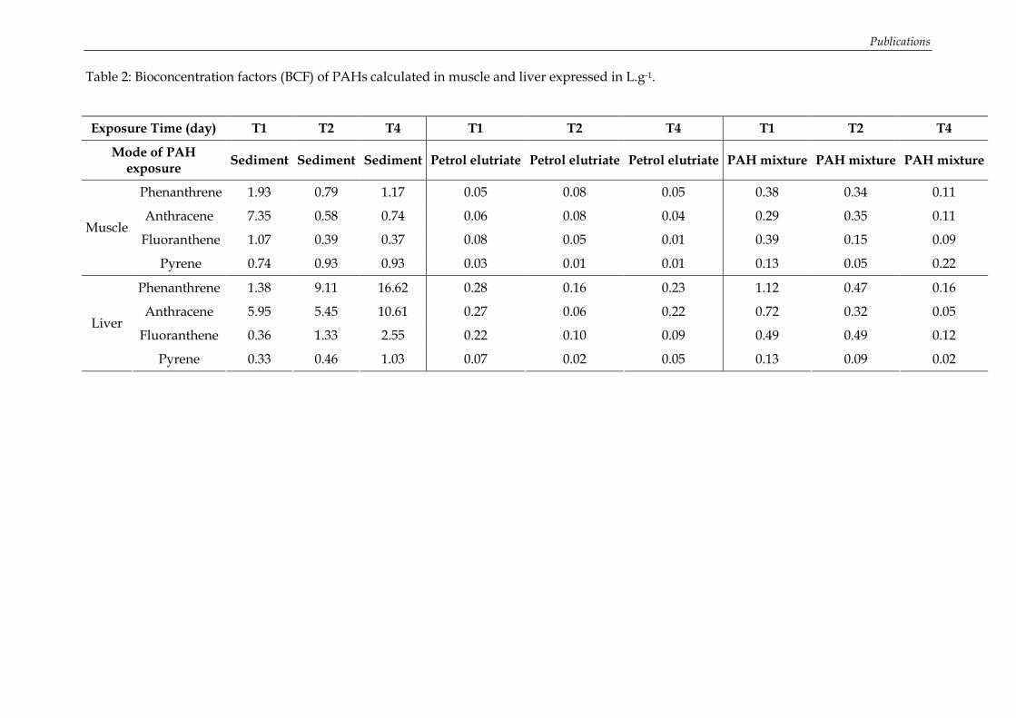
Publications
Table 2: Bioconcentration factors (BCF) of PAHs calculated in muscle and liver expressed in L.g-1.
Exposure Time (day) T1 T2 T4 T1 T2 T4 T1 T2 T4
Mode of PAH exposure
Sediment Sediment Sediment Petrol elutriate Petrol elutriate Petrol elutriate PAH mixture PAH mixture PAH mixture
Phenanthrene 1.93 0.79 1.17 0.05 0.08 0.05 0.38 0.34 0.11
Anthracene 7.35 0.58 0.74 0.06 0.08 0.04 0.29 0.35 0.11
Fluoranthene 1.07 0.39 0.37 0.08 0.05 0.01 0.39 0.15 0.09 Muscle
Pyrene 0.74 0.93 0.93 0.03 0.01 0.01 0.13 0.05 0.22
Phenanthrene 1.38 9.11 16.62 0.28 0.16 0.23 1.12 0.47 0.16
Anthracene 5.95 5.45 10.61 0.27 0.06 0.22 0.72 0.32 0.05
Fluoranthene 0.36 1.33 2.55 0.22 0.10 0.09 0.49 0.49 0.12 Liver
Pyrene 0.33 0.46 1.03 0.07 0.02 0.05 0.13 0.09 0.02

Publications
29
3
Figure 4: PAH metabolite concentrations in fish bile expressed in ng.g-1 of bile. A: Control fish; B: Sediment exposure; C: Petrol elutriate exposure; D: Dissoved PAH mixture exposure.
0
50
100
150
200
250
300
350
400
T0 T1 T2 T3 T4 T10
PA
H m
etab
olite
s co
nc. (
ng/g
of b
ile) OH-PAH
1-OHPOHPheOHBaP
A
0
10,000
20,000
30,000
40,000
50,000
60,000
70,000
80,000
T0 T1 T2 T3 T4 T10
PA
H m
etab
olite
s co
nc. (
ng/g
of b
ile) OH-PAH
1-OHPOHPheOHBaP
B
0
5,000
10,000
15,000
20,000
25,000
30,000
35,000
T0 T1 T2 T3 T4 T10
PA
H m
etab
olite
s co
nc. (
ng/g
of b
ile) OH-PAH
1-OHPOHPheOHBaP
C
0
50,000
100,000
150,000
200,000
250,000
300,000
350,000
T0 T1 T2 T3 T4 T10
PA
H m
etab
olite
s co
nc. (
ng/g
of b
ile) OH-PAH
1-OHPOHPheOHBaP
D
Experiment Time (Days)
Experiment Time (Days) Experiment Time (Days)
Experiment Time (Days)

Publications
294
3.4 DNA Strand breaks: the Comet Assay
For the control group, the results of an ANOVA showed an inter-individual variability in the extent of DNA damage in fish (p < 0.001). However, comet parameters appeared to be stable during the experimental period, validating our experimental conditions for fish maintenance at the laboratory.
In a second step, the data obtained for the control and the PAH-exposed groups were subjected to a main effects ANOVA analysis (factors: ‘ individual’, ‘treatment’, ‘experimental time’). Results obtained showed significant effects of experimental time and treatment on the extent of DNA strand breaks (p < 0.001). For the all set of data analyzed, a general increase in DNA damage was observed 4 days after the beginning of the experiment. Whatever the mode of exposure (petrol, sediment, dissolved phase), a higher level of DNA damage was measured in fish exposed to PAHs with comparison with the control group (Tukey test, p < 0.001, Figure 5). No difference in the extent of the genotoxic response was observed with the mode of PAH contamination (p > 0.05).
The effect of the depuration period was studied by t-test comparisons for each PAH exposed-group. For fish exposed to the contaminated sediment, a non-significant decrease in comet parameter was observed following depuration (p = 0.09). Decrease was significant for the fish exposed via the dissolved phase (p < 0.001) (Figure 6A). For fish exposed to the petrol, the level of DNA damage was still increasing during the depuration phase (p < 0.001) (Figure 6B).
Mean ±SE ±0,95 Conf. Interval
Control sediment petrol dissolved phase
Experimental groups
3,75
3,80
3,85
3,90
3,95
4,00
4,05
4,10
4,15
Sq
uar
e ro
ot
of
tail
DN
A
Figure 5: Effects of PAH exposure and mode of PAH exposure on the extent of DNA damage of fish erythrocytes.

Publications
295
Mean ±SE ±0,95 Conf. Interval
Before After
Depuration
3,9
4,0
4,1
4,2
4,3
4,4
4,5
4,6
Sq
uar
e ro
ot
of
tail
DN
A
Mean ±SE ±0,95 Conf. Interval
Before After
Depuration
4,0
4,1
4,2
4,3
4,4
4,5
4,6
Sq
uar
e ro
ot
of
tail
DN
A
Figure 6: Effect of depuration on the level of DNA strand breaks of fish exposed to a mixture of dissolved PAHs (A: upper graph) or to the petrol elutriate (B: lower graph).

Publications
296
3.5 Statistical correlations between biomarkers
A statistical analysis was performed taking into account all the data collected whatever the mode of PAH contamination (Table 3). Significant positive correlations were demonstrated between the level of DNA damage as measured by the comet assay and the level of different individual metabolites.
Table 3: Correlations observed between DNA damage and PAH metabolites in fish bile (Spearman correlations, *p < 0.05, n = 80)
Biomarkers 1-OHP 3-OHBaP OHPhe OHHAP
%Tail DNA 0.286* 0.250* 0.365* 0.325*
4 Discussion
4.1 Bioavailability and Bioaccumulation
The focus of the present study was to investigate sublethal effects of PAHs on juvenile turbots, emphasising the influence of the route of exposure and the biological effects induced in terms of genotoxicity.
As shown in Figures 1 and 2, the distribution of PAHs in the dissolved phase made it possible to highlight various behaviours of individual PAHs in the dissolved phase. In the experimental design, contents of nominal PAHs in the medium were targeted. The measurement of the water concentrations of PAHs showed they were certainly not constant in the dissolved phase. Targeted values of PAHs were not reached during the experiment. This justified the necessity of chemical analysis to measure the exact level of PAH exposure. It thus made it possible to define the real experimental conditions and to prove the feasibility of the experimental installation. The lowest effective concentrations were thus representative of the environmental concentrations. The bioavailability of PAHs in fish is a complex phenomenon involving different factors such as the percentage and the composition of the organic matter in the dissolved phase and the shape of the particles [38-40]. This is particularly true in the case of sediment exposure. Some works showed the importance of the particle size for the distribution of PAHs in the sediment [41, 42]. Thus the dissolved concentrations measured in the aquariums were different to the bioavailable PAH amount for the organism. In this study, each method of contamination reflected a particular PAHs distribution. In order to understand and to interpret the various processes of bioaccumulation and biotransformation in fish, it was necessary to consider the differences in PAHs bioavailability according to the ways of contamination. For elutriate exposure, phenanthrene and chrysene were the major compounds, according to the petrogenic origin of the PAH source. For the sedimentary exposure, fluoranthene and phenanthrene were predominant, which was a characteristic profile of sediments contaminated by PAHs.
Despite different PAH concentrations were reached in the dissolved phase during the sediment exposure and the petrol elutriate exposure, the PAH concentrations in turbot muscle and liver were similar. This observation corroborated the fact that bioavailability of PAHs differs according to the way of contamination. The absorption of PAHs dissolved in water by fish could be regarded as a simple partition between the water and the lipids [43]. Thus, PAHs of higher molecular weight and hydrophobic should be more easily bioavailable for absorbtion. However, physical constraints can occur by increasing the complexity of the

Publications
297
molecular structure and the volume occupied by the molecules. This could lead to a passive transfer through the lipidic membrane [43, 44]. Indeed contents of particulate (MOP) and dissolved (MOD) organic matter in water are very important factors which significantly deteriorate the absorption of PAH [40]. An increase in the values of MOP and MOD reduces the bioavailability of PAHs, affecting first the molecules of higher molecular weight flowed by those of weaker molecular weight, more water-soluble [40]. In the case of sediment contamination, the nature and the size of sediment particles are governing factors of PAH bioavailability and thus of PAH bioaccumulation in tissues. It is the same for the exposure to petrol elutriate. At the end of the exposure period (T4), PAH concentrations in muscles are similar for the sediment and for the petrol elutriate mode of exposure. For the organisms exposed to the mixture of dissolved PAHs, these concentrations are a little higher due to the largest amounts of PAHs dissolved in the aquariums during the exposure. In a general way, concentration of PAHs in muscles decreased during the phase of exposure, whatever the mode of contamination and the level of dissolved PAHs in water. Therefore, the metabolic capacity to regulate in the organism seems to be never exceeded in this experiment. At the end of the period of depuration (T10), PAH concentrations are similar whatever the mode of contamination. In muscle, they returned at the basic level measured in the control fishes. In the liver, they remained at a higher level than control fishes even if they dramatically decreased during the depuration period. No significant bioaccumulation was observed in muscles and in liver. The elimination of PAH by organism is thus a combination of passive diffusion and enzymatic transformations, followed by an excretion. This is why, the measurement of PAH body burden, defined as the internal and time-dependent exposure concentration of a contaminant in organism, is the result of a dynamic and complex balance between phenomena of assimilation and elimination [43].
When considering BCF values, BCF calculated in muscle exhibited lower values than those for liver. This is due to the higher lipid contents in liver than in muscle. Nevertheless, trends observed for muscle BCF were the same than those observed for liver BCF. BCF values were the highest following sediment contamination. BCF values for petrol elutriates exposure were the lowest and did not vary during the exposure. These results seemed to indicate that PAHs introduced via the sediment were better bioaccumulated. In fish, dissolved phase is the major source of exposure for low lipophilic compounds (log Kow < 5) whereas the particles of the sediment, just as food, can contribute in a substantial way to the bioaccumulation process of compounds with high log Kow (> 5) [45]. For these turbots which were not fed during the experimentation, the bioaccumulation is mainly due to respiratory exchanges [46, 47]. Nevertheless, it is necessary to take into account the way of BCF calculation to interpret these results. Indeed, the PAH measurement in the dissolved phase does not correspond completely to the quantity of bioavailable PAHs for the organism. In the case of the exposure to the petrol elutriate, small hydrocarbon pellets floated on the surface and in the water column. PAHs present in these pellets were not taken into account for the determination of the PAH concentration in the dissolved phase. Absorption by oral or dermal way in fish are however possible and can contribute to the BCF. Moreover, in the case of the petrol elutriate, it is not right to consider only PAH compounds. The heavy fuel, which composes this solution, is a complex mixture of saturated and unsaturated hydrocarbons. The alkenes are present in great quantity and their presence influences the physicochemical properties of the other molecules. Thus, the oil alkenes can have a role in the capacity of PAHs to cross lipid membranes of fish and thus can influence their absorption.
4.2 Biotransformation: PAH metabolites in bile
The level of PAH metabolites in the bile is depending on the level of PAH exposure but also on the flow rate of bile through gall bladder. The regulation of this flow is mainly due to the

Publications
298
feeding status of the organism since bile constituted an excretion way of the digestion process [48]. Because the animals were not fed during the experiment, the experiment conditions were different from that of the natural environment but allowed a higher amount of bile available for analysis. The choice of studied metabolites was made regarding the specificity of the parent compounds to be chemical markers of PAH origin of contamination. Phenanthrene being a predominant PAH in the case of petrogenic origin of PAH contaminations, the follow-up of its metabolites could bring additional information on the source of the contamination. In the same way, benzo(a)pyrene is a major PAH in the case of a pyrolytic origin of the contamination. Lastly, pyrene is a PAH present in both contamination from petrogenic and pyrolytic origins. Its metabolite can thus be a good indicator of a multi-source contamination, being more general and diffuse.
In this study, the level of PAH metabolites in the bile increased during the exposure and decreased during the depuration period. These levels of metabolites quantified in the bile of fish correlated with the levels of contamination of the dissolved phase, even if differences in nature and in quantity of metabolites formed existed. During the sediment exposure, the formation of bile metabolites was the latest and can be explained by the longer time required fro the induction of biotransformation enzymes. Bioavailability plays a role in the activation of the biotransformation processes. Higher is the quantity of PAHs dissolved in the dissolved phase, faster is expected to be the induction of the enzymatic systems involved in the production of PAH metabolites. In addition, the sedimentary mode of exposure can give variable results because of the differences in fish behaviour in the aquarium (hiding or stroke in the water column, ingestion or not of the sediment). This difference in fish behaviour could also exist in the other exposition routes. Nevertheless in the sediment exposure, this could lead to higher inter-individual differences in level of exposure and thus in the absorption of the parent PAHs.
A rapid production of metabolites was also observed whatever the levels of exposure of the dissolved phase in particular for the 1-hydroxypyrene (1-OHP), the major metabolite of pyrene. This indicated that the low BCF (Table 2) calculated for pyrene was the result of a very efficient metabolism rather than a pronounced reduced bioavailability. These results are in accordance with the findings of Spacies et al. [40], who determined in fish a high bioavailability of BaP which is a larger PAH molecule than pyrene The biotransformation was shown to be more efficient for pyrene than for phenanthrene in the present study. This is in agreement with the results of previous studies that have reported a more efficient metabolism of larger PAHs compared to smaller compounds [49, 50].
These observations corroborated the assumption that PAH metabolites and in particular 1-OHP could be used as early biomarker of exposure, even at low level of contamination. The use of the metabolites of phenanthrene seemed to be also good indicators of PAH exposure in fish. Similar results have been previously obtained in sheepshead minnows exposed to PAHs dissolved in seawater [49].
4.3 DNA strand breaks
During this study, genotoxicity of PAHs for turbot was confirmed whatever the tested mode of contamination. The genotoxic effect was significant only at day 4 of exposure. This delay in response may be attributed to the time necessary for the production of a threshold amount of genotoxic metabolites for which a positive response can be measured by the comet assay. During this study, the differences observed with the mode of contamination in the profile of PAH metabolites pointed out differences in PAH bioavailability. Despite obvious differences in biotransformation, it is noteworthy that the genotoxic response was of same order whatever the tested mode of contamination. The latter finding can be explained by the lack of significant differences between exposed groups in the production of genotoxic

Publications
299
metabolites. In fact, among the produced metabolites only one fraction is thought to be involved in the genotoxic response. In our study, 3-OHBaP is the only metabolite that is potentially genotoxic. In fish exposed to PAHs via the dissolved phase or the petrol, it is detectable in the bile from day 3 of exposure. Following sediment contamination, one more day of exposure is necessary for the detection of this metabolite. 3-OHBaP represents a small fraction of the total metabolites produced, from 0.3 to 19.1% of the metabolites analysed depending on the time and mode of exposure.
In the case of PAH, different mechanisms of genotoxicity have been proposed for higher vertebrates. The incomplete repair of stable and depurinating DNA adducts by base and nucleotide excision repair systems can lead to DNA breakage [51, 52] that could account for a high amount of the strand breaks induced by PAH exposure [53]. The biotransformation of PAH can also result in an oxidative stress via the by-production of reactive oxygen species by quinone metabolism [54-56]. DNA fragmentation occurs either by direct action on the DNA or by the incomplete repair of the resulting oxidized DNA bases [57, 58]. The production of DNA strand breakage was already demonstrated in fish following PAH exposure. A significant increase in the level of DNA strand-breaks and alkali-labile sites was shown in turbots exposed PAH contaminated sediment [59, 60]. Similar results were obtained in the rainbow trout [61] and in flounder exposed to waterborne BaP [62].
For fish exposed via the sediment or the dissolved phase, the decrease observed with depuration can indicate effective repair mechanisms of DNA damage in fish like in higher vertebrates. In fish exposed to the petrol, DNA damage still increased during the depuration phase. In this group, the balance between the production of genotoxic metabolites and the detoxication/DNA repair mechanisms may be different.
4.4 Interactions between biomarkers
The significant positive correlation observed between the levels of biliary PAH metabolites and the level of DNA strand breaks tend to confirm a rule for the biotransformation of PAHs in the genotoxic effects measured in turbot. Because of a rapid bile evacuation, it is noteworthy that the detection of PAH metabolites in fish bile is considered as an early marker of recent PAH exposure such as genotoxicity biomarker. During this study, only some few metabolites were analysed. They were selected because of their easy detection due to their production in high amount. Looking at genotoxicity as an endpoint, it would have been more pertinent to focus the chemical analysis on known genotoxic metabolites of PAHs. A large number of research papers [63-70] pointed out the rule of diols-, diol-epoxides and dione metabolites in the genotoxicity of PAHs. These metabolites can interact either directly with the DNA (diol-epoxides) or indirectly via the formation of reactive intermediates (e.g. semi-quinone radicals). Research is in course to allow a better detection of this kind of metabolites.
The biomarkers proposed in this study were validated in laboratory and also during campaigns in the Seine estuary (Normandy, France) [71]. The strong point of this study was the joint interpretation of chemical (parent PAHs, PAH metabolites) and biological data (genotoxicity) to demonstrate the relationship between PAH exposure and biological effects in terms of genotoxicity.
Acknowledgements: The authors wish to thank the National Program for Ecotoxicology (PNETOX), the French Minister of Environment and the research team IMOPHYS (Integration of molecular and physiologic responses to organic contaminants in coastal area) for research fundings. They want also to acknowledge the “Region Aquitaine” and the French National Council for Scientific Research (CNRS) for providing the PhD grant of M. Le Dû-Lacoste.

Publications
300
References
1. McElroy, A. E., Farrington, J. W., Teal, J. M., and Varanasi, U., Metabolism of Polycyclic Aromatic Hydrocarbons in the Aquatic Environment, Pp 1-40. 1989, Boca Raton: CRC Press.
2. Neff, J. M., Polycyclic Aromatic Hydrocarbons in the Aquatic Environment: Sources, Fates and Biological Effects. 1979, London: Applied Science Publishers Ltd. 262.
3. Budzinski, H., Jones, I., Bellocq, J., Piérard, C., and Garrigues, P. 1997. Marine Chemistry 58(1-2): p. 85-97.
4. Whyte, J. J., Jung, R. E., Schmitt, C. J., and Tillitt, D. E. 2000. Critical Reviews in Toxicology 30(4): p. 347-570.
5. GESAMP, (Joint Group of Experts on the Scientific Aspects of Marine Environmental Protection). Impact of Oil and Related Chemicals and Wastes on the Marine Environment., 50., G.R., Editor. 1993.
6. Meador, M. R., Brown, L. R., and Short, T. 2003. Ecological Indicators 3(2): p. 81-92.
7. Varanasi, U. and Stein, J. E. 1991. Environmental Health Perspectives 90: p. 93-100.
8. Hugget, R. J., Kimerle, R. A., Mehrle, P. M., and Bergman, H. L., Biomarkers. Biochemical, Physiological and Histological Markers of Anthropogenic Stress., ed. Publishers, L. 1992, Chelsea, MI.
9. Collier, T. K., Anulacion, B. F., Stein, J. E., Goks@?yr, A., and Varanasi, U. 1995. Environmental Toxicology and Chemistry 14(1): p. 143-152.
10. French, B. L., Reichert, W. L., Hom, T., Nishimoto, M., Sanborn, H. R., and Stein, J. E. 1996. Aquatic Toxicology 36(1-2): p. 1-16.
11. Myers, M. S., French, B. L., Reichert, W. L., Willis, M. L., Anulacion, B. F., Collier, T. K., and Stein, J. E. 1998. Marine Environmental Research 46(1-5): p. 197-202.
12. Spies, R. B., Stegeman, J. J., Hinton, D. E., Woodin, B., Smolowitz, R., Okihiro, M., and Shea, D. 1996. Aquatic Toxicology 34(3): p. 195-219.
13. Stein, J. E., Collier, T. K., Reichert, W. L., Casillas, E., Hom, T., and Varanasi, U. 1992. Environmental Toxicology and Chemistry 11: p. 701-714.
14. van der Oost, R., Beyer, J., and Vermeulen, N. P. E. 2003. Environmental Toxicology and Pharmacology 13(2): p. 57-149.
15. Mahadevan, B., Marston, C. P., Luch, A., Dashwood, W. M., Brooks, E., Pereira, C., Doehmer, J., and Baird, W. M. 2007. International Journal of Cancer 120(6): p. 1161-1168.
16. Sturve, J., Balk, L., Adolfsson-Eric, M., Lindstrom, P., Holmqvist, I., Parkkonen, J., Albertsson, E., Carney-Almroth, B., and Fo?rlin, L. 2006. Marine Environmental Research 62(SUPPL. 1).
17. Schiedek, D., Broeg, K., Bars?iene, J., Lehtonen, K. K., Gercken, J., Pfeifer, S., Vuontisja?rvi, H., Vuorinen, P. J., Dedonyte, V., Koehler, A., Balk, L., and Schneider, R. 2006. Marine Pollution Bulletin 53(8-9): p. 387-405.

Publications
301
18. Hansson, T., Schiedek, D., Lehtonen, K. K., Vuorinen, P. J., Liewenborg, B., Noaksson, E., Tja?rnlund, U., Hanson, M., and Balk, L. 2006. Marine Pollution Bulletin 53(8-9): p. 451-468.
19. James, M. O., Kleinow, K. M., Zhang, Y., Zheng, R., Wang, L., and Faux, L. R. 2004. Marine Environmental Research 58(2-5): p. 343-346.
20. Reynolds, W. J., Feist, S. W., Jones, G. J., Lyons, B. P., Sheahan, D. A., and Stentiford, G. D. 2003. Chemosphere 52(7): p. 1135-1145.
21. Telli-Karakoc, F., Ruddock, P. J., Bird, D. J., Hewer, A., Van Schanke, A., Phillips, D. H., and Peters, L. D. 2002. Marine Environmental Research 54(3-5): p. 511-515.
22. Johnson, L. L., Collier, T. K., and Stein, J. E. 2002. Aquatic Conservation: Marine and Freshwater Ecosystems 12(5): p. 517-538.
23. Akcha, F., Burgeot, T., Budzinski, H., Pfohl-Leszkowicz, A., and Narbonne, J. F. 2000. Marine Ecology Progress Series 205: p. 195-206.
24. Aas, E., Baussant, T., Balk, L., Liewenborg, B., and Andersen, O. K. 2000. Aquatic Toxicology 51(2): p. 241-258.
25. Rocher, B., Le Goff, J., Peluhet, L., Briand, M., Manduzio, H., Gallois, J., Devier, M. H., Geffard, O., Gricourt, L., Augagneur, S., Budzinski, H., Pottier, D., Andre, V., Lebailly, P., and Cachot, J. 2006. Aquatic Toxicology 79(1): p. 65-77.
26. Pagnout, C., Rast, C., Veber, A. M., Poupin, P., and Fe?rard, J. F. 2006. Ecotoxicology and Environmental Safety 65(2): p. 151-158.
27. Le Goff, J., Gallois, J., Pelhuet, L., Devier, M. H., Budzinski, H., Pottier, D., Andre, V., and Cachot, J. 2006. Aquatic Toxicology 79(1): p. 55-64.
28. Cachot, J., Geffard, O., Augagneur, S., Lacroix, S., Le Menach, K., Peluhet, L., Couteau, J., Denier, X., Devier, M. H., Pottier, D., and Budzinski, H. 2006. Aquatic Toxicology 79(3): p. 257-267.
29. Hoffmann D. J., R. B. A., Burton G. A., Cairns J., Handbook of Ecotoxicology. second edition ed. 2003: Lewis. 1290.
30. Gravato C. and M.A., S. 2003. Ecotoxicology and Environmental Safety 55: p. 352-358.
31. Gravato, C. and Santos, M. A. 2002. Ecotoxicology and Environmental Safety 51(2): p. 115-127.
32. Akcha, F., Vincent Hubert, F., and Pfhol-Leszkowicz, A. 2003. Mutation Research/Genetic Toxicology and Environmental Mutagenesis 534(1-2): p. 21-32.
33. Mazeas, L. and Budzinski, H. 2002. International Journal of Environmental Analytical Chemistry 82(3): p. 157-173.
34. Budzinski, H., Letellier, M., Garrigues, P., and Le Ménach, K. 1999. J. Chromatogr. A 837(1-2): p. 187-200.
35. Baumard, P. and Budzinski, H. 1997. Analusis 25: p. 246-252.

Publications
302
36. Baumard, P., Budzinski, H., and Garrigues, P. 1997. Fresenius J Anal Chem 359(6): p. 502-509.
37. Le Dû - Lacoste M and Budzinski H. Submitted. Anal Bioanal Chem.
38. Baussant, T., Sanni, S., Jonsson, G., Skadsheim, A., and Børseth, J. F. 2001. Environmental Toxicology and Chemistry 20(6): p. 1175-1184.
39. Jonsson G, B. R., Bamber SD, Baussant T. 2004. Environ Toxicol Chem. 23(6): p. 1538-48.
40. Spacie, A. 1983. Ecotoxicological and environmental safety 7(3): p. 330-341.
41. Jonhson-Restrepo, B., Olivero-Verbel, J., Lu, S., Guette-Fernandez, J., Baldiris-Avila, R., O'Byrne-Hoyos, I., Aldous, K., Addink, R., and Kannan, K. 2008. Environmental Pollution 151(3): p. 452-459.
42. Liang, Y., Britt, D., McLean, J., Sorensen, D., and Sims, R. 2007. Applied Microbiology and Biotechnology 74(6): p. 1368-1375.
43. Barron, M. G. 1990. Environ. Sci. Technol. 24(11): p. 1612-1618.
44. Opperhuizen, A. and Sijm, D. 1990. Environ. Toxicol. Chem. 9: p. 175-186.
45. Belfoid, A. C. 1996. Environmental Review 4: p. 276-299.
46. Kelly, B. C. 2004. Environ Toxicol Chem. 23(10): p. 2324-2336.
47. Randall, D. J. 1998. Chemosphere 37(7): p. 1263-1270.
48. Collier, T. K. and Varanasi, U. 1991. Archives of environmental contamination and toxicology 20(4): p. 462-473.
49. Jonsson, G., Bechmann, R., Bamber, S., and Baussant, T. 2004. Environ Toxicol Chem. 23(6): p. 1538-48.
50. Varanasi, U. and Gmur, D. J. 1981. Aquatic Toxicology 1(1): p. 49-67.
51. Frosina, G., Fortini, P., Rossi, O., Carrozino, F., Raspagliuo, G., Cox, L. S., Lane, D. P., Abbondandolo, A., and Dogliotti, E. 1996. J. Biol. Chem. 271: p. 9573-9578.
52. Van Steeg, H. 2001. Toxicol. Lett. 120: p. 209-219.
53. Speit, G. and Hartmann, A. 1995. Mutagen. 10: p. 555-559.
54. Flowers-Geary, L., Harvey, R. G., and Penning, T. M. 1992. Biochem. J. 11: p. 49- 58.
55. Gelboin, H. V. 1980. Physiol. Rev. 60: p. 1107-1166.
56. Bolton, J. L., Trush, M. A., Penning, T. M., Dryhurst, G., and Monks, T. J. 2000. Chemical Research in Toxicology 13(3): p. 135-160.
57. Laval, J., Jurado, J., Saparbaev, M., and Sidorkina, O. 1998. Mutat. Res. 402: p. 93-102.
58. Memisoglu, A. and Samson, L. 2000. Mutation Research - Fundamental and Molecular Mechanisms of Mutagenesis 451(1-2): p. 39-51.

Publications
303
59. Hartl, M. G. J., Kilemade, M., Sheehan, D., Mthersill, C., O’Halloran, J., O’Brien, N. M., and van Pelt, F. N. A. M. 2007. Mar. Environ. Res 64: p. 191-208.
60. Kilemade, M. F., Hartl, M. G. J., Sheehan, D., Mothersill, C., Van Pelt, F. N. A. M., O’Halloran, J., and O’Brien, N. M. 2004. Environ. Mol. Mutagen. 44: p. 56-64.
61. Inzunza, B., Orrego, R., Penalosa, M., Gavilan, J. F., and Barra, R. 2006. Ecotoxicology and Environmental Safety 65(2): p. 242-251.
62. Woo, S., Kim, S., Yum, S., Yim, U. H., Lee, T. K., and . , . 2006. Mar. Poll. Bull. 52: p. 1768-1775.
63. Afshar, C. E., Carrell, C. J., Carrell, H. L., Harvey, R. G., Kiselyov, A. S., Amin, S., and Glusker, J. P. 1996. Carcinogenesis 17(11): p. 2507-2511.
64. Basu, N., Billiard, S., Fragoso, N., Omoike, A., Tabash, S., Brown, S., and Hodson, P. 2001. Environmental Toxicology and Chemistry 20(6): p. 1244-1251.
65. Krahn, M. M., Myers, M. S., Burrows, D. G., and Malins, D. C. 1984. Xenobiotica 14(8): p. 633-646.
66. Krahn, M. M., Rhodes, L. D., Myers, M. S., Moore, L. K., MacLeod, W. D., and Malins, D. C. 1986. Archives of environmental contamination and toxicology 15(1): p. 61-67.
67. Pangrekar, J., Kandaswami, C., Kole, P., Kumar, S., and Sikka, H. C. 1995. Marine Environmental Research 39(1-4): p. 51-55.
68. Varanasi, U., Eberhart, B. T., Nishimoto, M., and Reichert, W. 1985. Proceedings of the American Association for Cancer Research VOL. 26.
69. Varanasi, U. and Nishimoto, M. 1985. Federation Proceedings 44(3).
70. Wenzel-Hartung, R., Brune, H., Grimmer, G., Germann, P., Timm, J., and Wosniok, W. 1990. Experimental Pathology 40(4): p. 221-227.
71. Le Dû - Lacoste M, Akcha F, Peluhet L, Le Menach K, Burgeot T, and Budzinski H. Submitted. Environmental Science & Technologies.

Publications
304

Publications
305
Publication n°8
Assessment of polycyclic aromatic hydrocarbons (PAH) pollution in dab (Limanda limanda) collected in the Seine estuary (France).
M. Le Dû-Lacostea, F. Akchab, L. Peluheta, K. Le Menacha, T. Burgeotb H. Budzinskia
aISM-LPTC, UMR 5255 CNRS – University Bordeaux I, Talence, FRANCE
bDEL-PC, IFREMER, Nantes, FRANCE
* Corresponding author : [email protected]
Tel: + 33 540 006 998
Fax: + 33 540 002 267
Abstract
The Seine estuary is well known to be widely contaminated by organic pollutants and especially by PAH. Fish are known to metabolize PAH triggering to the formation of genotoxic damages at the cellular and sub-cellular levels. In this work, relationships between liver 7-ethoxyresorufin-O-deethylase dealkylation (EROD) activity, DNA strand breaks in blood cells, and PAH metabolites in bile of dab (Limanda limanda) were analyzed. Female and male dab of two class of size (juvenile and adult) were collected by trawling in two sites with different degrees of pollution during March and September 2005 and 2006. Significant effect of sex, age, site and season were demonstrated on EROD activity and on the level of strand breaks. Significant interaction between age and sex was shown that might indicate the complex influence of other factors on the extent of DNA damage and induction of EROD activity (i.e. reproduction status). For PAH metabolites only the influence of the site and of the season was demonstrated. Generally speaking, dabs collected at the entrance of the estuary appeared to be the most impacted considering all the markers studied. Variations in biomarkers responses between males and females and between adults and juveniles may be due to seasonal variations related to the variations in lipid content and levels of biotransformation activities and/or spawning cycles. Correlations between DNA lesions and PAH metabolites showed the importance of combined analysis of chemical and biochemical markers to correctly assess the contribution of chemical contamination to the measured biological responses.
Keywords: PAH metabolites, DNA strand breaks, EROD activity, fish, biomonitoring.
Submitted to Environmental Science & Technologies

Publications
306
Introduction
Anthropogenic compounds of industrial, agricultural and domestic origin are discharged into the coastal environments inducing a variety of reactions in organism depending on their concentration, toxicity and exposure time [1]. In biomonitoring studies, a suitable set of biological responses can be useful not only to determine the degree of harm on biota health but also to identify the stressors or pollutants responsible for such effects. At a cellular level, it is possible to use indicators such as the hepatic mixed function oxygenase (MFO) activity to detect functional changes. Induction can be useful to determine the relationship between these discharges and their bioavailability to organisms [2], and to demonstrate exposure and residency. In this way, several studies have recognized the induction of the cytochrome P450-dependent MFO system (EROD activity) as an excellent biological indicator of exposure to anthropogenic organic contaminants and especially to polycyclic aromatic hydrocarbons (PAH) [3-11].
Since induction of the MFO system is considered a general biological indicator of exposure, the induction response does not reveal the identity of a specific class of pollutants [12]. Therefore determination of hydroxylated polycyclic aromatic hydrocarbons metabolites (OH-PAH) in bile has become a complementary method to assess and identify fish exposure to PAH [7, 13-15]. Biological effect monitoring, including determination of PAH metabolites, is part of international monitoring programmes, among them ‘OSPAR Joint Assessment and Monitoring Programme (JAMP)’. The OSPAR JAMP guideline are the basis for monitoring activities in the North Sea and include the measurement of PAH metabolites [16] with dab and flounder as target species. Only little is known about concentrations of PAH metabolites in dab from the North Sea. Some studies have been carried out with flounder [7, 14, 17] and plaice [18, 19], but investigations of PAH metabolites in dab bile are rare [3, 20]. In addition to EROD activity and PAH metabolites determination others biological markers are recommended for environmental biomonitoring of PAH exposure such as the comet assay [21]. Exposure to pro-oxidant pollutants such as PAH can lead to the formation of DNA strands breaks that can be measured with the comet assay.
PAH are ubiquitous contaminants of the marine environment because of their stability and because of the multiplicity of their sources. Pyrolytic processes represent the major source of PAH into the environment; this includes anthropogenic sources (incomplete combustion of organic matter such as petroleum derivatives) [22, 23] and natural sources (forest fires) [24]. PAH and alkylated PAH are also naturally present in crude oils resulting from the diagenetic and catagenetic transformation of organic matter. They belong to the list of priority pollutants established by the EPA (Environmental Protection Agency, USA) due to the mutagenicity and carcinogenicity of some of them. The exposure of organisms towards PAH has been often evaluated by measuring the bioaccumulated amounts. This approach can be criticized if we take into account biotransformation ability of these organisms. It does not either give information on the potential toxic effects.
The aim of the present field study was firstly to study bioavailability, bioaccumulation and biotransformation phenomena for PAH in the case of marine flat fish. The PAH exposure of benthic fishes was evaluated via the analysis of produced metabolites. A second objective was to study the relationship between exposure of organisms to these PAH, biotransformation and genotoxic effects. The EROD activity was studied in liver as phase 1 of metabolization of PAH. The produced metabolites were analyzed in bile in order to precise the rapid activation of PAH. Furthermore, primary alterations of DNA related to generated metabolites were examined in order to identify produced effects. The DNA-alterations were determined by the measurement of structural lesions of DNA (DNA-strand breaks). Finally, this work aimed to propose new tools for biomonitoring programs in the case of hydrocarbon pollutions in marine environment (oil spills). The determination of PAH metabolites on a more systematic way in environmental monitoring programs should lead to
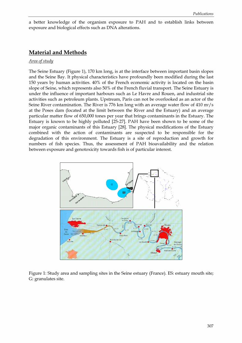
Publications
307
a better knowledge of the organism exposure to PAH and to establish links between exposure and biological effects such as DNA alterations.
Material and Methods
Area of study
The Seine Estuary (Figure 1), 170 km long, is at the interface between important basin slopes and the Seine Bay. It physical characteristics have profoundly been modified during the last 150 years by human activities. 40% of the French economic activity is located on the basin slope of Seine, which represents also 50% of the French fluvial transport. The Seine Estuary is under the influence of important harbours such as Le Havre and Rouen, and industrial site activities such as petroleum plants. Upstream, Paris can not be overlooked as an actor of the Seine River contamination. The River is 776 km long with an average water flow of 410 m3/s at the Poses dam (located at the limit between the River and the Estuary) and an average particular matter flow of 650,000 tones per year that brings contaminants in the Estuary. The Estuary is known to be highly polluted [25-27]. PAH have been shown to be some of the major organic contaminants of this Estuary [28]. The physical modifications of the Estuary combined with the action of contaminants are suspected to be responsible for the degradation of this environment. The Estuary is a site of reproduction and growth for numbers of fish species. Thus, the assessment of PAH bioavailability and the relation between exposure and genotoxicity towards fish is of particular interest.
Figure 1: Study area and sampling sites in the Seine estuary (France). ES: estuary mouth site; G: granulates site.

Publications
308
Sampling design and collection
Dab (Limanda limanda) were collected in March and September 2005 and in March and September 2006 by trawling at different sites in the Seine Bay (Seine Estuary, ES; Granulat Site, G) (Figure 1). The sampling locations have been previously determined with specific studies on dab [29, 30]. At each site, female and male dab of two sizes classes (14-18 and 22-26 cm) were collected from several trawl nets (standard haul duration of 20 min). These fish were considered, respectively, as juveniles (≤ 2 years-old) and adults (~2.5 to ≤ 4 years-old). In the eastern part of the Channel, sexual maturity is observed in the dab at an average age of 2.6 years, corresponding to an average size of 21.6 cm [31]. Fish were kept alive on board in a fish well and dissected once back to the quay. Blood (for comet assay), bile (for PAH metabolites determination) and liver (for EROD activity measurement) samples were stored individually at -80°C. The muscle and liver samples (for PAH body burden measurement) were pooled (n = 10) and stored at -20°C until analysis. The sampling design and collection are resumed in Table 1.
Chemical, solvents and reagents
Hydroxylated PAHs, 1-hydroxynaphtalene (1-OHN) and 2-hydroxynaphtalene (2-OHN) were purchased from Lancaster (Bischeim, France); 2-hydroxybiphenyl (2-OHBi), 9-hydroxyfluorene (9-OHFe) and 1-hydroxypyrene (1-OHP) from Sigma-Aldrich (Saint Quentin Falavier, France) and 9-hydroxyphenanthrene (9-OHPhe), 1-hydroxychrysene (1-OHC) and 3-hydroxybenzo(a)pyrene (3-OHBaP) from Promochem (Molsheim, France). 1-hydroxypyrene-d9 (1-OHPd9) was obtained from Cambridge Isotope Laboratories (Cluzeau Info Labo, Ste Foy La Grande, France). Concerning parent PAHs, the standard reference SRM 2260, constituted of about 20 aromatic compounds, was provided by the U.S. National Institute of Standards and Technology (Gaithersburg MD, USA) and perdeuterated aromatic compounds by MSD Isotopes (Montreal, Canada). All the standards and solvents used were of analytical grade (> 98%). Dichloromethane was provided by Acros Organics (Noisy-Le-Grand, France). Methanol Supersolv was provided by Merck and acetic acid 100% Normapur (analytical reagent grade, Scharlau) was obtained from ICS (Belin-Beliet, France). Sodium
acetate trihydrate 99% (purity > 99%) and β-glucuronidase-aryl-sulfatase mixture from Helix pomatia (100,000 and 7,500 units/ml respectively) were provided by Sigma Aldrich (St Quentin Falavier, France). 2-mercaptoethanol and bis(trimethylsylil)-trifluoroacetamide (BSTFA) were purchased from Acros Organics (Noisy-Le-Grand, France). Deionised water was obtained with a Milli-Q system (Millipore, Molsheim, France). Two solid-phase extraction (SPE) cartridges were used: the Strata-X cartridge (3 cc, 200 mg) from Phenomenex (Le Pecq, France) and the HF Bond Elut-PSA cartridge (3 cc, 500 mg) from Varian and provided by Atlantic Labo (Eysines, France). Aluminium oxide (150 basic type T; 0.063-0.2 mm) and silica gel (0.063-0.2 mm) were provided by VWR (Strasbourg, France).
RPMI 1640 medium, dimethyl sulfoxide (DMSO), 0.4% trypan-blue solution, ethidium bromide (BET), foetal bovine serum (SVF), normal and low melting point agarose, N-sarcosinate, nuclease P1, RNAse A, RNAse T1, proteinase K, micrococcal nuclease, spleen phosphodiesterase, T4 polynucleotide kinase, Triton X-100, sodium dodecylsulfate, phenol, SEVAG were purchased from Sigma Aldrich Chemicals.

Publications
309
Table 1: Sampling design and collection for the four campaigns.
Analysis PAH PAH OH-PAH EROD activity
Comet Assay
Sampling
Campaign Location Class of dabs
Muscle : pool (n=10)
Liver : pool (n=10)
Bile : individual (n=10)
Liver : individual
(n=5)
Blood : individual (n=10)
Males X X X X X Juveniles
Females X X X X X
Males X X X X X
Seine Estuary ES Adults
Females X X X X X
Males X X X X X Juveniles
Females
Males X X X X X
March 2005
Granulate G
Adults Females X X X X X
Males X X X X X Juveniles
Females X X X X X
Males X X X X X
Seine Estuary ES Adults
Females X X X
Males X X X X X Juveniles
Females X X X X X
Males X X X X X
September 2005
Granulate G
Adults Females X X X
Males Juveniles
Females
Males X X X
Seine Estuary ES Adults
Females X X X X X
Males X X X X X Juveniles
Females X X X X X
Males X X X X X
March 2006
Granulate G
Adults Females X X X X X
Males X X X X X Juveniles
Females X X X X X
Males X X X X X
Seine Estuary ES Adults
Females X X X X X
Males X X X X X Juveniles
Females X X X X X
Males X X X
September 2006
Granulate G
Adults Females X X X X X

Publications
310
PAH analysis
PAH were extracted from freeze-dried and grounded solid matrices (liver, muscle) by micro-wave assisted extraction (10 min, 30 W) with methylene chloride followed by filtration on clean glass cotton [32]. Several perdeuterated PAH used as internal standards were added to the samples prior to the extraction step for PAH quantification [33]. Extracts of the different matrices were then purified on aluminium oxide (Al2O3) and silica (SiO2) columns [34, 35] and analysed by GC/MS (gas chromatography/mass spectrometry). Extracts were analysed by an HP GC 6890A gas chromatograph Agilent Technologies (automated PTV pulsed splitless injection (25 psi, 1 min); purge delay: 1 min and purge flow: 60.6 ml/min; injector temperature: 270°C; interface temperature: 280°C; oven temperature: from 70°C (2 min) to 300°C (5 min) at 2°C/min) coupled to an HP MSD 5973 mass spectrometer (electron impact: 70 eV; voltage: 2000 V; source temperature: 150°C) both purchased from BIOS Analytique (l’Union, France). Analyses were performed in the SIM (selected ion monitoring) mode at 1.3 scan/s (Dwell time: 50 ms for each ion) using the molecular ions of the studied compounds. The capillary column was an HP5/MS Agilent Technologies (30 m x 0.25 mm ID x 0.25 film thickness) provided by BIOS Analytique (l’Union, France) and the carrier gas was helium 6.0 obtained from Linde (Toulouse, France). Different perdeuterated polycyclic aromatic hydrocarbons were used as internal standards for each class of aromaticity [33]. The response factors of PAH relatively to perdeuterated PAH were determined for each GC/MS sequence by injecting a mixture containing a solution of PAH (SRM 2260, National Institute of Science and Technology, Gaithersburg, MD, USA) and the solution of perdeuterated PAH used for spiking samples. The monitored PAH are, in ascending order of molecular weight, naphthalene* (N), acenaphthylene* (Ay), acenaphthene* (Ae), fluorene* (Fe), phenanthrene* (Phe), anthracene* (Ant), fluoranthene* (F), pyrene* (P), benz(a)anthracene* (BaA), chrysene*+triphenylene (C+T), benzo(b)fluoranthene* + benzo(j)fluoranthene + benzo(k)fluoranthene* (BbF+BjF+BkF=BF), benzo(a)pyrene* (BaP), indeno(1,2,3-cd)pyrene* (IP), benzo(g,h,i)perylene* (BPer) and dibenz(a,h)anthracene*+dibenz(a,c)anthracene (DB(ah)A+DB(ac)A=DBA). Compounds marked with a “*” are the 16 PAH of the US-EPA. In this study, the sum of those compounds is referred as 19 PAH because of the coelution of three other PAH by GC-MS.
PAH metabolites analysis
Bile samples were prepared according to the protocol described by Le Dû-Lacoste and Budzinski [36].
The weighted whole bile were thawed and then homogenized in precooled buffered water (sodium acetate buffer at pH 5.0 with acetic acid) (100 µl of bile: 2 ml buffer). The internal standard, 1-hydroxypyrene-d9, 20 µl of mercaptoethanol, used as an antioxidant, and 20 µl of β-glucuronidase and arylsulfatase mixture were added to the samples. They were then placed at 37°C in an oven during 18 hours for hydrolysis. After deconjugation, bile samples were ultrasonicated and centrifuged (10 min, 5 000 rpm, 20°C). Solid-phase Strata X cartridges were preconditioned with 2 ml methanol and 4 ml buffered water. The supernatants were loaded on cartridges and washed with 2 ml buffered water and 2 ml water/methanol (70/30, v/v). Water traces were then removed by applying vacuum on the cartridges during 45 min. Metabolites were then eluted with 5 ml of methanol. Extracts were reduced to dryness under nitrogen stream and redissolved in 1 ml methanol/methylene chloride (20/80, v/v) before purification made on solid-phase HF PSA Varian cartridges. Before loading the extracts redissolved in methanol/methylene chloride (20/80, v/v), the purification cartridges were first preconditioned with 2.5 ml methanol/methylene chloride (20/80, v/v). The elution of the compounds was then performed with 6 ml of the same mixture. Extracts were reduced to dryness under a nitrogen stream, redissolved in 50 µl

Publications
311
dichloromethane and 30 µl of a derivatizing agent (BSTFA) were finally added. The derivatization was then completed by incubation at 65°C during 30 min. After derivatization and before GC-MS analysis, a solution of deuterated internal standard (pyrene-d10, 20 µl) was added to the sample for recovery determination.
The analyses were carried out with an HP GC 6890A gas chromatograph Agilent Technologies coupled to an HP MSD 5973 Network mass selective detector Agilent Technologies, both purchased from BIOS Analytique (l’Union, France). The separation was performed on an Agilent Technologies HP5-MS capillary column (length: 30 m; internal diameter: 250 µm; stationary phase thickness: 0.25 µm; phase: 5% diphenyl-, 95% dimethyl-siloxane), with the following oven parameters: from 70°C (2 min) to 180 °C (1 min) at 5°C/min from 180°C to 290°C (1 min) at 10°C/min. The injection volume was set at 1 µl (automated PTV pulsed splitless injection (25 psi, 1.5 min)), while the injector temperature was set at 250°C and the interface temperature at 280°C. The purge flow was set at 60 ml/min during 1.5 min and helium 6.0 (Linde, Bassens, France) was used as the carrier gas (constant flow: 1 ml/min). Acquisition was performed in selected ion monitoring (SIM), with 1.53 scan/s and a dwell time of 50 ms for each ion. The source temperature was set at 150°C, and the electron multiplier voltage set at 2 000 V. The compounds were quantified in SIM mode using the ions below: 1-hydroxynaphtalene (m/z=201), 2-hydroxynaphtalene (m/z=216), 2-hydroxybiphenyl (m/z=211), 9-hydroxyfluorene (m/z=165), 9-hydroxyphenanthrene and isomers (m/z=266), 1-hydroxypyrene (m/z=290), 1-hydroxychrysene (m/z=316) 3-hydroxybenzo(a)pyrene (m/z=340) and 1-hydroxypyrene-d9 (m/z=299), pyrene-d10 (m/z=212). A mixture of the standard metabolites, 1-hydroxypyrene-d9, and pyrene-d10 in dichloromethane was injected, after derivatization, at the beginning and at the end of each sequence for the determination of response factors.
EROD activity
Individual liver samples were homogenized (5 ml/g tissue) in 150 mM KCl, 1 mM EDTA, 100 mM phospahte buffer pH 8, 1 mM dithiotreitol, pH 7.5. Samples were centrifuged (9000g, 15 min, 4°C) and the supernatants (S9 fraction) were recovered. The protein content of each fraction was determined by colorimetry using a Bradford method adapted for microplate reader (Safire, TECAN). EROD activity was measured applying a protocol adapted for fluorescence microplate reader. The assay was made of 10 µL of S9 fraction (5-10 µg proteins), 200 µL of 100 mM phosphate buffer (pH 8) and 10 µL of 46 µM 7-ethoxyresorufine. Reaction was started by the addition of 10 µl of 5 mM NADPH. The excitation and emission fluorescence wavelengths were set at respectively 535 and 580 nm. Measurement was made every 10s during 10 min. EROD activity was expressed in pmol/min/mg proteins.
Comet assay
Blood samples were slowly defrosted at ambient temperature and diluted in PBS buffer before analysis. The comet assay was performed as previously described in [30]. In order to obtain permanent preparations, the slides (two slides per sample) were immersed for 10 min in absolute ethanol for deshydrating, and allowed to dry at room temperature. Just before analysis, 75 µL of BET at 20 µg.ml-1 were deposited on the slide and spread over it using a cover glass. Slides were placed for at least 30 min at 4°C for coloration. Slides were analysed using an optical fluorescence microscope (Olympus BX60, x 40) fitted to a CDD camera (Olympus) and an image analysis system (Komet 4, Kinetic Imaging Ltd). Several parameters were calculated for each observed cell (75 cells/slide), including the percentage of DNA present in the comet tail.

Publications
312
Statistical analysis
Data normality was tested with a Shapiro-Wilk test. To normalize the distribution raw comet data were mathematically transformed. Transformed data as well as chemical data were analysed by Analysis of Variances (ANOVA) using Statistica 6.0 software (Statsoft, France). When a significant effect was observed, significant differences among means were determined using Tukey’s comparison test. Spearman correlations between markers were calculated. All tests were regarded as statistically significant when p < 0.05.
Results
Bioaccumulation: PAH in muscle and liver
The accumulation of PAH tissues (white muscle and livers) of dab sampled on the two sites was relatively limited (Figure 2). The values obtained were lower than those found for other flatfish species at the same locations. In this study concentrations ranged between 2 and 107 ng.g-1 dry weight for PAH content in muscle and between 16 and 102 ng.g-1 dry weight fro PAH content in livers. Mazéas et al. [37] found similar concentrations in flounder livers collected at the entrance of the Seine estuary (between 74 and 100 ng.g-1 dry weight). PAH are hydrophobic compounds that accumulate in lipids but they are also metabolized through specific pathways [18]. The trend displayed by PAH body burden in dab from the two locations suggested a chronic exposure to PAH but these data alone do not assess to a specific punctual contamination such as an oil spill or fuel discharges.
When compared the two locations (ES, Figure 2 A, B and Granulate, Figure 2 C, D) no discrimination between both of them has been possible significantly (Mann-Whtiney test, p < 0.05). However significant effects of the year and of the period of sampling (March or September, 2005 or 2006) were demonstrated whatever the area considered. In March the accumulation of PAH in tissues (muscle and livers) was higher than those in September (p < 0.001) and values obtained in 2005 were lower than those measured in 2006 (p < 0.001). These results could be linked with the Seine river flow rate at these periods of the year. Indeed the mean flow rates of the river were lower during the September campaigns (236 and 269 m3/s in 2005 and 2006, respectively) rather than during the March campaigns (495 and 1198 m3/s in 2005 and 2006, respectively). Lower rates suggest lower inputs of contaminants in the estuary and thus triggers a decrease in the PAH concentrations in tissues. The very highest flow rate for the Seine River observed in March 2006 as well as the increase in the PAH contents in tissues for the same period corroborate the link between the flow rate and bioaccumulation processes of PAH in dab.

Publications
313
Figure 2: Total PAH content (sum of 19 PAHs) in tissues (white muscle and livers) in dab collected from the assessed area in 2005 and 2006. Data from the estuary site are presented in figures A and B. Data from the granulate site are presented in figures C and D. ES: estuary site; G: granulate site; F: female; M: male; J: juvenile; A: adult. Concentrations expressed in ng.g-1 dry weight.
Biotransformation: PAH metabolites in bile
The concentrations revealed to be variable throughout time. Concentrations of total PAH metabolites (OH-PAH), OHPhe and 1-OHP are presented in Figure 3 for all campaigns and all groups of dabs collected in both sites. Major metabolites measured in bile were 1-OHP, OHPhe isomers and 2-OHBi (Figure 4). The biphenyl compound does not belong to the PAH group but it is present in high quantities in the marine environment. That is why its hydroxylated metabolite (2-OHBi) was quantified because it reveals a general pollution of the environment. Concerning 1-OHP and OHPhe, their contributions to the total sum of OH-PAH in bile ranged between 4 and 61% and between 5 and 38 %, respectively. It was also noticed that fishes which had the highest contribution in 1-OHP exhibited the lowest contribution in OHPhe, and conversely. The two markers seemed to be linked together.
The results obtained for the dab have been compared to other studies on flounders [37, 38] that have been collected in the Seine estuary and in other sites along the French Atlantic coasts. In this work, dabs from ES site exhibited similar concentrations of PAH metabolites that flounders collected at the same location. However, when compared the whole results, dabs collected in 2005-2006 have showed higher concentrations that flounders collected along the French Atlantic coasts. In 2005-2006, Laroche et al. [38] showed relatively low concentrations for flounders in the Loire estuary (between 91 and 174 ng.g-1 of bile) and in the Gironde estuary (between 70 and 213 ng.g-1 of bile). In the Seine estuary in 2002-2003, Mazéas et al. [37] have measured mean concentrations between 91 and 217 ng.g-1 of bile in flounders. Thus dabs collected in the Seine estuary in this survey (2005-2006) seemed to be more impacted than flounders collected along the French coasts. However such inter-species
0
20
40
60
80
100
120
FJES MJES FJES MJES FJES MJES
mars-05 mars-05 sept-05 sept-05 sept-06 sept-06
PA
H c
onc.
(ng
/g d
w)
PAH in white muscle PAH in liver
FAES MAES FAES MAES FAES FAES MAES
mars-05 mars-05 sept-05 sept-05 mars-06 sept-06 sept-06
PAH in white muscle PAH in liver
0
20
40
60
80
100
120
MJG MJG FJG FJG MJG FJG MJG
mars-05 sept-05 sept-05 mars-06 mars-06 sept-06 sept-06
PA
H c
onc.
(ng
/g d
w)
PAH in white muscle PAH in liver
FAG MAG FAG MAG FAG MAG FAG
mars-05 mars-05 sept-05 sept-05 mars-06 mars-06 sept-06
PAH in white muscle PAH in liver

Publications
314
and inter-sites comparisons should be relativized. Indeed the specific metabolism of each species can influence qualitatively and quantitatively concentrations of biliary PAH metabolites [39, 40].
When considering the total sum of PAH metabolites quantified (OH-PAH), influences of the site and of the year of sampling were demonstrated significantly (p < 0.001). Between 2005 and 2006 the level in PAH metabolites increased as well as between the September and the March surveys. These can be explained with the seasonal differences in the dab metabolism. Before the spawning season (March) the metabolism seems to be increased whereas during the summer season (September) and the sexual rest it seems to slow down. These seasonal differences have been already described in mussels with the RNO survey (National Observation Network) [41]. It was observed that PAH concentrations measured in mussels were higher in winter because of the higher flow rate of the Seine River that enhanced PAH inputs. This observation that is valid for the bioaccumulation phenomena is directly linked to biotransformation processes. Moreover dabs collected in the ES location showed higher levels of OH-PAH than those caught in the Granulate area. Thus the analysis of OH-PAH seems to be a good and reliable indicator for exposure of dabs to PAH.
When looking at the 1-OHP metabolite levels, significantly effects of the site and of the age (p < 0.001) were observed. Concentrations were 3 times higher at the ES site compared to the Granulate site and the adults presented 2.5 times highest levels of 1-OHP rather than juveniles. Moreover it was shown that juveniles of both sites presented similar concentrations of 1-OHP whereas adults of the ES sites had 4 times higher levels than those collected in the Granulate site. Additionally females from ES site showed higher levels of 1-OHP than males. As a result the influence of the Seine estuary mouth resulting in a higher input of contaminants highlighted different adaptation efforts for dabs according to sex and age. A more important bioaccumulation of PAH as well as a higher metabolism for adult fishes compared to juveniles could be explained by changes in feeding. Indeed feeding (nature, quality and quantity) is a factor that influences bioavailability of organic contaminants [42]. Moreover since females allocate more energy during the gametogenesis for the formation of energetic stocks, they bioaccumulate more PAH than males.
The total concentration of OH-PAH was highly correlated with the concentration of 1-OHP and with OHPhe (p < 0.0001). However no correlation was found between 1-OHP, OHPhe and 3-OHBaP. These markers seemed to be specific markers for PAH contamination’s source (pyrolytic, petrogenic or both). This is an advantage for the proposal of indicator and biomonitoring tools.

Publications
31
5
Figure 3: Mean concentrations of OH-PAH in dabs collected during the 4 surveys. Concentrations expressed in ng.g-1 of bile (Mean ± RSD, n=6). ES: estuary site; G: granulate site; F: female; M: male; J: juvenile; A: adult.
0
200
400
600
800
1,000
1,200
1,400
1,600
MAES FAES MAES FAES FA ES MA ES
mars-05 sept-05 sept-05 mars-06 sept-06 sept-06
OH
-PA
H (
ng/g
of b
ile) OH-PAH 1-OHP OHPhe
FJES MJES FJES MJES FJ ES MJ ES
mars-05 mars-05 sept-05 sept-05 sept-06 sept-06
OH-PAH 1-OHP OHPhe
0
200
400
600
800
1,000
1,200
1,400
1,600
FAG MAG FAG MAG FAG MAG FA G MA G
mars-05 mars-05 sept-05 sept-05 mars-06 mars-06 sept-06 sept-06
OH
-PA
H (
ng/g
of b
ile) OH-PAH 1-OHP OHPhe
MJG MJG FJG FJG MJG FJ G MJ G
mars-05 sept-05 sept-05 mars-06 mars-06 sept-06 sept-06
OH-PAH 1-OHP OHPhe
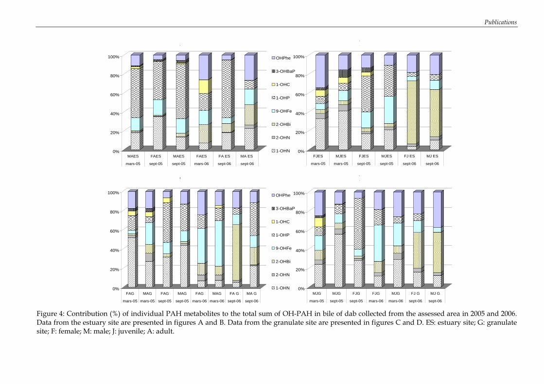
Publications
Figure 4: Contribution (%) of individual PAH metabolites to the total sum of OH-PAH in bile of dab collected from the assessed area in 2005 and 2006. Data from the estuary site are presented in figures A and B. Data from the granulate site are presented in figures C and D. ES: estuary site; G: granulate site; F: female; M: male; J: juvenile; A: adult.
0%
20%
40%
60%
80%
100%
FJES MJES FJES MJES FJ ES MJ ES
mars-05 mars-05 sept-05 sept-05 sept-06 sept-06
0%
20%
40%
60%
80%
100%
MAES FAES MAES FAES FA ES MA ES
mars-05 sept-05 sept-05 mars-06 sept-06 sept-06
OHPhe
3-OHBaP
1-OHC
1-OHP
9-OHFe
2-OHBi
2-OHN
1-OHN
0%
20%
40%
60%
80%
100%
FAG MAG FAG MAG FAG MAG FA G MA G
mars-05 mars-05 sept-05 sept-05 mars-06 mars-06 sept-06 sept-06
OHPhe
3-OHBaP
1-OHC
1-OHP
9-OHFe
2-OHBi
2-OHN
1-OHN 0%
20%
40%
60%
80%
100%
MJG MJG FJG FJG MJG FJ G MJ G
mars-05 sept-05 sept-05 mars-06 mars-06 sept-06 sept-06
A B
C D

Publications
317
DNA damages: Comet Assay
In order to study global effect for each factor (site, age, sex, season) it was decided to only work with a complete matrix of raw data. Thus the campaign of September 2005 and the set of raw data concerning female adults were considered.
In September 2005 all of the studied factors have shown a significant effect (p < 0.001 for the factors “sex” and “site”, 0.01 < p < 0.05 for the factor “age”). Generally speaking male dabs showed DNA strand break’s levels that were higher than those of female dabs (Figure 5A). Moreover adults presented higher levels of breakage than those of juveniles (Figure 5B). The interaction between the two factors (age and sex) was highly significant (p < 0.001). Whereas for the male population the level of breakages was higher for adults than for juveniles, the contrary was observed for the female population. These results confirmed those obtained during previous studies [29, 30]. The presence of a higher number of DNA strand breaks in adult than juvenile was attributed to age-related differences in activities involved in pollutant biotransformation. In fact, it has been shown for flatfish species an increase with age in the induction level of CYP1A protein and cytochrome P450-dependent enzymatic activities [43, 44]. Sex, like age, has an influence on the levels of biotransformation processes. However this effect showed seasonal variations because of sex-dependent influences on enzyme activities relative to negative temperature compensation and/or changes in hormonal status. In order to identify the most sensitive type of individuals for genotoxicity assessment by the comet assay, it appears so necessary to check for these effects for each season of the year.
When considering the population of female adult dabs collected in both sites the effect of the site factor was more precisely evaluated. Significant effect of the factor ‘site’ and of the factor ‘season’ and a significant interaction between the two factors were demonstrated (p < 0.001). Female adults collected on the ES site shown higher levels of DNA strand breaks than those collected on the Granulate site (Figure 5C). Nevertheless differences between the two stations varied according to the season and the year (Figure 5D). In March 2005 and March 2006, the levels of strand breaks were higher on the ES site rather than on the Granulate site. The contrary was stated in September 2005. This result correlated with the results exposed before. Since such an inter-site differences was no completely confirmed in September, winter (e.g. March) appears to be more appropriate season for observing differences in the extent of oxidative DNA lesions in this sentinel flatfish species.

Publications
Figure 5: Mean square root of percent tail DNA measured in dab collected from the assessed area in 2005 and 2006. (A), (B), (C): global effects of the ‘sex’, ‘age’ and ‘site’ factors (respectively) during the September 2005 campaign. (D): interactions between the factors ‘site’ and ‘season’ for the female adult dabs collected during the 4 campaigns. Expressed as mean ± SD.
ES G4,35
4,40
4,45
4,50
4,55
4,60
4,65
Rac
ine
du %
d'A
DN
dan
s la
que
ue d
e la
com
ète
Stations
Sq
ua
re r
oo
t o
f %
Ta
il D
NA
Adulte Juvenile4,40
4,42
4,44
4,46
4,48
4,50
4,52
4,54
4,56
4,58
4,60
4,62
dans
la q
ueue
de
la li
man
de
Adult Age Juvenile
Sq
ua
re r
oo
t o
f %
Ta
il D
NA
Femelle Mâle4,30
4,35
4,40
4,45
4,50
4,55
4,60
4,65
la q
ueue
de
la c
omèt
e
Female Sex Male
Sq
ua
re r
oo
t o
f %
Ta
il D
NA
ES G
Station d'échantillonnage
3,8
3,9
4,0
4,1
4,2
4,3
4,4
4,5
4,6
4,7
dans
la q
ueue
de
la c
omet
e
mars 05 septembre 05 mars 06
Sq
ua
re r
oo
t o
f %
Ta
il D
NA
Stations

Publications
319
EROD activity
The induction of cytochrome P4501A, assayed as EROD activity, showed significant differences in dab (p < 0.01). A Tukey comparison test indicated that EROD activities from dab from ES location were significantly higher than EROD activities in dab from granulates area (p < 0.01) (Figure 6A). This variability inter- and intra-site could be explained by an inter-individual variability already demonstrated [26, 45] since all factors (age, sex, site and season) are taken together. Nevertheless a global interpretation leads to confirm the influence of the Seine estuary mouth since the factor “site” is highly significant. Thus the measurement of the EROD activity appears sufficiently robust to determine the effect of the Seine plume after the integration of the whole factors. This result is in consistency with the analysis of PAH metabolites and DNA strand breakage.
When looking at a temporal effect (Figure 6B), this factor appeared to be very determinant (p < 0.0001). EROD activities measured in 2005 were lower than those measured in 2006 (p < 0.01) as well as activities measured in September that were lower than those measured in March (p < 0.0001). In 2006 the highest EROD activities were related to the concentrations of PAH in tissues and to the levels of PAH metabolites. 2005 was an atypical year because measures of EROD activities were higher in September than in March. However this atypical profile was related to the profile of DNA strand breaks (Figure 5D).
Besides EROD activities were higher for adults rather than for juveniles for both sexes. Differences between the two sexes were not significant for the adults. However within the same sex differences were observable between juveniles and adults. Males and females exhibited higher EROD activities when they were adults (p < 0.001 and p < 0.01, respectively). Males presented a higher sensibility to EROD activities. The effort for reproduction as well as the elimination of bioaccumulated contaminants during spawning [42] could explain the less sensitivity toward EROD activity in female dabs. On the contrary they appeared more sensible at the juvenile age (Figure 6C)
The combination of sex and age effects was in this study very significant for adults (p < 0.0001). The study of sex and age effects is representative of the dab population dynamics. The studied factors following on the variations of the EROD activity represent the metabolic effort done by the population for adaptation.
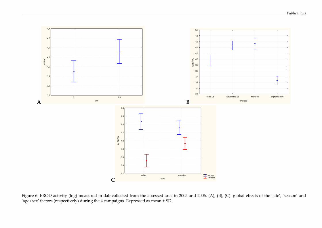
Publications
AG ES
Site
3,7
3,8
3,9
4,0
4,1
4,2
4,3
4,4
Ln E
RO
D
BMars 05 Septembre 05 Mars 06 Septembre 06
Période
2,8
3,0
3,2
3,4
3,6
3,8
4,0
4,2
4,4
4,6
4,8
5,0
Ln E
RO
D
C Adultes Juvéniles
Mâles Femelles
Sexe
3,2
3,4
3,6
3,8
4,0
4,2
4,4
4,6
4,8
Ln E
RO
D
Figure 6: EROD activity (log) measured in dab collected from the assessed area in 2005 and 2006. (A), (B), (C): global effects of the ‘site’, ‘season’ and ‘age/sex’ factors (respectively) during the 4 campaigns. Expressed as mean ± SD.

Publications
321
Interactions between biomarkers
To assess statistical interactions between biomarkers levels (PAH metabolites, EROD activity and DNA strand breaks), correlation analyses were undertaken on whole datasets (all seasons, field sites and groups of dabs combined together). Two observations were particularly interesting. The first one was the absence of correlation between EROD activities and PAH metabolites (OHPhe, 1-OHP or OH-PAH). Even though PAH metabolites indicated an exposure to PAH and even though EROD activities were measured and discriminated the two locations this lack of interactions takes in for questioning. An alternative explanation may be that the two markers are independently influenced by the short-term (days) migratory movements of the dab population within the Seine estuary. Biliary metabolites formation has been shown to respond over much shorter time scale than CYP1A1 induction. Several studies have reported the formation of detectable metabolites within hours (between 4 and 24h) after the exposure [46-49]. This rapid response coupled to the short persistence of metabolites in feeding fish [50] may give greater discrimination in estuarine monitoring. In contrast to metabolites, the time scale of maximum CYP1A1 induction under experimental exposure has been shown to be between 2 and 5 days and the return to control levels appeared between 4 and 7 days [51, 52]. Therefore this work tends to prove that fish caught from specific sample sites may more likely to reflect local contamination through their metabolite profile than through CYP1A1 induction. Besides others factors than migration can also influence the EROD activities such as the influence of multiple xenobiotic compounds (especially heavy metals and PCB) that do not influence the PAH metabolite profiles. The Seine estuary is well known for its multiple contamination sources and this can also explain the lack of correlation between the two markers. Looking at other interactions, DNA strand breaks were positively correlated with total sum of OH-PAH (p < 0.00002, n = 38), 1-OHP (p < 0.002, n = 38), and OHPhe (p < 0.03, n = 38). As stated before, PA metabolites have been detected in dab bile collected during this survey, even if the levels were very low. Thus the exposure of dabs to PAH has been demonstrated. Besides PAH are known to be priority contaminants in the environmental surveys due to the carcinogenic and mutagenic properties of some of them. These properties have been well documented in the literature [53-63]. In parallel genotoxic effects have been observed in collected dabs at the cellular level (activation of the enzymatic system CYP1A1 that catalyzes the biotransformation processes) and at the sub-cellular level (DNA stand breaks).
Thus the whole results of this field study in the Seine Estuary showed that the chemical contamination of the environment was directly linked to genotoxic effects and that it explained the observed damages. Consequently, the biotransformation of PAH would explicate in part the Genotoxicity observed, that could not be done by the bioaccumulation of PAH
Acknowledgements: The authors wish to thank the National Program for Ecotoxicology (PNETOX), the French Minister of Environment and the research team IMOPHYS (Integration of molecular and physiologic responses to organic contaminants in coastal area) for research fundings. They want also to acknowledge the “Region Aquitaine” and the French National Council for Scientific Research (CNRS) for providing the PhD grant of M. Le Dû-Lacoste.

Publications
322
References
1. Rudolph, A. and Rudolph, M. I. 1999. Bulletin of environmental contamination and toxicology 63: p. 639-645.
2. Fossi, M. C., Biomarkers: Strumenti Di Diagnosi E Prognosi Ambientale., ed. Press, R.E. 2000, Florence, Italy. 135 pp.
3. Kammann, U. 2007. Environmental Science and Pollution Research 14(2): p. 102-108.
4. Johnson, L. L., Ylitalo, G. M., Arkoosh, M. R., Kagley, A. N., Stafford, C., Bolton, J. L., Buzitis, J., Anulacion, B. F., and Collier, T. K. 2007. Environmental Monitoring and Assessment 124(1-3): p. 167-194.
5. Hanson, N. and Larsson, A. 2007. Journal of Environmental Monitoring 9(2): p. 168-173.
6. Wang, X., Mu, J., Wang, S., Lin, J., and Hong, H. 2006. Aquatic Ecosystem Health and Management 9(1): p. 49-53.
7. Vuorinen, P. J., Keinanen, M., Vuontisjarvi, H., Barsiene, J., Broeg, K., Forlin, L., Gercken, J., Kopecka, J., Kohler, A., Parkkonen, J., Pempkowiak, J., and Schiedek, D. 2006. Marine Pollution Bulletin 53(8-9): p. 479-487.
8. Sturve, J., Balk, L., Adolfsson-Eric, M., Lindstrom, P., Holmqvist, I., Parkkonen, J., Albertsson, E., Carney-Almroth, B., and Forlin, L. 2006. Marine Environmental Research 62(SUPPL. 1).
9. Pikkarainen, A. L. 2006. Chemosphere 65(10): p. 1888-1897.
10. Inzunza, B., Orrego, R., Penalosa, M., Gavilan, J. F., and Barra, R. 2006. Ecotoxicology and Environmental Safety 65(2): p. 242-251.
11. Fragoso, N. M., Hodson, P. V., and Zambon, S. 2006. Environmental Monitoring and Assessment 116(1-3): p. 481-511.
12. Barra, R., Sanchez-Hernandez, J. C., Orrego, R., Parra, O., and Gavilan, J. F. 2001. Chemosphere 45(4-5): p. 439-444.
13. van der Oost, R., Beyer, J., and Vermeulen, N. P. E. 2003. Environmental Toxicology and Pharmacology 13(2): p. 57-149.
14. Vuontisjärvi, H., Keinänen, M., Vuorinen, P. J., and Peltonen, K. 2004. Polycycl. Aromat. Compd. 24: p. 333-342.
15. Ruddock, P. J., Bird, D. J., McEvoy, J., and Peters, L. D. 2003. The Science of The Total Environment 301(1-3): p. 105-117.
16. OSPAR, Jamp: Guidelines for Contaminant-Specific Biological Effect Monitoring., Commission, O.O.a.P., Editor. 2005: London, UK.
17. Eggens, M. L., Opperhuizen, A., and Boon, J. P. 1996. Chemosphere 33(8): p. 1579-1596.
18. Budzinski, H., Mazéas, O., Tronczynski, J., Desaunay, Y., Bocquene, G., and Claireaux, G. 2004. Aquat. Living Resour. 17: p. 329-334.

Publications
323
19. Richardson, D. M., Gubbins, M. J., Davies, I. M., Moffat, C. F., and Pollard, P. M. 2004. Environmental Toxicology and Pharmacology 17(2): p. 79-85.
20. Schanke, A. v., Holtz, F., der Meer, J. v., Boon, J. P., Ariese, F., Stroomberg, G., den Berg, M. v., and Everaarts, J. M. 2001. Environmental Toxicology and Chemistry 20(8): p. 1641-1647.
21. Mitchelmore, C. L. and Chipman, J. K. 1998. Mutation research 399: p. 135-147.
22. Neff, J. M., Polycyclic Aromatic Hydrocarbons in the Aquatic Environment: Sources, Fates and Biological Effects. 1979, London: Applied Science Publishers Ltd. 262.
23. Budzinski, H., Jones, I., Bellocq, J., Piérard, C., and Garrigues, P. 1997. Marine Chemistry 58(1-2): p. 85-97.
24. Whyte, J. J., Jung, R. E., Schmitt, C. J., and Tillitt, D. E. 2000. Critical Reviews in Toxicology 30(4): p. 347-570.
25. Abarnou, A., Loizeau, V., Cugier, P., Le Guellec, A. M., and Ménesguen, A. Modélisation De La Bioaccumulation: L'exemple Des Pcb Dans Le Réseau Trophique Du Bar En Estuaire De Seine. in Modelisation en écologie, Actes Colloque PNETOX. 2000. Paris.
26. Galgani, F., Bocquené, G., Lucon, M., Grzebyk, D., Letrouit, F., and Claisse, D. 1991. Marine Pollution Bulletin 22(10): p. 494-500.
27. Jaouen, A., Abarnou, A., Loizeau, V., Le Guellec, A. M., Le Boulanger, F., and Minier, C., Non Ortho and Ortho Pcb and Pah in Food Webs from the Seine Estuary, in 9th Annual meeting of SETAC-EUROPE. 1999: Leipzig.
28. Tronczynski, J., Munschy, C., and Moisan, C. 1999. Fascicule Seine-Aval 12.
29. Akcha, F., Leday, G., and Pfohl-Leszkowicz, A. 2004. Mutation Research/Fundamental and Molecular Mechanisms of Mutagenesis 552(1-2): p. 197-207.
30. Akcha, F., Vincent Hubert, F., and Pfhol-Leszkowicz, A. 2003. Mutation Research/Genetic Toxicology and Environmental Mutagenesis 534(1-2): p. 21-32.
31. Deniel, C. and Tassel, M. 1986. Cybium 10: p. 155-176.
32. Budzinski, H., Letellier, M., Garrigues, P., and Le Ménach, K. 1999. J. Chromatogr. A 837(1-2): p. 187-200.
33. Baumard, P. and Budzinski, H. 1997. Analusis 25: p. 246-252.
34. Baumard, P., Budzinski, H., and Garrigues, P. 1997. Fresenius J Anal Chem 359(6): p. 502-509.
35. Mazeas, L. and Budzinski, H. 2002. International Journal of Environmental Analytical Chemistry 82(3): p. 157-173.
36. Le Dû - Lacoste M and Budzinski H. Submitted. Anal Bioanal Chem.
37. Mazéas, O., Budzinski, H., and Tronczynski, J. Submitted. Marine Pollution Bulletin.
38. Le Dû - Lacoste M, Peluhet L, LeMenach K, Desaunay Y, Laroche J, and Budzinski H. Submitted. Aquatic Living Resources.

Publications
324
39. Solbakken, J. E. and Palmork, K. H. 1981. Comparative Biochemistry And Physiology. C: Comparative Pharmacology 70(1): p. 21-26.
40. Krahn, M. M., Burrows, D. G., Ylitalo, G. M., Brown, D. W., Wigren, C. A., Collier, T. K., Chan, S.-L., and Varanasi, U. 1992. Environ Sci Technol 26: p. 116-126.
41. RNO, Surveillance Du Milieu Marin. Travaux Du Rno., in Ifremer et Ministère de l’Ecologie et du Développement Durable. 2006.
42. Loizeau, V., Abarnou, A., Cugier, P., Jaouen-Madoulet, A., Le Guellec, A. M., and Menesguen, A. 2001. Marine Pollution Bulletin 43: p. 242-255.
43. Peters, L. D. and Livingstone, D. R. 1995. Marine Environmental Research 39: p. 5-9.
44. Sleiderink, H. M., Beyer, J., Scholten, E., Goksoyr, A., Nieuwenhuize, J., Liere, J. M. V., Everaarts, J. M., and Boon, J. P. 1995. Aquatic Toxicology 32: p. 189-209.
45. Stegeman, J. J. and Lech, J. J. 1991. Environmental Health Perspectives 90: p. 101-109.
46. Le Dû - Lacoste M, Morin B, Akcha F, Burgeot T, and Budzinski H. Submitted. Aquatic Toxicology.
47. Varanasi, U., Reichert, W. L., and Stein, J. E. 1989. Cancer Research 49(5): p. 1171-1177.
48. Varanasi, U. and Gmur, D. J. 1981. Aquatic Toxicology 1(1): p. 49-67.
49. Aas, E., Baussant, T., Balk, L., Liewenborg, B., and Andersen, O. K. 2000. Aquatic Toxicology 51(2): p. 241-258.
50. Niimi, A. J. and Palazzo, V. 1986. Water Research 20(4): p. 503-507.
51. Collier, T. K. and Varanasi, U. 1991. Archives of environmental contamination and toxicology 20(4): p. 462-473.
52. Stagg, R. M., Rusin, J., McPhail, M., McIntosh, A. D., Moffat, C. F., and Craft, J. 2000. Environmental Toxicology and Chemistry 19: p. 2797-.
53. Arkoosh, M., Casillas, E., Clemons, E., Huffman, P., Kagley, A., Collier, T., and Stein, J. 2000. Marine Environmental Research 50(1-5): p. 470-471.
54. Arkoosh, M. R., Clemons, E., Huffman, P., Sanborn, H. R., Casillas, E., and Stein, J. E. 1996. Environmental Toxicology and Chemistry 15(7): p. 1154-1162.
55. Casillas, E., Misitano, D., Johnson, L. L., Rhodes, L. D., Collier, T. K., Stein, J. E., McCain, B. B., and Varanasi, U. 1991. Marine Environmental Research 31(2): p. 99-122.
56. Johnson, L., Casillas, E., Sol, S., Collier, T., Stein, J., and Varanasi, U. 1993. Marine Environmental Research 35(1): p. 165-170.
57. Johnson, L. L., Collier, T. K., and Stein, J. E. 2002. Aquatic Conservation: Marine and Freshwater Ecosystems 12(5): p. 517-538.
58. Johnson, L. L., Landahl, J. T., Kubin, L. A., Horness, B. H., Myers, M. S., Collier, T. K., and Stein, J. E. 1998. Journal of Sea Research 39(1): p. 125-137.

Publications
325
59. Johnson, L. L., Stein, J. E., Collier, T. K., Casillas, E., and Varanasi, U. 1994. The Science of the Total Environment 141(1): p. 241-260.
60. Myers, M. S., French, B. L., Reichert, W. L., Willis, M. L., Anulacion, B. F., Collier, T. K., and Stein, J. E. 1998. Marine Environmental Research 46(1-5): p. 197-202.
61. Myers, M. S., Johnson, L. L., Hom, T., Collier, T. K., Stein, J. E., and Varanasi, U. 1998. Marine Environmental Research 45(1): p. 47-67.
62. Rice, C. A., Myers, M. S., Willis, M. L., French, B. L., and Casillas, E. 2000. Marine Environmental Research 50(1-5): p. 527-533.
63. Stein, J. E., Reichert, W. L., Nishimoto, M., and Varanasi, U. 32p-Postlabeling of DNA: A Sensitive Method for Assessing Environmentally Induced Genotoxicity. 1989. Seattle, WA, USA: Publ by IEEE.

Publications
326

Publications
327
Publication n°9
Preliminary assessment of biliary Polycyclic Aromatic Hydrocarbon (PAH) Metabolites in fish from Guanabara Bay, Brazil.
M. F. G. Meniconia, M. Le Dû-Lacosteb, H. Budzinskib*, D.A.M. da Silvaa and V. J. Fernandes Jrc
a PETROBRAS/CENPES, Research & Development Center, Rio de Janeiro, RJ, Brazil
b UMR 5255 CNRS – University Bordeaux I, Talence, France
c Federal University of Rio Grande do Norte (UFRN), Department of Chemistry, Natal, Brazil
* Corresponding author: [email protected]
Tel: + 33 540 006 998
Fax: + 33 540 002 267
Abstract
Fish bile samples collected from several sites located in the Guanabara Bay (Brazil) were analyzed for 12 hydroxylated polycylic aromatic hydrocarbons (OH-PAH). The mean concentrations of total OH-PAH in fish bile were 30.7, 48.7, 75.6 and 15.2 µg.g-1 of bile for Boa Viagem, Botafogo, Paquetá Island and Refinery, respectively. The results suggested that Paquetá Island was the area the most polluted by PAHs whereas the area near the refinery exhibits lower concentrations in OH-PAHs. Spatial differences in 1-hydroxypyrene and in hydroxyphenanthrene isomer concentrations demonstrate the usefulness of PAH metabolites in fish bile as monitoring parameter in marine regions. This work is the first study that assesses the exposure of fish to PAHs via the determination of OH-PAHs in bile in the Guanabara Bay, which is known to be quite highly polluted.
Keywords: hydroxylated PAH metabolites, fish bile, Guanabara Bay
Submitted to Chemosphere

Publications
328
Introduction
Polycyclic aromatic hydrocarbons (PAHs) are present in worldwide aquatic environmental ecosystems [1] and their monitoring has been extensively performed in different matrices such as water, sediments, soil, atmospheric particulate matter and biota tissues. These compounds may be introduced into the environment by many different mechanisms, including natural and anthropogenic processes [2-11]. The sources of naturally occurring PAHs include natural fires, natural oil seepage and recent biological or diagenetic processes. Anthropogenic sources of PAHs are from direct runoff and discharges and indirect atmospheric deposition, such as wastes and releases/spills of petroleum and derivatives, river and sewage outfalls, maritime transport, pipelines and combustion or pyrolysis of organic matter such as petroleum, coal, wood.
Additional concern over the potential PAH effects on the aquatic organisms [12-17] has led to complementary and crucial studies on the bioaccumulation, biotransformation and elimination of these compounds in organisms, in order to have a comprehensive understanding of the environment contamination and bioavailability and toxicity of those compounds [1, 18]. For that purpose, the organism (es0pecially fish) exposure measurement through biliary PAH metabolites has been shown to be more efficient and appropriate rather than the parent PAH analysis into organism tissues [17, 19-24]. Depending on the organism ability to metabolize PAHs, the PAH congeners in the tissues will be usually detected in minor concentrations for these compounds are biotransformed into hydrophilic metabolites, being secreted into the bile and subsequently excreted into the excretion fluids (or alimentary tract).
In the present study, PAH metabolites in fish bile have been preliminarily investigated in Guanabara Bay, located in Rio de Janeiro, Brazil, in order to evaluate, at a short glance, the exposure of fish within a highly urban and industrialized ecosystem that receives intense chronic anthropogenic pollution and was the scene of an oil spill of 1,300 m3 of marine heavy fuel oil in January 2000 [25-27]. This study sought to quantify, by using GC-MS analysis, individual PAH metabolites in fish bile samples collected in 3 campaigns over the months of February, March and April 2006, along 2 regions of the bay, one at the entrance of the bay, with a relative higher renewable hydrodynamic energy and heterogenic hydrocarbon contamination, and the other in the inner part of the bay, in shallow waters with low hydrodynamics and high hydrocarbon contamination. Potential metabolites of priority PAHs listed by the US-EPA (United States Environmental Protection Agency) have been chosen for their interest in environmental surveys [28]. Their developed chemical structure is presented in Figure 1.
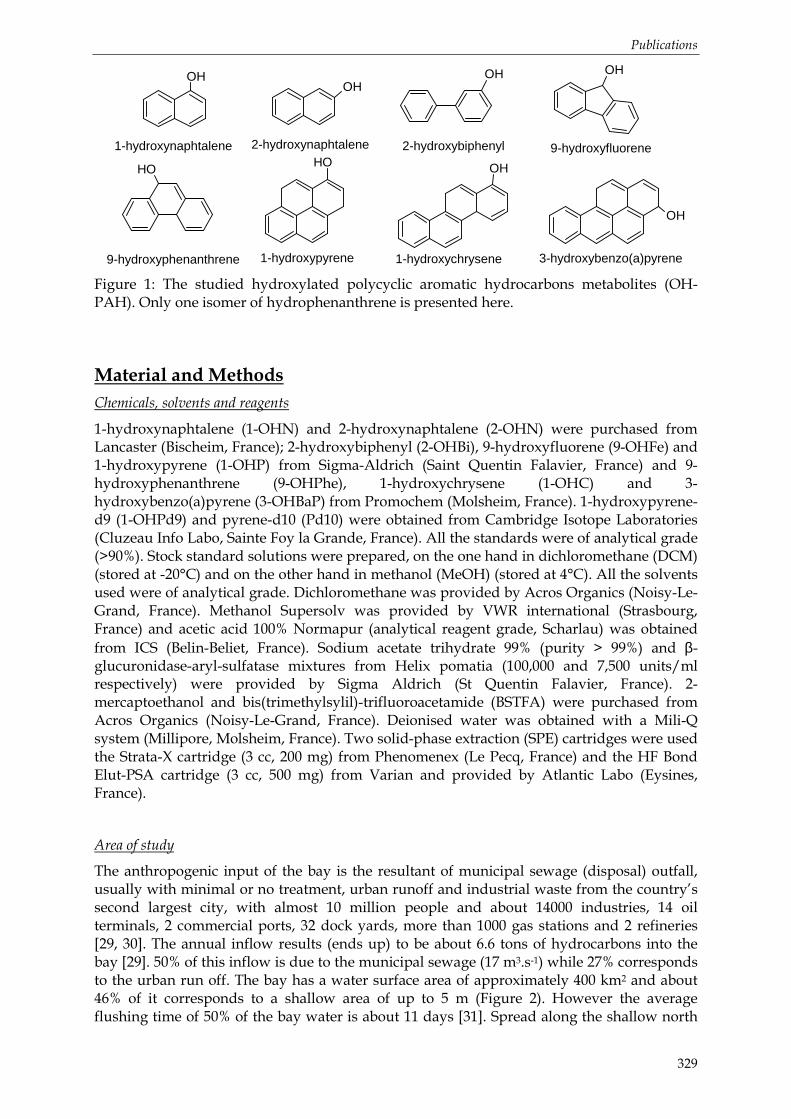
Publications
329
OHOH
OH OH
OH OH OH
OH
1-hydroxynaphtalene 9-hydroxyfluorene2-hydroxybiphenyl
1-hydroxypyrene
2-hydroxynaphtalene
9-hydroxyphenanthrene 1-hydroxychrysene 3-hydroxybenzo(a)pyrene
Figure 1: The studied hydroxylated polycyclic aromatic hydrocarbons metabolites (OH-PAH). Only one isomer of hydrophenanthrene is presented here.
Material and Methods
Chemicals, solvents and reagents
1-hydroxynaphtalene (1-OHN) and 2-hydroxynaphtalene (2-OHN) were purchased from Lancaster (Bischeim, France); 2-hydroxybiphenyl (2-OHBi), 9-hydroxyfluorene (9-OHFe) and 1-hydroxypyrene (1-OHP) from Sigma-Aldrich (Saint Quentin Falavier, France) and 9-hydroxyphenanthrene (9-OHPhe), 1-hydroxychrysene (1-OHC) and 3-hydroxybenzo(a)pyrene (3-OHBaP) from Promochem (Molsheim, France). 1-hydroxypyrene-d9 (1-OHPd9) and pyrene-d10 (Pd10) were obtained from Cambridge Isotope Laboratories (Cluzeau Info Labo, Sainte Foy la Grande, France). All the standards were of analytical grade (>90%). Stock standard solutions were prepared, on the one hand in dichloromethane (DCM) (stored at -20°C) and on the other hand in methanol (MeOH) (stored at 4°C). All the solvents used were of analytical grade. Dichloromethane was provided by Acros Organics (Noisy-Le-Grand, France). Methanol Supersolv was provided by VWR international (Strasbourg, France) and acetic acid 100% Normapur (analytical reagent grade, Scharlau) was obtained
from ICS (Belin-Beliet, France). Sodium acetate trihydrate 99% (purity > 99%) and β-glucuronidase-aryl-sulfatase mixtures from Helix pomatia (100,000 and 7,500 units/ml respectively) were provided by Sigma Aldrich (St Quentin Falavier, France). 2-mercaptoethanol and bis(trimethylsylil)-trifluoroacetamide (BSTFA) were purchased from Acros Organics (Noisy-Le-Grand, France). Deionised water was obtained with a Mili-Q system (Millipore, Molsheim, France). Two solid-phase extraction (SPE) cartridges were used the Strata-X cartridge (3 cc, 200 mg) from Phenomenex (Le Pecq, France) and the HF Bond Elut-PSA cartridge (3 cc, 500 mg) from Varian and provided by Atlantic Labo (Eysines, France).
Area of study
The anthropogenic input of the bay is the resultant of municipal sewage (disposal) outfall, usually with minimal or no treatment, urban runoff and industrial waste from the country’s second largest city, with almost 10 million people and about 14000 industries, 14 oil terminals, 2 commercial ports, 32 dock yards, more than 1000 gas stations and 2 refineries [29, 30]. The annual inflow results (ends up) to be about 6.6 tons of hydrocarbons into the bay [29]. 50% of this inflow is due to the municipal sewage (17 m3.s-1) while 27% corresponds to the urban run off. The bay has a water surface area of approximately 400 km2 and about 46% of it corresponds to a shallow area of up to 5 m (Figure 2). However the average flushing time of 50% of the bay water is about 11 days [31]. Spread along the shallow north

Publications
330
and northeast regions of the bay there are approximately 350 fish traps, which support the local artisanal fishery activity (Figure 2). Until the year 2000, the scientific literature reported only a few data in terms of hydrocarbon concentration in the Guanabara Bay sediments, based mainly upon academic studies. The PAH range was found heterogenic throughout the bay. Chalaux detected PAH concentrations varying from 1,051 to 5,861 ng.g-1 [32]. Hamacher observed lower levels for these compounds, in the range of 554 to 1,894 ng.g-1 [33]. On the other hand, Lima detected PAH concentrations from 1,564 to 18,438 ng.g-1 [34].
In relation to the oil spill accident, on 18 January 2000, approximately 1,300 m3 of marine fuel oil (MF-380) were released into the Guanabara Bay, Rio de Janeiro, Brazil, as a consequence of a pipeline rupture at the Duque de Caxias Refinery. The main portion of the oil, carried along by tidal currents and wind, reached the beaches and some islands in the northern and northeastern parts of the bay. Mangroves in the vicinity of the spill emission point were also affected. Immediately following the oil spill response, 22 water and 57 sediment samples were collected from the Guanabara Bay area [25-27, 35]. Based on the results of this diagnostic study, no significant impact on the intertidal sediments, water column and fish tissue of Guanabara Bay was observed due to the oil spill.
The concentrations of the Σ 16 PAHs and alkylated naphthalenes for 21 sediments collected along the bay in 2000, immediately after the oil spill accident, varied significantly, ranging from 304 to 16,808 ng.g-1 dry weight (median concentration: 2348 ng.g-1) [26]. In spite of the different compounds considered in each work, previous reported data for the studied area, varying from 554 to 18,438 ng.g-1 [32-34], have shown a similar range to the study after the accident, revealing no important influence of the spill on the contamination of the bay sediments. The concentration of PAHs in the bay was also found to be in the range of other estuarine and coastal regions in the world under anthropogenic influence [2, 9, 36-41].
Figure 2: The Guanabara Bay through the population distribution (A) and the water conditions (B). Blue means clean water. Red means much polluted water. Other colors show the variation between these two extremes.

Publications
331
Sampling design and collection
The aim of this study was to quantify individual biliary PAH metabolites present in 4 different fish species (Genidens genidens, Micropogonias furnieri, Cyclichthys spinosus, Ctenoscianea gracilicirrhus) collected in Guanabara Bay over the months of February, March and April of 2006 in order to preliminary assess the exposure to PAHs in the bay. Bottom trawling was carried out with a single net of 20 mm mesh, during 50 minutes, in order to collect the fish. The two areas of interest were chosen to represent different water qualities of the bay. Thus the inner stations are representative of a more contaminated region with low hydrodynamic energy and high eutrophication processes. The first station is located near the refinery and in the mouth of the oil spill of January 2000 (Dentro-Refinery (DR)). The other inner station is located near the mangrove area in which water is more stagnating and brackish (Dentro-Paquetá (DP)). On the other hand, stations located at the entrance of the bay (Botafogo (BF) and Boa Viagem (BV)) have higher hydrodynamic energy with a hydrocarbon contamination varying from low to high (Figure 3).
The collected fish were transported to the laboratory in ice in thermal boxes. Each fish was then identified, measured and the bile was removed, transferred to eppendorf flasks and immediately frozen into liquid nitrogen and then stored at -80°C until analysis.
Figure 3: Geographical location of the fish collection areas in Guanabara Bay for biliary PAH metabolites analysis. Dentro - Refinery: DR; Dentro - Paquetá Island: DP; Boa Viagem: BV; Botafogo: BF.

Publications
332
Sample preparation
Bile samples were pooled when there was an insufficient volume for individual analysis (Table 1). They were prepared according to a previously established protocol (Le Dû-Lacoste and Budzinski, submitted). The weighed whole bile was thawed and then homogenized in precooled buffered water (sodium acetate buffer at pH 5.0 with acetic acid) (100 µl of bile: 2 ml buffer). The internal standard, 1-hydroxypyrene-d9, 20 µl of mercaptoethanol, used as antioxidant, and 20 µl of β-glucuronidase and arylsulfatase mixture were added to the samples. They were then placed at 37°C in an oven for 18 hours for hydrolysis. Glass vials were used for the deconjugation step to avoid adsorption phenomena on inner surface.
After deconjugation the bile samples were ultrasonicated and centrifuged (10 min, 5 000 rpm, 20°C). Solid-phase Strata X cartridges were preconditioned with 2 ml of methanol and 4 ml of buffered water. The supernatants were loaded on cartridges and washed with 2 ml of buffered water and 2 ml of water/methanol (70/30, v/v). Water traces were then removed by applying vacuum on the cartridges during 45 min. Metabolites were then eluted with 5 ml of methanol. The extracts were reduced to dryness under a nitrogen stream and redissolved in 1 ml of methanol/methylene chloride (20/80, v/v) before purification.
Solid-phase HF PSA Varian cartridges were used for the purification step. Before loading the redissolved extracts into methanol/methylene chloride (20/80, v/v), the cartridges were first preconditioned with 2.5 ml of methanol/methylene chloride (20/80, v/v). The elution of the compounds was then performed with 6 ml of the same mixture. The extracts were reduced to dryness under a nitrogen stream, redissolved in 50 µl of dichloromethane and 30 µl of a derivatizing agent (BSTFA) were finally added. The derivatization was then completed by incubation at 65°C for 30 min.
After derivatization and before GC-MS analysis, a solution of deuterated internal standard (pyrene-d10, 20 µl) was added to the sample for recovery determination.
GC-MS Analysis
The analyses were carried out with an HP GC 6890A gas chromatograph Agilent Technologies coupled to an HP MSD 5973 Network mass selective detector Agilent Technologies, both purchased from BIOS Analytique (l’Union, France). The separation was performed on an Agilent Technologies HP5-MS capillary column (length: 30 m; internal diameter: 250 µm; stationary phase thickness: 0.25 µm; phase: 5% diphenyl-, 95% dimethyl-siloxane), with the following oven parameters: from 70°C (2 min) to 180 °C (1 min) at 5°C.min-1 from 180°C to 290°C (1 min) at 10°C.min-1. The injection volume was set at 1 µl (automated PTV pulsed splitless injection (25 psi, 1.5 min)), while the injector temperature was set at 250°C and the interface temperature at 280°C. The purge flow was set at 60 ml/min for 1.5 min and helium 6.0 (Linde, Bassens, France) was used as the carrier gas (constant flow: 1 ml.min-1). Acquisition was performed in selected ion monitoring (SIM), with 1.53 scan/s and a dwell time of 50 ms for each ion. The source temperature was set at 150°C, and the electron multiplier voltage set at 2,000 V.
The compounds were quantified in SIM mode using the ions below: 1-hydroxynaphtalene (m/z=201), 2-hydroxynaphtalene (m/z=216), 2-hydroxybiphenyl (m/z=211), 9-hydroxyfluorene (m/z=165), 9-hydroxyphenanthrene and isomers (m/z=266), 1-hydroxypyrene (m/z=290), 1-hydroxychrysene (m/z=316) 3-hydroxybenzo(a)pyrene (m/z=340) and 1-hydroxypyrene-d9 (m/z=299), pyrene-d10 (m/z=212).
A mixture of the standard metabolites, 1-hydroxypyrene-d9, and pyrene-d10 in dichloromethane was injected, after derivatization, at the beginning and at the end of each sequence for the determination of response factors.

Publications
333
Table 1: Individual PAH metabolites concentration in fish bile samples. Concentrations expressed in µg.g-1 of bile. Mean ± SD when it is precise. ND: not determined (< LOD [42])
Location Dentro - Paqueta island
Dentro -
Paqueta island
Boa Viagem
Dentro - Refinery
Boa Viagem
Botafogo
Specie Genidens genidens Micropogonias furnieri
Cyclichthys spilostylus
Ctenoscianea gracilicirrhus
Date February 2006 (n =
3)
March 2006
(n = 2)
April 2006
March 2006
April 2006
March 2006
(n = 2)
April 2006
(n = 3)
April 2006
1-OHN 0.9 ± 1.3 1.1 ± 1.0 1.2 18.9 3.4 0.3 ± 0.2 1.3 ± 1.1 2.5
2-OHN 15.4 ± 2.9 3.8 ± 1.2 ND 2.2 ND 0.3 ± 0.04 0.7 ± 0.4 1.9
2-OHBi 33.7 ± 1.0 15.9 ± 8.6 ND 10.3 ND 1.2 ± 0.2 1.9 ± 2.9 10.0
9-OHFe 19.1 ± 5.3 11.8 ± 0.3 ND 6.3 ND 0.8 ± 0.3 2.9 ± 6.5 8.5
4-OHPhe 3.8 ± 1.9 0.8 ± 1.1 1.5 2.2 ND 0.3 ± 0.2 0.1 ± 0.3 0.7
9-OHPhe ND 1.1 ± 1.6 ND ND ND ND ND ND
3-OHPhe ND ND ND ND ND 0.3 ± 0.5 3.9 ± 4.1 ND
1-OHPhe 36.1 ± 26.9 13.2 ± 2.8 7.5 18.0 ND 3.4 ± 1.4 7.6 ± 5.3 ND
2-OHPhe 19.6 ± 13.7 14.2 ± 3.3 ND 5.7 ND 1.3 ± 0.05 3.3 ± 3.0 5.2
1-OHP 11.6 ± 3.8 11.5 ± 4.2 2.8 10.1 9.2 7.4 ± 1.5 27.2 ± 5.3 20.0
1-OHC 1.2 ± 2.3 1.1 ± 2.0 ND ND ND ND ND ND
3-OHBaP ND ND ND ND ND ND ND ND
sum OHPhe 59.5 ± 39.8 29.3 ± 8.8 8.9 26.0 ND 5.2 ± 2.1 14.9 ± 6.7 5.9
sum OHPAH 141.4 ± 38.9 74.5 ± 0.6 12.9 73.7 12.6 15.2 ± 1.2 48.8 ± 12.5 48.7
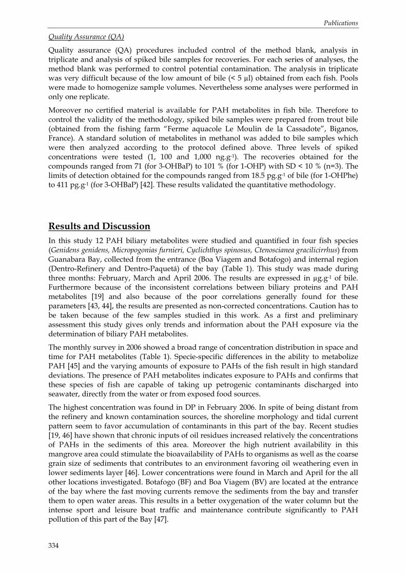
Publications
334
Quality Assurance (QA)
Quality assurance (QA) procedures included control of the method blank, analysis in triplicate and analysis of spiked bile samples for recoveries. For each series of analyses, the method blank was performed to control potential contamination. The analysis in triplicate was very difficult because of the low amount of bile (< 5 µl) obtained from each fish. Pools were made to homogenize sample volumes. Nevertheless some analyses were performed in only one replicate.
Moreover no certified material is available for PAH metabolites in fish bile. Therefore to control the validity of the methodology, spiked bile samples were prepared from trout bile (obtained from the fishing farm “Ferme aquacole Le Moulin de la Cassadote”, Biganos, France). A standard solution of metabolites in methanol was added to bile samples which were then analyzed according to the protocol defined above. Three levels of spiked concentrations were tested (1, 100 and 1,000 ng.g-1). The recoveries obtained for the compounds ranged from 71 (for 3-OHBaP) to 101 % (for 1-OHP) with SD < 10 % (n=3). The limits of detection obtained for the compounds ranged from 18.5 pg.g-1 of bile (for 1-OHPhe) to 411 pg.g-1 (for 3-OHBaP) [42]. These results validated the quantitative methodology.
Results and Discussion
In this study 12 PAH biliary metabolites were studied and quantified in four fish species (Genidens genidens, Micropogonias furnieri, Cyclichthys spinosus, Ctenoscianea gracilicirrhus) from Guanabara Bay, collected from the entrance (Boa Viagem and Botafogo) and internal region (Dentro-Refinery and Dentro-Paquetá) of the bay (Table 1). This study was made during three months: February, March and April 2006. The results are expressed in µg.g-1 of bile. Furthermore because of the inconsistent correlations between biliary proteins and PAH metabolites [19] and also because of the poor correlations generally found for these parameters [43, 44], the results are presented as non-corrected concentrations. Caution has to be taken because of the few samples studied in this work. As a first and preliminary assessment this study gives only trends and information about the PAH exposure via the determination of biliary PAH metabolites.
The monthly survey in 2006 showed a broad range of concentration distribution in space and time for PAH metabolites (Table 1). Specie-specific differences in the ability to metabolize PAH [45] and the varying amounts of exposure to PAHs of the fish result in high standard deviations. The presence of PAH metabolites indicates exposure to PAHs and confirms that these species of fish are capable of taking up petrogenic contaminants discharged into seawater, directly from the water or from exposed food sources.
The highest concentration was found in DP in February 2006. In spite of being distant from the refinery and known contamination sources, the shoreline morphology and tidal current pattern seem to favor accumulation of contaminants in this part of the bay. Recent studies [19, 46] have shown that chronic inputs of oil residues increased relatively the concentrations of PAHs in the sediments of this area. Moreover the high nutrient availability in this mangrove area could stimulate the bioavailability of PAHs to organisms as well as the coarse grain size of sediments that contributes to an environment favoring oil weathering even in lower sediments layer [46]. Lower concentrations were found in March and April for the all other locations investigated. Botafogo (BF) and Boa Viagem (BV) are located at the entrance of the bay where the fast moving currents remove the sediments from the bay and transfer them to open water areas. This results in a better oxygenation of the water column but the intense sport and leisure boat traffic and maintenance contribute significantly to PAH pollution of this part of the Bay [47].

Publications
335
Generally speaking three levels of PAH metabolite concentrations have been measured. The highest level (141.4 µg.g-1 of bile) was found in DP in February. The medium level ranged between 74.5 µg.g-1 (at DP in March) and 48.7 µg.g-1 (at BF in April). Finally the lowest level of PAH metabolites was between 15.2 µg.g-1 (at DR in March) and 12.6 µg.g-1 (at BV in April). By comparison, Da Silva [19] reported higher PAH metabolites concentrations in fish from Sao Sebastiao Channel (Sao Paulo, Brazil). The PAH metabolites were analyzed by liquid chromatography coupled to a fluorescence detection method (HPLC-F) and they ranged from 96.4 to 525.3 µg.g-1 of bile.
Concerning the site Dentro-Paquetá the concentrations measured in March 2006 are similar among the different species studied. Micropogonias furnieri and Genidens genidens are two species that live in brackish waters and the mean concentrations of PAH metabolites found (74.1 µg.g-1) were lower than the mean concentrations found for the same species in the Sao Sebastio Channel [19]. A temporal effect seems also to be present in this area. From February to April, the mean concentrations have been divided by 10. This could be explained by a change in the water temperature that has been proved to influence the bioavailability of PAHs to organisms and also to modify the biotransformation processes leading to a decrease in metabolite production. This decrease in metabolite concentrations could also be due to changes in the lifestyle of fish (changes in feeding, spawning time or migration from other sites). Finally this could also be due to a punctual contamination of PAHs. During this first assessment, no sediment or water sample has been sampled. No correlation or explanation can be drawn from the measure of the contamination of the system.
When studying the distribution patterns of individual PAH metabolites in the total sum measured (Figure 4) the major metabolite is different depending on the location. At the site Dentro-Paquetá, OHPhe are predominant (from 35 to 69 %) whereas at the location called Boa Viagem 1-OHP is the major metabolite quantified (56 and 73 %). Near the refinery (Dentro-Refinery) the major metabolite is also the 1-OHP (48%). Nevertheless the fingerprint left by the OHPhe is persistent since their contribution is always at least of 30 %. Botafogo is an exception but the absence of replicate does not allow us to conclude with certainty.
By calculating the ratio of OHPhe towards 1-OHP (OHPhe/1-OHP) two cases can be distinguished: OHPhe/1-OHP > 2 and OHPhe/1OHP < 1. To link this ratio to a potential source of PAH contamination, several diagnostic ratios such as Phe/Ant [48], Fluo/Pyr [49], MPhe/Phe [50], Chrys/BaA [51] have been calculated for each sediment sample corresponding to the studied areas. Table 2 sums up the diagnostic tools obtained for all locations. As stated when the petrogenic origin is determined by PAHs in sediments, it is confirmed by OHPAH ratio in bile, as well as for pyrolytic sources. The closer diagnostic PAH ratio to OH-PAH ratio seems to be Phe/Ant. For most of the samples the diagnostic ratios point to the presence of a mixture of pyrolytic and petrogenic PAHs. Soclo [52] considered in their study that samples with Phe/Ant < 10 and Fluo/Pyr ≤ 1 contained a mixture of pyrolytic and petrogenic materials with strong pyrolytic input. In such a case, only the site Dentro-Paquetá exhibited a petrogenic origin of PAH contamination.

Publications
Figure 4: Composition (%) of hydroxylated metabolites in bile of demersal fishes collected in Guanabara Bay in February, March and April 2006.
Dentro - Paqueta Island ( Genidens genidens )
0%
25%
50%
75%
100%
February 2006 March 2006 April 2006
sum OHPhe
3-OHBaP
1-OHC
1-OHP
9-OHFe
2-OHBi
2-OHN
1-OHN
Micropogonias furnieri
0%
25%
50%
75%
100%
March 2006 April 2006
Dentro - Paqueta island Boa Viagem
Cyclichthys spilostylus
0%
25%
50%
75%
100%
March 2006 April 2006
Dentro - Refinery Boa Viagem
Ctenoscianea gracilicirrhus - April 2006
0%
25%
50%
75%
100%
Botafogo

Publications
337
Table 2: Diagnostic ratios indicative of petrogenic or pyrolytic origin for PAH.
Phe/Ant Fluo/Pyr Chrys/BaA ΣC-Phe/Phe OHPhe/1-OHP
< 10 Pyr > 1 Pyr < 1 Pyr < 2 Pyr < 10 Pyr Stations
> 15 Petr < 1 Petr > 1 Petr > 2 Petr > 15 Petr
Diagnostic
Dentro - Paqueta 26.2 0.5 1 0.2 3.4 * Petrogenic
Dentro - Refinery 3 1.4 0.6 8.5 0.7 Pyrolytic
Boa Viagem 4.5 0.9 1 5.1 0.5 Pyrolytic
Botafogo 16.5 0.8 0.7 0.1 0.3 Pyrolytic
* mean value calculated for the 3 months survey
Good correlations were obtained between OHN, OHPhe and the total sum of OH-PAHs (Figure 5). Correlations were not as strong between 1-OHP and OHPhe and between 1-OHP and OH-PAH. These results show that petrogenic PAHs such as naphtalene and phenanthrene, are likely to be obtained from the same source, such as petroleum discharged into the channel. On the other hand, pyrene most likely has a source related to combustion and petroleum discharges that is unrelated to a specific source of PAHs [53].
The source of parent PAHs in the marine environment can be demonstrated by the relationship between OHPhe (or OHN) and 1-OHP (or OHBaP) in the bile. When OHPhe levels are high, a petrogenic source of PAHs is evident. Conversely, when BaP metabolites or/and pyrene metabolites are high, a pyrogenic source is predominate. Very few studies have tried to determine a diagnostic ratio based on PAH metabolites in bile to determine the origin of PAH contamination. Da Silva [19] gave a mean ratio of BaP/Phe equivalents of 0.05 for fish from the São Sebastião Channel. This ratio suggests that petrogenic PAH sources are the predominant contributors to total PAH in this region.
In this current study on fish from the Guanabara Bay the mean ratio of OHPhe/1-OHP was 3.4 ± 1.1 (n = 7). This value puts forward the theory that petrogenic PAH sources are prevalent in the Guanabara Bay. Two limits can be given for the diagnostic ratio: OHPhe/1-OHP > 2 for the petrogenic sources and OHPhe/1-OHP < 1 for the pyrolytic sources.

Publications
Figure 5: Correlation among log-transformed concentrations of PAH metabolites in bile of all samples from Guanabara Bay: (1) OHN and OHPhe, (2) 1-OHP and OHPhe, (3) 1-OHP and OH-PAH, and (4) OHPhe and OH-PAH.
R2 = 0.6176P < 0.001
-0.3
0.1
0.5
0.9
1.3
1.7
0.6 0.8 1.0 1.2 1.4 1.6 1.8
Conc. of OH-Phe (log 10, µg/g)
Con
c. o
f OH
N (
log
10, µ
g/g)
R2 = 0.6089P < 0.001
-0.3
-0.1
0.1
0.3
0.5
0.7
0.9
1.1
1.3
1.5
1.7
0.0 0.5 1.0 1.5
Conc. of OH-Phe (log 10, µg/g)
Con
c. o
f 1-O
HP
(lo
g 10
, µg/
g)
R2 = 0.7088P < 0.0001
-0.3
-0.1
0.1
0.3
0.5
0.7
0.9
1.1
1.3
1.5
1.7
0.0 0.5 1.0 1.5 2.0
Conc. of OH-PAH (log 10, µg/g)
Con
c. o
f 1-O
HP
(lo
g 10
, µg/
g) R2 = 0.9095
P < 0.0001
-0.3
0.2
0.7
1.2
1.7
2.2
0.0 0.5 1.0 1.5 2.0
Conc. of OH-PAH (log 10, µg/g) C
onc.
of O
H-P
he (
log
10, µ
g/g)

Publications
339
Conclusions
High levels of phenanthrene and pyrene metabolites in the bile of fish from the Guanabara Bay seem to effectively reveal the state of PAH contamination of the observed sites – the space variability concurs with the presence of different source strengths. The presence of petrogenic sources of PAHs in the internal area of the Bay is likely the result of inputs of petroleum and derivatives into these waters.
Similar to the expression of the proportion of individual PAHs as a percentage of total PAHs in sediments, OH-PAH profiles in fish bile can be used as a biomarker for identifying exposure sources of certain types of PAHs. Since individual PAHs are biotransformed and excreted at different rates by fish, the profile of OH-PAHs has a characteristic fingerprint. Although a variety of factors, bioavailability, and the concentration of parent PAHs in sediments [54], it is clear that the profile of parent PAHs in sediments is reflected in fish bile, as metabolites.
To conclude, as a first assessment, the Guanabara Bay is heavily polluted by PAHs and these chemicals in addition to other factors, may adversely affect the health of biota.
Acknowledgements: This work was financially supported by the ORQUE project (“Regional Observation of the Quality of the Environment” project). The authors also want to acknowledge the “Region Aquitaine” and the French National Council for Scientific Research (CNRS) for providing the PhD grant of M. Le Dû-Lacoste.

Publications
340
References
1. Neff, J. M., Polycyclic Aromatic Hydrocarbons in the Aquatic Environment: Sources, Fates and Biological Effects. 1979, London: Applied Science Publishers Ltd. 262.
2. Kennicutt II, M. C., Wadw, T. L., Presley, B. J., Requejo, J. M., Brooks, J. M., and Denoux, G. J. 1994. Environmental science & technology 28(1): p. 1-15.
3. Elias, V. O., Simoneit, B. R. T., and Cardoso J, Levoglucosan, a Molecular Fossil as Indicator of Biomass Burning Contribution in Sediments of the Amazon Shelf, in Proceedings of the seventh Latin-American Congress on Organic Geochemistry. 2000: Foz do Iguaçu, Parana, Brazil. p. 243-244.
4. Lipiatou, E. and Albaigés, J. 1994. Marine Chemistry 46: p. 153-164.
5. Philp, R. P., Fossil Fuel Biomarkers - Applications and Spectra, ed. Geophysics, M.i.G.a. Vol. 23. 1985, Amsterdam: Elsevier. 294.
6. Hites, R. A., Laflamme, R. E., and Windsor Jr, J. G. 1980. Advances in Chemistry Series: p. 289-311.
7. Yunker, M. B., MacDonald, R. W., Brewer, R., Sylvestre, S., Tuominen, T., Sekela, M., Mitchell, R. H., Paton, D. W., Fowler, B. R., Gray, C., Goyette, D., and Sullivan, D., Assessment of Natural and Anthropogenic Hydrocarbon Inputs Using Pahs as Tracers. The Fraser River Basin and Strait of Georgia 1987-1997., in Environment Canada and Fisheries and Oceans Canada, FRAP, R.D., Editor. 2000: Vancouver, BC. p. 128 pp.
8. Yunker, M. B., Backus, S. M., Graf Pannatier, E., Jeffries, D. S., and Macdonald, R. W. 2002. Estuarine, Coastal and Shelf Science 55(1): p. 1-31.
9. Readman, J. W., Mantoura, R. F. C., Llewellyn, C. A., Preston, M. R., and Reeves, A. D. 1986. Intern. J. Environ. Anal. Chem. 27: p. 29-54.
10. Budzinski, H., Jones, I., Bellocq, J., Piérard, C., and Garrigues, P. 1997. Marine Chemistry 58(1-2): p. 85-97.
11. Lipiatou, E., Tolosa, I., Simo, R., Bouloubassi, I., Dachs, J., Marti, S., Sicre, M. A., Bayona, J. M., Grimalt, J. O., Saliot, A., and Albaige?s, J. 1997. Deep-Sea Research Part II: Topical Studies in Oceanography 44(3-4): p. 881-905.
12. Harvey, R. C., Polycyclic Aromatic Hydrocarbons, Chemistry and Carcinigenity, ed. Press, C.U. 1991, Cambridge, UK. 11-87.
13. IARC, Monographs on the Evaluation of the Carcinogenic Risk of Chemicals to Human. Vol 32. 1983, International Agency for Research on Cancer: Lyon, France. p. 57-61.
14. James, M. O. 1989Biotransformation and Disposition of Pah in Aquatic Invertebrates, P 69-92, in Metabolism Fo Polycyclic Aromatic Hydrocarbons in the Aquatic Environment, Varanasi, U., Editor CRC Press: Boca Raton. p. 341.
15. Varanasi, U., Reichert, W. L., Le Eberhart, B. T., and Stein, J. E. 1989. Chemico-Biological Interactions 69(2-3): p. 203-216.
16. Varanasi, U., Reichert, W. L., Stein, J. E., Brown, D. W., and Sanborn, H. R. 1985. Eviron. Sci. Technol. 19: p. 836-841.
17. Varanasi, U. and Stein, J. E. 1991. Environmental Health Perspectives 90: p. 93-100.
18. Malins, D. C. and Hodgins, H. O. 1981. Environ Sci Technol (Feature) 15(11): p. 1273-1280.

Publications
341
19. Da Silva, D. A. M., Buzitis, J., Krahn, M. M., Bicego, M. C., and Pires-Vanin, A. M. S. 2006. Marine Pollution Bulletin 52(2): p. 175-183.
20. Jonsson, G., Bechmann, R., Bamber, S., and Baussant, T. 2004. Environ Toxicol Chem. 23(6): p. 1538-48.
21. Krahn, M. M., Burrows, D. G., Ylitalo, G. M., Brown, D. W., Wigren, C. A., Collier, T. K., Chan, S.-L., and Varanasi, U. 1992. Environ Sci Technol 26: p. 116-126.
22. Krahn, M. M., Kittle, J., Lewey J., and MacLeod, J., William D. 1986. Marine Environmental Research 20(4): p. 291-298.
23. Ruddock, P. J., Bird, D. J., McEvoy, J., and Peters, L. D. 2003. The Science of The Total Environment 301(1-3): p. 105-117.
24. van der Oost, R., Beyer, J., and Vermeulen, N. P. E. 2003. Environmental Toxicology and Pharmacology 13(2): p. 57-149.
25. Gabardo, I. T., Meniconi, M. F. G., Falcao, L. V., Vital, N. A. A., and Pereira, R. C. L. Hydrocarbon and Ecotoxicity in Seawater and Sediment Samples of Guanabara Bay after the Oil Spill in January 2000. in 2001 International Oil Spill Conference. 2001.
26. Meniconi, M. F. G., Barbanti, S. M., Gabardo, I. T., and Caicedo, N. L. Chemical Characterization of Environmental Samples after Oil Spill in Iguassu River, Parana, Brazil, July 2000. in International Oil Spill Conference. 2003.
27. Meniconi, M. F. G. and Gabardo, I. T. 2002. Environmental Forensics 3: p. 303-321.
28. Keith, L. H. and Telliard, W. A. 1979. Environ Sci Technol 13: p. 416-423.
29. FEEMA, Qualidade De Agua Da Baia De Guanabara. , in Programa de Despoluiçao da Baia de Guanabara - Programas Ambientais Complementares. 1998.
30. JICA, The Study on Recuperation of the Guanabara Bay Ecosystem, Ambiente, F.E.d.E.d.M., Editor. 1994: Rio de Janeiro, Brazil.
31. Kjerfve, B., Ribeiro, C. H. A., Dias, G. T. M., Filippo, A. M., and Quaresma, V. D. S. 1997. Continental Shelf Research. 17(13): p. 1609-1643.
32. Chalaux, N., Dinamica Costanera De Les Aportations Contaminantes Presents Als Efluents Urbans, in Universidade de Barcelone. 1995: Barcelona, Spain.
33. Hamacher, C., Determinaçao De Hidrocarbonetos Em Amostras De Agua E Sedimento Da Baia De Guanabara, in Departamento de Quimica. 1996, PUC-RJ: Rio de Janeiro.
34. Lima, A. L. C., Geocronologia De Hidrocarbonetos Poliaromaticos (Pah) - Estudo De Caso: Baia De Guanabara, in Departamento de Quimica. 1996, PUC-RJ: Rio de Janeiro.
35. Meniconi, M. F. G., Massone, C. G., and Scofield, A. D. L. Distribution and Sources of Polycyclic Aromatic Hydrocarbons in Sediments of Guanabara Bay, Brazil. in Proceedings of the 26th Artic and Marine Oil Spill Program (AMOP). 2003.
36. Baumard, P., Budzinski, H., and Garrigues, P. 1998. Marine Pollution Bulletin 36(8): p. 577-586.
37. Baumard, P., Budzinski, H., and Garrigues, P. 1998. Environmental Toxicology and Chemistry 17(5): p. 765-776.
38. Baumard, P., Budzinski, H., Garrigues, P., Dizer, H., and Hansen, P. D. 1999. Marine Environmental Research 47(1): p. 17-47.
39. Baumard, P., Budzinski, H., Michon, Q., Garrigues, P., Burgeot, T., and Bellocq, J. 1998. Estuarine, Coastal and Shelf Science 47(1): p. 77-90.

Publications
342
40. Pereira, W. E., Hostettler, F. D., and Rapp, J. B. 1996. Marine Environmental Research 41: p. 299-314.
41. Readman, J. W., Preston, M. R., and Mantoura, R. F. C. 1986. Marine Pollution Bulletin 17: p. 298-308.
42. Le Dû - Lacoste, M. and Budzinski, H. Submitted. Anal Bioanal Chem.
43. Ariese, F., Burgers, I., Oudhoff, K., Rutten, T., Stroomberg, G., and Vethaak, D. 1997.
44. Richardson, D. M., Gubbins, M. J., Davies, I. M., Moffat, C. F., and Pollard, P. M. 2004. Environmental Toxicology and Pharmacology 17(2): p. 79-85.
45. Varanasi, U., Reichert, W. L., and Stein, J. E. 1989. Cancer Research 49(5): p. 1171-1177.
46. Farias, C. O., Hamacher, C., Wagener, A. D. L. R., and Scofield, A. D. L. 2008. Organic Geochemistry 39: p. 289-307.
47. Azevedo, L. A., Bruning, I. M. R. D. A., and Moreira, I. 2004. Marine Pollution Bulletin 49: p. 1109-1126.
48. Soclo, H. H., Etude De La Distribution Des Hydrocarbures Aromatiques Polycycliques Dans Les Sédiments Récents. Identification Des Sources., in Sciences Chimiques. 1986, Université Bordeaux1: Bordeaux. p. 158 pp.
49. Sicre, M. A., Marty, J. C., Saliot, A., Aparicio, X., Grimalt, J., and Albaigès, J. 1987. Atmospheric Environment 21: p. 2247-2259.
50. Garrigues, P., Budzinski, H., Manitz, M. P., and Wise, S. 1995. Polycycl. Aromat. Compd. 7: p. 275-284.
51. Gschwend, P. M. and Hites, R. A. 1981. Geochimica et Cosmochimica Acta 45: p. 2359-2367.
52. Soclo, H. H., Garrigues, P., and Ewald, M. 2000. Marine Pollution Bulletin 40: p. 387-396.
53. Wang, Z., Fingas, M., and Page, D. S. 1999. J. Chromatogr. A 843: p. 369-411.
54. Vuorinen, P. J., Keinanen, M., Vuontisjarvi, H., Barsiene, J., Broeg, K., Forlin, L., Gercken, J., Kopecka, J., Kohler, A., Parkkonen, J., Pempkowiak, J., and Schiedek, D. 2006. Marine Pollution Bulletin 53(8-9): p. 479-487.

Annexes
343
ANNEXES

Annexes
344

Annexes
345
ANNEXE 1
Valeurs de toxicités aiguë et chronique déterminées chez différentes espèces de poisson
HAP Organisme Critère d’effet Toxicité
aiguë (µg.l-1)
Toxicité chronique
(µg.l-1) Référence
Oncorhynchus mykiss
NOEC (40j) survie - 120 [442]
Pimephales promelas (J)
CL50 (96h) 1990 - [442]
Pimephales promelas (A)
CL50 (96h) 7900 - [443]
Pimephales promelas (E-L)
LOEC (30j) reproduction
- 850 [443]
Pimephales promelas (E-L)
NOEC (30j) croissance - 450 [443]
Oncorhynchus mykiss (A)
CL50 (96h) 1600 - [443]
Oncorhynchus gorbuscha
CL50 (48h) 900 – 1000 - [444]
Naphtalène
Cyprinodon variegates (J)
CL50 (96h) 2400 - [445]
Pimephales promelas (J)
CL50 (96h) 1600 - [446] Acénaphthène
Oncorhynchus mykiss (J)
CL50 (96h) 670 - [446]
Gambusia affinis CL50 (24h) 150 - [2] Oncorhynchus mykiss (O-L)
CL50 (7j) 40 - [447]
Oncorhynchus mykiss (O-L)
NOEC (23j) éclosion - 4 [447] Phénanthrène
Pimephales promelas
NOEC (25j) mortalité - 10 [163]
Lepomis macrochirus (1 –
1,5 kg) CL50 (96h) 4,5 - [163]
Lepomis macrochirus
CL50 (96h) 11,9 - [175]
Lepomis macrochirus (1 –
1,5 kg)
NOEC (200h) mortalité
- 1,2 – 15 [163]
Pimephales promelas
CL50 (1,6j) 5,4 - [163]
Pimephales promelas
NOEC (9 sem) déformation
- 6,6 [448]
Anthracène
Pimephales promelas
NOEC (96h) mortalité - 5,4 [163]
Brachydanio rerio (O-L)
NOEC (41j) croissance - 4,8 [449] Fluoranthène
Brachydanio rerio (O-L)
NOEC (41j) mortalité - 48 [449]
Pyrène Pimephales promelas
CL50 (1,3h) 25,6 - [163]

Annexes
346
Pimephales promelas
NOEC (4j) mortalité - 25,6 [163]
Pimephales promelas
CL50 (3,7j) 1,8 - [163] BaA
Pimephales promelas
NOEC (5j) mortalité - 1,8 [163]
Brachydanio rerio (O-L)
CL50 (42j) 0,7 - [450]
Brachydanio rerio (O-L)
NOEC (42j) croissance - 0,2 [450] BkF
Brachydanio rerio (O-L)
NOEC (42j) mortalité - 0,4 [450]
Pimephales promelas
CL50 (48h) 5,6 (> sol) - [163]
Brachydanio rerio NOEC (28j)
croissance, éclosion, mortalité
- > 4 [449] BaP
Oncorhynchus mykiss
NOEC (36j) morphologie
- 2,4 [451]
Voir Chapitre 1 § 2.2.2 pour la définition des NOEC et LOEC
J : juvénile, A : adulte, E : embryon, O : œuf, L : larve « > sol » : valeur supérieure à la solubilité du composé dans l’eau.

Annexes
347
ANNEXE 2
Principes de la chromatographie en phase gazeuse couplée à la spectrométrie de masse simple et en tandem (GC/MS et GC-MS/MS)
Le couplage de la chromatographie en phase gazeuse et de la spectrométrie de masse est constitué de trois modules : un injecteur, une colonne capillaire dans un four et un détecteur.
Principes du couplage GC-MS et GC-MS/MS
Les composés sont tout d’abord volatilisés dans l’injecteur et entraînés dans le chromatogramme le long de la colonne chromatographique par un gaz vecteur, dans le cas de cette étude, l’hélium. Après avoir été séparés, les composés arrivent dans la source du spectromètre de masse qui va permettre l’ionisation des composés. Une fois ionisés les ions (ions précurseurs) vont être fragmentés en fonction de leur stabilité (ions produits). Les ions sont ensuite séparés d’après leurs rapports masse sur charge (m/z) dans un analyseur et être détectés par un multiplicateur d’électrons dans le cas de la spectrométrie de masse simple.
Dans le cas de la spectrométrie de masse en tandem, les ions produits sont à nouveaux fragmentés dans une cellule de collision en ions « fils » qui seront séparés en fonction de leurs rapports masse sur charge (m/z) dans l’analyseur et détectés par un multiplicateur d’électrons.
Dans les deux cas, on obtient donc un chromatogramme de l’extrait injecté et les spectres de masse des ions correspondant aux molécules, suffisamment volatiles et ionisables, dans la gamme de masses de l’appareil.
Les éléments importants dans un couplage GC/MS sont donc la source du spectromètre de masse qui va ioniser les molécules et l’analyseur qui va séparés les ions. Différents types de sources et d’analyseur sont commercialisés. Au cours de ces travaux de thèse, une source à impact électronique (EI) et un analyseur de masse de type quadripôle ont été utilisés.
Figure A : Appareillage utilisé en chromatographie en phase gazeuse, comprenant notamment un four, une colonne, un injecteur, un détecteur et un système de traitement des données.

Annexes
348
Figure B : Interface entre un chromatographe et un spectromètre de masse
Figure C : Schéma d'un spectromètre de masse de type quadripolaire
Figure D : Schéma d'un analyseur de type quadripôle

Annexes
349
ANNEXE 3
Principes et caractéristiques de la chromatographie liquide haute performance couplée à une détection par spectrométrie de masse simple (HPLC/MS) et en tandem (HPLC-MS/MS)
Le principe de base de la séparation HPLC est le passage d'un liquide (phase mobile) au travers d'une colonne (support solide = phase stationnaire). L’HPLC existe sous quatre types différents: HPLC en phase inverse, HPLC d'adsorption, HPLC échangeuse d'ions et HPLC d'exclusion. La polarité de la colonne ainsi que le type de solvant ont un impact sur la séparation des molécules dû à l'environnement chimique de l'ensemble.
Dans tout appareil de chromatographie liquide haute performance on retrouvera les éléments de base suivants (Figure A):
• un ou plusieurs réservoirs de phase mobile contenant soit des solvants purs soit des mélanges de solvants dans des concentrations connues.
• un système d'injection comportant une boucle d'échantillonnage calibrée (généralement une vanne RHEODYNE).
• une colonne remplie, en acier inox, de quelques centimètres de long.
• un détecteur permettant à la fois, de mettre en évidence la sortie des solutés de la colonne et de donner un signal proportionnel à la quantité de chacun de ces solutés, dans un mélange.
Figure A : Schéma d'un système de HPLC

Annexes
350
Dans le cas du couplage LC/MS, le détecteur est donc un spectromètre de masse simple qui comporte trois parties fondamentales : une source d’ionisation, un analyseur et un détecteur.
Dans ce couplage, la difficulté résulte dans la transformation du soluté en phase liquide en un ion en phase gazeuse. Ainsi la source d’ionisation joue à la fois un rôle de désolvatation et d’ionisation auquel peut être appliquée une pression et contenant une arrivée d’azote, permettant l’introduction de l’éluat sous forme de micro-gouttelettes (spray). Ces ions sont alors transférés de la source (pression atmosphérique) vers l’analyseur (vide poussé) par l’intermédiaire d’un capillaire sous tension dans lequel ils sont plus ou moins accélérés pour provoquer leur fragmentation. Ainsi par variation de la tension du capillaire, la fragmentation peut être contrôlée. Les ions obtenus sont alors séparés d’après leur rapports masse sur charge (m/z) dans l’analyseur quadripolaire et détectés en proportion de leur nombre par un multiplicateur d’électrons.
A l’heure actuelle, la majorité des interfaces se regroupent selon deux types d’ionisation : l’ionisation électrospray (ESI) et l’ionisation chimique à pression atmosphérique (APCI). De techniques alternatives utilisant la photo-ionisation atmosphérique (APPI) ont vu le jour mais restent très minoritaires. L’ESI et l’APCI (Figure B) sont toutes les deux des techniques d'ionisation à pression atmosphérique et sont considérées comme des méthodes douces d'ionisation en comparaison à celle utilisée dans le couplage de la chromatographie en phase gazeuse couplée à la spectrométrie de masse (GC/MS).
En ESI, la désolvatation et l’ionisation sont favorisées par la présence d’une électrode semi-cylindrique portée à un potentiel élevé. La différence de potentiel entre l’aiguille du nébuliseur et l’électrode crée un puissant champ électrique favorisant la polarisation de la surface des gouttelettes et donc la formation d’un spray. Cette méthode s’applique aux molécules de polarité moyenne à forte et sur une large gamme de poids moléculaire.
Figure B : Fonctionnement avec une ionisation ESI
En APCI, l’aiguille du nébuliseur est placée dans un cylindre chauffé (vaporiseur) permettant l’évaporation rapide des gouttelettes formées. La phase éluante LC et les composés sont alors sous forme gazeuse dans la source. Les molécules de solvants et d’azote sont alors ionisées par application d’une décharge électronique. Les analytes sont ensuite ionisés chimiquement par transfert de charge.

Annexes
351
Figure C : Fonctionnement avec une ionisation APCI

Annexes
352
ANNEXE 4
Conditions d’analyse des HAP par Chromatographie en phase gazeuse couplée à la spectrométrie de masse (GC/MS)
Séparation chromatographique
- Chromatographe en phase gazeuse : HP GC 6890A Agilent Technologies (BIOS Analytique, l’Union, France)
- Injecteur : PTV automatique en mode splitless pulsé (25 psi, 1 min), 270 °C
- Gaz vecteur : Hélium 6.0 (Linde, Toulouse, France)
- Débit : 1 ml.min-1
- Température de l’interface : 280°C
- Colonne : HP5-MS Agilent Technologies (BIOS Analytique, l’Union, France)
- 30 m x 0,25 mm ∅ x 0,25 µm d’épaisseur de phase constituée de 5 % de diphénylpolysiloxane et de 95 % de diméthylpolysiloxane
- Programme de température :
� 60 °C : 2 min
� 60-300 °C : 10 °C.min-1
� 300 °C : 5 min
- Purge : 1 min ; 60,6 ml.min-1
Détection par spectrométrie de masse
- Spectromètre de masse : HP MSD 5973 Network Agilent Technologies (BIOS Analytique, l’Union, France)
- Ionisation par impact électronique : 70 eV
- Température de la source : 150 °C
- Tension : 2 000 V
- Nombre de cycles par seconde : 1,3
- Dwell time : 50 ms

Annexes
353
ANNEXE 5
Conditions d’analyse des métabolites de HAP par Chromatographie en phase gazeuse couplée à la spectrométrie de masse (GC/MS)
Séparation chromatographique
- Chromatographe en phase gazeuse : HP GC 73 Agilent Technologies (BIOS Analytique, l’Union, France)
- Injecteur : PTV automatique en mode splitless pulsé (25 psi, 1,5 min), 250 °C
- Gaz vecteur : Hélium 6.0 (Linde, Toulouse, France)
- Débit : 1 ml.min-1
- Température de l’interface : 280°C
- Colonne : HP5-MS Agilent Technologies (BIOS Analytique, l’Union, France)
- 30 m x 0,25 mm ∅ x 0,25 µm d’épaisseur de phase constituée de 5 % de diphénylpolysiloxane et de 95 % de diméthylpolysiloxane
- Programme de température :
� 70 °C : 2 min
� 70-290 °C : 15 °C.min-1
� 290 °C : 10 min
- Purge : 1,5 min ; 60 ml.min-1
Détection par spectrométrie de masse
- Spectromètre de masse : HP MSD 5973 Network Agilent Technologies (BIOS Analytique, l’Union, France)
- Ionisation par impact électronique : 70 eV
- Température de la source : 150 °C
- Tension : 2 000 V
- Nombre de cycles par seconde : 1,53
- Dwell time : 50 ms

Annexes
354
ANNEXE 6
Conditions d’analyse des métabolites de HAP par Chromatographie en phase gazeuse couplée à la spectrométrie de masse en tandem (GC-MS/MS)
Séparation chromatographique
- Chromatographe en phase gazeuse : GC 6890 Agilent Technologies (BIOS Analytique, l’Union, France)
- Injecteur : 7683 Series Agilent Technologies PTV automatique en mode pulsé (25 psi, 1,5 min), 250 °C
- Gaz vecteur : Hélium 6.0 (Linde, Toulouse, France)
- Débit de Gaz vecteur : 1,3 ml.min-1
- Gaz de collision : Argon 6.0 (Linde, Toulouse, France)
- Pression du gaz de collision : 3.00 x 10⁻³ Bar
- Température de l’interface : 250°C
- Colonne : HP5-MS Agilent Technologies (BIOS Analytique, l’Union, France)
- 30 m x 0,25 mm ∅ x 0,25 µm d’épaisseur de phase constituée de 5 % de diphénylpolysiloxane et de 95 % de diméthylpolysiloxane
- Programme de température :
� 70 °C : 1 min
� 70-310 °C : 10 °C.min-1
� 310 °C : 5 min
- Purge : 1,5 min ; 60 ml.min-1
- Temps d’analyse total : 34 min
Détection par spectrométrie de masse en tandem
- Spectromètre de masse : RAB051 Waters Micromass® Quattro Micro™ (Waters Corporation, Manchester, UK)
- Ionisation par impact électronique : 70 eV
- Température de la source : 150 °C
- Tension : 2 000 V
- Nombre de cycles par seconde : 1,53
- Dwell time : 50 ms

Annexes
355
ANNEXE 7
Conditions d’analyse des métabolites de HAP mono-hydroxylés par Chromatographie en phase liquide ultra-performante couplée à la spectrométrie de masse en tandem (UPLC-
MS/MS)
Séparation chromatographique
- Chromatographe en phase liquide : Waters ACQUITY UPLC™ (Waters Corporation, Manchester, UK)
- Colonne : ACQUITY BEH C18 column (1.7 µm, 2.1 mm x 150 mm)
- Température de colonne : 30°C
- Phase mobile :
� A : Acétonitrile
� B : Eau Milli-Q
- Gradient d’élution :
� 0 – 2 min : 60/40 (A/B)
� 2 – 4 min : 60/40 – 80/20 (A/B)
� 4 – 6 min : 80/20 – 60/40 (A/B)
� 6 – 8 min : 60/40 (A/B)
- Débit de phase mobile : 0,45 ml.min-1
- Durée d’analyse : 8 min
- Volume d’injection : 10 µl
Ionisation et Détection par spectrométrie de masse en tandem
- Spectromètre de masse : Waters Micromass® Quattro Premier™ (Waters Corporation, Manchester, UK)
- Ionisation par électrospray en mode négatif
- Voltage du capillaire : 3 500 V
- Tension de cône et énergies de collision : Tableau 33
- Température de la source : 90 °C
- Température du gas de désolvatation (Azote) : 400°C
- Débit du gas de désolvatation : 1 000 l.h-1
- Débit du gas de collision : 90 l.h-1
- Mode d’acquisition : Multiple Reaction Monitoring (MRM)
� Inter-scan & Inter-channel : 20 & 5 ms
� Dwell time : 50 ms

Annexes
356
ANNEXE 8
Conditions d’analyse des métabolites primaires de HAP par Chromatographie en phase liquide ultra-performante couplée à la spectrométrie de masse en tandem (UPLC-MS/MS)
Séparation chromatographique
- Chromatographe en phase liquide : Waters ACQUITY UPLC™ (Waters Corporation, Manchester, UK)
- Colonne : ACQUITY BEH C18 column (1.7 µm, 2.1 mm x 150 mm)
- Température de colonne : 30°C
- Phase mobile :
� A : Acétonitrile + 0,1% acide formique
� B : Eau Milli-Q + 0,1% acide formique
- Gradient d’élution :
� 0 – 2 min : 40/60 (A/B)
� 2 – 6 min : 40/60 – 80/20 (A/B)
� 6 – 8 min : 80/20 – 40/60 (A/B)
� 8 – 10 min : 40/60 (A/B)
- Débit de phase mobile : 0,40 ml.min-1
- Durée d’analyse : 10 min
- Volume d’injection : 10 µl
Ionisation et Détection par spectrométrie de masse en tandem
- Spectromètre de masse : Waters Micromass® Quattro Premier™ (Waters Corporation, Manchester, UK)
- Ionisation par électrospray en modes négatif et positif
- Voltage du capillaire : 3 500 V
- Tension de cône et énergies de collision : Tableau 46
- Température de la source : 90 °C
- Température du gas de désolvatation (Azote) : 350°C
- Débit du gas de désolvatation : 900 l.h-1
- Débit du gas de collision : 80 l.h-1
- Mode d’acquisition : Multiple Reaction Monitoring (MRM)
� Inter-scan & Inter-channel : 20 & 5 ms
� Dwell time : 50 ms

Annexes
357
ANNEXE 9
Exposition Préliminaire de turbots à un mélange de HAP dissous dans la phase aqueuse en Mai 2005 (Chapitre II, § 2.3.1)
1. Dosage des HAP dans les muscles de turbots.
Tableaux A-1 : Concentrations en HAP dans les muscles de turbots mâles exposés à un mélange de HAP au cours du temps (jours). Concentrations exprimées en ng.g-1 de poids sec.
T0 T12h M T1 M T3 M T5 M T8 M T10 M
Phe 30,75 209,35 205,88 196,36 106,54 47,74 17,77 Ant 32,29 130,40 150,39 164,35 104,75 16,99 8,69 Fluo 6,18 92,16 81,95 69,38 33,99 26,22 7,61 Pyr 3,46 44,99 42,38 30,87 13,93 13,41 3,91 BaA 0,29 5,49 3,73 1,75 0,43 0,33 0,17
Triph+chrys 0,90 5,62 4,71 2,97 0,78 0,73 0,37 BeP 0,44 9,65 6,88 9,20 2,15 2,96 0,70 BaP nd 1,10 1,33 2,70 0,17 0,41 -0,05
Somme HAP 76,95 498,76 497,25 477,58 262,74 108,79 39,18
3MP nd nd 14,73 13,31 5,71 12,46 2,90 2MP nd 55,15 58,37 42,56 21,83 13,80 7,30 2MA nd nd 27,07 17,70 6,02 8,96 4,15
9MP + 1MA nd nd nd nd 3,56 4,33 0,55 1MP nd nd 15,08 14,52 5,48 7,17 3,70
Somme MPhe nd 55,15 115,25 88,08 42,61 46,72 18,60
Tableaux A-2 : Concentrations en HAP dans les muscles de turbots femelles exposées à un mélange de HAP au cours du temps (jours). Concentrations exprimées en ng.g-1 de poids sec.
T0 T12h F T1 F T2 F T3 F T5 F T8 F T10 F
Phe 30,75 198,39 124,74 110,42 132,70 112,53 48,26 16,44 Ant 32,29 148,25 79,97 65,69 85,67 52,51 14,25 12,69 Fluo 6,18 88,49 83,53 61,26 60,92 38,88 17,22 5,77 Pyr 3,46 52,13 44,19 31,82 31,62 22,55 9,55 3,14 BaA 0,29 5,47 4,45 2,14 1,62 0,57 0,58 0,08
Triph+chrys 0,90 6,58 5,48 3,50 2,81 1,34 0,82 0,10 BeP 0,44 9,52 9,46 7,53 5,62 2,23 1,53 0,88 BaP nd 1,15 1,33 1,03 2,26 0,32 0,28 -0,05
Somme HAP 76,95 509,98 353,15 283,39 323,22 230,93 92,48 39,06
3MP nd 20,08 17,19 22,66 11,72 4,47 8,61 1,36 2MP nd 64,53 50,83 36,02 31,01 25,67 14,54 3,79 2MA nd 16,65 12,67 18,18 14,75 7,79 8,61 2,65
9MP + 1MA nd 9,76 8,39 nd nd 4,41 3,76 0,07 1MP nd 13,28 12,53 13,85 10,96 6,33 6,75 1,24
Somme MPhe nd 124,30 101,61 90,72 68,45 48,67 42,27 9,10

Annexes
358
2. Dosage des HAP dans les muscles de turbots.
Tableaux B-1 : Concentrations en métabolites de HAP dans la bile de turbots mâles exposés à un mélange de HAP au cours du temps (jours). Concentrations exprimées en ng.g-1 de bile.
T0 T12h T1 T2 T3 T4 T5 T8 T10
1-OHN 81,80 56,16 42,17 27,66 20,12 31,51 44,17 9,67 15,89
2-OHN 50,78 167,17 111,99 154,37 59,82 102,54 121,07 153,00 303,44
2-OHBi 18,35 14,31 8,47 39,99 2,85 6,75 4,47 4,94 17,29
9-OHFe 48,46 59,71 54,62 68,36 19,80 39,07 31,36 48,86 130,02
4-OHPhe 0,00 5,58 3,26 5,81 9,14 10,70 10,54 25,31 40,03
9-OHPhe 1,17 6,89 11,11 35,94 61,04 54,25 46,36 45,14 62,20
3-OHPhe 1,45 25,41 77,21 335,85 209,14 315,08 322,77 730,43 1027,39
1-OHPhe 5,70 52,33 206,61 504,22 407,70 534,33 524,96 880,76 1287,48
2-OHPhe 3,88 16,25 57,94 207,78 210,92 283,80 326,47 548,27 794,92
1-OHP 16,00 2203,19 9692,97 13381,62 20963,66 28919,03 28558,40 16172,14 19127,69
1-OHC 2,78 5,97 46,36 185,94 283,95 330,60 494,98 200,04 252,11
3-OHBaP 2,18 24,70 541,19 887,46 3699,74 3909,50 4958,57 1659,18 1694,59
Tableaux B-2 : Concentrations en métabolites de HAP dans la bile de turbots femelles exposées à un mélange de HAP au cours du temps (jours). Concentrations exprimées en ng.g-1 de bile.
T0 T12h T1 T2 T3 T4 T5 T8 T10
1-OHN 81,80 100,32 68,32 78,96 36,72 36,61 42,71 17,92 19,86
2-OHN 50,78 96,46 79,72 172,06 42,65 69,63 112,79 255,75 245,12
2-OHBi 18,35 6,73 11,50 2,84 0,64 4,62 5,53 21,52 25,11
9-OHFe 48,46 51,42 42,88 61,17 21,61 32,14 33,36 96,76 119,39
4-OHPhe nd 1,73 3,06 6,61 9,71 14,84 12,32 34,74 49,45
9-OHPhe 1,17 4,66 6,42 48,82 44,30 46,94 90,02 115,77 108,87
3-OHPhe 1,45 18,77 37,44 206,41 294,46 324,03 317,91 819,88 1036,41
1-OHPhe 5,70 39,76 116,96 387,61 320,89 663,27 640,29 1092,12 1341,09
2-OHPhe 3,88 15,81 23,47 154,11 186,20 239,11 359,26 652,40 840,63
1-OHP 16,00 3126,33 6281,25 11266,96 16940,34 26883,96 26624,99 17760,02 13739,91
1-OHC 2,78 12,79 25,47 46,12 135,41 346,72 345,82 133,69 143,62
3-OHBaP 2,18 50,24 160,30 281,01 3004,84 3469,20 4047,93 1111,38 793,27

Annexes
359
ANNEXE 10
Exposition Préliminaire de turbots à un mélange de HAP dissous dans la phase aqueuse en Janvier 2006 (Chapitre II, § 2.3.1)
Tableau A : Concentrations en métabolites de HAP dans la bile de turbots exposés à un mélange de HAP durant 7 jours. Concentrations moyennes exprimées en ng.g-1 de bile (n=3)
Composés T0 T3 T7
4-OHPhe 0 ± 0 165 ± 19 287 ± 33
9-OHPhe 12 ± 1 656 ± 76 1 770 ± 206
3-OHPhe 15 ± 2 1474 ± 172 3 152 ± 367
1-OHPhe 57 ± 7 6 630 ± 773 9 865 ± 1150
2-OHPhe 39 ± 5 1 440 ± 168 2 096 ± 244
1-OHP 160 ± 13 154 758 ± 12 381 208 880 ± 167 10
1-OHC 28 ± 3 287 ± 33 426 ± 50
3-OHBaP 22 ± 3 1 752 ± 245 2 540 ± 356

Annexes
360
ANNEXE 11
Exposition Préliminaire de turbots à un mélange de HAP dissous dans la phase aqueuse en Juillet 2006 (Chapitre II, § 2.3.2)
1. Dosage des HAP dans l’eau des aquariums
Tableaux A-1 : Concentrations en HAP dans l’eau des aquariums de turbots non exposés au cours du temps. Concentrations moyennes exprimées en ng.l-1 d’eau.
T0 C T1 C T2 C T3 C T4 C T10 C
Naph 269 148 198 12 nd nd
Phe 34 35 14 9 6 7
Ay 2 3 2 2 3 11
Ae 4 7 4 1 1 1
Fe 9 11 6 2 2 2
Ant nd 6 1 nd 1 1
Fluo 23 26 12 5 5 6
Pyr 11 11 3 4 2 4
BaA 2 2 1 nd nd nd
triph+chrys 16 16 5 1 1 3
BbF nd nd nd nd nd nd
BkF nd nd nd nd nd nd
BeP nd 1 nd nd nd nd
BaP 16 20 8 nd 1 2
Per nd nd nd nd nd nd
IP nd nd nd nd nd nd
DaA+DaC nd nd nd nd nd nd
BP 3 2 1 nd 1 nd
SOMME HAP 388 287 256 35 21 37
Tableaux A-2 : Concentrations en HAP dans l’eau des aquariums de turbots exposés au mélange de HAP au cours du temps. Concentrations moyennes exprimées en ng.l-1 d’eau.
T0 M T1 M T2 M T3 M T4 M T10 M Bac de
décontamination
Naph 133 60 118 37 512 22 684 20 307 200 nd
Phe 38 12 516 6 855 5 408 7 045 6 130 14
Ant 14 8 411 4 658 3 195 4 373 3 499 nd
Fluo 38 12 077 4 399 2 824 3 908 2 656 9
Pyr 15 4 955 1 594 1 091 1 432 1 148 7
triph+chrys 81 6 483 1 640 1 030 1 052 499 nd
BaP 49 11 684 3 686 2 352 3 188 2 149 nd
SOMME HAP 368 116 244 60 344 38 584 41 305 16 281 30

Annexes
361
Tableaux A-3 : Concentrations en HAP dans l’eau des aquariums de turbots exposés au sédiment naturel au cours du temps. Concentrations moyennes exprimées en ng.l-1 d’eau.
T0 S T1 S T2 S T3 S T4 S T10 S Bac de
décontamination
Naph 169 13 151 151 151 117 38
Phe 75 77 23 68 14 13 8
Ay 1 3 5 3 3 3 1
Ae 6 6 5 7 2 2 1
Fe 4 20 6 19 4 3 2
Ant 54 7 7 8 4 5 2
Fluo 103 57 19 59 11 11 18
Pyr 35 26 8 27 4 4 30
BaA 1 5 1 4 nd nd 1
triph+chrys 41 25 12 18 3 2 5
BbF nd 12 1 4 nd nd 1
BkF nd nd nd 3 nd nd nd
BeP 2 6 nd nd nd nd 1
BaP 46 12 14 13 7 5 3
Per nd nd nd nd nd nd nd
IP nd 4 nd nd nd nd nd
DaA+DaC nd nd nd nd nd nd nd
BP nd nd nd 2 nd nd nd
SOMME HAP 538 275 250 386 204 164 111
Tableaux A-4 : Concentrations en HAP dans l’eau des aquariums de turbots exposés aux élutriats de petrole au cours du temps. Concentrations moyennes exprimées en ng.l-1 d’eau.
T0 P T1 P T2 P T3 P T4 P T10 P Bac de
décontamination
Naph 4 504 901 676 721 563 141 33
Phe 15 382 3 076 2 307 2 461 1 923 481 7
Ay nd nd nd nd nd nd 1
Ae nd nd nd nd nd nd 1
Fe nd nd nd nd nd nd 2
Ant 5 835 1 167 875 467 486 122 2
Fluo 6 689 1 338 736 535 557 139 15
Pyr 5 629 1 126 619 450 469 117 25
BaA 3 235 647 356 259 270 67 nd
triph+chrys 14 991 2 998 1 649 1 199 1 249 312 4
BbF 1 091 218 120 87 91 23 1
BkF 366 73 40 29 31 8 nd
BeP 2 243 449 247 179 187 47 1
BaP 6 879 1 376 757 550 573 143 3
Per 786 157 86 63 65 16 nd
IP 263 53 29 21 22 5 nd
DaA+DaC 467 93 70 37 39 10 nd
BP 924 185 139 74 77 19 nd
SOMME HAP 69 285 13 857 8 706 7 134 6 602 1 651 94

Annexes
362
2. Dosage des HAP dans les muscles des turbots
Tableaux B-1 : Concentrations en HAP dans les muscles des turbots non exposés au cours du temps. Concentrations moyennes exprimées en ng.g-1 de poids sec.
T0 C T1 C T2 C T3 C T4 C T10 C
Naph nd nd nd nd nd nd
2MN nd nd nd nd nd nd
1MN nd nd nd nd nd nd
Ay nd nd nd nd nd nd
Ae 0,88 0,56 0,81 0,26 0,85 0,55
Fe 2,06 1,56 2,17 0,74 2,07 2,11
Phe 24,39 19,95 31,02 30,73 30,81 19,27
3MP 0,58 0,04 0,63 0,14 0,78 19,73
2MP 0,49 0,11 0,66 0,14 0,92 1,93
2MA 0,43 nd nd nd nd 2,24
9MP + 1MA 0,37 0,2 0,45 0,19 0,64 1,4
1MP 0,38 0,14 0,66 0,14 0,7 1,53
Ant 3,88 3,73 5,57 17 4,41 2,62
Fluo 6,75 5,05 6,8 2,09 8,9 2,68
Pyr 4,66 3,48 3,46 1,25 2,67 0,95
BaA 0,69 0,28 0,39 0,09 0,22 nd
triph+chrys nd nd nd nd nd 1,56
Mchrys nd nd nd nd nd nd
BbF + BkF nd nd nd nd nd nd
BeP 1,17 1,07 1,14 0,28 0,65 nd
BaP 0,24 nd nd nd nd nd
Per nd nd nd nd nd nd
IP nd nd nd nd nd nd
DaA+DaC nd nd nd nd nd nd
BP nd nd nd nd nd nd
somme HAP 44,72 35,68 51,36 52,44 50,58 29,74
somme MHAP 2,25 0,49 2,4 0,61 3,04 26,83

Annexes
363
Tableaux B-2: Concentrations en HAP dans les muscles des turbots exposés au mélange de HAP au cours du temps. Concentrations moyennes exprimées en ng.g-1 de poids sec.
T0 C T1 M T2 M T3 M T4 M T10 M
Naph nd 57,74 1,46 nd nd nd
2MN nd nd nd nd nd 1,12
1MN nd nd nd nd nd 0,79
Ay nd nd nd nd nd nd
Ae 0,88 1,62 2,1 nd nd nd
Fe 2,06 8,03 7,94 nd nd 2,04
Phe 24,39 4733,25 2340,49 1506,5 794,45 355,99
3MP 0,58 269,37 nd 1,81 nd nd
2MP 0,49 nd nd 1,93 nd nd
2MA 0,43 nd nd 0,31 nd nd
9MP + 1MA 0,37 nd nd 2,52 nd nd
1MP 0,38 nd nd 1,37 nd nd
Ant 3,88 2424,89 1622,82 1154,51 486,75 248,97
Fluo 6,75 4762,77 650,93 923,05 341,31 65,34
Pyr 4,66 648,69 73,13 170,96 318,98 13,76
BaA 0,69 nd nd 10,09 7,07 nd
triph+chrys nd 54,19 9,37 nd nd 1,66
Mchrys nd nd nd nd nd nd
BbF + BkF nd nd nd nd nd nd
BeP 1,17 nd nd 2,01 1,41 nd
BaP 0,24 48,47 6,48 2,93 2,05 nd
Per nd nd nd nd nd nd
IP nd nd nd nd nd nd
DaA+DaC nd nd nd nd nd nd
BP nd nd nd nd nd nd
somme HAP 44,72 12739,65 4714,72 3770,05 1952,02 687,76
somme MHAP 2,25 269,37 0 7,94 0 1,91

Annexes
364
Tableaux B-3: Concentrations en HAP dans les muscles des turbots exposés au sédiment naturel au cours du temps. Concentrations moyennes exprimées en ng.g-1 de poids sec.
T0 S T1 S T2 S T3 S T4 S T10 S
napht nd nd nd nd nd nd
2MN nd nd nd nd nd nd
1MN nd nd nd nd nd nd
acénaphthylène nd 0,88 nd 0,16 nd nd
acénaphtène 0,88 1,22 0,33 2,21 0,67 nd
fluorène 2,06 2,58 1,12 3,89 1,75 0,57
phe 24,39 148,24 18,13 18,36 16,35 8,03
3MP 0,58 0,99 nd 0,72 0,07 nd
2MP 0,49 1,47 nd 0,77 0,07 nd
2MA 0,43 0,41 0,01 0,23 nd nd
9MP + 1MA 0,37 1,71 0,16 0,78 0,11 0,01
1MP 0,38 0,97 0,06 0,75 0,15 nd
ant 3,88 51,42 4,08 4,47 2,95 1,97
fluo 6,75 60,74 7,5 5,7 4,11 24,25
pyr 4,66 19,19 7,46 6,46 3,73 1,35
BaA 0,69 13,28 3,79 0,48 0 0
triph+chrys nd nd nd 1,74 1,1 0,43
Mchrys nd nd nd nd nd nd
BbF + BkF nd nd nd 1,72 nd nd
BeP 1,17 0,96 1,35 1,1 0,73 0,89
BaP 0,24 11,99 4,13 1,29 1,43 0
Per nd nd nd nd nd nd
IP nd nd nd nd nd nd
DaA+DaC nd nd nd nd nd nd
BP nd nd nd nd nd nd
somme HAP 44,72 310,5 47,89 47,58 32,82 37,49
somme MHAP 2,25 5,55 0,23 3,25 0,4 0,01

Annexes
365
Tableaux B-4: Concentrations en HAP dans les muscles des turbots exposés aux élutriats de petrole au cours du temps. Concentrations moyennes exprimées en ng.g-1 de poids sec.
T0 P T1 P T2 P T3 P T4 P T10 P
Naph nd nd nd nd nd nd
2MN nd 6,83 2,71 nd 2,83 nd
1MN nd 8,69 2,9 nd 3,46 nd
Ay nd nd nd nd nd nd
Ae 0,88 1,71 3,26 4,49 3,52 nd
Fe 2,06 11,58 15,74 15,32 14,14 4,7
Phe 24,39 164,55 181,45 197,24 94,25 21,16
3MP 0,58 25,67 19,36 64,61 74,41 1,2
2MP 0,49 34,45 24,14 23,85 12,13 1,14
2MA 0,43 10,09 9,16 29,85 14,26 0,51
9MP + 1MA 0,37 36,87 35,69 6,98 22,05 1,66
1MP 0,38 21,84 14,71 44,82 9,53 1,05
Ant 3,88 68,56 70,95 59,59 20,95 5,22
Fluo 6,75 101,28 33,44 24,31 7,3 3,19
Pyr 4,66 34,69 6,43 6,64 5,15 1,56
BaA 0,69 4,69 1,21 0,81 1,16 nd
triph+chrys nd 29,25 10,36 5,74 5,05 2,61
Mchrys nd 2,93 nd nd 2,51 nd
BbF + BkF nd 0,68 1,02 0,49 nd nd
BeP 1,17 5,05 1,33 0,45 0,57 nd
BaP 0,24 9,94 3,28 0,65 0,4 nd
Per nd nd 1,45 nd nd nd
IP nd nd nd nd nd nd
DaA+DaC nd nd nd nd nd nd
BP nd nd nd nd nd nd
somme HAP 44,72 431,98 329,92 315,73 152,49 38,44
somme MHAP 2,25 147,37 108,67 170,11 141,18 5,56

Annexes
366
3. Dosage des HAP dans les foies des turbots
Tableaux C-1 : Concentrations en HAP dans les foies des turbots non exposés au cours du temps. Concentrations moyennes exprimées en ng.g-1 de poids sec.
T0 C T1 C T2 C T3 C T4 C T10 C
Naph 26 21 24 17 28 nd
2MN 27 13 21 10 13 nd
1MN 21 8 11 6 15 nd
Ay 1 2 1 nd 1 nd
Ae nd 14 10 10 16 2
Fe 23 25 24 17 30 5
Phe 110 109 162 160 167 53
3MP 4 4 6 3 7 1
2MP 5 4 7 3 8 2
2MA 1 1 nd 1 nd 1
9MP + 1MA 2 2 3 3 3 1
1MP 4 4 5 3 6 1
Ant 4 3 4 49 5 17
Fluo 10 8 12 22 18 2
Pyr 4 4 3 3 5 1
BaA nd nd nd nd nd nd
triph+chrys nd nd nd nd nd nd
Mchrys nd nd nd nd nd nd
BbF + BkF nd nd nd nd nd nd
BeP nd nd nd nd nd nd
BaP nd nd nd nd nd nd
Per nd nd nd nd nd nd
IP nd nd nd nd nd nd
DaA+DaC nd nd nd nd nd nd
BP nd nd nd nd nd nd
somme HAP 178 186 240 277 271 80
somme MHAP 65 35 53 28 52 6

Annexes
367
Tableaux C-2 : Concentrations en HAP dans les foies des turbots exposés au mélange de HAP au cours du temps. Concentrations moyennes exprimées en ng.g-1 de poids sec.
T0 M T1 M T2 M T3 M T4 M T10 M
Naph 26 1 542 39 38 38 240
2MN 27 55 17 16 18 65
1MN 21 39 10 10 11 49
Ay 1 nd 5 1 1 4
Ae nd nd 25 28 20 12
Fe 23 48 38 42 38 17
Phe 110 14 004 3 190 2 648 1 113 210
3MP 4 nd 3 4 13 2
2MP 5 nd 4 6 16 2
2MA 1 nd 1 2 nd 6
9MP + 1MA 2 nd 6 8 10 2
1MP 4 nd 1 3 7 2
Ant 4 6 085 1 477 1 090 225 104
Fluo 10 5 876 2 135 1 496 471 12
Pyr 4 641 138 84 27 2
BaA nd nd nd nd nd nd
triph+chrys nd 21 19 15 11 nd
Mchrys nd nd nd nd nd nd
BbF + BkF nd nd nd nd nd nd
BeP nd nd nd 4 3 nd
BaP nd 4 7 3 2 nd
Per nd nd nd nd nd nd
IP nd nd nd nd nd nd
DaA+DaC nd nd nd nd nd nd
BP nd nd nd nd nd nd
somme HAP 178 28 221 7 073 5 448 1 950 602
somme MHAP 65 95 42 50 74 128

Annexes
368
Tableaux C-3 : Concentrations en HAP dans les foies des turbots exposés au sédiment naturel au cours du temps. Concentrations moyennes exprimées en ng.g-1 de poids sec.
T0 S T1 S T2 S T3 S T4 S T10 S
Naph 26 82 34 20 37 nd
2MN 27 36 14 13 15 nd
1MN 21 28 9 9 10 nd
Ay 1 nd 5 nd 6 1
Ae nd 6 22 17 24 5
Fe 23 8 27 37 30 8
Phe 110 106 209 278 233 59
3MP 4 2 4 8 5 2
2MP 5 4 5 10 5 2
2MA 1 6 1 1 1 7
9MP + 1MA 2 2 5 8 5 1
1MP 4 2 3 6 3 2
Ant 4 42 38 48 42 24
Fluo 10 21 25 48 28 6
Pyr 4 9 4 9 4 2
BaA nd nd nd nd nd nd
triph+chrys nd nd nd nd nd 1
Mchrys nd nd nd nd nd nd
BbF + BkF nd nd nd nd nd nd
BeP nd nd nd nd nd nd
BaP nd nd nd nd nd nd
Per nd nd nd nd nd nd
IP nd nd nd nd nd nd
DaA+DaC nd nd nd nd nd nd
BP nd nd nd nd nd nd
somme HAP 178 272 364 456 405 105
somme MHAP 65 80 40 53 44 14

Annexes
369
Tableaux C-4 : Concentrations en HAP dans les foies des turbots exposés aux élutriats de pétrole au cours du temps. Concentrations moyennes exprimées en ng.g-1 de poids sec.
T0 P T1 P T2 P T3 P T4 P T10 P
Naph 26 265 29 36 133 295
2MN 27 1 075 14 27 432 510
1MN 21 812 9 26 320 368
Ay 1 12 4 nd 8 14
Ae nd 27 25 36 32 41
Fe 23 138 45 80 87 58
Phe 110 857 362 468 448 208
3MP 4 191 21 47 87 5
2MP 5 247 37 62 109 13
2MA 1 77 6 14 27 127
9MP + 1MA 2 316 81 147 143 13
1MP 4 144 22 44 73 3
Ant 4 310 54 80 106 68
Fluo 10 297 77 151 47 6
Pyr 4 73 10 20 25 2
BaA nd 10 nd nd 3 nd
triph+chrys nd 97 93 88 33 5
Mchrys nd nd nd nd nd nd
BbF + BkF nd nd nd nd nd nd
BeP nd 15 10 nd 6 nd
BaP nd 4 3 nd nd nd
Per nd nd nd nd nd nd
IP nd nd nd nd nd nd
DaA+DaC nd nd nd nd nd nd
BP nd nd nd nd nd nd
somme HAP 178 2 105 711 959 928 697
somme MHAP 65 2 863 190 368 1 190 1 038

Annexes
370
4. Dosage des métabolites de HAP dans la bile des turbots
Tableaux D-1 : Concentrations en métabolites de HAP (OHHAP) dans la bile des turbots non exposés au cours du temps. Concentrations moyennes exprimées en ng.g-1 de bile (n=5 poissons).
T0 C T1 C T2 C T3 C T4 C T10 C
1-OHN 15 ± 11 7 ± 5 11 ± 4 27 ± 26 19 ± 33 88 ± 27
2-OHN 1 ± 0 1 ± 0 1 ± 0 3 ± 3 7 ± 10 10 ± 6
2-OHBi 4 ± 3 1 ± 1 2 ± 0 3 ± 1 11 ± 9 13 ± 4
9-OHFe 11 ± 5 4 ± 3 15 ± 3 15 ± 14 56 ± 6 62 ± 35
4-OHPHE 2 ± 1 1 ± 1 1 ± 0 2 ± 2 nd Nd
9-OHPHE 2 ± 2 1 ± 1 2 ± 0 2 ± 1 nd 12 ± 5
3-OHPHE 2 ± 1 2 ± 0 1 ± 0 2 ± 3 nd 28 ± 12
1-OHPHE 4 ± 4 2 ± 1 3 ± 1 2 ± 2 nd 22 ± 6
2-OHPHE 3 ± 3 3 ± 1 2 ± 1 3 ± 4 nd 29 ± 4
1-OHP 48 ± 40 148 ± 45 20 ± 9 36 ± 30 75 ± 41 133 ± 48
1-OHC nd nd nd nd nd nd
3-OHBaP nd nd nd nd nd nd
Tableaux D-2 : Concentrations en métabolites de HAP (OHHAP) dans la bile des turbots exposés au mélange de HAP au cours du temps. Concentrations moyennes exprimées en ng.g-1 de bile (n=5 poissons).
T0 M T1 M T2 M T3 M T4 M T10 M
1-OHN 15 ± 11 347 ± 172 1139 ± 473 12130 ± 5937 23062 ± 3746 9884 ± 2450
2-OHN 1 ± 0 79 ± 44 252 ± 145 1522 ± 909 2938 ± 592 1414 ± 298
2-OHBi 4 ± 3 11 ± 5 13 ± 0 85 ± 1 151 ± 20 58 ± 12
9-OHFe 11 ± 5 191 ± 89 78 ± 52 129 ± 41 240 ± 28 139 ± 40
4-OHPhe 2 ± 1 57 ± 46 139 ± 85 756 ± 50 1357 ± 148 857 ± 167
9-OHPhe 2 ± 2 114 ± 12 654 ± 53 2814 ± 1092 4896 ± 1058 1996 ± 494
3-OHPhe 2 ± 1 126 ± 59 613 ± 201 5520 ± 4890 10539 ± 6441 7355 ± 1397
1-OHPhe 4 ± 4 709 ± 233 3734 ± 744 12260 ± 11568 23676 ± 10817 16661 ± 7361
2-OHPhe 3 ± 3 251 ± 179 502 ± 193 3934 ± 967 7180 ± 1361 5476 ± 814
1-OHP 48 ± 40 19231 ± 5120 50929 ± 4668 101885 ± 10103 178626 ± 32918 79038 ± 9041
1-OHC nd 38 ± 22 64 ± 12 1203 ± 174 2192 ± 442 913 ± 169
3-OHBaP nd 156 ± 62 298 ± 180 10171 ± 637 16958 ± 6041 7527 ± 2976

Annexes
371
Tableaux D-3 : Concentrations en métabolites de HAP (OHHAP) dans la bile des turbots exposés sédiment naturel au cours du temps. Concentrations moyennes exprimées en ng.g-1 de bile (n=5 poissons).
T0 S T1 S T2 S T3 S T4 S T10 S
1-OHN 15 ± 11 34 ± 9 146 ± 6 51 ± 14 112 ± 7 177 ± 36
2-OHN 1 ± 0 2 ± 1 13 ± 1 15 ± 7 102 ± 8 59 ± 4
2-OHBi 4 ± 3 8 ± 2 208 ± 238 12 ± 7 36 ± 1 208 ± 54
9-OHFe 11 ± 5 50 ± 4 115 ± 65 95 ± 44 75 ± 2 168 ± 11
4-OHPhe 2 ± 1 16 ± 1 38 ± 11 nd 19 ± 2 70 ± 18
9-OHPhe 2 ± 2 9 ± 2 38 ± 23 24 ± 2 47 ± 8 57 ± 26
3-OHPhe 2 ± 1 7 ± 4 26 ± 1 40 ± 11 207 ± 12 180 ± 60
1-OHPhe 4 ± 4 12 ± 3 47 ± 12 60 ± 31 260 ± 14 155 ± 22
2-OHPhe 3 ± 3 11 ± 9 33 ± 9 37 ± 6 279 ± 17 167 ± 19
1-OHP 48 ± 40 72 ± 32 127 ± 83 503 ± 152 5105 ± 591 3960 ± 769
1-OHC nd nd nd nd nd nd
3-OHBaP nd nd nd 14 ± 9 nd 4 ± 3
Tableaux D-4 : Concentrations en métabolites de HAP (OHHAP) dans la bile des turbots exposés aux élutriats de pétrole au cours du temps. Concentrations moyennes exprimées en ng.g-1 de bile (n=5 poissons).
T0 P T1 P T2 P T3 P T4 P T10 P
1-OHN 15 ± 11 144 ± 21 221 ± 229 720 ± 389 3089 ± 2144 947 ± 498
2-OHN 1 ± 0 27 ± 3 45 ± 47 274 ± 87 902 ± 293 429 ± 226
2-OHBi 4 ± 3 63 ± 30 17 ± 17 82 ± 56 122 ± 46 166 ± 115
9-OHFe 11 ± 5 179 ± 62 128 ± 65 1867 ± 915 3325 ± 478 1327 ± 1073
4-OHPhe 2 ± 1 13 ± 9 17 ± 15 17 ± 11 41 ± 19 27 ± 14
9-OHPhe 2 ± 2 14 ± 0 27 ± 26 64 ± 28 219 ± 90 92 ± 33
3-OHPhe 2 ± 1 12 ± 2 11 ± 1 321 ± 185 431 ± 191 503 ± 215
1-OHPhe 4 ± 4 29 ± 1 58 ± 31 443 ± 110 1214 ± 477 513 ± 132
2-OHPhe 3 ± 3 33 ± 5 34 ± 27 335 ± 75 603 ± 133 468 ± 228
1-OHP 48 ± 40 669 ± 38 1351 ± 895 7907 ± 223 11415 ± 1697 16248 ± 4927
1-OHC nd 21 ± 20 7 ± 10 146 ± 81 407 ± 47 39 ± 96
3-OHBaP nd nd 57 ± 51 953 ± 328 5550 ± 2718 200 ± 223

Annexes
372
ANNEXE 12
Etude du suivi de la contamination chez la limande en Estuaire de Seine
(Chapitre II, § 2.4.1)
1. Teneurs en HAP dans les muscles de limandes
Tableau A-1 : Teneurs en HAP dans les muscles de limandes en ng.g-1 de poids sec pour les 4 campagnes d’échantillonnage et pour les différents groupes de limandes (analyse effectuée sur des lots de 10 limandes par groupe). 1ère partie.
Naph 2MN 1MN Ay Ae Fe Phe 3MP 2MP 2MA 9MP
+ 1MA
1MP Ant Fluo Pyr
FA ES nd 0,02 0,15 0,58 0,22 0,35 1,08 0,13 3,75 nd 0,13 0,19 0,46 0,55 0,35
MA ES
nd nd 0,11 0,21 0,27 0,66 1,33 0,21 6,21 0,08 0,17 0,17 0,33 0,71 0,07
FJ ES nd 1,19 1,12 0,83 0,55 0,82 2,59 0,63 0,93 0,12 0,92 0,50 0,42 1,32 1,41
MJ ES 1,31 2,80 2,36 0,51 0,70 1,08 2,35 0,24 10,41 nd 0,52 0,33 0,28 0,96 0,99
FA G nd 0,43 0,43 0,83 0,40 1,10 2,30 0,53 8,86 0,09 0,55 0,30 0,83 0,93 0,40
MA G nd 0,29 0,30 0,36 0,35 0,88 1,65 0,15 7,96 0,11 0,21 0,21 0,48 0,86 0,34
Ca
mp
ag
ne
de
Ma
rs 2
005
MJ G nd 1,16 0,95 0,53 0,50 0,89 2,51 0,39 11,31 0,13 0,59 0,49 0,66 1,28 1,15
FA ES 1,28 0,51 0,32 0,50 1,27 0,90 2,88 0,48 0,65 0,07 0,65 0,32 0,25 2,22 2,84
MA ES
0,12 0,08 0,04 0,42 nd 0,41 2,78 0,56 0,74 0,13 0,69 0,55 0,35 2,53 2,87
FJ ES nd nd nd 0,70 nd 0,36 5,93 0,61 1,16 0,27 0,87 0,64 0,91 2,04 2,72
MJ ES 0,41 nd nd 0,70 nd 0,49 10,90 1,39 1,67 0,50 1,77 0,96 0,60 3,81 5,97
FA G 1,26 0,59 0,33 0,29 1,24 1,35 4,34 0,90 1,20 0,16 1,28 1,07 0,27 2,34 3,79
MA G 1,60 1,08 0,63 nd nd nd 3,35 0,80 1,00 0,21 1,02 0,59 0,50 1,66 2,30
Ca
mp
ag
ne
de
Se
pte
mb
re 2
005
FJ G nd nd nd 0,50 nd 0,35 6,34 1,23 1,75 0,19 1,41 1,13 0,79 2,51 3,14
FAES nd nd 0,16 1,34 2,97 7,22 62,02 4,00 5,18 0,82 2,67 2,71 1,75 15,89 5,42
FAG nd 0,22 0,39 1,25 2,56 5,43 44,16 2,49 3,42 nd 1,78 1,68 1,23 9,77 3,91
MAG nd 0,49 0,67 0,72 2,12 4,54 34,27 1,69 2,27 nd 1,17 1,27 0,95 6,47 5,20
FJG nd 0,77 0,87 0,66 nd 5,40 26,48 1,15 1,39 0,23 0,83 0,74 0,79 5,45 9,81
Ca
mp
ag
ne
de
Ma
rs
200
6
MJG nd nd 0,16 0,37 nd 3,96 69,75 4,65 6,32 nd 3,29 3,29 1,53 23,36 9,02
FJ G nd 2,71 2,20 nd 3,15 1,65 nd nd nd nd nd nd nd nd nd
MJ G nd 1,88 1,42 2,41 1,27 0,94 nd nd nd nd nd nd nd nd nd
FA G nd nd nd 0,82 2,28 1,38 1,89 nd nd nd nd nd nd 0,57 2,61
FJ ES 0,37 2,35 2,20 3,51 4,07 2,10 0,95 nd nd nd nd nd nd nd nd
MJ ES 1,00 1,98 1,72 3,22 2,08 1,38 nd nd nd nd 0,21 nd nd nd nd
FA ES nd 2,97 2,83 3,34 0,77 1,06 0,35 nd nd nd nd nd 0,22 nd 0,59
Ca
mp
ag
ne
de
Se
pte
mb
re 2
006
MA ES
nd nd nd nd nd nd 1,14 nd nd nd nd nd nd 1,68 3,54

Annexes
373
Tableau A-2 : Teneurs en HAP dans les muscles de limandes en ng.g-1 de poids sec pour les 4 campagnes d’échantillonnage et pour les différents groupes de limandes (analyse effectuée sur des lots de 10 limandes par groupe). 2nd partie.
BaA triph+C Mchry BbF + BkF
BeP BaP Per IP DaA + DaC
BP somme
HAP somme MHAP
FA ES 0,10 nd nd 0,24 0,04 0,02 0,02 0,04 0,03 0,06 4,14 4,37
MA ES 0,16 0,02 nd 0,84 0,03 nd 0,01 0,01 0,03 0,02 4,70 6,95
FJ ES 0,24 0,16 nd 0,30 0,03 0,03 0,02 0,02 0,01 0,05 8,80 5,41
MJ ES 0,27 nd nd 0,43 0,05 0,02 0,01 0,04 0,02 0,06 9,08 16,66
FA G 0,33 0,03 nd 0,45 0,01 0,01 0,02 0,04 0,01 0,00 7,69 11,19
MA G 0,25 0,06 nd 0,40 0,14 0,00 0,01 0,01 0,03 0,02 5,84 9,23
Ca
mp
ag
ne
de
Ma
rs 2
005
MJ G 0,50 0,15 nd 0,58 0,13 0,09 0,04 0,10 nd 0,09 9,20 15,02
FA ES 0,52 1,36 nd 0,35 0,42 0,20 0,08 0,09 0,13 nd 15,29 3,00
MA ES 0,18 0,69 nd 0,70 0,31 0,21 nd nd nd nd 11,57 2,79
FJ ES 0,14 0,57 nd 1,23 0,41 0,20 0,13 nd nd nd 15,34 3,55
MJ ES 0,38 0,79 nd 1,32 0,52 0,41 nd nd nd nd 26,30 6,29
FA G 0,21 1,38 nd nd 0,20 0,11 nd nd nd nd 16,78 5,53
MA G 0,21 0,34 nd 0,91 nd nd nd nd nd nd 10,87 5,33
Ca
mp
ag
ne
de
Se
pte
mb
re 2
005
FJ G 0,25 0,38 nd 1,18 0,23 nd nd nd nd nd 15,67 5,71
FAES 0,23 nd 0,83 nd nd nd nd nd nd nd 96,84 16,37
FAG 0,06 nd 0,79 nd nd nd nd nd nd nd 68,37 10,77
MAG 0,10 nd 0,78 nd nd nd nd nd nd nd 54,37 8,34
FJG nd nd 0,81 nd nd nd nd nd nd nd 48,59 6,79
Ca
mp
ag
ne
de
Ma
rs
200
6
MJG 0,16 nd 0,73 nd nd nd nd nd nd nd 108,15 18,44
FJ G nd nd nd nd nd nd nd nd nd nd 4,80 4,91
MJ G nd nd nd nd nd nd nd nd nd nd 4,62 3,30
FA G nd nd nd nd nd nd nd nd nd nd 9,55 nd
FJ ES nd nd nd nd nd nd nd nd nd nd 11,00 4,55
MJ ES 0,10 0,10 nd nd nd nd nd nd nd nd 7,88 3,91
FA ES nd nd nd nd nd nd nd nd nd nd 6,33 5,80
Ca
mp
ag
ne
de
Se
pte
mb
re 2
006
MA ES nd nd nd nd nd nd nd nd nd nd 6,36 nd
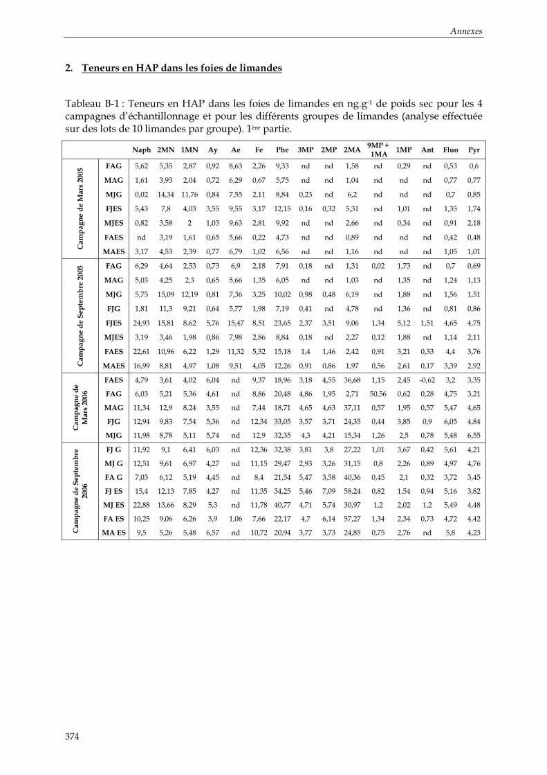
Annexes
374
2. Teneurs en HAP dans les foies de limandes
Tableau B-1 : Teneurs en HAP dans les foies de limandes en ng.g-1 de poids sec pour les 4 campagnes d’échantillonnage et pour les différents groupes de limandes (analyse effectuée sur des lots de 10 limandes par groupe). 1ère partie.
Naph 2MN 1MN Ay Ae Fe Phe 3MP 2MP 2MA 9MP + 1MA
1MP Ant Fluo Pyr
FAG 5,62 5,35 2,87 0,92 8,63 2,26 9,33 nd nd 1,58 nd 0,29 nd 0,53 0,6
MAG 1,61 3,93 2,04 0,72 6,29 0,67 5,75 nd nd 1,04 nd nd nd 0,77 0,77
MJG 0,02 14,34 11,76 0,84 7,55 2,11 8,84 0,23 nd 6,2 nd nd nd 0,7 0,85
FJES 5,43 7,8 4,03 3,55 9,55 3,17 12,15 0,16 0,32 5,31 nd 1,01 nd 1,35 1,74
MJES 0,82 3,58 2 1,03 9,63 2,81 9,92 nd nd 2,66 nd 0,34 nd 0,91 2,18
FAES nd 3,19 1,61 0,65 5,66 0,22 4,73 nd nd 0,89 nd nd nd 0,42 0,48
Ca
mp
ag
ne
de
Ma
rs 2
005
MAES 3,17 4,53 2,39 0,77 6,79 1,02 6,56 nd nd 1,16 nd nd nd 1,05 1,01
FAG 6,29 4,64 2,53 0,73 6,9 2,18 7,91 0,18 nd 1,31 0,02 1,73 nd 0,7 0,69
MAG 5,03 4,25 2,3 0,65 5,66 1,35 6,05 nd nd 1,03 nd 1,35 nd 1,24 1,13
MJG 5,75 15,09 12,19 0,81 7,36 3,25 10,02 0,98 0,48 6,19 nd 1,88 nd 1,56 1,51
FJG 1,81 11,3 9,21 0,64 5,77 1,98 7,19 0,41 nd 4,78 nd 1,36 nd 0,81 0,86
FJES 24,93 15,81 8,62 5,76 15,47 8,51 23,65 2,37 3,51 9,06 1,34 5,12 1,51 4,65 4,75
MJES 3,19 3,46 1,98 0,86 7,98 2,86 8,84 0,18 nd 2,27 0,12 1,88 nd 1,14 2,11
FAES 22,61 10,96 6,22 1,29 11,32 5,32 15,18 1,4 1,46 2,42 0,91 3,21 0,33 4,4 3,76
Ca
mp
ag
ne
de
Se
pte
mb
re 2
005
MAES 16,99 8,81 4,97 1,08 9,51 4,05 12,26 0,91 0,86 1,97 0,56 2,61 0,17 3,39 2,92
FAES 4,79 3,61 4,02 6,04 nd 9,37 18,96 3,18 4,55 36,68 1,15 2,45 -0,62 3,2 3,35
FAG 6,03 5,21 5,36 4,61 nd 8,86 20,48 4,86 1,95 2,71 50,56 0,62 0,28 4,75 3,21
MAG 11,34 12,9 8,24 3,55 nd 7,44 18,71 4,65 4,63 37,11 0,57 1,95 0,57 5,47 4,65
FJG 12,94 9,83 7,54 5,36 nd 12,34 33,05 3,57 3,71 24,35 0,44 3,85 0,9 6,05 4,84
Ca
mp
ag
ne
de
Ma
rs 2
006
MJG 11,98 8,78 5,11 5,74 nd 12,9 32,35 4,3 4,21 15,34 1,26 2,5 0,78 5,48 6,55
FJ G 11,92 9,1 6,41 6,03 nd 12,36 32,38 3,81 3,8 27,22 1,01 3,67 0,42 5,61 4,21
MJ G 12,51 9,61 6,97 4,27 nd 11,15 29,47 2,93 3,26 31,15 0,8 2,26 0,89 4,97 4,76
FA G 7,03 6,12 5,19 4,45 nd 8,4 21,54 5,47 3,58 40,36 0,45 2,1 0,32 3,72 3,45
FJ ES 15,4 12,13 7,85 4,27 nd 11,35 34,25 5,46 7,09 58,24 0,82 1,54 0,94 5,16 3,82
MJ ES 22,88 13,66 8,29 5,3 nd 11,78 40,77 4,71 5,74 30,97 1,2 2,02 1,2 5,49 4,48
FA ES 10,25 9,06 6,26 3,9 1,06 7,66 22,17 4,7 6,14 57,27 1,34 2,34 0,73 4,72 4,42
Ca
mp
ag
ne
de
Se
pte
mb
re
200
6
MA ES 9,5 5,26 5,48 6,57 nd 10,72 20,94 3,77 3,73 24,85 0,75 2,76 nd 5,8 4,23

Annexes
375
Tableau B-2 : Teneurs en HAP dans les foies de limandes en ng.g-1 de poids sec pour les 4 campagnes d’échantillonnage et pour les différents groupes de limandes (analyse effectuée sur des lots de 10 limandes par groupe). 2nd partie.
BaA triph+Chrys
M-Chrys
BbF + BkF
BeP BaP Per IP DaA+DaC
BP somme
HAP somme MHAP
FAG nd nd nd 1,14 0,98 0,58 nd nd nd nd 30,59 10,09
MAG nd nd nd 1,23 1,06 0,64 nd nd nd nd 19,51 7,01
MJG nd nd nd nd nd nd nd nd nd nd 20,91 32,53
FJES nd nd nd 7,61 nd nd nd nd nd nd 44,55 18,63
MJES nd nd nd 2,5 1,04 0,68 nd nd nd nd 31,52 8,58
FAES nd nd nd 1,11 0,95 0,58 nd nd nd nd 14,8 5,69
Ca
mp
ag
ne
de
Ma
rs 2
005
MAES nd nd nd 1,33 1,14 0,69 nd nd nd nd 23,53 8,08
FAG nd nd nd 0,92 0,78 0,46 nd nd nd nd 27,56 10,41
MAG nd nd nd 1,11 0,95 0,58 nd nd nd nd 23,75 8,93
MJG nd nd nd nd nd nd nd nd nd nd 30,26 36,81
FJG nd nd nd nd nd nd nd nd nd nd 19,06 27,06
FJES nd nd nd 12,34 nd nd nd nd nd nd 101,57 45,83
MJES nd nd nd 2,07 0,86 0,56 nd nd nd nd 30,47 9,89
FAES nd nd nd 2,22 1,9 1,16 nd nd nd nd 69,49 26,58
Ca
mp
ag
ne
de
Se
pte
mb
re 2
005
MAES nd nd nd 1,87 1,6 0,97 nd nd nd nd 54,81 20,69
FAES nd nd nd nd nd nd nd nd nd nd 45,09 55,64
FAG nd nd 4,51 nd nd nd nd nd nd nd 48,22 75,78
MAG 1,09 nd 2,82 nd nd nd nd nd nd nd 52,82 72,87
FJG nd nd nd nd nd nd nd nd nd nd 75,48 53,29
Ca
mp
ag
ne
de
Ma
rs 2
006
MJG nd nd 4,05 nd nd nd nd nd nd nd 75,78 45,55
FJ G nd nd 3,18 nd nd nd nd nd nd nd 72,93 58,21
MJ G nd 2,04 nd 2,14 3,04 nd nd nd nd nd 75,22 56,98
FA G nd nd 4,2 nd nd nd nd nd nd nd 48,9 67,49
FJ ES nd nd 3,32 nd nd nd nd nd nd nd 75,2 96,43
MJ ES 0,78 nd 2,59 5,78 5,01 nd nd nd nd nd 103,47 69,19
FA ES nd nd nd nd nd nd nd nd nd nd 54,9 87,11
Ca
mp
ag
ne
de
Se
pte
mb
re
200
6
MA ES nd nd 4,02 nd nd nd nd nd nd nd 57,14 50,63

Annexes
376
3. Teneurs en métabolites de HAP dans la bile de limandes
Tableau C : Teneurs en métabolites de HAP dans la bile de limandes en ng.g-1 de bile pour les 4 campagnes d’échantillonnage et pour les différents groupes de limandes (analyse effectuée sur des lots de 10 limandes par groupe).
1-OHN 2-OHN 2-OHBi 9-OHFe 4-
OHPhe 9-
OHPhe 3-
OHPhe 1-
OHPhe 2-
OHPhe 1-OHP
1-OHC
3-OHBaP
OHHAP
FJ ES 86 15 11 16 27 10 9 27 18 21 17 7 264
MJ ES 60 10 6 16 1 3 12 5 2 11 9 12 147
MA ES 82 4 6 63 5 7 8 24 7 238 9 5 458
MJ G 135 24 57 86 17 38 19 36 30 53 53 14 562
FA G 103 5 3 7 5 6 12 6 6 31 9 6 199
Ca
mp
ag
ne
de
Ma
rs
200
5
MA G 88 27 30 74 7 11 10 18 11 20 16 12 324
FJ ES 35 4 9 35 5 7 6 6 4 78 9 9 207
MJ ES 56 9 10 77 5 12 3 3 6 89 nd nd 270
FA ES 79 2 2 37 6 1 1 1 2 93 1 3 228
MA ES 21 1 6 25 2 3 1 nd 3 93 2 4 161
FJ G 12 1 1 3 1 nd nd 1 1 23 nd nd 43
MJ G 127 12 14 22 nd 6 nd 7 16 22 1 1 228
FA G 19 nd 2 7 1 1 nd 1 1 25 3 nd 60
Ca
mp
ag
ne
de
Se
pte
mb
re
200
5
MA G 20 1 1 5 1 2 nd 1 2 13 nd nd 46
FA ES 94 nd 266 202 39 118 46 103 47 245 200 nd 1 360
MA ES 57 nd 106 276 nd 64 23 nd nd 112 nd nd 638
FJ G 44 14 46 145 8 27 13 11 12 63 nd nd 383
MJ G 130 30 36 107 15 45 14 28 16 30 nd nd 451
FA G 14 12 24 72 3 23 nd 16 7 28 nd nd 199
Ca
mp
ag
ne
de
Ma
rs
200
6
MA G 27 20 33 172 5 27 nd 12 10 48 8 nd 362
FA ES 126 6 66 42 nd nd 4 20 11 435 nd nd 710
MA ES 144 23 138 106 nd nd 38 89 43 60 nd nd 641
MJ ES 42 14 205 40 nd nd 20 30 34 25 nd nd 410
FJ ES 20 14 371 25 nd nd 17 42 44 24 nd nd 557
FJ G 37 9 87 29 nd nd 11 24 19 16 nd nd 232
MJ G 40 9 136 15 nd nd 16 86 18 nd nd 0 320
FA G 13 5 142 26 nd nd 7 22 13 17 nd nd 245
Ca
mp
ag
ne
de
Se
pte
mb
re
200
6
MA G 61 3 48 33 nd nd 5 18 9 93 nd nd 270

Annexes
377
ANNEXE 13
Etude du suivi de la contamination dans la Baie de Guanabara (Brésil)
(Chapitre II, § 2.4.2)
Tableau A : Teneurs en métabolites de HAP dans la bile de poissons échantillonnés dans la Baie de Guanabara sur les sites de Dentro M et P, Botofago et Boa Viagem en Février, Mars et Avril 2006. Concentrations exprimées en µg.g-1 de bile (moyenne ± écartype)
Sites Dentro - Paqueta island Dentro - Paqueta island
Boa Viagem Dentro - Refinery
Boa Viagem Botafogo
Espèces Genidens genidens Micropogonias furnieri Cyclichthys spilostylus Ctenoscianea gracilicirrhus
Date Février 2006
(n = 3) Mars 2006
(n = 2) Avril 2006 Mars 2006 Avril 2006
Mars 2006 (n = 2)
Avril 2006 (n = 3)
Avril 2006
1-OHN 0,9 ± 1,3 1,1 ± 1,0 1,2 18,9 3,4 0,3 ± 0,2 1,3 ± 1,1 2,5
2-OHN 15,4 ± 2,9 3,8 ± 1,2 nd 2,2 nd 0,3 ± 0,04 0,7 ± 0,4 1,9
2-OHBi 33,7 ± 1,0 15,9 ± 8,6 nd 10,3 nd 1,2 ± 0,2 1,9 ± 2,9 10,0
9-OHFe 19,1 ± 5,3 11,8 ± 0,3 nd 6,3 nd 0,8 ± 0,3 2,9 ± 6,5 8,5
4-OHPhe 3,8 ± 1,9 0,8 ± 1,1 1,5 2,2 nd 0,3 ± 0,2 0,1 ± 0,3 0,7
9-OHPhe nd 1,1 ± 1,6 nd nd nd nd nd nd
3-OHPhe nd nd nd nd nd 0,3 ± 0,5 3,9 ± 4,1 nd
1-OHPhe 36,1 ± 26,9 13,2 ± 2,8 7,5 18,0 nd 3,4 ± 1,4 7,6 ± 5,3 nd
2-OHPhe 19,6 ± 13,7 14,2 ± 3,3 nd 5,7 nd 1,3 ± 0,05 3,3 ± 3,0 5,2
1-OHP 11,6 ± 3,8 11,5 ± 4,2 2,8 10,1 9,2 7,4 ± 1,5 27,2 ± 5,3 20,0
1-OHC 1,2 ± 2,3 1,1 ± 2,0 nd nd nd nd nd nd
3-OHBaP nd nd nd nd nd nd nd nd
OHPhe 59,5 ± 39,8 29,3 ± 8,8 8,9 26,0 nd 5,2 ± 2,1 14,9 ± 6,7 5,9
OHHAP 141,4 ± 38,9 74,5 ± 0,6 12,9 73,7 12,6 15,2 ± 1,2 48,8 ± 12,5 48,7


RESUME
Afin d’étudier la santé d’un écosystème marin et le potentiel toxique d’une contamination telle que celle liée à la présence d’hydrocarbures aromatiques polycycliques (HAP), il est nécessaire, outre de connaître les niveaux de contamination du milieu, de pouvoir accéder à la fraction toxique à laquelle les organismes aquatiques ont été exposés et de connaître les effets toxiques des contaminants incriminés. L’exposition et la contamination des organismes aquatiques aux HAP ont généralement été évaluées par le dosage des HAP bioaccumulés dans les tissus. Or, cette approche est critiquable si l'on tient compte des capacités de biotransformation des organismes, notamment des vertébrés, et des propriétés toxiques des produits de transformation formés. Dans ce contexte, l’objectif de cette thèse est d’étudier les phénomènes de bioccumulation et de biotransformation des HAP chez les organismes marins via l’étude des métabolites de HAP. Un effort de validation de biomarqueurs pertinents pour évaluer la génotoxicité des HAP en lien avec la contamination chimique des tissus et la production de métabolites est nécessaire.
Des méthodes de dosage des métabolites de HAP dans les matrices biologiques ont tout d’abord été mises au point. Ces outils analytiques sensibles, innovants et performants ont ensuite été appliqués lors d’expositions de poissons à des HAP via différentes voies de contamination en milieu contrôlé. Ils ont permis une meilleure connaissance des phénomènes de biotransformation des HAP. Enfin, des études de terrain ont été réalisées, notamment dans le cadre de l’étude de la contamination de la Baie de Seine, montrant l’applicabilité du dosage des métabolites de HAP dans l’évaluation de l’exposition des organismes aux HAP en milieu naturel. Dans le cadre d’une approche intégrée chimie/biologie, ces travaux ont permis d’apporter une contribution dans le transfert méthodologique des biomarqueurs de génotoxicité des HAP pour des applications en surveillance de l’Atlantique Nord et notamment dans la Manche.
Mots-clés : HAP, métabolites, poisson, surveillance environnementale, biotransformation, GC/MS, GC-MS/MS, UPLC-MS/MS
ABSTRACT
In order to study the health of a marine ecosystem and the toxic potential of a contamination such as that related to the presence of polycyclic aromatic hydrocarbons (PAHs), it is necessary, in addition to the determination of environmental contamination levels, to have access to the fraction for aquatic organisms have been exposed to and to identify the toxic effects of the contaminants. The exposure and contamination of aquatic organisms to PAHs have generally been evaluated by the quantification of bioaccumulated PAHs in tissues. However, this approach is criticable when taking into account the biotransformation capabilities of organisms such as vertebrates and the toxic properties of biotransformation products. In this way, the aim of this study is to study PAH bioaccumulation and biotransformation phenomena through the PAH metabolites study. An effort for the validation of relevant biomarkers to evaluate the link between the genotoxicity of PAHs, PAHs body burden and PAH metabolites production, is necessary.
Analytical techniques to quantify PAH metabolites in biological matrices have first been set up. Then, these sensible, innovating and powerful analytical tools have been applied to the study of fish exposures to PAHs through differents contamination sources in controlled conditions. This allowed to have a better understanding of PAH biotransformation phenomena. Finally, field studies have been led, notably to study the contamination of the Seine bay, demonstrating the applicability of the quantification of PAH metabolites to evaluate the exposure and the contamination of organisms to PAHs in natural environment. Within the framework of an integrated approach chemistry/biology, this work led to a contribution in the methodological transfer of biomarkers of PAH genotoxicity for biomonitorings in the North Atlantic and in particular in the English Channel.
Keywords : PAH, metabolites, fish, environmental survey, biotransformation, GC/MS, GC-MS/MS, UPLC-MS/MS