1

UNIVERSITÉ DE STRASBOURG

ÉCOLE DOCTORALE 269 (MSII)

ICube UMR 7357

THÈSE présentée par:

Le Anh PHAM

soutenue le : 13 Septembre 2018

pour obtenir le grade de : Docteur de l’université de Strasbourg

Discipline/ Spécialité : Energie et génie des procédés / Traitement des eaux

Consortium Algues-Bacteries Des Lagunes A Haut Rendement Algal: Evaluation Des Performances,

Devenir Des Nutriments Des Eaux Usees Et Conception A Base De Modeles Experimentaux Et Numeriques

THÈSE dirigée par :

WANKO NGNIEN Adrien MCF - HDR, ENGEES/Laboratoire ICube

LAURENT Julien MCF - HDR, ENGEES/Laboratoire ICube

RAPPORTEURS :

MOLLE Pascal Ingénieur de recherche - HDR, IRSTEA Lyon

CABASSUD Corinne Professeure - HDR, Insa Toulouse

AUTRES MEMBRES DU JURY :

ERNST Barbara Professeur, DSA - IPHC

HREIZ Rainier MCF, Université de Lorraine

2

Le Anh PHAM

Consortium Algues-Bacteries Des Lagunes A Haut Rendement Algal: Evaluation Des Performances,

Devenir Des Nutriments Des Eaux Usees Et Conception A Base De Modeles Experimentaux Et

Numeriques

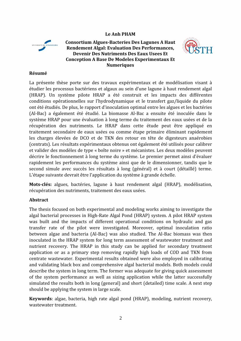
Résumé

La présente thèse porte sur des travaux expérimentaux et de modélisation visant à

étudier les processus bactériens et algaux au sein d’une lagune { haut rendement algal

(HRAP). Un système pilote HRAP a été construit et les impacts des différentes

conditions opérationnelles sur l’hydrodynamique et le transfert gaz/liquide du pilote

ont été étudiés. De plus, le rapport d'inoculation optimal entre les algues et les bactéries

(Al-Bac) a également été étudié. La biomasse Al-Bac a ensuite été inoculée dans le

système HRAP pour une évaluation à long terme du traitement des eaux usées et de la

récupération des nutriments. Le HRAP dans cette étude peut être appliqué en

traitement secondaire de eaux usées ou comme étape primaire éliminant rapidement

les charges élevées de DCO et de TKN des retour en tête de digesteurs anaérobies

(centrats). Les résultats expérimentaux obtenus ont également été utilisés pour calibrer

et valider des modèles de type « boîte noire » et mécanistes. Les deux modèles peuvent

décrire le fonctionnement à long terme du système. Le premier permet ainsi d'évaluer

rapidement les performances du système ainsi que de le dimensionner, tandis que le

second simule avec succès les résultats à long (général) et à court (détaillé) terme.

L'étape suivante devrait être l'application du système à grande échelle.

Mots-clés: algues, bactéries, lagune à haut rendement algal (HRAP), modélisation,

récupération des nutriments, traitement des eaux usées.

Abstract

The thesis focused on both experimental and modeling works aiming to investigate the

algal bacterial processes in High-Rate Algal Pond (HRAP) system. A pilot HRAP system

was built and the impacts of different operational conditions on hydraulic and gas

transfer rate of the pilot were investigated. Moreover, optimal inoculation ratio

between algae and bacteria (Al-Bac) was also studied. The Al-Bac biomass was then

inoculated in the HRAP system for long term assessment of wastewater treatment and

nutrient recovery. The HRAP in this study can be applied for secondary treatment

application or as a primary step removing rapidly high loads of COD and TKN from

centrate wastewater. Experimental results obtained were also employed in calibrating

and validating black box and comprehensive algal bacterial models. Both models could

describe the system in long term. The former was adequate for giving quick assessment

of the system performance as well as sizing application while the latter successfully

simulated the results both in long (general) and short (detailed) time scale. A next step

should be applying the system in large scale.

Keywords: algae, bacteria, high rate algal pond (HRAP), modeling, nutrient recovery,

wastewater treatment.

3

English title: Algal-Bacterial Consortium in High Rate Algal Pond: Evaluation of

Performances, Wastewater Nutrient Recovery And Experimental and Numerical Models

Based Design.

4

Acknowledgements

Firstly, to my supervisors Dr. Adrien WANKO and Dr. Julien LAURENT, as well as Dr.

Paul BOIS, another member of “the Fantastic Three”, thank you for your helps,

guidances and motivations throughout my PhD. Your supports are not only limited in

the research but also in many other aspects of life. I have learned a lot from you and I

appreciate it.

I would like to thank the members of my dissertation jury for their time and intellectual

contributions to my thesis. Your advices and discussions are also valuable to me for my

further development as a scientist.

I also couldn’t finish my PhD without valuable helps from technical staff of ENGEES.

Particularly, I would like to send my special thanks to Marie, Carole from LEE/ENGEES

for their technical support on sample analysis. Thank you for welcoming me to France

and always warning me the closing date of the supermarket. Besides, I also received

many helps while working in Icube Boussingault, therefore, I want to thank Abdel,

Martin, Joary, Fabrice and many other persons in Icube for your valuable supports. I

also want to thank people working in the wastewater treatment plant in Wantenauze

for your valuable support during my sampling campaign. Particularly, I would like to

thank Mr. PIERRE Frédéric, Directeur Développement, Valorhin, who is also being in my

jury as invited member. Your supports as well as practical advices helped me a lot in up-

scaling perspective.

My life in Strasbourg could be much more difficult without valuable support of my

colleagues and friends. Mamad, Max, Milena, Florent, Pulcherie, Teddy, Loic, Gille, Eloise,

Inest, thank you very much for your valuable helps in so many aspects of my life. My

thanks also come to my colleagues and friends from across the Atlantic Ocean. Juan, I

will never tell to anyone how you become a memorable PhD student to Professor

Robert. For Elena, your life threaten accidence in the wastewater treatment plant will

be safe with me and please accept my apologize for that. In addition, my PhD in France

could be more difficult without my Vietnamese friends. I want to thank Hải, Minh,

Hường, Duy, Lan, Sơn, Oanh, H{, Mi, Bình Đẳng and others friends in Vietnamese

Student Union of Strasbourg (AEVS) for making my life more enjoyable.

Last but not least, I want to thank my family for constant encouragement and love from

home while I’m far away. For my wife Van, I have been saying this for many times but

maybe it is the first time I say it in English, “thank you very much for your love and care,

without you, I couldn’t be as I am today, I love you”.

i

TABLE OF CONTENTS

LIST OF FIGURES ...................................................................................................................... v

LIST OF TABLES ................................................................................................................... viii

LIST OF ABBREVIATIONS ....................................................................................................... ix

INTRODUCTION .................................................................................................................... 1

1. Context and state of the art ....................................................................................... 1

2. Aims and Objectives .................................................................................................. 3

3. Thesis outline ............................................................................................................. 5

4. Thesis contribution ................................................................................................... 7

PART I LITERATURE REVIEW ............................................................................................. 9

CHAPTER 1 ALGAL BACTERIAL PROCESSES IN HRAP UNDER DIFFERENT

INFLUENCING FACTORS ...................................................................................................... 9

1.1 Introduction............................................................................................................ 9

1.2 Algal-bacterial interactions in wastewater treatment processes .................... 10

1.2.1 The interaction between algae and bacteria in wastewater environment

………………………………………………………………………………10

1.2.2 High Rate Algal Pond (HRAP) system ......................................................... 13

1.3 The factors impacting algal and bacterial processes in wastewater treatment

……………………………………………………………………………………16

1.3.1 Nutrients........................................................................................................ 16

1.3.2 Environmental factors .................................................................................. 21

1.3.3 Operational factors ....................................................................................... 25

1.4 Conclusions ........................................................................................................... 26

CHAPTER 2 HYDRAULIC, KINETIC AND GAS-LIQUID MASS TRANSFER STUDIES OF

THE HIGH RATE ALGAL POND .......................................................................................... 28

2.1 Introduction.......................................................................................................... 28

2.2 Hydraulic study .................................................................................................... 28

2.2.1 Experimental methods ................................................................................. 29

2.2.2 Hydraulic study – the RTD model ............................................................... 31

2.3 Reaction kinetic model ........................................................................................ 36

2.3.1 Reaction types ............................................................................................... 36

2.3.2 Reaction rate determination – coupled hydraulic and kinetic model ...... 38

2.4 Gas-liquid mass transfer study ........................................................................... 39

ii

2.4.1 The gas transfer rate and volumetric gas transfer coefficient .................. 39

2.4.2 Dynamic method ........................................................................................... 42

2.5 Conclusions ........................................................................................................... 43

CHAPTER 3 KINETIC MODELING OF THE ALGAL-BACTERIAL PROCESSES IN

WASTEWATER .................................................................................................................... 45

3.1 Introduction.......................................................................................................... 45

3.2 Model frameworks and kinetics ......................................................................... 46

3.2.1 Impact of light ............................................................................................... 48

3.2.2 Impact of temperature ................................................................................. 51

3.2.3 Nutrient factors ............................................................................................. 52

3.2.4 Algal bacterial biomass loss ......................................................................... 54

3.2.5 Impact of gas-liquid mass transfer .............................................................. 55

3.3 Conclusions ........................................................................................................... 56

PART II MATERIALS AND METHODS ............................................................................... 58

CHAPTER 4 EXPERIMENTAL METHODS FOR STUDYING ALGAL BACTERIAL

PROCESSES IN WASTEWATER .......................................................................................... 58

4.1 Algae and activated sludge inoculations preparation ....................................... 58

4.2 Experimental operations ..................................................................................... 60

4.3.1 Batch experiment to determine optimal algal bacterial inoculation ratio

………………………………………………………………………………60

4.3.2 Pilot experiment to determine the impact of different wastewater types,

hydraulic retention times and light intensities on the performance of HRAP ....... 63

CHAPTER 5 HYDRAULIC AND GAS-LIQUID MASS TRANSFER STUDIES OF PILOT

HRAP……………. .................................................................................................................... 69

5.1 Operational conditions applied .......................................................................... 69

5.2 Mixing characteristics and residence time distributions in HRAP .................. 70

5.3 Volumetric mass transfer coefficient (kLa) in HRAP ......................................... 73

5.4 Sensitivity analysis ............................................................................................... 74

CHAPTER 6 COUPLING RTD AND MIXED-ORDER KINETIC MODELS FOR HRAP

PERFORMANCE ASSESSMENT AND SIZING APPLICATION ............................................ 75

6.1 RTD and mixed-order kinetic models description ............................................ 75

6.1.1 Hydrodynamic (RTD) model....................................................................... 75

6.1.2 Coupling RTD and mixed-order kinetic models ............................................ 76

6.1.3 Data gathered for model verification ............................................................. 78

iii

6.2 Data analysis ......................................................................................................... 79

PART III RESULTS AND DISCUSSIONS .............................................................................. 80

CHAPTER 7 FINDING OPTIMAL ALGAL/BACTERIAL INOCULATION RATIO TO

IMPROVE ALGAL BIOMASS GROWTH AND SETTLING EFFICIENCY ............................. 80

7.1 Introduction.......................................................................................................... 80

7.2 Biomass growth.................................................................................................... 81

7.3 Biomass settleability ............................................................................................ 82

7.4 Nutrient removal efficiency ................................................................................ 83

7.5 Dynamics of dissolved oxygen and pH ............................................................... 84

7.6 Final choice of optimal inoculation ratio ........................................................... 86

7.7 Conclusions ........................................................................................................... 87

CHAPTER 8 IMPACTS OF OPERATIONAL CONDITIONS ON OXYGEN TRANSFER

RATE, MIXING CHARACTERISTICS AND RESIDENCE TIME DISTRIBUTION IN A PILOT

SCALE HIGH RATE ALGAL POND ...................................................................................... 89

8.1 Water flow regime ............................................................................................... 90

8.2 Paddle wheel vs water level on HRAP performance in closed condition ........ 90

8.3 Dominant effect of paddle wheel on oxygen transfer in HRAP ........................ 92

8.4 Operational conditions impacts on HRAP performance in closed condition .. 93

8.5 Impacts of operational conditions on residence time distributions in HRAP 94

8.6 Optimal operational conditions for algal-bacterial growth in HRAP .............. 96

8.7 Conclusions ........................................................................................................... 97

CHAPTER 9 LONG-TERM WASTEWATER TREATMENT BY ALGAL BACTERIAL

BIOMASS IN HIGH RATE ALGAL POND (HRAP): IMPACT OF NUTRIENT LOAD AND

HYDRAULIC RETENTION TIME ......................................................................................... 99

9.1 Impact of different nutrient loads and HRTs on wastewater treatment ......... 99

9.2 Impact of different nutrient loads and HRTs on biomass growth and recovery

…………………………………………………………………………………..103

9.3 Impact of different nutrient loads and HRTs on algal bacterial dynamic ..... 106

9.4 Conclusions and Perspectives ........................................................................... 110

CHAPTER 10 SIMULATION OF LONG TERM WASTEWATER TREATMENT BY A HIGH

RATE ALGAL POND: COUPLING RTD AND MIXED-ORDER KINETIC MODELS:

PERFORMANCE ASSESSMENT AND SIZING APPLICATION .......................................... 112

10.1 Coupled RTD and mixed-order kinetic model simulating long term HRAP

operation ....................................................................................................................... 113

10.1.1 Optimal reaction rate and reaction orders ............................................... 113

iv

10.1.2 Model evaluation ........................................................................................ 114

10.2 Relationship between experimental and model parameters ..................... 117

10.3 Coupled RTD and mixed-order kinetic model applied for sizing HRAP .... 119

10.4 Conclusions and Perspectives ....................................................................... 120

CHAPTER 11 SIMULATION OF ALGAL BACTERIAL PROCESSES IN WASTEWATER

TREATMENT HIGH RATE ALGAL POND – A GOOD MODELING PRACTICE

APPLICATION… ................................................................................................................. 123

11.1 Introduction .................................................................................................... 123

11.2 Project definition ............................................................................................ 124

11.3 Data collection and reconciliation ................................................................ 125

11.3.1 Data collection ............................................................................................ 125

11.3.2 Additional measurements .......................................................................... 127

11.4 Al-Bac model set-up for HRAP system ......................................................... 128

11.4.1 Model layout ................................................................................................ 128

11.4.2 Algal bacterial kinetic model ..................................................................... 128

11.4.3 Influent and effluent models ...................................................................... 139

11.4.4 Settler model ............................................................................................... 140

11.4.5 Aeration model ........................................................................................... 140

11.5 Calibration and validation ............................................................................. 140

11.6 Conclusions and Perspectives ....................................................................... 146

CONCLUSIONS AND PERSPECTIVES ............................................................................... 148

1 General conclusions of the thesis ......................................................................... 148

2 General perspectives ............................................................................................. 150

APPENDIX .......................................................................................................................... 155

REFERENCES ..................................................................................................................... 180

v

LIST OF FIGURES

Figure I Thesis outline illustration. ......................................................................................... 7

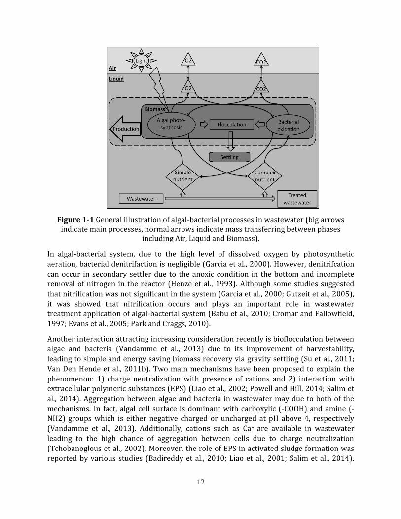
Figure 1-1 General illustration of algal-bacterial processes in wastewater (big arrows

indicate main processes, normal arrows indicate mass transferring between phases). ....................................................................................................................... 12

Figure 1-2 Cross-sectional side view of a HRAP with CO2 aeration (Park et al., 2010). ... 14

Figure 1-3 Distribution of nitrogen in a treatment system with nitrification (Sperling, 2007). .......................................................................................................................... 18

Figure 1-4 Illustration of algal specific growth rate depending on the optimal N:P ratio (Richmond, 2008). ...................................................................................................... 20

Figure 1-5 Typical photosynthesis–irradiance response curve with Pmax is maximum

photosynthetic rate reached at saturating irradiance (Ek) while Ec is irradiance compensation point (Barsanti and Gualtieri, 2006). ............................................... 21

Figure 1-6 Growth rate versus temperature curves for five unicellular algae with different optimal temperature (Eppley, 1972). ....................................................... 23

Figure 2-1 The exit age distribution curve E for fluid flowing through a vessel; also called the residence time distribution, or RTD (Levenspiel, 1999). ...................... 29

Figure 2-2 The RTD measurements following a) pulse method and b) step method (Fogler, 2006b). .......................................................................................................... 30

Figure 2-3 Illustration of the tracer pulse spreading due to axial dispersion according to the dispersion model (adapted from Levenspiel, 1999). ........................................ 33

Figure 2-4 Illustration of the Tanks-in-Series model (Levenspiel, 1999). ........................ 35

Figure 3-1 Example of using Peterson’s matrix for presenting process kinetics and stochiometry for aerobic growth of heterotrophic bacteria (Henze et al., 1987). 48

Figure 3-2 PFS model illustration (Wu and Merchuk, 2001). ............................................. 50

Figure 3-3 Illustration of death-regeneration with hydrolysis. ......................................... 55

Figure 4-1 Location of the wastewater treatment plant in Rosheim, Bas-Rhin, Grand Est,

France (sources: http://www.map-france.com/ and https://en.wikipedia.org/wiki/Rosheim). ............................................................... 59

Figure 4-2 Microscopic images (black line indicates 0.01mm) of dominant groups in the

algal consortium including (a.) Chlorella sp., (b.) Ulothrix sp., (c.) Scenedesmus sp.,

(d.) Pseudanabaenaceae sp., and (e.) Nitzschia sp. .................................................. 60

Figure 4-3 a. Real picture of a working reactor and b. Experimental protocol illustration:

highlighted arrows - shifting between phases, normal arrows - biomass,

physiochemical and biochemical measurements, dashed arrows – exchange aqueous phase with fresh synthetic wastewater. .................................................... 61

Figure 4-4 Side view and top view of a. the pilot HRAP and b. the settler. ....................... 64

Figure 4-5 General illustration of pilot HRAP experimental set-up (arrows indicate water and biomass flow, red dashed lines indicate measurements). .................... 66

Figure 5-1 Correlations between a. NaCl concentration and conductivity in the water and b. voltage, water level and paddle rotational speed. ........................................ 70

Figure 5-2 a. General illustration of pilot HRAP with tracer experiments in open

condition (normal figures and text), in closed condition (dashed figure and italic

text) and oxygen transfer rate experiments in closed condition (dashed figures,

vi

italic text in brackets). And b. Actual figure of the experimental setup in open condition. .................................................................................................................... 73

Figure 6-1 General procedure of HRAP simulation. ............................................................ 78

Figure 7-1 Global Al-Bac biomass and Chl-a productivities of biomass with different

initial algae/activated sludge ratios (error bars indicate variances of fitted values and observed values). ................................................................................................ 81

Figure 7-2 Average with standard error of dissolved oxygen (DO) concentration in different test reactors during reaction phase and feeding phase. ......................... 85

Figure 7-3 Average with standard error of pH in different test reactors during reaction phase and feeding phase. ........................................................................................... 86

Figure 8-1 Influence of paddle rotational speed, water level to Bodenstein number (a.)

and water velocity (b.) in pilot HRAP. ...................................................................... 91

Figure 8-2 Absolute-Relative sensitivity (dimensionless) of Bodenstein number versus

paddle rotational speed (a.) and water level (b.). The sign represents positive (no sign) or negative (- sign) correlation. ....................................................................... 92

Figure 8-3 Influence of paddle wheel rotation, water level to oxygen transfer coefficient in pilot HRAP. .............................................................................................................. 93

Figure 8-4 Absolute-Relative sensitivity (d-1) of oxygen transfer coefficient (kLaO2)

versus paddle rotational speed (a.) and water level (b.). The sign represents positive (no sign) or negative (- sign) correlation. .................................................. 93

Figure 8-5 Average Relative-Relative sensitivities (dimensionless) of oxygen transfer

coefficient and Bodenstein number versus water level and paddle rotational speed. Data was converted to absolute value for comparison. .............................. 94

Figure 8-6 Influence of inlet flow rate (a, d, f), paddle wheel rotation (b, e, g) and water

level (c, f, h) to effective volume fraction (ϵ: a, b, c), Short-circuiting Index (SI (%): d, e, f) and Peclet number (Pe: g, h, i) in pilot HRAP. ...................................... 96

Figure 9-1 COD, N and P concentrations at the influent and effluent of the HRAP (data of

LN_4d modality fit with left scale, data of HN_4d and HN_8d modalities fit with right scale)................................................................................................................. 100

Figure 9-2 Al-Bac biomass and Chl-a concentrations in the HRAP for different modalities. ................................................................................................................. 104

Figure 9-3 Al-Bac biomass and Chl-a production during the entire pilot experiment. .. 106

Figure 9-4 Example of decomposition of time series DO data (time scale in days and DO data in mg/L). ........................................................................................................... 107

Figure 9-5 Time decomposition of time series pH data recorded two weeks before (a.)

and after (b.) feeding wastewater with high nutrient load in the HRAP (time scale in days). ..................................................................................................................... 108

Figure 10-1 Experimental COD data at the effluent (diamond with error bars indicating

measurement uncertainty) of different modalities (graph title with best fit order in brackets) fitted to the coupled RTD and mixed-order kinetic model (line). ... 115

Figure 10-2 Experimental TN data at the effluent (diamond with error bars indicating

measurement uncertainty) of different modalities (graph title with best fit order

in brackets) fitted to the coupled RTD and mixed-order model (line). ............... 117

Figure 10-3 Experimental TKN data at the effluent (diamond with error bars indicating

measurement uncertainty) of different modalities (graph title with best fit order in brackets) fitted to the coupled RTD and mixed-order model (line). ............... 117

vii

Figure 10-4 PCA biplot showing relationships between various experimental and model

parameters for different modalities. In the figure, Chl_a and Bio_tot refer to

concentrations of Chlorophyll a and total biomass in HRAP. Inlet_i and E_i are the

inlet concentration and average removal efficiency of substance i, respectively.

While n_i, k_i and r_i are optimal reaction order, reaction rate constant and reaction rate of related to removal process of substance i, respectively. ........... 119

Figure 10-5 HRAP sizing following low light (a.) and high light models (b.) with the color bar indicates mean residence required. ................................................................. 120

Figure 11-1 General illustration of the HRAP simulation procedure. .............................. 125

Figure 11-2 Experimental (dots) and simulated (lines) TSS (a.), nitrate (b.), ammonium

(c.), and nitrite (d.) nitrogen values in the HRAP for 85 days since the day 55.

Measured TSS data was used for model calibration, 20% variation was calculated from the simulated result (a.). ................................................................................. 142

Figure 11-3 Experimental (dots) and simulated (line) DO and pH in the HRAP for 85 days since the day 55. .............................................................................................. 143

Figure 11-4 Experiment (dot) and simulation (line) data of DO concentration in HRAP from day 62 to 66 (a.) and from day 93 to 97 (b.). ................................................ 144

Figure 11-5 Experiment (dot) and simulation (line) data of pH in HRAP from day 58 to 61 (a.) and from day 76 to 79 (b.). .......................................................................... 145

Figure 11-6 Simulated concentrations of algae, heterotrophic, ammonium oxidizing and nitrite oxidizing bacteria in the HRAP for 85 days since the day 55. ................... 145

viii

LIST OF TABLES

Table 1-1 Design characteristics of different HRAPs. ......................................................... 14

Table 1-2 Outdoor HRAP systems for wastewater treatment in different conditions. .... 16

Table 4-1 Ingredients and measured nutrient contents of synthetic wastewater. .......... 62

Table 4-2 Operational characteristics of different stages. .................................................. 65

Table 6-1 Data of the HRAP performance for different modalities. ................................... 79

Table 7-1 Average Chl-a and TSS contents in the effluent and their proportions in total Chl-a and TSS contents of each reactor. ................................................................... 83

Table 7-2 Nutrient concentrations at the outlet of four reactors (mg/L, mean values in bold, n=9). ................................................................................................................... 84

Table 8-1 Reynolds and Froude numbers for different operational conditions. .............. 90

Table 9-1 Removal rates and removal efficiencies of COD, TKN, TN and TP for different modalities. ................................................................................................................. 103

Table 9-2 Physio-chemical and biomass monitoring parameters for different modalities..................................................................................................................................... 105

Table 9-3 Variances of decomposed DO (mg/L) and pH data for different modalities. . 109

Table 10-1 Optimal reaction orders n and reaction rate constants k in (mg/L)1-n

/day for

different modalities and pollutant. ......................................................................... 114

Table 11-1 Influent, HRAP and effluent measurements of the HRAP system, results are

given in average with standard deviation. Number of samples is given in brackets. .................................................................................................................... 127

Table 11-2 Model process rates. ......................................................................................... 132

Table 11-3 Model parameters. ............................................................................................ 133

Table 11-4 Stoichiometric parameters. .............................................................................. 135

Table 11-5 Mass fraction of elements on organic compounds. ........................................ 135

Table 11-6 Stoichiometric coefficients. .............................................................................. 136

Table 11-7 Mathematic expressions of stochiometric coefficients in each process. ...... 137

Table 11-8 Influent (I) and effluent (E) models. ................................................................ 139

Table 11-9 Ratios of different particulate species over total TSS in the HRAP in steady state simulation. ....................................................................................................... 141

ix

LIST OF ABBREVIATIONS

ADM anaerobic digestion model

AOB ammonium oxidizing bacteria

ASM activated sludge model

ASM-A activated sludge model - algae

BNR biological nutrient removal

Bo bodenstein number

BOD biological oxygen demand

CAS conventional activated sludge

CFD computational fluid dynamics

CO2 carbon dioxide

COD chemical oxygen demand content

CSTR continuous stirred tank reactor

DO dissolved oxygen concentration

EPS extracellular polymeric substances

Fr froude number

GMP good modelling practice

GRG2 generalized reduced gradient

HRAP high rate algal pond

HRP high rate pond

HRT hydraulic retention time

IWA International Water Association

NOB nitrite oxidizing bacteria

NSE nash-sutcliffe efficiency index

OECD organization for economic cooperation and development

OPR oxygen production rate

OTR oxygen transfer rate

OUR oxygen uptake rate

P/I photosynthetic-irradiance

PCA principle components analysis

PCB polychlorinated biphenyl

Pe peclet number

PFR plug flow reactor

PSF photosynthetic factory

PHA poly-hydroxy-alkanoates

Re reynolds number

RSS residual sum of squares

RTD residence time distribution

RWQM river water quality model

SBR sequencing batch reactor

SI short-circuiting index

SRT solids retention time

TIS tank-in-series

TKN total Kjeldahl nitrogen

TN total nitrogen

TP total phosphorus

TSS total suspended solid content

x

VSS volatile suspended solids

WWTP wastewater treatment plant

1

INTRODUCTION

1. Context and state of the art

Although covering two-thirds of the Earth’s surface, yet only a small fraction of water (less

than 0.5%) is readily available for human use (UNESCO, 2015). Together with modern

pressures such as population and economic growth, more and more people are facing

water scarcity every year. Around the world, 2.1 billion people are lacking of safely

managed water in which 844 million people have no access to basic drinking water service

(WHO, 2015). Until 2017, the main part of global water use is for agriculture (accounting

for 70%) and it is increasing (15% more by 2050). Ground water is pumped at faster rate

than it is recharged (World Bank, 2017). In this context, wastewater treatment plays a vital

role of accelerating the purification of water in nature (US EPA, 1998) and redistributing

water for agriculture (FAO, 1992).

Conventional wastewater treatment is the combination of physical, chemical, and biological

processes that can achieve various levels of treatment depending on the water reuse

applications (FAO, 1992). The levels are preliminary, primary (and advanced primary),

secondary (and/or secondary with nutrient removal), tertiary, and advanced treatments

(Abdel-Raouf et al., 2012; Noüe et al., 1992; Tchobanoglous et al., 2002). Among them,

primary and secondary treatments are the basic stages: the primary stage focuses on

removing settleable organic and inorganic solids by sedimentation while the secondary

treatment further removes the residual organics and suspended solids from the effluent

from primary treatment. Tertiary and further treatments are required if necessary (FAO,

1992; US EPA, 1998). In most cases, aerobic biological treatment with oxygen

supplementation (high rate biological process) is the dominant process in secondary stage

in which the bacterial activities are triggered by artificial oxygen addition to metabolize the

organic matter leaving new biomass and inorganic nutrients as the end-products. Activated

sludge, trickling filters, and rotating biological contactors are the most common high rate

processes with the first one being the most popular (US EPA, 1998).

Despite the fact that 85% of organic matters and suspended solids can be removed after

secondary treatment, inorganic phosphorus and nitrogen are still available in the effluent

which can cause secondary pollution requiring further step to be removed (FAO, 1992).

These additional steps (usually biological nitrification and denitrification) also increase the

total cost which may be doubled for each additional step. Moreover, the nutrients (nitrogen

and phosphorus) contained in wastewater are generally lost during these treatments

leading to incomplete utilization of natural resources (Noüe et al., 1992). In that context,

microalgae received early attraction due to its photosynthetic ability utilizing the nutrient

in wastewater and light to generate new biomass and oxygen that is required by organic

matter stabilization (Oswald and Gotaas, 1957). Therefore, the application of algae for

wastewater treatment and biofuels production is promising, especially in the recent

2

context of fuel shortage and climate change that raise the need of sustainable development

(Pittman et al., 2011; Rawat et al., 2011).

Despite this potential, there are several bottlenecks to tackle to further develop this

technology. One of them is harvesting algal biomass. Due to the small size of the algal cells

and their low concentration in culture solution, efficient harvesting of algal biomass from

water can account for 20-30% of total production cost (Mata et al., 2010; Pragya et al.,

2013). One solution is to enhance algal biomass settleability by bio-flocculation in which

activated sludge and algae are inoculated to form algal bacterial biomass. Although the

technique has been shown to improve biomass settling while keeping good treatment

efficiency (Gutzeit et al., 2005; Van Den Hende et al., 2011a), the inoculation ratio is still

diverse and its application in pilot scale is still lacking.

In order to apply algal based wastewater treatment at large scale, many efforts have been

spent to study the use of photobioreactor systems to improve algal growth (Muñoz and

Guieysse, 2006). Among them, high rate algal pond (HRAP) showed strong advantages

including low energy consumption and financial requirement, ease of maintenance and

feasibility in expanding to large scale (Mata et al., 2010). As a consequence, HRAP system

was applied in many places with wide range of environmental and hence operational

conditions (Picot et al., 1991; El Hamouri et al., 1995; Grönlund et al., 2010). In addition,

variation in operational condition can influences hydrodynamics and hence gas transfer

which are important especially in open aerobic biological reactor like HRAP (Garcia-Ochoa

and Gomez, 2009). Therefore, determining the impacts of operational conditions on

hydrodynamics and thus gas transfer in HRAP system is necessary.

In addition, although application of algal-bacterial biomass in HRAP system for wastewater

treatment and biomass production is promising, the dynamic between algae and bacteria

and its impact on long term performance of the system is still lacking. In addition, in recent

years, anaerobic digestion has become a popular solution for bioenergy production and the

use of its liquid effluent as nutrient source of HRAP system promoting nutrient recovery

has been attracting (Sawatdeenarunat et al., 2016). Hence, the impact of high nutrient load

from anaerobic digestion effluent on the algal bacterial dynamic deserves serious attention.

Due to the complexity of algal bacterial process which involves the dependence of many

interactions between different algal bacterial species inside the system on the variation of

different operational and environmental conditions (Cole, 1982; Kouzuma and Watanabe,

2015), the system is difficult to control and thus yet to be applied widely in industrial scale

(Mata et al., 2010). In this context, using mathematics model to simulate the algal-bacterial

processes could serve as a rapid and cost-effective method to study the system in order to

improve, manage and enlarge it in bigger scale. Extensive studies have been conducted to

develop comprehensive algal bacterial models (Buhr and Miller, 1983; Reichert et al., 2001;

Solimeno et al., 2017) providing a deep insight into the processes occurring in the system,

especially when coupling with advanced hydrodynamic model such as computational fluid

dynamics (CFD) model (Nauha and Alopaeus, 2013; Wu and Merchuk, 2001). Despite of

3

these achievements, more efforts are still required to improve the simulation in terms of

hydrodynamics, light attenuation or gas transfer of the algal bacterial system (Solimeno

and García, 2017). Moreover, a guideline for selecting factors and framework in model

construction simulating algal growth is also lacking (E. Lee et al., 2015).

Another modeling approach requiring only influent and effluent wastewater characteristics

is the classical black box reaction kinetic model (Levenspiel, 1999). Although only

considering global kinetic behavior of the system, the model was widely used for designing

purpose of the wastewater system providing satisfactory results (Henze, 2008). Hence the

application of this model type to the HRAP system is attractive especially when HRAP is

implemented in remote areas requiring quick and simple assessment. Also, since deviation

from the ideal hydraulic condition in the reactor is a common problem and always

influence the performance of the system, a coupled kinetic and hydraulic model is a

necessary step to improve the simulation by considering imperfect flow patterns in the

system (Fogler, 2006a). Therefore, efforts also should be made on investigating the

application of coupled global hydraulic and reaction kinetic model in performance

assessment and sizing of HRAP system.

2. Aims and Objectives

This thesis is conducted to understand the cooperation between algae and bacteria in

wastewater treatment and biomass production in order to improve the system

performance. The two main aspects included are experimental and modeling parts.

The experimental part consists of lab scale and pilot scale experiments:

Batch reactors were inoculated with different ratios and fed with synthetic

wastewater in order to compare different algae/activated sludge inoculation ratios

in terms of algal growth, treatment efficiency and biomass settling. Hence the

optimal algal bacterial inoculation ratio can be chosen.

A pilot HRAP was constructed and the impacts of operational conditions including

water level, inlet flow rate and paddle wheel movement on hydrodynamics as well

as gas transfer in the pilot were investigated. An optimal operational condition will

be chosen to apply in the pilot HRAP for algal-bacterial biomass cultivation.

Then, a long-term experiment was conducted to evaluate the dynamic between

algae and bacteria under medium and high nutrient loads within a pilot scale HRAP

inoculated with optimal algal-bacterial biomass. The performance of the system was

assessed in terms of treatment efficiency, biomass production and recovery. Impact

of hydraulic retention time (HRT) variation in high nutrient load condition on the

system was also investigated.

4

In the modeling part, both comprehensive algal bacterial kinetic model and black box

hydraulic and reaction kinetic model are developed. Data gathered from the pilot

experiment was used to calibrate and validate the models:

- A mixed-order kinetic model was coupled with a Residence Time Distribution (RTD)

model to simulate the data obtained from different long term experiments

conducted in the pilot scale HRAP. The relationships between different

environmental and operational conditions including light intensity, nutrient loading

or hydraulic retention time (HRT) and the model parameters including the reaction

order and reaction rate constant were evaluated. In a further step, the model

obtained was applied in a HRAP sizing application.

- An algal bacterial model simulating algal bacterial processes in the HRAP system

was also developed following Good Modelling Practice unified protocol (Rieger et

al., 2012) to investigate the dynamic of these processes.

In French:

Cette thèse vise à mieux comprendre la coopération entre les algues et les bactéries dans

un objectif de traitement des eaux usées et de production de biomasse. Deux aspects

principaux sont développés : d’une part l’étude expérimentale du procédé et d’autre part sa

modélisation.

La partie expérimentale consiste en des expériences à l'échelle du laboratoire et à l'échelle

pilote:

- Des réacteurs en discontinu ont été inoculés avec différents ratios algues/bactéries

et alimentés avec des eaux usées synthétiques afin de comparer les différents ratios

en termes de croissance des algues, d'efficacité du traitement et de décantation de la

biomasse. On peut donc choisir le rapport optimal d'inoculation.

- Une lagune à haut rendement algal (HRAP) pilote a été construite et les impacts des

conditions opérationnelles, comprenant le niveau d'eau, le débit d'entrée et le

mouvement de la roue à aubes sur l'hydrodynamique ainsi que le transfert de gaz

dans le pilote ont été étudiés. Les conditions opératoires optimales seront choisies

pour la culture de biomasse algale-bactérienne.

- Ensuite, une expérience pilote à long terme a été menée pour évaluer la dynamique

entre les algues et les bactéries avec des charges modérées et élevées en nutriments.

Les performances du système ont été évaluées en termes d'efficacité de traitement,

de production de biomasse et de sa récupération. L'impact de la variation du temps

de rétention hydraulique (HRT) dans des conditions de charge élevée en nutriments

a également été étudié.

Concernant la modélisation, deux approches sont développées : d’une part, un modèle

complet des cinétiques bactérienne et algale et d’autre part, un modèle de type « boîte

5

noire » couplant l’hydrodynamique et les cinétiques réactionnelles. Les données recueillies

dans le cadre de l'expérience pilote ont été utilisées pour caler et valider les modèles:

- Un modèle cinétique d'ordre mixte a été utilisé en association avec un modèle de

Distribution des Temps de Séjour (RTD) pour simuler les données obtenues à partir

de différentes expériences menées à l'échelle pilote . Les relations entre les

différentes conditions environnementales et opérationnelles, y compris l'intensité

lumineuse, la charge en éléments nutritifs ou le temps de rétention hydraulique

(HRT) et les paramètres du modèle, y compris l'ordre de réaction et la constante de

vitesse de réaction, ont été évaluées.

- Un modèle biocinétique simulant les processus bactériens et algaux dans le système

HRAP a également été développé selon le protocole unifié des bonnes pratiques de

modélisation (Rieger et al., 2012) pour étudier la dynamique de ces processus.

3. Thesis outline

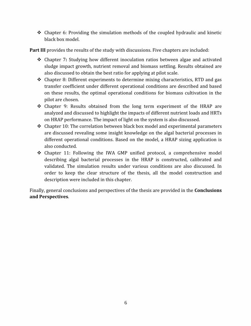
General outline of this thesis is illustrated in Figure I. Experimental and modeling works

with the links between chapters in one part as well as between parts are described.

Part I covers detailed description of the biochemical processes of algae and bacteria in

general as well as in HRAP system in particular. Different studying methods for hydraulics,

gas transfer and modeling of the HRAP are also described. This part includes:

Chapter 1: Reviewing knowledge concerning the processes of algae and bacteria in

wastewater including synergistic and antagonistic interactions. It is also reviewing

the knowledge concerning the use of HRAP in wastewater treatment and the factors

impacting algal and bacterial growth in HRAP for wastewater treatment and

biomass production.

Chapter 2: Information concerning the systemic hydraulic study methods and gas-

liquid mass transfer of HRAP is introduced.

Chapter 3: Providing the knowledge concerning kinetic model simulation methods

of algae and bacteria in HRAP system.

In Part II, the materials and methods of experimental and modeling works are introduced.

The part consists of three chapters relating to biochemical, hydraulic and gas transfer, and

modeling studies:

Chapter 4: Describing the materials and methods to study algal bacterial

wastewater treatment, growth and biomass settling in both lab scale and pilot scale

experiments.

Chapter 5: The pilot HRAP constructed as well as materials and methods related to

hydraulic and gas transfer studies in the HRAP are shown.

6

Chapter 6: Providing the simulation methods of the coupled hydraulic and kinetic

black box model.

Part III provides the results of the study with discussions. Five chapters are included:

Chapter 7: Studying how different inoculation ratios between algae and activated

sludge impact growth, nutrient removal and biomass settling. Results obtained are

also discussed to obtain the best ratio for applying at pilot scale.

Chapter 8: Different experiments to determine mixing characteristics, RTD and gas

transfer coefficient under different operational conditions are described and based

on these results, the optimal operational conditions for biomass cultivation in the

pilot are chosen.

Chapter 9: Results obtained from the long term experiment of the HRAP are

analyzed and discussed to highlight the impacts of different nutrient loads and HRTs

on HRAP performance. The impact of light on the system is also discussed.

Chapter 10: The correlation between black box model and experimental parameters

are discussed revealing some insight knowledge on the algal bacterial processes in

different operational conditions. Based on the model, a HRAP sizing application is

also conducted.

Chapter 11: Following the IWA GMP unified protocol, a comprehensive model

describing algal bacterial processes in the HRAP is constructed, calibrated and

validated. The simulation results under various conditions are also discussed. In

order to keep the clear structure of the thesis, all the model construction and

description were included in this chapter.

Finally, general conclusions and perspectives of the thesis are provided in the Conclusions

and Perspectives.

7

Figure I Thesis outline illustration.

4. Thesis contribution

The work described in the first part of chapter 4 and the entire chapter 7 is currently under

reviewing process of Water SA journal under the title:

PHAM Le Anh, Julien LAURENT, Paul BOIS, Adrien WANKO. Finding optimal algal/bacterial

inoculation ratio to improve algal biomass growth and settling efficiency.

The work described in chapter 5 and chapter 8 was presented as an oral presentation in

the IWA S2Small 2017 conference and the revised manuscript was under reviewing

process of Water Science and Technology journal:

Pham, L.A., Laurent, J., Bois, P., Wanko, A., 2017. Impacts of operational conditions on oxygen

transfer rate, mixing characteristics and residence time distribution in a pilot scale high rate

algal pond, in: The IWA S2Small2017 Conference on Small Water & Wastewater Systems and

Resources Oriented Sanitation. IWA, Nantes, France.

Pham, L. A., Laurent J., Bois P., Wanko A. Impacts of operational conditions on oxygen

transfer rate, mixing characteristics and residence time distribution in a pilot scale high rate

algal pond.

8

The work described in chapter 6 and chapter 10 was accepted as an oral presentation in

SWWS 2018 conference:

Reaction Order Of Biochemical Processes In HRAP Based On Pilot Experiments And

Systemic/biokinetic Modeling: Impact Of Light Intensity And Nutrient Loading, oral

presentation accepted in: SWWS and ROS, 2018 –Technion, Israel.

The work described in the second part of chapter 4 and chapter 11 was accepted as a

poster presentation in SWWS 2018 conference and submitted as a technical research paper

in Chemical Engineering Journal:

Algal Production And Wastewater Treatment In HRAP Under Different Light Intensities And

Nutrient Loadings, poster presentation accepted in: SWWS and ROS, 2018 –Technion, Israel.

Long-term wastewater treatment by algal bacterial biomass in high rate algal pond (HRAP):

impact of nutrient load and hydraulic retention time. Sumitted as Research Paper in Chemical

Engineering Journal.

9

PART I LITERATURE REVIEW

CHAPTER 1 ALGAL BACTERIAL PROCESSES IN HRAP UNDER DIFFERENT

INFLUENCING FACTORS

1.1 Introduction

Algae is the term used to call a group of organisms that has the ability to photosynthesize.

They can be in either macroscopic (macroalgae) or microscopic (microalgae) life forms

which the latter form being dominant. Their cells can be prokaryotes that lack a

membrane-bound nucleus or eukaryotes with a nucleus plus typical membrane-bound

organelles (Barsanti and Gualtieri, 2006; Bellinger and Sigee, 2015). Algal photosynthesis is

a light conversion process in which natural or artificial light energy is turned into

biochemical energy used to synthesize organic compounds. Photosynthetic pigments in

algal cell are key components for harvesting light energy (Richmond, 2008). Without light,

algae shift to respiration which instead of releasing, oxygen is consumed and carbon

dioxide is generated (Barsanti and Gualtieri, 2006). Some algae are known to use organic

carbon for heterotrophic activities, especially at irradiance limited condition but still

generally fundamental photosynthetic organisms (Bellinger and Sigee, 2015; Richmond,

2008).

For long time, microalgae have been recognized as a valuable source for human food

(Priyadarshani and Rath, 2012). With the development of algal cultivation techniques

started in late nineteenth century, industrial algal production expanded its application

range to fertilizers, animal and fish feeds, high value bio-molecules, pharmaceuticals,

cosmetics and food colorants (Andersen, 2005; Lawton et al., 2017; Priyadarshani and

Rath, 2012). As cells can accumulate a high amount of lipids and carbohydrates, it is an

ideal source for biofuels production (Mata et al., 2010; Sirajunnisa and Surendhiran, 2016;

Voloshin et al., 2016).

Using algae for wastewater treatment can also benefit in many ways. First of all, being

primary producers, algae have the ability to use inorganic nutrients as substrates

(Bellinger and Sigee, 2015; Richmond, 2008). Via photosynthesis, algae use light energy for

reproduction and metabolism, which consumes carbon dioxide and releases soluble oxygen

in water environment (Richmond, 2008). This process supports bacterial decomposing

processes and increases pH of water with a sanitation effect towards pathogenic bacteria

(Cole, 1982; Muñoz and Guieysse, 2006). It is also important to note that algae can be used

to remove metals under ion form in wastewater; removal can be through cell accumulation

or cell surface adsorption (Mehta and Gaur, 2005). Moreover, the growth of bacteria and

algae also enhances flocculation between them. Thus the algal-bacterial biomass can be

harvested by simple gravitational sedimentation (Gutzeit et al., 2005).

10

Recent context of algal nutrient recovery from wastewater has encouraged the application

of algae and bacteria in system serving both wastewater treatment and biomass production

purposes (Cai et al., 2013). Many studies have been done to investigate the interaction

between algae and bacteria in wastewater (Kouzuma and Watanabe, 2015; Unnithan et al.,

2014), the application of algae in wastewater treatment and biomass production (Park et

al., 2010; Sutherland et al., 2015) as well as the downstream processes including harvesting

the biomass (Milledge and Heaven, 2012; Pragya et al., 2013; Wan et al., 2015) and biomass

application in biofuels production (González-Fernández et al., 2012; Pragya et al., 2013;

Ward et al., 2014). Factors impacting the performance of the system (Kumar et al., 2015;

Sutherland et al., 2015) were also studied. The following sections focus on some of these

most important aspects including the interaction between algae and bacteria with

influencing factors and system design and operation.

1.2 Algal-bacterial interactions in wastewater treatment processes

1.2.1 The interaction between algae and bacteria in wastewater environment

Traditionally in wastewater engineering, the main attention is focused on suspended

solids, biodegradable organics, pathogens, nutrients (carbon, nitrogen and phosphorus),

heavy metals or dissolved inorganics constituents in wastewater. Hence, the biological

processes of consideration in wastewater are related to these constituents (Tchobanoglous

et al., 2002). Understanding these processes as well as the interactions between algae and

bacteria in wastewater allows better interpretation of the field data achieved, hence having

more accurate solution.

In activated sludge process, heterotrophic aerobic bacteria or heterotrophs are dominant

which use organic matter in wastewater as source of carbon and energy and oxygen as

preferred electron acceptor. Via the oxidation, organic matters are converted to simple end

products such as ammonium, nitrate and orthophosphorus ions that are partly consumed

by bacteria for their biomass production (Sperling, 2007). Beside heterotrophs, autotrophic

bacteria or autotrophs are important in wastewater treatment. These small bacterial

groups have ability to take electrons from ammonium and nitrite ions and reducing them to

nitrite and nitrate ions (nitrification), respectively (Gerardi, 2003). Moreover, when oxygen

is not available (anoxic condition), most of bacteria can use nitrate instead of oxygen to be

their electron acceptor, reducing it to nitrogen gas (denitrification) (Grady Jr et al., 2011).

Under specific process, enhanced phosphorus accumulation can occur, which increase the

amount of phosphorus removed. The growth of bacteria in the activated sludge process

also leads to flocculation of cells and thus sedimentation of the biomass. Therefore, the

biomass and incorporated matter can be removed, leaving clean effluent (Tchobanoglous et

al., 2002).

Algal photosynthesis contains two phases including light phase/light dependent phase and

the dark phase/light independent phase (C3 or Calvin-Benson cycle). The first phase

involves harvesting light energy/photons to produce biochemical energy-storing molecules

11

including NADPH and ATP; water molecule is used as the source of protons and electrons

leading to the generation of oxygen as by-product (Barsanti and Gualtieri, 2006). The latter

phase contains series of reactions in which carbon dioxide is reduced to form organic

compounds.

In wastewater, synergistic interactions between algae and bacteria can come from the both

sides (Cole, 1982; Unnithan et al., 2014) which are generally illustrated in Figure 1-1. With

exposure to light, algae provide oxygen into the environment for heterotrophic oxidation

and carbon dioxide generated by this process participates in the dark phase of

photosynthesis. The concentrations of these gases are also impacted by the gas transfer

between air and liquid which rate highly depends on mixing in the reactor (Garcia-Ochoa

and Gomez, 2009). Moreover, via their living activities including reproduction and death,

algae can release organic matter that is available as substrate for bacteria (Bell and

Mitchell, 1972; Cole, 1982). It also indicated that, algae may act as secondary habitat for

bacteria (Unnithan et al., 2014) which bacteria can attach onto algal cell surface, live inside

algal cell or coexist with algae in phycosphere (Cole, 1982; Kouzuma and Watanabe, 2015).

In turn, bacteria also show facilitative impacts on algal growth. As decomposer, bacteria

degrade organic matter to provide inorganic compounds back into the habitat which are

necessary for algal reproduction. The nutrient recycle process by bacteria is very important

especially for the limited nutrient for algae such as phosphorus (Cole, 1982). In addition,

besides of nutrient exchange, bacteria and algae can have other forms of synergistic

interaction including signal transduction and gene transfer (Kouzuma and Watanabe,

2015).

12

Figure 1-1 General illustration of algal-bacterial processes in wastewater (big arrows indicate main processes, normal arrows indicate mass transferring between phases

including Air, Liquid and Biomass).

In algal-bacterial system, due to the high level of dissolved oxygen by photosynthetic

aeration, bacterial denitrifaction is negligible (Garcia et al., 2000). However, denitrifcation

can occur in secondary settler due to the anoxic condition in the bottom and incomplete

removal of nitrogen in the reactor (Henze et al., 1993). Although some studies suggested

that nitrification was not significant in the system (Garcia et al., 2000; Gutzeit et al., 2005),

it was showed that nitrification occurs and plays an important role in wastewater

treatment application of algal-bacterial system (Babu et al., 2010; Cromar and Fallowfield,

1997; Evans et al., 2005; Park and Craggs, 2010).

Another interaction attracting increasing consideration recently is bioflocculation between

algae and bacteria (Vandamme et al., 2013) due to its improvement of harvestability,

leading to simple and energy saving biomass recovery via gravity settling (Su et al., 2011;

Van Den Hende et al., 2011b). Two main mechanisms have been proposed to explain the

phenomenon: 1) charge neutralization with presence of cations and 2) interaction with

extracellular polymeric substances (EPS) (Liao et al., 2002; Powell and Hill, 2014; Salim et

al., 2014). Aggregation between algae and bacteria in wastewater may due to both of the

mechanisms. In fact, algal cell surface is dominant with carboxylic (-COOH) and amine (-

NH2) groups which is either negative charged or uncharged at pH above 4, respectively

(Vandamme et al., 2013). Additionally, cations such as Ca+ are available in wastewater

leading to the high chance of aggregation between cells due to charge neutralization

(Tchobanoglous et al., 2002). Moreover, the role of EPS in activated sludge formation was

reported by various studies (Badireddy et al., 2010; Liao et al., 2001; Salim et al., 2014).

13

Various theories were proposed such as the divalent cation bridging theory which divalent

cations make bridge between negatively charged sites on the cell surface and negatively

charged groups on EPS or the alginate theory that linear alginate-like exopolysaccharide

produced by microbes bulked to form egg-box to cover cells together with the presence of

divalent cations (Ding et al., 2015). Therefore, flocculation between algae and bacteria in

wastewater may also be contributed by EPS.

Beside synergistic interactions, algal and bacterial living activities can lead to undesired

conditions for each other. Common antagonistic interaction in wastewater is inorganic

carbon competition between algae and autotrophic bacteria. Although carbon dioxide is

always dissolved into water from the atmosphere, the competition may decrease the

growth of algae due to their lower consumption rate (Muñoz and Guieysse, 2006).

Moreover, inorganic carbon consumption by algae leads to pH level increased, higher than

11 in some cases, which inhibits bacterial growth (Park et al., 2010). However, this

phenomenon is one of the desired characteristics when using algae for wastewater

treatment due to the reduction of pathogens at the outlet as a consequence of elevated pH

level (Abdel-Raouf et al., 2012). Host–pathogen relationship between algae and bacteria is

also common which can lead to lysis and death of the host on one hand while algae may

inhibit bacterial growth by releasing antibiotic compounds on the other hand (Cole, 1982;

Kouzuma and Watanabe, 2015).

1.2.2 High Rate Algal Pond (HRAP) system

Early studies on photosynthesis in sewage wastewater were conducted more than sixty

years ago (Oswald and Gotaas, 1957) focusing on a new oxidation-pond type which was

highly dependent on photosynthetic aeration. This new pond type had smaller size than the

conventional pond and its detention time was also much shorter (less than a week in

comparison with from three to six weeks or more). Due to enhancing its vertical mixing,

this pond type can develop a dense algal culture supporting a treatment rate of ten times

higher than conventional oxidation-pond. The advantages of this pond type which was then

called high rate pond (HRP) or high rate algal pond (HRAP) are clear including small area

requirement and promoting nutrient recovery via harvesting the biomass (El Hamouri et

al., 2003; Oswald and Gotaas, 1957). Since then, the new oxidation-pond or high-rate pond

has been applied as algal based wastewater treatment unit or algal cultivation facility in

many places (Kumar et al., 2015; Mata et al., 2010; Rawat et al., 2011).

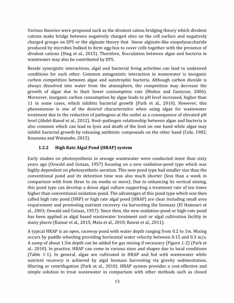
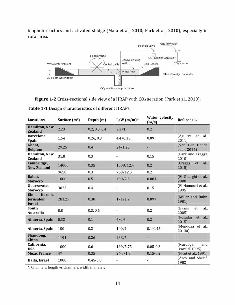
A typical HRAP is an open, raceway pond with water depth ranging from 0.2 to 1m. Mixing

occurs by paddle wheeling providing horizontal water velocity between 0.15 and 0.3 m/s.

A sump of about 1.5m depth can be added for gas mixing if necessary (Figure 1-2) (Park et

al., 2010). In practice, HRAP can come in various sizes and shapes due to local conditions

(Table 1-1). In general, algae are cultivated in HRAP and fed with wastewater while

nutrient recovery is achieved by algal biomass harvesting via gravity sedimentation,

filtering or centrifugation (Park et al., 2010). HRAP system provides a cost-effective and

simple solution to treat wastewater in comparison with other methods such as closed

14

biophotoreactors and activated sludge (Mata et al., 2010; Park et al., 2010), especially in

rural area.

Figure 1-2 Cross-sectional side view of a HRAP with CO2 aeration (Park et al., 2010).

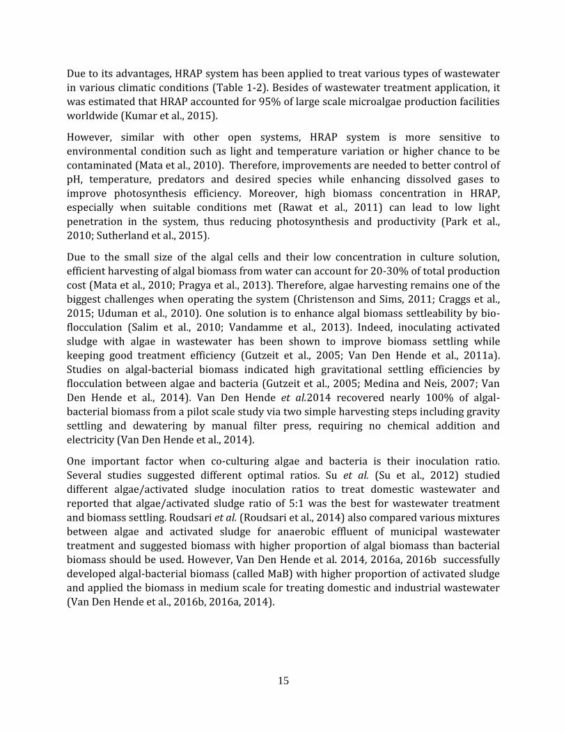
Table 1-1 Design characteristics of different HRAPs.

Locations Surface (m2) Depth (m) L/W (m/m)* Water velocity (m/s)

References

Hamilton, New Zealand

2.23 0.2, 0.3, 0.4 2.2/1 0.2

Barcelona, Spain

1.54 0.26, 0.3 4.4/0.35 0.09 (Aguirre et al., 2011)

Ghent, Belgium

29.25 0.4 24/1.25 - (Van Den Hende et al., 2014)

Hamilton, New Zealand

31.8 0.3 - 0.15 (Park and Craggs, 2010)

Cambridge, New Zealand

14000 0.35 1008/12.4 0.2 (Craggs et al., 2015)

9650 0.3 760/12.5 0.2 Rabat, Morocco

1000 0.5 400/2.5 0.084 (El Ouarghi et al., 2000)

Ouarzazate, Morocco

3023 0.4 - 0.15 (El Hamouri et al., 1995)

Ein Karem, Jerusalem, Israel

281.25 0.38 171/1.2 0.097 (Miller and Buhr, 1981)

South Australia

8.8 0.3, 0.6 - 0.2 (Evans et al., 2005)

Almería, Spain 8.33 0.1 6/0.6 0.2 (Posadas et al., 2015)

Almería, Spain 100 0.3 100/1 0.1-0.45 (Mendoza et al., 2013a)

Shandong, China

1191 0.26 238/5 -

California, USA

1000 0.6 190/5.75 0.05-0.3 (Nurdogan and Oswald, 1995)

Meze, France 47 0.35 24.8/1.9 0.15-0.2 (Picot et al., 1991)

Haifa, Israel 1000 0.45-0.8 - - (Azov and Shelef, 1982)

*: Channel’s length vs channel’s width in meter.

15

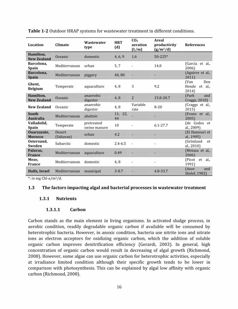
Due to its advantages, HRAP system has been applied to treat various types of wastewater

in various climatic conditions (Table 1-2). Besides of wastewater treatment application, it

was estimated that HRAP accounted for 95% of large scale microalgae production facilities

worldwide (Kumar et al., 2015).

However, similar with other open systems, HRAP system is more sensitive to

environmental condition such as light and temperature variation or higher chance to be

contaminated (Mata et al., 2010). Therefore, improvements are needed to better control of

pH, temperature, predators and desired species while enhancing dissolved gases to

improve photosynthesis efficiency. Moreover, high biomass concentration in HRAP,

especially when suitable conditions met (Rawat et al., 2011) can lead to low light

penetration in the system, thus reducing photosynthesis and productivity (Park et al.,

2010; Sutherland et al., 2015).

Due to the small size of the algal cells and their low concentration in culture solution,

efficient harvesting of algal biomass from water can account for 20-30% of total production

cost (Mata et al., 2010; Pragya et al., 2013). Therefore, algae harvesting remains one of the

biggest challenges when operating the system (Christenson and Sims, 2011; Craggs et al.,

2015; Uduman et al., 2010). One solution is to enhance algal biomass settleability by bio-

flocculation (Salim et al., 2010; Vandamme et al., 2013). Indeed, inoculating activated

sludge with algae in wastewater has been shown to improve biomass settling while

keeping good treatment efficiency (Gutzeit et al., 2005; Van Den Hende et al., 2011a).

Studies on algal-bacterial biomass indicated high gravitational settling efficiencies by

flocculation between algae and bacteria (Gutzeit et al., 2005; Medina and Neis, 2007; Van

Den Hende et al., 2014). Van Den Hende et al.2014 recovered nearly 100% of algal-

bacterial biomass from a pilot scale study via two simple harvesting steps including gravity

settling and dewatering by manual filter press, requiring no chemical addition and

electricity (Van Den Hende et al., 2014).

One important factor when co-culturing algae and bacteria is their inoculation ratio.

Several studies suggested different optimal ratios. Su et al. (Su et al., 2012) studied

different algae/activated sludge inoculation ratios to treat domestic wastewater and

reported that algae/activated sludge ratio of 5:1 was the best for wastewater treatment

and biomass settling. Roudsari et al. (Roudsari et al., 2014) also compared various mixtures

between algae and activated sludge for anaerobic effluent of municipal wastewater

treatment and suggested biomass with higher proportion of algal biomass than bacterial

biomass should be used. However, Van Den Hende et al. 2014, 2016a, 2016b successfully

developed algal-bacterial biomass (called MaB) with higher proportion of activated sludge

and applied the biomass in medium scale for treating domestic and industrial wastewater

(Van Den Hende et al., 2016b, 2016a, 2014).

16

Table 1-2 Outdoor HRAP systems for wastewater treatment in different conditions.

Location Climate Wastewater type

HRT (d)

CO2

aeration (L/m)

Areal productivity (g/m2/d)

References

Hamilton, New Zealand

Oceanic domestic 4, 6, 9 1.6 50-225*

Barcelona, Spain

Mediterranean urban 5, 7 - 14.8 (García et al., 2006)

Barcelona, Spain

Mediterranean piggery 40, 80 - - (Aguirre et al., 2011)

Ghent, Belgium

Temperate aquaculture 4, 8 3 9.2 (Van Den Hende et al., 2014)

Hamilton, New Zealand

Oceanic anaerobic digester

4, 8 2 15.8-20.7 (Park and Craggs, 2010)

New Zealand Oceanic anaerobic digester

4, 8 Variable rate

8-20 (Craggs et al., 2015)

South Australia

Mediterranean abattoir 11, 22, 44

- - (Evans et al., 2005)

Valladolid, Spain

Temperate pretreated swine manure

10 - 6.1-27.7 (de Godos et al., 2009)

Ouarzazate, Morocco

Desert (Saharan)

urban 4.2 - - (El Hamouri et al., 1995)

Ostersund, Sweden

Subarctic domestic 2.4-6.5 - - (Grönlund et al., 2010)

Palavas, France

Mediterranean aquaculture 0.49 - - (Metaxa et al., 2006)

Meze, France

Mediterranean domestic 4, 8 - - (Picot et al., 1991)

Haifa, Israel Mediterranean municipal 3-8.7 - 4.8-33.7 (Azov and Shelef, 1982)

*: in mg Chl-a/m2/d.

1.3 The factors impacting algal and bacterial processes in wastewater treatment

1.3.1 Nutrients

1.3.1.1 Carbon

Carbon stands as the main element in living organisms. In activated sludge process, in

aerobic condition, readily degradable organic carbon if available will be consumed by

heterotrophic bacteria. However, in anoxic condition, bacteria use nitrite ions and nitrate

ions as electron acceptors for oxidizing organic carbon, which the addition of soluble

organic carbon improves denitrification efficiency (Gerardi, 2003). In general, high

concentration of organic carbon would result in decreasing of algal growth (Richmond,

2008). However, some algae can use organic carbon for heterotrophic activities, especially

at irradiance limited condition although their specific growth tends to be lower in

comparison with photosynthesis. This can be explained by algal low affinity with organic

carbon (Richmond, 2008).

17

Inorganic carbon is the most important nutrient for microalgal growth contributing about

50% of algal biomass dry weight (Richmond, 2008). Algae can uptake either soluble carbon dioxide (CO2) or bicarbonate (HCO3

−) to be used in the Calvin-Benson cycle for synthesizing

organic carbon (Richmond, 2008). Although bicarbonate was suggested to directly

participate in organic carbon synthesis under low photosynthesis state (Falkowski, 1980),

after accumulated in algal cell, it may be hydrated to carbon dioxide by carbonic anhydrase

before used for organic carbon synthesis (Moroney and Ynalvez, 2007). In general, algae

can take up CO2 via diffusion, especially in low pH (Moazami-Goudarzi and Colman, 2012).

However, various studies agreed that in water, both carbon dioxide and bicarbonate can be

actively taken via CO2 concentrating mechanisms (Moroney and Ynalvez, 2007; Raven and

Johnston, 1991; Smith and Bidwell, 1989; Sültemeyer et al., 1991). The concentrating

process in aquatic algae is necessary, since water diffusion of CO2 is a thousand time lower

than in the air and additionally, at high level of pH, only small fraction of carbon dioxide is

available for algae while bicarbonate is abundance. The form of carbon that is available for

algae is dependent on pH which soluble carbon dioxide is the dominant form at pH ≤ 6.36

while bicarbonate form is dominant at pH ≥ 10.33 (Reichert et al., 2001). As the more

inorganic carbon is taken up by algae, the more proton is taken out of water causing an

increasing of pH level. The equilibrium of bicarbonate and carbon dioxide in water can be

described as follow:

𝐶𝑂2 + 𝐻2𝑂 ↔ 𝐻2𝐶𝑂3 (1-1) 𝐻2𝐶𝑂3 ↔ 𝐻𝐶𝑂3

− + 𝐻+ (1-2) 𝐻𝐶𝑂3

− ↔ 𝐶𝑂32− + 𝐻+ (1-3)

When algal-bacterial consortium is applied for wastewater treatment, part of CO2 demand

of algae is supplied by heterotrophic bacteria although competition on inorganic carbon

consumption between algae and autotrophic bacteria may occur. Additional carbon dioxide

sources (flue gases or rich carbon dioxide air) can be used to enhance algal growth (Park et

al., 2010) as well as control the pH level . If flue gas is chosen to aerated, gas purification is

also achieved . However, there were still some studies reporting no significant

improvement in either algal production or treatment efficiency when CO2 was aerated in

the outdoor system (Posadas et al., 2015; Van Den Hende et al., 2014). Moreover,

significant proportion of the additional air is likely to be lost to the atmosphere causing

additional carbon emission of the system (Richmond, 2008).

1.3.1.2 Nitrogen

After carbon, nitrogen contributes 7-10% of algal dry weight depending on the type of algae and environmental conditions. Algae can use both nitrate (NO3

−) and ammonium

(NH4+) nitrogen for their growth (Richmond, 2008). Bacteria also need nitrogen, which

about 14% of bacterial dry weight is contributed by this element. Similar with algae,

bacteria can use both nitrate (NO3−) and ammonium (NH4

+) or sometime nitrite (NO2−)

nitrogen as their sources although the oxidation state of nitrogen in ammonium ion is more

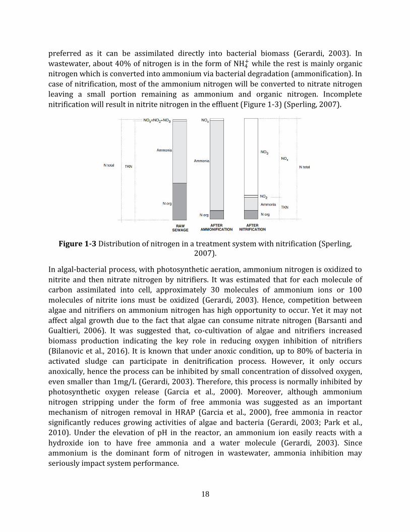
18

preferred as it can be assimilated directly into bacterial biomass (Gerardi, 2003). In

wastewater, about 40% of nitrogen is in the form of NH4+ while the rest is mainly organic

nitrogen which is converted into ammonium via bacterial degradation (ammonification). In

case of nitrification, most of the ammonium nitrogen will be converted to nitrate nitrogen

leaving a small portion remaining as ammonium and organic nitrogen. Incomplete

nitrification will result in nitrite nitrogen in the effluent (Figure 1-3) (Sperling, 2007).

Figure 1-3 Distribution of nitrogen in a treatment system with nitrification (Sperling, 2007).

In algal-bacterial process, with photosynthetic aeration, ammonium nitrogen is oxidized to

nitrite and then nitrate nitrogen by nitrifiers. It was estimated that for each molecule of

carbon assimilated into cell, approximately 30 molecules of ammonium ions or 100

molecules of nitrite ions must be oxidized (Gerardi, 2003). Hence, competition between

algae and nitrifiers on ammonium nitrogen has high opportunity to occur. Yet it may not

affect algal growth due to the fact that algae can consume nitrate nitrogen (Barsanti and

Gualtieri, 2006). It was suggested that, co-cultivation of algae and nitrifiers increased

biomass production indicating the key role in reducing oxygen inhibition of nitrifiers

(Bilanovic et al., 2016). It is known that under anoxic condition, up to 80% of bacteria in

activated sludge can participate in denitrification process. However, it only occurs

anoxically, hence the process can be inhibited by small concentration of dissolved oxygen,

even smaller than 1mg/L (Gerardi, 2003). Therefore, this process is normally inhibited by

photosynthetic oxygen release (Garcia et al., 2000). Moreover, although ammonium

nitrogen stripping under the form of free ammonia was suggested as an important

mechanism of nitrogen removal in HRAP (Garcia et al., 2000), free ammonia in reactor

significantly reduces growing activities of algae and bacteria (Gerardi, 2003; Park et al.,

2010). Under the elevation of pH in the reactor, an ammonium ion easily reacts with a

hydroxide ion to have free ammonia and a water molecule (Gerardi, 2003). Since

ammonium is the dominant form of nitrogen in wastewater, ammonia inhibition may

seriously impact system performance.

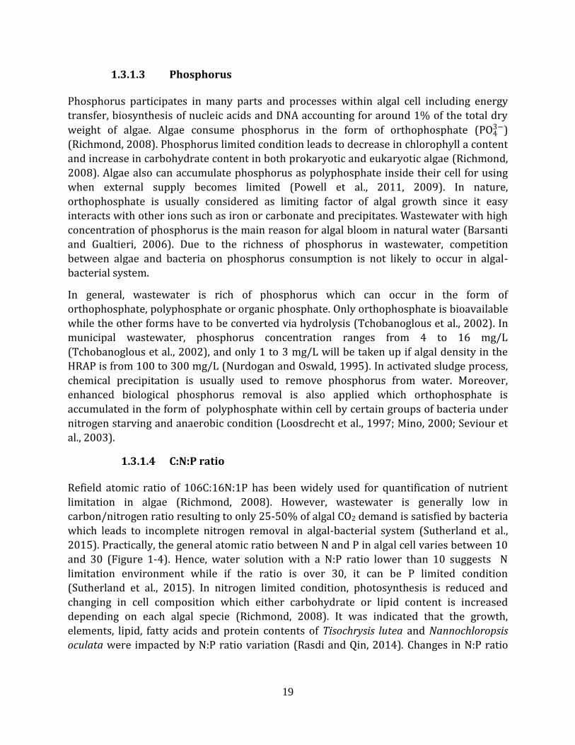
19

1.3.1.3 Phosphorus

Phosphorus participates in many parts and processes within algal cell including energy

transfer, biosynthesis of nucleic acids and DNA accounting for around 1% of the total dry

weight of algae. Algae consume phosphorus in the form of orthophosphate (PO43−)

(Richmond, 2008). Phosphorus limited condition leads to decrease in chlorophyll a content

and increase in carbohydrate content in both prokaryotic and eukaryotic algae (Richmond,

2008). Algae also can accumulate phosphorus as polyphosphate inside their cell for using

when external supply becomes limited (Powell et al., 2011, 2009). In nature,

orthophosphate is usually considered as limiting factor of algal growth since it easy

interacts with other ions such as iron or carbonate and precipitates. Wastewater with high

concentration of phosphorus is the main reason for algal bloom in natural water (Barsanti

and Gualtieri, 2006). Due to the richness of phosphorus in wastewater, competition

between algae and bacteria on phosphorus consumption is not likely to occur in algal-

bacterial system.

In general, wastewater is rich of phosphorus which can occur in the form of

orthophosphate, polyphosphate or organic phosphate. Only orthophosphate is bioavailable

while the other forms have to be converted via hydrolysis (Tchobanoglous et al., 2002). In

municipal wastewater, phosphorus concentration ranges from 4 to 16 mg/L

(Tchobanoglous et al., 2002), and only 1 to 3 mg/L will be taken up if algal density in the

HRAP is from 100 to 300 mg/L (Nurdogan and Oswald, 1995). In activated sludge process,

chemical precipitation is usually used to remove phosphorus from water. Moreover,

enhanced biological phosphorus removal is also applied which orthophosphate is

accumulated in the form of polyphosphate within cell by certain groups of bacteria under

nitrogen starving and anaerobic condition (Loosdrecht et al., 1997; Mino, 2000; Seviour et

al., 2003).

1.3.1.4 C:N:P ratio

Refield atomic ratio of 106C:16N:1P has been widely used for quantification of nutrient

limitation in algae (Richmond, 2008). However, wastewater is generally low in

carbon/nitrogen ratio resulting to only 25-50% of algal CO2 demand is satisfied by bacteria

which leads to incomplete nitrogen removal in algal-bacterial system (Sutherland et al.,

2015). Practically, the general atomic ratio between N and P in algal cell varies between 10

and 30 (Figure 1-4). Hence, water solution with a N:P ratio lower than 10 suggests N

limitation environment while if the ratio is over 30, it can be P limited condition

(Sutherland et al., 2015). In nitrogen limited condition, photosynthesis is reduced and

changing in cell composition which either carbohydrate or lipid content is increased

depending on each algal specie (Richmond, 2008). It was indicated that the growth,

elements, lipid, fatty acids and protein contents of Tisochrysis lutea and Nannochloropsis

oculata were impacted by N:P ratio variation (Rasdi and Qin, 2014). Changes in N:P ratio

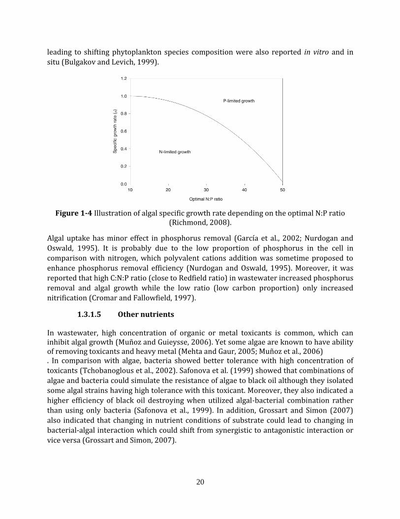
20

leading to shifting phytoplankton species composition were also reported in vitro and in

situ (Bulgakov and Levich, 1999).

Figure 1-4 Illustration of algal specific growth rate depending on the optimal N:P ratio (Richmond, 2008).

Algal uptake has minor effect in phosphorus removal (García et al., 2002; Nurdogan and

Oswald, 1995). It is probably due to the low proportion of phosphorus in the cell in

comparison with nitrogen, which polyvalent cations addition was sometime proposed to

enhance phosphorus removal efficiency (Nurdogan and Oswald, 1995). Moreover, it was

reported that high C:N:P ratio (close to Redfield ratio) in wastewater increased phosphorus

removal and algal growth while the low ratio (low carbon proportion) only increased

nitrification (Cromar and Fallowfield, 1997).

1.3.1.5 Other nutrients

In wastewater, high concentration of organic or metal toxicants is common, which can inhibit algal growth (Muñoz and Guieysse, 2006). Yet some algae are known to have ability of removing toxicants and heavy metal (Mehta and Gaur, 2005; Muñoz et al., 2006) . In comparison with algae, bacteria showed better tolerance with high concentration of

toxicants (Tchobanoglous et al., 2002). Safonova et al. (1999) showed that combinations of

algae and bacteria could simulate the resistance of algae to black oil although they isolated

some algal strains having high tolerance with this toxicant. Moreover, they also indicated a

higher efficiency of black oil destroying when utilized algal-bacterial combination rather

than using only bacteria (Safonova et al., 1999). In addition, Grossart and Simon (2007)

also indicated that changing in nutrient conditions of substrate could lead to changing in

bacterial-algal interaction which could shift from synergistic to antagonistic interaction or

vice versa (Grossart and Simon, 2007).

21

1.3.2 Environmental factors

1.3.2.1 Light

Light is vital for algal photosynthesis although optimal light intensity varies between

species. Some species preferred high light condition which may vary from 400 up to 850

µEm-2s-1 (Singh and Singh, 2015), other showed growth stimulation around 200 µEm-2s-1

(Simionato et al., 2013) while some benthic algae (diatoms) have high growth rate at low

light intensity of 25 µEm-2s-1 (Shi et al., 2015). In HRAP, suitable light intensity generally

ranges from 200 to 400 µEm-2s-1 (Muñoz and Guieysse, 2006).

Algae also have the ability to adjust for adaptation with natural light variation

(photoacclimation) which involves changing size and number of light-harvesting pigments

or changing the distribution of harvested energy (Barsanti and Gualtieri, 2006). However,

in general, insufficient light intensity causes photosynthesis to cease with no oxygen

generated, while high light intensity results to photoinhibition (Figure 1-5). As the light

intensity increased, the opportunity that photosynthetic reaction center receives more than

one photon is increased. It leads to overexcitation state or damage of the photosystem, both

of which result to reduction of the photosynthetic rate or photoinhibition (Richmond,

2008).

Figure 1-5 Typical photosynthesis–irradiance response curve with Pmax is maximum photosynthetic rate reached at saturating irradiance (Ek) while Ec is irradiance

compensation point (Barsanti and Gualtieri, 2006).

Beside light intensity, photoperiod also influences algal growth (C. S. Lee et al., 2015).

Although increasing light:dark ratio showed higher growth and nutrient removal rates

(Gonçalves et al., 2014), continuous light may be harmful to algal growth (Andersen, 2005).

It was indicated that a dark period is needed to provide NAD+ and NADP+ for

photosynthesis and reduce the total cost of algae cultivation (Bouterfas et al., 2006;

Simionato et al., 2013). In general, photoperiod ranging from 12 to 16h/day was suggested

to apply for algal cultivation (Andersen, 2005; James, 2012; Lavens and Sorgeloos, 1996).

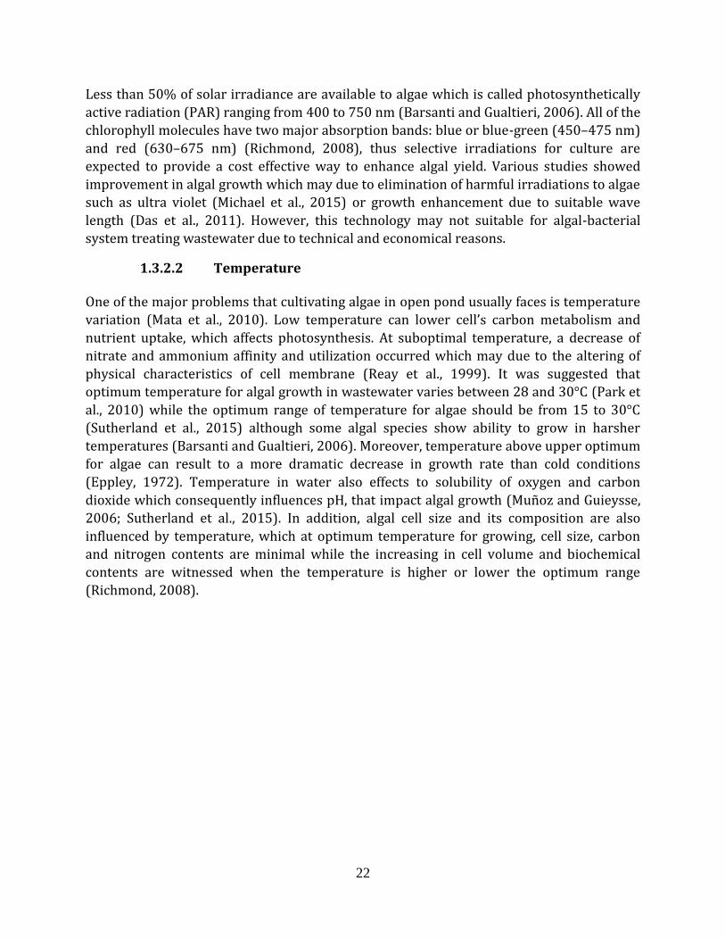
22

Less than 50% of solar irradiance are available to algae which is called photosynthetically

active radiation (PAR) ranging from 400 to 750 nm (Barsanti and Gualtieri, 2006). All of the

chlorophyll molecules have two major absorption bands: blue or blue-green (450–475 nm)

and red (630–675 nm) (Richmond, 2008), thus selective irradiations for culture are

expected to provide a cost effective way to enhance algal yield. Various studies showed

improvement in algal growth which may due to elimination of harmful irradiations to algae

such as ultra violet (Michael et al., 2015) or growth enhancement due to suitable wave

length (Das et al., 2011). However, this technology may not suitable for algal-bacterial

system treating wastewater due to technical and economical reasons.

1.3.2.2 Temperature

One of the major problems that cultivating algae in open pond usually faces is temperature

variation (Mata et al., 2010). Low temperature can lower cell’s carbon metabolism and

nutrient uptake, which affects photosynthesis. At suboptimal temperature, a decrease of

nitrate and ammonium affinity and utilization occurred which may due to the altering of

physical characteristics of cell membrane (Reay et al., 1999). It was suggested that

optimum temperature for algal growth in wastewater varies between 28 and 30°C (Park et

al., 2010) while the optimum range of temperature for algae should be from 15 to 30°C

(Sutherland et al., 2015) although some algal species show ability to grow in harsher

temperatures (Barsanti and Gualtieri, 2006). Moreover, temperature above upper optimum

for algae can result to a more dramatic decrease in growth rate than cold conditions

(Eppley, 1972). Temperature in water also effects to solubility of oxygen and carbon

dioxide which consequently influences pH, that impact algal growth (Muñoz and Guieysse,

2006; Sutherland et al., 2015). In addition, algal cell size and its composition are also

influenced by temperature, which at optimum temperature for growing, cell size, carbon

and nitrogen contents are minimal while the increasing in cell volume and biochemical

contents are witnessed when the temperature is higher or lower the optimum range

(Richmond, 2008).

23

Figure 1-6 Growth rate versus temperature curves for five unicellular algae with different optimal temperature (Eppley, 1972).

Temperature impact bacterial processes by influencing the enzymatic cellular reactions

and the diffusion of external substrate into cell (Grady Jr et al., 2011). Activated sludge has

optimum working temperature for nitrification from 28 to 32oC, which a decrease to 16oC

leads to 50% of nitrification efficiency lost and the losing can be as high as 80% when the

temperature falls to 10oC (Gerardi, 2003). Since nitrification bacteria only work in aerobic

condition, they live near surface layer of activated sludge, which causes them sensitive with

temperature changing. Moreover, a high temperature above 45oC also leads to nitrification

inhibited (Gerardi, 2003) though it is not likely to occur in temperate climate areas.

1.3.2.3 Dissolved oxygen

Obviously, one of the main purposes for applying algal-bacterial processes in wastewater

treatment is to utilize algal photosynthesis for providing oxygen to bacterial activities

(Cole, 1982; Kouzuma and Watanabe, 2015; Muñoz and Guieysse, 2006). Studies showed

that with appropriate cultivation, algae can provide enough oxygen to heterotrophic

bacteria which achieved satisfaction treatment efficiency (Muñoz et al., 2005; Su et al.,

2011; Van Den Hende et al., 2011a). However, an increase in DO content also causes

negative impacts (photorespiration) to algal photosynthesis which at high DO/CO2 ratio,

oxygen can compete with carbon dioxide leading to converting organic carbon to inorganic

form and hence, reducing photosynthesis (Richmond, 2008). In the case of activated sludge,

nitrifying bacteria require oxygen for nitrification and the optimum DO for the process is

24

from 2 to 3 mg/L. If DO falls down to lower 1.5 mg/L, a decreasing of nitrification is

occurred (Gerardi, 2003). In high rate algal ponds, supersaturation of DO can inhibit algal

photosynthesis which may occur when pollutant is depleted (Muñoz and Guieysse, 2006).

Moreover, without light, algae shift to respiration where instead of carbon dioxide, oxygen

is consumed for oxidizing cellular fuel to obtain energy in the form of ATP. Via this process,

carbon dioxide is released (Barsanti and Gualtieri, 2006). Therefore, competition of oxygen

between algae and bacteria at night may occur leading to low DO concentration.

1.3.2.4 pH and Salinity

Via inorganic carbon consumption by algal photosynthesis, algae alter the equilibrium of

CO2/HCO3−/CO3

2− in water leading to an increase of pH level, sometime exceeding 11 (Park

et al., 2010). This phenomenon usually inhibits bacterial growth which optimum pH for

nitrification ranges from 7.2 to 8, decreasing at pH above 9 (Gerardi, 2003). Hence, this

phenomenon is used to promote disinfection in wastewater (Abdel-Raouf et al., 2012).

Moreover, when pH level is high, the NH4+/NH3 equilibrium moves to release more

ammonia gas which can cause toxic condition for algae (Muñoz and Guieysse, 2006;

Sutherland et al., 2015). In addition, at high pH, orthophosphate ions tend to precipitate

causing nutrient limited for bacteria and algae (Yeoman et al., 1988).

Salinity variation normally inhibits marine phytoplankton by osmotic stress (Kirst, 1989)

although they are known to have high tolerant to changes in salinity (Barsanti and

Gualtieri, 2006). Some algae such as Chlorella ellipsoidea and Nannochloris oculata can

growth in wide range of salinity level, ranging from fresh water up to 30 PSU (Cho et al.,

2007). In general, salinity of 20-24 PSU was suggested to be optimal for marine algae

(Barsanti and Gualtieri, 2006).

1.3.2.5 Predators

The favorable conditions including high food availability, high oxygen level and a near

neutral pH support the establishment of zooplankton grazers in algal bacterial system.

Significant impacts of grazing on HRAP’s performance were reported such as changing

dominant algal species, dramatic reduction of productivity or reducing treatment efficiency

(Montemezzani et al., 2016). Physical methods such as filtration or hydrodynamic

cavitation, chemical methods like CO2 and NH3 promotion or biocides, and biological

including the use of competitor and predatory organisms were proposed to control the

development of zooplankton in the system (Montemezzani et al., 2015). In practice,

chemical CO2 injection showed potential in controlling selective zooplankton effectively

due to their tolerance with CO2 concentration. Hydrodynamic shear stress showed good

results in zooplankton mortality but also damage algal-bacterial flocs while biological

controlling should be investigated further (Montemezzani et al., 2017).

25

1.3.3 Operational factors

1.3.3.1 Hydraulic retention time (HRT)

The hydraulic retention time (HRT) of a system is the ratio of liquid volume in the system

over liquid volume removed from the system per unit of time (Sperling, 2007). Hence, HRT

can impact biological processes in the system by controlling the time provided for

microorganisms to growth (Sutherland et al., 2015). In general, HRT of HRAP system varies

from 3-9 days (Sutherland et al., 2015) which the duration of HRT applied influences the

system. In fact, short HRT (no more than 4 days) showed higher areal productivity (Park

and Craggs, 2010; Valigore et al., 2012) while long HRT (8-10 days) correlated with better

nutrient removal and higher biomass concentration (Cromar and Fallowfield, 1997).

However, too short HRT (2.7 days) showed poorer algal incorporation into biomass

(Medina and Neis, 2007). Adaptation strategy with seasonal variation to have optimal

nutrient removal by changing HRT was also suggested which short HRT is applied in spring

and summer while long HRT is applied in autumn and winter (Garcia et al., 2000;

Matamoros et al., 2015).

In a system with biomass recycling, solids retention time (SRT) is generally higher than

HRT. Enhancing nutrient removal efficiency resulting to significant reduction of required

reactor volume is suggested when biomass recycling is applied (Sperling, 2007). In HRAP,

biomass recycling showed enhancement algal species control, productivity and settling

hence harvesting efficiency (Park et al., 2013, 2011; Valigore et al., 2012).

1.3.3.2 Mixing

In HRAP, mixing is usually ensured by paddle wheel rotation which moves the mixed liquor

along the channel thus creating turbulence in the reactor (Park et al., 2010). Via mixing,

biomass sedimentation can be prevented which may lead to organic matter accumulation

at the bottom of the pond leading to decreasing algal exposure to light while promoting

anaerobic condition and toxic compounds released (Andersen, 2005). Moreover, well

mixed culture avoids heat, gas and nutrient gradients and also enhances mass transfer rate

between cell and culture medium (Grobbelaar, 1991). Mixing transports algal cells not only

along the channel (axial mixing) but also vertically (vertical mixing). The latter type of

mixing is important due to its transportation from dark zones of the pond to light zones

and vice versa (light/dark cycle) which decreases the impact of photoinhibition

(Sutherland et al., 2015). However, although HRAP can achieve good level of axial mixing,

its vertical mixing is poor, especially in the straight channel sections (Kumar et al., 2015;

Mendoza et al., 2013a). Algal acclimation to light/dark cycle was suggested due to the

change in photosynthetic units which are decreased in size but increased in quantity hence

improving growth, especially in high light condition (Kromkamp and Limbeek, 1993).

. In practice, flow velocity ranging from 0.2 to 0.3m/s is required in order to overcome

losses due to friction and irregularities of the pond and provide good mixing level in the

26

entire reactor (Andersen, 2005). Higher mixing rate may cause high shear stress damaging

algal cells and biomass flocculation, increasing in energy consumption and hence

operational cost (Kumar et al., 2015), and enhancing the health and environmental risk of

releasing bioaerosols (Sialve et al., 2015).

1.3.3.3 Water level

In general, water level in HRAP ranges from 0.1-1m (Muñoz and Guieysse, 2006;

Sutherland et al., 2015). Since the biomass concentration in HRAP can be high, available

light for photosynthesis could be limited by the absorbing and scattering effects of biomass

and matters in the upper layers leaving no light to the bottom layers (Grobbelaar et al.,

1990). Moreover, increasing water level usually leads to higher energy consumption per

unit area (Hadiyanto et al., 2013). Hence, the water should be kept as low as possible to

maximize light penetration (Andersen, 2005). However, low water level in the reactor also

allows higher temperature variation (Kumar et al., 2015) and water evaporation generally

has greater impact in reactor with lower water level due to higher relative proportion of

the lost water volume. Moreover, low water level also increases the size of the reactor in

case of a stable HRT required. Impact of increasing water level on productivity are diverse

which both positive and negative impacts were reported (Chiaramonti et al., 2013;

Sutherland et al., 2014b).

1.4 Conclusions

Harmonious cooperation between algae and bacteria has been studied and applied in

wastewater treatment for long time. Due to the fact that algal biomass is valuable, beside

the main purpose of photosynthetic aeration, biomass generated during the algal bacterial

treatment process is also harvested to apply in further applications. Many factors including

nutrients, environmental or operational conditions have been identified influencing the

algal bacterial cooperation and thus the performance of the system. Moreover, these factors

generally generate impacts in combination and with dynamic variation which require case

to case basis problem interpretation and process adaptation. Therefore, more effort is

needed to be paid to improve the system performance and management.

In the context of utilizing wastewater as nutrient source for algal production, an

algae/activated sludge inoculation ratio that can improve algal growth while efficiently

treat wastewater and have good biomass settling is necessary to investigate. However,

most of the above cited studies mainly focused on wastewater treatment efficiency and

biomass harvesting. Data showing how inoculation ratio between algae and activated

sludge impacts algal growth is still lacking. Hence a study aiming to compare different

algae/activated sludge inoculation ratios in terms of algal growth, treatment efficiency and

biomass settling is also required.

27

In French:

La coopération harmonieuse entre les algues et les bactéries a été étudiée et appliquée

dans le traitement des eaux usées depuis longtemps. En raison de la valeur de la biomasse

algale, outre le but principal de l'aération photosynthétique, la biomasse produite pendant

le processus de traitement bactérien des algues est également récoltée pour d'autres

applications. De nombreux facteurs, y compris les nutriments, les conditions

environnementales ou opérationnelles, ont été identifiés qui influencent la coopération

bactérienne des algues et donc la performance du système. De plus, ces facteurs génèrent

généralement des impacts combinés et avec des variations dynamiques qui nécessitent une

interprétation au cas par cas des problèmes et une adaptation des processus. Il faut donc

redoubler d'efforts pour améliorer la performance et la gestion du système.

Dans le contexte de l'utilisation des eaux usées comme source de nutriments pour la

production d'algues, il est nécessaire d'établir un rapport d'inoculation des algues et des

boues activées qui peut améliorer la croissance des algues tout en traitant efficacement les

eaux usées et en assurant une bonne décantation de la biomasse. Toutefois, la plupart des

études susmentionnées portaient principalement sur l'efficacité du traitement des eaux

usées et la collecte de la biomasse. Les données montrant comment le rapport d'inoculation

entre les algues et les boues activées a un impact sur la croissance des algues font toujours

défaut. C'est pourquoi une étude visant à comparer les différents rapports d'inoculation

des algues et des boues activées en termes de croissance des algues, d'efficacité du

traitement et de décantation de la biomasse est également nécessaire.

28

CHAPTER 2 HYDRAULIC, KINETIC AND GAS-LIQUID MASS TRANSFER STUDIES OF

THE HIGH RATE ALGAL POND

2.1 Introduction

Due to its advantages, HRAP can be applied in many places with wide range of

environmental conditions (Picot et al., 1991; El Hamouri et al., 1995; Grönlund et al., 2010).

Therefore, its operational conditions (water level, paddle wheel movement) must be

adjusted to improve algal photosynthesis and productivity by increasing the turbulent

mixing in the pond (Sutherland, et al., 2015). Moreover, the inlet flow rate may influence

the hydrodynamics inside HRAP. In addition, hydrodynamics is one of the major factors

influencing gas transfer in open aerobic biological reactor like HRAP (Garcia-Ochoa and

Gomez, 2009). Therefore, varying operational conditions could have a direct impact on gas

transfer or biochemical processes and on the performance of the system. To understand

how such variation in hydrodynamics impacts gas transfer in HRAP, the volumetric mass

transfer coefficient of oxygen will also be investigated. Therefore, detailed knowledge on

reactor hydraulic behavior as well as the studying methods is required.

In wastewater treatment engineering, a reactor is defined as a container (vessel, tank or

pond) involving physical operations, chemical and biological processes inside which its

performances are studied by mass-balance analysis (Tchobanoglous et al., 2002). The

performance of the system is based on the modifications of component and concentration

of the constituents during their residence time in the reactor which are due to hydraulic

transportation and reactions taking place in the reactor. Moreover, the efficiency of these

changes depend greatly on hydraulics of the reactor (Sperling, 2007). In addition, an

important process impacted by reactor hydraulics is gas-liquid mass transfer which plays a

vital role in wastewater treatment (Tchobanoglous et al., 2002). Hence, as a reactor

employing photosynthesis for wastewater treatment (Oswald and Gotaas, 1957), these

aspects of the HRAP should be investigated. In the following sections, knowledge of

hydraulics and the gas-liquid mass transfer studies will be reviewed.

2.2 Hydraulic study

Most of the reactors are designed to stimulate ideal flow patterns including plug flow and

mixed flow due to their optimal hydrodynamic efficiency and simple to treat (Levenspiel,

1999). If the reactor is dominant by plug flow behavior or being called as plug flow reactor

(PFR), the fluid particles will enter, pass through and exit the reactor in the same order

similar to piston movement without any mixing along the path. In the other case where the

reactor is completely mixed or continuous stirred tank reactor (CSTR), the fluid particles

will be immediately mixed as they enter the reactor. Thus the exit fluid will have the same

composition as the fluid inside the reactor (Sperling, 2007).

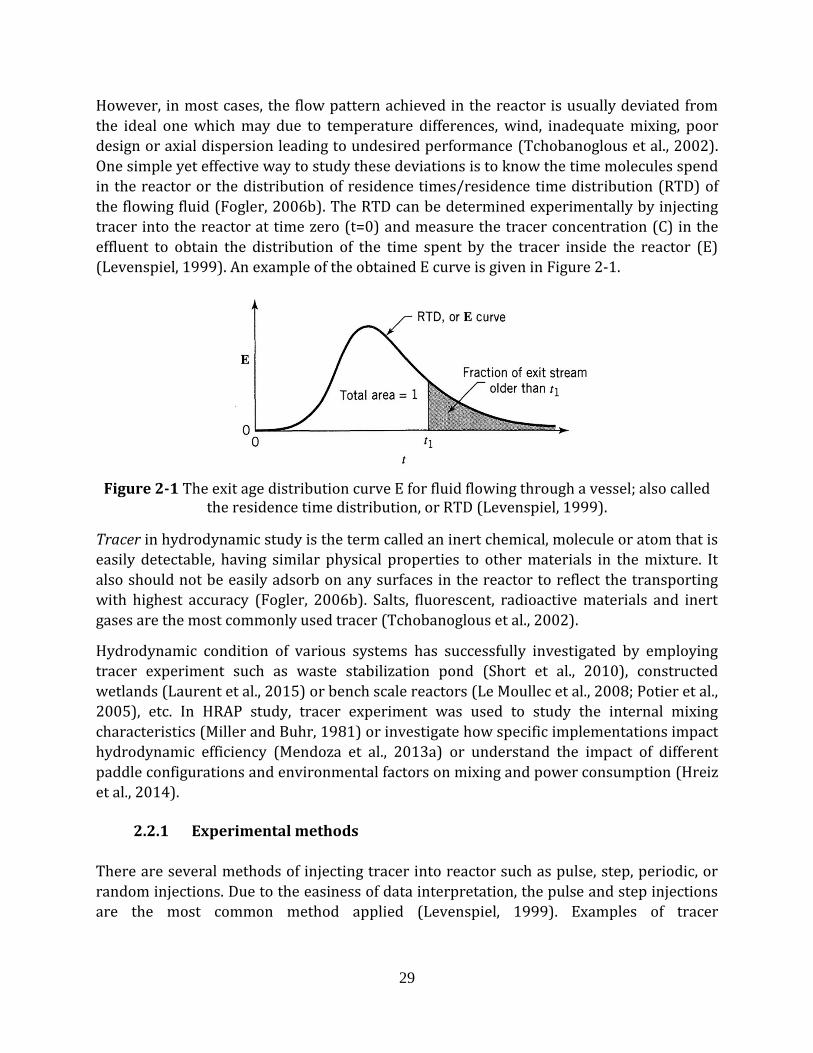
29

However, in most cases, the flow pattern achieved in the reactor is usually deviated from

the ideal one which may due to temperature differences, wind, inadequate mixing, poor

design or axial dispersion leading to undesired performance (Tchobanoglous et al., 2002).

One simple yet effective way to study these deviations is to know the time molecules spend

in the reactor or the distribution of residence times/residence time distribution (RTD) of

the flowing fluid (Fogler, 2006b). The RTD can be determined experimentally by injecting

tracer into the reactor at time zero (t=0) and measure the tracer concentration (C) in the

effluent to obtain the distribution of the time spent by the tracer inside the reactor (E)

(Levenspiel, 1999). An example of the obtained E curve is given in Figure 2-1.

Figure 2-1 The exit age distribution curve E for fluid flowing through a vessel; also called the residence time distribution, or RTD (Levenspiel, 1999).

Tracer in hydrodynamic study is the term called an inert chemical, molecule or atom that is

easily detectable, having similar physical properties to other materials in the mixture. It

also should not be easily adsorb on any surfaces in the reactor to reflect the transporting

with highest accuracy (Fogler, 2006b). Salts, fluorescent, radioactive materials and inert

gases are the most commonly used tracer (Tchobanoglous et al., 2002).

Hydrodynamic condition of various systems has successfully investigated by employing

tracer experiment such as waste stabilization pond (Short et al., 2010), constructed

wetlands (Laurent et al., 2015) or bench scale reactors (Le Moullec et al., 2008; Potier et al.,

2005), etc. In HRAP study, tracer experiment was used to study the internal mixing

characteristics (Miller and Buhr, 1981) or investigate how specific implementations impact

hydrodynamic efficiency (Mendoza et al., 2013a) or understand the impact of different

paddle configurations and environmental factors on mixing and power consumption (Hreiz

et al., 2014).

2.2.1 Experimental methods

There are several methods of injecting tracer into reactor such as pulse, step, periodic, or

random injections. Due to the easiness of data interpretation, the pulse and step injections

are the most common method applied (Levenspiel, 1999). Examples of tracer

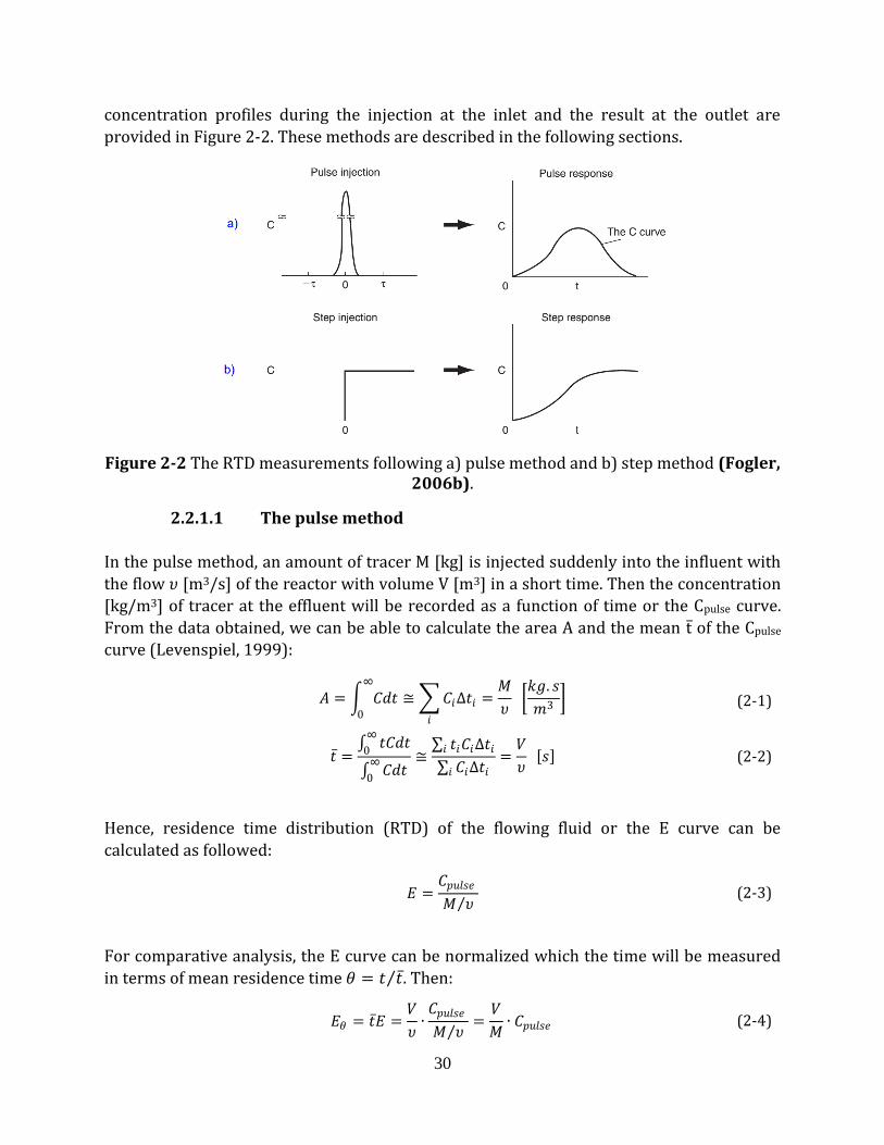
30

concentration profiles during the injection at the inlet and the result at the outlet are

provided in Figure 2-2. These methods are described in the following sections.

Figure 2-2 The RTD measurements following a) pulse method and b) step method (Fogler, 2006b).

2.2.1.1 The pulse method

In the pulse method, an amount of tracer M [kg] is injected suddenly into the influent with

the flow 𝜐 [m3/s] of the reactor with volume V [m3] in a short time. Then the concentration

[kg/m3] of tracer at the effluent will be recorded as a function of time or the Cpulse curve.

From the data obtained, we can be able to calculate the area A and the mean t of the Cpulse

curve (Levenspiel, 1999):

𝐴 = 𝐶𝑑𝑡

∞

0

≅ 𝐶𝑖∆𝑡𝑖 =𝑀

𝜐𝑖

𝑘𝑔. 𝑠

𝑚3 (2-1)

𝑡 =

𝑡𝐶𝑑𝑡∞

0

𝐶𝑑𝑡∞

0

≅ 𝑡𝑖𝐶𝑖∆𝑡𝑖𝑖

𝐶𝑖∆𝑡𝑖𝑖=

𝑉

𝜐 𝑠 (2-2)

Hence, residence time distribution (RTD) of the flowing fluid or the E curve can be

calculated as followed:

𝐸 =

𝐶𝑝𝑢𝑙𝑠𝑒

𝑀 𝜐 (2-3)

For comparative analysis, the E curve can be normalized which the time will be measured

in terms of mean residence time 𝜃 = 𝑡 𝑡 . Then:

𝐸𝜃 = 𝑡 𝐸 =

𝑉

𝜐∙𝐶𝑝𝑢𝑙𝑠𝑒

𝑀 𝜐 =

𝑉

𝑀∙ 𝐶𝑝𝑢𝑙𝑠𝑒 (2-4)

31

2.2.1.2 The step method

The step method involves injecting a constant concentration of tracer [kg/m3] into the

effluent flow 𝜐 [m3/s] of the reactor with volume V [m3] that is initiated at time t = 0. Stated

symbolically, we have (Fogler, 2006b):

𝐶0 𝑡 =

0, 𝑡 < 0𝐶0 , 𝑡 ≥ 0

(2-5)

Then the concentration Cstep of tracer in effluent of reactor will be recorded according the

time until the concentration in the effluent is indistinguishable from that in the influent.

The relationship between the tracer measured at the effluent and the influent can be

derived from material balance as followed (Levenspiel, 1999):

𝐶𝑚𝑎𝑥 =𝒎

𝜐 𝑘𝑔. 𝑠

𝑚3 (2-6)

𝑡 = 𝑡𝑑𝐶𝑠𝑡𝑒𝑝

𝐶𝑚𝑎𝑥

0

𝑑𝐶𝑠𝑡𝑒𝑝𝐶𝑚𝑎𝑥

0

=1

𝐶𝑚𝑎𝑥 𝑡𝑑𝐶𝑠𝑡𝑒𝑝

𝐶𝑚𝑎𝑥

0

𝑠 (2-7)

With 𝒎 [kg/s] is the flow rate of tracer in the influent.

The normalized RTD of the flowing fluid is the dimensionless form of the Cstep curve which

is called the F curve or the cumulative distribution curve. This curve is derived by:

𝐹 =𝜐

𝒎 𝐶𝑠𝑡𝑒𝑝 (2-8)

The relationship between the F curve and the E curve can be expressed as followed:

𝐹 = 𝐸𝑑𝑡𝑡

0

(2-9)

2.2.2 Hydraulic study – the RTD model

The use of mathematical models is important in determining the flow in reactor, extending

in capacity or diagnosing undesired behaviors (Fogler, 2006c). With the development of

computational power, complex model like computational fluid dynamics (CFD) became

possible to simulate detailed local interactions and hydraulic phenomena inside the

reactor. However, this model is still difficult to apply due to its complex and high

computational requirements (Le Moullec et al., 2010). Another popular method is the

32

traditional systemic model which was calibrated and/or validated by RTD data

(Danckwerts, 1953) in order to investigate the global function of the reactor. Although not

emphasizing in detailed phenomena, systemic model gives rapid results requiring simple

preparation and performance with useful knowledge which is suitable for process

optimization and control (Le Moullec et al., 2010).

With RTD data, the most important parameters can be calculated including t or the mean

time of passage and σ2 or the variance measuring the spread of the RTD curve. These

parameters are also called the first and the second moments, respectively and then used to

evaluate the parameters employed in the mathematical models (Miller and Buhr, 1981).

The calculations are presented by Levenspiel (1999):

𝑡 =

𝑡𝐶𝑑𝑡∞

0

𝐶𝑑𝑡∞

0

(2-10)

𝜍2 =

(𝑡 − 𝑡 )2 𝐶 𝑑𝑡∞

0

𝐶 𝑑𝑡∞

0

= 𝑡2𝐶 𝑑𝑡∞

0

𝐶 𝑑𝑡∞

0

− 𝑡 2 (2-11)

With these moments, two classical models are used to mathematically approximate mixing

behavior in the reactor, namely dispersion model and tank-in-series (TIS) model. These

models are roughly equivalent that can be applied to study the flow in most of the reactor

including pipes, packed beds, shaft kilns, long channels, screw conveyers, etc (Levenspiel,

1999). They will be described in the following sections.

2.2.2.1 The dispersion model

Dispersion model focuses on the axial dispersion of the material transported in a plug flow

which is governed by Fick’s law of diffusion. A dispersion coefficient D [m2/s] is used to

describe the process and a dimensionless group D uL is used to characterize the

spread/dispersion in the whole vessel (Fogler, 2006c). The group, called “vessel dispersion

number” as suggested by Levenspiel (1999), represents the ratio between movements

caused by longitudinal dispersion and by bulk flow. Therefore, if the vessel dispersion

number is significant larger than 1, dispersion is the dominant effect while in the case its

value is significant lower than 1, advection is the dominant factor in mass transport

(Tchobanoglous et al., 2002).

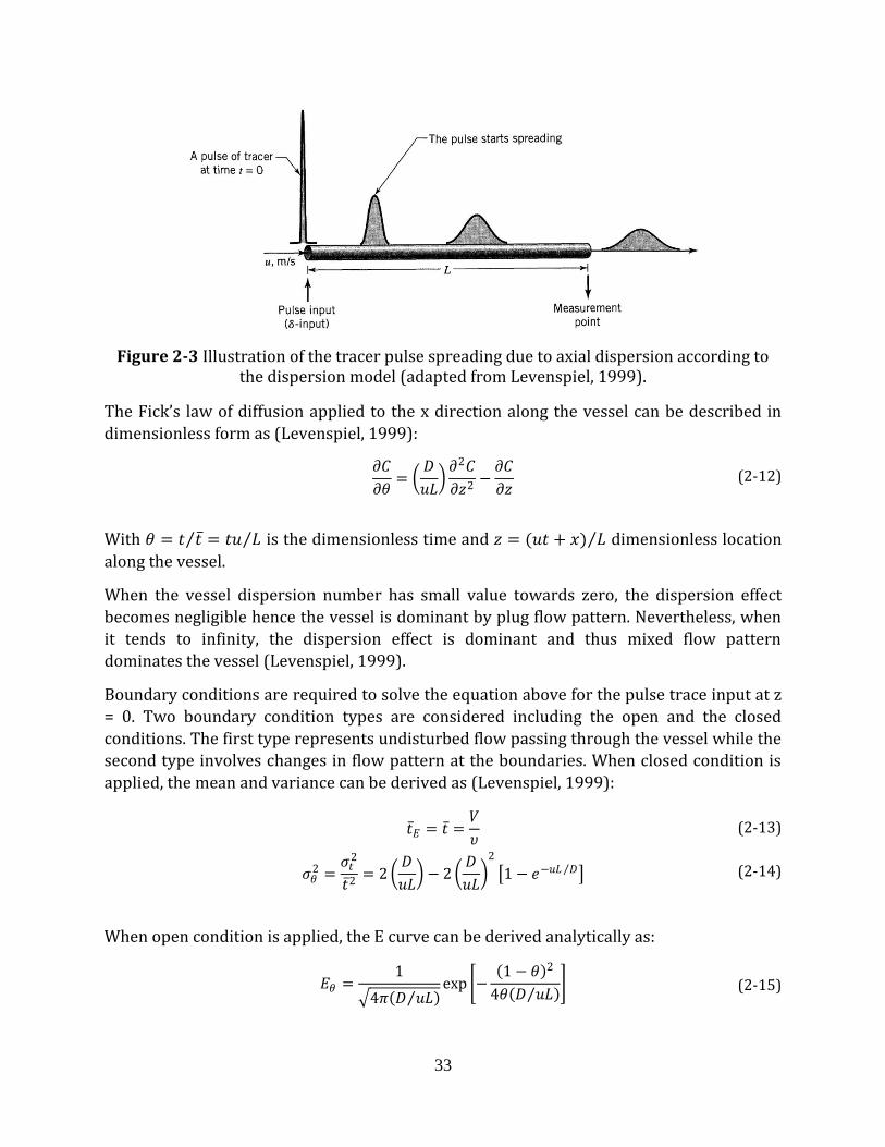
33

Figure 2-3 Illustration of the tracer pulse spreading due to axial dispersion according to the dispersion model (adapted from Levenspiel, 1999).

The Fick’s law of diffusion applied to the x direction along the vessel can be described in

dimensionless form as (Levenspiel, 1999):

𝜕𝐶

𝜕𝜃=

𝐷

𝑢𝐿 𝜕2𝐶

𝜕𝑧2−

𝜕𝐶

𝜕𝑧 (2-12)

With 𝜃 = 𝑡 𝑡 = 𝑡𝑢 𝐿 is the dimensionless time and 𝑧 = (𝑢𝑡 + 𝑥) 𝐿 dimensionless location

along the vessel.

When the vessel dispersion number has small value towards zero, the dispersion effect

becomes negligible hence the vessel is dominant by plug flow pattern. Nevertheless, when

it tends to infinity, the dispersion effect is dominant and thus mixed flow pattern

dominates the vessel (Levenspiel, 1999).

Boundary conditions are required to solve the equation above for the pulse trace input at z

= 0. Two boundary condition types are considered including the open and the closed

conditions. The first type represents undisturbed flow passing through the vessel while the

second type involves changes in flow pattern at the boundaries. When closed condition is

applied, the mean and variance can be derived as (Levenspiel, 1999):

𝑡 𝐸 = 𝑡 =

𝑉

𝜐 (2-13)

𝜍𝜃

2 =𝜍𝑡

2

𝑡 2= 2

𝐷

𝑢𝐿 − 2

𝐷

𝑢𝐿

2

1 − 𝑒−𝑢𝐿 𝐷 (2-14)

When open condition is applied, the E curve can be derived analytically as:

𝐸𝜃 =

1

4𝜋 𝐷 𝑢𝐿 exp −

1 − 𝜃 2

4𝜃 𝐷 𝑢𝐿 (2-15)

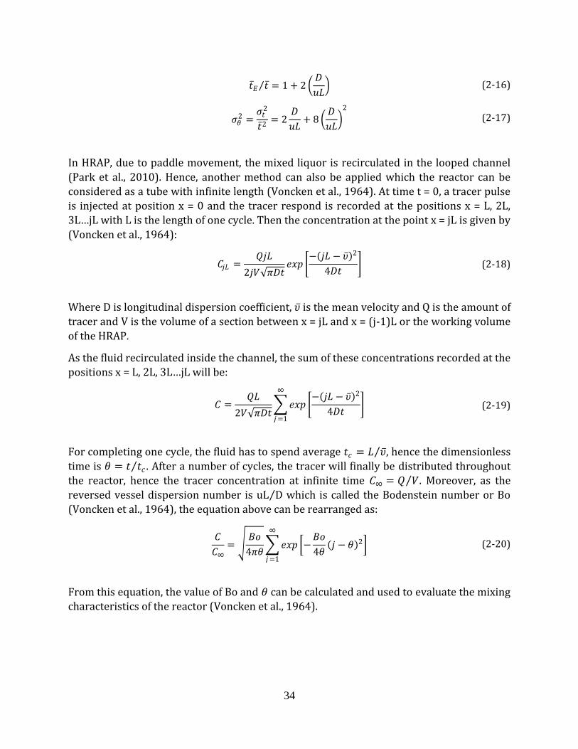
34

𝑡 𝐸 𝑡 = 1 + 2

𝐷

𝑢𝐿 (2-16)

𝜍𝜃

2 =𝜍𝑡

2

𝑡 2= 2

𝐷

𝑢𝐿+ 8

𝐷

𝑢𝐿

2

(2-17)

In HRAP, due to paddle movement, the mixed liquor is recirculated in the looped channel

(Park et al., 2010). Hence, another method can also be applied which the reactor can be

considered as a tube with infinite length (Voncken et al., 1964). At time t = 0, a tracer pulse

is injected at position x = 0 and the tracer respond is recorded at the positions x = L, 2L,

3L…jL with L is the length of one cycle. Then the concentration at the point x = jL is given by

(Voncken et al., 1964):

𝐶𝑗𝐿 =

𝑄𝑗𝐿

2𝑗𝑉 𝜋𝐷𝑡𝑒𝑥𝑝

− 𝑗𝐿 − 𝜐 2

4𝐷𝑡 (2-18)

Where D is longitudinal dispersion coefficient, 𝜐 is the mean velocity and Q is the amount of

tracer and V is the volume of a section between x = jL and x = (j-1)L or the working volume

of the HRAP.

As the fluid recirculated inside the channel, the sum of these concentrations recorded at the

positions x = L, 2L, 3L…jL will be:

𝐶 =

𝑄𝐿

2𝑉 𝜋𝐷𝑡 𝑒𝑥𝑝

− 𝑗𝐿 − 𝜐 2

4𝐷𝑡

∞

𝑗=1

(2-19)

For completing one cycle, the fluid has to spend average 𝑡𝑐 = 𝐿 𝜐 , hence the dimensionless

time is 𝜃 = 𝑡 𝑡𝑐 . After a number of cycles, the tracer will finally be distributed throughout

the reactor, hence the tracer concentration at infinite time 𝐶∞ = 𝑄 𝑉 . Moreover, as the

reversed vessel dispersion number is uL D which is called the Bodenstein number or Bo

(Voncken et al., 1964), the equation above can be rearranged as:

𝐶

𝐶∞=

𝐵𝑜

4𝜋𝜃 𝑒𝑥𝑝 −

𝐵𝑜

4𝜃 𝑗 − 𝜃 2

∞

𝑗=1

(2-20)

From this equation, the value of Bo and 𝜃 can be calculated and used to evaluate the mixing

characteristics of the reactor (Voncken et al., 1964).

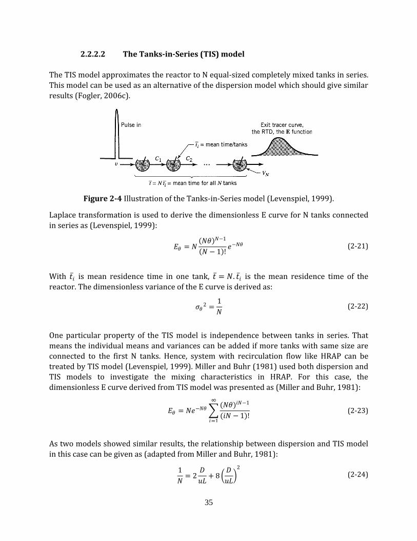
35

2.2.2.2 The Tanks-in-Series (TIS) model

The TIS model approximates the reactor to N equal-sized completely mixed tanks in series.

This model can be used as an alternative of the dispersion model which should give similar

results (Fogler, 2006c).

Figure 2-4 Illustration of the Tanks-in-Series model (Levenspiel, 1999).

Laplace transformation is used to derive the dimensionless E curve for N tanks connected

in series as (Levenspiel, 1999):

𝐸𝜃 = 𝑁

𝑁𝜃 𝑁−1

𝑁 − 1 !𝑒−𝑁𝜃 (2-21)

With 𝑡 𝑖 is mean residence time in one tank, 𝑡 = 𝑁. 𝑡 𝑖 is the mean residence time of the

reactor. The dimensionless variance of the E curve is derived as:

𝜍𝜃

2 =1

𝑁 (2-22)

One particular property of the TIS model is independence between tanks in series. That

means the individual means and variances can be added if more tanks with same size are

connected to the first N tanks. Hence, system with recirculation flow like HRAP can be

treated by TIS model (Levenspiel, 1999). Miller and Buhr (1981) used both dispersion and

TIS models to investigate the mixing characteristics in HRAP. For this case, the

dimensionless E curve derived from TIS model was presented as (Miller and Buhr, 1981):

𝐸𝜃 = 𝑁𝑒−𝑁𝜃

(𝑁𝜃)𝑖𝑁−1

(𝑖𝑁 − 1)!

∞

𝑖=1

(2-23)

As two models showed similar results, the relationship between dispersion and TIS model

in this case can be given as (adapted from Miller and Buhr, 1981):

1

𝑁= 2

𝐷

𝑢𝐿+ 8

𝐷

𝑢𝐿

2

(2-24)

36

Hence, useful information from both dispersion and TIS models can be employed to

integrate with algal and bacterial kinetics model in order to achieve a comprehensive

mathematical description of the system (Miller and Buhr, 1981).

2.3 Reaction kinetic model

The application of mathematic model to describe wastewater treatment process dated back

long time ago with an early example introduced by Phelps and Streete (1925) in simulating

the biochemical oxidation of organic matter in rivers and streams. According to the

authors, the oxidation rate of organic matter in terms of biological oxygen demand (BOD)

was described by the remaining organic matter concentration and a rate constant:

−𝑑𝐿 𝑑𝑡 = 𝑘𝐿 (2-25)

With L is the remaining oxygen demand of the organic substance in terms of oxygen, K is

the rate constant in day-1.

The equation (2-25) indicated that an equal proportion of the remaining BOD would be

removed in equal periods of time (Phelps and Streeter, 1925). Hence by determining the

rate constant which is impacted by temperature, one can predict the removal rate of

organic matter in polluted water. Similarly, reaction rate can be applied in predicting

reaction kinetics of different processes in wastewater treatment which is important

especially in design and performance assessment of a treatment facility (Henze, 2008). In

the following sections, different types of reaction as well as their mathematic description

and the determination of reaction rate function for a given data set are discussed.

2.3.1 Reaction types

Considering a general reaction:

𝛼𝐴 + 𝛽𝐵 + ⋯ → 𝑃𝑟𝑜𝑑𝑢𝑐𝑡 (2-26)

According to chemical reaction engineering, the rate of reaction is proportional to the

concentration of reactants A and B to the power of α and β, respectively. Hence, the rate

equation can be written as:

𝑅 = 𝑘𝐴𝛼𝐵𝛽 … (2-27)

With α and β are called the order of reaction with respect to reactant A and B, respectively

while the sum of α and β is the global reaction order of the reaction. In this sense, with α

and β being the stoichiometric coefficients of reactants, the sum of α and β is also known as

the molecularity of the reaction (Upadhyay, 2006).

However, in case of complex reaction such as the removal of pollutant from sewage water,

several processes may involve which the removal rate may depend on the most dominant

37

processes. Hence, the reaction order will be different with the theoretical molecularity of

the reaction which is called pseudo-order reactions (Upadhyay, 2006). A general form of n-

order rate equation can be expressed as:

𝑅 = −𝑑𝐶

𝑑𝑡= −𝑘𝐶𝑛 (2-28)

With C is the remaining concentration of pollutant while n is the pseudo-order of the

reaction. The minus sign indicates the direction of the reaction which C is removed

(Sperling, 2007).

If n = 0, (2-28) becomes:

𝑅 = −𝑑𝐶

𝑑𝑡= −𝑘 (2-29)

Hence, the rate of reaction in this case is independent on the pollutant concentration which

an integration form of the equation can be written as:

𝐶 = 𝐶0 − 𝑘𝑡 (2-30)

According to (2-30), for zero order reaction, constant removal rate of pollutant occurs in

the system which the decreasing of pollutant concentration C in the system follows linear

trend with the slop k (Sperling, 2007).

If n = 1, (2-29) will become:

𝑅 = −𝑑𝐶

𝑑𝑡= −𝑘𝐶 (2-31)

In this case, the rate of reaction is proportional to the concentration of pollutant. (2-31) can

also be expressed as:

𝐶 = 𝐶0𝑒−𝑘𝑡 (2-32)

Therefore, when the reaction follows first order, the decreasing of pollutant concentration

in the system follows exponential trend.

For an arbitrary n, another form of (2-28) can be used:

𝐶 = 𝐶𝑜1−𝑛 − 𝑘 ∙ 𝑡 ∙ (1 − 𝑛)

11−𝑛 (2-33)

With n ≠ 1.

It was indicated that with n > 1, (2-33) will never go to zero in finite time while for n < 1,

the concentration of pollutant will become negative at some finite time (Levenspiel, 1999):

𝐶 = 0 𝑎𝑡 𝑡 ≥𝐶0

1−𝑛

(1 − 𝑛)𝑘 (2-34)

Hence, in case of n < 1, the integration should not be conducted beyond the time indicated

in (2-34).

38

2.3.2 Reaction rate determination – coupled hydraulic and kinetic model

Common method in reaction rate determination is via curve fitting hence the values of rate

constant k and reaction order n are obtained by guessing in order to have the best fit with

experimental data (Levenspiel, 1999). Traditionally, the black box kinetic model employing

1st order of reaction was generally favored in simulating wastewater treatment facilities

such as waste stabilization pond (Marais and Shaw, 1961; Nameche and Vasel, 1998;

Thirumurthi, 1974), constructed wetland (Arheimer and Wittgren, 2002; Kadlec, 2000) or

high rate algal pond (HRAP) (El Hamouri et al., 2003). However, many studies indicated

kinetic model with order of reaction other than 1 showing good simulation of the practical

data (Adrian and Sanders, 1998, 1992; Paris et al., 1981). Another approach called mixed-

order model was proposed by Hewitt et al. (1979) and further developed by Borsuk and

Stow (2000) which the order of the kinetic reaction was remained as free parameter. This

model was found to provide better simulation than 1st order model of long term data of

biological oxygen demand (BOD) removal in streams and rivers or polychlorinated

biphenyl (PCB) declining in lake (Hewitt et al., 1979; Stow et al., 1999).

Moreover, it was also warned that the deviation from the ideal hydraulic condition in the

reactor is a common problem and always influence the performance of the system

(Levenspiel, 1999). Hence, a coupled kinetic and hydraulic model is a necessary step to

improve the simulation by considering imperfect flow patterns in the system (Fogler,

2006a). The most popular method to characterize global hydraulic behavior of a reactor is

by analyzing the residence time distribution (RTD) of the reactor obtained via tracer

experiment. The RTD curve E(t) provides information of time various fractions of fluid

(wastewater and suspended solids) spend in the reactor, and hence the contact time

distribution for the system (Levenspiel, 1999). The coupled kinetic and hydraulic model

then will be obtained by integrating RTD and kinetic models (Fogler, 2006a). The coupled

RTD and first order kinetic model was widely applied in simulating performance of

chemical reactors (Fogler, 2006a), stabilization ponds (Ellis and Rodrigues, 1993; Torres et

al., 1997) or treatment wetlands (Kadlec, 2000, 1994).

As indicated by various studies, inoculation between algae and activated sludge promotes

bioflocculation to form bigger flocs thus enhancing settleability (Gutzeit et al., 2005; Su et

al., 2011; Van Den Hende et al., 2011a). Study with large scale HRAP system treating

wastewater showed that the recovery efficiency of algal bacterial biomass could be up to

99% via simple gravity settling (Van Den Hende et al., 2014). These results suggest that the

mixed solution in the HRAP is mainly consisted of dilution constituents and suspended

algal bacterial flocs. Hence, in this case, the segregation model was found appropriate and

be employed to determine the mean conversion in the effluent following Fogler (2006):

𝐶𝑚 = 𝐶(𝑡) ∙ 𝐸(𝑡) ∙ 𝑑𝑡∞

0

(2-35)

With 𝐶𝑚 is the mean constituent concentration measured at the effluent in mg/L.

39

In additional, it was common knowledge that temperature variation is one of the main

factor impacting performance of the treatment system (Flegal and Schroeder, 1976; Ras et

al., 2013; Robarts and Zohary, 1987; Uhlmann, 1979). Hence the impact of temperature on

reaction rate was usually taken into account by employing Arrhenius or van’t Hoff-

Arrhenius theory (Sperling, 2007):

𝑘𝑇2

𝑘𝑇1

= 𝜃𝑇2−𝑇1 (2-36)

With 𝑘𝑇𝑖is the rate constant at temperature Ti and 𝜃 is the temperature coefficient which a

value of 1.047 was introduced by Phelps and Streeter (1925).

2.4 Gas-liquid mass transfer study

In HRAP, gas-liquid mass transfer has an important role which involves in stripping

unwanted gaseous constituents such as free ammonia (Garcia et al., 2000) or carbon

dioxide aeration for pH controlling and improving algal growth (Park and Craggs, 2010;

Posadas et al., 2015). There are several theories than explain the mechanism of gas transfer

across air-liquid interface including penetration model, surface-renewal model and two-

film theory. Among them, the two-film theory is the simplest yet providing comparable

results with other more complex models (Tchobanoglous et al., 2002). Hence this theory

remains the most popular method and is chosen to describe here.

2.4.1 The gas transfer rate and volumetric gas transfer coefficient

According to the two-film theory (Whitman, 1923), two stagnant and fixed in thickness

films exist next to the gas-liquid interface including the gas and liquid films. Between these

films, the gas molecules are transferred from the gas phase to the liquid phase (adsorption)

or vice versa (desorption) which their mass transfer rates are equal under steady state

condition. Following the Fick’s first law, the mass flux across these films can be expressed

as (Tchobanoglous et al., 2002):

𝑟 = 𝑘𝐺 𝑃𝐺 − 𝑃𝑖 = 𝑘𝐿(𝐶𝑖 − 𝐶𝐿) (2-37)

With r is the rate of mass transferred per unit area per unit time, kG and kL are the local

mass transfer coefficient, PG is the partial pressure in the bulk gas; and CL, the

concentration in the bulk liquid; index i refers to values at the gas–liquid interface. The driving forces causing transfer in the gas and liquid phases are 𝑃𝐺 − 𝑃𝑖 and (𝐶𝐿 − 𝐶𝑖),

respectively.

Since the value of kG and kL are difficult to obtain, the overall mass transfer coefficients are

more commonly used (Tchobanoglous et al., 2002). Moreover, according to Henry's law, at

equilibrium, the saturation concentration of dissolved gas in the bulk liquid can be related

40

to its partial pressure in the bulk gas phase by proportionality factor Henry's law constant

(p* = HC*). Hence, the mass flux can be written as:

𝑟 = 𝐾𝐺 𝑃𝐺 − 𝑃∗ = 𝐾𝐿(𝐶∗ − 𝐶𝐿) (2-38)

With KG and KL are the overall mass transfer coefficients, P* is the partial pressure in

equilibrium with liquid phase; C* is the saturation concentration in the bulk liquid in

equilibrium with gas phase.

In the case of slightly soluble gases including oxygen, nitrogen and carbon dioxide, the mass

transfer is controlled by the liquid phase while in the case of very soluble gases like

ammonia, the mass transfer is controlled by the gas phase. Then the relationships at which

the mass transfer is controlled by the liquid phase or the gas phase can be obtained,

respectively (Tchobanoglous et al., 2002):

1

𝐾𝐿=

1

𝑘𝐿+

1

𝐻𝑘𝐺 (2-39)

1

𝐾𝐺=

1

𝑘𝐺+

𝐻

𝑘𝐿 (2-40)

With H is the Henry's law constant.

Hence, the estimation of slightly soluble gas transfer rate per unit volume per unit time

from the gas to liquid phase can be derived as (Tchobanoglous et al., 2002):

𝑟𝜐 = 𝐾𝐿

𝐴

𝑉 𝐶∗ − 𝐶𝐿 = 𝑘𝐿𝑎(𝐶∗ − 𝐶𝐿) (2-41)

With 𝑟𝜐 is mass transfer rate per unit volume per unit time, A is area which the mass in

transferred through, V is volume which the mass is adsorbed, 𝑎 is interfacial area of mass

transfer per unit volume, and 𝐾𝐿𝑎 is the volumetric mass transfer coefficient.

The value of volumetric mass transfer coefficient (kLa) is dependent on water quality and

aeration mechanism. The determination of kLa in reactors is important for mass transfer

efficiency assessment and effects of operational conditions on the mass transfer rate

(Sperling, 2007). Most studies on gas transfer in wastewater treatment dedicate to oxygen

transfer due to its vital role in biological treatment and its low solubility. Impacts of

temperature, mixing intensity and tank geometry, wastewater characteristics on oxygen

transfer rate and its volumetric mass transfer coefficient were investigated

(Tchobanoglous et al., 2002).

In general, kLa value is also impacted by temperature which can be approximated by

Arrhenius equation as:

41

𝑘𝐿𝑎 𝑇 = 𝑘𝐿𝑎 20𝑜𝐶 𝜃 𝑇−20 (2-42)

With 𝑘𝐿𝑎 𝑇 is volumetric mass transfer coefficient at any temperature, 𝑘𝐿𝑎 20𝑜𝐶 is

volumetric mass transfer coefficient at 20oC, and 𝜃 is temperature coefficient ranging from

1.015 to 1.040 with typical value of 1.024 for mechanical and diffused aeration devices

(Tchobanoglous et al., 2002).

Moreover, the kLa value for wastewater can be calculated from the kLa for clean water

which the correction factor 𝛼 is given as:

𝛼 =

𝑘𝐿𝑎𝑤𝑎𝑠𝑡𝑒𝑤𝑎𝑡𝑒𝑟

𝑘𝐿𝑎𝑐𝑙𝑒𝑎𝑛 𝑤𝑎𝑡𝑒𝑟 (2-43)

With 𝛼 varies from 0.3 to 1.2 depending on aeration type, basin geometry, degree of mixing,

and wastewater characteristics (Tchobanoglous et al., 2002).

The effects of wastewater characteristics on oxygen solubility is also considered and

corrected as followed:

𝛽 =

𝐶𝑠,𝑤𝑎𝑠𝑡𝑒𝑤𝑎𝑡𝑒𝑟

𝐶𝑠,𝑐𝑙𝑒𝑎𝑛 𝑤𝑎𝑡𝑒𝑟 (2-44)

With 𝛽 ranging from 0.7 to 0.98 with typical value for wastewater of 0.95 is the correction

factor for the difference between oxygen solubility in clean water and wastewater due to

wastewater constituents such as salts, particulate matters or surfactants (Tchobanoglous et

al., 2002).

Finally, these correction factors can be applied to derive the actual oxygen transfer rate

from oxygen transfer rate at standard condition. The relationship can be described as

(Sperling, 2007):

𝑂𝑇𝑅𝐴 = 𝑂𝑇𝑅𝑆

𝑓𝐻 . 𝛽. 𝐶𝑆,𝑇 − 𝐶𝐿

𝐶𝑆,20 . 𝛼. 𝜃𝑇−20 (2-45)

With 𝑂𝑇𝑅𝐴 and 𝑂𝑇𝑅𝑆 are actual and standard oxygen transfer rates, respectively; 𝐶𝑆,20 and

𝐶𝑆,𝑇 are oxygen saturation concentrations at standard condition and at operating

temperature, respectively; 𝐶𝐿 is average concentration maintained in the reactor; and 𝑓𝐻 is

the altitude correction factor for 𝐶𝑆 which equals to 1 − 𝐻 9450 with altitude H (m).

For a given reactor, kLa can be determined with or without presence of biological process.

Chemical, physical or gas phase analysis methods have been used to experimentally obtain

kLa value in bioreactor for wastewater treatment (Garcia-Ochoa and Gomez, 2009). Among

them, dynamic method which involves recording the dynamic change of gas concentration

42

(oxygen in most cases) is interesting due to its wide application and ability to reflect the

influences of operational conditions on volumetric mass transfer coefficient.

2.4.2 Dynamic method

Dynamic method is based on recording oxygen variation in the reactor due to desorption or

absorption of oxygen. The most common method is to bring oxygen concentration in water

to near zero value (mainly by applying sodium sulfite in the presence of cobalt chloride as

catalyst) then due to the aeration system, the oxygen concentration in water is increased

until reaching its equilibrium level. Hence, the efficiency of aerating process can be

evaluated (Philichi, 1987).

Under well-mixed condition, the mass balance of oxygen in reactor is given as:

𝑑𝐶

𝑑𝑡= 𝑂𝑇𝑅 − 𝑂𝑈𝑅 + 𝑂𝑃𝑅 (2-46)

With OUR and OPR are oxygen uptake rate which is mainly related to bacterial activities

and oxygen production rate which is related to algal photosynthetic aeration. If OTR is

measured without biological activities, hence the terms OUR and OPR can be eliminated

and the mass balance equation becomes:

𝑑𝐶

𝑑𝑡= 𝐾𝐿𝑎. 𝐶𝑆 − 𝐶 (2-47)

Then the mass balance equation can be used to estimate the dynamic data in order to

obtain kLa value giving the best fit. According to European Standard (EN 12255-15, 2003),

exponential form of mass balance equation is used which the kLa value is estimated using

nonlinear least squares fit procedure. The exponential form is expressed as:

𝐶(𝑡) = 𝐶𝑆 − 𝐶𝑆 − 𝐶𝑜 𝑒𝑥𝑝 −𝐾𝐿𝑎. 𝑡 (2-48)

With 𝐶(𝑡) is oxygen concentration measured at time t and 𝐶𝑜 is the initial oxygen

concentration.

However, one factor should be accounted in the estimation is the respond time of oxygen

probe (Philichi, 1987). In practice, the oxygen probe requires a short time to respond to a

change in oxygen concentration variation, thus this delay time can impact the final result of

the experiment. As widely accepted in practice, the dynamic of oxygen probe can only be

neglected if its respond time is less than one-tenth of the oxygen transfer time measured

(1/ kLa) (Garcia-Ochoa and Gomez, 2009). The oxygen probe respond time can be

determined by creating an instantaneous change of the dissolved oxygen concentration

that is measured by the probe (lag test) (Philichi, 1987). The probe lag can be calculated

following first order relationship as:

43

𝑙𝑛

𝐶𝑓 − 𝐶

𝐶𝑓 − 𝐶𝑖 =

−𝑡

𝜏𝑟 (2-49)

With 𝐶𝑓 and 𝐶𝑖 are final and initial concentrations reading of the probe, respectively; C is

concentration value at time t; and 𝜏𝑟 is the probe respond time (Philichi, 1987).

Finally, the true value of kLa can be estimated with taking into account the respond time of

the probe as (Garcia-Ochoa and Gomez, 2009):

𝐶 𝑡 = 𝐶𝑆 +

𝐶𝑆 − 𝐶𝑜

1 − 𝜏𝑟 . 𝐾𝐿𝑎. 𝜏𝑟 . 𝐾𝐿𝑎. 𝑒𝑥𝑝

−𝑡

𝜏𝑟 − 𝑒𝑥𝑝 −𝐾𝐿𝑎. 𝑡 (2-50)

2.5 Conclusions

In this chapter, different hydraulic and gas transfer studying methods were reviewed. In

short, hydrodynamic and gas transfer studies of the HRAP system should be conducted in

order to understand the impacts of operational conditions on hydrodynamics in a pilot

scale HRAP as well as how such variation in hydrodynamics impacts gas transfer in HRAP.

Tracer experiment, either pulse or step method, can provide useful knowledge on the

global hydraulic behavior of the system by obtaining and analyzing the RTD curve. In

addition, in order to investigate the gas transfer rate of the system, dynamic method can be

used with taking the respond time of the probe in to account. The experimental results of

these tests may also serve as validating data for advanced fluid dynamic simulation.

Moreover, basic knowledge on reaction rate kinetic model and the coupled hydraulic

reaction rate kinetic model were also introduced. This model type can be used for the

designing purpose especially when HRAP is implemented in remote areas requiring quick

and simple assessment due to its simple requiring influent and effluent characteristics.

In French:

Dans ce chapitre, différentes méthodes d'études hydrauliques et de transfert de gaz ont été

passées en revue. En bref, des études hydrodynamiques et de transfert de gaz du système

HRAP devraient être menées afin de comprendre les impacts des conditions

opérationnelles sur l'hydrodynamique à l'échelle pilote HRAP ainsi que la façon dont une

telle variation de l'hydrodynamique affecte le transfert de gaz dans HRAP. L'expérience du

traceur, qu'il s'agisse d'une méthode par impulsions ou par étapes, peut fournir des

connaissances utiles sur le comportement hydraulique global du système en obtenant et en

analysant la courbe RTD. De plus, afin d'étudier le taux de transfert de gaz du système, la

méthode dynamique peut être utilisée en tenant compte du temps de réponse de la sonde.

Les résultats expérimentaux de ces essais peuvent également servir à valider les données

pour la simulation dynamique des fluides.

44

De plus, des connaissances de base sur le modèle cinétique de la vitesse de réaction et le

modèle cinétique de la vitesse de réaction hydraulique couplée ont également été

introduites. Ce type de modèle peut être utilisé pour la conception, en particulier lorsque le

HRAP est mis en œuvre dans des régions éloignées nécessitant une évaluation simple et

rapide en raison de ses caractéristiques d'influent et d'effluent.

45

CHAPTER 3 KINETIC MODELING OF THE ALGAL-BACTERIAL PROCESSES IN

WASTEWATER

3.1 Introduction

The system based on algal-bacterial processes has been widely recognized for its potential

not only in wastewater and flue gas treatment but also as a sustainable solution for

valuable biomass generation (Muñoz and Guieysse, 2006; Unnithan et al., 2014). However,

due to its complexity which involves many interactions between different species inside

the system (Cole, 1982; Kouzuma and Watanabe, 2015), it is difficult to control and thus yet

to be applied widely in industrial scale (Mata et al., 2010). In this context, using mathematic

models to simulate the algal-bacterial processes could serve as a rapid and cost-effective

method to study the system in order to improve, manage and enlarge it in bigger scale.

Kinetic modeling of bacterial growth has been studied extensively with the development of

activated sludge technology for wastewater treatment. An early example is the Activated

Sludge Model No. 1 (ASM1) (Henze et al., 1987) which provided a comprehensive approach

to simulate biochemical and physicochemical conversion processes in aeration reactor.

This model then became major reference for many scientific and practical projects (Gujer

et al., 1999). Following its success, new versions of ASM were released with further

adaptation including ASM2, ASM2d, and ASM3 (Henze et al., 2000). Modifications were also

included to deal with specific problem such as two-step nitrification and denitrification in

ASM3 (Iacopozzi et al., 2007). Besides, anaerobic digestion is another important operation

leading to the development of the Anaerobic Digestion Model No. 1 (ADM1) (Batstone et al.,

2002).

Algal growth kinetic modeling has also attracted significant attention (E. Lee et al., 2015).

Among all, light is the most important limiting factor influencing algal growth, hence many

models focus on this relationship (generally called photosynthetic-irradiance (P/I)

relationship). These models can be categorized into three groups depending on whether

light gradients and/or short light cycles are included (Béchet et al., 2013). In addition,

various models including influence of nutrient (C, N or P) as only limiting factor or in

combination with other factors on algal growth are also proposed (E. Lee et al., 2015).

One early kinetic models of algal-bacterial growth was developed by with relative simple

structure including algal and bacterial growth and decay together with basic

physiochemical processes in liquid phase . The kinetic model was then coupled with a

systemic hydrodynamic model simulating mixing characteristics in a high rate algal pond

(HRAP) (Miller and Buhr, 1981) and validated with field data which achieved good

agreement. This model was further developed with addition of CO2 from flue gas aeration,

however this work was yet to be validated (Yang, 2011). Moreover, inspired by the

development of bacterial kinetic model including ASM series and ADM, a model was

developed to simulate algal growth kinetic based on ASM framework (ASM-A) (Wágner et

46

al., 2016). Hence, the integration between ASM and ASM-A can be used to simulate algal

bacterial kinetics. Another compatible model with ASM series was developed by the

International Water Association (IWA) Task Group on River Water Quality Modelling called

River Water Quality Model no. 1 (RWQM1) (Reichert et al., 2001). This model covered a

wide range of processes and components used to simulate biochemical processes in river

system. Inspired by this model, an algal bacterial kinetic model was developed dedicated to

wastewater HRAP simulation (Solimeno et al., 2017).

In the following sections, the basic aspects including formulation of stochiometric

coefficients and type of kinetic models are reviewed. The processes of heterotrophic

bacteria, autotrophic (nitrifying) bacteria and algae will be discussed separately. Other

processes including hydrolysis, chemical equilibrium and gases transfer are also

considered.

3.2 Model frameworks and kinetics

Two major approaches when simulating growth kinetic in relation with nutrient factors are

introduced by Monod and Droop. While Monod made relation between bacterial growth

and the external concentration of nutrient, resulting in a hyperbolic equation with a half

saturation coefficient (3-1) (Monod, 1949), Droop suggested the growth of bacteria can be

controlled by internal concentration of nutrient in the cell and introduced nutrient cell

quota into the equation (3-2) (Droop, 1970). The two models were widely applied in

simulation of algal and/or bacterial growth kinetics (E. Lee et al., 2015). Although Droop-

based model can explain the absence of nutrient due to luxury uptake, competition

between different species or apply to simulate growth in unsteady-state (E. Lee et al.,

2015), it is difficult to measure the nutrient cell quota of the organism and the fact that cell

quota of microorganisms can vary depending on growth phase or between different

species/nutrient specific. In addition, Monod-based model showed easiness of

measurement of nutrient concentration and mathematical convenience (Gujer et al., 1999).

However, different growth conditions resulting to bacterial adaptation including nutrient

transport and thus impact of hydrodynamic condition, membrane permeability or gene

expression may influence half saturation coefficient in Monod’s model which leads to

uncertainties when applying into practical cases. Different conditions applied in each

experiment such as bacterial strains, inoculum history, biomass density or exposure length

also impact this coefficient (Ferenci, 1999). It was indicated that variation of half saturation

coefficient value obtained in different experiments could be explained by considering a

series of factors influencing transporting and metabolism processes. Hence a case-to-case

evaluation should be employed to determine this value (Arnaldos et al., 2015).

μ = μmax

S

KS + S

(3-1)

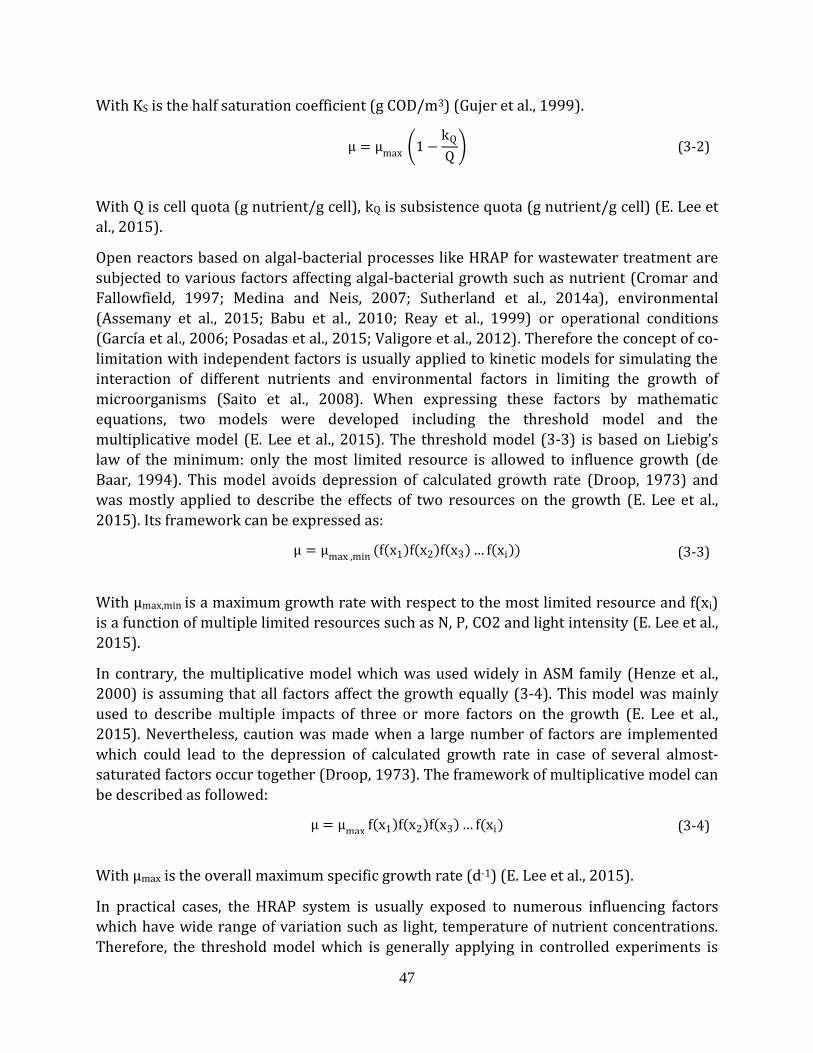
47

With KS is the half saturation coefficient (g COD/m3) (Gujer et al., 1999).

μ = μmax 1 −

kQ

Q (3-2)

With Q is cell quota (g nutrient/g cell), kQ is subsistence quota (g nutrient/g cell) (E. Lee et

al., 2015).

Open reactors based on algal-bacterial processes like HRAP for wastewater treatment are

subjected to various factors affecting algal-bacterial growth such as nutrient (Cromar and

Fallowfield, 1997; Medina and Neis, 2007; Sutherland et al., 2014a), environmental

(Assemany et al., 2015; Babu et al., 2010; Reay et al., 1999) or operational conditions

(García et al., 2006; Posadas et al., 2015; Valigore et al., 2012). Therefore the concept of co-

limitation with independent factors is usually applied to kinetic models for simulating the

interaction of different nutrients and environmental factors in limiting the growth of

microorganisms (Saito et al., 2008). When expressing these factors by mathematic

equations, two models were developed including the threshold model and the

multiplicative model (E. Lee et al., 2015). The threshold model (3-3) is based on Liebig’s

law of the minimum: only the most limited resource is allowed to influence growth (de

Baar, 1994). This model avoids depression of calculated growth rate (Droop, 1973) and

was mostly applied to describe the effects of two resources on the growth (E. Lee et al.,

2015). Its framework can be expressed as:

μ = μmax ,min (f x1 f x2 f x3 … f xi ) (3-3)

With μmax,min is a maximum growth rate with respect to the most limited resource and f(xi)

is a function of multiple limited resources such as N, P, CO2 and light intensity (E. Lee et al.,

2015).

In contrary, the multiplicative model which was used widely in ASM family (Henze et al.,

2000) is assuming that all factors affect the growth equally (3-4). This model was mainly

used to describe multiple impacts of three or more factors on the growth (E. Lee et al.,

2015). Nevertheless, caution was made when a large number of factors are implemented

which could lead to the depression of calculated growth rate in case of several almost-

saturated factors occur together (Droop, 1973). The framework of multiplicative model can

be described as followed:

μ = μmax f x1 f x2 f x3 … f(xi) (3-4)

With μmax is the overall maximum specific growth rate (d-1) (E. Lee et al., 2015).

In practical cases, the HRAP system is usually exposed to numerous influencing factors

which have wide range of variation such as light, temperature of nutrient concentrations.

Therefore, the threshold model which is generally applying in controlled experiments is

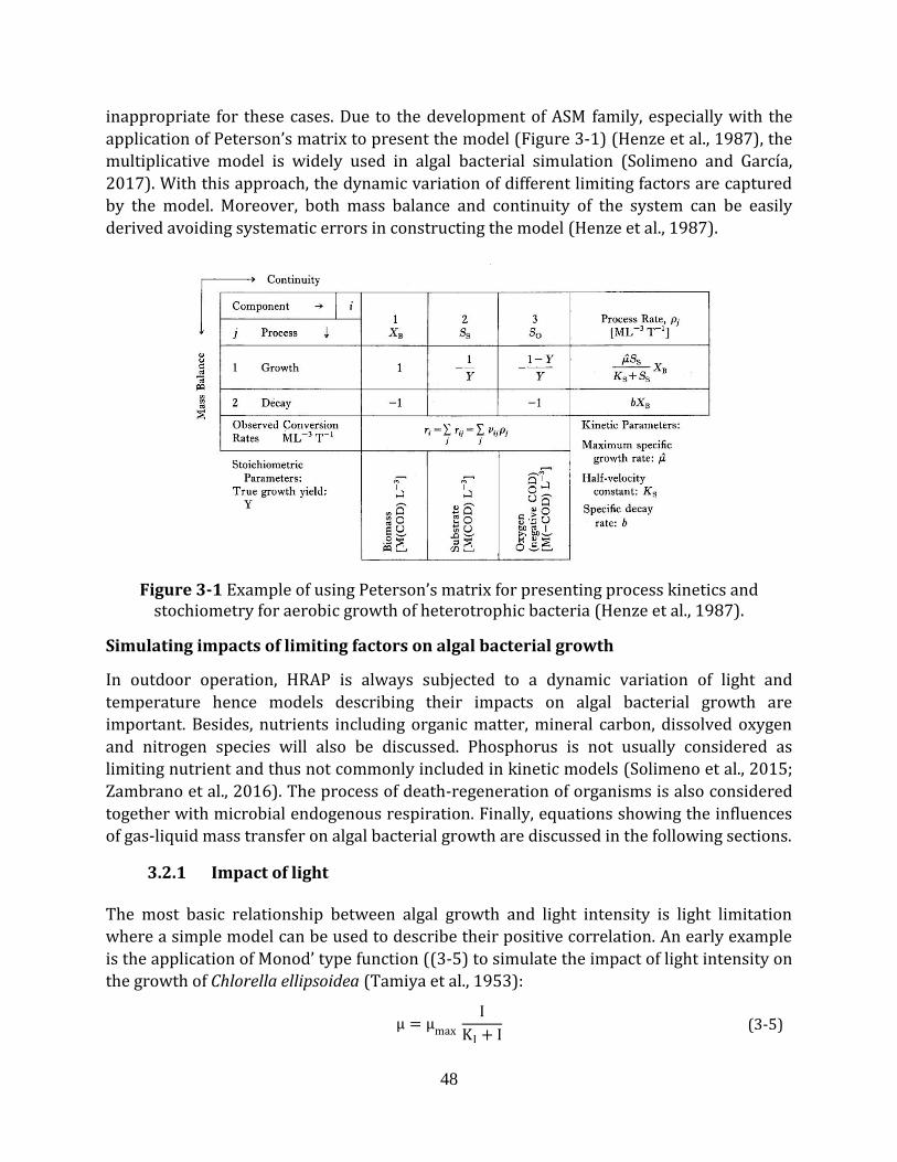
48

inappropriate for these cases. Due to the development of ASM family, especially with the

application of Peterson’s matrix to present the model (Figure 3-1) (Henze et al., 1987), the

multiplicative model is widely used in algal bacterial simulation (Solimeno and García,

2017). With this approach, the dynamic variation of different limiting factors are captured

by the model. Moreover, both mass balance and continuity of the system can be easily

derived avoiding systematic errors in constructing the model (Henze et al., 1987).

Figure 3-1 Example of using Peterson’s matrix for presenting process kinetics and stochiometry for aerobic growth of heterotrophic bacteria (Henze et al., 1987).

Simulating impacts of limiting factors on algal bacterial growth

In outdoor operation, HRAP is always subjected to a dynamic variation of light and

temperature hence models describing their impacts on algal bacterial growth are

important. Besides, nutrients including organic matter, mineral carbon, dissolved oxygen

and nitrogen species will also be discussed. Phosphorus is not usually considered as

limiting nutrient and thus not commonly included in kinetic models (Solimeno et al., 2015;

Zambrano et al., 2016). The process of death-regeneration of organisms is also considered

together with microbial endogenous respiration. Finally, equations showing the influences

of gas-liquid mass transfer on algal bacterial growth are discussed in the following sections.

3.2.1 Impact of light

The most basic relationship between algal growth and light intensity is light limitation

where a simple model can be used to describe their positive correlation. An early example

is the application of Monod’ type function ((3-5) to simulate the impact of light intensity on

the growth of Chlorella ellipsoidea (Tamiya et al., 1953):

μ = μmax

I

KI + I (3-5)

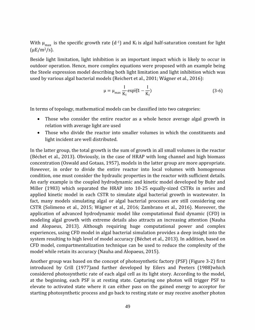
49

With μmax

is the specific growth rate (d-1) and KI is algal half-saturation constant for light

(μE/m2/s).

Beside light limitation, light inhibition is an important impact which is likely to occur in

outdoor operation. Hence, more complex equations were proposed with an example being

the Steele expression model describing both light limitation and light inhibition which was

used by various algal bacterial models (Reichert et al., 2001; Wágner et al., 2016):

μ = μmax

I

KIexp(1 −

I

KI) (3-6)

In terms of topology, mathematical models can be classified into two categories:

Those who consider the entire reactor as a whole hence average algal growth in

relation with average light are used

Those who divide the reactor into smaller volumes in which the constituents and

light incident are well distributed.

In the latter group, the total growth is the sum of growth in all small volumes in the reactor

(Béchet et al., 2013). Obviously, in the case of HRAP with long channel and high biomass

concentration (Oswald and Gotaas, 1957), models in the latter group are more appropriate.

However, in order to divide the entire reactor into local volumes with homogenous

condition, one must consider the hydraulic properties in the reactor with sufficient details.

An early example is the coupled hydrodynamic and kinetic model developed by Buhr and

Miller (1983) which separated the HRAP into 10-25 equally-sized CSTRs in series and

applied kinetic model in each CSTR to simulate algal bacterial growth in wastewater. In

fact, many models simulating algal or algal bacterial processes are still considering one

CSTR (Solimeno et al., 2015; Wágner et al., 2016; Zambrano et al., 2016). Moreover, the

application of advanced hydrodynamic model like computational fluid dynamic (CFD) in

modeling algal growth with extreme details also attracts an increasing attention (Nauha

and Alopaeus, 2013). Although requiring huge computational power and complex

experiences, using CFD model in algal bacterial simulation provides a deep insight into the

system resulting to high level of model accuracy (Béchet et al., 2013). In addition, based on

CFD model, compartmentalization technique can be used to reduce the complexity of the

model while retain its accuracy (Nauha and Alopaeus, 2015).

Another group was based on the concept of photosynthetic factory (PSF) (Figure 3-2) first

introduced by Crill (1977)and further developed by Eilers and Peeters (1988)which

considered photosynthetic rate of each algal cell as its light story. According to the model,

at the beginning, each PSF is at resting state. Capturing one photon will trigger PSF to

elevate to activated state where it can either pass on the gained energy to acceptor for

starting photosynthetic process and go back to resting state or may receive another photon

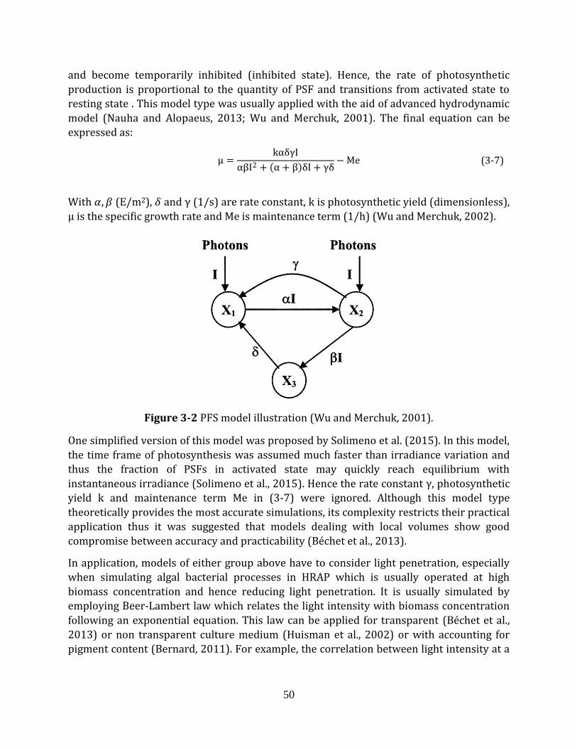
50

and become temporarily inhibited (inhibited state). Hence, the rate of photosynthetic

production is proportional to the quantity of PSF and transitions from activated state to

resting state . This model type was usually applied with the aid of advanced hydrodynamic

model (Nauha and Alopaeus, 2013; Wu and Merchuk, 2001). The final equation can be

expressed as:

μ =

kαδγI

αβI2 + α + β δI + γδ− Me (3-7)

With 𝛼, 𝛽 (E/m2), 𝛿 and γ (1/s) are rate constant, k is photosynthetic yield (dimensionless),

μ is the specific growth rate and Me is maintenance term (1/h) (Wu and Merchuk, 2002).

Figure 3-2 PFS model illustration (Wu and Merchuk, 2001).

One simplified version of this model was proposed by Solimeno et al. (2015). In this model,

the time frame of photosynthesis was assumed much faster than irradiance variation and

thus the fraction of PSFs in activated state may quickly reach equilibrium with

instantaneous irradiance (Solimeno et al., 2015). Hence the rate constant γ, photosynthetic

yield k and maintenance term Me in (3-7) were ignored. Although this model type

theoretically provides the most accurate simulations, its complexity restricts their practical

application thus it was suggested that models dealing with local volumes show good

compromise between accuracy and practicability (Béchet et al., 2013).

In application, models of either group above have to consider light penetration, especially

when simulating algal bacterial processes in HRAP which is usually operated at high

biomass concentration and hence reducing light penetration. It is usually simulated by

employing Beer-Lambert law which relates the light intensity with biomass concentration

following an exponential equation. This law can be applied for transparent (Béchet et al.,

2013) or non transparent culture medium (Huisman et al., 2002) or with accounting for

pigment content (Bernard, 2011). For example, the correlation between light intensity at a

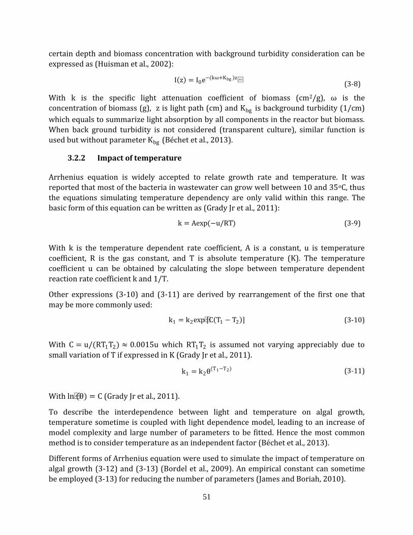
51

certain depth and biomass concentration with background turbidity consideration can be

expressed as (Huisman et al., 2002):

I z = I0e−(kω+Kbg )z

(3-8)

With k is the specific light attenuation coefficient of biomass (cm2/g), ω is the

concentration of biomass (g), z is light path (cm) and Kbg is background turbidity (1/cm)

which equals to summarize light absorption by all components in the reactor but biomass.

When back ground turbidity is not considered (transparent culture), similar function is

used but without parameter Kbg (Béchet et al., 2013).

3.2.2 Impact of temperature

Arrhenius equation is widely accepted to relate growth rate and temperature. It was

reported that most of the bacteria in wastewater can grow well between 10 and 35oC, thus

the equations simulating temperature dependency are only valid within this range. The

basic form of this equation can be written as (Grady Jr et al., 2011):

k = Aexp(−u/RT) (3-9)

With k is the temperature dependent rate coefficient, A is a constant, u is temperature

coefficient, R is the gas constant, and T is absolute temperature (K). The temperature

coefficient u can be obtained by calculating the slope between temperature dependent

reaction rate coefficient k and 1/T.

Other expressions (3-10) and (3-11) are derived by rearrangement of the first one that

may be more commonly used:

k1 = k2exp[C T1 − T2 ] (3-10)

With C = u/(RT1T2) ≈ 0.0015u which RT1T2 is assumed not varying appreciably due to

small variation of T if expressed in K (Grady Jr et al., 2011).

k1 = k2θ(T1−T2) (3-11)

With ln(θ) = C (Grady Jr et al., 2011).

To describe the interdependence between light and temperature on algal growth,

temperature sometime is coupled with light dependence model, leading to an increase of

model complexity and large number of parameters to be fitted. Hence the most common

method is to consider temperature as an independent factor (Béchet et al., 2013).

Different forms of Arrhenius equation were used to simulate the impact of temperature on

algal growth (3-12) and (3-13) (Bordel et al., 2009). An empirical constant can sometime

be employed (3-13) for reducing the number of parameters (James and Boriah, 2010).

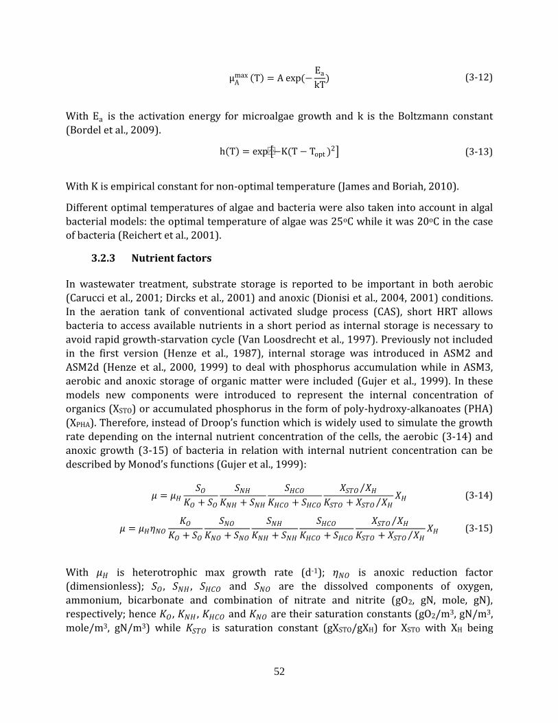
52

μA

max T = A exp(−Ea

kT) (3-12)

With Ea is the activation energy for microalgae growth and k is the Boltzmann constant

(Bordel et al., 2009).

h T = exp −K(T − Topt )2 (3-13)

With K is empirical constant for non-optimal temperature (James and Boriah, 2010).

Different optimal temperatures of algae and bacteria were also taken into account in algal

bacterial models: the optimal temperature of algae was 25oC while it was 20oC in the case

of bacteria (Reichert et al., 2001).

3.2.3 Nutrient factors

In wastewater treatment, substrate storage is reported to be important in both aerobic

(Carucci et al., 2001; Dircks et al., 2001) and anoxic (Dionisi et al., 2004, 2001) conditions.

In the aeration tank of conventional activated sludge process (CAS), short HRT allows

bacteria to access available nutrients in a short period as internal storage is necessary to

avoid rapid growth-starvation cycle (Van Loosdrecht et al., 1997). Previously not included

in the first version (Henze et al., 1987), internal storage was introduced in ASM2 and

ASM2d (Henze et al., 2000, 1999) to deal with phosphorus accumulation while in ASM3,

aerobic and anoxic storage of organic matter were included (Gujer et al., 1999). In these

models new components were introduced to represent the internal concentration of

organics (XSTO) or accumulated phosphorus in the form of poly-hydroxy-alkanoates (PHA)

(XPHA). Therefore, instead of Droop’s function which is widely used to simulate the growth

rate depending on the internal nutrient concentration of the cells, the aerobic (3-14) and

anoxic growth (3-15) of bacteria in relation with internal nutrient concentration can be

described by Monod’s functions (Gujer et al., 1999):

𝜇 = 𝜇𝐻

𝑆𝑂

𝐾𝑂 + 𝑆𝑂

𝑆𝑁𝐻

𝐾𝑁𝐻 + 𝑆𝑁𝐻

𝑆𝐻𝐶𝑂

𝐾𝐻𝐶𝑂 + 𝑆𝐻𝐶𝑂

𝑋𝑆𝑇𝑂 𝑋𝐻

𝐾𝑆𝑇𝑂 + 𝑋𝑆𝑇𝑂 𝑋𝐻 𝑋𝐻 (3-14)

𝜇 = 𝜇𝐻𝜂𝑁𝑂

𝐾𝑂

𝐾𝑂 + 𝑆𝑂

𝑆𝑁𝑂

𝐾𝑁𝑂 + 𝑆𝑁𝑂

𝑆𝑁𝐻

𝐾𝑁𝐻 + 𝑆𝑁𝐻

𝑆𝐻𝐶𝑂

𝐾𝐻𝐶𝑂 + 𝑆𝐻𝐶𝑂

𝑋𝑆𝑇𝑂 𝑋𝐻

𝐾𝑆𝑇𝑂 + 𝑋𝑆𝑇𝑂 𝑋𝐻 𝑋𝐻 (3-15)

With 𝜇𝐻 is heterotrophic max growth rate (d-1); 𝜂𝑁𝑂 is anoxic reduction factor

(dimensionless); 𝑆𝑂 , 𝑆𝑁𝐻 , 𝑆𝐻𝐶𝑂 and 𝑆𝑁𝑂 are the dissolved components of oxygen,

ammonium, bicarbonate and combination of nitrate and nitrite (gO2, gN, mole, gN),

respectively; hence 𝐾𝑂 , 𝐾𝑁𝐻 , 𝐾𝐻𝐶𝑂 and 𝐾𝑁𝑂 are their saturation constants (gO2/m3, gN/m3,

mole/m3, gN/m3) while 𝐾𝑆𝑇𝑂 is saturation constant (gXSTO/gXH) for XSTO with XH being

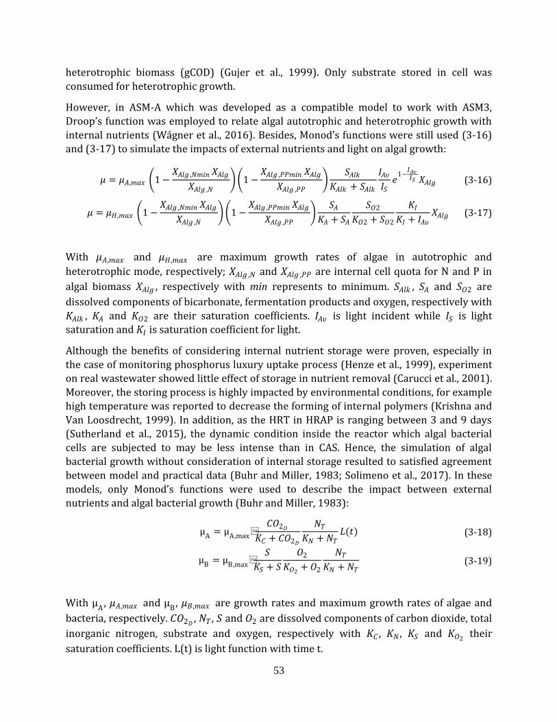
53

heterotrophic biomass (gCOD) (Gujer et al., 1999). Only substrate stored in cell was

consumed for heterotrophic growth.

However, in ASM-A which was developed as a compatible model to work with ASM3,

Droop’s function was employed to relate algal autotrophic and heterotrophic growth with

internal nutrients (Wágner et al., 2016). Besides, Monod’s functions were still used (3-16)

and (3-17) to simulate the impacts of external nutrients and light on algal growth:

𝜇 = 𝜇𝐴,𝑚𝑎𝑥 1 −

𝑋𝐴𝑙𝑔 ,𝑁𝑚𝑖𝑛 𝑋𝐴𝑙𝑔

𝑋𝐴𝑙𝑔 ,𝑁 1 −

𝑋𝐴𝑙𝑔 ,𝑃𝑃𝑚𝑖𝑛 𝑋𝐴𝑙𝑔

𝑋𝐴𝑙𝑔 ,𝑃𝑃

𝑆𝐴𝑙𝑘

𝐾𝐴𝑙𝑘 + 𝑆𝐴𝑙𝑘

𝐼𝐴𝜐

𝐼𝑆𝑒

1−𝐼𝐴𝜐𝐼𝑆 𝑋𝐴𝑙𝑔 (3-16)

𝜇 = 𝜇𝐻,𝑚𝑎𝑥 1 −

𝑋𝐴𝑙𝑔 ,𝑁𝑚𝑖𝑛 𝑋𝐴𝑙𝑔

𝑋𝐴𝑙𝑔 ,𝑁 1 −

𝑋𝐴𝑙𝑔 ,𝑃𝑃𝑚𝑖𝑛 𝑋𝐴𝑙𝑔

𝑋𝐴𝑙𝑔 ,𝑃𝑃

𝑆𝐴𝐾𝐴 + 𝑆𝐴

𝑆𝑂2

𝐾𝑂2 + 𝑆𝑂2

𝐾𝐼

𝐾𝐼 + 𝐼𝐴𝜐𝑋𝐴𝑙𝑔 (3-17)

With 𝜇𝐴,𝑚𝑎𝑥 and 𝜇𝐻,𝑚𝑎𝑥 are maximum growth rates of algae in autotrophic and

heterotrophic mode, respectively; 𝑋𝐴𝑙𝑔 ,𝑁 and 𝑋𝐴𝑙𝑔 ,𝑃𝑃 are internal cell quota for N and P in

algal biomass 𝑋𝐴𝑙𝑔 , respectively with min represents to minimum. 𝑆𝐴𝑙𝑘 , 𝑆𝐴 and 𝑆𝑂2 are

dissolved components of bicarbonate, fermentation products and oxygen, respectively with

𝐾𝐴𝑙𝑘 , 𝐾𝐴 and 𝐾𝑂2 are their saturation coefficients. 𝐼𝐴𝜐 is light incident while 𝐼𝑆 is light

saturation and 𝐾𝐼 is saturation coefficient for light.

Although the benefits of considering internal nutrient storage were proven, especially in

the case of monitoring phosphorus luxury uptake process (Henze et al., 1999), experiment

on real wastewater showed little effect of storage in nutrient removal (Carucci et al., 2001).

Moreover, the storing process is highly impacted by environmental conditions, for example

high temperature was reported to decrease the forming of internal polymers (Krishna and

Van Loosdrecht, 1999). In addition, as the HRT in HRAP is ranging between 3 and 9 days

(Sutherland et al., 2015), the dynamic condition inside the reactor which algal bacterial

cells are subjected to may be less intense than in CAS. Hence, the simulation of algal

bacterial growth without consideration of internal storage resulted to satisfied agreement

between model and practical data (Buhr and Miller, 1983; Solimeno et al., 2017). In these

models, only Monod’s functions were used to describe the impact between external

nutrients and algal bacterial growth (Buhr and Miller, 1983):

μA = μA,max

𝐶𝑂2𝐷

𝐾𝐶 + 𝐶𝑂2𝐷

𝑁𝑇

𝐾𝑁 + 𝑁𝑇𝐿(𝑡) (3-18)

μB = μB,max

𝑆

𝐾𝑆 + 𝑆

𝑂2

𝐾𝑂2+ 𝑂2

𝑁𝑇

𝐾𝑁 + 𝑁𝑇 (3-19)

With μA

, 𝜇𝐴,𝑚𝑎𝑥 and μB

, 𝜇𝐵,𝑚𝑎𝑥 are growth rates and maximum growth rates of algae and

bacteria, respectively. 𝐶𝑂2𝐷, 𝑁𝑇 , 𝑆 and 𝑂2 are dissolved components of carbon dioxide, total

inorganic nitrogen, substrate and oxygen, respectively with 𝐾𝐶 , 𝐾𝑁 , 𝐾𝑆 and 𝐾𝑂2 their

saturation coefficients. L(t) is light function with time t.

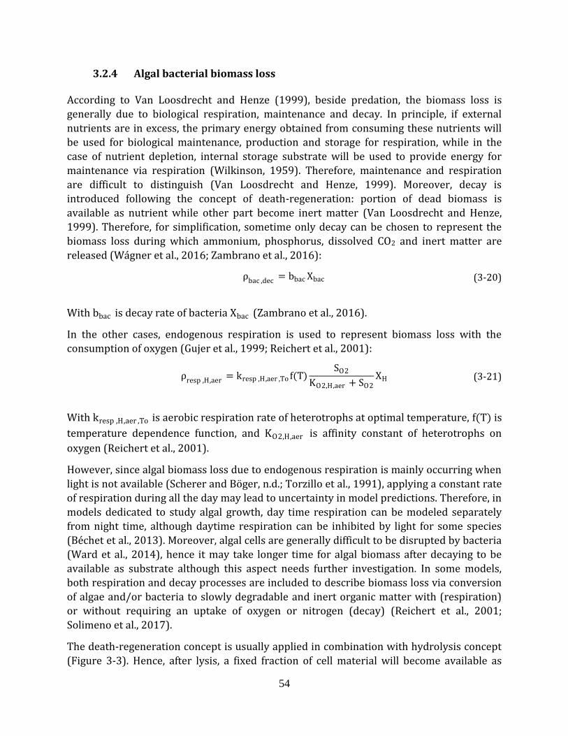
54

3.2.4 Algal bacterial biomass loss

According to Van Loosdrecht and Henze (1999), beside predation, the biomass loss is

generally due to biological respiration, maintenance and decay. In principle, if external

nutrients are in excess, the primary energy obtained from consuming these nutrients will

be used for biological maintenance, production and storage for respiration, while in the

case of nutrient depletion, internal storage substrate will be used to provide energy for

maintenance via respiration (Wilkinson, 1959). Therefore, maintenance and respiration

are difficult to distinguish (Van Loosdrecht and Henze, 1999). Moreover, decay is

introduced following the concept of death-regeneration: portion of dead biomass is

available as nutrient while other part become inert matter (Van Loosdrecht and Henze,

1999). Therefore, for simplification, sometime only decay can be chosen to represent the

biomass loss during which ammonium, phosphorus, dissolved CO2 and inert matter are

released (Wágner et al., 2016; Zambrano et al., 2016):

ρbac ,dec = bbac Xbac (3-20)

With bbac is decay rate of bacteria Xbac (Zambrano et al., 2016).

In the other cases, endogenous respiration is used to represent biomass loss with the

consumption of oxygen (Gujer et al., 1999; Reichert et al., 2001):

ρresp ,H,aer = kresp ,H,aer ,To f(T)

SO2

KO2,H,aer + SO2XH (3-21)

With kresp ,H,aer ,To is aerobic respiration rate of heterotrophs at optimal temperature, f(T) is

temperature dependence function, and KO2,H,aer is affinity constant of heterotrophs on

oxygen (Reichert et al., 2001).

However, since algal biomass loss due to endogenous respiration is mainly occurring when

light is not available (Scherer and Böger, n.d.; Torzillo et al., 1991), applying a constant rate

of respiration during all the day may lead to uncertainty in model predictions. Therefore, in

models dedicated to study algal growth, day time respiration can be modeled separately

from night time, although daytime respiration can be inhibited by light for some species

(Béchet et al., 2013). Moreover, algal cells are generally difficult to be disrupted by bacteria

(Ward et al., 2014), hence it may take longer time for algal biomass after decaying to be

available as substrate although this aspect needs further investigation. In some models,

both respiration and decay processes are included to describe biomass loss via conversion

of algae and/or bacteria to slowly degradable and inert organic matter with (respiration)

or without requiring an uptake of oxygen or nitrogen (decay) (Reichert et al., 2001;

Solimeno et al., 2017).

The death-regeneration concept is usually applied in combination with hydrolysis concept

(Figure 3-3). Hence, after lysis, a fixed fraction of cell material will become available as

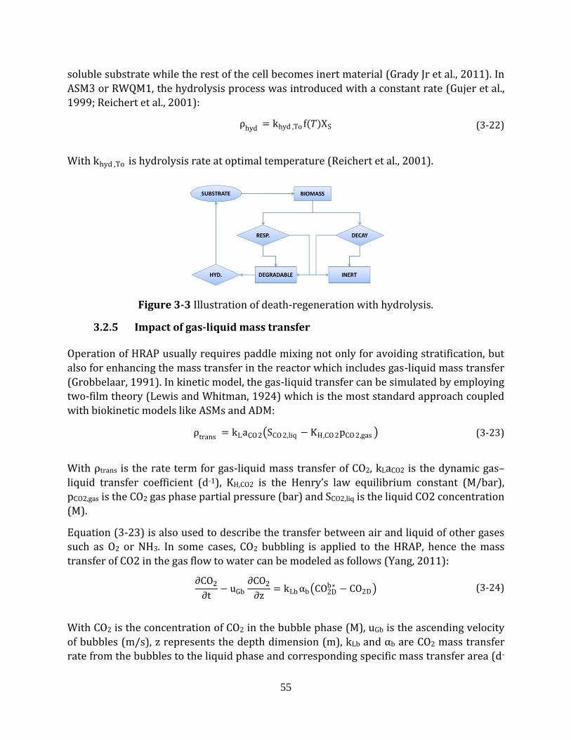
55

soluble substrate while the rest of the cell becomes inert material (Grady Jr et al., 2011). In

ASM3 or RWQM1, the hydrolysis process was introduced with a constant rate (Gujer et al.,

1999; Reichert et al., 2001):

ρhyd = khyd ,To f(𝑇)XS (3-22)

With khyd ,To is hydrolysis rate at optimal temperature (Reichert et al., 2001).

Figure 3-3 Illustration of death-regeneration with hydrolysis.

3.2.5 Impact of gas-liquid mass transfer

Operation of HRAP usually requires paddle mixing not only for avoiding stratification, but

also for enhancing the mass transfer in the reactor which includes gas-liquid mass transfer

(Grobbelaar, 1991). In kinetic model, the gas-liquid transfer can be simulated by employing

two-film theory (Lewis and Whitman, 1924) which is the most standard approach coupled

with biokinetic models like ASMs and ADM:

ρtrans = kLaCO 2 SCO 2,liq − KH,CO 2pCO 2,gas (3-23)

With ρtrans is the rate term for gas-liquid mass transfer of CO2, kLaCO2 is the dynamic gas–

liquid transfer coefficient (d-1), KH,CO2 is the Henry’s law equilibrium constant (M/bar),

pCO2,gas is the CO2 gas phase partial pressure (bar) and SCO2,liq is the liquid CO2 concentration

(M).

Equation (3-23) is also used to describe the transfer between air and liquid of other gases

such as O2 or NH3. In some cases, CO2 bubbling is applied to the HRAP, hence the mass

transfer of CO2 in the gas flow to water can be modeled as follows (Yang, 2011):

∂CO2

∂t− uGb

∂CO2

∂z= kLb αb CO2D

b∗ − CO2D (3-24)

With CO2 is the concentration of CO2 in the bubble phase (M), uGb is the ascending velocity

of bubbles (m/s), z represents the depth dimension (m), kLb and αb are CO2 mass transfer

rate from the bubbles to the liquid phase and corresponding specific mass transfer area (d-

56

1) (i.e., bubble surface area per unit gas volume), CO2Db∗ is the saturation concentration of the

dissolved CO2 in the liquid phase CO2D in equilibrium with the CO2 in the bubbles (M).

In general, two-film theory can be applied to simulate the gas-liquid mass transfer of other

gases including oxygen and ammonia. Although the volumetric mass transfer coefficient

can be experimentally estimated (El Ouarghi et al., 2000) to validate the model, only the

coefficient of oxygen can be directly obtained while the volumetric mass transfer

coefficients of other gas including ammonia and carbon dioxide can be derived using the

diffusivity ratio. For example, the volumetric mass transfer coefficient of CO2 can be

calculated as (Spérandio and Paul, 1997):

kLaCO 2

kLaO2=

DCO 2

DO2 (3-25)

With DCO 2 and DO2 are the diffusion coefficients of CO2 and O2 in water (m2/s),

respectively.

Moreover, the solubility of different gases is also taken into account which follows Henry’s

law (Carroll et al., 1991):

Mg∗ = KHg Pg (3-26)

With KH and P are Henry’s constant (M/bar) and partial pressure (bar) of the gas (g) in the

atmosphere while Mg∗ represents for the saturation concentration (M) of the dissolved gas.

It was noted that the saturation concentration of NH3 is usually considered as zero due to

its ignorable partial pressure in the atmosphere (Yang, 2011). This was supported by the

fact that nitrogen removal by ammonia stripping is important in HRAP (Garcia et al., 2000),

hence the ammonia flow from the reactor to the air outcompetes the ammonia adsorption.

3.3 Conclusions

Considering system optimization, the use of mathematical simulation offers a promising

methodology to reduce experimental costs. There is a wide variety of kinetic models

simulating algae and/or bacteria. Despite of the intensive contributions, more efforts are

still required to improve the simulation in terms of hydrodynamics, light attenuation or gas

transfer of the algal bacterial system. It was important to note that these aspects are

specific for each system requiring careful consideration when employing in the model.

Moreover, a guideline for selecting factors and framework in model construction

simulating algal growth is also lacking which usually leads to difficulty in assessment of

simulation quality and comparability. Hence, it is necessary for a modeling project to

respect standardized simulation protocol.

57

Although widely accepted in practice, a comprehensive model dedicating to HRAP system is

still rare. Moreover, a clear simulation protocol for algal bacterial processes in HRAP

system is still lacking. Therefore, in most of the model simulating HRAP system, minor

effort was spent in studying hydrodynamics, light attenuation or gas transfer for employing

in the model.

In French:

En ce qui concerne l'optimisation des systèmes, l'utilisation de la simulation mathématique

offre une méthodologie prometteuse pour réduire les coûts expérimentaux. Il existe une

grande variété de modèles cinétiques simulant les algues et/ou les bactéries. Malgré les

contributions intensives, des efforts supplémentaires sont encore nécessaires pour

améliorer la simulation en termes d'hydrodynamique, d'atténuation de la lumière ou de

transfert de gaz du système bactérien des algues. Il était important de noter que ces aspects

sont spécifiques à chaque système, ce qui exige un examen attentif lors de l'utilisation du

modèle. De plus, il n'existe pas non plus de lignes directrices pour la sélection des facteurs

et du cadre de construction de modèles simulant la croissance des algues, ce qui rend

généralement difficile l'évaluation de la qualité et de la comparabilité des simulations. Il est

donc nécessaire qu'un projet de modélisation respecte un protocole de simulation

standardisé.

Bien qu'il soit largement accepté dans la pratique, un modèle complet consacré au système

HRAP est encore rare. De plus, il manque encore un protocole de simulation clair pour les

processus bactériens des algues dans le système HRAP. Par conséquent, dans la plupart des

modèles simulant le système HRAP, un effort mineur a été consacré à l'étude de

l'hydrodynamique, de l'atténuation de la lumière ou du transfert de gaz pour l'utilisation

dans le modèle.

58

PART II MATERIALS AND METHODS

In this part, the materials and methods of experimental and modeling works are

introduced. The part consists of three chapters relating to biochemical, hydraulic and gas

transfer, and black box modeling studies. In order to keep the clear structure of the thesis,

all the model construction and description of the comprehensive algal bacterial model were

only included in chapter 11.

CHAPTER 4 EXPERIMENTAL METHODS FOR STUDYING ALGAL BACTERIAL

PROCESSES IN WASTEWATER

In the following sections, the condition and setup of experiments determining algal

bacterial inoculation ratio and the application of optimized algal bacterial biomass in pilot

HRAP are presented. Parameters including physiochemical values such as pH, dissolved

oxygen, light and temperature; nutrients such as nitrogen, organic matter and phosphorus;

and biomass such as chlorophyll a and biomass dry weight were frequently measured.

These data will be used to determine the impacts of different factors on algal bacterial

system performance.

In French:

Dans la première partie de ce chapitre, les matériels et méthodes utilisés pour étudier

l'impact des différents rapports d'inoculation des algues et des boues activées sur la

croissance des algues, l'élimination des nutriments et l'efficacité de décantation ont été

décrits. La biomasse algale-bactérienne (Al-Bac) a été cultivée dans des réacteurs SBR

alimentés avec des eaux usées synthétiques. Trois rapports algues/boues activées (5:1, 1:1

et 1:5) avec la biomasse algale comme contrôle ont été comparés. Le montage expérimental

et le fonctionnement ont également été illustrés. Différents paramètres ont été mesurés au

cours de l'expérience et les données obtenues ont été analysées à l'aide de méthodes

statistiques.

La deuxième partie concerne une expérience pilote à long terme utilisant une lagune à haut

rendement algal (HRAP) alimentée en eau usée réelle. Le rapport optimal (1:1)

d’inoculation a été utilisé. Le système HRAP est décrit. Diverses conditions opérationnelles,

y compris le temps de séjour hydraulique (HRT) et la charge en éléments nutritifs, ont été

appliquées. Des mesures à long terme de différents paramètres ont été effectuées et

diverses techniques d'analyse ont été utilisées pour analyser les données.

4.1 Algae and activated sludge inoculations preparation

Traditionally, in algae-based wastewater treatment systems, the term algae usually refers

to a consortium of local algal species in the wastewater which is allowed to develop in the

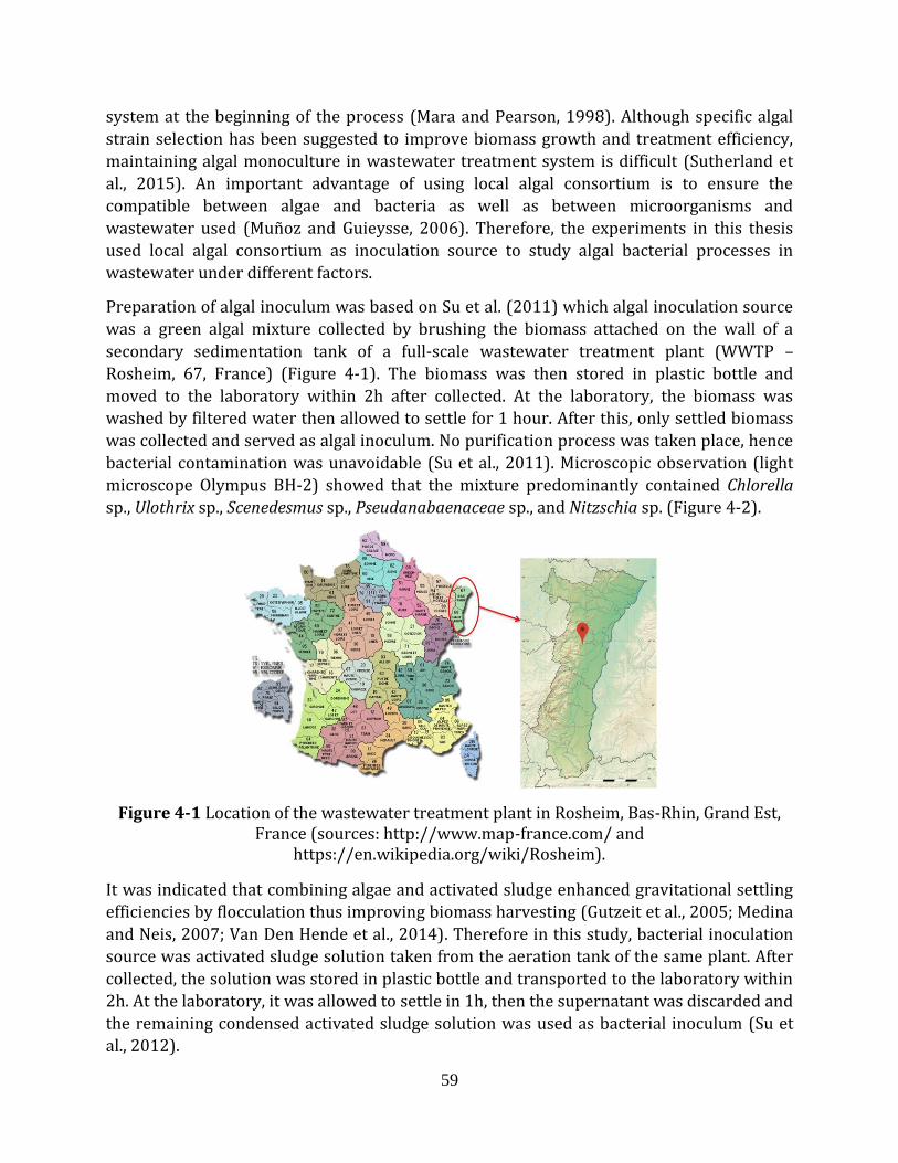
59

system at the beginning of the process (Mara and Pearson, 1998). Although specific algal

strain selection has been suggested to improve biomass growth and treatment efficiency,

maintaining algal monoculture in wastewater treatment system is difficult (Sutherland et

al., 2015). An important advantage of using local algal consortium is to ensure the

compatible between algae and bacteria as well as between microorganisms and

wastewater used (Muñoz and Guieysse, 2006). Therefore, the experiments in this thesis

used local algal consortium as inoculation source to study algal bacterial processes in

wastewater under different factors.

Preparation of algal inoculum was based on Su et al. (2011) which algal inoculation source

was a green algal mixture collected by brushing the biomass attached on the wall of a

secondary sedimentation tank of a full-scale wastewater treatment plant (WWTP –

Rosheim, 67, France) (Figure 4-1). The biomass was then stored in plastic bottle and

moved to the laboratory within 2h after collected. At the laboratory, the biomass was

washed by filtered water then allowed to settle for 1 hour. After this, only settled biomass

was collected and served as algal inoculum. No purification process was taken place, hence

bacterial contamination was unavoidable (Su et al., 2011). Microscopic observation (light

microscope Olympus BH-2) showed that the mixture predominantly contained Chlorella

sp., Ulothrix sp., Scenedesmus sp., Pseudanabaenaceae sp., and Nitzschia sp. (Figure 4-2).

Figure 4-1 Location of the wastewater treatment plant in Rosheim, Bas-Rhin, Grand Est, France (sources: http://www.map-france.com/ and

https://en.wikipedia.org/wiki/Rosheim).

It was indicated that combining algae and activated sludge enhanced gravitational settling

efficiencies by flocculation thus improving biomass harvesting (Gutzeit et al., 2005; Medina

and Neis, 2007; Van Den Hende et al., 2014). Therefore in this study, bacterial inoculation

source was activated sludge solution taken from the aeration tank of the same plant. After

collected, the solution was stored in plastic bottle and transported to the laboratory within

2h. At the laboratory, it was allowed to settle in 1h, then the supernatant was discarded and

the remaining condensed activated sludge solution was used as bacterial inoculum (Su et

al., 2012).

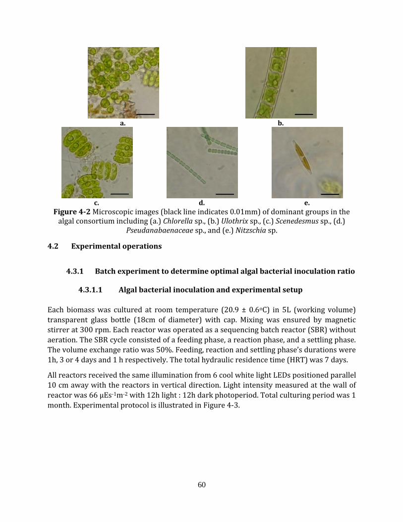
60

a. b.

c. d. e.

Figure 4-2 Microscopic images (black line indicates 0.01mm) of dominant groups in the algal consortium including (a.) Chlorella sp., (b.) Ulothrix sp., (c.) Scenedesmus sp., (d.)

Pseudanabaenaceae sp., and (e.) Nitzschia sp.

4.2 Experimental operations

4.3.1 Batch experiment to determine optimal algal bacterial inoculation ratio

4.3.1.1 Algal bacterial inoculation and experimental setup

Each biomass was cultured at room temperature (20.9 ± 0.6oC) in 5L (working volume)

transparent glass bottle (18cm of diameter) with cap. Mixing was ensured by magnetic

stirrer at 300 rpm. Each reactor was operated as a sequencing batch reactor (SBR) without

aeration. The SBR cycle consisted of a feeding phase, a reaction phase, and a settling phase.

The volume exchange ratio was 50%. Feeding, reaction and settling phase’s durations were

1h, 3 or 4 days and 1 h respectively. The total hydraulic residence time (HRT) was 7 days.

All reactors received the same illumination from 6 cool white light LEDs positioned parallel

10 cm away with the reactors in vertical direction. Light intensity measured at the wall of

reactor was 66 µEs-1m-2 with 12h light : 12h dark photoperiod. Total culturing period was 1

month. Experimental protocol is illustrated in Figure 4-3.

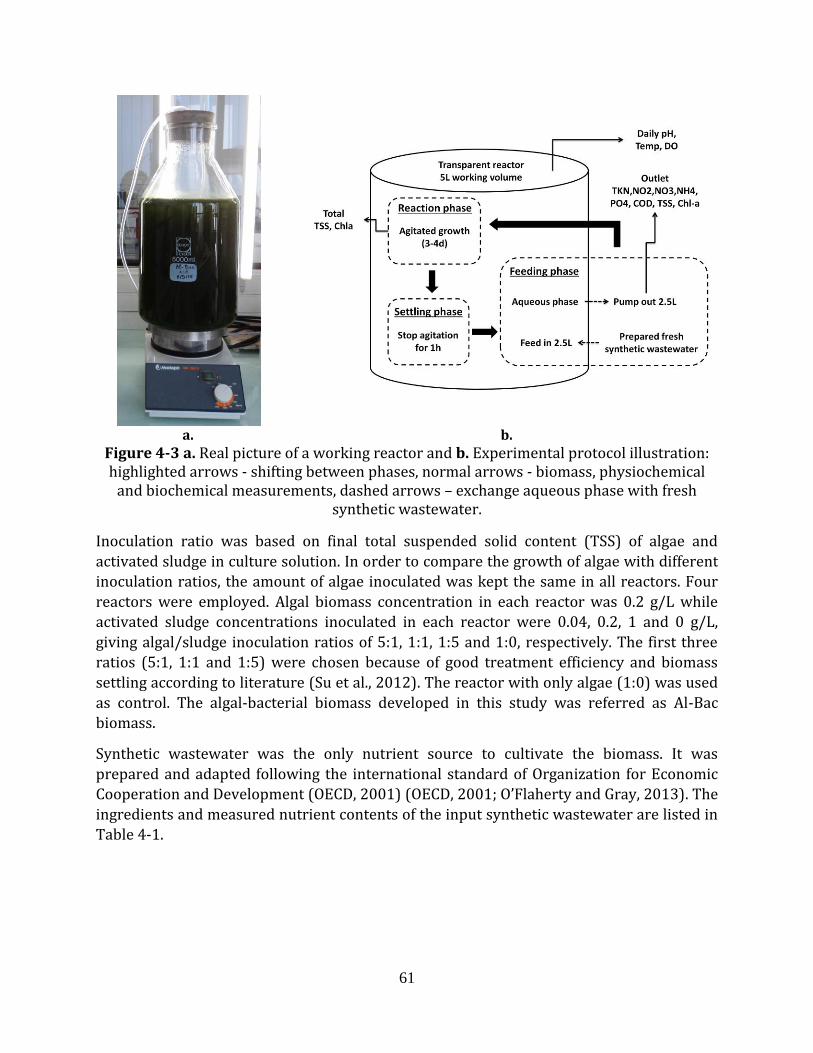
61

a. b. Figure 4-3 a. Real picture of a working reactor and b. Experimental protocol illustration: highlighted arrows - shifting between phases, normal arrows - biomass, physiochemical

and biochemical measurements, dashed arrows – exchange aqueous phase with fresh synthetic wastewater.

Inoculation ratio was based on final total suspended solid content (TSS) of algae and

activated sludge in culture solution. In order to compare the growth of algae with different

inoculation ratios, the amount of algae inoculated was kept the same in all reactors. Four

reactors were employed. Algal biomass concentration in each reactor was 0.2 g/L while

activated sludge concentrations inoculated in each reactor were 0.04, 0.2, 1 and 0 g/L,

giving algal/sludge inoculation ratios of 5:1, 1:1, 1:5 and 1:0, respectively. The first three

ratios (5:1, 1:1 and 1:5) were chosen because of good treatment efficiency and biomass

settling according to literature (Su et al., 2012). The reactor with only algae (1:0) was used

as control. The algal-bacterial biomass developed in this study was referred as Al-Bac

biomass.

Synthetic wastewater was the only nutrient source to cultivate the biomass. It was

prepared and adapted following the international standard of Organization for Economic

Cooperation and Development (OECD, 2001) (OECD, 2001; O’Flaherty and Gray, 2013). The

ingredients and measured nutrient contents of the input synthetic wastewater are listed in

Table 4-1.

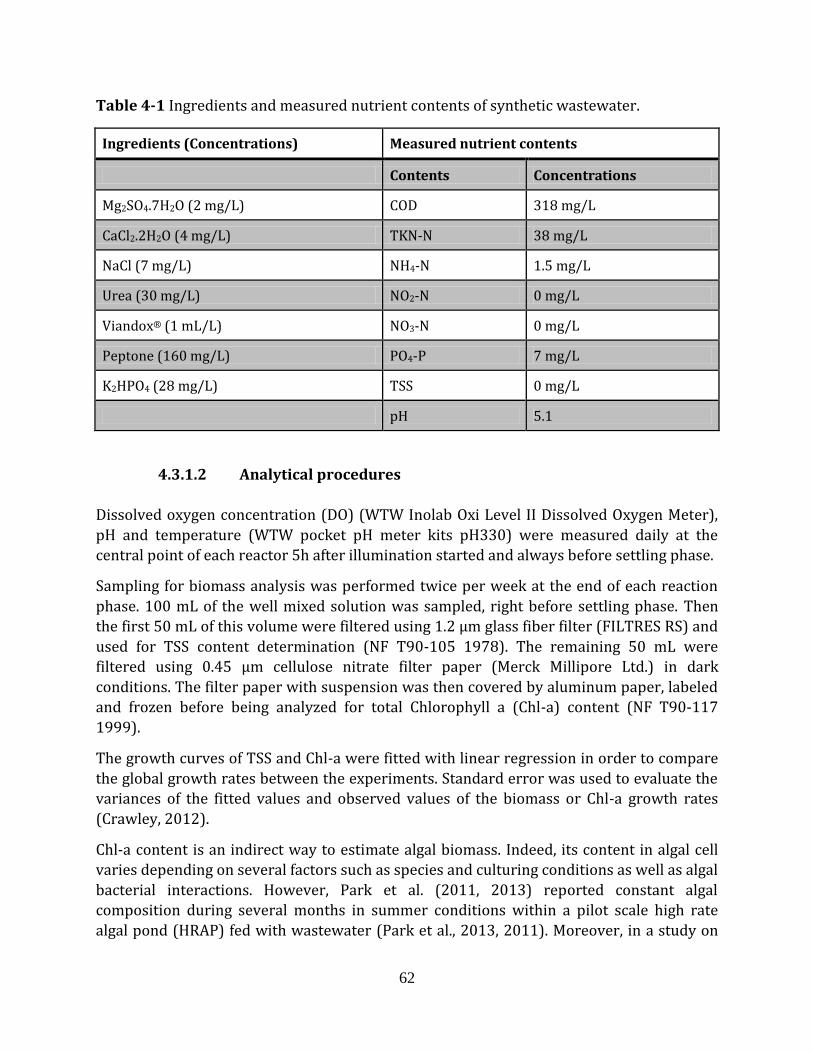
62

Table 4-1 Ingredients and measured nutrient contents of synthetic wastewater.

Ingredients (Concentrations) Measured nutrient contents

Contents Concentrations

Mg2SO4.7H2O (2 mg/L) COD 318 mg/L

CaCl2.2H2O (4 mg/L) TKN-N 38 mg/L

NaCl (7 mg/L) NH4-N 1.5 mg/L

Urea (30 mg/L) NO2-N 0 mg/L

Viandox® (1 mL/L) NO3-N 0 mg/L

Peptone (160 mg/L) PO4-P 7 mg/L

K2HPO4 (28 mg/L) TSS 0 mg/L

pH 5.1

4.3.1.2 Analytical procedures

Dissolved oxygen concentration (DO) (WTW Inolab Oxi Level II Dissolved Oxygen Meter),

pH and temperature (WTW pocket pH meter kits pH330) were measured daily at the

central point of each reactor 5h after illumination started and always before settling phase.

Sampling for biomass analysis was performed twice per week at the end of each reaction

phase. 100 mL of the well mixed solution was sampled, right before settling phase. Then

the first 50 mL of this volume were filtered using 1.2 µm glass fiber filter (FILTRES RS) and

used for TSS content determination (NF T90-105 1978). The remaining 50 mL were

filtered using 0.45 µm cellulose nitrate filter paper (Merck Millipore Ltd.) in dark

conditions. The filter paper with suspension was then covered by aluminum paper, labeled

and frozen before being analyzed for total Chlorophyll a (Chl-a) content (NF T90-117

1999).

The growth curves of TSS and Chl-a were fitted with linear regression in order to compare

the global growth rates between the experiments. Standard error was used to evaluate the

variances of the fitted values and observed values of the biomass or Chl-a growth rates

(Crawley, 2012).

Chl-a content is an indirect way to estimate algal biomass. Indeed, its content in algal cell

varies depending on several factors such as species and culturing conditions as well as algal

bacterial interactions. However, Park et al. (2011, 2013) reported constant algal

composition during several months in summer conditions within a pilot scale high rate

algal pond (HRAP) fed with wastewater (Park et al., 2013, 2011). Moreover, in a study on

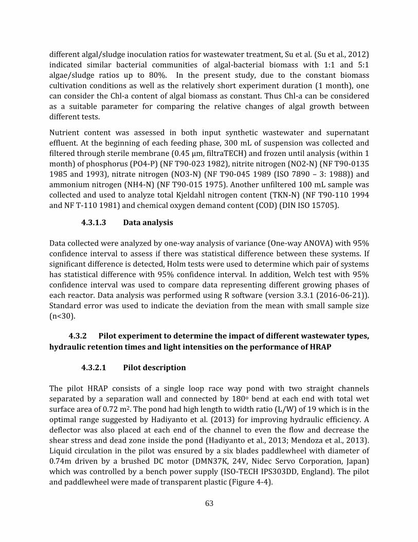
63

different algal/sludge inoculation ratios for wastewater treatment, Su et al. (Su et al., 2012)

indicated similar bacterial communities of algal-bacterial biomass with 1:1 and 5:1

algae/sludge ratios up to 80%. In the present study, due to the constant biomass

cultivation conditions as well as the relatively short experiment duration (1 month), one

can consider the Chl-a content of algal biomass as constant. Thus Chl-a can be considered

as a suitable parameter for comparing the relative changes of algal growth between

different tests.

Nutrient content was assessed in both input synthetic wastewater and supernatant

effluent. At the beginning of each feeding phase, 300 mL of suspension was collected and

filtered through sterile membrane (0.45 µm, filtraTECH) and frozen until analysis (within 1

month) of phosphorus (PO4-P) (NF T90-023 1982), nitrite nitrogen (NO2-N) (NF T90-0135

1985 and 1993), nitrate nitrogen (NO3-N) (NF T90-045 1989 (ISO 7890 – 3: 1988)) and

ammonium nitrogen (NH4-N) (NF T90-015 1975). Another unfiltered 100 mL sample was

collected and used to analyze total Kjeldahl nitrogen content (TKN-N) (NF T90-110 1994

and NF T-110 1981) and chemical oxygen demand content (COD) (DIN ISO 15705).

4.3.1.3 Data analysis

Data collected were analyzed by one-way analysis of variance (One-way ANOVA) with 95%

confidence interval to assess if there was statistical difference between these systems. If

significant difference is detected, Holm tests were used to determine which pair of systems

has statistical difference with 95% confidence interval. In addition, Welch test with 95%

confidence interval was used to compare data representing different growing phases of

each reactor. Data analysis was performed using R software (version 3.3.1 (2016-06-21)).

Standard error was used to indicate the deviation from the mean with small sample size

(n<30).

4.3.2 Pilot experiment to determine the impact of different wastewater types,

hydraulic retention times and light intensities on the performance of HRAP

4.3.2.1 Pilot description

The pilot HRAP consists of a single loop race way pond with two straight channels

separated by a separation wall and connected by 180o bend at each end with total wet

surface area of 0.72 m2. The pond had high length to width ratio (L/W) of 19 which is in the

optimal range suggested by Hadiyanto et al. (2013) for improving hydraulic efficiency. A

deflector was also placed at each end of the channel to even the flow and decrease the

shear stress and dead zone inside the pond (Hadiyanto et al., 2013; Mendoza et al., 2013).

Liquid circulation in the pilot was ensured by a six blades paddlewheel with diameter of

0.74m driven by a brushed DC motor (DMN37K, 24V, Nidec Servo Corporation, Japan)

which was controlled by a bench power supply (ISO-TECH IPS303DD, England). The pilot

and paddlewheel were made of transparent plastic (Figure 4-4).

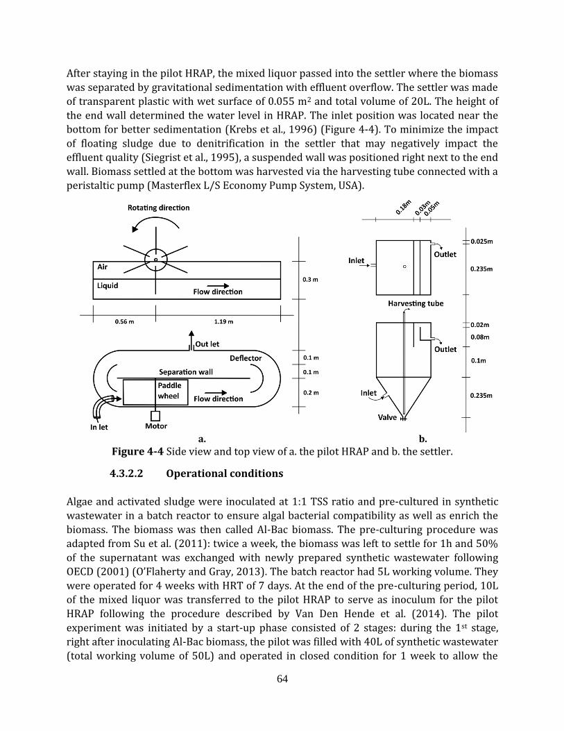
64

After staying in the pilot HRAP, the mixed liquor passed into the settler where the biomass

was separated by gravitational sedimentation with effluent overflow. The settler was made

of transparent plastic with wet surface of 0.055 m2 and total volume of 20L. The height of

the end wall determined the water level in HRAP. The inlet position was located near the

bottom for better sedimentation (Krebs et al., 1996) (Figure 4-4). To minimize the impact

of floating sludge due to denitrification in the settler that may negatively impact the

effluent quality (Siegrist et al., 1995), a suspended wall was positioned right next to the end

wall. Biomass settled at the bottom was harvested via the harvesting tube connected with a

peristaltic pump (Masterflex L/S Economy Pump System, USA).

a. b.

Figure 4-4 Side view and top view of a. the pilot HRAP and b. the settler.

4.3.2.2 Operational conditions

Algae and activated sludge were inoculated at 1:1 TSS ratio and pre-cultured in synthetic

wastewater in a batch reactor to ensure algal bacterial compatibility as well as enrich the

biomass. The biomass was then called Al-Bac biomass. The pre-culturing procedure was

adapted from Su et al. (2011): twice a week, the biomass was left to settle for 1h and 50%

of the supernatant was exchanged with newly prepared synthetic wastewater following

OECD (2001) (O’Flaherty and Gray, 2013). The batch reactor had 5L working volume. They

were operated for 4 weeks with HRT of 7 days. At the end of the pre-culturing period, 10L

of the mixed liquor was transferred to the pilot HRAP to serve as inoculum for the pilot

HRAP following the procedure described by Van Den Hende et al. (2014). The pilot

experiment was initiated by a start-up phase consisted of 2 stages: during the 1st stage,

right after inoculating Al-Bac biomass, the pilot was filled with 40L of synthetic wastewater

(total working volume of 50L) and operated in closed condition for 1 week to allow the

65

biomass developing in the pilot conditions. It was followed by the 2nd stage which an

additional volume of 30L primary treated wastewater (total working volume of 80L) was

provided to the HRAP. In this stage, the HRAP was operated in closed condition for better

adaptation of the biomass to real wastewater.

Primary treated and centrate wastewaters were collected from nearby WWTP ( Located at

La Wantzenau, 67000 Strasbourg, France) every 1 or 2 weeks and stored in a cooling tank

(CV 420, JAPY, France) at 4oC. In case of centrate wastewater collection, floating solids such

as sludge and other materials were discarded before mixing with primary treated

wastewater in the storage tank. Wastewater was fed to the pilot HRAP every 3h by a

peristaltic pump (Masterflex L/S Standard Digital Pump System) which was controlled by a

timer. By adjusting the pumping rate, the desired HRT was achieved.

Illumination was provided by a high-power LED light (ARIAH2 HIGHBAY, ENLITE, UK)

positioned on top of the pilot with the vertical distance to the water surface of 0.8m

providing a constant light intensity of 210 μEs-1m-2 at the water surface. The light intensity

applied was in the optimal range enhancing algal growth (Muñoz and Guieysse, 2006)

while the use of LED light was suggested by Morrow (2008). A timer was connected to the

light source to have a light/dark cycle of 14h/10h. The photoperiod was chosen to favor

the growth of algae but in balance with practical perspective (Bouterfas et al., 2006).

The pilot HRAP was operated indoor in 246 days from August 2017 to April 2018 (Table

4-2). The operating conditions were varied in order to investigate the impacts of different

nutrient loads and HRTs on the growth of Al-Bac biomass. The experimental setup was

illustrated in Figure 4-5.

Table 4-2 Operational characteristics of different stages.

Stage Name Time Wastewater* HRT (d) Study objective

1 LN_4d Aug - Dec 2017 (135 d) P 4 Long term performance 2 HN_4d Dec 2017 - Feb 2018 (53 d) P + C (2v:1v) 4 High nutrient impact 3 HN_8d Feb - Apr 2018 (57d) P + C (2v:1v) 8 High HRT impact

*: P/C is primary treated/centrate wastewater and v is volume.

In all experiments, the water level was maintained at 0.11m giving 80L of total volume. The

rotating speed of the paddle wheel was maintained at around 11.6 rpm for better mixing

and mass transfer, giving the mid-channel average velocity of 0.44 m/s (Pham et al., 2017).

Two times per week, all biomass settled at the bottom of the settler was harvested by

peristaltic pumping. During the first two weeks (day 0 to 15) of the first stage, all harvested

biomass was recycled back to the HRAP for accelerating the biomass growth and flocs

forming (Park et al., 2013). Then, during the next two weeks (day 16 to 29), 0.5L of the

harvested biomass was kept in freezer prior to be analyzed while the rest was recycled to

the HRAP. However, during this period, anaerobic condition occurred in the bottom layer of

settler (Henze et al., 1993) and hence the anaerobic solution recycled from settler

disturbed HRAP performance. Therefore, from day 30 of the first stage, except for the hour

66

when feeding occurred, a volume of 0.5L from the bottom of the settler was automatically

recycled to the HRAP every hour. The recycling was done by a peristaltic pump (Masterflex

L/S Standard Digital Pump System, USA) controlled by a timer.

Figure 4-5 General illustration of pilot HRAP experimental set-up (arrows indicate water and biomass flow, red dashed lines indicate measurements).

4.3.2.3 Sample collection and analytical procedures

Dissolved oxygen concentration (DO) (Portavo, Germany), pH and temperature (WTW,

Germany) were measured every 5-10 minutes for 3-5 days/week at the central point of the

channel after the paddle wheel in the HRAP. The probes were positioned 45o along the flow

to avoid biomass clogging and disturbing the measurement.

Sampling for nutrient content analysis was performed once per week around midday, right

before the feeding event. One sampling consisted of 500 mL of effluent from the settler and

500 mL of inlet wastewater from the storage tank. These samples were analyzed within

24h for total suspended solids (TSS) and occasionally volatile suspended solids (VSS) (NF

EN 872), chemical oxygen demand content (COD) (NANOCOLOR® COD 1500 according to

DIN ISO 15705), total Kjeldahl nitrogen content (TKN-N) (NF EN 25663), ammonium

nitrogen (NH4-N) (NF EN ISO 14911), nitrate nitrogen (NO3-N) (NF EN ISO 10304), nitrite

nitrogen (NO2-N) (NF EN ISO 10304), total phosphorus (NANOCOLOR® ortho- and total

Phosphate 15 according to DIN EN ISO 6878-D11) and orthophosphate (PO4-P) (NF EN ISO

67

10304). Chlorophyll a (Chl-a) (NF T90-117 1999) in the effluent was measured every week

while this content in inlet wastewater was only measured every 2 weeks.

Al-Bac biomass in HRAP was sampled 2 times/week and determined for total solids (TS)

(Symons and Morey, 1941) and sludge volume index (SVI) (Dick and Vesilind, 1969).

Chlorophyll a (Chl-a) (NF T90-117 1999) was measured once per week at the same time

with inlet wastewater and effluent. Al-Bac biomass harvested from settler was measured

for total solids (TS).

4.3.2.4 Data analysis

The productivity (4-1) and solid retention time (SRT) (4-2) of Al-Bac biomass were

calculated using simple mass balance equation suggested by (Tchobanoglous et al., 2002):

𝑃 = 𝑉𝑑𝑋𝐴𝑙−𝐵𝑎𝑐

𝑑𝑡− 𝑄𝑖𝑛 ∗ 𝑋𝑖𝑛 + 𝑄𝑜𝑢𝑡 ∗ 𝑋𝑜𝑢𝑡 + 𝑄𝑕𝑎𝑟𝑣𝑒𝑠𝑡𝑒𝑑 ∗ 𝑋𝑕𝑎𝑟𝑣𝑒𝑠𝑡𝑒𝑑 (4-1)

𝑆𝑅𝑇 =𝑋𝐴𝑙−𝐵𝑎𝑐 ∗ 𝑉

𝑄𝑕𝑎𝑟𝑣𝑒𝑠𝑡𝑒𝑑 ∗ 𝑋𝑕𝑎𝑟𝑣𝑒𝑠𝑡𝑒𝑑 + 𝑄𝑜𝑢𝑡 ∗ 𝑋𝑜𝑢𝑡 (4-2)

With P is productivity in mg TSS/L/d, XAl_bac/Xin/Xout/Xwastage is the concentration of

suspended solids (mg/L) in HRAP, inlet wastewater, treated effluent and harvested

biomass respectively. Qin/Qout/Qwastage is the influent/effluent/harvesting flow rate in L/d.

V is the total volume of HRAP in L and SRT is solid retention time of Al-Bac biomass in days.

The factors influencing DO dynamics in the HRAP were evaluated by analyzing recorded

DO profile. The observed DO dynamics in the HRAP with (4-3) and without light (4-4) can

be generally described as:

𝑑𝑂2,𝑙𝑖𝑔𝑕𝑡

𝑑𝑡= 𝑂𝑇𝑅 − 𝑂𝑈𝑅𝑙𝑖𝑔𝑕𝑡 + 𝑂𝑃𝑅 (4-3)

𝑑𝑂2,𝑑𝑎𝑟𝑘

𝑑𝑡= 𝑂𝑇𝑅 − 𝑂𝑈𝑅𝑑𝑎𝑟𝑘 (4-4)

With OTR, OUR and OPR stand for oxygen transfer, uptake and production rates in light and

dark conditions expressed in mg/L/d, respectively.

Treatment efficiencies were calculated as following:

𝐸 =𝐶𝑖𝑛 − 𝐶𝑜𝑢𝑡

𝐶𝑖𝑛∙ 100% (4-5)

With E is the treatment efficiency, Cin and Cout are the concentrations at the influent and

effluent, respectively.

Data statistical analysis was performed using R software (version 3.3.1 (2016-06-21)) (R

Core Team, 2016). In order to evaluate the impacts of different nutrient loads and HRTs on

the system’s performance, the difference between data sets from three stages was

68

determined. For comparing between two data sets, normal distribution of each data set

was first determined by a Shapiro-Wilk test. In case of normal distribution, comparison

between two data sets began with determining homoscedasticity by Fisher-Snedecor test

and then either Student-t test or Welch test was applied for equal or unequal variances,

respectively. In the other case, Mann-Whitney-Wilcoxon test was used. For multiple data

sets comparison, normally distributed data sets were determined for homoscedasticity by

Bartlett test and their significant differences were analyzed by ANOVA followed by

pairwise t-test or ANOVA-Welch correction followed by pairwise t-test in case of equaled

variances or unequaled variances, respectively. Otherwise, Kruskal-Wallis test followed by

Pairwise Wilcoxon Rank Sum Tests was used. All tests were applied with the threshold

value of 0.05. Averages were presented with standard deviations.

Moreover, to separate the impact of feeding and light/dark cycle, time series

decomposition was performed using the Seasonal and Trend decomposition using Loess

(STL) (stl function in R) (Crawley, 2012). In order to extract the feeding pattern, different

frequencies were applied depending on the recording intervals of the time series data.

69

CHAPTER 5 HYDRAULIC AND GAS-LIQUID MASS TRANSFER STUDIES OF PILOT

HRAP

In this chapter, materials and methods for determining the impacts of operational

conditions including water level, inlet flow rate and paddle wheel movement on

hydrodynamics in a pilot scale HRAP are described. To understand how such variation in

hydrodynamics impacts gas transfer in HRAP, the volumetric mass transfer coefficient of

oxygen method will also be introduced.

In French:

Ce chapitre décrit les différentes méthodes et calculs pour l'étude expérimentale de

l’hydrodynamique et du transfert d'oxygène du pilote. Des expériences de traçage sont

utilisées pour étudier le comportement hydraulique global de la HRAP en fonctionnement

continu. Des calculs détaillés ont été fournis. La même technique a été appliquée pour

étudier les caractéristiques de mélange du réacteur dans différentes combinaisons de

niveaux d'eau et de vitesse de rotation de la pale en fonctionnement fermé. Différents

paramètres ont été calculés pour évaluer le mélange et la vitesse d'écoulement de l'eau

dans le canal. Des conditions opérationnelles similaires ont ensuite été appliquées et le

taux de transfert d'oxygène a été étudié dans chaque cas selon la norme européenne. Enfin,

des analyses statistiques et de sensibilité ont été utilisées pour comparer les données

obtenues.

5.1 Operational conditions applied

Operational condition applied to the pilot HRAP was the combination of 3 different

operational parameters: water level, paddle rotational speed and in let flow rate. Due to the

capacity of the pilot, 3 water levels of 0.1, 0.15, and 0.2 m were chosen from the range of

operational depth reported by Muñoz and Guieysse (2006) to reach a total water volume of

72, 108 and 144 L, respectively. Three paddle movements in terms of voltage applied were

also selected representing low (3.5 Volt for 0.2±0.0A), medium (7 Volt for 0.3±0.1A) and

fast (10.5 Volt for 0.6±0.1A) mixing. The average paddle rotational speed obtained were 5.6

± 0.4, 11.6 ± 0.9 and 16.8 ± 2.1 rpm, respectively, resulting to expected average water flow

as high as 0.3 m/s (Andersen, 2005). Due to the water volume, inlet flow rates of 6 and 9

L/h were chosen to get 8, 12 and 18h of HRT depending on given combination. Overall, 27

experiments were conducted during this study. All the experiments were conducted indoor

with constant ambient temperature of about 20.9 ± 0.6 oC and air pressure of 0.98 atm. The

temperature and air pressure in this study were constant, and thus generating no

significant impact on the measurement and calculation. The basic physico-chemical

properties of the water used were pH of 7.4 ± 0.1, conductivity of 557.7 ± 1.15 μS/cm and

temperature of 15.1 ± 0.4 oC. These values were constant during the experiments, which

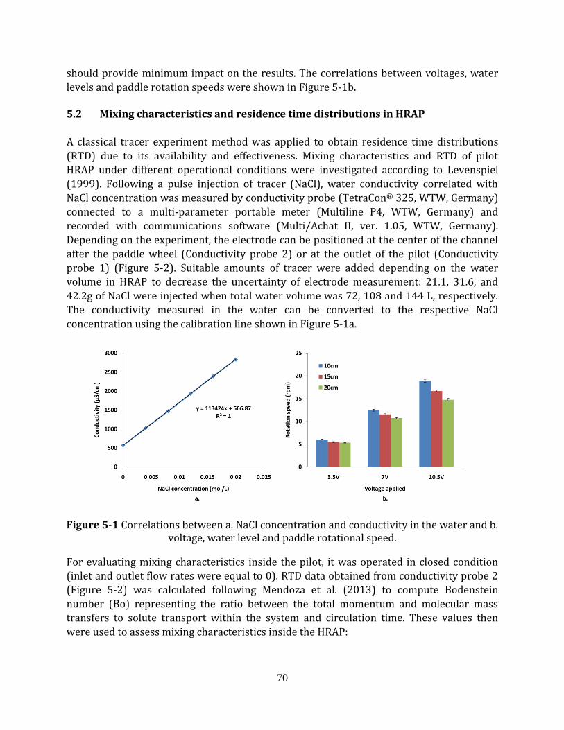
70

should provide minimum impact on the results. The correlations between voltages, water

levels and paddle rotation speeds were shown in Figure 5-1b.

5.2 Mixing characteristics and residence time distributions in HRAP

A classical tracer experiment method was applied to obtain residence time distributions

(RTD) due to its availability and effectiveness. Mixing characteristics and RTD of pilot

HRAP under different operational conditions were investigated according to Levenspiel

(1999). Following a pulse injection of tracer (NaCl), water conductivity correlated with

NaCl concentration was measured by conductivity probe (TetraCon® 325, WTW, Germany)

connected to a multi-parameter portable meter (Multiline P4, WTW, Germany) and

recorded with communications software (Multi/Achat II, ver. 1.05, WTW, Germany).

Depending on the experiment, the electrode can be positioned at the center of the channel

after the paddle wheel (Conductivity probe 2) or at the outlet of the pilot (Conductivity

probe 1) (Figure 5-2). Suitable amounts of tracer were added depending on the water

volume in HRAP to decrease the uncertainty of electrode measurement: 21.1, 31.6, and

42.2g of NaCl were injected when total water volume was 72, 108 and 144 L, respectively.

The conductivity measured in the water can be converted to the respective NaCl

concentration using the calibration line shown in Figure 5-1a.

Figure 5-1 Correlations between a. NaCl concentration and conductivity in the water and b. voltage, water level and paddle rotational speed.

For evaluating mixing characteristics inside the pilot, it was operated in closed condition

(inlet and outlet flow rates were equal to 0). RTD data obtained from conductivity probe 2

(Figure 5-2) was calculated following Mendoza et al. (2013) to compute Bodenstein

number (Bo) representing the ratio between the total momentum and molecular mass

transfers to solute transport within the system and circulation time. These values then

were used to assess mixing characteristics inside the HRAP:

71

𝐶

𝐶∞=

𝐵𝑜

4𝜋𝜃 𝑒𝑥𝑝 −

𝐵𝑜

4𝜃 𝑗 − 𝜃 2

∞

𝑗=1

(5-1)

With C is the concentration of tracer detected, C∞ is the concentration of tracer at infinite

time and θ is the dimensionless time which is denoted as θ=t/tc (tc is circulation time and t

is time) (Mendoza et al., 2013).

Moreover, in practice, HRAP is usually operated in continuous condition, thus RTD data

from experiments with continuous operational conditions (Conductivity probe 1) (Figure

5-2) was calculated based on Levenspiel (1999) and used to evaluate hydrodynamic

behavior of the pilot HRAP. Due to the stability of the pilot in long term operation, only 0.1

and 0.15m of water level were applied in continuous mode. Similarly, the highest paddle

rotational speed achieved at 10.5V was only applied with 0.1m of water level and 6L/h of

inlet flow rate. Calculation of systemic hydrodynamic parameters in continuous condition

(Levenspiel, 1999) are described as following:

Residence Time Distribution (RTD) function E(t) can be defined as E(t)Δt = fraction of

incoming water that stays in the reactor for a length of time between t and Δt. It is

calculated as follows:

𝐸 𝑡 =𝑄 𝑡 𝐶(𝑡)

𝑄 𝑡 𝐶 𝑡 𝑑𝑡∞

0

=𝑄 𝑡𝑖 𝐶(𝑡𝑖)

𝑄 𝑡𝑖 𝐶 𝑡𝑖 ∆𝑡𝑖 (5-2)

Mean residence time (t ):

𝑡 = 𝑡𝐸 𝑡 𝑑∞

0

= 𝑡𝑖𝐸(𝑡𝑖)∆𝑡𝑖 (5-3)

Variance (σ) which is a measure of the RTD curve’s spread:

𝜍 = 𝑡 − 𝑡 2𝐸 𝑡 𝑑𝑡∞

0

= 𝑡𝑖2𝐸 𝑡𝑖 ∆𝑡𝑖 − 𝑡 2 (5-4)

Dimensionless variance:

𝜍𝜃2 =

𝜍2

𝑡 2 (5-5)

Calculation of uL/D ratio or Peclet number for a closed vessel:

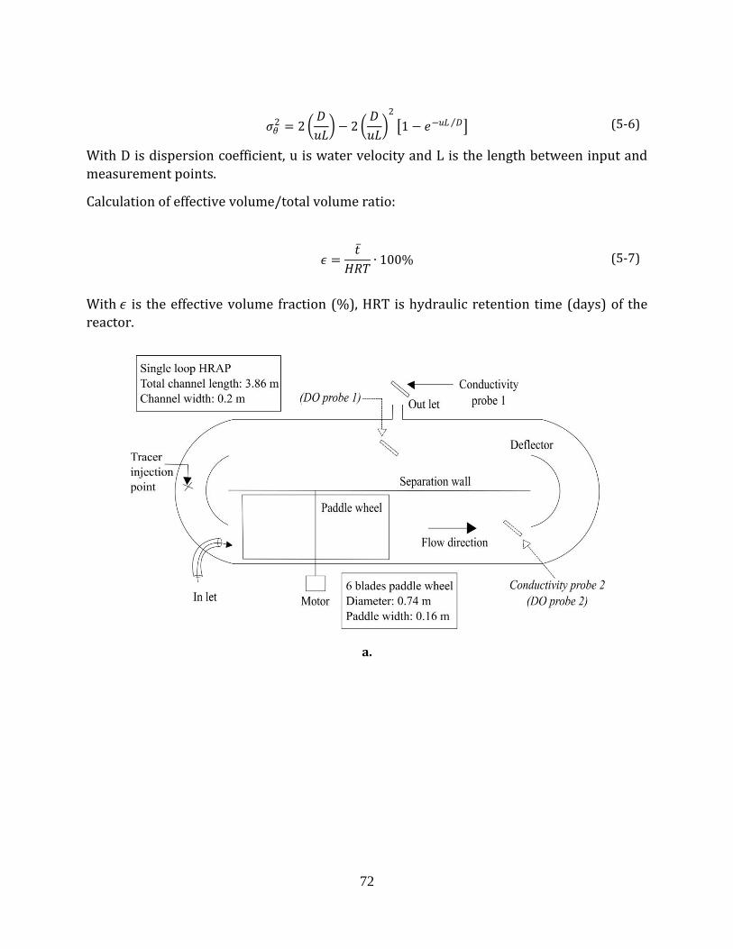
72

𝜍𝜃2 = 2

𝐷

𝑢𝐿 − 2

𝐷

𝑢𝐿

2

1 − 𝑒−𝑢𝐿 𝐷 (5-6)

With D is dispersion coefficient, u is water velocity and L is the length between input and

measurement points.

Calculation of effective volume/total volume ratio:

𝜖 =𝑡

𝐻𝑅𝑇∙ 100% (5-7)

With 𝜖 is the effective volume fraction (%), HRT is hydraulic retention time (days) of the

reactor.

a.

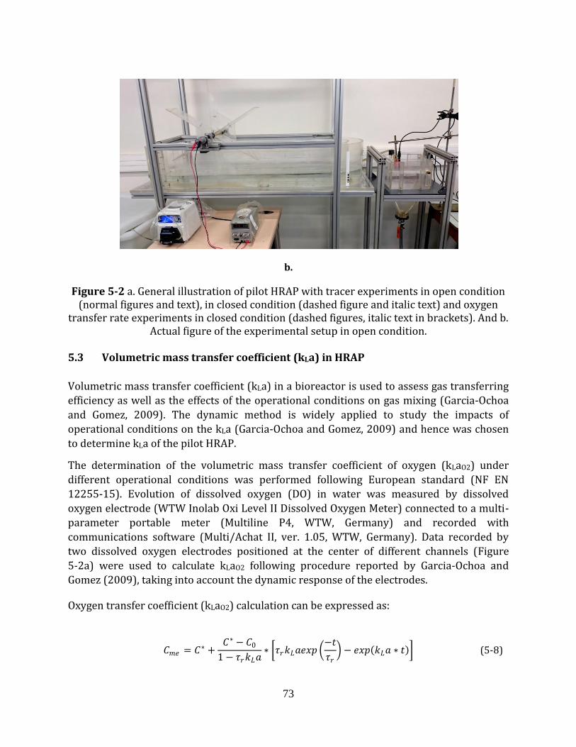
73

b.

Figure 5-2 a. General illustration of pilot HRAP with tracer experiments in open condition (normal figures and text), in closed condition (dashed figure and italic text) and oxygen

transfer rate experiments in closed condition (dashed figures, italic text in brackets). And b. Actual figure of the experimental setup in open condition.

5.3 Volumetric mass transfer coefficient (kLa) in HRAP

Volumetric mass transfer coefficient (kLa) in a bioreactor is used to assess gas transferring

efficiency as well as the effects of the operational conditions on gas mixing (Garcia-Ochoa

and Gomez, 2009). The dynamic method is widely applied to study the impacts of

operational conditions on the kLa (Garcia-Ochoa and Gomez, 2009) and hence was chosen

to determine kLa of the pilot HRAP.

The determination of the volumetric mass transfer coefficient of oxygen (kLaO2) under

different operational conditions was performed following European standard (NF EN

12255-15). Evolution of dissolved oxygen (DO) in water was measured by dissolved

oxygen electrode (WTW Inolab Oxi Level II Dissolved Oxygen Meter) connected to a multi-

parameter portable meter (Multiline P4, WTW, Germany) and recorded with

communications software (Multi/Achat II, ver. 1.05, WTW, Germany). Data recorded by

two dissolved oxygen electrodes positioned at the center of different channels (Figure

5-2a) were used to calculate kLaO2 following procedure reported by Garcia-Ochoa and

Gomez (2009), taking into account the dynamic response of the electrodes.

Oxygen transfer coefficient (kLaO2) calculation can be expressed as:

𝐶𝑚𝑒 = 𝐶∗ +𝐶∗ − 𝐶0

1 − 𝜏𝑟𝑘𝐿𝑎∗ 𝜏𝑟𝑘𝐿𝑎𝑒𝑥𝑝

−𝑡

𝜏𝑟 − 𝑒𝑥𝑝 𝑘𝐿𝑎 ∗ 𝑡 (5-8)

74

With Cme is the oxygen concentration measured by the electrode and C0 is the oxygen

concentration at the initial time of the aeration while C* is equilibrium value of oxygen

concentration. τr is the response time of the electrode and t is time (Garcia-Ochoa and

Gomez, 2009).

5.4 Sensitivity analysis

One-way ANOVA followed by Holm tests (95 % confidence interval) was applied in R

software (version 3.3.1 (2016-06-21)) to compare these effects. Two sensitivity functions

were used: the absolute-relative (a-r) sensitivity function measuring the absolute change in

the variable for a 100% change in input parameter, and the relative-relative (r-r)

sensitivity function measuring the relative change in the variable for a 100% change in

input parameter. The a-r sensitivity was used for quantitative comparisons of the effect of

different parameters (water level, paddle rotational speed) on a common variable y (Bo,

kLa). While the r-r sensitivity was used to compare effects of different parameters on

different variables (Reichert, 1994). The sensitivity functions are expressed as:

𝛿𝑦 ,𝑝𝑎 ,𝑟 = 𝑝

𝜕𝑦

𝜕𝑝 (5-9)

𝛿𝑦 ,𝑝𝑟 ,𝑟 =

𝑝

𝑦

𝜕𝑦

𝜕𝑝 (5-10)

With y is the variable that changes due to the change of parameter p (Reichert, 1994).

75

CHAPTER 6 COUPLING RTD AND MIXED-ORDER KINETIC MODELS FOR HRAP

PERFORMANCE ASSESSMENT AND SIZING APPLICATION

In this chapter, a mixed-order kinetic model coupled with a RTD model that was developed

in this study is described. It is used to simulate the data obtained from different long term

experiments conducted in a pilot scale HRAP. In a further step, the method of applying the

model for designing large scale HRAP systems for wastewater treatment is also described.

In French:

Dans ce chapitre, un modèle cinétique d'ordre mixte couplé à un modèle de Distribution

des Temps de Séjour a été développé sur la base des données obtenues à partir des

expériences pilotes HRAP. La procédure détaillée du processus de calage pour obtenir les

paramètres du modèle le mieux adapté a été illustrée. De plus, un résumé des données de

calage et de validation pour différentes modalités expérimentales est également fourni.

Deux coefficients ont été introduits pour évaluer l'adéquation entre le modèle et les

résultats expérimentaux.

6.1 RTD and mixed-order kinetic models description

6.1.1 Hydrodynamic (RTD) model

The hydrodynamic model of the HRAP pilot was obtained using tracer experiments data

(Pham et al., 2017) described in chapter 5 and chapter 8 of the thesis.The continuous

stirred-tank reactor (CSTR) appeared as the best hydrodynamic model with different

operational conditions such as water depth, paddle wheel speed and inlet flow rate. Hence

the hydraulic is well represented by the RTD function as following:

𝐸 𝑡 =1

𝜏∙ 𝑒−𝑡 𝜏 (6-1)

With 𝐸(𝑡) is the RTD function and 𝜏 is the mean residence time (Fogler, 2006a).

Mixed-order kinetic model

Using simple kinetics models, the reaction rate representing the removal of a constituent is

generally described as:

𝑟 = −𝑘𝑛 ∙ 𝐶𝑛 (6-2)

With r is the reaction rate in mg/L/day, 𝑘𝑛 is the mixed-order reaction rate constant with

the unit depending on n as (mg/L)1-n/day, C is the constituent concentration in mg/L and n

is the reaction order (Sperling, 2007). The minus sign represents the removal of the

constituent.

76

6.1.2 Coupling RTD and mixed-order kinetic models

As indicated by various studies, inoculation between algae and activated sludge promotes

bioflocculation to form bigger flocs thus enhancing settleability (Gutzeit et al., 2005; Su et

al., 2011; Van Den Hende et al., 2011a). Study with large scale HRAP system treating

wastewater showed that the recovery efficiency of algal bacterial biomass could be up to

99% via simple gravity settling (Van Den Hende et al., 2014). The mixed suspension in the

HRAP mainly consisted of dissolved constituents and suspended algal bacterial flocs.

Hence, the segregation model dealing with segregated elements of different ages in the

reactor was found appropriate to be employed in this study to determine the mean

conversion in the effluent following (Fogler, 2006a):

𝐶𝑚 = 𝐶(𝑡) ∙ 𝐸(𝑡) ∙ 𝑑𝑡∞

0

(6-3)

Where 𝐶𝑚 is the mean constituent concentration measured at the effluent in mg/L and C(t)

the instantaneous constituent concentration (mg/L) inside the HRAP or at the outlet due to

the CSTR model.

The integrated form of equation (6-2):

𝐶(𝑡) = 𝐶𝑜1−𝑛 − 𝑘𝑛 ∙ 𝑡 ∙ (1 − 𝑛)

11−𝑛

(6-4)

With Co is the constituent concentration at influent in mg/L.

The integrated form of coupled RTD and mixed-order kinetic model derived by substituting

(6-4) and (6-1) in (6-3):

𝐶𝑚 = 𝐶𝑜1−𝑛 − 𝑘𝑛 ∙ 𝑡 ∙ (1 − 𝑛)

11−𝑛 ∙

1

𝜏∙ 𝑒−𝑡 𝜏 ∙ 𝑑𝑡

∞

0

(6-5)

Cm calculation using Trapezoid rule and calculation of the residual sum of squares (RSS)

between model results and experimental data:

𝐶𝑚 = 𝐶(𝑡) ∙ 𝐸(𝑡) ∙ 𝑑𝑡∞

0

≈ 𝐶 𝑡𝑘−1 ∙ 𝐸 𝑡𝑘−1 + 𝐶 𝑡𝑘 ∙ 𝐸 𝑡𝑘

2∆𝑡𝑘

𝑁

𝑘=1

(6-6)

𝑅𝑆𝑆 = 𝐶𝑚 ,𝑗 − 𝐶𝑐𝑎𝑙 ,𝑗 2

𝑚

𝑗=1

(6-7)

With ∆𝑡𝑘 = 𝑡𝑘 − 𝑡𝑘−1 and N is the number of ∆𝑡𝑘 . 𝑅𝑆𝑆 is the residual sum of squares

between model result 𝐶𝑐𝑎𝑙 and experimental data 𝐶𝑚 .

It is common knowledge that temperature variation is one of the main factor impacting

performance of the treatment system (Flegal and Schroeder, 1976; Ras et al., 2013; Robarts

and Zohary, 1987; Uhlmann, 1979). Hence the impact of temperature on reaction rate was

77

usually taken into account by employing Arrhenius or van’t Hoff-Arrhenius theory

(Sperling, 2007). However, in this study, all experiments were conducted indoor with

similar range of temperature. Therefore no temperature factor was employed in this case

although it should be considered for further application of the model simulating outdoor

HRAP systems.

In the mixed-order model developed by Borsuk and Stow (2000), n remained a free

parameter receiving both integer and fractional values. Then parameter estimation was

performed for each set of long term data by applying Bayesian theorem (Borsuk and Stow,

2000). However, applying such procedure in addition to the coupled RTD and mixed-order

model would enhance the complexity which was not fit with the purpose of developing a

relative simple yet effective model for assessing the HRAP performance in this study.

Moreover, it was suggested that for most commonly found reactions, the order of reaction

is from 0 to 3 (Levenspiel, 1999; Upadhyay, 2006). In addition, simulation results from

previous studies on BOD removal showed consistent range of values of n between 0 and 4

(Adrian and Sanders, 1998, 1992; Borsuk and Stow, 2000; Stow et al., 1999). Therefore, in

this study, fixing the reaction order for each simulation to calibrate kn with n ranging from

0 to 4 with 0.5 steps was found appropriate.

Fitting procedure was done following least squares method. For each value of n, an initial

value of kn was chosen and the calculation of Cm was conducted for the whole data set of

each modality by numerical integration using Trapezoid rule. It was followed by calculating

the residual sum of squares (RSS) between model results and experimental data. Then

value of kn was varied to obtain minimum value of RSS by employing Generalized Reduced

Gradient (GRG2) nonlinear optimization solver method (Lasdon et al., 1974).

After fitting, the minimum RSS value of each model was compared to find the best model to

describe the data set (the best model having the smallest RSS value). A confidence interval

limit of 95% was used to distinguish the significance of relative difference between RSS

values. A relative difference lower than 5% was considered as insignificant and hence a

model with lower n value was chosen. This method aimed to decrease the uncertainty due

to numerical estimation and the complexity of the model while the significant difference

due to practical factors was still appreciated:

𝐷 = 𝑅𝑆𝑆𝑛 − 𝑅𝑆𝑆𝑛+1 ∙ 100 𝑆𝑛 , 𝑤𝑖𝑡𝑕

𝐷 < 5%, 𝐷 = 𝐷𝑖𝑛𝑠

𝐷 ≥ 5%, 𝐷 = 𝐷𝑠𝑖𝑔

(6-8)

With D is the relative difference between two RSS values with 𝐷𝑖𝑛𝑠 is the insignificant

relative difference and 𝐷𝑠𝑖𝑔 is the significant relative difference.

The fitting procedure was performed on Microsoft® Office Excel® 2007. General

procedure was presented in Figure 6-1.

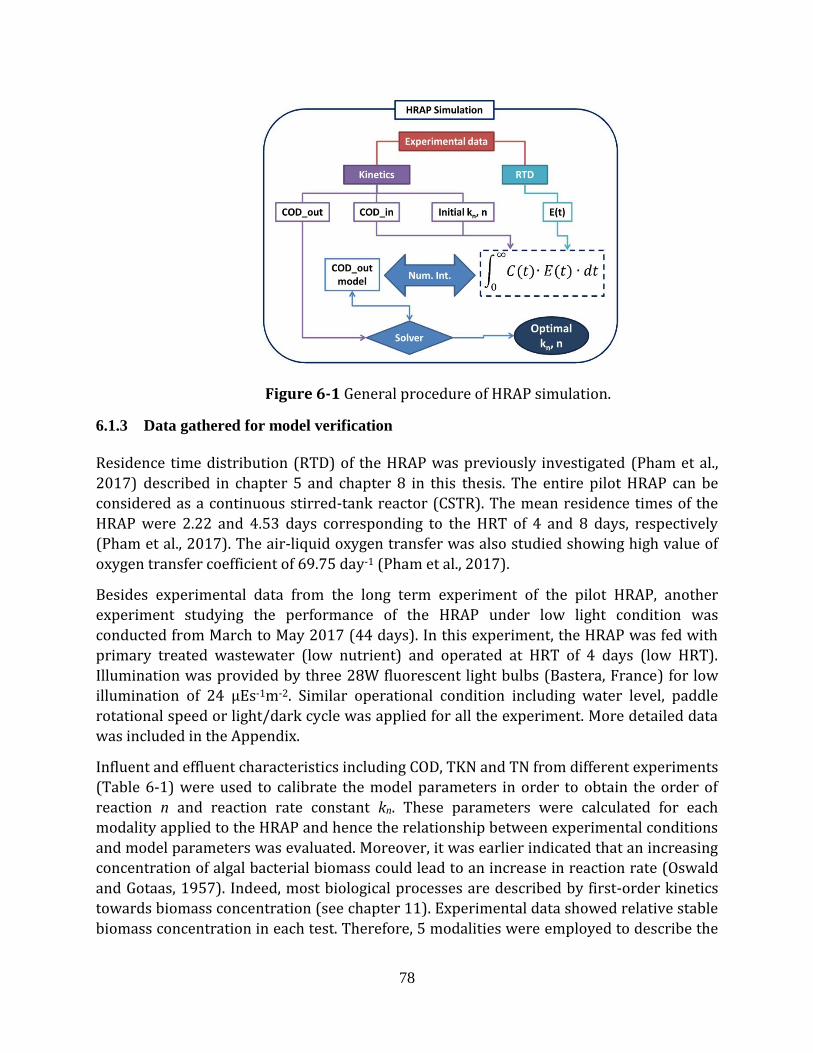
78

Figure 6-1 General procedure of HRAP simulation.

6.1.3 Data gathered for model verification

Residence time distribution (RTD) of the HRAP was previously investigated (Pham et al.,

2017) described in chapter 5 and chapter 8 in this thesis. The entire pilot HRAP can be

considered as a continuous stirred-tank reactor (CSTR). The mean residence times of the

HRAP were 2.22 and 4.53 days corresponding to the HRT of 4 and 8 days, respectively

(Pham et al., 2017). The air-liquid oxygen transfer was also studied showing high value of

oxygen transfer coefficient of 69.75 day-1 (Pham et al., 2017).

Besides experimental data from the long term experiment of the pilot HRAP, another

experiment studying the performance of the HRAP under low light condition was

conducted from March to May 2017 (44 days). In this experiment, the HRAP was fed with

primary treated wastewater (low nutrient) and operated at HRT of 4 days (low HRT).

Illumination was provided by three 28W fluorescent light bulbs (Bastera, France) for low

illumination of 24 μEs-1m-2. Similar operational condition including water level, paddle

rotational speed or light/dark cycle was applied for all the experiment. More detailed data

was included in the Appendix.

Influent and effluent characteristics including COD, TKN and TN from different experiments

(Table 6-1) were used to calibrate the model parameters in order to obtain the order of

reaction n and reaction rate constant kn. These parameters were calculated for each

modality applied to the HRAP and hence the relationship between experimental conditions

and model parameters was evaluated. Moreover, it was earlier indicated that an increasing

concentration of algal bacterial biomass could lead to an increase in reaction rate (Oswald

and Gotaas, 1957). Indeed, most biological processes are described by first-order kinetics

towards biomass concentration (see chapter 11). Experimental data showed relative stable

biomass concentration in each test. Therefore, 5 modalities were employed to describe the

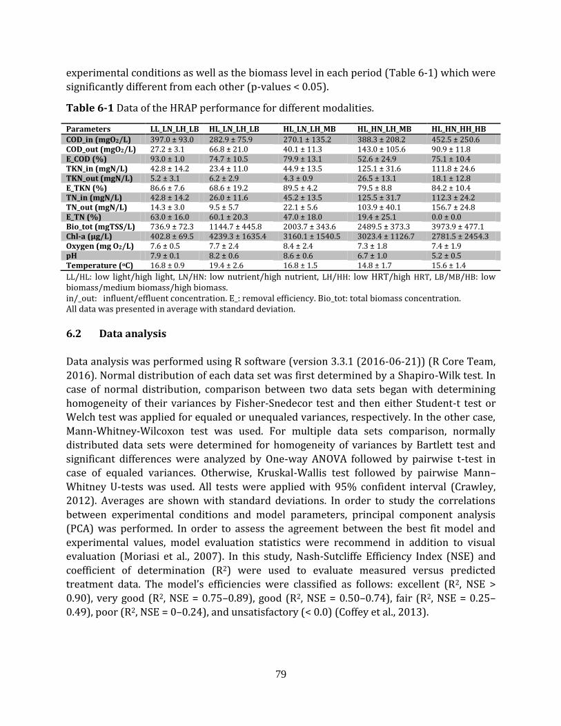
79

experimental conditions as well as the biomass level in each period (Table 6-1) which were

significantly different from each other (p-values < 0.05).

Table 6-1 Data of the HRAP performance for different modalities.

Parameters LL_LN_LH_LB HL_LN_LH_LB HL_LN_LH_MB HL_HN_LH_MB HL_HN_HH_HB

COD_in (mgO2/L) 397.0 ± 93.0 282.9 ± 75.9 270.1 ± 135.2 388.3 ± 208.2 452.5 ± 250.6 COD_out (mgO2/L) 27.2 ± 3.1 66.8 ± 21.0 40.1 ± 11.3 143.0 ± 105.6 90.9 ± 11.8 E_COD (%) 93.0 ± 1.0 74.7 ± 10.5 79.9 ± 13.1 52.6 ± 24.9 75.1 ± 10.4 TKN_in (mgN/L) 42.8 ± 14.2 23.4 ± 11.0 44.9 ± 13.5 125.1 ± 31.6 111.8 ± 24.6 TKN_out (mgN/L) 5.2 ± 3.1 6.2 ± 2.9 4.3 ± 0.9 26.5 ± 13.1 18.1 ± 12.8 E_TKN (%) 86.6 ± 7.6 68.6 ± 19.2 89.5 ± 4.2 79.5 ± 8.8 84.2 ± 10.4 TN_in (mgN/L) 42.8 ± 14.2 26.0 ± 11.6 45.2 ± 13.5 125.5 ± 31.7 112.3 ± 24.2 TN_out (mgN/L) 14.3 ± 3.0 9.5 ± 5.7 22.1 ± 5.6 103.9 ± 40.1 156.7 ± 24.8 E_TN (%) 63.0 ± 16.0 60.1 ± 20.3 47.0 ± 18.0 19.4 ± 25.1 0.0 ± 0.0 Bio_tot (mgTSS/L) 736.9 ± 72.3 1144.7 ± 445.8 2003.7 ± 343.6 2489.5 ± 373.3 3973.9 ± 477.1 Chl-a (μg/L) 402.8 ± 69.5 4239.3 ± 1635.4 3160.1 ± 1540.5 3023.4 ± 1126.7 2781.5 ± 2454.3 Oxygen (mg O2/L) 7.6 ± 0.5 7.7 ± 2.4 8.4 ± 2.4 7.3 ± 1.8 7.4 ± 1.9 pH 7.9 ± 0.1 8.2 ± 0.6 8.6 ± 0.6 6.7 ± 1.0 5.2 ± 0.5 Temperature (oC) 16.8 ± 0.9 19.4 ± 2.6 16.8 ± 1.5 14.8 ± 1.7 15.6 ± 1.4

LL/HL: low light/high light, LN/HN: low nutrient/high nutrient, LH/HH: low HRT/high HRT, LB/MB/HB: low biomass/medium biomass/high biomass. in/_out: influent/effluent concentration. E_: removal efficiency. Bio_tot: total biomass concentration. All data was presented in average with standard deviation.

6.2 Data analysis

Data analysis was performed using R software (version 3.3.1 (2016-06-21)) (R Core Team,

2016). Normal distribution of each data set was first determined by a Shapiro-Wilk test. In

case of normal distribution, comparison between two data sets began with determining

homogeneity of their variances by Fisher-Snedecor test and then either Student-t test or

Welch test was applied for equaled or unequaled variances, respectively. In the other case,

Mann-Whitney-Wilcoxon test was used. For multiple data sets comparison, normally

distributed data sets were determined for homogeneity of variances by Bartlett test and

significant differences were analyzed by One-way ANOVA followed by pairwise t-test in

case of equaled variances. Otherwise, Kruskal-Wallis test followed by pairwise Mann–

Whitney U-tests was used. All tests were applied with 95% confident interval (Crawley,

2012). Averages are shown with standard deviations. In order to study the correlations

between experimental conditions and model parameters, principal component analysis

(PCA) was performed. In order to assess the agreement between the best fit model and

experimental values, model evaluation statistics were recommend in addition to visual

evaluation (Moriasi et al., 2007). In this study, Nash-Sutcliffe Efficiency Index (NSE) and

coefficient of determination (R2) were used to evaluate measured versus predicted

treatment data. The model’s efficiencies were classified as follows: excellent (R2, NSE >

0.90), very good (R2, NSE = 0.75–0.89), good (R2, NSE = 0.50–0.74), fair (R2, NSE = 0.25–

0.49), poor (R2, NSE = 0–0.24), and unsatisfactory (< 0.0) (Coffey et al., 2013).

80

PART III RESULTS AND DISCUSSIONS

In this part, results of different experimental and modeling works are introduced and

discussed. Different inoculation ratios between algae and activated sludge were studied

(chapter 7), then an optimal inoculation ratio was chosen. A pilot HRAP was built and its

global hydraulic as well as gas transfer were investigated (chapter 8). Furthermore,

optimal biomass and operational conditions were employed in long term study on

wastewater treatment HRAP under different nutrient loads and HRTs (chapter 9). Results

achieved were used in calibration and validation black box (chapeter 10) and

comprehensive algal bacterial (chapter 11) models.

CHAPTER 7 FINDING OPTIMAL ALGAL/BACTERIAL INOCULATION RATIO TO

IMPROVE ALGAL BIOMASS GROWTH AND SETTLING EFFICIENCY

7.1 Introduction

Algal bacterial systems are promising for coupling wastewater treatment and nutrient

recovery (Muñoz and Guieysse, 2006). However, due to the small size of the algal cells and

their low concentration in culture solution, efficient harvesting algal biomass from water

can account 20-30% of total production cost (Mata et al., 2010; Pragya et al., 2013).

Therefore, algae harvesting remains one of the biggest challenges when operating the

system (Christenson and Sims, 2011; Craggs et al., 2015; Uduman et al., 2010). One solution

is to enhance algal biomass settleability by bio-flocculation (Salim et al., 2010; Vandamme

et al., 2013). Indeed, inoculating activated sludge with algae in wastewater has been shown

to improve biomass settling while keeping good treatment efficiency (Gutzeit et al., 2005;

Van Den Hende et al., 2011a). Studies on algal-bacterial biomass indicated high

gravitational settling efficiencies by flocculation between algae and bacteria (Gutzeit et al.,

2005; Medina and Neis, 2007; Van Den Hende et al., 2014). Van Den Hende et al. (2014)

recovered nearly 100% algal-bacterial biomass from a pilot scale study via two simple

harvesting steps including gravity settling and dewatering by manual filter press, requiring

no chemical addition and electricity (Van Den Hende et al., 2014). Therefore, the potential

of applying bio-flocculation technique into larger scale is promising.

One important factor when co-culturing algae and bacteria is their inoculation ratio.

Several studies suggested different optimal ratios. Su et al. studied different

algae/activated sludge inoculation ratios to treat domestic wastewater and reported that

algae/activated sludge ratio of 5:1 was the best for wastewater treatment and biomass

settling (Su et al., 2012). Roudsari et al. also compared various mixtures between algae and

activated sludge for anaerobic effluent of municipal wastewater treatment and suggested

biomass with higher proportion of algal biomass than bacterial biomass should be used

(Roudsari et al., 2014). However, Van Den Hende et al. successfully developed algal-

81

bacterial biomass (called MaB) with higher proportion of activated sludge and applied the

biomass in medium scale for treating domestic and industrial wastewater (Van Den Hende

et al., 2016b, 2016a, 2014). Moreover, most of the above cited studies mainly focused on

wastewater treatment efficiency and biomass harvesting. Data showing how inoculation

ratio between algae and activated sludge impacts algal growth is still lacking. Therefore a

study aiming to compare different algae/activated sludge inoculation ratios in terms of

algal growth, treatment efficiency and biomass settling is necessary.

Following chapter 4, results from batch experiments of algal-bacterial (Al-Bac) biomass

with three inoculation algae/activated sludge ratios (5:1, 1:1 and 1:5) with algal biomass as

control culturing in synthetic wastewater were shown. The impacts of different

algae/activated sludge inoculation ratios on algal growth, nutrient removal and settling

efficiency were discussed and the optimal ratio was chosen.

7.2 Biomass growth

The growth of total Al-Bac biomass during experimental period was estimated by TSS

measurements. Since the dissolved nutrients were the only supplement provided for each

reactor, any increase in total suspended solids inside the reactor was considered as a gain

in biomass. Besides the total Al-Bac biomass, the global productivity of Chl-a in each

reactor during experimental period, which is related to the increase of algae inside Al-Bac

biomass (Park and Craggs, 2010), was also monitored.

The slopes of TSS and Chl-a concentrations vs. time were used to derive the productivities

displayed in Figure 7-1.

Figure 7-1 Global Al-Bac biomass and Chl-a productivities of biomass with different initial algae/activated sludge ratios (error bars indicate standard error between fitted values and

observed values).

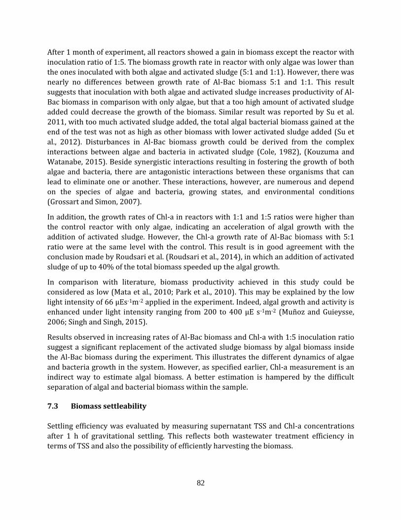
82

After 1 month of experiment, all reactors showed a gain in biomass except the reactor with

inoculation ratio of 1:5. The biomass growth rate in reactor with only algae was lower than

the ones inoculated with both algae and activated sludge (5:1 and 1:1). However, there was

nearly no differences between growth rate of Al-Bac biomass 5:1 and 1:1. This result

suggests that inoculation with both algae and activated sludge increases productivity of Al-

Bac biomass in comparison with only algae, but that a too high amount of activated sludge

added could decrease the growth of the biomass. Similar result was reported by Su et al.

2011, with too much activated sludge added, the total algal bacterial biomass gained at the

end of the test was not as high as other biomass with lower activated sludge added (Su et

al., 2012). Disturbances in Al-Bac biomass growth could be derived from the complex

interactions between algae and bacteria in activated sludge (Cole, 1982), (Kouzuma and

Watanabe, 2015). Beside synergistic interactions resulting in fostering the growth of both

algae and bacteria, there are antagonistic interactions between these organisms that can

lead to eliminate one or another. These interactions, however, are numerous and depend

on the species of algae and bacteria, growing states, and environmental conditions

(Grossart and Simon, 2007).

In addition, the growth rates of Chl-a in reactors with 1:1 and 1:5 ratios were higher than

the control reactor with only algae, indicating an acceleration of algal growth with the

addition of activated sludge. However, the Chl-a growth rate of Al-Bac biomass with 5:1

ratio were at the same level with the control. This result is in good agreement with the

conclusion made by Roudsari et al. (Roudsari et al., 2014), in which an addition of activated

sludge of up to 40% of the total biomass speeded up the algal growth.

In comparison with literature, biomass productivity achieved in this study could be

considered as low (Mata et al., 2010; Park et al., 2010). This may be explained by the low

light intensity of 66 µEs-1m-2 applied in the experiment. Indeed, algal growth and activity is

enhanced under light intensity ranging from 200 to 400 µE s-1m-2 (Muñoz and Guieysse,

2006; Singh and Singh, 2015).

Results observed in increasing rates of Al-Bac biomass and Chl-a with 1:5 inoculation ratio

suggest a significant replacement of the activated sludge biomass by algal biomass inside

the Al-Bac biomass during the experiment. This illustrates the different dynamics of algae

and bacteria growth in the system. However, as specified earlier, Chl-a measurement is an

indirect way to estimate algal biomass. A better estimation is hampered by the difficult

separation of algal and bacterial biomass within the sample.

7.3 Biomass settleability

Settling efficiency was evaluated by measuring supernatant TSS and Chl-a concentrations

after 1 h of gravitational settling. This reflects both wastewater treatment efficiency in

terms of TSS and also the possibility of efficiently harvesting the biomass.

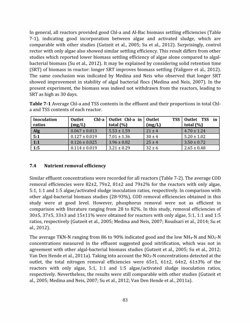
83

In general, all reactors provided good Chl-a and Al-Bac biomass settling efficiencies (Table

7-1), indicating good incorporation between algae and activated sludge, which are

comparable with other studies (Gutzeit et al., 2005; Su et al., 2012). Surprisingly, control

rector with only algae also showed similar settling efficiency. This result differs from other

studies which reported lower biomass settling efficiency of algae alone compared to algal-

bacterial biomass (Su et al., 2012). It may be explained by considering solid retention time

(SRT) of biomass in reactor: longer SRT improves biomass settling (Valigore et al., 2012).

The same conclusion was indicated by Medina and Neis who observed that longer SRT

showed improvement in stability of algal bacterial flocs (Medina and Neis, 2007). In the

present experiment, the biomass was indeed not withdrawn from the reactors, leading to

SRT as high as 30 days.

Table 7-1 Average Chl-a and TSS contents in the effluent and their proportions in total Chl-a and TSS contents of each reactor.

Inoculation ratios

Outlet Chl-a (mg/L)

Outlet Chl-a in total (%)

Outlet TSS (mg/L)

Outlet TSS in total (%)

Alg 0.067 ± 0.013 5.53 ± 1.59 21 ± 4 4.70 ± 1.24

5:1 0.127 ± 0.019 7.01 ± 1.36 30 ± 4 5.20 ± 1.02

1:1 0.126 ± 0.025 3.96 ± 0.82 25 ± 4 3.50 ± 0.72

1:5 0.114 ± 0.019 3.21 ± 0.29 32 ± 6 2.65 ± 0.48

7.4 Nutrient removal efficiency

Similar effluent concentrations were recorded for all reactors (Table 7-2). The average COD

removal efficiencies were 82±2, 79±2, 81±2 and 79±2% for the reactors with only algae,

5:1, 1:1 and 1:5 algae/activated sludge inoculation ratios, respectively. In comparison with

other algal-bacterial biomass studies (28-93%), COD removal efficiencies obtained in this

study were at good level. However, phosphorus removal were not as efficient in

comparison with literature ranging from 28 to 82%. In this study, removal efficiencies of

30±5, 37±5, 33±3 and 15±11% were obtained for reactors with only algae, 5:1, 1:1 and 1:5

ratios, respectively (Gutzeit et al., 2005; Medina and Neis, 2007; Roudsari et al., 2014; Su et

al., 2012).

The average TKN-N ranging from 86 to 90% indicated good and the low NH4-N and NO2-N

concentrations measured in the effluent suggested good nitrification, which was not in

agreement with other algal-bacterial biomass studies (Gutzeit et al., 2005; Su et al., 2012;

Van Den Hende et al., 2011a). Taking into account the NO3-N concentrations detected at the

outlet, the total nitrogen removal efficiencies were 65±1, 61±2, 64±2, 61±3% of the

reactors with only algae, 5:1, 1:1 and 1:5 algae/activated sludge inoculation ratios,

respectively. Nevertheless, the results were still comparable with other studies (Gutzeit et

al., 2005; Medina and Neis, 2007; Su et al., 2012; Van Den Hende et al., 2011a).

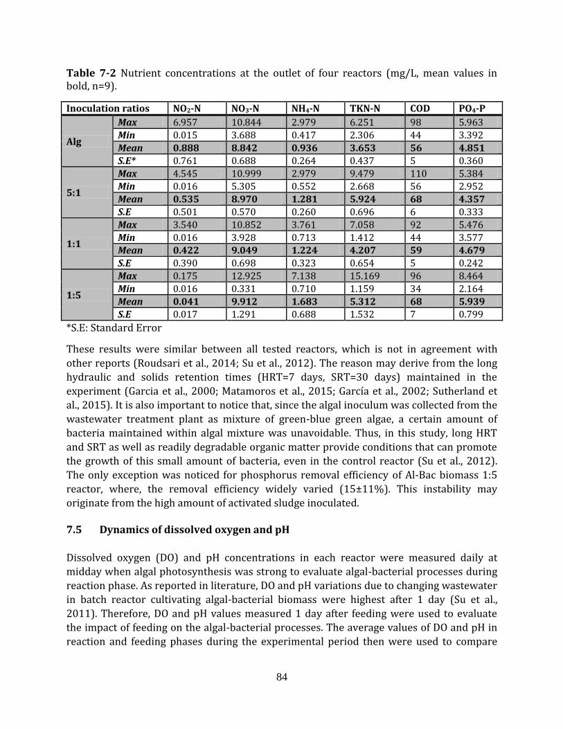
84

Table 7-2 Nutrient concentrations at the outlet of four reactors (mg/L, mean values in bold, n=9).

Inoculation ratios NO2-N NO3-N NH4-N TKN-N COD PO4-P

Alg

Max 6.957 10.844 2.979 6.251 98 5.963

Min 0.015 3.688 0.417 2.306 44 3.392

Mean 0.888 8.842 0.936 3.653 56 4.851

S.E* 0.761 0.688 0.264 0.437 5 0.360

5:1

Max 4.545 10.999 2.979 9.479 110 5.384 Min 0.016 5.305 0.552 2.668 56 2.952

Mean 0.535 8.970 1.281 5.924 68 4.357

S.E 0.501 0.570 0.260 0.696 6 0.333

1:1

Max 3.540 10.852 3.761 7.058 92 5.476

Min 0.016 3.928 0.713 1.412 44 3.577 Mean 0.422 9.049 1.224 4.207 59 4.679

S.E 0.390 0.698 0.323 0.654 5 0.242

1:5

Max 0.175 12.925 7.138 15.169 96 8.464

Min 0.016 0.331 0.710 1.159 34 2.164

Mean 0.041 9.912 1.683 5.312 68 5.939

S.E 0.017 1.291 0.688 1.532 7 0.799

*S.E: Standard Error

These results were similar between all tested reactors, which is not in agreement with

other reports (Roudsari et al., 2014; Su et al., 2012). The reason may derive from the long

hydraulic and solids retention times (HRT=7 days, SRT=30 days) maintained in the

experiment (Garcia et al., 2000; Matamoros et al., 2015; García et al., 2002; Sutherland et

al., 2015). It is also important to notice that, since the algal inoculum was collected from the

wastewater treatment plant as mixture of green-blue green algae, a certain amount of

bacteria maintained within algal mixture was unavoidable. Thus, in this study, long HRT

and SRT as well as readily degradable organic matter provide conditions that can promote

the growth of this small amount of bacteria, even in the control reactor (Su et al., 2012).

The only exception was noticed for phosphorus removal efficiency of Al-Bac biomass 1:5

reactor, where, the removal efficiency widely varied (15±11%). This instability may

originate from the high amount of activated sludge inoculated.

7.5 Dynamics of dissolved oxygen and pH

Dissolved oxygen (DO) and pH concentrations in each reactor were measured daily at

midday when algal photosynthesis was strong to evaluate algal-bacterial processes during

reaction phase. As reported in literature, DO and pH variations due to changing wastewater

in batch reactor cultivating algal-bacterial biomass were highest after 1 day (Su et al.,

2011). Therefore, DO and pH values measured 1 day after feeding were used to evaluate

the impact of feeding on the algal-bacterial processes. The average values of DO and pH in

reaction and feeding phases during the experimental period then were used to compare

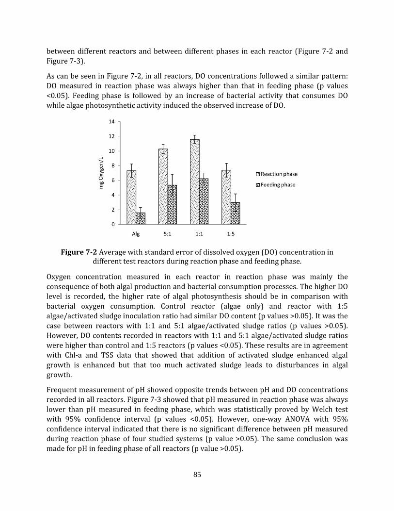
85

between different reactors and between different phases in each reactor (Figure 7-2 and

Figure 7-3).

As can be seen in Figure 7-2, in all reactors, DO concentrations followed a similar pattern:

DO measured in reaction phase was always higher than that in feeding phase (p values

<0.05). Feeding phase is followed by an increase of bacterial activity that consumes DO

while algae photosynthetic activity induced the observed increase of DO.

Figure 7-2 Average with standard error of dissolved oxygen (DO) concentration in different test reactors during reaction phase and feeding phase.

Oxygen concentration measured in each reactor in reaction phase was mainly the

consequence of both algal production and bacterial consumption processes. The higher DO

level is recorded, the higher rate of algal photosynthesis should be in comparison with

bacterial oxygen consumption. Control reactor (algae only) and reactor with 1:5

algae/activated sludge inoculation ratio had similar DO content (p values >0.05). It was the

case between reactors with 1:1 and 5:1 algae/activated sludge ratios (p values >0.05).

However, DO contents recorded in reactors with 1:1 and 5:1 algae/activated sludge ratios

were higher than control and 1:5 reactors (p values <0.05). These results are in agreement

with Chl-a and TSS data that showed that addition of activated sludge enhanced algal

growth is enhanced but that too much activated sludge leads to disturbances in algal

growth.

Frequent measurement of pH showed opposite trends between pH and DO concentrations

recorded in all reactors. Figure 7-3 showed that pH measured in reaction phase was always

lower than pH measured in feeding phase, which was statistically proved by Welch test

with 95% confidence interval (p values <0.05). However, one-way ANOVA with 95%

confidence interval indicated that there is no significant difference between pH measured

during reaction phase of four studied systems (p value >0.05). The same conclusion was

made for pH in feeding phase of all reactors (p value >0.05).

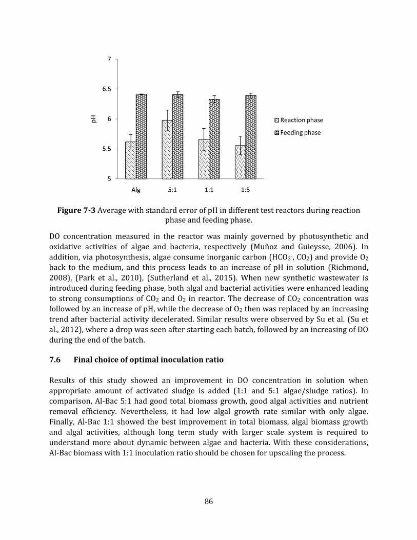
86

Figure 7-3 Average with standard error of pH in different test reactors during reaction phase and feeding phase.

DO concentration measured in the reactor was mainly governed by photosynthetic and

oxidative activities of algae and bacteria, respectively (Muñoz and Guieysse, 2006). In

addition, via photosynthesis, algae consume inorganic carbon (HCO3-, CO2) and provide O2

back to the medium, and this process leads to an increase of pH in solution (Richmond,

2008), (Park et al., 2010), (Sutherland et al., 2015). When new synthetic wastewater is

introduced during feeding phase, both algal and bacterial activities were enhanced leading

to strong consumptions of CO2 and O2 in reactor. The decrease of CO2 concentration was

followed by an increase of pH, while the decrease of O2 then was replaced by an increasing

trend after bacterial activity decelerated. Similar results were observed by Su et al. (Su et

al., 2012), where a drop was seen after starting each batch, followed by an increasing of DO

during the end of the batch.

7.6 Final choice of optimal inoculation ratio

Results of this study showed an improvement in DO concentration in solution when

appropriate amount of activated sludge is added (1:1 and 5:1 algae/sludge ratios). In

comparison, Al-Bac 5:1 had good total biomass growth, good algal activities and nutrient

removal efficiency. Nevertheless, it had low algal growth rate similar with only algae.

Finally, Al-Bac 1:1 showed the best improvement in total biomass, algal biomass growth

and algal activities, although long term study with larger scale system is required to

understand more about dynamic between algae and bacteria. With these considerations,

Al-Bac biomass with 1:1 inoculation ratio should be chosen for upscaling the process.

87

7.7 Conclusions

In this study, SBR reactors were used to cultivate Al-Bac biomass with different

algae/sludge inoculation ratios. In order to compare algal growth, initial algal biomass was

similar in every test. DO concentration and Chl-a content in all reactors were used to

evaluate algal activities, with high levels of DO and Chl-a growth rate indicating good algal

activities in the reactor. Local algal biomass showed good incorporation with bacterial

biomass (activated sludge): better algal growth occurred with Al-Bac biomass than with

only algae.

Several conclusions were made as follows:

- Adding activated sludge accelerated the growth of Al-Bac biomass although too

much activated sludge added may cause disturbance to the total biomass growth.

- Algal growth also increased with activated sludge added but significant amount of

sludge was required to have significant change.

- Biomass settling and nutrient removal efficiencies were similar in every test

including control with only algae. Possible reason may due to long hydraulic

retention time and solid retention time.

Among three inoculation ratios evaluated, Al-Bac biomass with 1:1 inoculation ratio

showed the best enhancement in total biomass, algal biomass growth, and algal activities.

In French:

Durant cette étude, des réacteurs fermés ont été utilisés pour cultiver la biomasse Al-Bac

avec différents rapports d'inoculation algues/boues. Afin de comparer la croissance des

algues, la biomasse initiale des algues était similaire dans tous les essais. La concentration

en oxygène dissous et la teneur en chlorophylle A (Chl-a) dans tous les réacteurs ont été

utilisées pour évaluer l’activité algale, des niveaux élevés d'oxygène et de Chl-a indiquant

un bon taux de croissance des algues dans le réacteur. La biomasse algale a montré une

bonne incorporation avec la biomasse bactérienne (boues activées) : une meilleure

croissance algale s'est produite avec la biomasse Al-Bac qu'avec seulement les algues.

Plusieurs conclusions ont été tirées comme suit:

- L'ajout de boues activées a accéléré la croissance de la biomasse Al-Bac, bien qu'une

trop grande quantité de boues activées ajoutées puisse perturber la croissance

totale de la biomasse.

- La croissance des algues a également augmenté avec l'augmentation de la

proportion de boues activées, mais une quantité importante de boues était

nécessaire pour qu'il y ait un changement significatif.

88

- L'efficacité de la décantation de la biomasse et de l'élimination des éléments

nutritifs était semblable dans tous les essais, y compris le contrôle avec seulement

des algues. Cela est sans doute lié aux longs temps de séjour hydraulique et de la

biomasse.

Parmi les trois rapports d'inoculation évalués, la biomasse Al-Bac avec un rapport

d'inoculation de 1:1 a montré la meilleure amélioration de la biomasse totale, de la

croissance de la biomasse algale et de activités algales.

89

CHAPTER 8 IMPACTS OF OPERATIONAL CONDITIONS ON OXYGEN TRANSFER RATE,

MIXING CHARACTERISTICS AND RESIDENCE TIME DISTRIBUTION IN A PILOT SCALE

HIGH RATE ALGAL POND

In general, open bioreactors and closed photobioreactors are the main systems applied for

algal cultivation (Muñoz and Guieysse, 2006). In comparison, closed photobioreactors

provide better control over cultivation conditions including nutrients, mixing, light and

temperature, hence they allow much denser algal culture to develop yet lower risk of

contamination. However, in practice, the closed condition results to heat and oxygen

accumulation that negatively impact the growth of algae. Moreover, illumination supply has

to rely on the penetration transparent material of the reactor which can be deteriorated.

Therefore, operation and maintenance of closed photobioreactors are complex and labor

consuming resulting in much higher cost of biomass production than open bioreactors

(Mata et al., 2010). Therefore, it was estimated that HRAP accounted for 95% of large scale

microalgae production facilities worldwide (Kumar et al., 2015). One major aspect when

operating HRAP is the hydrodynamics because proper mixing allows materials to be evenly

distributed in the pond, avoids sedimentation and thus anaerobic condition. Extensive

studies have been conducted to investigate the impacts of pond or paddlewheel designs as

well as some operational conditions on hydrodynamics and energy consumption in the

HRAP. Advanced mathematical models were employed to understand flowing patterns in

the raceway under such influences ( El Ouarghi et al., 2000; Jupsin et al., 2003; Bitog et al.,

2011; Hadiyanto et al., 2013; Liffman et al., 2013; Mendoza et al., 2013; Hreiz et al., 2014),

yet there is still need for experimental validation (Hadiyanto et al., 2013).

Due to its advantages, HRAP can be applied in many places with wide range of

environmental conditions (Picot et al., 1991; El Hamouri et al., 1995; Grönlund et al., 2010).

Therefore, its operational conditions (water level, paddle wheel movement) must be

adjusted to improve algal photosynthesis and productivity by increasing the turbulent

mixing in the pond (Sutherland, et al., 2015). Moreover, the inlet flow rate may influence

the hydrodynamics inside HRAP. In addition, hydrodynamics is one of the major factors

influencing gas transfer in open aerobic biological reactor like HRAP (Garcia-Ochoa and

Gomez, 2009). Therefore, varying operational conditions could have a direct impact on gas

transfer or biochemical processes and on the performance of the system.

The following sections provide results from different experiments studying global

hydraulic, mixing characteristics and oxygen transfer of the HRAP under different

operational conditions including paddle rotational speed, water level and inlet flow rate.

Impacts of these conditions were also discussed and the optimal conditions for algal

growth were chosen.

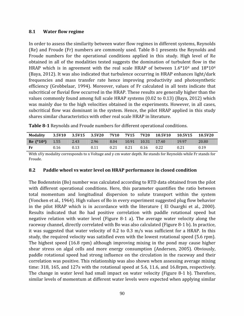
90

8.1 Water flow regime

In order to assess the similarity between water flow regimes in different systems, Reynolds

(Re) and Froude (Fr) numbers are commonly used. Table 8-1 presents the Reynolds and

Froude numbers for the operational conditions applied in this study. High level of Re

obtained in all of the modalities tested suggests the domination of turbulent flow in the

HRAP which is in agreement with the real scale HRAP of between 1.6*104 and 18*104

(Baya, 2012). It was also indicated that turbulence occurring in HRAP enhances light/dark

frequencies and mass transfer rate hence improving productivity and photosynthetic

efficiency (Grobbelaar, 1994). Moreover, values of Fr calculated in all tests indicate that

subcritical or fluvial flow occurred in the HRAP. These results are generally higher than the

values commonly found among full scale HRAP systems (0.02 to 0.13) (Baya, 2012) which

was mainly due to the high velocities obtained in the experiments. However, in all cases,

subcritical flow was dominant in the system. Hence, the pilot HRAP applied in this study

shares similar characteristics with other real scale HRAP in literature.

Table 8-1 Reynolds and Froude numbers for different operational conditions.

Modality 3.5V10 3.5V15 3.5V20 7V10 7V15 7V20 10.5V10 10.5V15 10.5V20

Re (*104) 1.55 2.43 2.96 8.04 10.91 10.31 17.40 19.97 20.80

Fr 0.16 0.13 0.11 0.21 0.21 0.16 0.22 0.21 0.19

With xVy modality corresponds to x Voltage and y cm water depth. Re stands for Reynolds while Fr stands for

Froude.

8.2 Paddle wheel vs water level on HRAP performance in closed condition

The Bodenstein (Bo) number was calculated according to RTD data obtained from the pilot

with different operational conditions. Here, this parameter quantifies the ratio between

total momentum and longitudinal dispersion to solute transport within the system

(Voncken et al., 1964). High values of Bo in every experiment suggested plug flow behavior

in the pilot HRAP which is in accordance with the literature ( El Ouarghi et al., 2000).

Results indicated that Bo had positive correlation with paddle rotational speed but

negative relation with water level (Figure 8-1 a). The average water velocity along the

raceway channel, directly correlated with Bo was also calculated (Figure 8-1 b). In practice,

it was suggested that water velocity of 0.2 to 0.3 m/s was sufficient for a HRAP. In this

study, the required velocity was satisfied even with the lowest rotational speed (5.6 rpm).

The highest speed (16.8 rpm) although improving mixing in the pond may cause higher

shear stress on algal cells and more energy consumption (Andersen, 2005). Obviously,

paddle rotational speed had strong influence on the circulation in the raceway and their

correlation was positive. This relationship was also shown when assessing average mixing

time: 318, 165, and 127s with the rotational speed at 5.6, 11.6, and 16.8rpm, respectively.

The change in water level had small impact on water velocity (Figure 8-1 b). Therefore,

similar levels of momentum at different water levels were expected when applying similar

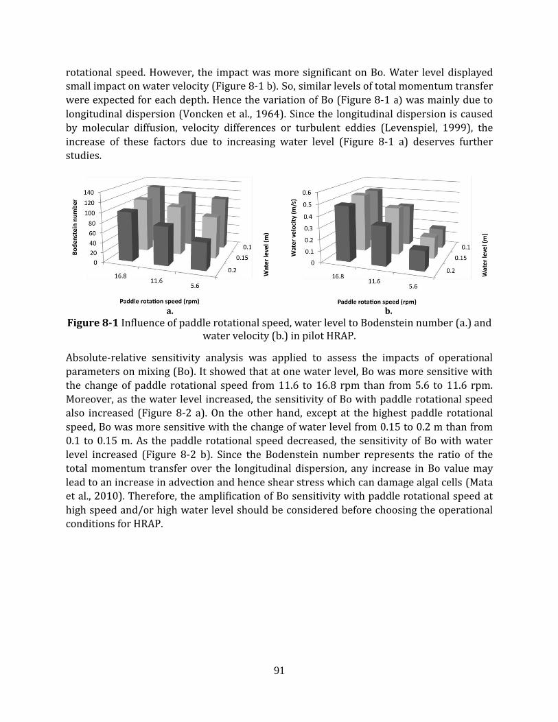
91

rotational speed. However, the impact was more significant on Bo. Water level displayed small impact on water velocity (Figure 8-1 b). So, similar levels of total momentum transfer

were expected for each depth. Hence the variation of Bo (Figure 8-1 a) was mainly due to

longitudinal dispersion (Voncken et al., 1964). Since the longitudinal dispersion is caused

by molecular diffusion, velocity differences or turbulent eddies (Levenspiel, 1999), the

increase of these factors due to increasing water level (Figure 8-1 a) deserves further

studies.

a. b.

Figure 8-1 Influence of paddle rotational speed, water level to Bodenstein number (a.) and water velocity (b.) in pilot HRAP.

Absolute-relative sensitivity analysis was applied to assess the impacts of operational

parameters on mixing (Bo). It showed that at one water level, Bo was more sensitive with

the change of paddle rotational speed from 11.6 to 16.8 rpm than from 5.6 to 11.6 rpm.

Moreover, as the water level increased, the sensitivity of Bo with paddle rotational speed

also increased (Figure 8-2 a). On the other hand, except at the highest paddle rotational

speed, Bo was more sensitive with the change of water level from 0.15 to 0.2 m than from

0.1 to 0.15 m. As the paddle rotational speed decreased, the sensitivity of Bo with water

level increased (Figure 8-2 b). Since the Bodenstein number represents the ratio of the

total momentum transfer over the longitudinal dispersion, any increase in Bo value may

lead to an increase in advection and hence shear stress which can damage algal cells (Mata

et al., 2010). Therefore, the amplification of Bo sensitivity with paddle rotational speed at

high speed and/or high water level should be considered before choosing the operational

conditions for HRAP.

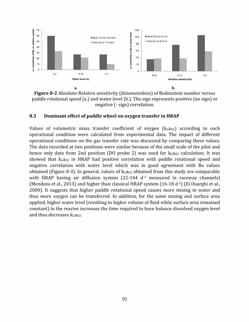
92

a.

b.

Figure 8-2 Absolute-Relative sensitivity (dimensionless) of Bodenstein number versus paddle rotational speed (a.) and water level (b.). The sign represents positive (no sign) or

negative (- sign) correlation.

8.3 Dominant effect of paddle wheel on oxygen transfer in HRAP

Values of volumetric mass transfer coefficient of oxygen (kLaO2) according to each

operational condition were calculated from experimental data. The impact of different

operational conditions on the gas transfer rate was discussed by comparing these values.

The data recorded at two positions were similar because of the small scale of the pilot and

hence only data from 2nd position (DO probe 2) was used for kLaO2 calculation. It was

showed that kLaO2 in HRAP had positive correlation with paddle rotational speed and

negative correlation with water level which was in good agreement with Bo values

obtained (Figure 8-3). In general, values of kLaO2 obtained from this study are comparable

with HRAP having air diffusion system (22-144 d-1 measured in raceway channels)

(Mendoza et al., 2013) and higher than classical HRAP system (16-18 d-1) (El Ouarghi et al.,

2000). It suggests that higher paddle rotational speed causes more mixing in water and

thus more oxygen can be transferred. In addition, for the same mixing and surface area

applied, higher water level (resulting to higher volume of fluid while surface area remained

constant) in the reactor increases the time required to have balance dissolved oxygen level

and thus decreases kLaO2.

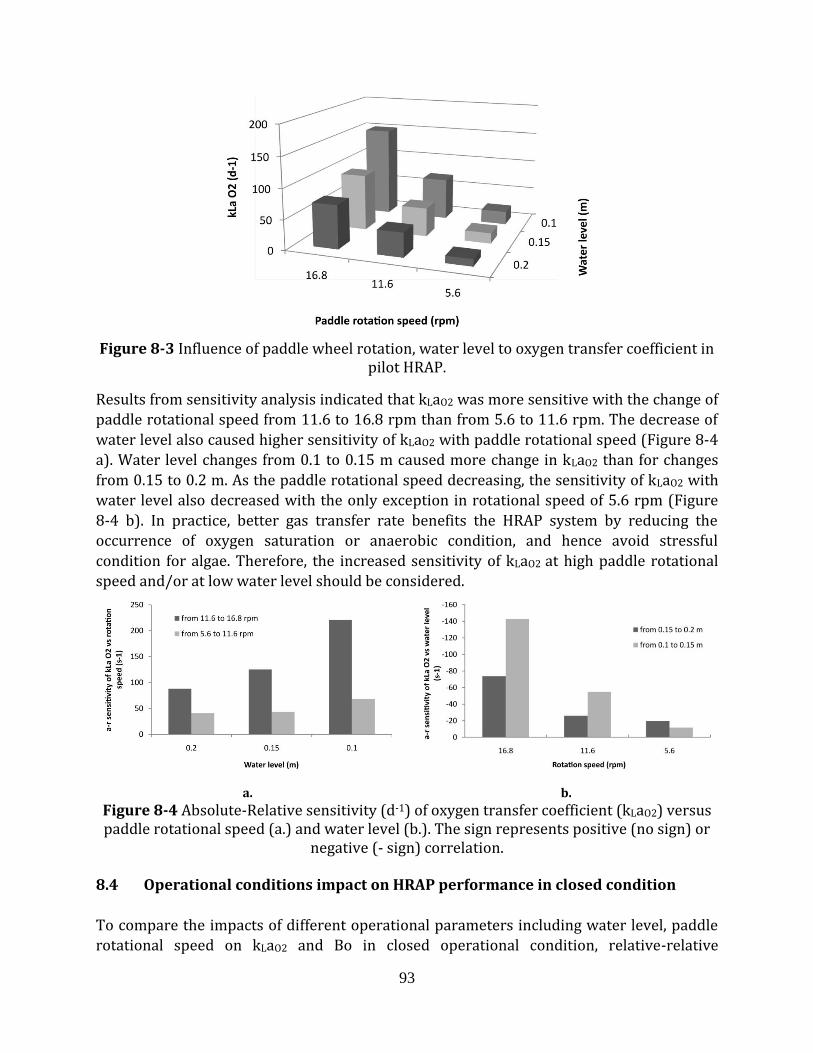
93

Figure 8-3 Influence of paddle wheel rotation, water level to oxygen transfer coefficient in pilot HRAP.

Results from sensitivity analysis indicated that kLaO2 was more sensitive with the change of

paddle rotational speed from 11.6 to 16.8 rpm than from 5.6 to 11.6 rpm. The decrease of

water level also caused higher sensitivity of kLaO2 with paddle rotational speed (Figure 8-4

a). Water level changes from 0.1 to 0.15 m caused more change in kLaO2 than for changes

from 0.15 to 0.2 m. As the paddle rotational speed decreasing, the sensitivity of kLaO2 with

water level also decreased with the only exception in rotational speed of 5.6 rpm (Figure

8-4 b). In practice, better gas transfer rate benefits the HRAP system by reducing the

occurrence of oxygen saturation or anaerobic condition, and hence avoid stressful

condition for algae. Therefore, the increased sensitivity of kLaO2 at high paddle rotational

speed and/or at low water level should be considered.

a.

b.

Figure 8-4 Absolute-Relative sensitivity (d-1) of oxygen transfer coefficient (kLaO2) versus paddle rotational speed (a.) and water level (b.). The sign represents positive (no sign) or

negative (- sign) correlation.

8.4 Operational conditions impact on HRAP performance in closed condition

To compare the impacts of different operational parameters including water level, paddle

rotational speed on kLaO2 and Bo in closed operational condition, relative-relative

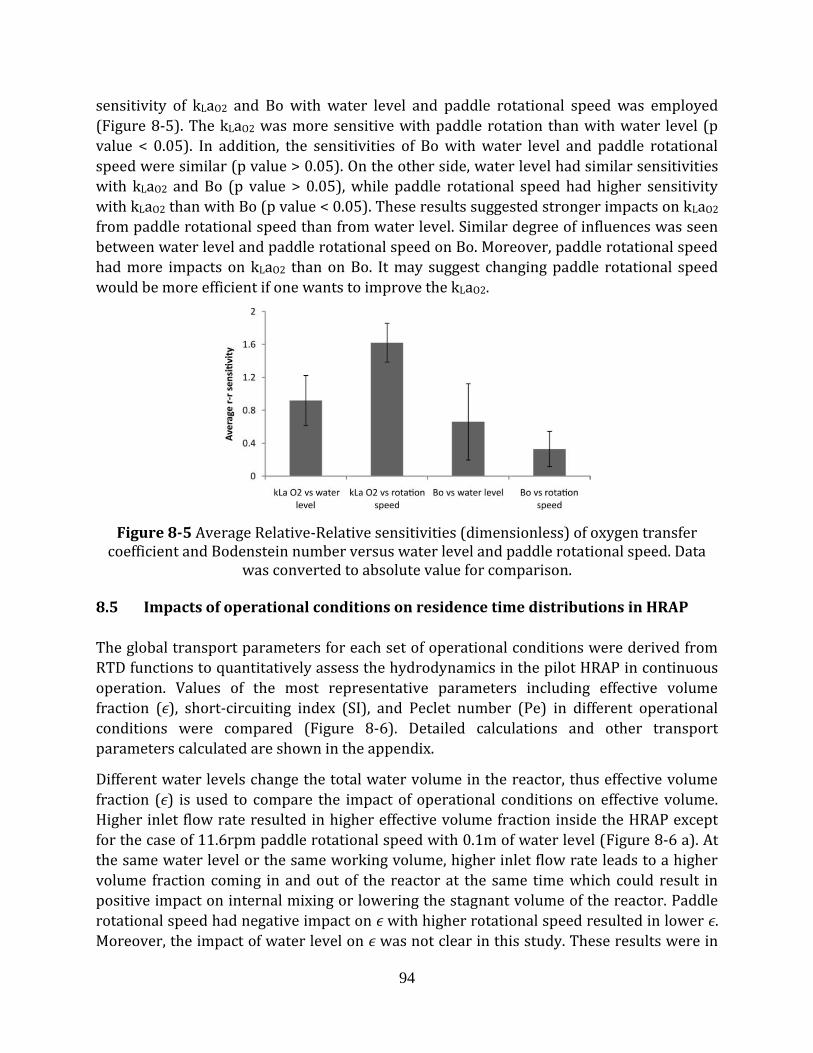
94

sensitivity of kLaO2 and Bo with water level and paddle rotational speed was employed

(Figure 8-5). The kLaO2 was more sensitive with paddle rotation than with water level (p

value < 0.05). In addition, the sensitivities of Bo with water level and paddle rotational

speed were similar (p value > 0.05). On the other side, water level had similar sensitivities

with kLaO2 and Bo (p value > 0.05), while paddle rotational speed had higher sensitivity

with kLaO2 than with Bo (p value < 0.05). These results suggested stronger impacts on kLaO2

from paddle rotational speed than from water level. Similar degree of influences was seen

between water level and paddle rotational speed on Bo. Moreover, paddle rotational speed

had more impacts on kLaO2 than on Bo. It may suggest changing paddle rotational speed

would be more efficient if one wants to improve the kLaO2.

Figure 8-5 Average Relative-Relative sensitivities (dimensionless) of oxygen transfer coefficient and Bodenstein number versus water level and paddle rotational speed. Data

was converted to absolute value for comparison.

8.5 Impacts of operational conditions on residence time distributions in HRAP

The global transport parameters for each set of operational conditions were derived from

RTD functions to quantitatively assess the hydrodynamics in the pilot HRAP in continuous

operation. Values of the most representative parameters including effective volume

fraction (ϵ), short-circuiting index (SI), and Peclet number (Pe) in different operational

conditions were compared (Figure 8-6). Detailed calculations and other transport

parameters calculated are shown in the appendix.

Different water levels change the total water volume in the reactor, thus effective volume

fraction (ϵ) is used to compare the impact of operational conditions on effective volume.

Higher inlet flow rate resulted in higher effective volume fraction inside the HRAP except

for the case of 11.6rpm paddle rotational speed with 0.1m of water level (Figure 8-6 a). At

the same water level or the same working volume, higher inlet flow rate leads to a higher

volume fraction coming in and out of the reactor at the same time which could result in

positive impact on internal mixing or lowering the stagnant volume of the reactor. Paddle

rotational speed had negative impact on ϵ with higher rotational speed resulted in lower ϵ.

Moreover, the impact of water level on ϵ was not clear in this study. These results were in

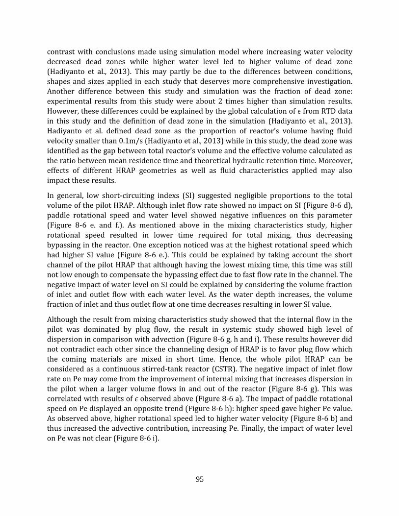
95

contrast with conclusions made using simulation model where increasing water velocity

decreased dead zones while higher water level led to higher volume of dead zone

(Hadiyanto et al., 2013). This may partly be due to the differences between conditions,

shapes and sizes applied in each study that deserves more comprehensive investigation.

Another difference between this study and simulation was the fraction of dead zone:

experimental results from this study were about 2 times higher than simulation results.

However, these differences could be explained by the global calculation of ϵ from RTD data

in this study and the definition of dead zone in the simulation (Hadiyanto et al., 2013).

Hadiyanto et al. defined dead zone as the proportion of reactor’s volume having fluid

velocity smaller than 0.1m/s (Hadiyanto et al., 2013) while in this study, the dead zone was

identified as the gap between total reactor’s volume and the effective volume calculated as

the ratio between mean residence time and theoretical hydraulic retention time. Moreover,

effects of different HRAP geometries as well as fluid characteristics applied may also

impact these results.

In general, low short-circuiting indexs (SI) suggested negligible proportions to the total

volume of the pilot HRAP. Although inlet flow rate showed no impact on SI (Figure 8-6 d),

paddle rotational speed and water level showed negative influences on this parameter

(Figure 8-6 e. and f.). As mentioned above in the mixing characteristics study, higher

rotational speed resulted in lower time required for total mixing, thus decreasing

bypassing in the reactor. One exception noticed was at the highest rotational speed which

had higher SI value (Figure 8-6 e.). This could be explained by taking account the short

channel of the pilot HRAP that although having the lowest mixing time, this time was still

not low enough to compensate the bypassing effect due to fast flow rate in the channel. The

negative impact of water level on SI could be explained by considering the volume fraction

of inlet and outlet flow with each water level. As the water depth increases, the volume

fraction of inlet and thus outlet flow at one time decreases resulting in lower SI value.

Although the result from mixing characteristics study showed that the internal flow in the

pilot was dominated by plug flow, the result in systemic study showed high level of

dispersion in comparison with advection (Figure 8-6 g, h and i). These results however did

not contradict each other since the channeling design of HRAP is to favor plug flow which

the coming materials are mixed in short time. Hence, the whole pilot HRAP can be

considered as a continuous stirred-tank reactor (CSTR). The negative impact of inlet flow

rate on Pe may come from the improvement of internal mixing that increases dispersion in

the pilot when a larger volume flows in and out of the reactor (Figure 8-6 g). This was

correlated with results of ϵ observed above (Figure 8-6 a). The impact of paddle rotational

speed on Pe displayed an opposite trend (Figure 8-6 h): higher speed gave higher Pe value.

As observed above, higher rotational speed led to higher water velocity (Figure 8-6 b) and

thus increased the advective contribution, increasing Pe. Finally, the impact of water level

on Pe was not clear (Figure 8-6 i).

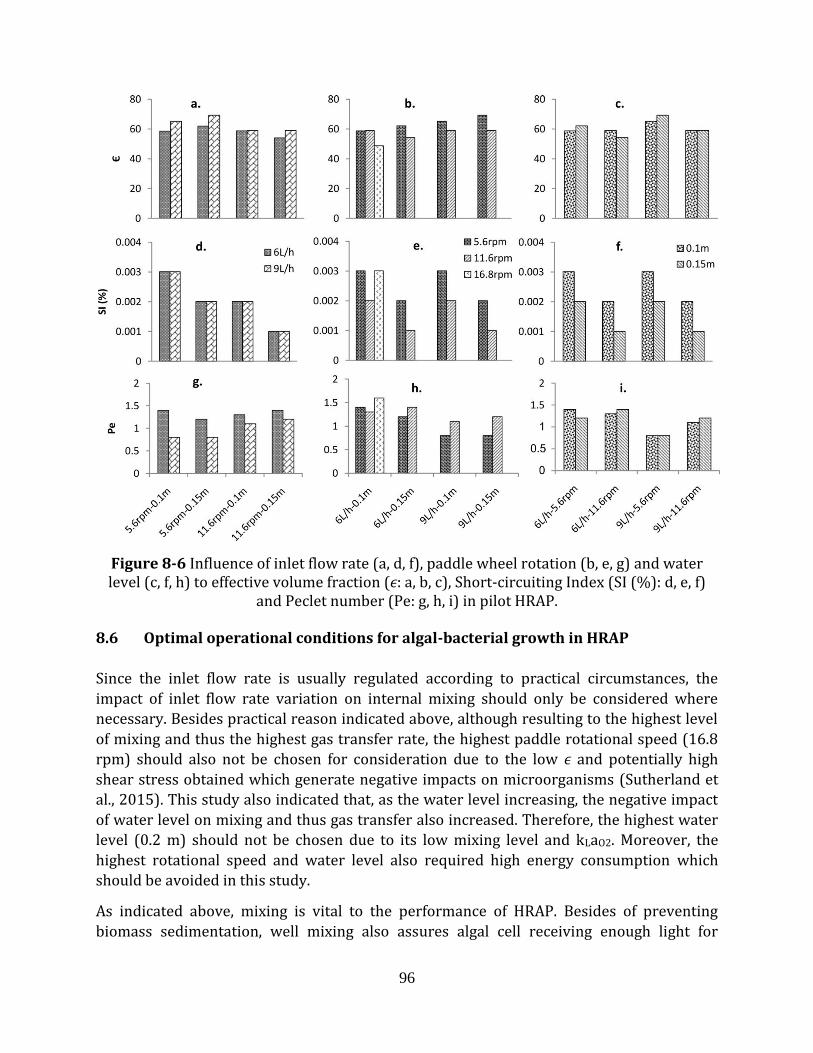
96

Figure 8-6 Influence of inlet flow rate (a, d, f), paddle wheel rotation (b, e, g) and water level (c, f, h) to effective volume fraction (ϵ: a, b, c), Short-circuiting Index (SI (%): d, e, f)

and Peclet number (Pe: g, h, i) in pilot HRAP.

8.6 Optimal operational conditions for algal-bacterial growth in HRAP

Since the inlet flow rate is usually regulated according to practical circumstances, the

impact of inlet flow rate variation on internal mixing should only be considered where

necessary. Besides practical reason indicated above, although resulting to the highest level

of mixing and thus the highest gas transfer rate, the highest paddle rotational speed (16.8

rpm) should also not be chosen for consideration due to the low ϵ and potentially high

shear stress obtained which generate negative impacts on microorganisms (Sutherland et

al., 2015). This study also indicated that, as the water level increasing, the negative impact

of water level on mixing and thus gas transfer also increased. Therefore, the highest water

level (0.2 m) should not be chosen due to its low mixing level and kLaO2. Moreover, the

highest rotational speed and water level also required high energy consumption which

should be avoided in this study.

As indicated above, mixing is vital to the performance of HRAP. Besides of preventing

biomass sedimentation, well mixing also assures algal cell receiving enough light for

97

photosynthesis. Moreover, high level of mixing also results to high gas transfer rate which

is important especially to decrease the occurrence of oxygen oversaturation or ammonia

accumulation in HRAP (Park et al., 2010). Due to the argument above, the low (5.6 rpm)

and medium (11.6 rpm) rotational speeds are considered. Although 5.6 rpm provided

higher ϵ and lower SI which may better support HRAP performance, these differences were

small and can be compensated by the benefit of higher gas transfer. Therefore, the medium

(11.6 rpm) should be applied for algal-bacterial growth.

Water level determines the light penetration into the culture and thus should be as shallow

as possible to maximize the amount of light provided to algae (Andersen, 2005). After

eliminating the highest value, two water levels of 0.1 and 0.15 m are considered which the

former resulted to higher level of mixing and thus higher gas transfer rate. Although low

water level also leads to thermal instability causing growth inhibition (Sutherland et al.,

2015), this risk is higher when applying the HRAP at outdoor condition. Therefore, with the

indoor condition in this study, the low water level of 0.1 m was the better option.

It was shown that variation of operational conditions resulted to changes in

hydrodynamics and gas transfer in the HRAP. In order to apply the pilot for algal-bacterial

growth, the chosen operational conditions should have positive impacts on biochemical

processes inside. Therefore, the best combination of operational conditions in this study

should be between water level of 0.1m and paddle rotational speed of 11.6rpm.

8.7 Conclusions

In this study, different combinations of water level, paddle rotational speed and flow rate

were applied to investigate their impacts on mixing characteristics, residence time

distributions and gas transfer coefficients of the pilot HRAP. In general, the pilot HRAP

shared similar characteristics with other real scale HRAPs and was dominated by turbulent

flow in its channel. Moreover, the HRAP showed good mixing level even with the lowest

paddle rotational speed applied, and hence the entire HRAP can be considered as a CSTR. In

closed condition, Bodenstein number, water velocity and oxygen transfer coefficient had

positive correlation with paddle rotational speed but negative correlation with water level

although the impact of water level on water velocity was small. Amplification effect of

water level and paddle rotational speed on sensitivity of Bo and kLaO2 should be noticed

and considered before applying operational parameters to HRAP system. Paddle rotational

speed had more impact on kLaO2 than on Bo. In open condition, effective volume fraction (ϵ)

had positive correlation with inlet flow rate and negative correlation with paddle rotation,

while the opposite was observed in the case of Pe. Variation of water level show unclear

impact on these parameters. Both water level and paddle rotational speed had negative

impacts on short-circuiting index (SI) while no correlation was observed when varying

inlet flow rate. The best combination of operational conditions for algal-bacterial growth in

HRAP is between low water level (0.1 m) and medium paddle rotational speed (11.6 rpm).

These data obtained could be useful for (i) algal-bacterial growth for waste water

98

treatment and biomass production, and (ii) calibrating 3D hydrodynamic model for better

studying the impact of operational conditions on HRAP. Moreover, a further step would be

to apply the knowledge achieved from pilot studies for designing and operating outdoor

large scale HRAP system, so the up-scaling factors can be evaluated.

In French:

Dans cette étude, différentes combinaisons de niveau d'eau, de vitesse de rotation des pales

et de débit d’alimentation ont été appliquées pour étudier leurs impacts sur les

caractéristiques de mélange, la distribution des temps de séjour et les coefficients de

transfert gaz/liquide de la HRAP pilote. En général, la HRAP pilote partageait des

caractéristiques semblables à celles d'autres HRAP à l'échelle réelle et était dominée par un

écoulement turbulent. Un bon niveau de mélange a été observé même avec la vitesse de

rotation de la pale la plus lente. L'ensemble du réacteur peut être considéré comme

parfaitement agité. Le nombre de Bodenstein (Bo), la vitesse de l'eau et le coefficient de

transfert d'oxygène sont corrélés positivement avec la vitesse de rotation de la pâle, mais

une négativement avec le niveau d'eau, bien que l'impact du niveau de l'eau sur la vitesse

linéaire de l'eau ait été faible. On peut noter l'effet d'amplification du niveau d'eau et de la

vitesse de rotation de la pâle sur la sensibilité du Bo et du coefficient de transfert

gaz/liquide doit être remarqué et pris en compte avant d'appliquer les paramètres

opérationnels au système HRAP. La vitesse de rotation de la pâle a plus d'impact sur le

coefficient de transfert que sur Bo. En condition ouverte, la fraction volumique effective (ϵ)

a une corrélation positive avec le débit d'entrée et une corrélation négative avec la rotation

de la pâle, alors que l'inverse a été observé dans le cas du nombre de Péclet. Les variations

du niveau d'eau montrent un impact peu clair sur ces paramètres. Le niveau d'eau et la

vitesse de rotation de la pale ont des impacts négatifs sur l'indice de court-circuit (SI), alors

qu'aucune corrélation n'a été observée lorsque le débit d'entrée variait. La meilleure

combinaison de conditions opérationnelles pour la croissance algale-bactérienne dans le

réacteur HRAP se situe entre un niveau d'eau bas (0,1 m) et une vitesse de rotation

moyenne de la palette (11,6 rpm). Ces données obtenues pourraient être utiles pour (i) la

croissance algale-bactérienne pour le traitement des eaux usées et la production de

biomasse, et (ii) l'étalonnage du modèle hydrodynamique 3D pour mieux étudier l'impact

des conditions opérationnelles sur le réacteur HRAP. En outre, une autre étape consisterait

à appliquer les connaissances acquises dans le cadre d'études pilotes pour la conception et

l'exploitation d'un système HRAP à grande échelle à l'extérieur, afin d'évaluer les facteurs

de mise à l'échelle.

99

CHAPTER 9 LONG-TERM WASTEWATER TREATMENT BY ALGAL BACTERIAL

BIOMASS IN HIGH RATE ALGAL POND (HRAP): IMPACT OF NUTRIENT LOAD AND

HYDRAULIC RETENTION TIME

Although application of algal-bacterial biomass in HRAP system for wastewater treatment

and biomass production is promising, the dynamic between algae and bacteria and its

impact on long term performance of the system is still lacking. In addition, in recent years,

anaerobic digestion has become a popular solution for bioenergy production and the use of

its liquid effluent as nutrient source of HRAP system promoting nutrient recovery has been

attracting (Sawatdeenarunat et al., 2016). Hence, the impact of high nutrient load from

anaerobic digestion effluent on the algal bacterial dynamic deserves serious attention.

In chapter 4, long-term pilot-scale HRAP operation was described. The aim was to evaluate

the dynamic between algae and bacteria under medium and high nutrient loads within a

pilot scale HRAP inoculated with algal-bacterial biomass. The performance of the system

was also assessed in terms of treatment efficiency, biomass production and recovery.

Impact of hydraulic retention time (HRT) variation in high nutrient load condition on the

system was also investigated.

Data collected from 246 days of HRAP system operation was evaluated. The performance of

the system in terms of treatment efficiency, biomass production and recovery is presented

and discussed. After this, further analyses were done in order to assess the dynamic of algal

bacterial processes under nutrient load and HRT variation.

9.1 Impact of different nutrient loads and HRTs on wastewater treatment

Influent and effluent concentrations of different wastewater constituents studied in the

entire pilot operation are presented in Figure 9-1. Dramatic increases of influent nitrogen

and phosphorus concentrations were noticed after the introduction of high nutrient load

wastewater in the last 2 stages. In comparison with the first stage, influent TKN

concentration increased from 34.8 ± 16.1 to 123.5 ± 33.8 mg N/L in the second stage and

114.5 ± 24.4 mg N/L in the last stage while TP concentration also raised from 4.3 ± 1.3 to

31.4 ± 11.5 mg P/L and 41.2 ± 14.3 mg P/L in the second and third stage, respectively.

However, the COD levels were at the same magnitude for the three modalities which were

313.3 ± 157.0, 339.9 ± 207.5 and 430.2 ± 243.8 mg O2/L for LN_4d, HN_4d and HN_8d,

respectively (p-value > 0.05). The result was in agreement with the indication that the main

constituents in liquid effluent from the anaerobic digestion system are ammonium nitrogen

and phosphorus (Sawatdeenarunat et al., 2016). Moreover, the high fluctuation of influent

COD concentration was also noticed, especially when wastewater with high nutrient load

was introduced. It suggests that the occurrence of bacterial degradation in the storage tank,

even at low temperature 4oC, can significantly reduce the COD level (Grady Jr et al., 2011).

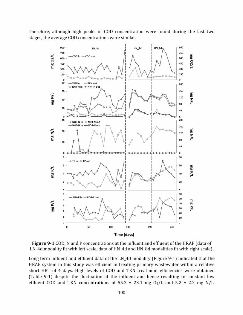
100

Therefore, although high peaks of COD concentration were found during the last two

stages, the average COD concentrations were similar.

Figure 9-1 COD, N and P concentrations at the influent and effluent of the HRAP (data of LN_4d modality fit with left scale, data of HN_4d and HN_8d modalities fit with right scale).

Long term influent and effluent data of the LN_4d modality (Figure 9-1) indicated that the

HRAP system in this study was efficient in treating primary wastewater within a relative

short HRT of 4 days. High levels of COD and TKN treatment efficiencies were obtained

(Table 9-1) despite the fluctuation at the influent and hence resulting to constant low

effluent COD and TKN concentrations of 55.2 ± 23.1 mg O2/L and 5.2 ± 2.2 mg N/L,

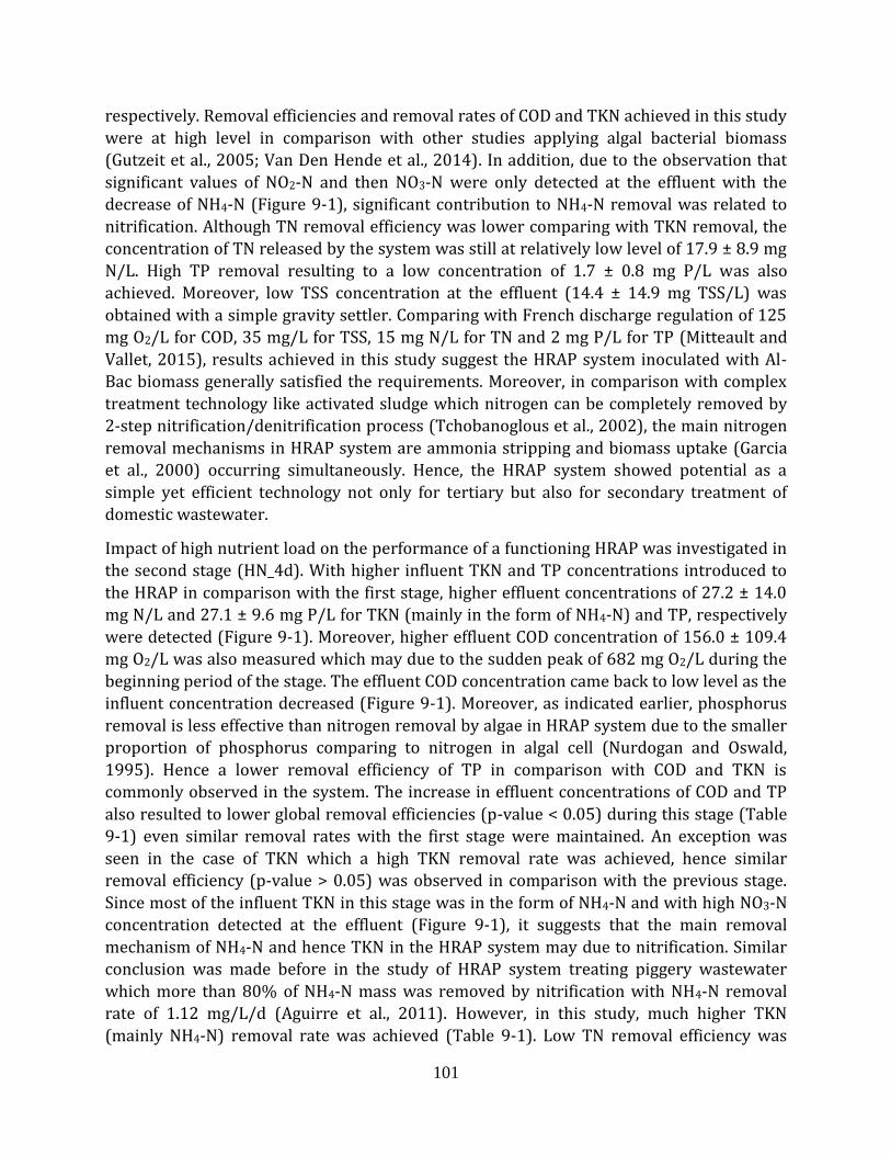
101

respectively. Removal efficiencies and removal rates of COD and TKN achieved in this study

were at high level in comparison with other studies applying algal bacterial biomass

(Gutzeit et al., 2005; Van Den Hende et al., 2014). In addition, due to the observation that

significant values of NO2-N and then NO3-N were only detected at the effluent with the

decrease of NH4-N (Figure 9-1), significant contribution to NH4-N removal was related to

nitrification. Although TN removal efficiency was lower comparing with TKN removal, the

concentration of TN released by the system was still at relatively low level of 17.9 ± 8.9 mg

N/L. High TP removal resulting to a low concentration of 1.7 ± 0.8 mg P/L was also

achieved. Moreover, low TSS concentration at the effluent (14.4 ± 14.9 mg TSS/L) was

obtained with a simple gravity settler. Comparing with French discharge regulation of 125

mg O2/L for COD, 35 mg/L for TSS, 15 mg N/L for TN and 2 mg P/L for TP (Mitteault and

Vallet, 2015), results achieved in this study suggest the HRAP system inoculated with Al-

Bac biomass generally satisfied the requirements. Moreover, in comparison with complex

treatment technology like activated sludge which nitrogen can be completely removed by

2-step nitrification/denitrification process (Tchobanoglous et al., 2002), the main nitrogen

removal mechanisms in HRAP system are ammonia stripping and biomass uptake (Garcia

et al., 2000) occurring simultaneously. Hence, the HRAP system showed potential as a

simple yet efficient technology not only for tertiary but also for secondary treatment of

domestic wastewater.

Impact of high nutrient load on the performance of a functioning HRAP was investigated in

the second stage (HN_4d). With higher influent TKN and TP concentrations introduced to

the HRAP in comparison with the first stage, higher effluent concentrations of 27.2 ± 14.0

mg N/L and 27.1 ± 9.6 mg P/L for TKN (mainly in the form of NH4-N) and TP, respectively

were detected (Figure 9-1). Moreover, higher effluent COD concentration of 156.0 ± 109.4

mg O2/L was also measured which may due to the sudden peak of 682 mg O2/L during the

beginning period of the stage. The effluent COD concentration came back to low level as the

influent concentration decreased (Figure 9-1). Moreover, as indicated earlier, phosphorus

removal is less effective than nitrogen removal by algae in HRAP system due to the smaller

proportion of phosphorus comparing to nitrogen in algal cell (Nurdogan and Oswald,

1995). Hence a lower removal efficiency of TP in comparison with COD and TKN is

commonly observed in the system. The increase in effluent concentrations of COD and TP

also resulted to lower global removal efficiencies (p-value < 0.05) during this stage (Table

9-1) even similar removal rates with the first stage were maintained. An exception was

seen in the case of TKN which a high TKN removal rate was achieved, hence similar

removal efficiency (p-value > 0.05) was observed in comparison with the previous stage.

Since most of the influent TKN in this stage was in the form of NH4-N and with high NO3-N

concentration detected at the effluent (Figure 9-1), it suggests that the main removal

mechanism of NH4-N and hence TKN in the HRAP system may due to nitrification. Similar

conclusion was made before in the study of HRAP system treating piggery wastewater

which more than 80% of NH4-N mass was removed by nitrification with NH4-N removal

rate of 1.12 mg/L/d (Aguirre et al., 2011). However, in this study, much higher TKN

(mainly NH4-N) removal rate was achieved (Table 9-1). Low TN removal efficiency was

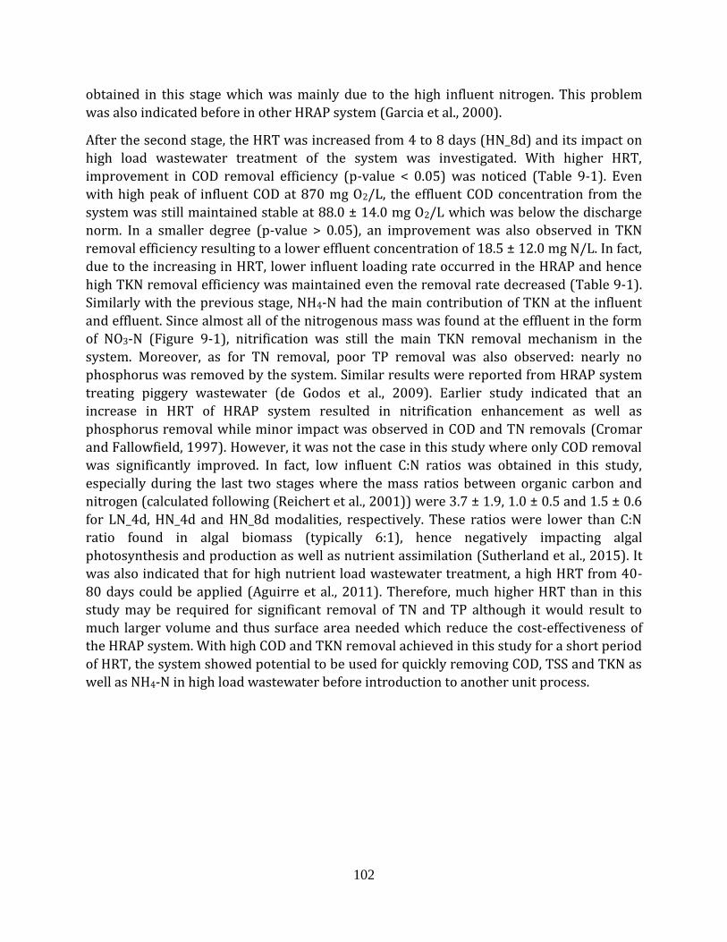
102

obtained in this stage which was mainly due to the high influent nitrogen. This problem

was also indicated before in other HRAP system (Garcia et al., 2000).

After the second stage, the HRT was increased from 4 to 8 days (HN_8d) and its impact on

high load wastewater treatment of the system was investigated. With higher HRT,

improvement in COD removal efficiency (p-value < 0.05) was noticed (Table 9-1). Even

with high peak of influent COD at 870 mg O2/L, the effluent COD concentration from the

system was still maintained stable at 88.0 ± 14.0 mg O2/L which was below the discharge

norm. In a smaller degree (p-value > 0.05), an improvement was also observed in TKN

removal efficiency resulting to a lower effluent concentration of 18.5 ± 12.0 mg N/L. In fact,

due to the increasing in HRT, lower influent loading rate occurred in the HRAP and hence

high TKN removal efficiency was maintained even the removal rate decreased (Table 9-1).

Similarly with the previous stage, NH4-N had the main contribution of TKN at the influent

and effluent. Since almost all of the nitrogenous mass was found at the effluent in the form

of NO3-N (Figure 9-1), nitrification was still the main TKN removal mechanism in the

system. Moreover, as for TN removal, poor TP removal was also observed: nearly no

phosphorus was removed by the system. Similar results were reported from HRAP system

treating piggery wastewater (de Godos et al., 2009). Earlier study indicated that an

increase in HRT of HRAP system resulted in nitrification enhancement as well as

phosphorus removal while minor impact was observed in COD and TN removals (Cromar

and Fallowfield, 1997). However, it was not the case in this study where only COD removal

was significantly improved. In fact, low influent C:N ratios was obtained in this study,

especially during the last two stages where the mass ratios between organic carbon and

nitrogen (calculated following (Reichert et al., 2001)) were 3.7 ± 1.9, 1.0 ± 0.5 and 1.5 ± 0.6

for LN_4d, HN_4d and HN_8d modalities, respectively. These ratios were lower than C:N

ratio found in algal biomass (typically 6:1), hence negatively impacting algal

photosynthesis and production as well as nutrient assimilation (Sutherland et al., 2015). It

was also indicated that for high nutrient load wastewater treatment, a high HRT from 40-

80 days could be applied (Aguirre et al., 2011). Therefore, much higher HRT than in this

study may be required for significant removal of TN and TP although it would result to

much larger volume and thus surface area needed which reduce the cost-effectiveness of

the HRAP system. With high COD and TKN removal achieved in this study for a short period

of HRT, the system showed potential to be used for quickly removing COD, TSS and TKN as

well as NH4-N in high load wastewater before introduction to another unit process.

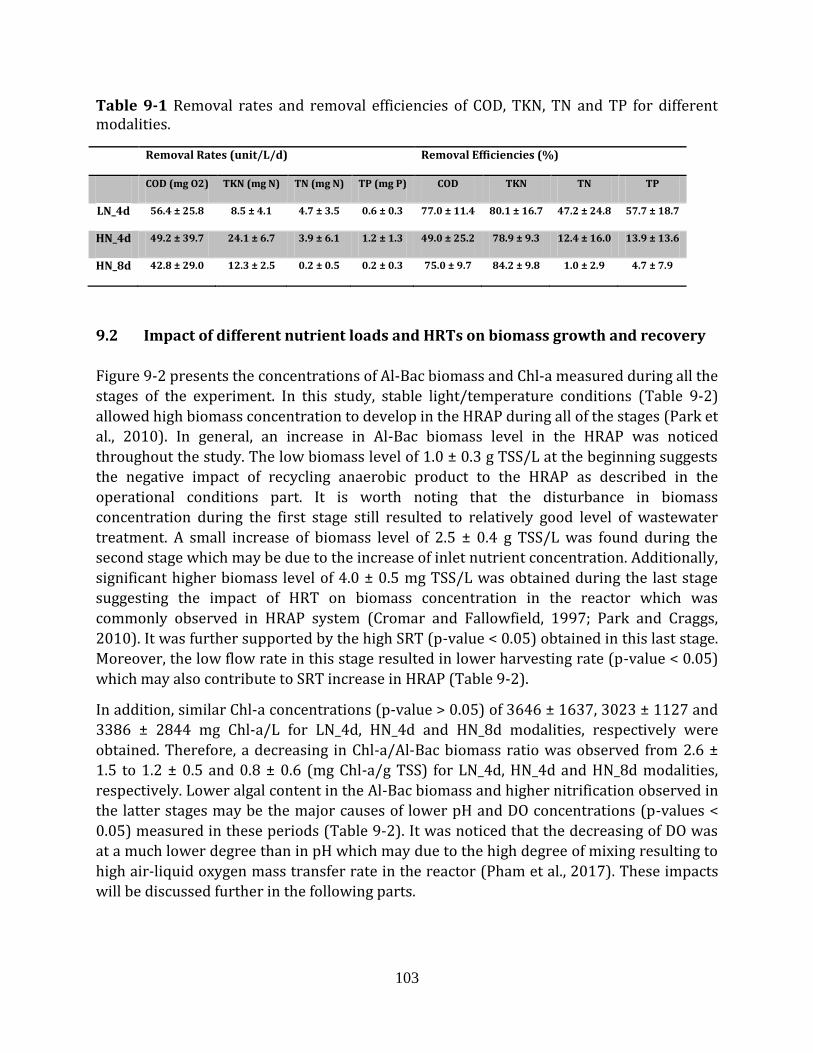
103

Table 9-1 Removal rates and removal efficiencies of COD, TKN, TN and TP for different modalities.

Removal Rates (unit/L/d) Removal Efficiencies (%)

COD (mg O2) TKN (mg N) TN (mg N) TP (mg P) COD TKN TN TP

LN_4d 56.4 ± 25.8 8.5 ± 4.1 4.7 ± 3.5 0.6 ± 0.3 77.0 ± 11.4 80.1 ± 16.7 47.2 ± 24.8 57.7 ± 18.7

HN_4d 49.2 ± 39.7 24.1 ± 6.7 3.9 ± 6.1 1.2 ± 1.3 49.0 ± 25.2 78.9 ± 9.3 12.4 ± 16.0 13.9 ± 13.6

HN_8d 42.8 ± 29.0 12.3 ± 2.5 0.2 ± 0.5 0.2 ± 0.3 75.0 ± 9.7 84.2 ± 9.8 1.0 ± 2.9 4.7 ± 7.9

9.2 Impact of different nutrient loads and HRTs on biomass growth and recovery

Figure 9-2 presents the concentrations of Al-Bac biomass and Chl-a measured during all the

stages of the experiment. In this study, stable light/temperature conditions (Table 9-2)

allowed high biomass concentration to develop in the HRAP during all of the stages (Park et

al., 2010). In general, an increase in Al-Bac biomass level in the HRAP was noticed

throughout the study. The low biomass level of 1.0 ± 0.3 g TSS/L at the beginning suggests

the negative impact of recycling anaerobic product to the HRAP as described in the

operational conditions part. It is worth noting that the disturbance in biomass

concentration during the first stage still resulted to relatively good level of wastewater

treatment. A small increase of biomass level of 2.5 ± 0.4 g TSS/L was found during the

second stage which may be due to the increase of inlet nutrient concentration. Additionally,

significant higher biomass level of 4.0 ± 0.5 mg TSS/L was obtained during the last stage

suggesting the impact of HRT on biomass concentration in the reactor which was

commonly observed in HRAP system (Cromar and Fallowfield, 1997; Park and Craggs,

2010). It was further supported by the high SRT (p-value < 0.05) obtained in this last stage.

Moreover, the low flow rate in this stage resulted in lower harvesting rate (p-value < 0.05)

which may also contribute to SRT increase in HRAP (Table 9-2).

In addition, similar Chl-a concentrations (p-value > 0.05) of 3646 ± 1637, 3023 ± 1127 and

3386 ± 2844 mg Chl-a/L for LN_4d, HN_4d and HN_8d modalities, respectively were

obtained. Therefore, a decreasing in Chl-a/Al-Bac biomass ratio was observed from 2.6 ±

1.5 to 1.2 ± 0.5 and 0.8 ± 0.6 (mg Chl-a/g TSS) for LN_4d, HN_4d and HN_8d modalities,

respectively. Lower algal content in the Al-Bac biomass and higher nitrification observed in

the latter stages may be the major causes of lower pH and DO concentrations (p-values <

0.05) measured in these periods (Table 9-2). It was noticed that the decreasing of DO was

at a much lower degree than in pH which may due to the high degree of mixing resulting to

high air-liquid oxygen mass transfer rate in the reactor (Pham et al., 2017). These impacts

will be discussed further in the following parts.

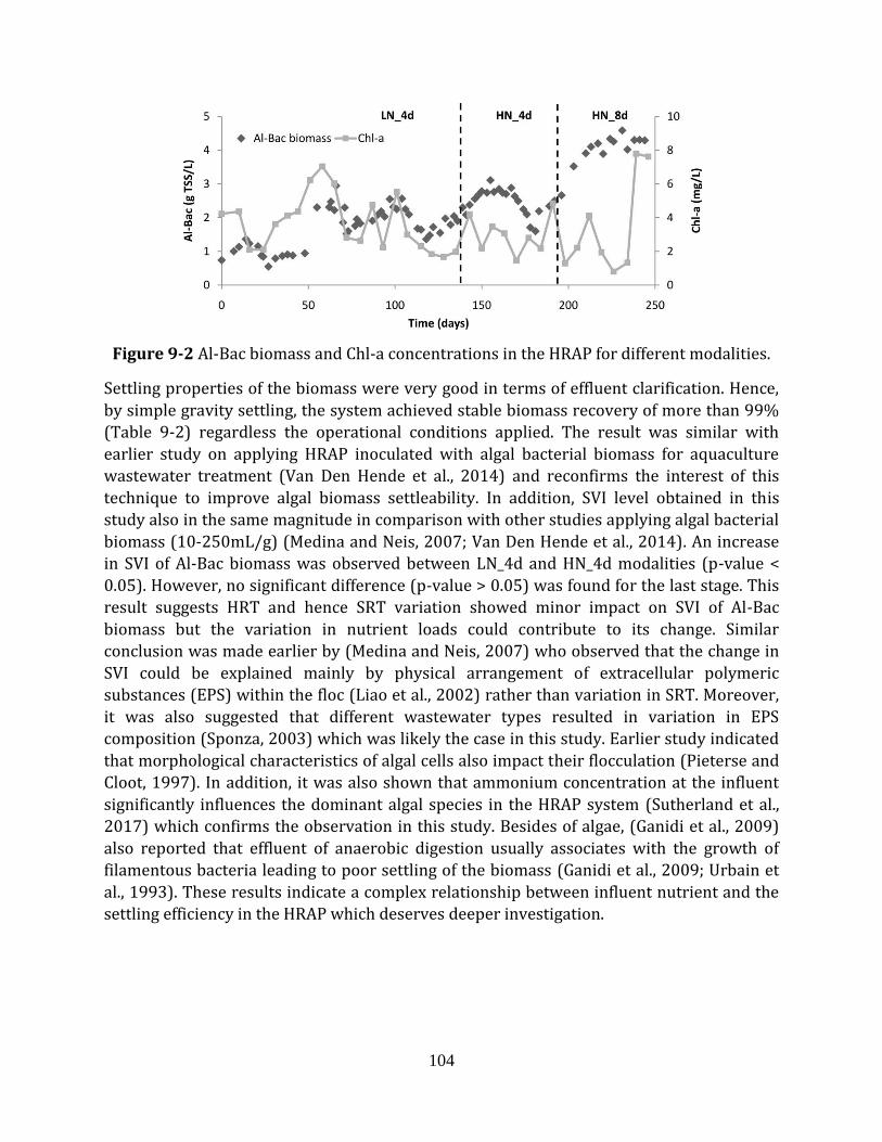
104

Figure 9-2 Al-Bac biomass and Chl-a concentrations in the HRAP for different modalities.

Settling properties of the biomass were very good in terms of effluent clarification. Hence,

by simple gravity settling, the system achieved stable biomass recovery of more than 99%

(Table 9-2) regardless the operational conditions applied. The result was similar with

earlier study on applying HRAP inoculated with algal bacterial biomass for aquaculture

wastewater treatment (Van Den Hende et al., 2014) and reconfirms the interest of this

technique to improve algal biomass settleability. In addition, SVI level obtained in this

study also in the same magnitude in comparison with other studies applying algal bacterial

biomass (10-250mL/g) (Medina and Neis, 2007; Van Den Hende et al., 2014). An increase

in SVI of Al-Bac biomass was observed between LN_4d and HN_4d modalities (p-value <

0.05). However, no significant difference (p-value > 0.05) was found for the last stage. This

result suggests HRT and hence SRT variation showed minor impact on SVI of Al-Bac

biomass but the variation in nutrient loads could contribute to its change. Similar

conclusion was made earlier by (Medina and Neis, 2007) who observed that the change in

SVI could be explained mainly by physical arrangement of extracellular polymeric

substances (EPS) within the floc (Liao et al., 2002) rather than variation in SRT. Moreover,

it was also suggested that different wastewater types resulted in variation in EPS

composition (Sponza, 2003) which was likely the case in this study. Earlier study indicated

that morphological characteristics of algal cells also impact their flocculation (Pieterse and

Cloot, 1997). In addition, it was also shown that ammonium concentration at the influent

significantly influences the dominant algal species in the HRAP system (Sutherland et al.,

2017) which confirms the observation in this study. Besides of algae, (Ganidi et al., 2009)

also reported that effluent of anaerobic digestion usually associates with the growth of

filamentous bacteria leading to poor settling of the biomass (Ganidi et al., 2009; Urbain et

al., 1993). These results indicate a complex relationship between influent nutrient and the

settling efficiency in the HRAP which deserves deeper investigation.

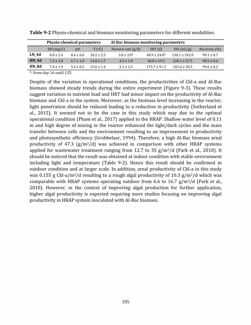
105

Table 9-2 Physio-chemical and biomass monitoring parameters for different modalities.

Physio-chemical parameters Al-Bac biomass monitoring parameters

DO (mg/L) pH T (oC) Harvest rate (g/d) SRT (d) SVI (mL/g) Recovery (%)

LN_4d 8.0 ± 2.4 8.4 ± 0.6 18.2 ± 2.5 3.8 ± 2.0* 40.9 ± 24.8* 130.1 ± 102.0 99.1 ± 0.7

HN_4d 7.3 ± 1.8 6.7 ± 1.0 14.8 ± 1.7 4.3 ± 1.8 48.8 ± 19.5 220.1 ± 57.5 98.9 ± 0.4

HN_8d 7.4 ± 1.9 5.2 ± 0.5 15.6 ± 1.4 2.1 ± 2.3 175.7 ± 91.3 181.6 ± 30.5 99.6 ± 0.2

*: from day 16 until 135.

Despite of the variation in operational conditions, the productivities of Chl-a and Al-Bac

biomass showed steady trends during the entire experiment (Figure 9-3). These results

suggest variation in nutrient load and HRT had minor impact on the productivity of Al-Bac

biomass and Chl-a in the system. Moreover, as the biomass level increasing in the reactor,

light penetration should be reduced leading to a reduction in productivity (Sutherland et

al., 2015). It seemed not to be the case in this study which may due to the optimal

operational condition (Pham et al., 2017) applied to the HRAP. Shallow water level of 0.11

m and high degree of mixing in the reactor enhanced the light/dark cycles and the mass

transfer between cells and the environment resulting to an improvement in productivity

and photosynthetic efficiency (Grobbelaar, 1994). Therefore, a high Al-Bac biomass areal

productivity of 47.3 (g/m2/d) was achieved in comparison with other HRAP systems

applied for wastewater treatment ranging from 12.7 to 35 g/m2/d (Park et al., 2010). It

should be noticed that the result was obtained at indoor condition with stable environment

including light and temperature (Table 9-2). Hence this result should be confirmed in

outdoor condition and at larger scale. In addition, areal productivity of Chl-a in this study

was 0.155 g Chl-a/m2/d resulting to a rough algal productivity of 10.3 g/m2/d which was

comparable with HRAP systems operating outdoor from 6.6 to 16.7 g/m2/d (Park et al.,

2010). However, in the context of improving algal production for further application,

higher algal productivity is expected requiring more studies focusing on improving algal

productivity in HRAP system inoculated with Al-Bac biomass.

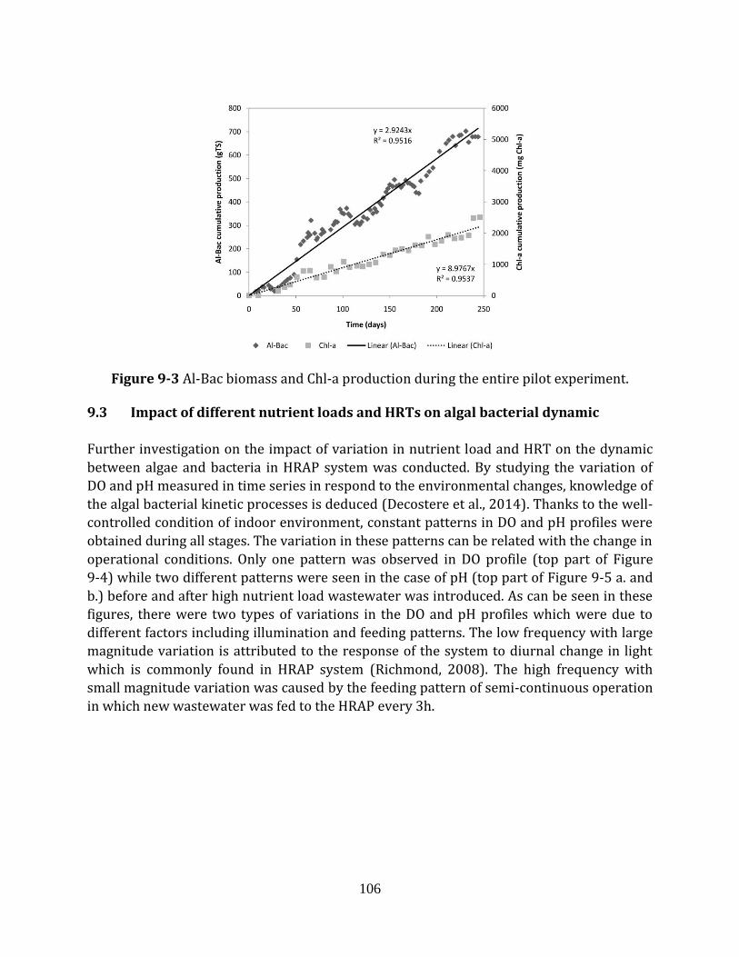
106

Figure 9-3 Al-Bac biomass and Chl-a production during the entire pilot experiment.

9.3 Impact of different nutrient loads and HRTs on algal bacterial dynamic

Further investigation on the impact of variation in nutrient load and HRT on the dynamic

between algae and bacteria in HRAP system was conducted. By studying the variation of

DO and pH measured in time series in respond to the environmental changes, knowledge of

the algal bacterial kinetic processes is deduced (Decostere et al., 2014). Thanks to the well-

controlled condition of indoor environment, constant patterns in DO and pH profiles were

obtained during all stages. The variation in these patterns can be related with the change in

operational conditions. Only one pattern was observed in DO profile (top part of Figure

9-4) while two different patterns were seen in the case of pH (top part of Figure 9-5 a. and

b.) before and after high nutrient load wastewater was introduced. As can be seen in these

figures, there were two types of variations in the DO and pH profiles which were due to

different factors including illumination and feeding patterns. The low frequency with large

magnitude variation is attributed to the response of the system to diurnal change in light

which is commonly found in HRAP system (Richmond, 2008). The high frequency with

small magnitude variation was caused by the feeding pattern of semi-continuous operation

in which new wastewater was fed to the HRAP every 3h.

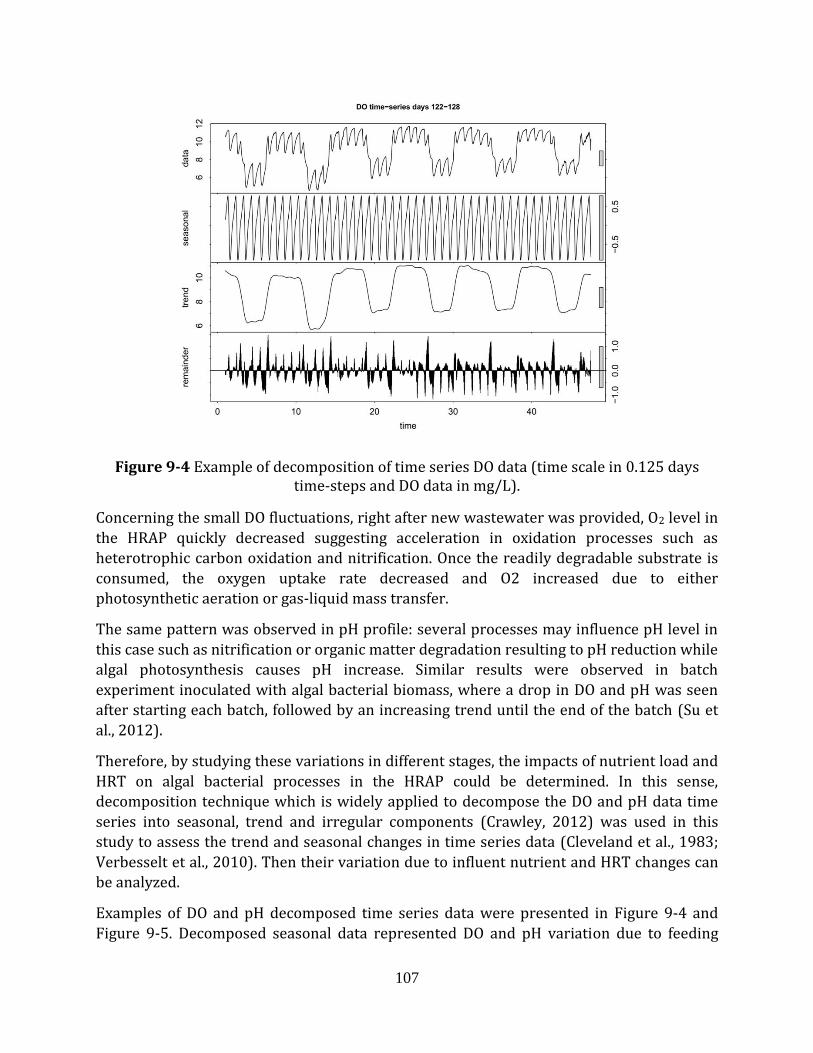
107

Figure 9-4 Example of decomposition of time series DO data (time scale in 0.125 days time-steps and DO data in mg/L).

Concerning the small DO fluctuations, right after new wastewater was provided, O2 level in

the HRAP quickly decreased suggesting acceleration in oxidation processes such as

heterotrophic carbon oxidation and nitrification. Once the readily degradable substrate is

consumed, the oxygen uptake rate decreased and O2 increased due to either

photosynthetic aeration or gas-liquid mass transfer.

The same pattern was observed in pH profile: several processes may influence pH level in

this case such as nitrification or organic matter degradation resulting to pH reduction while

algal photosynthesis causes pH increase. Similar results were observed in batch

experiment inoculated with algal bacterial biomass, where a drop in DO and pH was seen

after starting each batch, followed by an increasing trend until the end of the batch (Su et

al., 2012).

Therefore, by studying these variations in different stages, the impacts of nutrient load and

HRT on algal bacterial processes in the HRAP could be determined. In this sense,

decomposition technique which is widely applied to decompose the DO and pH data time

series into seasonal, trend and irregular components (Crawley, 2012) was used in this

study to assess the trend and seasonal changes in time series data (Cleveland et al., 1983;

Verbesselt et al., 2010). Then their variation due to influent nutrient and HRT changes can

be analyzed.

Examples of DO and pH decomposed time series data were presented in Figure 9-4 and

Figure 9-5. Decomposed seasonal data represented DO and pH variation due to feeding

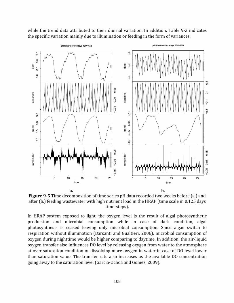
108

while the trend data attributed to their diurnal variation. In addition, Table 9-3 indicates

the specific variation mainly due to illumination or feeding in the form of variances.

a. b.

Figure 9-5 Time decomposition of time series pH data recorded two weeks before (a.) and after (b.) feeding wastewater with high nutrient load in the HRAP (time scale in 0.125 days

time-steps).

In HRAP system exposed to light, the oxygen level is the result of algal photosynthetic

production and microbial consumption while in case of dark condition, algal

photosynthesis is ceased leaving only microbial consumption. Since algae switch to

respiration without illumination (Barsanti and Gualtieri, 2006), microbial consumption of

oxygen during nighttime would be higher comparing to daytime. In addition, the air-liquid

oxygen transfer also influences DO level by releasing oxygen from water to the atmosphere

at over saturation condition or dissolving more oxygen in water in case of DO level lower

than saturation value. The transfer rate also increases as the available DO concentration

going away to the saturation level (Garcia-Ochoa and Gomez, 2009).

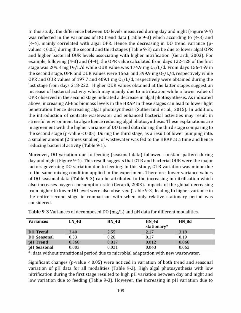
109

In this study, the difference between DO levels measured during day and night (Figure 9-4)

was reflected in the variances of DO trend data (Table 9-3) which according to (4-3) and

(4-4), mainly correlated with algal OPR. Hence the decreasing in DO trend variance (p-

values < 0.05) during the second and third stages (Table 9-3) can be due to lower algal OPR

and higher bacterial OUR levels associating with higher nitrification (Gerardi, 2003). For

example, following (4-3) and (4-4), the OPR value calculated from days 122-128 of the first

stage was 209.3 mg O2/L/d while OUR value was 174.9 mg O2/L/d. From days 156-159 in

the second stage, OPR and OUR values were 156.6 and 399.9 mg O2/L/d, respectively while

OPR and OUR values of 197.7 and 409.1 mg O2/L/d, respectively were obtained during the

last stage from days 218-222. Higher OUR values obtained at the latter stages suggest an

increase of bacterial activity which may mainly due to nitrification while a lower value of

OPR observed in the second stage indicated a decrease in algal photosynthesis. As indicated

above, increasing Al-Bac biomass levels in the HRAP in these stages can lead to lower light

penetration hence decreasing algal photosynthesis (Sutherland et al., 2015). In addition,

the introduction of centrate wastewater and enhanced bacterial activities may result in

stressful environment to algae hence reducing algal photosynthesis. These explanations are

in agreement with the higher variance of DO trend data during the third stage comparing to

the second stage (p-value < 0.05). During the third stage, as a result of lower pumping rate,

a smaller amount (2 times smaller) of wastewater was fed to the HRAP at a time and hence

reducing bacterial activity (Table 9-1).

Moreover, DO variation due to feeding (seasonal data) followed constant pattern during

day and night (Figure 9-4). This result suggests that OTR and bacterial OUR were the major

factors governing DO variation due to feeding. In this study, OTR variation was minor due

to the same mixing condition applied in the experiment. Therefore, lower variance values

of DO seasonal data (Table 9-3) can be attributed to the increasing in nitrification which

also increases oxygen consumption rate (Gerardi, 2003). Impacts of the global decreasing

from higher to lower DO level were also observed (Table 9-3) leading to higher variance in

the entire second stage in comparison with when only relative stationary period was

considered.

Table 9-3 Variances of decomposed DO (mg/L) and pH data for different modalities.

Variances LN_4d HN_4d HN_4d stationary*

HN_8d

DO_Trend 3.40 2.55 2.17 3.18 DO_Seasonal 0.33 0.28 0.17 0.19 pH_Trend 0.368 0.817 0.012 0.068 pH_Seasonal 0.003 0.021 0.043 0.062

*: data without transitional period due to microbial adaptation with new wastewater.

Significant changes (p-value < 0.05) were noticed in variation of both trend and seasonal

variation of pH data for all modalities (Table 9-3). High algal photosynthesis with low

nitrification during the first stage resulted to high pH variation between day and night and

low variation due to feeding (Table 9-3). However, the increasing in pH variation due to

110

feeding and decreasing in day-night pH variation suggests the domination of nitrification

after high nutrient load was introduced. The transition period was observed when

comparing variances of trend and seasonal pH data in the entire second stage with these

values without considering transition.

The decomposed data provided an insight into processes of algae and bacteria under

different operational conditions. A next step of employing these results for kinetic model

validation is promising.

9.4 Conclusions and Perspectives

Long term experiment was conducted to study the ability of HRAP inoculated with Al-Bac

biomass to treat primary treated wastewater as well as to investigate the impacts of high

nutrient load wastewater and HRT variation on the performance of the system in terms of

treatment efficiency, biomass production and recovery. In general, the system showed good

treatment levels of primary treated wastewater satisfying French discharge norm with 4

days of HRT. Around 99% of biomass recovery efficiency was achieved during the entire

experiment via simple gravity settling which reconfirms the advantage of Al-Bac biomass in

enhancing settleability. Hence the HRAP showed potential for a simple and efficient

secondary treatment application. High nutrient load wastewater resulted in poor TN and

TP treatment efficiencies and decreasing in COD removal, yet high removal of TKN as well

as NH4-N were still obtained. High HRT of 8 days showed improvement in COD removal,

but minor impact was observed in the case of TKN, TN and TP removals. Nitrification was

identified as the main mechanism in TKN and NH4-N removals of high nutrient load

wastewater. Over all, the system requires much higher HRT to significantly remove TN and

TP from high nutrient load wastewater or it can be used to remove quickly COD and TKN

from the wastewater before applying another treatment for NO3-N and TP removals.

Despite of the variation in operational conditions, constant production rates of Al-Bac

biomass and Chl-a were obtained during the entire experiment. Decomposition technique

was also used to study the dynamic of algal and bacterial processes under the impact of

high nutrient load wastewater and HRT variation. It was indicated that with the

introduction of high nutrient load wastewater, nitrification became the dominant process

while algal photosynthesis decreased. Results from this study showed potential to be

employed for model validation in order to further investigate the dynamic between algae

and bacteria in HRAP system.

In French:

Une expérience { long terme a été menée pour étudier la capacité d’un réacteur HRAP

pilote inoculé avec la biomasse Al-Bac à traiter les eaux usées décantées ainsi que pour

étudier les impacts des eaux usées à charge élevée en nutriments et de la variation du

temps de séjour hydraulique sur les performances du système en termes d'efficacité de

111

traitement, de production et de récupération de la biomasse. En général, le système a

montré de bons niveaux de traitement des eaux usées décantées, satisfaisant aux niveaux

de rejet de la réglementation française,avec un temps de séjour hydraulique de 4 jours. Une

efficacité de récupération de la biomasse d’environ 99% a été atteinte pendant toute la

durée de l'expérience avec une simple décantation, ce qui confirme à nouveau l'avantage de

la biomasse Al-Bac dans l'amélioration de la décantabilité. Le réacteur HRAP présente donc

un potentiel important pour une application de traitement secondaire simple et efficace.

Une charge élevée d'éléments nutritifs dans les eaux usées a entraîné une faible efficacité

du traitement de l’azote et du phosphore totaux ainsi qu’une diminution de l'élimination de

la DCO, mais tout en conservant une élimination élevée de l’azote réduit (nitrification).. Un

temps de séjour hydraulique de de 8 jours a permis une amélioration de l'élimination de la

DCO, mais un impact mineur a été observé dans le cas de l'élimination de l’azote et du

phosphore. La nitrification a été identifiée comme le principal mécanisme d'élimination de

l’azote des eaux usées fortrement chargées. Dans l'ensemble, le système nécessite un temps

de séjour hydraulique beaucoup plus élevé pour éliminer de façon significative l’azote total

et le phosphore des eaux usées fortement chargées. Il peut être utilisé pour éliminer

rapidement la DCO et l’azote Kjeldahl des eaux usées avant d'appliquer un autre traitement

pour l'élimination des nitrates produits et du phosphre. Malgré la variation des conditions

d'exploitation, des taux de production constants de biomasse Al-Bac et de Chl-a ont été

obtenus pendant toute la durée de l'expérience. La technique de décomposition de séries

temporelles a également été utilisée pour étudier la dynamique des processus algaux et

bactériens sous l'impact de la charge élevée en nutriments des eaux usées et de la variation

du temps de séjour. Il a été montré qu'avec l'introduction d'eaux usées à forte charge en

nutriments, la nitrification est devenue le processus dominant, tandis que la photosynthèse

des algues a diminué. Les résultats de cette étude seront utiles pour la validation de

modèles numériques afin d'étudier plus avant la dynamique entre les algues et les bactéries

dans le système HRAP.

112

CHAPTER 10 SIMULATION OF LONG TERM WASTEWATER TREATMENT BY A HIGH

RATE ALGAL POND: COUPLING RTD AND MIXED-ORDER KINETIC MODELS:

PERFORMANCE ASSESSMENT AND SIZING APPLICATION

Traditionally, the black box kinetic model employing 1st order of reaction applied to predict

the rate of biochemical oxidation of organic matter in river system (Phelps and Streeter,

1925). Due to its efficiency in terms of prediction as well as mathematical convenience, this

model was generally favored in simulating wastewater treatment facilities such as waste

stabilization pond(Crites et al., 2014), constructed wetland (Arheimer and Wittgren, 2002;

Kadlec, 2000) or high rate algal pond (HRAP) (El Hamouri et al., 2003). However, early

studies also indicated kinetic model with order of reaction other than 1 showing good

simulation of the practical data (Adrian and Sanders, 1998, 1992; Paris et al., 1981).

Another approach called mixed-order model was proposed by Hewitt et al. (1979) and

further developed by Borsuk and Stow (2000) which the order of the kinetic reaction was

remained as free parameter. This model was found to provide better simulation than 1st

order model of long term data of biological oxygen demand (BOD) removal in streams and

rivers or polychlorinated biphenyl (PCB) declining in lake (Hewitt et al., 1979; Stow et al.,

1999). Yet the application of mixed order model to simulate pollutant removal in HRAP is

still lacking. In addition, it was indicated that different environmental and operational

factors influence the performance of HRAP (Park et al., 2010; Sutherland et al., 2015) and

hence may indirectly impact the model parameters. Therefore studying such relationship

can reveal insight knowledge on the treatment processes in HRAP and improve assessment

of the performance of the system.

Moreover, since deviation from the ideal hydraulic condition in the reactor is a common

problem and always influence the performance of the system, a coupled kinetic and

hydraulic model is a necessary step to improve the simulation by considering imperfect

flow patterns in the system (Fogler, 2006a). The most popular method in chemical

engineering to characterize global hydraulic behavior of a reactor is by analyzing the

residence time distribution (RTD) of the reactor obtained via tracer experiment. The RTD

curve E(t) provides information of time various fractions of fluid (wastewater and

biomass) spend in the reactor, and hence the contact time distribution for the system. The

coupled kinetic and hydraulic model then will be obtained by integrating RTD and kinetic

models (Fogler, 2006a). The coupled RTD and first order kinetic model was widely applied

in simulating performance of chemical reactors (Fogler, 2006a), stabilization ponds (Ellis

and Rodrigues, 1993; Torres et al., 1997) or treatment wetlands (Kadlec, 2000, 1994).

Hence coupling RTD and mixed-order kinetic models is necessary to study which will

improve the accuracy of the model supporting better system assessment.

In chapter 5, a coupled mixed-order kinetic and RTD model was developed based on the

data obtained from the pilot HRAP experiments. Detailed procedure of the calibration

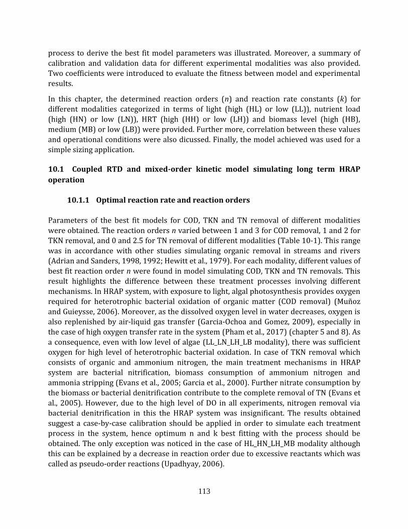
113

process to derive the best fit model parameters was illustrated. Moreover, a summary of

calibration and validation data for different experimental modalities was also provided.

Two coefficients were introduced to evaluate the fitness between model and experimental

results.

In this chapter, the determined reaction orders (n) and reaction rate constants (k) for

different modalities categorized in terms of light (high (HL) or low (LL)), nutrient load

(high (HN) or low (LN)), HRT (high (HH) or low (LH)) and biomass level (high (HB),

medium (MB) or low (LB)) were provided. Further more, correlation between these values

and operational conditions were also dicussed. Finally, the model achieved was used for a

simple sizing application.

10.1 Coupled RTD and mixed-order kinetic model simulating long term HRAP

operation

10.1.1 Optimal reaction rate and reaction orders

Parameters of the best fit models for COD, TKN and TN removal of different modalities

were obtained. The reaction orders n varied between 1 and 3 for COD removal, 1 and 2 for

TKN removal, and 0 and 2.5 for TN removal of different modalities (Table 10-1). This range

was in accordance with other studies simulating organic removal in streams and rivers

(Adrian and Sanders, 1998, 1992; Hewitt et al., 1979). For each modality, different values of

best fit reaction order n were found in model simulating COD, TKN and TN removals. This

result highlights the difference between these treatment processes involving different

mechanisms. In HRAP system, with exposure to light, algal photosynthesis provides oxygen

required for heterotrophic bacterial oxidation of organic matter (COD removal) (Muñoz

and Guieysse, 2006). Moreover, as the dissolved oxygen level in water decreases, oxygen is

also replenished by air-liquid gas transfer (Garcia-Ochoa and Gomez, 2009), especially in

the case of high oxygen transfer rate in the system (Pham et al., 2017) (chapter 5 and 8). As

a consequence, even with low level of algae (LL_LN_LH_LB modality), there was sufficient

oxygen for high level of heterotrophic bacterial oxidation. In case of TKN removal which

consists of organic and ammonium nitrogen, the main treatment mechanisms in HRAP

system are bacterial nitrification, biomass consumption of ammonium nitrogen and

ammonia stripping (Evans et al., 2005; Garcia et al., 2000). Further nitrate consumption by

the biomass or bacterial denitrification contribute to the complete removal of TN (Evans et

al., 2005). However, due to the high level of DO in all experiments, nitrogen removal via

bacterial denitrification in this the HRAP system was insignificant. The results obtained

suggest a case-by-case calibration should be applied in order to simulate each treatment

process in the system, hence optimum n and k best fitting with the process should be

obtained. The only exception was noticed in the case of HL_HN_LH_MB modality although

this can be explained by a decrease in reaction order due to excessive reactants which was

called as pseudo-order reactions (Upadhyay, 2006).

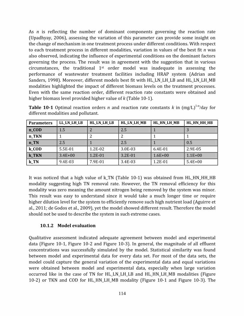
114

As n is reflecting the number of dominant components governing the reaction rate

(Upadhyay, 2006), assessing the variation of this parameter can provide some insight on

the change of mechanism in one treatment process under different conditions. With respect

to each treatment process in different modalities, variation in values of the best fit n was

also observed, indicating the influence of experimental conditions on the dominant factors

governing the process. The result was in agreement with the suggestion that in various

circumstances, the traditional 1st order model was inadequate in assessing the

performance of wastewater treatment facilities including HRAP system (Adrian and

Sanders, 1998). Moreover, different models best fit with HL_LN_LH_LB and HL_LN_LH_MB

modalities highlighted the impact of different biomass levels on the treatment processes.

Even with the same reaction order, different reaction rate constants were obtained and

higher biomass level provided higher value of k (Table 10-1).

Table 10-1 Optimal reaction orders n and reaction rate constants k in (mg/L)1-n

/day for different modalities and pollutant.

Parameters LL_LN_LH_LB HL_LN_LH_LB HL_LN_LH_MB HL_HN_LH_MB HL_HN_HH_HB

n_COD 1.5 2 2.5 1 3

n_TKN 1 2 2 1 1

n_TN 2.5 1 2.5 1 0.5

k_COD 5.5E-01 1.2E-02 3.0E-03 6.4E-01 2.9E-05

k_TKN 3.4E+00 1.2E-01 3.2E-01 1.6E+00 1.1E+00

k_TN 9.4E-03 7.9E-01 3.4E-03 1.2E-01 5.4E+00

It was noticed that a high value of k_TN (Table 10-1) was obtained from HL_HN_HH_HB

modality suggesting high TN removal rate. However, the TN removal efficiency for this

modality was zero meaning the amount nitrogen being removed by the system was minor.

This result was easy to understand since it would take a much longer time or require

higher dilution level for the system to efficiently remove such high nutrient load (Aguirre et

al., 2011; de Godos et al., 2009), yet the model showed different result. Therefore the model

should not be used to describe the system in such extreme cases.

10.1.2 Model evaluation

Qualitative assessment indicated adequate agreement between model and experimental

data (Figure 10-1, Figure 10-2 and Figure 10-3). In general, the magnitude of all effluent

concentrations was successfully simulated by the model. Statistical similarity was found

between model and experimental data for every data set. For most of the data sets, the

model could capture the general variation of the experimental data and equal variations

were obtained between model and experimental data, especially when large variation

occurred like in the case of TN for HL_LN_LH_LB and HL_HN_LH_MB modalities (Figure

10-2) or TKN and COD for HL_HN_LH_MB modality (Figure 10-1 and Figure 10-3). The

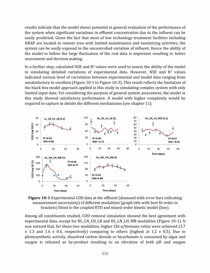
115

results indicate that the model shows potential in general evaluation of the performance of

the system when significant variations in effluent concentration due to the influent can be

easily predicted. Given the fact that most of low technology treatment facilities including

HRAP are located in remote area with limited maintenance and monitoring activities, the

system can be easily exposed to the uncontrolled variation of influent. Hence the ability of

the model to follow the large fluctuation of the real data is important resulting to better

assessment and decision making.

In a further step, calculated NSE and R2 values were used to assess the ability of the model

in simulating detailed variations of experimental data. However, NSE and R2 values

indicated various level of correlation between experimental and model data ranging from

unsatisfactory to excellent (Figure 10-1 to Figure 10-3). This result reflects the limitation of

the black box model approach applied in this study in simulating complex system with only

limited input data. Yet considering the purpose of general system assessment, the model in

this study showed satisfactory performance. A model with higher complexity would be

required to capture in details the different mechanisms (see chapter 11).

Figure 10-1 Experimental COD data at the effluent (diamond with error bars indicating measurement uncertainty) of different modalities (graph title with best fit order in

brackets) fitted to the coupled RTD and mixed-order kinetic model (line).

Among all constituents studied, COD removal simulation showed the best agreement with

experimental data, except for HL_LN_LH_LB and HL_LN_LH_MB modalities (Figure 10-1). It

was noticed that, for these two modalities, higher Chl-a/biomass ratios were achieved (3.7

± 1.3 and 1.6 ± 0.6, respectively) comparing to others (highest at 1.2 ± 0.5). Due to

photosynthetic activity, dissolved carbon dioxide or bicarbonate is consumed by algae and

oxygen is released as by-product resulting to an elevation of both pH and oxygen

116

concentration (Barsanti and Gualtieri, 2006). The high amount of algae in these cases did

not show significant reflection on oxygen concentration which was largely influenced by

the high air-liquid oxygen transfer rate in the HRAP. However, there was clear algal impact

on elevating pH level which could be up to the point that partly inhibits heterotrophic

bacterial oxidation, especially during the day (Sutherland et al., 2015). Hence, the

contribution of algae in COD removal process was substantial. Therefore, in these cases,

algal contribution may increase the complexity of the process and the model was not able

to properly describe this.

In wastewater treatment, TKN and TN removal mechanisms are generally more complex to

describe than COD removal (Gerardi, 2003). In this study, although the magnitude of

effluent TKN and TN concentrations and their variation due to influent concentration were

captured, the model generally showed prediction levels lower than good (Figure 10-3 and

Figure 10-2). In comparison with black box model approach like in this study, one can

study the system in more detailed by using the more sophisticated grey box model (Henze,

2008) such as the River Water Quality Model no. 1 (RWQM1) (Reichert et al., 2001) or the

Activated Sludge Model (ASM) family (Henze et al., 2000) in conjunction with the ASM-A

mode (Wágner et al., 2016) to simulate the HRAP system. These models divide the system

into various components with a complex network of processes. An example of this model

type was provided in chapter 11 of this thesis. However the satisfactory agreement

between model and experimental data of this model was yet to be achieved (Broekhuizen

et al., 2012) and despite of their development, more research is still needed (Solimeno and

García, 2017). Therefore, results obtained this study proved that the coupled RTD and

mixed-order kinetic model can serve as a simple and useful tool with adequate accuracy for

general assessment of HRAP system.

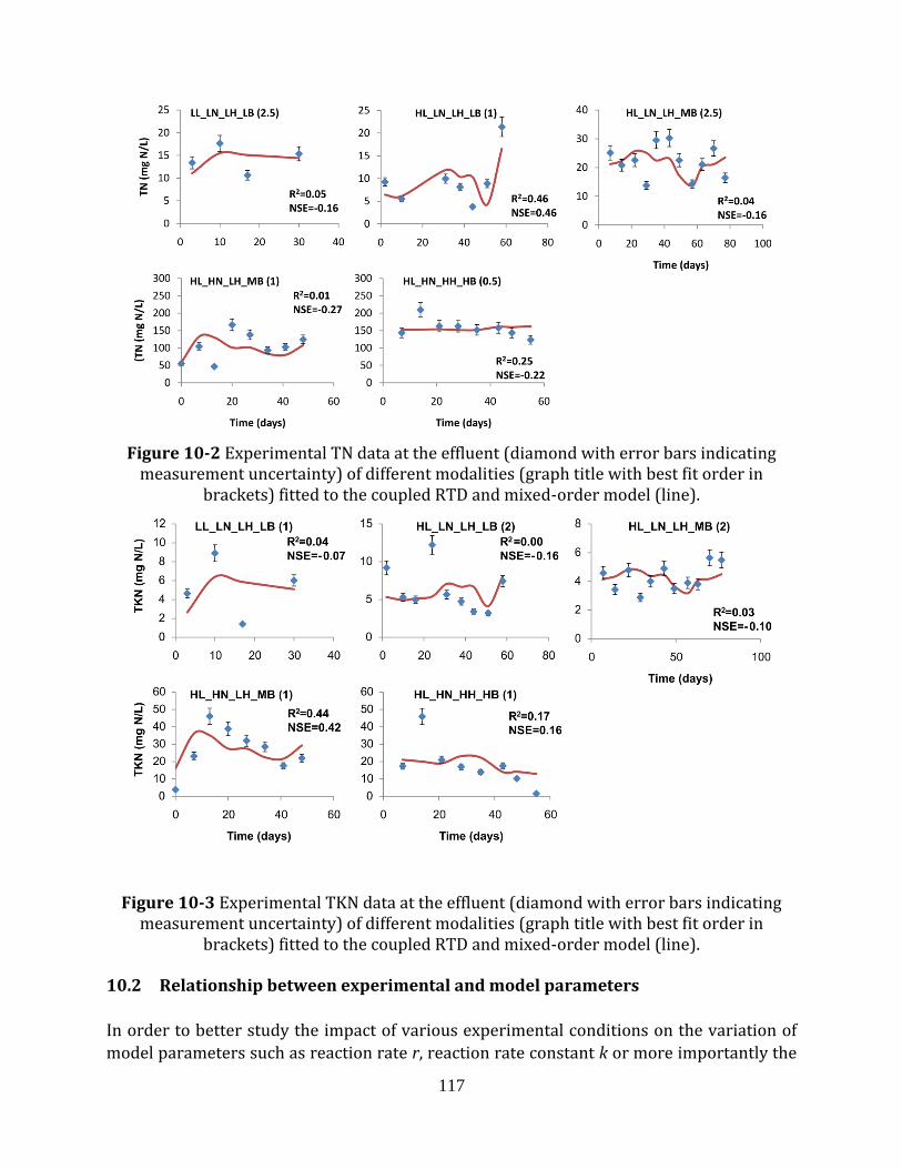
117

Figure 10-2 Experimental TN data at the effluent (diamond with error bars indicating measurement uncertainty) of different modalities (graph title with best fit order in

brackets) fitted to the coupled RTD and mixed-order model (line).

Figure 10-3 Experimental TKN data at the effluent (diamond with error bars indicating measurement uncertainty) of different modalities (graph title with best fit order in

brackets) fitted to the coupled RTD and mixed-order model (line).

10.2 Relationship between experimental and model parameters

In order to better study the impact of various experimental conditions on the variation of

model parameters such as reaction rate r, reaction rate constant k or more importantly the

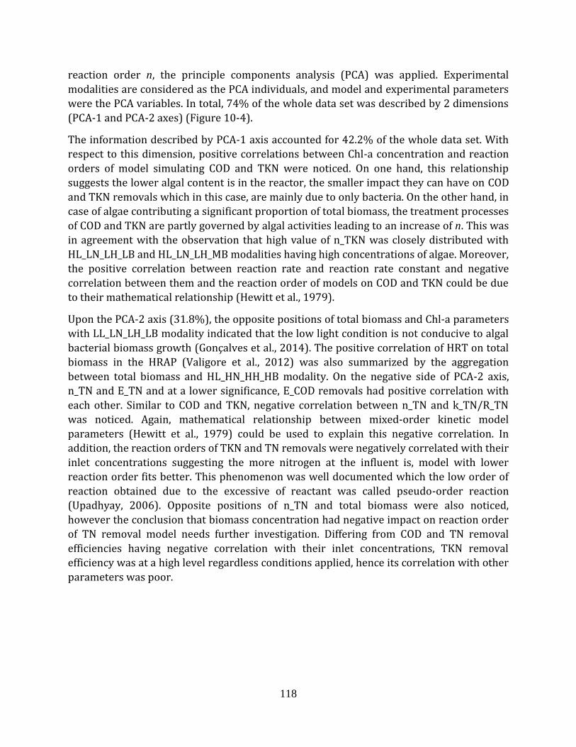
118

reaction order n, the principle components analysis (PCA) was applied. Experimental

modalities are considered as the PCA individuals, and model and experimental parameters

were the PCA variables. In total, 74% of the whole data set was described by 2 dimensions

(PCA-1 and PCA-2 axes) (Figure 10-4).

The information described by PCA-1 axis accounted for 42.2% of the whole data set. With

respect to this dimension, positive correlations between Chl-a concentration and reaction

orders of model simulating COD and TKN were noticed. On one hand, this relationship

suggests the lower algal content is in the reactor, the smaller impact they can have on COD

and TKN removals which in this case, are mainly due to only bacteria. On the other hand, in

case of algae contributing a significant proportion of total biomass, the treatment processes

of COD and TKN are partly governed by algal activities leading to an increase of n. This was

in agreement with the observation that high value of n_TKN was closely distributed with

HL_LN_LH_LB and HL_LN_LH_MB modalities having high concentrations of algae. Moreover,

the positive correlation between reaction rate and reaction rate constant and negative

correlation between them and the reaction order of models on COD and TKN could be due

to their mathematical relationship (Hewitt et al., 1979).

Upon the PCA-2 axis (31.8%), the opposite positions of total biomass and Chl-a parameters

with LL_LN_LH_LB modality indicated that the low light condition is not conducive to algal

bacterial biomass growth (Gonçalves et al., 2014). The positive correlation of HRT on total

biomass in the HRAP (Valigore et al., 2012) was also summarized by the aggregation

between total biomass and HL_HN_HH_HB modality. On the negative side of PCA-2 axis,

n_TN and E_TN and at a lower significance, E_COD removals had positive correlation with

each other. Similar to COD and TKN, negative correlation between n_TN and k_TN/R_TN

was noticed. Again, mathematical relationship between mixed-order kinetic model

parameters (Hewitt et al., 1979) could be used to explain this negative correlation. In

addition, the reaction orders of TKN and TN removals were negatively correlated with their

inlet concentrations suggesting the more nitrogen at the influent is, model with lower

reaction order fits better. This phenomenon was well documented which the low order of

reaction obtained due to the excessive of reactant was called pseudo-order reaction

(Upadhyay, 2006). Opposite positions of n_TN and total biomass were also noticed,

however the conclusion that biomass concentration had negative impact on reaction order

of TN removal model needs further investigation. Differing from COD and TN removal

efficiencies having negative correlation with their inlet concentrations, TKN removal

efficiency was at a high level regardless conditions applied, hence its correlation with other

parameters was poor.

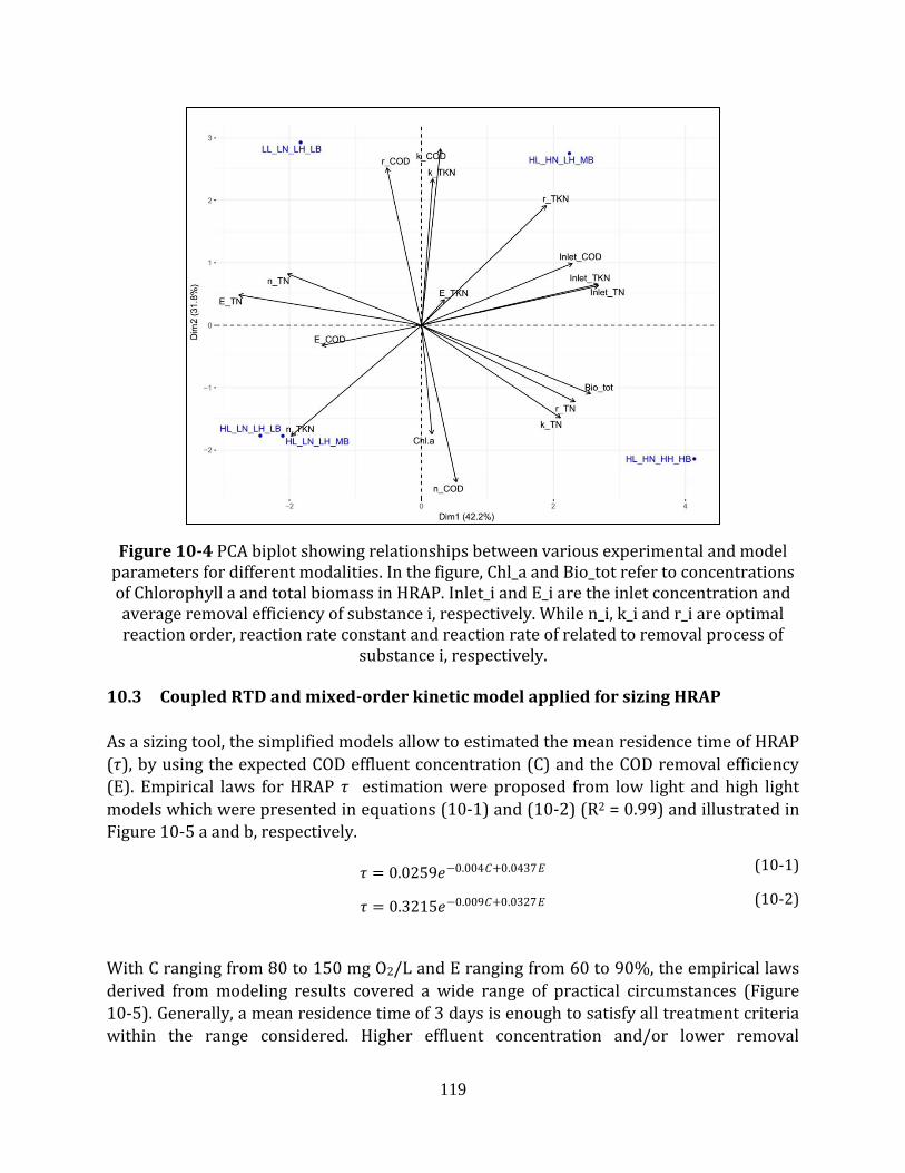
119

Figure 10-4 PCA biplot showing relationships between various experimental and model parameters for different modalities. In the figure, Chl_a and Bio_tot refer to concentrations of Chlorophyll a and total biomass in HRAP. Inlet_i and E_i are the inlet concentration and average removal efficiency of substance i, respectively. While n_i, k_i and r_i are optimal reaction order, reaction rate constant and reaction rate of related to removal process of

substance i, respectively.

10.3 Coupled RTD and mixed-order kinetic model applied for sizing HRAP

As a sizing tool, the simplified models allow to estimated the mean residence time of HRAP

(𝜏), by using the expected COD effluent concentration (C) and the COD removal efficiency

(E). Empirical laws for HRAP 𝜏 estimation were proposed from low light and high light

models which were presented in equations (10-1) and (10-2) (R2 = 0.99) and illustrated in

Figure 10-5 a and b, respectively.

𝜏 = 0.0259𝑒−0.004𝐶+0.0437𝐸 (10-1)

𝜏 = 0.3215𝑒−0.009𝐶+0.0327𝐸 (10-2)

With C ranging from 80 to 150 mg O2/L and E ranging from 60 to 90%, the empirical laws

derived from modeling results covered a wide range of practical circumstances (Figure

10-5). Generally, a mean residence time of 3 days is enough to satisfy all treatment criteria

within the range considered. Higher effluent concentration and/or lower removal

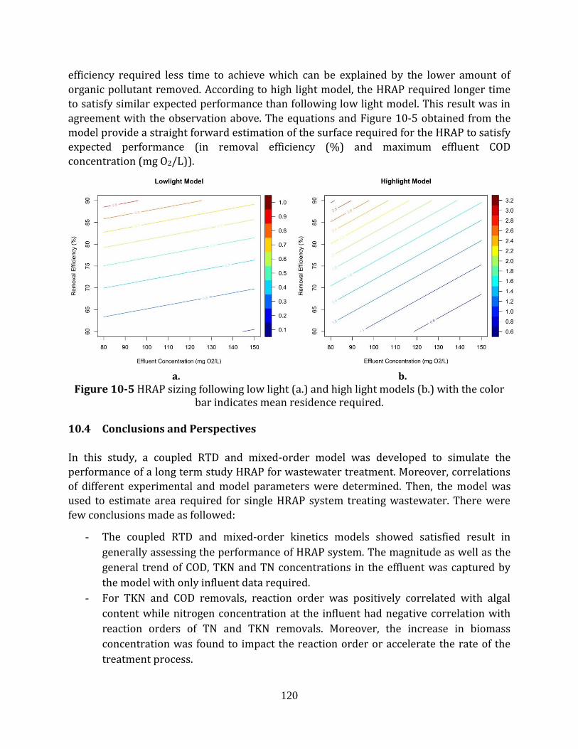
120

efficiency required less time to achieve which can be explained by the lower amount of

organic pollutant removed. According to high light model, the HRAP required longer time

to satisfy similar expected performance than following low light model. This result was in

agreement with the observation above. The equations and Figure 10-5 obtained from the

model provide a straight forward estimation of the surface required for the HRAP to satisfy

expected performance (in removal efficiency (%) and maximum effluent COD

concentration (mg O2/L)).

a. b.

Figure 10-5 HRAP sizing following low light (a.) and high light models (b.) with the color bar indicates mean residence required.

10.4 Conclusions and Perspectives

In this study, a coupled RTD and mixed-order model was developed to simulate the

performance of a long term study HRAP for wastewater treatment. Moreover, correlations

of different experimental and model parameters were determined. Then, the model was

used to estimate area required for single HRAP system treating wastewater. There were

few conclusions made as followed:

- The coupled RTD and mixed-order kinetics models showed satisfied result in

generally assessing the performance of HRAP system. The magnitude as well as the

general trend of COD, TKN and TN concentrations in the effluent was captured by

the model with only influent data required.

- For TKN and COD removals, reaction order was positively correlated with algal

content while nitrogen concentration at the influent had negative correlation with

reaction orders of TN and TKN removals. Moreover, the increase in biomass

concentration was found to impact the reaction order or accelerate the rate of the

treatment process.

121

- However, due to its limitation of black box model type, the detailed agreement

between model and experimental data was highly varied, ranging from

unsatisfactory to excellent. In extreme condition such as high load of nutrient at the

influent, the model was inappropriate to simulate the system performance. Hence,

more sophisticated model should be used for better investigation.

- From the model, empirical laws for HRAP mean residence time estimation was

provided as a sizing support. However, notices should be taken in the behavior of

the mixed-order kinetics model to avoid misinterpretation. Further validation with

outdoor HRAP system is necessary.

In French:

Dans cette étude, un modèle couplant distribution des temps de séjour et cinétiques

d'ordre mixte a été développé pour simuler la performance d’un réacteur HRAP pour le

traitement des eaux usées. Des corrélations entre les différents paramètres expérimentaux

et les paramètres du modèle ont été déterminées. Ensuite, le modèle a été utilisé pour

estimer la superficie requise pour un système HRAP traitant les eaux usées. Les conclusions

qui en ont été tirées sont les suivantes:

- Les modèles couplant distribution des temps de séjour et cinétiques d'ordre mixte

ont donné des résultats satisfaisants dans l'évaluation générale de la performance

du système HRAP. L'ampleur ainsi que la tendance générale des concentrations de

DCO, de TKN et de TN dans l'effluent ont été décrites par le modèle et seules les

données sur l'affluent ont été requises.

- Dans le cas de l'élimination de l’azote réduit et de la DCO, l'ordre de réaction est

corrélé positivement avec la teneur en algues, tandis que la concentration d'azote à

l'affluent a une corrélation négative avec les ordres de réaction de l'élimination de

l’azoite total et Kjeldahl. De plus, l'augmentation de la concentration de biomasse

s'est avérée avoir un impact sur l'ordre de réaction ou accélérer la vitesse de

réaction.

- Toutefois, en raison de la limitation de ce type de modèle « boîte noire »,

l'ajustement précis entre le modèle et les données expérimentales était très

variable, allant d'insatisfaisant à excellent. Dans des conditions extrêmes comme

une charge élevée de nutriments à l'affluent, le modèle ne permettait pas de simuler

la performance du système. Par conséquent, un modèle plus sophistiqué devrait être

utilisé pour une meilleure investigation.

- A partir du modèle, des lois empiriques pour l'estimation du temps de séjour moyen

ont été fournies comme support de dimensionnement. Toutefois, il faut tenir compte

du comportement du modèle de cinétique d'ordre mixte pour éviter les erreurs

122

d'interprétation. Une validation supplémentaire avec un système HRAP à plaine

échelle fonctionnant en extérieur est nécessaire.

123

CHAPTER 11 SIMULATION OF ALGAL BACTERIAL PROCESSES IN WASTEWATER

TREATMENT HIGH RATE ALGAL POND – A GOOD MODELING PRACTICE APPLICATION

11.1 Introduction

The application of algal-bacterial systems in wastewater treatment has attracted an

increasing recognition in the recent years. On one hand, in wastewater exposed to light,

synergistic interactions between algae and bacteria promote heterotrophic bacterial

oxidation of organic matters due to algal photosynthetic aeration, providing dissolved

oxygen and consuming inorganic carbon (Bellinger and Sigee, 2015; Richmond, 2008). This

process also increases sharply pH level of water resulting in a sanitation effect towards

pathogenic bacteria (Cole, 1982; Muñoz and Guieysse, 2006). In addition, nutrients

assimilated by algae and bacteria are removed and recovered by harvesting the flocculated

algal-bacterial biomass (Gutzeit et al., 2005; Van Den Hende et al., 2014). On the other

hand, due to the wide range of algal biomass application such as high value bio-molecules,

fertilizers or biofuel production (Lawton et al., 2017; Sirajunnisa and Surendhiran, 2016),

the use of wastewater as nutrient source for algal-bacterial biomass production has

received serious attention (Mata et al., 2010; Park et al., 2010).

High rate algal pond (HRAP) was developed as a result of early studies on photosynthesis

in sewage wastewater (Oswald and Gotaas, 1957). Typically, a HRAP is an open, raceway

pond operated at shallow water depth with paddlewheel as the only source of mixing (Park

et al., 2010). This design allows good level of mixing in the pond which promotes the

development of algal-bacterial biomass supporting a treatment rate of ten times higher

than the conventional stabilization pond (El Hamouri et al., 2003). Moreover, in

comparison with closed photobioreactor, operating HRAP requires lower energy and

simple maintenance as well as expanding (Mata et al., 2010). Hence HRAP has been widely

applied for wastewater treatment and algal biomass production (Kumar et al., 2015).

However, due to the dependence of algal-bacterial interactions inside the HRAP system on

the variation of different operational and environmental conditions (Cole, 1982; Kouzuma

and Watanabe, 2015), the system is difficult to control and thus yet to be applied widely at

full-scale (Mata et al., 2010). In this context, using mathematical models to simulate the

algal-bacterial processes could serve as a rapid and cost-effective method to study the

system for design and operation optimization as well as scale-up. In this regard, an early

kinetic model of algal-bacterial growth was developed by Buhr and Miller (1983) with

relative simple structure including algal and bacterial growth and decay together with

basic physiochemical processes in liquid phase (Buhr and Miller, 1983). The kinetic model

was then coupled with a systemic hydrodynamic model simulating mixing characteristics

in a high rate algal pond (HRAP) (Miller and Buhr, 1981) and validated with field data

which achieved good agreement. Moreover, inspired by the development of bacterial

kinetic model including activated sludge models (ASM) series and anaerobic digestion

model (ADM), a model was developed to simulate algal growth kinetic based on ASM

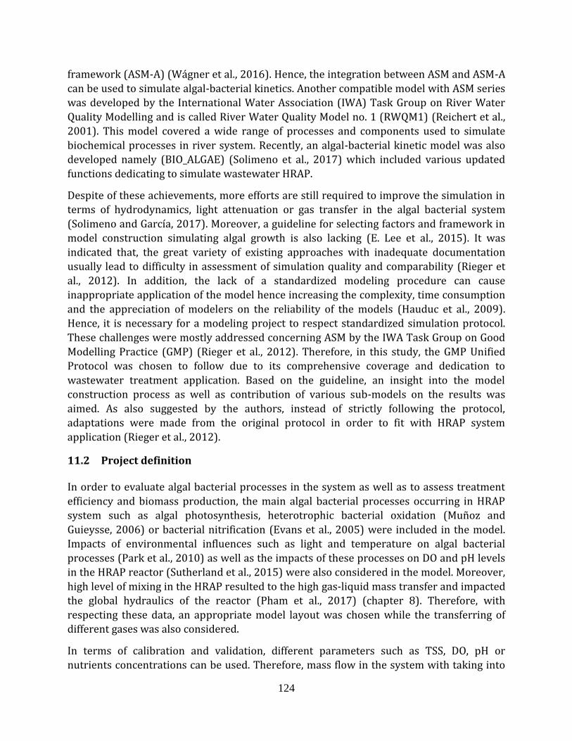
124

framework (ASM-A) (Wágner et al., 2016). Hence, the integration between ASM and ASM-A

can be used to simulate algal-bacterial kinetics. Another compatible model with ASM series

was developed by the International Water Association (IWA) Task Group on River Water

Quality Modelling and is called River Water Quality Model no. 1 (RWQM1) (Reichert et al.,

2001). This model covered a wide range of processes and components used to simulate

biochemical processes in river system. Recently, an algal-bacterial kinetic model was also

developed namely (BIO_ALGAE) (Solimeno et al., 2017) which included various updated

functions dedicating to simulate wastewater HRAP.

Despite of these achievements, more efforts are still required to improve the simulation in

terms of hydrodynamics, light attenuation or gas transfer in the algal bacterial system

(Solimeno and García, 2017). Moreover, a guideline for selecting factors and framework in

model construction simulating algal growth is also lacking (E. Lee et al., 2015). It was

indicated that, the great variety of existing approaches with inadequate documentation

usually lead to difficulty in assessment of simulation quality and comparability (Rieger et

al., 2012). In addition, the lack of a standardized modeling procedure can cause

inappropriate application of the model hence increasing the complexity, time consumption

and the appreciation of modelers on the reliability of the models (Hauduc et al., 2009).

Hence, it is necessary for a modeling project to respect standardized simulation protocol.

These challenges were mostly addressed concerning ASM by the IWA Task Group on Good

Modelling Practice (GMP) (Rieger et al., 2012). Therefore, in this study, the GMP Unified

Protocol was chosen to follow due to its comprehensive coverage and dedication to

wastewater treatment application. Based on the guideline, an insight into the model

construction process as well as contribution of various sub-models on the results was

aimed. As also suggested by the authors, instead of strictly following the protocol,

adaptations were made from the original protocol in order to fit with HRAP system

application (Rieger et al., 2012).

11.2 Project definition

In order to evaluate algal bacterial processes in the system as well as to assess treatment

efficiency and biomass production, the main algal bacterial processes occurring in HRAP

system such as algal photosynthesis, heterotrophic bacterial oxidation (Muñoz and

Guieysse, 2006) or bacterial nitrification (Evans et al., 2005) were included in the model.

Impacts of environmental influences such as light and temperature on algal bacterial

processes (Park et al., 2010) as well as the impacts of these processes on DO and pH levels

in the HRAP reactor (Sutherland et al., 2015) were also considered in the model. Moreover,

high level of mixing in the HRAP resulted to the high gas-liquid mass transfer and impacted

the global hydraulics of the reactor (Pham et al., 2017) (chapter 8). Therefore, with

respecting these data, an appropriate model layout was chosen while the transferring of

different gases was also considered.

In terms of calibration and validation, different parameters such as TSS, DO, pH or

nutrients concentrations can be used. Therefore, mass flow in the system with taking into

125

account settling and harvesting processes was included in the model (Rieger et al., 2012).

Experimental results from the long term pilot experiment (chapter 9) were used for

calibrating and validating the model. To simulate the variation of these data, dynamic

simulation was employed. General simulation protocol adapted to HRAP system is

illustrated in Figure 11-1.

Figure 11-1 General illustration of the HRAP simulation procedure.

11.3 Data collection and reconciliation

11.3.1 Data collection

Measured data from the experiment were categorized into input, physical and operational

data for implementing in input model while data related to performances and additional

data were used for model calibration and validation. This classification allows better

identification of essential data for model implementation, especially when dealing with

complex system such as activated sludge system (Rieger et al., 2012). Therefore, the same

approach was applied for collecting data from the HRAP experiment.

Input data

The input data provided information relating to influent mass loading of the system

including concentrations of various wastewater constituents, influent flow rates and

temperature of the reactor (Rieger et al., 2012). Sampling for nutrient content analysis was

performed once per week around midday, right before the feeding event. One sampling

consisted of 500 mL of inlet wastewater from the storage tank. The sample was analyzed

126

within 24h for total suspended solids (TSS) and occasionally volatile suspended solids

(VSS) (NF EN 872), chemical oxygen demand content (COD) (NANOCOLOR® COD 1500

according to DIN ISO 15705), total Kjeldahl nitrogen content (TKN-N) (NF EN 25663),

ammonium nitrogen (NH4-N) (NF EN ISO 14911), nitrate nitrogen (NO3-N) (NF EN ISO

10304) and nitrite nitrogen (NO2-N) (NF EN ISO 10304). Temperature of HRAP reactor

was measured with DO and pH measurement while the influent flow rate was controlled by

the feeding pump. Besides, in order to simulate algal photosynthesis, light intensity data is

important to collect. In the study, illumination was provided by a high-power LED light

(ARIAH2™ 200W IP65 LED HIGHBAY, ENLITE) positioned on top of the pilot with the

vertical distance to the water surface of 0.8m providing a constant light intensity of 210

μEs-1m-2 at the water surface. A timer was connected to the light source to have a

light/dark cycle of 14h/10h. Average values of the measured parameters are presented in

Table 11-1.

Physical and Operational data

Physical and operational data were obtained from previous studies (chapter 8) on global

hydraulics and oxygen transfer rate of the reactor (Pham et al., 2017). Water level was

maintained at 0.11m giving 80L of total volume. The rotating speed of the paddle wheel

was maintained at around 11.6 rpm for better mixing and mass transfer, giving the mid-

channel average velocity of 0.44 m/s.

Previous study on global hydraulics of the pilot HRAP (Pham et al., 2017) (chapter 8)

indicated that the entire pilot HRAP can be considered as a continuous stirred-tank reactor

(CSTR). In addition, gas transfer study was also conducted to determine oxygen transfer

coefficient (kLaO2) of the HRAP (Pham et al., 2017) (chapter 8). The volumetric mass

transfer coefficients of other gas including ammonia and carbon dioxide can be derived

using the diffusivity ratio. For example, the volumetric mass transfer coefficient of CO2 can

be calculated as (Spérandio and Paul, 1997):

kLaCO 2

kLaO2=

DCO 2

DO2

(11-1)

With DCO 2 and DO2 are the diffusion coefficients of CO2 and O2 in water, respectively.

Diffusion coefficients of O2, CO2 and NH3 in water at 25oC were 2.1, 1.92 and 1.64 10-

5.cm2/s, respectively (Cussler, 2009). Hence the calculated kLaCO2 and kLaNH3 were 66.69

and 61.64 day-1, respectively. With the given operational conditions, the HRAP had high

kLaO2 value of 69.75 day-1. It is important to notice that, these values were usually

calibrated or estimated in various algal bacterial model (Buhr and Miller, 1983; Solimeno et

al., 2017) although they have great influences on the model result (Solimeno et al., 2016).

Moreover, the values obtained in this study were at high level in comparison with usually

calibrated/estimated values of 3-6 day-1 (Buhr and Miller, 1983; Solimeno et al., 2017).

Hence significant impacts of these parameters in this case were expected.

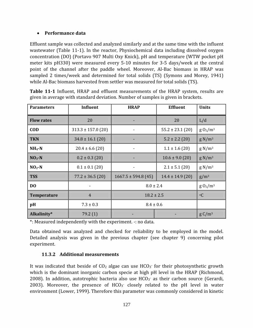
127

Performance data

Effluent sample was collected and analyzed similarly and at the same time with the influent

wastewater (Table 11-1). In the reactor, Physiochemical data including dissolved oxygen

concentration (DO) (Portavo 907 Multi Oxy Knick), pH and temperature (WTW pocket pH

meter kits pH330) were measured every 5-10 minutes for 3-5 days/week at the central

point of the channel after the paddle wheel. Moreover, Al-Bac biomass in HRAP was

sampled 2 times/week and determined for total solids (TS) (Symons and Morey, 1941)

while Al-Bac biomass harvested from settler was measured for total solids (TS).

Table 11-1 Influent, HRAP and effluent measurements of the HRAP system, results are given in average with standard deviation. Number of samples is given in brackets.

Parameters Influent HRAP Effluent Units

Flow rates 20 - 20 L/d

COD 313.3 ± 157.0 (20) - 55.2 ± 23.1 (20) g O2/m3

TKN 34.8 ± 16.1 (20) - 5.2 ± 2.2 (20) g N/m3

NH4-N 20.4 ± 6.6 (20) - 1.1 ± 1.6 (20) g N/m3

NO3-N 0.2 ± 0.3 (20) - 10.6 ± 9.0 (20) g N/m3

NO2-N 0.1 ± 0.1 (20) - 2.1 ± 5.1 (20) g N/m3

TSS 77.2 ± 36.5 (20) 1667.5 ± 594.8 (45) 14.4 ± 14.9 (20) g/m3

DO - 8.0 ± 2.4 g O2/m3

Temperature 4 18.2 ± 2.5 oC

pH 7.3 ± 0.3 8.4 ± 0.6

Alkalinity* 79.2 (1) - - g C/m3

*: Measured independently with the experiment. -: no data.

Data obtained was analyzed and checked for reliability to be employed in the model.

Detailed analysis was given in the previous chapter (see chapter 9) concerning pilot

experiment.

11.3.2 Additional measurements

It was indicated that beside of CO2 algae can use HCO3- for their photosynthetic growth

which is the dominant inorganic carbon specie at high pH level in the HRAP (Richmond,

2008). In addition, autotrophic bacteria also use HCO3- as their carbon source (Gerardi,

2003). Moreover, the presence of HCO3- closely related to the pH level in water

environment (Lower, 1999). Therefore this parameter was commonly considered in kinetic

128

models such as ASM or RWQM1 (Henze et al., 2000; Reichert et al., 2001) for algal bacterial

simulation. However, it was generally ignored when only performance assessment of the

system was required. Hence, additional measurement of influent HCO3- concentration was

conducted and one representative value was implemented (Table 11-1).

11.4 Al-Bac model set-up for HRAP system

11.4.1 Model layout

In practice, due to the long channel of full scale HRAP, Tank-in-Series (TIS) was commonly

applied (Buhr and Miller, 1983; El Ouarghi et al., 2000). Hence, the kinetic model is applied

to each tank (CSTR) which receives effluent from the previous one and discharges to the

next one in line (Buhr and Miller, 1983). However, in this case, results of global hydraulic

study of the pilot HRAP (Pham et al., 2017) indicated that the HRAP can be simulated as a

CSTR thus the algal bacterial kinetic model was applied to the entire reactor volume.

11.4.2 Algal bacterial kinetic model

A kinetic model describing algal bacterial processes in the HRAP was constructed. It is

mainly based on RWQM1 (Reichert et al., 2001) and BIO_ALGAE model (Solimeno et al.,

2017) due to their comprehensive as well as dedication for algal bacterial simulation.

Model components and processes selection was conducted with respect to experimental

results obtained.

11.4.2.1 Model components

The model follows the same nomenclatures as indicated in RWQM1 (Reichert et al., 2001).

In total, 18 components including 12 dissolved and 6 particulate components were

considered.

Model dissolved components included:

- Nitrogenous components include SNH4, SNH3, SNO3 and SNO2 [g N/m3] which are

ammonium, ammonia, nitrate and nitrite nitrogen, respectively. Ammonium

accounts a significant part in influent nitrogen and is also released after microbial

endogenous respiration or decay. Ammonium and ammonia are linked by acid-base

equilibrium, which are consumed by algae (XALG), heterotrophic bacteria (XH) and

ammonium oxidizing bacteria (XAOB). Ammonia volatilization strongly depends on

mixing condition in the reactor. Besides SNH4 and SNH3, algae and heterotrophic

bacteria can also used nitrate for their aerobic growth. Nitrate and nitrite can be

present in influent wastewater though usually in small concentrations. They are

mainly involved in nitrification process during which ammonium is converted to

nitrite and then to nitrate by ammonium and nitrite oxidizing bacteria, respectiviely

(XAOB, XNOB).

129

- Mineral carbonaceous components include SCO2, SHCO3 and SCO3 [g C/m3] which are

carbon dioxide, bicarbonate and carbonate, respectively. These components are

linked with each other by chemical equilibrium which is strongly correlated with pH

level. The first two components can be consumed by algae and autotrophic bacteria

(XAOB, XNOB). While all of these components can enter the reactor from influent

wastewater, carbon dioxide can also be dissolved to water from the air or vice versa.

It is also produced by microbial respiration or decay.

- Dissolved oxygen SO2 [g O2/m3] is produced during photosynthetic growth of algae

and can be transferred to/from the atmosphere. It is consumed during aerobic

respiration of all types of microorganisms.

- Hydrogen SH and hydroxide SOH [moles] ions are linked by chemical equilibrium

governing pH level. Hydrogen ions are involved in all chemical equilibriums in the

system and are produced by ammonium oxidizing bacteria (XAOB) and heterotrophic

bacteria (XH). SH decreases during the growth of algae and nitrite oxidizing bacteria

(XNOB), and during microbial endogenous respiration and decay.

- Soluble organic matters include SS and SI [g/m3] which are readily degradable and

inert organic matters, respectively. They can enter the reactor from the influent

wastewater or be produced via hydrolysis. Only SS can be consumed by

heterotrophic bacteria.

Model particulate components included:

- Algae biomass XALG increases following algal growth processes while decreases due

to algal decay and endogenous respiration. Due to the insignificant amount of Chl-a

detected in influent and effluent streams, algae are considered not present in

influent and effluent wastewater.

- Bacterial biomass includes heterotrophic bacteria XH, ammonium oxidizing bacteria

XAOB and nitrite oxidizing bacteria XNOB. While heterotrophic bacteria are

responsible for oxidizing organic matter and use it as the carbon source, the two

others use inorganic carbon (SCO2, SHCO3) to convert ammonium to nitrite and then

nitrate (XAOB, XNOB, respectively). All of them use oxygen for their production while

decreasing by endogenous respiration. Moreover, heterotrophic bacteria are also

responsible for hydrolysis.

- Particulate organic matters include slowly biodegradable (XS) and inert (XI) matters.

Both of them are present in influent wastewater and released after decay and

endogenous respiration processes. Only XS can be further converted to soluble

organic matters via hydrolysis.

130

11.4.2.2 Model processes

The algal bacterial kinetic model describes the interrelationship between algae, bacteria

and different chemical constituents in the HRAP reactor. Therefore, the growth processes

of algae and bacteria on different substrates and chemical equilibriums are included in the

model. Monod kinetics and multiplicative model framework were used to describe the

correlation between different limiting factors and algal/bacterial growth. The model

applied was mainly based on RWQM1 (Reichert et al., 2001) with necessary simplification.

Although the impact of predators on algal bacterial processes was indicated in HRAP

system (Montemezzani et al., 2016), their impact in this study was not significant. Hence, in

comparison with RWQM1, the processes related to consumers were neglected. Moreover,

due to the high DO level in the reactor (Table 11-1), anaerobic and anoxic processes were

also ignored. Experimental data also showed that phosphorus was not a limiting factor for

microbial growth as the effluent concentration of total phosphorus was 1.7 ± 0.8 mg P/L.

Hence it was not included in the model. Detailed mathematic expression of different model

processes and parameter values are shown in Table 11-2 and Table 11-3 while their

explanations are given below.

Algal growth processes

Algal growth processes are activated by light. Inorganic carbons (CO2 and HCO3-) are fixed

and nutrients (NH4, NO3) are consumed while O2 is released as a byproduct

(photosynthesis). Due to the microbial preference of ammonium over nitrate for growth, a

nitrate consumption limiting factor is included. Similar to the BIO_ALGAE model (Solimeno

et al., 2017), limiting factor of inorganic carbon over algal growth was employed yet due to

the high level of gas transfer in the experiment, algal inhibition due to high inorganic

carbon accumulation was not considered.

Bacterial growth processes

Different groups of bacteria are considered including heterotrophic bacteria, ammonium

oxidizing bacteria (first step of nitrification AOB) and nitrite oxidizing bacteria (second

step of nitrification NOB). The heterotrophic bacteria oxidize organic matter while

consuming nutrients (NH4, NO3) and O2 and releasing CO2. The released CO2 is in turns

available for both algal and nitrifying bacterial growth. In addition, the AOB convert

ammonium and ammonia in water to nitrite while the NOB convert nitrite to nitrate under

low ammonium level condition which is then available for heterotrophic bacteria and algae

(Iacopozzi et al., 2007). Moreover, due to the potential competition between algae and

nitrifying bacteria over carbon source, limiting factor of inorganic carbon over AOB and

NOB growth was employed. Due to the constant high level of dissolved oxygen in the

reactor during the entire experiment, only aerobic processes are included.

Biomass loss and regeneration

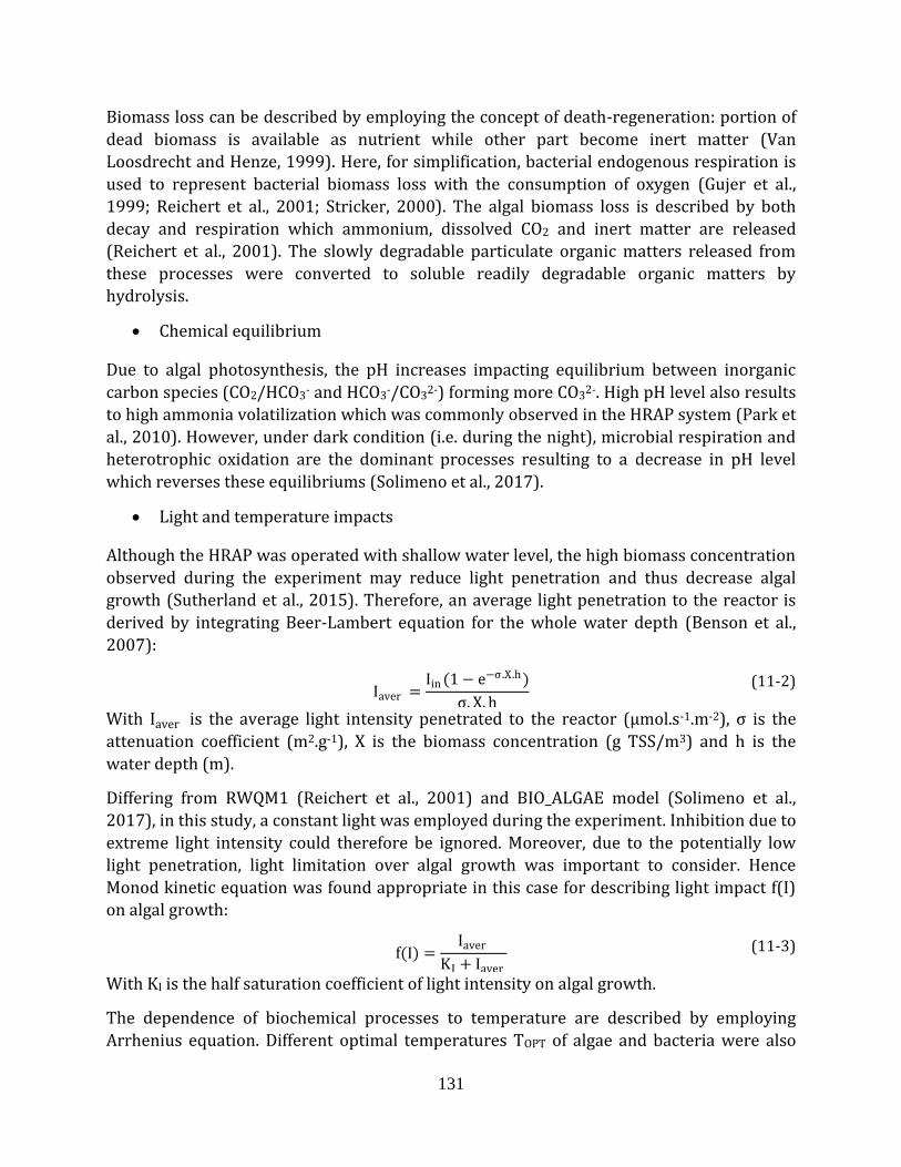
131

Biomass loss can be described by employing the concept of death-regeneration: portion of

dead biomass is available as nutrient while other part become inert matter (Van

Loosdrecht and Henze, 1999). Here, for simplification, bacterial endogenous respiration is

used to represent bacterial biomass loss with the consumption of oxygen (Gujer et al.,

1999; Reichert et al., 2001; Stricker, 2000). The algal biomass loss is described by both

decay and respiration which ammonium, dissolved CO2 and inert matter are released

(Reichert et al., 2001). The slowly degradable particulate organic matters released from

these processes were converted to soluble readily degradable organic matters by

hydrolysis.

Chemical equilibrium

Due to algal photosynthesis, the pH increases impacting equilibrium between inorganic

carbon species (CO2/HCO3- and HCO3-/CO32-) forming more CO32-. High pH level also results

to high ammonia volatilization which was commonly observed in the HRAP system (Park et

al., 2010). However, under dark condition (i.e. during the night), microbial respiration and

heterotrophic oxidation are the dominant processes resulting to a decrease in pH level

which reverses these equilibriums (Solimeno et al., 2017).

Light and temperature impacts

Although the HRAP was operated with shallow water level, the high biomass concentration

observed during the experiment may reduce light penetration and thus decrease algal

growth (Sutherland et al., 2015). Therefore, an average light penetration to the reactor is

derived by integrating Beer-Lambert equation for the whole water depth (Benson et al.,

2007):

Iaver =

Iin (1 − e−σ .X.h )

σ. X. h

(11-2)

With Iaver is the average light intensity penetrated to the reactor (μmol.s-1.m-2), σ is the

attenuation coefficient (m2.g-1), X is the biomass concentration (g TSS/m3) and h is the

water depth (m).

Differing from RWQM1 (Reichert et al., 2001) and BIO_ALGAE model (Solimeno et al.,

2017), in this study, a constant light was employed during the experiment. Inhibition due to

extreme light intensity could therefore be ignored. Moreover, due to the potentially low

light penetration, light limitation over algal growth was important to consider. Hence

Monod kinetic equation was found appropriate in this case for describing light impact f(I)

on algal growth:

f(I) =

Iaver

KI + Iaver (11-3)

With KI is the half saturation coefficient of light intensity on algal growth.

The dependence of biochemical processes to temperature are described by employing

Arrhenius equation. Different optimal temperatures TOPT of algae and bacteria were also

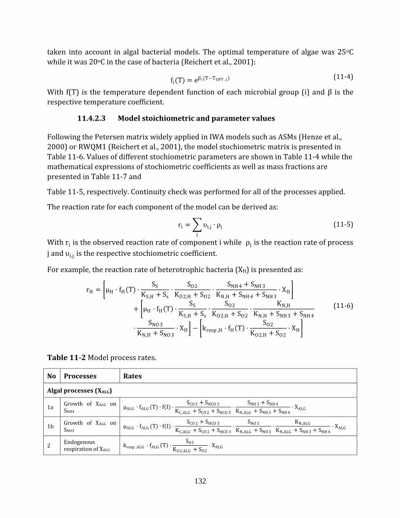
132

taken into account in algal bacterial models. The optimal temperature of algae was 25oC

while it was 20oC in the case of bacteria (Reichert et al., 2001):

fi(T) = eβ i (T−TOPT ,i ) (11-4)

With f(T) is the temperature dependent function of each microbial group (i) and β is the

respective temperature coefficient.

11.4.2.3 Model stoichiometric and parameter values

Following the Petersen matrix widely applied in IWA models such as ASMs (Henze et al.,

2000) or RWQM1 (Reichert et al., 2001), the model stochiometric matrix is presented in

Table 11-6. Values of different stochiometric parameters are shown in Table 11-4 while the

mathematical expressions of stochiometric coefficients as well as mass fractions are

presented in Table 11-7 and

Table 11-5, respectively. Continuity check was performed for all of the processes applied.

The reaction rate for each component of the model can be derived as:

ri = υi,j ∙ ρj

j

(11-5)

With ri is the observed reaction rate of component i while ρj is the reaction rate of process

j and υi,j is the respective stochiometric coefficient.

For example, the reaction rate of heterotrophic bacteria (XH) is presented as:

rH = μH · fH T ·

SS

KS,H + Ss·

SO2

KO2,H + SO2·

SNH 4 + SNH 3

KN,H + SNH 4 + SNH 3· XH

+ μH · fH T ·SS

KS,H + Ss·

SO2

KO2,H + SO2·

KN,H

KN,H + SNH 3 + SNH 4

·SNO 3

KN,H + SNO 3· XH − kresp ,H · fH T ·

SO2

KO2,H + SO2· XH

(11-6)

Table 11-2 Model process rates.

No Processes Rates

Algal processes (XALG)

1a Growth of XALG on SNH4

μALG ∙ fALG (T) ∙ f(I) ·SCO 2 + SHCO 3

KC,ALG + SCO 2 + SHCO 3·

SNH 3 + SNH 4

KN,ALG + SNH 3 + SNH 4· XALG

1b Growth of XALG on SNO3

μALG · fALG (T) ∙ f(I) ·SCO 2 + SHCO 3

KC,ALG + SCO 2 + SHCO 3·

SNO 3

KN,ALG + SNO 3·

KN,ALG

KN,ALG + SNH 3 + SNH 4· XALG

2 Endogenous respiration of XALG

kresp ,ALG · fALG T ·SO2

KO2,ALG + SO2· XALG

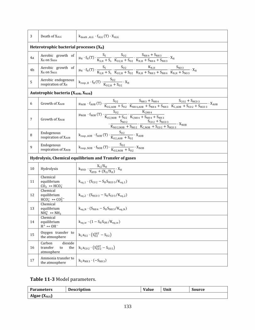
133

3 Death of XALG kdeath ,ALG · fALG T · XALG

Heterotrophic bacterial processes (XH)

4a Aerobic growth of XH on SNH4

μH · fH T ·SS

KS,H + Ss·

SO2

KO2,H + SO2·

SNH 4 + SNH 3

KN,H + SNH 4 + SNH 3· XH

4b Aerobic growth of XH on SNO3

μH · fH T ·SS

KS,H + Ss·

SO2

KO2,H + SO2·

KN,H

KN,H + SNH 3 + SNH 4·

SNO 3

KN,H + SNO 3· XH

5 Aerobic endogenous respiration of XH

kresp ,H · fH T ·SO2

KO2,H + SO2· XH

Autotrophic bacteria (XAOB, XNOB)

6 Growth of XAOB μAOB · fAOB T ·SO2

KO2,AOB + SO2·

SNH 3 + SNH 4

KNH 4,AOB + SNH 4 + SNH 3·

SCO2 + SHCO 3

KC,AOB + SCO 2 + SHCO 3· XAOB

7 Growth of XNOB

μNOB · fNOB T ·SO2

KO2,NOB + SO2·

KI,NH 4

KI,NH 4 + SNH 4 + SNH 3

·SNO 2

KNO 2,NOB + SNO 2·

SCO 2 + SHCO 3

KC,NOB + SCO 2 + SHCO 3· XNOB

8 Endogenous respiration of XAOB

kresp ,AOB · fAOB T ·SO2

KO2,AOB + SO2· XAOB

9 Endogenous respiration of XNOB

kresp ,NOB · fNOB T ·SO2

KO2,NOB + SO2· XNOB

Hydrolysis, Chemical equilibrium and Transfer of gases

10 Hydrolysis kHYD ·XS /XH

YHYD + (XS /XH)· XH

11 Chemical equilibrium CO2 ↔ HCO3

−

keq ,1 · (SCO 2 − SH SHCO 3 Keq ,1 )

12 Chemical equilibrium HCO3

− ↔ CO32−

keq ,2 · (SHCO 3 − SHSCO 3 Keq ,2 )

13 Chemical equilibrium NH4

+ ↔ NH3 keq ,N · (SNH 4 − SH SNH 3 Keq ,N )

14 Chemical equilibrium H+ ↔ OH−

keq ,w · (1 − SH SOH Keq ,w )

15 Oxygen transfer to the atmosphere

kLaO2 · SO2SAT − SO2

16 Carbon dioxide transfer to the atmosphere

kLaCO 2 · SCO 2SAT − SCO 2

17 Ammonia transfer to the atmosphere

kLaNH 3 · −SNH 3

Table 11-3 Model parameters.

Parameters Description Value Unit Source

Algae (XALG)

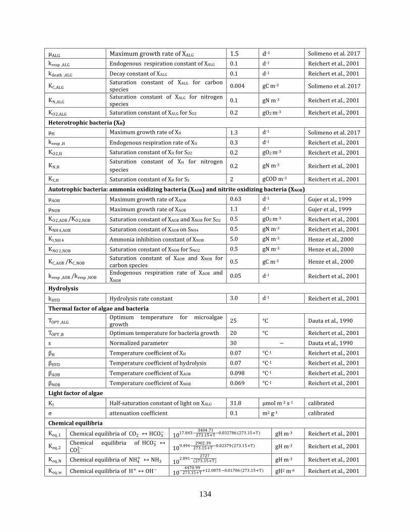
134

μALG Maximum growth rate of XALG 1.5 d-1 Solimeno et al. 2017

kresp ,ALG Endogenous respiration constant of XALG 0.1 d-1 Reichert et al., 2001

kdeath ,ALG Decay constant of XALG 0.1 d-1 Reichert et al., 2001

KC,ALG Saturation constant of XALG for carbon species

0.004 gC m-3 Solimeno et al. 2017

KN,ALG Saturation constant of XALG for nitrogen species

0.1 gN m-3 Reichert et al., 2001

KO2,ALG Saturation constant of XALG for SO2 0.2 gO2 m-3 Reichert et al., 2001

Heterotrophic bacteria (XH)

μH Maximum growth rate of XH 1.3 d-1 Solimeno et al. 2017

kresp ,H Endogenous respiration rate of XH 0.3 d-1 Reichert et al., 2001

KO2,H Saturation constant of XH for SO2 0.2 gO2 m-3 Reichert et al., 2001

KN,H Saturation constant of XH for nitrogen

species 0.2 gN m-3 Reichert et al., 2001

KS,H Saturation constant of XH for SS 2 gCOD m-3 Reichert et al., 2001

Autotrophic bacteria: ammonia oxidizing bacteria (XAOB) and nitrite oxidizing bacteria (XNOB)

μAOB Maximum growth rate of XAOB 0.63 d-1 Gujer et al., 1999

μNOB Maximum growth rate of XAOB 1.1 d-1 Gujer et al., 1999

KO2,AOB /KO2,NOB Saturation constant of XAOB and XNOB for SO2 0.5 gO2 m-3 Reichert et al., 2001

KNH 4,AOB Saturation constant of XAOB on SNH4 0.5 gN m-3 Reichert et al., 2001

KI,NH 4 Ammonia inhibition constant of XNOB 5.0 gN m-3 Henze et al., 2000

KNO 2,NOB Saturation constant of XNOB for SNO2 0.5 gN m-3 Henze et al., 2000

KC,AOB /KC,NOB Saturation constant of XAOB and XNOB for carbon species

0.5 gC m-3 Henze et al., 2000

kresp ,AOB /kresp ,NOB Endogenous respiration rate of XAOB and XNOB

0.05 d-1 Reichert et al., 2001

Hydrolysis

kHYD Hydrolysis rate constant 3.0 d-1 Reichert et al., 2001

Thermal factor of algae and bacteria

TOPT ,ALG Optimum temperature for microalgae growth

25 °C Dauta et al., 1990

TOPT ,B Optimum temperature for bacteria growth 20 °C Reichert et al., 2001

s Normalized parameter 30 − Dauta et al., 1990

βH Temperature coefficient of XH 0.07 °C-1 Reichert et al., 2001

βHYD Temperature coefficient of hydrolysis 0.07 °C-1 Reichert et al., 2001

βAOB Temperature coefficient of XAOB 0.098 °C-1 Reichert et al., 2001

βNOB Temperature coefficient of XNOB 0.069 °C-1 Reichert et al., 2001

Light factor of algae

KI Half-saturation constant of light on XALG 31.8 µmol m-2 s-1 calibrated

σ attenuation coefficient 0.1 m2 g-1 calibrated

Chemical equilibria

Keq ,1 Chemical equilibria of CO2 ↔ HCO3− 1017.843−

3404 .71273.15+T

−0.032786 (273.15+T) gH m-3 Reichert et al., 2001

Keq ,2 Chemical equilibria of HCO3

− ↔CO3

2− 109.494−2902.39

273.15+T−0.02379(273.15+T) gH m-3 Reichert et al., 2001

Keq ,N Chemical equilibria of NH4+ ↔ NH3 10

2.891−2727

(273.15+T) gH m-3 Reichert et al., 2001

Keq ,w Chemical equilibria of H+ ↔ OH− 10−4470.99

273.15+T+12.0875−0.01706 (273.15+T) gH2 m-6 Reichert et al., 2001

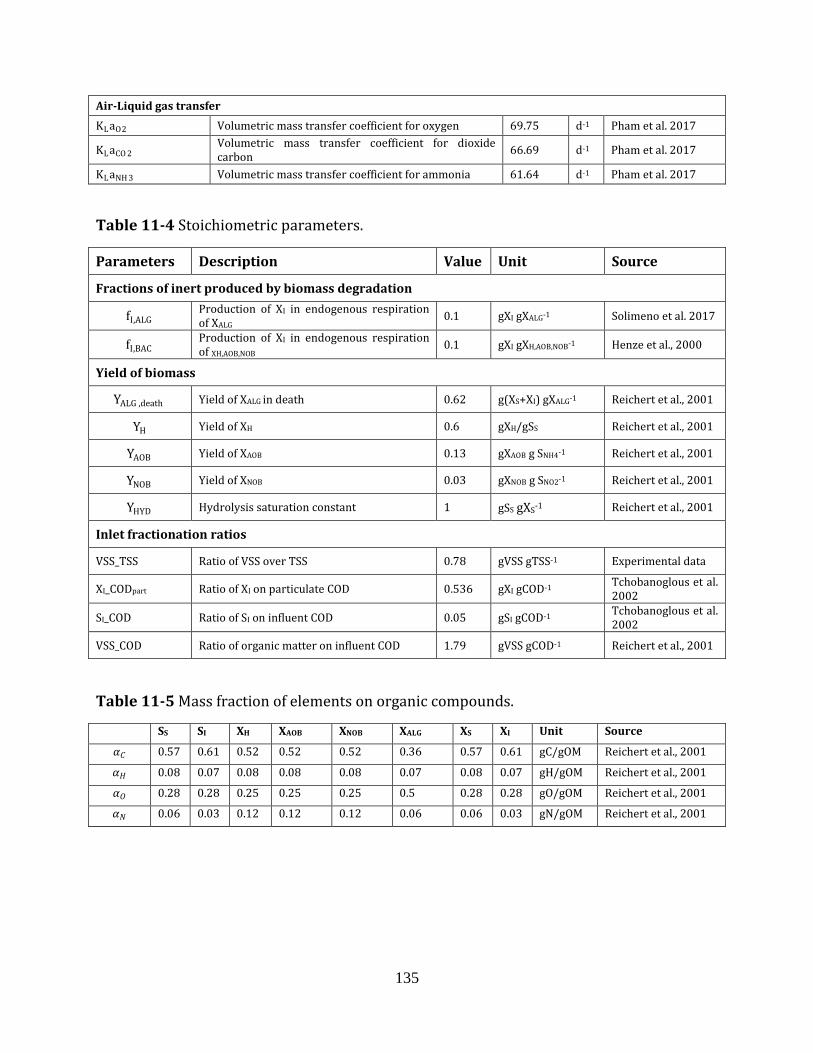
135

Air-Liquid gas transfer

KLaO2 Volumetric mass transfer coefficient for oxygen 69.75 d-1 Pham et al. 2017

KLaCO 2 Volumetric mass transfer coefficient for dioxide carbon

66.69 d-1 Pham et al. 2017

KLaNH 3 Volumetric mass transfer coefficient for ammonia 61.64 d-1 Pham et al. 2017

Table 11-4 Stoichiometric parameters.

Parameters Description Value Unit Source

Fractions of inert produced by biomass degradation

fI,ALG Production of XI in endogenous respiration of XALG

0.1 gXI gXALG-1 Solimeno et al. 2017

fI,BAC Production of XI in endogenous respiration of XH,AOB,NOB

0.1 gXI gXH,AOB,NOB-1 Henze et al., 2000

Yield of biomass

YALG ,death Yield of XALG in death 0.62 g(XS+XI) gXALG-1 Reichert et al., 2001

YH Yield of XH 0.6 gXH/gSS Reichert et al., 2001

YAOB Yield of XAOB 0.13 gXAOB g SNH4-1 Reichert et al., 2001

YNOB Yield of XNOB 0.03 gXNOB g SNO2-1 Reichert et al., 2001

YHYD Hydrolysis saturation constant 1 gSS gXS-1 Reichert et al., 2001

Inlet fractionation ratios

VSS_TSS Ratio of VSS over TSS 0.78 gVSS gTSS-1 Experimental data

XI_CODpart Ratio of XI on particulate COD 0.536 gXI gCOD-1 Tchobanoglous et al. 2002

SI_COD Ratio of SI on influent COD 0.05 gSI gCOD-1 Tchobanoglous et al. 2002

VSS_COD Ratio of organic matter on influent COD 1.79 gVSS gCOD-1 Reichert et al., 2001

Table 11-5 Mass fraction of elements on organic compounds.

SS SI XH XAOB XNOB XALG XS XI Unit Source

𝛼𝐶 0.57 0.61 0.52 0.52 0.52 0.36 0.57 0.61 gC/gOM Reichert et al., 2001

𝛼𝐻 0.08 0.07 0.08 0.08 0.08 0.07 0.08 0.07 gH/gOM Reichert et al., 2001

𝛼𝑂 0.28 0.28 0.25 0.25 0.25 0.5 0.28 0.28 gO/gOM Reichert et al., 2001

𝛼𝑁 0.06 0.03 0.12 0.12 0.12 0.06 0.06 0.03 gN/gOM Reichert et al., 2001

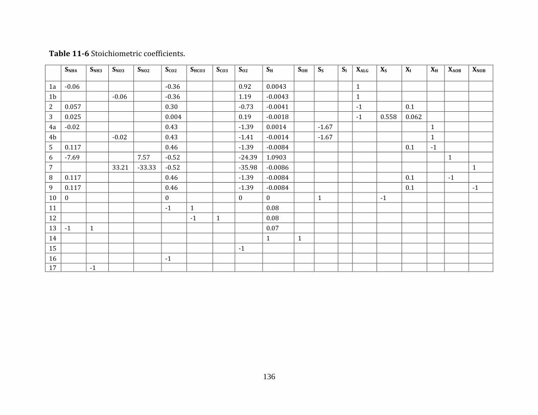
136

Table 11-6 Stoichiometric coefficients.

SNH4 SNH3 SNO3 SNO2 SCO2 SHCO3 SCO3 SO2 SH SOH SS SI XALG XS XI XH XAOB XNOB

1a -0.06 -0.36 0.92 0.0043 1

1b -0.06 -0.36 1.19 -0.0043 1

2 0.057 0.30 -0.73 -0.0041 -1 0.1

3 0.025 0.004 0.19 -0.0018 -1 0.558 0.062

4a -0.02 0.43 -1.39 0.0014 -1.67 1

4b -0.02 0.43 -1.41 -0.0014 -1.67 1

5 0.117 0.46 -1.39 -0.0084 0.1 -1

6 -7.69 7.57 -0.52 -24.39 1.0903 1

7 33.21 -33.33 -0.52 -35.98 -0.0086 1

8 0.117 0.46 -1.39 -0.0084 0.1 -1

9 0.117 0.46 -1.39 -0.0084 0.1 -1

10 0 0 0 0 1 -1

11 -1 1 0.08

12 -1 1 0.08

13 -1 1 0.07

14 1 1

15 -1

16 -1

17 -1

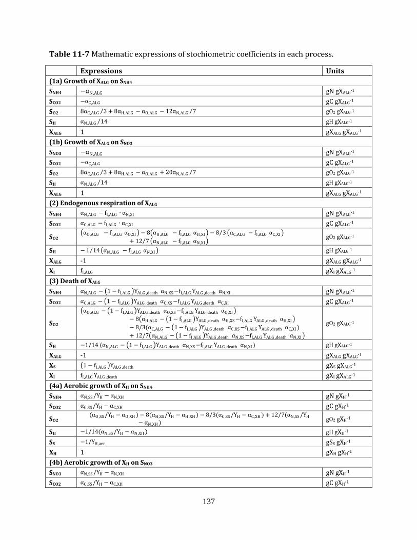
137

Table 11-7 Mathematic expressions of stochiometric coefficients in each process.

Expressions Units

(1a) Growth of XALG on SNH4

SNH4 −αN,ALG gN gXALG-1

SCO2 −αC,ALG gC gXALG-1

SO2 8αC,ALG 3 + 8αH,ALG − αO,ALG − 12αN,ALG 7 gO2 gXALG-1

SH αN,ALG 14 gH gXALG-1

XALG 1 gXALG gXALG-1

(1b) Growth of XALG on SNO3

SNO3 −αN,ALG gN gXALG-1

SCO2 −αC,ALG gC gXALG-1

SO2 8αC,ALG 3 + 8αH,ALG − αO,ALG + 20αN,ALG 7 gO2 gXALG-1

SH αN,ALG 14 gH gXALG-1

XALG 1 gXALG gXALG-1

(2) Endogenous respiration of XALG

SNH4 αN,ALG − fI,ALG ∙ αN,XI gN gXALG-1

SCO2 αC,ALG − fI,ALG ∙ αC,XI gC gXALG-1

SO2 αO,ALG − fI,ALG αO,XI − 8 αH,ALG − fI,ALG αH,XI − 8 3 αC,ALG − fI,ALG αC,XI

+ 12 7 αN,ALG − fI,ALG αN,XI gO2 gXALG-1

SH − 1 14 αN,ALG − fI,ALG αN,XI gH gXALG-1

XALG -1 gXALG gXALG-1

XI fI,ALG gXI gXALG-1

(3) Death of XALG

SNH4 αN,ALG − 1 − fI,ALG YALG ,death αN,XS −fI,ALG YALG ,death αN,XI gN gXALG-1

SCO2 αC,ALG − 1 − fI,ALG YALG ,death αC,XS −fI,ALG YALG ,death αC,XI gC gXALG-1

SO2

αO,ALG − 1 − fI,ALG YALG ,death αO,XS −fI,ALG YALG ,death αO,XI

− 8 αH,ALG − 1 − fI,ALG YALG ,death αH,XS −fI,ALG YALG ,death αH,XI

− 8/3(αC,ALG − 1 − fI,ALG YALG ,death αC,XS −fI,ALG YALG ,death αC,XI )

+ 12/7 αN,ALG − 1 − fI,ALG YALG ,death αN,XS −fI,ALG YALG ,death αN,XI

gO2 gXALG-1

SH −1/14 (αN,ALG − 1 − fI,ALG YALG ,death αN,XS −fI,ALG YALG ,death αN,XI ) gH gXALG-1

XALG -1 gXALG gXALG-1

XS 1 − fI,ALG YALG ,death gXS gXALG-1

XI fI,ALG YALG ,death gXI gXALG-1

(4a) Aerobic growth of XH on SNH4

SNH4 αN,SS /YH − αN,XH gN gXH-1

SCO2 αC,SS /YH − αC,XH gC gXH-1

SO2 (αO,SS /YH − αO,XH ) − 8(αH,SS /YH − αH,XH ) − 8/3(αC,SS /YH − αC,XH ) + 12/7(αN,SS /YH

− αN,XH ) gO2 gXH-1

SH −1/14(αN,SS /YH − αN,XH ) gH gXH-1

SS −1/YH,aer gSS gXH-1

XH 1 gXH gXH-1

(4b) Aerobic growth of XH on SNO3

SNO3 αN,SS /YH − αN,XH gN gXH-1

SCO2 αC,SS /YH − αC,XH gC gXH-1

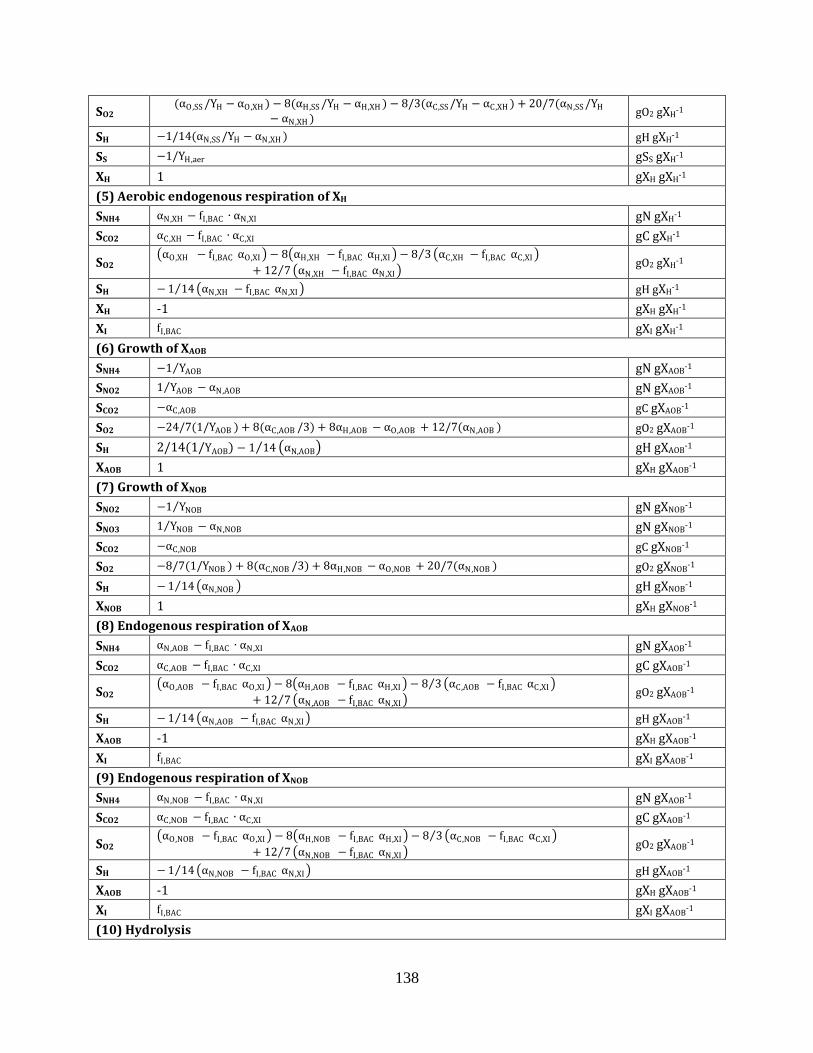
138

SO2 (αO,SS /YH − αO,XH ) − 8(αH,SS /YH − αH,XH ) − 8/3(αC,SS /YH − αC,XH ) + 20/7(αN,SS /YH

− αN,XH ) gO2 gXH-1

SH −1/14(αN,SS /YH − αN,XH ) gH gXH-1

SS −1/YH,aer gSS gXH-1

XH 1 gXH gXH-1

(5) Aerobic endogenous respiration of XH

SNH4 αN,XH − fI,BAC ∙ αN,XI gN gXH-1

SCO2 αC,XH − fI,BAC ∙ αC,XI gC gXH-1

SO2 αO,XH − fI,BAC αO,XI − 8 αH,XH − fI,BAC αH,XI − 8 3 αC,XH − fI,BAC αC,XI

+ 12 7 αN,XH − fI,BAC αN,XI gO2 gXH

-1

SH − 1 14 αN,XH − fI,BAC αN,XI gH gXH-1

XH -1 gXH gXH-1

XI fI,BAC gXI gXH-1

(6) Growth of XAOB

SNH4 −1 YAOB gN gXAOB-1

SNO2 1 YAOB − αN,AOB gN gXAOB-1

SCO2 −αC,AOB gC gXAOB-1

SO2 −24/7(1/YAOB ) + 8(αC,AOB /3) + 8αH,AOB − αO,AOB + 12/7(αN,AOB ) gO2 gXAOB-1

SH 2/14(1/YAOB) − 1 14 αN,AOB gH gXAOB-1

XAOB 1 gXH gXAOB-1

(7) Growth of XNOB

SNO2 −1 YNOB gN gXNOB-1

SNO3 1 YNOB − αN,NOB gN gXNOB-1

SCO2 −αC,NOB gC gXNOB-1

SO2 −8/7(1/YNOB ) + 8(αC,NOB /3) + 8αH,NOB − αO,NOB + 20/7(αN,NOB ) gO2 gXNOB-1

SH − 1 14 αN,NOB gH gXNOB-1

XNOB 1 gXH gXNOB-1

(8) Endogenous respiration of XAOB

SNH4 αN,AOB − fI,BAC ∙ αN,XI gN gXAOB-1

SCO2 αC,AOB − fI,BAC ∙ αC,XI gC gXAOB-1

SO2 αO,AOB − fI,BAC αO,XI − 8 αH,AOB − fI,BAC αH,XI − 8 3 αC,AOB − fI,BAC αC,XI

+ 12 7 αN,AOB − fI,BAC αN,XI gO2 gXAOB

-1

SH − 1 14 αN,AOB − fI,BAC αN,XI gH gXAOB-1

XAOB -1 gXH gXAOB-1

XI fI,BAC gXI gXAOB-1

(9) Endogenous respiration of XNOB

SNH4 αN,NOB − fI,BAC ∙ αN,XI gN gXAOB-1

SCO2 αC,NOB − fI,BAC ∙ αC,XI gC gXAOB-1

SO2 αO,NOB − fI,BAC αO,XI − 8 αH,NOB − fI,BAC αH,XI − 8 3 αC,NOB − fI,BAC αC,XI

+ 12 7 αN,NOB − fI,BAC αN,XI gO2 gXAOB

-1

SH − 1 14 αN,NOB − fI,BAC αN,XI gH gXAOB-1

XAOB -1 gXH gXAOB-1

XI fI,BAC gXI gXAOB-1

(10) Hydrolysis

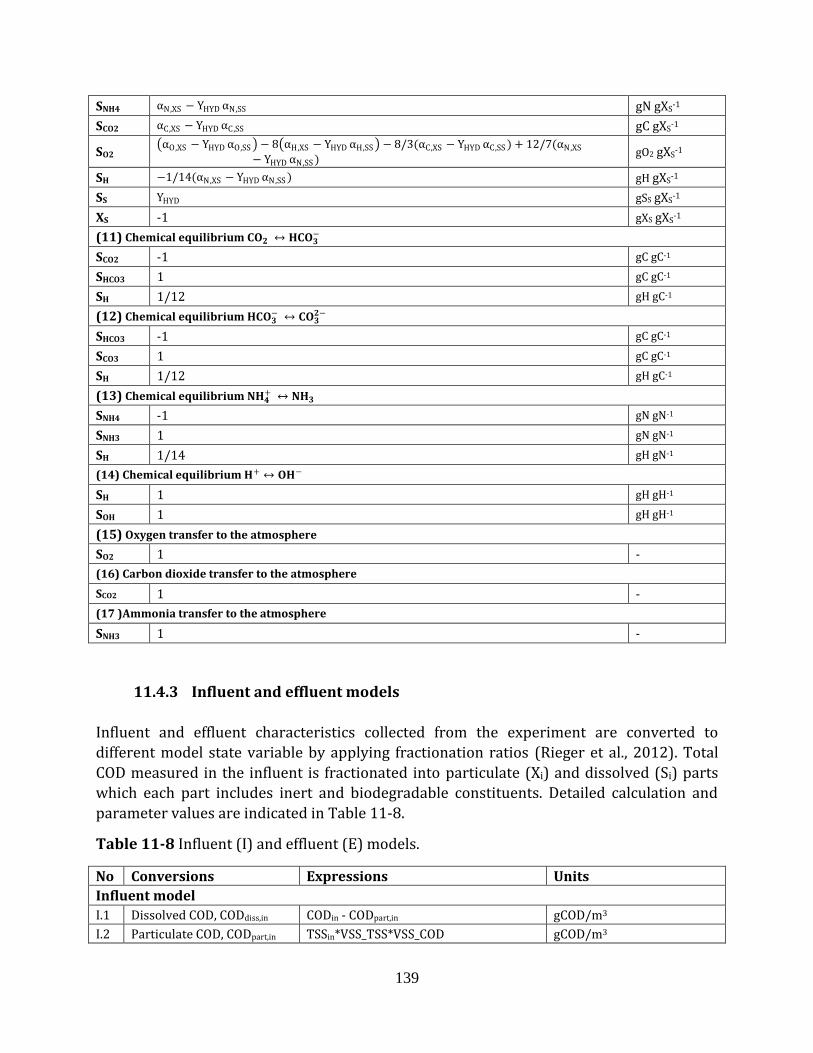
139

SNH4 αN,XS − YHYD αN,SS gN gXS-1

SCO2 αC,XS − YHYD αC,SS gC gXS-1

SO2 αO,XS − YHYD αO,SS − 8 αH,XS − YHYD αH,SS − 8/3(αC,XS − YHYD αC,SS ) + 12/7(αN,XS

− YHYD αN,SS ) gO2 gXS

-1

SH −1/14(αN,XS − YHYD αN,SS ) gH gXS-1

SS YHYD gSS gXS-1

XS -1 gXS gXS-1

(11) Chemical equilibrium 𝐂𝐎𝟐 ↔ 𝐇𝐂𝐎𝟑−

SCO2 -1 gC gC-1

SHCO3 1 gC gC-1

SH 1/12 gH gC-1

(12) Chemical equilibrium 𝐇𝐂𝐎𝟑− ↔ 𝐂𝐎𝟑

𝟐−

SHCO3 -1 gC gC-1

SCO3 1 gC gC-1

SH 1/12 gH gC-1

(13) Chemical equilibrium 𝐍𝐇𝟒+ ↔ 𝐍𝐇𝟑

SNH4 -1 gN gN-1

SNH3 1 gN gN-1

SH 1/14 gH gN-1

(14) Chemical equilibrium 𝐇+ ↔ 𝐎𝐇−

SH 1 gH gH-1

SOH 1 gH gH-1

(15) Oxygen transfer to the atmosphere

SO2 1 -

(16) Carbon dioxide transfer to the atmosphere

SCO2 1 -

(17 )Ammonia transfer to the atmosphere

SNH3 1 -

11.4.3 Influent and effluent models

Influent and effluent characteristics collected from the experiment are converted to

different model state variable by applying fractionation ratios (Rieger et al., 2012). Total

COD measured in the influent is fractionated into particulate (Xi) and dissolved (Si) parts

which each part includes inert and biodegradable constituents. Detailed calculation and

parameter values are indicated in Table 11-8.

Table 11-8 Influent (I) and effluent (E) models.

No Conversions Expressions Units

Influent model

I.1 Dissolved COD, CODdiss,in CODin - CODpart,in gCOD/m3

I.2 Particulate COD, CODpart,in TSSin*VSS_TSS*VSS_COD gCOD/m3

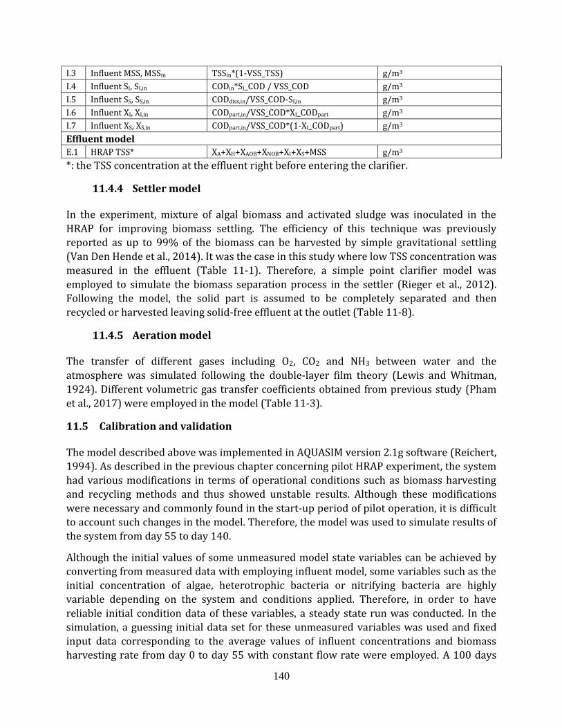
140

I.3 Influent MSS, MSSin TSSin*(1-VSS_TSS) g/m3

I.4 Influent SI, SI,in CODin*SI_COD / VSS_COD g/m3

I.5 Influent SS, SS,in CODdiss,in/VSS_COD-SI,in g/m3

I.6 Influent XI, XI,in CODpart,in/VSS_COD*XI_CODpart g/m3

I.7 Influent XS, XS,in CODpart,in/VSS_COD*(1-XI_CODpart) g/m3

Effluent model

E.1 HRAP TSS* XA+XH+XAOB+XNOB+XI+XS+MSS g/m3

*: the TSS concentration at the effluent right before entering the clarifier.

11.4.4 Settler model

In the experiment, mixture of algal biomass and activated sludge was inoculated in the

HRAP for improving biomass settling. The efficiency of this technique was previously

reported as up to 99% of the biomass can be harvested by simple gravitational settling

(Van Den Hende et al., 2014). It was the case in this study where low TSS concentration was

measured in the effluent (Table 11-1). Therefore, a simple point clarifier model was

employed to simulate the biomass separation process in the settler (Rieger et al., 2012).

Following the model, the solid part is assumed to be completely separated and then

recycled or harvested leaving solid-free effluent at the outlet (Table 11-8).

11.4.5 Aeration model

The transfer of different gases including O2, CO2 and NH3 between water and the

atmosphere was simulated following the double-layer film theory (Lewis and Whitman,

1924). Different volumetric gas transfer coefficients obtained from previous study (Pham

et al., 2017) were employed in the model (Table 11-3).

11.5 Calibration and validation

The model described above was implemented in AQUASIM version 2.1g software (Reichert,

1994). As described in the previous chapter concerning pilot HRAP experiment, the system

had various modifications in terms of operational conditions such as biomass harvesting

and recycling methods and thus showed unstable results. Although these modifications

were necessary and commonly found in the start-up period of pilot operation, it is difficult

to account such changes in the model. Therefore, the model was used to simulate results of

the system from day 55 to day 140.

Although the initial values of some unmeasured model state variables can be achieved by

converting from measured data with employing influent model, some variables such as the

initial concentration of algae, heterotrophic bacteria or nitrifying bacteria are highly

variable depending on the system and conditions applied. Therefore, in order to have

reliable initial condition data of these variables, a steady state run was conducted. In the

simulation, a guessing initial data set for these unmeasured variables was used and fixed

input data corresponding to the average values of influent concentrations and biomass

harvesting rate from day 0 to day 55 with constant flow rate were employed. A 100 days

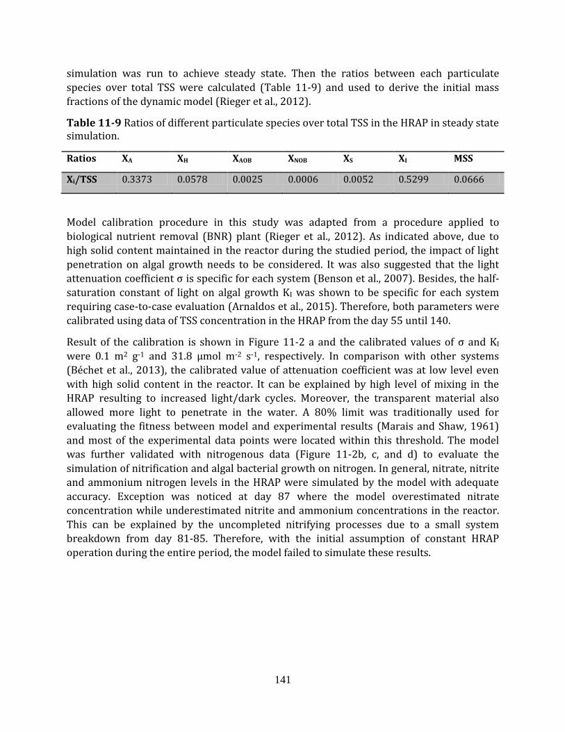
141

simulation was run to achieve steady state. Then the ratios between each particulate

species over total TSS were calculated (Table 11-9) and used to derive the initial mass

fractions of the dynamic model (Rieger et al., 2012).

Table 11-9 Ratios of different particulate species over total TSS in the HRAP in steady state simulation.

Ratios XA XH XAOB XNOB XS XI MSS

Xi/TSS 0.3373 0.0578 0.0025 0.0006 0.0052 0.5299 0.0666

Model calibration procedure in this study was adapted from a procedure applied to

biological nutrient removal (BNR) plant (Rieger et al., 2012). As indicated above, due to

high solid content maintained in the reactor during the studied period, the impact of light

penetration on algal growth needs to be considered. It was also suggested that the light

attenuation coefficient σ is specific for each system (Benson et al., 2007). Besides, the half-

saturation constant of light on algal growth KI was shown to be specific for each system

requiring case-to-case evaluation (Arnaldos et al., 2015). Therefore, both parameters were

calibrated using data of TSS concentration in the HRAP from the day 55 until 140.

Result of the calibration is shown in Figure 11-2 a and the calibrated values of σ and KI

were 0.1 m2 g-1 and 31.8 µmol m-2 s-1, respectively. In comparison with other systems

(Béchet et al., 2013), the calibrated value of attenuation coefficient was at low level even

with high solid content in the reactor. It can be explained by high level of mixing in the

HRAP resulting to increased light/dark cycles. Moreover, the transparent material also

allowed more light to penetrate in the water. A 80% limit was traditionally used for

evaluating the fitness between model and experimental results (Marais and Shaw, 1961)

and most of the experimental data points were located within this threshold. The model

was further validated with nitrogenous data (Figure 11-2b, c, and d) to evaluate the

simulation of nitrification and algal bacterial growth on nitrogen. In general, nitrate, nitrite

and ammonium nitrogen levels in the HRAP were simulated by the model with adequate

accuracy. Exception was noticed at day 87 where the model overestimated nitrate

concentration while underestimated nitrite and ammonium concentrations in the reactor.

This can be explained by the uncompleted nitrifying processes due to a small system

breakdown from day 81-85. Therefore, with the initial assumption of constant HRAP

operation during the entire period, the model failed to simulate these results.

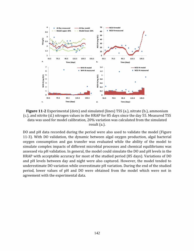
142

Figure 11-2 Experimental (dots) and simulated (lines) TSS (a.), nitrate (b.), ammonium (c.), and nitrite (d.) nitrogen values in the HRAP for 85 days since the day 55. Measured TSS

data was used for model calibration, 20% variation was calculated from the simulated result (a.).

DO and pH data recorded during the period were also used to validate the model (Figure

11-3). With DO validation, the dynamic between algal oxygen production, algal bacterial

oxygen consumption and gas transfer was evaluated while the ability of the model to

simulate complex impacts of different microbial processes and chemical equilibriums was

assessed via pH validation. In general, the model could simulate the DO and pH levels in the

HRAP with acceptable accuracy for most of the studied period (85 days). Variations of DO

and pH levels between day and night were also captured. However, the model tended to

underestimate DO variation while overestimate pH variation. During the end of the studied

period, lower values of pH and DO were obtained from the model which were not in

agreement with the experimental data.

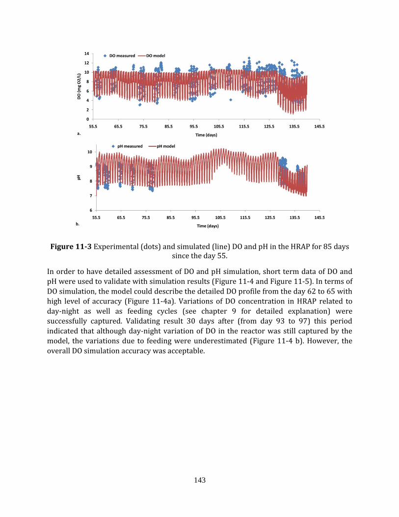
143

Figure 11-3 Experimental (dots) and simulated (line) DO and pH in the HRAP for 85 days since the day 55.

In order to have detailed assessment of DO and pH simulation, short term data of DO and

pH were used to validate with simulation results (Figure 11-4 and Figure 11-5). In terms of

DO simulation, the model could describe the detailed DO profile from the day 62 to 65 with

high level of accuracy (Figure 11-4a). Variations of DO concentration in HRAP related to

day-night as well as feeding cycles (see chapter 9 for detailed explanation) were

successfully captured. Validating result 30 days after (from day 93 to 97) this period

indicated that although day-night variation of DO in the reactor was still captured by the

model, the variations due to feeding were underestimated (Figure 11-4 b). However, the

overall DO simulation accuracy was acceptable.

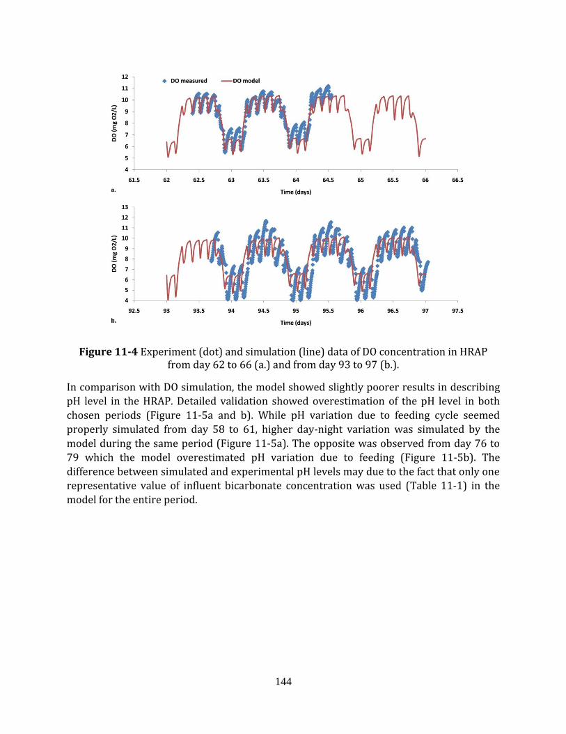
144

Figure 11-4 Experiment (dot) and simulation (line) data of DO concentration in HRAP from day 62 to 66 (a.) and from day 93 to 97 (b.).

In comparison with DO simulation, the model showed slightly poorer results in describing

pH level in the HRAP. Detailed validation showed overestimation of the pH level in both

chosen periods (Figure 11-5a and b). While pH variation due to feeding cycle seemed

properly simulated from day 58 to 61, higher day-night variation was simulated by the

model during the same period (Figure 11-5a). The opposite was observed from day 76 to

79 which the model overestimated pH variation due to feeding (Figure 11-5b). The

difference between simulated and experimental pH levels may due to the fact that only one

representative value of influent bicarbonate concentration was used (Table 11-1) in the

model for the entire period.

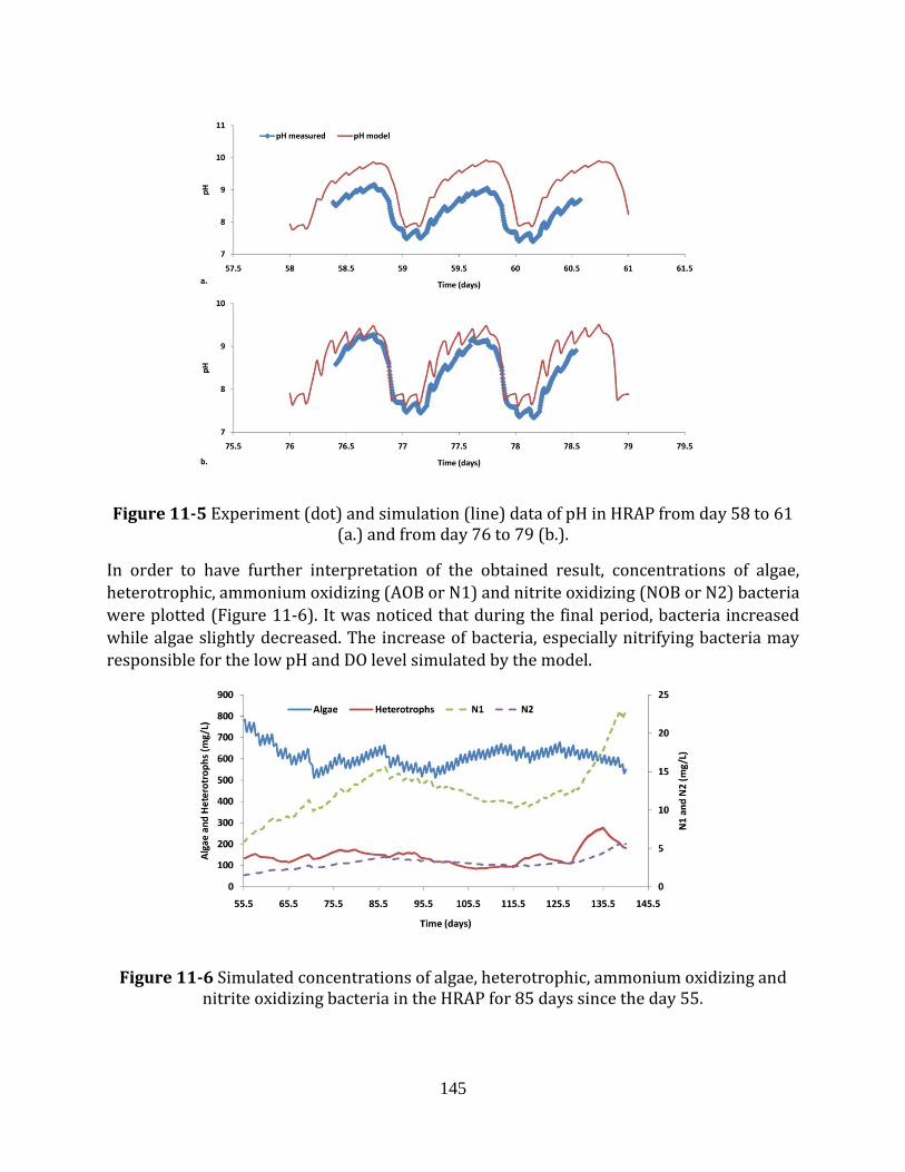
145

Figure 11-5 Experiment (dot) and simulation (line) data of pH in HRAP from day 58 to 61 (a.) and from day 76 to 79 (b.).

In order to have further interpretation of the obtained result, concentrations of algae,

heterotrophic, ammonium oxidizing (AOB or N1) and nitrite oxidizing (NOB or N2) bacteria

were plotted (Figure 11-6). It was noticed that during the final period, bacteria increased

while algae slightly decreased. The increase of bacteria, especially nitrifying bacteria may

responsible for the low pH and DO level simulated by the model.

Figure 11-6 Simulated concentrations of algae, heterotrophic, ammonium oxidizing and nitrite oxidizing bacteria in the HRAP for 85 days since the day 55.

146

It was interesting to note that the model results were obtained with acceptable accuracy by

calibrating only attenuation coefficient and half-saturation constant of light on algal

growth. This outcome suggests an appropriate data set as well as model parameters was

implemented. Importantly, it should be noticed that in other algal bacterial models

(Solimeno et al., 2017; Zambrano et al., 2016), the gas/liquid transfer coefficient of

different gases was usually calibrated which may result to great uncertainty due to its

sensitivity. In this study, these values were obtained experimentally hence the uncertainty

was decreased.

Moreover, the result also emphasized the advantage of applying the GMP unified protocol

while simulating HRAP system. The protocol provided a clear and comprehensive view of

various aspects for a simulation project which allows early detection of potential fault.

However, further study must be conducted in order to adapt the protocol to algal bacterial

simulation purpose. A stark example is considering light related factors such as light

penetration or light saturation coefficient. While most of the algal bacterial models only

focus on the kinetic model, the protocol provides a comprehensive model set-up including

different sub-models hence increasing simulation quality.

As described in the previous chapter, the HRAP system was also studied on its ability to

treat wastewater with high nutrient loads. Hence a further step would be applying the

model for this scenario.

11.6 Conclusions and Perspectives

In this study, the performance of a pilot HRAP was simulated following adapted IWA GMP

unified protocol. Data employed in the model was collected from a long term experiment

conducted in a pilot HRAP system for wastewater treatment. A comprehensive model was

constructed to simulate the system. From the results achieved, several conclusions were

made as following:

- With only attenuation coefficient and half-saturation constant of light on algal

growth calibrated, satisfactory simulation results were obtained. The model was

able to simulate TSS and nitrogenous concentrations, DO and pH levels in the HRAP

for 85 days with adequate accuracy. The model also successfully captured different

variations of DO and pH due to light/dark and feeding cycles.

- The results obtained suggest the importance of appropriate data set to be applied in

the model hence avoiding high uncertainty of the calibration process. The

importance of having a clear and comprehensive simulation protocol was also

emphasized.

- It was important to note that the gas transfer coefficient was obtained

experimentally to be employed in the model while usually being calibrated in

others. Therefore the uncertainty of the calibration process in this study was

decreased.

147

- In order to improve pH simulation, bicarbonate concentration should be measured

frequently.

The further step is to use the model to simulate the system treating wastewater with high

nutrient loads.

In French:

Durant cette étude, la performance d'un HRAP pilote a été simulée suivant une adaptation

du protocole unifié IWA GMP. Les données utilisées dans le modèle proviennent d'une

expérience menée dans un système pilote HRAP pour le traitement des eaux usées. Un

modèle complet a été construit pour simuler le système. Les résultats obtenus ont permis

de tirer les conclusions suivantes:

Avec uniquement le calage du coefficient d'atténuation et de la constante de demi-

saturation de la lumière sur la croissance des algues, des résultats de simulation

satisfaisants ont été obtenus. Le modèle a été en mesure de simuler les

concentrations de MES et d'azote, d'oxygène dissous ainsi que le pH dans le système

pendant 85 jours avec une précision adéquate. Le modèle a également reproduit

avec succès les différentes variations de l'oxygène dissous et du pH suite aux cycles

d’illumination et d'alimentation en eau usée.

Les résultats obtenus suggèrent l'importance d'un jeu de données appropriées, ce

qui permet d'éviter une forte incertitude dans le processus de calage. L'importance

d'avoir un protocole de simulation clair et complet a également été soulignée.

Il est important de noter que le coefficient de transfert de gaz a été obtenu

expérimentalement pour être utilisé dans le modèle alors qu'il est habituellement

calé dans d'autres modèles de la littérature. Par conséquent, l'incertitude de calage

dans cette étude a été réduite.

Afin d'améliorer la simulation du pH, la concentration de bicarbonate doit être

mesurée fréquemment.

L'étape suivante consiste à utiliser le modèle pour simuler le système traitant une eau usée

avec une charge élevée en nutriments.

148

CONCLUSIONS AND PERSPECTIVES

1 General conclusions of the thesis

Various experiments were conducted during the thesis to understand the cooperation

between algae and bacteria in wastewater treatment and biomass production in order to

improve the system performance. In terms of HRAP system, hydraulic and gas transfer

studies were also conducted to understand the impacts of different operational conditions

on global hydraulic, mixing and gas transfer rate in the HRAP reactor. Based on the data

collected from these works, different model types were developed giving an insight into

algal bacterial processes under different operational conditions. Conclusions were made as

following:

Al-Bac biomass development

Algal-bacterial (Al-Bac) biomass with three inoculation algae/activated sludge ratios (5:1,

1:1 and 1:5) with algal biomass as control were cultured and compared in terms of algal

growth, nutrient removal and settling efficiency. Results showed that algal productivity

was in positive correlation with the amount of activated sludge added. However, too much

activated sludge added can cause disturbance to the Al-Bac biomass growth and algal

bacterial processes. All reactors including control with only algae showed similar settling

and nutrient removal efficiencies which may be due to both long hydraulic and solid

retention times. Al-Bac biomass with 1:1 inoculation ratio showed the best enhancement in

terms of total biomass, algal biomass growth and algal activities. This ratio was applied for

inoculating Al-Bac biomass in pilot scale.

Hydraulics and gas transfer rate of the HRAP

Different combinations of operational parameters including water level, paddle rotational

speed and influent flow rate were applied to investigate their impacts on mixing

characteristics, residence time distribution and gas transfer rate in a pilot-scale high rate

algal pond. In closed condition, paddle rotational speed had positive correlation with

Bodenstein number (Bo), water velocity and oxygen volumetric mass transfer coefficient

(kLaO2) while increasing water level generated negative impact on these parameters,

although the impact of water level on water linear velocity was small. Amplification effect

of water level and paddle rotational speed on sensitivity of Bo and kLaO2 should be noticed.

Moreover, paddle rotational speed had more impact on kLaO2 than on Bo. The study in open

condition indicated that effective volume fraction had positive correlation with inlet flow

rate and negative correlation with paddle rotation, while the opposite was observed in the

case of Peclet number. The impact of water level variation on these parameters was

unclear. Both water level and paddle rotational speed had negative impacts on short-

circuiting index while no correlation was observed when varying inlet flow rate. In this

study, the optimal operational conditions included low water level (0.1 m) and medium

149

paddle rotational speed (11.6 rpm). These conditions were applied for wastewater

treatment application of the HRAP.

Long term operation of HRAP for wastewater treatment and biomass production

Long term experiment was conducted to study the ability of a high-rate algal pond (HRAP)

inoculated with algal biomass and activated sludge (Al-Bac biomass) to treat primary

treated and centrate wastewaters. The impacts of high nutrient load and hydraulic

retention time (HRT) variation on the performance of the system were evaluated in terms

of treatment efficiency, biomass production and recovery. The system was able to treat

primary treated wastewater with 4 days HRT, satisfying French discharge norm. Around

99% of biomass recovery efficiency was achieved during the entire experiment via simple

gravity settling. However, high nutrient load wastewater (centrate wastewater) resulted in

poor TN and TP treatment efficiencies and decrease in COD removal of the system, yet high

removal of TKN as well as NH4-N were still obtained. Higher HRT (8 days) showed

improvement in COD removal but minor impact was observed in the case of TKN, TN and

TP removals. Nitrification was the main mechanism explaining the high level of TKN

removal observed, especially at high nutrient load. This was confirmed by analyzing

decomposed time series data of pH and dissolved oxygen. Despite of the variation in

operational conditions, constant production rates of Al-Bac biomass and Chlorophyll-a

were obtained during the entire experiment. Results from this study showed potential of

using HRAP system for secondary treatment or quickly removing high level of COD and

TKN before further treatment. Data from this study can also be employed for model

validation to further investigate the dynamic between algae and bacteria in HRAP system.

Coupled RTD and mixed-order kinetic model assessing and sizing the HRAP

A black box model was built by coupling residence time distribution (RTD) and mixed-

order kinetic model to simulate long term operation of a pilot-scale high rate algal pond

(HRAP). In general, the coupled model showed satisfying agreement with measured

effluent concentrations using limited initial data. By assessing the relationship between

model and experimental parameters, the impacts of algal and bacterial processes on

wastewater treatment can also be investigated. Reaction orders of TKN and COD removals

were positively correlated with algal content indicating the significant contribution of algal

processes governing these treatments. while nitrogen concentration at the influent had

negative correlation with reaction orders of TN and TKN removals following the pseudo-

order reaction concept. Moreover, the increase in biomass concentration was found to

impact the reaction order or accelerate the rate of the treatment process. However, due to

limitation of black box model type, the model failed to simulate the system performance in

extreme condition such as extreme high load of nutrient at the influent. Using the coupled

RTD and mixed-order kinetics models for sizing HRAP in different case studies showed

promising results. The study also provides empirical laws for HRAP mean residence time

estimation using expected effluent concentration and removal efficiency.

150

Adaptation of IWA GMP unified protocol for modeling HRAP system

A comprehensive model simulating performance of a pilot HRAP was developed. The

simulation procedure was adapted from IWA GMP unified protocol. The model consisted of

different sub-models including influent and effluent models, biokinetic model, clarifier

model and aeration model. Various parameters of different sub-models were measured and

employed. Performance data from long term experiment conducted in the pilot HRAP was

used for model calibration and validation. When calibrating only attenuation coefficient

and half-saturation constant of light on algal growth, satisfactory simulation results were

obtained. The model was able to simulate TSS and nitrogenous concentrations, DO and pH

levels in the HRAP for 85 days with adequate accuracy. The model also successfully

captured different variations of DO and pH due to light/dark and feeding cycles. The results

obtained may be due to the appropriate data set applied in the model reducing uncertainty

of the calibration process. Moreover, a clear and comprehensive simulation protocol was

thought to be contributed. In order to improve pH simulation, bicarbonate concentration

should be measured frequently. The further step is to use the model to simulate the system

treating wastewater with high nutrient loads.

2 General perspectives

In this work, an optimal algae/activated sludge inoculation ratio was proposed. However,

the results also indicated that this ratio is highly dynamic, especially when the biomass is

applied in a long term operation system. Moreover, the dominant algal species can also be

changed due to various operational conditions which in turns, impacts the dynamic

between algae and bacteria. Therefore, more efforts should be spent on understanding

such changes.

The HRAP operation in this work showed promising results not only in secondary

treatment but also in rapidly reducing high loads of COD and TKN. However, the system

was operated indoor with relative constant environmental conditions. Therefore, a next

step would be applying the system in larger scale with outdoor conditions. Hence, by

comparing with this work, the impacts of environmental conditions can be emphasized.

The comprehensive model developed in this work showed promising simulation results,

yet different improvements are required. There is a need to further modification of the

GMP protocol in order to fit with algal bacterial modeling. Moreover, it was indicated that

advanced model like CFD can provide a detailed description of the physical behavior of the

reactor, hence greatly improving the simulation quality. However, the application of such

approach in HRAP system is still rarely published. In addition, it was also necessary to

validate the model with large scale system operated outdoor.

In French:

Conclusions générales de la these

151

Diverses expériences ont été menées au cours de la thèse pour comprendre la coopération

entre les algues et les bactéries dans le traitement des eaux usées et la production de

biomasse afin d'améliorer les performances du système. En ce qui concerne le système

HRAP, des études hydrauliques et de transfert de gaz ont également été menées pour

comprendre les impacts des différentes conditions opérationnelles sur l'hydraulique

globale, le mélange et le taux de transfert de gaz dans le réacteur HRAP. Sur la base des

données recueillies dans le cadre de ces travaux, différents types de modèles ont été

développés, donnant un aperçu des processus bactériens des algues dans différentes

conditions opérationnelles. Peu de conclusions ont été tirées comme suit:

Développement de la biomasse d'Al-Bac

La biomasse algale-bactérienne (Al-Bac) avec trois rapports algue/boues activées (5:1, 1:1

et 1:5) avec la biomasse algale comme contrôle a été cultivée et comparée en termes de

croissance des algues, d'élimination des nutriments et d'efficacité de sédimentation. Les

résultats ont montré que la productivité des algues était en corrélation positive avec la

quantité de boues activées ajoutées. Cependant, trop de boues activées ajoutées peuvent

perturber la croissance de la biomasse Al-Bac et les processus bactériens des algues. Tous

les réacteurs, y compris le contrôle avec seulement des algues, ont montré des efficacités

similaires de décantation et d'élimination des nutriments qui peuvent être dues à la fois à

de longs temps de rétention hydraulique et solide. La biomasse d'Al-Bac avec un rapport

d'inoculation de 1:1 a montré la meilleure amélioration en termes de biomasse totale, de

croissance de la biomasse algale et d'activités algales. Ce ratio a été appliqué pour

l'inoculation de la biomasse d'Al-Bac à l'échelle pilote.

Hydraulique et taux de transfert de gaz du HRAP

Différentes combinaisons de paramètres opérationnels, y compris le niveau d'eau, la

vitesse de rotation des pales et le débit de l'affluent, ont été appliquées pour étudier leurs

impacts sur les caractéristiques de mélange, la distribution du temps de séjour et le taux de

transfert de gaz dans un bassin d'algues à haut débit à l'échelle pilote. À l'état fermé, la

vitesse de rotation de la palette avait une corrélation positive avec le nombre de

Bodenstein (Bo), la vitesse de l'eau et le coefficient de transfert de masse volumétrique de

l'oxygène (kLaO2), tandis que l'augmentation du niveau de l'eau avait un impact négatif sur

ces paramètres, bien que l'impact du niveau de l'eau sur la vitesse linéaire de l'eau était

faible. L'effet d'amplification du niveau d'eau et de la vitesse de rotation de la palette sur la

sensibilité de Bo et kLaO2 doit être remarqué. De plus, la vitesse de rotation de la palette a

eu plus d'impact sur kLaO2 que sur Bo. L'étude à l'état ouvert a indiqué que la fraction

volumique effective avait une corrélation positive avec le débit d'entrée et une corrélation

négative avec la rotation de la palette, alors que l'inverse a été observé dans le cas du

nombre de Peclet. L'impact de la variation du niveau d'eau sur ces paramètres n'était pas

clair. Le niveau d'eau et la vitesse de rotation de la pale ont eu des effets négatifs sur

l'indice de court-circuit, mais aucune corrélation n'a été observée lorsque le débit d'entrée

variait. Dans cette étude, les conditions d'exploitation optimales comprenaient un niveau

152

d'eau bas (0,1 m) et une vitesse de rotation moyenne des palettes (11,6 rpm). Ces

conditions ont été appliquées pour l'application du HRAP au traitement des eaux usées.

Exploitation à long terme de HRAP pour le traitement des eaux usées et la

production de biomasse

Une expérience à long terme a été menée pour étudier la capacité d'un bassin d'algues à

haut débit (HRAP) inoculé avec de la biomasse algale et des boues activées (biomasse Al-

Bac) pour traiter les eaux usées primaires traitées et centrer les eaux usées. Les impacts de

la variation de la charge élevée en nutriments et du temps de rétention hydraulique (HRT)

sur la performance du système ont été évalués en termes d'efficacité de traitement, de

production de biomasse et de récupération. Le système a été en mesure de traiter les eaux

usées primaires traitées avec une HRT de 4 jours, satisfaisant à la norme française de rejet.

Environ 99% de l'efficacité de récupération de la biomasse a été atteinte pendant toute la

durée de l'expérience par simple décantation par gravité. Cependant, les eaux usées à forte

charge d'éléments nutritifs (eaux usées centrées) ont entraîné une faible efficacité de

traitement des TN et TP et une diminution de l'élimination de la DCO du système, mais on a

tout de même obtenu une forte élimination des TKN ainsi que du NH4-N. Une HRT plus

élevée (8 jours) a montré une amélioration de l'élimination de la DCO, mais un impact

mineur a été observé dans le cas de l'élimination des TKN, TN et TP. La nitrification était le

principal mécanisme expliquant le niveau élevé d'élimination du TKN observé, en

particulier en présence d'une charge élevée de nutriments. Cela a été confirmé par l'analyse

des données chronologiques décomposées du pH et de l'oxygène dissous. Malgré la

variation des conditions opérationnelles, des taux de production constants de biomasse Al-

Bac et de chlorophylle-a ont été obtenus pendant toute la durée de l'expérience. Les

résultats de cette étude ont montré qu'il est possible d'utiliser le système HRAP pour le

traitement secondaire ou d'éliminer rapidement les niveaux élevés de DCO et de TKN avant

de poursuivre le traitement. Les données de cette étude peuvent également être utilisées

pour la validation du modèle afin d'étudier plus en profondeur la dynamique entre les

algues et les bactéries dans le système HRAP.

Modèle DTS/cinétique d'ordre mixte pour l’évaluation et le dimensionnement

de lagune à haut rendement algal

Un modèle de boîte noire a été construit en couplant la distribution du temps de résidence

(RTD) et un modèle cinétique d'ordre mixte pour simuler l'exploitation à long terme d'un

bassin d'algues à haut débit (HRAP) à l'échelle pilote. En général, le modèle couplé a

montré un accord satisfaisant avec les concentrations mesurées dans l'effluent à l'aide de

données initiales limitées. En évaluant la relation entre le modèle et les paramètres

expérimentaux, il est également possible d'étudier l'impact des processus algaux et

bactériens sur le traitement des eaux usées. Les ordres de réaction des suppressions de

TKN et de DCO étaient corrélés positivement avec la teneur en algues, ce qui indique la

contribution significative des processus algales régissant ces traitements, tandis que la

concentration d'azote à l'affluent avait une corrélation négative avec les ordres de réaction

153

des suppressions de TN et de TKN à la suite du concept de réaction de pseudo-ordre. De

plus, l'augmentation de la concentration de biomasse s'est avérée avoir un impact sur

l'ordre de réaction ou accélérer le rythme du processus de traitement. Cependant, en raison

de la limitation du type de modèle de boîte noire, le modèle n'a pas réussi à simuler la

performance du système dans des conditions extrêmes telles qu'une charge extrêmement

élevée de nutriments à l'affluent. L'utilisation des modèles couplés de RTD et de cinétique

d'ordre mixte pour le dimensionnement du HRAP dans différentes études de cas a donné

des résultats prometteurs. L'étude fournit également des lois empiriques pour l'estimation

du temps de résidence moyen du HRAP en utilisant la concentration prévue de l'effluent et

l'efficacité de l'élimination.

Adaptation du protocole unifié IWA GMP pour la modélisation du système

HRAP

Un modèle complet simulant la performance d'un pilote HRAP a été développé. La

procédure de simulation a été adaptée du protocole unifié IWA GMP GMP. Le modèle

comprenait différents sous-modèles, y compris des modèles d'affluent et d'effluent, un

modèle biocinétique, un modèle de clarificateur et un modèle d'aération. Les données de

l'expérience à long terme menée ont été utilisées pour le calage et la validation du modèle.

En calant seulement le coefficient d'atténuation et la constante de demi-saturation de la

lumière sur la croissance des algues, des résultats de simulation satisfaisants ont été

obtenus. Le modèle a été en mesure de simuler les concentrations de MES,d'azote,

d'oxygène dissous et la pH dans le système HRAP pendant 85 jours avec une précision

adéquate. Le modèle a également reproduit avec succès les différentes variations de

l'oxygène dissous et du pH suite aux cycles d’illumination et d'alimentation en eau usée. Les

résultats obtenus sont dus au jeu de paramètres approprié appliqué dans le modèle, ce qui

réduit l'incertitude du processus de calage. De plus, un protocole de simulation clair et

complet est utile. Afin d'améliorer la simulation du pH, la concentration de bicarbonate doit

être mesurée fréquemment. L'étape suivante consiste à utiliser le modèle pour simuler le

système de traitement des eaux usées avec des charges élevées en nutriments.

Perspectives générales

Dans ce travail, un rapport optimal entre les algues et l'inoculation des boues activées a été

proposé. Cependant, les résultats indiquent également que ce ratio est très dynamique,

surtout lors d’un fonctionnement { mong terme du système. De plus, les espèces d'algues

dominantes peuvent également être modifiées en raison de diverses conditions

opérationnelles qui, à leur tour, ont un impact sur la dynamique entre les algues et les

bactéries. Par conséquent, davantage d'efforts devraient être consacrés à la compréhension

de ces changements.

L’exploitation de la lagune { haut rendement algal au cours de de travaila montré des

résultats prometteurs non seulement dans le traitement secondaire mais aussi dans la

réduction rapide des charges élevées de DCO et d’aote réduit. Toutefois, le système était

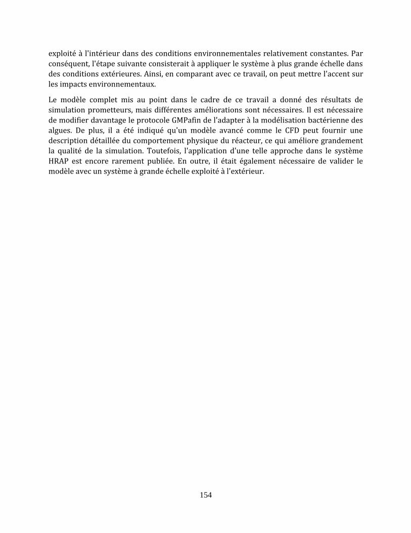
154

exploité à l'intérieur dans des conditions environnementales relativement constantes. Par

conséquent, l'étape suivante consisterait à appliquer le système à plus grande échelle dans

des conditions extérieures. Ainsi, en comparant avec ce travail, on peut mettre l'accent sur

les impacts environnementaux.

Le modèle complet mis au point dans le cadre de ce travail a donné des résultats de

simulation prometteurs, mais différentes améliorations sont nécessaires. Il est nécessaire

de modifier davantage le protocole GMPafin de l'adapter à la modélisation bactérienne des

algues. De plus, il a été indiqué qu'un modèle avancé comme le CFD peut fournir une

description détaillée du comportement physique du réacteur, ce qui améliore grandement

la qualité de la simulation. Toutefois, l'application d'une telle approche dans le système

HRAP est encore rarement publiée. En outre, il était également nécessaire de valider le

modèle avec un système à grande échelle exploité à l'extérieur.

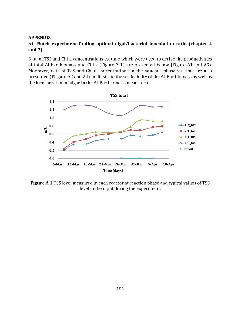
155

APPENDIX

A1. Batch experiment finding optimal algal/bacterial inoculation ratio (chapter 4

and 7)

Data of TSS and Chl-a concentrations vs. time which were used to derive the productivities

of total Al-Bac biomass and Chl-a (Figure 7-1) are presented below (Figure A1 and A3).

Moreover, data of TSS and Chl-a concentrations in the aqueous phase vs. time are also

presented (Firgure A2 and A4) to illustrate the settleability of the Al-Bac biomass as well as

the incorporation of algae in the Al-Bac biomass in each test.

Figure A 1 TSS level measured in each reactor at reaction phase and typical values of TSS level in the input during the experiment.

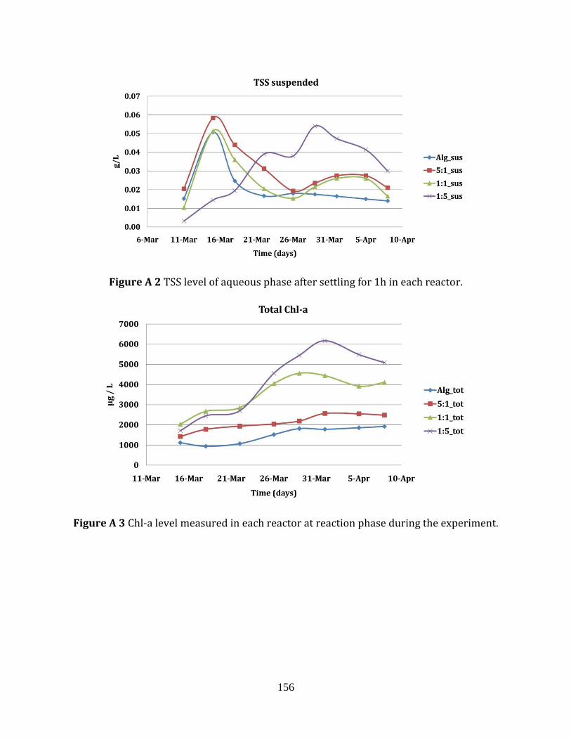
156

Figure A 2 TSS level of aqueous phase after settling for 1h in each reactor.

Figure A 3 Chl-a level measured in each reactor at reaction phase during the experiment.

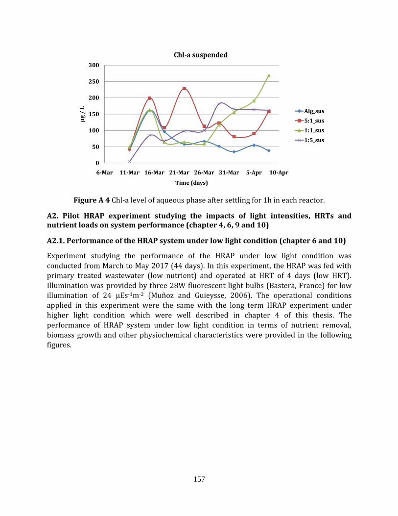
157

Figure A 4 Chl-a level of aqueous phase after settling for 1h in each reactor.

A2. Pilot HRAP experiment studying the impacts of light intensities, HRTs and nutrient loads on system performance (chapter 4, 6, 9 and 10)

A2.1. Performance of the HRAP system under low light condition (chapter 6 and 10)

Experiment studying the performance of the HRAP under low light condition was

conducted from March to May 2017 (44 days). In this experiment, the HRAP was fed with

primary treated wastewater (low nutrient) and operated at HRT of 4 days (low HRT).

Illumination was provided by three 28W fluorescent light bulbs (Bastera, France) for low

illumination of 24 μEs-1m-2 (Muñoz and Guieysse, 2006). The operational conditions

applied in this experiment were the same with the long term HRAP experiment under

higher light condition which were well described in chapter 4 of this thesis. The

performance of HRAP system under low light condition in terms of nutrient removal,

biomass growth and other physiochemical characteristics were provided in the following

figures.

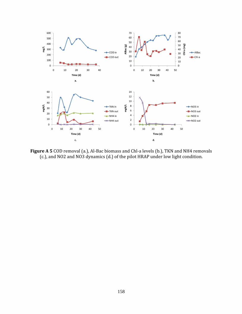
158

Figure A 5 COD removal (a.), Al-Bac biomass and Chl-a levels (b.), TKN and NH4 removals (c.), and NO2 and NO3 dynamics (d.) of the pilot HRAP under low light condition.

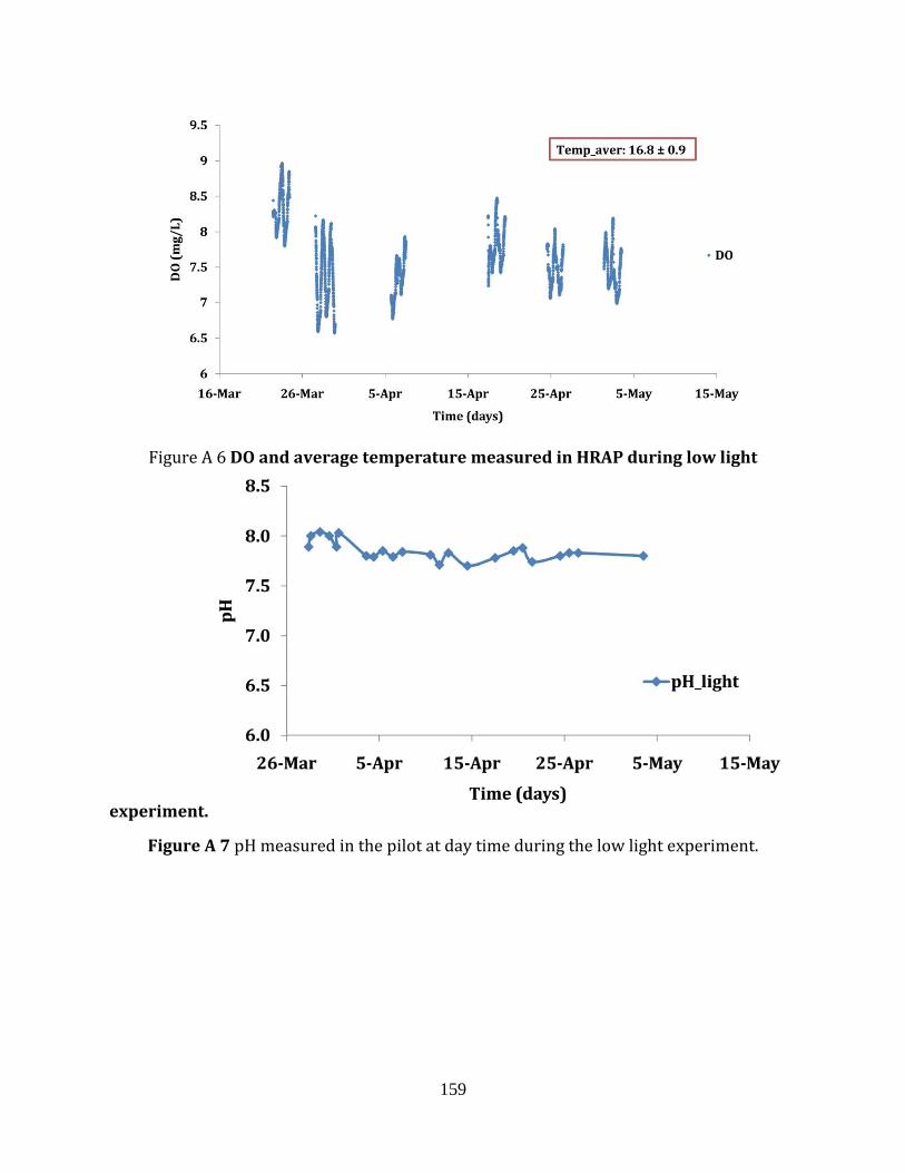
159

Figure A 6 DO and average temperature measured in HRAP during low light

experiment.

Figure A 7 pH measured in the pilot at day time during the low light experiment.

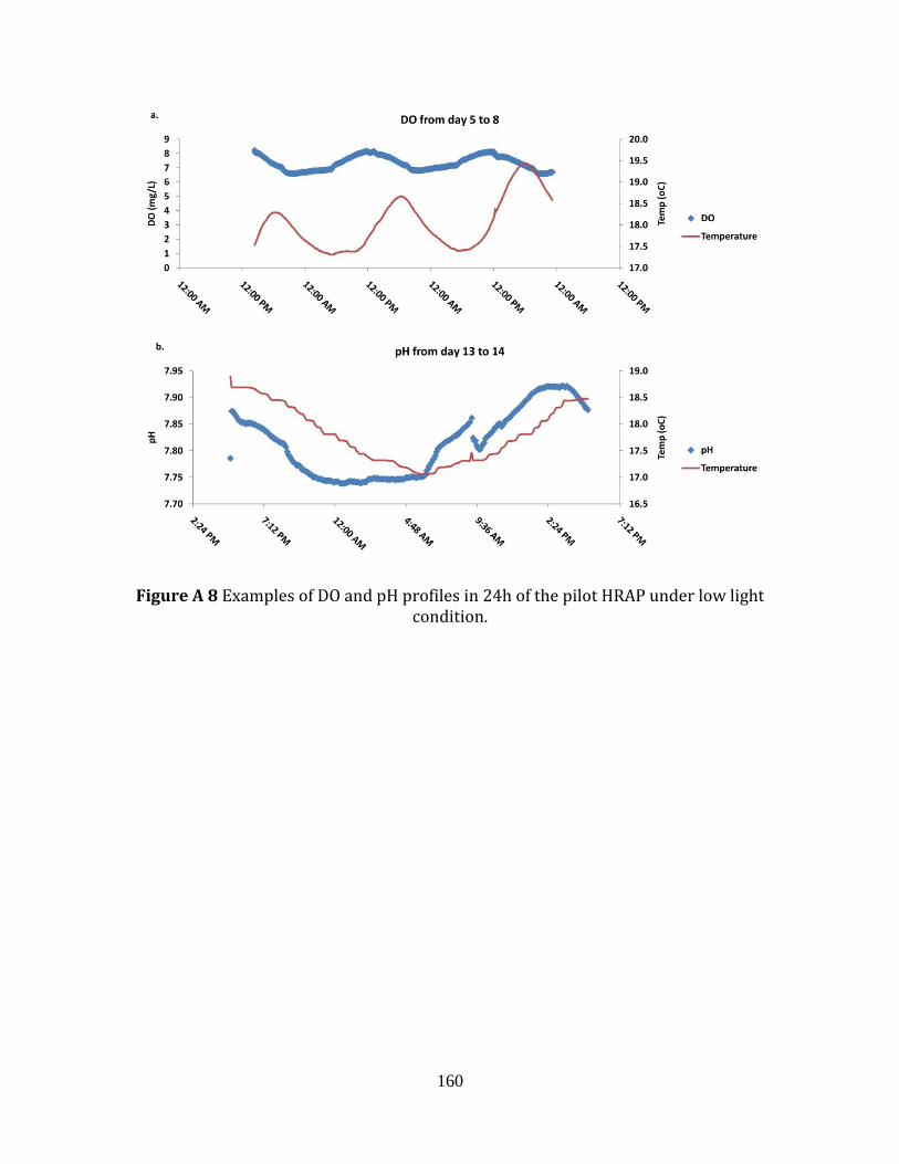
160

Figure A 8 Examples of DO and pH profiles in 24h of the pilot HRAP under low light condition.

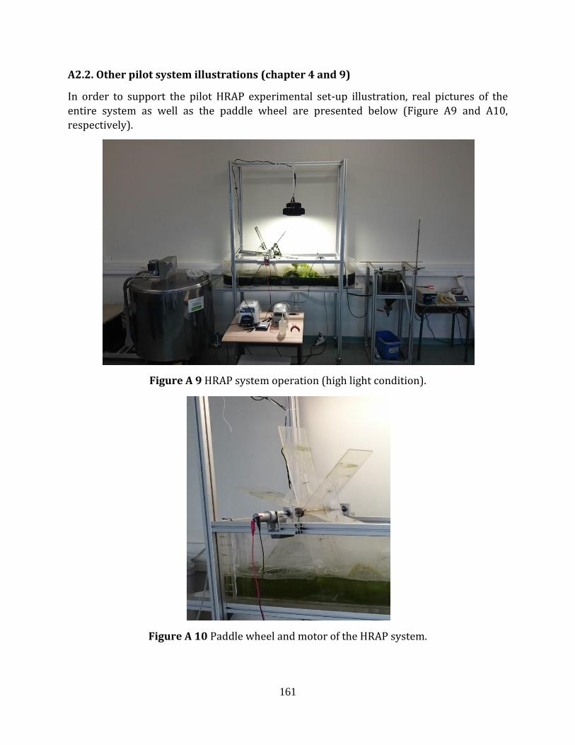
161

A2.2. Other pilot system illustrations (chapter 4 and 9)

In order to support the pilot HRAP experimental set-up illustration, real pictures of the

entire system as well as the paddle wheel are presented below (Figure A9 and A10,

respectively).

Figure A 9 HRAP system operation (high light condition).

Figure A 10 Paddle wheel and motor of the HRAP system.

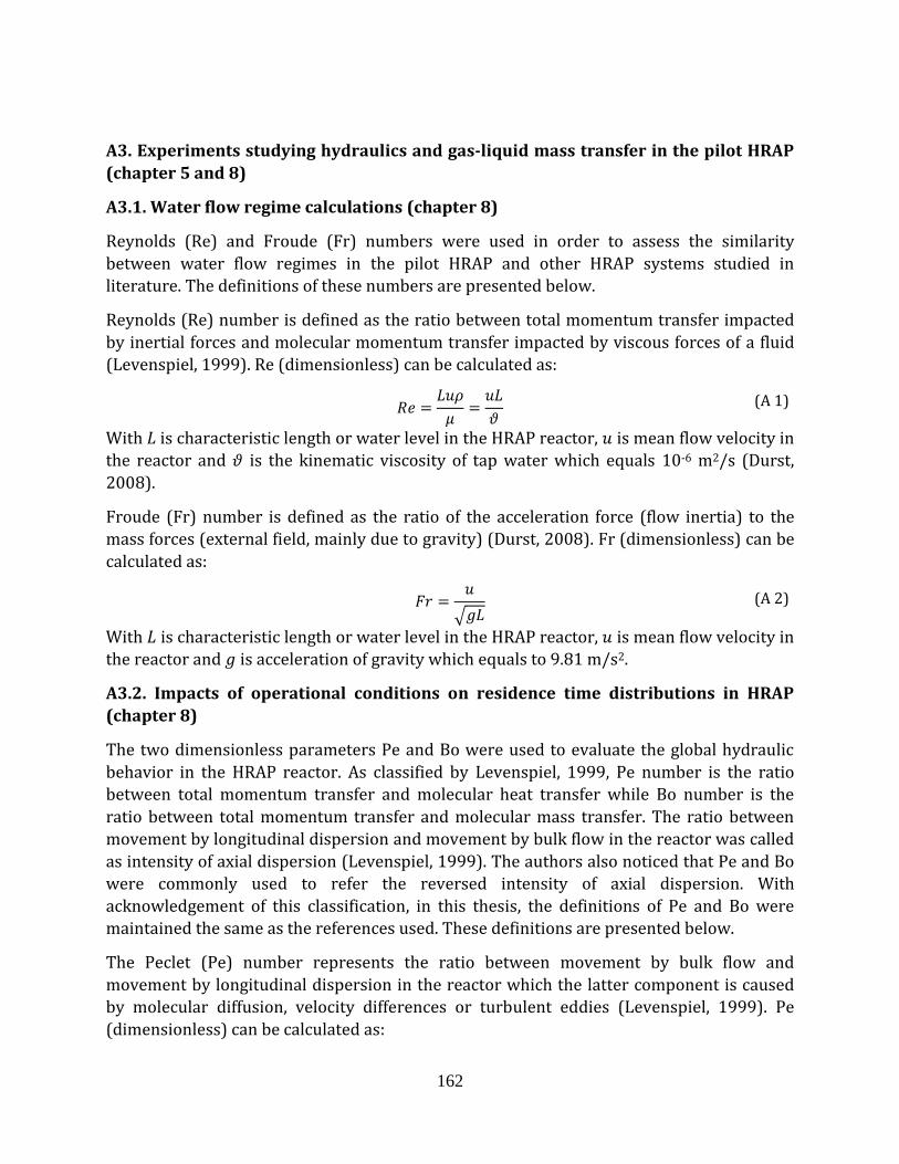
162

A3. Experiments studying hydraulics and gas-liquid mass transfer in the pilot HRAP

(chapter 5 and 8)

A3.1. Water flow regime calculations (chapter 8)

Reynolds (Re) and Froude (Fr) numbers were used in order to assess the similarity

between water flow regimes in the pilot HRAP and other HRAP systems studied in

literature. The definitions of these numbers are presented below.

Reynolds (Re) number is defined as the ratio between total momentum transfer impacted

by inertial forces and molecular momentum transfer impacted by viscous forces of a fluid

(Levenspiel, 1999). Re (dimensionless) can be calculated as:

𝑅𝑒 =𝐿𝑢𝜌

𝜇=

𝑢𝐿

𝜗 (A 1)

With L is characteristic length or water level in the HRAP reactor, 𝑢 is mean flow velocity in

the reactor and 𝜗 is the kinematic viscosity of tap water which equals 10-6 m2/s (Durst,

2008).

Froude (Fr) number is defined as the ratio of the acceleration force (flow inertia) to the

mass forces (external field, mainly due to gravity) (Durst, 2008). Fr (dimensionless) can be

calculated as:

𝐹𝑟 =𝑢

𝑔𝐿 (A 2)

With 𝐿 is characteristic length or water level in the HRAP reactor, 𝑢 is mean flow velocity in

the reactor and 𝑔 is acceleration of gravity which equals to 9.81 m/s2.

A3.2. Impacts of operational conditions on residence time distributions in HRAP

(chapter 8)

The two dimensionless parameters Pe and Bo were used to evaluate the global hydraulic

behavior in the HRAP reactor. As classified by Levenspiel, 1999, Pe number is the ratio

between total momentum transfer and molecular heat transfer while Bo number is the

ratio between total momentum transfer and molecular mass transfer. The ratio between

movement by longitudinal dispersion and movement by bulk flow in the reactor was called

as intensity of axial dispersion (Levenspiel, 1999). The authors also noticed that Pe and Bo

were commonly used to refer the reversed intensity of axial dispersion. With

acknowledgement of this classification, in this thesis, the definitions of Pe and Bo were

maintained the same as the references used. These definitions are presented below.

The Peclet (Pe) number represents the ratio between movement by bulk flow and

movement by longitudinal dispersion in the reactor which the latter component is caused

by molecular diffusion, velocity differences or turbulent eddies (Levenspiel, 1999). Pe

(dimensionless) can be calculated as:

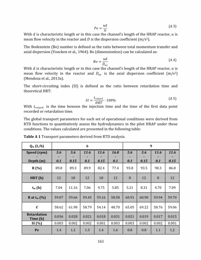
163

𝑃𝑒 =𝑢𝑑

𝐷

(A 3)

With 𝑑 is characteristic length or in this case the channel’s length of the HRAP reactor, 𝑢 is

mean flow velocity in the reactor and 𝐷 is the dispersion coefficient (m/s2).

The Bodenstein (Bo) number is defined as the ratio between total momentum transfer and

axial dispersion (Voncken et al., 1964). Bo (dimensionless) can be calculated as:

𝐵𝑜 =𝑢𝑑

𝐷𝑎𝑥 (A 4)

With 𝑑 is characteristic length or in this case the channel’s length of the HRAP reactor, 𝑢 is

mean flow velocity in the reactor and 𝐷𝑎𝑥 is the axial dispersion coefficient (m/s2)

(Mendoza et al., 2013a).

The short-circuiting index (SI) is defined as the ratio between retardation time and

theoretical HRT:

𝑆𝐼 =𝑡𝑟𝑒𝑡𝑎𝑟𝑑𝐻𝑅𝑇

∙ 100% (A 5)

With 𝑡𝑟𝑒𝑡𝑎𝑟𝑑 is the time beween the injection time and the time of the first data point

recorded or retardation time.

The global transport parameters for each set of operational conditions were derived from

RTD functions to quantitatively assess the hydrodynamics in the pilot HRAP under these

conditions. The values calculated are presented in the following table:

Table A 1 Transport parameters derived from RTD analysis.

Qin (L/h) 6 9

Speed (rpm) -

Depth (m)

5.6 -

0.1

5.6 -

0.15

11.6 -

0.1

11.6 -

0.15

16.8 -

0.1

5.6 -

0.1

5.6 -

0.15

11.6 -

0.1

11.6 -

0.15

R (%) 89.8 89.3 89.9 82.4 77.4 93.8 93.5 90.3 86.8

HRT (h) 12 18 12 18 12 8 12 8 12

tm (h) 7.04 11.16 7.06 9.75 5.85 5.21 8.31 4.70 7.09

R at tm (%) 59.07 59.66 59.45 59.16 58.58 60.91 60.90 59.94 59.70

Є 58.62 61.98 58.79 54.14 48.70 65.05 69.22 58.76 59.06

Retardation Time (h)

0.036 0.028 0.021 0.018 0.031 0.021 0.019 0.017 0.015

SI (%) 0.003 0.002 0.002 0.001 0.003 0.003 0.002 0.002 0.001

Pe 1.4 1.2 1.3 1.4 1.6 0.8 0.8 1.1 1.2

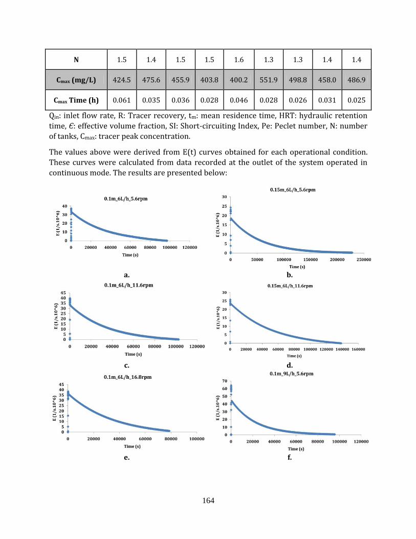
164

N 1.5 1.4 1.5 1.5 1.6 1.3 1.3 1.4 1.4

Cmax (mg/L) 424.5 475.6 455.9 403.8 400.2 551.9 498.8 458.0 486.9

Cmax Time (h) 0.061 0.035 0.036 0.028 0.046 0.028 0.026 0.031 0.025

Qin: inlet flow rate, R: Tracer recovery, tm: mean residence time, HRT: hydraulic retention

time, Є: effective volume fraction, SI: Short-circuiting Index, Pe: Peclet number, N: number

of tanks, Cmax: tracer peak concentration.

The values above were derived from E(t) curves obtained for each operational condition.

These curves were calculated from data recorded at the outlet of the system operated in

continuous mode. The results are presented below:

a. b.

c. d.

e. f.

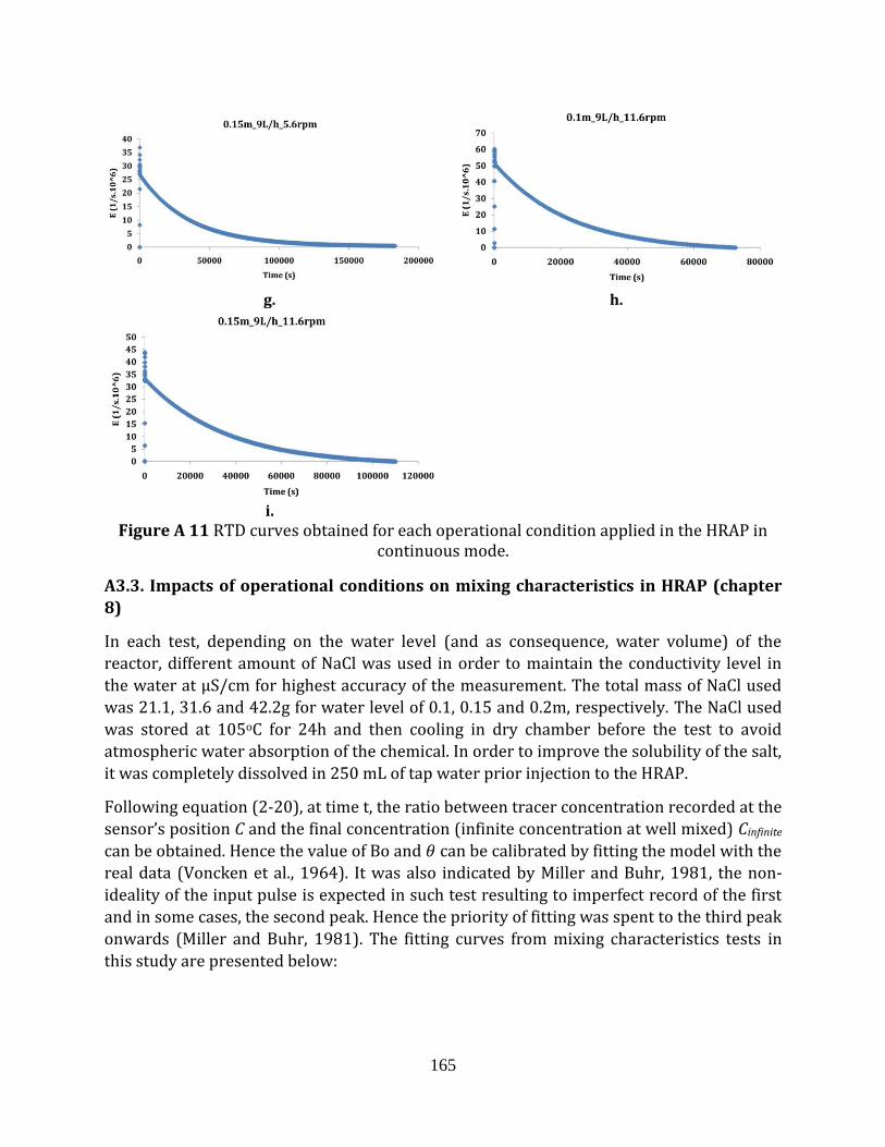
165

g. h.

i. Figure A 11 RTD curves obtained for each operational condition applied in the HRAP in

continuous mode.

A3.3. Impacts of operational conditions on mixing characteristics in HRAP (chapter

8)

In each test, depending on the water level (and as consequence, water volume) of the

reactor, different amount of NaCl was used in order to maintain the conductivity level in

the water at μS/cm for highest accuracy of the measurement. The total mass of NaCl used

was 21.1, 31.6 and 42.2g for water level of 0.1, 0.15 and 0.2m, respectively. The NaCl used

was stored at 105oC for 24h and then cooling in dry chamber before the test to avoid

atmospheric water absorption of the chemical. In order to improve the solubility of the salt,

it was completely dissolved in 250 mL of tap water prior injection to the HRAP.

Following equation (2-20), at time t, the ratio between tracer concentration recorded at the

sensor’s position C and the final concentration (infinite concentration at well mixed) Cinfinite

can be obtained. Hence the value of Bo and 𝜃 can be calibrated by fitting the model with the

real data (Voncken et al., 1964). It was also indicated by Miller and Buhr, 1981, the non-

ideality of the input pulse is expected in such test resulting to imperfect record of the first

and in some cases, the second peak. Hence the priority of fitting was spent to the third peak

onwards (Miller and Buhr, 1981). The fitting curves from mixing characteristics tests in

this study are presented below:

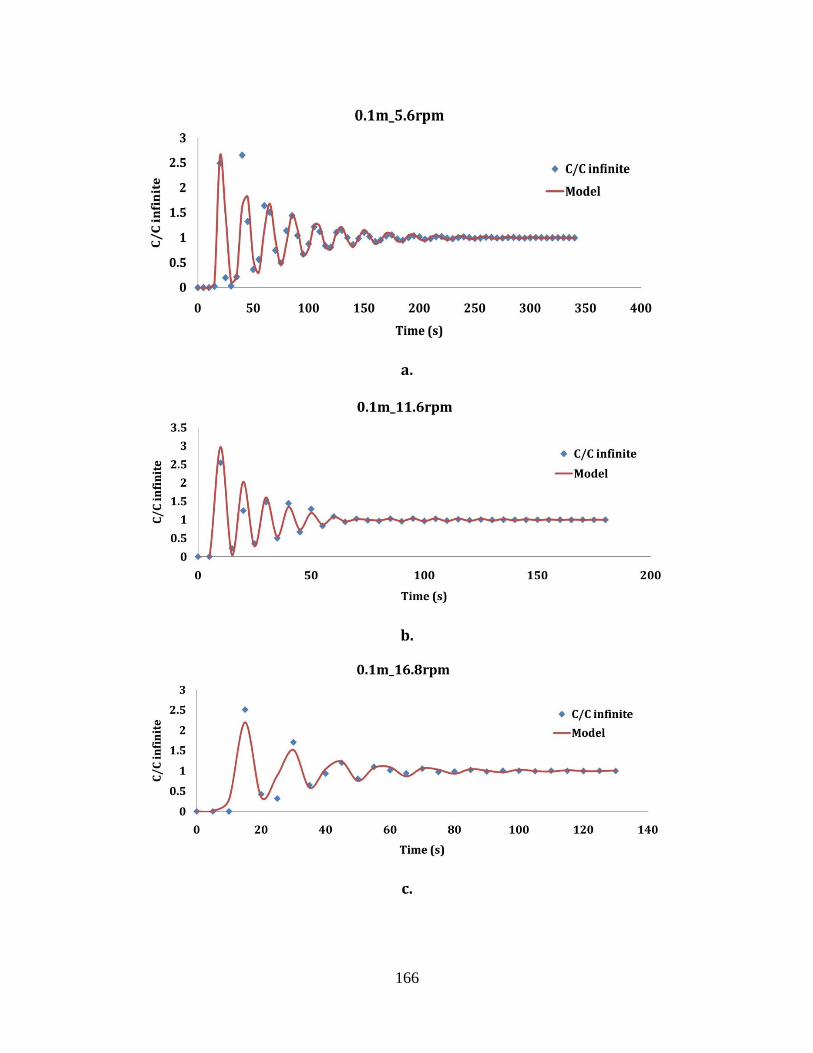
166

a.

b.

c.

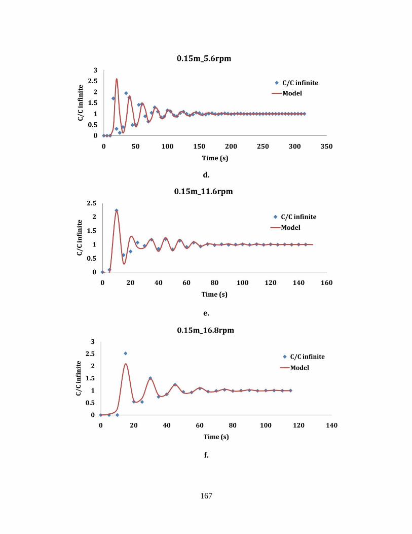
167

d.

e.

f.

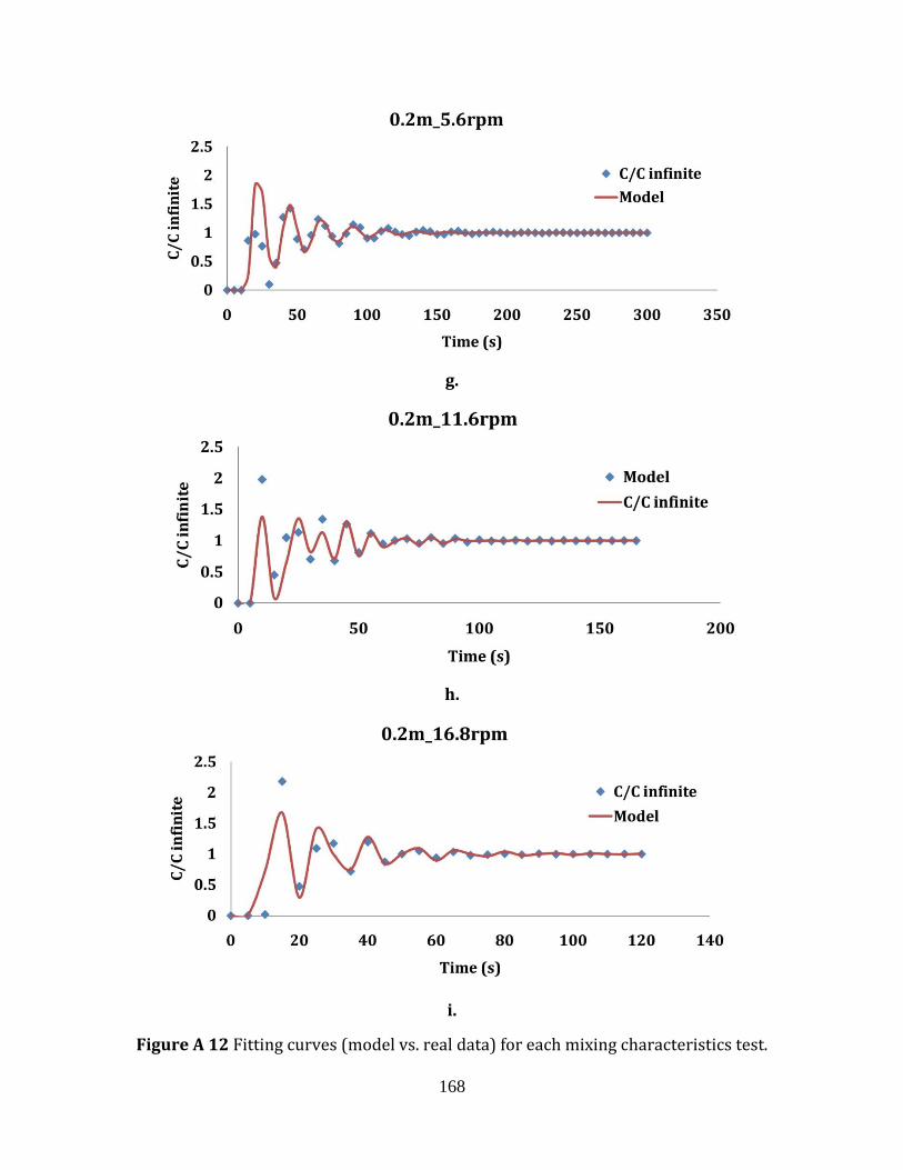
168

g.

h.

i.

Figure A 12 Fitting curves (model vs. real data) for each mixing characteristics test.

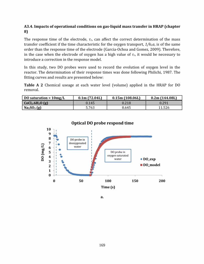
169

A3.4. Impacts of operational conditions on gas-liquid mass transfer in HRAP (chapter

8)

The response time of the electrode, τr, can affect the correct determination of the mass

transfer coefficient if the time characteristic for the oxygen transport, 1/kLa, is of the same

order than the response time of the electrode (Garcia-Ochoa and Gomez, 2009). Therefore,

in the case when the electrode of oxygen has a high value of τr, it would be necessary to

introduce a correction in the response model.

In this study, two DO probes were used to record the evolution of oxygen level in the

reactor. The determination of their response times was done following Philichi, 1987. The

fitting curves and results are presented below:

Table A 2 Chemical useage at each water level (volume) applied in the HRAP for DO removal.

DO saturation = 10mg/L 0.1m (72.04L) 0.15m (108.06L) 0.2m (144.08L)

CoCl2.6H2O (g) 0.145 0.218 0.291

Na2SO3 (g) 5.763 8.645 11.526

a.

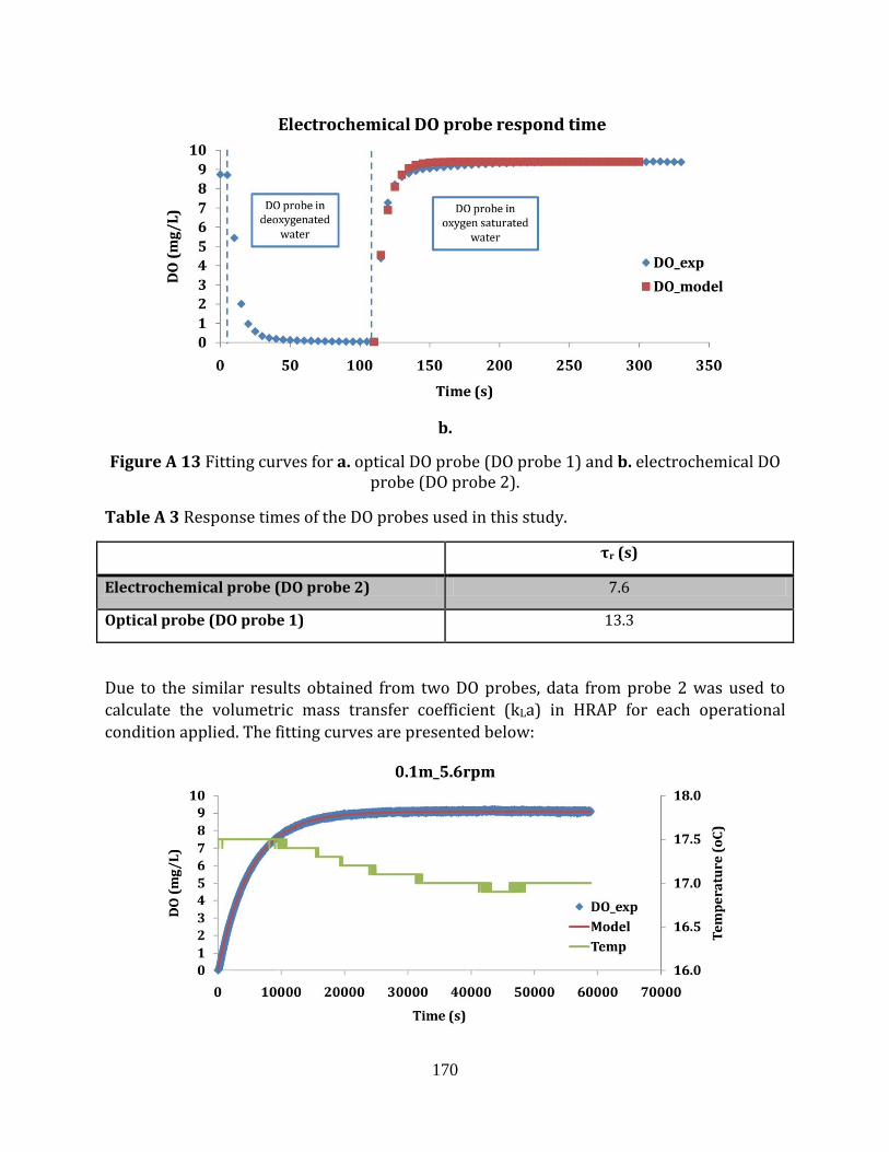
170

b.

Figure A 13 Fitting curves for a. optical DO probe (DO probe 1) and b. electrochemical DO probe (DO probe 2).

Table A 3 Response times of the DO probes used in this study.

τr (s)

Electrochemical probe (DO probe 2) 7.6

Optical probe (DO probe 1) 13.3

Due to the similar results obtained from two DO probes, data from probe 2 was used to

calculate the volumetric mass transfer coefficient (kLa) in HRAP for each operational

condition applied. The fitting curves are presented below:

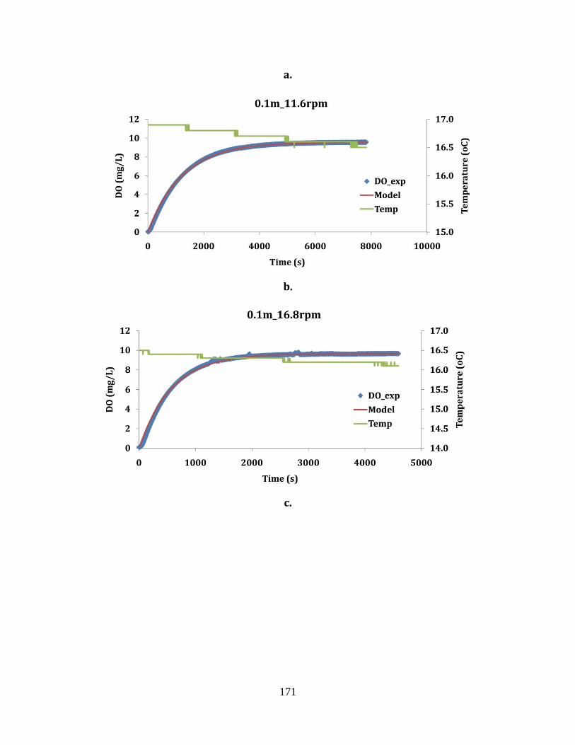
171

a.

b.

c.

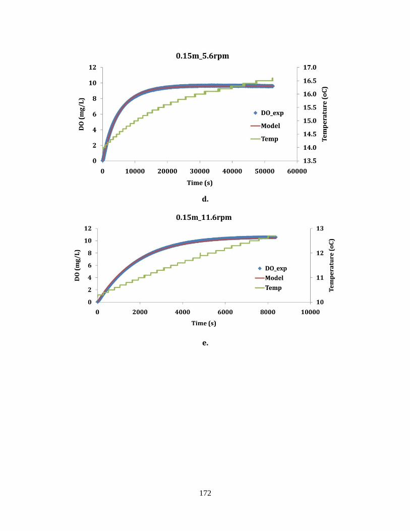
172

d.

e.

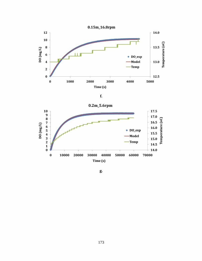
173

f.

g.

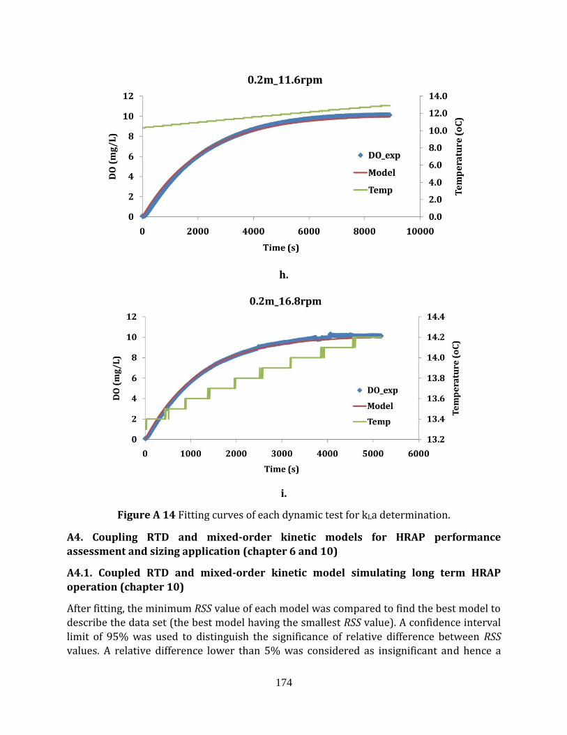
174

h.

i.

Figure A 14 Fitting curves of each dynamic test for kLa determination.

A4. Coupling RTD and mixed-order kinetic models for HRAP performance

assessment and sizing application (chapter 6 and 10)

A4.1. Coupled RTD and mixed-order kinetic model simulating long term HRAP

operation (chapter 10)

After fitting, the minimum RSS value of each model was compared to find the best model to

describe the data set (the best model having the smallest RSS value). A confidence interval

limit of 95% was used to distinguish the significance of relative difference between RSS

values. A relative difference lower than 5% was considered as insignificant and hence a

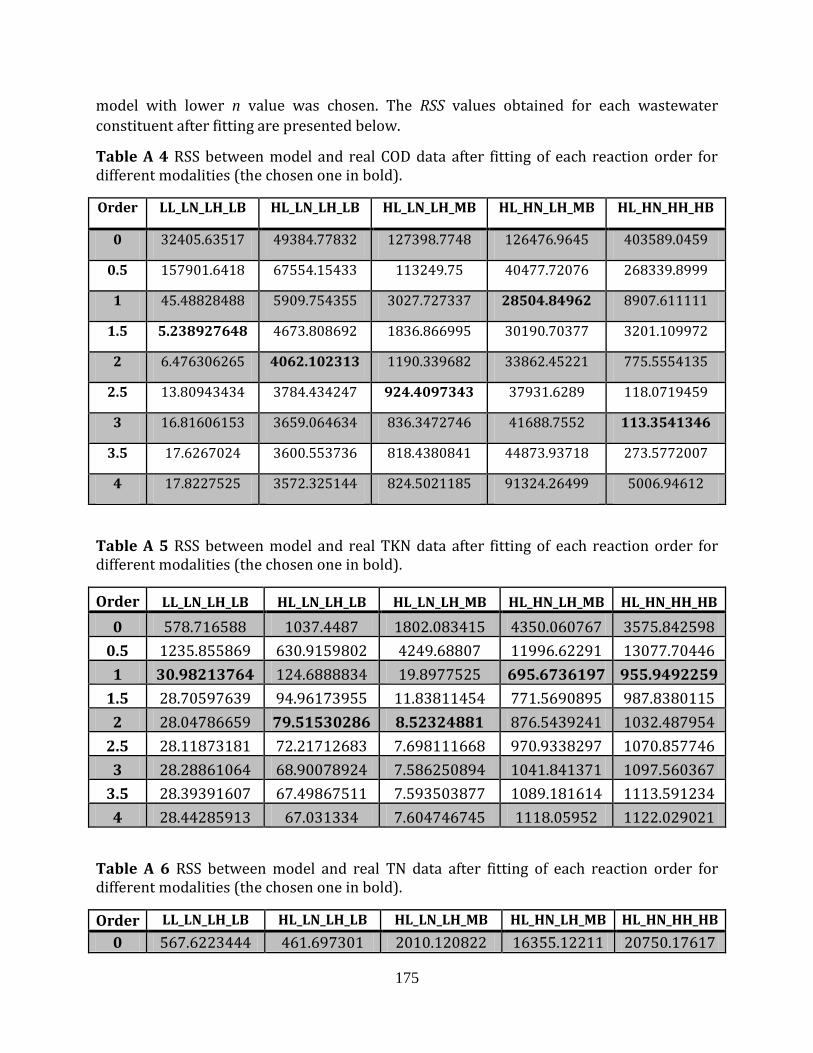
175

model with lower n value was chosen. The RSS values obtained for each wastewater

constituent after fitting are presented below.

Table A 4 RSS between model and real COD data after fitting of each reaction order for different modalities (the chosen one in bold).

Order LL_LN_LH_LB HL_LN_LH_LB HL_LN_LH_MB HL_HN_LH_MB HL_HN_HH_HB

0 32405.63517 49384.77832 127398.7748 126476.9645 403589.0459

0.5 157901.6418 67554.15433 113249.75 40477.72076 268339.8999

1 45.48828488 5909.754355 3027.727337 28504.84962 8907.611111

1.5 5.238927648 4673.808692 1836.866995 30190.70377 3201.109972

2 6.476306265 4062.102313 1190.339682 33862.45221 775.5554135

2.5 13.80943434 3784.434247 924.4097343 37931.6289 118.0719459

3 16.81606153 3659.064634 836.3472746 41688.7552 113.3541346

3.5 17.6267024 3600.553736 818.4380841 44873.93718 273.5772007

4 17.8227525 3572.325144 824.5021185 91324.26499 5006.94612

Table A 5 RSS between model and real TKN data after fitting of each reaction order for different modalities (the chosen one in bold).

Order LL_LN_LH_LB HL_LN_LH_LB HL_LN_LH_MB HL_HN_LH_MB HL_HN_HH_HB

0 578.716588 1037.4487 1802.083415 4350.060767 3575.842598

0.5 1235.855869 630.9159802 4249.68807 11996.62291 13077.70446

1 30.98213764 124.6888834 19.8977525 695.6736197 955.9492259

1.5 28.70597639 94.96173955 11.83811454 771.5690895 987.8380115

2 28.04786659 79.51530286 8.52324881 876.5439241 1032.487954

2.5 28.11873181 72.21712683 7.698111668 970.9338297 1070.857746

3 28.28861064 68.90078924 7.586250894 1041.841371 1097.560367

3.5 28.39391607 67.49867511 7.593503877 1089.181614 1113.591234

4 28.44285913 67.031334 7.604746745 1118.05952 1122.029021

Table A 6 RSS between model and real TN data after fitting of each reaction order for different modalities (the chosen one in bold).

Order LL_LN_LH_LB HL_LN_LH_LB HL_LN_LH_MB HL_HN_LH_MB HL_HN_HH_HB

0 567.6223444 461.697301 2010.120822 16355.12211 20750.17617

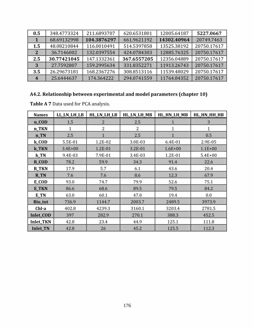
176

0.5 348.4773324 211.6893707 620.6531801 12005.64187 5227.0667

1 68.69132998 104.3876297 661.9621192 14302.40964 20749.7463

1.5 48.08210844 116.0010491 514.5397858 13525.38192 20750.17617

2 36.7146002 132.0397554 424.0784303 12885.76325 20750.17617

2.5 30.77421045 147.1332361 367.6557205 12356.04889 20750.17617

3 27.7592807 159.2995634 331.8352271 11913.26743 20750.17617

3.5 26.29673181 168.2367276 308.8513116 11539.48029 20750.17617

4 25.6444637 174.364222 294.0741559 11764.84352 20750.17617

A4.2. Relationship between experimental and model parameters (chapter 10)

Table A 7 Data used for PCA analysis.

Names LL_LN_LH_LB HL_LN_LH_LB HL_LN_LH_MB HL_HN_LH_MB HL_HN_HH_HB

n_COD 1.5 2 2.5 1 3

n_TKN 1 2 2 1 1

n_TN 2.5 1 2.5 1 0.5

k_COD 5.5E-01 1.2E-02 3.0E-03 6.4E-01 2.9E-05

k_TKN 3.4E+00 1.2E-01 3.2E-01 1.6E+00 1.1E+00

k_TN 9.4E-03 7.9E-01 3.4E-03 1.2E-01 5.4E+00

R_COD 78.2 59.9 34.3 91.4 22.6

R_TKN 17.9 5.7 6.1 43.6 20.4

R_TN 7.6 7.6 8.6 12.3 67.9

E_COD 93.0 74.7 79.9 52.6 75.1

E_TKN 86.6 68.6 89.5 79.5 84.2

E_TN 63.0 60.1 47.0 19.4 0.0

Bio_tot 736.9 1144.7 2003.7 2489.5 3973.9

Chl-a 402.8 4239.3 3160.1 3203.4 2781.5

Inlet_COD 397 282.9 270.1 388.3 452.5

Inlet_TKN 42.8 23.4 44.9 125.1 111.8

Inlet_TN 42.8 26 45.2 125.5 112.3

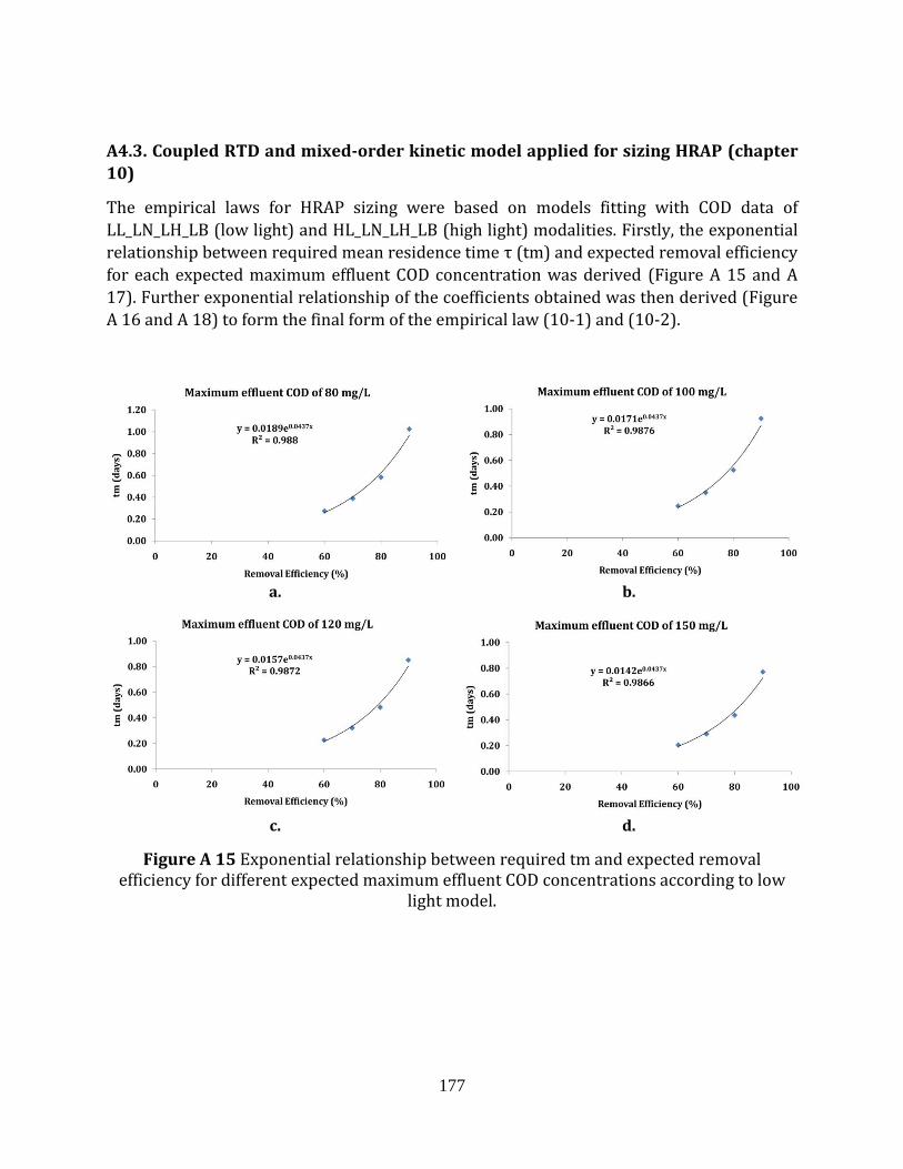
177

A4.3. Coupled RTD and mixed-order kinetic model applied for sizing HRAP (chapter

10)

The empirical laws for HRAP sizing were based on models fitting with COD data of

LL_LN_LH_LB (low light) and HL_LN_LH_LB (high light) modalities. Firstly, the exponential

relationship between required mean residence time τ (tm) and expected removal efficiency

for each expected maximum effluent COD concentration was derived (Figure A 15 and A

17). Further exponential relationship of the coefficients obtained was then derived (Figure

A 16 and A 18) to form the final form of the empirical law (10-1) and (10-2).

a. b.

c. d.

Figure A 15 Exponential relationship between required tm and expected removal efficiency for different expected maximum effluent COD concentrations according to low

light model.

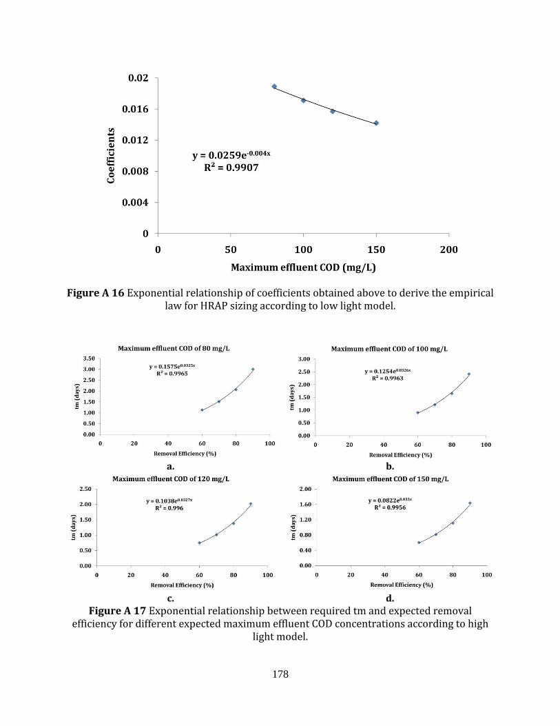
178

Figure A 16 Exponential relationship of coefficients obtained above to derive the empirical law for HRAP sizing according to low light model.

a. b.

c. d.

Figure A 17 Exponential relationship between required tm and expected removal efficiency for different expected maximum effluent COD concentrations according to high

light model.

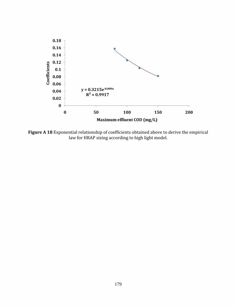
179

Figure A 18 Exponential relationship of coefficients obtained above to derive the empirical law for HRAP sizing according to high light model.

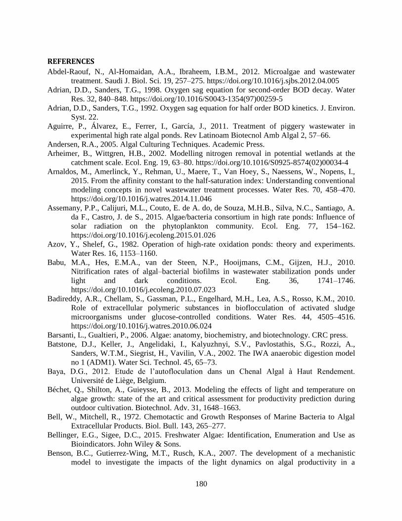
180

REFERENCES

Abdel-Raouf, N., Al-Homaidan, A.A., Ibraheem, I.B.M., 2012. Microalgae and wastewater

treatment. Saudi J. Biol. Sci. 19, 257–275. https://doi.org/10.1016/j.sjbs.2012.04.005

Adrian, D.D., Sanders, T.G., 1998. Oxygen sag equation for second-order BOD decay. Water

Res. 32, 840–848. https://doi.org/10.1016/S0043-1354(97)00259-5

Adrian, D.D., Sanders, T.G., 1992. Oxygen sag equation for half order BOD kinetics. J. Environ.

Syst. 22.

Aguirre, P., Álvarez, E., Ferrer, I., García, J., 2011. Treatment of piggery wastewater in

experimental high rate algal ponds. Rev Latinoam Biotecnol Amb Algal 2, 57–66.

Andersen, R.A., 2005. Algal Culturing Techniques. Academic Press.

Arheimer, B., Wittgren, H.B., 2002. Modelling nitrogen removal in potential wetlands at the

catchment scale. Ecol. Eng. 19, 63–80. https://doi.org/10.1016/S0925-8574(02)00034-4

Arnaldos, M., Amerlinck, Y., Rehman, U., Maere, T., Van Hoey, S., Naessens, W., Nopens, I.,

2015. From the affinity constant to the half-saturation index: Understanding conventional

modeling concepts in novel wastewater treatment processes. Water Res. 70, 458–470.

https://doi.org/10.1016/j.watres.2014.11.046

Assemany, P.P., Calijuri, M.L., Couto, E. de A. do, de Souza, M.H.B., Silva, N.C., Santiago, A.

da F., Castro, J. de S., 2015. Algae/bacteria consortium in high rate ponds: Influence of

solar radiation on the phytoplankton community. Ecol. Eng. 77, 154–162.

https://doi.org/10.1016/j.ecoleng.2015.01.026

Azov, Y., Shelef, G., 1982. Operation of high-rate oxidation ponds: theory and experiments.

Water Res. 16, 1153–1160.

Babu, M.A., Hes, E.M.A., van der Steen, N.P., Hooijmans, C.M., Gijzen, H.J., 2010.

Nitrification rates of algal–bacterial biofilms in wastewater stabilization ponds under

light and dark conditions. Ecol. Eng. 36, 1741–1746.

https://doi.org/10.1016/j.ecoleng.2010.07.023

Badireddy, A.R., Chellam, S., Gassman, P.L., Engelhard, M.H., Lea, A.S., Rosso, K.M., 2010.

Role of extracellular polymeric substances in bioflocculation of activated sludge

microorganisms under glucose-controlled conditions. Water Res. 44, 4505–4516.

https://doi.org/10.1016/j.watres.2010.06.024

Barsanti, L., Gualtieri, P., 2006. Algae: anatomy, biochemistry, and biotechnology. CRC press.

Batstone, D.J., Keller, J., Angelidaki, I., Kalyuzhnyi, S.V., Pavlostathis, S.G., Rozzi, A.,

Sanders, W.T.M., Siegrist, H., Vavilin, V.A., 2002. The IWA anaerobic digestion model

no 1 (ADM1). Water Sci. Technol. 45, 65–73.

Baya, D.G., 2012. Etude de l’autofloculation dans un Chenal Algal à Haut Rendement.

Université de Liège, Belgium.

Béchet, Q., Shilton, A., Guieysse, B., 2013. Modeling the effects of light and temperature on

algae growth: state of the art and critical assessment for productivity prediction during

outdoor cultivation. Biotechnol. Adv. 31, 1648–1663.

Bell, W., Mitchell, R., 1972. Chemotactic and Growth Responses of Marine Bacteria to Algal

Extracellular Products. Biol. Bull. 143, 265–277.

Bellinger, E.G., Sigee, D.C., 2015. Freshwater Algae: Identification, Enumeration and Use as

Bioindicators. John Wiley & Sons.

Benson, B.C., Gutierrez-Wing, M.T., Rusch, K.A., 2007. The development of a mechanistic

model to investigate the impacts of the light dynamics on algal productivity in a

181

Hydraulically Integrated Serial Turbidostat Algal Reactor (HISTAR). Aquac. Eng. 36,

198–211. https://doi.org/10.1016/j.aquaeng.2006.12.002

Bernard, O., 2011. Hurdles and challenges for modelling and control of microalgae for CO2

mitigation and biofuel production. J. Process Control, Special Issue:Selected Papers From

Two Joint IFAC Conferences: 9th International Symposium on Dynamics and Control of

Process Systems and the 11th International Symposium on Computer Applications in

Biotechnology, Leuven, Belgium, July 5-9, 2010. 21, 1378–1389.

https://doi.org/10.1016/j.jprocont.2011.07.012

Bilanovic, D., Holland, M., Starosvetsky, J., Armon, R., 2016. Co-cultivation of microalgae and

nitrifiers for higher biomass production and better carbon capture. Bioresour. Technol.

220, 282–288. https://doi.org/10.1016/j.biortech.2016.08.083

Bitog, J.P., Lee, I.-B., Lee, C.-G., Kim, K.-S., Hwang, H.-S., Hong, S.-W., Seo, I.-H., Kwon, K.-

S., Mostafa, E., 2011. Application of computational fluid dynamics for modeling and

designing photobioreactors for microalgae production: a review. Comput. Electron.

Agric. 76, 131–147. https://doi.org/10.1016/j.compag.2011.01.015

Bordel, S., Guieysse, B., Munoz, R., 2009. Mechanistic model for the reclamation of industrial

wastewaters using algal-bacterial photobioreactors. Environ. Sci. Technol. 43, 3200–

3207.

Borsuk, M.E., Stow, C.A., 2000. Bayesian parameter estimation in a mixed-order model of BOD

decay. Water Res. 34, 1830–1836. https://doi.org/10.1016/S0043-1354(99)00346-2

Bouterfas, R., Belkoura, M., Dauta, A., 2006. The effects of irradiance and photoperiod on the

growth rate of three freshwater green algae isolated from a eutrophic lake. Limnetica 25,

647–656.

Broekhuizen, N., Park, J.B., McBride, G.B., Craggs, R.J., 2012. Modification, calibration and

verification of the IWA River Water Quality Model to simulate a pilot-scale high rate

algal pond. Water Res. 46, 2911–2926.

Buhr, H.O., Miller, S.B., 1983. A dynamic model of the high-rate algal-bacterial wastewater

treatment pond. Water Res. 17, 29–37. https://doi.org/10.1016/0043-1354(83)90283-X

Bulgakov, N.G., Levich, A.P., 1999. The nitrogen : Phosphorus ratio as a factor regulating

phytoplankton community structure : Nutrient ratios. Arch. Für Hydrobiol. 146, 3–22.

Cai, T., Park, S.Y., Li, Y., 2013. Nutrient recovery from wastewater streams by microalgae:

Status and prospects. Renew. Sustain. Energy Rev. 19, 360–369.

https://doi.org/10.1016/j.rser.2012.11.030

Carroll, J.J., Slupsky, J.D., Mather, A.E., 1991. The Solubility of Carbon Dioxide in Water at

Low Pressure. J. Phys. Chem. Ref. Data 20, 1201–1209. https://doi.org/10.1063/1.555900

Carucci, A., Dionisi, D., Majone, M., Rolle, E., Smurra, P., 2001. Aerobic storage by activated

sludge on real wastewater. Water Res. 35, 3833–3844.

Chiaramonti, D., Prussi, M., Casini, D., Tredici, M.R., Rodolfi, L., Bassi, N., Zittelli, G.C.,

Bondioli, P., 2013. Review of energy balance in raceway ponds for microalgae

cultivation: Re-thinking a traditional system is possible. Appl. Energy, Special Issue on

Advances in sustainable biofuel production and use - XIX International Symposium on

Alcohol Fuels - ISAF 102, 101–111. https://doi.org/10.1016/j.apenergy.2012.07.040

Cho, S.H., JI, S.-C., Hur, S.B., Bae, J., PARK, I.-S., SONG, Y.-C., 2007. Optimum temperature

and salinity conditions for growth of green algae Chlorella ellipsoidea and Nannochloris

oculata. Fish. Sci. 73, 1050–1056.

182

Christenson, L., Sims, R., 2011. Production and harvesting of microalgae for wastewater

treatment, biofuels, and bioproducts. Biotechnol. Adv. 29, 686–702.

https://doi.org/10.1016/j.biotechadv.2011.05.015

Cleveland, W.S., Freeny, A.E., Graedel, T.E., 1983. The seasonal component of atmospheric

CO2: Information from new approaches to the decomposition of seasonal time series. J.

Geophys. Res. Oceans 88, 10934–10946. https://doi.org/10.1029/JC088iC15p10934

Coffey, R., Dorai-Raj, S., O’Flaherty, V., Cormican, M., Cummins, E., 2013. Modeling of

Pathogen Indicator Organisms in a Small-Scale Agricultural Catchment Using SWAT.

Hum. Ecol. Risk Assess. Int. J. 19, 232–253.

https://doi.org/10.1080/10807039.2012.701983

Cole, J.J., 1982. Interactions Between Bacteria and Algae in Aquatic Ecosystems. Annu. Rev.

Ecol. Syst. 13, 291–314. https://doi.org/10.1146/annurev.es.13.110182.001451

Craggs, R., Park, J., Sutherland, D., Heubeck, S., 2015. Economic construction and operation of

hectare-scale wastewater treatment enhanced pond systems. J. Appl. Phycol. 1–10.

https://doi.org/10.1007/s10811-015-0658-6

Crawley, M.J., 2012. The R Book. Wiley.

Crill, P.A., 1977. The photosynthesis-light curve: A simple analog model. J. Theor. Biol. 64,

503–516. https://doi.org/10.1016/0022-5193(77)90284-3

Crites, R.W., Middlebrooks, E.J., Bastian, R.K., 2014. Natural wastewater treatment systems.

CRC Press.

Cromar, N.J., Fallowfield, H.J., 1997. Effect of nutrient loading and retention time on

performance of high rate algal ponds. J. Appl. Phycol. 9, 301–309.

Cussler, E.L., 2009. Diffusion: Mass Transfer in Fluid Systems. Cambridge University Press.

Danckwerts, P.V., 1953. Continuous flow systems: Distribution of residence times. Chem. Eng.

Sci. 2, 1–13. https://doi.org/10.1016/0009-2509(53)80001-1

Das, P., Lei, W., Aziz, S.S., Obbard, J.P., 2011. Enhanced algae growth in both phototrophic and

mixotrophic culture under blue light. Bioresour. Technol. 102, 3883–3887.

https://doi.org/10.1016/j.biortech.2010.11.102

de Baar, H.J.W., 1994. von Liebig’s law of the minimum and plankton ecology (1899–1991).

Prog. Oceanogr. 33, 347–386. https://doi.org/10.1016/0079-6611(94)90022-1

de Godos, I., Blanco, S., García-Encina, P.A., Becares, E., Muñoz, R., 2009. Long-term

operation of high rate algal ponds for the bioremediation of piggery wastewaters at high

loading rates. Bioresour. Technol. 100, 4332–4339.

Decostere, B., Van Hulle, S.W., Duyck, M., Maere, T., Vervaeren, H., Nopens, I., 2014. The use

of a combined respirometric–titrimetric setup to assess the effect of environmental

conditions on micro-algal growth rate. J. Chem. Technol. Biotechnol. 91, 248–256.

https://doi.org/10.1002/jctb.4574

Dick, R.I., Vesilind, P.A., 1969. The Sludge Volume Index: What Is It? J. Water Pollut. Control

Fed. 41, 1285–1291.

Ding, Z., Bourven, I., Guibaud, G., van Hullebusch, E.D., Panico, A., Pirozzi, F., Esposito, G.,

2015. Role of extracellular polymeric substances (EPS) production in bioaggregation:

application to wastewater treatment. Appl. Microbiol. Biotechnol. 99, 9883–9905.

Dionisi, D., Majone, M., Ramadori, R., Beccari, M., 2001. The storage of acetate under anoxic

conditions. Water Res. 35, 2661–2668.

183

Dionisi, D., Renzi, V., Majone, M., Beccari, M., Ramadori, R., 2004. Storage of substrate

mixtures by activated sludges under dynamic conditions in anoxic or aerobic

environments. Water Res. 38, 2196–2206.

Dircks, K., Henze, M., van Loosdrecht, M.C., Mosb\a ek, H., Aspegren, H., 2001. Storage and

degradation of poly-β-hydroxybutyrate in activated sludge under aerobic conditions.

Water Res. 35, 2277–2285.

Droop, M.R., 1973. Some Thoughts on Nutrient Limitation in Algae. J. Phycol. 9, 264–272.

https://doi.org/10.1111/j.1529-8817.1973.tb04092.x

Droop, M.R., 1970. Vitamin B12 and marine ecology. Helgoländer Wiss. Meeresunters. 20,

629–636. https://doi.org/10.1007/BF01609935

Durst, F., 2008. Fluid Mechanics: An Introduction to the Theory of Fluid Flows. Springer-

Verlag, Berlin Heidelberg.

Eilers, P.H.C., Peeters, J.C.H., 1988. A model for the relationship between light intensity and the

rate of photosynthesis in phytoplankton. Ecol. Model. 42, 199–215.

https://doi.org/10.1016/0304-3800(88)90057-9

El Hamouri, B., Jellal, J., Outabiht, H., Nebri, B., Khallayoune, K., Benkerroum, A., Hajli, A.,

Firadi, R., 1995. The performance of a high-rate algal pond in the moroccan climate.

Water Sci. Technol., Waste Stabilisation Ponds and the Reuse of Pond Effluents 31, 67–

74. https://doi.org/10.1016/0273-1223(95)00493-7

El Hamouri, B., Rami, A., Vasel, J.-L., 2003. The reasons behind the performance superiority of

a high rate algal pond over three facultative ponds in series. Water Sci. Technol. 48, 269–

276.

El Ouarghi, H., Boumansour, B.E., Dufayt, O., El Hamouri, B., Vasel, J.L., 2000.

Hydrodynamics and oxygen balance in a high-rate algal pond. Water Sci. Technol. 42,

349–356.

Ellis, K.V., Rodrigues, P.C.C., 1993. Verification of two design approaches for stabilization

ponds. Water Res. 27, 1447–1454. https://doi.org/10.1016/0043-1354(93)90024-C

Eppley, R.W., 1972. Temperature and phytoplankton growth in the sea. Fish Bull 70, 1063–

1085.

Evans, R.A., Cromar, N.J., Fallowfield, H.J., 2005. Performance of a pilot-scale high rate algal

pond system treating abattoir wastewater in rural South Australia: nitrification and

denitrification. Water Sci. Technol. 51, 117–124.

Falkowski, P.G., 1980. Primary productivity in the sea. Springer.

FAO, 1992. Wastewater treatment [WWW Document]. URL

http://www.fao.org/docrep/t0551e/t0551e05.htm (accessed 2.9.18).

Ferenci, T., 1999. Growth of bacterial cultures’ 50 years on: towards an uncertainty principle

instead of constants in bacterial growth kinetics. Res. Microbiol. 150, 431–438.

Flegal, T.M., Schroeder, E.D., 1976. Temperature Effects on BOD Stoichiometry and Oxygen

Uptake Rate. J. Water Pollut. Control Fed. 48, 2700–2707.

Fogler, H.S., 2006a. Elements of Chemical Reaction Engineering. Prentice Hall PTR.

Fogler, H.S., 2006b. Chapter 13: Distributions of Residence Times for Chemical Reactors, in:

Elements of Chemical Reaction Engineering. Prentice Hall PTR.

Fogler, H.S., 2006c. Chapter 14: Models for Nonideal Reactors, in: Elements of Chemical

Reaction Engineering. Prentice Hall PTR.

Ganidi, N., Tyrrel, S., Cartmell, E., 2009. Anaerobic digestion foaming causes – A review.

Bioresour. Technol. 100, 5546–5554. https://doi.org/10.1016/j.biortech.2009.06.024

184

García, J., Green, B.F., Lundquist, T., Mujeriego, R., Hernández-Mariné, M., Oswald, W.J.,

2006. Long term diurnal variations in contaminant removal in high rate ponds treating

urban wastewater. Bioresour. Technol. 97, 1709–1715.

García, J., Hernández-Mariné, M., Mujeriego, R., 2002. Analysis of key variables controlling

phosphorus removal in high rate oxidation ponds provided with clarifiers. Water SA 28,

p–55. http://dx.doi.org/10.4314/wsa.v28i1.4868

Garcia, J., Mujeriego, R., Hernandez-Marine, M., 2000. High rate algal pond operating strategies

for urban wastewater nitrogen removal. J. Appl. Phycol. 12, 331–339.

https://doi.org/10.1023/A:1008146421368

Garcia-Ochoa, F., Gomez, E., 2009. Bioreactor scale-up and oxygen transfer rate in microbial

processes: An overview. Biotechnol. Adv. 27, 153–176.

https://doi.org/10.1016/j.biotechadv.2008.10.006

Gerardi, M.H., 2003. Nitrification and Denitrification in the Activated Sludge Process. John

Wiley & Sons.

Gonçalves, A.L., Simões, M., Pires, J.C.M., 2014. The effect of light supply on microalgal

growth, CO2 uptake and nutrient removal from wastewater. Energy Convers. Manag. 85,

530–536. https://doi.org/10.1016/j.enconman.2014.05.085

González-Fernández, C., Sialve, B., Bernet, N., Steyer, J.-P., 2012. Impact of microalgae

characteristics on their conversion to biofuel. Part II: Focus on biomethane production.

Biofuels Bioprod. Biorefining 6, 205–218. https://doi.org/10.1002/bbb.337

Grady Jr, C.L., Daigger, G.T., Love, N.G., Filipe, C.D., 2011. Biological wastewater treatment.

CRC press.

Grima, E.M., Fernández, F.A., Camacho, F.G., Chisti, Y., 1999. Photobioreactors: light regime,

mass transfer, and scaleup. J. Biotechnol. 70, 231–247. https://doi.org/10.1016/S0168-

1656(99)00078-4

Grobbelaar, J.U., 1994. Turbulence in mass algal cultures and the role of light/dark fluctuations.

J. Appl. Phycol. 6, 331–335. https://doi.org/10.1007/BF02181947

Grobbelaar, J.U., 1991. The influence of light/dark cycles in mixed algal cultures on their

productivity. Bioresour. Technol., Algal biotechnology 38, 189–194.

https://doi.org/10.1016/0960-8524(91)90153-B

Grobbelaar, J.U., Soeder, C.J., Stengel, E., 1990. Modeling algal productivity in large outdoor

cultures and waste treatment systems. Biomass 21, 297–314.

https://doi.org/10.1016/0144-4565(90)90079-Y

Grönlund, E., Hanæus, J., Johansson, E., Falk, S., 2010. Performance of an Experimental

Wastewater Treatment High-Rate Algal Pond in Subarctic Climate. Water Environ. Res.

82, 830–839. https://doi.org/10.2175/106143009X12487095236478

Grossart, H.-P., Simon, M., 2007. Interactions of planktonic algae and bacteria: effects on algal

growth and organic matter dynamics. Aquat. Microb. Ecol. 47, 163.

https://doi.org/10.3354/ame047163

Gujer, W., Henze, M., Mino, T., Loosdrecht, M. van, 1999. Activated sludge model No. 3. Water

Sci. Technol., Modelling and microbiology of activated sludge processes 39, 183–193.

https://doi.org/10.1016/S0273-1223(98)00785-9

Gutzeit, G., Lorch, D., Weber, A., Engels, M., Neis, U., 2005. Bioflocculent algal-bacterial

biomass improves low-cost wastewater treatment., in: Water Science and Technology : A

Journal of the International Association on Water Pollution Research. pp. 9–18.

185

Hadiyanto, H., Elmore, S., Van Gerven, T., Stankiewicz, A., 2013. Hydrodynamic evaluations in

high rate algae pond (HRAP) design. Chem. Eng. J. 217, 231–239.

https://doi.org/10.1016/j.cej.2012.12.015

Hauduc, H., Gillot, S., Rieger, L., Ohtsuki, T., Shaw, A., Takács, I., Winkler, S., 2009. Activated

sludge modelling in practice: an international survey. Water Sci. Technol. J. Int. Assoc.

Water Pollut. Res. 60, 1943–1951. https://doi.org/10.2166/wst.2009.223

Henze, M., 2008. Biological Wastewater Treatment: Principles, Modelling and Design. IWA

Publishing.

Henze, M., Dupont, R., Grau, P., de la Sota, A., 1993. Rising sludge in secondary settlers due to

denitrification. Water Res. 27, 231–236. https://doi.org/10.1016/0043-1354(93)90080-2

Henze, M., Grady, C.P.L.J., Gujer, W., Marais, G.V.R., Matsuo, T., 1987. Activated Sludge

Model No 1. ResearchGate 29.

Henze, M., Gujer, W., Mino, T., Matsuo, T., Wentzel, M.C., Marais, G. v. R., Van Loosdrecht,

M.C.M., 1999. Activated sludge model No.2D, ASM2D. Water Sci. Technol., Modelling

and microbiology of activated sludge processes 39, 165–182.

https://doi.org/10.1016/S0273-1223(98)00829-4

Henze, M., Gujer, W., Mino, T., van Loosdrecht, M.C.M., 2000. Activated sludge models

ASM1, ASM2, ASM2d and ASM3. IWA Publishing.

Hewitt, J., Hunter, J.V., Lockwood, D., 1979. A multiorder approach to bod kinetics. Water Res.

13, 325–329. https://doi.org/10.1016/0043-1354(79)90213-6

Hreiz, R., Sialve, B., Morchain, J., Escudié, R., Steyer, J.-P., Guiraud, P., 2014. Experimental

and numerical investigation of hydrodynamics in raceway reactors used for algaculture.

Chem. Eng. J. 250, 230–239. https://doi.org/10.1016/j.cej.2014.03.027

Huisman, J., Matthijs, H.C.P., Visser, P.M., Balke, H., Sigon, C.A.M., Passarge, J., Weissing,

F.J., Mur, L.R., 2002. Principles of the light-limited chemostat: theory and ecological

applications. Antonie Van Leeuwenhoek 81, 117–133.

https://doi.org/10.1023/A:1020537928216

Iacopozzi, I., Innocenti, V., Marsili-Libelli, S., Giusti, E., 2007. A modified Activated Sludge

Model No. 3 (ASM3) with two-step nitrification–denitrification. Environ. Model. Softw.

22, 847–861. https://doi.org/10.1016/j.envsoft.2006.05.009

James, D.E., 2012. Culturing algae.

James, S.C., Boriah, V., 2010. Modeling algae growth in an open-channel raceway. J. Comput.

Biol. 17, 895–906.

Jupsin, H., Praet, E., Vasel, J.-L., 2003. Dynamic mathematical model of high rate algal ponds

(HRAP). Water Sci. Technol. 48, 197–204.

Kadlec, R.H., 2000. The inadequacy of first-order treatment wetland models. Ecol. Eng. 15, 105–

119. https://doi.org/10.1016/S0925-8574(99)00039-7

Kadlec, R.H., 1994. Detention and mixing in free water wetlands. Ecol. Eng. 3, 345–380.

https://doi.org/10.1016/0925-8574(94)00007-7

Kirst, G.O., 1989. Salinity Tolerance of Eukaryotic Marine Algae. Annu. Rev. Plant Physiol.

Plant Mol. Biol. 41, 21–53. https://doi.org/10.1146/annurev.pp.41.060190.000321

Kouzuma, A., Watanabe, K., 2015. Exploring the potential of algae/bacteria interactions. Curr.

Opin. Biotechnol. 33, 125–129. https://doi.org/10.1016/j.copbio.2015.02.007

Krebs, P., Stamou, A.I., García-Heras, J.L., Rodi, W., 1996. Influence of inlet and outlet

configuration on the flow in secondary clarifiers. Water Sci. Technol., Water Quality

International ’96 Part 3: Modelling of Activated Sludge Processes; Microorganisms in

186

Activated Sludge and Biofilm Processes; Anareobic Biological Treatment; Biofouling 34,

1–9. https://doi.org/10.1016/0273-1223(96)00622-1

Krishna, C., Van Loosdrecht, M.C., 1999. Effect of temperature on storage polymers and

settleability of activated sludge. Water Res. 33, 2374–2382.

Kromkamp, J., Limbeek, M., 1993. Effect of short-term variation in irradiance on light

harvesting and photosynthesis of the marine diatom Skeletonema costatum: a laboratory

study simulating vertical mixing. Microbiology 139, 2277–2284.

https://doi.org/10.1099/00221287-139-9-2277

Kumar, K., Mishra, S.K., Shrivastav, A., Park, M.S., Yang, J.-W., 2015. Recent trends in the

mass cultivation of algae in raceway ponds. Renew. Sustain. Energy Rev. 51, 875–885.

https://doi.org/10.1016/j.rser.2015.06.033

Lasdon, L.S., Fox, R.L., Ratner, M.W., 1974. Nonlinear optimization using the generalized

reduced gradient method. Rev. Fr. Autom. Inform. Rech. Opérationnelle Rech.

Opérationnelle 3, 73–103.

Laurent, J., Bois, P., Nuel, M., Wanko, A., 2015. Systemic models of full-scale Surface Flow

Treatment Wetlands: Determination by application of fluorescent tracers. Chem. Eng. J.

264, 389–398.

Lavens, P., Sorgeloos, P., 1996. Manual on the production and use of live food for aquaculture.

Food and Agriculture Organization (FAO).

Lawton, R.J., Cole, A.J., Roberts, D.A., Paul, N.A., de Nys, R., 2017. The industrial ecology of

freshwater macroalgae for biomass applications. Algal Res., Wastewater and Algae;

opportunities, challenges and long term sustainability 24, 486–491.

https://doi.org/10.1016/j.algal.2016.08.019

Le Moullec, Y., Gentric, C., Potier, O., Leclerc, J.P., 2010. Comparison of systemic,

compartmental and CFD modelling approaches: Application to the simulation of a

biological reactor of wastewater treatment. Chem. Eng. Sci., 20th International

Symposium in Chemical Reaction Engineering—Green Chemical Reaction Engineering

for a Sustainable Future 65, 343–350. https://doi.org/10.1016/j.ces.2009.06.035

Le Moullec, Y., Potier, O., Gentric, C., Pierre Leclerc, J., 2008. Flow field and residence time

distribution simulation of a cross-flow gas–liquid wastewater treatment reactor using

CFD. Chem. Eng. Sci. 63, 2436–2449. https://doi.org/10.1016/j.ces.2008.01.029

Lee, C.S., Lee, S.-A., Ko, S.-R., Oh, H.-M., Ahn, C.-Y., 2015. Effects of photoperiod on nutrient

removal, biomass production, and algal-bacterial population dynamics in lab-scale

photobioreactors treating municipal wastewater. Water Res. 68, 680–691.

https://doi.org/10.1016/j.watres.2014.10.029

Lee, E., Jalalizadeh, M., Zhang, Q., 2015. Growth kinetic models for microalgae cultivation: A

review. Algal Res. 12, 497–512. https://doi.org/10.1016/j.algal.2015.10.004

Levenspiel, O., 1999. Chemical reaction engineering. Wiley.

Lewis, W.K., Whitman, W.G., 1924. Principles of Gas Absorption. Ind. Eng. Chem. 16, 1215–

1220. https://doi.org/10.1021/ie50180a002

Liao, B.Q., Allen, D.G., Droppo, I.G., Leppard, G.G., Liss, S.N., 2001. Surface properties of

sludge and their role in bioflocculation and settleability. Water Res. 35, 339–350.

https://doi.org/10.1016/S0043-1354(00)00277-3

Liao, B.Q., Allen, D.G., Leppard, G.G., Droppo, I.G., Liss, S.N., 2002. Interparticle Interactions

Affecting the Stability of Sludge Flocs. J. Colloid Interface Sci. 249, 372–380.

https://doi.org/10.1006/jcis.2002.8305

187

Liffman, K., Paterson, D.A., Liovic, P., Bandopadhayay, P., 2013. Comparing the energy

efficiency of different high rate algal raceway pond designs using computational fluid

dynamics. Chem. Eng. Res. Des. 91, 221–226.

https://doi.org/10.1016/j.cherd.2012.08.007

Loosdrecht, M.C.M. van, Hooijmans, C.M., Brdjanovic, D., Heijnen, J.J., 1997. Biological

phosphate removal processes. Appl. Microbiol. Biotechnol. 48, 289–296.

https://doi.org/10.1007/s002530051052

Lower, S.K., 1999. Carbonate equilibria in natural waters. Simon Fraser Univ. 544.

Mara, D.D., Pearson, H.W., 1998. Design manual for waste stabilization ponds in Mediterranean

countries. Lagoon Technology International, Leeds, UK.

Marais, G. v. R., Shaw, V.A., 1961. A rational theory for the design of sewage stabilization

ponds in Central and South Africa. South Afr. Inst. Civ. Eng. 3, 205–227.

Mata, T.M., Martins, A.A., Caetano, N.S., 2010. Microalgae for biodiesel production and other

applications: A review. Renew. Sustain. Energy Rev. 14, 217–232.

https://doi.org/10.1016/j.rser.2009.07.020

Matamoros, V., Gutiérrez, R., Ferrer, I., García, J., Bayona, J.M., 2015. Capability of

microalgae-based wastewater treatment systems to remove emerging organic

contaminants: a pilot-scale study. J. Hazard. Mater. 288, 34–42.

https://doi.org/10.1016/j.jhazmat.2015.02.002

Medina, M., Neis, U., 2007. Symbiotic algal bacterial wastewater treatment: Effect of food to

microorganism ratio and hydraulic retention time on the process performance. Water Sci.

Technol. J. Int. Assoc. Water Pollut. Res. 55, 165–71.

https://doi.org/10.2166/wst.2007.351

Mehta, S.K., Gaur, J.P., 2005. Use of algae for removing heavy metal ions from wastewater:

progress and prospects. Crit. Rev. Biotechnol. 25, 113–152.

Mendoza, J.L., Granados, M.R., de Godos, I., Acién, F.G., Molina, E., Banks, C., Heaven, S.,

2013a. Fluid-dynamic characterization of real-scale raceway reactors for microalgae

production. Biomass Bioenergy 54, 267–275.

https://doi.org/10.1016/j.biombioe.2013.03.017

Mendoza, J.L., Granados, M.R., de Godos, I., Acién, F.G., Molina, E., Heaven, S., Banks, C.J.,

2013b. Oxygen transfer and evolution in microalgal culture in open raceways. Bioresour.

Technol. 137, 188–195. https://doi.org/10.1016/j.biortech.2013.03.127

Metaxa, E., Deviller, G., Pagand, P., Alliaume, C., Casellas, C., Blancheton, J.-P., 2006. High

rate algal pond treatment for water reuse in a marine fish recirculation system: Water

purification and fish health. Aquaculture 252, 92–101.

Michael, C., del Ninno, M., Gross, M., Wen, Z., 2015. Use of wavelength-selective optical light

filters for enhanced microalgal growth in different algal cultivation systems. Bioresour.

Technol. 179, 473–482. https://doi.org/10.1016/j.biortech.2014.12.075

Milledge, J.J., Heaven, S., 2012. A review of the harvesting of micro-algae for biofuel

production. Rev. Environ. Sci. Biotechnol. 12, 165–178. https://doi.org/10.1007/s11157-

012-9301-z

Miller, H.O., Buhr, S.B.&, 1981. Mixing characteristics of a high-rate algae pond. Water SA 7,

08–15.

Mino, T., 2000. Microbial selection of polyphosphate-accumulating bacteria in activated sludge

wastewater treatment processes for enhanced biological phosphate removal. Biochem.

CC BIOKHIMIIA 65, 341–348.

188

Mitteault, F., Vallet, B., 2015. Arrêté du 21 juillet 2015 relatif aux systèmes d’assainissement

collectif et aux installations d’assainissement non collectif, à l’exception des installations

d’assainissement non collectif recevant une charge brute de pollution organique

inférieure ou égale à 1,2 kg/j de DBO5, NOR: DEVL1429608A.

Moazami-Goudarzi, M., Colman, B., 2012. Changes in carbon uptake mechanisms in two green

marine algae by reduced seawater pH. J. Exp. Mar. Biol. Ecol. 413, 94–99.

Monod, J., 1949. The growth of bacterial cultures. Annu. Rev. Microbiol. 3, 371–394.

Montemezzani, V., Duggan, I.C., Hogg, I.D., Craggs, R.J., 2017. Screening of potential

zooplankton control technologies for wastewater treatment High Rate Algal Ponds. Algal

Res. 22, 1–13. https://doi.org/10.1016/j.algal.2016.11.022

Montemezzani, V., Duggan, I.C., Hogg, I.D., Craggs, R.J., 2016. Zooplankton community

influence on seasonal performance and microalgal dominance in wastewater treatment

High Rate Algal Ponds. Algal Res. 17, 168–184.

https://doi.org/10.1016/j.algal.2016.04.014

Montemezzani, V., Duggan, I.C., Hogg, I.D., Craggs, R.J., 2015. A review of potential methods

for zooplankton control in wastewater treatment High Rate Algal Ponds and algal

production raceways. Algal Res. 11, 211–226.

Moriasi, D.N., J. G. Arnold, M. W. Van Liew, R. L. Bingner, R. D. Harmel, T. L. Veith, 2007.

Model Evaluation Guidelines for Systematic Quantification of Accuracy in Watershed

Simulations. Trans. ASABE 50, 885–900. https://doi.org/10.13031/2013.23153

Moroney, J.V., Ynalvez, R.A., 2007. Proposed Carbon Dioxide Concentrating Mechanism in

Chlamydomonas reinhardtii. Eukaryot. Cell 6, 1251–1259.

https://doi.org/10.1128/EC.00064-07

Morrow, R.C., 2008. LED lighting in horticulture. HortScience 43, 1947–1950.

Muñoz, R., Alvarez, M.T., Muñoz, A., Terrazas, E., Guieysse, B., Mattiasson, B., 2006.

Sequential removal of heavy metals ions and organic pollutants using an algal-bacterial

consortium. Chemosphere 63, 903–911.

https://doi.org/10.1016/j.chemosphere.2005.09.062

Muñoz, R., Guieysse, B., 2006. Algal–bacterial processes for the treatment of hazardous

contaminants: A review. Water Res. 40, 2799–2815.

https://doi.org/10.1016/j.watres.2006.06.011

Muñoz, R., Jacinto, M., Guieysse, B., Mattiasson, B., 2005. Combined carbon and nitrogen

removal from acetonitrile using algal–bacterial bioreactors. Appl. Microbiol. Biotechnol.

67, 699–707. https://doi.org/10.1007/s00253-004-1811-3

Nameche, T., Vasel, J.L., 1998. Hydrodynamic studies and modelization for aerated lagoons and

waste stabilization ponds. Water Res. 32, 3039–3045. https://doi.org/10.1016/S0043-

1354(98)00091-8

Nauha, E.K., Alopaeus, V., 2015. Modeling outdoors algal cultivation with compartmental

approach. Chem. Eng. J. 259, 945–960.

Nauha, E.K., Alopaeus, V., 2013. Modeling method for combining fluid dynamics and algal

growth in a bubble column photobioreactor. Chem. Eng. J. 229, 559–568.

https://doi.org/10.1016/j.cej.2013.06.065

Noüe, J. de la, Laliberté, G., Proulx, D., 1992. Algae and waste water. J. Appl. Phycol. 4, 247–

254. https://doi.org/10.1007/BF02161210

Nurdogan, Y., Oswald, W.J., 1995. Enhanced nutrient removal in high-rate ponds. Water Sci.

Technol. 31, 33–43.

189

OECD, 2001. OECD GUIDELINE FOR THE TESTING OF CHEMICALS. Simulation Test -

Aerobic Sewage Treatment: 303 A: Activated Sludge Units - 303 B: Biofilms.

O’Flaherty, E., Gray, N.F., 2013. A comparative analysis of the characteristics of a range of real

and synthetic wastewaters. Environ. Sci. Pollut. Res. 20, 8813–8830.

https://doi.org/10.1007/s11356-013-1863-y

Oswald, W.J., Gotaas, H.B., 1957. Photosynthesis in sewage treatment. Trans Am Soc Civ Eng

122, 73–105.

Paris, D.F., Steen, W.C., Baughman, G.L., Barnett, J.T., 1981. Second-order model to predict

microbial degradation of organic compounds in natural waters. Appl. Environ. Microbiol.

41, 603–609.

Park, J., Craggs, R., 2010. Wastewater treatment and algal production in high rate algal ponds

with carbon dioxide addition. https://doi.org/10.2166/wst.2010.951.

Park, J.B.K., Craggs, R.J., Shilton, A.N., 2013. Enhancing biomass energy yield from pilot-scale

high rate algal ponds with recycling. Water Res. 47, 4422–4432.

https://doi.org/10.1016/j.watres.2013.04.001

Park, J.B.K., Craggs, R.J., Shilton, A.N., 2011. Recycling algae to improve species control and

harvest efficiency from a high rate algal pond. Water Res. 45, 6637–6649.

https://doi.org/10.1016/j.watres.2011.09.042

Park, J.B.K., Craggs, R.J., Shilton, A.N., 2010. Wastewater treatment high rate algal ponds for

biofuel production. Bioresour. Technol., Special Issue: Biofuels - II: Algal Biofuels and

Microbial Fuel Cells 102, 35–42. https://doi.org/10.1016/j.biortech.2010.06.158

Pham, L.A., Laurent, J., Bois, P., Wanko, A., 2017. Impacts of operational conditions on oxygen

transfer rate, mixing characteristics and residence time distribution in a pilot scale high

rate algal pond, in: The IWA S2Small2017 Conference on Small Water & Wastewater

Systems and Resources Oriented Sanitation. IWA, Nantes, France.

Phelps, E.B., Streeter, H.W., 1925. A Study of the Pollution and Natural Purification of the Ohio

River (Technical Report No. 146), Public Health Bulletin. United States Public Health

Service, USA.

Philichi, T.L., 1987. The Effect of Dissolved Oxygen Probe Lag Upon Oxygen Transfer

Parameter Estimation (Msc thesis). UNIVERSITY OF CALIFORNIA, Los Angeles,

America.

Picot, B., El Halouani, H., Casellas, C., Moersidik, S., Bontoux, J., 1991. Nutrient removal by

high rate pond system in a Mediterranean climate (France). Water Sci. Technol. 23,

1535–1541.

Pieterse, A.J.H., Cloot, A., 1997. Algal cells and coagulation, flocculation and sedimentation

processes. Water Sci. Technol., The Role of Particle Characteristics in Separation

ProcessesSelected Proceedings of the IAWQ/IWSA Joint Specialist Group on Particle

Separation, 4th International Conference on The Role of Particle Characteristics in

Separation Processes 36, 111–118. https://doi.org/10.1016/S0273-1223(97)00427-7

Pittman, J.K., Dean, A.P., Osundeko, O., 2011. The potential of sustainable algal biofuel

production using wastewater resources. Bioresour. Technol. 102, 17–25.

Posadas, E., del Mar Morales, M., Gomez, C., Acién, F.G., Muñoz, R., 2015. Influence of pH

and CO 2 source on the performance of microalgae-based secondary domestic

wastewater treatment in outdoors pilot raceways. Chem. Eng. J. 265, 239–248.

190

Potier, O., Leclerc, J.-P., Pons, M.-N., 2005. Influence of geometrical and operational parameters

on the axial dispersion in an aerated channel reactor. Water Res. 39, 4454–4462.

https://doi.org/10.1016/j.watres.2005.08.024

Powell, N., Shilton, A., Chisti, Y., Pratt, S., 2009. Towards a luxury uptake process via

microalgae – Defining the polyphosphate dynamics. Water Res. 43, 4207–4213.

https://doi.org/10.1016/j.watres.2009.06.011

Powell, N., Shilton, A., Pratt, S., Chisti, Y., 2011. Luxury uptake of phosphorus by microalgae in

full-scale waste stabilisation ponds. Water Sci. Technol. J. Int. Assoc. Water Pollut. Res.

63, 704–709. https://doi.org/10.2166/wst.2011.116

Powell, R.J., Hill, R.T., 2014. Mechanism of Algal Aggregation by Bacillus sp. Strain RP1137.

Appl. Environ. Microbiol. 80, 4042–4050. https://doi.org/10.1128/AEM.00887-14

Pragya, N., Pandey, K.K., Sahoo, P.K., 2013. A review on harvesting, oil extraction and biofuels

production technologies from microalgae. Renew. Sustain. Energy Rev. 24, 159–171.

https://doi.org/10.1016/j.rser.2013.03.034

Priyadarshani, I., Rath, B., 2012. Commercial and industrial applications of micro algae–A

review. J Algal Biomass Utln 3, 89–100.

R Core Team, 2016. R: A language and environment for statistical computing. R Foundation for

Statistical Computing, Vienna, Austria.

Ras, M., Steyer, J.-P., Bernard, O., 2013. Temperature effect on microalgae: a crucial factor for

outdoor production. Rev. Environ. Sci. Biotechnol. 12, 153–164.

https://doi.org/10.1007/s11157-013-9310-6

Rasdi, N.W., Qin, J.G., 2014. Effect of N:P ratio on growth and chemical composition of

Nannochloropsis oculata and Tisochrysis lutea. J. Appl. Phycol. 1–10.

https://doi.org/10.1007/s10811-014-0495-z

Raven, J.A., Johnston, A.M., 1991. Mechanisms of inorganic-carbon acquisition in marine

phytoplankton and their implications for the use of other resources. Limnol. Oceanogr.

36, 1701–1714. https://doi.org/10.4319/lo.1991.36.8.1701

Rawat, I., Ranjith Kumar, R., Mutanda, T., Bux, F., 2011. Dual role of microalgae:

Phycoremediation of domestic wastewater and biomass production for sustainable

biofuels production. Appl. Energy, Special Issue of Energy from algae: Current status

and future trends 88, 3411–3424. https://doi.org/10.1016/j.apenergy.2010.11.025

Reay, D.S., Nedwell, D.B., Priddle, J., Ellis-Evans, J.C., 1999. Temperature dependence of

inorganic nitrogen uptake: reduced affinity for nitrate at suboptimal temperatures in both

algae and bacteria. Appl. Environ. Microbiol. 65, 2577–2584.

Reichert, P., 1994. AQUASIM–a tool for simulation and data analysis of aquatic systems. Water

Sci. Technol. 30, 21–30.

Reichert, P., Borchardt, D., Henze, M., Rauch, W., Shanahan, P., Somlyódy, L., Vanrolleghem,

P., 2001. River water quality model no. 1 (RWQM1): II. Biochemical process equations.

Water Sci. Technol. 43, 11–30.

Richmond, A., 2008. Handbook of Microalgal Culture: Biotechnology and Applied Phycology.

John Wiley & Sons.

Rieger, L., Gillot, S., Langergraber, G., Ohtsuki, T., Shaw, A., Tak´cs, I., Winkler, S., 2012.

Guidelines for Using Activated Sludge Models. Water Intell. Online, Scientific and

Technical Report Series 11, 287. https://doi.org/10.2166/9781780401164

Robarts, R.D., Zohary, T., 1987. Temperature effects on photosynthetic capacity, respiration, and

growth rates of bloom-forming cyanobacteria. N. Z. J. Mar. Freshw. Res. 21, 391–399.

191

Roudsari, F.P., Mehrnia, M.R., Asadi, A., Moayedi, Z., Ranjbar, R., 2014. Effect of

microalgae/activated sludge ratio on cooperative treatment of anaerobic effluent of

municipal wastewater. Appl. Biochem. Biotechnol. 172, 131–140.

https://doi.org/10.1007/s12010-013-0480-z

Safonova, E.T., Dmitrieva, I.A., Kvitko, K.V., 1999. The interaction of algae with alcanotrophic

bacteria in black oil decomposition. Resour. Conserv. Recycl. 27, 193–201.

https://doi.org/10.1016/S0921-3449(99)00014-2

Saito, M.A., Goepfert, T.J., Ritt, J.T., 2008. Some thoughts on the concept of colimitation: three

definitions and the importance of bioavailability. Limnol. Oceanogr. 53, 276–290.

Salim, S., Bosma, R., Vermuë, M.H., Wijffels, R.H., 2010. Harvesting of microalgae by bio-

flocculation. J. Appl. Phycol. 23, 849–855. https://doi.org/10.1007/s10811-010-9591-x

Salim, S., Kosterink, N.R., Wacka, N.T., Vermuë, M.H., Wijffels, R.H., 2014. Mechanism

behind autoflocculation of unicellular green microalgae Ettlia texensis. J. Biotechnol.

174, 34–38.

Sawatdeenarunat, C., Nguyen, D., Surendra, K.C., Shrestha, S., Rajendran, K., Oechsner, H.,

Xie, L., Khanal, S.K., 2016. Anaerobic biorefinery: Current status, challenges, and

opportunities. Bioresour. Technol. 215, 304–313.

Scherer, S., Böger, P., n.d. Respiration of blue-green algae in the light. Arch. Microbiol. 132,

329–332. https://doi.org/10.1007/BF00413384

Seviour, R.J., Mino, T., Onuki, M., 2003. The microbiology of biological phosphorus removal in

activated sludge systems. FEMS Microbiol. Rev. 27, 99–127.

https://doi.org/10.1016/S0168-6445(03)00021-4

Shi, P., Shen, H., Wang, W., Chen, W., Xie, P., 2015. The relationship between light intensity

and nutrient uptake kinetics in six freshwater diatoms. J. Environ. Sci. 34, 28–36.

https://doi.org/10.1016/j.jes.2015.03.003

Short, M.D., Cromar, N.J., Fallowfield, H.J., 2010. Hydrodynamic performance of pilot-scale

duckweed, algal-based, rock filter and attached-growth media reactors used for waste

stabilisation pond research. Ecol. Eng. 36, 1700–1708.

https://doi.org/10.1016/j.ecoleng.2010.07.015

Sialve, B., Gales, A., Hamelin, J., Wery, N., Steyer, J.-P., 2015. Bioaerosol emissions from open

microalgal processes and their potential environmental impacts: what can be learned from

natural and anthropogenic aquatic environments? Curr. Opin. Biotechnol. 33, 279–286.

https://doi.org/10.1016/j.copbio.2015.03.011

Siegrist, H., Krebs, P., Bühler, R., Purtschert, I., Rock, C., Rufer, R., 1995. Denitrification in

secondary clarifiers. Water Sci. Technol., Modelling and Control of Activated Sludge

Processes 31, 205–214. https://doi.org/10.1016/0273-1223(95)00193-Q

Simionato, D., Basso, S., Giacometti, G.M., Morosinotto, T., 2013. Optimization of light use

efficiency for biofuel production in algae. Biophys. Chem., XXI SIBPA Meeting 182,

71–78. https://doi.org/10.1016/j.bpc.2013.06.017

Singh, S.P., Singh, P., 2015. Effect of temperature and light on the growth of algae species: A

review. Renew. Sustain. Energy Rev. 50, 431–444.

https://doi.org/10.1016/j.rser.2015.05.024

Sirajunnisa, A.R., Surendhiran, D., 2016. Algae–A quintessential and positive resource of

bioethanol production: A comprehensive review. Renew. Sustain. Energy Rev. 66, 248–

267. https://doi.org/10.1016/j.rser.2016.07.024

192

Smith, R.G., Bidwell, R.G.S., 1989. Mechanism of Photosynthetic Carbon Dioxide Uptake by

the Red Macroalga, Chondrus crispus. Plant Physiol. 89, 93–99.

https://doi.org/10.1104/pp.89.1.93

Solimeno, A., García, J., 2017. Microalgae-bacteria models evolution: From microalgae steady-

state to integrated microalgae-bacteria wastewater treatment models - A comparative

review. Sci. Total Environ. 607–608, 1136–1150.

https://doi.org/10.1016/j.scitotenv.2017.07.114

Solimeno, A., Parker, L., Lundquist, T., García, J., 2017. Integral microalgae-bacteria model

(BIO_ALGAE): Application to wastewater high rate algal ponds. Sci. Total Environ.

601–602, 646–657. https://doi.org/10.1016/j.scitotenv.2017.05.215

Solimeno, A., Samsó, R., García, J., 2016. Parameter sensitivity analysis of a mechanistic model

to simulate microalgae growth. Algal Res. 15, 217–223.

https://doi.org/10.1016/j.algal.2016.02.027

Solimeno, A., Samsó, R., Uggetti, E., Sialve, B., Steyer, J.-P., Gabarró, A., García, J., 2015. New

mechanistic model to simulate microalgae growth. Algal Res. 12, 350–358.

Spérandio, M., Paul, E., 1997. Determination of carbon dioxide evolution rate using on-line gas

analysis during dynamic biodegradation experiments. Biotechnol. Bioeng. 53, 243–252.

https://doi.org/10.1002/(SICI)1097-0290(19970205)53:3<243::AID-BIT1>3.0.CO;2-I

Sperling, M.V., 2007. Basic Principles of Wastewater Treatment. IWA Publishing.

Sponza, D.T., 2003. Investigation of extracellular polymer substances (EPS) and

physicochemical properties of different activated sludge flocs under steady-state

conditions. Enzyme Microb. Technol. 32, 375–385. https://doi.org/10.1016/S0141-

0229(02)00309-5

Stow, C.A., Jackson, L.J., Carpenter, S.R., 1999. A Mixed-Order Model to Assess Contaminant

Declines. Environ. Monit. Assess. 55, 435–444.

https://doi.org/10.1023/A:1005940627896

Stricker, A.-E., 2000. Application de la modelisation a l’etude du traitement de l’azote par boues

activees en aeration prolongee : comparaison des performances en temps sec et en temps

de pluie. ENGEES, Strasbourg.

Su, Y., Mennerich, A., Urban, B., 2012. Synergistic cooperation between wastewater-born algae

and activated sludge for wastewater treatment: Influence of algae and sludge inoculation

ratios. Bioresour. Technol. 105, 67–73. https://doi.org/10.1016/j.biortech.2011.11.113

Su, Y., Mennerich, A., Urban, B., 2011. Municipal wastewater treatment and biomass

accumulation with a wastewater-born and settleable algal-bacterial culture. Water Res.

45, 3351–3358. https://doi.org/10.1016/j.watres.2011.03.046

Sültemeyer, D.F., Fock, H.P., Canvin, D.T., 1991. Active uptake of inorganic carbon by

Chlamydomonas reinhardtii: evidence for simultaneous transport of HCO3− and CO2

and characterization of active CO2 transport. Can. J. Bot. 69, 995–1002.

https://doi.org/10.1139/b91-128

Sutherland, D.L., Howard-Williams, C., Turnbull, M.H., Broady, P.A., Craggs, R.J., 2015.

Enhancing microalgal photosynthesis and productivity in wastewater treatment high rate

algal ponds for biofuel production. Bioresour. Technol., Advances in biofuels and

chemicals from algae 184, 222–229. https://doi.org/10.1016/j.biortech.2014.10.074

Sutherland, D.L., Turnbull, M.H., Broady, P.A., Craggs, R.J., 2014a. Effects of two different

nutrient loads on microalgal production, nutrient removal and photosynthetic efficiency

193

in pilot-scale wastewater high rate algal ponds. Water Res. 66, 53–62.

https://doi.org/10.1016/j.watres.2014.08.010

Sutherland, D.L., Turnbull, M.H., Craggs, R.J., 2017. Environmental drivers that influence

microalgal species in fullscale wastewater treatment high rate algal ponds. Water Res.

124, 504–512. https://doi.org/10.1016/j.watres.2017.08.012

Sutherland, D.L., Turnbull, M.H., Craggs, R.J., 2014b. Increased pond depth improves algal

productivity and nutrient removal in wastewater treatment high rate algal ponds. Water

Res. 53, 271–281. https://doi.org/10.1016/j.watres.2014.01.025

Symons, G.E., Morey, B., 1941. The Effect of Drying Time on the Determination of Solids in

Sewage and Sewage Sludges. Sew. Works J. 13, 936–939.

Tamiya, H., Hase, E., Shibata, K., Mituya, A., Iwamura, T., Nihei, T., Sasa, T., 1953. Kinetics of

growth of Chlorella, with special reference to its dependence on quantity of available

light and on temperature. Algal Cult. Lab. Pilot Plant 205–232.

Tchobanoglous, G., Burton, F., Stensel, H.D., 2002. Wastewater Engineering: Treatment and

Reuse. McGraw-Hill Education.

Thirumurthi, D., 1974. Design Criteria for Waste Stabilization Ponds. J. Water Pollut. Control

Fed. 46, 2094–2106.

Torres, J.J., Soler, A., Sáez, J., Ortuńo, J.F., 1997. Hydraulic performance of a deep wastewater

stabilization pond. Water Res. 31, 679–688. https://doi.org/10.1016/S0043-

1354(96)00293-X

Torzillo, G., Sacchi, A., Materassi, R., 1991. Temperature as an important factor affecting

productivity and night biomass loss in Spirulina platensis grown outdoors in tubular

photobioreactors. Bioresour. Technol., Algal biotechnology 38, 95–100.

https://doi.org/10.1016/0960-8524(91)90137-9

Uduman, N., Qi, Y., Danquah, M.K., Forde, G.M., Hoadley, A., 2010. Dewatering of microalgal

cultures: a major bottleneck to algae-based fuels. J. Renew. Sustain. Energy 2, 012701.

https://doi.org/10.1063/1.3294480

Uhlmann, D., 1979. Bod removal rates of waste stabilization ponds as a function of loading,

retention time, temperature and hydraulic flow pattern. Water Res. 13, 193–200.

https://doi.org/10.1016/0043-1354(79)90092-7

UNESCO, 2015. Water [WWW Document]. UNESCO. URL

https://en.unesco.org/themes/education-sustainable-development/water (accessed 2.9.18).

Unnithan, V.V., Unc, A., Smith, G.B., 2014. Mini-review: A priori considerations for bacteria–

algae interactions in algal biofuel systems receiving municipal wastewaters. Algal Res.,

Progress and Perspectives on Microalgal Mass Culture 4, 35–40.

https://doi.org/10.1016/j.algal.2013.11.009

Upadhyay, S.K., 2006. Chemical Kinetics and Reaction Dynamics. Springer Netherlands.

Urbain, V., Block, J.C., Manem, J., 1993. Bioflocculation in activated sludge: an analytic

approach. Water Res. 27, 829–838. https://doi.org/10.1016/0043-1354(93)90147-A

US EPA, 1998. How Wastewater Treatment Works...The Basics [WWW Document]. URL

https://www3.epa.gov/npdes/pubs/bastre.pdf (accessed 2.9.18).

Valigore, J.M., Gostomski, P.A., Wareham, D.G., O’Sullivan, A.D., 2012. Effects of hydraulic

and solids retention times on productivity and settleability of microbial (microalgal-

bacterial) biomass grown on primary treated wastewater as a biofuel feedstock. Water

Res. 46, 2957–2964. https://doi.org/10.1016/j.watres.2012.03.023

194

Van Den Hende, S., Beelen, V., Bore, G., Boon, N., Vervaeren, H., 2014. Up-scaling aquaculture

wastewater treatment by microalgal bacterial flocs: From lab reactors to an outdoor

raceway pond. Bioresour. Technol. 159, 342–354.

https://doi.org/10.1016/j.biortech.2014.02.113

Van Den Hende, S., Beelen, V., Julien, L., Lefoulon, A., Vanhoucke, T., Coolsaet, C.,

Sonnenholzner, S., Vervaeren, H., Rousseau, D.P.L., 2016a. Technical potential of

microalgal bacterial floc raceway ponds treating food-industry effluents while producing

microalgal bacterial biomass: An outdoor pilot-scale study. Bioresour. Technol. 218,

969–979. https://doi.org/10.1016/j.biortech.2016.07.065

Van Den Hende, S., Beyls, J., De Buyck, P.-J., Rousseau, D.P.L., 2016b. Food-industry-effluent-

grown microalgal bacterial flocs as a bioresource for high-value phycochemicals and

biogas. Algal Res. 18, 25–32. https://doi.org/10.1016/j.algal.2016.05.031

Van Den Hende, S., Vervaeren, H., Desmet, S., Boon, N., 2011a. Bioflocculation of microalgae

and bacteria combined with flue gas to improve sewage treatment. New Biotechnol.,

Recent advances in Environmental Biotechnology 29, 23–31.

https://doi.org/10.1016/j.nbt.2011.04.009

Van Den Hende, S., Vervaeren, H., Saveyn, H., Maes, G., Boon, N., 2011b. Microalgal bacterial

floc properties are improved by a balanced inorganic/organic carbon ratio. Biotechnol.

Bioeng. 108, 549–558. https://doi.org/10.1002/bit.22985

Van Loosdrecht, M.C.M., Henze, M., 1999. Maintenance, endogeneous respiration, lysis, decay

and predation. Water Sci. Technol., Modelling and microbiology of activated sludge

processes 39, 107–117. https://doi.org/10.1016/S0273-1223(98)00780-X

Van Loosdrecht, M.C.M., Pot, M.A., Heijnen, J.J., 1997. Importance of bacterial storage

polymers in bioprocesses. Water Sci. Technol. 35, 41–47.

Vandamme, D., Foubert, I., Muylaert, K., 2013. Flocculation as a low-cost method for harvesting

microalgae for bulk biomass production. Trends Biotechnol. 31, 233–239.

https://doi.org/10.1016/j.tibtech.2012.12.005

Vargas, G., Donoso-Bravo, A., Vergara, C., Ruiz-Filippi, G., 2016. Assessment of microalgae

and nitrifiers activity in a consortium in a continuous operation and the effect of oxygen

depletion. Electron. J. Biotechnol. 23, 63–68. https://doi.org/10.1016/j.ejbt.2016.08.002

Verbesselt, J., Hyndman, R., Newnham, G., Culvenor, D., 2010. Detecting trend and seasonal

changes in satellite image time series. Remote Sens. Environ. 114, 106–115.

https://doi.org/10.1016/j.rse.2009.08.014

Voloshin, R.A., Rodionova, M.V., Zharmukhamedov, S.K., Nejat Veziroglu, T., Allakhverdiev,

S.I., 2016. Review: Biofuel production from plant and algal biomass. Int. J. Hydrog.

Energy 41, 17257–17273. https://doi.org/10.1016/j.ijhydene.2016.07.084

Voncken, R.M., Holmes, D.B., Den Hartog, H.W., 1964. Fluid flow in turbine-stirred, baffled

tanks—III: Dispersion during circulation. Chem. Eng. Sci. 19, 209–213.

https://doi.org/10.1016/0009-2509(64)85031-4

Wágner, D.S., Valverde-Pérez, B., Sæbø, M., Bregua de la Sotilla, M., Van Wagenen, J., Smets,

B.F., Plósz, B.G., 2016. Towards a consensus-based biokinetic model for green

microalgae – The ASM-A. Water Res. 103, 485–499.

https://doi.org/10.1016/j.watres.2016.07.026

Wan, C., Alam, M.A., Zhao, X.-Q., Zhang, X.-Y., Guo, S.-L., Ho, S.-H., Chang, J.-S., Bai, F.-

W., 2015. Current progress and future prospect of microalgal biomass harvest using

195

various flocculation technologies. Bioresour. Technol., Advances in biofuels and

chemicals from algae 184, 251–257. https://doi.org/10.1016/j.biortech.2014.11.081

Ward, A.J., Lewis, D.M., Green, F.B., 2014. Anaerobic digestion of algae biomass: a review.

Algal Res. 5, 204–214.

Whitman, W.G., 1923. Preliminary Experimental Confirmation of the Two-FilmTheory of Gas

Absorption. Chem Met Eng. 29, 146–148.

WHO, (first), 2015. WHO | Drinking-water [WWW Document]. WHO. URL

http://www.who.int/mediacentre/factsheets/fs391/en/ (accessed 2.9.18).

Wilkinson, J.F., 1959. The problem of energy-storage compounds in bacteria. Exp. Cell Res.,

The Cytochemistry of Enzymes and Antigens 7, 111–130. https://doi.org/10.1016/0014-

4827(59)90237-X

World Bank, 2017. Water - Overview [WWW Document]. World Bank. URL

http://www.worldbank.org/en/topic/water/overview (accessed 2.9.18).

Wu, X., Merchuk, J.C., 2002. Simulation of algae growth in a bench-scale bubble column

reactor. Biotechnol. Bioeng. 80, 156–168. https://doi.org/10.1002/bit.10350

Wu, X., Merchuk, J.C., 2001. A model integrating fluid dynamics in photosynthesis and

photoinhibition processes. Chem. Eng. Sci. 56, 3527–3538.

https://doi.org/10.1016/S0009-2509(01)00048-3

Yang, A., 2011. Modeling and evaluation of CO2 supply and utilization in algal ponds. Ind. Eng.

Chem. Res. 50, 11181–11192.

Yeoman, S., Stephenson, T., Lester, J.N., Perry, R., 1988. The removal of phosphorus during

wastewater treatment: A review. Environ. Pollut. 49, 183–233.

https://doi.org/10.1016/0269-7491(88)90209-6

Zambrano, J., Krustok, I., Nehrenheim, E., Carlsson, B., 2016. A simple model for algae-bacteria

interaction in photo-bioreactors. Algal Res. 19, 155–161.

https://doi.org/10.1016/j.algal.2016.07.022