THESE` - univ-evry.fr · Universit´e D’Evry Val D’Essonne´ Ecole Doctorale Sciences et...
191
Universit´ e D’ ´ Evry Val D’Essonne ´ Ecole Doctorale Sciences et Ing´ enierie Laboratoire IBISC - ´ Equipe SIMOB TH ` ESE pr´ esent´ ee et soutenue publiquement le 21 Mars 2014 pour l’obtention du grade de Docteur de l’Universit´ e D’ ´ Evry Val D’Essonne sp´ ecialit´ e: Automatique par : Elie Georges Kahale Planification et Commande d’une Plate-Forme A´ eroport´ ee Stationnaire Autonome D´ edi´ ee ` a la Surveillance des Ouvrages d’Art COMPOSITION DU JURY Pr´ esident : R. Chatila DR. CNRS, Univ. Pierre et Marie Curie Rapporteur : R. Lozano DR. CNRS, Univ. Technologie de Compi` egne M. Chadli MCF, HDR, Univ.Picardie Jules Verne Examinateur : K. Kozlowski Pr., Univ. Technologie de Poznan H. Piet-Lahanier MCF, HDR, ONERA J. Lerbet Pr., Univ. ´ Evry Val d’Essonne Directeur : Y. Bestaoui-Sebbane MCF, HDR, Univ. ´ Evry Val d’Essonne Co-encadrant : P. Castillo, CR. CNRS, Univ. Technologie de Compi` egne Invit´ e: F. Derkx DR., IFSTTAR
Transcript of THESE` - univ-evry.fr · Universit´e D’Evry Val D’Essonne´ Ecole Doctorale Sciences et...
Universite D’Evry Val D’EssonneEcole Doctorale Sciences et Ingenierie
Laboratoire IBISC - Equipe SIMOB
THESE
presentee et soutenue publiquement le 21 Mars 2014
pour l’obtention du grade de
Docteur de l’Universite D’Evry Val D’Essonnespecialite : Automatique
par :
Elie Georges Kahale
Planification et Commande d’unePlate-Forme Aeroportee StationnaireAutonome Dediee a la Surveillance des
Ouvrages d’Art
COMPOSITION DU JURY
President : R. Chatila DR. CNRS, Univ. Pierre et Marie Curie
Rapporteur : R. Lozano DR. CNRS, Univ. Technologie de Compiegne
M. Chadli MCF, HDR, Univ.Picardie Jules Verne
Examinateur : K. Kozlowski Pr., Univ. Technologie de Poznan
H. Piet-Lahanier MCF, HDR, ONERA
J. Lerbet Pr., Univ. Evry Val d’Essonne
Directeur : Y. Bestaoui-Sebbane MCF, HDR, Univ. Evry Val d’Essonne
Co-encadrant : P. Castillo, CR. CNRS, Univ. Technologie de Compiegne
Invite : F. Derkx DR., IFSTTAR

Abstract
Today, the inspection of structures is carried out through visual assessments effected
by qualified inspectors. This procedure is very expensive and can put the personal in
dangerous situations. Consequently, the development of an unmanned aerial vehicle
equipped with on-board vision systems is privileged nowadays in order to facilitate the
access to unreachable zones.
In this context, the main focus in the thesis is developing original methods to deal with
planning, reference trajectories generation and tracking issues by a hovering airborne
platform. These methods should allow an automation of the flight in the presence of air
disturbances and obstacles. Within this framework, we are interested in two kinds of
aerial vehicles with hovering capacity: airship and quad-rotors.
Firstly, the mathematical representation of an aerial vehicle in the presence of wind has
been realized using the second law of newton.
Secondly, the question of trajectory generation in the presence of wind has been studied:
the problem of minimal time was formulated, analyzed analytically and solved numeri-
cally. Then, a strategy of trajectory planning based on operational research approaches
has been developed.
Thirdly, the problem of trajectory tracking was carried out. A nonlinear robust control
law based on Lyapunov analysis has been proposed. In addition, an autopilot based on
saturation functions for quad-rotor crafts has been developed.
All methods and algorithms proposed in this thesis have been validated through simu-
lations.


Resume
Aujourd’hui, l’inspection des ouvrages d’art est realisee de facon visuelle par des controleurs
sur l’ensemble de la structure. Cette procedure est couteuse et peut etre particulierement
dangereuse pour les intervenants. Pour cela, le developpement du systeme de vision
embarquee sur des drones est privilegie ces jours-ci afin de faciliter l’acces aux zones
dangereuses.
Dans ce contexte, le travail de cette these porte sur l’obtention des methodes originales
permettant la planification, la generation des trajectoires de reference, et le suivi de
ces trajectoires par une plate-forme aeroportee stationnaire autonome. Ces methodes
devront habiliter une automatisation du vol en presence de perturbations aerologiques
ainsi que des obstacles. Dans ce cadre, nous nous sommes interesses a deux types de
vehicules aeriens capable de vol stationnaire : le dirigeable et le quadri-rotors.
Premierement, la representation mathematique du vehicule volant en presence du vent a
ete realisee en se basant sur la deuxieme loi de Newton. Deuxiemement, la problematique
de generation de trajectoire en presence de vent a ete etudiee : le probleme de temps
minimal est formule, analyse analytiquement et resolu numeriquement. Ensuite, une
strategie de planification de trajectoire basee sur les approches de recherche operationnelle
a ete developpee.
Troisiemement, le probleme de suivi de trajectoire a ete aborde. Une loi de commande
non-lineaire robuste basee sur l’analyse de Lyapunov a ete proposee. En outre, un
pilote automatique basee sur les fonctions de saturations pour un quadri-rotors a ete
developpee.
Les methodes et algorithmes proposes dans cette these ont ete valides par des simula-
tions.

Acknowledgements
First and foremost I would like to express my heartfelt gratitude to my supervisor, Mrs.
Yasmina Bestaoui and Mr. Pedro Castillo for their enduring guidance, encouragement,
patience and support throughout my PhD work. They have been inspiring role models
during the last years, and I look forward to learning more from them for much longer.
As a thesis director, Mrs. Yasmina Bestaoui supported me in all stages of this work. She
always gave me constant encouragement and advice, despite her busy agenda. Without
her coherent and illuminating instruction, this thesis would not have reached its present
form.
I am especially grateful with Mr. Pedro Castillo. I highly appreciate his comments and
the time that he spent to improve our publications and provide me relevant advice. I
will not forget our very frequent teleconferences during which he gave me motivation
and encouragement.
My sincere thanks to Mr. Raja Chatila for agreeing to be the president of the thesis
defense examining committee. I also wish to express my most faithful gratitude to the
principal readers of this dissertation, Mr. Rogelio Lozano and Mr. Mohammed Chadli
for the excellent work they have done and the very swift time in which they have done
it. Likewise, I would like to thank Mrs. Helene Piet-Lahanier, Mr. Krzysztof Koz"lowski
and Mr. Jean Lerbet for accepting to participate in the defense of this thesis.
I gratefully acknowledge to IBISC laboratory and his director Mr. Saıd Mammar for
hosting me during the last four years.
I also want to thank all my friends for their support, help and encouragement.
Finally, no words can completely describe how grateful I am to my family: my mother
Mouna, my father Georges, my sister Diane, my aunt Solange and my fiancee Souaad.
I will be forever thankful with all of them for the support and confidence that they give
me.
vi

Contents
Abstract ii
Acknowledgements vi
List of Figures xi
List of Tables xiv
Nomenclature xv
1 Introduction 1
1.1 Structure Inspection . . . . . . . . . . . . . . . . . . . . . . . . . . . . . . 2
1.2 Motivation of this thesis and objective . . . . . . . . . . . . . . . . . . . . 3
1.3 Contributions of this thesis . . . . . . . . . . . . . . . . . . . . . . . . . . 3
1.4 Thesis outline . . . . . . . . . . . . . . . . . . . . . . . . . . . . . . . . . . 5
2 Modeling 7
2.1 Introduction . . . . . . . . . . . . . . . . . . . . . . . . . . . . . . . . . . . 7
2.2 Coordinate Systems . . . . . . . . . . . . . . . . . . . . . . . . . . . . . . 8
2.2.1 Earth Axes System . . . . . . . . . . . . . . . . . . . . . . . . . . . 8
2.2.2 Body Axes . . . . . . . . . . . . . . . . . . . . . . . . . . . . . . . 8
2.2.2.1 Body Fixed Frame . . . . . . . . . . . . . . . . . . . . . . 9
2.2.2.2 Stability Frame . . . . . . . . . . . . . . . . . . . . . . . 9
2.2.2.3 Wind Relative Frame . . . . . . . . . . . . . . . . . . . . 10
2.2.3 Coordinates Transformation . . . . . . . . . . . . . . . . . . . . . . 11
2.3 6DOF Equations of Motion (Rigid Body Model) . . . . . . . . . . . . . . 13
2.3.1 Equations of Motion for Lighter Than Air Vehicles . . . . . . . . . 13
2.3.1.1 Kinematics . . . . . . . . . . . . . . . . . . . . . . . . . . 14
2.3.1.2 Dynamics through Newton-Euler Approach . . . . . . . . 15
2.3.1.3 Dynamics through Lagrangian Approach . . . . . . . . . 20
2.3.2 Equations of Motion for Quad-rotors . . . . . . . . . . . . . . . . . 21
2.4 3DOF Equations of motion (Point Mass Model) . . . . . . . . . . . . . . . 24
2.4.1 Assumptions . . . . . . . . . . . . . . . . . . . . . . . . . . . . . . 25
2.4.2 Kinematic Equations . . . . . . . . . . . . . . . . . . . . . . . . . . 25
2.4.3 Dynamic Equations . . . . . . . . . . . . . . . . . . . . . . . . . . 26
2.4.3.1 Translational Dynamic of Lighter Than Air Vehicles . . . 29
2.4.4 Translational Equations of Motion for Quad-rotor crafts . . . . . . 33
viii

Contents ix
2.5 Wind Modeling . . . . . . . . . . . . . . . . . . . . . . . . . . . . . . . . . 35
2.5.1 Gusts Modeling . . . . . . . . . . . . . . . . . . . . . . . . . . . . . 36
2.5.2 Venturi effect . . . . . . . . . . . . . . . . . . . . . . . . . . . . . . 37
2.6 Conclusion . . . . . . . . . . . . . . . . . . . . . . . . . . . . . . . . . . . 41
3 Trajectory Generation and Motion Planning 43
3.1 Introduction . . . . . . . . . . . . . . . . . . . . . . . . . . . . . . . . . . . 43
3.2 State of Art . . . . . . . . . . . . . . . . . . . . . . . . . . . . . . . . . . . 44
3.2.1 Trajectory Generation . . . . . . . . . . . . . . . . . . . . . . . . . 44
3.2.1.1 Space-Time Separation . . . . . . . . . . . . . . . . . . . 45
3.2.1.2 Curvature and Torsion . . . . . . . . . . . . . . . . . . . 45
3.2.1.3 Constraints . . . . . . . . . . . . . . . . . . . . . . . . . . 47
3.2.1.4 Cartesian Polynomials . . . . . . . . . . . . . . . . . . . . 47
3.2.2 Motion Planning . . . . . . . . . . . . . . . . . . . . . . . . . . . . 48
3.2.2.1 Cell decomposition . . . . . . . . . . . . . . . . . . . . . . 49
3.2.2.2 Probabilistic roadmap approach . . . . . . . . . . . . . . 49
3.2.2.3 Rapidly-expanding random Tree (RRT) . . . . . . . . . . 50
3.2.2.4 A⋆ Algorithm . . . . . . . . . . . . . . . . . . . . . . . . . 51
3.2.2.5 Potential field planners . . . . . . . . . . . . . . . . . . . 51
3.2.2.6 Maneuver automaton . . . . . . . . . . . . . . . . . . . . 52
3.2.2.7 From operational research problems to motion planning . 53
3.2.2.8 Traveling Salesman Problem . . . . . . . . . . . . . . . . 53
3.2.2.9 Vehicle Routing Problem . . . . . . . . . . . . . . . . . . 55
3.3 Bridge Inspection . . . . . . . . . . . . . . . . . . . . . . . . . . . . . . . . 58
3.3.1 Accessibility and Controllability . . . . . . . . . . . . . . . . . . . 58
3.3.1.1 Affine nonlinear system . . . . . . . . . . . . . . . . . . . 58
3.3.1.2 Controllability . . . . . . . . . . . . . . . . . . . . . . . . 59
3.3.1.3 Reachable set . . . . . . . . . . . . . . . . . . . . . . . . . 59
3.3.1.4 Accessibility . . . . . . . . . . . . . . . . . . . . . . . . . 59
3.3.1.5 Controllability of kinematic aerial vehicle in the presenceof constant wind . . . . . . . . . . . . . . . . . . . . . . . 62
3.3.2 Trajectory Generation . . . . . . . . . . . . . . . . . . . . . . . . . 64
3.3.2.1 Optimal Control . . . . . . . . . . . . . . . . . . . . . . . 65
3.3.2.2 Sub-Optimal Trajectory Generation Algorithm . . . . . . 76
3.3.3 Updated Flight Planning . . . . . . . . . . . . . . . . . . . . . . . 84
3.3.3.1 Basic Problem Statement . . . . . . . . . . . . . . . . . . 85
3.3.3.2 Hierarchical Planning Structure . . . . . . . . . . . . . . 85
3.3.4 UAV Routing Problem for Bridge Inspection . . . . . . . . . . . . 87
3.3.4.1 Problem Statement . . . . . . . . . . . . . . . . . . . . . 89
3.3.4.2 Capacitated Vehicle Routing Problem . . . . . . . . . . . 90
3.4 Conclusion . . . . . . . . . . . . . . . . . . . . . . . . . . . . . . . . . . . 95
4 Trajectory Tracking 97
4.1 Introduction . . . . . . . . . . . . . . . . . . . . . . . . . . . . . . . . . . . 97
4.2 Robust Control Lyapunov Function . . . . . . . . . . . . . . . . . . . . . . 99
4.3 Inverse Optimality Design . . . . . . . . . . . . . . . . . . . . . . . . . . . 101
4.4 Robust nonlinear controller for the kinematic aerial vehicles . . . . . . . . 104
Contents x
4.4.1 Simulation Results . . . . . . . . . . . . . . . . . . . . . . . . . . . 106
4.4.1.1 Trajectory with a line form . . . . . . . . . . . . . . . . . 108
4.4.1.2 Trajectory with a curved form . . . . . . . . . . . . . . . 113
4.5 Robust nonlinear controller for lighter than air vehicle . . . . . . . . . . . 119
4.5.1 Simulation Results . . . . . . . . . . . . . . . . . . . . . . . . . . . 121
4.6 Trajectory Tracking for Quadrotors . . . . . . . . . . . . . . . . . . . . . . 131
4.6.1 Altitude and Yaw Control . . . . . . . . . . . . . . . . . . . . . . . 132
4.6.2 Roll and Lateral Position Control . . . . . . . . . . . . . . . . . . . 132
4.6.3 Pitch and Forward Position Control . . . . . . . . . . . . . . . . . 132
4.7 Simulation Results . . . . . . . . . . . . . . . . . . . . . . . . . . . . . . . 133
4.8 Conclusion . . . . . . . . . . . . . . . . . . . . . . . . . . . . . . . . . . . 138
5 Conclusion and Future Work 139
5.1 Conclusion . . . . . . . . . . . . . . . . . . . . . . . . . . . . . . . . . . . 139
5.2 Future Work . . . . . . . . . . . . . . . . . . . . . . . . . . . . . . . . . . 141
A Determining the Direction of Turn 143
A.1 Translation . . . . . . . . . . . . . . . . . . . . . . . . . . . . . . . . . . . 143
A.2 Rotation . . . . . . . . . . . . . . . . . . . . . . . . . . . . . . . . . . . . . 144
B Linear Phase Calculation 147
B.1 Problem Statement . . . . . . . . . . . . . . . . . . . . . . . . . . . . . . . 147
B.2 Proposed Solution . . . . . . . . . . . . . . . . . . . . . . . . . . . . . . . 148
C Trajectory Generation and Circular Arcs 151
C.1 Circular arc equations . . . . . . . . . . . . . . . . . . . . . . . . . . . . . 151
C.2 Common Tangent between Two Circles . . . . . . . . . . . . . . . . . . . 152
C.2.1 Determining the Center of Circle . . . . . . . . . . . . . . . . . . . 152
C.2.2 Tangential Points . . . . . . . . . . . . . . . . . . . . . . . . . . . . 153
Bibliography 157

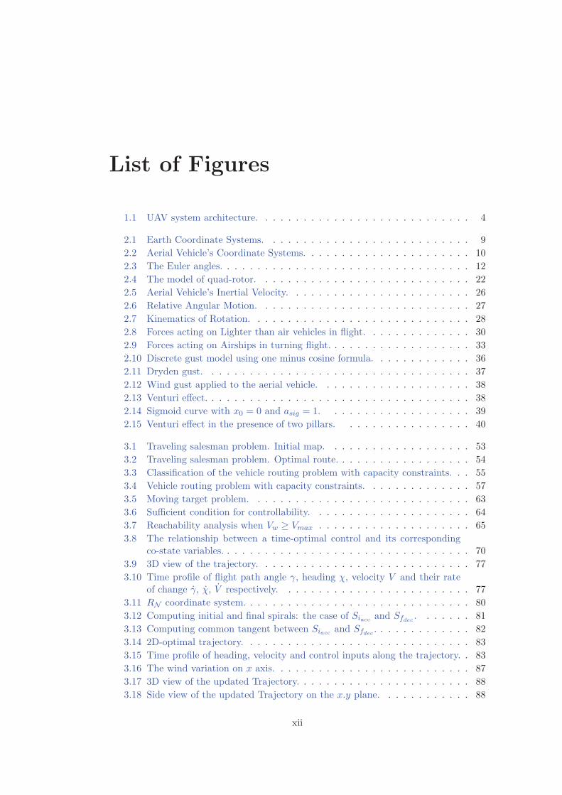
List of Figures
1.1 UAV system architecture. . . . . . . . . . . . . . . . . . . . . . . . . . . . 4
2.1 Earth Coordinate Systems. . . . . . . . . . . . . . . . . . . . . . . . . . . 9
2.2 Aerial Vehicle’s Coordinate Systems. . . . . . . . . . . . . . . . . . . . . . 10
2.3 The Euler angles. . . . . . . . . . . . . . . . . . . . . . . . . . . . . . . . . 12
2.4 The model of quad-rotor. . . . . . . . . . . . . . . . . . . . . . . . . . . . 22
2.5 Aerial Vehicle’s Inertial Velocity. . . . . . . . . . . . . . . . . . . . . . . . 26
2.6 Relative Angular Motion. . . . . . . . . . . . . . . . . . . . . . . . . . . . 27
2.7 Kinematics of Rotation. . . . . . . . . . . . . . . . . . . . . . . . . . . . . 28
2.8 Forces acting on Lighter than air vehicles in flight. . . . . . . . . . . . . . 30
2.9 Forces acting on Airships in turning flight. . . . . . . . . . . . . . . . . . . 33
2.10 Discrete gust model using one minus cosine formula. . . . . . . . . . . . . 36
2.11 Dryden gust. . . . . . . . . . . . . . . . . . . . . . . . . . . . . . . . . . . 37
2.12 Wind gust applied to the aerial vehicle. . . . . . . . . . . . . . . . . . . . 38
2.13 Venturi effect. . . . . . . . . . . . . . . . . . . . . . . . . . . . . . . . . . . 38
2.14 Sigmoid curve with x0 = 0 and asig = 1. . . . . . . . . . . . . . . . . . . 39
2.15 Venturi effect in the presence of two pillars. . . . . . . . . . . . . . . . . 40
3.1 Traveling salesman problem. Initial map. . . . . . . . . . . . . . . . . . . 53
3.2 Traveling salesman problem. Optimal route. . . . . . . . . . . . . . . . . . 54
3.3 Classification of the vehicle routing problem with capacity constraints. . . 55
3.4 Vehicle routing problem with capacity constraints. . . . . . . . . . . . . . 57
3.5 Moving target problem. . . . . . . . . . . . . . . . . . . . . . . . . . . . . 63
3.6 Sufficient condition for controllability. . . . . . . . . . . . . . . . . . . . . 64
3.7 Reachability analysis when Vw ≥ Vmax . . . . . . . . . . . . . . . . . . . . 65
3.8 The relationship between a time-optimal control and its correspondingco-state variables. . . . . . . . . . . . . . . . . . . . . . . . . . . . . . . . . 70
3.9 3D view of the trajectory. . . . . . . . . . . . . . . . . . . . . . . . . . . . 77
3.10 Time profile of flight path angle γ, heading χ, velocity V and their rateof change γ, χ, V respectively. . . . . . . . . . . . . . . . . . . . . . . . . 77
3.11 RN coordinate system. . . . . . . . . . . . . . . . . . . . . . . . . . . . . . 80
3.12 Computing initial and final spirals: the case of Siacc and Sfdec . . . . . . . 81
3.13 Computing common tangent between Siacc and Sfdec . . . . . . . . . . . . . 82
3.14 2D-optimal trajectory. . . . . . . . . . . . . . . . . . . . . . . . . . . . . . 83
3.15 Time profile of heading, velocity and control inputs along the trajectory. . 83
3.16 The wind variation on x axis. . . . . . . . . . . . . . . . . . . . . . . . . . 87
3.17 3D view of the updated Trajectory. . . . . . . . . . . . . . . . . . . . . . . 88
3.18 Side view of the updated Trajectory on the x.y plane. . . . . . . . . . . . 88
xii
List of Figures xiii
3.19 Side view of the updated Trajectory on the x.z plane. . . . . . . . . . . . 89
3.20 Simulation’s environment. . . . . . . . . . . . . . . . . . . . . . . . . . . . 93
3.21 Flight number 1: q1 → q9 → q8 → q1. . . . . . . . . . . . . . . . . . . . . . 93
3.22 Flight number 2: q1 → q2 → q6 → q3 → q1. . . . . . . . . . . . . . . . . . . 94
3.23 Flight number 3: q1 → q5 → q7 → q4 → q1. . . . . . . . . . . . . . . . . . . 94
4.1 Wind gust applied to the aerial vehicle. . . . . . . . . . . . . . . . . . . . 107
4.2 Relative error on x position (trajectory with a line form). . . . . . . . . . 109
4.3 Relative error on y position (trajectory with a line form). . . . . . . . . . 110
4.4 Relative error on z position (trajectory with a line form). . . . . . . . . . 110
4.5 Flight Path Angle response in closed-loop (trajectory with a line form). . 111
4.6 Heading Angle response in the closed-loop (trajectory with a line form). . 111
4.7 Velocity response in the closed-loop (trajectory with a line form). . . . . . 112
4.8 Control inputs responses u1, u2 and u3 (trajectory with a line form). . . . 112
4.9 Three dimensional view of the trajectory. . . . . . . . . . . . . . . . . . . 113
4.10 Relative error on x position (trajectory with a curve form). . . . . . . . . 115
4.11 Relative error on y position (trajectory with a curve form). . . . . . . . . 115
4.12 Relative error on z position (trajectory with a curve form). . . . . . . . . 116
4.13 Flight Path Angle response in closed-loop (trajectory with a curve form). 116
4.14 Heading Angle response in the closed-loop (trajectory with a curve form). 117
4.15 Velocity response in the closed-loop (trajectory with a curve form). . . . . 117
4.16 Control inputs responses u1, u2 and u3 (trajectory with a curve form). . . 118
4.17 Three dimensional view of the trajectory. . . . . . . . . . . . . . . . . . . 118
4.18 Wind gusts applied to the airship. . . . . . . . . . . . . . . . . . . . . . . 122
4.19 Relative error on x position (lighter than air vehicle). . . . . . . . . . . . 125
4.20 Relative error on y position (lighter than air vehicle). . . . . . . . . . . . . 126
4.21 Relative error on z position (lighter than air vehicle). . . . . . . . . . . . . 126
4.22 Flight Path Angle response in closed-loop (lighter than air vehicle). . . . . 127
4.23 Heading Angle response in the closed-loop (lighter than air vehicle). . . . 127
4.24 Velocity response in the closed-loop (lighter than air vehicle). . . . . . . . 128
4.25 Thrust response in the closed-loop (lighter than air vehicle). . . . . . . . . 128
4.26 Bank angle response in the closed-loop (lighter than air vehicle). . . . . . 129
4.27 Angle of attack response in the closed-loop (lighter than air vehicle). . . . 129
4.28 Control inputs responses u1, u2 and u3 (lighter than air vehicle). . . . . . 130
4.29 Three dimensional view of the trajectory. . . . . . . . . . . . . . . . . . . 130
4.30 Flying at a constant altitude trajectory. . . . . . . . . . . . . . . . . . . . 134
4.31 Time profile of yaw angle ψ, vehicle’s velocity and their rate of change ψ,V respectively. . . . . . . . . . . . . . . . . . . . . . . . . . . . . . . . . . 134
4.32 Yaw angle of quadrotor. . . . . . . . . . . . . . . . . . . . . . . . . . . . . 136
4.33 x-displacement of quadrotor. . . . . . . . . . . . . . . . . . . . . . . . . . 136
4.34 y-displacement of quadrotor. . . . . . . . . . . . . . . . . . . . . . . . . . 137
4.35 Time profile of pitch (θ) and roll (φ) angles. . . . . . . . . . . . . . . . . . 137
A.1 Translation. . . . . . . . . . . . . . . . . . . . . . . . . . . . . . . . . . . . 144
A.2 Rotation. . . . . . . . . . . . . . . . . . . . . . . . . . . . . . . . . . . . . 145
C.1 Common Tangents to Two Circles (r1 > r2). . . . . . . . . . . . . . . . . . 154
C.2 Common Tangents to Two Circles (r1 = r2). . . . . . . . . . . . . . . . . . 155
List of Tables
3.1 The different arc types of regular control . . . . . . . . . . . . . . . . . . . 72
3.2 The different arc types of singular control . . . . . . . . . . . . . . . . . . 73
3.3 Vehicle’s restrictions. . . . . . . . . . . . . . . . . . . . . . . . . . . . . . . 76
3.4 Initial and final configurations. . . . . . . . . . . . . . . . . . . . . . . . . 76
3.5 Example 3.1: Restrictions on state and control variables. . . . . . . . . . . 79
3.6 Example 3.1: Initial and desired orientation and velocity values. . . . . . 79
3.7 Vehicle’s restrictions. . . . . . . . . . . . . . . . . . . . . . . . . . . . . . . 86
3.8 Initial and final configurations. . . . . . . . . . . . . . . . . . . . . . . . . 86
3.9 Base station and way-points to be visited during the traveled trajectory. . 92
4.1 Restrictions on state and control variables . . . . . . . . . . . . . . . . . . 107
4.2 Initial and desired orientation and velocity values . . . . . . . . . . . . . . 108
4.3 The four selected operating points . . . . . . . . . . . . . . . . . . . . . . 114
4.4 Configurations to be visited during the traveled trajectory . . . . . . . . . 122
4.5 Restrictions on the lighter than air vehicle . . . . . . . . . . . . . . . . . . 123
4.6 Baseline lighter than air vehicle design parameters . . . . . . . . . . . . . 123
4.7 Restrictions on state and control variables . . . . . . . . . . . . . . . . . . 133
4.8 Configurations to be visited during the traveled trajectory . . . . . . . . . 135
xiv


Nomenclature
ARP Aircraft’s reference point
a Linear acceleration
B Buoyancy force (airships)
CSB Transformation matrix from RB to RS
CWB Transformation matrix from RB to RW
CBI Transformation matrix from RI to RB
CWI Transformation matrix from RI to RW
CWL Transformation matrix from RL to RW
CWS Transformation matrix from RS to RW
C(V ) Coriolis and centripetal effects (airships)
CA(V ) Coriolis and centripetal effects due to added mass and inertia
phenomena (airships)
CB Center of buoyancy (airships)
CG Center of gravity (airships)
Cl Roll stationary coefficient (airships)
CL Normal stationary coefficient (airships)
Cm Yaw stationary coefficient (airships)
Cn Pitch stationary coefficient (airships)
CN Lateral stationary coefficient (airships)
CT Tangential stationary coefficient (airships)
CV Center of volume (airships)−→D Unit vector pointing to Down
D Drag force (airships)−→E Unit vector pointing to East
EK Kinetic energy (quad-rotors)
EP Potential energy (quad-rotors)
fa Aerodynamical force (airships)
fAM Added mass force (airships)
Fext External forces
fT Thrust force (Airchips)
xvi

Nomenclature xvii
fg Gravity force (airships)
g Gravitational acceleration
H Hamiltonian function
IG Inertia matrix at CG (airships)
IN Inertia matrix at CV (airships)
Ixx Moment inertia with respect to x axis (airships)
Iyy Moment inertia with respect to y axis (airships)
Izz Moment inertia with respect to z axis (airships)
J inertia matrix (quad-rotors)
J1(η2) Linear velocity transformation matrix (airships)
J2(η2) Angular velocity transformation matrix (airships)
ℓ distance from the motor to the center of gravity (quad-rotors)
L Lift force (airships)
L Lagrangian function
L Robust control Lyapunov function
Lref Airship’s reference length
m Total mass of the vehicle
M Inertia matrix (airships)
Ma Added mass matrix resulting from the linear accelerations (airships)
MA Full added mass and inertia matrix (airships)
Mext External moments−→N Unit vector pointing to North
q Configuration−→r Position vector
RB Body Fixed Frame
RI Earth Fixed Inertial Frame
RL Local Horizon Frame
RS Stability Frame
RW Wind Relative Frame
Rx/φ Rotation matrix of an angle φ about x axis
Ry/θ Rotation matrix of an angle θ about y axis[rCVCG
×]
Skew-symmetric matrix associated to the distance from CV to
CG (airships)
Sref Airship’s reference area
T Thrust force
Ttrans Translational kinetic energy (quad-rotors)
Trot Rotational kinetic energy (quad-rotor)
U Control space

Nomenclature xviii
V Velocity vector
V All condidate Lyapunov function
V1 = [u, v, w]T Linear velocity vector expressed in RB
V2 = [p, a, r]T Angular velocity vector expressed in RB
Va Relative velocity
VG Velocity at CG (airships)
νhull Volume of airship’s hull
VV Velocity at CV (airships)
VW Wind velocity
ωRW/RIAngular velocity of RW with respect to RI
W Weight force
W Disturbances space
X State space
∆A Accessibility distribution
∆A0 Strong accessibility distribution
α Angle of attack
β Side-slip angle
χ Heading angle
γ Flight path angle
ψ Yaw angle
θ Pitch angle
φ Roll angle
η Six dimension vector position and orientation of the body fixed
frame (airships)
η1 = [x, y, z]T Position vector of the body fixed frame expressed in RI (airships)
η2 = [φ, θ,ψ]T Orientation vector of the body fixed frame expressed in RI (airships)
ρ Density of air
ΩRW/h Angular velocity of RW about hW
ΩRW/y Angular velocity of RW about yW
ϕ Generalized coordinates of quad-rotors craft
ΠG Angular momentum with respect to CG (airships)
ΠV Angular momentum with respect to CV (airships)
τa Aerodynamic tensor (airships)
τp Propulsion tensor (airships)
τs Static tensor (airships)
τsta Stationary phenomena tensor (airships)
τ = [τψ, τθ, τφ]T Translational force applied to quad-rotors craft
λ Co-state variables


Chapter 1
Introduction
Unmanned Aerial Vehicle technology have seen an enormous and promptly development
in the last two decades. This kind of aerial vehicles is being increasingly used in mili-
tary and civilian domains such as, surveillance, reconnaissance, mapping, cartography,
border patrol, inspection, homeland security, search and rescue, weather and hurricane
monitoring, fire detection, agricultural imaging, traffic monitoring, pollutant estimation,
etc... [40, 41, 63, 162].
Based on UAVs shapes and structures, they can be classified in the following categories,
[128, 134]:
• Fixed-wing UAV: This type of UAV is capable of flight using forward motion with
a relative velocity such that a sufficient lift is generated on wings. In addition, it
requires a runway for the take-off and landing.
• Rotary-wing UAV: This kind of aerial vehicle has the advantage of hovering capability
and high maneuverability. These aircrafts use one or more propellers to produce the
thrust force necessary for motion. In addition, the ability of rotor-crafts to take off
and land in limited spaces and to hover above targets, gives such kind of UAVs the
superiority over fixed wing aircrafts especially for missions that require hovering flight.
• Lighter than air UAV: Unlike fixed or rotary wing aerial vehicles, the lift of lighter
than air vehicles is mainly generated by buoyancy force. This characteristic makes
airships noiseless, ecological and very useful for long term environmental applications.
However, other classifications can be found in literature according to a variety of pa-
rameters that include, vehicle configuration, shapes, structures, size, weight, endurance
and range, maximum altitude, engine type among others.
1
Chapter 1. Introduction 2
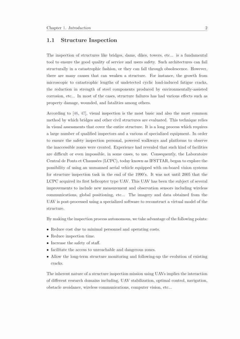
1.1 Structure Inspection
The inspection of structures like bridges, dams, dikes, towers, etc... is a fundamental
tool to ensure the good quality of service and users safety. Such architectures can fail
structurally in a catastrophic fashion, or they can fall through obsolescence. However,
there are many causes that can weaken a structure. For instance, the growth from
microscopic to catastrophic lengths of undetected cyclic load-induced fatigue cracks,
the reduction in strength of steel components produced by environmentally-assisted
corrosion, etc... In most of the cases, structure failures has had various effects such as
property damage, wounded, and fatalities among others.
According to [46, 47], visual inspection is the most basic and also the most common
method by which bridges and other civil structures are evaluated. This technique relies
in visual assessments that cover the entire structure. It is a long process which requires
a large number of qualified inspectors and a various of specialized equipment. In order
to ensure the safety inspection personal, powered walkways and platforms to observe
the inaccessible zones were created. Experience had revealed that such kind of facilities
are difficult or even impossible, in some cases, to use. Consequently, the Laboratoire
Central de Ponts et Chaussees (LCPC), today known as IFSTTAR, began to explore the
possibility of using an unmanned aerial vehicle equipped with on-board vision systems
for structure inspection task in the end of the 1990’s. It was not until 2005 that the
LCPC acquired its first helicopter type UAV. This UAV has been the subject of several
improvements to include new measurement and observation sensors including wireless
communications, global positioning, etc... The imagery and data obtained from the
UAV is post-processed using a specialized software to reconstruct a virtual model of the
structure.
By making the inspection process autonomous, we take advantage of the following points:
• Reduce cost due to minimal personnel and operating costs.
• Reduce inspection time.
• Increase the safety of staff.
• facilitate the access to unreachable and dangerous zones.
• Allow the long-term structure monitoring and following-up the evolution of existing
cracks.
The inherent nature of a structure inspection mission using UAVs implies the interaction
of different research domains including, UAV stabilization, optimal control, navigation,
obstacle avoidance, wireless communications, computer vision, etc...
Chapter 1. Introduction 3
1.2 Motivation of this thesis and objective
This thesis is motivated by autonomous UAV-based bridge inspection missions. From
flight planning point of view, the neighborhood of bridges is a challenging environment
due to the presence of obstacles, and different meteorological phenomenon. In addition,
resources optimization, risk and operational cost minimization are fundamental issues
in these kind of tasks. Therefore, we are interested in optimal trajectory planning in
presence of obstacles, and meteorological turbulence such as wind shear, Venturi effect,
Karman vortex among others. The main goal of this thesis is to automatize the motion
planning and optimize the generated trajectory for bridge inspection such that the task
is accomplished in a minimal time.
The nature of inspection mission requires an aerial vehicle capable of hovering flight.
Consequently, we are interested in two types of UAVs: airships and quadrotors. The
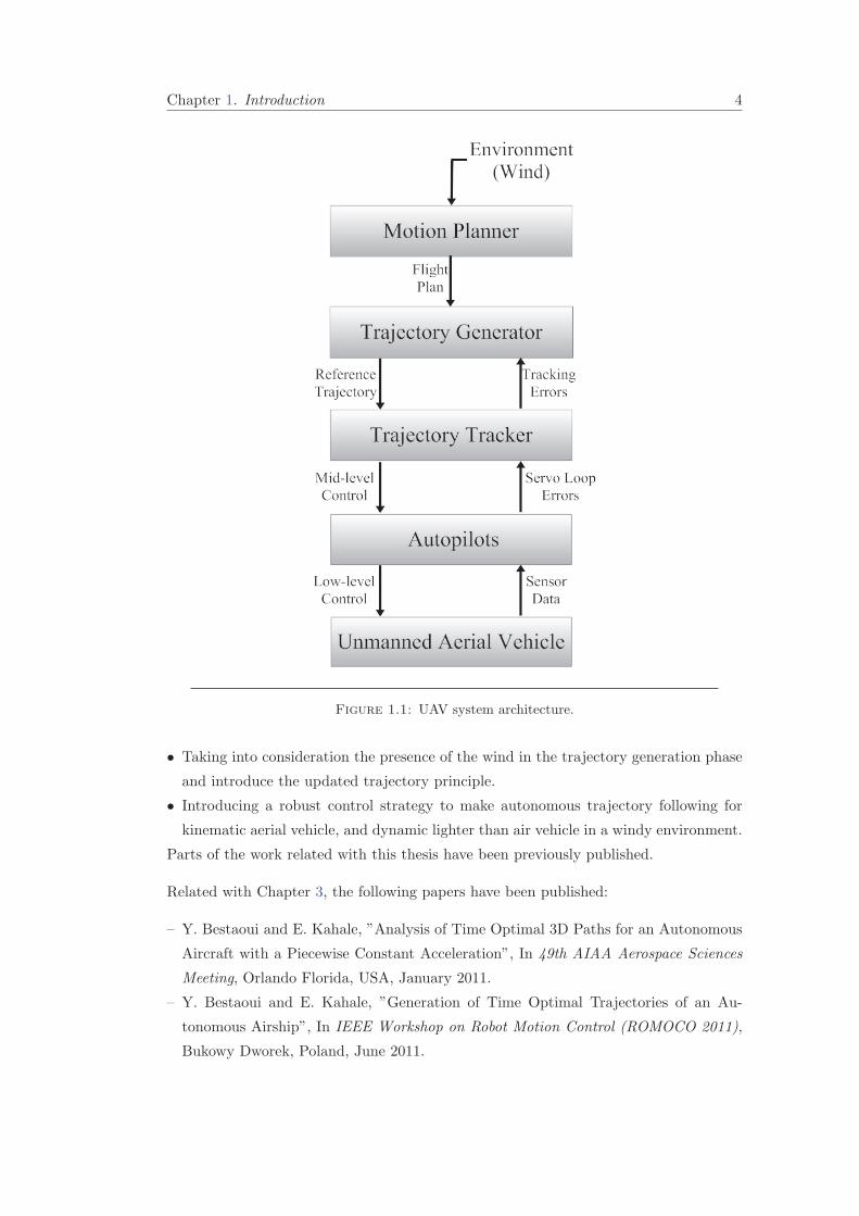
overall UAV system architecture, as presented in Fig. 1.1 consists of five layers: motion
planner, trajectory generator, trajectory tracker, autopilots, and the vehicle.
The motion planner creates a plan for the unmanned aerial vehicle defining a set of
way-points from the vehicle initial point to the desired final one. While, the trajectory
generator creates a flyable trajectory to connect way-points in the same order as it was
given to it by the motion planner. Next, the generated trajectory is given as reference
signals to the trajectory tracker which, in turn, computes the necessary mid-level control
inputs to ensure the trajectory following. Then, these inputs are provided to autopilots
as reference values to stabilize the UAV.
Our objective is to propose and develop algorithms to deal with motion planner, tra-
jectory generator, and trajectory tracker levels. The planner and trajectory generator
must take into consideration the measurable parameters of meteorological phenomena,
the on-board energy limitations, and the presence of obstacles in the environment. To-
ward this end, a flight planning system based on optimal control was proposed. On the
other side, the trajectory tracker should ensure trajectory following in the presence of
disturbances such as wind gusts. For this purpose a control strategy based on inverse
optimality was introduced.
1.3 Contributions of this thesis
The main contributions of this thesis are the following:
• Adopting kinematic point mass model for quad-rotors crafts.
• Planning in 3D with varying velocity, heading angle, and flight path angle.
Chapter 1. Introduction 4
Figure 1.1: UAV system architecture.
• Taking into consideration the presence of the wind in the trajectory generation phase
and introduce the updated trajectory principle.
• Introducing a robust control strategy to make autonomous trajectory following for
kinematic aerial vehicle, and dynamic lighter than air vehicle in a windy environment.
Parts of the work related with this thesis have been previously published.
Related with Chapter 3, the following papers have been published:
– Y. Bestaoui and E. Kahale, ”Analysis of Time Optimal 3D Paths for an Autonomous
Aircraft with a Piecewise Constant Acceleration”, In 49th AIAA Aerospace Sciences
Meeting, Orlando Florida, USA, January 2011.
– Y. Bestaoui and E. Kahale, ”Generation of Time Optimal Trajectories of an Au-
tonomous Airship”, In IEEE Workshop on Robot Motion Control (ROMOCO 2011),
Bukowy Dworek, Poland, June 2011.
Chapter 1. Introduction 5
– Y. Bestaoui and E. Kahale, ”Time Optimal Trajectories of a Lighter Than Air Robot
with Second Order Constraints and a Piecewise Constant Velocity Wind”, AIAA
Journal of Aerospace Computing Information and Communication, 10(4): 155-171,
April 2013.
Related with Chapter 4, the following papers has been published:
– E. Kahale, Y. Bestaoui, and P. Castillo, ”Path tracking of a small autonomous air-
plane in wind gusts”, In EEE/RSJ International Conference on Intelligent Robots and
Systems (IROS), Vilamoura, Algarve, Portugal, October 2012.
– E. Kahale, P. Castillo, and Y. Bestaoui, ”Autonomous path tracking of a kinematic
airship in presence of unknown gust”, In International Conference on Unmanned Air-
craft Systems (ICUAS), Philadelphia, PA, USA, June 2012.
An extended version of the last paper was also published in
– E. Kahale, P. Castillo, and Y. Bestaoui, ”Autonomous path tracking of a kinematic
airship in presence of unknown gust”, Journal of Intelligent and Robotic Systems,
69(1-4): 431-446, January 2013.
1.4 Thesis outline
The manuscript is divided into Three main chapters. General equations of motion for
lighter than air vehicles and quadrotors crafts are introduced in Chapter 2. The vehicles
are modeled in two different ways: a six degree of freedom model, called rigid body model
and devoted for stability and control problem, and a three degree of freedom model,
called point mass model used in navigation and guidance control systems. Besides the
mathematical representations of the aerial vehicles, the wind gusts and Venturi effect
modeling question has been addressed.
Chapter 3 treats the trajectory generation and motion planning problems. In general,
the autonomy of a UAV is defined as its capacity to accomplish different types of tasks
with a high level of performance, maneuverability and with less oversight of human
operators [12, 92]. These tasks require flexible and Powerful algorithms that convert
high-level mission specifications from humans into low-level descriptions of the vehicle’s
motion. The terms Motion Planning and Trajectory Planning are often employed for
such kind of problems [111]. In order to connect a starting and a target points, feasible
and flyable trajectories must be defined. The feasibility criteria is carried out by motion
planning algorithms. This process produce a plan to steer the UAV safely to its target,
without taking into account its dynamical constraints. Whilst, the trajectory generation
Chapter 1. Introduction 6
problem takes the solution obtained by the motion planning algorithm and determines
the way to fly along this solution with respect to the vehicle’s mechanical limitations.
In other words, it guarantees the flyable aspect of the trajectory [12, 111].
Once a feasible and flyable trajectory is generated, it becomes necessary to move one
step down into low-level control design. That means, to deal with trajectory tracking
question. This problem consists of stabilization of the state, or an output function of the
state, to a desired reference value, possibly time-varying [123]. This problem is handled
in chapter 4. Finally a general conclusion and perspective are given in chapter 5.
Chapter 2
Modeling
2.1 Introduction
In this chapter, the general equations of motion of an aerial vehicle flying in the Earth’s
atmosphere are derived and the coordinate systems in which these equations are written
are discussed. The aircraft is assumed to be a rigid body and the Newton’s laws of
motion are used.
The equations governing the translational and rotational motion of an aircraft can be
divided into the following two sets:
• Kinematic equations giving the translational and rotational position relative to
the earth reference frame.
• Dynamic equations relating forces to translational acceleration(Σ−−→Fext = m−→a
)
and moments to rotational acceleration(Σ−−→Mext = I
−→ω).
These equations are referred to as six degree of freedom (6DOF) equations of motion.
From navigation and guidance control system point of view, the vehicle’s rotation rates
are considered to be small. Thus, only translational equations known as three degree
of freedom (3DOF) equations of motion are used. These equations are uncoupled from
the rotational equations by assuming negligible rotation rates and neglecting the ef-
fect of control surface deflections on aerodynamic forces. For example, to maintain a
given speed for an aerial vehicle on cruise flight, the pitching moment is required to be
zero through an elevator deflection. This process contributes to the lift and drag forces
applied on the aircraft. Thus, by neglecting this contribution, the translational and
rotational equations can be uncoupled [81].
7
Chapter 2. Modeling 8
On the other hand, the stability and control problems are related to the relative motion
of the center of gravity of the aircraft with respect to the ground, and the motion of the
vehicle about its center of gravity. Hence, the stability and control studies involve the
use of the six degree of freedom equations of motion.
Next, the coordinate systems used to develop the equations of motion are pointed out.
2.2 Coordinate Systems
The vehicle’s motion in the space is defined by several coordinate systems which can be
classified into two categories: Earth axis and body axis. All coordinate systems used
are right handed orthogonal [38, 81, 121].
2.2.1 Earth Axes System
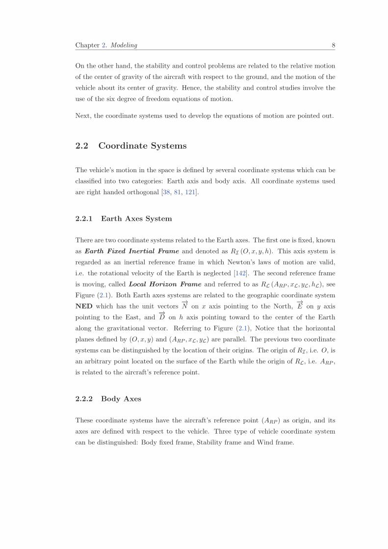
There are two coordinate systems related to the Earth axes. The first one is fixed, known
as Earth Fixed Inertial Frame and denoted as RI (O, x, y, h). This axis system is
regarded as an inertial reference frame in which Newton’s laws of motion are valid,
i.e. the rotational velocity of the Earth is neglected [142]. The second reference frame
is moving, called Local Horizon Frame and referred to as RL (ARP , xL, yL, hL), see
Figure (2.1). Both Earth axes systems are related to the geographic coordinate system
NED which has the unit vectors−→N on x axis pointing to the North,
−→E on y axis
pointing to the East, and−→D on h axis pointing toward to the center of the Earth
along the gravitational vector. Referring to Figure (2.1), Notice that the horizontal
planes defined by (O, x, y) and (ARP , xL, yL) are parallel. The previous two coordinate
systems can be distinguished by the location of their origins. The origin of RI , i.e. O, is
an arbitrary point located on the surface of the Earth while the origin of RL, i.e. ARP ,
is related to the aircraft’s reference point.
2.2.2 Body Axes
These coordinate systems have the aircraft’s reference point (ARP ) as origin, and its
axes are defined with respect to the vehicle. Three type of vehicle coordinate system
can be distinguished: Body fixed frame, Stability frame and Wind frame.
Chapter 2. Modeling 9
Figure 2.1: Earth Coordinate Systems.
2.2.2.1 Body Fixed Frame
The body fixed coordinate system, RB (ARP , xB, yB, hB) is attached to the vehicle and
constrained to move with it, see Figure (2.2). Thus when the aircraft goes from its
initial flight condition the axes move with the vehicle and the motion is quantified in
terms of perturbation variables referred to the moving axes. The (xB×hB) plane defines
the plane of symmetry of the aircraft such that the xB axis is directed along the axis of
symmetry. Thus yB axis is oriented to the right while hB axis is pointed downward.
2.2.2.2 Stability Frame
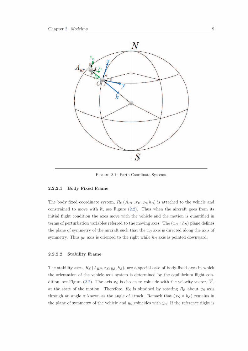
The stability axes, RS (ARP , xS , yS , hS), are a special case of body-fixed axes in which
the orientation of the vehicle axis system is determined by the equilibrium flight con-
dition, see Figure (2.2). The axis xS is chosen to coincide with the velocity vector,−→V ,
at the start of the motion. Therefore, RS is obtained by rotating RB about yB axis
through an angle α known as the angle of attack. Remark that (xS × hS) remains in
the plane of symmetry of the vehicle and yS coincides with yB. If the reference flight is
Chapter 2. Modeling 10
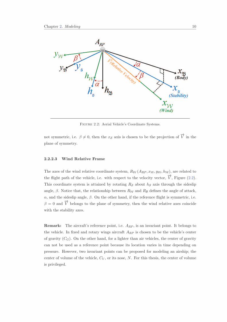
Figure 2.2: Aerial Vehicle’s Coordinate Systems.
not symmetric, i.e. β %= 0, then the xS axis is chosen to be the projection of−→V in the
plane of symmetry.
2.2.2.3 Wind Relative Frame
The axes of the wind relative coordinate system, RW (ARP , xW , yW , hW), are related to
the flight path of the vehicle, i.e. with respect to the velocity vector,−→V , Figure (2.2).
This coordinate system is attained by rotating RS about hS axis through the sideslip
angle, β. Notice that, the relationship between RW and RB defines the angle of attack,
α, and the sideslip angle, β. On the other hand, if the reference flight is symmetric, i.e.
β = 0 and−→V belongs to the plane of symmetry, then the wind relative axes coincide
with the stability axes.
Remark: The aircraft’s reference point, i.e. ARP , is an invariant point. It belongs to
the vehicle. In fixed and rotary wings aircraft ARP is chosen to be the vehicle’s center
of gravity (CG). On the other hand, for a lighter than air vehicles, the center of gravity
can not be used as a reference point because its location varies in time depending on
pressure. However, two invariant points can be proposed for modeling an airship; the
center of volume of the vehicle, CV , or its nose, N . For this thesis, the center of volume
is privileged.

Chapter 2. Modeling 11
2.2.3 Coordinates Transformation
Previously, we have defined the different coordinate systems used to describe the mo-
tion of an aerial vehicle. The relations between such frames are known as coordinates
transformation, and represent the orientation of each coordinate system with respect to
the others. The transformation matrices between RI , RB, RS , and RW are the subject
of the following paragraphs.
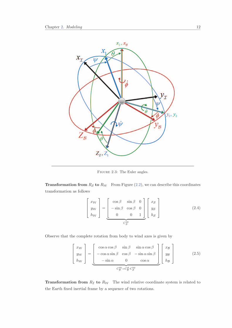
Transformation from RI to RB The description of RI with respect to RB is made
using the following sequence of rotation [155].
Starting from the Earth fixed inertial frame:
1. Rotating about the hI axis by ”ψ”, also known as yaw angle. The positive direction
of rotation is taken so that the nose turns toward to right.
2. Rotating about the new y axis by ”θ”, called as pitch angle. The positive direction
of rotation is defined in order that the nose points to up.
3. Rotate about the new x axis by ”φ”, also named roll angle. The positive direction
of rotation is presented such that the right-side heads to down.
Conversely, to go in the opposite direction, i.e. from the body frame to the Earth fixed
inertial frame, the sequence roll, pitch, yaw must be followed. Notice that the yaw,
pitch, and roll angles ψ, θ, φ are commonly referred to as Euler angles. This process is
illustrated in Figure (2.3). From previous, we can write
xB
yB
hB
= CB
I
xI
yI
hI
(2.1)
where CBI denotes the transformation matrix and is given by
CBI =
cos θ cosψ cos θ sinψ − sin θ
− cosφ sinψ + sinφ sin θ cosψ cosφ cosψ + sinφ sin θ sinψ sinφ cos θ
sinφ sinψ + cosφ sin θ cosψ − sinφ cosψ + cosφ sin θ sinψ cosφ cos θ
(2.2)
Transformation from RB to RS The transformation from body fixed frame to the
stability frame is done using the following relationship, see Figure (2.2)
xS
yS
hS
=
cosα 0 sinα
0 1 0
− sinα 0 cosα
︸ ︷︷ ︸CS
B
xB
yB
hB
(2.3)
Chapter 2. Modeling 12
Figure 2.3: The Euler angles.
Transformation from RS to RW From Figure (2.2), we can describe this coordinates
transformation as follows
xW
yW
hW
=
cosβ sinβ 0
− sinβ cosβ 0
0 0 1
︸ ︷︷ ︸CW
S
xS
yS
hS
(2.4)
Observe that the complete rotation from body to wind axes is given by
xW
yW
hW
=
cosα cosβ sinβ sinα cosβ
− cosα sinβ cosβ − sinα sinβ
− sinα 0 cosα
︸ ︷︷ ︸CW
B=CS
B·CW
S
xB
yB
hB
(2.5)
Transformation from RI to RW The wind relative coordinate system is related to
the Earth fixed inertial frame by a sequence of two rotations.

Chapter 2. Modeling 13
Starting from RI :
1. Rotating about the yI axis by ”γ”, also called as flight path angle. The positive
direction of rotation is taken in counter-clockwise direction.
2. Rotating about the new h axis by ”χ”, also known as heading angle. The positive
direction of rotation is taken in clockwise direction.
Thus, in terms of coordinate transformations we have
xW
yW
hW
=
cosχ cos γ sinχ cos γ − sin γ
− sinχ cosχ 0
cosχ sin γ sinχ sin γ cos γ
︸ ︷︷ ︸CW
I
xI
yI
hI
(2.6)
Since, the Earth fixed inertial frame and the local horizon frame are parallel to each
other. The matrix CWI can be used as a transformation matrix from RL to RW .
In the next section, a full six-degree-of-freedom (6DOF) nonlinear mathematical model
for both; Lighter Than Air Vehicles and Quad-Rotors flying in the space is carried out.
2.3 6DOF Equations of Motion (Rigid Body Model)
This modeling is also known as Rigid Body Model because it is derived in the body
fixed coordinate system, i.e. RB, and it assumes that the aerial vehicle is a rigid body.
2.3.1 Equations of Motion for Lighter Than Air Vehicles
The development of the 6DOF nonlinear equations of motion for an airship is similar to
a fixed-wing airplane. The major differences are caused by the structure of the vehicle
as it is buoyant and the fact that its motion displaces a large volume of surrounding air.
The buoyancy, added mass and added inertia forces, neglected in modeling the airplane’s
dynamics, add more nonlinear characteristics in the airship’s dynamics [11, 59, 98].
In addition, the lighter than air vehicle is an under-actuated system because it has fewer
control inputs than degrees of freedom. It is mainly controlled through thrust force and
control surfaces. The force inputs are available from two main propellers on each side of
gondola, which provides a complementary lift to oppose the weighting mass, as well as a
forward thrust controlling the longitudinal speed [17]. Furthermore, the fact of varying
the thrust generated by each propeller, through changing the angular velocity of each
engine, provides torque to control the rolling motion near hover. On the other side,
the flight control surface; i.e. rudders and elevators, of the tail provide torque input to
Chapter 2. Modeling 14
control pitching and yawing motions.
Deducing the dynamic model of airships requires the following assumptions:
• The hull is considered as a solid. Thus, the aero-elastic phenomena and the motion
of lifting gaze inside the hull are ignored.
• The mass of the blimp and its volume are considered as constant.
• The Earth is considered as flat above the flight area.
The general motion of the lighter than air vehicle in 6DOF can be described by the
following vectors [11, 59, 139]
η =[ηT1 , η
T2
]T; η1 = [x, y, z]T ; η2 = [φ, θ,ψ]T (2.7)
V =[V T1 , V T
2
]T; V1 = [u, v, w]T ; V2 = [p, q, r]T (2.8)
where, η denotes the position and orientation of CV with respect to RI and V presents
the linear and angular velocity expressed in RB. In the next section, the kinematic
equations relating the body fixed reference to the fixed Earth inertial reference will be
derived.
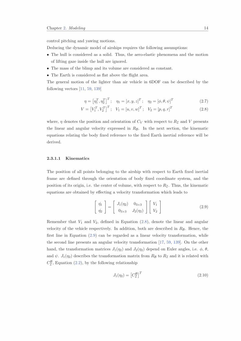
2.3.1.1 Kinematics
The position of all points belonging to the airship with respect to Earth fixed inertial
frame are defined through the orientation of body fixed coordinate system, and the
position of its origin, i.e. the center of volume, with respect to RI . Thus, the kinematic
equations are obtained by effecting a velocity transformation which leads to
[η1
η2
]=
[J1(η2) 03×3
03×3 J2(η2)
][V1
V2
](2.9)
Remember that V1 and V2, defined in Equation (2.8), denote the linear and angular
velocity of the vehicle respectively. In addition, both are described in RB. Hence, the
first line in Equation (2.9) can be regarded as a linear velocity transformation, while
the second line presents an angular velocity transformation [17, 59, 139]. On the other
hand, the transformation matrices J1(η2) and J2(η2) depend on Euler angles, i.e. φ, θ,
and ψ. J1(η2) describes the transformation matrix from RB to RI and it is related with
CBI , Equation (2.2), by the following relationship
J1(η2) =[CBI
]T(2.10)

Chapter 2. Modeling 15
Besides, from Figure (2.3) we state
V2 =
p
q
r
=
φ
0
0
+Rx/φ
0
θ
0
+Rx/φRy/θ
0
0
ψ
= J−1
2 (η2) η2 (2.11)
Expanding the previous equation yields to the following
J−12 (η2) =
1 0 0
0 cosφ cos θ sinφ
0 − sinφ cos θ cosφ
=⇒ J2 (η2) =
1 sinφ tan θ cosφ tan θ
0 cosφ − sinφ
0 sinφ sec θ cosφ sec θ
(2.12)
From Equation (2.9), Equation (2.10), and (2.12), we obtain
x =(cosψ cos θ)u+ (− sinψ cosφ+ cosψ sin θ sinφ) v (2.13a)
+ (sinψ sinφ+ cosψ sin θ cosφ)w
y =(sinψ cos θ)u+ (cosψ cosφ+ sinψ sin θ sinφ) v (2.13b)
+ (− cosψ sinφ+ sinψ sin θ cosφ)w
z =(− sin θ)u+ (cos θ sinφ) v + (cos θ cosφ)w (2.13c)
φ =(sinφ tan θ) q + (cosφ tan θ) r + p (2.13d)
θ =(cosφ) q + (− sinφ) r (2.13e)
ψ =(sinφ sec θ) q + (cosφ sec θ) r (2.13f)
The previous mathematical relationships describes the translational and rotational kine-
matic equations of a lighter than air vehicle moving in three dimensional space. In the
next section, the full 6DOF dynamical model of an airship is introduced.
2.3.1.2 Dynamics through Newton-Euler Approach
The mathematical representation of an airship’s flight dynamics describes the different
forces and moments acting on the vehicle during the flight. As this type of aerial vehicles
are filled by a light lifting gas, e.g. helium, the added mass and added inertia effects
arise due to the fact that the airship’s mass is of the same order of magnitude as the
mass of displaced air [11, 17, 98]. These effects are presented as forces and moments
with respect to linear and angular accelerations [11].
There are two different approaches used in the derivation of the 6DOF nonlinear dynam-
ical model of the lighter than air vehicles[17]. The first one is based on Newton-Euler’s
law, while the second one deals with the Lagrange-Hamilton framework.
Chapter 2. Modeling 16
The Newton-Euler approach in deriving dynamic equations is basically based on New-
ton’s law of motion which relates the forces and moments applied on the vehicle to the
resulting translational and rotational accelerations. Hence, for the translational motion
we have ∑−→F ext = m.−→a (2.14)
Where, m denotes the total mass of the vehicle, −→a presents its linear acceleration and−−→Fext expresses the generalized external force vector.
On the other hand, applying Newton-Euler principle and Koenig theorem in rotational
motion leads to ∑−→M ext =
dΠV
dt+
−→V V × P (2.15)
where Mext describes the moment vector acting on CV ,−→V V denotes the velocity at the
center of volume, and ΠV presents the angular momentum with respect to CV given by:
ΠV = ΠG +−−−−→CV CG ×m
−→V G (2.16)
= IG−→V 2 +
−−−−→CV CG ×m
−→V G
with
- ΠG is the angular momentum with respect to the center of gravity.
-−−−−→CV CG is the position vector of CG with respect to CV .
-−→V G is the velocity of CG.
- IG is the inertia matrix of the airship at CG.
Proceeding from Equation (2.14) and Equation (2.15), the lighter than air vehicle dy-
namic equations can be written as
MV = C(V )V + τs + τa + τp (2.17)
Here, M presents the vehicle’s inertia matrix, C(V ) denotes the Coriolis matrix, τs, τp,
and τa refer to the static, propulsion system, and aerodynamic tensors respectively. The
different components of Equation (2.17) are the subject of the following paragraphs.
Inertia matrix M This matrix is given by [17, 59]
M =
mI3×3 −m
[rCVCG
×]
m[rCVCG
×]
IN
(2.18)
where, I3×3 is the identity matrix, IN is the inertia matrix with respect to CV which,
under the assumption of the vehicle’s symmetry about xB × zB plane, takes the form
Chapter 2. Modeling 17
IN = IG +m−−−−→CV CG ×
(−→V 2 ×
−−−−→CV CG
)
=
Ixx 0 −Ixz
0 Iyy 0
−Izx 0 Izz
(2.19)
with Ixx, Iyy, and Izz are called the moments of inertia with respect to x, y, and z axes
respectively, while the rest of the elements are referred to as the products of inertia. On
the other side,[rCVCG
×]expresses the skew-symmetric matrix associated to the distance
from CV to CG. It is given by
[rCVCG
×]=
0 −az 0
az 0 −ax
0 ax 0
(2.20)
where,−−−−→CV CG =
[ax 0 az
]T(2.21)
Coriolis and Centrifugal tensor C(V )V It takes the following form
C(V )V =
V2 ×mV1 − V2 ×m
[rCVCG
×]V2
V2 × IcV2 + V1 ×mV1 + V2 ×m[rCVCG
×]V1 − V1 ×m
[rCVCG
×]V2
(2.22)
Static tensor τs It resulted from the static forces applied on the airship independently
of its motion. These forces are; the weight force−→W acting down-wards on the center of
gravity, and the buoyancy force−→B acting up-wards on the center of buoyancy CB. The
magnitude of these forces is given by
‖W‖ = m.g (2.23)
‖B‖ = ρ.νhull.g (2.24)
where, ρ refer to the density of the air and νhull denotes the volume of the airship’s hull.
On the other hand, the resulting moments are defined as
−→Mw =
−−−−→CV CG ×−→g (2.25)
−→MB =
−−−−→CV CB ×−→g (2.26)

Chapter 2. Modeling 18
with,−−−−→CV CG,
−−−−→CV CB defines the position vector from the vehicle’s center of volume CV
to its center of gravity CG and buoyancy CB respectively. Then, from previous relations,
the static tensor in fixed-body coordinate system can be determined by
τs = CBI
[ −→W +
−→B
−−−−→CV CG ×
−→W +
−−−−→CV CB ×
−→B
](2.27)
Aerodynamic Tensor τa The aerodynamics phenomena are basically depending on
the relative velocity of the vehicle. It can be categorized into two main classes: stationary
and non-stationary phenomena.
The stationary aspect is related to forces and moments resulting from the distribution
of the pressure around the body, and the friction forces due to the viscosity of air
[17, 126, 160]. Thus, the stationary phenomena tensor can be described as
τsta =1
2ρV 2Sref
CT
CL
CN
LrefCl
LrefCn
LrefCm
(2.28)
where Sref = ν2/3hull refer to the airship’s reference area, Lref presents the vehicle’s ref-
erence length, and CT , CL, CN , Cl, Cn, and Cm denote, tangential, normal, lateral,
roll, pitch, and yaw stationary coefficients respectively. These coefficients depend on the
geometry of the airship and the positions of the control surfaces [17]. In addition, it can
be obtained in two different ways. The first one is based on an experimental procedure
which consists on collecting data using wind tunnel. While, the second method uses an
analytic estimation calculated with a geometric quantities procedure [7, 11, 116].
On the other hand, considering an airship having a mass m which moves along xB axis
with a linear acceleration of u. The reaction of the surrounding air to this motion is
expressed as a force of non-stationary nature, i.e. depending on acceleration. This force
acts in the opposite direction of motion and it is proportional to the acceleration u
[59, 77]. The previous discussion can be described mathematically by
XA = −Xu.u (2.29)
Introducing this force in the equation of motion allow us to combine the coefficient Xu
linearly with the mass m of the vehicle. For this reason, Xu is named added mass
coefficient along the xB axis due to the acceleration u [9, 17, 26, 31]. Thus, the full
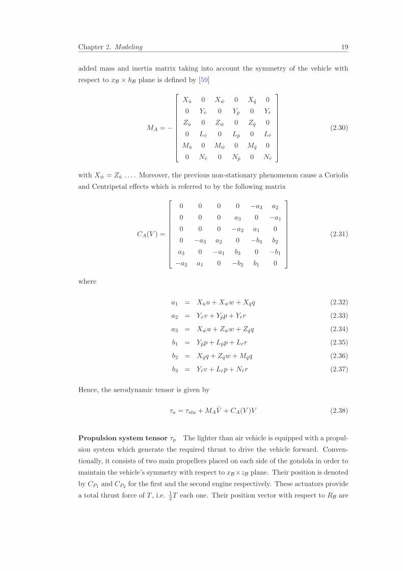
Chapter 2. Modeling 19
added mass and inertia matrix taking into account the symmetry of the vehicle with
respect to xB × hB plane is defined by [59]
MA = −
Xu 0 Xw 0 Xq 0
0 Yv 0 Yp 0 Yr
Zu 0 Zw 0 Zq 0
0 Lv 0 Lp 0 Lr
Mu 0 Mw 0 Mq 0
0 Nv 0 Np 0 Nr
(2.30)
with Xw = Zu . . . . Moreover, the previous non-stationary phenomenon cause a Coriolis
and Centripetal effects which is referred to by the following matrix
CA(V ) =
0 0 0 0 −a3 a2
0 0 0 a3 0 −a1
0 0 0 −a2 a1 0
0 −a3 a2 0 −b3 b2
a3 0 −a1 b3 0 −b1
−a2 a1 0 −b2 b1 0
(2.31)
where
a1 = Xuu+Xww +Xqq (2.32)
a2 = Yvv + Ypp+ Yrr (2.33)
a3 = Xwu+ Zww + Zqq (2.34)
b1 = Ypp+ Lpp+ Lrr (2.35)
b2 = Xqq + Zqw +Mqq (2.36)
b3 = Yrv + Lrp+Nrr (2.37)
Hence, the aerodynamic tensor is given by
τa = τsta +MAV + CA(V )V (2.38)
Propulsion system tensor τp The lighter than air vehicle is equipped with a propul-
sion system which generate the required thrust to drive the vehicle forward. Conven-
tionally, it consists of two main propellers placed on each side of the gondola in order to
maintain the vehicle’s symmetry with respect to xB×zB plane. Their position is denoted
by CP1 and CP2 for the first and the second engine respectively. These actuators provide
a total thrust force of T , i.e. 12T each one. Their position vector with respect to RB are
Chapter 2. Modeling 20
defined by
−−−−→CV CP1 = [Px Py Pz]
T (2.39)−−−−→CV CP2 = [Px − Py Pz]
T (2.40)
Thus, we have
τp =
T
0
0
0
T.Pz
0
(2.41)
From previous relations, the complete 6DOF nonlinear equations of motion for a lighter
than air vehicle using Newton-Euler approach is given by Equation (2.9) and Equation
(2.17). Remark that the previous modeling does not include the wind velocity. Assuming
that the airship is moving in a windy environment in which the wind velocity takes the
form
Vw =[uw vw ww pw qw rw
]T(2.42)
Then, the lighter than air vehicle moves with the following relative velocity
Va = V − Vw (2.43)
2.3.1.3 Dynamics through Lagrangian Approach
The Lagrangian method in deriving the dynamic model of airships deals with two scalar
energy function: kinetic energy EK and potential energy EP . It involves three basic
steps. The first one is to formulate the expression of EK and EP . The second one consists
of calculating the Lagrangian, denoted as L, according to the following relationship
L = EK − EP (2.44)
While, the final step is to apply the Lagrange equation given by
d
dt
(∂L
∂η
)−
∂L
∂η= F (2.45)
which in component form corresponds to a set of 6 second-order differential equations.
Notice that, Equation (2.45) is valid in any coordinate system, Earth fixed inertial and
fixed body frame as long as generalized coordinates are used, i.e. η [59].

Chapter 2. Modeling 21
For more details about the methods used above in modeling the lighter than air vehicle’s
equations of motion, i.e. Newton-Euler and Lagrangian, we invite you to refer [7, 11,
17, 59, 77, 116, 126, 160].
2.3.2 Equations of Motion for Quad-rotors
Quad-rotor is a type of aerial vehicle belonging to rotor-craft family. Contrary to lighter
than air vehicles, the lift needed to keep flight in rotor-crafts is produced aerodynamically
through rotating wings. A quad-rotor vehicle has four rotors. The front and the rear
rotors rotate counterclockwise, while the other two rotors rotate clockwise. In this
manner, the gyroscopic effects and the aerodynamic torques tend to cancel in trimmed
flight. The force produced by each rotor is proportional to its angular velocity, and
the sum of these forces gives the main thrust of the aerial vehicle, see Figure (2.4).
Hence, the quad-rotor is an under-actuated system because it has four inputs and six
degrees of freedom. The variation of the angular speed of each rotor allow to control the
vehicle. The pitch movement is obtained by increasing/decreasing the speed of the rear
motor while decreasing/increasing the speed of the front motor. The roll movement is
obtained similarly using the lateral motors. Whereas, the yaw movement is obtained by
increasing/decreasing the speed of the front and rear motors while decreasing/increasing
the speed of the lateral motors. These motions can be accomplished whilst keeping the
main thrust of the vehicle constant.
In order to deduce the mathematical model of the quad-rotor, the following assumption
is considered:
• The vehicle is assumed to be a solid body evolving in 3D space and subject to one
force and three moments.
• The dynamic of the four rotors is relatively fast and therefore it will be neglected as
well as the flexibility of the blades.
• The center of gravity is supposed to be located at the intersection of the line joining
motors M1 and M3 and the line joining motors M2 and M4, see Figure (2.4).
The generalized coordinates of the rotor-craft are
ϕ = (ζ, η) ∈ R6 (2.46)
where ζ = (x, y, z) ∈ R3 denotes the position of the center of gravity of the vehicle
relative to the frame RI , and η = (ψ, θ,φ) ∈ S3 presents Euler angles defined in the sub-
section 2.2.3. These angles define the orientation of the quad-rotor [32, 33, 127]. Notice
that ζ and η can be regarded as translational and rotational coordinates respectively.
The full quad-rotor dynamic model is obtained using Euler-Lagrange approach.
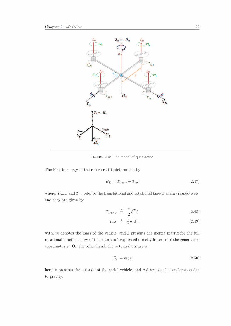
Chapter 2. Modeling 22
Figure 2.4: The model of quad-rotor.
The kinetic energy of the rotor-craft is determined by
EK = Ttrans + Trot (2.47)
where, Ttrans and Trot refer to the translational and rotational kinetic energy respectively,
and they are given by
Ttrans !m
2ζT ζ (2.48)
Trot !1
2ηT Jη (2.49)
with, m denotes the mass of the vehicle, and J presents the inertia matrix for the full
rotational kinetic energy of the rotor-craft expressed directly in terms of the generalized
coordinates ϕ. On the other hand, the potential energy is
EP = mgz (2.50)
here, z presents the altitude of the aerial vehicle, and g describes the acceleration due
to gravity.
Chapter 2. Modeling 23
Therefore, using Equation (2.44) the Lagrangian takes the form
L (ϕ, ϕ) = Ttrans + Trot − EP
=m
2ζT ζ +
1
2ηT Jη −mgz (2.51)
The external generalized force applied on the four-rotor aerial vehicle are presented by
the following vector
F =
[Fζ
τ
](2.52)
where
Fζ = CBI F ∈ R
3 (2.53)
is the translational force applied to the rotor-craft due to the main thrust, and
τ !
τψ
τθ
τφ
∈ R
3 (2.54)
represents the yaw, pitch, and roll moments. Finally, the rotation matrix CBI is defined
in Equation (2.2).
From Figure (2.4), it follows that
F =
0
0
u
(2.55)
where u is the main thrust of the vehicle and it is given by
u =4∑
i=4
fMi; fMi = kiw2i (2.56)
with ki > 0 is a constant and wi is the angular speed of the ith motor. On the other
side, the generalized torques are expressed as
τψ =
4∑
i=1
τMi (2.57)
τθ = ℓ (fM2 − fM4) (2.58)
τφ = ℓ (fM3 − fM1) (2.59)
here, ℓ is the distance from the motor to the center of gravity and τMi is the torque
produced by the ith motor.
Chapter 2. Modeling 24
Therefore, applying the Euler-Lagrange mechanics, Equation (2.45), leads to the follow-
ing
mζ +
0
0
mg
= Fζ (2.60)
Jη + C(η, η)η = τ (2.61)
where,
C(η, η) = J−1
2
∂
∂η
(ηT J
)(2.62)
is referred to as the Coriolis terms and it contains the gyroscopic and centrifugal terms
associated with η and depending on J.
Finally, from Equation (2.60) and Equation (2.61) we obtain
mx =− u sin θ (2.63a)
my =u cos θ sinφ (2.63b)
mz =u cos θ −mg (2.63c)
ψ =τψ (2.63d)
θ =τθ (2.63e)
φ =τφ (2.63f)
where, τψ, τθ, and τφ denote the yawing moment, pitching moment, and rolling moment
respectively. The relation between these moments and the torques τψ, τθ, and τφ is given
by
τ =
τψ
τθ
τφ
= J
−1 (τ − C(η, η)η) (2.64)
For more details see [32, 33, 127].
2.4 3DOF Equations of motion (Point Mass Model)
As we have seen previously, the attitude of an aerial vehicle is defined by its position,
orientation, and velocity. The value of these variables at a specific moment of time
constitute a vector known as configuration vector q. In order to reach a specified/final
configuration qf from the actual/initial one q0, the time profile of the aircraft’s attitude
variables must be determined at all the movement time. Therefore, from trajectory
generation point of view, the aerial vehicle is presented as a point (its reference point
Chapter 2. Modeling 25
ARP ) and only its translational equations are considered. This modeling is known as
Point Mass Model and it describes the inertial velocity vector−→V with respect to RI
and the external forces acting on the vehicle.
2.4.1 Assumptions
The derivation of the equations of motion for an aerial vehicle, considered as a point
mass, flying inside the Earth’s atmosphere requires the following assumptions [81, 82]
• The Earth is flat, its rotational velocity is neglected and the acceleration of the gravity
is constant and perpendicular to the surface of the Earth.
• The flight is symmetric which involves that the sideslip angle β is assumed to be
controlled to zero, and both the thrust force and the aerodynamic forces lie in the
plane of symmetry of the vehicle. This assumption guarantees the mathematical
accuracy of the point mass modeling.
2.4.2 Kinematic Equations
Kinematic equations are used to derive the differential equations for x, y and z which
represent the location of the vehicle with respect to RI [81]. Referring to Figure (2.5),
we can state−→r =
−→VI (2.65)
where−→r defines the position vector and
−→VI denotes the inertial velocity vector which
has the form−→VI =
−→V +
−→Vw (2.66)
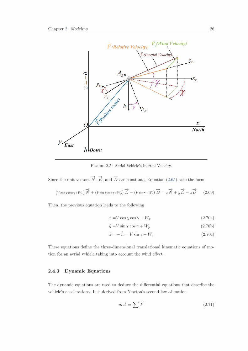
with−→V represents the relative velocity vector and
−→Vw describes the wind velocity vector.
In addition,−→V ∈ RI is defined by its magnitude V , the heading angle χ (measured from
the North to the projection of−→V in RL), and the flight path angle γ (vertically up to
−→V ).
−→Vw ∈ RI is composed by [Wx Wy Wz]
T .
Therefore from the previous and Figure (2.5), the right hand of Equation (2.65) becomes
−→VI = (V cosχ cos γ +Wx)
−→N + (V sinχ cos γ +Wy)
−→E + (−V sin γ −Wz)
−→D (2.67)
On the other hand, referring to Figure (2.5), we can state
−→r = x−→N + y
−→E − z
−→D (2.68)
Where, x and y define the down-range and cross-range respectively, and z denotes the
altitude.
Chapter 2. Modeling 26
Figure 2.5: Aerial Vehicle’s Inertial Velocity.
Since the unit vectors−→N ,
−→E , and
−→D are constants, Equation (2.65) take the form
(V cosχ cos γ+Wx)−→N + (V sinχ cos γ+Wy)
−→E − (V sin γ+Wz)
−→D = x
−→N + y
−→E − z
−→D (2.69)
Then, the previous equation leads to the following
x =V cosχ cos γ +Wx (2.70a)
y =V sinχ cos γ +Wy (2.70b)
z =− h = V sin γ +Wz (2.70c)
These equations define the three-dimensional translational kinematic equations of mo-
tion for an aerial vehicle taking into account the wind effect.
2.4.3 Dynamic Equations
The dynamic equations are used to deduce the differential equations that describe the
vehicle’s accelerations. It is derived from Newton’s second law of motion
m−→a =∑−→
F (2.71)

Chapter 2. Modeling 27
wherem represents the mass of the vehicle, −→a =−→VI denotes the inertial acceleration, and
−→F describes the external forces acting on the aerial vehicle. Observe that, the Equation
(2.71) is written with respect to the Earth fixed inertial frame, because it represents a
convenient base to follow the motion of the vehicle. In addition, Remember that the
relative velocity vector is described in RW and this frame is a rotating coordinate system
in which Newton’s Laws do not apply. Hence, we need a formula which transform the
time derivative between a fixed coordinate system and rotating one [165].
Relative Angular Motion Considering two coordinate systems O1x1y1z1 and Oxyz
the first one is fixed while the second one is rotating with respect to the first one with an
angular velocity ω. Let−→i ,
−→j , and
−→k be the unit vectors along the axes of the rotating
system Figure (2.6) and−→A be an arbitrary vector expressed as following
−→A = Ax
−→i +Ay
−→j +Az
−→k (2.72)
where, Ax, Ay, and Az denote the components of−→A along the rotating axes. Since Oxyz
is rotating, its associated unit vectors−→i ,
−→j , and
−→k are function of time. Thus, the
time derivative of−→A with respect to the fixed coordinate system is given as
d−→A
dt=
(dAx
dt
−→i +
dAy
dt
−→j +
dAz
dt
−→k
)+
(Ax
d−→i
dt+Ay
d−→j
dt+Az
d−→k
dt
)(2.73)
Figure 2.6: Relative Angular Motion.
Chapter 2. Modeling 28
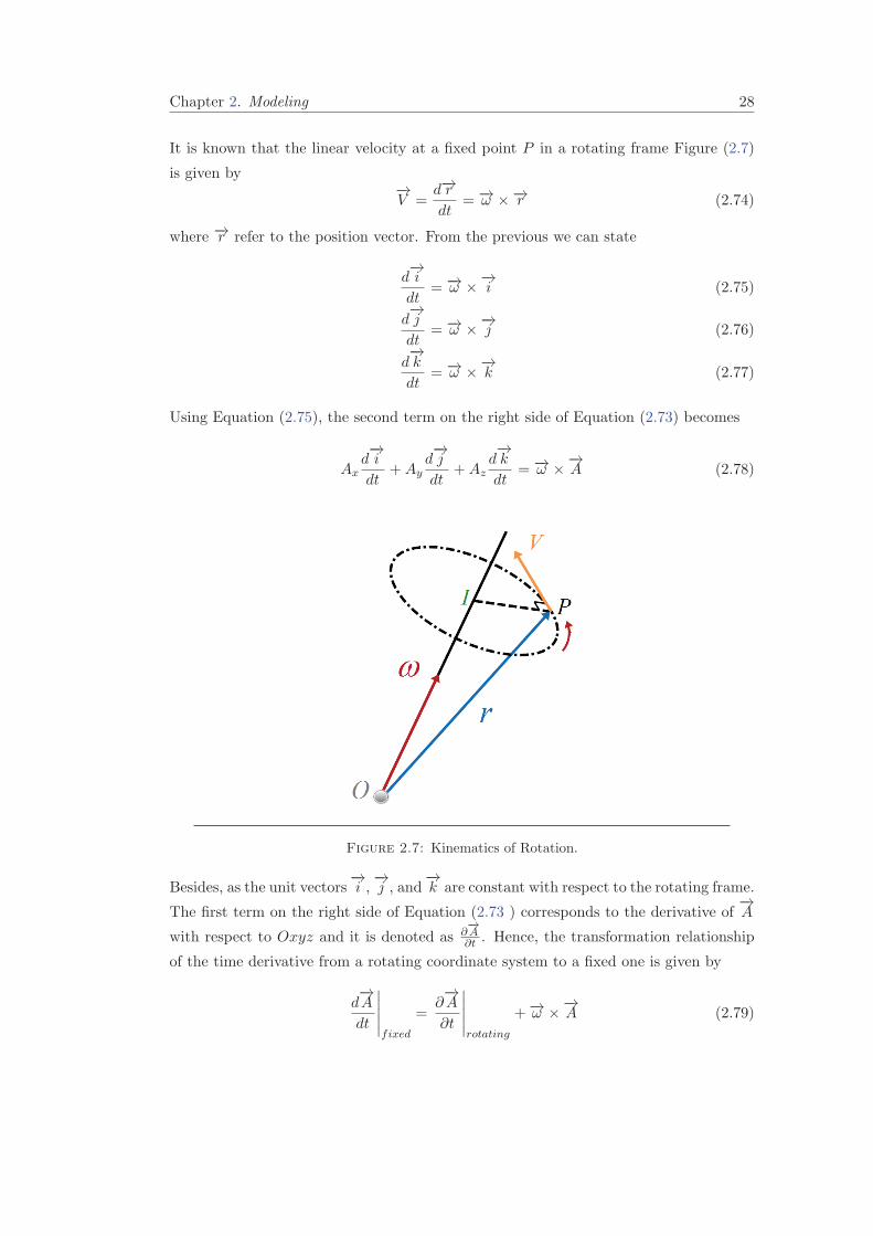
It is known that the linear velocity at a fixed point P in a rotating frame Figure (2.7)
is given by−→V =
d−→r
dt= −→ω ×−→r (2.74)
where −→r refer to the position vector. From the previous we can state
d−→i
dt= −→ω ×
−→i (2.75)
d−→j
dt= −→ω ×
−→j (2.76)
d−→k
dt= −→ω ×
−→k (2.77)
Using Equation (2.75), the second term on the right side of Equation (2.73) becomes
Axd−→i
dt+Ay
d−→j
dt+Az
d−→k
dt= −→ω ×
−→A (2.78)
Figure 2.7: Kinematics of Rotation.
Besides, as the unit vectors−→i ,
−→j , and
−→k are constant with respect to the rotating frame.
The first term on the right side of Equation (2.73 ) corresponds to the derivative of−→A
with respect to Oxyz and it is denoted as ∂−→A∂t . Hence, the transformation relationship
of the time derivative from a rotating coordinate system to a fixed one is given by
d−→A
dt
∣∣∣∣∣fixed
=∂−→A
∂t
∣∣∣∣∣rotating
+−→ω ×−→A (2.79)
Chapter 2. Modeling 29
Coming back to the vehicle’s acceleration −→a in Equation (2.71). From Equation (2.66)
we find
−→a =d−→VI
dt=
d−→V
dt+
d−→Vw
dt(2.80)
Then, using Equation (2.79) we can write
d−→V
dt
∣∣∣∣∣RI
=∂−→V
∂t
∣∣∣∣∣RW
+−→ω RW/RI×−→V (2.81)
Where, −→ω RW/RIdenotes the angular rotation of RW with respect to RI . This angular
velocity is expressed by
−→ω RW/RI=
0
γ
0
︸ ︷︷ ︸ΩRW/y
+
cos γ 0 − sin γ
0 1 0
sin γ 0 cos γ
︸ ︷︷ ︸RotRW/y
·
0
0
χ
︸ ︷︷ ︸ΩRW/h
=
−χ sin γ
γ
χ cos γ
(2.82)
with ΩRW/y and ΩRW/h present the angular velocity of RW about yW and hW respec-
tively, and RotRW/y describes the rotation matrix of RW about yW . Thus, Equation
(2.81) becomes
d−→V
dt=
V
0
0
+
−χ sin γ
γ
χ cos γ
×
V
0
0
=
V
χV cos γ
−γV
(2.83)
The wind rate term, i.e. the second term of the right side in Equation (2.80), is given
in RI bydVw
dt
∣∣∣∣RW
= CWL
dVw
dt
∣∣∣∣RI
(2.84)
with
dVw
dt
∣∣∣∣RI
=
Wx
Wy
Wz
In the following section, we will examine the external forces acting on lighter than air
vehicles.
2.4.3.1 Translational Dynamic of Lighter Than Air Vehicles
As we have seen previously, in the section 2.3.1.2, the external forces acting on the
aircraft are: the added mass force (fAM ), the gravity force (fg), the aerodynamical force
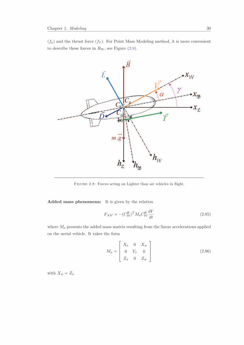
Chapter 2. Modeling 30
(fa) and the thrust force (fT ). For Point Mass Modeling method, it is more convenient
to describe these forces in RW , see Figure (2.8).
Figure 2.8: Forces acting on Lighter than air vehicles in flight.
Added mass phenomena: It is given by the relation
FAM = −(CBW)TMaC
BW
dV
dt(2.85)
where Ma presents the added mass matrix resulting from the linear accelerations applied
on the aerial vehicle. It takes the form
Ma =
Xu 0 Xw
0 Yv 0
Zu 0 Zw
(2.86)
with Xw = Zu

Chapter 2. Modeling 31
(CBW)TMaC
BW is a positive definite matrix with a main diagonal dominant. This matrix
can be approximated as following
(CBW)TMaC
BW =
m11 0 0
0 m22 0
0 0 m33
with
m11 = Xu cos2 α+ (Zu +Xw) cosα sinα+ Zw sin2 α
m22 = Yv
m33 = Xu sin2 α− (Zu +Xw) cosα sinα+ Zw cos2 α
Thus, the added mass force equation yields
FAM = −
m11 0 0
0 m22 0
0 0 m33
V
χV cos γ
−γV
(2.87)
Gravity force: It is given by the difference between the airship weight force−→W , and
the buoyancy force−→B . Then the gravity force fg is expressed as
fg = CWL
0
0
W −B
=
−(W −B) sin γ
0
(W −B) cos γ
(2.88)
where, W and B are defined in the same way as in Equation (2.23) and Equation (2.24).
Aerodynamical force: This force includes the drag force−→D , opposite to
−→V , and
the lift force−→L , orthogonal to
−→V , see Figure (2.8). These forces are expressed by the
following equations
L = 12CL(M,α)V 2Srefρ
D = 12CD(M,α)V 2Srefρ
(2.89)
with CL and CD denote the lift and drag parameters, respectively, M represents the
Mach number and α the attack angle.
On the other hand, atmospheric density is computed using the standard atmosphere.
Generally, the lift coefficient is a linear function of the angle of attack whilst the drag
Chapter 2. Modeling 32
coefficient is a quadratic function of CL(M,α).
CL(M,α) = CL0(M) + kLα(M)α (2.90a)
CD(M,α) = CD0 +KC2L = kD0(M) + kD1(M)α+ kD2(M)α2 (2.90b)
(2.90c)
where CL0 , CL1 and kD0 , kD1 , kD2 are resulting coefficients with respect to α. The in-
duced drag factor K can be determined from the aerodynamic efficiency Emax and the
zero-lift drag coefficient CD0 as
K =1
4CD0E2max
Observe that the model parameters can be estimated via wind tunnel experiments, more
details, see [165]. Therefore, fa is denoted by
fa =
−D
0
−L
(2.91)
Thrust force: In a symmetrical flight, the thrust vector−→T is always in the plane of
symmetry. This force is described in RW as
fT = CWB
T
0
0
=
T cosα
0
−T sinα
(2.92)
In order to determine the equations of motion, it is more convenient to associate the
aerodynamic and thrust forces. Then
fT + fa =
T cosα−D
0
−(T sinα+ L)
(2.93)
Notice from the previous equation that the aerodynamic and thrust forces contain two
components; FT = T cosα −D, force along the velocity vector and, FN = T sinα + L,
force orthogonal to the velocity in the symmetry plane.
In longitudinal flight, FN is in the vertical plane of the vehicle and the lateral force can
be neglected. In order to perform a turning flight, the lateral force must be included.
This force is obtained by a control action on the ailerons when rotating the vector−→L and

Chapter 2. Modeling 33
−→FN about
−→V through an angle σ called bank angle, see Figure (2.9). Mathematically
the previous is written as
faT =
T cosα−D
(T sinα+ L) sinσ
−(T sinα+ L) cosσ
(2.94)
Figure 2.9: Forces acting on Airships in turning flight.
Then, from Equations (2.80), (2.83), (2.84), (2.87), (2.88) and (2.94) we obtain
γ =(T sinα+ L) cosσ − cos γ(B −mg)
(m+m33)V+m
Wx cosχ sin γ + Wy sinχ sin γ + Wz cos γ
(m+m33)V(2.95a)
χ =(T sinα+ L) sinσ
(m+m22)V cos γ+m
Wx sinχ− Wy cosχ
(m+m22)V cos γ(2.95b)
V =T cosα−D − sin γ(B −mg)
m+m11−
m
m+m11(Wx cos γ cosχ+ Wy sinχ cos γ − Wz sin γ) (2.95c)
Therefore, Equation (2.70) and Equation (2.95) present the complete Point Mass Model
describing the translational equations of motion for lighter than air vehicles.
2.4.4 Translational Equations of Motion for Quad-rotor crafts
According to literature [32, 33, 127, 162], the quad-rotor aerial vehicles was always
regarded to as a rigid body and represented by its full 6DOF nonlinear translational
and rotational dynamics (see section 2.3.2). In this section, a new approach using Point
Chapter 2. Modeling 34
Mass Model to describe the quad-rotor crafts is adopted. This modeling is employed to
generate the reference trajectories for the aerial vehicle.
In general, the pitch angle is given as the sum of the flight path angle and the angle of
attack [155]
θ = γ + α (2.96)
But, for quad-rotor craft, the angle of attack is very small and consequently, it can be
neglected (α ≈ 0). Then, Equation (2.96) becomes
θ = γ (2.97)
Besides, as the heading angle χ is measured from the north to the projection of−→V in
xL × yL, this angle can be regarded as the yaw angle ψ. Thus,
χ = ψ (2.98)
Therefore, from the previous, Equation (2.70) takes the following form
x =V cosψ cos θ +Wx (2.99a)
y =V sinψ cos θ +Wy (2.99b)
z =V sin θ +Wz (2.99c)
Remember that the vehicle accelerations, Equation (2.83), are given as
• Longitudinal acceleration: along = V
• Lateral acceleration: alat = V χ cos γ
• Vertical acceleration: avert = V γ
Furthermore, notice, from Equation (2.70) and Equation (2.99), that γ, χ (θ, ψ for
quad-rotors), and V define the attitude of the aerial vehicle. Consequently and without
loss of generality, γ, χ, and V can be considered as control inputs for lighter than air
vehicle. Soγ = u1
χ = u2
V = u3
(2.100)
while θ, ψ, and V are supposed to be the control inputs for quad-rotor craft. Then,
θ = u1
ψ = u2
V = u3
(2.101)
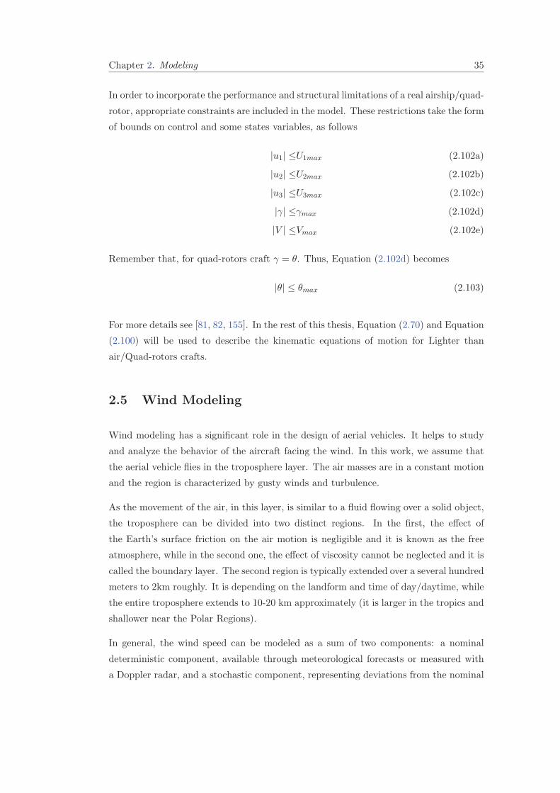
Chapter 2. Modeling 35
In order to incorporate the performance and structural limitations of a real airship/quad-
rotor, appropriate constraints are included in the model. These restrictions take the form
of bounds on control and some states variables, as follows
|u1| ≤U1max (2.102a)
|u2| ≤U2max (2.102b)
|u3| ≤U3max (2.102c)
|γ| ≤γmax (2.102d)
|V | ≤Vmax (2.102e)
Remember that, for quad-rotors craft γ = θ. Thus, Equation (2.102d) becomes
|θ| ≤ θmax (2.103)
For more details see [81, 82, 155]. In the rest of this thesis, Equation (2.70) and Equation
(2.100) will be used to describe the kinematic equations of motion for Lighter than
air/Quad-rotors crafts.
2.5 Wind Modeling
Wind modeling has a significant role in the design of aerial vehicles. It helps to study
and analyze the behavior of the aircraft facing the wind. In this work, we assume that
the aerial vehicle flies in the troposphere layer. The air masses are in a constant motion
and the region is characterized by gusty winds and turbulence.
As the movement of the air, in this layer, is similar to a fluid flowing over a solid object,
the troposphere can be divided into two distinct regions. In the first, the effect of
the Earth’s surface friction on the air motion is negligible and it is known as the free
atmosphere, while in the second one, the effect of viscosity cannot be neglected and it is
called the boundary layer. The second region is typically extended over a several hundred
meters to 2km roughly. It is depending on the landform and time of day/daytime, while
the entire troposphere extends to 10-20 km approximately (it is larger in the tropics and
shallower near the Polar Regions).
In general, the wind speed can be modeled as a sum of two components: a nominal
deterministic component, available through meteorological forecasts or measured with
a Doppler radar, and a stochastic component, representing deviations from the nominal
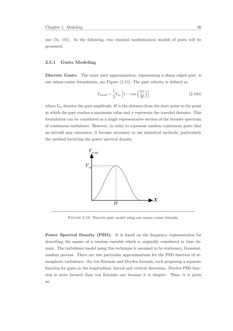
Chapter 2. Modeling 36
one [56, 105]. In the following, two classical mathematical models of gusts will be
presented.
2.5.1 Gusts Modeling
Discrete Gusts: The most used approximation, representing a sharp edged gust, is
one minus cosine formulation, see Figure (2.10). The gust velocity is defined as,
Vwind =1
2Vm
[1− cos
(πxH
)](2.104)
where Vm denotes the gust amplitude, H is the distance from the start point to the point
at which the gust reaches a maximum value and x represents the traveled distance. This
formulation can be considered as a single representative section of the broader spectrum
of continuous turbulence. However, in order to represent random continuous gusts that
an aircraft may encounter, it became necessary to use statistical methods, particularly
the method involving the power spectral density.
Figure 2.10: Discrete gust model using one minus cosine formula.
Power Spectral Density (PSD): It is based on the frequency representation for
describing the square of a random variable which is originally considered in time do-
main. The turbulence model using this technique is assumed to be stationary, Gaussian,
random process. There are two particular approximations for the PSD function of at-
mospheric turbulence: the von Karman and Dryden formula, each proposing a separate
function for gusts in the longitudinal, lateral and vertical directions. Dryden PSD func-
tion is more favored than von Karman one because it is simpler. Thus, it is given
as:
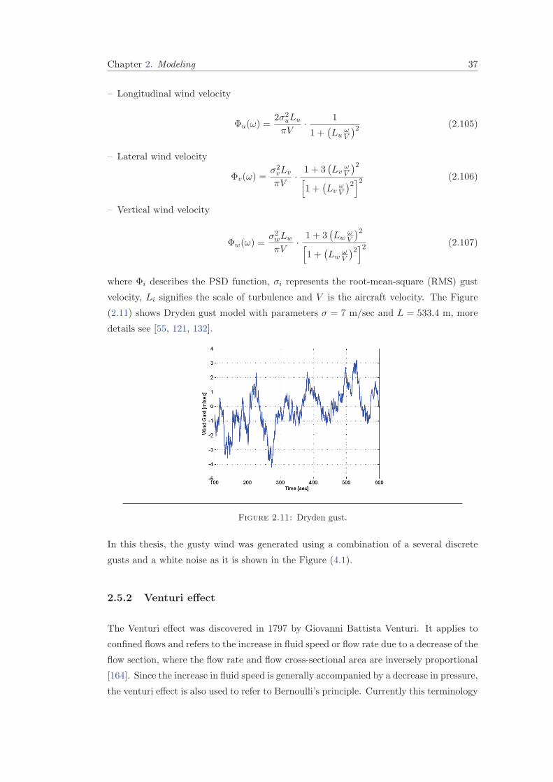
Chapter 2. Modeling 37
– Longitudinal wind velocity
Φu(ω) =2σ2
uLu
πV·
1
1 +(Lu
ωV
)2 (2.105)
– Lateral wind velocity
Φv(ω) =σ2vLv
πV·1 + 3
(Lv
ωV
)2[1 +
(Lv
ωV
)2]2 (2.106)
– Vertical wind velocity
Φw(ω) =σ2wLw
πV·1 + 3
(Lw
ωV
)2[1 +
(Lw
ωV
)2]2 (2.107)
where Φi describes the PSD function, σi represents the root-mean-square (RMS) gust
velocity, Li signifies the scale of turbulence and V is the aircraft velocity. The Figure
(2.11) shows Dryden gust model with parameters σ = 7 m/sec and L = 533.4 m, more
details see [55, 121, 132].
Figure 2.11: Dryden gust.
In this thesis, the gusty wind was generated using a combination of a several discrete
gusts and a white noise as it is shown in the Figure (4.1).
2.5.2 Venturi effect
The Venturi effect was discovered in 1797 by Giovanni Battista Venturi. It applies to
confined flows and refers to the increase in fluid speed or flow rate due to a decrease of the
flow section, where the flow rate and flow cross-sectional area are inversely proportional
[164]. Since the increase in fluid speed is generally accompanied by a decrease in pressure,
the venturi effect is also used to refer to Bernoulli’s principle. Currently this terminology
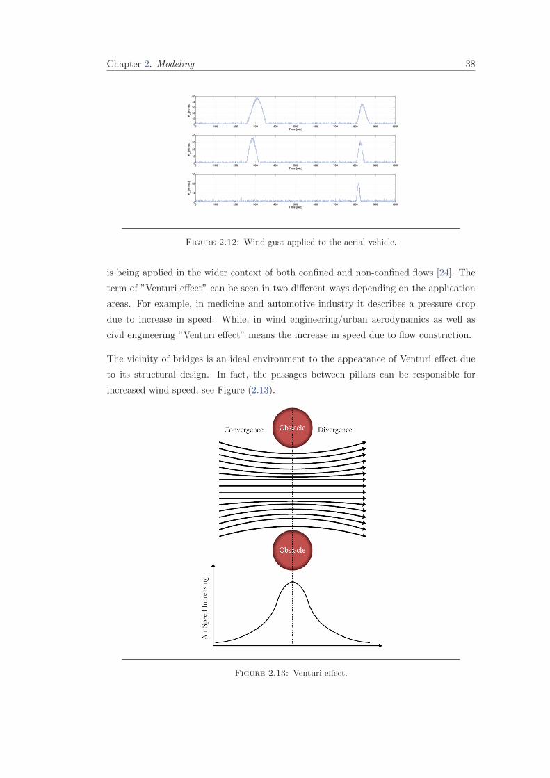
Chapter 2. Modeling 38
0 100 200 300 400 500 600 700 800 900 10000
10
20
30
40
50
Time [sec]
Wx [
m/s
ec
]
0 100 200 300 400 500 600 700 800 900 10000
10
20
30
40
Time [sec]
Wy [
m/s
ec
]
0 100 200 300 400 500 600 700 800 900 10000
10
20
30
Time [sec]
Wz [
m/s
ec
]
Figure 2.12: Wind gust applied to the aerial vehicle.
is being applied in the wider context of both confined and non-confined flows [24]. The
term of ”Venturi effect” can be seen in two different ways depending on the application
areas. For example, in medicine and automotive industry it describes a pressure drop
due to increase in speed. While, in wind engineering/urban aerodynamics as well as
civil engineering ”Venturi effect” means the increase in speed due to flow constriction.
The vicinity of bridges is an ideal environment to the appearance of Venturi effect due
to its structural design. In fact, the passages between pillars can be responsible for
increased wind speed, see Figure (2.13).
Figure 2.13: Venturi effect.
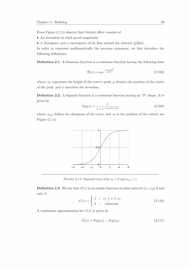
Chapter 2. Modeling 39
From Figure (2.13) observe that Venturi effect consists of:
• An increment in wind speed magnitude.
• A divergence and a convergence of air flow around the obstacle (pillar).
In order to represent mathematically the previous statement, we first introduce the
following definitions
Definition 2.1. A Gaussian function is a continous function having the following form
G (x) = aG e−(x−µ)2
2σ2 (2.108)
where, aG represents the height of the curve’s peak, µ denotes the position of the center
of the peak, and σ describes the deviation.
Definition 2.2. A Sigmoid function is a continous function having an ”S” shape. It is
given by
Sig(x) =1
1 + e−asig(x−x0)(2.109)
where, asig defines the sharpness of the curve, and x0 is the position of the switch, see
Figure (2.14).
Figure 2.14: Sigmoid curve with x0 = 0 and asig = 1.
Definition 2.3. We say that E (x) is an enable function on some interval x1, x2 if and
only if
E (x) =
1 ; x1 ≤ x ≤ x2
0 ; otherwise(2.110)
A continuous approximation for E (x) is given by
E (x) = Sig(x1)− Sig(x2) (2.111)

Chapter 2. Modeling 40
Considering the presence of two pillars, supposing a horizontal plan and assuming that
the wind is in the direction of x-axis, see Figure (2.15). Then the wind velocity compo-
nents on x and y axes are given as follows
Wx = G (x) (2.112a)
Wy = Wy1 +Wy2 (2.112b)
where, Wy1 and Wy2 presents the component divergence and convergence of the air flow
for the first and the second pillar respectively. These terms are defined as following
Wy1 = ay(y − yp1)E (y1)[E (x1)− E (x2)
](2.113a)
Wy2 = ay(y − yp2)E (y2)[E (x1)− E (x2)
](2.113b)
in the previous equation,
• yp1 and yp1 are the y-coordinate of the center of the first and the second pillar respec-
tively.
• E (xi) and E (yi) (for i = 1, 2) identify the neighborhood of the first and second pillars
on x and y axes respectively.
• the term E (x1)− E (x2) associates the divergence and convergence areas, according to
x axis, to the linear variation ay(y − ypi); i = 1, 2.
−5 0 5 10 15 20 25−10
−5
0
5
10
15
20
25
30
35
x [m]
y[m
]
Figure 2.15: Venturi effect in the presence of two pillars.

Chapter 2. Modeling 41
2.6 Conclusion
In this chapter, general equations of motion for lighter than air vehicles and quadrotors
crafts were introduced. The translational and rotational motion was uncoupled, and the
vehicles were modeled in two different ways. Firstly, a six degree of freedom equations of
motion, called rigid body model, was developed for lighter than air vehicle using Newton-
Euler approach, and for quadrotor crafts through Euler-Lagrange technique. This model
is devoted to treat the stability and control problems. Next, a three degree of freedom
translational equations of motion, called point mass model, was introduced. This model
is based on Newton’s second law and used to deal with navigation and guidance control
systems. Translational kinematics and dynamics for airships was realized, while the
kinematic model was adopted to present quadrotors crafts.
Besides the mathematical representations of the aerial vehicles, the wind modeling issue
has been addressed. Two models for gusts were presented. The first one represents
a sharp edged gust, while the second one is based on the frequency representation.
In addition, a mathematical relation modeling Venturi effect in the neighborhood of a
bridge was developed.
After describing the equations of motion of lighter than air vehicles and quadrotors
crafts, we address the questions of motion planning, trajectory generation, and tracking
for aerial vehicles in next chapters.

Chapter 3
Trajectory Generation and
Motion Planning
3.1 Introduction
One of the most important feature of an Unmanned Aerial Vehicle (UAV) is its capacity
to accomplish different type of tasks with a high level of performance, maneuverabil-
ity and with less oversight of human operators. This characteristic is also known as
autonomy [12, 92]. These tasks require flexible and Powerful algorithms that convert
high-level mission specifications from humans into low-level descriptions of the vehicle’s
motion. The terms Motion Planning and Trajectory Planning are often employed
for such kind of problems [111].
In order to connect a starting and a target points, feasible and flyable trajectories must
be defined. The feasibility criteria is carried out by motion planning algorithms. This
process produce a plan to steer the UAV safely to its target, without taking into account
its dynamical constraints. Whilst, the trajectory generation problem takes the solution
obtained by the motion planning algorithm and determines the way to fly along this so-
lution with respect to the vehicle’s mechanical limitations. In other words, it guarantees
the flyable aspect of the trajectory [12, 111].
The rest of this chapter is organized as follows: section 3.2 presents a state of art on
trajectory generation and motion planning. Section 3.3 discusses solutions proposed for
bridge inspection task. Finally, a conclusion is addressed in the section 3.4.
43
Chapter 3. Planning and Trajectory Generation 44
3.2 State of Art
3.2.1 Trajectory Generation
In addition to leading an aerial vehicle from an initial configuration to a final one and
complying with the vehicle’s physical constraints, there are often other requirements to
take into account in the trajectory generation process. For instance, limiting curvature,
reducing the traveled distance and consumed energy, etc...
In general, these are integrated in the design procedure as the optimization of a suit-
able cost criterion along the trajectory. The optimality of a trajectory can be defined
according to several objectives, like minimizing the transfer time or the energy [85, 87].
Traditionally, trajectories are optimized by the application of numerical optimal control
methods that are based on the calculus of variations. Dubins [51] considered a particle
moving with a constant velocity in the plane and subjected a constraint on trajectory
curvature. This problem is equivalent to the minimum time optimal trajectory problem
under a constant velocity and limitation on heading rate, without wind. He proved the
existence of shortest paths for his problem and showed that the optimal trajectory is one
of the following six solutions: RSL,RSR,LSR,LSL,RLR,LRL where R for Right
turn, S for straight line and L for Left turn. Knowing that all sub paths are allowed
to have zero length. So, his optimal trajectories are a combination of arc of circles and
segments of lines. Boukraa et al [28] presented a 3D trim trajectories planner algorithm
for an autonomous plane. The proposed algorithm used a sequence of five elementary
trim trajectories to generate a 3D global trajectory in space. A family of trim trajecto-
ries in level flight is used in all these references to construct paths. In the papers cited
above, the atmosphere was considered to be an isotropic and homogeneous medium, i.e.
when there is no wind and the air density is constant with altitude.
However, the natural wind proved itself to be a major parameter to successful flights
of aerial vehicles. It mostly affects a trajectory through its speed. McGee et al [120]
have described a method for finding the minimum time path from an initial position
and orientation to a final position and orientation in the 2D plane for an airplane with
a bounded turning rate in the presence of a known constant wind with a magnitude less
than the airplane velocity. The problem statement is equivalent to finding the minimum
time path from an initial configuration to a final one, over a moving virtual target, where
the velocity of the virtual target is equal and opposite to the velocity of the wind. Nelson
et al [131] have introduced a method for a mini aerial vehicle path following based on
the concept of vector field in the presence of constant wind disturbances. Rysdyk [143]
has presented a path formulation for maneuvering of a fixed wing aircraft in wind. The
inertial path of a fixed wing aircraft circling in wind can be formulated as a trochoid
Chapter 3. Planning and Trajectory Generation 45
curve. Jardin [83] has considered the minimum time problem for an airplane traveling
horizontally between two points in a variable wind field. Bijlsma [22] has referred to
route determination for an airplane traveling horizontally between two given points so
the transition time is minimized assuming that the wind field is fully known beforehand
for the complete passage. In these papers, only 2D horizontal motion was considered.
3.2.1.1 Space-Time Separation
Considering a given trajectory Cq(t) ∈ R3, for t ∈ [0, T ], which leads the aerial vehicle
from an initial point Cq (0) = Cq0 to a final point Cq (T ) = Cqf . This trajectory can
be broken down into a geometric path Cq(s) = [x(s) y(s) z(s)]T and a timing law
s = s(t). Where s denotes the curvilinear abscissa and satisfies
s ∈ [0, L] (3.1)
with, L: the length of the path.
Then, the velocity of the vehicle can be expressed as following
V =ds
dt(3.2)
The previous space-time separation implies
Cq =dCq
dt=
dCq
ds·ds
dt= C ′
q · V (3.3)
In addition, each point of the path Cq(s) can be described using three unitary orthogonal
vectors: tangent (−→T ), normal (
−→N ) and binormal (
−→B ). These vectors form the so-called
Frenet-Serret frame.
3.2.1.2 Curvature and Torsion
The importance of curvature κ and torsion τ comes from the fact that any curve in R3
can be completely defined by these variables [102].
The curvature is directly proportional to the lateral acceleration of the vehicle and, it
is inversely proportional to the minimum curvature radius (R) that can be flew by the
aircraft. It is expressed as following
κ =‖C ′
q × C ′′q ‖
‖C ′q‖
3(3.4)
In the other side, torsion is proportional to the vertical acceleration which is also phys-
ically limited. In addition, the value of τ is inversely proportional to the minimum

Chapter 3. Planning and Trajectory Generation 46
torsion radius (φ). It is presented as
τ =
(C ′q × C ′′
q
)· C ′′′
q
‖C ′q × C ′′
q ‖2
(3.5)
The first derivative of the flight path C ′q = [x′ y′ z′]T is deduced from equations (2.70)
and (3.3) as following
x′ =cosχ cos γ +Wx
V(3.6a)
y′ =sinχ cos γ +Wy
V(3.6b)
z′ =sin γ +Wz
V(3.6c)
While, the second and third derivatives are given as below
C ′′q =
Cq − V V ′C ′q
V 2(3.7)
C ′′′q =
...Cq − 3V ′V 2C ′′
q −(V ′′V + V ′2
)C ′qV
V 3(3.8)
In this manner, the curvature and torsion can formally be described as:
κ = f(γ,χ, V, γ′,χ′, V ′,Wx,Wy,Wz,W
′x,W
′y,W
′z
)(3.9a)
τ = f
(γ,χ, V, γ′,χ′, V ′, γ′′,χ′′, V ′′,Wx,
Wy,Wz,W′x,W
′y,W
′z,W
′′x ,W
′′y ,W
′′z
)(3.9b)
where, for lighter than air vehicles, γ′, χ′ and V ′ are obtained directly by dividing the
equation (2.95) by V as following
γ′ =(T sinα+ L) cosσ −mg cos γ
mV 2+
Wx cosχ sin γ + Wy sinχ sin γ + Wz cos γ
V(3.10a)
χ′ =(T sinα+ L) sinσ
mV 2 cos γ+
Wx sinχ− Wy cosχ
V cos γ(3.10b)
V ′ =T cosα−D −mg sin γ
mV− Wx cos γ cosχ− Wy sinχ cos γ + Wz sin γ (3.10c)
Whilst, their second derivatives are given by
γ′′ =γ − γ′V ′V
V 2(3.11a)
χ′′ =χ− χ′V ′V
V 2(3.11b)
V ′′ =V − V ′2V
V 2(3.11c)
Chapter 3. Planning and Trajectory Generation 47
3.2.1.3 Constraints
A path is said to be flyable if it meets with the kinematic and dynamic constraints of
the vehicle. Such motion constraints are introduced as bounds on the curvature (κ) and
the torsion (τ) of the path Cq(s)
|κ| ≤ κmax (3.12a)
|τ | ≤ τmax (3.12b)
Notice that, κmax and τmax are established from constraints imposed on the control and
state variables, Equation (2.102).
3.2.1.4 Cartesian Polynomials
After determining the required path Cq (s); s ∈ [s0, sf ], the related timing law must
be chosen so that resulting trajectory respects the restrictions imposed on the vehicle,
Equation (2.102). For example, in order to take the inputs bounds introduced to the air-
craft, Equation (2.102a), Equation (2.102b), and Equation (2.102c), into consideration,
it is necessary to verify whether the inputs (linear acceleration and angular velocities)
along the planned trajectory are admissible. When this is not achieved, a uniform scal-
ing is used to slow down the timing law. To do that, it is more convenient to rewrite
the timing law by replacing t with the normalized time variable T = t/T . Then, from
Equation (2.100), Equation (3.3) and Equation (3.2) we have
γ′ = u1ds
dT
dT
dt= u1
ds
dT
1
T(3.13)
χ′ = u2ds
dT
dT
dt= u2
ds
dT
1
T(3.14)
V ′ = u3ds
dT
dT
dt= u3
ds
dT
1
T(3.15)
Therefore, it is sufficient to increase the duration of the trajectory T to reduce uniformly
γ′, χ′ and V ′ so that the vehicle’s inputs remain within the given bounds.
Planning a trajectory directly without separating the geometric path from the timing
law could be effected by using the time variable t directly instead of the path parameter
s. A disadvantage of this approach is the fact that the duration of the trajectory must
be fixed (T = sf ). Thus, the uniform scaling cannot be used to satisfy bounds on the
vehicle’s input. That is because an increment (or decrement) of T implies a modification
on the geometric path associated to the planned trajectory [148].
Chapter 3. Planning and Trajectory Generation 48
Third-order Cartesian polynomials are known to be simple in real time implementation
[49]. Then, for two successive configurations (xi, yi, zi, γi, χi, Vi) and (xi+1, yi+1, zi+1,
γi+1, χi+1, Vi+1) we have:
x(s) =s3xi+1 − (s− 1)3xi + αxs2(s− 1) + βxs(s− 1)2 (3.16a)
x(s) =s3yi+1 − (s− 1)3yi + αys2(s− 1) + βys(s− 1)2 (3.16b)
x(s) =s3zi+1 − (s− 1)3zi + αzs2(s− 1) + βzs(s− 1)2 (3.16c)
With,
αx = TVi+1 cos(γi+1) cos(χi+1)− 3xi+1; βx = TVi+1 cos(γi+1) cos(χi+1) + 3xi+1;
αy = TVi+1 cos(γi+1) sin(χi+1)− 3yi+1; βy = TVi+1 cos(γi+1) sin(χi+1) + 3yi+1;
αz = TVi+1 sin(γi+1)− 3zi+1; βz = TVi+1 sin(γi+1) + 3zi+1;
(3.17)
For more details, please refer to [17, 49, 148].
3.2.2 Motion Planning
Flight planning involves creating a plan to guide an aerial robot from its initial position
to a desired destination way point [17]. Historically, two fields have contributed to
trajectory or motion planning methods: robotics and dynamics & control. The first
topic has a stronger focus on computational issues and real-time robot control, while
the second one emphasizes the dynamic behavior and more specific aspects of trajectory
performance [69].
The aim of motion planning algorithms is to define feasible trajectories to reach a desired
location. These trajectories must ensure the safety of the flight by taking into account
obstacles, collision avoidance and dangerous regions. A dangerous region is a space with
a critical flight condition like unusual low or high pressure, hazardous wind storms, or
any other factor affecting the flight. There are a variety of motion planning problem
types that can be found in the literature. Such classification is made according to:
• The knowledge of the environment: it is said to be static for a perfect knowledge and
dynamic in the opposite case.
• The type of obstacles: it is called time-invariant if the obstacles are fixed and time-
variant when the obstacles are allowed to move.
• The presence of constraints on the vehicle: differentially constrained (or kinodynamic)
when the vehicle’s equation of motion act as constraints on the path. While for
differentially unconstrained problems, the vehicle may use infinite accelerations to
acheve a path.

Chapter 3. Planning and Trajectory Generation 49
Motion planning under differential constraints can be considered as a variant of classical
Two-Point Boundary Value Problem (TPBVP) [76]. For a classical TPBVP, the
initial and final points are given, and the objective is to compute a trajectory through
the state space that connects initial and final states and which satisfies the differential
constraints. Motion planning involves the additional complication of avoiding obstacles
in the state space. Unfortunately, the techniques used to solve TPBVPs are not suitable
for motion planning because they are not designed to handle obstacles.
In next subsections, an overview on most successful differentially-constrained planning
algorithms in literature is presented.
3.2.2.1 Cell decomposition
The main idea of these approaches is to decompose the configuration space C into a
number of disjoint sets, called cells. The resulting structure of C called connectivity
graph G is considered as an important element of cell decomposition methods. Each cell
is represented as a node in this graph; and two nodes are connected by an edge if and
only if the two corresponding cells are adjacent.
Cell decomposition algorithms can be classified as exact or approximate. The major
difference between the previous two classes is the methods used to build the structure
of C. For exact methods, the union of all cells equal to the closure of the collision-free
configuration space. Whereas in approximate approaches, the structure of C is obtained
with cells which have a simple predefined shape.
3.2.2.2 Probabilistic roadmap approach
For high-dimensional planning problems, the exact algorithms are computationally too
expansive to calculate an explicit representation of the configuration space. Therefore,
probabilistic motion planning approaches have achieved a substantial attention through-
out the last decades because of their capability to solve high-dimensional problems in
acceptable execution times.
Probabilistic roadmap planers [3, 42, 94] work in two phases. The first one is a learning
phase while the second one is a query phase. In the learning phase, a graph, called
a roadmap, is built by randomly sampling the configuration space. The free-collision
configurations form the vertices of the roadmap. Then, the neighboring vertices are
connected by edges if their corresponding configurations can be connected by continuous
path through a local planner. The most common local planner simply checks a straight
line connecting the two configurations.
Chapter 3. Planning and Trajectory Generation 50
On the other side, during the query phase, the algorithm tries to connect the initial and
final configurations to the roadmap. Then, it search for a path connecting these two
states.
It is important to note that if the environment is static, then the roadmap can be
reused for further queries. Therefore, the algorithms used for dynamic environment are
classified as multiple query methods. In [25] a single query variant called Lazy PRM.
In this approach, the roadmap is built in the whole configuration space instead of the
collusion-free configuration space. Once, a path has been found in the query phase, a
collision checking algorithm is used to check the feasibility of the path.
However, the performance of Probabilistic roadmap planners can degrade if the solution
has to pass through a narrow passage. To cope with a such problem, several variations
and extensions have been proposed in [80, 122]. Another difficulty is the fast growing
number of nodes and samples in the roadmap. Solutions for a such problem can be
found in [1, 27, 79, 104, 151].
3.2.2.3 Rapidly-expanding random Tree (RRT)
Another probabilistic planing approach is Rapidly-Expanding Random Tree (RRT).
The basic idea of this method is building a tree which starts from the initial configuration
and explore the collision-free configuration space. The exploration is done through a
random sampling of the state space and expanding the search tree step-by-step. The
objective is to build a graph structure covering the configuration space with nodes,
explored positions and edges describing control inputs needed to move from node to
node [17, 99].
In each step, a random state (xrand) is chosen. Next, the nearest vertex (xnear) in the
tree (with respect to a chosen metric) is selected. Then, a new edge going from xnear
and pointing to xrand as well as describing the control effort needed to reach is added.
Finally, between all potential new configurations, the closest state to the desired final
configuration (xf ) is designated as a new state (xnew) and added to the tree as a new
vertex. This process is repeated until reaching the final configurations (xf ).
The RRT was described for the first time in [111, 112]. In these two papers, the vehicle
is considered holonomic; neither dynamics nor kinematic constraints are considered.
Another variation of RRT algorithm is described in [113]. The proposed algorithm is
based on two trees. The first one is grown from the initial configuration while the second
one from the desired final state. In every step, both trees try to connect to the same state
in configuration space. Thus, a path is often found very quickly at the cost of diverging
Chapter 3. Planning and Trajectory Generation 51
a lot from an optimal path. The major advantage of RRT-like methods is that they
are perfectly suitable for nonholonomic and differentially constrained planning problem
[114].
3.2.2.4 A⋆ Algorithm
The A⋆ algorithm belongs to graph search algorithms. This kind of approaches were
developed for computer science to find the shortest path between two nodes of connected
graphs. They were designed for computer networks to develop routing protocols and were
applied to path planning through decomposition of the path in waypoint sequences [44].
The A⋆ algorithm is considered as one of the most important solvers explicitly oriented to
motion-robotics [74]. It searches a graph efficiently with respect to a chosen heuristic and
cost function; and returns an optimal path if the heuristic is optimistic. An optimistic or
admissible heuristic always returns a value less than or equal to the cost of the shortest
path from the current node to the goal node within the graph. The cost function used
in A⋆ algorithm is the sum of the following two terms:
• Cost to go H : defined as a heuristic estimation of the distance from the neighbouring
cell xnear to the final one xf .
• Cost to come G : Known as the distance between the expanded cell x and the neigh-
bouring one xnear.
The G-value is 0 for the starting configuration and it increases while the algorithm
expands successive states. On the other side, the H-value is used to drive the states
expansion toward the desired final configuration, reducing this way the amount of ex-
panded cells and improving the convergence.
The input of A⋆ algorithm is the graph itself. So, the nodes can be naturally embedded
into the aerial vehicle free configuration space and have a specified coordinates. The
edges correspond to adjacent nodes and have the value of the cost appropriate to the
travel. The output of A⋆ algorithm is a back pointer path, in other words a sequence of
nodes starting from the goal configuration and coming back to the start states. More
details on A⋆ algorithm can be found in [17, 34, 44, 49].
3.2.2.5 Potential field planners
In these approaches, an artificial potential field is used in order to steer the aerial vehicle
from its initial configuration to a desired final one. The robot moves under the influence
of a potential field which is obtained as a superposition of an attractive potential to
the goal configuration and a repulsive potential from the obstacle regions. In other
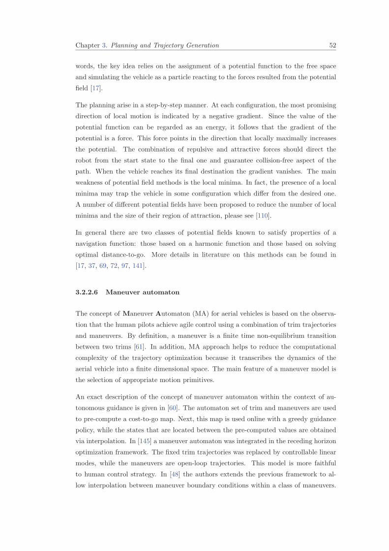
Chapter 3. Planning and Trajectory Generation 52
words, the key idea relies on the assignment of a potential function to the free space
and simulating the vehicle as a particle reacting to the forces resulted from the potential
field [17].
The planning arise in a step-by-step manner. At each configuration, the most promising
direction of local motion is indicated by a negative gradient. Since the value of the
potential function can be regarded as an energy, it follows that the gradient of the
potential is a force. This force points in the direction that locally maximally increases
the potential. The combination of repulsive and attractive forces should direct the
robot from the start state to the final one and guarantee collision-free aspect of the
path. When the vehicle reaches its final destination the gradient vanishes. The main
weakness of potential field methods is the local minima. In fact, the presence of a local
minima may trap the vehicle in some configuration which differ from the desired one.
A number of different potential fields have been proposed to reduce the number of local
minima and the size of their region of attraction, please see [110].
In general there are two classes of potential fields known to satisfy properties of a
navigation function: those based on a harmonic function and those based on solving
optimal distance-to-go. More details in literature on this methods can be found in
[17, 37, 69, 72, 97, 141].
3.2.2.6 Maneuver automaton
The concept of Maneuver Automaton (MA) for aerial vehicles is based on the observa-
tion that the human pilots achieve agile control using a combination of trim trajectories
and maneuvers. By definition, a maneuver is a finite time non-equilibrium transition
between two trims [61]. In addition, MA approach helps to reduce the computational
complexity of the trajectory optimization because it transcribes the dynamics of the
aerial vehicle into a finite dimensional space. The main feature of a maneuver model is
the selection of appropriate motion primitives.
An exact description of the concept of maneuver automaton within the context of au-
tonomous guidance is given in [60]. The automaton set of trim and maneuvers are used
to pre-compute a cost-to-go map. Next, this map is used online with a greedy guidance
policy, while the states that are located between the pre-computed values are obtained
via interpolation. In [145] a maneuver automaton was integrated in the receding horizon
optimization framework. The fixed trim trajectories was replaced by controllable linear
modes, while the maneuvers are open-loop trajectories. This model is more faithful
to human control strategy. In [48] the authors extends the previous framework to al-
low interpolation between maneuver boundary conditions within a class of maneuvers.
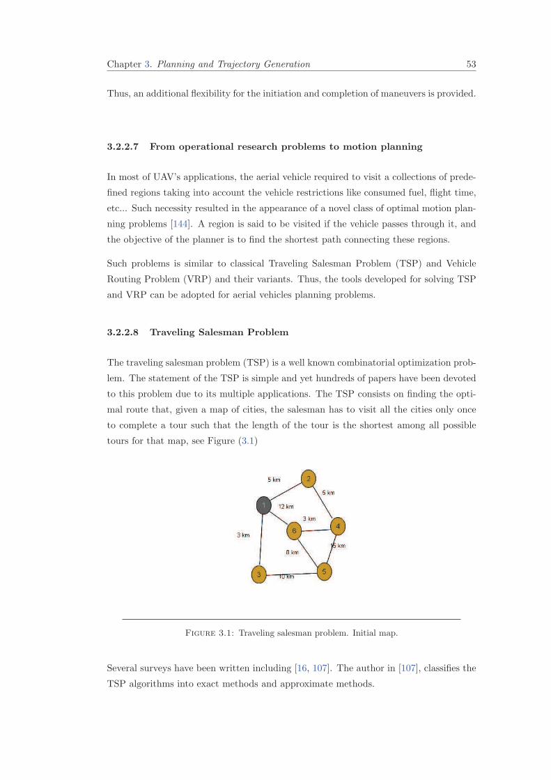
Chapter 3. Planning and Trajectory Generation 53
Thus, an additional flexibility for the initiation and completion of maneuvers is provided.
3.2.2.7 From operational research problems to motion planning
In most of UAV’s applications, the aerial vehicle required to visit a collections of prede-
fined regions taking into account the vehicle restrictions like consumed fuel, flight time,
etc... Such necessity resulted in the appearance of a novel class of optimal motion plan-
ning problems [144]. A region is said to be visited if the vehicle passes through it, and
the objective of the planner is to find the shortest path connecting these regions.
Such problems is similar to classical Traveling Salesman Problem (TSP) and Vehicle
Routing Problem (VRP) and their variants. Thus, the tools developed for solving TSP
and VRP can be adopted for aerial vehicles planning problems.
3.2.2.8 Traveling Salesman Problem
The traveling salesman problem (TSP) is a well known combinatorial optimization prob-
lem. The statement of the TSP is simple and yet hundreds of papers have been devoted
to this problem due to its multiple applications. The TSP consists on finding the opti-
mal route that, given a map of cities, the salesman has to visit all the cities only once
to complete a tour such that the length of the tour is the shortest among all possible
tours for that map, see Figure (3.1)
Figure 3.1: Traveling salesman problem. Initial map.
Several surveys have been written including [16, 107]. The author in [107], classifies the
TSP algorithms into exact methods and approximate methods.
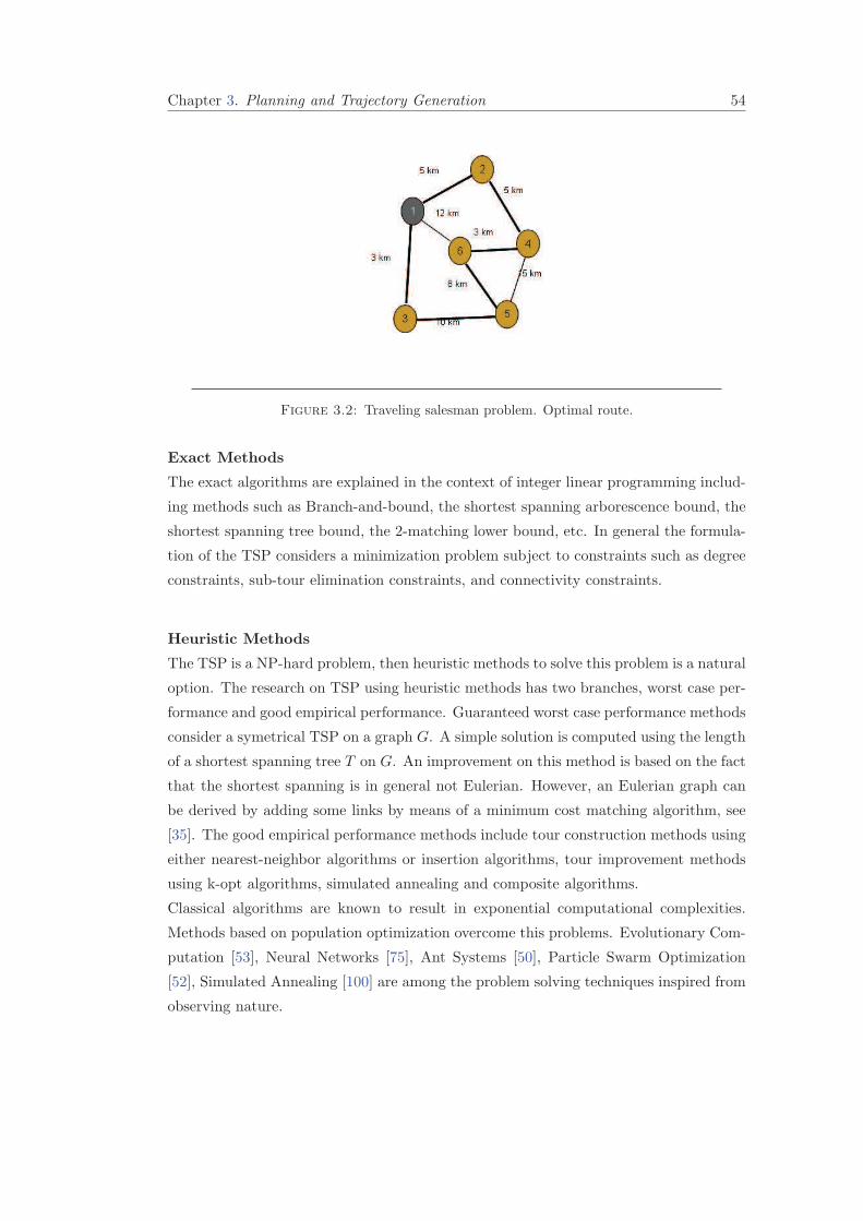
Chapter 3. Planning and Trajectory Generation 54
Figure 3.2: Traveling salesman problem. Optimal route.
Exact Methods
The exact algorithms are explained in the context of integer linear programming includ-
ing methods such as Branch-and-bound, the shortest spanning arborescence bound, the
shortest spanning tree bound, the 2-matching lower bound, etc. In general the formula-
tion of the TSP considers a minimization problem subject to constraints such as degree
constraints, sub-tour elimination constraints, and connectivity constraints.
Heuristic Methods
The TSP is a NP-hard problem, then heuristic methods to solve this problem is a natural
option. The research on TSP using heuristic methods has two branches, worst case per-
formance and good empirical performance. Guaranteed worst case performance methods
consider a symetrical TSP on a graph G. A simple solution is computed using the length
of a shortest spanning tree T on G. An improvement on this method is based on the fact
that the shortest spanning is in general not Eulerian. However, an Eulerian graph can
be derived by adding some links by means of a minimum cost matching algorithm, see
[35]. The good empirical performance methods include tour construction methods using
either nearest-neighbor algorithms or insertion algorithms, tour improvement methods
using k-opt algorithms, simulated annealing and composite algorithms.
Classical algorithms are known to result in exponential computational complexities.
Methods based on population optimization overcome this problems. Evolutionary Com-
putation [53], Neural Networks [75], Ant Systems [50], Particle Swarm Optimization
[52], Simulated Annealing [100] are among the problem solving techniques inspired from
observing nature.
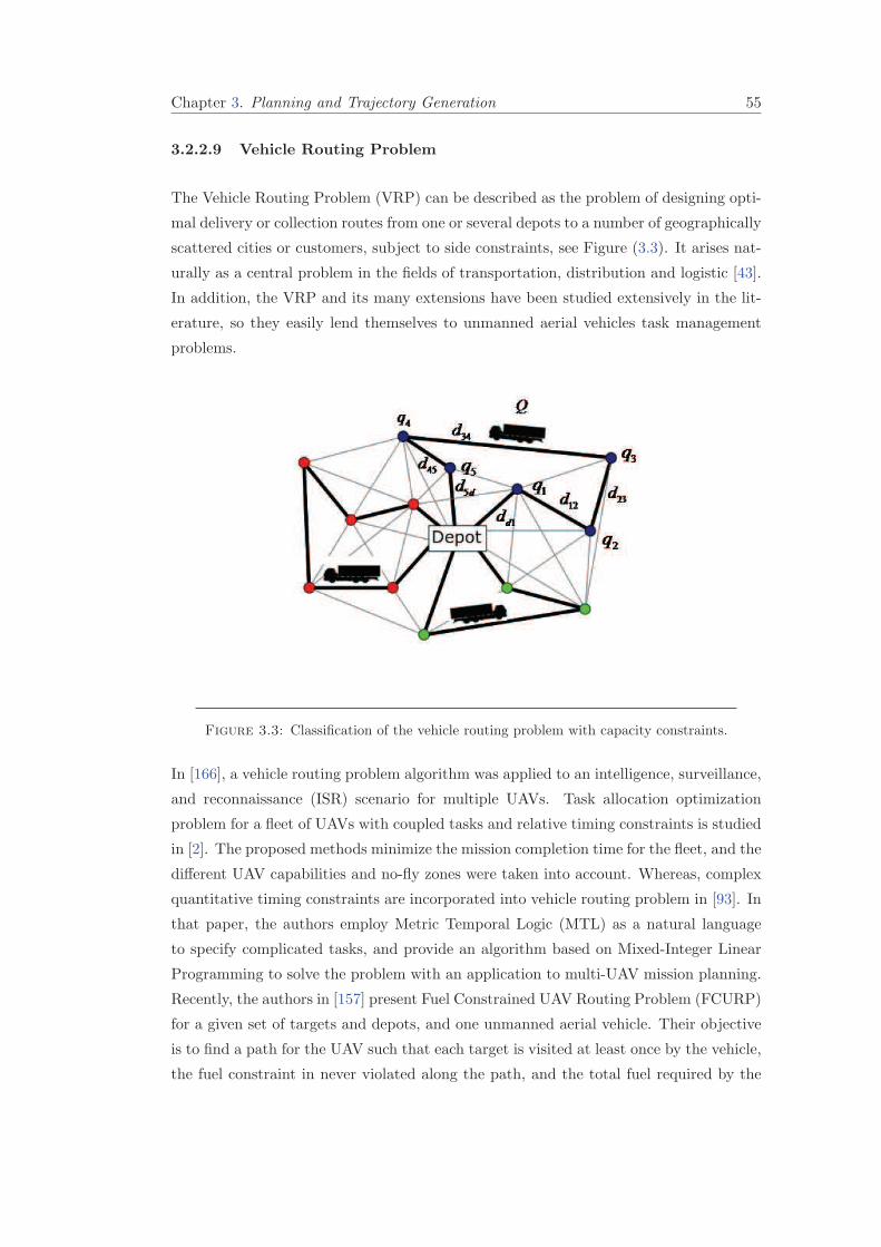
Chapter 3. Planning and Trajectory Generation 55
3.2.2.9 Vehicle Routing Problem
The Vehicle Routing Problem (VRP) can be described as the problem of designing opti-
mal delivery or collection routes from one or several depots to a number of geographically
scattered cities or customers, subject to side constraints, see Figure (3.3). It arises nat-
urally as a central problem in the fields of transportation, distribution and logistic [43].
In addition, the VRP and its many extensions have been studied extensively in the lit-
erature, so they easily lend themselves to unmanned aerial vehicles task management
problems.
Figure 3.3: Classification of the vehicle routing problem with capacity constraints.
In [166], a vehicle routing problem algorithm was applied to an intelligence, surveillance,
and reconnaissance (ISR) scenario for multiple UAVs. Task allocation optimization
problem for a fleet of UAVs with coupled tasks and relative timing constraints is studied
in [2]. The proposed methods minimize the mission completion time for the fleet, and the
different UAV capabilities and no-fly zones were taken into account. Whereas, complex
quantitative timing constraints are incorporated into vehicle routing problem in [93]. In
that paper, the authors employ Metric Temporal Logic (MTL) as a natural language
to specify complicated tasks, and provide an algorithm based on Mixed-Integer Linear
Programming to solve the problem with an application to multi-UAV mission planning.
Recently, the authors in [157] present Fuel Constrained UAV Routing Problem (FCURP)
for a given set of targets and depots, and one unmanned aerial vehicle. Their objective
is to find a path for the UAV such that each target is visited at least once by the vehicle,
the fuel constraint in never violated along the path, and the total fuel required by the

Chapter 3. Planning and Trajectory Generation 56
aerial vehicle is minimum. Other research on UAV routing and mission planning problem
can be found in [15, 57, 140, 146, 147].
Problem Formulation
Let G = (V,A) be a graph where V = V1, V2, ..., Vn is a set of vertices representing
locations to be visited by the UAV with its ground base at V1, and A is the set of arcs.
Suppose that C : A → R+ denote the cost function with C(Vi, Vj) representing the cost
of traveling from vertex Vi to vertex Vj . Observe that, C(Vi, Vj) can be interpreted as
consumed fuel, path length, travel time, etc...
In addition, assume that there are m vehicles available at the ground base, and all
vehicles are identical and have the same capacity. Then, the vehicle routing problem
consists of designing a set of beast-cost vehicle routes in such way that:
• Each city in V2, ..., Vn is visited exactly once by exactly one vehicle.
• All vehicle routes start and end at the ground base.
• Some side constraints are satisfied.
Variants of Vehicle Routing Problem
According to [161], the variants of the vehicle routing problem can be classified as shown
in Figure (3.4)
• Capacitated Vehicle Routing Problem (CVRP): CVRP is a vehicle routing problem in
which the vehicles have limited carrying capacity of the goods that must be delivered.
• Distance and Capacitated Vehicle Routing Problem (DCVRP): DCVRP is similar to
CVRP with an additional restriction on the allowed maximum distance traveled in
each tour.
• Vehicle Routing Problem with Time Windows (VRPTW):The additional restriction
in VRPTW is a time window associated with each customer, defining an interval
wherein the customer has to be supplied.
• Vehicle Routing Problem with Backhauling (VRPB): It is an extension of VRP that
includes both a set of customers to whom products are to be delivered, and a set
of vendors whose goods need to be transported back to the distribution center. In
addition, on each route all deliveries have to be made before any goods can be picked
up to avoid rearranging the loads on the vehicle.
• Vehicle Routing Problem with Backhauling and Time Windows (VRPBTW): It is a
combination between VRPB and VRPTW.
• Vehicle Routing Problem with Pickup and Delivery (VRPPD): It is a VRP in which
the customers have the possibility to return some commodities. In addition, VRPPD
must take into account that the goods can be fitted into the vehicle. This restriction
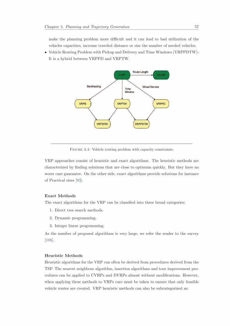
Chapter 3. Planning and Trajectory Generation 57
make the planning problem more difficult and it can lead to bad utilization of the
vehicles capacities, increase traveled distance or rise the number of needed vehicles.
• Vehicle Routing Problem with Pickup and Delivery and TimeWindows (VRPPDTW):
It is a hybrid between VRPPD and VRPTW.
Figure 3.4: Vehicle routing problem with capacity constraints.
VRP approaches consist of heuristic and exact algorithms. The heuristic methods are
characterized by finding solutions that are close to optimum quickly. But they have no
worst case guarantee. On the other side, exact algorithms provide solutions for instance
of Practical sizes [93].
Exact Methods
The exact algorithms for the VRP can be classified into three broad categories:
1. Direct tree search methods.
2. Dynamic programming.
3. Integer linear programming.
As the number of proposed algorithms is very large, we refer the reader to the survey
[108].
Heuristic Methods
Heuristic algorithms for the VRP can often be derived from procedures derived from the
TSP. The nearest neighbour algorithm, insertion algorithms and tour improvement pro-
cedures can be applied to CVRPs and DVRPs almost without modifications. However,
when applying these methods to VRPs care must be taken to ensure that only feasible
vehicle routes are created. VRP heuristic methods can also be subcategorized as:
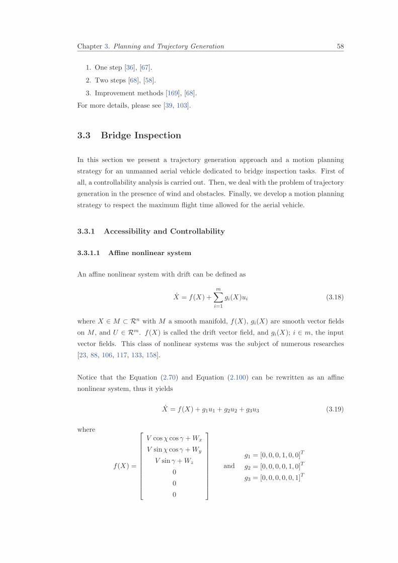
Chapter 3. Planning and Trajectory Generation 58
1. One step [36], [67].
2. Two steps [68], [58].
3. Improvement methods [169], [68].
For more details, please see [39, 103].
3.3 Bridge Inspection
In this section we present a trajectory generation approach and a motion planning
strategy for an unmanned aerial vehicle dedicated to bridge inspection tasks. First of
all, a controllability analysis is carried out. Then, we deal with the problem of trajectory
generation in the presence of wind and obstacles. Finally, we develop a motion planning
strategy to respect the maximum flight time allowed for the aerial vehicle.
3.3.1 Accessibility and Controllability
3.3.1.1 Affine nonlinear system
An affine nonlinear system with drift can be defined as
X = f(X) +m∑
i=1
gi(X)ui (3.18)
where X ∈ M ⊂ Rn with M a smooth manifold, f(X), gi(X) are smooth vector fields
on M , and U ∈ Rm. f(X) is called the drift vector field, and gi(X); i ∈ m, the input
vector fields. This class of nonlinear systems was the subject of numerous researches
[23, 88, 106, 117, 133, 158].
Notice that the Equation (2.70) and Equation (2.100) can be rewritten as an affine
nonlinear system, thus it yields
X = f(X) + g1u1 + g2u2 + g3u3 (3.19)
where
f(X) =
V cosχ cos γ +Wx
V sinχ cos γ +Wy
V sin γ +Wz
0
0
0
and
g1 = [0, 0, 0, 1, 0, 0]T
g2 = [0, 0, 0, 0, 1, 0]T
g3 = [0, 0, 0, 0, 0, 1]T
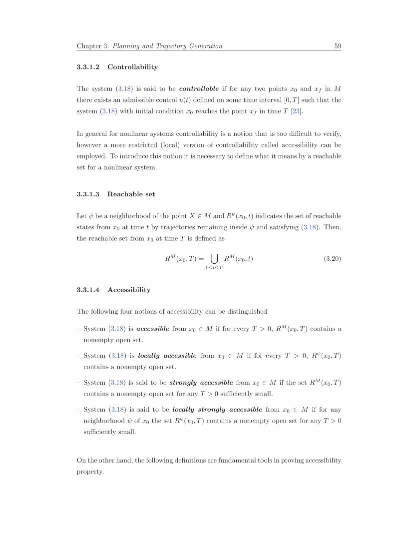
Chapter 3. Planning and Trajectory Generation 59
3.3.1.2 Controllability
The system (3.18) is said to be controllable if for any two points x0 and xf in M
there exists an admissible control u(t) defined on some time interval [0, T ] such that the
system (3.18) with initial condition x0 reaches the point xf in time T [23].
In general for nonlinear systems controllability is a notion that is too difficult to verify,
however a more restricted (local) version of controllability called accessibility can be
employed. To introduce this notion it is necessary to define what it means by a reachable
set for a nonlinear system.
3.3.1.3 Reachable set
Let ψ be a neighborhood of the point X ∈ M and Rψ(x0, t) indicates the set of reachable
states from x0 at time t by trajectories remaining inside ψ and satisfying (3.18). Then,
the reachable set from x0 at time T is defined as
RM (x0, T ) =⋃
0≤t≤T
RM (x0, t) (3.20)
3.3.1.4 Accessibility
The following four notions of accessibility can be distinguished
– System (3.18) is accessible from x0 ∈ M if for every T > 0, RM (x0, T ) contains a
nonempty open set.
– System (3.18) is locally accessible from x0 ∈ M if for every T > 0, Rψ(x0, T )
contains a nonempty open set.
– System (3.18) is said to be strongly accessible from x0 ∈ M if the set RM (x0, T )
contains a nonempty open set for any T > 0 sufficiently small.
– System (3.18) is said to be locally strongly accessible from x0 ∈ M if for any
neighborhood ψ of x0 the set Rψ(x0, T ) contains a nonempty open set for any T > 0
sufficiently small.
On the other hand, the following definitions are fundamental tools in proving accessibility
property.
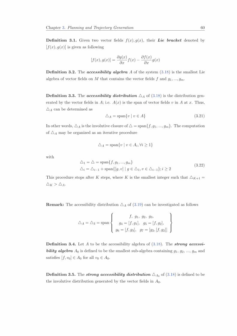
Chapter 3. Planning and Trajectory Generation 60
Definition 3.1. Given two vector fields f(x), g(x), their Lie bracket denoted by
[f(x), g(x)] is given as following
[f(x), g(x)] =∂g(x)
∂xf(x)−
∂f(x)
∂xg(x)
Definition 3.2. The accessibility algebra A of the system (3.18) is the smallest Lie
algebra of vector fields on M that contains the vector fields f and g1, ..., gm.
Definition 3.3. The accessibility distribution A of (3.18) is the distribution gen-
erated by the vector fields in A; i.e. A(x) is the span of vector fields v in A at x. Thus,
A can be determined as
A = spanv | v ∈ A (3.21)
In other words, A is the involutive closure of = spanf, g1, ..., gm. The computation
of A may be organized as an iterative procedure
A = spanv | v ∈ Ai, ∀i ≥ 1
with1 = = spanf, g1, ..., gm
i = i−1 + span[g, v] | g ∈ 1, v ∈ i−1; i ≥ 2(3.22)
This procedure stops after K steps, where K is the smallest integer such that K+1 =
K > A.
Remark: The accessibility distribution A of (3.19) can be investigated as follows
A = 3 = span
f, g1, g2, g3,
g4 = [f, g1], g5 = [f, g2],
g6 = [f, g3], g7 = [g2, [f, g2]]
Definition 3.4. Let A to be the accessibility algebra of (3.18). The strong accessi-
bility algebra A0 is defined to be the smallest sub-algebra containing g1, g2, ..., gm and
satisfies [f, v0] ∈ A0 for all v0 ∈ A0.
Definition 3.5. The strong accessibility distribution A0 of (3.18) is defined to be
the involutive distribution generated by the vector fields in A0.
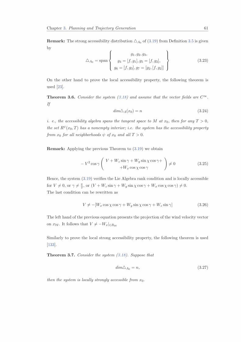
Chapter 3. Planning and Trajectory Generation 61
Remark: The strong accessibility distribution A0 of (3.19) from Definition 3.5 is given
by
A0 = span
g1, g2, g3,
g4 = [f, g1], g5 = [f, g2],
g6 = [f, g3], g7 = [g2, [f, g2]]
(3.23)
On the other hand to prove the local accessibility property, the following theorem is
used [23].
Theorem 3.6. Consider the system (3.18) and assume that the vector fields are C∞.
If
dimA(x0) = n (3.24)
i. e., the accessibility algebra spans the tangent space to M at x0, then for any T > 0,
the set Rψ(x0, T ) has a nonempty interior; i.e. the system has the accessibility property
from x0 for all neighborhoods ψ of x0 and all T > 0.
Remark: Applying the previous Theorem to (3.19) we obtain
− V 2 cos γ
(V +Wz sin γ +Wy sinχ cos γ+
+Wx cosχ cos γ
)%= 0 (3.25)
Hence, the system (3.19) verifies the Lie Algebra rank condition and is locally accessible
for V %= 0, or γ %= π2 , or (V +Wz sin γ +Wy sinχ cos γ +Wx cosχ cos γ) %= 0.
The last condition can be rewritten as
V %= −[Wx cosχ cos γ +Wy sinχ cos γ +Wz sin γ] (3.26)
The left hand of the previous equation presents the projection of the wind velocity vector
on xW . It follows that V %= −Wx|∈RW
Similarly to prove the local strong accessibility property, the following theorem is used
[133].
Theorem 3.7. Consider the system (3.18). Suppose that
dimA0 = n, (3.27)
then the system is locally strongly accessible from x0.

Chapter 3. Planning and Trajectory Generation 62
Remark: Using Theorem 3.7 the following condition is obtained
V 2 cos γ %= 0 (3.28)
Therefore the system (3.19) is locally strongly accessible if V %= 0 or γ %= π2 .
Notice that
1. Condition (3.24) is known as: Lie Algebra Rank Condition (LARC).
2. If the system (3.18) is driftless, i.e., f(X) = 0, the accessibility property charac-
terizes the controllability.
From the previous study, we conclude that the kinematic equations of the system can
be used to stabilize the aerial vehicle (airship/quad-rotor) around a trajectory. Observe
that, these equations do not provide us the (strong) accessibility property to stabilize
the vehicle in hovering flight mode (V = 0).
3.3.1.5 Controllability of kinematic aerial vehicle in the presence of constant
wind
In this section, we investigate another approach to find the necessary and sufficient
condition for the system (3.19) to be completely controllable. This method is a gener-
alization of the controllability analysis presented in [10] for a Dubins vehicle moving in
a plane in the presence of constant wind.
Assuming that the aircraft starts from an initial configuration q0 = [x0, y0, z0, γ0, χ0,
V0] to a final one qf = [xf , yf , zf , γf , χf , Vf ] as shown in Figure (3.5). In addition,
the wind velocity (Vw) is supposed to be a constant with a specified direction γw and
χw. Then, the guidance problem from q0 to qf in the presence of wind can be regarded
as a moving-target problem [10, 96]. For this purpose, it is more convenient to rewrite
Equation (3.19) as shown below
xn =V cosχ cos γ (3.29a)
yn =V sinχ cos γ (3.29b)
zn =V sin γ (3.29c)
γ =u1 (3.29d)
χ =u2 (3.29e)
V =u3 (3.29f)
where, xn ! x− wxt, yn ! y − wyt, and zn ! z − wzt.
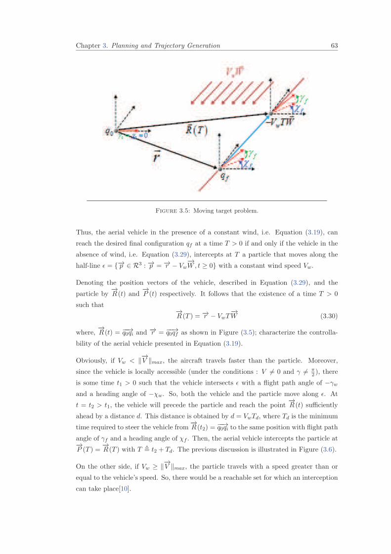
Chapter 3. Planning and Trajectory Generation 63
Figure 3.5: Moving target problem.
Thus, the aerial vehicle in the presence of a constant wind, i.e. Equation (3.19), can
reach the desired final configuration qf at a time T > 0 if and only if the vehicle in the
absence of wind, i.e. Equation (3.29), intercepts at T a particle that moves along the
half-line ǫ = −→p ∈ R3 : −→p = −→r − Vw−→W, t ≥ 0 with a constant wind speed Vw.
Denoting the position vectors of the vehicle, described in Equation (3.29), and the
particle by−→R (t) and
−→P (t) respectively. It follows that the existence of a time T > 0
such that−→R (T ) = −→r − VwT
−→W (3.30)
where,−→R (t) = −−→q0qi and
−→r = −−→q0qf as shown in Figure (3.5); characterize the controlla-
bility of the aerial vehicle presented in Equation (3.19).
Obviously, if Vw < ‖−→V ‖max, the aircraft travels faster than the particle. Moreover,
since the vehicle is locally accessible (under the conditions : V %= 0 and γ %= π2 ), there
is some time t1 > 0 such that the vehicle intersects ǫ with a flight path angle of −γw
and a heading angle of −χw. So, both the vehicle and the particle move along ǫ. At
t = t2 > t1, the vehicle will precede the particle and reach the point−→R (t) sufficiently
ahead by a distance d. This distance is obtained by d = VwTd, where Td is the minimum
time required to steer the vehicle from−→R (t2) =
−−→q0qi to the same position with flight path
angle of γf and a heading angle of χf . Then, the aerial vehicle intercepts the particle at−→P (T ) =
−→R (T ) with T ! t2 + Td. The previous discussion is illustrated in Figure (3.6).
On the other side, if Vw ≥ ‖−→V ‖max, the particle travels with a speed greater than or
equal to the vehicle’s speed. So, there would be a reachable set for which an interception
can take place[10].
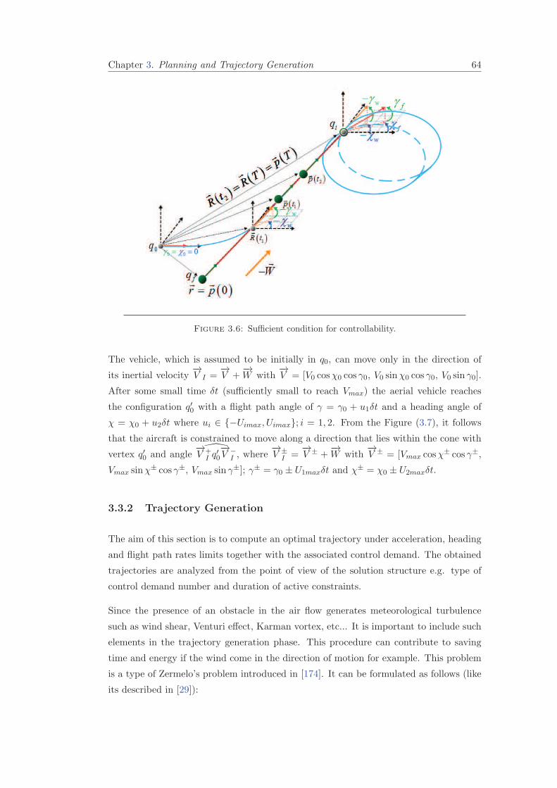
Chapter 3. Planning and Trajectory Generation 64
Figure 3.6: Sufficient condition for controllability.
The vehicle, which is assumed to be initially in q0, can move only in the direction of
its inertial velocity−→V I =
−→V +
−→W with
−→V = [V0 cosχ0 cos γ0, V0 sinχ0 cos γ0, V0 sin γ0].
After some small time δt (sufficiently small to reach Vmax) the aerial vehicle reaches
the configuration q′0 with a flight path angle of γ = γ0 + u1δt and a heading angle of
χ = χ0 + u2δt where ui ∈ −Uimax, Uimax; i = 1, 2. From the Figure (3.7), it follows
that the aircraft is constrained to move along a direction that lies within the cone with
vertex q′0 and angle−→
V +I q
′0
−→V −
I , where−→V ±
I =−→V ± +
−→W with
−→V ± = [Vmax cosχ
± cos γ±,
Vmax sinχ± cos γ±, Vmax sin γ
±]; γ± = γ0 ± U1maxδt and χ± = χ0 ± U2maxδt.
3.3.2 Trajectory Generation
The aim of this section is to compute an optimal trajectory under acceleration, heading
and flight path rates limits together with the associated control demand. The obtained
trajectories are analyzed from the point of view of the solution structure e.g. type of
control demand number and duration of active constraints.
Since the presence of an obstacle in the air flow generates meteorological turbulence
such as wind shear, Venturi effect, Karman vortex, etc... It is important to include such
elements in the trajectory generation phase. This procedure can contribute to saving
time and energy if the wind come in the direction of motion for example. This problem
is a type of Zermelo’s problem introduced in [174]. It can be formulated as follows (like
its described in [29]):
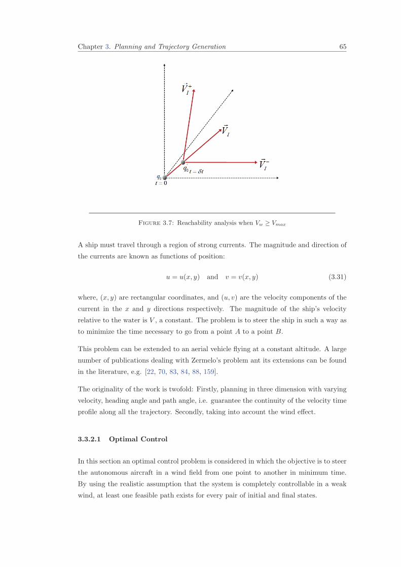
Chapter 3. Planning and Trajectory Generation 65
Figure 3.7: Reachability analysis when Vw ≥ Vmax
A ship must travel through a region of strong currents. The magnitude and direction of
the currents are known as functions of position:
u = u(x, y) and v = v(x, y) (3.31)
where, (x, y) are rectangular coordinates, and (u, v) are the velocity components of the
current in the x and y directions respectively. The magnitude of the ship’s velocity
relative to the water is V , a constant. The problem is to steer the ship in such a way as
to minimize the time necessary to go from a point A to a point B.
This problem can be extended to an aerial vehicle flying at a constant altitude. A large
number of publications dealing with Zermelo’s problem ant its extensions can be found
in the literature, e.g. [22, 70, 83, 84, 88, 159].
The originality of the work is twofold: Firstly, planning in three dimension with varying
velocity, heading angle and path angle, i.e. guarantee the continuity of the velocity time
profile along all the trajectory. Secondly, taking into account the wind effect.
3.3.2.1 Optimal Control
In this section an optimal control problem is considered in which the objective is to steer
the autonomous aircraft in a wind field from one point to another in minimum time.
By using the realistic assumption that the system is completely controllable in a weak
wind, at least one feasible path exists for every pair of initial and final states.
Chapter 3. Planning and Trajectory Generation 66
Thus, an admissible control trajectory u : [0, T ] .→ Ω ⊆ ℜm must be found such that
the aerial vehicle kinematic system described by the system of nonlinear differential
equations given in Equation (2.70) and Equation (2.100), which can be expressed as
X(t) = f (X(t), U(t), t) ;X(t) ∈ R6
U(t) ∈ R3(3.32)
is transferred from the initial configuration
x(0) = x0, y(0) = y0, z(0) = z0,χ(0) = χ0, γ(0) = γ0, V (0) = V0 (3.33)
into an admissible final configuration
x(T ) = xf , y(T ) = yf , z(T ) = zf ,χ(T ) = χf , γ(T ) = γf , V (T ) = Vf (3.34)
and such that the corresponding state trajectory satisfies the following limitations on
the control inputs and states
|u1| ≤u1max (3.35a)
|u2| ≤u2max (3.35b)
|u3| ≤u3max (3.35c)
|γ| ≤γmax (3.35d)
|V | ≤Vmax (3.35e)
(x− xc)2 + (y − yc)
2 + z2 ≥r2p (3.35f)
at all times t ∈ [0, T ] and such that the cost functional
min
∫ T
0dt (3.36)
is minimised.
The initial point can be required to be the origin of the ith way point and the final point
(i+ 1)th way point or the final destination point.
Note that Equation (3.35d) and Equation (3.35e) represents the physical limitations on
the vehicle while Equation (3.35f) describes a pillar of radius rp and situated in (xc, yc)
which is considered as an obstacle.
For points that are reachable, the resolution is based on the Pontryagin Minimum Princi-
ple which constitutes a generalization of Lagrange problem of the calculus of variations.
The Pontryagin Minimum Principle to obtain optimal control for the nonlinear system

Chapter 3. Planning and Trajectory Generation 67
3.32, without taking state constraints, Equation (3.35d), Equation (3.35e) and Equation
(3.35f), into account, can be summarized by the following different stages [19–21]
• Define the Hamiltonian function as
H(x(t), u(t),λ(t), t) = L(x(t), u(t), t) + λT f(t, x(t), u(t)) (3.37)
where, λ(t) is the co-state variable.
• Use the necessary condition of Weierstrass along x∗(t). Minimize H with respect to
|u(t)| ≤ umax as
H(x∗(t), u∗(t),λ∗(t), t) ≤ H(x∗(t), u(t),λ∗(t), t) (3.38)
where ∗ denote the optimal solution. This inequality must hold for any t for 0 ≤ t ≤ T .
• Solve the following set of 2n state and co-state equations:
x∗ =
(∂H
∂λ∗
)and λ∗ = −
(∂H
∂x∗
)(3.39)
such that the boundary conditions, Equation(3.33) and Equation (3.34), be satisfied.
This kind of problem is called Two Point Boundary Value Problem.
• Verify the transversality condition : If the final time T is free or not a priori spec-
ified and the Hamiltonian does not depend explicitly on time t, then the Hamiltonian
must be identically zero when evaluated along the optimal trajectory; that is
H(x∗(t), u∗(t),λ∗(t)) = 0 ∀t ∈ [0, T ] (3.40)
Let us now apply Pontryagin Minimum Principle to our system (3.19). The Hamiltonian
is defined as:
H = 1 + λ1(V cosχ cos γ +Wx) + λ2(V sinχ cos γ +Wy) (3.41)
+λ3(V sin γ +Wz) + λ4u1 + λ5u2 + λ6u3
The optimal control input must satisfy the following set of necessary conditions
X∗ =∂H
∂λ∗; λ∗ = −
∂H
∂X∗(3.42)
The co-state variables are free, i.e. unspecified, at both the initial and final times because
the corresponding state variables of the system are specified. A first interesting result
is the determination of a sufficient family of trajectories, i.e. a family of trajectories
containing an optimal solution for linking any two configurations.
The co-state equations are then obtained in the standard fashion by differentiating the
Chapter 3. Planning and Trajectory Generation 68
negative of the Hamiltonian with respect to the states where:
λ1∗= 0 ⇒ λ∗
1 = constant (3.43a)
λ2∗= 0 ⇒ λ∗
2 = constant (3.43b)
λ3∗= 0 ⇒ λ∗
3 = constant (3.43c)
λ4∗= λ∗
1V∗ cosχ∗ sin γ∗ + λ∗
2V∗ sinχ∗ sin γ∗ − λ∗
3V∗ cos γ∗ (3.43d)
λ5∗= λ∗
1V∗ sinχ∗ cos γ∗ − λ∗
2V∗ cosχ∗ cos γ∗ (3.43e)
= λ∗1(y
∗ −Wy)− λ∗2(x
∗ −Wx)
λ6∗= −λ∗
1 cosχ∗ cos γ∗ − λ∗
2 sinχ∗ cos γ∗ − λ∗
3 sin γ∗ (3.43f)
= −λ∗1
x∗ −Wx
V ∗− λ∗
2
y∗ −Wy
V ∗− λ∗
3
z∗ −Wz
V ∗
Defining the Hamiltonian and multiplier dynamics in this way, the minimum principle of
Pontryagin states that the control variable must be chosen to minimize the Hamiltonian
at every instant [130, 173].
Therefore, applying Equation (3.38) Leads to the following solution:
u∗i = δiuimax; i = 1, 2, 3 (3.44)
with δi denoting the -sign function defined as
δi =
1 for λ∗i+3 < 0
0 for λ∗i+3 = 0
−1 for λ∗i+3 > 0
(3.45)
This type of control called ′′bang-bang′′ is obtained from saturating inputs at all times,
or zero for singular control.
In order to take the states constraints into account we use penalty function methods
described in [130]. Let the inequality constraints on the states be expressed as
S (X(t), t) ≥ 0 (3.46)
where, S is a p ≤ n vector function of state and assumed to have continuous first and
second partial derivatives with respect to state x(t). Thus, Equation (3.35d), Equation
Chapter 3. Planning and Trajectory Generation 69
(3.35e) and Equation (3.35f) can be rewritten as follows
g1(γ) = γ2max − γ2 ≥ 0 (3.47a)
g2(V ) = V 2max − V 2 ≥ 0 (3.47b)
g3(x, y, z) = (x− xc)2 + (y − yc)
2 + z2 − r2p ≥ 0 (3.47c)
The key idea is to convert the inequality constraints into equality constraints. Therefore,
let us define a new state variable xn+1(t) by
Υ(t) = [g1(γ)]2H(g1) + [g2(V )]2H(g2) + [g2(x, y, z)]
2H(g3) (3.48)
where H(gi) is a unit Heaviside step function defined by
H(gi) =
0 for gi ≥ 0
1 for gi < 0(3.49)
The Equation (3.48) and Equation (3.49) mean that Υ(t) = 0 for all t when the con-
straints described in Equation (3.35d), Equation (3.35e), and Equation (3.35f) are sat-
isfied, whereas, Υ(t) ≥ 0 for all t, due to the square terms in Equation (3.48), if the
constraints are violated. Furthermore, let us require that the new variable Υ(t) has the
following boundary conditions
Υ(t0) = 0, and Υ(tf ) = 0 (3.50)
Let us now define the new Hamiltonian as
H = 1 + λ1(V cosχ cos γ +Wx) + λ2(V sinχ cos γ +Wy) + λ3(V sin γ +Wz) + λ4u1 (3.51)
+λ5u2 + λ6u3 + λ7
[[g1(γ)]
2H(g1) + [g2(V )]
2H(g2) + [g2(x, y, z)]
2H(g3)
]
Then, the necessary optimality conditions for the state are
X∗(t) = ∂H∂λ
Υ∗(t) = ∂H
∂λ7
(3.52)
and for the co-stateλ∗(t) = − ∂H
∂X
λ7∗(t) = −∂H
∂Υ= 0
(3.53)
Observe that λ7∗(t) = 0 because the Hamiltonian does not explicitly contain the new
state variable Υ(t).
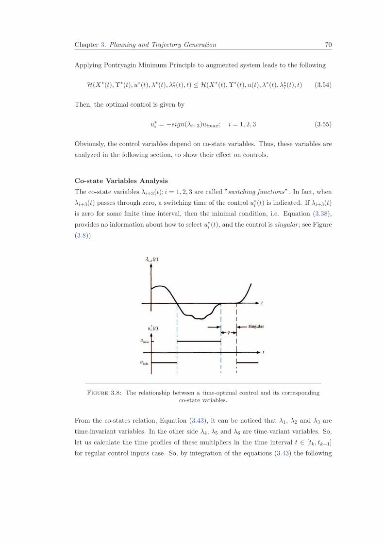
Chapter 3. Planning and Trajectory Generation 70
Applying Pontryagin Minimum Principle to augmented system leads to the following
H(X∗(t),Υ∗(t), u∗(t),λ∗(t),λ∗7(t), t) ≤ H(X∗(t),Υ∗(t), u(t),λ∗(t),λ∗
7(t), t) (3.54)
Then, the optimal control is given by
u∗i = −sign(λi+3)uimax; i = 1, 2, 3 (3.55)
Obviously, the control variables depend on co-state variables. Thus, these variables are
analyzed in the following section, to show their effect on controls.
Co-state Variables Analysis
The co-state variables λi+3(t); i = 1, 2, 3 are called ”switching functions”. In fact, when
λi+3(t) passes through zero, a switching time of the control u∗i (t) is indicated. If λi+3(t)
is zero for some finite time interval, then the minimal condition, i.e. Equation (3.38),
provides no information about how to select u∗i (t), and the control is singular ; see Figure
(3.8)).
Figure 3.8: The relationship between a time-optimal control and its correspondingco-state variables.
From the co-states relation, Equation (3.43), it can be noticed that λ1, λ2 and λ3 are
time-invariant variables. In the other side λ4, λ5 and λ6 are time-variant variables. So,
let us calculate the time profiles of these multipliers in the time interval t ∈ [tk, tk+1]
for regular control inputs case. So, by integration of the equations (3.43) the following
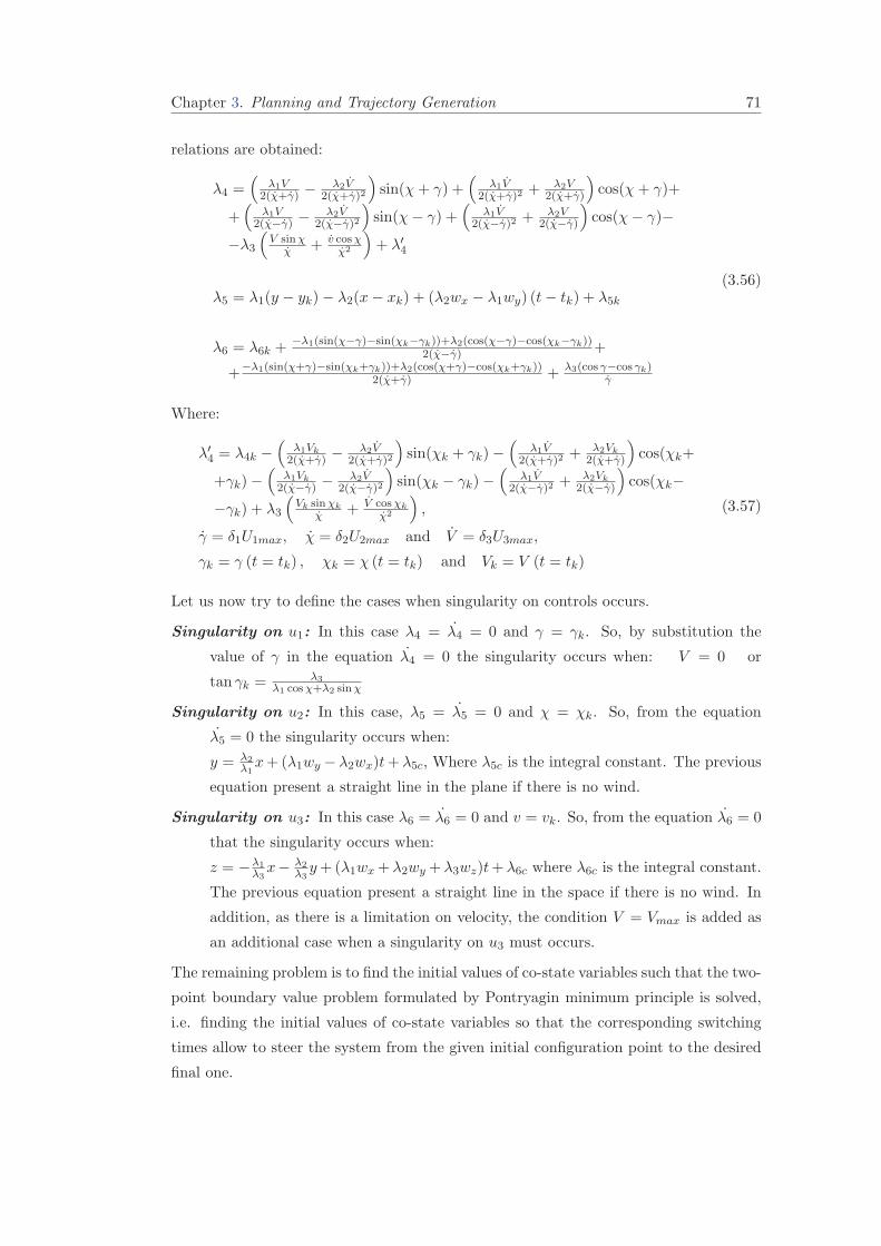
Chapter 3. Planning and Trajectory Generation 71
relations are obtained:
λ4 =(
λ1V2(χ+γ) −
λ2V2(χ+γ)2
)sin(χ+ γ) +
(λ1V
2(χ+γ)2+ λ2V
2(χ+γ)
)cos(χ+ γ)+
+(
λ1V2(χ−γ) −
λ2V2(χ−γ)2
)sin(χ− γ) +
(λ1V
2(χ−γ)2+ λ2V
2(χ−γ)
)cos(χ− γ)−
−λ3
(V sinχ
χ+ v cosχ
χ2
)+ λ′
4
λ5 = λ1(y − yk)− λ2(x− xk) + (λ2wx − λ1wy) (t− tk) + λ5k
λ6 = λ6k +−λ1(sin(χ−γ)−sin(χk−γk))+λ2(cos(χ−γ)−cos(χk−γk))
2(χ−γ) +
+−λ1(sin(χ+γ)−sin(χk+γk))+λ2(cos(χ+γ)−cos(χk+γk))2(χ+γ) + λ3(cos γ−cos γk)
γ
(3.56)
Where:
λ′4 = λ4k −
(λ1Vk
2(χ+γ) −λ2V
2(χ+γ)2
)sin(χk + γk)−
(λ1V
2(χ+γ)2+ λ2Vk
2(χ+γ)
)cos(χk+
+γk)−(
λ1Vk2(χ−γ) −
λ2V2(χ−γ)2
)sin(χk − γk)−
(λ1V
2(χ−γ)2+ λ2Vk
2(χ−γ)
)cos(χk−
−γk) + λ3
(Vk sinχk
χ+ V cosχk
χ2
),
γ = δ1U1max, χ = δ2U2max and V = δ3U3max,
γk = γ (t = tk) , χk = χ (t = tk) and Vk = V (t = tk)
(3.57)
Let us now try to define the cases when singularity on controls occurs.
Singularity on u1: In this case λ4 = λ4 = 0 and γ = γk. So, by substitution the
value of γ in the equation λ4 = 0 the singularity occurs when: V = 0 or
tan γk = λ3λ1 cosχ+λ2 sinχ
Singularity on u2: In this case, λ5 = λ5 = 0 and χ = χk. So, from the equation
λ5 = 0 the singularity occurs when:
y = λ2λ1x+ (λ1wy − λ2wx)t+ λ5c, Where λ5c is the integral constant. The previous
equation present a straight line in the plane if there is no wind.
Singularity on u3: In this case λ6 = λ6 = 0 and v = vk. So, from the equation λ6 = 0
that the singularity occurs when:
z = −λ1λ3x− λ2
λ3y+(λ1wx +λ2wy +λ3wz)t+λ6c where λ6c is the integral constant.
The previous equation present a straight line in the space if there is no wind. In
addition, as there is a limitation on velocity, the condition V = Vmax is added as
an additional case when a singularity on u3 must occurs.
The remaining problem is to find the initial values of co-state variables such that the two-
point boundary value problem formulated by Pontryagin minimum principle is solved,
i.e. finding the initial values of co-state variables so that the corresponding switching
times allow to steer the system from the given initial configuration point to the desired
final one.

Chapter 3. Planning and Trajectory Generation 72
Optimal Trajectories Analysis
This paragraph presents the time profiles of x, y, z, γ, χ and V for a time interval
t ∈ [tk tk+1] under two types of control inputs, i.e. regular (δiUimax ∈ +1,−1) and
singular (δiUimax = 0) control. Only the final result of the analytical integrations is
given:
– Regular arcs:
For regular control inputs, 8 different arcs exist as shown in the table (3.1).
u1 u2 u3
Regular arc type 1 +U1max +U2max +U3max
Regular arc type 2 +U1max +U2max −U3max
Regular arc type 3 +U1max −U2max +U3max
Regular arc type 4 +U1max −U2max −U3max
Regular arc type 5 −U1max +U2max +U3max
Regular arc type 6 −U1max +U2max −U3max
Regular arc type 7 −U1max −U2max +U3max
Regular arc type 8 −U1max −U2max −U3max
Table 3.1: The different arc types of regular control
So, the general arc of regular control is given as follows:
x = xk +v sin(χ+γ)−Vk sin(χk+γk)
2(δ2U2max+δ1U1max)+ δ3U3max(cos(χ+γ)−cos(χk+γk))
2(δ2U2max+δ1U1max)2+
+v sin(χ−γ)−Vk sin(χk−γk)2(δ2U2max−δ1U1max)
+ δ3U3max(cos(χ−γ)−cos(χk−γk))2(δ2U2max−δ1U1max)2
+ wx(t− tk)(3.58)
y = yk −v cos(χ+γ)−Vk cos(χk+γk)
2(δ2U2max+δ1U1max)+ δ3U3max(sin(χ+γ)−sin(χk+γk))
2(δ2U2max+δ1U1max)2−
−v cos(χ−γ)−Vk cos(χk−γk)2(δ2U2max−δ1U1max)
+ δ3U3max(sin(χ−γ)−sin(χk−γk))2(δ2U2max−δ1U1max)2
+ wy(t− tk)(3.59)
z = zk −v cos γ − vk cos γk
δ1U1max+
v(sin γ − sin γk)
U21max
+ wz(t− tk) (3.60)
γ = δ1U1max(t− tk) + γk (3.61)
χ = δ2U2max(t− tk) + χk (3.62)
v = δ3U3max(t− tk) + vk (3.63)
– Singular arcs:
In this case,7 different arcs exist as shown in the table (3.2).
The equations of the first type of singular arcs: In this case u1 = u2 = u3 = 0. Which
lead us to:x = (vk cosχk cos γk + wx)(t− tk) + xk
y = (vk sinχk cos γk + wy)(t− tk) + yk
z = (vk sin γk + wz)(t− tk) + zk
γ = γk, χ = χk, v = vk
(3.64)
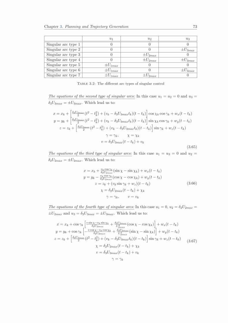
Chapter 3. Planning and Trajectory Generation 73
u1 u2 u3
Singular arc type 1 0 0 0
Singular arc type 2 0 0 ±U3max
Singular arc type 3 0 ±U2max 0
Singular arc type 4 0 ±U2max ±U3max
Singular arc type 5 ±U1max 0 0
Singular arc type 6 ±U1max 0 ±U3max
Singular arc type 7 ±U1max ±U2max 0
Table 3.2: The different arc types of singular control
The equations of the second type of singular arcs: In this case u1 = u2 = 0 and u3 =
δ3U3max = ±U3max. Which lead us to:
x = xk +[δ3U3max
2 (t2 − t2k) + (vk − δ3U3maxtk)(t− tk)]cosχk cos γk + wx(t− tk)
y = yk +[δ3U3max
2 (t2 − t2k) + (vk − δ3U3maxtk)(t− tk)]sinχk cos γk + wy(t− tk)
z = zk +[δ3U3max
2 (t2 − t2k) + (vk − δ3U3maxtk)(t− tk)]sin γk + wz(t− tk)
γ = γk, χ = χk
v = δ3U3max(t− tk) + vk(3.65)
The equations of the third type of singular arcs: In this case u1 = u3 = 0 and u2 =
δ2U2max = ±U2max. Which lead us to:
x = xk +vk cos γkδ2U2max
(sinχ− sinχk) + wx(t− tk)
y = yk −vk cos γkδ2U2max
(cosχ− cosχk) + wy(t− tk)
z = zk + (vk sin γk + wz)(t− tk)
χ = δ2U2max(t− tk) + χk
γ = γk, v = vk
(3.66)
The equations of the fourth type of singular arcs: In this case u1 = 0, u2 = δ2U2max =
±U2max and u3 = δ3U3max = ±U3max. Which lead us to:
x = xk + cos γk
[v sinχ−vk sinχk
δ2U2max+ δ3U3max
U22max
(cosχ− cosχk)]+ wx(t− tk)
y = yk + cos γk
[−v cosχ−vk cosχk
δ2U2max+ δ3U3max
U22max
(sinχ− sinχk)]+ wy(t− tk)
z = zk +[δ3U3max
2 (t2 − t2k) + (vk − δ3U3maxtk)(t− tk)]sin γk + wz(t− tk)
χ = δ2U2max(t− tk) + χk
v = δ3U3max(t− tk) + vk
γ = γk
(3.67)
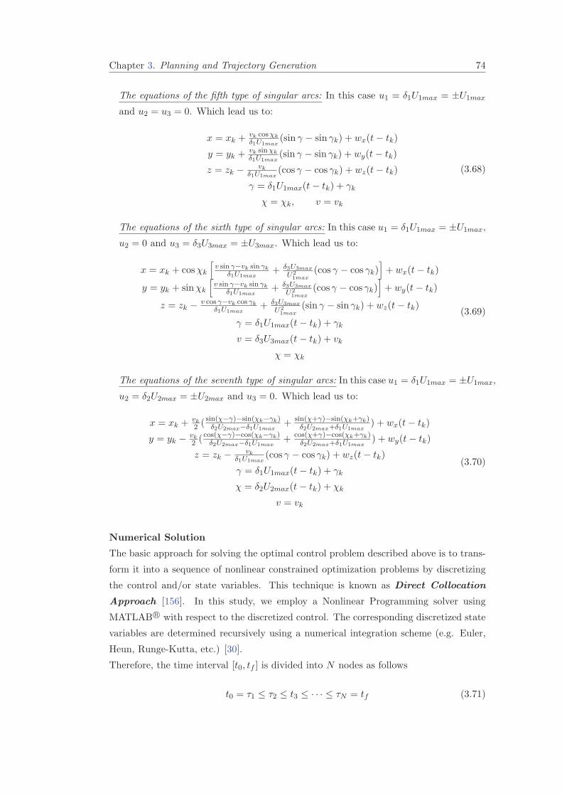
Chapter 3. Planning and Trajectory Generation 74
The equations of the fifth type of singular arcs: In this case u1 = δ1U1max = ±U1max
and u2 = u3 = 0. Which lead us to:
x = xk +vk cosχkδ1U1max
(sin γ − sin γk) + wx(t− tk)
y = yk +vk sinχkδ1U1max
(sin γ − sin γk) + wy(t− tk)
z = zk −vk
δ1U1max(cos γ − cos γk) + wz(t− tk)
γ = δ1U1max(t− tk) + γk
χ = χk, v = vk
(3.68)
The equations of the sixth type of singular arcs: In this case u1 = δ1U1max = ±U1max,
u2 = 0 and u3 = δ3U3max = ±U3max. Which lead us to:
x = xk + cosχk
[v sin γ−vk sin γk
δ1U1max+ δ3U3max
U21max
(cos γ − cos γk)]+ wx(t− tk)
y = yk + sinχk
[v sin γ−vk sin γk
δ1U1max+ δ3U3max
U21max
(cos γ − cos γk)]+ wy(t− tk)
z = zk −v cos γ−vk cos γk
δ1U1max+ δ3U3max
U21max
(sin γ − sin γk) + wz(t− tk)
γ = δ1U1max(t− tk) + γk
v = δ3U3max(t− tk) + vk
χ = χk
(3.69)
The equations of the seventh type of singular arcs: In this case u1 = δ1U1max = ±U1max,
u2 = δ2U2max = ±U2max and u3 = 0. Which lead us to:
x = xk +vk2 (
sin(χ−γ)−sin(χk−γk)δ2U2max−δ1U1max
+ sin(χ+γ)−sin(χk+γk)δ2U2max+δ1U1max
) + wx(t− tk)
y = yk −vk2 (
cos(χ−γ)−cos(χk−γk)δ2U2max−δ1U1max
+ cos(χ+γ)−cos(χk+γk)δ2U2max+δ1U1max
) + wy(t− tk)
z = zk −vk
δ1U1max(cos γ − cos γk) + wz(t− tk)
γ = δ1U1max(t− tk) + γk
χ = δ2U2max(t− tk) + χk
v = vk
(3.70)
Numerical Solution
The basic approach for solving the optimal control problem described above is to trans-
form it into a sequence of nonlinear constrained optimization problems by discretizing
the control and/or state variables. This technique is known as Direct Collocation
Approach [156]. In this study, we employ a Nonlinear Programming solver using
MATLAB R© with respect to the discretized control. The corresponding discretized state
variables are determined recursively using a numerical integration scheme (e.g. Euler,
Heun, Runge-Kutta, etc.) [30].
Therefore, the time interval [t0, tf ] is divided into N nodes as follows
t0 = τ1 ≤ τ2 ≤ t3 ≤ · · · ≤ τN = tf (3.71)
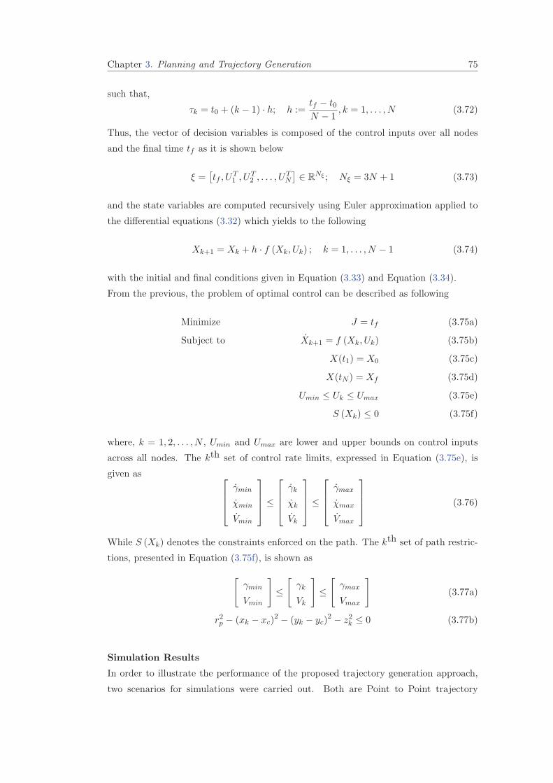
Chapter 3. Planning and Trajectory Generation 75
such that,
τk = t0 + (k − 1) · h; h :=tf − t0N − 1
, k = 1, . . . , N (3.72)
Thus, the vector of decision variables is composed of the control inputs over all nodes
and the final time tf as it is shown below
ξ =[tf , U
T1 , U
T2 , . . . , U
TN
]∈ R
Nξ ; Nξ = 3N + 1 (3.73)
and the state variables are computed recursively using Euler approximation applied to
the differential equations (3.32) which yields to the following
Xk+1 = Xk + h · f (Xk, Uk) ; k = 1, . . . , N − 1 (3.74)
with the initial and final conditions given in Equation (3.33) and Equation (3.34).
From the previous, the problem of optimal control can be described as following
Minimize J = tf (3.75a)
Subject to Xk+1 = f (Xk, Uk) (3.75b)
X(t1) = X0 (3.75c)
X(tN ) = Xf (3.75d)
Umin ≤ Uk ≤ Umax (3.75e)
S (Xk) ≤ 0 (3.75f)
where, k = 1, 2, . . . , N , Umin and Umax are lower and upper bounds on control inputs
across all nodes. The kth set of control rate limits, expressed in Equation (3.75e), is
given as
γmin
χmin
Vmin
≤
γk
χk
Vk
≤
γmax
χmax
Vmax
(3.76)
While S (Xk) denotes the constraints enforced on the path. The kth set of path restric-
tions, presented in Equation (3.75f), is shown as
[γmin
Vmin
]≤
[γk
Vk
]≤
[γmax
Vmax
](3.77a)
r2p − (xk − xc)2 − (yk − yc)
2 − z2k ≤ 0 (3.77b)
Simulation Results
In order to illustrate the performance of the proposed trajectory generation approach,
two scenarios for simulations were carried out. Both are Point to Point trajectory

Chapter 3. Planning and Trajectory Generation 76
with the same initial and final conditions. The first one presents a trajectory without
wind. While the second one take the presence of the wind into consideration. The
vehicle constraints and the initial/final configurations are provided in Tab. 3.7 and
Tab. 3.8 respectively. The wind is supposed to be a constant having the value of :
W = [Wx,Wy,Wz] = [2, 2, 1].
The trajectory in each case is discretized over 70 nodes, and the interior point algorithm
included in fmincon nonlinear programming solver in MATLAB" is used to compute
optimal trajectory. The obtained trajectory is described in Figure (3.9) and Figure
(3.10). The red and solid line denotes the case of the presence of the wind. The blue
dashed line is the trajectory without wind. The green arrows describe the direction of
the wind.
Table 3.3: Vehicle’s restrictions.
Minimum Variable Maximum Units
-20 γ 20 deg-5 V 5 m/sec-5 γ 5 deg/sec- 15 χ 15 deg/sec
- 1.25 V 1.25 m/sec2
Table 3.4: Initial and final configurations.
x [m] y [m] z [m] γ [Deg] χ [Deg] V [m/sec]
Initial value 0 0 0 0 0 3Desired value 30 20 10 0 0 4
Notice that the magnitude of the wind in this scenario is ||W || = 3[m/sec] which presents
60% of the vehicle’s maximal velocity. Remark that the final configuration is reached in
tf = 7.21[sec] in the presence of the wind, while it requires tf = 10.8[sec] to be attained
if there is no wind. Such results are consistent in the sense where the wind push the
vehicle from the back. However, if the wind comes from the front of the vehicle, it is
obvious that it will slow down the velocity and consequently the aircraft will require
more time to reach its target.
3.3.2.2 Sub-Optimal Trajectory Generation Algorithm
In this section, we introduce a trajectory generation algorithm based on geometrical
solution to join two points. The provided trajectory is near-optimal, and in some cases,
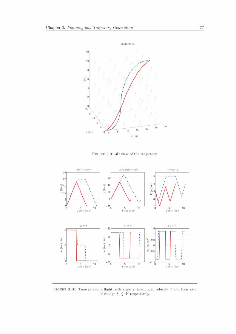
Chapter 3. Planning and Trajectory Generation 77
05
1015
2025
30
0
5
10
15
20
25
0
2
4
6
8
10
12
x [m]
Trajectory
y [m]
z[m
]
Figure 3.9: 3D view of the trajectory.
0 5 100
5
10
15
20
25
P athAngle
T ime [sec]
γ[D
eg]
0 5 10−20
0
20
40
60
HeadingAngle
T ime [sec]
χ[D
eg]
0 5 101
2
3
4
5
V elocity
T ime [sec]
V[m
/sec]
0 5 10
−5
0
5
u1 = γ
T ime [sec]
u1[D
eg/sec]
0 5 10−20
−10
0
10
20
u2 = χ
T ime [sec]
u2[D
eg/sec]
0 5 10−1.5
−1
−0.5
0
0.5
1
1.5
u3 = V
T ime [sec]
u3[m
/sec2]
Figure 3.10: Time profile of flight path angle γ, heading χ, velocity V and their rateof change γ, χ, V respectively.
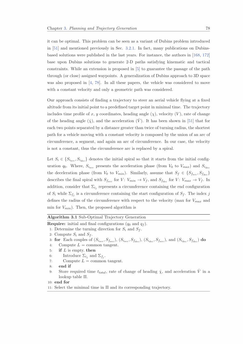
Chapter 3. Planning and Trajectory Generation 78
it can be optimal. This problem can be seen as a variant of Dubins problem introduced
in [51] and mentioned previously in Sec. 3.2.1. In fact, many publications on Dubins-
based solutions were published in the last years. For instance, the authors in [168, 172]
base upon Dubins solutions to generate 2-D paths satisfying kinematic and tactical
constraints. While an extension is proposed in [5] to guarantee the passage of the path
through (or close) assigned waypoints. A generalization of Dubins approach to 3D space
was also proposed in [4, 78]. In all these papers, the vehicle was considered to move
with a constant velocity and only a geometric path was considered.
Our approach consists of finding a trajectory to steer an aerial vehicle flying at a fixed
altitude from its initial point to a predefined target point in minimal time. The trajectory
includes time profile of x, y coordinates, heading angle (χ), velocity (V ), rate of change
of the heading angle (χ), and the acceleration (V ). It has been shown in [51] that for
each two points separated by a distance greater than twice of turning radius, the shortest
path for a vehicle moving with a constant velocity is composed by the union of an arc of
circumference, a segment, and again an arc of circumference. In our case, the velocity
is not a constant, thus the circumference arc is replaced by a spiral.
Let Si ∈ Siacc , Sidec denotes the initial spiral so that it starts from the initial config-
uration q0. Where, Siacc presents the acceleration phase (from V0 to Vmax) and Sidec
the deceleration phase (from V0 to Vmin). Similarly, assume that Sf ∈ Sfacc , Sfdec
describes the final spiral with Sfacc for V : Vmin → Vf , and Sfdec for V : Vmax → Vf . In
addition, consider that Σij represents a circumference containing the end configuration
of Si while Σfj is a circumference containing the start configuration of Sf . The index j
defines the radius of the circumference with respect to the velocity (max for Vmax and
min for Vmin). Then, the proposed algorithm is
Algorithm 3.1 Sub-Optimal Trajectory Generation
Require: initial and final configurations (q0 and qf ).1: Determine the turning direction for Si and Sf .2: Compute Si and Sf .3: for Each couples of (Siacc , Sfacc), (Siacc , Sfdec), (Sidec , Sfacc), and (Sidec , Sfdec) do4: Compute L = common tangent.5: if L is empty. then6: Introduce Σij and Σfj .7: Compute L = common tangent.8: end if9: Store required time ttotal, rate of change of heading χ, and acceleration V in a
lookup table Π.10: end for11: Select the minimal time in Π and its corresponding trajectory.
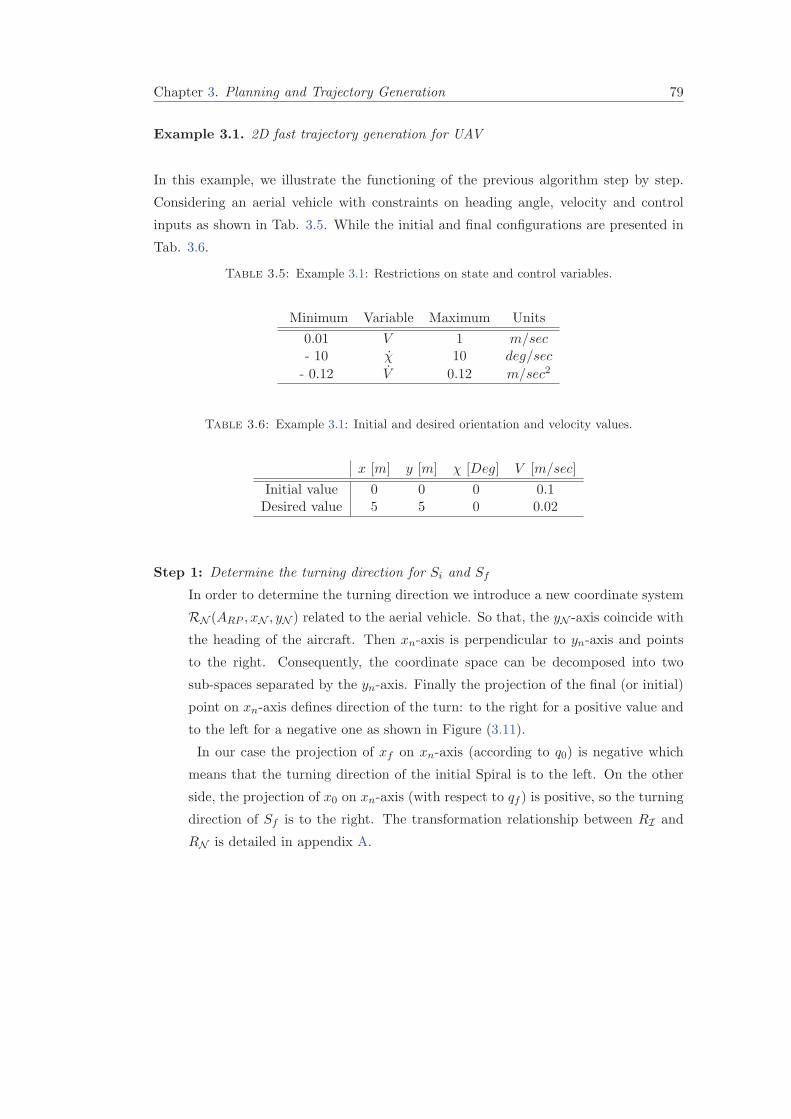
Chapter 3. Planning and Trajectory Generation 79
Example 3.1. 2D fast trajectory generation for UAV
In this example, we illustrate the functioning of the previous algorithm step by step.
Considering an aerial vehicle with constraints on heading angle, velocity and control
inputs as shown in Tab. 3.5. While the initial and final configurations are presented in
Tab. 3.6.
Table 3.5: Example 3.1: Restrictions on state and control variables.
Minimum Variable Maximum Units
0.01 V 1 m/sec- 10 χ 10 deg/sec
- 0.12 V 0.12 m/sec2
Table 3.6: Example 3.1: Initial and desired orientation and velocity values.
x [m] y [m] χ [Deg] V [m/sec]
Initial value 0 0 0 0.1Desired value 5 5 0 0.02
Step 1: Determine the turning direction for Si and Sf
In order to determine the turning direction we introduce a new coordinate system
RN (ARP , xN , yN ) related to the aerial vehicle. So that, the yN -axis coincide with
the heading of the aircraft. Then xn-axis is perpendicular to yn-axis and points
to the right. Consequently, the coordinate space can be decomposed into two
sub-spaces separated by the yn-axis. Finally the projection of the final (or initial)
point on xn-axis defines direction of the turn: to the right for a positive value and
to the left for a negative one as shown in Figure (3.11).
In our case the projection of xf on xn-axis (according to q0) is negative which
means that the turning direction of the initial Spiral is to the left. On the other
side, the projection of x0 on xn-axis (with respect to qf ) is positive, so the turning
direction of Sf is to the right. The transformation relationship between RI and
RN is detailed in appendix A.
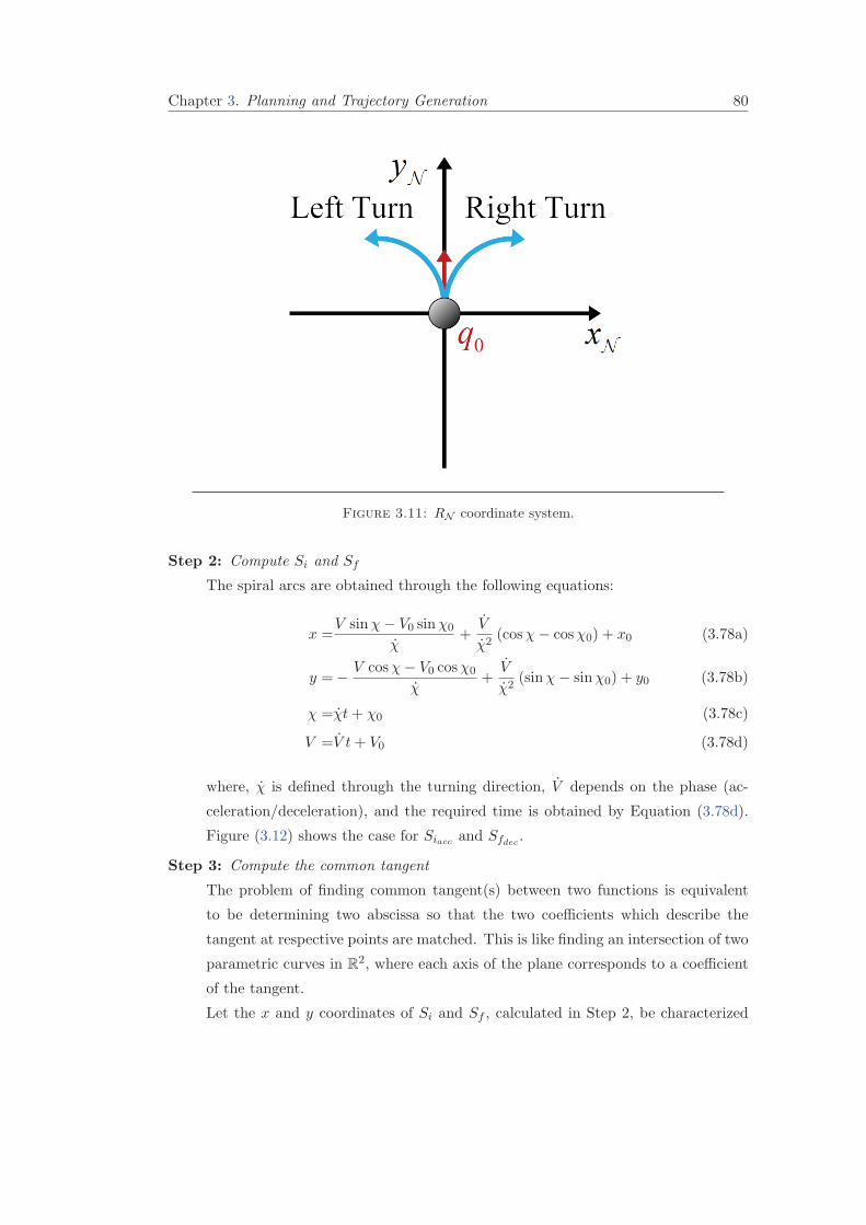
Chapter 3. Planning and Trajectory Generation 80
Figure 3.11: RN coordinate system.
Step 2: Compute Si and Sf
The spiral arcs are obtained through the following equations:
x =V sinχ− V0 sinχ0
χ+
V
χ2(cosχ− cosχ0) + x0 (3.78a)
y =−V cosχ− V0 cosχ0
χ+
V
χ2(sinχ− sinχ0) + y0 (3.78b)
χ =χt+ χ0 (3.78c)
V =V t+ V0 (3.78d)
where, χ is defined through the turning direction, V depends on the phase (ac-
celeration/deceleration), and the required time is obtained by Equation (3.78d).
Figure (3.12) shows the case for Siacc and Sfdec .
Step 3: Compute the common tangent
The problem of finding common tangent(s) between two functions is equivalent
to be determining two abscissa so that the two coefficients which describe the
tangent at respective points are matched. This is like finding an intersection of two
parametric curves in R2, where each axis of the plane corresponds to a coefficient
of the tangent.
Let the x and y coordinates of Si and Sf , calculated in Step 2, be characterized

Chapter 3. Planning and Trajectory Generation 81
0 0.5 1 1.5 2 2.5 3 3.5 4 4.5 50
0.5
1
1.5
2
2.5
3
3.5
4
4.5
5
x [m]
y[m
]
SiaccSfdec
q0
qf
Figure 3.12: Computing initial and final spirals: the case of Siaccand Sfdec .
by a cubic-spline as follows:
ySi = G1(x1) =ς3x21 + ς2x
21 + ς1x1 + ς0 (3.79a)
ySf= G2(x2) =ι3x
22 + ι2x
22 + ι1x2 + ι0 (3.79b)
where x1 ∈ x0 → xSi(end), and x2 ∈ xSf(start) → xf. Then the set of
tangents to Si can be defined by the equation
yG1 = aG1x+ bG1 (3.80)
where, aG1 is the slope of the line and bG1 is the constant term, called also y-
intercept. In addition, the slope of the tangent line is given by
aG1 =df(x1)
x1(3.81)
Therefore, from Equation (3.80) and Equation (3.81), we state the first parametric
curve as bellow
aG1 =3ς23x21 + 2ς2x1 + ς1 (3.82a)
bG1 =yG1 − aG1x1 (3.82b)
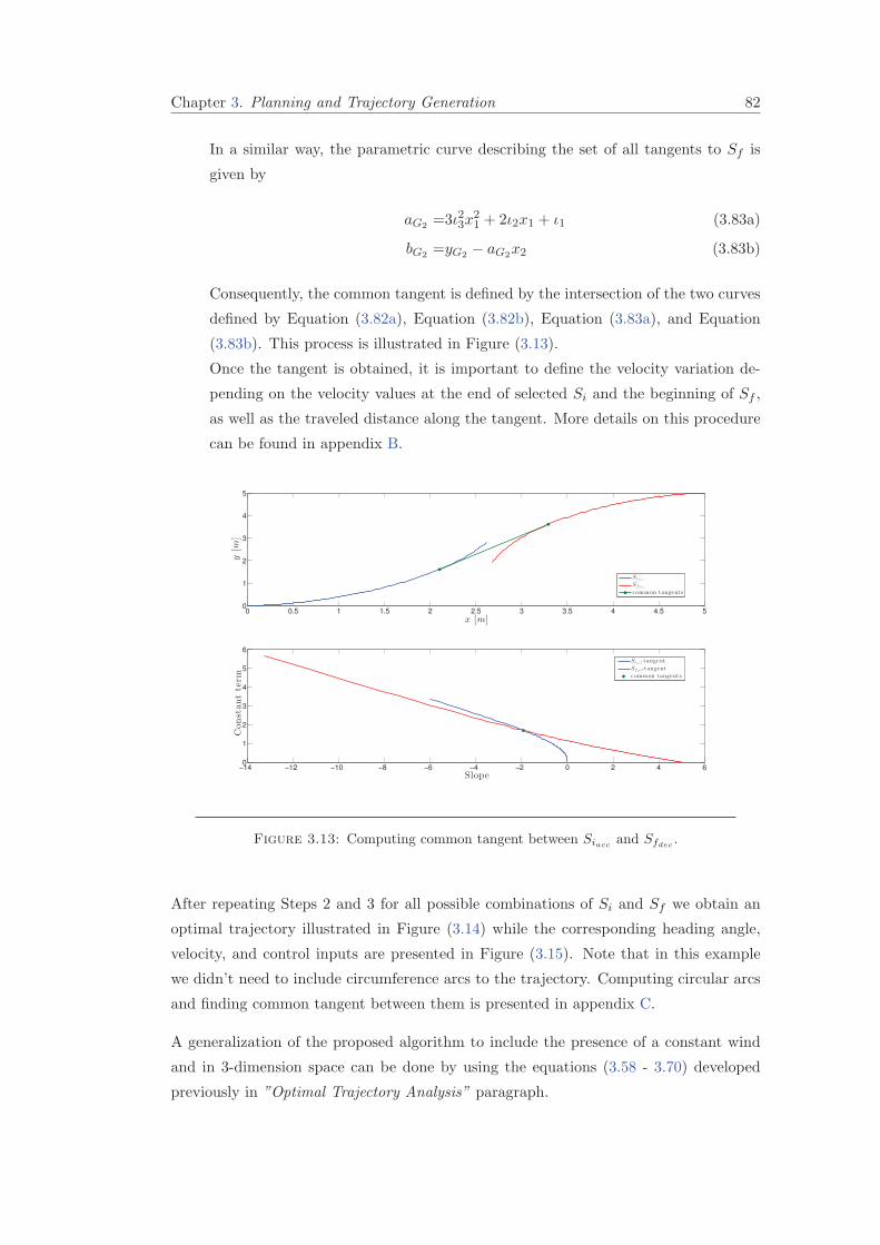
Chapter 3. Planning and Trajectory Generation 82
In a similar way, the parametric curve describing the set of all tangents to Sf is
given by
aG2 =3ι23x21 + 2ι2x1 + ι1 (3.83a)
bG2 =yG2 − aG2x2 (3.83b)
Consequently, the common tangent is defined by the intersection of the two curves
defined by Equation (3.82a), Equation (3.82b), Equation (3.83a), and Equation
(3.83b). This process is illustrated in Figure (3.13).
Once the tangent is obtained, it is important to define the velocity variation de-
pending on the velocity values at the end of selected Si and the beginning of Sf ,
as well as the traveled distance along the tangent. More details on this procedure
can be found in appendix B.
0 0.5 1 1.5 2 2.5 3 3.5 4 4.5 50
1
2
3
4
5
x [m]
y[m
]
−14 −12 −10 −8 −6 −4 −2 0 2 4 60
1
2
3
4
5
6
Slope
Constantterm
Sia c c-tangent
Sf d e c-tangent
common tangents
Sia c c
Sf d e c
common tangents
Figure 3.13: Computing common tangent between Siaccand Sfdec .
After repeating Steps 2 and 3 for all possible combinations of Si and Sf we obtain an
optimal trajectory illustrated in Figure (3.14) while the corresponding heading angle,
velocity, and control inputs are presented in Figure (3.15). Note that in this example
we didn’t need to include circumference arcs to the trajectory. Computing circular arcs
and finding common tangent between them is presented in appendix C.
A generalization of the proposed algorithm to include the presence of a constant wind
and in 3-dimension space can be done by using the equations (3.58 - 3.70) developed
previously in ”Optimal Trajectory Analysis” paragraph.
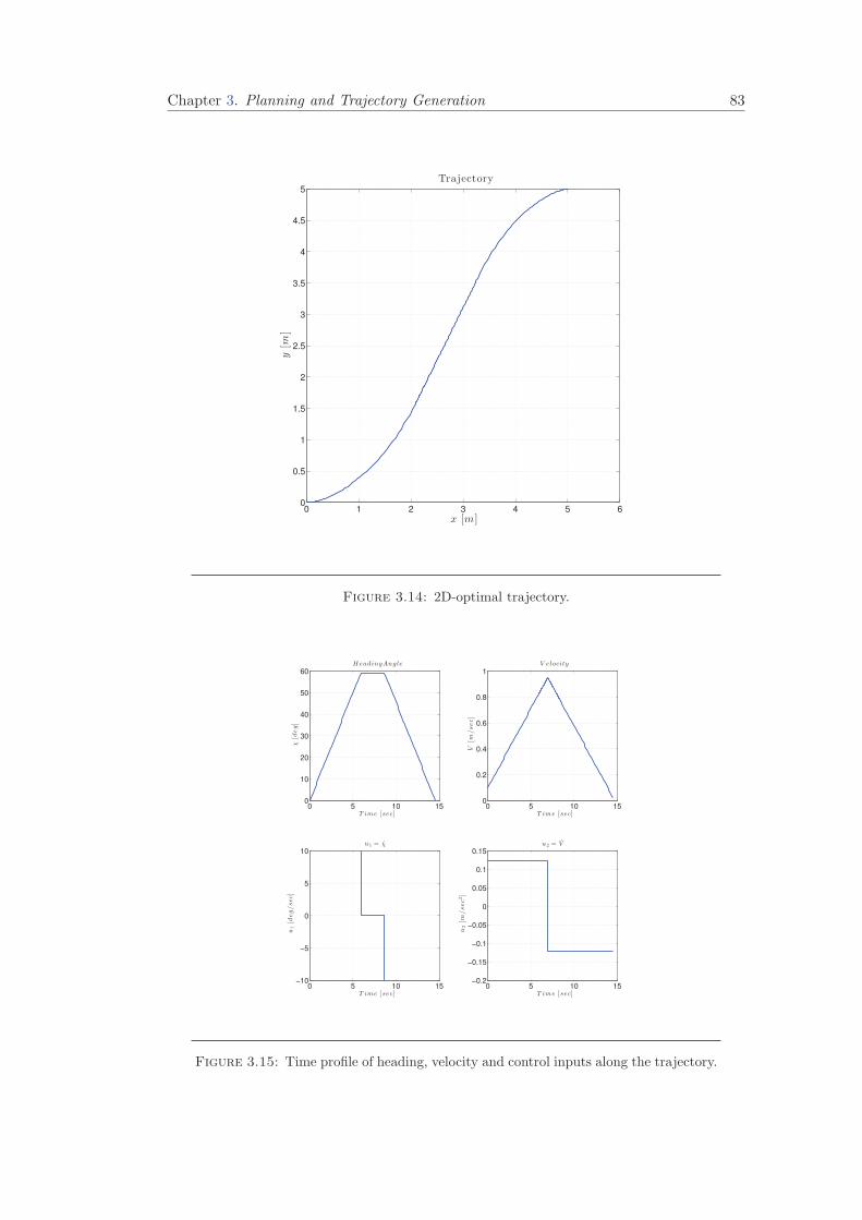
Chapter 3. Planning and Trajectory Generation 83
0 1 2 3 4 5 60
0.5
1
1.5
2
2.5
3
3.5
4
4.5
5
Trajectory
x [m]
y[m
]
Figure 3.14: 2D-optimal trajectory.
0 5 10 150
10
20
30
40
50
60
HeadingAngle
T ime [sec]
χ[deg]
0 5 10 150
0.2
0.4
0.6
0.8
1
V elocity
T ime [sec]
V[m
/sec]
0 5 10 15−10
−5
0
5
10
u 1 = χ
T ime [sec]
u1[deg/sec]
0 5 10 15−0.2
−0.15
−0.1
−0.05
0
0.05
0.1
0.15
u 2 = V
T ime [sec]
u2[m
/sec2]
Figure 3.15: Time profile of heading, velocity and control inputs along the trajectory.
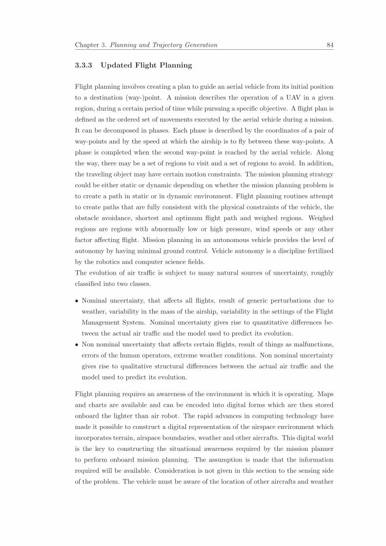
Chapter 3. Planning and Trajectory Generation 84
3.3.3 Updated Flight Planning
Flight planning involves creating a plan to guide an aerial vehicle from its initial position
to a destination (way-)point. A mission describes the operation of a UAV in a given
region, during a certain period of time while pursuing a specific objective. A flight plan is
defined as the ordered set of movements executed by the aerial vehicle during a mission.
It can be decomposed in phases. Each phase is described by the coordinates of a pair of
way-points and by the speed at which the airship is to fly between these way-points. A
phase is completed when the second way-point is reached by the aerial vehicle. Along
the way, there may be a set of regions to visit and a set of regions to avoid. In addition,
the traveling object may have certain motion constraints. The mission planning strategy
could be either static or dynamic depending on whether the mission planning problem is
to create a path in static or in dynamic environment. Flight planning routines attempt
to create paths that are fully consistent with the physical constraints of the vehicle, the
obstacle avoidance, shortest and optimum flight path and weighed regions. Weighed
regions are regions with abnormally low or high pressure, wind speeds or any other
factor affecting flight. Mission planning in an autonomous vehicle provides the level of
autonomy by having minimal ground control. Vehicle autonomy is a discipline fertilized
by the robotics and computer science fields.
The evolution of air traffic is subject to many natural sources of uncertainty, roughly
classified into two classes.
• Nominal uncertainty, that affects all flights, result of generic perturbations due to
weather, variability in the mass of the airship, variability in the settings of the Flight
Management System. Nominal uncertainty gives rise to quantitative differences be-
tween the actual air traffic and the model used to predict its evolution.
• Non nominal uncertainty that affects certain flights, result of things as malfunctions,
errors of the human operators, extreme weather conditions. Non nominal uncertainty
gives rise to qualitative structural differences between the actual air traffic and the
model used to predict its evolution.
Flight planning requires an awareness of the environment in which it is operating. Maps
and charts are available and can be encoded into digital forms which are then stored
onboard the lighter than air robot. The rapid advances in computing technology have
made it possible to construct a digital representation of the airspace environment which
incorporates terrain, airspace boundaries, weather and other aircrafts. This digital world
is the key to constructing the situational awareness required by the mission planner
to perform onboard mission planning. The assumption is made that the information
required will be available. Consideration is not given in this section to the sensing side
of the problem. The vehicle must be aware of the location of other aircrafts and weather
Chapter 3. Planning and Trajectory Generation 85
(e.g. storms). A number of methods exists for obtaining this information, as a radar
based system of the airborne dependent surveillance broadcast can provide the location
and speed of nearby aircraft.
Similarly, weather radar can also provide information for adverse weather condition.
In addition to the location of the entities within the world, their dimensions must be
known. Once the digital representation of the world (i.e. situational awareness) has
been created, high level activities such as mission planning can be performed.
In this study, the idea is simple: as uncertainty always exists due to numerous reasons, a
way of taking care of it is to update periodically the reference paths. If due to the wind
effect, the aerial vehicle has overshoot the way point it was supposed to go through, then
the next way point should be considered. The immediate measurements of the position
and orientation are taken as initial conditions for the next reference trajectories.
3.3.3.1 Basic Problem Statement
The basic problem is to move the vehicle from an initial configuration to the next
configuration. This question was solved in the previous section. The actual measured
wind velocity is assumed to be constant between two updates of the reference trajectories.
The constraints are first expressed in terms of thrust and velocities and then transformed
into limitations on flight path and heading angles.
3.3.3.2 Hierarchical Planning Structure
The structure necessary for the update of the reference trajectories is described in this
paragraph. A hierarchical structure appears because of the choice of the predicted arrival
time at each update. There exists an upper level of decision making and a lower level
where the time optimal problem is solved. One clock, associated with the lower level,
allows the reference trajectories computing. It is reset at each update. The following
concepts must be introduced to describe this hierarchical structure operation
• Periodic Updates : First, periodic updates are introduced. The period ∆ may be 10 to
100 times greater than the integration step of the differential equation. This depends
on the nature of the next way-point: fly-by, fly-over or destination point.
• Anticipated Updates : An important perturbation may occur between two periodic
updates. To handle this situation, a new reference trajectory is required. The concept
of anticipated update is thus important. To decide whether an important perturbation
occurs the System needs a supervision level.
• Supervision level: The supervision system is based on a spatiotemporal criterion.
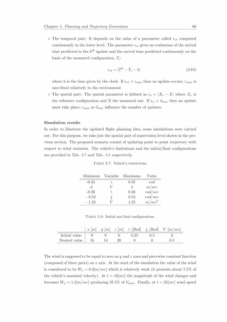
Chapter 3. Planning and Trajectory Generation 86
The temporal part: It depends on the value of a parameter called ect computed
continuously in the lower level. The parameter ect gives an evaluation of the arrival
time predicted in the kth update and the arrival time predicted continuously on the
basis of the measured configuration, Tc:
ect = |T k − Tc − h| (3.84)
where h is the time given by the clock. If ect > εmin then an update occurs; εmin is
user-fixed relatively to the environment
The spatial part: The spatial parameter is defined as es = |Xr − X| where Xr is
the reference configuration and X the measured one. If ex > δmin then an update
must take place; εmin as δmin influence the number of updates.
Simulation results
In order to illustrate the updated flight planning idea, some simulations were carried
out. For this purpose, we take just the spatial part of supervision level shown in the pre-
vious section. The proposed scenario consist of updating point to point trajectory with
respect to wind variation. The vehicle’s limitations and the initial/final configurations
are provided in Tab. 3.7 and Tab. 3.8 respectively.
Table 3.7: Vehicle’s restrictions.
Minimum Variable Maximum Units
-0.35 γ 0.35 rad-4 V 4 m/sec
-0.26 γ 0.26 rad/sec- 0.52 χ 0.52 rad/sec
- 1.25 V 1.25 m/sec2
Table 3.8: Initial and final configurations.
x [m] y [m] z [m] γ [Rad] χ [Rad] V [m/sec]
Initial value 0 0 0 0.25 0.5 2Desired value 16 14 20 0 0 0.5
The wind is supposed to be equal to zero on y and z axes and piecewise constant function
(composed of three parts) on x axis. At the start of the simulation the value of the wind
is considered to be Wx = 0.3[m/sec] which is relatively weak (it presents about 7.5% of
the vehicle’s maximal velocity). At t = 10[sec] the magnitude of the wind changes and
becomes Wx = 1.5[m/sec] producing 37.5% of Vmax. Finally, at t = 25[sec] wind speed

Chapter 3. Planning and Trajectory Generation 87
slow down to Wx = 0.5[m/sec] (12.5% of Vmax). Note that this value is equal to Vf .
The previous is presented in Figure (3.16).
Figure 3.16: The wind variation on x axis.
The resulting updated reference trajectory is illustrated in Figure (3.17) - Figure (3.19).
In those figures, the red line marked with triangle denotes the reference trajectories
given for the UAV while the solid blue line describe the computed trajectory from the
initial/actual configuration to the desired one.
A 3D view of the updated trajectory is shown in Figure (3.17). Whereas a side views of
this trajectory in the plane x.y and x.z are shown in the Figure (3.18) and Figure (3.19)
respectively.
Note that discontinuities on the reference trajectories are present. This is due to the
updates, when the real situation is taken into account.
3.3.4 UAV Routing Problem for Bridge Inspection
In this part, we consider the problem of bridge inspection using a small UAV. This
problem has been addressed in [70, 71]. In those papers, the authors have proposed two
solutions based on a hybridization between Zermelo’s navigation problem and TSP/VRP
approaches. The wind was supposed to vary linearly and the pillar was assumed as
points of interest to be visited by the vehicle. In other words, the configuration space
was considered to be obstacle-free. In addition, each point was characterized by only
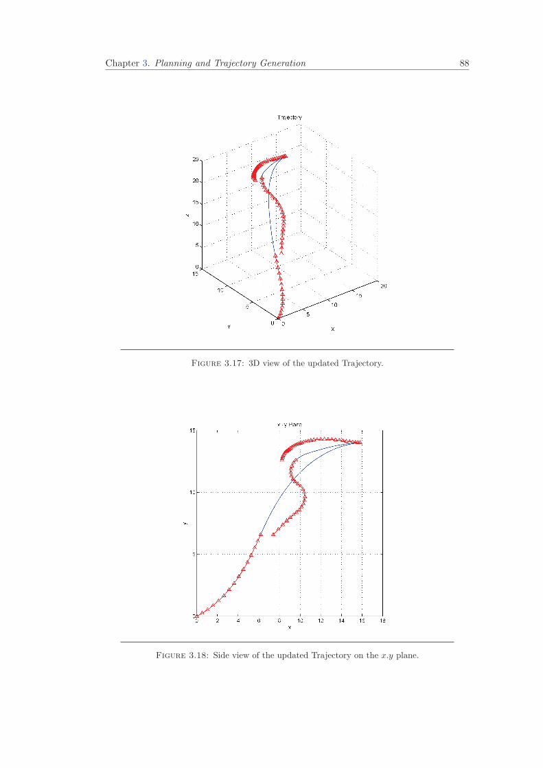
Chapter 3. Planning and Trajectory Generation 88
Figure 3.17: 3D view of the updated Trajectory.
Figure 3.18: Side view of the updated Trajectory on the x.y plane.
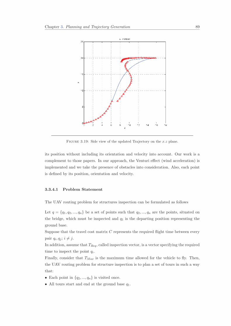
Chapter 3. Planning and Trajectory Generation 89
Figure 3.19: Side view of the updated Trajectory on the x.z plane.
its position without including its orientation and velocity into account. Our work is a
complement to those papers. In our approach, the Venturi effect (wind acceleration) is
implemented and we take the presence of obstacles into consideration. Also, each point
is defined by its position, orientation and velocity.
3.3.4.1 Problem Statement
The UAV routing problem for structures inspection can be formulated as follows
Let q = q1, q2, ..., qn be a set of points such that q2, ..., qn are the points, situated on
the bridge, which must be inspected and q1 is the departing position representing the
ground base.
Suppose that the travel cost matrix C represents the required flight time between every
pair qi, qj ; i %= j.
In addition, assume that TReq, called inspection vector, is a vector specifying the required
time to inspect the point qi.
Finally, consider that TMax is the maximum time allowed for the vehicle to fly. Then,
the UAV routing problem for structure inspection is to plan a set of tours in such a way
that:
• Each point in q2, ..., qn is visited once.
• All tours start and end at the ground base q1.
Chapter 3. Planning and Trajectory Generation 90
• The maximum time allowed to fly is never violated.
• The total time required to all tours is the minimum.
It is important to state here that the travel cost matrix is asymmetric. So, the required
time to fly from a point qi with an orientation of γi,χi and a velocity of Vi and arriving
at another point qj with an orientation of γj ,χj and a velocity of Vj may not be equal
to the required time to fly in the inverse direction.
3.3.4.2 Capacitated Vehicle Routing Problem
The Capacitated Vehicle Routing Problem is an interesting approach for structures
monitoring tasks. In fact, the limited carrying capacity of goods are replaced by an
allowed maximum flight time, and the number of vehicle can be regarded as the number
of vehicles required in UAVs fleet; Or the number of flights (for one aerial vehicle) needed
to cover the points of interest. To solve such a problem, a wide variety of methods have
been developed. These approaches are, frequently, classified as follows
• Constructive Methods: savings and insertion
• Improvement Methods: 2-change, 3-change, 2-relocate, 3-relocate, sweep, GENI.
In the following section, we present the savings method developed for solving CVRP.
Savings Method
The savings approach is an heuristic algorithm which was first proposed in 1964 by
Clarke and Wright [36] to solve a CVRP in which the number of vehicles is free. Its
basic idea is very simple. Considering a depot D and n demand points. Supposing that
initially the solution to the VRP consists of using n vehicles and dispatching one vehicle
to each one of the n demand points. Then, obviously, the total tour length of a such
solution is 2∑n
i=1C(D, i).
Now, if we use a single vehicle to serve two points, e.g. i and j, on a single trip, the total
distance traveled is reduced by the following amount
S(i, j) = 2C(D, i) + 2C(D, j)− [C(D, i) + C(i, j) + C(D, j)]
= C(D, i) + C(D, j)− C(i, j)(3.85)
The quantity S(i, j) is known as the savings resulting from combining points i and j
into a single tour. Whenever the value of S(i, j) larger, combining i and j in a single
tour becomes more desirable. However, i and j cannot be combined if the resulting tour
violates one or more of the constraints of the VRP.
Before describing the algorithm, we introduce the following definition

Chapter 3. Planning and Trajectory Generation 91
Definition 3.8. A point i is said to be interior to a route if it is not adjacent to the
depot D in the order of the traversal of points.
The savings algorithm of Clarke and Wright can now be presented (as expressed in [109])
as follows
Step 1 Compute the savings S(i, j) = C(D, i) +C(D, j)−C(i, j) for i, j = 2, .., n, and
i %= j.
Step 2 Rank the savings in descending order of magnitude.
Step 3 For the savings S(i, j) under consideration, include the arc (i, j) in a route if
the constraints imposed on the route will not be violated, and if
a. Neither i nor j have already been assigned to a route. In this case, a new
route is initiated including both i and j.
b. Exactly one of the two points (i or j) has already been included in an existing
route and that point is not interior to that route. In this case, the arc (i, j)
is added to the same route.
c. Both i and j have already been included in two different existing routes and
neither point is interior to its route. In this case, both routes are merged.
Step 4 If the savings list S(i, j) has not been exhausted, return to Step 3 and shift to
the next entry in the list;
otherwise, stop.
Note that, any points that have not been assigned yet to a route during Step 3 must
be served by a vehicle route that begins at the depot D visits the unassigned point and
returns to D.
The Clarke-Wright algorithm can be programmed to run very efficiently and, since
it involves very simple manipulations of the data set, it can be used with large-scale
problems. Since nodes are added to routes once or twice at a time, an additional
advantage of the algorithm is that it is possible to check whether each addition would
violate any set of constraints, even when that set is quite complicated. For example,
besides the constraints on maximum capacity and maximum distance, other constraints
might be included, such as a maximum number of points that any vehicle may visit.
A number of variants of this method was proposed, e.g. [67, 135]. The Clarke and
Wright algorithm suppose that the cost matrix C is symmetric, i.e. C(i, j) = C(j, i).
In addition it implicitly ignores vehicle fixed costs and fleet size. Vehicle costs f can
easily be taken into account by adding this constant to every Cj (j = 2, ..., n). Solutions
with a fixed number of vehicles can be obtained by repeating Step 3 until the required
number of routes has been reached, even if the savings become negative.
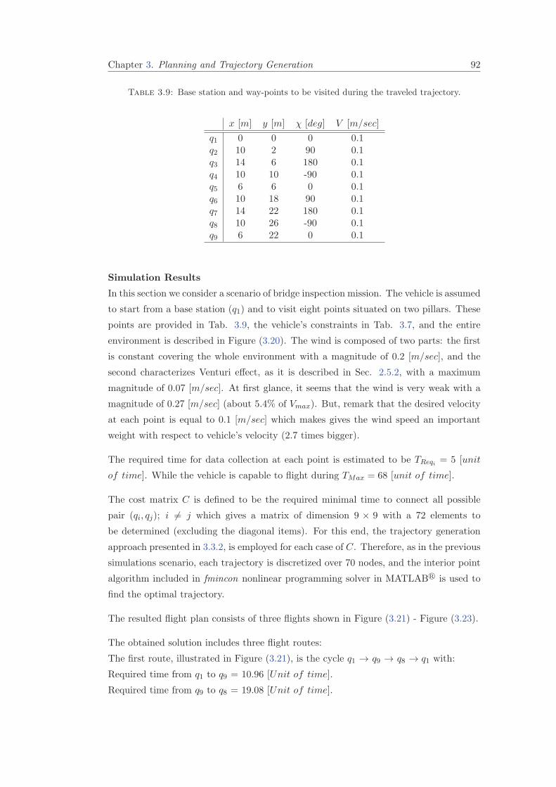
Chapter 3. Planning and Trajectory Generation 92
Table 3.9: Base station and way-points to be visited during the traveled trajectory.
x [m] y [m] χ [deg] V [m/sec]
q1 0 0 0 0.1q2 10 2 90 0.1q3 14 6 180 0.1q4 10 10 -90 0.1q5 6 6 0 0.1q6 10 18 90 0.1q7 14 22 180 0.1q8 10 26 -90 0.1q9 6 22 0 0.1
Simulation Results
In this section we consider a scenario of bridge inspection mission. The vehicle is assumed
to start from a base station (q1) and to visit eight points situated on two pillars. These
points are provided in Tab. 3.9, the vehicle’s constraints in Tab. 3.7, and the entire
environment is described in Figure (3.20). The wind is composed of two parts: the first
is constant covering the whole environment with a magnitude of 0.2 [m/sec], and the
second characterizes Venturi effect, as it is described in Sec. 2.5.2, with a maximum
magnitude of 0.07 [m/sec]. At first glance, it seems that the wind is very weak with a
magnitude of 0.27 [m/sec] (about 5.4% of Vmax). But, remark that the desired velocity
at each point is equal to 0.1 [m/sec] which makes gives the wind speed an important
weight with respect to vehicle’s velocity (2.7 times bigger).
The required time for data collection at each point is estimated to be TReqi = 5 [unit
of time]. While the vehicle is capable to flight during TMax = 68 [unit of time].
The cost matrix C is defined to be the required minimal time to connect all possible
pair (qi, qj); i %= j which gives a matrix of dimension 9 × 9 with a 72 elements to
be determined (excluding the diagonal items). For this end, the trajectory generation
approach presented in 3.3.2, is employed for each case of C. Therefore, as in the previous
simulations scenario, each trajectory is discretized over 70 nodes, and the interior point
algorithm included in fmincon nonlinear programming solver in MATLAB" is used to
find the optimal trajectory.
The resulted flight plan consists of three flights shown in Figure (3.21) - Figure (3.23).
The obtained solution includes three flight routes:
The first route, illustrated in Figure (3.21), is the cycle q1 → q9 → q8 → q1 with:
Required time from q1 to q9 = 10.96 [Unit of time].
Required time from q9 to q8 = 19.08 [Unit of time].
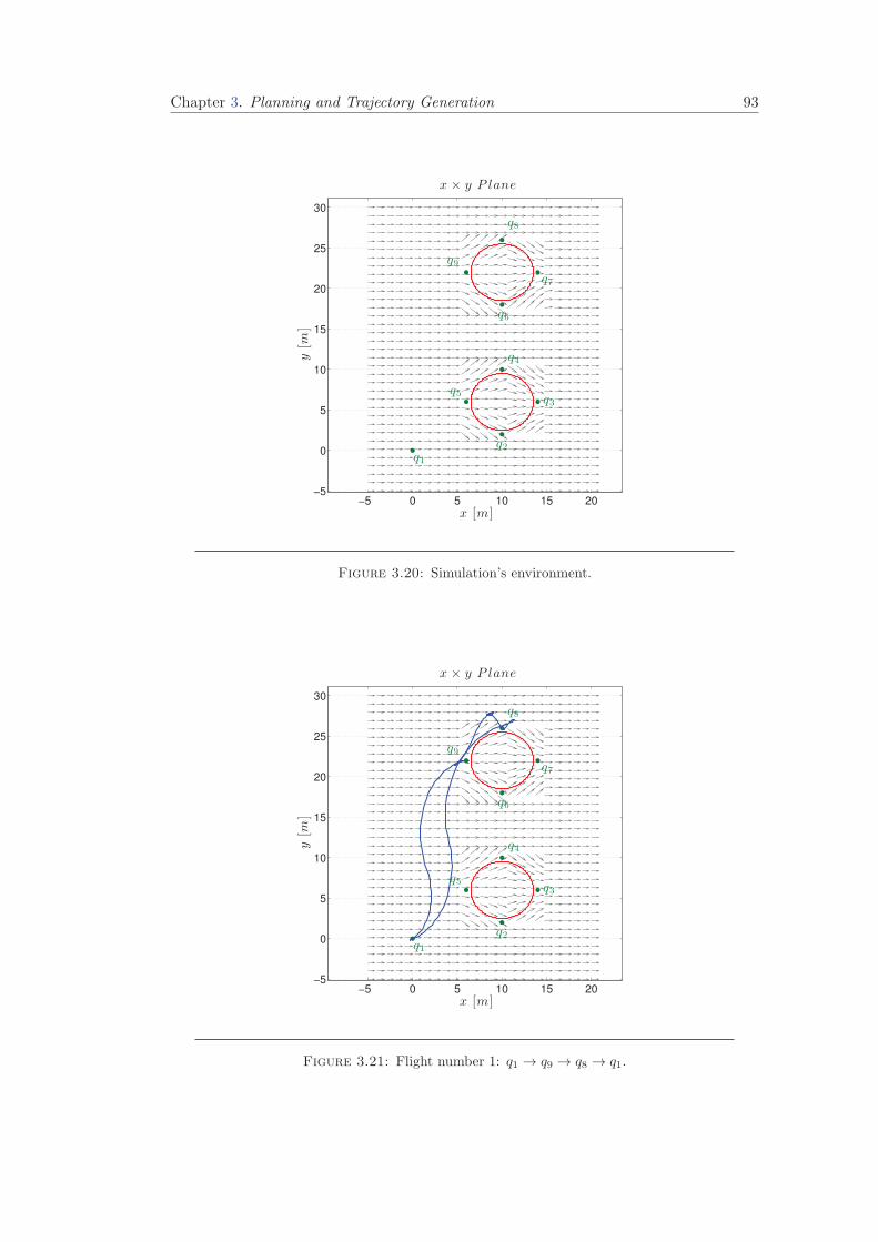
Chapter 3. Planning and Trajectory Generation 93
−5 0 5 10 15 20−5
0
5
10
15
20
25
30
x × y P lane
x [m]
y[m
]
q1
q2
q3
q4
q5
q6
q7
q8
q9
Figure 3.20: Simulation’s environment.
−5 0 5 10 15 20−5
0
5
10
15
20
25
30
x × y P lane
x [m]
y[m
]
q1
q2
q3
q4
q5
q6
q7
q8
q9
Figure 3.21: Flight number 1: q1 → q9 → q8 → q1.

Chapter 3. Planning and Trajectory Generation 94
−5 0 5 10 15 20−5
0
5
10
15
20
25
30
x × y P lane
x [m]
y[m
]
q1
q2
q3
q4
q5
q6
q7
q8
q9
Figure 3.22: Flight number 2: q1 → q2 → q6 → q3 → q1.
−5 0 5 10 15 20−5
0
5
10
15
20
25
30
x × y P lane
x [m]
y[m
]
q1
q2
q3
q4
q5
q6
q7
q8
q9
Figure 3.23: Flight number 3: q1 → q5 → q7 → q4 → q1.
Chapter 3. Planning and Trajectory Generation 95
Required time from q8 to q1 = 13.57 [Unit of time].
Total flight time on the route T = 53.62 [Unit of time].
The second route, presented in Figure (3.22), is the cycle q1 → q2 → q6 → q3 → q1 with:
Required time from q1 to q2 = 6.42 [Unit of time].
Required time from q2 to q6 = 10.43 [Unit of time].
Required time from q6 to q3 = 8.72 [Unit of time].
Required time from q3 to q1 = 8.91 [Unit of time].
Total flight time on the route T = 49.49 [Unit of time].
The third route, described in Figure (3.23), is the cycle q1 → q5 → q7 → q4 → q1 with:
Required time from q1 to q5 = 6.86 [Unit of time].
Required time from q5 to q7 = 12.97 [Unit of time].
Required time from q7 to q4 = 7.55 [Unit of time].
Required time from q4 to q1 = 10.00 [Unit of time].
Total flight time on the route T = 52.39 [Unit of time].
Notice that the total time for each route respects the vehicle’s capacity.
3.4 Conclusion
In this chapter, we have investigated the motion planning and trajectory generation
question for small UAV-based structure inspection missions. First of all, the accessibility
and controllability issues were considered. It has been proved that a kinematic aerial
vehicle is strongly accessible under the condition that its velocity is not equal to zero
and its flight path angle do not reach ninety degrees. Even-more, it has been shown that
the vehicle could be completely controllable if the wind velocity is strictly less than the
vehicle’s velocity.
Next, the problem of trajectory generation was addressed. An analysis of the time-
optimal trajectories of a kinematic aerial vehicle considering second-order constraints,
with a piecewise constant wind and the presence of obstacles was presented. The
minimum-time flight problem is formulated as a problem of the calculus of variations.
This formulation is converted to nonlinear constrained optimization problems and the
solution is obtained through a direct collocation approach. Geometric characterization
of the candidate trajectories satisfying the necessary conditions for time optimality was
also described. This characterization is used to develop a sub-optimal fast trajectory
generation algorithm. Besides, an updated flight planning is presented using the receding
horizon control as wind is considered to be piecewise constant.
Chapter 3. Planning and Trajectory Generation 96
Likewise, a strategy for trajectory planning was developed. The proposed method is
based on operational research approaches, especially capacitated vehicle routing prob-
lem. In fact, the solution is a modified CVRP algorithm that includes the maximum
flight time and loitering in optimization objective.
Chapter 4
Trajectory Tracking
Once a feasible and flyable trajectory is generated, it becomes necessary to move one
step down into low-level control design, that means, to deal with trajectory tracking
question. Such problem consists in stabilizing the state, or an output function of the
state, to a desired reference value, possibly time-varying [123]. The control strategies
proposed for this aim include two categories: traditional control methods and advanced
control [118]. The classical control algorithms (like PID) have the advantage to be easily
implemented and to provide reliable control performance. On the other hand, advanced
control methods are mainly developed to improve its control performance in a complex
and unstable flight environment.
4.1 Introduction
In order to make an unmanned aerial vehicle asymptotically track a desired reference tra-
jectory, several control methods have been developed in literature such as backstepping
control, robust control, model-prediction control and other intelligent control methods
[17, 33].
In [167], a robust control method for an airship is introduced. The control strategy
consists of an inner H∞ controller for the dynamics and an outer Single Input Sin-
gle Output Proportional or Proportional-Integral controller for the remaining states.
Similarly different solutions are also proposed, namely one-loop-at-a-time PID [125]
and Proportional-Integral control [54], sliding modes techniques [45, 171], vision-based
[8, 64, 73, 95, 149, 150, 163], fuzzy logic [138] and fuzzy logic improved with genetic al-
gorithms [137]. Other approaches include dynamic inversion for lateral and longitudinal
control with desired dynamics given by a linear optimal compensator[124] and input-
output linearization with a nonlinear controller [18, 170]. In the same way in [153], a
97
Chapter 4. Trajectory Tracking 98
nonlinear control strategy based on extended linearization is proposed to stabilize the
aerodynamic speed, altitude and heading of a small sized airship in cruise flight phase.
A popular technique used to control lighter than air vehicles is the backstepping method-
ology. In [14], the authors propose a time-varying controller, based on this approach, to
stabilize both the orientation and the position of this aerial vehicle to a fixed value. In
[13], a backstepping tracking feedback control for ascent and descent flight maneuvers is
also introduced. In this work the desired trajectories were constrained to be trimming.
In a similar way, in [139] and [11] the authors introduce a trajectory tracking controller
for the airship based on this approach. Furthermore, a control strategy based on com-
bination of backstepping and Exact Tracking Error Dynamics Passive Output Feedback
(ETDPOE) is proposed in [129].
Artificial neural network is another approach currently applied to airship control de-
signs. For example in [136], a neural network is applied to compensate the underlying
model errors and to control velocity, pitch and yaw angles for an airship. Likewise in
[86], a Particle Swarm Optimization algorithm and an updated neural network model to
approximate a tri-turbofan airship are presented. On the other hand, robust controllers
to stabilize airships have been also proposed. In [175], a robust adaptive controller us-
ing Lyapunov method and Matrosov theorem are presented. Similarly in [66], a model
predictive control is introduced to stabilize the airship system taking into account in-
equality constraints on position, velocity and thrust. In addition in [65], the inverse
optimal control approach was employed to design a trajectory tracking controller to sta-
bilize an airship in ideal environment. The proposed method takes only the uncertainties
into account without paying any attention to the potential perturbations applied on the
vehicle such wind gusts.
Even though there are a lot of modern control techniques which can be adopted for
unmanned aerial vehicle control, robust controllers remain interesting for real appli-
cations of these vehicles when they are exposed to unknown environment (like wind
gusts). In this chapter, we focus on introducing a robust control strategy to make au-
tonomous trajectory following of lighter than air/quad-rotors vehicles in the presence
of wind gust. The control algorithm is based on Robust Control Lyapunov Function
and Sontag’s universal stabilizing feedback. This method has been successfully applied
to the PVTOL aircraft and quad-rotors craft exposed to crosswind with a constant set
point [127, 128], neverthless it has never been applied to trajectory tracking for 3DOF
translational model of lighter than air vehicle and quad-rotors craft.
The rest of this chapter is organized as follows: The section 4.2 is dedicated to introduce
the concept of the Robust Control Lyapunov Function. While, the section 4.4 presents a
Chapter 4. Trajectory Tracking 99
nonlinear controller to stabilize kinematic airship/quad-rotors vehicles. The section 4.5
addresses the stabilization problem for a lighter than air vehicle tacking its dynamics, i.e.
Equation (2.95), into consideration. Finally, the section 4.6 describes autopilot design
strategy to a quad-rotors craft, based on its rigid body model, i.e. Equation (2.63).
4.2 Robust Control Lyapunov Function
Mathematical models of actual systems contain uncertainty terms representing the de-
signer’s lack of knowledge about parameter values and disturbances. These quantities
and inaccuracies in mathematical modeling itself, contribute to performance degradation
of feedback control system [176]. Self-tuning and adaptive control methods are based
on estimating the unknown system’s parameters and uncertainties through on-line iden-
tification algorithms. Then, this estimated parameters are used to provide a suitable
adaptive globally stable controller. The main disadvantage of these approaches is their
complexity.
On the other side, the deterministic control approaches provide a fixed nonlinear feed-
back control law which can be used directly to stabilize the system over a specified range
of system variations and perturbations. One of the main methods used in deterministic
control of uncertain systems is the Lyapunov control design technique.
In [119] Aleksandr Lyapunov proved that the stability of a dynamical system is guar-
anteed by the existence of a scalar valued function (called a Lyapunov function) of
the system state which has a strict minimum at the equilibrium state and whose value
decrease along every trajectory of the system. Since Lyapunov stability theory was de-
veloped for systems without inputs , it has been classically employed to test the stability
of closed loop control systems for which the control inputs has been replaced through
the predetermined feedback control. Anyway, an extension to the Lyapunov theory has
been made by using a candidate Lyapunov functions in the feedback control designing
procedure itself [6, 154]. The idea is to stabilize a control system by choosing a control
law in order to make the Lyapunov derivative negative. Such objective led to the intro-
duction of the control Lyapunov function (CLF). Therefore, considering the following
control system
x = f (x, u) (4.1)
Chapter 4. Trajectory Tracking 100
a control Lyapunov function (CLF) for a such system is a C1 ∗, positive definite, radially
unbounded † function L (x) such that
x %= 0 ⇒ infu∈U
∇L (x).f(x, u) < 0 (4.2)
where U is a convex set of admissible values of the control variable u.
Freemann and Kokotovic had generalized the CLF methodology to systems having both
control and disturbance inputs. Their work resulted in introducing the Robust Control
Lyapunov Function (RCLF). In addition, they proved that the existence of a RCLF
is necessary and sufficient to guarantee the robust stabilizability [62].
Considering the following three finite-dimensional Euclidean spaces X , U , W to be
the state, control and disturbances spaces respectively. Assuming a continuous function
f : X × U × W ×ℜ → X , we define the nonlinear control system Σ as
x = f (x, u, w, t) (4.3)
where x ∈ X is the state variables, u ∈ U is the control inputs, w ∈ W is the disturbance
input, and t ∈ ℜ is the time variable.
Definition 4.1. Suppose that ϕ1 and ϕ2 are class K∞‡ functions. The set of all C1
functions L : X ×ℜ → ℜ+ such that
ϕ1 (||x||) ≤ L (x, t) ≤ ϕ2 (||x||) (4.4)
is called the set of all candidate Lyapunov functions for testing the robust stability of
the system Σ, and denoted by V (X ).
Definition 4.2. The set P (X ) ⊃ V (X ) is the set of all continuous functions ϕ :
X ×ℜ → ℜ+ such that there exist F1,F2 ∈ K ‡ satisfying
F1 (||x||) ≤ ϕ (x, t) ≤ F2 (||x||) (4.5)
Definition 4.3. The Lyapunov derivative of L ∈ V (X ) is given by the following
relationship
LfL (x, u, w, t) := Lt (x, t) + Lx (x, t) .f (x, u, w, t) (4.6)
where Lt and Lx denote the partial derivatives of L with respect to time (t) and states
(x) consequently.
∗. A function f(x) is said to be C1 if it is differentiable and its derivative is continuous.†. A function f(x) : ℜn → ℜ is said to be radially unbounded if it satisfies the condition: ||x|| →
∞ ⇒ f(x) → ∞.‡. A continuous function f : [0, a[ → [0,∞[ is said to belong to class K if it is strictly increasing and
f(0) = 0. It is said to belong to class K∞ if a = ∞ and f(r) → ∞ as r → ∞.

Chapter 4. Trajectory Tracking 101
Definition 4.4. Let Y to be a finite-dimensional Euclidean space presenting the output
space, y ∈ Y to describe an output, t ∈ ℜ to present a time, and c ∈ ℜ+ to denote a
constant. We define the set Q (y, c, t) to be
Q (y, c, t) := x ∈ X : y ∈ Y (x, t) and L (x, t) ≥ c (4.7)
In other words, Q (y, c, t) is the set of all states x ∈ X which lie outside the c-level set
of L and which are consistent with the output y.
Based on the previous definitions, a function L ∈ V (X ) is said to be a Robust
Control Lyapunov Function (RCLF) for the system Σ, Equation (4.3), when there
exist cv ∈ ℜ+ and ϕv ∈ P (X ) such that
infu∈U
supx∈Q
supw∈W
[LfL (x, u, w, t) + ϕv (x, t)] < 0 (4.8)
for all y ∈ Y , all t ∈ ℜ and all c > cv [62].
Remark Supposing that Σ1 is a time-invariant system with full-state feedback, i.e.
X = Y and y(x) = x for all x ∈ X . Then, Equation (4.3) becomes
x = f (x, u, w) (4.9)
Thus, the time-invariant function L ∈ V (X ) is said to be a RCLF for Σ1 if and only
if there exist cv ∈ ℜ+ and a time-invariant function ϕv ∈ P (X ) such that
infu∈U
supw∈W
[LfL (x, u, w) + ϕv (x)] < 0 (4.10)
whenever L (x) > cv.
After defining a robust control Lyapunov function, the remaining task is to construct
a feedback control inputs which guarantee the stability of the system. This task is the
subject of the next section.
4.3 Inverse Optimality Design
Optimal feedback controllers are very interesting because, above ensuring the stability
of the closed-loop system, they guarantee many desired characteristics through the asso-
ciated cost functional which depends on the state and control variables. Therefore, the
optimality property plays an important role in the selection of the control inputs among
Chapter 4. Trajectory Tracking 102
the entire set of stabilizing control laws [62]. In order to benefit of such an advantage, it
is required to solve the steady-state Hamilton-Jacobi-Issacs (HJI) equation, which is the
optimality condition for the robust stabilization problem. The complexity of these con-
trollers comes from the fact that solving the HJI equation is an extremely difficult task
for a high order nonlinear system. Therefore, the robust optimal feedback stabilization
problem can be summarized as follows: Given a general time-invariant nonlinear system
and cost functional
x = f (x, u, w) , J =
∫ ∞
0K (x, y) dt (4.11)
find the feedback control u which achieves asymptotic stability of the equilibrium x = 0,
and minimizes the cost functional J . The steady-state HJI equation for this problem is
written as
0 = minu
maxw
[K (x, u) +∇L .f (x, u, w)] (4.12)
where the value function L is the unknown. However, it is possible to avoid solving the
steady-state HJI equation through many methods proposed in literature. One of these
approaches is the inverse optimality design methodology. The idea is to find a meaningful
cost functional such that the given RCLF is the corresponding value function, hence, the
solution of the steady-state HJI equation is obtained indirectly which allows to compute
the stabilizing optimal control law.
In [62] Freemann and Kokotovic showed that every RCLF solves the steady-state HJI
equation associated with a meaningful game. Moreover, they proposed an explicit math-
ematical relationship to generate an optimal feedback control law, called pointwise min-
norm, which involves only the RCLF, the system equations and design parameters with-
out solving the HJI equation nor to construct the cost functional. Hence, their approach
is described as follows:
Assume that the system Σ1 given in Equation (4.9) can be written as a nonlinear control
system affine in controls and disturbances
x = f0(x) + f1(x)u+ f2(x)w (4.13)
where x ∈ X describes the state variables, u ∈ U denotes the control inputs, w ∈ W
represents the disturbances, and f0(x) f1(x), f2(x) are continuous functions.
In addition, suppose that the disturbance is subjected to a constraint W : X # W
which is continuous with nonempty compact § values, and convex in u [62]. Then, a
disturbance w is said to be admissible when w ∈ W (x) for all x ∈ X .
§. A set A is said to be compact if it is closed and bounded.
Chapter 4. Trajectory Tracking 103
Given a Robust Control Lyapunov Function L for the system Σ1, we define D : X×U →
ℜ and K : X # U by
D(x, u) := maxw∈W(x)
[LfL (x, u, w) + ϕv(x)] (4.14)
K(x) := u ∈ U (x) : D(x, u) < 0 (4.15)
Then the above relationship implies that
D(x, u) = 0(x) +T1 (x)u (4.16)
K(x) =u ∈ U : 0(x) +T
1 (x)u < 0
(4.17)
where,
0(x) = ∇L (x).f0(x) + ‖∇L (x).f2(x)‖+ ϕv(x) (4.18)
1(x) = [∇L (x).f1(x)]T (4.19)
and ϕv(x) > 0.
Remark that D is continuous and convex in u. Moreover K is lower semi continuous
(lsc) ¶ with nonempty convex values on L −1 (cv,∞). A such set has a unique element
of minimum norm which can be defined using the projection theorem described in [101].
Theorem 4.5. [The projection theorem] Let G ⊂ H be a Hilbert subspace ‖ and let
x ∈ H.
Then,
1. There exist a unique element x ∈ G (called the projection of x onto G) such
that
‖x− x‖ = infy∈G
‖x− y‖ (4.20)
where ‖ · ‖ is the norm generated by the inner product associated with H.
2. x is (uniquely) characterized by
(x− x) ∈ G⊥ (4.21)
with, G⊥ denotes the orthogonal complement to G in H.
Therefore the control law that stabilize the system (4.13) is:
u(x) := argmin ‖u‖ : u ∈ K(x) (4.22)
¶. A set-valued function F : X # Z is said to be lower semi continuous when ∀x ∈ X , and forevery open set U ⊂ Z such that x ∈ F−1 (U) there exists a neighborhood V of x such that V ⊂ F−1 (U).
‖. A Hilbert space is a pair (H, (·, ·)) such that: H is a vector space, (·, ·) is an inner product, andthe normed space (H, ‖ · ‖) is complete, where ‖ · ‖ is the norm generated by (·, ·).
Chapter 4. Trajectory Tracking 104
From Equation (4.16), Equation (4.17), and the projection theorem (Theorem 4.5), the
Equation (4.22) becomes
u =
−0(x)1(x)
T1 (x)1(x)
; 0(x) > 0
0 ; 0(x) ≤ 0(4.23)
Observe that the control law, Equation (4.23) depends on ϕv through the 0 function.
Notice also that, there is never division by zero because the set K(x) is nonempty for
all x ∈ L −1 (cv,∞).
Remark: The function ϕv represents the desired negativity of the Lyapunov deriva-
tive, and it can be adjusted to achieve a tradeoff between the control effort and the rate
of convergence of the state to zero.
4.4 Robust nonlinear controller for the kinematic aerial
vehicles
In chapter 2, we modeled a kinematic aerial vehicle by the Equation (2.70) and Equation
(2.100). Remark that these equations can be rewritten in the form of (4.13) as it is shown
below [90, 91]
X =
V cosχ cos γ
V sinχ cos γ
V sin γ
0
0
0
+
0 0 0
0 0 0
0 0 0
1 0 0
0 1 0
0 0 1
U +
1 0 0
0 1 0
0 0 1
0 0 0
0 0 0
0 0 0
W (4.24)
with X = [x y z γ χ V ]T , U = [u1 u2 u3]T , and W = [Wx Wy Wz]
T .
Considering the following Lyapunov function
L (X) =1
2XTPX (4.25)
where P6×6 is a symmetric and positive definite matrix defined as the solution of the
following algebraic Riccati equation
ATX +XA−XBR−1BTX +Q = 0 (4.26)

Chapter 4. Trajectory Tracking 105
with, A and B denoting the state and input matrices of the linearized nominal system
(about an operation point XO, UO) respectively. As f1 and f2 are constant matrices,
then A and B are given by the following relationships
A =∂f0(X)
∂X
∣∣∣∣XO
(4.27)
B = f1 (4.28)
Thus, from previous it follows
A =
0 0 0 −V cosχ sin γ −V sinχ cos γ cosχ cos γ
0 0 0 −V sinχ sin γ V cosχ cos γ sinχ cos γ
0 0 0 V cos γ 0 sin γ
0 0 0 0 0 0
0 0 0 0 0 0
0 0 0 0 0 0
(4.29a)
B =
0 0 0
0 0 0
0 0 0
1 0 0
0 1 0
0 0 1
(4.29b)
Then , the derivative of the Lyapunov function becomes
∇L (X) =1
2
∂[XTPX]
∂X= PX =
[∇L1 ∇L2 ∇L3 ∇L4 ∇L5 ∇L6
]T
with
∇Li= PiX ; Pi is the i− th row of P.
In addition, from Equation (4.18) and Equation (4.19), 0(X) and 1(X) takes the
following form
0(X) = ∇L1V cosχ cos γ +∇L2V sinχ cos γ +∇L3V sin γ + ϕv(X)
+√∇2
L1+∇2
L2+∇2
L3
Chapter 4. Trajectory Tracking 106
and
1(X) =
∇L4
∇L5
∇L6
where ϕv(X) = XTMX and M6×6 is a diagonal positive matrix, such that,
ϕv(X) = M11x2 +M22y
2 +M33z2 ++M44γ
2 +M55χ2 +M66V
2
Consequently, the robust control laws yields
u1 =
−0(X).∇L4
∇2L4
+∇2L5
+∇2L6
; 0(X) > 0
0 ; 0(X) ≤ 0
u2 =
−0(X).∇L5
∇2L4
+∇2L5
+∇2L6
; 0(X) > 0
0 ; 0(X) ≤ 0
u3 =
−0(X).∇L6
∇2L4
+∇2L5
+∇2L6
; 0(X) > 0
0 ; 0(X) ≤ 0
(4.30)
4.4.1 Simulation Results
In order to validate the performance of the closed-loop system, two scenarios for sim-
ulations were carried out. The first one presents a trajectory with a line form while
the second one a trajectory with a curved form. The wind employed in these simu-
lations consists of an average value on each axis, and two gusts. The first begins at
time = 400[sec] while the second take place at time = 700[sec]. This wind is introduced
in the Figure (4.1). On the other hand, the constraints on flight path angle, velocity
and control variables are provided in Table 4.1.
Moreover, solving algebraic Riccati Equation (4.26) requires the identification of the
weight matrices Q and R. The matrix Q has a dimension of n×n; n = 6 and it must be
symmetric, positive semi-definite. Beside, the matrix R is a symmetric positive definite
and has a dimension of m×m; m = 3. The selection of the elements of Q and R matrices
play an important role in the closed loop response. Choosing Q to be large means that
the error variables (e = X −Xref ) must be smaller which implies a large control efforts.
On the contrary, taking large values for R matrix means that the control inputs must
be smaller resulting in large values of error variables. The selected values for Q and R
are
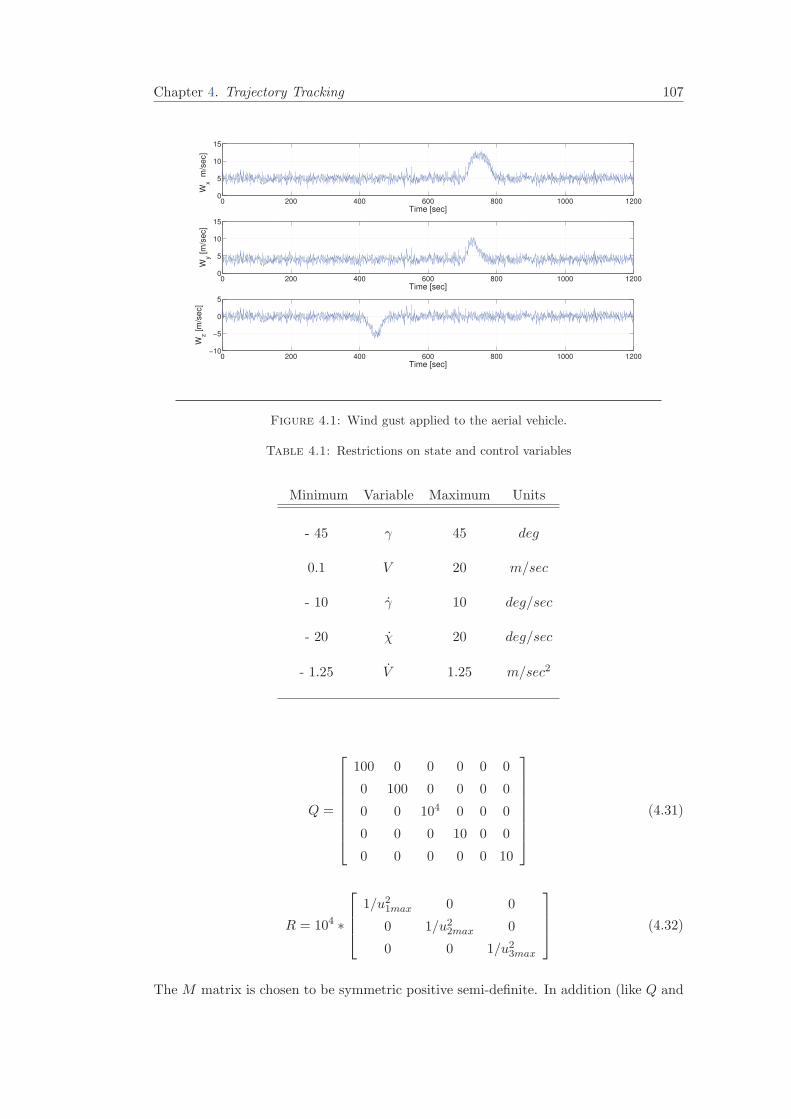
Chapter 4. Trajectory Tracking 107
0 200 400 600 800 1000 12000
5
10
15
Time [sec]W
x !
m/s
ec]
0 200 400 600 800 1000 12000
5
10
15
Time [sec]
Wy [
m/s
ec]
0 200 400 600 800 1000 1200−10
−5
0
5
Time [sec]
Wz [
m/s
ec]
Figure 4.1: Wind gust applied to the aerial vehicle.
Table 4.1: Restrictions on state and control variables
Minimum Variable Maximum Units
- 45 γ 45 deg
0.1 V 20 m/sec
- 10 γ 10 deg/sec
- 20 χ 20 deg/sec
- 1.25 V 1.25 m/sec2
Q =
100 0 0 0 0 0
0 100 0 0 0 0
0 0 104 0 0 0
0 0 0 10 0 0
0 0 0 0 0 10
(4.31)
R = 104 ∗
1/u21max 0 0
0 1/u22max 0
0 0 1/u23max
(4.32)
The M matrix is chosen to be symmetric positive semi-definite. In addition (like Q and
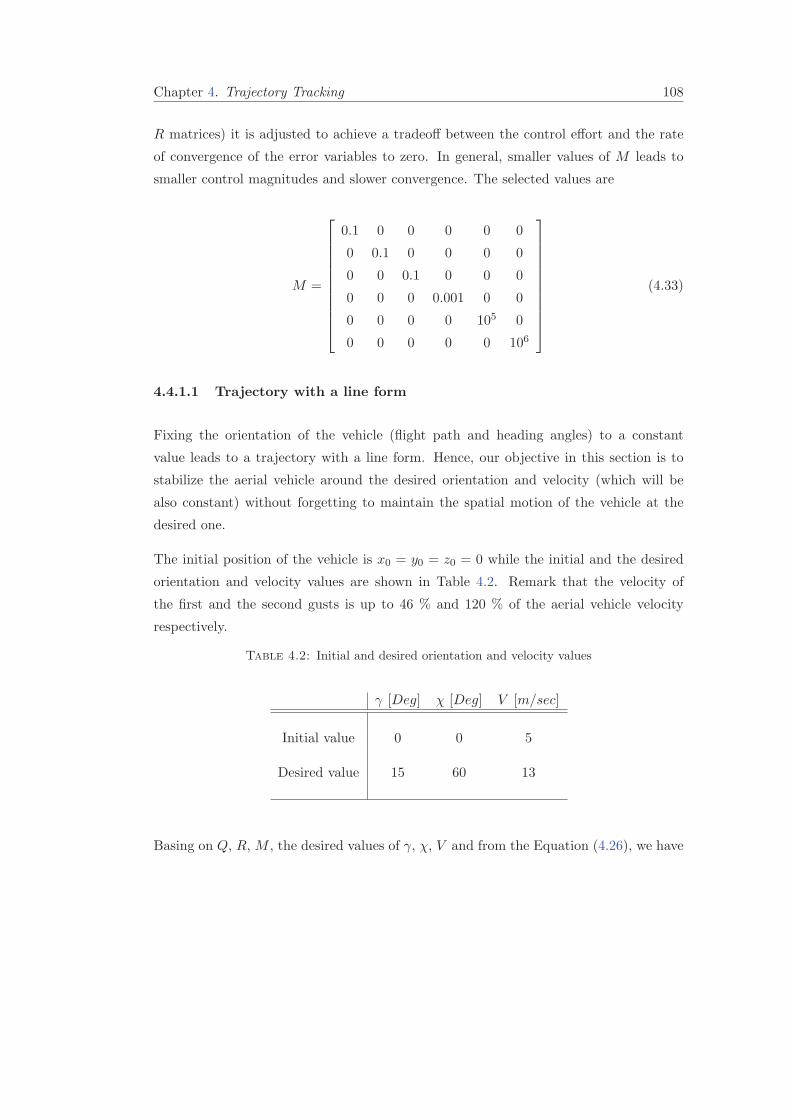
Chapter 4. Trajectory Tracking 108
R matrices) it is adjusted to achieve a tradeoff between the control effort and the rate
of convergence of the error variables to zero. In general, smaller values of M leads to
smaller control magnitudes and slower convergence. The selected values are
M =
0.1 0 0 0 0 0
0 0.1 0 0 0 0
0 0 0.1 0 0 0
0 0 0 0.001 0 0
0 0 0 0 105 0
0 0 0 0 0 106
(4.33)
4.4.1.1 Trajectory with a line form
Fixing the orientation of the vehicle (flight path and heading angles) to a constant
value leads to a trajectory with a line form. Hence, our objective in this section is to
stabilize the aerial vehicle around the desired orientation and velocity (which will be
also constant) without forgetting to maintain the spatial motion of the vehicle at the
desired one.
The initial position of the vehicle is x0 = y0 = z0 = 0 while the initial and the desired
orientation and velocity values are shown in Table 4.2. Remark that the velocity of
the first and the second gusts is up to 46 % and 120 % of the aerial vehicle velocity
respectively.
Table 4.2: Initial and desired orientation and velocity values
γ [Deg] χ [Deg] V [m/sec]
Initial value 0 0 5
Desired value 15 60 13
Basing on Q, R, M , the desired values of γ, χ, V and from the Equation (4.26), we have
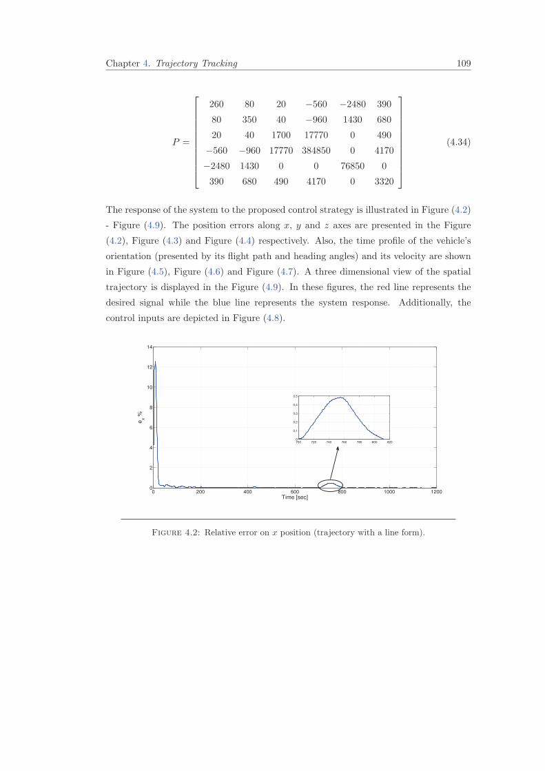
Chapter 4. Trajectory Tracking 109
P =
260 80 20 −560 −2480 390
80 350 40 −960 1430 680
20 40 1700 17770 0 490
−560 −960 17770 384850 0 4170
−2480 1430 0 0 76850 0
390 680 490 4170 0 3320
(4.34)
The response of the system to the proposed control strategy is illustrated in Figure (4.2)
- Figure (4.9). The position errors along x, y and z axes are presented in the Figure
(4.2), Figure (4.3) and Figure (4.4) respectively. Also, the time profile of the vehicle’s
orientation (presented by its flight path and heading angles) and its velocity are shown
in Figure (4.5), Figure (4.6) and Figure (4.7). A three dimensional view of the spatial
trajectory is displayed in the Figure (4.9). In these figures, the red line represents the
desired signal while the blue line represents the system response. Additionally, the
control inputs are depicted in Figure (4.8).
0 200 400 600 800 1000 12000
2
4
6
8
10
12
14
Time [sec]
ex %
700 720 740 760 780 800 8200
0.1
0.2
0.3
0.4
0.5
Figure 4.2: Relative error on x position (trajectory with a line form).

Chapter 4. Trajectory Tracking 110
0 200 400 600 800 1000 12000
10
20
30
40
50
60
70
Time [sec]
ey %
700 720 740 760 780 800 8200
0.05
0.1
0.15
0.2
0.25
Figure 4.3: Relative error on y position (trajectory with a line form).
0 200 400 600 800 1000 12000
10
20
30
40
50
60
70
Time [sec]
ez %
380 400 420 440 460 4800
0.2
0.4
0.6
0.8
Figure 4.4: Relative error on z position (trajectory with a line form).
Chapter 4. Trajectory Tracking 111
0 200 400 600 800 1000 12000
5
10
15
20
25
30
35
40
45
50
Time [sec]
γ [
De
g]
γ
γref
Figure 4.5: Flight Path Angle response in closed-loop (trajectory with a line form).
0 200 400 600 800 1000 12000
20
40
60
80
100
120
140
Time [sec]
χ [
De
g]
χ
χref
Figure 4.6: Heading Angle response in the closed-loop (trajectory with a line form).
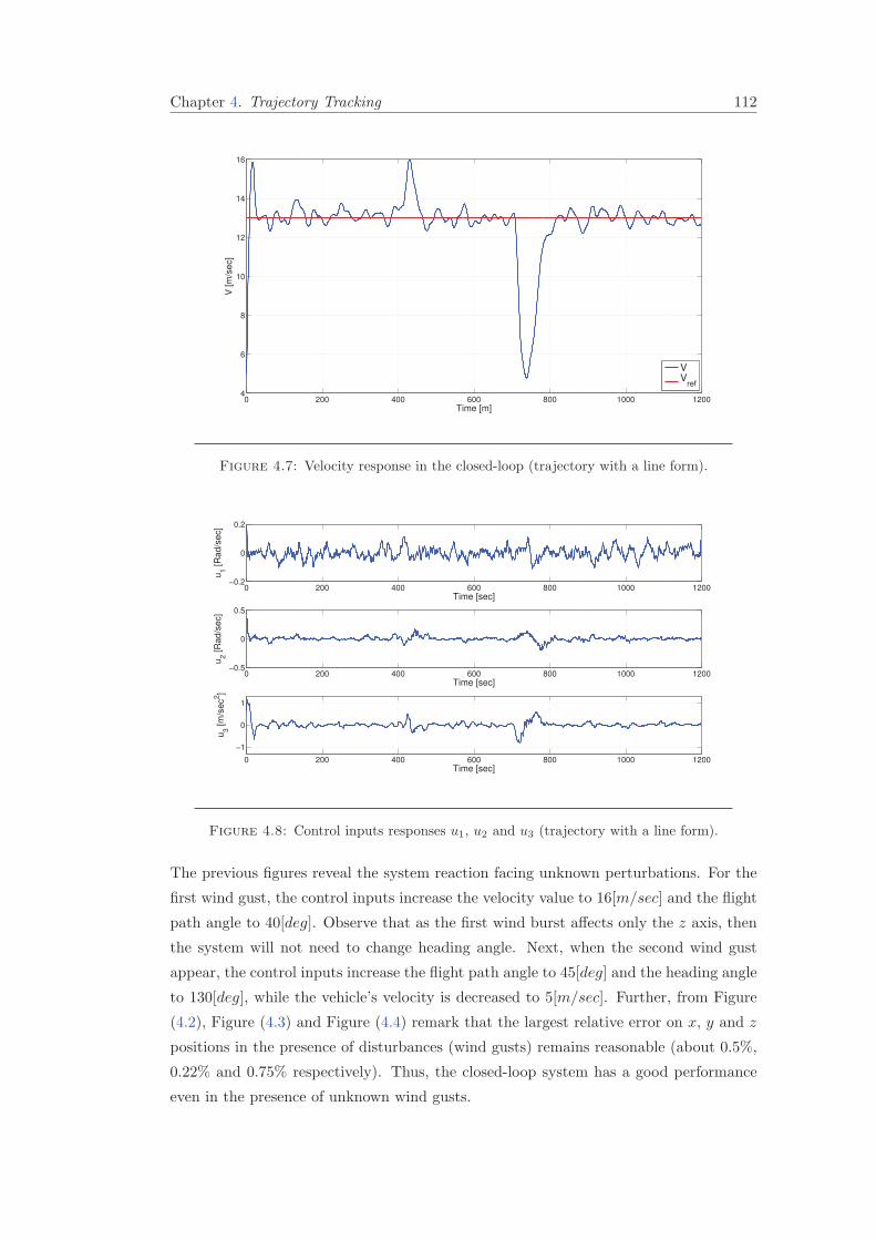
Chapter 4. Trajectory Tracking 112
0 200 400 600 800 1000 12004
6
8
10
12
14
16
Time [m]
V [
m/s
ec]
VV
ref
Figure 4.7: Velocity response in the closed-loop (trajectory with a line form).
0 200 400 600 800 1000 1200−0.2
0
0.2
Time [sec]
u1 [
Ra
d/s
ec]
0 200 400 600 800 1000 1200−0.5
0
0.5
Time [sec]
u2 [
Ra
d/s
ec]
0 200 400 600 800 1000 1200
−1
0
1
Time [sec]
u3 [
m/s
ec
2]
Figure 4.8: Control inputs responses u1, u2 and u3 (trajectory with a line form).
The previous figures reveal the system reaction facing unknown perturbations. For the
first wind gust, the control inputs increase the velocity value to 16[m/sec] and the flight
path angle to 40[deg]. Observe that as the first wind burst affects only the z axis, then
the system will not need to change heading angle. Next, when the second wind gust
appear, the control inputs increase the flight path angle to 45[deg] and the heading angle
to 130[deg], while the vehicle’s velocity is decreased to 5[m/sec]. Further, from Figure
(4.2), Figure (4.3) and Figure (4.4) remark that the largest relative error on x, y and z
positions in the presence of disturbances (wind gusts) remains reasonable (about 0.5%,
0.22% and 0.75% respectively). Thus, the closed-loop system has a good performance
even in the presence of unknown wind gusts.
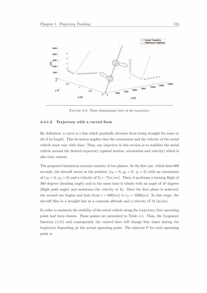
Chapter 4. Trajectory Tracking 113
Figure 4.9: Three dimensional view of the trajectory.
4.4.1.2 Trajectory with a curved form
By definition, a curve is a line which gradually deviates from being straight for some or
all of its length. This deviation implies that the orientation and the velocity of the aerial
vehicle must vary with time. Thus, our objective in this section is to stabilize the aerial
vehicle around the desired trajectory (spatial motion, orientation and velocity) which is
also time variant.
The proposed simulation scenario consists of two phases. In the first one, which lasts 600
seconds, the aircraft starts at the position (x0 = 0, y0 = 0, z0 = 0) with an orientation
of (γ0 = 0, χ0 = 0) and a velocity of V0 = 7[m/sec]. Then, it performs a turning flight of
360 degrees (heading angle) and in the same time it climbs with an angle of 10 degrees
(flight path angle) and maintains the velocity at V0. Once the first phase is achieved,
the second one begins and lasts from t = 600[sec] to tf = 1200[sec]. In this stage, the
aircraft flies in a straight line at a constant altitude and a velocity of 13 [m/sec].
In order to maintain the stability of the aerial vehicle along the trajectory, four operating
point had been chosen. These points are presented in Table 4.3. Thus, the Lyapunov
function (4.25) and consequently the control laws will change four times during the
trajectory depending on the actual operating point. The selected P for each operating
point is

Chapter 4. Trajectory Tracking 114
P1 =
210 0 0 0 −2860 0
0 400 40 −620 0 800
0 40 9440 56960 0 860
0 −620 56960 690750 0 7070
−2860 0 0 0 77590 0
0 800 860 7070 0 3320
(4.35)
P2 =
400 0 40 620 0 800
0 210 0 0 2860 0
−40 0 9440 56960 0 860
−620 0 56960 690750 0 7070
0 −2860 0 0 77590 0
800 0 860 7070 0 3320
(4.36)
P3 =
210 0 0 0 2860 0
0 400 −40 620 0 −800
0 −40 9440 56960 0 860
0 620 56960 690750 0 7070
2860 0 0 0 77590 0
0 −800 860 7070 0 3320
(4.37)
P4 =
400 0 40 −620 0 800
0 210 0 0 2860 0
40 0 9440 56960 0 860
−620 0 56960 690750 0 7070
0 2860 0 0 77590 0
800 0 860 7070 0 3320
(4.38)
Table 4.3: The four selected operating points
γ [Deg] χ [Deg] V [m/sec]
OP1 10 90 13
OP2 10 180 13
OP3 10 270 13
OP4 10 360 13
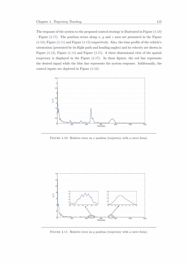
Chapter 4. Trajectory Tracking 115
The response of the system to the proposed control strategy is illustrated in Figure (4.10)
- Figure (4.17). The position errors along x, y and z axes are presented in the Figure
(4.10), Figure (4.11) and Figure (4.12) respectively. Also, the time profile of the vehicle’s
orientation (presented by its flight path and heading angles) and its velocity are shown in
Figure (4.13), Figure (4.14) and Figure (4.15). A three dimensional view of the spatial
trajectory is displayed in the Figure (4.17). In these figures, the red line represents
the desired signal while the blue line represents the system response. Additionally, the
control inputs are depicted in Figure (4.16).
0 200 400 600 800 1000 12000
0.5
1
1.5
2
2.5
3
3.5
4
4.5
Time [sec]
ex %
Figure 4.10: Relative error on x position (trajectory with a curve form).
0 200 400 600 800 1000 12000
2
4
6
8
10
12
14
Time [sec]
ey %
400 420 440 460 480 500 5200
0.1
0.2
0.3
0.4
0.5
700 710 720 730 740 750 760 770 7800
0.2
0.4
0.6
0.8
Figure 4.11: Relative error on y position (trajectory with a curve form).
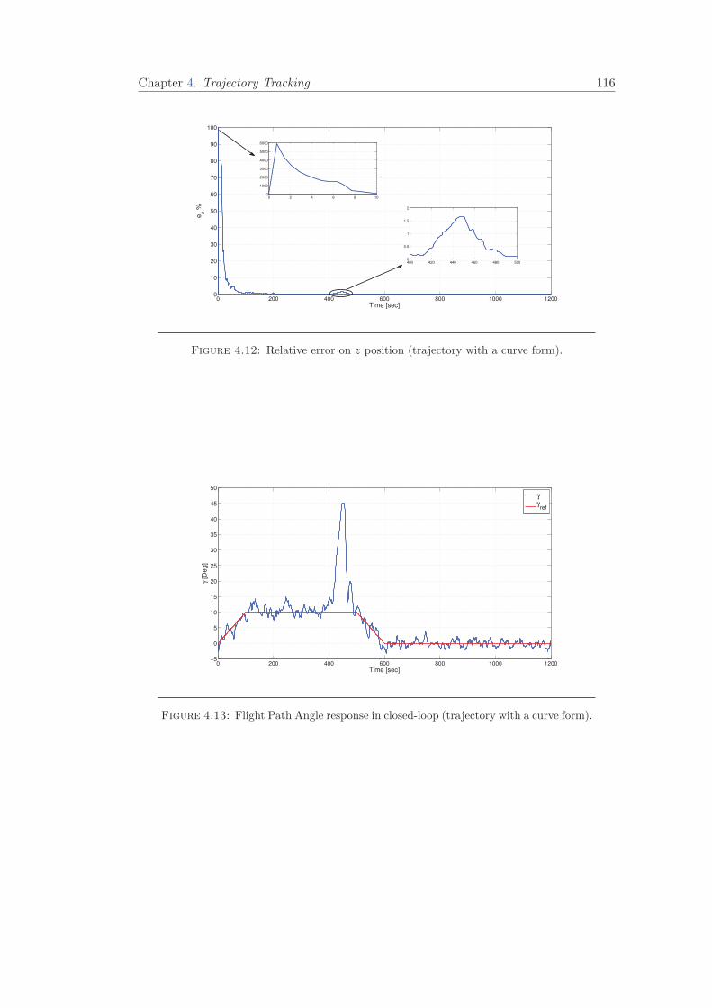
Chapter 4. Trajectory Tracking 116
0 200 400 600 800 1000 12000
10
20
30
40
50
60
70
80
90
100
Time [sec]
ez %
0 2 4 6 8 100
1000
2000
3000
4000
5000
6000
400 420 440 460 480 5000
0.5
1
1.5
2
Figure 4.12: Relative error on z position (trajectory with a curve form).
0 200 400 600 800 1000 1200−5
0
5
10
15
20
25
30
35
40
45
50
Time [sec]
γ [
De
g]
γ
γref
Figure 4.13: Flight Path Angle response in closed-loop (trajectory with a curve form).
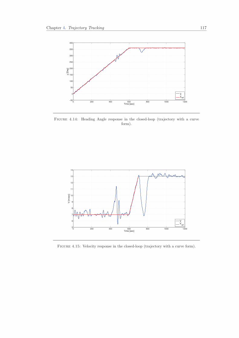
Chapter 4. Trajectory Tracking 117
0 200 400 600 800 1000 1200−50
0
50
100
150
200
250
300
350
400
Time [sec]
χ [D
eg
]
χ
χref
Figure 4.14: Heading Angle response in the closed-loop (trajectory with a curveform).
0 200 400 600 800 1000 12005
6
7
8
9
10
11
12
13
14
Time [sec]
V [
m/s
ec]
VV
ref
Figure 4.15: Velocity response in the closed-loop (trajectory with a curve form).
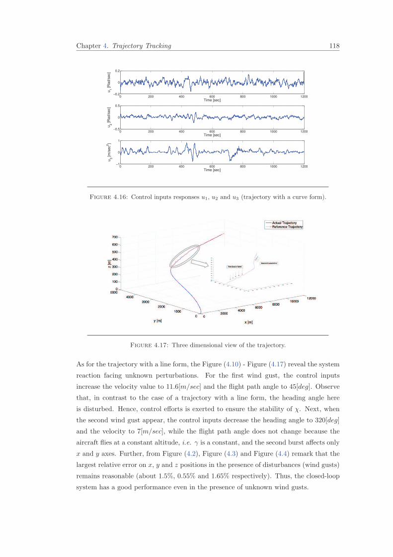
Chapter 4. Trajectory Tracking 118
0 200 400 600 800 1000 1200−0.2
0
0.2
Time [sec]
u1 [
Ra
d/s
ec]
0 200 400 600 800 1000 1200−0.5
0
0.5
Time [sec]
u2 [
Ra
d/s
ec]
0 200 400 600 800 1000 1200−1
0
1
Time [sec]
u3 [
m/s
ec
2]
Figure 4.16: Control inputs responses u1, u2 and u3 (trajectory with a curve form).
Figure 4.17: Three dimensional view of the trajectory.
As for the trajectory with a line form, the Figure (4.10) - Figure (4.17) reveal the system
reaction facing unknown perturbations. For the first wind gust, the control inputs
increase the velocity value to 11.6[m/sec] and the flight path angle to 45[deg]. Observe
that, in contrast to the case of a trajectory with a line form, the heading angle here
is disturbed. Hence, control efforts is exerted to ensure the stability of χ. Next, when
the second wind gust appear, the control inputs decrease the heading angle to 320[deg]
and the velocity to 7[m/sec], while the flight path angle does not change because the
aircraft flies at a constant altitude, i.e. γ is a constant, and the second burst affects only
x and y axes. Further, from Figure (4.2), Figure (4.3) and Figure (4.4) remark that the
largest relative error on x, y and z positions in the presence of disturbances (wind gusts)
remains reasonable (about 1.5%, 0.55% and 1.65% respectively). Thus, the closed-loop
system has a good performance even in the presence of unknown wind gusts.
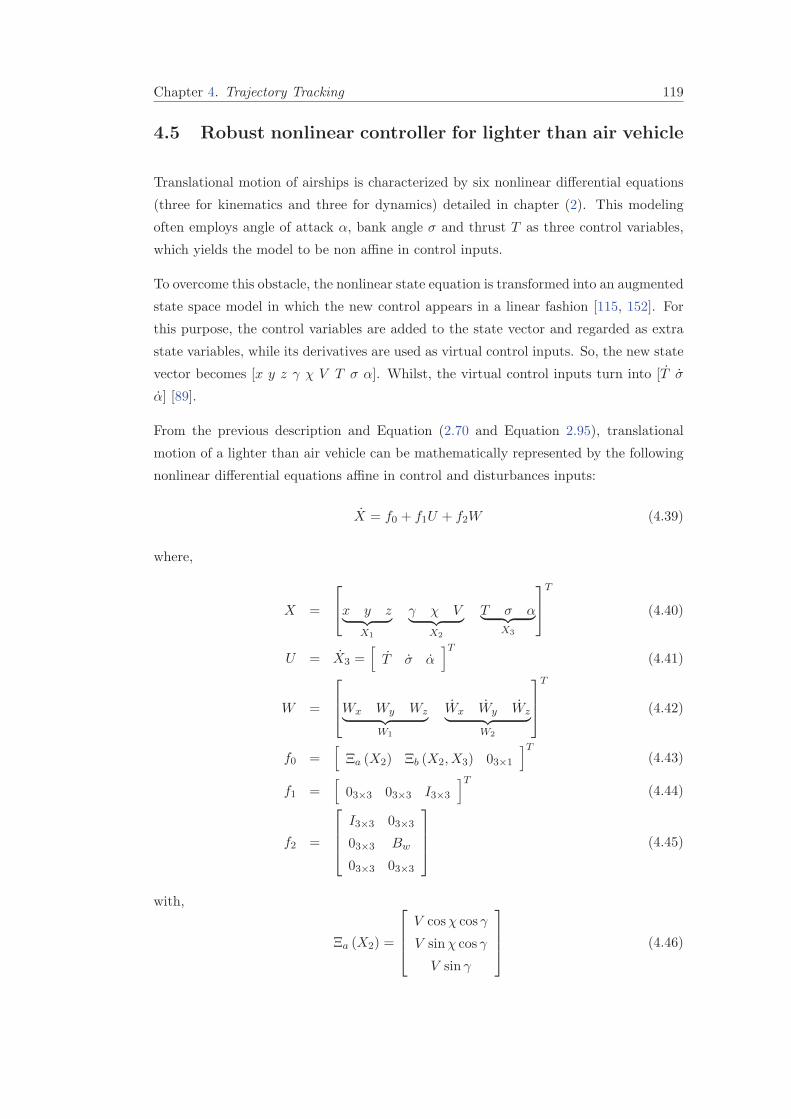
Chapter 4. Trajectory Tracking 119
4.5 Robust nonlinear controller for lighter than air vehicle
Translational motion of airships is characterized by six nonlinear differential equations
(three for kinematics and three for dynamics) detailed in chapter (2). This modeling
often employs angle of attack α, bank angle σ and thrust T as three control variables,
which yields the model to be non affine in control inputs.
To overcome this obstacle, the nonlinear state equation is transformed into an augmented
state space model in which the new control appears in a linear fashion [115, 152]. For
this purpose, the control variables are added to the state vector and regarded as extra
state variables, while its derivatives are used as virtual control inputs. So, the new state
vector becomes [x y z γ χ V T σ α]. Whilst, the virtual control inputs turn into [T σ
α] [89].
From the previous description and Equation (2.70 and Equation 2.95), translational
motion of a lighter than air vehicle can be mathematically represented by the following
nonlinear differential equations affine in control and disturbances inputs:
X = f0 + f1U + f2W (4.39)
where,
X =
x y z︸ ︷︷ ︸
X1
γ χ V︸ ︷︷ ︸X2
T σ α︸ ︷︷ ︸X3
T
(4.40)
U = X3 =[T σ α
]T(4.41)
W =
Wx Wy Wz︸ ︷︷ ︸
W1
Wx Wy Wz︸ ︷︷ ︸W2
T
(4.42)
f0 =[Ξa (X2) Ξb (X2, X3) 03×1
]T(4.43)
f1 =[03×3 03×3 I3×3
]T(4.44)
f2 =
I3×3 03×3
03×3 Bw
03×3 03×3
(4.45)
with,
Ξa (X2) =
V cosχ cos γ
V sinχ cos γ
V sin γ
(4.46)
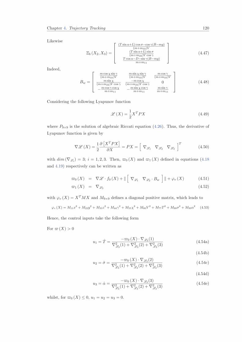
Chapter 4. Trajectory Tracking 120
Likewise
Ξb (X2, X3) =
(T sinα+L) cosσ−cos γ(B−mg)(m+m33)V
(T sinα+L) sinσ
(m+m22)V cos γT cosα−D−sin γ(B−mg)
m+m11
(4.47)
Indeed,
Bw =
m cosχ sin γ(m+m33)V
m sinχ sin γ(m+m33)V
m cos γ(m+m33)V
m sinχ(m+m22)V cos γ
−m cosχ(m+m22)V cos γ 0
−m cos γ cosχm+m11
−m sinχ cos γm+m11
m sin γm+m11
(4.48)
Considering the following Lyapunov function
L (X) =1
2XTPX (4.49)
where P9×9 is the solution of algebraic Riccati equation (4.26). Thus, the derivative of
Lyapunov function is given by
∇L (X) =1
2
∂[XTPX
]
∂X= PX =
[∇L1 ∇L2 ∇L3
]T(4.50)
with dim (∇Li) = 3; i = 1, 2, 3. Then, 0 (X) and 1 (X) defined in equations (4.18
and 4.19) respectively can be written as
0 (X) = ∇L · f0 (X) + ‖[∇L1 ∇L2 ·Bw
]‖+ ϕv (X) (4.51)
1 (X) = ∇L3 (4.52)
with ϕv (X) = XTMX and M9×9 defines a diagonal positive matrix, which leads to
ϕv (X) = M11x2 +M22y
2 +M33z2 +M44γ
2 +M55χ2 +M66V
2 +M77T2 +M88σ
2 +M99α2 (4.53)
Hence, the control inputs take the following form
For (X) > 0
u1 = T =−0 (X) ·∇L3(1)
∇2L3
(1) +∇2L3
(2) +∇2L3
(3)(4.54a)
(4.54b)
u2 = σ =−0 (X) ·∇L3(2)
∇2L3
(1) +∇2L3
(2) +∇2L3
(3)(4.54c)
(4.54d)
u3 = α =−0 (X) ·∇L3(3)
∇2L3
(1) +∇2L3
(2) +∇2L3
(3)(4.54e)
whilst, for 0 (X) ≤ 0, u1 = u2 = u3 = 0.
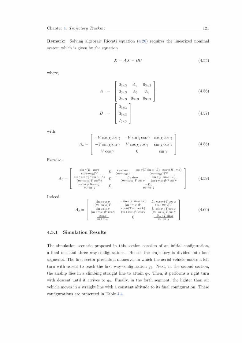
Chapter 4. Trajectory Tracking 121
Remark: Solving algebraic Riccati equation (4.26) requires the linearized nominal
system which is given by the equation
X = AX +BU (4.55)
where,
A =
03×3 Aa 03×3
03×3 Ab Ac
03×3 03×3 03×3
(4.56)
B =
03×3
03×3
I3×3
(4.57)
with,
Aa =
−V cosχ cos γ −V sinχ cos γ cosχ cos γ
−V sinχ sin γ V cosχ cos γ sinχ cos γ
V cos γ 0 sin γ
(4.58)
likewise,
Ab =
sin γ(B−mg)(m+m33)V
0 Lv cosσ(m+m33)
− cosσ(T sinα+L)−cos γ(B−mg)(m+m33)V 2
sin γ sinσ(T sinα+L)(m+m22)V cos2 γ
0 Lv sinσ(m+m22)V cosσ − sinσ(T sinα+L)
(m+m22)V 2 cos γ− cos γ(B−mg)
m+m110 −Dv
m+m11
(4.59)
Indeed,
Ac =
sinα cosσ(m+m33)V
− sinσ(T sinα+L)(m+m33)V
Lα cosσ+T cosα(m+m33)V
sinα sinσ(m+m22)V cos γ
cosσ(T sinα+L)(m+m22)V cos γ
Lα sinσ+T cosα(m+m22)V cos γ
cosαm+m11
0 −Dα+T sinαm+m11
(4.60)
4.5.1 Simulation Results
The simulation scenario proposed in this section consists of an initial configuration,
a final one and three way-configurations. Hence, the trajectory is divided into four
segments. The first sector presents a maneuver in which the aerial vehicle makes a left
turn with ascent to reach the first way-configuration q1. Next, in the second section,
the airship flies in a climbing straight line to attain q2. Then, it performs a right turn
with descent until it arrives to q3. Finally, in the forth segment, the lighter than air
vehicle moves in a straight line with a constant altitude to its final configuration. These
configurations are presented in Table 4.4.
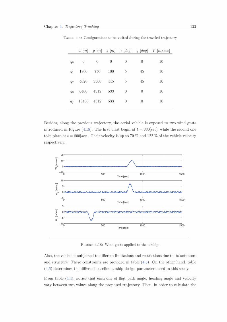
Chapter 4. Trajectory Tracking 122
Table 4.4: Configurations to be visited during the traveled trajectory
x [m] y [m] z [m] γ [deg] χ [deg] V [m/sec]
q0 0 0 0 0 0 10
q1 1800 750 100 5 45 10
q2 4620 3560 445 5 45 10
q3 6400 4312 533 0 0 10
qf 13406 4312 533 0 0 10
Besides, along the previous trajectory, the aerial vehicle is exposed to two wind gusts
introduced in Figure (4.18). The first blast begin at t = 330[sec], while the second one
take place at t = 800[sec]. Their velocity is up to 70 % and 122 % of the vehicle velocity
respectively.
0 500 1000 1500−10
0
10
20
Time [sec]
Wx [
m/s
ec]
0 500 1000 1500−5
0
5
10
Time [sec]
Wy [
m/s
ec]
0 500 1000 1500−10
−5
0
5
Time [sec]
Wz [
m/s
ec]
Figure 4.18: Wind gusts applied to the airship.
Also, the vehicle is subjected to different limitations and restrictions due to its actuators
and structure. These constraints are provided in table (4.5). On the other hand, table
(4.6) determines the different baseline airship design parameters used in this study.
From table (4.4), notice that each one of fligt path angle, heading angle and velocity
vary between two values along the proposed trajectory. Then, in order to calculate the
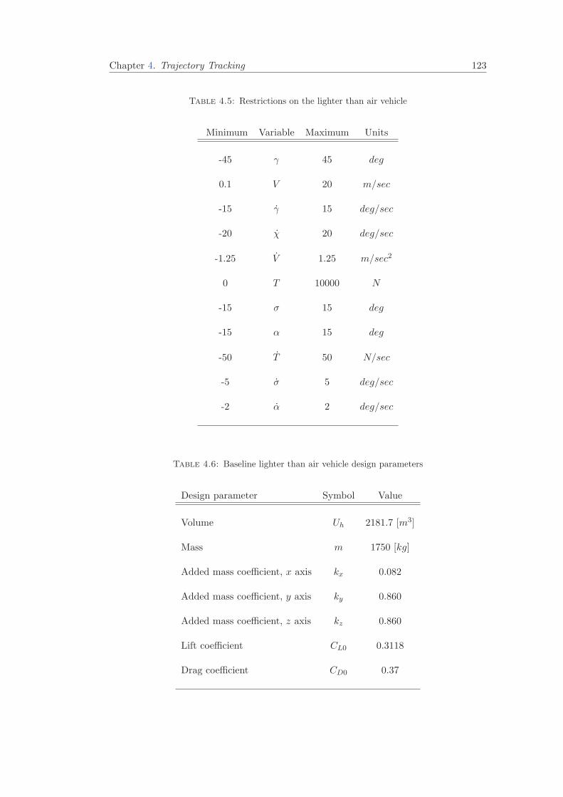
Chapter 4. Trajectory Tracking 123
Table 4.5: Restrictions on the lighter than air vehicle
Minimum Variable Maximum Units
-45 γ 45 deg
0.1 V 20 m/sec
-15 γ 15 deg/sec
-20 χ 20 deg/sec
-1.25 V 1.25 m/sec2
0 T 10000 N
-15 σ 15 deg
-15 α 15 deg
-50 T 50 N/sec
-5 σ 5 deg/sec
-2 α 2 deg/sec
Table 4.6: Baseline lighter than air vehicle design parameters
Design parameter Symbol Value
Volume Uh 2181.7 [m3]
Mass m 1750 [kg]
Added mass coefficient, x axis kx 0.082
Added mass coefficient, y axis ky 0.860
Added mass coefficient, z axis kz 0.860
Lift coefficient CL0 0.3118
Drag coefficient CD0 0.37
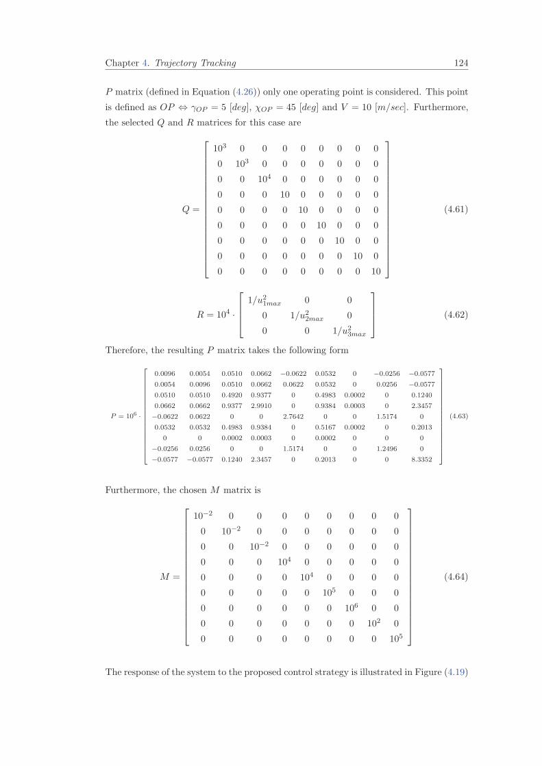
Chapter 4. Trajectory Tracking 124
P matrix (defined in Equation (4.26)) only one operating point is considered. This point
is defined as OP ⇔ γOP = 5 [deg], χOP = 45 [deg] and V = 10 [m/sec]. Furthermore,
the selected Q and R matrices for this case are
Q =
103 0 0 0 0 0 0 0 0
0 103 0 0 0 0 0 0 0
0 0 104 0 0 0 0 0 0
0 0 0 10 0 0 0 0 0
0 0 0 0 10 0 0 0 0
0 0 0 0 0 10 0 0 0
0 0 0 0 0 0 10 0 0
0 0 0 0 0 0 0 10 0
0 0 0 0 0 0 0 0 10
(4.61)
R = 104 ·
1/u21max 0 0
0 1/u22max 0
0 0 1/u23max
(4.62)
Therefore, the resulting P matrix takes the following form
P = 106 ·
0.0096 0.0054 0.0510 0.0662 −0.0622 0.0532 0 −0.0256 −0.0577
0.0054 0.0096 0.0510 0.0662 0.0622 0.0532 0 0.0256 −0.0577
0.0510 0.0510 0.4920 0.9377 0 0.4983 0.0002 0 0.1240
0.0662 0.0662 0.9377 2.9910 0 0.9384 0.0003 0 2.3457
−0.0622 0.0622 0 0 2.7642 0 0 1.5174 0
0.0532 0.0532 0.4983 0.9384 0 0.5167 0.0002 0 0.2013
0 0 0.0002 0.0003 0 0.0002 0 0 0
−0.0256 0.0256 0 0 1.5174 0 0 1.2496 0
−0.0577 −0.0577 0.1240 2.3457 0 0.2013 0 0 8.3352
(4.63)
Furthermore, the chosen M matrix is
M =
10−2 0 0 0 0 0 0 0 0
0 10−2 0 0 0 0 0 0 0
0 0 10−2 0 0 0 0 0 0
0 0 0 104 0 0 0 0 0
0 0 0 0 104 0 0 0 0
0 0 0 0 0 105 0 0 0
0 0 0 0 0 0 106 0 0
0 0 0 0 0 0 0 102 0
0 0 0 0 0 0 0 0 105
(4.64)
The response of the system to the proposed control strategy is illustrated in Figure (4.19)
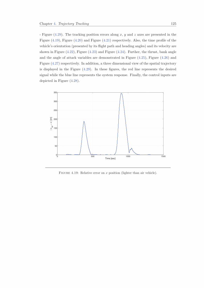
Chapter 4. Trajectory Tracking 125
- Figure (4.29). The tracking position errors along x, y and z axes are presented in the
Figure (4.19), Figure (4.20) and Figure (4.21) respectively. Also, the time profile of the
vehicle’s orientation (presented by its flight path and heading angles) and its velocity are
shown in Figure (4.22), Figure (4.23) and Figure (4.24). Further, the thrust, bank angle
and the angle of attack variables are demonstrated in Figure (4.25), Figure (4.26) and
Figure (4.27) respectively. In addition, a three dimensional view of the spatial trajectory
is displayed in the Figure (4.29). In these figures, the red line represents the desired
signal while the blue line represents the system response. Finally, the control inputs are
depicted in Figure (4.28).
0 500 1000 15000
50
100
150
200
250
300
350
Time [sec]
| x
ref −
x | [
m]
Figure 4.19: Relative error on x position (lighter than air vehicle).
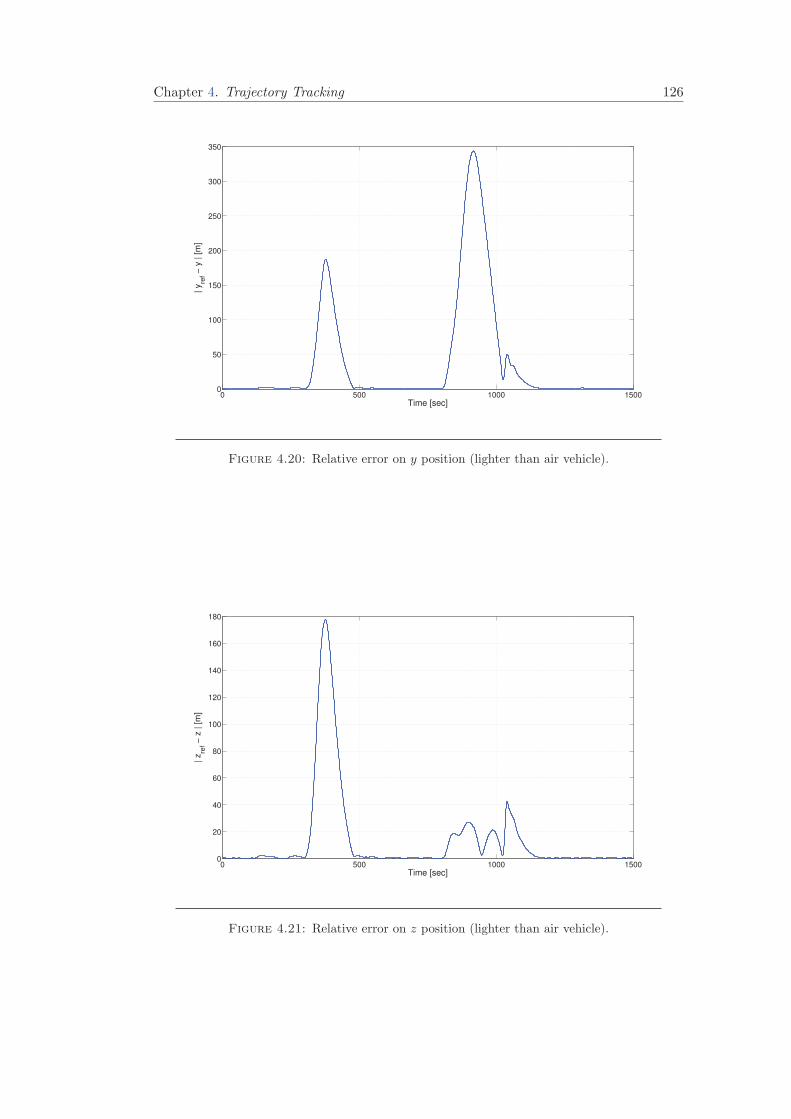
Chapter 4. Trajectory Tracking 126
0 500 1000 15000
50
100
150
200
250
300
350
Time [sec]
| y
ref −
y | [
m]
Figure 4.20: Relative error on y position (lighter than air vehicle).
0 500 1000 15000
20
40
60
80
100
120
140
160
180
Time [sec]
| z
ref −
z | [
m]
Figure 4.21: Relative error on z position (lighter than air vehicle).

Chapter 4. Trajectory Tracking 127
0 500 1000 1500−10
0
10
20
30
40
50
Time [sec]
γ [
De
g]
γ
γref
Figure 4.22: Flight Path Angle response in closed-loop (lighter than air vehicle).
0 500 1000 1500−40
−30
−20
−10
0
10
20
30
40
50
Time [sec]
χ [
De
g]
χ
χref
Figure 4.23: Heading Angle response in the closed-loop (lighter than air vehicle).
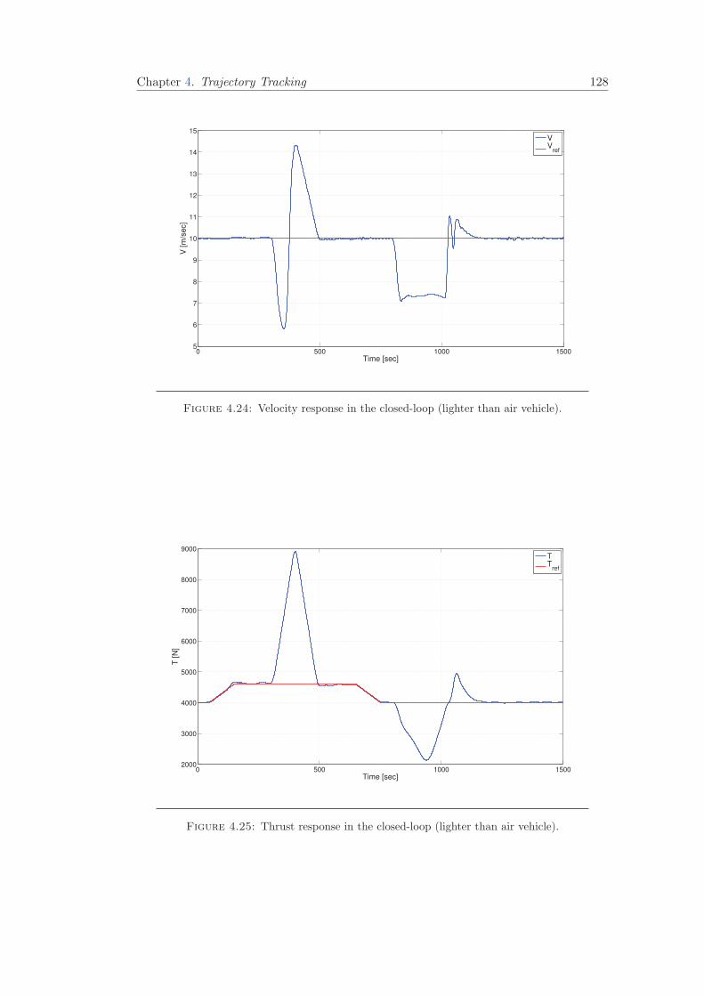
Chapter 4. Trajectory Tracking 128
0 500 1000 15005
6
7
8
9
10
11
12
13
14
15
Time [sec]
V [
m/s
ec]
VV
ref
Figure 4.24: Velocity response in the closed-loop (lighter than air vehicle).
0 500 1000 15002000
3000
4000
5000
6000
7000
8000
9000
Time [sec]
T [
N]
TT
ref
Figure 4.25: Thrust response in the closed-loop (lighter than air vehicle).
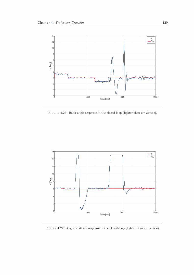
Chapter 4. Trajectory Tracking 129
0 500 1000 1500−6
−4
−2
0
2
4
6
8
10
12
14
Time [sec]
σ [
De
g]
σ
σref
Figure 4.26: Bank angle response in the closed-loop (lighter than air vehicle).
0 500 1000 15000
2
4
6
8
10
12
14
16
Time [sec]
α [
De
g]
α
αref
Figure 4.27: Angle of attack response in the closed-loop (lighter than air vehicle).
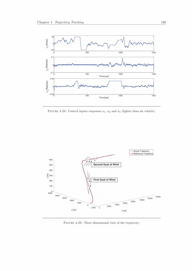
Chapter 4. Trajectory Tracking 130
0 500 1000 1500
−50
0
50
Time [sec]
u1 [
N/s
ec]
0 500 1000 1500−0.1
0
0.1
Time [sec]
u2 [
Ra
d/s
ec]
0 500 1000 1500−0.05
0
0.05
Time [sec]
u3 [
Ra
d/s
ec]
Figure 4.28: Control inputs responses u1, u2 and u3 (lighter than air vehicle).
02000
40006000
800010000
1200014000
−1000
0
1000
2000
3000
4000
50000
100
200
300
400
500
600
x [m]y [m]
z [
m]
Actual Trajectory
Reference Trajectory
First Gust of Wind
Second Gust of Wind
Figure 4.29: Three dimensional view of the trajectory.
Chapter 4. Trajectory Tracking 131
Figure (4.19) - Figure (4.29) illustrate the attitude of the system tracking a reference
trajectory and facing unknown disturbances. Notice that when the first wind gust arrives
(at t = 300 [sec]), the control inputs increase the thrust to 8900 Newton while the angle
of attack varies between 0.3 and 15 degrees before it stabilized at 6.12 degrees. Observe
also that there is no changes on the bank angle response to the first gust because this
blast affects only the z axis and when it arrives, the horizontal orientation of the vehicle
is already stabilized at a constant value. On the other hand, when the second gust
arrives (at t = 800 [sec]), the control inputs make the thrust to vary between 2120 and
4950 Newton, the bank angle to change between -5.6 and 12 degrees and the angle of
attack to be increased to 15 degrees. These changes affect directly the behavior of each
of γ, χ and V as it is demonstrated in Figure (4.22), Figure (4.23) and Figure (4.24).
From previous we conclude that the proposed control strategy has a good performance
guaranteeing the trajectory tracking even in the presence of unknown wind gusts.
4.6 Trajectory Tracking for Quadrotors
The aim of this section is to examine the applicability and compatibility of the reference
trajectories with the dynamics of the quadrator. For this purpose, we employ the trajec-
tory generated by the previous method to the rotorcraft’s rigid body model, Equation
(2.63) as reference signals; and we design an autopilot to ensure the trajectory tracking.
The control strategy used here is based on the control laws introduced in [32] and [33]
for stabilizing quadrotor at hover.
The controller regulates each one of the state variables in a sequence according to a
predefined priority rule as follows:
First of all, the desired altitude (z) is reached using the control input u. Then, the
yaw angle (ψ) is controlled through τψ. Next, the desired values of pitch angle (φ) and
y-displacement are reached by controlling τφ. Finally, the control input τθ is used to
obtain the desired pitch angle (θ) and x-displacement values.
Next, the following definition is fundamental for the control strategy.
Definition 4.6. The function σ (t) is said to be a saturation function if and only if
|σ (t) | ≤ M ; ∀M ∈ R+ (4.65)
Chapter 4. Trajectory Tracking 132
4.6.1 Altitude and Yaw Control
The control of z-displacement is ensured through the following control input
u = sec(θ) sec(φ)r (4.66)
where
r = −Kz1 (z − zref )− Kz2 (z − zref ) +mg (4.67)
with, Kz1 and Kz2 are positive constant, zref and zref are the desired vertical velocity
and altitude respectively. In addition, θ and φ are assumed to be limited such that they
can not reach 90 degrees.
On the other side, the yaw angle is controlled by applying
τψ = −σψ1
(Kψ1
(ψ − ψref
))− σψ2 (Kψ2 (ψ − ψref )) (4.68)
Substituting Equation (4.67) and Equation (4.68) into Equation (2.63c) and Equation
(2.63d), it follows that: z .→ zref , z .→ zref , ψ .→ ψref and ψ .→ ψref .
4.6.2 Roll and Lateral Position Control
Once z and z are stabilized, the Equation (2.63a) and Equation (2.63b) can be reduced
to
x = −g tan(θ) sec(φ) (4.69a)
y = g tan (φ) (4.69b)
Considering the subsystem (φ, y) given by Equation (4.69b) and Equation (2.63f). Then,
the control input for this subsystem is given by
τφ = −σφ1 (Kφ1 (y − yref ))− σφ2 (Kφ2 (y − yref ))
−σφ3
(Kφ3
(φ))
− σφ4 (Kφ4 (φ− φref ))(4.70)
where the controller gain parameters Kφ1, Kφ2, Kφ3 and Kφ4 are positive constant.
4.6.3 Pitch and Forward Position Control
From Equation (4.70) and Equation (4.69b) it follows that φ .→ 0. Then, the Equation
(4.69a) becomes x = −g tan(θ) Finally, the subsystem (θ, x) is controlled through τθ
Chapter 4. Trajectory Tracking 133
which is given by
τθ = σθ1 (Kθ1 (x− xref )) + σθ2 (Kθ2 (x− xref ))
−σθ3
(Kθ3
(θ))
− σθ4 (Kθ4 (θ − θref ))(4.71)
where the controller gain parameters Kθ1, Kθ2, Kθ3 and Kθ4 are positive constant.
4.7 Simulation Results
In this section, we consider a scenario of a quadrotor flying at fixed altitude. The trajec-
tory consists of an initial configuration, an initial one, and several way-configurations to
be visited by the aerial vehicle. Then, the optimization process described in sec. 3.3.2.1
is applied for every segment separately. Once the reference trajectory is generated, an
autopilot is designed to evaluate the validity of a such trajectory.
The constraints on pitch angle, velocity, and control variables are provided in Table 4.7.
Table 4.7: Restrictions on state and control variables
Minimum Variable Maximum Units
- 15 θ 15 deg0.001 V 0.2 m/sec
- 5 θ 5 deg/sec
- 10 ψ 10 deg/sec
- 0.01 V 0.01 m/sec2
As the vehicle is moving only in the horizontal plane (x× y), both θ and θ are equal to
zero. In addition we assume the lack of wind in the environment. Then, the equations of
motion presented in Equation (2.99) and Equation (2.101) are reduced to the following
x = V cosψ
y = V sinψ
ψ = u1
V = u2

Chapter 4. Trajectory Tracking 134
−2 0 2 4 6 8 10 120
5
10
15
20
25
30
35
40
x × y Plane
x [m]
y[m
]
q 0
q 1
q 2
q 3
q 4
q f
Figure 4.30: Flying at a constant altitude trajectory.
0 200 4000
50
100
150
200
Yaw Angle
Time [sec]
ψ[deg
]
0 200 4000
0.05
0.1
0.15
0.2
Velocity
Time [sec]
V
0 200 400−0.2
−0.1
0
0.1
0.2
Yaw Angular Velocity
Time [sec]
u1=
ψ[deg
/sec]
0 200 400−0.2
−0.1
0
0.1
0.2
Acceleration
Time [sec]
u2=
V
Figure 4.31: Time profile of yaw angle ψ, vehicle’s velocity and their rate of changeψ, V respectively.
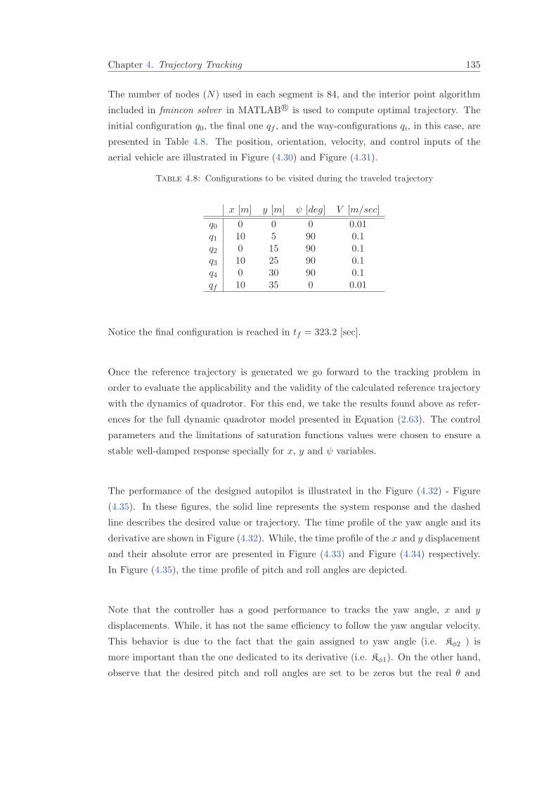
Chapter 4. Trajectory Tracking 135
The number of nodes (N) used in each segment is 84, and the interior point algorithm
included in fmincon solver in MATLAB R© is used to compute optimal trajectory. The
initial configuration q0, the final one qf , and the way-configurations qi, in this case, are
presented in Table 4.8. The position, orientation, velocity, and control inputs of the
aerial vehicle are illustrated in Figure (4.30) and Figure (4.31).
Table 4.8: Configurations to be visited during the traveled trajectory
x [m] y [m] ψ [deg] V [m/sec]
q0 0 0 0 0.01q1 10 5 90 0.1q2 0 15 90 0.1q3 10 25 90 0.1q4 0 30 90 0.1qf 10 35 0 0.01
Notice the final configuration is reached in tf = 323.2 [sec].
Once the reference trajectory is generated we go forward to the tracking problem in
order to evaluate the applicability and the validity of the calculated reference trajectory
with the dynamics of quadrotor. For this end, we take the results found above as refer-
ences for the full dynamic quadrotor model presented in Equation (2.63). The control
parameters and the limitations of saturation functions values were chosen to ensure a
stable well-damped response specially for x, y and ψ variables.
The performance of the designed autopilot is illustrated in the Figure (4.32) - Figure
(4.35). In these figures, the solid line represents the system response and the dashed
line describes the desired value or trajectory. The time profile of the yaw angle and its
derivative are shown in Figure (4.32). While, the time profile of the x and y displacement
and their absolute error are presented in Figure (4.33) and Figure (4.34) respectively.
In Figure (4.35), the time profile of pitch and roll angles are depicted.
Note that the controller has a good performance to tracks the yaw angle, x and y
displacements. While, it has not the same efficiency to follow the yaw angular velocity.
This behavior is due to the fact that the gain assigned to yaw angle (i.e. Kφ2 ) is
more important than the one dedicated to its derivative (i.e. Kφ1). On the other hand,
observe that the desired pitch and roll angles are set to be zeros but the real θ and

Chapter 4. Trajectory Tracking 136
0 50 100 150 200 250 300 350−50
0
50
100
150
200
Time [sec]ψ
[deg
]
Yaw Angle
ψref
ψ
0 50 100 150 200 250 300 350−10
−5
0
5
10
15
Yaw Angular Velocity
Time [sec]
ψ[deg
/sec]
ψref
ψ
Figure 4.32: Yaw angle of quadrotor.
φ differs for some periods of time which is due to movements on x and y axis and
acceleration/deceleration effects.
0 50 100 150 200 250 300 350−5
0
5
10
15
Time [sec]
x[m
]
x-displacement
0 50 100 150 200 250 300 3500
0.02
0.04
0.06
0.08
0.1
Absolute Error on x-axis
Time [sec]
ex
xxref
Figure 4.33: x-displacement of quadrotor.

Chapter 4. Trajectory Tracking 137
0 50 100 150 200 250 300 3500
10
20
30
40
Time [sec]
y[m
]
y-displacement
yyref
0 50 100 150 200 250 300 3500
0.01
0.02
0.03
0.04
0.05
0.06
Absolute Error on y-axis
Time [sec]
ey[m
]
Figure 4.34: y-displacement of quadrotor.
0 50 100 150 200 250 300 350−10
−5
0
5
10
Time [sec]
θ[deg
]
P itch Angle
θrefθ
0 50 100 150 200 250 300 350−5
0
5
10
Roll Angle
Time [sec]
φ[deg
]
φref
φ
Figure 4.35: Time profile of pitch (θ) and roll (φ) angles.

Chapter 4. Trajectory Tracking 138
4.8 Conclusion
In this chapter, Firstly, we have formulated and solved inverse optimal robust stabiliza-
tion problem to guarantee the trajectory tracking for a kinematic aerial vehicle and for a
dynamic lighter than air vehicle. These systems belongs to a specified class of nonlinear
control systems which are affine in control and disturbances inputs. The formulas (4.22)
and (4.23) introduced in [62] are used to generate robust control laws which have the
desirable properties of optimality and do not require the solution of HJI equation. Some
numerical simulations were carried out and some graphs were presented to illustrate the
good performance of the closed-loop system even in presence of unknown disturbances.
Secondly, an autopilot for an autonomous quadrotor has been designed. We formulated
a minimum time optimal control problem to generate the reference trajectory using the
vehicle’s point mass model. While the control strategy in the tracking problem was
designed through the quadrotor’s rigid body model.

Chapter 5
Conclusion and Future Work
5.1 Conclusion
UAV’s are a promising solution to the structure inspection problem. In fact the nature of
such missions implies the interaction of different research domains including, automatic
control, computer vision, image processing, wireless communications, aerial vehicle de-
sign, etc... The goal of this thesis is the development of motion planning, trajectory
generation and tracking algorithms in the presence of wind. Since inspection missions
require an aerial vehicle with a hovering capability, we were interested by two types of
unmanned aerial vehicles: Lighter than air vehicle and quadrotors. Thereby, we begin
with the mathematical representation for those aerial vehicles. Firstly, a six degree of
freedom equations of motion, called rigid body model, was developed for lighter than air
vehicle using Newton- Euler approach, and for quadrotor crafts through Euler-Lagrange
technique. This model is devoted to treat the stability and control problems. Next, a
three degree of freedom translational equations of motion, called point mass model, in-
cluding the wind was introduced. This model is based on Newton’s second law and used
to deal with navigation and guidance control systems. Translational kinematics and
dynamics for airships was realized, while the kinematic model was adopted to present
quadrotors crafts.
First of all, the accessibility and controllability issues were considered. It has been
proved that a kinematic aerial vehicle is strongly accessible under the condition that the
velocity is not equal to zero and if its flight path angle do not reach π2 . Moreover, it
has been shown that the vehicle could be completely controllable if the wind velocity is
strictly less than the vehicle’s velocity.
The proposed methods for reference trajectory generation are based on optimality no-
tion. The objective is chosen to be the traveling time. The minimum-time flight problem
139
Chapter 5. Conclusion and Future Work 140
is formulated as a problem of the calculus of variations. Then, this formulation is con-
verted to a nonlinear constrained optimization problem and it is solved through a direct
collocation approach. Geometric characterization of the candidate trajectories satisfying
the necessary conditions for time optimality is also described. Simulations are carried
out to validate the proposed algorithm. These results show the wind effect on the com-
puted trajectory. In fact, it can be a benefit in the sense where the wind push the vehicle
from the back, and a disadvantage if it comes from the front of the vehicle. Next, a sub-
optimal fast trajectory generation algorithm based on geometrical solution is proposed,
and an illustrative example is carried out. The main advantage of this algorithm is its
rapidity, while its main weakness is its applicability when the distance separating the
initial and final configurations is too small.
Besides, an updated flight planning strategy is proposed in which, the wind was con-
sidered as a constant piecewise function. The basic idea is to supervise the trajectory
with a spatiotemporal criterion and to decide when the reference trajectory has to be
updated. Simulation results reveal the presence of discontinuities in reference trajectory.
This phenomenon is caused by the updates when the real situation is taken into account.
The proposed motion planning method takes into consideration the energy limitation of
UAV as a maximal allowed flight time. In fact, a modification of a capacitated vehicle
routing problem is proposed. The limited carrying capacity of goods are replaced by an
allowed maximum flight time. Simulation results show that the proposed approach is
capable of finding time-optimal routes, taking into account the wind, while respecting
the maximum flight time of the vehicle.
Trajectory tracking problem is also addressed in this thesis. The proposed control strat-
egy should face the presence of unknown gusts. Then, a robust nonlinear control law
based on inverse optimality and robust Lyapunov Control Function is introduced for
kinematic aerial vehicle and for a dynamic lighter than air vehicle. The carried out
simulations prove the good performance of the controller.
Chapter 5. Conclusion and Future Work 141
5.2 Future Work
This thesis has highlighted a number of areas that would merit further investigation.
Some of these are listed below:
• All algorithms, introduced in this work, have been validated in simulations. Therefore,
an experimental validation should be carried out to confirm simulation results.
• The proposed sub-optimal fast algorithm takes into consideration only a planar flight
case, i.e. flying at a constant altitude. It will be interesting to improve this algorithm
to include a 3D case.
• In this work, all state variables and wind velocity are assumed to be available, which
could not be the case in real systems. Then, it becomes necessary to develop a state
and wind estimators to overcome such problem.
• The input of the trajectory planner is supposed to be a set of points predefined by the
user which is very difficult to handle for large-scale structures. Thus, an automatic
selection of points of interest methods is needed to be developed. This can be done
through meshing techniques for example.
• All developed methods and algorithms, in this thesis, are dedicated for a translational
flight. Consequently, a study on the stability of a hovering flight will be needed to
complete our work.

Appendix A
Determining the Direction of
Turn
Considering three points O, P , and M . Where, O presents the origin of Earth fixed
inertial coordinate system, P is the actual position and orientation of the aerial vehicle,
and M denotes the desired destination configuration. Lets RN to be a new coordinate
system having its origin located at P . So that, its yN -axis coincide with the heading
of the vehicle while its xN -axis, perpendicular to yN , points to the right direction.
Therefore, in order to define in which direction the aircraft must go to reach its final
destination, it is sufficient to look at the projection of M in RN , see Figure (3.11).
The projection of M in RN is obtained through a translation and a rotation.
A.1 Translation
The position of M with respect to P is defined through the vector−−→PM . From Figure
(A.1) we state−−→PM =
−−→PO +
−−→OM (A.1)
where,
−−→PO =(xO − xP )
−→i + (yO − yP )
−→j (A.2a)
−−→OM =(xM − xO)
−→i + (yM − yO)
−→j (A.2b)
Therefore,−−→PM = (xM − xP )
−→i + (yM − yP )
−→j (A.3)
143
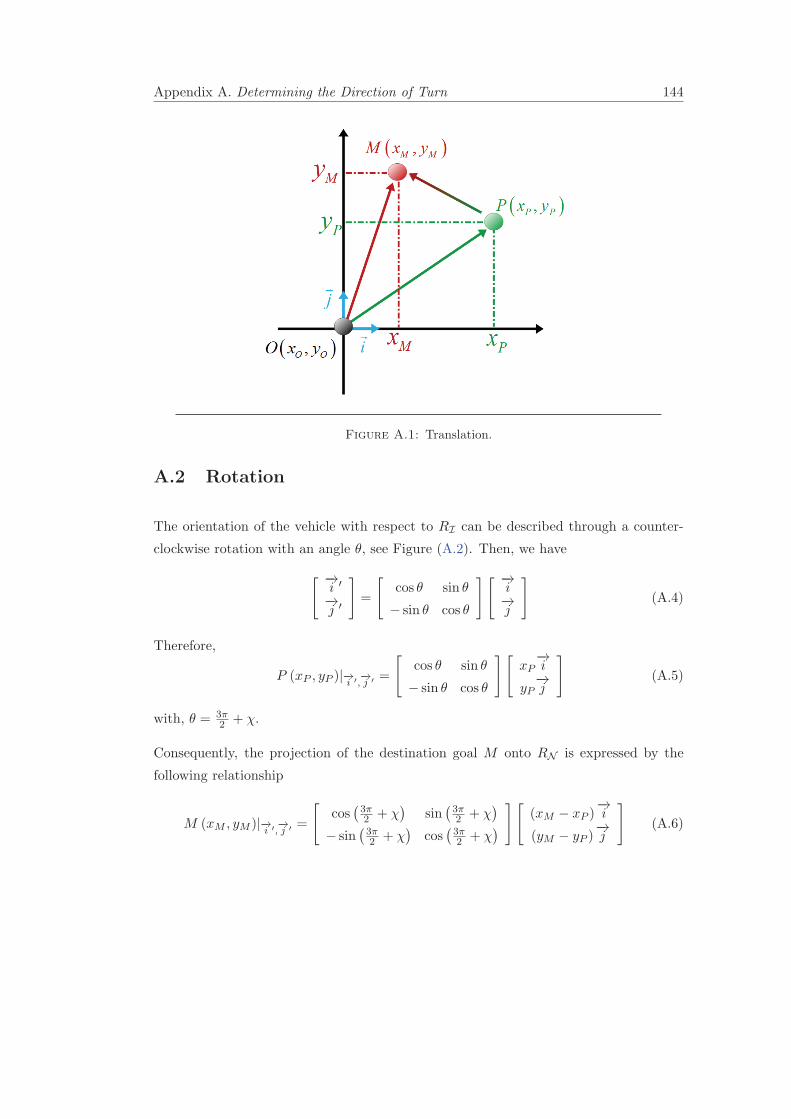
Appendix A. Determining the Direction of Turn 144
Figure A.1: Translation.
A.2 Rotation
The orientation of the vehicle with respect to RI can be described through a counter-
clockwise rotation with an angle θ, see Figure (A.2). Then, we have
[ −→i ′
−→j ′
]=
[cos θ sin θ
− sin θ cos θ
][ −→i−→j
](A.4)
Therefore,
P (xP , yP )|−→i ′,−→j ′
=
[cos θ sin θ
− sin θ cos θ
][xP
−→i
yP−→j
](A.5)
with, θ = 3π2 + χ.
Consequently, the projection of the destination goal M onto RN is expressed by the
following relationship
M (xM , yM )|−→i ′,
−→j ′
=
[cos
(3π2 + χ
)sin
(3π2 + χ
)
− sin(3π2 + χ
)cos
(3π2 + χ
)] [
(xM − xP )−→i
(yM − yP )−→j
](A.6)
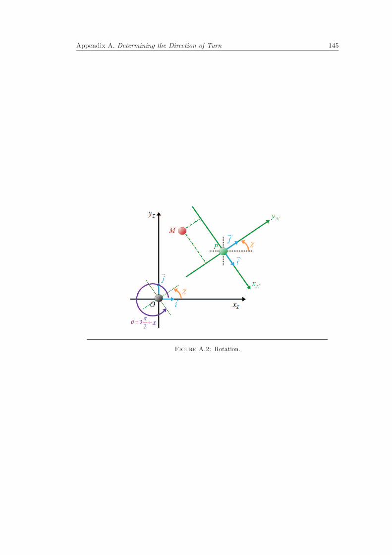
Appendix A. Determining the Direction of Turn 145
Figure A.2: Rotation.


Appendix B
Linear Phase Calculation
Remember that the equations of motion for an aerial vehicle flying at a fixed altitude is
given by
x =V cosχ (B.1a)
y =V sinχ (B.1b)
χ =u1 (B.1c)
V =u2 (B.1d)
Flying in a straight line means that the orientation of the aircraft is fixed, i.e. χ = χ0.
This implies that χ = u2 = 0. Then, integrating the Equation (B.1) leads to the
following
x =1
2u2 cosχ0t
2 + V0 cosχ0t+ x0 (B.2a)
y =1
2u2 sinχ0t
2 + V0 sinχ0 + y0 (B.2b)
χ =χ0 (B.2c)
V =u2t+ V0 (B.2d)
with u2 = ±u2max for acceleration and deceleration phases, while u2 = 0 entails the
constant velocity case.
B.1 Problem Statement
Considering two configurations q1 = [x1, y1,χ1, V1] and q2 = [x2, y2,χ2, V2], with χ1 =
χ2 = cte. In addition, assuming that reaching q2 from q1 can be done through a straight
147

Appendix B. Linear Phase Calculation 148
line. Then, the basic problem is to find a control u2 ∈ 0,±u2max such that the
continuity of the aerial vehicle’s velocity is guaranteed. In other words, defining the
acceleration, deceleration, and constant velocity segments along the trajectory.
B.2 Proposed Solution
To deal with the previous problem, we propose the following algorithm
Algorithm B.1 Linear Segments Calculation
Require: initial and final configurations (q1 and q2).1: Compute the distance (d) between q1 and q2.2: Determine the required distance for the acceleration/deceleration phase (dacc and
ddec).3: if d > dacc + ddec then4: Three linear segments are required to reach q2:
Compute switching points and traveled time for acceleration, deceleration, andconstant velocity segments.
5: else6: Two linear segments are required to reach q2:
Compute the time and the point to switch between the acceleration and deceler-ation phases.
7: end if8: return Switching time and configurations as well as control inputs along the tra-
jectory.
In the following, we describe in details the previous algorithm.
Step 1: Calculate the distance (d) between q1 and q2
This distance is given by:
d =√
(x2 − x1)2 + (y2 − y1)2 (B.3)
Step 2: Determine the required distance for the acceleration/deceleration phase (dacc
and ddec)
The required time to acceleration phase is obtained by
tacc =Vmax − V1
u2max(B.4)
Thus, from Equation (B.2a) and Equation (B.2b) we obtain
xacc =1
2u2max cosχ0t
2acc + V0 cosχ0tacc + x1 (B.5a)
yacc =1
2u2max sinχ0t
2acc + V0 sinχ0tacc + y1 (B.5b)
Appendix B. Linear Phase Calculation 149
where, (xacc, yacc) presents the end point of acceleration phase. Therefore, the
traveled distance during the acceleration phase is given by
dacc =√(xacc − x1)2 + (yacc − y1)2 (B.6)
In a similar way, we state
tdec =Vf − Vmax
−u2max(B.7)
xdec =x2 −1
2(−u2max) cosχ0t
2dec − Vmax cosχ0tdec (B.8a)
ydec =y2 −1
2(−u2max) sinχ0t
2dec − Vmax sinχ0tdec (B.8b)
ddec =√
(xf − xdec)2 + (yf − ydec)2 (B.9)
with, tdec is the required time to decelerate from Vmax to V2, (xdec, ydec) is the
start point of the deceleration phase, and ddec is the traveled distance during the
deceleration phase.
Step 4: Calculate switching points and traveled time for acceleration, deceleration, and
constant velocity segments
The switching points as well as the traveled time for acceleration and deceleration
phases has been already calculated in step 2. Then it remains to calculate the
traveled time for the constant segment. This one is given by
tconst =dconstVmax
(B.10)
where, dconst denotes the traveled distance which is obtained through the following
relationship
dconst =√(xdec − xacc)2 + (ydec − yacc)2 (B.11)
Step 6: Calculate the time and the point to switch between the acceleration and decel-
eration phases
Assuming two particles moving on the same line in an opposite direction. The first
one, P1, located at q1, while the second one, P2, based at q2. In addition, both
are in acceleration phase. Then the interception point of these two particles corre-
sponds to the switching time and point between the acceleration and deceleration
phases.
Next, we distinguish the following three cases:

Appendix B. Linear Phase Calculation 150
Case 1: V1 = V2
From Equation (B.2a), we state
xP1 =1
2u2max cosχ1t
2 + V1 cosχ1t+ x1 (B.12a)
xP1 =1
2u2max cos(χ2 + π)t2 + V2 cos(χ2 + π)t+ x2 (B.12b)
where, xP1 and xP2 denote the time profile of x-coordinate for the first and
second particle respectively. Then, at the interception point, we have xP1 =
xP2 . So,
1
2u2max (cosχ1 − cos(χ1 + π)) t2+(V1 cosχ1 − V2 cos(χ1 + π)) t+x1−x2 = 0 (B.13)
Since the time is the only unknown variable in the previous equation, then
solving this equation gives the switching time, tswt. Consequently, the switch-
ing velocity is given by
Vswt = u2maxtswt + V1 (B.14)
Case 2: V1 < V2
In this case, we compute the acceleration time tn required to reach a new
configuration qn such that Vn = V2. Then, we adopt the same strategy
described in case 1, after substituting q1 by qn, to compute the switching
configuration.
Case 3: V1 > V2
This situation is the opposite of case 2. So, we compute the acceleration time
tn necessary to reach a new configuration qn such that Vn = V1. Next, we we
compute the switching configuration in a similar way to case 1 after replacing
q2 by qn.

Appendix C
Trajectory Generation and
Circular Arcs
Assuming that the condition presented in the line 5 of the algorithm B.1 is not satisfied,
then two circumference Σij and Σfj containing the end configuration of Si and the start
configuration of Sf respectively must be included to the trajectory. The index j defines
the radius of the circumference with respect to the velocity (max for Vmax and min for
Vmin). Remember that in this case the velocity is a constant.
C.1 Circular arc equations
Flying in a circular motion implies that the velocity of the aerial vehicle is fixed while its
orientation is linearly changing. Then, the equations characterizing the circular motion
are
x =x0 +V0
u1(sinχ− sinχ0) (C.1a)
y =y0 −V0
u1(cosχ− cosχ0) (C.1b)
χ =χ0 + u1t (C.1c)
V =V0 (C.1d)
where, u1 = ±u1max for left or right turn, and q0 = [x0, y0,χ0, V0] is the vehicle’s initial
configuration.
151
Appendix C. Trajectory Generation and Circular Arcs 152
C.2 Common Tangent between Two Circles
In general, two circles have four common tangent (two outer tangents and two inner
tangents). To defines these tangents we need, first of all, to find the center and the
radius of the circles. Then, we can compute the tangential points on each circle.
C.2.1 Determining the Center of Circle
Defining the center of a circle which contains a configuration q1 = [x1, y1,χ1, V1] can be
done by the following four stages.
Step 1: This step consist of determining the radius of turn. Since the velocity of an
object traveling the circle is:
V1 =2πr
T= ωr (C.2)
where, r is the radius, T is the time required for one rotation, and ω is the angular
velocity. So we have:
r =V1
ω(C.3)
Step 2: Defining the straight line, L1 which passes in (x1, y1) in the direction of χ1.
L1 : y = a1x+ b1 (C.4)
with a1 = tan−1 (χ1) and b = y1 − a1x1.
Step 3: Characterizing the perpendicular line to L2.
L2 : y = a2x+ b2 (C.5)
with a2 = − 1a2
and b2 = y1 − a2x1.
Step 4: The intersection of L2 with the circle having a radius r and centered at (x1, y1):
y =a2x+ b2 (C.6a)
r2 =(x− x1)2 + (y − y1)
2 (C.6b)
gives the center of turn.

Appendix C. Trajectory Generation and Circular Arcs 153
C.2.2 Tangential Points
Considering the following two circles:
C1 : (x− a)2 + (y − b)2 = r21 (C.7a)
C2 : (x− c)2 + (y − d)2 = r22 (C.7b)
where (a, b), r1, (c, d), and r2 present the center and the radius of C1 and C2 respectively.
In addition assuming that r1 > r2 as it is shown in Figure (C.1). Then, the intersection
point of outer tangents Po is given by
xPo =r2a− r1c
r2 − r1(C.8a)
yPo =r2b− r1d
r2 − r1(C.8b)
Thus, the tangential points of the outer tangents located at C1 are:
xto1,2 =r21(xPo − a)± r1(yPo − b)
√(xPo − a)2 + (yPo − b)2 − r21
(xPo − a)2 + (yPo − b)2+ a (C.9a)
yto1,2 =r21(yPo − b)∓ r1(xPo − a)
√(xPo − a)2 + (yPo − b)2 − r21
(xPo − a)2 + (yPo − b)2+ b (C.9b)
In a similar way, the tangential points located at C2, i.e. xto3,4 , yto3,4 , can be computed
through Equation (C.9) by replacing a → c, b → d, and r1 → r2.
Therefore, the outer tangents are characterized by the equations
Lto1 : y =
(yto3 − yto1xto3 − xto1
)x+
(yto3
(yto3 − yto1xto3 − xto1
))xto3 (C.10a)
Lto2 : y =
(yto4 − yto2xto4 − xto2
)x+
(yto4
(yto4 − yto2xto4 − xto2
))xto4 (C.10b)
Besides, the intersection point of the two inner tangents is
xPi =r1c+ r2a
r1 + r2(C.11a)
yPi =r1d+ r2b
r1 + r2(C.11b)
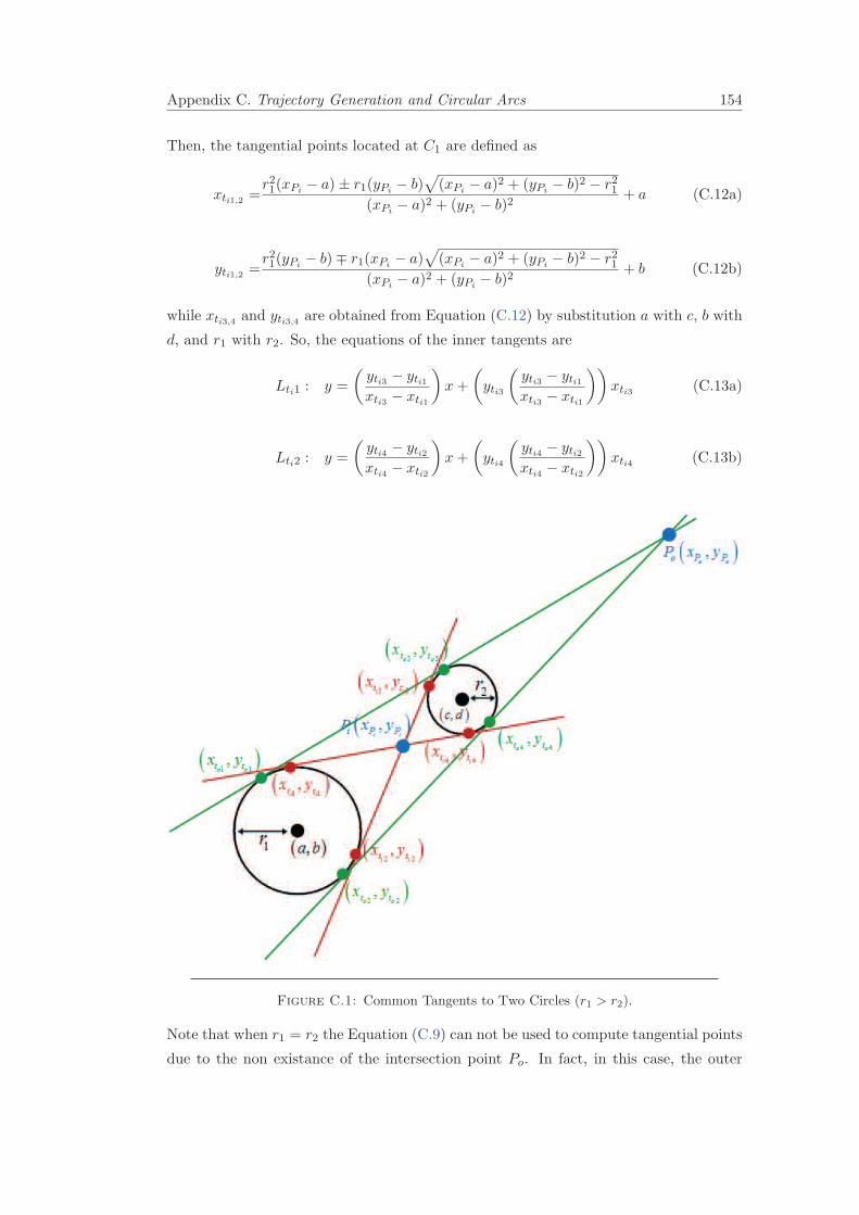
Appendix C. Trajectory Generation and Circular Arcs 154
Then, the tangential points located at C1 are defined as
xti1,2 =r21(xPi − a)± r1(yPi − b)
√(xPi − a)2 + (yPi − b)2 − r21
(xPi − a)2 + (yPi − b)2+ a (C.12a)
yti1,2 =r21(yPi − b)∓ r1(xPi − a)
√(xPi − a)2 + (yPi − b)2 − r21
(xPi − a)2 + (yPi − b)2+ b (C.12b)
while xti3,4 and yti3,4 are obtained from Equation (C.12) by substitution a with c, b with
d, and r1 with r2. So, the equations of the inner tangents are
Lti1 : y =
(yti3 − yti1xti3 − xti1
)x+
(yti3
(yti3 − yti1xti3 − xti1
))xti3 (C.13a)
Lti2 : y =
(yti4 − yti2xti4 − xti2
)x+
(yti4
(yti4 − yti2xti4 − xti2
))xti4 (C.13b)
Figure C.1: Common Tangents to Two Circles (r1 > r2).
Note that when r1 = r2 the Equation (C.9) can not be used to compute tangential points
due to the non existance of the intersection point Po. In fact, in this case, the outer

Appendix C. Trajectory Generation and Circular Arcs 155
tangents becomes parallel to each other as well as to the line passes by (a, b) and (c, d)
as it is illustrated in Figure (C.2).
Figure C.2: Common Tangents to Two Circles (r1 = r2).
Let LC denotes the line passing through the center of C1 and C2. Then, the tangential
points are the intersections between C1/C2 and the perpendicular lines to LC at (a, b)
and (c, d) respectively.


Bibliography
[1] D. Aarno, D. Kragic, and H.I. Christensen. Artificial potential biased probabilis-
tic roadmap method. In Proceedings of the IEEE International Conference on
Robotics and Automation (ICRA), volume 1, pages 461–466, New Orleans, LA,
USA, April 2004.
[2] M. Alighanbari, Y. Kuwata, and J.P. How. Coordination and control of multi-
ple uavs with timing constraints and loitering. In American Control Conference,
volume 6, pages 5311–5316, Denver, Colorado, USA, June 2003.
[3] N.M. Amato, O.B. Bayazit, L.K. Dale, C. Jones, and D. Vallejo. Obprm: An
obstacle-based prm for 3d workspaces. In Int. Workshop on Algorithmic Founda-
tions of Robotics (WAFR), Houston, Texas, USA, March 1998.
[4] G. Ambrosino, M. Ariola, U. Ciniglio, F. Corraro, E. De Lellis, and A. Pironti.
Path generation and tracking in 3-d for uavs. IEEE Transactions on Control
Systems Technology, 17(4):980–988, July 2009.
[5] E.P. Anderson and R.W. Beard. An algorithmic implementation of constrained
extremal control for uavs. In AIAA Guidance, Navigation, and Control Conference
and Exhibit, Monterey, California, USA, August 2002.
[6] Z. Artstein. Stabilization with relaxed controls. Nonlinear Analysis: Theory,
Methods & Applications, 7(11):1163–1173, November 1983.
[7] Z. Ashraf and M. A. Choudhry. Dynamic modeling of the airship using analytical
aerodynamic model. In International Conference on Emerging Technologies, pages
188–193, Islamabad, Pakistan, 19-20 October 2009.
[8] J. R. Azinheira, P. Rives, J. R. H. Carvalho, G. F. Silveira, E. C. De Paiva, and
S. S. Bueno. Visual servo control for the hovering of an outdoor robotic airship.
In IEEE International Conference on Robotics and Automation, pages 2787–2792,
Washington, DC, USA, May 2002.
[9] L. Bairstow. Applied Aerodynamics. Green and Co., London, 1920.
157

Bibliography 158
[10] E. Bakolas and P. Tsiotras. Time-optimal synthesis for the zermelo-markov-dubins
problem: The constant wind case. In American Control Conference, pages 6161–
6168, Marriott Waterfront, Baltimore, MD, USA, June–July 2010.
[11] H. Bang, S. Lee, and H. Lee. Nonlinear trajectory tracking using vectorial back-
steeping approach. In International Conference on Control, Automation and Sys-
tems, pages 169–174, COEX, Seoul, Korea, October 2008.
[12] A. Barrientos, P. Gutierrez, and J. Colorado. Advanced UAV Trajectory Genera-
tion: Planning and Guidance, Aerial Vehicles, T. M. Lam (Ed.). InTech, 2009.
[13] L. Beji and A. Abichou. Tracking control of trim trajectories of blimp for ascent
and descent flight maneuvers. International Journal of Control, 78(10):706–719,
July 2005.
[14] L. Beji, A. Abichou, and Y. Bestaoui. Stabilization of a nonlinear underactuated
autonomous airship - a combined averaging and backstepping approach. In the
3rd International Workshop on Robot Motion and Control (RoMoCo), Bukowy
Dworek, Poland, November 2002.
[15] J. Bellingham, M. Tillerson, A. Richards, and J.P. How. Multi-task allocation and
path planning for cooperation UAVs. In: Cooperative Control: Models, Applica-
tions and Algorithms, S. Butenko, R. Murphey, and P.M. Pardalos (Eds.). Kluwer
Academic Publishers, Netherlands, 2003.
[16] M. Bellmore and G.L. G. L. Nemhauser. The traveling salesman problem: A
survey. Operations Research, 59(3):538–558, May 2011.
[17] Y. Bestaoui. Lighter Than Air Robots. Number 58 in Intelligent Systems, Control
and Automation: Science and Engineering. Springer, Netherlands, 2012.
[18] Y. Bestaoui and S. Hima. Trajectory tracking of a dirigible in a high constant
altitude flight. In the 5th IFAC symposium on Nonlinear control systems, Saint
Petersburg, Russia, July 2001.
[19] Y. Bestaoui and E. Kahale. Analysis of time optimal 3d paths for an autonomous
aircraft with a piecewise constant acceleration. In 49th AIAA Aerospace Sciences
Meeting, Orlando Florida, USA, January 2011.
[20] Y. Bestaoui and E. Kahale. Generation of time optimal trajectories of an au-
tonomous airship. In IEEE Workshop on Robot Motion Control (ROMOCO),
Bukowy Dworek, Poland, June 2011.

Bibliography 159
[21] Y. Bestaoui and E. Kahale. Time optimal trajectories of a lighter than air robot
with second order constraints and a piecewise constant velocity wind. AIAA
Journal of Aerospace Computing Information and Communication, 10(4):155–171,
April 2013.
[22] S. J. Biljlsma. Optimal aircraft routing in general wind fields. AIAA Journal of
Guidance, Control and Dynamics, 32(3):1025–1029, May–June 2009.
[23] A. M. Bloch. Nonholonomic mechanics and Control. Springer, 2003.
[24] B. Blocken, P. Moonen, T. Stathopoulos, F. Asce, and J. Carmeliet. Numeri-
cal study on the existence of the venturi effect in passages between perpendicu-
lar buildings. Journal of Engineering Mechanics, 134(12):1021—-1028, December
2008.
[25] R. Bohlin and L. Kavraki. Path planning using lazy prm. In Proceedings of the
IEEE International Conference on Robotics and Automation (ICRA), volume 1,
pages 521–528, San Francisco, CA, USA, April 2000.
[26] A. Bonnet. Identification des coefficients aerodynamiques du dirigeable AS500 du
LAAS. Technical report. Etude Hydro-Aerodynamique, SUPAERO, 2003.
[27] V. Boor, M.H. Overmars, and A.F. Van der Stappen. The gaussian sampling
strategy for probabilistic roadmap planners. In Proceedings of the IEEE Interna-
tional Conference on Robotics and Automation (ICRA), pages 1018–1023, Detroit,
Michigan, USA, May 1999.
[28] D. Boukraa, Y. Bestaoui, and N. Azouz. Three dimensional trajectory genera-
tion for an autonomous plane. International Review of Aerospace Engineering,
1(4):355–365, August 2008.
[29] E. Bryson Jr. and Y.C. Ho. Applied Optimal Control. Taylor & Francis, 1975.
[30] C. Buskens and H. Maurer. Sqp-methods for solving optimal control problems with
control and state constraints: Adjoint variables, sensitivity analysis and real-time
control. Journal of Computational and Applied Mathematics, 120(1–2):85–108,
August 2000.
[31] C. Canudas de Wit, B. Siciliano, and G. (Eds.) Bastin. Theory of Robot Control.
Springer-Verlag, London, 1996.
[32] P. Castillo, R. Lozano, and A. Dzul. Stabilization of a mini rotorcraft with four
rotors. IEEE Control Systems Magazine, 25(6):45–55, December 2005.
Bibliography 160
[33] P. Castillo, R. Lozano, and A. E. Dzul. Modeling and Control of Mini-Flying
Machines. Springer-Verlag, London, 2005.
[34] H. Choset, K. Lynch, S. Hutchinson, G. Kantor, W. Burgard, L. Kavraki, and
S. Thrum. Principles of Robot Motion, Theory, Algorithms and Implementation.
MIT Press, Cambridge, 2005.
[35] N. Christofides. Worst case analysis of a new heuristic for the traveling salesman
problem. Report 388, Graduate School of Industrial Administration, Carniege-
Mellon University, Pittsburg, PA, USA, 1976.
[36] G. Clark and J.W. Wright. Scheduling of vehicles from a central depot to a number
of delivery points. Operations Research, 12(4):568–581, July 1964.
[37] C.I. Connolly, K. Souccar, and R.A. Grupen. A hamiltonian framework for kino-
dynamic planning and control. In IEEE International Conference on Robotics and
Automation, volume 3, pages 2746–2751, Nagoya, Japan, May 1995.
[38] M.V. Cook. Flight Dynamics Principles. Elsevier, UK, 2007.
[39] J.-F. Cordeau, M. Gendreau, G. Laporte, J.-Y. Potvin, and F. Semet. A guide to
vehicle routing heuristics. Journal of the Operational Research Society, 53(5):512–
522, May 2002.
[40] C.E. Corrigan, G.C. Roberts, M.V. Ramana, D. Kim, and V. Ramanathan. Cap-
turing vertical profiles of aerosols and black carbon over the indian ocean using
autonomous unmanned aerial vehicles. Journal of Atmospheric Chemistry and
Physics, 8(3):737–747, 2008.
[41] J.A. Curry, J. Maslaink, G. Holland, and J. Pinto. Applications of aerosondes in
the arctic. Bull. Amer. Meteor. Soc., 85(12):1855–1861, 2004.
[42] L.K. Dale and Amato N.M. Probabilistic roadmaps - putting it all together. In
Proceedings of the IEEE International Conference on Robotics and Automation
(ICRA), volume 2, pages 1940–1947, Seoul, Korea, May 2001.
[43] G.B. Dantzig and R. Ramser. The truck dispatching problem. Management Sci-
ence, 6(1):80–91, October 1959.
[44] L. De Filippis and G. Guglieri. Advanced Graph Search Algorithms for Path Plan-
ning of Flight Vehicles, Recent Advances in Aircraft Technology, R. K. Agarwal
(Ed.). InTech, 2012.
[45] E. De Pavia, F. Benjovengo, and S. Bueno. Sliding mode control for the path
following of an unmanned airship. In the 6th IFAC Symposium on Intelligent
Autonomous Vehicles, Toulouse, France, September 2007.
Bibliography 161
[46] F. Derkx, J. Dumoulin, J.-L. Sorin, and V. Legeay. Concept de plate-forme mobile
instrumentee (pmi) pour l’inspection des ouvrages d’art. In journees Micro-Drones
2-eme edition, Toulouse, France, September 2002.
[47] F. Derkx and F.L. Sorin. Inspection des ouvrages d’art par drone. bilan et pre-
spectives des travaux du lcpc. Bulletin des laboratoires des ponts et chausses,
(273):39–56, December 2008.
[48] C. Dever, B. Mettler, E. Feron, J. Popovic, and M. McConley. Trajectory interpo-
lation for parametrized maneuvering and flexible motion planning of autonomous
vehicles. In AIAA Guidance, Navigation, and Control Conference and Exhibit,
Providence, RI, USA, August 2004.
[49] S. Dicheva and Y. Bestaoui. 3d waypoint generation in a dynamic environment for
an airborne launch mission. Proceedings of the Institution of Mechanical Engineers,
Part G: Journal of Aerospace Engineering, 10(226):1283–1297, October 2012.
[50] M. Dorigo and T. Stutzle. Ant Colony Optimization. Prentice Hall, 2004.
[51] L. E. Dubins. On curves of minimal length with a constraint on average curvature
and with prescribed initial and terminal positions and tangents. American Journal
of Mathematics, 79(3):497–517, 1957.
[52] C. Eberhart and J. Kennedy. A new optimizer using particle swarm optimization.
In International Symposium on Micro Machine and Human Science, pages 39–43,
Nagoya, Japan, October 1995.
[53] A.E. Eiben and J.E. Smith. Introduction to Evolutionary Computing. Springer-
Verlag, 2003.
[54] A. Elfes, J. F. Montgomery, J. L. Hall, S. S. Joshi, J. Payne, and Bergh C. F.
Autonomous flight control for a planetary exploration aerobot. In AIAA Space
Conference, Long Beach, CA, August 2005.
[55] J. Etele. Overview of wind gust modelling with appli- cation to autonomous low-
level uav control. InMechanical and Aerospace Engineering Departement, Carelton
University, Ottawa, Canada, 2006.
[56] B. Etkin. Turbulent wind and its effect on flight. Journal of Aircraft, 18(5):327–
345, May 1981.
[57] M. Faied, A. Mostafa, and A. Gurard. Vehicle routing problem instances: Applica-
tion to multi-uav mission planning. In AIAA Guidance, Navigation, and Control
Conference and Exhibit, Toronto, Ontario, Canada, August 2010.
Bibliography 162
[58] B.A. Fisher and R. Jaikumar. A generalized assignment heuristic for vehicle rout-
ing. Networks, 11(2):109–124, 1981.
[59] T. I. Fossen. Guidance and Control of Ocean Vehicles. John Wiley & Sons Ltd.,
1994.
[60] E. Frazzoli, M.A. Dahleh, and E. Feron. A hybrid control architecture for aggres-
sive maneuvering of autonomous helicopters. In IEEE International Conference on
Decision and Control, volume 25, pages 2471–2476, Phoenix, AZ, USA, December
1999.
[61] E. Frazzoli, M.A. Dahleh, and E. Feron. Real-time motion planning for ag-
ile autonomous vehicles. AIAA Journal of Guidance, Control, and Dynamics,
25(1):116—-129, January 2002.
[62] R. A. Freemann and P. V. Kokotovic. Robust Nonlinear Control Design: State-
Space and Lyapunov Techniques. Birkhauser, 1996.
[63] E.W. Frew and T.X. Brown. Networking issues for small unmanned aircraft sys-
tems. Journal of Intelligent and Robotic Systems, 54(1–3):21–37, March 2009.
[64] T. Fukao, K. Fujitaniy, and T. Kanade. Image-based tracking control of a blimp.
In the 42nd IEEE Conference on Decision and Control, pages 3462–3467, Hawaii,
USA, December 2003.
[65] T. Fukao, T. Kanzawa, and K. Osuka. Inverse optimal tracking control of an aerial
blimp robot. In the 5th International Workshop on Robot Motion and Control
(RoMoCo), Poland, June 2005.
[66] H. Fukushima, R. Saito, and F. Matsumo. Model predictive control of an au-
tonomous blimp with input and output constraints. In IEEE International Con-
ference on Control Applications, pages 2184–2189, Munich, Germany, October
2006.
[67] T.J. Gaskell. Bases for vehicle fleet scheduling. Journal of the Operational Research
Society, 18(3):281–295, September 1967.
[68] B. Gillett and L.R. Miller. A heuristic algorithm for the vehicle-dispatch problem.
Operations Research, 22(2):340–349, Mars 1974.
[69] C. Goerzen, Z. Kong, and B. Mettler. A survey of motion planning algorithms
from the perspective of autonomous uav guidance. In KimonP. Valavanis, Ran-
dal Beard, Paul Oh, Anıbal Ollero, LeslieA. Piegl, and Hyunchui Shim, editors,
Selected papers from the 2nd International Symposium on UAVs, Reno, Nevada,
U.S.A. June 8–10, 2009, pages 65–100. Springer Netherlands, 2010.
Bibliography 163
[70] J.A. Guerrero, , and Y. Bestaoui. Uav path planning for structure inspection in
windy environments. Journal of Intelligent & Robotic Systems, 69(1-4):297–311,
January 2013.
[71] J.A. Guerrero and Y. Bestaoui. Optimal Trajectory Planning for Structure Inspec-
tion. Technical report. Laboratoire IBISC, Universite d’Evry Val d’Essonne, Evry,
France, December 2011.
[72] V. Guillemin and A. Pollack. Differential Topology. Prentice-Hall, New York,
USA, 1974.
[73] J. Hacker and B. H. Kroplin. An experimental study of visual flight trajectory
tracking and pose prediction for the automatic computer control of a miniature
airship. In SPIE International Society for Optical Engineering, pages 25–36, 2003.
[74] P. Hart, N. Nilsson, and B. Raphael. A formal basis for the heuristic determination
of minimum cost paths. IEEE Transactions on Systems Science and Cybernetics,
4(2):100–107, July 1968.
[75] S. Haykin. Neural Networks. Prentice Hall, 1999.
[76] M.T. Heath. Scientific Computing: An Introductory Survey, 2nd Ed. McGraw-
Hill, New York, 2002.
[77] S. Hima. Planification des trajectoires d’un dirigeable autonome. PhD. Thesis.
Universite d’Evry Val d’Essonne, Evry, France, 2005.
[78] S. Hota and D. Ghose. Optimal path planning for an aerial vehicle in 3d space.
In the 49th IEEE Conference on Decision and Control, pages 4902–4907, Atlanta,
Georgia, USA, December 2010.
[79] D. Hsu, T. Jiang, J.H. Reif, and Z. Sun. The bridge test for sampling narrow
passages with probabilistic roadmap planners. In Proceedings of the IEEE In-
ternational Conference on Robotics and Automation (ICRA), pages 4420–4426,
Taipei, Taiwan, September 2003.
[80] D. Hsu, L.E. Kavraki, J.-C. Latombe, R. Motwani, and S. Sorkin. On finding
narrow passages with probabilistic roadmap planners. In Int. Workshop on Algo-
rithmic Foundations of Robotics (WAFR), Houston, Texas, USA, March 1998.
[81] D. G. Hull. Fundamentals of Airplane Flight Mechanics. Springer, Berlin, 2007.
[82] F. Imado, Y. Heike, and T. Kinoshita. Research on a new aircraft point-mass
model. Journal of Aircraft, 48(4):1121–1130, July-August 2011.
Bibliography 164
[83] M. R. Jardin and A. E. Bryson. Neighboring optimal aircraft guidance in winds.
AIAA Journal of Guidance, Control and Dynamics, 24(4):710–715, July–August
2001.
[84] M.R. Jardin and E. Bryson Jr. Methods for computing minimum-time paths
in strong winds. Journal of Guidance, Control, and Dyncamics, 35(1):165–171,
January–February 2012.
[85] A. L. Jennings, R. Ordonez, and N. Ceccarelli. Dynamic programming applied
to uav way point path planning in wind. In IEEE International Symposium on
Computer-Aided Control System Design, pages 215–220, San Antonio, Texas, USA,
Septembre 2008.
[86] R. Jia, M. T. Frye, and C. Qian. Control of an airship using partical swarm
optimization and neural network. In IEEE International Conference on Systems,
Man, and Cybernetics, pages 1809–1814, San Antonio, TX, USA, October 2009.
[87] Z. Jiang and R. Ordonez. Robust approach and landing trajectory generation for
reusable launch vehicles in winds. In IEEE International Conference on Control
Applications, pages 930–935, San Antonio, Texas, USA, Septembre 2008.
[88] V. Jurdjevic. Geometric control theory. Cambridge University Press, Cambridge,
U.K., 2008.
[89] E. Kahale, Y. Bestaoui, and P. Castillo. Path tracking of a small autonomous air-
plane in wind gusts. In IEEE/RSJ International Conference on Intelligent Robots
and Systems (IROS), pages 402–407, Vilamoura, Algarve, Portugal, October 2012.
[90] E. Kahale, P. Castillo, and Y. Bestaoui. Autonomous path tracking of a kinematic
airship in presence of unknown gust. In International Conference on Unmanned
Air- craft Systems (ICUAS), Philadelphia, PA, USA, June 2012.
[91] E. Kahale, P. Castillo Garcia, and Y. Bestaoui. Autonomous path tracking of a
kinematic airship in presence of unknown gust. Journal of Intelligent and Robotic
Systems, 69(1-4):431–446, January 2013.
[92] F Kamrani and R. Ayani. UAV Path Planning in Search Operations, Aerial Ve-
hicles, T. M. Lam (Ed.). InTech, 2009.
[93] S. Karaman and E. Frazzoli. Vehicle routing problem with metric temporal logic
specifications. In the 47th IEEE Conference on Decision and Control, pages 3953–
3958, Cancun, Mexico, December 2008.
Bibliography 165
[94] L. Kavraki, P. Svestka, J.-C. Latombe, and M.H. Overmars. Probabilistic
roadmaps for path planning in high dimensional configuration spaces. IEEE Trans-
actions on Robotics and Automation, 12(4):566–580, August 1996.
[95] Y. Kawai, S. Kitagawa, S. Izoe, and M. Fujita. An unmanned planar blimp on vi-
sualfeedback control: Experimental results. In the 42nd SICE Annual Conference,
pages 680–685, 2003.
[96] H.J. Kelley. Guidance theory and extremal fields. IRE Transactions on Automatic
Control, 7(5):75–82, October 1962.
[97] O. Khatib and L.M. Mampey. Fonction Decision-Commande d’un Robot Manip-
ulateur. Technical report 2/7156. DERA/CERT, Toulouse, France, 1978.
[98] G. A. Khoury and J. D. Gillet. Airship Technology. Cambridge University Press,
Cambridge, 1999.
[99] J. Kim, J. Keller, and V. Kumar. Design and verification of controllers for airships.
In IEEE/RSJ International Conference on Intelligent Robots and Systems (IROS),
pages 54–60, Las Vegas, Nevada, USA, October 2003.
[100] S. Kirkpatrik. Optimization by simulated annealing: Quantitative study. Journal
of Statistical Physics, 34(5-6):975–986, March 1984.
[101] P. Klein. Lecture notes on Hilbert spaces and the projection theorem. Stockholms
Universitet, 2009.
[102] E. Kreyszig. Differential Geometry. Dover Publications, New York, 1991.
[103] S.N. Kumar and R. Panneerselvam. A survey on the vehicle routing problem and
its variants. Intelligent Information Management, 4(3):66–74, May 2012.
[104] H. Kurniawati and D. Hsu. Workspace importance sampling for probabilistic
roadmap planning. In IEEE/RSJ International Conference on Intelligent Robots
and Systems (IROS), pages 1618–1623, Sendai, Japan, September 28–October 2
2004.
[105] T. Kampke and A. Elfes. Optimal aerobot trajectory planning for wind based
opportunity flight control. In IEEE/RSI International Conference on Intelligent
Robots and Systems, pages 67–74, Las Vegas, Nevada, USA, October 2003.
[106] G. Lafferriere and H. J. Sussmann. A differential geometric approach to motion
planning. In NONHOLONOMIC MOTION PLANNING, pages 235–270. Kluwer,
1993.
Bibliography 166
[107] G. Laporte. The traveling salesman problem: An overview of exact and approxi-
mate algoritgms. European journal of Operational Research, 59(2):231–247, June
1992.
[108] G. Laporte and Y. Norbert. Exact Algorithms for the Vehicle Routing Problem.
Surveys in Combinatorial Optimization. ElSEVIER, Amsterdam, 1987.
[109] R.C. Larson and A.R. Odoni. Urban Operations Research. Prentice-Hall, Engle-
wood Cliffs,NJ, USA, 1981.
[110] J.-C. Latombe. Robot Motion Planning. Kluwer Academic Press, Massachusetts,
USA, 1991.
[111] S. M. LaValle. Planning Algorithms. Cambridge University Press, Cambridge,
U.K., 2006.
[112] S.M. LaValle. Rapidly-exploring random trees: a new tool for path planning. Tech-
nical report (TR 98–11). Computer Science Department, Iowa State University,
USA, 1998.
[113] S.M. LaValle and J.J. Kuffner. Rapidly-exploring random trees: Progress and
prospects. In Int. Workshop on Algorithmic Foundations of Robotics (WAFR),
Hanover, NH, USA, March 2000.
[114] S.M. LaValle and J.J. Kuffner. Randomized kinodynamic planning. International
Journal of Robotics Research, 20(5):378–400, May 2001.
[115] W.S. Levine. The Control Handbook, Second Edition : Control System, Advenced
Methods. CRC Press, Taylor & Francis Group, 2011.
[116] Y. Li and M. Nahon. Modeling and simulation of airship dynamics. Journal of
Guidance, Control, and Dynamics, 30(6):1691–1700, November–December 2007.
[117] Z. Li and J. F. (Ed.) Canny. Non holonomic Motion Planning. Kluwer Academic
Press, Berlin, 1992.
[118] Y. Liu, Z. Pan, D. Stirling, and F. Naghdy. Control of autonomous airship. In IEEE
International Conference on Robotics and Biomimetics (ROBIO), pages 2457–
2462, Guilin, China, December 2009.
[119] A. M. Lyapunov. Probleme general de la stabilite du mouvement. Annales de la
faculte des sciences de Toulouse, 9(2):203–474, 1907.
[120] T. McGee and J. K. Hedrick. Optimal path planning with a kinematic airplane
model. AIAA Journal of Guidance, Control and Dynamics, 30(2):629–633, March–
April 2007.

Bibliography 167
[121] D. Mclean. Automatic Flight Control Systems. Prentice Hall, UK, 1990.
[122] M. Morales, S. Rodrıguez, and N.M. Amato. Improving the connectivity of prm
roadmaps. In Proceedings of the IEEE International Conference on Robotics and
Automation (ICRA), pages 4427–4432, Taipei, Taiwan, September 2003.
[123] P. Morin and C. Samson. Trajectory Tracking for Non-holonomic Vehicles, Robot
Motion and Control, K. R. Kozlowski (Ed.). Springer-Verlag, London, 2006.
[124] A. Moutinho and J. R. Azinheira. Stability and robustness analysis of the aurora
airship control system using dynamic inversion. In IEEE International Conference
on Robotics and Automation, pages 2265–2270, Washington D. C., USA, April
2005.
[125] J. Mueller, Y. Zhoa, and M. Paluszek. Development of an aerodynamic model
and control law design for a high altitude airship. In AIAA Unmanned Unlimited
Conference, Chicago, USA, September 2004.
[126] J. B. Mueller, Y. J. Zhao, and W. L. Garrard. Optimal ascent trajectories for
stratospheric airships using wind energy. Journal of Guidance, Control, and Dy-
namics, 32(4):1232–1245, July 2009.
[127] L. E. Munoz. Stabilisation d’un vehicule aerien autonome en presence de vent.
PhD. Thesis. Universite de Technologie de Compiegne, Compiegne, France, 2012.
[128] L. E. Munoz, O. Santos, and P. Castillo. Robust nonlinear real-time control strat-
egy to stabilize a pvtol aircraft in crosswind. In IEEE/RSJ International Confer-
ence on Intelligent Robots and Systems (IROS), pages 1606–1611, Taipei, Taiwan,
October 2010.
[129] G. Murguia-Rendon, H. Rodriguez-Cortes, and M. Velasco-Villa. Trajectory track-
ing control for the planar dynamics of a thrust vectored airship. In the 52nd IEEE
International Midwest Symposium on Circuits and Systems (MWSCAS), pages
329–332, Cancun, Mexico, August 2009.
[130] D.S. Naidu. Optimal Control Systems. CRC Press LLC, 2003.
[131] R. Nelson, B. Barber, T. McLain, and R. Beard. Vector field path following for
miniature air vehicle. IEEE Transactions on Robotics, 23(3):519–529, June 2007.
[132] R. C. Nelson. Flight Stability and Automatic Control. McGraw-Hill, 1989.
[133] H. Nijmeijer and A. Van Der Schaft. Nonlinear Dynamical Control Systems.
Springer-Verlag, 1990.
Bibliography 168
[134] K. Nonami, F. Kendoul, S; Suzuki, W. Wang, and D. Nakazawa. Autonomous
Flying Robots: Unmanned Aerial Vehicles and Micro Aerial Vehicles. Springer,
2010.
[135] H. Paessens. The savings algorithm for the vehicle routing problem. European
journal of Operational Research, 34(3):336–344, March 1988.
[136] C. S. Park, H. Lee, M. J. Tahk, and H. Bang. Airship control using neural network
augmented model inversion. In IEEE Conference on Control Applications, pages
558–563, Istanbul, Turkey, June 2003.
[137] J. Rao, Z. Gong, J. Luo, and Xie S. A flight control and navigation system of a
small size unmanned airship. In IEEE International Conference on Mechatronics
and Automation, pages 1491–1496, Niagara Falls, Canada, July 2005.
[138] J. Rao, Z. Gong, J. Luo, and Xie S. Unmanned airships for emergency manage-
ment. In IEEE International Workshop on Safety, Security and Rescue Robotics,
pages 125–130, Kobe, Japan, June 2005.
[139] F. Repoulias and E. Papadopoulos. Robotic airship trajectory tracking control
using a backstepping methodology. In IEEE International Conference on Robotics
and Automation, pages 188–193, Pasadena, CA, May 2008.
[140] A. Richards, Y. Kuawta, and J.P. How. Experimental demonstrations of real-time
milp control. In AIAA Guidance, Navigation, and Control Conference and Exhibit,
Austin, Texas, USA, August 2003.
[141] E. Rimon and D.E. Koditschek. Exact robot navigation using cost functions: the
case of distinct spherical boundaries in en. In IEEE International Conference on
Robotics and Automation, volume 3, pages 1791–1796, Philadelphia, PA, USA,
April 1988.
[142] J. Roskam. Airplane Flight Dynamics and Automatic Flight Controls Part I. DAR-
corporation, USA, 2001.
[143] R. Rysdyk. Course and heading changes in significant wind. AIAA Journal of
Guidance, Control and Dynamics, 30(4):1168–1171, July–August 2007.
[144] K. Savla, E. Frazzoli, and F. Bullo. Traveling salsperson problems for dubins
vehicle. IEEE Transactions on Automatic Control, 53(6):1378–1391, July 2008.
[145] T. Schouwenaars, B. Mettler, E. Feron, and J. How. Hybrid model for trajectory
planning of agile autonomous vehicles. Journal of Aerospace Computing, Informa-
tion, and Communication, 1(12):629–651, December 2004.
Bibliography 169
[146] C. Schumacher, P. Chandler, M. Pachter, and L. Pachter. Uav task assignment
with timing constraints via mixed-integer linear programming. In AIAA 3rd Un-
manned Unlimited Technical Conference, Workshop and Exhibit, Chicago, Illinois,
USA, September 2004.
[147] C. Schumacher, P. Chandler, M. Pachter, and L. Pachter. Optimization of air ve-
hicles operations using mixed-integer linear programming. Journal of Operational
Research Society, 58:516–527, April 2007.
[148] B. Siciliano, L. Sciavicco, L. Villani, and G. Oriolo. Robotics: Modelling, Planning
and Control. Springer Verlag, London, 2009.
[149] G. F. Silveira, J. R. Azinheira, P. Rives, and Bueno S. S. Line following visual
servoing for aerial robots combined with complementary sensors. In the 11th In-
ternational Conference on Advanced Robotics, Coimbra, Portugal, June 2003.
[150] G. F. Silveira, J. R. H. Carvalho, P. Rives, J. R. Azinheira, S. S. Bueno, and
M. K. Madrid. Optimal visual servoed guidance of outdoor autonomous robotic
airships. In American Control Conference, pages 779–784, Anchorage, AK, USA,
May 2002.
[151] T. Simeon, J.P. Laumond, and C. Nissoux. Visibility based probabilistic roadmaps
for motion planning. Advanced Robotics Journal, 14(6):477–493, December 2000.
[152] S.N. Singh, M.L. Steinberg, and A.B. Page. Nonlinear adaptive and sliding mode
flight path control of f/a-18 model. IEEE Transactions on Aerospace and Elec-
tronic Systems, 39(4):1250–1262, 2003.
[153] L. Solaque, Z. Pinzon, and M. Duque. Nonlinear control of the airship cruise
flight phase with dynamical decoupling. In Electronics, Robotics and Automotive
Mechanics Conference (CERMA), pages 472–477, Morelos, Mexico, October 2008.
[154] E. D. Sontag. A lyapunov-like characterization of asymptotic controllability. SIAM
Journal on Control and Optimization, 21(3):462–471, May 1983.
[155] B. L. Stevens and F. L. Lewis. Aircraft Control and Simulation. Wiley, Canada,
2003.
[156] S. Subchan and R. Zbikowski. Computational Optimal Control Tools and Practice.
John Wiley & Sons Inc., 2009.
[157] K. Sundar and S. Rathinam. Algorithms for routing an unmanned aerial vehicle
in the presence of refueling depots. IEEE Transactions on Automation Science
and Engineering, 11(1):287–294, January 2014.

Bibliography 170
[158] H. J. Sussmann. A general theorem on local controllability. SIAM Journal on
Control and Optimization, 1(25):158–194, 1987.
[159] L. Techy. Optimal navigation in planar time-varying flow: Zermelo’s problem
revisited. Intelligent Service Robotics, 4(4):271–283, October 2011.
[160] P. G. Thomasson. Equations of motion of a vehicle in a moving fluid. Journal of
Aircraft, 37(4):630–639, July–August 2000.
[161] P. Toth and D. Vigo. The Vehicle Routing Problem. SIAM, Philadelphia, USA,
2002.
[162] K.P. Valavanis. Advances in Unmanned Aerial Vehicles: State of the Art and the
Road to Autonomy. Number 33 in Intelligent Systems, Control and Automation:
Science and Engineering. Springer, Netherlands, 2007.
[163] S. Van Der Zwaan, M. Perrone, A. Bernardino, and J. Santos-Victor. Control of
an aerial blimp based on visual input. In the 8th International Symposium on
Intelligent Robotic Systems, Reading, UK, July 2000.
[164] G.B. Venturi. Recherches experimentales sur le principe de la communication
laterale du mouvement dans les fluides, applique a l’explication de differens
phenomenes hydrauliques. Houel et Ducros: T. Barrois, Paris, France, 1797.
[165] N. X. Vinh. Flight Mechanics of High-Performance Aircraft. Number 4 in Cam-
bridge aerospace series. Cambridge University Press, Cambridge, 1993.
[166] A. Weinstein and C. Schumacher. UAV Scheduling vie the Vehicle Routing Problem
with Time Windows. Technical report, AFRL-VA-WP-TP-2007-306. Air Force
Research Laboratory, USA, 2007.
[167] D. A. Wimmer, M. Bildstein, K. H. Well, M. Schlenker, P. Kungl, and B. H.
Kroplin. Development and operation controllers for autonomous flight phases.
In Workshop on Aerial Robotics, IEEE International Conference on Intelligent
Robots and Systems, pages 55–68, Lausanne, Switzerland, October 2002.
[168] H. Wong, V. Kapila, and R. Vaidyanathan. Uav optimal path planning using c-
c-c class paths for target touring. In the 43rd IEEE Conference on Decision and
Control, pages 1105–1110, Nassau, Bahamas, December 2004.
[169] A. Wren and A. Holliday. Computer scheduling of vehicles from one or more
depots to a number of delivery points. Journal of the Operational Research Society,
23(3):333–344, September 1972.
Bibliography 171
[170] X. Wu, C. H. Moog, L. A. M. Martinez, and Y. Hu. Nonlinear control of a
buoyancy-driven airship. In the 48th IEEE Conference on Decision and Control
and 28th Chinese Control Conference, pages 2849–2854, Shanghai, China, Decem-
ber 2009.
[171] G. Xia and D. R. Corbett. Cooperative control systems of searching targets using
unmanned blimps. In the 5th Worth Congress on Intelligent Control and Automa-
tion, pages 1179–1183, Hangzhou, P.R. China, June 2004.
[172] G. Yang and V. Kapila. Optimal path planning for unmanned air vehicles with
kinematic and tactical constraints. In the 41st IEEE Conference on Decision and
Control, volume 2, pages 1301–1306, Las Vegas, Nevada, USA, December 2002.
[173] M. I. Zelikin and V. F. Borison. Theory of Chattering Control. Birkhauser, Basel,
1994.
[174] E. Zermelo. Uber das navigationsproblem bei ruhender oder veranderlicher wind-
verteilung. Journal of Applied Mathematics and Mechanics / Zeitschrift fur Ange-
wandte Mathematik und Mechanik, 11(2):114–124, 1931.
[175] Y. Zhang, W. D. Qu, Y. G. Xi, and Z. L. Cai. Adaptive stabilization and trajectory
tracking of airship with neutral buoyancy. Acta Automatica Sinica, 34(11):1437–
1440, November 2008.
[176] A. S. I. Zinober. Variable Structure and Lyapunov Control. Springer-Verlag, Lon-
don, 1994.


![Informatique Générale - Laboratoire IBISC[IBISC]hutzler/Cours/I11... · 2007-11-26 · Informatique générale - Systèmes d’exploitation Le système d’exploitation •Le système](https://static.fdocuments.fr/doc/165x107/5b9726e909d3f2501c8c0d28/informatique-generale-laboratoire-ibiscibisc-hutzlercoursi11-2007-11-26.jpg)