
Thèse en cotutelle présentée pour l'obtention du grade de Docteur ...
153
Par Lita Sari BARUS Thèse en cotutelle présentée pour l’obtention du grade de Docteur de l’UTC Contribution to the intercity modal choice considering the intracity transport systems : application of an adapted mixed multinomial Logit model for the Jakarta-Bandung corridor Soutenue le 30 octobre 2015 Spécialité : Génie des Systèmes Urbains D2223
Transcript of Thèse en cotutelle présentée pour l'obtention du grade de Docteur ...
Par Lita Sari BARUS
Thèse en cotutelle présentée pour l’obtention du grade de Docteur de l’UTC
Contribution to the intercity modal choice considering the intracity transport systems : application of an adapted mixed multinomial Logit model for the Jakarta-Bandung corridor
Soutenue le 30 octobre 2015 Spécialité : Génie des Systèmes Urbains
D2223
i
0.
Contribution to the Intercity Modal Choice considering the Intracity
Transport Systems:
Application of an Adapted Mixed Multinomial Logit Model for the
Jakarta-Bandung Corridor
Doctoral Thesis
Lita Sari BARUS
Thesis Committee:
BATOZ J.L. Professor, (Supervisor)
Université de Technologie de Compiègne
HADIWARDOYO S. P. Professor, Universitas Indonesia (Supervisor)
GALLAND S. Assistant Professor, HDR, (Reviewer)
Université de Technologie de Belfort-Montbéliard
KATILI I. Professor, Universitas Indonesia (Examiner)
MARTELL-FLORES H. Assistant Professor, (Co-Supervisor)
Université de Technologie de Compiègne
SANTOSA W. Professor, (Reviewer)
Universitas Katolik Parahyangan, Indonésie
SEITZ F. Professor, (Examiner)
Université de Technologie de Compiègne
TJAHJONO T. Associate Professor, (Examiner)
Universitas Indonesia
Laboratoire Avenues-GSU Departement of Civil Engineering,
Génie des Systèmes Urbains Engineering Faculty,
Université de Technologie Universitas Indonesia
de Compiègne, FRANCE INDONESIA
Universitas Indonesia

ii
PREFACE
This dissertation was written as a part of such activities in term of Doctoral Program
in Double Degree Indonesia-France with Prof. Dr. Ir. Irwan Katili, DEA as the Head
of the Program. The Program was run by cooperation between Civil Engineering
Department, Faculty of Engineering, Universitas Indonesia and Ecole Doctorale de
l'Université de Technologie de Compiègne and l’Unité de Recherche Avenues-GSU
(EA7284). These activities supported by Ministry of Higher Education of Indonesia
and French Government.
I would like to say thank you for Prof. Dr. Ir. Sigit Pranowo Hadiwardoyo, DEA as
my supervisor in Universitas Indonesia (UI) and Prof. Dr. Jean-Louis Batoz and Dr.
Hipolito Martell-Flores as my supervisors from Université de Technologie de
Compiègne (UTC), France. They have supervised and given many inputs for the
present research. I am grateful to honorable supervisor, reviewers, and examiner with
whom I have been given positive opinions and corrections. The first step examiners
for prequalification at UI are Prof. Dr. Ir. Irwan Katili, DEA and Ir. R. Jachrizal
Sumabrata, M.Sc (Eng), Ph.D. Meanwhile for the first year presentation reviewers at
Ecole Doctorale UTC M. Olivier Gapenne, Mme Natalie Molines, and M. Gilles
Morel. The second phase of examiners at UI are Prof. Dr. Ir. Ofyar Z. Tamin, M.Sc.,
Ir. Tri Cahyono, M.Sc, Ph.D., Ir. R. Jachrizal Sumabrata, M.Sc (Eng)., Ph.D., Ir.
Widjoyo Adi Prakoso, M.Sc, Ph.D and Dr. Ir. Nachry, M.T. For the final examination,
I would like to say thank you for the availability of Prof. Dr. habil. Stéphane Galland
and Prof. Dr. Ir. Wimpy Santosa, M.Eng, MSCE as "Rapporteurs" as well as Prof. Dr.
Ir. Dedi Priadi, DEA, Prof. Frédéric Seitz, and Dr. Ir. Tri Tjahjono, M.Sc. as
examiners. The doctoral studies would not have been possible without the financial
support by Ministry of Higher Education of Indonesia, by the French Ambassy and
CROUS (BGF Scholarship), by the research unit Avenues-GSU, UTC. Those
supports are duly acknowledged.

iii
I would like to send my appreciation also for support of Universitas Esa Unggul,
especially at City and Regional Planning Department. Additionally for my at Institute
of Technology (Lemtek) of Faculty of Engineering of University of Indonesia, all of
my friends on the Doctoral Program Year 2010, Faculty of Engineering University of
Indonesia and all of doctoral students at UTC, also for the support of secretariat team
at FTUI, les colleagues de Avenues-GSU and personnel de l’Ecole doctorale at UTC.
Thank you very much for the support from Prof. Abdellatif Benabdelhafid from
Université du Havre and (alm) Dr. Ir. Ismeth S. Abidin for their contributions to my
papers. As well as Mrs. Perak Samosir, S.Si, M.Si and Mrs. Sulistiyowati, S.Si,
M.Kom from Institute of Technology of Indonesia who help me in mathematics.
Along with a great team work of Prof. Dr. Ir. Leksmono Purwanto M.Sc (Eng) and
his students at Universitas Tarumanagara, Ir. Indah Kurniasari, M.Si and also from
some civil engineering students who help me in questionnaire distribution survey and
Perpustakaan Pusdiklat IR. H. Djuanda PT. Kereta Api Indonesia (Persero) which has
given the contributions at data and information, thank you very much.
Last but not least for a great love from my father, M. Barus, SH and my mother, T. S.
Depari at Medan and my father in law (alm Veteran Pejuang Kemerdekaan RI) Tuah
Sebayang and mother in law Timanken Ginting at Pondok Gede who always pray for
me. For my wonderful husband, Drs. Ahman Alam Sebayang, M.Sc, and my lovely
children, Angga Pratama Sebayang, Audi Pradinta Sebayang, and Aryanta Pramana
Sebayang, who are always with me and stay together with a strong spirit during the
colorful life in Indonesia and France. In fact, there are many other colleagues, friends,
and family members who give me supports during my study in Indonesia and France
that I cannot mention their name one by one, thank you very much.
Lita Sari Barus
iv
ABSTRACT
Name : Lita Sari Barus
Research Program : Urban Systems
Title : Contribution to the Intercity Modal Choice
considering the Intracity Transport Systems:
Application of an Adapted Mixed Multinomial Logit
Model for the Jakarta-Bandung Corridor
An ideal city or intercity transport system is one where all the transport networks,
involving in general different modes of transport, could serve together the cities
connections to fulfill a passenger demand and satisfaction. Each transport network
should have a logical layout (as possible with minimum discontinuities) to meet the
required demands. Also in that ideal system, the different modes of transport should
not only have their own good performances but also the exchange between modes
should be done with harmony. The conditions as mentioned above are worldwide
challenges. The present work deals with the transportation problematic between two
Indonesian cities, and also with the high modal competition on the Jakarta-Bandung
corridor. On that corridor, road transport is currently the main demanding mode for
passengers transportation. The airlines cannot compete and discontinued their
operations to this route. Nowadays, railway transport is decaying.
Passengers preferences are the main variables for the final modal choice. It is
necessary to know preferences due to their decisions impacts to choose one mode
over the others. Those preferences are in fact not simple to express in a complex city
and intercity transport system. In transportation, the Logit model is widely used as a
method to explore the problematic of modal choices involving a lot of different
variables. There are several Logit models already developed, such as “General
v
Extreme Value”, “Probit”, and “Nested model”, but in this research, they are not
compatible to solve our defined problems because there are some particular identified
variables to be taken into account. Therefore we propose the "Adapted Mixed
Multinomial Logit (AMML)" Model as a tool for analysis towards passenger's
decision in modal choices.
On the Jakarta-Bandung corridor, modal choices are influenced by the encountered
problems in intercity transport at origin and destination. One part on this research
deals with identification and understanding of the intracity transport problems of
origin and destination on the choice of transport mode in Jakarta-Bandung corridor
(Jakarta-Bandung and Bandung-Jakarta direction). The second part of this research
deals with the final decision process by analyzing the results of questionnaires
addressed to many users of the Jakarta-Bandung corridor. The five main variables of
the last questionnaire are travel time, overall cost, security conditions, quality of
travel information and connectivity conditions relevant to intercity transport and
intracities transport conditions as well. After validation of the questionaires, this
research uses the AMML model to get final decision result by comparing one mode
among three intercity transport mode (train, minibus, and car) using the values of the
variables. Taking into account the characteristics of each intercity mode of
transportation, the analysis identifies the most competitive intercity transport mode
for each situation from departure city to arrival city. Using alternative public and
private transport modes policies, one could in the future modify passenger choice on
intercity transport mode. Therefore, this study is relevant for improving of intracity
and intercity transport systems.
Keyword: Intracity and Intercity Transport Systems, Modal Competition, Modal
choice, Passengers’ Preferences, “Adapted Mixed Multinomial Logit (AMML)”
Model

vi
RÉSUMÉ
Nom/prénom : BARUS Lita Sari
Recherche programme : Génie des Systèmes Urbains
Titre : Contribution au choix modal interurbain en
considérant les systèmes de transport intra-
urbains: Application d'un modèle LOGIT mixte
multinomial adapté au corridor Jakarta-Bandung
Un système idéal de transport inter cités et intra cité est celui dont tous les réseaux de
transport, comprenant en général différents modes de transport, permet de donner
satisfaction aux demandes des passagers. Chaque réseau de transport doit avoir une
structure logique (la moins discontinue possible) pour répondre aux exigences
requises. Dans un système idéal, les différents modes de transport ne doivent pas
seulement se préoccuper de leurs bonnes performances propres, mais aussi d'échanger
de manière harmonieuse avec les autres modes de transport. Les conditions citées
précédemment restent un défi dans le monde entier. Ce travail de recherche traite de
la problématique des transports dans les villes d'Indonésie, Jakarta et Bandung, mais
également de la grande concurrence modale du trajet Jakarta-Bandung et Bandung-
Jakarta. Sur ces trajets, le transport routier est actuellement le principal mode de
transport emprunté. Les compagnies aériennes n'etaint pas à la hauteur de la
concurrence ne sont plus en service. Il convient d’ajouter à cela le fait que de nos
jours, le transport ferroviaire est en déclin.
Les préférences des passagers sont des variables très importantes à connaitre en
raison de leurs impacts pour choisir un mode de transport parmi d'autres. Ces
préférences ne sont pas simples à exprimer dans un système de transport intra cités et
inter cité complexe. Dans les transports, le modèle Logit est largement utilisé comme
une méthode pour aborder la problématique du choix de transport multimodal
comportant de multiples variables. Il existe plusieurs modèles Logit déjà développés,
tel que «General Extreme Value», «Probit», et «Nested». Mais dans la présente

vii
recherche, ces modèles ne sont pas appropriés pour la résolution de nos problèmes,
car il y a des variables particulières à identifier et à prendre en compte. Par
conséquent, nous avons développé pour nos besoins le modèle «Logit Mixed
Multinomial Adapté (LMMA)» comme outil dédié à l'analyse décisionnelle dans le
choix des modes de transport des passagers.
Sur le trajet Jakarta-Bandung (et Bandung-Jakarta), le choix du mode de transport est
influencé par les problèmes rencontrés dans les transports intra cité d'origine et de
destination. La première partie de nos travaux de recherches porte sur l'identification
et la compréhension des problèmes de transports intra cité d’origine et de destination
pour le choix du mode de transport entre Jakarta et Bandung (et puis entre Bandung et
Jakarta). La seconde partie concerne le processus de décision final en proposant et en
analysant les résultats d'un questionnaire adressé à de nombreux utilisateurs de la
liaison Jakarta-Bandung (et Bandung-Jakarta). Les cinq principales variables du
dernier questionnaire sont le temps de voyage total, le coût global, les conditions de
sécurité physique, la qualité des informations disponibles et celle des lieux de
connections. Ces cinq variables concernent aussi bien les transports intra cité (origine
et destination) que le transport inter-cité. Après validation des modelés, les résultats
d'aide à la décision sont obtenus en utilisant le modèle MMLA : chaque mode de
transport inter-cité (train, minibus, voiture) est comparé aux deux autres modes à
l'aide des valeurs des variables. L'analyse permet pour chaque situation d'origine et de
destination, et en tenant compte des services offerts par chaque mode inter-cité,
d’identifier quel est le mode le plus compétitif. Par la voie de politiques de transport
publiques et privées on pourrait apporter des modifications aux valeurs des variables
et ainsi modifier le choix d'un mode de transport inter-cité (ou le rendre plus
compétitif par rapport aux autres). Nos travaux constituent ainsi une proposition
importante pour l'amélioration des systèmes de transport intra cité et inter cité.

viii
Mot-clé: Systèmes de Transport Inter cité and Intra cité, Concurrence Modale, Choix
Modal, Préférences des Passagers, Modèle «Logit Mixte Multinomial Adapté
(LMMA)»
ix
Table of Content
Chapter I Introduction
1.1 Research Background 1
1.2 Problems Statement and Research Questions 4
1.3 Research Aim 5
1.4 Novelty, Scientific and Pragmatic Contributions 5
1.5 Research Outline 6
Chapter II Literature Study
2.1 Transportation System 8
2.1.1 Intercity Transport System 8
2.1.2 Intracity Transport System 11
2.2 Passengers and Modes Characteristics 13
2.2.1 Passengers Characteristics 13
2.2.2 Modes Characteristics 15
2.3 Services Variables of Modal Choice 17
2.4 Modal Choices Model 18
2.4.1 Utility Function 20
2.4.2 Probability Function 25
2.4.3 Estimator Method 29
2.4.4 Test of Model and Hypothesis 31
Chapter III Research Methodology
3.1 Research Framework 34
3.2 Survey Method 38
x
3.2.1 Determining Data and Variables 38
3.2.2. Respondents with Jakarta Origin 39
3.2.3 Respondents with Bandung as Origin 40
3.3 Questionnaires Survey Results 41
3.3.1 Survey Location 41
3.3.2 Data Compilation 42
3.3.3 Data Verification 43
3.3.4. Data Classification 44
3.3.5. Statistical Data Descriptions 45
3.4. Development Model 47
3.4.1 Model Challenges 47
3.4.2 The “AMML Model” 50
3.5. Validation Model 62
3.5.1 Validation with Other Equation of the AMML Model 62
3.5.2 Validation with New Data (External Validation) 67
3.6. Model Limitations 68
Chapter IV The “AMML Model” Application
4.1 Research Design 70
4.1.1 Primary Survey by Questionnaires Distribution 70
4.1.2 Concept Framework 72
4.2. Intercity Transport between Jakarta and Bandung 75
4.3. The Economic Affordability Analysis of Intercity Transport Modes 78
4.4. Evolution of Ideas about the Modal Competition 81
4.5. Analysis Data on the Corridor Jakarta-Bandung 84

xi
4.5.1 Respondents’ Profile on Direction Jakarta-Bandung 85
4.5.2 Respondents’ Profile on the direction Bandung-Jakarta 87
4.6. Modal Competition of Corridor 90
4.6.1 Variables’ Coefficients Values in Utility Function 90
4.6.2 Modal Choices 97
4.7 Transportation Characteristics 106
4.7.1 Quality Services Transportation on the Direction
Jakarta-Bandung 109
4.7.2 Quality Services Transportation on the Direction
Bandung-Jakarta 113
Chapter V Conclusion and Perspectives
5.1 Conclusion 117
5.1.1 The Consideration of Intracity Transport System in Intercity
Mode Choices 117
5.1.2 Model Development 118
5.1.3 Improving Mode’s Competitiveness 118
5.1.4 Model Simulation 118
5.2 Perspectives 119
References 120
Annex 125
xii
Table of Figures
Figure 2.1 Global Transport System 8
Figure 2.2 The Complexity of Intercity Transport System from Origin to
Destination 9
Figure 2.3 Passengers Decision Process in Choosing “The Package of
Transport Mode” in Total Transport Chain 14
Figure 2.4 An Illustration of the Three-Level Nested Logit Structure 27
Figure 3.1 Research Activity Flowchart 34
Figure 3.2 The Challenges of Intercity Transport Modes 35
Figure 3.3 Survey Method 38
Figure 3.4 Population Target 39
Figure 3.5 Jakarta Zones 41
Figure 3.6 Bandung Zones 42
Figure 3.7 Comparison between Nested Logit Approach and the "AMML
Model" 48
Figure 3.8 Position of Proposed Model among Other Models 50
Figure 3.9 Link "Intracity A - Intercity - Intracity B" 51
Figure 3.10 Intracity Transport at Departure City 52
Figure 3.11 Intracity Transport at Arrival City 55
Figure 3.12 Intercity Transport System 57
Figure 3.13 Analysis Process in using the "AMML Model" 60
Figure 4.1 Procedure Analysis 70
Figure 4.2 Private and Public Transport Modes on the Jakarta-Bandung

xiii
Corridor 71
Figure 4.3 Research Anatomy 72
Figure 4.4 Physiology of Decision Making 72
Figure 4.5 Psychology Design/Implementation 72
Figure 4.6 Concept Framework 73
Figure 4.7 Literature Study and Detail Procedure 74
Figure 4.8 Location Characteristic Analysis 74
Figure 4.9 The Jakarta-Bandung Corridor 76
Figure 4.10 Railway and Road Transport on the Jakarta-Bandung Corridor 76
Figure 4.11 Profile of Line Jakarta-Bandung 77
Figure 4.12 Number of Population in Jakarta and Bandung 77
Figure 4.13 Price Structure of Railway Comparison between PT. KAI and SNCF 81
Figure 4.14 Method of Collection Data by Survey and Process of Getting the
New Approach 82
Figure 4.15 Jakarta Zones as Origin for Train, Minibus and Car Passengers 85
Figure 4.16 Bandung Zones as Destination for Train, Minibus and Car
Passengers 86
Figure 4.17 Travel Time in Catching Air Plane, Train, Mini Bus and Car
from year 2008, 2010, and 2014 87
Figure 4.18 Cost of Using Air Plane, Train, Mini Bus and Car from
year 2008, 2010, and 2014 87
Figure 4.19 Bandung Zones as Origin for Train, Minibus and Car Passengers 88
Figure 4.20 Jakarta Zones as Destination for Train, Minibus and Car Passengers 88
Figure 4.21 Travel Time in Catching Train, Mini Bus and Car year 2014 89
xiv
Figure 4.22 Cost of Using Train, Mini Bus and Car year 2014 89
Figure 4.23 Choices from Jakarta to Bandung will be inclined to Minibus 100
Figure 4.23 Choices from Bandung to Jakarta will be inclined to Car 105
Figure 4.24 Utility Function Coefficients for Intracity Transport at
Jakarta as Departure City 109
Figure 4.25 Utility Function Coefficients for Intracity Transport at Bandung as
Arrival City 110
Figure 4.26 Utility Function for Intercity Transport on the Direction
Jakarta-Bandung 111
Figure 4.27 Utility Function Coefficients for Intracity Transport at
Bandung as Departure City 113
Figure 4.28 Utility Function Coefficients for Intracity Transport at
Jakarta as Arrival City 114
Figure 4.29 Utility Function Coefficients for Intercity Transport on
the direction Bandung-Jakarta 117

xv
Table of Tables
Table 2.1 Perceived Advantages and Disadvantages of Public Transport and
Private 16
Table 3.1 Samples Quantity 40
Table 3.2 Questionnaires Verification 44
Table 3.3 Descriptive Statistics Intracity at Departure City on
Jakarta-Bandung Direction 45
Table 3.4 Descriptive Statistics Intracity at Departure City on
Bandung-Jakarta Direction 46
Table 3.5 Descriptive Statistics on Intercity Jakarta-Bandung Direction 46
Table 3.6 Descriptive Statistics on Intercity Bandung-Jakarta Direction 46
Table 3.7 Descriptive Statistics Intracity at Arrival City on
Jakarta-Bandung Direction 47
Table 3.8 Descriptive Statistics Intracity at Arrival City on
Bandung-Jakarta Direction 47
Table 3.9 Comparison of Nested Logit Approach and the "AMML Model" 49
Table 3.10 Data from Departure City 53
Table 3.11 Data at Arrival city 55
Table 3.12 Data from Intercity Modes 57
Table 3.13 Data Analysis for Total Probability 61
Table 3.14 Data for Calculating Constants from Alternatives at Departure City 64
Table 3.15 Data for Calculating Constants from Alternatives at Arrival City 65
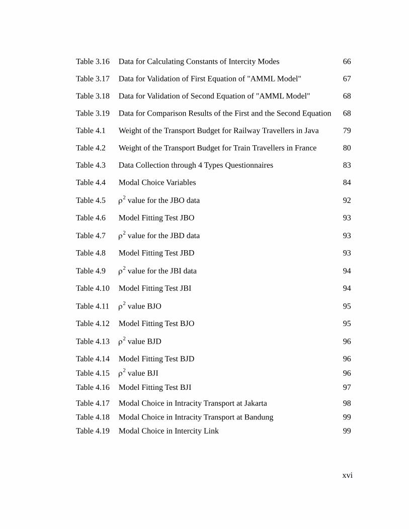
xvi
Table 3.16 Data for Calculating Constants of Intercity Modes 66
Table 3.17 Data for Validation of First Equation of "AMML Model" 67
Table 3.18 Data for Validation of Second Equation of "AMML Model" 68
Table 3.19 Data for Comparison Results of the First and the Second Equation 68
Table 4.1 Weight of the Transport Budget for Railway Travellers in Java 79
Table 4.2 Weight of the Transport Budget for Train Travellers in France 80
Table 4.3 Data Collection through 4 Types Questionnaires 83
Table 4.4 Modal Choice Variables 84
Table 4.5 2 value for the JBO data 92
Table 4.6 Model Fitting Test JBO 93
Table 4.7 2 value for the JBD data 93
Table 4.8 Model Fitting Test JBD 93
Table 4.9 2 value for the JBI data 94
Table 4.10 Model Fitting Test JBI 94
Table 4.11 2 value BJO 95
Table 4.12 Model Fitting Test BJO 95
Table 4.13 2 value BJD 96
Table 4.14 Model Fitting Test BJD 96
Table 4.15 2 value BJI 96
Table 4.16 Model Fitting Test BJI 97
Table 4.17 Modal Choice in Intracity Transport at Jakarta 98
Table 4.18 Modal Choice in Intracity Transport at Bandung 99
Table 4.19 Modal Choice in Intercity Link 99

xvii
Table 4.20 Modal Choice in Total Passengers Transport Chain 99
Table 4.21 External Validation o f Final Modal Choice in Intracity Mode
Jakarta-Bandung 102
Table 4.22 Calculation of Final Modal Choice by Second Equation of the
AMML Model 103
Table 4.23 Modal Choice in Intracity Transport at Bandung 104
Table 4.24 Modal Choice in Intracity Transport at Jakarta 104
Table 4.25 Modal Choice in Intercity Link 105
Table 4.26 Modal Choice in Total Passengers Transport Chain 105
Table 4.27 External Validation of Final Modal Choice in Intercity Transport
at Bandung-Jakarta 107
Table 4.28 Calculation of Final Mode Choice in Intercity Transport Mode
at Bandung-Jakarta Direction by Second Equation of the
AMML Model 108
Table 4.29 Quality Services Variables Comparison on the Direction
Jakarta-Bandung 112
Table 4.30 Quality Services Variables Comparison the direction
Bandung-Jakarta 116

1
Université de Technologie de Compiègne Universitas Indonesia
CHAPTER I INTRODUCTION
1.1 Research Background
The transportation activities between the big cities with short distances, such as
Jakarta – Bandung, could cause the density of traffic on their inter-city transport
network. Modes of transport, such as road transport, planes and trains, are some
choices of user to travel with. One has to choose a mode over the others. This can lead
to competition between modes.
The design of the transport network in an area can be as subsystems connected to other
subsystems, overall and integrated in a macro transport system. Relations between
these subsystems are as a result of the need for inter-subsystem (Tamin, 2000).
Furthermore, the connectivity between transportation in the city with transportation
between cities forms a transport system macro (global).
Intensive interconnection between two big cities with short distances can generate the
high traffic. Increasing the types and number of transport modes in the same corridor
raises competition in the competitive intermodal passenger numbers (Ming et al,
2010). Each passenger will use one type of mode that can provide maximum service to
meet the needs of passengers. Some studies have suggested the need for a flexible
transit services. This is to overcome the problems of sub-urbanization and dispersed
travel patterns (Koffman, 2004).
Competition between modes can occur in conditions of increased service, and then
change the passenger choice. Consequently types of modes that are not selected will
be the mode of losing the number of passengers. In this case, these type modes can not
survive in this competition. Transportation services needed include affordability, meet
2
Université de Technologie de Compiègne Universitas Indonesia
the required capacity, decent travel time, flexible or reliability of modes to meet the
needs of passengers (Vedagiri and Arasan, 2009)
Before the 20th century, the railway is growing rapidly in many countries, but
subsequently decreased mainly due to the construction of roads and improvement of
air transport services (Brons et al, 2009; Ayidin and Dzhaleva-Chonkova, 2013).
Railway investment needs to be maintained because it is an environmentally friendly
mode of transport and can improve the economy of a city. This transport can also
reduce the level of congestion. Although some researchers said the existence of
negative effects, including the noise around the railways and in station (Grimes and
Young, 2013).
Passengers have some criteria to travel according to their characteristics, the
destination and purpose of the trip. If an inter-city transport mode does not meet their
requirements then they will choose the other. On the other hand, if the transport mode
does not have a sufficient number of passengers, then its operating costs will be very
expensive. In the long term, this condition will be very inefficient because of
transportation services can not be storage (Yu and Lin, 2008). Types of modes that
cannot compete in the competition means it can be concluded inadequate to operate.
Transport modelling is used to analyze how the passengers make their decisions to
modal choice. This modelling can be evaluated numerically solutions through a
mathematical formula. In certain conditions, several models and studies have been
built to address the problems of alternative modes of transport. The selection process
of one mode to the others can be estimated by maximizing the utility offered from any
mode (McFadden in the 1970s in the Ming et al, 2010).
Some researchers have tried to establish some approaches to know intermodal service
gaps. The quality improvements of transport services for inter-city transport modes
3
Université de Technologie de Compiègne Universitas Indonesia
need the support of the quality services of intracity transport. This condition is in the
context of a total transport chain from origin to final destination.
Currently, the discussion of this topic is developed constantly to advanced levels of
some models of travel demand. Logit models is the model most often used in transport
planning, because this model has the ability to perform complex modelling travel
behaviour by simple mathematical techniques. Mathematical framework of a logit
model is based on maximizing the utility theory (Ben-Akiva and Lerman 1985). Logit
models are generally classified into two main categories, namely Binary and
Multinomial logit models. Binary logit models can perform modelling only two
choices and Multinomial logit models can be done in more than two options. In a
complex transport system, it is possible for more than two choices; therefore, this
study explores the Multinomial Logit Model.
Multinomial logit models are affected by the utility function. The change of utility
value will change the mode of choice opportunities. The probability is expressed in the
probability function of Multinomial Logit Model. Logit models in the form of a
mathematical model are a classical statistical formula. In its development, logit model
was adapted with some extra consideration. Fisher has developed into a logit Mix
(Fisher, 1950). Furthermore, McFadden and Train have been adapted into a Mixed
Multinomial Logit Model (McFadden and Train, 2000).
This research has been conducted on the formulation of a model to determine the
effect of the characteristics of the transport service in the city in determining the
choice of inter-city transport mode. The model was developed in discrete behaviour to
solve problems of inter-city transportation mode choice that affected by the transport
system in the city. The model has been applied to the Jakarta-Bandung corridor.
4
Université de Technologie de Compiègne Universitas Indonesia
1.2 Problems Statement and Research Questions
On a complex transportation system, modal choice between cities has become a
complex problem. Considerations of the passengers to choose the type of mode are not
only on the condition of the inter-city mode, but also the conditions of transport in the
city of origin and destination. In the big cities as the city of origin of the passengers
were in various zones, as well as at the final destination. In the city of origin and
destination, there are many public transportation possibilities that can be selected for
user from the area of origin to inter-city transport modes. There are alternatives that
can be either single or multi-modal transport. Complex transport conditions are a
challenge for multi-modal transport in competing with a single transport. These
complex situations are the problems in analyzing the characteristics of inter-city
transport mode choice.
Those problems led to the following research questions:
1. How can the characteristics of the users of intercity transport choose one intercity
transport mode over the others between the two major cities?
2. How to build a model of mode choice that considers the travelling from origin to
the final destination?
3. How does the improvement of a mode of transport can be done by using the
characteristics of the user's choice mode based on the level of service of various
types of mode choice?
This analysis is important in order to solve existing problems in realizing the
sustainability of all the available transport modes in the integration of the intracity and
intercity transport system.
5
Université de Technologie de Compiègne Universitas Indonesia
1.3 Research Aim
The research aims to obtain a formulation of inter-city passenger movement by
considering alternative modes of transportation on the network in the city. The
development of this model deals to the choice of modes on the network between cities,
especially big cities which are nearby. Results of the research are to obtain information
about the characteristics of users in determining the mode of choice. In this case study,
the focus is directed at the development of the railway service corridors Jakarta-
Bandung.
In the future, this approach could serve as a model in evaluating the improvement of
services and find the limits of customer satisfaction oriented. Increased services will
be able to increase the opportunity of a mode to be chosen over the others.
1.4 Novelty, Scientific and Pragmatic Contributions
Development of the classical approach Multinomial Logit Model is done for modal
choice problems in the integrated network of intracity and intercity transport which is
applied to the Jakarta-Bandung corridor. Model “Adapted Mixed Multinomial Logit
(AMML)” has been built to address these issues with a more precise calculation.
Pragmatic contributions are as follows:
1. Identification of transport services that contribute significantly to the inter-city
transport mode choice in modal competition, especially in the corridors Jakarta-
Bandung
2. Indicating the influence of transport services, in particular intracity transport
systems to the modal choice of intercity mode.

6
Université de Technologie de Compiègne Universitas Indonesia
Development model from the classical Multinomial Logit Model is necessary for the
integration links of intracity and intercity transport problems which could be applied
on the Jakarta-Bandung corridor. To deal with this problem “Adapted Mixed
Multinomial Logit (AMML)” Model can be used for the precise results.
1.5 Research Outline
This dissertation is organized as follows:
Chapter I Introduction
This chapter deals with description of the research background, problem statement and
research questions, research aim and significance of the research, novelty, scientific
and pragmatic contributions, and research outline.
Chapter II Literature Study
This chapter discusses about transportation system, intercity transport system, intracity
transport system, passengers and modes characteristics, service variables of modal
choice, modal choices model, in high modal competition, transport policies in
Indonesia, and conclusion.
Chapter III Research Methodology
This part explained research framework, survey method, questionnaires survey results,
model development, validation model, and model limitations are presented.

7
Université de Technologie de Compiègne Universitas Indonesia
Chapter IV The “AMML Model” Application
This chapter presents research design, intercity transport between Jakarta and
Bandung, the economic affordability analysis, of intercity transport modes, evolution
of ideas about the modal competition, analysis data on the corridor Jakarta-Bandung,
modal competition of corridor, and transportation characteristics.
Chapter V Conclusion and Perspectives
Finally, this part will resume this research with some conclusions. It contains some
topic about the consideration of intracity transport system in intercity mode choices,
model development, improving mode’s competitiveness, and model simulation.
Further analysis to the next researches was expressed on the perspectives.

8
Université de Technologie de Compiègne Universitas Indonesia
CHAPTER II LITERATURE STUDY
2.1 Transportation System
Transportation is a travelling of passengers or a movement of goods from one place to
another (Morlok, 1978). Bowersox (1981) has stated that the movement of goods or
travelling of passengers from one location to another because of the need to arrive in
certain location. This is a cause of product-driven. A sequence of transport modes
which are used to carry a certain quantity of goods from its origin to its destination is
called transport chain. In this chain it could need one or more transshipment
(Kristiansen, 2007). Travelling in a corridor could be associated with socioeconomic
and geographic activities. Geographical movements could be the movement between
one area to another within the city (intracity transport system) and also to other city
(inter-city transport system). The intracity transport system and intercity transport
system are subsystems in the global transport system (Figure 2.1.).
Figure 2.1. Global Transport System
2.1.1 Intercity Transport System
Inter-city transport mode serves passenger in traveling from one node to another
between cities. The demand between cities can be forecasted with a model (compiled

9
Université de Technologie de Compiègne Universitas Indonesia
by Manheim and Marvin 1979). Furthermore, the transport demand, by Kanafani
(1983), is analogous to the scheduled economic activities or a function of customer
demand to transport goods and services. These activities require time and energy as a
measure of performance of the transport system. Needs of this movement requires a
certain mode which has several criteria, such as the condition of the user, the
difference in income, time and cost.
In this research, it was found that passengers could not travel on one link. In their total
transport chain, it could be more than one link. The first link is a link with the
travelling between the origins to the modal node in the departure city. The second link
is the travelling between modal nodes at departure city to another modal node at
arrival city. The third link is the travelling between modal node at arrival city to the
final destination. Thus the study of inter-city transport has become a complex system
(Fig. 2.2).
Figure 2.2. The Complexity of Intercity Transport System from Origin to Destination
10
Université de Technologie de Compiègne Universitas Indonesia
In this case, travelling in inter-city transport link is not the main purpose. Inter-city
transport passengers have to face intracity transport problems to achieve their main
purpose. Therefore, inter-city transport link is influenced by several other links which
have different conditions of transport characteristics. The integration of the
components into intermodal is very important to realize a continuous travelling of
passengers, from “door to door” (Givoni and Rietveld, 2007).
Differences of transportation characteristics can be identified from the difference in
the level of service that provided by each type of modes on each link. Service levels
can be measured from the characteristic mode as variables. In the first link, the service
level is affected by the variable of intracity transport system. The second link is
influenced by service variables of the intercity transport mode. And the third link is
influenced by several variables of intracity transport system at the destination city.
Interaction between the two cities is supported by the intracity and inter-city
transports. These activities can use a single transport mode or multi-modal transport.
Some terms that used by some researchers for the needed to use more than one mode
of transport, such as a multi-modal, combined transport, intermodal transport and co-
modality (Reis et al., 2013). Multi-modal transport implies that there is a need to use
more than one mode on a particular link or a certain corridor. Intermodal transport
indicating at least the existence of two different transport modes involved in the total
transport chain “door to door” for a trip of passenger transport. The service conditions
given by a single transport mode or multi-modal transport is influenced by the
characteristic mode of transportation.
11
Université de Technologie de Compiègne Universitas Indonesia
2.1.2 Intracity Transport System
The transportation system in the city (transport system micro) is an activity within the
city that have a relationship between one and the other, for example, traveling to
work, school, center of sport activities and others from a particular place that is
integrated in the system of land use (Tamin, 2000). From one land use system to
another, the traveler uses the transport network system. The traffic flow is allowing
workers to go to work, students to go to school, and so on. In transportation planning,
traffic movement is designed to be easy and efficient, but in the reality, it could be
different.
Transportation modes designed to provide convenience and efficient, but there is a
problem of accessibility. Accessibility is a concept that combines land use regulation
system to be achieved through the transport network system (Black in Tamin, 2000).
Accessibility is the ability to measure the level of convenience to get to the destination
of the road network system. Accessibility can be a variable distance, travel time,
quality of service, or cost.
The formulation of accessibility within the city is a combination of several zones (N)
and all activities (A) in the central zone. Accessibility (K) for one zone is an intensity
of each activity in each zone in the city and access to reach the center zone of the
transport network system. The physical size for accessibility is as (Hansen, 1959 in
Suhardi B., 2004):
Ki = ……………………………………………………........………….….(2.1)
Where:
Ki ≡ accessibility zone i to other zone (d)
Ad ≡ Activity at zone d (such as number of jobs, etc)
tid ≡ time and cost from zone i to zone d

12
Université de Technologie de Compiègne Universitas Indonesia
Furthermore, the size of accessibility is developed with a systematic component of
maximum utility symbolized in logit models as V * (a measure of accessibility), where
Cn is a set of options, for the multinomial logit model. Accessibility is a measure of
the size scale of the efforts of several alternative trips. Generally, this measure is a
special measure individually. This measure takes into account the expected utility
value associated with a set of options as (Ben-Akiva and Lerman, 1985):
V*n = ………………………………...………………...…….…….(2.2)
Where:
V*n ≡ measure of accessibility
Uin ≡ utility value mode i
Users of multimodal transport require centre of transfer/transit. Transit system is a
system of transfers that use private transport to public transport or public transport to
public transport. Transit performance can be identified from a combination of
operating costs and service quality. In certain situations, there are the unfavorable
conditions for passengers, for example, the amount of time to wait, the time duration
of a trip by car or by walking activities (Chandra et al, 2011).
The transit system which did not connect directly from door to door, then it requires
the feeder transit service performance. Many transit feeder services with operations
following the pattern of the user's needs. Usually they adapt to the situation of
residential areas (Koffman, 2004; Potts et al., 2010). Their performance depends on
several factors such as the ability of the driver, stop frequency, the type of bus stops,
and the number of passengers at each stop. Furthermore, a major factor in the
performance of the feeder depending on the condition of the road network and
connectedness with the activities required (Chandra, 2013).
13
Université de Technologie de Compiègne Universitas Indonesia
Another study (Prasertsubpakij and Nitivattananon, 2012) of the Metro System in
Bangkok Metro System concluded that the perception of discomfort associated with
lack of accessibility, and safety of the surrounding environmental conditions. It would
be better if there is a balance access to services. This is accounted for in the model of
accessibility disaggregate transport users.
2.2 Passengers and Modes Characteristics
2.2.1 Passengers Characteristics
Passengers, who are traveling on intercity transport, depend on the availability of
private transport mode and public transport mode on the link. They will consider every
possible trip with all available existing modes. Passengers’ travel proposes are to do
some activities, for example to go to work, to study, to do sport, etc. According to
“Passengers Preferences”, the necessities of transport mode might be changed. If there
are several transport modes are available, then they will choose the most advantage
one (Tamin, 2000).
Any choice is, by definition, made from a nonempty set of alternatives. The
environment of the decision maker determines what we shall call be the universal set
of alternatives. Any single decision maker considers a subset of this universal set,
terms a choice set. The feasibility of an alternative is defined by a variety of constrains
(Ben-Akiva and Lerman, 1985). The selection process is done by calculating the
maximum value of total variables. Selected mode should be has a maximum value of
the potential benefits over the other (McFadden 1970s in Ming et al, 2010).
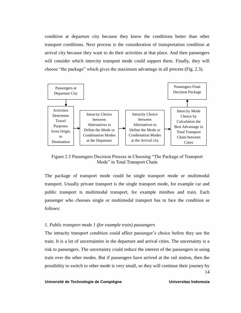
Passengers’ decision process is different from travel’s steps. Their decision process
depends on their way of thinking. It is begun with the consideration of transport
14
Université de Technologie de Compiègne Universitas Indonesia
condition at departure city because they know the conditions better than other
transport conditions. Next process is the consideration of transportation condition at
arrival city because they want to do their activities at that place. And then passengers
will consider which intercity transport mode could support them. Finally, they will
choose “the package” which gives the maximum advantage in all process (Fig. 2.3).
Figure 2.3 Passengers Decision Process in Choosing “The Package of Transport
Mode” in Total Transport Chain
The package of transport mode could be single transport mode or multimodal
transport. Usually private transport is the single transport mode, for example car and
public transport is multimodal transport, for example minibus and train. Each
passenger who chooses single or multimodal transport has to face the condition as
follows:
1. Public transport mode 1 (for example train) passengers
The intracity transport condition could affect passenger’s choice before they use the
train. It is a lot of uncertainties in the departure and arrival cities. The uncertainty is a
risk to passengers. The uncertainty could reduce the interest of the passengers in using
train over the other modes. But if passengers have arrived at the rail station, then the
possibility to switch to other mode is very small, so they will continue their journey by
Passengers at
Departure City
Intracity Choice
between
Alternatives to
Define the Mode or
Combination Modes
at the Departure
City
Passengers Final
Decision Package
Intercity Mode
Choice by
Calculation the
Best Advantage in
Total Transport
Chain between
Cities
Activities
Determine
Travel
Purposes
from Origin
to
Destination
Intracity Choice
between
Alternatives to
Define the Mode or
Combination Modes
at the Arrival city

15
Université de Technologie de Compiègne Universitas Indonesia
train. Thus the possibility to change to other mode when they have arrived at the rail
station can be ignored (0).
2. Public transport mode 2 (for example minibus) passengers
Although the minibus uses the toll road network as well as private car, but they are
considered in different network due to the different starting and end point of their
trips. Before and after intercity travelling, passengers could use one mode or some
combination modes from their home and to their final destination. Transport
conditions in intracity transport could affect the passenger intercity mode choices. If
they have arrived at minibus pole, then they continue to the next pole by minibus. The
possibility to switch to other modes is very small and in the mathematical models this
possibility is ignored (0).
3. Private transport passengers
When car passengers have arrived at the first highway toll gate, then they continue
their journey to the next highway toll gate by car. The intracity transport condition
does not allow them to change to other modes, because the intracity transport
condition is very complex, so to move to other mode will cause a lot of “costs”. This is
a normal condition, although in reality there are some passengers that can switch their
mode. That condition is ignored (0).
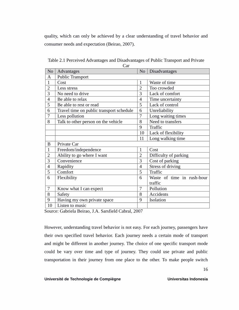
2.2.2 Modes Characteristics
Mode transport characteristic depends on its type, such as private or public mode
(Table 2.1). Nowadays, using private mode is more popular. The implication of this is
congestion and pollution. This situation could not attract a large number of car users to
switch to public transport (Henser, 1998). Policies could increase public transport
usage by promoting its image, but it is not enough. It should become more market-
oriented and competitive. It means that it has to improve public transport service
16
Université de Technologie de Compiègne Universitas Indonesia
quality, which can only be achieved by a clear understanding of travel behavior and
consumer needs and expectation (Beirao, 2007).
Table 2.1 Perceived Advantages and Disadvantages of Public Transport and Private
Car
No Advantages No Disadvantages
A Public Transport
1 Cost 1 Waste of time
2 Less stress 2 Too crowded
3 No need to drive 3 Lack of comfort
4 Be able to relax 4 Time uncertainty
5 Be able to rest or read 5 Lack of control
6 Travel time on public transport schedule 6 Unreliability
7 Less pollution 7 Long waiting times
8 Talk to other person on the vehicle 8 Need to transfers
9 Traffic
10 Lack of flexibility
11 Long walking time
B Private Car
1 Freedom/independence 1 Cost
2 Ability to go where I want 2 Difficulty of parking
3 Convenience 3 Cost of parking
4 Rapidity 4 Stress of driving
5 Comfort 5 Traffic
6 Flexibility 6 Waste of time in rush-hour
traffic
7 Know what I can expect 7 Pollution
8 Safety 8 Accidents
9 Having my own private space 9 Isolation
10 Listen to music
Source: Gabriela Beirao, J.A. Sarsfield Cabral, 2007
However, understanding travel behavior is not easy. For each journey, passengers have
their own specified travel behavior. Each journey needs a certain mode of transport
and might be different in another journey. The choice of one specific transport mode
could be vary over time and type of journey. They could use private and public
transportation in their journey from one place to the other. To make people switch
17
Université de Technologie de Compiègne Universitas Indonesia
totally to use public transport is a question of service quality. To get the best service
quality, each mode has to consider each variables constraints over the others.
2.3 Services Variables of Modal Choice
Users, operator, and government, as the stakeholders, have their own variables to
consider for one mode over the others. They optimize their variables to all available
alternatives to get the maximum advantage value of their utility and choose the
alternative with the highest value, but their interests are not the same (Lyons and
Harman, 2002).
Variables considered by users are as follows
- access time, characterized by deterministic variations (business/leisure,
residents/visitors), combined-mode choice, transfer location choice, route choice
- other variables, such as: departure time from home, arrival time at destination,
departure time from destination, arrival time at home, tour travel time, duration of
stay at destination, travel cost not including (extra) peak charge, peak charge
(second experiment only, probability of a seat (public transport mode only), and
frequency (public transport mode only). Reliable and offered at a suitable cost will
able to maximize convenience through travel opportunities (including
consideration of their life style changes, trust of the available information).
Variables considered by operator such as:
- traffic volumes, network capacity, distribution of car traffic among different time
periods during the day
- values of travel savings for access, line haul, egress trip legs, waiting times
- effect of fare competition on company profitability, overall network congestion.
18
Université de Technologie de Compiègne Universitas Indonesia
- traffic volumes, network capacity, distribution of car traffic among different time
periods during the day.
- the bottom line return on investment
- travelling time and lower operational costs per available seat kilometer.
- The primary market segment
Variables considered by government policy such as:
- inter-mixing of jobs-housing function
- an outline of the current form of the public transport (focus on bus and rail
services) looking at the complex responsibilities and relationships which entails.
- the main national initiatives for integrated traveler information provision
- regulatory controls over routes, time table, fares (deregulation) and sale of
publicly owned companies
- a better environment (reduced pollution), more efficient use of resources in all
transport system, more sustainable quality of life for everyone.
The importance of quality variables was discussed by some researchers and also the
research about accessibility evaluation of feeder transit services.
2.4. Modal Choices Model
The global transport system becomes more complex in function of its demand and of
the number of available modes and alternatives as the road network extension. A
wrong decision of a passenger in making a choice in the total travel would cause a
high cost or important extra delay. In the previous studies, computational technology
has led to the development of procedures to select the most appropriate travelling
mode. The quantification of travel attributes which influences certain individual in
mode choosing can be mathematically represented by modal choice model.

19
Université de Technologie de Compiègne Universitas Indonesia
Modal choice as a behaviour model is defined as a representation of decision that
made by consumers when confronted with alternative choices. This choice is made on
the basis of the term upon which the different travel modes are offered, for example
the travel times, costs, and other level-of-service attributes of the competing
alternative travelling modes. The shift from single modal toward multimodal system
could be done by improving the three performance indicator, such as cost efficiency,
service effectiveness, and cost effectiveness (Yu and Lin, 2008).
The models that tend to represent the travel behaviour of the individuals when
provided with a discrete set of travelling alternatives are commonly known as discrete
choice models. The method of transport mode division is a selection model by an
individual which is based in maximization of utility (McFadden 1970s in Ming et al,
2010). The utility of a travelling mode is defined as an attraction associated to an
individual for a specific trip. Therefore, the individual is visualized to select the mode
which has the maximum attraction, due to various attributes. This hypothesis is known
as utility maximization and all the travel demand models are based on this theory. An
essential transport demand analysis was the development of disaggregate travel
demand model base on discrete choice analysis methods. At the disaggregate travel
demand, it could observe that the behaviour of an individual as a decision maker in
choosing mode over the other.
The discrete choice model was continued, developed with an adaptation on random
utility theory (McFadden 1974 in Hensher and Rose, 2007). Random variables were
considered utility of modes alternatives in counting probability to choose and from
time to time it was expanded (Hensher and Rose, 2007). One mode cannot directly
take place of other mode, because of the differences in mode’s characteristic and
services. Passengers need to decide which one will give the maximum advantage to
them. The method to choose one mode over the other is known as modal choice

20
Université de Technologie de Compiègne Universitas Indonesia
model. Logit model is the previous and most popular method. Mathematical
framework of logit models is based on the theory of utility maximization. Logit
models are generally classified into two main categories namely binomial if there are
two choices and multinomial if there are more than two. The model is continuously
developed with some specific definition, such as (McFadden, 1981; Ben-Akiva and
Lerman, 1985):
1. Logit Model with:
Extreme value distribution
Error term is the Identically Independent Distribution (IID)
2. Probit Model with:
Normal distribution
Error not the Identically Independent Distribution (IID)
3. GEV Model with:
Multivariate extreme value distribution
Error not the Identically Independent Distribution (IID)
4. Nested Model with:
A structure which has partitions of the alternatives into groups (nests)
The choices should be dependent to be one group
If all modes are independently choice, than they can not consider as a
partition into a group.
2.4.1 Utility Function
All logit models are specified on the basis of utility function and are applied according
to the probability of an individual by selecting out a mode over the other. Utility value
of each mode can be found by analyzing the travellers’ satisfaction. The values of
variables are considered to have a strong relationship with the behaviour of the
21
Université de Technologie de Compiègne Universitas Indonesia
traveller’s satisfaction. Utility is defined as a maximized value by every individual. It
contains a random selection function. The random function will give an idea about the
value of the selection function V (i) or values of attributes have different effects on
different individuals or by the same individual at different times. This statement is
called random utility model and expressed as a vector notation of the utility function
(Ben-Akiva, 1985):
Uin = Vin + in.....................................................................................................(2.3)
Where:
Uin ≡ Utility value for the alternative (i) in individuals (n).
Vin ≡ Random variable of alternative (i) was observed (systematic) in individuals (n)
in ≡ alternative stochastic component (i) in individuals (n)
It was developed (Bliemer and Rose, 2005 in Hensher and Rose, 2007) with the
observed component of utility further consists of a vector of attribute levels x in as
follows:
Uin = V in (x in | βi) + in …………………………………………………………….(2.4)
Model development above is the basic principle of selection which shows that
individual will choose alternative (n), if the utility function U (n) of the alternative (n)
provide the greatest value among the other utility function U (n). Furthermore, to find
out the similarities Vin and the influences in their functions:
Vin = V (Xin) ............................................................................................................. (2.5)
To find out the various elements that affect the X, and estimate the unknown
parameters, a linear function of the parameters is used. This function is denoted as
follows:
22
Université de Technologie de Compiègne Universitas Indonesia
= [1, 2, ...,k] as a vector k is not known, then:
Vin = 1Xin1 + 2Xin2 + 3Xin3 + … + kXink...................................................... (2.6)
1, 2, 3, ...,k are treated as random variables distributed in the population. Linearity
in the parameters is not equivalent to linearity in the attributes.
This previous model has been adapted by some researchers. It is adapted to be an
exploratory Multinomial Logit Analysis with the case of single-vehicle motorcycle
accident severity (Shankar and Manner, 1996). This exploratory method was focused
in motorcycle accident severity which analyzes all influencing factors. There are five
levels of severity considerations, for example: property damage only, possible injury,
evident injury, disabling injury, and fatality. A multivariate model of motorcycle-rider
severity considers about environmental factors, roadway conditions, vehicle
characteristics, and rider attributes.
A utility function by this research is identified as follows (Shankar and Manner, 1996):
in i n in............................................................................................................(2.7)
Where:
Sin ≡ utility value (with different symbol)
Xn ≡ a vector of measurable characteristics that determine the severity (for
example rider age, rider gender, roadway attributes, prevailing weather
conditions, vehicle type, usage of helmets, and so on)
βi ≡ a vector of estimable coefficients
ɛin ≡ an error term that accounts for unobserved factors influencing accident
severity
23
Université de Technologie de Compiègne Universitas Indonesia
βiXn in this equation is the observable component of severity determination because
the vector Xn contains measurable variables (for example roadway attribute at the
location of accident n) and in is the unobserved portion.
Other theoretical development of utility function is using heteroscedastic control for
random coefficients and error components in mixed logit. It identifies preference
heterogeneity and focuses on the formulation which depends on the selection of
random parameters. The objective of this research is to capture additional parameters
which are specifically unobserved. This research uses utility function as follows
(Greene and Hensher, 2007):
Uqjt = qjt qjt ...................................................................................................... (2.8)
Their special equation that have been developed for the constant value to be a linear
equation as follows:
qk k k q q,k qk ………………………….…..……......(2.9)
Where q,kis a random variable with E[ q,k] = 0 and Var [ q,k] = a2
k, a known constant
and q,k = σk x exp[ŋ’khq]
Hence, the development can be done by using linear regression method with special
coefficient features attained via parameterization in exponential, logistic, and
multinomial logit forms. This research contained types of multiple linear regressions
for prediction. The objective of this development is to get the range of coefficients in
an assigned, the logistic parameterization is used which is able to avoid
multicollinearity effect.
24
Université de Technologie de Compiègne Universitas Indonesia
This research uses linear regression formula as follows (Lipovetsky, 2009):
yi = a1xi1 +…
+ anxin + εi ≡ ŷi + εi, ……………………..............................................(2.10)
The model suggested nonlinear parameterization of regression coefficients. If all non-
negative coefficients are sought, they can be presented in the exponential
parameterization:
aj= exp (ɣj), .............................................................................................................(2.11)
Where: ɣj are the estimated parameters. To obtain the coefficients of regression
between amin to amax, a logistic parameterization can be applied:
aj = amin + (amax-amin/1 + exp (-ɣj)) …………………………....................................(2.12)
For amin = 0 and amax = 1, each coefficient of regression would belong to the [0,1]
interval. The multinomial-logit parameterization:
aj= exp (ɣj)/exp (ɣ1) + exp(ɣ2) + … + exp(ɣn), ɣ1 = 0 .....................................(2.13)
Other previous study applied in the case of airport choice in multi-airport regions
(Hess and Polak, 2005). This is the analysis of the behaviour of air travellers to choose
airports. The sensitive variable is access time which characterized by deterministic
variations (business/leisure, residents/visitors).

25
Université de Technologie de Compiègne Universitas Indonesia
2.4.2 Probability Function
A. Probability in Multinomial Logit Model
Probability function in Multinomial Logit Model as a mode choice model is based on
utility function of all modes. The “Multinomial Logit Model” built with the
mathematical equations as follows (Ben-Akiva, 1985):
Pn (i) = .......................................... (2.14)
Where:
Pn (i) ≡ Probability of individuals (n) to alternative (i)
e ≡ exponential
j ≡ the number of options
Vin ≡ Random utility of alternative (i) was observed (systematic) in individuals
(n)
Vjn ≡ Random utility of alternative (j) was observed (systematic) in individuals
(n)
Cn ≡ number of choices on the individual (n) is constrained because of their
background,
Where Cn∊C and C is the set of alternatives that exist in the universe (universal set)
This model uses several assumptions:
a. Random component of utility (in) is an independently and identically
distribution (IID) with a Gumbel distribution. Independent means when the
factor is not observed, it does not affect existing utilities.
b. The response of the individual against the alternative attribute is homogeneous,
so that the unobserved characteristics of individuals are not sensitive to attributes
of alternatives.
eV
in
j∊Cn eV
jn
0 < Pn (i) < 1, for all i ∊ Cn
and
Pn (i) = 1

26
Université de Technologie de Compiègne Universitas Indonesia
c. Variation of covariance and error of the alternatives are identical among
individuals.
This previous modal choice has been applied in real modal choice condition in some
countries in as seen in several researches. In fact, due to some differences in the
situation of each country and also some difference in the certain aspect, it is necessary
to develop in more detail to suit to the problem in the field.
Approach for models of this type, which is assumed as ɛin’s with generalized extreme
value (GEV) distribution and using estimated standard maximum likelihood methods
is developed by. The GEV assumption produces the simple multinomial logit model
(McFadden, 1981):
Pn(i)=exp[βiXn]/∑ exp[βIXn] ...................................................................................(2.15)
All variables are as previously defined. And the vector βi is estimated by standard
maximum likelihood methods.
B. Probability in Nested Logit Model
Other previous study about competitive multi-modal transit services with some groups
in the choice alternative was run with a nested logit approach. The model used
combined-mode choices of travellers, and the strategic interactions between the private
service operators (Lo et al., 2004). Method of analysis was the nested logit (NL)
approach with a three-level NL choice model, such as:
- Combined-mode choice
- Transfer location choice
- Route choice
27
Université de Technologie de Compiègne Universitas Indonesia
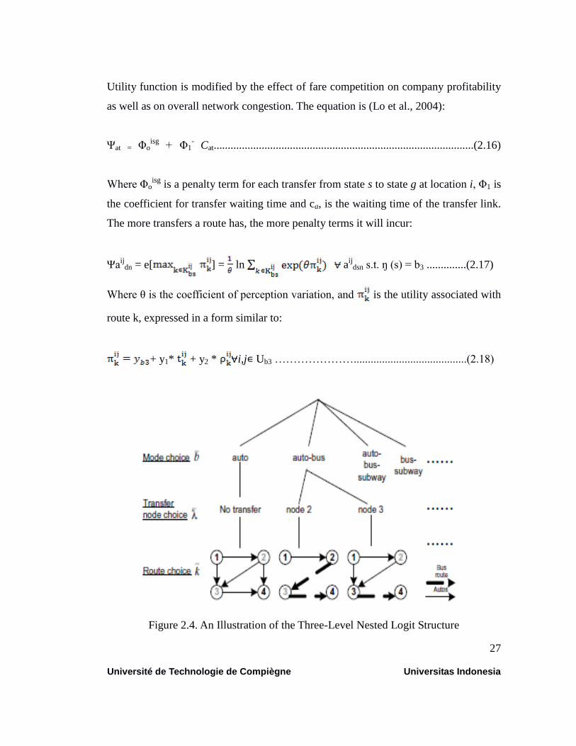
Utility function is modified by the effect of fare competition on company profitability
as well as on overall network congestion. The equation is (Lo et al., 2004):
Ψat = Φoisg
+ Φ1-
Cat............................................................................................(2.16)
Where Φoisg
is a penalty term for each transfer from state s to state g at location i, Φ1 is
the coefficient for transfer waiting time and ca, is the waiting time of the transfer link.
The more transfers a route has, the more penalty terms it will incur:
Ψaij
dn = e[ ] = ln aij
dsn s.t. ŋ (s) = b3 ..............(2.17)
Where θ is the coefficient of perception variation, and is the utility associated with
route k, expressed in a form similar to:
+ y1* + y2 * ⩝i,j∊ Ub3 …………………........................................(2.18)
Figure 2.4. An Illustration of the Three-Level Nested Logit Structure
28
Université de Technologie de Compiègne Universitas Indonesia
Where is a mode-specific constant; is the travel time on route k; is the
monetary cost associated with route k, which can be specific to the particular mode in
Class 3- as taxi charge or gasoline cost etc. Fig. 2.4 explains an illustration of the three
level nested logit structures:
= .......................................................................................(2.19)
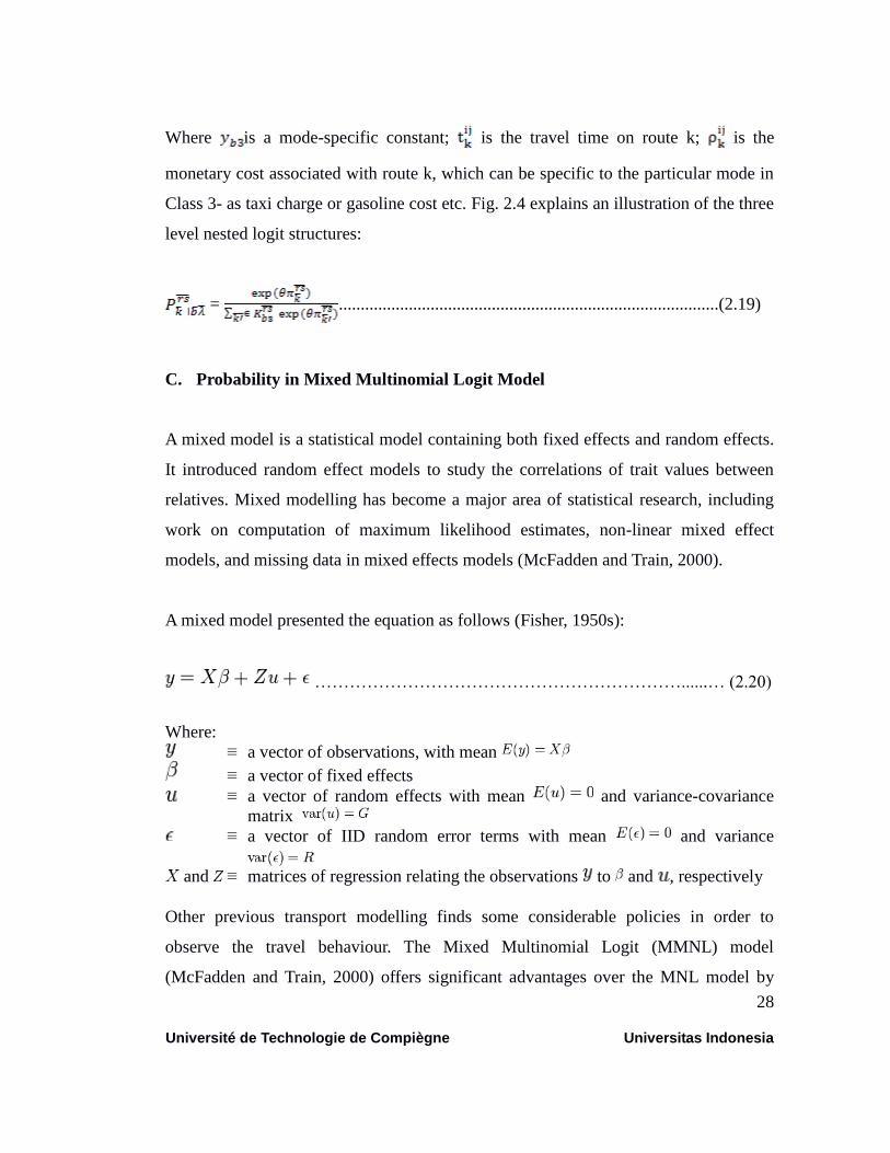
C. Probability in Mixed Multinomial Logit Model
A mixed model is a statistical model containing both fixed effects and random effects.
It introduced random effect models to study the correlations of trait values between
relatives. Mixed modelling has become a major area of statistical research, including
work on computation of maximum likelihood estimates, non-linear mixed effect
models, and missing data in mixed effects models (McFadden and Train, 2000).
A mixed model presented the equation as follows (Fisher, 1950s):
………………………………………………………......… (2.20)
Where:
≡ a vector of observations, with mean
≡ a vector of fixed effects
≡ a vector of random effects with mean and variance-covariance
matrix
≡ a vector of IID random error terms with mean and variance
and ≡ matrices of regression relating the observations to and , respectively
Other previous transport modelling finds some considerable policies in order to
observe the travel behaviour. The Mixed Multinomial Logit (MMNL) model
(McFadden and Train, 2000) offers significant advantages over the MNL model by

29
Université de Technologie de Compiègne Universitas Indonesia
allowing for random taste variation across decision makers. Their advantage
acknowledges the differences across agents in their sensitivities to factor such as fare
and frequency. The random-coefficients formulation of the MMNL model uses
integration of the MNL choice probabilities over the assumed distribution of the taste
coefficient, such that the probability of individual n choosing alternative i is
(McFadden and Train, 2000):
∫β(ev(β,Xni)
/v(β,Xnj)
)f( …………………..............................(2.21)
Where:
≡ the vector of observations, with continue function
Xni ≡ the vector of explanatory variables for alternative i as faced by decision
maker n
β ≡ the vector of taste coefficients, In the MMNL model, the vector β is
distributed randomly across decision makers, with density f(β׀ϴ),
ϴ ≡ a vector of parameters to be estimated that represent, for example, the
mean and the variance of preferences in the population.
V(β,Xni) ≡ the observed utility of alternative i
2.4.3 Estimator Method
Generally, there are two model estimation techniques namely the maximum likelihood
and least squares method. They used to estimate the discrete modal choice models, in
order to calculate the values of the unknown coefficients. The method of maximum
likelihood is the most common procedure used for determining the estimators in logit
model. The maximum likelihood estimators are the values of the parameters for which
the observed sample is most likely to have occurred. The method requires a sample of
individual modal choice decision-makers along with the data regarding the travelling
mode chosen and the attributes of that particular mode. The basic formulation of the
method, that involves the maximization of the likelihood function as (Ben-Akiva and
Lerman 1985):
N
Pn(i)yin
Pn(j)yjn
n=1
30
Université de Technologie de Compiègne Universitas Indonesia
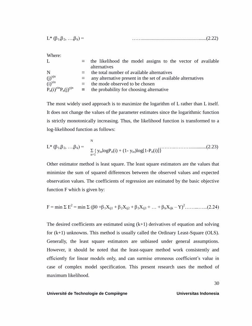
L* (1,2, …,k) = ……....................................................(2.22)
Where:
L ≡ the likelihood the model assigns to the vector of available
alternatives
N ≡ the total number of available alternatives
(j)yjn
≡ any alternative present in the set of available alternatives
(i)yin
≡ the mode observed to be chosen
Pn(i)yin
Pn(j)yjn
≡ the probability for choosing alternative
The most widely used approach is to maximize the logarithm of L rather than L itself.
It does not change the values of the parameter estimates since the logarithmic function
is strictly monotonically increasing. Thus, the likelihood function is transformed to a
log-likelihood function as follows:
L* (1,2, …,k) = ………..……….............(2.23)
Other estimator method is least square. The least square estimators are the values that
minimize the sum of squared differences between the observed values and expected
observation values. The coefficients of regression are estimated by the basic objective
function F which is given by:
F = min Ʃ E2 = min Ʃ (β0 +1Xij1 + 2Xij2 + 3Xij3 + … + kXijk – Y)
2……...…...(2.24)
The desired coefficients are estimated using (k+1) derivatives of equation and solving
for (k+1) unknowns. This method is usually called the Ordinary Least-Square (OLS).
Generally, the least square estimators are unbiased under general assumptions.
However, it should be noted that the least-square method work consistently and
efficiently for linear models only, and can surmise erroneous coefficient’s value in
case of complex model specification. This present research uses the method of
maximum likelihood.
N
yinlogPn(i) + (1- yin)log[1-Pn(i)]} n=1

31
Université de Technologie de Compiègne Universitas Indonesia
2.4.4 Test of Model and Hypothesis
There are several statistical tests for the model that would be accepted. Measurement
of the level of compliance data (Goodness of Fit), such as:
A. Likelihood-Ratio Value Index (rho-squared = 2)
Value of the log likelihood function is the evaluation of parameter values that we
expect in the equation. The calculation of log likelihood values uses the assumption
that the errors are normally distributed. The size of the suitability of the data stated in
the likelihood ratio index = (0) and likelihood ratio = 2 (c) and is defined as
(Ben-Akiva and Lerman 1985):
.................................................................................... (2.25)
and
.................................................................................... (2.26)
where:
L () ≡ The likelihood (L) maximum value, where the log likelihood value at
convergence is reached
L (0) ≡ Initial likelihood, if all parameters = 0
L (c) ≡ Initial likelihood or the probability Pn where the value of the option is
simply used to estimate the log likelihood that has the same probability of
selection of alternative options with market share or proportion of these
alternatives in the overall sample.
Value of 2 is ranged between 0 and 1. The smaller of the likelihood ratio value (L)
will increasingly significant or large difference in the value of L () with L (c) or L (0).
This shows the spread of the analyzed data. An index likelihood ratio 2 interval
between 0.15 and 0.2 indicates the relevance of the data (Hu et al., 2006).
2(0) = 1 – L
()
L(0)
2(c) = 1 – L
()
L(c)
32
Université de Technologie de Compiègne Universitas Indonesia
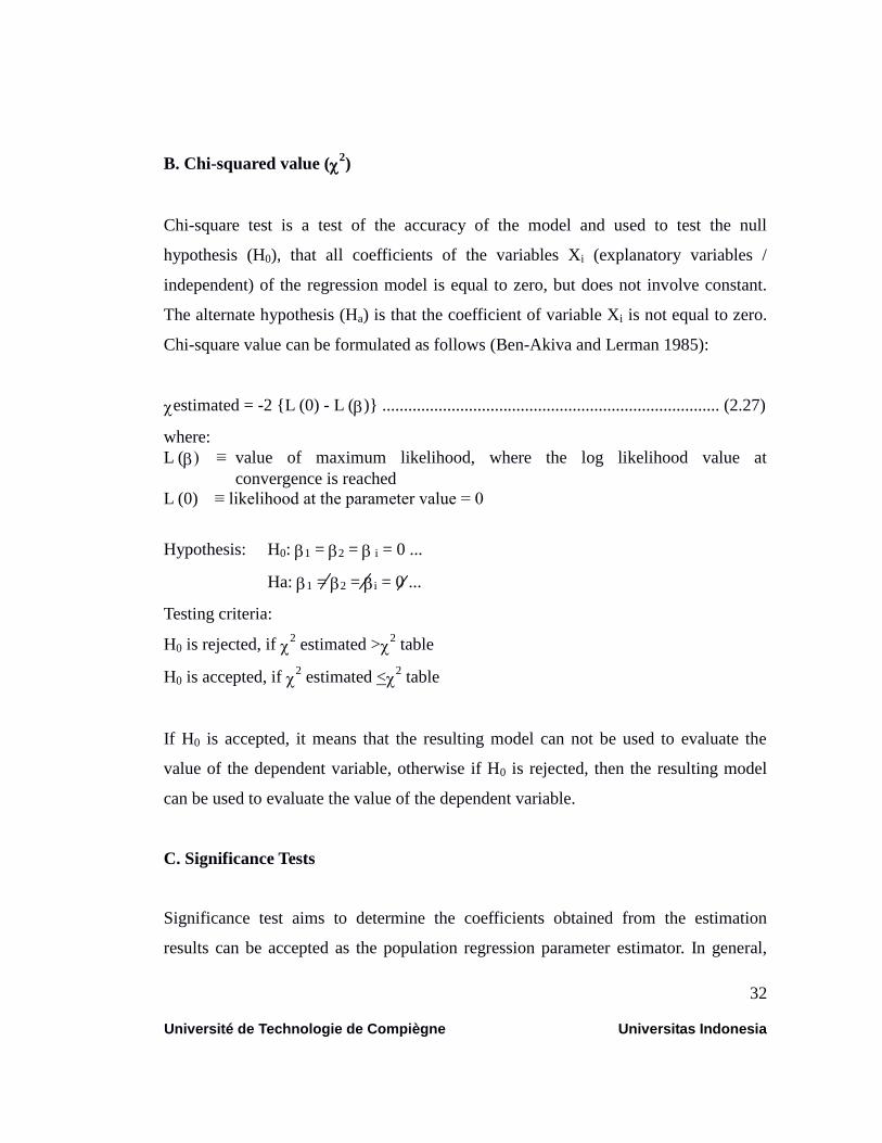
B. Chi-squared value (2)
Chi-square test is a test of the accuracy of the model and used to test the null
hypothesis (H0), that all coefficients of the variables Xi (explanatory variables /
independent) of the regression model is equal to zero, but does not involve constant.
The alternate hypothesis (Ha) is that the coefficient of variable Xi is not equal to zero.
Chi-square value can be formulated as follows (Ben-Akiva and Lerman 1985):
estimated = -2 {L (0) - L ()} .............................................................................. (2.27)
where:
L () ≡ value of maximum likelihood, where the log likelihood value at
convergence is reached
L (0) ≡ likelihood at the parameter value = 0
Hypothesis: H0: 1 = 2 = i = 0 ...
Ha: 1 = 2 = i = 0 ...
Testing criteria:
H0 is rejected, if 2 estimated >
2 table
H0 is accepted, if 2 estimated <
2 table
If H0 is accepted, it means that the resulting model can not be used to evaluate the
value of the dependent variable, otherwise if H0 is rejected, then the resulting model
can be used to evaluate the value of the dependent variable.
C. Significance Tests
Significance test aims to determine the coefficients obtained from the estimation
results can be accepted as the population regression parameter estimator. In general,

33
Université de Technologie de Compiègne Universitas Indonesia
significance tests are able to test the hypothesis of individual coefficients of each
independent variable. This test uses the test statistic t with the following formula (Ben-
Akiva and Lerman 1985):
b-
t = .............................................................................................................(2.28)
Sb
Where:
Sb ≡ standard error coefficient
b ≡ coefficient obtained
≡ Coefficient of the estimated population
T tests used to test the null hypothesis (H0), that each coefficient equal to zero and the
alternative hypothesis (Ha) is that if each coefficient of the model is not equal to zero.
Hypothesis: H0: j = 0
Ha: j = 0
Criteria for testing: H0 is rejected if the t count > t / 2, nk-1
H0 is accepted if the t count < t / 2, n-k-1
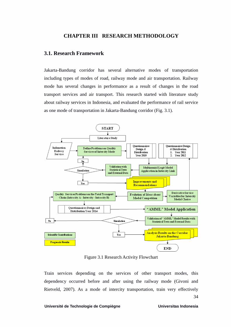
34
Université de Technologie de Compiègne Universitas Indonesia
CHAPTER III RESEARCH METHODOLOGY
3.1. Research Framework
Jakarta-Bandung corridor has several alternative modes of transportation
including types of modes of road, railway mode and air transportation. Railway
mode has several changes in performance as a result of changes in the road
transport services and air transport. This research started with literature study
about railway services in Indonesia, and evaluated the performance of rail service
as one mode of transportation in Jakarta-Bandung corridor (Fig. 3.1).
Figure 3.1 Research Activity Flowchart
Train services depending on the services of other transport modes, this
dependency occurred before and after using the railway mode (Givoni and
Rietveld, 2007). As a mode of intercity transportation, train very effectively
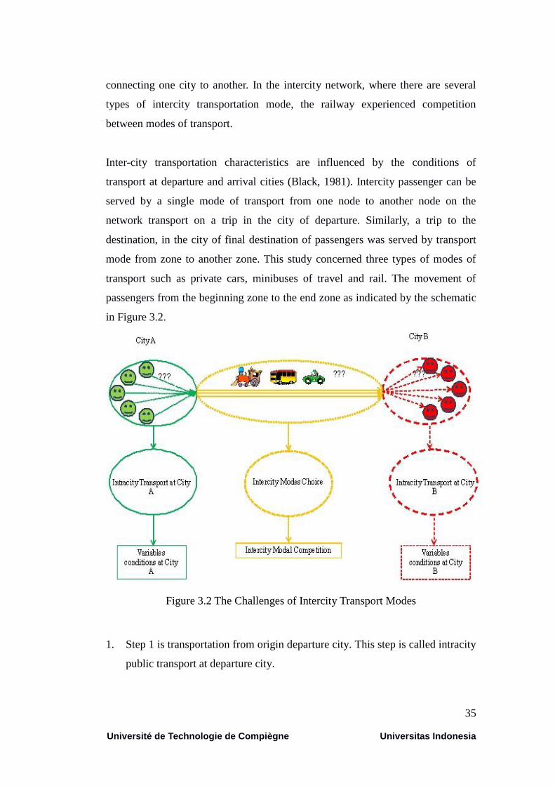
35
Université de Technologie de Compiègne Universitas Indonesia
connecting one city to another. In the intercity network, where there are several
types of intercity transportation mode, the railway experienced competition
between modes of transport.
Inter-city transportation characteristics are influenced by the conditions of
transport at departure and arrival cities (Black, 1981). Intercity passenger can be
served by a single mode of transport from one node to another node on the
network transport on a trip in the city of departure. Similarly, a trip to the
destination, in the city of final destination of passengers was served by transport
mode from zone to another zone. This study concerned three types of modes of
transport such as private cars, minibuses of travel and rail. The movement of
passengers from the beginning zone to the end zone as indicated by the schematic
in Figure 3.2.
Figure 3.2 The Challenges of Intercity Transport Modes
1. Step 1 is transportation from origin departure city. This step is called intracity
public transport at departure city.
36
Université de Technologie de Compiègne Universitas Indonesia
Passengers will choose a single transport mode or combination of modes of
transport for travel within the city. The choice is a private car or public
transport is the mode in which the choice of the type that has the best
advantage. All the possibility to choose the mode of transport will be given a
value of 1, because passengers would choose only one mode of transport or
the alternatives that have multiple modes of combination. For the choice of a
private car, then the node mode of transportation in the city of departure is the
toll gate. In this trip there are certain costs, time and other transport
conditions. Furthermore, for the choice of the minibus, then node modes
departure city is pool minibus and to train the node choice mode of
transportation in the city is the departure of the train station.
In this case study, it considers the five quality service variables, then the
formula as follows:
UIOi = fIO (VIO1, VIO2, VIO3, VIO4,VIO5) ……….………………...….. (3.1)
Where:
UIOi ≡ Utility value alternative i
VIO1 ≡ TtoU ≡ Travel time alternative i
VIO2 ≡ PoU ≡ Price alternative i
VIO3 ≡ SoC ≡ Safety alternative i
VIO4 ≡ IoC ≡ Information alternative i
VIO5 ≡ CoC ≡ Connectivity alternative i
i ≡ Mo ≡ number of alternatives in departure city (Mo1 ≡
to go to rail station, Mo2 ≡ to go to minibus
pole, Mo3 ≡ to go to highway toll road)
2. Step 2 is transportation between two modal nodes in each city. This step is
called intercity transport.
The passengers have arrived at the highway toll gate, or at the pole or at the
rail station, and then they will use the available modes at the modal node.
In this case study, it only considers the four quality service variables. It uses
the formula as follows:

37
Université de Technologie de Compiègne Universitas Indonesia
UM = fM(VM1, VM2, VM3, VM4) ……..….………………………....…. (3.2)
Where:
UMi ≡ Utility value alternative i
VM1 ≡ TtiU ≡ Travel time alternative i
VM2 ≡ PiU ≡ Price alternative i
VM3 ≡ SiC ≡ Safety alternative i
VM4 ≡ IiC ≡ Information alternative i
i ≡ Mi ≡ number of alternatives in departure city or at
arrival city (Mi1 ≡ train, Mi2 ≡ minibus, Mi3 ≡
car)
3. Step 3 is transportation from modal node at arrival city to final destination.
This condition is called intracity transport at arrival city.
The passengers have arrived at modal node (highway toll gate, pool minibus,
rail station) in arrival city; passengers continue to go to their final destination.
They use a private car, and then they go directly to their final destination. The
user of public transport, for example minibus or train, then the passengers
will switch to other modes. The user of minibus, they might use a mode
which provided by the owner of the minibus company, or replaced it by other
modes which are available in the arrival city likewise train’s passengers.
In this case study, it also considers the five quality service variables, so the
formula as follows:
UID = fID(VIDD1, VID2, VID3, VID4,VID5) ……….………….....…….... (3.3)
Where:
UIDi ≡ Utility value alternative i
VID1 ≡ TtdU ≡ Travel time alternative i
VID2 ≡ PdU ≡ Price alternative i
VID3 ≡ SdC ≡ Safety alternative i
VID4 ≡ IdC ≡ Information alternative i
VID5 ≡ CdC ≡ Connectivity alternative i
i ≡ MD ≡ number of alternatives at arrival city (MD1 ≡ from
rail station, MD2 ≡ from minibus pole, MD3 ≡
from highway toll road)
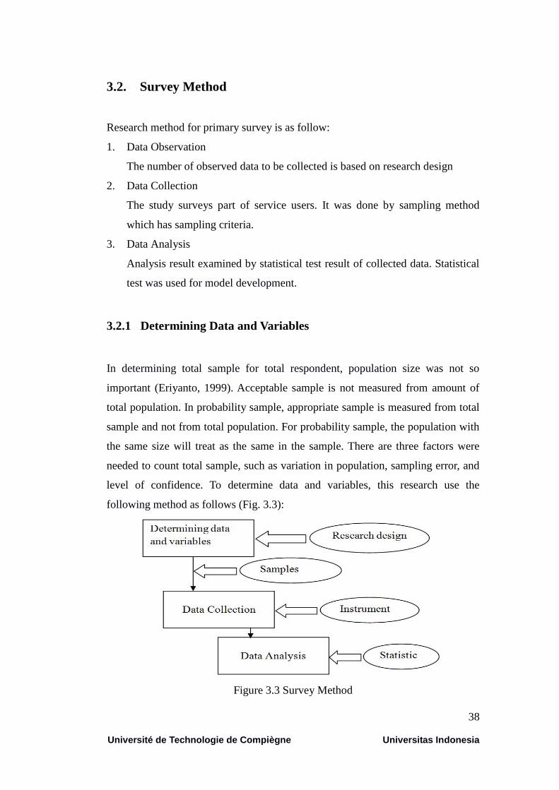
38
Université de Technologie de Compiègne Universitas Indonesia
3.2. Survey Method
Research method for primary survey is as follow:
1. Data Observation
The number of observed data to be collected is based on research design
2. Data Collection
The study surveys part of service users. It was done by sampling method
which has sampling criteria.
3. Data Analysis
Analysis result examined by statistical test result of collected data. Statistical
test was used for model development.
3.2.1 Determining Data and Variables
In determining total sample for total respondent, population size was not so
important (Eriyanto, 1999). Acceptable sample is not measured from amount of
total population. In probability sample, appropriate sample is measured from total
sample and not from total population. For probability sample, the population with
the same size will treat as the same in the sample. There are three factors were
needed to count total sample, such as variation in population, sampling error, and
level of confidence. To determine data and variables, this research use the
following method as follows (Fig. 3.3):
Figure 3.3 Survey Method
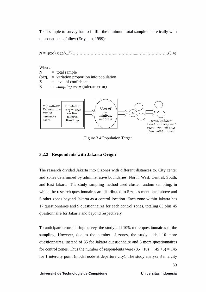
39
Université de Technologie de Compiègne Universitas Indonesia
Total sample to survey has to fullfill the minimum total sample theoretically with
the equation as follow (Eriyanto, 1999):
N = (pxq) x (Z2/E
2) …………………………...…………...……..……………(3.4)
Where:
N = total sample
(pxq) = variation proportion into population
Z = level of confidence
E = sampling error (tolerate error)
Figure 3.4 Population Target
3.2.2 Respondents with Jakarta Origin
The research divided Jakarta into 5 zones with different distances to. City center
and zones determined by administrative boundaries, North, West, Central, South,
and East Jakarta. The study sampling method used cluster random sampling, in
which the research questionnaires are distributed to 5 zones mentioned above and
5 other zones beyond Jakarta as a control location. Each zone within Jakarta has
17 questionnaires and 9 questionnaires for each control zones, totaling 85 plus 45
questionnaire for Jakarta and beyond respectively.
To anticipate errors during survey, the study add 10% more questionnaires to the
sampling. However, due to the number of zones, the study added 10 more
questionnaires, instead of 85 for Jakarta questionnaire and 5 more questionnaires
for control zones. Thus the number of respondents were (85 +10) + (45 +5) = 145
for 1 intercity point (modal node at departure city). The study analyze 3 intercity
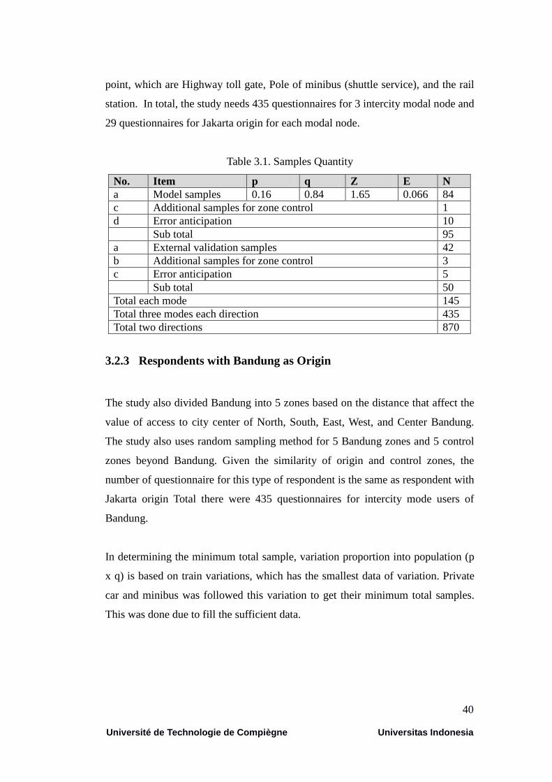
40
Université de Technologie de Compiègne Universitas Indonesia
point, which are Highway toll gate, Pole of minibus (shuttle service), and the rail
station. In total, the study needs 435 questionnaires for 3 intercity modal node and
29 questionnaires for Jakarta origin for each modal node.
Table 3.1. Samples Quantity
No. Item p q Z E N
a Model samples 0.16 0.84 1.65 0.066 84
c Additional samples for zone control 1
d Error anticipation 10
Sub total 95
a External validation samples 42
b Additional samples for zone control 3
c Error anticipation 5
Sub total 50
Total each mode 145
Total three modes each direction 435
Total two directions 870
3.2.3 Respondents with Bandung as Origin
The study also divided Bandung into 5 zones based on the distance that affect the
value of access to city center of North, South, East, West, and Center Bandung.
The study also uses random sampling method for 5 Bandung zones and 5 control
zones beyond Bandung. Given the similarity of origin and control zones, the
number of questionnaire for this type of respondent is the same as respondent with
Jakarta origin Total there were 435 questionnaires for intercity mode users of
Bandung.
In determining the minimum total sample, variation proportion into population (p
x q) is based on train variations, which has the smallest data of variation. Private
car and minibus was followed this variation to get their minimum total samples.
This was done due to fill the sufficient data.

41
Université de Technologie de Compiègne Universitas Indonesia
3.3. Questionnaires Survey Results
3.3.1. Survey Location
The last survey was applied for passengers who were interest in traveling between
the Jakarta-Bandung corridor. Jakarta area consists of North Jakarta, West Jakarta,
Central Jakarta, South Jakarta, and East Jakarta (Fig. 3.5). Location boundaries
were needed to be determined because not all modes can give the same services
from one zone another. Particularly for railway, its intercity modal node was only
serving Jakarta City and Bandung (Fig. 3.6), so location survey became only all
zones in Jakarta and Bandung.
Figure 3.5 Jakarta Zones
South
Jakarta
West Jakarta
East
Jakarta
Centre
Jakarta
Jakarta Utara

42
Université de Technologie de Compiègne Universitas Indonesia
Figure 3.6 Bandung Zones
3.3.2 Data Compilation
In the previous study about "Estimating Modal Shift of Car Travelers to Bus on
Introduction of Bus Priority System" (Vedagiri P. and Arasan V. T, 2009), it used
home-interview survey for collecting data based on the stated preference approach
and analyzed the data with a binary logit model of mode-choice method. A home-
interview survey was conducted in a residential area, which has reasonable
accessibility to bus service (walking time to bus stop varies from 3–15 min).
During the survey, the respondents were asked to base their response on their
previous day trips.
In the other previous study of "The use of stated preference techniques to model
modal choices on intercity trips in Ireland" (Ahern et al., 2008), the data
collection method used stated preference and revealed preference techniques.
Questionnaires were issued on-board in the buses and trains on the Dublin–Sligo
North Bandung
West
Bandung
Centre
Bandung
South
Bandung
East Bandung
43
Université de Technologie de Compiègne Universitas Indonesia
and Dublin–Galway routes. Their two types of state preference questionnaire were
ranking and stated choice.
Revealed preference method disadvantage is the choices that are made by
respondents are known outcomes, although they are dependent on the
respondent’s perceptions of attribute levels, which may or may not be accurate
(Hensher, 1994). Stated preference studies allow us to examine how decision-
making varies as different types of attribute profiles and levels are considered
(Hensher, 1994). Its disadvantage is if hypothetical situations are far removed
from the respondent’s daily experience, the stated preference study will result in
poor models and inaccurate results.
Stated preference data allows us to look at preferences in hypothetical situations
and to make longer-term evaluations. Pooling stated preference and revealed
preference data must be done with great care as not all stated preference studies
can be pooled with revealed preference studies. In certain condition, collecting
revealed preference data is more accurate than stated preference data.
Previous researchers have used the “stated preference” and "revealed preference"
studies to explore different modal attributes. In this research, the same approaches
were adopted. Passenger’s preference survey was done by personal interview. It is
difficult to send the questions by internet facility due to the penetration of
computer and internet to Jakarta-Bandung passengers do not have high access to
middle and low income group.
3.3.3. Data Verification
Before analyzing the data, it should be tested about its quality. Testing the quality
of data is done by verification questionnaire and data adjustment. Questionnaires
were produced 900 sheets. They were produced more to anticipate error
conditions such as lost, damage, fault, and to use for trial activities. Minimum
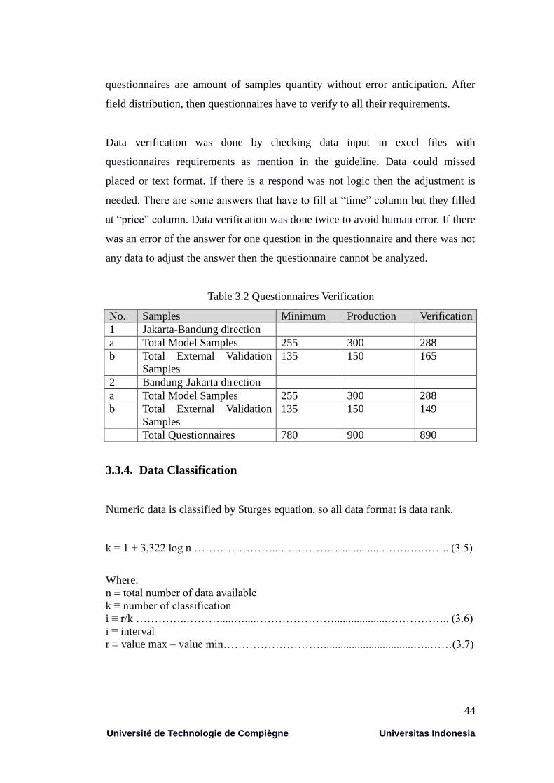
44
Université de Technologie de Compiègne Universitas Indonesia
questionnaires are amount of samples quantity without error anticipation. After
field distribution, then questionnaires have to verify to all their requirements.
Data verification was done by checking data input in excel files with
questionnaires requirements as mention in the guideline. Data could missed
placed or text format. If there is a respond was not logic then the adjustment is
needed. There are some answers that have to fill at “time” column but they filled
at “price” column. Data verification was done twice to avoid human error. If there
was an error of the answer for one question in the questionnaire and there was not
any data to adjust the answer then the questionnaire cannot be analyzed.
Table 3.2 Questionnaires Verification
No. Samples Minimum Production Verification
1 Jakarta-Bandung direction
a Total Model Samples 255 300 288
b Total External Validation
Samples
135 150 165
2 Bandung-Jakarta direction
a Total Model Samples 255 300 288
b Total External Validation
Samples
135 150 149
Total Questionnaires 780 900 890
3.3.4. Data Classification
Numeric data is classified by Sturges equation, so all data format is data rank.
k = 1 + 3,322 log n …………………...…..…………..............…….….…….. (3.5)
Where:
n ≡ total number of data available
k ≡ number of classification
i ≡ r/k …………..……….....…....…………………...................…………….. (3.6)
i ≡ interval
r ≡ value max – value min………………………................................…..……(3.7)
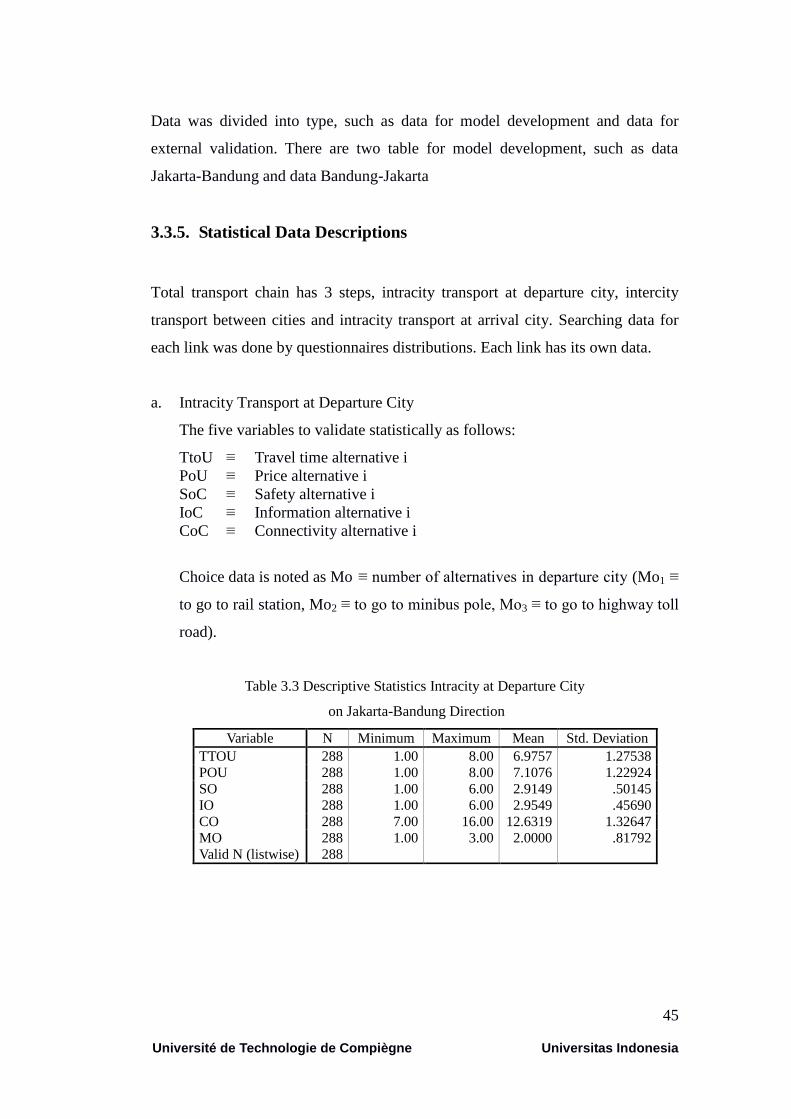
45
Université de Technologie de Compiègne Universitas Indonesia
Data was divided into type, such as data for model development and data for
external validation. There are two table for model development, such as data
Jakarta-Bandung and data Bandung-Jakarta
3.3.5. Statistical Data Descriptions
Total transport chain has 3 steps, intracity transport at departure city, intercity
transport between cities and intracity transport at arrival city. Searching data for
each link was done by questionnaires distributions. Each link has its own data.
a. Intracity Transport at Departure City
The five variables to validate statistically as follows:
TtoU ≡ Travel time alternative i
PoU ≡ Price alternative i
SoC ≡ Safety alternative i
IoC ≡ Information alternative i
CoC ≡ Connectivity alternative i
Choice data is noted as Mo ≡ number of alternatives in departure city (Mo1 ≡
to go to rail station, Mo2 ≡ to go to minibus pole, Mo3 ≡ to go to highway toll
road).
Table 3.3 Descriptive Statistics Intracity at Departure City
on Jakarta-Bandung Direction
Variable N Minimum Maximum Mean Std. Deviation
TTOU 288 1.00 8.00 6.9757 1.27538
POU 288 1.00 8.00 7.1076 1.22924
SO 288 1.00 6.00 2.9149 .50145
IO 288 1.00 6.00 2.9549 .45690
CO 288 7.00 16.00 12.6319 1.32647
MO 288 1.00 3.00 2.0000 .81792
Valid N (listwise) 288
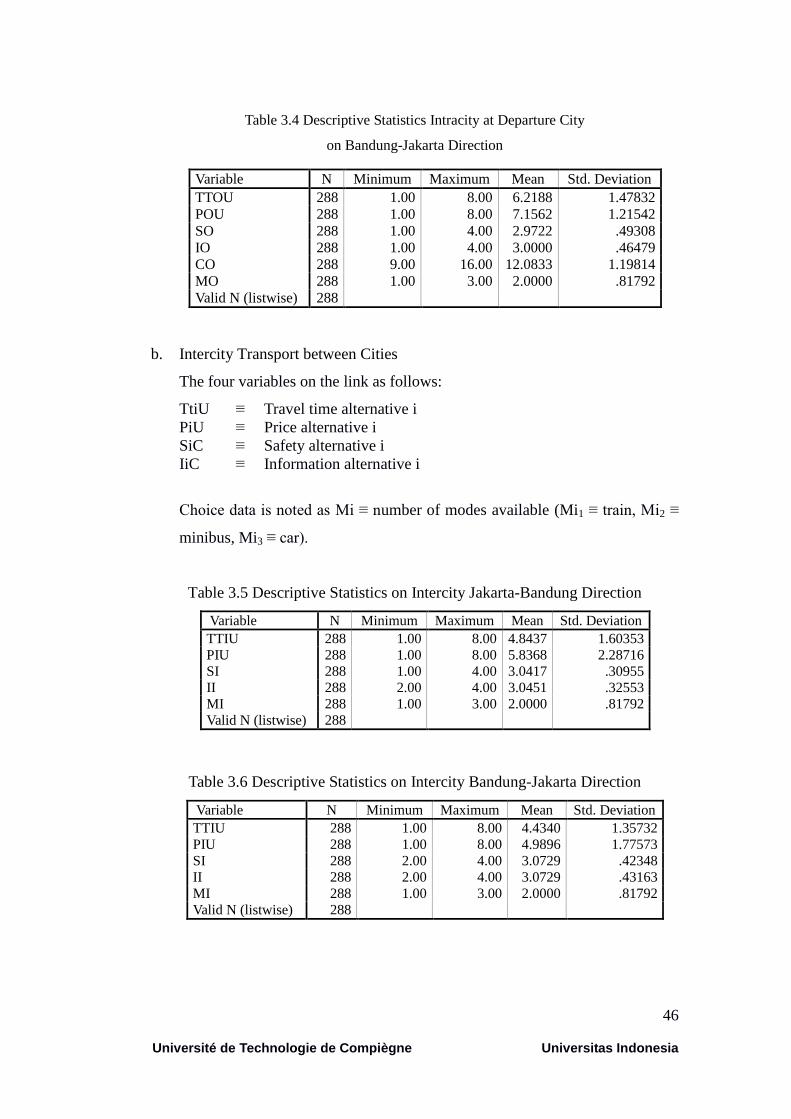
46
Université de Technologie de Compiègne Universitas Indonesia
Table 3.4 Descriptive Statistics Intracity at Departure City
on Bandung-Jakarta Direction
Variable N Minimum Maximum Mean Std. Deviation
TTOU 288 1.00 8.00 6.2188 1.47832
POU 288 1.00 8.00 7.1562 1.21542
SO 288 1.00 4.00 2.9722 .49308
IO 288 1.00 4.00 3.0000 .46479
CO 288 9.00 16.00 12.0833 1.19814
MO 288 1.00 3.00 2.0000 .81792
Valid N (listwise) 288
b. Intercity Transport between Cities
The four variables on the link as follows:
TtiU ≡ Travel time alternative i
PiU ≡ Price alternative i
SiC ≡ Safety alternative i
IiC ≡ Information alternative i
Choice data is noted as Mi ≡ number of modes available (Mi1 ≡ train, Mi2 ≡
minibus, Mi3 ≡ car).
Table 3.5 Descriptive Statistics on Intercity Jakarta-Bandung Direction
Variable N Minimum Maximum Mean Std. Deviation
TTIU 288 1.00 8.00 4.8437 1.60353
PIU 288 1.00 8.00 5.8368 2.28716
SI 288 1.00 4.00 3.0417 .30955
II 288 2.00 4.00 3.0451 .32553
MI 288 1.00 3.00 2.0000 .81792
Valid N (listwise) 288
Table 3.6 Descriptive Statistics on Intercity Bandung-Jakarta Direction
Variable N Minimum Maximum Mean Std. Deviation
TTIU 288 1.00 8.00 4.4340 1.35732
PIU 288 1.00 8.00 4.9896 1.77573
SI 288 2.00 4.00 3.0729 .42348
II 288 2.00 4.00 3.0729 .43163
MI 288 1.00 3.00 2.0000 .81792
Valid N (listwise) 288
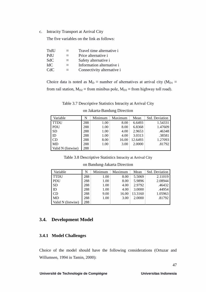
47
Université de Technologie de Compiègne Universitas Indonesia
c. Intracity Transport at Arrival City
The five variables on the link as follows:
TtdU ≡ Travel time alternative i
PdU ≡ Price alternative i
SdC ≡ Safety alternative i
IdC ≡ Information alternative i
CdC ≡ Connectivity alternative i
Choice data is noted as MD ≡ number of alternatives at arrival city (MD1 ≡
from rail station, MD2 ≡ from minibus pole, MD3 ≡ from highway toll road).
Table 3.7 Descriptive Statistics Intracity at Arrival City
on Jakarta-Bandung Direction
Variable N Minimum Maximum Mean Std. Deviation
TTDU 288 1.00 8.00 6.6493 1.54331
PDU 288 1.00 8.00 6.8368 1.47609
SD 288 1.00 4.00 2.9653 .46348
ID 288 1.00 4.00 3.0313 .38581
CD 288 8.00 16.00 12.6493 1.27093
MD 288 1.00 3.00 2.0000 .81792
Valid N (listwise) 288
Table 3.8 Descriptive Statistics Intracity at Arrival City
on Bandung-Jakarta Direction
Variable N Minimum Maximum Mean Std. Deviation
TTDU 288 1.00 8.00 5.5069 2.11019
PDU 288 1.00 8.00 5.9896 2.08944
SD 288 1.00 4.00 2.9792 .46432
ID 288 1.00 4.00 3.0000 .44954
CD 288 9.00 16.00 13.3160 1.05963
MD 288 1.00 3.00 2.0000 .81792
Valid N (listwise) 288
3.4. Development Model
3.4.1 Model Challenges
Choice of the model should have the following considerations (Ortuzar and
Willumsen, 1994 in Tamin, 2000):
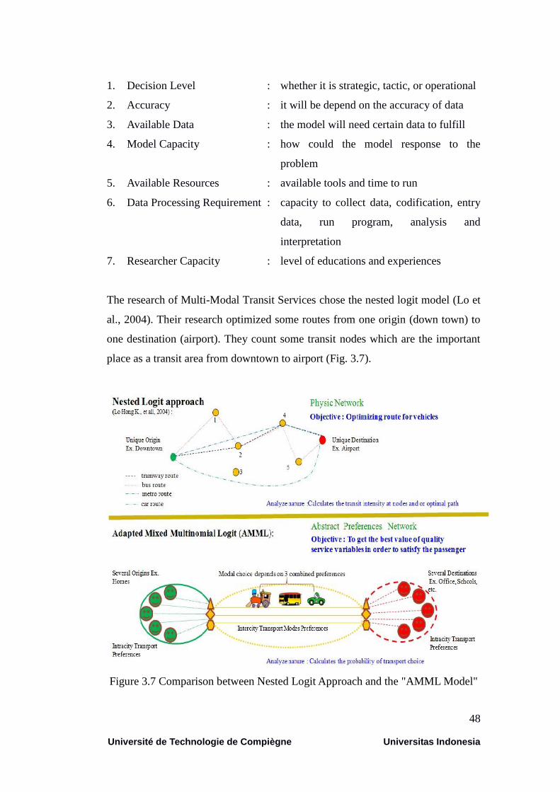
48
Université de Technologie de Compiègne Universitas Indonesia
1. Decision Level : whether it is strategic, tactic, or operational
2. Accuracy : it will be depend on the accuracy of data
3. Available Data : the model will need certain data to fulfill
4. Model Capacity : how could the model response to the
problem
5. Available Resources : available tools and time to run
6. Data Processing Requirement : capacity to collect data, codification, entry
data, run program, analysis and
interpretation
7. Researcher Capacity : level of educations and experiences
The research of Multi-Modal Transit Services chose the nested logit model (Lo et
al., 2004). Their research optimized some routes from one origin (down town) to
one destination (airport). They count some transit nodes which are the important
place as a transit area from downtown to airport (Fig. 3.7).
Figure 3.7 Comparison between Nested Logit Approach and the "AMML Model"
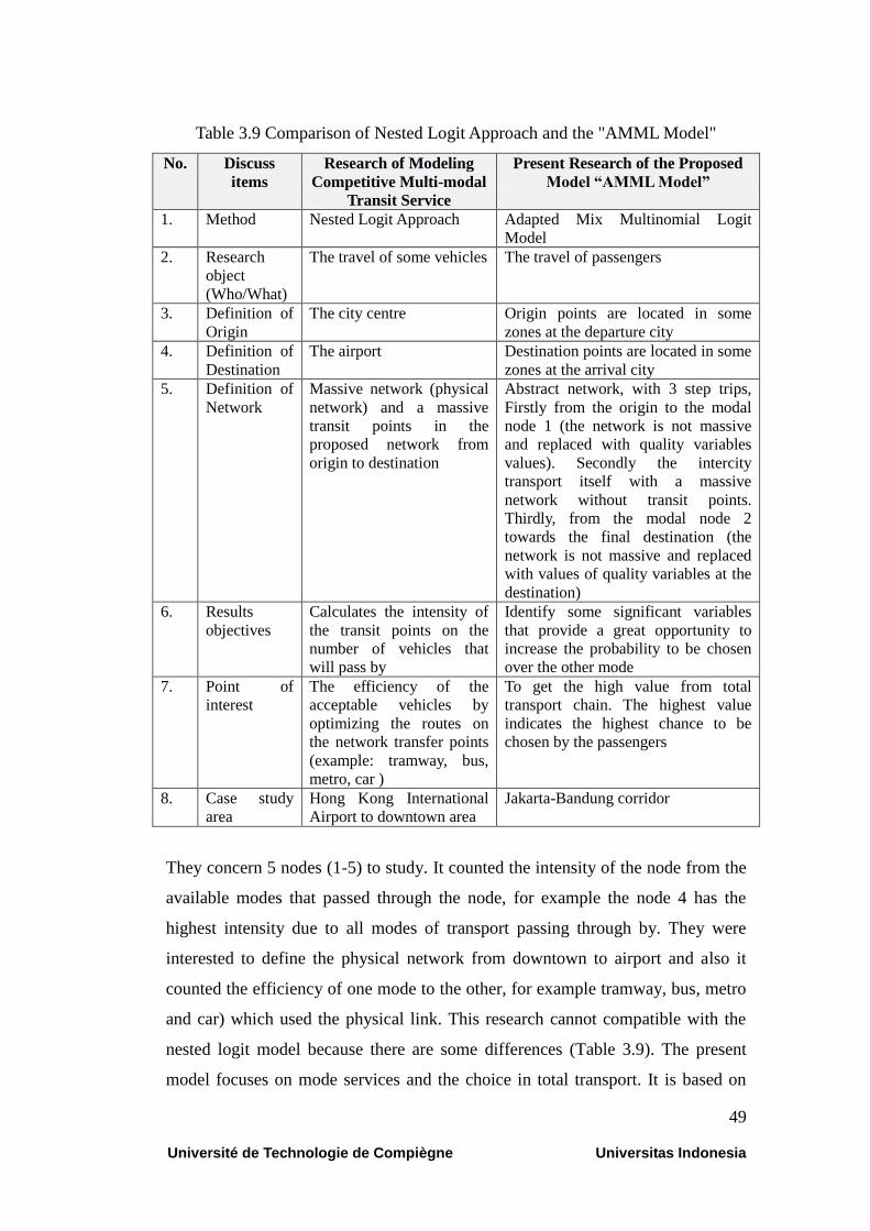
49
Université de Technologie de Compiègne Universitas Indonesia
Table 3.9 Comparison of Nested Logit Approach and the "AMML Model"
No. Discuss
items
Research of Modeling
Competitive Multi-modal
Transit Service
Present Research of the Proposed
Model “AMML Model”
1. Method Nested Logit Approach Adapted Mix Multinomial Logit
Model
2. Research
object
(Who/What)
The travel of some vehicles The travel of passengers
3. Definition of
Origin
The city centre Origin points are located in some
zones at the departure city
4. Definition of
Destination
The airport Destination points are located in some
zones at the arrival city
5. Definition of
Network
Massive network (physical
network) and a massive
transit points in the
proposed network from
origin to destination
Abstract network, with 3 step trips,
Firstly from the origin to the modal
node 1 (the network is not massive
and replaced with quality variables
values). Secondly the intercity
transport itself with a massive
network without transit points.
Thirdly, from the modal node 2
towards the final destination (the
network is not massive and replaced
with values of quality variables at the
destination)
6. Results
objectives
Calculates the intensity of
the transit points on the
number of vehicles that
will pass by
Identify some significant variables
that provide a great opportunity to
increase the probability to be chosen
over the other mode
7. Point of
interest
The efficiency of the
acceptable vehicles by
optimizing the routes on
the network transfer points
(example: tramway, bus,
metro, car )
To get the high value from total
transport chain. The highest value
indicates the highest chance to be
chosen by the passengers
8. Case study
area
Hong Kong International
Airport to downtown area
Jakarta-Bandung corridor
They concern 5 nodes (1-5) to study. It counted the intensity of the node from the
available modes that passed through the node, for example the node 4 has the
highest intensity due to all modes of transport passing through by. They were
interested to define the physical network from downtown to airport and also it
counted the efficiency of one mode to the other, for example tramway, bus, metro
and car) which used the physical link. This research cannot compatible with the
nested logit model because there are some differences (Table 3.9). The present
model focuses on mode services and the choice in total transport. It is based on
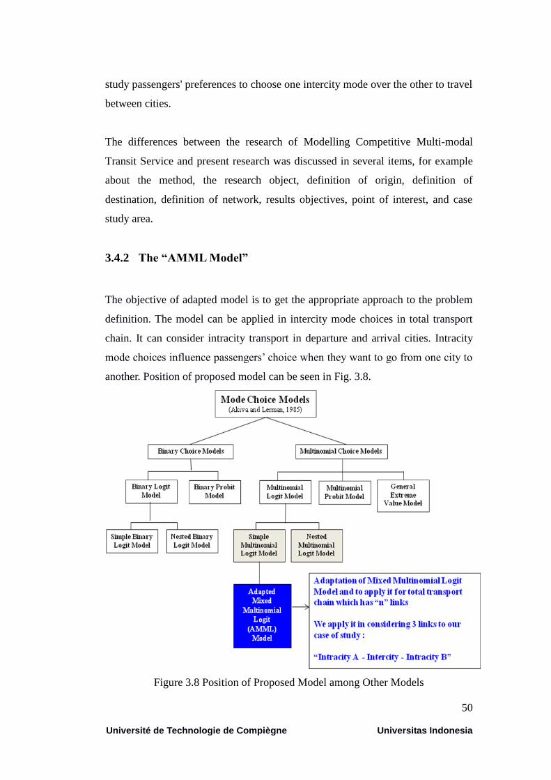
50
Université de Technologie de Compiègne Universitas Indonesia
study passengers' preferences to choose one intercity mode over the other to travel
between cities.
The differences between the research of Modelling Competitive Multi-modal
Transit Service and present research was discussed in several items, for example
about the method, the research object, definition of origin, definition of
destination, definition of network, results objectives, point of interest, and case
study area.
3.4.2 The “AMML Model”
The objective of adapted model is to get the appropriate approach to the problem
definition. The model can be applied in intercity mode choices in total transport
chain. It can consider intracity transport in departure and arrival cities. Intracity
mode choices influence passengers’ choice when they want to go from one city to
another. Position of proposed model can be seen in Fig. 3.8.
Figure 3.8 Position of Proposed Model among Other Models
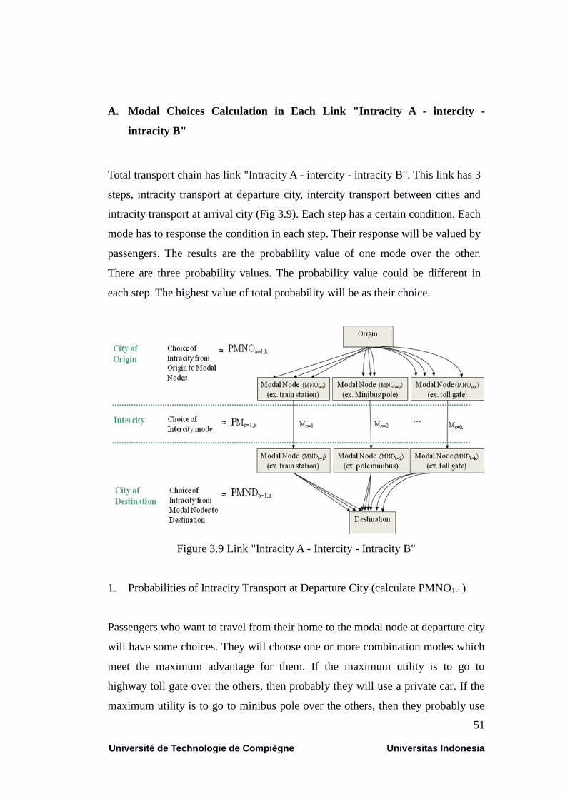
51
Université de Technologie de Compiègne Universitas Indonesia
A. Modal Choices Calculation in Each Link "Intracity A - intercity -
intracity B"
Total transport chain has link "Intracity A - intercity - intracity B". This link has 3
steps, intracity transport at departure city, intercity transport between cities and
intracity transport at arrival city (Fig 3.9). Each step has a certain condition. Each
mode has to response the condition in each step. Their response will be valued by
passengers. The results are the probability value of one mode over the other.
There are three probability values. The probability value could be different in
each step. The highest value of total probability will be as their choice.
Figure 3.9 Link "Intracity A - Intercity - Intracity B"
1. Probabilities of Intracity Transport at Departure City (calculate PMNO1-i )
Passengers who want to travel from their home to the modal node at departure city
will have some choices. They will choose one or more combination modes which
meet the maximum advantage for them. If the maximum utility is to go to
highway toll gate over the others, then probably they will use a private car. If the
maximum utility is to go to minibus pole over the others, then they probably use
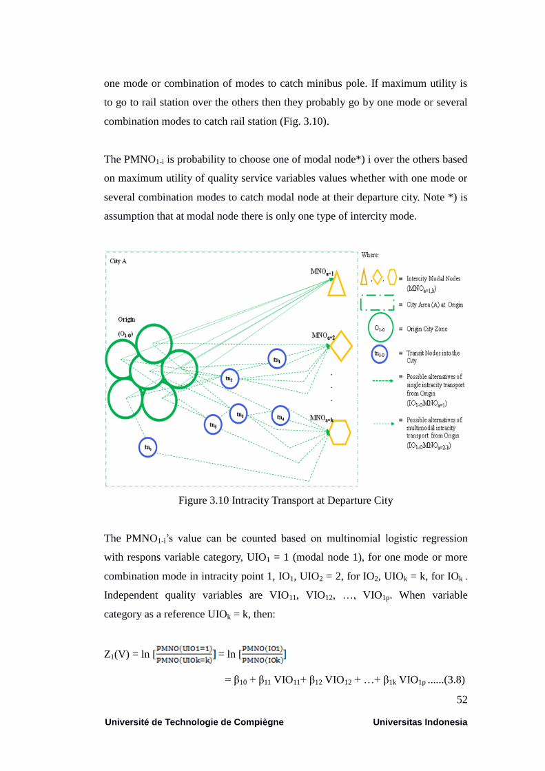
52
Université de Technologie de Compiègne Universitas Indonesia
one mode or combination of modes to catch minibus pole. If maximum utility is
to go to rail station over the others then they probably go by one mode or several
combination modes to catch rail station (Fig. 3.10).
The PMNO1-i is probability to choose one of modal node*) i over the others based
on maximum utility of quality service variables values whether with one mode or
several combination modes to catch modal node at their departure city. Note *) is
assumption that at modal node there is only one type of intercity mode.
Figure 3.10 Intracity Transport at Departure City
The PMNO1-i’s value can be counted based on multinomial logistic regression
with respons variable category, UIO1 = 1 (modal node 1), for one mode or more
combination mode in intracity point 1, IO1, UIO2 = 2, for IO2, UIOk = k, for IOk .
Independent quality variables are VIO11, VIO12, …, VIO1p. When variable
category as a reference UIOk = k, then:
Z1(V) = ln [ = ln [
= β10 + β11 VIO11+ β12 VIO12 + …+ β1k VIO1p ......(3.8)
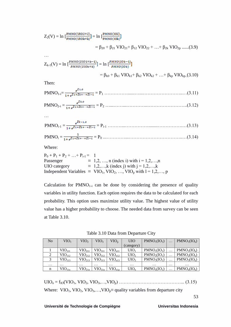
53
Université de Technologie de Compiègne Universitas Indonesia
Z2(V) = ln [ = ln [
= β20 + β21 VIO21+ β12 VIO22 + …+ β2k VIO2p ......(3.9)
…
Zk-1(V) = ln [ = ln [
= βk0 + βk1 VIOk1+ βk2 VIOk2 + …+ βkp VIOkp..(3.10)
Then:
PMNO1-i= = P1 ……………......…...……………………..…(3.11)
PMNO2-i = = P2 …...……...…………..……………………..(3.12)
…
PMNOi-1 = = Pi-1 ………...……………........…………….…(3.13)
PMNOi = = P0 ...…………...……………………………..…(3.14)
Where:
P0 + P1 + P2 + …+ Pi-1 = 1
Passenger ≡ 1,2, …, n (index i) with i = 1,2,…,n
UIO category ≡ 1,2,…,k (index j) with j = 1,2,…,k
Independent Variables ≡ VIO1, VIO2, …, VIOp with l = 1,2,…, p
Calculation for PMNO1-i can be done by considering the presence of quality
variables in utility function. Each option requires the data to be calculated for each
probability. This option uses maximize utility value. The highest value of utility
value has a higher probability to choose. The needed data from survey can be seen
at Table 3.10.
Table 3.10 Data from Departure City
No VIO1 VIO2 VIO3 VIOp UIO
(category)
PMNO1(IO1) … PMNO1(IOk)
1 VIO111 VIO211 VIO311 VIOn11 UIO1 PMNO1(IO1) … PMNO1(IOk)
2 VIO112 VIO212 VIO312 VIOn12 UIO2 PMNO2(IO1) … PMNO2(IOk)
3 VIO113 VIO213 VIO313 VIOn13 UIO3 PMNO3(IO1) … PMNO3(IOk)
… … … … … … … … …
n VIO11n VIO21n VIO31n VIOn1p UIOn PMNOn(IO1) … PMNOn(IOk)
UIOo = fIO(VIO1, VIO2, VIO3,…,VIOp) ……….…………………………... (3.15)
Where: VIO1, VIO2, VIO3,…,VIOp≡ quality variables from departure city
54
Université de Technologie de Compiègne Universitas Indonesia
This research, equation of intracity transport accessibility is expressed by utility
values of quality variables (UIOi). In case study, it considers the five quality
service variables, then the formula as follows:
UIOi = β0 + β1 Pi + β2 Tti + β3 Si + β4 Ci + β5 Ini……………………………(3.16)
Where:
UIOi ≡ Utility value alternative i
Pi ≡ Price alternative i
Tti ≡ Travel time alternative i
Si ≡ Safety alternative i
Ci ≡ Connectivity alternative i
Ini ≡ Information alternative i
i ≡ number of alternatives in departure city or at arrival city
β0, β1, … β5 ≡ constants
If the variable data (VIO1, VIO2, VIO3,..., VIOp) and choice (UIO category) were
obtained from the survey, then it can be used to estimate the value of constants β0
and other variables (β1, β2 , β3, ... βn). Calculations were performed by using the
maximum likelihood estimator in the logistic regression method.
…………......……... (3.17)
Where :
UIO(category) ≡ modal node at departure city that was chosen
VIO1, VIO2, VIO3,…,VIOn ≡ quality variables from departure city
β0, β1, β2, β3,… βn ≡ estimated constants
Probability with Utility value (UIO) with reference of the eq. 2.14 in chapter 2 as
follows:
PMNO(IOi) = ……………………………………….........….(3.18)
Where:
PMNO (IOi) ≡ Probability of modal node i was chosen from departure city
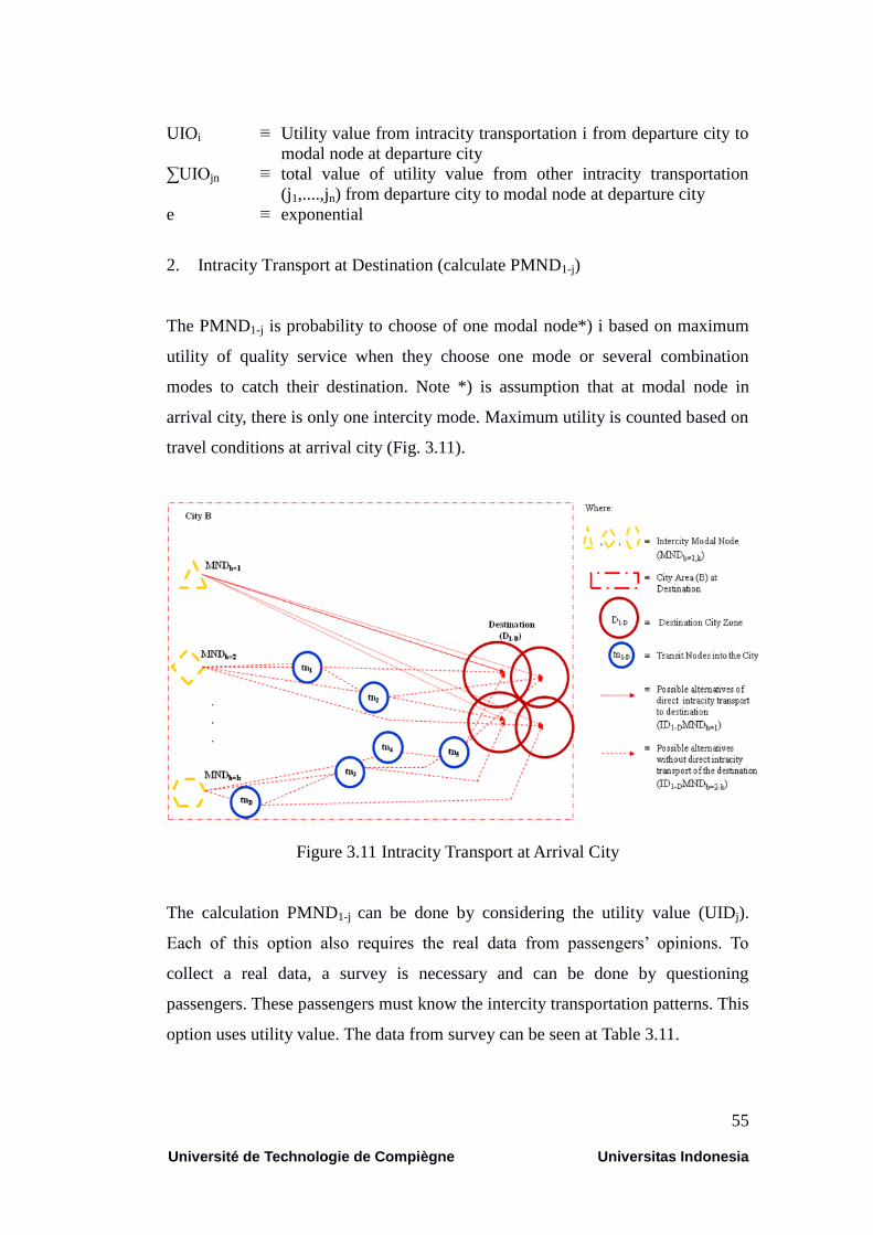
55
Université de Technologie de Compiègne Universitas Indonesia
UIOi
≡ Utility value from intracity transportation i from departure city to
modal node at departure city
∑UIOjn ≡ total value of utility value from other intracity transportation
(j1,....,jn) from departure city to modal node at departure city
e ≡ exponential
2. Intracity Transport at Destination (calculate PMND1-j)
The PMND1-j is probability to choose of one modal node*) i based on maximum
utility of quality service when they choose one mode or several combination
modes to catch their destination. Note *) is assumption that at modal node in
arrival city, there is only one intercity mode. Maximum utility is counted based on
travel conditions at arrival city (Fig. 3.11).
Figure 3.11 Intracity Transport at Arrival City
The calculation PMND1-j can be done by considering the utility value (UIDj).
Each of this option also requires the real data from passengers’ opinions. To
collect a real data, a survey is necessary and can be done by questioning
passengers. These passengers must know the intercity transportation patterns. This
option uses utility value. The data from survey can be seen at Table 3.11.
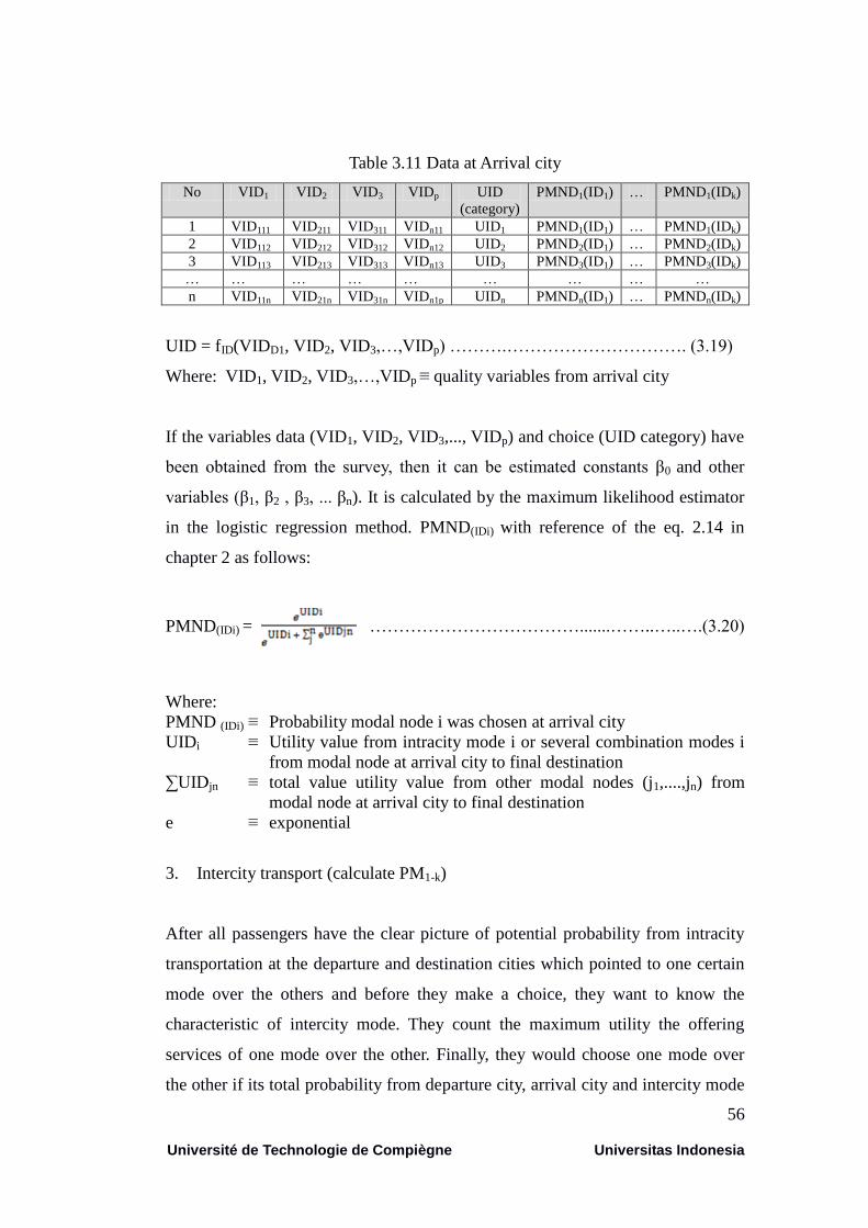
56
Université de Technologie de Compiègne Universitas Indonesia
Table 3.11 Data at Arrival city
No VID1 VID2 VID3 VIDp UID
(category)
PMND1(ID1) … PMND1(IDk)
1 VID111 VID211 VID311 VIDn11 UID1 PMND1(ID1) … PMND1(IDk)
2 VID112 VID212 VID312 VIDn12 UID2 PMND2(ID1) … PMND2(IDk)
3 VID113 VID213 VID313 VIDn13 UID3 PMND3(ID1) … PMND3(IDk)
… … … … … … … … …
n VID11n VID21n VID31n VIDn1p UIDn PMNDn(ID1) … PMNDn(IDk)
UID = fID(VIDD1, VID2, VID3,…,VIDp) ……….…………………………. (3.19)
Where: VID1, VID2, VID3,…,VIDp ≡ quality variables from arrival city
If the variables data (VID1, VID2, VID3,..., VIDp) and choice (UID category) have
been obtained from the survey, then it can be estimated constants β0 and other
variables (β1, β2 , β3, ... βn). It is calculated by the maximum likelihood estimator
in the logistic regression method. PMND(IDi) with reference of the eq. 2.14 in
chapter 2 as follows:
PMND(IDi) = ……………………………….......……..…..….(3.20)
Where:
PMND (IDi) ≡ Probability modal node i was chosen at arrival city
UIDi
≡ Utility value from intracity mode i or several combination modes i
from modal node at arrival city to final destination
∑UIDjn ≡ total value utility value from other modal nodes (j1,....,jn) from
modal node at arrival city to final destination
e ≡ exponential
3. Intercity transport (calculate PM1-k)
After all passengers have the clear picture of potential probability from intracity
transportation at the departure and destination cities which pointed to one certain
mode over the others and before they make a choice, they want to know the
characteristic of intercity mode. They count the maximum utility the offering
services of one mode over the other. Finally, they would choose one mode over
the other if its total probability from departure city, arrival city and intercity mode

57
Université de Technologie de Compiègne Universitas Indonesia
is the highest. At this link, passengers can have a direct trip because there is only
one mode is available. If one passenger has arrived at modal node at departure
city, then they will continue their journey to modal node at arrival city (Fig. 3.12).
Figure 3.12 Intercity Transport System
Calculation for PM1-k can also be done by considering the utility value. It requires
the data survey to calculate the probability. The data from survey on intercity link
can be seen at Table 3.12.
Table 3.12 Data from Intercity Modes
No VM1 VM2 VM3 VMp UM
(category)
PM(M1) … PM(Mk)
1 VM111 VM211 VM311 VMn11 UM1 PM1(M1) … PM(Mk)
2 VM112 VM212 VM312 VMn12 UM2 PM2(M1) … PM2(Mk)
3 VM113 VM213 VM313 VMn13 UM3 PM3(M1) … PM3(Mk)
… … … … … … … … …
n VM11n VM21n VM31n VMn1p UMn PMn(M1) … PMn(Mk)
Um = fM(VM1, VM2, VM3,…,VMp) …….……………..……………….…. (3.21)
Where: VM1, VM2, VM3,…,VMp≡ quality variables from intercity modes
If the variables in data are VM1, VM2, VM3,..., VMp and choice (UM category)
have been obtained from the survey, then it can be estimated constants β0 and
other variables (β1, β2 , β3, ... βn). Calculations were performed using the
58
Université de Technologie de Compiègne Universitas Indonesia
maximum likelihood estimator in the logistic regression method. PM1-k with
reference of the eq. 2.14 in chapter 2 as follows:
PM1-k= …………………..……….....………..…………..….(3.22)
Where:
PM1-k ≡ Probability intercity mode i was chosen
UMi
≡ Utility value from intercity mode i
∑UMjn ≡ total value utility value from other intercity modes (j1,....,jn)
e ≡ exponential
B. Modal Choices Calculation in Total Transport Chain as the Final Choice
Journey behaviour for passengers who want to go from departure city to arrival
city has three steps, first departure city to modal node at departure city (IO),
modal node at departure city to modal node at arrival city (M), and modal node at
arrival city to final destination (ID). Journey behaviour is in a conditional
probability with 3 events. Conditional probability with 3 events is as follows
(Walpole et al, 2012):
P(A3|A1∩A2) = …………......….…………...……………...……(3.23)
P(A1∩A2∩A3) = P(A3|A1∩A2) . P(A1∩A2) …………….………..…..………(3.24)
P(A1∩A2∩A3) = P(A3|A1∩A2) . P(A2|A1) . P(A1) …………………..……….(3.25)
P(A1∩A2∩A3) = P(A1) . P(A2|A1) . P(A3|A1∩A2) ………….………..…..…..(3.26)
Where:
P(A3|A1∩A2) ≡ Probability of A3 even which will happened if probabilities of A1
and A2 were known
A1, A2, A3 ≡ Events with index hierarchy
People need to do their activities. They have to travel to other city if their activity
is not in their city. Before travelling, they observe the transport condition at their
city then the transport conditions at the arrival city, then they consider offered
services from each mode, and finally they make a final choice (Tamin, 2000).
59
Université de Technologie de Compiègne Universitas Indonesia
These 3 evens are in the conditional probability. Conditional probability with 3
steps of decision process by passengers can be formulated as follows:
P(M|IO∩ID) = ………………………….............……………..…(3.27)
P(IO∩ID∩M) = P(M|IO∩ID) . P(IO∩ID) ….……….…….……………...…(3.28)
P(IO∩ID∩M) = P(IO) . P(ID|IO) . P(M|IO∩ID) ………….……………….(3.29)
Where:
P(IO∩ID∩M) ≡ Probability M which will be count after probability IO and
ID has been known
P(IO) ≡ Probability of one alternative is chosen which is from one
mode or several modes combined at departure city
P(ID|IO) ≡ Probability of one alternative is chosen which is from one
mode or several modes combined at arrival city after
counting probability of one alternative at departure city
P(M|IO∩ID) ≡ Probability of intercity mode is chosen after counting
probability of one alternative at departure city and one
alternative at arrival city
IO ≡ Decision process steps 1 from origin to intercity at
departure city
ID ≡ Decision process steps 2 from modal node at arrival city to
final destination
M ≡ Decision process steps 3 from modal node at departure city
to point modal node at arrival city
This formulation model has a “mixed structure”. P(IO∩ID∩M) as y is a vector of
observations, with :
P(M|IO∩ID) as β is a vector of fixed effects
P(IO) as u1 is an additional vector 1
P(ID|OI) as u2 is an other additional vector 2
Final choice depends on total probability from departure city to arrival city, such
as decisions at process 1, 2, and 3. Final choice will be the choice with the highest
value. The final choice is the results from a conditional probability process
(Fig.3.13).
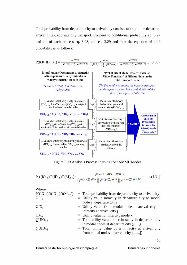
60
Université de Technologie de Compiègne Universitas Indonesia
Total probability from departure city to arrival city consists of trip in the departure
arrival cities, and intercity transport. Concern to conditional probability eq. 3.27
and eq. of each process eq. 3.28, and eq. 3.29 and then the equation of total
probability is as follows:
P(IO∩ID∩M) = . . …(3.30)
Figure 3.13 Analysis Process in using the "AMML Model"
Pij((IOi-k)∩(IDi-k)∩(M)i-k)= ....….(3.31)
Where:
P((IO1-i)∩(ID1-j)∩(M1-k)) ≡ Total probability from departure city to arrival city
UIOi
≡ Utility value intracity in departure city to modal
node at departure city i
UIDj ≡ Utility value from modal node at arrival city to
intracity at arrival city j
UMk ≡ Utility value for intercity mode k
∑UIO1-i ≡ Total utility value other intracity in departure city
to modal nodes at departure city (1,....,i)
∑UID1-j ≡ Total utility value other intracity at arrival city
from modal nodes at arrival city (1,....,j)
61
Université de Technologie de Compiègne Universitas Indonesia
∑UM1-k ≡ Total utility value other intercity modes (1,....,k)
e ≡ exponential
General equation of intercity mode choice probability is described on eq. 3.32.
This equation is called Adapted Mixed Multinomial Logit (AMML) Model.
……………………………..........(3.32)
Where: PIntercity mode choice is probability of intercity mode. ULq is each utility value
of each link. ƩULqr is a number of utility values from available mode on each
link, r is available modes (M1-k), q is link’s articulations (I1-n), and e is
exponential.
Table 3.13 Data Analysis for Total Probability
No P(IO1-i ) P(ID1-j) P(M)1-k Pij((IO1-i)∩(ID1-j)∩(M)1-k
1 P(IO1-i )1 P(ID1-j)1 P((M)1-k)1 Pij((IO1-i)∩(ID1-j)∩(M1-k) 1
2 P(IO1-i )2 P(ID1-j)2 P((M)1-k)2 Pij((IO1-i)∩(ID1-j)∩(M1-k) 2
3 P(IO1-i )3 P(ID1-j)3 P((M)1-k)3 Pij((IO1-i)∩(ID1-j)∩(M1-k) 3
… … … … …
n P(IO1-i )n P(ID1-j)n P((M)1-k)n Pij((IO1-i)∩(ID1-j)∩(M1-k) n
The “AMML” Model calculates total transport chain probabilities of each
intercity transport mode. Adaptation is done by concern to the formulation of
additional probability of intracity transport at departure and arrival cities which
are influence of the final intercity mode choice.
Possible probabilities results of the of passenger’s choice are as follows:
1. If P(IO1-i) high, P(IDi) high, P(M1-k) high, then Pi((IO1-i)∩(IDi)∩(M1-k)) >
Pj((IO1-i) ∩(IDj-k) ∩(M1-k))
2. If P(IO1-i) high, P(IDi) high, P(M1-k)low, then Pi((IO1-i)∩(IDi)∩ (M1-k)) >
Pj((IO1-i) ∩(IDj-k) ∩((M1-k))
3. If P(IO1-i) high, P(IDi) low, (M1-k)) low, then Pi((IO1-i)∩(IDi)∩ (M1-k)) >
Pj((IO1-i) ∩(IDjk) ∩( (M1-k))

62
Université de Technologie de Compiègne Universitas Indonesia
4. If P(IO1-i ) low, P(IDi) low, P(M1-k) high, then Pi((IO1-i)∩(IDi)∩( (M1-k)) >
Pj((IO1-i) ∩(IDjk) ∩( (M1-k))
5. If P(OIi) low, P(IDi) high, P(Mi) high, then Pi((OIi)∩(Di)∩(M)i) > Pj((OIj-k)
∩(IDjk) ∩ ((M1-k))
Total possibilities that would occur without the passenger’s choice are as follows:
1. P(OIi) low, P(IDi) low, P(M1-k) low, then Pi((OIi)∩(IDi)∩(M1-k) < Pj((OIj-
k)∩(IDj-k)∩ (M1-k))
2. P(OIi) high, P(IDi) high, P(M1-k) low, then Pi((OIi)∩(IDi)∩ (M1-k) < Pj((OIj-
k)∩(IDj-k)∩ (M1-k))
3. P(OIi) high, P(IDi) low, P(M1-k) low, then Pi((OIi)∩(IDi)∩ (M1-k)) < Pj((OIj-
k)∩(IDj-k)∩ ((M1-k))
4. P(OIi) low, P(IDi) low, P(M1-k) high, then Pi((OIi)∩(IDi)∩ (M1-k)< Pj((OIj-
k)∩(IDj-k)∩ ((M1-k))
5. P(OIi) low, P(IDi) high, P(M1-k) high, then Pi((OIi)∩(IDi)∩ (M1-k)) < Pj((OIj-
k)∩(IDj-k)∩ (M1-k))
3.5. Validation Model
The mathematical models obtained are tested by some statistical tests. If the
values are acceptable, then the mathematical models can be used for evaluation.
Furthermore, the models need to be validated. Validation is done by calculating
results with using the AMML Model. There are 2 ways to validate the obtained
models. First is by using other equations of the AMML model. It is the probability
model which formulated with combination between some constants and utility
function. The second is using the new additional data to confirm the choice
results.
3.5.1 Validation with Other Equation of the AMML Model
1. Intracity transport at departure city (calculate PMNO1-i)
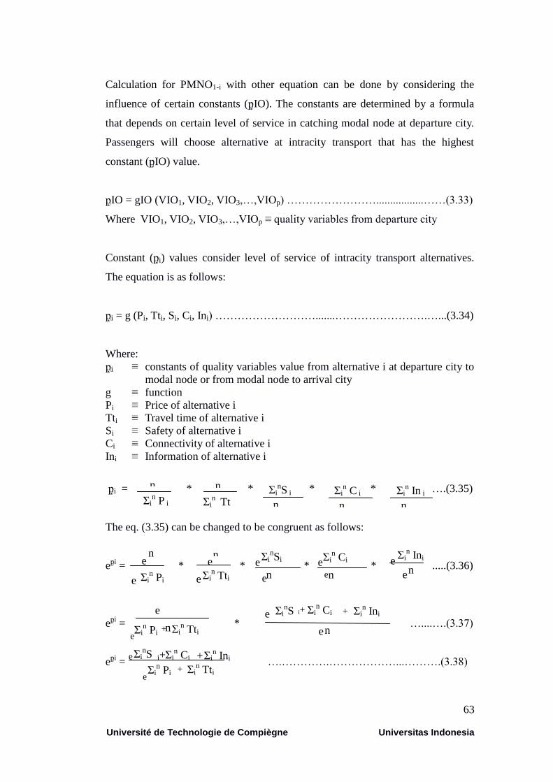
63
Université de Technologie de Compiègne Universitas Indonesia
Calculation for PMNO1-i with other equation can be done by considering the
influence of certain constants (ᶈIO). The constants are determined by a formula
that depends on certain level of service in catching modal node at departure city.
Passengers will choose alternative at intracity transport that has the highest
constant (ᶈIO) value.
ᶈIO = gIO (VIO1, VIO2, VIO3,…,VIOp) …………………….................……(3.33)
Where VIO1, VIO2, VIO3,…,VIOp ≡ quality variables from departure city
Constant (ᶈi) values consider level of service of intracity transport alternatives.
The equation is as follows:
ᶈi = g (Pi, Tti, Si, Ci, Ini) ……………………….......…………………….…...(3.34)
Where:
ᶈi ≡ constants of quality variables value from alternative i at departure city to
modal node or from modal node to arrival city
g ≡ function
Pi ≡ Price of alternative i
Tti ≡ Travel time of alternative i
Si ≡ Safety of alternative i
Ci ≡ Connectivity of alternative i
Ini ≡ Information of alternative i
ᶈi = * * * * ….(3.35)
The eq. (3.35) can be changed to be congruent as follows:
eᶈi
= * * * * .....(3.36)
eᶈi
= * …....….(3.37)
eᶈi
= ….………….………………...……….(3.38)
n n Ʃin C i
n
ƩinS i
n
Ʃin In i
n Ʃin Tt
i
Ʃin P i
e Ʃi
nSi
n e Ʃi
n Ci
n
e Ʃi
n Ini n
e n
e
e e n e Ʃin Tti e Ʃi
n Pi e
n
Ʃin Ini Ʃi
n Ci i+ Ʃi
nS
n
+ e e
Ʃin Tti
e + Ʃi
n Pi e
Ʃin Ci Ʃi
n Ini + i+ Ʃi
nS e
Ʃin Tti + Ʃi
n Pi
e
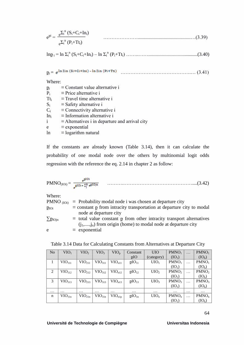
64
Université de Technologie de Compiègne Universitas Indonesia
eᶈi
= …………………...........................................…(3.39)
lnᶈ i = ln Ʃin (Si+Ci+Ini) – ln Ʃi
n (Pi+Tti) ……..……........................................(3.40)
ᶈi = …………………………………….… (3.41)
Where:
ᶈi ≡ Constant value alternative i
Pi ≡ Price alternative i
Tti ≡ Travel time alternative i
Si ≡ Safety alternative i
Ci ≡ Connectivity alternative i
Ini ≡ Information alternative i
i ≡ Alternatives i in departure and arrival city
e ≡ exponential
ln ≡ logarithm natural
If the constants are already known (Table 3.14), then it can calculate the
probability of one modal node over the others by multinomial logit odds
regression with the reference the eq. 2.14 in chapter 2 as follow:
PMNO(IOi) = ……….……………………………………....(3.42)
Where:
PMNO (IOi) ≡ Probability modal node i was chosen at departure city
ᶈIOi
≡ constant ᶈ from intracity transportation at departure city to modal
node at departure city
∑ᶈIOjn ≡ total value constant ᶈ from other intracity transport alternatives
(j1,....,jn) from origin (home) to modal node at departure city
e ≡ exponential
Table 3.14 Data for Calculating Constants from Alternatives at Departure City
No VIO1 VIO2 VIO3 VIOp Constant
ᶈIO
UIO
(category)
PMNO1
(IO1)
… PMNO1
(IOk)
1 VIO111 VIO211 VIO311 VIOn11 ᶈIO11 UIO1 PMNO1
(IO1)
… PMNO1
(IOk)
2 VIO112 VIO212 VIO312 VIOn12 ᶈIO12 UIO2 PMNO2
(IO1)
… PMNO2
(IOk)
3 VIO113 VIO213 VIO313 VIOn13 ᶈIO13 UIO3 PMNO3
(IO1)
… PMNO3
(IOk)
… … … … … … … … … …
n VIO11n VIO21n VIO31n VIOn1p ᶈIO1n UIOn PMNOn
(IO1)
… PMNOn
(IOk)
Ʃin (Si+Ci+Ini)
Ʃin (Pi+Tti)
e
e

65
Université de Technologie de Compiègne Universitas Indonesia
2. Intracity Transport at Arrival city (calculate PMND1-j)
The calculation PMND1-j can be done by considering the influence of certain
constants (ᶈIDi). In this option, constant value of ᶈID is counted using certain
equation (see eq. 3.41). Passengers will prefer alternative intracity that has the
highest ᶈD value. Identified data from passengers’ preference can be seen at Table
3.15.
ᶈID = gID (VID1, VID2, VID3,…,VIDp) ………………………………….…(3.43)
Where VID1, VID2, VID3,…,VIDp≡ variables of quality service at arrival city
Table 3.15 Data for Calculating Constants from Alternatives at Arrival City
No VID1 VID2 VID3 VIDp Constant
ᶈID
UID
(category)
PMND1
(ID1)
… PMND1
(IDk)
1 VID111 VID211 VID311 VIDn11 ᶈID11 UID1 PMND1
(ID1)
… PMND1
(IDk)
2 VID112 VID212 VID312 VIDn12 ᶈID12 UID2 PMND2
(ID1)
… PMND2
(IDk)
3 VID113 VID213 VID313 VIDn13 ᶈID13 UID3 PMND3
(ID1)
… PMND3
(IDk)
… … … … … … … … … …
n VID11n VID21n VID31n VIDn1p ᶈID1n UIDn PMNDn
(ID1)
… PMNDn
(IDk)
If the constants are already known, then the probability of one mode over the
other modes can be calculated with the reference the eq. 2.14 in chapter 2:
PMND(IDi) = ……………………………….....…….........(3.44)
Where:
PMND (IDi) ≡ Probability modal node i was chosen at arrival city
ᶈIDi ≡ constant ᶈ from intracity transportation i from modal node at arrival
city to final destination
∑ᶈIDjn ≡ total value constant ᶈ from other modal nodes (j1,....,jn) from modal
node at arrival city to final destination
e ≡ exponential
3. Intercity transport (calculate PM1-k)
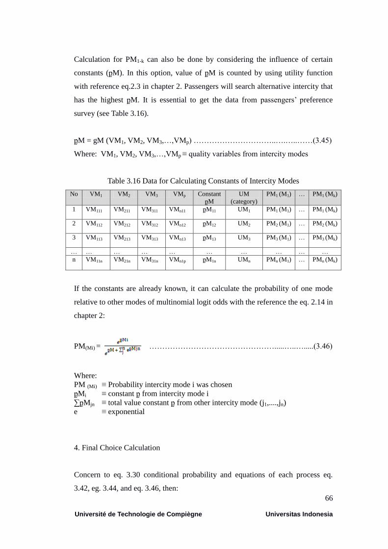
66
Université de Technologie de Compiègne Universitas Indonesia
Calculation for PM1-k can also be done by considering the influence of certain
constants (ᶈM). In this option, value of ᶈM is counted by using utility function
with reference eq.2.3 in chapter 2. Passengers will search alternative intercity that
has the highest ᶈM. It is essential to get the data from passengers’ preference
survey (see Table 3.16).
ᶈM = gM (VM1, VM2, VM3,…,VMp) …………………………..….…..……(3.45)
Where: VM1, VM2, VM3,…,VMp ≡ quality variables from intercity modes
Table 3.16 Data for Calculating Constants of Intercity Modes
No VM1 VM2 VM3 VMp Constant
ᶈM
UM
(category)
PM1 (M1) … PM1 (Mk)
1 VM111 VM211 VM311 VMn11 ᶈM11 UM1 PM1 (M1) … PM1 (Mk)
2 VM112 VM212 VM312 VMn12 ᶈM12 UM2 PM2 (M1) … PM2 (Mk)
3 VM113 VM213 VM313 VMn13 ᶈM13 UM3 PM3 (M1) … PM3 (Mk)
… … … … … … … … … …
n VM11n VM21n VM31n VMn1p ᶈM1n UMn PMn (M1) … PMn (Mk)
If the constants are already known, it can calculate the probability of one mode
relative to other modes of multinomial logit odds with the reference the eq. 2.14 in
chapter 2:
PM(Mi) = ………………………………………….....…..….....(3.46)
Where:
PM (Mi) ≡ Probability intercity mode i was chosen
ᶈMi
≡ constant ᶈ from intercity mode i
∑ᶈMjn ≡ total value constant ᶈ from other intercity mode (j1,....,jn)
e ≡ exponential
4. Final Choice Calculation
Concern to eq. 3.30 conditional probability and equations of each process eq.
3.42, eg. 3.44, and eq. 3.46, then:
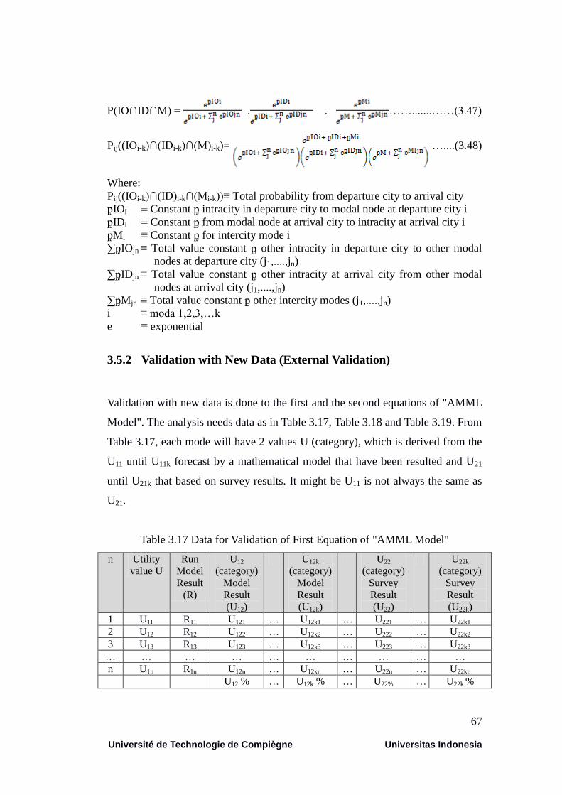
67
Université de Technologie de Compiègne Universitas Indonesia
P(IO∩ID∩M) = . . …….......……(3.47)
Pij((IOi-k)∩(IDi-k)∩(M)i-k)= …....(3.48)
Where:
Pij((IOi-k)∩(ID)i-k∩(Mi-k))≡ Total probability from departure city to arrival city
ᶈIOi
≡ Constant ᶈ intracity in departure city to modal node at departure city i
ᶈIDi
≡ Constant ᶈ from modal node at arrival city to intracity at arrival city i
ᶈMi ≡ Constant ᶈ for intercity mode i
∑ᶈIOjn ≡ Total value constant ᶈ other intracity in departure city to other modal
nodes at departure city (j1,....,jn)
∑ᶈIDjn ≡ Total value constant ᶈ other intracity at arrival city from other modal
nodes at arrival city (j1,....,jn)
∑ᶈMjn ≡ Total value constant ᶈ other intercity modes (j1,....,jn)
i ≡ moda 1,2,3,…k
e ≡ exponential
3.5.2 Validation with New Data (External Validation)
Validation with new data is done to the first and the second equations of "AMML
Model". The analysis needs data as in Table 3.17, Table 3.18 and Table 3.19. From
Table 3.17, each mode will have 2 values U (category), which is derived from the
U11 until U11k forecast by a mathematical model that have been resulted and U21
until U21k that based on survey results. It might be U11 is not always the same as
U21.
Table 3.17 Data for Validation of First Equation of "AMML Model"
n Utility
value U
Run
Model
Result
(R)
U12
(category)
Model
Result
(U12)
U12k
(category)
Model
Result
(U12k)
U22
(category)
Survey
Result
(U22)
U22k
(category)
Survey
Result
(U22k)
1 U11 R11 U121 … U12k1 … U221 … U22k1
2 U12 R12 U122 … U12k2 … U222 … U22k2
3 U13 R13 U123 … U12k3 … U223 … U22k3
… … … … … … … … … …
n U1n R1n U12n … U12kn … U22n … U22kn
U12 % … U12k % … U22% … U22k %
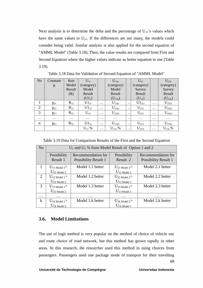
68
Université de Technologie de Compiègne Universitas Indonesia
Next analysis is to determine the delta and the percentage of U11’s values which
have the same values to U21. If the differences are not many, the models could
consider being valid. Similar analysis is also applied for the second equation of
"AMML Model" (Table 3.18). Then, the value results are compared from First and
Second Equation where the higher values indicate as better equation to use (Table
3.19).
Table 3.18 Data for Validation of Second Equation of "AMML Model"
No Constant
ᶈ
Run
Model
Result
(R)
U11
(category)
Model
Result
(U11)
U11k
(category)
Model
Result
(U11k)
U21
(category)
Survey
Result
(U21)
U21k
(category)
Survey
Result
(U21k)
1 ᶈ11 R11 U111 … U11k1 … U1211 … U21k1
2 ᶈ12 R12 U112 … U11k2 … U212 … U21k2
3 ᶈ13 R13 U13 … U11k3 … U213 … U21k3
… … … … … … … … … …
n ᶈ1n R1n U11n … U11kn … U21n … U21kn
U11 % … U11k % … U21% … U21k %
Table 3.19 Data for Comparison Results of the First and the Second Equation
No U1 and U2 % from Model Result of Option 1 and 2
Possibility
Result 1
Recommendation for
Possibility Result 1
Possibility
Result 2
Recommendation for
Possibility Result 1
1 U11 Model 1>
U21 Model 2
Model 1.1 better U21 Model 2>
U11 Model 1
Model 2.1 better
2 U12 Model 1>
U22 Model 2
Model 1.2 better U22 Model 2>
U12 Model 1
Model 2.2 better
3 U13 Model 1>
U23 Model 2
Model 1.3 better U23 Model 2>
U13 Model 1
Model 2.3 better
… … … … …
k U1k Model 1>
U2k Model 2
Model 1.k better U2k Model 2>
U1k Model 1
Model 2.k better
3.6. Model Limitations
The use of logit method is very popular on the method of choice of vehicle use
and route choice of road network, but this method has grown rapidly in other
areas. In this research, the researcher used this method in using choices from
passengers. Passengers used one package mode of transport for their travelling
69
Université de Technologie de Compiègne Universitas Indonesia
from home to their final destination. They never used other packages and already
know the pattern and gave their opinions. Error might occur with some opinions
which are not in this pattern.
The existence of a complex system of society led to the handling of public
transport services which is viewed from the side of technology, design, and the
existing transportation system. Characteristics of multi-disciplinary fields of
transportation science are inseparable from the role of a real transportation system
involving various sectors of activity, such as socio-economic activities of urban
society (Soehodho, 2000). These activities are in line with the time complexity of
the problems that requires of the completion.
It considers the nature and characteristics of the transportation problem that is
inherent to society itself, so it needs to be seen comprehensively. In this research,
the authors developed a model oriented in the context of transport policy-making
in transport demand using a variety of alternative models, alternative assumptions,
theories, analytical methods, parameters and test the model. The development of
model however needs more data and details picture of the situations.
Discussing the problems of the private and public transport service in Indonesia is
incomplete without other disciplines. In advance usage, this method could applied
to determine the market segments of transportation, such as particular passengers
characteristic that were chosen because of several variables that really stands out
among certain characteristic. For example, it can use to determine the choice of
young people from their departure city to their final destination. It also can use to
determine the choice of certain people with the same class income who travel
from some links articulations. The total probability function is could be
implemented in real condition that always has a possible situation to change its
equations.

70
Université de Technologie de Compiègne Universitas Indonesia
CHAPTER IV THE “AMML MODEL” APPLICATION
4.1 Research Design
4.1.1 Primary Survey by Questionnaires Distribution
The research was conducted by eight phases (Fig. 4.1). Firstly, literature study
gave insight knowledge on general problems base on experts’ theories, premises,
and opinions in books, study report, and journals papers. Secondly, their written
report was discussed to obtain the main and significant problems and method to
implement. Thirdly, all input was to assist of developing the questionnaires in and
methodology to distribute. Before distributing questionnaires, it was necessary to
survey the location and to do some simulation to make sure the implementation.
The survey was done on the Jakarta-Bandung corridor targeting passenger of three
modes of transportation. This research use the "AMML model" for data analysis,
which were validated with some probability models scenarios. The final results
were interpreted and were formulated into policy recommendations to improve
services of private and public transport modes.
Figure 4.1 Procedure Analysis

71
Université de Technologie de Compiègne Universitas Indonesia
Research anatomy was as follow:
Research issues were indicated by problems on modes’ services conditions of
private and public transport that are not really good in current situation (Fig.
4.2).
Research significance to do the research was the needed actions for
improvement modes services with supports of intracity transport systems on
the Jakarta-Bandung corridor.
Research classification as follow (Fig. 4.3):
o Primary survey was done for applying model development (action
research)
o Problem characteristic was descriptive correlation research
o Character and data type were empirical research and opinion (passengers
preferences)
o Research methods were literature study, field survey, and questionnaires
distribution.
Benefit to be achieved in this activity is identified recommendations to better
improve supply conditions both private and public transport services in
Jakarta-Bandung corridor (Fig. 4.4)
Implication: it was necessary to develop and to improve supply condition to
be sustainable in the future (Fig. 4.5).
Figure 4.2 Private and Public Transport Modes on the Jakarta-Bandung Corridor

72
Université de Technologie de Compiègne Universitas Indonesia
Figure 4.3 Research Anatomy
Figure 4.4 Physiology of Decision Making
Figure 4.5 Psychology Design/Implementation
4.1.2 Concept Framework
This chapter elaborates the concept framework from general transport problem to
more detail case study. Research framework to identify research activities from
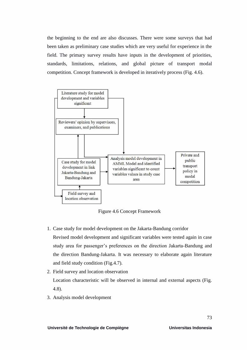
73
Université de Technologie de Compiègne Universitas Indonesia
the beginning to the end are also discusses. There were some surveys that had
been taken as preliminary case studies which are very useful for experience in the
field. The primary survey results have inputs in the development of priorities,
standards, limitations, relations, and global picture of transport modal
competition. Concept framework is developed in iteratively process (Fig. 4.6).
Figure 4.6 Concept Framework
1. Case study for model development on the Jakarta-Bandung corridor
Revised model development and significant variables were tested again in case
study area for passenger’s preferences on the direction Jakarta-Bandung and
the direction Bandung-Jakarta. It was necessary to elaborate again literature
and field study condition (Fig.4.7).
2. Field survey and location observation
Location characteristic will be observed in internal and external aspects (Fig.
4.8).
3. Analysis model development
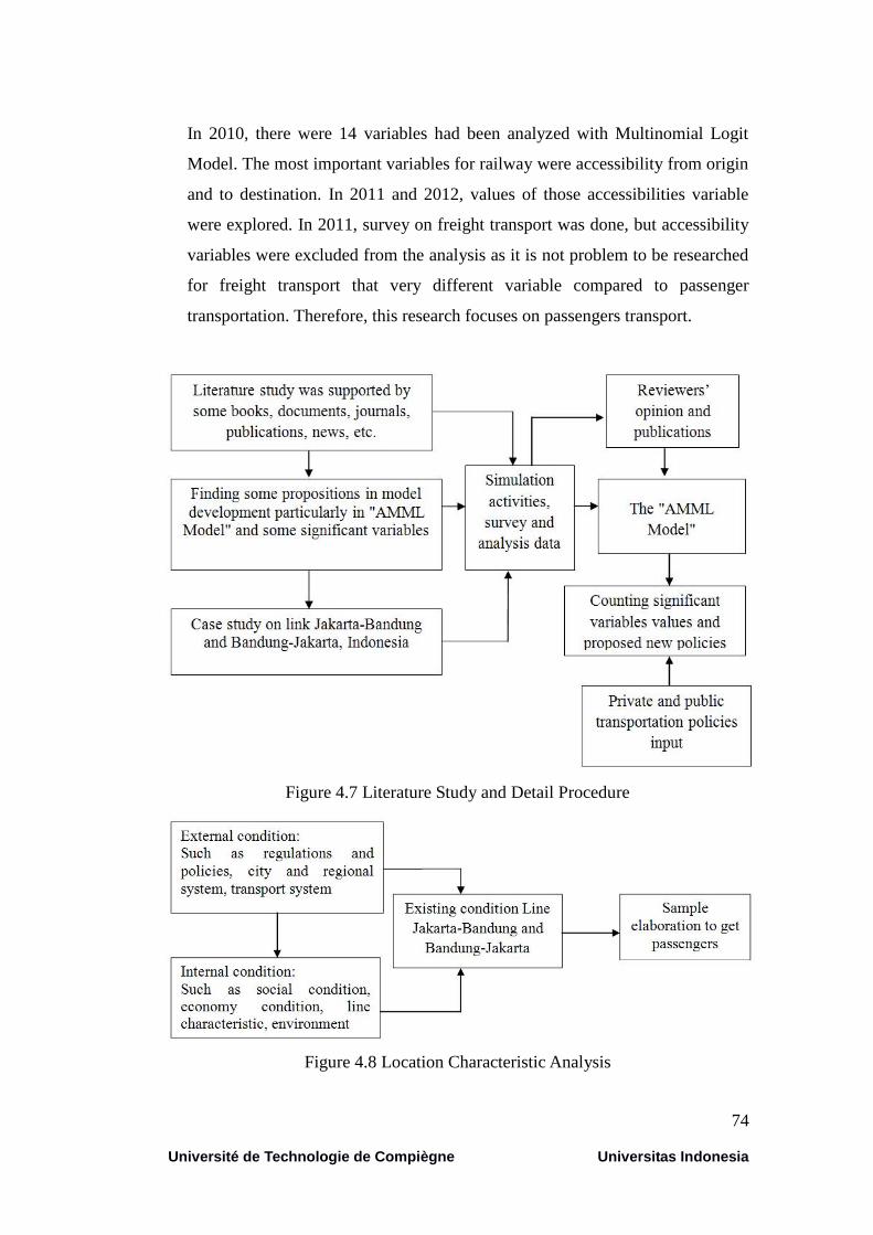
74
Université de Technologie de Compiègne Universitas Indonesia
In 2010, there were 14 variables had been analyzed with Multinomial Logit
Model. The most important variables for railway were accessibility from origin
and to destination. In 2011 and 2012, values of those accessibilities variable
were explored. In 2011, survey on freight transport was done, but accessibility
variables were excluded from the analysis as it is not problem to be researched
for freight transport that very different variable compared to passenger
transportation. Therefore, this research focuses on passengers transport.
Figure 4.7 Literature Study and Detail Procedure
Figure 4.8 Location Characteristic Analysis
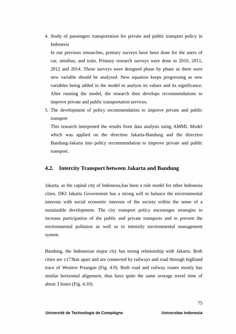
75
Université de Technologie de Compiègne Universitas Indonesia
4. Study of passengers transportation for private and public transport policy in
Indonesia
In our previous researches, primary surveys have been done for the users of
car, minibus, and train. Primary research surveys were done in 2010, 2011,
2012 and 2014. Those surveys were designed phase by phase as there were
new variable should be analyzed. New equation keeps progressing as new
variables being added in the model to analyze its values and its significance.
After running the model, the research then develops recommendations to
improve private and public transportation services.
5. The development of policy recommendation to improve private and public
transport
This research interpreted the results from data analysis using AMML Model
which was applied on the direction Jakarta-Bandung and the direction
Bandung-Jakarta into policy recommendation to improve private and public
transport.
4.2. Intercity Transport between Jakarta and Bandung
Jakarta, as the capital city of Indonesia,has been a role model for other Indonesia
cities. DKI Jakarta Government has a strong will to balance the environmental
interests with social economic interests of the society within the sense of a
sustainable development. The city transport policy encourages strategies to
increase participation of the public and private transports and to prevent the
environmental pollution as well as to intensify environmental management
system.
Bandung, the Indonesian major city has strong relationship with Jakarta. Both
cities are ±173km apart and are connected by railways and road through highland
trace of Western Priangan (Fig. 4.9). Both road and railway routes mostly has
similar horizontal alignment, thus have quite the same average travel time of
about 3 hours (Fig. 4.10).
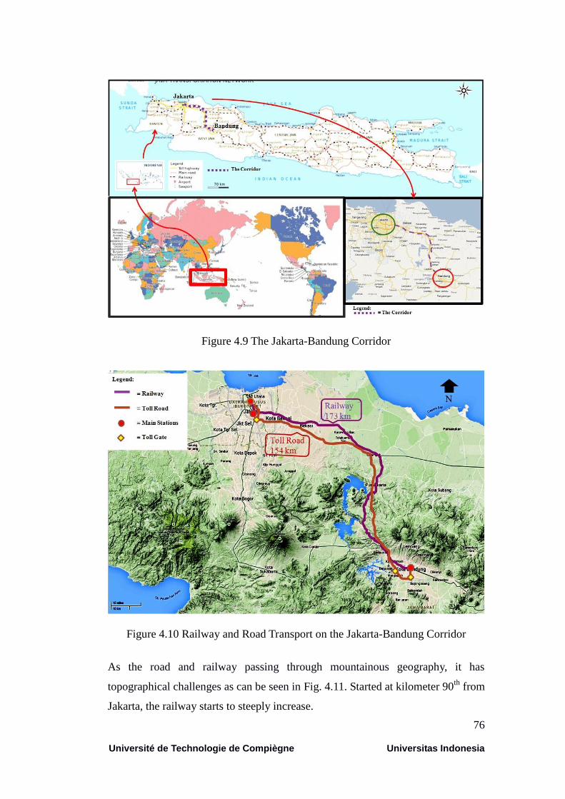
76
Université de Technologie de Compiègne Universitas Indonesia
Figure 4.9 The Jakarta-Bandung Corridor
Figure 4.10 Railway and Road Transport on the Jakarta-Bandung Corridor
As the road and railway passing through mountainous geography, it has
topographical challenges as can be seen in Fig. 4.11. Started at kilometer 90th
from
Jakarta, the railway starts to steeply increase.

77
Université de Technologie de Compiègne Universitas Indonesia
Source: Dirjen Perkeretaapian
Figure 4.11 Profile of Line Jakarta-Bandung
Before 2010, the railway service cannot keep up with significant increasing
transport demand. On Java Island the train share is decreasing by -0.9 % per year
(Van der Ven, 2010). The situation for railway is very ironic, because its services
are decaying due to decreasing demands. Statistic data of Jakarta and Bandung
from 2000 to 2014 (BPS, 2014,) shows steady increase of population (Fig. 12). At
27 April 2010, after 39 years in serving PT. KAI discontinue Parahyangan Batavia
train and only continue to operate Argo Gede Train, which was change to be Argo
Parahyangan.
Source: BPS DKI Jakarta dan BPS Kota Bandung, 2015
Figure 4.12 Number of Population in Jakarta and Bandung

78
Université de Technologie de Compiègne Universitas Indonesia
The Parahyangan Batavia train has been serving Jakarta-Bandung corridor since
May 16th
,1884. At that time, Jakarta-Bandung was a favorite line among the
Dutch. It was because the railway track has a very beautiful scenery and cool air.
In 1995, PT. Kereta Api Indonesia (Indonesian Railway Company) launched Argo
Gede Train,to complement the Parahyangan Train. A decade after the government
built the Cipularang toll road from Jakarta to Bandung, and immediately the
Parahyangan occupancy rate only 50%. PT. KAI’s effort to cut the tarif failed to
regain passenger and causing a 36 billion IDR loss one year.
Generally in Indonesia, there are many railway lines operating in negative
incomes and cannot cover infrastructure investment and rolling stock maintenance
raw materials. Particularly in Java where 30% of railway lines are abandoned with
critically condition. Therefore nowadays, there are many actions and policies are
planned to improve railway conditions.
4.3. The Economic Affordability Analysis of Intercity Transport
Modes
The existing Indonesian environmental laws and regulations show government
commitment on environment protection, quality service improvement, and
infrastructure investment in mass transportation system development. In regard to
environmental aspect, that every development of mass transport system should
pass environment impact. As for infrastructure investment, the Law No.22 of 2009
on traffic and road transport mandates that all major cities with over 500,000
populations should develop master plan to include mass transport system
infrastructure and travel management system. Those policies encourage the
development of railway services between two main cities, such as Jakarta and
Bandung.
To be financially sustainable, as a mass transportation, train should meet the
economic affordability of its potential riders. It is imperative to understand the
paying capacity (affordability) of people against the services. This research

79
Université de Technologie de Compiègne Universitas Indonesia
categorized such capacity into 4 income levels which are very low, low, medium,
and high income. They will spend their money to pay the cost of travel depending
to tariff classification and travel distance.
In Java, train service price is less competitive compare to other modes of land
transport, such as car, minibus and bus. This situation can be better described from
the losing demand of current train service. There are two cases to aforementioned
problem. First, is “Jakarta – Bandung” trip which is short distance intercity travel
with around 173km of distance. The train service is 200.000 IDR, the bus service
is 50.000 IDR, the car is 300.000 IDR, and the minibus is 200.000 IDR (Jakarta-
Bandung price of transports by mode, 2015). Second is “Jakarta – Surabaya” trip,
which is long distance intercity travel with 1000 km of distance. The train service
is IDR 1.200.000, the bus service is IDR 50.000, the car is IDR 2.662.200 and the
minibus service is IDR 1.200.000 ("Jakarta-Surabaya" price of transports by
mode, 2012). It was considered the prices of round-trip travels particularly for
public transport it is in “Economic class” by different modes. From both case, bus
has the lowest price over other modes. The average economic group of people
accessing train service as their daily transportation is difficult (Table 4.1).
Table 4.1 Weight of the Transport Budget for Railway Travellers in Java
Economic Active Population 2011 Units Income class
Total = 171,206,108 hab High Medium Low Very Low
Percentage of the Economic active population >
15 years old [%] 20 40 28,87 11,13
Population by class of income x 1000 [hab] 34241 68482 49427 19055
Average Salarie/month [IDR] 6635000 4578000 2504000 800000
Tarifs for round trip at 200km. (1) Executive class
(2)Business classe (3),(4) Economic[IDR] 212130 121468 111696 111696
Transport budget/month in considering quotidian rail
displacements for round trip between cities separated
by 200 km (20 travels)
[IDR] 4242600 2429360 2233920 2233920
Weight of transport budget into the individual income
per month [%] 1060650 303670 386893 1003558
Weight of transport budget into the individual income
per month [%] 64 53 89 279
Sources: Barus et al., 2012

80
Université de Technologie de Compiègne Universitas Indonesia
Currently, the price of train services in Java is perceived as very high for general
population and particularly for the “income class” of travelers. Despite of prices
segmentation in train service, it is still difficult for "Low" and “Very low” income
to access train service. This condition means that train cannot be used as a daily
mode choice by those people. The use of trains is to serve less than daily travel
trip.
As a comparison, this research try to analyze what happen in France. It was
different from the use of railway in France. It could serve daily travel trip. The
economic accessibility of the traveler is good enough (Table 4.2), if the threshold
of the "weight of transport budget" = 1/3 of income is respected. Prices of train
service in France effectively allow most of population to access it.
Sources: Barus et al., 2012
For the daily travels between cities, with the distance around 173 km, the railway
is not "competitive" with car, minibus and bus. And even for the long distance
travels in Java the train is “little competitive". It was known that train in current
situation cannot be used as a daily mode for traveling. It also cannot compare to
the bus service. It might be bus as the mode which can be as the daily mode for
travelling. In conclusion, bus as a mode which can be functioned as a mass
transport more than train. Then if this research will continue to research the
competition, it should exclude bus as mode in comparison. Train cannot compete
Economic Active Population 2011 Units Income class
Total = 28,390,000 hab High Medium Low Very Low
Percentage of the Economic active population >
18 years old [%] 20 50 30 30
Population by class of income x 1000 [hab] 5678 14195 8517 8517
Average Salarie/month [€] 5085 1937 1271 1000
Tarifs for round trip at 200km. (1) First class
(2)Second classe (3) Students & Low income
workers
[€] 50 33 18 18
Transport budget/month in considering quotidian rail
displacements for round trip between cities separated
by 200 km (20 travels)
[€] 1000 660 360 360
Weight of transport budget into the individual income
per month [%] 20 34 28 36
Table 4.2 Weight of the Transport Budget for Train Travellers in France

81
Université de Technologie de Compiègne Universitas Indonesia
to bus, beside it has different segment market and also different characteristic
where bus has not fixed stop. Train could compete with minibus, and private car
on the Jakarta-Bandung corridor.
4.4. Evolution of Ideas about the Modal Competition
In exploring intercity transportation on the Jakarta-Bandung corridor, the research
did a field survey. Data collection is started by collecting secondary data, such as
reports, books, maps, articles, papers, and studies by PT. KAI, ministry of
transportation, cities' survey and some train projects. These data were very useful,
however primary data are still needed to be collected (Fig.4.14). Therefore, this
research took primary data from survey questionnaires and visual observations.
Questionnaire surveys were taken 4 times, in 2010, 2011, 2012 and 2014. Each
year, questionnaires were distributed with respect to the survey and data collection
methodology. The survey was designed in sequential basis in which the preceding
survey will provide basis for the following survey for refinement and
sophistication. The first survey was designed with certain problem definition and
the results analysis becomes an input to the second survey. The second survey
0
50
100
150
200
250
300
High Medium Low Very LowWeig
ht o
f tr
an
sp
ort
bu
dg
et
into
th
e m
on
thly
in
co
me
[%]
People Income Level
Comparison of prices structure of rail transport
KERETA API
SNCF
“Threshold” of
Transport
Budget Weight
= 1/3 of income
Figure 4.13 Price Structure of Railway Comparison between PT. KAI and SNCF
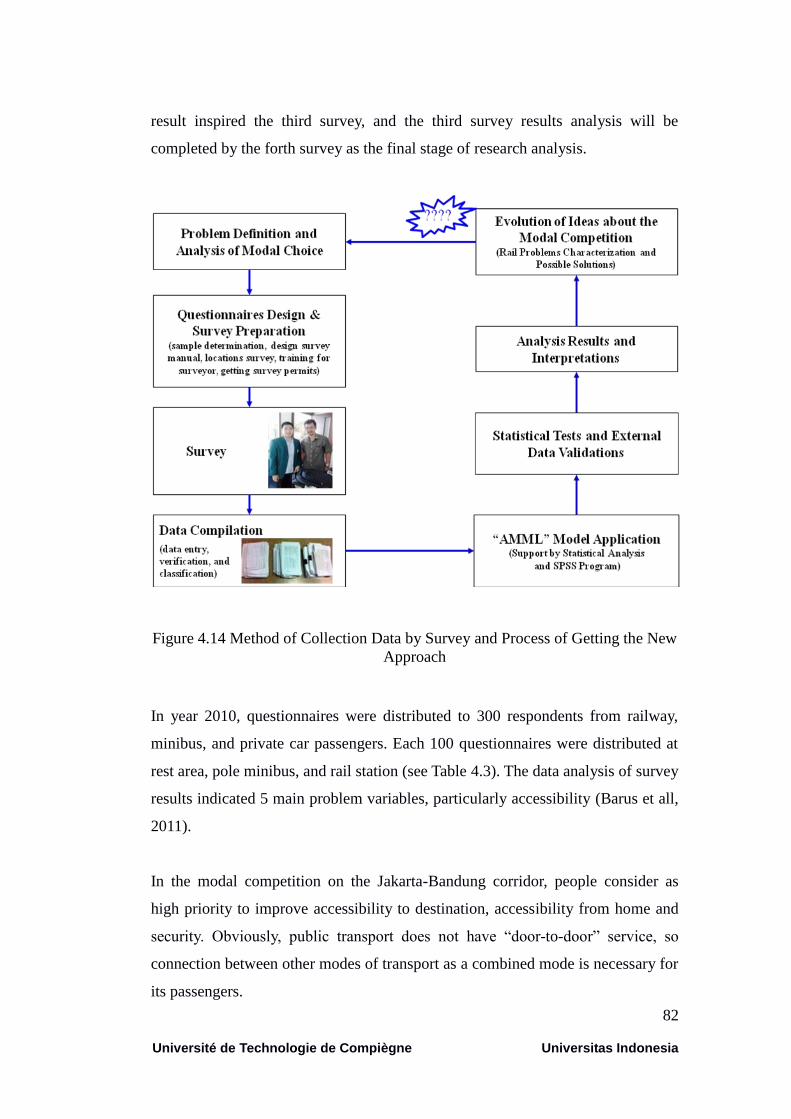
82
Université de Technologie de Compiègne Universitas Indonesia
result inspired the third survey, and the third survey results analysis will be
completed by the forth survey as the final stage of research analysis.
Figure 4.14 Method of Collection Data by Survey and Process of Getting the New
Approach
In year 2010, questionnaires were distributed to 300 respondents from railway,
minibus, and private car passengers. Each 100 questionnaires were distributed at
rest area, pole minibus, and rail station (see Table 4.3). The data analysis of survey
results indicated 5 main problem variables, particularly accessibility (Barus et all,
2011).
In the modal competition on the Jakarta-Bandung corridor, people consider as
high priority to improve accessibility to destination, accessibility from home and
security. Obviously, public transport does not have “door-to-door” service, so
connection between other modes of transport as a combined mode is necessary for
its passengers.

83
Université de Technologie de Compiègne Universitas Indonesia
Table 4.3 Data Collection through 4 Types Questionnaires
In particular to analysis for railway competitiveness over the other modes,
variable of accessibility to destination is more important than accessibility from
home because people are generally familiar with their immediate surroundings
and transportation option proximity to their home. It would be difficult to take any
risk if they didn’t know the environment around their destination. Thus, if
accessibility to the rail station is not adequate and involve some uncertainty in
transferring from one transport mode to another, people will not feel safe to travel
to their desire location.
In year 2011, the research distributed 180 questionnaires to capture 3 opinions of
train, minibus and private car passengers. It took place in rest area, pole minibus,
and rail station along Jakarta-Bandung corridor. There were also 93 questionnaires
with 186 of freight forwarders/shippers preferences in transporting their freight
from Jakarta to Surabaya. The survey showed different problem between
passengers and freight. The accessibility is the main problem of passenger
transportation but not for the freight. Therefore, this research focuses on
passengers transport. However on passenger’s preference survey, it was found that
there were not any additional significant variables.

84
Université de Technologie de Compiègne Universitas Indonesia
In year 2012, the same type of survey in 2011 was done to add additional data, but
the results were the same, and then the proposed model was changed. The idea
turned to use the “AMML Model”. The accessibility from home variable was
changed to be intracity variables at origin and accessibility to destination variable
was changed to be intracity variables at destination.
Table 4.4 Modal Choice Variables
4.5. Analysis Data on the Corridor Jakarta-Bandung
This research applied “the AMML Model” with questionnaires distribution on
year 2014 in the case study of Jakarta-Bandung corridor (Annex). Passengers’
background from the samples showed that there are some different conditions
between the direction Jakarta-Bandung and the direction Bandung-Jakarta.

85
Université de Technologie de Compiègne Universitas Indonesia
4.5.1 Respondents’ Profile on Direction Jakarta-Bandung
A. Respondents’ Origin and Destination on the Jakarta-Bandung
Direction
The biggest percentage of railway passengers’ from Jakarta origin is from the
Central Jakarta (28.13%), while the lowest percentage is from Western Jakarta
(15.63%). The destination area at Bandung, the most favorable is the centre
(39.58%) and the lowest is to go to the west (10.42%).
For minibus passengers’ distribution, they were mostly also from Central Jakarta
(62.50%), while the lowest were from Northern Jakarta (2.08%). As for the
destination area in Bandung, they preferred Northern Bandung (42.71%) and least
preferred Southern Bandung (7.2%).
Figure 4.15 Jakarta Zones as Origin for Train, Minibus and Car Passengers
The study results for car’s passengers have different distribution of origin from
railway’s and minibus’s passengers’. Southern Jakarta is the highest origin of car
passengers (31.25%) while Northern Jakarta is the least origin (4.17%) which
similar to train's and minibus's passengers. As for the destination area of car’s
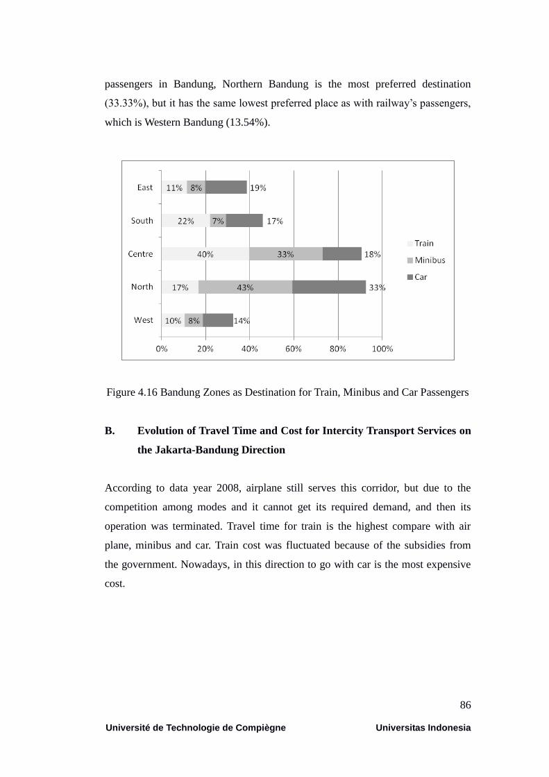
86
Université de Technologie de Compiègne Universitas Indonesia
passengers in Bandung, Northern Bandung is the most preferred destination
(33.33%), but it has the same lowest preferred place as with railway’s passengers,
which is Western Bandung (13.54%).
Figure 4.16 Bandung Zones as Destination for Train, Minibus and Car Passengers
B. Evolution of Travel Time and Cost for Intercity Transport Services on
the Jakarta-Bandung Direction
According to data year 2008, airplane still serves this corridor, but due to the
competition among modes and it cannot get its required demand, and then its
operation was terminated. Travel time for train is the highest compare with air
plane, minibus and car. Train cost was fluctuated because of the subsidies from
the government. Nowadays, in this direction to go with car is the most expensive
cost.
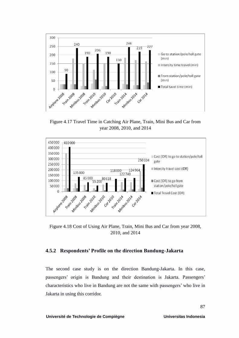
87
Université de Technologie de Compiègne Universitas Indonesia
Figure 4.17 Travel Time in Catching Air Plane, Train, Mini Bus and Car from
year 2008, 2010, and 2014
Figure 4.18 Cost of Using Air Plane, Train, Mini Bus and Car from year 2008,
2010, and 2014
4.5.2 Respondents’ Profile on the direction Bandung-Jakarta
The second case study is on the direction Bandung-Jakarta. In this case,
passengers’ origin is Bandung and their destination is Jakarta. Passengers’
characteristics who live in Bandung are not the same with passengers’ who live in
Jakarta in using this corridor.
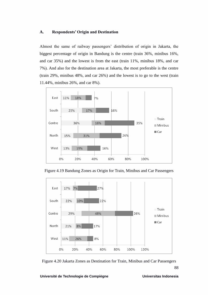
88
Université de Technologie de Compiègne Universitas Indonesia
A. Respondents’ Origin and Destination
Almost the same of railway passengers’ distribution of origin in Jakarta, the
biggest percentage of origin in Bandung is the centre (train 36%, minibus 16%,
and car 35%) and the lowest is from the east (train 11%, minibus 18%, and car
7%). And also for the destination area at Jakarta, the most preferable is the centre
(train 29%, minibus 48%, and car 26%) and the lowest is to go to the west (train
11.44%, minibus 26%, and car 8%).
Figure 4.19 Bandung Zones as Origin for Train, Minibus and Car Passengers
Figure 4.20 Jakarta Zones as Destination for Train, Minibus and Car Passengers
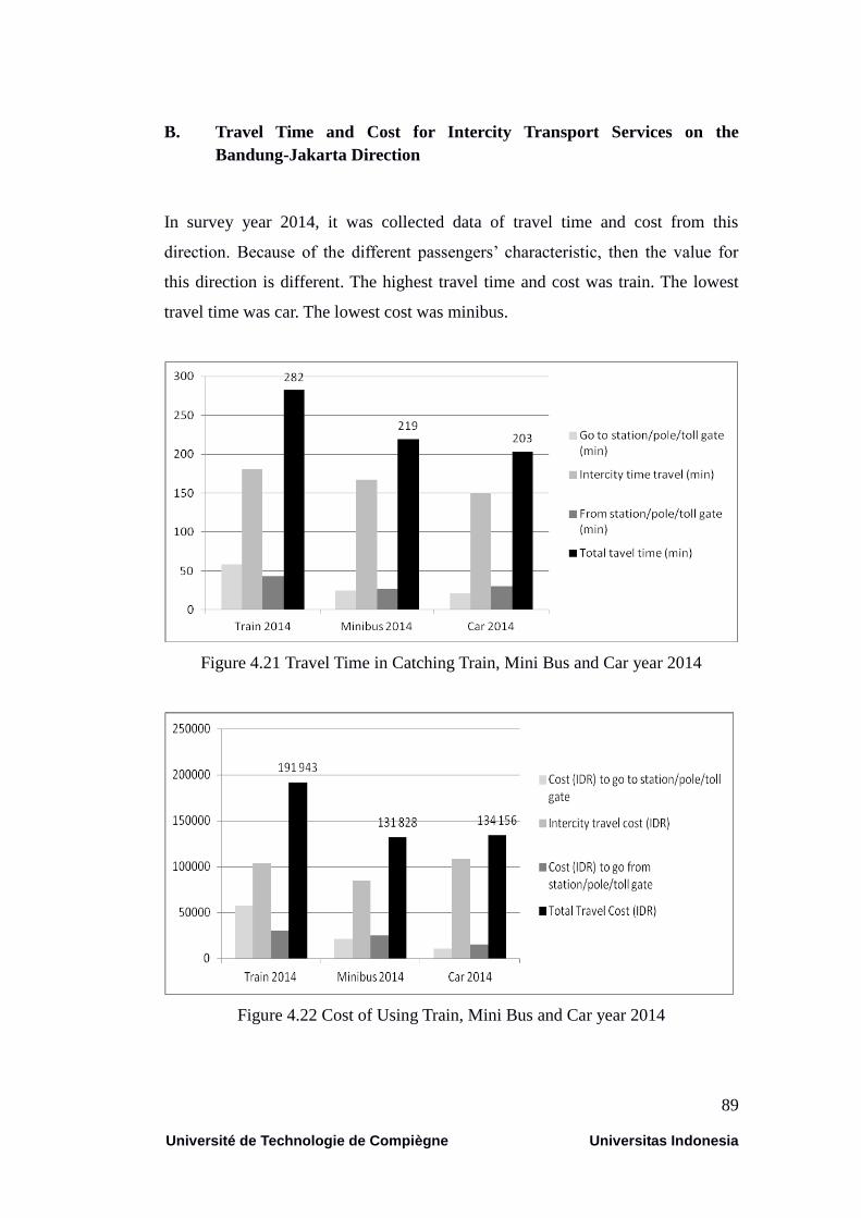
89
Université de Technologie de Compiègne Universitas Indonesia
B. Travel Time and Cost for Intercity Transport Services on the
Bandung-Jakarta Direction
In survey year 2014, it was collected data of travel time and cost from this
direction. Because of the different passengers’ characteristic, then the value for
this direction is different. The highest travel time and cost was train. The lowest
travel time was car. The lowest cost was minibus.
Figure 4.21 Travel Time in Catching Train, Mini Bus and Car year 2014
Figure 4.22 Cost of Using Train, Mini Bus and Car year 2014

90
Université de Technologie de Compiègne Universitas Indonesia
4.6. Modal Competition of Corridor
4.6.1 Variables’ Coefficients Values in Utility Function
Utility value was used to measure the degree of satisfaction obtained by a
choosing one mode of intercity transport. This utility value depends on individual
factors of each type of transport service. In this research, a representative
passenger was assumed for all traveler purposes (business/worker, student, doing
personal or familial matter and leisure) to choose the intercity mode to travel
yielding the highest utility. Utility function is usually expressed as a linear number
of independent variables affected by β factors. This approach assumes that the
socio-economic factors greatly affect the modal choice process. There are three
important utility functions to observe:
1. Utility Function of intracity transport at departure city
2. Utility Function of intracity transport at arrival city
3. Utility Function of intercity modes
Independent variables or “choice factors” that we observed for intracity transport
at departure city were total transport time from home to modal node 1 (VIO1),
cost from home to modal node 1 (VIO2), safety condition from home to modal
node 1 (VIO3), information available from home to modal node 1 (VIO4),
connection condition from home to modal node 1 (VIO5). For intracity transport
at arrival city, we observed total transport time from modal node 2 to arrival city
(VID1), cost from modal node 2 to arrival city (VID2), safety condition from
modal node 2 to arrival city (VID3), information available from modal node 2 to
arrival city (VID4), connection condition from modal node 2 to arrival city
(VID5). Considerations of intercity modes service variables were total transport
time from modal node 1 to modal node 2 (VM1), cost from modal node 1 to
modal node 2 (VM2), safety condition from modal node 1 to modal node 2
(VM3), information available from modal node 1 to modal node 2 (VM4), The
results show the utility of improvements for each factor of the intercity modes on

91
Université de Technologie de Compiègne Universitas Indonesia
the direction Jakarta-Bandung to gain in competitiveness according to passengers
preferences.
Each individual respondent will make decision base on several types of options.
This research will identify the most influential variable in any decision made. This
approach could also provide an overview of the variables which is relatively
important to the socio-economic characteristics that in turn can influence policy
making process. Discrete choice questionnaire will be translated into ordinal and
nominal data with the size of Likert scale. The ordinal measurement was used by
asking respondent to fill by making cross (x) in one of the choices in the
questionnaires. The associated with variables scaling from 1 to 4 (ordinal data)
that reflect Likert scale as the following conditions:
1 = not good
2 = less good
3 = good
4 = very good
The comparative reference value is 0, it represents the “private car” mode
preferences. When factors are positive for “minibus” or “train”, it means that
users have current preferences for “car”. Positive coefficients for “minibus” and
“train” mean that the correspondent variables are the most important factors to
improve their own competitiveness. When factors are negative for “minibus” or
“train”, it means that users have current preferences them over the factors of
“car”. So, negative coefficients for “minibus” and “train” mean that the
correspondent factors do not need to be improved, they represent their current
strengths.
A. Direction Jakarta-Bandung
The application of "AMML" model based on our distribution value sample (Ben
Ben-Akiva, 1985) on the Jakarta-Bandung corridor let us to obtain the utility
values of modes in competition. The analysis of these functions and their
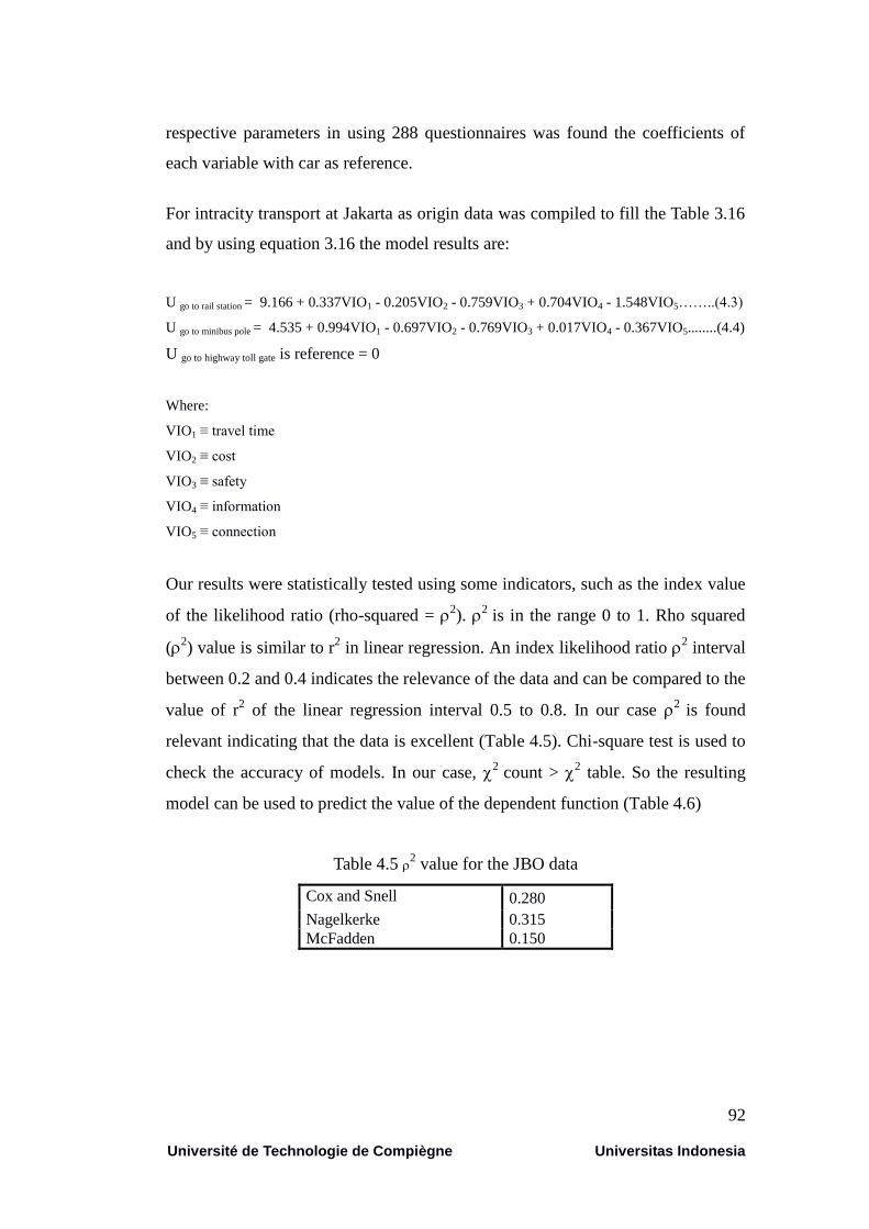
92
Université de Technologie de Compiègne Universitas Indonesia
respective parameters in using 288 questionnaires was found the coefficients of
each variable with car as reference.
For intracity transport at Jakarta as origin data was compiled to fill the Table 3.16
and by using equation 3.16 the model results are:
U go to rail station = 9.166 + 0.337VIO1 - 0.205VIO2 - 0.759VIO3 + 0.704VIO4 - 1.548VIO5……..(4.3)
U go to minibus pole = 4.535 + 0.994VIO1 - 0.697VIO2 - 0.769VIO3 + 0.017VIO4 - 0.367VIO5........(4.4)
U go to highway toll gate is reference = 0
Where:
VIO1 ≡ travel time
VIO2 ≡ cost
VIO3 ≡ safety
VIO4 ≡ information
VIO5 ≡ connection
Our results were statistically tested using some indicators, such as the index value
of the likelihood ratio (rho-squared = 2).
2 is in the range 0 to 1. Rho squared
(2) value is similar to r
2 in linear regression. An index likelihood ratio
2 interval
between 0.2 and 0.4 indicates the relevance of the data and can be compared to the
value of r2 of the linear regression interval 0.5 to 0.8. In our case
2 is found
relevant indicating that the data is excellent (Table 4.5). Chi-square test is used to
check the accuracy of models. In our case, 2
count > 2 table. So the resulting
model can be used to predict the value of the dependent function (Table 4.6)
Table 4.5 2 value for the JBO data
Cox and Snell 0.280
Nagelkerke 0.315
McFadden 0.150
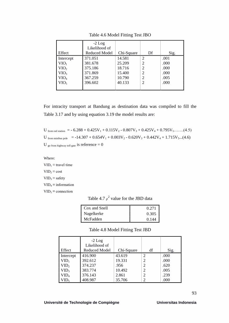
93
Université de Technologie de Compiègne Universitas Indonesia
Table 4.6 Model Fitting Test JBO
Effect
-2 Log
Likelihood of
Reduced Model Chi-Square Df Sig.
Intercept 371.051 14.581 2 .001
VIO1 381.678 25.209 2 .000
VIO2 375.186 18.716 2 .000
VIO3 371.869 15.400 2 .000
VIO4 367.259 10.790 2 .005
VIO5 396.602 40.133 2 .000
For intracity transport at Bandung as destination data was compiled to fill the
Table 3.17 and by using equation 3.19 the model results are:
U from rail station = - 6.288 + 0.425V1 + 0.115V2 - 0.807V3 + 0.425V4 + 0.795V5…….(4.5)
U from minibus pole = -14.307 + 0.654V1 + 0.003V2 - 0.620V3 + 0.442V4 + 1.715V5...(4.6)
U go from highway toll gate is reference = 0
Where:
VID1 ≡ travel time
VID2 ≡ cost
VID3 ≡ safety
VID4 ≡ information
VID5 ≡ connection
Table 4.7 2 value for the JBD data
Cox and Snell 0.271
Nagelkerke 0.305
McFadden 0.144
Table 4.8 Model Fitting Test JBD
Effect
-2 Log
Likelihood of
Reduced Model Chi-Square df Sig.
Intercept 416.900 43.619 2 .000
VID1 392.612 19.331 2 .000
VID2 374.237 .956 2 .620
VID3 383.774 10.492 2 .005
VID4 376.143 2.861 2 .239
VID5 408.987 35.706 2 .000
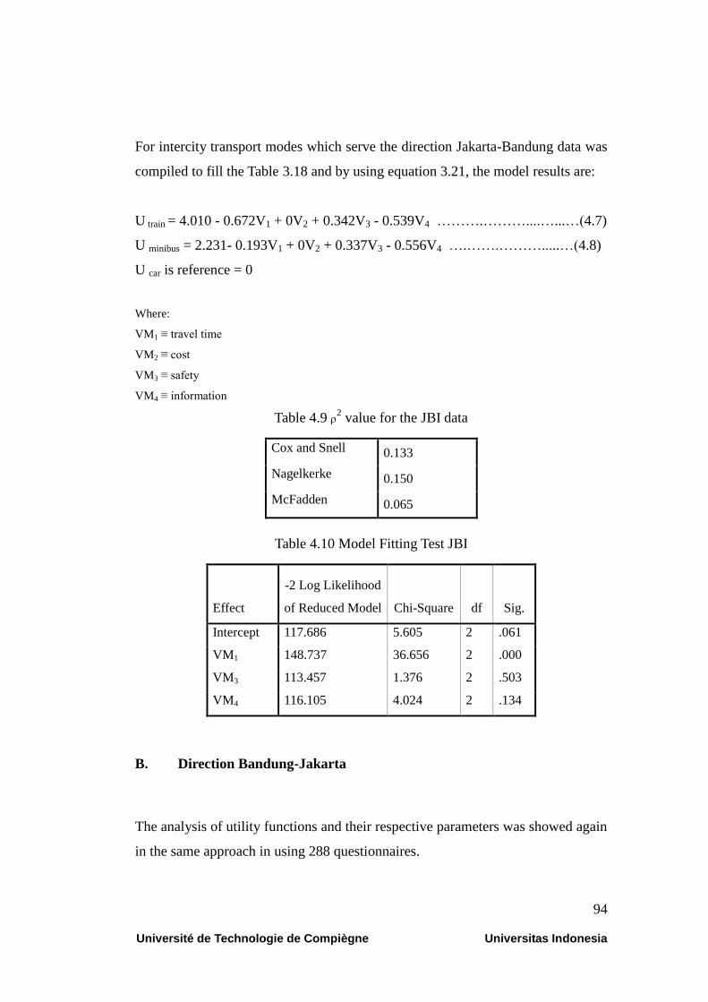
94
Université de Technologie de Compiègne Universitas Indonesia
For intercity transport modes which serve the direction Jakarta-Bandung data was
compiled to fill the Table 3.18 and by using equation 3.21, the model results are:
U train = 4.010 - 0.672V1 + 0V2 + 0.342V3 - 0.539V4 ……….………....…...…(4.7)
U minibus = 2.231- 0.193V1 + 0V2 + 0.337V3 - 0.556V4 ….…….……….....…(4.8)
U car is reference = 0
Where:
VM1 ≡ travel time
VM2 ≡ cost
VM3 ≡ safety
VM4 ≡ information
Table 4.9 2 value for the JBI data
Cox and Snell 0.133
Nagelkerke 0.150
McFadden 0.065
Table 4.10 Model Fitting Test JBI
Effect
-2 Log Likelihood
of Reduced Model Chi-Square df Sig.
Intercept 117.686 5.605 2 .061
VM1 148.737 36.656 2 .000
VM3 113.457 1.376 2 .503
VM4 116.105 4.024 2 .134
B. Direction Bandung-Jakarta
The analysis of utility functions and their respective parameters was showed again
in the same approach in using 288 questionnaires.
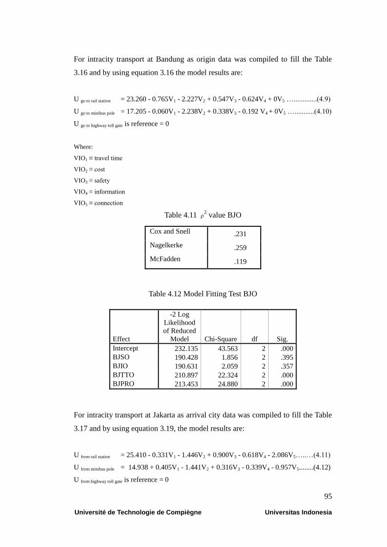
95
Université de Technologie de Compiègne Universitas Indonesia
For intracity transport at Bandung as origin data was compiled to fill the Table
3.16 and by using equation 3.16 the model results are:
U go to rail station = 23.260 - 0.765V1 - 2.227V2 + 0.547V3 - 0.624V4 + 0V5 ….............(4.9)
U go to minibus pole = 17.205 - 0.060V1 - 2.238V2 + 0.338V3 - 0.192 V4 + 0V5 …...........(4.10)
U go to highway toll gate is reference = 0
Where:
VIO1 ≡ travel time
VIO2 ≡ cost
VIO3 ≡ safety
VIO4 ≡ information
VIO5 ≡ connection
Table 4.11 2 value BJO
Cox and Snell .231
Nagelkerke .259
McFadden .119
Table 4.12 Model Fitting Test BJO
Effect
-2 Log
Likelihood
of Reduced
Model Chi-Square df Sig.
Intercept 232.135 43.563 2 .000
BJSO 190.428 1.856 2 .395
BJIO 190.631 2.059 2 .357
BJTTO 210.897 22.324 2 .000
BJPRO 213.453 24.880 2 .000
For intracity transport at Jakarta as arrival city data was compiled to fill the Table
3.17 and by using equation 3.19, the model results are:
U from rail station = 25.410 - 0.331V1 - 1.446V2 + 0.900V3 - 0.618V4 - 2.086V5…..…(4.11)
U from minibus pole = 14.938 + 0.405V1 - 1.441V2 + 0.316V3 - 0.339V4 - 0.957V5........(4.12)
U from highway toll gate is reference = 0
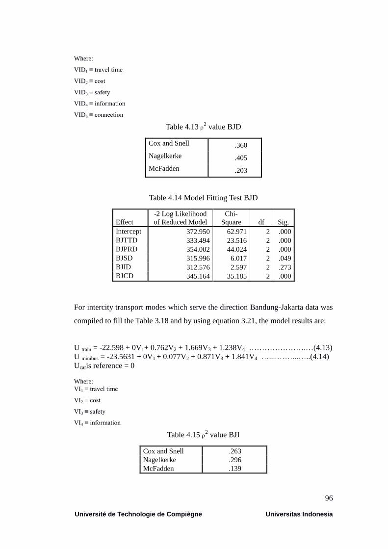
96
Université de Technologie de Compiègne Universitas Indonesia
Where:
VID1 ≡ travel time
VID2 ≡ cost
VID3 ≡ safety
VID4 ≡ information
VID5 ≡ connection
Table 4.13 2 value BJD
Cox and Snell .360
Nagelkerke .405
McFadden .203
Table 4.14 Model Fitting Test BJD
Effect
-2 Log Likelihood
of Reduced Model
Chi-
Square df Sig.
Intercept 372.950 62.971 2 .000
BJTTD 333.494 23.516 2 .000
BJPRD 354.002 44.024 2 .000
BJSD 315.996 6.017 2 .049
BJID 312.576 2.597 2 .273
BJCD 345.164 35.185 2 .000
For intercity transport modes which serve the direction Bandung-Jakarta data was
compiled to fill the Table 3.18 and by using equation 3.21, the model results are:
U train = -22.598 + 0V1+ 0.762V2 + 1.669V3 + 1.238V4 ………………….…(4.13)
U minibus = -23.5631 + 0V1 + 0.077V2 + 0.871V3 + 1.841V4 …....……...…..(4.14)
Ucaris reference = 0
Where:
VI1 ≡ travel time
VI2 ≡ cost
VI3 ≡ safety
VI4 ≡ information
Table 4.15 2 value BJI
Cox and Snell .263
Nagelkerke .296
McFadden .139
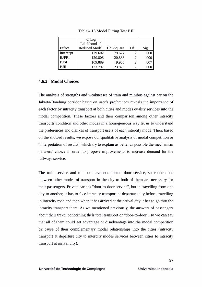
97
Université de Technologie de Compiègne Universitas Indonesia
Table 4.16 Model Fitting Test BJI
Effect
-2 Log
Likelihood of
Reduced Model Chi-Square Df Sig.
Intercept 179.602 79.677 2 .000
BJPRI 120.808 20.883 2 .000
BJSI 109.889 9.965 2 .007
BJII 123.797 23.873 2 .000
4.6.2 Modal Choices
The analysis of strengths and weaknesses of train and minibus against car on the
Jakarta-Bandung corridor based on user’s preferences reveals the importance of
each factor by intracity transport at both cities and modes quality services into the
modal competition. These factors and their comparison among other intracity
transports condition and other modes in a homogeneous way let us to understand
the preferences and dislikes of transport users of each intercity mode. Then, based
on the showed results, we expose our qualitative analysis of modal competition or
“interpretation of results” which try to explain as better as possible the mechanism
of users’ choice in order to propose improvements to increase demand for the
railways service.
The train service and minibus have not door-to-door service, so connections
between other modes of transport in the city to both of them are necessary for
their passengers. Private car has "door-to-door service", but in travelling from one
city to another, it has to face intracity transport at departure city before travelling
in intercity road and then when it has arrived at the arrival city it has to go thru the
intracity transport there. As we mentioned previously, the answers of passengers
about their travel concerning their total transport or “door-to-door”, so we can say
that all of them could get advantage or disadvantage into the modal competition
by cause of their complementary modal relationships into the cities (intracity
transport at departure city to intercity modes services between cities to intracity
transport at arrival city).
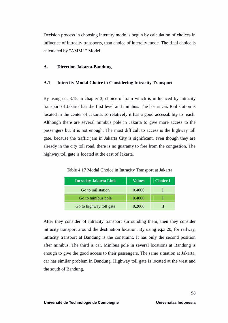
98
Université de Technologie de Compiègne Universitas Indonesia
Decision process in choosing intercity mode is begun by calculation of choices in
influence of intracity transports, than choice of intercity mode. The final choice is
calculated by "AMML" Model.
A. Direction Jakarta-Bandung
A.1 Intercity Modal Choice in Considering Intracity Transport
By using eq. 3.18 in chapter 3, choice of train which is influenced by intracity
transport of Jakarta has the first level and minibus. The last is car. Rail station is
located in the center of Jakarta, so relatively it has a good accessibility to reach.
Although there are several minibus pole in Jakarta to give more access to the
passengers but it is not enough. The most difficult to access is the highway toll
gate, because the traffic jam in Jakarta City is significant, even though they are
already in the city toll road, there is no guaranty to free from the congestion. The
highway toll gate is located at the east of Jakarta.
Table 4.17 Modal Choice in Intracity Transport at Jakarta
Intracity Jakarta Link Values Choice I
Go to rail station 0.4000 I
Go to minibus pole 0.4000 I
Go to highway toll gate 0,2000 II
After they consider of intracity transport surrounding them, then they consider
intracity transport around the destination location. By using eq.3.20, for railway,
intracity transport at Bandung is the constraint. It has only the second position
after minibus. The third is car. Minibus pole in several locations at Bandung is
enough to give the good access to their passengers. The same situation at Jakarta,
car has similar problem in Bandung. Highway toll gate is located at the west and
the south of Bandung.

99
Université de Technologie de Compiègne Universitas Indonesia
Table 4.18 Modal Choice in Intracity Transport at Bandung
Intracity Bandung Link Values Choice II
From rail station 0.3100 II
From minibus pole 0.5000 I
From highway toll gate 0.1900 III
By using eq. 3.22, services that have been given by train are good enough. It
already reaches the first level than other modes. The second is minibus, the third
is car. It means, even though there are several quality variables have to improve
for train, but in modal competition, it cannot reach the best services.
Table 4.19 Modal Choice in Intercity Link
Intercity link Values Choice III
Train 0.4200 I
Minibus 0.3000 II
Car 0.2800 III
In reality condition at total passenger transport chain, the offered services of each
mode are not enough, because train is not the first choice as intercity transport
mode. We use "AMML" Model to prove which one is the best in modal
competition on this link (eq. 3.31).
Table 4.20 Modal Choice in Total Passengers Transport Chain
Intercity Modal competition Values Choice Final
Train 0.4241 II
Minibus 0.4893 I
Car 0.0846 III
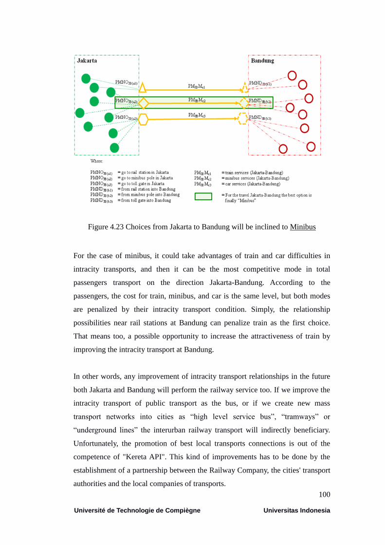
100
Université de Technologie de Compiègne Universitas Indonesia
Figure 4.23 Choices from Jakarta to Bandung will be inclined to Minibus
For the case of minibus, it could take advantages of train and car difficulties in
intracity transports, and then it can be the most competitive mode in total
passengers transport on the direction Jakarta-Bandung. According to the
passengers, the cost for train, minibus, and car is the same level, but both modes
are penalized by their intracity transport condition. Simply, the relationship
possibilities near rail stations at Bandung can penalize train as the first choice.
That means too, a possible opportunity to increase the attractiveness of train by
improving the intracity transport at Bandung.
In other words, any improvement of intracity transport relationships in the future
both Jakarta and Bandung will perform the railway service too. If we improve the
intracity transport of public transport as the bus, or if we create new mass
transport networks into cities as “high level service bus”, “tramways” or
“underground lines” the interurban railway transport will indirectly beneficiary.
Unfortunately, the promotion of best local transports connections is out of the
competence of "Kereta API". This kind of improvements has to be done by the
establishment of a partnership between the Railway Company, the cities' transport
authorities and the local companies of transports.

101
Université de Technologie de Compiègne Universitas Indonesia
For the internal solutions, the budget of investment may be the first constraint.
But in any case the suggested improvements do not represent important amounts
in comparison with the damages that a continuity of loss of demand may provoke.
The next step is the evaluation of “improvements safety condition”. It could
realize by supporting all kind of facilities that passengers can feel save in
travelling with. At least it is the less expensive improvements in the short term.
A.2 Validation Results
By using split half method, a half of data was used (after verification there are 165
questionnaires) to validate the choice results with the equation 3.31. The
validation results showed that minibus is confirmed as the most competitive mode
over the others (Table 4.21). The differences between two survey results are not
significant (0-14%). This identification will permit to do formulate the most
pertinent recommendations in order to improve the quality of a transport mode
and make it advance into the modal competition.
The final result could be calculated with the other equation of the AMML Model
(eq. 3.48). The validation of the second calculation is confirmed again that
minibus has the highest opportunity (Table 4.22).
B. Direction Bandung-Jakarta
B.1 Intercity Modal Choice in Considering Intracity Transport
By using eq. 3.18, choice of railway is supported by intracity transport of
Bandung. It has the first level. The second is minibus and the third is car. Rail
station is located in the center of Bandung, so relatively it has a good accessibility
to reach. The most difficult to access is the highway toll gate, because the traffic
jam in Bandung City is significant, too. The highway toll gate is located at the
west and the south of Bandung.
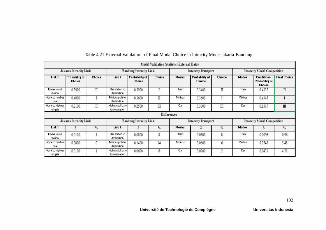
102
Université de Technologie de Compiègne Universitas Indonesia
Table 4.21 External Validation o f Final Modal Choice in Intracity Mode Jakarta-Bandung
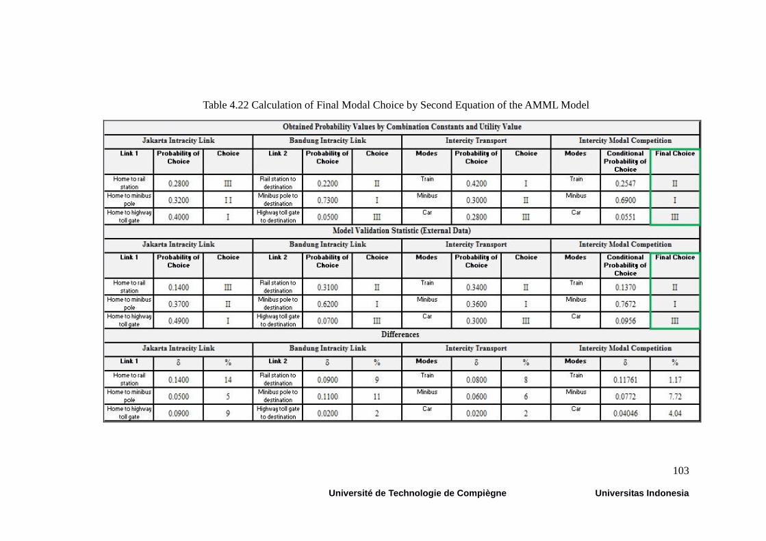
103
Université de Technologie de Compiègne Universitas Indonesia
Table 4.22 Calculation of Final Modal Choice by Second Equation of the AMML Model

104
Université de Technologie de Compiègne Universitas Indonesia
Table 4.23 Modal Choice in Intracity Transport at Bandung
Intracity Bandung Values Choice I
Go to Rail station 0.6300 I
Go to Minibus Pole 0.2300 II
Go to Highway toll gate 0.1400 III
After they arrived at arrival city Jakarta, then they consider intracity transport in
the city. By using eq. 3.20, for railway, intracity transport at Jakarta is not the
constraint. It has the first position after minibus. The third is car. Minibus pole has
several locations at Jakarta but they are enough to give the good access to their
passengers when arrive there. The same situation at Bandung, car has similar
problem in Jakarta. Highway toll gate is not located at the center of the city.
Table 4.24 Modal Choice in Intracity Transport at Jakarta
Intracity Jakarta Values Choice II
From Rail station 0,6700 I
From Minibus Pole 0,2300 II
From Highway toll gate 0,1000 III
By using eq. 3.22, as a mode of intracity transport, in Bandung passengers’
opinion train is not good enough in comparing with other modes. It only reaches
the third level than other modes. The second is minibus, and the first is car. It
means, there are several quality variables of railway that has to improve in modal
competition. Even though railway is supported by its intracity transport condition,
but if it cannot give the good service by itself, it is not enough in total passenger
transport chain.
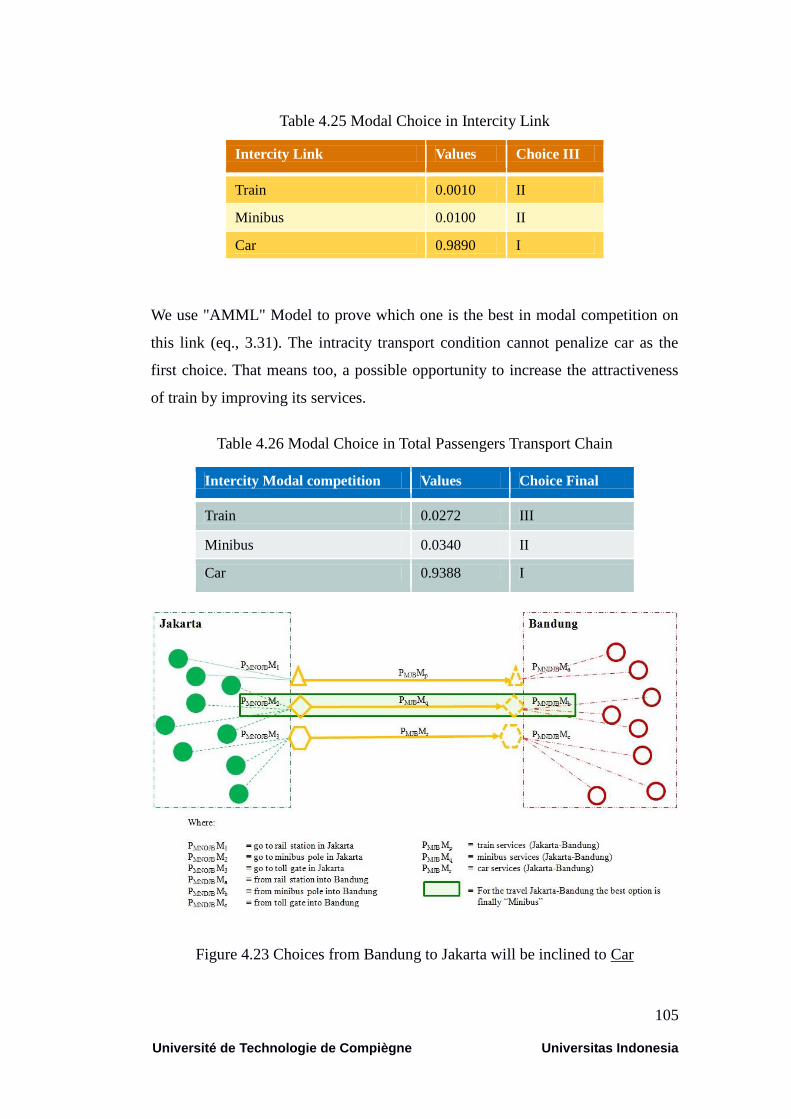
105
Université de Technologie de Compiègne Universitas Indonesia
Table 4.25 Modal Choice in Intercity Link
Intercity Link Values Choice III
Train 0.0010 II
Minibus 0.0100 II
Car 0.9890 I
We use "AMML" Model to prove which one is the best in modal competition on
this link (eq., 3.31). The intracity transport condition cannot penalize car as the
first choice. That means too, a possible opportunity to increase the attractiveness
of train by improving its services.
Table 4.26 Modal Choice in Total Passengers Transport Chain
Intercity Modal competition Values Choice Final
Train 0.0272 III
Minibus 0.0340 II
Car 0.9388 I
Figure 4.23 Choices from Bandung to Jakarta will be inclined to Car

106
Université de Technologie de Compiègne Universitas Indonesia
B2. Validation Results
With the same method of the direction Jakarta-Bandung (split half, after
verification there are 149 questionnaires), the results of the direction Bandung-
Jakarta were validated. The external data validation results showed that car is
confirmed as the most competitive mode over the others (Table 4.27). The
differences are in between 0-61.
The biggest difference is in the intracity transport mode choice at Bandung for
minibus and train. Then, the validation continues to double check with the other
equation of the AMML Model. The equation of the other AMML Model
formulation refers to the eq. 3.48. The validation of the second calculation is
confirmed again that car has the highest opportunity (Table 4.28).
4.7 Transportation Characteristics
Even though in the same corridor, but the favorable choice is different between
passengers who travel from Jakarta to Bandung and as return, from Bandung to
Jakarta. In these two directions, the results do not consider the first and the last
mile distance. The results describe the passengers’ journey with the nearest mode
to use from their home and at their final destination.
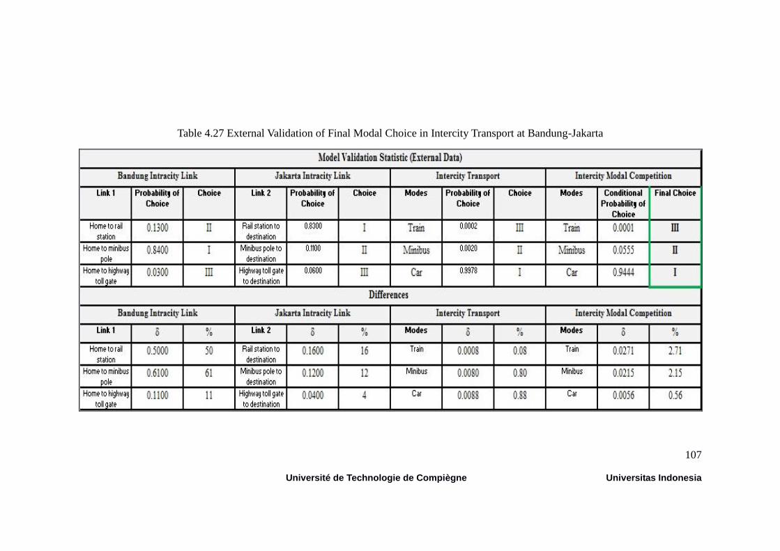
107
Université de Technologie de Compiègne Universitas Indonesia
Table 4.27 External Validation of Final Modal Choice in Intercity Transport at Bandung-Jakarta
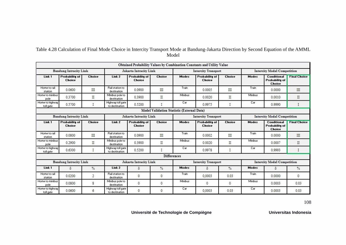
108
Université de Technologie de Compiègne Universitas Indonesia
Table 4.28 Calculation of Final Mode Choice in Intercity Transport Mode at Bandung-Jakarta Direction by Second Equation of the AMML
Model
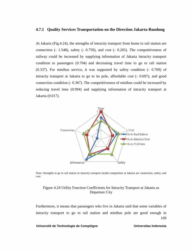
109
Université de Technologie de Compiègne Universitas Indonesia
4.7.1 Quality Services Transportation on the Direction Jakarta-Bandung
At Jakarta (Fig.4.24), the strengths of intracity transport from home to rail station are
connection (- 1.548), safety (- 0.759), and cost (- 0.205). The competitiveness of
railway could be increased by supplying information of Jakarta intracity transport
condition to passengers (0.704) and decreasing travel time to go to rail station
(0.337). For minibus service, it was supported by safety condition (- 0.769) of
intracity transport at Jakarta to go to its pole, affordable cost (- 0.697), and good
connection condition (- 0.367). The competitiveness of minibus could be increased by
reducing travel time (0.994) and supplying information of intracity transport at
Jakarta (0.017).
Note: Strengths to go to rail station in intracity transport modal competition at Jakarta are connection, safety, and
cost.
Figure 4.24 Utility Function Coefficients for Intracity Transport at Jakarta as
Departure City
Furthermore, it means that passengers who live in Jakarta said that some variables of
intracity transport to go to rail station and minibus pole are good enough in
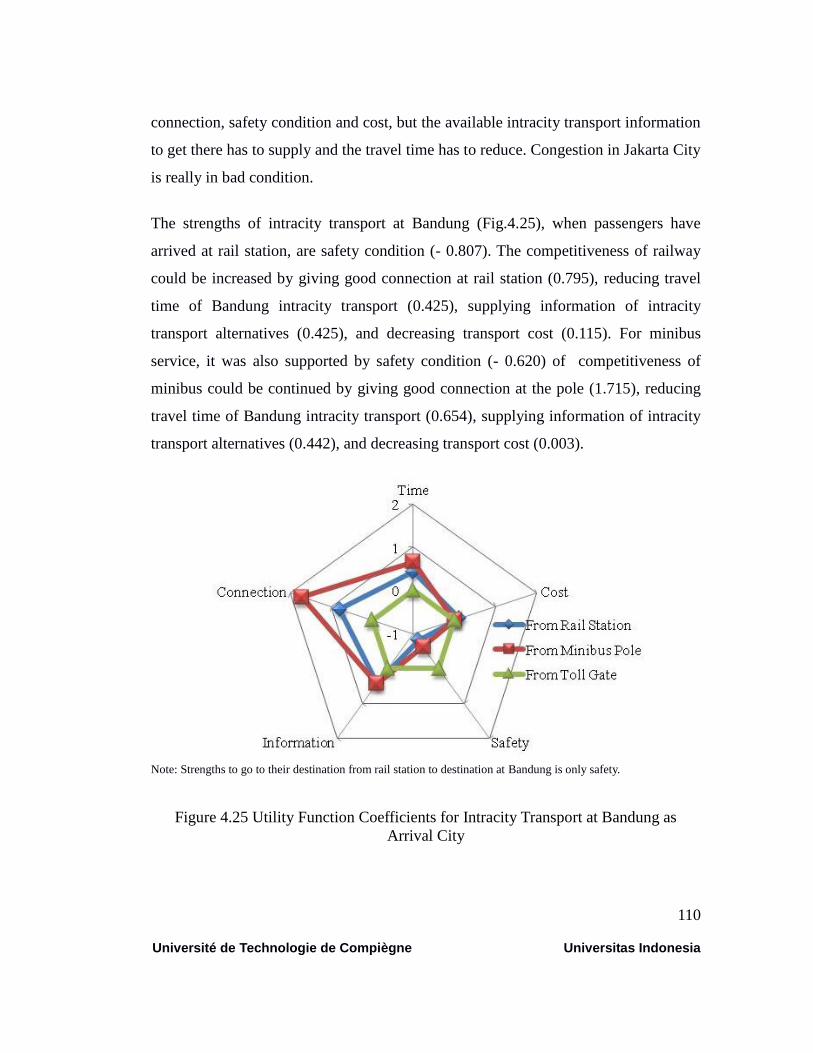
110
Université de Technologie de Compiègne Universitas Indonesia
connection, safety condition and cost, but the available intracity transport information
to get there has to supply and the travel time has to reduce. Congestion in Jakarta City
is really in bad condition.
The strengths of intracity transport at Bandung (Fig.4.25), when passengers have
arrived at rail station, are safety condition (- 0.807). The competitiveness of railway
could be increased by giving good connection at rail station (0.795), reducing travel
time of Bandung intracity transport (0.425), supplying information of intracity
transport alternatives (0.425), and decreasing transport cost (0.115). For minibus
service, it was also supported by safety condition (- 0.620) of competitiveness of
minibus could be continued by giving good connection at the pole (1.715), reducing
travel time of Bandung intracity transport (0.654), supplying information of intracity
transport alternatives (0.442), and decreasing transport cost (0.003).
Note: Strengths to go to their destination from rail station to destination at Bandung is only safety.
Figure 4.25 Utility Function Coefficients for Intracity Transport at Bandung as
Arrival City
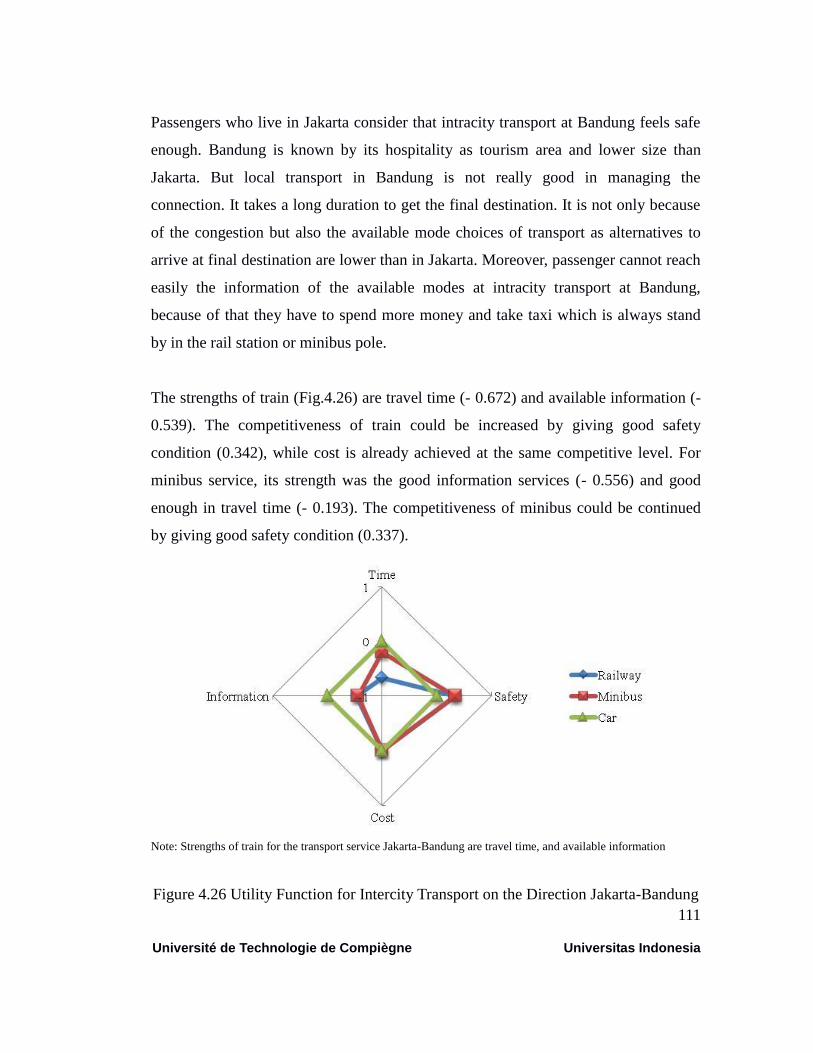
111
Université de Technologie de Compiègne Universitas Indonesia
Passengers who live in Jakarta consider that intracity transport at Bandung feels safe
enough. Bandung is known by its hospitality as tourism area and lower size than
Jakarta. But local transport in Bandung is not really good in managing the
connection. It takes a long duration to get the final destination. It is not only because
of the congestion but also the available mode choices of transport as alternatives to
arrive at final destination are lower than in Jakarta. Moreover, passenger cannot reach
easily the information of the available modes at intracity transport at Bandung,
because of that they have to spend more money and take taxi which is always stand
by in the rail station or minibus pole.
The strengths of train (Fig.4.26) are travel time (- 0.672) and available information (-
0.539). The competitiveness of train could be increased by giving good safety
condition (0.342), while cost is already achieved at the same competitive level. For
minibus service, its strength was the good information services (- 0.556) and good
enough in travel time (- 0.193). The competitiveness of minibus could be continued
by giving good safety condition (0.337).
Note: Strengths of train for the transport service Jakarta-Bandung are travel time, and available information
Figure 4.26 Utility Function for Intercity Transport on the Direction Jakarta-Bandung
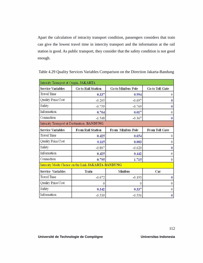
112
Université de Technologie de Compiègne Universitas Indonesia
Apart the calculation of intracity transport condition, passengers considers that train
can give the lowest travel time in intercity transport and the information at the rail
station is good. As public transport, they consider that the safety condition is not good
enough.
Table 4.29 Quality Services Variables Comparison on the Direction Jakarta-Bandung

113
Université de Technologie de Compiègne Universitas Indonesia
4.7.2 Quality Services Transportation on the Direction Bandung-Jakarta
At Bandung, the strengths of intracity transport from home to go to rail station are
cost (-.227), travel time (- 0.765), and information (- 0.624). The competitiveness of
railway could be increased by giving safety condition of Bandung intracity transport
condition to passengers (0.547). For minibus service, it was supported by affordable
cost (- 2.238) of intracity transport at Bandung to go to its pole, enough information
(- 0.192), and good travel duration (-0.060). The competitiveness of minibus could be
increased by giving safety condition (0.338) of intracity transport at Bandung.
Note: Strengths to go to rail station in at Bandung are cost, travel time and information
Figure 4.27 Utility Function Coefficients for Intracity Transport at Bandung as
Departure City
Passengers who live in Bandung feel that intracity transports at Bandung are still not
safe enough, although passengers who live in Jakarta said that it is safe enough. But
for them local transport in Bandung is good in connection, cost, information and
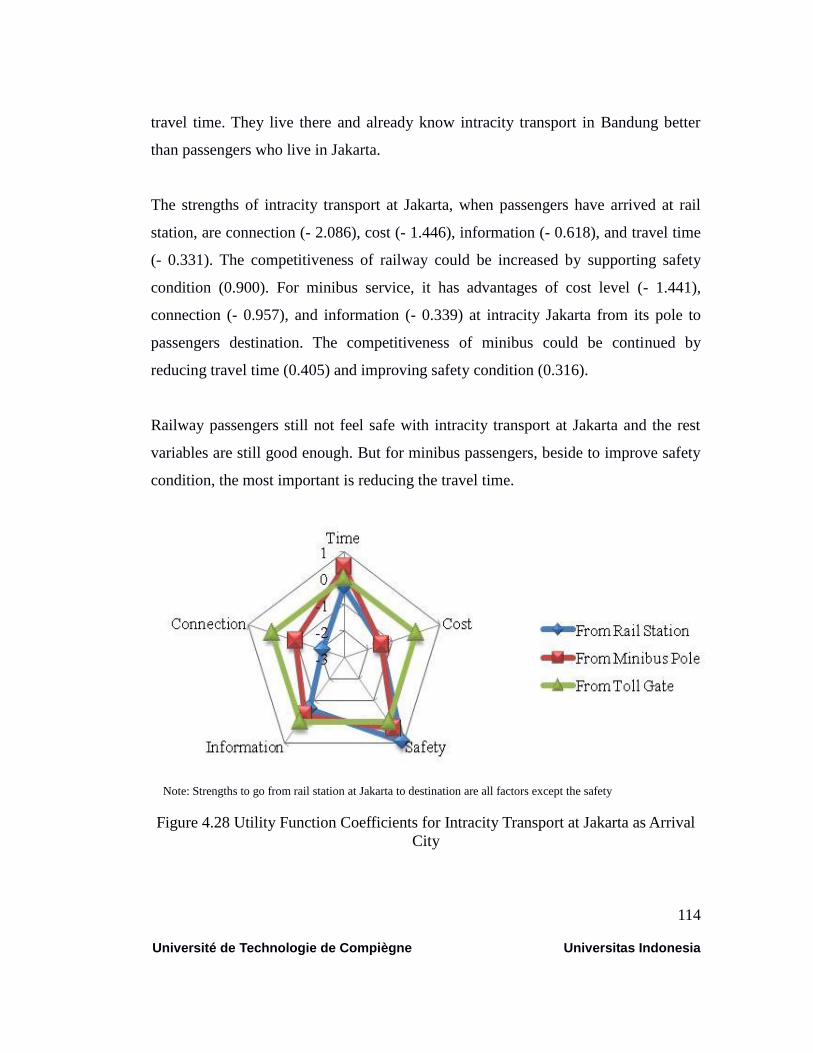
114
Université de Technologie de Compiègne Universitas Indonesia
travel time. They live there and already know intracity transport in Bandung better
than passengers who live in Jakarta.
The strengths of intracity transport at Jakarta, when passengers have arrived at rail
station, are connection (- 2.086), cost (- 1.446), information (- 0.618), and travel time
(- 0.331). The competitiveness of railway could be increased by supporting safety
condition (0.900). For minibus service, it has advantages of cost level (- 1.441),
connection (- 0.957), and information (- 0.339) at intracity Jakarta from its pole to
passengers destination. The competitiveness of minibus could be continued by
reducing travel time (0.405) and improving safety condition (0.316).
Railway passengers still not feel safe with intracity transport at Jakarta and the rest
variables are still good enough. But for minibus passengers, beside to improve safety
condition, the most important is reducing the travel time.
Note: Strengths to go from rail station at Jakarta to destination are all factors except the safety
Figure 4.28 Utility Function Coefficients for Intracity Transport at Jakarta as Arrival
City
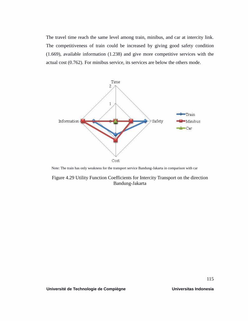
115
Université de Technologie de Compiègne Universitas Indonesia
The travel time reach the same level among train, minibus, and car at intercity link.
The competitiveness of train could be increased by giving good safety condition
(1.669), available information (1.238) and give more competitive services with the
actual cost (0.762). For minibus service, its services are below the others mode.
Note: The train has only weakness for the transport service Bandung-Jakarta in comparison with car
Figure 4.29 Utility Function Coefficients for Intercity Transport on the direction
Bandung-Jakarta
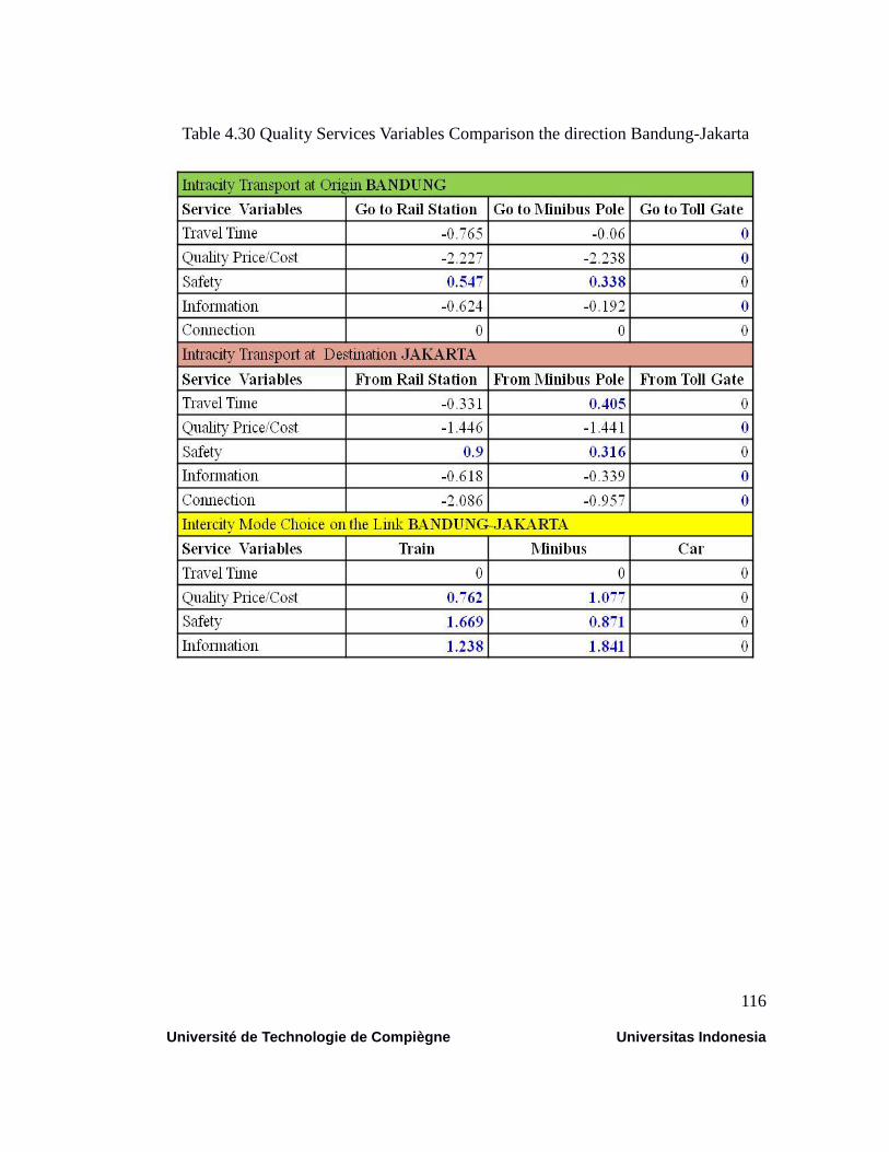
116
Université de Technologie de Compiègne Universitas Indonesia
Table 4.30 Quality Services Variables Comparison the direction Bandung-Jakarta
117
Université de Technologie de Compiègne Universitas Indonesia
CHAPTER V CONCLUSION AND PERSPECTIVES
5.1 Conclusion
Adapted Mixed Multinomial Logit (AMML) model" is a model that has been
developed from the Multinomial Logit Model for the analysis of alternative modes of
transportation between the two cities to include the characteristics of the transport in
the city. The case study on the transport network has been established at the Jakarta-
Bandung corridor, and has resulted in a formulation that can be used to evaluate the
performance of modes of transport that connects the two cities. The characteristics of
the transport network between the two cities have been expressed in the coefficient β.
This coefficient obtained from the process of identifying the parameters of the model
AMML.
5.1.1 The Consideration of Intracity Transport System in Intercity Mode
Choices
Characteristics of transport in the city have a strong relationship in determining the
choice of the type of inter-city transportation mode. Efforts to improve the
performance of one type of mode in an inter-city network will not be optimal when it
is not supported by the increase in performance of modes of transport in the two
cities. Transportation modes can be chosen by the passenger, each mode of transport
should have the characteristics of the service as required by the passenger. The design
of the service level of each type of mode of transportation between cities can include
characteristics of the overall service network, the transport network in the city and
inter-city network.

118
Université de Technologie de Compiègne Universitas Indonesia
5.1.2 Model Development
The AMML model has two equations, the first is using multi utility functions and the
second is using combination between constants and utility function. The second
equation could confirm the first results equation. The confirmation results also could
do by using external data that can apply to the two equations. There are some
limitations to consider. The model could apply with its requirements.
5.1.3 Improving Mode’s Competitiveness
The survey was done in systematically process, and the final step the models have
been verified by the statistical tests and have been confirmed by external validation.
The results describe the passengers’ journey with the nearest mode to use from their
home and at their final destination.
From the analysis of the results are as follows:
1. The quality service variables are in the respective order :
a. travel time, cost, safety, information, and connection for intracity at
departure and destination cities
b. travel time, cost, safety and information for intercity mode services
2. From this study it can be seen that the preference of passengers to travel Jakarta -
Bandung is minibus transport modes, but to Bandung - Jakarta is the private car.
5.1.4 Model Simulation
The model generic was present in the model development and it was applied on the
direction Jakarta-Bandung and Bandung-Jakarta. The applications have produced two
119
Université de Technologie de Compiègne Universitas Indonesia
certain models which can be simulated to the future conditions. The simulation model
was needed to predict the competitiveness of the one mode over the other modes.
5.2 Perspectives
Based on the analysis and discussion, some suggestions are proposed:
1. Recommendation for policies and regulations:
a. Characteristics of each mode of transportation are very different to fulfill
passengers’ demands, so some policies towards all modes are needed.
b. Travel time, cost, safety, information availability, and connection condition
need to be improve in particular for the railway transport. Any policy to
regulate those services should promote equality for all modes to be chosen
by passengers.
c. The results of our research allow different proposals for the improvement of
transportation policies in the context of sustainable urban and regional
development.
2. Perspective for further research:
This research can also be adapted to other types of modes, such as high speed rail
that the government plans to develop for Jakarta-Bandung and the Jakarta-
Surabaya corridor. Beside of the replication, this research can also still be
explored with the same data to determine the final choice of specified segment
market of intercity transport, such as the final decision for workers, students, or
tourists.
The methodology of this study can also be used for the analysis of the minibus
and car transportation segments. It can be also useful for the freight
transportation (global or segmented) between big cities.

120
Université de Technologie de Compiègne Universitas Indonesia
REFERENCES
1. Ahern, Aoife A., Tapley, Nigel, 2007, The Use of Stated Preference Techniques
to Model Modal Choices on Interurban Trips in Ireland, Transportation
Research, pp 15-27
2. Aydin, G., Anna Dzhaleva-Chonkova, 2013, Discussions on rail in urban areas
and rail history, Research in Transportation Economics, pp 84-88
3. Barus, Lita Sari, 2012, Study of people's economic accessibility to railways
transport: Prospecting solutions to generate transport demand and to open
social mobility possibilities, National Conference in Marseille, France, 12p
4. Barus, Lita Sari, Hipolito Martell-Flores, Jean Louis Batoz, 2012, Analysis of
“economic accessibility” to railway's transport for passengers in Indonesia:
Prospecting solutions to generate transport demand by train and to improve
interurban mobility, Proceeding book of Urban Mobility Conference in
Surabaya, Indonesia, 9p
5. Barus, Lita Sari, Sigit Pranowo Hadiwardoyo, Benabdelhafid Abdellatif, 2010,
Integrated Public Transport Development for Two Connected Urban Areas,
Hammamet, Tunisia, IEEE Explore Digital Library, page 495-501
6. Barus, Lita Sari, Sigit Pranowo Hadiwardoyo, 2010, Go Green with Public
Transport for Two Connected Urban Areas, Bali, Indonesia, 12p
7. Barus, Lita Sari, Sigit Pranowo Hadiwardoyo, Hipolito Martell-Flores, Jean Louis
Batoz, 2013, Modal Competition for Freight in Land Transportation on
Jakarta-Surabaya corridor, Journal of Civil and Environmental Research, ISSN
(Paper) 2224-5790, ISSN (Online) 2225-0514, 14p
8. Black, J.A. (1981), Urban Transport Planning: Theory and Practice, London,
Cromm Helm.
9. Beirao, G., J.A. Sarsfield Cabral, 2007, Understanding attitudes towards public
transport and private car: A qualitative study, Transport Policy, pp.478–489
121
Université de Technologie de Compiègne Universitas Indonesia
10. Ben-Akiva, Moshe dan Lerman, Steven R., 1985, Discrete Choice Analysis, MIT
Press, Mass., Newyork, ISBN 1-262-02217-6, 390p
11. Biro Pusat Statistik, 2014, Bandung Dalam Angka 2014, Bandung
12. Biro Pusat Statistik, 2014, Jakarta Dalam Angka 20014, Jakarta
13. Biro Pusat Statistik Kabupaten Bandung, 2014, Kabupaten Bandung Dalam
Angka, 2014, Bandung
14. Bowersox, Donald, David Closs, M. Bixby Cooper, 1981, Supply Chain
Logistics Management, McGraw-Hill, New York, ISBN 0072351004, 656p
15. Brons, Martijn, Moshe Givoni, Piet Rietveld, 2009, Access to railway stations
and its potential in increasing rail use, Transportation Research Part A, pp 136–
149
16. Chandra, S, Luca Quadrifoglio, 2013, A new street connectivity indicator to
predict performance for feeder transit services, Transportation Research, pp. 67–
80
17. Chandra, S., Muhammad Ehsanul Bari, Prem Chand Devarasetty, Sharada Vadali,
2013, Accessibility evaluations of feeder transit services, Transportation
Research, pp 47–63
18. Eriyanto, 1999, Metodologi Polling Memberdayakan Suara Rakyat, PT. Remaja
Rosdakarya, Bandung
19. Fisher, R. A., 1950, Statistical Methods for Research Worker, Oliver & Boyd,
354p
20. Ghozali, Imam, 2009, Analisis Multivariate Lanjutan dengan Program SPSS,
Badan Penerbit Universitas Diponegoro, Semarang, Indonesia, ISBN
979.704.387.8, 241p
21. Givoni, Moshe, Piet Rietveld, 2007, The access journey to the railway station
and its role in passengers’ satisfaction with rail travel, Transport Policy, pp357–
365

122
Université de Technologie de Compiègne Universitas Indonesia
22. Greene, William H., David A. Hensher, 2006, Heteroscedastic control for
random coefficients and error components in mixed logit, Elsevier Ltd., pp 610-
623
23. Grimes, Arthur, Chris Young, 2013, Spatial effects of urban rail upgrades,
Journal of Transport Geography 30, pp 1–6
24. Hadiwardoyo, Sigit Pranowo, Lita Sari Barus, Hipolito Martell-Flores, Jean Luis
Batoz, 2013, Railway Development Opportunity for Two Connected Urban
Areas, International Journal of Engineering Science, 12p
25. Hensher, David A., John M. Rose, 2006, Development of commuter and non-
commuter mode choice models for the assessment of new public transport
infrastructure projects: A case study, Elsevier Ltd, pp 428-443
26. Hess Stephane, John W. Polak, 2004, Mixed logit modelling of airport choice in
multi-airport regions, Elsevier Ltd., pp 59-68
27. Kanafani, Abib K., 1983, Transport Demand Analysis, McGraw-Hill, New York,
ISBN 0070332711, 320p
28. Keqi, WU, MAO Baohua, WANG Yongliang, SUN Quanxin, 2013, Intercity
Rail Transport Pricing Strategy Based on efficacy Coefficient Method, Journal
Transportation System Engineering & IT, pp.105−110.
29. Koffman, David, 2004, Operational Experiences with Flexible Transit Services
A Synthesis of Transit Practice, Transportation Research Board Washington,
D.C., 71p
30. Kristiansen, Jørgen, Hans Henrik W. Johannsen, 2007, Transport Systems
Concepts and Definitions, Sutranet, 18p
31. Li, X., Luca Quadrifoglio, 2010, Feeder transit services: Choosing between
fixed and demand responsive policy, Transportation Research, pp.770–780
32. Lo Hong K., Chun-Wing Yip, Quentin K. Wan, 2004, Modeling competitive
multi-modal transit services: a nested logit approach, Elsevier Ltd., pp 251-272

123
Université de Technologie de Compiègne Universitas Indonesia
33. Lyons, Glenn, Reg Harman, 2002, The UK public transport industry and
provision of multi-modal traveller information, International Journal of
Transport Management, pp 1–13
34. Manheim, Marvin L., 1979, Fundamentals of Transportation System Analysis,
MIT Press, Cambrige, Mass., ISBN 0262131293
35. Mauski, Charles F., Daniel L. Mc. Fadden, 1981, Structural Analysis of Discrete
Data and Econometric Applications, MIT Press, Cambrige, Mass., ISBN
0262131595, pp 198-272
36. Mc. Fadden, D., K. T rain, 2000, Mixed MNL Model for Discrete Response,
Journal of Applied Econometrics, John Wiley & Son, Ltd., pp 447-470
37. Ming HE, GUO Xiucheng*, RAN Jiangyu, WU Cairui, ZHU Wei, LIU Chaoping,
2010, Forecasting Rail Transit Split with Disaggregated MNL Model, Journal
Transport System Engineering & IT, pp 136-142
38. Morlok, Edward K., 1978, Introduction to Transportation, Engineering and
Planning, McGraw-Hill, New York, 767p, ISBN 0070431329
39. Oppenheim, Nobert, 1980, Applied Models in Urban and Regional Analysis,
Prentice-Hall Inc., Englewood Cliffs, New Jersey. 352p
40. Prasertsubpakij, D., Vilas Nitivattananon, Evaluating accessibility to Bangkok
Metro Systems using multi-dimensional criteria across user groups, IATSS
Research, pp. 56–65
41. Potts, John F., Maxine A. Marshall, Emmett C. Crockett, Joel Washington, 2010,
A Guide for Planning and Operating Flexible Public Transportation Services,
Transportation Research Board, Washington D.C., 98p
42. Reis, V., J. Fabian Meier, Giuseppe Pace, Roberto Palacin, 2013, Rail and multi-
modal transport, Research in Transportation Economics pp.17-30
43. Shankar, Venkataraman, Fred Manner, 1996, An Exploring Multinomial Logit
Analysis of Single-Vehicle Motorcycle Accident Severity, Journal of Safety
Research, USA, pp. 183-194
124
Université de Technologie de Compiègne Universitas Indonesia
44. Suhardi, Bambang, 2004, Model Potensial Gravitasi Hansen untuk Menentukan
Pertumbuhan Populasi Daerah, Performa Vol.3, No.1, pp. 28-32
45. Suhodo, Sutanto, 2000, Peluang Penelitian Domain Transport Pada Milenium
Mendatang: Bagian I, State of The Art, Jurnal Teknologi, FTUI, Jakarta, ISSN
0215-1685
46. Tamin, Ofyar Z., 2000, Perencanaan dan Pemodelan Transportasi, Penerbit
ITB, Bandung, ISBN 979-9299-10-1, 633p
47. Van der Ven, Joris, Potensi Pasar Kereta Api di Indonesia, Indonesian
Infrastructure Initiative, Australia Indonesia Partnership, Jakarta, 2010, pp. 3-5
48. Vedagiri P., Arasan V. T., 2009, Estimating Modal Shift of Car Travelers to Bus
on Introduction of Bus Priority System, Journal of Transportation Systems
Engineering and Information Technology, pp 120-129
49. Walpole, Ronald E. and Myers, Raymond H., 2012, Ilmu Peluang dan Statistika
untuk Insinyur dan Ilmuwan, Edisi Keempat, Penerbit ITB, Bandung,
50. Yu, Ming-Miin, Erwin T.J. Lin, 2008, Efficiency and effectiveness in railway
performance using a multi-activity network DEA model, Omega 36, pp 1005-
1017
125
Université de Technologie de Compiègne Universitas Indonesia
Annex
Data Compilation and Analysis
1. Data Compilation
a. Choices Data
When data entry has been finished, then data compilation started to define
variables values. Choice values are identified by the answer of the question with
notation “V.1 ≡ Kendaraan yang paling sering digunakan antar kota Jakarta-
Bandung”.
If they answered train then the notation in xl file would become
o Mo1 = 1, is the value to go to rail station
o Mi1 = 1, is the value of train
o MD1 = 1, is the value from rail station
if minibus, then:
o Mo2 = 2, is the value to go to minibus pole
o Mi2 = 2, is the value of minibus
o MD2 = 2, is the value from minibus pole
and if car then:
o Mo3 = 3, is the value to go to highway toll gate
o Mi3 = 3, is the value of car
o MD3 = 3, is the value from highway toll gate
b. Intracity Transport at Departure City
There are five service variables to consider on this link.
Travel time to go to modal node (TtoU) is the additional of travel time
when passengers used one or several modes to go to modal node 1 (for
example rail station, minibus pole, or highway toll gate). The values that

126
Université de Technologie de Compiègne Universitas Indonesia
has been used:
o ”III.2Wr ≡ Kondisi kendaraan Ojek/Motor, Waktu Rata-rata”
o ”III.3Br ≡ Kondisi kendaraan Bajaj/Becak, Biaya Rata-rata”
o ”III.4Wr ≡ Kondisi kendaraan Angkot/Metromini, Waktu Rata-rata”
o ”III.5Wr ≡ Kondisi kendaraan Taxi, Waktu Rata-rata”
o ”III.6Wr ≡ Kondisi kendaraan Mobil Pribadi, Waktu Rata-rata”
o ”III.7Wr ≡ Kondisi kendaraan Bis, Waktu Rata-rata”
Cost (PoU) has been spent to go to modal node. The values that has
been used are the additional values from:
o ”III.2Br ≡ Kondisi kendaraan Ojek/Motor, Biaya Rata-rata”
o ”III.3Br ≡ Kondisi kendaraan Bajaj/Becak, Biaya Rata-rata”
o ”III.4Br ≡ Kondisi kendaraan Angkot/Metromini, Biaya Rata-rata”
o ”III.5Br ≡ Kondisi kendaraan Taxi, Biaya Rata-rata”
o ”III.6Br ≡ Kondisi kendaraan Mobil Pribadi, Biaya Rata-rata”
o ”III.7Br ≡ Kondisi kendaraan Bis, Biaya Rata-rata”
Safety condition to go to modal node (SoC), the values that has been
used are the additional values from:
o ”III.2K ≡ Kondisi kendaraan Ojek/Motor, Keamanan”
o ”III.3K ≡ Kondisi kendaraan Bajaj/Becak, Keamanan”
o ”III.4K ≡ Kondisi kendaraan Angkot/Metromini, Keamanan”
o ”III.5K ≡ Kondisi kendaraan Taxi, Keamanan”
o ”III.6K ≡ Kondisi kendaraan Mobil Pribadi, Keamanan”
o ”III.7K ≡ Kondisi kendaraan Bis, Keamanan”
Information condition to go to modal node (IoC), the values that has
been used are the additional values from:
o ”III.2I ≡ Kondisi kendaraan Ojek/Motor, Informasi”
o ”III.3I ≡ Kondisi kendaraan Bajaj/Becak, Informasi”
o ”III.4I ≡ Kondisi kendaraan Angkot/Metromini, Informasi”
o ”III.5I ≡ Kondisi kendaraan Taxi, Informasi”

127
Université de Technologie de Compiègne Universitas Indonesia
o ”III.6I ≡ Kondisi kendaraan Mobil Pribadi, Informasi”
o ”III.7I ≡ Kondisi kendaraan Bis, Informasi”
Connection condition at modal node 1 (CoC). The nominal values were
classified with Sturges rank, then it can be got the total values from:
o ”IV.1W ≡ Waktu tunggu rata-rata ketika akan keluar kota dari kota
asal”
o ”IV.4B ≡ Biaya tunggu rata-rata ketika akan keluar kota”
o ”IV.5 ≡ Keamanan ditempat tunggu ketika akan keluar kota”
o ”IV.6 ≡ Ketersediaan informasi ditempat tunggu ketika akan keluar
kota”
c. Intercity transport
There are four variables for this link. The values that have been obtained
from:
Travel time (TtiU) is from notation “V.2Wr ≡ Kondisi kendaraan antar
kota, Waktu Rata-rata”
Cost (PiU) is from notation “V.2Br ≡ Kondisi kendaraan antar kota,
Biaya Rata-rata”
Safety condition (SiC) is from notation “V.2K ≡ Kondisi kendaraan antar
kota, Keamanan”
Information condition (IiC) is from notation “V.2I≡Kondisi kendaraan
antar kota, Informasi”
d. Intracity Transport at Departure City
Travel time from modal node (TtdU) is the additional of travel time when
passengers used one or several modes from modal node 2 (for example
rail station, minibus pole, or highway toll gate) to go to the final
destination. The values that has been used:
o ”VI.2Wr ≡ Kondisi kendaraan Ojek/Motor, Waktu Rata-rata”

128
Université de Technologie de Compiègne Universitas Indonesia
o ”VI.3Wr ≡ Kondisi kendaraan Bajaj/Becak, Waktu Rata-rata”
o ”VI.4Wr ≡ Kondisi kendaraan Angkot/Metromini, Waktu Rata-rata”
o ”VI.5Wr ≡ Kondisi kendaraan Taxi, Waktu Rata-rata”
o ”VI.6Wr ≡ Kondisi kendaraan Mobil Pribadi, Waktu Rata-rata”
o ”VI.7Wr ≡ Kondisi kendaraan Bis, Waktu Rata-rata”
Cost (PdU) has been spent from modal node 2 to go to final destination.
The values that has been used are the additional values from:
o ”VI.2Br ≡ Kondisi kendaraan Ojek/Motor, Biaya Rata-rata”
o ”VI.3Br ≡ Kondisi kendaraan Bajaj/Becak, Biaya Rata-rata”
o ”VI.4Br ≡ Kondisi kendaraan Angkot/Metromini, Biaya Rata-rata”
o ”VI.5Br ≡ Kondisi kendaraan Taxi, Biaya Rata-rata”
o ”VI.6Br ≡ Kondisi kendaraan Mobil Pribadi, Biaya Rata-rata”
o ”VI.7Br ≡ Kondisi kendaraan Bis, Biaya Rata-rata”
Safety condition from modal node 2 (SdC), the values that has been used
are the additional values from:
o ”VI.2K ≡ Kondisi kendaraan Ojek/Motor, Keamanan”
o ”VI.3K ≡ Kondisi kendaraan Bajaj/Becak, Keamanan”
o ”VI.4K ≡ Kondisi kendaraan Angkot/Metromini, Keamanan”
o ”VI.5K ≡ Kondisi kendaraan Taxi, Keamanan”
o ”VI.6K ≡ Kondisi kendaraan Mobil Pribadi, Keamanan”
o ”VI.7K ≡ Kondisi kendaraan Bis, Keamanan”
Information condition (IdC) from modal node 2, the values that has been
used are the additional values from:
o ”VI.2I ≡ Kondisi kendaraan Ojek/Motor, Informasi”
o ”VI.3I ≡ Kondisi kendaraan Bajaj/Becak, Informasi”
o ”VI.4I ≡ Kondisi kendaraan Angkot/Metromini, Informasi”
o ”VI.5I ≡ Kondisi kendaraan Taxi, Informasi”
o ”VI.6I ≡ Kondisi kendaraan Mobil Pribadi, Informasi”
o ”VI.7I ≡ Kondisi kendaraan Bis, Informasi”
129
Université de Technologie de Compiègne Universitas Indonesia
Connection condition at modal node 2 (CdC). The nominal values were
classified with Sturges rank, then it can be got the total values from:
o ”VII.1W ≡ Waktu tunggu rata-rata ketika tiba ditempat tujuan”
o ”VII.3B ≡ Biaya rata-rata ketika tiba ditempat tujuan”
o ”VII.5 ≡ Keamanan ditempat tunggu ketika tiba ditempat tujuan”
o ”VII.6 ≡ Ketersediaan informasi ditempat tunggu ketika tiba ditempat
tujuan”
2. Data Verification
Data verification was done by checking data input in excel files with questionnaires
requirements as mention in the guideline. Data could missed placed or text format.
Data with the illogic input was deleted. Data verification was done twice to avoid
human error.
3. Data Classification
Numeric data is classified by Sturges equation, so all data format is data rank.
k = 1 + 3,322 log n ……………………...…..…………..............………….….. (1)
Where:
n ≡ total number of data available
k ≡ number of classification
i ≡ r/k ……………………….....…....…………………............................…….. (2)
i ≡ interval
r ≡ value max – value min……………………………................................……(3)
Data was divided into type, such as data for model development and data for external
validation. There are two table for model development, such as data Jakarta-Bandung
(Table 1, 2, and 3) and data Bandung-Jakarta (Table 4, 5, and 6).

130
Université de Technologie de Compiègne Universitas Indonesia
Tabel 1 Classified Data of Train Package on the Jakarta-Bandung Direction
Respondent TtoU PoU SoC IoC CoC TtiU PiU SiC IiC TtdU PdU SdC IdC CdC
1 8 7 6 6 5,5 4 8 4 4 7 5 6 6 6,5
2 7 7 6 6 5 4 8 6 6 7 7 6 6 7
3 8 8 6 6 6,5 4 8 6 6 8 8 6 6 6
4 7 7 6 6 6 4 8 6 6 6 8 6 6 6,5
5 8 8 6 6 6,5 4 8 6 6 6 8 6 6 6,5
6 8 8 6 6 6,5 2 8 6 6 5 8 4 6 5
7 8 8 6 6 7 5 8 6 6 7 5 8 8 5,5
8 7 5 8 8 6 5 8 8 8 8 5 6 6 6
9 7 8 6 6 5,5 4 8 8 8 7 8 4 6 4
10 7 8 6 6 6,5 4 8 8 8 4 5 8 8 6
11 8 7 6 6 6,5 4 8 6 6 7 7 6 6 6
12 6 8 4 6 7 4 8 6 6 6 8 6 6 6,5
13 6 8 6 6 6 4 8 6 6 6 8 6 6 7
14 7 8 6 6 7 4 8 6 6 6 8 6 6 7
15 7 8 6 6 7 4 8 6 6 8 8 4 6 6,5
16 6 8 6 6 7 2 8 6 6 7 8 4 6 6,5
17 8 8 6 6 5 4 8 6 6 7 8 6 6 5,5
18 7 7 6 6 6 4 8 6 6 7 6 6 6 6,5
19 8 7 6 6 5 4 8 6 6 6 8 6 6 6,5
20 7 7 6 6 6 2 8 6 6 8 8 4 6 7
21 7 8 6 6 5 4 8 6 6 5 8 6 6 6
22 7 8 6 6 5 4 8 6 6 6 8 6 6 6
23 8 8 6 6 6,5 4 8 6 6 8 8 6 6 7
24 8 7 6 6 6 4 8 6 6 7 6 6 6 7
25 8 7 6 6 4 5 8 6 6 8 7 6 6 6,5
26 8 7 6 6 6 2 8 6 8 7 7 4 6 6,5
27 7 8 4 4 6 4 8 6 6 7 7 6 6 6,5
28 7 6 6 6 6 5 8 8 6 7 7 6 6 6,5
29 8 8 6 6 6 2 8 6 6 8 8 6 6 6
30 7 6 6 8 5,5 4 8 6 6 8 8 4 6 6
31 7 5 6 6 4,5 2 8 6 6 8 8 6 6 7
32 8 7 5 5 6,5 2 7 6 6 8 8 4 4 7
33 7 7 6 6 6 2 8 6 6 6 4 6 6 5
34 8 7 6 6 5,5 2 8 6 6 7 8 6 6 6
35 8 8 6 6 6,5 2 8 6 6 8 8 6 6 6,5
36 7 5 6 6 6,5 2 8 4 4 6 5 6 6 6
37 8 8 6 6 6,5 4 8 6 6 6 8 4 6 6
38 8 8 6 6 6 4 8 6 6 5 8 6 6 5
39 7 6 4 6 6,5 2 8 6 6 8 8 6 6 7
40 8 8 4 6 6,5 4 8 6 6 8 8 6 6 7
41 8 7 8 8 8 4 8 6 6 7 5 6 6 6,5
42 8 8 8 8 6 4 8 6 6 8 7 6 6 7
43 8 8 6 6 6 2 8 6 6 4 8 6 6 6
44 7 8 6 6 6,5 4 8 6 6 4 8 6 6 7
45 7 8 4 6 7 4 8 6 6 7 8 6 6 6,5
46 8 8 6 6 7 2 8 6 6 8 8 4 6 7
47 8 7 6 6 6 2 8 6 6 8 7 6 6 7
48 7 8 6 6 6,5 4 8 6 6 8 8 6 6 7
49 7 5 6 6 5,5 5 8 6 6 5 1 6 6 7
50 6 8 6 5 7 4 8 6 6 8 8 4 6 7
51 7 8 6 4 6,5 5 8 6 6 6 8 4 6 7
52 8 7 6 6 6 4 8 6 6 8 8 6 6 6,5
53 8 8 6 6 5,5 5 8 6 6 8 7 6 6 6,5
54 8 7 6 6 5,5 4 8 6 6 7 7 6 6 6
55 8 6 6 6 6,5 4 8 6 6 8 6 6 6 6,5
56 8 7 4 6 6,5 2 8 6 6 8 8 6 6 7
57 8 7 6 6 6 4 8 6 6 7 8 6 6 6
58 6 8 4 6 5,5 4 8 6 6 6 8 6 6 6
59 7 8 4 6 5,5 2 8 6 4 8 5 6 6 5,5
60 7 7 6 6 6,5 4 8 8 8 8 5 6 6 6
61 8 7 6 6 6 4 8 6 6 8 6 6 6 5,5
62 3 8 6 6 6,5 2 8 6 6 7 5 6 6 6,5
63 7 8 6 6 4,5 2 8 6 6 7 8 6 6 6
64 1 8 4 6 5,5 4 8 6 6 7 8 6 6 7
65 8 8 4 6 6,5 4 8 6 6 6 8 4 6 5,5
66 8 7 6 6 5,5 4 8 6 6 8 6 6 6 5
67 7 5 6 6 5 4 8 6 6 7 7 6 6 4,5
68 8 7 6 6 7 4 8 6 6 8 7 6 6 7
69 7 7 6 6 6 4 8 6 6 8 6 6 6 4,5
70 7 8 6 6 6 4 8 6 6 7 7 6 6 5,5
71 7 8 6 6 6,5 2 8 6 6 8 8 6 6 6,5
72 8 8 6 6 7 4 8 6 6 6 4 6 6 6,5
73 8 8 6 6 6,5 4 8 6 6 7 8 6 6 7
74 7 7 6 6 6 4 8 6 6 8 6 6 6 4,5
75 7 5 8 8 6,5 2 8 6 6 8 6 6 6 6,5
76 8 5 6 6 5 1 8 6 6 7 7 6 6 4,5
77 6 8 6 6 5 1 8 6 6 7 8 6 6 6
78 8 7 6 6 6 4 8 6 6 8 7 6 6 5,5
79 7 5 6 6 6,5 4 8 6 6 8 8 6 6 6
80 6 7 6 6 5,5 4 8 6 6 7 7 6 6 5,5
81 6 8 6 6 6,5 4 8 6 6 6 8 6 4 7
82 7 8 6 6 6,5 4 8 6 6 8 8 4 6 7
83 7 5 6 6 6 4 8 6 6 8 7 6 6 7
84 5 5 6 6 3,5 5 8 6 6 7 5 6 6 7
85 7 8 4 6 6,5 4 8 6 6 8 7 6 6 6,5
86 7 8 6 6 7 5 8 6 6 8 8 6 6 6,5
87 7 8 6 6 6,5 4 8 6 6 8 8 6 6 7
88 7 6 6 6 6 4 8 6 6 8 8 6 6 7
89 8 8 6 6 4,5 4 8 6 6 7 7 6 6 7
90 7 8 6 6 7 4 8 6 6 8 8 6 6 6,5
91 7 5 6 6 6 4 8 6 6 7 6 6 6 7
92 8 8 6 6 4 4 8 6 6 8 6 6 6 6,5
93 6 2 6 6 4,5 4 8 6 6 7 6 6 6 7
94 8 6 6 6 6 4 8 6 6 8 7 6 6 6
95 8 7 4 6 7 4 8 6 6 8 8 4 6 7
96 6 8 6 6 4 4 8 6 6 8 8 6 6 7
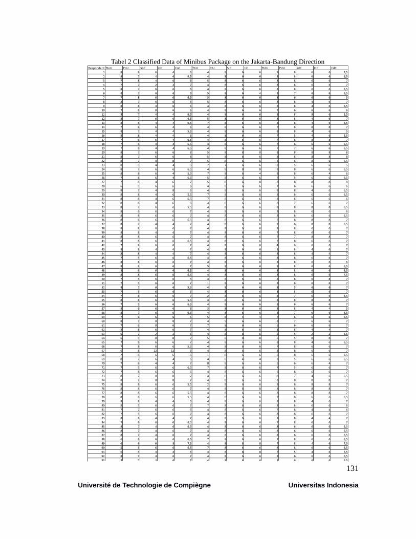
131
Université de Technologie de Compiègne Universitas Indonesia
Tabel 2 Classified Data of Minibus Package on the Jakarta-Bandung Direction Respondent TtoU PoU SoC IoC CoC TtiU PiU SiC IiC TtdU PdU SdC IdC CdC
1 8 8 6 4 6 4 8 6 6 8 8 6 6 7,5
2 8 7 4 6 6,5 4 8 6 6 8 8 6 6 6,5
3 7 8 4 6 6 5 8 6 6 8 8 6 6 7
4 7 7 2 2 7 4 8 6 6 8 8 6 6 7
5 8 7 6 6 6 4 8 6 6 8 8 6 6 6,5
6 8 7 6 6 6 5 8 6 4 8 7 6 6 6,5
7 7 8 6 6 6,5 5 8 6 6 8 6 6 6 5
8 8 7 6 6 6 5 8 6 6 8 8 4 6 7
9 8 8 4 6 6 4 8 6 6 8 8 4 6 6,5
10 7 8 8 6 6 4 8 6 6 7 6 6 6 6
11 8 7 4 4 6,5 4 8 6 6 8 8 8 6 5,5
12 8 7 6 6 6,5 5 8 6 6 8 8 4 6 7
13 8 8 4 4 6,5 7 8 6 6 8 8 4 6 6,5
14 7 6 6 4 6 4 8 6 6 7 8 8 8 7
15 8 7 4 4 5,5 4 8 6 6 8 8 4 6 5
16 8 8 4 4 6 4 8 6 6 7 5 4 6 5,5
17 7 6 6 4 6,5 4 8 6 6 7 8 8 8 7
18 7 8 4 4 6,5 4 8 6 6 7 6 6 6 6,5
19 7 8 4 4 6,5 4 8 6 6 7 7 6 6 6,5
20 8 7 6 6 8 5 8 8 8 8 8 8 8 8
21 8 7 6 6 8 5 8 6 6 8 8 8 8 8
22 8 7 8 8 7 5 8 6 6 1 6 8 6 6,5
23 8 5 4 4 5 7 7 6 6 8 5 6 6 5
24 8 7 6 6 6,5 4 8 8 8 8 8 6 6 6,5
25 8 8 6 4 5,5 7 8 6 4 8 8 6 4 6
26 7 8 6 4 6,5 5 8 6 6 7 5 6 6 6,5
27 7 8 4 6 7 5 8 6 8 8 8 8 8 8
28 6 5 6 6 6 4 8 6 6 7 6 6 6 6
29 8 7 4 8 6 4 8 6 6 8 8 4 6 6,5
30 8 8 4 6 5,5 7 8 6 6 8 6 6 6 6,5
31 8 8 4 6 6,5 7 8 6 6 8 6 6 6 6
32 8 8 4 6 6 4 8 6 6 8 7 6 6 7
33 8 7 6 6 5,5 4 8 6 6 8 8 8 8 6,5
34 8 6 6 6 7 4 8 6 6 8 8 6 6 6
35 8 8 6 6 7 4 8 6 6 8 8 6 6 6,5
36 8 6 6 6 6,5 4 8 6 6 7 8 8 8 7
37 8 7 4 4 7 4 8 6 6 7 6 8 8 6,5
38 8 8 6 6 7 4 8 6 6 8 8 6 6 7
39 8 8 4 4 7 4 8 6 6 7 8 6 6 7
40 8 8 6 6 7 4 8 6 6 7 7 8 8 7
41 8 8 6 6 6,5 4 8 6 6 7 8 6 6 7
42 7 8 6 6 7 4 8 6 6 4 6 6 6 7
43 8 8 4 4 7 4 8 6 6 8 8 4 6 7
44 8 8 4 4 7 4 8 6 6 8 8 4 4 7
45 7 5 6 6 6,5 4 8 6 6 8 8 6 6 7
46 8 8 6 6 7 4 8 6 6 8 8 6 6 6
47 8 8 6 6 7 5 8 6 6 8 8 6 6 6,5
48 8 6 6 6 6,5 4 8 6 6 8 8 6 6 6,5
49 8 8 6 6 6,5 4 8 6 6 8 8 6 6 7,5
50 7 5 6 6 5 4 8 6 6 8 8 6 8 7
51 7 5 6 6 7 1 8 6 6 8 6 6 6 7
52 8 7 6 6 5,5 4 8 6 6 8 5 6 6 7
53 7 5 6 6 5 4 8 6 6 8 8 6 6 7
54 7 8 6 6 7 2 8 6 6 8 7 6 6 6,5
55 8 8 6 6 5,5 4 8 6 6 8 8 8 8 7
56 7 5 6 6 6,5 4 8 6 6 8 6 6 6 7
57 8 6 6 6 6 3 8 6 6 8 8 4 4 5
58 8 7 6 6 6,5 4 8 6 6 8 7 6 6 6,5
59 7 6 6 6 5 5 8 4 4 7 6 6 6 6,5
60 8 7 8 8 7 4 5 6 6 8 7 6 6 7
61 7 6 8 6 7 7 8 6 6 6 6 6 6 7
62 8 8 6 6 7 4 8 6 6 8 8 4 4 7
63 6 7 2 2 6 4 8 8 6 5 5 2 2 6,5
64 6 5 8 8 7 5 8 8 8 5 5 8 8 7
65 7 8 6 6 7 4 8 6 6 8 8 4 6 6,5
66 7 8 6 6 5,5 4 8 6 6 7 8 6 6 7
67 6 8 12 12 6 4 8 6 6 8 8 6 6 7
68 7 8 6 6 6 1 8 6 6 6 8 6 6 6,5
69 8 7 6 4 6 4 8 4 4 3 5 6 6 6,5
70 7 8 4 4 7 8 8 6 6 5 6 6 4 7
71 7 5 6 6 6,5 7 8 6 6 7 5 6 6 7
72 7 8 6 6 6 4 8 6 6 6 8 6 6 7
73 8 7 8 8 7 4 8 6 6 8 7 4 6 6,5
74 8 7 8 8 7 4 8 6 6 8 8 8 8 7
75 8 8 6 6 5,5 2 8 6 6 8 8 8 8 7
76 8 8 6 6 7 4 8 8 8 8 8 8 8 7
77 8 8 6 6 5,5 4 8 6 6 8 8 8 8 7
78 8 8 6 6 5,5 4 8 6 6 7 8 6 6 6,5
79 8 8 4 4 6 4 8 6 6 8 8 4 6 7
80 8 5 6 6 7 7 8 6 6 8 8 6 6 6
81 7 7 6 6 6 4 8 6 6 7 8 4 4 6
82 7 5 6 6 7 4 8 6 6 8 8 6 6 7
83 8 8 4 4 7 4 8 6 6 8 8 4 4 7
84 7 6 6 6 6,5 4 8 6 6 7 8 6 6 7
85 8 7 4 6 6,5 4 8 6 6 8 6 6 6 6,5
86 8 7 4 6 7 4 8 6 6 8 6 6 6 6,5
87 8 7 4 6 7 4 8 6 6 8 6 6 6 6,5
88 6 6 6 6 6,5 7 8 6 6 7 8 6 6 6,5
89 6 6 6 8 7,5 4 8 8 8 7 8 4 6 7,5
90 5 5 6 6 6,5 7 8 6 6 4 8 6 6 6,5
91 6 5 4 4 6 4 8 8 8 7 5 4 6 5,5
92 8 7 4 6 7 4 8 6 6 8 6 6 6 6,5
93 8 7 4 6 7 4 8 6 6 8 6 6 6 6,5
94 6 1 6 4 4,5 4 8 4 4 5 1 6 6 4,5
95 7 8 6 6 5,5 7 8 6 6 8 8 8 8 6
96 7 8 6 6 6,5 4 8 6 6 8 8 6 6 7
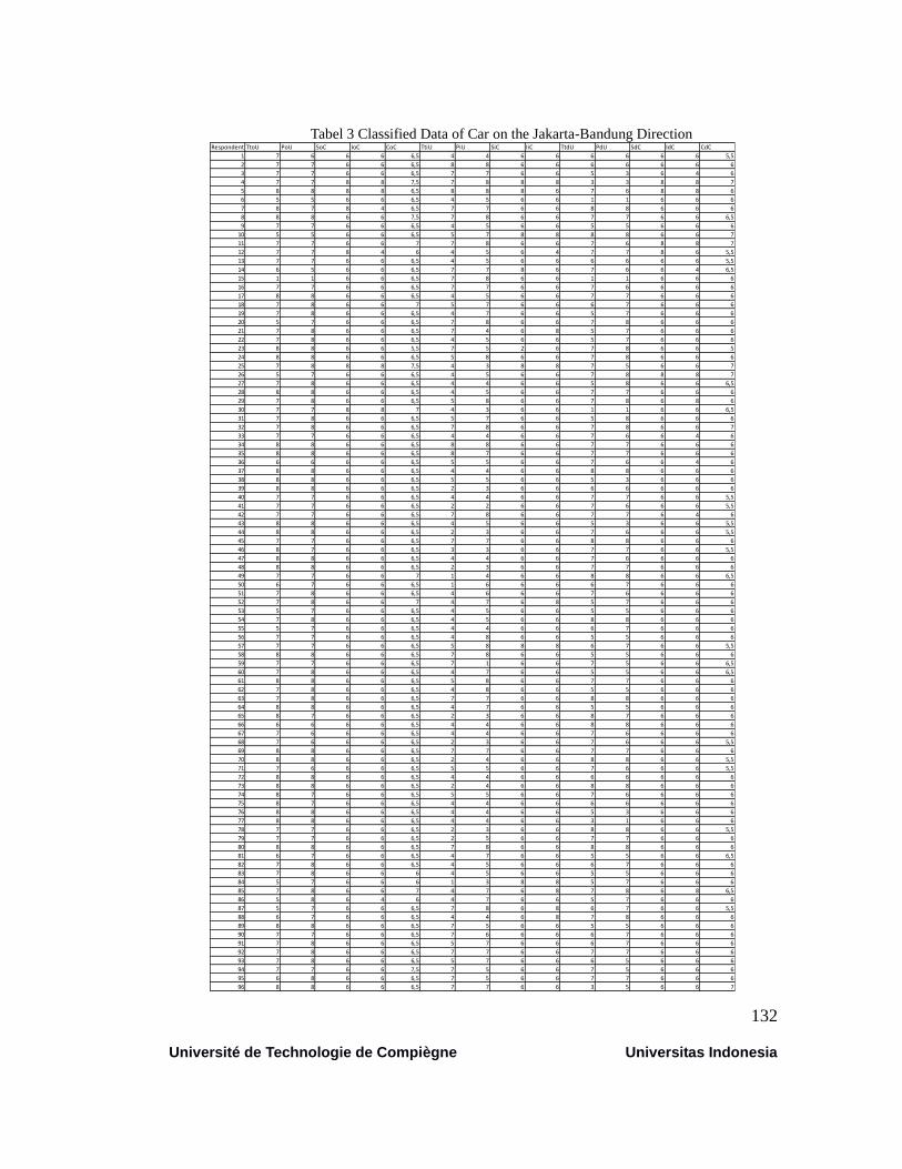
132
Université de Technologie de Compiègne Universitas Indonesia
Tabel 3 Classified Data of Car on the Jakarta-Bandung Direction Respondent TtoU PoU SoC IoC CoC TtiU PiU SiC IiC TtdU PdU SdC IdC CdC
1 7 6 6 6 6,5 4 4 6 6 6 6 6 6 5,5
2 7 7 6 6 6,5 8 8 6 6 6 6 6 6 6
3 7 7 6 6 6,5 7 7 6 6 5 3 6 4 6
4 7 7 8 8 7,5 7 8 8 8 3 3 8 8 7
5 8 8 8 8 6,5 8 8 8 6 7 6 8 8 6
6 5 5 6 6 6,5 4 5 6 6 1 1 6 6 6
7 8 7 8 4 6,5 7 7 6 6 8 8 6 6 6
8 8 8 6 6 7,5 7 8 6 6 7 7 6 6 6,5
9 7 7 6 6 6,5 4 5 6 6 5 5 6 6 6
10 5 5 6 6 6,5 5 7 8 8 8 8 6 6 7
11 7 7 6 6 7 7 8 6 6 7 6 8 8 7
12 7 7 8 4 6 4 5 6 4 7 7 8 6 5,5
13 7 7 6 6 6,5 4 5 6 6 6 6 6 6 5,5
14 6 5 6 6 6,5 7 7 8 6 7 6 6 4 6,5
15 1 1 6 6 6,5 7 8 6 6 1 1 6 6 6
16 7 7 6 6 6,5 7 7 6 6 7 6 6 6 6
17 8 8 6 6 6,5 4 5 6 6 7 7 6 6 6
18 7 8 6 6 7 5 7 6 6 6 7 6 6 6
19 7 8 6 6 6,5 4 7 6 6 5 7 6 6 6
20 5 7 6 6 6,5 7 8 6 6 7 8 6 6 6
21 7 8 6 6 6,5 7 4 6 8 5 7 6 6 6
22 7 8 6 6 6,5 4 5 6 6 5 7 6 6 6
23 8 8 6 6 5,5 7 5 2 6 7 8 6 6 5
24 8 8 6 6 6,5 5 8 6 6 7 8 6 6 6
25 7 8 8 8 7,5 4 3 8 8 7 5 6 6 7
26 5 7 6 6 6,5 4 5 6 6 7 8 8 8 7
27 7 8 6 6 6,5 4 4 6 6 5 8 6 6 6,5
28 8 8 6 6 6,5 4 5 6 6 7 7 6 6 6
29 7 8 6 6 6,5 5 8 6 6 7 8 6 8 6
30 7 7 8 8 7 4 3 6 6 1 1 6 6 6,5
31 7 8 6 6 6,5 5 7 6 6 5 8 6 6 6
32 7 8 6 6 6,5 7 8 6 6 7 8 6 6 7
33 7 7 6 6 6,5 4 4 6 6 7 6 6 4 6
34 8 8 6 6 6,5 8 8 6 6 7 7 6 6 6
35 8 8 6 6 6,5 8 7 6 6 7 7 6 6 6
36 6 6 6 6 6,5 5 5 6 6 7 6 6 4 6
37 8 8 6 6 6,5 4 4 6 6 8 8 6 6 6
38 8 8 6 6 6,5 5 5 6 6 5 3 6 6 6
39 8 8 6 6 6,5 2 3 6 6 6 6 6 6 6
40 7 7 6 6 6,5 4 4 6 6 7 7 6 6 5,5
41 7 7 6 6 6,5 2 2 6 6 7 6 6 6 5,5
42 7 7 6 6 6,5 7 8 6 6 7 7 6 4 6
43 8 8 6 6 6,5 4 5 6 6 5 3 6 6 5,5
44 8 8 6 6 6,5 2 3 6 6 7 6 6 6 5,5
45 7 7 6 6 6,5 7 7 6 6 8 8 6 6 6
46 8 7 6 6 6,5 3 3 6 6 7 7 6 6 5,5
47 8 8 6 6 6,5 4 4 6 6 7 6 6 6 6
48 8 8 6 6 6,5 2 3 6 6 7 7 6 6 6
49 7 7 6 6 7 1 4 6 6 8 8 6 6 6,5
50 6 7 6 6 6,5 1 6 6 6 6 7 6 6 6
51 7 8 6 6 6,5 4 6 6 6 7 6 6 6 6
52 7 8 6 6 7 4 7 6 8 5 7 6 6 6
53 5 7 6 6 6,5 4 5 6 6 5 5 6 6 6
54 7 8 6 6 6,5 4 5 6 6 8 8 6 6 6
55 5 7 6 6 6,5 4 4 6 6 6 7 6 6 6
56 7 7 6 6 6,5 4 8 6 6 5 5 6 6 6
57 7 7 6 6 6,5 5 8 8 8 6 7 6 6 5,5
58 8 8 6 6 6,5 7 8 6 6 5 5 6 6 6
59 7 7 6 6 6,5 7 1 6 6 7 5 6 6 6,5
60 7 8 6 6 6,5 4 7 6 6 5 5 6 6 6,5
61 8 8 6 6 6,5 5 8 6 6 7 7 6 6 6
62 7 8 6 6 6,5 4 8 6 6 5 5 6 6 6
63 7 8 6 6 6,5 7 7 6 6 8 8 6 6 6
64 8 8 6 6 6,5 4 7 6 6 5 5 6 6 6
65 8 7 6 6 6,5 2 3 6 6 8 7 6 6 6
66 6 6 6 6 6,5 4 4 6 6 8 8 6 6 6
67 7 6 6 6 6,5 4 4 6 6 7 6 6 6 6
68 7 6 6 6 6,5 2 3 6 6 7 6 6 6 5,5
69 8 8 6 6 6,5 7 7 6 6 7 7 6 6 6
70 8 8 6 6 6,5 2 4 6 6 8 8 6 6 5,5
71 7 6 6 6 6,5 5 5 6 6 7 6 6 6 5,5
72 8 8 6 6 6,5 4 4 6 6 6 6 6 6 6
73 8 8 6 6 6,5 2 4 6 6 8 8 6 6 6
74 8 7 6 6 6,5 5 5 6 6 7 6 6 6 6
75 8 7 6 6 6,5 4 4 6 6 6 6 6 6 6
76 8 8 6 6 6,5 4 4 6 6 5 3 6 6 6
77 8 8 6 6 6,5 4 4 6 6 3 1 6 6 6
78 7 7 6 6 6,5 2 3 6 6 8 8 6 6 5,5
79 7 7 6 6 6,5 2 5 6 6 7 7 6 6 6
80 8 8 6 6 6,5 7 8 6 6 8 8 6 6 6
81 6 7 6 6 6,5 4 7 6 6 5 5 6 6 6,5
82 7 8 6 6 6,5 4 5 6 6 6 7 6 6 6
83 7 8 6 6 6 4 5 6 6 5 5 6 6 6
84 5 7 6 6 6 1 3 8 8 5 7 6 6 6
85 7 8 6 6 7 4 7 6 8 7 8 6 8 6,5
86 5 8 6 4 6 4 7 6 6 5 7 6 6 6
87 5 7 6 6 6,5 7 8 6 8 6 7 6 6 5,5
88 6 7 6 6 6,5 4 4 6 8 7 8 6 6 6
89 8 8 6 6 6,5 7 5 6 6 5 5 6 6 6
90 7 7 6 6 6,5 7 6 6 6 6 7 6 6 6
91 7 8 6 6 6,5 5 7 6 6 6 7 6 6 6
92 7 8 6 6 6,5 7 7 6 6 7 7 6 6 6
93 7 8 6 6 6,5 5 7 6 6 6 5 6 6 6
94 7 7 6 6 7,5 7 5 6 6 7 5 6 6 6
95 6 8 6 6 6,5 7 5 6 6 7 7 6 6 6
96 8 8 6 6 6,5 7 7 6 6 3 5 6 6 7

133
Université de Technologie de Compiègne Universitas Indonesia
Tabel 4 Classified Data of Train Package on the Bandung-Jakarta Direction Respondent TtoU PoU SoC IoC CoC TtiU PiU SiC IiC TtdU PdU SdC IdC CdC
1 7 8 6 6 5 3 7 6 6 7 8 6 6 6,5
2 6 7 6 6 5 3 7 6 6 7 8 6 6 5,5
3 7 8 6 6 5,5 3 7 6 6 7 6 6 6 5,5
4 7 8 6 6 5,5 3 7 6 6 6 8 6 6 7
5 5 7 6 6 5 3 7 6 6 7 6 6 6 5,5
6 7 8 6 6 6 3 7 6 6 6 8 6 6 6,5
7 1 7 4 4 5,5 3 7 6 6 3 8 6 6 4,5
8 6 7 6 6 6 3 7 6 6 5 7 6 6 6,5
9 6 6 6 4 4,5 3 7 6 6 7 6 6 6 6,5
10 7 7 6 6 6 3 7 6 6 5 8 6 6 5,5
11 5 7 8 8 6 3 7 6 6 7 6 8 8 6,5
12 7 7 6 6 6 3 7 6 6 3 8 6 6 5,5
13 6 8 6 6 6 3 7 6 6 6 8 6 6 6
14 6 7 6 6 5,5 3 7 6 6 5 6 6 4 6
15 7 8 6 6 6 3 7 6 6 7 6 6 6 6
16 5 7 6 6 5 3 7 6 6 3 4 6 6 6
17 5 8 6 6 6 3 7 8 8 6 8 8 8 6
18 7 8 6 6 6 3 7 6 6 5 7 6 6 6,5
19 6 8 4 4 5,5 3 7 8 8 3 8 6 6 6,5
20 6 8 6 6 6,5 3 7 6 6 7 8 8 8 6,5
21 7 8 4 4 5,5 3 7 6 6 7 8 8 8 6,5
22 6 8 4 4 5,5 3 7 6 6 7 8 6 6 6,5
23 8 7 6 6 6 3 6 8 8 5 6 8 8 6,5
24 5 7 8 8 5 3 7 6 6 8 8 4 4 7
25 5 6 6 6 7 3 6 8 8 5 5 4 4 7
26 6 7 6 6 7 3 6 6 6 7 8 8 8 6,5
27 6 8 8 8 6 3 7 6 6 5 3 6 6 7
28 8 8 4 4 5 3 6 8 8 7 8 6 6 7
29 8 8 6 6 5,5 3 7 6 6 8 8 6 6 6,5
30 7 8 4 4 7,5 3 7 8 8 7 8 8 8 8
31 6 5 6 6 5 3 8 6 6 7 6 4 4 7
32 8 8 4 4 6 3 7 6 6 5 8 4 4 6
33 5 7 6 6 5,5 3 7 6 6 5 8 6 6 6
34 6 7 6 6 5 3 7 6 6 5 5 6 6 6
35 7 8 6 6 5,5 3 6 6 6 5 5 6 6 6
36 6 8 6 6 5,5 3 6 6 6 7 7 6 4 5,5
37 6 8 6 6 5 3 6 6 6 5 5 4 6 5,5
38 6 7 6 6 5,5 3 6 6 6 7 7 6 6 6
39 7 8 6 6 5 3 6 6 6 6 8 6 6 5,5
40 7 7 6 6 5,5 2 6 6 6 6 6 6 6 7
41 7 8 6 6 5,5 3 6 6 6 6 7 6 6 7
42 6 8 6 6 5,5 3 7 6 6 3 8 6 6 6
43 7 7 6 6 6 3 6 6 6 6 5 6 6 6,5
44 6 8 6 6 6 3 7 6 6 3 8 6 6 6,5
45 6 7 6 6 5,5 3 8 6 6 7 6 6 6 6
46 6 8 6 6 6 3 8 6 6 5 8 6 6 6
47 5 5 6 6 6 3 7 6 6 6 6 6 6 7
48 5 7 6 6 6 3 7 6 6 6 7 6 6 6
49 7 7 6 6 5,5 3 7 6 6 7 6 6 6 6,5
50 7 7 6 6 5,5 3 7 6 6 8 7 6 6 5
51 6 7 6 6 5,5 3 7 8 8 8 8 6 6 6,5
52 7 8 6 6 5,5 3 7 6 6 7 8 6 6 6
53 5 6 8 8 5 3 7 6 6 8 8 8 8 5,5
54 5 8 6 6 5 3 7 6 6 8 8 6 6 6,5
55 5 7 6 6 5,5 3 7 6 6 5 5 6 6 5,5
56 8 8 4 4 5,5 3 8 8 8 7 6 6 6 6,5
57 8 8 6 6 5,5 3 7 6 6 5 8 4 4 7,5
58 6 8 4 4 5,5 3 7 6 6 5 8 6 6 6,5
59 6 8 6 6 6,5 3 6 6 6 7 8 6 6 7
60 7 7 6 6 5,5 3 7 6 6 7 6 6 6 6,5
61 3 3 6 6 5 3 6 8 8 7 6 6 6 7
62 8 8 6 6 5 3 7 6 6 8 7 6 6 6,5
63 7 8 6 6 6,5 3 7 6 6 7 6 6 6 6
64 8 8 4 4 5,5 3 6 8 8 7 8 8 8 6,5
65 7 7 8 8 5 3 7 6 4 7 6 6 6 6
66 6 8 4 6 6 3 7 6 6 5 8 6 4 6,5
67 7 7 6 6 5,5 3 7 6 6 6 5 6 6 7
68 6 7 6 6 6 3 8 6 6 5 5 6 6 6
69 7 8 6 6 5,5 3 7 6 6 6 8 6 6 6
70 6 8 6 6 6,5 3 7 6 6 5 8 6 6 6
71 5 7 6 6 5,5 3 6 6 6 6 6 4 6 6
72 7 8 6 6 5,5 3 8 6 6 5 8 6 6 6
73 6 8 6 6 6 3 8 6 6 5 5 6 4 6,5
74 7 8 6 6 6 3 6 6 6 6 6 4 6 6
75 5 6 6 6 5 3 6 6 6 6 6 6 4 6
76 5 8 6 6 5 3 7 6 6 5 6 6 6 6,5
77 7 8 6 6 5,5 3 6 6 6 6 7 6 6 6,5
78 7 8 6 6 5,5 3 7 6 6 3 8 6 6 6
79 7 7 6 6 5,5 3 8 6 6 5 8 6 6 6,5
80 5 8 6 6 5,5 3 7 6 6 3 6 6 6 6
81 7 7 6 6 5 3 8 8 8 5 8 6 6 7,5
82 7 7 6 6 5 2 8 8 8 5 8 6 6 6,5
83 6 8 8 8 6,5 3 8 8 8 7 7 8 8 7,5
84 7 7 6 6 5,5 3 8 8 8 7 7 8 8 6
85 8 8 6 6 6 3 7 8 8 8 8 6 6 7,5
86 8 8 6 6 6 3 7 8 8 8 8 6 6 7,5
87 5 6 8 8 6 3 7 8 8 8 6 8 8 7,5
88 8 7 6 6 6 3 7 6 6 8 6 6 6 7,5
89 8 7 8 8 6,5 3 7 8 8 8 8 6 6 6,5
90 8 7 6 6 5,5 3 7 6 6 8 8 6 6 7
91 8 7 6 6 6,5 3 7 6 6 5 8 6 6 6,5
92 8 7 4 4 5,5 5 7 6 6 5 8 4 4 7
93 3 5 8 8 7 2 8 8 8 5 3 8 8 6
94 8 8 6 6 6 3 8 6 6 8 8 6 6 6,5
95 5 7 8 8 6 3 7 8 8 7 5 8 8 6,5
96 8 8 6 6 7 3 7 8 8 6 7 8 8 6,5

134
Université de Technologie de Compiègne Universitas Indonesia
Tabel 5 Classified Data of Minibus Package on the Bandung-Jakarta Direction
Respondent TtoU PoU SoC IoC CoC TtiU PiU SiC IiC TtdU PdU SdC IdC CdC
1 8 8 6 6 6,5 6 7 8 8 7 8 6 6 7
2 7 8 4 4 7 6 7 8 8 7 8 8 8 6
3 8 8 8 8 6,5 6 7 8 8 7 8 6 6 8
4 8 8 4 4 8 6 7 8 8 7 8 6 6 8
5 8 8 4 6 7,5 3 7 6 6 8 8 8 8 8
6 8 8 6 6 7 5 7 6 6 7 8 6 6 7
7 7 8 8 8 6 3 7 6 6 7 3 6 6 7
8 8 8 6 6 6 5 7 6 6 7 8 6 6 6,5
9 7 8 6 6 7 3 7 6 6 7 6 6 6 7
10 8 8 6 6 6 3 7 6 6 7 8 6 6 7
11 7 8 6 6 6,5 3 7 6 6 7 7 6 6 7
12 7 8 6 6 7 5 7 6 6 7 8 6 6 6,5
13 7 8 6 6 6,5 3 7 6 6 8 8 4 4 7
14 7 8 6 6 7 3 7 6 6 5 7 6 6 7
15 8 8 6 6 6 3 7 6 6 7 8 6 6 7
16 7 8 6 6 6,5 3 7 6 6 7 6 6 6 7
17 8 8 4 4 6,5 5 7 6 6 7 8 8 8 7
18 8 8 4 4 6 5 7 6 6 7 8 8 8 5,5
19 7 8 2 2 7 3 7 6 6 7 8 4 4 7
20 7 8 8 8 7 3 7 6 6 7 6 6 6 7
21 7 8 6 6 7 3 7 6 6 5 3 6 6 7
22 7 8 6 6 7 3 7 6 6 7 8 6 6 7
23 7 8 8 8 7 3 7 6 6 7 6 6 6 7
24 7 8 6 6 6,5 3 7 6 6 7 8 4 4 6,5
25 7 8 8 8 7 3 7 8 8 7 8 8 8 7
26 6 6 6 4 8 3 7 6 6 5 3 6 6 7
27 7 8 4 4 7,5 6 7 6 6 7 8 4 4 6,5
28 6 8 4 4 7 6 7 8 8 7 7 4 4 7
29 5 4 6 6 7,5 6 7 8 8 5 1 8 8 7,5
30 7 8 8 8 7,5 5 7 8 8 7 8 6 6 7,5
31 8 8 6 6 6,5 6 7 6 6 7 6 6 6 7
32 5 5 6 6 7,5 5 7 6 6 5 3 6 6 7,5
33 8 8 4 4 7 3 7 6 6 8 8 6 6 7
34 7 7 6 6 6 1 7 6 6 7 8 6 6 7
35 7 8 6 6 5,5 3 7 6 6 7 8 6 6 6
36 8 8 6 6 7 3 7 6 6 8 8 6 6 7
37 7 8 6 6 6 3 7 6 6 7 8 6 6 7
38 8 8 8 8 7 3 7 6 6 8 8 6 6 7
39 8 8 8 8 6,5 3 7 6 6 7 8 6 6 7
40 7 8 6 6 5,5 3 7 6 6 8 8 6 6 6
41 8 8 8 8 7 3 7 6 6 7 6 6 6 7
42 7 8 6 6 7 3 7 6 6 7 8 6 6 6,5
43 7 8 8 8 7 3 7 6 6 8 7 6 6 7
44 7 8 4 4 6 3 7 6 6 8 8 4 4 7
45 7 7 6 6 6 3 7 6 6 8 8 6 6 7
46 7 8 4 4 6,5 5 7 6 6 8 8 6 6 6,5
47 7 8 6 6 6 3 7 6 6 7 7 6 6 6,5
48 7 8 6 6 5,5 5 7 6 6 8 8 6 6 5,5
49 7 8 6 6 6 3 7 6 6 7 6 8 8 5,5
50 5 8 4 4 6,5 5 7 6 6 8 8 2 2 6,5
51 5 8 4 4 6,5 5 7 6 6 8 7 6 6 6
52 6 8 8 8 7 6 7 8 8 6 8 8 8 7
53 7 8 6 6 5,5 3 7 6 6 6 8 8 8 7
54 7 8 8 8 6 3 7 8 8 7 8 8 8 6,5
55 6 1 6 6 6 6 7 8 8 7 3 6 6 7
56 7 7 6 6 5,5 2 7 6 6 7 6 6 6 6,5
57 8 7 6 6 6 3 7 8 8 7 6 6 6 7
58 8 8 6 6 6,5 3 7 6 6 8 8 4 6 6,5
59 7 8 8 8 7 3 7 4 8 8 8 6 2 8
60 5 6 6 6 6,5 8 8 6 6 7 6 6 6 6,5
61 7 8 4 6 7 8 7 6 6 5 8 4 4 6
62 8 8 6 6 6,5 3 7 6 6 8 8 4 4 6,5
63 5 7 6 6 6,5 3 7 6 6 8 8 6 6 7
64 7 8 6 6 6 3 7 6 6 7 8 6 6 6
65 7 8 6 6 7 5 7 4 4 5 7 6 6 6,5
66 7 8 6 6 7 3 7 6 6 5 7 6 6 7
67 7 8 6 6 6 3 7 6 6 7 8 6 6 7
68 8 8 6 6 5,5 3 7 6 6 7 7 6 6 7
69 7 8 4 4 7 6 7 6 6 7 8 4 6 7
70 7 7 8 8 7,5 1 7 8 8 8 8 8 8 7
71 7 8 8 8 6,5 3 7 8 8 7 8 4 6 6,5
72 7 8 6 6 5,5 3 7 6 6 7 8 6 6 7
73 8 8 6 6 5,5 3 7 6 6 8 7 6 6 6
74 8 8 6 6 7 3 7 6 6 8 7 6 6 6,5
75 7 6 6 6 6 3 7 6 6 8 8 6 6 6,5
76 8 8 6 6 5,5 3 7 6 6 7 7 6 6 7
77 8 8 6 6 6 3 7 6 6 8 7 6 6 7
78 7 8 6 6 6 3 7 6 6 7 8 6 6 7
79 7 8 6 6 5,5 3 7 6 6 6 8 6 6 6,5
80 7 8 6 6 6,5 3 7 6 6 7 8 6 6 6
81 7 7 8 8 7,5 1 7 8 8 8 8 8 8 7
82 7 8 8 8 6,5 3 7 8 8 7 8 4 6 6,5
83 8 8 6 6 6,5 3 7 6 6 8 8 4 4 6,5
84 7 8 4 6 7 8 7 6 6 5 8 4 4 6
85 5 6 6 6 6,5 8 7 6 6 7 6 6 6 6,5
86 7 7 6 6 6 1 7 6 6 7 8 6 6 7
87 7 7 6 6 6,5 3 7 6 6 7 6 6 6 6,5
88 7 8 6 6 6 2 7 6 6 7 8 6 6 6,5
89 8 8 6 6 6 2 7 6 6 7 6 6 6 5,5
90 7 7 6 6 6 3 7 6 6 1 6 6 6 6,5
91 7 8 6 6 6,5 6 7 6 6 7 8 6 6 6
92 7 7 6 6 6 3 7 6 6 7 7 6 6 6
93 7 8 8 8 7 3 7 6 6 8 7 6 6 6
94 8 8 8 8 6,5 3 7 6 6 7 8 6 6 6
95 8 8 8 8 6 3 7 6 6 8 8 6 6 6
96 7 7 6 6 6 3 7 6 6 8 8 6 6 6
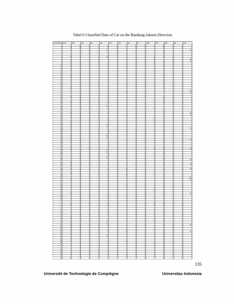
135
Université de Technologie de Compiègne Universitas Indonesia
Tabel 6 Classified Data of Car on the Bandung-Jakarta Direction
Respondent TtoU PoU SoC IoC CoC TtiU PiU SiC IiC TtdU PdU SdC IdC CdC
1 7 8 6 6 6 3 7 6 6 7 8 6 6 7
2 8 8 6 6 6 6 7 6 6 7 8 6 6 7
3 8 8 6 6 5,5 6 5 6 6 7 8 6 6 6,5
4 7 8 6 6 6 6 7 6 6 7 8 6 6 7
5 7 8 6 6 6 6 5 6 6 7 8 6 6 7
6 8 8 4 4 5,5 6 7 4 4 5 8 6 6 7
7 7 7 6 6 6 5 5 6 6 8 7 6 6 6,5
8 8 8 6 6 6 3 7 6 6 8 8 6 6 6,5
9 8 8 6 6 6 3 4 6 6 8 8 6 6 7
10 8 8 6 6 6 3 7 6 6 5 8 6 6 7
11 7 8 6 6 6 5 5 6 6 5 7 6 6 7
12 8 8 6 6 5 8 5 6 6 8 8 6 6 7
13 7 8 6 6 6 5 7 6 4 5 7 4 6 7
14 8 8 6 6 6 6 7 6 6 7 8 6 6 7
15 8 8 6 6 6 6 7 4 6 8 8 6 6 7
16 5 8 6 6 6 5 7 4 6 8 8 6 6 7
17 5 7 6 6 6 5 7 6 6 7 8 6 6 7
18 7 8 6 6 6 3 4 6 6 7 8 6 6 7
19 7 8 6 6 6 7 7 6 6 7 7 6 6 7
20 8 8 6 6 6 3 7 6 6 7 8 6 6 7
21 7 8 6 6 6 3 7 6 6 7 7 6 6 6,5
22 7 8 6 6 6 3 6 6 6 7 7 6 6 6,5
23 7 8 6 6 6 6 7 6 6 7 7 6 6 7
24 8 8 6 6 6 5 7 6 6 7 8 6 6 7
25 7 8 6 6 6 5 7 6 6 7 8 6 6 6
26 8 8 6 6 6 5 7 6 4 6 8 6 6 7
27 7 8 6 6 6 5 7 6 6 7 8 6 6 7
28 8 8 6 6 4,5 5 7 6 6 7 7 6 6 7
29 7 8 6 6 6 5 7 6 6 6 7 6 6 7
30 7 8 6 6 6 5 7 6 6 7 8 6 6 7
31 8 8 6 6 6 6 7 6 6 7 8 6 6 5,5
32 7 8 6 6 6 5 2 6 6 7 8 6 6 6,5
33 8 8 6 6 6 3 7 4 4 5 8 4 6 7
34 7 8 6 6 6 3 7 4 4 8 8 6 6 7
35 8 8 6 6 6 5 7 6 6 8 8 6 6 7
36 8 8 6 6 6 3 4 4 6 7 8 4 4 7
37 8 8 6 6 5,5 5 5 4 6 5 8 6 6 7
38 8 8 6 6 6 5 7 6 6 7 8 6 6 6,5
39 8 8 6 6 6 6 7 4 6 5 8 4 6 7
40 7 8 6 6 6 6 7 6 6 7 8 6 6 7
41 8 8 6 6 5,5 7 6 6 6 7 8 6 6 7
42 8 8 6 6 5,5 6 7 6 6 7 8 6 6 7
43 8 8 6 6 6 5 7 6 6 7 8 4 6 6,5
44 8 8 6 6 6 6 7 6 6 7 8 6 6 7
45 7 8 6 6 6 5 7 4 4 7 8 6 6 7
46 6 8 6 6 6 5 7 4 4 7 8 6 6 7
47 3 7 6 6 6 3 7 6 6 8 8 6 6 6,5
48 8 8 6 6 6,5 6 5 6 6 7 8 6 6 7
49 7 8 6 6 5,5 1 1 6 6 5 8 6 6 7
50 7 8 6 6 6 6 5 6 6 8 8 6 6 7
51 7 8 6 6 5,5 2 5 6 6 7 8 6 6 7
52 7 8 6 6 6 5 7 6 6 7 8 6 6 6,5
53 8 8 6 6 6 6 7 6 6 7 8 6 6 7
54 8 8 6 6 6 5 7 6 6 7 8 6 6 6,5
55 8 8 6 6 6 5 7 6 4 7 8 6 6 7
56 8 8 6 6 6 3 8 6 4 7 8 6 6 6,5
57 7 8 6 6 6 6 8 6 6 7 8 6 6 7
58 8 8 6 6 6 3 7 6 6 6 8 6 6 7
59 7 8 6 6 6 3 8 6 4 7 8 6 6 7
60 7 8 6 6 6 5 7 6 6 7 8 6 6 6,5
61 8 8 6 6 6 5 7 6 6 7 8 6 6 6,5
62 7 8 6 6 6 5 7 6 6 7 8 6 6 7
63 7 8 6 6 6 5 8 6 6 7 8 6 6 7
64 7 8 6 6 6 3 7 6 6 7 8 6 6 7
65 7 8 6 6 6 6 7 6 6 8 8 6 6 7
66 7 8 6 6 6 5 7 6 6 6 8 6 6 7
67 8 8 4 6 6 3 7 6 6 5 8 6 6 6,5
68 7 8 6 6 6 2 5 4 6 7 8 4 6 7
69 7 8 6 6 6 6 5 6 6 8 8 6 6 7
70 7 8 4 6 6 3 5 6 6 7 8 4 6 7
71 7 8 6 6 6 5 7 6 6 5 8 6 6 7
72 8 8 6 6 6 5 7 6 6 8 8 6 6 7
73 7 8 4 6 6 5 5 6 6 7 8 6 6 7
74 7 8 6 6 6 5 7 6 6 7 8 6 6 7
75 5 8 4 6 6 5 7 6 6 8 8 6 6 7
76 7 8 6 6 6 5 7 6 6 5 8 6 6 7
77 7 8 4 6 6 6 7 4 6 5 8 4 4 7
78 8 8 4 6 6 3 5 4 6 8 8 6 6 7
79 7 8 6 6 6 3 7 6 6 8 8 6 6 7
80 8 8 6 6 5,5 6 7 6 6 5 8 6 6 7
81 8 8 6 6 6 5 7 6 6 7 8 6 6 6,5
82 8 8 6 6 6 5 7 6 6 7 8 6 6 7
83 8 8 6 6 6 6 8 6 4 8 8 6 6 7
84 8 8 6 6 6 5 8 6 4 7 8 6 6 6,5
85 8 8 6 6 6 5 7 6 6 7 8 6 6 7
86 7 8 6 6 5,5 3 7 6 6 7 8 6 6 7
87 6 8 6 6 6 5 7 6 6 7 8 6 6 7
88 8 8 4 4 6 7 8 4 4 7 8 6 6 7
89 7 8 4 4 6 5 7 6 4 6 8 6 6 7
90 7 8 6 6 6 3 7 6 6 6 8 6 6 7
91 7 8 6 6 6 5 7 6 6 5 8 6 6 7
92 7 8 6 6 6 3 7 6 6 7 8 6 6 7
93 7 8 6 6 6 3 7 6 6 7 8 6 6 7
94 6 8 6 6 6 3 7 6 6 7 8 6 6 7
95 7 8 6 6 6 5 8 6 4 6 8 6 6 7
96 8 8 6 6 6 3 7 6 6 7 8 6 6 7