Th ese - unilim.fr · postes d’ater a l’universit e de Paris xii ainsi que Marc Giusti qui...
198
UNIVERSIT ´ E DE LIMOGES ´ ECOLE DOCTORALE Science – Technologie – Sant´ e FACULT ´ E des sciences et techniques Laboratoire d’Arithm´ etique, de Calcul formel et d’Optimisation Th` ese pour obtenir le grade de DOCTEUR DE L’UNIVERSIT ´ E DE LIMOGES Discipline : Math´ ematiques Sp´ ecialit´ e : Calcul formel pr´ esent´ ee et soutenue par Thomas CLUZEAU le 23 septembre 2004 Algorithmique modulaire des ´ equations diff´ erentielles lin´ eaires Th` ese dirig´ ee par Moulay A. Barkatou et Jacques-Arthur Weil Jury Rapporteurs Anne Duval, Professeur ` a l’universit´ e de Lille Mark Giesbrecht, Professeur ` a l’universit´ e de Waterloo (Canada) Examinateurs Manuel Bronstein, Directeur de recherche ` a l’INRIA Mark van Hoeij, Professeur ` a l’universit´ e d’´ etat de Floride (E.-U.) Jean-Pierre Ramis, Professeur ` a l’universit´ e de Toulouse Bruno Salvy, Directeur de recherche ` a l’INRIA Directeurs Moulay A. Barkatou, Professeur ` a l’universit´ e de Limoges Jacques-Arthur Weil, Maˆ ıtre de conf´ erences ` a l’universit´ e de Limoges
Transcript of Th ese - unilim.fr · postes d’ater a l’universit e de Paris xii ainsi que Marc Giusti qui...

UNIVERSITE DE LIMOGESECOLE DOCTORALE Science – Technologie – Sante
FACULTE des sciences et techniques
Laboratoire d’Arithmetique, de Calcul formel et d’Optimisation
Thesepour obtenir le grade de
DOCTEUR DE L’UNIVERSITE DE LIMOGES
Discipline : Mathematiques Specialite : Calcul formel
presentee et soutenue
par
Thomas CLUZEAU
le 23 septembre 2004
Algorithmique modulaire des equations
differentielles lineaires
These dirigee par Moulay A. Barkatou et Jacques-Arthur Weil
Jury
Rapporteurs Anne Duval, Professeur a l’universite de LilleMark Giesbrecht, Professeur a l’universite de Waterloo (Canada)
Examinateurs Manuel Bronstein, Directeur de recherche a l’INRIA
Mark van Hoeij, Professeur a l’universite d’etat de Floride (E.-U.)Jean-Pierre Ramis, Professeur a l’universite de ToulouseBruno Salvy, Directeur de recherche a l’INRIA
Directeurs Moulay A. Barkatou, Professeur a l’universite de LimogesJacques-Arthur Weil, Maıtre de conferences a l’universite de Limoges

Remerciements
Cette these a ete preparee entre 2000 et 2004 au sein du Laboratoire d’Arithmetique,Calcul formel et Optimisation (laco) de l’universite de Limoges et a ete financee, de2000 a 2003, par la region Limousin.
De nombreuses personnes ont participe, plus ou moins directement, a la reussite decette these : je vais essayer de vous les presenter en esperant n’oublier personne.
Pourquoi une these en calcul formel ? En effectuant un retour quatre ans en arriere,je m’apercois que trois personnes ont contribue directement au fait que je me sois lancedans une these en calcul formel : tout d’abord, au cours de ma maıtrise a Limoges, j’aiete fascine par la maniere avec laquelle Jacques-Arthur Weil conduisait son cours decalcul formel ; malgre des horaires matinaux, il reussissait toujours a rendre le coursvivant et ce grace a un enthousiasme hors du commun. Ensuite, durant mon dea, j’aieu la chance de suivre un cours de Jean-Claude Yakoubsohn. La encore, j’ai senti queplus que nous transmettre des connaissances, l’orateur nous faisait partager sa passion.Enfin, Evelyne Hubert a dirige mon stage de dea et donc, en quelque sorte, guide mespremiers pas dans la recherche. Ce stage a certainement servi de declic au depart decette aventure ; elle y est donc pour beaucoup. Ces trois personnes sont a l’origine decette these et je leur en suis donc tres reconnaissant.
Jacques-Arthur Weil m’a propose un sujet de these ouvert et passionnant. Toutau long de ce travail, ses encouragements, son enthousiasme debordant et sa curiositescientifique ont toujours reussi a stimuler ma motivation. Il a su diriger ce travail memelors des deux annees qu’il a passe a Nice et nos conversations, scientifiques ou non, ontete une aide precieuse pour moi. Qu’il accepte tous mes remerciements et ma reconnais-sance.
Cette these etait deja commencee depuis un an lorsque Moulay Barkatou est ar-rive a Limoges. Cependant, grace a ses larges connaissances mathematiques, il a suimmediatement proposer des directions de recherche qui se sont averees fructuseuses.Sa rigueur scientifique m’a toujours aidee a clarifier les problemes. Elle a aussi permisde canaliser les «delires utopiques» de Jacques-Arthur. Il n’a cesse de repondre, avecentrain, a mes questions et ce, dans un climat des plus convivial. Qu’il trouve ici l’ex-pression de ma gratitude.
Mark van Hoeij peut, en quelque sorte, etre considere comme mon troisieme direc-teur de these. Il m’a accueilli deux mois chez lui a Tallahassee (en Floride) et a ainsipu me faire profiter de toutes ses connaissances et me communiquer sa passion pourla recherche. Il a co-signe avec moi deux articles qui constituent les chapitres deux ettrois de cette these. Sans lui, ce travail n’existerait pas et c’est donc un immense plaisirpour moi qu’il participe a mon jury. Je profite de l’occasion pour remercier aussi safemme Susan pour l’accueil formidable qu’elle m’a reserve lors de mes deux sejours a
iii
iv
Tallahassee.
Depuis mon stage de dea, j’ai eu la chance d’etre invite plusieurs fois au projetcafe de l’inria de Sophia Antipolis. Lors de ces sejours, Manuel Bronstein m’a reserveun accueil chaleureux. De plus, il a toujours montre beaucoup d’interet pour mon tra-vail et m’a, a de nombreuses reprises, donne des conseils tres pertinents. Je tiens a l’enremercier et je suis tres honore qu’il ai accepte de participer a mon jury.
L’annee que j’ai passe au laboratoire stix de l’Ecole polytechnique m’a permis decotoyer Bruno Salvy. Lors des seances de travail que nous avons pu partager, il a tou-jours repondu, avec entrain et dans un climat tres convivial, aux nombreuses questions(parfois tres naıves) que j’ai pu lui poser. Je suis heureux qu’il ait bien voulu participera mon jury.
Je suis tres reconnaissant a Anne Duval et Mark Giesbrecht d’avoir accepte d’etrerapporteurs ; je les remercie d’avoir lu, en details, cette these et d’avoir ainsi temoignede l’attention a mes travaux. Leurs remarques judicieuses ont permis d’ameliorer laqualite de ce memoire.
C’est un immmense honneur pour moi que Jean-Pierre Ramis ait accepte de prendrepart a mon jury et qu’il ait ainsi montre de l’interet a mon travail. Je lui en suis tresreconnaissant.
Les articles de Marius van der Put ont servi de point de depart a mon travail. Aucours de ma these, il m’a donne certaines directions de recherche tres pertinentes. Qu’ilen soit remercie.
L’environement de travail est un ingredient indispensable a la reussite d’une these.J’ai passe mes trois premieres annees dans le «bureau vert» en compagnie de MatthieuLefloc’h et Mikael Lescop. Il y a toujours reigne une ambiance tres detendue, parfoispeut etre meme trop en certaines periodes ou la non-motivation de l’un des trois sepropageait chez les autres. Meme si nous avions rarement le meme point de vue surles actualites du monde du football ou du tennis, nous nous retrouvions toujours surla meme longueur d’onde a l’approche de l’ete ou le bureau devenait le siege du fan-club de Jan Ullrich. Je les remercie donc tous les deux pour avoir fait que cette thesese deroule dans les meilleurs conditions et je leur souhaite bon courage pour l’avenir.Je souhaite aussi bon courage au nouvel habitant du bureau Guilhem Castagnos, quirentre parfaitement dans l’esprit «bureau vert».
J’ai cohabite pendant plus de trois ans avec les membres du laco. Je tiens a re-mercier les anciens et actuels thesards (Ma « grande soeur de recherche» DelphineBoucher, Cyril Brunie, Laurent Dubreuil, Meriem Heraoua, Nicolas Le Roux, SamuelMaffre, Carmen Nedeloaia, Ayoub Otmani, Philippe Segalat et Cyril Vervoux) pour leursoutien permanent, tous les membres de l’equipe calcul formel ainsi qu’Alexandre Ca-
v
bot, Philippe Gaborit (pour ses conseils souvent pertinents), Henri Massias, AbdelkaderNecer et Stephane Vinatier. Je remercie tout particulierement Yolande Vieceli dont ladisponibilite et la bonne humeur contribuent pleinement a l’ambiance joyeuse qui regnedans les couloirs du batiment de mathematiques : que deviendrait le laco sans elle ? Jeremercie enfin Martine Guerletin, Sylvie Laval, Nadine Tchefranoff et Patricia Vareillepour leur sympathie et la maniere avec laquelle elles ont contribue a me faciliter lestaches administratives.
J’ai passe ma quatrieme annee de these au sein du laboratoire stix de l’Ecole po-lytechnique. Je remercie Jean-Moulin Ollagnier qui a soutenu mes candidatures sur lespostes d’ater a l’universite de Paris xii ainsi que Marc Giusti qui m’a accueilli dansson laboratoire et m’a ainsi fait beneficier de conditions de travail ideales. Je remercieXavier Dahan, Anne Fredet et Pierre Midy qui ont ete mes collegues de bureau pendanttoute cette annee. Mention speciale a ma «deuxieme grande soeur de recherche» AnneFredet avec qui travailler est toujours un plaisir et ce malgre nos divergences de pointde vue sur de nombreux sujets (en fait presque sur tout !). Une grande partie du qua-trieme chapitre est un travail realise en collaboration avec elle et elle a donc fortementcontribue a la reussite de cette these. Je remercie aussi Alin Bostan pour s’etre interessea mon travail depuis le debut et avec qui il est toujours tres agreable de travailler. Jen’oublie pas tous les autres membres du laboratoire stix et tout particulierement KilianCavalotti, Nicole Dubois, Christian Flech, Pierre Lafon (peut etre mon futur colleguede location de pedalos aux Bahamas), Gregoire Lecerf, Francois Ollivier, Eric Schost etBernd Wiebelt.
Je remercie aussi Jean-Baptiste Aubin et Edouard Pennamen avec qui ce fut ungrand plaisir de travailler a Paris xii ainsi que Jean-Marie Aubry pour m’avoir permisd’enseigner des matieres tout a fait interessantes.
Durant ma these, j’ai ete amene a beaucoup voyager, soit pour assister a desconferences, soit pour participer a des seminaires. Cela m’a permis de rencontrer plu-sieurs personnes que je souhaite remercier : Alban Quadrat, Raphael Bomboy, GwenoleArs, Olivier Cormier, Solen Corvez, Felix Ulmer, Philippe Aubry, Magali Bardet, Mo-hab Safey El Din, Guenael Renault, Philippe Trebuchet, Olivier Ruatta, GuillaumeCheze, Frederic Chyzak, Ha Le, Ludovic Meunier (merci pour la visite guidee des envi-rons d’un hopital de Philadelphie), A. H. M. Levelt, Elie Compoint (a qui j’ai reussi afaire apprecier un disque de heavy metal), B. Heinrich Matzat, Julia Hartmann, Jorisvan der Hoeven, Georges Labahn, Claude-Pierre Jeannerod, Jean-Guillaume Dumas,Yang Zhang et Sergei A. Abramov.
Tout au long de cette these, j’ai eu la chance de pouvoir toujours compter sur mafamille et mes amis. Meme si leur contribution a ce travail paraıt moindre, je suis per-suade qu’en m’accompagnant dans la vie de tous les jours, ils m’ont permis de menercette these a termes dans les meilleurs conditions. Je remercie donc chaleureusementmes parents, mon frere et Genevieve ainsi que toute ma famille, mon «brother of me-
vi
tal» Franck ainsi que sa femme Sophie, sans oublier Marie, Valentine et Victor, Pierre(dit « le tocard»), Karine, Anne, David et toute la famille Aubreton, sans oublier So-phie, Richard et la famille Auroux. J’ai une pensee pour tous mes amis du Tennis Clubde Feytiat (certains etant aussi d’excellents camarades de soirees !) : Ben «Poupoune»
Fredon, Pierre Miran et sa femme Sandrine (c’est bon ca !), Bruno Bernard-Coffre, Da-vid Petitet, Olivier Carpe (alias Tony Montana), Xavier Chanut et Laurence Dartois(aussi connue sous les pseudos de Kim ou Abby), ainsi que pour tous ceux avec quij’ai eu la chance de partager d’autres grandes soirees : Eric, Carole, Pascal et la familleBeyssac, Charles, Alexandra, Hugues et la famille Francois, Arnaud «Nono» Boscheret le grand «Gourou» Emmanuel Cadic (pour les soirees de meditation au temple),Francois Delost et Maude Guillot (entre autre pour les soirees degustation de petitepoire . . . ca va me manquer !), les deux autres membres de la couinche ligue, i. e., GillesReynaud et Xavier Sidot, Steph’ et Guillaume de l’O’brien Tavern pour leur accueiltoujours formidable, Sandra pour sa folie de tous les instants, Delphine, Christophe,Jean-Marc, Matmaz, toute la grande troupe du water-polo limougeaud (les filles, lesgars sans oublier Jerome et Charles), PSG (aussi surnomme Jean-Pierre Bacri ou POBpour Philippe of O’Brien), Christian Vincon, Sylvain Jeamot et Marc de Roos, mesamis physiciens (personne n’est parfait) Benoıt Brousse et Matthieu Valetas et touteautre personne avec qui j’ai pu passer des bons moments.
Enfin je remercie tous les groupes de heavy metal de la planete pour tout le plaisirqu’ils me procurent a travers leurs disques et leurs concerts :
“Heavy Metal is the law that keeps us all united freeA law that shatters earth and hell
Heavy Metal can’t be beaten by any dynastyWe’re all wizards fightin’ with our spell”
(M. Weikath, K. Hansen)
Table des matieres
Introduction generale 1
1 Factorisation en caracteristique p 111.1 Generalites . . . . . . . . . . . . . . . . . . . . . . . . . . . . . . . . . . 13
1.1.1 Corps et systemes differentiels . . . . . . . . . . . . . . . . . . . . 131.1.2 Operateur et module differentiel associe . . . . . . . . . . . . . . . 141.1.3 Correspondance Systeme/Operateur scalaire . . . . . . . . . . . . 141.1.4 D’autres definitions . . . . . . . . . . . . . . . . . . . . . . . . . . 161.1.5 Factorisation de systemes differentiels . . . . . . . . . . . . . . . . 161.1.6 Systemes differentiels en caracteristique p . . . . . . . . . . . . . . 18
1.2 Solutions rationnelles . . . . . . . . . . . . . . . . . . . . . . . . . . . . . 191.2.1 Cas d’un systeme . . . . . . . . . . . . . . . . . . . . . . . . . . . 191.2.2 Cas d’un operateur scalaire . . . . . . . . . . . . . . . . . . . . . 21
1.3 La p-courbure d’un systeme differentiel lineaire . . . . . . . . . . . . . . . 221.3.1 Definition et calcul . . . . . . . . . . . . . . . . . . . . . . . . . . 221.3.2 Classification des modules differentiels . . . . . . . . . . . . . . . 241.3.3 Systemes ayant une p-courbure nulle . . . . . . . . . . . . . . . . 251.3.4 Systemes ayant une p-courbure scalaire . . . . . . . . . . . . . . . 261.3.5 Solutions rationnelles et p-courbure . . . . . . . . . . . . . . . . . 29
1.4 L’eigenring d’un systeme differentiel lineaire . . . . . . . . . . . . . . . . 331.4.1 Definition et calcul . . . . . . . . . . . . . . . . . . . . . . . . . . 331.4.2 Eigenring et p-courbure . . . . . . . . . . . . . . . . . . . . . . . 34
1.5 Decomposition maximale . . . . . . . . . . . . . . . . . . . . . . . . . . . 351.5.1 Decomposition isotypique . . . . . . . . . . . . . . . . . . . . . . 361.5.2 Le cas χ(Ap) = F m . . . . . . . . . . . . . . . . . . . . . . . . . . 38
1.6 Le cas indecomposable . . . . . . . . . . . . . . . . . . . . . . . . . . . . 421.7 Generalisations immediates . . . . . . . . . . . . . . . . . . . . . . . . . . 44
1.7.1 Factorisation « locale» . . . . . . . . . . . . . . . . . . . . . . . . 451.7.2 Factorisation de systemes d’equations aux differences . . . . . . . 45
1.8 Factorisation de systemes d’E. aux D. P. . . . . . . . . . . . . . . . . . . 461.8.1 Systemes D-finis . . . . . . . . . . . . . . . . . . . . . . . . . . . 471.8.2 Factorisation et eigenrings . . . . . . . . . . . . . . . . . . . . . . 481.8.3 Systemes d’e.d.p. en caracteristique p . . . . . . . . . . . . . . . . 491.8.4 Factorisation de systemes d’e.d.p. en caracteristique p . . . . . . . 52
vii
viii TABLE DES MATIERES
1.8.5 Reduction simultanee de matrices qui commutent . . . . . . . . . 55
2 Solutions Exponentielles d’E. D. L. 652.1 Preliminaries . . . . . . . . . . . . . . . . . . . . . . . . . . . . . . . . . 68
2.1.1 Differential operators in characteristic zero . . . . . . . . . . . . . 682.1.2 Differential operators in characteristic p . . . . . . . . . . . . . . 712.1.3 Reduction modulo p and factorization . . . . . . . . . . . . . . . . 72
2.2 Examples . . . . . . . . . . . . . . . . . . . . . . . . . . . . . . . . . . . 742.2.1 Example 1 . . . . . . . . . . . . . . . . . . . . . . . . . . . . . . . 742.2.2 Example 2 . . . . . . . . . . . . . . . . . . . . . . . . . . . . . . . 752.2.3 Example 3 . . . . . . . . . . . . . . . . . . . . . . . . . . . . . . . 75
2.3 Roots of χp(L) and τ -reduced terms . . . . . . . . . . . . . . . . . . . . . 762.4 Exponential solutions and roots of χp(L) . . . . . . . . . . . . . . . . . . 78
2.4.1 Classes of exponential solutions . . . . . . . . . . . . . . . . . . . 782.4.2 Links between Cl(L) and R(χp(L)) . . . . . . . . . . . . . . . . . 79
2.5 Modular improvements of the combinatorial problem . . . . . . . . . . . 802.5.1 Some precisions on the vocabulary . . . . . . . . . . . . . . . . . 802.5.2 Finding C-combinations matching the modular information . . . . 822.5.3 Some remarks on the choice of p . . . . . . . . . . . . . . . . . . . 842.5.4 Finding all exponential solutions defined over a given field . . . . 84
2.6 A way to handle the field problem . . . . . . . . . . . . . . . . . . . . . . 862.6.1 Two ways to obtain bounds . . . . . . . . . . . . . . . . . . . . . 862.6.2 An algorithm to find an exponential solution over an algebraic
extension . . . . . . . . . . . . . . . . . . . . . . . . . . . . . . . 892.7 An algorithm to find all exponential solutions . . . . . . . . . . . . . . . 92
2.7.1 Some remarks on the algorithm . . . . . . . . . . . . . . . . . . . 962.7.2 Computing radical solutions . . . . . . . . . . . . . . . . . . . . . 982.7.3 Almost all primes . . . . . . . . . . . . . . . . . . . . . . . . . . . 98
3 Solutions Hypergeometriques d’E. aux D. L. 1013.1 Hypergeometric terms . . . . . . . . . . . . . . . . . . . . . . . . . . . . 1033.2 The symmetric product . . . . . . . . . . . . . . . . . . . . . . . . . . . . 1053.3 What does it mean to be a finite singularity ? . . . . . . . . . . . . . . . 1073.4 How to compute gp(L) for finite p. . . . . . . . . . . . . . . . . . . . . . 1093.5 How to compute g∞(L). . . . . . . . . . . . . . . . . . . . . . . . . . . . 1133.6 Representing the finite singularities . . . . . . . . . . . . . . . . . . . . . 1173.7 Computing e-solutions . . . . . . . . . . . . . . . . . . . . . . . . . . . . 1183.8 Computing a hard solution . . . . . . . . . . . . . . . . . . . . . . . . . . 1203.9 An algorithm to find all hypergeometric solutions . . . . . . . . . . . . . 123
3.9.1 Some possible improvements . . . . . . . . . . . . . . . . . . . . . 1263.10 Modular improvements . . . . . . . . . . . . . . . . . . . . . . . . . . . . 127
3.10.1 Difference operators in characteristic p . . . . . . . . . . . . . . . 1273.10.2 Local types at infinity and R(χp(L)) . . . . . . . . . . . . . . . . 1283.10.3 How to improve HypSols using the p-curvature ? . . . . . . . . . . 130
TABLE DES MATIERES ix
3.11 Computation timings . . . . . . . . . . . . . . . . . . . . . . . . . . . . . 1313.12 An analogue algorithm for q-difference equations . . . . . . . . . . . . . . 132
3.12.1 Local types . . . . . . . . . . . . . . . . . . . . . . . . . . . . . . 1333.12.2 Fuchs’ relations . . . . . . . . . . . . . . . . . . . . . . . . . . . . 134
4 Solutions polynomiales d’E. D. L. 1354.1 Preliminaires sur les solutions polynomiales . . . . . . . . . . . . . . . . . 136
4.1.1 Equation aux recurrences associee . . . . . . . . . . . . . . . . . . 1364.1.2 Degre des solutions polynomiales . . . . . . . . . . . . . . . . . . 138
4.2 Calcul en caracteristique zero . . . . . . . . . . . . . . . . . . . . . . . . 1384.2.1 Resoudre le systeme lineaire associe . . . . . . . . . . . . . . . . . 1384.2.2 L’algorithme d’Abramov, Bronstein et Petkovsek . . . . . . . . . 1394.2.3 L’algorithme de Barkatou . . . . . . . . . . . . . . . . . . . . . . 141
4.3 Calcul en caracteristique p . . . . . . . . . . . . . . . . . . . . . . . . . . 1474.3.1 A partir des solutions rationnelles . . . . . . . . . . . . . . . . . . 1474.3.2 Solutions polynomiales ayant un degre donne . . . . . . . . . . . . 149
4.4 Tester la non-existence . . . . . . . . . . . . . . . . . . . . . . . . . . . . 1504.4.1 Test rapide . . . . . . . . . . . . . . . . . . . . . . . . . . . . . . 1504.4.2 Un nouveau test modulaire . . . . . . . . . . . . . . . . . . . . . . 152
4.5 Reconstruction . . . . . . . . . . . . . . . . . . . . . . . . . . . . . . . . 1544.5.1 Bases echelonnees . . . . . . . . . . . . . . . . . . . . . . . . . . . 1554.5.2 Nombres premiers pertinents . . . . . . . . . . . . . . . . . . . . . 1564.5.3 Comment combiner les solutions polynomiales modulo plusieurs
premiers ? . . . . . . . . . . . . . . . . . . . . . . . . . . . . . . . 1584.6 Algorithme modulaire . . . . . . . . . . . . . . . . . . . . . . . . . . . . 160
4.6.1 Borne sur la taille des coefficients . . . . . . . . . . . . . . . . . . 1604.6.2 Algorithme . . . . . . . . . . . . . . . . . . . . . . . . . . . . . . 162
4.7 Conclusion et perspectives . . . . . . . . . . . . . . . . . . . . . . . . . . 164
Appendice : implantation 169
Bibliographie 179

x TABLE DES MATIERES
Introduction generale
Cadre et sujet de cette these
Une equation differentielle lineaire homogene d’ordre n (n entier naturel) peuts’ecrire sous la forme
an y(n) + an−1 y(n−1) + · · ·+ a1 y′ + a0 y = 0, (1)
ou les ai sont des fonctions de la variable x et ou y(i) designe la derivee i-eme de ypar rapport a x. De telles equations apparaissent naturellement lorsque l’on cherche adecrire certains phenomenes physiques et ont, par consequent, ete largement etudiees. Sil’on s’interesse au probleme suivant : etant donne les coefficients a0, . . . , an, determinerles « solutions » de l’equation (1), alors le terme « solution » doit etre prealablementprecise. En effet, selon la forme des solutions que l’on recherche, les outils a utiliserpeuvent etre tres differents. D’autre part, en fonction des proprietes des phenomenesdecrits par cette equation que l’on cherche a degager, certaines formes de solutionsseront plus adaptees que d’autres. Dans ce memoire, nous considererons principalementdes solutions « sous forme close» c’est-a-dire exprimables de maniere exacte a l’aide defonctions usuelles.
Les methodes modulaires ont deja montre leur interet dans diverses branches ducalcul formel en donnant naissance a de nombreux algorithmes performants (voir [GG99,Chapitre 5]). Par exemple, a ce jour, l’algorithme le plus efficace pour factoriser despolynomes a coefficients dans Z est l’algorithme modulaire developpe par van Hoeijdans [Ho02]. Le schema de fonctionnement general de ces methodes modulaires est lesuivant :
– Reduire le probleme a son analogue en caracteristique p,– Resoudre le probleme en caracteristique p,– Reconstruire la solution du probleme initial en caracteristique zero.
Un des interets majeurs de ces methodes est que resoudre un probleme en caracteristiquep est souvent plus simple qu’en caracteristique zero : le principal avantage est qu’encaracteristique p, la taille des entiers qui interviennent dans les calculs intermediairesest controlee.
La theorie des equations differentielles en caracteristique p a beaucoup ete etudieedans les annees soixante-dix et quatre-vingt par des mathematiciens comme Katz,Honda ou les Chudnovsky (voir par exemple [Ka70, Ho81, CC85]). Un theme centralde ces travaux etait la conjecture de Grothendieck (voir Conjecture 1 dans le chapitre1 et les references donnees a cet endroit) sur les p-courbures. Cependant, la litterature
1
2 INTRODUCTION GENERALE
concernant l’algorithmique modulaire des equations differentielles lineaires est assez res-treinte : ce n’est que dans les annees quatre-vingt-dix, dans les travaux de van der Put([Pu95, Pu96, Pu97]-voir aussi [PS03, Chapitre 13]) que l’on trouve les premieres ideesdans cette direction.
Dans cette these, nous nous proposons d’etudier et developper une approche algo-rithmique modulaire pour l’etude des equations differentielles lineaires. Par consequent,les questions generales se trouvant a la base de ce travail sont du type : peut-on contruiredes algorithmes modulaires efficaces pour etudier les equations differentielles lineaires ?Quel type d’informations peut-on esperer d’un calcul modulaire ? Peut-on a l’aide decalculs modulaires ameliorer les algorithmes existant ?
Factorisation d’operateurs differentiels lineaires
Un premier probleme naturel a regarder d’un point de vue modulaire est celui dela factorisation d’operateurs differentiels lineaires. A l’equation differentielle lineairehomogene (1), on associe l’operateur differentiel lineaire
L = an ∂n + an−1 ∂n−1 + · · ·+ a1 ∂ + a0, (2)
agissant sur y. Si les coefficients ai appartiennent a K = C(x) pour un certain corps denombre C ⊆ Q (ou Q represente la cloture algebrique du corps Q des nombres ration-nels), alors L appartient a l’anneau non-commutatif K[∂] dans lequel la multiplicationest definie par ∂ x = x ∂+1. Cet anneau est euclidien a droite (et a gauche) et factoriserl’operateur L donne des informations sur les solutions de l’equation (1). Par exemple unfacteur a droite d’ordre un ∂−r de L avec r appartenant a Q(x) correspond a une solu-tion exponentielle y = exp(
∫
r) de (1), i. e., une solution dont la derivee logarithmiquey′/y = r appartient a Q(x).
Le probleme de la reductibilite d’equations differentielles lineaires est apparu dansla deuxieme partie du dix-neuvieme siecle lorsque l’on a cherche a developper unetheorie pour etudier les equations differentielles analogue a celle de Lagrange et Galoispour les equations algebriques. Le probleme plus specifique de la factorisation effectived’operateurs differentiels lineaires a ete tres etudie depuis le debut des annees quatre-vingt-dix. A ce jour, il existe essentiellement trois types de methodes pour aborder ceprobleme. La premiere remonte aux travaux de Beke a la fin du dix-neuvieme siecle([Be1894]) et a ete amelioree dans les annees quatre-vingt-dix ([Sc89, Br94, Ts94]-voiraussi [PS03, 4.2.1]). Elle revient a considerer des puissances exterieures de l’operateur,a en calculer les solutions exponentielles puis a verifier des conditions de Plucker. Unedeuxieme approche est apparue aussi a la fin des annees quatre-vingt-dix : van Hoeij([Ho97a, Ho97b]) a propose un algorithme calculant tout d’abord des factorisationslocales de l’operateur puis les relevant en des factorisations globales. Une strategieanalogue traitant directement les systemes differentiels a ete developpee par Barka-tou et Pflugel dans [BP98]. Une troisieme methode communement attribuee a Sin-ger ([Si96]) date elle aussi des annees quatre-vingt-dix (voir [Gi98, Ba01, BP98] ou[PS03, 4.2.2]). Elle est basee sur un ensemble, appele eigenring, que l’on associe a unoperateur differentiel. Cet ensemble peut etre vu comme l’anneau des endomorphismes
INTRODUCTION GENERALE 3
differentiels associe a l’operateur et la connaissance d’elements non-triviaux dans cetensemble conduit directement a des factorisations de l’operateur. Notons que les idees ala base de cette troisieme approche apparaissent des les annees trente dans les travauxde Jacobson ([Ja37]).
Chapitre 1 : factorisation en caracteristique p
Dans l’optique de construire un algorithme modulaire de factorisation d’operateursdifferentiels, nous nous sommes tout d’abord concentres sur le probleme de la factorisa-tion en caracteristique p qui constitue le sujet du premier chapitre. Nous developponsun algorithme de factorisation de systemes differentiels en caracteristique p. Notonsqu’a toute equation differentielle lineaire homogene est associe un systeme differentiellineaire (sous forme compagnon) et reciproquement, a tout systeme differentiel lineaireest associee (via un vecteur cyclique) une equation differentielle lineaire homogene (voir[CK02]).
Pour ce faire, nous nous sommes tout d’abord interesses aux travaux de van derPut ([Pu95, Pu96, Pu97]), travaux qui a notre connaissance etaient alors les seuls exis-tants sur le probleme de la factorisation d’operateurs differentiels en caracteristiquep. Dans [Pu95], l’auteur montre qu’en caracteristique p, les modules differentiels sontentierement classifies par la forme de Jordan d’un objet qui leur est associe : la p-courbure. A partir de cette classification, le meme auteur a montre dans [Pu97] commentfactoriser des operateurs differentiels lineaires scalaires en caracteristique p. Ces travauxont resolu theoriquement le probleme de la factorisation d’operateurs differentiels en ca-racteristique p. Cependant, un travail algorithmique restait necessaire, notamment pourtraiter directement les systemes : ceci constitue le theme central de cette partie.
Pour developper un algorithme de factorisation de systemes differentiels lineairesen caracteristique p, nous utilisons les idees de [Pu97] mais nous exhibons aussi lesliens entre la p-courbure et l’eigenring ce qui nous permet de suivre l’approche proposeepar Barkatou dans [Ba01] qui ne depend pas de la caracteristique. Nous comparonsdifferentes strategies, fournissons une implantation (voir Annexe) et une analyse decomplexite. Nous contribuons a l’amelioration de la methode de van der Put : une foisque la decomposition isotypique de l’operateur a ete calculee alors, contrairement a l’al-gorithme de van der Put, nous utilisons l’eigenring tout entier pour eviter des calculspotentiellement couteux dans des extensions algebriques. Ceci mene a des methodes ra-tionnelles pour calculer a la fois une decomposition maximale et une reduction maximaledes blocs indecomposables.
Parallelement a notre travail, Giesbrecht et Zhang ont donne dans [GZ03] un al-gorithme de factorisation de polynomes de Ore (une classe d’operateurs contenant lesoperateurs differentiels lineaires) en caracteristique p. Toute cette partie constitue uneversion plus detaillee de l’article [Cl03].
Factorisation de systemes d’equations aux derivees partiellesD-finis en caracteristique p
Toujours dans ce premier chapitre, nous generalisons les methodes decrites ci-dessus
4 INTRODUCTION GENERALE
pour developper un algorithme de factorisation de systemes d’equations aux deriveespartielles D-finis en carateristique p. Le probleme de la factorisation effective de telssystemes a ete etudie recemment par Li, Schwarz et Tsarev qui ont montre commentadapter l’algorithme de Beke dans ce cas (voir [LST02, LST03] et aussi [Ts98, Ts01]).De tels systemes peuvent s’ecrire sous la forme S = {∂i(Y ) = Ai Y }1≤i≤m ou les Ai
sont des matrices carrees a coefficients dans Fp(x1, . . . , xm) et ∂i := ddxi
. La D-finitudeimplique que les systemes consideres verifient les conditions d’integrabilite donneespar : ∂i(Aj) − ∂j(Ai) + Ai Aj − Aj Ai = 0. Nous montrons comment l’algorithme quenous avons developpe dans le cas differentiel ordinaire, c’est-a-dire dans le cas ou nousn’avons qu’une seule derivation, peut s’appliquer ici pour factoriser individuellementchaque ∂i(Y ) = Ai Y . Ensuite nous utilisons l’hypothese de D-finitude pour ramener leprobleme a celui de la reduction simultanee de matrices qui commutent. Nous apportonsaussi notre contribution a l’etude de ce probleme en proposant une nouvelle approcheconsistant a considerer une combinaison lineaire a coefficients indetermines des matricesque nous cherchons a reduire simultanement.
Interlude : reconstruire des factorisations en caracteristique zero
La derniere etape d’une approche modulaire pour factoriser les operateurs differentielsconsiste a reconstruire, a partir de factorisations modulo p, des factorisations en ca-racteristique zero. Une fois encore, les seuls travaux existants sur ce sujet sont ceuxde van der Put. Dans [Pu96], il propose un algorithme modulaire pour factoriser lesoperateurs differentiels d’ordre 2. Cependant comme l’auteur le fait remarquer cet algo-rithme possede certaines limitations (a la fois theoriques et algorithmiques) qui font quetel quel il ne peut etre completement satisfaisant. Dans [Pu97], le meme auteur proposed’utiliser l’algorithme L.L.L. (voir [GG99, Chapitre 16] ou [LLL82]) pour reconstruireles facteurs mais ici encore, ceci ne semble pas mener a un algorithme modulaire completefficace.
Si l’on examine le probleme analogue dans le monde commutatif, i. e., la factorisationde polynomes alors on remarque que les algorithmes modulaires (Berlekamp-Zassenhaus[GG99, Chapitres 14 et 15]-[LLL82, Ho02]) suivent principalement le schema suivant :
– reduire les coefficients du polynome modulo un nombre premier p,– calculer les facteurs du polynome modulo p (algebre lineaire),– deduire des facteurs p-adiques (lemme de Hensel, [GG99, 15.4]),– recombiner les facteurs.
La terminaison des algorithmes de ce type repose sur l’existence de la borne de Mignotte(voir [GG99, Corollary 6.33]) sur la taille des coefficients des facteurs.
Si l’on cherche a adapter ce schema a notre cas, alors a partir de la troisieme etape,plusieurs problemes majeurs apparaissent. Tout d’abord, une remontee type Henseldans le cas des operateurs differentiels semble etre beaucoup moins simple que dansle cas des polynomes. En effet, supposons qu’un operateur differentiel L admette pourdeveloppement p-adique L = L0 + p L1 + · · · avec les Li ∈ Fp(x)[∂] et supposons quel’on dispose d’une factorisation mod p, L0 = M0 N0 . Si nous voulons relever cettefactorisation en une factorisation modulo p2 alors nous sommes ramenes a trouver M1
INTRODUCTION GENERALE 5
et N1 dans Fp(x)[∂] tels que L0 +p L1 = (M0 +p M1) (N0 +p N1) mod p2 : il vient doncM1 N0 + M0 N1 = L1 de sorte que M1 et N1 sont solutions d’une equation differentiellemixte (voir [Ho96]). On voit ainsi qu’a chaque etape d’une remontee type Hensel on estramene a resoudre une equation differentielle mixte ce qui s’avere assez couteux. Nousne disposons donc pas actuellement d’un procede efficace nous permettant de realiserune remontee type Hensel. Notons que pour ce probleme, une solution pourrait etre deconsiderer plutot que des equations differentielles modulo p, des equations differentiellesiteratives : cette notion introduite par Hasse et Schmidt dans les annees trente a etereprise recemment par Matzat et van der Put pour construire une (bonne) theoriede Picard-Vessiot en caracteristique positive ([Ma01, MP02] ou [PS03, 13.3.2]). D’autrepart, la phase de recombinaison est elle aussi beaucoup plus compliquee, essentiellementa cause du fait que, contrairement au cas des polynomes, la factorisation d’un operateurdifferentiel n’est pas unique. Par exemple ∂2 = (∂ + 1
x+c) (∂− 1
x−c) pour toute constante
c dans Q. Cette non-unicite de la factorisation rend tout aussi difficile la constructiond’une borne type Mignotte dans le cas differentiel.En consequence de ces problemes, nous allons par la suite chercher a degager le typed’informations pertinentes que l’on peut esperer obtenir d’un calcul modulaire et, utiliserces informations pour ameliorer certains algorithmes existants.
Chapitre 2 : solutions exponentiellesd’equations differentielles lineaires
Nous nous interessons ici au probleme du calcul de solutions exponentielles ou demaniere equivalente de facteurs a droite d’ordre 1. Nous considerons donc une equationdifferentielle homogene de la forme (1) ayant des coefficients dans C(x) ou C est un corpsde nombre quelconque. Pour calculer les solutions exponentielles d’une telle equation,l’algorithme communement utilise est celui de Beke qui remonte a la fin du dix-neuviemesiecle ([Be1894]-voir aussi [Ho97b, 3.4] ou [PS03, 4.1]). Un algorithme calculant directe-ment les solutions exponentielles d’un systeme differentiel lineaire a ete developpe parPflugel dans [Pf97].
L’algorithme de Beke peut etre decrit comme suit : tout d’abord, en chaque singula-rite de l’equation differentielle, nous calculons des objets appeles exposants generalisesqui ont deja ete utilises par van Hoeij dans [Ho97a, Ho97b]. Cette notion d’exposantsgeneralises est tres proche de la notion, plus connue, de «parties exponentielles lo-cales». Notons qu’en chaque singularite, ces exposants generalises sont en nombre finiegal a n. Ensuite pour chaque combinaison d’exposants generalises (choisir un exposantgeneralise a chaque singularite), le probleme est ramene au calcul des solutions polyno-miales (voir Chapitre 4) d’une equation differentielle auxiliaire. Tel quel, cet algorithmepossede deux principaux inconvenients :
– un probleme combinatoire : si l’on note m le nombre de singularites, nous avonsalors au plus nm combinaisons d’exposants generalises a tester,
– un probleme d’extensions algebriques : les singularites et les exposants generalisessont definis sur des extensions algebriques du corps de nombre C et par consequent
6 INTRODUCTION GENERALE
les combinaisons peuvent etre definies sur de grandes extensions algebriques deC : le degre de ces extensions peut atteindre m! nm (si on procede naivement).
Considerons l’operateur differentiel suivant :
L = 9(x3 − 2)5∂3 + (x3 − 2)(2x10 − 12x7 + 108x5 + 24x4 − 216x2 − 16x − 9)∂
−2x(190x6 − 274x3 − 27x − 212).
L possede trois singularites a distance finie a savoir les racines de x3 −2. En chacune deces 3 singularites les exposants generalises sont 2, 1
36α2
(x−α)− 1
18α et − 1
36α2
(x−α)+4+ 1
18α ou
α := RootOf(x3−2). A l’infini, les exposants generalises sont 0,− 53,−4
3. Par consequent,
l’algorithme de Beke aura 34 = 81 combinaisons a tester et certaines d’entre elles sontdefinies sur des extensions algebriques de degre 6 de Q.
Dans ce deuxieme chapitre, qui constitue un article ecrit avec M. van Hoeij (voir[CH04]), nous presentons un nouvel algorithme pour calculer les solutions exponentiellesd’equations differentielles lineaires ayant des coefficients dans C(x) ou C est un corps denombre quelconque. L’idee a la base de notre algorithme est de combiner des informa-tions locales et modulaires. Plus precisement, nous prouvons les liens entre la reductionmodulo p des exposants generalises et la p-courbure ce qui nous permet d’utiliser descalculs modulaires pour reduire le nombre de combinaisons a tester dans l’algorithmede Beke. Ceci s’avere d’autant plus interessant si les combinaisons eliminees sont cellesdefinies sur de grandes extensions algebriques. Pour pouvoir utiliser ces calculs mo-dulaires, nous avons besoin d’eviter certains nombres premiers : nous montrons donccomment calculer un «bon» nombre premier.
Revenons a l’operateur precedent. Le nombre premier p = 5 est un bon nombrepremier pour L. En cherchant parmi les exposants generalises ceux qui coıncident avecl’information encodee par la p-courbure, nous pouvons conclure qu’une solution expo-nentielle de L ne peut venir que d’une combinaison ou nous avons choisi l’exposantgeneralise 1
36α2
(x−α)− 1
18α en la singularite α. Ceci reduit donc le nombre de possibilites a
tester de 81 a 3 et de plus toutes les combinaisons definies sur des extensions algebriquesde Q ont ete eliminees (par un argument de trace).
Ensuite nous proposons une methode pour aborder le probleme du corps (ici aussiles informations modulaires peuvent s’averer utiles) : nous montrons comment trouverles extensions de C sur lesquelles des solutions exponentielles peuvent etre definies. Apartir de cela, nous donnons un algorithme complet calculant une base de solutionsexponentielles d’une equation differentielle lineaire.
Chapitre 3 : solutions hypergeometriquesd’equations aux differences lineaires
Une fois le travail sur les solutions exponentielles acheve, la question naturelle quenous nous sommes poses a ete la suivante : peut-on utiliser le meme genre de techniquesc’est-a-dire combiner des informations locales et modulaires pour ameliorer l’algorithmede calcul de solutions hypergeometriques d’equations aux differences lineaires ?
INTRODUCTION GENERALE 7
Une equation aux differences lineaire d’ordre n peut s’ecrire sous la forme
L(u(x)) = an(x) u(x + n) + an−1(x) u(x + n − 1) + · · · + a0(x) u(x) = 0, (3)
ou les ai sont des elements de C(x) pour un certain corps de nombre C. Les solutionshypergeometriques sont l’analogue des solutions exponentielles a savoir les fonctions usatisfaisants (3) et telles que u(x + 1)/u(x) ∈ Q(x). Depuis le debut des annees quatre-vingt-dix, l’algorithme utilise pour calculer les solutions hypergeometriques est celuideveloppe par Petkovsek dans [Pe92] (voir aussi [PWZ96]). Bien qu’ayant d’interessantesapplications, en pratique, cet algorithme est limite car il calcule dans le corps dedecomposition de a0 an qui est souvent tres gros. De plus, meme lorsque le corps dedecomposition n’est pas trop gros, l’algorithme n’est pas optimal puisqu’il considereplus de combinaisons qu’il n’est necessaire : pour etre plus precis, il prend en comptetoutes les combinaisons comprenant un facteur (pas necessairement irreductible) de a0
et un facteur de an.Nous reprenons ici l’exemple donne par van Hoeij dans [Ho99, 1.5]. Considerons
l’equation aux differences lineaires
a3(x) u(x + 3) + a2(x) u(x + 2) + a1(x) u(x + 1) + a0(x) u(x) = 0,
ou :a0(x) = 18 (2 x + 3) (x + 2) (140 x3 + 1151 x2 + 3114 x + 2781) (x + 1)2,
a1(x) = −(x + 2) (23660 x6 + 302879 x5 + 1581604 x4 + 4314577 x3 + 6487290 x2 +5099454 x + 1638144),
a2(x) = (18380306 x2 + 13291032 x + 237304 x6 + 1637876 x5 + 4046652 + 14560 x7 +6200310 x4 + 13887720 x3),
a3(x) = −4(140 x3 + 731 x2 + 1232 x + 678) (2 x + 7)2 (x + 3)2.
Pour cet operateur, l’algorithme de Petkovsek est amene a considerer 6912 combinaisonset a calculer dans le corps de decomposition de a0 a3. Ceci entraine de nombreux calculscouteux qui rendent l’algorithme peu performant sur cet exemple.
Pour parer a ces problemes, van Hoeij a introduit dans [Ho99] le concept de singu-larite a distance finie : ces singularites sont les racines de a0 an modulo Z. En chaquesingularite a distance finie, il a defini, par analogie avec la notion d’exposants generalises,des types locaux. En prenant aussi en compte une notion de type local a l’infini, il aexhibe des relations de Fuchs pour les equations aux differences (notons qu’il a ici deuxrelations de Fuchs contre une seule dans le cas differentiel). La consequence de son tra-vail est une adaptation de l’algorithme de Beke, decrit au chapitre 2, aux equations auxdifferences lineaires.
Revenons a l’exemple precedent. Pour cet exemple les racines de a3 sont −7/2, −3,α1, α2, α3 ou les αi sont les racines de 140 x3 + 731 x2 + 1232 x + 678 et celles de a0
sont −3/2, −2, −1, α1 − 1, α2 − 1, α3 − 1. Les singularites a distance finies sont doncpi = αi + Z pour i ∈ {1, 2, 3}, p4 = 0 + Z et p5 = 1/2 + Z. En chacune d’elles, nouscalculons alors les types locaux : ici nous trouvons {0} en p1, p2, p3, {−2,−1, 0, 1, 2} enp4 et {−2,−1, 0, 1} en p5. Par consequent il n’y aura que 20 combinaisons a tester dansun algorithme type Beke. Notons encore que les 20 combinaisons en question ne feront
8 INTRODUCTION GENERALE
intervenir aucune extension algebrique. Dans cette explication nous n’avons pas pris encompte les types locaux a l’infini ce qui grace aux relations de Fuchs qui en decoulentaurait encore diminuer le nombre de cas a tester.
Ce chapitre 3 fait aussi l’objet d’un article (soumis) ecrit avec M. van Hoeij. Lescontributions que nous apportons au probleme sont de natures diverses. Tout d’abord,nous donnons des details precis sur comment implanter de maniere efficace l’algorithmede [Ho99]. Notons qu’une version tres proche de l’algorithme donne dans ce chapitre aete implantee par van Hoeij et est disponible dans Maple 9. Une methode pour eviter lescalculs dans le corps de decomposition de a0 an avait ete proposee dans [Ho99] lorsquel’ordre de l’operateur est inferieur ou egal a 3. Nous generalisons ici ces resultats a unordre quelconque. Ensuite, nous montrons comment obtenir les memes filtres modulairesque dans le cas du calcul des solutions exponentielles. Pour ce faire, nous prouvons lesliens entre la reduction modulo p des types locaux et la p-courbure de l’equation auxdifferences reduite modulo p. Nous decrivons les ameliorations de l’algorithme qui endecoulent. Nous terminons ce chapitre en montrant comment tout ce qui a ete fait icipourrait etre fait de la meme maniere dans le cas des equations aux q-differences. Pourceci nous introduisons les notions nouvelles de types locaux et relations de Fuchs pourles equations aux q-differences. La consequence immediate de ces nouvelles definitionsest un algorithme analogue a celui developpe dans ce chapitre pour calculer les solutionsq-hypergeometriques d’equations aux q-differences lineaires.
Chapitre 4 : solutions polynomialesd’equations differentielles lineaires
Le quatrieme chapitre de cette these est consacre au calcul de solutions polyno-miales d’equations differentielles lineaires. Ce probleme, deja etudie par Liouville au dix-neuvieme siecle, est particulierement important car il se trouve etre une sous-procedureindispensable a de nombreux algorithmes en calculs formels. Par exemple, comme nousl’avons vu au chapitre 2, calculer les solutions exponentielles d’une equation differentiellelineaire se ramene au calcul des solutions polynomiales d’equations differentielles lineairesauxiliaires. Actuellement, les deux principaux algorithmes utilises sont celui de Abra-mov, Bronstein et Petkovsek ([ABP95]) et celui de Barkatou ([Ba97, Ba99]). Ces deuxalgorithmes fonctionnent tous les deux de la maniere suivante : tout d’abord on calculeles degres possibles pour d’eventuelles solutions polynomiales puis on calcule les coeffi-cients des solutions cherchees. Dans cette partie, nous detaillons ces deux algorithmes,etudions leur complexite et les comparons.
La principale contribution de ce chapitre est le developpement d’un algorithme mo-dulaire pour calculer les solutions polynomiales d’une equation differentielle lineaire.Contrairement aux algorithmes des chapitres deux et trois qui utilisent l’informationmodulaire comme filtre, celui-ci est entierement modulaire. Nous montrons tout d’abordque les deux algorithmes cites precedemment peuvent etre adapte a la caracteristiquep. Nous pouvons ainsi, a l’aide de la version modulaire de l’un de ces algorithmes,calculer les solutions polynomiales de l’equation reduite modulo certains nombres pre-miers. Nous reconstruisons ensuite les solutions de l’equation en caracteristique zero
INTRODUCTION GENERALE 9
en utilisant une version rationnelle de l’algorithme des restes chinois ([GG99, 5.10])qui fonctionne comme suit : tout d’abord avec l’algorithme (classique) des restes chi-nois ([GG99, 5.4]), nous obtenons des polynomes a coefficients entiers puis, a partirde ces polynomes, nous reconstruisons des polynomes a coefficients rationnels a l’aidede la methode de reconstruction rationnelle ([GG99, 5.10] ou [CE95]). Pour prouverla correction de ce procede, nous exhibons une borne a priori sur la taille des coeffi-cients des solutions polynomiales d’une equation differentielle lineaire. Une alternativea cette methode consiste a calculer les solutions polynomiales modulo un seul premierp et a les relever a l’aide d’un relevement type Hensel. Notons qu’a notre connaissancecet algorithme est le premier algorithme entierement modulaire dedie aux equationsdifferentielles. La complexite de cet algorithme modulaire est etudiee, l’algorithme estimplante et nous comparons differentes strategies.
Notre approche modulaire fournit d’interessants resultats theoriques qui menent ades tests de non-existence de solution polynomiale non-nulle tres utiles en pratique.
Considerons par exemple l’operateur differentiel lineaire suivant :
L = (x2 +x+8)2 ∂4 +(x2 +x+8) (2 x8− 5814 x− 5331) ∂3 +(x16 +256 x7 +23261828 x
+10595524−8696 x9+12684698 x2−7963 x8) ∂2+(−25039 x12+359649 x10−1163014557
+ 11410642 x5 − 621906702 x3 − 159337 x11 + 23047 x13 + 6957787 x7 + 8819879 x8
+ 249 x14 + 530621566 x4 − 2888 x15 − 67752682 x6 − 3710072636 x− 3623065826 x2
+ 915047 x9)∂ + 2086568 x14 − 35187260057 x5 − 359808 x13 − 2959136216 x8
+ 288366200961 x2 − 828786528 x9 + 5642839360 x7 + 12468795209 x6 + 47582358547
+ 199846009415 x− 46102704943 x4 + 39075760 x11 + 130179393143 x3 + 360154648 x10
− 33298936 x12.Le degre d’eventuelles solutions polynomiales appartient a l’ensemble {1441, 1448}. Parconsequent, les algorithmes usuels mettent beaucoup de temps pour arriver a la conclu-sion que cet operateur ne possede pas de solution polynomiale non-nulle. Avec notretest modulaire, nous sommes en mesure de detecter cette non-existence a faible cout :un calcul modulo p = 3 est suffisant.
Ces tests modulaires de non-existence de solution polynomiale non-nulle sont tresutiles en pratique : en effet, dans la plupart des problemes se ramenant au calcul dessolutions polynomiales d’operateurs auxiliaires, ces operateurs auxiliaires possedent descoefficients beaucoup plus gros que ceux de l’operateur de depart et passent les tests denon-existence contenus dans les algorithmes classiques (car ils possedent des exposantsentiers positifs en chaque singularite). Par exemple l’operateur L donne au-dessus estl’un des operateurs dont nous sommes amene a chercher les solutions polynomialeslorsque l’on cherche a calculer toutes les solutions exponentielles de l’operateur
(x2 + x + 8)2 ∂4 − (x2 + x + 8) (2 x8 − 6 x − 13) ∂3 + (−28 x8 + 76 + 29 x +
x16 − 128 x7 + 8 x2 − 20 x9) ∂2 + (−448 x6 − 66 x8 + 2 x − 104 x7 + 8 x15 + 11) ∂.
Une partie de ce chapitre constitue un travail realise en collaboration avec A. Fredet.

10 INTRODUCTION GENERALE
Chapitre 1
Factorisation de systemesdifferentiels en caracteristique p
Introduction
Le probleme de la factorisation d’operateurs differentiels scalaires L =∑n
i=0 ai (d/dx)i
avec les ai ∈ Q(x), ou plus generalement de systemes differentiels lineaires homogenesY ′ = A Y ou A est une matrice carree de taille n a coefficients dans Q(x), est unprobleme important et non-trivial en calcul formel. De nos jours, il existe essentielle-ment trois types de methodes pour aborder ce probleme. La premiere remonte a Beke(voir [Be1894]) et revient a considerer des puissances exterieures du systeme, a en calcu-ler les solutions exponentielles puis a verifier les relations de Plucker. Des ameliorationsalgorithmiques de cette methode sont donnees dans [Sc89, Br94, Ts94] (voir aussi [PS03,Section 4.2.1] ou encore [CW04, Appendix A]). Une deuxieme approche ([Ho97a, Ho97b]pour le cas scalaire, [BP98] pour les systemes) etudie les factorisations locales et lesreleve en des factorisations globales. Une troisieme methode ([Si96, Ba01, BP98] ou[PS03, Section 4.2.2]) dont les idees de base apparaissaient deja dans [Ja37] est baseesur le calcul et l’utilisation de l’anneau des endomorphismes de l’espace des solutions dusysteme, appele eigenring. L’existence de diviseurs de zero (resp. d’idempotents) danscet anneau permet de reduire (resp. decomposer) le systeme differentiel.
Le fait que les meilleurs algorithmes de factorisation de polynomes soient bases surdes methodes modulaires (Berlekamp-Zassenhaus [GG99, Section 14.8], [LLL82] ou en-core [Ho02]), nous amene a penser qu’une approche similaire pourrait etre satisfaisantedans notre cas. De plus, en pratique, les algorithmes existants sont limites par les di-mensions (du systeme et de ses coefficients) du probleme et, excepte dans [Gr90], nousn’avons pas d’analyse de complexite. En fait, comme pour la factorisation de polynomes(voir le chapitre 4), il est interessant d’avoir plusieurs algorithmes car la diversite dessituations entraine qu’aucun algorithme n’est universellement meilleur que les autres.Toutes ces raisons constituent les principales motivations pour developper des methodesmodulaires dans le cas differentiel. Ce chapitre est un premier pas dans cette direction :on s’interesse a la factorisation de systemes differentiels lineaires a coefficients dans
11
12 CHAPITRE 1. FACTORISATION EN CARACTERISTIQUE P
Fp(x).
La theorie des equations differentielles en caracteristique p prend ses racines dansdes travaux comme [Ka70, Ho81, Ka82, CC85]. Plus recemment, van der Put a donnedans [Pu95] (voir aussi [PS03, 13.1]) une classification des modules differentiels en ca-racteristique p. Ceci fournit naturellement un algorithme complet (voir [Pu97]) pour fac-toriser les operateurs differentiels en caracteristique p : cet algorithme est base sur le faitque la forme de Jordan de la p-courbure donne toutes les factorisations de l’operateur.Dans [GZ03], Giesbrecht et Zhang presentent une methode alternative pour factori-ser et decomposer des polynomes de Ore (une classe d’objets contenant les operateursdifferentiels) a coefficients dans Fp(x). Leurs algorithmes reposent sur les diviseurs dezero ainsi que les idempotents contenus dans l’eigenring ; ils montrent comment calculerde tels elements en utilisant l’algorithme developpe dans [IRS94] et comment en deduiredes factorisations du polynome de Ore.
La premiere contribution de ce chapitre est une comparaison de differentes strategies,une analyse de complexite ainsi qu’une implantation (Voir Appendice). Pour developperun algorithme de factorisation de systemes differentiels en caracteristique p, nous nousbasons sur la classification des modules differentiels en caracteristique p ce qui nousamene a reduire la p-courbure du systeme. Certains resultats pouvant se voir a partirde cette classification sont re-demontres d’une maniere elementaire et algorithmique cequi nous permet d’implanter un algorithme de factorisation de systemes et de faciliterla generalisation de notre algorithme a d’autres cas et notamment au cas des systemesd’equations aux derivees partielles. Nous etablissons aussi les liens entre la p-courbureet l’eigenring du systeme ; nous pouvons ainsi presenter notre algorithme en suivant lamethode developpee par Barkatou dans [Ba01] qui ne depend pas de la caracteristique.Nous contribuons aussi a l’amelioration de la methode de van der Put : une fois quela decomposition isotypique de l’operateur a ete calculee alors, contrairement a l’algo-rithme de van der Put, nous utilisons l’eigenring tout entier pour nous eviter de calculerdans des extensions algebriques de Fp(x). Cela mene a des methodes rationnelles pourcalculer a la fois une decomposition maximale et une reduction maximale des blocsindecomposables.
D’une maniere tout a fait naturelle, nous generalisons notre algorithme pour ob-tenir un algorithme donnant les « factorisations locales» de systemes differentiels encaracteristique p, ainsi qu’un algorithme de factorisation des systemes d’equations auxdifferences lineaires en caracteristique p.
Nous nous interessons ensuite au cas des systemes d’equations aux derivees partiellesD-finis. Ici, la generalisation de notre algorithme s’avere un peu plus compliquee caron ne dispose plus de la classification des modules differentiels en caracteristique p. Ce-pendant, en tirant parti du fait que nous avons re-ecrits d’une maniere elementaire lespreuves de certains resultats pouvant se voir a partir de cette classification, nous mon-trons comment les generaliser. En cherchant a developper un algorithme de factorisation
1.1. GENERALITES 13
analogue a celui donne dans le cas differentiel ordinaire, nous sommes amenes a reduiresimultanement une famille de matrices qui commutent ; nous etudions donc ce dernierprobleme et nous proposons une nouvelle approche en considerant une combinaisonlineaire a coefficients indetermines des matrices a reduire simultanement.
1.1 Generalites
Nous rappelons ici certaines notions utilisees dans la suite de ce chapitre : mis a partla proposition 1, tout ceci est standard (voir [PS03, Ja37, Or33, In26, Si96, Gr90, Ba01]).La plupart des definitions donnees ne dependent pas de la caracteristique et sontenoncees pour un corps F arbitraire.
1.1.1 Corps et systemes differentiels
Definition 1. Une application ∂ : F → F est une derivation sur F si elle satisfait lesdeux conditions suivantes :
∀ x, y ∈ F , ∂(x + y) = ∂(x) + ∂(y),∂(x y) = x ∂(y) + ∂(x) y.
Un corps F muni d’une derivation ∂ est appele corps differentiel et note (F , ∂). L’en-semble
Const(F) := {f ∈ F / ∂(f) = 0}est un corps appele corps des constantes de (F , ∂).
Exemple 1. Le corps k(x) des fractions rationnelles en la variable x et a coefficientsdans un corps k, muni de la derivation usuelle d
dxest un corps differentiel. Si k est de
caracteristique zero, alors le corps des constantes de (k(x), ddx
) est k. En revanche si kest de caracteristique p > 0, le corps des constantes de (k(x), d
dx) est k(xp).
Soit (F , ∂) un corps differentiel. Pour une matrice quelconque A = (aij)i,j avec lesai,j dans F , nous notons ∂(A) la matrice (∂(ai,j))i,j. Dans la suite, nous consideronsuniquement des systemes differentiels lineaires (homogenes) de la forme ∂(Y ) = A Yavec A ∈ Mn(F), l’ensemble des matrices carrees de taille n a coefficients dans F . Unsysteme ∂(Y ) = A Y sera note [A]. L’entier n est appele dimension du systeme [A].
Soit P ∈ GLn(F), le sous-ensemble de Mn(F) forme des matrices inversibles. Si l’onsubstitue Y = P Z dans l’equation ∂(Y ) = A Y , alors Z verifie le systeme
∂(Z) = P−1(A P − ∂(P )) Z,
ce qui justifie la definition suivante :
Definition 2. Soit (F , ∂) un corps differentiel. Deux systemes differentiels lineaires[A] et [B] avec A, B ∈ Mn(F) sont dits equivalents sur F s’il existe une matrice P ∈GLn(F) telle que
B = P−1(A P − ∂(P )).
14 CHAPITRE 1. FACTORISATION EN CARACTERISTIQUE P
Dans la suite, pour alleger les notations, nous poserons
P [A] := [P−1(A P − ∂(P ))].
1.1.2 Operateur et module differentiel associe
A un systeme differentiel [A] avec A ∈ Mn(F), nous associons l’operateur
∆A := ∂ − A : Fn → Fn.
Cet operateur verifie la condition de Leibniz : pour tout couple (f, v) dans F × Fn,∆A(f v) = ∂(f) v + f ∆A(v) ; c’est donc un operateur differentiel Const(F)-lineaire.
Remarque 1. Un calcul direct montre que si B = P [A], alors ∆B = P−1 ∆A P .
Notons D := F [X] l’anneau non-commutatif dans lequel la multiplication est definiecomme suit : pour tout a dans F , X a := a X + a′. On peut alors munir Fn d’unestructure de module sur D, structure associee a notre systeme differentiel [A] ; plusprecisement, (Fn, ∆A) est un module differentiel :
Definition 3. Un module differentiel (M, ∆) est la donnee d’un F-espace vectoriel dedimension finie muni d’une application additive ∆ : M → M verifiant la condition deLeibniz ∆(f v) = ∂(f) v + f ∆(v) pour tout f ∈ F et pour tout m ∈ M .
Un module differentiel (M, ∆) est aussi un D-module sous l’action
∀f ∈ D, ∀m ∈ M, f.m = f(∆) m.
Nous renvoyons a [PS03] pour tout detail concernant les modules differentiels et a[Pu95] pour tout ce qui concerne la structure de module differentiel en caracteristiquep.
1.1.3 Correspondance Systeme/Operateur scalaire
Soit (F , ∂) un corps differentiel quelconque. Dans ce chapitre nous nous interessonsaux systemes differentiels lineaires ∂(Y ) = A Y , mais aussi aux operateurs differentielslineaires scalaires a coefficients dans (F , ∂) c’est-a-dire aux operateurs de la forme L =∑n
i=0 ai ∂i avec les ai dans F et an 6= 0. Il existe une correspondance entre ces deux
classes d’objets : a tout operateur differentiel lineaire scalaire L =∑n
i=0 ai ∂i d’ordre n
on associe le systeme differentiel lineaire ∂(Z) = C Z ou
C =
0 1 0 0 · · · 00 0 1 0 · · · 0...
......
......
...0 0 0 0 · · · 1
−a0/an −a1/an · · · · · · · · · −an−1/an
, Z =
y∂(y)
...∂n−1(y)
.
1.1. GENERALITES 15
Reciproquement, si le corps differentiel (F , ∂) possede un element non-constant (etsi p > n dans le cas ou F est de caracteristique p), alors, d’apres le lemme du vecteurcyclique, a tout systeme differentiel lineaire [A] a coefficients dans (F , ∂), on peut asso-cier un operateur differentiel lineaire scalaire par le procede qui suit (voir [Ba93, Section5]).
Definition 4. Soit [A] un systeme differentiel lineaire avec A ∈ Mn(F). Soit Λ0 unvecteur (ecrit en ligne) de Fn et considerons la suite de vecteurs (Λi)i definie par Λi+1 =∂(Λi) + Λi A pour tout i ≥ 1. On dit que Λ0 est un vecteur cyclique si le determinant
de la matrice
Λ0...
Λn−1
∈ Mn(F) est non-nul.
Nous renvoyons a [CK02] (et aux references donnees dans cet article) pour lesresultats d’existence de vecteurs cycliques sur differents corps differentiels (voir aussil’exposition faite dans [Co36]).
Remarque 2. Lorsque le corps differentiel est (k(x), ddx
), alors l’existence d’un vecteurcyclique est assuree si k est de caracteristique zero. Cependant si k est de caracteristiquep, alors l’existence d’un vecteur cyclique pour un systeme differentiel lineaire [A] estassuree seulement si p est superieur a la dimension n du systeme (voir [CK02, Section6]).
Soit Λ0 un vecteur cyclique. Pour toute solution Y de [A], y := Λ0 Y verifie L(y) = 0ou L =
∑ni=0 ai ∂
i avec les ai donnes par :
an = det
Λ0...
Λn−1
, a0 = (−1)n det
Λ1...
Λn
et, si i /∈ {0, n}, ai = (−1)n−i det
Λ0...
Λi−1
Λi+1...
Λn
.
Le fait que Λ0 soit cyclique induit une bijection entre l’espace des solutions de L etcelui de [A].
On en deduit alors la proposition suivante qui nous sera utile pour certaines analysesde complexite.
Proposition 1. Soit [A] un systeme differentiel lineaire de dimension n a coefficientsdans (k(x), d
dx) ou k est soit un corps de caracteristique zero, soit un corps de ca-
racteristique p > n. Soit a une borne sur le degre en x des entrees de A. Calculer unvecteur cyclique peut se faire en O(n5) operations dans k.Soit Λ0 un vecteur cyclique et soit λ une borne sur le degre en x des entrees de Λ0.Alors une borne sur le degre en x des coefficients de l’operateur scalaire L associe estn λ + a n (n+1)
2.
16 CHAPITRE 1. FACTORISATION EN CARACTERISTIQUE P
Demonstration. Tout d’abord, le resultat de complexite provient de [CK02, Section 4].Maintenant, si degx(A) ≤ a et degx(Λ0) ≤ λ, alors pour tout i, le degre en x des Λi
definis dans la definition 4 est inferieur ou egal a λ + i a. De plus, d’apres les formulespour les ai donnees ci-dessus, on a : pour tout i, degx(ai) ≤ n λ + a (n (n+1)
2− i) ; d’ou
le resultat.
1.1.4 D’autres definitions
Dans certaines preuves de ce chapitre, nous aurons besoin de considerer l’adjoint dusysteme differentiel lineaire [A].
Definition 5. Soit (F , ∂) un corps differentiel et A ∈ Mn(F). Le systeme adjoint note[A∗] du systeme [A] est le systeme [− tA] ou tA designe la transposee de la matrice A.
Notons que si Y est une matrice fondamentale de solutions de [A], alors (Y −1)∗ =(−tY −1) est une matrice fondamentale de solutions de [A∗].
Dans ce qui suit nous utiliserons les notions de solutions rationnelles et algebriquesd’un systeme differentiel lineaire.
Definition 6. Soit (F , ∂) un corps differentiel et A ∈ Mn(F).On appelle solution rationnelle de [A] un vecteur Y ∈ Fn satisfaisant Y ′ = A Y .On appelle solution algebrique de [A] un vecteur Y ∈ Fn verifiant Y ′ = A Y et dont lesentrees appartiennent a une extension algebrique de F .Lorsque F = k(x) avec k corps quelconque, alors on appelle solution polynomiale de[A] un vecteur Y ∈ k[x]n satisfaisant Y ′ = A Y .
Remarque 3. Lorsque F = k(x) ou k est un corps de caracteristique p, l’existence desolutions rationnelles est equivalente a l’existence de solutions polynomiales : en effet,si Y = t(y1, . . . , yn) ∈ k(x)n est une solution rationnelle de [A] et si D est le plus petitcommun multiple des denominateurs des yi eleve a la puissance p, alors D Y ∈ k[x]n estune solution polynomiale de [A]. Notons, pour etre complet, que dans ce cas l’existencede solutions rationnelles est aussi equivalente a l’existence de solutions sous forme deseries (voir [Ho81, Lemma 1]), i. e., dans k((x))n.
1.1.5 Factorisation de systemes differentiels
Definition 7. Soit (F , ∂) un corps differentiel et A ∈ Mn(F). Le systeme differentiellineaire [A] est dit reductible sur F s’il existe un systeme equivalent (sur F) [B] avec
B =
(
B[1] B[3]
0 B[2]
)
,
ou B[1] et B[2] sont deux matrices carrees de taille strictement inferieure a n.Si [A] n’est pas reductible sur F , alors il est dit irreductible sur F .
1.1. GENERALITES 17
Dans le cas ou [A] est reductible, [B [2]] est appele un facteur de [A]. Cette termi-nologie est justifiee par le fait que si Z est solution de ∂(Z) = B [2] Z, alors t(0, Z) estsolution de [B] = P [A] de sorte que P t(0, Z) est solution de [A].
Definition 8. Soit (F , ∂) un corps differentiel et A ∈ Mn(F). Le systeme differentiellineaire [A] est dit decomposable sur F s’il existe un systeme equivalent (sur F) [B]avec
B =
(
B[1] 00 B[2]
)
:=
2⊕
i=1
B[i],
ou B[1] et B[2] sont deux matrices carrees de taille strictement inferieure a n.Dans la suite, nous noterons aussi [B] =
⊕2i=1[B
[i]].Si [A] n’est pas decomposable sur F , alors il est dit indecomposable sur F .
Dans le cas ou [A] est decomposable, [B [1]] et [B[2]] sont tous les deux des facteursde [A].
Definition 9. Soit (F , ∂) un corps differentiel et A ∈ Mn(F). Le systeme differentiellineaire [A] est dit completement reductible sur F s’il existe un systeme equivalent (surF) [B] avec
[B] =
r⊕
i=1
[B[i]],
ou r ≥ 1 et ou chaque [B [i]] (i = 1, . . . , r) est irreductible sur F .
Remarque 4. Un systeme irreductible est completement reductible. Un systeme a lafois reductible et completement reductible est decomposable.
Notons que [A] decomposable, reductible, completement reductible au sens ou nousl’avons defini ci-dessus est equivalent a (Fn, ∆A) decomposable, reductible, completementreductible au sens des D-modules.
Le sujet de ce chapitre est la factorisation de systemes differentiels lineaires. Definissonsdonc precisement ce que nous entendons par factoriser un systeme differentiel.
Definition 10. Soit (F , ∂) un corps differentiel et A ∈ Mn(F). Factoriser le systemedifferentiel lineaire [A] sur F signifie soit trouver un systeme equivalent (sur F) [B] avecB diagonale ou triangulaire par blocs, soit prouver qu’un tel systeme equivalent n’existepas. Autrement dit, cela signifie decider si [A] est decomposable ou indecomposable,reductible ou irreductible, et dans le cas decomposable ou reductible, calculer les fac-teurs.
L’interet de factoriser un systeme differentiel reside surtout dans le fait qu’une foisle systeme factorise, le resoudre se ramene a resoudre des systemes de dimensions pluspetites : si [A] est equivalent a [B] avec
[B] = P [A] = [B[1]]⊕
[B[2]],
18 CHAPITRE 1. FACTORISATION EN CARACTERISTIQUE P
alors resoudre [A] revient a resoudre separement [B [1]] et [B[2]]. De maniere analogue,si [A] est equivalent a [B] = P [A] avec
B =
(
B[1] B[3]
0 B[2]
)
,
alors resoudre [A] peut se faire « en cascade» de la maniere suivante : on resout toutd’abord ∂(Y2) = B[2] Y2, puis on reporte la solution Y2 dans l’equation ∂(Y1) = B1 Y1 +B3 Y2 que l’on resout en Y1.
1.1.6 Systemes differentiels en caracteristique p
A partir de maintenant et jusqu’a la section 1.8, K designe un corps de caracteristiquep > 0 satisfaisant [K : K(p)] = p, ou K(p) := {f p | f ∈ K}. Le corps K est donc unespace vectoriel de dimension p sur K(p) ; dans la suite nous nous fixons un x ∈ KrK(p),et nous identifions K a
⊕p−1i=0 K(p) xi.
Munissons K de la derivation ′ := ddx
definie par
y′ = y1 + 2 y2 x + · · · + (p − 1) yp−1 xp−2,
pour tout y = y0 + y1 x + · · · + yp−1 xp−1 appartenant a K.
Ceci fait de (K,′ ) un corps differentiel ayant comme corps des constantes Const(K) =K(p).
Dans nos algorithmes, nous nous placerons toujours dans le cas ou K = k(x) aveck = Fq et q = pr avec r entier naturel superieur ou egal a 1 et p premier. Dans ce cas,nous avons toujours K(p) = k(xp).
Pour alleger les notations, nous posons
C := Const(K) = K(p).
Soit [A] un systeme differentiel lineaire avec A ∈ Mn(K). L’operateur differentiel∆A : Kn → Kn associe a [A] peut etre vu comme un endomorphisme de Cnp. Nousverrons par la suite que ce simple fait s’avere tres utile : par exemple, nous pouvonsl’utiliser pour calculer de maniere tres simple les solutions rationnelles d’un systemedifferentiel lineaire en caracteristique p.
Dans ce chapitre, nous nous interessons uniquement a la factorisation de systemesdifferentiels en caracteristique p. Cependant, nous gardons toujours en tete le fait quele sujet sous-jacent est la factorisation en caracteristique zero : etant donne un systemedifferentiel [A] en caracteristique zero (a coefficients dans un corps de nombres), pourpresque tout nombre premier p, nous pouvons reduire les coefficients de A modulo p etassocier ainsi a [A] un systeme differentiel en caracteristique p (a coefficients dans uncertain Fq, q = pr). En effet, il suffit que p soit tel que les coefficients de la matrice Apuissent etre reduits modulo p ce qui n’en exclut qu’un nombre fini. Pour des detailsconcernant la reduction modulo p d’un element e appartenant a un corps de nombres,nous renvoyons a la section 2.1.3 du chapitre 2.
1.2. SOLUTIONS RATIONNELLES 19
1.2 Solutions rationnelles
Nous allons voir ici que calculer les solutions rationnelles d’un systeme differentiellineaire (ou d’une equation differentielle lineaire scalaire) a coefficients dans k(x) estbeaucoup plus facile (au moins theoriquement) en caracteristique p (e.g., k = Fp) qu’encaracteristique zero (e.g., k = Q). En caracteristique zero, l’algorithme classique procedecomme suit (voir par exemple [Ba99] pour les systemes et [Br92] pour les equationsscalaires) :
– on calcule un multiple du denominateur et le degre du numerateur d’eventuellessolutions rationnelles,
– on calcule les solutions polynomiales (voir Chapitre 4) d’un systeme (ou operateur)auxiliaire.
En caracteristique p, tout ces calculs se ramenent a la resolution d’un systeme lineairehomogene.
1.2.1 Cas d’un systeme
Soit [A] un systeme differentiel lineaire avec A ∈ Mn(K). Dans cette section, nousnous interessons au probleme de trouver toutes les solutions rationnelles de [A]. Rappe-lons que l’ensemble des solutions rationnelles de [A] est un espace vectoriel de dimensioninferieure ou egale a n sur C : nous allons chercher a en exhiber une base. Comme nouspouvons ici regarder ∆A comme un endomorphisme de Cnp, le calcul d’une base de so-lutions rationnelles de [A] se ramene a la resolution d’un systeme lineaire homogene detaille np.
En pratique, pour calculer les solutions rationnelles de [A], il nous suffit donc dechoisir une base de Cnp, former la matrice de ∆A dans cette base et en calculer le noyau.Ceci peut se faire en procedant ainsi : soit Y ∈ Kn ; on peut ecrire
Y = Y0 + Y1 x + · · ·+ Yp−1 xp−1,
ou les Yi appartiennent a Cn. De la meme facon, on a
A = A[0] + A[1] x + · · · + A[p−1] xp−1,
ou les A[i] appartiennent a Mn(C).On obtient alors
Y ′ = Y1 + 2 Y2 x + · · · + (p − 1) Yp−1 xp−2,
d’un cote, et de l’autre
A Y = C0 + C1 x + · · · + Cp−1 xp−1,
avec
∀ h ∈ {0, . . . , p − 2}, Ch =∑
i+j=h
A[i] Yj + xp∑
i+j=h+p
A[i] Yj et Cp−1 =∑
i+j=p−1
A[i] Yj.
20 CHAPITRE 1. FACTORISATION EN CARACTERISTIQUE P
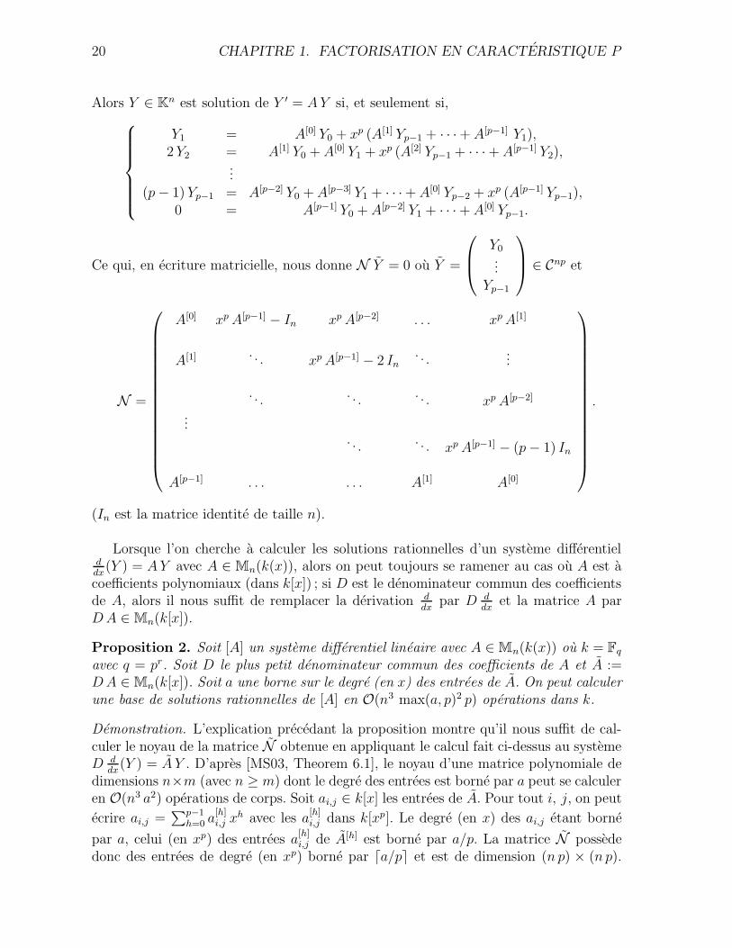
Alors Y ∈ Kn est solution de Y ′ = A Y si, et seulement si,
Y1 = A[0] Y0 + xp (A[1] Yp−1 + · · ·+ A[p−1] Y1),2 Y2 = A[1] Y0 + A[0] Y1 + xp (A[2] Yp−1 + · · · + A[p−1] Y2),
...(p − 1) Yp−1 = A[p−2] Y0 + A[p−3] Y1 + · · ·+ A[0] Yp−2 + xp (A[p−1] Yp−1),
0 = A[p−1] Y0 + A[p−2] Y1 + · · · + A[0] Yp−1.
Ce qui, en ecriture matricielle, nous donne N Y = 0 ou Y =
Y0...
Yp−1
∈ Cnp et
N =
A[0] xp A[p−1] − In xp A[p−2] . . . xp A[1]
A[1] . . . xp A[p−1] − 2 In. . .
...
. . .. . .
. . . xp A[p−2]
.... . .
. . . xp A[p−1] − (p − 1) In
A[p−1] . . . . . . A[1] A[0]
.
(In est la matrice identite de taille n).
Lorsque l’on cherche a calculer les solutions rationnelles d’un systeme differentielddx
(Y ) = A Y avec A ∈ Mn(k(x)), alors on peut toujours se ramener au cas ou A est acoefficients polynomiaux (dans k[x]) ; si D est le denominateur commun des coefficientsde A, alors il nous suffit de remplacer la derivation d
dxpar D d
dxet la matrice A par
D A ∈ Mn(k[x]).
Proposition 2. Soit [A] un systeme differentiel lineaire avec A ∈ Mn(k(x)) ou k = Fq
avec q = pr. Soit D le plus petit denominateur commun des coefficients de A et A :=D A ∈ Mn(k[x]). Soit a une borne sur le degre (en x) des entrees de A. On peut calculerune base de solutions rationnelles de [A] en O(n3 max(a, p)2 p) operations dans k.
Demonstration. L’explication precedant la proposition montre qu’il nous suffit de cal-culer le noyau de la matrice N obtenue en appliquant le calcul fait ci-dessus au systemeD d
dx(Y ) = A Y . D’apres [MS03, Theorem 6.1], le noyau d’une matrice polynomiale de
dimensions n×m (avec n ≥ m) dont le degre des entrees est borne par a peut se calculeren O(n3 a2) operations de corps. Soit ai,j ∈ k[x] les entrees de A. Pour tout i, j, on peut
ecrire ai,j =∑p−1
h=0 a[h]i,j xh avec les a
[h]i,j dans k[xp]. Le degre (en x) des ai,j etant borne
par a, celui (en xp) des entrees a[h]i,j de A[h] est borne par a/p. La matrice N possede
donc des entrees de degre (en xp) borne par da/pe et est de dimension (n p) × (n p).
1.2. SOLUTIONS RATIONNELLES 21
Par consequent, si a ≥ p, on peut considerer les entrees de N comme des polynomesen la variable c := xp de degre borne par a/p + 1 ; dans ce cas, son noyau se calcule
en O(n3 a2 p) operations dans k. Si a < p (ce qui est equivalent au fait que les a[k]i,j sont
dans k) et si A n’est pas a coefficients dans k, le degre en xp des entrees de N est 1 et lacomplexite du calcul du noyau de N devient O(n3 p3) operations dans k. Finalement, siA est a coefficients dans k, alors les entrees de N appartiennent a k et son noyau peutaussi se calculer en O(n3 p3) operations dans k.
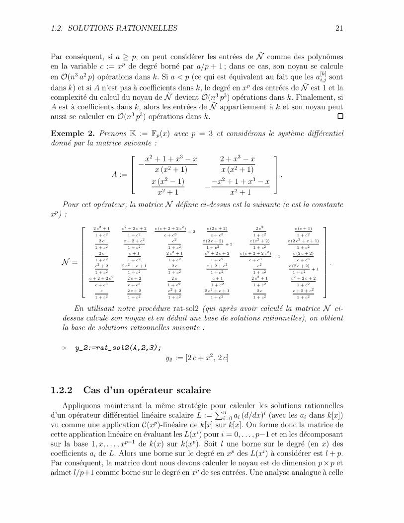
Exemple 2. Prenons K := Fp(x) avec p = 3 et considerons le systeme differentieldonne par la matrice suivante :
A :=
−x2 + 1 + x3 − x
x (x2 + 1)
2 + x3 − x
x (x2 + 1)
x (x2 − 1)
x2 + 1−−x2 + 1 + x3 − x
x2 + 1
.
Pour cet operateur, la matrice N definie ci-dessus est la suivante (c est la constantexp) :
N =
2 c2 + 1
1 + c2
c2 + 2 c + 2
1 + c2
c (c + 2 + 2 c2)
c + c3+ 2
c (2 c + 2)
c + c3
2 c2
1 + c2
c (c + 1)
1 + c2
2 c
1 + c2
c + 2 + c2
1 + c2
c2
1 + c2
c (2 c + 2)
1 + c2+ 2
c (c2 + 2)
1 + c2
c (2 c2 + c + 1)
1 + c2
2 c
1 + c2
c + 1
1 + c2
2 c2 + 1
1 + c2
c2 + 2 c + 2
1 + c2
c (c + 2 + 2 c2)
c + c3+ 1
c (2 c + 2)
c + c3
c2 + 2
1 + c2
2 c2 + c + 1
1 + c2
2 c
1 + c2
c + 2 + c2
1 + c2
c2
1 + c2
c (2 c + 2)
1 + c2+ 1
c + 2 + 2 c2
c + c3
2 c + 2
c + c3
2 c
1 + c2
c + 1
1 + c2
2 c2 + 1
1 + c2
c2 + 2 c + 2
1 + c2
c
1 + c2
2 c + 2
1 + c2
c2 + 2
1 + c2
2 c2 + c + 1
1 + c2
2 c
1 + c2
c + 2 + c2
1 + c2
.
En utilisant notre procedure rat-sol2 (qui apres avoir calcule la matrice N ci-dessus calcule son noyau et en deduit une base de solutions rationnelles), on obtientla base de solutions rationnelles suivante :
> y_2:=rat_sol2(A,2,3);
y2 := [2 c + x2, 2 c]
1.2.2 Cas d’un operateur scalaire
Appliquons maintenant la meme strategie pour calculer les solutions rationnellesd’un operateur differentiel lineaire scalaire L :=
∑ni=0 ai (d/dx)i (avec les ai dans k[x])
vu comme une application C(xp)-lineaire de k[x] sur k[x]. On forme donc la matrice decette application lineaire en evaluant les L(xi) pour i = 0, . . . , p−1 et en les decomposantsur la base 1, x, . . . , xp−1 de k(x) sur k(xp). Soit l une borne sur le degre (en x) descoefficients ai de L. Alors une borne sur le degre en xp des L(xi) a considerer est l + p.Par consequent, la matrice dont nous devons calculer le noyau est de dimension p×p etadmet l/p+1 comme borne sur le degre en xp de ses entrees. Une analyse analogue a celle
22 CHAPITRE 1. FACTORISATION EN CARACTERISTIQUE P
de la preuve de la proposition 2 nous fournit donc une complexite en O(max(l, p)2 p)operations dans k.
Par consequent, on peut penser que calculer les solutions rationnelles d’un systemedifferentiel lineaire [A] en caracteristique p en le transformant en une equation scalaireL a l’aide d’un vecteur cyclique pourrait etre plus efficace. On sait, d’apres la proposi-tion 1, qu’en caracteristique p (avec p > n), calculer un vecteur cyclique Λ0 coute O(n5)operations dans k. De plus, si les degres de Λ et A sont respectivement bornes par λet a, alors on obtient une borne de la forme nλ + a n (n+1)
2pour le degre des coefficients
de L (voir Proposition 1). Supposons maintenant que p > a et que p est aussi plus
grand que le degre des coefficients du vecteur cyclique (par exemple p > n λ+a n (n+1)2
).Dans ce cas, calculer les solutions rationnelles en passant par un vecteur cyclique couteO(n5 +p3) operations dans k alors qu’un calcul direct sur le systeme coute O(n3p3). Parconsequent, nous pouvons conclure que la methode du vecteur cyclique est plus efficaceseulement lorsque p est beaucoup plus grand que n. Lorsque p et n ont le meme ordrede grandeur (ou lorsque p est plus petit que n et qu’un vecteur cyclique existe), alorsun calcul direct est plus efficace.
1.3 La p-courbure d’un systeme differentiel lineaire
1.3.1 Definition et calcul
Definition 11. Soit [A] un systeme differentiel lineaire avec A ∈ Mn(K). La p-courburede [A] est l’operateur de Kn dans Kn defini par
∆pA :=
(
d
dx− A
)p
.
Avant de montrer comment calculer cet objet en pratique, nous donnons deuxpremieres proprietes ainsi que quelques exemples.
Lemme 1. Soit [A] un systeme differentiel avec A ∈ Mn(K). La p-courbure ∆pA du
systeme [A] est une application K-lineaire.
Demonstration. On montre tout d’abord par recurrence sur j que pour tout j ≥ 0 etpour tout couple (a, v) dans K × Kn,
∆jA(a v) =
j∑
i=0
(
ji
)
a(i)∆j−iA (v).
Par consequent, pour tout couple (a, v) de K × Kn,
∆pA(a v) = a(p) v + a ∆p
A(v),
et le fait que l’application ( ddx
)p soit nulle sur K (ce qui implique a(p) = 0 dans laprecedente formule) nous permet de conclure.
1.3. LA P -COURBURE D’UN SYSTEME DIFFERENTIEL LINEAIRE 23
Lemme 2. Si deux systemes differentiels lineaires [A] et [B] sont equivalents, alorsleurs p-courbures sont semblables. Precisement, si [B] = P [A], alors ∆p
B = P−1 ∆pA P .
Demonstration. Ceci provient directement de la remarque que si B = P [A], alors ∆B =P−1 ∆A P .
Exemple 3. On peut verifier que :(a). La p-courbure du systeme differentiel y ′ = µ y, de dimension 1, est µ(p−1) + µp.(b). Si A = µ I, alors ∆p
A = (µ(p−1) + µp) I.
(c). Si A =⊕r
i=1 µi Ini, alors ∆p
A =⊕r
i=1(µ(p−1)i + µp
i ) Ini.
(d). Si A =⊕r
i=1 A[i], alors ∆pA =
⊕ri=1 ∆p
A[i].(e). Si [A∗] represente le systeme adjoint de [A], alors ∆p
A∗ = −t∆pA. Autrement dit,
la p-courbure de l’adjoint (au sens des systemes differentiels) est egale a l’adjoint de lap-courbure en appelant adjoint d’une matrice M la matrice −tM .
Dans [Ka82], Katz propose un algorithme pour le calcul de la p-courbure d’unsysteme differentiel : on definit la suite (Ai)i≥0, que nous appelons suite de Lie de[A], par
A0 := In et ∀i ≥ 0, Ai+1 := ∆A(Ai) = A′i − A Ai. (1.1)
On calcule A2, A3, . . . , Ap et Ap est exactement la matrice de l’operateur differentiel ∆pA
dans la base canonique de Kn, i. e., la p-courbure. Dans la suite, nous ne ferons pas dedistinction entre l’operateur ∆p
A et sa matrice Ap.Soit A ∈ Mn(k(x)) avec k = Fq ou q = pr. En pratique, pour calculer Ap, nous
adaptons les formules (1.1) pour que tous les calculs se fassent dans k[x], i. e., sansdenominateurs (voir la procedure LiePol dans l’annexe) ; soit D ∈ k[x] tel que A :=D A ∈ Mn(k[x]). Alors, pour tout i ≥ 1, Ai := Di Ai ∈ Mn(k[x]) et on obtient ainsi laformule de recurrence suivante :
Ai+1 = D A′i − (D′ i + A) Ai. (1.2)
Proposition 3. Soit [A] un systeme differentiel avec A ∈ Mn(k(x)) ou k = Fq, q = pr.Soit D le plus petit denominateur commun des coefficients de A et A := D A ∈ Mn(k[x]).Soit a une borne sur le degre (en x) des entrees de A. Soit ω un reel tel que le produit dedeux matrices dans Mn(F), avec F corps quelconque, puisse se faire en O(nω) produitsdans F . Alors, la p-courbure de [A] peut se calculer en O(nω a log(a) p2) operationsdans k.
Precisons que, par exemple, la methode de Strassen pour la multiplication de ma-trices correspond a ω = log2 7 (voir [GG99, 12.1]).
Demonstration. D’apres (1.2), calculer la p-courbure necessite p produits de matricesde polynomes de dimension n×n ayant des coefficients de degre respectivement bornespar a, 2a, . . . , (p − 1) a. Ceci peut donc se faire en O(nω p) produits de polynomes.Maintenant, on peut conclure car la F.F.T. ([GG99, Section 8]) permet de calculer leproduit de deux polynomes de degres respectivement bornes par a et i a en O(i a log(a))operations de corps.
24 CHAPITRE 1. FACTORISATION EN CARACTERISTIQUE P
Calculer la p-courbure (pour p > n) d’un operateur differentiel scalaire ayant descoefficients de degre borne par l en utilisant les formules de recurrences donnees dans[PS03, 13.2.2, p.335] donne une complexite en O(n2 l log(l) p) operations dans k. Iciaussi comparons le calcul direct de la p-courbure du systeme a la methode passant parun vecteur cyclique. D’apres la proposition 1, si a est une borne sur le degre des entreesde A, une borne sur le degre des coefficients de l’operateur L calcule a partir d’unvecteur cyclique est b = nλ + a (n+1)n
2(λ borne sur le degre des coefficients du vecteur
cyclique). Donc, via un vecteur cyclique, la p-courbure se calcule en O(n5+n2 b log(b) p)operations dans k. Par consequent, le calcul en passant par un vecteur cyclique est plusavantageux seulement lorsque p est beaucoup plus grand que n. Dans le cas contraireou p et n ont le meme ordre de grandeur, le calcul direct sur le systeme est plus efficace.Rappelons que le cas p < n est exclu car l’existence d’un vecteur cyclique n’est alorsplus assuree.
1.3.2 Classification des modules differentiels
Dans [Pu95] (voir aussi [PS03, Chapitre 13]), van der Put donne une classificationdes modules differentiels en caracteristique p. La consequence de cette classificationpour le probleme de factorisation est la suivante : la forme de Jordan (sur C) de lap-courbure d’un systeme differentiel lineaire [A] donne toutes les factorisations de [A].Voici brievement comment est construite cette classification (pour plus de details, voir[Pu95] ou [PS03, Ch. 13]) : considerons les deux categories suivantes :
– les modules differentiels (voir Definition 3) munis du produit tensoriel usuel,– les C[T ]-modules (C[T ] : anneau commutatif des polynomes a coefficients dans C)
de dimension finie sur C. Un element de cette categorie est donne par un couple(N, Θ) ou N est un K-espace vectoriel de dimension n, Θ est un endomorphismede N et l’action de C[T ] sur N est definie par
f.m = f(Θ) m, ∀f ∈ C[T ], ∀m ∈ N,
et cette seconde categorie est munie du produit tensoriel defini par (N1, Θ1) ⊗C
(N2, Θ2) = (N1 ⊗C N2, Θ) ou Θ = Θ1 ⊗C IN1 + IN2 ⊗C Θ2.
Le resultat de van der Put peut se resumer ainsi : si le corps K possede une certainepropriete1, par exemple K = Fp(x) ou Fp((x)), alors le foncteur qui envoie (Cn, Θ) sur(Kn, ∆) ou ∆ est determine tel que ∆p = I ⊗C Θ (avec l’identification Kn = K ⊗C Cn)fournit l’equivalence entre les deux categories decrites ci-dessus. La forme de Jordan(sur C) de la p-courbure ∆p
A donne la factorisation complete du C[T ]-module (Cn, ΘA)avec ∆p
A = I ⊗C ΘA. Par consequent, comme le foncteur defini ci-dessus respecte lesconstructions de l’algebre lineaire, ceci nous donne aussi la factorisation complete dumodule differentiel (Kn, ∆A) associe.
1Il n’existe pas de corps non-commutatif de degre p2 sur son centre Z avec Z extension finie de K.C’est le cas lorsque K est un corps C1 ([Ja80, Definition 11.5, p. 649]), ou corps quasi-algebriquement
clos.
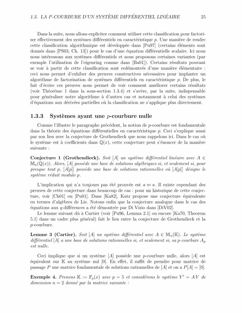
1.3. LA P -COURBURE D’UN SYSTEME DIFFERENTIEL LINEAIRE 25
Dans la suite, nous allons expliciter comment utiliser cette classification pour factori-ser effectivement des systemes differentiels en caracteristique p. Une maniere de rendrecette classification algorithmique est developpee dans [Pu97] (certains elements sontdonnes dans [PS03, Ch. 13]) pour le cas d’une equation differentielle scalaire. Ici nousnous interessons aux systemes differentiels et nous proposons certaines variantes (parexemple l’utilisation de l’eigenring comme dans [Ba01]). Certains resultats pouvantse voir a partir de cette classification sont redemontres d’une maniere elementaire :ceci nous permet d’exhiber des preuves constructives necessaires pour implanter unalgorithme de factorisation de systemes differentiels en caracteristique p. De plus, lefait d’ecrire ces preuves nous permet de voir comment ameliorer certains resultats(voir Theoreme 1 dans la sous-section 1.3.4) et s’avere, par la suite, indispensablepour generaliser notre algorithme a d’autres cas et notamment a celui des systemesd’equations aux derivees partielles ou la classification ne s’applique plus directement.
1.3.3 Systemes ayant une p-courbure nulle
Comme l’illustre le paragraphe precedent, la notion de p-courbure est fondamentaledans la theorie des equations differentielles en caracteristique p. Ceci s’explique aussipar son lien avec la conjecture de Grothendieck que nous rappelons ici. Dans le cas oule systeme est a coefficients dans Q(x), cette conjecture peut s’enoncer de la manieresuivante :
Conjecture 1 (Grothendieck). Soit [A] un systeme differentiel lineaire avec A ∈Mn(Q(x)). Alors, [A] possede une base de solutions algebriques si, et seulement si, pourpresque tout p, [A[p]] possede une base de solutions rationnelles ou [A[p]] designe lesysteme reduit modulo p.
L’implication qui n’a toujours pas ete prouvee est «⇐». Il existe cependant despreuves de cette conjecture dans beaucoup de cas : pour un historique de cette conjec-ture, voir [Ch01] ou [Pu01]. Dans [Ka82], Katz propose une conjecture equivalenteen termes d’algebres de Lie. Notons enfin que la conjecture analogue dans le cas desequations aux q-differences a ete demontree par Di Vizio dans [DiV02].
Le lemme suivant du a Cartier (voir [Pu96, Lemma 2.1] ou encore [Ka70, Theorem5.1] dans un cadre plus general) fait le lien entre la conjecture de Grothendieck et lap-courbure.
Lemme 3 (Cartier). Soit [A] un systeme differentiel avec A ∈ Mn(K). Le systemedifferentiel [A] a une base de solutions rationnelles si, et seulement si, sa p-courbure Ap
est nulle.
Ceci implique que si un systeme [A] possede une p-courbure nulle, alors [A] estequivalent sur K au systeme nul [0]. En effet, il suffit de prendre pour matrice depassage P une matrice fondamentale de solutions rationnelles de [A] et on a P [A] = [0].
Exemple 4. Prenons K := Fp(x) avec p = 5 et considerons le systeme Y ′ = A Y dedimension n = 2 donne par la matrice suivante :
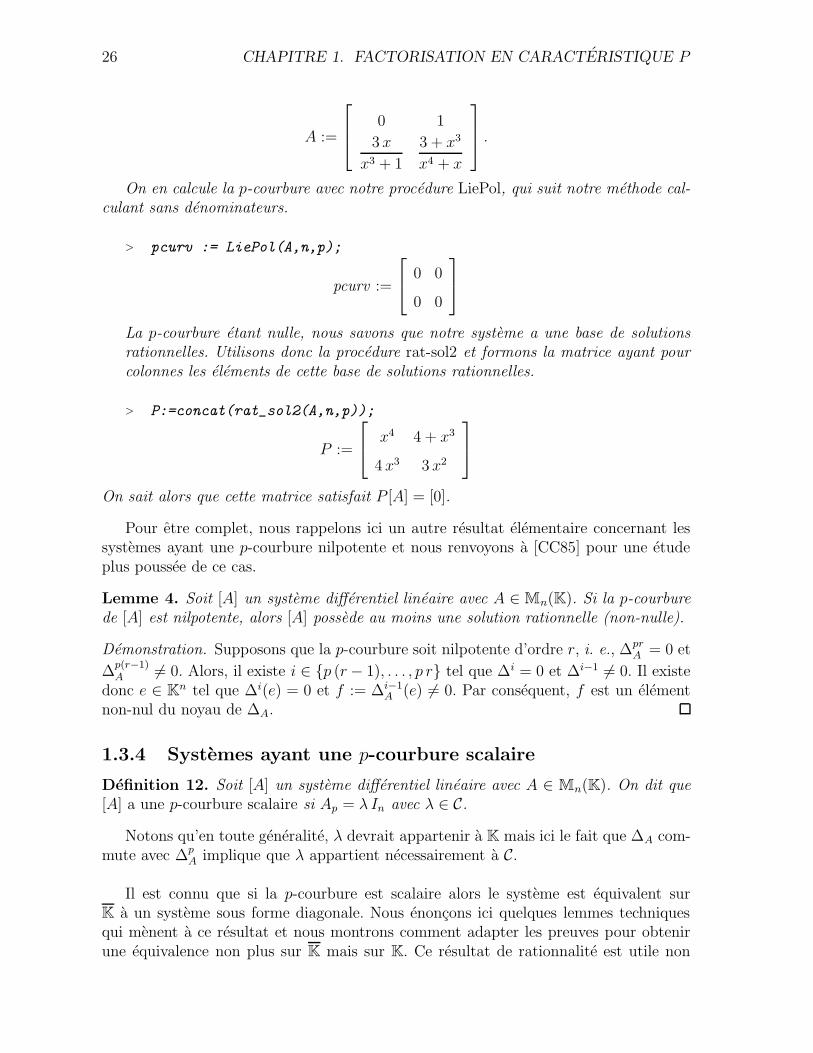
26 CHAPITRE 1. FACTORISATION EN CARACTERISTIQUE P
A :=
0 1
3 x
x3 + 1
3 + x3
x4 + x
.
On en calcule la p-courbure avec notre procedure LiePol, qui suit notre methode cal-culant sans denominateurs.
> pcurv := LiePol(A,n,p);
pcurv :=
0 0
0 0
La p-courbure etant nulle, nous savons que notre systeme a une base de solutionsrationnelles. Utilisons donc la procedure rat-sol2 et formons la matrice ayant pourcolonnes les elements de cette base de solutions rationnelles.
> P:=concat(rat_sol2(A,n,p));
P :=
x4 4 + x3
4 x3 3 x2
On sait alors que cette matrice satisfait P [A] = [0].
Pour etre complet, nous rappelons ici un autre resultat elementaire concernant lessystemes ayant une p-courbure nilpotente et nous renvoyons a [CC85] pour une etudeplus poussee de ce cas.
Lemme 4. Soit [A] un systeme differentiel lineaire avec A ∈ Mn(K). Si la p-courburede [A] est nilpotente, alors [A] possede au moins une solution rationnelle (non-nulle).
Demonstration. Supposons que la p-courbure soit nilpotente d’ordre r, i. e., ∆prA = 0 et
∆p(r−1)A 6= 0. Alors, il existe i ∈ {p (r − 1), . . . , p r} tel que ∆i = 0 et ∆i−1 6= 0. Il existe
donc e ∈ Kn tel que ∆i(e) = 0 et f := ∆i−1A (e) 6= 0. Par consequent, f est un element
non-nul du noyau de ∆A.
1.3.4 Systemes ayant une p-courbure scalaire
Definition 12. Soit [A] un systeme differentiel lineaire avec A ∈ Mn(K). On dit que[A] a une p-courbure scalaire si Ap = λ In avec λ ∈ C.
Notons qu’en toute generalite, λ devrait appartenir a K mais ici le fait que ∆A com-mute avec ∆p
A implique que λ appartient necessairement a C.
Il est connu que si la p-courbure est scalaire alors le systeme est equivalent surK a un systeme sous forme diagonale. Nous enoncons ici quelques lemmes techniquesqui menent a ce resultat et nous montrons comment adapter les preuves pour obtenirune equivalence non plus sur K mais sur K. Ce resultat de rationnalite est utile non
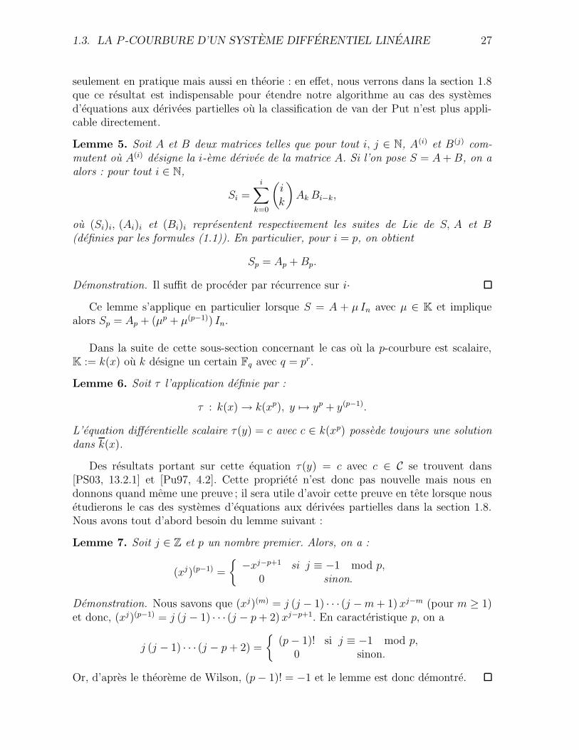
1.3. LA P -COURBURE D’UN SYSTEME DIFFERENTIEL LINEAIRE 27
seulement en pratique mais aussi en theorie : en effet, nous verrons dans la section 1.8que ce resultat est indispensable pour etendre notre algorithme au cas des systemesd’equations aux derivees partielles ou la classification de van der Put n’est plus appli-cable directement.
Lemme 5. Soit A et B deux matrices telles que pour tout i, j ∈ N, A(i) et B(j) com-mutent ou A(i) designe la i-eme derivee de la matrice A. Si l’on pose S = A + B, on aalors : pour tout i ∈ N,
Si =i∑
k=0
(
ik
)
Ak Bi−k,
ou (Si)i, (Ai)i et (Bi)i representent respectivement les suites de Lie de S, A et B(definies par les formules (1.1)). En particulier, pour i = p, on obtient
Sp = Ap + Bp.
Demonstration. Il suffit de proceder par recurrence sur i·Ce lemme s’applique en particulier lorsque S = A + µ In avec µ ∈ K et implique
alors Sp = Ap + (µp + µ(p−1)) In.
Dans la suite de cette sous-section concernant le cas ou la p-courbure est scalaire,K := k(x) ou k designe un certain Fq avec q = pr.
Lemme 6. Soit τ l’application definie par :
τ : k(x) → k(xp), y 7→ yp + y(p−1).
L’equation differentielle scalaire τ(y) = c avec c ∈ k(xp) possede toujours une solutiondans k(x).
Des resultats portant sur cette equation τ(y) = c avec c ∈ C se trouvent dans[PS03, 13.2.1] et [Pu97, 4.2]. Cette propriete n’est donc pas nouvelle mais nous endonnons quand meme une preuve ; il sera utile d’avoir cette preuve en tete lorsque nousetudierons le cas des systemes d’equations aux derivees partielles dans la section 1.8.Nous avons tout d’abord besoin du lemme suivant :
Lemme 7. Soit j ∈ Z et p un nombre premier. Alors, on a :
(xj)(p−1) =
{
−xj−p+1 si j ≡ −1 mod p,0 sinon.
Demonstration. Nous savons que (xj)(m) = j (j − 1) · · · (j − m + 1) xj−m (pour m ≥ 1)et donc, (xj)(p−1) = j (j − 1) · · · (j − p + 2) xj−p+1. En caracteristique p, on a
j (j − 1) · · · (j − p + 2) =
{
(p − 1)! si j ≡ −1 mod p,0 sinon.
Or, d’apres le theoreme de Wilson, (p − 1)! = −1 et le lemme est donc demontre.
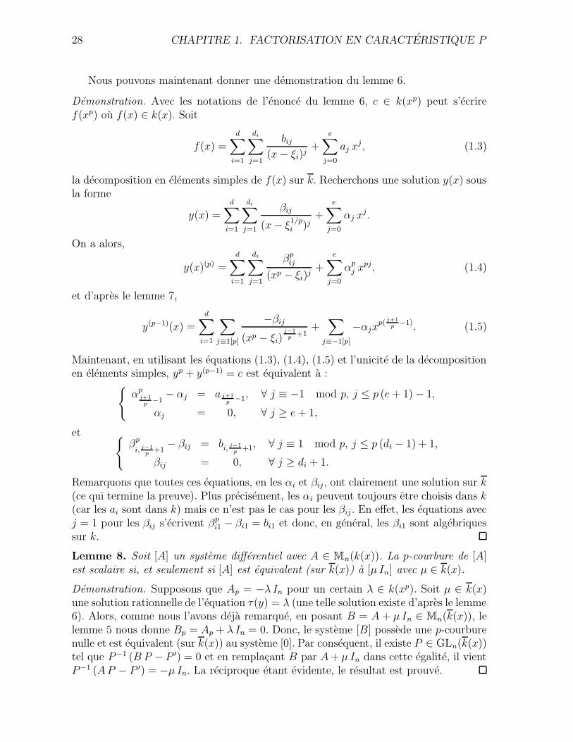
28 CHAPITRE 1. FACTORISATION EN CARACTERISTIQUE P
Nous pouvons maintenant donner une demonstration du lemme 6.
Demonstration. Avec les notations de l’enonce du lemme 6, c ∈ k(xp) peut s’ecriref(xp) ou f(x) ∈ k(x). Soit
f(x) =d∑
i=1
di∑
j=1
bij
(x − ξi)j+
e∑
j=0
aj xj, (1.3)
la decomposition en elements simples de f(x) sur k. Recherchons une solution y(x) sousla forme
y(x) =d∑
i=1
di∑
j=1
βij
(x − ξ1/pi )j
+e∑
j=0
αj xj.
On a alors,
y(x)(p) =
d∑
i=1
di∑
j=1
βpij
(xp − ξi)j+
e∑
j=0
αpj xpj, (1.4)
et d’apres le lemme 7,
y(p−1)(x) =d∑
i=1
∑
j≡1[p]
−βij
(xp − ξi)j−1
p+1
+∑
j≡−1[p]
−αjxp( j+1
p−1). (1.5)
Maintenant, en utilisant les equations (1.3), (1.4), (1.5) et l’unicite de la decompositionen elements simples, yp + y(p−1) = c est equivalent a :
{
αpj+1
p−1
− αj = a j+1p
−1, ∀ j ≡ −1 mod p, j ≤ p (e + 1) − 1,
αj = 0, ∀ j ≥ e + 1,
et{
βp
i, j−1p
+1− βij = bi, j−1
p+1, ∀ j ≡ 1 mod p, j ≤ p (di − 1) + 1,
βij = 0, ∀ j ≥ di + 1.
Remarquons que toutes ces equations, en les αi et βij, ont clairement une solution sur k(ce qui termine la preuve). Plus precisement, les αi peuvent toujours etre choisis dans k(car les ai sont dans k) mais ce n’est pas le cas pour les βij. En effet, les equations avecj = 1 pour les βij s’ecrivent βp
i1 − βi1 = bi1 et donc, en general, les βi1 sont algebriquessur k.
Lemme 8. Soit [A] un systeme differentiel avec A ∈ Mn(k(x)). La p-courbure de [A]est scalaire si, et seulement si [A] est equivalent (sur k(x)) a [µ In] avec µ ∈ k(x).
Demonstration. Supposons que Ap = −λ In pour un certain λ ∈ k(xp). Soit µ ∈ k(x)une solution rationnelle de l’equation τ(y) = λ (une telle solution existe d’apres le lemme6). Alors, comme nous l’avons deja remarque, en posant B = A + µ In ∈ Mn(k(x)), lelemme 5 nous donne Bp = Ap + λ In = 0. Donc, le systeme [B] possede une p-courburenulle et est equivalent (sur k(x)) au systeme [0]. Par consequent, il existe P ∈ GLn(k(x))tel que P−1 (B P − P ′) = 0 et en remplacant B par A + µ In dans cette egalite, il vientP−1 (A P − P ′) = −µ In. La reciproque etant evidente, le resultat est prouve.
1.3. LA P -COURBURE D’UN SYSTEME DIFFERENTIEL LINEAIRE 29
Nous donnons maintenant une version rationnelle du lemme 8 qui constitue notrecontribution dans ce cas ou la p-courbure est scalaire :
Theoreme 1. Soit [A] un systeme differentiel avec A ∈ Mn(k(x)). Si p ne divise pasn, la p-courbure de [A] est scalaire si, et seulement si, [A] est equivalent (sur k(x)) a[µ In] avec µ ∈ k(x).
Demonstration. Nous avons Ap = −λ In et nous savons d’apres le lemme precedentqu’il existe P ∈ GLn(k(x)) tel que P [A] = P−1 A P − P−1 P ′ = −µ In avec µ ∈ k(x)
et τ(µ) = λ. Donc tr(A) − det(P )′
det(P )= −n µ et pour p ne divisant n, nous avons µ =
− 1n
tr(A) + 1n
det(P )′
det(P ); ceci implique que − 1
ntr(A) ∈ k(x) est une solution de τ(y) = λ.
Alors, en reprenant la demonstration du lemme precedent et en remplacant µ ∈ k(x)par − 1
ntr(A) ∈ k(x), on obtient le resultat annonce.
Ce resultat de rationnalite donne une methode rationnelle et algorithmique pourfactoriser (sur k(x)) des systemes qui possedent une p-courbure scalaire. Une astuceanalogue pour calculer a partir d’un operateur differentiel scalaire L ∈ k(x)[∂] ayant unep-courbure de la forme λ I avec λ ∈ k(xp) une solution µ ∈ k(x) de l’equation τ(y) = λest donnee dans [Pu97, 2.11]. La methode est la suivante : soit M = gcrd(L, ∂p − λ) =∂m + bm−1 ∂m−1 + · · ·+ b0 ou m ∈ N et gcrd represente le plus grand commun diviseura droite d’operateurs differentiels. L’element − bm−1
mest alors solution de τ(y) = λ.
Exemple 5. Si l’on essaye de resoudre l’equation τ(y) = 1/x5 dans Fp(x) pour p = 5,alors en suivant la preuve du lemme 6, on trouve que y doit s’ecrire β/x ou β est solutionde β5 − β = 1. Cette equation n’ayant pas de solutions dans Fp, l’equation τ(y) = 1/x5
ne possede pas de solutions dans Fp(x) mais seulement dans Fp(x). D’apres le theoremeprecedent, il n’existe donc pas de systemes differentiels a coefficients dans F5(x) et dedimension n 6= 5 n1 dont la p-courbure est egale a −1/x5 In. Ceci illustre le fait que lap-courbure d’un systeme differentiel a coefficients dans k(x) ne peut pas etre n’importequoi.
1.3.5 Solutions rationnelles et p-courbure
Nous rappelons maintenant un resultat, du a Katz (voir [Ka70]), faisant la liaisonentre l’espace SA des solutions rationnelles d’un systeme differentiel et le noyau de sap-courbure. Nous reproduisons ici la preuve de Katz non seulement pour la convenancedu lecteur mais aussi pour son caractere algorithmique.
Soit SA := {Y ∈ Kn |Y ′ = A Y } l’espace des solutions rationnelles de [A]. Il est clairque SA est inclus dans le noyau ker(Ap) de la p-courbure Ap (car ∆A(Y ) = 0 implique∆p
A(Y ) = 0).
Lemme 9 (Katz). ker(Ap) = SA ⊗C K, et en particulier, dimC SA = dimK ker(Ap).
Demonstration. La projection
Pr : Kn → Kn, v 7→ Pr(v) :=
p−1∑
i=0
(−x)i
i!∆i
A(v)
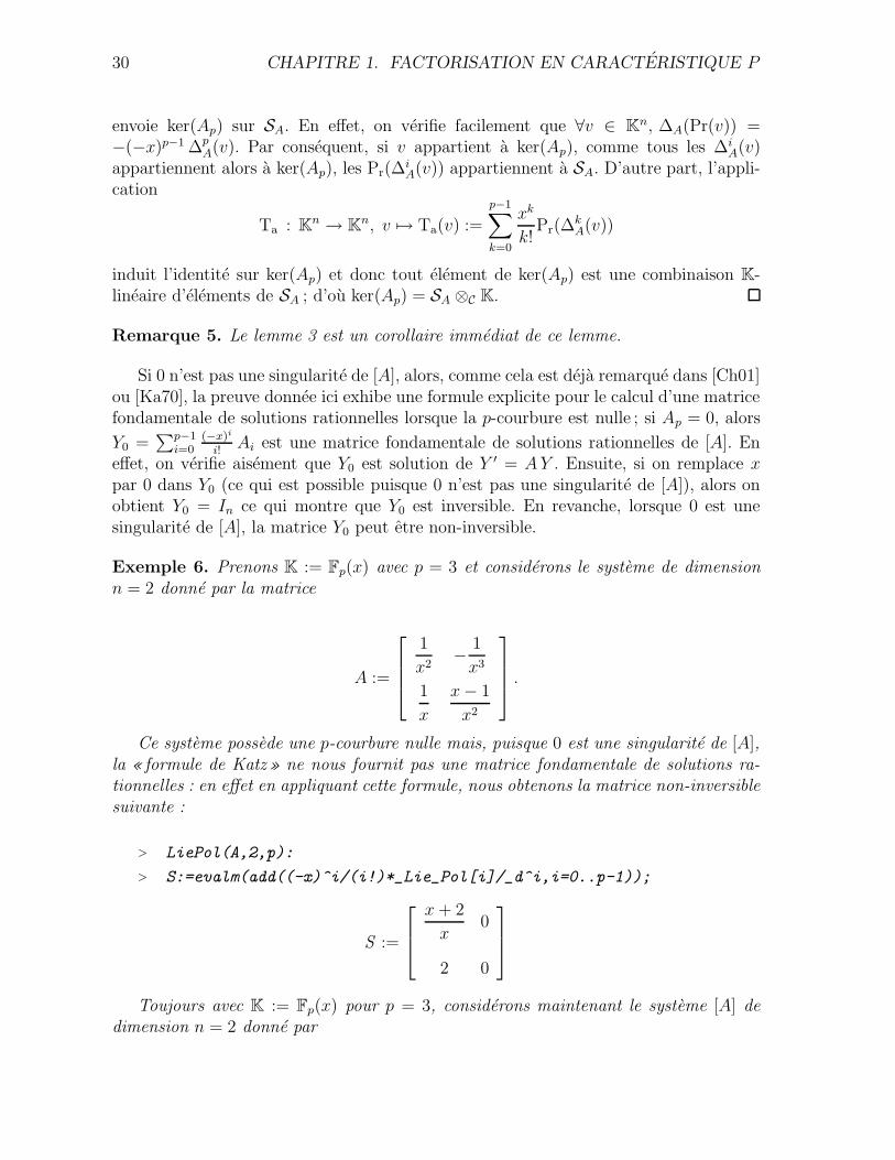
30 CHAPITRE 1. FACTORISATION EN CARACTERISTIQUE P
envoie ker(Ap) sur SA. En effet, on verifie facilement que ∀v ∈ Kn, ∆A(Pr(v)) =−(−x)p−1 ∆p
A(v). Par consequent, si v appartient a ker(Ap), comme tous les ∆iA(v)
appartiennent alors a ker(Ap), les Pr(∆iA(v)) appartiennent a SA. D’autre part, l’appli-
cation
Ta : Kn → Kn, v 7→ Ta(v) :=
p−1∑
k=0
xk
k!Pr(∆
kA(v))
induit l’identite sur ker(Ap) et donc tout element de ker(Ap) est une combinaison K-lineaire d’elements de SA ; d’ou ker(Ap) = SA ⊗C K.
Remarque 5. Le lemme 3 est un corollaire immediat de ce lemme.
Si 0 n’est pas une singularite de [A], alors, comme cela est deja remarque dans [Ch01]ou [Ka70], la preuve donnee ici exhibe une formule explicite pour le calcul d’une matricefondamentale de solutions rationnelles lorsque la p-courbure est nulle ; si Ap = 0, alors
Y0 =∑p−1
i=0(−x)i
i!Ai est une matrice fondamentale de solutions rationnelles de [A]. En
effet, on verifie aisement que Y0 est solution de Y ′ = A Y . Ensuite, si on remplace xpar 0 dans Y0 (ce qui est possible puisque 0 n’est pas une singularite de [A]), alors onobtient Y0 = In ce qui montre que Y0 est inversible. En revanche, lorsque 0 est unesingularite de [A], la matrice Y0 peut etre non-inversible.
Exemple 6. Prenons K := Fp(x) avec p = 3 et considerons le systeme de dimensionn = 2 donne par la matrice
A :=
1
x2− 1
x3
1
x
x − 1
x2
.
Ce systeme possede une p-courbure nulle mais, puisque 0 est une singularite de [A],la « formule de Katz » ne nous fournit pas une matrice fondamentale de solutions ra-tionnelles : en effet en appliquant cette formule, nous obtenons la matrice non-inversiblesuivante :
> LiePol(A,2,p):
> S:=evalm(add((-x)^i/(i!)*_Lie_Pol[i]/_d^i,i=0..p-1));
S :=
x + 2
x0
2 0
Toujours avec K := Fp(x) pour p = 3, considerons maintenant le systeme [A] dedimension n = 2 donne par
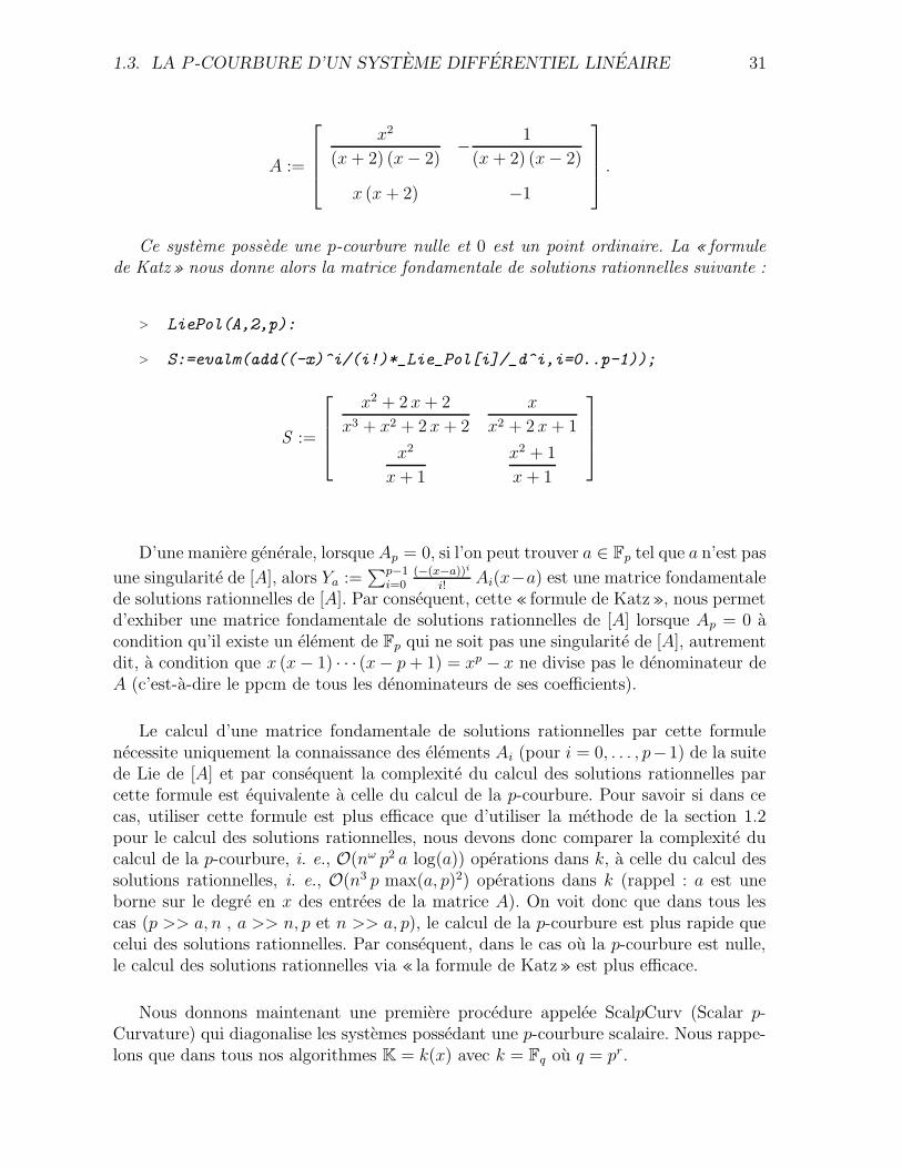
1.3. LA P -COURBURE D’UN SYSTEME DIFFERENTIEL LINEAIRE 31
A :=
x2
(x + 2) (x − 2)− 1
(x + 2) (x − 2)
x (x + 2) −1
.
Ce systeme possede une p-courbure nulle et 0 est un point ordinaire. La « formulede Katz» nous donne alors la matrice fondamentale de solutions rationnelles suivante :
> LiePol(A,2,p):
> S:=evalm(add((-x)^i/(i!)*_Lie_Pol[i]/_d^i,i=0..p-1));
S :=
x2 + 2 x + 2
x3 + x2 + 2 x + 2
x
x2 + 2 x + 1
x2
x + 1
x2 + 1
x + 1
D’une maniere generale, lorsque Ap = 0, si l’on peut trouver a ∈ Fp tel que a n’est pas
une singularite de [A], alors Ya :=∑p−1
i=0(−(x−a))i
i!Ai(x−a) est une matrice fondamentale
de solutions rationnelles de [A]. Par consequent, cette « formule de Katz», nous permetd’exhiber une matrice fondamentale de solutions rationnelles de [A] lorsque Ap = 0 acondition qu’il existe un element de Fp qui ne soit pas une singularite de [A], autrementdit, a condition que x (x − 1) · · · (x − p + 1) = xp − x ne divise pas le denominateur deA (c’est-a-dire le ppcm de tous les denominateurs de ses coefficients).
Le calcul d’une matrice fondamentale de solutions rationnelles par cette formulenecessite uniquement la connaissance des elements Ai (pour i = 0, . . . , p−1) de la suitede Lie de [A] et par consequent la complexite du calcul des solutions rationnelles parcette formule est equivalente a celle du calcul de la p-courbure. Pour savoir si dans cecas, utiliser cette formule est plus efficace que d’utiliser la methode de la section 1.2pour le calcul des solutions rationnelles, nous devons donc comparer la complexite ducalcul de la p-courbure, i. e., O(nω p2 a log(a)) operations dans k, a celle du calcul dessolutions rationnelles, i. e., O(n3 p max(a, p)2) operations dans k (rappel : a est uneborne sur le degre en x des entrees de la matrice A). On voit donc que dans tous lescas (p >> a, n , a >> n, p et n >> a, p), le calcul de la p-courbure est plus rapide quecelui des solutions rationnelles. Par consequent, dans le cas ou la p-courbure est nulle,le calcul des solutions rationnelles via « la formule de Katz» est plus efficace.
Nous donnons maintenant une premiere procedure appelee ScalpCurv (Scalar p-Curvature) qui diagonalise les systemes possedant une p-courbure scalaire. Nous rappe-lons que dans tous nos algorithmes K = k(x) avec k = Fq ou q = pr.
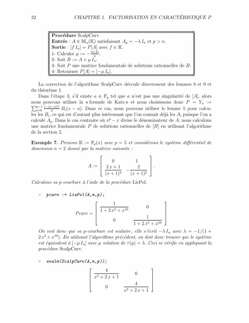
32 CHAPITRE 1. FACTORISATION EN CARACTERISTIQUE P
Procedure ScalpCurvEntree : A ∈ Mn(K) satisfaisant Ap = −λ In et p > n.Sortie : [f In] = P [A] avec f ∈ K.
1- Calculer µ := − tr(A)n
.2- Soit B := A + µ In.3- Soit P une matrice fondamentale de solutions rationnelles de B.4- Retourner P [A] = [−µ In].
La correction de l’algorithme ScalpCurv decoule directement des lemmes 8 et 9 etdu theoreme 1.
Dans l’etape 3, s’il existe a ∈ Fp tel que a n’est pas une singularite de [A], alorsnous pouvons utiliser la « formule de Katz» et nous choisissons donc P = Ya :=∑p−1
i=0(−(x−a))i
i!Bi(x − a). Dans ce cas, nous pouvons utiliser le lemme 5 pour calcu-
ler les Bi, ce qui est d’autant plus interessant que l’on connait deja les Ai puisque l’on acalcule Ap. Dans le cas contraire ou xp − x divise le denominateur de A, nous calculonsune matrice fondamentale P de solutions rationnelles de [B] en utilisant l’algorithmede la section 2.
Exemple 7. Prenons K := Fp(x) avec p = 5 et considerons le systeme differentiel dedimension n = 2 donne par la matrice suivante :
A :=
0 12 x + 1
(x + 1)4− 2
(x + 1)2
.
Calculons sa p-courbure a l’aide de la procedure LiePol.
> pcurv := LiePol(A,n,p);
Pcurv =
1
1 + 2 x5 + x100
01
1 + 2 x5 + x10
On voit donc que sa p-courbure est scalaire ; elle s’ecrit −λ In avec λ = −1/(1 +2 x5 + x10). En utilisant l’algorithme precedent, on doit donc trouver que le systemeest equivalent a [−µ In] avec µ solution de τ(y) = λ. Ceci se verifie en appliquant laprocedure ScalpCurv.
> evalm(ScalpCurv(A,n,p));
4
x2 + 2 x + 10
04
x2 + 2 x + 1
1.4. L’EIGENRING D’UN SYSTEME DIFFERENTIEL LINEAIRE 33
Notons que − tr(A)n
= 1(x2+2 x+1)
ce qui est bien coherent avec la theorie.
1.4 L’eigenring d’un systeme differentiel lineaire
Dans cette section, nous rappelons la definition de l’eigenring associe a un systemedifferentiel ainsi qu’une methode pour le calculer en pratique. Ensuite, nous prouvons lesliens entre l’eigenring et la p-courbure d’un systeme differentiel lineaire et nous donnonsquelques resultats sur sa dimension.
1.4.1 Definition et calcul
Tout comme en caracteristique zero (voir par exemple [Si96, Ba01]), en caracteristiquep, l’eigenring associe a un systeme differentiel peut se definir de la facon suivante :
Definition 13. Soit [A] un systeme differentiel avec A ∈ Mn(K). L’eigenring E(A) de[A] est l’ensemble defini par
E(A) = {P ∈ Mn(K) |P ′ = A P − P A}.L’eigenring est une C-algebre de dimension finie inferieure ou egale a n2. En par-
ticulier, il contient la matrice identite In. Par consequent, le polynome minimal (etaussi caracteristique) d’un element de l’eigenring aura ses coefficients dans le corps desconstantes C.
D’apres la definition 13, calculer l’eigenring revient a trouver les solutions ration-nelles du systeme P ′ = A P−P A. Ceci peut se faire de la maniere suivante : consideronsl’application
Vect : Mn(K) → Kn2
, P =
· · · L1 · · ·...
· · · Ln · · ·
7→
tL1...
tLn
,
ou les Li designent les lignes de la matrice P . On montre alors que
P ′ = A P − P A ⇐⇒ Vect(P )′ = (A ⊗ In − In ⊗ tA) Vect(P ),
et, par consequent, trouver une base de l’eigenring equivaut a calculer une base desolutions rationnelles du systeme differentiel Z ′ = (A⊗ In− In⊗ tA) Z de dimension n2.L’approche decrite ci-dessus ne depend pas de la caracteristique. Cependant, comptetenu du fait qu’il est (theoriquement) plus facile de calculer les solutions rationnelles encaracteristique p qu’en caracteristique zero, calculer l’eigenring est aussi plus facile ; cecirevient a resoudre un systeme lineaire homogene de dimension n2 p (Voir la section 1.2)de telle sorte que d’apres la proposition 2, nous pouvons affirmer :
Proposition 4. Soit [A] un systeme differentiel avec A ∈ Mn(k(x)) ou k = Fp ou Fp.Soit D le plus petit denominateur commun des coefficients de A = A ⊗ In − In ⊗ tAet soit A := DA ∈ Mn(k[x]). Soit a une borne sur le degre des entrees de A. Alorsl’eigenring de [A] peut se calculer en O(n6 max(a, p)2 p) operations dans k.
34 CHAPITRE 1. FACTORISATION EN CARACTERISTIQUE P
Dans [GZ03], Giesbrecht et Zhang utilisent aussi cette methode pour calculer l’ei-genring d’un polynome de Ore en caracteristique p.
Un algorithme plus efficace pour calculer l’eigenring d’un systeme differentiel a co-efficients dans F(x) ou F est un corps de caracteristique zero se trouve dans [BP98].Pour le cas des equations scalaires, nous renvoyons a [Ho96].
Nous rappelons maintenant quelques resultats sur la dimension de l’eigenring entant qu’espace vectoriel sur C. Nous commencons par un lemme tres utile :
Lemme 10 ([Ba01], Proposition 2). Si [A] et [B] sont deux systemes equivalents,alors leurs eigenrings sont isomorphes (en tant que C-algebres). Plus precisement, si[B] = P [A], alors l’isomorphisme entre E(A) et E(B) est donne par T 7→ P −1 T P .
Si [A] est irreductible, alors E(A) est un corps (voir par exemple [Ba01, Theorem1]). La reciproque est fausse mais on peut quand meme montrer (voir [Ba01]) que :
Lemme 11. Soit [A] un systeme differentiel avec A ∈ Mn(K). Si [A] est equivalent a[B] =
⊕si=1[A
[i]], alors dim(E(A)) ≥ s.
Demonstration. L’eigenring de [B] =⊕s
i=1[A[i]] contient toutes les matrices de la forme
c1 In1 0. . .
0 cs Ins
avec c1, . . . , cs ∈ C (les ni designent les dimensions des blocs A[i]). Donc, dim(E(B)) =dim(E(A)) ≥ s.
1.4.2 Eigenring et p-courbure
L’eigenring d’un systeme differentiel [A] peut aussi etre vu comme l’ensemble desapplications K-lineaires de Kn dans Kn qui commutent avec ∆A. On en deduit facilementque :
Lemme 12. Soit [A] un systeme differentiel avec A ∈ Mn(K). La p-courbure Ap de [A]appartient a l’eigenring,
Ap ∈ E(A).
Plus precisement, si l’on note Com(Ap) l’ensemble des matrices dans Mn(K) qui com-mutent avec Ap et C[Ap] l’ensemble des polynomes en Ap a coefficients dans C, alors ona les inclusions (d’ensembles) suivantes :
C[Ap] ⊆ E(A) ⊆ Com(Ap). (1.6)
1.5. DECOMPOSITION MAXIMALE 35
Remarque 6. Une consequence interessante de ce lemme est que, contrairement a cequi se passe en caracteristique zero, nous pouvons ici calculer un element de l’eigenring,a savoir la p-courbure, sans determiner entierement l’eigenring.Le lemme 12 donne aussi une autre methode pour calculer l’eigenring ; calculer l’en-semble Com(Ap) et pour T ∈ Com(Ap) tester si T ′ = A T − T A.
Nous allons maintenant affiner le lemme precedent en prouvant le resultat suivantqui est une consequence des lemmes 5 et 9.
Proposition 5. Com(Ap) = E(A)⊗CK et en particulier, dimC(E(A)) = dimK(Com(Ap)).
Demonstration. Considerons a nouveau le systeme differentiel Z ′ = (A ⊗ In − In ⊗tA) Z := AZ. D’apres le lemme 9, nous savons que ker(Ap) = SA⊗C K ou SA representel’espace des solutions rationnelles de [A]. De plus, nous avons E(A) ∼= SA et Com(Ap) ∼=ker(Ap ⊗ In − In ⊗ tAp) donc il nous reste juste a verifier que Ap = Ap ⊗ In − In ⊗ tAp.Ceci provient directement du fait que prendre la p-courbure est un foncteur commutantavec les constructions sur les modules differentiels (voir la sous-section 1.3.2) mais nousen donnons ici une preuve elementaire. Avec la notation standard A∗ pour la matriceadjointe −tAp de Ap, on applique le lemme 5 a A ⊗ In et In ⊗ A∗. Une verificationimmediate montre que ces matrices satisfont les hypotheses du lemme : d’ou Ap =(A ⊗ In)p + (In ⊗ A∗)p. Il ne reste alors plus qu’a remarquer que ∀i ∈ N, (A ⊗ In)i =Ai ⊗ In pour prouver que Ap = Ap ⊗ In + In ⊗ (A∗)p. On conclut en utilisant la relation(A∗)p = −tAp.
Corollaire 1. Soit χ(Ap) := det(λ I −Ap) (resp. χmin(Ap)) le polynome caracteristique(resp. minimal) de la p-courbure. Si χ(Ap) = χmin(Ap), alors E(A) = C[Ap].
Demonstration. D’apres la proposition precedente, on a Com(Ap) = E(A) ⊗C K. Deplus, on a clairement K[Ap] = C[Ap] ⊗C K. Par consequent, si K[Ap] = Com(Ap), alorsE(A) = C[Ap] (puisque C[Ap] ⊂ E(A)). On termine la preuve en utilisant que (voir [Ja85,Ex. 7 p. 202 et Corollary of Theorem 3.16 p. 207]), K[Ap] = Com(Ap) est equivalent aχ(Ap) = χmin(Ap).
1.5 Decomposition maximale
Dans tout ce qui suit, nous noterons respectivement χ(M) := det(λ I − M) etχmin(M) les polynomes caracteristique et minimal d’une matrice M .
Le but dans cette partie est de calculer une decomposition maximale de [A], c’est-a-dire, trouver P tel que [B] = P [A] =
⊕ri=1[B
[i]] ou les [B[i]] sont indecomposables.Comme cela est etabli dans [Pu95] (voir aussi [PS03, 13]), la forme de Jordan de la p-courbure donne la factorisation complete du module differentiel associe a [A]. Ceci peutetre rendu algorithmique en deux etapes : tout d’abord, on calcule une decompositionisotypique (voir Definition 14 ci-dessous). Puis, dans un second temps, on affine cettedecomposition pour obtenir une decomposition maximale. Compte tenu du fait que lamethode donnee par van der Put pour effectuer cette seconde etape peut necessiter des
36 CHAPITRE 1. FACTORISATION EN CARACTERISTIQUE P
calculs (possiblement couteux) dans des extensions algebriques, nous proposons ici unemethode alternative basee sur l’eigenring.
1.5.1 Decomposition isotypique
Definition 14. Soit [A] un systeme differentiel avec A ∈ Mn(K). Une decompositionisotypique de [A] est une decomposition de la forme [A] =
⊕ri=1[A
[i]] ou, pour touti ∈ {1, . . . , r}, χ((A[i])p) = F mi
i avec Fi irreductible sur C[X], Fi 6= Fj pour i 6= j etmi ≥ 1.
Soit [A] un systeme differentiel avec A ∈ Mn(K). Nous donnons ici un algorithmepour calculer une decomposition isotypique de [A]. Cet algorithme s’inspire a la fois del’algorithme de van der Put dans le cas scalaire (algorithme decoulant directement dela classification-voir [Pu97]) et de la methode de Barkatou dans [Ba01] pour factoriserles systemes differentiels lineaires en caracteristique zero.
Proposition 6 ([Ba01], Theorem 2). Soit [A] un systeme differentiel avec A ∈Mn(K). Si, pour un certain T ∈ E(A), χ(T ) = F1 · · ·Fr avec les Fi ∈ C[X] et pour touti 6= j, gcd(Fi, Fj) = 1, alors nous pouvons effectivement trouver P ∈ GLn(K) tel queP [A] =
⊕ri=1[A
[i]].
Demonstration. Pour la convenance du lecteur, nous repetons ici la preuve de [Ba01,Theorem 2]. Supposons r = 2 ce qui n’enleve rien a la generalite de cette preuve.Soit T ∈ E(A) et P ∈ GLn(K) tels que P−1 T P =
⊕2i=1 T [i] avec χ(T [i]) = Fi et
gcd(F1, F2) = 1. Considerons B := P [A] =
(
B[11] B[12]
B[21] B[22]
)
ou les B[ii] ont les memes
dimensions que les T [i]. Nous devons montrer que B[21] = B[12] = 0. D’apres le lemme10, P−1 T P ∈ E(B) et donc
(
T [1]′ 00 T [2]′
)
=
(
B[11] B[12]
B[21] B[22]
) (
T [1] 00 T [2]
)
−(
T [1] 00 T [2]
) (
B[11] B[12]
B[21] B[22]
)
.
Ceci implique en particulier 0 = B [21] T [1] − T [2] B[21]. Maintenant, avec l’hypothesegcd(F1, F2) = 1, un resultat classique d’algebre lineaire (voir Corollary S2.3 dans[GLR82]) affirme que la seule solution du systeme 0 = X T [1] − T [2] X est la solu-tion nulle et donc B[21] = 0. De la meme maniere, on montre que B [12] = 0 ce quitermine la preuve.
Theoreme 2. Soit [A] un systeme differentiel avec A ∈ Mn(K). L’algorithme suivantcalcule une decomposition isotypique de [A] :
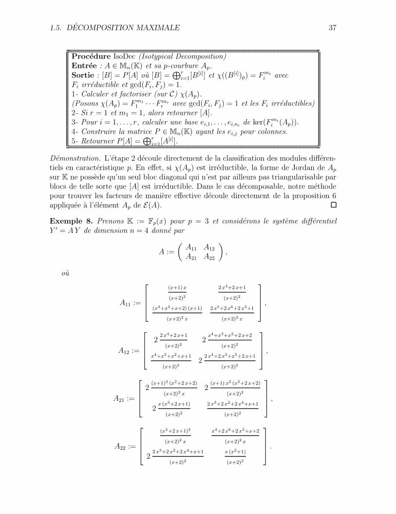
1.5. DECOMPOSITION MAXIMALE 37
Procedure IsoDec (Isotypical Decomposition)Entree : A ∈ Mn(K) et sa p-courbure Ap.Sortie : [B] = P [A] ou [B] =
⊕ri=1[B
[i]] et χ((B[i])p) = F mi
i avecFi irreductible et gcd(Fi, Fj) = 1.1- Calculer et factoriser (sur C) χ(Ap).(Posons χ(Ap) = F m1
1 · · ·F mrr avec gcd(Fi, Fj) = 1 et les Fi irreductibles)
2- Si r = 1 et m1 = 1, alors retourner [A].3- Pour i = 1, . . . , r, calculer une base ei,1, . . . , ei,ni
de ker(F mi
i (Ap)).4- Construire la matrice P ∈ Mn(K) ayant les ei,j pour colonnes.5- Retourner P [A] =
⊕ri=1[A
[i]].
Demonstration. L’etape 2 decoule directement de la classification des modules differen-tiels en caracteristique p. En effet, si χ(Ap) est irreductible, la forme de Jordan de Ap
sur K ne possede qu’un seul bloc diagonal qui n’est par ailleurs pas triangularisable parblocs de telle sorte que [A] est irreductible. Dans le cas decomposable, notre methodepour trouver les facteurs de maniere effective decoule directement de la proposition 6appliquee a l’element Ap de E(A).
Exemple 8. Prenons K := Fp(x) pour p = 3 et considerons le systeme differentielY ′ = A Y de dimension n = 4 donne par
A :=
(
A11 A12
A21 A22
)
,
ou
A11 :=
(x+1) x
(x+2)2
2 x4+2 x+1
(x+2)2
(x3+x2+x+2) (x+1)
(x+2)2 x
2 x5+2 x6+2 x3+1
(x+2)2 x
,
A12 :=
22 x4+2 x+1
(x+2)22
x4+x3+x2+2 x+2
(x+2)2
x4+x5+x2+x+1
(x+2)22
2 x4+2 x3+x5+2 x+1
(x+2)2
,
A21 :=
2(x+1)3 (x2+2 x+2)
(x+2)2 x2
(x+1) x2 (x2+2 x+2)
(x+2)2
2x (x3+2 x+1)
(x+2)2
2 x3+2 x2+2 x4+x+1
(x+2)2
,
A22 :=
(x3+2 x+1)2
(x+2)2 x
x4+2 x6+2 x3+x+2
(x+2)2 x
22 x3+2 x2+2 x4+x+1
(x+2)2
x (x2+1)
(x+2)2
.
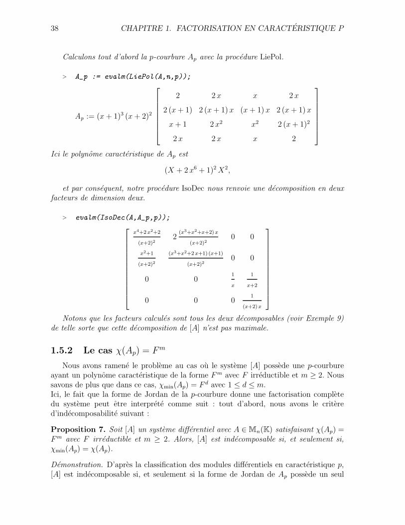
38 CHAPITRE 1. FACTORISATION EN CARACTERISTIQUE P
Calculons tout d’abord la p-courbure Ap avec la procedure LiePol.
> A_p := evalm(LiePol(A,n,p));
Ap := (x + 1)3 (x + 2)2
2 2 x x 2 x
2 (x + 1) 2 (x + 1) x (x + 1) x 2 (x + 1) x
x + 1 2 x2 x2 2 (x + 1)2
2 x 2 x x 2
Ici le polynome caracteristique de Ap est
(X + 2 x6 + 1)2 X2,
et par consequent, notre procedure IsoDec nous renvoie une decomposition en deuxfacteurs de dimension deux.
> evalm(IsoDec(A,A_p,p));
x4+2 x2+2
(x+2)22
(x3+x2+x+2) x
(x+2)20 0
x2+1
(x+2)2
(x3+x2+2 x+1) (x+1)
(x+2)20 0
0 01
x
1
x+2
0 0 01
(x+2) x
Notons que les facteurs calcules sont tous les deux decomposables (voir Exemple 9)de telle sorte que cette decomposition de [A] n’est pas maximale.
1.5.2 Le cas χ(Ap) = Fm
Nous avons ramene le probleme au cas ou le systeme [A] possede une p-courbureayant un polynome caracteristique de la forme F m avec F irreductible et m ≥ 2. Noussavons de plus que dans ce cas, χmin(Ap) = F d avec 1 ≤ d ≤ m.Ici, le fait que la forme de Jordan de la p-courbure donne une factorisation completedu systeme peut etre interprete comme suit : tout d’abord, nous avons le critered’indecomposabilite suivant :
Proposition 7. Soit [A] un systeme differentiel avec A ∈ Mn(K) satisfaisant χ(Ap) =F m avec F irreductible et m ≥ 2. Alors, [A] est indecomposable si, et seulement si,χmin(Ap) = χ(Ap).
Demonstration. D’apres la classification des modules differentiels en caracteristique p,[A] est indecomposable si, et seulement si la forme de Jordan de Ap possede un seul
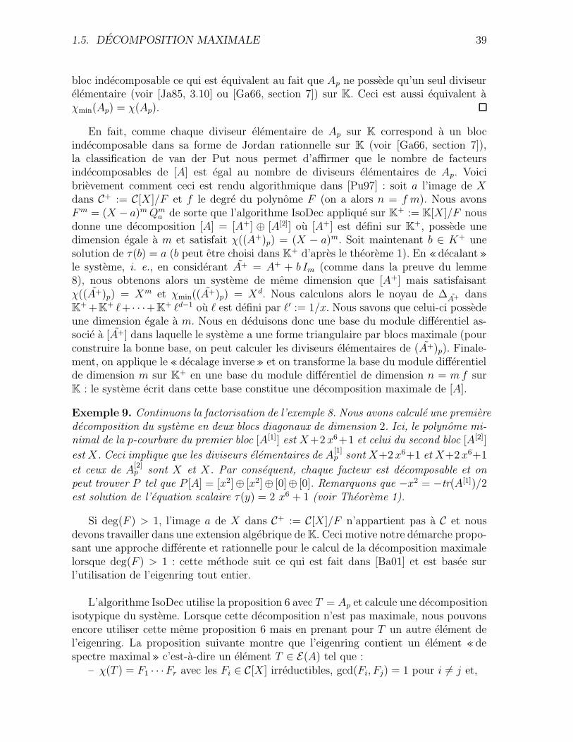
1.5. DECOMPOSITION MAXIMALE 39
bloc indecomposable ce qui est equivalent au fait que Ap ne possede qu’un seul diviseurelementaire (voir [Ja85, 3.10] ou [Ga66, section 7]) sur K. Ceci est aussi equivalent aχmin(Ap) = χ(Ap).
En fait, comme chaque diviseur elementaire de Ap sur K correspond a un blocindecomposable dans sa forme de Jordan rationnelle sur K (voir [Ga66, section 7]),la classification de van der Put nous permet d’affirmer que le nombre de facteursindecomposables de [A] est egal au nombre de diviseurs elementaires de Ap. Voicibrievement comment ceci est rendu algorithmique dans [Pu97] : soit a l’image de Xdans C+ := C[X]/F et f le degre du polynome F (on a alors n = f m). Nous avonsF m = (X − a)m Qm
a de sorte que l’algorithme IsoDec applique sur K+ := K[X]/F nousdonne une decomposition [A] = [A+] ⊕ [A[2]] ou [A+] est defini sur K+, possede unedimension egale a m et satisfait χ((A+)p) = (X − a)m. Soit maintenant b ∈ K+ unesolution de τ(b) = a (b peut etre choisi dans K+ d’apres le theoreme 1). En «decalant»le systeme, i. e., en considerant A+ = A+ + b Im (comme dans la preuve du lemme8), nous obtenons alors un systeme de meme dimension que [A+] mais satisfaisantχ((A+)p) = Xm et χmin((A+)p) = Xd. Nous calculons alors le noyau de ∆A+ dansK+ +K+ `+ · · ·+K+ `d−1 ou ` est defini par `′ := 1/x. Nous savons que celui-ci possedeune dimension egale a m. Nous en deduisons donc une base du module differentiel as-socie a [A+] dans laquelle le systeme a une forme triangulaire par blocs maximale (pourconstruire la bonne base, on peut calculer les diviseurs elementaires de (A+)p). Finale-ment, on applique le «decalage inverse» et on transforme la base du module differentielde dimension m sur K+ en une base du module differentiel de dimension n = m f surK : le systeme ecrit dans cette base constitue une decomposition maximale de [A].
Exemple 9. Continuons la factorisation de l’exemple 8. Nous avons calcule une premieredecomposition du systeme en deux blocs diagonaux de dimension 2. Ici, le polynome mi-nimal de la p-courbure du premier bloc [A[1]] est X+2 x6+1 et celui du second bloc [A[2]]
est X. Ceci implique que les diviseurs elementaires de A[1]p sont X+2 x6+1 et X+2 x6+1
et ceux de A[2]p sont X et X. Par consequent, chaque facteur est decomposable et on
peut trouver P tel que P [A] = [x2]⊕ [x2]⊕ [0]⊕ [0]. Remarquons que −x2 = −tr(A[1])/2est solution de l’equation scalaire τ(y) = 2 x6 + 1 (voir Theoreme 1).
Si deg(F ) > 1, l’image a de X dans C+ := C[X]/F n’appartient pas a C et nousdevons travailler dans une extension algebrique de K. Ceci motive notre demarche propo-sant une approche differente et rationnelle pour le calcul de la decomposition maximalelorsque deg(F ) > 1 : cette methode suit ce qui est fait dans [Ba01] et est basee surl’utilisation de l’eigenring tout entier.
L’algorithme IsoDec utilise la proposition 6 avec T = Ap et calcule une decompositionisotypique du systeme. Lorsque cette decomposition n’est pas maximale, nous pouvonsencore utiliser cette meme proposition 6 mais en prenant pour T un autre element del’eigenring. La proposition suivante montre que l’eigenring contient un element «despectre maximal» c’est-a-dire un element T ∈ E(A) tel que :
– χ(T ) = F1 · · ·Fr avec les Fi ∈ C[X] irreductibles, gcd(Fi, Fj) = 1 pour i 6= j et,
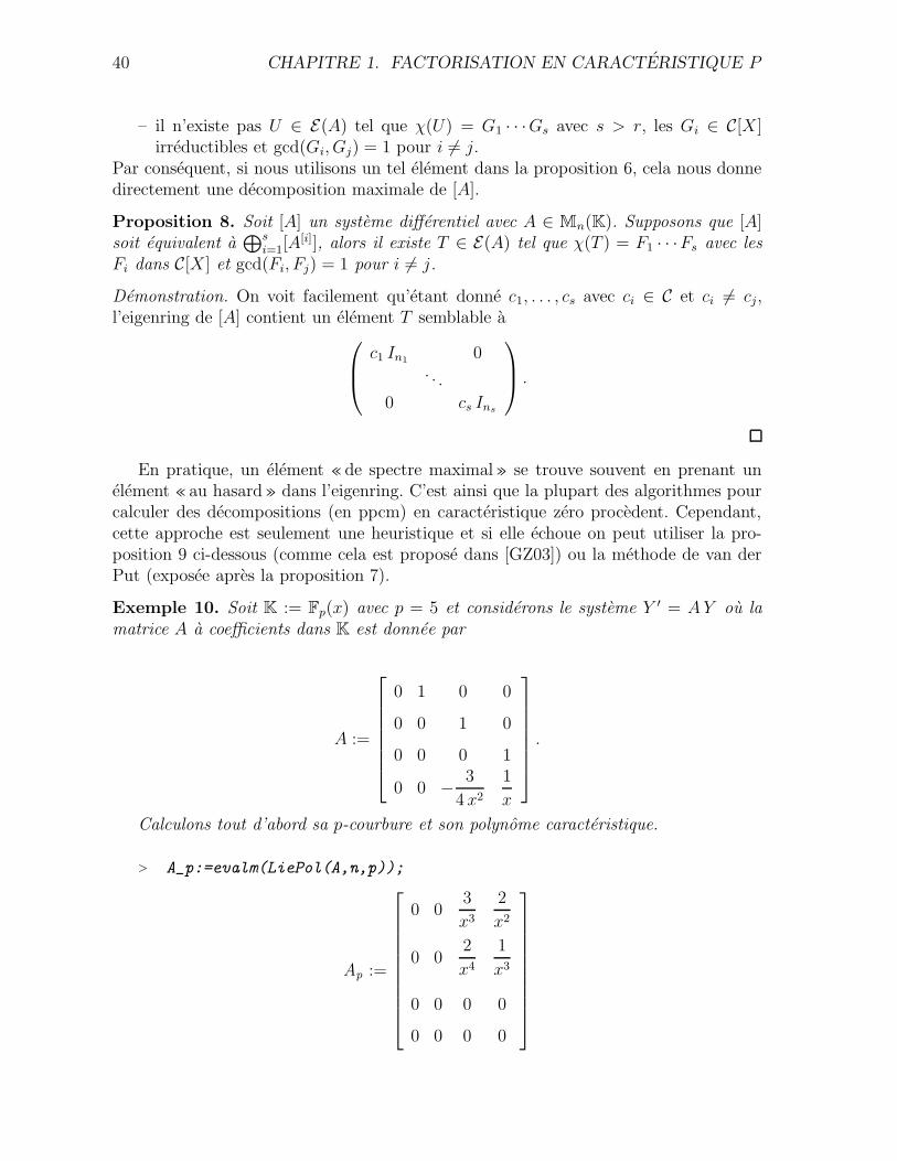
40 CHAPITRE 1. FACTORISATION EN CARACTERISTIQUE P
– il n’existe pas U ∈ E(A) tel que χ(U) = G1 · · ·Gs avec s > r, les Gi ∈ C[X]irreductibles et gcd(Gi, Gj) = 1 pour i 6= j.
Par consequent, si nous utilisons un tel element dans la proposition 6, cela nous donnedirectement une decomposition maximale de [A].
Proposition 8. Soit [A] un systeme differentiel avec A ∈ Mn(K). Supposons que [A]soit equivalent a
⊕si=1[A
[i]], alors il existe T ∈ E(A) tel que χ(T ) = F1 · · ·Fs avec lesFi dans C[X] et gcd(Fi, Fj) = 1 pour i 6= j.
Demonstration. On voit facilement qu’etant donne c1, . . . , cs avec ci ∈ C et ci 6= cj,l’eigenring de [A] contient un element T semblable a
c1 In1 0. . .
0 cs Ins
.
En pratique, un element «de spectre maximal» se trouve souvent en prenant unelement « au hasard» dans l’eigenring. C’est ainsi que la plupart des algorithmes pourcalculer des decompositions (en ppcm) en caracteristique zero procedent. Cependant,cette approche est seulement une heuristique et si elle echoue on peut utiliser la pro-position 9 ci-dessous (comme cela est propose dans [GZ03]) ou la methode de van derPut (exposee apres la proposition 7).
Exemple 10. Soit K := Fp(x) avec p = 5 et considerons le systeme Y ′ = A Y ou lamatrice A a coefficients dans K est donnee par
A :=
0 1 0 0
0 0 1 0
0 0 0 1
0 0 − 3
4 x2
1
x
.
Calculons tout d’abord sa p-courbure et son polynome caracteristique.
> A_p:=evalm(LiePol(A,n,p));
Ap :=
0 03
x3
2
x2
0 02
x4
1
x3
0 0 0 0
0 0 0 0
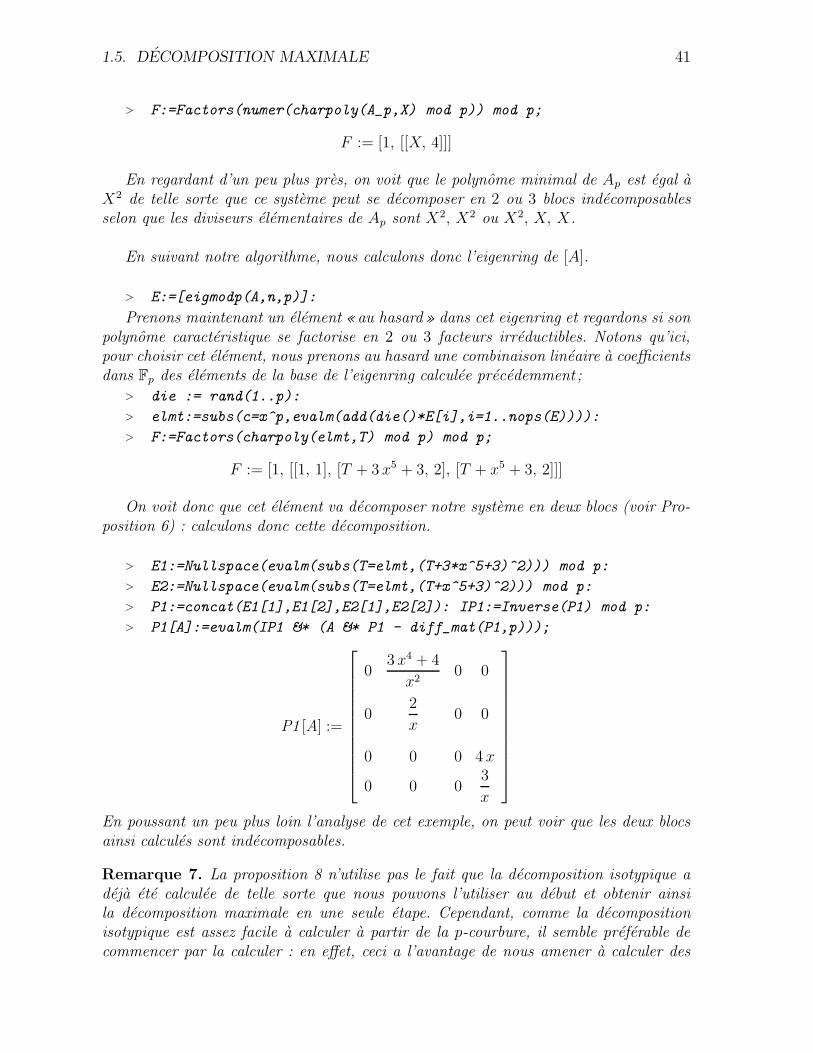
1.5. DECOMPOSITION MAXIMALE 41
> F:=Factors(numer(charpoly(A_p,X) mod p)) mod p;
F := [1, [[X, 4]]]
En regardant d’un peu plus pres, on voit que le polynome minimal de Ap est egal aX2 de telle sorte que ce systeme peut se decomposer en 2 ou 3 blocs indecomposablesselon que les diviseurs elementaires de Ap sont X2, X2 ou X2, X, X.
En suivant notre algorithme, nous calculons donc l’eigenring de [A].
> E:=[eigmodp(A,n,p)]:
Prenons maintenant un element « au hasard» dans cet eigenring et regardons si sonpolynome caracteristique se factorise en 2 ou 3 facteurs irreductibles. Notons qu’ici,pour choisir cet element, nous prenons au hasard une combinaison lineaire a coefficientsdans Fp des elements de la base de l’eigenring calculee precedemment ;
> die := rand(1..p):
> elmt:=subs(c=x^p,evalm(add(die()*E[i],i=1..nops(E)))):
> F:=Factors(charpoly(elmt,T) mod p) mod p;
F := [1, [[1, 1], [T + 3 x5 + 3, 2], [T + x5 + 3, 2]]]
On voit donc que cet element va decomposer notre systeme en deux blocs (voir Pro-position 6) : calculons donc cette decomposition.
> E1:=Nullspace(evalm(subs(T=elmt,(T+3*x^5+3)^2))) mod p:
> E2:=Nullspace(evalm(subs(T=elmt,(T+x^5+3)^2))) mod p:
> P1:=concat(E1[1],E1[2],E2[1],E2[2]): IP1:=Inverse(P1) mod p:
> P1[A]:=evalm(IP1 &* (A &* P1 - diff_mat(P1,p)));
P1 [A] :=
03 x4 + 4
x20 0
02
x0 0
0 0 0 4 x
0 0 03
x
En poussant un peu plus loin l’analyse de cet exemple, on peut voir que les deux blocsainsi calcules sont indecomposables.
Remarque 7. La proposition 8 n’utilise pas le fait que la decomposition isotypique adeja ete calculee de telle sorte que nous pouvons l’utiliser au debut et obtenir ainsila decomposition maximale en une seule etape. Cependant, comme la decompositionisotypique est assez facile a calculer a partir de la p-courbure, il semble preferable decommencer par la calculer : en effet, ceci a l’avantage de nous amener a calculer des
42 CHAPITRE 1. FACTORISATION EN CARACTERISTIQUE P
eigenrings de systemes de dimension plus petite. De plus, pour calculer ces eigenrings,nous pouvons tirer partie du lemme 12 comme suit : connaissant la p-courbure Ap dusysteme dont nous devons calculer l’eigenring, nous savons que I, Ap, . . . , Ad−1
p (avecd = degx(χmin(Ap))) sont des elements C-independants de l’eigenring ce qui nous permetde reduire encore les calculs (en reduisant la dimension du systeme dont on cherchel’eigenring) a effectuer pour obtenir une base complete de l’eigenring.
Voici une autre maniere d’utiliser l’eigenring pour factoriser notre systeme. Letheoreme suivant ([Ja80, Proposition 3.1 p. 111]) fournit un critere d’indecomposabilite.
Proposition 9. Soit A ∈ Mn(K), A 6= 0. Alors, [A] est indecomposable si, et seulementsi E(A) ne contient pas d’idempotent autre que 0 et In.
Demonstration. Supposons [A] decomposable. Il existe alors T ∈ E(A) semblable a(
In1 00 0
)
. Il est alors clair que T 6= 0, T 6= In et T 2 = T .
Reciproquement, si E(A) contient un idempotent T different de 0 et I, alors d’apres laproposition 6, [A] est decomposable.
Par consequent, calculer de maniere recursive (i. e., jusqu’a ce que les facteurssoient indecomposables) des idempotents dans l’eigenring permet aussi de calculer unedecomposition maximale de [A]. Cette methode est celle utilisee par Giesbrecht et Zhangdans [GZ03] pour decomposer des polynomes de Ore en caracteristique p. Pour ce faire,ils montrent comment utiliser l’algorithme de decomposition d’algebres associativesdonne dans [IRS94] pour calculer de «bons» idempotents dans l’eigenring. Leur al-gorithme est donc construit d’une maniere assez differente du notre : ils raisonnentdirectement sur l’eigenring du systeme de depart alors que nous faisons le choix dedecomposer d’abord au maximum en utilisant la p-courbure (plus facile a calculer).Nous ne calculons l’eigenring que lorsque nous ne pouvons plus continuer a decomposeravec la p-courbure sans aller calculer dans des extensions algebriques du corps de base.
Remarque 8. Soit F un corps quelconque. Une matrice M ∈ Mn(F) est dite semi-simple si tout sous-espace invariant par M admet un sous-espace supplementaire in-variant par M . En particulier, Une matrice M ∈ Mn(F) est semi-simple si elle estdiagonalisable sur F .On deduit alors facilement de ce qui precede le resultat suivant : si [A] est un systemedifferentiel avec A ∈ Mn(K), alors sa p-courbure Ap est semi-simple si, et seulement si,le systeme est completement reductible sur K.
1.6 Le cas indecomposable
Dans cette section, nous donnons une alternative rationnelle a la methode de vander Put dans le cas ou le systeme [A] est indecomposable, i. e., χ(Ap) = χmin(Ap) = F m
avec F irreductible et m > 1 (rappelons que si m = 1, alors [A] est irreductible). Nousmontrons comment calculer une reduction maximale, c’est-a-dire, comment obtenir unsysteme equivalent a [A] ayant une forme triangulaire par blocs avec des blocs diagonauxirreductibles. Ce resultat peut s’enoncer comme suit :
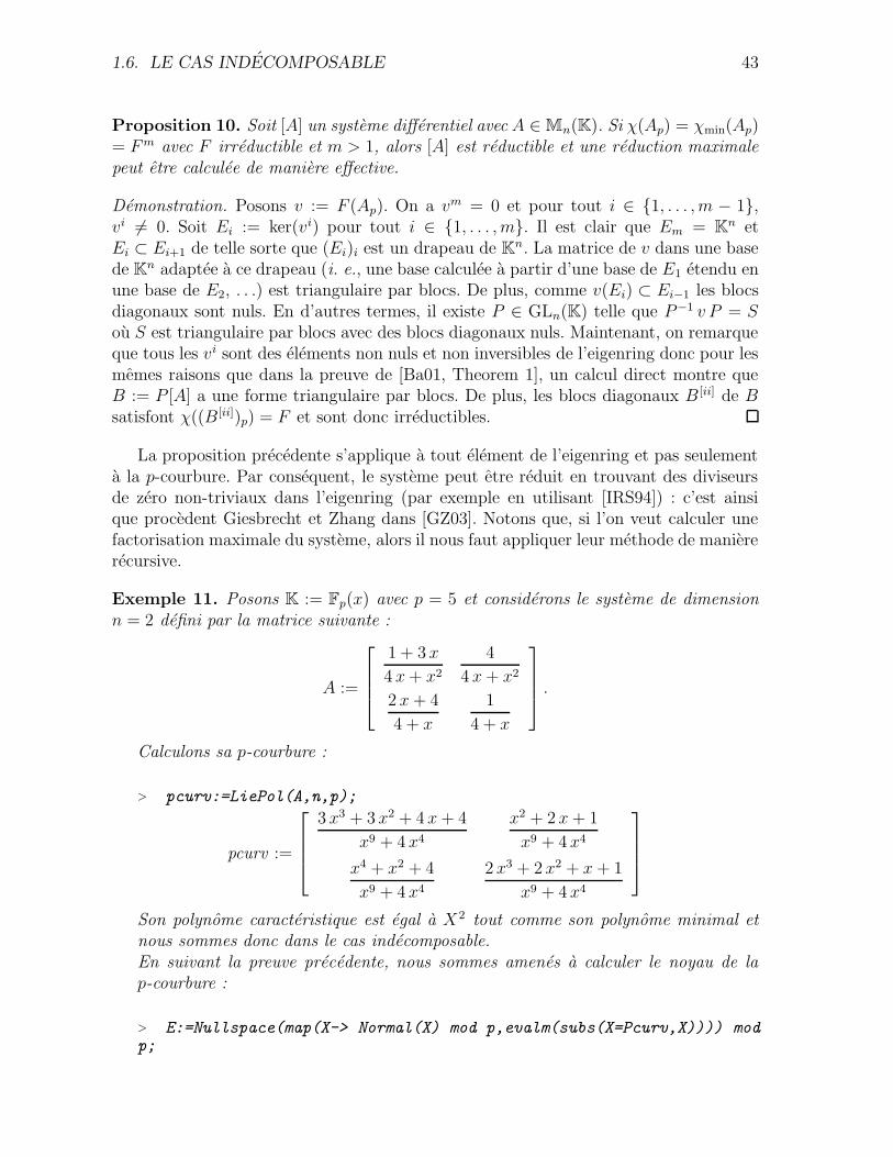
1.6. LE CAS INDECOMPOSABLE 43
Proposition 10. Soit [A] un systeme differentiel avec A ∈ Mn(K). Si χ(Ap) = χmin(Ap)= F m avec F irreductible et m > 1, alors [A] est reductible et une reduction maximalepeut etre calculee de maniere effective.
Demonstration. Posons v := F (Ap). On a vm = 0 et pour tout i ∈ {1, . . . , m − 1},vi 6= 0. Soit Ei := ker(vi) pour tout i ∈ {1, . . . , m}. Il est clair que Em = Kn etEi ⊂ Ei+1 de telle sorte que (Ei)i est un drapeau de Kn. La matrice de v dans une basede Kn adaptee a ce drapeau (i. e., une base calculee a partir d’une base de E1 etendu enune base de E2, . . .) est triangulaire par blocs. De plus, comme v(Ei) ⊂ Ei−1 les blocsdiagonaux sont nuls. En d’autres termes, il existe P ∈ GLn(K) telle que P−1 v P = Sou S est triangulaire par blocs avec des blocs diagonaux nuls. Maintenant, on remarqueque tous les vi sont des elements non nuls et non inversibles de l’eigenring donc pour lesmemes raisons que dans la preuve de [Ba01, Theorem 1], un calcul direct montre queB := P [A] a une forme triangulaire par blocs. De plus, les blocs diagonaux B [ii] de Bsatisfont χ((B[ii])p) = F et sont donc irreductibles.
La proposition precedente s’applique a tout element de l’eigenring et pas seulementa la p-courbure. Par consequent, le systeme peut etre reduit en trouvant des diviseursde zero non-triviaux dans l’eigenring (par exemple en utilisant [IRS94]) : c’est ainsique procedent Giesbrecht et Zhang dans [GZ03]. Notons que, si l’on veut calculer unefactorisation maximale du systeme, alors il nous faut appliquer leur methode de maniererecursive.
Exemple 11. Posons K := Fp(x) avec p = 5 et considerons le systeme de dimensionn = 2 defini par la matrice suivante :
A :=
1 + 3 x
4 x + x2
4
4 x + x2
2 x + 4
4 + x
1
4 + x
.
Calculons sa p-courbure :
> pcurv:=LiePol(A,n,p);
pcurv :=
3 x3 + 3 x2 + 4 x + 4
x9 + 4 x4
x2 + 2 x + 1
x9 + 4 x4
x4 + x2 + 4
x9 + 4 x4
2 x3 + 2 x2 + x + 1
x9 + 4 x4
Son polynome caracteristique est egal a X2 tout comme son polynome minimal etnous sommes donc dans le cas indecomposable.En suivant la preuve precedente, nous sommes amenes a calculer le noyau de lap-courbure :
> E:=Nullspace(map(X-> Normal(X) mod p,evalm(subs(X=Pcurv,X)))) modp;
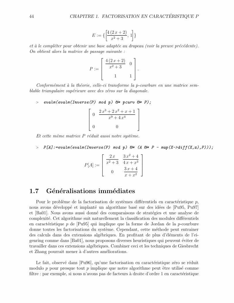
44 CHAPITRE 1. FACTORISATION EN CARACTERISTIQUE P
E := {[
4 (2 x + 2)
x2 + 3, 1
]
}
et a le completer pour obtenir une base adaptee au drapeau (voir la preuve precedente).On obtient alors la matrice de passage suivante :
P :=
4 (2 x + 2)
x2 + 30
1 1
.
Conformement a la theorie, celle-ci transforme la p-courbure en une matrice sem-blable triangulaire superieure avec des zeros sur la diagonale.
> evalm(evalm(Inverse(P) mod p) &* pcurv &* P);
02 x3 + 2 x2 + x + 1
x9 + 4 x4
0 0
Et cette meme matrice P reduit aussi notre systeme.
> P[A]:=evalm(evalm(Inverse(P) mod p) &* (A &* P - map(X->diff(X,x),P)));
P [A] :=
2 x
x2 + 3
3 x2 + 4
4 x + x3
03 x + 4
x + x2
1.7 Generalisations immediates
Pour le probleme de la factorisation de systemes differentiels en caracteristique p,nous avons developpe et implante un algorithme base sur des idees de [Pu95, Pu97]et [Ba01]. Nous avons aussi donne des comparaisons de strategies et une analyse decomplexite. Cet algorithme suit naturellement la classification des modules differentielsen caracteristique p de [Pu95] qui implique que la forme de Jordan de la p-courburedonne toutes les factorisations du systeme. Cependant, cette methode peut entrainerdes calculs dans des extensions algebriques. En profitant de plus d’elements de l’ei-genring comme dans [Ba01], nous proposons diverses heuristiques qui peuvent eviter detravailler dans ces extensions algebriques. Combiner ceci et les techniques de Giesbrechtet Zhang pourrait mener a d’autres ameliorations.
Le fait, observe dans [Pu96], qu’une factorisation en caracteristique zero se reduitmodulo p pour presque tout p implique que notre algorithme peut etre utilise commefiltre : par exemple, si nous n’avons pas de facteurs a droite d’ordre 1 en caracteristique
1.7. GENERALISATIONS IMMEDIATES 45
p, alors nous n’avons pas de solutions exponentielles en caracteristique zero. Un algo-rithme utilisant des methodes modulaires pour calculer les solutions exponentielles encaracteristique zero est developpe dans le chapitre 2 (voir aussi [CH04]).
Nous allons maintenant montrer comment adapter l’algorithme de factorisation desystemes differentiels developpe dans les sections 1.3 a 1.6 a d’autres situations :
1.7.1 Factorisation « locale »
Dans cette sous-section, nous donnons les elements necessaires pour generaliser l’al-gorithme decrit dans les sections 1.3 a 1.6 au cas des systemes a coefficients dans K((x)).
Soit [A] un systeme differentiel avec A ∈ Mn(K((x))). Les notions de p-courbure eteigenring peuvent etre definies de la meme facon que dans les definitions 7 et 13. Enremarquant que K((x)) est un corps C1 ([Ja80, Definition 11.5, p. 649]), on deduit que laclassification des modules differentiels en caracteristique p reste directement applicabledans ce cas (voir la sous-section 1.3.2).
Pour construire un algorithme comme nous l’avons fait dans les parties 1.3 a 1.6dans le cas ou A ∈ Mn(K(x)), il ne nous reste donc plus qu’a savoir factoriser unpolynome a coefficients dans Fq((x)) ou q = pr : ceci peut se faire grace au theoreme deNewton/Puiseux suivant (voir par exemple [Abh90, Lecture 12]) :
Theoreme 3. Soit F (Y ) = Y n + an−1(x) Y n−1 + · · · + a0(x) un polynome unitaire acoefficients dans k((x)) avec k = Fp ou p > n. Il existe r ∈ N∗, non divisible par p, telque F (Y ) =
∏ni=1(Y − νi) avec νi ∈ k((x1/r)).
Tous les ingredients necessaires sont maintenant reunis et, en appliquant ce theoremeau polynome caracteristique de la p-courbure, on obtient une generalisation immediatede notre algorithme au cas des systemes a coefficients dans K((x)).
Remarque 9. Dans le theoreme 3, si F designe le polynome caracteristique de la p-courbure, alors les νi sont lies a ce qu’on appelle les exposants generalises de l’operateurdifferentiel. En fait, on peut definir une notion d’exposants generalises en caracteristiquep de la meme maniere qu’en caracteristique zero et montrer qu’ils ne sont autres queles reductions mod p des exposants generalises en caracteristique zero : tout ceci seradetaille dans le chapitre 2.
1.7.2 Factorisation de systemes d’equations aux differences
L’algorithme developpe dans le cadre des systemes differentiels lineaires Y (x)′ =A(x) Y (x) peut etre generalise au cas des systemes aux differences lineaires Y (x + 1) =A(x) Y (x). Le corps differentiel (k(x),′ ) ou k = Fq avec q = pr est remplace par le corpsaux differences (k(x), σ) ou σ est defini par σ(x) = x + 1 et σ(f) = f , pour tout f ∈ k.Le corps des constantes {a ∈ k | σ(a) = a} est alors k(xp − x) (voir [PS97, Chapter 5]
46 CHAPITRE 1. FACTORISATION EN CARACTERISTIQUE P
ou [GZ03, Theorem 3.1]).
Tout comme dans le cas differentiel, il existe une notion naturelle de p-courbure :
Definition 15. Soit σ(Y ) = A Y avec A ∈ GLn(k(x)) (k = Fq, q = pr) un systemed’equations aux differences lineaire. Sa p-courbure est le produit de matrices A(x + p−1) · · ·A(x + 1) A(x).
Une classification des modules aux differences en caracteristique p (analogue a cellede [Pu95] ou [PS03, Ch. 13] dans le cas differentiel) est donnee dans [PS97, Ch. 5].Cette classification implique la aussi que la forme de Jordan de la p-courbure donnetoutes les factorisations du systeme aux differences. L’equation τ(y) := y(p−1) + yp = λavec λ ∈ k(xp) consideree dans la sous-section 1.3.4 est ici remplacee par τ1(u) :=u(x + p − 1) · · ·u(x + 1) u(x) = λ avec λ ∈ k(xp − x). Dans le cas ou la p-courbure estscalaire, le resultat de rationnalite du theoreme 1 ne reste pas vrai ; en effet, si l’on sup-pose p > n et que l’on essaye d’adapter la preuve, l’analogue de la solution Tr(A)/n del’equation τ(y) = λ est ici la solution det(A)1/n a l’equation τ1(y) = λ et nous perdonsdonc la rationnalite de cette solution.
Nous pouvons aussi definir un eigenring (voir par exemple [Ba01, Bom01]) : soitσ(Y ) = A Y un systeme d’equations aux differences lineaire avec A ∈ Mn(k(x)). L’ei-genring E(A) de [A] est l’ensemble defini par
E(A) = {P ∈ Mn(k(x)) | σ(P ) A = A P}.
Tous les elements necessaires au developpement d’un algorithme analogue a celuique nous avons donne dans le cas differentiel sont donc reunis et l’algorithme suitnaturellement. Notons encore que :
– les resultats de [Ba01] restent vrais dans le cas aux differences ([Ba01] est ecritdans le cadre general des equations pseudo-lineaires),
– l’algorithme de Giesbrecht et Zhang ([GZ03]) factorise tout polynome de Ore doncen particulier les operateurs aux differences.
1.8 Factorisation de systemes d’equations aux
derivees partielles en caracteristique p
Dans cette partie, nous generalisons l’algorithme decrit precedemment pour facto-riser certains systemes d’equations aux derivees partielles en caracteristique p : plusprecisement, nous montrons comment ramener le probleme a la reduction d’une com-binaison lineaire a coefficients indetermines de matrices qui commutent. Le fait d’etreamene a reduire une combinaison lineaire a coefficients indetermines de matrices pourfactoriser un systeme d’equations aux derivees partielles apparait deja de manierenaturelle lorsque l’on considere des systemes a coefficients constants. En effet, soitA1, . . . , Am des matrices carrees a coefficients constants qui commutent entre elles deux
1.8. FACTORISATION DE SYSTEMES D’E. AUX D. P. 47
a deux. Considerons le systeme D-fini donne par les ∆i := ∂i − Ai. Chaque systeme∆i(Y ) = 0 a pour solution exp(Ai xi) Ci avec Ci vecteur constant (∂i(Ci) = 0) de sorteque Y = exp(A1 x1 + · · · + Am xm) est une solution commune a chaque ∆i(Y ) = 0. Orsi l’on veut calculer cette exponentielle de matrice, il nous faut reduire la combinaisonlineaire a coefficients indetermines A1 x1 + · · · + Am xm.
Concernant le probleme de la factorisation de systemes d’equations aux deriveespartielles en caracteristique zero, recemment, Li, Schwarz et Tsarev ont montre (voir[LST02, LST03]) comment adapter l’algorithme de Beke au cadre des systemes d’equationsaux derivees partielles D-finis. Notons encore que dans sa these ([Wu04]), Wu decriraun algorithme de factorisation dans le cadre plus general des equations fonctionnelles.
1.8.1 Systemes D-finis
Soit F = k(x1, . . . , xm) le corps des fractions rationnelles en m variables x1, . . . , xm
et a coefficients dans un corps k. Pour i appartenant a {1, . . . , m}, notons ∂i := ddxi
l’operateur de derivation par rapport a la i-eme variable. Soit Θ := {∂1, . . . , ∂m} lemonoıde commutatif genere par les derivations ∂i.
En suivant la terminologie de [PS03, Appendix D], on dit alors que (F , Θ) est unΘ-corps ou corps differentiel partiel.
Definition 16. Soit (F , Θ) un corps differentiel partiel. L’anneau des operateurs differen-tiels partiels a coefficients dans F note F [Θ] est l’anneau (non-commutatif) des po-lynomes en les variables ∂i satisfaisant les deux conditions suivantes :
– les ∂i commutent entre eux deux a deux,– pour tout i ∈ {1, . . . , m} et tout a ∈ F , ∂i a = a ∂i + ∂i(a).
Definition 17. Un systeme d’equations aux derivees partielles est donne par un en-semble fini d’elements de l’anneau F [Θ]. A tout systeme S d’equations aux deriveespartielles, on associe l’ideal (a gauche) genere par les elements de S que l’on note (S).
Dans cette partie, tous les systemes d’equations aux derivees partielles que nousconsiderons sont supposes ecrits sous la forme
∆1(y) = 0 avec ∆1 := ∂1 − A1,...
∆m(y) = 0 avec ∆m := ∂m − Am,
(1.7)
ou les Ai sont des matrices de taille n ∈ N∗ a coefficients dans F et les ∆i commutententre eux deux a deux : cette commutativite implique les relations suivantes, appeleesconditions d’integrabilite, sur les matrices Ai (voir par exemple [PS03, Appendix D]) :
∂i(Aj) − ∂j(Ai) + Ai Aj − Aj Ai = 0, (1.8)
pour tout i, j dans {1, . . . , m}.De tels systemes sont des systemes d’equations aux derivees partielles D-finis.
48 CHAPITRE 1. FACTORISATION EN CARACTERISTIQUE P
Definition 18. Un systeme S d’equations aux derivees partielles est D-fini si l’idealassocie (S) est de dimension (differentielle) zero.
Si S est D-fini, alors le F -espace vectoriel F [Θ]/(S) est de dimension finie. Lessystemes D-finis correspondent donc a des F [Θ]-modules c’est-a-dire a des espaces vec-toriels de dimension finie sur F qui sont des modules a gauche pour l’anneau F [Θ] (Voir[PS03, Appendix D]). En terme de solutions, la D-finitude est equivalente au fait queles solutions du systeme ne dependent que d’un nombre fini de constantes.
Etant donne un systeme d’equations aux derivees partielles quelconque S, il existedes algorithmes permettant de tester si le systeme est D-fini et, si oui, de l’ecrire sousla forme (1.7). Par exemple, ceci peut se faire en calculant une base de Janet (baseaussi appelee base involutive dans la litterature) du systeme (voir [Ja20, Ja29, HS02,BCGPR03]). Ces bases de Janet peuvent etre vues comme une sorte d’analogue desbases de Groebner (non reduites). L’interet est qu’une base de Janet fournit une basedu quotient F [Θ]/(S) : la finitude de cette base est alors equivalente au fait que lesysteme soit D-fini et les Ai s’obtiennent en calculant l’action des ∂i sur la base duquotient. En particulier, la dimension n des Ai est egale au cardinal de cette base.
1.8.2 Factorisation et eigenrings
De la meme maniere que nous l’avons fait dans la sous-section 1.1.5, nous pouvonsdefinir ici les notions de systemes decomposables et reductibles et en deduire ce que nousentendons par factoriser un systeme d’equations aux derivees partielles.
Definition 19. Soit (F , Θ) un corps differentiel partiel et considerons un systemed’equations aux derivees partielles S.On dit que le systeme S est decomposable (sur F) s’il existe une matrice P inversiblea coefficients dans F telle que pour tout i dans {1, . . . , m}, P −1 (Ai P − ∂i(P )) soitdiagonale par blocs. Un systeme qui n’est pas decomposable est dit indecomposable.On dit que le systeme S est reductible (sur F) s’il existe une matrice P inversiblea coefficients dans F telle que pour tout i dans {1, . . . , m}, P −1 (Ai P − ∂i(P )) soittriangulaire par blocs. Un systeme qui n’est pas reductible est dit irreductible.
Definition 20. Soit (F , Θ) un corps differentiel partiel et considerons un systemed’equations aux derivees partielles S. Factoriser le systeme S signifie, soit trouverune matrice P inversible a coefficients dans F telle que pour tout i dans {1, . . . , m},P−1 (Ai P − ∂i(P )) soit diagonale ou triangulaire par blocs, soit montrer qu’une tellematrice P n’existe pas. Autrement dit, cela signifie decider si S est decomposable ouindecomposable, reductible ou irreductible, et dans le cas decomposable ou reductible,trouver une matrice P reduisant ou decomposant simultanement tous les systemes ∂i(Y ) =Ai Y .
Factoriser un systeme d’equations aux derivees partielles signifie donc factorisersimultanement les systemes ∂i(Y ) = Ai Y . En particulier, nous voyons deja que si l’un
1.8. FACTORISATION DE SYSTEMES D’E. AUX D. P. 49
de ces systemes est irreductible sur F , alors le systeme S est lui aussi irreductible surF .
Dans le cas differentiel classique, nous avons caracterise l’eigenring d’un systeme∆A(Y ) = 0 comme l’ensemble des endomorphismes differentiels qui commutent avec∆A : nous prenons ici cette caracterisation pour definition.
Definition 21. Soit (F , Θ) un corps differentiel partiel et considerons un systemed’equations aux derivees partielles S. L’eigenring du systeme est
E(S) := {P ∈ Mn(F) | ∀i ∈ {1, . . . , m}, P ∆i = ∆i P}.
Si l’on note Ei(S) := {P ∈ Mn(F) |P ∆i = ∆i P} alors on a
E(S) = ∩ni=1Ei(S).
Ces ensembles Ei(S) sont appeles les eigenrings partiels.
De maniere analogue a ce qui se passe dans le cas differentiel ordinaire, la connais-sance d’un element non-trivial dans l’eigenring donne immediatement une factorisationdu systeme.
1.8.3 Systemes d’e.d.p. en caracteristique p
Considerons maintenant le corps differentiel partiel (K, Θ) de caracteristique p ouK := k(x1, . . . , xm) avec k = Fq, q = pr. Comme nous avons ici plusieurs derivations,nous definissons des p-courbures partielles.
Definition 22. Soit S un systeme d’equations aux derivees partielles a coefficientsdans (K, Θ). Les p-courbures partielles du systeme S sont les operateurs ∆p
i , pour i ∈{1, . . . , m}, agissant sur Kn.
Notons que dans [Ka82], Katz definit aussi une notion de p-courbure dans le casde plusieurs derivations et remarque les liens entre cette p-courbure et l’eigenring dusysteme.
Lemme 13. Soit S un systeme d’equations aux derivees partielles a coefficients dans(K, Θ). Les p-courbures partielles ∆p
i commutent entre elles (deux a deux) et appar-tiennent a l’eigenring E(S). De plus le polynome minimal (et caracteristique) de chaque∆p
i est a coefficients dans k(xp1, . . . , x
pm).
Demonstration. Le fait que les p-coubures partielles commutent et appartiennent al’eigenring decoule directement du fait que les ∆i commutent entre eux deux a deux.Soit χ1(T ) := T n +
∑n−1i=0 fiT
i le polynome minimal de D1 := ∆p1. On sait que χ1 est a
coefficients dans le corps des constantes de (k(x1, . . . , xm), ∂1), i. e., k(x2, . . . , xm)(xp1).
Pour tout j ∈ {2, . . . , m}, on a ∆j(χ1(D1)) = 0. En utilisant le fait que ∆j verifie lacondition de Leibniz, on obtient alors
∑n−1i=0 ∂j(fi) Di
1 = 0. Maintenant, comme χ1 estle polynome minimal de D1, il vient ∂j(fi) = 0 pour tout i ∈ {0, . . . , n−1} et pour toutj ∈ {2, . . . , m} ; d’ou le resultat.
50 CHAPITRE 1. FACTORISATION EN CARACTERISTIQUE P
Le corps de base K = k(x1, . . . , xm) avec k = Fq et q = pr verifie K(p) := {f p | f ∈K} = k(xp
1, . . . , xpm). Nous avons donc [K : K(p)] = m p 6= p de sorte que la premiere
hypothese sur le corps de base, necessaire pour que la classification de van der Put s’ap-plique directement, n’est pas satisfaite. Cependant, certaines preuves que nous avonsre-ecrites d’une maniere elementaire et constructive peuvent s’adapter ici et nous per-mettent de generaliser les resultats de la section 1.3.
Interessons nous tout d’abord au lemme de Cartier (voir Lemme 3 dans le casdifferentiel ordinaire) dans le cadre des equations aux derivees partielles (voir [Ka70,Theorem 5.1]).
Proposition 11 (Cartier). Soit S un systeme d’equations aux derivees partielles acoefficients dans (K, Θ). Les p-coubures partielles ∆p
i sont toutes nulles si, et seulementsi, le systeme S possede une base de solutions rationnelles.
Ici, S possede une base de solutions rationnelles signifie qu’il existe une base desolutions rationnelles commune a tous les ∆i(Y ) = 0. Autrement dit, il existe P ∈GLn(K) telle que, pour tout i ∈ {1, . . . , m}, P−1 (Ai P − ∂i(P )) = 0.
Demonstration. L’implication «⇐» etant immediate, il nous suffit de montrer «⇒».Considerons tout d’abord le corps differentiel (k(x2, . . . , xm)(x1), ∂1) ayant pour corps deconstantes k(x2, . . . , xm)(xp
1), et regardons ∆1 comme un operateur differentiel agissantsur k(x2, . . . , xm)(x1)
n ; puisqu’il verifie ∆p1 = 0, le lemme de Cartier nous permet
d’affirmer l’existence de P1 ∈ GLn(k(x2, . . . , xm)(x1)) telle que P−11 ∆1 P1 = ∂1. Pour
i ∈ {1, . . . , m}, posons ∆i = P−11 ∆i P1 := ∂i−Bi pour des matrices Bi a coefficients dans
k(x1, . . . , xm). Les conditions d’integrabilite impliquent que pour tout i ∈ {1, . . . , m},∂1(Bi) = 0 de sorte que les Bi sont a coefficients dans k(x2, . . . , xm)(xp
1). Utilisonsmaintenant l’hypothese ∆2
p= 0 et appliquons le lemme de Cartier a ∆2 : il existe P2 ∈
GLn(k(x2, . . . , xm)(xp1)) telle que P−1
2 ∆2 P2 = ∂2. De plus P2 ∈ GLn(k(x2, . . . , xm)(xp1))
implique que ∂1 commute avec P2 et donc P−12 ∆1 P2 = P−1
2 ∂1 P2 = ∂1. En continuantce raisonnement on trouve finalement une matrice P = P1 · · ·Pm inversible a coefficientsdans k(x1, . . . , xm) telle que pour tout i ∈ {1, . . . , m}, P−1 ∆i P = ∂i d’ou le resultat.
Cette preuve exhibe un algorithme pour le calcul d’une matrice fondamentale desolutions rationnelles d’un systeme d’equations aux derivees partielles :
– Pour i = 1 a m, poser A[1]i := Ai.
– Pour i = 1 a m :– Calculer une matrice fondamentale Pi de solutions rationnelles du systeme
differentiel (a une variable) ∂i(Y ) = A[i]i Y ,
– pour j = 1 a m, calculer A[i+1]j := P−1
i (A[i]j Pi − ∂j(Pi)).
– Retourner P1 · · ·Pm.
Remarque 10. Dans le cas ou l’une des p-courbures partielles est nulle, alors, apres
1.8. FACTORISATION DE SYSTEMES D’E. AUX D. P. 51
un changement de base, le systeme (1.7) s’ecrit
∆1(y) = 0 avec ∆1 := ∂1,...
∆m(y) = 0 avec ∆m := ∂m − Am,
(1.9)
de sorte que les conditions d’integrabilite (1.8) impliquent ∂1(Aj) = 0 pour tout j ∈{2, . . . , m}. On peut donc en deduire que le systeme ne depend plus de x1 mais seulementde xp
1.
Regardons maintenant le cas ou toutes les p-courbures partielles ∆pi sont scalaires
c’est-a-dire, pour tout i ∈ {1, . . . , m}, ∆pi = λi In avec λi ∈ k(xp
1, . . . , xpm) (voir Lemme
13).
Considerons tout d’abord individuellement le systeme ∂1(Y ) = A1 Y a coefficientsdans le corps differentiel K = k(x2, . . . , xm)(x1) muni de la derivation ∂1 et ayantpour corps de constantes k(x2, . . . , xm)(xp
1). Notre resultat de rationnalite (Theoreme1) est ici indispensable. En effet, si l’on considere une equation ∂p−1
1 (y) + yp = c avecc ∈ k(x2, . . . , xm)(xp
1), alors en utilisant la decomposition en elements simples nousne pouvons que demontrer l’existence d’une solution dans k(x2, . . . , xm)(x1) (voir lelemme 6 et sa preuve). Cependant le resultat du theoreme 1 peut aussi etre utilise iciet nous donne une solution dans k(x2, . . . , xm)(x1). Plus precisement, si ∆p
1 = −λ1 In,alors µ1 = −Tr(A1)/n verifie ∂p−1
1 (µ1) + µp1 = λ1 et le systeme ∂1(Y ) = A1 Y est donc
equivalent sur K a [µ1 In].
Proposition 12. Soit S un systeme d’equations aux derivees partielles a coefficientsdans (K, Θ). Les p-coubures partielles ∆p
i sont toutes scalaires si, et seulement si, lesysteme S est equivalent sur K a un « systeme diagonal». Autrement dit, pour tout i ∈{1, . . . , m}, ∆p
i = λi In avec λi ∈ k(xp1, . . . , x
pm) si, et seulement si, il existe P ∈ GLn(K)
telle que pour tout i ∈ {1, . . . , m}, P−1 (Ai P − ∂i(P )) = µi In avec µi ∈ K.
Demonstration. Supposons m = 2 ce qui n’enleve rien a la generalite de la preuve.Considerons donc un systeme d’equations aux derivees partielles (∂1 − A1, ∂2 − A2) telque ∆p
1 = −λ1 In et ∆p2 = −λ2 In avec λ1, λ2 ∈ k(xp
1, xp2). Posons µ1 = −Tr(A1)/n et
µ2 = −Tr(A2)/n et considerons le systeme d’equations aux derivees partielles (∆1 +µ1 In, ∆2 +µ2 In). Par construction ce systeme possede des p-courbures partielles nulles.De plus la condition d’integrabilite pour ce nouveau systeme est satisfaite : en effet,apres simplifications, cette condition s’ecrit ∂1(µ2) = ∂2(µ1) ce qui est equivalent aTr(∂1(A2)) = Tr(∂2(A1)) ou encore, d’apres (1.8), a Tr(A2 A1) = Tr(A1 A2). La propo-sition 11 nous affirme alors l’existence d’une matrice P inversible et a coefficients dansK telle que P−1 ( (A1 + µ1 In) P − ∂i(P )) = P−1 ( (A2 + µ2 In) P − ∂i(P )) = 0 ; d’ou leresultat.
Ici aussi nous pouvons donner une « formule de Katz», analogue a celle donnee dansla sous-section 1.3.5, pour le calcul d’une matrice fondamentale de solutions rationnelles
52 CHAPITRE 1. FACTORISATION EN CARACTERISTIQUE P
lorsque les p-courbures partielles sont toutes nulles. Pour ceci, pour i ∈ {1, . . . , m},definissons
Pri : Kn → Kn, v 7→p−1∑
k=0
(−xi)k
k!∆k
i (v).
On verifie alors que :– pour tout v ∈ Kn, ∆i(Pri(v)) = − (−xi)
p−1 ∆pi (v) de sorte que Pri envoye ker(∆p
i )sur ker(∆i),
– pour tout i, j ∈ {1, . . . , m} tels que i 6= j, ∆j(Pri(v)) = Pri(∆j(v)) de sorte queles Pri commutent entre eux deux a deux.
Posons maintenant Pr :=∏m
i=1 Pri. Cet operateur de Kn dans Kn satisfait alors lapropriete suivante : pour tout i ∈ {1, . . . , m}, si ∆p
i (v) = 0, alors ∆i(Pr(v)) = 0.D’apres [Ka70, §5, p. 191], cette formule pour Pr(v) peut etre developpee et on
obtient ainsi :
Pr(v) =∑
ω
m∏
i=1
(−xi)ωi
ωi!
m∏
i=1
∆ωi
i (v),
ou la somme est prise sur tous les r-uplets ω = (ω1, . . . , ωr) d’entiers tels que 0 ≤ ωi ≤p − 1.
Ceci nous donne donc une formule explicite pour le calcul d’une matrice fondamen-tale de solutions rationnelles d’un systeme d’equations aux derivees partielles dans lecas ou les p-courbures partielles ∆p
i sont toutes nulles et ou (0, . . . , 0) n’annule pas ledenominateur du systeme (voir la discussion suivant la remarque 5).
Remarque 11. Dans [Ka70], Katz donne aussi un analogue de la « formule de Taylor»
Ta (utilisee dans la preuve du lemme 9 de la sous-section 1.3.5) dans le cas de plusieursderivations.
1.8.4 Factorisation de systemes d’e.d.p. en caracteristique p
Soit S un systeme d’equations aux derivees partielles a coefficients dans (K, Θ) avecK = k(x1, . . . , xm) et k = Fq ou q = pr. On sait que pour factoriser individuellementle systeme ∂i(Y ) = Ai Y , alors nous pouvons appliquer l’algorithme developpe dansles sections 1.3 a 1.6. Pour ce faire, nous utilisons la p-courbure partielle ∆p
i ainsi quel’eigenring partiel Ei(S). Tout ceci peut se faire puisqu’au cours de l’algorithme, nous nefaisons rien d’autre que de l’algebre lineaire, soit sur la p-courbure, soit sur un elementde l’eigenring. Maintenant, si nous voulons factoriser le systeme d’equations aux deriveespartielles S, nous devons factoriser simultanement les ∂i(Y ) = Ai Y . Nous sommes doncamenes a reduire simultanement les p-courbures partielles ∆p
i qui commutent d’apresle lemme 13. Le probleme de la reduction simultanee de matrices qui commutent seraetudie dans la sous-section-suivante.
Comme nous l’avons fait dans le cas differentiel ordinaire, nous allons tout d’abordchercher a decomposer le systeme puis nous montrerons comment reduire les blocs
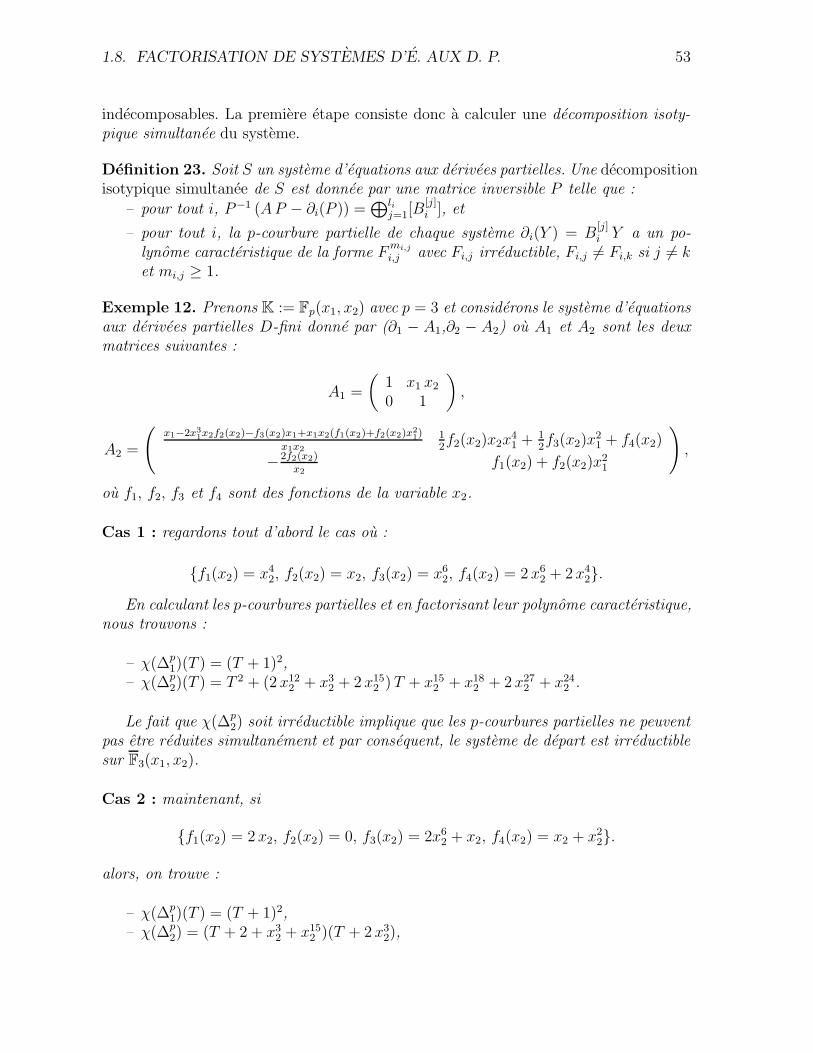
1.8. FACTORISATION DE SYSTEMES D’E. AUX D. P. 53
indecomposables. La premiere etape consiste donc a calculer une decomposition isoty-pique simultanee du systeme.
Definition 23. Soit S un systeme d’equations aux derivees partielles. Une decompositionisotypique simultanee de S est donnee par une matrice inversible P telle que :
– pour tout i, P−1 (A P − ∂i(P )) =⊕li
j=1[B[j]i ], et
– pour tout i, la p-courbure partielle de chaque systeme ∂i(Y ) = B[j]i Y a un po-
lynome caracteristique de la forme Fmi,j
i,j avec Fi,j irreductible, Fi,j 6= Fi,k si j 6= ket mi,j ≥ 1.
Exemple 12. Prenons K := Fp(x1, x2) avec p = 3 et considerons le systeme d’equationsaux derivees partielles D-fini donne par (∂1 − A1,∂2 − A2) ou A1 et A2 sont les deuxmatrices suivantes :
A1 =
(
1 x1 x2
0 1
)
,
A2 =
(
x1−2x31x2f2(x2)−f3(x2)x1+x1x2(f1(x2)+f2(x2)x2
1)
x1x2
12f2(x2)x2x
41 + 1
2f3(x2)x
21 + f4(x2)
−2f2(x2)x2
f1(x2) + f2(x2)x21
)
,
ou f1, f2, f3 et f4 sont des fonctions de la variable x2.
Cas 1 : regardons tout d’abord le cas ou :
{f1(x2) = x42, f2(x2) = x2, f3(x2) = x6
2, f4(x2) = 2 x62 + 2 x4
2}.
En calculant les p-courbures partielles et en factorisant leur polynome caracteristique,nous trouvons :
– χ(∆p1)(T ) = (T + 1)2,
– χ(∆p2)(T ) = T 2 + (2 x12
2 + x32 + 2 x15
2 ) T + x152 + x18
2 + 2 x272 + x24
2 .
Le fait que χ(∆p2) soit irreductible implique que les p-courbures partielles ne peuvent
pas etre reduites simultanement et par consequent, le systeme de depart est irreductiblesur F3(x1, x2).
Cas 2 : maintenant, si
{f1(x2) = 2 x2, f2(x2) = 0, f3(x2) = 2x62 + x2, f4(x2) = x2 + x2
2}.
alors, on trouve :
– χ(∆p1)(T ) = (T + 1)2,
– χ(∆p2) = (T + 2 + x3
2 + x152 )(T + 2 x3
2),
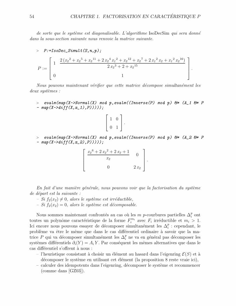
54 CHAPITRE 1. FACTORISATION EN CARACTERISTIQUE P
de sorte que le systeme est diagonalisable. L’algorithme IsoDecSim qui sera donnedans la sous-section suivante nous renvoie la matrice suivante.
> P:=IsoDec_Simult(S,n,p);
P :=
12 (x2
2 + x25 + x2
11 + 2 x24 x1
2 + x212 + x2
7 + 2 x12 x2 + x1
2 x216)
2 x23 + 2 + x2
15
0 1
.
Nous pouvons maintenant verifier que cette matrice decompose simultanement lesdeux systemes :
> evalm(map(X->Normal(X) mod p,evalm((Inverse(P) mod p) &* (A_1 &* P- map(X->diff(X,x_1),P)))));
1 0
0 1
.
> evalm(map(X->Normal(X) mod p,evalm((Inverse(P) mod p) &* (A_2 &* P- map(X->diff(X,x_2),P)))));
x26 + 2 x2
2 + 2 x2 + 1
x2
0
0 2 x2
.
En fait d’une maniere generale, nous pouvons voir que la factorisation du systemede depart est la suivante :
– Si f2(x2) 6= 0, alors le systeme est irreductible,– Si f2(x2) = 0, alors le systeme est decomposable.
Nous sommes maintenant confrontes au cas ou les m p-courbures partielles ∆pi ont
toutes un polynome caracteristique de la forme F mi
i avec Fi irreductible et mi > 1.Ici encore nous pouvons essayer de decomposer simultanement les ∆p
i : cependant, leprobleme va etre le meme que dans le cas differentiel ordinaire a savoir que la ma-trice P qui va decomposer simultanement les ∆p
i ne va en general pas decomposer lessystemes differentiels ∂i(Y ) = Ai Y . Par consequent les memes alternatives que dans lecas differentiel s’offrent a nous :
– l’heuristique consistant a choisir un element au hasard dans l’eigenring E(S) et adecomposer le systeme en utilisant cet element (la proposition 8 reste vraie ici),
– calculer des idempotents dans l’eigenring, decomposer le systeme et recommencer(comme dans [GZ03]).
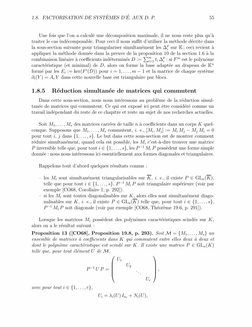
1.8. FACTORISATION DE SYSTEMES D’E. AUX D. P. 55
Une fois que l’on a calcule une decomposition maximale, il ne nous reste plus qu’atraiter le cas indecomposable. Pour ceci il nous suffit d’utiliser la methode decrite dansla sous-section suivante pour triangulariser simultanement les ∆p
i sur K ; ceci revient aappliquer la methode donnee dans la preuve de la proposition 10 de la section 1.6 a lacombinaison lineaire a coefficients indetermines D :=
∑mi=1 ti ∆
pi : si F m est le polynome
caracteristique (et minimal) de D, alors on forme la base adaptee au drapeau de Kn
forme par les Ei := ker(F i(D)) pour i = 1, . . . , m − 1 et la matrice de chaque systeme∂i(Y ) = Ai Y dans cette nouvelle base est triangulaire par blocs.
1.8.5 Reduction simultanee de matrices qui commutent
Dans cette sous-section, nous nous interessons au probleme de la reduction simul-tanee de matrices qui commutent. Ce qui est expose ici peut etre considere comme untravail independant du reste de ce chapitre et reste un sujet de nos recherches actuelles.
Soit M1, . . . , Ms des matrices carrees de taille n a coefficients dans un corps K quel-conque. Supposons que M1, . . . , Ms commutent, i. e., [Mi, Mj] := Mi Mj − Mj Mi = 0pour tout i, j dans {1, . . . , s}. Le but dans cette sous-section est de montrer commentreduire simultanement, quand cela est possible, les Mi c’est-a-dire trouver une matriceP inversible telle que, pour tout i ∈ {1, . . . , s}, les P−1 Mi P possedent une forme simpledonnee : nous nous interessons ici essentiellement aux formes diagonales et triangulaires.
Rappelons tout d’abord quelques resultats connus :
– les Mi sont simultanement triangularisables sur K, i. e., il existe P ∈ GLn(K),telle que pour tout i ∈ {1, . . . , s}, P−1 Mi P soit triangulaire superieure (voir parexemple [CO68, Corollaire 1, p. 292]).
– si les Mi sont toutes diagonalisables sur K, alors elles sont simultanement diago-nalisables sur K, i. e., il existe P ∈ GLn(K) telle que, pour tout i ∈ {1, . . . , s},P−1 Mi P soit diagonale (voir par exemple [CO68, Theoreme 19.6, p. 291]).
Lorsque les matrices Mi possedent des polynomes caracteristiques scindes sur K,alors on a le resultat suivant :
Proposition 13 ([CO68], Proposition 19.8, p. 293). Soit M = {M1, . . . , Ms} unensemble de matrices a coefficients dans K qui commutent entre elles deux a deux etdont le polynome caracteristique est scinde sur K. Il existe une matrice P ∈ GLn(K)telle que, pour tout element U de M,
P−1 U P =
U1
U2
. . .
Ur
,
avec pour tout i ∈ {1, . . . , r},Ui = λi(U) Ini
+ Ni(U),
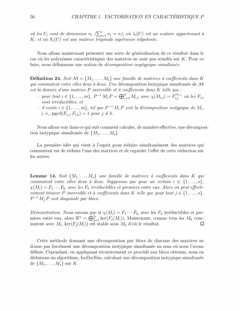
56 CHAPITRE 1. FACTORISATION EN CARACTERISTIQUE P
ou les Ui sont de dimension ni (∑r
i=1 ni = n), ou λi(U) est un scalaire appartenant aK, et ou Ni(U) est une matrice trigonale superieure nilpotente.
Nous allons maintenant presenter une sorte de generalisation de ce resultat dans lecas ou les polynomes caracteristiques des matrices ne sont pas scindes sur K. Pour cefaire, nous definissons une notion de decomposition isoptypique simultanee.
Definition 24. Soit M = {M1, . . . , Ms} une famille de matrices a coefficients dans Kqui commutent entre elles deux a deux. Une decomposition isotypique simultanee de Mest la donnee d’une matrice P inversible et a coefficients dans K telle que :
– pour tout i ∈ {1, . . . , m}, P−1 Mi P =⊕d
j=1 Mi,j avec χ(Mi,j) = Fmi,j
i,j ou les Fi,j
sont irreductibles, et– il existe i ∈ {1, . . . , m}, tel que P−1 Mi P soit la decomposition isotypique de Mi,
i. e., pgcd(Fi,j, Fi,k) = 1 pour j 6= k.
Nous allons voir dans ce qui suit comment calculer, de maniere effective, une decomposi-tion isotypique simultanee de {M1, . . . , Ms}.
La premiere idee qui vient a l’esprit pour reduire simultanement des matrices quicommutent est de reduire l’une des matrices et de regarder l’effet de cette reduction surles autres.
Lemme 14. Soit {M1, . . . , Ms} une famille de matrices a coefficients dans K quicommutent entre elles deux a deux. Supposons que pour un certain i ∈ {1, . . . , s},χ(Mi) = F1 · · ·Fbi
avec les Fk irreductibles et premiers entre eux. Alors on peut effecti-vement trouver P inversible et a coefficients dans K telle que pour tout j ∈ {1, . . . , s},P−1 Mj P soit diagonale par blocs.
Demonstration. Nous savons que si χ(Mi) = F1 · · ·Fbiavec les Fk irreductibles et pre-
miers entre eux, alors Kn =⊕bi
j=1 ker(Fj(Mi)). Maintenant, comme tous les Mk com-mutent avec Mi, ker(Fj(Mi)) est stable sous Mk d’ou le resultat.
Cette methode donnant une decomposition par blocs de chacune des matrices nedonne pas forcement une decomposition isotypique simultanee au sens ou nous l’avonsdefinie. Cependant, en appliquant recursivement ce procede aux blocs obtenus, nous endeduisons un algorithme, IsoDecSim, calculant une decomposition isotypique simultaneede {M1, . . . , Ms} sur K.
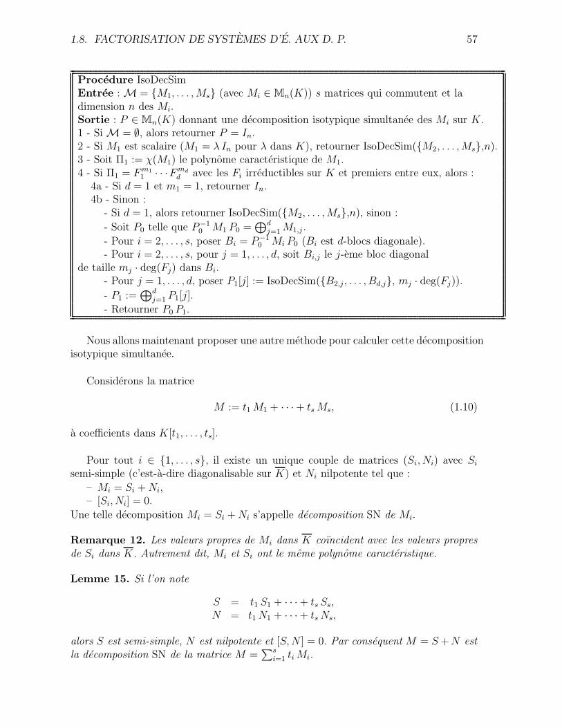
1.8. FACTORISATION DE SYSTEMES D’E. AUX D. P. 57
Procedure IsoDecSimEntree : M = {M1, . . . , Ms} (avec Mi ∈ Mn(K)) s matrices qui commutent et ladimension n des Mi.Sortie : P ∈ Mn(K) donnant une decomposition isotypique simultanee des Mi sur K.1 - Si M = ∅, alors retourner P = In.2 - Si M1 est scalaire (M1 = λ In pour λ dans K), retourner IsoDecSim({M2, . . . , Ms},n).3 - Soit Π1 := χ(M1) le polynome caracteristique de M1.4 - Si Π1 = F m1
1 · · ·F md
d avec les Fi irreductibles sur K et premiers entre eux, alors :4a - Si d = 1 et m1 = 1, retourner In.4b - Sinon :
- Si d = 1, alors retourner IsoDecSim({M2, . . . , Ms},n), sinon :
- Soit P0 telle que P−10 M1 P0 =
⊕dj=1 M1,j .
- Pour i = 2, . . . , s, poser Bi = P−10 Mi P0 (Bi est d-blocs diagonale).
- Pour i = 2, . . . , s, pour j = 1, . . . , d, soit Bi,j le j-eme bloc diagonalde taille mj · deg(Fj) dans Bi.
- Pour j = 1, . . . , d, poser P1[j] := IsoDecSim({B2,j, . . . , Bd,j}, mj · deg(Fj)).
- P1 :=⊕d
j=1 P1[j].
- Retourner P0 P1.
Nous allons maintenant proposer une autre methode pour calculer cette decompositionisotypique simultanee.
Considerons la matrice
M := t1 M1 + · · ·+ ts Ms, (1.10)
a coefficients dans K[t1, . . . , ts].
Pour tout i ∈ {1, . . . , s}, il existe un unique couple de matrices (Si, Ni) avec Si
semi-simple (c’est-a-dire diagonalisable sur K) et Ni nilpotente tel que :
– Mi = Si + Ni,– [Si, Ni] = 0.
Une telle decomposition Mi = Si + Ni s’appelle decomposition SN de Mi.
Remarque 12. Les valeurs propres de Mi dans K coıncident avec les valeurs propresde Si dans K. Autrement dit, Mi et Si ont le meme polynome caracteristique.
Lemme 15. Si l’on note
S = t1 S1 + · · · + ts Ss,N = t1 N1 + · · · + ts Ns,
alors S est semi-simple, N est nilpotente et [S, N ] = 0. Par consequent M = S +N estla decomposition SN de la matrice M =
∑si=1 ti Mi.
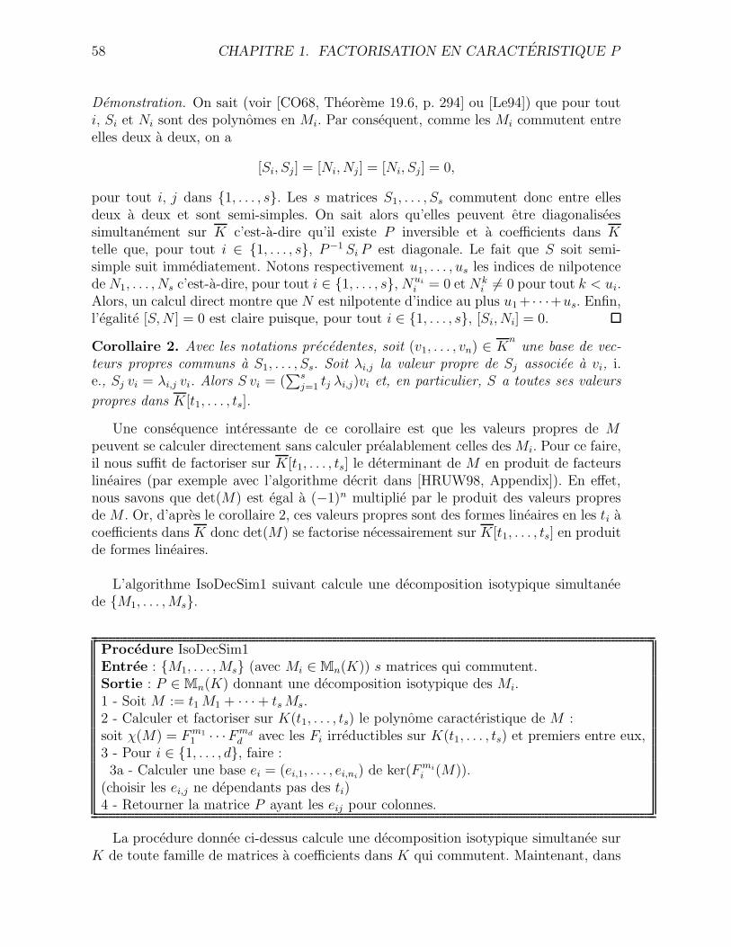
58 CHAPITRE 1. FACTORISATION EN CARACTERISTIQUE P
Demonstration. On sait (voir [CO68, Theoreme 19.6, p. 294] ou [Le94]) que pour touti, Si et Ni sont des polynomes en Mi. Par consequent, comme les Mi commutent entreelles deux a deux, on a
[Si, Sj] = [Ni, Nj] = [Ni, Sj] = 0,
pour tout i, j dans {1, . . . , s}. Les s matrices S1, . . . , Ss commutent donc entre ellesdeux a deux et sont semi-simples. On sait alors qu’elles peuvent etre diagonaliseessimultanement sur K c’est-a-dire qu’il existe P inversible et a coefficients dans Ktelle que, pour tout i ∈ {1, . . . , s}, P−1 Si P est diagonale. Le fait que S soit semi-simple suit immediatement. Notons respectivement u1, . . . , us les indices de nilpotencede N1, . . . , Ns c’est-a-dire, pour tout i ∈ {1, . . . , s}, Nui
i = 0 et Nki 6= 0 pour tout k < ui.
Alors, un calcul direct montre que N est nilpotente d’indice au plus u1 + · · ·+us. Enfin,l’egalite [S, N ] = 0 est claire puisque, pour tout i ∈ {1, . . . , s}, [Si, Ni] = 0.
Corollaire 2. Avec les notations precedentes, soit (v1, . . . , vn) ∈ Kn
une base de vec-teurs propres communs a S1, . . . , Ss. Soit λi,j la valeur propre de Sj associee a vi, i.e., Sj vi = λi,j vi. Alors S vi = (
∑sj=1 tj λi,j)vi et, en particulier, S a toutes ses valeurs
propres dans K[t1, . . . , ts].
Une consequence interessante de ce corollaire est que les valeurs propres de Mpeuvent se calculer directement sans calculer prealablement celles des Mi. Pour ce faire,il nous suffit de factoriser sur K[t1, . . . , ts] le determinant de M en produit de facteurslineaires (par exemple avec l’algorithme decrit dans [HRUW98, Appendix]). En effet,nous savons que det(M) est egal a (−1)n multiplie par le produit des valeurs propresde M . Or, d’apres le corollaire 2, ces valeurs propres sont des formes lineaires en les ti acoefficients dans K donc det(M) se factorise necessairement sur K[t1, . . . , ts] en produitde formes lineaires.
L’algorithme IsoDecSim1 suivant calcule une decomposition isotypique simultaneede {M1, . . . , Ms}.
Procedure IsoDecSim1Entree : {M1, . . . , Ms} (avec Mi ∈ Mn(K)) s matrices qui commutent.Sortie : P ∈ Mn(K) donnant une decomposition isotypique des Mi.1 - Soit M := t1 M1 + · · · + ts Ms.2 - Calculer et factoriser sur K(t1, . . . , ts) le polynome caracteristique de M :soit χ(M) = F m1
1 · · ·F md
d avec les Fi irreductibles sur K(t1, . . . , ts) et premiers entre eux,3 - Pour i ∈ {1, . . . , d}, faire :3a - Calculer une base ei = (ei,1, . . . , ei,ni
) de ker(F mi
i (M)).(choisir les ei,j ne dependants pas des ti)4 - Retourner la matrice P ayant les eij pour colonnes.
La procedure donnee ci-dessus calcule une decomposition isotypique simultanee surK de toute famille de matrices a coefficients dans K qui commutent. Maintenant, dans
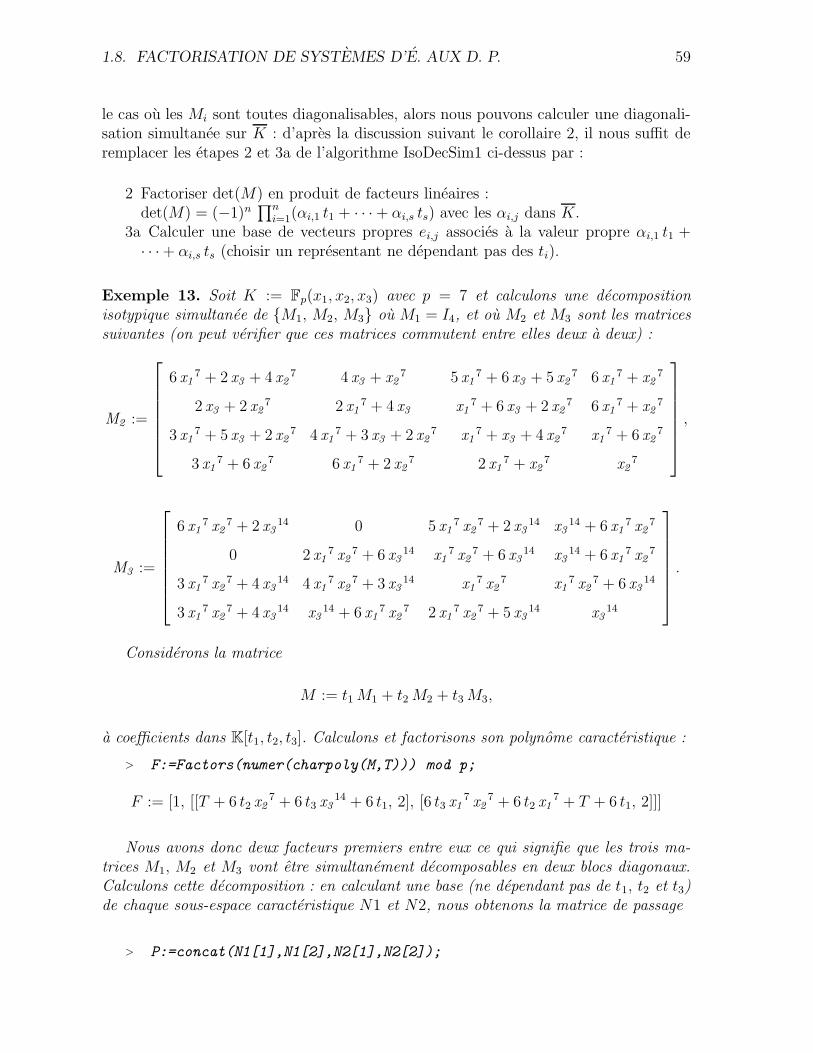
1.8. FACTORISATION DE SYSTEMES D’E. AUX D. P. 59
le cas ou les Mi sont toutes diagonalisables, alors nous pouvons calculer une diagonali-sation simultanee sur K : d’apres la discussion suivant le corollaire 2, il nous suffit deremplacer les etapes 2 et 3a de l’algorithme IsoDecSim1 ci-dessus par :
2 Factoriser det(M) en produit de facteurs lineaires :det(M) = (−1)n
∏ni=1(αi,1 t1 + · · · + αi,s ts) avec les αi,j dans K.
3a Calculer une base de vecteurs propres ei,j associes a la valeur propre αi,1 t1 +· · ·+ αi,s ts (choisir un representant ne dependant pas des ti).
Exemple 13. Soit K := Fp(x1, x2, x3) avec p = 7 et calculons une decompositionisotypique simultanee de {M1, M2, M3} ou M1 = I4, et ou M2 et M3 sont les matricessuivantes (on peut verifier que ces matrices commutent entre elles deux a deux) :
M2 :=
6 x17 + 2 x3 + 4 x2
7 4 x3 + x27 5 x1
7 + 6 x3 + 5 x27 6 x1
7 + x27
2 x3 + 2 x27 2 x1
7 + 4 x3 x17 + 6 x3 + 2 x2
7 6 x17 + x2
7
3 x17 + 5 x3 + 2 x2
7 4 x17 + 3 x3 + 2 x2
7 x17 + x3 + 4 x2
7 x17 + 6 x2
7
3 x17 + 6 x2
7 6 x17 + 2 x2
7 2 x17 + x2
7 x27
,
M3 :=
6 x17 x2
7 + 2 x314 0 5 x1
7 x27 + 2 x3
14 x314 + 6 x1
7 x27
0 2 x17 x2
7 + 6 x314 x1
7 x27 + 6 x3
14 x314 + 6 x1
7 x27
3 x17 x2
7 + 4 x314 4 x1
7 x27 + 3 x3
14 x17 x2
7 x17 x2
7 + 6 x314
3 x17 x2
7 + 4 x314 x3
14 + 6 x17 x2
7 2 x17 x2
7 + 5 x314 x3
14
.
Considerons la matrice
M := t1 M1 + t2 M2 + t3 M3,
a coefficients dans K[t1, t2, t3]. Calculons et factorisons son polynome caracteristique :
> F:=Factors(numer(charpoly(M,T))) mod p;
F := [1, [[T + 6 t2 x27 + 6 t3 x3
14 + 6 t1, 2], [6 t3 x17 x2
7 + 6 t2 x17 + T + 6 t1, 2]]]
Nous avons donc deux facteurs premiers entre eux ce qui signifie que les trois ma-trices M1, M2 et M3 vont etre simultanement decomposables en deux blocs diagonaux.Calculons cette decomposition : en calculant une base (ne dependant pas de t1, t2 et t3)de chaque sous-espace caracteristique N1 et N2, nous obtenons la matrice de passage
> P:=concat(N1[1],N1[2],N2[1],N2[2]);
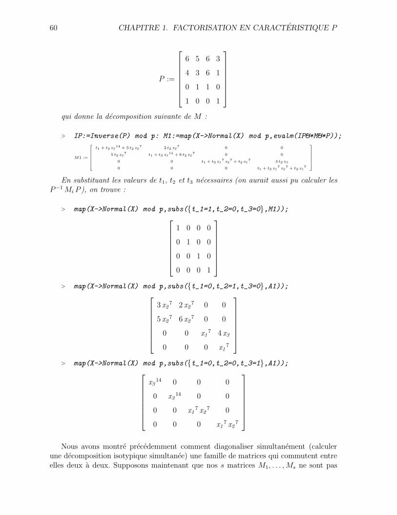
60 CHAPITRE 1. FACTORISATION EN CARACTERISTIQUE P
P :=
6 5 6 3
4 3 6 1
0 1 1 0
1 0 0 1
qui donne la decomposition suivante de M :
> IP:=Inverse(P) mod p: M1:=map(X->Normal(X) mod p,evalm(IP&*M&*P));
M1 :=
2
6
6
6
6
6
4
t1 + t3 x314 + 3 t2 x2
7 2 t2 x27 0 0
5 t2 x27 t1 + t3 x3
14 + 6 t2 x27 0 0
0 0 t1 + t3 x17
x27 + t2 x1
7 4 t2 x3
0 0 0 t1 + t3 x17
x27 + t2 x1
7
3
7
7
7
7
7
5
En substituant les valeurs de t1, t2 et t3 necessaires (on aurait aussi pu calculer lesP−1 Mi P ), on trouve :
> map(X->Normal(X) mod p,subs({t_1=1,t_2=0,t_3=0},M1));
1 0 0 0
0 1 0 0
0 0 1 0
0 0 0 1
> map(X->Normal(X) mod p,subs({t_1=0,t_2=1,t_3=0},A1));
3 x27 2 x2
7 0 0
5 x27 6 x2
7 0 0
0 0 x17 4 x3
0 0 0 x17
> map(X->Normal(X) mod p,subs({t_1=0,t_2=0,t_3=1},A1));
x314 0 0 0
0 x314 0 0
0 0 x17 x2
7 0
0 0 0 x17 x2
7
Nous avons montre precedemment comment diagonaliser simultanement (calculerune decomposition isotypique simultanee) une famille de matrices qui commutent entreelles deux a deux. Supposons maintenant que nos s matrices M1, . . . , Ms ne sont pas
1.8. FACTORISATION DE SYSTEMES D’E. AUX D. P. 61
simultanement diagonalisables par blocs et voyons comment les triangulariser simul-tanement. Considerons une nouvelle fois la matrice
M = t1 M1 + · · ·+ ts Ms,
ou les ti sont des indeterminees. Alors, en raisonnant comme nous l’avons fait precedem-ment, il n’est pas difficile de voir qu’en triangularisant cette matrice M (par exempleen suivant la methode usuelle - voir [CO68, Chapitre 19, Section 7]) sur K[t1, . . . , ts],nous obtenons en particulier la triangularisation simultanee sur K des Mi. De la memefacon, si nous voulons triangulariser simultanement par blocs les Mi sur K, alors il noussuffit de triangulariser par blocs sur K la matrice M .
Exemple 14. Nous nous proposons de triangulariser simultanement sur Q les matricesM1 et M2 suivantes (M1 et M2 commutent) :
M1 :=
9373
1371
−961
1371
1369
1371
7079
1371
,
M2 :=
9373
8226
−961
8226
1369
8226
7079
8226
.
Considerons la matrice M = t1 M1 + t2 M2 a coefficients dans Q[t1, t2] et factorisonsson polynome caracteristique.
> M:=evalm(t_1*M_1+t_2*M_2);
M :=
9373 t11371
+9373 t28226
−961 t11371
− 961 t28226
1369 t11371
+1369 t28226
7079 t11371
+7079 t28226
> factors(charpoly(M,T));
[1, [[T − 6 t1 − t2 , 2]]]
Calculons le vecteur propre associe a l’unique valeur propre de M .
> N_1:=nullspace(evalm(subs(T=G,T-6*t_1-t_2)))[1];
N1 :=
[
1,37
31
]
62 CHAPITRE 1. FACTORISATION EN CARACTERISTIQUE P
L’espace propre associe est de dimension 1 et donc M n’est pas diagonalisable. Pourtriangulariser M , il nous suffit de completer N1 en une base de Q2. Ici le vecteur [1, 0]convient et nous obtenons ainsi la matrice de changement de base suivante :
> P:=concat(N_1,[1,0]);IP:=inverse(P):
P :=
1 137
310
> evalm(IP&*A&*P);
6 t1 + t21147 t11371
+1147 t28226
0 6 t1 + t2
Nous avons alors triangularise simultanement M1 et M2 :
> evalm(IP&*M_1&*P);
61147
1371
0 6
> evalm(IP&*M_2&*P);
11147
8226
0 1
Dans ce qui precede, nous avons vu comment diagonaliser et triangulariser simul-tanement des matrices qui commutent. La reduction simultanee de matrices qui com-mutent a d’autres formes normales (e.g., Jordan, Frobenius, . . .) est plus compliqueenotamment du fait que ces formes normales de matrices ne sont pas stables par addition(par exemple la somme de deux matrices sous forme de Jordan n’est en general pas unematrice sous forme de Jordan). Precisons encore que des matrices qui commutent nesont pas necessairement simultanement Jordanisables : un exemple explicite est donnedans [Ca94, 3.1].
Conclusion de la section 1.8
Pour generaliser l’algorithme developpe dans les sections 1.3 a 1.6 au cas des systemesd’equations aux derivees partielles D-finis en caracteristique p, nous avons defini desnotions de p-courbure et d’eigenring et nous avons exhibe les liens qui existent entre cesdeux notions. Dans ce nouveau cadre, nous ne disposons plus d’une classification des
1.8. FACTORISATION DE SYSTEMES D’E. AUX D. P. 63
modules differentiels en caracteristique p ; cependant le fait que, dans le cas differentielordinaire, nous avions enonce et prouve certains resultats, decoulant directement de laclassification, d’une maniere elementaire (et algorithmique), nous a permis de generaliserici ces resultats sans problemes. En utilisant l’hypothese de D-finitude, qui impliqueimmediatement que les p-courbures partielles commutent entre elles deux a deux, nousavons montre qu’en suivant l’approche faite dans le cas differentiel ordinaire, notre al-gorithme de factorisation se ramene au probleme de la reduction simultanee de matricesqui commutent.
En nous concentrant sur ce dernier probleme, nous avons montre comment diago-naliser (resp. triangulariser) simultanement des matrices qui commutent. Pour ce faire,nous avons considere une combinaison lineaire a coefficients indetermines de nos ma-trices : en effet, en diagonalisant (resp. triangularisant) cette combinaison lineaire, nousdiagonalisons (resp. triangularisons) en particulier chaque matrice. Les formes diago-nales et triangulaires sont les deux formes normales qui nous servent a factoriser lessystemes differentiels en caracteristique p (voir les sections 1.4 et 1.5 de ce chapitre) :par consequent, nous avons developpe tous les ingredients necessaires pour obtenir unalgorithme de factorisation de systemes d’equations aux derivees partielles D-finis encaracteristique p.
En ce qui concerne la reduction simultanee a d’autres formes normales (Frobenius,Jordan, . . .), il semble que nous puissions aussi obtenir des informations interessantesen regardant une combinaison lineaire a coefficients indetermines et nous continuons atravailler sur ce probleme.

64 CHAPITRE 1. FACTORISATION EN CARACTERISTIQUE P
Chapitre 2
A Modular Algorithm forComputing the ExponentialSolutions of a Linear DifferentialOperator
Ce chapıtre constitue une publication ([CH04]) co-ecrite avec Mark van Hoeij etparue dans Journal of Symbolic Computation : le texte a ete laisse dans sa langued’origine.
Introduction
An ordinary differential equation
y(n) + an−1y(n−1) + · · · + a0y = 0 (2.1)
corresponds to a differential operator
∂n + an−1∂n−1 + · · ·+ a0∂
0 (2.2)
acting on y. Let C ⊂ Q be some number field (we will allow more general C in Sec-tion 2.7.1). The topic of this paper is finding exponential solutions of (2.1) when theai are in C(x). By this we mean : finding all r ∈ Q(x) for which y = exp(
∫
r) is asolution of (2.1). This is equivalent to finding first order right hand factors ∂ − r withr ∈ Q(x) of (3.1). Consequently, it can be viewed as part of the more general problemof factoring differential operators. Beke gave two factoring algorithms in [Be1894] (seealso [PS03, 4.1 and 4.2.1]), one algorithm for first order factors (which we will refer toas Beke’s algorithm in this paper) and one algorithm (which uses first order factors)for higher order factors. Other factoring algorithms are the local to global method of[Ho97a, Ho97b] and the eigenring method ([Si96], [PS03, 4.2.2]). Computing exponen-tial solutions (computing first order factors) with these algorithms can be slow. It is notdifficult to find examples where Maple’s expsols takes a long time, even though it uses
65
66 CHAPITRE 2. SOLUTIONS EXPONENTIELLES D’E. D. L.
an almost rational version of Beke’s algorithm, the local to global method, as well asthe eigenring method. The goal in this paper is to give a faster algorithm. We combinemodular methods with an almost rational version of Beke’s algorithm to obtain Algo-rithm ExpSolsInC which computes the exponential solutions defined over a given fieldC. Then we study the field problem, which is necessary for giving an efficient algorithmExpSols for computing all exponential solutions.
We sketch Beke’s method using the vocabulary of this paper. First, at each singula-rity, one computes a finite number (at most n) of objects called generalized exponents.Then, for each combination of generalized exponents (choose one generalized exponentat each singularity), the problem reduces to computing polynomial solutions (e.g., with[ABP95]) of some other differential operator. There are two main problems :
– a combinatorial problem : one has to choose a generalized exponent at each sin-gularity which could lead to a large number (at most nm where m is the numberof singularities) of possible combinations.
– a field problem : singularities and generalized exponents are often defined overalgebraic extensions of C, so some combinations can be defined over large algebraicextensions of C.
If neither problem occurs then Beke’s algorithm usually works well in practice. Thus weare mainly interested in situations where one or both of these two problems do occur.If we can discard combinations in advance then that would address the combinatorialproblem, and in some cases even the field problem if the discarded combinations includethose that are defined over large extensions of C. Our first main goal is to do this withcomputations modulo a prime number p.
The algebraic theory of ordinary differential equations in characteristic p is studiedin [Ho81, Ka82, CC85, Pu95]. For the problem of factoring differential operators withcoefficients in Fp(x), van der Put showed in [Pu95] (this is also recalled in [Pu96, 2.1]and [PS03, 13.1]) that the relevant object is the p-curvature since it determines thedifferential module mod p and all factorizations of the operator. More recently, analgorithm to factor Ore polynomials with coefficients in Fp(x) is included in [GZ03]. Thisalgorithm is based on the eigenring method adapted to characteristic p and generalizesthe work of [Gi98] that tackles the problem of factoring differential operators over Fq
where q = pl for p prime and l ∈ N∗. An algorithm to factor differential systems overFp(x), giving links between the p-curvature and the eigenring, is found in [Cl03].
The natural idea to lift modular factorizations to characteristic zero has been studiedin [Pu96, 4.3] and [PS03, 13.2.3]. In this paper we propose a different approach becausethere are many problems that prevent lifting from becoming an efficient and completealgorithm for characteristic zero. For example, there could be many factorizations incharacteristic p, and it is not clear which of these should be lifted. Also, it is not clearhow to do efficient Hensel lifting. Using more than one prime leads to the combinatorialproblem of combining factors of different characteristics, and using large prime(s) makesp-curvature computations or factoring operators mod p expensive. We propose not touse factors of the operator mod p for problems in characteristic zero, but to use onlythe characteristic polynomial of the p-curvature.
To reduce the number of combinations to check in Beke’s algorithm, we prove links
67
between eigenvalues in Fp(xp) of the p-curvature and the reduction mod p of the genera-
lized exponents appearing in possible solutions. Algorithm CombMatchRoot determineswhich generalized exponents match a given eigenvalue. Algorithm ExpSolsInC uses thisinformation to compute all exponential solutions defined over a field C (this C mustbe given in the input). Unfortunately, there are cases (see Section 5) where our mod pcomputations yield no improvements for the combinatorial problem.
The field problem refers to the problem that the usual Beke’s algorithm computeswith a generalized exponent at every singularity simultaneously. So the degree of thefield extension of C in Beke’s algorithm depends exponentially on m, the number ofsingularities (an extension of degree ≤ m! for the singularities followed by an extensionof degree ≤ nm for the generalized exponents). Of course this can easily choke thecomputation. Algorithm ExpSolsInC does not have this large field problem because thehighest degree extensions of C it uses are those given by just one singularity. In fact,on complicated examples usually most of the work in ExpSolsInC consists of rational(i.e., over C) computations and not of computations in field extensions. However, forExpSolsInC to find an exponential solution y, it needs in its input a field over which ycan be defined. From now on, the field problem refers to the problem of finding such afield without constructing very large extensions that choke the computation. Our secondmain goal is solving this field problem.
Our final algorithm ExpSols first calls ExpSolsInC, then uses modular informationto check if more exponential solutions could exist, and if so, it will first reduce the orderas much as possible before tackling the field problem. After that, it calls the recursiveFindASol algorithm which solves the field problem and returns an exponential solutiondefined over an extension, if such solution exists. We give several bounds (one of which isbased on the p-curvature) for the degree of a field extension needed to find an exponentialsolution. Algorithm FindASol uses these bounds and makes an algebraic extension todecrease these bounds. It does this recursively and each time it calls ExpSolsInC tosearch for a solution over the new field. This continues until either a solution is foundor until the bound becomes 1.
We summarize the two main new results in this paper :
– We use information mod p in several ways (in Section 5 for the combinatorialproblem and Section 6 for improving bounds that are used in the field problem)to speed up computation of exponential solutions in characteristic 0.To accomplish this there is a subtle but important difficulty to be overcome. Thereare many results known that hold for almost all p, but if such p can not easily beidentified (an example is given in Section 2.7.3) then the algorithm can not usethe result. The algorithm needs to know which p it can use. This restriction hasnumerous consequences, and the algorithm needs to be designed with this issuein mind. We will give a notion of good primes in Definition 46, and then only useresults that hold for all good p. Another important issue is that the definition ofgood primes should discard as few primes as possible (for large p the p-curvaturecomputation becomes slow, so only small p are useful for speeding up ExpSols).
– Our second main new result is Algorithm FindASol in Section 2.6.2, a recursivealgorithm that constructs a field extension over which an exponential solution (if
68 CHAPITRE 2. SOLUTIONS EXPONENTIELLES D’E. D. L.
one exists) can be defined.An efficiency advantage of Beke’s method over the local to global method in [Ho97b]or the eigenring method in [Si96] is that it directly computes first order factors. Incontrast, the local to global method often needs to compute higher order factorsbefore it can reach the first order factors, and the eigenring method first has tocompute the eigenring. The greatest disadvantage of Beke’s method in comparisonto the eigenring and local to global approaches is its use of a splitting field, andthis is the issue that Algorithm FindASol resolves.
The paper is organized as follows. Section 1 contains the vocabulary needed toread this paper, in particular the notions of generalized exponents, reduction mod p,and p-curvature. Section 2 illustrates in a few examples how mod p computations canreduce the combinatorial problem. In Sections 3 and 4 we give links between the p-curvature and generalized exponents. Section 5 contains Algorithm CombMatchModpthat reduces the number of combinations to check and Algorithm ExpSolsInC thatcomputes all exponential solutions defined over a given field C. Section 6 addresses thefield problem. Combining these algorithms in Section 7 we give Algorithm ExpSols thatcomputes a basis of all exponential solutions, up to conjugation over C.
2.1 Preliminaries
In this section we briefly recall the concepts that are needed to read the next sec-tions. The first subsection contains the necessary material in characteristic zero, thesecond subsection deals with characteristic p, and the third deals with reduction fromcharacteristic 0 to characteristic p.
2.1.1 Differential operators in characteristic zero
Let Q denote the algebraic closure of Q. We endow the fraction field Q(x) of the ringQ[x] of polynomials in the indeterminate x with the usual differentiation ′ := d
dx. The
field of constants of the differential field (Q(x),′ ) is then Q. Now, we consider the non-commutative ring Q(x)[∂] of differential operators over the differential field (Q(x),′ ) ;in this ring, the multiplication is given by ∀ u ∈ Q(x), ∂u = u∂ + u′. After multiplyingif necessary by some element of Q(x), a non-zero element L ∈ Q(x)[∂] can be writtenas
L = an∂n + an−1∂n−1 + . . . + a0∂
0, ai ∈ Q[x], an 6= 0 and gcd(a0, . . . , an) = 1. (2.3)
As usual, n will be called the order of the differential operator L.
Singularities and generalized exponents
We start with some classical definitions that can be found for example in [In26].
Definition 1. Let L ∈ Q(x)[∂] be written as in (2.3). A point x0 ∈ Q is said to be asingular point (or a singularity) of L if it is a root of an. Otherwise, it is said to be aregular (or ordinary) point of L.
2.1. PRELIMINARIES 69
In this paper we always consider the point at infinity as a singular point, whether itis singular or not. To each differential operator L ∈ Q(x)[∂], we associate the subset S ofQ containing all finite singularities. The set of all singularities of L is then S := S∪{∞}.
Let δ := x∂ and remark that Q(x)[∂] = Q(x)[δ] ⊂ Q((x))[δ].
Definition 2. Let L be a non-zero differential operator in Q((x))[δ]. L can be written∑∞
i=v xipi(δ) for some polynomials pi over Q and pv 6= 0. Then the indicial equation ofL is the polynomial pv. Its roots in Q are called the exponents of L at x = 0 (see [In26,7.21] or [HW97, Lemma 11]).
The notion of exponents can be generalized in the sense of [HW97, 3.2] : thereare several distinct ways to define generalized exponents. We choose here the algebraicdefinition of [Ho97a, Ho97b] that is easy to extend to characteristic p. We first give thedefinition at the point x = 0 and then extend it to all points. At a point xi ∈ Q∪{∞},we define the local parameter ti by
ti :=
{
x − xi if xi ∈ Q,1/x if xi = ∞.
Definition 3. Let e ∈ Q[x− 1k ] with k minimal in N∗ and let Lδ→δ+e denote the diffe-
rential operator L ∈ Q(x)[δ] in which we have replaced δ by δ +e. Then e is said to be ageneralized exponent of L at x = 0 if 0 is a root of the indicial equation of Lδ→δ+e. Thenumber k is called the ramification (index) of e. The multiplicity of the root 0 in theindicial equation is called the multiplicity of e. If k = 1 then e is called an unramifiedgeneralized exponent. If k = 1 and L has no generalized exponent e for which e − e isa negative integer then e is called a Z-minimal generalized exponent.
Definition 4. Let e ∈ Q[t− 1
k
i ]. Then e is said to be a generalized exponent of L atx = xi if eti→x (e in which we have replaced ti by x) is a generalized exponent of Lti→x
at x = 0. Here Lti→x refers to the automorphism of Q(x)[∂] given by x 7→ x + xi at afinite point and x 7→ 1/x at infinity. This leads to ∂ 7→ ∂ at a finite point and ∂ 7→ −x2∂at infinity.
Generalized exponents are useful for computing exponential solutions, see Lemma 1and Remark 3. At each point xi, there are exactly n generalized exponents counted withmultiplicity. The point xi is called a regular singular point of L when all generalizedexponents are constants, in which case they are just the usual exponents. At a regularpoint xi the (generalized) exponents are 0, 1, . . . , n−1. For further details on generalizedexponents see [Ho97a, Ho97b, HW97].
Exponential solutions and first order right hand factors
Definition 5. Let L ∈ Q(x)[∂] and let y 6= 0 belong to a differential field extension ofQ(x) with Q as field of constants. Assume that L(y) = 0.Then, y is said to be an exponential solution of L if y ′/y ∈ Q(x). It is said to be aradical solution if there exists a positive integer m such that ym ∈ Q(x) and finally,it is said to be a rational (respectively polynomial) solution if y ∈ Q(x) (respectivelyy ∈ Q[x]).
70 CHAPITRE 2. SOLUTIONS EXPONENTIELLES D’E. D. L.
An exponential solution y of L corresponds to the first order right hand factor∂ − y′/y of L.
Remark 1. In this paper it will not be necessary to distinguish an exponential functiony from a scalar multiple of y. Hence we may represent y by its logarithmic derivativey′/y ∈ Q(x) or by its minimal annihilating operator ∂ − y ′/y.
Definition 6. Let L ∈ Q(x)[∂] be of order n > 1. R ∈ Q(x)[∂] of order 0 < m < n issaid to be a right hand factor of L if there exists l ∈ Q(x)[∂] such that L = lR.
Lemma 1 below (analogous to [Bou00, Proposition 8]) shows that the notions ofgeneralized exponent, exponential solution and first order right hand factor are closelyrelated.
Lemma 1. Let r ∈ Q(x). If ∂−r is a first order right hand factor of L ∈ Q(x)[∂], thenfor all xi in S, there exists a generalized exponent exi
∈ Q[t−1i ] of L at xi such that
r = S +Q′
Qwhere S =
∑
xi∈S
exi
ti− t∞e∗∞,
and (Fuchs’ relation)
deg(Q) +∑
xi∈S
Const(exi) = 0, in particular −
∑
xi∈S
Const(exi) ∈ N (2.4)
where Q ∈ Q[x], the Const(exi) are the constant terms of the exi
and e∗∞ := e∞ −Const(e∞).
Proof. Let exibe the generalized exponent of ∂−r at xi. Since ∂−r is a right hand factor
of L, this is also a generalized exponent of L (see [Ho97b, Lemma 3.2]). Now L∂→∂+S
has right hand factor ∂ − r where r = r − S. Let S ′ be the set of all finite singularitiesof ∂ − r and let ∆ = S ′ \ S. So xi ∈ ∆ if and only if xi is a regular point of L (henceexi
∈ N) but a singular point (hence exi6= 0) of ∂ − r. Now r =
∑
xi
exi
ti− t∞e∗∞ if we
take the sum over all finite singularities of ∂ − r. Hence r =∑
xi∈∆
exi
ti. Then ∂ − r has
a polynomial solution Q =∏
xi∈∆ texi
i . Fuchs’ relation (which applied to ∂ − r is just areformulation of the fact that the sum of the residues of r is zero) says that if we sumConst(exi
) over all singularities of ∂−r then the result is zero,∑
xi∈S∪∆ Const(exi) = 0.
Then Equation (2.4) follows from the observation that deg(Q) =∑
xi∈∆ exi.2
Remark 2. In our algorithm we only need to compute unramified generalized exponentsof L, those are the only ones that can be relevant for our algorithm.
If at a singularity xi ∈ S there are two generalized exponents exi,1 and exi,2 whosedifference d = exi,1 − exi,2 is a positive integer, then exi,1 is not relevant in the sensethat the lemma stays true if we never use exi,1 (because replacing exi,1 and Q by exi,2
and tdi Q does not change S + Q′/Q). So, in our algorithm, we will only use Z-minimalgeneralized exponents.
2.1. PRELIMINARIES 71
The r defined in the previous lemma matches the exponential solution
exp(
∫
S) Q.
If all exiare rational numbers then this exponential solution can be written as
Q∏
xi∈S
texi
i (2.5)
so this is a radical solution. We see then that the radical solutions correspond to theexponential solutions for which all associated generalized exponents are rational num-bers.
Remark 3. If we only know the generalized exponents defining some exponential so-lution modulo rational numbers (respectively modulo integers), then finding such expo-nential solution reduces to finding radical solutions (respectively rational solutions) ofL∂→∂+S.
2.1.2 Differential operators in characteristic p
Let Fp denote the algebraic closure of the finite field Fp. We define the ring Fp(x)[∂]of differential operators in the same way as in characteristic zero. The main differenceis that the field of constants of (Fp(x),′ ) is Fp(x
p) (see [Pu01] or [GZ03, Lemma 3.3]).
The p-curvature and the map y 7→ y(p−1) + yp
The central tool for studying differential operators in characteristic p is the p-curvature ; we recall a definition and we refer to [Ka82, CC85] and [PS03, 13.2.2] formore information. The differential field Fp(x) is a finite dimensional vector space overits field of constants Fp(x
p) :
Fp(x) =
p−1⊕
i=0
Fp(xp)xi.
To any differential operator L ∈ Fp(x)[∂], one can associate the differential module
ML := Fp(x)[∂]/Fp(x)[∂]L.
This module is equipped with a Fp(xp)-linear map ∂ (coming from the left multiplication
by ∂ on Fp(x)[∂]) satisfying
∂fm = f ′m + f ∂m for all m ∈ ML, f ∈ Fp(x).
Definition 7. Let L ∈ Fp(x)[∂]. The p-curvature of L is the Fp(x)-linear map ∂ p actingon the differential module ML associated to L.
72 CHAPITRE 2. SOLUTIONS EXPONENTIELLES D’E. D. L.
An algorithm to compute the p-curvature matrix is given in [PS03, 13.2.2]. The map
τ : Fp(x) → Fp(xp),
y 7→ y(p−1) + yp
is very useful when we deal with order one right hand factors in characteristic p. Detailscan be found in [[PS03], 13.2.1] and [Pu95] ; we only recall a lemma that we will oftenuse :
Lemma 2 ([Pu95], Lemma 1.4.2). The map τ : Fp(x) → Fp(xp) is a surjective
additive map with kernel { z′
z| z ∈ Fp(x)∗ }.
In [Pu95], van der Put proves that for the problem of factoring a differential operatorin characteristic p (or in an equivalent way its associated differential module ML), thep-curvature is the relevant object since its characteristic properties give all possiblefactorizations of the operator.
We will note χp(L) the characteristic polynomial of the p-curvature of L ∈ Fp(x)[∂].As we are only interested in first order factors, the only modular information that wewill use are the roots in Fp(x
p) (with multiplicities) of χp(L). We denote R(χp(L)) asthe set of roots of χp(L) in Fp(x
p).
Lemma 3. Let L ∈ Fp(x)[∂].(a). If L = L1L2 then χp(L) = χp(L1)χp(L2) with deg(χp(Li)) = order(Li).(b). The map µ from the set of all first order monic right hand factors of L in Fp(x)[∂]to R(χp(L)) given by µ(∂ − r) := τ(r) is well defined and surjective.
Proof. The claim (a) follows from the classification (the equivalence of categories) of[Pu95] and [PS03, 13.1]. That the map µ is well defined follows from the first claim andthe fact that τ(r) is the p-curvature of the order one operator ∂ − r (see [Pu96, Lemma2.2]). Surjectivity follows from the classification as well.2
2.1.3 Reduction modulo p and factorization
Let vp : Q → Z∪{∞} denote the standard p-adic valuation on Q. There are infinitelymany ways to extend this valuation to a valuation vp : Q → Q ∪ {∞}. We assume thatone such choice is made. Let Rp = {a ∈ Q | vp(a) ≥ 0}, and consider the maximal idealI = {a ∈ Rp | vp(a) > 0}. Now choose an isomorphism Rp/I ∼= Fp.
Definition 8. Having fixed the above choices, we denote the image of a ∈ Rp in Fp bya[p]. This is called the reduction of a mod p.
Note that a[p], the reduction of a mod p, depends not only on a and p but dependson the choice of vp as well. However, for compactness of notation we will only mentionp even when we refer to both p and vp. If a ∈ Q is not in Rp then a[p] is not defined.In our algorithm, we will apply the reduction map [p] : Rp → Fp to only finitely manyalgebraic numbers that are known in advance. Thus, it is not difficult to choose a primep and valuation vp in such a way that a[p] is always defined for all numbers a for which
2.1. PRELIMINARIES 73
the reduction map [p] is used. The a’s we reduce mod p are finite in number and thusthey are elements of a finite extension K of Q. There are only finitely many possiblechoices for vp on K. We will assume that such p and vp are chosen, so that all instancesof the notation a[p] are defined. For more details on this choice see Section 5.3.
In practice, reducing an algebraic number a mod p is done as follows : Let a1, . . . , an
be those algebraic numbers that have previously been reduced mod p, but take onlythose whose reduction mod p may appear in the same expression as a[p] in the al-gorithm (if the reductions of a1, . . . , an and some other numbers b1, . . . , bm are usedcompletely independently, then the algorithm will still be valid if it computes the reduc-tions of these two sets of numbers independently, using one valuation on Q(a1, . . . , an)and an independently chosen valuation on Q(b1, . . . , bm). This way the larger fieldQ(a1, . . . , an, b1, . . . , bm) does not need to be constructed). Then determine the mini-mal polynomial of a over K := Q(a1, . . . , an). Reduce this minimal polynomial modp, then the coefficients are in a field we will denote by K[p], which is defined asFp(a1[p], . . . , an[p]). Factor this polynomial over K[p], and choose one of the irredu-cible factors. Then determine a field extension of K[p] in which this irreducible factorhas a root, and let a[p] be that root.
We will apply the reduction map [p] to the singularities of L, which are in Q∪{∞}.If a = ∞ then we define a[p] as ∞. Two distinct singularities of L can have the sameimage under [p], in which case we say that p is not a good prime (see condition (C3)in Definition 46 in Section 3). Note that this definition of good prime depends not onlyon p, but depends on vp as well (recall that when we refer to both p and vp we will onlymention p for brevity).
If a is some object defined over Q (like L, a local parameter ti, or a generalizedexponent exi
) we can define a[p] by applying the reduction map [p] to all coefficients.We show now that without too many assumptions on p a factorization of a differential
operator in characteristic zero can be reduced mod p. This result can be found in [Pu96].
Proposition 1. Let L ∈ Q(x)[∂] and let p be such that L can be reduced mod p. IfL = L1L2 then, after possibly replacing L1 and L2 by cL1 and 1
cL2 for some constant
c ∈ Q, we have L[p] = L1[p] L2[p].
We allow to replace L1 and L2 by cL1 and 1cL2 for some constant c to avoid patho-
logies of the form L1 = 1p∂ and L2 = p∂.
Proof. The only thing to prove is that cL1 and 1cL2 can be reduced mod p for some
constant c. Any p-adic valuation vp on Q can be extended to Q[x] (this statementis a form of Gauss’ lemma. To define vp(f) for a non-zero polynomial one takes thesmallest valuation of the coefficients). The valuation can then be extended to the frac-tion field Q(x), and then be extended to Q(x)[∂] (again, take the minimal valuation ofthe coefficients). Then L[p] is defined if and only if vp(L) ≥ 0. Let c be a constantwith valuation −vp(L1), so vp(cL1) = 0, hence cL1 can be reduced mod p. Thenvp(
1cL2) = vp(cL1) + vp(
1cL2) = vp(cL1
1cL2) = vp(L1L2) = vp(L) ≥ 0, so 1
cL2 can
be reduced mod p as well.2
74 CHAPITRE 2. SOLUTIONS EXPONENTIELLES D’E. D. L.
One obtains the following two criteria (these can also be easily deduced from [Pu95]) :
Corollary 1. Let L ∈ Q(x)[∂] and let p be a prime such that L can be reduced mod p.Assume further that the order n of L does not drop after the reduction.If χp(L) is irreducible over Fp(x
p) then L is irreducible over Q(x).If χp(L) has no roots in Fp(x
p) then L has no exponential solutions.
Proof. It follows directly from the previous proposition, [Cl03, Theorem 4.1-Step 2] andLemma 3(b).2
As an example, let L = (x2 + x + 8)∂2 + (−x8 + x + 6)∂ + 1 and p = 3. Then χp(L)has no roots and this is a very fast way to show that L has no exponential solutions.Without modular methods this would have taken much longer because one of the degreebounds (one ends up searching for polynomial solutions of some other operators) turnsout to be very high in this example.
In the corollary, the hypothesis that the order does not drop can not be omitted.For example, the operator (p∂ + 1)∂ is reducible in characteristic 0 but its reductionL[p] = ∂ is irreducible.
2.2 Examples
We will illustrate our modular improvements for the combinatorial problem (seethe introduction) with a few examples. These improvements rely on Proposition 1 andLemma 3(b) in the following way. A first order factor in characteristic zero leads to afirst order factor in characteristic p by Proposition 1, which in turn corresponds to aroot of χp(L) by Lemma 3(b).
2.2.1 Example 1
Consider the following differential operator :
L = ∂3 − 2x2 − x + 4
2x2∂2 − 3x3 − 4x2 − 3x − 2
2x4∂ +
2x3 − 3x − 2
2x4.
The singularities are 0 and ∞. Generalized exponents are 0, 52
+ 1x, 2 + 1
xat 0 and
−t−1∞ , −t
− 12
∞ , t− 1
2∞ at ∞ (recall that t∞ = 1
x). The usual Beke’s algorithm will have
three combinations to check since we only have one unramified generalized exponentat ∞, and three at 0. We will use this example to illustrate our modular method,even though our method generally does not speed up trivial examples (L is trivial forBeke’s algorithm because the number of combinations is very small and there is no fieldproblem).
Let p = 3 and note c = xp. The characteristic polynomial χp(L) of the p-curvaturematrix is (λ2 + λ/c2 + 2/c + 1/c4)(λ + 2) and has only the root λ = 1. We will see inSection 2.5.2 that this root excludes the choices 5
2+ 1
xand 2 + 1
xat 0 ; consequently,
there remains only one combination to check.
2.2. EXAMPLES 75
For each of the 3 combinations, Beke’s algorithm will check Fuchs’ relation (Equa-tion (2.4) in Lemma 1). This check will be very fast because since there is no fieldproblem in this example, we do not have to construct a complicated number field inorder to do this check. One of the three combinations passes this check, and it yields asolution. In this example, the modular method would not provide a speedup because itdiscarded only two combinations (which otherwise would have been discarded anywayby Fuchs’ relation). In the next example, our modular method discards more combina-tions, and moreover, the discarded combinations include all “hard” combinations, i.e.,those not invariant under the Galois group of Q over Q.
2.2.2 Example 2
Let
L = 9(x3 − 2)5∂3 + (x3 − 2)(2x10 − 12x7 + 108x5 + 24x4 − 216x2 − 16x − 9)∂
−2x(190x6 − 274x3 − 27x − 212).
There are three finite singularities ; the roots of x3 − 2, with generalized exponents2, 1
36α2
(x−α)− 1
18α and − 1
36α2
(x−α)+4+ 1
18α where α := RootOf(x3−2). At infinity, the gene-
ralized exponents are 0,− 53,−4
3. So the usual Beke’s algorithm will have 81 combinations
to try. Let p = 5 and look at the reduction mod p of the singularities and generalizedexponents. First, we factor x3−2 = (x+2)(x2 +3x+4) mod p, so α reduces to 3 as wellas to β := RootOf(x2+3x+4) in characteristic p. After reduction mod p the situation isthen as follows : we have the singularity 3 with generalized exponents 2, 4
x+2− 1, − 4
x+2
and the singularities β with generalized exponents 2, β2
(x−β)+ 3β, − β2
(x−β)+ 4 + 2β.
At infinity the generalized exponents become 0 (with multiplicity 2) and 2. Now, wecompute χp(L) and see that its only root is λ = s where s := 4c4+2c+1
c6+c3+4and c = xp.
Our method consists then in finding which generalized exponents reduced mod p couldmatch such a root s. Here, the result is that s can only correspond to the choice 4
x+2−1
at 3, β2
(x−β)+ 3β at β and any choice at infinity. This means that in characteristic zero,
a possible exponential solution must involve the generalized exponent 136
α2
(x−α)− 1
18α at
α. This reduces the number of possible combinations from 81 to 3. Moreover, we haveeliminated all “hard” combinations, i.e., those for which the sum S in Lemma 1 wouldnot be in Q(x).
If two generalized exponents differ by a rational number, then our mod p com-putation can not detect which one to take, which is an important limitation. This iswhy three combinations remained after the mod p computation even though there wasonly one root of χp(L). Of the three remaining combinations only one satisfies Fuchs’relation, and this combination yields an exponential solution.
2.2.3 Example 3
Let p be a prime number and consider the operator L = x4∂2−px∂−2x−1. Then pis a good prime in the sense of Definition 46 below. However, despite the fact that L[p]
76 CHAPITRE 2. SOLUTIONS EXPONENTIELLES D’E. D. L.
exists and can even be factored, neither of the two generalized exponents 3+1/p+p/x2
and −1/p of L at x = 0 can be reduced mod p. So both can be discarded by Lemma 4and hence L has no exponential solutions.
2.3 Roots of χp(L) and τ-reduced terms
Definition 9. If r is an object in characteristic zero we set τ(r) := τ(r [p]).Let exi
∈ Q[t−1i ] be an unramified generalized exponent of L ∈ Q(x)[∂] at a point xi ∈
Q∪ {∞}. Let p be such that xi and exican both be reduced mod p. The τ -reduced term
corresponding to exiis then defined as
τred(exi) :=
{
τ(exi
ti) if xi ∈ Q,
−τ(t∞e∗∞) if xi = ∞
where e∗∞ denotes e∞ without its constant term.
Remark 4. If e ∈ Q then e[p] ∈ Fp and Lemma 2 implies τred(e) = 0.
Definition 10. A prime p is a good prime for L if the following conditions hold :(C1)- The coefficients of L can be reduced mod p and the order of L does not decreaseafter reduction mod p, i.e., an[p] 6= 0.(C2)- All singularities can be reduced mod p.(C3)- Distinct singularities stay distinct after reduction mod p.
If L is written in the form (2.3), then Condition (C2) simply means “degx(an[p]) =degx(an)”. And (C3) means that the largest square-free factor of an remains square-freemod p. Checking if a prime p is good is fairly easy in practice. All three conditions areuseful in our algorithm, for example, without (C3) we would have to replace AlgorithmCombMatchRoot in Section 2.5.2 by a more complicated algorithm. The lemma belowuses (C3) as well. Nevertheless, if p is not a good prime, then it is often still possible toobtain some useful information from a computation mod p, but we will not detail this.
Lemma 4. Let L ∈ Q(x)[∂] and p be a good prime for L. If ∂ − r with r ∈ Q(x) is amonic first order right hand factor of L and if exi
∈ Q[t−1i ] is the generalized exponent
of ∂ − r at xi, then exican be reduced mod p.
Proof. From Lemma 1, there exists a generalized exponent exi∈ Q[t−1
i ] of L at eachsingularity xi such that
r =∑
xi∈S
exi
ti− t∞e∗∞ +
Q′
Q, (2.6)
where Q ∈ Q[x] and e∗∞ is e∞ without its constant term. Since p satisfies (C1), r canbe reduced mod p (see Proposition 1). Now Q is defined up to a multiplicative constant(which we can choose in such a way that Q[p] is defined and is not zero), so Q′/Q canbe reduced mod p and hence the remaining part
∑
xi∈Sexi
/ti − t∞e∗∞ can be reducedmod p as well. Conditions (C2)+(C3) in Definition 46 imply that we can recover e∗∞[p]
2.3. ROOTS OF χP (L) AND τ -REDUCED TERMS 77
and exi[p] for xi ∈ S from (
∑
xi∈Sexi
/ti − t∞e∗∞)[p] and therefore exi[p] is well defined.
Then the same is true for e∞[p] by Fuchs’ relation.2
We now give two new results linking the τ -reduced terms and the eigenvalues of thep-curvature in Fp(x
p), i.e., the elements of R(χp(L)). First another definition :
Definition 11. Let L ∈ Q(x)[∂]. We say that s ∈ R(χp(L)) comes from characteristiczero if there exists r ∈ Q(x) such that ∂ − r is a right hand factor of L in characteristiczero and s = τ(r).
Proposition 2. Let L ∈ Q(x)[∂] and let p be a good prime for L. If s ∈ R(χp(L))comes from characteristic zero, then ∀ xi ∈ S, there exists a generalized exponent exi
atxi such that :
s =∑
xi∈S
τred(exi).
Proof. By definition, s ∈ R(χp(L)) comes from characteristic zero means that thereexists r ∈ Q(x) such ∂ − r is a right hand factor of L. From Lemma 1, there existsthen a generalized exponent exi
∈ Q[t−1i ] of L at each singularity xi such that r can
be written in the form (2.6) where Q ∈ Q[x] and e∗∞ is e∞ without its constant term.Since p is a good prime for L and Q is defined up to a multiplicative constant (which wecan choose in such a way that Q[p] is defined and is not zero), the reduction mod p ofeach term in Equation (2.6) is well defined (see also Lemma 4 above). Now using thats = τ(r), the result follows directly from Lemma 2 and the definition of the τred(exi
).2
Proposition 3. For almost all primes p the condition that s comes from characteristic0 may be omitted.
Proof. As we will not need this result for our algorithm, we will only sketch a proof.First we note that generalized exponents can be defined in characteristic p. Definitions 3and 4 are completely algebraic : the operations required are additions and multiplica-tions in Q(x), tests to zero in Q and computing the roots of a polynomial in Q[x].Obviously these operations also make sense in characteristic p so the definitions areeasily translated to characteristic p provided that the ramification k is not divisible byp (this is not an issue because we only consider k = 1 in this paper). The generalizedexponents are here defined mod p, which is coherent with the fact that we want tp
i tohave generalized exponent 0 at xi (because tpi is in the field of constants) as well asgeneralized exponent p at xi because it vanishes with multiplicity p at xi. Note that thenotions of singularity, indicial equation and exponents in characteristic p have alreadybeen introduced in [Ho81] and [CC85].
Lemma 1 can also be adapted to characteristic p (the lemma is just a statementabout the relation between a rational function and its local expansions). Then one canalso give the analogue of Proposition 2 in characteristic p, with L ∈ Fp(x)[∂], with thexi in Fp ∪ {∞}, the unramified generalized exponents exi
in Fp[t−1i ], but now s can be
any root of χp(L).
78 CHAPITRE 2. SOLUTIONS EXPONENTIELLES D’E. D. L.
Let L ∈ Q(x)[∂], let p be a good prime, and let s be any root of χp(L), not necessa-rily coming from characteristic 0. Applying the mod p analogue of Proposition 2 to L[p]we see that even if s does not come from characteristic 0, the statement in Proposition 2still holds if we replace the generalized exponents exi
of L by the generalized exponentsof L[p]. This completes the proof because for all but finitely many good primes p, re-duction mod p will induce a bijection between the (unramified) generalized exponentsof L and those of L[p].2
One obtains the following corollary which is related to the converse of [Ho81, Theo-rem 2] and [CC85, Corollary 1.4]. Indeed, their statement (attributed to Katz) is : if L[p]has “sufficiently many solutions in a weak sense”, which is equivalent to “L has nilpotentp-curvature”, for almost all p, then all the exponents of L are rational numbers.
Corollary 2. Let L ∈ Q(x)[∂]. If all generalized exponents of L are rational numbers,then for almost all primes, R(χp(L)) ⊆ {0}.
Proof. If exi∈ Q then τred(exi
) = 0 and the result follows from Proposition 3.2
2.4 Exponential solutions and roots of χp(L)
2.4.1 Classes of exponential solutions
Definition 12. The class exiof a generalized exponent exi
is exi:= exi
mod Q, theequivalence class of exi
modulo Q.
Two generalized exponents exiand e′xi
that have the same class exiand that can both
be reduced mod p satisfy τ(exi) = τ(e′xi
) by Remark 4. So we can define τ(exi) := τ(exi
),and τred(exi
) := τred(exi). The corresponding definition for exponential solutions is :
Definition 13. Let y be an exponential solution of L, ∂ − r be the associated firstorder right hand factor of L and exi
the associated generalized exponents in the senseof Lemma 1. Then the class Cl(y) of y is defined as the image of r = y ′/y in Q(x)/ ∼where a ∼ b ⇔ a − b = g′
gfor some radical function g 6= 0. We can identify
Cl(y) =∑
xi∈S
exi
ti− t∞e∗∞.
Two exponential solutions have the same class if and only if their quotient is aradical function, if and only if at every point, the associated generalized exponents havethe same class. Now, to L ∈ Q(x)[∂] we associate the class-set
Cl(L) := {Cl(y) ∈ Q(x)/ ∼ | y exponential solution of L }.
2.4. EXPONENTIAL SOLUTIONS AND ROOTS OF χP (L) 79
2.4.2 Links between Cl(L) and R(χp(L))
Lemma 5. Let L ∈ Q(x)[∂] and p be a good prime for L. There is a map
Ψ : Cl(L) → R(χp(L)),
Cl(y) 7→ τ(y′/y) =∑
xi∈S
τred(exi).
Proof. Let Cl(y) ∈ Cl(L). An exponential solution y corresponds to a first order righthand factor ∂ − r of L in characteristic zero where r = y ′/y. Since p is a good primefor L, this factorization can be reduced mod p (see Proposition 1) and we have thusa first order right hand factor ∂ − r[p] of L[p]. Now from Lemma 3, τ(r) ∈ R(χp(L)).The lemma is then clear using Proposition 2 since τ(r) is an element of R(χp(L)) thatcomes from characteristic zero.2
Given L, there are two natural questions about Ψ :(Q1)- Is Ψ surjective for almost all good primes ?(Q2)- Does there exist a good prime p such that Ψ is injective ?
Proposition 4. The answer to questions (Q1) and (Q2) can be no.
Proof. We give one example for each question. For (Q1), if we take a differential operatorthat has a basis of algebraic (but no exponential) solutions, then Cl(L) = ∅. The provedpart of Grothendieck’s conjecture (see [Ka82], [Ch01] or [Pu01] for statements andhistories of this conjecture) says that for almost all primes the p-curvature is zero sothat R(χp(L)) = {0}. For (Q2), take an operator L with the following 8 exponentialsolutions :
xe0(x − 1)e1(x − 2)e2
for e0 ∈ {0,√
2}, e1 ∈ {0,√
3} and e2 ∈ {0,√
6}. Modulo every prime p, at least one ofthe three square roots becomes an element of Fp. Suppose for example that
√6[p] ∈ Fp.
Consider then the exponential solutions y1 and y2 corresponding to choices respectively(0, 0, 0) and (0, 0,
√6) for (e0, e1, e2). Then Cl(y1) 6= Cl(y2) but they have the same
image under Ψ.2
The previous proposition says that we can not always choose a prime number forwhich each root of χp(L) corresponds to at most one class of exponential solutions. Theexample illustrates the cause of this, and one can show the following (note that we donot use this in our algorithm) :
Proposition 5. Let L ∈ Q(x)[∂]. If there exists a good prime p for L for which :
(∗) ∀ xi ∈ S, exi,2 − exi,1 /∈ Q ⇒ exi,2[p] − exi,1[p] /∈ Fp
then, for that prime, Ψ is injective.
80 CHAPITRE 2. SOLUTIONS EXPONENTIELLES D’E. D. L.
Proof. Suppose that Cl(y1) =∑
xi∈S
exi,1
ti− t∞e∗∞,1 and Cl(y2) =
∑
xi∈S
exi,2
ti− t∞e∗∞,2
are two distinct elements of Cl(L) and suppose that Ψ(Cl(y1)) = Ψ(Cl(y2)).
Ψ(Cl(y1)) = Ψ(Cl(y2)) ⇔ ∑
xi∈Sτred(exi,1) =
∑
xi∈Sτred(exi,2),
⇔ τ(∑
xi∈S
exi,1
ti− t∞e∗∞,1) = τ(
∑
xi∈S
exi,2
ti− t∞e∗∞,2),
⇔ ∑
xi∈S
exi,2−exi,1
ti− t∞(e∗∞,2 − e∗∞,1) = g′
g, for g ∈ Fp(x)∗.
This leads to : ∀xi∈S, exi,2[p] − exi,1[p] ∈ Fp and e∗∞,2[p] − e∗∞,1[p] = 0 which, by Fuchs’relation, implies that also e∞,2[p]−e∞,1[p] ∈ Fp. On the other hand, the hypothesis thatCl(y1) 6= Cl(y2) means that ∃ i ∈ S, exi,2 − exi,1 /∈ Q which contradicts condition (∗).2
2.5 Modular improvements of the combinatorial pro-
blem
Definition 14. Let L ∈ Q(x)[∂]. L is said to be rad-regular if there exists r ∈ Q(x)such that L∂→∂+r has all its unramified generalized exponents in Q. Otherwise, L issaid to be rad-singular ; it means that there exists a singularity xi with two unramifiedgeneralized exponents whose difference is not in Q.
As mentioned in the introduction, we want to address two problems in Beke’s algo-rithm : the combinatorial problem and the field problem. In this section we focus onlyon the combinatorial problem and not on the field problem ; we suppose that a numberfield C is given and develop an algorithm that finds all exponential solutions definedover C. We show how a careful modular analysis can effectively reduce the combinato-rial problem if L is rad-singular. Unfortunately, in the rad-regular case no reduction inthe combinatorial problem is obtained (see also Section 2.7.2).
2.5.1 Some precisions on the vocabulary
Let C be a number field. In light of Remark 1 we use the terminology :
Definition 15. An exponential function y is defined over C if y ′/y ∈ C(x).
When C is not algebraically closed, we will not consider all roots of the leadingcoefficient an of L, we will only consider one root for each irreducible factor over C. Sothe number of singularities that our algorithm considers is the number of irreduciblefactors of an (this number depends on the field C) plus one (the point at infinity). Theonly extensions of C that we will work with in Section 2.5 are extensions given by asingle irreducible factor of an in C[x], so Algorithm ExpSolsInC in Section 2.5.4 doesnot use computationally expensive nested extensions.
Definition 16. A place is either a monic irreducible polynomial Pi in C[x] or ∞.At each place Pi 6= ∞, we define the point xi as the class of x in C[x]/(Pi) notedRootOf(Pi). At the place ∞, the point is also ∞.
2.5. MODULAR IMPROVEMENTS OF THE COMBINATORIAL PROBLEM 81
If the degree of Pi is one, then we can view xi as an element of C. Recall that wehave the local parameter ti = x − xi at finite points and ti = 1/x at ∞. We adapt thenotion of singularity and generalized exponents to the purpose of this section :
Definition 17. The C-singularities of L ∈ C(x)[∂] written as in (2.3) are the pointsat the places Pi for all monic irreducible factors Pi of an in C[x] and the point ∞. Wekeep the notations S for the set of finite C-singularities and S = S∪{∞}. Furthermore,a C-generalized exponent of L at xi is an unramified generalized exponent of L at theC-singularity xi that further belongs to C(xi)[t
−1i ]. The degree of a C-singularity xi is
the degree of Pi if xi 6= ∞, and it is 1 if xi = ∞.
A first order operator ∂ − r ∈ C(x)[∂] has a C-generalized exponent at every C-singularity. Hence, if at a C-singularity of L there are no C-generalized exponents, thenL can not have exponential solutions defined over C.
Definition 18. A C-combination is a list composed of one C-generalized exponent exi
at each C-singularity xi ∈ S.
The exponential solutions that we are looking for (those defined over C) match firstorder right hand factors ∂ − r with r ∈ C(x) as in Lemma 1 but here we write :
r =∑
xi∈S
Tri(exi
ti) − t∞e∗∞ +
Q′
Q(2.7)
where Tri is the trace over the field extension C(xi, x) ⊃ C(x). The term Tri(exi/ti) ∈
C(x) is the sum of all conjugates of exi/ti over C(x). So the above r is as in Lemma 1
with the additional property r ∈ C(x), which means that for any σ in the Galois groupof Q(x) over C(x), if we choose exi
at xi in Lemma 1 then we must choose σ(exi) at
σ(xi) (σ maps the unramified generalized exponents of L ∈ C(x)[∂] at xi to those atσ(xi)). We extend Definition 9 to finite C-singularities xi as follows :
τred(exi) := τ(Tri(
exi
ti)).
Definition 19. Let P be a problem defined over a field C of characteristic 0 for whichthe following holds : if s is a solution of P defined over an algebraic extension of C,then all conjugates of s over C are solutions as well. Then we say that s1, . . . , sk arethe solutions of P up to conjugation over C when :
- for each si a finite extension Ci of C is given such that si is defined over Ci and,- for any solution s of P defined over any algebraic extension C ′ of C there is preciselyone i such that Ci can be embedded in C ′ over C and si corresponds to s under thisembedding.
We define the degree (or algebraic degree) of si over C as [Ci : C]. The total numberof solutions defined over C equals the sum of the degrees over C of the si.
Each such problem P that we need to solve (such as : find the singularities, find thegeneralized exponents at a singularity xi, find the exponential solutions) will be solved
82 CHAPITRE 2. SOLUTIONS EXPONENTIELLES D’E. D. L.
up to conjugation, this in order to prevent computationally expensive splitting fields.In this terminology, “computing the C-singularities” and “computing the singularitiesup to conjugation over C” have identical meaning : factor an over C and construct afield Ci = C(xi) = C[x]/(Pi) for each factor Pi (the singularity at infinity has degree1 hence its field is C). Solving a problem up to conjugation over C does not involveconstructing fields that contain more than one Ci, which means that we are not able toperform arithmetic between objects defined over distinct Ci’s (unless of course when thedegrees are 1, i.e., when these Ci’s are just C). That is why the exi
/ti in equation (2.7)must first be “traced down” to an object defined over C before we can add them.
When we compute generalized exponents at xi (recall that we only need the un-ramified generalized exponents), we compute them up to conjugation over C(xi). TheC-generalized exponents are those of (algebraic) degree 1 over C(xi). Generalized ex-ponents of degree > 1 will not be used in Section 5, they will be used in AlgorithmFindASol in Section 2.6.2.
2.5.2 Finding C-combinations matching the modular informa-
tion
Let L ∈ C(x)[∂] where C is a number field. Suppose that L has m finite C-singularities x1, . . . , xm and consider the following set :
Comb := {(ex1, . . . , exm, e∞) | exi
is a C-generalized exponent of L at xi }.
The elements of Comb are called C-combinations mod Q. Note that the set Combdepends on C in two ways. First, the xi correspond to irreducible factors of an over C.Second, the exi
must be defined over C(xi). We have an injective map Cl(L) → Comb.From Proposition 2, if p is a good prime for L, we have a map from the set of theelements of R(χp(L)) that come from characteristic zero (the elements that interest us)to the set of subsets of Comb, or just to Comb itself if Condition (∗) in Proposition 5holds. Consider now the map
Φ : Comb → Fp(xp),
(ex1 , . . . , exm, e∞) 7→ ∑
xi∈Sτred(exi
).
Definition 20. Let s ∈ R(χp(L)) and h ∈ Comb. We say that h matches s if Φ(h) =s. We say that h satisfies Fuchs’ relation if
∑
xi∈STri(Const(exi
)) + Const(e∞) = 0mod Q.
Given an element s of R(χp(L)) for a good prime p, we can effectively find the finiteset of elements h of Comb that match s. A naive way to do that consists in taking theimage under Φ of all possible C-combinations mod Q and keeping those with image s.A reason for including Condition (C3) in the definition of a good prime is so that wecan give a more practical method (Algorithm CombMatchRoot below).
In the sequel, F := C[p] denotes the image of the number field C after reductionmod p. In practice C is given by some (possibly nested) RootOf’s so that this reduction
2.5. MODULAR IMPROVEMENTS OF THE COMBINATORIAL PROBLEM 83
makes sense (recall that choosing a reduction [p] means choosing factors mod p of thepolynomials defining the RootOf’s).
Since F is finite, the map U 7→ Up is an isomorphism from F[x] to F[xp], and wedenote the inverse isomorphism by V 7→ V 1/p. If r = a
b+ c with a, b, c ∈ F[x] and
deg(a) < deg(b) then τ(r) can be written as AB
+ C with deg(A) < deg(B), B = bp
(here gcd(A, B) need not be 1) and C = τ(c). So if V ∈ F[xp] divides the denominatorof τ(r) then V 1/p ∈ F[x] divides the denominator of r.
Algorithm CombMatchRootInput : a number field C, a good prime p for L, the reduction [p], s ∈ R(χp(L)) ∩ F(xp)and the data structure of C-singularities and C-generalized exponents of L.Output : the elements h of Comb matching s and satisfying Fuchs’ relation.
1 - For each xi ∈ S and each exiat xi compute τred(exi
).
2 - Compute the partial fraction decomposition∑Ns
i=1Ui
Vnii
+ W of s with Ui, W ∈ F[xp],
Vi irreducible in F[xp] and deg(Ui) < deg(V ni
i ).3 - Remove all e∞ for which τred(e∞) 6= W ; if none remain, then return ∅ and stop.4 - For each i = 1 . . . Ns,
4a - Find the C-singularity xj = RootOf(Pj) such that V1/pi ∈ F[x] divides Pj[p],
4b - Remove all exjfor which the partial fraction decomposition of τred(exj
) does notcontain the term Ui
Vnii
; if none remain, then return ∅ and stop.
5 - For all remaining exj, compute all combinations h = (ex1, . . . , exm
, e∞) that satisfyFuchs’ relation and return those as output.
In step 1, if the reduction mod p fails then exican be discarded by the same argument
as in Lemma 4. In steps 3 and 4b, if nothing remains, then there are no first order righthand factors ∂ − r of L with r ∈ C(x) and s = τ(r). Condition (C3) in the definition of
good primes is used in step 4a to make sure that the Pj for which V1/pi divides Pj[p] is
unique (the existence of such a Pj follows from the fact that a pole of a root of χp(L)is a singularity of L[p]).
Remark 5. It follows from Lemma 4 that if exican not be reduced mod p then it can not
be relevant for the algorithm, it can not correspond to any first order right hand factor.It follows from Algorithm CombMatchRoot above that a generalized exponent that canbe reduced mod p but that does not match any element of R(χp(L)) can not be relevanteither. If, adding these notions of relevant to those of Remark 2 ( i.e., unramified, Z-minimal), no relevant generalized exponents remain at a certain singularity xi then thereare no exponential solutions and we can stop the computation. If at a certain xi onlyone relevant generalized exponent remains then we call xi a semi-apparent singularitybecause it does not contribute to the combinatorial problem. In Algorithm FindASol inSection 6 it is important that we use only relevant generalized exponents to preventmaking unnecessary field extensions.
84 CHAPITRE 2. SOLUTIONS EXPONENTIELLES D’E. D. L.
Algorithm CombMatchModp :Input : an operator L ∈ C(x)[∂], a number field C, the data structure E of C-singularitiesand C-generalized exponents of L.Output : the set of C-combinations mod Q that match a root of χp(L) for a good prime pand that satisfy Fuchs’ relation.1 - If at some C-singularity there are no C-generalized exponents, return ∅ and stop.2 - Choose a good prime p for L (choose a reduction [p]).3 - Compute R(χp(L)) and (to be used in Section 2.7) Nroots := the total number of roots
of χp(L) in Fp(xp) counted with multiplicity.
4 - Return the union of CombMatchRoot(C,p,[p],s,E) for s ∈ R(χp(L)) ∩ F(xp).
One can often (use Condition (∗) in Proposition 5) find a prime such that each smatches at most one C-combination mod Q (i.e., the set CombMatchRoot(C,p,[p],s,E)has ≤ 1 elements for each s). But Proposition 4 shows that such prime does not alwaysexist so that, in practice, we do not try to find one.
2.5.3 Some remarks on the choice of p
We can choose p as follows. Start with p = 2, and as long as a reduction mod p of acoefficient of L fails, or if one of the other conditions of a good prime in Definition 46is not met, we take the next prime. So we compute the smallest good prime. There are,however, certain cases where another choice could be better. In hard cases (when we needto use Algorithm FindASol, or when the number of combinations is very high) we maywant to try a few more primes and select the best one. In very easy examples such as inSection 2.1 it can be best to use no primes at all because the combinatorial problem wasalready practically trivial without modular methods. Another situation where there isno improvement in the combinatorial problem is when L is rad-regular (see Definition 14and also Section 7.2) and the p-curvature computation does not exclude existence ofexponential solutions. In most cases we only use the smallest good p, and in the unusualevent that this p is large then we skip the modular improvements given in Section 5because p-curvature computations become expensive for large p. Exceptions are veryeasy cases (use no modular methods) and very hard cases (check more than one primeand select the best one).
2.5.4 Finding all exponential solutions defined over a givenfield
Algorithm CombMatchModp computes a set of possible combinations for C-generalizedexponents mod Q that could appear in an exponential solution defined over C. We willuse this to find all exponential solutions defined over C.
Recall that with the notations of Equation (2.7) and Lemma 1, an exponentialsolution can be written as exp(
∫
S) Q where S =∑
xi∈STri(
exi
ti) − t∞e∗∞ and Q is a
polynomial. After CombMatchModp, it remains to check which C-combinations mod Q
2.5. MODULAR IMPROVEMENTS OF THE COMBINATORIAL PROBLEM 85
lead to exponential solutions and to compute these exponential solutions. A natural ideais : at each C-singularity, given a exi
we take the finitely many generalized exponentsexj
satisfying exjmod Q = exi
and we have thus a finite number of C-combinations(ex1, . . . , exm
, e∞), hence a finite number of possibilities for S after checking Fuchs’relation. Then for each S, we construct the operator L∂→∂+S having as solutions thoseof L divided by exp(
∫
S), and we search for polynomial solutions Q of that operator.We define an E-combination as a C-combination that uses only generalized expo-
nents that appear in our data structure E. As already mentioned in Remark 2, replacingexi
by exi− d and Q by tdi Q for some d ∈ Z leaves the expression exp(
∫
S) Q invariant.So we only need one generalized exponent in each equivalence class mod Z. To assurethat Q is a polynomial we only put Z-minimal generalized exponents in our data struc-ture E, i.e., unramified generalized exponents that are minimal in their equivalenceclass mod Z. This is also true for the point at infinity ; although the constant term ofe∞ does not contribute to S in Lemma 1, it does contribute in Equation (2.4) to thedegree bound for Q (the number N in step 4 is used as a degree bound for the Qi instep 4b), and using only Z-minimal generalized exponents at infinity ensures that thisdegree bound is not too low.
Algorithm ExpSolsInC :Input : an operator L ∈ C(x)[∂], a number field C.Output : Sol, a basis of exponential solutions of L defined over C.1 - Compute the data structure E of C-singularities and Z-minimal C-generalized exponents.2 - M := CombMatchModp(L,C,E).3 - Sol := ∅.4 - For each E-combination (ex1, . . . , exm
, e∞) whose class mod Q is in M , and that satisfies :N := −Const(e∞) −∑xi∈S
Tri(Const(exi)) ∈ N, do :
4a - Let S :=∑
xi∈STri(
exi
ti) − t∞e∗∞ and L := L∂→∂+S,
4b - Compute a basis Q1, . . . , Qw of polynomial solutions in C[x] for L,4c - If w > 0 then, add the exp(
∫
S) Qj to Sol.5 - Return Sol.
We can pre-compute the Tri(Const(exi)) and Tri(
exi
ti), from then on all the work in
the loop in step 4 (which may dominate the computation time, see also Section 7.1)takes place over C.
To use this procedure in the recursive algorithm FindASol in Section 6.2, we needto allow two extra inputs. First, an option called “just one” ; if this option is given thenwe only need to return just one (if it exists) exponential solution defined over C butnot a totally arbitrary one. We return a solution exp(
∫
S) Q with S as in the algorithm,but with Q of minimal possible degree. Second, an optional set F may be given inthe input. Each element of F is a couple (xi, exi
) where xi is a C-singularity of degree1 (see Definition 17) and exi
is a C-generalized exponent at xi. This couple encodesthe command : “in the data structure E in step 1 of ExpSolsInC, throw away all C-generalized exponents at xi except exi
”. This reduces the number of E-combinations to
86 CHAPITRE 2. SOLUTIONS EXPONENTIELLES D’E. D. L.
be checked. Note that usually not all C-singularities will appear in F , so in general thereis still a combinatorial problem. Furthermore, if F 6= ∅, then it is of course possible thatno exponential solutions over C are found even if such solutions exist.
2.6 A way to handle the field problem
Let L ∈ C(x)[∂] with C ⊂ Q. We want to find a basis of all exponential solutions,so we may have to search for exponential solutions defined over algebraic extensions ofC. Before constructing such extensions, we first want to bound their degrees.
2.6.1 Two ways to obtain bounds
We start with a few definitions, in particular we need the notion of type. Many usefulproperties of the type of a differential operator can be found in [Or32] (where type iscalled Art-Begriff). We will only use the type for first order operators, or equivalently,for exponential solutions :
Definition 21. Two exponential functions y1 and y2 are said to be of the same typeif y1/y2 is a rational function. This defines an equivalence relation, and type(y1), thetype of y1, is defined to be the equivalence class of y1. We say that y1 and y2 have thesame local type at xi if y1/y2 is meromorphic at xi, which is equivalent to saying thatthe generalized exponents of ∂ − y′
1/y1 and ∂ − y′2/y2 at xi differ by an integer.
We will identify an exponential solution y with its minimal operator ∂ − y ′/y ∈Q(x)[∂], and so we shall not distinguish y from a constant multiple of y. This makesit easy to describe what we mean by a conjugate of y ; if σ is an element of the Galoisgroup of Q over some number field C, then by σ(y) we simply mean a non-zero solutionof ∂ − σ(y′/y).
Two exponential functions have the same type if and only if they have the same localtype at every point xi. The type of the exponential solution y = exp(
∫
S) Q with S and
Q as in Lemma 1 can be uniquely represented as∑
xi∈S
eximod Z
ti− t∞e∗∞ where e∗∞ is
e∞ without its constant term (recall that this constant term depends on the constantterms of the other exi
by Fuchs’ relation). The Galois group of Q over C acts on the setof all types.
Definition 22. Let C be a number field, y be an exponential function. Let K be thefield of definition of y over C, which is defined as the smallest number field K thatcontains C for which y′/y ∈ K(x). Then the algebraic degree of y over C is [K : C].We say that y is of minimal algebraic degree m over C if [K : C] = m and there existno exponential function y, of the same type as y, having smaller algebraic degree overC.
Let C be a number field, let y be an exponential function, and let K be the fieldof definition of y over C. Let L1 = ∂ − y′/y ∈ K(x)[∂]. Let L1, . . . , Lr ∈ Q(x)[∂] bethe conjugates of L1 over C, and let L = LCLM(L1, . . . , Lr) ∈ C(x)[∂]. It is easy to
2.6. A WAY TO HANDLE THE FIELD PROBLEM 87
calculate a basis of all exponential solutions of L that have the same type as y ; computeL := L∂→∂+y′/y ∈ K(x)[∂], compute a basis b1, . . . , bk ∈ K(x) of rational solutions of
L, then take b1y, . . . , bky. Let R ∈ K(x)[∂] be the monic operator with b1y, . . . , bky assolutions. Now R is the unique monic operator whose solution space is the set of allsolutions of L with the same type as y, so R is uniquely determined by two things :L ∈ C(x) and type(y). Hence, any element σ of the Galois group of Q over C that leavestype(y) invariant leaves R invariant as well. Conversely, if σ leaves R invariant, it leavestype(y) invariant as well because R has precisely one type of exponential solutions.Thus, one can define a field of definition of type(y) over C, namely as the smallestfield C ′ that contains C for which R ∈ C ′(x)[∂]. Note that since R ∈ K(x)[∂], one hasC ′ ⊆ K, hence : the field of definition of y over C contains the field of definition oftype(y) over C.
We will now prove constructively that y is of minimal algebraic degree over C ifand only if the fields of definition of y and type(y) are the same. To do this, we willshow that R has an exponential solution defined over C ′, in fact, we will show that thealgorithm ExpSolsInC with input R, C ′ will find such solutions. Since R has only onetype, there is exactly one local type at each singularity xi, so generalized exponents atxi are unique modulo integers. So if σ is in the Galois group of Q over C ′(xi), then itcan only move a generalized exponent exi
by an integer, but this implies that σ leavesexi
invariant, and thus exi∈ C ′(xi)[t
−1i ], i.e., exi
is a C ′-generalized exponent. Hencethere is exactly one Z-minimal C ′-generalized exponent at every singularity xi, whichimplies that ExpSolsInC(R,C ′) will try exactly one C ′-combination. This combinationhas the same type as y, and since all solutions of R have this type, ExpSolsInC willfind a basis y1, . . . , yk of solutions of R, defined over C ′, where k is the order of R. Weconclude the following :
Lemma 6. Let C be a number field and L ∈ C(x)[∂]. If y is an exponential solutionof L defined over some algebraic extension K of C, then its conjugates over C are alsosolutions of L.Given L and y, we can compute y1, . . . , yk of minimal algebraic degree over C that forma basis of all exponential solutions of L of the same type as y.If y is of minimal algebraic degree over C, then the distinct conjugates of y over C areof distinct type and hence linearly independent.
Proof. The fact that for L ∈ C(x)[∂], the conjugates over C of solutions are againsolutions is clear.From the foregoing, given L and y, we can compute an operator R ∈ K(x)[∂] whosesolution space is precisely the set of all exponential solutions of L of the same type as y.We can calculate the smallest field C ′ containing C for which R ∈ C ′(x)[∂], and can finda basis y1, . . . , yk of solutions of R with ExpSolsInC(R,C ′). Then y1, . . . , yk are definedover C ′, which is the field of definition of their type, so they have minimal algebraicdegree over C. And they form a basis of all exponential solutions of L of the same typeas y.
If σ is in the Galois group of Q over C, and if two objects have the same field ofdefinition over C, then σ leaves the first object invariant if and only if σ acts as the
88 CHAPITRE 2. SOLUTIONS EXPONENTIELLES D’E. D. L.
identity on the field of definition, if and only if σ leaves the second object invariant.Now if y is of minimal algebraic degree over C, then it has the same field of definitionas type(y), so σ leaves type(y) invariant if and only if σ leaves y (which we identify with∂ − y′/y because we do not want to distinguish y from scalar multiples of y) invariant.Thus, distinct conjugates of y must have distinct types.2
Therefore, if we have an exponential solution of minimal algebraic degree m, thenthis exponential solution gives in fact m linearly independent solutions. In the outputof our algorithm we will only return exponential solutions up to conjugation over C. Inorder to make it easier to count how many linearly independent solutions such an outputrepresents, we will only allow exponential solutions in the output that have minimalalgebraic degree over C.
Definition 23. If C is a number field, xi a singularity of L and exia generalized ex-
ponent at xi, then the field C(xi; exi) is the extension of C given by xi and the coefficients
of exi.
Proposition 6. Let C be a number field, L ∈ C(x)[∂], xi a singularity, ti the localparameter, and let e ∈ Q[t−1
i ]. Let b1 be the number of distinct generalized exponentsexi
of L at xi with exi− e ∈ Z. Suppose that y is an exponential solution of minimal
algebraic degree m over C(xi; e) with generalized exponent e at xi. Then m ≤ b1.
Proof. By the previous Lemma, the conjugates of y over C(xi; e) form m linearlyindependent exponential solutions, all of which have generalized exponent in e + Zat xi. These exponential solutions (viewed as formal solutions at xi) can be writtenφj(ti) exp(
∫
e/ti dti) where φj(ti) ∈ Q((ti)) for all j ∈ {1, . . . , m}. After Gaussian eli-mination on the vectors of coefficients of the φj(ti), we obtain m formal solutions at xi
with distinct generalized exponents in e + Z. Then m ≤ b1 because there are only b1
such generalized exponents at xi.2
The modular approach yields a different bound :
Proposition 7. Let C be a number field, let L ∈ C(x)[∂] and let p be a good primefor L. Let b2 be the number of roots of χp(L) (counted with multiplicity) that match (inthe sense of Algorithm CombMatchRoot) the choice exi
at xi. Let y be an exponentialsolution of minimal algebraic degree m over C(xi; exi
), and generalized exponent exiat
xi. Then m ≤ b2.
Proof. Let R ∈ C(xi; exi)(x)[∂] be the right hand factor whose solutions are spanned by
all exponential solutions y of L that have generalized exponent exiat xi. Since there are
at least m independent such solutions, the order d of R is at least m. All solutions ofR have the same local type at xi (namely the local type exi
mod Z, see Definition 21).Now R factors as a product of first order factors R = R1R2 · · ·Rd because R has abasis of exponential solutions. All Ri have the same local type at xi, so for each Ri, thegeneralized exponent at xi must be congruent to exi
mod Z. Hence the root of χp(Ri)matches exi
at xi. The proposition now follows from the fact that R and R1, . . . , Rd can
2.6. A WAY TO HANDLE THE FIELD PROBLEM 89
be reduced mod p (see Proposition 1) and Lemma 3(a).2
We now have two bounds b1 and b2 for the degree of the extension needed overC(xi; exi
). We do not know in advance which is smaller, so we compute both and takethe minimum.
Definition 24. To each couple (xi, exi) we associate the bound b(xi,exi
) := min(b1, b2).
2.6.2 An algorithm to find an exponential solution over analgebraic extension
Let L ∈ C(x)[∂] with C ⊂ Q. We suppose that L has no exponential solutionsdefined over C and we want to find (if it exists) an exponential solution defined over analgebraic extension of C. We will use Algorithm ExpSolsInC that finds the exponentialsolutions of L defined over a given field, as well as the bounds from the previous section.To find an exponential solution over an algebraic extension of C, we increase the fieldstep by step by adding extensions coming from singularities or generalized exponents,and at each step we use ExpSolsInC to search for an exponential solution over the newfield. The bounds tell us when we can stop making field extensions.
For efficiency reasons we first want to reduce the order of the problem as much aspossible before introducing field extensions, which is precisely what Algorithm ExpSolsin Section 7 does before it calls Algorithm FindASol below. And since the order can bereduced whenever a solution is found, we want FindASol to stop computing as soon asit finds a solution.
In the algorithm we denote ei,j, j = 1, . . . , ni as all, up to conjugation over C(xi),see Definition 19, relevant (see Remarks 2 and 5) generalized exponents at xi. If ni = 0then we can stop the algorithm, the output is ∅. Let F be a data structure as inthe comments after Algorithm ExpSolsInC. If xi appears in F , which means that ageneralized exponent at xi has already been chosen, then ni := 1. We denote di,j :=[C(xi; ei,j) : C(xi)], which is the degree as in Definition 19 of ei,j over C(xi). Now wedefine b(xi,ei,j ,F ) as in Definition 24 with as difference that in Proposition 7 we onlycount those roots of χp(L) that match all generalized exponents specified in F . Ofcourse, before we enter step 5 we discard all ei,j for which b(xi,ei,j ,F ) = 0 because wewant ni to be as small as possible, and if any ni vanishes then we stop.
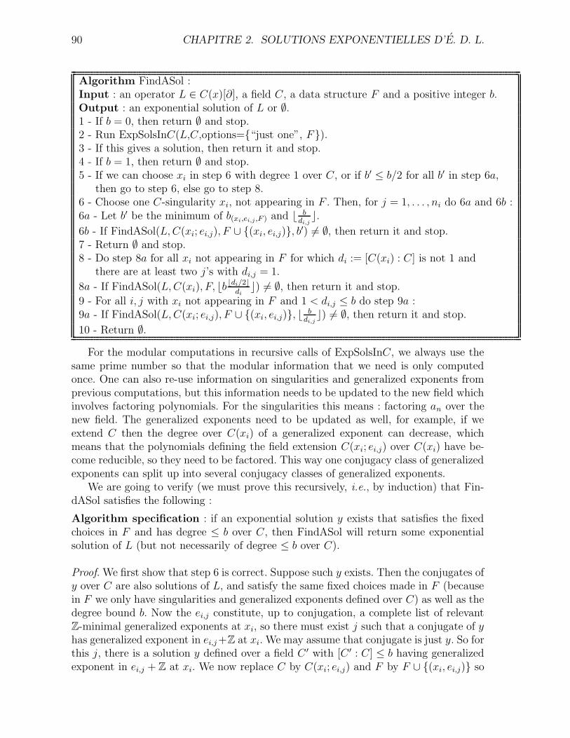
90 CHAPITRE 2. SOLUTIONS EXPONENTIELLES D’E. D. L.
Algorithm FindASol :Input : an operator L ∈ C(x)[∂], a field C, a data structure F and a positive integer b.Output : an exponential solution of L or ∅.1 - If b = 0, then return ∅ and stop.2 - Run ExpSolsInC(L,C,options={“just one”, F}).3 - If this gives a solution, then return it and stop.4 - If b = 1, then return ∅ and stop.5 - If we can choose xi in step 6 with degree 1 over C, or if b′ ≤ b/2 for all b′ in step 6a,
then go to step 6, else go to step 8.6 - Choose one C-singularity xi, not appearing in F . Then, for j = 1, . . . , ni do 6a and 6b :6a - Let b′ be the minimum of b(xi,ei,j ,F ) and b b
di,jc.
6b - If FindASol(L, C(xi; ei,j), F ∪ {(xi, ei,j)}, b′) 6= ∅, then return it and stop.7 - Return ∅ and stop.8 - Do step 8a for all xi not appearing in F for which di := [C(xi) : C] is not 1 and
there are at least two j’s with di,j = 1.
8a - If FindASol(L, C(xi), F, bb bdi/2cdi
c) 6= ∅, then return it and stop.
9 - For all i, j with xi not appearing in F and 1 < di,j ≤ b do step 9a :9a - If FindASol(L, C(xi; ei,j), F ∪ {(xi, ei,j)}, b b
di,jc) 6= ∅, then return it and stop.
10 - Return ∅.
For the modular computations in recursive calls of ExpSolsInC, we always use thesame prime number so that the modular information that we need is only computedonce. One can also re-use information on singularities and generalized exponents fromprevious computations, but this information needs to be updated to the new field whichinvolves factoring polynomials. For the singularities this means : factoring an over thenew field. The generalized exponents need to be updated as well, for example, if weextend C then the degree over C(xi) of a generalized exponent can decrease, whichmeans that the polynomials defining the field extension C(xi; ei,j) over C(xi) have be-come reducible, so they need to be factored. This way one conjugacy class of generalizedexponents can split up into several conjugacy classes of generalized exponents.
We are going to verify (we must prove this recursively, i.e., by induction) that Fin-dASol satisfies the following :
Algorithm specification : if an exponential solution y exists that satisfies the fixedchoices in F and has degree ≤ b over C, then FindASol will return some exponentialsolution of L (but not necessarily of degree ≤ b over C).
Proof. We first show that step 6 is correct. Suppose such y exists. Then the conjugates ofy over C are also solutions of L, and satisfy the same fixed choices made in F (becausein F we only have singularities and generalized exponents defined over C) as well as thedegree bound b. Now the ei,j constitute, up to conjugation, a complete list of relevantZ-minimal generalized exponents at xi, so there must exist j such that a conjugate of yhas generalized exponent in ei,j +Z at xi. We may assume that conjugate is just y. So forthis j, there is a solution y defined over a field C ′ with [C ′ : C] ≤ b having generalizedexponent in ei,j + Z at xi. We now replace C by C(xi; ei,j) and F by F ∪ {(xi, ei,j)} so
2.6. A WAY TO HANDLE THE FIELD PROBLEM 91
we may use the degree bounds from the previous section. We included a new bound inthe algorithm as well, namely b b
di,jc, which holds because :
ei,j is a C ′-generalized exponent since it corresponds (mod Z) to the solution y definedover C ′. So C ′(xi) = C ′(xi; ei,j). Let b = [C ′(xi) : C(xi)]. Now C ′(xi) = C ′(xi; ei,j)contains C(xi; ei,j), which has degree di,j over C(xi), and so [C ′(xi) : C(xi; ei,j)] = b/di,j.Now y is defined over C ′, hence over C ′(xi), which is an extension of C(xi; ei,j) of degreeb/di,j and this is ≤ b b
di,jc because b ≤ [C ′ : C] ≤ b.
Now steps 8 and 9. Again suppose that an exponential solution y exists that satisfiesthe fixed choices in F and has degree ≤ b over C. Let again C ′ be the field of definitionof y over C. If every C ′-combination was also a C-combination then ExpSolsInC(L, C)and ExpSolsInC(L, C ′) would have to find an equal number of solutions ; so FindASolwill return a solution in step 3. Thus we may assume that not every C ′-combinationis a C-combination, so there are more C’-combinations than C-combinations. This canonly happen when at least one of the following is true :
(I). There are more C’-singularities than C-singularities, or :(II). There exists a C-singularity xi at which there are more C ′-generalized exponentsthan C-generalized exponents.
Case (I) will be handled by step 8 and case (II) by step 9. Suppose that (I) holds.Then the minimal polynomial of some C-singularity xi must be reducible over C ′.This minimal polynomial has degree di. One of the factors over C ′ must have degreed′ ≤ bdi/2c. By abuse of notation we denote xi as a root of that factor as well. So then[C ′(xi) : C ′] = d′, [C ′ : C] ≤ b, so [C ′(xi) : C] ≤ d′b. Now C(xi) is a field between C ′(xi)and C having degree di over C, so [C ′(xi) : C(xi)] = [C ′(xi) : C]/di ≤ d′b/di ≤ bε whereε := bdi/2c/di. Note that ε = 1/2 when di is even, and ε < 1/2 when di is odd. Now yis defined over C ′, hence also over C ′(xi), which is an extension of degree ≤ bε over ournew field C(xi). Hence the degree bound used in step 8a is correct.
Note that if there exists an i for which there is no j with di,j = 1 then a solutiony necessarily involves a generalized exponent at xi that is not defined over C(xi), thecase that is treated by step 9, and in this case the algorithm stays correct (but becomesmore efficient) if we skip 8 and use only this i in step 9. And if there is only one j withdi,j = 1, then either we must choose this j (at xi and its conjugates over C), or theproblem is handled by step 9 (in which case it is enough to use only this i in 9).
Increasing the number of singularities does not increase the number of combinationsif there is only one choice to be made at these singularities, thus skipping i in step 8when there is only one j with di,j = 1 is correct.
Now assume that (I) does not hold (then every C ′-singularity is a C-singularity)and assume that (II) holds. Then at some C-singularity xi we have a C’-generalizedexponent exi
that is not a C-generalized exponent. Say that this generalized exponentis defined over C ′(xi) but has degree di,j over C(xi). The degree bound b b
di,jc in step 9a
can then be proved with the same arguments as before, which completes the proof thatFindASol satisfies its specification.2
The degree bound drops at least a factor 2 each time we use recursion with an
92 CHAPITRE 2. SOLUTIONS EXPONENTIELLES D’E. D. L.
extension of C. So if the initial degree bound b is less than 4 then the extensions weconstruct are not greater than those given by a single xi (in step 8) or a single couple(xi, exi
) in step 9. If b < 8 then we will stack at most 2 such extensions (each givenby an xi or by a couple (xi, exi
)) on top of each other, which is generally feasible inpractice. So unless the degree bound is very high we do not expect the algorithm tochoke on these algebraic extensions. And even if the degree bound is very high (order≥ Nroots ≥ 8), the alternatives currently used by Maple’s expsols need not be better.
We can further improve the algorithm with modular methods. For example, certainxi in step 8 may be omitted on the basis of modular information, namely when noneof the roots of χp(L) allows a combination that uses distinct generalized exponents attwo singularities conjugated to xi.
If a root of χp(L) can only match a solution defined over C (this can happen whenit must use an ei,j for which C(xi; ei,j) = C and the bound in Definition 24 is 1) thenwe can discard this root after step 2. Reducing the number of roots of χp(L) in thisway reduces the bounds and the ni’s which may help prevent making some unnecessaryfield extensions.
Step 8a can be improved in the following way. If the recursive call for xi returns∅, then later recursive calls in step 8a should be prevented from factoring the minimalpolynomial of xi over the new fields, and prevented from making that same extensionxi again.
A similar improvement is possible in step 6b. If the recursive call for ei,j returns ∅,then we could discard ei,j. This will prevent later recursive calls from trying ei,j again.But it also reduces the number of generalized exponents, which may improve the boundb (see the number Ni in comment [1] after Algorithm ExpSols in Section 7).
2.7 An algorithm to find all exponential solutions
In this section, we give a complete algorithm to find a basis, up to conjugation, forall exponential solutions of a differential operator L ∈ C(x)[∂] where C ⊂ Q. The gene-ral idea in this recursive algorithm is the following. Using our procedure ExpSolsInC,we first compute the “easy” first order factors, that is, those defined over C. Then bylooking at the value of Nroots (from Algorithm CombMatchModp) we check if theremay exist more exponential solutions, which are then necessarily not definable over C.If such exponential solutions could exist then we first recursively remove all “easy” fac-tors, both on the right as well as on the left using the adjoint L∗ of L (see [In26, 5.3] or[PS03, 2.1]) until there are no more easy factors on either side. We do this because wewant to make the order of the operator as small as possible before entering the “hard”case (i.e., searching for exponential solutions defined over algebraic extensions usingAlgorithm FindASol). The specifications of the following ExpSols algorithm are the fol-lowing : first, it should not return the “same” solution more than once, more precisely :the output gives only one exponential solution in each conjugacy class. This is becausewe want the output to be a basis up to conjugation. Second, the solutions given in theoutput must all be of minimal algebraic degree over C, because this guarantees (seeLemma 10) that their conjugates over C are linearly independent. To count the number
2.7. AN ALGORITHM TO FIND ALL EXPONENTIAL SOLUTIONS 93
of elements in the basis of exponential solutions, we must count a solution y given inthe output d(y) times, where d(y) is the degree over C of the field of definition of y.In the following, Card(Sol) denotes the number of elements of the set Sol. The numberof solutions represented by Sol is the sum of d(y) taken over y ∈ Sol. Finally, we markwith a [.] the steps for which explanations or comments are given after the algorithm.
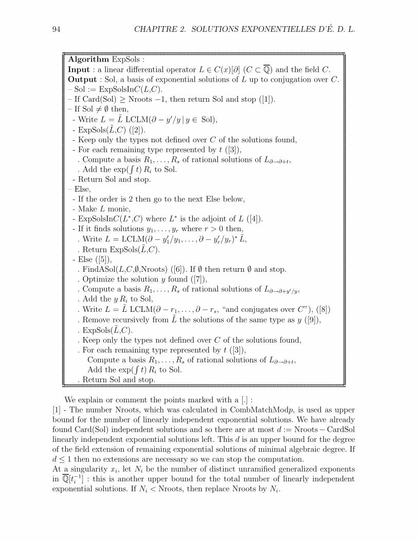
94 CHAPITRE 2. SOLUTIONS EXPONENTIELLES D’E. D. L.
Algorithm ExpSols :
Input : a linear differential operator L ∈ C(x)[∂] (C ⊂ Q) and the field C.Output : Sol, a basis of exponential solutions of L up to conjugation over C.– Sol := ExpSolsInC(L,C).– If Card(Sol) ≥ Nroots −1, then return Sol and stop ([1]).– If Sol 6= ∅ then,
- Write L = L LCLM(∂ − y′/y | y ∈ Sol),
- ExpSols(L,C) ([2]).- Keep only the types not defined over C of the solutions found,- For each remaining type represented by t ([3]),. Compute a basis R1, . . . , Rs of rational solutions of L∂→∂+t,. Add the exp(
∫
t) Ri to Sol.- Return Sol and stop.
– Else,- If the order is 2 then go to the next Else below,- Make L monic,- ExpSolsInC(L∗,C) where L∗ is the adjoint of L ([4]).- If it finds solutions y1, . . . , yr where r > 0 then,
. Write L = LCLM(∂ − y′1/y1, . . . , ∂ − y′
r/yr)∗ L,
. Return ExpSols(L,C).- Else ([5]),. FindASol(L,C,∅,Nroots) ([6]). If ∅ then return ∅ and stop.. Optimize the solution y found ([7]),. Compute a basis R1, . . . , Rs of rational solutions of L∂→∂+y′/y,. Add the y Ri to Sol,
. Write L = L LCLM(∂ − r1, . . . , ∂ − rs, “and conjugates over C”), ([8])
. Remove recursively from L the solutions of the same type as y ([9]),
. ExpSols(L,C).
. Keep only the types not defined over C of the solutions found,
. For each remaining type represented by t ([3]),Compute a basis R1, . . . , Rs of rational solutions of L∂→∂+t,Add the exp(
∫
t) Ri to Sol.. Return Sol and stop.
We explain or comment the points marked with a [.] :[1] - The number Nroots, which was calculated in CombMatchModp, is used as upperbound for the number of linearly independent exponential solutions. We have alreadyfound Card(Sol) independent solutions and so there are at most d := Nroots−CardSollinearly independent exponential solutions left. This d is an upper bound for the degreeof the field extension of remaining exponential solutions of minimal algebraic degree. Ifd ≤ 1 then no extensions are necessary so we can stop the computation.At a singularity xi, let Ni be the number of distinct unramified generalized exponentsin Q[t−1
i ] : this is another upper bound for the total number of linearly independentexponential solutions. If Ni < Nroots, then replace Nroots by Ni.
2.7. AN ALGORITHM TO FIND ALL EXPONENTIAL SOLUTIONS 95
[2] - At this point the roots of the p-curvature have already been computed, and neednot be computed again ; we can simply take the roots (with multiplicity) for χp(L) andreduce the multiplicities according to the solutions found.[3] - We have applied recursion on a left factor of L so the exponential solutions foundare in general not exponential solutions of L. We will only use the types of the expo-nential solutions of this left factor, not the exponential solutions themselves. We skiptypes defined over C because all exponential solutions over C have already been found.From [Or32] or [Ho97b, Lemma 7.1], the types of exponential solutions of L that arenot yet found must be among the types in the left factor L of L.[4] - We will apply FindASol only when all easy factors have been removed both on theleft and on the right. Removal of easy factors, left or right, does not cause solutions tobe lost because we only do this after all easy solutions have already been computed andstored in the set Sol, in the first step of the algorithm. To find the easy left factors, weapply ExpSolsInC to the adjoint operator L∗ to find the easy exponential solutions ofL∗ which correspond to easy left factors of L (see [PS03, 2.1]). Then we apply recursionon the remaining right hand factor.[5] - If the order of the operator is two, and if the bounds in FindASol do not immedia-tely rule out a solution defined over an extension, then the formulas given in [UW96]would be a good alternative to FindASol. If the order is three, then an alternative wouldbe the eigenring method (see [PS03]) but we do not expect that to be better than Fin-dASol, especially if one implements some shortcuts for order 3 in FindASol (such as :we only need to consider extensions in FindASol that have a degree 3 subfield. And :if at xi there are two non-conjugated generalized exponents that do not differ by aninteger, then C(xi) is the only extension that needs to be considered).[6] - Here, we reach the point where there is nothing left to do than entering the “hardcase”, trying to find a solution over an extension of C with FindASol. An a priori firstbound is Nroots, the number of roots in Fp(x
p) counted with multiplicity of χp(L) fora good prime p. Note that a more detailed analysis could lead to a sharper bound. Forexample, if two roots of χp(L) can not correspond to conjugated exponential solutions,or if one can conclude using the bounds in Section 2.6.1 that some root of χp(L) cannot correspond to an exponential solution of minimal algebraic degree Nroots, then wecould give FindASol a better bound.[7] - Let y be an exponential solution. We can write y ′/y = P1/P2 where P1 and P2
are polynomials with gcd 1 and P2 is monic. The field of definition of y is then thefield generated over C by the coefficients of P1 and P2. By “optimizing the solution”we mean two things : 1). Using this solution y to find a solution of minimal algebraicdegree over C. And 2). Making sure that the field that the algorithm gives for y (thisfield contains the field of definition of y) is actually equal to the field of definition of y.Both 1) and 2) are important. We want y to be of minimal algebraic degree so that weknow that its conjugates are linearly independent. But the way we count the numberof conjugates of y, i.e., the way we determine the number d(y), is not by looking at y,but by looking at the field given for y. The field provided for y by Algorithm FindASolcontains, but need not be not equal to, the field of definition of y. So to optimize y,we take the field given for y, and then determine the subfield generated over C by the
96 CHAPITRE 2. SOLUTIONS EXPONENTIELLES D’E. D. L.
coefficients of P1 and P2. Then we find defining equations (i.e., new RootOf’s) for thissubfield, and use them to rewrite the coefficients of P1 and P2. This then takes care of2). To do 1), we could use the approach in Lemma 10, however, this is not necessarybecause the special choice that Algorithm ExpSolsInC makes when the option “justone” is given causes 1) to be automatically satisfied. The polynomial Q is of minimaldegree with this option given, which leads to uniqueness of y ′/y which in turn causes yto already be of minimal algebraic degree over C.[8] - Here ri = R′
i/Ri + y′/y. One can compute this LCLM using the method of unde-termined coefficients and solving linear equations over C(x), this can be done withoutactually constructing the conjugates of y′/y.[9] - What is meant here is to also remove solutions whose type is conjugated over Cto the type of y. We will remove such solutions recursively because if we do not thenit would be non-trivial to ensure the specification of the algorithm that the “same”solution is not returned more than once. So before we call ExpSols on the remainingleft factor L of L, we first remove from L all exponential solutions of the same typeas (conjugates of) y, and we keep repeating this until L no longer has solutions ofthis type. A recursive procedure to achieve that is the following : compute the ratio-nal solutions Ri of L∂→∂+y′/y ; each one gives a first order right hand factor ∂ − ri
of L where ri = R′i/Ri + y′/y. If there are none then return L else write L = L1
LCLM(∂ − r1, . . . , ∂ − rs, “and conjugates over C”) and apply recursion on L1.
2.7.1 Some remarks on the algorithm
Remark on ExpSolsInC : Even though we use Algorithm CombMatchModp,there could still be combinations in step 4 that do not lead to an exponential solution(if for example the number of combinations is greater than Nroots then we alreadyknow in advance that this will be the case). If the degree bound (the number N instep 4) for polynomial solutions is high, or if C is a complicated field, or if there aremany combinations to be checked, then to make the algorithm efficient we need a quickway to discard non-solution-combinations before doing all the work in steps 4a and 4b,because each of these two steps can dominate the computation time.
In step 4, we can of course pre-compute the traces, so that all computations instep 4 are rational (i.e., over C). Computing S in step 4a then only involves additionsin C(x). However, that does not imply that computing S is cheap, because normalizingS (writing S as P1/P2 where P1, P2 are polynomials with no common factors) can bean expensive operation if C is a complicated field. Computation of L = L∂→∂+S can beeven more expensive because we need to multiply, differentiate, and add in C(x). Andsince step 4a is applied to each combination, one can easily spend more time in step 4athan in steps 1 and 2 combined. And if N is large then 4b can take even more time.
Often the N ’s are very small, and one can improve the running time of ExpSolsInCsubstantially by implementing some cases for step 4b separately, such as the case N = 0(in that case we should use a fast zero test for L(1) without computing L itself) and thecase N small non-zero : here, one would be tempted to take an ansatz
∑Ni=0 cix
i, and tocompute the coefficients of L(ansatz) which gives linear equations for the unknowns ci.
2.7. AN ALGORITHM TO FIND ALL EXPONENTIAL SOLUTIONS 97
But for small N and large L this results in much more equations than we need becausethere are only N + 1 unknowns. In this case, to make the ansatz approach efficient weshould not fully evaluate L(ansatz) because then we computed much more equationsthan we need. Instead we should evaluate just enough coefficients of L(ansatz) (and dothis without fully computing L itself) so that we have enough equations to determine theci, and once the ci ∈ C are found then we finish with a quick zero test for L(
∑Ni=0 cix
i).For large N we propose to compute L and to use [ABP95].
If we find w > 0 polynomial solutions in step 4b then the computation time in 4aand 4b was well spent even if those steps took a lot of time. But when w = 0, and ifC is a complicated field or N is a large number, then we want to avoid 4a and 4b withhigh probability. This is done as follows : take a prime number p (in general this p isnot the same prime as we used for the p-curvature because for the p-curvature we onlyuse small primes) such that p is greater than N plus the order of L, and also C[p] = Fp
(such primes have density at least 1/[C : Q] so they are easy to find). Then computeL[p] ∈ Fp(x)[∂] and check if it allows a polynomial solution of degree ≤ N . If not, skip4a and 4b.
More general fields : It is not difficult to generalize our algorithm to arbitrary fieldsof characteristic 0. We may assume that C is the field generated by the coefficients of L,so then C is a finitely generated extension of Q, say C = Q(t1, . . . , tk)[α1, . . . , αl] wheret1, . . . , tk are algebraically independent and the αi are algebraic over Q(t1, . . . , tk). Thenthe reduction mod p works as follows : choose random values for ti in Q. This gives amap f1 from a subring R1 of Q(t1, . . . , tk) to Q. If not all coefficients of the minimalpolynomial of α1 are in R1, then choose different random values for ti. After that, theminimal polynomial of α1 is mapped to a polynomial over Q, we can choose an irre-ducible factor, a root α′
1 of that factor, and map α1 to α′1. Do the same for α2, . . . , αl.
This way we have a map f2 from a subring R2 of C to the field Q(α′1, . . . , α
′l). We can
then choose a reduction mod p in the same way as before, so we have a map g from asubring of Q(α′
1, . . . , α′l) to a finite field. Then let the map [p] be the composition g ◦ f2
of these two maps, which will be defined on some subring R3 of R2. One can alwaysfind evaluations in Q for the ti and a prime number p such that all elements of C thatwe want to reduce mod p are in R3.
Logarithms : Generalized exponents correspond to formal solutions. Since we are onlyinterested in exponential solutions, the formal solutions that contain a logarithm arenot of interest to us. Because of this, we can disregard those generalized exponents thatdo not correspond to a formal solution without a logarithm. Note that in any givenequivalence class mod Z, this observation could eliminate some but never all unramifiedgeneralized exponents, so it does not help much for the combinatorial problem. However,this observation may reduce the number of distinct unramified generalized exponents insome equivalence classes mod Z, which can reduce the bound in Proposition 6 as well asthe number Ni in comment [1] after Algorithm ExpSols. This could speed up AlgorithmFindASol. Note that if L has an exponential solution of minimal algebraic degree n− 1where n is the order of L, then the adjoint of L has an exponential solution defined
98 CHAPITRE 2. SOLUTIONS EXPONENTIELLES D’E. D. L.
over C. Algorithm ExpSols removes this solution, hence, if ExpSols calls FindASol withdegree bound (the number b in FindASol) Ni = n − 1 then we may use n − 2 instead.
Deciding which generalized exponents match formal solutions without logarithmscan be done if we compute d+1 terms of the formal solutions, where d is the exponent-difference. We propose to do this computation only when ExpSols has to call FindASol.To speed up this computation, one could compute the formal solutions modulo a suitablylarge prime number, if a logarithm occurs then a logarithm must occur in characteristiczero as well.
A related implementation : Although we do not have an implementation for thealgorithm ExpSols in this paper, there is an implementation in Maple 9 for the diffe-rence case, i.e., a procedure that computes the hypergeometric solutions of a differenceequation. This implementation follows some of the ideas in this paper and performsvery well in practice (a paper concerning the difference case is planned). We expect ourExpSols to perform equally well.
2.7.2 Computing radical solutions
Computing radical solutions is almost the same problem as computing exponentialsolutions, with only a few differences :
1. One only uses generalized exponents that are in Q, see Equation (2.5) and Remark 3.2. τred maps rational numbers to zero, which implies that the only root of χp(L) thatmatters is 0, but also implies that there is no reduction in the combinatorial problem.
This means that for computing radical solutions, the only useful modular informationis the multiplicity of the root 0 in χp(L), which we can use as a bound for the numberof linearly independent radical solutions, hence as a bound for the degree of the fieldextension over which such solutions (of minimal algebraic degree) are defined.
To save computation time, we can compute this multiplicity without computingχp(L), in the following way : Take a good prime p. Then compute a basis z1, . . . , zs
of rational solutions of L[p]. If s = 0 then return 0, otherwise write L[p] = L1L2
where z1, . . . , zs is a basis of solutions of L2, apply recursion to L1, then add s to theresult for L1, and return the answer. We expect this to be faster than computing χp(L)because rational solutions of a differential operator in characteristic p can be computedvery quickly, O(max(l, p)2p) field operations where l is a bound on the degree of thecoefficients of L, see [Cl03].
2.7.3 Almost all primes
There are many results known that hold for all but finitely many p. For example, itis easy to show that
Lemma 7. For all but finitely many p, the number of linearly independent radicalsolutions of L is bounded by the dimension of the space of rational solutions of L[p].
2.7. AN ALGORITHM TO FIND ALL EXPONENTIAL SOLUTIONS 99
Thus, for almost all p, we could have used the number s in the previous section as abound. The reader may wonder why we did not do so. The problem here is that of themany results that are known for all but finitely many p, the only ones we can use for thealgorithm are those for which a small prime p can be exhibited with little computation.This problem is also the reason that the only information we use from the p-curvatureis its characteristic polynomial.
100 CHAPITRE 2. SOLUTIONS EXPONENTIELLES D’E. D. L.
Chapitre 3
Computing HypergeometricSolutions of Linear RecurrenceEquations
Ce chapıtre constitue un article soumis au journal Applicable Algebra in Engineering,Communication and Computing co-ecrit avec Mark van Hoeij : le texte a ete laisse danssa langue d’origine.
Introduction
Let C be a field of characteristic zero and C its algebraic closure. In many examples,C = Q, but C can also be a number field and may also have transcendental degree > 0over Q, as long as the standard algorithms (such as zero-test in C, factoring in C[x],etc.) are available.
A linear difference operator
L = an τn + an−1 τn−1 + · · ·+ a0 τ 0, (3.1)
with ai = ai(x) ∈ C(x) is an operator that acts on functions u = u(x) in the followingway :
L(u) = an(x) u(x + n) + an−1(x) u(x + n − 1) + · · ·+ a0(x) u(x).
The set of all such operators is denoted by C(x)[τ ]. This is a non-commutative ring ;multiplication is given by composition. We will always assume that the leading coefficientan and the trailing coefficient a0 are both non-zero. In this case, n is called the order ofL. The field of definition of L is the smallest field C ′ ⊆ C such that L ∈ C ′(x)[τ ].
The linear difference operator L in (3.1) corresponds to the linear recurrence equation(or relation)
L(u) = 0, i.e., an(x) u(x + n) + an−1(x) u(x + n − 1) + · · · + a0(x) u(x) = 0. (3.2)
A solution of L is a function u for which L(u) = 0. A hypergeometric solution is asolution u for which u(x + 1)/u(x) is a rational function, i.e., an element of C(x).
101
102 CHAPITRE 3. SOLUTIONS HYPERGEOMETRIQUES D’E. AUX D. L.
Computing a hypergeometric solution u is equivalent to computing a first order factorτ − u(x + 1)/u(x) of L in C(x)[τ ].
An algorithm for computing hypergeometric solutions of linear recurrence relationswith polynomial coefficients was first given by Petkovsek in [Pe92]. This algorithm isvery useful and has interesting applications. Unfortunately, in practice it is limitedto the case where a0 and an do not have complicated roots because the algorithmcomputes the splitting field of a0 an and this can easily run out of control. Even whenthis splitting field is not too complicated, the algorithm is still not optimal because itsearches through more combinations than necessary (see [Ho99, Example 1.5] and also[We01, Section 6.3]). To address these problems, the concept of finite singularities wasintroduced in [Ho99]. This notion and the associated Fuchs’ relations allow to reduce thenumber of combinations to check and to mimic Beke’s algorithm to find exponentialsolutions of linear differential equations (see [Be1894] or [CH04]). For n < 4, [Ho99,Theorems 2 and 3] show how to avoid splitting fields. In this paper we extend this toorder > 4. We also give a number of additional improvements. We detail the steps ofthe algorithm and we show how they can be done efficiently. The complete HypSolsalgorithm is described in Section 9 and uses a similar approach as Algorithm ExpSolsin [CH04] which computes the exponential solutions of linear differential equations. Wewill show in Section 10 how modular computations can be used to improve several stepsin the algorithm. Finally, we will show how to construct an analogue algorithm for q-difference equations when q is not a root of unity. Note that a q-analogue of Petkovsek’salgorithm is given in [APP98].
To summarize, the main contributions of the paper are :
– More details on how to implement the algorithm in [Ho99] efficiently.– How to avoid splitting fields for arbitrary order (in [Ho99] this was done for order
6 3).– Modular improvements in Section 10.– Introduction of local types and Fuchs’ relations for q-difference equations in Sec-
tion 12, so that an algorithm along the same lines can be given for the q-differencecase as well.
The paper is organized as follows. Section 1 recalls the vocabulary concerning hy-pergeometric terms and their local types. Section 2 shows how the symmetric product isused in the algorithm. Sections 3 and 4 deals with the finite singularities : we show howthe possible local types at these singularities can be computed efficiently. In Section 5the same problem concerning the point at infinity is addressed. Section 6 discusses is-sues about field extensions. In Section 7 we give Algorithm ESols to compute the “easy”solutions and in Section 8 we describe Algorithm HSol that computes a “hard” hyper-geometric solution addressing the field problem. The complete Algorithm HypSols isgiven in Section 9 which also lists a number of additional improvements. Section 10details how modular computations can improve the algorithm. In Section 11, we givesome timings. Finally, in the last section, we introduce the notions needed to constructan analogue algorithm for q-difference equations when q is not a root of unity.
3.1. HYPERGEOMETRIC TERMS 103
3.1 Hypergeometric terms
Let C be a field of characteristic zero and C be its algebraic closure. In [PS97, Section6.2], the authors prove the existence and uniqueness (up to difference isomorphisms) ofa universal extension V for difference equations with coefficients in C(x). Consequently,given a difference operator L, we can view the solutions of L(y) = 0 as elements of thisuniversal extension V. The dimension of the solution space (the kernel of L : V → V)is n.
One can view V as a subring of the ring S which is defined as follows
S = {[f ] | f ∈ CN},
where [f ] is the equivalence class of all f ∈ CN
for which f − f has finite support. Iff is a function that is defined on all but finitely many elements of N, then its image[f ] ∈ S is well defined. This way C(x) can be viewed as a subring of S.
Definition 25. A non-zero expression u(x) ∈ V is called a hypergeometric term if itsatisfies u(x + 1)/u(x) ∈ C(x). The rational function r(x) = u(x + 1)/u(x) ∈ C(x) isthen called the certificate of u(x). It is the analogue of the logarithmic derivative fromthe differential case.
Let u(x) be a hypergeometric term, and view u(x) as an element of S. If C = C thenwe can use Gamma functions to represent u(x) by a function, defined for sufficientlylarge integers, as follows :
cx R(x)
k∏
i=1
Γ(x − αi)ei,
where c ∈ C∗, R(x) ∈ C(x) and ∀ i ∈ {1, . . . , k}, αi ∈ C and ei ∈ Z.
In this paper, we do not need to distinguish a hypergeometric term u(x) from aconstant times u(x). Thus we can represent u(x) by its certificate, which explains thefollowing definition.
Definition 26. Let C be a field of characteristic zero. A hypergeometric term u(x) issaid to be defined over C if u(x + 1)/u(x) ∈ C(x).
Definition 27. Let u1(x), u2(x) be hypergeometric terms, and r1(x) = u1(x+1)/u1(x),r2(x) = u2(x + 1)/u2(x) be their certificates. Then u1(x) and u2(x) are said to be ofthe same type (or similar) if u1(x)/u2(x) ∈ C(x), or equivalently, if r1(x)/r2(x) is thecertificate of a rational function.
Remark 6. The following property (see [PWZ96, Proposition 5.6.2]) shows that thisnotion is very natural :u1, u2 are of the same type ⇔ u1 + u2 is either a hypergeometric term or zero.
In fact, if u1, . . . , uk are hypergeometric terms of distinct types then they are C(x)-linearly independent. Let u(x) be a hypergeometric term defined over C and let r(x) ∈
104 CHAPITRE 3. SOLUTIONS HYPERGEOMETRIQUES D’E. AUX D. L.
C(x) be its certificate. We can factor r(x) over C as follows. Note that in general C willnot be algebraically closed, so the factors need not be linear.
r(x) = c φ1(x)e1 · · ·φm(x)em , (3.3)
with c ∈ C∗, ei ∈ Z, and φi(x) = xdeg(φi)+φi,1xdeg(φi)−1+· · ·+φi,deg(φi)x
0, where φi,j ∈ C,and φi ∈ C[x] is monic and irreducible over C. Because r(x) is a rational function, themultiplicities ei can be negative.
Denote t := 1/x. Now r(x) = r(1/t) can be written as
c tv (1 + d t + O(t2)), (3.4)
where c ∈ C∗, v ∈ Z and d ∈ C. Equations (3.3) and (3.4) are related in the followingway : the number c is the same, and furthermore :
v = −m∑
i=1
ei deg(φi) and d =
m∑
i=1
ei φi,1.
If we factor r(x) over C, so r(x) = c∏
i(x − αi)ei, then we can write v = −∑i ei and
d = −∑i ei αi.
Definition 28. With the notations above, the local type of the hypergeometric termu(x) at x = ∞ is defined as
g∞(u(x)) = (c, v, d + Z) ∈ C∗ × Z × C/Z.
If g∞(u1) = (c1, v1, d1+Z) and g∞(u2) = (c2, v2, d2+Z), then g∞(u1 u2) = (c1 c2, v1+v2, d1 + d2 + Z).
Example 1. Let
u(x) = 7x Γ(x + 13)Γ(x + 6
5)3
Γ(x − 23)Γ(x − 4
5)
(3.5)
be a hypergeometric term defined over Q. Then
r(x) =u(x + 1)
u(x)= 7
(
x +1
3
)1(
x − 2
3
)−1(
x +6
5
)3(
x − 4
5
)−1
,
so thatc = 7, v = −(1 · 1 − 1 · 1 + 3 · 1 − 1 · 1) = −2,
and
d = 1 · 1
3− 1 ·
(
−2
3
)
+ 3 · 6
5− 1 ·
(
−4
5
)
+ Z =27
5+ Z.
Consequently,
g∞(u(x)) =
(
7,−2,27
5+ Z
)
.
This could have been deduced from the expansion of r(x) at infinity :
r(x) = r
(
1
t
)
= 7 t−2
(
1 +27
5t + O(t2)
)
.
3.2. THE SYMMETRIC PRODUCT 105
Definition 29. Let u(x) be a hypergeometric term defined over a field C of characte-ristic zero and let r(x) = u(x + 1)/u(x) ∈ C(x) be as in Equation (3.3). Let q ∈ C andlet p = q +Z be the image of q in C/Z. Then the local type or valuation growth of u(x)at the “point” p is defined as :
gp(u(x)) =∑
i
ei where the sum is taken over all i for which φi has a root in p.
Note that φi(π) = 0 for some π ∈ p is equivalent to saying that φi(q + l) = 0 forsome l ∈ Z.
Example 2. Let u(x) be as in Example 1.For p = 2/3+Z, we have gp(u(x)) = 1−1 = 0 and for p = 4/5+Z, gp(u(x)) = 3−1 = 2.If p is any other element of Q/Z, then gp(u(x)) = 0.So for this example we have calculated the local types of u(x) for all p ∈ Q/Z∪{∞}. Wecan verify now that the so-called Fuchs’ relations (see [Ho99, Equation 3]) are verified :
v +∑
p∈Q/Z
gp(u(x)) = 0 and d +∑
p∈Q/Z
gp(u(x)) p ≡ 0 mod Z. (3.6)
The first one is −2 + 0 + 2 = 0, and the second is 275
+(
0 · 23
+ 2 · 45
)
≡ 0 mod Z.
The following statement is part of [Ho99, Theorem 1].
Theorem 1. Let u1(x) and u2(x) be hypergeometric terms. Then u1(x) and u2(x) areof the same type if and only if they have the same local type at every p ∈ C/Z ∪ {∞}.
This theorem is central to the algorithm. The way the algorithm uses it is as follows :from the definition of type, if we know the type of u(x), then we know u(x) up to someunknown factor in C(x). The theorem says that we know the type of u(x) if and only ifwe know the local type of u(x) at all “points” p ∈ C/Z ∪ {∞}. Hence, in order to finda hypergeometric solution u(x) of a linear recurrence equation, we first have to find thetype of u(x), and in order to do that we first have to find the possible local types ofu(x) at each p ∈ C/Z ∪ {∞}. In Section 4 we compute for p ∈ C/Z a finite set gp(L)of possible local types of L at p. This means that for every hypergeometric solution u ofL, the local type gp(u) of u at p is an element of gp(L). In Section 5 we do the same forp = ∞.
3.2 The symmetric product
Definition 30. Let L1, L2 ∈ C(x)[τ ]. The symmetric product L1©s L2 of L1 and L2 isdefined as the monic operator L ∈ C(x)[τ ] of smallest order such that L(u1 u2) = 0 forall u1, u2 ∈ V with L1(u1) = 0 and L2(u2) = 0.
In this paper, we only use this when the order of L2 is 1, and we give a formula forthis case.
106 CHAPITRE 3. SOLUTIONS HYPERGEOMETRIQUES D’E. AUX D. L.
Let L =∑n
i=0 aiτi ∈ C(x)[τ ] be a linear difference operator with ai ∈ C(x) and let
r ∈ C(x). Then
L©s (τ − r) =1
bn
n∑
i=0
biτi where bn = an and ∀ i ≤ n − 1, bi(x) = ai(x)
n−1∏
j=i
r(x + j).
We made the result monic (dividing by the leading coefficient bn) in order to makeL©s (τ−r) uniquely defined. However, in the implementation, uniqueness is not necessaryhere, and we multiply L©s (τ − r) by a polynomial in order to avoid computing withfractions.
One way that the symmetric product is used in the algorithm is as follows : supposewe have chosen a candidate, that is, for each point p we have chosen a possible localtype of L at p (i.e., an element of gp(L)). If this candidate does not satisfy Fuchs’relations given in Equation (3.6) then the candidate does not correspond to the type ofany hypergeometric term u(x) (see [Ho99, Theorem 1]), and thus it can be discarded.If it does satisfy these relations, then we have a candidate type. Then we apply a fewtests in order to quickly discard those types for which it is easy to decide that L hasno hypergeometric solution of that type. If the candidate type passes these tests, thenwe want to compute a basis u1, . . . , um of all hypergeometric solutions of L of thattype (if such solutions exist). We construct a function r(x) ∈ C(x) that representsthis candidate type. This means that a non-zero solution u of τ − r has this type. Sou1/u, . . . , um/u must be in C(x). Now 1/u is a solution of τ −1/r and so from Definition30 it follows that
u1
u, . . . ,
um
uis a basis of rational solutions of L©s (τ − 1
r).
The calculation that leads to gp(L) for p ∈ C/Z in Section 4 is the same as the com-putation of the bounds in [Ho98]. By re-using this information, we can calculate thebounds for the rational solutions of L©s (τ − 1/r) (bound for the denominator and forthe degree of the numerator) before we even calculate the operator L©s (τ − 1/r). Thisis useful, for example if the bound for the degree of the numerator is negative (thisis one of the tests used) then we can discard the candidate type without computingL©s (τ − 1/r). We do not need to run an algorithm for computing bounds (see [Abr95]or [Ho98]) for L©s (τ − 1/r) because by re-using numbers already computed during thegp(L) computation in Section 4 we can determine exactly the same bound as whatwould have been obtained with [Ho98].
So we need to compute rational solutions of L©s (τ −1/r), but since we already knowa bound for the denominator and the degree of the numerator, we can construct r(x)in such a way that we are reduced to finding polynomial solutions (with degree-boundalready known) of L©s (τ − 1/r), see Algorithm Search in Section 7. As mentioned, ifthe degree-bound is negative then the candidate type is discarded. If the degree-boundis 0 then we take the sum of the coefficients of L©s (τ − 1/r) and do a zero-test (firsta fast probabilistic test, then if necessary a full test). If the degree-bound is positivebut not high, then we proceed by computing and solving necessary linear equations for
3.3. WHAT DOES IT MEAN TO BE A FINITE SINGULARITY? 107
the coefficients of the polynomial solutions. Since we do not want to solve systems ofequations with many variables, we should use a different method if the degree-bound ishigh (see [ABP95, Ba97]).
3.3 What does it mean to be a finite singularity ?
Definition 31 (Definition 8 in [Ho99]). Let L = anτn + · · · + a0τ0 ∈ C(x)[τ ] with
an 6= 0 and a0 6= 0. After multiplying L on the left by a suitable element of C(x), wemay assume that the coefficients ai are in C[x] and gcd(a0, . . . , an) = 1. Then q ∈ C iscalled a problem point of L if q is a root of the polynomial a0(x) an(x − n).
We want a notion of singularities that is invariant under the shift operation p 7→ p+1.Now p is invariant under the shift if p = ∞ (Section 5 discusses the singularity p = ∞)but not invariant if p ∈ C. Thus, we will deviate from other definitions in the literature(our problem points are called singularities in [No29]) and define finite singularities asfollows :
Definition 32. p ∈ C/Z is called a finite singularity of L if L has a problem point inp.
Example 3. Let
L = x
(
x − 1
3
)(
x +1
4
)
τ 2 − τ + x(x − 3).
The order is n = 2. The roots of the trailing coefficient give the problem points 0 and 3,and the roots of the leading coefficient give the problem points 0 + 2, 1/3 + 2, −1/4 + 2.If u(x) ∈ V is a hypergeometric solution of L and if q ∈ Q then
q
(
q − 1
3
)(
q +1
4
)
u(q + 2) − u(q + 1) + q(q − 3)u(q) = 0,
whenever this is defined. Solving for u(q + 2) gives
u(q + 2) = −−u(q + 1) + q(q − 3)u(q)
q(q − 13)(q + 1
4)
, in general u(q + n) = −n−1∑
i=0
ai(q)
an(q)u(q + i),
(3.7)and solving for u(q) leads to
u(q) = −q(q − 13)(q + 1
4)u(q + 2) − u(q + 1)
q(q − 3), in general u(q) = −
n∑
i=1
ai(q)
a0(q)u(q + i).
(3.8)Formula (3.7) can be used to compute u(q + 2) from previous u-values if q + 2 is not aproblem point whereas Formula (3.8) can be used to compute u(q) from next u-values if
108 CHAPITRE 3. SOLUTIONS HYPERGEOMETRIQUES D’E. AUX D. L.
q is not a problem point. Consequently the problem points of L are {0, 1/3,−1/4}+2 ={2, 7/3, 7/4} and {0, 3}. This means that the finite singularities are
{
2 + Z,7
3+ Z,
7
4+ Z, 0 + Z, 3 + Z
}
=
{
Z,1
3+ Z,
3
4+ Z
}
,
so there are three finite singularities.Consider p = Z. If for example the values of u(−5), u(−4) are given, then we can
use the relations (3.7,3.8) to calculate u(q) for q ∈ Z with q < 2. But u(2) can not becomputed because taking q = 0 in equation (3.7) leads to a division by zero. If u(8), u(9)were given, then u(q) could be computed for all q ∈ Z for which q > 3. We can not reachu(3) from u(8), u(9) because taking q = 3 in equation (3.8) results again in a divisionby zero.
The point p = 1/3 + Z is a finite singularity. If u(5 + 1/3), u(6 + 1/3) were given,then u(q) can be determined with equations (3.7,3.8) for all q ∈ p. However, if u(−5 +1/3), u(−4+1/3) were given then not all u(q), q ∈ p can be determined. So p is singular,but one only notices its singular behavior when going from the left to the right (withEquation (3.7)), and not when going from the right to the left (with Equation (3.8)).The point p = 3/4 + Z is a finite singularity for the same reason.
Any other element of Q/Z is not a singularity. For example, p = 1/2 + Z is not afinite singularity of L, because whenever we know any two consecutive values of u on pthen the two formulas (3.7,3.8) allow us to go freely to the left and right without everbumping into a division by zero ; there are no problem points in p = 1/2 + Z.
In general, if p is a finite singularity, if n consecutive values u(q+1), u(q+2), . . . , u(q+n) are given, and if q + 1, . . . , q + n are on the left of the problem points, then u(q + l)can be computed for all integers l 6 n, but not always for all positive integers l becausethat would require passing through problem points. This is the essence of the conceptof left solutions of L at p introduced in [Ho99] : they are solutions defined on a left halfline. Similarly, if q + 1, . . . , q + n were on the right of the problem points, then u(q + l)could be determined for positive integers l, which means we have right solutions of Lat p, they are defined on a right half line.
The set of all left (resp. right) solutions at p is denoted by Vp,l(L) (resp. Vp,r(L)). Fora precise definition of these sets, see [Ho99, Section 2]. Both are n-dimensional vectorspaces, where n is the order of L (we always assume that an and a0 are non-zero). Soat a finite singularity p we distinguish two kinds of solutions, left and right solutions,which are separated by the problem points. If p is non-singular then Vp,l(L) and Vp,r(L)are not separated and so they can be identified.
Deforming the singularity p is a method to bypass the problem points, in order togo from the left to the right solutions, as well as from the right to the left solutions.The deformed operator Lε is obtained by substituting x 7→ x+ ε in L. This deformationmoves the singularity p to p − ε, and turns p into a non-singular point : dividing byzero is now replaced by dividing by ε. Here ε is a new constant ; deforming increases ourfield of constants from C to C(ε). Because of this change of constants, elements of thetwo solution spaces (left and right) of L at p can not be identified in a unique way with
3.4. HOW TO COMPUTE GP (L) FOR FINITE P . 109
solutions of the deformed operator Lε, but we will see in Section 9.1 (see also [Ho99,Section 4.2]) that it is still possible to define useful maps between these solution spaces.
The main information we gather by going from the left to the right and from theright to the left in the deformed operator Lε is the multiplicity of the factor ε that willappear in the denominator (or in the numerator). In the next section, the set gp(L)is constructed from this data, and so is a bound for the denominators of the rationalsolutions to be computed in the algorithm (the same bound as in [Ho98]).
3.4 How to compute gp(L) for finite p.
Let C be a field of characteristic zero and let L ∈ C(x)[τ ] be a linear differenceoperator. Let p ∈ C/Z. In [Ho99] a procedure was given to calculate a finite set denotedby gp(L) that has the property :
u(x) hypergeometric solution of L =⇒ gp(u(x)) ∈ gp(L). (3.9)
Note : the converse does not hold in general.We shall show how this can be done in practice in an efficient way. If p = q + Z ∈ C/Zwhere q ∈ C then computing with the singularity p of L is equivalent to computing withthe singularity 0 + Z of the operator Lq where Lq is the operator obtained from L bysubstituting x+q for x. So without loss of generality we may assume that the singularityp to be considered is p = Z. Note though that (see the discussion in Section 3.6), givenL ∈ C(x)[τ ] for some field C of characteristic zero, if q 6∈ C then we need to temporarily(as long as we are computing with this singularity) replace the field C by C ′ = C(q)because Lq ∈ C ′(x)[τ ].
Now we will assume that L ∈ C ′[x][τ ] has order n and that p = Z is the singularityto be studied. Then the problem points corresponding to p are the integer roots ofa0(x) an(x − n). We take the largest possible pl ∈ p such that for all integers q 6 pl,the two consecutive sequences u(pl − n), . . . , u(pl − 1) and u(q − n), . . . , u(q − 1) canbe computed from each other via the two equations (3.7,3.8) without bumping intodivisions by zero. Then we can identify every left solution of L at p with a vector(u(pl − n), . . . , u(pl − 1)) with entries in C, because given any n consecutive valuesof such a left solution, we can determine (u(pl − n), . . . , u(pl − 1)) by repeated useof Equation (3.7), and furthermore, given (u(pl − n), . . . , u(pl − 1)) we can determineu(q) for all integers q < pl by repeated use of Equation (3.8). Similarly, we can take thesmallest integer pr ∈ p such that we can go back and forth between (u(pr+1), . . . , u(pr+n)) and (u(q + 1), . . . , u(q + n)) for all q > pr. This way each right solution of L at pcan be identified with a vector (u(pr + 1), . . . , u(pr + n)) with entries in C.
Remark 7. The condition back and forth is important in order for such smallest pr ∈ pto exist. For example if L = τ 2 − x2 and p = Z then starting with (u(pr + 1), u(pr + 2))and say pr < 0 we can go arbitrarily far to the right, but say we go to (u(1), u(2)), thengoing from there to (u(pr + 1), u(pr + 2)) without dividing by zero is not possible whenpr < 0. So for L = τ 2 −x2 we can not take pr < 0. We see that pr = 0. For L = τ 2 −x2
110 CHAPITRE 3. SOLUTIONS HYPERGEOMETRIQUES D’E. AUX D. L.
and p = Z we have pl = 2. Notice that pl − n is always smaller than pr + 1, but that{pl − n, . . . , pl − 1} and {pr + 1, . . . , pr + n} are not necessarily disjoint.
Example 4. Back to Example 3, we recall that, concerning the finite singularity p = Z,we have seen that we can not obtain u(2) from previous u-values nor can we obtain u(0)or u(3) from next u-values. One finds pl = 2 and pr = 3.
Since Lε, the operator obtained by substituting x+ε for x in L, has no singularity atp = Z, its solution space at p, Vp(Lε) := {u : p → C(ε) |Lε(u) = 0} is an n-dimensionalC(ε)-vector space. We now specify two bases u1, . . . , un and v1, . . . , vn of Vp(Lε) in thefollowing way :
ui(pl − j) = δi,j and vi(pr + j) = δi,j for i, j ∈ {1, . . . , n},
where δi,j is 1 if i = j and 0 otherwise. If we substitute ε = 0 in u1, . . . , un then onemay have divisions by 0, but these do not occur at q < pl. This way we obtain a basis{u1, . . . , un} = {u1, . . . , un}ε=0 of left solutions of L at p. Likewise, {v1, . . . , vn}ε=0 isdefined at all q > pr, and this results in a basis of right solutions of L at p.
Definition 33. Let a ∈ C(ε). The valuation vε(a) of a at ε = 0 is the element ofZ ∪ {∞} defined as follows : if a 6= 0 then vε(a) is the largest integer m ∈ Z such thata/εm ∈ C[[ε]] and vε(0) = ∞.
So
vε(a) > 0 ⇐⇒ aε=0 = 0 and vε(a) < 0 ⇐⇒ a has a pole at ε = 0.
Now, for p = Z, we want to compute a set gp(L) satisfying the specification of (3.9).First, for q ∈ {pl − n, . . . , pr + n}, we consider the following integers :
Bl(q) = min16i6n
vε(ui(q)) and Br(q) = min16i6n
vε(vi(q)). (3.10)
These integers are very useful since they also lead to bounds for the denominators ofrational solutions in the same way as in [Ho98].
Definition 34. The minimum valuation growth gp,r(L) and the maximum valuationgrowth gp,l(L) of L at p are defined as
gp,r(L) = min{Bl(q) | q > pr}, gp,l(L) = −min{Br(q) | q < pl}, (3.11)
and the set of valuation growths gp(L) is then
gp(L) := {m ∈ Z | gp,r(L) 6 m 6 gp,l(L)}.
Note on difference modules : If p ∈ C/Z and if two operators L1, L2 define iso-morphic difference modules (for a definition see [PS97]) then gp(L1) = gp(L2), andthus gp can be defined for difference modules. This gp behaves in a predictable waywith respect to tensor products, direct sums, etc. Moreover, if gp(L1) = {0} then there
3.4. HOW TO COMPUTE GP (L) FOR FINITE P . 111
exists an operator L2 defining an isomorphic difference module, for which p is not a sin-gularity. We do not detail this because difference modules are not needed for this paper.
If u = u(x) is a hypergeometric solution of L, then its local type gp(u) at p, alsocalled its valuation growth, must be an element of this set gp(L), see [Ho99]. If gp(L) hasonly one element, then that leaves only one choice for gp(u). In that case p is called asemi-apparent singularity. If 0 is the only element of gp(L) then p is called an apparentsingularity. The singularities that are most significant in the algorithm are the oneswhere there is more than one choice for gp(u), i.e., the singularities p where gp(L) hasmore than one element. Such singularities are called essential singularities.
If L has a basis of rational solutions, then all singularities are apparent. More gene-rally, if L has n linearly independent hypergeometric solutions, then gp,r(L) is preciselythe smallest gp(u) of all hypergeometric solutions u of L, and gp,l(L) is the largestgp(u). If L has fewer than n linearly independent hypergeometric solutions then gp,r(L)and gp,l(L) are just bounds for gp(u) and are often no longer sharp. If L = L1L2 thengp(L2) ⊆ gp(L) always holds, but it is easy to find examples where gp(L2) 6= gp(L),even when L does not have more hypergeometric solutions than L2. This already occurswhen L = (τ −x)(τ −x) = τ 2−(2x+1)τ +x2. Fortunately, this does not imply that thealgorithm will have to construct many unnecessary operators L©s (τ − 1/r) to check forrational solutions because Fuchs’ relations (Equation (3.6)) are usually quite selective.Now, in order to calculate the minimum valuation growth gp,r(L) from the formu-las (3.10) and (3.11), we have to start from the ui (which take values 0 and 1 atpl −n, . . . , pl − 1) and evaluate them at pr +1, . . . , pr +n. This computation starts withvalues at pl − n, . . . , pl − 1, and then goes to the right using Equation (3.7).Similarly, to compute the maximum valuation growth gp,l(L), we start with values 0 and1 for vi at pr + 1, . . . , pr + n, and then we proceed to the left (with Equation (3.8)) inorder to evaluate vi at pl − n, . . . , pl − 1.
Truncated power series :Suppose we want to calculate Bl(q) for q ∈ {pl − n, . . . , pr + n}. We need to computethe ui(q) for i ∈ {1, . . . , n} and q ∈ {pl, . . . , pr + n}. For efficiency reasons, we wantto prevent computing in our new field of constants C ′(ε). Recall that C ′ is the fieldextension of C given by the singularity p ∈ C/Z that we shifted to p = Z. Note thatcomputing the sets gp(L) using direct computations in C ′(ε) hurts the running time ofthe algorithm : this is remarked in [We01, Section 6.3].As we are merely interested in the ε-valuations of the ui(q), these ui(q) ∈ C ′(ε) can bereplaced by truncated power series in ε, i.e., power series of the form
∑
i<a ciεi +O(εa)
where the sum is finite and a ∈ Z. This a is called the accuracy of the truncated powerseries. If a0(x), . . . , an(x) are the coefficients of L then a0(x + ε), . . . , an(x + ε) are thecoefficients of Lε. Let N0 (resp. Nn) be the number of roots (counted with multiplicity)of a0(x) (resp. an(x)) in p. When we compute the next term with Equation (3.7), theaccuracy decreases by the ε-valuation of an(q + ε), which is the same as the order ofan(x) at x = q. Combined, going from the left to the right, the accuracy decreasesby Nn. We can recover the ε-valuation of an element of C ′(ε) from a truncated power
112 CHAPITRE 3. SOLUTIONS HYPERGEOMETRIQUES D’E. AUX D. L.
series when the accuracy is greater than the ε-valuation. We start computing withu(pl − n), . . . , u(pl − 1) with initial accuracy a = N0 + Nn + 1. Going to the right withEquation (3.7), the accuracy has decreased by Nn when we reach ui(q) with q > pr,so the remaining accuracy is a − Nn. Considering the fact that one can go back withEquation (3.8), it is not difficult to show that N0 is an a priori upper bound for gp,r(L),hence the remaining accuracy a − Nn = N0 + 1 suffices to determine gp,r(L). The sameinitial accuracy N0 + Nn + 1 suffices to compute gp,l(L) as well.
Example 5. Let L = (x−1) (x+1) τ 2−x (x2+x−1) τ+x2 (x−1) and p = Z. The problempoints are 1, 3 and 0, 1. Here 1, 3 are the solutions of an(x−n) = (x−1−2) (x+1−2) =0, and 0, 1 are the roots of a0. Now pl − n, . . . , pl − 1 (the starting points for the ui) is−1, 0 because this is the furthest to the right for which the following is true : for anyq, q + 1 ∈ p on the left of −1, 0 one can go back and forth between q, q + 1 and −1, 0without dividing by zero. Likewise, pr + 1, . . . , pr +n (the starting points for the vi) willbe 2, 3.
Replacing x by x + ε to determine Lε, and solving u(x + 2) from Lε(u) = 0 like inEquation (3.7) we get
u(x + 2) = −−(x + ε) ((x + ε)2 + (x + ε) − 1) u(x + 1) + (x + ε)2(x + ε − 1)u(x)
(x + ε − 1)(x + ε + 1).
N0 + Nn + 1 = 6 so we start with : u1(−1) = 0 + O(ε6), u1(0) = 1 + O(ε6). Likewise,take u2(−1) = 1 + O(ε6), u2(0) = 0 + O(ε6). Then substitute x = −1, 0, 1 in the aboveequation to find :
u1(1) = − 12ε− 1
4+ 7ε
8− ε2
16− ε3
32− ε4
64+ O (ε5) , u2(1) = −1
ε+ 2 − ε + O (ε5) ,
u1(2) = −12
+ ε4
+ ε2
8+ 9
16ε3 − 23
32ε4 +O (ε5) , u2(2) = −1+3 ε−3 ε2 +2 ε3−2 ε4 +O (ε5) ,
u1(3) = −14− 1
4ε + 3
16ε2 + 11
16ε3 + O (ε4) , u2(3) = −1
2+ 7
4ε − 3
8ε2 − 13
16ε3 + O (ε4) .
The accuracy, indicated by O(εa), drops when we divide by ε.Now Bl(q) = min{vε(u1(q)), vε(u2(q))} and gp,r(L) = min{Bl(2), Bl(3)} so we haveBl(1) = −1, Bl(2) = 0, Bl(3) = 0, and gp,r(L) = 0.Now use Lε(v) = 0 to write v(x) as a linear combination of v(x+1) and v(x+2). Thenstart with v1(2) = 1+O(ε6), v1(3) = 0+O(ε6) and v2(2) = 0+O(ε6), v2(3) = 1+O(ε6)and compute for i = 1, 2 the values of vi(x) at x = 1, 0,−1. At x = 1 we divide bya0(1 + ε) and the accuracy drops by 1. Then at x = 0 we divide by a0(0 + ε) andthe accuracy drops by 2. So for i = 1, 2 we find vi(1) with accuracy 5, and find vi(0)and vi(−1) with accuracy 3 which is more than enough to determine gp,l(L). We findBr(1) = −1, Br(0) = −1, Br(−1) = −1 and gp,l(L) = −min{Br(0), Br(−1)} = 1.Finally, we get
gp(L) = {m ∈ Z | gp,r(L) 6 m 6 gp,l(L)} = {0, 1}.
Our algorithm for computing hypergeometric solutions will try two candidate types (seeSection 2) for this example. In one of these candidate types, we have the element 0 fromgp(L) and the number c from Section 1 is 1. For this candidate type we need to findrational solutions of L. Now max{B l(q), Br(q)} is a lower bound for the valuation of
3.5. HOW TO COMPUTE G∞(L). 113
a rational solution at x = q. This bound is −1 at x = 1 and zero elsewhere, thus, therational solution must be of the form (x − 1)−1 times a polynomial. The degree boundfor this polynomial is obtained from the information at p = ∞ computed in the nextsection. This degree bound is zero, and thus what remains to be done for this candidatetype is to check if (x − 1)−1 is a solution, which it is.
The next candidate type has the element 1 from gp(L) and the number c is again 1.So we have to compute the rational solutions of L©s (τ − 1/r) where τ − r should have
the desired candidate type, which implies that r = x τ(f)f
for some rational function f .
Now the Bl(q) number for L©s (τ −1/r) is the Bl(q) number for L plus the Bl(q) number
for τ − 1/r. The same holds for Br(q). We can choose f in r = x τ(f)f
in such a way
that L©s (τ − 1/r) will have max{B l(q), Br(q)} = 0 for all q ∈ C. This way, the rationalsolutions of L©s (τ − 1/r) must be polynomials. The r obtained this way is r = x − 1.The degree bound for the polynomial solutions is zero, thus, the algorithm checks if thesolution Γ(x − 1) of τ − r is a solution of L, which it is.
Example 6. Let us see briefly what we obtain for the operator given in Example 3. InExample 4, we found pl = 2 and pr = 3, so we start with values of ui at 0, 1 and go to theright. We find Bl(2) = Bl(3) = Bl(4) = Bl(5) = −1 so that gp,r(L) = −1. Then we startwith values of vi at 4, 5 and go the the left, and we find Br(3) = Br(2) = Br(1) = −1,Br(0) = −2. So gp,l(L) = −min{−1,−2} = 2 and finally, gp(L) = {−1, 0, 1, 2}.
Modular computations :We can further improve this by computing modulo prime numbers. In our Maple im-plementation, this is done as follows : take three “big” primes p1, p2 and p3, considerthe coefficients of the truncated power series as elements of Fpi
(details concerning thereduction of elements in C ′ modulo p are included in [CH04, Sections 1.3 and 7.1]) andmake the computations modulo each pi. If these three modular computations lead tothe same result, then return it and stop, otherwise take new primes.
Remark 8. With these two tricks, reducing rational functions in ε to truncated powerseries, and reducing the elements of C ′ to a finite field, computing the sets gp(L) for
p ∈ C/Z is quite fast and does generally not dominate the running time of our algorithm.
3.5 How to compute g∞(L).
As with finite points, given L ∈ C(x)[τ ], one can exhibit a finite set g∞(L) suchthat :
u(x) hypergeometric solution of L =⇒ g∞(u(x)) ∈ g∞(L).
We detail here how we can compute this set with the classical techniques (see[Ad28, Bi30, No29]) used to compute the formal solutions at infinity of linear differenceoperators. Our approach is based on the following easy lemma which follows directlyfrom the definition of the local type at infinity and the exposition in [Ad28] or [Bi30].
114 CHAPITRE 3. SOLUTIONS HYPERGEOMETRIQUES D’E. AUX D. L.
Lemma 8. Let L ∈ C[x][τ ]. If L has a hypergeometric solution u = u(x) with lo-cal type (c, v, d + Z) at infinity, then L has a formal solution at infinity of the formΓ(x)−v cx xd F (1/x) where F (1/x) is a formal power series in 1/x.
The possible couples (c, v) ∈ C ×Z appearing in the formal solutions at infinity canbe read from the so-called Newton τ -polygon (see [BD94] and note that similar polygonsalready appeared in [Ad28, Bi30]) and more precisely −v is a (integer) slope of thispolygon whereas c is a root of the Newton τ -polynomial (or characteristic equation)associated with the slope −v.
Definition 35. Let L =∑n
i=0 ai τi ∈ C[x][τ ]. For (u, v) ∈ R2, let L(u, v) := {(x, y) ∈
R2 | x = u, y > v}. Let M(L) be the union of the L(i,− deg(ai, x)) for i ∈ {0, . . . , n}with ai 6= 0. The Newton τ -polygon of L is the convex hull of M(L).
We give now an algorithm that computes only relevant (i.e., integer) slopes of theNewton τ -polygon with their associated Newton τ -polynomial.
Algorithm τPolygon :
Input : L := anτn + · · · + a0τ0 with ai ∈ C[x], a0, an 6= 0.
Output : The integer slopes of the Newton τ -polygon and their correspondingNewton τ -polynomials.1. If n = 0, then return ∅ and stop.2. For i ∈ {0, . . . , n}, let vi := − deg(ai, x) (if ai = 0 then vi = ∞).3. s := max((vn − vi)/(n − i), i = 0, . . . , n − 1).4. m := min(i < n | (vn − vi)/(n − i) = s).5. R := ∅.6. If s ∈ Z, then
6a. P :=∑n−m
i=0 coefficient(an−i, xs i−vn) xn−m−i,
6b. R := {[s, P ]}.7. Return R ∪ τPolygon( amτm + · · ·+ a0τ
0 ) and stop.
Example 7. Let
L := x4 τ 5 + (5 x5 − 12 x3 − 3 x) τ 4 − (x6 + x + 7) τ 3 − (140 x3 + 1) τ 2 + 10 x5 τ − 8 x3.
The Newton τ -polygon of L is :
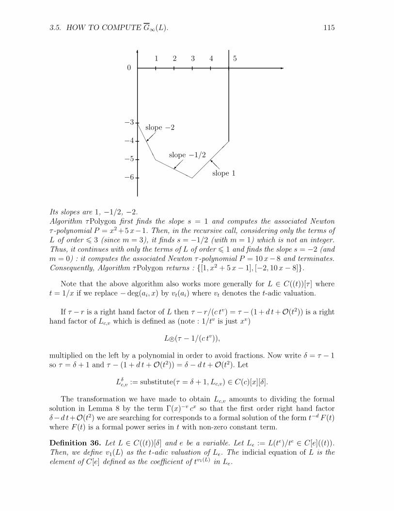
3.5. HOW TO COMPUTE G∞(L). 115
6
-
AAAAAAHHHHHH�
��
��
�
0
−3
−4
−5
−6
1 2 3 4 5
��
slope −2
��
slope −1/2
@@Islope 1
Its slopes are 1, −1/2, −2.Algorithm τPolygon first finds the slope s = 1 and computes the associated Newtonτ -polynomial P = x2 +5 x−1. Then, in the recursive call, considering only the terms ofL of order 6 3 (since m = 3), it finds s = −1/2 (with m = 1) which is not an integer.Thus, it continues with only the terms of L of order 6 1 and finds the slope s = −2 (andm = 0) : it computes the associated Newton τ -polynomial P = 10 x− 8 and terminates.Consequently, Algorithm τPolygon returns : {[1, x2 + 5 x − 1], [−2, 10 x − 8]}.
Note that the above algorithm also works more generally for L ∈ C((t))[τ ] wheret = 1/x if we replace − deg(ai, x) by vt(ai) where vt denotes the t-adic valuation.
If τ − r is a right hand factor of L then τ − r/(c tv) = τ − (1 + d t +O(t2)) is a righthand factor of Lc,v which is defined as (note : 1/tv is just xv)
L©s (τ − 1/(c tv)),
multiplied on the left by a polynomial in order to avoid fractions. Now write δ = τ − 1so τ = δ + 1 and τ − (1 + d t + O(t2)) = δ − d t + O(t2). Let
Lδc,v := substitute(τ = δ + 1, Lc,v) ∈ C(c)[x][δ].
The transformation we have made to obtain Lc,v amounts to dividing the formalsolution in Lemma 8 by the term Γ(x)−v cx so that the first order right hand factorδ−d t+O(t2) we are searching for corresponds to a formal solution of the form t−d F (t)where F (t) is a formal power series in t with non-zero constant term.
Definition 36. Let L ∈ C((t))[δ] and e be a variable. Let Le := L(te)/te ∈ C[e]((t)).Then, we define v1(L) as the t-adic valuation of Le. The indicial equation of L is theelement of C[e] defined as the coefficient of tv1(L) in Le.
116 CHAPITRE 3. SOLUTIONS HYPERGEOMETRIQUES D’E. AUX D. L.
This definition is the one used in [AB98]. Note that, in [BD94, Section 2.1], a slightlydifferent indicial equation is defined from another polygon we can associate to a diffe-rence operator : the Newton δ-polygon. Our indicial equation can be computed in thesame way.
If f ∈ C((t))∗ has t-adic valuation vt(f), then the t-adic valuation of L(f) is vt(f)+v1(L) if vt(f) is not a root of the indicial equation and is > vt(f) + v1(L) otherwise.Consequently, v1(L) can be viewed as the amount the t-adic valuation changes if weapply L to a “generic element” of C((t)). It is then easy to see that if L1, L2 ∈ C((t))[δ],then v1(L1 L2) = v1(L1) + v1(L2) so that v1 is a valuation on C((t))[δ].Note that v1(t
i δj) = i+j, and that if L =∑
i,j ai,j ti δj then v1(L) = min(i+j | ai,j 6= 0).So the only coefficients that contribute to the indicial equation are the ai,j for whichi + j = v1(L). Set ej = (−1)j e (e + 1) (e + 2) · · · (e + j − 1) ∈ C[e] then δj(te)/te =ej tj +O(tj+1) so the indicial equation of L =
∑
i,j ai,j ti δj is the sum of the ai,j ej takenover all i, j for which i + j = v1(L). From [Ad28, Bi30] we know that :
Lemma 9. If L ∈ C((t))[δ] has a solution of the form te F (t) where F (t) is a formalpower series in t with non-zero constant term and e ∈ C, then e is a root of the indicialequation of L.
The roots of the indicial equation are called the exponents of L. The numbers d weare looking for are negated exponents d = −e.
Algorithm LocalTypeAt∞ :
Input : L ∈ C(x)[τ ] and the field C.Output : the set g∞(L), up to conjugation over C.1. A := ∅.2. P := τPolygon(L). If ∅, then return ∅.3. For each [−v, P ] ∈ P, do :
3a. For each (up to conjugation over C) root c of P , do :(i) Lc,v := L©s (τ − xv/c),(ii) Clear denominators in Lc,v,(iii) Lδ
c,v := substitute(τ = δ + 1, Lc,v),(iv) Compute the indicial equation of Lδ
c,v,(v) For each (up to conjugation over C) root e of this indicial equation, do :
- Set d := −e and add (c, v, d + Z) to A.4. Return A.
Remark 9. For efficiency reasons, step 3a is implemented slightly differently : TakeLv := L©s (τ − xv) and let L =
∑
ai,jx−iδj =
∑
ai,jtiδj be the operator obtained from
Lv by substituting τ = δ + c. We do not actually calculate L completely, rather, wecompute only those terms ai,jt
iδj for which i + j = v1(L). Then sum ai,j cj (−1)j e (e +1) · · · (e+j−1) over those i, j to get the indicial equation. The factor cj corrects for thefact that we did not include c in the computation of Lv for better efficiency (this helps
3.6. REPRESENTING THE FINITE SINGULARITIES 117
in particular when c involves an algebraic extension). This way, the indicial equationgenerally takes very little CPU time to calculate.
Example 8. We continue with example 7. The output of Algorithm τPolygon was{[1, x2 + 5 x − 1], [−2, 10 x − 8]}. The first root we consider is c = α where α =RootOf(x2 + 5 x − 1). Step 3a then leads to one possibility for −d namely −5/29 α +89/29. The second possible c is 4/5 which leads to −d = 0. Consequently, we have :
g∞(L) = {(α,−1, 5/29 α − 89/29), (4/5, 2, 0)}.
Definition 37. The roots-number of (c, v, d + Z) ∈ g∞(L) is the number of distinctroots of the indicial equation of Lδ
c,v in e + Z where e = −d. The formal-sol-dimension
of (c, v, d + Z) is the dimension of the formal solutions of Lδc,v in te C((t)).
The formal-sol-dimension is less than or equal to the roots-number. Each of thesetwo numbers can be used (see Proposition 8) to bound the degree of an extension ofthe field C(c, d) over which possible hypergeometric solutions may be defined. In thispaper we use the roots-number since it is less work to implement. However, instead onemay also use the formal-sol-dimension which leads to a better bound. The same issuefor the differential case is discussed in the comments on logarithms in [CH04, Section7.1].
3.6 Representing the finite singularities
Let L = an τn + · · · + a0 τ 0 where the ai are polynomials in x with coefficients ina field C of characteristic zero. Suppose that C is the field of definition of L. In ouralgorithm we will use algebraic extensions C ′ of C but not splitting fields. Hence, we cannot work with all roots of a0(x) an(x − n) simultaneously. This restriction is necessarybecause the construction of a splitting field can be prohibitively costly. This does notimply that there are any roots of a0(x) an(x − n) that we can not compute with, wecan compute with each root, but we should compute with only one root at a time. Thisalso means that throughout the computation we always need to keep track of what thebase field C is and what the current extension field C ′ is, in particular, when factoringa polynomial it is essential (for efficiency as well as correctness of the algorithm) tospecify the correct field. The algorithm SingOverC below is essentially trivial, but weinclude it to emphasize this field issue. First another definition :
Definition 38. Let f(x), g(x) ∈ C[x]. If there exists an integer m such that f(x) =g(x + m) then f(x) and g(x) are said shift equivalent.
Algorithm SingOverC :
Input : L ∈ C(x)[τ ] and the field C.Output : the set of finite singularities of L over C, up to conjugation over C.1. Sing := ∅.2. Let S be the set of monic irreducible factors of an(x) a0(x) in C[x].
118 CHAPITRE 3. SOLUTIONS HYPERGEOMETRIQUES D’E. AUX D. L.
3. Now take a subset T ⊆ S such that precisely one polynomial has been chosenin each shift equivalence class.4. For all P ∈ T , do :
4a. Take a root xP of P (see comments below),4b. Sing := Sing ∪{[P, xP ]}.
5. Return Sing.
The output Sing is given as couples [P, xP ] where P ∈ C[x] is irreducible over Cand xP = RootOf(P, x), which denotes the image of x in C ′ = C[x]/(P ). So the setSing represents all finite singularities “up to conjugation over C” (see [CH04, 5.1] fordetails). Note that no calculation takes place in Step 4a. Instead, this step involves theconstruction of a data structure : one needs to construct a field C ′ generated by oneroot xP of the polynomial P .
After the set Sing has been computed, our base field is still C in many places in thealgorithm. An exception is of course when we compute with a singularity p = xP + Zin which case the base field is C ′ = C(xP ).
Given Sing, if we want to determine the singularities over a field extension of C thenwe take each [P, xP ] in Sing, we factor P over the field extension, and replace [P, xP ]by the set of all [P ′, xP ′] for all irreducible factors P ′ of P .
3.7 Computing e-solutions
Definition 39. Let C be a field of characteristic zero. The field of definition of ahypergeometric term u(x) over C is the smallest field C ′ ⊇ C for which r(x) ∈ C ′(x)where r(x) = u(x + 1)/u(x). The cvd-field of u is the field C(c, d) where c, d are as inEquation (3.4). For L ∈ C(x)[τ ], the cvd-fields of L are the C(c, d) for (c, v, d + Z) ∈g∞(L).
The cvd-field of a hypergeometric term u is a subfield of the field of definition of u.
Definition 40. Let C be a field of characteristic zero and L ∈ C(x)[τ ]. An easy hy-pergeometric solution, or e-solution for short, is a hypergeometric solution of L definedover its cvd-field.
Definition 41. For r ∈ C(x), let hyp(r) ∈ V denote a non-zero solution of τ − r.
Note that hyp(r) is not uniquely defined, but only defined up to a constant factor.However, that will not play a role in this paper.
Example 9. Let L ∈ Q(x)[τ ] and assume that L has both u1 := hyp(x2+√
2) and u2 :=hyp(x+
√2) as hypergeometric solutions. By definition, u1 is a hypergeometric solution
of τ −(x2 +√
2) so its local type at infinity is (1,−2, Z) since x2 +√
2 = 1 t−2 (1+O(t2))with t = 1/x, and so its cvd-field is Q : it follows that this is not an e-solution. Now,x +
√2 = 1 t−1 (1 +
√2 t1 + O(t2)) thus the local type at infinity of u2 is (1,−1,
√2+ Z)
and its cvd-field is Q(√
2) so u2 is an e-solution of L.
3.7. COMPUTING E-SOLUTIONS 119
We will give an algorithm, called ESols, that computes all e-solutions having a givenlocal type (c, v, d+Z) at infinity. In this algorithm, two main parts can be distinguished :an initialization phase and a search phase. In the sequel, we will need to use the fullalgorithm (in HypSols in Section 9) as well as the search phase alone (in HSol inSection 8) : for this reason, we split up the algorithm into two procedures.
The first one, called Search, will only be called once the finite singularities [P1, x1], . . . ,[Ps, xs] over C and the gxi
(L) have already been calculated. Moreover, this proceduresearches for e-solutions (that are defined over C(c, d)) so that the Pi have to be factoredover C(c, d) : in the algorithm, we denote Pi = Pi,1 · · ·Pi,mi
this factorization and thePi,j (irreducible over C(c, d)) are given as input. The field C ′ in the input of AlgorithmSearch will be C(c, d) if Search is called from Algorithm ESols, or an extension of C(c, d)when called from Algorithm HSol in the next section.
Algorithm Search :Input : L ∈ C(x)[τ ], the field C ′, (c, v, d + Z) ∈ g∞(L), the gxi
(L) and the Pi,j.Output : Sol, a basis of all e-solutions of L with local type (c, v, d + Z) at ∞.1. Let Sol := ∅.2. For each combination (l1,1, . . . , l1,m1 , . . . , ls,ms
) with li,j ∈ gxi(L) that satisfies
the two Fuchs’ relations (Equation (3.6)), do :
2a. Let r := c∏
i,j Pli,ji,j ,
2b. Compute R ∈ C ′(x) (see comments below) and let r := r τ(R)R
,
2c. Compute L := L©s (τ − 1/r),
2d. Compute a basis Q1, . . . , Qw of polynomial solutions in C ′[x] for L,2e. If w > 0, then add the hyp(r) Qi to Sol.
3. Return Sol.
Regarding Step 2b, we have to compute the rational solutions of the operator L©s (τ−1/r). The computation in Section 4 produces gxi
(L) as well as the numbers Bl(q) andBr(q) in Equation (3.10). Given these B l(q), Br(q) for L, it is trivial to deduce thenumbers Bl(q), Br(q) for the operator L©s (τ −1/r). The numbers Bl(q) and Br(q) wereused in [Ho98] to compute a denominator bound for rational solutions, more precisely,they were used to compute a rational function R such that all rational solutions arepolynomials times R (this R is a product of powers of shifts of the Pi,j). Thus, rationalsolutions of L©s (τ − 1/r) correspond to polynomial solutions of the operator L in Step2c. Given (c, v, d + Z) and the numbers Bl(q), Br(q), it is easy to calculate the degreebound for the polynomial solutions of L before computing R and L. Our implementationdoes this so that computing L can be avoided whenever the degree bound is a negativeinteger.
To use this procedure in the recursive algorithm HSol in Section 8, we need to allowone extra input, namely an option called “just one” ; if this option is given then weonly need to return just one (if it exists) e-solution but not a totally arbitrary one. Wereturn a hyp(r) Q with Q of minimal possible degree.
Now we give the complete ESols Algorithm which after an initialization of the localinformations at finite singularities calls Search.
120 CHAPITRE 3. SOLUTIONS HYPERGEOMETRIQUES D’E. AUX D. L.
Algorithm ESols :Input : L ∈ C(x)[τ ], the field C and (c, v, d + Z) ∈ g∞(L).Output : Sol, a basis of all e-solutions of L with local type (c, v, d + Z)at ∞.1. Let S := SingOverC(L, C) and s := Card(S).2. For [Pi, xi] ∈ S, compute gxi
(L).3. Let C ′ := C(c, d) be the cvd-field.4. For i ∈ {1, . . . , s}, factor Pi over C ′ : let Pi := Pi,1 · · ·Pi,mi
.5. Sol := Search(L,C ′,(c, v, d + Z),{gxi
(L)}i,{Pi,j}i,j).6. Return Sol.
We store the result from steps 1 and 2 so that the computed information can be re-usedlater without repeating this computation, for example, we can re-use this informationif ESols is called again with the same L but a new (c, v, d + Z).
3.8 Computing a hard solution
Let C be a field of characteristic zero and L ∈ C(x)[τ ]. In this paper we aim to finda basis of all hypergeometric solutions of L so we may have to search for hypergeometricsolutions defined over algebraic extensions of the cvd-fields of L. We first bound thedegrees of such extensions.
As in the differential case (see [CH04, Section 6.1]), we define the notion the minimalalgebraic degree :
Definition 42. Let C be a field of characteristic zero and u be a hypergeometric term.Let C ′ be the field of definition of u over C (see Definition 39). Then the algebraicdegree of u over C is [C ′ : C]. We say that u is of minimal algebraic degree m over Cif [C ′ : C] = m and there exist no hypergeometric term v, of the same type as u, havingsmaller algebraic degree over C.
Then, adapting the exposition in [CH04, Section 6.1] from the differential case, wecan prove the following ([CH04, Lemma 6.3]) :
Lemma 10. Let C be a field of characteristic zero and L ∈ C(x)[τ ]. If u is a hypergeo-metric solution of L defined over some algebraic extension C ′ of C, then its conjugatesover C are also solutions of L.Given L and u, we can compute u1, . . . , uk of minimal algebraic degree over C that forma basis of all hypergeometric solutions of L of the same type as u.If u is of minimal algebraic degree over C, then the distinct conjugates of u over C areof distinct type and hence linearly independent.
This implies that a hypergeometric solution of L of minimal algebraic degree mcorresponds to m linearly independent hypergeometric solutions of L. In AlgorithmHypSols in Section 9, we only return hypergeometric solutions up to conjugation over
3.8. COMPUTING A HARD SOLUTION 121
C. Therefore to make it easier to count the number of linearly independent solutionsrepresented by this output, we want HypSols to only return hypergeometric solutionsof minimal algebraic degree.
Proposition 8. Let L ∈ C(x)[τ ] where C is a field of characteristic zero and let(c, v, d + Z) ∈ g∞(L). Let B1(c, v, d) be the roots-number of (c, v, d + Z) (see Definition37). If u is a hypergeometric solution of minimal algebraic degree m over the cvd-fieldof u with local type (c, v, d + Z) at infinity, then m 6 B1(c, v, d).
Proof. From Lemma 10, the conjugates of u form m linearly independent hypergeometricsolutions of L, all of which have local type (c, n, d + Z) at infinity. Now (see Section 5),these hypergeometric solutions correspond to formal solutions at infinity of Lδ
c,v that
can be written t−d Fi(t), i ∈ {1, . . . , m}, where Fi(t) ∈ C[[t]]. After Gaussian elimina-tion on the vectors of coefficients of the Fi(t), we obtain m formal solutions t−d Fi(t) ofLδ
c,v with distinct exponents. Hence, we can conclude m 6 B1(c, v, d) by Definition 37.2
Let L ∈ C(x)[τ ] where C is some field of characteristic zero and suppose that L hasno e-solutions of local type (c, v, d + Z) at infinity. We want to compute (if it exists) asolution with local type (c, v, d+Z) at infinity defined over an algebraic extension of itscvd-field. To improve the efficiency of the final algorithm HypSols, we will first computethe e-solutions and reduce the order before entering the “hard cases”. In these cases,where we must introduce algebraic extensions of the cvd-fields of L, we want to stop assoon as a solution is found since it also leads to a reduction of order. Moreover as thisalgorithm is only run once the e-solutions have been computed, the finite singularitiesSing = {[P1, x1], . . . , [Ps, xs]} over C and the gxi
(L) are already known. AlgorithmHypSols calls Algorithm HSol with arguments : L, a cvd-field C(c, d) of L, (c, v, d+ Z),a bound B, the set Sing, and the empty set for F . So the field that is denoted as Cin Algorithm HSol is initially a cvd-field C(c, d), and so in Algorithm HSol we alwayshave c, d ∈ C.
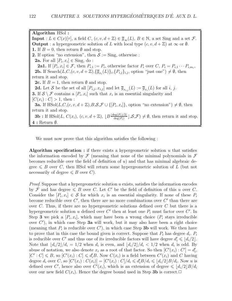
122 CHAPITRE 3. SOLUTIONS HYPERGEOMETRIQUES D’E. AUX D. L.
Algorithm HSol :Input : L ∈ C(x)[τ ], a field C, (c, v, d + Z) ∈ g∞(L), B ∈ N, a set Sing and a set F .Output : a hypergeometric solution of L with local type (c, v, d + Z) at ∞ or ∅.1. If B = 0, then return ∅ and stop.2. If option “no extension”, then S := Sing, otherwise :2a. For all [Pi, xi] ∈ Sing, do :2a1. If [Pi, xi] ∈ F , then Pi,1 := Pi, otherwise factor Pi over C, Pi = Pi,1 · · ·Pi,mi
,2b. If Search(L,C,(c, v, d + Z),{gxi
(L)}i,{Pi,j}i,j, option “just one”) 6= ∅, thenreturn it and stop.2c. If B = 1, then return ∅ and stop.2d. Let S be the set of all [Pi,j, xi,j] and let gxi,j
(L) := gxi(L) for all i, j.
3. If S \ F contains a [Pi, xi] such that xi is an essential singularity and[C(xi) : C] > 1, then :3a. If HSol(L,C,(c, v, d + Z),B,S,F ∪ {[Pi, xi]}, option “no extension”) 6= ∅, then
return it and stop.
3b : If HSol(L, C(xi), (c, v, d + Z), bB bdeg(Pi)/2cdeg(Pi)
c,S,F) 6= ∅, then return it and stop.
4 : Return ∅.
We must now prove that this algorithm satisfies the following :
Algorithm specification : if there exists a hypergeometric solution u that satisfiesthe information encoded by F (meaning that none of the minimal polynomials in Fbecomes reducible over the field of definition of u) and that has minimal algebraic de-gree 6 B over C, then HSol will return some hypergeometric solution of L (but notnecessarily of degree 6 B over C).
Proof. Suppose that a hypergeometric solution u exists, satisfies the information encodesby F and has degree 6 B over C. Let C ′ be the field of definition of this u over C.Consider the [Pi, xi] ∈ S for which xi is an essential singularity. If none of these Pi
become reducible over C ′, then there are no more combinations over C ′ than there areover C. Thus, if there are no hypergeometric solutions defined over C but there is ahypergeometric solution u defined over C ′ then at least one Pi must factor over C ′. InStep 3 we pick a [Pi, xi], which may have been a wrong choice (Pi stays irreducibleover C ′), in which case Step 3a will work, but it may also have been a right choice(meaning that Pi is reducible over C ′), in which case Step 3b will work. We then haveto prove that in this case the bound given is correct. Suppose that Pi has degree di. Pi
is reducible over C ′ and thus one of its irreducible factors will have degree d′i 6 bdi/2c.
Note that bdi/2c/di = 1/2 when di is even, and bdi/2c/di < 1/2 when di is odd. Byabuse of notation, we also denote xi as a root of that factor. So then [C ′(xi) : C ′] = d′
i,[C ′ : C] 6 B, so [C ′(xi) : C] 6 d′
iB. Now C(xi) is a field between C ′(xi) and C havingdegree di over C, so [C ′(xi) : C(xi)] = [C ′(xi) : C]/di 6 d′
iB/di 6 bdi/2cB/di. Now u isdefined over C ′, hence also over C ′(xi), which is an extension of degree 6 bdi/2cB/di
over our new field C(xi). Hence the degree bound used in Step 3b is correct.2
3.9. AN ALGORITHM TO FIND ALL HYPERGEOMETRIC SOLUTIONS 123
3.9 An algorithm to find all hypergeometric solu-
tions
In this section, we present an algorithm to compute a basis of all hypergeometricsolutions (up to conjugation) of a difference operator L with coefficients in C(x) whereC is a field of characteristic zero. Our algorithm uses the same strategy and satisfiesthe same specifications as Algorithm ExpSols in [CH04, Section 7].
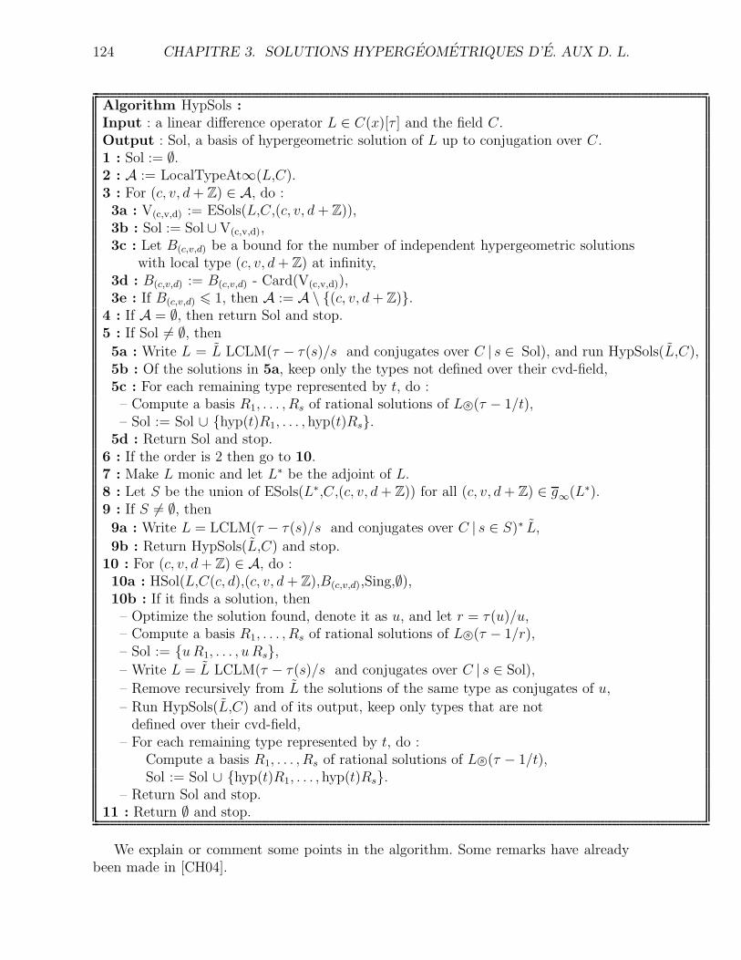
124 CHAPITRE 3. SOLUTIONS HYPERGEOMETRIQUES D’E. AUX D. L.
Algorithm HypSols :Input : a linear difference operator L ∈ C(x)[τ ] and the field C.Output : Sol, a basis of hypergeometric solution of L up to conjugation over C.1 : Sol := ∅.2 : A := LocalTypeAt∞(L,C).3 : For (c, v, d + Z) ∈ A, do :3a : V(c,v,d) := ESols(L,C,(c, v, d + Z)),3b : Sol := Sol ∪ V(c,v,d),3c : Let B(c,v,d) be a bound for the number of independent hypergeometric solutions
with local type (c, v, d + Z) at infinity,3d : B(c,v,d) := B(c,v,d) - Card(V(c,v,d)),3e : If B(c,v,d) 6 1, then A := A \ {(c, v, d + Z)}.
4 : If A = ∅, then return Sol and stop.5 : If Sol 6= ∅, then
5a : Write L = L LCLM(τ − τ(s)/s and conjugates over C | s ∈ Sol), and run HypSols(L,C),5b : Of the solutions in 5a, keep only the types not defined over their cvd-field,5c : For each remaining type represented by t, do :– Compute a basis R1, . . . , Rs of rational solutions of L©s (τ − 1/t),– Sol := Sol ∪ {hyp(t)R1, . . . , hyp(t)Rs}.
5d : Return Sol and stop.6 : If the order is 2 then go to 10.7 : Make L monic and let L∗ be the adjoint of L.8 : Let S be the union of ESols(L∗,C,(c, v, d + Z)) for all (c, v, d + Z) ∈ g∞(L∗).9 : If S 6= ∅, then
9a : Write L = LCLM(τ − τ(s)/s and conjugates over C | s ∈ S)∗ L,
9b : Return HypSols(L,C) and stop.10 : For (c, v, d + Z) ∈ A, do :10a : HSol(L,C(c, d),(c, v, d + Z),B(c,v,d),Sing,∅),10b : If it finds a solution, then– Optimize the solution found, denote it as u, and let r = τ(u)/u,– Compute a basis R1, . . . , Rs of rational solutions of L©s (τ − 1/r),– Sol := {u R1, . . . , u Rs},– Write L = L LCLM(τ − τ(s)/s and conjugates over C | s ∈ Sol),
– Remove recursively from L the solutions of the same type as conjugates of u,
– Run HypSols(L,C) and of its output, keep only types that are notdefined over their cvd-field,
– For each remaining type represented by t, do :Compute a basis R1, . . . , Rs of rational solutions of L©s (τ − 1/t),Sol := Sol ∪ {hyp(t)R1, . . . , hyp(t)Rs}.
– Return Sol and stop.11 : Return ∅ and stop.
We explain or comment some points in the algorithm. Some remarks have alreadybeen made in [CH04].
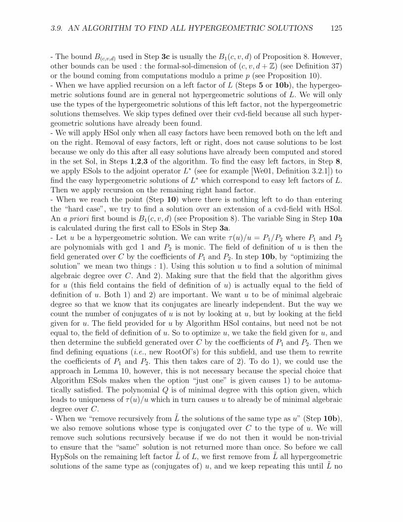
3.9. AN ALGORITHM TO FIND ALL HYPERGEOMETRIC SOLUTIONS 125
- The bound B(c,v,d) used in Step 3c is usually the B1(c, v, d) of Proposition 8. However,other bounds can be used : the formal-sol-dimension of (c, v, d + Z) (see Definition 37)or the bound coming from computations modulo a prime p (see Proposition 10).- When we have applied recursion on a left factor of L (Steps 5 or 10b), the hypergeo-metric solutions found are in general not hypergeometric solutions of L. We will onlyuse the types of the hypergeometric solutions of this left factor, not the hypergeometricsolutions themselves. We skip types defined over their cvd-field because all such hyper-geometric solutions have already been found.- We will apply HSol only when all easy factors have been removed both on the left andon the right. Removal of easy factors, left or right, does not cause solutions to be lostbecause we only do this after all easy solutions have already been computed and storedin the set Sol, in Steps 1,2,3 of the algorithm. To find the easy left factors, in Step 8,we apply ESols to the adjoint operator L∗ (see for example [We01, Definition 3.2.1]) tofind the easy hypergeometric solutions of L∗ which correspond to easy left factors of L.Then we apply recursion on the remaining right hand factor.- When we reach the point (Step 10) where there is nothing left to do than enteringthe “hard case”, we try to find a solution over an extension of a cvd-field with HSol.An a priori first bound is B1(c, v, d) (see Proposition 8). The variable Sing in Step 10ais calculated during the first call to ESols in Step 3a.- Let u be a hypergeometric solution. We can write τ(u)/u = P1/P2 where P1 and P2
are polynomials with gcd 1 and P2 is monic. The field of definition of u is then thefield generated over C by the coefficients of P1 and P2. In step 10b, by “optimizing thesolution” we mean two things : 1). Using this solution u to find a solution of minimalalgebraic degree over C. And 2). Making sure that the field that the algorithm givesfor u (this field contains the field of definition of u) is actually equal to the field ofdefinition of u. Both 1) and 2) are important. We want u to be of minimal algebraicdegree so that we know that its conjugates are linearly independent. But the way wecount the number of conjugates of u is not by looking at u, but by looking at the fieldgiven for u. The field provided for u by Algorithm HSol contains, but need not be notequal to, the field of definition of u. So to optimize u, we take the field given for u, andthen determine the subfield generated over C by the coefficients of P1 and P2. Then wefind defining equations (i.e., new RootOf’s) for this subfield, and use them to rewritethe coefficients of P1 and P2. This then takes care of 2). To do 1), we could use theapproach in Lemma 10, however, this is not necessary because the special choice thatAlgorithm ESols makes when the option “just one” is given causes 1) to be automa-tically satisfied. The polynomial Q is of minimal degree with this option given, whichleads to uniqueness of τ(u)/u which in turn causes u to already be of minimal algebraicdegree over C.- When we “remove recursively from L the solutions of the same type as u” (Step 10b),we also remove solutions whose type is conjugated over C to the type of u. We willremove such solutions recursively because if we do not then it would be non-trivialto ensure that the “same” solution is not returned more than once. So before we callHypSols on the remaining left factor L of L, we first remove from L all hypergeometricsolutions of the same type as (conjugates of) u, and we keep repeating this until L no
126 CHAPITRE 3. SOLUTIONS HYPERGEOMETRIQUES D’E. AUX D. L.
longer has solutions of this type. A recursive procedure to achieve that is the following :compute the rational solutions Ri of L©s (τ − 1/r) where r = τ(u)/u is the certificate ofu. Each Ri gives a first order right hand factor τ −ri of L where ri = rτ(Ri)/Ri. If thereare none, then return L else write L = L1 LCLM(τ − r1, . . . , τ − rs, “and conjugatesover C”) and apply recursion on L1.
3.9.1 Some possible improvements
We shall give two possible improvements that can be added to Algorithm HypSols.The first one is included in the Maple implementation.
Maps between Vp,l(L) and Vp,r(L), and possible degrees of field extensions :we show how the ranks of the maps between left and right solution spaces Vp,l(L) andVp,r(L) at finite singularities p can be used to discard certain cases during the searchphase of the algorithm.Let p be a finite singularity of L. Let gp,r = gp,r(L) be the smallest and gp,l = gp,l(L) thelargest element of gp(L). In [Ho99, Section 4.2], the author shows how to construct twomaps Ep,r : Vp,l(L) → Vp,r(L) and Ep,l : Vp,r(L) → Vp,l(L) by defining their action onexplicit basis. In our implementation, we only use the rank of these maps. If rkr is therank of Ep,r, and rkl is the rank of Ep,l, then this gives us the following information :
– there can be at most rkr linearly independent hypergeometric solutions u withgp(u) = gp,r (minimal valuation growth),
– at most n − rkr with gp(u) > gp,r (more than minimal valuation growth),– at most rkl with gp(u) = gp,l (maximal valuation growth), and,– at most n − rkl with gp(u) < gp,l (less than maximal valuation growth).
This can be exploited in several ways :
1. Suppose that there can be at most 2 independent solutions with less than maximalvaluation growth, and suppose that the algorithm already found 2 such solutions.Then from that moment on, we no longer need to consider the case gp(u) < gp,l,and so we may assume gp(u) = gp,l.
2. Or suppose that there can be at most 1 linearly independent solution with minimalvaluation growth. Then, if there exists such a solution u with gp(u) minimal, andif p = q + Z with q ∈ C, then the certificate r(x) = u(x + 1)/u(x) of u mustbe an element of C(x). The reason for that is that if r(x) was defined over anextension C ′ of C, then by taking conjugates of r(x) over C ′ we would find morethan 1 linearly independent solution with minimal valuation growth at p. Moregenerally, suppose that there are at most s1 independent solutions with maximalvaluation growth, but s2 have already been found. So there can remain at mosts1−s2 independent hypergeometric solutions u(x) with maximal valuation growth,and this means that for computing the certificate r(x) = u(x + 1)/u(x) of sucha solution, it is not necessary to consider field extensions of degree more thans1 − s2.
These results are generalizations of [Ho99, Theorems 2 and 3] and can be proven in asimilar way.
3.10. MODULAR IMPROVEMENTS 127
Sorting the local types at infinity : it can be useful to sort the local types at infinityin such a way that we compute the solutions that have the smallest fields of definitionfirst. The reason is that each time a solution is found, the number of combinations tobe considered may be reduced following the items above, so we want to compute firstthose solutions that are the least expensive to calculate.
3.10 Modular improvements
We shall propose a number of improvements we can add to Algorithm HypSols usingp-curvature computations. This section has its own theoretical interest since, as it isdone in [CH04] for the differential case, we give links between the local informationin characteristic zero and the roots of the characteristic polynomial of the p-curvaturematrix.
3.10.1 Difference operators in characteristic p
In this part, most results are stated without proof since they are just adaptations ofresults in [CH04, 1.2] from the differential to the difference case. A classification (similarto that for the differential case) of difference modules in characteristic p can be foundin [PS97, Chapter 5].
Let Fp denote the algebraic closure of the finite field Fp. We define the ring Fp(x)[τ ]of difference operators in the same way as in characteristic zero. The main differenceis that the constant field is then Fp(x
p − x) (see [PS97, Chapter 5] or [GZ03, Theorem3.1]). To simplify the notations, we set :
λ := xp − x.
The central tool to study recurrence relations in characteristic p is the p-curvature ;we give a definition of the p-curvature when the equation is written in matrix formY (x + 1) = A(x) Y (x) with A(x) ∈ Mn(Fp(x)) and for more details we refer to [PS97,Chapter 5] and references therein. Note that a difference operator L ∈ Fp(x)[τ ] isnaturally associated to a linear difference equation in matrix form ; take for A(x) thecompanion matrix of L.
Definition 43. Let Y (x+1) = A(x) Y (x) with A(x) ∈ Mn(Fp(x)) be a linear differenceequation. Its p-curvature is defined as the product of matrices A(x + p − 1) · · ·A(x +1) A(x).
Consider the following group homomorphisms :
τ1 : Fp(x)∗ → Fp(λ)∗, u 7→ u(x + p − 1) · · ·u(x + 1) u(x),
andτ2 : Fp → Fp, a 7→ ap − a,
which are related by Equation (3.12) below.
128 CHAPITRE 3. SOLUTIONS HYPERGEOMETRIQUES D’E. AUX D. L.
Lemma 11. (i) : The map τ1 : Fp(x)∗ → Fp(λ)∗ is a surjective multiplicative map withkernel {τ(u)/u | u ∈ Fp(x)∗}.(ii) : The map τ2 is a surjective additive map with kernel Fp.
Proof. (ii) is obvious, and (i) follows from (ii) and Equation (3.12) below (one can alsofollow a similar result for the differential case in [Pu95, Lemma 1.4.2]).2
For L ∈ Fp(x)[τ ], let χp(L) denote the characteristic polynomial of the p-curvatureof L. As we are only interested in first order factors, the only modular information thatwe can use are the roots in Fp(λ) (with multiplicities) of χp(L). We denote R(χp(L))as the set of roots of χp(L) in Fp(λ).
Lemma 12. Let L ∈ Fp(x)[τ ].(i) : If L = L1L2, then χp(L) = χp(L1)χp(L2) with deg(χp(Li)) = order(Li).(ii) : The map from the set of monic first order right hand factors of L in Fp(x)[τ ] toR(χp(L)) defined by τ − r 7→ τ1(r) is well defined and surjective.
As in the differential case, the key ingredient to use modular information for com-puting hypergeometric solutions of L ∈ C(x)[τ ] is the known fact that, with few as-sumptions on the prime p to be chosen, a factorization of L in characteristic zero canbe reduced mod p.
Definition 44. For some object f in characteristic zero, we note f [p] its reductionmodulo p in the sense of [CH04, Sections 1.3 and 7.1].
The following proposition and its corollary can be proven as [CH04, Proposition1.15] and [CH04, Corollary 1.16].
Proposition 9. Let C be a field of characteristic zero, let L ∈ C(x)[τ ] and let p besuch that L can be reduced mod p. If L = L1L2 then, after possibly replacing L1 and L2
by cL1 and 1cL2 for some constant c ∈ C, we have L[p] = L1[p] L2[p].
Corollary 3. Let C be a field of characteristic zero, let L ∈ C(x)[τ ] and let p be aprime such that L can be reduced mod p. Assume further that the order n of L does notdrop after the reduction.(i) : If χp(L) is irreducible over Fp(λ), then L is irreducible over C(x).(ii) : If χp(L) has no roots in Fp(λ), then L has no hypergeometric solutions.
3.10.2 Local types at infinity and R(χp(L))
Definition 45. If a is an object in characteristic zero, then for i ∈ {1, 2}, we setτi(a) := τi(a[p]).
If d ∈ C and d[p] is defined then τ2(d + Z) is defined since τ2(i) = 0 for i ∈ Z.

3.10. MODULAR IMPROVEMENTS 129
Lemma 13. Let r(x) = c τ(Q)Q
∏mi=1(x − xi)
ei ∈ C(x) with c, xi ∈ C, ei ∈ Z and
Q ∈ C[x]. Assume further that the xi, c, Q can be reduced mod p and that Q[p] 6= 0.Then
τ1(r(x)) = cp∏
i
(λ − τ2(xi))ei. (3.12)
Furthermore, if r(x) has expansion c tv (1 + d t + O(t2)) at infinity, then
τ1(r(x)) = cp tvλ (1 + τ2(d) tλ + O(t2λ)), (3.13)
where
tλ :=1
λ=
1
xp − x.
Proof. We have τ1(r(x)) = τ1(cτ(Q)
Q
∏
i(x − xi)ei) = τ1(c)
∏si=1(τ1(x − xi))
ei since,
from Lemma 11, τ1 is multiplicative and τ(Q)/Q ∈ ker(τ1). Now, clearly τ1(c) = cp.Furthermore, we have τ1(x) = (x+p−1) · · · (x+1) x = xp−x and substituting x = x−xi
in this equality leads to τ1(x − xi) = (x − xi)p − (x − xi) = λ − τ2(xi). Equation (3.12)
is then clear.For (3.13), we only need to prove that the coefficient τ2(d) of tλ is correct. Let d denotethis coefficient. From (3.12), we have d = −∑i eiτ2(xi). But we also know from Section 1
that d = −∑i eixi so that an easy verification leads to τ2(d) = d.2
Definition 46. Let L = anτn + · · ·+ a0τ0 ∈ C(x)[τ ] for some field C of characteristic
zero and assume that an, a0 6= 0. After multiplying L on the left by a suitable elementof C(x), we may assume the coefficients ai are in C[x] and gcd(a0, . . . , an) = 1.We say that a prime p is a good prime for L if the two following conditions hold :(C1) : the coefficients of L can be reduced mod p and a0[p] 6= 0, an[p] 6= 0.(C2) : the finite singularities can be reduced mod p.
Condition (C1) means that the order does not decrease after reduction mod p.Condition (C2) simply means that the leading coefficient of the polynomials a0 and an
do not reduce to zero mod p.
We give now a new result linking local types of hypergeometric solutions and eigen-values of the p-curvature in Fp(λ).
Theorem 2. Let C be a field of characteristic zero, let L ∈ C(x)[τ ] and let p be agood prime for L. Suppose that τ − r is a right hand factor of L with r ∈ C(x). Lets = τ1(r) ∈ R(χp(L)). Then there exist ei ∈ gxi
(L) at each finite singularity xi of Land (c, v, d + Z) ∈ g∞(L) such that c, d can be reduced mod p and(i) : s = cp
∏
i(λ − τ2(xi))ei,
(ii) : the expansion at infinity of s is cp tvλ (1 + τ2(d) tλ + O(t2λ)).
Proof. One can prove (for example, adapt the proof of [CH04, Lemma 1.8] to the diffe-rence case) that if τ − r is a first order right hand factor of L then there exist a local
130 CHAPITRE 3. SOLUTIONS HYPERGEOMETRIQUES D’E. AUX D. L.
type ei ∈ gxi(L) at each finite singularity xi of L, a local type (c, v, d + Z) ∈ g∞(L) at
infinity and a rational function R ∈ C(x) such that :
r = cτ(R)
R
∏
i
(x − xi)ei = c tv (1 + d t + O(t2)).
Since p satisfies conditions (C1) in Definition 46, r can be reduced mod p (see Propo-sition 9). Now from Condition (C2),
∏
i(x− xi)ei can be reduced mod p and is further
not zero mod p. Furthermore, R is defined modulo a multiplicative constant which wecan choose in such a way that R[p] is defined and not zero. Then τ(R)/R is also definedand not zero mod p. Consequently, c can be reduced mod p, and c[p] 6= 0, because c is
the quotient of r and τ(R)R
∏
i(x − xi)ei which both reduce to something non-zero mod
p. Then d can also be reduced mod p. Now the two formulas (i) and (ii) follows directlyfrom Lemma 13.2
3.10.3 How to improve HypSols using the p-curvature ?
The first improvement we propose for HypSols is a bound unrelated to the one ofProposition 8. Consequently, in practice, we may use the minimum of all these bounds.This bound is, in some cases, used in the Maple implementation.
Proposition 10. Let C be a field of characteristic zero, let L ∈ C(x)[∂] and let p bea good prime for L. Let (c, v, d + Z) ∈ g∞(L). Let B2(c, v, d) be the number of roots sof χp(L) (counted with multiplicity) that have expansion cp tnλ (1 + τ2(d) tλ + O(t2λ)) atinfinity. If u is a hypergeometric solution of minimal algebraic degree m over its cvd-fieldwith local type (c, v, d + Z) at infinity, then m 6 B2(c, v, d).
Proof. Let C ′ be the cvd-field. Let R ∈ C ′(x)[τ ] be the right hand factor of L whose solu-tions are spanned by all hypergeometric solutions u of L that have local type (c, v, d+Z)at infinity. Since there are at least m independent such solutions, the order o of R isat least m. All solutions of R have the same local type (c, v, d + Z) at infinity. NowR factors as a product of first order factors R = R1R2 · · ·Ro because R has a basis ofhypergeometric solutions. All Ri have the same local type at infinity, so for each Ri,the local type at infinity must be (c, v, d + Z). Hence the root of χp(Ri) has expansioncp tvλ (1+τ2(d) tλ +O(t2λ)) at infinity (see Theorem 2). The proposition now follows fromthe fact that R and R1, . . . , Ro can be reduced mod p (see Proposition 9) and Lemma12(i).2
Some other possible improvements can be deduced from Theorem 2 : these ones arenot used in the Maple implementation :(I). Suppose we are searching for the e-solutions of L ∈ C(x)[τ ] that have local type(c, v, d+ Z) at infinity. Let p be a good prime for L. Distinct singularities do not neces-sarily stay distinct after reduction mod p. However one can use the following approachto discard some combinations in Step 2 of Algorithm Search. Using the notation ofSearch : let S ⊂ R(χp(L)) be the set of eigenvalues of the p-curvature matrix having
3.11. COMPUTATION TIMINGS 131
expansion cp tvλ (1 + τ2(d) tλ + O(t2λ)) at infinity. For each s ∈ S, one can compute thecombinations in Step 2 of Algorithm Search that “match this root” as follows : factors over C ′[p](λ) (let s = V e1
1 · · ·V el
l ). For all k ∈ {1, . . . , l}, consider all the couples (i, j)such that Vk divides τ1(Pi,j) and remove all the combinations such that the sum takenover all such (i, j) of the mi,j is not equal to ek. After that, keep only the combinationsmatching at least one element of S.
Remark 10. This method to discard some combinations is very close to the one usedin [CH04, Section 5.2] in the differential case.
(II). From the proof of Theorem 2, if for a good prime p for L, we have an element(c, v, d + Z) ∈ g∞(L) such that c or d can not be reduced mod p, or c reduces to 0 modp, then this (c, v, d + Z) can be thrown away.
Example 10. Taking p = 29 and p = 5 which are good primes in Example 7 one seesthat all elements of g∞(L) given in Example 8 can be thrown away, so the example hasno hypergeometric solutions.
3.11 Computation timings
A Maple implementation of HypSols by the second author has been available since2001 onhttp://www.math.fsu.edu/~hoeij/maple.html and is now included in Maple 9. Touse it, do with(LREtools): and then call hypergeomsols. Older versions of Maplehave an implementation of Petkovsek’s algorithm (called here PetkoSols). This algo-rithm can still be called in Maple 9 by setting _Env_old_hypergeomsols:=true beforecalling hypergeomsols. A comparison on 36 examples can be found onhttp://www.math.fsu.edu/~hoeij/comparison_hypergeomsols.The tests show that HypSols is much faster than PetkoSols except on very smallexamples. We give one additional example :
L(u) = u(x + 2) − (x + 1) (2 x2 + 3 x + 2) u(x + 1) + (x6 + 2 x5 + x4 − 2) u(x) = 0.
Recall that hyp(r) is short notation for a solution u of the operator τ − r. The operatorL has a basis of two hypergeometric solutions, which are conjugated over Q. If HypSolsis given the field C = Q then the output of HypSols will contain only one solutionu(x) = hyp(x3 + x2 +
√2) because the output is a basis up to conjugation over C. Note
that HypSols needed to enter the “hard case” (Algorithm HSol) to find this solution.Since the user will expect hypergeomsols to return a basis of solutions, not a basis upto conjugation, Maple will compute all conjugates of x3 + x2 +
√2 over C = Q. The
expression hyp(r) can be rewritten as∏x−1
k=0 r(k) but it can also be written as a productof Γ functions (Maple’s choice depends on the factorization of r). The output of
with(LREtools):
L := u(x)*(x^6+2*x^5+x^4-2)-(x+1)*(2*x^2+3*x+2)*u(x+1)+u(x+2);
hypergeomsols(L, u(x), {}, output=basis);
132 CHAPITRE 3. SOLUTIONS HYPERGEOMETRIQUES D’E. AUX D. L.
in Maple 9 on this example is
x−1∏
k=0
(
k3 + k2 +√
2)
,
x−1∏
k=0
(
k3 + k2 −√
2)
.
The computation takes about 1.2 seconds (Pentium 733 MHz). In PetkoSols the exampletakes about 436 seconds. Mathematica’s implementation of Petkovsek’s algorithm findsno solutions because it is limited to the case where a0 and an have no irreducible factorsof degree > 2, see [PWZ96, Section 8.5].
Another comparison between the algorithm in [Ho99] and Petkovsek’s algorithm wasdone in [We01, Section 6.3]. Here, the author points out the problem with the numberof cases Petkovsek’s algorithm must consider and the high cost of computing the setsgp(L), most likely caused by not using truncated power series as in Section 4. Theauthor also remarks that, unlike [Ho99], Petkovsek’s algorithm may return too many(i.e., linearly dependent) solutions.
3.12 An analogue algorithm for q-difference equa-
tions
In this section, we explain briefly how to develop the q-analogue of HypSols, forcomputing q-hypergeometric solutions of q-difference operators when q is not a root ofunity and not zero. The q-analogue of Petkovsek’s algorithm was given in [APP98].
We consider a field C of characteristic zero and its algebraic closure C. To simplifythe notations, we set K := C(x).
Definition 47. Let q ∈ C, not zero and not a root of unity. A q-difference operatorL :=
∑ni=0 ai τ
i with ai = ai(x) ∈ C(x) is an operator that acts on u = u(x) as follows :
L(u(x)) =
n∑
i=0
ai(x) u(qix).
In [PS97, Section 12.1], the authors prove the existence of a universal extension Vq
for q-difference equations with coefficients in C(x).
Definition 48. An expression u(x) ∈ Vq is called a q-hypergeometric term if it satisfiesu(qx)/u(x) ∈ C(x).
We are going to show that we can define a notion of local type at each point forfirst order q-difference operators (or q-hypergeometric terms) and construct sets contai-ning the possible local types for possible first order right hand factors of q-differenceoperators. We shall also exhibit Fuchs’ relations and show that the type of a first orderq-difference operator (see Definition 49) only depends on its local types at each point.
3.12. AN ANALOGUE ALGORITHM FOR Q-DIFFERENCE EQUATIONS 133
3.12.1 Local types
While a difference operator has only one special singularity, namely at ∞, a q-difference operator has two special singularities : 0 and ∞. Consider the two followinggroups with multiplication ©s where ©s is defined as in Definition 30 :
K∗©s := {τ − r | r ∈ K∗} and K∗
R := {τ − τ(r)
r| r ∈ K∗}.
Note that K∗ ∼= K∗©s (resp. K∗/C∗ ∼= K∗
R) under r 7→ τ − r (resp. r 7→ τ − τ(r)/r).
Definition 49. Let r in K∗. The type of τ − r is defined as the image of τ − r inK∗
©s /K∗R.
Special singularities
Here, we will define the local type at 0 and ∞ of L = τ − r with r ∈ K∗. Let 〈q〉denote the multiplicative group generated by q (remember that q is not a root of unityand not zero).
Definition 50. For e ∈ C∗, denote e = {e qi | i ∈ Z}, the image of e in C
∗/〈q〉.
LetG0 = G∞ := C
∗/〈q〉 × Z.
We will use the additive notation for this group : (c1, v1) + (c2, v2) = (c1c2, v1 + v2).The element r ∈ K∗ can both be written in the form r = c0 xv0 (1 + O(x1)) andr = c∞ tv∞ (1 + O(t1)) where t := 1/x, c0, c∞ ∈ C
∗and v0, v∞ ∈ Z.
Definition 51. With these notations, the local types of L = τ − r at 0 and ∞ arerespectively defined as :
g0(L) = (c0, v0) ∈ G0,
andg∞(L) = (c∞, v∞) ∈ G∞.
Note that g0 (resp. g∞) define homomorphisms from K∗©s /K∗
R to G0 (resp. G∞). Sog0(τ − r) and g∞(τ − r) only depend on the type of τ − r.
Other Singularities
Definition 52. Let C be a field of characteristic zero and L ∈ C[x][τ ] be a q-differenceoperator. Then α ∈ C
∗is a problem point of L if α is a root of a0(x) an(x/qn).
α ∈ C∗/〈q〉 is a singularity of L if L has a problem point in α.
Definition 53. For e ∈ C∗
and r ∈ K∗, we define the valuation ve(r) of r at e as thelargest integer m such that r/(x − e)m ∈ C[[x − e]]. The valuation of 0 is ∞.
Definition 54. For α ∈ C∗/〈q〉, we define the group homomorphism vα : K∗ → Z given
by vα(r) =∑
e∈α ve(r). The local type of L = τ − r at α is defined as
gα(L) = vα(r) ∈ Z.
It is easy to show that gα(τ − r) only depends on the type of τ − r.
134 CHAPITRE 3. SOLUTIONS HYPERGEOMETRIQUES D’E. AUX D. L.
3.12.2 Fuchs’ relations
Let G+ be the additive group of functions C∗/〈q〉 → Z with finite support and let
H := G+ × G0 × G∞.
Definition 55. The collection of local types of L = τ − r is defined as
g(L) := (α 7→ gα(L), g0(L), g∞(L)) ∈ H.
Lemma 14 (Fuchs’ Relations). Let L = τ − r ∈ K∗©s .
If g(L) := (α 7→ gα(L), (c0, v0), (c∞, v∞)) ∈ H is the collection of local types of L, thenwe have
v0 + v∞ +∑
α∈C∗
/〈q〉
g(α) = 0 and c0 = c∞∏
α∈C∗
/〈q〉
(−α)g(α). (3.14)
Proof. One can check this for generators of the group K∗©s , i.e., the τ − c with c ∈ C
∗
and the τ − (x − e) with e ∈ C.2
Let HF be the subset of H containing all the elements satisfying Fuchs’ relationsgiven by Equation (3.14).
Proposition 11. g induces a group isomorphism from K∗©s /K∗
R to HF .
Proof. Let g : K∗©s → H be as in Definition 55. From the previous lemma, the image of
g is contained in HF . The map is surjective since if F = (f, (c0, v0), (c∞, v∞)) ∈ HF ,then F = g(L) where L = τ − c∞ xv0 (x − α1)
f(α1) · · · (x − αm)f(αm). Here, c∞ is a re-presentant in C
∗of c∞ and α1, . . . , αm are representants in C
∗for the αi ∈ C
∗/〈q〉 for
which f(αi) 6= 0, and αi 6= αj if i 6= j. Furthermore, it is easy to check that such an L isin K∗
R only if F = (0, (1, 0), (1, 0)) which is the identity in HF . So the kernel of g is K∗R.2
Consequently, the type of a q-difference operator of order one is determined by itslocal types. Now, as in the difference case, given L ∈ K[τ ], one can effectively constructsets containing all possible local types of possible order one right hand factors of L.Then q-HypSols, the q-analogue of HypSols, follows naturally.
Chapitre 4
Solutions polynomiales d’equationsdifferentielles lineaires
Introduction
En calcul formel, calculer les solutions polynomiales d’une equation differentiellelineaire est une etape centrale dans beaucoup d’algorithmes ; par exemple, les algo-rithmes classiques calculant les solutions rationnelles (voir [Br92, Ba99]) ou exponen-tielles (voir Chapitre 2) d’equations differentielles lineaires se ramenent au calcul de so-lutions polynomiales. De nos jours plusieurs algorithmes existent (voir [ABP95], [Ba99]- ou sa version scalaire dans [Ba97] et les references donnees dans ces papiers) et lavariete des situations semble actuellement empecher un algorithme donne d’etre univer-sellement meilleur que les autres. Le but dans ce chapitre est d’evaluer la pertinence desinformations modulaires que l’on peut obtenir pour ce probleme du calcul des solutionspolynomiales d’equations differentielles lineaires.
Pour ce faire, nous construisons un algorithme modulaire pour calculer les solutionspolynomiales d’equations differentielles lineaires. Cet algorithme procede comme suit :
– on calcule les solutions polynomiales modulo des nombres premiers p avec la ver-sion modulaire de l’un des algorithmes classiques ([ABP95] ou [Ba99]),
– on reconstruit les solutions polynomiales en caracteristique zero en utilisant unecombinaison de l’algorithme des restes chinois (voir [GG99, 5.4]) et de la recons-truction rationnelle (voir [GG99, 5.10] ou encore [CE95, Mo04]).
Contrairement aux algorithmes presentes dans les chapitres 2 et 3 qui utilisent l’infor-mation modulaire comme filtre, cet algorithme est completement modulaire et, a notreconnaissance, c’est le premier algorithme completement modulaire calculant des solu-tions d’equations differentielles lineaires.
Notre algorithme modulaire ne peut pas etre universellement meilleur que les algo-rithmes existants : en effet, nous savons que les algorithmes modulaires sont surtoutefficaces pour resoudre des problemes dans lesquels la taille des objets consideres dans
135
136 CHAPITRE 4. SOLUTIONS POLYNOMIALES D’E. D. L.
les calculs intermediaires est significativement plus grande que celle de la sortie cequi n’est, en general, pas le cas pour le calcul des solutions polynomiales d’equationsdifferentielles lineaires. Pour confirmer cela et avoir une idee des cas dans lesquels onpeut esperer que notre algorithme soit meilleur que ceux qui existent :
– nous etudions la complexite des deux algorithmes les plus utilises a savoir celuid’Abramov, Bronstein et Petkovsek (voir [ABP95]) et celui de Barkatou (voir[Ba99]),
– nous analysons la complexite de notre algorithme modulaire et effectuons la com-paraison. Ceci nous permet d’exhiber des classes naturelles d’operateurs pourlesquels notre algorithme est plus efficace.
Notre analyse modulaire fournit au passage des resultats interessants qui menent ades tests de non-existence de solutions polynomiales non-nulles tres utiles en pratique.Nous pouvons meme obtenir mieux que des tests de non-existence puisque notre ap-proche donne des heuristiques pour le calcul de la dimension de l’espace des solutionsrationnelles ce qui peut s’averer tres utile pour certains problemes en theorie de Galoisdifferentielle. Notons encore que les avancees recentes de [Bos03] permettent d’ameliorerencore ces resultats.
4.1 Preliminaires sur les solutions polynomiales
Dans un soucis de completude, nous rappelons ici brievement quelques faits bienconnus concernant les solutions polynomiales d’equations differentielles lineaires. Pourplus de details, nous renvoyons a [In26] ou [ABP95].
4.1.1 Equation aux recurrences associee
Soit L = an ∂n + · · · + a0 un operateur differentiel lineaire avec les ai dans Z[x].Supposons que a0, . . . , an sont premiers entre eux (dans Q[x]) ce qui n’affecte pas lageneralite de ce qui suit. Pour un tel L, definissons
A := −mini
(valx(ai) − i), B := maxi
(degx(ai) − i), (4.1)
ou, pour un polynome f appartenant a Z[x], valx(f) et degx(f) representent respecti-vement la valuation x-adique et le degre en x de f .
On note alors
ai =
B∑
j=−A
ai,j xi+j,
avec les ai,j dans Z et pour j ∈ {−A, . . . , B}, on pose
αj(k) :=n∑
i=0
ai,jk!
(k − i)!∈ Z. (4.2)
4.1. PRELIMINAIRES SUR LES SOLUTIONS POLYNOMIALES 137
Si y =∑N
i=v yi xi avec yv 6= 0 et yN 6= 0 est une solution polynomiale de L, alors
L(y) =N∑
i=v
yi
(
α−A(i) xi−A + · · · + αB(i) xi+B)
,
=
N+B∑
i=v−A
(α−A(i + A) yi+A + · · ·+ αB(i − B) yi−B) xi,
avec la convention yi = 0 des que i < v ou i > N . Donc la relation L(y) = 0 impliqueque les yi satisfont la recurrence lineaire
α−A(i + A) yi+A + · · · + αB(i − B) yi−B = 0. (4.3)
Pour i = N + B, l’equation (4.3) donne αB(N) yN = 0. De meme, pour i = v − A,nous obtenons α−A(v) yv = 0. Par consequent, puisque yN 6= 0 (respectivement yv 6= 0),le degre N (resp. la valuation v) de la solution polynomiale y est necessairement uneracine entiere positive du polynome αB (resp. α−A).
Definition 25. Soit A et B definis par (4.1). On dit que αB (resp. α−A) est le polynomeindiciel de L en x = ∞ (resp. x = 0).
Notons que les racines de αB ne sont pas exactement ce que l’on appelle exposantsde L a l’infini dans la litterature mais leurs opposes.
Exemple 15. Considerons l’operateur
Lm = m x ∂2 − x ∂ + m2,
ou m est un entier naturel non-nul fixe. Pour cet operateur, nous avons A = −min(1−2, 1−1, 0−0) = 1 et B = max(1−2, 1−1, 0−0) = 0. Ecrivons l’equation aux recurrenceslineaire associee a L : on a
L(∑
i yi xi) = m x
∑
i i (i − 1) yi xi−2 − x
∑
i i yi xi−1 + m2
∑
i yi xi,
=∑
i[m i (i + 1) yi+1 + (m2 − i) yi]xi.
La recurrence lineaire associee a L s’ecrit donc :
m i (i + 1) yi+1 + (m2 − i) yi = 0.
On voit ainsi que le polynome indiciel de L en x = ∞ est α0(T ) = m2 − T et doncune eventuelle solution polynomiale de L ne peut avoir que m2 pour degre. Le polynomeindiciel en x = 0 est α−1(T ) = m T (T − 1) et la valuation d’une eventuelle solutionpolynomiale de L est necessairement 0 ou 1. Notons qu’ici on peut voir que cette va-luation ne peut etre que 1 : en effet, pour i = 0, l’equation aux recurrences lineairedonne m2 y0 = 0 et donc le coefficient constant y0 d’une solution polynomiale de Lm estnecessairement nul.
138 CHAPITRE 4. SOLUTIONS POLYNOMIALES D’E. D. L.
4.1.2 Degre des solutions polynomiales
Notons I(L,∞) l’ensemble (fini) contenant toutes les racines entieres positives (dis-tinctes) du polynome indiciel de L a l’infini. D’apres la sous-section precedente, le degred’une solution polynomiale de L doit appartenir a cet ensemble I(L,∞). De la memefacon, la valuation d’une solution polynomiale de L doit etre un element de l’ensembledes racines entieres positives (distinctes) du polynome indiciel de L en zero. Par la suite,nous supposerons que la borne inferieure pour la valuation d’une eventuelle solution po-lynomiale, i. e., la plus petite racine entiere positive de α−A, est 0. Ceci n’affecte pas lageneralite de ce qui suit puisque cela est toujours satisfait a un changement de variablepres.
Alors que l’algorithme de [ABP95] utilise seulement une borne sur le degre d’eventuellessolutions polynomiales, notre algorithme (comme celui de [Ba97]) necessite la connais-sance de l’ensemble fini I(L,∞) tout entier. Une borne sur le degre des solutions poly-nomiales est evidemment donnee par le plus grand element de I(L,∞).
A partir de I(L,∞), nous pouvons aussi deduire une borne sur la dimension del’espace des solutions polynomiales non-nulles de L : son cardinal #I(L,∞) (qui est ≤n). Ceci donne en particulier un premier test pour detecter la non-existence de solutionspolynomiales non-nulles. Bien que tres simple, ce test peut etre utile en pratique : parexemple, pour un operateur differentiel lineaire L choisi au hasard, I(L,∞) est videce qui suffit pour prouver que L n’a pas de solutions polynomiales non-nulles. Notonsencore que ce test peut etre ameliore en considerant les polynomes indiciels en toutes lessingularites de L : si le polynome indiciel de L en une singularite quelconque de L n’apas de racines entieres positives, alors L n’a pas de solutions polynomiales non-nulles(ceci est remarque dans [Ba97, Remark 1]).
4.2 Calculer les solutions polynomiales
en caracteristique zero
Dans cette partie divisee en trois sous-sections, nous rappelons 3 methodes pourcalculer les solutions polynomiales d’une equation differentielle lineaire.
4.2.1 Resoudre le systeme lineaire associe
Une premiere methode (naıve) pour calculer les solutions polynomiales d’un operateurdifferentiel L ∈ Z[x][∂] est la suivante : soit N une borne sur le degre d’eventuelles so-lutions polynomiales de L. On cherche donc des solutions polynomiales de la formey =
∑Ni=0 yi x
i avec les yi a determiner dans Q. L’equation L(y) = 0 donne alors unsysteme lineaire de dimension (N + A + B + 1) × (N + 1) pour les yi : en effet, ilnous suffit de faire varier i de −A a N +B dans (4.3) pour obtenir toutes les equationsfaisant intervenir y0, . . . , yN . Calculer les solutions polynomiales revient a resoudre cesysteme. Si l’on regarde d’un peu plus pres, alors on s’apercoit que ce systeme est de laforme suivante :
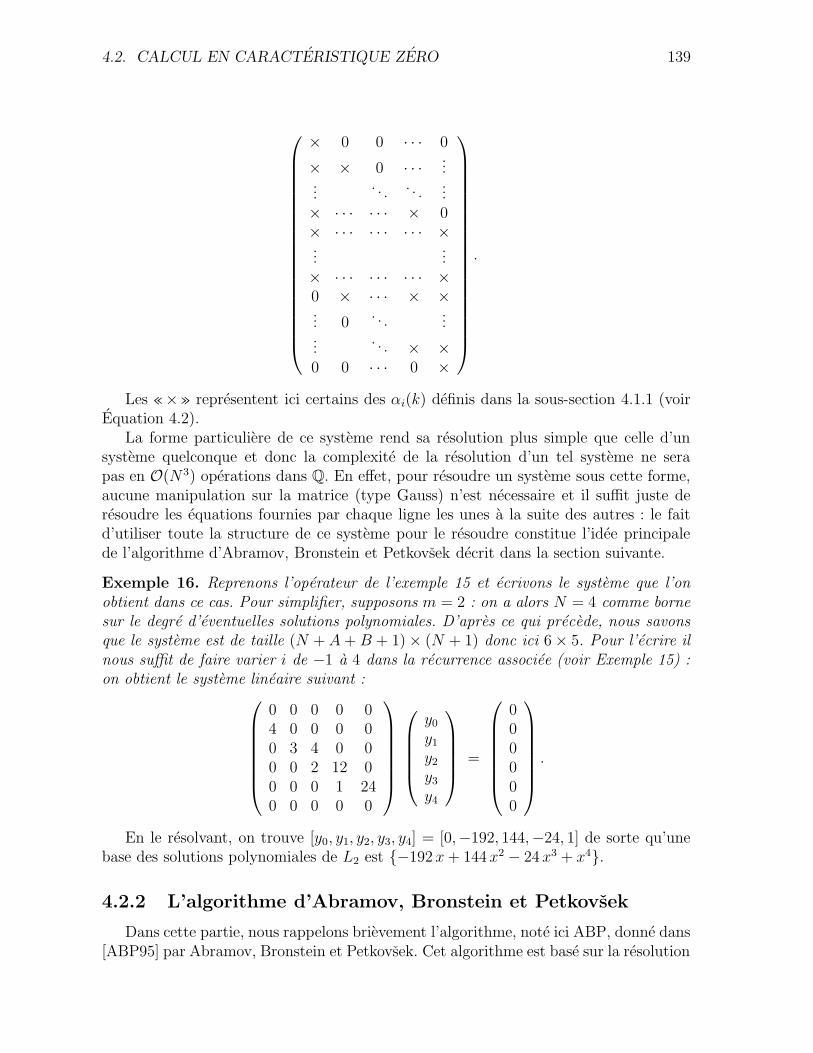
4.2. CALCUL EN CARACTERISTIQUE ZERO 139
× 0 0 · · · 0
× × 0 · · · ......
. . .. . .
...× · · · · · · × 0× · · · · · · · · · ×...
...× · · · · · · · · · ×0 × · · · × ×... 0
. . ....
.... . . × ×
0 0 · · · 0 ×
.
Les «×» representent ici certains des αi(k) definis dans la sous-section 4.1.1 (voirEquation 4.2).
La forme particuliere de ce systeme rend sa resolution plus simple que celle d’unsysteme quelconque et donc la complexite de la resolution d’un tel systeme ne serapas en O(N3) operations dans Q. En effet, pour resoudre un systeme sous cette forme,aucune manipulation sur la matrice (type Gauss) n’est necessaire et il suffit juste deresoudre les equations fournies par chaque ligne les unes a la suite des autres : le faitd’utiliser toute la structure de ce systeme pour le resoudre constitue l’idee principalede l’algorithme d’Abramov, Bronstein et Petkovsek decrit dans la section suivante.
Exemple 16. Reprenons l’operateur de l’exemple 15 et ecrivons le systeme que l’onobtient dans ce cas. Pour simplifier, supposons m = 2 : on a alors N = 4 comme bornesur le degre d’eventuelles solutions polynomiales. D’apres ce qui precede, nous savonsque le systeme est de taille (N + A + B + 1) × (N + 1) donc ici 6 × 5. Pour l’ecrire ilnous suffit de faire varier i de −1 a 4 dans la recurrence associee (voir Exemple 15) :on obtient le systeme lineaire suivant :
0 0 0 0 04 0 0 0 00 3 4 0 00 0 2 12 00 0 0 1 240 0 0 0 0
y0
y1
y2
y3
y4
=
000000
.
En le resolvant, on trouve [y0, y1, y2, y3, y4] = [0,−192, 144,−24, 1] de sorte qu’unebase des solutions polynomiales de L2 est {−192 x + 144 x2 − 24 x3 + x4}.
4.2.2 L’algorithme d’Abramov, Bronstein et Petkovsek
Dans cette partie, nous rappelons brievement l’algorithme, note ici ABP, donne dans[ABP95] par Abramov, Bronstein et Petkovsek. Cet algorithme est base sur la resolution
140 CHAPITRE 4. SOLUTIONS POLYNOMIALES D’E. D. L.
de l’equation aux recurrences (4.3). Nous etudions ensuite sa complexite.
Pour la description de l’algorithme, nous nous placons dans la situation de [ABP95]c’est-a-dire que nous supposons que 0 est un point ordinaire de l’operateur differentielL : les racines du polynome indiciel α−A de L en 0 sont alors 0, . . . , n− 1. Si 0 n’est pasordinaire, alors il nous faut faire un changement de variable.
Remarque 13. Il est possible de modifier cet algorithme pour le rendre correct memesi on ne se place pas en un point ordinaire. Pour ceci il nous faut prendre en compte lescontraintes lineaires sur les conditions initiales qui nous sont imposees par l’equationaux recurrences. Notons qu’en pratique il est souvent plus avantageux de se placer en unpoint non-ordinaire puisque l’equation indicielle possede alors (en general) un nombrede racines entieres positives strictement inferieur a n.
Algorithme ABP
Entree : L =∑n
i=0 ai ∂i ∈ Q[x][∂] satisfaisant an(0) 6= 0 et une borne N sur le
degre d’eventuelles solutions polynomiales de L.Sortie : une base des solutions polynomiales de L de degre inferieur ou egal a N .
1. Pour j ∈ {−A, . . . , B}, calculer les αj,
2. Pour k ∈ {0, . . . , N + A + B}, calculer les αj(k) (evaluation multi-points 1),
3. Pour i de 1 a n faire :
3a. Soit yi =∑N+A+B
j=0 yi,j xj ou pour j ∈ {0, . . . , n − 1}, yi,j = δji−1.
3b. Utiliser la recurrence (4.3) pour calculer les yi,j pour j ∈ {0, . . . , N +A+B},
4. Resoudre (en les ci) le systeme lineaire donne par les∑n
i=1 ci yi,N+j = 0 pourj ∈ {1, . . . , A + B},
5. Retourner les∑n
i=1 ci yi pour tout (c1, . . . , cn) trouve a l’etape 4.
Exemple 17. Regardons l’evolution de cet algorithme sur l’operateur L2 de l’exemple15. Le point 0 n’est pas ordinaire donc nous devons effectuer un changement de variable :envoyons par exemple x sur x − 1. La recurrence devient alors
−2 (i + 2) (i + 1) yi+2 + (i + 1) (2 i + 1) yi+1 + (4 − i) yi = 0.
Nous avons maintenant A = 2, B = 0 et N = 4. Posons y1 =∑6
j=0 y1,j xj avec y1,0 = 1,
y1,1 = 0 et y2 =∑6
j=0 y2,j xj avec y2,0 = 0, y2,1 = 1. La recurrence nous donne alors
1Dans [Bos03, Chapter 5] (voir aussi [BLS03]), l’auteur montre qu’un polynome P de degre d acoefficients dans un corps F peut etre evalue en d + 1 points de F en O(M(d) log(d)) operations dansF ou M(d) est le cout de la multiplication de deux polynomes univaries de degre d ; la contribution estl’amelioration de la constante masquee par la notation O. Ce resultat de complexite sur l’evaluationmulti-points sera utilise plusieurs fois par la suite.
4.2. CALCUL EN CARACTERISTIQUE ZERO 141
d’un cote y1,2 = 1, y1,3 = 1/2, y1,4 = 19/48, y1,5 = 139/480, y1,6 = 139/640 et de l’autrey2,2 = 1/4, y2,3 = 3/8, y2,4 = 49/192, y2,5 = 361/1920, y2,6 = 361/2560. Nous devons
ensuite resoudre le systeme M t(c1, c2) = t(0, 0) avec M =
( 139480
3611920
139640
3612560
)
. On trouve
c1 = c et c2 = −556/361 c et une base de solutions polynomiales de l’operateur en x− 1est donnee par {y1 − 556/361 y2}. Nous effectuons ensuite le changement de variableinverse (x 7→ x + 1) et nous retrouvons la base de solutions polynomiales de L2 trouveedans l’exemple 16 a savoir {x4 − 24 x3 + 144 x2 − 192 x}.
Proposition 14. Soit L ∈ Q[x][∂] un operateur differentiel d’ordre n, A et B definis par(4.1) et N une borne sur le degre d’eventuelles solutions polynomiales de L. L’algorithmeABP donne ci-dessus est correct et calcule une base des solutions polynomiales de L enO(N n2 (A + B)) operations dans Q.
Demonstration. Pour la correction de cet algorithme, nous renvoyons a [ABP95].Dans le cas ou 0 n’est pas un point ordinaire, nous devons faire un changement devariable x 7→ x + a avec a ∈ Z. D’apres la formule ai =
∑Bi=−A ai,j xi+j ceci peut
se faire en O((n + 1) (A + B) (n + B)) operations dans Q. Pour la suite de l’analysede complexite, nous basons notre preuve sur [Bos03, 10.2]. Dans l’etape 1, calculer lespolynomes αi revient a ecrire L en fonction de la derivation d’Euler δ := x d
dx. En
effet, si L ∈ Q[x][δ], alors la relation δj xk = kj xk donne directement les αi. EcrireL en fonction de δ peut se faire en O(M(n) (A + B) log(n)) operations dans Q ouM(d) est le cout de la multiplication de deux polynomes univaries de degre ≤ d (note :avec la FFT, ceci peut se faire en O(d log(d) log(log(d))) operations de corps ; voir[GG99, Theorem 8.23]). Nous savons (voir [Bos03] ou [BLS03]) qu’avec les techniquesde l’evaluation multi-points, un polynome P de degre d a coefficients dans un corpsF peut etre evalue en d + 1 points de F en O(M(d) log(d)) operations dans F ouM(d) est le cout de la multiplication de deux polynomes de degre d. Par consequent,dans l’etape 2, nous pouvons evaluer les A + B + 1 polynomes αj de degre ≤ n enles points 0, . . . , N + A + B en O((A + B + 1) N+A+B
nM(n) log(n)) operations dans
Q. Dans l’etape 3b, nous calculons les N + A + B − n coefficients manquants de yi enO((N + A + B − n) (A + B)) operations dans Q. A l’etape 4, nous avons a resoudreun systeme lineaire de dimensions (A + B) × n : or comme nous sommes en un pointregulier A = n et nous avons donc plus d’equations que d’inconnus : la resolution dusysteme peut donc se faire en O((A + B) n2) operations dans Q.
4.2.3 L’algorithme de Barkatou
Le troisieme algorithme calculant les solutions polynomiales d’equations differentielleslineaires que nous rappelons ici est celui donne par Barkatou dans [Ba97] qui n’est autreque la version scalaire de celui propose dans [Ba99]). Cet algorithme est ici presente endetails et sa complexite est etudiee. Un algorithme utilisant le meme style d’idee estpresente dans [AK91].
142 CHAPITRE 4. SOLUTIONS POLYNOMIALES D’E. D. L.
Notations et idee de l’algorithme
Commencons par fixer quelques notations. Soit
L =n∑
i=0
ai δi,
avec δ = x ddx
et ai ∈ Q(x). Dans ce qui suit, le degre d’une fraction rationnelle designela difference entre le degre de son numerateur et celui de son denominateur. Notons
B = maxi
(degx(ai)),
(remarque : comme L est ici ecrit en fonction de la derivation d’Euler, ce B correspondbien au B defini dans (4.1)) et
ai(x) = ai xdegx(ai) + · · · ,
avec ai ∈ Q (ai = 0 si ai = 0) et ou « · · · » designe une somme de termes de degrestrictement inferieur a degx(ai). On a alors,
L(xλ) = αB(λ) xλ+B + · · ·+ α−A(λ) xλ−A,
ou A est defini par −A = mini(valx(ai)) et, avec les notations precedentes,
αB(k) =n∑
i=0
ai ki
est le polynome indiciel de L a l’infini.
Pour simplifier la description de l’algorithme, nous supposons que B = 0 ce quin’enleve rien a la generalite : en effet si B 6= 0, alors il nous suffit de remplacer L parx−B L et b par x−B b dans tout ce qui suit.
On a alors le lemme suivant :
Lemme 16 ([Ba97], Lemma 1). Avec les notations precedentes et en supposantB = 0, on a : pour tout z ∈ Q(x), degx(L(z)) ≤ degx(z) avec egalite si, et seulementsi, αB(degx(z)) 6= 0.
On considere ici des equations non-homogenes L(y) = b avec b ∈ Q(x). Meme sidans ce chapitre c’est uniquement le cas homogene qui nous interesse, la maniere dontcet algorithme procede nous amene de toute facon a considerer des equations non-homogenes (l’algorithme ABP fonctionne lui aussi dans le cas non-homogene - voir[ABP95]). Soit y ∈ Q[x] et ecrivons
y = c xµ + z,
4.2. CALCUL EN CARACTERISTIQUE ZERO 143
avec c ∈ Q∗ et µ ∈ N. On a alors
L(y) = b ⇔ L(z) = b − c L(xµ).
L’idee a la base de l’algorithme est alors la suivante : essayer de determiner c ∈ Q∗ etµ ∈ N tels que L(y) = b et degx(z) < degx(y) = µ. Si on trouve un tel couple (c, µ)alors on recommence avec z a la place de y et l’equation L(z) = b − c L(xµ) a la placede L(y) = b et ainsi de suite jusqu’a ce que l’on obtienne une equation de la forme
L(w) = b − L(∑
finie
ci xµi)
qui n’a pas de solutions polynomiales (pas de choix possible pour c et µ verifiant lesconditions demandees). Par consequent, l’equation de depart L(y) = b aura une solutionpolynomiale non-nulle si, et seulement si, L(
∑
finie ci xµi) = b.
Comment choisir c ∈ Q∗ et µ ∈ N tels que L(c xµ + z) = b et degx(z) < µ ?
Notons b = b0 +∑m
i=1 ci bi avec m ≤ n et les bi ∈ Q(x) : au cours de l’algorithme lesecond membre de notre equation peut contenir des parametres ci. Soit
R := {λ ∈ N |αB(λ) = 0},
l’ensemble des racines entieres positives du polynome indiciel αB de L a l’infini. Notonsη le degre de b et
b = b xη + · · · ,
avec la convention b = 0 si η = −∞.Si y = c xµ + z, alors
L(y) = b ⇔ L(z) = b − c L(xµ),⇔ L(z) = b xη − c αB(µ) xµ + · · · .
(4.4)
D’apres le lemme 16, si un couple (c, µ) est solution de notre probleme, alorsdegx(L(z)) ≤ degx(z) < µ. Pour simplifier les notations, posons
E := b xη − c αB(µ) xµ + · · · .
Trois cas sont a distinguer :
1) Si [R 6= ∅ et η < maxR], alors il nous suffit de prendre µ = maxR et c pa-rametre arbitraire. Par la suite c est considere comme un parametre. On retire alors µde l’ensemble R.
2) Si [R = ∅ et η < 0], alors, pour tout µ ≥ 0, le degre du second membre de E estegal a µ et il n’existe donc pas de couple (c, µ) solution de notre probleme.
144 CHAPITRE 4. SOLUTIONS POLYNOMIALES D’E. D. L.
3) Si [R 6= ∅ et η ≥ maxR] ou [R = ∅ et η ≥ 0], alors le seul choix possible pourµ est µ = η (car si µ > η, alors le degre de E est egal a µ). Avec µ = η, l’equation 4.4donne
L(z) = (b − c αB(η)) xη + · · · ,
et donc necessairement
b − c αB(η) = 0. (4.5)
Cette derniere equation admet une solution c ∈ Q∗ si, et seulement si, [αB(η) 6= 0] ou[αB(η) = 0 et b = 0]. Ici encore, trois cas sont a distinguer :
3.1) Si αB(η) 6= 0, il suffit de prendre c = bαB(η)
.
3.2) Si αB(η) = 0 et si le systeme lineaire en les ci donne par b(c1, . . . , cm) = 0 a unesolution, alors il suffit de prendre c parametre arbitraire. Dans ce cas, on retireµ = η de l’ensemble R.
3.3) Si αB(η) = 0 et si le systeme lineaire en les ci donne par b(c1, . . . , cm) = 0 n’apas de solution, alors il n’existe pas de couple (c, µ) solution de notre probleme.
Notons que ce procede se termine puisqu’a chaque etape, soit le degre du secondmembre decroit, soit le nombre d’elements de R diminue.
Lorsque ce procede se termine (c’est-a-dire que nous sommes dans le cas ou il n’existepas de c et µ repondant au probleme), nous avons une equation de la forme L(w) =b − L(
∑
finie ci xµi) (ou les ci sont des parametres arbitraires) qui n’a pas de solutions
polynomiales. Dans ce cas∑
finie ci xµi est la solution polynomiale generale de l’equation
de depart si, et seulement si, L(w) = 0. Ce L(w) s’ecrit∑ fi xi
g(x)ou les fi sont des
polynomes de degre 0 ou 1 en les parametres ci et il ne nous reste donc plus qu’aresoudre le systeme en les ci forme par les equations fi = 0.
Exemple 18. Comme nous l’avons fait pour l’algorithme ABP dans la sous-sectionprecedente, regardons comment evolue l’algorithme de Barkatou sur l’operateur L2 donnedans l’exemple 15. On a ici B = 0 de telle sorte qu’aucune modification preliminairesur l’operateur n’est necessaire. D’apres l’exemple 15, l’ensemble R defini ci-dessus estici egal a {4}. Initialement nous avons donc maxR = 4 et η = −∞ de telle sorte quenous passons dans le cas 1 (voir ci-dessus). Nous posons donc µ1 = 4 et c1 constantearbitraire. En posant y = c1 x4 + z, nous sommes conduits a examiner l’equationL(z) = −c1 L(x4) = −24 c1 x3. Le degre du second membre est donc egal a 3. Mainte-nant R est vide et η = 3 ≥ 0 donc nous passons dans le cas 3. De plus, necessairement,αB(3) 6= 0 donc nous passons dans 3.1. Il vient donc z = −24 c1 x3 + w et w sa-tisfait L(w) = 288 c1 x2. Ensuite nous repassons dans 3.1 et donc w = 144 c1 x2 + vavec L(v) = −576 c1 x. A l’etape suivante, toujours en passant par le cas 3.1, nousavons v = −192 c1 x + u ou u verifie L(u) = 0. Nous en arrivons donc au pointou R = ∅ et η < 0 de telle sorte que l’algorithme se termine puisque nous sommesdans le cas 2. Nous avons donc construit l’eventuelle solution polynomiale generaley = c1 x4 − 24 c1 x3 + 144 c1 x2 − 192 c1 x. A la fin nous avons L(y) = 0 et nous n’avonsdonc aucune condition a verifier de telle sorte que {x4 − 24 x3 +144 x2 − 192 x} est unebase de solutions polynomiales de L2.
4.2. CALCUL EN CARACTERISTIQUE ZERO 145
Nous pouvons resumer toute l’explication donnee ci-dessus par l’algorithme suivant :
Algorithme Barkatou
Entree : L ∈ Q(x)[δ].Sortie : la solution polynomiale generale de L(y) = 0.
1. Si B 6= 0, alors remplacer L par x−B L.
2. Calculer αB(= α0). Soit R := [u ∈ N |αB(u) = 0] et r := #R.
3. Si r = 0, alors retourner 0. Sinon :
4. Poser sol := 0, η := −∞ et sm := 0.
5. Tant que η > 0 ou r > 0, faire :
5a. Si r > 0 et R[r] > η, alors :sol := sol + c[r] xR[r],sm := sm − c[r] L(xR[r]),η := deg(sm) et r := r − 1.
5b. Sinon, si r > 0 et R[r] = η, alors :lcb := lcoeff(sm, x),Resoudre lcb = 0 en les ci,S’il n’y a pas de solution, alors poser η := −1 et r := 0 (stop).Sinon :Assigner aux ci les valeurs trouvees,sol := sol + c[r] xR[r],sm := sm − c[r] L(xR[r]),η := deg(sm) et r := r − 1.
5c. Sinon :lcb := lcoeff(sm, x),w := lcb/α0(η),sol := sol + w xη,η := deg(sm).
6. Si sm 6= 0, alors :
6a. Resoudre le systeme en les ci forme par les coefficients du numerateur de sm.
6b. Si ce systeme n’a pas de solutions, alors retourner 0.
6c. Sinon, assigner aux ci les valeurs trouvees.
7. Retourner sol.
Proposition 15. Soit L ∈ Z[x][∂] un operateur differentiel lineaire d’ordre n, A et Bdefinis par (4.1) et N une borne sur le degre d’eventuelles solutions polynomiales de L.L’algorithme de Barkatou donne ci-dessus est correct et calcule une base de solutionspolynomiales de L de degre inferieur ou egal a N en au plus O(N n2 (A+B)) operationsdans Q.
146 CHAPITRE 4. SOLUTIONS POLYNOMIALES D’E. D. L.
Demonstration. Pour la correction de cet algorithme, nous renvoyons a [Ba97].Le nombre d’operations faites par cet algorithme recursif depend fortement du nombrede passage dans la sous-procedure cherchant c et µ (nombre de passage dans la boucle« tant que» dans l’algorithme ci-dessus). Ce nombre de passage correspond au nombrede coefficients non-nuls dans l’ecriture de la solution polynoniale generale de L. Ici nousallons nous interesser au cas extreme ou nous avons une base de solutions en seriesdans Q[[1/x]][x] avec des parties polynomiales denses (N +1 coefficients non-nuls) maisaucune solution polynomiale non-nulle : ceci nous donnera donc une estimation de lacomplexite maximale de l’algorithme. Pour pouvoir comparer cet algorithme aux autres,nous devons supposer que l’operateur de depart est ecrit en la derivation ∂ et que nousavons une equation homogene c’est-a-dire qu’initialement le second membre b est nul.Il nous faut donc tout d’abord ecrire l’operateur en fonction de la derivation d’Euler cequi se fait en O(M(n) (A + B) log(n)) operations dans Q ou M(d) est le cout de lamultiplication de deux polynomes de degre ≤ d (voir la preuve de la proposition 14).Notons que ceci est de toute facon necessaire pour calculer les polynomes αi definisdans la partie 4.1.1. Ensuite, au cours de l’algorithme nous aurons besoin d’evaluer lesL(xµ) ou L(xη) pour toute racine entiere positive µ de αB et pour les degres η desseconds membres qui apparaissent au cours de l’algorithme : ces µ et η sont toujours≤ N . Pour ceci nous utilisons encore une fois les techniques de l’evaluation multi-points(voir [Bos03] ou [BLS03]) qui impliquent qu’un polynome P de degre d a coefficientsdans un corps F peut etre evalue en d + 1 points de F en O(M(d) log(d)) operationsdans F ou M(d) est le cout de la multiplication de deux polynomes de degre d. Parconsequent, nous pouvons evaluer au prealable les A + B + 1 polynomes αj de degre≤ n en 0, . . . , N en O((A + B + 1) N
nM(n) log(n)) operations dans Q. Maintenant,
nous passons N + 1 fois dans la sous-procedure cherchant c et µ et la solution generalesous forme de serie depend de n constantes arbitraires. Cela signifie que nous passonsn fois dans l’etape 5a ou 5b et N + 1 − n fois dans le cas 5c. Comme l’etape 5b estplus couteuse que 5a, supposons que nous passons n− 1 fois dans 5b et 1 fois dans 5a :lors du premier passage dans la boucle « tant que», nous passons forcement dans 5apuisque le degre du second membre est initialement −∞ (notons que, vu les evaluationspreliminaires, ce premier passage a un cout constant). Dans 5b, nous devons resoudreune equation lineaire en les ci : resoudre cette equation signifie ici ecrire le dernierparametre arbitraire introduit en fonction des precedents de telle sorte que ceci couteau plus O(n) operations dans Q puisque qu’au maximum nous aurons n parametres.La mise a jour du second membre a un cout constant puisque nous avons deja evalueles αi. Ensuite, nous devons passer N + 1 − n fois dans 5c et toujours grace au faitque les evaluations ont ete faites au prealable ceci possede un cout constant. A la fin,il nous reste a resoudre le systeme forme par les fi = 0 (ou les fi sont les coefficientsdu numerateur du second membre final). Ce systeme possede n inconnues (les ci) et lenombre d’equations (le degre du numerateur du second membre final) est majore parN : sa resolution coute donc O(N n2) operations dans Q.
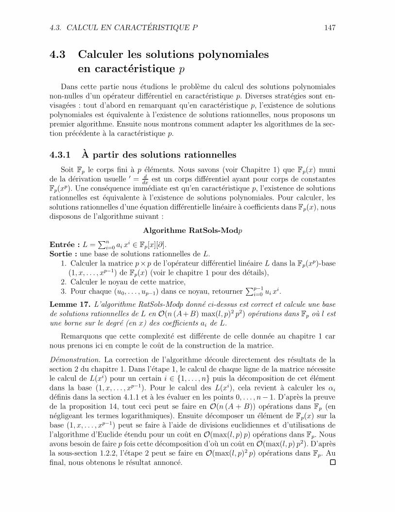
4.3. CALCUL EN CARACTERISTIQUE P 147
4.3 Calculer les solutions polynomiales
en caracteristique p
Dans cette partie nous etudions le probleme du calcul des solutions polynomialesnon-nulles d’un operateur differentiel en caracteristique p. Diverses strategies sont en-visagees : tout d’abord en remarquant qu’en caracteristique p, l’existence de solutionspolynomiales est equivalente a l’existence de solutions rationnelles, nous proposons unpremier algorithme. Ensuite nous montrons comment adapter les algorithmes de la sec-tion precedente a la caracteristique p.
4.3.1 A partir des solutions rationnelles
Soit Fp le corps fini a p elements. Nous savons (voir Chapitre 1) que Fp(x) munide la derivation usuelle ′ = d
dxest un corps differentiel ayant pour corps de constantes
Fp(xp). Une consequence immediate est qu’en caracteristique p, l’existence de solutions
rationnelles est equivalente a l’existence de solutions polynomiales. Pour calculer, lessolutions rationnelles d’une equation differentielle lineaire a coefficients dans Fp(x), nousdisposons de l’algorithme suivant :
Algorithme RatSols-Modp
Entree : L =∑n
i=0 ai xi ∈ Fp[x][∂].
Sortie : une base de solutions rationnelles de L.1. Calculer la matrice p× p de l’operateur differentiel lineaire L dans la Fp(x
p)-base(1, x, . . . , xp−1) de Fp(x) (voir le chapitre 1 pour des details),
2. Calculer le noyau de cette matrice,3. Pour chaque (u0, . . . , up−1) dans ce noyau, retourner
∑p−1i=0 ui x
i.
Lemme 17. L’algorithme RatSols-Modp donne ci-dessus est correct et calcule une basede solutions rationnelles de L en O(n (A+B) max(l, p)2 p2) operations dans Fp ou l estune borne sur le degre (en x) des coefficients ai de L.
Remarquons que cette complexite est differente de celle donnee au chapitre 1 carnous prenons ici en compte le cout de la construction de la matrice.
Demonstration. La correction de l’algorithme decoule directement des resultats de lasection 2 du chapitre 1. Dans l’etape 1, le calcul de chaque ligne de la matrice necessitele calcul de L(xi) pour un certain i ∈ {1, . . . , n} puis la decomposition de cet elementdans la base (1, x, . . . , xp−1). Pour le calcul des L(xi), cela revient a calculer les αi
definis dans la section 4.1.1 et a les evaluer en les points 0, . . . , n− 1. D’apres la preuvede la proposition 14, tout ceci peut se faire en O(n (A + B)) operations dans Fp (ennegligeant les termes logarithmiques). Ensuite decomposer un element de Fp(x) sur labase (1, x, . . . , xp−1) peut se faire a l’aide de divisions euclidiennes et d’utilisations del’algorithme d’Euclide etendu pour un cout en O(max(l, p) p) operations dans Fp. Nousavons besoin de faire p fois cette decomposition d’ou un cout en O(max(l, p) p2). D’apresla sous-section 1.2.2, l’etape 2 peut se faire en O(max(l, p)2 p) operations dans Fp. Aufinal, nous obtenons le resultat annonce.
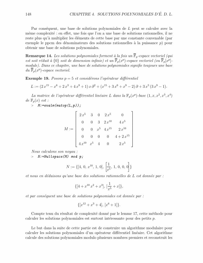
148 CHAPITRE 4. SOLUTIONS POLYNOMIALES D’E. D. L.
Par consequent, une base de solutions polynomiales de L peut se calculer avec lameme complexite : en effet, une fois que l’on a une base de solutions rationnelles, il nereste plus qu’a multiplier les elements de cette base par une constante convenable (parexemple le ppcm des denominateurs des solutions rationnelles a la puissance p) pourobtenir une base de solutions polynomiales.
Remarque 14. Les solutions polynomiales forment a la fois un Fp-espace vectoriel (quiest soit reduit a {0} soit de dimension infinie) et un Fp(x
p)-espace vectoriel (ou Fp[xp]-
module). Dans ce chapitre, une base de solutions polynomiales signifie toujours une basedu Fp(x
p)-espace vectoriel.
Exemple 19. Posons p = 5 et considerons l’operateur differentiel
L := (2 x15 − x6 + 2 x3 + 4 x9 + 1) x ∂2 + (x15 + 3 x6 + x9 − 2) ∂ + 3 x5 (3 x9 − 1).
La matrice de l’operateur differentiel lineaire L dans la Fp(xp)-base (1, x, x2, x3, x4)
de Fp(x) est :> M:=evalm(matop(L,p));
M :=
2 x5 3 0 2 x5 0
0 0 3 2 x10 4 x5
0 0 x5 4 x15 2 x10
0 0 0 0 4 + 2 x15
4 x10 x5 4 0 2 x5
Nous calculons son noyau :> N:=Nullspace(M) mod p;
N := {[4, 0, x10, 1, 0],
[
1
x5, 1, 0, 0, 0
]
}
et nous en deduisons qu’une base des solutions rationnelles de L est donnee par :
{[4 + x10 x2 + x3], [1
x5+ x]},
et par consequent une base de solutions polynomiales est donnee par :
{[x12 + x3 + 4], [x6 + 1]}.
Compte tenu du resultat de complexite donne par le lemme 17, cette methode pourcalculer les solutions polynomiales est surtout interessante pour des petits p.
Le but dans la suite de cette partie est de construire un algorithme modulaire pourcalculer les solutions polynomiales d’un operateur differentiel lineaire. Cet algorithmecalcule des solutions polynomiales modulo plusieurs nombres premiers et reconstruit les
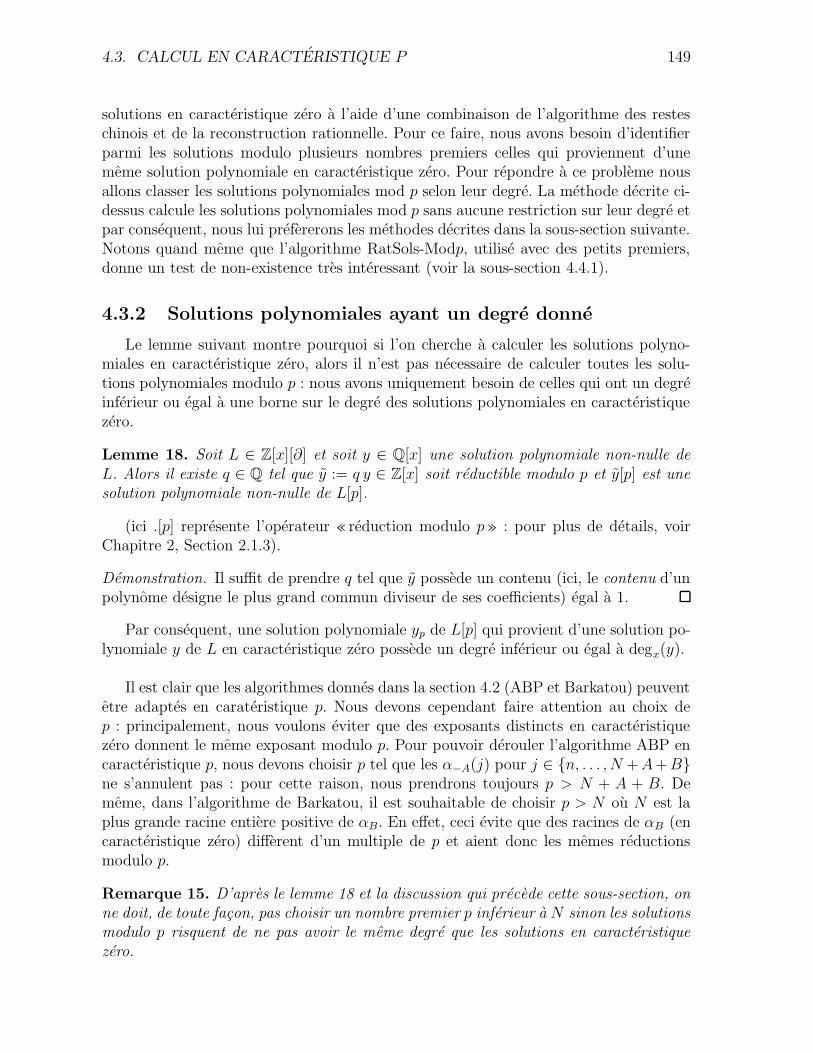
4.3. CALCUL EN CARACTERISTIQUE P 149
solutions en caracteristique zero a l’aide d’une combinaison de l’algorithme des resteschinois et de la reconstruction rationnelle. Pour ce faire, nous avons besoin d’identifierparmi les solutions modulo plusieurs nombres premiers celles qui proviennent d’unememe solution polynomiale en caracteristique zero. Pour repondre a ce probleme nousallons classer les solutions polynomiales mod p selon leur degre. La methode decrite ci-dessus calcule les solutions polynomiales mod p sans aucune restriction sur leur degre etpar consequent, nous lui prefererons les methodes decrites dans la sous-section suivante.Notons quand meme que l’algorithme RatSols-Modp, utilise avec des petits premiers,donne un test de non-existence tres interessant (voir la sous-section 4.4.1).
4.3.2 Solutions polynomiales ayant un degre donne
Le lemme suivant montre pourquoi si l’on cherche a calculer les solutions polyno-miales en caracteristique zero, alors il n’est pas necessaire de calculer toutes les solu-tions polynomiales modulo p : nous avons uniquement besoin de celles qui ont un degreinferieur ou egal a une borne sur le degre des solutions polynomiales en caracteristiquezero.
Lemme 18. Soit L ∈ Z[x][∂] et soit y ∈ Q[x] une solution polynomiale non-nulle deL. Alors il existe q ∈ Q tel que y := q y ∈ Z[x] soit reductible modulo p et y[p] est unesolution polynomiale non-nulle de L[p].
(ici .[p] represente l’operateur « reduction modulo p» : pour plus de details, voirChapitre 2, Section 2.1.3).
Demonstration. Il suffit de prendre q tel que y possede un contenu (ici, le contenu d’unpolynome designe le plus grand commun diviseur de ses coefficients) egal a 1.
Par consequent, une solution polynomiale yp de L[p] qui provient d’une solution po-lynomiale y de L en caracteristique zero possede un degre inferieur ou egal a degx(y).
Il est clair que les algorithmes donnes dans la section 4.2 (ABP et Barkatou) peuventetre adaptes en carateristique p. Nous devons cependant faire attention au choix dep : principalement, nous voulons eviter que des exposants distincts en caracteristiquezero donnent le meme exposant modulo p. Pour pouvoir derouler l’algorithme ABP encaracteristique p, nous devons choisir p tel que les α−A(j) pour j ∈ {n, . . . , N +A+B}ne s’annulent pas : pour cette raison, nous prendrons toujours p > N + A + B. Dememe, dans l’algorithme de Barkatou, il est souhaitable de choisir p > N ou N est laplus grande racine entiere positive de αB. En effet, ceci evite que des racines de αB (encaracteristique zero) different d’un multiple de p et aient donc les memes reductionsmodulo p.
Remarque 15. D’apres le lemme 18 et la discussion qui precede cette sous-section, onne doit, de toute facon, pas choisir un nombre premier p inferieur a N sinon les solutionsmodulo p risquent de ne pas avoir le meme degre que les solutions en caracteristiquezero.
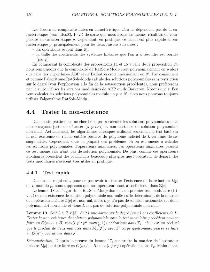
150 CHAPITRE 4. SOLUTIONS POLYNOMIALES D’E. D. L.
Les etudes de complexite faites en caracteristique zero ne dependent pas de la ca-racteristique (voir [Bos03, 10.2]) de sorte que nous avons les memes resultats de com-plexite en caracteristique p. Cependant, en pratique, ce calcul est plus rapide en ca-racteristique p, principalement pour les deux raisons suivantes :
– les operations se font dans Fp,– la taille des coefficients des systemes lineaires que l’on a a resoudre est bornee
(par p).En comparant la complexite des propositions 14 et 15 a celle de la proposition 17,
nous remarquons que la complexite de RatSols-Modp croıt polynomialement en p alorsque celle des algorithmes ABP et de Barkatou croıt lineairement en N . Par consequentet comme l’algorithme RatSols-Modp calcule des solutions polynomiales sans restrictionsur le degre (voir l’explication a la fin de la sous-section precedente), nous prefereronspar la suite utiliser les versions modulaires de ABP ou de Barkatou. Notons que si l’onveut calculer les solutions polynomiales modulo un p < N , alors nous pouvons toujoursutiliser l’algorithme RatSols-Modp.
4.4 Tester la non-existence
Dans cette partie nous ne cherchons pas a calculer les solutions polynomiales maisnous essayons juste de detecter (a priori) la non-existence de solution polynomialenon-nulle. Actuellement, les algorithmes classiques utilisent seulement le test base surla non-existence de racine entiere positive du polynome indiciel de L en l’une de sessingularites. Cependant, dans la plupart des problemes ou on est amene a calculerles solutions polynomiales d’operateurs auxiliaires, ces operateurs auxiliaires passentce test meme s’ils n’ont pas de solution polynomiale. De plus, comme ces operateursauxiliaires possedent des coefficients beaucoup plus gros que l’operateur de depart, destests modulaires s’averent tres utiles en pratique.
4.4.1 Test rapide
Dans tout ce qui suit, pour ne pas avoir a discuter l’existence de la reduction L[p]de L modulo p, nous supposons que nos operateurs sont a coefficients dans Z[x].
Le lemme 18 et l’algorithme RatSols-Modp donnent un premier test modulaire (tri-vial) de non-existence de solution polynomiale non-nulle : si le determinant de la matricede l’operateur lineaire L[p] est non-nul, alors L[p] n’a pas de solution rationnelle (et doncpolynomiale) non-nulle et donc L n’a pas de solution polynomiale non-nulle.
Lemme 19. Soit L ∈ Z[x][∂]. Soit l une borne sur le degre (en x) des coefficients de L.Tester la non existence de solution polynomiale avec le test modulaire precedent peut sefaire en O(n (A + B) max(l, p)2 pω max( l
p, 1)) operations dans Fp, ou ω est un reel tel
que le produit de deux matrices dans Mn(F), avec F corps quelconque, puisse se faireen O(nω) operations dans F .
Demonstration. D’apres la preuve du lemme 17, construire la matrice de l’operateurlineaire L[p] peut se faire en O(n (A+B) max(l, p)2 p) operations dans Fp. Maintenant,
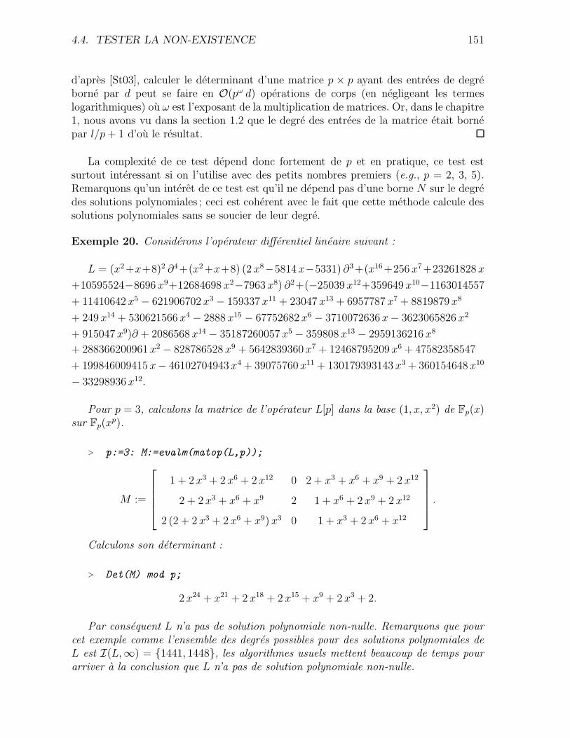
4.4. TESTER LA NON-EXISTENCE 151
d’apres [St03], calculer le determinant d’une matrice p × p ayant des entrees de degreborne par d peut se faire en O(pω d) operations de corps (en negligeant les termeslogarithmiques) ou ω est l’exposant de la multiplication de matrices. Or, dans le chapitre1, nous avons vu dans la section 1.2 que le degre des entrees de la matrice etait bornepar l/p + 1 d’ou le resultat.
La complexite de ce test depend donc fortement de p et en pratique, ce test estsurtout interessant si on l’utilise avec des petits nombres premiers (e.g., p = 2, 3, 5).Remarquons qu’un interet de ce test est qu’il ne depend pas d’une borne N sur le degredes solutions polynomiales ; ceci est coherent avec le fait que cette methode calcule dessolutions polynomiales sans se soucier de leur degre.
Exemple 20. Considerons l’operateur differentiel lineaire suivant :
L = (x2+x+8)2 ∂4+(x2 +x+8) (2 x8−5814 x−5331) ∂3+(x16+256 x7+23261828 x
+10595524−8696 x9+12684698 x2−7963 x8) ∂2+(−25039 x12+359649 x10−1163014557
+ 11410642 x5 − 621906702 x3 − 159337 x11 + 23047 x13 + 6957787 x7 + 8819879 x8
+ 249 x14 + 530621566 x4 − 2888 x15 − 67752682 x6 − 3710072636 x− 3623065826 x2
+ 915047 x9)∂ + 2086568 x14 − 35187260057 x5 − 359808 x13 − 2959136216 x8
+ 288366200961 x2 − 828786528 x9 + 5642839360 x7 + 12468795209 x6 + 47582358547
+ 199846009415 x− 46102704943 x4 + 39075760 x11 + 130179393143 x3 + 360154648 x10
− 33298936 x12.
Pour p = 3, calculons la matrice de l’operateur L[p] dans la base (1, x, x2) de Fp(x)sur Fp(x
p).
> p:=3: M:=evalm(matop(L,p));
M :=
1 + 2 x3 + 2 x6 + 2 x12 0 2 + x3 + x6 + x9 + 2 x12
2 + 2 x3 + x6 + x9 2 1 + x6 + 2 x9 + 2 x12
2 (2 + 2 x3 + 2 x6 + x9) x3 0 1 + x3 + 2 x6 + x12
.
Calculons son determinant :
> Det(M) mod p;
2 x24 + x21 + 2 x18 + 2 x15 + x9 + 2 x3 + 2.
Par consequent L n’a pas de solution polynomiale non-nulle. Remarquons que pourcet exemple comme l’ensemble des degres possibles pour des solutions polynomiales deL est I(L,∞) = {1441, 1448}, les algorithmes usuels mettent beaucoup de temps pourarriver a la conclusion que L n’a pas de solution polynomiale non-nulle.
152 CHAPITRE 4. SOLUTIONS POLYNOMIALES D’E. D. L.
Il existe cependant des cas ou l’operateur passe ce test pour tout p bien qu’il nepossede pas de solution polynomiale non-nulle en caracteristique zero : les deux exemplessuivants illustrent ce fait.
Exemple 21. Considerons l’operateur differentiel
L = (x + 1) ∂2 + (x2 + x − 10) ∂ − 9 x + 1.
Cet operateur n’a pas de solution polynomiale non-nulle en caracteristique zero mais onpeut montrer que pour tout p, L[p] possede une solution polynomiale non-nulle : en effet,nous avons L = ((x + 1) ∂ − 10) (∂ + x) := L1 L2 ou L1 possede la solution polynomialeQ := (x + 1)10 et L2 n’a pas de solution rationnelle non-nulle. Maintenant, pour toutnombre premier p, L2 induit une bijection L2[p] de Fp(x) dans lui-meme (car il n’a pasde solution rationnelle) : soit T l’inverse de cette bijection. Alors, pour tout premier p,T (Q[p]) est une solution rationnelle de L[p] et notre test echoue pour tout p.
Exemple 22. Considerons l’operateur d’Euler homogene
L = x3 ∂2 + x (x + 1) ∂ − 1.
Cet operateur n’a pas de solution polynomiale non-nulle en caracteristique zero. Parcontre, il possede y(x) =
∑∞i=0(−1)i i! xi+1 comme solution formelle (l’autre solution
formelle etant exp(1/x)) et par consequent, pour tout p, L[p] possede la solution poly-nomiale y[p](x) =
∑p−1i=0 (−1)i i! xi+1.
4.4.2 Un nouveau test modulaire
Lorsque la borne sur le degre N est grande (et que les tests decrits precedemmentechouent), alors nous voulons commencer a calculer des solutions polynomiales seule-ment si celles-ci ont de grandes chances d’exister. Par consequent, dans ce cas, nouspouvons nous autoriser a passer plus de temps pour essayer de detecter la non-existencede solutions polynomiales.
Soit L ∈ Z[x][∂] et notons VN l’espace vectoriel des solutions polynomiales de L dedegre inferieur ou egal a N . Une premiere borne a priori sur la dimension de VN estdonnee par #I(L,∞) (voir la sous-section 4.1.2).
Comme nous l’avons vu dans l’exemple 21, l’operateur differentiel reduit L[p] peutavoir des solutions polynomiales non-nulles pour tout p meme lorsque L ne possede pasde solution polynomiale non-nulle en caracteristique zero. Cependant, en prenant encompte une borne sur le degre, nous avons :
Theoreme 4. Soit L ∈ Z[x][∂] et soit N une borne sur le degre d’eventuelles solutionspolynomiales de L. Alors pour presque tout p, la dimension de l’espace des solutionspolynomiales de degre inferieur ou egal a N de L et L[p] est la meme.
Demonstration. Pour calculer la dimension de VN , on peut ecrire une eventuelle solutionpolynomiale de L sous la forme
∑Ni=0 yi x
i et ecrire le systeme lineaire pour les inconnuesyi ∈ Q (voir Section 4.2.1). La matrice M de ce systeme est alors de dimension (N +A+
4.4. TESTER LA NON-EXISTENCE 153
B+1)×(N +1) ou A et B sont definis dans (4.1). La dimension de VN en caracteristiquezero est egale a N + 1 − rang(M). Maintenant, le meme procede peut etre applique encaracteristique p a L[p] et la matrice du systeme obtenu est exactement M [p]. Parconsequent, la dimension de l’espace des solutions polynomiales de degre inferieur ouegal a N de L[p] est N + 1 − rang(M [p]). Nous concluons en remarquant que pourpresque tout p, rang(M [p]) = rang(M) ; en effet, il suffit de supposer que l’eliminationde Gauss sur les matrices M et M [p] se deroule de la meme facon ce qui n’exclut qu’unnombre fini de premiers.
La preuve de ce theoreme nous indique quels vont etre les mauvais premiers c’est-a-dire ceux pour lesquels L[p] possedera une (ou plusieurs) solution(s) parasite(s) : avecles notations de la preuve, ceux sont les p tels que rang(M [p]) < rang(M). Cependant,si l’on cherche a calculer ces nombres premiers p, il nous faut calculer et factoriser ledeterminant principal de M et le cout de cette operation est a peu pres equivalent a celuide la resolution du systeme M Y = 0 c’est-a-dire a celui du calcul des solutions polyno-miales. Par consequent en pratique nous ne calculerons pas ces mauvais premiers (voirla sous-section 4.5.2) mais nous utiliserons plutot une strategie reposant sur l’argumentportant sur le degre des solutions parasites donne par le corollaire suivant.
Corollaire 3. Soit L ∈ Z[x][∂] et soit N une borne sur le degre d’eventuelles solutionspolynomiales de L. Il n’existe qu’un nombre fini de nombres premiers p tels que L[p]possede une solution polynomiale de degre ≤ N ne provenant pas de caracteristique zero(au sens du lemme 18).
Demonstration. Raisonnons par l’absurde et supposons que pour une infinite de p, L[p]possede une solution polynomiale non-nulle ne provenant pas d’une solution de L etayant un degre inferieur ou egal a N . Comme cette solution ne provient pas d’une solu-tion de L, pour une infinite de p, la dimension de l’espace des solutions polynomiales dedegre inferieur ou egal a N de L[p] sera superieure a celle de L ce qui est en contradictionavec le theoreme precedent.
Ces resultats theoriquement interessants menent a un test de non-existence de solu-tion polynomiale non-nulle :
1. calculer une borne N sur le degre d’eventuelles solutions polynomiales non-nullesde L en caracteristique zero,
2. choisir un premier p > N + A + B,
3. calculer le rang rp de M [p] (voir la preuve du theoreme 4 ci-dessus). Si rp = N +1,alors L[p] n’a pas de solution polynomiale non-nulle de degre ≤ N et donc L n’apas de solution polynomiale non-nulle.
L’algorithme de [MS98] calcule le rang de M [p] en O((N +A+B) Nω−1) operationsdans Fp ou N est une borne sur le degre d’eventuelles solutions polynomiales, A etB sont definis dans (4.1) et ω est l’exposant de l’algebre lineaire : cette complexiteest equivalente a celle pour resoudre le systeme lineaire. Ceci limite donc l’interet de
154 CHAPITRE 4. SOLUTIONS POLYNOMIALES D’E. D. L.
ce test en pratique. Cependant, recemment, dans [SSV04], les auteurs montrent com-ment calculer le rang d’une matrice a coefficients dans Z d’une maniere plus efficace :ces resultats sont encourageants et nous esperons qu’ils pourront etre generalises a lacaracteristique p (actuellement cette methode ne s’applique pas en caracteristique p).
Exemple 23. Revenons a l’exemple 21. Pour cet exemple le test modulaire de la sous-section precedente echoue. En regardant d’un peu plus pres, on voit que I(L,∞) = {9}et donc N = 9 est le degre d’une eventuelle solution polynomiale. De plus, nous avonsA = 2 et B = 1 de sorte que nous choisissons p > 12. Si nous appliquons le testci-dessus a L, alors nous detecterons la non-existence de solution polynomiale non-nulle sauf si le p choisi a l’etape 2 est p = 19. En effet, pour tout nombre premier pstrictement superieur a 12 sauf pour p = 19, nous avons rp = N + 1 puisque, pour cetexemple, p = 19 est l’unique mauvais premier superieur a 12 ; ceci vient du fait que ledeterminant principal de la matrice M est egal a 214 · 34 · 52 · 7 · 19.
La methode suggeree par le test donne ici donne aussi une heuristique pour cal-culer la dimension de l’espace des solutions polynomiales en caracteristique zero : eneffet, avec les notations precedentes, pour presque tout p, cette dimension est egale aN +1−rang(M [p]). Cependant, des que N est « grand», il est plus judicieux de calculerla dimension de l’espace des solutions polynomiales modulo p en calculant une base desolutions polynomiales grace a la version modulaire de ABP ou Barkatou modulo p ; eneffet au lieu d’etre en O(Nω), la complexite est alors lineaire en N .Le fait de disposer d’une heuristique pour calculer la dimension de l’espace des solu-tions polynomiales en caracteristique zero est particulierement interessant pour certainsproblemes de theorie de Galois differentielle ou cette dimension donne des informationssur le groupe cherche. Par exemple, les solutions rationnelles de puissances symetriquesd’operateurs differentiels lineaires induisent des espaces d’invariants des groupes de Ga-lois differentiels, et on discrimine les groupes entre eux en comparant ces dimensions(voir [HRUW98, Algorithm 4.1], [Ul03, Theorem 3.2 and Algorithm 3.4] ou encore[Cor01, CSTU02]).
4.5 Reconstruire les solutions polynomiales
en caracteristique zero
Dans ce qui suit, notre but est de calculer une base de solutions polynomiales de L[p]pour plusieurs premiers p et de les combiner pour obtenir une base de solutions polyno-miales de L. Pour ce faire, pour chaque element y d’une base de solutions polynomialesde L, nous devons etre capable de retrouver y[p] parmi les elements d’une base de solu-tions polynomiales de L[p]. De plus, nous devons nous assurer que les bases modulairesne contiennent pas de « solution parasite», i. e., des solutions qui ne proviennent pasde solutions en caracteristique zero. Par consequent, nous devons calculer des bases desolutions polynomiales sous une forme canonique et exclure certains mauvais nombrespremiers.
4.5. RECONSTRUCTION 155
4.5.1 Bases echelonnees
Dans cette sous-section, si aucune autre condition n’est precisee, K represente soitQ soit Fp.
Definition 26. Soit L ∈ K[x][∂] et soit B = {y[1], . . . , y[r]} avec yi ∈ K[x] une base de
solutions polynomiales de L. Pour i ∈ {1, . . . , r}, on note y [i] =∑di
j=0 y[i]j xj avec les
di ∈ N tels que d1 > · · · > dr, les y[i]j ∈ K et pour tout i ∈ {1, . . . , r}, y
[i]di6= 0.
B est une base echelonnee si pour tout i ∈ {1, . . . , r}, y[i]di
= 1 et, pour tout i, j ∈{1, . . . , r} avec i 6= j, y
[i]dj
= 0.
Ces bases echelonnees apparaissent d’une maniere tout a fait naturelle et sont lesbases calculees par la plupart des algorithmes classiques.
Etant donne une base quelconque {y[1], . . . , y[r]} de solutions polynomiales, une baseechelonnee peut se calculer en faisant de l’elimination de Gauss sur les vecteurs formesdes coefficients des y[i].
Nous avons de plus le resultat d’unicite (classique et tres simple) suivant :
Lemme 20. Etant donne L ∈ K[x][∂], il existe une unique base echelonnee de solutionspolynomiales de L.
Le theoreme suivant fait le lien entre la base echelonnee de solutions polynomialesd’un operateur differentiel L en caracteristique zero et celle de sa reduction L[p] modulop :
Theoreme 5. Soit L ∈ Z[x][∂] et soit N une borne sur le degre d’eventuelles solutionspolynomiales de L. Soit B = {y[1], . . . , y[r]} la base echelonnee de solutions polynomialesde degre ≤ N de L. Alors, pour presque tout p, B[p] := {y [1][p], . . . , y[r][p]} est la baseechelonnee, notee Bp, de solutions polynomiales de degre ≤ N de L[p].
Demonstration. Tout d’abord, d’apres le theoreme 4, pour presque tout p, B[p] et Bp
ont le meme nombre d’elements. Maintenant, d’apres le lemme 20, il y a une uniquebase echelonnee de solutions polynomiales de degre ≤ N de L[p] et donc, il nous suffitde montrer que, pour presque tout p, B[p] est une base echelonnee. Or, comme leselements de B sont supposes unitaires, cette derniere affirmation est vraie pour toutp n’apparaissant pas dans les denominateurs des coefficients. Par consequent, des queB[p] est bien definie, c’est encore une base echelonnee.
Remarque 16. Ce theoreme et le theoreme 4 ne restent pas vrais si l’on omet la condi-tion sur le degre des solutions polynomiales considerees qui est suppose ≤ N . En effet,un operateur differentiel lineaire peut posseder des solutions polynomiales non-nullesmod p pour tout p et ne pas avoir de solutions polynomiales non-nulles en caracteristiquezero (voir l’exemple 21).
Avec les notations du theoreme precedent, il est possible que B[p] 6= Bp :
156 CHAPITRE 4. SOLUTIONS POLYNOMIALES D’E. D. L.
Exemple 24. Considerons l’operateur differentiel
L = 3 x2 ∂2 − 19 x ∂ + 7.
On a alors B = {x7}, et donc B[11] = {x7} mais B11 = {x7, x4}.Comme nous supposons toujours p ≥ N , les degres des elements de B et B[p] definis
au theoreme 5 doivent etre les memes. Donc, en pratique, lorsque l’on dispose de deuxbases modulaires Bp1 et Bp2 pour deux premiers distincts p1 et p2, nous devons toutd’abord verifier que les degres des elements des deux bases sont les memes et qu’ilsappartiennent a I(L,∞). Si cela n’est pas verifie, alors l’un des deux premiers estmauvais.
4.5.2 Nombres premiers pertinents
Comme nous l’avons deja fait remarquer, pour utiliser les algorithmes ABP et Bar-katou en caracteristique p, nous devons supposer que les nombres premiers p que l’onprend sont superieurs a N + A + B, ou N est une borne sur le degre d’eventuellessolutions polynomiales de L et les entiers A et B sont definis par (4.1).
Comme nous sommes seulement interesses par les solutions polynomiales mod pqui correspondent a des solutions polynomiales de degre ≤ N en caracteristique zero,nous voulons essayer d’eviter l’apparition de nouvelles solutions «parasites» mod p.Le theoreme 4 montre que cette apparition de solutions «parasites» ne peut survenirque pour un nombre fini de nombres premiers. Comme nous l’avons remarque dansle chapitre 2, cette observation ne peut pas etre utile en pratique si nous ne pouvonspas exhiber les mauvais premiers ce qui est malheureusement le cas ici ; rappelons quele cout du calcul des mauvais premiers est equivalent a celui du calcul d’une base desolutions polynomiales en caracteristique zero (voir l’explication suivant le theoreme 4).Cependant, quelques mauvais premiers peuvent tout de meme etre retires a l’avance amoindre cout.
Proposition 16. Soit L =∑n
i=0 ai δi ∈ Z[x][δ] ou δ = x ∂ et soit α(L,∞) son po-
lynome indiciel a l’infini. Soit p un nombre premier tel que : pour tout i ∈ {0, . . . , n},lcoeff(ai, x) 6= 0 mod p (ou lcoeff(f, x) designe le coefficient dominant d’un polynomef ∈ K[x]). Alors le polynome indiciel α(L[p],∞) de L[p] a l’infini est egal a α(L,∞)[p],la reduction de α(L,∞) modulo p.
Demonstration. Ceci provient du fait que, lorsque L est ecrit en la derivation d’Eulerδ, les coefficients dominants de ses coefficients ai sont exactement les coefficients dupolynome indiciel de L a l’infini.
Soit L =∑n
i=0 ai ∂i ∈ Z[x][∂] et p un premier superieur a N + A + B, ou A et B
sont definis dans (4.1) et N est une borne sur le degre d’eventuelles solutions polyno-miales de L. Meme lorsque pour tout i ∈ {0, . . . , n}, lcoeff(ai, x) 6= 0 mod p, les degresdes elements d’une base echelonnee de solutions polynomiales de L[p] peuvent ne pasappartenir a I(L,∞). En effet, une racine r rationnelle (mais non entiere) du polynomeindiciel de L a l’infini peut satisfaire r[p] ≤ N (r[p] ∈ Fp vu comme un element de Nqui est ≤ p − 1) et conduire a une nouvelle solution polynomiale mod p.
4.5. RECONSTRUCTION 157
Exemple 25. Considerons l’operateur de l’exemple 24. Il admet 3(N − 7) (N − 1/3)comme polynome indiciel a l’infini. Une borne sur le degre d’eventuelles solutions po-lynomiales de L est donc N = 7. De plus, nous avons A = B = 0 de telle sorte quel’on peut prendre n’importe quel premier strictement plus grand que 7 excepte p = 19qui modifie le polynome indiciel a l’infini (voir Proposition 16). Maintenant, commela reduction de 1/3 modulo p = 11 (resp. p = 17) est egale a 4 ≤ N (resp. 6 ≤ N),nous n’allons pas considerer les premiers p = 11 et p = 17. En effet, modulo p = 11et p = 17, L[p] possede une solution polynomiale de degre ≤ N qui ne vient pas d’unesolution polynomiale de L en caracteristique zero. Notons que pour tout premier p > 7,et p /∈ {11, 17}, 1/3 mod p > N .
Definition 27. Soit L =∑n
i=0 ai ∂i ∈ Z[x][∂] et N une borne sur le degre d’eventuelles
solutions polynomiales de L. On dit qu’un nombre premier p est pertinent pour L si ilest strictement plus grand que N + A + B et si il satisfait de plus les deux conditionssuivantes :
– si l’on note L =∑n
i=0 ai δi l’operateur L ecrit en la derivation d’Euler δ = x ∂,
alors, pour tout i ∈ {1, . . . , n}, lcoeff(ai, x) 6= 0 mod p,– il n’y a pas de racine rationnelle du polynome indiciel de L a l’infini dont la
reduction modulo p est un element de Fp inferieur ou egal a N .
Remarque 17. En pratique, il est facile de tester si un nombre premier p est pertinent.Nous pouvons de plus exhiber un ensemble contenant tous les premiers non-pertinents.Ces nombres premiers sont pertinents plus que bons car il se peut que modulo un premierp pertinent, L[p] possede des solutions parasites : dans l’exemple 23, p = 19 est pertinentmais L[p] possede une solution parasite. Cependant, comme nous l’avons deja remarque(voir l’explication suivant le theoreme 4), il serait trop couteux de calculer les mauvaisnombres premiers.
La strategie employee dans notre algorithme final (voir la sous-section 4.6.2) nousoblige a disposer d’une infinite de nombres premiers : comme nous n’utiliserons que despremiers pertinents, nous devons montrer qu’il en existe une infinite :
Proposition 17. Etant donne L ∈ Z[x][∂], il existe une infinite de nombres premierspertinents pour L.
Demonstration. Il nous suffit de montrer qu’etant donne N ∈ N et q ∈ Q, alors pourp assez grand, q[p] > N 2. Soit donc q = n
d∈ Q avec n, d ∈ Z∗ et d /∈ Z× = {−1, 1}.
Soit p un premier tel que pgcd(d, p) = 1 (pour p assez grand ceci est toujours verifie).Le theoreme de Bezout nous affirme alors qu’il existe a, b ∈ Z tels que a d + b p = 1,d’ou (a n) d + (b n) p = n. De plus, la division euclidienne de a n par p nous fournit s, rtels que a n = s p + r avec 0 ≤ r < p. On obtient donc r d + b′ p = n avec b′ = s d + b n,d’ou r = n
d− b′
dp. Or par definition r = q[p] donc en prenant les valeurs absolues et
en utilisant l’inegalite triangulaire, on obtient |q[p]| ≥ | b′d
p| − |q|. Maintenant comme
2Pour clarifier cette inegalite, nous devons definir precisement q[p] : le rationnel q, vu comme unelement de l’anneau Zp des entiers p-adiques est envoye sur un element de Fp = Zp/(p) que l’on plongeensuite dans {0, . . . , p − 1} pour obtenir q[p].
158 CHAPITRE 4. SOLUTIONS POLYNOMIALES D’E. D. L.
b′ 6= 0 (sinon on aurait r = nd∈ Z ce qui impliquerait d ∈ Z×), en faisant tendre p vers
+∞, on obtient limp→+∞ |q[p]| = +∞ d’ou le resultat.
Remarque 18. La preuve ci-dessus peut etre generalisee au cas ou q appartient aun corps de nombre quelconque : plus precisement, on peut montrer que si K est uneextension finie de Q, si q = n
d∈ K avec n ∈ OK , l’anneau des entiers de K, d ∈ Z
et q /∈ {0, . . . , p − 1}, alors etant donne N ∈ N, pour p assez grand q[p] > N . Celanous permettrait d’affiner la deuxieme condition sur les nombres premiers pertinentsqui deviendrait :
– il n’y a pas de racine non-entiere du polynome indiciel de L a l’infini dont lareduction modulo p est un element de Fp inferieur ou egal a N .
Dans notre algorithme, si nous avons deja calcule des bases echelonnees de solutionspolynomiales modulo plusieurs premiers pertinents et si ces bases n’ont pas le memenombre d’elements, alors nous jetons celles qui ont le plus d’elements : en effet, la theorienous assure que celles-ci contiennent trop d’elements (e.g., des solutions parasites). Lesbases que l’on garde peuvent tres bien etre jetees si l’on rajoute des calculs modulod’autres premiers pertinents. Cependant, nous pouvons assurer (voir Theoreme 4) quececi ne peut arriver qu’un nombre fini de fois et donc, pour p assez grand, toutes lesbases calculees auront le meme nombre d’elements.
4.5.3 Comment combiner les solutions polynomiales moduloplusieurs premiers ?
Soit L un operateur differentiel lineaire et N une borne sur le degre d’eventuellessolutions polynomiales de L. Soit p1, . . . , pm des nombres premiers pertinents pourL et Bp1, . . . ,Bpm
les bases echelonnees de solutions polynomiales de degre ≤ N deL[p1], . . . , L[pm]. Supposons qu’elles possedent toutes le meme nombre d’elements (voirla discussion a la fin de la sous-section precedente). Pour i dans {1, . . . , m}, on pose
Bpi:= {y[1]
pi , . . . , y[s]pi }. En considerant leur degre, nous pouvons relier un a un les elements
des Bpi: supposons alors que pour tout i, j dans {1, . . . , m} et k dans {1, . . . , s}, y
[k]pi et
y[k]pj aient le meme degre. Pour k dans {1, . . . , s}, nous pouvons utiliser l’algorithme des
restes chinois (voir [GG99, Section 5.4]) et la reconstruction rationnelle (voir [GG99,Section 5.10] ou [CE95, Mo04]) pour trouver un polynome y [k] ∈ Q[x] dont les reductions
modulo p1, . . . , pm sont respectivement egales a y[k]p1 , . . . , y
[k]pm. Voici brievement comment
on procede :
Algorithme CombPolySols
Entree : des nombres premiers p1, . . . , pm, y[k]p1 ∈ Bp1 , . . . , y
[k]pm ∈ Bpm
ayant le memedegre.Sortie : y[k] ∈ Q[x] tel que y[k] ≡ y
[k]pi mod pi pour i = 1, . . . , m.
4.5. RECONSTRUCTION 159
1. Si m > 1, alors utiliser l’algorithme des restes chinois pour calculer f ∈ Z[x] tel
que f ≡ y[k]pi mod pi pour i ∈ {1, . . . , m}. Sinon, poser f := y
[k]p1 .
2. Appliquer la reconstruction rationnelle aux coefficients de f .
Si nous avons calcule les solutions polynomiales modulo un seul premier (m = 1),alors l’algorithme des restes chinois est inutile.On peut tester si f ∈ Z[x] verifie L(f) = 0 avant de faire la reconstruction rationnelle.Notons P :=
∏mi=1 pi. Appliquer la reconstruction rationnelle aux coefficients fi de f
signifie, pour chaque i, chercher ni et di tels que ni
di= fi mod P , gcd(di, P ) = 1,
|ni| <√
P/2 et 0 ≤ di ≤√
P/2.Cette reconstruction rationnelle peut echouer (par exemple si P n’est pas assez grand) :dans ce cas, nous calculons des solutions polynomiales modulo plus de nombres premierset nous recommencons.
Remarque 19. Si l’on note b la borne donnee par la proposition 18 (voir la sous-section4.6.1) sur la taille du numerateur et du denominateur des solutions polynomiales de L,alors on pourrait utiliser b a la place de
√
P/2 comme borne sur la taille des ni et di
dans ce qui precede : cependant, comme nous le verrons par la suite cette borne est engeneral beaucoup plus grande que la taille des coefficients de sorte qu’il est plus judicieuxd’utiliser
√
P/2. Notons que des que√
P/2 est superieur a b nous pouvons etre sur ques’il existe des solutions polynomiales en caracteristique zero, alors nous disposons desuffisamment de calculs modulaires pour les reconstruire.
Lemme 21. Soit P :=∏m
i=1 pi. La complexite de l’algorithme CombPolySols donneci-dessus est en O(N log(P )2) operations de mots.
A partir de maintenant, nous allons prendre en compte la taille (machine) des entierssur lesquels nous travaillons et donc donner nos complexites en « operations de mots».Cela nous permettra de pouvoir comparer la complexite de notre algorithme modulairea celle des algorithmes de la section 4.2.
Le resultat donne dans ce lemme est la complexite pour reconstruire une seuleeventuelle solution polynomiale en caracteristique zero de sorte que ceci doit etre faitau plus n fois (puisque l’ordre n de L est aussi une borne sur le nombre de solutionspolynomiales de L lineairement independantes).
Demonstration. Soit P :=∏m
i=1 pi. D’apres [GG99, Theorem 5.8], la premiere etape denotre algorithme peut se faire en O(N log(P )2) operations de mots (note : si N est une
borne sur le degre, alors N est aussi une borne sur le nombre de coefficients des y[k]pi ).
La reconstruction rationnelle repose sur l’algorithme d’Euclide etendu (voir [GG99,Sections 5.10 and 11.1] ou bien [Mo04]) et peut elle aussi se faire en O(N log(P )2) d’oule resultat.
Exemple 26. Considerons l’operateur differentiel lineaire
L = (−21x4 + 6x − 489x2) ∂2 + (56x3 + 2 + 326x) ∂ − 42x2 − 326.
160 CHAPITRE 4. SOLUTIONS POLYNOMIALES D’E. D. L.
Nous avons I(L,∞) = {3}, et donc une borne sur le degre d’eventuelles solutions poly-nomiales de L est N = 3. Nous ne considerons ici que des nombres premiers strictementplus grands que N + A + B = 3 + 1 + 2 = 6 excepte p = 7 qui n’est pas pertinent cartous les lcoeff(ai, x) se reduisent a 0 mod 7.Nous obtenons les solutions suivantes : x3 +9 x+1 mod 11, x3 +7 x+1 mod 13. L’al-gorithme des restes chinois applique a ces solutions produit le polynome x3 + 20 x + 1.Nous testons si ce polynome y satisfait la condition L(y) = 0. Comme il ne la satisfaitpas, nous lancons la reconstruction rationnelle qui nous renvoie le polynome x3− 3
7x+1
qui, lui non plus, ne satisfait pas L(y) = 0. Par consequent, nous cherchons les solutionspolynomiales modulo le nombre premier pertinent suivant qui est ici p = 17. Nous ob-tenons la solution polynomiale x3 + 10 x+ 1 mod 17. Nous appliquons l’algorithme desrestes chinois qui nous donne le polynome x3+163 x+1. Ce polynome satisfait L(y) = 0et donc, la base echelonnee de solutions polynomiales de L est {x3 + 163 x + 1}.
Nous pourrions aussi reconstruire les solutions polynomiales en caracteristique zeroen calculant les solutions polynomiales de L modulo p, p2, . . .. Comme cette methode estplus efficace dans le cas de la resolution de systeme lineaire, il se peut qu’ici aussi celasoit plus efficace. Cependant, cette approche n’utilisant qu’un seul nombre premier p,le choix de ce nombre premier serait alors crucial ce qui constituerait un reel problemepuisque qu’actuellement nous ne pouvons pas exhiber un «bon» premier a moindrecout : en effet, le calcul des mauvais premiers a un cout equivalent au calcul d’une basede solutions polynomiales en caracteristique zero (voir l’explication suivant le theoreme4). De plus il faudrait aussi voir comment calculer les solutions polynomiales d’unoperateur differentiel lineaire modulo des puissances de p : ceci devrait pouvoir se faireavec l’algorithme ABP ou celui de Barkatou puisque ceux-ci fonctionnent aussi lorsquel’equation est non-homogene (voir [ABP95, Ba97]). Notons aussi qu’un avantage denotre procede utilisant plusieurs nombres premiers, est que nous avons ainsi plus dechances de detecter rapidement la non-existence de solutions polynomiales non-nulles.
4.6 Algorithme modulaire
4.6.1 Borne sur la taille des coefficients
En resume, la demarche que nous allons suivre dans notre algorithme modulaireest la suivante : nous calculons des bases de solutions polynomiales de L modulo plu-sieurs nombres premiers pertinents, puis, nous reconstruisons (a l’aide de l’algorithmeCombPolySols) a partir de ces solutions polynomiales modulaires des polynomes a co-efficients dans Q. Ensuite, nous testons si ces polynomes sont bien des solutions en ca-racteristique zero. Si c’est le cas, nous avons termine, sinon nous calculons les solutionspolynomiales modulo d’autres nombres premiers pertinents. Pour assurer la terminaisonde ce procede, nous devons montrer l’existence d’une borne sur la taille des coefficientsdes solutions polynomiales en caracteristique zero.
Proposition 18. Soit L =∑n
i=0 ai ∂i ∈ Z[x][∂] avec ai =
∑Bj=−A ai,j xi+j ou A et B
sont definies par l’equation (4.1). Soit N une borne sur le degre d’eventuelles solutions
4.6. ALGORITHME MODULAIRE 161
polynomiales de L. Si B est la base echelonnee de solutions polynomiales (dans Q[x])de L, alors la taille du numerateur et du denominateur de ses elements est bornee par(N + 1)(N+1)/2 M (N+1) ou
M = maxi,k
|αi(k)|,
pour −A ≤ i ≤ B et 0 ≤ k ≤ N + A + B, avec
αi(k) =n∑
j=0
aj,ik!
(k − j)!∈ Z.
Demonstration. Comme nous l’avons vu dans la section 4.2.1, des que nous avons uneborne N sur le degre des solutions polynomiales de L, nous ecrivons y =
∑Ni=0 yi x
i
une eventuelle solution polynomiale et nous avons alors un systeme lineaire S pourles yi. Ce systeme est de dimension (N + A + B + 1) × (N + 1). Notons r le rangde ce systeme (nous savons alors que la dimension de l’espace des solutions est egala N + 1 − r). Pour resoudre ce systeme nous sommes donc amenes a resoudre unsysteme (non-homogene) principal Sr de taille r × r. Supposons que ce systeme soitforme des r premieres lignes de S. Comme le determinant ∆ de Sr est non-nul, nouspouvons appliquer les formules de Cramer et ecrire la solution generale de Sr sous laforme (y0, . . . , yr−1) avec yi = ∆i
∆ou ∆i est le determinant du systeme Sr ou l’on a
remplace la (i+1)-eme colonne par le second membre (qui est une combinaison lineairedes inconnues non-principales yr, . . . , yN). La taille du denominateur des yi est doncbornee par celle de |∆|. D’apres la section 4.2.1, les coefficients le Sr sont des αi(k)avec −A ≤ i ≤ B et 0 ≤ k ≤ N + A + B donc a l’aide de l’inegalite d’Hadamard([GG99, Theorem 16.6]), nous pouvons majorer |∆| par rr/2 maxi,k |αi(k)|r. Chaque
∆i s’ecrit∑N
i=r δi yi ou les δi sont eux aussi majores par rr/2 maxi,k |αi(k)|r et les yi
pour i = r, . . . , N sont ici consideres comme des parametres. Pour obtenir une base desN + 1 − r solutions polynomiales, il nous suffit alors de prendre les solutions donneespar (yr, . . . , yN) = (1, 0, . . . , 0), (0, 1, 0, . . . , 0), . . . dans ce qui precede. On obtient alorsle resultat annonce en majorant r par N + 1.
Remarque 20. Dans la demonstration precedente nous avons majore « grossierement»la taille des coefficients et il ne fait aucun doute que la borne que nous exhibons peut etreamelioree. Par exemple, si l’on tient compte de la forme tres particuliere du systemelineaire S et que l’on ecrit soigneusement de proche en proche les solutions, on peut obte-nir 2N−1 MN (resp. MN ) comme borne sur la taille des numerateurs (resp. denominateurs)des elements de la base echelonnee de solutions polynomiales de degre inferieur ou egal aN de L. Il semble tout de meme que, de toute maniere, cette borne soit « intrinsequementnon optimale», dans le sens ou on ne connait actuellement pas de borne a priori (commela notre) qui soit atteinte sur un exemple.Pour obtenir des bornes sur la taille des coefficients des solutions polynomiales, nouspouvons aussi utiliser le lemme de Siegel (voir par exemple [BV83] ou [Ch01, 1.5]) :nous avons vu que calculer les solutions polynomiales revient a resoudre un systemelineaire. Or le lemme de Siegel (classique) montre l’existence d’une solution non-nullede « petite » taille pour un systeme lineaire sous-determine. Ceci est surtout interessantsi l’on cherche a borner la taille d’une seule solution.
162 CHAPITRE 4. SOLUTIONS POLYNOMIALES D’E. D. L.
Exemple 27. Reprenons le cas de l’operateur donne dans l’exemple 15. En cherchantses solutions polynomiales nous avons ecrit le systeme lineaire satisfait par leurs coeffi-cients de sorte que la proposition 18 nous donne B = 55/2 245 = 199065600
√5 comme
borne sur la taille des numerateurs et denominateurs des coefficients de la solution po-lynomiale. On voit donc ici que cette borne est nettement superieure a la taille reelledes coefficients de l’element de la base echelonnee de solutions polynomiales de L quiest {x4 − 24 x3 + 144 x2 − 192 x}.
4.6.2 Algorithme
Supposons que l’on dispose de l’ensemble I(L,∞) defini dans la sous-section 4.1.2(et donc d’une borne N sur le degre). Alors, on peut calculer recursivement une baseechelonnee de solutions polynomiales dans Q[x] de L ∈ Z[x][∂] comme suit :
Algorithme RecPolySols
Entree : L, [p1, . . . , ps−1, ps], [Bp1 , . . . ,Bps−1].Sortie : la base echelonnee B de solutions polynomiales non-nulles de L ou ∅.
1. Calculer Bps.
2. Si Bps= ∅, alors retourner ∅.
3. Sinon :3a. Si degx(Bps
) * I(L,∞), alorsretourner RecPolySols(L,[p1, . . . , ps−1, next(ps)],[Bp1 , . . . ,Bps−1]).
3b. Sinon :(i). Si s > 1 et #(Bps
) > #(Bps−1), alorsretourner RecPolySols(L,[p1, . . . , ps−1, next(ps)],[Bp1 , . . . ,Bps−1 ]).
(ii). Si s = 1 ou #(Bps) < #(Bps−1), alors :
- Appliquer l’algorithme CombPolySols aux elements de Bps,
(on obtient ainsi une base B candidate)- Tester si les elements y de B verifient tous L(y) = 0,- Si oui, alors retourner B,- Sinon retourner RecPolySols(L,[ps, next(ps)],[Bps
]).(iii). Appliquer l’algorithme CombPolySols aux elements de Bp1 , . . . ,Bps
(on obtient ainsi une base B candidate),(iv). Tester si les elements y de B verifient tous L(y) = 0,(v). Si oui, alors retourner B,(vi). Sinon, retourner RecPolySols(L,[p1, . . . , ps, next(ps)],[Bp1 , . . . ,Bps
]).
En entree, p1, . . . , ps−1 designent des premiers pertinents modulo lesquels nous avonsdeja calcule des bases echelonnees Bp1, . . . ,Bps−1 de solutions polynomiales et tels queles Bpi
ne suffisent pas a reconstruire une base echelonnee de solutions polynomiales encaracteristique zero. Dans ce cas, nous avons besoin de plus de calculs modulaires et nousconsiderons donc un nouveau premier pertinent ps. Initialement, nous ne connaissons
4.6. ALGORITHME MODULAIRE 163
aucune base modulaire et nous appelons donc l’algorithme avec l’entree (L, [p1], []) oup1 est le plus petit nombre premier pertinent pour L.Dans l’algorithme ci-dessus next(ps) designe le plus petit nombre premier pertinentstrictement superieur a ps.Dans l’etape 3a., degx(Bps
) designe l’ensemble des degres des elements de Bpsde sorte
que si degx(Bps) * I(L,∞), alors nous ne considerons pas les calculs modulo ps. En
effet, le fait que degx(Bps) * I(L,∞) signifie que ps est un mauvais premier.
Dans l’algorithme RecPolySols tel qu’il est decrit ci-dessus, nous n’utilisons pas ex-plicitement la borne exhibee dans la proposition 18 sur la taille des coefficients dessolutions polynomiales de L. En effet, si nous voulions l’utiliser, alors il nous faudraitcalculer des bases modulaires jusqu’a ce que le produit des premiers pour lesquels nousavons une base echelonnee soit superieur a cette borne. Or, comme nous l’avons faitremarquer cette borne n’est pas optimale de sorte que ce procede nous obligerait aconsiderer beaucoup plus de premiers que necessaire.
Dans le procede decrit ci-dessus, il se peut qu’a une certaine etape la reconstructionnous fournisse un certain nombre de solutions polynomiales de L mais pas la totalitec’est-a-dire pas une base. Dans ce cas avant de continuer, nous pouvons retirer les so-lutions deja trouvees ce qui va reduire l’ordre de l’operateur differentiel a considerer etpourrait donc accelerer les calculs suivants (a condition que cela n’augmente pas tropla taille des coefficiens de l’ operateur).
Pour resumer nous donnons ici le schema general de l’algorithme modulaire que nousproposons ici :
Algorithme ModPolySols
Entree : L ∈ Z[x][∂],Sortie : la base echelonnee de solutions polynomiales non-nulles de L ou ∅.
1. Calculer I(L,∞). Si I(L,∞) = ∅, alors retourner ∅.Soit N son plus grand element.
2. Appliquer le test rapide de non-existence de solutions polynomiales non-nulles(voir Section 4.4.1) pour p = 2, 3, 5. Si le test est positif, alors retourner ∅.
3. Appliquer l’algorithme RecPolySols.
Proposition 19. Soit L ∈ Z[x][∂], A et B definis par (4.1) et N (resp. b) une bornesur le degre (resp. la taille des coefficients - voir Proposition 18) d’eventuelles solutionspolynomiales de L. Notons h := log(b) une borne sur la hauteur des coefficients des so-lutions cherchees. Alors, l’algorithme ModPolySols donne ci-dessus termine et retourneune base echelonnee de solutions polynomiales de L en O(h3 N n2 (A + B)) operationsde mots.
Demonstration. Pour montrer la correction de l’algorithme, il nous suffit de montrer lacorrection (terminaison) de l’algorithme RecPolySols. Tout d’abord, si L ne possede pas
164 CHAPITRE 4. SOLUTIONS POLYNOMIALES D’E. D. L.
de solution polynomiale non-nulle, alors d’apres le theoreme 4, nous ne pouvons trouverdes solutions polynomiales de degre ≤ N modulo p que pour un nombre fini de p etnous detecterons donc necessairement cette non-existence. Supposons maintenant queL possede des solutions polynomiales. Nous savons qu’il existe une infinite de nombrespremiers pertinents (voir Proposition 17) de sorte que le nombre de premiers pertinentsque nous pouvons considerer n’est pas limite. Or, pour p assez grand (superieur auplus grand mauvais premier), toutes les bases modulaires Bpi
auront le meme nombred’elements. Par consequent, pour p assez grand, a chaque passage (recursif) dans l’al-gorithme RecPolySols, soit nous trouvons la base echelonnee de solutions polynomialesen caracteristique zero, soit le produit des premiers pertinents consideres augmente.La taille des coefficients des solutions polynomiales cherchees est bornee par b : parconsequent, en considerant suffisament de pi le produit P des pi satisfait
√
P/2 > b etnous pouvons alors assurer qu’a ce moment la, la base echelonnee de solutions polyno-miales que nous allons reconstruire a l’aide de notre algorithme CombPolySols sera labonne (voir la sous-section 4.5.3).Pour pouvoir reconstruire les solutions nous avons besoin de h = log(b) nombres pre-miers pertinents. Maintenant si on utilise la version modulaire de l’agorithme ABP,alors calculer les solutions modulaires coute O(h N n2 (A + B)) operations de mots :en effet on peut majorer « grossierement» la taille des entiers sur lesquels on calculepar h. La reconstruction coute elle a chaque fois au plus h2 N n operations de mots.Enfin, pour chaque polynome y reconstruit, la verification L(y) = 0 peut se faire enun cout equivalent a celui du calcul des solutions polynomiales : en effet calculer lasolution polynomiale generale de L peut se faire en deroulant la recurrence lineaire as-sociee a L et verifier qu’un polynome y satisfait L(y) = 0 peut se faire en verifiant queses coefficients satisfont cette meme recurrence lineaire ce qui du point de vue de lacomplexite est equivalent (voir aussi [Bos03, Ch10, p. 294]). On obtient donc le resultatde complexite annonce.
Remarque 21. Une maniere d’ameliorer notre methode consiste a ne pas reconstuire lessolutions a chaque fois que l’on ajoute une base modulaire mais seulement lorsque l’ondispose de plusieurs nouvelles bases modulaires. C’est ainsi que procedent les auteursdans [HM02] pour developper un algorithme modulaire calculant le pgcd de polynomesa coefficients dans des corps de nombres Q(α1, . . . , αr) avec les αi algebriques sur Q.L’interet est que cela diminue le cout de la reconstruction. Dans cette reconstruction leprobleme vient de la reconstruction rationnelle et non de l’algorithme des restes chinoisqui lui peut se faire au fur et a mesure pour un cout total en O(h2). Comme cela estremarque dans [HM02], en utilisant cette amelioration, on peut gagner un facteur hdans la complexite de notre algorithme donnee par la proposition 19.
4.7 Conclusion et perspectives
Si l’on compare la complexite de notre algorithme modulaire (Proposition 19) acelles des algorithmes ABP et Barkatou (Propositions 14 et 15), on s’apercoit que :
4.7. CONCLUSION ET PERSPECTIVES 165
– les dependances en N , n et A + B sont, dans tous les cas, lineaires,– la dependance en h est lineaire pour ABP et Barkatou mais, a cause de la re-
construction, elle est cubique pour notre algorithme modulaire (si l’on utilisel’amelioration de la remarque 21, alors la dependance reste quadratique).
Par consequent, notre analyse de complexite montre que notre algorithme modulaireperd « en general» d’un facteur h par rapport a ABP et Barkatou.
Pour pouvoir observer cette difference en pratique, nous avons compare des implanta-tions de notre algorithme et de ABP et Barkatou. Nous avons procede comme suit : nousfixons des bornes sur le nombre de solutions polynomiales lineairement independantes,la taille de leur degre et de leurs coefficients et nous construisons au hasard des poly-nomes satisfaisant ces choix. Ensuite nous construisons l’operateur differentiel admet-tant ces polynomes comme base de solutions polynomiales et nous observons les tempsde calculs des differents algorithmes. La conclusion est que, conformement a ce que l’onpeut attendre, notre algorithme est en general moins rapide que ABP ou Barkatou. Ladifference est surtout significative lorsque les coefficients de l’operateur sont petits parrapport a ceux des elements d’une base echelonnee de solutions polynomiales (note :ceci n’est pas une surprise). Typiquement, pour l’operateur donne dans l’exemple 15,des que l’on fait croıtre un peu le parametre m, notre algorithme met beaucoup plusde temps que les deux autres pour calculer la base echelonnee de solutions polynomiales.
Cependant lorsque les coefficients de la sortie sont plus petits que ceux de l’operateurou que ceux intervenants dans les calculs intermediaires, alors notre algorithme devientcompetitif :
Exemple 28. Si l’on considere l’operateur d’ordre 2 possedant comme solutions 1+x+· · ·+xd (avec d ∈ N∗) et exp(x), alors notre algorithme est plus rapide qu’ABP ou Bar-katou. A titre d’indication, voici les temps (en secondes) obtenus pour certaines valeursde d par les differents algorithmes consideres. ABP et Barkatou sont des versions desalgorithmes du meme nom implantees respectivement par M. Bronstein dans Bernina3
et M. A. Barkatou dans Maple. ModPolySols est une implantation par M. Bronstein enBernina d’un algorithme tres proche de notre algorithme modulaire. Les calculs ont etefaits dans Maple 9 (Bernina a une interface avec Maple) sur une machine possedantles caracteristiques suivantes : processeur Pentium M 1.6 GHz, Intel 855GME chipset,760 de RAM.
3http ://www-sop.inria.fr/cafe/Manuel.Bronstein/sumit/bernina.html
166 CHAPITRE 4. SOLUTIONS POLYNOMIALES D’E. D. L.
d temps(ABP) temps(Barkatou) temps(ModPolySols)
100 0.71 0.159 0.24200 4.08 0.519 0.49300 12.64 1.176 0.95400 30.63 2.063 1.57500 62.87 3.428 2.33800 310.43 9.346 6.411000 682.16 14.729 8.12
Ces temps peuvent s’interpreter de la maniere suivante : L’algorithme ABP va cal-culer le debut du developpement d’une base de solutions sous forme de series en 0 ; ilcalculera donc le debut du developpement de l’exponentielle en 0 bien que ceci soit in-utile. Quant a la difference entre les temps obtenus pour notre algorithme et celui deBarkatou, elle s’explique par le fait que dans notre algorithme les calculs vont se fairemodulo p au lieu de se faire dans Q. Sur cet exemple particulier, le fait que Barkatousoit plus rapide que ABP vient uniquement du fait que Barkatou se place a l’infini etne calcule donc pas le developpement de l’exponentielle. Il est cependant possible deconstruire un exemple ou le cas contraire se produit, i. e., il y a deux series a developpera l’infini et une seule en zero de sorte que ABP sera alors plus rapide que Barkatou.
Ces observations nous permettent d’exhiber des familles naturelles d’operateurs pourlesquels notre algorithme sera meilleur que les algorithmes existants : typiquement, lesconstructions (puissances symetriques, exterieures,. . .) sur les operateurs differentielssont des objets eliminants, i. e., venant d’une elimination type vecteur cyclique, dontles coefficients sont « artificiellement gros» par rapport a la taille de leurs solutions.Le calcul des solutions polynomiales de telles constructions est tres utile en theoriede Galois differentielle ou l’on discrimine les groupes en fonction du fait que certainesconstructions possedent ou non des solutions rationnelles.
Exemple 29. Considerons l’operateur d’ordre 3
L := Dx 3 +(−2069 x + 744 + 800 x2)
900 x2 (x − 1)2Dx − −18985 x2 + 13987 x − 4352 + 4800 x3
5400 x3 (x − 1)3,
et cherchons a determiner son groupe de Galois differentiel (ses solutions liouvilliennes)en utilisant l’algorithme donne dans [HRUW98, 4.1]. Apres avoir montre que L estirreductible et que son groupe de Galois differentiel ne peut pas etre imprimitif, ons’interesse au calcul d’invariants. En considerant la 2-eme puissance symetrique L©s 2
de L, on montre l’existence d’un invariant de degre 2 et on est donc conduit a chercherdes invariants de degre 6. Pour ce faire nous devons chercher les solutions polynomialesde la 6-eme puissance symetrique L©s 6 de L : L©s 6 est un operateur d’ordre 28 ayantde « tres gros» coefficients ; pour donner une idee de la taille de ces coefficients, lenumerateur du coefficient de ∂27 (c’est-a-dire du plus petit coefficient) est un polynomedense de degre 108 dont le debut du developpement est :
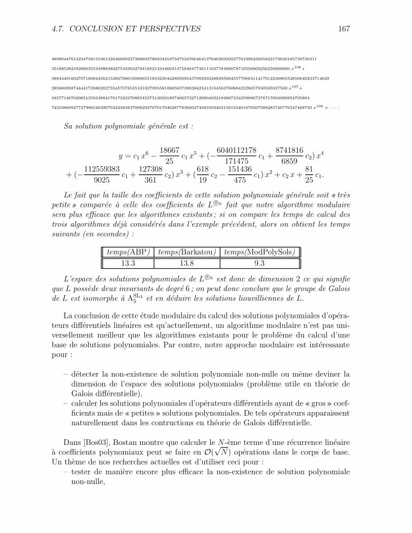
4.7. CONCLUSION ET PERSPECTIVES 167
489904476132347381519612264668922728869378693421973475247664641376462093922776199623605822173620185739730311
3518853821828863553498838027543304279418521434460414758404773611103778498078719556009256250000000 x108+
38844491602707186844562153667686100686551653230442805695437092503288295664557796631141791223686552850640233714629
285800958744441728862027354575785351618279955810685837390384254131645037608842328057930585937500 x107+
585771467029651355638841761732337086545375136921897466573271299049321948873342598867376717694080954705804
7431986092772799652639979222383837098202767017046287783606274565593463138155401076507308285746776547468750 x106 + · · · .
Sa solution polynomiale generale est :
y = c1 x6 − 18667
25c1 x5 + (−6040112178
171475c1 +
8741816
6859c2) x4
+ (−112559383
9025c1 +
127308
361c2) x3 + (
618
19c2 −
151436
475c1) x2 + c2 x +
81
25c1.
Le fait que la taille des coefficients de cette solution polynomiale generale soit « trespetite » comparee a celle des coefficients de L©s 6 fait que notre algorithme modulairesera plus efficace que les algorithmes existants ; si on compare les temps de calcul destrois algorithmes deja consideres dans l’exemple precedent, alors on obtient les tempssuivants (en secondes) :
temps(ABP) temps(Barkatou) temps(ModPolySols)
13.3 13.8 9.3
L’espace des solutions polynomiales de L©s 6 est donc de dimension 2 ce qui signifieque L possede deux invariants de degre 6 ; on peut donc conclure que le groupe de Galoisde L est isomorphe a ASL3
5 et en deduire les solutions liouvilliennes de L.
La conclusion de cette etude modulaire du calcul des solutions polynomiales d’opera-teurs differentiels lineaires est qu’actuellement, un algorithme modulaire n’est pas uni-versellement meilleur que les algorithmes existants pour le probleme du calcul d’unebase de solutions polynomiales. Par contre, notre approche modulaire est interessantepour :
– detecter la non-existence de solution polynomiale non-nulle ou meme deviner ladimension de l’espace des solutions polynomiales (probleme utile en theorie deGalois differentielle),
– calculer les solutions polynomiales d’operateurs differentiels ayant de « gros» coef-ficients mais de «petites» solutions polynomiales. De tels operateurs apparaissentnaturellement dans les contructions en theorie de Galois differentielle.
Dans [Bos03], Bostan montre que calculer le N -eme terme d’une recurrence lineairea coefficients polynomiaux peut se faire en O(
√N) operations dans le corps de base.
Un theme de nos recherches actuelles est d’utiliser ceci pour :– tester de maniere encore plus efficace la non-existence de solution polynomiale
non-nulle,

168 CHAPITRE 4. SOLUTIONS POLYNOMIALES D’E. D. L.
– calculer probabilistiquement la dimension de l’espace des solutions polynomiales,– calculer une base de solutions polynomiales.
Appendice
Systemes differentiels
Nous donnons ici les procedures servant a factoriser un systeme differentiel en ca-racteristique p. Ces procedures sont ecrites dans le logiciel de calcul formel Maple ; ellessont disponibles ahttp://www.unilim.fr/pages_perso/thomas.cluzeau/CluzeauModularFactorization
avec quelques explications sur les methodes utilisees. Les packages necessaires sont DE-tools et linalg.
Les systemes differentiels que nous considerons sont supposses a coefficients dansFp(z).
p-courbure
La procedure suivante calcule la p-courbure d’un systeme Y ′ = A Y avec A ∈Mn(Fp(z)) en suivant la methode sans denominateurs detaillee dans la sous-section 1.3.1.La variable z est donnee en entree : ceci nous permet d’utiliser aussi cette procedurepour calculer les p-courbures partielles dans le cas des systemes d’equations aux deriveespartielles. Les variables Lie Pol et d sont globales ; ceci nous permet de les re-utilisersi l’on souhaite cacluler une matrice fondamentale de solutions rationnelles avec la« formule de Katz» (voir Sous-section 1.3.5).
LiePol := proc (A, n, p, z)local i, j, B, S, De, d1 ;global Lie Pol, d ;
De := map(denom, A) ;d := lcm(seq( seq(Dei, j, j=1 .. n), i=1 .. n)) ;
d1 := diff( d, z) ;B := evalm( d ∗ A) ;Lie Pol0 := Matrix(n, n, shape=identity) ;Lie Pol1 := - B ;for i from 2 to pdoLie Poli := map(X → modp(Normal(X), p), evalm (
evalm( d ∗ diff mat( Lie Poli−1, p)) − ‘&*‘(B, Lie Poli−1)- evalm((i − 1) ∗ d1 ∗ Lie Poli−1)))
end do ;RETURN(map(X → modp(Normal(X), p), evalm( Lie Polp/ dp)))
end proc
169
170 Appendice : implantation
Polynome caracteristique
La procedure suivante calcule le polynome caracteristique d’une matrice M ∈ Mn(Fp(z)).Comme pour nos algorithmes les matrices dont nous devons calculer le polynome ca-racteristique sont a coefficients polynomiaux, nous n’utilisons pas la procedure charpolyde Maple, peu efficace lorsque les matrices sont a coefficients polynomiaux. Sur uneidee de M. van Hoeij, nous utilisons plutot une methode d’interpolation ; pour disposerd’assez de points pour pouvoir interpoler, p doit etre choisi strictement plus grand que n.
Char Pol modp := proc (M, λ , z, p)local n, Id, Mat, i, S, X , Mat pol ;
n := rowdim(M) ;Id := Matrix(n, n, shape=identity) ;Mat := evalm(λ ∗ Id− M) ;Mat pol := map(X → simplify(X) modp, concat( seq(
evalm(simplify(col( Mat, i)∗ lcm(seq(denom( col(Mat, i)j), j=1 .. n)))), i=1.. n))) ;
X := [seq(i, i=0 .. n)] ;S := [seq(Det(evalm( map(v → subs(λ =Xi, v), Mat pol)))mod p, i=1 .. n +
1)] ;RETURN(
collect(Rem(Primpart( Interp(X, S, λ )modp, λ) modp, zp - c, z)modp,λ ))end proc
LBTM et UBTM
Ces deux procedures construisent des matrices de Toeplitz par blocs (inferieures ousuperieures) ; ceci nous sera utile pour construire la matrice de l’operateur ∆A appeleeN dans la sous-section 1.2.1.
LBTM := proc (L, r, n, p)local N, j, T ;
if 0 < r thenN := matrix(n, n, 0) ;T := augment(stackmatrix( op(L)),
seq(stackmatrix(N $ j, op(L)1..r−j), j=1 .. r - 1))end if
end proc
UBTM := proc (L, r, n)local N, j, T ;
if 0 < r thenN := matrix(n, n, 0) ;T :=
stackmatrix(augment(op (L)), seq(augment(N $ j, op(L)1..r−j), j=1 .. r -
Appendice : implantation 171
1))end if
end proc
Decomposition d’une fraction rationnelle sur la base (1, z, . . . , zp−1)
Cette procedure decompose une fraction rationnelle appartenant a Fp(z) dans labase (1, z, . . . , zp−1) de Fp(z) sur Fp(z
p).
pdecomposition := proc (f, p)local PP, i, f1, Q, P1, S1, R, Q1, j ;
f := Normal(F)modp ;PP := numer(f) ;Q := denom(f) ;P1 := Rem(PP, zp - c, z)modp ;Q1 := Rem(Q, zp - c, z) modp ;Gcdex(Q1, zp - c, z, ’S1 ’, ’t’)mod p ;R := Rem(P1 ∗ S1, zp - c, z)modp ;for j from 0 to p - 1do f1j+1 := coeff(R , z, j)modp end do ;RETURN(seq(f1i, i=1 .. p))
end proc
Decomposition d’une matrice sur la base (1, z, . . . , zp−1)
pdecomposition mat := proc (A, n, p)local CC, i, Mat ;
CC := convert(map( pdecomposition, A, p, α ), array) ;for i to pdo Mati := concat(seq(col( CC, i + j ∗ p), j=0 .. n - 1)) end do ;RETURN(seq(evalm( Mati), i=1 .. p))
end proc
Derivee terme a terme d’une matrice
diff mat := proc(A, p) RETURN(map(modp, map(diff, evalm(A), z), p)) end proc
Matrice de l’operateur ∆A dans la base canonique de Fp(z)n sur Fp(zp)n
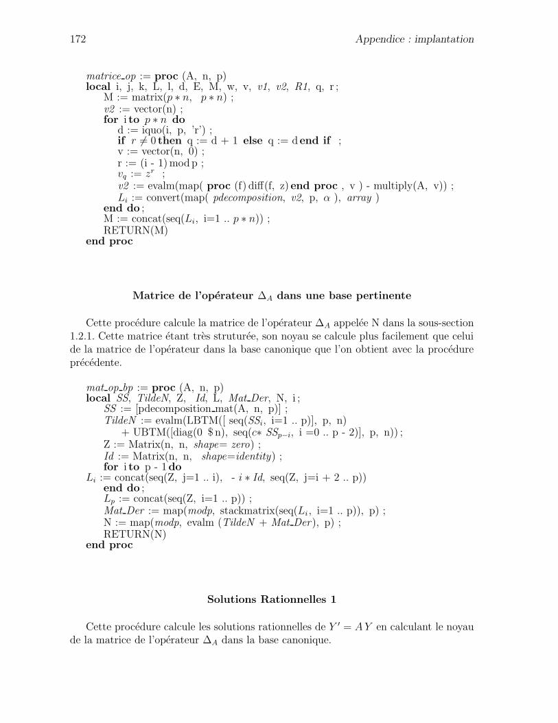
172 Appendice : implantation
matrice op := proc (A, n, p)local i, j, k, L, l, d, E, M, w, v, v1, v2, R1, q, r ;
M := matrix(p ∗ n, p ∗ n) ;v2 := vector(n) ;for i to p ∗ n do
d := iquo(i, p, ’r’) ;if r 6= 0 then q := d + 1 else q := d end if ;v := vector(n, 0) ;r := (i - 1)modp ;vq := zr ;v2 := evalm(map( proc (f) diff(f, z) end proc , v ) - multiply(A, v)) ;Li := convert(map( pdecomposition, v2, p, α ), array )
end do ;M := concat(seq(Li, i=1 .. p ∗ n)) ;RETURN(M)
end proc
Matrice de l’operateur ∆A dans une base pertinente
Cette procedure calcule la matrice de l’operateur ∆A appelee N dans la sous-section1.2.1. Cette matrice etant tres struturee, son noyau se calcule plus facilement que celuide la matrice de l’operateur dans la base canonique que l’on obtient avec la procedureprecedente.
mat op bp := proc (A, n, p)local SS, TildeN, Z, Id, L, Mat Der, N, i ;
SS := [pdecomposition mat(A, n, p)] ;TildeN := evalm(LBTM([ seq(SSi, i=1 .. p)], p, n)
+ UBTM([diag(0 $ n), seq(c∗ SSp−i, i =0 .. p - 2)], p, n)) ;Z := Matrix(n, n, shape= zero) ;Id := Matrix(n, n, shape=identity) ;for i to p - 1do
Li := concat(seq(Z, j=1 .. i), - i ∗ Id, seq(Z, j=i + 2 .. p))end do ;Lp := concat(seq(Z, i=1 .. p)) ;Mat Der := map(modp, stackmatrix(seq(Li, i=1 .. p)), p) ;N := map(modp, evalm (TildeN + Mat Der), p) ;RETURN(N)
end proc
Solutions Rationnelles 1
Cette procedure calcule les solutions rationnelles de Y ′ = A Y en calculant le noyaude la matrice de l’operateur ∆A dans la base canonique.
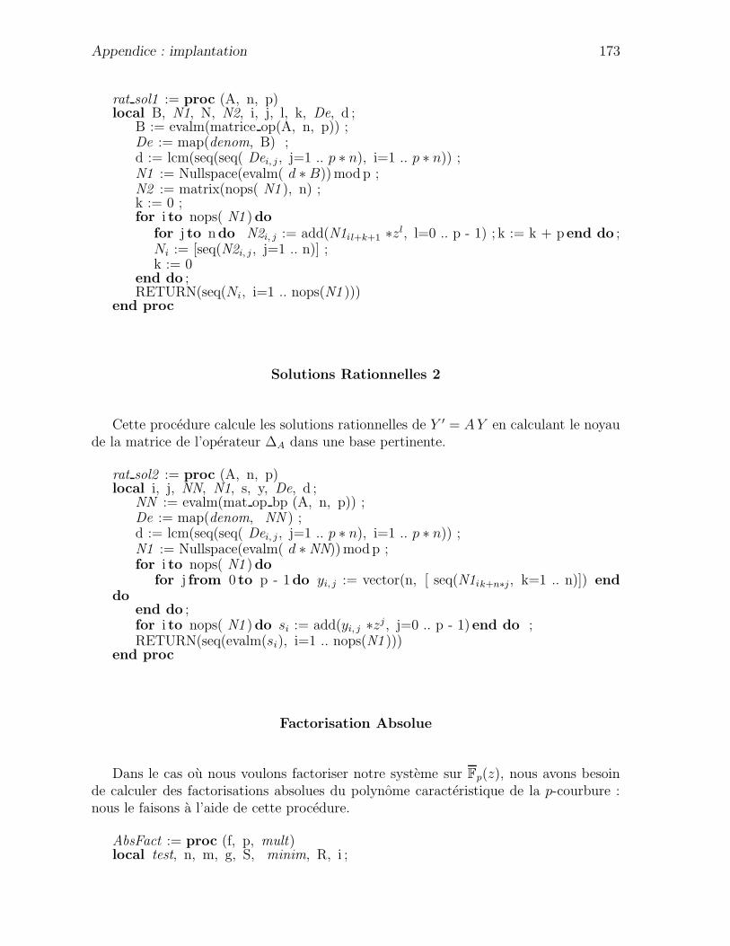
Appendice : implantation 173
rat sol1 := proc (A, n, p)local B, N1, N, N2, i, j, l, k, De, d ;
B := evalm(matrice op(A, n, p)) ;De := map(denom, B) ;d := lcm(seq(seq( Dei, j, j=1 .. p ∗ n), i=1 .. p ∗ n)) ;N1 := Nullspace(evalm( d ∗ B))modp ;N2 := matrix(nops( N1 ), n) ;k := 0 ;for i to nops( N1 )do
for j to ndo N2i, j := add(N1il+k+1 ∗zl, l=0 .. p - 1) ; k := k + p end do ;Ni := [seq(N2i, j, j=1 .. n)] ;k := 0
end do ;RETURN(seq(Ni, i=1 .. nops(N1 )))
end proc
Solutions Rationnelles 2
Cette procedure calcule les solutions rationnelles de Y ′ = A Y en calculant le noyaude la matrice de l’operateur ∆A dans une base pertinente.
rat sol2 := proc (A, n, p)local i, j, NN, N1, s, y, De, d ;
NN := evalm(mat op bp (A, n, p)) ;De := map(denom, NN ) ;d := lcm(seq(seq( Dei, j, j=1 .. p ∗ n), i=1 .. p ∗ n)) ;N1 := Nullspace(evalm( d ∗ NN))modp ;for i to nops( N1 )do
for j from 0 to p - 1do yi, j := vector(n, [ seq(N1ik+n∗j, k=1 .. n)]) enddo
end do ;for i to nops( N1 )do si := add(yi, j ∗zj, j=0 .. p - 1) end do ;RETURN(seq(evalm(si), i=1 .. nops(N1 )))
end proc
Factorisation Absolue
Dans le cas ou nous voulons factoriser notre systeme sur Fp(z), nous avons besoinde calculer des factorisations absolues du polynome caracteristique de la p-courbure :nous le faisons a l’aide de cette procedure.
AbsFact := proc (f, p, mult)local test, n, m, g, S, minim, R, i ;
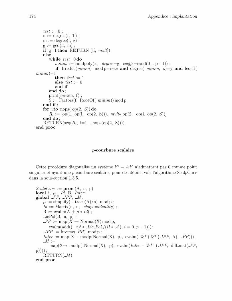
174 Appendice : implantation
test := 0 ;n := degree(f, T) ;m := degree(f, z) ;g := gcd(n, m) ;if g=1 then RETURN ([f, mult ])else
while test=0dominim := randpoly(x, degree=g, coeffs=rand(0 .. p - 1)) ;if Irreduc(minim) modp=true and degree( minim, x)=g and lcoeff(
minim)=1then test := 1else test := 0end if
end do ;print(minim, f) ;S := Factors(f, RootOf( minim))modp
end if ;for i to nops( op(2, S))do
Ri := [op(1, op(i, op(2, S))), mult∗ op(2, op(i, op(2, S))]end do ;RETURN(seq(Ri, i=1 .. nops(op(2, S))))
end proc
p-courbure scalaire
Cette procedure diagonalise un systeme Y ′ = A Y n’admettant pas 0 comme pointsingulier et ayant une p-courbure scalaire ; pour des details voir l’algorithme ScalpCurvdans la sous-section 1.3.5.
ScalpCurv := proc (A, n, p)local i, µ , Id, B, Inter ;global PP, IPP, M ;
µ := simplify( - trace(A)/n) modp ;Id := Matrix(n, n, shape=identity) ;B := evalm(A + µ ∗ Id) ;LiePol(B, n, p) ;PP := map(X → Normal(X)modp,
evalm(add((−z)i ∗ Lie Poli/(i ! ∗ di), i = 0..p − 1))) ;IPP := Inverse( PP) modp ;
Inter := map(X→ modp(Normal(X), p), evalm( ‘&*‘(‘&*‘( IPP, A), PP))) ;M :=
map(X→ modp( Normal(X), p), evalm(Inter - ‘&*‘ ( IPP, diff mat( PP,p)))) ;
RETURN( M )end proc
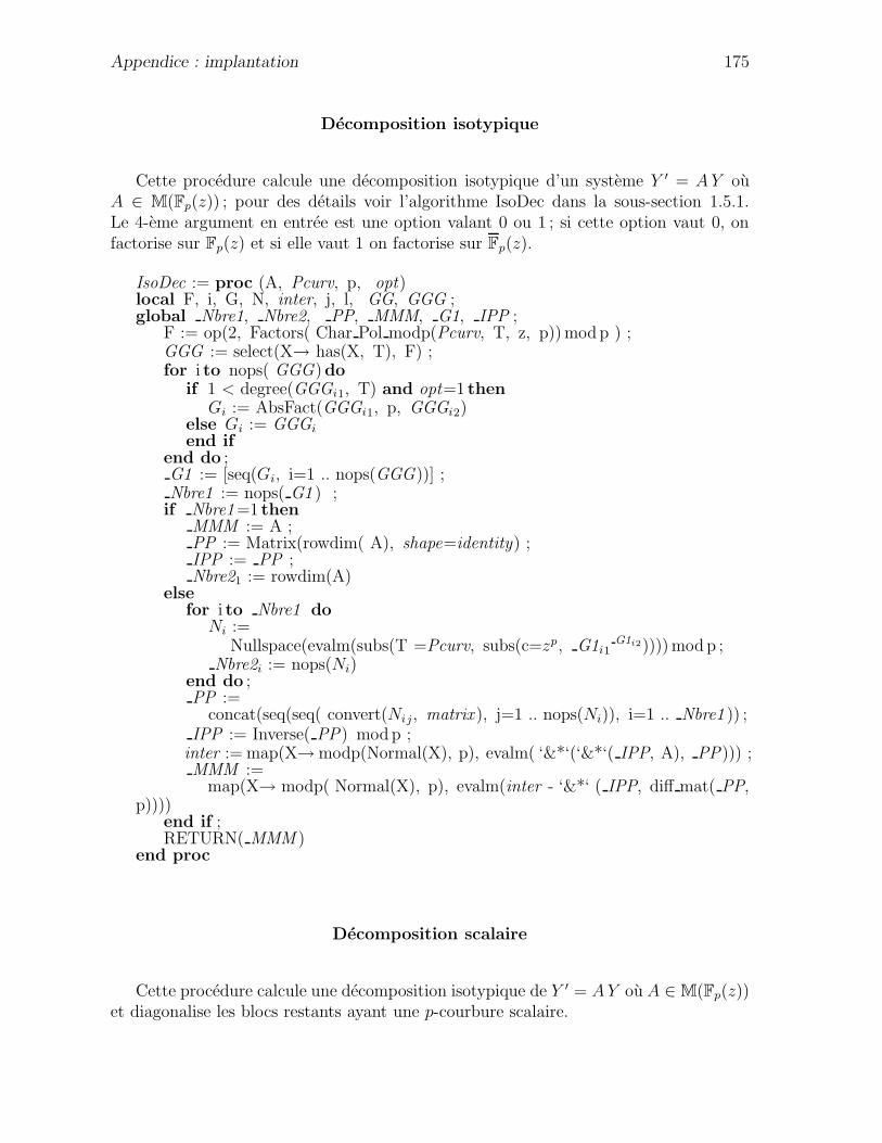
Appendice : implantation 175
Decomposition isotypique
Cette procedure calcule une decomposition isotypique d’un systeme Y ′ = A Y ouA ∈ M(Fp(z)) ; pour des details voir l’algorithme IsoDec dans la sous-section 1.5.1.Le 4-eme argument en entree est une option valant 0 ou 1 ; si cette option vaut 0, onfactorise sur Fp(z) et si elle vaut 1 on factorise sur Fp(z).
IsoDec := proc (A, Pcurv, p, opt)local F, i, G, N, inter, j, l, GG, GGG ;global Nbre1, Nbre2, PP, MMM, G1, IPP ;
F := op(2, Factors( Char Pol modp(Pcurv, T, z, p))modp ) ;GGG := select(X→ has(X, T), F) ;for i to nops( GGG)do
if 1 < degree(GGGi1, T) and opt=1 thenGi := AbsFact(GGGi1, p, GGGi2)
else Gi := GGGiend if
end do ;G1 := [seq(Gi, i=1 .. nops(GGG))] ;Nbre1 := nops( G1 ) ;if Nbre1=1 then
MMM := A ;PP := Matrix(rowdim( A), shape=identity) ;IPP := PP ;Nbre21 := rowdim(A)
elsefor i to Nbre1 do
Ni :=Nullspace(evalm(subs(T =Pcurv, subs(c=zp, G1i1
G1i2))))modp ;Nbre2i := nops(Ni)
end do ;PP :=
concat(seq(seq( convert(Nij, matrix ), j=1 .. nops(Ni)), i=1 .. Nbre1 )) ;IPP := Inverse( PP) modp ;
inter := map(X→ modp(Normal(X), p), evalm( ‘&*‘(‘&*‘( IPP, A), PP))) ;MMM :=
map(X→ modp( Normal(X), p), evalm(inter - ‘&*‘ ( IPP, diff mat( PP,p))))
end if ;RETURN( MMM )
end proc
Decomposition scalaire
Cette procedure calcule une decomposition isotypique de Y ′ = A Y ou A ∈ M(Fp(z))et diagonalise les blocs restants ayant une p-courbure scalaire.
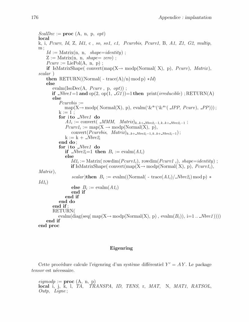
176 Appendice : implantation
ScalDec := proc (A, n, p, opt)localk, i, Pcurv, Id, Z, Id1, c , so, so1, c1, Pcurvbis, Pcurv1, B, A1, Z1, G2, multip,m ;
Id := Matrix(n, n, shape=identity) ;Z := Matrix(n, n, shape= zero) ;Pcurv := LiePol(A, n, p) ;if IsMatrixShape( convert(map(X→ modp(Normal( X), p), Pcurv), Matrix ),
scalar )then RETURN((Normal( - trace(A)/n)modp) ∗Id)else
evalm(IsoDec(A, Pcurv , p, opt)) ;if Nbre1=1 and op(2, op(1, G1 ))=1 then print(irreducible) ; RETURN(A)else
Pcurvbis :=map(X→ modp( Normal(X), p), evalm(‘&*‘(‘&*‘( IPP, Pcurv), PP))) ;
k := 1 ;for i to Nbre1 do
A1i := convert( MMM, Matrix)k..k+ Nbre2i−1, k..k+ Nbre2i−1 ;Pcurv1i := map(X → modp(Normal(X), p),
convert(Pcurvbis, Matrix)k..k+ Nbre2i−1, k..k+ Nbre2i−1) ;k := k + Nbre2i
end do ;for i to Nbre1 do
if Nbre2i=1 then Bi := evalm(A1i)else
Id1i := Matrix( rowdim(Pcurv1i), rowdim(Pcurv1 i), shape=identity) ;if IsMatrixShape( convert(map(X→ modp(Normal( X), p), Pcurv1i),
Matrix ),scalar)then Bi := evalm((Normal( - trace(A1i)/ Nbre2i)modp) ∗
Id1i)else Bi := evalm(A1i)end if
end ifend do
end if ;RETURN(
evalm(diag(seq( map(X→ modp(Normal(X), p) , evalm(Bi)), i=1 .. Nbre1 ))))end if
end proc
Eigenring
Cette procedure calcule l’eigenring d’un systeme differentiel Y ′ = A Y . Le packagetensor est necessaire.
eigmodp := proc (A, n, p)local i, j, k, l, TA, TRANSPA, ID, TENS, r, MAT, N, MAT1, RATSOL,Outp, Ligne ;
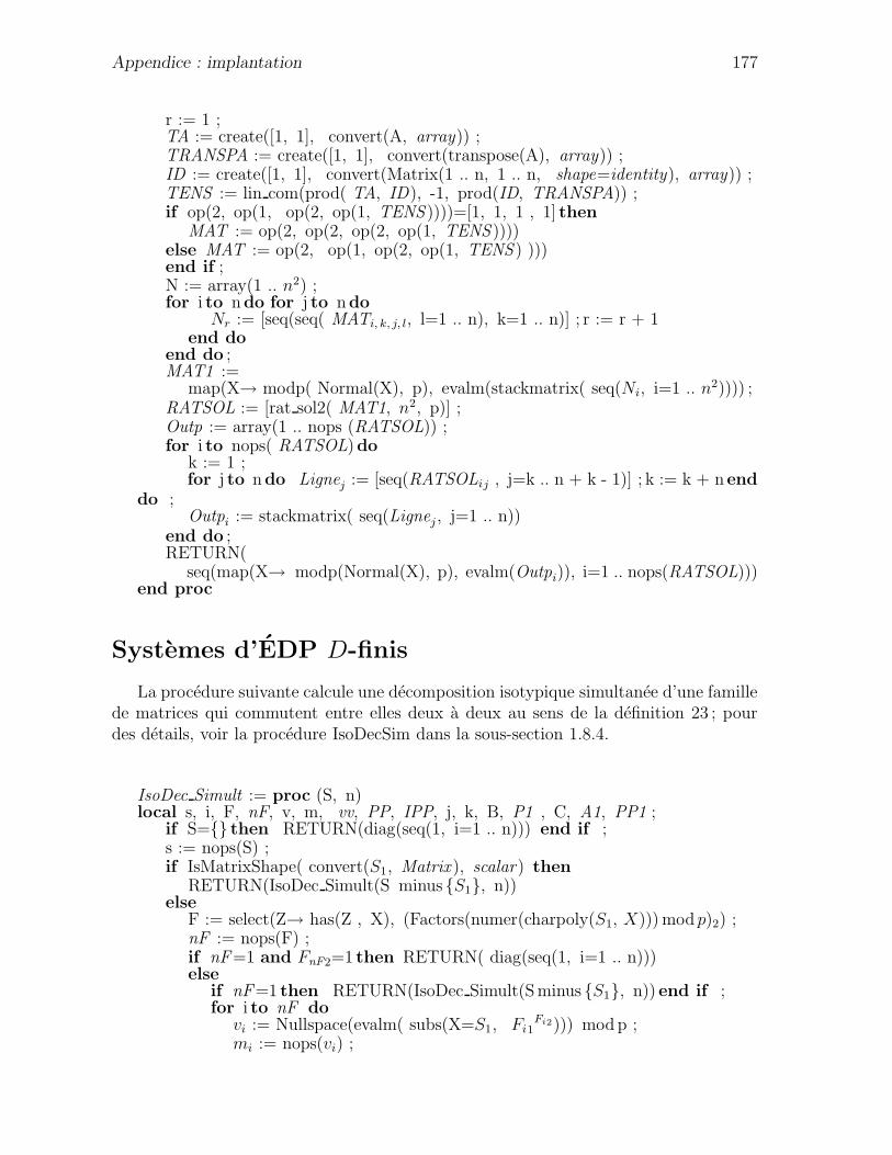
Appendice : implantation 177
r := 1 ;TA := create([1, 1], convert(A, array)) ;TRANSPA := create([1, 1], convert(transpose(A), array)) ;ID := create([1, 1], convert(Matrix(1 .. n, 1 .. n, shape=identity), array)) ;TENS := lin com(prod( TA, ID), -1, prod(ID, TRANSPA)) ;if op(2, op(1, op(2, op(1, TENS ))))=[1, 1, 1 , 1] then
MAT := op(2, op(2, op(2, op(1, TENS ))))else MAT := op(2, op(1, op(2, op(1, TENS ) )))end if ;N := array(1 .. n2) ;for i to ndo for j to ndo
Nr := [seq(seq( MATi, k, j, l, l=1 .. n), k=1 .. n)] ; r := r + 1end do
end do ;MAT1 :=
map(X→ modp( Normal(X), p), evalm(stackmatrix( seq(Ni, i=1 .. n2)))) ;RATSOL := [rat sol2( MAT1, n2, p)] ;Outp := array(1 .. nops (RATSOL)) ;for i to nops( RATSOL)do
k := 1 ;for j to ndo Lignej := [seq(RATSOLij , j=k .. n + k - 1)] ; k := k + n end
do ;Outpi := stackmatrix( seq(Lignej, j=1 .. n))
end do ;RETURN(
seq(map(X→ modp(Normal(X), p), evalm(Outpi)), i=1 .. nops(RATSOL)))end proc
Systemes d’EDP D-finis
La procedure suivante calcule une decomposition isotypique simultanee d’une famillede matrices qui commutent entre elles deux a deux au sens de la definition 23 ; pourdes details, voir la procedure IsoDecSim dans la sous-section 1.8.4.
IsoDec Simult := proc (S, n)local s, i, F, nF, v, m, vv, PP, IPP, j, k, B, P1 , C, A1, PP1 ;
if S={} then RETURN(diag(seq(1, i=1 .. n))) end if ;s := nops(S) ;if IsMatrixShape( convert(S1, Matrix ), scalar) then
RETURN(IsoDec Simult(S minus {S1}, n))else
F := select(Z→ has(Z , X), (Factors(numer(charpoly(S1, X))) mod p)2) ;nF := nops(F) ;if nF=1 and FnF2=1 then RETURN( diag(seq(1, i=1 .. n)))else
if nF=1 then RETURN(IsoDec Simult(Sminus {S1}, n)) end if ;for i to nF do
vi := Nullspace(evalm( subs(X=S1, Fi1Fi2))) modp ;
mi := nops(vi) ;
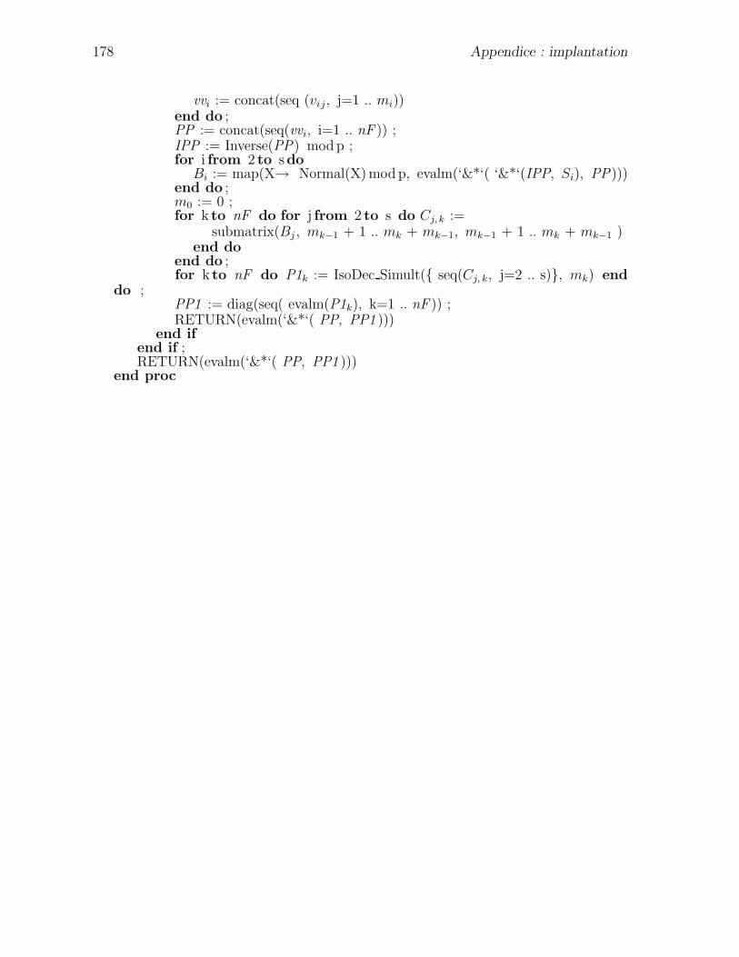
178 Appendice : implantation
vvi := concat(seq (vij, j=1 .. mi))end do ;PP := concat(seq(vvi, i=1 .. nF )) ;IPP := Inverse(PP) modp ;for i from 2 to sdo
Bi := map(X→ Normal(X)modp, evalm(‘&*‘( ‘&*‘(IPP, Si), PP)))end do ;m0 := 0 ;for k to nF do for j from 2 to s do Cj, k :=
submatrix(Bj , mk−1 + 1 .. mk + mk−1, mk−1 + 1 .. mk + mk−1 )end do
end do ;for k to nF do P1k := IsoDec Simult({ seq(Cj, k, j=2 .. s)}, mk) end
do ;PP1 := diag(seq( evalm(P1k), k=1 .. nF )) ;RETURN(evalm(‘&*‘( PP, PP1 )))
end ifend if ;RETURN(evalm(‘&*‘( PP, PP1 )))
end proc
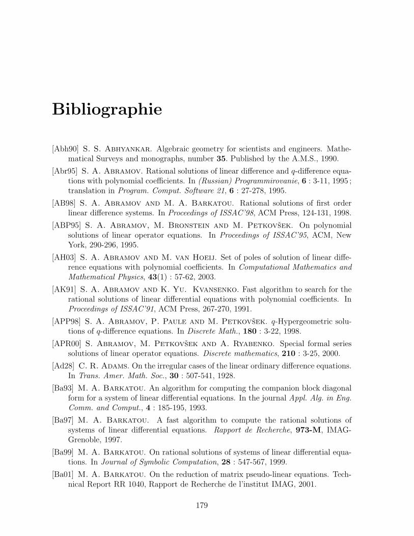
Bibliographie
[Abh90] S. S. Abhyankar. Algebraic geometry for scientists and engineers. Mathe-matical Surveys and monographs, number 35. Published by the A.M.S., 1990.
[Abr95] S. A. Abramov. Rational solutions of linear difference and q-difference equa-tions with polynomial coefficients. In (Russian) Programmirovanie, 6 : 3-11, 1995 ;translation in Program. Comput. Software 21, 6 : 27-278, 1995.
[AB98] S. A. Abramov and M. A. Barkatou. Rational solutions of first orderlinear difference systems. In Proceedings of ISSAC’98, ACM Press, 124-131, 1998.
[ABP95] S. A. Abramov, M. Bronstein and M. Petkovsek. On polynomialsolutions of linear operator equations. In Proceedings of ISSAC’95, ACM, NewYork, 290-296, 1995.
[AH03] S. A. Abramov and M. van Hoeij. Set of poles of solution of linear diffe-rence equations with polynomial coefficients. In Computational Mathematics andMathematical Physics, 43(1) : 57-62, 2003.
[AK91] S. A. Abramov and K. Yu. Kvansenko. Fast algorithm to search for therational solutions of linear differential equations with polynomial coefficients. InProceedings of ISSAC’91, ACM Press, 267-270, 1991.
[APP98] S. A. Abramov, P. Paule and M. Petkovsek. q-Hypergeometric solu-tions of q-difference equations. In Discrete Math., 180 : 3-22, 1998.
[APR00] S. Abramov, M. Petkovsek and A. Ryabenko. Special formal seriessolutions of linear operator equations. Discrete mathematics, 210 : 3-25, 2000.
[Ad28] C. R. Adams. On the irregular cases of the linear ordinary difference equations.In Trans. Amer. Math. Soc., 30 : 507-541, 1928.
[Ba93] M. A. Barkatou. An algorithm for computing the companion block diagonalform for a system of linear differential equations. In the journal Appl. Alg. in Eng.Comm. and Comput., 4 : 185-195, 1993.
[Ba97] M. A. Barkatou. A fast algorithm to compute the rational solutions ofsystems of linear differential equations. Rapport de Recherche, 973-M, IMAG-Grenoble, 1997.
[Ba99] M. A. Barkatou. On rational solutions of systems of linear differential equa-tions. In Journal of Symbolic Computation, 28 : 547-567, 1999.
[Ba01] M. A. Barkatou. On the reduction of matrix pseudo-linear equations. Tech-nical Report RR 1040, Rapport de Recherche de l’institut IMAG, 2001.
179
180 BIBLIOGRAPHIE
[BD94] M. A. Barkatou and A. Duval. Sur les series formelles solutionsd’equations aux differences polynomiales. In Ann. Inst. Fourier(Grenoble), 44(2) :495-524, 1994.
[BP98] M. A. Barkatou and E. Pflugel. On the equivalence problem of lineardifferential systems and its application for factoring completely reducible systems.In Proceedings of ISSAC’98, ACM Press, 268-275, 1998.
[Be1894] E. Beke. Die irreduzibilitat der homogenen linearen differentialgleichungen.In Math. Ann., 45 : 278-294, 1894.
[Bi30] G. D. Birkhoff. Formal theory of irregular linear difference equations. InActa Math., 54 : 205-246, 1930.
[BCGPR03] Y. A. Blinkov, C. F. Cid, V. T. Gerdt, W. Plesken and D. Ro-
bertz. The Maple package “Janet” : II. Polynomial Systems. In CASC, 2003.
[BV83] E. Bombieri and J. Vaaler. On Siegel’s lemma. In Invent. Math., 73(1) :11-32, 1983.
[Bom01] R. Bomboy. Reductibilite et resolubilite des equations aux differences finies.These de l’Universite de Nice-Sophia Antipolis, 2001.
[Bos03] A. Bostan. Algorithmique efficace pour des operations de base en calculformel. These de l’Ecole polytechnique, 2003.
[BLS03] A. Bostan, G. Lecerf and E. Schost. Tellegen’s principle into practice.In Proceeding of ISSAC’03, ACM Press, 37-44, 2003.
[Bou00] D. Boucher. Sur les equations differentielles lineaires parametrees, une ap-plication aux systemes Hamiltoniens. These de l’Universite de Limoges, 2000.
[Br92] M. Bronstein. On solutions of linear ordinary differential equations in theircoefficient field. In Journal of Symbolic Computation, 13 : 413-440, 1992.
[Br94] M. Bronstein. An improved algorithm for factoring linear ordinary differentialoperators. In Proceedings of ISSAC’94, ACM Press, 336-340, 1994.
[Ca94] J. Cai. Computing Jordan normal forms exactly for commuting matrices inpolynomial time. In International Journal of Foundations of Computer Sciences,5(3) : 293-302, 1994.
[CO68] L. Chambadal and J. L. Ovaert. Algebre lineaire et algebre tensorielle.Dunot Universite, Paris, 1968.
[Ch01] A. Chambert-Loir. Theoremes d’algebricite en geometrie diophantienne.Seminaire Bourbaki, expose No. 886, Mars 2001.
[CC85] D. V. Chudnovsky and G. V. Chudnovsky. Applications of Pade ap-proximations to the Grothendieck conjecture on linear equations. In Lecture Notesin Mathematics, Number Theory, vol. 1135 : 52-100, 1985.
[CK02] R. C. Churchill and J. J. Kovacic. Cyclic vectors. In Differential Algebraand Related Topics, Proceedings of the International Workshop, Rutgers University,Newark, November 2-3 2002.
BIBLIOGRAPHIE 181
[Cl03] T. Cluzeau. Factorization of differential systems in characteristic p. In Pro-ceedings of ISSAC’03, ACM Press, 58-65, 2003.
[CH04] T. Cluzeau and M. van Hoeij. A modular algorithm for computing theexponential solutions of a linear differential operator. In Journal of Symbolic Com-putation, 38(3) : 1043-1076, 2004.
[CE95] G. E. Collins and M. J. Encarnacion. Efficient rational number recons-truction. In Journal of Symbolic Computation, 20(3) : 287-297, 1995.
[CW04] E. Compoint and J.-A. Weil. Absolute reducibility of differential operatorsand Galois groups. In Journal of Algebra, 275 : 77-105, 2004.
[Co36] F. T. Cope. Formal solutions of irregular linear differential equations, Part II.In Amer. J. Math., 58 : 130-140, 1936.
[Cor01] O. Cormier. On liouvillian solutions of linear differential equations of order4 and 5. In Proceedings of ISSAC’01, ACM Press : 93-100, 2001.
[CSTU02] O. Cormier, M. F. Singer, B. T. Trager and F. Ulmer. Linear dif-ferential operators for polynomial equations. In Journal of Symbolic Computation,34 : 355-398, 2002.
[DiV02] L. Di Vizio. Arithmetic theory of q-difference equations : the q-analogueof Grothendieck-Katz’s conjecture on p-curvatures. In Invent. Math., 150(3) :517-578, 2002.
[Du83] A. Duval. Lemmes de Hensel et factorisation formelle pour les operateurs auxdifferences. In Funkcial Ekvac., 26 : 349-368, 1983.
[En94] M. J. Encarnacion. On a modular algorithm for computing gcds of polyno-mials over algebraic number fields. In Proceedings of ISSAC’94, ACM Press, 58-65,1994.
[Ga66] F. R. Gantmacher. Theorie des matrices, Tome 1. Dunot (Paris), 1966.
[GG99] J. von zur Gathen and J. Gerhart. Modern computer algebra. CambridgeUniversity Press, 1999.
[Gi98] M. Giesbrecht. Factoring in skew-polynomial rings over finite fields. In Jour-nal of Symbolic Computation, 24(5) : 463-486, 1998.
[GZ03] M. Giesbrecht and Y. Zhang. Factoring and decomposing Ore polynomialsover Fp(t). In Proceedings of ISSAC’03, ACM Press, 127-134, 2003.
[GLR82] I. Gohberg, P. Lancaster and L. Rodman. Matrix polynomials. InAcademic Press (New york, London, Paris), 1982.
[Gr90] D. Y. Grigoriev. Complexity of irreducibility testing for a system of linearordinary differential equations. In Proceedings of ISSAC’90, ACM Press, 225-230,1990.
[HS02] M. Hausdorf and M. Seiler. Involutives basis in MuPAD-Part I : involutivedivisions. In MathPad, 11/1 : 51-56, 2002.
[Hoe98] S. Hoeppner. Differential equations with 2-term recursion. In ManuscriptaMath., 95(3) : 349-362, 1998.
182 BIBLIOGRAPHIE
[Hon81] T. Honda. Algebraic differential equations. In Symp. Math., 24 : 169-204,1981.
[Ho96] M. van Hoeij. Rational solutions of the mixed differential equation and itsapplication to factorization of differential operators. In Proceedings of ISSAC’96,ACM Press, 219-225, 1996.
[Ho97b] M. van Hoeij. Factorization of differential operators with rational functionscoefficients. Journal Of Symbolic Computation, 24 : 537-561, 1997.
[Ho97a] M. van Hoeij. Formal solutions and factorization of differential operatorswith power series coefficients. Journal Of Symbolic Computation, 24 : 1-30, 1997.
[Ho98] M. van Hoeij. Rational solutions of linear difference equations. In Proceedingsof ISSAC’98 : 120-123, 1998.
[Ho99] M. van Hoeij. Finite singularities and hypergeometric solutions of linear re-currence equations. In Journal of Pure and Applied Algebra, 139 : 109-131, 1999.
[Ho02] M. van Hoeij. Factoring polynomials and the knapsack problem. Journal ofNumber Theory, 95 : 167-189, 2002.
[HM02] M. van Hoeij and M. Monagan. A modular gcd algorithm over numberfields presented with multiple extensions. In Proceedings of ISSAC’02, ACM Press,109-116, 2002.
[HRUW98] M. van Hoeij, J.-F. Ragot, F. Ulmer and J.-A. Weil. Liouvilliansolutions of linear differential equations of order three and higher. In Journal ofSymbolic Computation, 11 : 1-17, 1998.
[HW97] M. van Hoeij and J.-A. Weil. An algorithm for computing invariantsof differential Galois groups. In Journal of Pure and Applied Algebra, 117-118 :353-379, 1997.
[Ho81] T. Honda. Algebraic differential equations. In Symp. Math., 24 : 169-204,1981.
[In26] E. L. Ince. Ordinary differential equations. Dover Publications, INC. NewYork, 1926.
[IRS94] G. Ivanyos, L Ronyai, and A. Szanto. Decomposition of algebras overFq(X1, . . . , Xm). In the journal Appl. Alg. in Eng. Comm. and Comp., 5(2) : 71-90,1994.
[Ja37] N. Jacobson. Pseudo-linear transformations. In Annals of Math., 38(2) :484-507, 1937.
[Ja85] N. Jacobson. Basic algebra I, Second Edition. W.H. Freeman and Compagny,New York, 1985.
[Ja80] N. Jacobson. Basic algebra II. W.H. Freeman and Compagny, San Francisco,1980.
[Ja20] M. Janet. Sur les systemes aux derivees partielles. In Journal de Math., 8-emeserie, III, 65-151, 1924.
BIBLIOGRAPHIE 183
[Ja29] M. Janet. Lecons sur les systemes d’equations aux derivees partielles. InCahiers Scientifiques, IV, Gauthiers-Villars, 1929.
[Ka70] N. Katz. Nilpotent connections and the monodromy theorem : applications ofa result of Turritin. In Publ. Math. I. H. E. S., 39 : 355-412, 1970.
[Ka82] N. Katz. A conjecture in the arithmetic theory of differential equations. Bull.Soc. Math. France, 110 : 203-239, 1982.
[LLL82] A. K. Lenstra, H. W. Lenstra Jr. and L. Lovasz. Factoring polyno-mials with rational coefficients. In Math. Ann., 261 : 515-534, 1982.
[Le94] A. H. M. Levelt. The semi-simple part of a matrix. In Algorithmen in deAlgebra, 85-88, 1994.
[LST02] Z. Li, F. Schwarz and S. P. Tsarev. Factoring zero-dimensional idealsof linear partial differential operators. In Proceedings of ISSAC’02, ACM Press,168-175, 2002.
[LST03] Z. Li, F. Schwarz and S. P. Tsarev. Factoring systems of linear PDEswith finite-dimensional solution spaces. In Journal of Symbolic Computation, 36(3-4) : 443-471, 2003.
[Ma01] B. H. Matzat. Differential Galois theory in positive characteristic. Notes byJ. Hartmann. In IWR-Preprint, 2001-35.
[MP02] B. H. Matzat and M. van der Put. Constructive differential Galois theoryIn IWR-Preprint, 2002-02.
[Mo04] M. Monagan. Maximal quotient rational reconstruction : an almost optimalalgorithm for rational reconstruction. In Proceedings of ISSAC’04, ACM Press,2004.
[MS98] T. Mulders and A. Storjohann. Fast algorithms for linear algebra moduloN . Lecture notes in computer science, 1461, Algorithms-ESA’98 : 139-150, 1998.
[MS03] T. Mulders and A. Storjohann. On lattice reduction for polynomialmatrices. Journal of Symbolic Computation, 35(4) : 377-401, 2003.
[No29] N. E. Norlund. Lecons sur les equations lineaires aux differences finies. InGauthiers Villard et Cie, Paris, 1929.
[Or32] O. Ore. Formale theorie der linearen differentialgleichungen (Zweiter Teil), InJ. fur d. Reine u. angew. Math., 168 : 233-252, 1932.
[Or33] O. Ore. Theory of non-commutative polynomials. In Annals of Math., 34 :480-508, 1933.
[Pe92] M. Petkovsek. Hypergeometric solutions of linear recurrences with polynomialcoefficients. In Journal of Symbolic Computation, 14(2-3) : 243-264, 1992.
[PWZ96] M. Petkovsek, H. S. Wilf and D. Zeilberger. A = B. With a forewordby Donald E. Knuth., 1996.
[Pf97] E. Pflugel. An algorithm for computing exponential solutions of first orderlinear differential systems. In Proceedings of ISSAC’97, ACM Press, 164-171, 1997.
184 BIBLIOGRAPHIE
[Pu95] M. van der Put. Differential equations in characteristic p. In Comp. Math.,97 : 227-251, 1995.
[Pu96] M. van der Put. Reduction modulo p of differential equations. Indag.Math.N.S., 7(3) : 367-387, 1996.
[Pu97] M. van der Put. Modular methods for factoring differential operators. Un-published manuscript (Preliminary Version), 1997.
[Pu01] M. van der Put. Grothendieck’s conjecture for the rish equation y ′ = ay + b.Indag. Math., 12(1) : 113-124, 2001.
[PS97] M. van der Put and M. F. Singer. Galois theory of difference equations.In Lectures Notes in Mathematics, vol. 1666, Springer (Berlin), 1997.
[PS03] M. van der Put and M. F. Singer. Galois Theory of Linear DifferentialEquations, vol. 328. Grundlehren der mathematischen Wissenschaften, Springer,2003.
[SSV04] D. Saunders, A. Storjohann and G. Villard. Matrix Rank Certifica-tion. In Electronic Journal of Linear Algebra, vol. 11 : 16-23, 2004.
[Sc89] F. Schwarz. A factorization algorithm for linear ordinary differential equations.In Proceedings of ISSAC’89, ACM Press, 17-25, 1989.
[Si91] M. F. Singer. Liouvillian solutions of linear differential equations with liou-villian coefficients. Journal of Symbolic Computation, 11 : 251-273, 1991.
[Si96] M. F. Singer. Testing reducibility of linear differential operators : a grouptheoretic perspective. In the journal Appl. Alg. in Eng. Comm. and Comp., 7(2) :77-104, 1996.
[St03] A. Storjohann. High-order lifting and integrality certification. In Journal ofSymbolic Computation 36(3-4) : 613-648, 2003.
[Ts94] S. P. Tsarev. Some problems that arise in the factorization of linear ordi-nary differential operators. In Programmirovanie, 1 : 45-48, 1994. Translation inProgramming and Comput. Software, 20(1) : 27-29, 1994.
[Ts98] S. P. Tsarev. Factorization of linear partial differential operators and theDarboux integrability of nonlinear PDEs. In SIGSAM Bulletin, 32(4) : 21-28,1998.
[Ts01] S. P. Tsarev. Factorization of overdetermined systems of linear partial dif-ferential equations with finite-dimensional solution space. In Computer algebra inscientific computing (Konstanz) : 529-539, 2001.
[Ul03] F. Ulmer. Liouvillian solutions of third order differential equations. In Journalof Symbolic Computation, 36 : 855-889, 2003.
[UW96] F. Ulmer and J.-A. Weil. Note on Kovacic’s algorithm. In Journal OfSymbolic Computation, 22 : 179-200, 1996.
[We01] C. Weixlbaumer. Solutions of difference equations with polynomial coeffi-cients. Diplomarbeit, RICS Linz, Johannes Kepler Universitat, 2001.
[Wu04] M. Wu. Factorization and decomposition of linear functional systems. PhDthesis, in preparation, 2004.
Abstract : Modular methods lead to very efficient algorithms in many areas of com-puter algebra and particularly for the study of algebraic equations. The goal of thisthesis is to show how these modular techniques can be adapted to the differential caseand allow to create new algorithms (or to improve existing algorithms) for linear diffe-rential equations. The first part deals with the factorisation of differential operators inpositive characteristic. The “miracle” in characteristic p is that the problem reduces tolinear algebra. Using this fact, we develop algorithm for factoring differential systems.We give the complexity of the distinct steps of this algorithm. Finally, we generalizeit to the setting of partial differential systems. The topic of the second part is makingBeke’s algorithm to compute the exponential solutions of linear differential equationsmore efficient. This algorithms suffers from two drawbacks : a combinatorial problemand a field problem. We show that combining local “geometric” data (the generalizedexponents) and modular “arithmetic” data (the eigenvalues of the p-curvature) allowsto decrease the number of combinations usually considered by the algorithm and toreduce the degree of the algebraic extensions of the base field needed to compute theexponential solutions. In the third part, we prove that a similar approach applies tothe same problem for difference equations. In the last section, we develop a fully mo-dular algorithm for computing the polynomial solutions of linear differential equationsin characteristic zero. We evaluate the relevance of the modular informations that canbe obtained for this problem. We give and compare the complexity of our algorithmand that of the existing ones. Finally, thanks to experimental comparisons, we exhibita class of differential equations for which our modular approach is more relevant thanexisting algorithms. Most of our algorithms have been implemented in the computeralgebra system Maple.
Resume : Les methodes modulaires conduisent a des algorithmes tres efficaces dans denombreux domaines en calcul formel et notamment dans celui des equations algebriques.Le but de cette these est de montrer comment ces techniques modulaires s’adaptent aucas differentiel et permettent de developper de nouveaux algorithmes (ou d’ameliorerdes algorithmes existants) pour l’etude d’equations differentielles lineaires. La premierepartie traite du probleme de la factorisation d’operateurs differentiels en caracteristiquepositive. Le «miracle» de la caracteristique p est que le probleme peut se reduire ade l’algebre lineaire. En exploitant ce fait, nous developpons un algorithme de facto-risation de systemes differentiels. Nous donnons la complexite des differentes etapesde cet algorithme. Enfin, nous le generalisons au cadre de systemes d’equations auxderivees partielles. L’objet de la deuxieme partie est de rendre plus efficace l’algorithmede Beke pour le calcul des solutions exponentielles d’equations differentielles lineaires.Cet algorithme possede deux inconveniants majeurs qui le rendent peu efficace : unprobleme combinatoire et un probleme de corps. Nous montrons qu’en combinant desinformations « geometriques» locales (les exposants generalises) et des informations« arithmetiques» modulaires (les valeurs propres de la p-courbure), nous pouvons dimi-nuer le nombre de combinaisons considerees habituellement par l’algorithme et reduire ledegre des extensions algebriques du corps de base necessaires au calcul des solutions ex-ponentielles. Dans la troisieme partie, nous demontrons qu’une demarche similaire s’ap-plique pour le probleme analogue dans le cas des equations aux differences. Finalement,dans la derniere partie, nous developpons un algorithme entierement modulaire cal-culant les solutions polynomiales d’equations differentielles lineaires en caracteristiquezero. Nous evaluons la pertinence des informations modulaires que l’on peut obtenirpour ce probleme. Nous donnons et comparons les complexites de notre algorithme etdes algorithmes existants. Puis, grace a des comparaisons experimentales, nous exhibonsdes classes d’equations pour lesquelles notre approche modulaire est mieux adaptee queles algorithmes existants. La plupart de nos algorithmes ont ete implantes dans le logicielde calcul formel Maple.