Statistical synthesis of tropical cyclone tracks in a …crlmd/stage_US/report.pdf · Statistical...

Rapport de stagede deuxieme année de Magistère de l’Ecole Normale Supérieure

10 Février - 10 Aout

Statistical synthesis of tropical cyclone tracks ina risk evaluation perspective

Synthèse de trajectoires de cyclones selon un modèlestatistique dans une perspective d’estimation des risques

Camille Risi

sous la direction de

Kerry Emanuel

au

Massachussets Institute of TechnologyDepartment of Earth, Atmospheric and Planetary Sciences

Program in Atmosphere, Oceans and Climate

Statistical synthesis of tropical cyclone tracks in a risk evaluationperspective

Camille Risi

February 10th - August 10th

Summary

During my 6-month internship, I was involved in a project to assess long-term wind risks related to tropical cyclones.While the tropical cyclone natural frequency is quite low and relatively few cyclones have been recorded in the past, thisproject relies on the synthesis of a large number of tropical cyclones that statistically conform to real ones. Cyclone tracksare first generated through a statistical model based on the historical cyclone track record. A deterministic and dynamicalintensity and wind model is then applied along these synthetic tracks.

I worked on the development and implementation of the track synthesis algorithm. Cyclone tracks are modeled as aMarkov chain. Genesis and conditional probabilities are first estimated from the historical cyclone tracks database. Tracksare then created during a Monte Carlo simulation.

Main problems faced are on the one hand the limited number of recorded tracks in the database from which to estimateprobabilities, and on the other hand, the excessively large size of the probability arrays to estimate and store.

Résumé

Au cours de mon stage de 6 mois, j’ai participé à un projet d’estimation des risques, à long terme, de vents liés auxcyclones tropicaux. Tandis que la fréquence naturelle des cyclones tropicaux est assez faible et que relativement peu decyclones ont été enregistrés dans le passé, ce projet repose sur la synthèse d’un très grand nombre de cyclones conformesstatistiquement aux réels. Les trajectoires de cyclones sont d’abord synthetisées selon un modèle statistique fondé sur labase de données des cyclones enregistrés dans le passé. Le long de celles-ci est ensuite appliqué un modèle dynamique etdéterministe d’intensité et de vents.

J’ai travaillé au cours de mon stage sur le développement et l’implémentation de l’algorithme de synthèse de trajectoires.Les trajectoires de cyclones sont modélisées sous la forme d’une chaine de Markov. Les probabilités conditionnelles et degénèse sont tout d’abord calculées à partir des données historiques. Les trajectoires sont ensuite créées au cours d’unesimulation de Monte carlo.

Les principaux problèmes auquels j’ai du faire face sont d’une part le faible nombre de trajectoires enregistrées dans labase de donnée, à partir desquels estimer les probabilités, et d’autre part la taille excessivement importante des tableaux deprobabilités à estimer et stocker.

2

Introduction

My 6-month internship took place at the Massachusetts Institute of Technology under the supervision of Dr. KerryEmanuel, within the Program in Atmosphere, Oceans and Climate of the Department of Earth, Atmospheric and PlanetarySciences. I got involved in a project to assess long-term wind risks related to tropical cyclones.

A tropical cyclone(TC) is a cyclonically rotating storm with typical horizontal scales of 100-1000 km and whichextends through the depth of the troposphere. Tropical cyclones originate over tropical oceans, are driven principally byheat transfer from the ocean surface, and die over cold water or land ([Emanuel, 2003, Emanuel, 1998]). They are alsocalledhurricanesin North Atlantic andtyphoonsin Western Pacific.

Tropical cyclones are among the most destructive and lethal natural disasters. They cause loss of lives and enormousproperty damage around the world every year. While greatest risks to life commonly results from flooding and landslidesfollowing storm surges or torrential rains (300,000 people are estimated to have died from a TC-associated storm surge inBangladesh in 1970 ([hrd, 2004])), the largest part of material and financial damage are usually caused by hurricane-relatedhigh winds, and resulting roof loss, building failure and air-borne debris ([Wyatt, 1999, Cochran, 2000]). As an example,the losses Hurricane Andrew in 1992 is responsible for reached US $26.5 billion ([hrd, 2004]).

It is therefore of high importance not only to be able to precisely forecast approaching TCs on the short term, but also toassess long term risks in perspectives of reinsurance, emergency planning, population warning in vulnerable coastal areas,land management and building codes establishment.

Generally, long term hurricane assessment models consist in, on the one hand, a meteorological component, to assesswind or storm surges probabilities, and on the other hand, loss projection models that take into account environmentvulnerability ([Powell and coauthors, 2003]). The project I was involved in focuses on the meteorological component. Thegoal is to estimate long term TC-related wind probabilities through a simulation of a large number of TCs. TC tracksare synthesized through a statistical model. A dynamical intensity model is then applied along these synthetic tracks. Idevelopped and implemented the track simulation algorithm.

This report is organized as follows: in the first section, I introduce the database used and explain how the track simula-tion algorithm I worked on integrates into the context of the wind risk assessment project. In a second section, I describethe methodology of this model, and techniques used to cope with the problem of the limited historical record to draw sta-tistical inference from. In a third section, I present results obtained by this track simulation algorithm. Finally, I’ll give adiscussion of these results and the methods used, both from the quality of the synthetic tracks and in the perspective of thenext steps toward the achievement of the risk assessment project. I will also describe some improvements that could havebeen brought to this algorithm, as well as alternatives to this Markov chain track model.

Contents

1 Presentation of the track simulation algorithm into the context of the wind risk estimation project 51.1 The tropical cyclone database. . . . . . . . . . . . . . . . . . . . . . . . . . . . . . . . . . . . . . . . . . 51.2 Previous methods used to estimate wind probabilities from the tropical cyclone database. . . . . . . . . . 5

1.2.1 Traditional methodology: wind field reconstruction of historical local cyclones. . . . . . . . . . . 51.2.2 Problems related to the limited number of samples in the tropical cyclone database. . . . . . . . . 61.2.3 Interest of Monte Carlo techniques to deal with the limited historical record. . . . . . . . . . . . . 6

1.3 The statistical-dynamical approach of the project. . . . . . . . . . . . . . . . . . . . . . . . . . . . . . . 61.3.1 Methodology. . . . . . . . . . . . . . . . . . . . . . . . . . . . . . . . . . . . . . . . . . . . . . 61.3.2 The dynamical intensity model. . . . . . . . . . . . . . . . . . . . . . . . . . . . . . . . . . . . 71.3.3 The track simulation models. . . . . . . . . . . . . . . . . . . . . . . . . . . . . . . . . . . . . . 7

2 The statistical track simulation algorithm: methodology and techniques 82.1 Methodology: modeling tracks as Markov chains. . . . . . . . . . . . . . . . . . . . . . . . . . . . . . . 82.2 Initiation probabilities. . . . . . . . . . . . . . . . . . . . . . . . . . . . . . . . . . . . . . . . . . . . . . 8

2.2.1 Computation of the genesis probabilities: importance of smoothing. . . . . . . . . . . . . . . . . 82.2.2 Sampling from the genesis probabilities. . . . . . . . . . . . . . . . . . . . . . . . . . . . . . . . 92.2.3 Uncertainties of genesis location before the satellite era. . . . . . . . . . . . . . . . . . . . . . . . 9

2.3 Transition probabilities. . . . . . . . . . . . . . . . . . . . . . . . . . . . . . . . . . . . . . . . . . . . . 92.3.1 Discretization of predictors. . . . . . . . . . . . . . . . . . . . . . . . . . . . . . . . . . . . . . .102.3.2 Choice of predictors and predictands. . . . . . . . . . . . . . . . . . . . . . . . . . . . . . . . . .112.3.3 Computation of the transition probabilities. . . . . . . . . . . . . . . . . . . . . . . . . . . . . .152.3.4 Sampling from the transition transition probabilities algorithm. . . . . . . . . . . . . . . . . . . . 18

3

2.4 Termination probabilities. . . . . . . . . . . . . . . . . . . . . . . . . . . . . . . . . . . . . . . . . . . .19

3 Results: comparison of synthetic tracks to HURDAT tracks 193.1 Synthetic tracks’ general aspect compared to HURDAT. . . . . . . . . . . . . . . . . . . . . . . . . . . . 193.2 Comparison of speed, direction, acceleration and direction rate of change global and spatial distributions. 19

3.2.1 Termination pdf used to avoid the termination bias when comparing synthetic tracks and HURDATtracks . . . . . . . . . . . . . . . . . . . . . . . . . . . . . . . . . . . . . . . . . . . . . . . . . .20

3.2.2 Comparison of synthetic tracks to all HURDAT tracks. . . . . . . . . . . . . . . . . . . . . . . . 213.2.3 A significant difference between pre- and post-1970 HURDAT tracks. . . . . . . . . . . . . . . . 213.2.4 A local example: tracks within 300km from Boston. . . . . . . . . . . . . . . . . . . . . . . . . . 22

3.3 Comparison of the mutual information matrices between synthetic tracks and HURDAT tracks. . . . . . . 233.3.1 The mutual information matrix as a similarity measure between HURDAT and synthetic tracks. . . 233.3.2 Interpretation. . . . . . . . . . . . . . . . . . . . . . . . . . . . . . . . . . . . . . . . . . . . . .23

3.4 Number of sample to consider in a set. . . . . . . . . . . . . . . . . . . . . . . . . . . . . . . . . . . . .24

4 Discussion of the method and alternatives 244.1 What could have been improved. . . . . . . . . . . . . . . . . . . . . . . . . . . . . . . . . . . . . . . .244.2 Advantages and drawbacks inherent to the methodology from the quality of synthetic tracks point of view. 26

4.2.1 Advantages and drawback of discretization. . . . . . . . . . . . . . . . . . . . . . . . . . . . . .264.2.2 Advantages and drawback of estimating all pdfs in advance. . . . . . . . . . . . . . . . . . . . . 264.2.3 An alternative with neither discretization nor pdf pre-estimation. . . . . . . . . . . . . . . . . . . 264.2.4 Uncertainties on track location before the satellite era. . . . . . . . . . . . . . . . . . . . . . . . . 29

4.3 Drawback of this track simulation method in the perspective of intensity computation along the tracks. . . 294.3.1 incompatibility between track and wind shear and its consequences. . . . . . . . . . . . . . . . . 294.3.2 An alternative: a more dynamical track simulation model based on the steering concept. . . . . . . 304.3.3 Comparison of tracks simulated through the purely statistical model and through steering concept

in the perspective of the wind risk estimations. . . . . . . . . . . . . . . . . . . . . . . . . . . . .31

Appendix 33

A Markov Chains 33

B Parametric and non-parametric representation of probability density functions 33

C Sampling from a probability density function 34

D Smoothing 34

E Mutual information and its measures 35

F Measures of similarity between two distributions 36

4

1 Presentation of the track simulation algorithm into the context of the windrisk estimation project

In the perspective of long term risk assessment, the goal is to accurately estimate TC-related wind speed probabilitiesfor any given coastal location. A variety of methods exist to estimate these probabilities, but all draw statistical inferencefrom the past tropical cyclone database.

1.1 The tropical cyclone database

The TC database used by all authors and which we also use is the “best-track” dataset. This historical record is acompilation of the past TCs’ geographical positions (latitudes and longitudes) and intensities1 at 6 hour intervals.

For a given TC, the “best track“ is a post-storm reanalysis of the track, considering tools such as satellite imagery,radar depictions, or in earliest TCs, observation from ships or land stations, to determine the storm’s most likely tracks andintensity ([Jarvinen et al., 1984]).

The “best track” data-set is available for all basins. For the Northern Atlantic basin, for example, the database is calledHURDAT and is maintained and updated by the National Hurricane Center in Miami. 1288 tracks are recorded form 1851to 2002. 60 such tracks are shown in figure1.

−100 −80 −60 −40 −20 0

10

20

30

40

50

60

70

60 HURDAT tracks

Figure 1:60 random tracks drawn from the 1288 HURDAT tracks: the North Atlantic TC database.

1.2 Previous methods used to estimate wind probabilities from the tropical cyclone database

1.2.1 Traditional methodology: wind field reconstruction of historical local cyclones

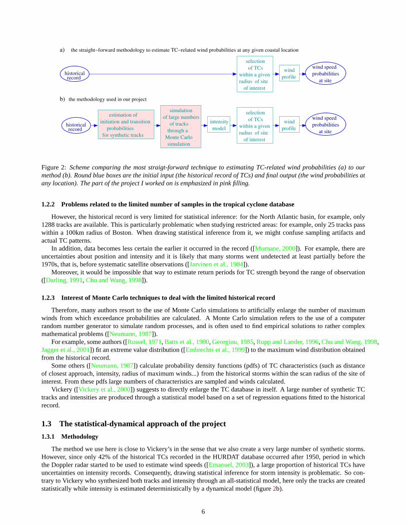
The most straight-forward methodology to estimate TC-related wind probabilities at any coastal location is summarizedin figure2 a.

To estimate wind speed probabilities in a particular location, accounting for spatially varying TC climatology, onlyhistorical TC tracks passing within a given radius (the scan radius) of that location are selected. Within this subregion, TCcharacteristics are assumed uniform.

Since the TC database only yields information about track and intensity, an empirical or analytical wind profile modelis applied to deduce the wind caused by these selected historical TCs at the site of interest. From the obtained time seriesof winds at the site of interest, the wind speed probabilities are computed.

1The intensity of a TC is its maximum 1-min or 10-min averaged wind speed at an altitude of 10m. It can also be estimated from minimum centralpressure, also available for most recent tracks.

5

of interestof siteradius

within a given

selectionof TCs

of interestof siteradius

within a given

selectionof TCs

the straight−forward methodology to estimate TC−related wind probabilities at any given coastal locationa)

the methodology used in our projectb)

at siteprobabilitieswind speed

at siteprobabilitieswind speed

recordhistorical

recordhistorical intensity

modelwind

profile

windprofile

initiation and transitionestimation of

probabilitiesfor synthetic tracks

of large numberssimulation

of tracksthrough a

Monte Carlosimulation

Figure 2: Scheme comparing the most straigt-forward technique to estimating TC-related wind probabilities (a) to ourmethod (b). Round blue boxes are the initial input (the historical record of TCs) and final output (the wind probabilities atany location). The part of the project I worked on is emphasized in pink filling.

1.2.2 Problems related to the limited number of samples in the tropical cyclone database

However, the historical record is very limited for statistical inference: for the North Atlantic basin, for example, only1288 tracks are available. This is particularly problematic when studying restricted areas: for example, only 25 tracks passwithin a 100km radius of Boston. When drawing statistical inference from it, we might confuse sampling artifacts andactual TC patterns.

In addition, data becomes less certain the earlier it occurred in the record ([Murnane, 2000]). For example, there areuncertainties about position and intensity and it is likely that many storms went undetected at least partially before the1970s, that is, before systematic satellite observations ([Jarvinen et al., 1984]).

Moreover, it would be impossible that way to estimate return periods for TC strength beyond the range of observation([Darling, 1991, Chu and Wang, 1998]).

1.2.3 Interest of Monte Carlo techniques to deal with the limited historical record

Therefore, many authors resort to the use of Monte Carlo simulations to artificially enlarge the number of maximumwinds from which exceedance probabilities are calculated. A Monte Carlo simulation refers to the use of a computerrandom number generator to simulate random processes, and is often used to find empirical solutions to rather complexmathematical problems ([Neumann, 1987]).

For example, some authors ([Russel, 1971, Batts et al., 1980, Georgiou, 1985, Rupp and Lander, 1996, Chu and Wang, 1998,Jagger et al., 2001]) fit an extreme value distribution ([Embrechts et al., 1999]) to the maximum wind distribution obtainedfrom the historical record.

Some others ([Neumann, 1987]) calculate probability density functions (pdfs) of TC characteristics (such as distanceof closest approach, intensity, radius of maximum winds...) from the historical storms within the scan radius of the site ofinterest. From these pdfs large numbers of characteristics are sampled and winds calculated.

Vickery ([Vickery et al., 2000]) suggests to directly enlarge the TC database in itself. A large number of synthetic TCtracks and intensities are produced through a statistical model based on a set of regression equations fitted to the historicalrecord.

1.3 The statistical-dynamical approach of the project

1.3.1 Methodology

The method we use here is close to Vickery’s in the sense that we also create a very large number of synthetic storms.However, since only 42% of the historical TCs recorded in the HURDAT database occurred after 1950, period in whichthe Doppler radar started to be used to estimate wind speeds ([Emanuel, 2003]), a large proportion of historical TCs haveuncertainties on intensity records. Consequently, drawing statistical inference for storm intensity is problematic. So con-trary to Vickery who synthesized both tracks and intensity through an all-statistical model, here only the tracks are createdstatistically while intensity is estimated deterministically by a dynamical model (figure2b).

6

This approach, named statistical-dynamical, requires 2 components:

1. A statistical track simulation model, to create large numbers of different and diverse tracks whose key motion prop-erties (geographical positions, translation speeds, headings, etc) conform statistically to historical data.

2. A dynamical, deterministic intensity model, which is ran along the tracks.

1.3.2 The dynamical intensity model

The dynamical model used is the Coupled Hurricane Intensity Prediction System (CHIPS)([Emanuel et al., 2003]). Theinput of this 3-D axisymetric balance model are:

1. monthly mean potential intensity2 maps, calculated from the NCEP reanalysis data.

2. wind at 250hPa and 850hPa: this allows to approximate vertical wind shear, which is known to have a strong influenceon TC intensity ([DeMaria and Kaplan, 1994]).

3. upper ocean thermal structure: the intensity model is coupled with a 1D ocean model, to account for the feedbackfrom the ocean.

4. the TC’s track.

Creating the input tracks is the role of the track simulation models, on which I focused during my internship.

1.3.3 The track simulation models

Two kind of track simulation approaches exist: statistical and dynamical. Both of these two approaches are used in therisk assessment project.

Statistical models The track generation technique I worked on is statistical. Statistical models draw inference from thestatistical record to relate current and previous TC position (calledpredictors) to the next position and behavior (predic-tands: what we try to predict).

For example, Neumann ([Hope and Neumann, 1970]), in the HURRAN (Hurricane Analog) model, suggested to searchhistorical analogs to the track being simulated, and calculate probabilities for the simulated tracks’ next position from thesehistorical analogs.

He later suggested a multiple regression model, CLIPER (Climatology-Persistence)([Neumann, 1972]) based on a set ofpolynomial regression to relate a selected number of predictors to predictands. Predictands consist in the TC next translationspeeds and headings. Predictors include both climatology (geographical position) and persistence (TC’s previous positionsand displacements). Vickery ([Vickery et al., 2000]) uses a “simplified CLIPER” approach in which fixed predictors andpredictands are linked by a set of linear regressions depending on geographical location.

The HURRAN and CLIPER models were initially devised for real time forecasting of particular approaching tracks. Onthe contrary, our goal is to synthesize large numbers of diverse and random tracks. Therefore, contrary to these traditionalmethods, we chose to generate tracks as Markov chains.

Dynamical models Dynamical models predict track movements from meteorological variables, such as environmentalwind fields, making use of the “steering concept” ([hrd, 2004]), in which TCs are assumed advected by the environmentalflow, with a correction to account for the beta effect3. In the project, such a approach was also used, with a statisticallygenerated wind field.

Although the projects applies to all TCs basins (North Atlantic, Western and Eastern Pacific, Indian Ocean, SouthernHemisphere), all explanations and illustrations will be given for the North Atlantic basin, for which models were initiallydeveloped.

2When modeling a TC as an heat engine suggested as suggested by Emanuel ([Emanuel, 1988b, Emanuel, 1988a, Emanuel, 1995,M. and Emanuel, 1998]), the maximum intensity achievable (called potential intensity) by the TC is computable from the temperatures of the heat source(the sea) and the cold source (the stratosphere).

3The beta-effect is the effect the TC has on the environmental vorticity field. The disturbance of this vorticity field results in steering the TC towardsthe North-West at about 1 to 3 m/s.

7

2 The statistical track simulation algorithm: methodology and techniques

2.1 Methodology: modeling tracks as Markov chains

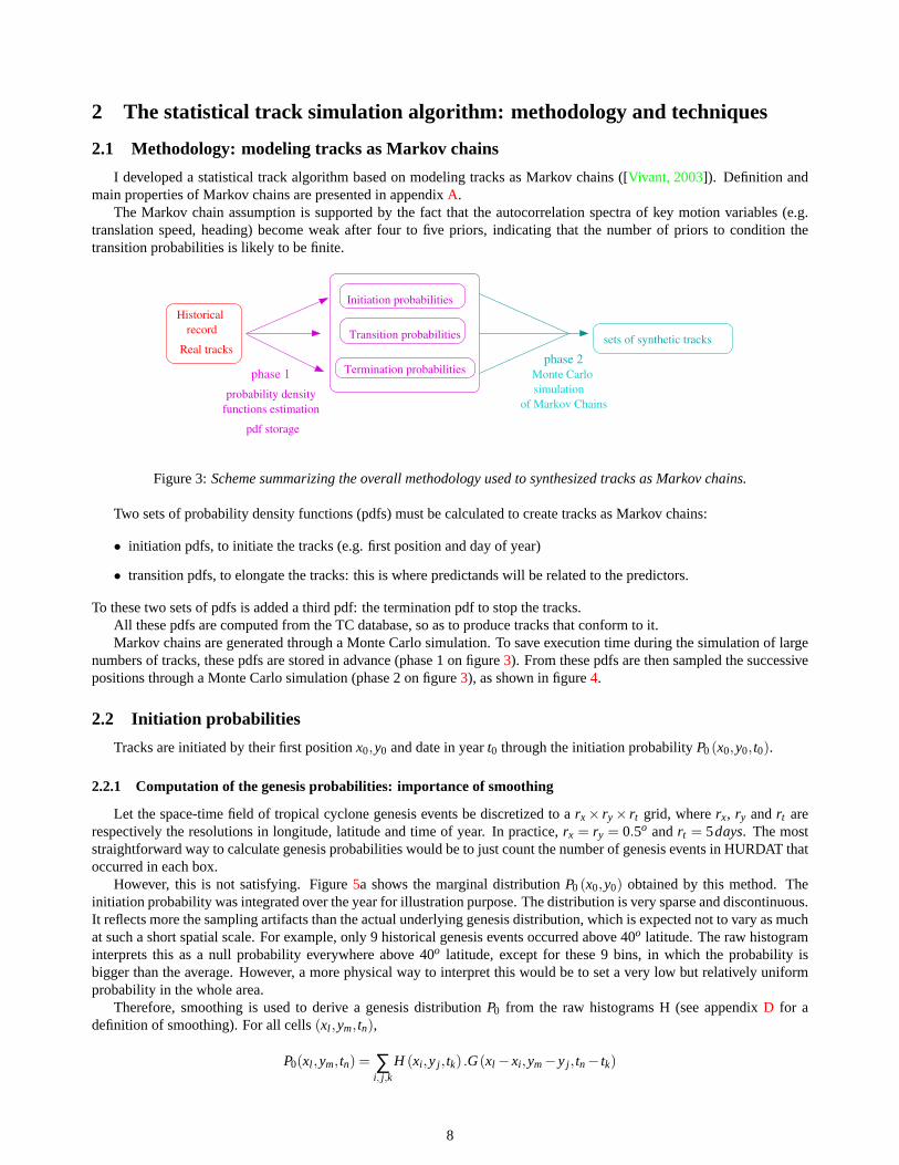
I developed a statistical track algorithm based on modeling tracks as Markov chains ([Vivant, 2003]). Definition andmain properties of Markov chains are presented in appendixA.

The Markov chain assumption is supported by the fact that the autocorrelation spectra of key motion variables (e.g.translation speed, heading) become weak after four to five priors, indicating that the number of priors to condition thetransition probabilities is likely to be finite.

Real tracks

Historicalrecord Transition probabilities

Termination probabilities

Initiation probabilities

sets of synthetic tracks

of Markov ChainssimulationMonte Carlo

probability densityfunctions estimation

phase 2

pdf storage

phase 1

Figure 3:Scheme summarizing the overall methodology used to synthesized tracks as Markov chains.

Two sets of probability density functions (pdfs) must be calculated to create tracks as Markov chains:

• initiation pdfs, to initiate the tracks (e.g. first position and day of year)

• transition pdfs, to elongate the tracks: this is where predictands will be related to the predictors.

To these two sets of pdfs is added a third pdf: the termination pdf to stop the tracks.All these pdfs are computed from the TC database, so as to produce tracks that conform to it.Markov chains are generated through a Monte Carlo simulation. To save execution time during the simulation of large

numbers of tracks, these pdfs are stored in advance (phase 1 on figure3). From these pdfs are then sampled the successivepositions through a Monte Carlo simulation (phase 2 on figure3), as shown in figure4.

2.2 Initiation probabilities

Tracks are initiated by their first positionx0,y0 and date in yeart0 through the initiation probabilityP0 (x0,y0, t0).

2.2.1 Computation of the genesis probabilities: importance of smoothing

Let the space-time field of tropical cyclone genesis events be discretized to arx× ry× rt grid, whererx, ry andrt arerespectively the resolutions in longitude, latitude and time of year. In practice,rx = ry = 0.5o andrt = 5days. The moststraightforward way to calculate genesis probabilities would be to just count the number of genesis events in HURDAT thatoccurred in each box.

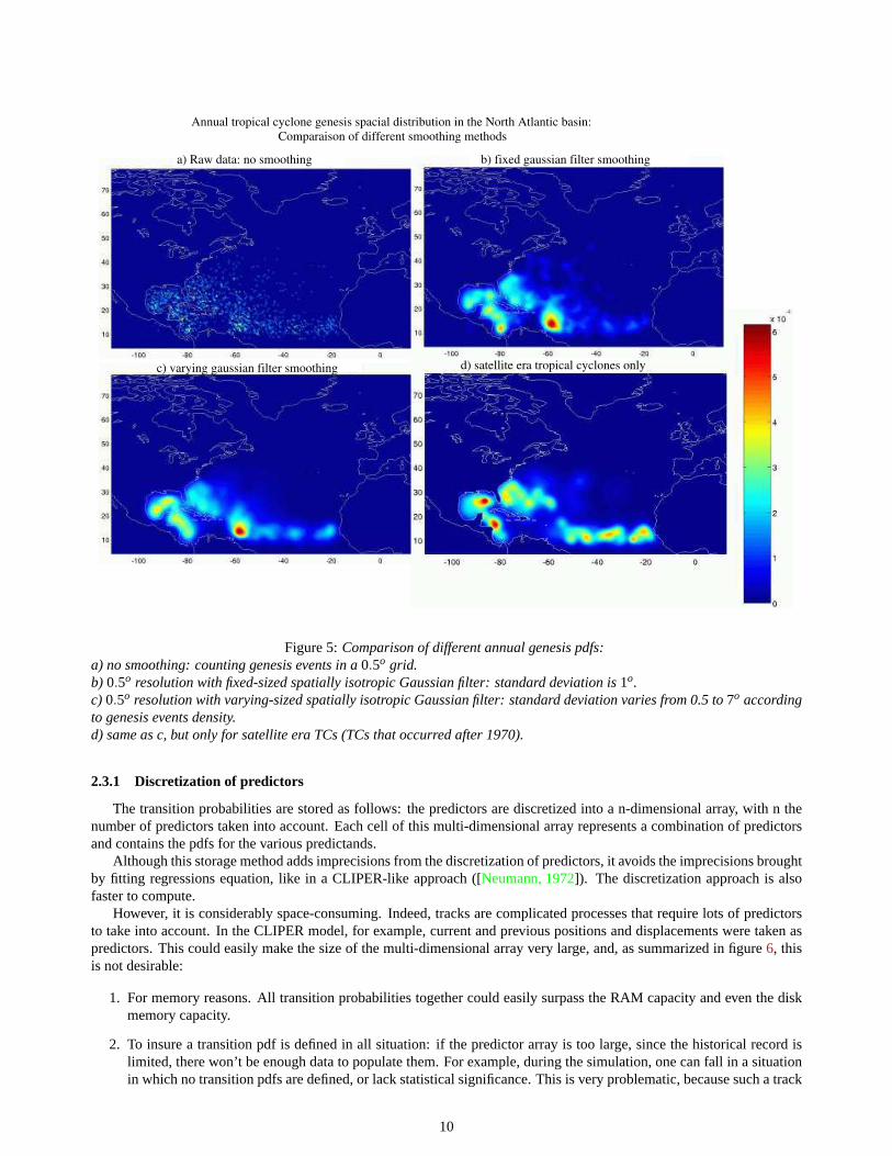
However, this is not satisfying. Figure5a shows the marginal distributionP0 (x0,y0) obtained by this method. Theinitiation probability was integrated over the year for illustration purpose. The distribution is very sparse and discontinuous.It reflects more the sampling artifacts than the actual underlying genesis distribution, which is expected not to vary as muchat such a short spatial scale. For example, only 9 historical genesis events occurred above 40o latitude. The raw histograminterprets this as a null probability everywhere above 40o latitude, except for these 9 bins, in which the probability isbigger than the average. However, a more physical way to interpret this would be to set a very low but relatively uniformprobability in the whole area.

Therefore, smoothing is used to derive a genesis distributionP0 from the raw histograms H (see appendixD for adefinition of smoothing). For all cells(xl ,ym, tn),

P0(xl ,ym, tn) = ∑i, j,k

H (xi ,y j , tk) .G(xl −xi ,ym−y j , tn− tk)

8

scan radiusof target point?

withingo

storage of the track

track terminated?

Next position

set of synthetic tracks

Sample transition pdf

New track first position

Sample initiation pdfs

yesno

yesno

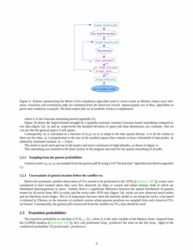
Figure 4:Scheme summarizing the Monte Carlo simulation algorithm used to create tracks as Markov chains once initi-ation, transition and termination pdfs are estimated from the historical record. Inputs/outputs are in blue, algorithms ingreen and conditions in purple. The final output (the set of synthetic tracks) is emphasized.

where G is the Gaussian smoothing kernel (appendixD).Figure5b shows the improvements brought by a spatially-isotropic constant Gaussian kernel smoothing compared to

raw data (figure5a). σx andσt , respectively the standard deviation in space and time dimensions, are constants. But wecan see that the general aspect is still sparse.

Consequently,σx is calculated as a function of (x,y), so as to adapt to the data spatial density: it is all the widest asthere are few data.σx is proportional to the size of the smallest square that contains at least a threshold of data points.σt

arbitrarily remained constant:σt = 5days.The result is much more precise in the tropics and more continuous in high latitudes, as shown in figure5c.This smoothing was retained in the final version of the program and used for the spatial smoothing of all pdfs.

2.2.2 Sampling from the genesis probabilities

Genesis events(x0,y0, t0) are sampled from the genesis pdfP0 using a 3-D “hit and miss” algorithm (recalled in appendixC).

2.2.3 Uncertainties of genesis location before the satellite era

Before the systematic satellite observation of TCs started to be performed in the 1970s ([Emanuel, 2003]), events wereconsidered to have formed where they were first observed, by ships or coastal and island stations, both of which aredistributed inhomogeneous in space. Indeed, there’s a significant difference between the spatial distribution of genesisevents for all tracks from 1851 to today and the tracks after 1970 only (figure5d): tracks are now observed much earlierand are therefore much longer. This is of importance because when the intensity model is ran along the tracks, wind speedis initiated at 25knots, so the intensity of synthetic storms whom genesis positions are sampled from early historical TCsare biased. Consequently, the genesis pdf constructed from the satellite era TCs only should be used.

2.3 Transition probabilities

The transition probability to calculate isP(Xi+1 | Xi), whereXi is the state variable of the Markov chain. Inspired fromthe CLIPER notation ([Neumann, 1972]), let’s call predictand(resp. predictor) the term on the left (resp. right) of theconditional probability:P(predictands| predictors).

9

a) Raw data: no smoothing

c) varying gaussian filter smoothing

b) fixed gaussian filter smoothing

Annual tropical cyclone genesis spacial distribution in the North Atlantic basin:Comparaison of different smoothing methods

d) satellite era tropical cyclones only

Figure 5:Comparison of different annual genesis pdfs:a) no smoothing: counting genesis events in a0.5o grid.b) 0.5o resolution with fixed-sized spatially isotropic Gaussian filter: standard deviation is1o.c) 0.5o resolution with varying-sized spatially isotropic Gaussian filter: standard deviation varies from 0.5 to7o accordingto genesis events density.d) same as c, but only for satellite era TCs (TCs that occurred after 1970).

2.3.1 Discretization of predictors

The transition probabilities are stored as follows: the predictors are discretized into a n-dimensional array, with n thenumber of predictors taken into account. Each cell of this multi-dimensional array represents a combination of predictorsand contains the pdfs for the various predictands.

Although this storage method adds imprecisions from the discretization of predictors, it avoids the imprecisions broughtby fitting regressions equation, like in a CLIPER-like approach ([Neumann, 1972]). The discretization approach is alsofaster to compute.

However, it is considerably space-consuming. Indeed, tracks are complicated processes that require lots of predictorsto take into account. In the CLIPER model, for example, current and previous positions and displacements were taken aspredictors. This could easily make the size of the multi-dimensional array very large, and, as summarized in figure6, thisis not desirable:

1. For memory reasons. All transition probabilities together could easily surpass the RAM capacity and even the diskmemory capacity.

2. To insure a transition pdf is defined in all situation: if the predictor array is too large, since the historical record islimited, there won’t be enough data to populate them. For example, during the simulation, one can fall in a situationin which no transition pdfs are defined, or lack statistical significance. This is very problematic, because such a track

10

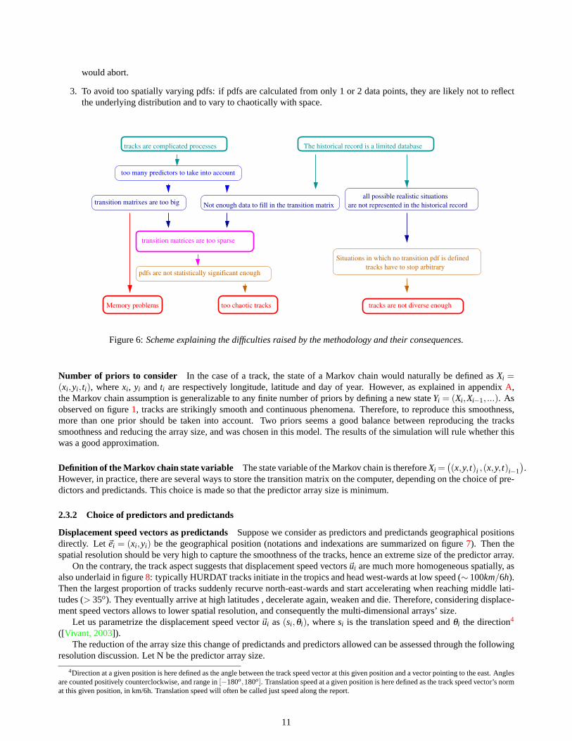
would abort.

3. To avoid too spatially varying pdfs: if pdfs are calculated from only 1 or 2 data points, they are likely not to reflectthe underlying distribution and to vary to chaotically with space.

transition matrices are too sparse

pdfs are not statistically significant enough

Situations in which no transition pdf is definedtracks have to stop arbitrary

too chaotic tracksMemory problems

all possible realistic situationsare not represented in the historical record

tracks are complicated processes The historical record is a limited database

too many predictors to take into account

transition matrixes are too big Not enough data to fill in the transition matrix

tracks are not diverse enough

Figure 6:Scheme explaining the difficulties raised by the methodology and their consequences.

Number of priors to consider In the case of a track, the state of a Markov chain would naturally be defined asXi =(xi ,yi , ti), wherexi , yi andti are respectively longitude, latitude and day of year. However, as explained in appendixA,the Markov chain assumption is generalizable to any finite number of priors by defining a new stateYi = (Xi ,Xi−1, ...). Asobserved on figure1, tracks are strikingly smooth and continuous phenomena. Therefore, to reproduce this smoothness,more than one prior should be taken into account. Two priors seems a good balance between reproducing the trackssmoothness and reducing the array size, and was chosen in this model. The results of the simulation will rule whether thiswas a good approximation.

Definition of the Markov chain state variable The state variable of the Markov chain is thereforeXi =((x,y, t)i ,(x,y, t)i−1

).

However, in practice, there are several ways to store the transition matrix on the computer, depending on the choice of pre-dictors and predictands. This choice is made so that the predictor array size is minimum.

2.3.2 Choice of predictors and predictands

Displacement speed vectors as predictandsSuppose we consider as predictors and predictands geographical positionsdirectly. Let~ei = (xi ,yi) be the geographical position (notations and indexations are summarized on figure7). Then thespatial resolution should be very high to capture the smoothness of the tracks, hence an extreme size of the predictor array.

On the contrary, the track aspect suggests that displacement speed vectors~ui are much more homogeneous spatially, asalso underlaid in figure8: typically HURDAT tracks initiate in the tropics and head west-wards at low speed (∼ 100km/6h).Then the largest proportion of tracks suddenly recurve north-east-wards and start accelerating when reaching middle lati-tudes (> 35o). They eventually arrive at high latitudes , decelerate again, weaken and die. Therefore, considering displace-ment speed vectors allows to lower spatial resolution, and consequently the multi-dimensional arrays’ size.

Let us parametrize the displacement speed vector~ui as(si ,θi), wheresi is the translation speed andθi the direction4

([Vivant, 2003]).The reduction of the array size this change of predictands and predictors allowed can be assessed through the following

resolution discussion. Let N be the predictor array size.

4Direction at a given position is here defined as the angle between the track speed vector at this given position and a vector pointing to the east. Anglesare counted positively counterclockwise, and range in[−180o,180o]. Translation speed at a given position is here defined as the track speed vector’s normat this given position, in km/6h. Translation speed will often be called just speed along the report.

11

sx 6hrs

i−1

i−1s i−1,xi ,yi

i−1

,i is

x , yi−1i−1=ei−1

i−1u =

ui =. .s ,i i

. xi+1, yi+1=ei+1

=ie

ui =

Figure 7: Figure defining variable notations used and the way they are indexed. In red are represented the 6-hourlypositions (x,y), in blue are the 6-hour-averaged speed vectors, defined by its norm (translation speed s) and directionθ ,and in orange is the rate of change of the speed vector, defined by its norm (the accelerations) and direction (direction rateof changeθ ), and the way they are indexed.

Orientation expectation given location

Orientation in degrees

b)Translation speed expectation given location

Speed in km/6h

a)

Figure 8: HURDAT motion as a function of geographical location: a) speed spatial distribution. b) direction spatialdistribution. Maps were calculated directly from HURDAT, by computing the expectation for each5×5o box.

Suppose we directly consider geographical positions and express the transition probability with 2 priors asP(~ei+1 |~ei ,~ei−1).For tracks to look smooth, it is observed that a spatial resolution of at least 0.1o is required. Let the North Atlantic basinspread from−110o to 10o in longitude and from 0 to 60oin latitude. Then we haveN = (1200×600)2 ' 5×1011. Onthe contrary, suppose we consider the transition probabilityP(~ui |~ei ,~ui−1). Speeds range between 0 and 800km/6h ap-proximately, and directions between−180o and 180o. To insure the same 0.1o precision, the resolution in speed shouldbe approximately 10km/6h and 5o in direction. Besides, a spatial resolution of 0.5o is sufficient to capture the spatialvariations of the displacement speed vectors. Hence, a array size ofN = 240×120×80×72' 2×108cells.

Rate of change of displacement speed vectors as predictandsFigure9 shows the conditional probabilitiesP(si | si−1)andP(θi | θi−1). One notice that all values are clustered around the first diagonal: speed and direction are very smoothlyvarying. Therefore, most of the space is wasted in this representation. A more efficient representation would be to considerthe variations from the first diagonal, that is, take the derivatives:~ui =

(si , θi

), where ˙si is the acceleration andθi the

direction rate of change:

~ui =~ui−1 +~ui (1)

This short array size calculation shows the improvements brought by considering the transition probabilityP(~ui |~ei ,~ui−1

):

to get the same 0.1o precision on~ei+1, as previously explained, the resolution on~ui and thus~ui should be of(10km/6h, 5o)approximately. However, a resolution of 40km/6h and of 20o for speed and direction respectively is observed to be suffi-cient to have the same resolution if calculating~ui from equation1. Consequently,N = 240×120×20×18' 107.

To conclude, to limit the predictor array size, the transition probability is stored as:

12

as a function of a given previous speed or directionProbability of speed and direction

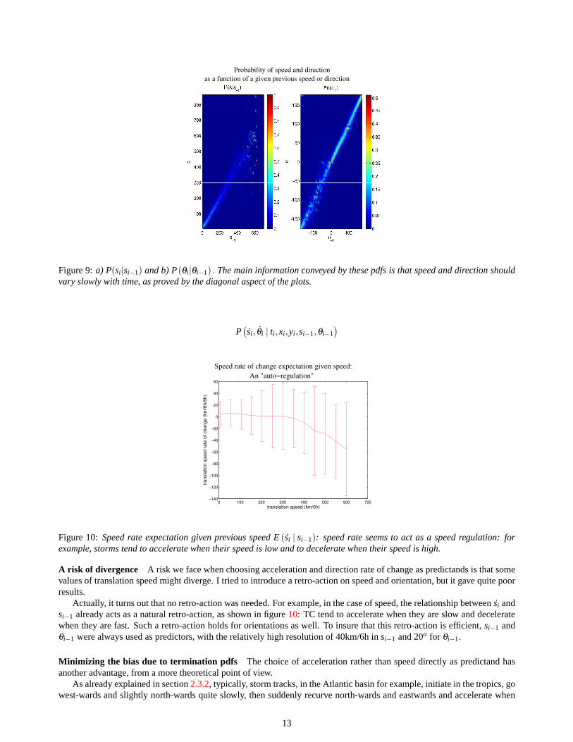
Figure 9:a) P(si |si−1) and b) P(θi |θi−1) . The main information conveyed by these pdfs is that speed and direction shouldvary slowly with time, as proved by the diagonal aspect of the plots.

P(si , θi | ti ,xi ,yi ,si−1,θi−1

)

0 100 200 300 400 500 600 700−140

−120

−100

−80

−60

−40

−20

0

20

40

60

translation speed (km/6h)

trans

latio

n sp

eed

rate

of c

hang

e (k

m/6

h/6h

)

An "auto−regulation"Speed rate of change expectation given speed:

Figure 10:Speed rate expectation given previous speed E(si | si−1): speed rate seems to act as a speed regulation: forexample, storms tend to accelerate when their speed is low and to decelerate when their speed is high.

A risk of divergence A risk we face when choosing acceleration and direction rate of change as predictands is that somevalues of translation speed might diverge. I tried to introduce a retro-action on speed and orientation, but it gave quite poorresults.

Actually, it turns out that no retro-action was needed. For example, in the case of speed, the relationship between ˙si andsi−1 already acts as a natural retro-action, as shown in figure10: TC tend to accelerate when they are slow and deceleratewhen they are fast. Such a retro-action holds for orientations as well. To insure that this retro-action is efficient,si−1 andθi−1 were always used as predictors, with the relatively high resolution of 40km/6h insi−1 and 20o for θi−1.

Minimizing the bias due to termination pdfs The choice of acceleration rather than speed directly as predictand hasanother advantage, from a more theoretical point of view.

As already explained in section2.3.2, typically, storm tracks, in the Atlantic basin for example, initiate in the tropics, gowest-wards and slightly north-wards quite slowly, then suddenly recurve north-wards and eastwards and accelerate when

13

Acceleration expectation (km/6h/6h)

Spatial distribution of accelerationb)

Speed expectation (km/6h)

a)

Probability for a track to stop at a given locationc)

spatial distribution of translation speed

Figure 11:a) Annual spatial distribution of the speed expectation, phrased on a5×5ogrid with no smoothing. 2 distinctivebelts can be identified, as plotted in black.b) Annual spatial distribution of the acceleration expectation, phrased on a5×5ogrid with no smoothing. 3 distinctivebelts can be identified, as plotted in black.c) Probability for a track to die as a function of location, phrased on a0.5×0.5o grid with the same smoothing as used forthe computation of the genesis pdfs. Tracks are most likely to die over land or cold water.The fact that real tracks that move slowly out of the tropics are more likely to die leads to a significant difference betweenthe acceleration spatial distribution and the speed distribution.

reaching latitudes about 30 - 35o, and eventually slow down when reaching latitudes about 50o .However, while the acceleration map clearly shows these 3 belts (figure8b), the speed mean map displays only 2 belts:

low speeds bellow 40 - 45o latitude, and high speeds above (figure8a). This is because slow storms that have spent a longtime over cold water die (figure8c), so even if storms tend to decelerate in high latitudes, only fast storm survive, thus thehigh speeds in high latitudes.

Consequently, drawing inference directly from track speeds should lead to an overestimation of storm acceleration inmid-latitudes, and a underestimation of storm deceleration in high latitudes.

The bias at a given location (x,y) can be formulated as follow:Let Pth(s | x,y) be the theoretical speed pdf, from which the HURDAT speed distributionPH(s | x,y) is derived by

truncating tracks if the event “dead” has occurred. Thus, we can calculate that

PH (s | x,y) = Pth(s | x,y)×1−Pth(”dead” | s,x,y).Pth(x,y)

1−Pth(”dead” | x,y)= Pth(s | x,y)× f (s)

with f (s) a normalizing factor that all the more disrupts the theoretical distribution asf (s) varies a lot with s, that is, ifPth(”dead” | s,x,y) varies a lot with s.

In our statistical model, statistical inference should be drawn from the unknown theoretical distribution, but is actuallydrawn from the HURDAT known distribution. In other words, we implicitly assume in this model thatPH (s | x,y)' Pth(s |

14

x,y), that isPth(”dead” | s,x,y) doesn’t vary too much with s. This assumption is obviously not valid.Suppose now we consider ˙s . The assumption made now becomes thatPth(”dead” | s,x,y) doesn’t vary too much with

s. Although acceleration ˙s is related with speed s and therefore with the survival of a track in high latitudes, ˙s is in practicemuch less related to the survival of the storm than the translation speed directly.

Therefore, the choice of acceleration as predictand minimizes the bias due to the termination pdfs.

2.3.3 Computation of the transition probabilities

As justified in section2.3.2, the transition pdf to compute is

P(si , θi | ti ,xi ,yi ,si−1,θi−1

)One also notices that upon this state variable definition, the initiation pdf must contain the pdfs to sample the first speed

s0 and directionθ0 as well. They are sampled from the conditional pdfP(s | x,y, t) andP(θ | x,y, t) . These conditionalpdfs are estimated and sampled from using exactly the same methods and techniques as for the transition pdfs, detailed inthis section.

2.3.3.1 Independence assumptions Suppose we directly compute pdfs asP(si , θi | ti ,xi ,yi ,si−1,θi−1

)for the Northern

Atlantic basin. As explained in section2.3.1, N' 1.107×Nt cells (if Nt is the number of bins in the time of year dimension).But the database only contains about 3.5.104data points. Data is therefore not abundant enough to populate the transitionmatrix.

A way to reduce the pdf matrix dimension is to make some independence assumptions.

Speed-direction independence assumptionFor example, we can assume that s is independent fromθ ([Vivant, 2003]):

P(si , θi | ti ,xi ,yi ,si−1,θi

)' P(si | ti ,xi ,yi ,si−1) .P

(θi | ti ,xi ,yi ,θi−1

)This allows a great reduction of the transition pdf array. This approximation is questionable: it is known that TC move

much faster when heading north-eastwards. However, it can be justified by the fact that a large part of the relation betweens andθ might be explained by the relation both have to latitude. Results of the simulations will rule whether this is actuallya valid approximation.

Climatology-persistence independence assumptionAnother stronger assumption had also been put forward in ear-lier versions of the algorithm: assuming that probabilities given climatological factors and given persistence factors areindependent. In these versions of the algorithm, the predictands used were actuallysandθ . However, such an assumptionapplied to the predictands ˙s andθ would have the same affect and would be expressed as:

P(si |ti ,si−1,xi ,yi)' P(si |ti ,si−1) .P(si |ti ,xi ,yi)

and

P(θi |ti ,si−1,xi ,yi

)' P

(θi |ti ,si−1

).P(θi |ti ,xi ,yi

)The speed and direction distributions of tracks created under this assumption differed from real tracks. For example, in

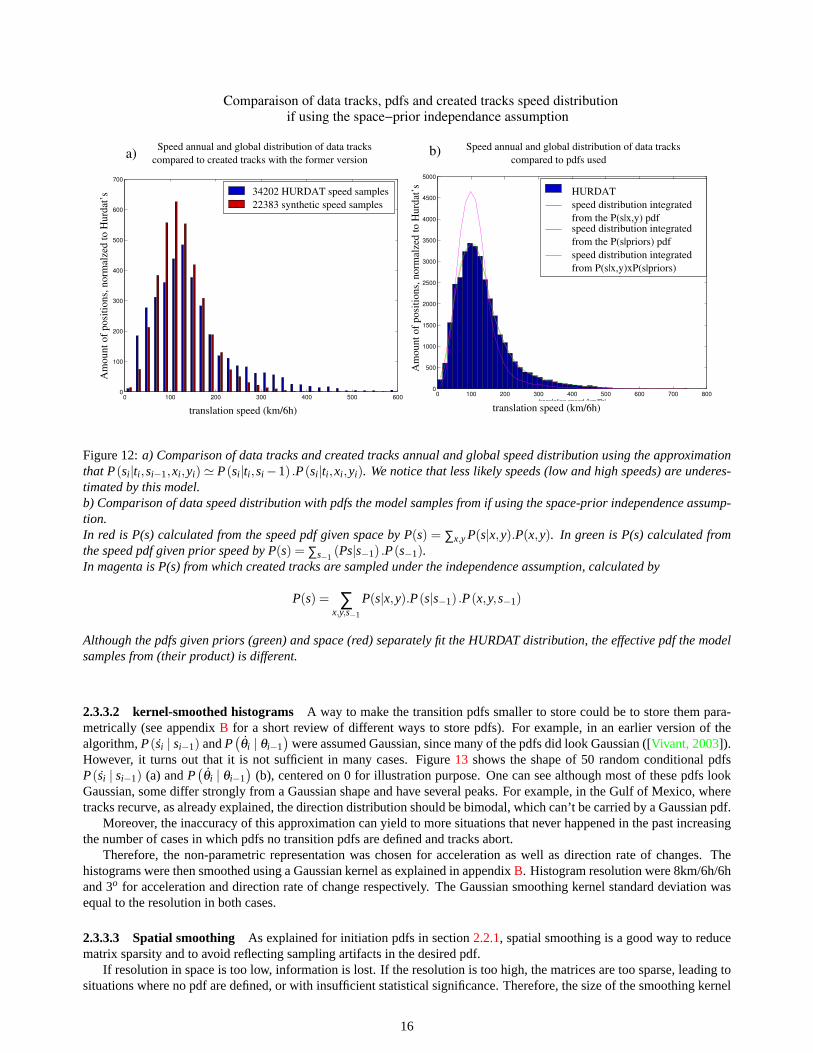
the case of speed, high probabilities are exaggerated and low probabilities under estimated (figure12 a). This is becausethe probability is calculated as a product. This proves that the transition probabilities given priors and given location arenot independent. When calculating the real probability the program samples from, making the product of the two pdfs, weverify that it fits created tracks but it is different from the HURDAT distribution (figure12b, magenta curve).

This is particularly problematic in the perspective of wind risk assessment in extratropical locations such as Boston:only fast moving tracks are able to maintain a large intensity in such high latitudes. Therefore, an underestimation of highspeeds would underestimate wind risks in such coastal locations. This approximation was therefore abandoned.

15

0 100 200 300 400 500 6000

100

200

300

400

500

600

700speed distribution everywhere in North Atlantic

3679 position from hurdat17053 position from created tracks

0 100 200 300 400 500 600 700 8000

500

1000

1500

2000

2500

3000

3500

4000

4500

5000speed distribution of data tracks compared to pdf used


speed given spacespeed given priorsproduct of twohurdat

HURDATspeed distribution integratedfrom the P(s|x,y) pdfspeed distribution integratedfrom the P(s|priors) pdfspeed distribution integratedfrom P(s|x,y)xP(s|priors)

compared to created tracks with the former versionSpeed annual and global distribution of data tracksa) compared to pdfs used

b)

if using the space−prior independance assumptionComparaison of data tracks, pdfs and created tracks speed distribution

translation speed (km/6h) translation speed (km/6h)

Speed annual and global distribution of data tracks

34202 HURDAT speed samples22383 synthetic speed samples

Am

ount

of p

ositi

ons,

nor

mal

zed

to H

urda

t’s

Am

ount

of p

ositi

ons,

nor

mal

zed

to H

urda

t’s

Figure 12:a) Comparison of data tracks and created tracks annual and global speed distribution using the approximationthat P(si |ti ,si−1,xi ,yi)' P(si |ti ,si −1) .P(si |ti ,xi ,yi). We notice that less likely speeds (low and high speeds) are underes-timated by this model.b) Comparison of data speed distribution with pdfs the model samples from if using the space-prior independence assump-tion.In red is P(s) calculated from the speed pdf given space by P(s) = ∑x,yP(s|x,y).P(x,y). In green is P(s) calculated fromthe speed pdf given prior speed by P(s) = ∑s−1

(Ps|s−1) .P(s−1).In magenta is P(s) from which created tracks are sampled under the independence assumption, calculated by

P(s) = ∑x,y,s−1

P(s|x,y).P(s|s−1) .P(x,y,s−1)

Although the pdfs given priors (green) and space (red) separately fit the HURDAT distribution, the effective pdf the modelsamples from (their product) is different.

2.3.3.2 kernel-smoothed histograms A way to make the transition pdfs smaller to store could be to store them para-metrically (see appendixB for a short review of different ways to store pdfs). For example, in an earlier version of thealgorithm,P(si | si−1) andP

(θi | θi−1

)were assumed Gaussian, since many of the pdfs did look Gaussian ([Vivant, 2003]).

However, it turns out that it is not sufficient in many cases. Figure13 shows the shape of 50 random conditional pdfsP(si | si−1) (a) andP

(θi | θi−1

)(b), centered on 0 for illustration purpose. One can see although most of these pdfs look

Gaussian, some differ strongly from a Gaussian shape and have several peaks. For example, in the Gulf of Mexico, wheretracks recurve, as already explained, the direction distribution should be bimodal, which can’t be carried by a Gaussian pdf.

Moreover, the inaccuracy of this approximation can yield to more situations that never happened in the past increasingthe number of cases in which pdfs no transition pdfs are defined and tracks abort.

Therefore, the non-parametric representation was chosen for acceleration as well as direction rate of changes. Thehistograms were then smoothed using a Gaussian kernel as explained in appendixB. Histogram resolution were 8km/6h/6hand 3o for acceleration and direction rate of change respectively. The Gaussian smoothing kernel standard deviation wasequal to the resolution in both cases.

2.3.3.3 Spatial smoothing As explained for initiation pdfs in section2.2.1, spatial smoothing is a good way to reducematrix sparsity and to avoid reflecting sampling artifacts in the desired pdf.

If resolution in space is too low, information is lost. If the resolution is too high, the matrices are too sparse, leading tosituations where no pdf are defined, or with insufficient statistical significance. Therefore, the size of the smoothing kernel

16

−200 −100 0 100 2000

0.1

0.2

0.3

0.4

0.5

0.6

0.7

aspect of pdfs P(sr|s−1

,x,y)

speed rate in km/6h/6h−100 0 100

0

0.05

0.1

0.15

0.2

0.25

0.3

0.35

0.4

aspect of pdfs P(ar|a1,x,y)

direction rate in degrees/6h

pdf value pdf value

a) acceleration b) direction rate of change

probability density functions centered on pdfs’ maximaShapes of acceleration and direction rate of change probabilities given priors:

Figure 13:Shape of 50 random conditional pdfs P(si | si−1)(a) and P(θi | θi−1

)(b) . Pdfs were centered on 0 so that their

maximum value was on 0 and shapes can easily be compared. Notice although most pdfs and their average (plotted inblack) look Gaussian, a significant number of pdfs show more than one peak.

varies in space to adapt to the density of data samples, and the same spatially varying Gaussian kernel presented in section2 was used to smooth the pdfs in space. Arbitrarily, no smoothing was performed neither in time nor previous speed anddirection dimensions.

To sum up, the formula used to compute the transition pdf is as follow: Let q stands for either s orθ . For a given timeperiod t , previous speed or directionq−1, position(xm,yn) and predictand ˙ql :

P(ql | xm,yn,q−1, t) =P(ql ,xm,yn,q−1, t)

P(xm,yn,q−1, t)=

∑i, j,k H (qk,xi ,y j , t,q−1) .e− 1

2

((xm−xi)

2+(yn−yj)2

σx(xi ,yj)+(ql−qk)

2

σh

)

c(xm,yn,q−1, t)

whereH (qk,xi ,y j , t,q−1) is raw number of data points falling in the cell(qk,xi ,y j , t,q−1) , c(xm,yn,q−1, t) is a normal-izing constant that insures that the conditional pdf integrates to 1,σx (xi ,y j) is the spatially varying standard deviation ofthe Gaussian smoothing kernel andσh is the standard deviation of the histogram smoothing kernel.

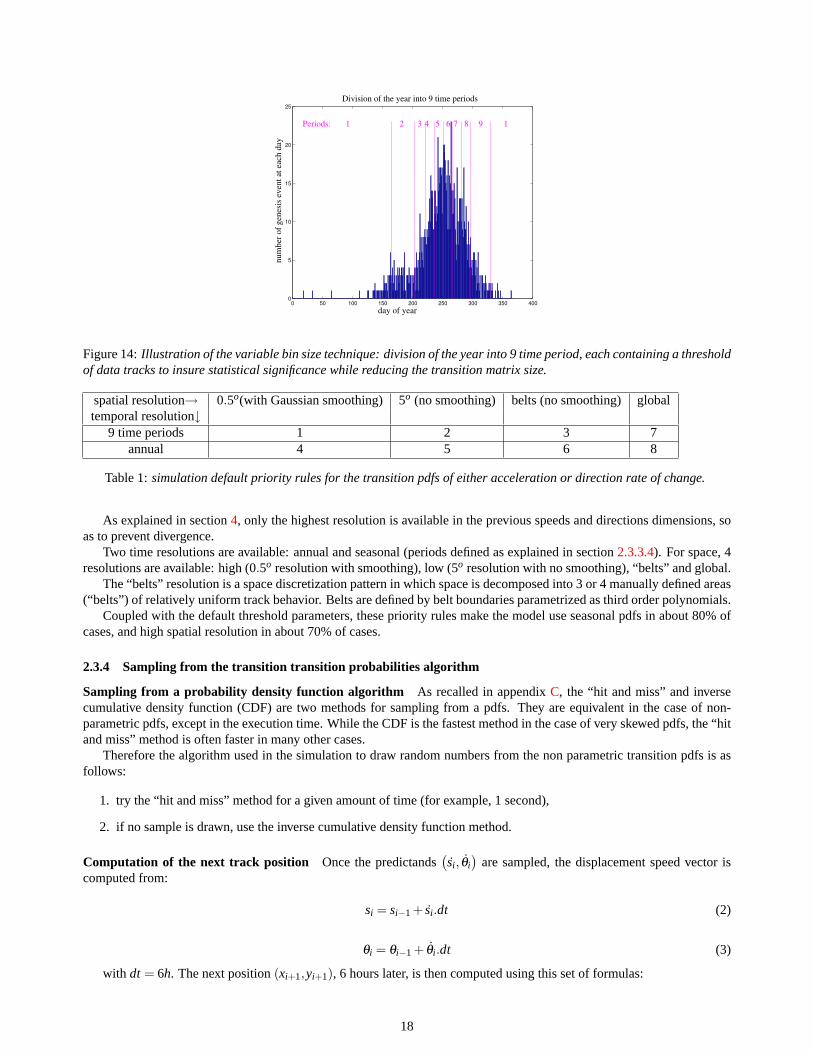
2.3.3.4 variable grid size To insure that a pdf meet statistical significance standards even in periods of the year whenvery few historical events were recorded, the resolution is made variable in the time dimension. The year is divided into 9time periods (figure14) containing at least a given number of data points.

To insure a physical significance as well, 3 other conditions were added, which prevail over the first one:

1. a maximum length, above which track behaviors get very different,

2. a minimum length, bellow which it would be waste of memory to make separate periods. A length of 15 days waschosen here,

3. the first period starting date is manually chosen so that it separate 2 time periods in which tracks show differentbehaviors.

2.3.3.5 Variable window method Multiple resolutions for the predictor array are available. That way, if no transitionpdf is defined, or was estimated from to few data points, then a coarser resolution is used, and so on.

The resolution used is the finest possible that satisfied a threshold of statistical significance. To choose between loweringthe resolution in one predictor or the other, priority rules are set. Priority rules used in standard simulations are shown intable1.

17

0 50 100 150 200 250 300 350 4000

5

10

15

20

25

Periods:

num

ber o

f gen

esis

eve

nt a

t eac

h da

y

day of year

Division of the year into 9 time periods

1 2 3 4 5 6 7 8 9 1

Figure 14:Illustration of the variable bin size technique: division of the year into 9 time period, each containing a thresholdof data tracks to insure statistical significance while reducing the transition matrix size.

spatial resolution→ 0.5o(with Gaussian smoothing) 5o (no smoothing) belts (no smoothing) globaltemporal resolution↓

9 time periods 1 2 3 7annual 4 5 6 8

Table 1:simulation default priority rules for the transition pdfs of either acceleration or direction rate of change.

As explained in section4, only the highest resolution is available in the previous speeds and directions dimensions, soas to prevent divergence.

Two time resolutions are available: annual and seasonal (periods defined as explained in section2.3.3.4). For space, 4resolutions are available: high (0.5o resolution with smoothing), low (5o resolution with no smoothing), “belts” and global.

The “belts” resolution is a space discretization pattern in which space is decomposed into 3 or 4 manually defined areas(“belts”) of relatively uniform track behavior. Belts are defined by belt boundaries parametrized as third order polynomials.

Coupled with the default threshold parameters, these priority rules make the model use seasonal pdfs in about 80% ofcases, and high spatial resolution in about 70% of cases.

2.3.4 Sampling from the transition transition probabilities algorithm

Sampling from a probability density function algorithm As recalled in appendixC, the “hit and miss” and inversecumulative density function (CDF) are two methods for sampling from a pdfs. They are equivalent in the case of non-parametric pdfs, except in the execution time. While the CDF is the fastest method in the case of very skewed pdfs, the “hitand miss” method is often faster in many other cases.

Therefore the algorithm used in the simulation to draw random numbers from the non parametric transition pdfs is asfollows:

1. try the “hit and miss” method for a given amount of time (for example, 1 second),

2. if no sample is drawn, use the inverse cumulative density function method.

Computation of the next track position Once the predictands(si , θi

)are sampled, the displacement speed vector is

computed from:

si = si−1 + si .dt (2)

θi = θi−1 + θi .dt (3)

with dt = 6h. The next position(xi+1,yi+1), 6 hours later, is then computed using this set of formulas:

18

yi+1 = yi +180π.Rt

.si .dt.sin(

θi .π

180

)(4)

xi+1 = xi +180

π.Rt .cos( yi .π

180

) .si .dt.cos(

θi .π

180

)(5)

where whereRt is the earth radius anddt is the 6-hour interval.

2.4 Termination probabilities

In our case, a third set of pdfs is needed: the termination pdfs to stop the tracks, so that time is not wasted in prolongatingthe tracks where it is not likely to survive. Since an intensity model will rule whether a TC still exists or dies (by convention,a TC is ruled “dead” if its intensity fall below 17m/s), a termination pdf is not of greatest importance, as long as track arenever stopped before they being rule dead by the intensity model. Therefore, a simple termination pdf based on hurricaneactivity was chosen:P(stop| location) = 1 if P(location) < threshold, and 0 otherwise.

Two other conditions might lead to track termination as well: if the maximum number of 6-hourly position (120) isreached, or if no transition pdf have been found even at the lowest resolution (which happens in 0.05% of cases).

3 Results: comparison of synthetic tracks to HURDAT tracks

The goal of the statistical track algorithm described is to produce large numbers of different tracks that statisticallyconform to HURDAT. In this section are presented some comparison between real and synthetic tracks to assess theirsimilarity.

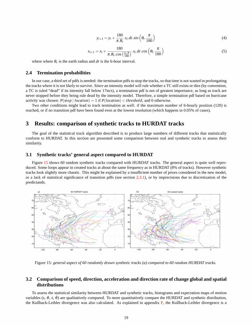
3.1 Synthetic tracks’ general aspect compared to HURDAT

Figure15 shows 60 random synthetic tracks compared with HURDAT tracks. The general aspect is quite well repro-duced. Some loops appear in created tracks at about the same frequency as in HURDAT (8% of tracks). However synthetictracks look slightly more chaotic. This might be explained by a insufficient number of priors considered in the new model,or a lack of statistical significance of transition pdfs (see section2.3.1), or by imprecisions due to discretization of thepredictands.

−100 −80 −60 −40 −20 0

10

20

30

40

50

60

70

60 created tracks

−100 −80 −60 −40 −20 0

10

20

30

40

50

60

70

60 HURDAT tracks b)a)

Figure 15:general aspect of 60 randomly drawn synthetic tracks (a) compared to 60 random HURDAT tracks.

3.2 Comparison of speed, direction, acceleration and direction rate of change global and spatialdistributions

To assess the statistical similarity between HURDAT and synthetic tracks, histograms and expectation maps of motionvariables (s,θ , s, θ ) are qualitatively compared. To more quantitatively compare the HURDAT and synthetic distribution,the Kullback-Leibler divergence was also calculated. As explained in appendixF, the Kullback-Leibler divergence is a

19

measure of the distance between two distribution ([Cover and Thomas, 1991]). These measure was chosen here becauseeither the whole HURDAT dataset or the post-1970 HURDAT dataset may be considered as the true distribution we try toreproduce through a model.

3.2.1 Termination pdf used to avoid the termination bias when comparing synthetic tracks and HURDAT tracks

As explained in section4, the fact that synthetic tracks are continued untilP(x,y) < thresholdwhereas HURDAT tracksstop over cold water, which occurs usually much earlier, adds a bias on some distributions, translation speed in particular.


c)b) Simulation 1 Simulation2

HURDATa)


Figure 16:Comparison of the spatial (b and c) speed distributions for 2 different runs of the model: in simulation 1, theregular termination criterion was used: P(stop| x,y) = 1 if P(x,y) < thresholdand 0 otherwise. In simulation 2, a morephysical termination pdf is applied: P(stop| timespend overcold water)Both are compared to HURDAT (a)

So as to better compare HURDAT and synthetic tracks, a new termination pdf was here tested. Figures16 and17compare 2 simulations with different termination probability:

1. In simulation 1 was use the regular termination criterion:P(stop| x,y) = 1 if P(x,y) < thresholdand 0 otherwise(figure16b and17d).

2. In simulation 2, a more physical termination pdf is applied:P(stop| timespend overcold water), cold water beingarbitrarily defined as higher latitudes than a threshold (20o was here chosen) (figures16c and17b). Thus, simulation2 tracks in average die much sooner.

Both simulations results are compared to HURDAT (figure16a). As expected, there are globally to many high speedsamples in simulation 1 (figure17a), as tracks last much longer thus have the time to accelerate. Besides, speeds in highlatitudes are too low compared to HURDAT (figure16b), since slow tracks were continued in the simulation whereas theydie in HURDAT.

On the contrary, the more physical termination pdf yields results very similar to HURDAT (figures16c and17b). Thisnew termination criterion was used for all direct comparisons between HURDAT tracks and synthetic tracks.

20

0 100 200 300 400 500 6000

500

1000

1500

2000

2500

3000

3500

4000

4500speed distribution everywhere in Northern Atlantic


0 100 200 300 400 500 6000

500

1000

1500

2000

2500

3000

3500

4000

4500speed distribution everywhere in Northern Atlantic


from HURDAT34202 positions

from created tracks35129 positions

from HURDAT34202 positions

from created tracks35129 positions


Simulation2a) Simulation 1 b)

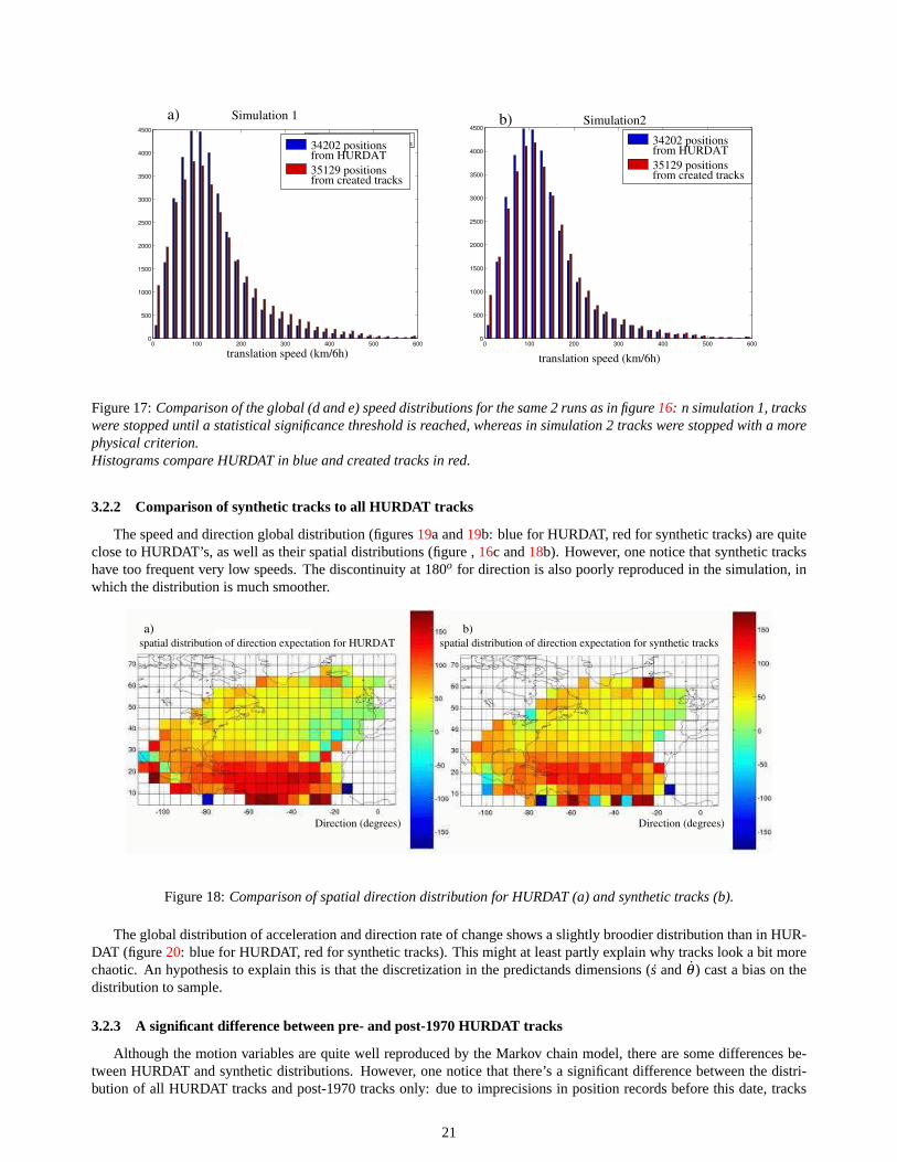
Figure 17:Comparison of the global (d and e) speed distributions for the same 2 runs as in figure16: n simulation 1, trackswere stopped until a statistical significance threshold is reached, whereas in simulation 2 tracks were stopped with a morephysical criterion.Histograms compare HURDAT in blue and created tracks in red.

3.2.2 Comparison of synthetic tracks to all HURDAT tracks

The speed and direction global distribution (figures19a and19b: blue for HURDAT, red for synthetic tracks) are quiteclose to HURDAT’s, as well as their spatial distributions (figure ,16c and18b). However, one notice that synthetic trackshave too frequent very low speeds. The discontinuity at 180o for direction is also poorly reproduced in the simulation, inwhich the distribution is much smoother.

Direction (degrees) Direction (degrees)

spatial distribution of direction expectation for HURDAT spatial distribution of direction expectation for synthetic tracksa) b)

Figure 18:Comparison of spatial direction distribution for HURDAT (a) and synthetic tracks (b).

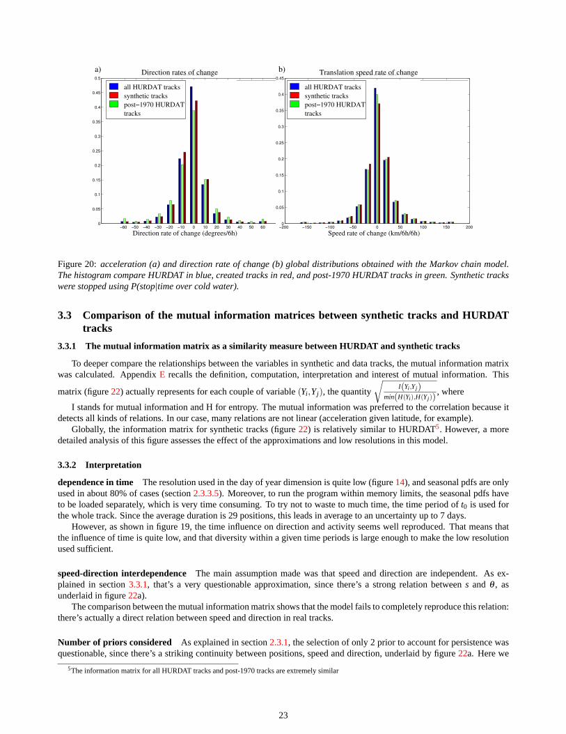
The global distribution of acceleration and direction rate of change shows a slightly broodier distribution than in HUR-DAT (figure 20: blue for HURDAT, red for synthetic tracks). This might at least partly explain why tracks look a bit morechaotic. An hypothesis to explain this is that the discretization in the predictands dimensions ( ˙s andθ ) cast a bias on thedistribution to sample.

3.2.3 A significant difference between pre- and post-1970 HURDAT tracks

Although the motion variables are quite well reproduced by the Markov chain model, there are some differences be-tween HURDAT and synthetic distributions. However, one notice that there’s a significant difference between the distri-bution of all HURDAT tracks and post-1970 tracks only: due to imprecisions in position records before this date, tracks

21

−100 0 100 200 300 400 500 600 700 800 9000

0.05

0.1

0.15

0.2

0.25

0.3

0.35speed distribution

all trackssatelite erasimulation Markov

−200 −150 −100 −50 0 50 100 150 2000

0.02

0.04

0.06

0.08

0.1

0.12

0.14

0.16

0.18direction distribution


Global direction distribution

Direction (degrees)

Num

ber o

f pos

ition

s no

rmal

ized

to H

urda

ta)

Num

ber o

f pos

ition

s no

rmal

ized

to H

urda

t

Speed (km/6h)

b) Global speed distribution

all HURDAT trackssynthetic trackspost−1970 HURDAT tracks

all HURDAT trackssynthetic trackspost−1970 HURDAT tracks

Figure 19:The histograms compare all HURDAT tracks in blue , created tracks in red, and post-1970 HURDAT tracks ingreen. Synthetic tracks were stopped using P(stop|time spent over cold water).a) speed distributionb) direction distribution

appear smoother and less erratic before this date (as shown by broader direction, acceleration and direction rate of changehistograms: green on figures18a and20), and the discontinuity at 180o is not as clear in post-1970 tracks only.

Table 2 compares the Kullback-Leibler divergence between synthetic tracks distributions and on the one hand, allHURDAT tracks, and on the other hand, post-1970 HURDAT tracks.

The synthetic distributions are expected to be closer to the all HURDAT tracks histogram than the post-1970 tracksonly. However, it is the contrary for speed and accelerations: maybe the use of second order predictands were able toreproduce some intrinsic properties of TC tracks that were not fully captures in the pre-satellite tracks.

HURDAT set→ whole HURDAT post-1970 onlydistribution compared↓

translation speed 0.0090 0.0050direction 0.0194 0.0323

acceleration 0.0057 0.0031direction rate of change 0.0054 0.0287

Table 2:Kullback-Leibler divergence values applied to the comparison of the speed, direction, acceleration and directionrate of change distributions obtained from the synthetic tracks, with the distributions obtained from the whole HURDATdataset (first column) and for post-1970 tracks only (second column).

3.2.4 A local example: tracks within 300km from Boston

Inn the wind risk estimation model perspective, tracks coming within a given radius of a given location are selected. Itis therefore important to assess the spatial precision of the statistical model.

For illustration, the translation speed distribution within 300km of Boston obtained with synthetic tracks is compared toHURDAT in figure21. The translation speed is a key variable for risk assessment in extratropical locations: exceptionallyhigh translation speeds can make some hurricanes maintain high intensities and be very damaging even in extratropicalregions in which the local potential intensity (defined in section1) is very low. The 1938 New England “Long IslandExpress” is an example: although hitting a region of low potential intensity, this fastest moving hurricane ever recordedranks among the most fatal hurricanes in the US history ([Valee and Dion, 1998]).

The translation speed distribution within 300km of Boston is extremely well reproduced by the statistical model.

22

−60 −50 −40 −30 −20 −10 0 10 20 30 40 50 600

0.05

0.1

0.15

0.2

0.25

0.3

0.35

0.4

0.45

0.5deviation distribution


−200 −150 −100 −50 0 50 100 150 2000

0.05

0.1

0.15

0.2

0.25

0.3

0.35

0.4

0.45acceleration distribution


all HURDAT trackssynthetic trackspost−1970 HURDATtracks

all HURDAT trackssynthetic trackspost−1970 HURDATtracks

Direction rates of change Translation speed rate of changea) b)

Direction rate of change (degrees/6h) Speed rate of change (km/6h/6h)

Figure 20:acceleration (a) and direction rate of change (b) global distributions obtained with the Markov chain model.The histogram compare HURDAT in blue, created tracks in red, and post-1970 HURDAT tracks in green. Synthetic trackswere stopped using P(stop|time over cold water).

3.3 Comparison of the mutual information matrices between synthetic tracks and HURDATtracks

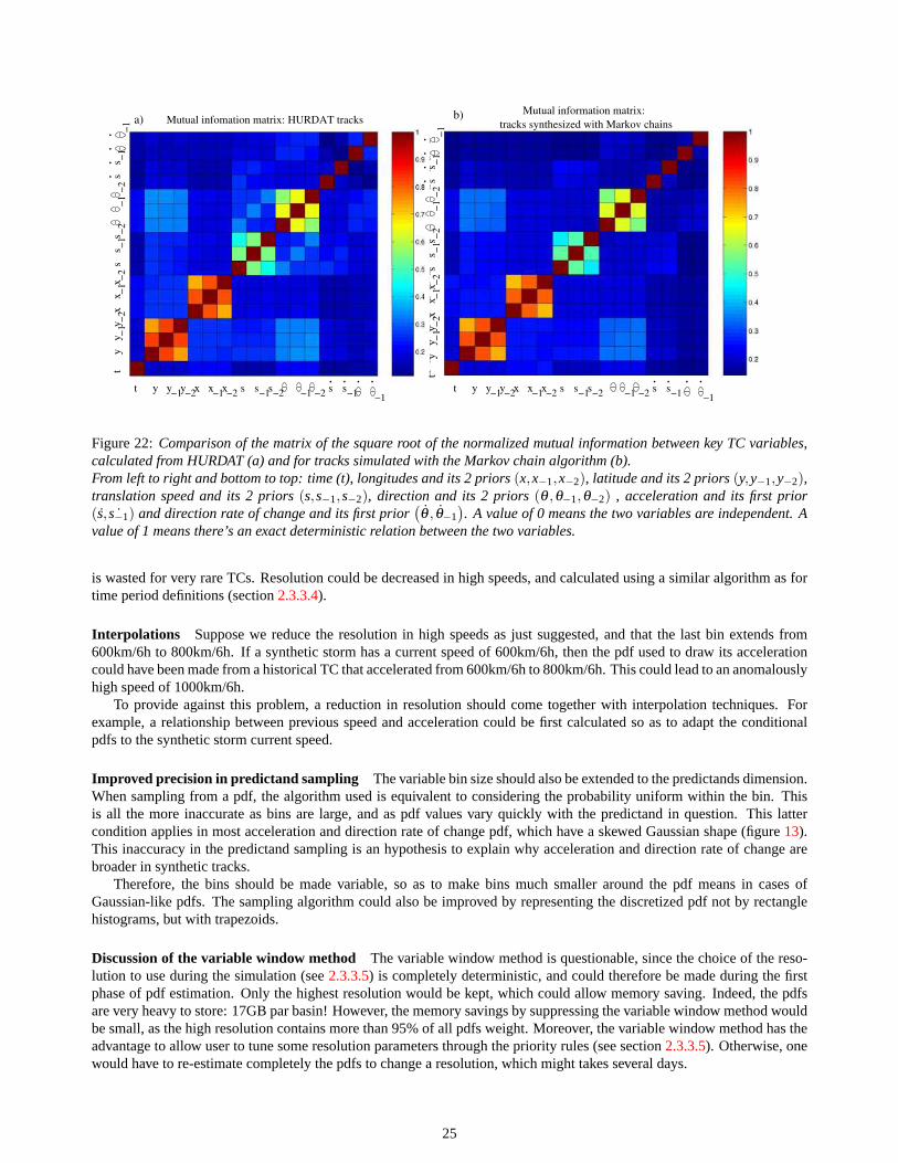
3.3.1 The mutual information matrix as a similarity measure between HURDAT and synthetic tracks

To deeper compare the relationships between the variables in synthetic and data tracks, the mutual information matrixwas calculated. AppendixE recalls the definition, computation, interpretation and interest of mutual information. This

matrix (figure22) actually represents for each couple of variable(Yi ,Yj), the quantity

√I(Yi ,Yj)

min(H(Yi),H(Yj )), where

I stands for mutual information and H for entropy. The mutual information was preferred to the correlation because itdetects all kinds of relations. In our case, many relations are not linear (acceleration given latitude, for example).

Globally, the information matrix for synthetic tracks (figure22) is relatively similar to HURDAT5. However, a moredetailed analysis of this figure assesses the effect of the approximations and low resolutions in this model.

3.3.2 Interpretation

dependence in time The resolution used in the day of year dimension is quite low (figure14), and seasonal pdfs are onlyused in about 80% of cases (section2.3.3.5). Moreover, to run the program within memory limits, the seasonal pdfs haveto be loaded separately, which is very time consuming. To try not to waste to much time, the time period oft0 is used forthe whole track. Since the average duration is 29 positions, this leads in average to an uncertainty up to 7 days.

However, as shown in figure 19, the time influence on direction and activity seems well reproduced. That means thatthe influence of time is quite low, and that diversity within a given time periods is large enough to make the low resolutionused sufficient.

speed-direction interdependence The main assumption made was that speed and direction are independent. As ex-plained in section3.3.1, that’s a very questionable approximation, since there’s a strong relation betweens and θ , asunderlaid in figure22a).

The comparison between the mutual information matrix shows that the model fails to completely reproduce this relation:there’s actually a direct relation between speed and direction in real tracks.

Number of priors considered As explained in section2.3.1, the selection of only 2 prior to account for persistence wasquestionable, since there’s a striking continuity between positions, speed and direction, underlaid by figure22a. Here we

5The information matrix for all HURDAT tracks and post-1970 tracks are extremely similar

23

0 100 200 300 400 500 600 700 800 9000

5

10

15

20

25

30

35speed distribution within 300 km from boston

209 position from hurdat742 position from created tracks209 HURDAT samples

742 samples from created tracks

Num

ber o

f pos

ition

s no

rmal

ized

to H

urda

t’s

Translation speed (km/6h)

Tracks created with new model compared to HurdatTranslation speed distribution within 300km from Boston:

Figure 21:Translation speed distribution within 300km of Boston for tracks created with the Markov Chain model (red),compared to HURDAT (blue). Synthetic tracks were stopped using P(stop|time over cold water).

can see that persistence in speed, direction and location is surprisingly well reproduced. We can therefore consider that thereduction of persistence predictors to 2 priors only was far a viable approximation.

However, figure22b shows that relations betweenθ andθ , and betweenθ andθ−1, are underestimated by the model.The persistence in direction rate of change is problematic. The relations betweenθ ,θ and ˙θ−1 is important in the recurva-ture and looping processes: when a track starts recurving, it keeps on recurving, or when a track starts looping, it finishesits loop. The lack of persistence in direction rate of change might partly explain that synthetic tracks are more chaotic thanHURDAT’s.

3.4 Number of sample to consider in a set

When creating a set of 100 tracks, the distribution of any synthetic variable may strongly differ from HURDAT due tosampling artifacts. In the example of the genesis month distribution, figure23 shows the standard deviation of histogramsbars for 100 sets of 100 tracks.

What is the minimum number of tracks to create in a set to insure that the set is representative, and its distributions areclose to HURDAT? As shown in figure23, the more samples in a set, the closer in average the synthetic distribution fromHURDAT. Such tests were conducted in the case of genesis month, and it seems that at least 500 or 600 tracks per set areneeded for the set to be satisfyingly representative.

When wind risk probabilities are computed, a set of 1,000 tracks was used to compute wind exceedance probabilitiesin the whole Atlantic basin, and sets of 15,000 tracks were generated to compute probabilities on specific coastal sites.

4 Discussion of the method and alternatives

4.1 What could have been improved

Lower resolution in longitude HURDAT’s mutual information matrix ( figure22a) shows that speed and direction aremuch more linked to latitude than longitude. Therefore, the resolution in longitude could be reduced from 0.5o to 5o

without much loss of information. The consequent gain of space of a factor of 10 could be used to increase the pdfsstatistical significance and/or add new predictors. For example, one could take into account the dependency betweendirection and speed and the dependency of previous direction rate of change on current direction rate of change. Both ofthese relationships are lacking in the current algorithm.

Generalize variable bin size to all predictors The variable bin size used to define time periods (section2.3.3.4) couldbe generalized to all predictors. For example, in the case of predictorsi−1, the resolution is 40km/6h and speeds range in[0,800] km/6h. However, very few storm reach translation speeds greater than 400km/6h. Consequently, half of the space

24

−1 −2 −1 −2 −1 −2 −1 −2 −1 −1t y x sy y x x s s s s

. . ..−2s

−1

..−1s

.s.

−2−1−1 −2 −1 −2 −1t y x sy y x x s

−1−2

−1−2

−1−2

−1−2

−1−1

ty

xs

yy

xx

ss

ss

..

..

−1−2

−1−2

−1−2

−1−2

−1−1

ty

xs

yy

xx

ss

ss

..

..

Mutual infomation matrix: HURDAT tracks tracks synthesized with Markov chainsMutual information matrix:

a) b)

Figure 22:Comparison of the matrix of the square root of the normalized mutual information between key TC variables,calculated from HURDAT (a) and for tracks simulated with the Markov chain algorithm (b).From left to right and bottom to top: time (t), longitudes and its 2 priors(x,x−1,x−2), latitude and its 2 priors(y,y−1,y−2),translation speed and its 2 priors(s,s−1,s−2), direction and its 2 priors(θ ,θ−1,θ−2) , acceleration and its first prior(s, ˙s−1) and direction rate of change and its first prior

(θ , θ−1

). A value of 0 means the two variables are independent. A

value of 1 means there’s an exact deterministic relation between the two variables.

is wasted for very rare TCs. Resolution could be decreased in high speeds, and calculated using a similar algorithm as fortime period definitions (section2.3.3.4).

Interpolations Suppose we reduce the resolution in high speeds as just suggested, and that the last bin extends from600km/6h to 800km/6h. If a synthetic storm has a current speed of 600km/6h, then the pdf used to draw its accelerationcould have been made from a historical TC that accelerated from 600km/6h to 800km/6h. This could lead to an anomalouslyhigh speed of 1000km/6h.

To provide against this problem, a reduction in resolution should come together with interpolation techniques. Forexample, a relationship between previous speed and acceleration could be first calculated so as to adapt the conditionalpdfs to the synthetic storm current speed.

Improved precision in predictand sampling The variable bin size should also be extended to the predictands dimension.When sampling from a pdf, the algorithm used is equivalent to considering the probability uniform within the bin. Thisis all the more inaccurate as bins are large, and as pdf values vary quickly with the predictand in question. This lattercondition applies in most acceleration and direction rate of change pdf, which have a skewed Gaussian shape (figure13).This inaccuracy in the predictand sampling is an hypothesis to explain why acceleration and direction rate of change arebroader in synthetic tracks.

Therefore, the bins should be made variable, so as to make bins much smaller around the pdf means in cases ofGaussian-like pdfs. The sampling algorithm could also be improved by representing the discretized pdf not by rectanglehistograms, but with trapezoids.

Discussion of the variable window method The variable window method is questionable, since the choice of the reso-lution to use during the simulation (see2.3.3.5) is completely deterministic, and could therefore be made during the firstphase of pdf estimation. Only the highest resolution would be kept, which could allow memory saving. Indeed, the pdfsare very heavy to store: 17GB par basin! However, the memory savings by suppressing the variable window method wouldbe small, as the high resolution contains more than 95% of all pdfs weight. Moreover, the variable window method has theadvantage to allow user to tune some resolution parameters through the priority rules (see section2.3.3.5). Otherwise, onewould have to re-estimate completely the pdfs to change a resolution, which might takes several days.

25

1 2 3 4 5 6 7 8 9 10 11 12−0.05

0

0.05

0.1

0.15

0.2

0.25

0.3

0.35

0.4genesis time for Hurdat and created tracks sets

months of year

gene

sis

prob

abili

ty

100 sets of 100 created tracks100 sets of 800 created trackshurdat

HURDAT

100 sets of800 synthetic tracks

100 sets of100 synthetic tracks

for sets of 100 and 800 created tracks.Comparison of genesis times distributions standard deviations

gene

sis

prob

abili

ty

month of year

Figure 23: The red histogram represents HURDAT genesis dates distribution. In blue (resp green) is represented the meanand standard deviation of 100 histogram bars value produced for each of the 100 sets of 100 (resp 800) synthetic tracks

Utilization of low-level file-access functions to reduce simulation execution timeDuring the simulation, more than 5hours are lost in loading the large pdfs files, time period after time-period (since all pdfs would surpass the RAM capacity).The file-loading is accomplished using a high-level matlab function, which is very convenient to use, but is very slow.Some time might be saved by using lower-level file access functions, that enable to directly read a value in a binary filewithout the need of loading the entire files.

4.2 Advantages and drawbacks inherent to the methodology from the quality of synthetic trackspoint of view

Although many improvement could have made the synthetic tracks more realistic and closer to HURDAT, there aresome drawbacks that are inherent to the methodology used, in particular the decision to discretize variables and to estimateall pdfs in advance and store them.

4.2.1 Advantages and drawback of discretization

The discretization of variable offers a very convenient way to store the pdfs, in an explicit manner. Moreover, it avoidsthe errors related to regression equations or parametric representation of the relationships. However, discretization addsimprecisions from the uniformity assumption both in the predictor and predictand dimensions, as explained in section4.1.

Besides, it also make the pdfs considerably heavy. One can wonder how come we end up with 17GB of pdfs, while thehistorical record has hardly 5MB...

4.2.2 Advantages and drawback of estimating all pdfs in advance

Estimating all pdfs in advance presents the advantage that the simulation should then be very fast. However, this is notthe case because of the huge amount of pdf data to load.

Besides, the pdf estimation phase takes about one week. This is a drawback when one wants to change the resolutions,the smoothing parameters or the choice of predictors and predictands.

4.2.3 An alternative with neither discretization nor pdf pre-estimation

I suggested and implemented an alternate algorithm to the Markov chain approach, based on analog selection. There-after, the Markov chain algorithm and this alternate algorithm will be named algorithm 1 and 1’ respectively.

26

Methodology The idea is inspired from the analog motion model HURRAN ([Hope and Neumann, 1970]). The algo-rithm used is schemed in figure24. Track are initiated as in the previously described algorithm . Then, for each forwardstep, an historical analog case sampled from the HURDAT database, with a probability proportional to a score S measuringthe similarity between HURDAT potential analogs and the track being synthesized.

Let−→XH =

(tH ,xH ,yH ,sH

−1,θH−1, θ

H−1

)be the vector of predictors for any potential HURDAT analog H and

−→Xs=

(ts,xs,ys,ss

−1,θs−1, θ

s−1

)the situation of the track being synthesized. Let−→r =

(dt,dx,dy,ds,dθ ,dθ

)be a vector of resolution parameters. Then the

score S is calculated as

S(−→

XH ,−→Xs,−→r

)= e

−∑ni=1

(Xs

i −XHi

ri

)2

with n the number of components in the predictors vectors.Note that there is no more independence assumption between speed and direction, and that the previous direction rate

of change, which was lacking in the previous algorithm, is now a predictor.Let θanalog andsanalog be the direction rate of change and acceleration of the selected analog respectively respectively.

Then the acceleration and direction rate of change for the track being synthesized,θi andsi , are assumed to follow a normaldistributionN

(θanalog,σθ

)andN

(sanalog,σs

)respectively.

Tracks are terminated with the same termination pdfs as in algorithm 1.

go within scan radiusof target point?

track terminated?

forward equations

. .s and

storage of the track

yesno

yes

no

Next position

Samplefor the synthetic track

Sample one analog

selection of HURDAT analogs forthe track being synthesized

New track first position

initiation pdfSample

set of synthetic tracks

Figure 24:Scheme summarizing the alternate algorithm 1’ based on analog selection. Inputs/outputs are in blue, algo-rithms in green and conditions in purple. The final output (the set of synthetic tracks) is emphasized. The structure of thesynthesis algorithm is very similar to algorithm 1, except that a transition algorithm based on analog selection is usedinstead of transition pdfs directly. Initiation and termination pdfs are the same as in the Markov chain algorithm.

Similarity between this approach and the explicit Markov chain approach Although these two algorithms are verydifferent in approach, they are very similar in practice.

27

• The analog selection through a Gaussian score is comparable to the Gaussian smoothing used in space in algorithm1, except there is no discretization of predictors here.

• The pdf estimation is similar in the way they both use Gaussian kernel to smooth the historical data points, except nomore discretization of predictands is carried out here.

• A big difference however is that this algorithm insures that both ˙s andθ are sampled from the same analog, and areconsequently mutually consistent.

−100 −80 −60 −40 −20 0

10

20

30

40

50

60

70

60 created tracks

s. .

s. .t sy y y x xx s s−1 −1 −2 −1 −1−2 −2 −1 −1

s..

s..

ts

yy

yx

xx

ss

−1−1

−2−1

−1−2

−2−1

−1

with algorithm 1’

a) 60 random tracks created with algorithm 1’

Mutual information matrix for tracks createdb)

Figure 25:Results obtained with the alternate analog algorithm 1’:a) general aspect of 60 randomly drawn synthetic tracks. This can be compared with HURDAT (figure8a) and algorithm1 (figure15).b) Matrix of the square root of the normalized mutual information between key TC variables. This can be compared withHURDAT and algorithm 1 (figure22).

results and discussion The aspect of the tracks is similar to HURDAT tracks (figure25), although they also look slightlymore chaotic. As in algorithm 1, this might be due to an insufficient statistical significance of the pdfs.

track synthesis algorithm→ algorithm1 algorithm 1’ algorithm2distribution compared↓ (Markov chain) (analog selection) (steering concept)

translation speed 0.0090 0.0052 0.0489direction 0.0194 0.0139 0.0299

acceleration 0.0057 0.0007 0.1063direction rate of change 0.0054 0.0018 0.0893

Table 3:Values of the Kullback-Leibler divergence applied to compare synthetic distributions of speed, direction, acceler-ation and direction rate of change to these same distributions for all HURDAT tracks. Algorithm 1 is the algorithm basedon an explicit Markov chain. The 2 last columns are alternatives for this model: algorithm 1’i s the algorithm based onanalog selection. Algorithm 2 is the algorithm based on steering concept.

The speed, direction, acceleration and direction rate of change are presented in figure26 (red histograms). Table3compares the Kullback-Leibler divergence obtained for this algorithm (second column) compared to algorithm 1 (firstcolumn) (the third column is an another alternative described later). The distributions obtained with this alternative aremore similar to HURDAT for all the four motion variables analyzed.

The biggest improvement is for the acceleration and direction rate (figure26c and d, table3) probably because noimprecisions were added through discretization.

This algorithm allows to have closer distributions to HURDAT tracks. However, the errors are slightly larger whencompared to satellite-era tracks only (not shown).

28

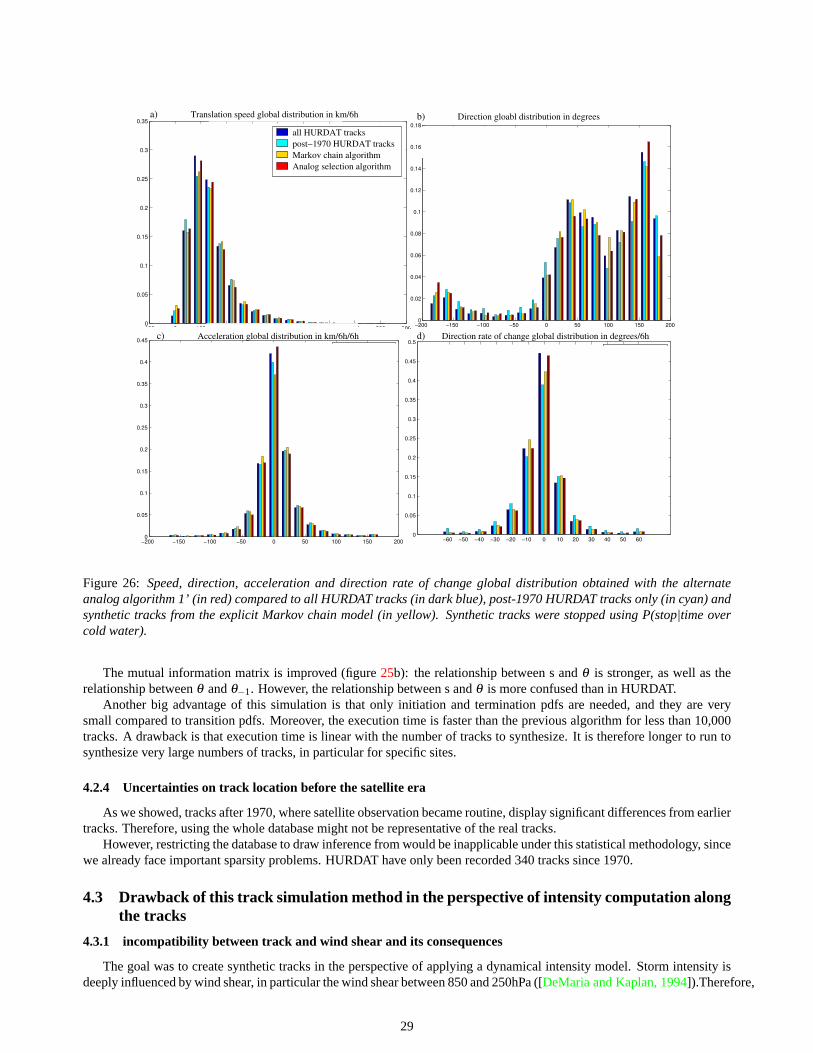
−100 0 100 200 300 400 500 600 700 800 9000

0.05

0.1

0.15

0.2

0.25

0.3

0.35speed distribution

all trackssatelite erasimulation Markovsimulation analog

−200 −150 −100 −50 0 50 100 150 2000

0.02

0.04

0.06

0.08

0.1

0.12

0.14

0.16

0.18direction distribution


−200 −150 −100 −50 0 50 100 150 2000

0.05

0.1

0.15

0.2

0.25

0.3

0.35

0.4

0.45acceleration distribution


−60 −50 −40 −30 −20 −10 0 10 20 30 40 50 600

0.05

0.1

0.15

0.2

0.25

0.3

0.35

0.4

0.45

0.5deviation distribution


all HURDAT trackspost−1970 HURDAT tracksMarkov chain algorithmAnalog selection algorithm

Translation speed global distribution in km/6h a) b) Direction gloabl distribution in degrees

c) Acceleration global distribution in km/6h/6h d) Direction rate of change global distribution in degrees/6h

Figure 26: Speed, direction, acceleration and direction rate of change global distribution obtained with the alternateanalog algorithm 1’ (in red) compared to all HURDAT tracks (in dark blue), post-1970 HURDAT tracks only (in cyan) andsynthetic tracks from the explicit Markov chain model (in yellow). Synthetic tracks were stopped using P(stop|time overcold water).

The mutual information matrix is improved (figure25b): the relationship between s andθ is stronger, as well as therelationship betweenθ andθ−1. However, the relationship between s andθ is more confused than in HURDAT.

Another big advantage of this simulation is that only initiation and termination pdfs are needed, and they are verysmall compared to transition pdfs. Moreover, the execution time is faster than the previous algorithm for less than 10,000tracks. A drawback is that execution time is linear with the number of tracks to synthesize. It is therefore longer to run tosynthesize very large numbers of tracks, in particular for specific sites.

4.2.4 Uncertainties on track location before the satellite era

As we showed, tracks after 1970, where satellite observation became routine, display significant differences from earliertracks. Therefore, using the whole database might not be representative of the real tracks.

However, restricting the database to draw inference from would be inapplicable under this statistical methodology, sincewe already face important sparsity problems. HURDAT have only been recorded 340 tracks since 1970.

4.3 Drawback of this track simulation method in the perspective of intensity computation alongthe tracks

4.3.1 incompatibility between track and wind shear and its consequences

The goal was to create synthetic tracks in the perspective of applying a dynamical intensity model. Storm intensity isdeeply influenced by wind shear, in particular the wind shear between 850 and 250hPa ([DeMaria and Kaplan, 1994]).Therefore,

29

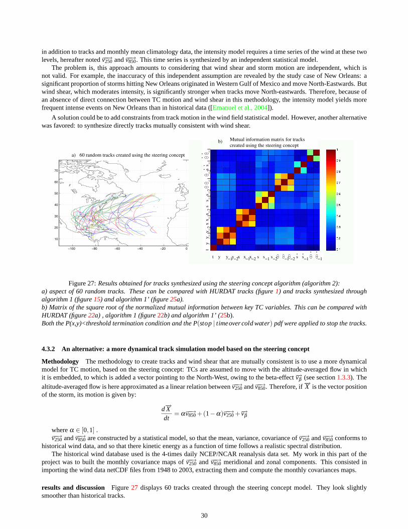
in addition to tracks and monthly mean climatology data, the intensity model requires a time series of the wind at these twolevels, hereafter noted−−→v250 and−−→v850. This time series is synthesized by an independent statistical model.

The problem is, this approach amounts to considering that wind shear and storm motion are independent, which isnot valid. For example, the inaccuracy of this independent assumption are revealed by the study case of New Orleans: asignificant proportion of storms hitting New Orleans originated in Western Gulf of Mexico and move North-Eastwards. Butwind shear, which moderates intensity, is significantly stronger when tracks move North-eastwards. Therefore, because ofan absence of direct connection between TC motion and wind shear in this methodology, the intensity model yields morefrequent intense events on New Orleans than in historical data ([Emanuel et al., 2004]).

A solution could be to add constraints from track motion in the wind field statistical model. However, another alternativewas favored: to synthesize directly tracks mutually consistent with wind shear.

−100 −80 −60 −40 −20 0

10

20

30

40

50

60

70

60 created tracks, steering concept

s. .

s. .

t y sxy y x x s s−1 −1 −1 −1 −1 −1−2 −2 −2 −2

s. s...

ty

xy −1

y −2x −1

x −2s

s −1s −2

−1−2

−1−1

Mutual information matrix for trackscreated using the steering concept

b)

a) 60 random tracks created using the steering concept

Figure 27:Results obtained for tracks synthesized using the steering concept algorithm (algorithm 2):a) aspect of 60 random tracks. These can be compared with HURDAT tracks (figure1) and tracks synthesized throughalgorithm 1 (figure15) and algorithm 1’ (figure25a).b) Matrix of the square root of the normalized mutual information between key TC variables. This can be compared withHURDAT (figure22a) , algorithm 1 (figure22b) and algorithm 1’ (25b).Both the P(x,y)<threshold termination condition and the P(stop| timeovercold water) pdf were applied to stop the tracks.

4.3.2 An alternative: a more dynamical track simulation model based on the steering concept

Methodology The methodology to create tracks and wind shear that are mutually consistent is to use a more dynamicalmodel for TC motion, based on the steering concept: TCs are assumed to move with the altitude-averaged flow in whichit is embedded, to which is added a vector pointing to the North-West, owing to the beta-effect−→vβ (see section1.3.3). Thealtitude-averaged flow is here approximated as a linear relation between−−→v250 and−−→v850. Therefore, if−→X is the vector positionof the storm, its motion is given by:

d−→Xdt

= α−−→v850+(1−α)−−→v250+−→vβ

whereα ∈ [0,1] .−−→v250 and−−→v850 are constructed by a statistical model, so that the mean, variance, covariance of−−→v250 and−−→v850 conforms to

historical wind data, and so that there kinetic energy as a function of time follows a realistic spectral distribution.The historical wind database used is the 4-times daily NCEP/NCAR reanalysis data set. My work in this part of the

project was to built the monthly covariance maps of−−→v250 and−−→v850 meridional and zonal components. This consisted inimporting the wind data netCDF files from 1948 to 2003, extracting them and compute the monthly covariances maps.

results and discussion Figure 27 displays 60 tracks created through the steering concept model. They look slightlysmoother than historical tracks.

30

Tracks created using this algorithm also have slightly less accurate s,θ , sandθ distributions (see values of the Kullback-Leibler divergence in table3, third column). Note that in the steering concept algorithm, tracks are stopped when movingout of a rectangle domain extending from−110o to −20o in longitude and 0o to 50o in latitude. To better compare theresults with HURDAT and the other synthesis algorithms, a combination of all used termination criteria for the differentsimulation methods were used: rectangle domain,P(stop| timeovercold water) andP(x,y) < threshold.

This method have the advantage not to do any assumption about which predictors to select, how many priors to consideror about the independence between s andθ . Therefore, as expected, the information matrix (figure27) displays high mutualinformation values between most of the motion variables, in particular consecutive speeds, directions, directions rates ofchange, accelerations, and combinations of these variables. However, theses values are strikingly larger than in real tracks.

The main advantage of this algorithm is to create tracks and wind shear that are mutually consistent. Nevertheless,similarity between the resulting tracks and HURDAT, although not as good as the statistical models, are surprisingly goodif considering that HURDAT tracks were never taken directly into account in the synthesis algorithm.

4.3.3 Comparison of tracks simulated through the purely statistical model and through steering concept in theperspective of the wind risk estimations

Both the purely statistical and the steering concept methods were used in the wind risk estimation model and compared.They yields similar results in the study cases such as Miami, in which historical data is abundant. Besides, in this

location, TC undergo no particularly strong interactions with wind shear and follow the steering concept well.However, in many other cases, the two methods yield interestingly different wind risk estimates. For example, in a

study case such as New Orleans, where a proportion of tracks are affected by strong wind shear, wind risks estimates frompurely statistically simulated tracks are flawed by the incompatibility between tracks and wind shear.

On the other hand, in a study case such as Boston, tropical cyclone often undergo an extratropical transition, thatis, they switch from a tropical regime to an extratropical one. In particular, the translation speed increases, which isresponsible for maintaining high intensities over cold waters. But during extratropical transition, the steering assumptionis no more sufficient to model the storm motion. Therefore, extreme hurricane events are underestimated when evaluatingwind probabilities on Boston using tracks synthesized through the steering concept. On the contrary, the extratropicaltransition effects on motion are reflected by the historical database, and thus in the purely statistically simulated tracks.

31

Conclusion

In the perspective of calculating wind probabilities over given coastal locations, a statistical model was developedto simulate large number of hurricane tracks whose motion properties are conform to the historical data. Simulated asMarkov chains whose initiation and transition probabilities are computed from the historical database, this track simulationtechnique yields motion properties extremely similar to the database. However, the Markov chain assumption together withvarious independence assumption, on the one hand between motion characteristics and on the other hand between motionand wind shear, is a drawback of this technique. Moreover, the robustness of the statistics is questionable in areas with fewdata.

These drawbacks are avoided in a more dynamical alternative to this statistical model, based on the steering concept.Tropical cyclone motion is slightly less similar to the historical data, which was never directly taken into account, butdisplays more consistency between different motion characteristics, as well as between motion and wind shear.

Both methods were used in the wind risk estimation model, compared and contrasted. They turn out to be complemen-tary: depending on environmental influences undergone and historical data abundance, each method has its strength andweakness.

This coupled statistical-deterministic approach is new and contrasts with all previous wind probability estimation mod-els. The synthesis of a large number of tracks provides a convenient way to interpolate track properties in location, and thedeterministic intensity model allows to avoid the paucity of reliable historical intensity estimates.

Perspectives for this project are to further develop the track synthesis algorithm, in particular, accelerate the algorithmbased on analog selection. Besides, it is also planned to integrate interdecadal variability, to which tropical cyclone activityis very sensitive ([Gray et al., 1992]).

An important question one can ask is: how can one evaluate this model? The model results were here comparedto direct estimates from historical data, and the results were positive. However, a validation on independent data mightbe interesting, in particular for extreme events that are beyond the range of observation. For example, some historicalreconstitution yields some information about landfalling storm back to the 1600s in the US. Some geological informationcould be also used to validate wind probabilities on a very long term ([Murnane, 2000]).

Acknowledgments

I would like to warmly thank my supervisor Kerry Emanuel for welcoming me for this internship. I enjoyed theopportunity he gave me to work with a lot of independence. I also appreciated his availability to provide explanations whenneeded. This internship really taught me a lot.

I’m also very grateful to Sai Ravela. He spent a lot of time to give me judicious advice and useful explanations. Hishelp, both during my internship and for the redaction of this report, was very precious.

I thank Emanuel Vivant for sending me documentations about the former versions of the track simulation routines.

32

Appendix

A Markov Chains

A Markov process is a series of states(Xi)i∈[1,n], discrete or continuous, in which∀i ∈ [1,n], the transition from stateXi to Xi+1is defined by a transition probability conditioned only upon the immediately preceding stateXi (called the firstprior), independently of the path by which the preceding state was reached and of time i ([Lange, 2003]). Let a, b, c, ... bepossible values of the state X. Then∀i ∈ [1,n],

P(Xi+1 = a | Xi = b, Xi−1 = c, ...) = P(Xi+1 = a | Xi = b) = P(a | b)

This is called the Markov assumption. This assumption allows to greatly simplify many complicated problems.To build a Markov process, two sets of probability density functions (pdfs) are required ([Lange, 2003]):

1. Initiation probabilityP(X0), to initiate the process

2. transition probabilitiesP(a | b) to elongate the process.

A Markov process in which states X are discrete is called a Markov chain. Transition probabilities in a Markov chain canbe represented as a transition matrix T, so that∀(a j ,ak) ∈Ω2, whereΩ is the set of possible states, and∀i ∈ [1,n],

T( j,k) = P(Xi+1 = a j | Xi = ak)

It’s important to note that the definition of a Markov chain can be generalized to any series of states for which thetransition probability depends on a finite number of preceding states (calledpriors). Suppose the transition probability isconditioned uponτ priors. Then the transition probability isP(Xi | Xi−1, Xi−2, ...Xi−τ). A new state Y can be defined asYi = (Xi , Xi−1, ...Xi−τ+1) and the transition probability can be expressed asP(Yi |Yi−1). The Markov chain assumption isthus satisfied.

B Parametric and non-parametric representation of probability density func-tions

Let P(X) be the distribution of a random variable X from which(xi)i∈[1,n] samples are observed. P(X) can be estimatedand stored in two ways:

1. Parametrically

P(X) is assumed to have a given shape, for example: uniform , Gaussian, Weibull... Function parameters can beestimated to fit the sample distribution the best. Such probability density functions (pdfs) are very small to store, since onlythe estimated function parameters are stored. However, precision is lost if the assumption of the chosen shape is not valid.

An advantage to parametrically store a pdf is that the distribution always reflect the smoothness and continuity of theunderlying distribution, even if n is very small. However, small sample size might cast a bias on the function parameterestimation.

2. Non-parametrically

No assumption is made on the pdf shape. The pdf is stored as a histogram(H j) j∈[1,N], with N the number of histogrambins. Errors are added from the discretization of the variable to predict, but the resulting pdf is in many cases more accurate,as long as the resolution is sufficiently high. The main drawback is that it uses much more storage (N histogram values,plus information about the bin centers(b j) j∈[1,N]).

The histogram might be calculated by just counting the number of sample that fall into each bin. However, this rawhistogram might not reflect the smoothness of the underlying distribution, since histograms are very sensitive to the samplesize, in particular ifn N.

To avoid this problem, histograms can be smoothed using a smoothing kernel ([Wand and Jones, 1995]): for each bin j,

33

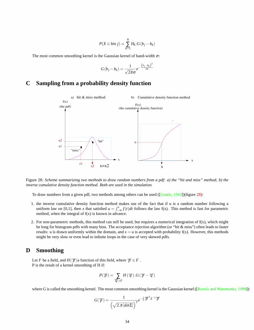
P(X ∈ bin j) =N

∑k=1

Hk.G(b j −bk)

The most common smoothing kernel is the Gaussian kernel of band-widthσ :

G(b j −bk) =1√2πσ

e−(bj−bk)

2

2σ

C Sampling from a probability density function

x1

"hit"

"miss"

f(x)(the pdf)

hit & miss methoda)

x2 x=x2x

b) Cumulative density function method

u

x

F(x)(the cumulative density function)

x

u2

u1

Figure 28:Scheme summarizing two methods to draw random numbers from a pdf: a) the “hit and miss” method; b) theinverse cumulative density function method. Both are used in the simulation.

To draw numbers from a given pdf, two methods among others can be used ([Gentle, 1943])(figure28):

1. the inverse cumulative density function method makes use of the fact that if u is a random number following auniform law on [0,1], thenx that satisfiedu =

∫ x−∞ f (t)dt follows the law f(x). This method is fast for parametric

method, when the integral of f(x) is known in advance.

2. For non-parametric methods, this method can still be used, but requires a numerical integration of f(x), which mightbe long for histogram pdfs with many bins. The acceptance rejection algorithm (or “hit & miss”) often leads to fasterresults: u is drawn uniformly within the domain, andx = u is accepted with probability f(x). However, this methodsmight be very slow or even lead to infinite loops in the case of very skewed pdfs.

D Smoothing

Let F be a field, andH(−→p )a function of this field, where−→p ∈ F .P is the result of a kernel smoothing of H if:

P(−→p ) = ∑−→q ∈F

H (−→q ) .G(−→p −−→q )

where G is called the smoothing kernel. The most common smoothing kernel is the Gaussian kernel ([Ravela and Mammatha, 1999]):

G(−→p ) =1(√

2.π |detΣ|)3 e−

12−→p T Σ−1−→p

34

whereΣ is the covariance matrix. For example, in a 3-D case and expressed on the principal component basis,

Σ =σ2

x 0 00 σ2

y 00 0 σ2

t

with σx, σy andσt the standard deviations of the Gaussian kernel in x,y,and t dimensions respectively. If these standarddeviations are equal, then the smoothing is said isotropic. Standard deviation can be whether constant or functions of−→p aswell.

E Mutual information and its measures

To estimate the relation between two random variables X and Y with observed values(xi)i∈[1,n] and (yi)i∈[1,n], thecorrelation coefficient r, defined as

r2 =cov(X,Y)√V(X).V(Y)

wherecovstands for covariance and V for variance is often used.However, to detect relations that are not linear, the mutual information ([Shannon, 1948]) is of great interest.The entropy H of a random variable X, with a distribution represented as an histogram discretized as(Xi)i∈[1,N], where

N is the number of bins in the histogram, is calculated as

H(X) =−N

∑i=1

P(X = Xi).log(P(X = Xi))

Entropy gives the uncertainty of a random variable X. For example, it is maximum for a uniform distribution andminimum (0) for a Dirac distribution.

The uncertainty of variable X given Y can be similarly measured:

H(X |Y) =−M

∑j=1

P(Y = Yj)N

∑i=1

P(X = Xi |Y = Yj).log(P(X = Xi |Y = Yj))

where Y’s distribution is discretized on a M-bin histogram.The mutual information I, defined as

I(X,Y) = H(X)−H(X |Y) = H(Y)−H(Y | X)

is a measure of the relation existing between X and Y.I(X,Y) = 0 if there is no relation at all, andI(X,Y) = H(X) ifthere is a deterministic relation between X and Y.The mutual information can be normalized by its maximum possible value as

IN(X,Y) =I(X,Y)

min(H(X),H(Y))

if min(H(X),H(Y)) 6= 0 (or IN(X,Y) = 0 otherwise), to obtain a coefficientIN between 0 and 1 and comparable fromrandom variables to others ([Li et al., 2003]).

To study the relation between a set of p random variables(Yi)i∈p, the mutual information matrix M can be computed so

that∀(i, j) ∈ [1, p]2,

M(i, j) = IN (Yi ,Yj)

In practice, the mutual information tends to yield either values very close to 1, or values very close to 0. Therefore, thesquare root of the normalized mutual information was used in this report to better visualize the results.

35

F Measures of similarity between two distributions

Many measures exist to assess the similarity between two non-parametric distributions: Bhattacharyya distance, theχ2

distance, the Kullback-Leibler divergence, root-mean-squares errors...Let (Hi)i∈[1,n] and(Gi)i∈[1,n] be two pdfs stored as n-bins histograms.The Kullback-Leibler divergence, also called relative entropy, is a measure of the inefficiency of assuming that the

distribution is G while the true distribution is H ([Cover and Thomas, 1991]). Therefore, it is the most natural measure ofsimilarity to use when one of the distribution is assumed true and the other is an approximation of it. The Kullback-Leiblerdivergence is expressed as:

D(H |G) =n

∑i=1

Hi .log

(Hi

Gi

)It is equal to 0 if the two distributions are equal, and is all the largest as distributions are different. It can be seen as a

“distance” between two distributions, although it is not a true distance since it is not symmetric.The Kullback-Leibler divergence was chosen in this report to assess the similarity between synthetic and historical

tracks.

36

References

[hrd, 2004] (2004). National Oceanic and Atmospheric Administration’s web page, Hurricane Division Center:http://www.aoml.noaa.gov.

[Batts et al., 1980]Batts, M., Cordes, L., Russell, L., Shaver, J., and Simiu, E. (1980). Hurricane wind speeds in the unitedstates. Technical report, U.S. Dept. of Commerce - National Bureau of Standards, NBS Builing Science Series, 124.

[Chu and Wang, 1998]Chu, P.-S. and Wang, J. (1998). Modeling return periods of tropical cyclones intensities in thevicinity of hawaii. J. Appl. Meteor., 37, 951-960.

[Cochran, 2000]Cochran, L. (2000). Wind engineering as related to tropical cyclones. C.p.p.’s technical publications,routledge press, Cermak Peterka Petersen (CPP), Inc.

[Cover and Thomas, 1991]Cover, T. and Thomas, J. (1991).Elements of information theory. John Wiley and Sons.

[Darling, 1991] Darling, R. W. R. (1991). Estimating probabilities of hurricane wind speeds using a large-scale empiricalmodel.Journal of Climate, 4,1035-1046.

[DeMaria and Kaplan, 1994]DeMaria, M. and Kaplan, J. (1994). A statistical hurricane intensity prediction scheme(ships) for the atlantic basin.Weather and Forecast, 9, 209-220.

[Emanuel, 1995]Emanuel, K. (1995). Sensitivity of tropical cyclones to surface exchange coefficients and a revisedsteady-state model incorporating eye dynamics.J. Atmos. Sci.,52, 3969-3976.

[Emanuel, 1998]Emanuel, K. (1998). Lecture notes: Tropical cyclones. http://wind.mit.edu/ emanuel/geosys/geosys.html.

[Emanuel, 2003]Emanuel, K. (2003). Tropical cyclones.Annu.Rev. Earth Planet. Sci. 2003 31:75-104.

[Emanuel et al., 2003]Emanuel, K., DesAutel, C., Holloway, C., and Korty, R. (2003). Environmental control of tropicalcyclone intensity.Journal of the Atmospheric Sciences: Vol. 61, No. 7, pp. 843-858.

[Emanuel et al., 2004]Emanuel, K., Ravela, S., Vivant, E., and Risi, C. (2004). A combined statistical-deterministicapproach to hurricane risk assessment.

[Emanuel, 1988a]Emanuel, K. A. (1988a). The maximum intensity of hurricanes.J. Atmos. Sci., 45, 1143-1155.

[Emanuel, 1988b]Emanuel, K. A. (1988b). Toward a more general theory of hurricanes.Amer. Sci., 76, 370-379.

[Embrechts et al., 1999]Embrechts, P., Resnick, S., and Samadorodnitsky, G. (1999). Extreme value theory as a manage-ment tool.North American Actuarial Journal, 3, 30-41.

[Gentle, 1943]Gentle, J. (1943).Random Numbers generation and Monte Carlo methods. New York: Springer-Verlag,c2003.

[Georgiou, 1985]Georgiou, P. N. (1985).Design wind speeds in tropical cyclone-prone regions.PhD thesis, Universityof Western Ontario.

[Gray et al., 1992]Gray, W. M., Landsea, P., Mielke, J. P., and Berry, K. (1992). Predicting atlantic seasonal hurricaneactivity 6-11 months in advance.Wea. Forcasting, 7, 440-455.

[Hope and Neumann, 1970]Hope, J. R. and Neumann, C. J. (1970). An operational technique for relating the movementof existing tropical cyclones to past tracks.Monthly weather review, vol 98,12, 925-933.

[Jagger et al., 2001]Jagger, T., Elsner, J. B., and Niu, X. (2001). A dynamic probability model of hurricane winds incoastal counties of the united states.J. Appl. Meteor., 40, 853-863.

[Jarvinen et al., 1984]Jarvinen, B. R., Neuman, C., and Davis, M. (1984). A tropical cyclone data tape for the northatlantic basin 1886-1983: Contents, limitations and uses.NOAA Tech. Memo., NWSNHC-38.

[Lange, 2003]Lange, K. (2003).Applied probability. New York: Springer-Verlag, c2003.

[Li et al., 2003] Li, M., Chen, X., ma, B., and Vitanyi, P. (2003). The similarity metric.Proceedings of the 14th ACM-SIAMSymposium, held in Phoenix, USA, pp. 1889-1894.

37

[M. and Emanuel, 1998]M., B. and Emanuel, K. A. (1998). Dissipative heating and hurricane intensity.Meteor. Atm.Physics 55, 233-240.

[Murnane, 2000]Murnane, R. e. a. (2000). Hurricane landfall probabilities along the east and gulf coasts of the unitedstates.Eos, Trans. Amer. Geophys. Union, 81, 433-438.

[Neumann, 1987]Neumann, C. (1987). The national hurricane center risk analysis program (hurisk) (reprinted with cor-rections 1991.NOAA Tech. Memo., NWS NHC-38, 57pp.

[Neumann, 1972]Neumann, C. J. (1972). An alternate to the hurran (hurrican analog) tropical cyclone forecast system.NOAA Tech. Memo., NWS SR-62, 22pp.

[Powell and coauthors, 2003]Powell, M. and coauthors (2003). State of florida hurricane loss projection model: atmo-spheric science component. Technical report, Florida Commission on hurricane loss projection methodology.

[Ravela and Mammatha, 1999]Ravela, S. and Mammatha, R. (1999).Gaussian filtered representation of images. Ency-clopedia of Electrical and Electronical Engeneering.

[Rupp and Lander, 1996]Rupp, J. A. and Lander, M. A. (1996). A technique for estimating recurrence intervals of tropicalcyclone-relted high winds in the tropics: Results for guam.J. Appl. Meteor., 35, 627-637.

[Russel, 1971]Russel, L. J. (1971). Probability distributions for hurricane effects.J. Waterw. Harbors Coastal Eng. Div.Amer. Soc. Civ. Eng., 97, 139-154.

[Shannon, 1948]Shannon, C. (1948). A mathematical theory of communication.Bell Syst. Tech. J., vol. 27, pp. 379-423and 623-656.

[Valee and Dion, 1998]Valee, D. R. and Dion, M. R. (1998).Southern New England Tropical Storms and Hurricanes, ANinety-Eight Year Summary (1909-1997). National Weather Service, Taunton, MA.

[Vickery et al., 2000]Vickery, P. J., Skerjl, P., Steckley, A. c., and Twinsdale, L. (2000). Simulation of hurricane risk inthe united states using an empirical storm track modeling technique.Journal of structural engineering, 126, 1222-1237.

[Vivant, 2003] Vivant, E. (2003). Statistical hurricane tracks simulation methods as applied to the atlantic hurricanedatabase. Master’s thesis, MIT. Rapport de stage de fin de scolarite a l’Ecole Polytechnique.

[Wand and Jones, 1995]Wand, M. and Jones, M. (1995).Kernel Smoothing. Monographs on Statistics and AppliedProbability.

[Wyatt, 1999] Wyatt, T. (1999). Wind effects. Dealing with natural disasters. Meeting between the Royal Society and theRoyal Academy of Engineering.

38

Statistical synthesis of tropical cyclone tracks in a …crlmd/stage_US/report.pdf · Statistical...

Documents

Transcript of Statistical synthesis of tropical cyclone tracks in a …crlmd/stage_US/report.pdf · Statistical...