SSH-aerosol

SSH-aerosol user manual and test cases

About

Purpose: introduction to SSH-aerosol and launching simulations for test cases. Verybasic post-processing is also presented.

Authors:Karine Sartelet, karine.sartelet@enpc.fr;Youngseob Kim, youngseob.kim@enpc.fr;Zhizhao Wang, zhizhao.wang@enpc.fr;Cedric Flageul, cedric.flageul@enpc.fr;Florian Couvidat, florian.couvidat@ineris.fr.

SSH-aerosol version: 1.0

SSH-aerosol is distributed under the GNU General Public License v3

Copyright (C) 2019 CEREA (ENPC), INERIS

Contents

1 Introduction 3

2 Folder structure 42.1 Source code . . . . . . . . . . . . . . . . . . . . . . . . . . . . . . . . . . . . . . . 42.2 Input files . . . . . . . . . . . . . . . . . . . . . . . . . . . . . . . . . . . . . . . . 42.3 Output files . . . . . . . . . . . . . . . . . . . . . . . . . . . . . . . . . . . . . . . 4

3 Array structure 5

4 Main options 64.1 Meteorology . . . . . . . . . . . . . . . . . . . . . . . . . . . . . . . . . . . . . . . 64.2 Time . . . . . . . . . . . . . . . . . . . . . . . . . . . . . . . . . . . . . . . . . . . 64.3 Initial conditions . . . . . . . . . . . . . . . . . . . . . . . . . . . . . . . . . . . . 74.4 Mixing state . . . . . . . . . . . . . . . . . . . . . . . . . . . . . . . . . . . . . . . 84.5 Gas and aerosol species . . . . . . . . . . . . . . . . . . . . . . . . . . . . . . . . 84.6 Emissions . . . . . . . . . . . . . . . . . . . . . . . . . . . . . . . . . . . . . . . . 94.7 Numerical and physical options . . . . . . . . . . . . . . . . . . . . . . . . . . . . 9

4.7.1 Gas-phase chemistry . . . . . . . . . . . . . . . . . . . . . . . . . . . . . . 94.7.2 Numerical issues related to aerosols . . . . . . . . . . . . . . . . . . . . . 104.7.3 Coagulation . . . . . . . . . . . . . . . . . . . . . . . . . . . . . . . . . . . 114.7.4 Condensation/evaporation . . . . . . . . . . . . . . . . . . . . . . . . . . . 114.7.5 Nucleation . . . . . . . . . . . . . . . . . . . . . . . . . . . . . . . . . . . 12

1

4.7.6 Organics . . . . . . . . . . . . . . . . . . . . . . . . . . . . . . . . . . . . . 124.8 Output . . . . . . . . . . . . . . . . . . . . . . . . . . . . . . . . . . . . . . . . . 134.9 Coupling with external tools . . . . . . . . . . . . . . . . . . . . . . . . . . . . . . 13

5 Test cases 165.1 Dynamic of coagulation and condensation . . . . . . . . . . . . . . . . . . . . . . 16

5.1.1 Coagulation . . . . . . . . . . . . . . . . . . . . . . . . . . . . . . . . . . . 165.1.2 Condensation of sulfate . . . . . . . . . . . . . . . . . . . . . . . . . . . . 175.1.3 Condensation of low-volatility organics . . . . . . . . . . . . . . . . . . . . 185.1.4 Condensation/evaporation of inorganics . . . . . . . . . . . . . . . . . . . 195.1.5 Kelvin effect . . . . . . . . . . . . . . . . . . . . . . . . . . . . . . . . . . 205.1.6 Nucleation . . . . . . . . . . . . . . . . . . . . . . . . . . . . . . . . . . . 20

5.2 Modelling of aerosol formation . . . . . . . . . . . . . . . . . . . . . . . . . . . . 225.3 Mixing state . . . . . . . . . . . . . . . . . . . . . . . . . . . . . . . . . . . . . . . 23

5.3.1 Coagulation . . . . . . . . . . . . . . . . . . . . . . . . . . . . . . . . . . . 235.3.2 Condensation . . . . . . . . . . . . . . . . . . . . . . . . . . . . . . . . . . 24

5.4 Viscosity . . . . . . . . . . . . . . . . . . . . . . . . . . . . . . . . . . . . . . . . . 25

6 References 27

2

1 Introduction

The SSH-aerosol model represents the physico chemical transformation undergone by aerosolsin the troposphere. The term aerosol designs here particles with the surrounding gas. SSH-aerosol is designed to be modular and the user can choose the physical and chemical complexityrequired. The model is based on the merge of three state-of-the-art models:

• SCRAM : The Size-Composition Resolved Aerosol Model [Zhu et al., 2015] that simulatesthe dynamics and the mixing state of atmospheric particles. It classifies particles byboth composition and size, based on a comprehensive combination of all chemical speciesand their mass-fraction sections. All three main processes involved in aerosol dynamics(coagulation, condensation/evaporation and nucleation) are included.

• SOAP: The Secondary Organic Aerosol Processor [Couvidat and Sartelet, 2015] is a ther-modynamic model that compute the partitioning of organic compounds. It takes intoaccount several processes involved in the formation of organic aerosol (hygroscopicity,absorption into the aqueous phase of particles, non-ideality and phase separation) andcomputes the formation of organic aerosol either with a classic equilibrium representation(the partitioning of organic compounds is instantaneous) or with a dynamic representa-tion (where the model solves the dynamic of the condensation/evaporation limited by theviscosity of the particle). The dynamic representation was successfully used [Kim et al.,2019] for the first study with a 3D air quality model on the impact of particle viscosity onSOA formation.

• H2O: The Hydrophilic/Hydrophobic Organics [Couvidat et al., 2012] mechanism uses amolecular surrogate approach to represent the myriad of formation of semi-volatile organiccompounds formed from the oxidation in the atmosphere of volatile organic compounds.The mechanism was shown to give satisfactory results for SOA formation (for examplein [Kim et al., 2019]).

SSH-aerosol is a free software. You can redistribute it and/or modify it under the terms ofthe GNU General Public License as published by the Free Software Foundation.

Hardware and software requirement

SSH-aerosol is written in the programming language FORTRAN and C++. It can run on PC ora cluster with both the gfortran and the GNU gcc compiler and under a Linux system. Intel com-piler should also wrk. If not, please report to ssh-aerosol-help@liste.enpc.fr. Before thecompilation, make sure the construction tool: SCONS has already been installed. If not you canobtain it through the instruction of the site: http://www.scons.org/wiki/SconsTutorial1

The following external libraries are required:

• C++ library Blitz++ (https://github.com/blitzpp/blitz)

• NetCDF library may be required if you have precomputed coagulation repartition co-efficients, you can download from the following site: http://www.unidata.ucar.edu/

downloads/netcdf/index.jsp

After all the required software and library are ready, the compilation can be done by typing asimple command: compile, within a terminal under the program main path.

The random access memory (RAM) requirement for a 0D simulation is very small.

3

2 Folder structure

The SSH-aerosol package contains different repertories for source code, configuration files, inputfiles, output files, and visualisation of outputs.

2.1 Source code

The folder src is where all source code files are stored. The main program file is ssh-aerosol.f90.Besides, there are 2 sub-folders under the src directory: the scons folder contains the filesnecessary for compiling the program and the include folder contains the source code, which isitself separated in different folders

• Module contains SCRAM subroutines to model aerosol dynamics

• SOAP contains SOAP subroutines to model organic aerosol thermodynamic

• CHEMISTRY contains H2O subroutines to model gas-phase chemistry. These routines aregenerated from a list of reactions and species specified in the folder spack.

• spack contains the gas-phase chemical model generator.

• AtmoData is a tool for data processing in atmospheric sciences.

• RDB contains subroutines for size redistribution used in SCRAM.

• isorropia aec contains ISORROPIA subroutines, a well known module for the computationof inorganic thermodynamic equilibrium between gas and aerosol.

• INC contains include files which define some system parameter variables.

2.2 Input files

The main configuration file for the program of SSH-aerosol is namelist.ssh. It requires severalinput data:

• The list of species and their properties. They are in the repertory species-list.

• The initial concentrations and emissions, which are in the repertory inputs.

• The configuration files are in the repertory INIT.

2.3 Output files

The simulation results are stored in the folder results. The folder graph contains a few pythonroutines to postprocess the results and display. During the simulation, five subfolders and areport file are automatically generated/updated in the folder results:

• Subfolder gas: this subfolder contains files that record the time variation of gas phase massconcentration (µg m−3) of each species. The species name (which is defined by the specieslist) is adopted as the file name (ex.HNO3.txt).In each file, a total of N + 1 rows of data are listed (N represents the number of iterations).The first line in the file records the initial concentration before the simulation, while linei (i = 2, 3,..., N + 1) records the gas phase mass concentration after i-1 time steps in thesimulation. All the concentration files files described in the folder results follow the sameoutput format.

4

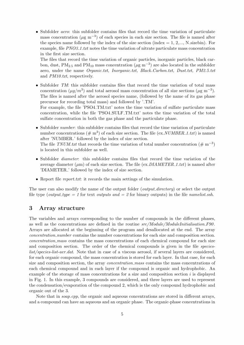
• Subfolder aero: this subfolder contains files that record the time variation of particulatemass concentration (µg m−3) of each species in each size section. The file is named afterthe species name followed by the index of the size section (index = 1, 2,..., N sizebin). Forexample, file PNO3 1.txt notes the time variation of nitrate particulate mass concentrationin the first size section.The files that record the time variation of organic particles, inorganic particles, black car-bon, dust, PM2.5 and PM10 mass concentration (µg m−3) are also located in the subfolderaero, under the name Organic.txt, Inorganic.txt, Black Carbon.txt, Dust.txt, PM2.5.txtand PM10.txt, respectively.

• Subfolder TM: this subfolder contains files that record the time variation of total massconcentration (µg/m3) and total aerosol mass concentration of all size sections (µg m−3).The files is named after the aerosol species name, (followed by the name of its gas phaseprecursor for recording total mass) and followed by ’ TM’.For example, the file ’PSO4 TM.txt’ notes the time variation of sulfate particulate massconcentration, while the file ’PSO4 SULF TM.txt’ notes the time variation of the totalsulfate concentration in both the gas phase and the particulate phase.

• Subfolder number: this subfolder contains files that record the time variation of particulatenumber concentrations (# m3) of each size section. The file (ex.NUMBER 1.txt) is namedafter ’NUMBER ’ followed by the index of size section.The file TNUM.txt that records the time variation of total number concentration (# m−3)is located in this subfolder as well.

• Subfolder diameter: this subfolder contains files that record the time variation of theaverage diameter (µm) of each size section. The file (ex.DIAMETER 1.txt) is named after’DIAMETER ’ followed by the index of size section.

• Report file report.txt: it records the main settings of the simulation.

The user can also modify the name of the output folder (output directory) or select the outputfile type (output type = 1 for text outputs and = 2 for binary outputs) in the file namelist.ssh.

3 Array structure

The variables and arrays corresponding to the number of compounds in the different phases,as well as the concentrations are defined in the routine src/Module/ModuleInitialisation.F90 .Arrays are allocated at the beginning of the program and desallocated at the end. The arrayconcentration number contains the number concentrations for each size and composition section.concentration mass contains the mass concentrations of each chemical compound for each sizeand composition section. The order of the chemical compounds is given in the file species-list/species-list-aer.dat. Note that in case of a viscous aerosol, if several layers are considered,for each organic compound, the mass concentration is stored for each layer. In that case, for eachsize and composition section, the array concentration mass contains the mass concentrations ofeach chemical compound and in each layer if the compound is organic and hydrophobic. Anexample of the storage of mass concentrations for a size and composition section i is displayedin Fig. 1. In this example, 3 compounds are considered, and three layers are used to representthe condensation/evaporation of the compound 2, which is the only compound hydrophobic andorganic out of the 3.

Note that in soap.cpp, the organic and aqueous concentrations are stored in different arrays,and a compound can have an aqueous and an organic phase. The organic-phase concentrations in

5

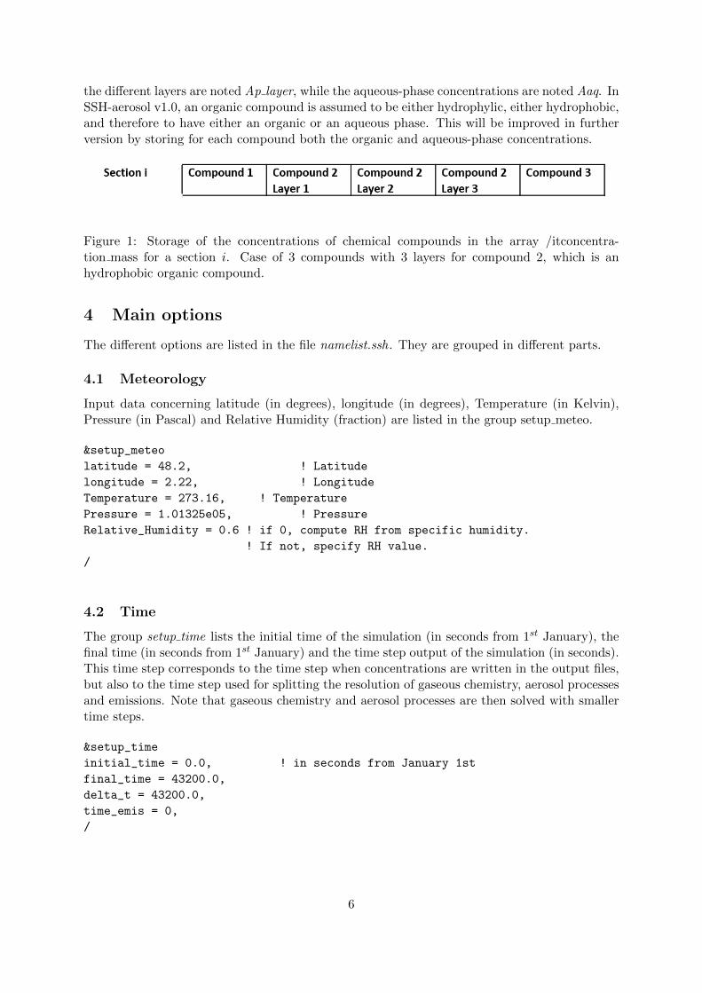
the different layers are noted Ap layer, while the aqueous-phase concentrations are noted Aaq. InSSH-aerosol v1.0, an organic compound is assumed to be either hydrophylic, either hydrophobic,and therefore to have either an organic or an aqueous phase. This will be improved in furtherversion by storing for each compound both the organic and aqueous-phase concentrations.

Figure 1: Storage of the concentrations of chemical compounds in the array /itconcentra-tion mass for a section i. Case of 3 compounds with 3 layers for compound 2, which is anhydrophobic organic compound.

4 Main options

The different options are listed in the file namelist.ssh. They are grouped in different parts.

4.1 Meteorology

Input data concerning latitude (in degrees), longitude (in degrees), Temperature (in Kelvin),Pressure (in Pascal) and Relative Humidity (fraction) are listed in the group setup meteo.

&setup_meteo

latitude = 48.2, ! Latitude

longitude = 2.22, ! Longitude

Temperature = 273.16, ! Temperature

Pressure = 1.01325e05, ! Pressure

Relative_Humidity = 0.6 ! if 0, compute RH from specific humidity.

! If not, specify RH value.

/

4.2 Time

The group setup time lists the initial time of the simulation (in seconds from 1st January), thefinal time (in seconds from 1st January) and the time step output of the simulation (in seconds).This time step corresponds to the time step when concentrations are written in the output files,but also to the time step used for splitting the resolution of gaseous chemistry, aerosol processesand emissions. Note that gaseous chemistry and aerosol processes are then solved with smallertime steps.

&setup_time

initial_time = 0.0, ! in seconds from January 1st

final_time = 43200.0,

delta_t = 43200.0,

time_emis = 0,

/

6

4.3 Initial conditions

The group initial condition lists the initial conditions of the simulation. The number of sizesections is defined in the variable N sizebin. The variable tag dbd defines whether particle sizebounds are either generated in the program by assuming they are equally spaced logarithmically(tag dbd = 0 ) or whether they are read (tag dbd = 1 ). If they are read, they need to be specifiedin the group initial diam distribution. The variable tag init defines whether the particles areinternally mixed (tag init = 0 ) or not (tag init = 1 ) initially. It needs to be set to 0 in thecurrent model version. The variable with init num defines whether number concentrations areestimated from mass concentrations and diameters of each size section (with init num = 0 ) orwhether number concentrations are read (with init num = 1 ). The variable wet diam estimationis equal to 0 if isorropia is called initially to estimate the liquid water content of particles and thewet diameter. If wet diam estimation is equal to 1, the initial wet diameter is estimated fromthe input water concentrations (and so it is equal to the dry diameter if water concentration iszero initially). Finally, the names of the files containing initial gas and mass concentrations andnumber concentrations (if with init num = 1 ) are specified by the variables init gas conc file,init aero conc mass file and init num conc num file respectively. The unit for gas and aerosolmass concentrations is µg m−3, and the unit for number concentration is #particles m−3.

&initial_condition

with_init_num = 1, ! 0 estimated from mass and diameter;

! 1 number conc. for each bin is read

tag_init = 0, ! initial method for aerosol species

! (0 internally mixed,

! 1 mixing_state resolved (notavailable)

wet_diam_estimation = 1 ! Initial estimation of wet diameter

! (0 = isorropia, 1=none)

tag_dbd = 1, ! Method for defining particle size bounds

! (0 if they are auto generated, 1 if bounds are read)

N_sizebin = 50, ! Number of size bin

init_gas_conc_file = "inputs/init_gas.dat", ! Initial data for gas

init_aero_conc_mass_file = "inputs/init_aero.dat", ! Initial data for aero mass

init_aero_conc_num_file = "inputs/init_num.dat", ! Initial data for aero number

/

&initial_diam_distribution

diam_input = 1.0000000000000000E-03 1.2022644346174130E-03

1.4454397707459280E-03 1.7378008287493760E-03 2.0892961308540399E-03

2.5118864315095799E-03 3.0199517204020170E-03 3.6307805477010140E-03

4.3651583224016601E-03 5.2480746024977272E-03 6.3095734448019337E-03

7.5857757502918377E-03 9.1201083935590985E-03 1.0964781961431851E-02

1.3182567385564069E-02 1.5848931924611141E-02 1.9054607179632480E-02

2.2908676527677741E-02 2.7542287033381681E-02 3.3113112148259113E-02

3.9810717055349727E-02 4.7863009232263859E-02 5.7543993733715687E-02

6.9183097091893658E-02 8.3176377110267125E-02 1.0000000000000001E-01

1.2022644346174140E-01 1.4454397707459279E-01 1.7378008287493751E-01

2.0892961308540400E-01 2.5118864315095812E-01 3.0199517204020171E-01

3.6307805477010152E-01 4.3651583224016621E-01 5.2480746024977298E-01

6.3095734448019380E-01 7.5857757502918444E-01 9.1201083935590987E-01

1.0964781961431860E+00 1.3182567385564070E+00 1.5848931924611140E+00

7

1.9054607179632490E+00 2.2908676527677749E+00 2.7542287033381689E+00

3.3113112148259121E+00 3.9810717055349771E+00 4.7863009232263849E+00

5.7543993733715766E+00 6.9183097091893693E+00 8.3176377110267090E+00

1.0000000000000011E+01

/

4.4 Mixing state

The group mixing state defines the mixing state of particles. The variable tag external is set to 0for internally-mixed particles and to 1 for mixing-state resolved particles. The variable N groupsdefines the number of group of aerosol compounds for which the composition is discretised. It isset to 1 for internal mixing, because the composition of compounds is then not discretised. In caseof mixing-state resolved particles, the belonging of each compound to a group is specified in theinput file detailing the aerosol compounds and their properties. The variable N frac determinesthe number of mass fraction sections used in the discretisation of composition. Finally, thevariable kind composition determines whether the fraction are discretized by the program (theyare then evenly discretised, kind composition = 1 ), or whether they are read. If they are read,they need to be specified in the group fraction distribution.

&mixing_state

tag_external = 0, ! Mixing state(0 for internally mixed,

! 1 for mixing-state resolved)

N_groups = 1, ! Nb of species groups

N_frac = 1, ! Nb of mass fraction sections

kind_composition = 1, ! Fraction discretization methods

! (1 for auto discretization and

! 0 for manual discretization)

/

&fraction_distribution

frac_input= 0.0 1.0, ! Set fraction bounds manully

/

4.5 Gas and aerosol species

The gas phase species are detailed in the group gas phase species, where the variable species list filecontains the name of the file with the list of gas-phase species. In this file, gas-phase species arelisted together with their molar weight in g/mol. Note that the order of the species in this fileshould not be changed. It is set by the preprocessor of gas-phase chemical schemes.

&gas_phase_species

species_list_file = "./species-list/species-list-cb05en.dat"

/

Aerosol species are detailed in the group aerosol species, where the variable aerosol species list filecontains the name of the file with the list of aerosol species. In this file, each aerosol speciesis listed on a line, together with specific properties: the group to which the species belong incase of mixing-state resolved particles, their molar weight (g/mol) and gaseous precursors, the

8

collision factor, molecular diameter (Angstrom), surface tension (N/m), accomodation coeffi-cient (between 0 and 1) and density in µg µm3. The categories to which species correspond arealso listed. They should not be modified and they must correspond to those set in the routineModuleInitialisation.f90 of SSH-aerosol.

&aerosol_species

aerosol_species_list_file = "./species-list/species-list-aer.dat",

/

4.6 Emissions

The group emissions defines options linked to emissions. The variable tag emis defines whetheremissions are used (tag emis = 1 ) or not (tag emis = 0 ). Emissions are assumed to be inter-nally mixed. Gas-phase emissions and/or particle-phase emissions can be specified. Numberconcentrations at emission may be determined from mass emissions and section diameters if thevariable with emis num is set to 0. They are read from a file is the variable with emis num isset to 1. The name of the file containing the list of gas-phase emitted species and their emissionrates should be specified using the variable emis gas file. Similarly, the name of the file contain-ing the list of aerosol-phase emitted species and their emission rates should be specified usingthe variable emis aero mass file. Note that the unit for emission rates is µg m−3 s−1. If numberemissions are read, the name of the files containing emission rates should be specified using thevariable emis aero num file. The units of number emissions should be #particles m−3 s−1.

&emissions

tag_emis = 0, ! 0 Without emissions,

! 1 with internally-mixed emissions,

! 2 with externally-mixed emissions

with_emis_num = 0, ! 0 if number estimated from mass and diameter;

! 1 if read

emis_gas_file = "./inputs/emis_gas.dat",

emis_aero_mass_file = "./inputs/emis_aero.dat",

emis_aero_num_file = "./inputs/emis_aero_num.dat"

/

4.7 Numerical and physical options

4.7.1 Gas-phase chemistry

The group physic gas chemistry lists options related to gas-phase chemistry. The variabletag chem defines whether gas-phase chemistry is used (tag chem = 1 ) or not (tag chem =0 ).Photolysis reactions may be taken into account (with photolysis = 1 ) or ignored (with photolysis= 0 ). In case photolysis reactions are taken into account, they may be attenuated by clouds.The cloud attenuation (variable attenuation) has a value below 1 in case of cloud attenuationof photolysis, and it is equal to 1 if no cloud attenuation (clear sky). Heterogeneous reactionsat the surface of particles may be taken into account (variable with heterogeneous = 1 ) or ig-nored (variable with heterogeneous = 0 ). An adaptive time step may be used to solve gaseouschemistry (variable with adaptive). It is advised to use the adaptative time step and to set therelative tolerance to decide if the time step is kept to 0.01 or 0.001. The minimum time step (inseconds) that can be used in the solver is set with the variable min adaptive time step.

&physic_gas_chemistry

9

tag_chem = 0, ! Tag of gas-phase chemistry

attenuation = 1.d0, ! Cloud attenuation field (0 to 1)

! (1 = no attenuation)

option_photolysis = 1, ! 1 if default photolysis rates,

! 2 if read from binary files.

time_update_photolysis = 100000. ! if photolysis are read,

! time in seconds between two reads

with_heterogeneous = 0, ! Tag of heterogeneous reaction

with_adaptive = 1, ! Tag of adaptive time step for chemistry

! 1 if adaptive time step.

adaptive_time_step_tolerance = 0.001, ! Relative tolerance to decide

! if the time step is kept

min_adaptive_time_step = 0.001, ! Minimum time step in seconds

photolysis_dir = "./photolysis/", ! Directory where binary files are.

photolysis_file = "./photolysis/photolysis-cb05.dat", ! Photolysis list

n_time_angle = 9, ! Parameters specific to the tabulation

! of photolysis rates

time_angle_min = 0.d0, ! if read from files

delta_time_angle = 1.d0,

n_latitude = 10,

latitude_min = 0.d0,

delta_latitude = 10.d0,

n_altitude = 9,

altitude_photolysis_input = 0.0, 1000.0, 2000.0, 3000.0, 4000.0, 5000.0,

10000.0, 15000.0, 20000.0,

/

4.7.2 Numerical issues related to aerosols

The group physic particle numerical issues lists options related to numerical issues when solv-ing aerosol dynamics. The variable DTAEROMIN specifies the The minimum time step (inseconds) that can be used in the solver. Different redistribution methods of mass and num-ber concentrations onto the fixed diameter grids may be used (variable redistribution method).If only the process of condensation/evaporation is considered for aerosol dynamics, then it ispossible to not apply redistribution (redistribution method = 0 ). If nucleation and/or coagu-lation is also considered, then a redistribution method should be chosen. It is advised to usethe redistribution 10 (moving diameter) or 12 (Euler coupled). The different redistributions(redistribution method) are Euler mass (3), Euler number (4), hemen (5), moving diameter (10),area-based as in SIREAM (11), Euler coupled (12). The density of particles may be computedduring the simulation depending on the composition of particles if the variable with fixed densityis set to 0. If it is set to 1, then the density is fixed through the simulation to the value set bythe variable fixed density (in µg µm−3). Note that the variable fixed density needs to be set.

Numerically, the nucleation and condensation/evaporation of inorganics are always solved si-multaneously, because nucleation and condensation/evaporation are competing processes. Coag-ulation may also be coupled to nucleation and condensation/evaporation if the variable splittingis set to 1. If splitting = 0, coagulation is splitted from nucleation and condensation/evaporation.If nucleation is taken into account, it is recommended to set splitting to 1.

&physic_particle_numerical_issues

DTAEROMIN = 1E-5, ! Minimum time step

10

redistribution_method = 0, ! Redistibution method: 0: no redistribution

! 10: 10 Moving Diameter, 12: euler_coupled

with_fixed_density = 1, ! 1 if density is fixed - 0 else

fixed_density = 1.84D-06,

splitting = 0, ! 0 if coagulation and

! (condensation/evaporation+nucleation) are splitted

! 1 if they are not

/

4.7.3 Coagulation

The group physic coagulation lists options related to coagulation. The variable with coag defineswhether coagulation is taken into account (with coag = 1 ) or not (with coag =0 ). Repartitioncoefficients may be computed in the simulation (i compute repart = 1 ) or read from a netcdf file(i compute repart = 0 ). If they are read from a file, its name should be specified (Coefficient file).If they are computed, the number of Monte Carlo points used to compute them should bespecified (Nmc). This number should be large enough and its value depends on the sectiondiscretisation used.

&physic_coagulation

with_coag = 1, ! Tag of coagulation

i_compute_repart = 1, ! 0 if repartition coeff are not computed

! but read from file, 1 if they are

i_write_repart = 0, ! 1 to write repartition coeff file, 0 otherwise

Coefficient_file = "coef_s1_f1_b6.nc", ! Repartition coefficient file

Nmc = 2000 ! Number of Monte Carlo points to compute

! repartition coefficients

/

4.7.4 Condensation/evaporation

The group physic condensation lists options related to condensation/evaporation. The vari-able with cond defines whether condensation/evaporation is taken into account (with cond =1 ) or not (with cond =0 ). Kelvin effect may be taken into account (with kelvin effect = 1 ), asrecommended if ultrafine particles are simulated, or ignored (with kelvin effect = 0 ). For thecondensation/evaporation of inorganic compounds, Cut dim corresponds to the diameter underwhich thermodynamic equilibrium is assumed. Set it to 0 to compute dynamically condensa-tion/evaporation for all particles, and set it to a value larger than larger diameter to assumethermodynamic equilibrium. For the condensation/evaporation of organic compounds, ISOAP-DYN determines whether thermodynamic equilibrium is assumed for all particles (ISOAPDYN= 0 ) or whether condensation/evaporation is computed dynamically (ISOAPDYN = 1 ). Evenif it is computed dynamically, thermodynamic equilibrium may be used for the condensa-tion/evaporation of small particles by setting a characteristic time under which equilibrium isassumed for organics (e.g. tequilibrium = 0.1 seconds). For numerical reasons, tequilibrium maynot be set to 0, but condensation/evaporation of all particles is solved dynamically if (ISOAP-DYN = 1 ) and tequilibrium is set to a small value (e.g. 1.d-15). In the current version of thecode, the diffusion coefficient dorg in the organic phase is assumed constant. Typical valueswould be 1.d-12 for non viscous particles and 1.d-24 for very viscous particles. The variablecoupled phases should be set to 1 if the resolution of the aqueous and organic phases is coupledand to 0 if they are solved independently. The interactions between compounds in the particles

11

may be assumed to be ideal (activity model = 1 ), or activity coefficients may be computed withunifac (interactions between organics only, activity model = 2 ) or with aiomfac (activity model= 3 ).

&physic_condensation

with_cond = 0, ! Tag of condensation/evaporation

Cut_dim = 0.0, ! Diameter under which equilibrium

! is assumed for inorganics

ISOAPDYN = 1, ! 0 = equilibrium, 1 = dynamic

nlayer = 1,

with_kelvin_effect = 0, ! 1 if kelvin effect is taken into account.

tequilibrium = 0.1, ! time under which equilibrium

! is assumed for organics.

dorg = 1.d-12, ! diffusion coefficient

! in the organic phase.

coupled_phases = 1, ! 1 if aqueous and organic phases

! are coupled

activity_model = 1, ! 1: ideal, 2: unifac, 3: aiomfac

epser = 0.01, ! relative error for time step adjustment

epser_soap = 0.01, ! relative difference of ros2 in SOAP

/

4.7.5 Nucleation

The group physic nucleation lists options related to nucleation. The variable with nucl defineswhether nucleation is taken into account (with nucl = 1 ) or not (with nucl =0 ). If nucleationis taken into account, then the lower diameter bound should be about 1 nm. Three nucleationmodels are implemented.

• binary: water and sulfate with the parameterisation of [Vehkamaki et al., 2002] (nucl model= 0 )

• ternary: water, sulfate and ammonium with the parameterisation of [Napari et al., 2002](nucl model = 1 ) or with the parameterisation of [Merikanto et al., 2007,Merikanto et al.,2009] (nucl model = 2 ). To avoid artificially large nucleation rates in the parameterisationof [Napari et al., 2002], a maximum nucleation rate of 1.d6 #particles cm−3 is set.

&physic_nucleation

with_nucl = 0, ! Tag of nucleation

! Need to have the lowest diameter about 1 nm.

nucl_model = 0, ! Nucleation model

! (0: binary of Vekhamaki, 1: ternary of Napari,

! 2: ternary of Merikanto)

/

4.7.6 Organics

Concerning organic reactions in the particles, oligomerization of pinonaldehyde may be consid-ered (with oligomerization = 1 ) or not.

12

&physic_organic

with_oligomerization = 1

/

4.8 Output

The output directory may be specified, as well as the format of the files (text if output type =1 , and binary if output type = 2 ).

&output

output_directory = "results/coag/",

output_type = 1 ! 1: text, 2: binary

/

4.9 Coupling with external tools

SSH-aerosol can be coupled with external (3D) tools using the shared library (libssh-aerosol.so)available in the src folder after compilation. The .so file is produced with the command./compile --sharedlib=yes. A prototype of the typical workflow is described hereafter.

Prerequisite

The following piece of C code is taken from the open-source CFD code Code Saturne. Thesubroutine get dl function pointer is used to interact with the members of the shared libraryobject.

/*----------------------------------------------------------------------------

* Get a shared library function pointer

*

* parameters:

* handle <-- pointer to shared library (result of dlopen)

* name <-- name of function symbol in library

* errors_are_fatal <-- abort if true, silently ignore if false

*

* returns:

* pointer to function in shared library

*----------------------------------------------------------------------------*/

static void *

_get_dl_function_pointer(void *handle,

const char *lib_path,

const char *name,

bool errors_are_fatal)

{

void *retval = NULL;

char *error = NULL;

dlerror(); /* Clear any existing error */

retval = dlsym(handle, name);

error = dlerror();

13

if (error != NULL) { /* Try different symbol names */

char *name_ = NULL;

dlerror(); /* Clear any existing error */

int _size_ = strlen(name) + strlen("_");

BFT_MALLOC(name_, _size_ + 1, char);

strcpy(name_, name);

strcat(name_, "_");

retval = dlsym(handle, name_);

error = dlerror();

BFT_FREE(name_);

}

if (error != NULL && errors_are_fatal)

bft_error(__FILE__, __LINE__, 0,

_("Error while trying to find symbol %s in lib %s: %s\n"),

name,

lib_path,

dlerror());

return retval;

}

Initialisation

First, the external code should load the shared library using dlopen.

/* Load the shared object */

_aerosol_so = dlopen(lib_path, RTLD_LAZY);

Then, it should decide whether SSH-aerosol outputs to the terminal or to a file.

/* Declare SSH-aerosol as not running standalone */

{

typedef void (*cs_set_sshaerosol_t)(bool*);

cs_set_sshaerosol_t fct =

(cs_set_sshaerosol_t) _get_dl_function_pointer(_aerosol_so,

lib_path,

"api_set_sshaerosol_standalone",

true);

bool flag = false;

fct(&flag);

}

/* Force SSH-aerosol to write output to a file */

if (cs_glob_rank_id <= 0) {

typedef void (*cs_set_sshaerosol_t)(bool*);

cs_set_sshaerosol_t fct =

(cs_set_sshaerosol_t) _get_dl_function_pointer(_aerosol_so,

lib_path,

"api_set_sshaerosol_logger",

true);

14

bool flag = true;

fct(&flag);

}

Then, SSH-aerosol can be initialised.

/* Initialize SSH-aerosol */

{

const char namelist_ssh[40] = "namelist_coag.ssh";

typedef void (*cs_set_sshaerosol_t)(char*);

cs_set_sshaerosol_t fct =

(cs_set_sshaerosol_t) _get_dl_function_pointer(_aerosol_so,

lib_path,

"api_sshaerosol_initialize",

true);

fct(&namelist_ssh);

}

Time advancement

The time advancement in the external 3D code could look as follow: for each time step, a loopon the cells is performed and the code

• Sets (initialises) the time step in SSH-aerosol using api set sshaerosol dt

• Sets the Pressure, Temperature, pH, ... in SSH-aerosol using api set sshaerosol temperature

and similar functions

• Sets the gaseous concentrations in SSH-aerosol using api set sshaerosol gas concentration

• Sets the aerosol concentrations in SSH-aerosol using api set sshaerosol aero concentration

• Sets the aerosol numbers in SSH-aerosol using api set sshaerosol aero number

• Advance in time (computes one time step) for the gaseous chemistry and for the aerosolchemistry in the given cell using api call sshaerosol gaschemistry andapi call sshaerosol aerochemistry

• Reads the new concentrations in the given cell from SSH-aerosol using the api get *

functions and use them in the external code

Finalisation

At the end of the simulation, the external tool should call the subroutine api sshaerosol finalize.Then, the shared library can be released using dlclose.

dlclose(_aerosol_so);

Parallelism

If the external tool is running with MPI, each MPI process should load the shared library andperform all the aforementioned operations. However, please note that only one MPI process canuse the logger (api set sshaerosol logger).

15

5 Test cases

This section presents a few test-cases to demonstrate how the model works.During the practical session, we will work in the directory ssh-aerosol . To compile the

program, please type compile. Before compiling, you may clean previous compilation by typingclean.

The main options of the simulations are detailed in the namelist files (for example INIT/namefile coag.ssh),which are in the folder INIT, and initial conditions (meteorological, gas and aerosol concentra-tions) are required. The simulation can be run by typing ssh-aerosol INIT/namefile coag.ssh.

The list of species and parameters are detailed in the files species-list/species-list-aer-en.datand species-list/species-list-cb05en. The name and location of the files can be modified in theconfiguration file namelist*.ssh.

Different processes can be considered (set the flag to 1) or ignored (set the flag to 0): emissions(flag tag emis), gaseous chemistry (flag tag chem), coagulation (flag with coag), condensation(flag with cond), nucleation (flag with nucl). Internal mixing (flag tag external set to 0) ormixing-state resolved particles (flag tag external set to 1) can be considered.

5.1 Dynamic of coagulation and condensation

In the literature, to test the overall behaviour of PM models, the following basic tests of con-densation and coagulation of sulfate are often considered [Seigneur et al., 1986, Zhang et al.,1999, Binkowski and Roselle, 2003]. A tri-modal PM distribution is considered initially, withparticles being made exclusively of sulfate. The parameters of the initial distribution consideredhere are those of hazy conditions for the condensation test with a sulphuric acid production rateof 9.9 µg m−3, and those of urban conditions for the coagulation test [Seigneur et al., 1986,Zhanget al., 1999] , because these two tests represent the two most stringent conditions for coagulationand condensation. Temperature is taken as 283.15 K. Simulations are conducted for 12 hours.The reference solutions for the coagulation and condensation tests are those of [Zhang et al.,1999] obtained with another models.

5.1.1 Coagulation

The configuration file for this test is namelist coag.ssh. In the coagulation test case, only coag-ulation is considered by setting the variable of with coag of the file namelist coag.ssh to 1.

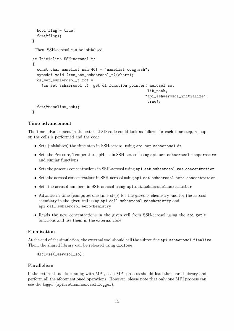
The partition coefficients may be precomputed in a C++ routine. Here, the coefficients aredirectly computed by SSH-aerosol (option i compute repart), using a Monte-Carlo method (Nmcrepresents the Monte Carlo number). The larger Nmc is, the more accurate the coefficients are,but the more CPU time it takes to compute them. Run the simulation by typing ssh-aerosolINIT/namelist coag.ssh. You can compare the number and volume distribution of particles atthe initial time and after 12 h by going to the repertory graph and by running the pythonscript dN Vdlogd coag.py. SSH-aerosol does very well in representing the growth of particles bycoagulation, as shown in Fig 2.

16

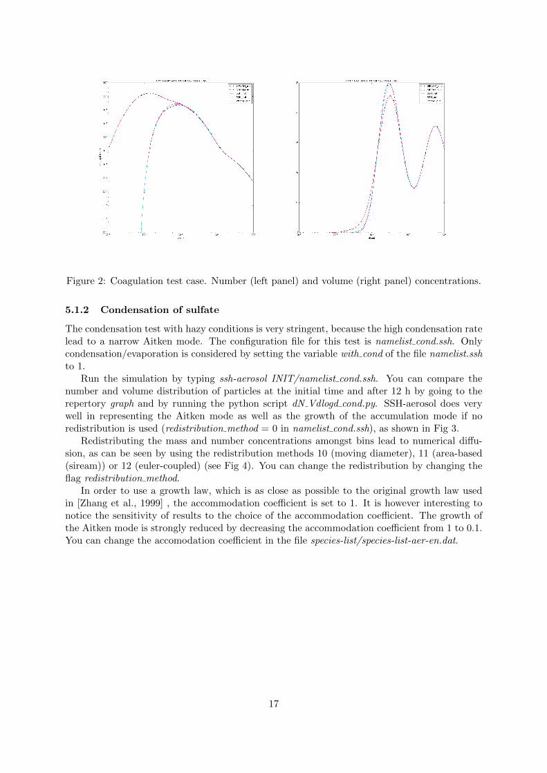
Figure 2: Coagulation test case. Number (left panel) and volume (right panel) concentrations.

5.1.2 Condensation of sulfate

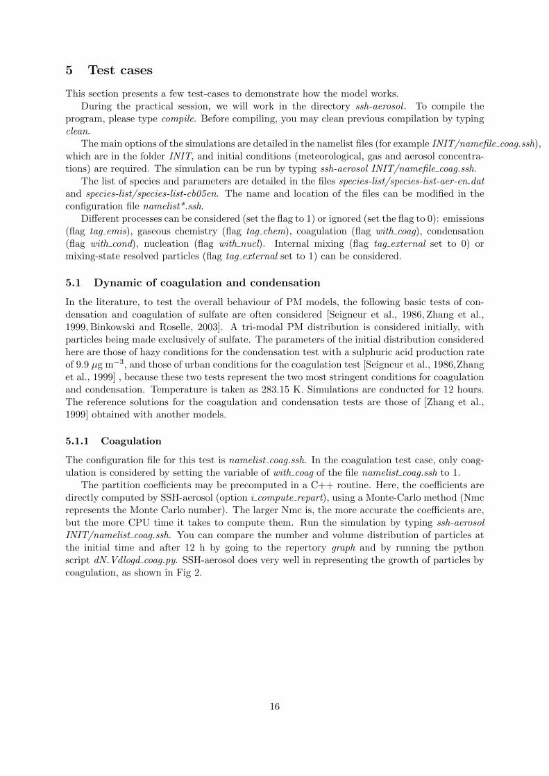
The condensation test with hazy conditions is very stringent, because the high condensation ratelead to a narrow Aitken mode. The configuration file for this test is namelist cond.ssh. Onlycondensation/evaporation is considered by setting the variable with cond of the file namelist.sshto 1.

Run the simulation by typing ssh-aerosol INIT/namelist cond.ssh. You can compare thenumber and volume distribution of particles at the initial time and after 12 h by going to therepertory graph and by running the python script dN Vdlogd cond.py. SSH-aerosol does verywell in representing the Aitken mode as well as the growth of the accumulation mode if noredistribution is used (redistribution method = 0 in namelist cond.ssh), as shown in Fig 3.

Redistributing the mass and number concentrations amongst bins lead to numerical diffu-sion, as can be seen by using the redistribution methods 10 (moving diameter), 11 (area-based(siream)) or 12 (euler-coupled) (see Fig 4). You can change the redistribution by changing theflag redistribution method.

In order to use a growth law, which is as close as possible to the original growth law usedin [Zhang et al., 1999] , the accommodation coefficient is set to 1. It is however interesting tonotice the sensitivity of results to the choice of the accommodation coefficient. The growth ofthe Aitken mode is strongly reduced by decreasing the accommodation coefficient from 1 to 0.1.You can change the accomodation coefficient in the file species-list/species-list-aer-en.dat.

17

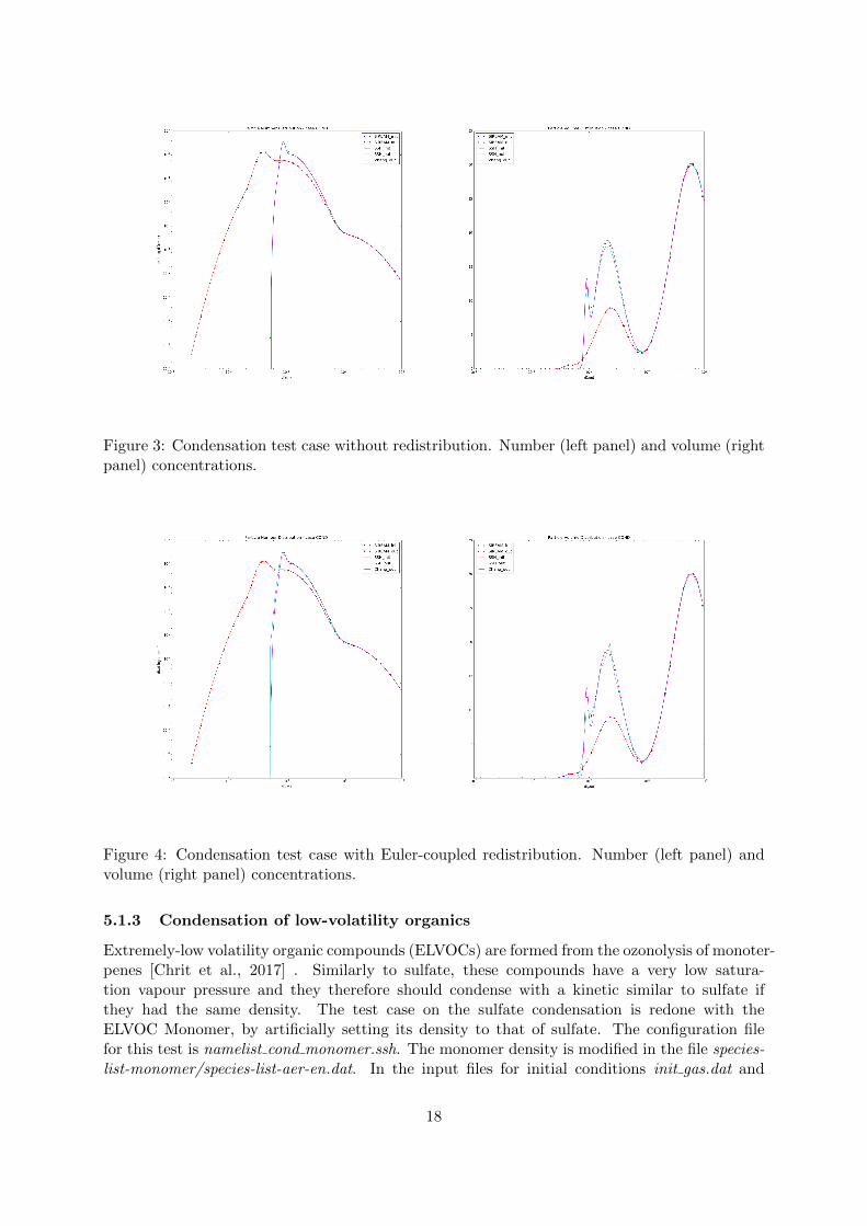
Figure 3: Condensation test case without redistribution. Number (left panel) and volume (rightpanel) concentrations.

Figure 4: Condensation test case with Euler-coupled redistribution. Number (left panel) andvolume (right panel) concentrations.

5.1.3 Condensation of low-volatility organics

Extremely-low volatility organic compounds (ELVOCs) are formed from the ozonolysis of monoter-penes [Chrit et al., 2017] . Similarly to sulfate, these compounds have a very low satura-tion vapour pressure and they therefore should condense with a kinetic similar to sulfate ifthey had the same density. The test case on the sulfate condensation is redone with theELVOC Monomer, by artificially setting its density to that of sulfate. The configuration filefor this test is namelist cond monomer.ssh. The monomer density is modified in the file species-list-monomer/species-list-aer-en.dat. In the input files for initial conditions init gas.dat and

18

init aero.dat of the directory inputs/inputs-cond-monomer/, initial concentrations are assignedto monomer rather than sulfate. You can plot the number and volume distribution by using thepython script graph/dN Vdlogd cond monomer.py. The distributions are similar to those of thesulfate case.

5.1.4 Condensation/evaporation of inorganics

For inorganic compounds, differences between the particle compositions computed using equilib-rium and dynamical sectional models have been stressed by numerous authors such as [Sarteletet al., 2006] . This test case simulates the test case of the highly polluted day of 25 June 2001of [Sartelet et al., 2006] . Measurements of PM and gaseous species made in Tokyo (Japan) aretaken as initial conditions. Because the data were averaged continuously during 24 hours undervarying meteorological conditions, this study can not assess the importance of the equilibriumapproach compared to the dynamical approach. The model results obtained after thermody-namic equilibrium is reached are then compared.

The configuration file for this test is namelist cond-evap-inorg.ssh for the case where con-densation/evaporation is dynamic. Only condensation/evaporation is considered by setting thevariable of namelist cond-evap-inorg.ssh with cond to 1. The variable Cut dim corresponds tothe diameter until which thermodynamic is assumed. It is set to 0 to solve the condensa-tion/evaporation with a dynamic approach.

To compare this simulation to a simulation where thermodynamic equilibrium is assumedfor condensation/evaporation, please set Cut dim to 40 (the maximum diameter of the particlesconsidered here). This is done in the configuration file namelist cond-evap-inorg-eq.ssh.

To assess the differences between these simulations, you can compare the time evolution ofNH3 and HNO3, by running the python script graph/gas cond-evap.py. As shown in Fig 5, thegas-phase concentrations quickly reach thermodynamic equilibrium.

Figure 5: Condensation/evaporation of inorganic test case. Time evolution of HNO3 concentra-tions (left panel) and NH3 concentrations (right panel).

19

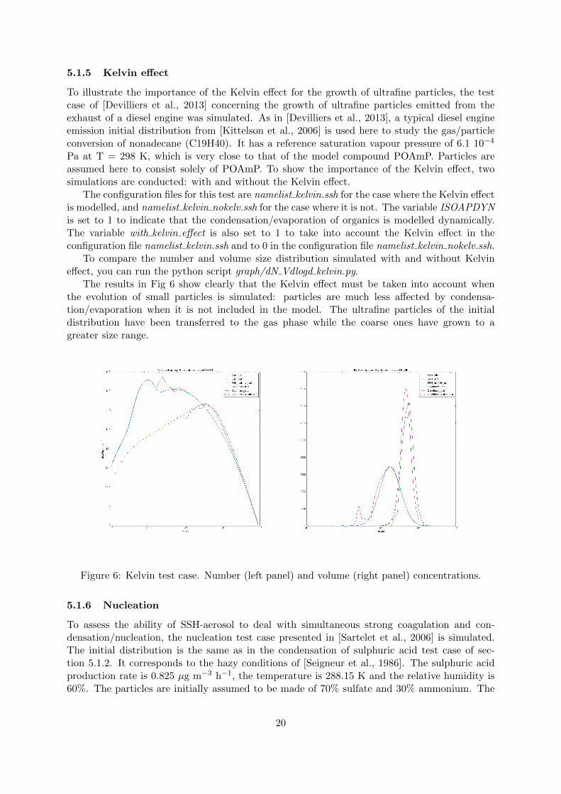
5.1.5 Kelvin effect

To illustrate the importance of the Kelvin effect for the growth of ultrafine particles, the testcase of [Devilliers et al., 2013] concerning the growth of ultrafine particles emitted from theexhaust of a diesel engine was simulated. As in [Devilliers et al., 2013], a typical diesel engineemission initial distribution from [Kittelson et al., 2006] is used here to study the gas/particleconversion of nonadecane (C19H40). It has a reference saturation vapour pressure of 6.1 10−4

Pa at T = 298 K, which is very close to that of the model compound POAmP. Particles areassumed here to consist solely of POAmP. To show the importance of the Kelvin effect, twosimulations are conducted: with and without the Kelvin effect.

The configuration files for this test are namelist kelvin.ssh for the case where the Kelvin effectis modelled, and namelist kelvin nokelv.ssh for the case where it is not. The variable ISOAPDYNis set to 1 to indicate that the condensation/evaporation of organics is modelled dynamically.The variable with kelvin effect is also set to 1 to take into account the Kelvin effect in theconfiguration file namelist kelvin.ssh and to 0 in the configuration file namelist kelvin nokelv.ssh.

To compare the number and volume size distribution simulated with and without Kelvineffect, you can run the python script graph/dN Vdlogd kelvin.py.

The results in Fig 6 show clearly that the Kelvin effect must be taken into account whenthe evolution of small particles is simulated: particles are much less affected by condensa-tion/evaporation when it is not included in the model. The ultrafine particles of the initialdistribution have been transferred to the gas phase while the coarse ones have grown to agreater size range.

Figure 6: Kelvin test case. Number (left panel) and volume (right panel) concentrations.

5.1.6 Nucleation

To assess the ability of SSH-aerosol to deal with simultaneous strong coagulation and con-densation/nucleation, the nucleation test case presented in [Sartelet et al., 2006] is simulated.The initial distribution is the same as in the condensation of sulphuric acid test case of sec-tion 5.1.2. It corresponds to the hazy conditions of [Seigneur et al., 1986]. The sulphuric acidproduction rate is 0.825 µg m−3 h−1, the temperature is 288.15 K and the relative humidity is60%. The particles are initially assumed to be made of 70% sulfate and 30% ammonium. The

20

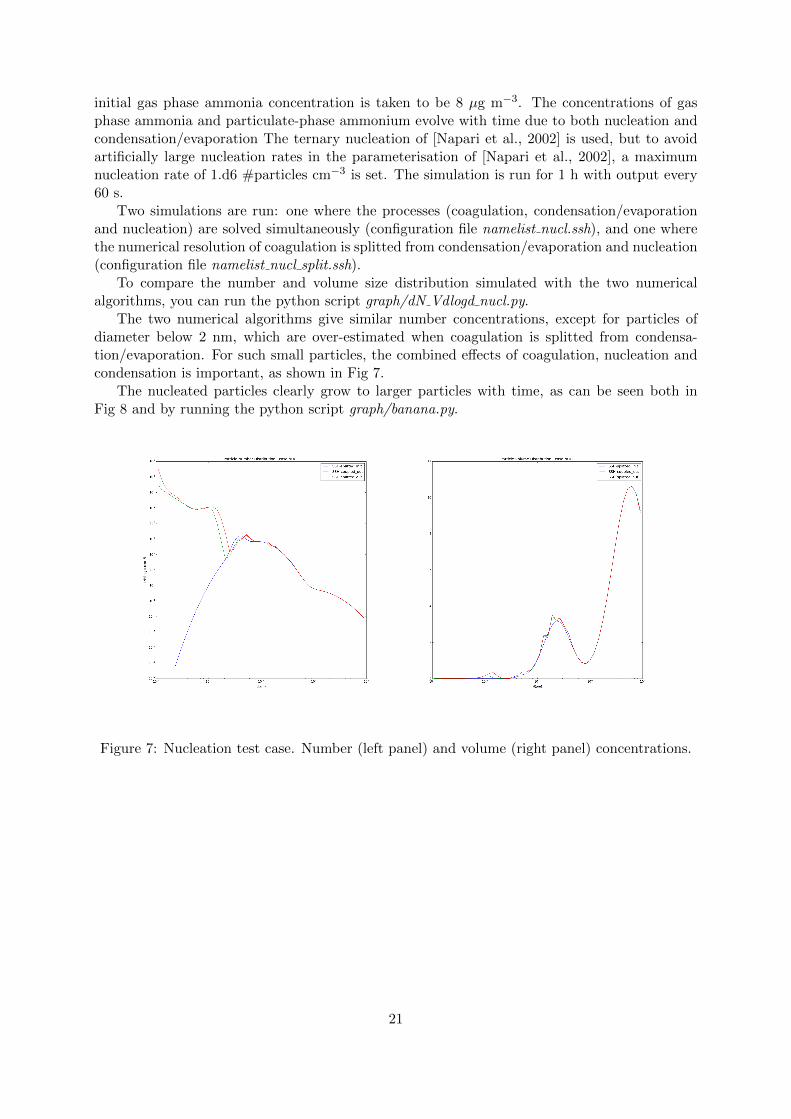
initial gas phase ammonia concentration is taken to be 8 µg m−3. The concentrations of gasphase ammonia and particulate-phase ammonium evolve with time due to both nucleation andcondensation/evaporation The ternary nucleation of [Napari et al., 2002] is used, but to avoidartificially large nucleation rates in the parameterisation of [Napari et al., 2002], a maximumnucleation rate of 1.d6 #particles cm−3 is set. The simulation is run for 1 h with output every60 s.

Two simulations are run: one where the processes (coagulation, condensation/evaporationand nucleation) are solved simultaneously (configuration file namelist nucl.ssh), and one wherethe numerical resolution of coagulation is splitted from condensation/evaporation and nucleation(configuration file namelist nucl split.ssh).

To compare the number and volume size distribution simulated with the two numericalalgorithms, you can run the python script graph/dN Vdlogd nucl.py.

The two numerical algorithms give similar number concentrations, except for particles ofdiameter below 2 nm, which are over-estimated when coagulation is splitted from condensa-tion/evaporation. For such small particles, the combined effects of coagulation, nucleation andcondensation is important, as shown in Fig 7.

The nucleated particles clearly grow to larger particles with time, as can be seen both inFig 8 and by running the python script graph/banana.py.

Figure 7: Nucleation test case. Number (left panel) and volume (right panel) concentrations.

21

Figure 8: Nucleation test case. Time evolution of the number concentrations.

5.2 Modelling of aerosol formation

After emission into the atmosphere, the oxidation of volatile organic compounds (VOCs) leadsto less volatile compounds than the precursors. These compounds condense more easily ontoparticles than their precursors and they contribute to the increase of particle mass.

[Platt et al., 2013] performed ageing experiments on emissions from an Euro 5 gasoline car.They monitored the total hydrocarbon mass (THC) as well as organic aerosol (OA) concentra-tions. The test case presented here corresponds to the simulation performed in [Sartelet et al.,2018].

In our model, THC is assumed to be the sum of VOC and I/S VOCs (intermediate andsemi-volatile VOCs). THC is initialised as measured in the experiments of [Platt et al., 2013]before lights-on (1.4 ppmv + 0.9 ppmv of propene). IVOCs are estimated from VOC emissionsusing the ratio 0.17 estimated by [Zhao et al., 2016], and NOx concentrations are initialised suchas having a VOC/NOx ratio equal to 5.6 as in [Platt et al., 2013] . The speciation of VOCs tomodel species was done following [Theloke and Friedrich, 2007].

The configuration file for this test is namelist platt.ssh.Not only condensation/evaporation is considered by setting the variable of namelist platt.ssh

with cond to 1, but also gaseous chemistry ( tag chem=1). Photolysis rates are predefined inthis version of ssh, and a more accurate representation of those (similar to what is used in 3D)will be implemented soon.

After running the model for 5 h, the evolution of the aerosol concentrations with time maybe displayed by running the script plot platt particles.py. As in the experiment after correctionfor wall loss, the concentrations of particles is about 200 µg m−3. More than half of the massorigins from the condensation/evaporation of aged I/S VOCs, as shown in Fig 9. The inorganicconcentrations stay low (5 µg m−3 of sulfate was introduced initially as a seed and does notvary during the simulation; and nitrate stays below 9 µg m−3).

22

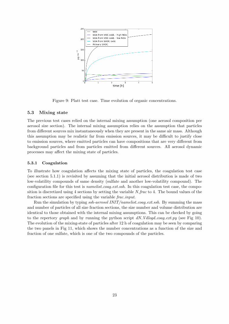
Figure 9: Platt test case. Time evolution of organic concentrations.

5.3 Mixing state

The previous test cases relied on the internal mixing assumption (one aerosol composition peraerosol size section). The internal mixing assumption relies on the assumption that particlesfrom different sources mix instantaneously when they are present in the same air mass. Althoughthis assumption may be realistic far from emission sources, it may be difficult to justify closeto emission sources, where emitted particles can have compositions that are very different frombackground particles and from particles emitted from different sources. All aerosol dynamicprocesses may affect the mixing state of particles.

5.3.1 Coagulation

To illustrate how coagulation affects the mixing state of particles, the coagulation test case(see section 5.1.1) is revisited by assuming that the initial aerosol distribution is made of twolow-volatility compounds of same density (sulfate and another low-volatility compound). Theconfiguration file for this test is namelist coag ext.ssh. In this coagulation test case, the compo-sition is discretized using 4 sections by setting the variable N frac to 4. The bound values of thefraction sections are specified using the variable frac input.

Run the simulation by typing ssh-aerosol INIT/namelist coag ext.ssh. By summing the massand number of particles of all size fraction sections, the size number and volume distribution areidentical to those obtained with the internal mixing assumptions. This can be checked by goingto the repertory graph and by running the python script dN Vdlogd coag ext.py (see Fig 10).The evolution of the mixing-state of particles after 12 h of coagulation may be seen by comparingthe two panels in Fig 11, which shows the number concentrations as a function of the size andfraction of one sulfate, which is one of the two compounds of the particles.

23

Figure 10: Coagulation test case with mixing-state modelling. Number (left panel) and volume(right panel) concentrations.

Figure 11: Number concentrations as a function of the size and fraction of one of the twocompounds at initial time (left panel) and after 12 h of simulation (right panel).

5.3.2 Condensation

The effect of condensation on the mixing state is assessed by revisiting the condensation testcase (typical of a regional haze scenario, see section 5.1.2) by assuming that the initial aerosoldistribution is made of two low-volatility compounds of same density (sulfate and another low-volatility compound). As in [Zhu et al., 2015], 10 composition fractions are used. The con-figuration file for this test is namelist cond ext.ssh. Run the simulation by typing ssh-aerosolINIT/namelist cond ext.ssh. By summing the mass and number of particles of all size fractionsections, the size number and volume distribution are identical to those obtained with the inter-nal mixing assumptions. This can be checked by going to the repertory graph and by running thepython script dN Vdlogd cond ext.py (see Fig 12). The evolution of the mixing-state of particlesafter 12 h of condensation and coagulation may be seen by comparing the two panels in Fig 13,which shows the mass concentrations as a function of the size and fraction of one sulfate, which

24

is one of the two compounds of the particles. Sulphuric acid condenses to form sulfate. Becausethe condensation rate is greater for particles of low diameters, the sulfate fraction is greater forthose particles at the end of the simulation (Figure 13).

Figure 12: Regional haze test case with mixing-state modelling. Number (left panel) and volume(right panel) concentrations.

Figure 13: Mass concentrations as a function of the size and fraction of one of the two compoundsat initial time (left panel) and after 12 h of simulation (right panel).

5.4 Viscosity

The gas/particle mass transfer is strongly affected by particle viscosity. To illustrate this effect,the condensation of hydrophobic organic surrogates of different volatility is studied for differentvalues of the viscosity, represented by different values of the organic-phase diffusion coefficientsD (10−18, 10−19, 10−20, 10−21, 10−22, 10−23, 10−24 m2 s−1). The value D = 10−12 m2 s−1 corre-sponds to an inviscid particle, while the value D = 10−24 m2 s−1 corresponds to a very viscousparticle. Each particle is discretized into 5 layers to model the flux of diffusion of the organiccompounds in the particle. The test cases presented here are similar to those of the Figure 6

25

of [Couvidat and Sartelet, 2015]. Three surrogates are successively studied: SOAlP, POAlP andPOAmP and which have partitioning coefficients Kp equal to 100 m3 µg−1, 1 m3 µg−1, and0.01 m3 µg−1. The surrogate that condenses is initially only in the gas phase, with a mass of5 µg m−3. It condenses on an organic phase of 5 µg m−3 made of SOAlP, which has a verylow volatility (Kp = 100 m3 µg−1). The test cases may be launched by launching the scriptINIT/launch visco.sh. After computation of the condensation of the surrogates from differentvalues of the viscosity, three graphs can be displayed by running the scripts conc visco poalp.py,conc visco poamp.py, conc visco soalp.py (one graph per surrogate). They are shown in Fig 14,which represents the time variations of particle-phase organic concentrations of the surrogate(POAlP in upper left panel, POAmP in upper right panel and SOAlP in lower panel). Thesurrogate of low volatility (SOAlP) condenses quickly onto the organic phase, independently ofthe viscosity (upper left panel of Fig 14). All the organic mass is then in the particle phase. Al-though the condensation of POAlP is influenced by the viscosity, a large fraction of the gas-phaseconcentration of POAlP condenses quickly (upper right panel of Fig 14). For POAmP, whichis the most volatile of the three surrogates, high viscosity (low diffusion coefficient) stronglyinhibits the condensation of POAmP (lower right panel of Fig 14).

Figure 14: Viscosity test case: time evolution of organic concentrations (SOAlP in the upperleft, POAlP in the upper right, POAmP in the lower left) for several organic-phase diffusivity:10−18 (dark blue), 10−19 (light blue), 10−20 (green), 10−21 (yellow), 10−22 (magenta), 10−23

(red), 10−24 (black) m2 s−1.

26

6 References

References

[Binkowski and Roselle, 2003] Binkowski, F. S. and Roselle, S. J. (2003). Models-3 communitymultiscale air quality (cmaq) model aerosol component 1. model description. Journal ofgeophysical research: Atmospheres, 108(D6).

[Chrit et al., 2017] Chrit, M., Sartelet, K., Sciare, J., Pey, J., Marchand, N., Couvidat, F., Sel-legri, K., and Beekmann, M. (2017). Modelling organic aerosol concentrations and propertiesduring charmex summer campaigns of 2012 and 2013 in the western mediterranean region.Atmospheric Chemistry and Physics, 17(20):12509–12531.

[Couvidat et al., 2012] Couvidat, F., Debry, E., Sartelet, K., and Seigneur, C. (2012). A hy-drophilic/hydrophobic organic (h2o) aerosol model: Development, evaluation and sensitivityanalysis. Journal of Geophysical Research: Atmospheres, 117(D10).

[Couvidat and Sartelet, 2015] Couvidat, F. and Sartelet, K. (2015). The secondary organicaerosol processor (soap v1. 0) model: a unified model with different ranges of complexitybased on the molecular surrogate approach. Geoscientific Model Development, 8(4):1111–1138.

[Devilliers et al., 2013] Devilliers, M., Debry, E., Sartelet, K., and Seigneur, C. (2013). A newalgorithm to solve condensation/evaporation for ultra fine, fine, and coarse particles. Journalof Aerosol Science, 55:116–136.

[Kim et al., 2019] Kim, Y., Sartelet, K., and Couvidat, F. (2019). Modeling the effect of non-ideality, dynamic mass transfer and viscosity on soa formation in a 3-d air quality model.Atmospheric Chemistry and Physics, 19(2):1241–1261.

[Kittelson et al., 2006] Kittelson, D., Watts, W., and Johnson, J. (2006). On-road and labora-tory evaluation of combustion aerosolspart1: Summary of diesel engine results. Journal ofAerosol Science, 37(8):913–930.

[Merikanto et al., 2007] Merikanto, J., Napari, I., Vehkamaki, H., Anttila, T., and Kulmala,M. (2007). New parameterization of sulfuric acid-ammonia-water ternary nucleation rates attropospheric conditions. J. of Geophys. Res., 112(D15207).

[Merikanto et al., 2009] Merikanto, J., Napari, I., Vehkam¨aki, H., Anttila, T., and Kulmala,M. (2009). Correction to ”new parameterization of sulfuric acid-ammonia-water ternary nu-cleation rates at tropospheric conditions”. J. of Geophys. Res., 114(D09206).

[Napari et al., 2002] Napari, I., Noppel, M., Vehkamaki, H., and Kulmala, M. (2002).Parametrization of ternary nucleation rates for h2so4-nh3-h2o vapors. J. of Geophys. Res.,107 (D19).

[Platt et al., 2013] Platt, S. M., Haddad, I. E., Zardini, A., Clairotte, M., Astorga, C., Wolf,R., Slowik, J., Temime-Roussel, B., Marchand, N., Jezek, I., et al. (2013). Secondary organicaerosol formation from gasoline vehicle emissions in a new mobile environmental reactionchamber. Atmospheric Chemistry and Physics, 13(18):9141–9158.

[Sartelet et al., 2006] Sartelet, K., Hayami, H., Albriet, B., and Sportisse, B. (2006). Develop-ment and preliminary validation of a modal aerosol model for tropospheric chemistry: Mam.Aerosol Science and Technology, 40(2):118–127.

27

[Sartelet et al., 2018] Sartelet, K., Zhu, S., Moukhtar, S., Andre, M., Andre, J., Gros, V., Favez,O., Brasseur, A., and Redaelli, M. (2018). Emission of intermediate, semi and low volatileorganic compounds from traffic and their impact on secondary organic aerosol concentrationsover greater paris. Atmospheric Environment, 180:126–137.

[Seigneur et al., 1986] Seigneur, C., Hudischewskyj, A. B., Seinfeld, J. H., Whitby, K. T.,Whitby, E. R., Brock, J. R., and Barnes, H. M. (1986). Simulation of aerosol dynamics:A comparative review of mathematical models. Aerosol Science and Technology, 5(2):205–222.

[Theloke and Friedrich, 2007] Theloke, J. and Friedrich, R. (2007). Compilation of a databaseon the composition of anthropogenic voc emissions for atmospheric modeling in europe. At-mospheric Environment, 41(19):4148–4160.

[Vehkamaki et al., 2002] Vehkamaki, H., Kulmala, M., Napari, I., K.E.J., L., Timmreck, C.,Noppel, M., and Laaksonen, A. (2002). An improved parameterization for sulfuric acid-water nucleation rates for tropospheric and stratospheric conditions. J. of Geophys. Res.,107(D22):4622.

[Zhang et al., 1999] Zhang, Y., Seigneur, C., Seinfeld, J. H., Jacobson, M. Z., and Binkowski,F. S. (1999). Simulation of aerosol dynamics: A comparative review of algorithms used in airquality models. Aerosol Science & Technology, 31(6):487–514.

[Zhao et al., 2016] Zhao, Y., Nguyen, N. T., Presto, A. A., Hennigan, C. J., May, A. A., andRobinson, A. L. (2016). Intermediate volatility organic compound emissions from on-roadgasoline vehicles and small off-road gasoline engines. Environmental science & technology,50(8):4554–4563.

[Zhu et al., 2015] Zhu, S., Sartelet, K. N., and Seigneur, C. (2015). A size-composition resolvedaerosol model for simulating the dynamics of externally mixed particles: Scram (v 1.0). Geo-scientific Model Development, 8(6):1595–1612.

28