Speech Recognition of Spoken Digits · Case study: Speech Recognition of Spoken Digits • General...
21
Presenter: Stefanie Peters Prof. Dr.-Ing. Andreas König Speech Recognition of Spoken Digits Stefanie Peters May 10, 2006 Prof. Dr.-Ing. Andreas König Institute of Integrated Sensor Systems Dept. of Electrical Engineering and Information Technology
Transcript of Speech Recognition of Spoken Digits · Case study: Speech Recognition of Spoken Digits • General...
Presenter: Stefanie Peters Prof. Dr.-Ing. Andreas König
Speech Recognition of Spoken Digits
Stefanie Peters
May 10, 2006Prof. Dr.-Ing. Andreas König
Institute of Integrated Sensor Systems
Dept. of Electrical Engineering and Information Technology
Presenter: Stefanie Peters Prof. Dr.-Ing. Andreas König
Lecture Information
Sensor Signal Processing
Prof. Dr.-Ing. Andreas KönigInstitute of Integrated Sensor Systems
Dept. of Electrical Engineering and Information TechnologyUniversity of Kaiserslautern
Fall Semester 2005
Presenter: Stefanie Peters Prof. Dr.-Ing. Andreas König
What did we learn?
Signal Processing and Analysis
Feature Computation
Cluster Analysis
Dimensionality Reduction Techniques
Presenter: Stefanie Peters Prof. Dr.-Ing. Andreas König
What did we learn?
Data Visualisation & Analysis
Classification Techniques
Sensor Fusion
Systematic Design of Sensor Systems
Presenter: Stefanie Peters Prof. Dr.-Ing. Andreas König
Sensor Signal Processing Project Case study: Speech Recognition of Spoken Digits
• General task for a project:
– Design and implementation of a recognition system for either image or audio data with the programs Matlab and/or QuickCog
• Recording / taking of training data
• Preprocessing to enhance input signals for a ensuing feature computation
• Selection and computation of suitable features
• Classification of training and test data
– Here:
• Recording of spoken digits with a microphone
• Implementation of a digit recognition system with Matlab
Presenter: Stefanie Peters Prof. Dr.-Ing. Andreas König
Training Data
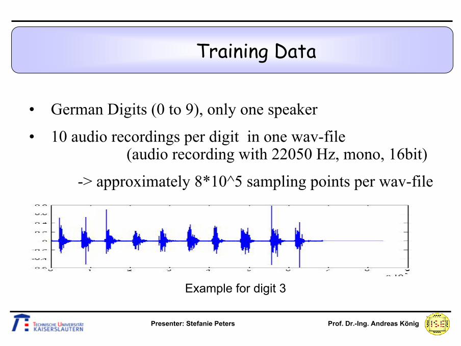
• German Digits (0 to 9), only one speaker
• 10 audio recordings per digit in one wav-file (audio recording with 22050 Hz, mono, 16bit)
-> approximately 8*10^5 sampling points per wav-file
Example for digit 3
Presenter: Stefanie Peters Prof. Dr.-Ing. Andreas König
Preprocessing of the Audio Signal
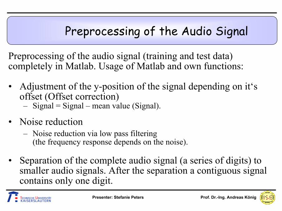
Preprocessing of the audio signal (training and test data) completely in Matlab. Usage of Matlab and own functions:
• Adjustment of the y-position of the signal depending on it‘s offset (Offset correction)– Signal = Signal – mean value (Signal).
• Noise reduction– Noise reduction via low pass filtering
(the frequency response depends on the noise).
• Separation of the complete audio signal (a series of digits) to smaller audio signals. After the separation a contiguous signal contains only one digit.
Presenter: Stefanie Peters Prof. Dr.-Ing. Andreas König
Separation of the Audio Signal
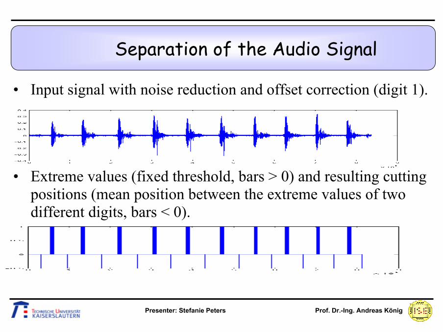
• Input signal with noise reduction and offset correction (digit 1).
• Extreme values (fixed threshold, bars > 0) and resulting cuttingpositions (mean position between the extreme values of two different digits, bars < 0).
Presenter: Stefanie Peters Prof. Dr.-Ing. Andreas König
Separation of the Audio Signal
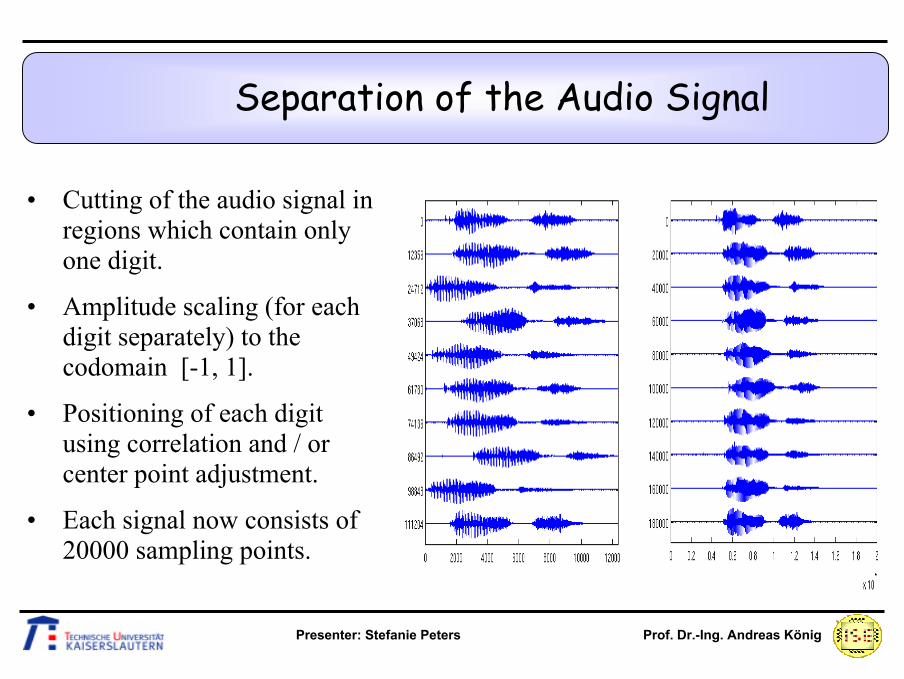
• Cutting of the audio signal in regions which contain only one digit.
• Amplitude scaling (for each digit separately) to thecodomain [-1, 1].
• Positioning of each digit using correlation and / or center point adjustment.
• Each signal now consists of 20000 sampling points.
Presenter: Stefanie Peters Prof. Dr.-Ing. Andreas König
Feature Computation (1)
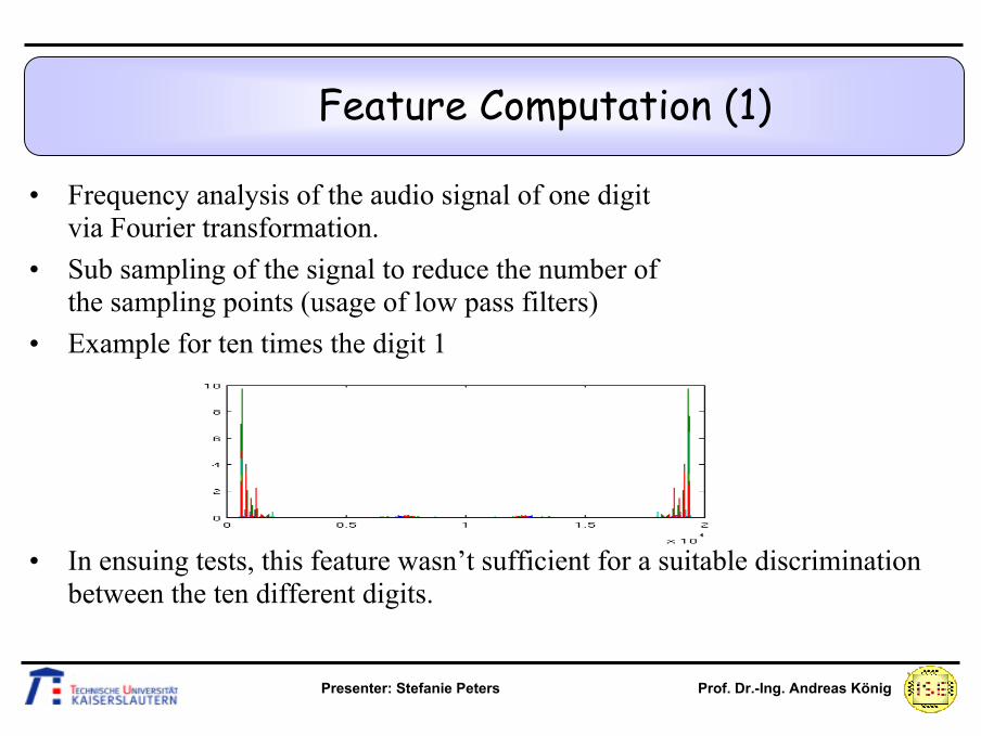
• Frequency analysis of the audio signal of one digit via Fourier transformation.
• Sub sampling of the signal to reduce the number of the sampling points (usage of low pass filters)
• Example for ten times the digit 1
• In ensuing tests, this feature wasn’t sufficient for a suitable discrimination between the ten different digits.
Presenter: Stefanie Peters Prof. Dr.-Ing. Andreas König
Feature Computation (2)
• Mel Frequency Cepstral Coefficients (MFCC)
– Usage of the ‚Auditory Toolbox: A Matlab Toolbox for Auditory Modeling Work‘ for the MFCC Computation:
– Windowing of the input signal (here: with a hamming window, usually sampling windows every 10 msec)
– Discrete Fourier transformation of each window
– Logarithm (base 10) of the Fourier coefficients
– Mapping of the results to the „Mel-Scale“ using triangle filters
– Usage of the first 13 MFCC parameter curves
Presenter: Stefanie Peters Prof. Dr.-Ing. Andreas König
Feature Computation (2)
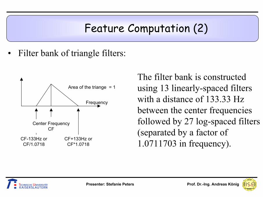
• Filter bank of triangle filters:
Area of the triange = 1
Frequency
CF+133Hz orCF*1.0718
CF-133Hz orCF/1.0718
Center FrequencyCF
The filter bank is constructed using 13 linearly-spaced filters with a distance of 133.33 Hz between the center frequencies followed by 27 log-spaced filters (separated by a factor of 1.0711703 in frequency).
Presenter: Stefanie Peters Prof. Dr.-Ing. Andreas König
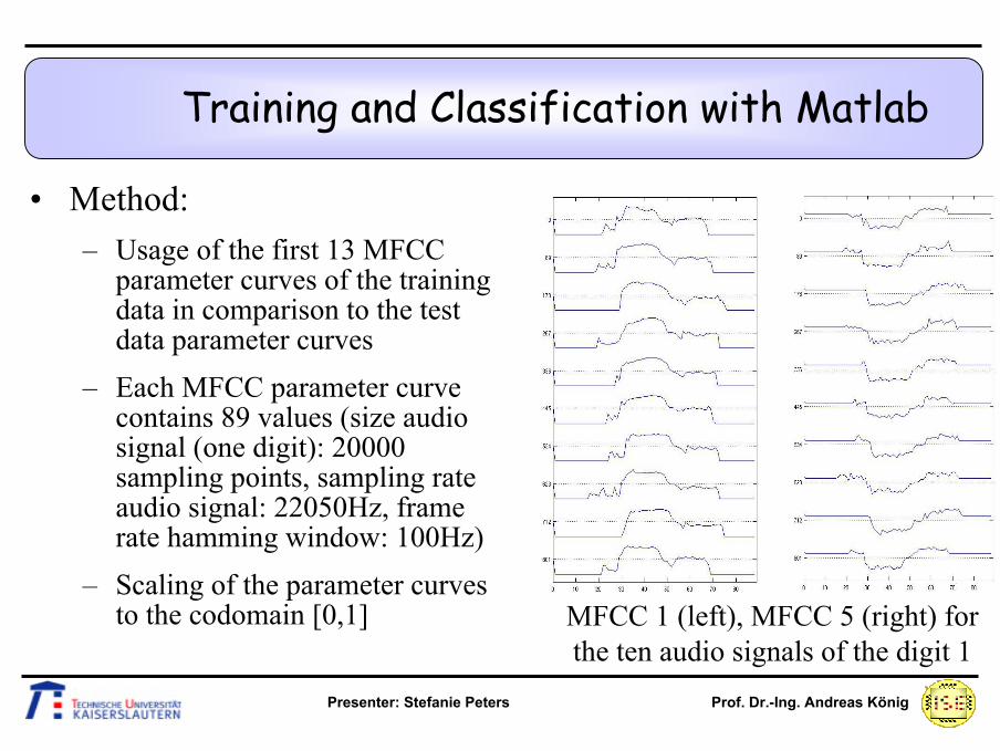
Training and Classification with Matlab
• Method:– Usage of the first 13 MFCC
parameter curves of the training data in comparison to the test data parameter curves
– Each MFCC parameter curve contains 89 values (size audio signal (one digit): 20000 sampling points, sampling rate audio signal: 22050Hz, frame rate hamming window: 100Hz)
– Scaling of the parameter curves to the codomain [0,1] MFCC 1 (left), MFCC 5 (right) for
the ten audio signals of the digit 1
Presenter: Stefanie Peters Prof. Dr.-Ing. Andreas König
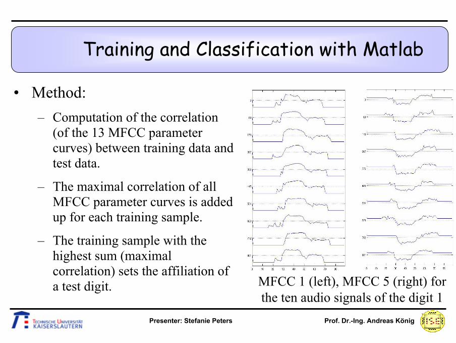
Training and Classification with Matlab
• Method:– Computation of the correlation
(of the 13 MFCC parameter curves) between training data and test data.
– The maximal correlation of all MFCC parameter curves is added up for each training sample.
– The training sample with the highest sum (maximal correlation) sets the affiliation of a test digit. MFCC 1 (left), MFCC 5 (right) for
the ten audio signals of the digit 1
Presenter: Stefanie Peters Prof. Dr.-Ing. Andreas König
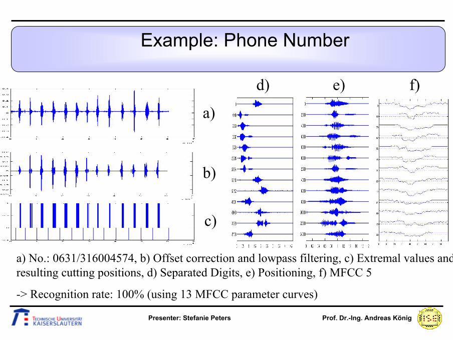
Example: Phone Number
a)
b)
c)
d) e) f)
a) No.: 0631/316004574, b) Offset correction and lowpass filtering, c) Extremal values and resulting cutting positions, d) Separated Digits, e) Positioning, f) MFCC 5
-> Recognition rate: 100% (using 13 MFCC parameter curves)
Presenter: Stefanie Peters Prof. Dr.-Ing. Andreas König
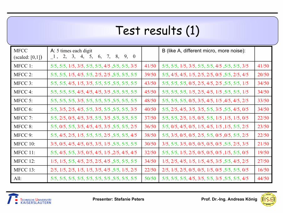
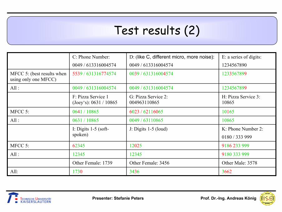
Test results
• As a result of the classification method all training samples are classified correctly.
• In the following table, the results of the classification for different test audio signals are shown, using only one MFCC parameter curve at a time as well as the combined results for all 13 parameter curves.
• Displayed are the recognition rates using the normalizes MFCC parameter curves. Wrong classification is highlighted in red color.
Presenter: Stefanie Peters Prof. Dr.-Ing. Andreas König
44/50
16/50
27/50
19/50
21/50
22/50
23/50
22/50
34/50
33/50
34/50
34/50
20/50
41/50
5/5, 5/5, 5/5, 4/5, 3/5, 5/5, 3/5 ,5/5, 5/5, 4/5
2/5, 1/5, 2/5, 0/5, 0/5, 1/5, 0/5 ,5/5, 5/5, 0/5
1/5, 2/5, 4/5, 1/5, 1/5, 4/5, 3/5 ,5/5, 4/5, 2/5
5/5, 5/5, 1/5, 2/5, 0/5, 0/5, 0/5 ,1/5, 5/5, 0/5
3/5, 5/5, 3/5, 0/5, 0/5, 0/5, 0/5 ,5/5, 2/5, 3/5
5/5, 3/5, 0/5, 0/5, 2/5, 5/5, 0/5 ,0/5, 5/5, 2/5
5/5, 0/5, 4/5, 0/5, 1/5, 4/5, 1/5 ,1/5, 5/5, 2/5
5/5, 5/5, 2/5, 1/5, 0/5, 5/5, 1/5 ,1/5, 1/5, 0/5
5/5, 2/5, 4/5, 3/5, 3/5, 5/5, 3/5 ,5/5, 4/5, 0/5
5/5, 5/5, 5/5, 0/5, 3/5, 4/5, 1/5 ,4/5, 4/5, 2/5
5/5, 5/5, 5/5, 1/5, 2/5, 4/5, 1/5 ,5/5, 5/5, 1/5
5/5, 5/5, 5/5, 0/5, 2/5, 4/5, 2/5 ,5/5, 5/5, 1/5
5/5, 4/5, 4/5, 1/5, 2/5, 2/5, 0/5 ,5/5, 2/5, 4/5
5/5, 5/5, 1/5, 3/5, 5/5, 5/5, 4/5 ,5/5, 5/5, 3/5
B (like A, different micro, more noise):
50/50
22/50
34/50
32/50
30/50
38/50
36/50
37/50
40/50
48/50
45/50
43/50
39/50
41/50
2/5, 1/5, 2/5, 1/5, 1/5, 3/5, 4/5 ,5/5, 1/5, 2/5MFCC 13:
5/5, 5/5, 1/5, 4/5, 5/5, 2/5, 2/5 ,5/5, 5/5, 5/5MFCC 2:
5/5, 5/5, 4/5, 1/5, 3/5, 5/5, 5/5 ,5/5, 5/5, 5/5MFCC 3:
5/5, 5/5, 5/5, 4/5, 4/5, 4/5, 3/5 ,5/5, 5/5, 5/5MFCC 4:
5/5, 5/5, 5/5, 3/5, 5/5, 5/5, 5/5 ,5/5, 5/5, 5/5MFCC 5:
5/5, 3/5, 2/5, 4/5, 5/5, 3/5, 5/5 ,5/5, 5/5, 3/5MFCC 6:
5/5, 2/5, 0/5, 4/5, 3/5, 5/5, 3/5 ,5/5, 5/5, 5/5MFCC 7:
5/5, 0/5, 5/5, 3/5, 4/5, 4/5, 3/5 ,5/5, 5/5, 2/5MFCC 8:
5/5, 4/5, 2/5, 1/5, 5/5, 5/5, 2/5 ,5/5, 5/5, 4/5MFCC 9:
3/5, 0/5, 4/5, 4/5, 0/5, 3/5, 1/5 ,5/5, 5/5, 5/5MFCC 10:
5/5, 4/5, 5/5, 3/5, 0/5, 4/5, 1/5 ,2/5, 4/5, 4/5MFCC 11:
1/5, 1/5, 5/5, 4/5, 2/5, 2/5, 4/5 ,5/5, 5/5, 5/5MFCC 12:
5/5, 5/5, 5/5, 5/5, 5/5, 5/5, 5/5 ,5/5, 5/5, 5/5 All:
5/5, 5/5, 1/5, 3/5, 5/5, 5/5, 4/5 ,5/5, 5/5, 3/5MFCC 1:
A: 5 times each digit_1 , 2, 3, 4, 5, 6, 7, 8, 9, 0
MFCC (scaled: [0,1])
Test results (1)
Presenter: Stefanie Peters Prof. Dr.-Ing. Andreas König
366234361730All:
9186 233 9991202562345MFCC 5:
9180 333 9991234512345All :
Other Male: 3578Other Female: 3456Other Female: 1739
108650049 / 631108650631 / 10865All :
K: Phone Number 2: 0180 / 333 999
J: Digits 1-5 (loud)I: Digits 1-5 (soft-spoken)
12345678990049 / 6313160045740049 / 631316004574All :
H: Pizza Service 3: 10865
G: Pizza Service 2: 004963110865
F: Pizza Service 1 (Joey‘s): 0631 / 10865
101656023 / 621160650641 / 10865MFCC 5:
12335678990039 / 6313160045745539 / 631316774574MFCC 5: (best results when using only one MFCC)
D: (like C, different micro, more noise):0049 / 613316004574
E: a series of digits:1234567890
C: Phone Number: 0049 / 613316004574
Test results (2)
Presenter: Stefanie Peters Prof. Dr.-Ing. Andreas König
Conclusions
• Results:
– Suitable training of a recognition system that recognizes spoken digits from one speaker.
– More than one MFCC parameter curve is needed for the classification.
– Pattern Matching via correlation needs a lot of time.(Training: 100 digits -> 1 min, Testing: 10 digits -> 2 min)
– No suitable digit recognition for different speakers.
• Further problems:
– Scaling of the length of a spoken digit is difficult to implement.
Presenter: Stefanie Peters Prof. Dr.-Ing. Andreas König
Questions
Presenter: Stefanie Peters Prof. Dr.-Ing. Andreas König
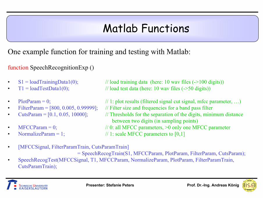
Matlab Functions
One example function for training and testing with Matlab:
function SpeechRecognitionExp ()
• S1 = loadTrainingData1(0); // load training data (here: 10 wav files (->100 digits)) • T1 = loadTestData1(0); // load test data (here: 10 wav files (->50 digits))
• PlotParam = 0; // 1: plot results (filtered signal cut signal, mfcc parameter, …)• FilterParam = [800, 0.005, 0.99999]; // Filter size and frequencies for a band pass filter• CutsParam = [0.1, 0.05, 10000]; // Thresholds for the separation of the digits, minimum distance
between two digits (in sampling points)• MFCCParam = 0; // 0: all MFCC parameters, >0 only one MFCC parameter• NormalizeParam = 1; // 1: scale MFCC parameters to [0,1]
• [MFCCSignal, FilterParamTrain, CutsParamTrain]= SpeechRecogTrain(S1, MFCCParam, PlotParam, FilterParam, CutsParam);
• SpeechRecogTest(MFCCSignal, T1, MFCCParam, NormalizeParam, PlotParam, FilterParamTrain,CutsParamTrain);


![NEURO COMPUTING @ CEA TECH - ASPROM · Handwritten digits 60,000 + 10,000 10 99.79% [3] ... Real-time digits recognition ... • Explore Deep Neural Network ...](https://static.fdocuments.fr/doc/165x107/5b2c167e7f8b9a163e8bbab9/neuro-computing-cea-tech-handwritten-digits-60000-10000-10-9979-3.jpg)