Astroparticle Physics 95 (2017) 44–56

Contents lists available at ScienceDirect

Astroparticle Physics

journal homepage: www.elsevier.com/locate/astropartphys

Spectral calibration of the fluorescence telescopes of the Pierre Auger

Observatory

A. Aab

bz , P. Abreu

bq , M. Aglietta

ax , aw , I. Al Samarai af , I.F.M. Albuquerque

r , I. Allekotte

a , A. Almela

h , k , J. Alvarez Castillo

bm , J. Alvarez-Muñiz

by , G.A. Anastasi ao , aq , L. Anchordoqui cf , B. Andrada

h , S. Andringa

bq , C. Aramo

au , F. Arqueros bw , N. Arsene

bs , H. Asorey

a , aa , P. Assis bq , J. Aublin

af , G. Avila

i , j , A.M. Badescu

bt , A. Balaceanu

br , F. Barbato

be , R.J. Barreira Luz

bq , J.J. Beatty

ck , K.H. Becker ah , J.A. Bellido

l , C. Berat ag , M.E. Bertaina

bg , aw , P.L. Biermann

cp , J. Biteau

ae , S.G. Blaess l , A. Blanco

bq , J. Blazek

ac , C. Bleve

ba , as , M. Bohácová ac , D. Boncioli aq , cr , C. Bonifazi x , N. Borodai bn , A.M. Botti h , aj , J. Brack

cv , I. Brancus br , T. Bretz

al , A. Bridgeman

aj , F.L. Briechle

al , P. Buchholz

an , A. Bueno

bx , S. Buitink

bz , M. Buscemi bc , ar , K.S. Caballero-Mora

bk , L. Caccianiga

bd , A. Cancio

k , h , F. Canfora

bz , L. Caramete

bs , R. Caruso

bc , ar , A. Castellina

ax , aw , F. Catalani r , G. Cataldi as , L. Cazon

bq , A.G. Chavez

bl , J.A. Chinellato

s , J. Chudoba

ac , R.W. Clay

l , A. Cobos h , R. Colalillo

be , au , A. Coleman

cl , L. Collica

aw , M.R. Coluccia

ba , as , R. Conceição

bq , G. Consolati at , ay , F. Contreras i , j , M.J. Cooper l , S. Coutu

cl , C.E. Covault cd , J. Cronin

cm , S. D’Amico

az , as , B. Daniel s , S. Dasso

e , c , K. Daumiller aj , B.R. Dawson

l , R.M. de Almeida

z , S.J. de Jong

bz , cb , G. De Mauro

bz , J.R.T. de Mello Neto

x , y , I. De Mitri ba , as , J. de Oliveira

z , V. de Souza

q , J. Debatin

aj , O. Deligny

ae , M.L. Díaz Castro

s , F. Diogo

bq , C. Dobrigkeit s , J.C. D’Olivo

bm , Q. Dorosti an , R.C. dos Anjos w , M.T. Dova

d , A. Dundovic

am , J. Ebr ac , R. Engel aj , M. Erdmann

al , M. Erfani an , C.O. Escobar ct , J. Espadanal bq , A. Etchegoyen

h , k , H. Falcke

bz , cc , cb , J. Farmer cm , G. Farrar ci , A.C. Fauth

s , N. Fazzini ct , F. Fenu

bg , aw , B. Fick

ch , J.M. Figueira

h , A. Filip ci c

bu , bv , O. Fratu

bt , M.M. Freire

f , T. Fujii cm , A. Fuster h , k , R. Gaior af , B. García

g , D. Garcia-Pinto

bw , F. Gaté cs , H. Gemmeke

ak , A. Gherghel-Lascu

br , U. Giaccari x , M. Giammarchi at , M. Giller bo , D. Głas bp , C. Glaser al , G. Golup

a , M. Gómez Berisso

a , P.F. Gómez Vitale

i , j , N. González

h , aj , B. Gookin

cv , A. Gorgi ax , aw , P. Gorham

cw , A.F. Grillo

aq , T.D. Grubb

l , F. Guarino

be , au , G.P. Guedes t , R. Halliday

cd , M.R. Hampel h , P. Hansen

d , D. Harari a , T.A. Harrison

l , J.L. Harton

cv , A. Haungs aj , T. Hebbeker al , D. Heck

aj , P. Heimann

an , A.E. Herve

ai , G.C. Hill l , C. Hojvat ct , E. Holt aj , h , P. Homola

bn , J.R. Hörandel bz , cb , P. Horvath

ad , M. Hrabovský ad , T. Huege

aj , J. Hulsman

h , aj , A. Insolia

bc , ar , P.G. Isar bs , I. Jandt ah , J.A. Johnsen

ce , M. Josebachuili h , J. Jurysek

ac , A. Kääpä ah , O. Kambeitz

ai , K.H. Kampert ah , B. Keilhauer aj , N. Kemmerich

r , E. Kemp

s , J. Kemp

al , R.M. Kieckhafer ch , H.O. Klages aj , M. Kleifges ak , J. Kleinfeller i , R. Krause

al , N. Krohm

ah , D. Kuempel al , G. Kukec Mezek

bv , N. Kunka

ak , A. Kuotb Awad

aj , B.L. Lago

o , D. LaHurd

cd , R.G. Lang

q , M. Lauscher al , R. Legumina

bo , M.A. Leigui de Oliveira

v , A. Letessier-Selvon

af , I. Lhenry-Yvon

ae , K. Link

ai , D. Lo Presti bc , L. Lopes bq , R. López

bh , A. López Casado

by , R. Lorek

cd , Q. Luce

ae , A. Lucero

h , k , M. Malacari cm , M. Mallamaci bd , at , D. Mandat ac , P. Mantsch

ct , A.G. Mariazzi d , I.C. Mari s m , G. Marsella

ba , as , D. Martello

ba , as , H. Martinez

bi , O. Martínez Bravo

bh , J.J. Masías Meza

c , H.J. Mathes aj , S. Mathys ah , J. Matthews cg , J.A.J. Matthews cx , G. Matthiae

bf , av , E. Mayotte

ah , P.O. Mazur ct , C. Medina

ce ,

∗ Corresponding author.

E-mail address: auger_spokespersons@fnal.gov (The Pierre Auger Collaboration).

http://dx.doi.org/10.1016/j.astropartphys.2017.09.001

0927-6505/© 2017 Elsevier B.V. All rights reserved.

A. Aab et al. / Astroparticle Physics 95 (2017) 44–56 45

G. Medina-Tanco

bm , D. Melo

h , A. Menshikov

ak , K.-D. Merenda

ce , S. Michal ad , M.I. Micheletti f , L. Middendorf al , L. Miramonti bd , at , B. Mitrica

br , D. Mockler ai , S. Mollerach

a , F. Montanet ag , C. Morello

ax , aw , M. Mostafá cl , A.L. Müller h , aj , G. Müller al , M.A. Muller s , u , S. Müller aj , h , R. Mussa

aw , I. Naranjo

a , L. Nellen

bm , P.H. Nguyen

l , M. Niculescu-Oglinzanu

br , M. Niechciol an , L. Niemietz

ah , T. Niggemann

al , D. Nitz

ch , D. Nosek

ab , V. Novotny

ab , L. Nožka

ad , L.A. Núñez

aa , L. Ochilo

an , F. Oikonomou

cl , A. Olinto

cm , M. Palatka

ac , J. Pallotta

b , P. Papenbreer ah , G. Parente

by , A. Parra

bh , T. Paul cf , M. Pech

ac , F. Pedreira

by , J. P e kala

bn , R. Pelayo

bj , J. Peña-Rodriguez

aa , L.A.S. Pereira

s , M. Perlin

h , L. Perrone

ba , as , C. Peters al , S. Petrera

ao , aq , J. Phuntsok

cl , R. Piegaia

c , T. Pierog

aj , M. Pimenta

bq , V. Pirronello

bc , ar , M. Platino

h , M. Plum

al , C. Porowski bn , R.R. Prado

q , P. Privitera

cm , M. Prouza

ac , E.J. Quel b , S. Querchfeld

ah , S. Quinn

cd , R. Ramos-Pollan

aa , J. Rautenberg

ah , D. Ravignani h , J. Ridky

ac , F. Riehn

bq , M. Risse

an , P. Ristori b , V. Rizi bb , aq , W. Rodrigues de Carvalho

r , G. Rodriguez

Fernandez

bf , av , J. Rodriguez Rojo

i , D. Rogozin

aj , M.J. Roncoroni h , M. Roth

aj , E. Roulet a , A.C. Rovero

e , P. Ruehl an , S.J. Saffi l , A. Saftoiu

br , F. Salamida

bb , aq , H. Salazar bh , A. Saleh

bv , F. Salesa Greus cl , G. Salina

av , F. Sánchez

h , P. Sanchez-Lucas bx , E.M. Santos r , E. Santos h , F. Sarazin

ce , R. Sarmento

bq , C. Sarmiento-Cano

h , R. Sato

i , M. Schauer ah , V. Scherini as , H. Schieler aj , M. Schimp

ah , D. Schmidt aj , h , O. Scholten

ca , cq , P. Schovánek

ac , F.G. Schröder aj , S. Schröder ah , A. Schulz

ai , J. Schumacher al , S.J. Sciutto

d , A. Segreto

ap , ar , A. Shadkam

cg ,

R.C. Shellard

n , G. Sigl am , G. Silli h , aj , O. Sima

cu , A. Smiałkowski bo , R. Šmída

aj , G.R. Snow

cn , P. Sommers cl , S. Sonntag

an , R. Squartini i , D. Stanca

br , S. Stani c

bv , J. Stasielak

bn , P. Stassi ag , M. Stolpovskiy

ag , F. Strafella

ba , as , A. Streich

ai , F. Suarez

h , k , M. Suarez Durán

aa , T. Sudholz

l , T. Suomijärvi ae , A.D. Supanitsky

e , J. Šupík

ad , J. Swain

cj , Z. Szadkowski bp , A. Taboada

ai , O.A. Taborda

a , V.M. Theodoro

s , C. Timmermans cb , bz , C.J. Todero Peixoto

p , L. Tomankova

aj , B. Tomé bq , G. Torralba Elipe

by , P. Travnicek

ac , M. Trini bv , R. Ulrich

aj , M. Unger aj , M. Urban

al , J.F. Valdés Galicia

bm , I. Valiño

by , L. Valore

be , au , G. van Aar bz , P. van Bodegom

l , A.M. van den

Berg

ca , A. van Vliet bz , E. Varela

bh , B. Vargas Cárdenas bm , G. Varner cw , R.A. Vázquez

by , D. Veberi c

aj , C. Ventura

y , I.D. Vergara Quispe

d , V. Verzi av , J. Vicha

ac , L. Villaseñor bl , S. Vorobiov

bv , H. Wahlberg

d , O. Wainberg

h , k , D. Walz

al , A .A . Watson

co , M. Weber ak , A. Weindl aj , L. Wiencke

ce , H. Wilczy nski bn , M. Wirtz

al , D. Wittkowski ah , B. Wundheiler h , L. Yang

bv , A. Yushkov

h , E. Zas by , D. Zavrtanik

bv , bu , M. Zavrtanik

bu , bv , A. Zepeda

bi , B. Zimmermann

ak , M. Ziolkowski an , Z. Zong

ae , F. Zuccarello

bc , ar , The Pierre Auger Collaboration

∗

a Centro Atómico Bariloche and Instituto Balseiro (CNEA-UNCuyo-CONICET), San Carlos de Bariloche, Argentina b Centro de Investigaciones en Láseres y Aplicaciones, CITEDEF and CONICET, Villa Martelli, Argentina c Departamento de Física and Departamento de Ciencias de la Atmósfera y los Océanos, FCEyN, Universidad de Buenos Aires and CONICET, Buenos Aires,

Argentina d IFLP, Universidad Nacional de La Plata and CONICET, La Plata, Argentina e Instituto de Astronomía y Física del Espacio (IAFE, CONICET-UBA), Buenos Aires, Argentina f Instituto de Física de Rosario (IFIR) – CONICET/U.N.R. and Facultad de Ciencias Bioquímicas y Farmacéuticas U.N.R., Rosario, Argentina g Instituto de Tecnologías en Detección y Astropartículas (CNEA, CONICET, UNSAM), and Universidad Tecnológica Nacional – Facultad Regional Mendoza

(CONICET/CNEA), Mendoza, Argentina h Instituto de Tecnologías en Detección y Astropartículas (CNEA, CONICET, UNSAM), Buenos Aires, Argentina i Observatorio Pierre Auger, Malargüe, Argentina j Observatorio Pierre Auger and Comisión Nacional de Energía Atómica, Malargüe, Argentina k Universidad Tecnológica Nacional – Facultad Regional Buenos Aires, Buenos Aires, Argentina l University of Adelaide, Adelaide, S.A., Australia m Université Libre de Bruxelles (ULB), Brussels, Belgium

n Centro Brasileiro de Pesquisas Fisicas, Rio de Janeiro, RJ, Brazil o Centro Federal de Educação Tecnológica Celso Suckow da Fonseca, Nova Friburgo, Brazil p Universidade de São Paulo, Escola de Engenharia de Lorena, Lorena, SP, Brazil q Universidade de São Paulo, Instituto de Física de São Carlos, São Carlos, SP, Brazil r Universidade de São Paulo, Instituto de Física, São Paulo, SP, Brazil s Universidade Estadual de Campinas, IFGW, Campinas, SP, Brazil t Universidade Estadual de Feira de Santana, Feira de Santana, Brazil u Universidade Federal de Pelotas, Pelotas, RS, Brazil v Universidade Federal do ABC, Santo André, SP, Brazil w Universidade Federal do Paraná, Setor Palotina, Palotina, Brazil x Universidade Federal do Rio de Janeiro, Instituto de Física, Rio de Janeiro, RJ, Brazil y Universidade Federal do Rio de Janeiro (UFRJ), Observatório do Valongo, Rio de Janeiro, RJ, Brazil z Universidade Federal Fluminense, EEIMVR, Volta Redonda, RJ, Brazil aa Universidad Industrial de Santander, Bucaramanga, Colombia ab Faculty of Mathematics and Physics, Charles University, Institute of Particle and Nuclear Physics, Prague, Czech Republic ac Institute of Physics of the Czech Academy of Sciences, Prague, Czech Republic

46 A. Aab et al. / Astroparticle Physics 95 (2017) 44–56

ad Palacky University, RCPTM, Olomouc, Czech Republic ae Institut de Physique Nucléaire d’Orsay (IPNO), Université Paris-Sud, Univ. Paris/Saclay, CNRS-IN2P3, Orsay, France af Laboratoire de Physique Nucléaire et de Hautes Energies (LPNHE), Universités Paris 6 et Paris 7, CNRS-IN2P3, Paris, France ag Laboratoire de Physique Subatomique et de Cosmologie (LPSC), Université Grenoble-Alpes, CNRS/IN2P3, Grenoble, France ah Department of Physics, Bergische Universität Wuppertal, Wuppertal, Germany ai Karlsruhe Institute of Technology, Institut für Experimentelle Kernphysik (IEKP), Karlsruhe, Germany aj Karlsruhe Institute of Technology, Institut für Kernphysik, Karlsruhe, Germany ak Karlsruhe Institute of Technology, Institut für Prozessdatenverarbeitung und Elektronik, Karlsruhe, Germany al RWTH Aachen University, III. Physikalisches Institut A, Aachen, Germany am Universität Hamburg, II. Institut für Theoretische Physik, Hamburg, Germany an Universität Siegen, Fachbereich 7 Physik – Experimentelle Teilchenphysik, Siegen, Germany ao Gran Sasso Science Institute (INFN), L’Aquila, Italy ap INAF – Istituto di Astrofisica Spaziale e Fisica Cosmica di Palermo, Palermo, Italy aq INFN Laboratori Nazionali del Gran Sasso, Assergi (L’Aquila), Italy ar INFN, Sezione di Catania, Catania, Italy as INFN, Sezione di Lecce, Lecce, Italy at INFN, Sezione di Milano, Milano, Italy au INFN, Sezione di Napoli, Napoli, Italy av INFN, Sezione di Roma “Tor Vergata”, Roma, Italy aw INFN, Sezione di Torino, Torino, Italy ax Osservatorio Astrofisico di Torino (INAF), Torino, Italy ay Politecnico di Milano, Dipartimento di Scienze e Tecnologie Aerospaziali , Milano, Italy az Università del Salento, Dipartimento di Ingegneria, Lecce, Italy ba Università del Salento, Dipartimento di Matematica e Fisica “E. De Giorgi”, Lecce, Italy bb Università dell’Aquila, Dipartimento di Scienze Fisiche e Chimiche, L’Aquila, Italy bc Università di Catania, Dipartimento di Fisica e Astronomia, Catania, Italy bd Università di Milano, Dipartimento di Fisica, Milano, Italy be Università di Napoli “Federico II”, Dipartimento di Fisica “Ettore Pancini“, Napoli, Italy bf Università di Roma “Tor Vergata”, Dipartimento di Fisica, Roma, Italy bg Università Torino, Dipartimento di Fisica, Torino, Italy bh Benemérita Universidad Autónoma de Puebla, Puebla, México bi Centro de Investigación y de Estudios Avanzados del IPN (CINVESTAV), México, D.F., México bj Unidad Profesional Interdisciplinaria en Ingeniería y Tecnologías Avanzadas del Instituto Politécnico Nacional (UPIITA-IPN), México, D.F., México bk Universidad Autónoma de Chiapas, Tuxtla Gutiérrez, Chiapas, México bl Universidad Michoacana de San Nicolás de Hidalgo, Morelia, Michoacán, México bm Universidad Nacional Autónoma de México, México, D.F., México bn Institute of Nuclear Physics PAN, Krakow, Poland bo University of Łód z, Faculty of Astrophysics, Łód z, Poland bp University of Łód z, Faculty of High-Energy Astrophysics, Łód z, Poland bq Laboratório de Instrumentação e Física Experimental de Partículas – LIP and Instituto Superior Técnico – IST, Universidade de Lisboa – UL, Lisboa,

Portugal br “Horia Hulubei” National Institute for Physics and Nuclear Engineering, Bucharest-Magurele, Romania bs Institute of Space Science, Bucharest-Magurele, Romania bt University Politehnica of Bucharest, Bucharest, Romania bu Experimental Particle Physics Department, J. Stefan Institute, Ljubljana, Slovenia bv Center for Astrophysics and Cosmology (CAC), University of Nova Gorica, Nova Gorica, Slovenia bw Universidad Complutense de Madrid, Madrid, Spain bx Universidad de Granada and C.A.F.P.E., Granada, Spain by Universidad de Santiago de Compostela, Santiago de Compostela, Spain bz IMAPP, Radboud University Nijmegen, Nijmegen, The Netherlands ca KVI – Center for Advanced Radiation Technology, University of Groningen, Groningen, The Netherlands cb Nationaal Instituut voor Kernfysica en Hoge Energie Fysica (NIKHEF), Science Park, Amsterdam, The Netherlands cc Stichting Astronomisch Onderzoek in Nederland (ASTRON), Dwingeloo, The Netherlands cd Case Western Reserve University, Cleveland, OH, USA ce Colorado School of Mines, Golden, CO, USA cf Department of Physics and Astronomy, Lehman College, City University of New York, Bronx, NY, USA cg Louisiana State University, Baton Rouge, LA, USA ch Michigan Technological University, Houghton, MI, USA ci New York University, New York, NY, USA cj Northeastern University, Boston, MA, USA ck Ohio State University, Columbus, OH, USA cl Pennsylvania State University, University Park, PA, USA cm University of Chicago, Enrico Fermi Institute, Chicago, IL, USA cn University of Nebraska, Lincoln, NE, USA co School of Physics and Astronomy, University of Leeds, Leeds, United Kingdom

cp Max-Planck-Institut für Radioastronomie, Bonn, Germany cq also at Vrije Universiteit Brussels, Brussels, Belgium

cr now at Deutsches Elektronen-Synchrotron (DESY), Zeuthen, Germany cs SUBATECH, École des Mines de Nantes, CNRS-IN2P3, Université de Nantes, France ct Fermi National Accelerator Laboratory, USA cu Physics Department, University of Bucharest, Bucharest, Romania cv Colorado State University, Fort Collins, CO cw University of Hawaii, Honolulu, HI, USA cx University of New Mexico, Albuquerque, NM, USA

A. Aab et al. / Astroparticle Physics 95 (2017) 44–56 47

a r t i c l e i n f o

Article history:

Received 3 June 2017

Revised 16 August 2017

Accepted 2 September 2017

Available online 8 September 2017

Keywords:

Auger observatory

Nitrogen fluorescence

Extensive air shower

Calibration

a b s t r a c t

We present a novel method to measure precisely the relative spectral response of the fluorescence tele-

scopes of the Pierre Auger Observatory. We used a portable light source based on a xenon flasher and

a monochromator to measure the relative spectral efficiencies of eight telescopes in steps of 5 nm from

280 nm to 440 nm. Each point in a scan had approximately 2 nm FWHM out of the monochromator. Dif-

ferent sets of telescopes in the observatory have different optical components, and the eight telescopes

measured represent two each of the four combinations of components represented in the observatory. We

made an end-to-end measurement of the response from different combinations of optical components,

and the monochromator setup allowed for more precise and complete measurements than our previous

multi-wavelength calibrations. We find an overall uncertainty in the calibration of the spectral response

of most of the telescopes of 1.5% for all wavelengths; the six oldest telescopes have larger overall uncer-

tainties of about 2.2%. We also report changes in physics measurables due to the change in calibration,

which are generally small.

© 2017 Elsevier B.V. All rights reserved.

1

t

h

s

s

c

f

i

t

S

o

3

g

o

p

a

A

o

t

t

e

c

t

a

c

c

t

i

v

c

o

E

c

o

a

d

×

a

v

m

P

O

t

p

t

p

m

c

s

n

s

U

s

c

t

l

s

t

w

a

r

t

O

e

s

n

a

fi

t

r

F

t

e

c

v

s

t

t

i

e

a

s

o

o

k

r

. Introduction

The Pierre Auger Observatory [1] has been designed to study

he origin and the nature of ultra high-energy cosmic rays, which

ave energies above 10 18 eV. The construction of the complete ob-

ervatory following the original design finished in 2008. The ob-

ervatory is located in Malargüe, Argentina, and consists of two

omplementary detector systems, which provide independent in-

ormation on the cosmic ray events. Extensive Air Showers (EAS)

nitiated by cosmic rays in the Earth’s atmosphere are measured by

he Surface Detector (SD) and the Fluorescence Detector (FD). The

D is composed of 1660 water Cherenkov detectors located mostly

n a triangular array of 1.5 km spacing covering an area of roughly

0 0 0 km

2 . The SD measures the EAS secondary particles reaching

round level [2] . The FD is designed to measure the nitrogen flu-

rescence light produced in the atmosphere by the EAS secondary

articles. The FD is composed of 27 telescopes overlooking the SD

rray from four sites, Los Leones (LL), Los Morados (LM), Loma

marilla (LA), and Coihueco (CO) [3] . The SD takes data continu-

usly, but the FD operates only on clear nights, and care is taken

o avoid exposure to too much moonlight.

The energy of the primary cosmic ray is a key measurable for

he science of the observatory, and the FD measurement of the en-

rgy, with lower independent systematic uncertainties, is used to

alibrate the SD energy scale using events observed by both de-

ectors. The work described here explains how the FD calibration

t wavelengths across the nitrogen fluorescence spectrum has re-

ently been improved, resulting in smaller related systematic un-

ertainties.

The buildings at the four FD sites each have six independent

elescopes, and each telescope has a 30 °× 30 ° field of view, lead-

ng to a 180 ° coverage in azimuth and from 2 ° to 32 ° in ele-

ation at each building. Additionally, three specialized telescopes

alled HEAT [4] are located near Coihueco to overlook a portion

f the SD array at higher elevations, from 32 ° to 62 °, to register

AS of lower energies. All these telescopes are housed in climate-

ontrolled buildings, isolated from dust and day light. The layout

f the observatory is shown schematically in Fig. 1 .

Each FD telescope is composed of several optical components

s shown in Fig. 2 : a 2.2 m aperture diaphragm, a UV filter to re-

uce the background light, a Schmidt corrector annulus, a 3.5 m

3.5 m tessellated spherical mirror, and a camera formed by an

rray of 440 hexagonal photomultipliers (PMT) each with a field of

iew of 1.5 ° full angle. Each PMT has a light concentrator approxi-

ating a hexagonal Winston cone to reduce dead spaces between

MTs [3] .

The energy calibration of the data [5,6] for the Pierre Auger

bservatory, including events observed by the SD only, relies on

he calibration of the FD. Events observed by both FD and SD

rovide the link from the FD, which is absolutely calibrated, to

he SD data. To calibrate the FD three different procedures are

erformed: the absolute [7] , the relative [8] , and the spectral (or

ulti-wavelength) calibrations [9] . We focus here on the spectral

alibration, which is a relative measurement that relates the ab-

olute calibration performed at 365 nm to wavelengths across the

itrogen fluorescence spectrum, which is shown in Fig. 3 .

To perform this measurement the drum-shaped portable light

ource used for the absolute calibration [7] was adapted to emit

V light across the wavelength range of interest. The drum light

ource is designed to uniformly illuminate all 440 PMTs in a single

amera simultaneously when it is placed at the aperture of the FD

elescope, enabling the end-to-end calibration.

The FD response as a function of wavelength was initially calcu-

ated as a convolution of separate reflection or transmission mea-

urements of each optical component used in the first Los Leones

elescopes [11] . The first end-to-end spectral calibration of the FD

as performed using the drum light source with a xenon flasher

nd filter wheel to provide five points across the FD wavelength

esponse [9] . This measurement represented an improvement for

he energy estimation of all events observed by the Pierre Auger

bservatory as it has been shown to increase the reconstructed en-

rgy of events by nearly 4% for all energies [12] . However, that re-

ult has two limitations: first, the differences in FD optical compo-

ents were not measured since only one telescope was calibrated;

nd second, determining the FD spectral response curve using only

ve points involved a complicated fitting procedure, and was par-

icularly difficult considering the large width of the filters, which

esulted in relatively large systematic uncertainties.

The aim of the work described in this paper was to measure the

D efficiency at many points across the nitrogen fluorescence spec-

rum with a reduced wavelength bite at each point, and to do it at

nough telescopes to cover the different combinations of optical

omponents making up all the telescopes within the Auger Obser-

atory. The spectral calibration described here proceeds in three

teps. First, the relative drum emission spectrum is measured in

he dark hall lab in Malargüe with a specific calibration PMT, called

he “Lab-PMT”, observing the drum at a large distance, in a sim-

lar fashion to the absolute calibration of the drum; see [7] and

xplanatory drawings therein. Knowing the intensity of the drum

t each wavelength, we next measure the response of the FD tele-

copes to the output of the multi-wavelength drum over the course

f several nights, while recording data from a monitoring photodi-

de (PD) exposed to the narrow-band light at each point to ensure

nowledge of the relative drum spectrum. Finally, the FD telescope

esponse is normalized by the measured relative drum emission

48 A. Aab et al. / Astroparticle Physics 95 (2017) 44–56

Fig. 1. A schematic of the Pierre Auger Observatory where each black dot is a wa-

ter Cherenkov detector. Locations of the fluorescence telescopes are shown along

the perimeter of the surface detector array, where the blue lines indicate their indi-

vidual field of view. The field of view of the HEAT telescopes are indicated with red

lines. (For interpretation of the references to color in this figure legend, the reader

is referred to the web version of this article.)

Fig. 2. The optical components of an individual fluorescence telescope.

Fig. 3. The nitrogen fluorescence spectrum as measured by the AIRFLY collaboration

[10] showing the 21 major transitions.

t

b

c

p

p

c

s

s

s

i

w

t

s

spectrum at every wavelength, and we evaluate the associated sys-

tematic uncertainties in the final calculation of the efficiency.

This following sections describe the measurements and anal-

ysis of data taken during March 2014: FD optical components in

Section 2 ; the new drum light source in Section 3 ; measurements

of the drum light source spectrum in Section 4 ; calibrations per-

formed at the FD telescopes in Section 5 ; FD efficiency as a func-

tion of wavelength in Section 6 ; and final calibration results in

Section 7 . Effects on physics measurables due to changing calibra-

tions are discussed in Section 8 .

2. Optical components of the fluorescence telescopes

There are two types of mirrors used in the telescopes, and the

glass used for the corrector rings was produced using two differ-

ent glass-making procedures. The 12 mirrors at Los Leones and Los

Morados are aluminum with a 2 mm AlMgSiO 5 layer glued on as

the reflective surface, and the 12 mirrors at Coihueco and Loma

Amarilla are composed of a borosilicate glass with a 90 nm Al layer

and then a 110 nm SiO 2 layer (see [3] for more details). Two differ-

ent procedures were used to grow the borosilicate glass used in

the corrector rings, both by Schott Glass Manufactures. 1 One type

is called Borofloat 33 2 , and the other is a crown glass labeled P-

BK7, 3 and the transmission of UV light differs for these two prod-

ucts.

Given the different wavelength dependencies of the above com-

ponents, our aim was to measure the four combinations of mirrors

and corrector rings present in the FDs. This meant calibrating at

three of the four FD buildings. Table 1 shows the eight telescopes

we calibrated at the three FD sites along with which components

make up each telescope. Calibration of these eight telescopes gives

a complete coverage of the different components and a duplicate

measure of each combination.

1 Schott Glass, http://www.us.schott.com/english/index.html . 2 Borofloat, http://www.us.schott.com/borofloat/english/attribute/optical . 3 P-BK7, http://www.schott.com/advanced _ optics/us/abbe _ datasheets/schott _

datasheet _ all _ us.pdf .

r

t

i

l

t

w

As seen in Table 1 , the telescopes CO 4/5 are the only ones

hat have same nominal components as those located at other FD

uildings, which have different construction dates. It is usually the

ase that optical components degrade their properties when ex-

osed to light and ambient conditions (ageing), whose effect de-

ends on exposure time. Even if FD telescopes are kept in climate-

ontrolled buildings, an analysis of ageing follows. Regarding the

pectral calibration, what has to be evaluated is the change in the

pectral response of a given FD telescope, i.e. the shape of the re-

ponse curve vs wavelength. This kind of differential degradation

s not obviously seen at the FD telescopes. One way to evaluate

hether there is any change in the spectral response is to track

he absolute calibration done periodically at 375 nm [1,2] . The ab-

olute calibration is scaled at any given date by using the nightly

elative calibration, which is done at 470 nm [1,2] . Because these

wo calibrations are done at different wavelengths, any change

n the spectral response would translate in a drift of the abso-

ute calibration with time. In Table 2 we show the variations of

he ratio (R) of absolute calibrations performed in 2010 and 2013,

here R = (Abs − Abs ) /Abs , along with the date of fin-

2013 2010 2013

A. Aab et al. / Astroparticle Physics 95 (2017) 44–56 49

Table 1

List of the FD telescopes we calibrated and their respective optical components.

Calibration at these eight FD telescopes gives a complete coverage of the different

components and a duplicate measure of each combination. The last column indi-

cates all other (unmeasured) telescopes with the same optical components.

FD telescope Mirror Type Corrector Ring FDs with same

components

Coihueco 2 Glass BK7

Coihueco 3 Glass BK7 CO2/3

Coihueco 4 Glass Borofloat 33 CO1,4-6, LA,

Coihueco 5 Glass Borofloat 33 HEAT

Los Morados 4 Aluminum Borofloat 33

Los Morados 5 Aluminum Borofloat 33 LM

Los Leones 3 Aluminum BK7

Los Leones 4 Aluminum BK7 LL1-6

Table 2

List of FD buildings and dates when construction was finished and operation

started. 1t is the elapsed time until measurements done for this work (March

2014). R is the ratio of absolute calibrations performed in 2010 and 2013 (see text).

FD building Built 1t [yr] R [%]

Los Leones 5/2004 9.8 + 1.4

Coihueco 5/2004 9.8 – 1.6

Los Morados 3/2005 9.0 – 0.5

Loma Amarilla 2/2007 7.1 – 0.8

HEAT 9/2009 4.5

i

t

t

a

c

e

s

r

q

3

s

i

w

t

F

o

e

fi

t

c

m

2

w

l

w

t

t

a

o

f

s

m

t

e

a

d

m

t

a

p

a

i

d

w

t

m

t

s

x

t

u

t

d

c

4

s

o

w

t

w

4

a

s

d

T

t

t

[

w

i

l

T

t

fi

s

m

c

a

c

s

t

t

w

s

s

shed construction for telescopes at a given building. As seen in the

able, the variations do not respond to any ageing pattern, e.g. for

he oldest telescopes there is a positive variation for LL and a neg-

tive variation for CO. Moreover, the overall effect that telescopes

ould have in data analysis do not change the final reconstructed

nergy significantly (see Fig. 49 in [1] ). For these reasons, we con-

ider that different time of telescope construction do not play a

ole in the spectral calibration described in this paper and, conse-

uently, CO 4/5 can be taken as representative of LA and HEAT.

. Monochromator drum setup

The work described in [9] was the first in-situ end-to-end mea-

urement of the FD efficiency as a function of wavelength. It lim-

ted the measurement to only five points across the ∼ 150 nm

ide acceptance of the FDs, and the filters had a fairly wide spec-

ral width, about ∼ 15 nm FWHM, as shown in the bottom of

ig. 4 . The large spectral width led to a complicated procedure

f accounting for the width effects along the rising and falling

dges of the efficiency curve [9] . In addition, since there were only

ve measured points, the resulting calibration curve had to be in-

erpolated between the points, and the original piece-wise effi-

iency curve [11] was used as the starting point. In the five-point

easurement [9] the efficiency was assumed to go to zero below

90 nm and above 425 nm since the filters did not extend to these

avelengths, thus the values resulting from the piece-wise convo-

ution of the component efficiencies [11] were the only data for

avelengths below 290 nm and above 425 nm.

These reasons are the motivation for using a monochromator

o select the wavelengths out of a UV spectrum. A monochroma-

or allows for a high resolution probe across the FD acceptance,

nd a far more detailed measurement can be performed. The top

f Fig. 4 shows the output of the monochromator in 5 nm steps

rom 275 nm to 450 nm with a xenon flasher as the input, each

tep with a 2 nm FWHM. The xenon flasher is an Excelitas PAX-10

odel 4 with improved EM noise reduction and variable flash in-

ensity. The monochromator output width was chosen to provide

4 PAX-10 10-Watt precision-aligned pulsed Xenon light source - http://www.

xcelitas.com/downloads/dts _ pax10.pdf .

b

reasonable compromise between wavelength resolution and the

rum intensity required for use at the FDs.

For the work described here, an enclosure housing the

onochromator and xenon flasher was mounted onto the rear of

he drum. The enclosure was insulated and contained a heater and

ssociated controlling circuitry to maintain a stable 20 ± 2 °C tem-

erature for monochromator reliability.

A custom 25.4 mm diameter aluminum tube was fabricated and

ttached to the output of the monochromator; it protrudes into the

nterior of the drum. At the end of the tube a 0.23 mm thick Teflon

iffuser ensured that the illumination of the front face of the drum

as uniform as measured with long-exposure CCD images, similar

o what had been measured previously [3,13] .

A photodiode (PD) was mounted near the output of the

onochromator, but upstream of the tube that protruded into

he drum, allowing for pulse-by-pulse monitoring of the emis-

ion spectrum from the monochromator. The monochromator and

enon flasher were controlled with the same common gateway in-

erface (CGI) web page and calibration electronics that have been

sed in the absolute calibration [7] . Scanning of the monochroma-

or, triggering of the flasher, and data acquisition from monitoring

evices and the FD were all fully automated using CGI code and

URL 5 scripts over the wireless LAN used for drum calibrations.

. Lab measurements and the drum spectrum

To characterize the drum emission as a function of wavelength,

everal measurements were needed in the laboratory. For the

ne-week calibration campaign described here, four measurements

ere performed in the lab, two prior to any field work at the FD

elescopes, one two days later and the last one at the end of the

eek.

.1. Drum emission

With the automated scanning of the monochromator and data

cquisition we took measurements of the relative drum emission

pectrum as viewed by the calibration Lab-PMT. The monitoring PD

etector measured the monochromator output as described above.

he setup for these measurements had the drum at the far end of

he dark hall and the Lab-PMT inside the darkbox in the calibra-

ion room, about 16 m away from the Teflon face of the drum. See

7] for a detailed description of the dark hall calibration setup.

The average response of the Lab-PMT to 100 pulses of the drum

as recorded as a function of wavelength from 250 nm to 450 nm,

n steps of 1 nm. The uncertainty in the average for a given wave-

ength was calculated as the standard deviation of the mean, σDrum √

100 .

he solid grey line in Fig. 5 shows an example of one of these spec-

ra. We took averages of the four spectra at each wavelength as the

nal measurement of the drum spectrum, which is shown in the

ame figure as blue dots. This final drum spectrum used measure-

ents in steps of 5 nm corresponding to the step size used when

alibrating the FD telescopes. For wavelengths between 320 nm

nd 390 nm, the four measurements were generally statistically

onsistent. But for wavelengths at the low and high ends of the

pectrum there was disagreement; Section 4.3 explains how we in-

roduce a systematic uncertainty to account for this disagreement.

For each of these four spectra measured with the Lab-PMT

here are data from the monitoring PD. The monitoring PD data

ere handled in the same way; we made an average of the four

pectra recorded by the PD and an associated error based on the

pread of the four measurements. These data are shown in Fig. 5 as

lack line and points.

5 cURL Documentation - http://curl.haxx.se/ .

50 A. Aab et al. / Astroparticle Physics 95 (2017) 44–56

Fig. 4. A comparison showing the spectral width of the output of the monochromator sampled every 5 nm (top, this work) and the notch filter spectral transmission

(bottom, [9] ). The y-axes are the intensity in arbitrary units for the monochromator and the normalized transmission for the notch filters.

Fig. 5. Drum emission spectra. Solid grey line: one of the measured spectra taken with the Lab-PMT; the line shows the average responses to 100 pulses of the drum as

a function of wavelength, in steps of 1 nm. Blue points: the averaged drum spectrum as measured by the Lab-PMT throughout the calibration campaign; the spectrum is

taken in steps of 5 nm as this is what is used to measure the FD responses; error bars are the statistical uncertainties, which are generally smaller than the plotted points.

Black line and points: the averaged drum spectrum as measured by the monitoring photodiode (PD) throughout the calibration campaign, in steps of 5 nm.

t

p

f

t

f

r

w

o

u

s

v

t

t

m

m

r

4.2. Lab-PMT quantum efficiency

A measurement of the quantum efficiency (QE) of the Lab-PMT,

which is used to measure the relative drum emission spectrum,

has to be performed to measure the relative response of a given FD

telescope at different wavelengths. The method used here is sim-

ilar to what was done previously [9] except, instead of a DC deu-

terium lamp, we used the xenon flasher as the UV light source into

the monochromator. For the work reported here we only needed a

relative measurement of the QE, and so several uncertainties asso-

ciated with an absolute QE measurement are not included in this

work.

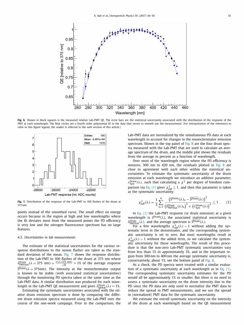
Several measurements of the Lab-PMT QE were performed prior

to and after the FD spectral calibration campaign, and these mea-

surements typically yielded curves consistent with the data shown

as black squares in Fig. 6 . The error bars are the statistical un-

certainty associated with the spread in the response of the PMT

o 100 pulses at each wavelength. The variations in the QE from

oint to point are typical when this kind of measurement is per-

ormed (e.g. see [9] ), although they are not expected. In an attempt

o smooth out these variations we fit the PMT QE curve with a

ourth order polynomial shown as blue circles in the figure. The er-

or bars in the fit are the relative statistical uncertainty for a given

avelength applied to the interpolated values in the fit. Deviations

f the fit from measured points are largest at both the lower and

pper ends of the wavelength range. However, the FD response is

ignificant only in the range 310–410 nm (see Fig. 9 ) where the de-

iations are less than 2% with RMS of approximately 1%. We take

his 1% as a conservative estimate of the systematic uncertainty in

he measurement of the Lab-PMT QE: δDrum

QESyst (λ) ≈ 1% .

Changing the nature of the fitted curve or using simply the

easured black points from Fig. 6 has little effect on measure-

ents of EAS events. For example a change of order 0.1% on the

econstructed energy would result from using the measured QE

A. Aab et al. / Astroparticle Physics 95 (2017) 44–56 51

Fig. 6. Shown in black squares is the measured relative Lab-PMT QE. The error bars are the statistical uncertainty associated with the distribution of the response of the

PMT at each wavelength. The blue circles are a fourth order polynomial fit to the data that serves to smooth out the measurement. (For interpretation of the references to

color in this figure legend, the reader is referred to the web version of this article.)

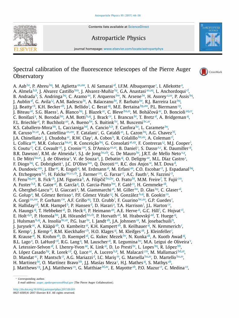
Fig. 7. Distribution of the response of the Lab-PMT to 100 flashes of the drum at

375 nm.

p

o

t

i

f

4

s

d

t

δ

S

i

t

L

l

a

e

c

L

w

s

t

a

f

n

c

c

e

ε

p

a

w

δ

t

a

χ

a

d

f

g

c

t

T

w

a

P

r

i

o

oints instead of the smoothed curve. The small effect on energy

ccurs because in the region at high and low wavelengths where

he fit deviates most from the measured points the FD efficiency

s very low and the nitrogen fluorescence spectrum has no large

eatures.

.3. Uncertainties in lab measurements

The estimate of the statistical uncertainties for the various re-

ponse distributions to the xenon flasher are taken as the stan-

ard deviation of the mean. Fig. 7 shows the response distribu-

ion of the Lab-PMT to 100 flashes of the drum at 375 nm whereDrum

PMTStat (λ = 375 nm ) =

σ (λ=375 nm ) √

N ≈ 1% of the average response

Drum (λ = 375 nm ) . The intensity at the monochromator output

s known to be stable (with associated statistical uncertainties)

hrough the monitoring PD spectra taken at the same time as the

ab-PMT data. A similar distribution was produced for each wave-

ength in the Lab-PMT QE measurement and gives δDrum

QEStat (λ) ≈ 1% .

Estimating the systematic uncertainties associated with the rel-

tive drum emission spectrum is done by comparing the differ-

nt drum emission spectra measured using the Lab-PMT over the

ourse of the one-week campaign. Prior to the comparison, the

ab-PMT data are normalized by the simultaneous PD data at each

avelength to account for changes in the monochromator emission

pectrum. Shown in the top panel of Fig. 8 are the four drum spec-

ra measured with the Lab-PMT that are used to calculate an aver-

ge spectrum of the drum, and the middle plot shows the residuals

rom the average in percent as a function of wavelength.

Over most of the wavelength region where the FD efficiency is

onzero, 300 nm to 420 nm, the residuals plotted in Fig. 8 are

lose to agreement with each other within the statistical un-

ertainties. To estimate the systematic uncertainty of the drum

mission at each wavelength we introduce an additive parameter,

Drum

Syst (λ) , such that calculating a χ2 per degree of freedom com-

arison via Eq. (1) gives χ2 ndf

. 1 , and then this parameter is taken

s the systematic uncertainty:

χ2 ndf (λ) =

1

3

4 X

n =1

¡S Drum (λ) n − S Drum (λ)

¢2

¡δDrum

PMTStat (λ) n

¢2 +

¡ε Drum

Syst (λ)

¢2 . 1 . (1)

In Eq. (1) the Lab-PMT response (or drum emission) at a given

avelength is S Drum ( λ), the associated statistical uncertainty isDrum

PMTStat (λ) , and the average spectrum is S Drum (λ) .

For a few wavelengths χ2 ndf

(λ) < 1 without adding the sys-

ematic term in the denominator, and the corresponding system-

tic uncertainty is set to zero. But most wavelengths result in2 ndf

(λ) > 1 without the added term, so we calculate the system-

tic uncertainty for those wavelengths. The result of this proce-

ure is that the non-zero Lab-PMT systematic uncertainties vary

rom less than 1% to approximately 3%, and in the important re-

ion from 300 nm to 400 nm the average systematic uncertainty is,

onservatively, about 1%, see the bottom panel of Fig. 8 .

As a check, the PD spectra were treated with a similar evalua-

ion of a systematic uncertainty at each wavelength as in Eq. (1) .

he corresponding systematic uncertainty estimates for the PD

ould all be approximately 1% or smaller. But there is no need to

ssess a systematic uncertainty on the drum intensity due to the

D since the PD data are only used to normalize the PMT data to

educe the spread in PMT measurements, and we use the spread

n (normalized) PMT data for the systematic uncertainty.

We estimate the overall systematic uncertainty on the intensity

f the drum at each wavelength based on the QE measurement

52 A. Aab et al. / Astroparticle Physics 95 (2017) 44–56

Fig. 8. Four drum emission spectra as measured by the Lab-PMT (top), residuals from the average in percent (middle), the resulting systematic uncertainty ε Drum Syst (λ) shown

as a percent of the PMT response at a given wavelength (bottom).

Fig. 9. Relative efficiencies for the average of Los Morados telescopes 4 and 5. Top : the five filter curve shown as a dashed blue line [9] and the monochromator result

shown as the solid line. Error bars are statistical uncertainties, and the red brackets are the systematic uncertainties calculated as described in Section 5 . Bottom : difference

between the five filter result and this work. The error bars and brackets are the same as in the top plot, shown here for clarity. (For interpretation of the references to color

in this figure legend, the reader is referred to the web version of this article.)

5

r

5

w

of the Lab-PMT ( δDrum

QESyst (λ) ≈ 1% ) and the four measurements of

the drum spectrum ( ε Drum

Syst (λ) ≈ 1% ). Each of these uncertainties

is conservatively about 1% in the main region of the FD efficiency

and nitrogen fluorescence spectrum, so a reasonable estimate of

the overall systematic uncertainty of the drum intensity is found

by adding them in quadrature: 1.4%.

t

. FD measurements

During the March 2014 calibration campaign we measured the

esponse of the eight telescopes, as specified in Table 1 , in steps of

nm, over the course of five days. Data from the monitoring PD

ere also acquired during the FD measurements to be able to con-

rol for changes in the drum spectral emission. The procedure for

A. Aab et al. / Astroparticle Physics 95 (2017) 44–56 53

m

w

t

w

b

s

w

a

t

t

l

f

i

e

t

s

c

o

e

i

s

n

s

g

o

o

o

s

s

t

5

t

m

a

t

f

t

i

f

w

n

T

l

w

a

a

i

i

s

(

F

t

l

r

Table 3

εFD and β values obtained via Eq. (2) for the similarly constructed tele-

scopes. The εFD for a given pair of telescopes is given in percentage

relative to the averaged response of the pair of telescopes at 375 nm.

FDs εFD [%] β

Coihueco 2/3 0.34 0.97

Coihueco 4/5 0.48 1.02

Los Morados 4/5 0.14 1.01

Los Leones 3/4 1.7 1.05

r

s

m

t

s

t

n

c

r

a

u

s

t

g

t

n

a

d

u

a

o

u

3

s

(

l

c

c

t

f

o

i

C

1

f

d

u

t

i

t

0

t

t

b

t

5

s

n

w

easuring the telescope response to the multi-wavelength drum

as to first scan from 255 nm to 445 nm in steps of 10 nm, and

hen scan from 250 nm to 450 nm in steps of 10 nm. At each

avelength a series of 100 pulses from the drum was recorded

y the FD data acquisition at a rate of 1 Hz. A full telescope re-

ponse is then an interleaving of these scans. Later in analysis,

avelengths that result in essentially zero FD efficiency - at low

nd high wavelengths in the scan corresponding to the edges of

he nitrogen spectrum - were dropped and set to zero.

In the previous sections we evaluated the systematic uncer-

ainty in the drum light source intensity as a function of wave-

ength. The contributions to this uncertainty are the spread in the

our measurements of the drum intensity over the week of the cal-

bration campaign and the systematic uncertainty in the quantum

fficiency of the PMT used to measure the drum output.

In this section we evaluate the uncertainty in the responses of

he telescopes to the drum by comparing the responses of tele-

copes with the same optical components - see Table 1 . We do this

omparison because we have not measured every telescope in the

bservatory, so we have to develop a single calibration constant for

ach wavelength for each of the four sets of optical components

n the table. Then we use these calibration constants for all tele-

copes with like components (again, see Table 1 ), including those

ot measured. Combining this uncertainty on the FD response, de-

cribed below, with the drum emission systematic uncertainty will

ive the overall systematic uncertainties on the spectral calibration

f the telescopes. As we will see below, of the four combinations

f optical components in Table 1 three will result in systematics

n FD response well below the systematics from the drum emis-

ion, but one pair of telescopes will have significantly different re-

ponses to the drum resulting in a systematic uncertainty larger

han that from the drum intensity.

.1. FD systematic uncertainties evaluated by comparing similar

elescopes

We assume that the FDs built with like components - the same

irror and corrector ring types - should give similar responses,

nd to test that assumption we make a comparison between them

o derive a meaningful systematic uncertainty. To that end we per-

orm a χ2 test and introduce parameters to minimize the χ2 such

hat χ2 ndf

. 1 for ndf = 34 , where there are 35 wavelengths used

n the comparison. The parameters introduced are an overall scale

actor β that is applied to one of the FD responses, and then εFD

hich is an estimate of a systematic uncertainty that would be

eeded to account for the difference between the two telescopes.

hus the raw response of one of the FDs as a function of wave-

ength is then β ∗¡F D Resp (λ) ± δFD

Stat (λ) ± ε FD

¢in the comparison,

here δFD Stat

(λ) is the statistical uncertainty (small) as mentioned

t the end of this section. The scale factor β does not represent

systematic uncertainty, it just accounts for any overall difference

n response between the two telescopes. This is similar to perform-

ng a relative calibration analysis as in [14] between the two tele-

copes.

The minimization is done in two steps according to Eq.

2) where the sum is over the N λ measured wavelength points:

χ2 ndf =

1

34

N λX

n=1

³F D 1 (λ) n − β ∗ F D 2 (λ) n

´2

³δFD 1

Stat (λ) n

´2

+

³β ∗ δFD 2

Stat (λ) n

´2

+

³β ∗ ε FD

´2 .

(2) irst a minimum in χ2 is found by setting ε FD = 0 and allowing

he scale factor β to vary. Once β has been determined, εFD is al-

owed to vary until χ2 ndf

. 1 . Prior to the minimization the FD 2 ( λ)

esponse data are normalized by the ratio of the monitoring PD

esponse as measured at FD 1 and FD 2 for a given wavelength. This

erves to divide out any change in intensity of the light source as

easured by the PD just downstream of the monochromator, and

his normalization does, as expected, improve the agreement in re-

ponse for some telescope pairs.

The values for εFD and β are listed in Table 3 for each pair of

elescopes that are constructed with nominally identical compo-

ents, and the systematic uncertainties, εFD , are reported as a per-

entage of the average response of the two telescopes at 375 nm.

Aside from Los Leones telescopes 3 and 4, the εFD values de-

ived through this minimization technique are all less than 0.5 % ,

nd the β scale factors are all within about 3 % of unity. The val-

es obtained for Los Leones, although larger than the others, are

till small. By trying to find a reason for this difference we note

hat telescope 4 was part of the Engineering Array (EA, [15] ) to-

ether with telescope 5. However, both telescopes were rebuilt af-

er the EA operation, particularly the mirrors were all replaced by

ew ones after re-setting the design parameters. So, the discrep-

ncy between LL 3 and 4 is highly probably not caused by any

ifference in used materials and, in any case, is included in the

ncertainties.

We use the εFD calculated for a given pair of FD telescopes as

systematic uncertainty across all wavelengths for all telescopes

f the corresponding construction; see Table 1 . These systematic

ncertainties are then normalized by the telescope response at

75 nm and are added in quadrature with the uncertainties as-

ociated with the spread in Lab-PMT measurements of the drum

about 1% in important wavelength range, a function of wave-

ength), and the Lab-PMT QE (1%, not wavelength dependent) to

alculate the overall systematic uncertainty on telescopes of each

ombination of optical components. An example result is plotted as

he red brackets in Fig. 9 for the Los Morados telescopes 4 and 5;

or this pair (and like telescopes) the overall systematic uncertainty

n the FD response is approximately p

1 2 + 1 2 + 0 . 14 2 = 1 . 4% , and

t is dominated by the uncertainty in the drum intensity. For the

oihueco instruments the overall systematic uncertainty is about

.5%. For the telescopes at Los Leones the uncertainty from the dif-

erence in response between the two telescopes is larger than the

rum-related systematic uncertainties, and the overall systematic

ncertainty on all of the Los Leones telescopes is about 2.2%.

The statistics of the data taken with the drum light source at

he FD telescopes also contribute to the uncertainties on the cal-

bration constants. The typical spread in the average response of

he 440 PMTs to the 100 drum pulses at a given wavelength is

.4% RMS, which is much smaller than the systematic uncertain-

ies. Adding the statistical uncertainty in quadrature with the sys-

ematic uncertainties yields the overall uncertainties on the cali-

ration constants listed in Table 4 , which are the main result of

his work.

.2. Photodiode monitor data

We performed a comparison between the average dark hall PD

pectrum and each of the spectra measured for the data-taking

ights at the FDs to ensure that the light source was stable and

as consistent with what had been measured in the lab. An over-

54 A. Aab et al. / Astroparticle Physics 95 (2017) 44–56

Table 4

Overall uncertainties on spectral calibration constants for the pairs of telescopes

measured and all other (unmeasured) telescopes with the same optical components.

FDs Overall FDs with same

uncertainty [%] components

Coihueco 2/3 1.5 CO2/3

Coihueco 4/5 1.5 CO1,4-6, LA, HEAT

Los Morados 4/5 1.5 y LM

Los Leones 3/4 2.2 LL1-6

Table 5

Comparison of spectral response for FD telescopes with different com-

ponents. χ2 ndf

values obtained for the sets in Table 1 , where ndf = 34 .

Comparison χ2 ndf

Coihueco 2/3 vs. Coihueco 4/5 2.4

Los Morados 4/5 vs. Los Leones 3/4 0.21

Coihueco 4/5 vs Los Morados 4/5 57

Coihueco 2/3 vs. Los Leones 3/4 10

Coihueco 2/3 vs. Los Morados 4/5 144

Los Leones 3/4 vs. Coihueco 4/5 6.7

c

d

t

s

t

o

a

P

b

t

e

t

a

C

o

C

s

f

t

5

s

t

s

c

t

b

s

t

s

m

s

M

s

T

b

χ

c

w

5

o

p

χ

v

all correction of 1.00 ± 0.01 night to night was found as the aver-

age ratio of the PD response at the FD to that at the lab to ac-

commodate any overall variations in intensity or response due to

temperature effects, and then we performed a χ2 comparison for

all the measured wavelengths. For all measuring nights at the FDs

the PD spectra agree very well, the comparison gives a χ2 ndf

∼ 1

where ndf = 34 for each, implying that the spectrum as observed

by the PD was the same at all locations.

6. Calculation of the FD efficiency

We calculate the relative FD efficiency for each telescope by di-

viding the measured telescope response to the drum by the mea-

sured drum emission spectrum. The relative drum emission spec-

trum is measured as described in Section 4 and takes into account

the Lab-PMT quantum efficiency over the range from 250 nm to

450 nm.

The relative efficiency for a given telescope at a given wave-

length, F D

Rel eff

(λ) , is calculated for each wavelength from 280 nm

to 440 nm in steps of 5 nm:

F D

Rel eff (λ) =

F D Resp (λ) ∗ QE Lab PMT (λ)

S Drum (λ) ∗ 1

F D eff (λ = 375 nm ) . (3)

The curves are taken relative to the efficiency of the telescope at

375 nm since this is what is used in the Pierre Auger Observatory

reconstruction software [16] for all FD calculations. The range in

wavelength from 280 nm to 440 nm used for evaluating the FD

efficiency is smaller than the range measured in the lab because

below 280 nm and above 440 nm the light level is near zero in-

tensity for the nitrogen emission spectrum and the FD response is

also very near zero. As an example, Fig. 9 shows the relative effi-

ciency for the Los Morados telescopes 4 and 5 based on this work

compared with the previous measurement [9] .

The uncertainties in the FD efficiencies have statistical and sys-

tematic components associated with the measurement of the rela-

tive emission spectrum of the drum, the Lab-PMT QE, and the FD

response to the multi-wavelength drum. The statistical uncertain-

ties associated with the lab work and the FD responses are prop-

agated through the calculation of the FD efficiency via Eq. (3) as

a function of wavelength. All systematic uncertainties described

above associated with the lab work, the Lab-PMT and its QE, the

FD response, and εFD for a given FD telescope, are added together

in quadrature as a function of wavelength.

For much of the wavelength range the new results agree with

the older five-point scan. The disagreement at the shortest and

longest wavelengths is perhaps not surprising since the previous

lowest and highest measurements were at 320 nm and 405 nm,

and the efficiency was extrapolated to zero from those points fol-

lowing the piecewise curve [11] . The efficiency was assumed to go

to zero below 295 nm and above 425 nm.

7. Comparison of telescopes with differing optical components

After estimating the systematic uncertainties for each measured

FD telescope, ε , we made a χ2 comparison between the six

FD

ombinations of unlike FD optical components listed in Table 1 to

etermine whether the unlike components result in any different

elescope responses. In calculating the χ2 ndf

for the differently con-

tructed FD telescopes we use the ratio of the PD data taken at

he corresponding FDs to normalize the average response of one

f the FD types. The PD data from the two FD data-taking nights

re averaged as a function of wavelength and the ratio of the

D averages from the two types of FDs are applied to the com-

ined FD response along with the statistical and systematic uncer-

ainties. Using this normalization serves to divide out any differ-

nces in the drum spectrum between the two measurements of

he FD types. An example for calculating the χ2 between the aver-

ge of Coihueco 2 and Coihueco 3 ( S CO23 (λ) n ) and the average of

oihueco 4 and 5 follows. The uncertainties in Eq. (4) have obvi-

us labels; for example ε CO23 FD

is the systematic uncertainty for the

oihueco telescopes 2 and 3 from Table 3 .

χ2 ndf

=

1

34

N λP

n=1

³S CO23 (λ) n −PD Ratio (λ) n ∗S CO45 (λ) n

´2

¡δCO23

Stat (λ) n

¢2

+ ¡

PD Ratio (λ) n ∗δCO45 Stat

(λ) n

¢2

+ ¡ε CO23

FD

¢2

+ ¡ε CO45

FD

¢2 ,

P D Ratio (λ) ≡ S PD CO23

(λ)

S PD CO45

(λ) (4)

The results of the comparisons are shown in Table 5 . The tele-

copes with different components are all significantly different

rom each other except when comparing the average of Los Leones

elescopes 3 and 4 to the average of Los Morados telescopes 4 and

. In principle this low χ2 could indicate that all telescopes con-

tructed with components like those at Los Leones 3 and 4 and

hose constructed like Los Morados telescopes 4 and 5 have the

ame response, and therefore could share the relative calibration

onstants that are the goal of this work. However, the two de-

ectors at Los Leones have a much greater difference in response

etween them than do the two telescopes from Los Morados: the

ystematic uncertainty in Table 3 for Los Leones telescopes is more

han a factor of 10 larger than that for Los Morados ones. The large

ystematic uncertainty for the telescopes at Los Leones could be

asking a real difference with those at Los Morados. For this rea-

on we feel it is reasonable not to combine the Los Leones and Los

orados telescopes to calculate the final spectral calibration con-

tants.

We conclude that all four sets of FD telescopes listed in

able 1 need different spectral calibrations, and four sets of cali-

ration constants have been computed.

Examining the results in Tables 5 and 1 we note that the largest2 ndf

values in Table 5 are associated with changing mirrors not

hanging corrector rings. For example, comparing Coihueco 4/5

ith Los Morados 4/5 changes only the mirror and gives a χ2 ndf

of

5, but comparing Coihueco 4/5 with Coihueco 2/3, which changes

nly the corrector ring, yields a χ2 ndf

of 5.6. Changing both com-

onents by comparing Coihueco 2/3 with Los Morados 4/5 gives a2 ndf

of 161, but we note that the telescopes at Los Morados have a

ery small systematic uncertainty in Table 3 . These examples have

A. Aab et al. / Astroparticle Physics 95 (2017) 44–56 55

s

c

d

i

p

8

s

b

i

i

s

l

e

m

fi

l

e

t

t

l

a

n

s

a

e

T

a

t

m

c

k

u

t

3

9

9

t

p

s

p

t

n

t

o

d

w

t

s

-

l

s

2

r

c

s

c

o

e

s

a

c

e

c

s

e

o

t

A

P

t

i

a

N

N

G

N

t

R

C

t

J

N

T

L

–

S

m

D

t

w

A

d

(

l

D

W

M

B

a

d

C

i

1

P

d

W

O

R

a

N

H

P

P

d

R

o far left out the Los Leones telescopes. The large systematic un-

ertainty derived by comparing the two Los Leones telescopes re-

uces the χ2 ndf

values when comparing to other telescopes, but the

dea that the mirrors are the main effect is still present when com-

aring the Los Leones telescopes to the others.

. Effect on physics measurables

To evaluate the effect a new calibration has on physics mea-

urables, we reconstructed a set of events using the new cali-

ration and compare to results from that same set of events us-

ng the prior calibration. When we did this exercise upon chang-

ng from initial piecewise to the five-point calibration, the recon-

tructed energies increased about 4% at 10 18 eV, and the increase

essened slightly to 3.6% at 10 19 eV [12] . The lessening of the en-

rgy increase due the five-point calibration is understood because

uch of the change in calibration was at low wavelengths, and the

ve-point calibration makes the FDs less efficient at short wave-

engths making the reconstructed energy higher. The higher energy

vents make more light, and they can be detected at greater dis-

ances than lower energy events. But at greater distances more of

he short wavelength light will be Rayleigh scattered away, so the

ower wavelengths - and the change in calibration there - do not

ffect the higher energy events as much when we change to the

ew calibration.

When we change from the five-point to the calibration de-

cribed here, the reconstructed energies increase on average over

ll FD telescopes by about 1%, and that increase is relatively flat in

nergy. However, this increase is not the same at all the telescopes.

he increase in reconstructed energy is greatest at Los Leones,

bout 2.8% at 10 18 eV falling to 2.5% at 10 19 eV. For Los Morados

he reconstructed event energies increase by about 1.8% without

uch energy dependence. For all other telescopes the energy in-

reases, but those increases are less than 0.35% for all energies.

All these changes in the reconstructed energy are important to

now to fully characterize the telescopes. Regarding the associated

ncertainties, they are all significantly smaller than the uncertain-

ies involved in the energy scale for the FD telescopes (see Table

in [1] ), particularly the 3.6% from the Fluorescence yield and the

.9% from the FD calibration.

. Conclusions

Determining the spectral response of the Pierre Auger Observa-

ory fluorescence telescopes is essential to the success of the ex-

eriment. A method using a monochromator-based portable light

ource has been used for eight FD telescopes with measurements

erformed every five nanometers from 280 nm to 440 nm. With

he calibration of these eight telescopes, the four possible combi-

ations of different optical components in the FD were covered,

hus assuring the spectral calibration of all FD telescopes at the

bservatory.

The uncertainty associated with the emission spectrum of the

rum light source used for the calibration was found to be 1.4%,

hich is an improvement on our previous 3.5% [9] .

For the present work we compared telescopes with nominally

he same optical components, and we find that such pairs have the

ame spectral response within a fraction of a percent - as expected

for three out of the four pairs of like telescopes. But one pair with

ike components, the oldest telescopes in the observatory, shows a

ignificant difference in spectral response.

The overall uncertainty in the FD spectral response is 1.5% for

1 of the 27 telescopes. The overall systematic uncertainty for the

emaining six telescopes is 2.2%, and is somewhat larger on ac-

ount of the larger difference between the two telescopes mea-

ured.

We also compared the differently constructed telescopes. These

omparisons show significantly different efficiencies as a function

f wavelength, with differences mainly in the rising edge of the

fficiency curve between 300 nm and 340 nm. The differences

eem to come mostly from the two different mirror types, and they

re reflected in different calibration constants for each of the four

ombinations of optical components.

The new calibration constants affect the reconstruction of EAS

vents, and we looked at two important quantities. The primary

osmic ray energy increases by 1.8% to 2.8% for half of the tele-

copes in the observatory, and for the other half the change in en-

rgy is negligible. The position of the maximum in shower devel-

pment in the atmosphere, X max , is not changed significantly by

he change in calibration.

cknowledgments

The successful installation, commissioning, and operation of the

ierre Auger Observatory would not have been possible without

he strong commitment and effort from the technical and admin-

strative staff in Malargüe. We are very grateful to the following

gencies and organizations for financial support:

Argentina – Comisión Nacional de Energía Atómica; Agencia

acional de Promoción Científica y Tecnológica (ANPCyT); Consejo

acional de Investigaciones Científicas y Técnicas (CONICET);

obierno de la Provincia de Mendoza; Municipalidad de Malargüe;

DM Holdings and Valle Las Leñas; in gratitude for their con-

inuing cooperation over land access; Australia – the Australian

esearch Council; Brazil – Conselho Nacional de Desenvolvimento

ientífico e Tecnológico (CNPq); Financiadora de Estudos e Proje-

os (FINEP); Fundação de Amparo à Pesquisa do Estado de Rio de

aneiro (FAPERJ); São Paulo Research Foundation ( FAPESP ) Grants

o. 2010/07359-6 and No. 1999/05404-3 ; Ministério de Ciência e

ecnologia (MCT); Czech Republic – Grant No. MSMT CR LG15014 ,

O1305 , LM2015038 and CZ.02.1.01/0.0/0.0/16_013/0 0 01402 ; France

Centre de Calcul IN2P3/CNRS; Centre National de la Recherche

cientifique (CNRS); Conseil Régional Ile-de-France; Départe-

ent Physique Nucléaire et Corpusculaire (PNC-IN2P3/CNRS);

épartement Sciences de l’Univers (SDU-INSU/ CNRS ); Insti-

ut Lagrange de Paris (ILP) Grant No. LABEX ANR-10-LABX-63

ithin the Investissements d’Avenir Programme Grant No.

NR-11-IDEX-0 0 04-02 ; Germany – Bundesministerium für Bil-

ung und Forschung (BMBF); Deutsche Forschungsgemeinschaft

DFG); Finanzministerium Baden-Württemberg; Helmholtz Al-

iance for Astroparticle Physics (HAP); Helmholtz-Gemeinschaft

eutscher Forschungszentren (HGF); Ministerium für Innovation,

issenschaft und Forschung des Landes Nordrhein-Westfalen;

inisterium für Wissenschaft, Forschung und Kunst des Landes

aden-Württemberg; Italy – Istituto Nazionale di Fisica Nucle-

re (INFN); Istituto Nazionale di Astrofisica (INAF); Ministero

ell’Istruzione, dell’Universitá e della Ricerca (MIUR); CETEMPS

enter of Excellence; Ministero degli Affari Esteri (MAE); Mex-

co – Consejo Nacional de Ciencia y Tecnología ( CONACYT ) No.

67733 ; Universidad Nacional Autónoma de México (UNAM);

APIIT DGAPA-UNAM; The Netherlands – Ministerie van On-

erwijs, Cultuur en Wetenschap; Nederlandse Organisatie voor

etenschappelijk Onderzoek (NWO); Stichting voor Fundamenteel

nderzoek der Materie (FOM); Poland – National Centre for

esearch and Development, Grants No. ERA-NET-ASPERA/01/11

nd No. ERA-NET-ASPERA/02/11; National Science Centre , Grants

o. 2013/08/M/ST9/00322 , No. 2013/08/M/ST9/00728 and No.

ARMONIA 5–2013/10/M/ST9/0 0 062 , UMO-2016/22/M/ST9/0 0198 ;

ortugal – Portuguese national funds and FEDER funds within

rograma Operacional Factores de Competitividade through Fun-

ação para a Ciência e a Tecnologia (COMPETE); Romania –

omanian Authority for Scientific Research ANCS; CNDI-UEFISCDI

56 A. Aab et al. / Astroparticle Physics 95 (2017) 44–56

[

partnership projects Grants No. 20/2012 and No.194/2012 and

PN 16 42 01 02; Slovenia – Slovenian Research Agency; Spain

– Comunidad de Madrid; Fondo Europeo de Desarrollo Regional

(FEDER) funds; Ministerio de Economía yCompetitividad; Xunta

de Galicia; European Community 7th Framework Program Grant

No. FP7-PEOPLE-2012-IEF-328826 ; USA – Department of Energy ,

Contracts No. DE-AC02-07CH11359 , No. DE-FR02-04ER41300 , No.

DE-FG02-99ER41107 and No. DE-SC0011689 ; National Science

Foundation , Grant No. 0450696 ; The Grainger Foundation; Marie

Curie-IRSES/EPLANET; European Particle Physics Latin American

Network; European Union 7th Framework Program, Grant No.

PIRSES-2009-GA-246806 ; European Union ’s Horizon 2020 research

and innovation programme (Grant No. 646623 ); and UNESCO.

References

[1] A. Aab , et al. , The Pierre Auger cosmic ray observatory, Nuclear Instrum. Meth-

ods Phys. Res. Sect. A 798 (2015) 172–213 . [2] I. Allekotte, et al., The surface detector system of the pierre auger observatory,

Nuclear Instrum. Methods Phys. Res. Sect. A 586 (3) (2008) 409–420, doi: 10.1016/j.nima.2007.12.016 .

[3] J. Abraham, et al., The fluorescence detector of the Pierre Auger observatory,Nuclear Instrum. Methods Phys. Res. Sect. A 620 (2–3) (2010) 227–251, doi: 10.

1016/j.nima.2010.04.023 .

[4] T.H.-J. Mathes , et al. , The HEAT telescopes of the Pierre Auger observatory sta-tus and first data, in: Proc. of the 32 nd ICRC, Beijing, China, 2011, pp. 153–156 .

[5] M. Roth , et al. , Measurement of the UHECR energy spectrum using data fromthe surface detector of the Pierre Auger Observatory, in: Proc. of the 30 th ICRC,

Mérida, Mexico, 2007 . [6] J. Abraham, et al., Observation of the suppression of the flux of cosmic rays

above 4 × 10 19 ev, Phys. Rev. Lett. 101 (2008) 061101, doi: 10.1103/PhysRevLett.101.061101 .

[7] J. Brack, et al., Absolute calibration of a large-diameter light source, JINST 8(2013) P05014, doi: 10.1088/1748-0221 .

[8] R. Knapik , et al. , The absolute, relative and multi-wavelength calibration of

the Pierre Auger observatory fluorescence detectors, in: Proc. of the 30 th ICRC,Mérida, Mexico, 2007 .

[9] A. Rovero, P. Bauleo, J. Brack, J. Harton, R. Knapik, Multi-wavelength calibrationprocedure for the pierre auger observatory fluorescence detectors, Astropart.

Phys. 31 (4) (2009) 305–311, doi: 10.1016/j.astropartphys.20 09.02.0 09 . [10] M. Ave , et al. , Spectrally resolved pressure dependence measurements of air

fluorescence emission with AIRFLY, Nuclear Instrum. Methods Phys. Res. Sect.

A 597 (1) (2008) 41–45 . [11] J.A. Matthews , Optical calibration of the auger fluorescence telescopes, in: As-

tronomical Telescopes and Instrumentation, International Society for Opticsand Photonics, 2003, pp. 121–130 .

12] A. Aab, et al., The Pierre Auger observatory: contributions to the 33rd interna-tional cosmic ray conference (ICRC 2013) arXiv: 1307.5059 .

[13] J. Brack , R. Meyhandan , G. Hofman , J. Matthews , Absolute photometric calibra-

tion of large aperture optical systems, Astropart. Phys. 20 (6) (2004) 653–659 . [14] C. Aramo , et al. , Optical relative calibration and stability monitoring for the

auger fluorescence detector, in: Proc. of the 29th ICRC, Pune, India, 2005 . [15] J. Abraham, et al., Properties and performance of the prototype instrument

for the pierre auger observatory, Nuclear Instrum. Methods Phys. Res. A 523(2004) 50–95, doi: 10.1016/j.nima.2003.12.012 .

[16] S. Argiró, et al. , The offline software framework of the Pierre Auger observatory,

Nuclear Instrum. Methods Phys. Res. Sect. A 580 (3) (2007) 1485–1496 .