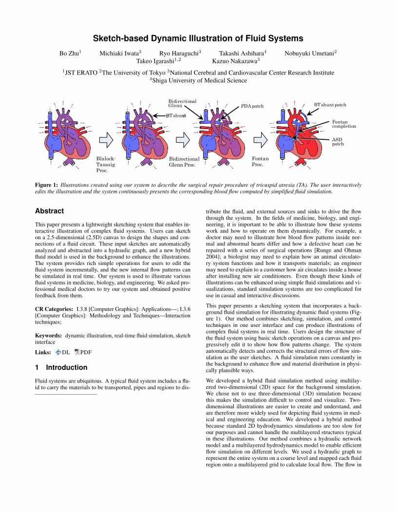
Sketch-based Dynamic Illustration of Fluid Systems

Bo Zhu1 Michiaki Iwata3 Ryo Haraguchi3 Takashi Ashihara4 Nobuyuki Umetani2

Takeo Igarashi1,2 Kazuo Nakazawa3

1JST ERATO 2The University of Tokyo 3National Cerebral and Cardiovascular Center Research Institute4Shiga University of Medical Science

Blalock-

Taussig

Proc.

Bidirectional

Glenn Proc.

Fontan

Proc.

BT shunt

PDA patchBidirectional Glenn

Fontancompletion

BT shunt patch

ASDpatch

Figure 1: Illustrations created using our system to describe the surgical repair procedure of tricuspid atresia (TA). The user interactivelyedits the illustration and the system continuously presents the corresponding blood flow computed by simplified fluid simulation.

Abstract

This paper presents a lightweight sketching system that enables in-teractive illustration of complex fluid systems. Users can sketchon a 2.5-dimensional (2.5D) canvas to design the shapes and con-nections of a fluid circuit. These input sketches are automaticallyanalyzed and abstracted into a hydraulic graph, and a new hybridfluid model is used in the background to enhance the illustrations.The system provides rich simple operations for users to edit thefluid system incrementally, and the new internal flow patterns canbe simulated in real time. Our system is used to illustrate variousfluid systems in medicine, biology, and engineering. We asked pro-fessional medical doctors to try our system and obtained positivefeedback from them.

CR Categories: I.3.8 [Computer Graphics]: Applications—; I.3.6[Computer Graphics]: Methodology and Techniques—Interactiontechniques;

Keywords: dynamic illustration, real-time fluid simulation, sketchinterface

Links: DL PDF

1 Introduction

Fluid systems are ubiquitous. A typical fluid system includes a flu-id to carry the materials to be transported, pipes and regions to dis-

tribute the fluid, and external sources and sinks to drive the flowthrough the system. In the fields of medicine, biology, and engi-neering, it is important to be able to illustrate how these systemswork and how to operate on them dynamically. For example, adoctor may need to illustrate how blood flow patterns inside nor-mal and abnormal hearts differ and how a defective heart can berepaired with a series of surgical operations [Runge and Ohman2004]; a biologist may need to explain how an animal circulato-ry system functions and how it transports materials; an engineermay need to explain to a customer how air circulates inside a houseafter installing new air conditioners. Even though these kinds ofillustrations can be enhanced using simple fluid simulations and vi-sualizations, standard simulation systems are too complicated foruse in casual and interactive discussions.

This paper presents a sketching system that incorporates a back-ground fluid simulation for illustrating dynamic fluid systems (Fig-ure 1). Our method combines sketching, simulation, and controltechniques in one user interface and can produce illustrations ofcomplex fluid systems in real time. Users design the structure ofthe fluid system using basic sketch operations on a canvas and pro-gressively edit it to show how flow patterns change. The systemautomatically detects and corrects the structural errors of flow sim-ulation as the user sketches. A fluid simulation runs constantly inthe background to enhance flow and material distribution in physi-cally plausible ways.

We developed a hybrid fluid simulation method using multilay-ered two-dimensional (2D) space for the background simulation.We chose not to use three-dimensional (3D) simulation becausethis makes the simulation difficult to control and visualize. Two-dimensional illustrations are easier to create and understand, andare therefore more widely used for depicting fluid systems in med-ical and engineering education. We developed a hybrid methodbecause standard 2D hydrodynamics simulations are too slow forour purposes and cannot handle the multilayered structures typicalin these illustrations. Our method combines a hydraulic networkmodel and a multilayered hydrodynamics model to enable efficientflow simulation on different levels. We used a hydraulic graph torepresent the entire system on a coarse level and mapped each fluidregion onto a multilayered grid to calculate local flow. The flow in

the hydraulic network is calculated first and is then used to drive thehydrodynamics model in various regions by providing boundary ve-locities. The structures inside regions can conversely influence theflow in the network to avoid topological errors in model coupling.

The main contributions are listed as follows:

• We propose a novel application: editable, dynamic fluid illus-tration for interactive discussion and communication of fluidsystems.

• We present a novel 2.5D representation for such fluid illus-trations consisting of regions and pipes, and present sketch-based user interfaces to edit them interactively.

• We present a novel hybrid algorithm for fluid simulation thatcouples hydraulic simulation for the global flow in a networkwith hydrodynamics simulation for regional fluid.

• We show the feasibility and effectiveness of the system bypresenting a solid implementation with feedback from profes-sional medical doctors.

2 Related Work

Explanatory illustration is an effective way to communicate sci-entific and technical information visually. Many studies have fo-cused on how to generate these illustrations automatically [Ebertet al. 2005]. Recently, researchers have been especially interest-ed in generating illustrations to explain dynamic physics systems.Mitra et al. [2010] proposed a method based on shape and contactanalysis to illustrate how mechanical assemblies function. Vainioet al. [2005] designed a virtual learning environment for explain-ing complex medical phenomena to medical students. Zhang et al.[2006] proposed a system for designing vector field on surfaces.Schroeder et al. [2010] designed a sketch-based interface for artiststo illustrate 2D vector fields.

Flow visualization methods visualize the results of flow simula-tion by drawing arrows or streamlines [Turk and Banks 1996],texture-based methods by applying flow patterns to random tex-utures [Cabral and Leedom 1993; Laramee et al. 2004], geomet-ric methods by extracting geometric objects such as streamlines orstream surfaces [McLouglin et al. 2010], and feature-based method-s by visualizing physically meaningful parts such as vortices [Postet al. 2003]. These techniques rely on offline simulation results andcan provide accurate visual effects. However, preparing these kind-s of illustrations is time consuming, and users cannot interactivelyedit the fluid system under consideration.

Sketching interfaces have been used for designing static 3Dscenes, such as models of geometrical objects [Igarashi et al. 1999;Gingold et al. 2009], scene phototypes [Zeleznik et al. 1996], andplants [Ijiri et al. 2006]. They have been combined with anima-tion systems to illustrate dynamic phenomena [Davis 2007; Daviset al. 2008] including fluid phenomena [Angelidis et al. 2006; Ok-abe et al. 2009]. Certain physics engines such as Crayon Physic-s1, Phun2, and Physicafe3, also provide sketch interfaces that allowusers to design their own physics systems. However, these systemsare mainly designed to simulate fluid flow in an open space and arenot directly applicable to flow in a closed circuit as typically foundin medical and engineering illustrations.

Fluid simulation is an established technique widely used in manyfields. Many researchers have worked to produce photorealistic 3D

1http://www.crayonphysics.com/2http://www.phunland.com/3http://www.prometech.co.jp/english/products/physicafe.html/

fluid effects in real-time applications [Cohen et al. 2010]. In ad-dition to these 3D simulation techniques, 2D hydraulic models arealso widely used to enable efficient simulation of system behavioron a macroscopic level. Yu et al. [2009] used a hydrographic net-work model to simulate rivers in real time. Sewall et al. [2010] useda graph model to simulate traffic flow in a city. Hydraulic modelsare also widely used in biomedical modeling, especially blood flowsimulation [Formaggia and Veneziani 2003; Nobile 2009; Almeder1999]. Hybrid methods have been proposed to model both macro-scopic and microscopic fluid phenomena in one scene. Irving et al.[2006] coupled 2D and 3D simulation techniques to model largequantities of water with surface details. Nobile [2009] proposeda two-way coupled method to simulate blood flow at various res-olutions and tested the system using a very simplified model. Incontrast, our model couples the global hydraulic network and localhydrodynamics regions in one-way to provide plausible real-timeenhancement for illustrations. Similar approach is used in humanbody simulation coupling local muscles and global skeletons [Leeet al. 2009].

3 User Interface

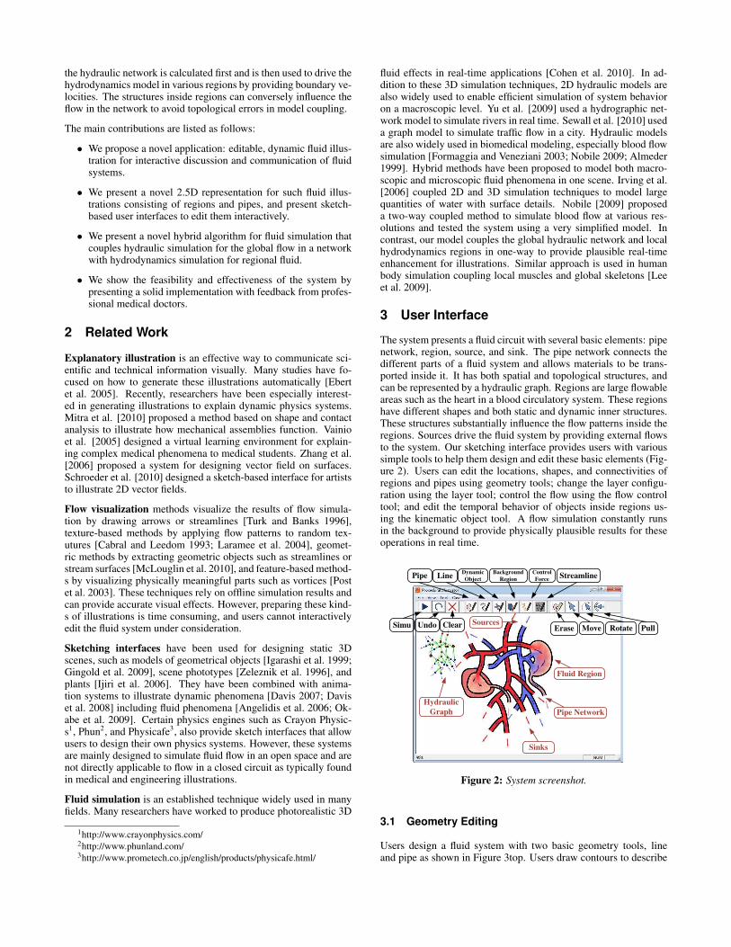
The system presents a fluid circuit with several basic elements: pipenetwork, region, source, and sink. The pipe network connects thedifferent parts of a fluid system and allows materials to be trans-ported inside it. It has both spatial and topological structures, andcan be represented by a hydraulic graph. Regions are large flowableareas such as the heart in a blood circulatory system. These regionshave different shapes and both static and dynamic inner structures.These structures substantially influence the flow patterns inside theregions. Sources drive the fluid system by providing external flowsto the system. Our sketching interface provides users with varioussimple tools to help them design and edit these basic elements (Fig-ure 2). Users can edit the locations, shapes, and connectivities ofregions and pipes using geometry tools; change the layer configu-ration using the layer tool; control the flow using the flow controltool; and edit the temporal behavior of objects inside regions us-ing the kinematic object tool. A flow simulation constantly runsin the background to provide physically plausible results for theseoperations in real time.

Fluid Region

Simu Undo Clear

LinePipe

Move Rotate PullErase

Pipe Network

Hydraulic

Graph

Control

Force

Dynamic

ObjectStreamline

Background

Region

Sources

Sinks

Figure 2: System screenshot.

3.1 Geometry Editing

Users design a fluid system with two basic geometry tools, lineand pipe as shown in Figure 3top. Users draw contours to describe

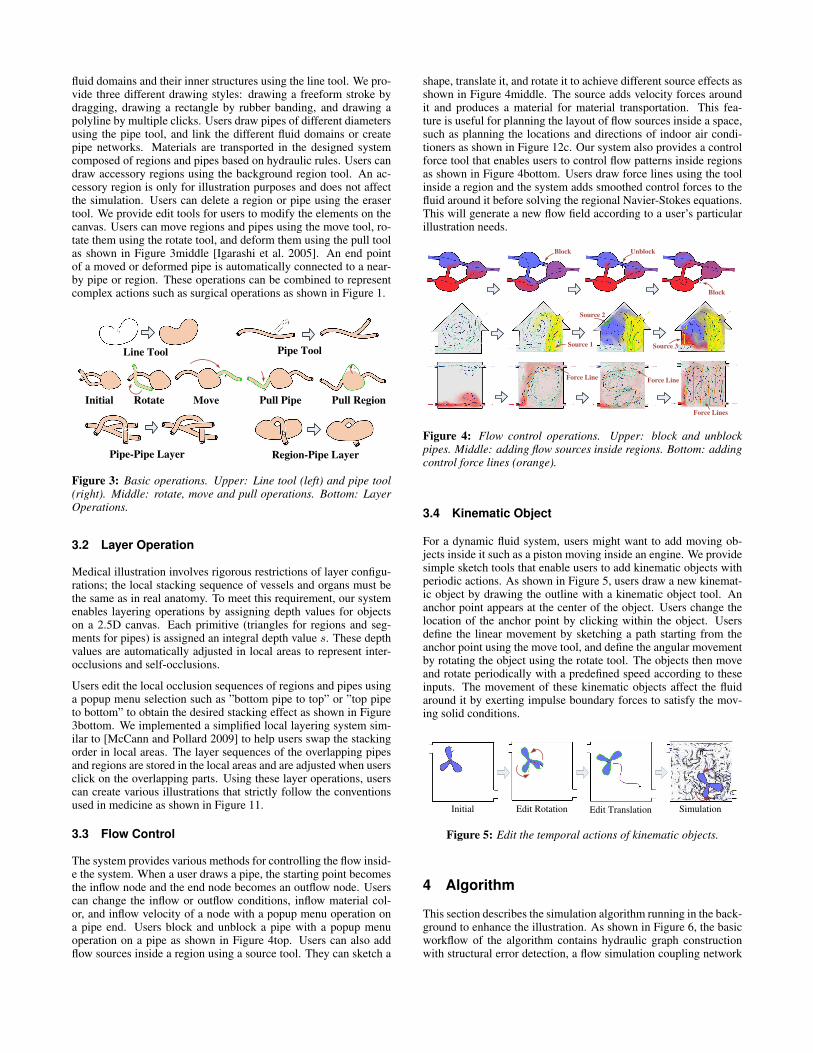
fluid domains and their inner structures using the line tool. We pro-vide three different drawing styles: drawing a freeform stroke bydragging, drawing a rectangle by rubber banding, and drawing apolyline by multiple clicks. Users draw pipes of different diametersusing the pipe tool, and link the different fluid domains or createpipe networks. Materials are transported in the designed systemcomposed of regions and pipes based on hydraulic rules. Users candraw accessory regions using the background region tool. An ac-cessory region is only for illustration purposes and does not affectthe simulation. Users can delete a region or pipe using the erasertool. We provide edit tools for users to modify the elements on thecanvas. Users can move regions and pipes using the move tool, ro-tate them using the rotate tool, and deform them using the pull toolas shown in Figure 3middle [Igarashi et al. 2005]. An end pointof a moved or deformed pipe is automatically connected to a near-by pipe or region. These operations can be combined to representcomplex actions such as surgical operations as shown in Figure 1.

Rotate Move Pull Pipe Pull RegionInitial

Pipe ToolLine Tool

Pipe-Pipe Layer Region-Pipe Layer

Figure 3: Basic operations. Upper: Line tool (left) and pipe tool(right). Middle: rotate, move and pull operations. Bottom: LayerOperations.

3.2 Layer Operation

Medical illustration involves rigorous restrictions of layer configu-rations; the local stacking sequence of vessels and organs must bethe same as in real anatomy. To meet this requirement, our systemenables layering operations by assigning depth values for objectson a 2.5D canvas. Each primitive (triangles for regions and seg-ments for pipes) is assigned an integral depth value s. These depthvalues are automatically adjusted in local areas to represent inter-occlusions and self-occlusions.

Users edit the local occlusion sequences of regions and pipes usinga popup menu selection such as ”bottom pipe to top” or ”top pipeto bottom” to obtain the desired stacking effect as shown in Figure3bottom. We implemented a simplified local layering system sim-ilar to [McCann and Pollard 2009] to help users swap the stackingorder in local areas. The layer sequences of the overlapping pipesand regions are stored in the local areas and are adjusted when usersclick on the overlapping parts. Using these layer operations, userscan create various illustrations that strictly follow the conventionsused in medicine as shown in Figure 11.

3.3 Flow Control

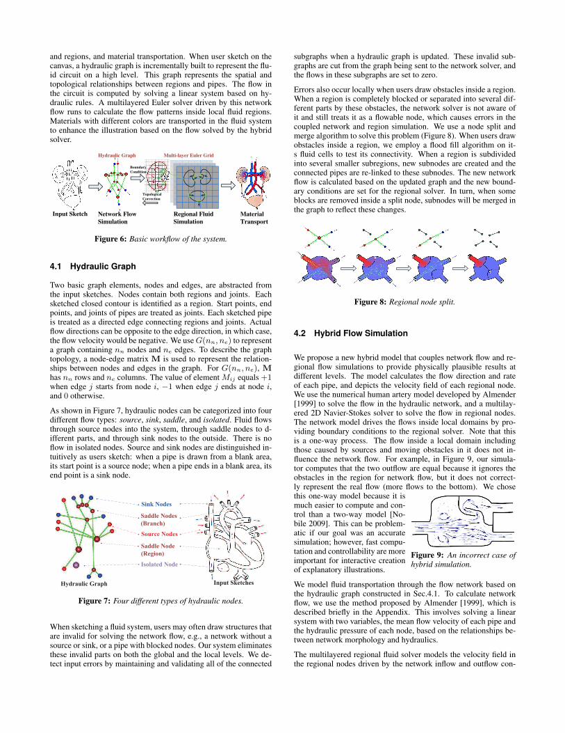
The system provides various methods for controlling the flow insid-e the system. When a user draws a pipe, the starting point becomesthe inflow node and the end node becomes an outflow node. Userscan change the inflow or outflow conditions, inflow material col-or, and inflow velocity of a node with a popup menu operation ona pipe end. Users block and unblock a pipe with a popup menuoperation on a pipe as shown in Figure 4top. Users can also addflow sources inside a region using a source tool. They can sketch a

shape, translate it, and rotate it to achieve different source effects asshown in Figure 4middle. The source adds velocity forces aroundit and produces a material for material transportation. This fea-ture is useful for planning the layout of flow sources inside a space,such as planning the locations and directions of indoor air condi-tioners as shown in Figure 12c. Our system also provides a controlforce tool that enables users to control flow patterns inside regionsas shown in Figure 4bottom. Users draw force lines using the toolinside a region and the system adds smoothed control forces to thefluid around it before solving the regional Navier-Stokes equations.This will generate a new flow field according to a user’s particularillustration needs.

Block Unblock

Block

Source 1

Source 2

Source 3

Force LineForce Line

Force Lines

Figure 4: Flow control operations. Upper: block and unblockpipes. Middle: adding flow sources inside regions. Bottom: addingcontrol force lines (orange).

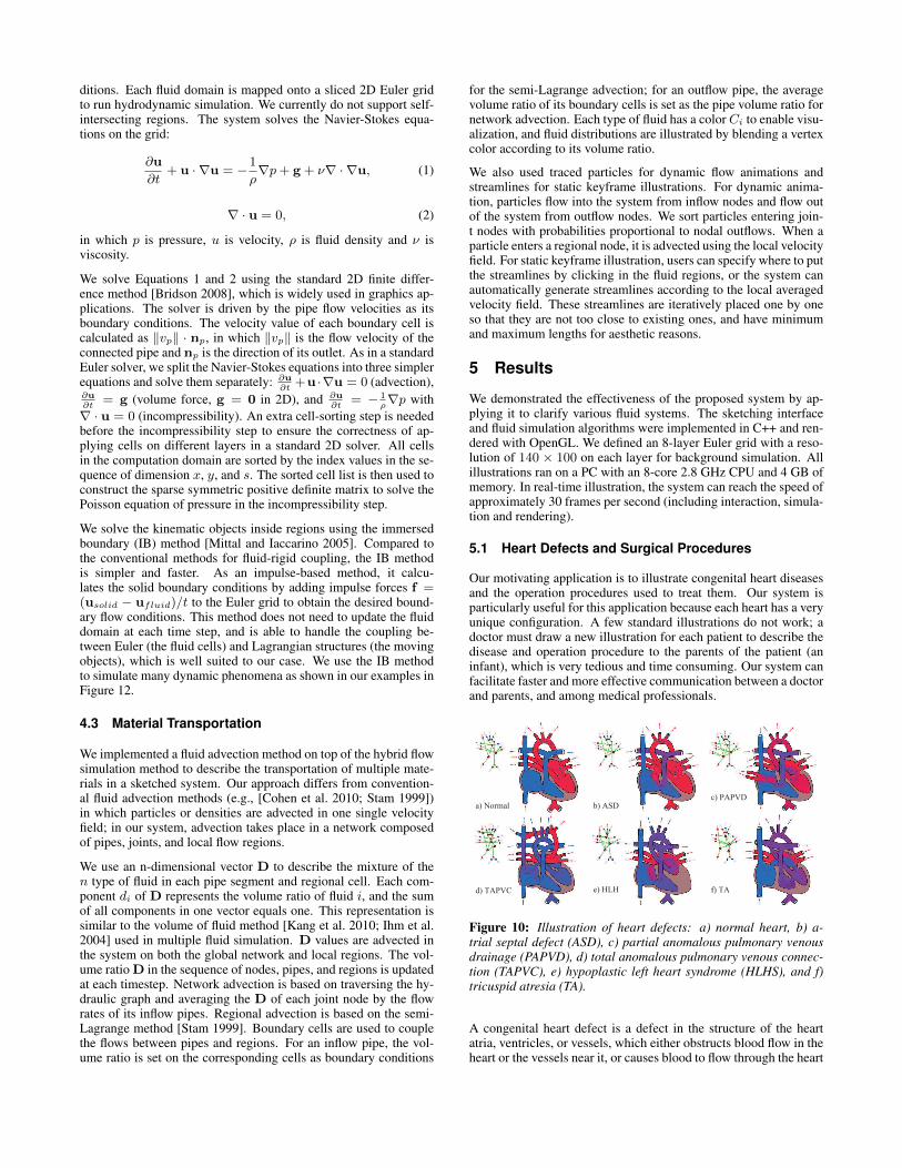
3.4 Kinematic Object

For a dynamic fluid system, users might want to add moving ob-jects inside it such as a piston moving inside an engine. We providesimple sketch tools that enable users to add kinematic objects withperiodic actions. As shown in Figure 5, users draw a new kinemat-ic object by drawing the outline with a kinematic object tool. Ananchor point appears at the center of the object. Users change thelocation of the anchor point by clicking within the object. Usersdefine the linear movement by sketching a path starting from theanchor point using the move tool, and define the angular movementby rotating the object using the rotate tool. The objects then moveand rotate periodically with a predefined speed according to theseinputs. The movement of these kinematic objects affect the fluidaround it by exerting impulse boundary forces to satisfy the mov-ing solid conditions.

Initial Edit Rotation Edit Translation Simulation

Figure 5: Edit the temporal actions of kinematic objects.

4 Algorithm

This section describes the simulation algorithm running in the back-ground to enhance the illustration. As shown in Figure 6, the basicworkflow of the algorithm contains hydraulic graph constructionwith structural error detection, a flow simulation coupling network

and regions, and material transportation. When user sketch on thecanvas, a hydraulic graph is incrementally built to represent the flu-id circuit on a high level. This graph represents the spatial andtopological relationships between regions and pipes. The flow inthe circuit is computed by solving a linear system based on hy-draulic rules. A multilayered Euler solver driven by this networkflow runs to calculate the flow patterns inside local fluid regions.Materials with different colors are transported in the fluid systemto enhance the illustration based on the flow solved by the hybridsolver.

Input Sketch

Hydraulic Graph Multi-layer Euler Grid

Regional Fluid

Simulation

Material

Transport

Network Flow

Simulation

Topological

Correction

Boundary

Condition

Figure 6: Basic workflow of the system.

4.1 Hydraulic Graph

Two basic graph elements, nodes and edges, are abstracted fromthe input sketches. Nodes contain both regions and joints. Eachsketched closed contour is identified as a region. Start points, endpoints, and joints of pipes are treated as joints. Each sketched pipeis treated as a directed edge connecting regions and joints. Actualflow directions can be opposite to the edge direction, in which case,the flow velocity would be negative. We useG(nn, ne) to representa graph containing nn nodes and ne edges. To describe the graphtopology, a node-edge matrix M is used to represent the relation-ships between nodes and edges in the graph. For G(nn, ne), Mhas nn rows and ne columns. The value of element Mij equals +1when edge j starts from node i, −1 when edge j ends at node i,and 0 otherwise.

As shown in Figure 7, hydraulic nodes can be categorized into fourdifferent flow types: source, sink, saddle, and isolated. Fluid flowsthrough source nodes into the system, through saddle nodes to d-ifferent parts, and through sink nodes to the outside. There is noflow in isolated nodes. Source and sink nodes are distinguished in-tuitively as users sketch: when a pipe is drawn from a blank area,its start point is a source node; when a pipe ends in a blank area, itsend point is a sink node.

Hydraulic Graph Input Sketches

Sink Nodes

Source Nodes

Saddle Nodes

(Branch)

Saddle Node

(Region)

Isolated Node

Figure 7: Four different types of hydraulic nodes.

When sketching a fluid system, users may often draw structures thatare invalid for solving the network flow, e.g., a network without asource or sink, or a pipe with blocked nodes. Our system eliminatesthese invalid parts on both the global and the local levels. We de-tect input errors by maintaining and validating all of the connected

subgraphs when a hydraulic graph is updated. These invalid sub-graphs are cut from the graph being sent to the network solver, andthe flows in these subgraphs are set to zero.

Errors also occur locally when users draw obstacles inside a region.When a region is completely blocked or separated into several dif-ferent parts by these obstacles, the network solver is not aware ofit and still treats it as a flowable node, which causes errors in thecoupled network and region simulation. We use a node split andmerge algorithm to solve this problem (Figure 8). When users drawobstacles inside a region, we employ a flood fill algorithm on it-s fluid cells to test its connectivity. When a region is subdividedinto several smaller subregions, new subnodes are created and theconnected pipes are re-linked to these subnodes. The new networkflow is calculated based on the updated graph and the new bound-ary conditions are set for the regional solver. In turn, when someblocks are removed inside a split node, subnodes will be merged inthe graph to reflect these changes.

Figure 8: Regional node split.

4.2 Hybrid Flow Simulation

We propose a new hybrid model that couples network flow and re-gional flow simulations to provide physically plausible results atdifferent levels. The model calculates the flow direction and rateof each pipe, and depicts the velocity field of each regional node.We use the numerical human artery model developed by Almender[1999] to solve the flow in the hydraulic network, and a multilay-ered 2D Navier-Stokes solver to solve the flow in regional nodes.The network model drives the flows inside local domains by pro-viding boundary conditions to the regional solver. Note that thisis a one-way process. The flow inside a local domain includingthose caused by sources and moving obstacles in it does not in-fluence the network flow. For example, in Figure 9, our simula-tor computes that the two outflow are equal because it ignores theobstacles in the region for network flow, but it does not correct-ly represent the real flow (more flows to the bottom). We chosethis one-way model because it ismuch easier to compute and con-trol than a two-way model [No-bile 2009]. This can be problem-atic if our goal was an accuratesimulation; however, fast compu-tation and controllability are moreimportant for interactive creationof explanatory illustrations.

Figure 9: An incorrect case ofhybrid simulation.

We model fluid transportation through the flow network based onthe hydraulic graph constructed in Sec.4.1. To calculate networkflow, we use the method proposed by Almender [1999], which isdescribed briefly in the Appendix. This involves solving a linearsystem with two variables, the mean flow velocity of each pipe andthe hydraulic pressure of each node, based on the relationships be-tween network morphology and hydraulics.

The multilayered regional fluid solver models the velocity field inthe regional nodes driven by the network inflow and outflow con-

ditions. Each fluid domain is mapped onto a sliced 2D Euler gridto run hydrodynamic simulation. We currently do not support self-intersecting regions. The system solves the Navier-Stokes equa-tions on the grid:

∂u

∂t+ u · ∇u = −1

ρ∇p+ g + ν∇ · ∇u, (1)

∇ · u = 0, (2)

in which p is pressure, u is velocity, ρ is fluid density and ν isviscosity.

We solve Equations 1 and 2 using the standard 2D finite differ-ence method [Bridson 2008], which is widely used in graphics ap-plications. The solver is driven by the pipe flow velocities as itsboundary conditions. The velocity value of each boundary cell iscalculated as ‖vp‖ · np, in which ‖vp‖ is the flow velocity of theconnected pipe and np is the direction of its outlet. As in a standardEuler solver, we split the Navier-Stokes equations into three simplerequations and solve them separately: ∂u

∂t+u ·∇u = 0 (advection),

∂u∂t

= g (volume force, g = 0 in 2D), and ∂u∂t

= − 1ρ∇p with

∇ · u = 0 (incompressibility). An extra cell-sorting step is neededbefore the incompressibility step to ensure the correctness of ap-plying cells on different layers in a standard 2D solver. All cellsin the computation domain are sorted by the index values in the se-quence of dimension x, y, and s. The sorted cell list is then used toconstruct the sparse symmetric positive definite matrix to solve thePoisson equation of pressure in the incompressibility step.

We solve the kinematic objects inside regions using the immersedboundary (IB) method [Mittal and Iaccarino 2005]. Compared tothe conventional methods for fluid-rigid coupling, the IB methodis simpler and faster. As an impulse-based method, it calcu-lates the solid boundary conditions by adding impulse forces f =(usolid − ufluid)/t to the Euler grid to obtain the desired bound-ary flow conditions. This method does not need to update the fluiddomain at each time step, and is able to handle the coupling be-tween Euler (the fluid cells) and Lagrangian structures (the movingobjects), which is well suited to our case. We use the IB methodto simulate many dynamic phenomena as shown in our examples inFigure 12.

4.3 Material Transportation

We implemented a fluid advection method on top of the hybrid flowsimulation method to describe the transportation of multiple mate-rials in a sketched system. Our approach differs from convention-al fluid advection methods (e.g., [Cohen et al. 2010; Stam 1999])in which particles or densities are advected in one single velocityfield; in our system, advection takes place in a network composedof pipes, joints, and local flow regions.

We use an n-dimensional vector D to describe the mixture of then type of fluid in each pipe segment and regional cell. Each com-ponent di of D represents the volume ratio of fluid i, and the sumof all components in one vector equals one. This representation issimilar to the volume of fluid method [Kang et al. 2010; Ihm et al.2004] used in multiple fluid simulation. D values are advected inthe system on both the global network and local regions. The vol-ume ratio D in the sequence of nodes, pipes, and regions is updatedat each timestep. Network advection is based on traversing the hy-draulic graph and averaging the D of each joint node by the flowrates of its inflow pipes. Regional advection is based on the semi-Lagrange method [Stam 1999]. Boundary cells are used to couplethe flows between pipes and regions. For an inflow pipe, the vol-ume ratio is set on the corresponding cells as boundary conditions

for the semi-Lagrange advection; for an outflow pipe, the averagevolume ratio of its boundary cells is set as the pipe volume ratio fornetwork advection. Each type of fluid has a colorCi to enable visu-alization, and fluid distributions are illustrated by blending a vertexcolor according to its volume ratio.

We also used traced particles for dynamic flow animations andstreamlines for static keyframe illustrations. For dynamic anima-tion, particles flow into the system from inflow nodes and flow outof the system from outflow nodes. We sort particles entering join-t nodes with probabilities proportional to nodal outflows. When aparticle enters a regional node, it is advected using the local velocityfield. For static keyframe illustration, users can specify where to putthe streamlines by clicking in the fluid regions, or the system canautomatically generate streamlines according to the local averagedvelocity field. These streamlines are iteratively placed one by oneso that they are not too close to existing ones, and have minimumand maximum lengths for aesthetic reasons.

5 Results

We demonstrated the effectiveness of the proposed system by ap-plying it to clarify various fluid systems. The sketching interfaceand fluid simulation algorithms were implemented in C++ and ren-dered with OpenGL. We defined an 8-layer Euler grid with a reso-lution of 140 × 100 on each layer for background simulation. Allillustrations ran on a PC with an 8-core 2.8 GHz CPU and 4 GB ofmemory. In real-time illustration, the system can reach the speed ofapproximately 30 frames per second (including interaction, simula-tion and rendering).

5.1 Heart Defects and Surgical Procedures

Our motivating application is to illustrate congenital heart diseasesand the operation procedures used to treat them. Our system isparticularly useful for this application because each heart has a veryunique configuration. A few standard illustrations do not work; adoctor must draw a new illustration for each patient to describe thedisease and operation procedure to the parents of the patient (aninfant), which is very tedious and time consuming. Our system canfacilitate faster and more effective communication between a doctorand parents, and among medical professionals.

a) Normal b) ASDc) PAPVD

d) TAPVC e) HLH f) TA

Figure 10: Illustration of heart defects: a) normal heart, b) a-trial septal defect (ASD), c) partial anomalous pulmonary venousdrainage (PAPVD), d) total anomalous pulmonary venous connec-tion (TAPVC), e) hypoplastic left heart syndrome (HLHS), and f)tricuspid atresia (TA).

A congenital heart defect is a defect in the structure of the heartatria, ventricles, or vessels, which either obstructs blood flow in theheart or the vessels near it, or causes blood to flow through the heart

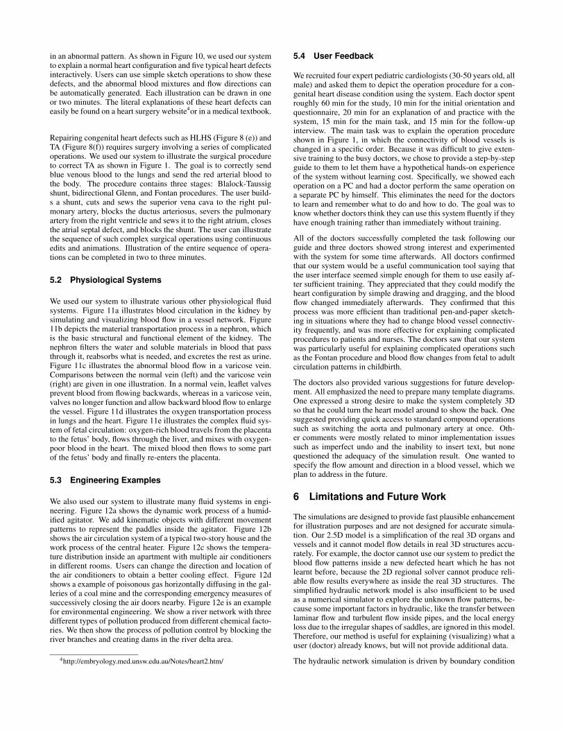
in an abnormal pattern. As shown in Figure 10, we used our systemto explain a normal heart configuration and five typical heart defectsinteractively. Users can use simple sketch operations to show thesedefects, and the abnormal blood mixtures and flow directions canbe automatically generated. Each illustration can be drawn in oneor two minutes. The literal explanations of these heart defects caneasily be found on a heart surgery website4or in a medical textbook.

Repairing congenital heart defects such as HLHS (Figure 8 (e)) andTA (Figure 8(f)) requires surgery involving a series of complicatedoperations. We used our system to illustrate the surgical procedureto correct TA as shown in Figure 1. The goal is to correctly sendblue venous blood to the lungs and send the red arterial blood tothe body. The procedure contains three stages: Blalock-Taussigshunt, bidirectional Glenn, and Fontan procedures. The user build-s a shunt, cuts and sews the superior vena cava to the right pul-monary artery, blocks the ductus arteriosus, severs the pulmonaryartery from the right ventricle and sews it to the right atrium, closesthe atrial septal defect, and blocks the shunt. The user can illustratethe sequence of such complex surgical operations using continuousedits and animations. Illustration of the entire sequence of opera-tions can be completed in two to three minutes.

5.2 Physiological Systems

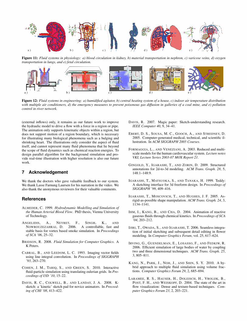
We used our system to illustrate various other physiological fluidsystems. Figure 11a illustrates blood circulation in the kidney bysimulating and visualizing blood flow in a vessel network. Figure11b depicts the material transportation process in a nephron, whichis the basic structural and functional element of the kidney. Thenephron filters the water and soluble materials in blood that passthrough it, reabsorbs what is needed, and excretes the rest as urine.Figure 11c illustrates the abnormal blood flow in a varicose vein.Comparisons between the normal vein (left) and the varicose vein(right) are given in one illustration. In a normal vein, leaflet valvesprevent blood from flowing backwards, whereas in a varicose vein,valves no longer function and allow backward blood flow to enlargethe vessel. Figure 11d illustrates the oxygen transportation processin lungs and the heart. Figure 11e illustrates the complex fluid sys-tem of fetal circulation: oxygen-rich blood travels from the placentato the fetus’ body, flows through the liver, and mixes with oxygen-poor blood in the heart. The mixed blood then flows to some partof the fetus’ body and finally re-enters the placenta.

5.3 Engineering Examples

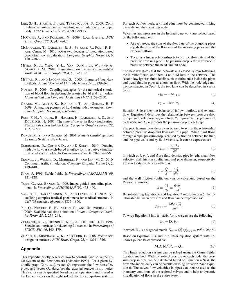
We also used our system to illustrate many fluid systems in engi-neering. Figure 12a shows the dynamic work process of a humid-ified agitator. We add kinematic objects with different movementpatterns to represent the paddles inside the agitator. Figure 12bshows the air circulation system of a typical two-story house and thework process of the central heater. Figure 12c shows the tempera-ture distribution inside an apartment with multiple air conditionersin different rooms. Users can change the direction and location ofthe air conditioners to obtain a better cooling effect. Figure 12dshows a example of poisonous gas horizontally diffusing in the gal-leries of a coal mine and the corresponding emergency measures ofsuccessively closing the air doors nearby. Figure 12e is an examplefor environmental engineering. We show a river network with threedifferent types of pollution produced from different chemical facto-ries. We then show the process of pollution control by blocking theriver branches and creating dams in the river delta area.

4http://embryology.med.unsw.edu.au/Notes/heart2.htm/

5.4 User Feedback

We recruited four expert pediatric cardiologists (30-50 years old, allmale) and asked them to depict the operation procedure for a con-genital heart disease condition using the system. Each doctor spentroughly 60 min for the study, 10 min for the initial orientation andquestionnaire, 20 min for an explanation of and practice with thesystem, 15 min for the main task, and 15 min for the follow-upinterview. The main task was to explain the operation procedureshown in Figure 1, in which the connectivity of blood vessels ischanged in a specific order. Because it was difficult to give exten-sive training to the busy doctors, we chose to provide a step-by-stepguide to them to let them have a hypothetical hands-on experienceof the system without learning cost. Specifically, we showed eachoperation on a PC and had a doctor perform the same operation ona separate PC by himself. This eliminates the need for the doctorsto learn and remember what to do and how to do. The goal was toknow whether doctors think they can use this system fluently if theyhave enough training rather than immediately without training.

All of the doctors successfully completed the task following ourguide and three doctors showed strong interest and experimentedwith the system for some time afterwards. All doctors confirmedthat our system would be a useful communication tool saying thatthe user interface seemed simple enough for them to use easily af-ter sufficient training. They appreciated that they could modify theheart configuration by simple drawing and dragging, and the bloodflow changed immediately afterwards. They confirmed that thisprocess was more efficient than traditional pen-and-paper sketch-ing in situations where they had to change blood vessel connectiv-ity frequently, and was more effective for explaining complicatedprocedures to patients and nurses. The doctors saw that our systemwas particularly useful for explaining complicated operations suchas the Fontan procedure and blood flow changes from fetal to adultcirculation patterns in childbirth.

The doctors also provided various suggestions for future develop-ment. All emphasized the need to prepare many template diagrams.One expressed a strong desire to make the system completely 3Dso that he could turn the heart model around to show the back. Onesuggested providing quick access to standard compound operationssuch as switching the aorta and pulmonary artery at once. Oth-er comments were mostly related to minor implementation issuessuch as imperfect undo and the inability to insert text, but nonequestioned the adequacy of the simulation result. One wanted tospecify the flow amount and direction in a blood vessel, which weplan to address in the future.

6 Limitations and Future Work

The simulations are designed to provide fast plausible enhancementfor illustration purposes and are not designed for accurate simula-tion. Our 2.5D model is a simplification of the real 3D organs andvessels and it cannot model flow details in real 3D structures accu-rately. For example, the doctor cannot use our system to predict theblood flow patterns inside a new defected heart which he has notlearnt before, because the 2D regional solver cannot produce reli-able flow results everywhere as inside the real 3D structures. Thesimplified hydraulic network model is also insufficient to be usedas a numerical simulator to explore the unknown flow patterns, be-cause some important factors in hydraulic, like the transfer betweenlaminar flow and turbulent flow inside pipes, and the local energyloss due to the irregular shapes of saddles, are ignored in this model.Therefore, our method is useful for explaining (visualizing) what auser (doctor) already knows, but will not provide additional data.

The hydraulic network simulation is driven by boundary condition

a ) b ) c ) d ) e )

Figure 11: Fluid systems in physiology: a) blood circulation in kidney, b) material transportation in nephron, c) varicose veins, d) oxygentransportation in lungs, and e) fetal circulation.

e )a ) b ) c ) d )

Figure 12: Fluid systems in engineering: a) humidified agitator, b) central heating system of a house, c) indoor air temperature distributionwith multiple air conditioners, d) the emergency measures to prevent poisonous gas diffusion in galleries of a coal mine, and e) pollutioncontrol in river network.

(external inflows) only, it remains as our future work to improvethe hydraulic model to drive a flow with a force in a region or pipe.The animation only supports kinematic objects within a region, butdoes not support motion of a region boundary, which is necessaryfor illustrating many biological phenomena such as a bulging andshrinking heart. The illustrations only consider the aspect of fluiditself, and cannot represent many fluid phenomena that lie beyondthe scope of fluid dynamics such as chemical reaction energies. Todesign parallel algorithm for the background simulation and pro-vide real-time illustration with higher resolution is also our futurework.

7 Acknowledgement

We thank the doctors who gave valuable feedback to our system.We thank Lasse Farnung Laursen for his narration in the video. Wealso thank the anonymous reviewers for their valuable comments.

References

ALMEDER, C. 1999. Hydrodynamic Modelling and Simulation ofthe Human Arterial Blood Flow. PhD thesis, Vienna Universityof Technology.

ANGELIDIS, A., NEYRET, F., SINGH, K., ANDNOWROUZEZAHRAI, D. 2006. A controllable, fast andstable basis for vortex based smoke simulation. In Proceedingsof SCA ’06, 25–32.

BRIDSON, R. 2008. Fluid Simulation for Computer Graphics. AK Peters.

CABRAL, B., AND LEEDOM, L. C. 1993. Imaging vector fieldsusing line integral convolution. In Proceedings of SIGGRAPH’93, 263–270.

COHEN, J. M., TARIQ, S., AND GREEN, S. 2010. Interactivefluid-particle simulation using translating eulerian grids. In Pro-ceedings of I3D ’10, 15–22.

DAVIS, R. C., COLWELL, B., AND LANDAY, J. A. 2008. K-sketch: a ’kinetic’ sketch pad for novice animators. In Proceed-ing of CHI ’08, 413–422.

DAVIS, R. 2007. Magic paper: Sketch-understanding research.IEEE Computer 40, 9, 34–41.

EBERT, D. S., SOUSA, M. C., GOOCH, A., AND STREDNEY, D.2005. Computer-generated medical, technical, and scientific il-lustration. In ACM SIGGRAPH 2005 Courses.

FORMAGGIA, L., AND VENEZIANI, A. 2003. Reduced and multi-scale models for the human cardiovascular system. Lecture notesVKI, Lecture Series 2003-07 MOX Report 21.

GINGOLD, Y., IGARASHI, T., AND ZORIN, D. 2009. Structuredannotations for 2d-to-3d modeling. ACM Trans. Graph. 28, 5,148:1–148:9.

IGARASHI, T., MATSUOKA, S., AND TANAKA, H. 1999. Teddy:A sketching interface for 3d freeform design. In Proceedings ofSIGGRAPH ’99, 409–416.

IGARASHI, T., MOSCOVICH, T., AND HUGHES, J. F. 2005. As-rigid-as-possible shape manipulation. ACM Trans. Graph. 24, 3,1134–1141.

IHM, I., KANG, B., AND CHA, D. 2004. Animation of reactivegaseous fluids through chemical kinetics. In Proceedings of SCA’04, 203–212.

IJIRI, T., OWADA, S., AND IGARASHI, T. 2006. Seamless integra-tion of initial sketching and subsequent detail editing in flowermodeling. In Computer Graphics Forum, vol. 25, 617–624.

IRVING, G., GUENDELMAN, E., LOSASSO, F., AND FEDKIW, R.2006. Efficient simulation of large bodies of water by couplingtwo and three dimensional techniques. ACM Trans. Graph. 25,3, 805–811.

KANG, N., PARK, J., NOH, J., AND SHIN, S. Y. 2010. A hy-brid approach to multiple fluid simulation using volume frac-tions. Computer Graphics Forum 29, 2, 685–694.

LARAMEE, R. S., HAUSER, H., DOLEISCH, H., VROLIJK, B.,POST, F. H., AND WEISKOPF, D. 2004. The state of the art inflow visualization: Dense and texture-based techniques. Com-puter Graphics Forum 23, 2, 203–221.

LEE, S.-H., SIFAKIS, E., AND TERZOPOULOS, D. 2009. Com-prehensive biomechanical modeling and simulation of the upperbody. ACM Trans. Graph. 28, 4, 99:1–99:17.

MCCANN, J., AND POLLARD, N. 2009. Local layering. ACMTrans. Graph. 28, 3, 84:1–84:7.

MCLOUGLIN, T., LARAMEE, R. S., PEIKERT, R., POST, F. H.,AND CHEN, M. 2010. Over two decades of integration-basedgeometric flow visualization. Computer Graphics Forum 29, 6,1807–1829.

MITRA, N. J., YANG, Y.-L., YAN, D.-M., LI, W., AND A-GRAWALA, M. 2010. Illustrating how mechanical assemblieswork. ACM Trans. Graph. 29, 4, 58:1–58:12.

MITTAL, R., AND IACCARINO, G. 2005. Immersed boundarymethods. Annual Review of Fluid Mechanics 37, 1, 239–261.

NOBILE, F. 2009. Coupling strategies for the numerical simula-tion of blood flow in deformable arteries by 3d and 1d models.Mathematical and Computer Modelling 11-12, 2152–2160.

OKABE, M., ANJYO, K., IGARASHI, T., AND SEIDEL, H.-P.2009. Animating pictures of fluid using video examples. Com-puter Graphics Forum 28, 2, 677–686.

POST, F. H., VROLIJK, B., HAUSER, H., LARAMEE, R. S., ANDDOLEISCH, H. 2003. The state of the art in flow visualisation:Feature extraction and tracking. Computer Graphics Forum 22,4, 775–792.

RUNGE, M. S., AND OHMAN, M. 2004. Netter’s Cardiology. IconLearning Systems, New Jersey.

SCHROEDER, D., COFFEY, D., AND D.KEEFE. 2010. Drawingwith the flow: A sketch-based interface for illustrative visualiza-tion of 2d vector fields. In Proceedings of SBIM ’2010, 49–56.

SEWALL, J., WILKIE, D., MERRELL, P., AND LIN, M. C. 2010.Continuum traffic simulation. Computer Graphics Forum 29, 2,439–448.

STAM, J. 1999. Stable fluids. In Proceedings of SIGGRAPH ’99,121–128.

TURK, G., AND BANKS, D. 1996. Image-guided streamline place-ment. In Proceedings of SIGGRAPH ’96, 453–460.

VAINIO, T., HAKKARAINEN, K., AND LEVONEN, J. 2005. Vi-sualizing complex medical phenomena for medical students. InCHI ’05 extended abstracts, 1857–1860.

YU, Q., NEYRET, F., BRUNETON, E., AND HOLZSCHUCH, N.2009. Scalable real-time animation of rivers. Computer Graph-ics Forum 28, 2, 239–248.

ZELEZNIK, R. C., HERNDON, K. P., AND HUGHES, J. F. 1996.Sketch: an interface for sketching 3d scenes. In Proceedings ofSIGGRAPH ’96, 163–170.

ZHANG, E., MISCHAIKOW, K., AND TURK, G. 2006. Vector fielddesign on surfaces. ACM Trans. Graph. 25, 4, 1294–1326.

Appendix

This appendix briefly describes how to construct and solve the lin-ear system of the flow network [Almeder 1999]. For a given hy-draulic graph G(nn, ne), vector Qe represents the flow rate of nepipes, and vector Qn describes the external sources in nn nodes.This vector can be specified based on user operations and is used asthe known values on the right side of the linear equation systems.

For each outflow node, a virtual edge must be constructed linkingthe node and the collecting node.

Velocities and pressures in the hydraulic network are solved basedon the following laws:

• At each node, the sum of the flow rate of the outgoing pipesequals the sum of the flow rate of the incoming pipes and theexternal inflows.

• There is a linear relationship between the flow rate and thepressure drop in a pipe. The pressure drop is the difference inpressure between the head and tail node.

The first law states that the network is a closed system followingthe Kirchhoff rule, and there is no fluid loss in the network. Thesecond law ignores fluid details such as turbulence inside the pipesand treats fluid in pipes as a laminar flow. With the node-edge ma-trix constructed in Sec.4.1, the two laws can be described in vectorform:

Qn = −MQe, (3)

Pe = −MTPn. (4)

Equation 3 describes the balance of inflow, outflow, and externalflow. Equation 4 describes the relationship between pressure dropin pipe and node pressure, in which Pn represents the pressure ofeach node and Pe represents the pressure drop in each pipe.

The pipe laminar flow theory can be used to set up the relationshipbetween pressure drop and flow rate in a pipe. When fluid flowsthrough a pipe, pressure drop is caused by friction between the fluidand the pipe walls and by fluid viscosity. It can be expressed as:

pdrop =ρlv2λ

2d, (5)

in which ρ, l, v, λ and d are fluid density, pipe length, mean flowvelocity, wall friction coefficient, and pipe diameter, respectively.Flow velocity can be calculated as:

v =Q

S=

4Q

d2π, (6)

and the wall friction coefficient can be calculated based on theReynolds number:

λ =64

Re=

64ν

vd. (7)

By substituting Equation 6 and Equation 7 into Equation 5, the re-lationship between pressure and flow can be expressed as:

pdrop =128ρνlQ

πd4. (8)

To wrap Equation 8 into a matrix form, we can use the following:

Qe = DePe, (9)

in which De is a diagonal matrixDii = Qie/pidrop = πd4/128ρλl.

Based on Equation 3, 4 and 9, a linear equation system with un-known pn can be expressed as:

MDeMTPn = Qn. (10)

This linear equation system can be solved using the Gauss-Seideliteration method. With the solved pressure on each node, the pres-sure drop in pipe can be calculated based on Equation 4.Next, theflow rate and velocity can be calculated using Equation 9 and Equa-tion 6. The solved flow velocities in pipes can then be used as theboundary conditions of the regional solvers and to help to dynamicvisualization of flows in the entire system.