sae A STATA PACKAGE FOR UNIT LEVEL SMALL AREA ESTIMATION...
31
Poverty & Equity Global Practice Working Paper 177 sae A STATA PACKAGE FOR UNIT LEVEL SMALL AREA ESTIMATION Minh Cong Nguyen Paul Corral João Pedro Azevedo Qinghua Zhao October 2018 Public Disclosure Authorized Public Disclosure Authorized Public Disclosure Authorized Public Disclosure Authorized
Transcript of sae A STATA PACKAGE FOR UNIT LEVEL SMALL AREA ESTIMATION...
Poverty & Equity Global Practice Working Paper 177
sae
A STATA PACKAGE FOR UNIT LEVEL SMALL AREA ESTIMATION
Minh Cong Nguyen Paul Corral
João Pedro Azevedo Qinghua Zhao
October 2018
Pub
lic D
iscl
osur
e A
utho
rized
Pub
lic D
iscl
osur
e A
utho
rized
Pub
lic D
iscl
osur
e A
utho
rized
Pub
lic D
iscl
osur
e A
utho
rized
Poverty & Equity Global Practice Working Paper 177
ABSTRACT This paper presents a new family of Stata functions devoted to small area estimation. Small area methods attempt to solve low representativeness of surveys within areas, or the lack of data for specific areas/sub-populations. This is accomplished by incorporating information from outside sources. Such target data sets are becoming increasingly available and can take the form of a traditional population census, but also large scale administrative records from tax administrations, or geospatial information produced using remote sensing. The strength of these target data sets is their granularity on the subpopulations of interest, however, in many cases they lack the ability to collect analytically relevant variables such as welfare or caloric intake. The family of functions introduced follow a modular design to have the flexibility with which these can be expanded in the future. This can be accomplished by the authors and/or other collaborators from the Stata community. Thus far, a major limitation of such analysis in Stata has been the large size of target data sets. The package introduces new mata functions and a plugin used to circumvent memory limitations that inevitably arise when working with big data. From an estimation perspective, the paper starts by implementing a methodology that has been widely used for the production of several poverty maps.
This paper is a product of the Poverty and Equity Global Practice Group. It is part of a larger effort by the World Bank to provide open access to its research and contribute to development policy discussions around the world. The authors may be contacted at [email protected].
This paper is co-published with the World Bank Policy Research Working Papers.
The Poverty & Equity Global Practice Working Paper Series disseminates the findings of work in progress to encourage the exchange of ideas about development issues. An objective of the series is to get the findings out quickly, even if the presentations are less than fully polished. The papers carry the names of the authors and should be cited accordingly. The findings, interpretations, and conclusions expressed in this paper are entirely those of the authors. They do not necessarily represent the views of the International Bank for Reconstruction and Development/World Bank and its affiliated organizations, or those of the Executive Directors of the World Bank or the governments they represent.
‒ Poverty & Equity Global Practice Knowledge Management & Learning Team
sae: A Stata Package for Unit Level Small Area Estimation
Minh Cong Nguyen,∗Paul Corral, João Pedro Azevedo, and Qinghua Zhao†‡
Octber, 2018
Key words: Small area estimation, ELL, Poverty mapping, Poverty map, Big Data, GeospatialJEL classification: C55, C87, C15∗Minh Cong Nguyen, Paul Corral, and João Pedro Azevedo: The World Bank Group - Poverty and Inequality Global
Practice†Qinghua Zhao: The World Bank Group - Development Economics Research Group‡The authors acknowledge financial support from the World Bank. We also thank Ken Simler, and Roy Van der Weide
for comments on an earlier draft and several discussions. We thank Alexandru Cojocaru, William Seitz, Kristen Himelein,Fernando Morales, Pallavi Vyas, and David Newhouse for beta testing earlier versions of the command. We also thank CarolinaSanchez, Francisco Ferreira, and Luis Felipe Lopez-Calva for providing support and space to work on this. Finally we thank theGlobal Solutions Group on Welfare Measurement and Statistical Capacity, as well as all attendants of the ECAPOV SeminarSeries and Summer University courses on Small Area Estimation.Any error or omission is the authors’ responsiblility alone.
1 Introduction
Household surveys that are designed for national or sub-national (i.e. regions or states) level parameterestimates often lack a sufficiently large sample size to generate accurate direct estimates for smaller domainsor sub-populations.1 Any area for which the sample is not sufficiently large to produce an estimate ofadequate precision is referred to as a small area. Consequently small area methods attempt to address lowrepresentativeness of surveys within areas, or the lack of data for specific areas/sub-populations. This isaccomplished by incorporating information from supplementary sources. In the methodology presented byElbers, Lanjouw, and Lanjouw (2003) the desired estimate is produced by a model done using survey datawhich is then linked to outside information such as a population census, administrative records, and/orgeospatial information obtained through remote sensing. As Rao and Molina (2015) state, the availabilityof these auxiliary data as well as a valid model are essential for obtaining successful small area estimates(SAE).
In the case of poverty measures, which are nonlinear functions, small area estimation methods coupledwith Monte Carlo simulations are a useful statistical technique for monitoring poverty along with its spatialdistribution and evolution.2 Poverty estimates are often produced by statistical agencies, and commonly arethe product of a household survey. Household surveys usually are the main source of welfare (expenditureor income) used to produce poverty estimates, yet most are only reliable up to a certain geographical level.Therefore, a commonly adopted solution has been to borrow strength from a national census, administrativerecords, and/or geospatial information which allows for representativeness for small areas. Nevertheless,these outside data sources often lack detailed expenditure or income information required for producingestimates of poverty. Small area methods attempt to exploit each data’s attributes to obtain estimators thatcan be used at dis-aggregated levels.
Poverty at lower geographical levels can be used to identify areas that are in need of attention, or that maybe lagging behind the rest of the country. For example, the Government of Ecuador after an earthquakethat occurred on April 16, 2016 relied on small area estimates of poverty to decide where help was neededmost. The small area estimates of poverty for Ecuador, which were released not long before the earthquake,proved to be an invaluable resource for the rebuilding effort in the country.
One of the most common small area methods used for poverty estimates is the one proposed by Elbers,Lanjouw, and Lanjouw (2003, henceforth ELL).3 This methodology has been widely adopted by the WorldBank and has been applied in numerous poverty maps4 conducted by the institution. In its efforts tomake the implementation of the ELL methodology as straightforward as possible, the World Bank createda software package that could be easily used by anyone. The software, PovMap (Zhao, 2006),5 has provento be an invaluable resource for the World Bank as well as for many statistical agencies, line ministries, andother international organizations seeking to create their own small area estimates of poverty. The softwareis freely available and has a graphical user interface which simplifies its use. Nevertheless, more advanced
1For example districts, municipalities, migrant populations, or populations with disabilities.2Poverty is a nonlinear function of welfare, consequently small area estimation methods of linear characteristics are invalid
(Molina and Rao, 2010). A proposed solution to this problem is to use Monte Carlo simulation to obtain multiple vectors ofthe measure of interest (Elbers, Lanjouw, and Lanjouw, 2003).
3For a detailed discussion of different applications of small area poverty estimates by the World Bank, readers should referto Bedi et al. (2007), for other applications readers should refer to Rao and Moline (2015).
4Poverty map is the common name within the World Bank for the methodology where the obtained estimates are mappedfor illustrative purposes.
5downloadable from: http://iresearch.worldbank.org/PovMap/PovMap2/setup.zip
2
practitioners who may wish for more functionality and options may have to program it themselves. In aneffort to simplify the process, we have created a family of Stata commands which implement small areaestimation methods, and provide users with a valid, modular, and flexible alternative to PovMap. All of theresults produced with sae have been bench-marked with the well established PovMap software, and are anexact match.6
In the following section we discuss the linking model and focus on the first stage of the estimation. How thevariance of the location effect present in the linking model is accounted for is discussed afterwards. This isinitiated by presenting the ELL methodology for decomposing the first stage residuals’s variance parameters.Afterwards, this is followed by Henderson’s Method III decomposition of the residual’s variance parametersand the adaptation of Huang and Hidiroglou’s (2003) GLS and implemented by Van der Weide (2014) inan update to the PovMap software. Then we present Empirical Bayes prediction of the location effects. Wefinally present the command’s syntax along with examples of its use.
2 First Stage: Model
When survey data is not sufficiently precise for reliable estimates at low geographical levels, small areaestimation can be implemented. This commonly relies on borrowing strength from outside sources to generateindirect estimates (Rao and Molina, 2015). For example, when attempting to obtain welfare estimates at lowgeographical levels, it is possible to borrow strength from census data. Censuses in most cases do not collectsufficient information on incomes and/or expenditures. On the other hand household surveys tend to collectdetailed information on incomes and/or expenditures which allows the generation of welfare statistics suchas poverty and inequality measures. Although welfare statistics can be obtained using household surveys,these are rarely sufficiently large to allow for statistics corrsponding to small areas (Tarozzi and Deaton,2009). Small area estimation methods attempt to exploit the large sample size of census data and combinethis with the information from household surveys in an attempt to obtain reliable statistics for small areas.
In its essence the small area estimation presented here relies on using household survey data to estimatea joint distribution of the variable of interest and observed correlates, and use the parameters to simulatewelfare using census data (Demombynes et al., 2008). Throughout the text we focus on welfare imputation,since this is what the Elbers, Lanjouw, and Lanjouw (2003) methodology focused on, nevertheless it can beapplied for other continuous measures aside from welfare.
The first step towards small area welfare simulation is a per-capita7 welfare model, estimated via ordinaryleast squares (OLS), or weighted least squares (WLS):
lnY = Xβols + u (1)
where lnY is a N × 1 matrix indicating the household’s welfare measure (usually in logarithms, but notnecessarily),8 X is a N×K matrix of household characteristics, and u which is a N×1 matrix of disturbances.To achieve valid small area estimates it is necessary that the set of explanatory variables, X, used in the
6For the 1st stage of the analysis. The second stage relies on Monte-Carlo simulations, and thus differences are likely toarise.
7Other household equivalization methods are also feasible, for example adult equivalent household welfare.8Logarithmic transformation is usually preferred since it makes the data more symmetrical (Haslett et al., 2010).
3
first stage model can also be found in the census data. It is important that the variables are comparedbeforehand to verify that not only their definitions are in agreement, but also their distributions.9
In the design of household surveys, clusters are commonly the primary sampling unit. Households withina cluster are usually not independent from one another, to allow for the clustering of households and theirinterrelatedness it is possible to specify equation (1) for a household as:
ln ych = xchβ + uch
,– where the indexes c and h stand for cluster and observation, respectively – and disturbances (uch) areassumed to have the following specification (Haslett et al., 2010):
uch = ηc + ech (2)
where ηc and ech, are assumed to be independent from each other with different data generating processes(Haslett et al., 2010).10 Therefore the resulting model we wish to estimate is a linear mixed model (Van derWeide, 2014).11
The literature has suggested different methods for estimating the unconditional variances of these param-eters;12 for the purposes of this paper focus is given to the methods presented by Elbers, Lanjouw, andLanjouw (2003), and the adaptation of Henderson’s Method III by Huang and Hidiroglou (2003) detailedand expanded upon by Van der Weide (2014). The next section describes in detail these two approaches.
3 Estimating the unconditional variance of the residual parameters
3.1 The ELL Methodology
The methodology for estimating the location’s unconditional variance detailed by ELL (2002 and 2003) ispresented in the discussion below. The method consists of two steps. The initial step relies on estimatinga welfare model (Eq:1) using household survey data, and then obtaining generalized least square (GLS)estimates for the model. Given the interrelatedness between households in a cluster, ordinary least squaresis not the most efficient estimator. The second stage consists in utilizing the parameter estimates from thefirst stage and applying these to census data to obtain small area poverty and inequality measures.
Because the motivation is to implement the methodology into a Stata command, where possible, we alsofollow the methods implemented by PovMap (Zhao, 2006). It must be noted, however, that the methodologyutilized by ELL is not necessarily the one followed by the PovMap software. Places where methodologiesdiffer will be indicated in footnotes.
9This point is crucial, and the quality of a good poverty map is highly dependent on these two criteria being met. For furtherdiscussion and motivation refer to: Tarozzi and Deaton (2009).
10Note that the interrelatedness of ηc across observations is already a violation of OLS assumptions.11Molina and Rao (2010) follow the naming convention of a nested error linear regression model. Regardless of its name,
standard OLS is invalid under this structure.12Rao and Molina (2015).
4
From the estimation of equation 1 we obtain the residuals uch, and by defining uc.as the weighted averageof uch for a specific cluster we can obtain ech:13
uch = uc. + (uch − uc.) = ηc + ech (3)
where uc. is equal to ηc.14
The unconditional variance of the location effect ηc given by ELL (2002) is:
σ2η = max
(∑c wc(uc. − u..)2 −
∑c wc(1− wc)τ2
c∑c wc(1− wc)
; 0)
(4)
where u.. =∑c wcuc.(where wc represents the cluster’s weight, i.e. wc =
∑h whc) and
τ2c =
∑h (ech − ec.)2
nc (nc − 1) (5)
where ec. =∑
hech
nc. 15
3.1.1 Estimating the Alpha Model (heteroskedasticity)16
The variance of the idiosyncratic error (ech) is specified by ELL (2003) through a parametric form of het-eroskedasticity:17
E[e2ch
]= σ2
ech=[A expZ
′bhα +B
1 + expZ′bhα
](6)
In ELL (2003) this is simplified by setting B = 0 and A = 1.05 max(e2ch
), and thus the simpler form is
estimated via OLS:18
ln[
e2ch
A− e2ch
]= Z
′
chα+ rch (7)
This approach resembles that of Harvey (1976), nevertheless the prediction is bounded.
By defining exp(Z
′chα)
= D and using the delta method,19 the household specific conditional varianceestimator for ech is equal to (Elbers, Lanjouw, and Lanjouw, 2002):
13ech denotes the household specific error component.14Although, ELL (2003) notes that weigths are to be used, the PovMap software does not utilize weights when obtaining uc.15nc is the number of observations in cluster c.16The heteroskadistic model is relevant for the variance estimation under ELL’s method, as well as the one under Henderson’s
method III. In its current form, the methodology is from ELL (2003).17Users have the option to allow for homoskedasticity, in which case σe = σu − ση , where σu is the estimated variance of the
residuals from the consumption model (equation 1). If the user chooses homoskedasticity, equations 6 through 8 are omitted.18This is the actual model used by PovMap, which we also implement.19The result is the outcome from a second order Taylor expansion for the E
[σ2ech
].
5
σ2e,ch ≈
[AD
1 +D
]+ 1
2Var(r)[AD(1−D)
(1 +D)3
](8)
where Var(r) is the estimated variance from the residuals of the model in equation (7).
3.1.2 Estimating the distribution of σ2η
ELL (2002) proposes two methods to obtain the variance of σ2η :
1. By simulation (ELL, 2002):
(a) Estimate σ2η from equation (4) which yields σ2
η
(b) Estimate σ2e,ch from equation (8) which yields σ2
e,ch
(c) Assuming ηc and ech are independent and normally distributed with mean 0, new values for uchare generated using equation (2)
(d) Compute a new estimate σ2η from equation (4)
(e) Repeat (a) - (d) and keep all simulated values of σ2η
From the simulated values of σ2η, the sampling variance of σ2
η
(Var
(σ2η
))can be obtained directly.
2. The sampling variance of σ2η can also be obtained by the following formula (ELL, 2002):20
Var(σ2η
)=∑c
2a2c
[(σ2η
)2 +(τ2c
)2 + 2σ2η τ
2c
]+ b2
c
(τ2c
)2
nc − 1
(9)
where ac = wc/ [∑c wc (1− wc)], and bc = wc(1− wc)/ [
∑c wc (1− wc)].
(a) This is noted by ELL to be an approximation of the sampling variance of σ2η. It assumes within
cluster homoskedasticity of the household error component. For a more comprehensive discussionon this matter refer to ELL (2002).
The command, in its present form only allows for estimation using the second method,21 when estimatingthe unconditional variance of σ2
η using the ELL methodology.
3.1.3 ELL’s GLS Estimator
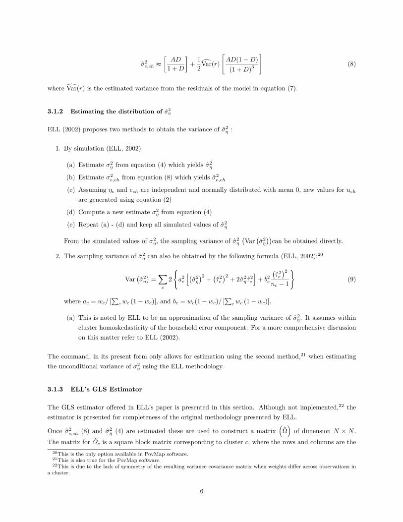
The GLS estimator offered in ELL’s paper is presented in this section. Although not implemented,22 theestimator is presented for completeness of the original methodology presented by ELL.
Once σ2e,ch (8) and σ2
η (4) are estimated these are used to construct a matrix(
Ω)
of dimension N × N .The matrix for Ωc is a square block matrix corresponding to cluster c, where the rows and columns are the
20This is the only option available in PovMap software.21This is also true for the PovMap software.22This is due to the lack of symmetry of the resulting variance covariance matrix when weights differ across observations in
a cluster.
6
number of observations in the cluster. Within cluster covariance is given by σ2η. On the diagonal σ2
e,ch isadded to obtain the observation specific disturbance varaince. The resulting cluster block of this N ×Nmatrix is equal to:
Ωc =
σ2η + σ2
e,ch σ2η · · · σ2
η
σ2η σ2
η + σ2e,ch . . . σ2
η
......
. . ....
σ2η σ2
η · · · σ2η + σ2
e,ch
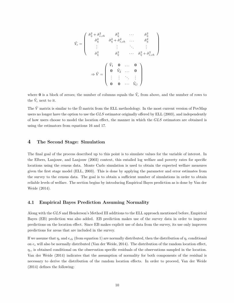
⇒ Ω =
Ω1 0 . . . 00 Ω2 . . . 0...
.... . .
...0 0 · · · ΩC
where 0 is a block of zeroes; the number of columns equals the Ωc from above, and the number of rows tothe Ωc next to it.
Ω is the variance-covariance matrix of the error vector necessary to estimate equation (1) via GLS and obtainβGLS and Var
(βGLS
). The estimates for the GLS detailed by ELL (2003) are:
βGLS =(X ′WΩ−1X
)−1X ′WΩ−1Y (10)
and
Var(βGLS
)=(X ′WΩ−1X
)−1 (X ′WΩ−1WX) (X ′WΩ−1X
)−1 (11)
where W is a N × N diagonal matrix of sampling weights. Because WΩ−1 is usually not symmetric,23
as noted by Haslett et al. (2010), the variance covariance matrix must be adjusted to obtain a symmetricmatrix. This is done by obtaining the average of the variance covariance matrix and its transpose (Haslettet al., 2010).
Newer versions of the PovMap software no longer obtain GLS estimates using this approach. Adjustmentshave been made in order to better incorporate the survey weights into Ω. The newest version of PovMapuses the GLS estimator presented by Huang and Hidiroglou (2003), which is discussed below.
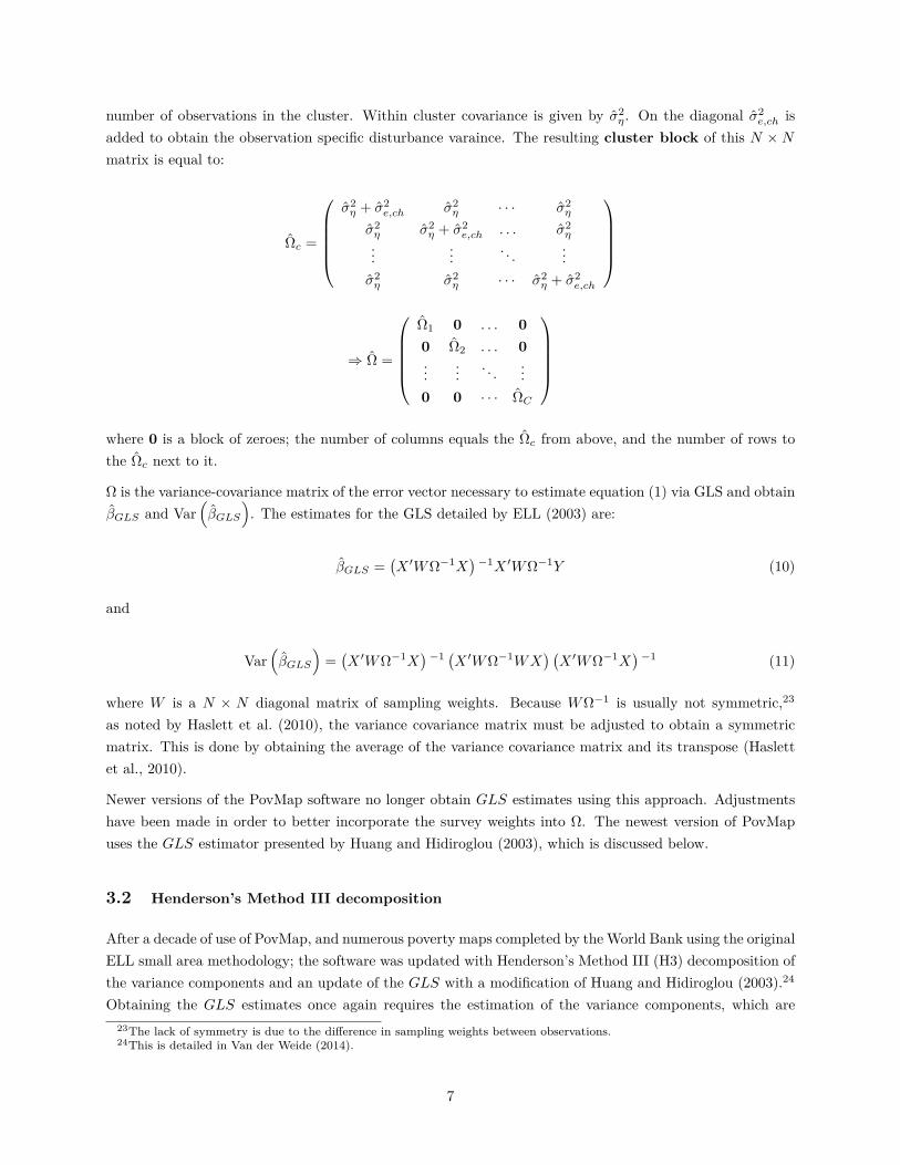
3.2 Henderson’s Method III decomposition
After a decade of use of PovMap, and numerous poverty maps completed by the World Bank using the originalELL small area methodology; the software was updated with Henderson’s Method III (H3) decomposition ofthe variance components and an update of the GLS with a modification of Huang and Hidiroglou (2003).24
Obtaining the GLS estimates once again requires the estimation of the variance components, which are23The lack of symmetry is due to the difference in sampling weights between observations.24This is detailed in Van der Weide (2014).
7
estimated using a variation of Henderson’s Method III (Henderson, 1953). The variation takes into accountthe use of survey weights and was presented by Huang and Hidiroglou (2003). We follow the presentationoffered by Van der Weide (2014) which builds on Huang and Hidiroglou (2003).
In order to obtain the variance components of the βGLS it is necessary to first estimate a model whichsubtracts each of the cluster’s means from the variables. To achieve this we first need to define the left handside of the model. For each cluster in our estimation the left hand side is (omitting the natural logarithmonly for display purposes):
yc = Yc −(Yc ⊗ 1T
)where Yc is a T × 1 vector (where T is the number of surveyed observations in the cluster) , correspondingto cluster c, of our welfare variable used in equation 1 Yc is a scalar which is the weighted mean value of Ycfor cluster c. 1T is a T × 1 vector of 1s, and ⊗ is the Kroenecker product. Finally, we define y as a N × 1matrix which is a vector of all the cluster ycs.
For the right hand side we follow the same de-meaning procedure and obtain a matrix x. Additionally,define x of dimensions C ×K where C is the number of areas in the survey, with each row representing thedemeaned xc for a specific cluster. With these in hand it is possible to define the following:
SSE = y′W y − y
′W x
(x
′W x
)−1x
′W y
t2 = tr[(
x′W x
)−1 (x
′(W W ) x
)−1]
t3 = tr[(X ′WX)−1
X ′ (W W )X]
t4 = tr[(X ′WX)−1
x′(Wc Wc) x
]where Wc is a C × C diagonal matrix of cluster weights, and represents the Hadamard product. UsingSSE, t2, t3, and t4 it is possible to estimate the variances σ2
e and σ2η:
σ2e = SSE∑
chwch −∑c
(∑hw2ch∑
hwch
)− t2
(12)
σ2η =
Y ′WY − Y ′WX (X ′WX)−1X ′WY − (
∑ch wch − t3) σ2
e∑ch wch − t4
(13)
To obtain the estimates of ηc Van der Weide (2014) provides the following for each cluster c:
γc,w =σ2η
σ2η + σ2
e
(∑hwch∑
hw2ch
)consequently the ηc for a particular cluster is:
ηc = γc,w∑h
wchuch −1C
∑c
γc,w
(∑h
wchuch
)(14)
8
With the updated estimate of ηc it is possible to update the estimate of ech:
ech = uch − ηc −∑ch
(uch − ηc) (15)
Additionally the distribution of echis adjusted such that its variance is equal to σ2e .
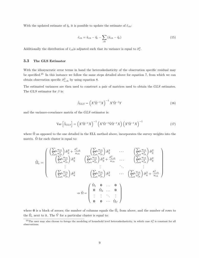
3.3 The GLS Estimator
With the idiosyncratic error terms in hand the heteroskedasticity of the observation specific residual maybe specified.25 In this instance we follow the same steps detailed above for equation 7, from which we canobtain observation specific σ2
e,ch by using equation 8.
The estimated variances are then used to construct a pair of matrices used to obtain the GLS estimates.The GLS estimator for β is:
βGLS =(X ′Ω−1X
)−1X ′Ω−1Y (16)
and the variance-covariance matrix of the GLS estimator is:
Var[βGLS
]=(X ′Ω−1X
)−1 (X ′Ω−1VΩ−1X
)(X ′Ω−1X
)−1(17)
where Ω as opposed to the one detailed in the ELL method above, incorporates the survey weights into thematrix. Ω for each cluster is equal to:
Ωc =
(∑hwch∑
hw2ch
)σ2η + σ2
e,ch
wch
(∑hwch∑
hw2ch
)σ2η · · ·
(∑hwch∑
hw2ch
)σ2η(∑
hwch∑
hw2ch
)σ2η
(∑hwch∑
hw2ch
)σ2η + σ2
e,ch
wch. . .
(∑hwch∑
hw2ch
)σ2η
... ... . . . ...(∑hwch∑
hw2ch
)σ2η
(∑hwch∑
hw2ch
)σ2η · · ·
(∑hwch∑
hw2ch
)σ2η + σ2
e,ch
wch
⇒ Ω =
Ω1 0 . . . 00 Ω2 . . . 0...
.... . .
...0 0 · · · ΩC
where 0 is a block of zeroes; the number of columns equals the Ωc from above, and the number of rows tothe Ωc next to it. The V for a particular cluster is equal to:
25The user may also choose to forego the modeling of household level heteroskedasticity, in which case σ2e is constant for all
observations.
9
Vc =
σ2η + σ2
e,ch σ2η · · · σ2
η
σ2η σ2
η + σ2e,ch . . . σ2
η
......
. . ....
σ2η σ2
η · · · σ2η + σ2
e,ch
⇒ V =
V1 0 . . . 00 V2 . . . 0...
.... . .
...0 0 · · · VC
where 0 is a block of zeroes; the number of columns equals the Vc from above, and the number of rows tothe Vc next to it.
The V matrix is similar to the Ω matrix from the ELL methodology. In the most current version of PovMapusers no longer have the option to use the GLS estimator originally offered by ELL (2003), and independentlyof how users choose to model the location effect, the manner in which the GLS estimators are obtained isusing the estimators from equations 16 and 17.
4 The Second Stage: Simulation
The final goal of the process described up to this point is to simulate values for the variable of interest. Inthe Elbers, Lanjouw, and Lanjouw (2003) context, this entailed log welfare and poverty rates for specificlocations using the census data. Monte Carlo simulation is used to obtain the expected welfare measuresgiven the first stage model (ELL, 2003). This is done by applying the parameter and error estimates fromthe survey to the census data. The goal is to obtain a sufficient number of simulations in order to obtainreliable levels of welfare. The section begins by introducing Empirical Bayes prediction as is done by Van derWeide (2014).
4.1 Empirical Bayes Prediction Assuming Normality
Along with the GLS and Henderson’s Method III additions to the ELL approach mentioned before, EmpiricalBayes (EB) prediction was also added. EB prediction makes use of the survey data in order to improvepredictions on the location effect. Since EB makes explicit use of data from the survey, its use only improvespredictions for areas that are included in the survey.
If we assume that ηc and ech (from equation 1) are normally distributed, then the distribution of ηc conditionalon ec will also be normally distributed (Van der Weide, 2014). The distribution of the random location effect,ηc, is obtained conditional on the observation specific residuals of the observations sampled in the location.Van der Weide (2014) indicates that the assumption of normality for both components of the residual isnecessary to derive the distribution of the random location effects. In order to proceed, Van der Weide(2014) defines the following:
10
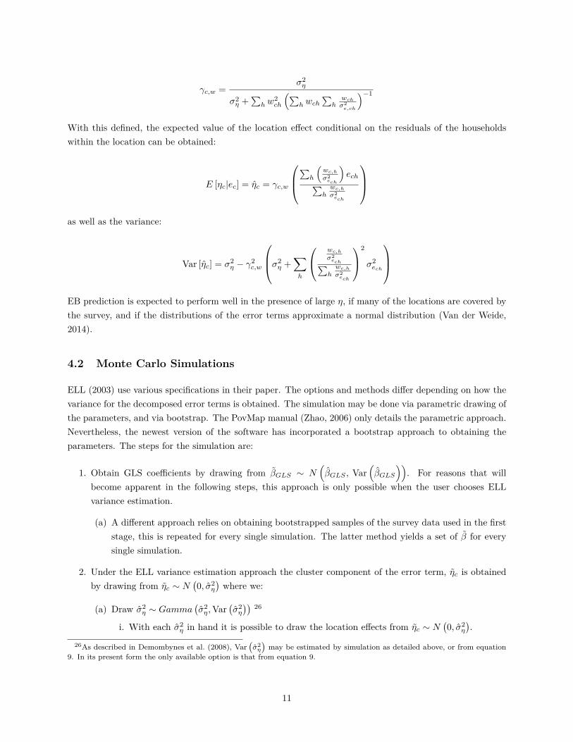
γc,w =σ2η
σ2η +
∑h w
2ch
(∑h wch
∑hwch
σ2e,ch
)−1
With this defined, the expected value of the location effect conditional on the residuals of the householdswithin the location can be obtained:
E [ηc|ec] = ηc = γc,w
∑h
(wc,h
σ2ech
)ech∑
hwc,h
σ2ech
as well as the variance:
Var [ηc] = σ2η − γ2
c,w
σ2η +
∑h
wc,h
σ2ech∑hwc,h
σ2ech
2
σ2ech
EB prediction is expected to perform well in the presence of large η, if many of the locations are covered bythe survey, and if the distributions of the error terms approximate a normal distribution (Van der Weide,2014).
4.2 Monte Carlo Simulations
ELL (2003) use various specifications in their paper. The options and methods differ depending on how thevariance for the decomposed error terms is obtained. The simulation may be done via parametric drawing ofthe parameters, and via bootstrap. The PovMap manual (Zhao, 2006) only details the parametric approach.Nevertheless, the newest version of the software has incorporated a bootstrap approach to obtaining theparameters. The steps for the simulation are:
1. Obtain GLS coefficients by drawing from βGLS ∼ N(βGLS , Var
(βGLS
)). For reasons that will
become apparent in the following steps, this approach is only possible when the user chooses ELLvariance estimation.
(a) A different approach relies on obtaining bootstrapped samples of the survey data used in the firststage, this is repeated for every single simulation. The latter method yields a set of β for everysingle simulation.
2. Under the ELL variance estimation approach the cluster component of the error term, ηc is obtainedby drawing from ηc ∼ N
(0, σ2
η
)where we:
(a) Draw σ2η ∼ Gamma
(σ2η,Var
(σ2η
)) 26
i. With each σ2η in hand it is possible to draw the location effects from ηc ∼ N
(0, σ2
η
).
26As described in Demombynes et al. (2008), Var(σ2η
)may be estimated by simulation as detailed above, or from equation
9. In its present form the only available option is that from equation 9.
11
ii. Additionally, ηc could be drawn from those estimated in the first stage (semi-parametric),this is possible to do in the parametric and bootstrapped simulation.
Under Henderson’s method III (H3) there is no defined distribution for the σ2η parameter. Consequently,
bootstrapped samples of the survey data are used to obtain σ2η and all other parameters for every single
simulation. This approach is also available under ELL methods. The bootstrap is also necessary forthe instances when EB is chosen. When EB is chosen, the bootstrap produces a vector of ηs and of σ2
ηc
for each of the clusters included in the survey and thus for every simulation we draw ηc ∼ N(ηc, σ
2ηc
).
For clusters not included in the survey the drawing is: ηc ∼ N(0, σ2
η
).
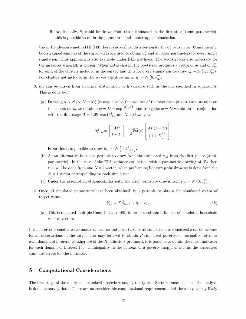
3. ech can be drawn from a normal distribution with variance such as the one specified in equation 8.This is done by:
(a) Drawing α ∼ N (α, Var(α)) (it may also be the product of the bootstrap process) and using it onthe census data, we obtain a new D = exp
(Z
′chα), and using the new D we obtain in conjunction
with the first stage A = 1.05 max(e2ch
)and Var(r) we get:
σ2e,ch ≈
[AD
1 + D
]+ 1
2Var(r)
AB(1− D)(1 + D
)3
From this it is possible to draw ech ∼ N
(0, σ2
e,ch
).
(b) As an alternative it is also possible to draw from the estimated ech from the first phase (semi-parametric). In the case of the ELL variance estimation with a parametric drawing of β′s thenthis will be done from one N ×1 vector, when performing bootstrap the drawing is done from theN × 1 vector corresponding to each simulation.
(c) Under the assumption of homoskedasticity, the error terms are drawn from ech ∼ N(0, σ2
e
).
4. Once all simulated parameters have been obtained, it is possible to obtain the simulated vector oftarget values:
Ych = XβGLS + ηc + ech (18)
(a) This is repeated multiple times (usually 100) in order to obtain a full set of simulated householdwelfare vectors.
If the interest is small area estimates of income and poverty, once all simulations are finalized a set of incomesfor all observations in the target data may be used to obtain R simulated poverty, or inequality rates foreach domain of interest. Making use of the R indicators produced, it is possible to obtain the mean indicatorfor each domain of interest (i.e. municipality in the context of a poverty map), as well as the associatedstandard errors for the indicator.
5 Computational Considerations
The first stage of the analysis is standard procedure among the typical Stata commands, since the analysisis done on survey data. There are no considerable computational requirements, and the analysis may likely
12
be performed using the majority of computers available to users. On the other hand, the Monte Carlosimulation requires the use of the census data. Census data, depending on the country, can range fromanywhere between roughly 30,000 observations to almost half a billion. Depending on a user’s computersetup, a couple million observations can really slow down the computer to a crawl. Assuming variablesin double type precision, a 5 million observation dataset with 30 variables will require roughly 1.1 GB ofmemory. Therefore, in order to speed up the second stage operation and to be able to operate with largerdatasets, a couple of modifications are implemented.
The first modification concerns importing the census data and formatting it in a more memory friendly way.Along with the main command we supply a sub-command that allows the user to import the census datafor the second stage, sae data import. The data is imported one vector at a time and saved into a Mataformat file which is used for the processing of each regressor at a time for each simulation to obtain thepredicted welfare. Proceeding in this manner, the maximum number of observations that can be used in thesimulation stage is increased. As shown in the examples section, this setup requires preparing the targetdataset beforehand. Due to this setup, the Monte Carlo simulations are executed one vector at a time. Forsmaller datasets it is likely that performing all simulations in one go results in quicker execution times,27
once we move on to larger census data this method provides faster execution times and allows for moreefficient memory management.
The second modification, is a plugin for processing the simulations and producing the required indicators.This is only used/necessary for processing indicators. The processing is also done one simulation at a time,just like the Monte Carlo simulations. The plugin speeds up the process considerably, especially whenrequesting Gini coefficients.28
6 The sae Command and Sub-Commands
The sae command and sub-commands for modeling, simulating, and data manipulation are introducedbelow. The common syntax for the command is:
sae [routine] [sub routine]
Currently available routines and subroutines are:
• sae data import||export : This is used to import the target dataset to a more manageableformat for the simulations. It is also used to export the resulting simulations to a dataset of theuser’s preference.
• sae model lmm/povmap : This routine is for obtaining the GLS estimates of the first stage. Thesub-routines, lmm (linear mixed model) and povmap are used interchangeably.29
• sae simulate lmm/povmap : This routine and sub-routine obtains the GLS estimates of the firststage, and goes on to perform the Monte Carlo simulations.
27This is particularly true for the MP version of Stata, which makes use of more than one core for its operations.28Gini coefficients require sorting at every level, this is done much faster using a C plugin. Stata’s sorting speed (as of this
writing), including Mata’s, is much slower than that of many other software.29Future work aims to incorporate additional methodologies, such as models for discrete left hand side variables .
13

• sae proc stats||inds : The stats and inds sub-routines are useful for processing Mata formattedsimulation output and producing indicators with new thresholds or weights, as well as profiling.
The routines and sub-routines are described in the sections below.
6.1 Preparing the Target Dataset
Due to the potential large size of the target data set, the sae command comes with an ancillary sub-command(sae data import) useful for preparing the target dataset and converting it into a Mata format dataset tominimize the overall burden put on the system. The command’s syntax is as follows:
sae data import, datain(string) varlist(string) area(string) uniqid(string)
dataout(string)
The options of the command are all required.
• The datain() option indicates the path and file name of the Stata format dataset to be convertedinto a Mata format dataset.
• The varlist() option specifies all the variables to be imported into the Mata format dataset. Thevariables specified will be available for the simulation stage of the analysis. Variables must have similarnames between datasets. Additionally, users should include here any additional variables they wish toinclude, as well as expansion factors for the target data.
• The uniqid() option specifies the numeric variable that indicates the unique identifiers in the targetdataset. This is necessary to ensure replicability of the analysis, and the name should match the oneof the unique identifier from the source dataset.
• The area() option is necessary and specifies at which level the clustering is done, it indicates atwhich level the ηc is obtained. The only constraint is that the variable must be numeric and shouldmatch across datasets, although it is recommended it follows a hierarchical structure similar to the oneproposed by Zhao (2006).
– The hierarchical id should be of the same length for all observations. For example: AAMMEEE.30
This structure facilitiates getting final estimates at different aggregation levels.
• The dataout() option indicates the path and filename of the Mata format dataset that will be usedwhen running the Monte Carlo simulations.
6.1.1 Example: Preparing the Target Data
The sae command requires users to import the target data into a Mata data format file. This is done tofacilitate the process of simulations in the second stage due to the potential large size of the target data.
30In the case this were done for a specific country, AA stands for the highest aggregation level, MM stands for the secondhighest aggregation level, and EEE, stands for the lowest aggregation level.
14
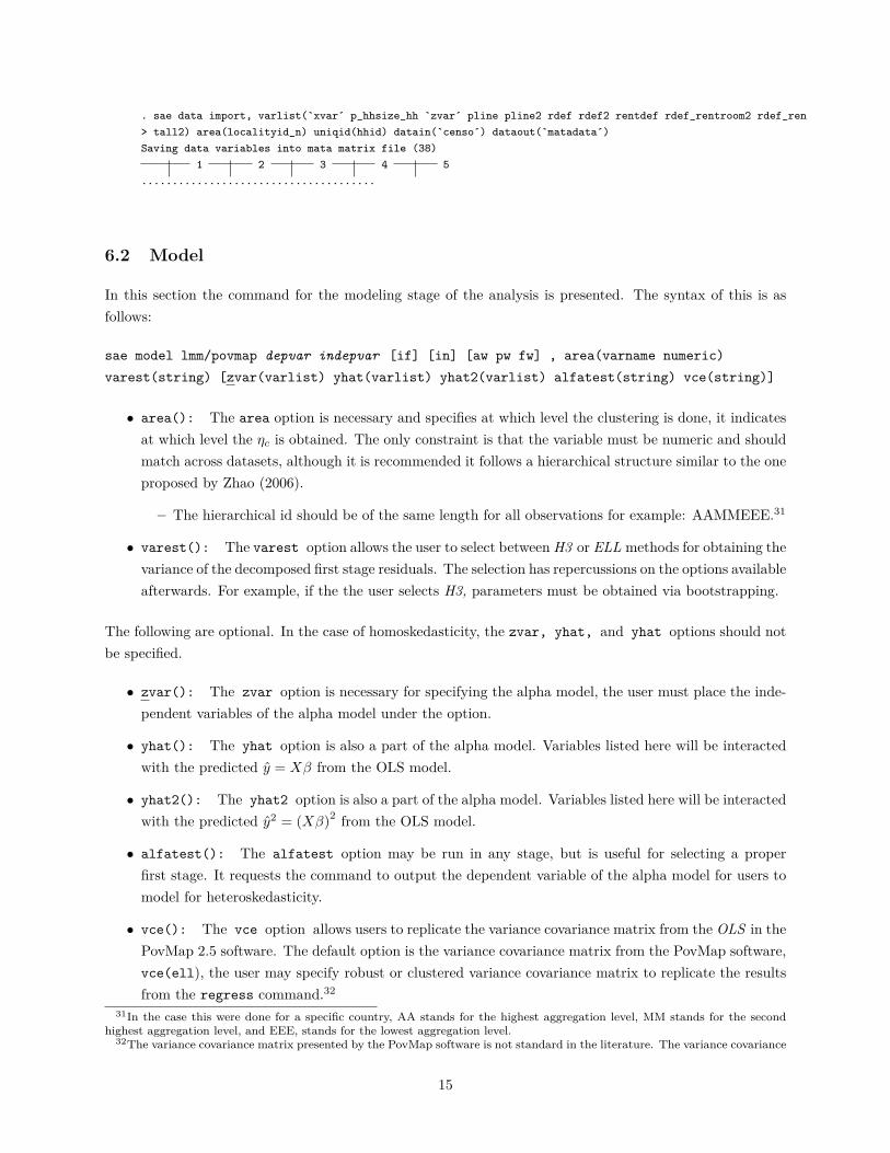
. sae data import, varlist(`xvar´ p_hhsize_hh `zvar´ pline pline2 rdef rdef2 rentdef rdef_rentroom2 rdef_ren> tall2) area(localityid_n) uniqid(hhid) datain(`censo´) dataout(`matadata´)Saving data variables into mata matrix file (38)
1 2 3 4 5......................................
6.2 Model
In this section the command for the modeling stage of the analysis is presented. The syntax of this is asfollows:
sae model lmm/povmap depvar indepvar [if] [in] [aw pw fw] , area(varname numeric)
varest(string) [zvar(varlist) yhat(varlist) yhat2(varlist) alfatest(string) vce(string)]
• area(): The area option is necessary and specifies at which level the clustering is done, it indicatesat which level the ηc is obtained. The only constraint is that the variable must be numeric and shouldmatch across datasets, although it is recommended it follows a hierarchical structure similar to the oneproposed by Zhao (2006).
– The hierarchical id should be of the same length for all observations for example: AAMMEEE.31
• varest(): The varest option allows the user to select between H3 or ELL methods for obtaining thevariance of the decomposed first stage residuals. The selection has repercussions on the options availableafterwards. For example, if the the user selects H3, parameters must be obtained via bootstrapping.
The following are optional. In the case of homoskedasticity, the zvar, yhat, and yhat options should notbe specified.
• zvar(): The zvar option is necessary for specifying the alpha model, the user must place the inde-pendent variables of the alpha model under the option.
• yhat(): The yhat option is also a part of the alpha model. Variables listed here will be interactedwith the predicted y = Xβ from the OLS model.
• yhat2(): The yhat2 option is also a part of the alpha model. Variables listed here will be interactedwith the predicted y2 = (Xβ)2 from the OLS model.
• alfatest(): The alfatest option may be run in any stage, but is useful for selecting a properfirst stage. It requests the command to output the dependent variable of the alpha model for users tomodel for heteroskedasticity.
• vce(): The vce option allows users to replicate the variance covariance matrix from the OLS in thePovMap 2.5 software. The default option is the variance covariance matrix from the PovMap software,vce(ell), the user may specify robust or clustered variance covariance matrix to replicate the resultsfrom the regress command.32
31In the case this were done for a specific country, AA stands for the highest aggregation level, MM stands for the secondhighest aggregation level, and EEE, stands for the lowest aggregation level.
32The variance covariance matrix presented by the PovMap software is not standard in the literature. The variance covariance
15
6.2.1 Running the First Stage (welfare model)
The entire process of small area estimation may be run in two stages. It is possible to test the first stageof the analysis before moving on to the simulation which makes use of the target data. To obtain the firststage of the analysis, the user must have the data ready, and it is recommended that the user has predefinedas macros the variables to be used.
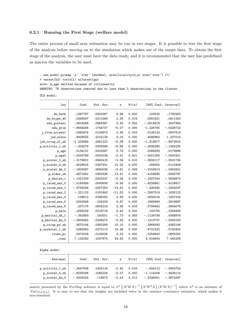
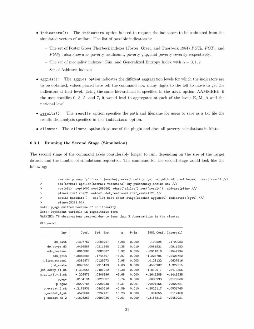
. sae model povmap `y´ `xvar´ [aw=hhw], area(localityid_n) zvar(`zvar´) ///> varest(h3) vce(ell) alfatest(pp)note: p_age omitted because of collinearityWARNING: 76 observations removed due to less than 3 observations in the cluster.
OLS model:
lny Coef. Std. Err. z P>|z| [95% Conf. Interval]
dw_bath .1397767 .0200267 6.98 0.000 .100525 .1790283dw_btype_d3 .0496587 .0211568 2.35 0.019 .0081921 .0911253edu_postsec .0816588 .0883387 0.92 0.355 -.0914818 .2547994
edu_prim -.8848284 .1744707 -5.07 0.000 -1.226785 -.5428722j_firm_access1 .0382874 .0129973 2.95 0.003 .0128132 .0637616
jud_erate .8928555 .2215139 4.03 0.000 .4586962 1.327015jud_occup_el_sh -1.333666 .2481222 -5.38 0.000 -1.819977 -.8473555p_activity_1_sh -.204576 .0306396 -6.68 0.000 -.2646285 -.1445235
p_age .0134131 .0023387 5.74 0.000 .0088293 .0179968p_age2 -.0000788 .0000238 -3.31 0.001 -.0001255 -.0000321
p_ecstat_2_sh -.2178931 .0840416 -2.59 0.010 -.3826117 -.0531745p_ecstat_4_sh .4529504 .0297431 15.23 0.000 .394655 .5112458p_ecstat_hh_2 -.1803367 .0690036 -2.61 0.009 -.3155813 -.0450921
p_elder_sh .4871691 .0363326 13.41 0.000 .4159585 .5583797p_hhsize_1 -.1331209 .0253237 -5.26 0.000 -.1827544 -.0834874
p_isced_max_0 -.5169389 .0540608 -9.56 0.000 -.6228961 -.4109817p_isced_max_1 -.3758244 .0257253 -14.61 0.000 -.426245 -.3254037p_isced_max_2 -.221132 .0191942 -11.52 0.000 -.2587519 -.1835122p_isced_max_4 .138612 .0286283 4.84 0.000 .0825016 .1947225p_isced_max_5 .2343928 .024233 9.67 0.000 .1868969 .2818887p_isced_max_6 .237176 .0802218 2.96 0.003 .0799442 .3944078
p_male .1836228 .0218718 8.40 0.000 .140755 .2264906p_marital_hh_1 -.052893 .030501 -1.73 0.083 -.1126738 .0068878p_marital_hh_3 -.0809455 .0206275 -3.92 0.000 -.1213747 -.0405163p_occup_pr_sh .3670144 .0363299 10.10 0.000 .2958092 .4382196
p_workstat_1_sh .5260943 .0270113 19.48 0.000 .4731532 .5790354rooms_pc .0470549 .0109036 4.32 0.000 .0256843 .0684255
_cons 7.132082 .1597874 44.63 0.000 6.818904 7.445259
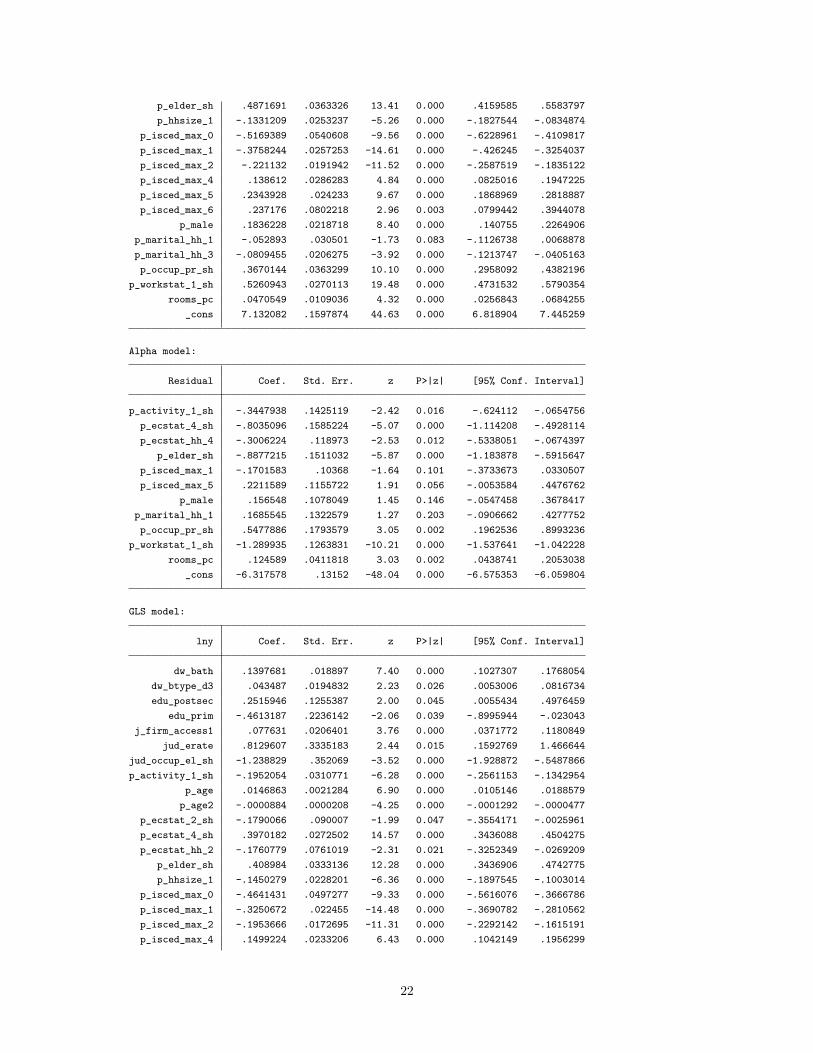
Alpha model:
Residual Coef. Std. Err. z P>|z| [95% Conf. Interval]
p_activity_1_sh -.3447938 .1425119 -2.42 0.016 -.624112 -.0654756p_ecstat_4_sh -.8035096 .1585224 -5.07 0.000 -1.114208 -.4928114p_ecstat_hh_4 -.3006224 .118973 -2.53 0.012 -.5338051 -.0674397
matrix presented by the PovMap software is equal to σ2[(X′WX)−1 (X′W 2X
)(X′WX)−1] where σ2 is an estimate of
Var(wchuch). It is easy to see that the weights are included twice in the variance covariance estimator, which makes itnon-standard.
16
p_elder_sh -.8877215 .1511032 -5.87 0.000 -1.183878 -.5915647p_isced_max_1 -.1701583 .10368 -1.64 0.101 -.3733673 .0330507p_isced_max_5 .2211589 .1155722 1.91 0.056 -.0053584 .4476762
p_male .156548 .1078049 1.45 0.146 -.0547458 .3678417p_marital_hh_1 .1685545 .1322579 1.27 0.203 -.0906662 .4277752p_occup_pr_sh .5477886 .1793579 3.05 0.002 .1962536 .8993236
p_workstat_1_sh -1.289935 .1263831 -10.21 0.000 -1.537641 -1.042228rooms_pc .124589 .0411818 3.03 0.002 .0438741 .2053038
_cons -6.317578 .13152 -48.04 0.000 -6.575353 -6.059804
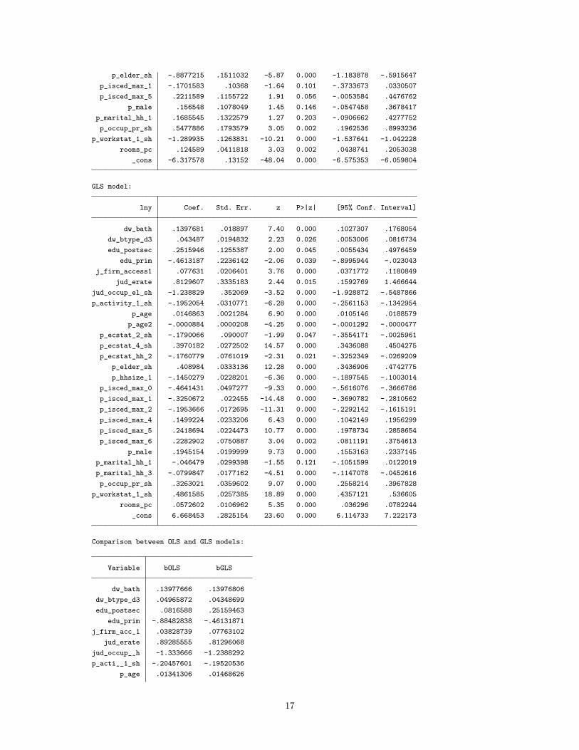
GLS model:
lny Coef. Std. Err. z P>|z| [95% Conf. Interval]
dw_bath .1397681 .018897 7.40 0.000 .1027307 .1768054dw_btype_d3 .043487 .0194832 2.23 0.026 .0053006 .0816734edu_postsec .2515946 .1255387 2.00 0.045 .0055434 .4976459
edu_prim -.4613187 .2236142 -2.06 0.039 -.8995944 -.023043j_firm_access1 .077631 .0206401 3.76 0.000 .0371772 .1180849
jud_erate .8129607 .3335183 2.44 0.015 .1592769 1.466644jud_occup_el_sh -1.238829 .352069 -3.52 0.000 -1.928872 -.5487866p_activity_1_sh -.1952054 .0310771 -6.28 0.000 -.2561153 -.1342954
p_age .0146863 .0021284 6.90 0.000 .0105146 .0188579p_age2 -.0000884 .0000208 -4.25 0.000 -.0001292 -.0000477
p_ecstat_2_sh -.1790066 .090007 -1.99 0.047 -.3554171 -.0025961p_ecstat_4_sh .3970182 .0272502 14.57 0.000 .3436088 .4504275p_ecstat_hh_2 -.1760779 .0761019 -2.31 0.021 -.3252349 -.0269209
p_elder_sh .408984 .0333136 12.28 0.000 .3436906 .4742775p_hhsize_1 -.1450279 .0228201 -6.36 0.000 -.1897545 -.1003014
p_isced_max_0 -.4641431 .0497277 -9.33 0.000 -.5616076 -.3666786p_isced_max_1 -.3250672 .022455 -14.48 0.000 -.3690782 -.2810562p_isced_max_2 -.1953666 .0172695 -11.31 0.000 -.2292142 -.1615191p_isced_max_4 .1499224 .0233206 6.43 0.000 .1042149 .1956299p_isced_max_5 .2418694 .0224473 10.77 0.000 .1978734 .2858654p_isced_max_6 .2282902 .0750887 3.04 0.002 .0811191 .3754613
p_male .1945154 .0199999 9.73 0.000 .1553163 .2337145p_marital_hh_1 -.046479 .0299398 -1.55 0.121 -.1051599 .0122019p_marital_hh_3 -.0799847 .0177162 -4.51 0.000 -.1147078 -.0452616p_occup_pr_sh .3263021 .0359602 9.07 0.000 .2558214 .3967828
p_workstat_1_sh .4861585 .0257385 18.89 0.000 .4357121 .536605rooms_pc .0572602 .0106962 5.35 0.000 .036296 .0782244
_cons 6.668453 .2825154 23.60 0.000 6.114733 7.222173
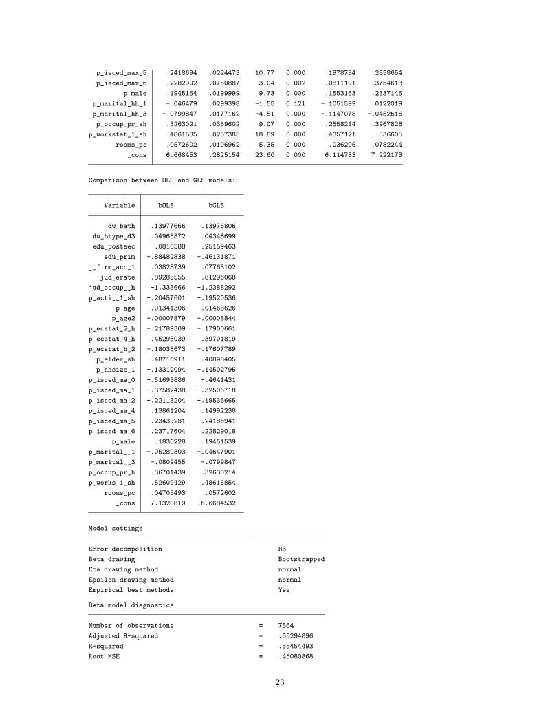
Comparison between OLS and GLS models:
Variable bOLS bGLS
dw_bath .13977666 .13976806dw_btype_d3 .04965872 .04348699edu_postsec .0816588 .25159463
edu_prim -.88482838 -.46131871j_firm_acc~1 .03828739 .07763102
jud_erate .89285555 .81296068jud_occup_~h -1.333666 -1.2388292p_acti~_1_sh -.20457601 -.19520536
p_age .01341306 .01468626
17
p_age2 -.00007879 -.00008844p_ecstat_2~h -.21789309 -.17900661p_ecstat_4~h .45295039 .39701819p_ecstat_h~2 -.18033673 -.17607789
p_elder_sh .48716911 .40898405p_hhsize_1 -.13312094 -.14502795
p_isced_ma~0 -.51693886 -.4641431p_isced_ma~1 -.37582438 -.32506718p_isced_ma~2 -.22113204 -.19536665p_isced_ma~4 .13861204 .14992238p_isced_ma~5 .23439281 .24186941p_isced_ma~6 .23717604 .22829018
p_male .1836228 .19451539p_marital_~1 -.05289303 -.04647901p_marital_~3 -.0809455 -.0799847p_occup_pr~h .36701439 .32630214p_works~1_sh .52609429 .48615854
rooms_pc .04705493 .0572602_cons 7.1320819 6.6684532
Model settings
Error decomposition H3
Beta model diagnostics
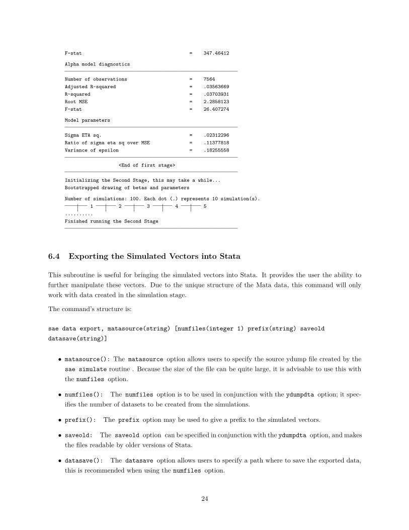
Number of observations = 7564Adjusted R-squared = .55294896R-squared = .55454493Root MSE = .45080868F-stat = 347.46412
Alpha model diagnostics
Number of observations = 7564Adjusted R-squared = .03563669R-squared = .03703931Root MSE = 2.2858123F-stat = 26.407274
Model parameters
Sigma ETA sq. = .02312296Ratio of sigma eta sq over MSE = .11377818Variance of epsilon = .18255558
<End of first stage>
6.3 Monte Carlo Simulation
The simulation part of the analysis requires more inputs from the user. Depending on the details given andthe purpose of the analysis, the user may obtain poverty rates by the different locations specified or justoutput the simulated vectors to a dataset of her choosing. The syntax for the simulation stage is:
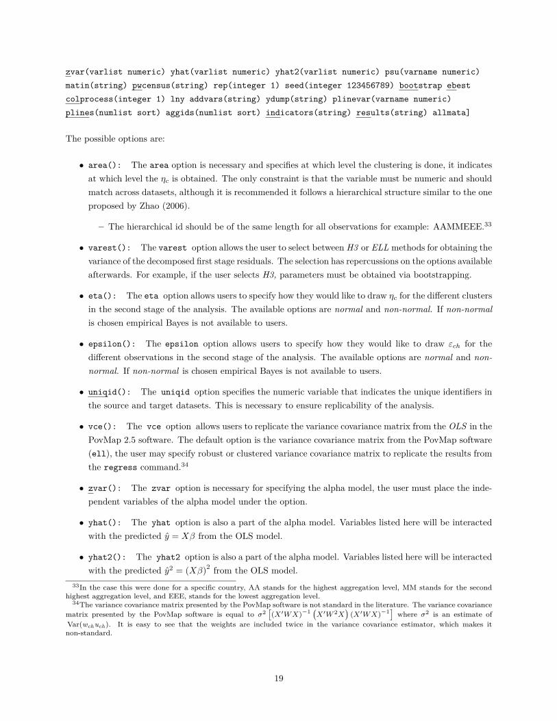
sae simulate lmm/povmap depvar indepvar [if] [in] [aw pw fw], area(varname numeric)
varest(string) eta(string) epsilon(string) uniqid(varname numeric) [vce(string)
18
zvar(varlist numeric) yhat(varlist numeric) yhat2(varlist numeric) psu(varname numeric)
matin(string) pwcensus(string) rep(integer 1) seed(integer 123456789) bootstrap ebest
colprocess(integer 1) lny addvars(string) ydump(string) plinevar(varname numeric)
plines(numlist sort) aggids(numlist sort) indicators(string) results(string) allmata]
The possible options are:
• area(): The area option is necessary and specifies at which level the clustering is done, it indicatesat which level the ηc is obtained. The only constraint is that the variable must be numeric and shouldmatch across datasets, although it is recommended it follows a hierarchical structure similar to the oneproposed by Zhao (2006).
– The hierarchical id should be of the same length for all observations for example: AAMMEEE.33
• varest(): The varest option allows the user to select between H3 or ELL methods for obtaining thevariance of the decomposed first stage residuals. The selection has repercussions on the options availableafterwards. For example, if the user selects H3, parameters must be obtained via bootstrapping.
• eta(): The eta option allows users to specify how they would like to draw ηc for the different clustersin the second stage of the analysis. The available options are normal and non-normal. If non-normalis chosen empirical Bayes is not available to users.
• epsilon(): The epsilon option allows users to specify how they would like to draw εch for thedifferent observations in the second stage of the analysis. The available options are normal and non-normal. If non-normal is chosen empirical Bayes is not available to users.
• uniqid(): The uniqid option specifies the numeric variable that indicates the unique identifiers inthe source and target datasets. This is necessary to ensure replicability of the analysis.
• vce(): The vce option allows users to replicate the variance covariance matrix from the OLS in thePovMap 2.5 software. The default option is the variance covariance matrix from the PovMap software(ell), the user may specify robust or clustered variance covariance matrix to replicate the results fromthe regress command.34
• zvar(): The zvar option is necessary for specifying the alpha model, the user must place the inde-pendent variables of the alpha model under the option.
• yhat(): The yhat option is also a part of the alpha model. Variables listed here will be interactedwith the predicted y = Xβ from the OLS model.
• yhat2(): The yhat2 option is also a part of the alpha model. Variables listed here will be interactedwith the predicted y2 = (Xβ)2 from the OLS model.
33In the case this were done for a specific country, AA stands for the highest aggregation level, MM stands for the secondhighest aggregation level, and EEE, stands for the lowest aggregation level.
34The variance covariance matrix presented by the PovMap software is not standard in the literature. The variance covariancematrix presented by the PovMap software is equal to σ2
[(X′WX)−1 (X′W 2X
)(X′WX)−1] where σ2 is an estimate of
Var(wchuch). It is easy to see that the weights are included twice in the variance covariance estimator, which makes itnon-standard.
19

• psu(): The psu option indicates the numeric variable in the source data for the level at which boot-strapped samples are to be obtained. This option is required for the cases when obtaining bootstrappedparameters is necessary. If not specified, the level defaults to the cluster level, that is the level specifiedin the area option.
• matin(): The matin option indicates the path and filename of the Mata format target dataset. Thedataset is created from the sae data import command; it is necessary for the second stage.
• pwcensus(): The pwcensus option indicates the variable which corresponds to the expansion factorsto be used in the target dataset, it must always be specified for the second stage. The user must haveadded the variable to the imported data (sae data import) i.e. the target data.
• rep(): The rep option is necessary for the second stage, and indicates the number of Monte-Carlosimulations to be done in the second stage of the procedure.
• seed(): The seed option is necessary for the second stage of the analysis and ensures replicability.Users should be aware that Stata’s default pseudo-random number generator in Stata 14 is differentthan that of previous versions.
• bootstrap: The bootstrap option indicates that the parameters used for the second stage of theanalysis are to be obtained via bootstrap methods. If this option is not specified the default methodis parametric drawing of the parameters.
• ebest: The ebest option indicates that empirical Bayes methods are to be used for the secondstage. If this option is used, it is necessary that eta(normal), epsilon(normal), and bootsrap
options be used.
• colprocess(): The colprocess option is related to the processing of the second stage. Because ofthe potential large size of the target data set the default is one column at a time, this however may beincreased with potential gains in speed.
• lny: The lny option indicates that the dependent variable in the welfare model is in log form. Thisis relevant for the second stage of the analysis in order to get appropriate simulated values.
• addvars(): The addvars option allows users to add variables to the dataset created from the sim-ulations. These variables must have been included into the target dataset created with the sae data
import command.
• ydump(): The ydump option is necessary for the second stage of the analysis. The user must providepath and filename for a Mata format dataset to be created with the simulated dependent variables.
• plinevar(): The plinevar option allows users to indicate a variable in the target data set which isto be used as the threshold for the Foster Greer Thorbeck indexes (Foster, Greer, and Thorbeck 1984)to be predicted from the second stage simulations. The user must have added the variable in the sae
data import command when preparing the target dataset. Only one variable may be specified.
• plines(): The plines option allows users to explicitly indicate the threshold to be used, this optionis preferred when the threshold is constant across all observations. Additionally, it is possible to specifymultiple lines, separated by a space.
20
• indicators(): The indicators option is used to request the indicators to be estimated from thesimulated vectors of welfare. The list of possible indicators is:
– The set of Foster Greer Thorbeck indexes (Foster, Greer, and Thorbeck 1984) FGT0, FGT1, andFGT2 ; also known as poverty headcount, poverty gap, and poverty severity respectively.
– The set of inequality indexes: Gini, and Generalized Entropy Index with α = 0, 1, 2
– Set of Atkinson indexes
• aggids(): The aggids option indicates the different aggregation levels for which the indicators areto be obtained, values placed here tell the command how many digits to the left to move to get theindicators at that level. Using the same hierarchical id specified in the area option, AAMMEEE, ifthe user specifies 0, 3, 5, and 7, it would lead to aggregates at each of the levels E, M, A and thenational level.
• results(): The results option specifies the path and filename for users to save as a txt file theresults the analysis specified in the indicators option.
• allmata: The allmata option skips use of the plugin and does all poverty calculations in Mata.
6.3.1 Running the Second Stage (Simulation)
The second stage of the command takes considerably longer to run, depending on the size of the targetdataset and the number of simulations requested. The command for the second stage would look like thefollowing:
. sae sim povmap `y´ `xvar´ [aw=hhw], area(localityid_n) uniqid(hhid) psu(thepsu) zvar(`zvar´) ///> eta(normal) epsilon(normal) varest(h3) lny pwcensus(p_hhsize_hh) ///> vce(ell) rep(100) seed(89546) ydump(`sfiles´) res(`result´) addvars(pline ///> pline2 rdef rdef2 rentdef rdef_rentroom2 rdef_rentall2) ///> matin(`matadata´) col(10) boot ebest stage(second) aggids(0) indicators(fgt0) ///> plines(5291.52)note: p_age omitted because of collinearityNote: Dependent variable in logarithmic formWARNING: 76 observations removed due to less than 3 observations in the cluster.
OLS model:
lny Coef. Std. Err. z P>|z| [95% Conf. Interval]
dw_bath .1397767 .0200267 6.98 0.000 .100525 .1790283dw_btype_d3 .0496587 .0211568 2.35 0.019 .0081921 .0911253edu_postsec .0816588 .0883387 0.92 0.355 -.0914818 .2547994
edu_prim -.8848284 .1744707 -5.07 0.000 -1.226785 -.5428722j_firm_access1 .0382874 .0129973 2.95 0.003 .0128132 .0637616
jud_erate .8928555 .2215139 4.03 0.000 .4586962 1.327015jud_occup_el_sh -1.333666 .2481222 -5.38 0.000 -1.819977 -.8473555p_activity_1_sh -.204576 .0306396 -6.68 0.000 -.2646285 -.1445235
p_age .0134131 .0023387 5.74 0.000 .0088293 .0179968p_age2 -.0000788 .0000238 -3.31 0.001 -.0001255 -.0000321
p_ecstat_2_sh -.2178931 .0840416 -2.59 0.010 -.3826117 -.0531745p_ecstat_4_sh .4529504 .0297431 15.23 0.000 .394655 .5112458p_ecstat_hh_2 -.1803367 .0690036 -2.61 0.009 -.3155813 -.0450921
21
p_elder_sh .4871691 .0363326 13.41 0.000 .4159585 .5583797p_hhsize_1 -.1331209 .0253237 -5.26 0.000 -.1827544 -.0834874
p_isced_max_0 -.5169389 .0540608 -9.56 0.000 -.6228961 -.4109817p_isced_max_1 -.3758244 .0257253 -14.61 0.000 -.426245 -.3254037p_isced_max_2 -.221132 .0191942 -11.52 0.000 -.2587519 -.1835122p_isced_max_4 .138612 .0286283 4.84 0.000 .0825016 .1947225p_isced_max_5 .2343928 .024233 9.67 0.000 .1868969 .2818887p_isced_max_6 .237176 .0802218 2.96 0.003 .0799442 .3944078
p_male .1836228 .0218718 8.40 0.000 .140755 .2264906p_marital_hh_1 -.052893 .030501 -1.73 0.083 -.1126738 .0068878p_marital_hh_3 -.0809455 .0206275 -3.92 0.000 -.1213747 -.0405163p_occup_pr_sh .3670144 .0363299 10.10 0.000 .2958092 .4382196
p_workstat_1_sh .5260943 .0270113 19.48 0.000 .4731532 .5790354rooms_pc .0470549 .0109036 4.32 0.000 .0256843 .0684255
_cons 7.132082 .1597874 44.63 0.000 6.818904 7.445259
Alpha model:
Residual Coef. Std. Err. z P>|z| [95% Conf. Interval]
p_activity_1_sh -.3447938 .1425119 -2.42 0.016 -.624112 -.0654756p_ecstat_4_sh -.8035096 .1585224 -5.07 0.000 -1.114208 -.4928114p_ecstat_hh_4 -.3006224 .118973 -2.53 0.012 -.5338051 -.0674397
p_elder_sh -.8877215 .1511032 -5.87 0.000 -1.183878 -.5915647p_isced_max_1 -.1701583 .10368 -1.64 0.101 -.3733673 .0330507p_isced_max_5 .2211589 .1155722 1.91 0.056 -.0053584 .4476762
p_male .156548 .1078049 1.45 0.146 -.0547458 .3678417p_marital_hh_1 .1685545 .1322579 1.27 0.203 -.0906662 .4277752p_occup_pr_sh .5477886 .1793579 3.05 0.002 .1962536 .8993236
p_workstat_1_sh -1.289935 .1263831 -10.21 0.000 -1.537641 -1.042228rooms_pc .124589 .0411818 3.03 0.002 .0438741 .2053038
_cons -6.317578 .13152 -48.04 0.000 -6.575353 -6.059804
GLS model:
lny Coef. Std. Err. z P>|z| [95% Conf. Interval]
dw_bath .1397681 .018897 7.40 0.000 .1027307 .1768054dw_btype_d3 .043487 .0194832 2.23 0.026 .0053006 .0816734edu_postsec .2515946 .1255387 2.00 0.045 .0055434 .4976459
edu_prim -.4613187 .2236142 -2.06 0.039 -.8995944 -.023043j_firm_access1 .077631 .0206401 3.76 0.000 .0371772 .1180849
jud_erate .8129607 .3335183 2.44 0.015 .1592769 1.466644jud_occup_el_sh -1.238829 .352069 -3.52 0.000 -1.928872 -.5487866p_activity_1_sh -.1952054 .0310771 -6.28 0.000 -.2561153 -.1342954
p_age .0146863 .0021284 6.90 0.000 .0105146 .0188579p_age2 -.0000884 .0000208 -4.25 0.000 -.0001292 -.0000477
p_ecstat_2_sh -.1790066 .090007 -1.99 0.047 -.3554171 -.0025961p_ecstat_4_sh .3970182 .0272502 14.57 0.000 .3436088 .4504275p_ecstat_hh_2 -.1760779 .0761019 -2.31 0.021 -.3252349 -.0269209
p_elder_sh .408984 .0333136 12.28 0.000 .3436906 .4742775p_hhsize_1 -.1450279 .0228201 -6.36 0.000 -.1897545 -.1003014
p_isced_max_0 -.4641431 .0497277 -9.33 0.000 -.5616076 -.3666786p_isced_max_1 -.3250672 .022455 -14.48 0.000 -.3690782 -.2810562p_isced_max_2 -.1953666 .0172695 -11.31 0.000 -.2292142 -.1615191p_isced_max_4 .1499224 .0233206 6.43 0.000 .1042149 .1956299
22
p_isced_max_5 .2418694 .0224473 10.77 0.000 .1978734 .2858654p_isced_max_6 .2282902 .0750887 3.04 0.002 .0811191 .3754613
p_male .1945154 .0199999 9.73 0.000 .1553163 .2337145p_marital_hh_1 -.046479 .0299398 -1.55 0.121 -.1051599 .0122019p_marital_hh_3 -.0799847 .0177162 -4.51 0.000 -.1147078 -.0452616p_occup_pr_sh .3263021 .0359602 9.07 0.000 .2558214 .3967828
p_workstat_1_sh .4861585 .0257385 18.89 0.000 .4357121 .536605rooms_pc .0572602 .0106962 5.35 0.000 .036296 .0782244
_cons 6.668453 .2825154 23.60 0.000 6.114733 7.222173
Comparison between OLS and GLS models:
Variable bOLS bGLS
dw_bath .13977666 .13976806dw_btype_d3 .04965872 .04348699edu_postsec .0816588 .25159463
edu_prim -.88482838 -.46131871j_firm_acc~1 .03828739 .07763102
jud_erate .89285555 .81296068jud_occup_~h -1.333666 -1.2388292p_acti~_1_sh -.20457601 -.19520536
p_age .01341306 .01468626p_age2 -.00007879 -.00008844
p_ecstat_2~h -.21789309 -.17900661p_ecstat_4~h .45295039 .39701819p_ecstat_h~2 -.18033673 -.17607789
p_elder_sh .48716911 .40898405p_hhsize_1 -.13312094 -.14502795
p_isced_ma~0 -.51693886 -.4641431p_isced_ma~1 -.37582438 -.32506718p_isced_ma~2 -.22113204 -.19536665p_isced_ma~4 .13861204 .14992238p_isced_ma~5 .23439281 .24186941p_isced_ma~6 .23717604 .22829018
p_male .1836228 .19451539p_marital_~1 -.05289303 -.04647901p_marital_~3 -.0809455 -.0799847p_occup_pr~h .36701439 .32630214p_works~1_sh .52609429 .48615854
rooms_pc .04705493 .0572602_cons 7.1320819 6.6684532
Model settings
Error decomposition H3Beta drawing BootstrappedEta drawing method normalEpsilon drawing method normalEmpirical best methods Yes
Beta model diagnostics
Number of observations = 7564Adjusted R-squared = .55294896R-squared = .55454493Root MSE = .45080868
23
F-stat = 347.46412
Alpha model diagnostics
Number of observations = 7564Adjusted R-squared = .03563669R-squared = .03703931Root MSE = 2.2858123F-stat = 26.407274
Model parameters
Sigma ETA sq. = .02312296Ratio of sigma eta sq over MSE = .11377818Variance of epsilon = .18255558
<End of first stage>
Initializing the Second Stage, this may take a while...Bootstrapped drawing of betas and parameters
Number of simulations: 100. Each dot (.) represents 10 simulation(s).1 2 3 4 5
..........Finished running the Second Stage
6.4 Exporting the Simulated Vectors into Stata
This subroutine is useful for bringing the simulated vectors into Stata. It provides the user the ability tofurther manipulate these vectors. Due to the unique structure of the Mata data, this command will onlywork with data created in the simulation stage.
The command’s structure is:
sae data export, matasource(string) [numfiles(integer 1) prefix(string) saveold
datasave(string)]
• matasource(): The matasource option allows users to specify the source ydump file created by thesae simulate routine . Because the size of the file can be quite large, it is advisable to use this withthe numfiles option.
• numfiles(): The numfiles option is to be used in conjunction with the ydumpdta option; it spec-ifies the number of datasets to be created from the simulations.
• prefix(): The prefix option may be used to give a prefix to the simulated vectors.
• saveold: The saveold option can be specified in conjunction with the ydumpdta option, and makesthe files readable by older versions of Stata.
• datasave(): The datasave option allows users to specify a path where to save the exported data,this is recommended when using the numfiles option.
24
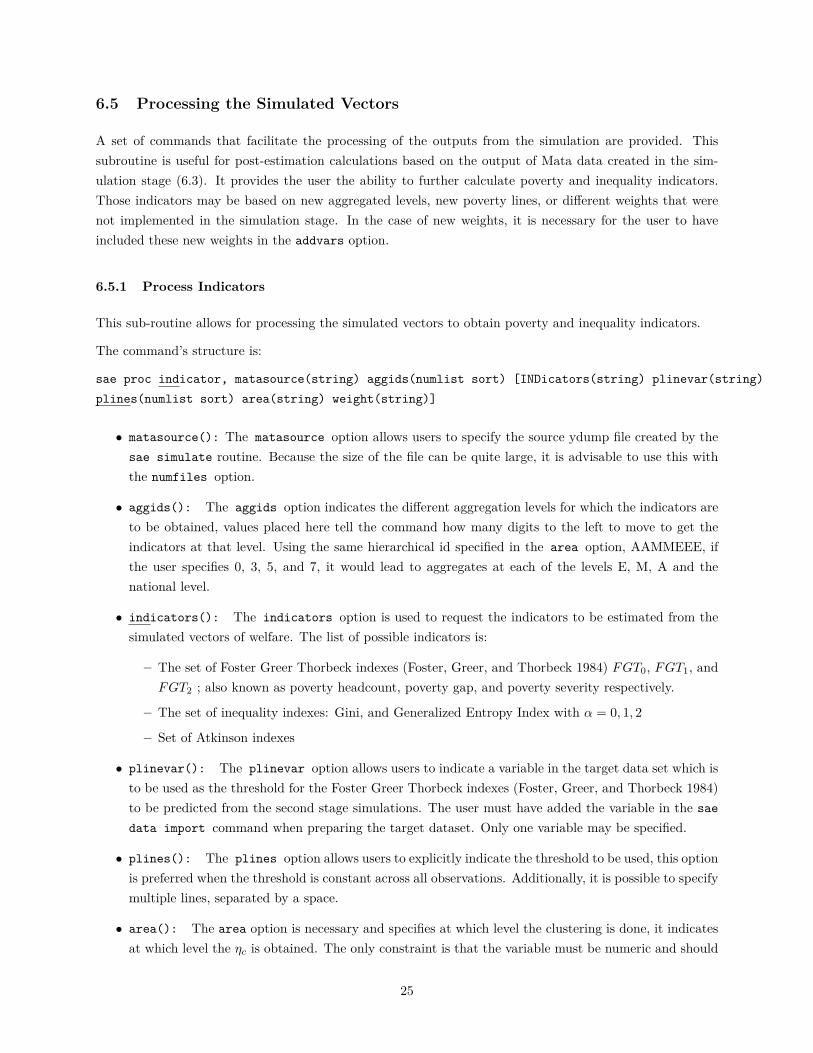
6.5 Processing the Simulated Vectors
A set of commands that facilitate the processing of the outputs from the simulation are provided. Thissubroutine is useful for post-estimation calculations based on the output of Mata data created in the sim-ulation stage (6.3). It provides the user the ability to further calculate poverty and inequality indicators.Those indicators may be based on new aggregated levels, new poverty lines, or different weights that werenot implemented in the simulation stage. In the case of new weights, it is necessary for the user to haveincluded these new weights in the addvars option.
6.5.1 Process Indicators
This sub-routine allows for processing the simulated vectors to obtain poverty and inequality indicators.
The command’s structure is:
sae proc indicator, matasource(string) aggids(numlist sort) [INDicators(string) plinevar(string)
plines(numlist sort) area(string) weight(string)]
• matasource(): The matasource option allows users to specify the source ydump file created by thesae simulate routine. Because the size of the file can be quite large, it is advisable to use this withthe numfiles option.
• aggids(): The aggids option indicates the different aggregation levels for which the indicators areto be obtained, values placed here tell the command how many digits to the left to move to get theindicators at that level. Using the same hierarchical id specified in the area option, AAMMEEE, ifthe user specifies 0, 3, 5, and 7, it would lead to aggregates at each of the levels E, M, A and thenational level.
• indicators(): The indicators option is used to request the indicators to be estimated from thesimulated vectors of welfare. The list of possible indicators is:
– The set of Foster Greer Thorbeck indexes (Foster, Greer, and Thorbeck 1984) FGT0, FGT1, andFGT2 ; also known as poverty headcount, poverty gap, and poverty severity respectively.
– The set of inequality indexes: Gini, and Generalized Entropy Index with α = 0, 1, 2
– Set of Atkinson indexes
• plinevar(): The plinevar option allows users to indicate a variable in the target data set which isto be used as the threshold for the Foster Greer Thorbeck indexes (Foster, Greer, and Thorbeck 1984)to be predicted from the second stage simulations. The user must have added the variable in the sae
data import command when preparing the target dataset. Only one variable may be specified.
• plines(): The plines option allows users to explicitly indicate the threshold to be used, this optionis preferred when the threshold is constant across all observations. Additionally, it is possible to specifymultiple lines, separated by a space.
• area(): The area option is necessary and specifies at which level the clustering is done, it indicatesat which level the ηc is obtained. The only constraint is that the variable must be numeric and should
25
match across datasets, although it is recommended it follows a hierarchical structure similar to theone proposed by Zhao (2006). Note that in this step, the default is to use the defined areas from thesimulation step. In this option the user is given the opportunity to change this grouping.
– The hierarchical id should be of the same length for all observations for example: AAMMEEE.
• weight(): The weight option indicates the new variable which corresponds to the expansion factorsto be used in the target/ydump dataset. The default option is to use the weight variable saved in theydump file, if a variable is specified here all results will be obtained with this new weighing. The usermust have added the variable to the target data imported (sae data import).
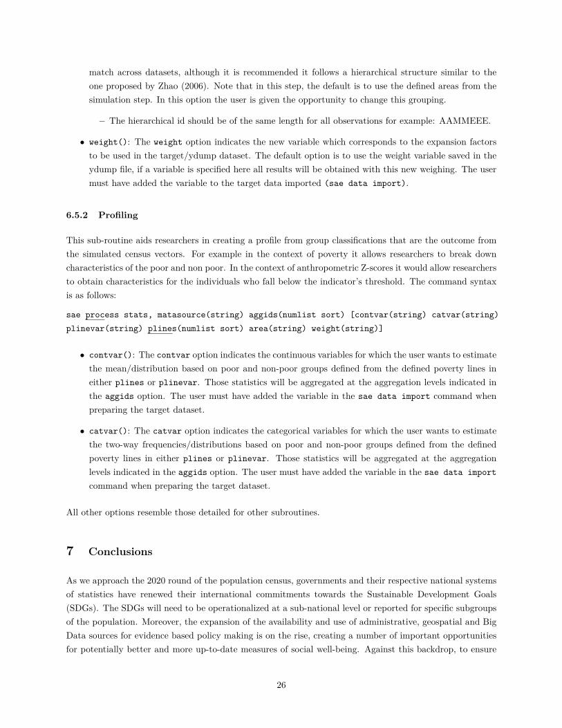
6.5.2 Profiling
This sub-routine aids researchers in creating a profile from group classifications that are the outcome fromthe simulated census vectors. For example in the context of poverty it allows researchers to break downcharacteristics of the poor and non poor. In the context of anthropometric Z-scores it would allow researchersto obtain characteristics for the individuals who fall below the indicator’s threshold. The command syntaxis as follows:
sae process stats, matasource(string) aggids(numlist sort) [contvar(string) catvar(string)
plinevar(string) plines(numlist sort) area(string) weight(string)]
• contvar(): The contvar option indicates the continuous variables for which the user wants to estimatethe mean/distribution based on poor and non-poor groups defined from the defined poverty lines ineither plines or plinevar. Those statistics will be aggregated at the aggregation levels indicated inthe aggids option. The user must have added the variable in the sae data import command whenpreparing the target dataset.
• catvar(): The catvar option indicates the categorical variables for which the user wants to estimatethe two-way frequencies/distributions based on poor and non-poor groups defined from the definedpoverty lines in either plines or plinevar. Those statistics will be aggregated at the aggregationlevels indicated in the aggids option. The user must have added the variable in the sae data import
command when preparing the target dataset.
All other options resemble those detailed for other subroutines.
7 Conclusions
As we approach the 2020 round of the population census, governments and their respective national systemsof statistics have renewed their international commitments towards the Sustainable Development Goals(SDGs). The SDGs will need to be operationalized at a sub-national level or reported for specific subgroupsof the population. Moreover, the expansion of the availability and use of administrative, geospatial and BigData sources for evidence based policy making is on the rise, creating a number of important opportunitiesfor potentially better and more up-to-date measures of social well-being. Against this backdrop, to ensure
26
the much needed quality and rigor of the analysis produced, the advancement and availability of statisticallyvalid methods with proper inference such as small area estimates are required.
Direct estimates of poverty and inequality from household surveys are only reliable up to a certain regionallevel. When estimates are needed at lower, more disaggregated levels, the reliability of these is questionable.Under a set of specific assumptions, data from outside sources along with household survey data may becombined in order to provide policy makers with a more complete picture of poverty and inequality alongwith the spatial heterogeneity of these indicators.
In this paper we introduce a new family of Stata functions, sae, which were designed in a modular and flexibleway to manage the data, estimate models, conduct simulations, and compute indicators of interest. Theestimation functions have been bench-marked against the World Bank’s PovMap software for full validation.
We hope that the flexibility of this new family of functions will encourage producers of SAE to documentand report in a more systematic manner the robustness of their results to alternative methodological choicesmade, improving the replicability and increasing the transparency of this estimation process. Its modularnature creates a platform for the introduction of new estimation techniques, such as count and binary models.Additionally, the modular nature encourages collaboration from the broader Stata community.
27
References
Bedi, T., A. Coudouel, and K. Simler (2007). More than a pretty picture: using poverty maps to designbetter policies and interventions. World Bank Publications.
Demombynes, G., C. Elbers, J. O. Lanjouw, and P. Lanjouw (2008). How good is a map? putting smallarea estimation to the test. Rivista Internazionale di Scienze Sociali, 465–494.
Elbers, C., J. O. Lanjouw, and P. Lanjouw (2002). Micro-level estimation of welfare. 2911.
Elbers, C., J. O. Lanjouw, and P. Lanjouw (2003). Micro–level estimation of poverty and inequality. Econo-metrica 71 (1), 355–364.
Foster, J., J. Greer, and E. Thorbecke (1984). A class of decomposable poverty measures. Econometrica:Journal of the Econometric Society, 761–766.
Harvey, A. C. (1976). Estimating regression models with multiplicative heteroscedasticity. Econometrica:Journal of the Econometric Society, 461–465.
Haslett, S., M. Isidro, and G. Jones (2010). Comparison of survey regression techniques in the context ofsmall area estimation of poverty. Survey Methodology 36 (2), 157–170.
Henderson, C. R. (1953). Estimation of variance and covariance components. Biometrics 9 (2), 226–252.
Huang, R. and M. Hidiroglou (2003). Design consistent estimators for a mixed linear model on survey data.Proceedings of the Survey Research Methods Section, American Statistical Association (2003), 1897–1904.
Molina, I. and J. Rao (2010). Small area estimation of poverty indicators. Canadian Journal of Statis-tics 38 (3), 369–385.
Rao, J. N. and I. Molina (2015). Small area estimation. John Wiley & Sons.
Tarozzi, A. and A. Deaton (2009). Using census and survey data to estimate poverty and inequality forsmall areas. The review of economics and statistics 91 (4), 773–792.
Van der Weide, R. (2014). Gls estimation and empirical bayes prediction for linear mixed models withheteroskedasticity and sampling weights: a background study for the povmap project. World Bank PolicyResearch Working Paper (7028).
Zhao, Q. (2006). User manual for povmap. World Bank. http://siteresources. worldbank.org/INTPGI/Resources/342674-1092157888460/Zhao_ ManualPovMap. pdf .
28

To access full collection, visit the World Bank Documents & Report in the Poverty & Equity Global Practice
Working Paper series list.
www.worldbank.org/poverty