Atmospheric Pollution Research 6 (2015) 312 321

© Author(s) 2015. This work is distributed under the Creative Commons Attribution 3.0 License.

AAtm spheric PPollution RResearchwww.atmospolres.com

Case studies of methane dispersion patterns and odor strength in vicinity of municipal solid waste landfill of Cluj–Napoca, Romania, using numerical modeling Vasile Filip Soporan 1, Lucian Nascutiu 2, Bianca Soporan 3, Carol Pavai 1

1 The Center for Promoting Entrepreneurship in Sustainable Development Domain, Technical University of Cluj–Napoca, Romania2 Department of Mechanical Engineering, Technical University of Cluj–Napoca, Romania3 Department of Environmental Engineering and Sustainable Development Entrepreneurship, Technical University of Cluj–Napoca, Romania

ABSTRACTThe study investigates the local characteristics of methane dispersion generated by the Pata Rat non–compliantmunicipal solid waste (MSW) landfill located in vicinity of Cluj–Napoca, Romania, using a numerical model developedat The Center for Promoting Entrepreneurship in the Sustainable Development Domain, from Technical University ofCluj–Napoca. The model was applied to the analysis of the methane dispersion emitted from the landfill, in twodifferent weather conditions. In the first case the synoptic scale effects were weak favoring local flow development,while in the second case, the synoptic scale effects were predominant. The numerical model takes into account thelocal orography and daytime heating. In the studied area, the topography presents substantial variation, which affectsthe airflow dynamics. The initial conditions are formulated using observational data, recorded at the Meteorologicaland Aerological Station Cluj–Napoca, as well as the Meteorological Station of Cluj–Napoca International Airport. In thefirst case, wind direction and intensity present diurnal variations due to the thermally induced local circulations. In airlayers near the ground, up to 350–400 m, these variations are more pronounced and significantly influence thedispersion of methane. In the second case, local effects are blurred by a more intense synoptic scale circulation. Inthese conditions the area affected by methane dispersion is much lower as compared to the previous case. In addition,the time intervals for presence of unpleasant odor due to landfill gases were estimated. Simulation shows that thedispersion is strongly influenced by the weather conditions and local topography. The results indicate the possibility ofusing the model as a decisional support in assessing the applications and strategies for air pollution control on localscale. An accurate mapping of pollutant dispersion is useful both for urban planning and residential developers.

Keywords: Atmospheric dispersion, odorous pollutant, numerical modeling, complex terrain, decision support tool

Corresponding Author:Vasile Filip Soporan

: +40 723 300 045: +40 264 202 793: vfsoporan@gmail.com

Article History:Received: 30 April 2014Revised: 01 October 2014Accepted: 02 October 2014

doi: 10.5094/APR.2015.035

1. Introduction

In recent decades numerous experimental and modeling studieshave been conducted in order to obtain information on pollutantdispersion. Depending on the chosen purpose, different techniqueshave been used for monitoring and modeling. Some of these studiesare purely experimental, presenting and analyzing measurementsfrom a small area. Others are purely theoretical, focusing on theinvestigation of pollutant dispersion caused by different flow regimesof atmospheric air. In another category we can mention studiescombining field measurements with mathematical modeling. Theliterature shows a wide variety of mathematical models used tostudy the dispersion of air pollutants, ranging from simple analyticalmodels (e.g., Mayhoub et al., 2003; Anikender and Goyal, 2012) tocomplex ones, using the complete set of equations for atmosphericflow and thermodynamics (e.g. Lagouvardos et al., 1996; Martilli,2003; Costa et al., 2005; Schmitz, 2005; Kakosimos et al., 2011;Lesouef et al., 2011; Aloyan et al., 2012; Konglok and Pochai, 2012).The most frequently used models are the Box, Gaussian, Lagrangianand Eulerian models (Holmes and Morawska, 2006).

In Romania, the requirements of national and Europeanpolicies on air quality improvement measures require monitoringconcentrations of air pollutants and conducting impact studies onair quality. The target of these studies is to identify risk areas andsituations where the concentration of pollutants can reach and even

exceed the critical threshold of danger (e.g. Grigoras et al., 2012;Grigoras and Mocioaca, 2012). In this context, there is need forcomplex diffusion models which work in different weather conditions and can integrate heterogeneous characteristics of the land.

The purpose of this study is to investigate the local characteristics of air pollutants dispersion, generated by the non–compliantMSW landfill situated at Pata Rat, in vicinity of Cluj–Napoca(Romania), using a numerical model developed by The Center forPromoting Entrepreneurship in the Sustainable DevelopmentDomain, from Technical University of Cluj–Napoca. The model wasapplied to the analysis of the methane dispersion emitted from thelandfill, in two different situations. The major difference betweenthem is determined by the weather conditions. In the first case, dueto weak south–western synoptic flow and enhanced atmosphericstability, local scale thermal circulations are induced by the complexterrain, which influence the pollutants transport patterns and formbad dispersion conditions. In the second case, under influence of anintense north–western flow in lower troposphere, the synoptic scaleforcing was dominant creating better dispersion conditions.

The study area has significant terrain variations, which influence the airflow dynamics. The ascendant motions on the windward slopes, the convergence zones on the leeward sides and theelevated heat sources generated by slopes exposed to the sunhave strong influences on convective activity dynamics (Souza et

Soporan et al. – Atmospheric Pollution Research (APR) 313

al., 2000; Holton, 2004; Bianco et al., 2006) and thus play animportant role in the dispersion of air pollutants. Generally, thevertical distribution of temperature and pollutants over an unevenground surface present a more complex structure than over a flathorizontal ground (Reuten et al., 2007).

Pata Rat MSW landfill was opened in 1973, with a storage areaof 9 hectares, and was designed for the storage of 3.5 million tonsof waste for 30 years. It should have been closed in 2003, but is stillin use. In time, the surface of deposit came to exceed 18 ha andthe stored waste 10 million tons (Hategan et al., 2012).Environmental pollution of water, air and soil has led to changes inthe ecosystem and the legitimate use of the area. In adverseweather conditions the impact of landfill is felt on a wide area,aerosols arising from the uncontrolled burning of waste spreadover a distance of 15 to 20 km, favoring production of fog onSomes Valley. The odor released from decomposition processespersist throughout the year, just the intensity and propagationdistance varies depending on weather conditions.

2. Data and Methods

Dispersion analysis of landfill methane emitted was made on aparallelepiped shaped domain of the planetary boundary layer

with dimensions 30 km × 30 km × 3 km. The bottom limit of thisdomain, the ground surface, is centered on Pata Rat landfill and isbounded by geographic coordinates;

in SW corner =46.63° =23.5°in NE corner =46.8998° =23.893064°

In Figure S1a, presented in Supporting Material (SM), is shownthe location of analysis domain. The landfill is marked with D, andthe Airport with A. Terrain elevations vary between 270 and 800 m(see the SM, Figure S1b).

Dispersion of air pollutants are governed by atmosphericmotions, advection and diffusion, which in turn are influenced bythe thermodynamic parameters of atmosphere. Governing equations of the numerical model is based on fundamental physicalprinciples, expressed by the relations of conservation for momentum,mass, heat and moisture, taking into account the interaction ofatmosphere with the ground surface that has thermal andorographic inhomogeneities. In Cartesian coordinate system theseequations are the Navier–Stokes equations, the continuity equation,the equations for conservation of heat and moisture, and theequation of state for humid air:

(1)

(2)

(3)

(4)

(5)

(6)

(7)

where x, y and z are the independent spatial variables, t is thetime, u, v and w are the velocity vector components expressed inm s–1, , and are the coefficients of horizontal andvertical turbulent viscosity in m2 s–1, and Kx Ky and Kz are thehorizontal and vertical turbulent diffusion coefficients expressed inm2 s–1. T(x, y, z, t) is the temperature in K, q(x, y, z, t) is the specifichumidity in kg kg–1 (kg of water vapor contained in kg of moist air),cp is the specific heat of air at constant pressure in J kg–1 K–1, f is theCoriolis parameter in s–1, and R is the gas constant for dry air inm2 s–2 K–1. In Equations (5) and (6) is the vertical temperaturegradient in K m–1, d is the adiabatic lapse rate of dry orunsaturated moist air, and Lv is the latent heat of water vapor inJ kg–1.

The system of Equations (1)–(7) was completed with advection–diffusion equation of pollutants:

(8)

where C(x, y, z, t) is the concentration of pollutant in atmosphere.

To initialize the model, observational data from ground leveland altitude were used. These data were recorded at the Meteorological and Aerological Station Cluj–Napoca code WMO (World

Meteorological Organization) 15120, and at the MeteorologicalStation of Cluj–Napoca International Airport code ICAO (International Civil Aviation Organization) LRCL. The observed values oftemperature, humidity, pressure and horizontal components ofwind were interpolated to the numerical model levels. This is ahorizontally homogeneous initialization (Kallos, 1989; Lagouvardoset al., 1996). For t=0 it is assumed that the methane concentrationin the environment is zero, and the methane emission takes placeat the ground level with a constant emission rate.

At all lateral boundaries, zero gradient boundary conditions(Gross, 2001; Costa et al., 2005; Aloyan et al., 2012) were utilizedfor temperature, humidity, pressure and concentration. At theinflow lateral boundaries wind velocity components normal to theboundary were specified, and for tangential components the zerogradient condition were formulated. These specified values wereextracted from numerical products of regional scale prognosticmodel GFS (Global Forecasting System) and from ESRL (EarthSystem Research Laboratory) database. At the outflow lateralboundaries the zero gradient conditions were applied for allvelocity components. At the upper limit of integration domainvalues of boundary conditions for velocity components, temperature, pressure and humidity were specified, and for methaneconcentration the zero gradient conditions C/ z=0 were imposed.At the lower limit of integration domain typical conditions for rigid

Soporan et al. – Atmospheric Pollution Research (APR) 314

boundaries were applied. Thermal radiation is taken into accountindirectly, by imposing a sinusoidal diurnal temperature variation.The Smagorinsky–Lilly turbulence model (Lilly, 1962; Smagorinsky,1963; Clark, 1979; Aloyan et al., 2012) were adopted for estimationof subgrid–scale fluxes, coefficients of turbulent diffusion, andturbulent viscosity.

For discretization of the governing equations the controlvolume based, finite difference, method was used (Patankar, 1980;Markatos, 1989; McDonough, 2007). The integration domain wassubdivided into parallelepiped shaped computational cells. Allscalar unknowns were computed at the center of each cell, whilethe velocities are computed at the faces of cell. This means thatstaggered grids were employed for discretization of the momentumequations. For temporal discretization an implicit Euler scheme wasused. The SIMPLEC algorithm has been adopted to treat thevelocity–pressure coupling (McDonough, 2007).

Site description and source characteristics input into the modelare presented in Text S1 (see the SM).

2.1. Observational evidences and model sensitivity studies

Heat and mass transfer capability of model and sensitivity to thegrid spacing were validated against experimental measurements,earlier in the years 1998–2003, and proved to be reasonablyaccurate (Soporan et al., 2003).

Unfortunately, for the study region, reliable measurementdata of methane concentrations to be compared with simulationresults are missing, but the few measured values existent for Cluj–Napoca, are in good concordance with the simulation results.

Processing of wind direction observations, recorded betweenyears 1971–2000 at the Meteorological Station of Cluj–NapocaInternational Airport, clearly indicates the channeling feature ofsurface wind to W–E direction, along the Somes Valley. Table S1(see the SM) presents the relative frequencies of occurrence ofwind direction on the 8 directions (Sandu et al., 2008). Value of12.4% from W and the 11.5% from E, compared to the frequenciesof the other directions indicate the predominance of channelingeffect in layers near the ground, in central part of study domain.The numerical model captures well this channeling effect togetherwith the diurnal variation of wind direction caused by the hill–valley and valley–hill breezes. In Figure S2a and S2b (see the SM)are presented 2 horizontal sections in wind field at altitude of325 m above mean sea level (MSL) at 06:42 LT and 10:51 LT in06.08.2012, provided by the model. These also show the contourof channel–shaped relief in the center of the analysis domain. Thechanges in surface wind direction, from W–>E to E–>W, in centralpart of study domain are caused by the onset of valley–hill breezeat 07:30 LT, after the beginning of thermal circulations.

Figure S2c and S2d (see the SM) present a horizontal section inwind field at altitude of 325 m above MSL at 20:48 LT and one at1 225 m above MSL at 10:51 LT in 06.08.2012, provided by themodel. Figure S2c (see the SM) show the surface wind after thebeginning of the hill–valley breeze at 20:00 LT, and Figure S2d (seethe SM) indicates that at altitude of 1 225 m the wind is directedmainly from SW to NE following the synoptic scale circulation.Details are presented in Section 3.1.

We performed sensitivity experiments of the model resultsregarding the turbulence model set–up and the grid sizes. In allnumerical experiments we used constant spatial increments, whichmeans, that the size of the control volumes was identical to themesh cell size.

To examine the effect of value of the Smagorinsky constant tothe model results, we performed 3 separate runs with differentvalues of Cs: 0.11, 0.17 and 0.22. In all runs the integration domain

was the one shown in Figure S1a (see the SM), and the spatialincrements were same, dx=dy=500 m and dz=50 m. Also, the initialconditions were same to those described in Section 2. We namethese runs R11, R17 and R22. The methane concentrations obtainedwith these runs for 06:00 and 08:00 LT are presented in Figure S6(see the SM) for R11 and R22, and in Figure 1a and 1b for R17.Analysis results show that the area affected by methaneconcentrations greater than zero is greater in the case of R11 thanin case of R17 or R22, both at 06:00 and at 08:00 LT. It is inconcordance with the Lilly's result (Lilly, 1967) that the subgridscale dissipation is proportional to (Cs )2, thus lower values of Csgive lower levels of subgrid dissipation. Instead, maximum concentrations are slightly lower in the case of R11 and R17, than in R22.The increased dissipation in case R22 seems to dampens down theturbulence, and thus reduces the horizontal and vertical extent ofdispersion and in this way leads to greater accumulation ofconcentrations.

To have an objective measure of the differences between thethree runs, we calculated for each run the area of surface occupiedby methane at 25 m height above ground level, with concentrations higher than 0 ppmv. Also, we computed the standarddeviation for 06:00 and 08:00 LT. The results are shown in Table S2(see the SM) together with the standard deviations for maximumconcentrations obtained in these runs. Due to the values ofstandard deviation and the fact that values obtained by R17 arecloser to the mean than those obtained by R11 and R22, wechoose Cs=0.17 as an optimal value for our discretization scheme.

To estimate the sensitivity of the model to the grid sizes werun the model with different spatial discretization. Grid G1 with30x30x60 computational cells and dx=dy=1 000 m, dz=50 m, gridG2 with 60x60x60 computational cells and dx=dy=500 m, dz=50 m,and G3 with 120x120x60 computational cells and dx=dy=250 m,dz=50 m. In these experiments a Smagorinsky constant Cs=0.17was used. The time series of wind measured at MeteorologicalStation of Cluj–Napoca International Airport were compared withthe corresponding time series obtained by simulations. The graphsfor time evolution of components u and v measured (uobs, vobs) andmodeled (umod, vmod) are shown in Figure S7a–S7f (see the SM). Themodel was run with grid G1 7 hours, with G2 24 hours and with G38 hours. The root mean square (RMS) error for wind componentsobserved and provided by model with grids G1, G2 and G3 arepresented in Table S3. For grid G2 is shown in parentheses thevalue for the first 7 hours of run, for a better comparison with theG1 and G3. We consider the discretization with grid G2 optimal,although the RMS error for v component is less good than in caseof G3.

In Figures S7g and S7h (see the SM)are presented the verticaldistribution of temperature and specific humidity measured atMeteorological and Aerological Station Cluj–Napoca, at 03:00 LT on07.08.2012, together with the model provided temperature andspecific humidity values, obtained with grid G2, in computationalcells located above station. It shows that the model overestimatethe intensity of thermal inversion, and push the level of inversionabove with 260 m, and the vertical distribution of specific humidityis less accurate.

3. Case Studies

Two representative days were selected, with appropriateweather conditions for cases in which the effects of local circulationswere dominant, and for those in which the synoptic scale effectsprevailed. The selection was based on analysis of surface pressuremaps in Europe, along with the upper air maps for levels of 850and 700 hPa. In parallel aerological soundings and hourly meteorological messages, emitted from the two weather stations in Cluj–Napoca, were analyzed. In this way 6 August 2012 was identified asa typical day in which local weather conditions were dominant, and

Soporan et al. – Atmospheric Pollution Research (APR) 315

6 April 2011 as a typical day for prevalence of synoptic scaleeffects.

Using the data archive at Regional Forecast Center Cluj, foryears 2008–2010, the relative frequencies of occurrence of synopticsituations generating these weather conditions, in the study area,were determined. In first case an average value of 8.7% wasobtained for summer season, and 9.8% in the second case forspring season. This methodology used to selection of representative days is similar to that used by Philippopoulos et al. (2009).

In both cases, numerical experiments were carried out onintegration domain with a grid that have the spatial incrementsdx=dy=500 m and dz=50 m. A constant emission rate of methaneequal to 122.8 g m–2 day–1 was assumed, which is an estimationbased on measurement data obtained by Vac (Soporan) et al.(2012), using a network of borehole wells and a gas analyzer. Thisemission rate is consistent with other reported values for non–conformal solid waste landfills, with same extensions and in sameclimatological conditions (Goldsmith et al., 2012).

3.1. Case 1 – August 6, 2012

August 6, 2012, was a typical day for a scenario with unfavorable weather conditions for atmospheric dispersion. Large scaleweather conditions with weak synoptic forcing favored the predominance of local effects. At ground level Eastern Europe isdominated by an anticyclone field (see the SM, Figure S3c) causingweak atmospheric circulations in study region.

In altitude, at level of 850 hPa, warm air masses of north–African origins were favored the formation of a warm ridge withtemperatures above 20 °C (see the SM, Figure S3a). One can seethat Romania was situated on axis of warm ridge, in a weak south–western synoptic scale circulation in the lower troposphere. Theanticyclonic field and the warm ridge led to the clear sky andformation of nocturnal thermal inversion.

The aerological sounding from Cluj–Napoca indicate weaksouth–western wind, with 2–5 m s–1 at all levels in the lowertroposphere, and stable thermal stratification conditions (see theSM, Figure S3b). At altitude of 1 015 m above MSL, one canobserve the presence of a thermal inversion of 5.4 °C. The upperlimit of the inversion layer is a barrier to upward vertical movements. In this context the synoptic scale effects were blurred bythe effects of local circulations generated by the orography and thenon–uniform heating of ground.

The observational data from 04:30 LT were used as initial data,and the evolution of wind, temperature, humidity and pollutantdispersion within the next 24 hours were simulated. During theday, modeled wind direction and intensity presented variationsdue to local orographic effects and of the daytime cumulativeheating. In the layers near the ground, up to the 350–400 m abovethe ground, these variations are more pronounced and significantlyinfluence the atmospheric dispersion. Before 07:30 LT the surfacewind was channeled on Somes Valley and blow from W to E, and inthe north–eastern part of valley from SW to NE, which are typicalfeatures of hill–valley breeze generated by local orography. Then,after 07:30 LT, the increasing surface temperature generate valley–hill breezes, which are channeled from E to W in the center of theintegration domain. In the evening, after 20:00 LT, when thetemperature drops again, arise again hill–valley breezes which arechanneled from W to E, and in the north–eastern part of thedomain from SW to NE. A detailed description of the hill–valley andvalley–hill winds can be found in Souza et al. (2000) and inRampanelli et al. (2004).

In altitudes, above 1 200 m, the influence of topography isweaker, and the simulated wind is directed mainly from SW to NEfollowing the synoptic scale circulation. At these altitudes only the

convective circulations in the afternoon hours disrupt temporarilythe wind field. It should be noted that atmospheric stabilityprevented the formation of moist convection, and upward movements have not reached the level of condensation.

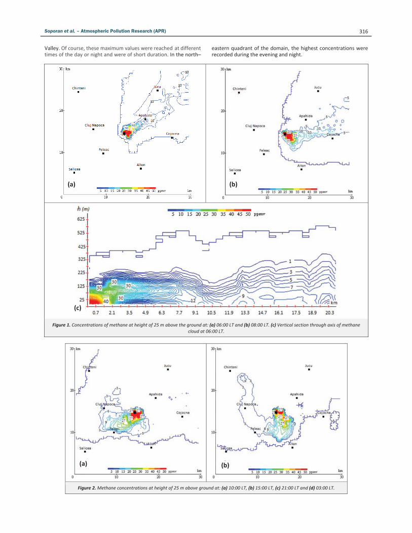
These diurnal variations in wind field produced major changesin the dispersion of methane generated by Pata Rat landfill. In thefirst 3 hours of simulation, the dispersion of methane was madefrom landfill, marked with an asterisk, to NE following the SomesValley (Figure 1a).

After the beginning of thermal circulations at 07:30 LT, thesurface wind change gradually and tend to rotate the axis ofmethane cloud southward (Figure 1b). A vertical section throughthe methane cloud at 06:00 LT, along its axis, corresponding toimage in Figure 1a, is shown in Figure 1c.

One can see that concentrations higher than 30 ppmv werefound at distances up to 3.5 km from the deposit, with a verticalextension of up to 140 m. The isoline heights of 1 ppmv extendfrom 150 m, at a distance of 10 km from the deposit, up to 330 mat 20 km from the deposit. The isoline with a concentration of0.001 ppmv, was imposed as the outer contour of the methanecloud. In this context, it is seen that the cloud of methane does notexceed the height of 525 m.

At 09:00 LT the eastern extremity of the methane cloud continue to move to south, while near the landfill, the methane beginto spread to W, due to the initiation of easterly wind in centralarea of integration domain. Between 09:00 and 10:00 LT easternedge of methane cloud dissipates, while western flank of the cloudreaches the central area of Cluj–Napoca with values of 3 ppmv(Figure 2a).

Between 10:00 and 12:00 LT the westward expansion of themethane cloud continued. In the afternoon, the surface temperatures rises close to the maximum cumulative heating and convectivevertical motions occur, but these not reaches the condensationlevel that was situated at 831 hPa, approximately 1 714 m.

The increases in atmospheric turbulence, caused by thevertical motions, tend to enhance the methane dispersion anddiminish the concentrations. Thus, at 15:00 LT, the concentrationsat west of Cluj–Napoca and Feleac, were decreased below 3 ppmv(Figure 2b). Also, one can see the increase of concentrations atsouth of the deposit, on the northern slopes of Feleac Hill, due tothe valley–hill breezes.

Local circulations generated by the complex topography arewell captured by the numerical model. Between 18:00 and20:00 LT, once with the weakening of the convective circulation,the methane cloud extends westward again, so at 20:00 LT, incentral square of Cluj–Napoca town, at height of 25 m thesimulated methane concentrations were 10–12 ppmv.

After 20:00 LT, once with the temperature drop, the valley–hillside breezes ceases and reborn the hill–valley breezes. Simultaneously, begin the dispersion of concentrations from deposit to Eand NE (Figure 2c). Until 24:00 LT the concentrations in north–western part of the domain of integration was diluted below1 ppmv, while in the north–eastern part were increased andextended to the limits of integration domain.

In the following hours of the night of 06/07 August, theconcentrations of 3 ppmv and above remain in the north–easternquadrant of the integration domain (Figure 2d).

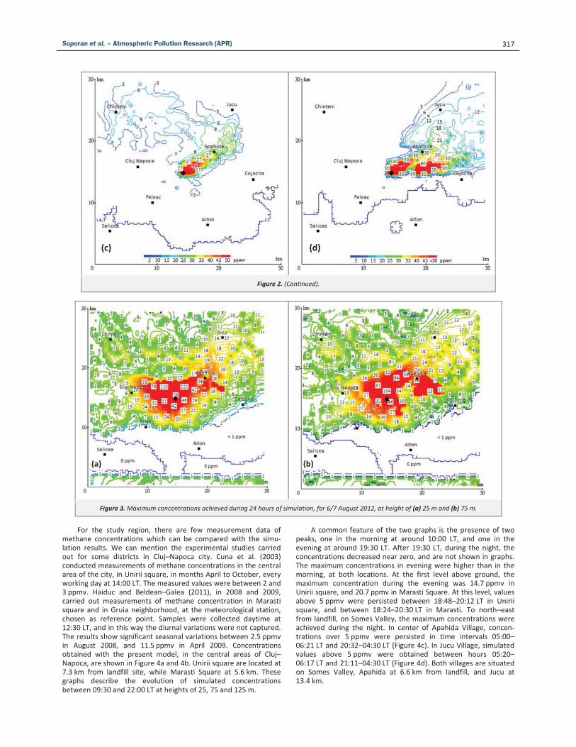
The maximum concentrations obtained are shown in Figure 3,on the first two model levels above ground, during the 24 hourssimulated. The highest values on both levels were recorded incenter of domain and to north–east from landfill, along the Somes

Soporan et al. – Atmospheric Pollution Research (APR) 316

Valley. Of course, these maximum values were reached at differenttimes of the day or night and were of short duration. In the north–

eastern quadrant of the domain, the highest concentrations wererecorded during the evening and night.

Figure 1. Concentrations of methane at height of 25 m above the ground at: (a) 06:00 LT and (b) 08:00 LT. (c) Vertical section through axis of methanecloud at 06:00 LT.

Figure 2.Methane concentrations at height of 25 m above ground at: (a) 10:00 LT, (b) 15:00 LT, (c) 21:00 LT and (d) 03:00 LT.

(a) (b)

(c)

(a) (b)

Soporan et al. – Atmospheric Pollution Research (APR) 317

Figure 2. (Continued).

Figure 3.Maximum concentrations achieved during 24 hours of simulation, for 6/7 August 2012, at height of (a) 25 m and (b) 75 m.

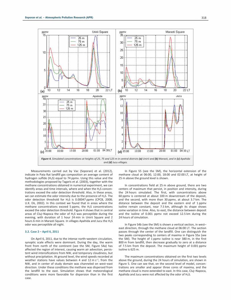
For the study region, there are few measurement data ofmethane concentrations which can be compared with the simulation results. We can mention the experimental studies carriedout for some districts in Cluj–Napoca city. Cuna et al. (2003)conducted measurements of methane concentrations in the centralarea of the city, in Unirii square, in months April to October, everyworking day at 14:00 LT. The measured values were between 2 and3 ppmv. Haiduc and Beldean–Galea (2011), in 2008 and 2009,carried out measurements of methane concentration in Marastisquare and in Gruia neighborhood, at the meteorological station,chosen as reference point. Samples were collected daytime at12:30 LT, and in this way the diurnal variations were not captured.The results show significant seasonal variations between 2.5 ppmvin August 2008, and 11.5 ppmv in April 2009. Concentrationsobtained with the present model, in the central areas of Cluj–Napoca, are shown in Figure 4a and 4b. Unirii square are located at7.3 km from landfill site, while Marasti Square at 5.6 km. Thesegraphs describe the evolution of simulated concentrationsbetween 09:30 and 22:00 LT at heights of 25, 75 and 125 m.

A common feature of the two graphs is the presence of twopeaks, one in the morning at around 10:00 LT, and one in theevening at around 19:30 LT. After 19:30 LT, during the night, theconcentrations decreased near zero, and are not shown in graphs.The maximum concentrations in evening were higher than in themorning, at both locations. At the first level above ground, themaximum concentration during the evening was 14.7 ppmv inUnirii square, and 20.7 ppmv in Marasti Square. At this level, valuesabove 5 ppmv were persisted between 18:48–20:12 LT in Uniriisquare, and between 18:24–20:30 LT in Marasti. To north–eastfrom landfill, on Somes Valley, the maximum concentrations wereachieved during the night. In center of Apahida Village, concentrations over 5 ppmv were persisted in time intervals 05:00–06:21 LT and 20:32–04:30 LT (Figure 4c). In Jucu Village, simulatedvalues above 5 ppmv were obtained between hours 05:20–06:17 LT and 21:11–04:30 LT (Figure 4d). Both villages are situatedon Somes Valley, Apahida at 6.6 km from landfill, and Jucu at13.4 km.

(c) (d)

(a) (b)

Soporan et al. – Atmospheric Pollution Research (APR) 318

Figure 4. Simulated concentrations at heights of 25, 75 and 125 m in central districts (a) Unirii and (b)Marasti, and in (c) Apahidaand (d) Jucu villages.

Measurements carried out by Vac (Soporan) et al. (2012),indicate in Pata Rat landfill gas composition an average content ofhydrogen sulfide (H2S) equal to 74 ppmv. Using this value and themethodologies proposed by Tagaris et al. (2003), together with themethane concentrations obtained in numerical experiment, we canidentify areas and time intervals, where and when the H2S concentrations exceed the odor detection threshold. Also, in these areas,we can estimate the odor intensity due to the presence of H2S. Theodor detection threshold for H2S is 0.00047 ppmv (CPCB, 2008;U.K. EA, 2002). In this context we found that in areas where themethane concentrations exceed 5 ppmv, the H2S concentrationsexceed the odor detection threshold. Figure 4 shows that in centralareas of Cluj–Napoca the odor of H2S was perceptible during theevening, with duration of 1 hour 24 min in Unirii Square and 2hours 6 min in Marasti Square. In villages Apahida and Jucu the H2Sodor was perceptible all night.

3.2. Case 2 – April 6, 2011

On April 6, 2011, due to the intense north–western circulation,synoptic scale effects were dominant. During the day, the warmfront from north of the continent (see the SM, Figure S4a) hasaffected the region of interest, causing warm air advection, persistent wind intensifications from NW, and temporary cloudiness, butwithout precipitation. At ground level, the wind speeds recorded atweather stations have values between 4 and 12 m s–1, from theNW, and in center of study domain was channeled on west–eastdirection. Under these conditions the methane was dispersed fromthe landfill to the east. Simulation shows that meteorologicalconditions were more favorable for dispersion than in the firstcase.

In Figure S5 (see the SM), the horizontal extension of themethane cloud at 06:00, 12:00, 18:00 and 02:00 LT, at height of25 m above the ground level is shown.

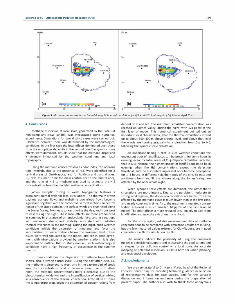
In concentrations field at 25 m above ground, there are twocenters of maximum that persist, in position and intensity, duringthe 24 hours simulated. The first, with concentrations above60 ppmv is centered at about 100 m downstream of the deposit,and the second, with more than 30 ppmv, at about 3.7 km. Thedistance between the deposit and the eastern end of 1 ppmvisoline remain constant, near 7.5 km, although its shape showssome variation in time. Also, to east, the distance between depositand the isoline of 0.001 ppmv not exceed 12.5 km during the24 hours of simulation.

In Figure S4b (see the SM) is shown a vertical section, in west–east direction, through the methane cloud at 06:00 LT. The sectionpasses through the center of the landfill. One can distinguish thetwo peaks corresponding to centers of maxima in Figure S5a (seethe SM). The height of 1 ppmv isoline is near 380 m, in the first800 m from landfill, then decrease gradually to zero at a distanceof 7.5 km from the deposit. The maximum height of 0.001 ppmvisoline is 625 m.

The maximum concentrations obtained on the first two levelsabove the ground, during the 24 hours of simulation, are shown inFigure 5. One can see that, on the second level of model, concentrations are smaller and appear three cores of maxima, and themethane cloud is more extended to east. In this case, Cluj–Napoca,Apahida and Jucu were not affected by the odor of H2S.

(a) (b)

(c) (d)

Soporan et al. – Atmospheric Pollution Research (APR) 319

Figure 5.Maximum concentrations achieved during 24 hours of simulation, for 6/7 April 2011, at height of (a) 25 m and (b) 75 m.

4. Conclusions

Methane dispersion at local scale, generated by the Pata Ratnon–compliant MSW landfill, was investigated using numericalexperiments. Simulations for two distinct cases were carried out.Difference between them was determined by the meteorologicalconditions. In the first case the local effects dominated over thosefrom the synoptic scale, while in the second case the synoptic scaleeffects were dominant. Results show that the methane dispersionis strongly influenced by the weather conditions and localtopography.

Using the methane concentrations as odor index, the odoroustime intervals, due to the presence of H2S, were identified for 2central areas of Cluj–Napoca, and for Apahida and Jucu villages.H2S was assumed to be the main contributor to the landfill odor,and the ratio of H2S to methane was used to estimate the H2Sconcentrations from the modeled methane concentrations.

When synoptic forcing is weak, topography features aprominent diurnal cycle for local circulations. The thermally drivendaytime upslope flows and nighttime downslope flows becomesignificant, together with the convective vertical motions. In centralregion of the study domain, the surface winds are channeled alongthe Somes Valley, from east to west during the day, and from westto east during the night. These local effects are more pronouncedin summer, in presence of an anticyclonic field, and in situationswith enhanced atmospheric stability associated with radiativethermal inversions in the morning. During the night, such weatherconditions inhibit the dispersion of methane, and favor theaccumulation of concentrations below the inversion level. Theseissues were well simulated by the model, and are in good agreement with observations provided by weather stations. It is alsoimportant to outline, that in study domain, such meteorologicalconditions have a high frequency of occurrence in the summermonths.

In these conditions the dispersion of methane from landfillshows, also, a strong diurnal cycle. During the day, after 09:00 LT,the methane is dispersed to west, and in the eastern part of studyarea the concentrations tend to decrease toward zero. In afternoon, the methane concentrations mark a decrease due to thephotochemical oxidation and the intensification of vertical mixing,as a consequence of the thermal convection. After 20:00 LT, oncethe temperature drop, begin the dispersion of concentrations from

deposit to E and NE. The maximum simulated concentration wasreached on Somes Valley, during the night, with 121 ppmv at thefirst level of model. This numerical experiment pointed out animportant local characteristic, that the thermal circulations extendup to about 350–400 m above ground level, and above that levelthe winds are turning gradually to a direction from SW to NE,following the synoptic scale circulation.

An important finding is that in such weather conditions theunpleasant odor of landfill gases can be present, for some hours inevening, even in central areas of Cluj–Napoca. Simulation indicate,that in Cluj–Napoca, the highest impact of landfill appears to be inevening, when the H2S concentrations exceed the detectionthreshold, and the associated unpleasant odor become perceptiblefor 1–3 hours, in different neighborhoods of the city. To east andnorth–east from landfill, the villages along the Somes Valley, areaffected by the odor whole night.

When synoptic scale effects are dominant, the atmosphericcirculations are more intense. Due to the persistent moderate tostrong wind regimes, the dispersion conditions are better. The areaaffected by the methane cloud is much lower than in the first case,and nearly constant in time. Also, the maximum simulated concentration achieved is much smaller, 64 ppmv at the first level ofmodel. The odor affects a more reduced area, mainly to east fromlandfill site, and near the axis of methane cloud.

For the study region, reliable measurement data of methaneconcentrations to be compared with simulation results are missing,but the few measured values existent for Cluj–Napoca, are in goodconcordance with the simulation results.

The results indicate the possibility of using the numericalmodel as a decisional support tool in assessing the applications andstrategies for air pollution control on a local scale. An accuratemapping of pollutant dispersion is useful both for urban planningand residential developers.

Acknowledgments

We are very grateful to Dr. Narcis Maier, head of the RegionalForecast Center Cluj, for providing technical guidance in selectionof representative days for case studies, and for the valuablediscussion and information exchange during the preparation ofpresent paper. The authors also wish to thank three anonymous

(a) (b)

Soporan et al. – Atmospheric Pollution Research (APR) 320

reviewers for their constructive comments that greatly improvedthe content of this paper.

Supporting Material Available

Site description and source characteristics input into the model(Text S1), Study area with landfill in center (Figure S1a), Terrainelevations vary between 270 and 800 m (Figure S1b), Aerial view ofMSW landfill (Figure S1c), Horizontal sections in wind field providedby model at altitude of 325 m above MSL at 06:42, 10:51, 20:48 LTand at 1 225 m above MSL at 10:51 LT in 06.08.2012 (Figure S2),Temperature field at 850 hPa level on 06.08.2012, 03:00 LT (FigureS3a), Aerological sounding from Cluj–Napoca on 06.08.2012,03:00 LT (Figure S3b), Surface pressure field on 06.08.2012 at03:00 LT (Figure S3c), Surface pressure field on 06.04.2011,15:00 LT (Figure S4a), Vertical section in west–east directionthrough methane cloud at 06:00 LT on 06.04.2011 (Figure S4b),Methane concentrations at height of 25 m above the ground at06:00, 12:00 and 18:00 LT on 06.04.2011 and at 02:00 LT on07.04.2011 (Figure S5), Methane concentrations provided bymodel in sensitivity runs R11 and R22 at 06:00 and 08:00 LT on06.08.2012 (Figure S6), Time evolution of observed and modeledwind components in sensitivity runs G1, G2 and G3 for 06.08.2012and vertical distribution of temperature and specific humidity,measured and provided by model, at 03:00 LT on 07.08.2012(Figure S7), Mean annual relative frequencies of occurrences ofwind direction on 8 directions in % (Table S1), Size of area withconcentrations greater than 0 ppmv and maximum value ofconcentrations in sensitivity experiences of results to Cs values(Table S2), RMS error for wind components provided by modelwith grids G1, G2 and G3 (Table S3). This information is availablefree of charge via the Internet at http://www.atmospolres.com.

References

Aloyan, A.E., Arutyunyan, V.O., Yermakov, A.N., Zagaynov, V.A., Mensink,C., De Ridder, K., Van de Vel, K., Deutsch, F., 2012. Modeling theregional dynamics of gaseous admixtures and aerosols in the areas ofLake Baikal (Russia) and Antwerp (Belgium). Aerosol and Air QualityResearch 12, 707–721.

Anikender, K., Goyal, P., 2012. An analytical model for pollutants dispersionreleased from different sources in atmospheric boundary layer. Journalof Environmental Research and Development 7, 131–138.

Bianco, L., Tomassetti, B., Coppola, E., Fracassi, A., Verdecchia, M., Visconti,G., 2006. Thermally driven circulation in a region of complextopography: Comparison of wind–profiling radar measurement andMM5 numerical predictions. Annales Geophysicae 24, 1537–1549.

Clark, T.L., 1979. Numerical simulations with a three–dimensional cloudmodel: Lateral boundary condition experiments and multicellularsevere storm simulations. Journal of the Atmospheric Sciences 36,2191–2215.

Costa, A., Macedonio, G., Chiodini, G., 2005. Numerical model of gasdispersion emitted from volcanic sources. Annals of Geophysics 48,805–815.

CPCB (Central Pollution Control Board), 2008. Guidelines on OdourPollution and its Control, Ministry of Environment & Forests,Government of India, Report No. 1100 32, Delhi, 57 pages.

Cuna, C., Ardelean, P., Cuna, S., 2003. The analysis of atmospheric methaneconcentration in the Areal of Cluj. Studia Universitatis Babes–Bolyai,Physica XLVIII, 565–567.

Goldsmith, C.D., Chanton, J., Abichou, T., Swan, N., Green, R., Hater, G.,2012. Methane emissions from 20 landfills across the United Statesusing vertical radial plume mapping. Journal of the Air & WasteManagement Association 62, 183–197.

Grigoras, G., Mocioaca, G., 2012. Air quality assessment in Craiova urbanarea. Romanian Reports in Physics 64, 768–787.

Grigoras, G., Cuculeanu, V., Ene, G., Mocioaca, G., Deneanu, A., 2012. Airpollution dispersion modeling in a polluted industrial area of complexterrain from Romania. Romanian Reports in Physics 64, 173–186.

Gross, G., 2001. On the applicability of a numerical model system forcalculating new European air pollution measures. MeteorologischeZeitschrift 10, 307–314.

Haiduc, I., Beldean–Galea, M.S., 2011. Variation of greenhouse gases inurban areas – case study: CO2, CO and CH4 in three Romanian cities, inAir Quality–Models and Applications, edited by Popovic, D., INTech, UK,pp. 289–318.

Hategan, R.M., Popita, G.E., Varga, I., Popovici, A., Frentiu, T., 2012. Theheavy metals impact on surface water and soil in the non–sanitarymunicipal landfill "Pata Rat"– Cluj–Napoca. Studia Universitatis Babes–Bolyai Chemia 57, 119–126.

Holmes, N.S., Morawska, L., 2006. A review of dispersion modelling and itsapplication to the dispersion of particles: An overview of differentdispersion models available. Atmospheric Environment 40, 5902–5928.

Holton, J.R., 2004. The planetary boundary layer, in An Introduction toDynamic Meteorology, edited by Dmowska, R., Holton J.R., Rossby H.T.,Elsevier Academic Press, U.S.A., pp. 116–140.

Kakosimos, K.E., Assael, M.J., Lioumbas, J.S., Spiridis, A.S., 2011.Atmospheric dispersion modelling of the fugitive particulate matterfrom overburden dumps with numerical and integral models.Atmospheric Pollution Research 2, 24–33.

Kallos, G., 1989. The use of mesoscale models on air–pollution studies inindustrial installations. Environmental Software 4, 117 – 122.

Konglok, S.A., Pochai, N., 2012. A numerical treatment of smoke dispersionmodel from three sources using fractional step method. AdvancedStudies in Theoretical Physics 6, 217–223.

Lagouvardos, K., Kotroni, V., Kallos, G., 1996. Exploring the effects ofdifferent types of model initialisation: Simulation of a severe air–pollution episode in Athens, Greece. Meteorological Applications 3,147–155.

Lesouef, D., Gheusi, F., Delmas, R., Escobar, J., 2011. Numerical simulationsof local circulations and pollution transport over Reunion Island.Annales Geophysicae 29, 53–69.

Lilly, D.K., 1967. The representation of small scale turbulence in numericalsimulation experiments. Proceedings of the IBM Scientific ComputingSymposium on Environmental Sciences, IBM Data Processing Division,White Plains, New York., pp. 195–210.

Lilly, D.K., 1962. On the numerical simulation of buoyant convection. Tellus14, 148–172.

Markatos, N.C., 1989. Computational fluid–flow capabilities and software.Ironmaking & Steelmaking 16, 266–273.

Martilli, A., 2003. A two–dimensional numerical study of the impact of acity on atmospheric circulation and pollutant dispersion in a coastalenvironment. Boundary–Layer Meteorology 108, 91–119.

Mayhoub, A.B., Essa, K.S.M., Aly, S., 2003. Analytical form of pollutantsdispersion for different atmospheric conditions. Romanian Reports inPhysics 55, 94–101.

McDonough, J.M., 2007. Solution Algorithms for the N.–S. Equations,Lectures in Computational Fluid Dynamics of Incompressible Flow:Mathematics, Algorithms and Implementations, Departments ofMechanical Engineering and Mathematics, University of Kentucky, pp.99–143. http://www.engr.uky.edu/~acfd/me691–lctr–nts.pdf, accessedin January 2013.

Patankar, S.V., 1980. Calculation of the flow field, in Numerical HeatTransfer and Fluid Flow, Taylor & Francis, New York, pp. 113–138.

Philippopoulos, K., Deligiorgi, D., Karvounis, G., Tzanakou, M., 2009.Pollution dispersion modeling at Chania, Greece, under variousmeteorological conditions. Proceedings of the 5th InternationalConference on Energy, Environment, Ecosystems and SustainableDevelopment (EEESD ’09), September 28–30, 2009, Vouliagmeni,Athens, Greece, pp. 133–138.

Rampanelli, G., Zardi, D., Rotunno, R., 2004. Mechanisms of up–valleywinds. Journal of the Atmospheric Sciences 61, 3097–3111.

Soporan et al. – Atmospheric Pollution Research (APR) 321

Reuten, C., Steyn, D.G., Allen, S.E., 2007. Water tank studies of atmosphericboundary layer structure and air pollution transport in upslope flowsystems. Journal of Geophysical Research–Atmospheres 112, art. no.D11114.

Sandu, I., Pescaru, V.I., Poiana, I., 2008. The Climate of Romania, (inRomanian), Editura Academiei, Bucuresti, pp. 171–187.

Schmitz, R., 2005. Modelling of air pollution dispersion in Santiago de Chile.Atmospheric Environment 39, 2035–2047.

Smagorinsky, J., 1963. General circulation experiments with the primitiveequations.Monthly Weather Review 91, 99–164.

Soporan, V.F., Vamos, C., Pavai, C., 2003. Numerical Modeling ofSolidification, (in Romanian), Editura Dacia, Cluj–Napoca, pp. 89–197.

Souza, E.P., Renno, N.O., Dias, M.A.F.S., 2000. Convective circulationsinduced by surface heterogeneities. Journal of the AtmosphericSciences 57, 2915–2922.

U.K. EA (United Kingdom Environment Agency), 2002. Investigation of theComposition and Emissions of Trace Components in Landfill Gas,Technical Report No. P1–438/TRR, Bristol, 148 pages.

Tagaris, E., Sotiropoulou, R.E.P., Pilinis, C., Halvadakis, C.P., 2003. Amethodology to estimate odors around landfill sites: The use ofmethane as an odor index and its utility in landfill siting. Journal of theAir & Waste Management Association 53, 629–634.

Vac (Soporan), M.B., Soporan, V.F., Cocis, E.A., Batranescu, G., Nemes, O.,2012. Gas Analysis of Municipal Landfill Emissions. Studia UniversitatisBabes – Bolyai, Chemia LVII, 23–30.