Quelques EDP simples r´esolues avec FreeFem++, Astuces et Trucs

Quelques EDP simplesresolues avec FreeFem++,

Astuces et TrucsF. Hecht

Laboratoire Jacques-Louis Lions

Universite Pierre et Marie Curie

Paris, France

with O. Pironneau

http://www.freefem.org mailto:[email protected]

Journee Gamni, IHP, 23 sept. 2005 1

http://www.freefem.org

mailto:[email protected]

PLAN

– Historique

– Introduction Freefem++

– nouveaute

– Equation de Poisson dependante du temps

– Ecriture variationnelle

– Ecriture matricielle (Optimiser)

– frontiere Libre

– Inequation variationnelle

– Methode de Joint

– Conclusion / Future

http://www.freefem.org/


HISTORIQUE

Idee suivre le cours de calcul scientifique, Olivier, Frederic, M2, UPMC,

second semestre

– Macgfem ( Olivier , ....)

– freefem (Oliver, Bernardi Dominique, Prud’homme, Frederic)

– freefem+ (Olivier, Bernardi Dominique, Frederic)

– freefem++ (Frederic , Olivier, Antoine Le Hyaric)

– freefem3d (Stephane Del Pino, Olivier)


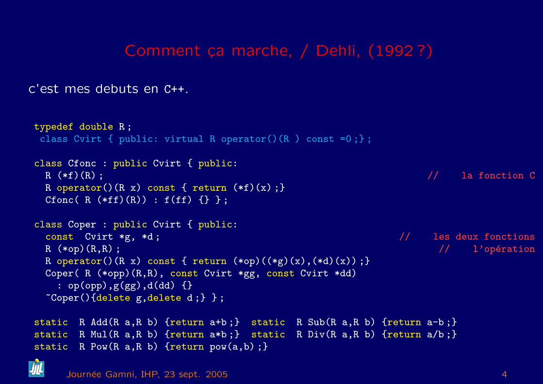
Comment ca marche, / Dehli, (1992 ?)

c’est mes debuts en C++.

typedef double R ;class Cvirt public: virtual R operator()(R ) const =0 ; ;

class Cfonc : public Cvirt public:R (*f)(R) ; // la fonction CR operator()(R x) const return (*f)(x) ;Cfonc( R (*ff)(R)) : f(ff) ;

class Coper : public Cvirt public:const Cvirt *g, *d ; // les deux fonctionsR (*op)(R,R) ; // l’operationR operator()(R x) const return (*op)((*g)(x),(*d)(x)) ;Coper( R (*opp)(R,R), const Cvirt *gg, const Cvirt *dd)

: op(opp),g(gg),d(dd) ~Coper()delete g,delete d ; ;

static R Add(R a,R b) return a+b ; static R Sub(R a,R b) return a-b ;static R Mul(R a,R b) return a*b ; static R Div(R a,R b) return a/b ;static R Pow(R a,R b) return pow(a,b) ;


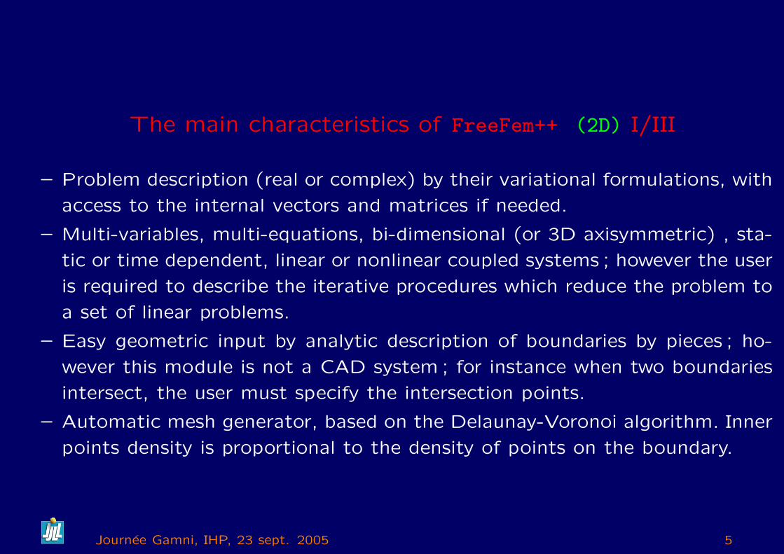
The main characteristics of FreeFem++ (2D) I/III

– Problem description (real or complex) by their variational formulations, with

access to the internal vectors and matrices if needed.

– Multi-variables, multi-equations, bi-dimensional (or 3D axisymmetric) , sta-

tic or time dependent, linear or nonlinear coupled systems ; however the user

is required to describe the iterative procedures which reduce the problem to

a set of linear problems.

– Easy geometric input by analytic description of boundaries by pieces ; ho-

wever this module is not a CAD system ; for instance when two boundaries

intersect, the user must specify the intersection points.

– Automatic mesh generator, based on the Delaunay-Voronoi algorithm. Inner

points density is proportional to the density of points on the boundary.


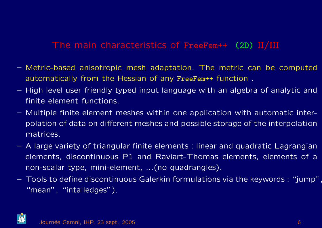
The main characteristics of FreeFem++ (2D) II/III

– Metric-based anisotropic mesh adaptation. The metric can be computed

automatically from the Hessian of any FreeFem++ function .

– High level user friendly typed input language with an algebra of analytic and

finite element functions.

– Multiple finite element meshes within one application with automatic inter-

polation of data on different meshes and possible storage of the interpolation

matrices.

– A large variety of triangular finite elements : linear and quadratic Lagrangian

elements, discontinuous P1 and Raviart-Thomas elements, elements of a

non-scalar type, mini-element, ...(no quadrangles).

– Tools to define discontinuous Galerkin formulations via the keywords : “jump”,

“mean”, “intalledges”).


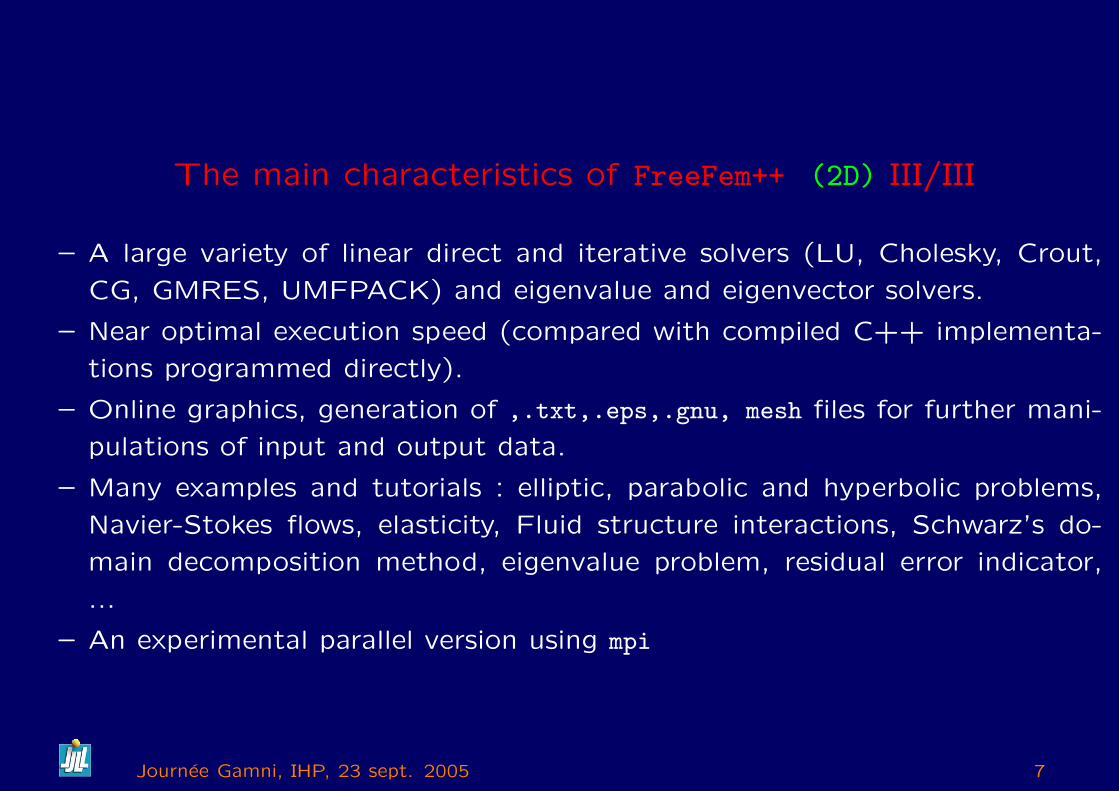
The main characteristics of FreeFem++ (2D) III/III

– A large variety of linear direct and iterative solvers (LU, Cholesky, Crout,

CG, GMRES, UMFPACK) and eigenvalue and eigenvector solvers.

– Near optimal execution speed (compared with compiled C++ implementa-

tions programmed directly).

– Online graphics, generation of ,.txt,.eps,.gnu, mesh files for further mani-

pulations of input and output data.

– Many examples and tutorials : elliptic, parabolic and hyperbolic problems,

Navier-Stokes flows, elasticity, Fluid structure interactions, Schwarz’s do-

main decomposition method, eigenvalue problem, residual error indicator,

...

– An experimental parallel version using mpi


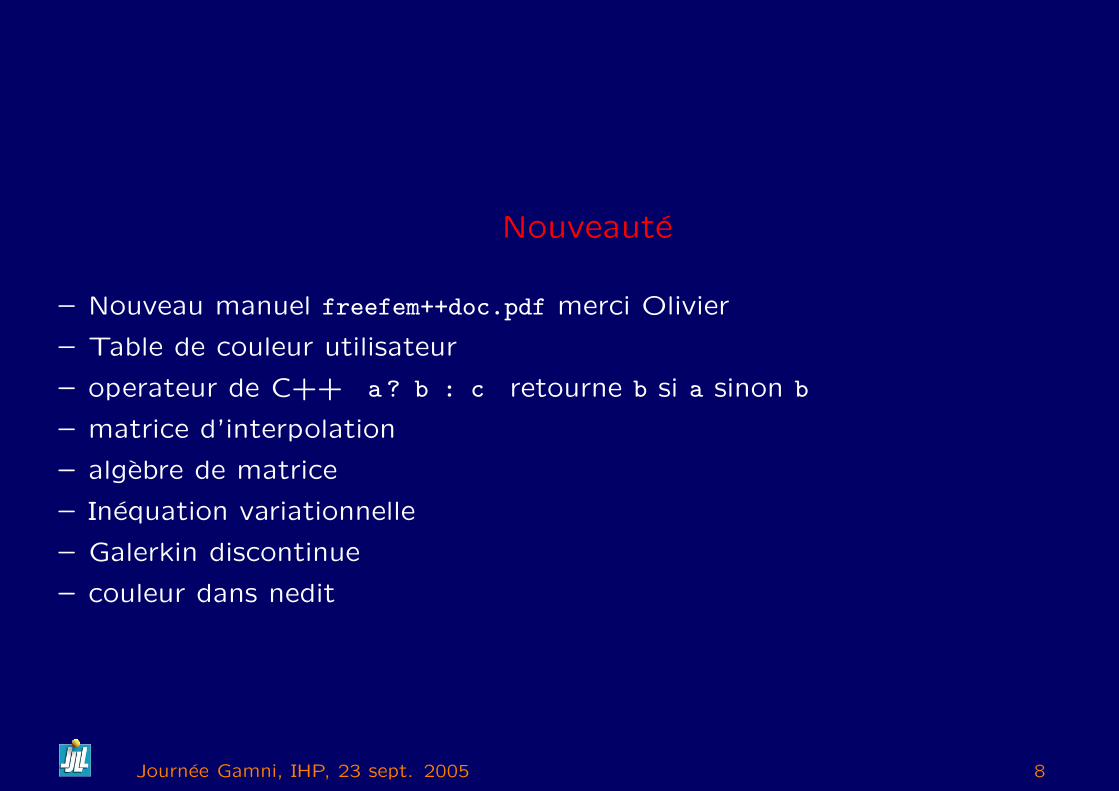
Nouveaute

– Nouveau manuel freefem++doc.pdf merci Olivier

– Table de couleur utilisateur

– operateur de C++ a ? b : c retourne b si a sinon b

– matrice d’interpolation

– algebre de matrice

– Inequation variationnelle

– Galerkin discontinue

– couleur dans nedit


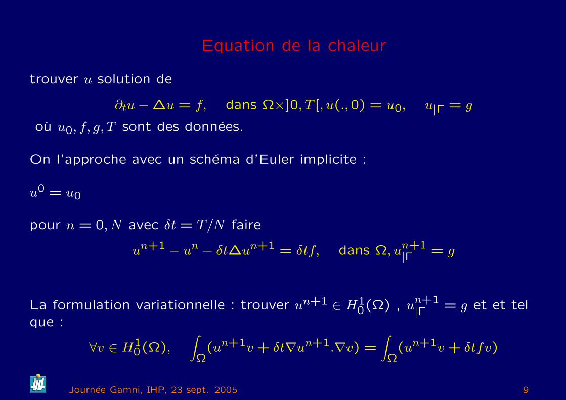
Equation de la chaleur

trouver u solution de

∂tu−∆u = f, dans Ω×]0, T [, u(.,0) = u0, u|Γ = g

ou u0, f, g, T sont des donnees.

On l’approche avec un schema d’Euler implicite :

u0 = u0

pour n = 0, N avec δt = T/N faire

un+1 − un − δt∆un+1 = δtf, dans Ω, un+1|Γ = g

La formulation variationnelle : trouver un+1 ∈ H10(Ω) , un+1

|Γ = g et et telque :

∀v ∈ H10(Ω),

∫Ω(un+1v + δt∇un+1.∇v) =

∫Ω(un+1v + δtfv)


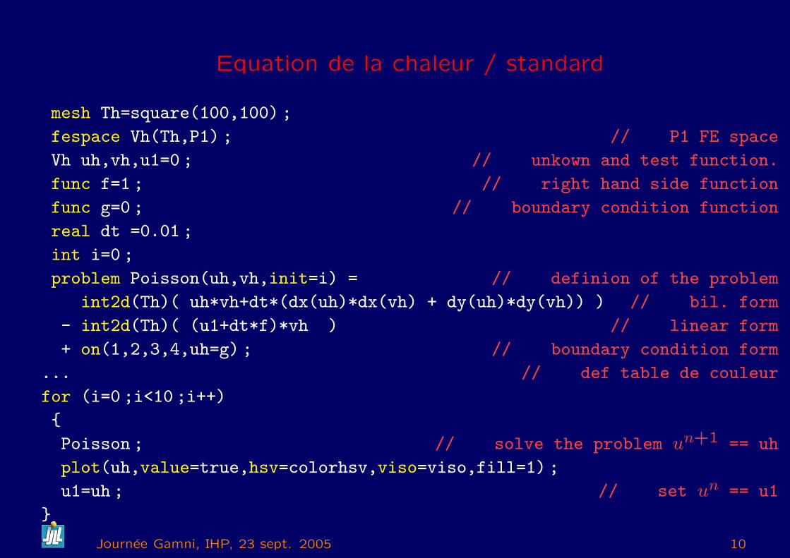
Equation de la chaleur / standard

mesh Th=square(100,100) ;

fespace Vh(Th,P1) ; // P1 FE space

Vh uh,vh,u1=0 ; // unkown and test function.

func f=1 ; // right hand side function

func g=0 ; // boundary condition function

real dt =0.01 ;

int i=0 ;

problem Poisson(uh,vh,init=i) = // definion of the problem

int2d(Th)( uh*vh+dt*(dx(uh)*dx(vh) + dy(uh)*dy(vh)) ) // bil. form

- int2d(Th)( (u1+dt*f)*vh ) // linear form

+ on(1,2,3,4,uh=g) ; // boundary condition form

... // def table de couleur

for (i=0 ;i<10 ;i++)

Poisson ; // solve the problem un+1 == uh

plot(uh,value=true,hsv=colorhsv,viso=viso,fill=1) ;

u1=uh ; // set un == u1


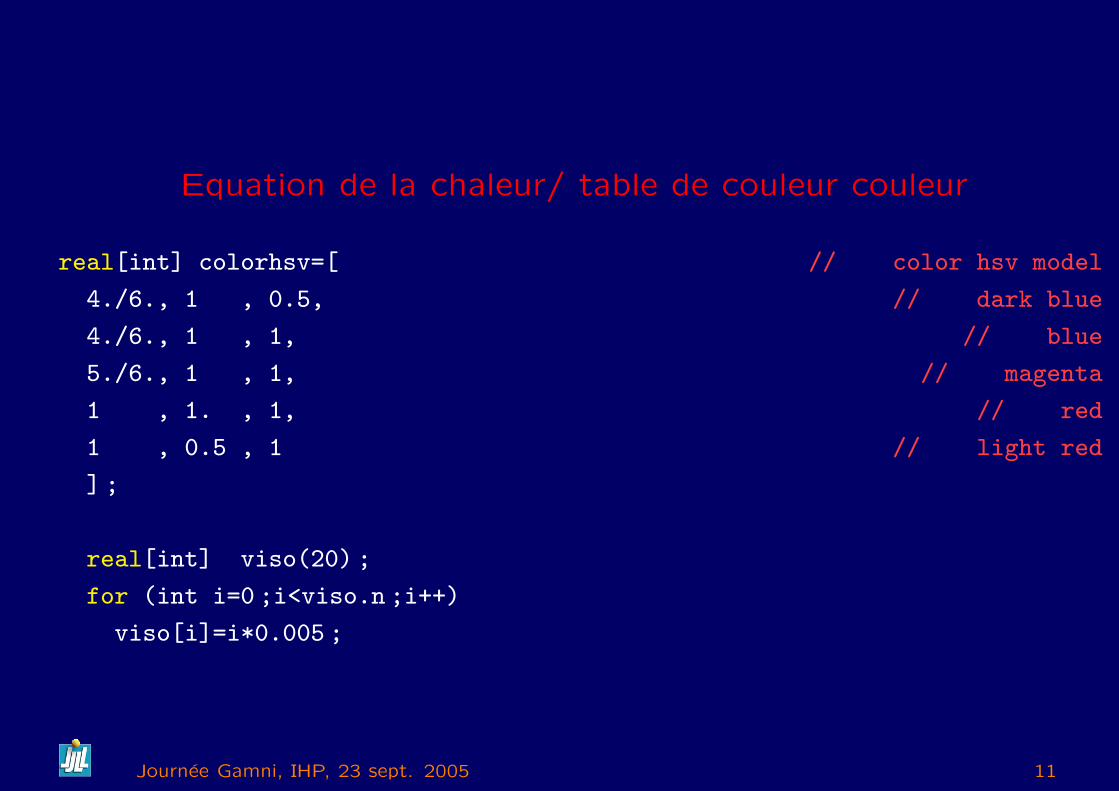
Equation de la chaleur/ table de couleur couleur

real[int] colorhsv=[ // color hsv model

4./6., 1 , 0.5, // dark blue

4./6., 1 , 1, // blue

5./6., 1 , 1, // magenta

1 , 1. , 1, // red

1 , 0.5 , 1 // light red

] ;

real[int] viso(20) ;

for (int i=0 ;i<viso.n ;i++)

viso[i]=i*0.005 ;


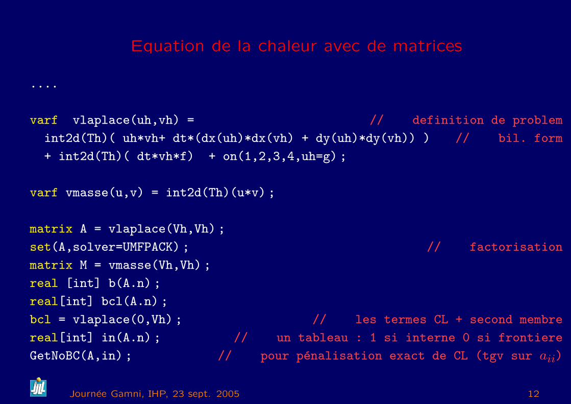
Equation de la chaleur avec de matrices

....

varf vlaplace(uh,vh) = // definition de problem

int2d(Th)( uh*vh+ dt*(dx(uh)*dx(vh) + dy(uh)*dy(vh)) ) // bil. form

+ int2d(Th)( dt*vh*f) + on(1,2,3,4,uh=g) ;

varf vmasse(u,v) = int2d(Th)(u*v) ;

matrix A = vlaplace(Vh,Vh) ;

set(A,solver=UMFPACK) ; // factorisation

matrix M = vmasse(Vh,Vh) ;

real [int] b(A.n) ;

real[int] bcl(A.n) ;

bcl = vlaplace(0,Vh) ; // les termes CL + second membre

real[int] in(A.n) ; // un tableau : 1 si interne 0 si frontiere

GetNoBC(A,in) ; // pour penalisation exact de CL (tgv sur aii)


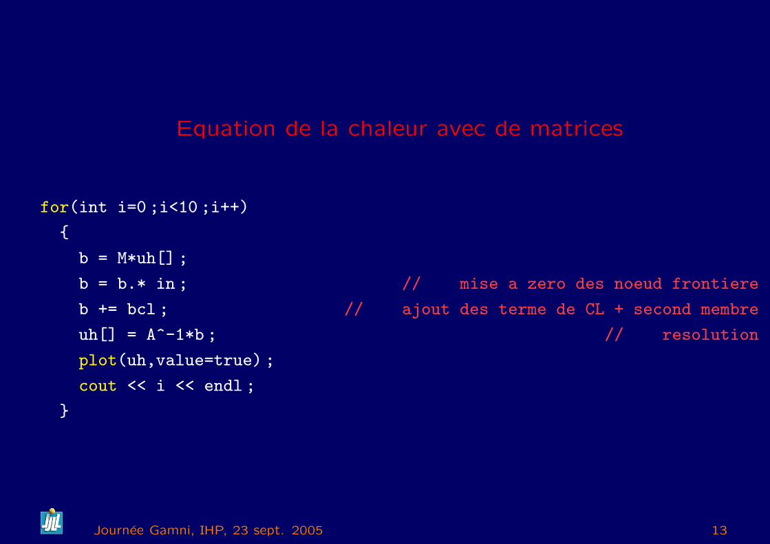
Equation de la chaleur avec de matrices

for(int i=0 ;i<10 ;i++)

b = M*uh[] ;

b = b.* in ; // mise a zero des noeud frontiere

b += bcl ; // ajout des terme de CL + second membre

uh[] = A^-1*b ; // resolution

plot(uh,value=true) ;

cout << i << endl ;


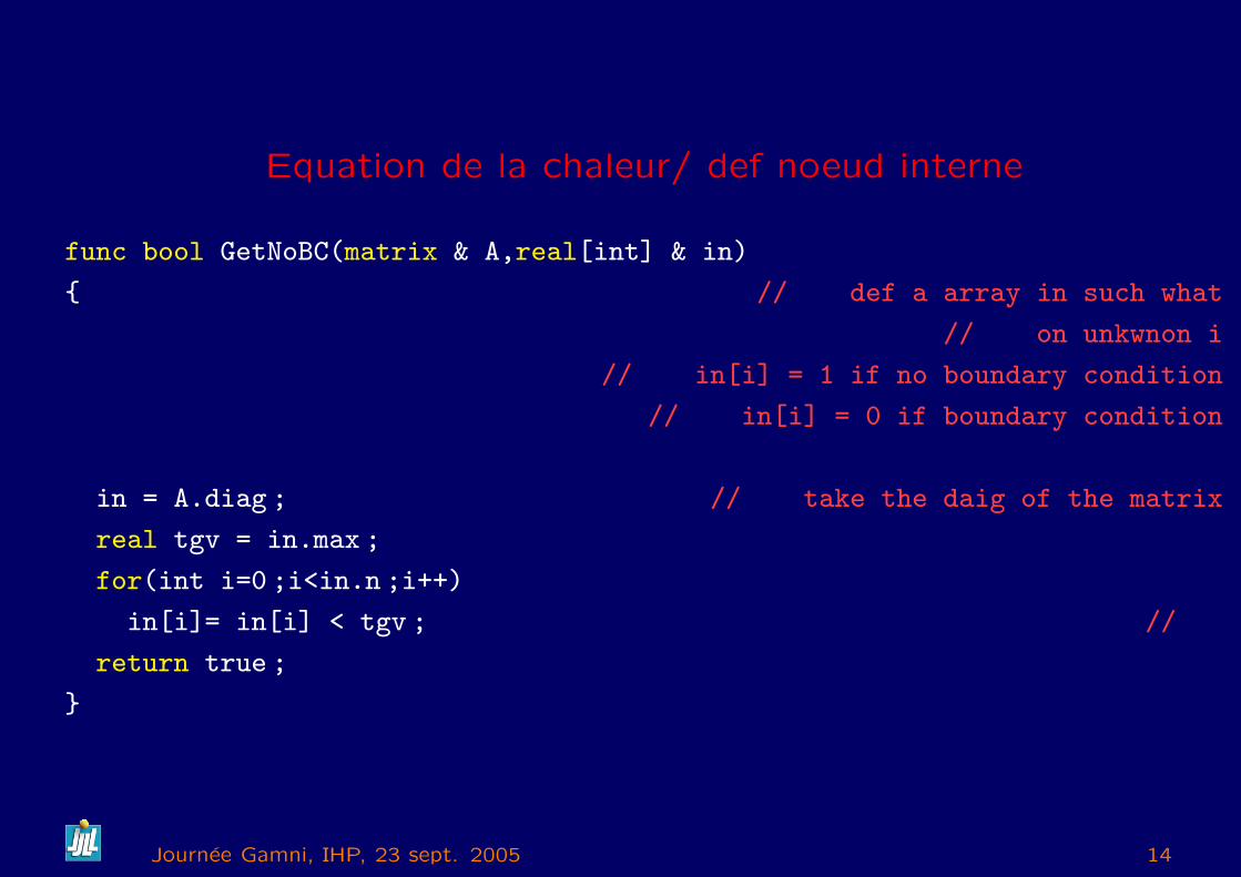
Equation de la chaleur/ def noeud interne

func bool GetNoBC(matrix & A,real[int] & in)

// def a array in such what

// on unkwnon i

// in[i] = 1 if no boundary condition

// in[i] = 0 if boundary condition

in = A.diag ; // take the daig of the matrix

real tgv = in.max ;

for(int i=0 ;i<in.n ;i++)

in[i]= in[i] < tgv ; //

return true ;


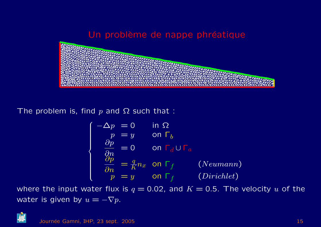
Un probleme de nappe phreatique

The problem is, find p and Ω such that :

−∆p = 0 in Ωp = y on Γb

∂p

∂n= 0 on Γd ∪ Γa

∂p

∂n= q

Knx on Γf (Neumann)

p = y on Γf (Dirichlet)

where the input water flux is q = 0.02, and K = 0.5. The velocity u of the

water is given by u = −∇p.


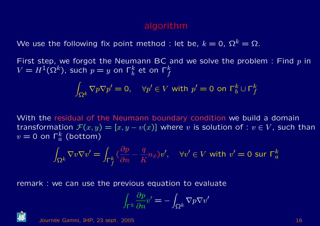
algorithm

We use the following fix point method : let be, k = 0, Ωk = Ω.

First step, we forgot the Neumann BC and we solve the problem : Find p inV = H1(Ωk), such p = y on Γk

b et on Γkf∫

Ωk∇p∇p′ = 0, ∀p′ ∈ V with p′ = 0 on Γk

b ∪ Γkf

With the residual of the Neumann boundary condition we build a domaintransformation F(x, y) = [x, y − v(x)] where v is solution of : v ∈ V , such thanv = 0 on Γk

a (bottom)∫Ωk

∇v∇v′ =∫Γk

f

(∂p

∂n−

q

Knx)v

′, ∀v′ ∈ V with v′ = 0 sur Γka

remark : we can use the previous equation to evaluate∫Γk

∂p

∂nv′ = −

∫Ωk

∇p∇v′


The new domain is : Ωk+1 = F(Ωk)

Warning if is the movement is too large we can have triangle overlapping.

problem Pp(p,pp,solver=CG) = int2d(Th)( dx(p)*dx(pp)+dy(p)*dy(pp))

+ on(b,f,p=y) ;

problem Pv(v,vv,solver=CG) = int2d(Th)( dx(v)*dx(vv)+dy(v)*dy(vv))

+ on (a, v=0) + int1d(Th,f)(vv*((Q/K)*N.y)) + wdpdn[] ) ;

while(errv>1e-6)

j++ ; Pp ;

wdpdn[] = A*p[] ; wdpdn[] = wdpdn[].*onfree[] ; wdpdn[] = -wdpdn[] ;

// hack

Pv ; errv=int1d(Th,f)(v*v) ;

coef = 1 ;

// Here french cooking if overlapping see the example

Th=movemesh(Th,[x,y-coef*v]) ; // deformation

file:///Users/hecht/Desktop/ffday


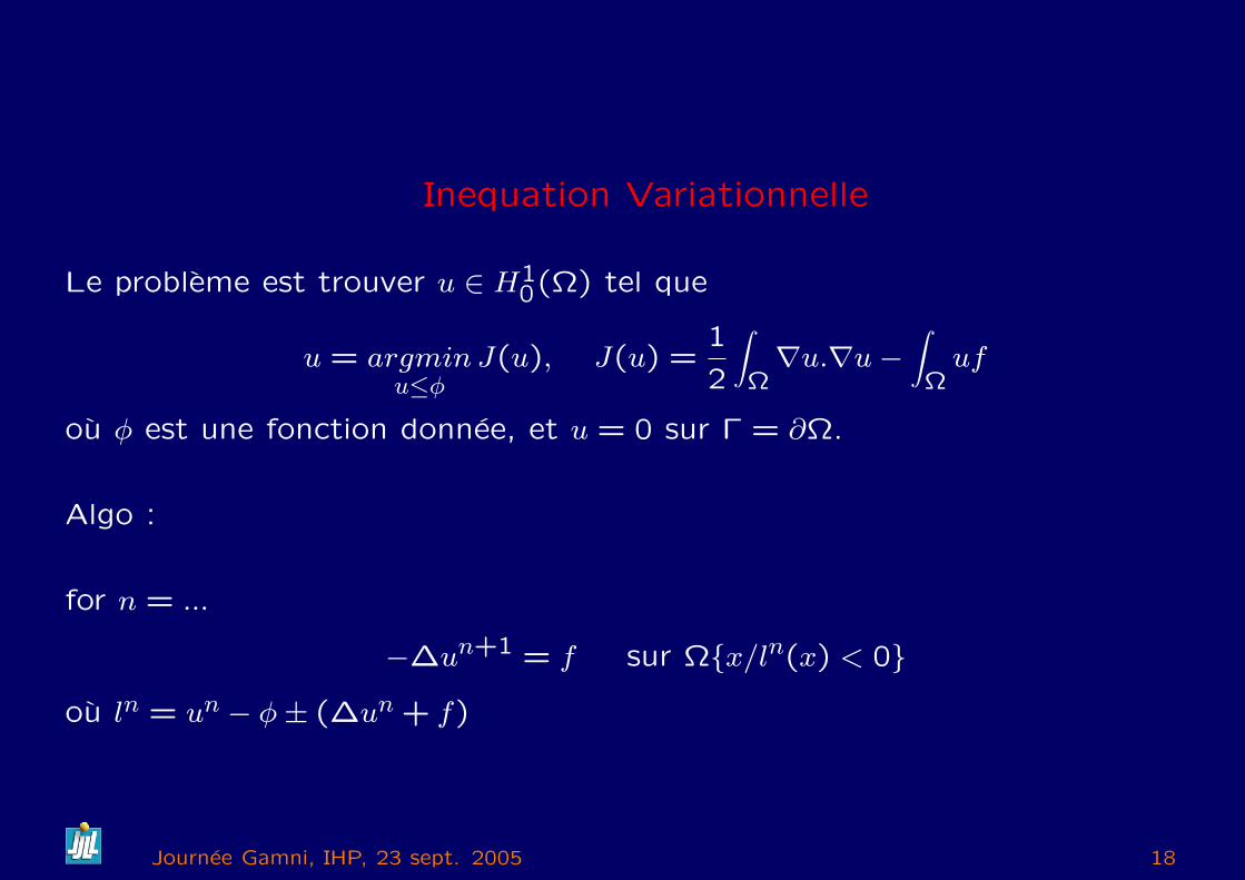
Inequation Variationnelle

Le probleme est trouver u ∈ H10(Ω) tel que

u = argminu≤φ

J(u), J(u) =1

2

∫Ω∇u.∇u−

∫Ω

uf

ou φ est une fonction donnee, et u = 0 sur Γ = ∂Ω.

Algo :

for n = ...

−∆un+1 = f sur Ωx/ln(x) < 0

ou ln = un − φ± (∆un + f)


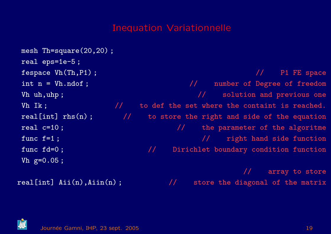
Inequation Variationnelle

mesh Th=square(20,20) ;

real eps=1e-5 ;

fespace Vh(Th,P1) ; // P1 FE space

int n = Vh.ndof ; // number of Degree of freedom

Vh uh,uhp ; // solution and previous one

Vh Ik ; // to def the set where the containt is reached.

real[int] rhs(n) ; // to store the right and side of the equation

real c=10 ; // the parameter of the algoritme

func f=1 ; // right hand side function

func fd=0 ; // Dirichlet boundary condition function

Vh g=0.05 ;

// array to store

real[int] Aii(n),Aiin(n) ; // store the diagonal of the matrix


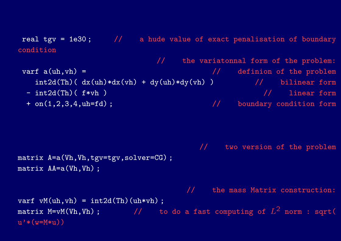
real tgv = 1e30 ; // a hude value of exact penalisation of boundary

condition

// the variatonnal form of the problem:

varf a(uh,vh) = // definion of the problem

int2d(Th)( dx(uh)*dx(vh) + dy(uh)*dy(vh) ) // bilinear form

- int2d(Th)( f*vh ) // linear form

+ on(1,2,3,4,uh=fd) ; // boundary condition form

// two version of the problem

matrix A=a(Vh,Vh,tgv=tgv,solver=CG) ;

matrix AA=a(Vh,Vh) ;

// the mass Matrix construction:

varf vM(uh,vh) = int2d(Th)(uh*vh) ;

matrix M=vM(Vh,Vh) ; // to do a fast computing of L2 norm : sqrt(

u’*(w=M*u))

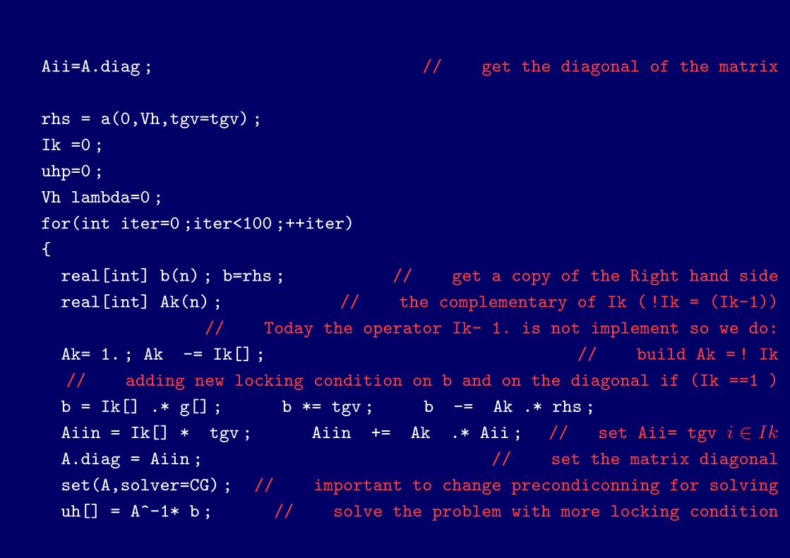
Aii=A.diag ; // get the diagonal of the matrix

rhs = a(0,Vh,tgv=tgv) ;

Ik =0 ;

uhp=0 ;

Vh lambda=0 ;

for(int iter=0 ;iter<100 ;++iter)

real[int] b(n) ; b=rhs ; // get a copy of the Right hand side

real[int] Ak(n) ; // the complementary of Ik ( !Ik = (Ik-1))

// Today the operator Ik- 1. is not implement so we do:

Ak= 1. ; Ak -= Ik[] ; // build Ak = ! Ik

// adding new locking condition on b and on the diagonal if (Ik ==1 )

b = Ik[] .* g[] ; b *= tgv ; b -= Ak .* rhs ;

Aiin = Ik[] * tgv ; Aiin += Ak .* Aii ; // set Aii= tgv i ∈ Ik

A.diag = Aiin ; // set the matrix diagonal

set(A,solver=CG) ; // important to change precondiconning for solving

uh[] = A^-1* b ; // solve the problem with more locking condition

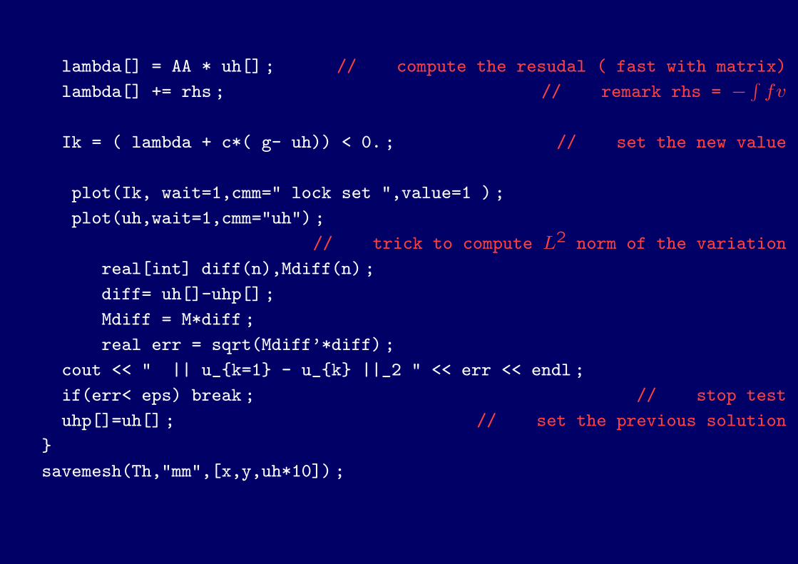
lambda[] = AA * uh[] ; // compute the resudal ( fast with matrix)

lambda[] += rhs ; // remark rhs = −∫

fv

Ik = ( lambda + c*( g- uh)) < 0. ; // set the new value

plot(Ik, wait=1,cmm=" lock set ",value=1 ) ;

plot(uh,wait=1,cmm="uh") ;

// trick to compute L2 norm of the variation

real[int] diff(n),Mdiff(n) ;

diff= uh[]-uhp[] ;

Mdiff = M*diff ;

real err = sqrt(Mdiff’*diff) ;

cout << " || u_k=1 - u_k ||_2 " << err << endl ;

if(err< eps) break ; // stop test

uhp[]=uh[] ; // set the previous solution

savemesh(Th,"mm",[x,y,uh*10]) ;

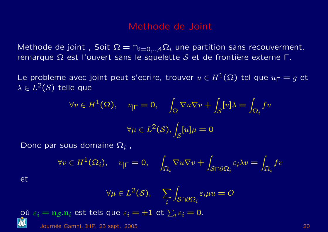
Methode de Joint

Methode de joint , Soit Ω = ∩i=0,..,4Ωi une partition sans recouverment.remarque Ω est l’ouvert sans le squelette S et de frontiere externe Γ.

Le probleme avec joint peut s’ecrire, trouver u ∈ H1(Ω) tel que uΓ = g etλ ∈ L2(S) telle que

∀v ∈ H1(Ω), v|Γ = 0,∫Ω∇u∇v +

∫S[v]λ =

∫Ωi

fv

∀µ ∈ L2(S),∫S[u]µ = 0

Donc par sous domaine Ωi ,

∀v ∈ H1(Ωi), v|Γ = 0,∫Ωi

∇u∇v +∫S∩∂Ωi

εiλv =∫Ωi

fv

et

∀µ ∈ L2(S),∑i

∫S∩∂Ωi

εiµu = O

ou εi = nS.ni est tels que εi = ±1 et∑

i εi = 0.


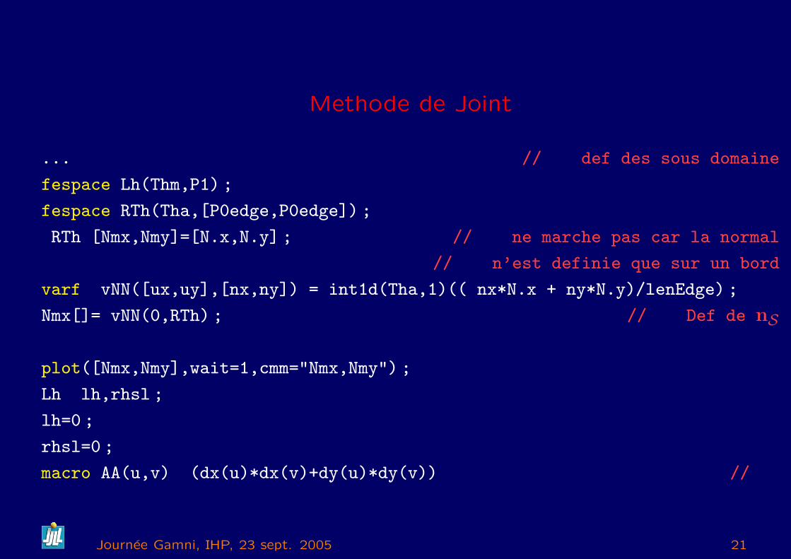
Methode de Joint

... // def des sous domaine

fespace Lh(Thm,P1) ;

fespace RTh(Tha,[P0edge,P0edge]) ;

RTh [Nmx,Nmy]=[N.x,N.y] ; // ne marche pas car la normal

// n’est definie que sur un bord

varf vNN([ux,uy],[nx,ny]) = int1d(Tha,1)(( nx*N.x + ny*N.y)/lenEdge) ;

Nmx[]= vNN(0,RTh) ; // Def de nS

plot([Nmx,Nmy],wait=1,cmm="Nmx,Nmy") ;

Lh lh,rhsl ;

lh=0 ;

rhsl=0 ;

macro AA(u,v) (dx(u)*dx(v)+dy(u)*dy(v)) //


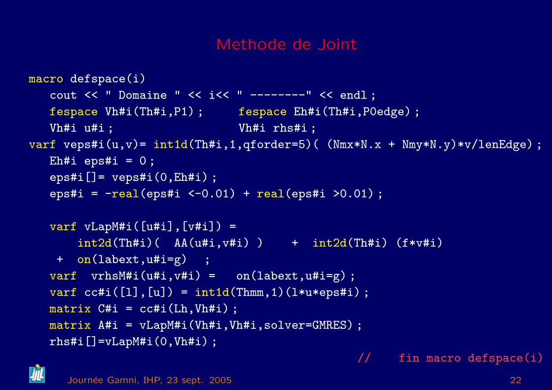
Methode de Joint

macro defspace(i)

cout << " Domaine " << i<< " --------" << endl ;

fespace Vh#i(Th#i,P1) ; fespace Eh#i(Th#i,P0edge) ;

Vh#i u#i ; Vh#i rhs#i ;

varf veps#i(u,v)= int1d(Th#i,1,qforder=5)( (Nmx*N.x + Nmy*N.y)*v/lenEdge) ;

Eh#i eps#i = 0 ;

eps#i[]= veps#i(0,Eh#i) ;

eps#i = -real(eps#i <-0.01) + real(eps#i >0.01) ;

varf vLapM#i([u#i],[v#i]) =

int2d(Th#i)( AA(u#i,v#i) ) + int2d(Th#i) (f*v#i)

+ on(labext,u#i=g) ;

varf vrhsM#i(u#i,v#i) = on(labext,u#i=g) ;

varf cc#i([l],[u]) = int1d(Thmm,1)(l*u*eps#i) ;

matrix C#i = cc#i(Lh,Vh#i) ;

matrix A#i = vLapM#i(Vh#i,Vh#i,solver=GMRES) ;

rhs#i[]=vLapM#i(0,Vh#i) ;

// fin macro defspace(i)


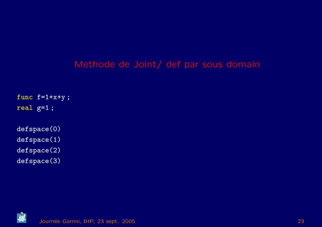
Methode de Joint/ def par sous domain

func f=1+x+y ;

real g=1 ;

defspace(0)

defspace(1)

defspace(2)

defspace(3)


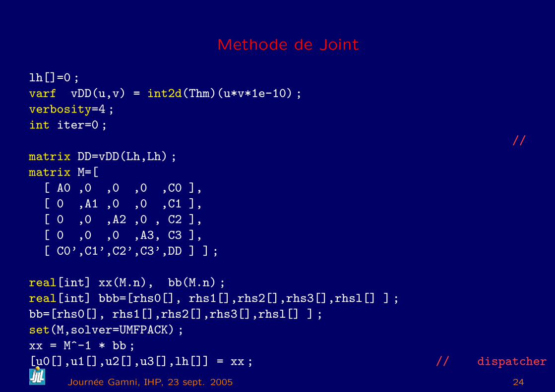
Methode de Joint

lh[]=0 ;

varf vDD(u,v) = int2d(Thm)(u*v*1e-10) ;

verbosity=4 ;

int iter=0 ;

//

matrix DD=vDD(Lh,Lh) ;

matrix M=[

[ A0 ,0 ,0 ,0 ,C0 ],

[ 0 ,A1 ,0 ,0 ,C1 ],

[ 0 ,0 ,A2 ,0 , C2 ],

[ 0 ,0 ,0 ,A3, C3 ],

[ C0’,C1’,C2’,C3’,DD ] ] ;

real[int] xx(M.n), bb(M.n) ;

real[int] bbb=[rhs0[], rhs1[],rhs2[],rhs3[],rhsl[] ] ;

bb=[rhs0[], rhs1[],rhs2[],rhs3[],rhsl[] ] ;

set(M,solver=UMFPACK) ;

xx = M^-1 * bb ;

[u0[],u1[],u2[],u3[],lh[]] = xx ; // dispatcher


Conclusion and Future

It is a useful tool to teaches Finite Element Method, and to test some

nontrivial algorithm.

– FreeFem by the web (ffw) (P. Have et A. Le Hyaric)

– No linear technics with automatic differentiation

– 3D

– Suite et FIN. (L’avenir ne manque pas de future et lycee de Versailles)

Thank, for your attention ?


Quelques EDP simples r´esolues avec FreeFem++, Astuces et Trucs

Documents

Transcript of Quelques EDP simples r´esolues avec FreeFem++, Astuces et Trucs