Q921 de2 lec5 v1

Drilling Engineering 2 Course (1st Ed.)

mailto:[email protected]

http://bit.ly/Q921-DE2

mailto:[email protected]



1. drilling hydraulics: A. types & criteria of fluid flow

B. fluid Rheology and modelsa. Bingham plastic & Power-law models

1. Laminar Flow in Pipes and Annuli

2. Turbulent Flow in Pipes and Annuli

3. Pressure Drop Across Surface Connections

4. Pressure Drop Across Bit

5. Optimization of Bit Hydraulics

6. Particle Slip Velocity

laminar flowing pattern application

For drilling operations the fluid flow of mud and

cement slurries are most important.

When laminar flowing pattern occurs, the following set of equations can be applied

to calculate the friction pressure drop [psi] Δp, the shear rate at the pipe wall 𝛾𝑤and the circulation bottom hole pressure for the different flow models:

Fall 13 H. AlamiNia Drilling Engineering 2 Course (1st Ed.) 5

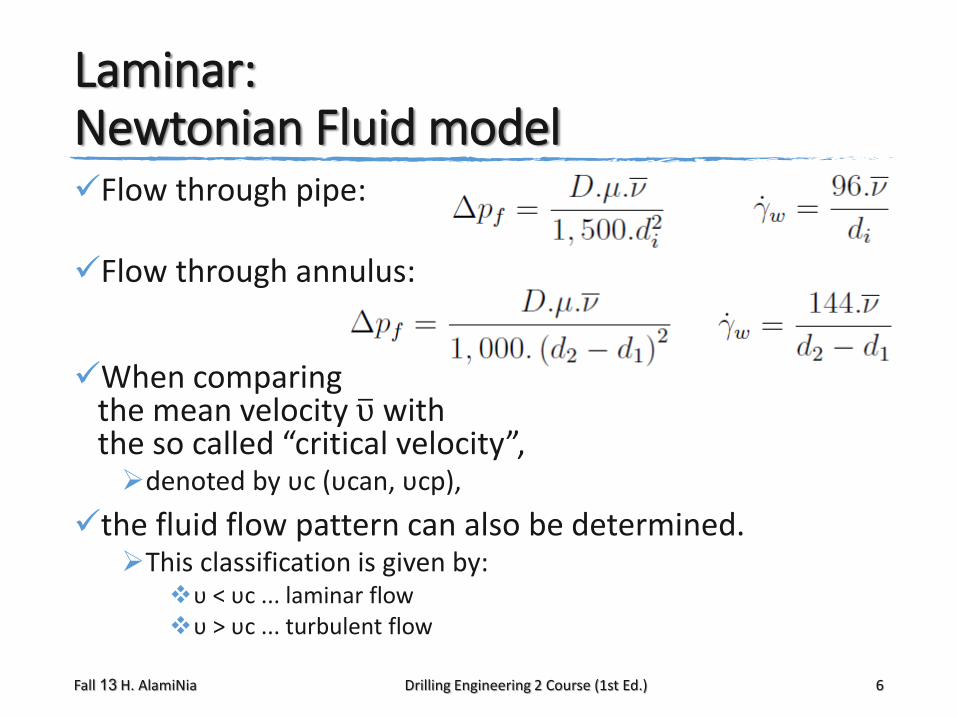
Laminar: Newtonian Fluid modelFlow through pipe:

Flow through annulus:

When comparing the mean velocity υ with the so called “critical velocity”, denoted by υc (υcan, υcp),

the fluid flow pattern can also be determined. This classification is given by:

υ < υc ... laminar flowυ > υc ... turbulent flow


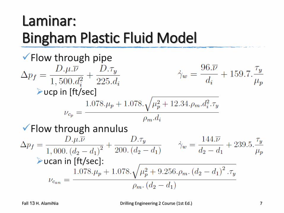
Laminar: Bingham Plastic Fluid ModelFlow through pipe

υcp in [ft/sec]

Flow through annulus

υcan in [ft/sec]:


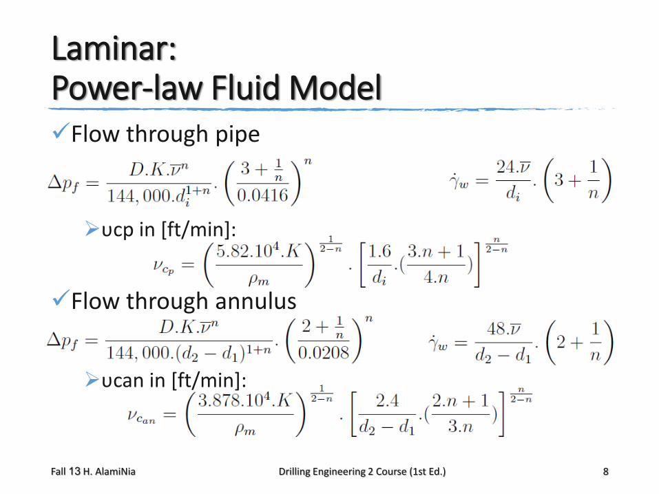
Laminar: Power-law Fluid ModelFlow through pipe

υcp in [ft/min]:

Flow through annulus

υcan in [ft/min]:


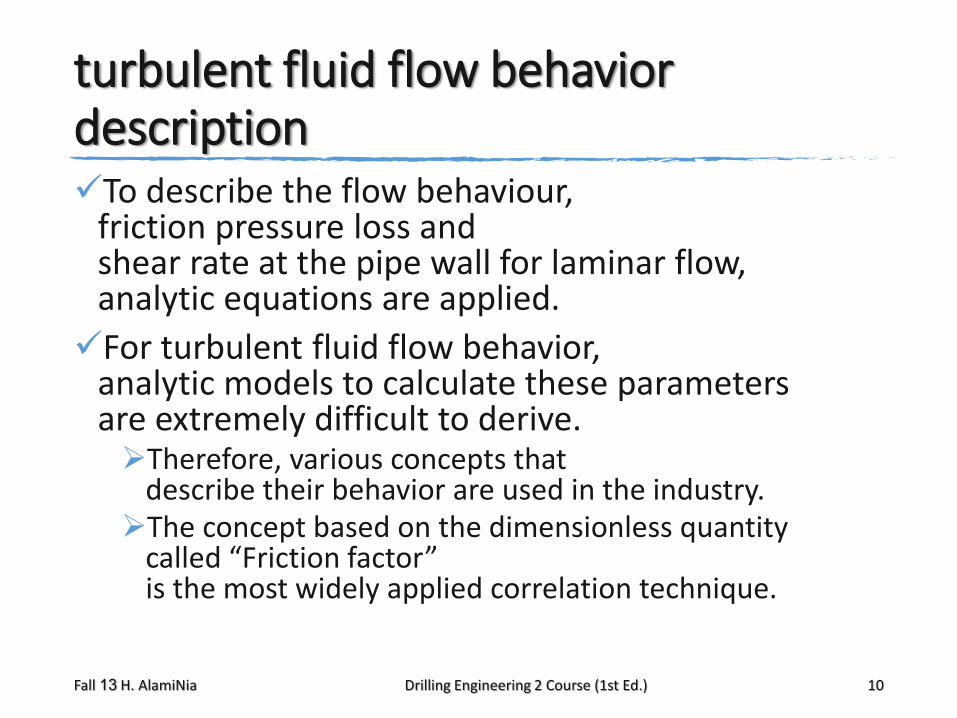
turbulent fluid flow behavior description To describe the flow behaviour,

friction pressure loss and shear rate at the pipe wall for laminar flow, analytic equations are applied.

For turbulent fluid flow behavior, analytic models to calculate these parameters are extremely difficult to derive. Therefore, various concepts that

describe their behavior are used in the industry.The concept based on the dimensionless quantity

called “Friction factor” is the most widely applied correlation technique.


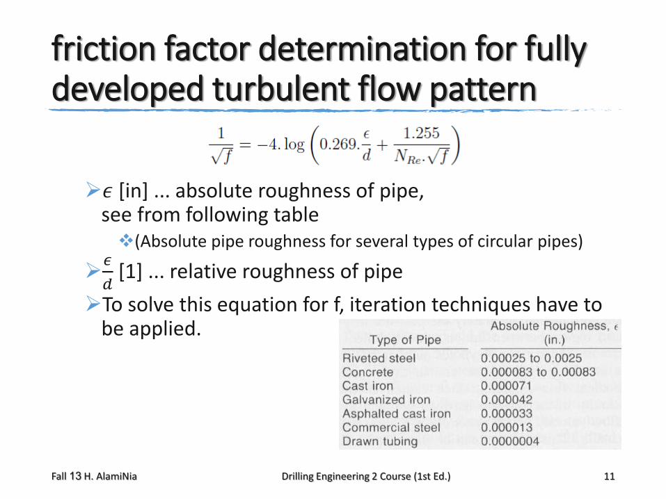
friction factor determination for fully developed turbulent flow pattern

𝜖 [in] ... absolute roughness of pipe, see from following table (Absolute pipe roughness for several types of circular pipes)

𝜖

𝑑[1] ... relative roughness of pipe

To solve this equation for f, iteration techniques have to be applied.


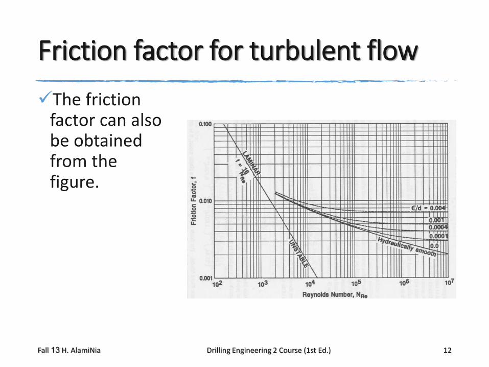
Friction factor for turbulent flow

The friction factor can also be obtained from the figure.


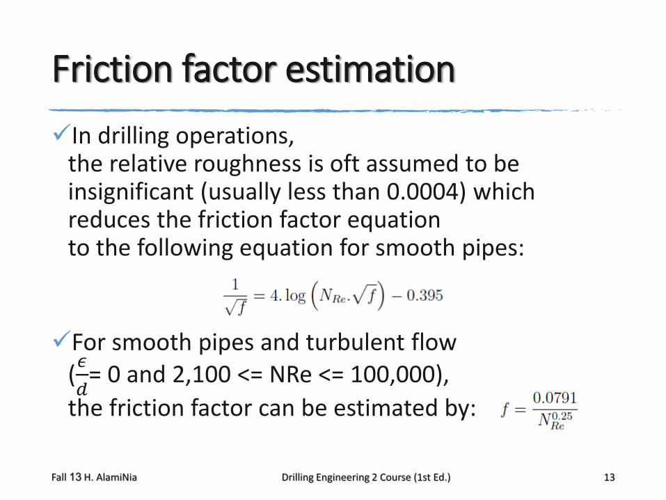
Friction factor estimation

In drilling operations, the relative roughness is oft assumed to be insignificant (usually less than 0.0004) which reduces the friction factor equation to the following equation for smooth pipes:

For smooth pipes and turbulent flow (𝜖

𝑑= 0 and 2,100 <= NRe <= 100,000),

the friction factor can be estimated by:


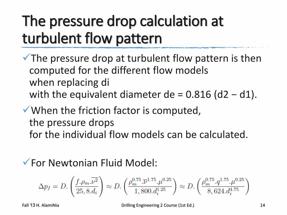
The pressure drop calculation at turbulent flow patternThe pressure drop at turbulent flow pattern is then

computed for the different flow models when replacing di with the equivalent diameter de = 0.816 (d2 − d1).

When the friction factor is computed, the pressure drops for the individual flow models can be calculated.

For Newtonian Fluid Model:


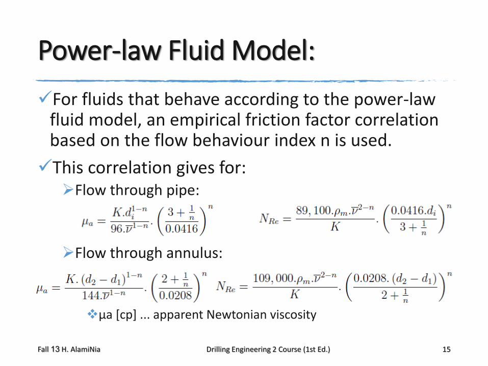
Power-law Fluid Model:

For fluids that behave according to the power-law fluid model, an empirical friction factor correlation based on the flow behaviour index n is used.

This correlation gives for:Flow through pipe:

Flow through annulus:

μa [cp] ... apparent Newtonian viscosity


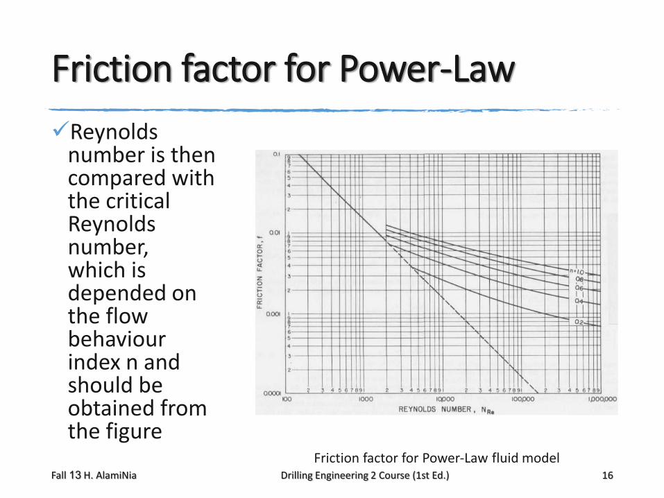
Friction factor for Power-Law

Reynolds number is then compared with the critical Reynolds number, which is depended on the flow behaviour index n and should be obtained from the figure

Friction factor for Power-Law fluid modelFall 13 H. AlamiNia Drilling Engineering 2 Course (1st Ed.) 16

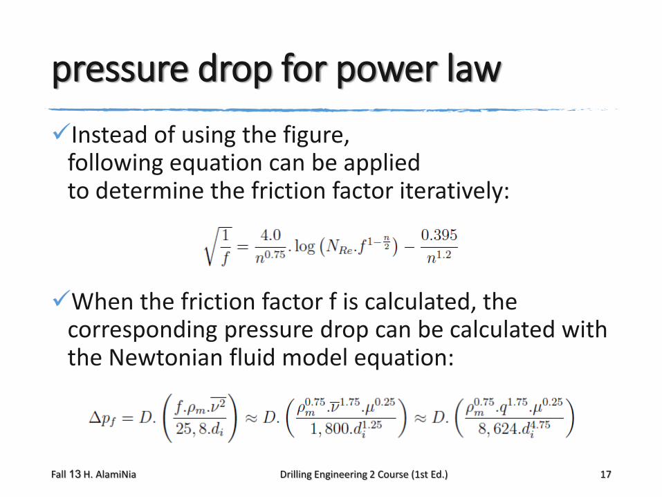
pressure drop for power law

Instead of using the figure, following equation can be applied to determine the friction factor iteratively:

When the friction factor f is calculated, the corresponding pressure drop can be calculated with the Newtonian fluid model equation:


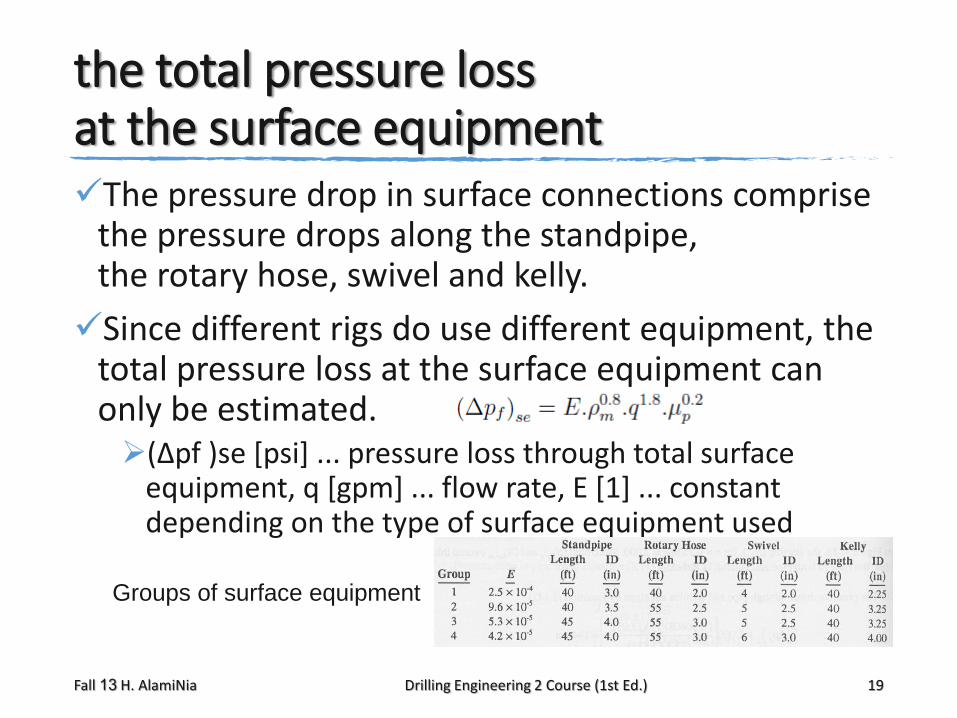
the total pressure loss at the surface equipmentThe pressure drop in surface connections comprise

the pressure drops along the standpipe, the rotary hose, swivel and kelly.

Since different rigs do use different equipment, the total pressure loss at the surface equipment can only be estimated. (Δpf )se [psi] ... pressure loss through total surface

equipment, q [gpm] ... flow rate, E [1] ... constant depending on the type of surface equipment used


Groups of surface equipment

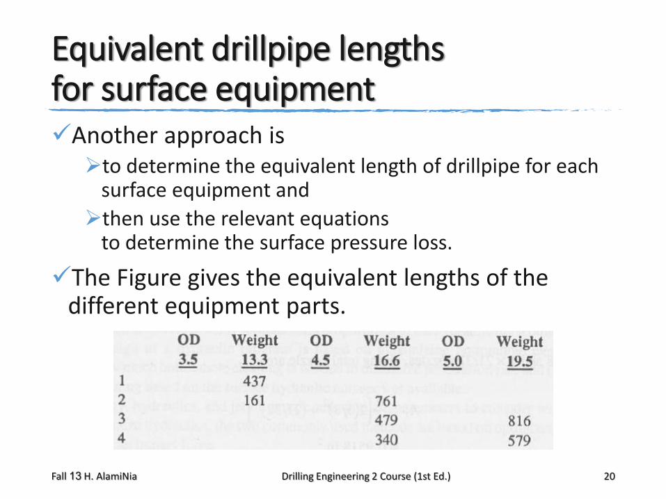
Equivalent drillpipe lengths for surface equipmentAnother approach is

to determine the equivalent length of drillpipe for each surface equipment and

then use the relevant equations to determine the surface pressure loss.

The Figure gives the equivalent lengths of the different equipment parts.


pressure drop across the bit

The pressure drop across the bit is mainly due to the change of fluid velocities in the nozzles.

To increase the penetration rate, when the mud flows through the nozzles its speed is increased drastically which causes a high impact force when the mud hits the bottom of the hole. This high fluid speed on the other hand

causes a relative high pressure loss.

This pressure loss is very sensitive to the nozzle seize.


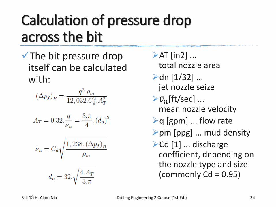
Calculation of pressure drop across the bitThe bit pressure drop

itself can be calculated with:

AT [in2] ... total nozzle area

dn [1/32] ... jet nozzle seize

𝜐𝑛[ft/sec] ... mean nozzle velocity

q [gpm] ... flow rate

ρm [ppg] ... mud density

Cd [1] ... discharge coefficient, depending on the nozzle type and size (commonly Cd = 0.95)


Initiating Circulation

All the equations to calculate the individual pressure drops presented above assume a nonthixotropic behavior of the mud.

In reality, an additional pressure drop is observed when circulation is started due to the thixotropic structures which have to be broken down.

This initial phase of addition pressure drop may last for one full circulation cycle.


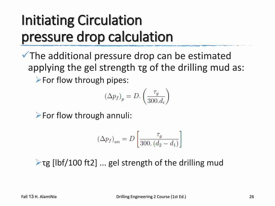
Initiating Circulation pressure drop calculationThe additional pressure drop can be estimated

applying the gel strength τg of the drilling mud as:For flow through pipes:

For flow through annuli:

τg [lbf/100 ft2] ... gel strength of the drilling mud


hydraulic program design

The penetration rate in many formations is roughly proportional to the hydraulic horsepower expended at the bit.

To drill most efficiently hydraulic programs are designed for maximum bottom hole cleaning

(how much bottom hole cleaning is necessary to reach maximum penetration rate)

combined with maximum bottom hole cleaning based on the surface hydraulic horsepower availability.


drilling optimization parameters

For this reason, mud rheology,

hydraulics (individual pressure drops) and

bit nozzle selection are the parameters to consider for drilling optimization.

To optimize drilling hydraulics, different approaches can be made. The hydraulics can be designed to either optimize the nozzle velocity,

the bit hydraulic horsepower or

to optimize the jet impact force.


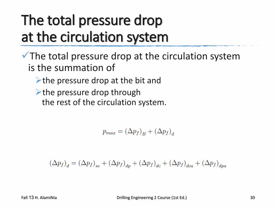
The total pressure drop at the circulation systemThe total pressure drop at the circulation system

is the summation of the pressure drop at the bit and

the pressure drop through the rest of the circulation system.


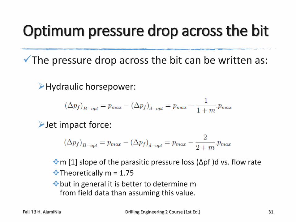
Optimum pressure drop across the bit

The pressure drop across the bit can be written as:

Hydraulic horsepower:

Jet impact force:

m [1] slope of the parasitic pressure loss (Δpf )d vs. flow rate

Theoretically m = 1.75

but in general it is better to determine m from field data than assuming this value.


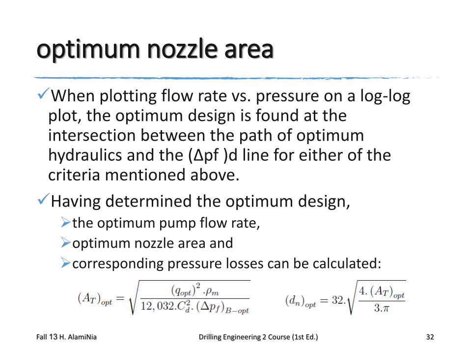
optimum nozzle area

When plotting flow rate vs. pressure on a log-log plot, the optimum design is found at the intersection between the path of optimum hydraulics and the (Δpf )d line for either of the criteria mentioned above.

Having determined the optimum design, the optimum pump flow rate,

optimum nozzle area and

corresponding pressure losses can be calculated:


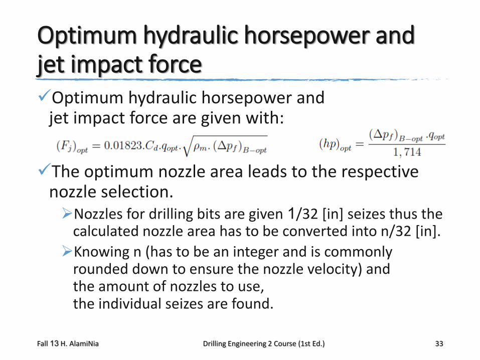
Optimum hydraulic horsepower and jet impact forceOptimum hydraulic horsepower and

jet impact force are given with:

The optimum nozzle area leads to the respective nozzle selection. Nozzles for drilling bits are given 1/32 [in] seizes thus the

calculated nozzle area has to be converted into n/32 [in].

Knowing n (has to be an integer and is commonly rounded down to ensure the nozzle velocity) and the amount of nozzles to use, the individual seizes are found.


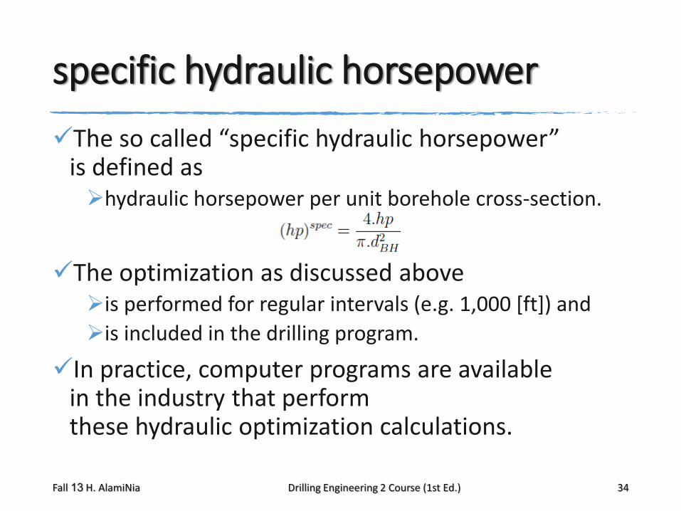
specific hydraulic horsepower

The so called “specific hydraulic horsepower” is defined as hydraulic horsepower per unit borehole cross-section.

The optimization as discussed above is performed for regular intervals (e.g. 1,000 [ft]) and

is included in the drilling program.

In practice, computer programs are available in the industry that perform these hydraulic optimization calculations.


The annular flow of the drilling fluid

The annular flow of the drilling fluid (carrying drilling cuttings and a certain amount of gas to the surface,)is disturbed by frictional and centrifugal forces

caused by the rotation of the drillstring.

In practice, when it is noticed that inefficient hole cleaning is present, either the mud flow rate is increased or the effective viscosity of the mud is increased or both adjustments are performed.

To estimate the slip velocity of the cuttings, following correlation methods were developed empirically

and are widely accepted and used in the industry:


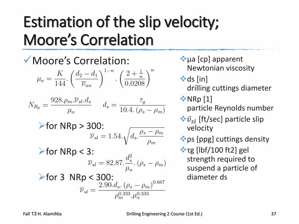
Estimation of the slip velocity;Moore’s CorrelationMoore’s Correlation:

for NRp > 300:

for NRp < 3:

for 3 NRp < 300:

μa [cp] apparent Newtonian viscosity

ds [in] drilling cuttings diameter

NRp [1] particle Reynolds number

𝜐𝑠𝑙 [ft/sec] particle slip velocity

ρs [ppg] cuttings density

τg [lbf/100 ft2] gel strength required to suspend a particle of diameter ds


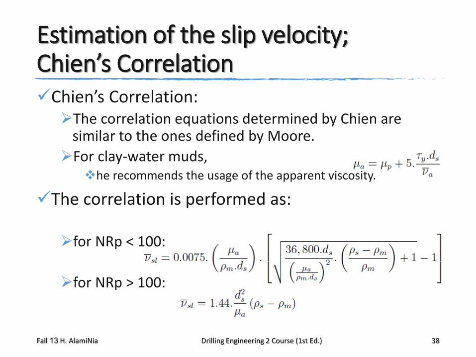
Estimation of the slip velocity;Chien’s CorrelationChien’s Correlation:

The correlation equations determined by Chien are similar to the ones defined by Moore.

For clay-water muds, he recommends the usage of the apparent viscosity.

The correlation is performed as:

for NRp < 100:

for NRp > 100:


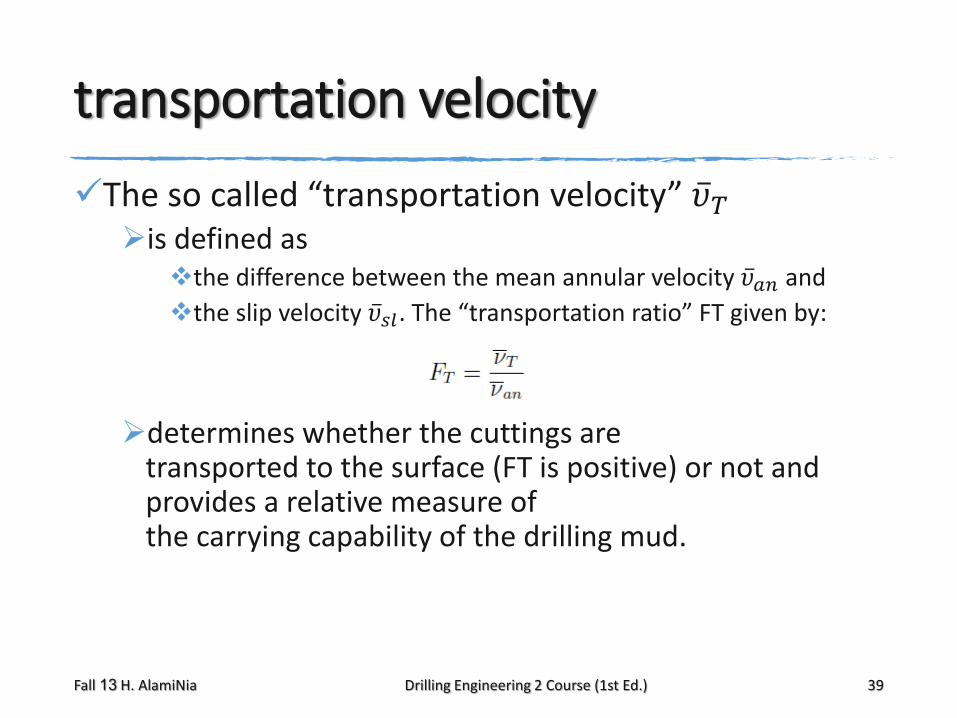
transportation velocity

The so called “transportation velocity” 𝜐𝑇is defined as

the difference between the mean annular velocity 𝜐𝑎𝑛 and

the slip velocity 𝜐𝑠𝑙. The “transportation ratio” FT given by:

determines whether the cuttings are transported to the surface (FT is positive) or not and provides a relative measure of the carrying capability of the drilling mud.


minimum mean annular velocity

To have proper hole cleaning and with the knowledge of the transport velocity, a minimum mean annular velocity can be determined.

This minimum mean annular velocity has to be calculated at the annulus with the maximum cross-section area and in this way determines the minimum pump rate.

As a rule of thumb,

• a minimum mean annular velocity of 3 [ft/sec] is often applied.


1. Dipl.-Ing. Wolfgang F. Prassl. “Drilling Engineering.” Master of Petroleum Engineering. Curtin University of Technology, 2001. Chapter 4

Q921 de2 lec5 v1

Technology

Transcript of Q921 de2 lec5 v1