UNIVERSITE DE MONTREAL

ECOLE POLYTECHNIQUE DE MONTREAL

Proposition de recherche

FUSION OF MULTIMODAL CARDIACIMAGE SEQUENCES

HERVE LOMBAERTDEPARTEMENT DE GENIE INFORMATIQUEECOLE POLYTECHNIQUE DE MONTREAL

c© Herve Lombaert, 2007

Resume

L’interpretation des donnees medicales reste aujourd’hui une con-trainte majeure aux interventions cardiaques. La qualite des im-ages en salle operatoire est souvent faible comparee aux donneespreoperatoires telles que les scans TDM (Tomodensitometrie) ou IRM(Imagerie par Resonance Magnetique). Des algorithmes de traite-ment d’images permettent d’extraire et de combiner l’informationde differentes sources de donnees acquises avant et pendantl’intervention. Ces algorithmes peuvent ainsi mettre en evidence desstructures anatomiques en haute resolution et les superposer sur desimages acquises en intervention. Avec l’evolution de la technolo-gie, des images 4D (3D+t) deviennent disponibles. Le but de cettethese consiste a fusionner des sequences d’images multi-modales pourle guidage d’interventions cardiaques. Afin d’atteindre cet objectif,le probleme de segmentation 4D ainsi que le recalage non-rigide 4Dseront etudies. Ils permettront d’etablir des correspondances clairessur deux sequences d’un organe dynamique tel que le cœur. Unemethode sera egalement proposee pour unifier la segmentation et lerecalage spatio-temporel dans une meme formulation mathematique.

Abstract

A major limitation of cardiac interventions is the understanding ofthe heart anatomy on medical images. The quality of interventionalimages is generally poor compared to preoperative scans such as 3DCT (Computed Tomography) or MR (Magnetic Resonance). Imageprocessing algorithms digest and combine information from differentdata-sets acquired prior to and during intervention. They can isolatecardiac structures in high resolution and align them with interven-tional images. As the technology evolves, 4D images (3D+t) becomeavailable. This thesis will provide the fusion of multi-modal sequencesfor image guided cardiac interventions. 4D segmentation and 4D non-rigid registration are proposed to tackle this objective. They will allowdirect one-to-one correspondence in two different sequences of a mov-ing organ such as the heart. The method will propose a mathematicalframework unifying spatio-temporal segmentation and registration.

Contents

1 Introduction 31.1 Objectives . . . . . . . . . . . . . . . . . . . . . . . . . . . . . . . 41.2 Hypothesises . . . . . . . . . . . . . . . . . . . . . . . . . . . . . 5

2 Background 72.1 The heart . . . . . . . . . . . . . . . . . . . . . . . . . . . . . . . 7

2.1.1 Physiology . . . . . . . . . . . . . . . . . . . . . . . . . . 72.1.2 Coronary circulation . . . . . . . . . . . . . . . . . . . . . 92.1.3 Cardiac electrophysiology . . . . . . . . . . . . . . . . . . 9

2.2 Cardiac imaging . . . . . . . . . . . . . . . . . . . . . . . . . . . 112.2.1 Fluoroscopy . . . . . . . . . . . . . . . . . . . . . . . . . . 122.2.2 Preoperative imaging . . . . . . . . . . . . . . . . . . . . . 132.2.3 Alternative interventional imaging . . . . . . . . . . . . . 14

2.3 Image guided interventions . . . . . . . . . . . . . . . . . . . . . 172.4 Registration . . . . . . . . . . . . . . . . . . . . . . . . . . . . . . 20

2.4.1 Deformation models . . . . . . . . . . . . . . . . . . . . . 202.4.2 Temporal domain . . . . . . . . . . . . . . . . . . . . . . . 232.4.3 Similarity measures . . . . . . . . . . . . . . . . . . . . . 24

2.5 Segmentation . . . . . . . . . . . . . . . . . . . . . . . . . . . . . 262.5.1 Variational approaches . . . . . . . . . . . . . . . . . . . . 272.5.2 Graph based approaches . . . . . . . . . . . . . . . . . . . 29

2.6 Joint segmentation and registration . . . . . . . . . . . . . . . . . 30

3 Method 323.1 4D segmentation . . . . . . . . . . . . . . . . . . . . . . . . . . . 32

3.1.1 Levelset approach . . . . . . . . . . . . . . . . . . . . . . 333.1.2 Graph cut approach . . . . . . . . . . . . . . . . . . . . . 35

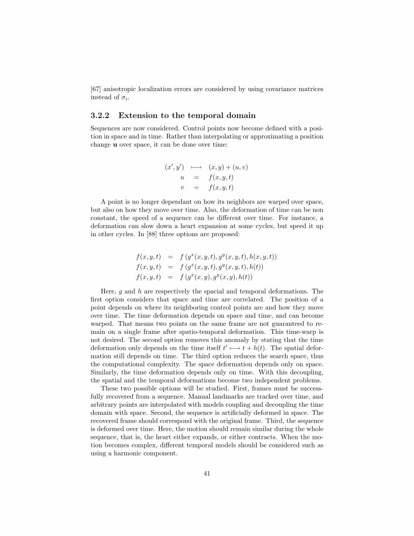
3.2 Frame interpolation . . . . . . . . . . . . . . . . . . . . . . . . . 383.2.1 Thin Plate Splines . . . . . . . . . . . . . . . . . . . . . . 393.2.2 Extension to the temporal domain . . . . . . . . . . . . . 41

3.3 4D registration . . . . . . . . . . . . . . . . . . . . . . . . . . . . 423.3.1 Spatio-temporal component . . . . . . . . . . . . . . . . . 423.3.2 Gradient descent based optimization . . . . . . . . . . . . 423.3.3 Graph cut approach for optimization . . . . . . . . . . . . 43

1

3.4 Joint segmentation and registration . . . . . . . . . . . . . . . . . 463.5 Validation . . . . . . . . . . . . . . . . . . . . . . . . . . . . . . . 48

3.5.1 Segmentation . . . . . . . . . . . . . . . . . . . . . . . . . 483.5.2 Frame interpolation . . . . . . . . . . . . . . . . . . . . . 483.5.3 Registration . . . . . . . . . . . . . . . . . . . . . . . . . . 49

3.6 Timeline . . . . . . . . . . . . . . . . . . . . . . . . . . . . . . . . 50

4 Preliminary results 524.1 4D Segmentation . . . . . . . . . . . . . . . . . . . . . . . . . . . 524.2 Landmark-based non-rigid registration with graph cuts . . . . . . 534.3 Motion interpolation of control points with Thin-Plates . . . . . 564.4 Building a visualization library and development platform . . . . 58

5 Conclusion 60

2

Chapter 1

Introduction

Cardiovascular diseases are the number 1 killer in the US with over 930,000deaths annually. In this country alone nearly 71 millions live with a form ofcardiovascular disease; almost 7 million operations or procedures are performedannually and cost over 400 billion dollars ([1]). Image guided interventions (Fig1.1) are popular procedures for the diagnostic and the treatment of abnormalheart rythms, coronary diseases, as well as of some congenital heart diseasesand valve diseases. Rather than opening up the heart, this procedure involvesthe insertion of one or more catheters inside the heart; they are long small tubesusually inserted in the upper thigh (groin) and pushed towards the heart. As

Figure 1.1: An example of image guided intervention. The physician manip-ulates small objects inside the patient’s body with images and informationsprovided by monitors (Image from Siemens).

3

Figure 1.2: Segmentation of anatomical structures allows a better understandingof images. Here the left atrium is highlighted on a planar reconstruction on theleft, and on a 3D view on the right.

the intervention is performed with no direct visual contact, the need for imag-ing technologies becomes essential. Extracting and combining information fromdifferent images provide detailed roadmaps which make image-guided interven-tions possible. As the technology evolves, images are not only available in 2Dand 3D but also in 4D (animated volumes, 3D+t).

Medical images are often acquired before an intervention, mainly to getfamiliar with the patient’s heart function and anatomy as well as to plan thesurgery accordingly. These images contain a tremendous amount of information,and they need to be processed in order to show only what is necessary for theintervention. For instance, segmentation algorithms can highlight a particularcardiac structure (Fig. 1.2), and registration algorithms can align multipleimages (Fig. 1.3). Visual correspondences with the patient’s anatomy, toolsand catheters become easy to localize and identify on a computer screen. Someinterventions even rely on segmentation and registration. Due to the nature ofthe images, these algorithms need to perform in challenging conditions. Imagesare black and white and are usually degraded with a significant amount of noise.The heart structures have complex geometries and weak boundaries. Thinsvessels or valves may be blurry or invisible on the images. Also, as the heartundergoes complex deformations and motions, alignment of the images cannotbe achieved with simple translations and rotations. In such case scenario, robustsegmentation combined with non-rigid registration become essential.

1.1 Objectives

During cardiac surgeries, image sequences from multiple modalities are available.Their quality is often a compromise between spatial and temporal resolutions.Typically, a high spatial resolution sequence does not provide a good temporalresolution. For instance the quality of 3D volumes (CT or MR) acquired pre-

4

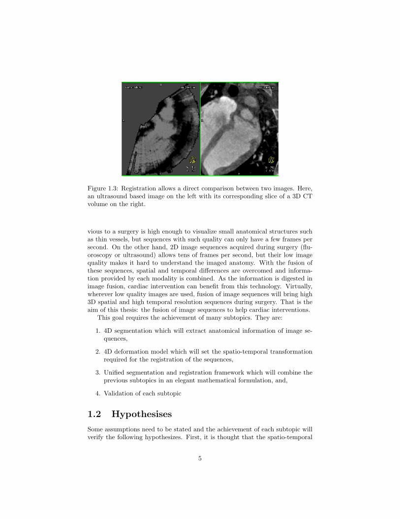
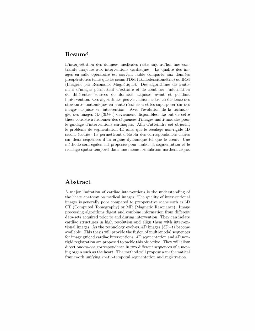
Figure 1.3: Registration allows a direct comparison between two images. Here,an ultrasound based image on the left with its corresponding slice of a 3D CTvolume on the right.

vious to a surgery is high enough to visualize small anatomical structures suchas thin vessels, but sequences with such quality can only have a few frames persecond. On the other hand, 2D image sequences acquired during surgery (flu-oroscopy or ultrasound) allows tens of frames per second, but their low imagequality makes it hard to understand the imaged anatomy. With the fusion ofthese sequences, spatial and temporal differences are overcomed and informa-tion provided by each modality is combined. As the information is digested inimage fusion, cardiac intervention can benefit from this technology. Virtually,wherever low quality images are used, fusion of image sequences will bring high3D spatial and high temporal resolution sequences during surgery. That is theaim of this thesis: the fusion of image sequences to help cardiac interventions.

This goal requires the achievement of many subtopics. They are:

1. 4D segmentation which will extract anatomical information of image se-quences,

2. 4D deformation model which will set the spatio-temporal transformationrequired for the registration of the sequences,

3. Unified segmentation and registration framework which will combine theprevious subtopics in an elegant mathematical formulation, and,

4. Validation of each subtopic

1.2 Hypothesises

Some assumptions need to be stated and the achievement of each subtopic willverify the following hypothesizes. First, it is thought that the spatio-temporal

5

registration will increase the temporal resolution of a sequence having initially alow temporal resolution. That is, with a few high quality images and a motionmodel, it is possible to generate a fluid high quality sequence. Second, it isassumed that the heart beat can be described with a deformation model overspace and over time. The temporal resolution of a sequence can be increasedby interpolating new frames between acquired frames. Third, it is consideredthat the additional information available from the temporal domain will im-prove segmentation as well as registration. Working in a higher dimension willhelp the perception of coherent structures over time which is not necessarilytrivial to detect when analyzing a single frame. It is often implied that twoimages being registered are temporally aligned, however this is not necessarilytrue, and typical registration methods can fail if they are done in the spatialdomain only. The registration problem is more well-posed when working in thespatio-temporal dimension. At last, it is believed that the segmentation and theregistration problem is a mutual problem. When images are correctly aligned,boundaries of corresponding anatomy should match: registration helps segmen-tation; and when corresponding anatomy is known, their alignment becomeseasier: segmentation guides registration.

This thesis proposes the fusion of multimodal sequences for image guidedcardiac interventions. First, basic notions of the heart physiology, imagingtechnologies as well as of popular image guided cardiac interventions will bedescribed. Second, a literature survey will picture the current state-of-the-artof segmentation and registration techniques which are prerequisite for imagefusion. Third, methods along with a timeline will be proposed to tackle thethesis objective and its different subtopics which are: a 4D segmentation, acardiac deformation model, a 4D registration, and a unified framework. Lastly,preliminary results will be presented. This includes work done in segmentation,registration, and motion interpolation.

6

Chapter 2

Background

Often cardiac interventions require difficult and precise mental gymnastics fromthe physician. Imaging devices provide the visualization of these manipula-tions, but the need to process information from these images is essential toguide the interventions. For instance, EP procedures would simply not be pos-sible without visualization of the catheter aligned with the heart anatomy ([2]).Computer algorithms digest information from multiple sources, and their resultsare crucial for most minimally invasive interventions. The heart anatomy is firstdescribed and serves as a background to understand the interventions involvedby major heart diseases. Next, the state-of-the-art for image registration andsegmentation is reviewed.

2.1 The heart

The Merriam-Webster defines the heart as ”a hollow muscular organ of verte-brate animals that by its rhythmic contraction acts as a force pump maintainingthe circulation of the blood”. It has about the size of a fist and is located in thechest behind the breastbone. The heart undergoes a local deformation due tothe cardiac beating, but also a global deformation due to the respiration motion([3, 4, 5]). With humans, as well as with all other mammals, the heart has twoparts, the left and the right one. Each has an atrium and a ventricle as seen onthe figure 2.1.

2.1.1 Physiology

The right part pumps deoxygenated blood from the body to the lungs, whilethe left part pumps oxygenated blood from the lungs to the body. During thiscycle blood circulates through all 4 chambers. It arrives in the right atriumfrom the inferior and superior venae cavae (IVC, SVC). Once enough bloodis accumulated, the tricuspid valve opens and blood is transferred to the rightventricle (RV). The contraction of the right ventricle opens the pulmonary valve

7

Figure 2.1: A human heart has 4 chambers: Left Atrium (LA), Left Ventricle(LV), Right Atrium (RA), Right Ventricle (RV). Blood 1) enters the heart in theRA, 2) transfers to the RV; 3) LV contraction pushes blood into the lungs; 4)blood returns in the heart in the LA, 5) transfers to the LV; 6) LV contractionejects blood throughout the body (Image from the American Heart Association).

and expels the deoxygenated blood in the pulmonary artery (PA) and circulatesthrough the lungs where it is oxygenated. Blood comes back in the heart in theleft atrium (LA) through the 4 pulmonary veins (PV). It is often a misconceptionto think that venous blood is deoxygenated. A more correct definition wouldbe that a vein carries blood returning to the heart and an artery carries bloodpumped out from the heart. Once the left atrium is filled, the mitral valveopens and the blood is transferred in the left ventricle (LV). The left ventriclemyocardium, its wall, is the thickest of all chambers as it is the strongest musclein the heart. Its shape is typically an ellipsoid and its transverse, short axis,section is almost circular. When the left ventricle contracts, it ejects blood intothe aorta and goes through the whole body until it comes back to the heart fora new cycle. The figure 2.1 summarizes the cardiac cycle.

The blood stopped by the valve closures produces the heart sound. In acycle, two successive sounds (”lub-dub”) is produced by the closing of first,the tricuspid and mitral valves, and second, the pulmonary and aortic valves.A perturbation of this sound can be caused by a heart defect, for instance astenotic valve, that is a narrowed valve opening, or a congenital defect such asan atrial or ventricular septal defect, that is a hole between the atria or theventricles.

8

Figure 2.2: Coronary arteries provide oxygenated blood to the muscle heart.Two arteries begin at the base of the aorta. They later bifurcate to cover thewhole heart (Images from the Gray’s anatomy).

2.1.2 Coronary circulation

Blood supply within the heart is done with the coronary arteries (Fig 2.2).Two branches start at the root of the aorta. The right side of the heart issupplied with the right coronary artery (RCA). The left coronary artery (LCA)is usually short and quickly bifurcates into the left anterior descending artery(LAD), which runs on the front side of the heart and between the ventricles,and the left circumflex artery (LCX), which runs on the lateral side of the heart.Further bifurcations vary significantly in the population. Blood from the heartmyocardium is collected with the coronary sinus (CS). It runs on the left sideof the heart between the left atrium and the left ventricle. It ends in the rightatrium.

Coronary diseases caused 1 out of every 5 deaths in the US, that’s morethan 650,000 deaths annually ([1]). Along the years, fat and cholesterol buildup fatty deposits, narrowing the coronary arteries and its lumen. These plaquesprevent the heart muscle, the myocardium, from being well supplied with blood.If completely obstructed, this can lead to a heart failure causing a heart attack.

2.1.3 Cardiac electrophysiology

A healthy heart has a good synchronization of cardiac muscle contractions (sys-tole) and relaxation (diastole). The upper chambers (LA and RA) first contract,followed by the two lower chambers (LV and RV). The contractions are causedby electric signals propagating throughout the heart. They originate from thesinoatrial (SA) node and travel in the atria (Fig 2.3). They reach the atrioven-tricular (AV) node before going in the ventricles.

An electrocardiogram (ECG, or EKG in german) measures the electric cur-rent in the heart. A typical ECG, as shown on the figure 2.4, contains suc-

9

Figure 2.3: The heart muscle is stimulated by electric currents propagatingthroughout the heart. They start in the sinoatrial (SA) node, propagate in theatria until reaching the atrioventricular (AV) node. From there, they travelthrough the ventricles causing their contractions (Image from the AmericanHeart Association).

Figure 2.4: The electrocardiogram (ECG) shows the evolution of the cardiacelectric activity. The atria are first contracted (P wave), the ventricle contrac-tions follow shortly after (QRS complex), and at the end of the cardiac cycle,the T wave resets the electrical system. On the right, typical and untypicalECG are shown. When the heart beat becomes irregular, the patient is said tohave arrhythmia (Image from Merck).

10

Figure 2.5: Arrhythmia is caused by perturbed electrical paths in the heart.When this happens in the atria, they quiver and can affect the heart pumpingability. Atrial fibrillation is the most common form of arrhythmia (Image fromthe NIH).

cessively a P wave, a QRS complex, and a T wave. The P wave causes thecontraction of both atria. An anomaly with P waves is a sign of atrial problem.Shortly after, the QRS complex triggers the ventricle contractions. As there ismore muscle mass involved, the electric variation is larger. Electric current trav-els through cells, each triggering (P wave and QRS complex) correspond to thedepolarization of these cells. To return to their normal state, a re-polarizationis required. This is the T wave. Sometimes a remnant can appear as a fourthwave, the U wave.

About 2.2 million patients in the United States have atrial fibrillation (A-Fib) ([6]) and every year it causes death to more than 75,000 of them ([1, 7]).A-Fib is the most common form of abnormal heart rhythm, a perturbed cardiacelectric activity. Electric signals may be trapped in loops or in wrong paths(Fig 2.5), usually in the pulmonary veins, causing the heart to beat irregularly.A-Fib affects the blood flow and clots are eventually formed. They can latertravel in the body and cause damage in different organs, or can result in astroke if ending up in the brain. It can also decrease the heart pumping abilityresulting in a heart failure. Ventricular fibrillation (V-Fib) is more serious asthe ventricle no longer pumps blood effectively in the body. V-fib leads to deathwithin minutes and it is considered a medical emergency.

2.2 Cardiac imaging

The process of creating an image is called imaging. This is essential withminimally invasive procedures where tools such as catheters are guided insidethe body with no visual contact.

11

(a) (b)

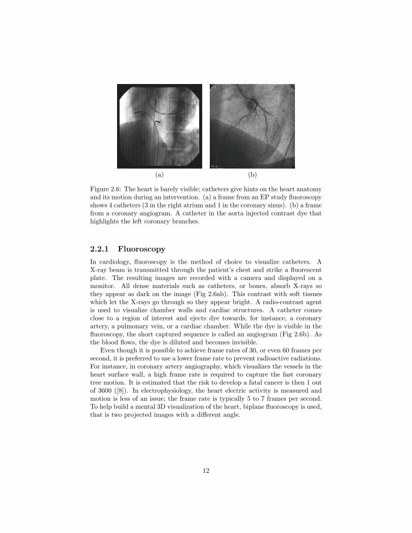
Figure 2.6: The heart is barely visible; catheters give hints on the heart anatomyand its motion during an intervention. (a) a frame from an EP study fluoroscopyshows 4 catheters (3 in the right atrium and 1 in the coronary sinus). (b) a framefrom a coronary angiogram. A catheter in the aorta injected contrast dye thathighlights the left coronary branches.

2.2.1 Fluoroscopy

In cardiology, fluoroscopy is the method of choice to visualize catheters. AX-ray beam is transmitted through the patient’s chest and strike a fluorescentplate. The resulting images are recorded with a camera and displayed on amonitor. All dense materials such as catheters, or bones, absorb X-rays sothey appear as dark on the image (Fig 2.6ab). This contrast with soft tissueswhich let the X-rays go through so they appear bright. A radio-contrast agentis used to visualize chamber walls and cardiac structures. A catheter comesclose to a region of interest and ejects dye towards, for instance, a coronaryartery, a pulmonary vein, or a cardiac chamber. While the dye is visible in thefluoroscopy, the short captured sequence is called an angiogram (Fig 2.6b). Asthe blood flows, the dye is diluted and becomes invisible.

Even though it is possible to achieve frame rates of 30, or even 60 frames persecond, it is preferred to use a lower frame rate to prevent radioactive radiations.For instance, in coronary artery angiography, which visualizes the vessels in theheart surface wall, a high frame rate is required to capture the fast coronarytree motion. It is estimated that the risk to develop a fatal cancer is then 1 outof 3600 ([8]). In electrophysiology, the heart electric activity is measured andmotion is less of an issue; the frame rate is typically 5 to 7 frames per second.To help build a mental 3D visualization of the heart, biplane fluoroscopy is used,that is two projected images with a different angle.

12

Figure 2.7: CT is a reconstruction from multiple X-rays. Hard structures suchas bones will appear bright on the image. A contrast agent has been used tohighlight the two ventricles. On the left, a transversal slice of the heart is shown.The two ventricles and the spine are visible. On the right, a 3D view of the CTvolume.

2.2.2 Preoperative imaging

If the detailed anatomy of the patient’s heart is required before an intervention,a 3D computed tomography (CT) or a magnetic resonance (MR) is performed.This will help the physicians plan the surgery.

In a CT scan (Fig 2.7), detectors rotating around the patient collect X-rayimages from different angles. With enough images, it is possible to reconstructa volume in 3D. Although the image quality of such volumes is excellent com-pared to other modalities, the amount of radiation involved makes it prohibitive.Studies in adult patients ([9, 10]) show that the risk to develop the risk of afatal cancer is 1 chance in 2000. In children the risk is much higher ([11]).

In magnetic resonance imaging (Fig 2.8), no radiation is used. A magneticfield is rather used and measures the relaxation time of excited atoms. Eachatom normally spins around an axis. By exciting atoms, it is possible to lineup the spinning axis. When atoms return to their natural spinning axis, energyis released and can be measured by coils in the scanner. By smartly spatiallyaltering the magnetic field, it is possible to reconstruct a 3D volume. Differentprotocols exist to image specific structures. Use of contrast dye, or change inthe imaging parameters can highlight a region or another.

Positron emission tomography (PET) ([12, 13]) is different than anatomicalimaging such as CT and MR. Rather than picturing the anatomical structures,PET measures their functionality (Fig 2.9a). A radioactive tracer injected in theblood emits positrons which vanish with nearby electrons. This reaction releasesgamma photons that are caught with detectors surrounding the patient. Once

13

Figure 2.8: MR measures hydrogen density that is watery tissues will appearas bright on the image. On the left, the picture shows a coronal slice of thechest. On the right, this is the 3D MR volume. The heart is in the middle ofthe image.

enough photons are collected, 3D images can be reconstructed. PET is used inoncology to detect cancer because tumors need more blood than healthy organs.It is not yet popular in clinical cardiology as it remains an expensive technology.

The physics underlying the PET imaging is similar ([14]) to the singlepositron emission computed tomography (SPECT) ([15]). They differ on the ra-dioactive tracer used, much cheaper and easier to produce than the PET tracer,as well as on the capturing device ([16]). Rather than a ring of detectors, arotating gamma camera is used to collect the photons. The spatial resolutionof SPECT images is lower than PET images. Both technologies are used incardiology to detect areas of the heart with decreased blood flow. Obstructedcoronary arteries or dead myocardium will produce dark regions (Fig 2.9b).

2.2.3 Alternative interventional imaging

While fluoroscopy is widely used to detect anatomical landmarks, it is not veryadequate for complex interventional procedures. Imaging is limited to projectiveviews, heart anatomy is hardly visible and requires contrast dye injection, andthe biplane equipment is also encumbering in the operating room. Alternativeinterventional imaging is being studied; among them two promising modalitiesare ultrasound and magnetic resonance imaging.

With ultrasound imaging (Fig 2.10abc), a high frequency sound is sentthrough the body and its echo makes it possible to detect interfaces in thebody. Ultrasound imaging was first used in the cardiac field in the 1960s as aresearch experiment ([19]). In the 1980s ultrasound imaging became more pop-ular with the development of the intravascular ultrasound (IVUS) ([20]) and the

14

(a) (b)

Figure 2.9: (a) PET measures metabolism, that is a bright spot on the im-age means there is a concentration of blood. Here the picture shows variouscross-sections of the left ventricle myocardium. (b) SPECT uses a very similartechnology as PET, but a different radioactive tracer is used, its resolution istypically lower than PET. On the first images, blood does not circulate well inpart of the myocardium wall (Images from [14]).

intracardiac echocardiography (ICE) ([21]).An IVUS catheter provides polar images from inside a vessel (Fig 2.10b).

As the catheter is pulled out, the image sequence shows successive vessel crosssections. It is used to study the narrowing of coronary arteries. IVUS canrecognize lesions that are not visible with typical coronary angiography ([17]).

ICE (Fig 2.10c) is a different approach; it provides 2D planar images from aprobe placed in the esophagus or directly in the heart from the aorta or from thevenae cavae. Sequence can be acquired at a frame rate of 20 frames per secondor more. 3D ultrasound is possible with sequential 2D image acquisitions ([22]),although recent research already shows true 3D acquisition ([23]). ICE can beused for monitoring in electrophysiology ([18]). It is possible to acquire imagesfrom the left atrium and pulmonary veins with a fairly good quality.

With magnetic resonance imaging, catheters can be guided in the heart withlive visualization (Fig 2.11). MR guided interventions can be used in electro-physiology ([24]). Coils from the MR scanner track catheters in real time, andmagnetic resonance imaging visualizes lesions of the pulmonary vein ablations.During intervention, three 2D planes can be interactively manipulated thoughan interactive front end (IFE). These planes command continuous MR acquisi-tions to visualize the live heart anatomy and the catheter positions. Once thecatheters are lead to the pulmonary veins and ablations are performed, with aproper imaging protocol, it is possible to image ablation lesions. Knowing thelesion positions and sizes, it is possible to close the gaps between them. Currentlive image acquisitions during this procedure are done with 1 or 2 frames persecond. However, previous to the surgery, a 4D MR acquisition can be done

15

(a) cardiac

(b) IVUS

(c) ICE

Figure 2.10: Ultrasound measures tissue echoes that is interfaces in the body willgenerate bright regions on the image. In (a) with a probe placed on the patient’schest, the 4 cardiac chambers with ventricles on the top and atria on the bottomare visible. (b) IVUS is an ultrasound technology. The probe is inside a vesseland displays plaques in the cross section. (c) ICE is an ultrasound technology.The probe is inside the heart. This EP study shows the left atrium with theleft upper pulmonary vein (LUPV), the right upper and lower pulmonary vein(RUPV, RLPV) as well as the left atrium appendage (LAA) (Images from (a)Philips, (b) [17], (c)[18]).

16

Figure 2.11: Catheters can be tracked with MR coils. It becomes possible tovisualize electrodes during an intervention (Image from [24]).

Figure 2.12: In 1929, general belief was that any entry in the heart would befatal. Werner Forssman performed the first catherization on his own heart. Thepicture shows a catheter tip lying into his right atrium.

from multiple cardiac cycles. Such a reconstruction can have as much as 40volumes per second ([25]).

2.3 Image guided interventions

The first known heart catheterization ([26]) was in 1929. Werner Forssmanninserted a 65 cm catheter in his own heart from his arm. He then walked inthe radiology department where he took an X-ray of his heart with the catheterlying in his right atrium (Fig 2.12). He was eventually fired from his hospital forthis. Later with two coworkers, they received a Nobel Prize for their pioneeringwork.

17

(a) (b)

Figure 2.13: (a) Catheters are inserted in the groin (as seen on the picture), thearm, or the neck. It is threaded towards the heart for diagnostic or treatment.(b) During angioplasty, a balloon catheter is inserted in a narrowed vessel.Inflation of the balloon will widen the vessel and restore a normal blood flow.At the same time a tubular structure is installed to keep the vessel open (Imagefrom the NIH).

Today the catheterization of the heart is performed daily for diagnostics andtreatments. For instance, it is used to measure blood pressure, get informationon the pumping ability, and map electric activity of the heart. Dye can beinjected to visualize cardiac structures such as coronary arteries or pulmonaryveins. Tools can also be brought inside the heart for minimally invasive inter-ventions. During a typical procedure, the patient is given a sedative to relax.A catheter sheath is inserted into a vein (Fig 2.13a), usually in the upper thigh(groin), the arm, or the neck. Catheters can then be inserted and threaded intothe heart. Short fluoroscopic sequences are used to guide the catheter correctly.Longer shots are used during the intervention in the heart.

angioplasty When dealing with a narrowed or obstructed coronary, a balloonis used to open the vessel (Fig 2.13b). This is called an angioplasty ([27, 28]).A balloon is placed on the tip of a catheter. During the intervention, dye isinjected in the coronary artery before the catheter is placed in the narrowing ofthe vessel. The balloon is inflated until a normal blood flow is restored in thevessel. When inflating, a stent, a small metal or plastic tube, is installed in the

18

Figure 2.14: With atrial fibrillation, abnormal electric activity often arises fromthe pulmonary veins. They are isolated with incisions made around them withablation catheters. The picture shows a left atrium with ablation sites in red.

vessel to keep it open. Other types of treatment include the use of a grinder toremove the plaques blocking the coronary artery; this is called an atheroctomy,and the use of laser to vaporize the plaque.

valvuloplasty Heart valves can become narrowed with calcium deposits. Aprocedure similar to the balloon angioplasty is then performed. It is called avalvuloplasty. A balloon is inflated in the narrowed valve and broad the opening.A promising experiment ([29]) has been done where an artificial valve is broughtinto the heart through the groin and placed in lieu of the defective valve.

congenital defect correction Some congenital diseases such as the atrialseptal defect can be treated with catheterization of the heart ([30]). If the holebetween the atria is not too large, a closure device can be brought and placedin the hole.

Electrophysiology procedure The cause of A-Fib often comes from elec-trical currents trapped in loops around the pulmonary veins ([31, 32]. Thisrequired an open heart surgery called the Maze procedure ([33]) with a heart-lung bypass machine. Abnormal electrical paths from the pulmonary veins weredisconnected with precise incisions in the left atrium. Nowadays ([34, 35]), elec-trophysiology (EP) procedures are minimally invasive. Lesions are created withcatheters (Fig 2.14) delivering an electric current of up to 50 W applied during60 to 120 sec. As it is still not clear what energy source should be used for ab-lation, other sources are currently being considered such as cryothermy ([36]),laser ([37]), or microwave ([38]).

19

2.4 Registration

Aligning images from the same scene is a typical problem in image processing.It is used in many fields. For instance, with satellite pictures, aligning continentcontours can show storm evolutions, with images from digital cameras, aligningimages can create panoramas. With medical images, bringing information fromdifferent image modalities together can reveal new information such as tumors,or in our application, anatomy features essential for electrophysiology. Solvingthe registration problem will find the best alignment of images. That means itwill find the transformation T between two images such that:

I ′ = T (I).

Many challenges exist, the features and shapes on the images can be movedand distorted as well as with different intensities. The transformation can begeometric (transformation t on spatial coordinates x) or applied on the imageintensities (transformation f on pixel intensities i):

i′(x) = f (i (t(x)) .

In 1984, Venot and Leclerc ([39]) proposed to automate digitized angiogra-phy by finding the optimal translation of images. Also, early registration meth-ods were mostly rigid and feature-based as reviewed by [40]. Another survey([41]) describes early frameworks as having the following components: featurespace, extracting information from the image, search space, modeling the trans-formation of extracted features, search strategy, dictating the transformationevolution, and similarity measure, telling how well the current transformationis. These components are involved in all works reviewed in this section. Itis organized as an evolution of cardiac image registration techniques towardspatio-temporal applications.

2.4.1 Deformation models

The need for non-rigid transformation arose in cardiac imaging where the heartmotion cannot be described by rigid transformation. One of the first attempts([42]) used a high order polynomial to register 2D myocardial perfusion image.Today, many models are used in various medical applications. See [43] for arecent survey on non-rigid registration and [44] for a review of methods appliedto cardiac images.

Demetri Terzopoulos et al. unified the shape description and the motiondescription in an elastic deformation model ([45]). A parameterized surface Ωminimizes an energy such that:∫

Ω

α(s0 − s1)2 + β(κ0 − κ1)2 + γ(τ0 − τ1)2da,

where α, β, and γ are coefficients for respectively stretching (s), bending (κ),and twisting (τ). Rather than adding an elasticity constraint on the deformable

20

shape, Gary Christensen et al. added the elasticity constraint to the deformationfield. In [46], he presented two new non-rigid physical models, which can bothbe seen as vector fields solving the registration problem, but differing by theequations governing these vector fields. Both models minimizes an energy sothe deformation field u correctly align two images, that is modeled with the dataterm D(u), and so that the deformation field is kept smooth, that is modeledwith the elastic term E(u):

u = arg minu

(D(u) + E(u)) .

The elastic force is proportional to the deformation, and the data term drivesthe deformation of an image into the target image. With small displacementthe elastic model can be considered ([47]), while the viscous fluid model shouldbe preferred when considering large displacement ([48, 49]).

Vector fields can also be computed by solving the optical flow equation([50, 51, 52]) which assumes a point keeps a similar intensity over time:

I0(x, y) = I1(x + δx, y + δy).

In [53], additional constraints on the optical flow are used to guarantee massconservation of a volume. This method proved to be efficient to compute velocityfields of a human heart in 4D CT data. Rather than using image intensity todrive the physical forces, statistical shape information can also be used suchas in [54, 55]. When only a few points are used for registration, which mightbe desirable to avoid expensive computation, interpolation of the deformationfield can be efficiently achieved with spline based transformation models such asthin-plate splines [56, 57, 58] or free-form deformations [59, 60, 61, 62]. Each isa parametric model and requires the management of control points. The use ofa grid manipulated by control points to model biological deformation has beenproposed as early as 1917 by D’Arcy Wentworth Thompson where he tries todescribe shape differences with simple mathematical transformations ([63]).

The classical spline model interpolates a position Q(u) on a curve with aparameter u. Each control point pi has a global influence on the curve suchthat:

Q(u) =n∑

i=0

piBi(u).

Here, Bi(u) is a basis function, the B-spline is often used. The position cansimilarely be interpolated on a surface patch with a parameter (u, v):

Q(u, v) =n∑

i=0

m∑j=0

pijBi(u)Bj(v).

This spline interpolation model can be generalized to any dimension with hypersurface patches. The free-form deformation model ([64]) is a lattice composed ofsuch a spline hyper patch where each lattice node is a control point. An object isembedded in the lattice, and as the lattice deforms with the control points, the

21

object undergoes the same deformation. The hyper suface patch interpolates theobject deformation between the lattice nodes. With B-spline, each control pointhas a local influence in the deformation field. This makes the model suitablefor localized deformations. Also, control points are not attached to the imagepoints, that means moving a control point will not directly move a point on theimage with the same motion. However, [65] proposes a direct manipulation ofthe free-form deformation by computing the inverse deformation.

With thin-plate splines, control points directly manipulate the spline andcan be placed arbitrarily anywhere and each point has a global influence on thedeformation field. This model can be illustrated with a flat metallic surfacethat keeps a minimal global bending. Control points anchor the plate at thegiven positions and the interpolation is done by computing the surface heighth = f(x, y) where f minimizes the surface curvature:∫∫

R2

((∂2f

∂x2

)2

+ 2(

∂2f

∂x∂y

)2

+(

∂2f

∂y2

)2)

dxdy,

or in any dimension, the functional:

Jd(f) =∑

α1+...+αd

2!α1!...αd!

∫Rd

(∂2f

∂xα11 ...∂xαd

d

)2

dx.

Jean Duchon ([56]) and later Jean Meinguet ([57]) initially proposed the use ofsuch a thin plate equation. Fred Bookstein proposes a solution with:

f(x, y) = a1 + a2x + a3y +n∑

i=0

wiU (|pi − (x, y)|) .

The summation term is the influence of control points on the surface, it isasymptotically flat. U(r) is a basis function, it is

∣∣x3∣∣ in 1D, r2 log r2 in 2D,

and |x| in 3D. The first terms correspond to the affine part which describes aflat plane that best matches all the control points. It is possible to find thecoefficients ai, wi with linear algebra.

Approximation is required to correct errors on control point positions due tothe imaging or due to feature localizations. With thin-plate splines, Booksteinuses a relaxation term λ ([58]):

f(x, y) = a1 + a2x + a3y + λn∑

i=0

wiU (|pi − (x, y)|) ,

but this term affects the overal surface. Approximation schemes were laterstudied by adding a localization uncertainty to each control point. With anisotropic uncertainty ([66]), each control point is relaxed to a sphere, and thebending energy becomes:

Jλ(f) =1n

n∑i=1

|hi − f(pi)|2

σ2i

+ λJd(f).

22

Covariance matrix can be used for anisotropic uncertainty ([67]). Landmarksnow become ellipsoids and in extreme cases planes or segments. When con-sidering the heart motion, additional physical constraints can be used. In [68]a deformation field of the myocardium is computed by formulating the prob-lem as a stochastic estimation problem. A priori information is coming fromtwo physiological assumptions, neighbor points have the same motion, and themyocardium volume does not change. Another constraint can be used in thetemporal domain. Deformation of a beating heart is indeed cyclic. The use ofperiodic model such as harmonic functions for temporal estimation is well suitedfor cardiac motion as described in [69].

2.4.2 Temporal domain

Modern imaging technology allows visualization of the heart motion. In the1950s, fluoroscopy was revolutionized with the use of fluorescent screen andmotion could be captured ([70]) with the invention of the television camera.Later, in the 1980s, researchers from the Mayo clinic ([71, 72]) had the goal tocreate a Dynamic Spatial Reconstructor, that is a 4D CT imaging device withup to 20 volumes per second. The technology was at that time not availableto achieve this goal. Lately, in [73], 4D CT imaging is possible with rates of10 volumes per second up to 20 volumes per second. However, radiation dosedue to X-rays has to be considered. For a coronary angiogram, 4D CT has arisk of inducing a fatal cancer of 1 in 1400, while fluoroscopy has a risk of 1in 3600 ([8]). It is also important to note 4D CT is not a true 4D acquisition.It is a reconstruction based on multiple planes acquired over a short period oftime from a rotational scanner. True 3D slice acquisition such as MR imaging,which is non-radioactive, can be used for a 4D visualization. MR tagging wasproposed by [74] where a pattern of spatially altered magnetization is appliedin the myocardium to visualize its motion. This idea has been retaken witha novel technique in [75] and a grid rather than an arbitrary pattern ([76]) isused. Tracking of MR tagged grid points can be used for the interpolation ofthe motion field such as [77] where a thin-plate splines is used for a mapping oftwo consecutive images. [78] surveys deformation models used in segmentation,registration or motion tracking in medical image analysis.

With temporal data, sequence-to-sequence alignment removes spatial ambi-guities that cannot be handled with image-to-image alignment. Early work in[79] tackles the shape change modeling in a medical image sequence. A shapefrom segmentation is parameterized in a grid like coordinate system and track-ing is made by assuming various point intensity of the shape to remain constantover time. To limit the space of possible solution, shape smoothness is used dur-ing tracking. In computer vision, Caspi and Irani align a video sequence withdifferent objects in motion with a reference sequence ([80]). As the sequencesdepict the same scene taken at the same time, the presented method cannotbe applied to cardiac sequences where the heart can have a different motion intwo different acquisitions. From the same group [81], spatio-temporal alignmentcan be used for temporal super resolution. By using multiple sequences from

23

the same scene, motion with a higher frame rate than the video acquisition canbe recovered. This is an extension of the original spatial super resolution [82]where higher resolution than the acquisition device can be achieved by aligningmultiple images of the same scene.

In the medical field [83] is an early medical application of spatio-temporalregistration of cardiac images. Temporal alignment of a SPECT and a MRsequence is done by comparing the volume of the left ventricle at different times.Linear interpolation is then used to create corresponding frames. Perperidis etal. ([84]) used affine transformation to achieve 4D registration in MR imagesequences. The spatial and the temporal components are separated to ensuresthe principle of causality, that means points in a reference frame cannot findcorrespondence in various frames over time. The deformation model T is thendecoupled with:

T : (x, y, z, t) 7→ (x′(x, y, z), y′(x, y, z), z′(x, y, z), t′(t)) ,

where the spatial position is independent of the temporal component. Theneed for a more sophisticated temporal model is motivated by that fact thatthe heart follows a very unique motion. For instance, it has been shown ([85])that each point in the left ventricle wall follows its own, but locally coherent,trajectory over time. Recovering motion between temporally distanced frameswith interpolation is therefore challenging and easily prone to error. Furtherwork was done by Rueckert et al. ([62]) where he introduces free-form defor-mations for spatial alignment. This work has later been extended by Perperidiset al. ([86]) to a spatio-temporal model where the temporal component uses anaffine transformation, and has finally come to a complete 4D spatio-temporalfree-form deformation model ([87]). His work is gathered in his thesis ([88])where spatio-temporal registration is used to build atlases describing the car-diac motion [89, 90]. However the question of whether the heart undergoesthe same deformation model with different patients still remains open. In themeantime, individual models of beating heart is possible by using informationextracted from anatomical structures, such as in [91]. Another application ofspatio-temporal registration is to deform a sequence so it appears stationary asin [92, 93]. Here ultrasound imaging is considered. Rather than only consideringpairs of images as in [94], B-splines are used to find a global spatio-temporaldeformation field. Interpolation as well as approximation over time is anotherimportant application of spatio-temporal registration. In [95] a more generalsmoothing spline framework is used to simulate the deformation of a torso sur-face over time.

2.4.3 Similarity measures

Traditionally, feature points previously selected were used for multimodal regis-tration ([96]). Intensity based approaches were introduced in [97]. Registrationwere done by minimizing the variance of the ratios of one image to the other,

24

or:

J(T ) =∑

x∈I∩I′

((i(x)

i′(t(x))

)−(

i(x)i′(t(x))

))2

.

Soon after, Hill et al. ([98]) introduces the joint histogram for registration. Inthe same group, Van den Elsen et al. publish in [99] a method based on thecorrelation of the gradient:

J(T ) =∑

x∈I∩I′

∇i(x)∇i′(t(x)).

Collignon et al. ([100]) and Studholme et al. ([101]) propose to use entropyas a similarity measure. Many definitions exists for the entropy (H), they allmeasure the information carried by a message (e.g. an image), Shannon ([102])proposed as a definition:

H(I) =∑

i

pi log1pi

,

where pi is the probability of a pixel to have intensity i. All pi are actuallythe histogram of an image. Later, Viola and Wells ([103]) and Collignon etal. ([104, 105]) found, in the same year, a new approach based on mutualinformation. Between two images, the mutual information is defined as:

MI(A,B) = H(A) + H(B)−H(A,B),

where the first two terms are the entropy of the histograms of image A and B,and H(A,B) is the entropy of the joint histogram of image A and B. Regis-tration is done by maximizing the mutual information. The cost function tominimize is:

J(T ) = −MI(I, T (I)).

This similarity measure is not invariant to the overlaping region. If it is small,the mutual information between both images is going to be small. To correctthis bias, normalized mutual information ([106]) is used. [107] surveys recentmethods based on mutual information. It is known to be one of the best suit-able similarity measures for multimodal registration. Entropy and mutual in-formation are derived from the machine learning and information theory fields([102]). Another important similarity measure from the information theory isthe Kullback-Leibler distance ([108]). This similarity measure has recently beenused for registration in [109]. It measures the distance from an expected jointhistogram distribution and an observed distribution. When an a priori distri-bution is known, this methods proved to be more robust in a multi resolutionscheme ([110]). Improvement has also been done by the same authors by usingjoint class histogram ([111]) which uses joint distributions of labels instead ofintensities. Similarity measures are all easily extendable to the spatio-temporaldomain. That is a new sum operator needs to be used in order to iterate throughthe whole spatio-temporal sequence.

25

Figure 2.15: Edge finding is fast with the convolution of a filter such as theSobel detector.

2.5 Segmentation

When features need to be localized, segmentation becomes a critical step. Ithelps identify regions, boundaries, or landmarks in an image. Very simpletechniques include edge highlighting or thresholding. Edge operators such as thePrewitt or Sobel detectors (Fig 2.15) can be convolved in an image to hightlightedges in certain orientation. One simple version of these filters is the followingtwo operators, the first detect vertical lines, the second detects horizontal lines: −1 0 +1

−1 0 +1−1 0 +1

and

+1 +1 +10 0 0−1 −1 −1

.

The Marr and Hildreth operator ([112]), known as the mexican hat, is symmetricand finds edges in all directions. More complex edge detection techniques, suchas the Canny detector ([113]), can close short gaps in broken edges and generatepixel thin contours. These methods give hints on observable edges present inthe image. Landmarks could be derived from these edges. Another approachwould be to derive landmarks from regions. Thresholding is a simple techniquetesting against pixel intensities to segment a region. The threshold value can beset manually or can be found automatically. In [114], a line is drawn betweenhistogram peaks, and the threshold value is given by the intersection of a per-pendicular line and the histogram. Many other ad-hoc techniques exist to findan optimal threshold, [115] reviews 40 of them. However the state-of-the-artstill remains based on Otsu’s work ([116]). The main idea is to minimize theweighted within-class variance in each class. When multiple objects are in theimage, [117] extends Otsu’s technique by recursively applying thresholding onthe highest peak until all other peaks are removed. Another popular techniquefor segmentation is region growing. Their origin can be traced back to 1970in [118]. From a provided ”phagocyte” seed, a region is filled until the seedcannot grow any further. In [119], the seed is grown toward neighboring pixelswhose intensities are the most similar to the grown region. Thresholding and

26

region growing differs by their approach to segmentation. Thresholding meth-ods would successively split regions, that is a top-down approach, while regiongrowing methods merge pixels or regions; that is a bottom-up approach. [120]is the first attempt to combine both approaches. Segmentation is performedby traversing a tree whose leaves are pixels, and root is the whole image. In-termediate nodes are regions. Organizing the image as a tree is concept usedby watershed algorithms. Vincent and Soille ([121]) introduced the concept offinding watersheds to segment images. The image is considered as a elevationmap where the height of a pixel is given by its intensity. Watershed lines arefound by flooding the image topography. Water flood catching basins and meetat watershed lines. These lines separate regions.

In the book [122], Jean-Michel Morel has the feeling that ”most segmentationalgorithms try to minimize [. . . ] one and the same segmentation energy”. DavidMumford refers this book in [123] as an excellent introduction to all the basicalgorithms and variational methods for image segmentation. The reviewer withJyant Shah actually first used an energy minimization for image segmentationin their seminal paper [124] (journal paper [125], and book [126]). Imagesare considered as piecewise smooth signals. Each regions has homogeneousintensities. The energy functional is designed to drive the solution towards asegmentation F that explains well the observed image I, to keep pixel intensities,i, within a region very alike, that is a smooth segmentation ‖∇F‖2, and to limitthe length of boundary Γ between segmented regions. These three criteria arerespectively:

E(F,Γ) =∫

R(i− f)2dx +

∫R−Γ

‖∇f‖2dx + |Γ|.

Their work is a modification of [127, 128, 129] that propose a similar energy for-mulation in a Bayesian framework and not in a variational approach. Nowadays,state-of-the-art segmentation algorithms all minimize an energy functional andmany are based on the piecewise smooth Mumford Shah ([130]).

2.5.1 Variational approaches

Kass et al. proposed a deformable contour driven by external forces. In [132],it is known as a snake, or active contour. The contour evolution minimizesan energy functional which contains high level information such as the contourcurvature, and low level information such as the local gradient direction.

In order to extend the gradient influence far away from the edges, [133]proposes the gradient vector flow. The gradient field points towards edges,which is a desirable driving force for a snake. However, this field gets weak as theedge becomes distant, and the gradient is generally non-existent in homogeneousregion. The diffusion of the gradient field keeps the gradient vector flow similarto the image gradient in edge vicinities, and yields a slow varying vector fieldin homogeneous regions where the image gradient is too weak. This improvesdramatically the convergence to image edges.

27

Figure 2.16: A contour separates two regions. Here an energy drives the contourtowards the denser cloud of points (Image from [131]).

The active contour formulation cannot handle topology changes. The snakecannot split and merge. In [134], Stanley Osher and James A. Sethian proposethe idea of evolving a surface instead of a front. The contour is defined with theintersection of the surface and a plane, that is a level set of the surface. Withthis method, rather than using an explicit approach to track a boundary, it istracked implicitly with a surface evolution in a higher dimension. As the surfaceevolves, its level sets undergo splits and merges. Topology changes are handlednaturally. The surface is usually a signed distance transform, measuring thedistance from a point to the surface zero level set. Internal forces, such as thecurvature penalization and external forces, such as a ballooning force, can drivethe surface evolution. Forces derived from an image are used to segment regions([135]). The level set evolution slows down when it reaches an image boundary,this happens when the image gradient is strong.

As the level set method minimizes any kind of energy, many other functionalshave been proposed. For instance, with geodesic active contour ([136]) thesnake energy is solved in a level set framework, it can even use the gradientvector flow as external force ([137]). In [131] Tony Chan and Luminita Veseuse a region based approach instead of looking for boundaries (Fig 2.16). Theirenergy functional is a variant of the piecewise smooth Mumford and Shah, andit is designed to efficiently separate an object from its background. [138] cansegment up to three regions with a similar approach.

Many optimizations and simplifications of the level set methods exist.Sethian simplifies the level set method with the fast marching method whenthe driving force does not change sign, that means when the contour is alwayseither expanding or collapsing. In [139, 140] the computation is performed ina narrow band around the current surface level set. In [141], the level set isused without re-initialization by adding an energy term forcing the surface tobe close to the distance transform.

28

Figure 2.17: To an image, a graph can be associated. A cut in this graph willoptimize the separation between the foreground and the background (Imagefrom [142]).

2.5.2 Graph based approaches

In the 1920s Max Wertheimer fathered the Gestalt theory movement ([143],partial translation [144]). He suggested that cognition is a whole and cannot beexplained by summing each parallel operation alone. Applied to visual percep-tion, that means global properties such as image partitions cannot be found bycombining separate low-level cues and requires an organization and grouping ofthese cues. Using a graph to segment an image is an elegant implementation ofthis theory. Each leaf of the graph can correspond to a pixel of an image, andproperties can be modeled with nodes connected to the pixels. Regions can befound by cutting the graph. Wu and Leahy ([145]) used this approach to clusterdata with a cut isolating clusters. Each possible cut has a cost, and finding thebest cut can be done by minimizing an energy cost functional.

The minimum cut problem is identical to finding the maximum flow of agraph ([146]), and polynomial time algorithm can be used to efficiently findan optimal cut ([147, 148]). However the minimum cut can favor small lengthcuts, generating small clusters. In image segmentation, that means isolating asingle pixel can be cheaper than segmenting a large homogeneous region. Toovercome this problem, Jianbo Shi and Jitendra Malik proposed to normalizethe cut cost ([149, 150]). The energy is defined to be the ratio of the cost ofa cut between two regions and the cost of a cut between a region and all itssurrounding regions. The minimum normalized cut is computed by solving anEigen value system. This can involve accumulation of approximation errors andexpensive computation.

29

Yuri Boykov and Marie-Pierre Jolly used a new graph based method forimage segmentation in [151, 142]. The graph cut method also uses a node foreach pixel (Fig 2.17 shows an example with a 9 pixel image). In addition, thegraph contains two special terminal nodes, a source and a sink. Each pixel isconnected to its neighboring nodes as well as to the terminals. Searching for theminimum cut between the terminal nodes will separate the graph into two subtrees, one corresponding to the object region, and the other to the backgroundregion. In [148] Yuri Boykov and Vladimir Kolmogorov introduced a new al-gorithm which still outperforms any state-of-the-art minimum cut, maximumflow algorithm. The algorithm guarantees converge of the solution to the globaloptimum in polynomial time. When time and memory becomes an issue, opti-mization techniques are possible; [152] tracks excesses and deficits in the graphuntil convergence; [153] uses a multilevel approach to solve the minimum cutiteratively; [154] uses super node, where each node corresponds to a watershedregion; [155] evolves a minimum in a narrow band until convergence.

Graph cuts can also be used for energy minimization ([156, 157, 158, 159]).Yuri Boykov, Olga Veksler and Ramin Zabih describe two algorithms for energyminimization with graph cuts, alpha expansion and alpha-beta swap ([156]).They both are an iteration of graph cuts between two regions, and the energyis minimized by each step until convergence. Both algorithm are fully describedin Olga’s Veksler thesis ([160]). This method is used in many applications incomputer vision such as image restoration ([161, 156]), disparity from stereo([162, 156]), motion segmentation ([163, 164]), surface reconstruction ([165,166, 167]), as well as super resolution ([168]). It not impossible to foresee anapplication of graph cuts to solve the registration problem.

2.6 Joint segmentation and registration

As segmentation and registration can both be solved by minimizing energies,solving them jointly is a promising method. This approach has been verylittle explored, and has not yet been applied to the spatio-temporal domain.Traditionally, feature-based registration uses points ([170]), edges or surfaces([171, 172]) from segmentation. Registration quality depends on the featurelocalization step. Rather than seeing both steps as separate process, they canbe solved simultaneously. In [173], segmentation and registration are solved inan unified framework. However, the method uses a two stage algorithm, wheresegmentation and registration are still solved individually. In [174], both pro-cesses are expressed in the same formulation. It is truly solved simultaneouslyin a variational framework. Non-rigid transformations (Fig 2.18) can also behandled as in [169]. Furthermore, solving simultaneously segmentation and reg-istration within the same framework can answer the registration of partial dataas proposed in [175, 176]. The registration is solved by treating differently, i.e.,by segmenting, matching data and missing data between two images. Thesejoint approaches provide elegant unifying frameworks. Solving simultaneouslywhat may be one unique problem, could become a leading approach for both

30

Figure 2.18: The left column and the right column shows two bladders. The seg-mentation (green and yellow contours) and the registration (red arrows mappingthe green contour to the yellow one) are solved jointly (Image from [169]).

segmentation and registration.

31

Chapter 3

Method

As 4D images will become more common in the future, the research area canbe aimed towards the temporal aspect of the segmentation and the registrationproblem. The thesis objective, the fusion of multi-modal image sequences, andeach of its subtopics will be tackled in this section. First, 4D segmentationwill be investigated in order to extract anatomical informations. Second, a de-formation model will describe how to interpolate data over the spatio-temporaldomain. Third, in order to achieve 4D non-rigid registration, an optimizer basedon graph cuts will be described. And at last, the segmentation and the registra-tion problem will be combined in the same framework. Moreover, validationsalong with a timeline will be proposed for each method.

3.1 4D segmentation

The amount of information contained in medical images can become overwhelm-ing during an intervention. Understanding the images and localizing anatomicalstructures or medical tools are not easy tasks with medical images, especiallywhen dealing with multiple image sequences. The time spent interpreting theseimages can be greatly improved with segmentation. These algorithms will high-light anatomical structures of interest, or show medical tools with a distinctiverepresentation. When dealing with multiple images or sequences, correspondingstructures or tools can be efficiently found with a common coloring code or rep-resentation. In this section, a method is proposed to efficiently segment objectsin 4D images.

As introduced in the previous literature survey an elegant way of defining animage with objects is with the Mumford-Shah functional ([130]). It assumes thateach object element are similar in a way, for instance, each pixel of an object hasa similar intensity, that is the image is approximated by a piecewise constantfunction ([125]). Each constant piece of an image, with value ui corresponds tothe object i. The function u and its interfaces Γ is found by minimizing thefollowing functional:

32

Figure 3.1: Here the zero level set of the surface is a square. It separates theimage (on the plane) in two regions, the background and the foreground.

J(u, Γ) =∫

I

(I − u)2dx + λ

∫I−Γ

|∇u|2dx + µ

∫Γ

dx

The first term is the data fit, it penalizes the solution u if it is not closeenough to the image I. The second term is the smoothness term, it penalizeschanges in the solution u. The last term is the interface length, it is directlylinked to the number of objects in the solution u. That is, if there are manyobjects, the interface Γ should be large, if there are a few objects, the interfaceshould rather be small. The coefficients λ and µ controls the smoothness andthe graininess of the solution u.

3.1.1 Levelset approach

This functional is efficiently minimized with the level set method in [131]. Thismethod is a numerical framework that embeds the solution in a higher dimen-sion. For instance, when working with a 2D image, the solution becomes a 3Dsurface that evolves with forces derived from the functional to minimize. Thezero levelset can define a binary segmentation (Fig 3.1), that is the object isdefined with what is inside the intersection of the evolving surface and the zeroplane, and the background is defined with what is outside the zero levelset.Let φ(x) be the evolving surface. The zero levelset of this surface defines thesegmentation boundary Γ : x(t), and the surface has by definition no height:

φ(x(t), t) = 0

Studying its motion over time leads to:

33

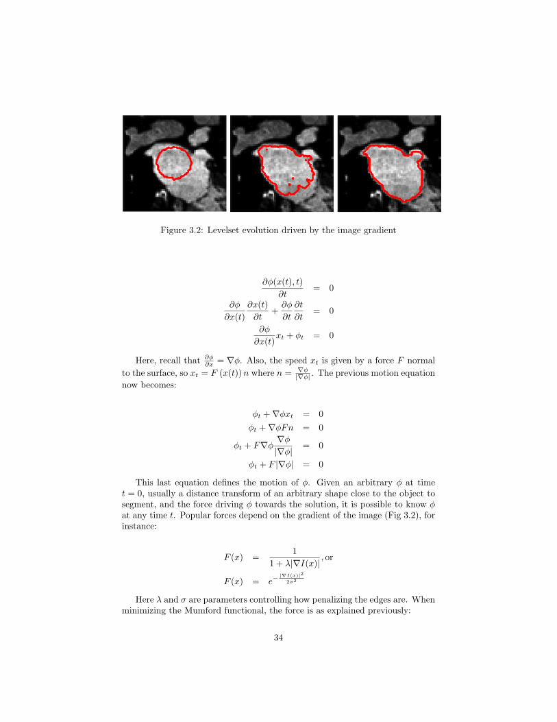
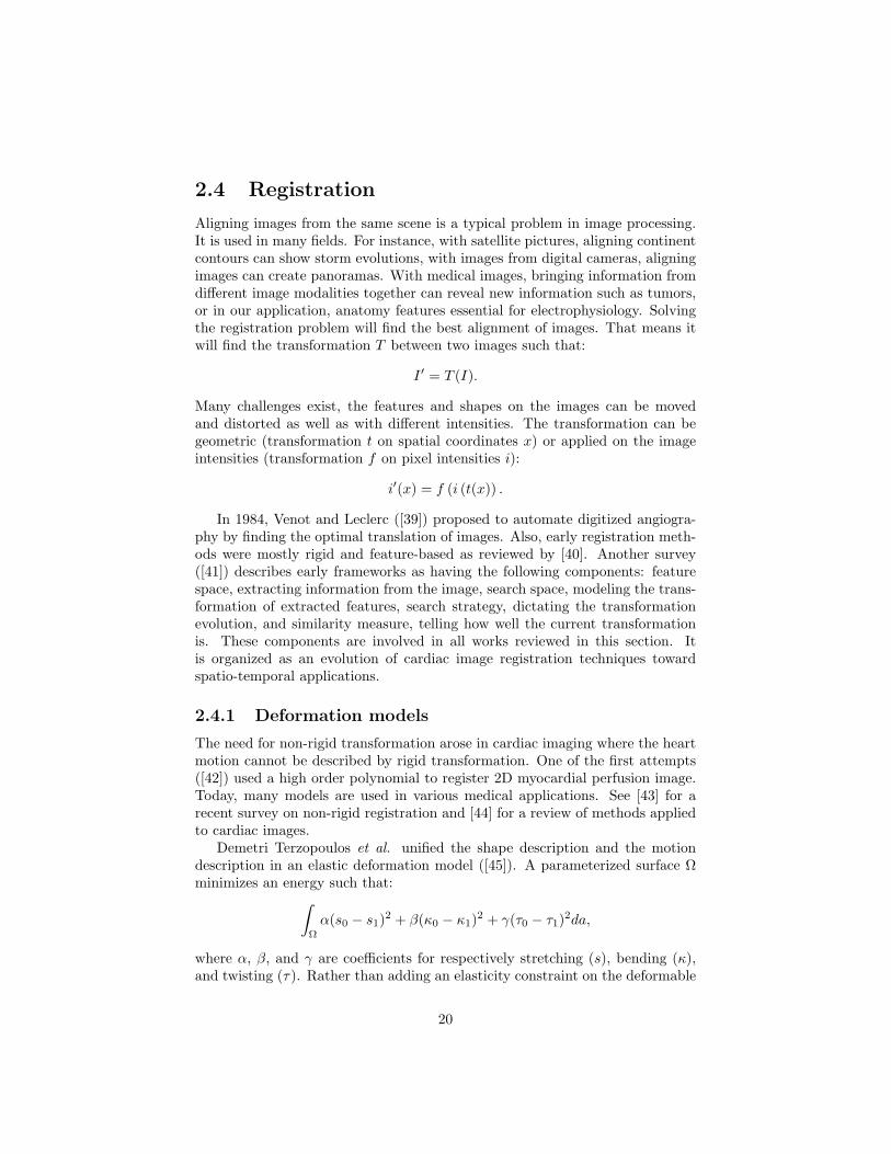
Figure 3.2: Levelset evolution driven by the image gradient

∂φ(x(t), t)∂t

= 0

∂φ

∂x(t)∂x(t)

∂t+

∂φ

∂t

∂t

∂t= 0

∂φ

∂x(t)xt + φt = 0

Here, recall that ∂φ∂x = ∇φ. Also, the speed xt is given by a force F normal

to the surface, so xt = F (x(t))n where n = ∇φ|∇φ| . The previous motion equation

now becomes:

φt +∇φxt = 0φt +∇φFn = 0

φt + F∇φ∇φ

|∇φ|= 0

φt + F |∇φ| = 0

This last equation defines the motion of φ. Given an arbitrary φ at timet = 0, usually a distance transform of an arbitrary shape close to the object tosegment, and the force driving φ towards the solution, it is possible to know φat any time t. Popular forces depend on the gradient of the image (Fig 3.2), forinstance:

F (x) =1

1 + λ|∇I(x)|, or

F (x) = e−|∇I(x)|2

2σ2

Here λ and σ are parameters controlling how penalizing the edges are. Whenminimizing the Mumford functional, the force is as explained previously:

34

F (x) = λ1

∫φ≥0

(I(x)− c1)2dx + λ2

∫φ<0

(I(x)− c2)2dx + µ · lengthφ = 0

With c1 and c2 being the mean intensity of the region outside and inside thezero levelset. A trick is used here to compute the length of the zero level setwith the gradient of the Heaviside function of φ, lengthφ = 0 =

∫I|∇H(φ)|dx.

It is possible to use approximating functions of the Heaviside as well as of theDirac function. [131] gives all the implementation details.

The levelset method can easily extend to 3D as well as 4D. The evolvingsurface becomes a hyper surface and the mathematics remains the same in N-D.

3.1.2 Graph cut approach

The graph cut method also minimizes a Mumford-Shah like functional ([151]).A graph is used for the image; each of its node is corresponding to a pixel. A cutin the graph will separate it in two labels, one corresponds to the object, andthe second corresponds to the background. The graph and its edges implementa functional and its minimization is done by finding the minimum cut of thegraph. As this problem is equivalent to solving the maximum flow of a graph([146]), the solution can be found efficiently in polynomial time. The energyfunctional has two parts:

E(u) =∑p∈I

Dp (up) + µ∑

p, q ∈ Nup 6= uq

Vp,q (up, uq)

The first term is the data term, it tells how well the solution u fits with theobserved image. The second term is the smoothness term, it ensures the solutionu is smooth, for instance both the object and the background regions wouldhave homogeneous intensities. The unknown variable u is a binary variable(u = ”obj”, ”bkg”), it tells wherever the pixel up is part of an object or partof a background.

To construct the graph (Fig 3.3), each pixel node is connected to its neigh-borhood. These neighborhood links correspond to the smoothness term of theenergy to minimize. As explained earlier, it ensures the solution u is smooth.When segmenting an image, if two neighboring pixels p and q have close inten-sities, that means they are probably within the same region. Cutting the linkVp,q should be penalized. Thus popular weights for the link Vp,q are:

Vp,q =1

1 + λ (I(p)− I(q))2, or

Vp,q = e−(I(p)−I(q))2

2σ2

35

Figure 3.3: Each pixel of an image is associated with one node. Pixel neighboringlinks define the segmentation smoothness. Two terminal links (source and sink)will separate the image into foreground and background (Image from [147]).

Beside the pixel nodes, two special nodes, the terminal nodes S, T, areused, one represents the object and the second represents the background. Eachpixel node of the graph is connected to both terminals. The weights of theterminal links tell how likely a pixel is going to be an object or a background.When segmenting an object out of a background, pixels within a region can beset as object with links to the object terminal node set to infinity and links to thebackground terminal node set to zero, the background can be set with links tothe object terminal node set to zero and links to the background terminal nodeset to infinity. As with the levelset method described previously, the terminallinks can also be the difference between pixel intensity and the intensity mean(c1 or c2) of the object or of the background:

Dp(”obj”) = (I(p)− c1)Dp(”bkg”) = (I(p)− c2)

The minimum cut of the graph will find the best separation between theobject node and the background node, ensuring each region to be homogeneous(Fig 3.4). Recently, the Mumford-Shah functional can be solved with graphcuts ([177]). The trick is to use the Cauchy-Crofton formula to approximate theboundary length ([178, 179]) by counting the number nc(θ, ρ) of intersection ofa line xcox(θ) + ysin(θ) = ρ with the boundary C:

length(C) =12

∫ π

0

∫ ∞

−∞nc(θ, ρ)dρdθ

Further links have been made between the levelset method and the graphcuts ([180]).

It still remains an active area of research and contribution can be made byextending the graph cut method to the temporal domain. Along the conceptof spatial neighborhood NS , the definition of a temporal neighborhood NT will

36

Figure 3.4: Here the left atrium of a heart has been segmentated and is high-lighted in red in the original 3D volume.

model the way information propagates through time. Time constraints can alsobe implemented with the use of directional links. The energy to minimize willthen become:

E(u) =∑p∈I

Dp (u(p))

+ µ∑

pt, qt ∈ NS

u(p, t) 6= u(q, t)

Vp,q (u(p, t), u(q, t))

+ ν∑

pt, qt+1 ∈ NT

u(p, t) 6= u(q, t + 1)

Vp,q (u(p, t), u(q, t + 1))

The standard graph cut method requires 24 bytes per node and 14 bytes perlink with Vladimir’s Kolmogorov implementation available on his website. Witha 1024x1024 2D image, that makes roughly 80MB for a graph of connection 4.For a typical 3D volume of 5123 voxels, 13.5GB are required to hold the graphinto memory. This is not possible with today’s computers. To overcome thisproblem, a multilevel approach has been used (Fig. 3.5). A coarse graph is firstused to get a rough estimate of the segmentation results. The result is thenprojected in a narrow band on the next level. A finer graph is used to recoverthe details, e.g., thin structures. With such approach, it is possible to segmenta 5123 volume within 30 seconds and with less than 2GB of memory. The resultof this multilevel approach has been published at ICCV 2005 ([153]).

37

Figure 3.5: Details of the multilevel approach for graph cut segmentation: a)downsampling of the image, b) segmentation with a low resolution graph, c)construction of a narrow band around the low resolution segmentation, d) seg-mentation with a high resolution narrow banded graph.

3.2 Frame interpolation

A real motion is captured with an image sequence. As the observed data isdiscrete, it becomes hard to recover the motion between acquired frames. Thesolution to this problem is the use of a continuous deformation model. Withthe right assumptions and a model correctly fitting the observed images, interframes can be generated with a good level of accuracy. Being able to know themotion at any time will become important when trying to register multiple imagesequences. Indeed, the frames of the different sequences (e.g. I1(ti) and I2(t′i),ith frames of the first and the second sequences) could not be synchronized overtime (i.e. ti 6= t′i) and this will lead to errors as trying to register temporallymisaligned images is already an ill-posed problem.

One good assumption is the smoothness of the motion. This criteria issatisfied by minimizing the curvature of the deformation field. In 2D, the change(u, v) of the position of a point (x, y) is given by:

(x′, y′) 7−→ (x, y) + (u, v)

J(u) =∫∫

R2

((∂2u

∂x2

)2

+ 2(

∂2u

∂x∂y

)2

+(

∂2u

∂y2

)2)

dxdy

J(v) =∫∫

R2

((∂2v

∂x2

)2

+ 2(

∂2v

∂x∂y

)2

+(

∂2v

∂y2

)2)

dxdy

38

Figure 3.6: A thin plate spline is forced to pass at the control point positions.Here the red dots define the surface shape and curvature.

Figure 3.7: Here thin plate splines deform an image in order to correct theoriginal image (original on the left, transformed image on the right).

u = arg minu

J(u)

v = arg minv

J(v)

3.2.1 Thin Plate Splines

Usually the deformation field is known at some points. For instance, specificmarkers or landmarks provide reliable deformations (u, v) at the control pointsPi. The thin plate spline is a solution to this problem with an elegant physicalinterpretation. The control points set the height of a thin metal sheet (Fig 3.6).As the sheet tries to get the minimal bending energy, its curvature is minimized.The height of this sheet is given for any position by:

f(x, y) = a1 + a2x + a3y +n∑

i=1

wiU(|Pi − (x, y)|)

In 2D (Fig 3.7), two thin plate splines are used, one for the horizontal motionu = fu(x, y), and one for the vertical motion v = fv(x, y). The unknowns arethe parameters a1, a2, a3 and wi. The first three terms is the linear part of

39

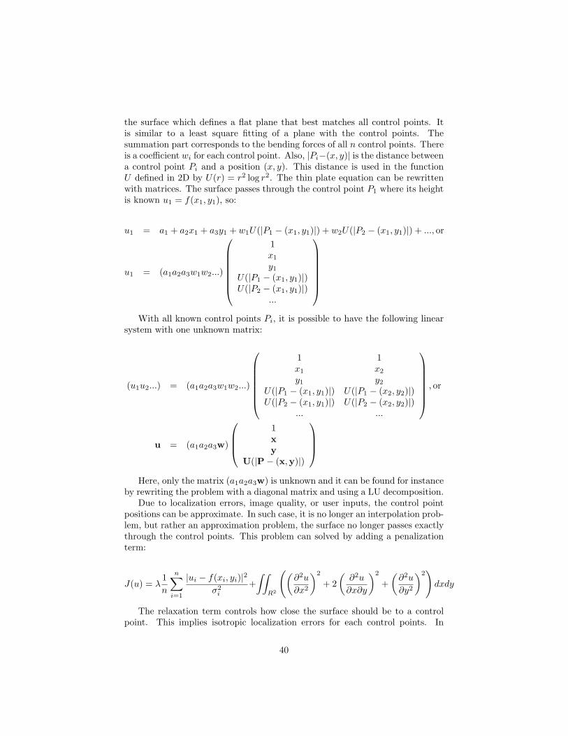
the surface which defines a flat plane that best matches all control points. Itis similar to a least square fitting of a plane with the control points. Thesummation part corresponds to the bending forces of all n control points. Thereis a coefficient wi for each control point. Also, |Pi−(x, y)| is the distance betweena control point Pi and a position (x, y). This distance is used in the functionU defined in 2D by U(r) = r2 log r2. The thin plate equation can be rewrittenwith matrices. The surface passes through the control point P1 where its heightis known u1 = f(x1, y1), so:

u1 = a1 + a2x1 + a3y1 + w1U(|P1 − (x1, y1)|) + w2U(|P2 − (x1, y1)|) + ..., or

u1 = (a1a2a3w1w2...)

1x1

y1

U(|P1 − (x1, y1)|)U(|P2 − (x1, y1)|)

...

With all known control points Pi, it is possible to have the following linear

system with one unknown matrix:

(u1u2...) = (a1a2a3w1w2...)

1 1x1 x2

y1 y2

U(|P1 − (x1, y1)|) U(|P1 − (x2, y2)|)U(|P2 − (x1, y1)|) U(|P2 − (x2, y2)|)

... ...

, or

u = (a1a2a3w)

1xy

U(|P− (x,y)|)

Here, only the matrix (a1a2a3w) is unknown and it can be found for instance

by rewriting the problem with a diagonal matrix and using a LU decomposition.Due to localization errors, image quality, or user inputs, the control point

positions can be approximate. In such case, it is no longer an interpolation prob-lem, but rather an approximation problem, the surface no longer passes exactlythrough the control points. This problem can solved by adding a penalizationterm:

J(u) = λ1n

n∑i=1

|ui − f(xi, yi)|2

σ2i

+∫∫

R2

((∂2u

∂x2

)2

+ 2(

∂2u

∂x∂y

)2

+(

∂2u

∂y2

)2)

dxdy

The relaxation term controls how close the surface should be to a controlpoint. This implies isotropic localization errors for each control points. In

40

[67] anisotropic localization errors are considered by using covariance matricesinstead of σi.

3.2.2 Extension to the temporal domain

Sequences are now considered. Control points now become defined with a posi-tion in space and in time. Rather than interpolating or approximating a positionchange u over space, it can be done over time:

(x′, y′) 7−→ (x, y) + (u, v)u = f(x, y, t)v = f(x, y, t)

A point is no longer dependant on how its neighbors are warped over space,but also on how they move over time. Also, the deformation of time can be nonconstant, the speed of a sequence can be different over time. For instance, adeformation can slow down a heart expansion at some cycles, but speed it upin other cycles. In [88] three options are proposed:

f(x, y, t) = f (gx(x, y, t), gy(x, y, t), h(x, y, t))f(x, y, t) = f (gx(x, y, t), gy(x, y, t), h(t))f(x, y, t) = f (gx(x, y), gy(x, y), h(t))

Here, g and h are respectively the spacial and temporal deformations. Thefirst option considers that space and time are correlated. The position of apoint depends on where its neighboring control points are and how they moveover time. The time deformation depends on space and time, and can becomewarped. That means two points on the same frame are not guaranteed to re-main on a single frame after spatio-temporal deformation. This time-warp isnot desired. The second option removes this anomaly by stating that the timedeformation only depends on the time itself t′ 7−→ t + h(t). The spatial defor-mation still depends on time. The third option reduces the search space, thusthe computational complexity. The space deformation depends only on space.Similarly, the time deformation depends only on time. With this decoupling,the spatial and the temporal deformations become two independent problems.

These two possible options will be studied. First, frames must be success-fully recovered from a sequence. Manual landmarks are tracked over time, andarbitrary points are interpolated with models coupling and decoupling the timedomain with space. Second, the sequence is artificially deformed in space. Therecovered frame should correspond with the original frame. Third, the sequenceis deformed over time. Here, the motion should remain similar during the wholesequence, that is, the heart either expands, or either contracts. When the mo-tion becomes complex, different temporal models should be considered such asusing a harmonic component.

41

3.3 4D registration

As the heart undergoes a complex motion, two image sequences of the same hearttaken at different times, possibly with different image modalities, should be verydifferent. Non rigid registration is required to correctly align the sequences inspace as well as in time. From two image sequences I1 and I2, the spatio-temporal registration should solve the following problem for the transformationT :

I2 = T (I1)

3.3.1 Spatio-temporal component

The transformation T between two image sequences I1 and I2 can be decom-posed with a spatial component T x and a temporal component T t. The twotransformation formulations explained earlier in section 3.2.2 now becomes:

I2(t) = T xt(I1, T

t(t)), or

I2(t) = T x(I1(T t(t))

)The first formulation assumes the spatial and the temporal components are

correlated with each other. It tells that a combined spatio-temporal registra-tion is performed, i.e., the whole two sequences are used to find at once thecorresponding frames, in other words, the goal is to find the best frames thatcan potentially match. On the other hand, the last formulation assumes inde-pendent spatial and temporal components. It tells that a temporal registrationis first performed, followed by a spatial registration, i.e., the two correspondingframes are selected by comparing undeformed frames and are later warped untilthey match.

Although the second option does not necessarily lead to the best transfor-mation, each step (temporal and spatial registration) needs to optimize a fewparameters at a time. The search domain is thus drastically reduced.

3.3.2 Gradient descent based optimization

To find the right transformation, a similarity measure is required:

T = arg minTdiff (T (i1), i2)

The minimization of this last equation is typically done by computing thederivative of diff (T (i1), i2) with respect to T . As seen in the literature sur-vey, popular similarity measures are the squared difference, or the correlationcoefficient when dealing with images of the same modality, and the mutual infor-mation or entropy based similarity measures when dealing with multi modalityimages. For instance, with the squared difference and considering only transla-tions in the transformation T :

42

diff (T (i1), i2) = (i1(x + t)− i2(x))2

In order to compute its derivative, the Taylor expansion is used to get thefollowing:

diff (T (i1), i2) = (i1(x + t)− i2(x))2

' (i1(x) +∇i1(x)t− i2(x))2

The derivative with respect to t is then:

∂diff (T (i1), i2)∂t

= 2∇i1 (x) (i1(x) +∇i1(x)t− i2(x))

This can be used with the gradient descent method to iteratively refine aninitial guess towards a local minimum. In the initial squared difference equation,it is possible to notice a linear system:

diff (T (i1), i2) = (∇i1(x)t− (i2 (x)− i1 (x)))2

t = arg mintdiff (T (i1), i2) ⇐⇒ ∇i1(x) · t ' (i2 (x)− i1 (x))

Here diff (T (i1), i2) should be as small as possible, ideally zero. This isequivalent to solve ∇i1(x) · t ' (i2 (x)− i1 (x)) for t where ' is a least squareapproximation. The problem becomes a linear system similar to Ax = b. Solvingfor t can be done with a LU decomposition or a singular value decomposition(example in [181] or [182]). Approximation due to the initial Taylor expansioncan generate errors. When the displacement t becomes large, refinement will berequired to minimize these errors.

3.3.3 Graph cut approach for optimization

Beside the gradient descent based algorithms, other optimizers exist such as thegenetic algorithm or the simulated annealing. These more complex methodsallow large moves at each iteration rather than small updates computed fromthe gradient. This allows a faster convergence to a local minimum.

The graph cut method described next can also be used as an optimizer. Ithas been used to segment motion from a sequence ([156, 164, 163]). An earlyexperiment also shows it is possible to use graph cuts with mutual information([183]).

A graph cut finds the optimal solution to a binary problem. However whena pixel can be assigned many labels (fp), a serie of graph cuts can be used tominimize the following type of energy:

E(f) =∑p∈P

Dp(ip, fp) +∑

p,q∈NVp,q(fp, fq)

43

The first term is the data term. It penalizes the current labeling f if it is toodifferent with the observed data i. The second term is the smoothness term. Itpenalizes the labeling f if it is not smooth enough, that is if the labels of twoneighboring pixels, fp and fq, are too different. There are three constraints onthis smoothness term:

1. V (α, β) = 0 ⇐⇒ α = β

2. V (α, β) = V (β, α) ≥ 0

3. V (α, β) ≤ V (α, γ) + V (γ, β)

The first two conditions guarantee that there is energy between two differentlabels, if not, that means the two labels are the same. The last condition definesthe triangle rule. A shortcut between two states is always cheaper or similarthan taking intermediate states. If the smoothness term satisfies only the firsttwo conditions, it is said to be a semi-metric term. If the last condition is alsosatisfied, it is said to be a metric term.

The alpha-expansion algorithm can only be used with a metric term. Oth-erwise, the alpha-beta swap can be used with a semi-metric and a metric term.

Whenever the alpha-expansion algorithm is used, it is guaranteed that thelocal minimum is within a known factor of the global minimum. This factor is:

2 maxp,q∈N

maxα6=β V (α, β)minα6=β V (α, β)

By definition this factor can be as small as 2. That means if the maximumpossible smoothness term is V (α, β) = 1 and the minimum possible is V (α, β) =0, the local minimum that the alpha-expansion algorithm will find is at mosttwice the global minimum E∗.

The alpha-beta swap does not guarantee any closeness to the global mini-mum.

Alpha-expansion algorithm The main idea of the alpha-expansion algo-rithm is to successively segment all α and non-α pixels with graph cuts. Thealgorithm will iterate through each possible value for α at each new iteration.It stops when it converges.

At each iteration, the α region Pα can only expand. This changes somehowthe way the graph weights are set. For this reason, when two neighboring nodesdoes not currently have the same label, an intermediate node is inserted andlinks are weighted so they are relative to the distance to the α label.

44

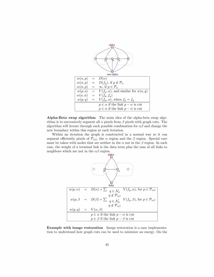
w(α, p) = D(α)w(α, p) = D(fp), if p /∈ Pα

w(α, p) = ∞, if p ∈ Pα

w(p, a) = V (fp, α), and similar for w(a, q)w(a, α) = V (fp, fq)w(p, q) = V (fp, α), when fp = fq

p ∈ α if the link p− α is cutp ∈ α if the link p− α is cut

Alpha-Beta swap algorithm The main idea of the alpha-beta swap algo-rithm is to successively segment all α pixels from β pixels with graph cuts. Thealgorithm will iterate through each possible combination for αβ and change thenew boundary within this region at each iteration.

Within an iteration the graph is constructed in a normal way so it cansegment efficiently pixels of Pαβ , the α region and the β region. Special caremust be taken with nodes that are neither in the α nor in the β region. In suchcase, the weight of a terminal link is the data term plus the sum of all links toneighbors which are not in the αβ region.

w(p, α) = D(α) +∑

q ∈ Np

q /∈ Pαβ

V (fq, α), for p ∈ Pαβ

w(p, β = D(β) +∑

q ∈ Np

q /∈ Pαβ

V (fq, β), for p ∈ Pαβ

w(p, q) = V (α, β)p ∈ α if the link p− α is cutp ∈ β if the link p− β is cut

Example with image restoration Image restoration is a easy implementa-tion to understand how graph cuts can be used to minimize an energy. On the

45

Figure 3.8: Energy minimization with graph cuts can restore a noisy image(on the left). An energy designed to keep the pixel intensities as smooth willgenerate the image on the right.

figure 3.8 is an image with embedded squares of intensity values 255, 191, 128,64. Noise were added to the original image so the intensity becomes i′ = i± 10.Possible labels are all integers between 0 and 255. Here the data term is a simplesquared difference D(ip, fp) = (ip − fp)2 where ip is the observed intensity ofa pixel and fp is restored intensity of the pixel. The smoothness term is thePotts model V (fp, fq) = λT (fp 6= fq) where T (expr) = 1 is expr is true, or zerootherwise. Doing some graph analyzing, it turned out that using λ = 2331 willmake internal link weights competitive with the terminal links. The figure 3.8shows the results of this image restoration. Only a few seconds is needed foreither the alpha-expansion or the alpha-beta swap algorithm to converge.

Deformation Map Recovering the deformation map could be useful in aregistration framework. An original image Ia is deformed (Fig 3.9). The upperpart is moved right and the bottom part of the image is moved left. The resultingimage is Ib. The data term is the squared difference between the pixel intensityia(x) and ib(x+L) where L is the translation of pixel x from its original position.The smoothness term used is again the Potts model with λ = 25. The labelset is all possible translations with ±15 horizontal pixes and ±3 vertical pixels.The figure 3.9 shows the result of the algorithm. The algorithm runs within acouple of minutes until convergence.

3.4 Joint segmentation and registration

The previous subtopics were about segmentation and registration. Unifyingthese two problems in the same mathematical framework would be an elegantand robust way to simultaneously solve segmentation and registration. Theseare indeed very intimate problems. When aligning images, corresponding struc-tures becomes easier to identify, thus segmentation can be improved by aligningimages. Similarly, if the shape and localization of corresponding structures are

46

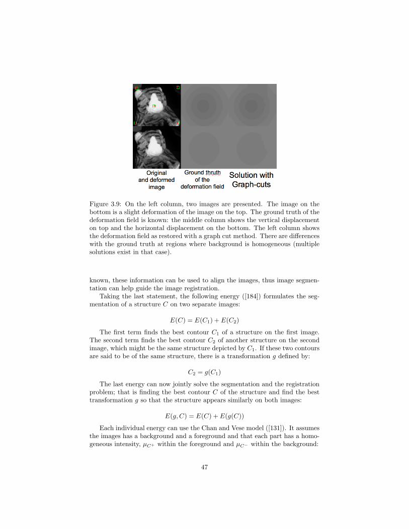
Figure 3.9: On the left column, two images are presented. The image on thebottom is a slight deformation of the image on the top. The ground truth of thedeformation field is known: the middle column shows the vertical displacementon top and the horizontal displacement on the bottom. The left column showsthe deformation field as restored with a graph cut method. There are differenceswith the ground truth at regions where background is homogeneous (multiplesolutions exist in that case).

known, these information can be used to align the images, thus image segmen-tation can help guide the image registration.

Taking the last statement, the following energy ([184]) formulates the seg-mentation of a structure C on two separate images:

E(C) = E(C1) + E(C2)

The first term finds the best contour C1 of a structure on the first image.The second term finds the best contour C2 of another structure on the secondimage, which might be the same structure depicted by C1. If these two contoursare said to be of the same structure, there is a transformation g defined by:

C2 = g(C1)

The last energy can now jointly solve the segmentation and the registrationproblem; that is finding the best contour C of the structure and find the besttransformation g so that the structure appears similarly on both images:

E(g, C) = E(C) + E(g(C))

Each individual energy can use the Chan and Vese model ([131]). It assumesthe images has a background and a foreground and that each part has a homo-geneous intensity, µC+ within the foreground and µC− within the background:

47

E(g, C) =∫

C+(i0(x)− µC+)2 dx +

∫C−

(i0(x)− µC−)2 dx

+∫

C+

(i1(x)− µC+

)2dx +

∫C−

(i1(x)− µC−

)2dx

This model is typically minimized in a level set framework but as shown aprevious section graph cuts can also be used to minimize energies.

3.5 Validation

The validation of each subtopic will follow the same procedure. First, a vali-dation using simulated data will be done. Each subtopic presents its own chal-lenges (discussed next), therefore, the simulated data should make sure theytest each of these challenges. Second, the algorithms will run on data acquiredfrom phantom devices. And at last, real data will be used.

3.5.1 Segmentation

It is hard to claim segmentation is good or not as this is a very subjectivejudgment. Object boundaries can be blurred or inexistent; no ground truthexists for complex images. Validation requires simple test images with clearboundaries that all can concur. However, it then becomes hard to test thesegmentation algorithm in extreme conditions where the boundary becomesarguable.

Validating a spatio-temporal segmentation can be done with an image se-quence where a known object moves. The segmentation algorithm should detectthe object at all frames and the boundary should remain smooth in the temporaldomain. Initially the object should be overlapping from frame to frame as if theobject is in slow motion. A second test can include an object which does notoverlap from frame to frame. This can simulate a fast moving coronary arterythat can move from a few millimeters between two frames. The spatio-temporalsegmentation should show improvements over the spatial segmentation. Thatis segmenting individually each frame should lead to ambiguities that can besolved if all frames are segmented simultaneously.

Tests with real images should correctly segment the coronary arteries inangiogram fluoroscopy and CT, and the different cardiac chambers such as theleft atrium.

3.5.2 Frame interpolation

Frame interpolation over time should recover correctly a voluntary missingframe. Validation will be done by comparing the recovered frame with theoriginal frame.

48

The robustness of the frame interpolation will be validated by removing ormisplacing one or more control points. The interpolated sequence should ideallybe wrong around the misplaced control points. This can be validated with anartificially deformed sequence considered as the ground truth. Reproducing thedeformation with misplaced control points will generate another sequence whichcan be compared with the ground truth. This could lead to a method allowingthe localization of wrong or misplaced control points.

Frame interpolation should also allow the increase, or the decrease, of thesequence frame rate. The motion on the interpolated sequence should remainsmooth. This can be done by tracking a point over time and checking its velocityover the interpolated frames.

Rather than interpolating within the sequence, trimming the sequence wouldallow the robustness of the algorithm with extrapolation. With missing framesat the end, the observable motion from the remaining frame should allow theextrapolation of the missing frames. Validation could be done by comparing therecovered frames with the original frames.

3.5.3 Registration

Synthetic images can be used to validate the registration algorithm. Simpleforms should align correctly over space and over time. The multi-modality sce-nario can be tested with images of resembling appearance, for instance intensityreverted images.

With two image sequences, an artificial temporal deformation of one se-quence can be done. For instance the frame rate can be changed at certaintime in the sequence. The spatio-temporal registration should correct the ar-tificial temporal deformation and both sequences should be well synchronized.Measurements can be done on how the two sequences differ.

Comparison with a state-of-the-art method, such as the optical flow, shouldbe performed. The registration of the new method and of the optical flow shouldbe similar.

Ambiguities should be tested. This becomes important in 2D/3D registra-tion where fluoroscopic projections on 2D planes can have many 3D interpre-tations. Synthetic fluoroscopic images with known 3D structures can be used.Validation can be done with registration of the plane with the original 3D struc-tures.

Temporal ambiguities can occur with simple forms. For instance an imagewith a small circle inside a larger circle is rotated (Fig 3.10). Two interpreta-tions are possible, either the image has rotated, or either the small circle hasbeen translated. This ambiguity should be removed with additional clues suchas another structure in the image. Again, here, no ground truth exists andthe recovered motion is subjective, but the spatio-temporal registration shouldgenerate a coherent solution.

The validation of the unified segmentation and registration framework shouldshow improvements over solutions provided with separate segmentation andregistration. The segmentation should be more robust to noise if used in this

49

Figure 3.10: How to recover the transformation between these two images: didthe large circle rotated with the small circle, or did it remained still while thesmall circle translated?

MICCAI Medical Image Computing and Computer Assisted InterventionMarch 16, 2007

ICCV International Conference on Computer VisionApril 10, 2007

ISBI International Symposium on Biomedical Imaging∼ October 2007

CVPR Computer Vision and Pattern Recognition∼ November, 2008

ECCV European Conference on Computer VisionMarch 14, 2008

ICPR International Conference on Pattern Recognition∼ mid 2008

Table 3.1: Major conferences

unified framework. In the same matter registration should also be more robustto noise.

3.6 Timeline

Two fields can be targeted for publications: medical imaging, and computervision. The table 3.1 shows a list of major conferences in both fields with theirdeadlines. Journals have no deadlines, the table 3.2 is a list of major journalsin the area with their publisher. A Gantt diagram summarizes the proposed

PAMI, Transactions on Pattern Analysis and Machine Intelligence IEEEIJCV, International Journal of Computer Vision SpringerComputer Vision and Image Understanding ElsevierTransactions on Medical Imaging IEEEMedical Image Analysis Elsevier

Table 3.2: Major journals

50

Figure 3.11: Gantt chart of the proposed thesis

51

thesis in the figure 3.11.

52

Chapter 4

Preliminary results

Early experiments are presented in this section. First, the banded graph cutalgorithm ([153]) has been modified in order to handle the segmentation of large4D data sets. Second, a proof of concept has been done in order to show thatgraph cuts can indeed be used for non-rigid segmentation. Third, the motion oflandmarks are tracked using a 4D deformation model. At last, a visualizationlibrary is presented, as well as a development framework for quick and easyalgorithm implementation.

4.1 4D Segmentation

A method based on 4D graph cuts has been proposed to segment large 4Ddatasets. The following description is a summary of a publication submited toMICCAI 2007. The objective is to show that temporal correlation improves thesegmentation accuracy. In order to handle large datasets, the graph cut methodhas been used using a multiresolution approach.

The graph cut method described earlier in the section 3.1.2 can be used in4D. Besides the spatial links, the graph is constructed with temporal links as

Figure 4.1: 4D graph corresponding to 3 frames of a 33 volume. Spatial n-linksin grey lines, temporal n-links for a single node in green lines, and t-links in redand blue.

53

Figure 4.2: Banded approach: (a) object and background seed points providedby the user; (b) global shape computed via graph cuts; (c) construction of theband around the coarse boundary; (d) refinement of the boundary (thick blackcontour) using fast competitive region growing.

shown in the figure 4.1. The cost of a link between two nodes p and q is based onthe intensity difference, wp,q = f(|Ip−Iq|). A temporal link connects two nodesrepresenting two pixels on two different frames, p(t) and q(t+1). The temporalintegrity can be controled by a factor τ that is used when computing the costof the link wp(t),q(t+1) = τ · f(|Ip(t) − Iq(t+1) |).

As proposed in [153], a multiresolution approach is proposed to handle med-ical volumes. The refinement step has been improved with a modified seededregion growing (Fig 4.2). First, coarse graph cuts yield a rough estimate ofthe final segmenation. Second, a narrow band is constructed around the coarseboundary. A competitive region growing takes place between the inner andthe outer boundaries of the narrow band. A priority queue dictates the wayeach region grows. The order in the queue depends on the intensity differencediff(p) = |Ip − Ipar(p)| between the candidate pixel p and its parent par(p).For a newly inserted pixel in the priority queue, its key value key(p) is an inte-gration of previous keys, i.e., key(p) = diff(p) + λ · key(par(p)). When λ > 0,this heuristics favors the growing of regions close to the seed points. Hence, λsimulates the smoothness of the grown boundary.

The figure 4.3 shows that the segmentation accuracy is improved when cap-turing temporal correlations. When an image is degraded by noise, spatialinformation becomes weak. A true 4D segmentation yields a better result thana 3D segmentation of a single frame. The figure 4.4 shows that this method iscomparable to standard graph cuts algorithms.

4.2 Landmark-based non-rigid registration withgraph cuts

This experiment presents an approach based on graph cuts initially used formotion segmentation that is being applied to the non-rigid registration prob-lem. It has been accepted at ICIAR 2007 ([185]). The main objective is tointroduce landmarks in the graph cut minimization framework. First, non-rigidregistration is formulated as an energy minimization problem that can be solved

54

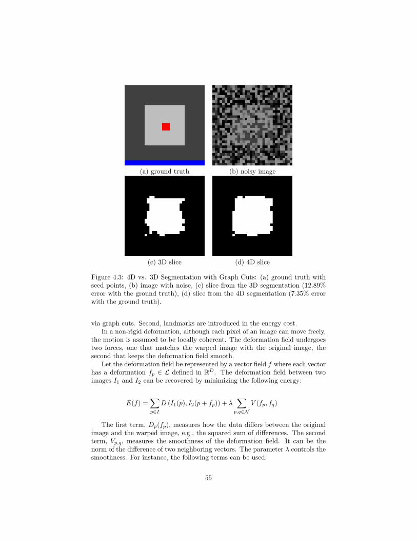
(a) ground truth (b) noisy image

(c) 3D slice (d) 4D slice

Figure 4.3: 4D vs. 3D Segmentation with Graph Cuts: (a) ground truth withseed points, (b) image with noise, (c) slice from the 3D segmentation (12.89%error with the ground truth), (d) slice from the 4D segmentation (7.35% errorwith the ground truth).

via graph cuts. Second, landmarks are introduced in the energy cost.In a non-rigid deformation, although each pixel of an image can move freely,

the motion is assumed to be locally coherent. The deformation field undergoestwo forces, one that matches the warped image with the original image, thesecond that keeps the deformation field smooth.

Let the deformation field be represented by a vector field f where each vectorhas a deformation fp ∈ L defined in RD. The deformation field between twoimages I1 and I2 can be recovered by minimizing the following energy:

E(f) =∑p∈I

D (I1(p), I2(p + fp)) + λ∑

p,q∈NV (fp, fq)

The first term, Dp(fp), measures how the data differs between the originalimage and the warped image, e.g., the squared sum of differences. The secondterm, Vp,q, measures the smoothness of the deformation field. It can be thenorm of the difference of two neighboring vectors. The parameter λ controls thesmoothness. For instance, the following terms can be used:

55

(a) seed points (b) 3D Graph Cuts

(c) 4D M. banded GC (d) our method

Figure 4.4: Comparison with existing methods: (a) seed points for the leftventricle segmentation, (b) 3D standard graph cuts on a single frame (20.88s,1270MB), (c) 4D multilevel banded graph cuts on 15 frames (44.72s, 854MB),(d) our method on 15 frames (9.42sec, 253MB).

D(I1, I2) = (I1(p)− I2(p + fp))2

V (fp, fq) = |fp − fq|2

A landmark k ∈ K can influence its neighborhood by using a penalty costover the whole image. This penalty is infinity at the landmark site p(k), andquickly decreases around the landmark. For instance, the data term is chosento be:

Dp(α) = dp(α) + µ∑k∈K

f(k) 6=α

r2

|p(k)− p|2

Besides the standard data cost dp(α) (e.g. sum of squared differences),all landmarks, whose deformation f(k) 6= α, provide a penalty based on thedistance of the point p to each landmark. Here r is the distance within which

56

the landmark k has a strong effect on point p. Beyond this distance, the penaltydrops below 1 and tends to 0 at infinity. If the point p is at a landmark site,the penalty is infinity and it is not possible to assign the value α at this point.µ is a factor controlling the penalty of landmarks.

The energy as described earlier with its data and smoothness term is then:

E(f) =∑p∈I

(I1(p)− I2(p + fp))2 + µ

∑p∈I

∑k∈K

f(k) 6=fp

r2

|p(k)− p|2+ λ

∑p,q∈N

|fp − fq|2

This energy can be minimized via graph cuts by the two algorithms describedearlier in the section 3.3.3. Results show indeed that the minimization canregister two images. The figure 4.5 shows the non-rigid registration of twoframes from a cineangiogram.

4.3 Motion interpolation of control points withThin-Plates

Early experiments have been tried for motion interpolation with thin platesplines. As described in a previous section, thin plate splines can be usedto interpolate a deformation field. One spline is used to interpolate a defor-mation parameter. Here a sequence of 2D images is considered. A motion isparameterized with a horizontal and vertical displacement:

(xt

yt

)=

(x0

y0

)+(

fx(x0, y0, t)fy(x0, y0, t)

)The displacement of a point from its original position (x0, y0) can be de-

scribed with a translation defined by two thin plates fx and fy. Each of thesesplines is a 4D hypersurface; that is a 3D point (2D+t) with its hyper-height:

h = f(x, y, t) = a0 + a1x + a2y + a3t + σni=0wiU(|Pi − (x, y, t)|)

The thin plate spline equation has been explained in a previous section.There are n control points, each defined by its spatial and temporal coordinates(x, y, t).

The experiment involves a coronary angiogram. Points on the coronary aredefined on the initial frames. Later in the sequence, the position of these controlpoints is corrected at certain frames. The result (Fig 4.6) shows that with ashort sequence of 20 frames, defining 5 control points at only 4 frames is enoughto describe accurately the motion of the coronary arteries.

57

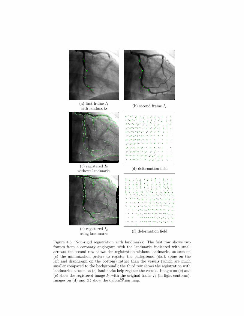
(a) first frame I1

with landmarks (b) second frame I2

(c) registered I2

without landmarks (d) deformation field

(e) registered I2

using landmarks (f) deformation field

Figure 4.5: Non-rigid registration with landmarks: The first row shows twoframes from a coronary angiogram with the landmarks indicated with smallarrows; the second row shows the registration without landmarks, as seen on(c) the minimization prefers to register the background (dark spine on theleft and diaphragm on the bottom) rather than the vessels (which are muchsmaller compared to the background); the third row shows the registration withlandmarks, as seen on (e) landmarks help register the vessels. Images on (c) and(e) show the registered image I2 with the original frame I1 (in light contours).Images on (d) and (f) show the deformation map.58

Figure 4.6: The motion of the control points are interpolated over time. Witha sequence of 20 frames, the control points are defined at 4 different frames.Here a frame where the control points have not been defined is shown. On theleft is the last known position of the control points. It is clear that the lastknown position is no longer valid as the vessels have moved. On the right arethe interpolated positions of the control points. With interpolation, the controlpoints remain correctly on the vessel over the whole sequence.

Deformation map with thin plates Interpolation of a deformation mapwith thin plates has been tried earlier. With 2 splines and the displacementfield defined at a few control points, it is possible to generate a deformationmap for the whole image. Assigning intensities from an image at each point ofthe deformation map allows image warping such as in the figure 3.7.

Deformation map with graph cuts A new method using graph cuts hasbeen described in a previous section (3.3.3). The deformation map is found byminimizing an energy with graph cuts. The main idea is to find a label for eachpixel. The label set is all possible deformations. The energy guarantees thatthe label map will explain well the deformation between two images and will besmooth (Fig 3.9).

4.4 Building a visualization library and devel-opment platform

Visualization is an important aspect of this thesis. Results need to be seenin 3D. Thus, the development of a 3D visualization library is required. A 3Drenderer has been implemented with OpenGL 3D textures. This is achievedby applying textures on stacked planes parallel to the screen. As hundreds ofplanes are used, the generated image looks like a solid volume as seen on thefigure 4.7.

A development platform has been done in order to simplify algorithm de-

59

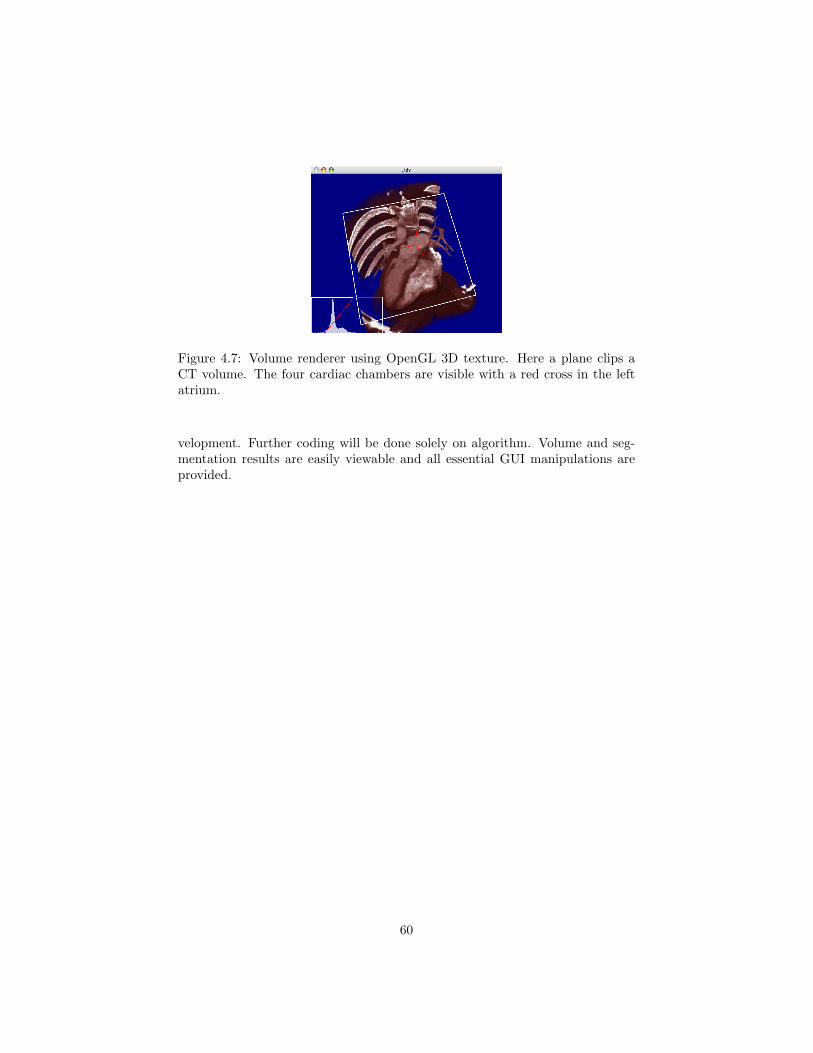
Figure 4.7: Volume renderer using OpenGL 3D texture. Here a plane clips aCT volume. The four cardiac chambers are visible with a red cross in the leftatrium.

velopment. Further coding will be done solely on algorithm. Volume and seg-mentation results are easily viewable and all essential GUI manipulations areprovided.

60

Chapter 5

Conclusion

Cardiovascular diseases are the number 1 killer in most western countries. Imageguided interventions are popular procedures for the diagnostic and the treat-ment of many cardiac diseases. As the intervention is performed with no directvisual contact, a major limitation is the understanding of the patient’s heartanatomy and function. In such conditions, the need for imaging technologiesbecomes essential, however, medical images contain a tremendous amount ofinformation. Extracting and combining digested information from different im-ages provide detailed roadmaps that make image-guided interventions possible.As the technology evolves, images are not only available in 2D and 3D, but alsoin 4D (3D+t). The research area is aimed towards the temporal aspect of thesegmentation and the registration problem.

The heart anatomy and function has been described along with the currentstate-of-the-art of segmentation and registration methods. The fusion of multi-modal cardiac image sequences is a subject where many contributions has yetto be made. Therefore, this thesis will focus in this field. Subtopics includessegmentation, deformation model, and non-rigid registration of image sequences.

All subtopics can be formulated as an energy minization problem. Ratherthan solving segmentation and registration separately, it is hypothesized thatthey are both a mutual problem. When images are correctly aligned, bound-aries of corresponding anatomy should match: registration helps segmentation;and when corresponding anatomy is known, their alignement becomes easier:segmentation guides registration. The main contribution of this thesis will even-tually be a mathematical framework unifying spatio-temporal segmentation andregistration.

61

Bibliography

[1] Thomas Thom, Nancy Haase, Wayne Rosamond, Virginia J. Howard,John Rumsfeld, Teri Manolio, Zhi-Jie Zheng, Katherine Flegal, Christo-pher O’donnell, Steven Kittner, Donald Lloyd-Jones, David C. Goff, andYuling Hong. Heart disease and stroke statistics–2006 update. Circulation,113:85–151, 2006.

[2] Yiyong Sun, Fred S. Azar, Chenyang Xu, Gal Hayam, Assaf Preiss, Nor-bert Rahn, and Frank Sauer. Registration of high-resolution 3d atrialimages with electroanatomical cardiac mapping: evaluation of registra-tion methodology. volume 5744, pages 299–307. SPIE, 2005.

[3] G. Shechter, C. Ozturk, J. R. Resar, and E. R. Mcveigh. Respiratorymotion of the heart from free breathing coronary angiograms. MedicalImaging, IEEE Transactions on, 23(8):1046–1056, 2004.

[4] D. Manke, K. Nehrke, P. Rosch, and O. Dossel. Study of respiratorymotion of the heart in coronary mr angiography. International Journal ofBioelectromagnetism, 2(2), 2000.

[5] M. M. Ter-Pogossian, S. R. Bergmann, and B. E. Sobel. Influence ofcardiac and respiratory motion on tomographic reconstructions of theheart: implications for quantitative nuclear cardiology. J Comput AssistTomogr, 6(6):1148–1155, December 1982.

[6] W. M. Feinberg, J. L. Blackshear, A. Laupacis, R. Kronmal, and R. G.Hart. Prevalence, age distribution, and gender of patients with atrialfibrillation. analysis and implications. Arch Intern Med, 155(5):469–473,March 1995.

[7] Emelia J. Benjamin, Philip A. Wolf, Ralph B. D’Agostino, Halit Silber-shatz, William B. Kannel, and Daniel Levy. Impact of atrial fibrillation onthe risk of death : The framingham heart study. Circulation, 98(10):946–952, September 1998.

[8] Duncan R. Coles, Mary A. Smail, Ian S. Negus, Peter Wilde, Martin Ober-hoff, Karl R. Karsch, and Andreas Baumbach. Comparison of radiationdoses from multislice computed tomography coronary angiography and

62

conventional diagnostic angiography. Journal of the American College ofCardiology, 47(9):1840–1845, May 2006.

[9] W. Huda. Is energy imparted a good measure of the radiation risk associ-ated with ct examinations? Phys Med Biol, 29(9):1137–1142, September1984.

[10] K. Faulkner and B. M. Moores. Radiation dose and somatic risk fromcomputed tomography. Acta Radiol, 28(4):483–488, 1987.

[11] D. Brenner, C. Elliston, E. Hall, and W. Berdon. Estimated risks ofradiation-induced fatal cancer from pediatric ct. AJR Am J Roentgenol,176(2):289–296, February 2001.

[12] G. L. Brownell, C. A. Burnham, Hoop B. Jr, and D. E. Bohning. Quan-titative dynamic studies using short-lived radioisotopes and positron de-tection. In in Proceedings of the Symposium on Dynamic Studies withRadioisotopes in Medicine, pages 161–172, Rotterdam, The Netherlands,September 1970. International Atomic Energy Agency.

[13] M. M. Ter-Pogossian, M. E. Phelps, E. J. Hoffman, and N. A. Mullani. Apositron-emission transaxial tomograph for nuclear imaging (pett). Radi-ology, 114(1):89–98, January 1975.

[14] Karin Knesaurek and Josef Machac. Comparison of f-18 spect with petin myocardial imaging: A realistic thorax-cardiac phantom study. BMCNuclear Medicine, 6:5+, October 2006.

[15] D. E. Kuhl and R. Q. Edwards. Image separation radioisotope scanning.Radiology, 80:653–661, 1963.

[16] H. O. Anger. Scintillation camera with multichannel collimators. J NuclMed, 5:515–531, July 1964.

[17] Paul Schoenhagen and Steven Nissen. Understanding coronary arterydisease: tomographic imaging with intravascular ultrasound. Heart,88(1):91–96, 2002.

[18] N. F. Marrouche, D. O. Martin, O. Wazni, A. M. Gillinov, A. Klein,M. Bhargava, E. Saad, D. Bash, H. Yamada, W. Jaber, R. Schweikert,P. Tchou, A. Abdul-Karim, W. Saliba, and A. Natale. Phased-arrayintracardiac echocardiography monitoring during pulmonary vein isolationin patients with atrial fibrillation: impact on outcome and complications.Circulation, 107(21):2710–2716, June 2003.

[19] N. Bom, C. T. Lancee, and F. C. Van Egmond. An ultrasonic intracardiacscanner. Ultrasonics, 10(2):72–76, March 1972.

[20] Cr Meyer, Eh Chiang, Kp Fechner, Dw Fitting, Dm Williams, andAj Buda. Feasibility of high-resolution, intravascular ultrasonic imagingcatheters. Radiology, 168(1):113–116, July 1988.

63

[21] J. B. Seward, B. K. Khandheria, C. G. McGregor, T. J. Locke, and A. J.Tajik. Transvascular and intracardiac two-dimensional echocardiography.Echocardiography, 7(4):457–464, July 1990.

[22] A. Fenster and D. B. Downey. 3-d ultrasound imaging: a review. Engi-neering in Medicine and Biology Magazine, IEEE, 15(6):41–51, 1996.

[23] M. P. Fronheiser, E. D. Light, and S. W. Smith. Real-time 3d ultrasoundwith multiple transducer arrays. volume 1, pages 786–789 Vol.1, 2004.

[24] Albert C. Lardo, Elliot R. Mcveigh, Pitayadet Jumrussirikul, Ronald D.Berger, Hugh Calkins, Joao Lima, and Henry R. Halperin. Visualizationand temporal/spatial characterization of cardiac radiofrequency ablationlesions using magnetic resonance imaging. Circulation, 102(6):698–705,August 2000.

[25] Qi Zhang, R. Eagleson, and T. M. Peters. Real-time visualization of 4dcardiac mr images using graphics processing units. pages 343–346, 2006.

[26] Nobel Lectures, Physiology or Medicine 1942-1962. Elsevier PublishingCompany, Amsterdam, 1964.

[27] C. T. DOTTER and M. P. JUDKINS. Transluminal treatment of arte-riosclerotic obstruction. description of a new technic and a preliminaryreport of its application. Circulation, 30:654–670, November 1964.

[28] A. R. Gruntzig, A. Senning, and W. E. Siegenthaler. Nonoperative di-latation of coronary-artery stenosis: percutaneous transluminal coronaryangioplasty. N Engl J Med, 301(2):61–68, July 1979.

[29] E. Grube, J. C. Laborde, U. Gerckens, T. Felderhoff, B. Sauren, L. Buelles-feld, R. Mueller, M. Menichelli, T. Schmidt, B. Zickmann, S. Iversen, andG. W. Stone. Percutaneous implantation of the corevalve self-expandingvalve prosthesis in high-risk patients with aortic valve disease: the sieg-burg first-in-man study. Circulation, 114(15):1616–1624, October 2006.

[30] P. G. Bjørnstad. Is interventional closure the current treatment of choicefor selected patients with deficient atrial septation? Cardiol Young,16(1):3–10, February 2006.

[31] M. Haıssaguerre, L. Gencel, B. Fischer, P. Le Metayer, F. Poquet, F. I.Marcus, and J. Clementy. Successful catheter ablation of atrial fibrillation.J Cardiovasc Electrophysiol, 5(12):1045–1052, December 1994.

[32] S. A. Chen, M. H. Hsieh, C. T. Tai, C. F. Tsai, V. S. Prakash, W. C. Yu,T. L. Hsu, Y. A. Ding, and M. S. Chang. Initiation of atrial fibrillation byectopic beats originating from the pulmonary veins: electrophysiologicalcharacteristics, pharmacological responses, and effects of radiofrequencyablation. Circulation, 100(18):1879–1886, November 1999.

64

[33] J. L. Cox, J. P. Boineau, R. B. Schuessler, K. M. Kater, and D. G. Lappas.Five-year experience with the maze procedure for atrial fibrillation. AnnThorac Surg, 56(4), October 1993.

[34] James D. Maloney, Ladyne Milner, Serge Barold, Barbara Czerska, andMichael Markel. Two-staged biatrial linear and focal ablation to restoresinus rhythm in patients with refractory chronic atrial fibrillation: Proce-dure experience and follow-up beyond 1 year. Pacing and Clinical Elec-trophysiology, 21(11):2527–2532, 1998.

[35] C. Pappone, G. Oreto, F. Lamberti, G. Vicedomini, M. L. Loricchio, S. Sh-pun, M. Rillo, M. P. Calabro, A. Conversano, S. A. Ben-Haim, R. Cap-pato, and S. Chierchia. Catheter ablation of paroxysmal atrial fibrillationusing a 3d mapping system. Circulation, 100(11):1203–1208, September1999.

[36] A. C. Skanes, G. Klein, A. Krahn, and R. Yee. Cryoablation: potentialsand pitfalls. J Cardiovasc Electrophysiol, 15(10 Suppl), October 2004.

[37] N. M. Fried, A. Tsitlik, K. C. Rent, R. D. Berger, A. C. Lardo, H. Calkins,and H. R. Halperin. Laser ablation of the pulmonary veins by usinga fiberoptic balloon catheter: implications for treatment of paroxysmalatrial fibrillation. Lasers Surg Med, 28(3):197–203, 2001.

[38] M. Knaut, S. M. Tugtekin, and K. Matschke. Pulmonary vein isolation bymicrowave energy ablation in patients with permanent atrial fibrillation.J Card Surg, 19(3):211–215, 2004.

[39] A. Venot and V. Leclerc. Automated correction of patient motion andgray values prior to subtraction in digitized angiography. IEEE TransMed Imaging, 3(4):179–186, 1984.

[40] Lisa G. Brown. A survey of image registration techniques. ACM Comput.Surv., 24(4):325–376, December 1992.

[41] P. A. van den Elsen, E. J. D. Pol, and M. A. Viergever. Medical im-age matching-a review with classification. Engineering in Medicine andBiology Magazine, IEEE, 12(1):26–39, 1993.

[42] M. Singh, W. Frei, T. Shibata, and G. C. Huth. A digital technique foraccurate change detection in nuclear medical images 0 with application tomyocardial perfusion studies using thallium-201. IEEE Transactions onNuclear Science, 1(26):565–575, 1979.

[43] W. R. Crum, T. Hartkens, and D. L. Hill. Non-rigid image registration:theory and practice. The British Journal of Radiology, 77(2):140–153,2004.

65

[44] T. Makela, P. Clarysse, O. Sipila, N. Pauna, Q. C. Pham, T. Katila, andI. E. Magnin. A review of cardiac image registration methods. IEEETrans Med Imaging, 21(9):1011–1021, September 2002.

[45] Demetri Terzopoulos, John Platt, Alan Barr, and Kurt Fleischer. Elas-tically deformable models. SIGGRAPH Comput. Graph., 21(4):205–214,July 1987.

[46] Gary E. Christensen, Michael I. Miller, Michael W. Vannier, and UlfGrenander. Individualizing neuroanatomical atlases using a massivelyparallel computer. Computer, 29(1):32–38, January 1996.

[47] C. Davatzikos and J. L. Prince. Brain image registration based on curvemapping. In Biomedical Image Analysis, 1994., Proceedings of the IEEEWorkshop on, pages 245–254, 1994.

[48] G. E. Christensen, R. D. Rabbitt, and M. I. Miller. Deformable templatesusing large deformation kinematics. Image Processing, IEEE Transactionson, 5(10):1435–1447, 1996.

[49] E. D’Agostino, F. Maes, D. Vandermeulen, and P. Suetens. A viscousfluid model for multimodal non-rigid image registration using mutual in-formation. Med Image Anal, 7(4):565–575, December 2003.

[50] B. D. Lucas and T. Kanade. An iterative image registration techniquewith an application to stereo vision. In Imaging Understanding Workshop,pages 121–130, 1981.

[51] Horn and Schunck. Determining optical flow. Artificial Intelligence, 17(1-3):185–203, August 1981.

[52] Berthold K. P. Horn and Brian G. Schunck. Determining optical flow.Physics-Based Vision: Principles And Practice, pages 389–407, 1992.

[53] S. M. Song and R. M. Leahy. Computation of 3-d velocity fields from 3-dcine ct images of a human heart. Medical Imaging, IEEE Transactionson, 10(3):295–306, 1991.

[54] Yongme Wang and Lawrence H. Staib. Elastic model based non-rigidregistration incorporating statistical shape information. In Medical ImageComputing and Computer-Assisted Interventation — MICCAI’98, volume1496, pages 1162–1173, 1998.

[55] Yongmei Wang and Lawrence H. Staib. Physical model-based non-rigidregistration incorporating statistical shape information. Medical ImageAnalysis, 4(1):7–20, March 2000.

[56] J. Duchon. Interpolation des fonctions de deux variables suivant leprincipe de la flexion des plaques minces. Revue d’automation, infor-matique et recherche operationelle, 10(12):5–12, 1976.

66

[57] Jean Meinguet. Multivariate interpolation at arbitrary points made sim-ple. Zeitschrift fur Angewandte Mathematik und Physik, 30(2):292–304,1979.

[58] F. L. Bookstein. Principal warps: thin-plate splines and the decompositionof deformations. IEEE Transactions on Pattern Analysis and MachineIntelligence, 11(6):567–585, 1989.

[59] Seung-Yong Lee, Kyung-Yong Chwa, and Sung Y. Shin. Image meta-morphosis using snakes and free-form deformations. In SIGGRAPH ’95:Proceedings of the 22nd annual conference on Computer graphics and in-teractive techniques, pages 439–448, New York, NY, USA, 1995. ACMPress.

[60] S. Lee, G. Wolberg, and S. Y. Shin. Scattered data interpolation withmultilevel b-splines. Visualization and Computer Graphics, IEEE Trans-actions on, 3(3):228–244, 1997.

[61] E. Bardinet, L. D. Cohen, and N. Ayache. Tracking and motion analysisof the left ventricle with deformable superquadrics. Med. Image Anal.,1(2):129–149, June 1996.

[62] D. Rueckert, L. I. Sonoda, C. Hayes, D. L. Hill, M. O. Leach, and D. J.Hawkes. Nonrigid registration using free-form deformations: applicationto breast MR images. IEEE Transactions on Medical Imaging, 18(8):712–721, August 1999.

[63] D’Arcy W. Thompson. On Growth and Form. Courier Dover Publications,1917.

[64] Thomas W. Sederberg and Scott R. Parry. Free-form deformation of solidgeometric models. In SIGGRAPH ’86: Proceedings of the 13th annualconference on Computer graphics and interactive techniques, pages 151–160, New York, NY, USA, 1986. ACM Press.

[65] William M. Hsu, John F. Hughes, and Henry Kaufman. Direct manipu-lation of free-form deformations. In SIGGRAPH ’92: Proceedings of the19th annual conference on Computer graphics and interactive techniques,pages 177–184, New York, NY, USA, 1992. ACM Press.

[66] Grace Wahba. Spline models for observational data, volume 59 of CBMS-NSF Regional Conference Series in Applied Mathematics. Society forIndustrial and Applied Mathematics (SIAM), Philadelphia, PA, 1990.

[67] K. Rohr, H. S. Stiehl, R. Sprengel, T. M. Buzug, J. Weese, and M. H.Kuhn. Landmark-based elastic registration using approximating thin-plate splines. Medical Imaging, IEEE Transactions on, 20(6):526–534,2001.

67

[68] T. S. Denney and J. L. Prince. Reconstruction of 3-d left ventricularmotion from planar tagged cardiac mr images: an estimation theoreticapproach. Medical Imaging, IEEE Transactions on, 14(4):625–635, 1995.

[69] J. C. Mceachen, A. Nehorai, and J. S. Duncan. Multiframe temporal esti-mation of cardiac nonrigid motion. Image Processing, IEEE Transactionson, 9(4):651–665, 2000.

[70] A. Jutra. Video-tele-radiodiagnosis. L’union medicale du Canada,88:1215–1217, October 1959.

[71] R. A. Robb. Dynamic spatial reconstructor: an x-ray video fluoroscopicct scanner for dynamic volume imaging of moving organs. IEEE TransMedical Imaging, 1(1):22–34, 1982.

[72] R. A. Robb, L. J. Sinak, E. A. Hoffman, J. H. Kinsey, L. D. Harris, andE. L. Ritman. Dynamic volume imaging of moving organs. Journal ofMedical Systems, 6(6), December 1982.

[73] K. Saito, M. Saito, S. Komatu, and K. Ohtomo. Real-time four-dimensional imaging of the heart with multi-detector row ct. Radiograph-ics, 23(1), 2003.

[74] E. A. Zerhouni, D. M. Parish, W. J. Rogers, A. Yang, and E. P. Shapiro.Human heart: tagging with mr imaging–a method for noninvasive assess-ment of myocardial motion. Radiology, 169(1):59–63, October 1988.

[75] L. Axel and L. Dougherty. Mr imaging of motion with spatial modulationof magnetization. Radiology, 171(3):841–845, June 1989.

[76] B. D. Bolster, E. R. Mcveigh, and E. A. Zerhouni. Myocardial taggingin polar coordinates with use of striped tags. Radiology, 177(3):769–772,December 1990.

[77] S. Kumar and D. Goldgof. Automatic tracking of spamm grid and theestimation of deformation parameters from cardiac mr images. MedicalImaging, IEEE Transactions on, 13(1):122–132, 1994.

[78] T. Mcinerney and D. Terzopoulos. Deformable models in medical imageanalysis: a survey. Medical Image Analysis, 1(2):91–108, June 1996.

[79] K. Bartels, A. Bovik, S. J. Aggarwal, and K. R. Diller. The analysis ofbiological shape changes from multidimensional dynamic images. ComputMed Imaging Graph, 17(2):89–99, 1993.

[80] Yaron Caspi and Michal Irani. Spatio-temporal alignment of sequences.IEEE Trans. Pattern Anal. Mach. Intell., 24(11):1409–1424, November2002.

68

[81] E. Shechtman, Yaron Caspi, and Michal Irani. Increasing space-time reso-lution in video. In ECCV ’02: Proceedings of the 7th European Conferenceon Computer Vision-Part I, pages 753–768, London, UK, 2002. Springer-Verlag.

[82] Michal Irani and Shmuel Peleg. Improving resolution by image registra-tion. CVGIP: Graph. Models Image Process., 53(3):231–239, May 1991.

[83] T. L. Faber, R. W. Mccoll, R. M. Opperman, J. R. Corbett, and R. M.Peshock. Spatial and temporal registration of cardiac spect and mr images:methods and evaluation. Radiology, 179(3):857–861, June 1991.

[84] Dimitrios Perperidis, Anil Rao, Maria Lorenzo-Valdes, Raad Mohiaddin,and Daniel Rueckert. Spatio-temporal Alignment of 4D Cardiac MR Im-ages, volume 2674 of Lecture Notes in Computer Science, pages 205–214.Springer Berlin / Heidelberg, August 2003.

[85] D. G. Gibson, T. A. Prewitt, and D. J. Brown. Analysis of left ventricularwall movement during isovolumic relaxation and its relation to coronaryartery disease. Br Heart J, 38(10):1010–1019, October 1976.

[86] D. Perperidis, A. Rao, R. Mohiaddin, and D. Rueckert. Non-rigid Spatio-Temporal Alignment of 4D Cardiac MR Images, volume 2717 of LectureNotes in Computer Science, pages 191–200. Springer Berlin / Heidelberg,November 2003.

[87] Dimitrios Perperidis, Raad H. Mohiaddin, and Daniel Rueckert. Spatio-temporal free-form registration of cardiac mr image sequences. MedicalImage Analysis, 9(5):441–456, October 2005.

[88] Dimitrios Perperidis. Spatio-temporal registration and modelling of theheart using cardiovascular MR imaging. PhD thesis, University of London,September 2005.

[89] Anil Rao, Gerardo, Raghavendra Chandrashekara, Maria L. Valdes, RaadMohiaddin, and Daniel Rueckert. Construction of a cardiac motion atlasfrom mr using non-rigid registration. In FIMH, pages 141–150, 2003.

[90] D. Perperidis, M. Lorenzo-Valdes, R. Chandrashekara, A. Rao, R. Mohi-addin, G. I. Sanchez-Ortiz, and D. Rueckert. Building a 4d atlas of thecardiac anatomy and motion using mr imaging. In Biomedical Imaging:Macro to Nano, 2004. IEEE International Symposium on, volume 1, pages412–415. IEEE Computer Society, 2004.

[91] Rana Haddad, Patrick Clarysse, Maciej Orkisz, Pierre Croisille, DidierRevel, and Isabelle E. Magnin. A realistic anthropomorphic numericalmodel of the beating heart. In FIMH, pages 384–393, 2005.

69

[92] M. J. Ledesma-Carbayo, J. Kybic, M. Suhling, P. Hunziker, M. Desco,A. Santos, and M. Unser. Cardiac ultrasound motion detection by elas-tic registration exploiting temporal coherence. In Biomedical Imaging,2002. Proceedings. 2002 IEEE International Symposium on, pages 585–588, 2002.

[93] M. J. Ledesma-Carbayo, J. Kybic, M. Desco, A. Santos, M. Suhling,P. Hunziker, and M. Unser. Spatio-temporal nonrigid registrationfor ultrasound cardiac motion estimation. IEEE Trans Med Imaging,24(9):1113–1126, September 2005.

[94] Marıa J. Ledesma-Carbayo, Jan Kybic, Manuel Desco, Andres Santos,and Michael Unser. Cardiac motion analysis from ultrasound sequencesusing non-rigid registration. In MICCAI ’01: Proceedings of the 4th Inter-national Conference on Medical Image Computing and Computer-AssistedIntervention, pages 889–896, London, UK, 2001. Springer-Verlag.

[95] F. Cheriet, D. Jiang, and N. F. Stewart. Modelling and simulation ofscoliotic deformities. In Modelling, Identification and Control (MIC 2005),pages 16–18, Innsbruck, Austria, February 2005.

[96] J. B. Maintz and M. A. Viergever. A survey of medical image registration.Medical Image Analysis, 2(1):1–36, March 1998.

[97] R. P. Woods, S. R. Cherry, and J. C. Mazziotta. Rapid automated al-gorithm for aligning and reslicing pet images. J Comput Assist Tomogr,16(4):620–633, 1992.

[98] Derek L. G. Hill, David J. Hawkes, Neil A. Harrison, and Cliff F. Ruff.A strategy for automated multimodality image registration incorporatinganatomical knowledge and imager characteristics. In IPMI ’93: Proceed-ings of the 13th International Conference on Information Processing inMedical Imaging, pages 182–196, London, UK, 1993. Springer-Verlag.

[99] P. A. Van den Elsen, J. B. A. Maintz, E. J. D. Pol, and M. A. Viergever.Automatic registration of ct and mr brain images using correlation ofgeometrical features. Medical Imaging, IEEE Transactions on, 14(2):384–396, 1995.

[100] Andre Collignon, Dirk Vandermeulen, Paul Suetens, and Guy Marchal. 3dmulti-modality medical image registration using feature space clustering.In CVRMed ’95: Proceedings of the First International Conference onComputer Vision, Virtual Reality and Robotics in Medicine, pages 195–204, London, UK, 1995. Springer-Verlag.

[101] C. Studholme, D. L. G. Hill, and D. J. Hawkes. Multiresolution voxel simi-larity measures for mr-pet registration. In Yves Bizais, Christian Barillot,and Robert Di Paola, editors, Proceedings of Information Processing inMedical Imaging, volume 3, pages 287–298, Ile de Berder, France, June1995. Kluwer Academic Publishers.

70

[102] C. Shannon. A mathematical theory of communication. Technical report,Bell System, July 1948.

[103] P. Viola and W. M. Wells. Alignment by maximization of mutual in-formation. In Computer Vision, 1995. Proceedings, Fifth InternationalConference on, pages 16–23, 1995.

[104] A. Collignon, F. Maes, D. Delaere, P. Vandermeulen, P. Suetens, andG. Marchal. automated multimodality image registration based on infor-mation theory. In Yves Bizais, Christian Barillot, and Robert Di Paola,editors, Proceedings of Information Processing in Medical Imaging, vol-ume 3, pages 263–274, Ile de Berder, France, June 1995. Kluwer AcademicPublishers.

[105] F. Maes, A. Collignon, D. Vandermeulen, G. Marchal, and P. Suetens.Multimodality image registration by maximization of mutual information.IEEE Trans Med Imaging, 16(2):187–198, April 1997.

[106] C. Studholme, D. L. G. Hill, and D. J. Hawkes. An overlap invariantentropy measure of 3d medical image alignment. Pattern Recognition,32(1):71–86, January 1999.

[107] J. P. Pluim, J. B. Maintz, and M. A. Viergever. Mutual-information-based registration of medical images: a survey. IEEE Trans Med Imaging,22(8):986–1004, August 2003.

[108] S. Kullback. Information theory and statistics. John Wiley and Sons.,New York, 1959.

[109] Albert C. S. Chung, William M. Wells, Alexander Norbash, and Eric.Multi-modal image registration by minimising kullback-leibler distance.In MICCAI ’02: Proceedings of the 5th International Conference on Med-ical Image Computing and Computer-Assisted Intervention-Part II, pages525–532, London, UK, 2002. Springer-Verlag.

[110] Rui Gan, Jue Wu, Albert C. S. Chung, Simon C. H. Yu, and William M.Wells. Multiresolution image registration based on kullback-leibler dis-tance, 2004.

[111] Ho-Ming Chen, A. C. S. Chung, S. C. H. Yu, A. Norbash, and W. M. Wells.Multi-modal image registration by minimizing kullback-leibler distancebetween expected and observed joint class histograms. In Computer Visionand Pattern Recognition, 2003. Proceedings. 2003 IEEE Computer SocietyConference on, volume 2, pages II–570–6 vol.2, 2003.

[112] D. Marr and E. Hildreth. Theory of edge detection. In Proceedings of theRoyal Society of London, volume 207, pages 187–217, February 1980.

[113] J. Canny. A computational approach to edge detection. IEEE Trans.Pattern Anal. Mach. Intell., 8(6):679–698, November 1986.

71

[114] G. W. Zack, W. E. Rogers, and S. A. Latt. Automatic measurement ofsister chromatid exchange frequency. J Histochem Cytochem, 25(7):741–753, July 1977.

[115] Mehmet Sezgin and Bulent Sankur. Survey over image thresholding tech-niques and quantitative performance evaluation. Journal of ElectronicImaging, 13(1):146–168, 2004.

[116] N. Otsu. A threshold selection method from gray level histograms. IEEETrans. Systems, Man and Cybernetics, 9:62–66, March 1979.

[117] M. Cheriet, J. N. Said, and C. Y. Suen. A recursive thresholding tech-nique for image segmentation. Image Processing, IEEE Transactions on,7(6):918–921, 1998.

[118] C. R. Brice and C. L. Fennema. Scene analysis using regions. ArtificialIntelligence Journal, 1(3):205–226, 1970.

[119] R. Adams and L. Bischof. Seeded region growing. IEEE Trans on PAMI,16(6):641–647, 1994.

[120] Steven L. Horowitz and Theodosios Pavlidis. Picture segmentation by atree traversal algorithm. J. ACM, 23(2):368–388, April 1976.

[121] L. Vincent and P. Soille. Watersheds in digital spaces: an efficient al-gorithm based on immersion simulations. Pattern Analysis and MachineIntelligence, IEEE Transactions on, 13(6):583–598, 1991.

[122] Jean M. Morel and Sergio Solimini. Variational methods in image seg-mentation. Birkhauser Boston Inc., Cambridge, MA, USA, 1995.

[123] David Mumford. Book review: Variational methods in image segmenta-tion, April 1996.

[124] David Mumford and Jayant Shah. Boundary detection by minimizingfunctionals. In Proceedings of IEEE Conference on Computer Vision andPattern Recognition, pages 22–26, San Fransisco, 1985.

[125] David Mumford and Jyant Shah. Optimal approximation by piecewisesmooth functions and associated variational problems. Communicationson Pure Applied Mathematics, 42:577–685, 1989.

[126] David Mumford. The Bayesian rationale for the variational formulation,chapter 5, pages 137–147. Ed. Dordrecht, Kluwer, The Netherlands, 1994.

[127] D. B. Cooper, H. Elliott, F. Cohen, L. Reiss, and P. Symosek. Stochasticboundary estimation and object recognition. Image Modeling, pages 63–94, 1981.

72

[128] Stuart Geman and Donald Geman. Stochastic relaxation, gibbs distribu-tions, and the bayesian restoration of images. IEEE Trans. Pattern Anal.Mach. Intell., 6:721–741, 1984.

[129] Jose L. Marroquin. Surface reconstruction preserving discontinuities.Technical report, Massachusetts Institute of Technology, Cambridge, MA,USA, 1984.

[130] J. Petitot. An introduction to the mumford-shah segmentation model. JPhysiol Paris, 97(2-3):335–342, 2003.

[131] Tony Chan and Luminita Vese. An active contour model without edges. InSCALE-SPACE ’99: Proceedings of the Second International Conferenceon Scale-Space Theories in Computer Vision, pages 141–151, London, UK,1999. Springer-Verlag.

[132] Michael Kass, Andrew Witkin, and Demetri Terzopoulos. Snakes: Activecontour models. International Journal of Computer Vision, V1(4):321–331, January 1988.

[133] Chenyang Xu and Jerry L. Prince. Gradient vector flow: A new externalforce for snakes. In CVPR ’97: Proceedings of the 1997 Conference onComputer Vision and Pattern Recognition (CVPR ’97), Washington, DC,USA, 1997. IEEE Computer Society.

[134] Stanley Osher and James A. Sethian. Fronts propagating with curvature-dependent speed: Algorithms based on hamilton-jacobi formulations. Jof Comp Physics, 79:12–49, 1988.

[135] Ravi Malladi, James A. Sethian, and Baba C. Vemuri. Shape modelingwith front propagation: A level set approach. IEEE Transactions onPattern Analysis and Machine Intelligence, 17(2):158–175, 1995.

[136] V. Caselles, R. Kimmel, and G. Sapiro. Geodesic active contours. InICCV ’95: Proceedings of the Fifth International Conference on ComputerVision, Washington, DC, USA, 1995. IEEE Computer Society.

[137] Nikos Paragios, Olivier Mellina-Gottardo, and Visvanathan Ramesh. Gra-dient vector flow fast geometric active contours. IEEE Trans. PatternAnal. Mach. Intell., 26(3):402–407, March 2004.

[138] Anthony Yezzi, Andy Tsai, and Alan Willsky. A statistical approach tosnakes for bimodal and trimodal imagery. In ICCV ’99: Proceedings ofthe International Conference on Computer Vision-Volume 2, Washington,DC, USA, 1999. IEEE Computer Society.

[139] David L. Chopp. Computing minimal surfaces via level set curvature flow.J. Comput. Phys., 106(1):77–91, May 1993.

73

[140] David Adalsteinsson and James A. Sethian. A fast level set method forpropagating interfaces. J. Comput. Phys., 118(2):269–277, May 1995.

[141] Chunming Li, Chenyang Xu, Changfeng Gui, and M. D. Fox. Level setevolution without re-initialization: a new variational formulation. In Com-puter Vision and Pattern Recognition, 2005. CVPR 2005. IEEE ComputerSociety Conference on, volume 1, pages 430–436, 2005.

[142] Yuri Boykov and Gareth Funka-Lea. Graph cuts and efficient n-d imagesegmentation. Int. J. Comput. Vision, 70(2):109–131, November 2006.

[143] Max Wertheimer. Uber gestalttheorie. Philosophische Zeitschrift furForschung und Aussprache, 1:39–60, 1925.

[144] Max Wertheimer. Laws of Organization in Perceptual Forms, pages 71–88.Harcout, Brace and Company, 1938.

[145] Z. Wu and R. Leahy. An optimal graph theoretic approach to data cluster-ing: theory and its application to image segmentation. Pattern Analysisand Machine Intelligence, IEEE Transactions on, 15(11):1101–1113, 1993.

[146] L. R. Ford and D. R. Fulkerson. Flows in Networks. Princeton UniversityPress, Princeton, NJ, 1962.

[147] Y. Boykov and V. Kolmogorov. An experimental comparison of min-cut/max-flow algorithms for energy minimization in vision. IEEE Trans-actions on Pattern Analysis and Machine Intelligence, 26(9):1124–1137,September 2004.

[148] Yuri Boykov and Vladimir Kolmogorov. An experimental comparison ofmin-cut/max-flow algorithms for energy minimization in vision. In En-ergy Minimization Methods in Computer Vision and Pattern Recognition,pages 359–374, 2001.

[149] Jianbo Shi and Jitendra Malik. Normalized cuts and image segmentation.In Computer Vision and Pattern Recognition, 1997. Proceedings., 1997IEEE Computer Society Conference on, pages 731–737, 1997.

[150] Jianbo Shi and J. Malik. Normalized cuts and image segmentation. IEEETrans on PAMI, 22(8):888–905, 2000.

[151] Yuri Boykov and Marie-Pierre Jolly. Interactive organ segmentation usinggraph cuts. In MICCAI, pages 276–286, London, UK, 2000. Springer-Verlag.

[152] Olivier Juan and Yuri Boykov. Active graph cuts. In CVPR, volume 1,pages 1023–1029, 2006.

[153] Herve Lombaert, Yiyong Sun, Leo Grady, and Chenyang Xu. A multilevelbanded graph cuts method for fast image segmentation. In ICCV, pages259–265, Washington, DC, USA, 2005. IEEE Computer Society.

74

[154] Yin Li, Jian Sun, Chi-Keung Tang, and Heung-Yeung Shum. Lazy snap-ping. ACM Trans. Graph., 23(3):303–308, August 2004.

[155] Ning Xu, R. Bansal, and N. Ahuja. Object segmentation using graph cutsbased active contours. In CVPR, volume 2, pages 46–53, 2003.

[156] Y. Boykov, O. Veksler, and R. Zabih. Fast approximate energy minimiza-tion via graph cuts. IEEE Transactions on Pattern Analysis and MachineIntelligence, 23(11):1222–1239, 2001.

[157] Vladimir Kolmogorov and Ramin Zabih. What energy functions can beminimized via graph cuts? In ECCV (3), pages 65–81, 2002.

[158] V. Kolmogorov and R. Zabin. What energy functions can be minimizedvia graph cuts? Pattern Analysis and Machine Intelligence, IEEE Trans-actions on, 26(2):147–159, 2004.

[159] Daniel Freedman and Petros Drineas. Energy minimization via graphcuts: Settling what is possible, June 2005.

[160] Olga Veksler. Efficient Graph-Based Energy Minimization Methods inComputer Vision. PhD thesis, Cornell University, August 1999.

[161] D. Greig, B. Porteous, and A. Seheult. Exact maximum a posteriori esti-mation for binary images. Royal Journal on Statistical Society, 51(2):271–279, 1989.

[162] Sebastien Roy and Ingemar J. Cox. A maximum-flow formulation of the n-camera stereo correspondence problem. In ICCV ’98: Proceedings of theSixth International Conference on Computer Vision, Washington, DC,USA, 1998. IEEE Computer Society.

[163] Thomas Schoenemann and Daniel Cremers. Near real-time motion seg-mentation using graph cuts. In K. Franke, editor, 28th Annual Symposiumof the German Association for Pattern Recognition, volume 4174, pages455–464, Berlin Heidelberg, 2006. Springer-Verlag.

[164] Mubarak Shah and Jiangjian Xiao. Motion layer extraction in the presenceof occlusion using graph cuts. IEEE Transactions on Pattern AnalysisMachine Intelligence, 27(10):1644–1659, October 2005.

[165] Vladimir Kolmogorov and Ramin Zabih. Multi-camera scene reconstruc-tion via graph cuts. In ECCV ’02: Proceedings of the 7th European Con-ference on Computer Vision-Part III, pages 82–96, London, UK, 2002.Springer-Verlag.

[166] Sylvain Paris, Francois X. Sillion, and Long Quan. A surface reconstruc-tion method using global graph cut optimization. Int. J. Comput. Vision,66(2):141–161, February 2006.

75

[167] Victor Lempitsky, Yuri Boykov, and Denis Ivanov. Oriented visibilityfor multiview reconstruction. In 9th European Conference on ComputerVision, volume 3, pages 226–238, May 2006.

[168] Uma Mudenagudi, Ram Singla, Prem Kalra, and Subhashis Banerjee.Super resolution using graph-cut. In 7th Asian Conference on ComputerVision, volume 3851, pages —-, Hyderabad, India, January 2006.

[169] G. Unal and G. Slabaugh. Coupled pdes for non-rigid registration andsegmentation. In Computer Vision and Pattern Recognition, IEEE Com-puter Society Conference on, volume 1, pages 168–175. IEEE ComputerSociety, June 2005.

[170] K. S. Arun, T. S. Huang, and S. D. Blostein. Least-squares fitting of two3-d point sets. IEEE Trans. Pattern Anal. Mach. Intell., 9(5):698–700,September 1987.

[171] G. Borgefors. Hierarchical chamfer matching: a parametric edge matchingalgorithm. Pattern Analysis and Machine Intelligence, IEEE Transactionson, 10(6):849–865, 1988.

[172] Zhengyou Zhang. Iterative point matching for registration of free-formcurves and surfaces. International Journal of Computer Vision, 13(2):119–152, October 1994.

[173] Ravi Bansal, Lawrence H. Staib, Zhe Chen, Anand Rangarajan, JonathanKnisely, Ravinder Nath, and James S. Duncan. A novel approach for theregistration of 2d portal and 3d ct images for treatment setup verificationin radiotherapy. In MICCAI, pages 1075–1086, 1998.

[174] A. Yezzi, L. Zollei, and T. Kapur. A variational framework for jointsegmentation and registration. In Mathematical Methods in BiomedicalImage Analysis, 2001. MMBIA 2001. IEEE Workshop on, pages 44–51,2001.

[175] Senthil Periaswamy and Hany Farid. Elastic registration with partialdata. In Second International Workshop on Biomedical Image Registra-tion, Philadelphia, PA, 2003.

[176] S. Periaswamy and H. Farid. Medical image registration with partial data.Medical Image Analysis, (10):452–464, 2006.

[177] Xiang Zeng, Wei Chen, and Qunsheng Peng. Efficiently solving the piece-wise constant mumford-shah model using graph cuts. Technical report,State Key Lab of CAD&CG, Zhejiang University, P.R. China, 2006.

[178] V. Kolmogorov and Y. Boykov. What metrics can be approximated by geo-cuts, or global optimization of length/area and flux. In Computer Vision,2005. ICCV 2005. Tenth IEEE International Conference on, volume 1,pages 564–571 Vol. 1, 2005.

76

[179] Y. Boykov and V. Kolmogorov. Computing geodesics and minimal sur-faces via graph cuts. In Computer Vision, 2003. Proceedings. Ninth IEEEInternational Conference on, pages 26–33 vol.1, 2003.

[180] Yuri Boykov, Vladimir Kolmogorov, Daniel Cremers, and Andrew Delong.An integral solution to surface evolution pdes via geo-cuts. In ECCV 2006,9th European Conference on Computer Vision, volume 3953 of LectureNotes in Computer Science, pages 409–422. Springer, June 2006.

[181] Richard Szeliski. Image alignment and stitching: A tutorial. Technicalreport, Microsoft Research, 2005.

[182] Heung-Yeung Shum and R. Szeliski. Construction and refinement ofpanoramic mosaics with global and local alignment. In Computer Vision,1998. Sixth International Conference on, pages 953–956, 1998.

[183] Junhwan Kim, V. Kolmogorov, and R. Zabih. Visual correspondenceusing energy minimization and mutual information. In Proceedings of theNinth IEEE International Conference on Computer Vision, ICCV 2003,volume 2, pages 1033–1040, Nice, France, October 2003.

[184] A. Yezzi, L. Zollei, and T. Kapur. A variational framework for integratingsegmentation and registration through active contours. Med Image Anal,7(2):171–185, June 2003.

[185] Herve Lombaert, Yiyong Sun, and Farida Cheriet. Landmark-based non-rigid registration via graph cuts. In To appear in International Conferenceon Image Analysis and Recognition. Springer-Verlab, August 2007.

77