Primordial abundance in the universe&

Dark Matter detection

Satya Gontcho A GontchoMagistère1ère année de Physique Fondamentale

Advisor: Yann MambriniLaboratoire de Physique Théorique d’Orsay

Université Paris-Sud 11Faculté des Sciences d’Orsay

September 9, 2011

Résumé

Après avoir détaillé comment sont survenus les principaux découplages dans l’histoire de l’univers pri-mordial et comment nous pouvons utiliser l’équation de Boltzmann pour calculer les abondances actuelles,nous nous concentrerons sur le cas de la matière noire. Nous montrerons comment le rayonnement syn-chrotron peut être utilisé, avec l’équation de Boltzmann, pour contraindre la masse de particules candidatesau titre de matière noire.

Abstract

After explaining how the main decoupling happened in the early universe and how the Boltzmannequation can be used to derive today’s abundances we will turn our focus on the case of dark matter. Wewill show how the synchrotron radiation can be used, along with the Boltzmann equation, to constrain themass of dark matter particles.

TABLE OF CONTENTS

Introduction . . . . . . . . . . . . . . . . . . . . . . . . . . . . . . . . . . . . . . .. . . . . . 1Dark Matter evidence . . . . . . . . . . . . . . . . . . . . . . . . . . . . . . . . .. . . . 1

1. Visible Matter abundance . . . . . . . . . . . . . . . . . . . . . . . . . . .. . . . . . . . . 31.1. Usefull relation in cosmology . . . . . . . . . . . . . . . . . . . . .. . . . . . . . . 31.2. Entropy . . . . . . . . . . . . . . . . . . . . . . . . . . . . . . . . . . . . . . . .. . 31.3. Abundance of light species . . . . . . . . . . . . . . . . . . . . . . . .. . . . . . . . 3

2. Dark Matter abundance . . . . . . . . . . . . . . . . . . . . . . . . . . . . . .. . . . . . . . 72.1. The Boltzmann equation . . . . . . . . . . . . . . . . . . . . . . . . . . .. . . . . . 72.2. Number density at equilibrium . . . . . . . . . . . . . . . . . . . . .. . . . . . . . . 7

3. Dark Matter detection . . . . . . . . . . . . . . . . . . . . . . . . . . . . . .. . . . . . . . 83.1. Possible detection methods . . . . . . . . . . . . . . . . . . . . . . .. . . . . . . . . 83.2. Synchrotron radiation . . . . . . . . . . . . . . . . . . . . . . . . . . .. . . . . . . 9

Conclusion . . . . . . . . . . . . . . . . . . . . . . . . . . . . . . . . . . . . . . . . .. . . . 11Acknowledgments . . . . . . . . . . . . . . . . . . . . . . . . . . . . . . . . . . . .. . . . . . 12Appendix A . . . . . . . . . . . . . . . . . . . . . . . . . . . . . . . . . . . . . . . . . .. . . 13Appendix B . . . . . . . . . . . . . . . . . . . . . . . . . . . . . . . . . . . . . . . . . .. . . 14Appendix C . . . . . . . . . . . . . . . . . . . . . . . . . . . . . . . . . . . . . . . . . .. . . 16References . . . . . . . . . . . . . . . . . . . . . . . . . . . . . . . . . . . . . . . . .. . . . . 17

espace

Introduction

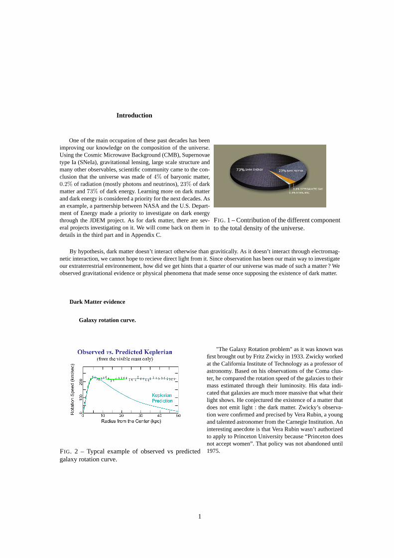
One of the main occupation of these past decades has beenimproving our knowledge on the composition of the universe.Using the Cosmic Microwave Background (CMB), Supernovaetype Ia (SNeIa), gravitational lensing, large scale structure andmany other observables, scientific community came to the con-clusion that the universe was made of4% of baryonic matter,0.2% of radiation (mostly photons and neutrinos),23% of darkmatter and73% of dark energy. Learning more on dark matterand dark energy is considered a priority for the next decades. Asan example, a partnership between NASA and the U.S. Depart-ment of Energy made a priority to investigate on dark energythrough the JDEM project. As for dark matter, there are sev-eral projects investigating on it. We will come back on them indetails in the third part and in Appendix C.

FIG. 1 – Contribution of the different componentto the total density of the universe.

By hypothesis, dark matter doesn’t interact otherwise than gravitically. As it doesn’t interact through electromag-netic interaction, we cannot hope to recieve direct light from it. Since observation has been our main way to investigateour extraterrestrial environnement, how did we get hints that a quarter of our universe was made of such a matter ? Weobserved gravitational evidence or physical phenomena that made sense once supposing the existence of dark matter.

Dark Matter evidence

Galaxy rotation curve.

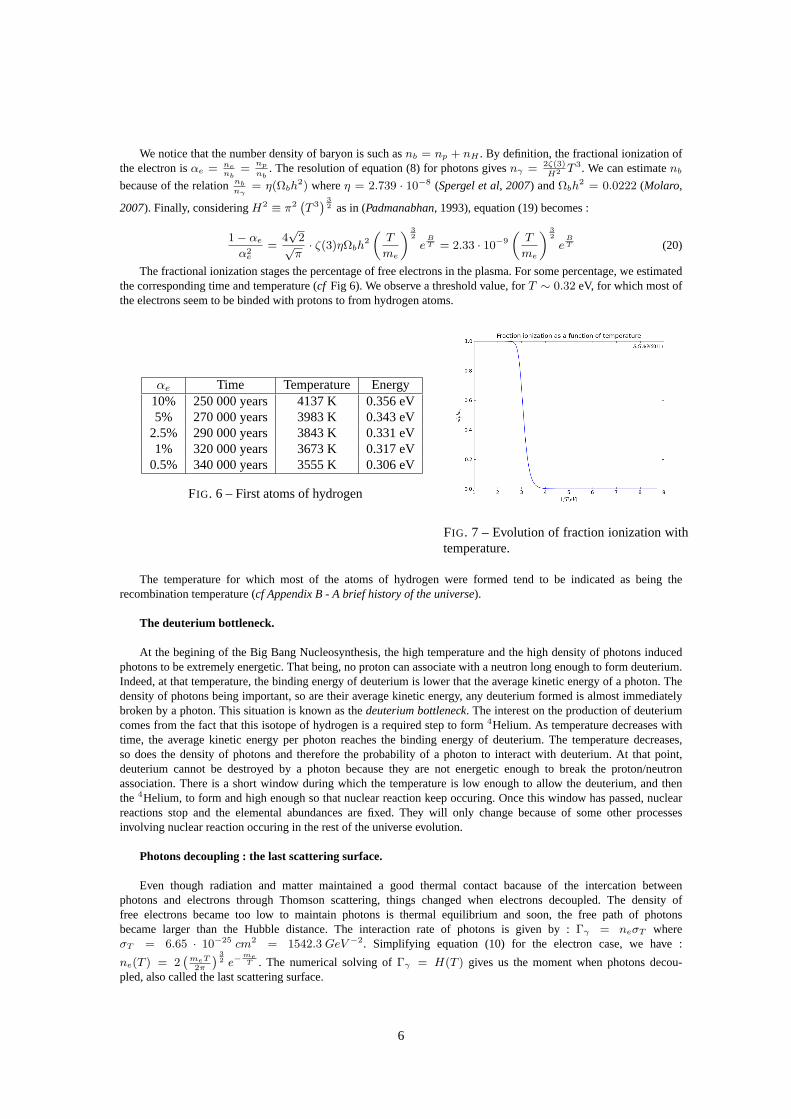
FIG. 2 – Typcal example of observed vs predictedgalaxy rotation curve.

"The Galaxy Rotation problem" as it was known wasfirst brought out by Fritz Zwicky in 1933. Zwicky workedat the California Institute of Technology as a professor ofastronomy. Based on his observations of the Coma clus-ter, he compared the rotation speed of the galaxies to theirmass estimated through their luminosity. His data indi-cated that galaxies are much more massive that what theirlight shows. He conjectured the existence of a matter thatdoes not emit light : the dark matter. Zwicky’s observa-tion were confirmed and precised by Vera Rubin, a youngand talented astronomer from the Carnegie Institution. Aninteresting anecdote is that Vera Rubin wasn’t authorizedto apply to Princeton University because “Princeton doesnot accept women”. That policy was not abandoned until1975.

1

Cosmic Microwave Background.

Evidence of dark matter can be found in CMB1 fluctuations2. We observe3 ∆TT

∼ 10−5. Those fluctuations areproportional to the overdensties of baryonic gasδb. At photons decoupling,δb ∼ 10−5. From that moment, galaxiesand structures formation starts. At the begining of those formations, the density contrast is of the order of 180 whenconsidering non linear anisotropies and the equivalent of the linear extrapolation is of the order of 1.5. Between theprimordial fluctuations and the density contrasts observed at structure formation, there is a difference of, roughlyspeaking, 5 order of magnitude. In linear regime, density fluctuations increase proportionally to the scale factor,a(t). Starting from a redshiftzCMB = 11004, this impose that the formation of the structure happened at a negativeredshift, i.e. in the future. This being ridiculous, a possible explanation is topropose the existence of a massivefluid that doesn’t interact with photons. The density fluctuations of that fluid may have increased before the photonsdecoupling : we suppose that these fluctuations reached10−3 or 10−2 by the time ofzCMB . For more precision onthe cosmology related to CMB, please refer to (Challinor, 2009).

Bullet cluster.

In the Bullet cluster, we can observe two clusters of galaxies thathave quite recently passed right through each other. About90% ofordinary matter in a cluster is intergalactic gas emitting hot X-ray andnot the galaxies themselves. As the two clusters passed through eachother, the hot gas in each smacked into the gas in the other, while theindividulas galaxies and the dark matter passed right through. Indeed,dark matter is presumed to be collisionless. In appendix A, you cansee how the hot gas is stuck in the middle of the two clusters that arenow made of galaxies and dark matter which are continuing their wayafter passing through each other. As explained in detail in (Clowe,2006) and in (Bradac, 2006), the fact that the gas stopped at the pointof collision and stayed localised in the zone between the two clustersis an indication that there is a additional mass helping the galaxiesto contain gravitationally the interacting gas. That additional masssupposidely being dark matter.

FIG. 3 – The Bullet Cluster : Dark Matterin blue and hot gas in pink.

Gravitational lensing.

FIG. 4 – Gravitational lensing.

In astrophysics, a gravitational lens refers to a distributionof matter located between an observer and a distant source.This distribution of matter apply a strong gravtitational fieldaround itself. As a result, the light travelling towards the ob-server will be bent. When observing this phenomenon forgalaxy clusters as the matter distribution, we notice that thebending is stronger than expected for a cluster as massive ascalculated through its luminosty. We then come to the conclu-sion that there is a strong component of matter that doesn’temit light in galaxy clusters : this would be dark matter.

place

1Even though Penzias and Wilson were awarded the Nobel Prize for the discovery of the cosmic microwave background radiation,it is Ralph Alpher that was the first along with his collaborator Robert Herman that were to predict its existence in 1948.

2See Appendix A for the image of the first 2 weeks light survey of PLANCK.3rms value.4See Appendix B for a brief history of the universe.

2

1. Visible Matter abundance

1.1. Usefull relation in cosmology

Time-Temperature correspondance.

In a thermal equilibrium regime whereT ≪ m [derived from (Kolb & Turner, 1990)] :

t ∼„

T

MeV

«−n

≡„

E

MeV

«−n

≡„

E0(z + 1)

MeV

«−n

(1)

wheren = 2 in radiation dominated era andn = 32

in matter dominated era.

Hubble parameter.

The Friedmann equation gives :

H =a

a=

s

„

8πGρ

3

«

(2)

Where H is the Hubble constant. It is a function of the scale factor. It relates “ the stretching “ of the universe.Given that we consider the situation whereT ≪ m, the energy density is5 :

ρ(T ) = gE(T )π2

30T 4 where gE(T ) = 2 + 6 · 7

8(Tν

Tγ

)4 = 3.36 (3)

Then, the expression of the Hubble parameter as a function of temperature is :

H(T ) =p

(0.299 · π3GT 4) (4)

From (Kolb & Turner, 1990), we know that the Hubble parameter as a function of mass is :

H(m) = 1.67g12∗

m2

mpl

(5)

where :g∗ =P

i=bosons gi

`

Ti

T

´4+ 7

8

P

i=fermions gi

`

Ti

T

´4is the degree of freedom.

1.2. Entropy

The entropy is a useful quantity that can be used to monitor the changes in an expanding universe. The expandinguniverse can be seen as a closed system for which the second law of thermodynamics can be writen as :

dU = TdS − pdV (6)

Sinceρ, the energy density6 is a quantity often used in cosmology, equation (6) can be expressed as :

TdS = d((ρ + p)V ) + V dp (7)

Using the comoving coordinates, the comoving volume isV ≡ a3.

By substitutingdp = ρ+p

TdT in equation (7) and then by integrating, we are now able to express the entropy as a

function of temperature :S = a3(ρ + p)/T . From that, we can define the entropy density :s ≡ SV

= ρ+p

T.

1.3. Abundance of light species

All along this work, we will focus on a quantity,n, called abundance or number density. The abundance of aspecies is related to its density throughρ = mn. The definition of the number density on terms of phase space densitygives :

n ≡ geµT

Z

d3p

(2π)3e−

ET (8)

5In part 1.3, we will come back on the ratioTνTγ

.6U ≡ ρV

3

whereµ is the chemical potential.

At equilibrium :

n ≡(

g`

mT2π

´

32 e−

mT , m ≫ T

g T3

π2 , m ≪ T(9)

Using equation (9), the number density of a species with chargeZ and atomic numberA is given by :

nA = gA

„

mAT

2π

«

32

e−(mA−µa)

T (10)

If we want to express that number density as a function of the neutron’sand proton’s abundance, we use the factthatmp ≃ mn ≃ mN , µA = Zµp + (A − Z)µn and that the binding energy isBA = Zmp + (A − Z)mn − mA.The equation (10) becomes :

nA =gAA

32

2Ae

BAT n(A−Z)

n nZp

„

2π

mNT

«

3(A−1)2

eBAT (11)

Now that we know how to express the number density, we can use it to find out at which temperature particlesfreed from the plasma. Indeed , at fist, all particles interacted with each other at a very high energy and hence formeda plasma. As temperature decreased, either because of the ratio of mass over temperature (e−

mT ) or the ratio of

binding energy over temperature (e−BT ) in the number density or either because the cross section was decreasing, the

interaction rate7 failed to compensate the effect of the expansion of the universe. As a consequence, the mean free pathof particles became at least the size of the universe8 : meaning, the particles decouple from the plasma.

Neutron freeze out.

The advantage of following nuclear reaction at so early time is that all possible nuclei have binding energies lessthan typical photon energies. That way, only the weak interaction that causes conversion between protons and neutronsmatters :(p)+(e) (n)+(ν) and(p)+(~ν) (n)+(e+). Since protons and neutrons are a key element to the earlyreactions that took place in the early universe, the abundance of light elements that resulted from these early reactionsis directly related to the neutron-proton ratio. In equilibrium, this ratio should vary as :

Nn

Np

= e−mn−mp

T (12)

From (Peacock,1999), we are assuming that the weak interaction switch off, freezing the neutron abundance at atemperature of :T ≃ 1.39 · 1010 K. Therefore, the equilibrium neutron-proton ratio is :

Nn

Np

= e−mn−mp

T ≃ 0.34 (13)

This result isn’t completely accurate because the freeze-out conditionwas calculated assuming a temperature wellabove the electron mass threshold, whereas it appears that freeze-out actually occurs at about this critical temperature.In practice, the neutron abundance is lower. However, the equation (13) gives us a reference for the proton-neutronabundance when the early reactions occured.

Neutrino decoupling.

Neutrinos are kept in thermal equilibrium by the weak reaction :(ν)+(ν) (e−)+(e+). The cross section of thisinteraction isσ ∼ GF T 2. GF is the Fermi coupling constant. We are making the masseless particles approximation :n ≡ T 3. Therefore the interaction rate is :Γν = nνσν |v| = GF T 5. The equality between the interction rate we justgave and the Hubble parameter expressed in equation (4) is solved numerically and the result is :

T (νdecoupling) = 3.16 · 1010 K = 2.73 MeV (14)

7In natural units, the interaction rate is the inverse of the mean free path.8The size of the universe≃ the Hubble distanceH−1

4

Electrons and positrons decoupling.

WhenT ≪ me, the eletrons and positrons fall out of chemical equilibrium with the photonsbecause the densitynumber of electrons and positrons is decreasing exponentially with the Boltzmann factore−

mT . Assumingne− =

ne+ = ne, the annihilation rate at thermal equilibrium is :Γe = ne(T ) παm2

e. When filling in the expression of the

number density in that regime of equilibrium :

Γe ∼ α2

s

„

T 3

8πme

«

e−meT (15)

The end of chemical equilibrium happens whenH(T ) = Γe(T ). The numerical solving gives :

T (edecoupling) ∼ me

40= 148 · 106 K = 12.8 keV (16)

The decoupling is a process that conserves the entropy :s = g∗Tγ = constant. When the electrons and positronsare decouplinga, the degree of freedom decreases and there-fore the temperature rises. Physically, we say that electronsand positrons transfer some of their energy to the photons tomaintain the entropy. At the time neutrinos decoupled, neutri-nos and photons had the same temperature :Tν = Tγ . Sincethat decoupling,Tν andTγ followed the same law of evolu-tion. But when the electrons and positrons gave their energyto the photons, the degree of libertyb changed forg∗ = 11

2

makingTγ getting bigger thanTν .

aNota Bene : we are still under the thermal equilibrium conditionsbSee the degree of freedom as a function of temperature in Ap-

pendix B. FIG. 5 – Expansion of the universe vs Interactionrate for electrons and positrons.

Finally, when the photons decouple, the degree of freedom change forg∗ = 2 and thanks to the conservation ofthe entropy, we can write the following equalities :

T aftere− decouplingγ =

„

11

4

«

13

T beforee− decouplingγ (17)

T nowν =

„

4

11

«

13

T nowγ (18)

That way, we can compute the photons and neutrinos temperature at anytime from the temperature of the photonstoday. We used that relation in part 1.1 to compute an expression of the Hubble parameter as a function of temperature.

The first atoms.

We now want to find out at which temperature were formed the first atomsof hydrogen. To do so, we define ourframework with the following assumptions :

• the universe is in thermodynamic equilibrium

• the universe is electrically neutral (ne = np)

• what we call recombination is a proton and an electron combining to form a hydrogen atom in the ground state(p + e− H + γ)

From equation (10) and expressingµp andµe as functions ofnp andne like we did to express equation (11), thenumber density of hydrigen is :

nH =

„

gH

gpge

«

npne

„

meT

2π

«− 32

eBT (19)

5

We notice that the number density of baryon is such asnb = np + nH . By definition, the fractional ionization ofthe electron isαe = ne

nb=

np

nb. The resolution of equation (8) for photons givesnγ = 2ζ(3)

H2 T 3. We can estimatenb

because of the relationnb

nγ= η(Ωbh

2) whereη = 2.739 · 10−8 (Spergel et al, 2007) andΩbh2 = 0.0222 (Molaro,

2007). Finally, consideringH2 ≡ π2`

T 3´

32 as in (Padmanabhan, 1993), equation (19) becomes :

1 − αe

α2e

=4√

2√π

· ζ(3)ηΩbh2

„

T

me

«

32

eBT = 2.33 · 10−9

„

T

me

«

32

eBT (20)

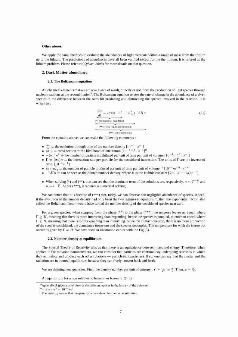
The fractional ionization stages the percentage of free electrons in the plasma. For some percentage, we estimatedthe corresponding time and temperature (cf Fig 6). We observe a threshold value, forT ∼ 0.32 eV, for which most ofthe electrons seem to be binded with protons to from hydrogen atoms.

αe Time Temperature Energy10% 250 000 years 4137 K 0.356 eV5% 270 000 years 3983 K 0.343 eV

2.5% 290 000 years 3843 K 0.331 eV1% 320 000 years 3673 K 0.317 eV

0.5% 340 000 years 3555 K 0.306 eV

FIG. 6 – First atoms of hydrogen

FIG. 7 – Evolution of fraction ionization withtemperature.

The temperature for which most of the atoms of hydrogen were formedtend to be indicated as being therecombination temperature (cf Appendix B - A brief history of the universe).

The deuterium bottleneck.

At the begining of the Big Bang Nucleosynthesis, the high temperature and the high density of photons inducedphotons to be extremely energetic. That being, no proton can associate with a neutron long enough to form deuterium.Indeed, at that temperature, the binding energy of deuterium is lower that the average kinetic energy of a photon. Thedensity of photons being important, so are their average kinetic energy, any deuterium formed is almost immediatelybroken by a photon. This situation is known as thedeuterium bottleneck. The interest on the production of deuteriumcomes from the fact that this isotope of hydrogen is a required step to form 4Helium. As temperature decreases withtime, the average kinetic energy per photon reaches the binding energy of deuterium. The temperature decreases,so does the density of photons and therefore the probability of a photon to interact with deuterium. At that point,deuterium cannot be destroyed by a photon because they are not energetic enough to break the proton/neutronassociation. There is a short window during which the temperature is low enough to allow the deuterium, and thenthe 4Helium, to form and high enough so that nuclear reaction keep occuring.Once this window has passed, nuclearreactions stop and the elemental abundances are fixed. They will only change because of some other processesinvolving nuclear reaction occuring in the rest of the universe evolution.

Photons decoupling : the last scattering surface.

Even though radiation and matter maintained a good thermal contact bacause of the intercation betweenphotons and electrons through Thomson scattering, things changed when electrons decoupled. The density offree electrons became too low to maintain photons is thermal equilibrium and soon, the free path of photonsbecame larger than the Hubble distance. The interaction rate of photons is given by : Γγ = neσT whereσT = 6.65 · 10−25 cm2 = 1542.3 GeV −2. Simplifying equation (10) for the electron case, we have :

ne(T ) = 2`

meT2π

´

32 e−

meT . The numerical solving ofΓγ = H(T ) gives us the moment when photons decou-

pled, also called the last scattering surface.

6

Other atoms.

We apply the same methods to evaluate the abundances of light elements withina range of mass from the tritiumup to the lithium. The predictions of abundances have all been verified except for the the lithium. It is refered as thelithium problem. Please refer to (Cyburt, 2008) for more details on that question.

2. Dark Matter abundance

2.1. The Boltzmann equation

All chemical elements that we are now aware of result, directly or not, from the production of light species throughnuclear reactions at the recombination9. The Boltzmann equation relates the rate of change in the abundance of a givenspecies to the difference between the rates for producing and eliminating the species involved in the reaction. It iswriten as :

dn

dt= 〈σv〉(−n2

| z

(*) first regime at equilibrium

+ n2eq)

| z

(**) second regime at equilibrium

−3Hn

| z

(***) out of equilibrium

(21)

From the equation above, we can make the following comments :

• dndt

≡ the evolution through time of the number density [m−3 · s−1]• 〈σv〉 = cross section≡ the likelihood of intercation [10−4m3 · s−1]10

• −〈σv〉n2 ≡ the number of particle annihilated per unit of time per unit of volume [10−4m−3 · s−1]• Γ = 〈σv〉n ≡ the interaction rate per particle for the considered interaction. The units ofΓ are the inverse of

time. [10−4s−1]• 〈σv〉n2

eq ≡ the number of particle produced per unit of time per unit of volume11 [10−4m−3 · s−1]• −3Hn ≡ can be seen as the diluted number density, where H is the Hubble constant [km · s−1 · Mpc−1]

• When solving (*) and (**), one can see that the dominant term of the solutions are, respectively,n ∼ T− 32 and

n ∼ e−mT . As for (***), it requires a numerical solving.

We can notice that it is because of (***) that, today, we can observe nonnegligible abundance of species. Indeed,if the evolution of the number density had only been the two regimes at equilibrium, then the exponential factor, alsocalled the Boltzmann factor, would have turned the number density of the considered species near zero.

For a given species, when stepping from the phase (**) to the phase (***), the universe leaves an epoch whereΓ ≥ H, meaning that there is more interacting than expanding, hence the speciesis coupled, to enter an epoch whereΓ ≤ H, meaning that there is more expanding than interacting. Since the interactions stop, there is no more productionof the species considered, the abundancefreeze out and the species decouples. The temperature for wich the freeze outoccurs is given byΓ = H. We have seen an illustration earlier with the Fig (5).

2.2. Number density at equilibrium

The Special Theory of Relativity tells us that there is an equivalence between mass and energy. Therefore, whenapplied to the radiation dominated era, we can consider that particles are continuously undergoing reactions in whichthey annihilate and produce each other (photons↔ particles/antiparticles). If so, one can say that the matter and theradiation are in thermal equilibrium because they can freely convert back and forth.

We are defining new quantites. First, the density number per unit of entropy : Y = nT3 ≃ n

s. Then,x = m

T.

At equilibrium for a non relativistic fermion or boson (x ≫ 3) :

9Appendix A gives a brief view of the different epochs in the history of the universe.10σ is in cm2

≡ 10−4m2.

11The indexeq means that the quantity is considered for thermal equilibrium.

7

Yeq =45

2π4

“π

8

”

12 g

g∗sx

32 e−x = 0.145 · g

g∗sx

32 e−x (22)

From (Kolb & Turner, 1990), we know that for a relativistic boson (x ≪ 3) :

Yeq =45

2π4ζ(3)

g

g∗s= 0.278 · g

g∗s(23)

For a relativistic fermion (x ≪ 3) :

Yeq =45

2π4ζ(3)

34g

g∗s= 0.209 · g

g∗s(24)

Whereg∗s =P

i=bosons gi

`

Ti

T

´3+ 7

8

P

i=fermions gi

`

Ti

T

´3is the effective degree of freedom of all particles

(including the relativistic ones).

FIG. 8 – Freeze out.The continuous line is theabundance at equilibrium. The dashed lines aretoday abundances.

Let’s consider the(χ)+(χ) (SM)+(SM) reaction :the conversion of standard model particles into dark matterparticles. Because ofdx

dt= −m T

T= −xH, the equation (21)

becomes :

dY

dx=

λ

x2

`

Y 2SM − Y 2´

(25)

Whereλ = m3〈σv〉H

.

When solving numerically this equation, we find thatY de-parts fromYeq aroundx ≃ 10. By integration of equation(25), we have :

Z Y∞

Yf

dY

Y 2≃ −

Z ∞

xf

λdx

x2(26)

⇒ Y∞ ≡ xf

λbecause in radiation dominated eraY∞ ≪ Yf

(27)Then, a good approximation for relic abundance is :Y∞ ≃ 10

λ.

The smaller the value ofλ, the sooner happens the freeze out. Indeed :

λ ց≡

8

<

:

m ց light particles decouples sooner than heavy particlesH ր the sooner particles decouple, the bigger is the value of the Hubble parameter〈σv〉 ց for fixed conditions, light particles are less likely to interact than heavy particles

(28)

We can link that to the observed density,Ωχ =ρχ

ρc, using :

Yχ =nχ

T 3=

#χρχ

mχT 3=

10

λ

ρc

ρc

= Y∞ (29)

Therefore :

Ωχ =10T 3H

#χm2χ〈σv〉 (30)

3. Dark Matter detection

3.1. Possible detection methods

There is two type of detection methods : the direct one and the indirect one.The first method consists in detectorslooking for direct interaction with dark matter particles. The second methodconsists on detecting the products or

8

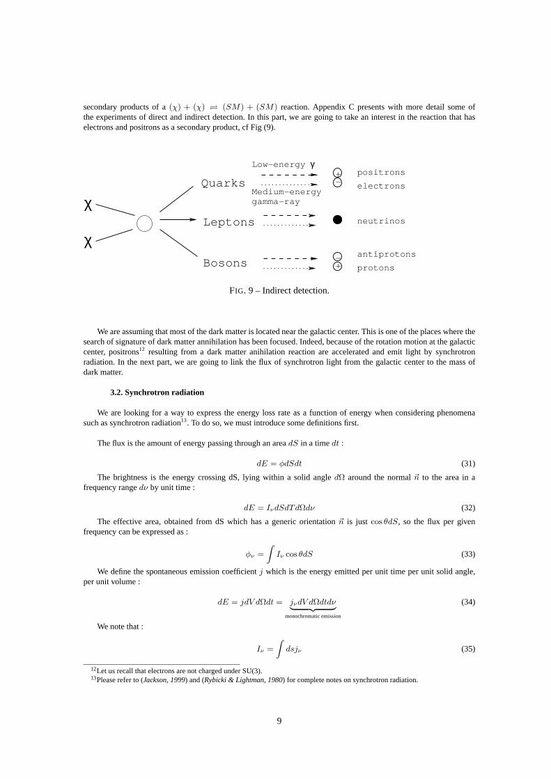
secondary products of a(χ) + (χ) (SM) + (SM) reaction. Appendix C presents with more detail some ofthe experiments of direct and indirect detection. In this part, we are goingto take an interest in the reaction that haselectrons and positrons as a secondary product, cf Fig (9).

χ

χLeptons

Quarks

Bosons

Low−energy γ

Medium−energy gamma−ray

+−

−+

positrons

electrons

neutrinos

antiprotons

protons

FIG. 9 – Indirect detection.

We are assuming that most of the dark matter is located near the galactic center. This is one of the places where thesearch of signature of dark matter annihilation has been focused. Indeed, because of the rotation motion at the galacticcenter, positrons12 resulting from a dark matter anihilation reaction are accelerated and emit light by synchrotronradiation. In the next part, we are going to link the flux of synchrotron lightfrom the galactic center to the mass ofdark matter.

3.2. Synchrotron radiation

We are looking for a way to express the energy loss rate as a function of energy when considering phenomenasuch as synchrotron radiation13. To do so, we must introduce some definitions first.

The flux is the amount of energy passing through an areadS in a timedt :

dE = φdSdt (31)

The brightness is the energy crossing dS, lying within a solid angledΩ around the normal~n to the area in afrequency rangedν by unit time :

dE = IνdSdTdΩdν (32)

The effective area, obtained from dS which has a generic orientation~n is just cos θdS, so the flux per givenfrequency can be expressed as :

φν =

Z

Iν cos θdS (33)

We define the spontaneous emission coefficientj which is the energy emitted per unit time per unit solid angle,per unit volume :

dE = jdV dΩdt = jνdV dΩdtdν| z

monochromatic emission

(34)

We note that :

Iν =

Z

dsjν (35)

12Let us recall that electrons are not charged under SU(3).13Please refer to (Jackson, 1999) and (Rybicki & Lightman, 1980) for complete notes on synchrotron radiation.

9

whereds is the line of sight element. For an isotropic emitter, or for a random distribution of emitters, the equation(34) becomes by integration :

jν =1

4πPν (36)

Pν is the radiated power per unit volume, per unit frequency. So, ifne is the number density of electrons :

Pν =ne

νP (E) (37)

We now need to compute the radiated powerP (E). To do so, we use the fact that a synchrotron emission is therelativistic limit of the cyclotron radiation. The Larmor formula gives the total power radiated by a nonrelativistic pointcharge as it accelerates :

PLarmor =e2

6πǫ0c3| ~a |2 (38)

The expression of motion allows us to express the Larmor formula as a function of magnetic field :

md~v

dt= e~v ∧ ~B ⇒ v|| = constant; v⊥ = a⊥ =

ev⊥m

(39)

When implementing equation (39) in equation (38) :

PLarmor =e4B2v2

⊥

6πǫ0m2c3(40)

Let’s now consider very relativistic positrons. In special relativity, the Lorentz transformation on accelerationsgives14 :

P ≃ e4E2B2

m4(41)

Now that we have computed the power as a function of the electromagnetic field, we need to apply what wasrelevant for one charged particule to the flux of particle coming from the galactic center. The motion of positronscoming from the galactic center is given by the diffusion equation :

∂

∂t

dne

dEe| z

spectrum variation in time

= ~∇ ·»

κ(Ee, ~r) · ~∇ dne

dEe

–

| z

diffusion

+∂

∂Ee

»

b(Ee, ~r)dne

dEe

–

| z

energy loss

+ Q(Ee, ~r)| z

source

(42)

We are now going to make the following assumptions :

– because of thermal equilibrium, we suppose that creation and loss ratehave the same order of magnitude :∂∂t

dne

dEe= 0

– in the inner part of the galaxy, we neglect the diffusion :~∇ ·h

κ(Ee, ~r) · ~∇ dne

dEe

i

= 0

Hence we are left with :

Q(Ee, ~r) +∂

∂Ee

»

b(Ee, ~r)dne

dEe

–

= 0 (43)

From equation (43), the spectrum is thus given by :

dne

dEe

=τ

Ee

Z mχc2

Ee

dE′e, Q(E′

e, ~r) where the time scale is :τ =Ee

b(Ee, ~r)(44)

Plus, the source term is, by construction :

Q = 〈σv〉dNe

dEe

»

ρχ

mχ

–2

(45)

Let us now compute the energy loss rate. Near the galactic center, we neglect the Compton radiation and theBremsstrahlung radiation and we keep the following terms :b(Ee, ~r) = Psynchr + PICS . WherePsynchr is theSynchrotron radiation power, andPICS is the Inverse Compton scattering power. Those terms can be expressed as :

Psynchr ≃ E2B2 (46)

14We are taking back the notationsc = ~ = 1.

10

PICS ≃ E2Urad(~r)(∝ σT ) (47)

Urad(~r) has the same dimension that an energy density.

Therefore the energy loss rate is :

b(Ee, ~r) = Psynchr

„

1 +Urad

B2

«

(48)

Now that we have everything, let’s compute the flux. The synchrotron radiation energy density per unit time andunit frequency is :

Lν(~r) =

Z

Pν(E)dn

dE(E,~r)dE (49)

Hence, the energy flux by unit frequency is :

Jν =1

4π

Z

line of sightd~lLν(~l) (50)

=

Z

dEd~l〈σv〉8π

„

ρχ

mχ

«2 „

e4E2B2

m4e

«−11

b(Ee, ~r)e3Bme

φ“

νnuc

” (51)

FIG. 10 – Energy flux as a function of magneticfield for different light dark matter masses.

As we can see on Fig (10), when plotting the flux as a func-tion of the magnetic fielda, one can observe the followongbehaviour :

Jν ≡ B

B2 + #(52)

The flux reaches a maximum aroundB ≃ 30 µG. Indeed,for lower magnetic field positrons emit a weak radiation. Formagnetic field stronger than30 µG, positrons radiate morethan before but there is an energy loss because of differentphysical pocesses (ICS...).

It is also interesting to notice thatdndE

∼ 1m2

χ. Hence, the

heaviermχ, the smallerdndE

, the smaller isJν .

aFollowing the Boehm model of light dark matter,cf (Boehm,2003), (Boehm, 2007) and (Boehm, 2010).

† Thank you to Bryan Zaldivar Montero for Fig (10).

When taking a look at the equation (51), we notice that we can now constrainthe mass of a particle of dark matter :the flux is an observable, the magnetic field is modelised quite accuratly nearthe galactic center and an estimation ofΩχ has been made through different observational cosmology experiments.

Conclusion

After familiarising ourselves with the problem of abundances in the early universe and how we can derive today’sabundances thanks to the Boltzmann equation, we have seen how the synchrotron radiation can be used as a methodto constrain the mass of dark matter particles. A step further is to overlap theresults of different dark matter detectionexperiments to constrain more efficientlymχ. That has been done with the LEP and Tevatron analysis in (Mambrini& Zaldivar, 2011). Overlapping other analysis from different dark matter search experiments and the results of theupcoming months of Higgs search at LHC are crucial in the “Beyond the Standard Model” field.

11

ACKNOWLEDGMENTS

First of all, I would like to thank Yann Mambrini. I highly appreciated the qualityof his explanations, and theclear-sightedness of his physical opinions. I learned a lot thanks to him.

I am grateful for all the help Bryan Zaldivar Montero provided me with. Ivalue the discussions we had.

The Magic Mondays15 organised by Yann Mambrini and Adam Falkowski, and the SINJE16 helped making mystay at LPT a really enriching period.

I would like to thank Bryan, Julio, Antoine and Maxime, whom I shared an office with, for the nice workenvironment they provided.

Finally, I thank Henk Hilhorst for his allowing me to do an internship in his laboratory.

15Weekly review of relevant article in theoretical particle physics and cosmology, most often dark matter related.16Séminaire INformel des JEunes.

12

APPENDIX A - INTRODUCTION

espace

♦ The Cosmic Microwave Background.

FIG. 11 – First map of a strip of the sky by PLANCK satellite after 2weeks of continuous sky survey.

♦ The Bullet Cluster.

FIG. 12 – Dark Matter position in the Bullet clus-ter.

FIG. 13 – Gas position in the Bullet cluster.

13

APPENDIX B - V ISIBLE MATTER ABUNDANCE

espace

♦ History of the universe.

Epoch/Event Time Temperature Energy RedshiftHot Big Bang - - - -

Inflation - - - -Reheating - T = 0 K end of reheating - z ≃ 10

28

-Radiation domination era- - - - zreheating ends

Baryongenesis-Leptogenesis 10−4 s 2 · 10

12200 MeV z = 10

11

Primordial Nucleosynthesis 100 s 109 K 0.1 MeV z = 10

9

-Matter domination era- 100 000 years 9000 K 0.81 eV z = 3400

Recombination 380 000 years 3000 K 0.3 eV z = 1100

Reionization 3.2 · 108 years 120 K 0.01 eV z = 20

First galaxies formation 1.3 · 109 years 60 K 5 · 10

−3 eV z = 10

-Dark Energy domination era- 9.4 · 109 years 4.8 K 4·10

−4 eV z = 0.75

Today 15 · 109 years 2.7 K 2.35 · 10

−4 eV z = 0

FIG. 14 – Brief history of the universe

♦ Decoupling : sum up.

FIG. 15 – Timeline for decoupling.

14

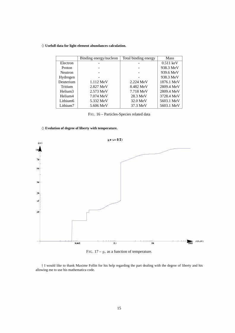
♦ Usefull data for light element abundances calculation.

Binding energy/nucleon Total binding energy MassElectron - - 0.511 keVProton - - 938.3 MeV

Neutron - - 939.6 MeVHydrogen - - 938.3 MeVDeuterium 1.112 MeV 2.224 MeV 1876.1 MeV

Tritium 2.827 MeV 8.482 MeV 2809.4 MeVHelium3 2.573 MeV 7.718 MeV 2809.4 MeVHelium4 7.074 MeV 28.3 MeV 3728.4 MeVLithium6 5.332 MeV 32.0 MeV 5603.1 MeVLithium7 5.606 MeV 37.3 MeV 5603.1 MeV

FIG. 16 – Particles-Species related data

♦ Evolution of degree of liberty with temperature.

FIG. 17 –g∗ as a function of temperature.

† I would like to thank Maxime Follin for his help regarding the part dealing with thedegree of liberty and hisallowing me to use his mathematica code.

15

APPENDIX C - DARK MATTER DETECTION

♦ Direct Detection.

XENON : " XENON100 is a new dark matter search experiment, aiming to increase the fiducial liquid xenontarget mass to 100 kg with a 100 times reduction in background rate, compared to the XENON10 experiment whichused liquid xenon as a sensitive detector medium to search for WIMPs (Weakly Interacting Massive Particles)."⊲ http ://xenon.astro.columbia.edu/index.html

CoGeNT : "The CoGeNT Dark Matter Experiment is a direct search for signals from interactions of dark matterparticles in a low-background germanium detector located at Soudan Underground Laboratory in Soudan, MN."⊲ http ://cogent.pnnl.gov/

Other direct search experiments : COUPP, CDMS, DAMA, EDELWEISS,CRESST, EURECA, ZEPLIN, DEAP,ArDM, WARP, LUX, SIMPLE, PICASSO, DMTPC, DRIFT, KIMS...

♦ Indirect Detection.

PAMELA : "Among the most plausible candidates for dark matter are weakly interacting massive particles(WIMP), of which the supersimmetric neutralino is a favourite candidate from the point of view of particlephysics.Neutralino are Majorana fermions and will annihilate with each other in the halo, resulting in the symmetricproduction of particles and antiparticles, the latter providing an observablesignature. The Pamela Instrument isinstalled on the up-ward side of the Resurs-DK1 satellite and has been launched the 15th of June 2006 from the launchsite of Bajkonour in Kazakhstan by a rocket Soyuz. With Pamela we look for annihilations that produce antiprotonsand positrons."⊲ http ://pamela.roma2.infn.it/index.php

Other indirect search experiments : WMAP,FERMI/GLAST, ATIC, VERITAS, HESS, IceCube, AMS...

16

REFERENCES

Boehm, C., Silk, J., Enßlin, T. 2010, arXiv :1008.5175Boehm, C., Silk, J. 2007, Phys.Lett. B661 (2008) 287-289Boehm, C., Fayet, P., Silk, J. 2003, Phys.Rev. D69 (2004) 101302Bradac, M., et al. 2006, ApJ, 652, 937, arXiv :astro-ph/0608408v1Challinor, A., Peiris, H., 2009, arXiv :0903.5158v1Clowe, D., et al. 2006, ApJ, 648, 109, arXiv :astro-ph/0608407Cyburt, R. H, Fields, B. D., Olive, K.A., 2008, arXiv :0808.2818v1Jackson, J. D.,Classical Electrodynamics, John Wiley & Sons Inc., 1999, Chapter 14Kolb, E. W., Turner, M. S.,The Early Universe, Westview, Frontiers of Physics, 1990Mambrini, Y., Zaldivar, B. 2011, arXiv :1106.4819Molaro, P. 2007, arXiv :0708.3922Padmanabhan,T.,Structure formation in the universe, Cambridge University Press, 1993, p101-118Peacock,J. A.,Cosmological physics, Cambridge University Press, 1999, p292-299Rybicki, G.B., Lightman A.P.,Radiative processes in astrophysics, John Wiley & Sons Inc., 1980, Chapter 6Spergel, D. N., et al. 2007, ApJS, 170, 377, DOI : 10.1086/513700

17