POUR PDF - copie 2 - lri.frbibli/Rapports-internes/2013/RR1567.pdf · 1 University of York,...

L R I

CNRS – Université de Paris Sud Centre d’Orsay

LABORATOIRE DE RECHERCHE EN INFORMATIQUE Bâtiment 650

91405 ORSAY Cedex (France)

RAPPORT DE RECHERCHE

DATA-FLOW COVERAGE FOR TESTING IN

CIRCUS

CAVALCANTI A / GAUDEL M C

Unité Mixte de Recherche 8623 CNRS-Université Paris Sud – LRI

12/2013

Rapport de Recherche N° 1567

Data-flow coverage for testing in Circus

Ana Cavalcanti1 and Marie-Claude Gaudel2

1 University of York, Department of Computer ScienceYork YO10 5DD, UK

2 LRI, Universite de Paris-Sud and CNRSOrsay 91405, France

revised version 12/2013

Abstract. Circus is a state-rich process algebra for refinement basedon Z and CSP. In previous work, we have defined a testing theory forCircus, and some selection criteria based on its exhaustive test set. Here,we consider a different class of criteria, based on the text of the models,rather than directly on their operational semantics. In particular, weconsider data-flow based coverage. In adapting the classical results oncoverage of programs to abstract Circus models, we define a notion ofspecification traces, consider models with data anomalies, and cater forthe internal nature of state and state changes. Our main results are aframework for data-flow based coverage, a novel criterion suited to state-rich process models, and a notion of instantiation of traces.

Abstract. Circus est une algebre de processus avec une notion d’etatinterne, qui combine le pouvoir de Z pour modeliser des types abstraitsde donnees et les constructions de CSP pour specifier des comportementsreactifs et concurrents. Circus permet aussi de decrire des raffinementsvers des modeles concrets ou meme des programmes. Les modeles ab-straits impliquent couramment du nondeterminisme, qui peut venir desoperations sur les donnees ou des choix internes de comportement, dufait qu’on ignore les details de l’implementation.

Precedemment, nous avons etabli une theorie du test pour Circus. Cettetheorie est de nature symbolique : pour capturer la logique des typesde donnees et les comportements conditionnels (gardes), nous utilisonsune notion de “trace symbolique contrainte”, directement derivee dela semantique operationnelle du langage. Cette notion sert de base ala definition de tests symboliques associes a un modele. Une notiond’instantiation definit comment obtenir des tests concrets.

Du fait que cette approche est conduite par la semantique operationnelledu langage, elle a permis de definir des jeux de tests exhaustifs et de prou-ver cette exhaustivite. Dans ce cadre, nous avons defini plusieurs criteresde selection de sous-ensembles des jeux de tests exhaustifs comme la cou-verture des traces symboliques contraintes bornees, ou la couverture dessynchronisations.

Dans ce rapport, nous considerons une classe de criteres de selection detests bases sur le texte du modele Circus plutot que sur sa semantiqueoperationnelle, plus specifiquement la couverture des flots de donnees.

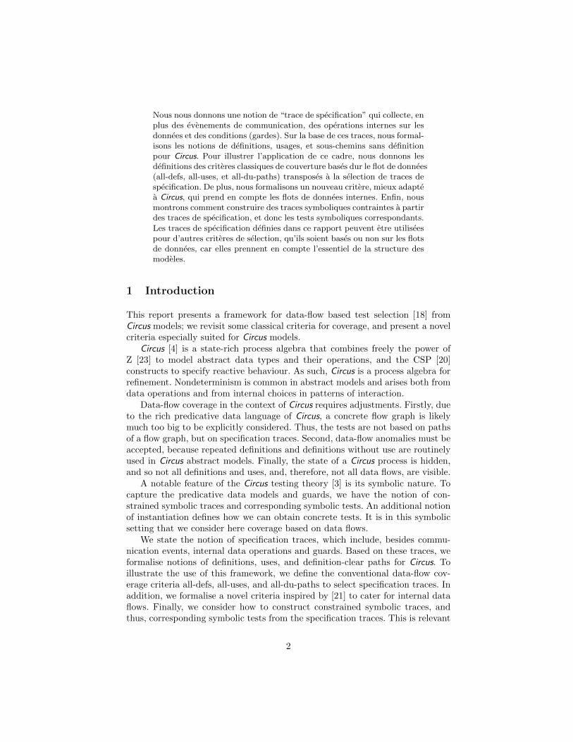
Nous nous donnons une notion de “trace de specification” qui collecte, enplus des evenements de communication, des operations internes sur lesdonnees et des conditions (gardes). Sur la base de ces traces, nous formal-isons les notions de definitions, usages, et sous-chemins sans definitionpour Circus. Pour illustrer l’application de ce cadre, nous donnons lesdefinitions des criteres classiques de couverture bases dur le flot de donnees(all-defs, all-uses, et all-du-paths) transposes a la selection de traces despecification. De plus, nous formalisons un nouveau critere, mieux adaptea Circus, qui prend en compte les flots de donnees internes. Enfin, nousmontrons comment construire des traces symboliques contraintes a partirdes traces de specification, et donc les tests symboliques correspondants.Les traces de specification definies dans ce rapport peuvent etre utiliseespour d’autres criteres de selection, qu’ils soient bases ou non sur les flotsde donnees, car elles prennent en compte l’essentiel de la structure desmodeles.

1 Introduction

This report presents a framework for data-flow based test selection [18] fromCircus models; we revisit some classical criteria for coverage, and present a novelcriteria especially suited for Circus models.

Circus [4] is a state-rich process algebra that combines freely the power ofZ [23] to model abstract data types and their operations, and the CSP [20]constructs to specify reactive behaviour. As such, Circus is a process algebra forrefinement. Nondeterminism is common in abstract models and arises both fromdata operations and from internal choices in patterns of interaction.

Data-flow coverage in the context of Circus requires adjustments. Firstly, dueto the rich predicative data language of Circus, a concrete flow graph is likelymuch too big to be explicitly considered. Thus, the tests are not based on pathsof a flow graph, but on specification traces. Second, data-flow anomalies must beaccepted, because repeated definitions and definitions without use are routinelyused in Circus abstract models. Finally, the state of a Circus process is hidden,and so not all definitions and uses, and, therefore, not all data flows, are visible.

A notable feature of the Circus testing theory [3] is its symbolic nature. Tocapture the predicative data models and guards, we have the notion of con-strained symbolic traces and corresponding symbolic tests. An additional notionof instantiation defines how we can obtain concrete tests. It is in this symbolicsetting that we consider here coverage based on data flows.

We state the notion of specification traces, which include, besides commu-nication events, internal data operations and guards. Based on these traces, weformalise notions of definitions, uses, and definition-clear paths for Circus. Toillustrate the use of this framework, we define the conventional data-flow cov-erage criteria all-defs, all-uses, and all-du-paths to select specification traces. Inaddition, we formalise a novel criteria inspired by [21] to cater for internal dataflows. Finally, we consider how to construct constrained symbolic traces, andthus, corresponding symbolic tests from the specification traces. This is relevant

2

for all selection criteria based on specification traces (and not only data-flow cri-teria). Given the formal setting of our work, based on the operational semanticsof Circus and additional transition systems in [2], we can prove unbias of theselected tests. This means that they cannot reject correct systems.

In the next section, we give an overview of the notations and definitionsused in our work. Section 3 presents our framework and Section 4 our newcriterion. Section 5 addresses the general issue of constructing tests from selectedspecification traces. Finally, we consider related works in Section 6 and concludein Section 7, where we also indicate lines for further work.

2 Background material

This section describes Circus, its operational semantics, and data-flow coverage.

2.1 Circus notation

A Circus model defines channels and processes like in CSP. Figure 1 presents anextract from the model of a cash machine. It uses a given set CARD of validcards, a set Note of the kinds of notes available (10, 20, and 50), and a setCash == bag Note to represent cash. The definitions of these sets are omitted.

The first paragraph in Figure 1 declares four channels: inc is used to requestthe withdrawal using a card of some cash, outc to return a card, cash to providecash, and refill to refill the note bank in the machine. The second paragraph isan explicit definition for a process called CashMachine.

The first paragraph of the CashMachine definition is a Z schema CMStatemarked as the state definition. Circus processes have a private state, and interactwith each other and their environment using channels. The state of CashMachineincludes just one component: nBank , which is a function that records the avail-able number of notes of each type: at most cap.

State operations can be defined by Z schemas. For instance, DispenseNotesspecifies an operation that takes an amount a? of money as input, and outputsa bag notes! of Notes, if there are enough available to make up the requiredamount. DispenseNotes includes the schema ∆CMState to bring into scope thenames of the state components defined in CMState and their dashed counterpartsto represent the state after the execution of DispenseNotes. To specify notes!,we require that the sum of its elements (Σ notes!) is a?, and that, for each kindn of Note, the number of notes in notes! is available in the bank. DispenseNotesalso updates nBank , by decreasing its number of notes accordingly.

Another schema DispenseError defines the behaviour of the operation whenthere are not enough notes in the bank to provide the requested amount a?; theresult is the empty bag [[ ]] . The Z schema calculus is used to define the totaloperation Dispense as the disjunction of DispenseNotes and DispenseError .

State operations are called actions in Circus, and can also be defined usingMorgan’s specification statements [14] or guarded commands from Dijkstra’slanguage [7]. CSP constructs can also be used to specify actions.

3

[CARD ]channel inc : CARD × N1; outc : CARD ; cash : Cash; refillNote == {10, 20, 50}Cash == bag Note

process CashMachine = begin

state CMState == [ nBank : Note→ 0 . . cap ]

DispenseNotes∆CMStatea? : N1

notes! : Cash

Σ notes! = a?∀n : Note • (notes! ] n) ≤ nBank n ∧ nBank ′ n = (nBank n)− (notes! ] n)

DispenseErrorΞCMStatea? : N1; notes! : Cash

¬ ∃ns : Cash • Σ ns = a? ∧ ∀n : Note • (ns ] n) ≤ nBank nnotes! = [[ ]]

Dispense == DispenseNotes ∨ DispenseError

•

µ X •

inc?c?a→Xuoutc!c→Xu

var notes : Cash •Dispense; (notes 6= [[ ]] )N cash!notes → Skip

@(notes = [[ ]] )N Skip

;outc!c→X

@refill → (nBank := { 10 7→ cap, 20 7→ cap, 50 7→ cap } ; X

end

Fig. 1. Cash machine model

4

For instance, the behaviour of the process CashMachine is defined by a re-cursive action at the end after the ‘•’. A recursion µ X • F (X ) has a bodygiven by F (X ), where occurrences of X are recursive calls. In our example, therecursion first offers a choice between an input inc?c?a, which accepts a card cand a request to withdraw the amount a, and a synchronisation on refill , whichis a request to fill the nBank . The actions that offer these communications arecombined in an external choice (@) to be exercised by the environment.

If refill is chosen, an assignment changes the value of nBank to record anumber cap of notes of all kinds. If inc?c?a is chosen, then we have an inter-nal (nondeterministic) choice of possible follow-on actions: recursing immedi-ately (without returning the card or producing the money), returning the cardvia an output outc!c before recursing, or considering the dispensation of cashbefore returning the card and recursing. In the dispensation, a local variablenotes is declared, the operation Dispense is called, and then an external choiceof two guarded actions is offered. If there is some cash available (notes 6= [[ ]] ),then it can dispensed via cash!notes. Otherwise the action terminates (Skip).Here, nondeterminism comes from the fact that the specification does not gointo details of bank management (stolen cards, bank accounts, and so on).

This example shows how Z and CSP constructs can be intermixed freely. Afull account of Circus and its semantics is given in [17]. The Circus operationalsemantics is briefly discussed and illustrated in the next section.

2.2 Circus operational semantics and tests

The Circus operational semantics [3] is distinctive in its symbolic account of stateupdates. As usual, it is based on a transition relation that associates configura-tions and a label. For processes, the configurations are processes themselves; foractions A, they are triples of the form (c | s |= A).

The first component c of those triples is a constraint over symbolic variablesused to define labels and the state. These are texts that denote Circus predicates(over symbolic variables). We use typewriter font for pieces of text. The secondcomponent s is a total assignment x := w of symbolic variables w to all statecomponents x in scope. State assignments can also include declarations andundeclarations of variables using the constructs var x := e and end x. The stateassignments define a specific value (represented by a symbolic variable) for allvariables in scope. The last component of a configuration is an action A.

The labels are either empty, represented by ε, or symbolic communicationsof the form c?w or c!w, where c is a channel name and w is a symbolic variablethat represents an input (?) or an output (!) value.

We define the notion of traces in the expected way. Due to the symbolicnature of configurations and labels, we obtain constrained symbolic traces, orcstraces, for short. These are pairs formed by a sequence of labels, that is, asymbolic trace, and a constraint over the symbolic variables used in the labels.

For a process begin state [ x : T ] • A end, the cstraces over an alphabet a

are those of its main action A, starting from a state in which x takes any value

5

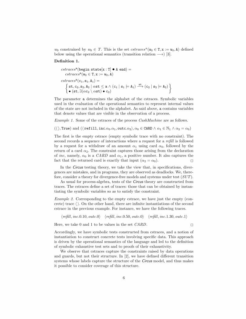
w0 constrained by w0 ∈ T . This is the set cstracesa(w0 ∈ T, x := w0, A) definedbelow using the operational semantics (transition relation −→) [3].

Definition 1.

cstracesa(begin state[x : T] • A end) =cstracesa(w0 ∈ T, x := w0, A)

cstracesa(c1, s1, A1) ={st, c2, s2, A2 | αst ≤ a ∧ (c1 | s1 |= A1)

st−→ (c2 | s2 |= A2)• (st,∃(αc2 \ αst) • c2)

}The parameter a determines the alphabet of the cstraces. Symbolic variablesused in the evaluation of the operational semantics to represent internal valuesof the state are not included in the alphabet. As said above, a contains variablesthat denote values that are visible in the observation of a process.

Example 1. Some of the cstraces of the process CashMachine are as follows.

(〈〉, True) and (〈 refill, inc.α0.α1, outc.α2〉, α0 ∈ CARD ∧ α1 ∈ N1 ∧ α2 = α0)

The first is the empty cstrace (empty symbolic trace with no constraint). Thesecond records a sequence of interactions where a request for a refill is followedby a request for a withdraw of an amount α1 using card α0, followed by thereturn of a card α2. The constraint captures those arising from the declarationof inc, namely, α0 is a CARD and α1, a positive number. It also captures thefact that the returned card is exactly that input (α2 = α0). 2

In the Circus testing theory, we take the view that, in specifications, diver-gences are mistakes, and in programs, they are observed as deadlocks. We, there-fore, consider a theory for divergence-free models and systems under test (SUT ).

As usual for process-algebra, tests of the Circus theory are constructed fromtraces. The cstraces define a set of traces: those that can be obtained by instan-tiating the symbolic variables so as to satisfy the constraint.

Example 2. Corresponding to the empty cstrace, we have just the empty (con-crete) trace 〈〉. On the other hand, there are infinite instantiations of the secondcstrace in the previous example. For instance, we have the following traces.

〈refill , inc.0.10, outc.0〉〈refill , inc.0.50, outc.0〉〈refill , inc.1.30, outc.1〉

Here, we take 0 and 1 to be values in the set CARD . 2

Accordingly, we have symbolic tests constructed from cstraces, and a notion ofinstantiation to construct concrete tests involving specific data. This approachis driven by the operational semantics of the language and led to the definitionof symbolic exhaustive test sets and to proofs of their exhaustivity.

We observe that cstraces capture the constraints raised by data operationsand guards, but not their structure. In [2], we have defined different transitionsystems whose labels capture the structure of the Circus model, and thus makesit possible to consider coverage of this structure.

6

Label ::= Pred | Comm | LActComm ::= ε | CName | CName!Exp | CName?VName | CName?VName : PredLAct ::= VName∗ : [Pred ,Pred ] | Schema | VName := Exp

| var VName : Exp | var VName := Exp | end VName

Fig. 2. Syntax of specification labels.

Example 3. The following is a cstrace of CashMachine that captures a withdrawrequest followed by cash dispensation.

( 〈 inc.α0.α1, cash.α2〉,α0 ∈ CARD ∧ α1 ∈ N1 ∧ Σα2 = α1 ∧ ∀ n : Note • (α2 ] n) ≤ cap)

The constraint defines the essential properties of the cash α2 dispensed, but notthe fact that these properties are established by variable declaration followed bya schema action call, and a guarded action. 2

So, while cstraces are useful for trace-selection based on constraints, they do notsupport selection based on the structure of the Circus model. To this end, in [2]we have presented a collection of transition systems whose labels are pieces ofthe model: guards (predicates), communications, or simple Circus actions. Thesyntactic category of Labels is defined in Figure 2; the sets Pred , Exp, CName,VName, and Schema are those of the Circus predicates, expressions, channel andvariable names, and Z schemas [16, 1].

In this paper, we use the transition relation =⇒RP , called just =⇒ here,to define a notion of specification traces, used to consider data-flow coveragecriteria. This is in contrast to what is done for sequential imperative programswhere data flow graphs are considered.

2.3 Data-flow coverage

Data-flow coverage criteria were originally developed for sequential imperativelanguages based on the notion of definition-use associations [18]. The motivationwas to check, via some test, that a variable has been assigned a correct value bycausing the execution of a path in a data-flow graph from the point of assignmentto a point where the assigned value is used.

Definition-use associations are traditionally defined in terms of data-flowgraph as triples (d , u, v), where d is a node in which the variable v is defined,that is, some value is assigned to it, u is a node in which the value of v is used,and there is a definition-clear path with respect to v from d to u. In this con-text, the strongest data-flow criterion, all definition-use paths, requires that, foreach variable, every definition-clear path (with at most one iteration by loop)is executed. In order to reduce the number of tests required, weaker strategiessuch as all-definitions and all-uses have been defined.

7

(c | s |= A)〈〉⇒⇒ (c | s |= A)

(c1 | s1 |= A1)l

=⇒ (c2 | s2 |= A2)

(c1 | s1 |= A1)〈 l〉⇒⇒ (c2 | s2 |= A2)

(c1 | s1 |= A1)spt1⇒⇒ (c2 | s2 |= A2) (c2 | s2 |= A2)

spt2⇒⇒ (c3 | s3 |= A3)

(c1 | s1 |= A1)spt1a

spt2⇒⇒ (c3 | s3 |= A3)

Table 1. Annotated transition relation: specification traces

When using these criteria, it is often assumed that the data-flow graph hasunique start and end nodes and there is no data-flow anomaly [6]. This meansthat on every path from the start to the end node, there is no use of a variablev not preceded by some node with a definition of v , and that after such a node,there is always some other node with a use of v . These restrictions mainly aimat facilitating the comparison of the criteria. They are acceptable for sequentialimperative programs and ensure that there is always some test sets satisfyingthe criteria. With our definitions such anomalies just lead to empty test sets.

Abstract specifications involving concurrency and communications, however,require adjustments to the notions underlying data-flow analysis and cover-age (see, for instance [21] and [11]). We discuss some of them in Section 6 andin our work, as already said, we do not assume absence of anomalies.

3 Data-flow coverage in Circus

Here, we define the specification traces resulting from the transition relation =⇒.We then state the notions of definition and use of Circus variables and discussthe issue of anomalies. Afterwards, we define classical coverage criteria.

3.1 Specification traces

It is straightforward to define traces (sequences) of specification labels based on=⇒. The transition relation⇒⇒ annotated with such traces is defined in Table 1.

Example 4. For CashMachine, for instance, the following traces of specificationlabels, as well as their prefixes, are reachable according to ⇒⇒.

〈inc?c?a, outc!c, inc?c?a, var notes〉〈inc?c?a, var notes, Dispense, notes 6= [[ ]] , cash!notes, outc!c)〉 2

We need, however, to consider enriched labels that include a tag to distinguishthe various occurrences of communications and actions in the Circus specifica-tion. This is needed because data-flow coverage criteria are based on individualdefinitions or uses of a given variable occurring in the specification (or program).

8

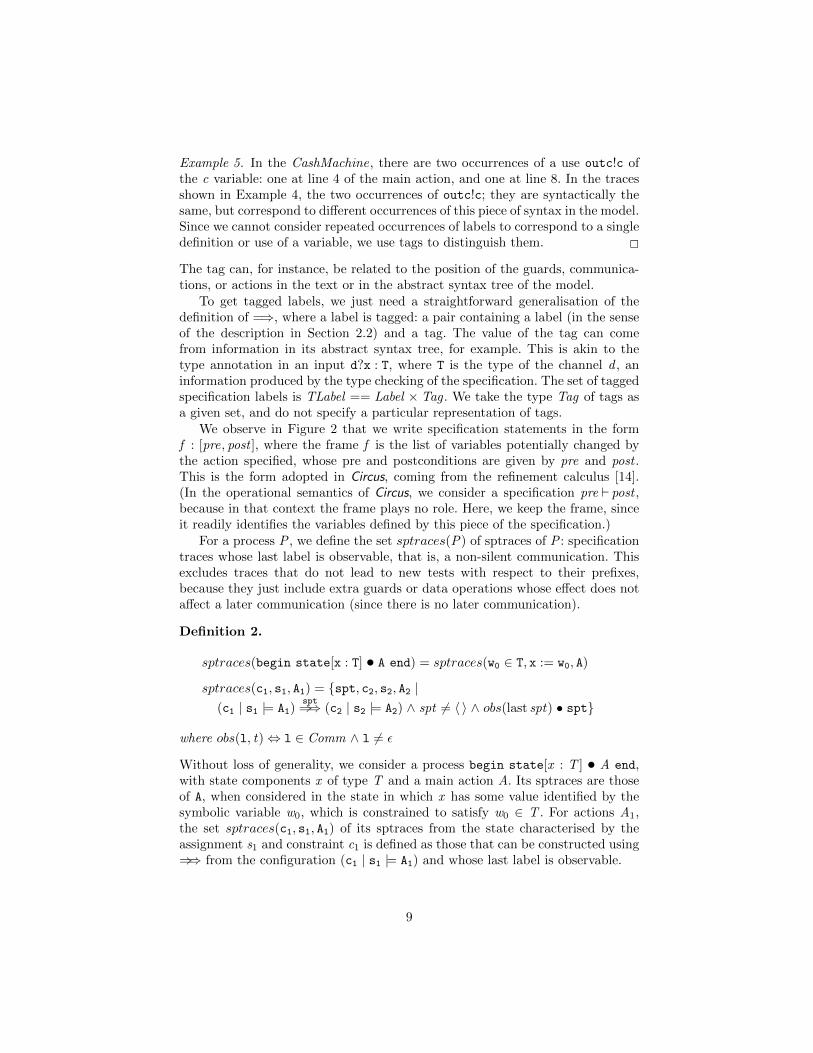
Example 5. In the CashMachine, there are two occurrences of a use outc!c ofthe c variable: one at line 4 of the main action, and one at line 8. In the tracesshown in Example 4, the two occurrences of outc!c; they are syntactically thesame, but correspond to different occurrences of this piece of syntax in the model.Since we cannot consider repeated occurrences of labels to correspond to a singledefinition or use of a variable, we use tags to distinguish them. 2

The tag can, for instance, be related to the position of the guards, communica-tions, or actions in the text or in the abstract syntax tree of the model.

To get tagged labels, we just need a straightforward generalisation of thedefinition of =⇒, where a label is tagged: a pair containing a label (in the senseof the description in Section 2.2) and a tag. The value of the tag can comefrom information in its abstract syntax tree, for example. This is akin to thetype annotation in an input d?x : T, where T is the type of the channel d , aninformation produced by the type checking of the specification. The set of taggedspecification labels is TLabel == Label × Tag . We take the type Tag of tags asa given set, and do not specify a particular representation of tags.

We observe in Figure 2 that we write specification statements in the formf : [pre, post ], where the frame f is the list of variables potentially changed bythe action specified, whose pre and postconditions are given by pre and post .This is the form adopted in Circus, coming from the refinement calculus [14].(In the operational semantics of Circus, we consider a specification pre ` post ,because in that context the frame plays no role. Here, we keep the frame, sinceit readily identifies the variables defined by this piece of the specification.)

For a process P , we define the set sptraces(P) of sptraces of P : specificationtraces whose last label is observable, that is, a non-silent communication. Thisexcludes traces that do not lead to new tests with respect to their prefixes,because they just include extra guards or data operations whose effect does notaffect a later communication (since there is no later communication).

Definition 2.

sptraces(begin state[x : T] • A end) = sptraces(w0 ∈ T, x := w0, A)

sptraces(c1, s1, A1) = {spt, c2, s2, A2 |(c1 | s1 |= A1)

spt⇒⇒ (c2 | s2 |= A2) ∧ spt 6= 〈〉 ∧ obs(last spt) • spt}

where obs(l, t)⇔ l ∈ Comm ∧ l 6= ε

Without loss of generality, we consider a process begin state[x : T ] • A end,with state components x of type T and a main action A. Its sptraces are thoseof A, when considered in the state in which x has some value identified by thesymbolic variable w0, which is constrained to satisfy w0 ∈ T . For actions A1,the set sptraces(c1, s1, A1) of its sptraces from the state characterised by theassignment s1 and constraint c1 is defined as those that can be constructed using⇒⇒ from the configuration (c1 | s1 |= A1) and whose last label is observable.

9

Example 6. Some sptraces of CashMachine are as follows. (In examples, we omittags when they are not needed, and below we distinguish the two occurrences ofoutc!c by the tags tag1 and tag2.)

〈inc?c?a, (outc!c, tag1)〉〈inc?c?a, (outc!c, tag1), inc?c?a〉〈inc?c?a, var notes, Dispense, notes 6= [[ ]] , cash!notes〉〈inc?c?a, var notes, Dispense, notes 6= [[ ]] , cash!notes, (outc!c, tag2)〉

We note that the first specification trace in Example 4 is not an sptrace. 2

The conversion of sptraces to constrained symbolic traces, which it the subjectof Section 5, provides a way of obtaining symbolic tests from the specificationtraces. In what follows, we consider data-coverage criteria to select a subset ofthe sptraces of a given process P . Each of the criteria are based on the notionsof definitions and uses of a given variable x , which we formalise next.

3.2 Definitions and uses

In an sptrace, a definition is a tagged label, where the label is a communicationor an action that may assign a new value to a Circus variable, that is, an inputcommunication, a specification statement, a Z schema where some variables arewritten, an assignment, or a var declaration, which, in Circus causes an initiali-sation. Formally, the set defs(x, P) of definitions of a variable x in a process P canbe identified from the set of sptraces of P as follows, where we use the functiondefs(x, spt) that characterises the definitions of x in a particular sptrace spt.

Definition 3. defs(x, P) =⋃{ spt : sptraces(P) • defs(x, spt) }

The set defs(x, spt) can be specified inductively as follows.

Definition 4. defs(x, 〈〉) = ∅defs(x, tla spt) = ({tl} ∩ defs(x)) ∪ defs(x, spt)

The empty trace has no definitions. If the trace is a tagged label tl followed bythe trace spt, we include tl if it is a definition of x as characterised by defs(x ).The definitions of spt are themselves given by defs(x, spt).

The tagged labels in which x is written (defined) can be specified as follows.

Definition 5. defs(x) = { tl : TLabel | x ∈ defV(tl) }

The set defV(tl) of such variables for a label tl is specified inductively. Weadopt here the convention that g stands for an element of Pred , that is, a guardlabel, d for a channel name, an element of CName, e an expression, an elementof Expr , and A for a list of label actions, elements of LAct . We use subscriptswhen we need more of these meta-variables. The tags play no role here, and weignore them in the definition of defV.

10

Definition 6.

defV(g) = defV(ε) = defV(d) = defV(d!e) = defV(end y) = ∅defV(d?x, t) = defV(d?x : c, t) = { x } defV(f : [pre, post]) = { f }defV(Op) = wrtV (Op) defV(x := e) = { x }defV(var x : T) = { x } defV(var x := e) = { x }

A Morgan specification statement f : [pre, post ] is a pre-post specification thatcan only modify the variables explicitly listed in the frame f .

The set wrtV (Op) of written variables of a schema Op is defined in [4, page 161]to include the variables that are potentially modified by the schema, and itsidentification is not a purely syntactic issue. This set includes the variables v inthe state of Op that are not constrained by an equality v ′ = v in Op. Followingthe usual over-approximation in data-flow analysis, we can take the pessimistic,but conservative, view that Op potentially writes to all variables in scope andavoid the requirement for theorem proving.

Example 7. Coming back to the CashMachine (and ignoring tags) we have:

defs(c, CashMachine) = {inc?c?a}defs(a, CashMachine) = {inc?c?a}defs(notes, CashMachine) = {var notes : Cash, Dispense}defs(nBank, CashMachine) = {Dispense,

nBank := { 10 7→ cap, 20 7→ cap, 50 7→ cap }}

2

The notion of (externally visible) use is simpler: a tagged label with an outputcommunication. Formally, the set e-uses(x, P) of uses of a variable x in a processP can be identified from its set of sptraces.

Definition 7. e-uses(x, P) =⋃{ spt : sptraces(P) • e-uses(x, spt) }

The set e-uses(x, spt) of uses of x in a trace spt can be specified as follows.

Definition 8. e-uses(x, 〈〉) = ∅e-uses(x, tla spt) = ({tl} ∩ e-uses(x)) ∪ e-uses(x, spt)

Finally, the general notion of uses of a variable x is defined below.

Definition 9. e-uses(x) = {d : CName; e : Exp; t : Tag | x ∈ FV (e) • (d!e, t)}

These are labels (d!e, t) where x occurs free in the expression e. We use FV (e)to denote the set of free variables of an expression e.

At this point, we consider e-uses, but not the classical notion of p-uses, whichrelates to uses in predicates and, in the context of Circus, are not observable. Weintroduce a notion of internal uses (i-uses) later on in Section 4.1. In a Circusmodel, internal uses of a variable are its occurrences in predicates (of guards anddata operations, for example) and also in assigning expressions.

11

Example 8. We have e-uses(c, CashMachine) = {(outc!c, tag1), (outc!c, tag2) }and e-uses(notes, CashMachine) = {cash!notes}. There are no other externallyvisible uses in CashMachine. 2

We observe that a label cannot be both a definition and a use of a variable,because a use is an output communication, which does not define any variable.Besides, a label can be neither a definition nor a use (this is the case for refill)and then not considered for data-flow coverage.

The property clear-path(spt, df, u, x) characterises the fact that the trace spthas a subsequence that starts with the label df, finishes with the label u, with nodefinition of the variable x . (We note that, although we consider subsequences ofa trace rather than paths of a graph, for consistency with classical terminology,we use the term clear path, rather than clear subsequence, anyway.)

Definition 10.

clear-path(spt, df, u, x)⇔ ∃ i : 1 . .# spt • spt i = df ∧∃ j : (i + 1) . .# spt • spt j = u ∧∀ k : (i + 1) . . (j − 1) • spt k 6∈ defs(x, P)

Example 9. We consider the sptraces below.

〈inc?c?a, var notes, Dispense, notes = [[ ]] , (outc!c, tag2)〉〈inc?c?a, var notes, Dispense, notes 6= [[ ]] , cash!notes, (outc!c, tag2)〉

They have a clear path from inc?c?a to (outc!c, tag2) with respect to c. 2

A e-use u of a variable x is said to be reachable by a definition df of x if thereis a trace spt such that clear-path(spt, df, u, x).

3.3 Data-flow anomalies and Circus

Three data-flow anomalies are usually identified: (1) a use of a variable withouta previous definition; (2) two definitions without an intermediate use; and (3) adefinition without use. While these all raise concerns in a program, it is not thecase of (2) and (3) in a Circus model. Because a variable declaration is a variabledefinition that assigns an arbitrary value to a variable, it is common to follow itup with a second definition that restricts that value.

In addition, it is not rare to use a communication d?x to define just that thevalue x to be input via the channel d is not restricted (and also later not used).In an abstract specification, a process involving such a communication might,for example, be combined in parallel with another process that captures anotherrequirement concerned with restricting these values x , while the requirementcaptured by the process that defines d?x is not concerned with such values.

As we can see in the following sections, the data-coverage criteria that weconsider are based on the set of definitions of a variable x . When a definitioninvolved in any of the above anomalies is considered, it imposes no restrictionon the set of tests under consideration for coverage. In practical terms, no testsare required as a consequence of the presence of such definitions.

12

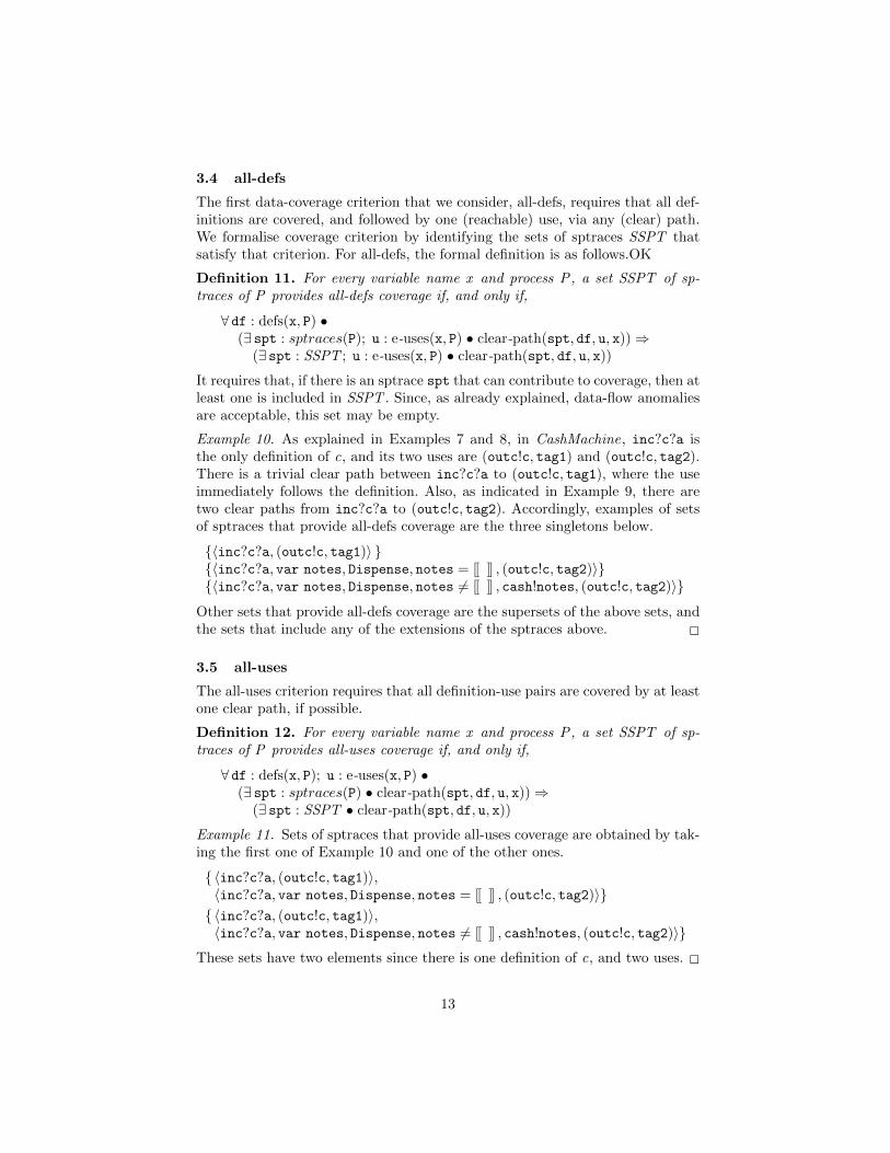
3.4 all-defs

The first data-coverage criterion that we consider, all-defs, requires that all def-initions are covered, and followed by one (reachable) use, via any (clear) path.We formalise coverage criterion by identifying the sets of sptraces SSPT thatsatisfy that criterion. For all-defs, the formal definition is as follows.OK

Definition 11. For every variable name x and process P, a set SSPT of sp-traces of P provides all-defs coverage if, and only if,

∀ df : defs(x, P) •(∃ spt : sptraces(P); u : e-uses(x, P) • clear-path(spt, df, u, x))⇒

(∃ spt : SSPT ; u : e-uses(x, P) • clear-path(spt, df, u, x))

It requires that, if there is an sptrace spt that can contribute to coverage, then atleast one is included in SSPT . Since, as already explained, data-flow anomaliesare acceptable, this set may be empty.

Example 10. As explained in Examples 7 and 8, in CashMachine, inc?c?a isthe only definition of c, and its two uses are (outc!c, tag1) and (outc!c, tag2).There is a trivial clear path between inc?c?a to (outc!c, tag1), where the useimmediately follows the definition. Also, as indicated in Example 9, there aretwo clear paths from inc?c?a to (outc!c, tag2). Accordingly, examples of setsof sptraces that provide all-defs coverage are the three singletons below.

{〈inc?c?a, (outc!c, tag1)〉 }{〈inc?c?a, var notes, Dispense, notes = [[ ]] , (outc!c, tag2)〉}{〈inc?c?a, var notes, Dispense, notes 6= [[ ]] , cash!notes, (outc!c, tag2)〉}

Other sets that provide all-defs coverage are the supersets of the above sets, andthe sets that include any of the extensions of the sptraces above. 2

3.5 all-uses

The all-uses criterion requires that all definition-use pairs are covered by at leastone clear path, if possible.

Definition 12. For every variable name x and process P, a set SSPT of sp-traces of P provides all-uses coverage if, and only if,

∀ df : defs(x, P); u : e-uses(x, P) •(∃ spt : sptraces(P) • clear-path(spt, df, u, x))⇒

(∃ spt : SSPT • clear-path(spt, df, u, x))

Example 11. Sets of sptraces that provide all-uses coverage are obtained by tak-ing the first one of Example 10 and one of the other ones.

{ 〈inc?c?a, (outc!c, tag1)〉,〈inc?c?a, var notes, Dispense, notes = [[ ]] , (outc!c, tag2)〉}{ 〈inc?c?a, (outc!c, tag1)〉,〈inc?c?a, var notes, Dispense, notes 6= [[ ]] , cash!notes, (outc!c, tag2)〉}

These sets have two elements since there is one definition of c, and two uses. 2

13

3.6 all-du-paths

The all-du-paths criterion requires that all definition-use pairs are covered by allpossible paths. Our notion of path, as already said, is based on sptraces.

Definition 13. For every variable name x and process P, a set SSPT of sp-traces of P provides all-du-paths coverage if, and only if,

∀ df : defs(x, P); u : e-uses(x, P); p : all-du-sub-path(x, P, df, u) •∃ spt : SSPT ; spt1, spt2 : seq TLabel • spt = spt1 a p a spt2

The traces spt1 and spt2 are an initialisation and a finalisation trace that deter-mine an sptrace of P that covers p. The set all-du-sub-path(x, P, df, u) containsall the paths in P , according to its set of sptraces, that start with df, finish withu, and is clear of definitions of x in between.

Definition 14.

all-du-sub-path(x, P, df, u) ={ spt : sptraces(P); i : 1 . .# spt ; j : (i + 1) . .# spt |

spt i = df ∧ spt j = u ∧ ∀ k : (i + 1) . . (j − 1) • spt k 6∈ defs(x, P))• (i . . j ) � spt }

Example 12. A set of sptraces that provides all-du-paths coverage is obtainedby selecting the three sptraces of example 10

{ 〈inc?c?a, (outc!c, tag1)〉,〈inc?c?a, var notes, Dispense, notes = [[ ]] , (outc!c, tag2)〉〈inc?c?a, varnotes, Dispense, notes 6= [[ ]] , cash!notes, (outc!c, tag2)〉}

2

Example 13. When considering data-flow coverage of the variable notes, weobserve that it is defined in the Dispense schema and it has one use only,cash!notes at line 8 of the main action. There is a unique def-clear path be-tween them. Thus a single sptrace is sufficient to provide coverage accordingto any of the three criteria: it just needs to contain the two consecutive labelscorresponding to this definition and this use as indicated below.

〈. . . , inc?c?a, var notes, Dispense, notes 6= [[ ]] , cash!notes, . . .〉

For instance, the singleton below provides all-defs, all-uses and all-du-paths cov-erage with respect to the variable notes.

{〈inc?c?a, var notes, Dispense, notes 6= [[ ]] , cash!notes, (outc!c, tag2)〉}

2

14

This mostly concludes our discussion of the standard data-flow coverage criteria.We note, however, that the CashMachine variables are c, a, notes, and nBank ,and that nBank and a are used internally only. Thus, there is no def-clear pathfrom their definition to an external use, and given the definitions of all-defs,all-uses and all-du-paths, every set of sptraces provides coverage with respect tothese criteria and these variables. They contribute, however, to our next moreelaborate criterion, which takes the nature of Circus models into account, em-phasizing dependencies between different variables.

In addition, the structure of schemas is not taken into account. For instance,Dispense is a disjunction, and the criteria above do not force the coverage of thetwo cases, even if the last one achieves it due to the existence of two definition-clear paths that cover them. Coverage of the structure of Z schemas could beanother selection criterion by itself, or combined with data-flow analysis.

4 sel-var-df-chain-trace

The definition of this criterion is based on the notion of a var-df-chain, which weintroduce first (Section 4.1). Afterwards, we formalise this novel criterion (Sec-tion 4.2), and lastly we apply it to the CashMachine (Section 4.3). Roughly, theidea is to identify sptraces that include chains of definition and associated inter-nal uses of variables, such that each variable affects the next one in the chain.For state-rich models, we expect an interesting number of such chains.

4.1 var-df-chain

A suffix of an sptrace spt starting at position i (that is, (i . . # spt) � spt) isin the set var-df-chain(x, P) of var-df-chains of P for x if it starts with a labelspt i that defines x and subsequently has a clear path to a label spt j . This labelmust either be a use of x , and in this case it must be the last label of spt, oraffect the definition of another variable y , and in this case spt must continuewith a var-df-chain for y. The continuation is determined by (j . . # spt) � spt ,the subsequence of spt from the position j .

Definition 15.

var-df-chain(x, P) ={ spt : sptraces(P); i : 1 . .# spt ; j : (i + 1) . .# spt | spt i ∈ defs(x, P) ∧ (∀ k : (i + 1) . . (j − 1) • spt k 6∈ defs(x, P)) ∧(

(spt j ∈ e-uses(x, P) ∧ j = # spt) ∨(∃ y • affects(x, y, spt j ) ∧ (j . .# spt) � spt ∈ var-df-chain(y, P))

)• (i . .# spt) � spt

}

A variable x affects the definition of another variable y in a tagged label tl if itis an internal use of x and a definition of y .

Definition 16. affects(x, y, tl) = x ∈ i-useV(tl) ∧ y ∈ defs(tl)

15

An internal use of a variable is an occurrence of it in a guard or action. (Thisnotion of internal use subsumes the classical notion of p-uses.) The set i-useV(tl)of variables used in a tagged label tl, internally, is defined as follows.

Definition 17.

i-useV(g) = FV (g) i-useV(ε) = i-useV(d) = ∅i-useV(d!e) = i-useV(d?x) = ∅ <<<<<<< .minei-useV(d?x : g) = FV (g) \ {x} ======= i-useV(d?x : c) = FV (c) \ {x} >>>>>>> .r3463i-useV(f : [pre, pos]) = FV (pre) ∪ FV (pos)i-useV(Op) = FV (Op) i-useV(x := e) = FV (e)i-useV(var x : T) = ∅ i-useV(var x := e) = FV (e)i-useV(end y) = ∅

We observe that not all free occurrences of a variable constitute an internal useof it. For example, an assignment to a variable is not an use of it.

4.2 The criterion

We observe that var-df-chains are not sptraces, but suffixes of sptraces. So,coverage is provided by sptraces that have such suffixes, rather than by thevar-df-chains themselves. In particular, sel-var-df-chain-trace coverage requiresthat every chain in a model is covered by at least one sptrace.

Definition 18. For every variable name x and process P, a set SSPT of sp-traces of P provides sel-var-df-chain-trace coverage if, and only if,

∀ spt1 : var-df-chain(x, P) •∃ spt2 : SSPT ; spt3 : seq TLabel • spt2 = spt3 a spt1

The specification trace spt3 is an initialisation trace that leads to the chain.This is the most demanding of the criteria in this report as shown below.

Theorem 1 For every set SSPT of sptraces, if it provides sel-var-df-chain-tracecoverage, then it provides all-du-paths coverage. Additionally, if it provides all-du-paths coverage, then it provides all-uses coverage. Finally, if it provides all-uses coverage, then it provides all-defs coverage.

The proof of this theorem uses our detailed formalisation of all definitions. Itestablishes subset inclusion for each pair of the sets of sets of sptraces thatprovide coverage according to Definitions 11, 12, 13 and 18.

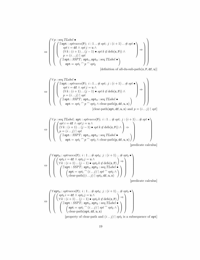
Proof.Case sel-var-df-chain-trace ensures all-paths(∀ spt1 : var-df-chain(x, P) •∃ spt2 : SSPT ; spt3 : seq TLabel • spt2 = spt3 a spt1

)⇔

16

∀ spt1 : seq TLabel ; spt4 : sptraces(P);i : 1 . .# spt4; j : (i + 1) . .# spt4 •

spt4 i ∈ defs(x, P) ∧(∀ k : (i + 1) . . (j − 1) • spt4 k 6∈ defs(x, P)) ∧

(spt4 j ∈ e-uses(x, P) ∧ j = # spt4) ∨∃ y •affects(x, y, spt4 j ) ∧(j . .# spt) � spt4 ∈ var-df-chain(y, P))

∧

spt1 = (i . .# spt4) � spt4

⇒∃ spt2 : SSPT ; spt3 : seq TLabel • spt2 = spt3 a spt1

[definition of var-df-chain(x, P)]

⇒

∀ spt1 : seq TLabel ; spt4 : sptraces(P);i : 1 . .# spt4; j : (i + 1) . .# spt4 •

spt4 i ∈ defs(x, P) ∧(∀ k : (i + 1) . . (j − 1) • spt4 k 6∈ defs(x, P)) ∧spt4 j ∈ e-uses(x, P) ∧ j = # spt4 ∧spt1 = (i . .# spt4) � spt4

⇒∃ spt2 : SSPT ; spt3 : seq TLabel • spt2 = spt3 a spt1

[predicate calculus]

⇔

∀ spt4 : sptraces(P); i : 1 . .# spt4; p : seq TLabel •

∃ df : defs(x, P); u : e-uses(x, P) • spt4 i = df ∧ spt4 (# spt4) = u ∧

(∀ k : (i + 1) . . (# spt4 − 1) • spt4 k 6∈ defs(x, P)) ∧p = (i . .# spt4) � spt4

⇒∃ spt : SSPT ; spt1 : seq TLabel • spt = spt1 a p)

[property of sets]

⇔

∀ spt4 : sptraces(P); i : 1 . .# spt4;df : defs(x, P); u : e-uses(x, P); p : seq TLabel • spt4 i = df ∧ spt4 (# spt4) = u ∧

(∀ k : (i + 1) . . (# spt4 − 1) • spt4 k 6∈ defs(x, P)) ∧p = (i . .# spt4) � spt4

⇒∃ spt : SSPT ; spt1 : seq TLabel • spt = spt1 a p


17

⇔

∀ spt4 : sptraces(P); i : 1 . .# spt4; j : i . .# spt4;df : defs(x, P); u : e-uses(x, P); p : seq TLabel • spt4 i = df ∧ spt4 j = u ∧

(∀ k : (i + 1) . . (j − 1) • spt4 k 6∈ defs(x, P)) ∧p = (i . . j ) � spt4

⇒(∃ spt : SSPT ; spt1 : seq TLabel • spt = spt1 a p)

[{spt : sptraces(P); i : 1 . .# spt | P(spt ,# spt) • (i . .# spt) � spt} =]

[{spt : sptraces(P); i : 1 . .# spt ; j ; i . .# spt | P(spt , j ) • (i . . j ) � spt}][since sptraces(P) is prefix closed]

⇔

∀ spt4 : sptraces(P); i : 1 . .# spt4; j : (i + 1) . .# spt4;df : defs(x, P); u : e-uses(x, P); p : seq TLabel • spt4 i = df ∧ spt4 j = u ∧


⇒(∃ spt : SSPT ; spt1 : seq TLabel • spt = spt1 a p)

[df 6= u by defs(x, P) ∩ e-uses(x, P) = ∅]

⇒

∀ spt4 : sptraces(P); i : 1 . .# spt4; j : (i + 1) . .# spt4;df : defs(x, P); u : e-uses(x, P); p : seq TLabel • spt4 i = df ∧ spt4 j = u ∧


⇒(∃ spt : SSPT ; spt1, spt2 : seq TLabel •spt = spt1 a p a spt2

)

[take spt2 = 〈〉]

⇔

∀ df : defs(x, P); u : e-uses(x, P); p : seq TLabel •

∃ spt : sptraces(P); i : 1 . .# spt ; j : (i + 1) . .# spt •

spt i = df ∧ spt j = u ∧(∀ k : (i + 1) . . (j − 1) • spt k 6∈ defs(x, P)) ∧p = (i . . j ) � spt


)


⇔(∀ df : defs(x, P); u : e-uses(x, P); p : all-du-sub-path(x, P, df, u) •∃ spt : SSPT ; spt1, spt2 : seq TLabel • spt = spt1 a p a spt2

)[definition of all-du-sub-path(x, P, df, u)]

Case all-paths ensures all-uses(∀ p : all-du-sub-path(x, P, df, u) •∃ spt : SSPT ; spt1, spt2 : seq TLabel • spt = spt1 a p a spt2

)

18

⇔

∀ p : seq TLabel •




)

[definition of all-du-sub-path(x, P, df, u)]

⇔

∀ p : seq TLabel •



⇒(∃ spt : SSPT ; spt1, spt2 : seq TLabel •spt = spt1 a p a spt2 ∧ clear-path(p, df, u, x)

)

[clear-path(spt, df, u, x) and p = (i . . j ) � spt ]

⇔

∀ p : seq TLabel ; spt : sptraces(P); i : 1 . .# spt ; j : (i + 1) . .# spt • spt i = df ∧ spt j = u ∧

(∀ k : (i + 1) . . (j − 1) • spt k 6∈ defs(x, P)) ∧p = (i . . j ) � spt

⇒(∃ spt : SSPT ; spt1, spt2 : seq TLabel •spt = spt1 a p a spt2 ∧ clear-path(p, df, u, x)

)


⇔

∀ spt3 : sptraces(P); i : 1 . .# spt3; j : (i + 1) . .# spt3 •(

spt3 i = df ∧ spt3 j = u ∧∀ k : (i + 1) . . (j − 1) • spt3 k 6∈ defs(x, P)

)⇒∃ spt : SSPT ; spt1, spt2 : seq TLabel •(

spt = spt1 a (i . . j ) � spt a spt2 ∧clear-path((i . . j ) � spt3, df, u, x)

)


⇔



)⇒∃ spt : SSPT ; spt1, spt2 : seq TLabel •(

spt = spt1 a (i . . j ) � spt a spt2 ∧clear-path(spt, df, u, x)

)

[property of clear-path and (i . . j ) � spt3 is a subsequence of spt]

19

⇒



)⇒(

(∃ spt : SSPT • clear-path(spt, df, u, x)) ∧(∃ spt : sptraces(P) • clear-path(spt, df, u, x))

)


⇔

∃ spt3 : sptraces(P); i : 1 . .# spt3; j : (i + 1) . .# spt3 •(


) ⇒((∃ spt : SSPT • clear-path(spt, df, u, x)) ∧(∃ spt : sptraces(P) • clear-path(spt, df, u, x))

)


⇔

(∃ spt : sptraces(P) • clear-path(spt, df, u, x))⇒((∃ spt : SSPT • clear-path(spt, df, u, x)) ∧(∃ spt : sptraces(P) • clear-path(spt, df, u, x))

)[definition of clear-path(spt, df, u, x)]

⇔(

(∃ spt : sptraces(P) • clear-path(spt, df, u, x))⇒(∃ spt : SSPT • clear-path(spt, df, u, x))

)[predicate calculus]

Case all-uses ensures all-defs∀ u : e-uses(x, P) •(∃ spt : sptraces(P) • clear-path(spt, df, u, x))⇒

(∃ spt : SSPT • clear-path(spt, df, u, x))

⇒

∀ u : e-uses(x, P) •(∃ spt : sptraces(P) • clear-path(spt, df, u, x))⇒

(∃ spt : SSPT ; u : e-uses(x, P) • clear-path(spt, df, u, x))


⇔(

(∃ spt : sptraces(P); u : e-uses(x, P) • clear-path(spt, df, u, x))⇒(∃ spt : SSPT ; u : e-uses(x, P) • clear-path(spt, df, u, x))

)[predicate calculus]

2

4.3 Examples

The very basic var-df-chains, where the same variable is considered as the start-ing definition and the final use, with a clear path with respect to this vari-able in between, are covered by the above criteria. More interesting are thosevar-df-chains where intermediate variables that are defined and then used intro-duce dependencies between definition and use of different variables.

20

A first example is the definition of a in inc?c?a and the use of notes incash!notes. The dependency comes from the fact that notes belongs to the set ofwritten variables of Dispense, a is an input of this schema, and within Dispense,there is the constraint: Σ notes! = a?. Thus affects(a, notes, Dispense) holds,and since cash!notes ∈ e-uses(notes, CashMachine), we have the var-df-chain:

〈inc?c?a, var notes, Dispense, notes 6= [[ ]] , cash!notes〉

We note that its coverage is required by all-du-paths by accident, because it ispart of a clear path between a definition of c and a use of c. Here, the effect ofthe definition of a on the value of notes is explicitly required to be covered. Thevar-df-chains identified below, however, are not required to be covered by theprevious criteria. They give rise to new tests.

Other examples of var-df-chains are introduced by the definitions of nBank .The label nBank := { 10 7→ cap, 20 7→ cap, 50 7→ cap } is such a definition, andnBank is used in Dispense. Moreover, notes is externally used in the labelcash!notes. This leads to the following var-df-chain.

〈nBank := { 10 7→ cap, 20 7→ cap, 50 7→ cap },inc?c?a, var notes, Dispense, notes 6= [[ ]] , cash!notes〉

Coverage of this chain leads to coverage of the effect of a refill event, after whichthe value of nBank is updated as indicated above. An initialisation trace thatleads to the above var-df-chain is simply 〈refill〉.

Another definition of the nBank variable is in the DispenseNotes schema,namely: nBank ′ n = (nBank n)−(notes! ] n). Moreover, DispenseNotes also hasan internal use of nBank . Finally, the path below is clear of nBank definitionsbetween the two occurrences of Dispense.

〈Dispense,notes 6= [[ ]] , cash!notes, (outc!c, tag2), inc?c?a, var notes, Dispense〉

This leads to the var-df-chain below, where the second occurrence of Dispenseis also taken as a definition of notes, which is used externally in the final label.

〈Dispense,notes 6= [[ ]] , cash!notes, (outc!c, tag2), inc?c?a, var notes, Dispense,notes 6= [[ ]] , cash!notes〉

A possible initialisation trace for this var-df-chain is 〈inc?c?a〉.As already mentioned, our new criterion sel-var-df-chain is inspired by the

work in [21], but there are fundamental differences that go beyond the speci-ficities of the Circus framework. Because of the nature of Circus, it is importantnot to consider only traces that start with a definition characterised by an inputcommunication like in [21]. The internal state is just as important as any input.

Moreover, throwing away traces that are prefixes of other selected traces likein [21] is not applicable to testing for traces refinement or deadlock reduction(known as the conf relation), which are the conformance relations considered

21

c ∧ (s; g)

(c | s |= 〈g〉a spt)ε−→ST (c ∧ (s; g) | s |= spt)

c ∧ T 6= ∅

(c | s |= 〈d?x : T〉a spt)d?w0−→ST (c ∧ w0 ∈ T | s; var x := w0 |= spt)

c

(c | s |= 〈d!e〉a spt)d!w0−→ST (c ∧ (s; w0 = e) | s |= spt)

(c1 | s1 |= A1)ε−→ (c2 | s2 |= Skip)

(c1 | s1 |= 〈A1〉a spt)ε−→ST (c2 | s2 |= spt)

Table 2. Operational semantics of sptraces; w0 stand for fresh symbolic variables

for the Circus testing theory [3]. A trace is used to construct tests that checkforbidden continuations and required acceptances at a particular point of theSUT history, and that check is not subsumed by tests that arise from longertraces. It is the reason why we do not pursue maximality as in [21].

In the next section, we explain how to obtain cstraces from sptraces (toconstruct symbolic tests). This is essential for generating tests from the selectedsptraces and states the link of these tests with the operational semantics andthe Circus testing theory, whether data-flow coverage is used for selection or not.

5 Conversion of specification traces to symbolic traces

Converting an sptrace to a symbolic trace requires an operational semantics forsptraces, which we provide in Table 2. It defines a transition relation −→ST

using four rules: one for when the first label is a guard, two for when it is eitheran input or an output, and one for an action label A. In this last case, the rules ofthe operational semantics transition rule −→ define the new transition relation.

Like in the operational semantics, the configuration is a triple, but here,instead of a process or action, we have an sptrace associated with a constraint

c and a state assignment s. From a configuration (c | s |= 〈l〉a spt) with an

sptrace 〈l〉 a spt, we have a transition to a configuration with spt. The newconstraint and state depend on the label l.

For a guard, a transition requires that c is satisfiable and g holds in thecurrent state (s; g). In this case, the transition is silent: it has label ε.

Input and output communications give rise to non-silent transitions with la-bels like those of the operational semantics: symbolic inputs and outputs. Inputsd?x: T are annotated with the type T of channel d . The new constraint recordsthat the input value represented by the fresh symbolic variable w0 has type Tand the state is enriched with a declaration of x whose initial value is set to w0.

22

(c1 | s1 |= spt1)ε−→ST (c2 | s2 |= spt2)

(c1 | s1 |= spt1)〈〉→→ (c2 | s2 |= spt2)

(c1 | s1 |= spt1)d?α0−→ST (c2 | s2 |= spt2)

(c1 | s1 |= spt1)〈 d?α0 〉→→ (c2 | s2 |= spt2)

(c1 | s1 |= spt1)d!α0−→ST (c2 | s2 |= spt2)

(c1 | s1 |= spt1)〈 d.α0 〉→→ (c2 | s2 |= spt2)

(c1 | s1 |= spt1)st1→→ (c2 | s2 |= spt2) (c2 | s2 |= spt2)

st2→→ (c3 | s3 |= spt3)

(c1 | s1 |= spt1)st1a

st2→→ (c3 | s3 |= spt3)

Table 3. Annotated transition relation: symbolic traces for sptraces

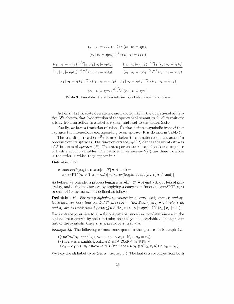
Actions, that is, state operations, are handled like in the operational seman-tics. We observe that, by definition of the operational semantics [3], all transitionsarising from an action in a label are silent and lead to the action Skip.

Finally, we have a transition relationst→→ that defines a symbolic trace st that

captures the interactions corresponding to an sptrace. It is defined in Table 3.

The transition relationst→→ is used below to characterise the cstraces of a

process from its sptraces. The function cstraceSPTa(P) defines the set of cstraces

of P in terms of sptraces(P). The extra parameter a is an alphabet: a sequenceof fresh symbolic variables. The cstraces in cstraceSPT

a(P) use these variablesin the order in which they appear in a.

Definition 19.

cstraceSPTa(begin state[x : T ] • A end) =

convSPTa(w0 ∈ T, x := w0) L sptraces(begin state[x : T ] • A end) M

As before, we consider a process begin state[x : T ] • A end without loss of gen-erality, and define its cstraces by applying a conversion function convSPTa(c, s)to each of its sptraces. It is defined as follows.

Definition 20. For every alphabet a, constraint c, state assignment s and sp-trace spt, we have that convSPTa(c, s) spt = (st,∃(αc \ αst) • c1) where st

and c1 are characterised by αst ≤ a ∧ ∃ s1 • (c | s |= spt)st→→ (c1 | s1 |= 〈〉).

Each sptrace gives rise to exactly one cstrace, since any nondeterminism in theactions are captured by the constraint on the symbolic variables. The alphabetαst of the symbolic trace st is a prefix of a: αst ≤ a.

Example 14. The following cstraces correspond to the sptraces in Example 12.

(〈inc?α0?α1, outc!α2〉, α0 ∈ CARD ∧ α1 ∈ N1 ∧ α2 = α0)( 〈inc?α0?α1, cash!α2, outc!α3〉, α0 ∈ CARD ∧ α1 ∈ N1 ∧Σα2 = α1 ∧ (∃ w0 : Note→ N • (∀ n : Note • α2 ] n) ≤ w0 n)) ∧ α3 = α0)

We take the alphabet to be 〈α0, α1, α2, α3, . . .〉. The first cstrace comes from both

23

the first and the second sptrace in Example 12. The second cstrace comes fromthe last sptrace in Example 12. The quantified symbolic variable w0 representsthe internal value of nBank , which is not observable in the trace, but contributesto the specification of the observable value α2.

Two sptraces give rise to the same cstrace because after a withdraw request,the card may be returned immediately for one of two reasons: there is a problemwith the card account (like insufficient funds) or there is no money in the cashmachine. Since the model abstracts away the existence of accounts and theirbalances, we cannot distinguish these behaviours by tests from this model.

This is reflected in the fact that the two sptraces have different tags associatedwith the outc!c event. This indicates that they correspond to two different partsof the model. This distinction is not testable and that may be a problem forunderstanding or observing the SUT. A testing tool might, for example, warnthat a distinction may need to be introduced or instrumented in the SUT. 2

The cstraces defined by the operational semantics capture just observable labels.On the other hand, sptraces were defined specifically to capture the structure ofthe model, and in doing so, it captures guards and data operations that are notvisible in the interface of the SUT. So, it is not surprising that, as illustratedin the above example, there are sptraces that lead to the same cstrace. Theycorrespond to paths in the model that are not distinguishable from the SUT.Requiring their absence in programs is reasonable, but in abstract models thatinvolve nondeterminism, this is not realistic.

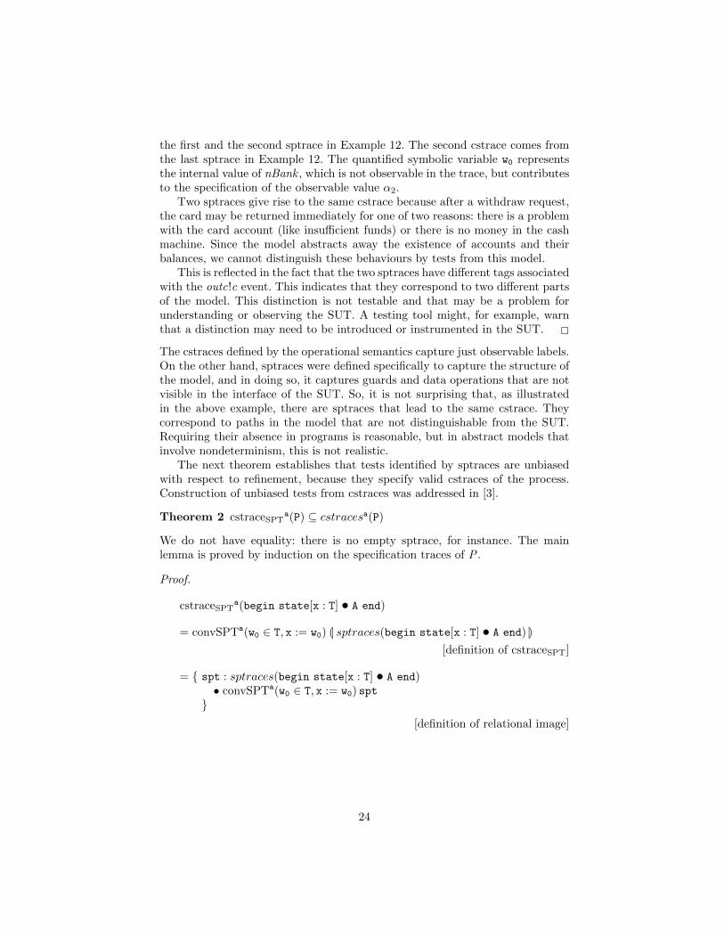
The next theorem establishes that tests identified by sptraces are unbiasedwith respect to refinement, because they specify valid cstraces of the process.Construction of unbiased tests from cstraces was addressed in [3].

Theorem 2 cstraceSPTa(P) ⊆ cstracesa(P)

We do not have equality: there is no empty sptrace, for instance. The mainlemma is proved by induction on the specification traces of P .

Proof.

cstraceSPTa(begin state[x : T] • A end)

= convSPTa(w0 ∈ T, x := w0) L sptraces(begin state[x : T] • A end) M[definition of cstraceSPT]

= { spt : sptraces(begin state[x : T] • A end)• convSPTa(w0 ∈ T, x := w0) spt}

[definition of relational image]

24

= { spt : sptraces(begin state[x : T] • A end); st; c1; s1 |αst ≤ a ∧ (w0 ∈ T | x := w0 |= spt)

st→→ (c1 | s1 |= 〈〉)• (st,∃(αc \ αst) • c1)}

[definition of convSPT]

= { spt; st; c1; s1; c2; s2; A2 |(w0 ∈ T | x := w0 |= A)

spt⇒⇒ (c2 | s2 |= A2) ∧ obs(last spt) ∧αst ≤ a ∧ (w0 ∈ T | x := w0 |= spt)

st→→ (c1 | s1 |= 〈〉)• (st,∃(αc \ αst) • c1)}

[definition of sptraces]

⊆ { st; c1; s1; A2 |αst ≤ a ∧ (w0 ∈ T | x := w0 |= A)

st−→ (c1 | s1 |= A2)• (st,∃(αc \ αst) • c1)}

[Lemma 1]

= cstracesa(begin state[x : T] • A end) [definition of cstraces]

2

The lemma below establishes the relationship between the transition relations⇒⇒, for specification traces, and −→, for the operational semantics of actions,which we reproduce in the appendix. The equality between the existential quan-tifications is semantic equality, not syntactic: the predicates identified by thepieces of text built out of the constraints and traces are equivalent.

Lemma 1.

∀ spt; st; c1; s1; A1; c2; s2; A2; c3; s3 •((c1 | s1 |= A1)

spt⇒⇒ (c2 | s2 |= A2) ∧ (c1 | s1 |= spt)st→→ (c3 | s3 |= 〈〉)

)⇒∃ c4, s4, A4 •(c1 | s1 |= A1)

st−→ (c4 | s4 |= A4) ∧(∃(αc3 \ αst) • c3) = (∃(αc4 \ αst) • c4)

Proof. Direct consequence of Proposition 1 and Lemma 2. 2

Lemma 2.


spt⇒⇒ (c2 | s2 |= A2) ∧ (c1 | s1 |= spt)st→→ (c3 | s3 |= 〈〉))⇒

(∃(αc3 \ αst) • c3) = (∃(αc2 \ αst) • c2)

Proof. By induction on st.

25

Case 〈〉

(c1 | s1 |= spt)〈〉→→ (c3 | s3 |= 〈〉)

In this case, by the definition of →→ and −→ST , spt is a sequence of guardsand actions (without communications). We establish the result by case analysison spt.

Subcase 〈g〉a spt

(c1 | s1 |= 〈g〉a spt)st→→ (c3 | s3 |= 〈〉) ∧ (c1 | s1 |= A1)

〈g〉aspt⇒⇒ (c2 | s2 |= A2)

⇒

∃ A3 •(c1 | s1 |= 〈g〉a spt)

〈〉→→ (c1 ∧ (s1; g) | s1 |= spt) ∧(c1 ∧ (s1; g) | s1 |= spt)

〈〉→→ (c3 | s3 |= 〈〉) ∧(c1 | s1 |= A1)

〈g〉⇒⇒ (c1 ∧ (s1; g) | s1 |= A3) ∧(c1 ∧ (s1; g) | s1 |= A3)

spt⇒⇒ (c2 | s2 |= A2)

[Lemma 3]

⇒ (∃αc3 • c3) = (∃αc2 • c2) [by induction hypothesis]

Subcase 〈A〉a spt, where A is an action of a label: similar.

Case 〈d?α0〉

(c1 | s1 |= spt)〈d?α0〉→→ (c3 | s3 |= 〈〉)

In this case, by the definition of →→ and −→ST , spt is a sequence of guardsand actions that ends with an input on the channel d . We again establish theresult by case analysis on spt. If it starts with a guard or an action, the proofis similar to that presented above. For 〈d?x〉, we have the following.

(c1 | s1 |= 〈d?x〉) 〈d?α0〉→→ (c3 | s3 |= 〈〉) ∧ (c1 | s1 |= A1)〈d?x〉⇒⇒ (c2 | s2 |= A2)

⇒ c3 = c1 ∧ α0 ∈ T ∧∃ A3 • (c1 | s1 |= A1)

〈d?x〉⇒⇒ (c1 ∧ α0 ∈ T | s1; var x := α0 |= A3)

[Lemma 4]

⇒ c3 = c1 ∧ α0 ∈ T ∧ c2 = c1 ∧ α0 ∈ T [Proposition 2]

⇒ c3 = c2

⇒ (∃(αc3 \ {α0}) • c3) = (∃(αc2 \ {α0}) • c2) [predicate calculus]

Case 〈d!α0〉 Similar, but relies on Lemma 5.

26

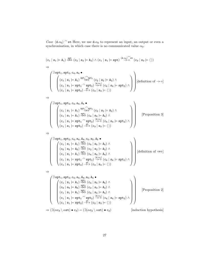
Case 〈d.α0〉 a st Here, we use d.α0 to represent an input, an output or even asynchronisation, in which case there is no communicated value α0.

(c1 | s1 |= A1)spt⇒⇒ (c2 | s2 |= A2) ∧ (c1 | s1 |= spt)

〈d.α0〉ast→→ (c3 | s3 |= 〈〉)

⇒∃ spt1, spt2, c4, s4 • (c1 | s1 |= A1)

spt1a

spt2⇒⇒ (c2 | s2 |= A2) ∧(c1 | s1 |= spt1

a spt2)〈d.α0〉→→ (c4 | s4 |= spt2) ∧

(c1 | s1 |= spt2)st→→ (c3 | s3 |= 〈〉)

[definition of →→]

⇒

∃ spt1, spt2, c4, s4, A4 •(c1 | s1 |= A1)

spt1a

spt2⇒⇒ (c2 | s2 |= A2) ∧(c1 | s1 |= A1)

spt1⇒⇒ (c4 | s4 |= A4) ∧(c1 | s1 |= spt1

a spt2)〈d.α0〉→→ (c4 | s4 |= spt2) ∧

(c1 | s1 |= spt2)st→→ (c3 | s3 |= 〈〉)

[Proposition 3]

⇒

∃ spt1, spt2, c4, s4, A4, c5, s5, A5 •(c1 | s1 |= A1)

spt1⇒⇒ (c5 | s5 |= A5) ∧(c5 | s5 |= A5)

spt2⇒⇒ (c2 | s2 |= A2) ∧(c1 | s1 |= A1)

spt1⇒⇒ (c4 | s4 |= A4) ∧(c1 | s1 |= spt1

a spt2)〈d.α0〉→→ (c4 | s4 |= spt2) ∧

(c1 | s1 |= spt2)st→→ (c3 | s3 |= 〈〉)

[definition of ⇒⇒]

⇒

∃ spt1, spt2, c4, s4, A4, s5, A5 •(c1 | s1 |= A1)

spt1⇒⇒ (c4 | s5 |= A5) ∧(c5 | s5 |= A5)

spt2⇒⇒ (c2 | s2 |= A2) ∧(c1 | s1 |= A1)

spt1⇒⇒ (c4 | s4 |= A4) ∧(c1 | s1 |= spt1

a spt2)〈d.α0〉→→ (c4 | s4 |= spt2) ∧

(c1 | s1 |= spt2)st→→ (c3 | s3 |= 〈〉)

[Proposition 2]

⇒ (∃(αc3 \ αst) • c3) = (∃(αc2 \ αst) • c2) [induction hypothesis]

27

⇒ (∃(αc3 \ ({α0} ∪ αst)) • c3) = (∃(αc2 \ ({α0} ∪ αst)) • c2)[predicate calculus]

2

The definitions of the various transition systems ensure the property below.

Proposition 1.


spt⇒⇒ (c2 | s2 |= A2) ∧ (c1 | s1 |= spt)st→→ (c3 | s3 |= 〈〉))

⇒(c1 | s1 |= A1)

st−→ (c2 | s2 |= A2)

Lemma 3.

∀ c1, s1, A1, g, spt, c3, s3, A3 | (c1 | s1 |= A1)〈g〉aspt⇒⇒ (c3 | s3 |= A3) •

(∃ A2 • (c1 | s1 |= A1)〈g〉⇒⇒ (c1 ∧ (s1; g) | s1 |= A2))

Proof. By induction on A1, considering the cases where the label can be 〈g〉.

Case g N A Direct from Rule (5) in Appendix B and Proposition 3. In Ap-pendix B we present the transition system that defines the labels determined byan action, and is the basis for the definition of ⇒⇒. The relation =⇒P definedin Appendix B is a partial relation for actions. It is used in conjunction with theoperational semantics (included in Appendix A) to define =⇒.

Case let x • A1 Direct from Rule (10) in Appendix B and the induction hy-pothesis.

Case A1; B Direct from Rule (11) in Appendix B and the induction hypothesis.

Case (spar v | x | y | x1 := z1 • A1) J cs K (spar v | y | x | x2 := z2 • A2)In Rule (13) of Appendix B, we conclude by the induction hypothesis thatc3 = c1 ∧ (s1; end v, y; g), which can be simplified as follows.

c3 = c1 ∧ (s1; end v, y; g)

= c3 = c1 ∧ (s1; g)

[since v, y are not free in g, because names are not reused in actions]

For the state assignment, the induction hypothesis gives s3 = s1; end v, y. If s1is a statement assignment over v, y and x, then s1; end v, y ∧ s1; end x = s1.

28

Case A1\cs Direct from Rule (16) in Appendix B and the induction hypothesis.2

Proposition 2.

(c1 | s1 |= A1)spt⇒⇒ (c2 | s2 |= A2) ∧ (c1 | s1 |= A1)

spt⇒⇒ (c3 | s3 |= A3)⇒c2 = c3

This proposition follows from the fact that⇒⇒ identifies a unique path in A1 viaspt and then follows however many silent moves of the operational semanticsare possible. These silent moves are for Skip; A and u, which do not change c1.Finally, for (spar v | x | y | x1 := z1 • A1) J cs K (spar v | y | x | x2 := z2 • A2), asimple induction would justify that the constraint is maintained.

Lemma 4.

∀ c1, s1, A1, d, x, c3, s3, A3 | (c1 | s1 |= A1)〈d?x〉aspt⇒⇒ (c3 | s3 |= A3) •

(∃ A2, α0 • (c1 | s1 |= A1)〈d?x〉⇒⇒ (c1 ∧ α0 ∈ T | s1; var x := α0 |= A2))

Proof. By case analysis on A1 like in the proof of Lemma 3.

Case d?x : T−→ A Direct from Rule (7) in Appendix B and Proposition 3.

Cases let x • A1, A1 ; B, and A1\cs are similar to those in the proof of Lemma 3.We observe that, in the case of hiding, if d is in the set cs of hidden channels,then the communication d?x cannot be in the trace. So, we conclude that d isnot in the channel.

Case (spar v | x | y | x1 := z1 • A1) J cs K (spar v | y | x | x2 := z2 • A2)In Rule (13) of Appendix B, we conclude by the induction hypothesis thatc3 = c1 ∧ α0 ∈ T, as required, and that s3 = s1; end v, y; var a := α0. Ifs1 is a statement assignment over variables are v, y and x, then

s1; end v, y; var a := α0 ∧ s1; end z

= s1; var a := α0; end v, y ∧ s1; end z

= s1; var a := α0

2

Lemma 5.

∀ c1, s1, A1, d, e, c3, s3, A3 | (c1 | s1 |= A1)〈d!e〉aspt⇒⇒ (c3 | s3 |= A3) •

(∃ A2, α0 • (c1 | s1 |= A1)〈d!e〉⇒⇒ (c1 ∧ (s1; α0 = e) | s1 |= A2))

Proof. By case analysis on A1. The interesting cases are as follows.

29

Case d!e−→ A Direct from Rule (6) in Appendix B and Proposition 3.

Case (spar v | x | y | x1 := z1 • A1) J cs K (spar v | y | x | x2 := z2 • A2)If Rule (13) of Appendix B is applicable, the argument is similar to that inthe proof of Lemma 3. If Rule (14) is applicable, we conclude by Lemma 4c3 = c1 ∧ α0 ∈ T, and that c4 = c1 ∧ (s1; end v, x; α0 = e) by the inductionhypothesis. Their conjunction can be simplified as follows.

c1 ∧ α0 ∈ T ∧ c1 ∧ (s1; end v, x; α0 = e)

= c1 ∧ (s1; end v, x; α0 = e)

[α0 = e⇒ α0 ∈ T since the action is well typed]

= c1 ∧ (s1; α0 = e)

[since v, x are not free in e, because names are not reused in actions]

Moreover, by Lemma 4, s3 = s1; end v, y; var a := α0, and by the inductionhypothesis, s4 = s1; var a := α0. If s1 is a state assignment over variables v, yand x, then

∃α0 • (s1; end v, y; var a := α0; α0 = a)⇔ ((s1; var a := α0); (α0 = e))

= ∃α0 • true⇔ true

= true

This gives us the required result for the constraint. For the state assignment,the result is a direct consequence of the definition of Rule (14). 2

The definitions of the various transition systems ensure the property below.

Proposition 3. For every spt1 ∈ sptraces(c1, s1, A1)

(c1 | s1 |= spt1)st→→ (c2 | s2 |= spt2)⇒

(∃ A2 • (c1 | s1 |= A1)spt1−spt2⇒⇒ (c2 | s2 |= A2))

We use spt1−spt2, where spt2 is a suffix of spt1 to denote a prefix of spt1: thatcontaining all its elements before spt2. This concludes our proof of unbias forevery selection strategy based on sptraces.

6 Related works

Data-flow analysis of communicating system has raised interest for quite a while.In one of the first works in this area, Reif and Smolka [19] presented a techniquebased on the construction, from the considered set of communicating processes,of an special directed acyclic graph called the event spanning graph and pro-vided an approximation of the data flow analysis for the case where the onlyinterferences between processes are message primitives.

30

Concerning programs, we can cite, among many others, [15], where Nau-movitch et al. presented a generalisation to concurrent Java programs of anapproach where the accuracy of the data-flow analysis based on a data-flowgraph can be improved by supplying additional information, expressed as a fi-nite state automata, to represent the possible communications among threadsand feasibility constraints. This technique had been extended in [8] and appliedto Ada programs. Since then, numerous specialised techniques and tools havebeen developed for data flow analysis of multithreaded programs.

More recently, Chugh et al. in [5] have shown how to use race detection todetermine when data-flow facts may be killed by the actions of other threads.The approach is not tied to any particular concurrency constructs since variousrace-detection engines can be used. It makes it possible to improve precision andscalability of the data-flow analysis of a large class of concurrent programs.

Concerning models, in [11], Labbe and Gallois address the issue of slicingcommunicating symbolic automata specifications, more precisely IOSTS, andthus extend data-flow analysis to this kind of models. The emphasis there is onmodel reduction. Testing is just mentioned as a perspective.

Data-flow based testing for state-based specification languages has been appliedto Lotos by Van der Schoot and Ural in [21], to SDL and Estelle (that is, EFSM)by Ural and others in [22], and extended with control dependencies in [10].As said in Section 4, our sel-var-df-chain-trace selection criterion is inspiredfrom [21], but different, due to the notion of internal state in Circus and to theforms of symbolic tests considered in the Circus testing theory. These differences,however, should not prevent its extension to control dependencies, possibly bysome slight enrichment of our tagged labels. However, our aim in this paper ismore to exemplify via data-flow coverage how to relate coverage of the structureof a Circus model to the tests derived from its operational semantics than tomultiply examples of possible criteria. Thus this extension is not developed here.

In another context, Tse et al. have adapted data-flow testing to service orches-trations specified in WS-BPEL in [12], and to service choreographies in [13]. Fromthe specifications, they build an XPath Rewriting Graph, which captures thespecificities of the underlying process algebras, which is very different from Cir-cus, with loose coupling between processes, XML messages, and XPath queries.Data-flow entities (that is, defs, uses, and def-clear sub-paths) are then rede-fined as Q-DEF, Q-USE, and Q-DU, from where data-flow criteria similar to theconventional ones we present in Section 3 are established.

7 Conclusions

We have presented here a framework for selection of tests from Circus modelsbased on data-flow coverage criteria for specification traces, which record se-quences of guards, communications and actions defined by a model. To illustratethe use of the definitions, we have formalised some coverage criteria, includinga new criterion that takes into account specification traces with internal defi-nitions and uses. Proof of unbias of the selected tests is possible due to formal

31

nature of our setting. We have formalised also the procedure to construct Circuscstraces (used to construct tests) from our specification traces. Our formal defi-nitions are, in particular, suited for use with the Circus testing tool in [9], whichis based on a theorem prover, namely Isabelle/HOL.

Many variants of data-flow coverage criteria can be considered in our frame-work. For instance, we can consider only inputs as definitions, as in [21]; we canalso restrict i-useV to uses within predicates in line with the classical p-usescriterion [18]. In these cases, fewer tests are required. As already said, controldependencies as in [10] could be taken into account.

In addition, the specification traces defined in this paper can be used for otherselection criteria, data-flow based and other ones as well, since most features ofthe models are kept. It is our plan to consider a number of selection criteriafor Circus tests. Besides data-flow coverage, we have already considered criteriabased on cstraces, including synchronisation coverage, a specific criterion forcoverage of parallelisms. We plan to explore criteria that consider a variety ofCircus constructs in an integrated way, to include, for instance, notions of Zschema coverage, case splitting in the pre and postcondition of specificationstatements, control dependencies and test purposes expressed in Circus. We planalso to address in a formal framework the problem of monitoring such tests.

Acknowledgments

We warmly thank Frederic Voisin for several pertinent comments. We are gratefulto the Royal Society and the CNRS for funding our collaboration.

References

1. ISO/IEC 13568:2002. Information technology—Z formal specification notation—syntax, type system and semantics. International Standard.

2. A. L. C. Cavalcanti and M.-C. Gaudel. Specification Coverage for Testing in Circus.In UTP, volume 6445 of LNCS, pages 1 – 45. Springer, 2010.

3. A. L. C. Cavalcanti and M.-C. Gaudel. Testing for Refinement in Circus. ActaInformatica, 48(2):97 – 147, 2011.

4. A. L. C. Cavalcanti, A. C. A. Sampaio, and J. C. P. Woodcock. A RefinementStrategy for Circus. FACJ, 15(2 - 3):146 – 181, 2003.

5. R. Chugh et al. Dataflow analysis for concurrent programs using datarace detec-tion. In ACM SIGPLAN PLDI, pages 316 – 326. ACM, 2008.

6. L. A. Clarke, A. Podgurski, D. J. Richardson, and S. J. Zeil. A Comparison ofData Flow Path Selection Criteria. In ICSE, pages 244 – 251, 1985.

7. E. W. Dijkstra. A Discipline of Programming. Prentice-Hall, 1976.8. M. B. Dwyer et al. Flow analysis for verifying properties of concurrent software

systems. ACM ToSEM, 13(4):359 – 430, 2004.9. A. Feliachi, M. C. Gaudel, M. Wenzel, and B. Wolff. The Circus Testing Theory

Revisited in Isabelle/HOL. In 15th ICFEM, volume 8144 of LNCS, pages 243 –260. Springer, 2013.

10. H. S. Hong and H. Ural. Dependence testing: Extending data flow testing withcontrol dependence. In TESTCOM, pages 23 – 39, 2005.

32

11. S. Labbe and J.-P. Gallois. Slicing communicating automata specifications: poly-nomial algorithms for model reduction. FACJ, 20(6):563 – 595, 2008.

12. L. Mei, W. K. Chan, and T. H. Tse. Data flow testing of service-oriented workflowapplications. In ICSE, pages 371 – 380, 2008.

13. L. Mei, W. K. Chan, and T. H. Tse. Data flow testing of service choreography. InESEC/FSE, pages 151 – 160, 2009.

14. C. C. Morgan. Programming from Specifications. Prentice-Hall, 2nd edition, 1994.15. G. Naumovich, G. S. Avrunin, and L. A. Clarke. Data flow analysis for checking

properties of concurrent Java programs. In ICSE, pages 399 – 410. ACM, 1999.16. M. V. M. Oliveira. Formal Derivation of State-Rich Reactive Programs Using

Circus. PhD thesis, University of York, 2006.17. M. V. M. Oliveira, A. L. C. Cavalcanti, and J. C. P. Woodcock. A UTP Semantics

for Circus. FACJ, 21(1-2):3 – 32, 2009.18. S. Rapps and E. J. Weyuker. Selecting software test data using data flow informa-

tion. IEEE TSE, 11(4):367 – 375, 1985.19. J. H. Reif and S. A. Smolka. Data flow analysis of distributed communicating

processes. International Journal of Parallel Programming, 19(1):1 – 30, 1990.20. A. W. Roscoe. Understanding Concurrent Systems. Texts in Computer Science.

Springer, 2011.21. H. V. D. Schoot and H. Ural. Data flow analysis of system specifications in LOTOS.

International Journal of Software Engineering and Knowledge Engineering, 7:43 –68, 1997.

22. H. Ural, K. Saleh, and A. W. Williams. Test generation based on control and datadependencies within system specifications in SDL. Computer Communications,23(7):609 – 627, 2000.

23. J. C. P. Woodcock and J. Davies. Using Z—Specification, Refinement, and Proof.Prentice-Hall, 1996.

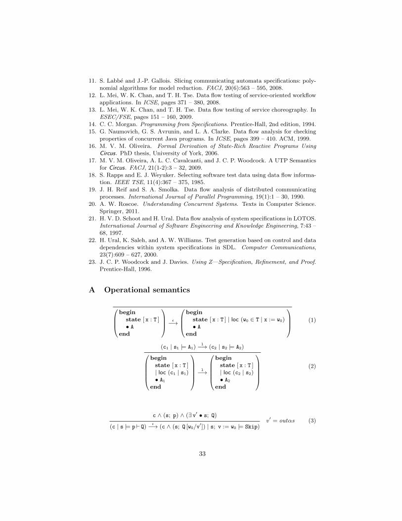
A Operational semantics

begin

state [ x : T ]• A

end

ε−→

begin

state [ x : T ] | loc (w0 ∈ T | x := w0)• A

end

(1)

(c1 | s1 |= A1)l−→ (c2 | s2 |= A2)

beginstate [ x : T ]| loc (c1 | s1)• A1

end

l−→

beginstate [ x : T ]| loc (c2 | s2)• A2

end

(2)

c ∧ (s; p) ∧ (∃ v′ • s; Q)

(c | s |= p` Q)ε−→ (c ∧ (s; Q [w0/v

′]) | s; v := w0 |= Skip)v ′ = outαs (3)

33

c ∧ ¬ (s; p)

(c | s |= p` Q)ε−→ (c | s |= Chaos)

(4)

c

(c | s |= Chaos)ε−→ (c | s |= Chaos)

(5)

c

(c | s |= v := e)ε−→ (c ∧ (s; w0 = e) | s; v := w0 |= Skip)

(6)

c ∧ (s; preOp)

(c | s |= Op)ε−→ (c ∧ (s; Op [w0/v

′]) | s; v := w0 |= Skip)v ′ = outαs (7)

c ∧ ¬ (s; preOp)

(c | s |= Op)ε−→ (c | s |= Chaos)

(8)

c

(c | s |= d!e→ A)d!w0−→ (c ∧ (s; w0 = e) | s |= A)

(9)

c ∧ T 6= ∅ x 6∈ αs

(c | s |= d?x : T→ A)d?w0−→ (c ∧ w0 ∈ T | s; var x := w0 |= let x • A)

(10)

c ∧ T 6= ∅ x 6∈ αs

(c | s |= var x : T • A)ε−→ (c ∧ w0 ∈ T | s; var x := w0 |= let x • A)

(11)

(c1 | s1 |= A1)l−→ (c2 | s2 |= A2)

(c1 | s1 |= let x • A1)l−→ (c2 | s2 |= let x • A2)

(12)

c

(c | s |= let x • Skip)ε−→ (c | s; end x |= Skip)

(13)

34

(c1 | s1 |= A1)l−→ (c2 | s2 |= A2)

(c1 | s1 |= A1; B)l−→ (c2 | s2 |= A2; B)

(14)

c

(c | s |= Skip; A)ε−→ (c | s |= A)

(15)

c

(c | s |= A1 u A2)ε−→ (c | s |= A1)

c

(c | s |= A1 u A2)ε−→ (c | s |= A2)

(16)

c ∧ (s; g)

(c | s |= g N A)ε−→ (c ∧ (s; g) | s |= A)

(17)

c

(c | s |= A1 @ A2)ε−→ (c | s |= (loc c | s • A1)� (loc c | s • A2))

(18)

c1

(c | s |= (loc c1 | s1 • Skip)� (loc c2 | s2 • A))ε−→ (c1 | s1 |= Skip)

(19)

c2

(c | s |= (loc c1 | s1 • A)� (loc c2 | s2 • Skip))ε−→ (c2 | s2 |= Skip)

(20)

(c1 | s1 |= A1)ε−→ (c3 | s3 |= A3)

c | s|= (loc c1 | s1 • A1)�(loc c2 | s2 • A2)

ε−→

c | s|= (loc c3 | s3 • A3)�(loc c2 | s2 • A2)

(21)

(c2 | s2 |= A2)ε−→ (c3 | s3 |= A3)

c | s|= (loc c1 | s1 • A1)�(loc c2 | s2 • A2)

ε−→

c | s|= (loc c1 | s1 • A1)�(loc c3 | s3 • A3)

(22)

35

(c1 | s1 |= A1)l−→ (c3 | s3 |= A3) l 6= ε

(c | s |= (loc c1 | s1 • A1)� (loc c2 | s2 • A2))l−→ (c3 | s3 |= A3)

(23)

(c2 | s2 |= A2)l−→ (c3 | s3 |= A3) l 6= ε

(c | s |= (loc c1 | s1 • A1)� (loc c2 | s2 • A2))l−→ (c3 | s3 |= A3)

(24)

c

(c | s |= A1 J x1 | cs | x2 K A2)ε−→

c | s|=(par s | x1 • A1) J cs K (par s | x2 • A2)

(25)

cc | s|= (par s1 | x1 • Skip)

JcsK(par s2 | x2 • Skip)

ε−→ (c | (∃ x′2 • s1) ∧ (∃ x′1 • s2) |= Skip)

(26)

(c | s1 |= A1)l−→ (c3 | s3 |= A3) l = ε ∨ chan l 6∈ cs

c | s|= (par s1 | x1 • A1)

JcsK(par s2 | x2 • A2)

l−→

c3 | s|= (par s3 | x1 • A3)


(27)

(c | s2 |= A2)l−→ (c3 | s3 |= A3) l = ε ∨ chan l 6∈ cs

c | s|= (par s1 | x1 • A1)


l−→

c3 | s|= (par s1 | x1 • A1)


(28)

36

(c | s1 |= A1)d?w1−→ (c3 | s3 |= A3) ∧ (c | s2 |= A2)

d!w2−→ (c4 | s4 |= A4)

∨

(c | s1 |= A1)d!w1−→ (c3 | s3 |= A3) ∧ (c | s2 |= A2)

d?w2−→ (c4 | s4 |= A4)

∨

(c | s1 |= A1)d!w1−→ (c3 | s3 |= A3) ∧ (c | s2 |= A2)

d!w2−→ (c4 | s4 |= A4)

d ∈ cs c3 ∧ c4 ∧ w1 = w2

c | s|= (par s1 | x1 • A1)


d!w2−→

c3 ∧ c4 ∧ w1 = w2 | s|= (par s3 | x1 • A3)


(29)

(c | s1 |= A1)d?w1−→ (c3 | s3 |= A3) (c | s2 |= A2)

d?w2−→ (c4 | s4 |= A4)

d ∈ cs c3 ∧ c4 ∧ w1 = w2c | s|= (par s1 | x1 • A1)


d?w2−→

c3 ∧ c4 ∧ w1 = w2 | s|= (par s3 | x1 • A3)


(30)

(c1 | s1 |= A1)l−→ (c2 | s2 |= A2) l 6= ε chan l 6∈ cs

(c1 | s1 |= A1 \ cs)l−→ (c2 | s2 |= A2 \ cs)

(31)

(c1 | s1 |= A1)l−→ (c2 | s2 |= A2) l = ε ∨ chan l ∈ cs

(c1 | s1 |= A1 \ cs)ε−→ (c2 | s2 |= A2 \ cs)

(32)

c

(c | s |= Skip \ cs)ε−→ (c | s |= Skip)

(33)

c

(c | s |= µ X • A, δ) ε−→ (c | s |= A, δ ⊕ {X 7→ A})(34)

37

c

(c | s |= X, δ)ε−→ (c | s |= δ X, δ)

(35)

B Specification-oriented transition system: labels

The rule for processes is not specifically for the transition system for the relation=⇒P that defines the labels arising from an action. The transition system of=⇒P is used in combination with the operational semantics to define maximalnon-silent transitions with specification labels. These are characterised by therelation =⇒, for which we define a transition rule for processes.

(state(P1) |= maction(P1))l

=⇒ (state(P2) |= maction(P2))

P1l

=⇒ P2

(1)

It is the transition system for =⇒P that is referenced in proofs presented in thisreport, and we reproduce it below.

c ∧ (s; p) ∧ (∃ v ′ • s; Q)

(c | s |= p` Q)p` Q

=⇒P (c ∧ (s; Q [w0/v′]) | s; v := w0 |= Skip)

v ′ = outαs (2)

c ∧ (s; preOp)

(c | s |= Op)Op

=⇒ (c ∧ (s; Op [w0/v′]) | s; v := w0 |= Skip)

v ′ = outαs (3)

c

(c | s |= v := e)v:=e

=⇒P (c ∧ (s; w0 = e) | s; v := w0 |= Skip)(4)

c ∧ (s; g)

(c | s |= g N A)g

=⇒P (c ∧ (s; g) | s |= A)(5)

c

(c | s |= d!e→ A)d!e

=⇒P (c ∧ (s; w0 = e) | s |= A)(6)

c ∧ T 6= ∅ x 6∈ αs

(c | s |= d?x : T→ A)d?x=⇒ (c ∧ w0 ∈ T | s; var x := w0 |= let x • A)

(7)

38

c ∧ T 6= ∅ x 6∈ αs

(c | s |= var x : T • A)(var x:T)=⇒P (c ∧ w0 ∈ T | s; var x := w0 |= let x • A)

(8)

c

(c | s |= let x • Skip)(end x)=⇒P (c | s; end x |= Skip)

(9)

(c1 | s1 |= A1)l

=⇒P (c2 | s2 |= A2)

(c1 | s1 |= let x • A1)l

=⇒P (c2 | s2 |= let x • A2)(10)

(c1 | s1 |= A1)l

=⇒P (c2 | s2 |= A2)

(c1 | s1 |= A1; B)l

=⇒P (c2 | s2 |= A2; B)(11)

c

(c | s |= A1 J x1 | cs | x2 K A2)var vl,vr:=v,v

=⇒Pc | s; var vl, vr := v, v|= (spar v | vl | vr | x1 := x1l • A1[vl/v])

JcsK(spar v | vr | vl | x2 := x2r • A2[vr/v])

v ′ = outαsv = x1, x2fresh vl , vr

(12)

(c | s; end v, y |= A1)l

=⇒P (c3 | s3 |= A3) chan l = ε ∨ chan l 6∈ cs

(c | s |= (spar v | x | y | x1 := z1 • A1) J cs K (spar v | y | x | x2 := z2 • A2))l

=⇒Pc3 | s3 ∧ s; end x

|= (spar v | x � (end l), (var l) | y | x1 := z1 • A3)JcsK

(spar v | y | x � (end l), (var l) | x2 := z2 • A2)

(13)

39

(c | s; end v, y |= A1)d?a

=⇒P (c3 | s3 |= A3)

(c | s; end v, x |= A2)d!e

=⇒P (c4 | s4 |= A4)

d ∈ cs c3 ∧ c4 ∧ ∃w0 • (s3; (w0 = a))⇔ (s4; (w0 = e))

(c | s |= (spar v | x | y | x1 := z1 • A1) J cs K (spar v | y | x | x2 := z2 • A2))d!e

=⇒Pc3 ∧ c4 ∧ ∃ w0 • (s3; (w0 = a))⇔ (s4; (w0 = e)) | s|= (spar v | x � a | y | x1 := z1 • A3)

Jcs | var a := e | s3 ∧ s4 ∧ s; end x, yK(spar v | y | x � a | x2 := z1 • A4)

(14)

The above rule uses a new parallel construct that keeps track of the new inputvariable declared and the new state obtained as a consequence. It is used toensure that, as required here, all transitions have a single label, and the labelcontains a guard, a communication, or an action. The next rule ensures that inthe next step of the evaluation of the parallelism, the variable declaration andstate change are recorded. This concern was not present in [2].

c

(c | s |=

(spar v | x | y | x1 := z1 • A1)Jcs | var a := e | s1K

(spar v | y | x | x2 := z2 • A2)

)

var a:=e=⇒P

(c | s1 |= (spar v | x | y | x1 := z1 • A1) J cs K (spar v | y | x | x2 := z2 • A2))

(15)

Rules similar to those above for parallelism are needed for external choice.

(c1 | s1 |= A1)l

=⇒P (c2 | s2 |= A2) chan l 6∈ cs

(c1 | s1 |= A1 \ cs)l

=⇒P (c2 | s2 |= A2 \ cs)(16)

Above, we assume that, if l is not a communication, then chan l is some specialchannel ε that does not belong to any synchronisation set cs.

40

POUR PDF - copie 2 - lri.frbibli/Rapports-internes/2013/RR1567.pdf · 1 University of York,...

Documents

Transcript of POUR PDF - copie 2 - lri.frbibli/Rapports-internes/2013/RR1567.pdf · 1 University of York,...