Planification de la distribution en contextes de ... · Jacques Renaud, directeur de recherche ....
157
Planification de la distribution en contextes de déploiement d’urgence et de logistique hospitalière Thèse Ana María Anaya-Arenas Doctorat en sciences de l’administration – Opérations et systèmes de décision Philosophiæ doctor (Ph.D.) Québec, Canada © Ana María Anaya-Arenas, 2016
Transcript of Planification de la distribution en contextes de ... · Jacques Renaud, directeur de recherche ....
Planification de la distribution en contextes de déploiement d’urgence et de logistique hospitalière
Thèse
Ana María Anaya-Arenas
Doctorat en sciences de l’administration – Opérations et systèmes de
décision
Philosophiæ doctor (Ph.D.)
Québec, Canada
© Ana María Anaya-Arenas, 2016
Planification de la distribution en contextes de déploiement d’urgence et de logistique hospitalière
Thèse
Ana María Anaya-Arenas
Sous la direction de :
Jacques Renaud, directeur de recherche
Angel Ruiz, codirecteur de recherche

iii
Résumé L’optimisation de la distribution est une préoccupation centrale dans l’amélioration
de la performance des systèmes industriels et des entreprises de services. Avec les
avancées technologiques et l’évolution du monde des affaires, de nouveaux domaines
d’application posent des défis aux gestionnaires. Évidemment, ces problèmes de
distribution deviennent aussi des centres d’intérêt pour les chercheurs. Cette thèse
étudie l’application des méthodes de recherche opérationnelle (R.O.) à l’optimisation
des chaînes logistiques dans deux contextes précis : le déploiement logistique en
situation d’urgence et la logistique hospitalière. Ces contextes particuliers constituent
deux domaines en forte croissance présentant des d’impacts majeurs sur la
population. Ils sont des contextes de distribution complexes et difficiles qui exigent
une approche scientifique rigoureuse afin d’obtenir de bons résultats et, ultimement,
garantir le bien-être de la communauté.
Les contributions de cette thèse se rapportent à ces deux domaines. D’abord, nous
présentons une révision systématique de la littérature sur le déploiement logistique en
situation d’urgence (Chapitre 2) qui nous permet de consolider et de classifier les
travaux les plus importants du domaine ainsi que d’identifier les lacunes dans les
propositions actuelles. Cette analyse supporte notre seconde contribution où nous
proposons et évaluons trois modèles pour la conception d’un réseau logistique pour
une distribution juste de l’aide (Chapitre 3). Les modèles cherchent à assurer une
distribution équitable de l’aide entre les points de demande ainsi qu’une stabilité dans
le temps. Ces modèles permettent les arrérages de la demande et adaptent l’offre aux
besoins de façon plus flexible et réaliste.
Le deuxième axe de recherche découle d’un mandat de recherche avec le Ministère de
la Santé et de Services sociaux du Québec (MSSS). En collaboration avec les
gestionnaires du système de santé québécois, nous avons abordé la problématique du
transport d’échantillons biomédicaux. Nous proposons deux modèles d’optimisation
et une approche de résolution simple pour résoudre ce problème difficile de collecte
d’échantillons (Chapitre 4). Cette contribution est par la suite généralisée avec la
synchronisation des horaires d’ouverture de centres de prélèvement lors de la

iv
planification des tournées. Une procédure itérative de recherche locale est proposée
pour résoudre le problème (Chapitre 5). Il en découle un outil efficace pour la
planification des tournées de véhicules dans le réseau des laboratoires québécois.
v
Abstract Optimisation in distribution is a major concern towards the performance’s
improvement of manufacturing and service industries. Together with the evolution of
the business’ world and technology advancements, new practical challenges need to
be faced by managers. These challenges are thus a point of interest to researchers.
This thesis concentrates on the application of operational research (O.R.) techniques
to optimise supply chains in two precise contexts: relief distribution and healthcare
logistics. These two research domains have grown a lot recently and have major
impacts on the population. These are two complex and difficult distribution settings
that require a scientific approach to improve their performance and thus warrant the
welfare among the population.
This thesis’s contributions relate to those two axes. First, we present a systematic
review of the available literature in relief distribution (Chapter 2) to consolidate and
classify the most important works in the field, as well as to identify the research’s
gaps in the current propositions and approaches. This analysis inspires and supports
our second contribution. In Chapter 3, we present and evaluate three models to
optimise the design of relief distribution networks oriented to fairness in distribution.
The models seek to ensure an equitable distribution between the points of demand
and in a stable fashion in time. In addition, the models allow the backorder of demand
to offer a more realistic and flexible distribution plan.
The second research context result from a request from Quebec’s Ministry of Health
and Social Services (Ministère de la Santé et des Services sociaux – MSSS). In
partnership with the managers of Quebec’s healthcare system, we propose an
approach to tackle the biomedical sample transportation problem faced by the
laboratories’ network in Quebec’s province. We propose two mathematical
formulations and some fast heuristics to solve the problem (Chapter 4). This
contribution is later extended to include the opening hours’ synchronisation for the
specimen collection centers and the number and frequency of pick-ups. We propose
an iterated local search procedure (ILS) to find a routing plan minimising total

vi
billable hours (Chapter 5). This leads to an efficient tool to routing planning in the
medical laboratories’ network in Quebec.

x
Liste de tableaux
Table 2.1 – Research topics in emergency logistics. ............................................................ 21
Table 2.2 – Location and network design problems in relief distribution. ........................... 24
Table 2.3 – Transportation problems in relief distribution. .................................................. 29
Table 2.4 – Combined Location-Transportation problems in relief distribution. ................ 34
Table 3.1 – Results produced for 10 small instances (temporary shortness). ...................... 74
Table 3.2 – Results produced for 10 small instances (extreme shortness). .......................... 76
Table 3.3 – Results produced for larger-sized instances in temporary shortness. ................ 77
Table 3.4 – Results produced for larger-sized instances in extreme shortness. ................... 77
Table 4.1 – Results produced by the two formulations (time limit = 3 600 sec.). ............. 102
Table 4.2 – Results produced for large instances using an initial heuristic solution. ......... 103
Table 4.3 – Performance of the proposed heuristics. ......................................................... 105
Table 5.1 – Average results over the three set of instances. ............................................... 133
Table 5.2 – Average distances produced by ILS and the methods proposed in Anaya-
Arenas et al. (2015). ........................................................................................................... 134

xi
Liste de figures
Figure 1.1 – Contributions de la thèse. .................................................................................. 8
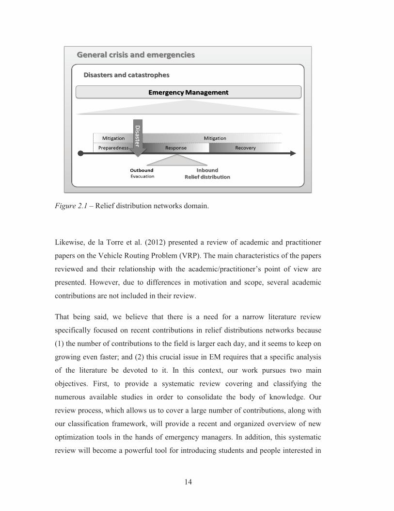
Figure 2.1 – Relief distribution networks domain. .............................................................. 14
Figure 2.2 – Emergency response logistic network. ............................................................ 20
Figure 3.1 – Example of a piecewise cost function for 𝑢𝑧𝑓𝑡. .............................................. 66
Figure 3.2 – Dissatisfaction percentage for instance I1. ...................................................... 72
Figure 3.3 – Dissatisfaction percentage for instance I11. .................................................... 75
Figure 4.1 – Feasible or unfeasible routes with respect to the sample transportation
time. ...................................................................................................................................... 89
Figure 5.1 – Example of interdependency between pick-ups at SCC 𝑔. ........................... 114
Figure 5.2 – Example of opening decision and collection period at SCC 𝑔. ..................... 118
Figure 5.3 – Example of a BSTP network configuration. .................................................. 119
Figure 5.4 – Example of a reason to create waiting time in a solution. ............................. 119
Figure 5.5 – Basic structure our ILS approach. ................................................................. 121
Figure 5.6 – Impact of the interdependency in the LS phase. ............................................ 125
Figure 5.7 – Time windows estimation for a solution 𝑠. ................................................... 127
Figure 5.8 – Movement in R1 leading to an unfeasible solution. ...................................... 128
xii
Al autor de mis días
“17 ¡Cuán preciosos, oh Dios, me son tus pensamientos! ¡Cuán inmensa es la suma de ellos!
18 Si me propusiera contarlos, sumarían más que los granos de arena.
Y si terminara de hacerlo, aún estaría a tu lado.” Salmos 139:17-18
À l’auteur de mes jours
« 17 Combien tes desseins, ô Dieu, sont, pour moi, impénétrables, et comme ils sont innombrables!
18 Si je les comptais, ils seraient bien plus nombreux que les grains de sable sur les bords des mers.
Voici: je m'éveille, je suis encore avec toi. » Psaumes 139 :17-18

xiii
Remerciements D’après mon expérience, une thèse de doctorat est la combinaison de nombreux
ingrédients. Évidemment, ce document contient le résultat de plusieurs années de
recherche, de réflexions et d’analyses. C’est aussi l’aboutissement d’un travail
acharné où j’ai dû faire preuve d’engagement, de ténacité, de persévérance et de
patience. Je n’aurais pas pu achever ce projet si je n’avais été soutenue par de
nombreuses personnes de mon entourage professionnel et personnel. Je suis ravie de
pouvoir exprimer dans ces lignes mes plus sincères remerciements à tous ceux qui ont
contribué d’une façon ou d’une autre à mon travail. Tout d’abord, j’aimerais
remercier el autor de mis días, mon Dieu et mon Sauveur Jésus-Christ. Je suis le
résultat de sa grâce et de son amour dans ma vie et je crois vivement que c’est sa
bienveillance qui m’a guidée jusqu’à aujourd’hui.
Mes plus sincères remerciements vont à Jacques Renaud, mon directeur de thèse, qui
a toujours était là pour moi et qui a su m’encadrer de façon attentive et respectueuse.
Ses qualités humaines ainsi que ses fortes compétences en tant que chercheur et
directeur m’ont soutenue aux moments nécessaires. Je tiens à reconnaître aussi
l’encadrement et le soutien d’Angel Ruiz, mon codirecteur, qui grâce à sa créativité et
à sa vision de nos problématiques de recherche, a souvent inspiré mon travail. Je le
remercie surtout d’avoir su m’écouter et de m’apprendre à voler de mes propres ailes.
Jacques, Angel, je vous remercie d’avoir embarqué avec moi dans cette aventure,
d’avoir cru en moi et en mon potentiel. Dès le début et jusqu’à la fin, vous m’avez
toujours amené à pousser mes limites. Cela a été un véritable plaisir de travailler avec
vous pendant ces années et j’espère que l’on pourra réaliser beaucoup d’autres projets
ensemble. J’aimerais aussi sincèrement remercier Fayez Boctor du département
d’Opérations et Systèmes de Décision de l’Université Laval et Caroline Prodhon de
l’Institut Charles Delaunay de l’Université de Technologie de Troyes, d’avoir accepté
de faire partie de mon comité ainsi que pour nos moments d’échanges et de
discussions qui ont enrichi mon travail. Je tiens également à remercier Marie-Ève
Rancourt d’avoir accepté d’agir à titre d’examinatrice externe pour cette thèse.

xiv
Un profond et sincère remerciement à ma famille. Mes parents, mes sœurs, mes
beaux-frères, et la joie de mon cœur : Pauli, Emi et AndrésDa (mes nièces et mon
neveu). Merci de vos encouragements et votre appui à tout moment. Merci d’avoir
rêvé avec moi et de m’avoir soutenue dans ma décision de partir et de rester si
longtemps loin de vous. Mon cœur a été, il est et il sera toujours avec vous (Gracias a
mi familia bonita por todo su apoyo en este tiempo. Gracias por haber soñado
conmigo cuando decidí continuar por este camino. Pero sobretodo, quiero darles las
gracias por haber pagado conmigo el precio más alto que tiene este logro: alejarme
de su cotidianidad. Así que gracias por perdonar mi ausencia para que pudiera vivir
esta experiencia. Mi corazón simpre estuvo, está y estará con ustedes.) Merci à ma
famille ici à Québec : Guillaume, Nicole, Andrea, Nana, Natalia, Pablito, Gabie,
Alain et Rachel, et toute la belle gang qui m’a accompagnée toutes ces années. Nos
moments ensemble ont été décisifs pour la réalisation de ce projet. À plusieurs
reprises, vous m’avez donné la force et le courage nécessaires de continuer sur ce
chemin. Votre amitié est certainement l’un des plus beaux cadeaux que m’a offert ma
vie québécoise.
Une petite dédicace à tous ceux avec qui j’ai partagé mes jours à la FSA et au
CIRRELT. Très spécialement à Sana Dahmen, plus qu’une collègue, tu es devenue
une amie précieuse. Merci pour nos cafés, nos heures de travail sans fin, nos courses
à minuit pour prendre le dernier bus et notre appui mutuel dans ce métier. J’espère
bien qu’on pourra réaliser toutes les collaborations dont on a autant parlé. Merci aussi
à Jean-Philippe Gagliardi pour son écoute et ses conseils personnels et professionnels.
Merci JPhD pour la chanson du vendredi. Merci à Louise, Piero, Oli, et toute la belle
gang du CIRRELT et de la FSA. Ça fait vraiment plaisir de travailler avec vous
autres.

xv
Avant-propos Cette thèse de doctorat est la consolidation de mes travaux de recherche menés au
sein du Centre interuniversitaire de recherche sur les réseaux d’entreprise, la
logistique et le transport (CIRRELT) à la Faculté des sciences de l’administration de
l’Université Laval. Les contributions de la thèse sont présentées sous la forme de
quatre articles scientifiques. Chaque article a été écrit avec la collaboration d’autres
chercheurs, principalement de mes directeurs de recherche : Jacques Renaud et Angel
Ruiz. Pour chacun des quatre articles qui composent cette thèse, je me suis impliquée
en tant que chercheuse principale et première auteure. Plus précisément, mon rôle fut
de proposer les problématiques de recherche, les approches de modélisation et les
méthodes de résolution, le tout en concertation avec les coauteurs. Je me suis
également occupée du travail de programmation, de l’expérimentation, de l’analyse
des résultats et de la rédaction de la première version des articles.
Le premier article intitulé « Relief distribution networks : a systematic review » a été
coécrit avec Jacques Renaud et Angel Ruiz. Il a été accepté pour publication dans
Annals of Operations Research le 19 mars 2014 et publié en décembre 2014
(Volume 223, Issue 1, pp 53-79). Ce projet a fait l’objet d’un tutoriel sur le
déploiement logistique en situation d’urgence (emergency logistics) donné aux
Journées de l’Optimisation 2012, du 7 au 9 mai 2012 à Montréal. J’ai aussi été invité
à l’Universidad Industrial de Santander le 10 janvier 2013 en Colombie, et à
l’Université de Technologie de Troyes le 28 mai 2015, afin de donner une séance
d’introduction sur les réseaux logistiques en réponse aux sinistres.
Le deuxième article intitulé « Models for a fair humanitarian relief distribution » a
été coécrit avec Jacques Renaud et Angel Ruiz et soumis pour publication dans
Production and Operations Management le 24 août 2015. Une version préliminaire a
été arbitrée par le comité d’évaluation et publiée dans les actes de la conférence
internationale IESM 2013 (International Conference of Industrial Engineering and
Systems Management 2013), qui a eu lieu à Rabat au Maroc du 28 au 30
octobre 2013. De plus, il a été présenté dans deux autres conférences internationales
xvi
en 2013, soit aux Journées de l’Optimisation, du 6 au 8 mai 2013 à Montréal, et au
2013 INFORMS Annual Meeting à Minneapolis du 6 au 9 octobre 2013.
Le troisième article intitulé « Biomedical sample transportation in the province of
Quebec: a case study » a été rédigé en collaboration avec Thomas Chabot, Jacques
Renaud et Angel Ruiz. L’article a été accepté dans un numéro spécial sur le transport
dans la gestion de la chaîne d’approvisionnement du International Journal of
Production Research le 29 janvier 2015 et publié en ligne le 9 mars 2015. Les
résultats de cet article ont été présentés dans deux conférences internationales, soit le
56e congrès annuel de la SCRO à Ottawa du 26 au 28 mai 2014, et la conférence
internationale CORS/INFORMS 2015 à Montréal, du 14 au 17 juin 2015.
Le quatrième article intitulé « An ILS approach to solve the biomedical sample
transportation problem in the province of Quebec » a été coécrit avec Caroline
Prodhon, Hasan Murat Asfar et Christian Prins, de l’Université de Technologie de
Troyes. Cet article est le résultat du travail effectué lors d’un séjour de recherche
réalisé entre mars et juin 2015 avec ces trois membres de l’équipe du laboratoire
d’opérations et systèmes industriels (LOSI) à Troyes. La version incluse dans cette
thèse a été acceptée le 15 juillet 2015 pour publication dans les actes de la Conférence
internationale de génie industriel (CIGI) qui aura lieu à Québec du 26 au 28 octobre
2015.

3
d’avoir une meilleure compréhension des axes de recherche de cette thèse, une
présentation générale des principales caractéristiques de chacun des domaines
d’application sera effectuée dans les sous-sections suivantes.
1.2.1. Déploiement logistique en situation d’urgence Le déploiement en situation d’urgence est un des nombreux thèmes couverts par une
vaste littérature qui se regroupe sous l’appellation de « gestion de crises » (emergency
management). La gestion de crises est définie par Haddow et al. (2007) comme la
discipline qui gère les risques reliés aux catastrophes. En considérant une vision
purement temporelle, la gestion de crises peut être divisée en quatre grandes phases
(Altay & Green III 2006; Galindo & Batta 2013; Haddow et al. 2007) : deux phases
précédant l’évènement (atténuation et préparation) et deux phases post-crise (réponse
et récupération). Le déploiement logistique est au cœur de la gestion de crises à
plusieurs moments, mais il occupe plus particulièrement plus de 80 % des opérations
nécessaires lors de la réponse à un sinistre (Van Wassenhove 2006). Dans cette thèse,
nous nous intéressons plus précisément à la distribution de l’aide en réponse à un
sinistre. Le déploiement logistique d’urgence a été défini par Sheu (2007) comme « A
process of planning, managing and controlling the efficient flows of relief,
information, and services from the points of origin to the points of destination to meet
the urgent needs of the affected people under emergency conditions. » Bien que ce
domaine de recherche soit assez nouveau, les contributions se multiplient rapidement
dans plusieurs domaines de la gestion ainsi que dans l’optimisation du réseau
logistique. Clairement, le déploiement logistique d’urgence se distingue des
problèmes connus et habituellement traités dans le domaine industriel (Holguín-Veras
et al. 2012; Kovács & Spens 2009; Van Wassenhove & Pedraza Martínez 2012). La
dynamique de la demande, l’environnement d’opération instable et l’énorme coût lié
à « l’insatisfaction de la demande » (c’est-à-dire ne pas répondre adéquatement aux
besoins des sinistrés) sont quelques exemples des difficultés particulières reliées à la
logistique d’urgence.
Dans le premier axe de recherche de cette thèse, nous proposons d’abord une
synthèse de la littérature sur le déploiement d’urgence. Cette synthèse est motivée par

4
la variété et la forte croissance du nombre d’articles publiés lors des dix dernières
années. Cette révision systématique vient consolider et organiser les travaux
disponibles pour les gestionnaires de crise et identifier des problématiques de
recherche peu explorées et prometteuses. Par la suite, nous nous intéressons à la
planification d’un réseau en situation d’urgence en considérant l’importance d’une
distribution stable et équitable des produits. Ce travail nous permet de proposer des
modèles détaillés pour la planification d’un réseau de distribution juste, rapide et
efficace.
1.2.2. Logistique hospitalière Le MSSS défini la logistique hospitalière comme « l’ensemble des activités
permettant de synchroniser et de coordonner, voire de fluidifier les flux physiques,
financiers, d'information afin que la prestation de soins de santé se réalise de manière
sécuritaire, efficace et efficiente »1. Le deuxième axe de cette thèse se positionne dans
le domaine de la logistique hospitalière, plus particulièrement sur la planification du
transport des échantillons biomédicaux. Dans un réseau médical, plusieurs tests
médicaux sont nécessaires afin d’assurer une bonne qualité des diagnostics et un
traitement adéquat des patients. Cela se traduit par une grande variété de types
d’échantillons biomédicaux à analyser qui sont prélevés dans des cliniques, des
hôpitaux ou dans des centres de prélèvement (CP). Cependant, les CP ne sont pas
outillés pour analyser les échantillons, et ce, dû aux coûts élevés des équipements
d’analyse. Ces derniers sont répartis stratégiquement dans quelques laboratoires qui
couvrent le territoire québécois. Les échantillons sont donc envoyés vers un
laboratoire pour analyse, ce qui crée une importante demande de transport.
Notre problématique se concentre sur le transport des échantillons biomédicaux des
CP vers les laboratoires. Ces opérations engendrent différents défis au niveau
logistique. En premier lieu, le produit à transporter exige une gestion spéciale au
niveau des temps de traitement, occasionnée par la durée de vie limitée de
1 Guide en logistique hospitalière (http://www.msss.gouv.qc.ca/documentation/planification-immobiliere/app/DocRepository/1/Publications/Guide/110629_Guide_logistique_hospitaliere.pdf

6
1.3.1. Contributions dans le domaine du déploiement d’urgence
Revue systématique de la littérature sur le déploiement d’urgence
Le Chapitre 2 présente la première publication de cette thèse. Cet article a trois
apports fondamentaux. Tout d’abord, il vient consolider et centraliser de façon
ordonnée les nombreuses études proposées dans la littérature sur le domaine. Plus de
170 articles ont été consultés sur cinq bases de données. Un total de 83 articles est
finalement inclus et analysé dans notre revue. Deuxièmement, nous avons constaté
que la littérature suit fidèlement la ligne décisionnelle des gestionnaires de crise.
Quatre catégories de décisions sont identifiées (localisation, routage,
localisation/routage, et autres) et pour chacune d’elle nous précisons clairement leurs
principales caractéristiques, tant au niveau de la modélisation que de l’outil de
résolution proposé. Troisièmement, avec cette revue de la littérature, nous avons pu
identifier les problématiques abordées dans la littérature récente et faire ressortir des
besoins et des opportunités de futures recherches dans le domaine.
Modèles pour une distribution juste de l’aide humanitaire
Dans le Chapitre 3, nous proposons divers modèles pour effectuer la configuration et
l’exploitation d’un réseau de distribution en situation d’urgence. Les modèles sont
conçus pour construire un réseau logistique maximisant la satisfaction de la demande
tout en cherchant à effectuer une répartition juste des produits disponibles. Ce
chapitre propose trois contributions principales : (1) donner aux gestionnaires de crise
un outil précis pour la conception d’un réseau de distribution qui considère les défis
propres au déploiement d’urgence; (2) considérer dans la décision de conception du
réseau l’objectif d’équité pour assurer une répartition juste des ressources
disponibles; et (3) évaluer différentes définitions possibles d’équité pour donner aux
gestionnaires des critères de performance à examiner lors d’un déploiement
d’urgence.

7
1.3.2. Contributions dans le domaine de logistique hospitalière
Transport d’échantillons biomédicaux dans la province de Québec : un cas d’étude
Dans cet article nous présentons en détail le cas du transport d’échantillons
biomédicaux, tel qu’il est vécu dans la province de Québec. Cet article contient deux
contributions précises : (1) dans un premier temps nous présentons deux formulations
mathématiques alternatives pour résoudre cette problématique comme un problème
de tournées de véhicules avec fenêtres de temps et plusieurs tournées par camion; (2)
nous proposons une méthode de résolution simple et efficace pour la planification des
tournées de transport d’échantillons biomédicaux sur le territoire québécois. Ces deux
contributions ont été mises en commun dans le but de construire un outil d’aide à la
planification pour les gestionnaires du réseau des laboratoires d’analyse au Québec.
Plusieurs rapports de recherche déposés au MSSS sont basés sur ces développements.
Une méthode itérative de recherche locale pour résoudre le problème de transport d’échantillons biomédicaux au Québec
Le Chapitre 5 est une extension du travail présenté dans le Chapitre 4 et s’aligne avec
les objectifs du Ministère afin de proposer des modifications structurelles au réseau,
dont le nombre et les heures de passages dans les centres de prélèvement. Ce chapitre
propose deux contributions précises. Tout d’abord, une extension de la problématique
étudiée est formulée. Nous cherchons à synchroniser les heures d’ouverture des
centres de prélèvement tout en effectuant le nombre optimal de collectes à chaque
centre. L’objectif est de minimiser le temps facturable (durée totale des routes) en
garantissant qu’aucun échantillon ne périsse. Deuxièmement, dû à la complexité du
problème, une métaheuristique s’avère nécessaire pour une résolution efficace. Nous
proposons une procédure itérative de recherche locale (ILS) et la qualité de la
méthode est testée à l’aide d’instances réelles, tirées du réseau des laboratoires du
Québec.
La Figure 1.1 illustre le cadre général de cette thèse, ainsi que les deux axes de
recherche principaux. Les contributions sont placées à l’intérieur des axes étudiés,
encadrés par l’application de méthodes de recherche opérationnelle pour la

8
planification de la distribution. Bien que ces deux axes de recherche soient liés à deux
contextes logistiques différents, ils poursuivent un objectif commun : desservir les
personnes concernées en visant leur bien-être et l’exploitation efficiente du système
opérationnel.
Figure 1.1 – Contributions de la thèse.
Planification de la distribution en contextes de déploiement d’urgence et de logistique hospitalière
Intérêt scientifique et pratique
Revue systématique de la littérature sur le déploiement d’urgence
Consolidation systématiqueQuatre catégories de problèmes
Analyse des besoins de recherche future
Déploiement logistique d’urgence
Modèles pour une distribution juste d’aide humanitaire
Modèles détaillés multipériodeConsidération d’équité et stabilitéNouveaux critères de performance
Transport d’échantillons biomédicaux dans la province de Québec : un cas
d’étude Deux modélisations pour le problème
Méthode de résolution rapide et efficace
Logistique hospitalière
Procédure itérative de recherche locale pour le problème de transport des
échantillons biomédicaux au QuébecPlanification efficace de l’heure d'ouverture
des centres de prélèvementNombre et fréquence optimal de cueillette
Méthode itérative de recherche local

9
Chapitre 2
2. Revue systématique de la littérature sur le déploiement d’urgence
Depuis les vingt dernières années, la communauté scientifique s’est de plus en plus
tournée vers le domaine de la gestion de crises, ou emergency management, et plus
précisément vers le déploiement logistique lors de situations d’urgence. Le nombre et
la variété des contributions dédiées au design ou à la gestion de la chaîne de
distribution d’aide aux sinistrés ont explosés lors des dernières années. Ceci justifie le
besoin d’une analyse systématique et structurée des travaux existants dans le
domaine. Basé sur une méthodologie scientifique, cet article, qui consolide et
classifie les travaux de recherche publiés, a trois objectifs. Premièrement, effectuer
une mise à jour de la recherche disponible sur les réseaux de distribution d’aide en se
concentrant sur le volet logistique du problème (volet qui a été négligé dans les
études précédentes). En second lieu, souligner les aspects et les enjeux les plus
importants dans les modèles et les stratégies de résolution existants. Finalement,
identifier des perspectives de recherche future qui ont encore besoin d’être explorées.
Article 1: Relief distribution networks: a systematic review
Ce chapitre fait l’objet d’une publication sous la forme d’article de journal : Anaya-
Arenas, A.M., Renaud, J. & Ruiz, A., 2014. Relief distribution networks: a systematic
review. Annals of Operations Research, 223(1), pp.53–79.
Abstract In the last 20 years, Emergency Management has received increasing
attention from the scientific community. Meanwhile, the study of relief distribution
networks has become one of the most popular topics within the Emergency
Management field. In fact, the number and variety of contributions devoted to the
design or the management of relief distribution networks has exploded in the recent
years, motivating the need for a structured and systematic analysis of the works on
this specific topic. To this end, this paper presents a systematic review of
contributions on relief distribution networks in response to disasters. Through a


11
EM, also known as disaster management, can be defined as a discipline dealing with
disasters related risk (Haddow et al. 2007). According to the International Federation
of Red Cross and Red Crescent Societies, a disaster is “a sudden, calamitous event
that seriously disrupts the functioning of a community or society and causes human,
material, and economic or environmental losses that exceed the community’s or
society’s ability to cope using its own resources.”4 Considering this, a distinction
between emergency management and daily emergencies management must be made.
Contrary to disasters, daily emergencies are usually well handled by the affected
community‘s daily operations. Therefore, the context, challenges, urgency and impact
of the operations in both cases are quite different. This was underlined by Simpson &
Hancock (2009) who presented a review of 50 years in emergency response, covering
the period between 1965 and 2007. The authors showed the literature’s shift in recent
years, leaving the daily applications and turning more to disaster related emergencies.
Crisis management refers to different types of crisis and a large set of contributions
may therefore be referenced under that term. Natarajarathinam et al. (2009) reviewed
publications pertaining to supply chain management (SCM) in times of crisis. The
literature selected by the athors’s focused on SCM disruptions i.e. business logistics
reacting to unexpected crisis, either internal (company crisis) or external (sudden-
onset and slow-onset disasters, financial crisis, market crises, etc.). A small part of
the review related to catastrophes, defined as a part of external crisis.
EM is a discipline of continuous work on infrastructure and peoples’ awareness.
Altay and Green (2006) were among the first to review the available scientific papers
using Operations Research and Management Science (OR/MS) applied to EM. Their
review of articles published between 1980 and 2004, provided statistics and classified
contributions based on the approach, the phase of application, the review of
publication and more. Galindo & Batta (2013) added to this work by reviewing
papers from 2005 to 2010 and following up of the conclusions of Altay & Green
(2006).
4 http://www.ifrc.org/en/what-we-do/disaster-management/about-disasters/what-is-a-disaster/

12
From a chronological standpoint, the literature often divides the EM’s continuous
process into four different phases (Altay & Green 2006; Haddow et al. 2007;
McLoughlin 1985): mitigation, preparedness, response and recovery. The mitigation
and preparedness phases take place before the disaster. These phases are aimed at
lowering the probabilities of a disaster occurring or minimizing its possible effects.
The response and recovery phases are post-disaster phases. The response phase seeks
to minimize the disaster’s effects by helping people as quickly as possible and
preventing any more loss while the recovery phase supports the community in its
effort to return to a normal state. The actual division of these phases will be discussed
further on.
Many academic publications have contributed to the research done on one or more of
these phases. According to Altay & Green (2006) and Galindo & Batta (2013) more
than 264 papers have been published on EM and a special attention has been given to
the response phase. More than 33% of the papers included in both reviews focused on
the response phase, in which the major activities are logistic oriented (e.g. opening
shelters, relief distribution centers, medical care and rescue teams dispatching, etc.).
Indeed, we have come to conclude that 80% of EM concerns logistic activities (Van
Wassenhove, 2006), reason why emergency logistics (EL) is a very popular research
application nowadays.
2.1.1. Motivation for a relief distribution networks literature review
Many authors have acknowledged that the particularities of the emergency
management context bring on some new challenges, especially in regards to logistics
optimization (Holguín-Veras et al. 2012; Kovács & Spens 2007; Sheu 2007b; Van
Wassenhove & Pedraza Martínez 2012). Very recently, Holguín-Veras et al. (2012)
published a paper on the unique features of post-disaster humanitarian interventions.
Their work elaborates on the differences between interventions made during the
immediate response to disasters, and those made in the recovery phase. These efforts
may also be divided into short-term and long-term recovery activities. The long-term
recovery activities can be included in regular humanitarian actions carried out in the
13
long term. Regular humanitarian actions also include the response to slow-onset
disasters, like the delivery of food to regions afflicted with chronic crises or the
delivery of medicines to people in developing countries, and have a more stable
environment of operations. On the other side, the logistical efforts required by an
immediate post-disaster’s response distribution are made in extreme conditions and
therefore demand new ways of organizations. The varying networks’ goals, the
associated organizations, the participants’ interactions and the pressing nature of the
distribution are all motivating factors in the elaboration of a new logistic structure’s
framework able to cope with these challenges. We recommend Lettieri et al. (2009)
and Kovács & Spens (2007) for a review. Lettieri et al. (2009) also presented an
analysis oriented on a disaster management theoretical framework, the phases in EM,
the actors involved and the technology (DSS, GIS, etc). In order to define a general
framework for the relief supply chain, Kovács & Spens (2007) included both
academic and practitioner journals in their topical review. Without a doubt, an
analysis of the distribution network’s management challenges is vital to the
development of DSS and tools for crisis managers. However, a large portion of the
literature is devoted to the logistics aspects of the relief distribution. Holguín-Veras et
al. (2012) highlighted the urgency in understanding the workings of the relief
distribution network in specific logistics’ aspects, like the knowledge of demand, the
considered objectives, the periodicity and the decision-making structure. Until now,
these major differences had been neglected, and our work comes to support the
analysis that researchers need to do in order to approach this complex problem.
Figure 2.1 presents the specific interest of this review pertaining to relief distribution
networks and its related fields.
Within the specific field of relief distribution networks, two recent literature reviews
are relevant to our work. Caunhye et al. (2012) analyzed logistics optimization papers
in a pre and post disaster context. Even if the motivations and global scopes are close
to ours, our results showed that the authors’ methodology (Content Analysis) left a
good number of papers out their review. In addition, we can add to their work more
than 40 papers published between 2010 and 2013.


16
1. The review’s needs and general goals were established. Faced with the
emergency logistics literature’s state, with numerous and diverse
contributions, our team felt the need for a detailed picture the research done
on relief distribution networks. More precisely, this systematic review is about
the relief supply chain deployed in immediate response to disasters. This
meant that, the literature reviewed had to include an Operational Research
(OR) component with the goal of optimizing the distribution center location,
resource allocation, or humanitarian aid transportation after a disaster, as well
as others logistics tasks, for relief distribution, as it was shown in Figure 2.1.
2. With this general thought, five relevant databases were selected as search
engines for our process. Three of them were related to administration
sciences: ABI/Inform Global, Academic Search Premier and Business Source
Premier. The other two were OR oriented: Compendex for engineering and
technology, and Inspec for calculations in physics, electronics, and
information science. A multi-disciplinary database was included: ISI’ Web of
Science.
3. Based on our knowledge and expertise in the field, as well as the review of 20
well-recognized references in the literature, a set of key words was selected to
define two search chains. These search chains were identified in the title,
abstract, citation and/or subject of the articles. The words used our search
chains were emergenc*; disaster*; catastroph*; “Extreme Events”;
Humanitarian*; Aid; Assistanc*; Relief*; Logistic*; “Supply Chain”;
Response; Distribution. The word “optimization” created an enormous
restriction of the results and so, it was not considered in our search chains.
4. To help us to restrict our search results, a date range was defined. We only
considered works published between 1990 and 2013. This decision was
justified by the fact that the most significant advancements in the EM research
field were done in the last decade. In addition, the previous studies focused on
nuclear emergency response, a strong trend in the 1980s. At the time,
17
emergency management was not really structured or formalized (Altay &
Green, 2006).
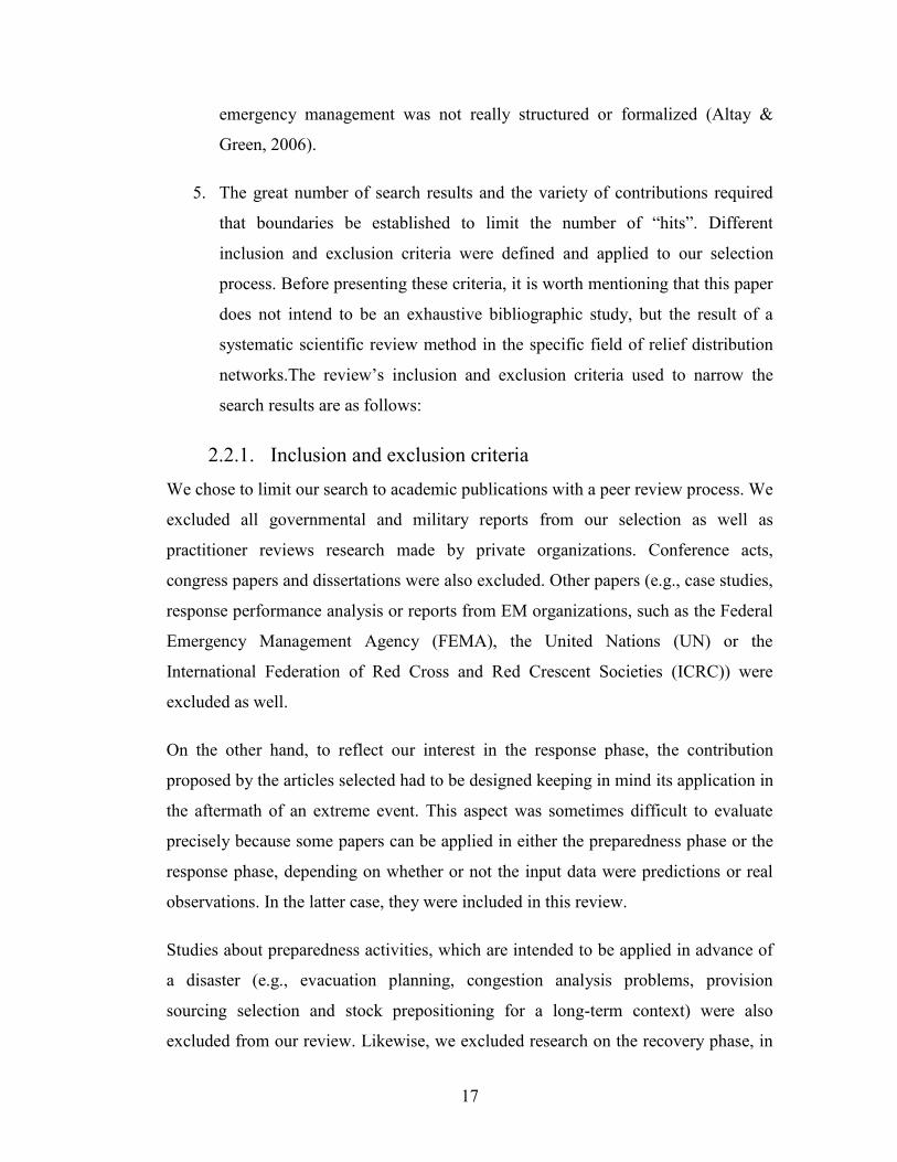
5. The great number of search results and the variety of contributions required
that boundaries be established to limit the number of “hits”. Different
inclusion and exclusion criteria were defined and applied to our selection
process. Before presenting these criteria, it is worth mentioning that this paper
does not intend to be an exhaustive bibliographic study, but the result of a
systematic scientific review method in the specific field of relief distribution
networks.The review’s inclusion and exclusion criteria used to narrow the
search results are as follows:
2.2.1. Inclusion and exclusion criteria We chose to limit our search to academic publications with a peer review process. We
excluded all governmental and military reports from our selection as well as
practitioner reviews research made by private organizations. Conference acts,
congress papers and dissertations were also excluded. Other papers (e.g., case studies,
response performance analysis or reports from EM organizations, such as the Federal
Emergency Management Agency (FEMA), the United Nations (UN) or the
International Federation of Red Cross and Red Crescent Societies (ICRC)) were
excluded as well.
On the other hand, to reflect our interest in the response phase, the contribution
proposed by the articles selected had to be designed keeping in mind its application in
the aftermath of an extreme event. This aspect was sometimes difficult to evaluate
precisely because some papers can be applied in either the preparedness phase or the
response phase, depending on whether or not the input data were predictions or real
observations. In the latter case, they were included in this review.
Studies about preparedness activities, which are intended to be applied in advance of
a disaster (e.g., evacuation planning, congestion analysis problems, provision
sourcing selection and stock prepositioning for a long-term context) were also
excluded from our review. Likewise, we excluded research on the recovery phase, in

18
which the planning horizon defined for the problem is longer than the one for the
response phase. Also, the research objective has a more strategically sustainable
perspective. Although not considered in this review, we tend to point out the interest
of these papers and the importance of their contributions.
Furthermore, given the large number of papers and the context particularities, we
limited our search to papers considering sudden-onset disasters only (Van
Wassenhove 2006), such as the 9/11 terrorists attacks in NYC or the earthquake in
Haiti in January 2010. This means that the relief distribution in a slow-onset disaster
context (e.g., famine or drought) is out of our scope.
6. After establishing the review’s boundaries, the search process was executed in
the different databases. The search was executed in two phases. A first
databases search was conducted in June 2011, and 4169 papers were found.
Then, as an update, we proceeded to a second in June 2013. We looked for
papers published between June 2011 and June 2013, finding 368 new papers.
A total of 4537 papers were found by the search engines. The title and abstract
of the search results were considered and compared to our inclusion and
exclusion criteria. This first filter left a total of 107 papers for further analysis.
Additionally, the following additional sources were consulted to make the
research as rich as possible: (1) a previous search in the references of the
initial databases of the well-known articles led to the addition of 22 new
references. (2) Furthermore, our search protocol led us to the discovery of
seven previously published special issues in emergency management:
Transportation Research, Part E, Vol. 43, No. 6, 2007; International Journal of
Physical Distribution & Logistics Management, Vol. 39, No. 6, “SCM in time
of crisis humanitarian,” 2009; International Journal of Physical Distribution &
Logistics Management, Vol. 40, No. 8-9, “Transforming humanitarian
logistics,” 2010; International Journal of Production Economics, Vol. 126,
No.1, 2010; OR Spectrum, Vol. 33, No. 3, 2011; and Socio-Economic
Planning Sciences Volume 46, Issue 1, “Special Issue: Disaster Planning and

20
networks imply an inbound flow of relief from the cold to the hot zone, but also an
outbound flow aimed at moving people or materials towards safer areas located either
inside or outside the hot zone. Despite of the importance of such outbound flows, this
review focuses on the inbound part. Figure 2.2 presents a diagram of the general
emergency logistic network.
Figure 2.2 – Emergency response logistic network.
Our review process shows that the literature is well aligned with this decisional
framework. Therefore, the papers reviewed were divided into the following
categories: (1) location/allocation and network design problems, (2) transportation
problems, (3) combined location and transportation problems, and (4) other less
popular, but still important, topics in relief distribution. Note that, given that our
interest is limited to relief distribution networks, the resource allocation problem is
only defined for the commodities and capacity assignments in the HADCs. In most
cases, this aspect is covered in the network design decisions.
21
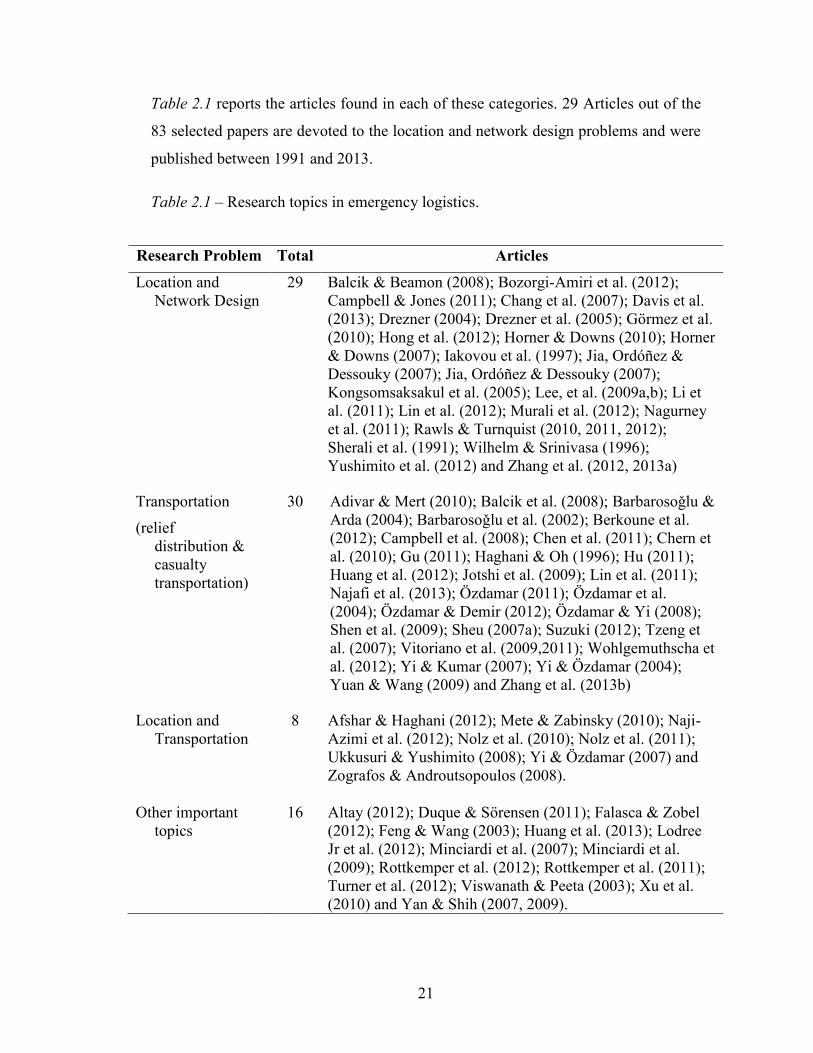
Table 2.1 reports the articles found in each of these categories. 29 Articles out of the
83 selected papers are devoted to the location and network design problems and were
published between 1991 and 2013.
Table 2.1 – Research topics in emergency logistics.
Research Problem Total Articles
Location and Network Design
29 Balcik & Beamon (2008); Bozorgi-Amiri et al. (2012); Campbell & Jones (2011); Chang et al. (2007); Davis et al. (2013); Drezner (2004); Drezner et al. (2005); Gӧrmez et al. (2010); Hong et al. (2012); Horner & Downs (2010); Horner & Downs (2007); Iakovou et al. (1997); Jia, Ordóñez & Dessouky (2007); Jia, Ordóñez & Dessouky (2007); Kongsomsaksakul et al. (2005); Lee, et al. (2009a,b); Li et al. (2011); Lin et al. (2012); Murali et al. (2012); Nagurney et al. (2011); Rawls & Turnquist (2010, 2011, 2012); Sherali et al. (1991); Wilhelm & Srinivasa (1996); Yushimito et al. (2012) and Zhang et al. (2012, 2013a)
Transportation
(relief distribution & casualty transportation)
30 Adivar & Mert (2010); Balcik et al. (2008); Barbarosoǧlu & Arda (2004); Barbarosoǧlu et al. (2002); Berkoune et al. (2012); Campbell et al. (2008); Chen et al. (2011); Chern et al. (2010); Gu (2011); Haghani & Oh (1996); Hu (2011); Huang et al. (2012); Jotshi et al. (2009); Lin et al. (2011); Najafi et al. (2013); Özdamar (2011); Özdamar et al. (2004); Özdamar & Demir (2012); Özdamar & Yi (2008); Shen et al. (2009); Sheu (2007a); Suzuki (2012); Tzeng et al. (2007); Vitoriano et al. (2009,2011); Wohlgemuthscha et al. (2012); Yi & Kumar (2007); Yi & Özdamar (2004); Yuan & Wang (2009) and Zhang et al. (2013b)
Location and Transportation
8 Afshar & Haghani (2012); Mete & Zabinsky (2010); Naji-Azimi et al. (2012); Nolz et al. (2010); Nolz et al. (2011); Ukkusuri & Yushimito (2008); Yi & Özdamar (2007) and Zografos & Androutsopoulos (2008).
Other important topics
16 Altay (2012); Duque & Sӧrensen (2011); Falasca & Zobel (2012); Feng & Wang (2003); Huang et al. (2013); Lodree Jr et al. (2012); Minciardi et al. (2007); Minciardi et al. (2009); Rottkemper et al. (2012); Rottkemper et al. (2011); Turner et al. (2012); Viswanath & Peeta (2003); Xu et al. (2010) and Yan & Shih (2007, 2009).
22
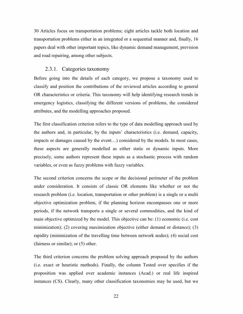
30 Articles focus on transportation problems; eight articles tackle both location and
transportation problems either in an integrated or a sequential manner and, finally, 16
papers deal with other important topics, like dynamic demand management, prevision
and road repairing, among other subjects.
2.3.1. Categories taxonomy Before going into the details of each category, we propose a taxonomy used to
classify and position the contributions of the reviewed articles according to general
OR characteristics or criteria. This taxonomy will help identifying research trends in
emergency logistics, classifying the different versions of problems, the considered
attributes, and the modelling approaches proposed.
The first classification criterion refers to the type of data modelling approach used by
the authors and, in particular, by the inputs’ characteristics (i.e. demand, capacity,
impacts or damages caused by the event…) considered by the models. In most cases,
these aspects are generally modelled as either static or dynamic inputs. More
precisely, some authors represent these inputs as a stochastic process with random
variables, or even as fuzzy problems with fuzzy variables.
The second criterion concerns the scope or the decisional perimeter of the problem
under consideration. It consists of classic OR elements like whether or not the
research problem (i.e. location, transportation or other problem) is a single or a multi
objective optimization problem, if the planning horizon encompasses one or more
periods, if the network transports a single or several commodities, and the kind of
main objective optimized by the model. This objective can be: (1) economic (i.e. cost
minimization); (2) covering maximization objective (either demand or distance); (3)
rapidity (minimization of the travelling time between network nodes); (4) social cost
(fairness or similar); or (5) other.
The third criterion concerns the problem solving approach proposed by the authors
(i.e. exact or heuristic methods). Finally, the column Tested over specifies if the
proposition was applied over academic instances (Acad.) or real life inspired
instances (CS). Clearly, many other classification taxonomies may be used, but we

24
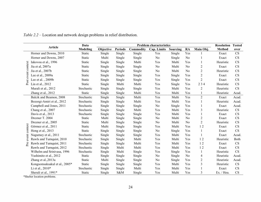
Table 2.2 – Location and network design problems in relief distribution.
Article Data Modeling
Problem characteristics Resolution Method
Tested over Objective Periods Commodity Cap. Limits Sourcing RA Main Obj.
Post
eve
nt c
onte
xt
Horner and Downs, 2010 Static Single Single Single Yes Single Yes 1 Exact CS Horner and Downs, 2007 Static Multi Single Single No Single No 1 Exact CS Iakovou et al., 1996 Static Single Single Multi Yes Multi Yes 1 Heuristic CS Jia et al, 2007a Static Single Single Single No Multi No 2 Exact CS Jia et al., 2007b Static Single Single Single No Multi No 2 Heuristic CS Lee et al., 2009a Static Single Single Single Yes Single Yes 2 Exact CS Lee et al. , 2009b Static Single Single Single Yes Single Yes 2 Exact CS Lin et al., 2012 Static Single Multi Multi Yes Single Yes 2 3 4 Heuristic CS Murali et al., 2012 Stochastic Single Single Single Yes Multi Yes 2 Heuristic CS Zhang et al., 2012 Static Single Single Multi Yes Multi Yes 1 Heuristic Acad.
Pre
even
t con
text
Balcik and Beamon, 2008 Stochastic Single Single Multi Yes Multi Yes 2 Exact Acad. Bozorgi-Amiri et al., 2012 Stochastic Single Single Multi Yes Multi Yes 1 Heuristic Acad. Campbell and Jones, 2011 Stochastic Single Single Single No Single Yes 1 Exact Acad. Chang et al., 2007 Stochastic Single Single Multi Yes Multi Yes 3 Heuristic CS Davis et al., 2013 Stochastic Single Single Single Yes Multi Yes 1 Exact CS Drezner T. 2004 Static Multi Single Single No Multi No 2 Exact CS Drezner et al., 2005 Static Multi Single Single No Multi No 2 Heuristic CS Görmez et al., 2011 Static Multi Single Single Yes Multi Yes 1 2 Exact CS Hong et al., 2013 Static Single Single Single No Single Yes 1 Exact CS Nagurney et al., 2011 Stochastic Single Single Single Yes Multi Yes 1 Exact Acad. Rawls and Turnquist, 2010 Stochastic Single Single Multi Yes Multi Yes 1 2 Heuristic Both Rawls and Turnquist, 2011 Stochastic Single Single Multi Yes Multi Yes 1 2 Exact CS Rawls and Turnquist, 2012 Stochastic Single Multi Multi Yes Multi Yes 1 2 Exact CS Wilhelm and Srinivasa, 1996 Stochastic Single Multi Single Yes Single Yes 1 Heuristic CS Yushimito et al., 2012 Static Single Single Single No Single No 4 Heuristic Acad. Zhang et al.,2013a Static Multi Single Single No Single Yes 2 Heuristic Acad. Kongsomsaksakul et al., 2005* Static Single Single Single Yes Multi Yes 3 Heuristic CS Li et al., 2010* Stochastic Single Single Multi Yes Multi Yes 1 Exact CS Sherali et al., 1991* Static Single S&M Single Yes Multi Yes 3 Ex. / Heu. CS
*Shelter location problems.
25
This hypothesis creates a “steady” environment that allows propositions in this
category to define, as an input known a priori in the model, the demand and the
location of clients, as well as the disaster impacts. Our review shows that the articles
in this category present a more traditional facility location problem (FLP) structure,
they are mainly static and seek to optimize a single objective (either cost
minimization, covering maximization in distance or quantity or rapidity) and this,
during a single period. In addition, most of the location and network design problems
are directed to a single-commodity relief distribution, representing a global demand.
Horner and Downs (2007; 2010), present a multi-echelon network designed for
intermediate distribution facilities (Break of Bulk points). Iakovou et al. (1997)
present the strategic and tactical decisions involved in locating the clean-up
equipment for oil spill disaster. Other authors deal with the location-allocation of
medical services in response to emergencies with a covering objective, forcing a
minimum satisfaction of demand such as (Jia et al. 2007a; Jia et al. 2007b), and (Lee
et al. 2009a; Lee et al. 2009b).
However, models able to accurately represent the disaster reality may be more
desirable. Indeed, even after a disaster has hit the zone, information about demand is
hard to obtain, and a stochastic modeling approach can be useful to represent the
incertitude related to the process of the impact’s estimation. Recent contributions
tackled this issue with stochastic models that maximized coverage (like Murali et al.
2012), models reflecting post-disaster challenges as disaster overlapping (Zhang et al.
2012), or fairness in distribution objectives (Lin et al. 2012). It is worth mentioning
that, as we indicated before, the contributions in this section still present the classic
structure of the FLP applied to emergency situations, without real insight into the
context difficulties being reflected in their models. With the recent exception of the
papers published in 2012, neither the objectives nor the constraints of the model
present a particular feature in relief distribution. We firmly believe that these recent
contributions come as an answer to the need for detailed models that supporting
decision- making.

26
The second group contains the propositions with a Pre-event context. The strategic
nature of the location problem has encouraged many authors to work on the right
network design in order to prepare for disaster response. Even though our article
selection process is limited to the relief distribution network in response to disasters,
these models can also be applied as an immediate response to the disaster; therefore,
these propositions are included in this review. Moreover, many contributions in this
section actually consider both stages in their modeling approach, dealing with stock
prepositioning decisions, and then reallocation after a disaster occurrence. For
instance, some of the papers present stochastic models, in which the site location is
chosen to satisfy demand under different possible disasters (Rawls & Turnquist 2010)
or their impacts: Balcik & Beamon (2008) also includes pre and post disaster budget
constraints; the service quality level (Rawls & Turnquist 2011); the possible locations
of disaster related damages (Campbell & Jones 2011) or multilevel considerations for
network design (Chang et al. 2007). Recently this has starting to shift towards a
prepositioning problem that includes, beyond the risk of damages (demand), the
demand location (Rawls & Turnquist 2012), available supplies (Davis et al. 2013),
outsourcing needs (Nagurney et al. 2011) and even transportation and buying costs
(Bozorgi-Amiri et al. 2012). Wilhelm & Srinivasa (1996) focus on the risks related to
the reliability of the relief distribution network, which is still present in a post-disaster
context. Other authors concentrate their efforts more towards a model definition with
the main objective warranting relief distribution to its maximum capacity. In this
case, a covering objective is used to minimize uncovered demand (Drezner 2004;
Drezner et al. 2005; Gӧrmez et al. 2010; Hong et al. 2012), including characteristics
as social cost (Yushimito et al. 2012) or covering and rapidity objective (Zhang et al.
2013a).
Three papers considered the sheltering location (and allocation) problem in a pre-
disaster context. Even though they are evacuation-oriented, these papers were
retained, because the location decisions for the evacuation problem at this level are
the same as for the distribution context. Kongsomsaksakul et al. (2005) and Sherali et
al. (1991) defined an optimal sheltering network that minimizes transportation time,

28
the number as well as the variety of propositions, this topic was the most popular in
emergency logistics research, In fact, we noticed that transportation contributions are
closer to the specific challenges of relief distribution. Thanks to the operational basis
of the transportation task, the problem definition of these contributions is more
specific to the response to disaster context and allows for the definition of a more
practical distribution problem. For instance, the objectives defined in the
contributions’ transportation problem are more varied than for location cases and
focus more on the distribution’s rapidity or the satisfaction of demand than on total
operational costs.
Since the transportation problem’s characteristics changed, the table structure
proposed in the previous section was modified, leading to Table 2.3. The first four
columns show the already defined general characteristics. The fifth is the Depots
column, indicating if the problem is defined as a single depot or multiple depots.
Then, some vehicle’s characteristics of the model are observed. The Capacity Limits
column summarizes whether or not the proposition limits the vehicle’s capacity. This
column shows the limitation considered: volume capacity, weight capacity, time of
the driver’s shift, cost, number of vehicles available, or the number of units to
transport. The seventh column, Fleet Comp., shows whether the model uses a
heterogeneous fleet of vehicles or homogeneous fleet to construct the route. This is an
important feature in humanitarian logistics because several organizations are involved
in emergency response activities and the need for numerous types of resources (i.e.
vehicles) is very common. Finally, the column Tr. Mode shows whether the problem
is stated as a multi-modal problem or the specific type of transportation mode (i.e.
ground, air or water). The different papers concerned with relief transportation
decisions are presented in Table 2.3.
It is well accepted that transportation and routing problems are very difficult to solve.
Even in the industrial context, academics and practitioners have been working for
decades on this optimization problem. The problem's difficulty increases as the
model’s level of detail increases.

29
Table 2.3 – Transportation problems in relief distribution.
Authors Data Modeling
Problem characteristics Resolution Method
Tested over
Obj. Periods Commodity Depots Capacity Limits Fleet Comp.
Tr. Mode
Main Obj.
Rel
ief D
istri
butio
n
Adivar and Mert, 2010 Fuzzy Multi Multi Multi Multi Weight Hetero. Multi 1 5 Exact CS Balcik et al., 2008 Dynamic Single Multi Multi Single Vol./Time/Fleet Hetero. Ground 1 2 Exact Acad. Barbarosoǧlu et al., 2004 Stochastic Single Single Multi Multi Units Hetero. Multi 1 Exact CS Berkoune et al., 2012 Static Single Single Multi Multi W./Vol./Time/Fleet Hetero. Ground 3 Heur. Acad. Campbell et al., 2008 Static Single Single Single Single No Homo. Ground 3 Heur. Acad. Chen et al., 2011 Static Single Single Single Multi Units Homo. Ground 3 Exact CS Gu, 2011 Sta.-Fuz. Single Single S&M Multi Units Homo. Ground 2 Exact Acad. Haghani et al., 1996 Static Single Multi Multi Multi Units/Fleet Hetero. Multi 1 Heur. Acad. Hu, 2011 Static Multi Single Multi Single No Hetero. Multi 1 Exact Acad. Huang et al., 2012 Static Single Single Single Single Units Homo. Ground 3 2 4 Heur. Acad. Lin et al., 2011 Static S&M Multi Multi Single W./Vol./Time/Fleet Homo. Ground 2 3 4 Heur. Acad. Özdamar et al., 2004 Dynamic Single Multi Multi Multi Weight/Fleet Hetero. Multi 2 Heur. CS Shen et al., 2009 Stochastic Single Single Single Single Units/Fleet Hetero. Ground 2 3 Heur. Acad. Sheu, 2007a Dynamic Multi Multi Multi Multi Units/Fleet Hetero. Ground 2 1 Exact CS Suzuki 2012 Static Single Single Single Single Weight/Fuel/Time Hetero. Ground 2 4 Exact Acad. Tzeng et al,2007 Dynamic Multi Multi Multi Multi Volume Homo. Ground 1 3 4 Exact/Sim. Acad. Vitoriano et al., 2011 Stochastic Multi Single Single Multi Units/Fleet/Budget Hetero. Ground 1 3 4 5 Exact CS Vitoriano et al., 2009 Stochastic Multi Single Single Multi Units/Budget Hetero. Ground 1 3 4 5 Exact CS Wohlgemuth et al., 2012 Dynamic Single Multi Single Single Units Homo. Ground 3 1 Heuristic Acad. Yuan and Wang, 2009 Static S.&M. Multi Single Single No Homo. Ground 3 5 Heur./Sim. Acad. Zhang et al. 2013b Static Single Multi Single Single No Homo. Ground 3 Heuristic Acad. Jotshi et al., 2009a Static Multi Single Single Multi Units/Fleet Homo. Ground 2 Heur./Sim. CS
Dis
t. an
d Ev
acua
tion Barbarosoǧlu et al., 2002 Static Multi Single Multi Multi Weight/Fleet/Time Hetero. Air 1 Heur. Acad.
Chern et al., 2010 Dynamic Multi Multi Multi Multi Units/Fleet/Fuel Hetero. Multi 2 3 1 Heur. Acad. Najafi et al., 2013 Stochastic Multi Multi Multi Multi W./Vol./Units/Fleet Hetero. Multi 2 1 Exact CS Özdamar and Demir, 2012 Static Single Single Multi Multi Fleet/Units Hetero. Ground 3 Heur. Acad. Özdamar and Yi., 2008 Static Single Multi Multi Multi Units/Fleet Hetero. Ground 3 Heur. Acad. Özdamar, 2011 Static Single Single Multi Multi Weight/Time/Units Homo. Air 3 Heur. Acad. Yi and Kumar, 2007 Static Single Multi Multi Multi Weight/Fleet Hetero. Ground 2 Heur. Acad. Yi and Özdamar, 2004 Fuzzy Single Multi Multi Multi Weight/Fleet Hetero. Multi 2 Exact CS
a Causality transportation problem
30
If we deal, all at the same time, with stochastic data, heterogeneous vehicle fleet, in a
multi-period and multi-commodity network context (which is probably the closest to
reality), the resulting model will be extremely hard to solve; which is not at all
wanted when looking for fast and efficient solutions. Therefore, authors will usually
choose the factors that best adapt to their study context and will establish hypotheses
on the other features to simplify the model. For instance, some authors have a
traditional approach to the data type (e.g., a deterministic static or dynamic data
model) in order to consider a multi-period planning horizon (Wohlgemuthscha et al.
2012; Yuan & Wang 2009; Zhang et al. 2013b) or a multi-commodity network
(Berkoune et al. 2012; Gu 2011; Hu 2011), or even both (Balcik et al. 2008; Haghani
& Oh 1996; Lin et al. 2011; Özdamar et al. 2004; Sheu 2007a; Tzeng et al. 2007).
Even though their data setting is deterministic, these papers define a complex
distribution network close to the relief distribution’s reality, with a proper level of
detail to reflect the crisis manager’s challenges. We believe this to be a very
important point to establish models for decision making for the daily operations of
relief distribution.
On the other side, some authors have a “traditional” approach to their problem’s
characteristics (i.e. static data, single-commodity and single period considerations)
but with the objective of exploring new approaches to the relief distribution problem.
For example, the transportation contributions have varied objectives beyond cost
minimization. The most popular objective regarding these problems is the rapidity
objective, usually defined through a minimum travel time objective or a minimum
latest arrival time. Campbell et al. (2008) were among of the first to explore the major
difference between relief and commercial distribution by proposing three different
objectives for a fast delivery. Chen et al. (2011) defined a distribution problem
integrated in a DSS with the support of a Geographic Information System (GIS).
Suzuki (2012) had a static consideration but studied a coverage and equity objective
that also included fuel limitation. On the other hand, Huang et al. (2012) defined three
main objectives for the relief distribution challenge: rapidity, demand satisfaction and
equity (i.e. equity, efficacy and efficiency). Theirs was one of the first propositions to
approach the equity objective in an explicit way.
31
Through random or fuzzy variables, many authors also considered the uncertainty
related to the relief distribution context that are reflected in demand, arc capacity,
travel time or network reliability (Adivar & Mert 2010; Barbarosoǧlu & Arda 2004;
Shen et al. 2009; Vitoriano et al. 2009; Vitoriano et al. 2011). These papers’ main
contribution acknowledges the different sources of uncertainty in a post-disaster
context, thus providing crisis managers with a more robust distribution plan.
However, these contributions left aside the dynamic aspect of the problem and
focused on a single period planning horizon. We believe this to be a useful twist that
should soon be included in the emergency logistics planning. As we stated before, the
changing environment is an important challenge in this context and a flexible network
is still a major need.
When working on transportation problems, one should also consider the problems
related to the transportation of casualties. During our review process, we noticed how
the evacuation’s planning decisions demand another type of analysis on an
operational level (i.e. traffic assignment problems and congestion analysis, among
others), which are out of the scope of our review. Contrariwise, the casualty
transportation problem is sort of a “victims’ transportation problem” and is part of the
tasks needed to bring relief to affected people, which allowed us to review casualty
transportation problems in this paper. In fact, some authors tackled both relief
distribution and casualty transportation problems in their optimization model. In
general, the model finds the optimal route to distribute relief products and transport
victims from the danger zone to health centers. This results in a much more complex
network problem, becoming a multi-commodity problem often presented with a
multi-period planning horizon. Some of them have a static data setting, planning
helicopter scheduling (Barbarosoǧlu et al. 2002; Özdamar 2011) or a heterogeneous
vehicle problem (Özdamar & Demir 2012; Özdamar & Yi 2008; Yi & Kumar 2007).
Others present a dynamic problem (Chern et al., 2010) or a fuzzy stochastic problem
(Najafi et al. 2013; W. Yi & L. Özdamar 2004). Finally, in their paper, Jotshi et al.
(2009) dealt exclusively with the casualty transportation problem.


34
Table 2.4 – Combined Location-Transportation problems in relief distribution.
Authors Data Modeling
Problem characteristics
Resolution Method
Tested over Objective Periods Commodity Site
capacity R.A Depots
and Sourcing
Tr. Capacity Limits
Fleet Comp.
Tr. Mode
Main Obj.
Afshar and Hagani, 2012 Dynamic Single Multi Multi Yes Yes Multi Units/Fleet/Weight Hetero. Multi 2 Exact Acad
Mete and Zabinsky, 2010 Stochastic Single Single Multi Yes Yes Multi Units/Fleet Hetero. Ground 1 3 Exact CS
Naji-Azimi et al., 2012 Static Single Single Multi No No Single Weight/Fleet Hetero. Ground 3 Heuristic Acad
Nolz et al.,2010 Static Multi Single Single Yes No Single Units/Fleet Hetero. Multi 2 3 Heuristic CS
Nolz et al., 2011 Static Multi Single Single Yes No Single Units/Fleet Homo. Ground 5 3 Heuristic CS
Ukkusuri and Yushimito, 2008
Static-Stoch. Single Single Single No No Single Budget/Fleet Homo. Ground 1 Exact Acad
Yi, W. and Özdamar, L., 2007 Dynamic Single Multi Multi Yes Yes Multi Weight Hetero. Ground 2 Heurisitic CS
Zografos and Androutsopoulos, 2008 Static Multi Single Single Yes Yes Single Units/Fleet Homo. Ground 3 5 Heuristic CS


36
discipline and its boundaries has become a matter of urgency. As shown in the
Introduction, the terms “emergency”, “emergency logistics”, “humanitarian logistics”
and “response to crisis”, among others, are applied in a wide range of contexts and
from diverse standpoints, making it difficult to consolidate the knowledge and the
scientific contributions.
Furthermore, and despite its theoretical value, the relevance of some structuring
works to the relief distribution’s practice, like the 4-phases definition commonly
accepted in the literature, is debatable. In fact, we have shown that many of the
proposed location models for a pre-disaster phase can also easily be applied during
the response phase. A response model, embedded in a Decision Support System, can
be used in the training and preparedness process. Similarly, once the data has become
available, a preparedness model can lead to an optimal response plan. We can
conclude that, unlike the traditional approach in EM literature, the location and
network design problem are not exclusive to the pre-disaster phase. Moreover, we
think that the disaster timeline and the related operations need to be refined to
harmoniously encompass the response as well as the short and long-term recovery
activities.
Our second observation concerns the well-established differences between business
and humanitarian logistics. Pioneer contributions in the field defined general response
models, mostly within a multi-commodity network (Barbarosoǧlu & Arda 2004;
Barbarosoǧlu et al. 2002; Drezner 2004; Drezner et al. 2005; Haghani & Oh 1996;
Özdamar et al. 2004; Viswanath & Peeta 2003; Yi & Özdamar 2004). Despite their
efforts, it seems that most of these contributions did not focus adequately in the
specific characteristics of humanitarian logistics like the knowledge of demand, the
considered objectives, the periodicity and the decision-making structure (Holguín-
Veras et al., 2012). Hopefully, our knowledge and comprehension level of
humanitarian challenges increases and recent articles present more sophisticated
models, which better suit the specific context and needs, especially in the case of
transportation problems (Berkoune et al. 2012; Gu 2011; Huang et al. 2012; Lee et al.
2009a; Lin et al. 2012; Lin et al. 2011; Murali et al. 2012; Özdamar 2011; Yan &
37
Shih 2009). Nonetheless, we think that the sudden and dramatic nature of
humanitarian problems should be emphasized in future research works.
Our third observation concerns the difficult tradeoff between modeling the desired
level of detail and the model’s solvability. As more and more sophisticated, yet
realistic models appear, it becomes increasingly difficult to solve them efficiently,
particularly in a response context where decisions need to be made quickly. Thereby,
papers proposing approximated methods (e.g. Nolz et al. 2010; Yi & Özdamar 2007;
Berkoune et al. 2012; Lin et al. 2012; Murali et al. 2012; Wohlgemuthscha et al.
2012) are becoming more and more popular than the ones, focusing in modeling
aspects, where commercial software is used to solve the proposed mathematical
formulation (Horner & Downs 2010; Jia, Ordóñez & Dessouky 2007; Lin et al. 2011;
Rawls & Turnquist 2011).
The stochastic and dynamic propositions are still rare. Even during the response
phase, the level of uncertainty and, more so, the variability level are quite high, and a
deterministic static modeling approach can easily lead to a low performance of the
distribution tasks. However, stochastic and dynamic models being much harder to
solve, significant effort is needed to efficiently solve the propositions.
Our fourth observation, which is in fact a set of observations, pertains specifically to
the works on network design. First, we think that the nature of the different nodes or
sites in the network needs to be revised and refined. Although the use of distribution
centers and distribution points similar to those in the business SC seems to be widely
accepted, we should not forget that, in the business case, those facilities are designed
and built to perform logistic activities, which is not the case in a post-disaster context.
Indeed, most humanitarian sites rely on the transformation of facilities like arenas or
schools making it difficult to anticipate their flows and capacity to handle
humanitarian activities. In general, the literature has neglected the aspect related to
the “ability” of a facility to perform a given humanitarian and it would be interesting
to see it included in future works. Even more important, we found that a very few of
papers tackled multi-period cases in network design, neglecting the fact that the
deployed network is usually temporary and needs to be flexible to accommodate the

38
demand’s variation. Moreover, in a multi-period planning horizon, facilities can be
opened, closed and reopened during the planning horizon; therefore sites costs and
capacities strongly impact the decisions. However, including this analysis and
defining opening and closing costs in a manner relevant in a practical context still
presents a challenge. For instance, one can account for the time and efforts required
to open and prepare a given site by reducing its capacity during the period in which
the site is open, while others may limit the number of sites to be open by constraining
the number of available human resources to operate them.
Finally, we have already discussed the type of objectives that should direct the design
decisions, and the small variety of modeling objectives (most articles present a cost
minimization objective). However, while limited discussion have been devoted to
justify whether or not single objective models are more suitable than multi-objective
ones (Lin et al., 2012; Drezner et al., 2005), neither were about the choice of
measures encompassed by the objective function.
Our fifth observation is related to works on transportation problems. It includes two
comments and conclusions. Our first remark concerns once again the goal of the
proposed models. The most popular objective in these problems is “rapidity”, usually
achieved by minimizing the total travel time or the latest arrival time. However,
recent works have identified new and appealing objectives like minimization of the
risk associated to the loss of a truck and its load, or the fair relief distribution (e.g.
Vitoriano et al. 2009; Vitoriano et al. 2011). More specifically, Huang et al. (2012) is
the only paper to highlight the paramount importance of a fair sharing of the available
relief among the people in need. For their part, Lin et al. (2011); Tzeng et al.( 2007);
Vitoriano et al. (2009) and Vitoriano et al. (2011) considered it more as a secondary
objective. The notion of “equity”, overlooked in the literature, becomes even more
important when multi-period contexts are considered. Since available relief and
demand may vary from one period to another, it seems reasonable to expect some
flexibility in the way that demand is satisfied. This offers the possibility of delivering
lower quantities to some people, provided that they receive higher quantities in the
subsequent periods. Nonetheless, our review did not report any paper dealing

39
explicitly with the possibility of relief backordering. We believe that this should be
presented in order to offer a better support to the distribution decisions.
Our second comment on the reviewed papers relates to whether relief is distributed by
truck routes or by dedicated trips. In fact, an analysis of this aspect has been
disregarded in the literature, and both options are valid approaches on relief
distribution. de la Torre et al., (2012) presented a review of papers on relief
distribution where trucks performed delivery routes. On the other hand, other authors
(see for example Berkoune et al., 2012) proposed a multi-trips approach to satisfy the
PODs’ demand.
Our sixth observation concerns the works that we have classified as “Combined
location-transportation problems”. The number of papers dealing with location-
allocation problems have, without a doubt, increased very quickly in the last two
years, with a total of nine papers published between 2011 and 2013 (31% of the
location papers). We believe that the increasing attention devoted these types of
problems indicates that there is a new research stream seeking to adopt a more
integrated approach in order to cope with the diverse decisional levels related to relief
network problems. As in the business SC case, where combined location and
transportation problems have now been studied for several years, (Nagy & Salhi
2007; Salhi & Rand 1989) models addressing the links and dependencies of these two
problems in a relief distribution context are required. Even more so, distributed
modeling approaches are promising research areas and their application goes beyond
the integrated location-routing problem to suit the global framework of response to
disasters.
As a whole, it appears to us that research on relief distribution is now entering a
consolidation phase, where academics have cumulated a good knowledge of disaster
relief operations. The research approaches, originally very inspired from the business
SC ones, have become more specialized and closer to the specific relief distribution
context. Hence, the number of real-life inspired instances tackled in the literature is
rather high, ranging from 33% in the case of transportation problems to up to 72% in
the case of location and network design problems.
40
2.8.2. Trends and challenges Nowadays, there is an increasing interest in tackling new subjects, such as the
international scheme in response effort, service quality, equity and social objectives,
or the integration of technological advances. See, for instance, Adivar & Mert 2010;
Chen et al. 2011; Huang et al. 2012; Mete & Zabinsky 2010; Rawls & Turnquist
2011; Turner et al. 2012. Also, we are beginning to see the application of other
classic OR/MS problems to the humanitarian logistics field. For example,
contributions aimed at improving the organization or the management of other
support activities can still be explored, especially in a dynamic real-time context (e.g.,
demand estimation, inventory management and personal management). Research on
stock relocation and stock management (e.g., Rottkemper et al., 2011) would help
supporting the response phase’s daily operations better. Furthermore, the research
done on casualty transportation is still very limited. To the best of our knowledge,
this important topic has only been addressed by Jotshi et al. (2009), and the few
combined flow contributions (like Özdamar 2011).
In addition, coordination is a challenging subject that still may be improved upon.
However enough has been said on the importance and critical stage of coordination in
humanitarian logistics and we now need to find a way to merge with the logistics
optimization problems (e.g. coordination level indicators, collaboration planning
models, etc.).We firmly believe that a deeper analysis of this area by way of a wider,
probably hybrid, modeling approach could achieve the integration of these
relationships.
Meanwhile, additional efforts need to put forth to increase the coherence between the
hypothesis and considerations used to design the relief distribution networks and the
decisions actually made in those networks. We still find discrepancy and separation
in, among others, the objectives sought by the optimization and the manager’s
problems, the hypothesis, the planning horizons and the limitation of resources. In
this sense, the alignment of objectives must not only be achieved through the logistic
network stages (the different problems) but also through the different levels of the
distribution chain (external supply sources, supply, temporal distribution facilities,

43
Balcik, B., Beamon, B.M. & Smilowitz, K., 2008. Last mile distribution in humanitarian relief. Journal of Intelligent Transportation Systems, 12(2), pp.51–63.
Barbarosoǧlu, G. & Arda, Y., 2004. A two-stage stochastic programming framework for transportation planning in disaster response. Journal of the Operational Research Society, 55(1), pp.43–53.
Barbarosoǧlu, G., Özdamar, L. & Cevik, A., 2002. An interactive approach for hierarchical analysis of helicopter logistics in disaster relief operations. European Journal of Operational Research, 140(1), pp.118–133.
Berkoune, D., Renaud, J., Rekik, M., & Ruiz, A., 2012. Transportation in Disaster Response Operations. Socio-Economic Planning Sciences, 46(1), pp. 23-32.
Bozorgi-Amiri, A, Jabalameli, M.S., Alinaghian, M. & Heydari, M., 2012. A modified particle swarm optimization for disaster relief logistics under uncertain environment. The International Journal of Advanced Manufacturing Technology, 60(1), pp.357–371.
Campbell, A.M. & Jones, P.C., 2011. Prepositioning supplies in preparation for disasters. European Journal of Operational Research, 209(2), pp.156–165.
Campbell, A.M., Vandenbussche, D. & Hermann, W., 2008. Routing for relief efforts. Transportation Science, 42(2), pp.127–145.
Caunhye, A.M., Nie, X. & Pokharel, S., 2012. Optimization models in emergency logistics: A literature review. Socio-Economic Planning Sciences, 46(1), pp.4–13.
Chang, M.-S., Tseng, Y.-L. & Chen, J.-W., 2007. A scenario planning approach for the flood emergency logistics preparation problem under uncertainty. Transportation Research Part E: Logistics and Transportation Review, 43(6), pp.737–754.
Chen, A.Y., Peña-Mora, F. & Ouyang, Y., 2011. A collaborative GIS framework to support equipment distribution for civil engineering disaster response operations. Automation in Construction, 20(5), pp.637–648.
Chern, C.-C., Chen, Y.-L. & Kung, L.-C., 2010. A heuristic relief transportation planning algorithm for emergency supply chain management. International Journal of Computer Mathematics, 87(7), pp.1638–1664.
Davis, L.B., Samanlioglu, F., Qu, X. & Root, S., 2013. Inventory planning and coordination in disaster relief efforts. International Journal of Production Economics, 141, pp.561–573.
Drezner, T., 2004. Location of casualty collection points. Environment and Planning C: Government and Policy, 22(6), pp.899–912.

44
Drezner, T., Drezner, Z. & Salhi, S., 2005. A multi-objective heuristic approach for the casualty collection points location problem. Journal of the Operational Research Society, 57(6), pp.727–734.
Duque, P.M. & Sӧrensen, K., 2011. A GRASP metaheuristic to improve accessibility after a disaster. OR spectrum, 33(3), pp.525–542.
Falasca, M. & Zobel, C., 2012. An optimization model for volunteer assignments in humanitarian organizations. Socio-Economic Planning Sciences, (46), pp. 250-260.
Feng, C.-M. & Wang, T.-C., 2003. Highway emergency rehabilitation scheduling in post-earthquake 72 hours. Journal of the 5th Eastern Asia Society for Transportation Studies, 5, pp. 55-69.
Galindo, G. & Batta, R., 2013. Review of Recent Developments in OR/MS Research in Disaster Operations Management. European Journal of Operational Research, 203, pp.201–211.
Gu, Y., 2011. Research on Optimization of Relief Supplies Distribution Aimed to Minimize Disaster Losses. Journal of Computers, 6(3), pp.603–609.
Gӧrmez, N., Kӧksalan, M. & Salman, F., 2010. Locating disaster response facilities in Istanbul. Journal of the Operational Research Society, 62(7), pp.1239–1252.
Haddow, G.D., Bullock, J.A. & Coppola, D.P., 2007. Introduction to emergency management Third ed., Oxford: Butterworth-Heinemann.
Haghani, A. & Oh, S.-C., 1996. Formulation and solution of a multi-commodity, multi-modal network flow model for disaster relief operations. Transportation Research Part A: Policy and Practice, 30(3), pp.231–250.
Holguín-Veras, J. Hart, W.H., Jaller, M., Van Wassenhove, L.N. Pérez, N. & Wachtendorf, T., 2012. On the unique features of post-disaster humanitarian logistics. Journal of Operations Management, 30, pp.494–506.
Hong, J.D., Xie, Y. & Jeong, K.Y., 2012. Development and evaluation of an integrated emergency response facility location model. Journal of Industrial Engineering and Management, 5(1), pp.4–21.
Horner, M.W. & Downs, J.A., 2010. Optimizing hurricane disaster relief goods distribution: model development and application with respect to planning strategies. Disasters, 34(3), pp.821–844.
Horner, M.W. & Downs, J.A., 2007. Testing a flexible geographic information system-based network flow model for routing hurricane disaster relief goods. Transportation Research Record: Journal of the Transportation Research Board, 2022(1), pp.47–54.

45
Hu, Z.-H., 2011. A container multimodal transportation scheduling approach based on immune affinity model for emergency relief. Expert Systems with Applications, 38(3), pp.2632–2639.
Huang, M., Smilowitz, K. & Balcik, B., 2012. Models for relief routing: Equity, efficiency and efficacy. Transportation research part E: logistics and transportation review, 48(1), pp.2–18.
Huang, M., Smilowitz, K.R. & Balcik, B., 2013. A continuous approximation approach for assessment routing in disaster relief. Transportation Research Part B: Methodological, 50, pp.20–41.
Iakovou, E. et al., 1997. Optimal location and capacity of emergency cleanup equipment for oil spill response. European journal of operational research, 96(1), pp.72–80.
Jia, H., Ordóñez, F. & Dessouky, M., 2007. A modeling framework for facility location of medical services for large-scale emergencies. IIE transactions, 39(1), pp.41–55.
Jia, H., Ordóñez, F. & Dessouky, M., 2007. Solution approaches for facility location of medical supplies for large-scale emergencies. Computers & Industrial Engineering, 52(2), pp.257–276.
Jotshi, A., Gong, Q. & Batta, R., 2009. Dispatching and routing of emergency vehicles in disaster mitigation using data fusion. Socio-Economic Planning Sciences, 43(1), pp.1–24.
Kitchenham, B., 2004. Procedures for performing systematic reviews. Keele, UK, Keele University, 33.
Kongsomsaksakul, S., Yang, C. & Chen, A., 2005. Shelter location-allocation model for flood evacuation planning. Journal of the Eastern Asia Society for Transportation Studies, 6(1), pp.4237–4252.
Kovács, G. & Spens, K., 2007. Humanitarian logistics in disaster relief operations. International Journal of Physical Distribution & Logistics Management, 37(2), pp.99–114.
Lee, E.K., Chen, C.H., Pietz, F. & Benecke B., 2009a. Modeling and optimizing the public-health infrastructure for emergency response. Interfaces, 39(5), pp.476–490.
Lee, E.K., Smalley, H.K., Zhang, Y. & Pietz, F., 2009b. Facility location and multi-modality mass dispensing strategies and emergency response for biodefence and infectious disease outbreaks. International Journal of Risk Assessment and Management, 12(2), pp.311–351.
Lettieri, E., Masella, C. & Radaelli, G., 2009. Disaster management: findings from a systematic review. Disaster Prevention and Management, 18(2), pp.117–136.

46
Li, L., Jin, M. & Zhang, L., 2011. Sheltering network planning and management with a case in the Gulf Coast region. International Journal of Production Economics, 131(2), pp.431–440.
Lin, Y.-H. et al., 2011. A logistics model for emergency supply of critical items in the aftermath of a disaster. Socio-Economic Planning Sciences, 45(4), pp.132–145.
Lin, Y.H. Batta, R., Rogerson, P. Blatt, A. & Flanigan, M., 2012. Location of temporary depots to facilitate relief operations after an earthquake. Socio-Economic Planning Sciences, 46(2), pp.112–123.
Lodree Jr, E.J., Ballard, K.N. & Song, C.H., 2012. Pre-positioning hurricane supplies in a commercial supply chain. Socio-Economic Planning Sciences, 46(4), pp.291–305.
McLoughlin, D., 1985. A framework for integrated emergency management. Public Administration Review, 45, pp.165–172.
Mete, H.O. & Zabinsky, Z.B., 2010. Stochastic optimization of medical supply location and distribution in disaster management. International Journal of Production Economics, 126(1), pp.76–84.
Minciardi, R., Sacile, R. & Trasforini, E., 2007. A decision support system for resource intervention in real-time emergency management. International Journal of Emergency Management, 4(1), pp.59–71.
Minciardi, R., Sacile, R. & Trasforini, E., 2009. Resource allocation in integrated preoperational and operational management of natural hazards. Risk Analysis, 29(1), pp.62–75.
Murali, P., Ordóñez, F. & Dessouky, M., 2012. Facility location under demand uncertainty: Response to a large-scale bio-terror attack. Socio-Economic Planning Sciences, 46(1), pp.78–87.
Nagurney, A., Yu, M. & Qiang, Q., 2011. Supply chain network design for critical needs with outsourcing. Papers in Regional Science, 90(1), pp.123–142.
Nagy, G. & Salhi, S., 2007. Location-routing: Issues, models and methods. European Journal of Operational Research, 177(2), pp.649-672.
Najafi, M., Eshghi, K. & Dullaert, W., 2013. A multi-objective robust optimization model for logistics planning in the earthquake response phase. Transportation Research Part E: Logistics and Transportation Review, 49(1), pp.217–249.
Naji-Azimi, Z., Renaud, J., Ruiz, A. & Salari, M., 2012. A covering tour approach to the location of satellite distribution centers to supply humanitarian aid. European Journal of Operational Research, 222(3), pp.596–605.
47
Natarajarathinam, M., Capar, I. & Narayanan, A., 2009. Managing supply chains in times of crisis: a review of literature and insights. International Journal of Physical Distribution & Logistics Management, 39(7), pp.535–573.
Nolz, P.C., Doerner, K.F. & Hartl, R.F., 2010. Water distribution in disaster relief. International Journal of Physical Distribution & Logistics Management, 40(8/9), pp.693–708.
Nolz, P.C., Semet, F. & Doerner, K.F., 2011. Risk approaches for delivering disaster relief supplies. Or spectrum, 33(3), pp.543–569.
Özdamar, L., 2011. Planning helicopter logistics in disaster relief. OR spectrum, 33(3), pp.655–672.
Özdamar, L. & Demir, O., 2012. A hierarchical clustering and routing procedure for large scale disaster relief logistics planning. Transportation Research Part E: Logistics and Transportation Review, 48(3), pp.591–602.
Özdamar, L., Ekinci, E. & Küçükyazici, B., 2004. Emergency logistics planning in natural disasters. Annals of operations research, 129(1-4), pp.217–245.
Özdamar, Linet & Yi, Wei, 2008. Greedy neighborhood search for disaster relief and evacuation logistics. Intelligent Systems, IEEE, 23(1), pp.14–23.
Rawls, C.G. & Turnquist, M.A., 2012. Pre-positioning and dynamic delivery planning for short-term response following a natural disaster. Socio-Economic Planning Sciences, 46(1), pp.46–54.
Rawls, C.G. & Turnquist, M.A., 2010. Pre-positioning of emergency supplies for disaster response. Transportation research part B: Methodological, 44(4), pp.521–534.
Rawls, C.G. & Turnquist, M.A., 2011. Pre-positioning planning for emergency response with service quality constraints. OR spectrum, 33(3), pp.481–498.
Rottkemper, B. et al., 2011. Inventory relocation for overlapping disaster settings in humanitarian operations. OR spectrum, 33(3), pp.721–749.
Rottkemper, B., Fischer, K. & Blecken, A., 2012. A transshipment model for distribution and inventory relocation under uncertainty in humanitarian operations. Socio-Economic Planning Sciences, 46(1), pp.98–109.
Salhi, S. & Rand, G.K., 1989. The effect of ignoring routes when locating depots. European journal of operational research, 39(2), pp.150-156.
Shen, Z., Dessouky, M.M. & Ordóñez, F., 2009. A two-stage vehicle routing model for large-scale bioterrorism emergencies. Networks, 54(4), pp.255–269.
48
Sherali, H.D., Carter, T.B. & Hobeika, A.G., 1991. A location-allocation model and algorithm for evacuation planning under hurricane/flood conditions. Transportation Research Part B: Methodological, 25(6), pp.439–452.
Sheu, J.B., 2007a. An emergency logistics distribution approach for quick response to urgent relief demand in disasters. Transportation Research Part E: Logistics and Transportation Review, 43(6), pp.687–709.
Sheu, J.B., 2007b. Challenges of emergency logistics management. Transportation Research Part E: Logistics and Transportation Review, 43(6), pp.655–659.
Sheu, J.B., 2010. Dynamic relief-demand management for emergency logistics operations under large-scale disasters. Transportation Research Part E: Logistics and Transportation Review, 46(1), pp.1–17.
Simpson, N. & Hancock, P., 2009. Fifty years of operational research and emergency response. Journal of the Operational Research Society, pp.S126–S139.
Staples, M. & Niazi, M., 2007. Experiences using systematic review guidelines. Journal of Systems and Software, 80(9), pp.1425–1437.
Suzuki, Y., 2012. Disaster-Relief Logistics With Limited Fuel Supply. Journal of Business Logistics, 33(2), pp.145–157.
de la Torre, L.E., Dolinskaya, I.S. & Smilowitz, K.R., 2012. Disaster relief routing: Integrating research and practice. Socio-Economic Planning Sciences, 46(1), pp.88–97.
Tranfield, D., Denyer, D. & Smart, P., 2003. Towards a methodology for developing evidence-informed management knowledge by means of systematic review. British Journal of Management, 14(3), pp.207–222.
Turner, J.P. et al., 2012. Mitigating shortage and distribution costs in damaged water networks. Socio-Economic Planning Sciences, 46(4), pp.315–326.
Tzeng, G.-H., Cheng, H.-J. & Huang, T.D., 2007. Multi-objective optimal planning for designing relief delivery systems. Transportation Research Part E: Logistics and Transportation Review, 43(6), pp.673–686.
Ukkusuri, S.V. & Yushimito, W.F., 2008. Location routing approach for the humanitarian prepositioning problem. Transportation Research Record: Journal of the Transportation Research Board, 2089(1), pp.18–25.
Viswanath, K. & Peeta, S., 2003. Multicommodity maximal covering network design problem for planning critical routes for earthquake response. Transportation Research Record: Journal of the Transportation Research Board, 1857(1), pp.1–10.

49
Vitoriano, B, Ortuno, T. & Tirado, G, 2009. HADS, a goal programming-based humanitarian aid distribution system. Journal of Multi-Criteria Decision Analysis, 16(1-2), pp.55–64.
Vitoriano, B., Ortuño, M.T., Tirado, G., & Montero J., 2011. A multi-criteria optimization model for humanitarian aid distribution. Journal of Global Optimization, 51(2), pp.189–208.
Van Wassenhove, L. N. & Pedraza Martínez, A.J., 2012. Using OR to adapt supply chain management best practices to humanitarian logistics. International Transactions in Operational Research, 19(1-2), pp.307–322.
Van Wassenhove, L. N., 2006. Humanitarian aid logistics: supply chain management in high gear. Journal of the Operational Research Society, 57(5), pp.475–489.
Wilhelm, W. & Srinivasa, A.V., 1996. A Strategic, Area-wide Contingency Planning Model for Oil Spill Cleanup Operations with Application Demonstrated to the Galveston Bay Area*. Decision Sciences, 27(4), pp.767–799.
Wohlgemuthscha, Oloruntoba, R. & Clausen, U., 2012. Dynamic vehicle routing with anticipation in disaster relief. Socio-Economic Planning Sciences.
Xu, X., Qi, Y. & Hua, Z., 2010. Forecasting demand of commodities after natural disasters. Expert Systems with Applications, 37(6), pp.4313–4317.
Yan, S. & Shih, Y.-L., 2007. A time-space network model for work team scheduling after a major disaster. Journal of the Chinese Institute of Engineers, 30(1), pp.63–75.
Yan, S. & Shih, Y.-L., 2009. Optimal scheduling of emergency roadway repair and subsequent relief distribution. Computers & Operations Research, 36(6), pp.2049–2065.
Yi, W. & Kumar, A., 2007. Ant colony optimization for disaster relief operations. Transportation Research Part E: Logistics and Transportation Review, 43(6), pp.660–672.
Yi, W. & Özdamar, L., 2004. Fuzzy modeling for coordinating logistics in emergencies. International Scientific Journal of Methods and Models of Complexity-Special Issue on Societal Problems in Turkey, 7(1).
Yi, Wei & Özdamar, Linet, 2007. A dynamic logistics coordination model for evacuation and support in disaster response activities. European Journal of Operational Research, 179(3), pp.1177–1193.
Yuan, Y. & Wang, D., 2009. Path selection model and algorithm for emergency logistics management. Computers & Industrial Engineering, 56(3), pp.1081–1094.

50
Yushimito, W.F., Jaller, M. & Ukkusuri, S., 2012. A Voronoi-based heuristic algorithm for locating distribution centers in disasters. Networks and Spatial Economics, 12(1), pp.21–39.
Zhang, J., Dong, M. & Frank Chen, F., 2013. A bottleneck Steiner tree based multi-objective location model and intelligent optimization of emergency logistics systems. Robotics and Computer-Integrated Manufacturing, 48(55).
Zhang, J.-H., Li, J. & Liu, Z.-P., 2012. Multiple-resource and multiple-depot emergency response problem considering secondary disasters. Expert Systems with Applications, 39(12), pp.11066–11071.
Zhang, X. et al., 2013. Route selection for emergency logistics management: A bio-inspired algorithm. Safety Science, 54, pp.87–91.
Zografos, K.G. & Androutsopoulos, K.N., 2008. A decision support system for integrated hazardous materials routing and emergency response decisions. Transportation research part C: emerging technologies, 16(6), pp.684–703.

51
Chapitre 3
3. Modèles pour une distribution juste de l’aide humanitaire
La « justice » au moment de la distribution de l’aide humanitaire est devenue un
concept clef pour les gestionnaires dans le déploiement logistique d’urgence. Après
un désastre, au moment où les besoins surpassent la capacité de réponse, une
distribution efficiente et juste de l’aide disponible est attendue de la part des
décideurs. Cette prémisse est supportée par l’analyse de la littérature effectuée au
Chapitre 2 ainsi que par nos travaux précédents en partenariat avec l’équipe de la
section Défense et Sécurité publique de Fujitsu Consulting (Canada) Inc. Lors de
cette collaboration, nous avons développé un système de d’aide à la décision (DSS)
pour la distribution d’aide suite à un désastre (Rekik et al. 2013). Le système inclut
deux modules, un premier pour la localisation et l’approvisionnement des différents
centres de distribution d’aide humanitaire (CDAH), et un second dédié à la
planification du transport à partir des CDAH afin de satisfaire les besoins des points
de demande. Finalement, un outil d’analyse multicritère permet de supporter la prise
de décision des gestionnaires. En analysant les solutions proposées par le DSS, nous
avons constaté que lorsque la capacité totale est inférieure aux besoins, plusieurs
points de demande peuvent être complètement ignorés alors que d’autres sont
pleinement satisfaits. Ceci est le résultat d’un système de planification guidé
exclusivement par des critères d’efficacité et d’efficience. Un tel comportement
n’était pas acceptable par nos partenaires. En effet, l’une des préoccupations majeures
des gestionnaires de crise est de s’assurer que les besoins de la population touchée
soient satisfaits avec justice et équité.
Cet article présente trois modèles multipériodes pour supporter la prise de décisions
lors de la distribution de l’aide suite à une catastrophe. Les modèles prennent en
considération l’objectif de justice et tiennent compte des variations de l’offre et de la
demande qui peuvent émerger dans ce contexte. Les modèles gèrent également les
arrérages avec équité afin de compenser les besoins de la population dès que possible.

53
because if the relief demand is not satisfied in terms of both quantities and time, the
safety and well-being of the affected people are jeopardized. Thirdly, relief must be
distributed in a “fair” manner among the people in need (Anaya-Arenas et al. 2014;
Holguín-Veras et al. 2012; Holguín-Veras et al. 2013). Our concern on justice in
distribution was also promoted by Fujitsu Consulting (Canada) Inc., one of our
previous partners in emergency logistics developments. Past results on design and
planning of relief distribution (Rekik et al. 2013) showed that when the response’s
capacity is smaller than demand, and if fairness is not seek explicitly in the
optimization models, some PoDs can be completely neglected while others are fully
covered. This behavior was rejected by our partner, understanding then the
importance of the principals of justice and impartiality for humanitarian decision
makers.
This paper proposes two main contributions. Firstly, we propose a multi-period
formulation for the design of a relief distribution network where the opening
decisions of humanitarian aid distribution centers (HADC), and the allocation of
demand to the HACDs, are reconsidered at every period. In addition, because of the
limited amounts of relief available, we allow the demand to be backordered, although
only for a limited time or number of periods. A limited backorder of demand allows
us to provide a more flexible and realistic logistic plan. Secondly, since this network
must be planned in such a way that it maximizes fairness in the distribution, three
different objective functions will be proposed and their performance assessed using a
set of metrics.
The rest of this article is organized as follows. Section 2 reports the most relevant
works in the literature. Section 3 presents a discussion on the notion of fairness, and
what we expect from a fair relief distribution plan. Section 4 states the addressed
problem. Section 5 presents three different mathematical formulations for fair
distribution network design and operations. Section 6 presents numerical
experiments, while Section 7 concludes this work and suggests research perspectives.

55
two contributions on the relief distribution network design literature included the
fairness objective. Lin et al. (2012) included a penalty cost for unfairness in service in
its cost minimization objective function to design temporal depots in the affected-
area, and Yushimito et al. (2012) used an economic function including social cost. As
we can see, the use of fairness objectives is still spare, and the most common
approach for it is a deviation minimization. However, we will show how other cost
functions can indeed be more efficient, as it was presented by Huang et al. (2012) and
Holguín-Veras et al. (2013).
Holguín-Veras et al. (2013) is one of the few works to underline the need for
objective functions to represent the real challenge of post-disaster humanitarian
logistic models. They discussed how social costs must be included in the objective
function, in addition to the logistics cost. To do it, a monotonic, non-linear and
convex cost function, in respect to the deprivation time, is proposed to estimate the
human suffering caused by the supplies’ deficit of goods or services to a community
in the aftermath of a disaster. Their contribution was later extended in Pérez-
Rodríguez and Holguín-Veras (2015) were this proposition was applied for a routing
and inventory allocation problem. Through their analysis, they underlined the
opportunity cost linked to the satisfaction of clients’ demand and the need for multi-
period models that account for the temporal effect of demand’s dissatisfaction. These
two aspects are highly important for the development of a fair distribution chain and
are therefore captured in our proposition.
Although several objectives are pursued when designing and operating a relief
distribution network, the fairness objective is the major focus of our work. This is due
to its significance and rareness, which also makes this principle the hardest one to
define and measure. The next section discusses fairness and how to apply and
measure it in a relief distribution network design.


57
effectiveness and flexibility. They recognised the need of fairness, but they did not
specify any indicator or proxy related to it.
We believe that in a multiperiod context, fairness needs to be achieved within the
same period, and across periods. With fairness within periods we aim at minimizing
the differences on the percentage of demand satisfaction between PoDs in a given
period. Consequently, if there is a shortness at a given period 𝑡, it is preferred to
deliver to each customer an equal fraction of their demand rather than fully satisfy
some PoDs while leaving others suffering important shortages. On the other hand,
fairness across periods refers to how the distribution plan balances eventual
shortages by “rationing” the available supplies among the PoDs during the planning
horizon. In other words, it might be preferable to deliver PoDs with a portion of their
demand, rather than to fully satisfy demand in a period and fully unsatisfying it in
another. In the following, we name the fairness within periods as “equity” and
fairness across periods as “stability”. Aiming at quantifying the fairness of a given
distribution plan, we define four measures on the differences in shortage among the
deserved PoDs. These measures are based on the range and the dispersion and
specifically concern equity and stability.
Equity and stability as ranges in proportion of demand shortage
Let uzt be the shortage (in percentage) of PoD z at period t. We define the two
following range-based measures:
𝑅1 =
∑ (max𝑧{𝑢𝑧𝑡}− min𝑧{𝑢𝑧𝑡})𝑡 ∈𝑇
|𝑇| and 𝑅2
= ∑ (max𝑡{𝑢𝑧𝑡}− min𝑡{𝑢𝑧𝑡})𝑧∈𝑍
|𝑍|
where T refers to the set of periods in the planning horizon and Z to the set of PoDs.
Range 𝑅1 computes the average, over all periods, of the demand shortage ranges of
PoDs for each period. Alternatively, range 𝑅2 computes the average, over all PoDs,
of the range of each PoD shortage over all periods. Therefore, whereas a small value
in 𝑅1 shows that all the PoDs are similarly satisfied at each period, a small value of
𝑅2 testifies that, on average, PoDs have received a relatively stable satisfaction of
demand.

58
Equity and stability in terms of global dispersion
Variance and standard deviation are measures used to quantify the dispersion of a set
of data around its average value. Let us define 𝑢.. as the global average of the demand
shortage over all PoDs and all periods (in percentage), and 𝜎2𝑔𝑙𝑜𝑏𝑎𝑙 be the shortage’s
global variance over all PoDs and periods computed as:
𝜎2𝑔𝑙𝑜𝑏𝑎𝑙 =
∑ ∑ (𝑢𝑧𝑡 − 𝑢∙∙)2
𝑧 ∈𝑍𝑡 ∈𝑇
|𝑇| × |𝑍| − 1
The following paragraphs show how a classic analysis of variance allows us to
identify the components of equity (within a period) and stability (across periods) in
the relief distribution decisions. The numerator of 𝜎2𝑔𝑙𝑜𝑏𝑎𝑙 is a Total Sum of Squares
(TSS) of the deviations of the shortages’ values from their average value. Taking
periods as a main factor, TSS can be decomposed in two independent terms: Sum of
Squares Within periods (𝑆𝑆𝑊𝑇) and Between periods (𝑆𝑆𝐵𝑇). This decomposition
let us quantify how much of the global dispersion is due to the variability inside
(within) the periods and how much is due to the variability of distribution decisions
between the periods. More precisely,
∑ ∑ (𝑢𝑧𝑡 − 𝑢∙∙)2
𝑧 ∈𝑍𝑡 ∈𝑇 = 𝑇𝑆𝑆 = 𝑆𝑆𝑊𝑇 + 𝑆𝑆𝐵𝑇
with:
𝑆𝑆𝑊𝑇 = ∑ ∑ (𝑢𝑧𝑡 − 𝑢∙𝑡)2𝑧 ∈𝑍𝑡 ∈𝑇 and 𝑆𝑆𝐵𝑇 = |𝑍| ∑ (𝑢∙𝑡 − 𝑢∙∙)
2𝑡 ∈𝑇 ,
where 𝑢∙𝑡 is the average over all PoD’s of the shortage percentage for period t
(i.e. 𝑢∙𝑡 = ∑ 𝑢𝑧𝑡𝑧 ∈𝑍 |𝑍|⁄ ). 𝑆𝑆𝑊𝑇 measures in the planning horizon if, period by
period, the PoDs are all similarly satisfied; therefore, it is the basic component of
equity among PoDs. On his side, 𝑆𝑆𝐵𝑇 shows the dispersion of the average demand
shortage per period around the global mean value (𝑢..). Therefore, 𝑆𝑆𝐵𝑇 is related to
the stability of the distribution decisions in time (all PoDs combined). We believe that
𝑆𝑆𝐵𝑇 is a good measurement of how the distribution decisions are able to “smooth”
the supply variations in the planning horizon.

60
If a PoD does not receive its complete demand for a given period, we assume that it
can be backordered and fulfilled within the next period. If the backordered demand is
not delivered during the next period, this demand is considered lost. We have fixed
the limit of backordered demand to one period, considering that compensating
demand after more than one period can be too late and cause as much damage as if
demand is never delivered. Evidently, this can be adjusted accordingly to the time’s
discretization used and the needs of the crisis managers. Please notice that the
formulation can be easily extended to consider two periods of backorder or more. On
the other side, allowing backorders gives flexibility to managers, but it must be
avoided whenever possible. To reflect this, we establish a penalty cost 𝛽1𝑓 if the
demand for a function 𝑓 is delayed by one period, and 𝛽2𝑓 if demand is lost, with
𝛽2𝑓 ≫ 𝛽1𝑓.
Each HADC 𝑙 has a specific global capacity limit by period (𝐺𝑙𝑜𝑏𝑙𝑡) and a capacity
limit by function (𝐶𝑎𝑝𝐷𝑙𝑓𝑡), also by period. This capacity is expressed in number of
pallets. On the other hand, suppliers’ capacity is also limited to a number of pallets
for each function at each period (𝐶𝑎𝑝𝑆𝑠𝑓𝑡). Finally, each HADC needs a specific
number of professionals (𝑛𝑙) to operate at its full capacity. However, there is a
restriction on the total number of personnel 𝑁𝑡 available at each period 𝑡, which in
fact limits the total number of HADC to open. Also, the opening of an HADC
requires some setting-up activities, decreasing in practice the center’s available
operation time for the period. We therefore assume that, during the period when a
center is open, its capacity of incoming and outgoing flow is reduced by a factor α <
1. Contrariwise, a center can be closed at any period without any additional cost.
The transportation of relief (from suppliers to HADCs and finally from HADCs to
PoDs) is assumed to be done by truckloads of capacity 𝑃 (same vehicle type). A
transportation capacity limit is established for both the number of trips between a
supplier 𝑠 and a center 𝑙 (𝑉𝑠𝑠𝑙), as well as the number of trips between a pair of
HADC 𝑙 and PoD 𝑧 (𝑉𝑑𝑙𝑧) at any period.

61
The proposed optimization models seek to define a relief distribution network
focusing in three primary aspects. First, we seek to minimize the demand shortage
while maximizing fairness. The secondary objective (efficiency) is achieved by
minimizing the total travel time, affecting directly the allocation decisions. Lastly,
rapidity in distribution is not included in the objective function, but assured using
maximum access time constraints for the supply (τ1) and the distribution (τ2). In the
following, we introduce additional notation and then we present common constraints
for the three models. Finally, each of the alternative objective functions are proposed.
Notice that all the quantities as well as capacities are expressed in pallets, but they
can be expressed using any other standard measure.
Sets
𝑆𝑙 Set of suppliers within the maximum distance of HADC 𝑙 (𝑠 ∈ 𝑆𝑙 ∶ 𝑐𝑠𝑙 ≤ 𝜏1);
𝐿𝑠 Set of HADCs that are within the maximum distance of supplier 𝑠 (𝑙 ∈ 𝐿𝑠 ∶ 𝑐𝑠𝑙 ≤ 𝜏1);
𝐿𝑧 Set of HADCs that are within the maximum distance of PoD 𝑧 ( 𝑙 ∈ 𝐿𝑧 : 𝑐𝑙𝑧 ≤ 𝜏2);
𝑍𝑙 Set of PoDs that are within the maximum distance of HADC 𝑙 (𝑧 ∈ 𝑍𝑙 ∶ 𝑐𝑙𝑧 ≤ 𝜏2);
Decisions variables
𝑥𝑡𝑙 binary variable equal to 1 if the HADC 𝑙 is open at period 𝑡, zero otherwise;
𝑦𝑡𝑙 binary variable equal to 1 if the HADC 𝑙 is operating at period 𝑡, zero otherwise;
𝑄𝑠𝑠𝑙𝑓𝑡 quantity of function 𝑓 sent from supplier 𝑠 to HADC 𝑙 at the beginning of period 𝑡;
𝑄𝑑𝑙𝑧𝑓𝑡 quantity of function 𝑓 sent from HADC 𝑙 ∈ 𝐿𝑧 to PoD 𝑧 ∈ 𝑍 during period 𝑡;
𝑆𝑧𝑓𝑡,𝑡+1− quantity of function 𝑓 not delivered at PoD 𝑧 during period 𝑡, scheduled to be
delivered at period t + 1;
𝑆𝑧𝑓𝑡,𝑡+2− quantity of function 𝑓 not delivered at PoD 𝑧 during period 𝑡, and that will not be
delivered at the end of period 𝑡 + 1, so it is counted as lost demand;
𝐼𝑙𝑓𝑡 inventory at HADC 𝑙 of function 𝑓 at the end of period 𝑡;

62
3.4.1. Common constraints The following set of constraints defines the general framework of the described system (as the distribution and flow dynamics) and the basic restrictions of the resources (capacity limits). These constraints are common to the three proposed models.
𝑆𝑧𝑓1,2− + 𝑆𝑧𝑓1,3
− + ∑ 𝑄𝑑𝑙𝑧𝑓1𝑙∈𝐿𝑧= 𝑑𝑧𝑓1 ∀ 𝑧 ∈ 𝑍, 𝑓 ∈ 𝐹 (1)
𝑆𝑧𝑓𝑡,𝑡+1− + 𝑆𝑧𝑓𝑡,𝑡+2
− + ∑ 𝑄𝑑𝑙𝑧𝑓𝑡𝑙∈𝐿𝑧= 𝑑𝑧𝑓𝑡 + 𝑆𝑧𝑓𝑡−1,𝑡
− ∀ 𝑧 ∈ 𝑍, 𝑓 ∈ 𝐹, 𝑡 = 2, … 𝑇 (2)
𝑆𝑧𝑓𝑡,𝑡+1− + 𝑆𝑧𝑓𝑡,𝑡+2
− ≤ 𝑑𝑧𝑓𝑡 ∀ 𝑧 ∈ 𝑍, 𝑓 ∈ 𝐹, 𝑡 ∈ 𝑇 (3)
∑ (𝑥𝑙𝑡 + 𝑦𝑙𝑡)𝑙 ∈𝐿𝑧≥ 1 ∀ 𝑧 ∈ 𝑍, 𝑡 ∈ 𝑇 (4)
∑ 𝑄𝑠𝑠𝑙𝑓𝑡𝑙∈𝐿𝑠≤ 𝐶𝑎𝑝𝑆𝑠𝑓𝑡 ∀ 𝑠 ∈ 𝑆, 𝑓 ∈ 𝐹, 𝑡 ∈ 𝑇 (5)
𝐼𝑙𝑓0 = 0 ∀ 𝑙 ∈ 𝐿, 𝑓 ∈ 𝐹 (6)
𝐼𝑙𝑓𝑡 = 𝐼𝑙𝑓𝑡−1 + ∑ 𝑄𝑠𝑠𝑙𝑓𝑡𝑠∈𝑆𝑙− ∑ 𝑄𝑑𝑙𝑧𝑓𝑡𝑧∈𝑍𝑙
∀ 𝑙 ∈ 𝐿, 𝑓 ∈ 𝐹, 𝑡 ∈ 𝑇 (7)
∑ 𝐼𝑙𝑓𝑡𝐹𝑓 ≤ 𝐺𝑙𝑜𝑏𝑙𝑡(𝑥𝑙𝑡 + 𝑦𝑙𝑡) ∀ 𝑙 ∈ 𝐿, 𝑡 ∈ 𝑇 (8)
𝐼𝑙𝑓𝑡 ≤ 𝐶𝑎𝑝𝐷𝑙𝑓𝑡 ∀ 𝑙 ∈ 𝐿, 𝑓 ∈ 𝐹, 𝑡 ∈ 𝑇 (9)
∑ 𝑄𝑠𝑠𝑙𝑓𝑡𝐹𝑓
𝑃≤ 𝑉𝑠𝑠𝑙𝑡(𝛼𝑥𝑙𝑡 + 𝑦𝑙𝑡) ∀ 𝑠 ∈ 𝑆𝑙, 𝑙 ∈ 𝐿, 𝑡 ∈ 𝑇 (10)
∑ 𝑄𝑑𝑙𝑧𝑓𝑡𝐹𝑓
𝑃 ≤ 𝑉𝑑𝑙𝑧𝑡(𝛼𝑥𝑙𝑡 + 𝑦𝑙𝑡) ∀ 𝑧 ∈ 𝑍𝑙 , 𝑙 ∈ 𝐿, 𝑡 ∈ 𝑇 (11)
∑ 𝑛𝑙(𝑥𝑙𝑡 + 𝑦𝑙𝑡)𝐿𝑙 ≤ 𝑁𝑡 ∀ 𝑡 ∈ 𝑇 (12)
𝑥𝑙𝑡 + 𝑦𝑙𝑡 ≤ 1 ∀ 𝑙 ∈ 𝐿, 𝑡 ∈ 𝑇 (13)
𝑦𝑙𝑡 ≤ 𝑥𝑙𝑡−1 + 𝑦𝑙𝑡−1 ∀ 𝑙 ∈ 𝐿, 𝑡 = 2 … 𝑇 (14)
𝑦𝑙𝑡−1 + 𝑥𝑙𝑡 ≤ 1 ∀ 𝑙 ∈ 𝐿, 𝑡 = 2 … 𝑇 (15)
𝑥𝑙𝑡−1 + 𝑥𝑙𝑡 ≤ 1 ∀ 𝑙 ∈ 𝐿, 𝑡 = 2 … 𝑇 (16)
63
𝑥𝑙𝑡, 𝑦𝑙𝑡 = {0,1} ∀ 𝑙 ∈ 𝐿, 𝑡 ∈ 𝑇 (17)
𝑆𝑧𝑓𝑡,𝑡+1− , 𝑆𝑧𝑓𝑡,𝑡+2
− , 𝑄𝑠𝑙𝑓𝑡, 𝑄𝑙𝑧𝑓𝑡, 𝐼𝑙𝑓𝑡, ≥ 0 ∀ 𝑠 ∈ 𝑆𝑙 𝑧 ∈ 𝑍𝑙 , 𝑙 ∈ 𝐿, 𝑓 ∈ 𝐹,
𝑡 ∈ 𝑇
(18)
Constraints set (1) defines the quantity of the humanitarian function 𝑓 not delivered
to PoD 𝑧 at period 1, which are scheduled to be delivered at period 2 or will be
considered as lost. This equation is generalized in constraints (2) for the other
periods. Constraints (3) limit the quantity that can be backordered (or lost) for a given
period to the demand of the period. These constraints also assure that backordered
demand is delivered during the period where it is expected. Constraints (4) require
that an active HADC (opened or already in operation) within the covering distance of
each PoD must be open at every period. Constraints (5) state that the total flow of a
given function sent to the HADCs from a given supplier 𝑠 at period 𝑡 must respect the
supplier’s capacity. Constraints (6) and (7) stablish the balance of flow to define the
inventory levels at each center 𝑙, at each period 𝑡 and for each function 𝑓. This
inventory level has to respect the total capacity limit of every HADC (8), as well as
the capacity limit by function (9), at every period. Constraints (10) and (11) define
the number of loads that will traverse an arc (𝑠, 𝑙) and (𝑙, 𝑧), respectively, at period 𝑡
considering that each trip can carry 𝑃 pallets, and state that the total number of trips,
from suppliers to HADCs and from HADCs to PoDs, needs to respect the imposed
limits. They also consider that the capacity of a center 𝑙 is reduced by α at its opening
period. Finally, constraints (12) establish the available staff’s limit at every period.
Constraints (13) to (16) link the opening and the operation variables for every HADC
at every period. They ensure that a HADC cannot be operating and opened at the
same period (constraint 13) and if it is operating a certain period 𝑡, it is because it was
already opened or operating (constraint 14). Constraints 15 states that in order to open
a HADC in a period 𝑡, it has to be closed (not operating) in the previous period.
Finally, constraints (16) state that a HADC cannot be opened for two periods in a
row. These last two constraints are only useful in the specific case where the global
capacity is greater than the demand; otherwise they are redundant with constraints
(10) and (11).
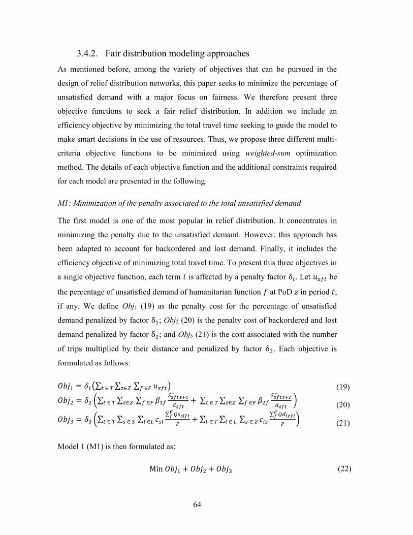
64
3.4.2. Fair distribution modeling approaches As mentioned before, among the variety of objectives that can be pursued in the
design of relief distribution networks, this paper seeks to minimize the percentage of
unsatisfied demand with a major focus on fairness. We therefore present three
objective functions to seek a fair relief distribution. In addition we include an
efficiency objective by minimizing the total travel time seeking to guide the model to
make smart decisions in the use of resources. Thus, we propose three different multi-
criteria objective functions to be minimized using weighted-sum optimization
method. The details of each objective function and the additional constraints required
for each model are presented in the following.
M1: Minimization of the penalty associated to the total unsatisfied demand
The first model is one of the most popular in relief distribution. It concentrates in
minimizing the penalty due to the unsatisfied demand. However, this approach has
been adapted to account for backordered and lost demand. Finally, it includes the
efficiency objective of minimizing total travel time. To present this three objectives in
a single objective function, each term 𝑖 is affected by a penalty factor δ𝑖. Let 𝑢𝑧𝑓𝑡 be
the percentage of unsatisfied demand of humanitarian function 𝑓 at PoD 𝑧 in period 𝑡,
if any. We define Obj1 (19) as the penalty cost for the percentage of unsatisfied
demand penalized by factor δ1; Obj2 (20) is the penalty cost of backordered and lost
demand penalized by factor δ2; and Obj3 (21) is the cost associated with the number
of trips multiplied by their distance and penalized by factor δ3. Each objective is
formulated as follows:
𝑂𝑏𝑗1 = 𝛿1(∑ ∑ ∑ 𝑢𝑧𝑓𝑡𝑓 ∈𝐹𝑧∈𝑍 𝑡 ∈ 𝑇 ) (19)
𝑂𝑏𝑗2 = 𝛿2 (∑ ∑ ∑ 𝛽1𝑓
𝑆𝑧𝑓𝑡,𝑡+1−
𝑑𝑧𝑓𝑡𝑓 ∈𝐹𝑧∈𝑍 𝑡 ∈ 𝑇 + ∑ ∑ ∑ 𝛽2𝑓
𝑆𝑧𝑓𝑡,𝑡+2−
𝑑𝑧𝑓𝑡𝑓 ∈𝐹𝑧∈𝑍 𝑡 ∈ 𝑇 ) (20)
𝑂𝑏𝑗3 = 𝛿3 (∑ ∑ ∑ 𝑐𝑠𝑙
∑ 𝑄𝑠𝑠𝑙𝑓𝑡𝐹𝑓
𝑃𝑙 ∈𝐿𝑠 ∈ 𝑆 𝑡 ∈ 𝑇 + ∑ ∑ ∑ 𝑐𝑙𝑧
∑ 𝑄𝑑𝑙𝑧𝑓𝑡𝐹𝑓
𝑃𝑧 ∈ 𝑍𝑙 ∈ 𝐿 𝑡 ∈ 𝑇 ) (21)
Model 1 (M1) is then formulated as:
Min 𝑂𝑏𝑗1 + 𝑂𝑏𝑗2 + 𝑂𝑏𝑗3 (22)
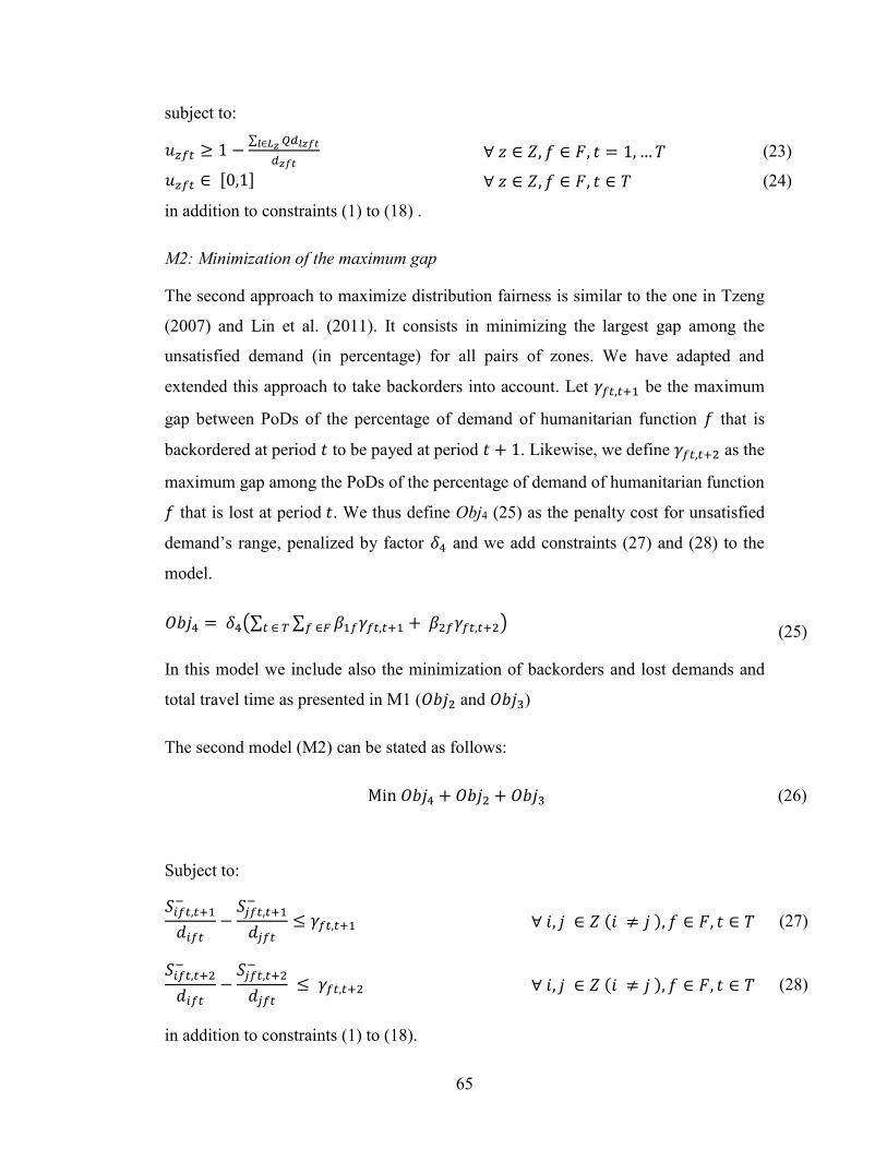
65
subject to:
𝑢𝑧𝑓𝑡 ≥ 1 −∑ 𝑄𝑑𝑙𝑧𝑓𝑡𝑙∈𝐿𝑧
𝑑𝑧𝑓𝑡 ∀ 𝑧 ∈ 𝑍, 𝑓 ∈ 𝐹, 𝑡 = 1, … 𝑇 (23)
𝑢𝑧𝑓𝑡 ∈ [0,1] ∀ 𝑧 ∈ 𝑍, 𝑓 ∈ 𝐹, 𝑡 ∈ 𝑇 (24)
in addition to constraints (1) to (18) .
M2: Minimization of the maximum gap
The second approach to maximize distribution fairness is similar to the one in Tzeng
(2007) and Lin et al. (2011). It consists in minimizing the largest gap among the
unsatisfied demand (in percentage) for all pairs of zones. We have adapted and
extended this approach to take backorders into account. Let 𝛾𝑓𝑡,𝑡+1 be the maximum
gap between PoDs of the percentage of demand of humanitarian function 𝑓 that is
backordered at period 𝑡 to be payed at period 𝑡 + 1. Likewise, we define 𝛾𝑓𝑡,𝑡+2 as the
maximum gap among the PoDs of the percentage of demand of humanitarian function
𝑓 that is lost at period 𝑡. We thus define Obj4 (25) as the penalty cost for unsatisfied
demand’s range, penalized by factor 𝛿4 and we add constraints (27) and (28) to the
model.
𝑂𝑏𝑗4 = 𝛿4(∑ ∑ 𝛽1𝑓𝛾𝑓𝑡,𝑡+1 + 𝛽2𝑓𝛾𝑓𝑡,𝑡+2𝑓 ∈𝐹𝑡 ∈ 𝑇 ) (25)
In this model we include also the minimization of backorders and lost demands and
total travel time as presented in M1 (𝑂𝑏𝑗2 and 𝑂𝑏𝑗3)
The second model (M2) can be stated as follows:
Min 𝑂𝑏𝑗4 + 𝑂𝑏𝑗2 + 𝑂𝑏𝑗3 (26)
Subject to:
𝑆𝑖𝑓𝑡,𝑡+1−
𝑑𝑖𝑓𝑡−
𝑆𝑗𝑓𝑡,𝑡+1−
𝑑𝑗𝑓𝑡≤ 𝛾𝑓𝑡,𝑡+1 ∀ 𝑖, 𝑗 ∈ 𝑍 (𝑖 ≠ 𝑗 ), 𝑓 ∈ 𝐹, 𝑡 ∈ 𝑇 (27)
𝑆𝑖𝑓𝑡,𝑡+2−
𝑑𝑖𝑓𝑡−
𝑆𝑗𝑓𝑡,𝑡+2−
𝑑𝑗𝑓𝑡 ≤ 𝛾𝑓𝑡,𝑡+2 ∀ 𝑖, 𝑗 ∈ 𝑍 (𝑖 ≠ 𝑗 ), 𝑓 ∈ 𝐹, 𝑡 ∈ 𝑇 (28)
in addition to constraints (1) to (18).
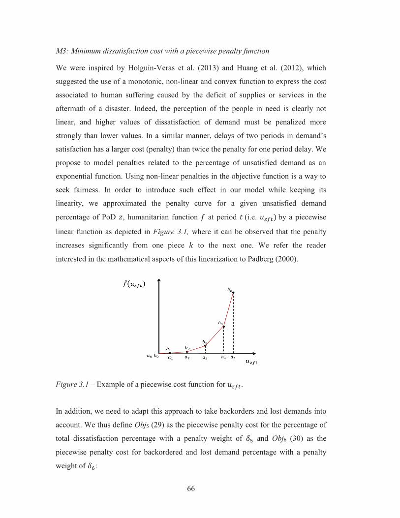
67
𝑂𝑏𝑗5 = 𝛿5 ∑ ∑ ∑ 𝑓 ∈ 𝐹𝑧 ∈ 𝑍 𝑡 ∈ 𝑇 [𝑓(𝑢𝑧𝑓𝑡𝑘)] (29)
𝑂𝑏𝑗6 = 𝛿6[𝛽1𝑓𝑓(𝑢𝑧𝑓𝑡,𝑡+1,𝑘) + 𝛽2𝑓𝑓(𝑢𝑧𝑓𝑡,𝑡+2,𝑘)] (30)
Then, we include the efficiency objective (𝑂𝑏𝑗3) as is done in M1 and M2. M3 can be
stated as follows:
𝑀𝑖𝑛 𝑂𝑏𝑗5 + 𝑂𝑏𝑗6 + 𝑂𝑏𝑗3 (31)
The first two terms of (31) accounts for the penalty associated to unsatisfied demand
(as well as the backorder and lost demand) for each product, each PoD and each
period. This is given by the piecewise linear function defined by the following
functions:
𝑓(𝑢𝑧𝑓𝑡𝑘) = ∑ 𝑐𝑘 𝐾𝑘=1 𝑢𝑧𝑓𝑡𝑘 (32)
𝑓(𝑢𝑧𝑓𝑡,𝑡+1,𝑘) = ∑ 𝑐𝑘 𝐾𝑘=1 𝑢𝑧,𝑓,𝑡,𝑡+1,𝑘 (33)
𝑓(𝑢𝑧𝑓𝑡,𝑡+2,𝑘) = ∑ 𝑐𝑘 𝐾𝑘=1 𝑢𝑧,𝑓,𝑡,𝑡+2,𝑘 (34)
where 𝑢𝑧𝑓𝑡𝑘 ∈ [0, 𝑎𝑘 − 𝑎𝑘−1] is the percentage, of the demand of function 𝑓 not
delivered to PoD 𝑧 at period 𝑡, that is inside the piece 𝑘, 𝑐𝑘 is the slope of piece 𝑘
(𝑐𝑘 =𝑏𝑘−𝑏𝑘−1
𝑎𝑘−𝑎𝑘−1) and (𝑎𝑘, 𝑏𝑘) is the breaking point of the piecewise function related to
piece 𝑘 (same for backorder and lost demand). The last term computes the penalty
associated to distribution time as in the previous models. Model M3 requires the
following constraints (in addition to constraints (1) to (18)):
∑ 𝑢𝑧𝑓𝑡𝑘𝐾𝑘=1 ≥ 1 −
∑ 𝑄𝑑𝑙𝑧𝑓𝑡𝑙∈𝐿𝑧
𝑑𝑧𝑓𝑡 ∀ 𝑧 ∈ 𝑍, 𝑓 ∈ 𝐹, 𝑡 = 1, … 𝑇 (35)
∑ 𝑢𝑧,𝑓,𝑡,𝑡+1,𝑘𝐾𝑘=1 =
𝑆𝑧𝑓𝑡,𝑡+1−
𝑑𝑧𝑓𝑡 ∀ 𝑧 ∈ 𝑍, 𝑓 ∈ 𝐹, 𝑡 = 1, … 𝑇 (36)
∑ 𝑢𝑧,𝑓,𝑡,𝑡+2,𝑘𝐾𝑘=1 =
𝑆𝑧𝑓𝑡,𝑡+2−
𝑑𝑧𝑓𝑡 ∀ 𝑧 ∈ 𝑍, 𝑓 ∈ 𝐹, 𝑡 = 1, … 𝑇 (37)
𝑢𝑧𝑓𝑡𝑘 ≤ (𝑎𝑘 − 𝑎𝑘−1) ∀ 𝑧 ∈ 𝑍, 𝑓 ∈ 𝐹, 𝑡 = 1, … 𝑇, 𝑘 ∈ 𝐾 (38)

68
𝑢𝑧𝑓𝑡,𝑡+1,𝑘 ≤ (𝑎𝑘 − 𝑎𝑘−1) ∀ 𝑧 ∈ 𝑍, 𝑓 ∈ 𝐹, 𝑡 = 1, … 𝑇, 𝑘 ∈ 𝐾 (39)
𝑢𝑧𝑓𝑡,𝑡+2,𝑘 ≤ (𝑎𝑘 − 𝑎𝑘−1) ∀ 𝑧 ∈ 𝑍, 𝑓 ∈ 𝐹, 𝑡 = 1, … 𝑇, 𝑘 ∈ 𝐾 (40)
𝑢𝑧𝑓𝑡𝑘, 𝑢𝑧𝑓𝑡,𝑡+1,𝑘, 𝑢𝑧𝑓𝑡,𝑡+2,𝑘 ∈ [0,1] ∀ 𝑧 ∈ 𝑍, 𝑓 ∈ 𝐹, 𝑡 ∈ 𝑇 (41)
Constraints (35) to (37) link the piecewise variables and the demand shortage
quantities, computing the total percentage of unsatisfied demand, the demand
backorder at periods t + 1 and t + 2 (lost demand) respectively, divided by demand
of period 𝑡. Notice that in the case of a compensation (i.e. if backordered demand is
paid in a given period 𝑡), the total delivery might be higher than the demand of 𝑡. In
this case, the dissatisfaction percentage is computed as null. Constraints (38) to (40)
ensure that variables 𝑢𝑧𝑡𝑓,𝑡+1,𝑘 and 𝑢𝑧𝑡𝑓,𝑡+2,𝑘 cannot be greater that the length of
interval 𝑘. These constraints, together with the objective function, force the sequential
use of each piece of the piecewise function for variables 𝑢𝑧𝑓𝑡𝑘, 𝑢𝑧𝑓𝑡,𝑡+1,𝑘, 𝑢𝑧𝑓𝑡,𝑡+2,𝑘
respectively. Constraint set (41) define the domain for the piecewise variables.
Needless to say, the quality of the solutions produced by model M3 depends on the
number and the bounds of the pieces used in the piecewise function. Therefore, a
heuristic procedure is proposed to find a good compromise in this matter. This
method is presented in the next paragraphs.
3.4.3. Iterative approach to construct the piecewise linear function The number of pieces in the piecewise linear function and their breakpoints have a
strong influence on the quality of the solution as well as on its solvability. Three
considerations must be kept in mind when designing the piecewise function. First, a
better approximation of the exponential function may be obtained by using more
pieces, but by doing so the model becomes more difficult to solve. Second, since the
piecewise cost function is intended to enforce equity by trying to group all PoDs in
the same dissatisfaction level (the same piece) pieces should be small enough. Third,
the fairest value of unsatisfied demand depends on the offer/demand ratio of a period
and its evolution in time. In other words, the proper number and value of each piece
can differ according to the specific instance. We therefore propose a heuristic

69
procedure to fix the number of pieces, the bounds of each one as well as the slope of
each piece by an iterative approach.
In the following, we illustrate the algorithm used to set the piecewise function of a
particular humanitarian function 𝑓 (i.e. considering 𝑢𝑧𝑓𝑡 as 𝑢𝑧𝑡). The heuristic is
initialized with only two pieces per variable (|𝐾| = 2). We define 𝐴 as the set of
breakpoints 𝑎𝑘. 𝐴 is initialized with the minimum value of the ratio offer/demand in
the horizon (named 𝑚𝑖𝑛𝑡 𝜌𝑡), seeking to fix an upper bound of dissatisfaction i.e. 𝐴 =
{0; min𝑡 𝜌𝑡 ; 1}. Then, M3 is solved to optimality and the solution produced is
analyzed in order to decide if new pieces should be added to the piecewise function
and the model solved again (next iteration).
At a given iteration 𝑖, the average unsatisfied demand’s percentage (𝑢..𝑖) and the
global standard deviation (𝜎𝑔𝑙𝑜𝑏𝑎𝑙𝑖 as defined in Section 3.1) of the present solution
are computed. If 𝜎𝑔𝑙𝑜𝑏𝑎𝑙𝑖 is greater than the standard deviation goal (𝜎𝑤𝑎𝑛𝑡𝑒𝑑 set
arbitrary to zero), three new pieces are added around 𝑢..𝑖, with three new breakpoints
added to set 𝐴 as {𝑢..𝑖 −
𝜎𝑔𝑙𝑜𝑏𝑎𝑙𝑖
2; 𝑢..
𝑖 ; 𝑢..𝑖 +
𝜎𝑔𝑙𝑜𝑏𝑎𝑙𝑖
2}. Slopes for all the pieces are
recalculated. To this end, we set a base penalty value for the first piece in the
function, and then the slope for each piece is increased by 1.1 times the rate between
the highest and the lowest demand (i.e. 𝑐𝑘 = 𝑐𝑘−1 × 1.1 𝐷𝑚𝑎𝑥
𝐷𝑚𝑖𝑛 ). After the
recalculating the cost piecewise function, the model is redefined and solved again. If
the new solution results in a reduction in 𝜎𝑔𝑙𝑜𝑏𝑎𝑙𝑖 a new iteration 𝑖 + 1 begins. If no
improvement is achieved, the same procedure is applied over the backorder and lost
demand variables. The procedure is repeated until a given stop criterion is met (e.g.
maximal number of iterations, or until the improvement obtained with current
iteration is not significant or null). At the end, the last solution is retained and
reported as the solution of M3. The Algorithm 3.1 allows us to adapt the shape of the
piecewise function dynamically.
71
planning horizon (|T|). A problem is defined over a total area (TA) of [1000 × 900],
inside of which we define an affected area (AA) of [600 × 500]. The PoDs’ and
HADCs’ location is randomly generated inside the AA, and the set of suppliers inside
the TA, but outside the AA. The demand for each PoD at the first period is randomly
generated in the range of [20;70] for every humanitarian function. The capacity of
any HADC 𝑙 is set at 60% of the total demand (𝐶𝑎𝑝𝐷𝑙𝑓𝑡 = 0.6 ∑ 𝑑𝑧𝑓𝑡𝑧∈𝑍 ). In all our
numerical experiments we seek to represent our main interest in minimizing the
unsatisfied demand percentage and the fairness objective, which has been overlooked
in the past. Therefore, in M1 we applied δ1 ≫ δ2 ≫ δ3, with δ1 ≅ 100δ2 ≅ 1000δ3;
for M2 we applied δ4 ≫ δ2 ≫ δ3, with δ4 ≅ 100δ2 ≅ 1000δ3 and for M3 we
applied δ5 ≫ δ6 ≫ δ3, with δ5 ≅ 100δ6 ≅ 1000δ3.
Depending on the nature and the gravity of the event (demand) and the availability of
resources (number and capacity of responders), different supply scenarios can be
considered. Following that, we defined two basic theoretical scenarios.
Scenario 1 - Temporary shortness of resources
In the first periods in the aftermath of a disaster, the available resources are limited
and vary from one period to another on the planning horizon. In other words, periods
of shortness alternate with others showing reasonable offer levels corresponding to
the arrival of help from national and international organizations. In this case, the
backordering of the unsatisfied demand becomes an interesting solution available to
crisis managers.
Scenario 2: Extreme shortness of resources
In this scenario, the available supplies, in addition to the foreseen arrivals of relief,
will be systematically under the requirements. Crisis managers cannot make a
commitment towards future deliveries to compensate for the shortness. In this case,
crisis managers would try to distribute the available relief in the most fair manner.
We model both of our instances’ scenarios for a particular humanitarian function on
an offer/demand ratio 𝜌𝑡 for each time periods. In temporary shortness, suppliers have


73
If we look at how shortage is shared between the PoDs for a given period, M2 and
M3 split the shortness in a rather homogeneous manner: all the PoDs suffer similar
shortages. However, M1 concentrates shortages only on a few PoDs, and those will
experience very high values of dissatisfaction. For instance, PoD four’s demand is
100%, 50% and 50% unsatisfied in periods two to four. If we now look at how the
global shortage is handled in time, we observe that M1 and M2 simply distribute the
available quantities at each period. However, M3 shows a more elaborated behavior,
which translates in a smoother distribution. In fact, M3 reserves some quantities
during periods one and two in order to minimize the impact of the shortage in periods
three to five. Doing so, the maximum dissatisfaction percentage suffered by any PoD
and at any period is under 20%, while in M1’s solution some PoDs experience up to
100% of unsatisfied demand and in M2’s solution PoDs suffer up to 60%. The
piecewise approximation achieves a rationalization of resources, resulting in an
equitable distribution among PoDs (the same or almost the same dissatisfaction level)
in a period, and this in a stable matter across time in the shortness periods. To sum
up, both M2 and M3’s solutions achieve a good “equity” between the PoDs, but M3
is also able to achieve an excellent “stability”.
Let us now see how these behaviors are captured by the proposed numerical
indicators. Table 3.1 reports the numerical results produced by models M1, M2 and
M3. To measure the quality of the distribution plan obtained by each model, we
report two global measures: the global average dissatisfaction percentage (𝑢..), and
the global standard deviation (𝜎𝑔𝑙𝑜𝑏𝑎𝑙), which concerns to the dispersion in
distribution. Then, we also compute mean sum of squares within time (𝑊𝑇 ) and
between time (𝐵𝑇 ) and the two range indicators (𝑅1 and 𝑅2
). Finally, we calculate the
total traveled distance (𝐷) and record the total computation time to solve each model
in seconds.
Let us consider first the results produced for I1. We observe that M1 achieves a lower
value for 𝑢.. (i.e. a better global satisfaction). The reason is that, although all the three
models distribute the same quantity of help, M1 prefers to give slightly higher
quantities to PoDs 5 and 6 because the marginal impact of a single additional help
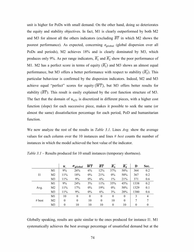
74
unit is higher for PoDs with small demand. On the other hand, doing so deteriorates
the equity and stability objectives. In fact, M1 is clearly outperformed by both M2
and M3 for almost all the others indicators (excluding 𝐵𝑇 in which M2 shows the
poorest performance). As expected, concerning 𝜎𝑔𝑙𝑜𝑏𝑎𝑙 (global dispersion over all
PoDs and periods), M2 achieves 18% and is clearly dominated by M3, which
produces only 9%. As per range indicators, 𝑅1 and 𝑅2
show the poor performance of
M1. M2 has a perfect score in terms of equity (𝑅1 ) and M3 shows an almost equal
performance, but M3 offers a better performance with respect to stability (𝑅2 ). This
particular behaviour is confirmed by the dispersion indicators. Indeed, M2 and M3
achieve equal “perfect” scores for equity (𝑊𝑇 ), but M3 offers better results for
stability (𝐵𝑇 ). This result is easily explained by the cost function structure of M3.
The fact that the domain of 𝑢𝑧𝑓𝑡 is discretized in different pieces, with a higher cost
function (slope) for each successive piece, makes it possible to seek the same (or
almost the same) dissatisfaction percentage for each period, PoD and humanitarian
function.
We now analyze the rest of the results in Table 3.1. Lines Avg. show the average
values for each column over the 10 instances and lines # best counts the number of
instances in which the model achieved the best value of the indicator.
Table 3.1 – Results produced for 10 small instances (temporary shortness).
𝒖.. 𝝈𝒈𝒍𝒐𝒃𝒂𝒍 𝑾𝑻 𝑩𝑻 𝑹𝟏
𝑹𝟐 D Sec.
I1 M1 9% 26% 6% 12% 37% 50% 364 0.2 M2 11% 18% 0% 21% 0% 50% 367 0.2 M3 11% 9% 0% 6% 1% 21% 371 0.6
Avg. M1 9% 24% 5% 11% 35% 45% 1338 0.2 M2 11% 17% 0% 19% 0% 50% 1329 0.1 M3 11% 9% 0% 6% 3% 20% 1380 0.6
# best M1 10 0 0 0 0 0 3 4 M2 0 0 10 0 10 0 7 7 M3 0 10 10 10 0 10 0 0
Globally speaking, results are quite similar to the ones produced for instance I1. M1
systematically achieves the best average percentage of unsatisfied demand but at the
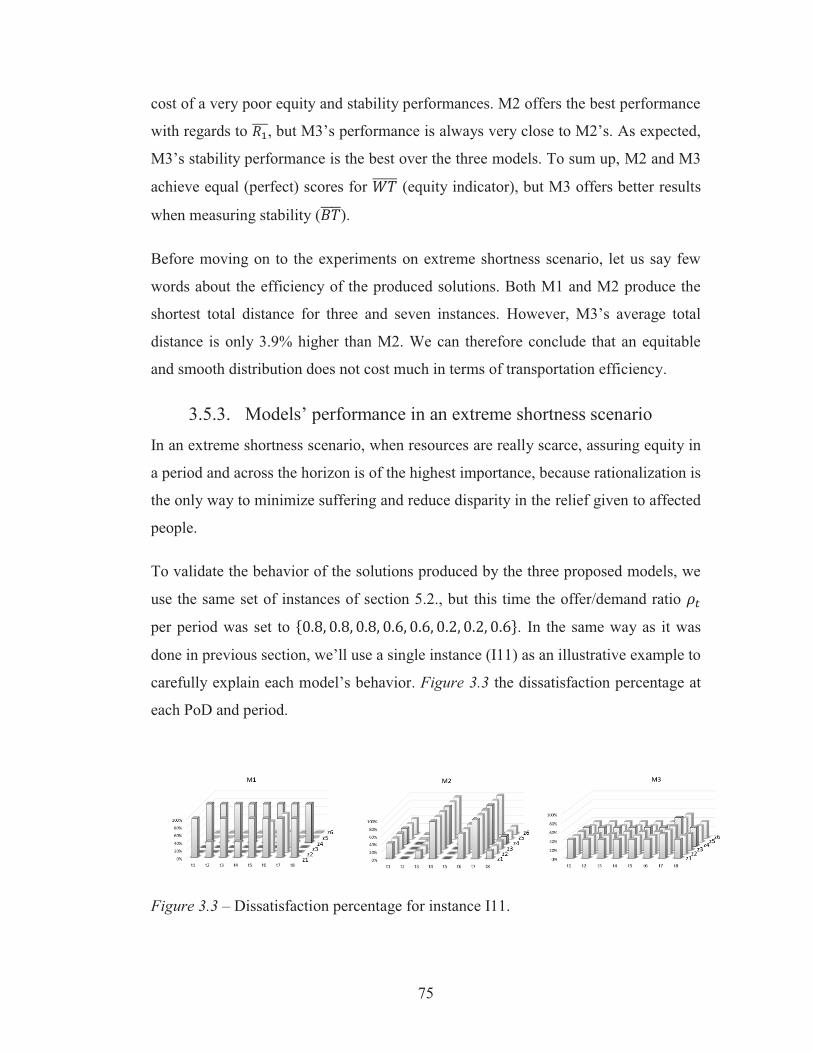
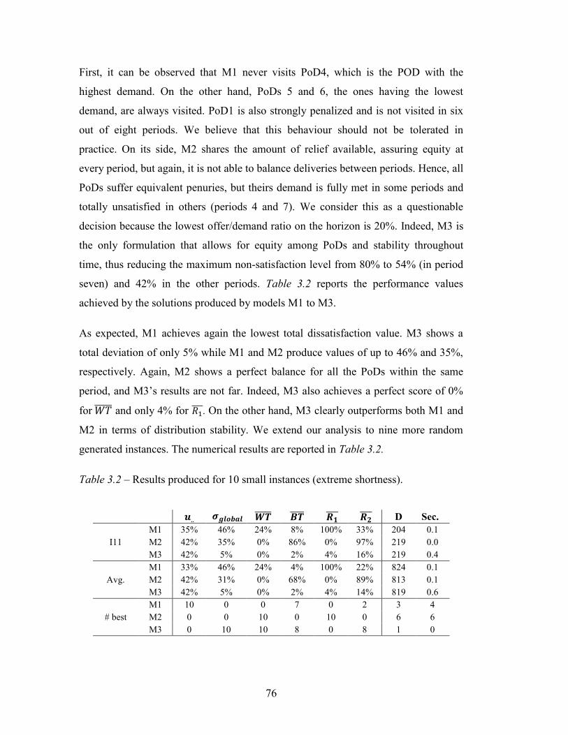
76
First, it can be observed that M1 never visits PoD4, which is the POD with the
highest demand. On the other hand, PoDs 5 and 6, the ones having the lowest
demand, are always visited. PoD1 is also strongly penalized and is not visited in six
out of eight periods. We believe that this behaviour should not be tolerated in
practice. On its side, M2 shares the amount of relief available, assuring equity at
every period, but again, it is not able to balance deliveries between periods. Hence, all
PoDs suffer equivalent penuries, but theirs demand is fully met in some periods and
totally unsatisfied in others (periods 4 and 7). We consider this as a questionable
decision because the lowest offer/demand ratio on the horizon is 20%. Indeed, M3 is
the only formulation that allows for equity among PoDs and stability throughout
time, thus reducing the maximum non-satisfaction level from 80% to 54% (in period
seven) and 42% in the other periods. Table 3.2 reports the performance values
achieved by the solutions produced by models M1 to M3.
As expected, M1 achieves again the lowest total dissatisfaction value. M3 shows a
total deviation of only 5% while M1 and M2 produce values of up to 46% and 35%,
respectively. Again, M2 shows a perfect balance for all the PoDs within the same
period, and M3’s results are not far. Indeed, M3 also achieves a perfect score of 0%
for 𝑊𝑇 and only 4% for 𝑅1 . On the other hand, M3 clearly outperforms both M1 and
M2 in terms of distribution stability. We extend our analysis to nine more random
generated instances. The numerical results are reported in Table 3.2.
Table 3.2 – Results produced for 10 small instances (extreme shortness).
𝒖.. 𝝈𝒈𝒍𝒐𝒃𝒂𝒍 𝑾𝑻 𝑩𝑻 𝑹𝟏
𝑹𝟐 D Sec.
I11 M1 35% 46% 24% 8% 100% 33% 204 0.1 M2 42% 35% 0% 86% 0% 97% 219 0.0 M3 42% 5% 0% 2% 4% 16% 219 0.4
Avg. M1 33% 46% 24% 4% 100% 22% 824 0.1 M2 42% 31% 0% 68% 0% 89% 813 0.1 M3 42% 5% 0% 2% 4% 14% 819 0.6
# best M1 10 0 0 7 0 2 3 4 M2 0 0 10 0 10 0 6 6 M3 0 10 10 8 0 8 1 0

77
As in the temporary shortness case, M3 minimizes global deviation and offers the
best possible equity and stability performances at a negligible increase in the
distribution distance.
3.5.4. Models’ performance in larger-sized instances We will dedicate the last part of this section to show the models’ performance over a
set of 20 instances with a more realistic size. The objective is to test the models’
capacity to ensure a fair distribution over a much larger set of PoDs, and to test, at the
same time, the computational effort of each model. Following the pattern described in
section 5.2 and 5.3, we solve 10 instances for temporary shortness and 10 instances
for extreme shortness cases. For each scenario we test five medium-size instances and
five large-size instances. We define as “medium-size” instances with a total of 20
PoDs, 10 potential HADCs, six suppliers, one humanitarian function and eight
periods. Large-size instances have 50 PoDs, 20 HADCs, six suppliers, one function
and eight periods. Table 3.3 and Table 3.4 summarize the results for the temporary
and extreme shortness scenarios respectively.
Table 3.3 – Results produced for larger-sized instances in temporary shortness.
𝒖.. 𝝈𝒈𝒍𝒐𝒃𝒂𝒍 𝑾𝑻 𝑩𝑻 𝑹𝟏
𝑹𝟐 D Sec.
Avg. over 5 medium instances
M1 9% 26% 6% 35% 62% 45% 3590 0.1 M2 11% 17% 0% 63% 0% 49% 3475 2.3 M3 11% 9% 0% 18% 3% 19% 4005 1.6
Avg. over 5 large instances
M1 9% 27% 6% 89% 62% 49% 8003 0.3 M2 11% 16% 0% 143% 0% 49% 7782 35.3 M3 10% 9% 0% 45% 4% 19% 8840 3.4
Table 3.4 – Results produced for larger-sized instances in extreme shortness.
𝒖.. 𝝈𝒈𝒍𝒐𝒃𝒂𝒍 𝑾𝑻 𝑩𝑻 𝑹𝟏
𝑹𝟐 D Sec.
Avg. over 5 medium instances
M1 33% 47% 23% 6% 100% 12% 2110 0.1 M2 43% 30% 0% 205% 0% 93% 2062 2.9 M3 42% 2% 0% 0% 4% 4% 2069 1.4
Avg. over 5 large instances
M1 33% 47% 22% 1% 100% 4% 4751 0.2 M2 42% 26% 0% 413% 0% 76% 4657 10.2 M3 42% 3% 0% 1% 5% 4% 4723 0.9

80
Holguín-Veras, J., Pérez, N., Jaller, M., Van Wassenhove, L.N. & Aros-Vera, F., 2013. On the appropriate objective function for post-disaster humanitarian logistics models. Journal of Operations Management, 31(5), pp.262–280.
Huang, M., Smilowitz, K. & Balcik, B., 2012. Models for relief routing: Equity, efficiency and efficacy. Transportation research part E: logistics and transportation review, 48(1), pp.2–18.
Kovács, G. & Spens, K., 2007. Humanitarian logistics in disaster relief operations. International Journal of Physical Distribution & Logistics Management, 37(2), pp.99–114.
Lin, Y., Batta, R., Rogerson, P., Blatt, A. & Flanigan, M., 2011. A logistics model for emergency supply of critical items in the aftermath of a disaster. Socio-Economic Planning Sciences, 45(4), pp.132 – 145.
Lin, Y., Batta, R., Rogerson, P.A., Blatt, A. & Flanigan, M., 2011. A logistics model for emergency supply of critical items in the aftermath of a disaster. Socio-Economic Planning Sciences, 45(4), pp.132–145.
Lin, Y., Batta, R., Rogerson, P.A., Blatt, A. & Flanigan, M., 2012. Location of temporary depots to facilitate relief operations after an earthquake. Socio-Economic Planning Sciences. 46(2), pp.112–123.
Padberg, M., 2000. Approximating separable nonlinear functions via mixed zero-one programs. Operations Research Letters, 27(1), pp.1–5.
Rekik, M., Ruiz, A., Renaud, J., Berkoune, D. & Paquet, S., 2013. A decision support system for humanitarian network design and distribution operations. In Humanitarian and Relief Logistics: research issues, case studies and future trends. edited by Zeimpekis, V., and Ichoua, S., and Minis, I., pp. 1–20. New York: Springer.
Suzuki, Y., 2012. Disaster-Relief Logistics With Limited Fuel Supply. Journal of Business Logistics, 33(2), pp.145–157.
Tzeng, G.H., Cheng, H.J. & Huang, T.D., 2007. Multi-objective optimal planning for designing relief delivery systems. Transportation Research Part E: Logistics and Transportation Review, 43(6), pp.673–686.
Vitoriano, B., Ortuño, T., Tirado, G. & Montero, J., 2010. A multi-criteria optimization model for humanitarian aid distribution. Journal of Global Optimization, pp.1–20.

81
Vitoriano, B., Ortuño, T. & Tirado, G., 2009. HADS, a goal programming-based humanitarian aid distribution system. Journal of Multi-Criteria Decision Analysis, 16 (1-2), pp.55–64.
Yushimito, W.F., Jaller, M. & Ukkusuri, S., 2012. A Voronoi-based heuristic algorithm for locating distribution centers in disasters. Networks and Spatial Economics, 12(1), pp.21–39.

82
Chapitre 4
4. Transport des échantillons biomédicaux dans la province de Québec : un cas d’étude
Le transport d’échantillons biomédicaux joue un rôle central dans un système de
santé efficace. Développé dans le cadre d’une collaboration avec le Ministère de la
Santé et des Services sociaux du Québec (MSSS), cet article décrit les défis du
transport d’échantillons biomédicaux pour la province du Québec. Ce problème est
modélisé comme une variante du problème de tournées de véhicules avec fenêtres de
temps et plusieurs voyages. Les routes sont planifiées à partir d’un laboratoire pour
satisfaire les requêtes de transport d’échantillons qui proviennent des centres de
prélèvement du réseau, tout en considérant plusieurs contraintes pratiques. On
considère que ces routes sont effectuées par un transporteur externe et facturées en
termes de distance (nombre total de kilomètres à parcourir). Autrement dit, il n’y a
pas un coût fixe à payer pour l’utilisation d’un véhicule. Cependant, le gestionnaire
du réseau a toujours intérêt à avoir une estimation du nombre total de véhicules qui
sont demandés dans le plan de transport. Nous proposons deux formulations
mathématiques alternatives ainsi que quelques heuristiques rapides pour minimiser la
distance totale parcourue dans le processus de transport. La performance de la
méthode proposée est testée sur un cas d’étude réel de la province de Québec.
Article 3: Biomedical sample transportation in the province of
Quebec: a case study
Ce chapitre fait l’objet d’une publication sous la forme d’article de journal : Anaya-
Arenas, A.M., Chabot, T., Renaud, J. & Ruiz, A., 2015. Biomedical sample
transportation in the province of Quebec: a case study. International Journal of
Production Research, (ahead-of-print), pp.1–14.
Abstract: Biomedical sample management plays a central role in an efficient
healthcare system and requires important resources. Based on our collaboration with
the Quebec’s Ministère de la Santé et des Services sociaux (Ministry of Health and
84
transportation and (2) the quality of the transportation done by the transportation
providers.
Aiming at improving the services offered to the population and controlling the
associated costs, the MSSS engaged in a supply chain optimisation project named
Optilab. Optilab seeks to enhance the quality of the services provided by the network
of laboratories in terms of security, accessibility, efficiency and efficacy (MSSS,
2012). To this end, Optilab intends to formalize and consolidate the transportation of
biomedical specimens in Quebec. In fact, the MSSS plans to contract samples’
transportation services to private carriers selected through a public tender process
specifying the technical requirements and physical conditions ruling the samples’
transportation. However, in order to receive realistic bids, the MSSS cannot only
provide the total number of samples to transport and the list of origins and
destinations. Instead, the MSSS must provide a statement of works (SOW) translating
their requirements into “transportation efforts” expressed in terms of approximated
number of pickups and deliveries to perform, realistic number of vehicles needed, the
shape and distance of the routes, and other logistic information. This is precisely the
goal of the present research aimed at organizing and establishing daily transportation
operations for biomedical samples. The results of this research will help the MSSS to
estimate their transportation needs rather than biomedical ones, in order to compose
their future SOW, allowing the private providers to determine their best bids.
This paper presents two major contributions. Firstly, it describes the Quebec’s
biomedical sample transportation context and proposes two alternative formulations
for solving it. Secondly, it proposes a solving approach able to produce transportation
plans to deal efficiently with the daily sample transportation needs of the Quebec’s
healthcare network. These plans will provide good estimations of the logistic work to
be performed by external contractors and will assist the MSSS in refining their future
SOW.
This article is structured as follows. Section 2 describes the biomedical sample
transportation context. Section 3 reviews the related literature. Section 4 presents two
mathematical formulations, and Section 5 introduces heuristic approaches to solve it.

86
samples’ maximum transportation time and the multiple transportation requests at
each SCC. Unlike other related contexts, such as blood collecting (Doerner et al.,
2008 and Doerner and Hartl, 2008) which considers that the product starts
deteriorating right after the donation, we assume that as long as samples are kept at
SCCs, their deterioration is slowed down due to the controlled temperature and
optimal storage conditions. However, as soon as samples are out of the SCC facilities,
the samples integrity cannot be guaranteed, even if they are transported in cooler
boxes. Therefore, we modeled this limitation on a maximal transportation time,
which depends on the type of the particular samples collected, to preserve the
samples’ lifespan. Thus, after collection, each sample box must arrive at the lab
within a given time frame. Otherwise, samples deteriorate and may become unusable,
increasing tremendously both the lab’s costs and affecting the quality of the service.
In fact, an unusable sample forces the patient to make a second collection, which
delays the analysis and doubles the operations costs of the entire process (collecting,
transporting and analyzing).
On the other hand, and despite the ideal environmental conditions at SCCs, the
samples maximum lifespan is limited, so SCCs does not want to keep the collected
specimens for too long a time. This is why each SCC may make a different number of
samples transportation requests, depending on its daily opening hours. For example,
if an SCC is open from 9am to 1pm, it is not desirable to keep the samples during the
entire morning, and then make a single transportation request at the end of the day.
Instead, it is preferable to make at least two different pick-up appointments.
Moreover, these two appointments should not be too close (e.g., it would not be
useful to make a visit at noon and another one at 1pm) because this can prove as
inefficient as just making one pick-up. Hence, we allowed SCCs to propose time
windows for theirs transportation requests according to the particularities of their own
clients and practices; for example, a very active SCC open between 9am to 1pm could
require a first pick-up between 10:30 and 11, and a second one between 13 and 13:30.
These multiple pick-ups are also desirable because they contribute to ensure a
smoother supply of sample boxes to labs and thus help balancing their workload.


88
results to a problem inspired from the case of a French furniture manufacturer.
Recently, Mingozzi et al. (2013) proposed an exact algorithm and solved benchmark
instances with up to 120 customers.
As one could expect, recent research has addressed situations merging time windows
with multi-trip vehicle routing problems (MTVRP-TW). Battarra et al. (2009) solved
a MTVRP-TW with multiple incompatible commodities, with the objective of
minimizing the number of vehicles. Cattaruzza et al. (2014) proposed an iterated local
search algorithm for the MTVRP-TW. Martínez and Amaya (2013) used a tabu
search algorithm for solving an MTVRP-TW with loading constraints. Azi et al.
(2014) developed an adaptive large neighborhood search algorithm for the MTVRP
where the objective is first to maximize the number of served customers, and then to
minimize the total distance traveled by the vehicles. Wang et al. (2014) proposed a
metaheuristic based on a pool of routes to solve the MTVRP-TW. We can conclude
that MTVRP-TW is a rather new, yet challenging, problem reflecting the aim of
researchers to incorporate real life features or attributes into their routing models.
Vidal et al. (2013) presents a very detailed survey compiling most of the constraints
and attributes proposed in the literature for routing problems, as well as the heuristic
approaches developed to deal with them. Later, they developed a unified and generic
solution framework for multi-attribute routing problems (Vidal et al. 2014).
Our review of the related literature allowed us to identify five specific works which
deals with the collection or transportation of biomedical products or presents
characteristics making them appear to be very close to the BSTP. Therefore, it is
worth positioning the BSTP with respect to them. First, Liu et al. (2013) studied a
routing problem where biomedical samples needed to be collected and delivered to
laboratories. In their case, four types of deliveries and pick-up requirements were
considered. As in the BSTP, visits had to respect time windows, but in their case each
node required only one visit and each vehicle performed a single route.
The two following papers, Doerner et al. (2008) and Doerner and Hartl (2008), dealt
with a blood collection problem. As in our context, they assumed a limit on the
transportation time to preserve the blood’s quality, and allowed the planning of


91
Each SCC 𝑖 requires a specific number of transportation requests (𝑞 = 1, … , 𝑄𝑖). For
SCC i, its qth pick-up has to be done inside a time window [𝑎𝑖𝑞, 𝑏𝑖𝑞], where 𝑎𝑖𝑞 is the
earliest time the transport may arrive (otherwise, it has to wait) to perform the pick-up
𝑞 of SCC 𝑖, and 𝑏𝑖𝑞 is the latest accepted arrival time. Time windows are considered
to be hard constraints. In addition, we need to consider the loading time (𝜏𝑖) at each
SCC and the unloading time (τ0) of the vehicle at the Lab before a new route can be
started. Furthermore, let 𝑇𝑚𝑎𝑥𝑖 be the maximal transportation time for the types of
samples collected at SCC i.
In order to define a transportation plan that respects the practical constraints of our
problem and minimize transportation costs, we define the following decision
variables.
𝑥𝑖𝑗𝑘𝑟 Binary variable equal to 1 if the arc (𝑖, 𝑗) is used by vehicle 𝑘 in its route 𝑟; 0 otherwise.
𝑦𝑗𝑞𝑘𝑟 Binary variable equal to 1 if the qth request of SCC 𝑗 is done by vehicle 𝑘 in its route 𝑟; 0 otherwise.
𝑢𝑖𝑘𝑟 Continuous variable that indicates the visit time of SCC 𝑖 by vehicle 𝑘 in route 𝑟.
Model BSTP-MR is stated as follows:
𝑀𝑖𝑛 ∑ ∑ ∑ ∑ 𝑑𝑖𝑗𝑥𝑖𝑗𝑘𝑟
𝑅
𝑟=1
𝐾
𝑘=1
𝑛+1
𝑗=1
𝑛
𝑖=0 (1.1)
Subject to:
∑ 𝑥𝑖𝑗𝑘𝑟𝑛𝑖=0 ≤ 1 𝑗 = 1, … , 𝑛; 𝑘 = 1, … , 𝐾 ;
𝑟 = 1, … , 𝑅
(1.2)
∑ 𝑥𝑖𝑗𝑘𝑟𝑛𝑖=0 − ∑ 𝑥𝑗𝑙𝑘𝑟
𝑛+1𝑙=1 = 0 𝑗 = 1, … , 𝑛; 𝑘 = 1, … , 𝐾 ;
𝑟 = 1, … , 𝑅
(1.3)
∑ 𝑥0𝑗𝑘𝑟𝑛𝑗=1 ≤ 1 𝑘 = 1, … , 𝐾; 𝑟 = 1, … , 𝑅 (1.4)
∑ 𝑥0𝑗𝑘𝑟𝑛𝑗=1 − ∑ 𝑥𝑗,𝑛+1𝑘𝑟
𝑛𝑗=1 = 0 𝑘 = 1, … , 𝐾; 𝑟 = 1, … , 𝑅 (1.5)
∑ 𝑥0𝑗𝑘𝑟𝑛𝑗=1 − ∑ 𝑥0𝑗𝑘𝑟−1
𝑛𝑗=1 ≤ 0 𝑘 = 1, … , 𝐾; 𝑟 = 2, … , 𝑅 (1.6)

92
∑ ∑ 𝑦𝑗𝑞𝑘𝑟𝑅𝑟=1
𝐾𝑘=1 = 1 𝑗 = 1, … , 𝑛; 𝑞 = 1, … 𝑄𝑗 (1.7)
∑ 𝑦𝑗𝑞𝑘𝑟𝑄𝑗
𝑞=1 − ∑ 𝑥𝑖𝑗𝑘𝑟𝑛𝑖=0 = 0 𝑗 = 1, … , 𝑛; 𝑘 = 1, … , 𝐾 ;
𝑟 = 1, … , 𝑅
(1.8)
𝑢𝑖𝑘𝑟 + 𝜏𝑖 + 𝑡𝑖𝑗 − 𝑢𝑗𝑘𝑟 ≤ 𝑇𝑘(1 − 𝑥𝑖𝑗𝑘𝑟) 𝑖 = 0, … , 𝑛; 𝑗 = 1, … 𝑛 + 1;
𝑘 = 1, … , 𝐾 ; 𝑟 = 1, … , 𝑅
(1.9)
𝑎𝑗𝑞 − 𝑇𝑘(1 − 𝑦𝑗𝑝𝑘𝑟) ≤ 𝑢𝑗𝑘𝑟 ≤ 𝑏𝑗𝑞 +
𝑇𝑘(1 − 𝑦𝑗𝑝𝑘𝑟)
𝑗 = 1, … , 𝑛; 𝑘 = 1, … , 𝐾
𝑟 = 1, … , 𝑅; 𝑞 = 1, … , 𝑄𝑗
(1.10)
𝑢0𝑘𝑟 ≥ 𝑢𝑛+1,𝑘,𝑟−1 𝑘 = 1, … , 𝐾; 𝑟 = 2, … , 𝑅 (1.11)
𝑢𝑛+1𝑘𝑟 − 𝑢𝑗𝑘𝑟 ≤ 𝑇𝑚𝑎𝑥𝑗
+ 𝑇𝑘(1 − ∑ 𝑥𝑖𝑗𝑘𝑟𝑛𝑖=0 ) 𝑗 = 1, … , 𝑛; 𝑘 = 1, … , 𝐾 ;
𝑟 = 1, … , 𝑅
(1.12)
𝑢𝑛+1,𝑘𝑟 − 𝑢0,𝑘1 ≤ 𝑇𝑘 k = 1, … , 𝐾; 𝑟 = 1, … , 𝑅 (1.13)
Objective (1.1) is to find a transportation plan that minimizes the total traveled
distance. Constraints (1.2) ensure that an SCC 𝑗 is visited at most once per route 𝑟 of
vehicle k. Constraints (1.3) force the flow of each vehicle 𝑘 for each of its routes 𝑟 to
be balanced at each SCC of the network. This means that if an arc enters node 𝑗 on a
route 𝑟 of vehicle 𝑘, there must be an arc that leaves the same node for the same
(𝑘, 𝑟) combination. Constraints (1.4) state that a truck 𝑘 can start a route 𝑟 or not, but
(1.5) if the vehicle starts a route, it must come back to depot (node 𝑛 + 1).
Constraints (1.6) order the routes; thus, route 𝑟 is started if and only if route 𝑟 − 1 has
already been created. Constraints (1.7) and (1.8) verify the pick-up request
satisfaction. Constraints (1.7) state that each pick-up 𝑞 for each SCC 𝑗 is done by one,
and only one, vehicle route (𝑘, 𝑟) combination; constraints (1.8) link the arc to the
pick-up variables, which means that if a pick-up is done by route 𝑟 of truck 𝑘 it is
because an arc of this combination entered to the node 𝑗. Constraints (1.9) to (1.13)
handle the time constraints. Constraints (1.9) have two main purposes: first, it
estimates the arrival time at every node (clients or dummy depot), and second, it
forces the sub-tours’ elimination. Then, constraints (1.10) set the upper and lower
bound of the time windows, forcing a pick-up q from client 𝑗 and done with vehicle 𝑘
on its route 𝑟 (𝑦𝑗𝑞𝑘𝑟 = 1), to fall within the time window of the pick-up request;

93
otherwise, the constraints are irrelevant (when 𝑦𝑗𝑞𝑘𝑟 = 0). Here Tk is used as a big M
value. Constraints (1.11) ensure that the starting time of route 𝑟 is later than the
arriving time of route 𝑟 − 1 at node (n+1). Constraints (1.12) impose the maximum
transportation time length limit (returning time to the lab minus the pick-up time at
any 𝑗 is less than the limit 𝑇𝑚𝑎𝑥𝑗 if j is visited by vehicle k on its route r). Constraints
(1.13) force vehicle 𝑘 to comply with the total length of its work shift.
Formulation BSTP-MR is difficult to solve due, in part, by the homogeneity of the
considered fleet because there are numerous possible equivalent solutions. Therefore,
and in order to strengthen the formulation, we adapted the two symmetry breaking
constraints proposed by Coelho and Laporte (2014) to our context.
∑ 𝑥0𝑗𝑘1𝑛𝑗=1 − ∑ 𝑥0𝑗𝑘−1,1
𝑛𝑗=1 ≤ 0 𝑘 = 2, … , 𝐾 (1.14)
∑ 𝑦𝑗𝑞𝑘𝑟𝑅𝑟=1 − ∑ ∑ ∑ 𝑦𝑖𝑙𝑘−1,𝑟
𝑅𝑟=1
𝑄𝑗
𝑙=1𝑗−1𝑖=1 −
∑ ∑ 𝑦𝑗𝑙𝑘−1,𝑟𝑅𝑟=1
𝑞−1𝑙=1 ≤ 0
𝑗 = 1, … , 𝑛; 𝑞 = 1, … 𝑄𝑗,
𝑘 = 2, … , 𝐾
(1.15)
Constraints (1.14) state that a vehicle 𝑘 can be used (leave the depot for the first time)
if, and only if, a vehicle 𝑘 − 1 has already been used in a tour. This restriction is
extended to the clients’ nodes with constraints (1.15). These constraints state that if a
request 𝑞 of a SCC 𝑗 is performed by any route of vehicle 𝑘, then a vehicle 𝑘 − 1 is
used and performs the request of at least one client with a smaller index (𝑖 < 𝑗), or a
request of SCC 𝑗 with smaller index than 𝑞 (𝑙 < 𝑞).
4.4.2. Model 2: Extended graph (BSTP-EG) In the BSTP-EG, each transportation request is represented by a specific node, so if
SCC 𝑖 requires 𝑄𝑖 pick-ups, 𝑖 is represented by 𝑄𝑖 nodes located at the same place,
each needing one request. Therefore, the original set N is extended into a set P of p
nodes (𝑝 = ∑ 𝑄𝑖𝑛𝑖=1 ).
We define a complete graph 𝐺2 = {𝑉2, 𝐴}, where 𝑉2 = {𝑣0, 𝑣1, … , 𝑣𝑝, 𝑣𝑝+1} is the set
of nodes in the network, which includes the laboratory as nodes {𝑣0, 𝑣𝑝+1} and the set
94
𝑃 = {𝑣1, 𝑣2, … , 𝑣𝑝}, with the 𝑝 transportation requests of the SCCs. We also define
𝑃𝑛 as the set of nodes representing the pick-ups requested by the original SCC 𝑛.
Therefore, node set 𝑃 is composed of a set of pick-ups originating from different
SCCs (i.e. 𝑃 = ⋃ 𝑃𝑛𝑛 ). Finally, we consider the arc set 𝐴 = {(𝑣𝑖, 𝑣𝑗): 𝑣𝑖 , 𝑣𝑗 ∈
𝑉2, 𝑖 ≠ 𝑗, 𝑖 = 0, … , 𝑝, 𝑗 = 1, … 𝑝 + 1}. Clearly, 𝑡𝑖𝑗 and 𝑑𝑖𝑗 are equal to zero for every
(𝑣𝑖 , 𝑣𝑗) if 𝑖 and 𝑗 ∈ 𝑃𝑛 (i.e. nodes 𝑖 and 𝑗 correspond to two requests from the same
SCC). In addition, each request needs to be performed within its original time
window [𝑎𝑗 , 𝑏𝑗]. Finally, no more than one node from each Pn can be visited on any
route. The rest of the notation of model BSTP-MR is also valid for model BSTP-EG.
The following decisions variables are used:
𝑥𝑖𝑗𝑘𝑟 Binary variable equal to 1 if the arc (𝑖, 𝑗) is used by vehicle 𝑘 on its route 𝑟; 0 otherwise.
𝑢𝑖𝑘𝑟 Continuous variable that indicates the visit time of pick-up 𝑖 by vehicle 𝑘 on route 𝑟.
𝑀𝑖𝑛 ∑ ∑ ∑ ∑ 𝑑𝑖𝑗𝑥𝑖𝑗𝑘𝑟
𝑅
𝑟=1
𝐾
𝑘=1
𝑝+1
𝑗=1
𝑝
𝑖=0 (2.1)
Subject to:
∑ ∑ ∑ 𝑥𝑖𝑗𝑘𝑟𝑝𝑖=0
𝑅𝑟=1
𝐾𝑘=1 = 1 𝑗 = 1, … , 𝑝 (2.2)
∑ ∑ 𝑥𝑖𝑗𝑘𝑟𝑝𝑖=0𝑗 ∈ 𝑃𝑛
≤ 1 𝑛 = 1, … , 𝑁; 𝑘 = 1, … , 𝐾;
𝑟 = 1, … , 𝑅
(2.3)
∑ 𝑥𝑖𝑗𝑘𝑟𝑝𝑖=0 − ∑ 𝑥𝑗𝑙𝑘𝑟
𝑝+1𝑙=1 = 0 𝑗 = 1, … , 𝑝; 𝑘 = 1, … , 𝐾; 𝑟 = 1, … , 𝑅 (2.4)
∑ 𝑥0𝑗𝑘𝑟𝑝𝑗=1 ≤ 1 𝑘 = 1, … , 𝐾; 𝑟 = 1, … , 𝑅 (2.5)
∑ 𝑥0𝑗𝑘𝑟𝑝𝑗=1 − ∑ 𝑥𝑗,𝑝+1𝑘𝑟
𝑝𝑗=1 = 0 𝑘 = 1, … , 𝐾; 𝑟 = 1, … , 𝑅 (2.6)
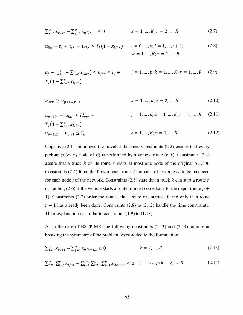
95
∑ 𝑥0𝑗𝑘𝑟𝑝𝑗=1 − ∑ 𝑥0𝑗𝑘𝑟−1
𝑝𝑗=1 ≤ 0 𝑘 = 1, … , 𝐾; 𝑟 = 2, … , 𝑅 (2.7)
𝑢𝑖𝑘𝑟 + 𝜏𝑖 + 𝑡𝑖𝑗 − 𝑢𝑗𝑘𝑟 ≤ 𝑇𝑘(1 − 𝑥𝑖𝑗𝑘𝑟) 𝑖 = 0, … , 𝑝; 𝑗 = 1, … 𝑝 + 1;
𝑘 = 1, … , 𝐾; 𝑟 = 1, … , 𝑅
(2.8)
𝑎𝑗 − 𝑇𝑘(1 − ∑ 𝑥𝑖𝑗𝑘𝑟𝑝𝑖=0 ) ≤ 𝑢𝑗𝑘𝑟 ≤ 𝑏𝑗 +
𝑇𝑘(1 − ∑ 𝑥𝑖𝑗𝑘𝑟𝑝𝑖=0 )
𝑗 = 1, … , 𝑝; 𝑘 = 1, … , 𝐾; 𝑟 = 1, … , 𝑅 (2.9)
𝑢0𝑘𝑟 ≥ 𝑢𝑝+1,𝑘,𝑟−1 𝑘 = 1, … , 𝐾; 𝑟 = 2, … , 𝑅 (2.10)
𝑢𝑝+1𝑘𝑟 − 𝑢𝑗𝑘𝑟 ≤ 𝑇𝑚𝑎𝑥𝑗
+
𝑇𝑘(1 − ∑ 𝑥𝑖𝑗𝑘𝑟𝑝𝑖=0 )
𝑗 = 1, … , 𝑝, 𝑘 = 1, … , 𝐾; 𝑟 = 1, … , 𝑅 (2.11)
𝑢𝑝+1,𝑘𝑟 − 𝑢0,𝑘1 ≤ 𝑇𝑘 k = 1, … , 𝐾; 𝑟 = 1, … , 𝑅 (2.12)
Objective (2.1) minimizes the traveled distance. Constraints (2.2) ensure that every
pick-up 𝑝 (every node of P) is performed by a vehicle route (r, k). Constraints (2.3)
assure that a truck 𝑘 on its route 𝑟 visits at most one node of the original SCC 𝑛.
Constraints (2.4) force the flow of each truck 𝑘 for each of its routes 𝑟 to be balanced
for each node j of the network. Constraints (2.5) state that a truck 𝑘 can start a route 𝑟
or not but, (2.6) if the vehicle starts a route, it must come back to the depot (node 𝑝 +
1). Constraints (2.7) order the routes; thus, route 𝑟 is started if, and only if, a route
𝑟 − 1 has already been done. Constraints (2.8) to (2.12) handle the time constraints.
Their explanation is similar to constraints (1.9) to (1.13).
As in the case of BSTP-MR, the following constraints (2.13) and (2.14), aiming at
breaking the symmetry of the problem, were added to the formulation.
∑ 𝑥0𝑗𝑘1𝑝𝑗=1 − ∑ 𝑥0𝑗𝑘−1,1
𝑝𝑗=1 ≤ 0 𝑘 = 2, … , 𝐾 (2.13)
∑ ∑ 𝑥𝑖𝑗𝑘𝑟𝑝𝑖=1
𝑅𝑟=1 − ∑ ∑ ∑ 𝑥𝑖𝑙𝑘−1,𝑟
𝑝𝑖=1
𝑅𝑟=1
𝑗−1𝑙=1 ≤ 0 𝑗 = 1, … 𝑝; 𝑘 = 2, … , 𝐾 (2.14)


97
the beginning of its time window (𝑎𝑖) (i.e. 𝐷𝑟 = 𝑎𝑖 − 𝑡0𝑖 − 𝜏0). The visit time of
node 𝑖 is set (𝑈𝑖𝑟 = 𝑎𝑖). Deletes 𝑖 from 𝑇𝑅.
Step 1.2 Adding visits to the current route: Considers the next transportation request
𝑗 ∈ 𝑇𝑅 and verifies the three following conditions:
1. SCC stating the request j has not been visited in the current route 𝑟. 2. It is possible to arrive at 𝑗 before the end of its time window (𝑈𝑖𝑟 + 𝜏𝑖 + 𝑡𝑖𝑗 ≤
𝑏𝑗). 3. After visiting 𝑗 at time 𝑈𝑗𝑟 = 𝑚𝑎𝑥{𝑈𝑖𝑟 + 𝜏𝑖 + 𝑡𝑖𝑗; 𝑎𝑗}, it is possible to return
to the lab, respecting the maximal travel time 𝑇𝑚𝑎𝑥𝑘 of all the requests k in the
route.
If all three are satisfied, j is added to route 𝑟, 𝑈𝑗𝑟 is set as the earliest possible service
time to point 𝑗 (𝑈𝑗𝑟 = 𝑚𝑎𝑥{𝑈𝑖𝑟 + 𝜏𝑖 + 𝑡𝑖𝑗; 𝑎𝑗}), and 𝑗 is erased from TR. Node 𝑗
becomes the current position in route r, and the next potential visit is evaluated.
When none of the transportation requests in TR are eligible, the route is closed, and
the vehicle goes back to the lab. Then, we can calculate 𝐹𝑟 as the finishing time of
route 𝑟 (𝐹𝑟 = 𝑈𝑗𝑟 + 𝜏𝑗 + 𝑡𝑗0). If TR is not empty, go to Step 1.1 to create route 𝑟 =
𝑟 + 1; otherwise, the algorithm goes to Step 2.
Step 2 Vehicles’ assignment
Let R be the set of feasible routes sorted in ascending order of their departure time
𝐷𝑟. The routes are assigned to vehicles in order to construct the carriers’ schedule.
This is done by assigning a subset of routes to a specific vehicle k. Vehicle k’s
departure and finishing times are 𝑈𝑘𝑑 and 𝑈𝑘
𝑓, respectively. To initialise this phase, we
set 𝑘 = 1. The first route 𝑟 ∈ 𝑅 is selected, and we set 𝑈𝑘𝑑 = 𝐷𝑟 and 𝑈𝑘
𝑓= 𝐹𝑟. Route
r is deleted from R.
Then we select the next route 𝑟′ ∈ 𝑅 and evaluate the two following conditions:
1. The departure time of route 𝑟′, 𝐷𝑟′, is later (greater) than 𝑈𝑘𝑓.
2. The schedule of vehicle 𝑘, 𝐹𝑟′ − 𝑈𝑘𝑑, complies with the daily work shift limit
𝑇𝑘.

98
If the two conditions are respected, route 𝑟′ is added to the schedule of vehicle 𝑘, we
set 𝑈𝑘𝑓
= 𝐹𝑟′ and we erase 𝑟′ from the list 𝑅. Otherwise, the next route is considered.
The process is repeated until no route in 𝑅 can be assigned to vehicle 𝑘, in which case
k’s schedule is finished. If there are still routes not assigned to any vehicle, a new
vehicle 𝑘 = 𝑘 + 1 is created, and Step 2 is repeated until all routes are assigned.
4.5.2. H2: Schedule construction This heuristic produces the schedule of the vehicles directly. This means that vehicles
are activated one at a time, and the transportation requests are assigned to them one
by one in order to create its routes. Let 𝑘 = 1 the first vehicle.
Step 1 Vehicle initialisation
Select a transportation request 𝑖 ∈ 𝑇𝑅. The vehicle k is started with request 𝑖 and TR
is updated. 𝑈𝑘𝑑 is set in such a way that the vehicle collects empty boxes at the lab and
leaves in time to be at the beginning of the time window 𝑖. The arrival time to node 𝑖
is set (𝑈𝑖𝑘 = 𝑎𝑖).
Step 2 Schedule construction
Let 𝑖 be the last node visited in the current route. We define a subset 𝐽′ of feasible
destinations that could be visited from i. A feasible node satisfies all three of the
conditions in Step 1.2 of H1 and allows the vehicle to visit node j and to go back to
the lab without exceeding the daily shift’s duration 𝑇𝑘. Then, a destination 𝑗 ∈ 𝐽′ is
selected according to a selection criterion (either the closest request to i, or the one
having the earliest time window) and is added to the vehicle. 𝑈𝑗𝑘 is updated, 𝑗 is
erased from 𝑇𝑅, and this step is re-executed. If none of the requests in 𝑇𝑅 can be
added to 𝐽′, the vehicle returns to lab and 𝑈𝑘𝑓 is set. Then, a new route for vehicle 𝑘 is
initiated. The first visit 𝑗 in this new route will be the first request in 𝑇𝑅 satisfying the
next two conditions:
1. Vehicle k is able to arrive to 𝑗 before the end of the node’s time window (𝑏𝑗).
2. Vehicle 𝑘 is able to go to 𝑗 and return to the lab before the end of the drivers’ shift.
99
If the two conditions are guaranteed, 𝑗 is added, TR is updated, and Step 2 is re-
executed. Otherwise, a new vehicle 𝑘 = 𝑘 + 1 is activated, and the heuristic goes to
Step 1. The procedure is repeated until 𝑇𝑅 is empty.
4.5.3. Multi-start versions of H1 and H2 In order to improve H1 and H2’s robustness with respect to the requests’ order in TR,
we executed both heuristics H1 and H2 several times, choosing a different request in
the initialisation process (independently of its order in TR) for each execution.
We also observed that, due to the maximum sample transportation time constraint,
departure times have an important impact on the routes. Indeed, delaying a departure
might reduce in some cases the waiting time at SCCs and thus the sample
transportation time. However, it is not possible to predict when such a strategy might
result in better solutions, nor how much it might delay the departure time. Therefore,
we decided to modify H1 and H2 in such a way that for each considered initialization
request j, the heuristics will set the departure time to 𝑎𝑗, 𝑏𝑗 and at the middle of j’s
time window ((𝑏𝑗 − 𝑎𝑗) 2⁄ ).
4.5.4. Local improvement An iterative local improvement procedure is applied to all the solutions obtained by
the previously described heuristics. A feasible solution 𝑆 is composed of 𝐾 vehicles,
each vehicle performing multiple routes. The neighborhood of a given solution is
obtained by moving a request v assigned to a vehicle k to a later position in any of k’s
routes. If the move leads to a distance reduction, the feasibility of the neighboring
solution is verified. Starting with the first vehicle, its complete neighborhood is
evaluated, and the best feasible move is implemented. The procedure is repeated until
no improvement is found. Then the procedure is applied to the following vehicle,
until all the other vehicles’ schedules have been considered.

101
Computational time was initially limited to 3 600 sec. Table 4.1 reports the distance
of the best feasible solution (Dist.), its gap in percentage with respect to the best
lower bound (Gap) and the computational time (Sec.). Column k reports the required
number of vehicles which, in fact, happened to be the same for both models and for
all cases. Lastly, Table 4.1 also includes a column called Dist (k-1) which will be
discussed later in this section. Table 4.1 does not contain results for the larger
instances because Gurobi was unable to find any integer feasible solution, except for
one particular instance.
All the Small instances were solved to optimality in negligible time. Considering
Medium instances, formulation BSTP-MR gave proof of optimality in 12 cases out of
13, while BSTP-EG reached all 13 optimal solutions. Moreover, BSTP-EG seems to
be more efficient because on average, it only requires less than one-third of the
computing time used by BSTP-MR.
Before moving to the experiments on the larger instances, it is worth to mentioning
the results reported in column Dist(k-1). If you will recall, formulations BSTP-MR
and BSTP-EG both seek to minimize the total traveled distance, regardless of the
required number of vehicles or routes. Although such approach seems right if a
contract with external carriers is being considered, it is worth wondering if, in doing
so, the solver neglected solutions using fewer vehicles but requiring slightly higher
traveling distances. These non-optimal solutions could be extremely appealing from a
practical standpoint. In order to explore the existence of such solutions, we observed
for each instance the number of vehicles k in the optimal solution, and we ran the
instances again, this time limiting the number of vehicles to k-1. These results are
reported in column Dist(k-1). In 12 out of 25 cases, the instances were “unfeasible”
(UF). In eight cases, solutions having exactly the same total traveled distance (=)
were produced by assigning the same set of routes to the new set of vehicles. Finally,
in five cases, we observed that solutions using fewer vehicles are still possible
requiring between 0.2% and 21.3 % additional kilometers.
As per the Large instances, we extended the limit on the computational time to
10 800 seconds but Gurobi was still unable to find any integer feasible solution other

102
than for I-38, for which the gaps reported were of around 29%. Given the difficulty
shown by Gurobi in finding an integer solution, we decided to provide the solver with
an initial feasible solution.
Table 4.1 – Results produced by the two formulations (time limit = 3 600 sec.).
BSTP-MR BSTP-EG
Inst. k Dist. Gap Sec. Dist. Gap Sec. Dist (k-1)
Smal
l
I-1 2 193.9 0.0 0.0 193.9 0.0 0.0 UF I-2 1 125.3 0.0 0.2 125.3 0.0 0.1 UF I-3 3 311.8 0.0 0.1 311.8 0.0 0.1 = I-4 3 235.8 0.0 0.2 235.8 0.0 0.1 UF I-5 3 324.2 0.0 0.1 324.2 0.0 0.2 = I-6 3 270.7 0.0 0.6 270.7 0.0 0.3 UF I-7 3 279.9 0.0 0.5 279.9 0.0 0.2 UF I-8 3 267.9 0.0 0.6 267.9 0.0 0.2 UF I-9 2 184.0 0.0 0.0 184.0 0.0 0.2 UF I-10 3 556.8 0.0 0.2 556.8 0.0 0.0 UF I-11 4 618.9 0.0 0.4 618.9 0.0 0.1 623.5 I-12 3 199.4 0.0 0.3 199.4 0.0 0.2 =
Avg. : 297.4 0.0 0.3 297.4 0.0 0.2
Med
ium
I-13 7 754.4 0.0 0.0 754.4 0.0 0.1 = I-14 4 230.3 0.0 0.8 230.3 0.0 0.3 = I-15 3 234.0 0.0 0.2 234.0 0.0 0.3 UF I-16 2 126.0 0.0 0.5 126.0 0.0 0.6 152.8 I-17 3 193.0 0.0 0.3 193.0 0.0 0.3 = I-18 3 193.0 0.0 0.5 193.0 0.0 0.4 = I-19 4 284.7 0.0 1.1 284.7 0.0 0.9 UF I-20 3 301.3 0.0 3.0 301.3 0.0 1.5 UF I-21 3 154.9 0.0 211.2 154.9 0.0 20.4 158.9 I-22 3 230.1 0.0 8.7 230.1 0.0 14.2 253.7 I-23 5 931.3 0.0 244.9 931.3 0.0 251.3 = I-24 5 995.3 0.0 1079.6 995.3 0.0 128.8 997.2 I-25 7 991.3 3.4 3600.0 990.5 0.0 1012.2 UF
Avg.: 432.3 0.3 396.2 432.2 0.0 110.1

103
To this end, we used the best solutions found by the heuristics presented in Section 5.
Table 4.2 reports the results of these experiments, where column Best Heuristic Dist.
gives the best solution found by the heuristics for each instance. We used these
solutions as starting solutions for Gurobi, and we allotted 10 800 seconds of
computational time, but the best results achieved after 3 600 seconds were also
recorded.
Table 4.2 – Results produced for large instances using an initial heuristic solution.
BSTP-MR BSTP-EG
Best Heuristic
3 600 sec 10 800 sec 3 600 sec 10 800 sec
Inst. Dist. k Dist. Gap Dist. Gap Dist. Gap Dist. Gap k I-26 1229.3 6 1183.2 31.2 1183.2 27.0 1183.2 27.0 1183.2 26.8 6 I-27 1923.3 10 1923.3 8.6 1923.3 8.1 1923.3 7.0 1832.8 1.2 10 I-28 2108.9 9 2108.9 61.7 2108.9 60.6 2108.9 59.2 2108.9 56.2 9 I-29 497.0 6 497.0 7.6 497.0 7.4 497.0 8.4 497.0 8.3 6 I-30 523.7 6 523.7 11.2 523.7 10.9 523.7 10.2 523.7 10.1 6 I-31 636.8 6 636.8 15.9 636.8 15.6 636.8 13.8 636.8 13.7 6 I-32 1700.7 7 1700.7 36.9 1700.7 36.7 1700.7 23.3 1700.7 23.3 7 I-33 638.4 6 603.7 15.7 603.7 15.7 600.7 9.3 586.7 6.9 6 I-34 1787.0 9 1787.0 40.3 1787.0 40.1 1787.0 29.9 1787.0 29.7 9 I-35 1883.1 8 1883.1 39.4 1883.1 39.2 1883.1 29.6 1883.1 28.5 8 I-36 1888.3 8 1888.3 39.5 1888.3 39.0 1888.3 31.4 1888.3 29.6 8 I-37 2022.3 8 2022.3 40.0 2022.3 39.6 2022.3 29.9 2022.3 29.0 8 I-38 460.7 6 460.7 25.4 460.7 25.4 448.6 17.0 445.1 16.3 6 Avg: 1330.7 1324.5 28.7 1324.5 28.1 1323.3 22.8 1315.0 21.5
After one hour, the average distance produced by the heuristics (1 330.7) was reduced
to 1 324.5 and 1 323.3 by BSTP-MR and BSTP-EG, respectively. After two
additional hours of computing, BSTP-MR reached no additional improvement, while
BSTP-EG found better solutions for three instances out of 13. These improvements
reduced the total distance slightly. In particular, we observed reductions ranging from
3.39 % up to 8.1 %. Still, the optimality gaps produced by both formulations
remained quite high, 28.1% and 21.5% in average, which confirms their poor
104
performance in closing the optimality gap. However, we can conclude that after 3 600
or 10 800 seconds of computing time, BSTP-EG produced slightly better solution in
terms of distance and optimality gaps than BSTP-MR.
4.6.3. Results produced by the heuristics Table 4.3 reports the results produced by H1 and H2 alone (under header Without
local improvement.) or after applying the improvement procedure. For each instance,
H1 was executed 3*|𝑇𝑅| times, with each execution using a different request in the
initialisation phase and, for each request, using the three arrival times strategies (at
the beginning, at the middle and at the end of the time window). As per H2, each
instance was executed 2*3*|𝑇𝑅| times, because two options for the selection criterion
were available (choose the closest request or the one having the earliest time
window).
The left part of Table 4.3 reports the results for H1, H2 and the best solution between
H1 and H2 (column Min). The right part reports the same data but after applying the
Local improvement procedure. An asterisk * beside the instance number indicates
that a proven optimal solution is known for the given instance. Moreover, table cells
are empty for these instances for which the heuristic methods reached a proven
optimal solution (or the same value as the best known solution). The corresponding
best distances are also reported. The rightmost column, HDist, reports the best
heuristic’s value, which consists of running both H1 and H2 with improvement and
selecting the best outcome. Computational times were always under one second and
are therefore not reported.
Concerning the Small instances, H1 and H2 produced eight optimal solutions, and the
average gap for the remaining four small instances ranged from 5.4% up to 23.9%.
The local improvement procedure reduced these gaps in three out of four cases. All in
one, H1 and H2 alone produced solutions with an average gap of 3.5% with respect to
optimal solutions, and the average gap was reduced to only 1.7% by the local
improvement procedure.
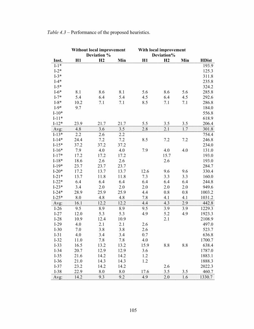
105
Table 4.3 – Performance of the proposed heuristics.
Without local improvement With local improvement
Deviation % Deviation% Inst. H1 H2 Min H1 H2 Min HDist I-1* 0.0 0.0 0.0 0.0 0.0 0.0 193.9 I-2* 0.0 0.0 0.0 0.0 0.0 0.0 125.3 I-3* 0.0 0.0 0.0 0.0 0.0 0.0 311.8 I-4* 0.0 0.0 0.0 0.0 0.0 0.0 235.8 I-5* 0.0 0.0 0.0 0.0 0.0 0.0 324.2 I-6* 8.1 8.6 8.1 5.6 8.6 5.6 285.8 I-7* 5.4 6.4 5.4 4.5 6.4 4.5 292.6 I-8* 10.2 7.1 7.1 8.5 7.1 7.1 286.8 I-9* 9.7 0.0 0.0 0.0 0.0 184.0
I-10* 0.0 0.0 0.0 0.0 0.0 0.0 556.8 I-11* 0.0 0.0 0.0 0.0 0.0 0.0 618.9 I-12* 23.9 21.7 21.7 5.5 3.5 3.5 206.4 Avg: 4.8 3.6 3.5 2.8 2.1 1.7 301.8 I-13* 2.2 2.6 2.2 0.0 0.0 0.0 754.4 I-14* 24.4 7.2 7.2 8.5 7.2 7.2 246.8 I-15* 37.2 37.2 37.2 0.0 0.0 0.0 234.0 I-16* 7.9 4.0 4.0 7.9 4.0 4.0 131.0 I-17* 17.2 17.2 17.2 0.0 15.7 0.0 193.0 I-18* 18.6 2.6 2.6 0.0 2.6 0.0 193.0 I-19* 23.7 23.7 23.7 0.0 0.0 0.0 284.7 I-20* 17.2 13.7 13.7 12.6 9.6 9.6 330.4 I-21* 13.7 11.8 11.8 7.3 3.3 3.3 160.0 I-22* 6.4 6.4 6.4 6.4 6.4 6.4 244.8 I-23* 3.4 2.0 2.0 2.0 2.0 2.0 949.6 I-24* 28.9 25.9 25.9 4.4 0.8 0.8 1003.2 I-25* 8.0 4.8 4.8 7.8 4.1 4.1 1031.2 Avg: 16.1 12.2 12.2 4.4 4.3 2.9 442.8 I-26 9.5 8.9 8.9 9.5 3.9 3.9 1229.3 I-27 12.0 5.3 5.3 4.9 5.2 4.9 1923.3 I-28 10.9 12.4 10.9 0.0 2.1 0.0 2108.9 I-29 4.0 2.1 2.1 2.6 0.0 0.0 497.0 I-30 7.0 3.8 3.8 2.6 0.0 0.0 523.7 I-31 4.0 3.4 3.4 0.7 0.0 0.0 636.8 I-32 11.0 7.8 7.8 4.0 0.0 0.0 1700.7 I-33 16.5 13.2 13.2 15.9 8.8 8.8 638.4 I-34 20.7 12.9 12.9 3.6 0.0 0.0 1787.0 I-35 21.6 14.2 14.2 1.2 0.0 0.0 1883.1 I-36 21.0 14.3 14.3 1.2 0.0 0.0 1888.3 I-37 23.2 14.2 14.2 0.0 2.6 0.0 2022.3 I-38 22.9 8.0 8.0 17.6 3.5 3.5 460.7 Avg: 14.2 9.3 9.2 4.9 2.0 1.6 1330.7


108
Battarra, M., Monaci, M. and Vigo, D., 2009. An adaptive guidance approach for the heuristic solution of a minimum multiple trip vehicle routing problem. Computers & Operations Research, 36(11), pp.3041–3050.
Brandão, J. and Mercer, A., 1997. A tabu search algorithm for the multi-trip vehicle routing and scheduling problem. European Journal of Operational Research, 100(1), pp.180–191.
Brandão, J. and Mercer, A., 1998. The multi-trip vehicle routing problem. Journal of the Operational research society, 49 (8), pp.799–805.
Bräysy, O. and Gendreau, M., 2005a. Vehicle routing problem with time windows, Part I: Route construction and local search algorithms. Transportation science, 39(1), pp.104–118.
Bräysy, O. and Gendreau, M., 2005b. Vehicle routing problem with time windows, Part II: Metaheuristics. Transportation science, 39(1), pp.119–139.
Cattaruzza, D., Absi, N., Feillet, D. and Vigo, D., 2014. An Iterated Local Search for the Multi Commodity Multi Trip Vehicle Routing Problem with Time Windows. Computers & Operations Research, 51, pp.257–267.
Coelho, L.C, and Laporte, G., 2014. Improved solutions for inventory-routing problems through valid inequalities and input ordering, International Journal of Production Economics, 155, pp. 391–397.
Cordeau, J.-F., Desaulniers, G., Desrosiers, J., Solomon, M.M. and Soumis, F., 2001. “VRP with time windows.” In The vehicle routing problem edited by P. Toth and D. Vigo, , pp. 157–193. Philadelphia, PA: SIAM.
Doerner, K.F., Gronalt, M., Hartl, R.F., Kiechle, G. and Reimann, M., 2008. Exact and heuristic algorithms for the vehicle routing problem with multiple interdependent time windows. Computers & Operations Research, 35(9), pp.3034–3048.
Doerner K. F. & Hartl R., 2008 “Health care logistics, emergency preparedness, and disaster relief: New challenges for routing problems with a focus on the Austrian Situation.” In The Vehicle Routing Problem: Latest Advances and New Challenges, edited by B. Golden, S. Raghavan and E. Wasil, pp. 527-550. New York: Springer.
Fleischmann B., 1990. The vehicle routing problem with multiple use of vehicles. Working paper, Fachbereich Wirtschaftswissenschaften, Universität Hamburg, Germany.

109
Hernández, F., Feillet, D., Giroudeau, R. and Naud, O., 2014. A new exact algorithm to solve the multi-trip vehicle routing problem with time windows and limited duration. 4OR, 12, pp.1–25.
Kallehauge, B., 2008. Formulations and exact algorithms for the vehicle routing problem with time windows. Computers & Operations Research, 35(7), pp.2307–2330.
Liu, R., Xie, X., Augusto, V. and Rodríguez, C., 2013. Heuristic algorithms for a vehicle routing problem with simultaneous delivery and pickup and time windows in home health care. European Journal of Operational Research, 230(3), pp.475–486.
Martínez, L. and Amaya, C., 2013. A vehicle routing problem with multi-trips and time windows for circular items. Journal of the Operational Research Society, 64(11), pp.1630–1643.
Ministère de Santé et des Services Sociaux, 2012. Démarche d'optimisation des services offerts par les laboratoires de biologie médicale du Québec. [Optimisation process of Québec’s Province laboratories’ services in medical biology]. (m.D. Québec, éd.) Optilab express.
Mingozzi, A., Roberti, R. and Toth, P., 2013. An exact algorithm for the multitrip vehicle routing problem. INFORMS Journal on Computing, 25(2), pp.193–207.
Olivera, A. and Viera, O., 2007. Adaptive memory programming for the vehicle routing problem with multiple trips. Computers & Operations Research, 34(1), pp.28–47.
Prins, C., 2002. Efficient heuristics for the heterogeneous fleet multitrip VRP with application to a large-scale real case. Journal of Mathematical Modelling and Algorithms, 1(2), pp.135–150.
Renaud J., Ruiz A., Chabot T., Anaya-Arenas A. M. & Zue Ntoutoume J. L., 2013. Modélisation et optimisation du transport d’échantillons en biologie médicale [Modeling and Optimisation of the Biomedical Sample Transportation Problem]. Technical report, Ministère de la santé et des services sociaux, Octobre 2013.
Taillard, Éric D., Laporte, G. and Gendreau, M., 1996. Vehicle routeing with multiple use of vehicles. Journal of the Operational research society, 47 (8), pp.1065–1070.

110
Vidal T., Crainic T. G., Gendreau M. & Prins C., 2013. Heuristics for multi-attribute vehicle routing problems: A survey and synthesis. European Journal of Operational Research, 231, pp. 1-21.
Vidal T., Crainic T. G., Gendreau M. & Prins C., 2014. A unified solution framework for multi-attribute vehicle routing problems. European Journal of Operational Research, 234, pp. 658-673.
Wang, Z., Liang, W. and Hu, X., 2014. A metaheuristic based on a pool of routes for the vehicle routing problem with multiple trips and time windows. Journal of the Operational Research Society, 65(1), pp.37–48.
111
Chapitre 5
5. Une méthode itérative de recherche locale pour résoudre le problème de transport d’échantillons biomédicaux au Québec
Le but de cet article est de résoudre le problème de transport d'échantillons
biomédicaux pour le réseau des laboratoires du Québec. Les prélèvements sont
effectués dans divers établissements de soins de santé (ou centres de prélèvements –
CPs). Ensuite, les échantillons doivent être analysés, dans la plupart des cas, dans un
laboratoire externe (lab) où les prélèvements doivent être expédiés. La courte durée
de vie des échantillons biomédicaux exige que plusieurs passages par journée soient
faits aux CPs et impose une contrainte forte sur la durée maximale des routes. Suite à
notre première collaboration avec le Ministère de Santé et de Services sociaux du
Québec (MSSS) (Anaya-Arenas et al. 2015), le MSSS a réévalué ses besoins et remis
en considération les hypothèses précédemment appliquées sur le nombre de
cueillettes à faire à chaque CP et leur fenêtres de temps. Ceci est fait afin d’obtenir
une meilleure planification centralisée et coordonnée sur les décisions de transport du
réseau. Dans ce contexte, nous cherchons à définir une planification efficace des
heures d'ouverture des CPs et un ensemble de routes pour effectuer le nombre optimal
de collectes à chacun des centres. L’objectif est de minimiser le temps facturable
(durée totale des routes) tout en garantissant qu’aucun échantillon ne périsse pendant
le transport ni dans les CPs. Nous abordons le problème par une procédure itérative
de recherche locale (ILS). L'idée principale est d'explorer à chaque itération le
voisinage local d’une solution perturbée. Nous avons testé la méthode proposée sur
les instances réelles, tirées du réseau de laboratoires au Québec.
Article 4: An ILS approach to solve the biomedical sample
transportation problem in the province of Quebec
Ce chapitre fait l’objet d’un article accepté pour présentation dans une conférence
internationale avec comité d’évaluation: Anaya-Arenas, A.M., Prodhon, C., Afsar,

113
thus the samples have to be sent to an external laboratory (lab). This analysis has to
be made inside the samples’ lifespan, or the specimens will perish and tests have to
be performed again. Therefore, due to samples’ lifespan, an SCC might request
several pick-ups per day to preserve samples’ quality. Evidently, this transportation
task requires an efficient planning to ensure service quality, to avoid delays and loss
of samples and to reduce operation costs. This research work is an extension of our
partnership with the MSSS of the Canadian province of Quebec. The MSSS is
responsible for supporting and overseeing Quebec’s health network, and one of its
current priorities in is the optimization of the laboratories' network services
(embedded in a supply chain optimization project named Optilab). In a previous
work, Anaya-Arenas et al., (2015) performed the formalization of the BSTP faced by
the MSSS. The authors considered a first version of the problem where the SCCs
state several transportation requests that have to be performed inside strict time
windows, including also other time constraints related to the perishable nature of
specimens and Quebec’s laboratory network. The problem was modeled as a multi-
trip vehicle routing problem with time windows (MTVRP-TW), two mathematical
formulations were proposed, and MSSS’s real instances were solved with a
combination of fast heuristics and a commercial branch and bound software.
In the current phase of the project, some key aspects on the network’s structure are
reconsidered, and an efficient metaheuristic is proposed to develop more productive
transportation plans for the MSSS. Two primary hypotheses are lifted to include in
our problem the optimization of the SCCs’ operation decisions. First of all, we
include in our analysis the SCC’s decisions concerning the number and frequency of
the transportation requests. Until now, each SCC provided the number of pick-ups to
be performed during the workday with strict time windows. However, these
parameters represent a major restriction in the transportation planning, and can lead
ultimately to inefficient use of resources, and there is no prove that the estimations of
the SCCs are accurate. We thus include the SCC’s capacity into our analysis seeking
to find the optimal number of visits. We consider that SCCs have a limited stocking
capacity, which must be respected in order to avoid that samples perish. In other
words, we no longer talk about a fixed time window for a transportation request, but a

115
the SCC. On the other hand, even if the collection periods are defined by the
particular demand and workload of a SCC, in a crowed network, like the one in
Montreal’s downtown, many SCCs can have a similar (even the same) schedule. This
fact can easily result in multiple and simultaneous transportations request at different
locations and finally incompatibles SCCs for a transportation plan, increasing the
transportation costs. A more interesting approach could be to define the right opening
hours of the SCCs, keeping into account their demand and specific needs, in order to
get a simpler and more synchronized schedule for the entire set of SCCs. To guide
this decision inside the working schedule of the SCCs, a time window is set around
its usual opening hour. Then, once it is opened, the SCC’s collecting period (total
collecting time) is respected.
Blood collection and clinical specimen collection were first addressed in the 1970s
(McDonald, 1972). However, due to the specific constraints attached to the context,
as well as the practical impact in social welfare, biomedical sample logistics has
regained attention in recent years, and some related works had been added to the
literature. Yi (2003) was one of the first to approach the blood transportation as a
variant of the VRP with time windows (VRPTW). Their collection points need to be
visited (once) inside its operation time window to bring blood back to a central depot
to be treated. As there is only one pick-up that can be done to each center, the later
the pick-up is done, more blood can be brought back to the depot. The objective is to
maximize the quantity of blood that is collected and treated, respecting
transportation’s time constraints and minimizing logistics’ cost. More recently,
Sahinyazan et al. (2015) present a tour mobile collection system for the Red Cross in
Turkey. Their main concern is to define the tours for the mobile collection units
(vehicles) selecting the nodes to be used as base for the collection. Then, a second
tour needs to be planned each day to pick-up collected blood through the planning
horizon. As in the case of Yi (2003), there is only one pick-up to perform at each
client per day. This is a different and simpler approach that the one stated in our
problem because there is no interdependency between pick-ups. On their side, Yücel
et al. (2013) present what they denominated as the collection for processing problem.
Their contribution is including the laboratory’s processing rate in the tour’s planning.

117
operations vary from a sample type to another. Even so, after preparation, all the
samples are consolidated and stocked in standard refrigerated sample boxes, which
are transported. A typical box can content up to 80 different samples. Due to the size
of the boxes, and the small number of boxes send by SCCs at each pick-up, we
consider that each SCC states a number of transportation requests during their work
day and it will never overpass vehicles’ capacity. A major determinant of the
samples’ lifespan is the capacity of the SCC to pre-treat the samples and stock them
in optimal conditions before sending them to the lab. In fact, we can assume that as
long as samples are kept at SCCs, their deterioration is slowed down. However, each
SCC 𝑔 has limited conservation capacity 𝐶𝑔 that in many cases is smaller than the
capacity required for the entire operation day. This means that, inside its operation
hours, an SCC 𝑔 might need to call several transportation requests to liberate its
stocking capacity. We can therefore estimate a maximal timespan inter-pick-ups to
ensure that SCC’s capacity is always respected as follows: ∆𝑚𝑎𝑥𝑔
= 𝐶𝑔 𝜆𝑔⁄ . This is the
first particularity of the BSTP and a major challenge in transportation planning. The
second one is the travel time limit. In fact, once the boxes leave the SCC, the optimal
conditions of temperature cannot be warranted, so deterioration process is
accelerated. Therefore, as soon as samples are out of the SCC facility, they must
arrive to the lab within a maximal transportation time. This time limit can vary from
a sample to another. Hence, each transportation request 𝑝 has a particular time limit
for transportation, noted 𝑇𝑚𝑎𝑥𝑝 , deduced by the most urgent sample transported in it.
To summarize, a vehicle must visit the SCCs and recover the samples’ boxes
(completely full or not) before a maximum time from its last visit, and return to the
lab in time to avoid that any of transported samples (in the route) perish.
In addition to the time-constraints described before, the BSTP has other particularities
related to the SCCs. First of all, SCCs opening time can be modified, inside a small
window, in order to contribute to a better global transportation plan. Let us thus
define 𝑎𝑔 as the opening time for SCC 𝑔, which is inside its opening time window
[𝑒𝑔, 𝑙𝑔]. Let 𝑒𝑔 and 𝑙𝑔 be the earliest and latest hour that SCC 𝑔 can open
(respectively). However, remember that the collection period is fixed for each SCC,
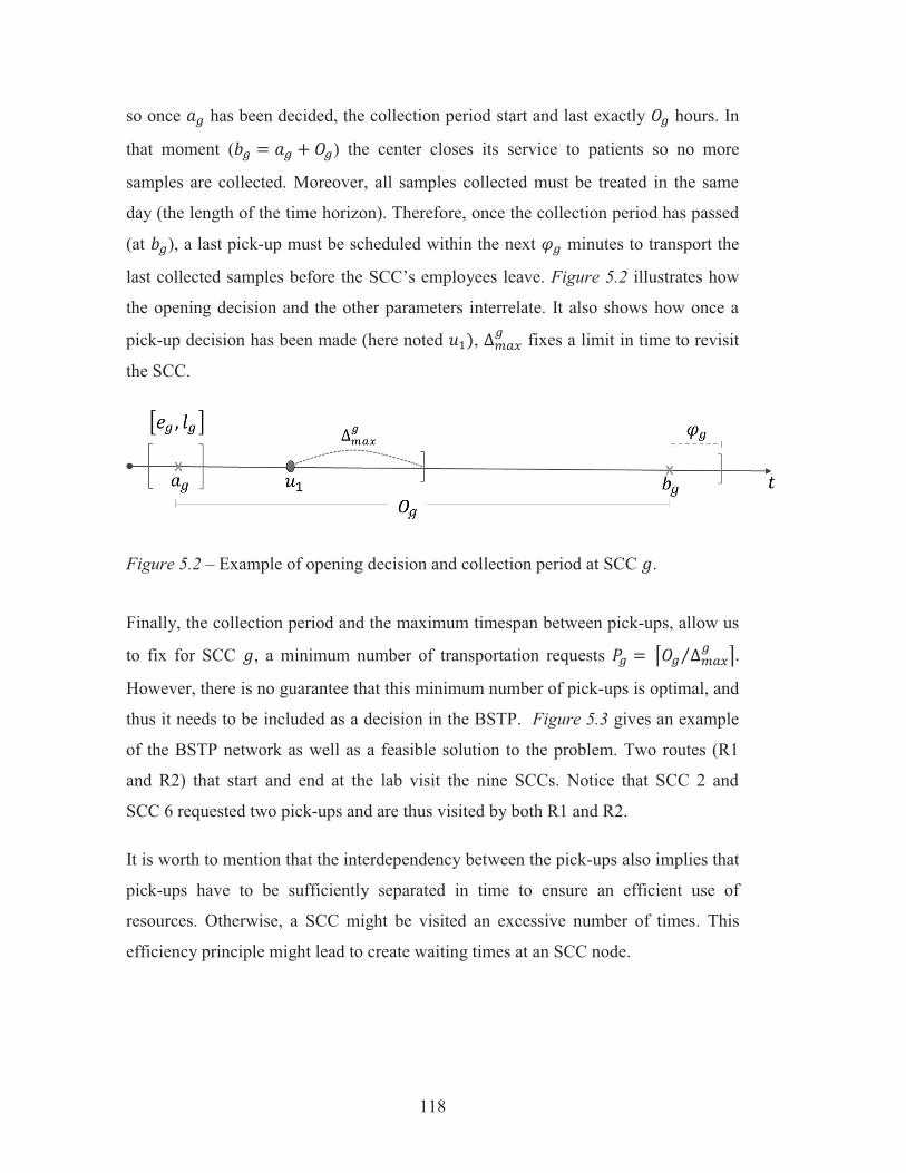


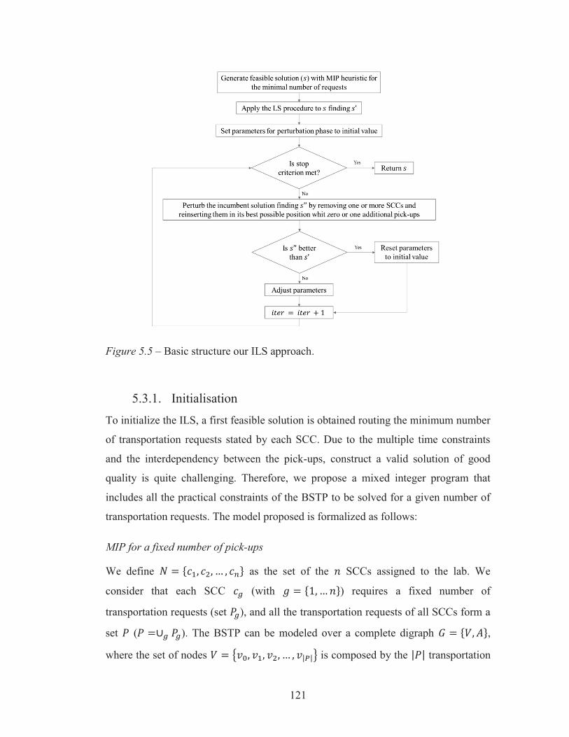
122
requests of all SCCs, and the laboratory ({𝑣0}) where the routes must start and end.
We consider and unlimited fleet of vehicles available at the lab to perform the routes.
Without loss of generality, we label the pick-ups so that {𝑣1, 𝑣2, … 𝑣|𝑃1|} are the
transportation requests of SCC 1, {𝑣|𝑃1|+1, … , 𝑣|𝑃1|+|𝑃2| } are requests of SCC 2 and so
on. More precisely, we define 𝐼𝑔 as the set of index for the requests of a center 𝑐𝑔
where 𝐼𝑔 = {∑ |𝑃ℎ|𝑔−1ℎ=1 + 1, … , ∑ |𝑃ℎ|𝑔
ℎ=1 }.
In addition, we define an arc set 𝐴 = {(𝑣𝑖, 𝑣𝑗): 𝑣𝑖 , 𝑣𝑗 ∈ 𝑉, 𝑖 ≠ 𝑗, 𝑖, 𝑗 = 0, … , |𝑃|} and
for each arc (𝑣𝑖 , 𝑣𝑗) a fixed transportation time (𝑡𝑖𝑗) is known. Evidently, 𝑡𝑖𝑗 is fixed
to zero to all 𝑣𝑖 and 𝑣𝑗 belonging to the same SCC (𝑣𝑖 , 𝑣𝑗 ∈ 𝑃𝑔). In addition to the
notation defined in Section 2, we need to consider the loading time at 𝑐𝑔 (𝜏𝑔) and the
unloading time of the vehicle at the lab before a new route can be started (τ0). The
objective is to define a transportation plan (set of routes) defining the service time for
each one of the transportation request of each SCC, as well as the opening hours of
the SCCs, in order to warrant that none of the samples perish and to minimize total
route duration. The BSTP can be modeled as a MIP as follows:
Decisions variables
𝑥𝑖𝑗 binary variable equal to one if node 𝑖 is visited before node 𝑗.
𝑢𝑖 continuous variable that indicates the time when pick-up 𝑖 is performed.
𝑑𝑖 continuous variable that indicates the duration of the route that starts at node 𝑖.
𝑎𝑔 continuous variable that indicates the opening hour of SCC~𝑔.
𝑏𝑔 continuous variable that indicates the end of collection period hour of SCC 𝑔.
𝑓𝑖𝑝 the maximum remaining time at node 𝑖, to bring request 𝑝 to the lab before
perishing.
BSTP for a fixed number of pick-ups
𝑀𝑖𝑛 ∑ 𝑑𝑖
|𝑃|
𝑖=1
(1)
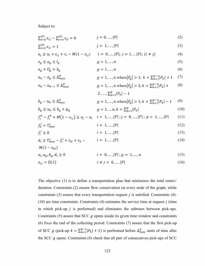
123
Subject to:
∑ 𝑥𝑖𝑗|𝑃|𝑖=0 − ∑ 𝑥𝑗𝑖
|𝑃|𝑖=0 = 0 𝑗 = 0, … , |𝑃| (2)
∑ 𝑥𝑖𝑗|𝑃|𝑖=0 = 1 𝑗 = 1, … , |𝑃| (3)
𝑢𝑗 ≥ 𝑢𝑖 + 𝑡𝑖𝑗 + 𝜏𝑖 − 𝑀(1 − 𝑥𝑖𝑗) 𝑖 = 0, … , |𝑃|; 𝑗 = 1, … |𝑃|; (𝑖 ≠ 𝑗) (4)
𝑒𝑔 ≤ 𝑎𝑔 ≤ 𝑙𝑔 𝑔 = 1, … , 𝑛 (5)
𝑎𝑔 + 𝑂𝑔 = 𝑏𝑔 𝑔 = 1, … , 𝑛 (6)
𝑢𝑘 − 𝑎𝑔 ≤ ∆𝑚𝑎𝑥𝑔 𝑔 = 1, … , 𝑛 where|𝑃𝑔| > 1; 𝑘 = ∑ |𝑃ℎ| + 1
𝑔−1ℎ=1 (7)
𝑢𝑘 − 𝑢𝑘−1 ≤ ∆𝑚𝑎𝑥𝑔 𝑔 = 1, … , 𝑛 where|𝑃𝑔| > 2; 𝑘 = ∑ |𝑃ℎ|𝑔−1
ℎ=1 +
2 , … , ∑ |𝑃ℎ|𝑔ℎ=1 − 1
(8)
𝑏𝑔 − 𝑢𝑘 ≤ ∆𝑚𝑎𝑥𝑔 𝑔 = 1, … , 𝑛 where|𝑃𝑔| > 1; 𝑘 = ∑ |𝑃ℎ|𝑔−1
ℎ=1 − 1 (9)
𝑏𝑔 ≤ 𝑢𝑘 ≤ 𝑏𝑔 + 𝜑𝑔 𝑔 = 1, … 𝑛; 𝑘 = ∑ |𝑃ℎ|𝑔ℎ=1 (10)
𝑓𝑗𝑝 − 𝑓𝑖
𝑝 + 𝑀(1 − 𝑥𝑖𝑗) ≥ 𝑢𝑗 − 𝑢𝑖 𝑖 = 1, … , |𝑃| ; 𝑗 = 0, … , |𝑃| ; 𝑝 = 1, … , |𝑃| (11)
𝑓0𝑖 = 𝑇𝑚𝑎𝑥
𝑖 𝑖 = 1, … , |𝑃| (12)
𝑓𝑖𝑖 ≥ 0 𝑖 = 1, … , |𝑃| (13)
𝑑𝑖 ≥ 𝑇𝑚𝑎𝑥𝑖 − 𝑓𝑖
𝑖 + 𝑡0𝑖 + 𝜏0 −
𝑀(1 − 𝑥0𝑖)
𝑖 = 1, … , |𝑃| (14)
𝑢𝑖 , 𝑎𝑔, 𝑏𝑔, 𝑑𝑖 ≥ 0 𝑖 = 0, … , |𝑃| ; 𝑔 = 1, … , 𝑛 (15)
𝑥𝑖𝑗 = {0,1} 𝑖 ≠ 𝑗 = 0, … , |𝑃| (16)
The objective (1) is to define a transportation plan that minimizes the total routes’
duration. Constraints (2) ensure flow conservation on every node of the graph, while
constraints (3) ensure that every transportation request 𝑗 is satisfied. Constraints (4)-
(10) are time constraints. Constraints (4) estimates the service time at request 𝑗 (time
in which pick-up 𝑗 is performed) and eliminates the subtours between pick-ups.
Constraints (5) assure that SCC 𝑔 opens inside its given time window and constraints
(6) fixes the end of the collecting period. Constraints (7) assure that the first pick-up
of SCC 𝑔 (pick-up 𝑘 = ∑ |𝑃ℎ|𝑔−1ℎ=1 + 1) is performed before ∆𝑚𝑎𝑥
𝑔 units of time after
the SCC 𝑔 opens. Constraints (8) check that all pair of consecutives pick-ups of SCC
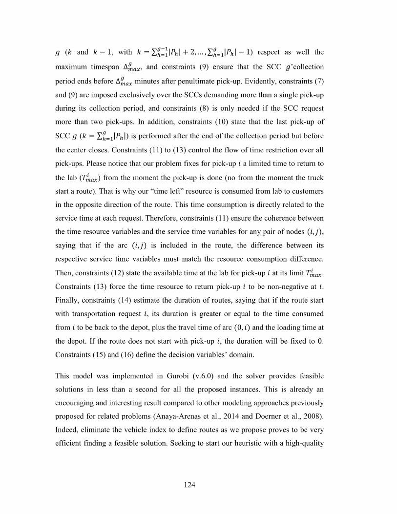
124
𝑔 (𝑘 and 𝑘 − 1, with 𝑘 = ∑ |𝑃ℎ|𝑔−1ℎ=1 + 2, … , ∑ |𝑃ℎ|𝑔
ℎ=1 − 1) respect as well the
maximum timespan ∆𝑚𝑎𝑥𝑔 , and constraints (9) ensure that the SCC 𝑔’collection
period ends before ∆𝑚𝑎𝑥𝑔 minutes after penultimate pick-up. Evidently, constraints (7)
and (9) are imposed exclusively over the SCCs demanding more than a single pick-up
during its collection period, and constraints (8) is only needed if the SCC request
more than two pick-ups. In addition, constraints (10) state that the last pick-up of
SCC 𝑔 (𝑘 = ∑ |𝑃ℎ|𝑔ℎ=1 ) is performed after the end of the collection period but before
the center closes. Constraints (11) to (13) control the flow of time restriction over all
pick-ups. Please notice that our problem fixes for pick-up 𝑖 a limited time to return to
the lab (𝑇𝑚𝑎𝑥𝑖 ) from the moment the pick-up is done (no from the moment the truck
start a route). That is why our “time left” resource is consumed from lab to customers
in the opposite direction of the route. This time consumption is directly related to the
service time at each request. Therefore, constraints (11) ensure the coherence between
the time resource variables and the service time variables for any pair of nodes (𝑖, 𝑗),
saying that if the arc (𝑖, 𝑗) is included in the route, the difference between its
respective service time variables must match the resource consumption difference.
Then, constraints (12) state the available time at the lab for pick-up 𝑖 at its limit 𝑇𝑚𝑎𝑥𝑖 .
Constraints (13) force the time resource to return pick-up 𝑖 to be non-negative at 𝑖.
Finally, constraints (14) estimate the duration of routes, saying that if the route start
with transportation request 𝑖, its duration is greater or equal to the time consumed
from 𝑖 to be back to the depot, plus the travel time of arc (0, 𝑖) and the loading time at
the depot. If the route does not start with pick-up 𝑖, the duration will be fixed to 0.
Constraints (15) and (16) define the decision variables’ domain.
This model was implemented in Gurobi (v.6.0) and the solver provides feasible
solutions in less than a second for all the proposed instances. This is already an
encouraging and interesting result compared to other modeling approaches previously
proposed for related problems (Anaya-Arenas et al., 2014 and Doerner et al., 2008).
Indeed, eliminate the vehicle index to define routes as we propose proves to be very
efficient finding a feasible solution. Seeking to start our heuristic with a high-quality

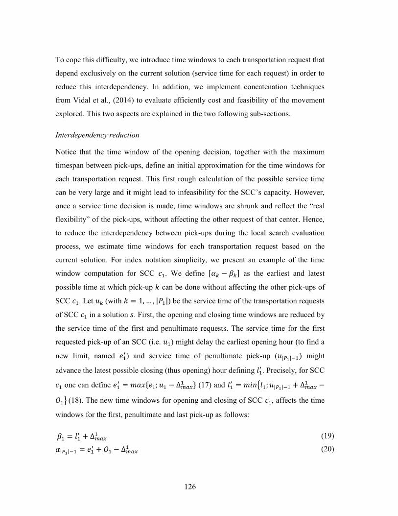
126
To cope this difficulty, we introduce time windows to each transportation request that
depend exclusively on the current solution (service time for each request) in order to
reduce this interdependency. In addition, we implement concatenation techniques
from Vidal et al., (2014) to evaluate efficiently cost and feasibility of the movement
explored. This two aspects are explained in the two following sub-sections.
Interdependency reduction
Notice that the time window of the opening decision, together with the maximum
timespan between pick-ups, define an initial approximation for the time windows for
each transportation request. This first rough calculation of the possible service time
can be very large and it might lead to infeasibility for the SCC’s capacity. However,
once a service time decision is made, time windows are shrunk and reflect the “real
flexibility” of the pick-ups, without affecting the other request of that center. Hence,
to reduce the interdependency between pick-ups during the local search evaluation
process, we estimate time windows for each transportation request based on the
current solution. For index notation simplicity, we present an example of the time
window computation for SCC 𝑐1. We define [𝛼𝑘 − 𝛽𝑘] as the earliest and latest
possible time at which pick-up 𝑘 can be done without affecting the other pick-ups of
SCC 𝑐1. Let 𝑢𝑘 (with 𝑘 = 1, … , |𝑃1|) be the service time of the transportation requests
of SCC 𝑐1 in a solution 𝑠. First, the opening and closing time windows are reduced by
the service time of the first and penultimate requests. The service time for the first
requested pick-up of an SCC (i.e. 𝑢1) might delay the earliest opening hour (to find a
new limit, named 𝑒1′) and service time of penultimate pick-up (𝑢|𝑃1|−1) might
advance the latest possible closing (thus opening) hour defining 𝑙1′ . Precisely, for SCC
𝑐1 one can define 𝑒1′ = 𝑚𝑎𝑥{𝑒1; 𝑢1 − ∆𝑚𝑎𝑥
1 } (17) and 𝑙1′ = 𝑚𝑖𝑛{𝑙1; 𝑢|𝑃1|−1 + ∆𝑚𝑎𝑥
1 −
𝑂1} (18). The new time windows for opening and closing of SCC 𝑐1, affects the time
windows for the first, penultimate and last pick-up as follows:
𝛽1 = 𝑙1′ + ∆𝑚𝑎𝑥
1 (19)
𝛼|𝑃1|−1 = 𝑒1′ + 𝑂1 − ∆𝑚𝑎𝑥
1 (20)


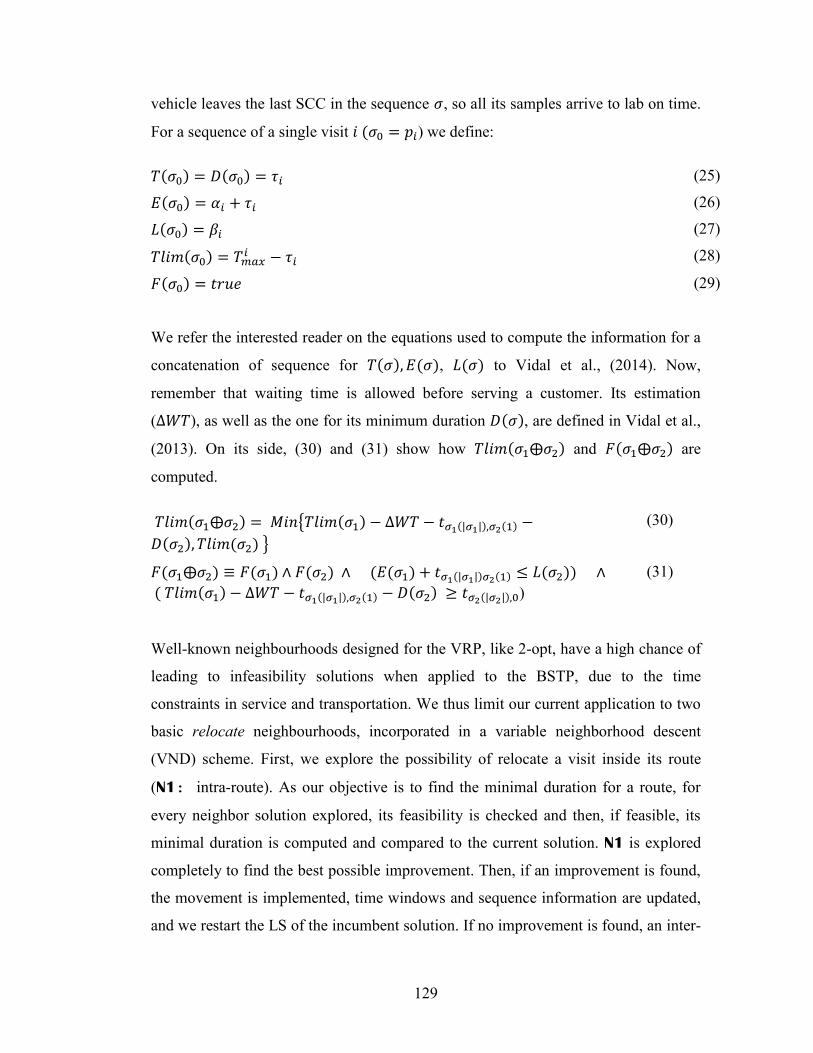
129
vehicle leaves the last SCC in the sequence 𝜎, so all its samples arrive to lab on time.
For a sequence of a single visit 𝑖 (𝜎0 = 𝑝𝑖) we define:
𝑇(𝜎0) = 𝐷(𝜎0) = 𝜏𝑖 (25)
𝐸(𝜎0) = 𝛼𝑖 + 𝜏𝑖 (26)
𝐿(𝜎0) = 𝛽𝑖 (27)
𝑇𝑙𝑖𝑚(𝜎0) = 𝑇𝑚𝑎𝑥𝑖 − 𝜏𝑖 (28)
𝐹(𝜎0) = 𝑡𝑟𝑢𝑒 (29)
We refer the interested reader on the equations used to compute the information for a
concatenation of sequence for 𝑇(𝜎), 𝐸(𝜎), 𝐿(𝜎) to Vidal et al., (2014). Now,
remember that waiting time is allowed before serving a customer. Its estimation
(Δ𝑊𝑇), as well as the one for its minimum duration 𝐷(𝜎), are defined in Vidal et al.,
(2013). On its side, (30) and (31) show how 𝑇𝑙𝑖𝑚(𝜎1⨁𝜎2) and 𝐹(𝜎1⨁𝜎2) are
computed.
𝑇𝑙𝑖𝑚(𝜎1⨁𝜎2) = 𝑀𝑖𝑛{𝑇𝑙𝑖𝑚(𝜎1) − Δ𝑊𝑇 − 𝑡𝜎1(|𝜎1|),𝜎2(1) −
𝐷(𝜎2), 𝑇𝑙𝑖𝑚(𝜎2) } (30)
𝐹(𝜎1⨁𝜎2) ≡ 𝐹(𝜎1) ∧ 𝐹(𝜎2) ∧ (𝐸(𝜎1) + 𝑡𝜎1(|𝜎1|)𝜎2(1) ≤ 𝐿(𝜎2)) ∧
( 𝑇𝑙𝑖𝑚(𝜎1) − Δ𝑊𝑇 − 𝑡𝜎1(|𝜎1|),𝜎2(1) − 𝐷(𝜎2) ≥ 𝑡𝜎2(|𝜎2|),0) (31)
Well-known neighbourhoods designed for the VRP, like 2-opt, have a high chance of
leading to infeasibility solutions when applied to the BSTP, due to the time
constraints in service and transportation. We thus limit our current application to two
basic relocate neighbourhoods, incorporated in a variable neighborhood descent
(VND) scheme. First, we explore the possibility of relocate a visit inside its route
(N1: intra-route). As our objective is to find the minimal duration for a route, for
every neighbor solution explored, its feasibility is checked and then, if feasible, its
minimal duration is computed and compared to the current solution. N1 is explored
completely to find the best possible improvement. Then, if an improvement is found,
the movement is implemented, time windows and sequence information are updated,
and we restart the LS of the incumbent solution. If no improvement is found, an inter-

130
route relocate neighborhood is explored (N2: inter-route) and we proceed as done in
N1. When a move is performed in N2, the LS goes back to N1 to explore the intra-
route of the routes affected by the inter-route. The procedure is repeated until no
further improvement can be found.
5.3.3. Perturbation The LS procedure seeks to improve the routing decisions based on the estimated time
windows calculated for a given solution. However, as it was explained before, this
procedure ignores the flexibility that is added by the time window of the opening
decisions, or the possibility of making extra visits to one or several SCCs. Indeed,
considering the operation decisions for the SCC has a great complexity that can
hardly be coped directly with the time windows estimation and relocate
neighbourhoods. Hence, we propose to explore this upper-level decision through a
perturbation of the current solution. The basic idea of the perturbation stage is to
remove all the transportation requests of one or several SCCs from the solution, and
then to reinsert them in the best possible position. Removing an SCC from the routes
gives us the opportunity to reset the opening decisions and the service time decisions
at the same time. Different criteria can be defined to select the SCCs to remove.
However, seeking to guide the search, we limit the selection criterion to remove the
SCC with the pick-up that produces the highest increase on total duration. Once the
selected SCCs have been removed, the remaining routes are improved by LS, seeking
to shake the solution. On its side, the time windows on the transportation request
removed from the solution are reset to the first approximation and reinserted one by
one. Evidently, at each request insertion, the time windows must be properly updated
in order to avoid infeasibilities. Once all the requests have been reinserted, a new
solution is obtained and its basic neighbourhoods are explored by the LS.
Nonetheless, nothing can ensure that the solution will be improved. In this case, the
solution found is still accepted (implanted), but no improvement successive iterations
are limited to a small number (Fails’) before a diversification is applied, defining a
farther neighborhood.

131
There are two main diversification parameters in our ILS. First, we define 𝜗1 as the
number of SCCs that are removed from the incumbent solution. Second, when an
SCC is removed, it can be reinserted requesting the same numbers of pick-ups as
before, or more. Although in a particular configuration making more than the
minimum pick-up can result in a better result, it would not probably be the case for
all the SCCs and for no more than one pick-up per SCC (Doerner et al., 2008). The
objective is thus to find the right set of customers (if any) that by adding one pick-up,
lead to a better solution. To handle this aspect, let us define 𝜗2 as the number of
additional pick-ups inserted to the request of the removed SCC. These two
parameters are initially set to 𝜗1 = 1 and 𝜗2 = 0, and are increased gradually through
the ILS if no improvement is reached. In addition, when an SCC has been removed
during the perturbation procedure, it is tagged as forbidden to guide the search to a
new part of the solution space. At the beginning, a single SCC is removed and
reinserted (the same number of pick-ups as requested before). Then, if no
improvement is found for a certain number of iterations, 𝜗1 is increased, and the
process is repeated until a certain limit 𝜗1′ . Finally, if no improvement is possible by
removing 𝜗1′ SCCs, we restart 𝜗1=1 and the SCCs removed will now be reinserted but
with an additional pick-up (each). The forbidden list is restarted when 𝜗1 or 𝜗2 are
incremented. Pseudo-code of the ILS is summarized by Algorithm 5.1
Algorithm 5.1 – ILS for the BSTP.
1. 𝑠 ← MIP heuristic for minimum number of transportation request.
2. 𝑠 ← 𝐿𝑆(𝑠)
3. Fix 𝜗1=1; 𝜗2 = 0; nbFails = 0; forbidden = ∅; 𝑖𝑡𝑒𝑟 = 0
4. 𝑠′ ← 𝑠
5. Do until iter= 𝑖𝑡𝑒𝑟′ 𝒐𝒓 all the SCCs are tagged as forbidden.
5.1. Remove 𝜗1 SCCs from 𝑠’ producing a partial solution �� and tagged them as forbidden.
5.2. �� ← 𝐿𝑆(��)
5.3. Reinsert the |𝑃𝑔| + 𝜗2 pick-ups of the removed SCCs to �� obtaining 𝑠′′.
5.4. 𝑠′′ ← 𝐿𝑆(𝑠′′)

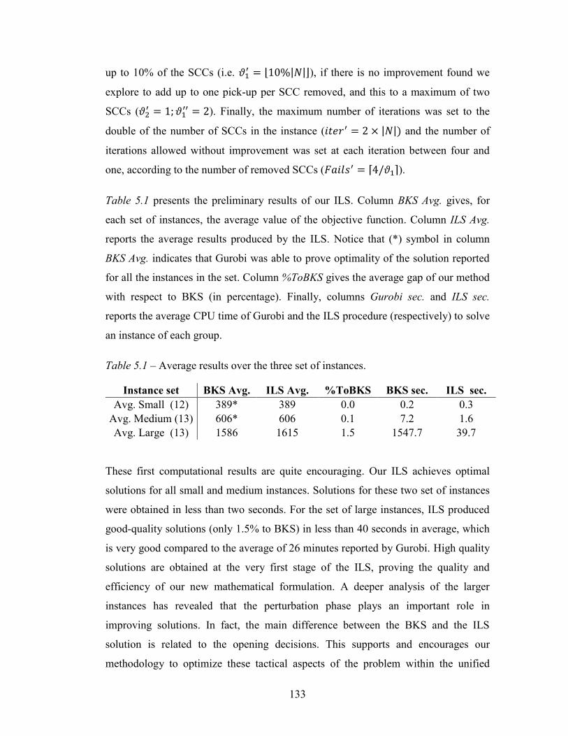
133
up to 10% of the SCCs (i.e. 𝜗1′ = ⌊10%|𝑁|⌋), if there is no improvement found we
explore to add up to one pick-up per SCC removed, and this to a maximum of two
SCCs (𝜗2′ = 1; 𝜗1
′′ = 2). Finally, the maximum number of iterations was set to the
double of the number of SCCs in the instance (𝑖𝑡𝑒𝑟′ = 2 × |𝑁|) and the number of
iterations allowed without improvement was set at each iteration between four and
one, according to the number of removed SCCs (𝐹𝑎𝑖𝑙𝑠′ = ⌈4/𝜗1⌉).
Table 5.1 presents the preliminary results of our ILS. Column BKS Avg. gives, for
each set of instances, the average value of the objective function. Column ILS Avg.
reports the average results produced by the ILS. Notice that (*) symbol in column
BKS Avg. indicates that Gurobi was able to prove optimality of the solution reported
for all the instances in the set. Column %ToBKS gives the average gap of our method
with respect to BKS (in percentage). Finally, columns Gurobi sec. and ILS sec.
reports the average CPU time of Gurobi and the ILS procedure (respectively) to solve
an instance of each group.
Table 5.1 – Average results over the three set of instances.
Instance set BKS Avg. ILS Avg. %ToBKS BKS sec. ILS sec. Avg. Small (12) 389* 389 0.0 0.2 0.3
Avg. Medium (13) 606* 606 0.1 7.2 1.6 Avg. Large (13) 1586 1615 1.5 1547.7 39.7
These first computational results are quite encouraging. Our ILS achieves optimal
solutions for all small and medium instances. Solutions for these two set of instances
were obtained in less than two seconds. For the set of large instances, ILS produced
good-quality solutions (only 1.5% to BKS) in less than 40 seconds in average, which
is very good compared to the average of 26 minutes reported by Gurobi. High quality
solutions are obtained at the very first stage of the ILS, proving the quality and
efficiency of our new mathematical formulation. A deeper analysis of the larger
instances has revealed that the perturbation phase plays an important role in
improving solutions. In fact, the main difference between the BKS and the ILS
solution is related to the opening decisions. This supports and encourages our
methodology to optimize these tactical aspects of the problem within the unified

134
approach. In addition, the small computational times prove how a metaheuristic
approach is suitable to solve the BSTP.
To explore the quality of the transportation plan defined by this new approach, we
compare the solutions obtained with our ILS procedure (in terms of total distance) to
the ones reported by Anaya-Arenas et al. (2015). To this end, we used the network of
SCCs and Labs and the requests proposed in Anaya-Arenas et al. (2015). Notice that
Anaya-Arenas et al. (2015) also includes time windows and aims at minimizing the
total distance. Therefore, comparing the results produced by these two different
models allows us to illustrate how the rigid time windows in Anaya-Arenas et al.
(2015) lead in most of the cases to higher total distances. The results are presented in
Table 5.2. Please note that in all the instances tested the number of transportation
request are the same for the two approaches.
Table 5.2 – Average distances produced by ILS and the methods proposed in Anaya-Arenas et al. (2015).
Instance set Total distance (Km) CPU time (sec.) BSTP-MR BSTP-EG ILS BSTP-MR BSTP-EG ILS
Avg. Small (12) 297.4 297.4 294.7 0.3 0.2 0.3 Avg. Medium (13) 432.3 432.2 435.1 396.2 110.1 1.6 Avg. Large (13) 1324.5 1323.3 1199.3 3600.1 3600.3 39.7
As it can be seen in Table 5.2, the approach proposed in this paper leads, in average,
to solutions (transportation plans) with smaller total traveled distance. For small
instances, the distances are reduced by 1% in average and for the larger ones by 9.3%
(BSTP-EG vs. ILS). On the other hand, on medium size instances the ILS needed
0.5% more km. (in average) than the solution reported in Anaya-Arenas et al. (2015).
This shows a relative advantage in the transportation costs to the fact of eliminating
the time windows constraints and including the SCC opening hour in the optimization
decisions.
Based on our empirical study, a deeper analysis is currently being held to improve the
perturbation procedure. In addition, different parameters tuning (on the maximum
number of SCCs to remove, additional visits to reinsert, or number of iterations) and

136
interdependent time windows. Computers & Operations Research, 35(9), pp. 3034-3048.
McDonald, JJ. (1972) Vehicle Scheduling-A Case Study. Operational Research Quarterly. JSTOR, pp. 433–44.
Şahinyazan, F. G., Kara, B. Y., & Taner, M. R. (2015). Selective vehicle routing for a mobile blood donation system. European Journal of Operational Research, 245(1), pp. 22-34.
Vidal, T., Crainic, T.G., Gendreau, M. & Prins, C., (2013). Heuristics for multi-attribute vehicle routing problems: A survey and synthesis. European Journal of Operational Research, 231(1), pp.1–21.
Vidal, T., Crainic, T. G., Gendreau, M., and Prins, C. (2013). A hybrid genetic algorithm with adaptive diversity management for a large class of vehicle routing problems with time-windows. Computers & Operations Research, 40(1), pp. 475-489.
Vidal, T., Crainic, T. G., Gendreau, M., and Prins, C. (2014). A unified solution framework for multi-attribute vehicle routing problems. European Journal of Operational Research, 234(3), pp. 658-673.
Yi, J. (2003). Vehicle routing with time windows and time-dependent rewards: A problem from the American Red Cross. Manufacturing & Service Operations Management, 5(1), pp. 74-77.
Yücel, E., Salman, F. S., Gel, E. S., Örmeci, E. L., and Gel, A. (2013). Optimizing specimen collection for processing in clinical testing laboratories. European Journal of Operational Research, 227(3), pp. 503-514.

137
Conclusion générale et perspectives de recherche future En appliquant les techniques issues de la recherche opérationnelle, nous avons
développé des outils pour optimiser la distribution dans le contexte du déploiement en
situation d’urgence et du transport d’échantillons biomédicaux.
Dans le domaine du déploiement en situation d’urgence, nous avons fait une revue
systématique de la littérature. En utilisant une procédure de compilation et de
synthèse transparente et reproductible, nous avons exploré plus de 170 références et
87 articles ont finalement été retenus et analysés. Nous avons classifié les
contributions en quatre groupes : 1) le problème de localisation de centres de
distribution d’aide humanitaire, 2) le problème de transport à l’intérieure d’un réseau,
3) le problème de localisation et routage, et 4) autres problématiques. Les attributs
plus importants dans la modélisation, les hypothèses de base et les objectifs
poursuivis ont été identifiés. Cette analyse a permis de faire ressortir les besoins de
recherche dans le domaine. Des modèles plus réalistes avec des objectifs et des
contraintes de capacité adaptés sont toujours nécessaires. De plus, nous soulevons un
besoin d’harmonisation dans les étapes de design et d’exploitation du réseau, ainsi
qu’un besoin pour des méthodes de résolution efficaces pouvant être intégrées dans
des outils d’aide à la décision.
Parmi les différentes pistes de recherche identifiées au Chapitre 2, et grâce à notre
collaboration avec notre partenaire Fujitsu Canada, une inquiétude sur la justesse
dans la distribution lors d’un déploiement d’urgence est la base de notre deuxième
contribution. Nous avons traité, dans le Chapitre 3, trois modèles d’optimisation
multipériode pour le design d’un réseau de distribution d’aide après une catastrophe.
Ces modèles, qui sont très détaillés, priorisent la minimisation de la non-satisfaction
de la demande et mettent de l’avant le principe de justice. Afin de mieux analyser et
d’incorporer le principe de justice dans la planification logistique, des mesures de
performance, qui reflètent l’équité et la stabilité dans la distribution d’aide, ont été
proposées. Ces modèles ont été testés sur des instances réalistes et il en ressort que la

138
fonction linéaire par morceaux développée s’est avérée la plus adéquate pour garantir
une distribution équitable et stable dans le temps. De plus, notre formulation
considère les arrérages de la demande. Les modèles gèrent donc la rationalisation des
ressources mais également la compensation des besoins lorsque l’offre est rétablie.
L’aspect multipériode des modèles développés permet au réseau de s’adapter aux
variations dynamiques de la demande.
En ce qui concerne des recherches futures, nous pensons qu’une utilisation
intéressante des formulations proposées serait de simuler la migration des sinistrés.
De plus, une étude empirique détaillée sur des instances plus complexes serait
pertinente pour bien analyser les possibilités des modèles proposés. Une belle
perspective de recherche qui s’ouvre à ce sujet est de penser à l’intégration de ces
propositions dans une procédure de planification en horizon roulant. Ceci permettrait
au décideur d’actualiser les données entrantes pour le système (comme la localisation
des sinistrés et les prévisions de la capacité réelle disponible et de la demande) au fur
et à mesure qu’elles se rendent disponibles, et d’optimiser les décisions de
distribution de façon dynamique. De la même façon, l’intégration de ce modèle
d’optimisation avec un modèle de simulation serait une prolongation qui permettrait
de fournir un outil de préparation et d’entrainement complet pour les gestionnaires de
crises.
Aux Chapitres 4 et 5 de la thèse, nous avons étudié le problème de transport
d’échantillons biomédicaux. Une présentation de ce problème complexe dans le
réseau des laboratoires d’analyse de la province de Québec est faite au Chapitre 4.
Nous avons formalisé cette problématique comme un problème de tournées de
véhicules avec plusieurs fenêtres de temps par client et des camions qui peuvent faire
plusieurs routes. Nous avons proposé deux modèles d’optimisation et ils ont été testés
sur un ensemble de problèmes provenant du réseau de santé québécois. Nous avons
comparé les deux modèles en utilisant un logiciel commercial d’optimisation (Gurobi
v.6.0) et nous en avons conclu que, en moyenne, la formulation sur le graphe étendu
semble plus efficiente au niveau des temps de résolution et de la qualité de la
solution. Cependant, le problème est toujours très difficile à résoudre et nécessite des
139
temps de calcul élevés. Pour contourner ce problème, nous avons présenté une
méthode de résolution composite, basée sur l’utilisation d’heuristiques simples afin
de fournir une solution initiale au solveur et diminuer grandement le temps de
résolution nécessaire. Le travail que nous avons présenté au Chapitre 4 est la
première étape dans le processus d’optimisation du réseau des laboratoires dans la
province de Québec. Lors de cette collaboration, nous avons déposé divers rapports
techniques qui ont permis au MSSS de mieux exprimer leurs besoins en matière de
transport.
Suite à ces travaux, le MSSS a continué ses réflexions et envisage de modifier les
heures d’ouvertures des centres de prélèvement ainsi que le nombre de passage à
ceux-ci afin de donner de la souplesse au réseau. C’est cette nouvelle problématique
que nous étudions dans le Chapitre 5 où nous développons une métaheuristique pour
résoudre ce cas qui peut être vu comme une extension du problème de base décrit au
Chapitre 4. Tout d’abord, nous avons inclus dans la problématique la capacité des
centres de prélèvements (CPs). Ceci nous a permis de remettre en question le nombre
et la fréquence de ramassages demandés par un CP donné. Nous avons aussi remplacé
les fenêtres de temps par un temps maximal entre les passages. De plus, nous avons
considéré la synchronisation des horaires d’ouverture des CPs. Il en résulte une
problématique de transport plus complexe et nouvelle dans la littérature du transport
d’échantillons biomédicaux. Nous avons présenté une nouvelle formulation pour ce
problème avec un nombre fixe de requêtes qui s’est avéré efficace pour trouver
rapidement des solutions de bonne qualité. Finalement, une procédure itérative de
recherche locale (ILS) a été proposée et elle s’est avérée également efficace. La
méthode a trouvé des solutions de très bonne qualité, souvent optimales, en moins de
20 secondes pour les plus grandes instances, ce qui est moins que 1 % du temps
requis par un solveur commercial.
Ce travail sert de base pour continuer l’optimisation des processus dans le système de
transport des échantillons dans les laboratoires au Québec. Nous croyons qu’une
analyse plus avancée sur la configuration du réseau est toujours pertinente pour le cas
québécois. Plusieurs extensions de ce travail s’avèrent intéressantes. Par exemple,

140
l’inclusion d’une analyse de la capacité de traitement des échantillons au laboratoire.
Jusqu’à maintenant, le MSSS fixe un temps maximal de transport pour éviter la perte
des échantillons, en considérant qu’une fois rendu au laboratoire les échantillons sont
aussitôt traités. Cependant, il n’y a pas vraiment de garantie du temps d’attente réel
d’un échantillon à l’intérieur du laboratoire. Une analyse détaillée des processus de
réception et des charges de travail des laboratoires permettrait au décideur d’en tenir
compte pour une estimation plus réelle du temps maximal de transport. D’autre part,
on pourrait aussi reconsidérer l’affectation des CPs aux laboratoires et réévaluer la
configuration du réseau dans une extension du problème de type « Location-
Routing ». Finalement, une approche toujours intéressante serait d’inclure la
planification des tournées dans un outil dynamique, qui permettrait d’intégrer une
analyse de la capacité des CPs en temps réel en fonction de la demande observée.
Ceci permettrait au décideur d’ajuster la programmation des visites à l’intérieur d’une
journée. Des études futures s’avèrent nécessaires pour analyser ce sujet.
141
Bibliographie Altay, N. & Green, W.G., 2006. OR/MS research in disaster operations management.
European Journal of Operational Research, 175(1), pp.475–493.
Galindo, G. & Batta, R., 2013. Review of Recent Developments in OR/MS Research in Disaster Operations Management. European Journal of Operational Research, 203, pp.201–211.
Haddow, G.D., Bullock, J.A. & Coppola, D.P., 2007. Introduction to emergency management (3rd ed.), Oxford: Butterworth-Heinemann.
Holguín-Veras, J., Hart, W.H., Jaller, M., Van Wassenhove, L.N., Pérez, N. and Wachtendorf, T., 2012. On the unique features of post-disaster humanitarian logistics. Journal of Operations Management, 30, pp.494– 506.
Kovács, G. & Spens, K., 2009. Identifying challenges in humanitarian logistics. International Journal of Physical Distribution & Logistics Management, 39(6), pp.506–528.
Sheu, J.B., 2007. Challenges of emergency logistics management. Transportation Research Part E: Logistics and Transportation Review, 43(6), pp.655–659.
Van Wassenhove, L.N., 2006. Humanitarian aid logistics: supply chain management in high gear. Journal of the Operational Research Society, 57(5), pp.475–489.
Van Wassenhove, L.N. & Pedraza Martínez, A.J., 2012. Using OR to adapt supply chain management best practices to humanitarian logistics. International Transactions in Operational Research, 19(1-2), pp.307–322.