
Optimisation of Radio Access Network Cloud Architectures ... · Optimisation of Radio Access...
159
Optimisation of Radio Access Network Cloud Architectures Deployment in LTE-Advanced Andrea Marotta Thesis to obtain the Master of Science Degree in Electrical and Computer Engineering Supervisor: Prof. Luís Manuel de Jesus Sousa Correia Examination Committee Chairperson: Prof. José Eduardo Charters Ribeiro da Cunha Sanguino Supervisor: Prof. Luís Manuel de Jesus Sousa Correia Member of Committee: Prof. António José Castelo Branco Rodrigues July 2015
Transcript of Optimisation of Radio Access Network Cloud Architectures ... · Optimisation of Radio Access...
Optimisation of Radio Access Network Cloud Architectures
Deployment in LTE-Advanced
Andrea Marotta
Thesis to obtain the Master of Science Degree in
Electrical and Computer Engineering
Supervisor: Prof. Luís Manuel de Jesus Sousa Correia
Examination Committee
Chairperson: Prof. José Eduardo Charters Ribeiro da Cunha Sanguino
Supervisor: Prof. Luís Manuel de Jesus Sousa Correia
Member of Committee: Prof. António José Castelo Branco Rodrigues
July 2015

ii

iii
To my family

iv

v
Acknowledgements
Acknowledgements
First of all, I would like to thank Prof. Luís M. Correia for giving me the opportunity to develop my thesis
work under his supervision and for all the precious advices. I will never forget what I have learned from
him by observing the way he treats students, researchers and collaborators, for the kindness and
steadiness with which he leads the activities of a wonderful group of people that is GROW. I really
appreciate his care, to give me his “Buongiorno” with smile in all the occasions.
To GROW and all its members for welcoming me to their office, for taking always care of me and for
involving me in their daily activities and inviting me to some important events, such as EuCAP and
particularly STAR WARM. Special thanks to Lúcio Ferreira for his consideration towards my work and
for his sympathy and friendship.
To the Ph.D. students of GROW, Behnam Rouzbehani, Kenan Turbic, Mojgan Barahman and Sina
Khatibi, for their valuable advices and for all the good time we spent together. Thanks for being sincere
friends.
To my colleagues Ana Cláudia Castro, Carlos Martins, João Pires, Ricardo Gameiro, and specially
Miguel Sá, for all the information he shared with me and for helping me in the development of this work.
To the friends that I met in Lisbon, Martina Moscarelli, Livia Pallotta, Beatrice Scucchia and Eleonora
Martino, for their support and friendship.
To the city of Lisbon for being so cosy, exciting and, not negligible, full of base stations!
To Prof. Fortunato Santucci, for giving me the opportunity to do this wonderful experience, and to Prof.
Serafino Cicerone for his constant availability.
To all the friends in Italy supporting me during this experience.
To my family for all the sacrifices they did for me and for encouraging me to do all my best.
To Giulia, inexhaustible source of sweetness, love and energy for me.

vi
vii
Abstract
Abstract
The objective of this thesis was to analyse how Cloud Radio Access Network technology can improve
network performance in LTE-A, by taking advantage of the separation between Remote Radio Head
and Base Band Unit. This work consists of a study concerning the impact of C-RAN and virtualisation
techniques in an operator’s network in a near future, namely in terms of the necessary number of storage
and processing nodes and the links in between, taking increasingly network constraints into account
(e.g., latency) as well as deployment ones (e.g., service area, deployment strategy, and expected
proliferation of Remote Radio Heads). A model was implemented, which takes the positioning of cell
sites available in an urban scenario as input, and computes the number and a possible placement of
processing nodes for different constraints – an estimate of the number of required blade servers in each
node is also computed. Results show that between 2 and 62 Baseband processing Units pools are
required to cover the whole scenario of Lisbon, depending on the fronthaul delay restriction. An inverse
proportionality relation between the number of blade servers and their corresponding capacity has been
ascertained. Moreover, the model has been applied to two different from many aspects urban scenarios,
which are the city of Lisbon in Portugal and the city of L’Aquila in Italy.
Keywords
LTE-Advanced, SDN, C-RAN, Deployment, Delay.
viii
Resumo
Resumo
O objetivo da presente tese foi analisar de que forma a tecnologia Cloud Radio Access Network pode
contribuir para melhorar o desempenho da rede LTE-A tirando partido da separação entre o Remote
Radio Head e a Base Band Unit. Este trabalho consiste num estudo do impacto da C-RAN e das
técnicas de virtualização na rede de um operador num futuro próximo, nomeadamente em termos do
número de nós de processamento e armazenamento, e de ligações necessárias tendo em conta
restrições cada vez mais apertadas (como latência e distribuição espacial de Remote Radio Heads).
Um modelo foi implementado que toma como entrada a localização de estações base num cenário
urbano, e que calcula o número e posicionamento possível dos nós de processamento atendendo a
diferentes restrições - uma estimativa do número de servidores necessários em cada nó é também
calculado. Os resultados mostram que são necessárias entre 2 e 62 Baseband Processing Units Pools
para assegurar a cobertura da cidade de Lisboa, dependendo da restrição no fronthaul. Uma relação
de proporcionalidade inversa foi verificada entre o número de servidores e a correspondente
capacidade. Além de Lisboa, o modelo foi aplicado à cidade de L'Aquila em Itália.
Palavras-chave
LTE-Advanced, SDN, C-RAN, Deployment, Delay.
ix
Sommario
Sommario L’obiettivo di questa tesi è stato quello di analizzare come la tecnologia delle Cloud Radio Access
Networks possa migliorare le performance di rete per LTE-A avvantaggiandosi della separazione tra
Remote Radio Head e Base Band Unit. Questo lavoro consiste in uno studio concernente l’impatto
dell’architettura Cloud RAN e delle tecniche di virtualizzazione nella rete dell’operatore in un futuro
prossimo in termini di numero di nodi necessario per l’elaborazione delle informazioni e collegamenti
tra tali nodi e le antenne dislocate nel contesto urbano tenendo in considerazione crescenti vincoli di
rete (quali il delay) e vincoli legati al deployment (le dimensioni dell’ area da servire, differenti strategie
di distribuzione, la proliferazione di Remote Radio Heads). E’ stato implementato un modello che
prende in input le posizioni delle Base Stations disponibili in uno scenario urbano e computa il numero
e le possibili posizioni dei centri di calcolo per differenti requisiti; viene inoltre fornita una stima del
numero di blade servers richiesti per ogni nodo. I risultati mostrano che un numero compreso tra 2 e
62 pool di Base Band Units è richiesto per servire l’intero scenario della città di Lisbona in base al
massimo delay richiesto per il segmento fronthaul. Un relazione di proporzionalità inversa tra il numero
di blade server e la loro corrispondente capacità è stata appurata. Inoltre il modello è stato applicato a
due scenari che possono essere considerati differenti per diversi aspetti: la città di Lisbona in Portogallo
e quella di L’Aquila in Italia.
Parole chiave
LTE-Advanced, SDN, C-RAN, Deployment, Delay.

x
xi
Table of Contents
Table of Contents
Acknowledgements ................................................................................. v
Abstract ................................................................................................. vii
Resumo ................................................................................................ viii
Sommario .............................................................................................. ix
Table of Contents ................................................................................... xi
List of Figures ....................................................................................... xiii
List of Tables ....................................................................................... xviii
List of Acronyms ................................................................................... xx
List of Symbols .................................................................................... xxiii
List of Software ................................................................................... xxvi
1 Introduction .................................................................................. 1
1.1 Overview.................................................................................................. 2
1.2 Motivation and contents ........................................................................... 5
2 Basic concepts and state of the art ............................................... 7
2.1 LTE aspects ............................................................................................. 8
2.1.1 Network architecture .............................................................................................. 8
2.1.2 Radio interface..................................................................................................... 11
2.2 C-RAN and virtualisation ....................................................................... 13
2.2.1 Software-Defined Networking .............................................................................. 13
2.2.2 Network functions virtualisation ........................................................................... 15
2.2.3 Cloud Radio Access Network .............................................................................. 16
2.3 Optimisation of capacity and load balancing.......................................... 18
2.3.1 Load Balancing .................................................................................................... 18
2.3.2 Optimisation of capacity ...................................................................................... 21
2.4 State of the art ....................................................................................... 23
xii
3 Model Development and Implementation ................................... 27
3.1 Description of the problem ..................................................................... 28
3.2 Performance metrics ............................................................................. 29
3.2.1 Latency ................................................................................................................ 29
3.2.2 Processing Power ................................................................................................ 31
3.2.3 Capacity ............................................................................................................... 33
3.3 Model Overview ..................................................................................... 35
3.3.1 Model structure .................................................................................................... 35
3.3.2 RRHs proliferation ............................................................................................... 37
3.3.3 BBU pools positioning ......................................................................................... 37
3.3.4 Load Balancing .................................................................................................... 43
3.3.5 BBU pools dimensioning ..................................................................................... 45
3.4 Model assessment ................................................................................. 46
4 Results Analysis ......................................................................... 47
4.1 Scenarios............................................................................................... 48
4.2 BBU positioning algorithms comparison ................................................ 50
4.3 Analysis of the reference scenario ......................................................... 52
4.4 Analysis of latency ................................................................................. 56
4.5 RRHs proliferation impact ...................................................................... 62
4.6 Impact of scenario dimensioning ........................................................... 65
4.7 Impact of deployment strategies ............................................................ 68
4.8 L’Aquila scenario ................................................................................... 71
5 Conclusions ................................................................................ 75
Annex A. Processing Power Complexity Tables ................................. 81
Annex B. Full results for the reference scenario ................................. 83
Annex C. Full results for latency constraint variation .......................... 89
Annex D. Full results for RRHs proliferation ..................................... 101
Annex E. Full results for scenario dimensioning ............................... 107
Annex F. Full results for the impact of deployment strategies .......... 117
Annex G. Full results for L’Aquila scenario ....................................... 123
References.......................................................................................... 129
xiii
List of Figures
List of Figures Figure 1.1. Global total traffic in mobile networks, 2010-2015 (extracted from [Eric15]). ............. 2
Figure 1.2. Comparison between the trends of ARPU and TCO (extracted from [GSMA13]). ..... 3
Figure 1.3 CAPEX of a Cell Site (extracted from [CMRI11]). ........................................................ 4
Figure 1.4 OPEX of a Cell Site (extracted from [CMRI11]). .......................................................... 4
Figure 1.5 Vision of Mobile Cloud Networking (extracted from [SPHG14]). ................................. 5
Figure 2.1 Overall EPS architecture of the LTE system (extracted from [HoTo11]). .................... 9
Figure 2.2 LTE protocol architecture (DL) (extracted from [DPSB08]). ...................................... 11
Figure 2.3 Resource allocation in OFDMA (extracted from [HoTo11]). ...................................... 12
Figure 2.4 Resource allocation in SC-FDMA (extracted from [HoTo11]). ................................... 13
Figure 2.5 Generic SDN architecture (extracted from [JZHT14]). ............................................... 15
Figure 2.6. Basic NFV Framework (extracted from [Damo13]). .................................................. 16
Figure 2.7 Split of functions between RRH and BBU (extracted from [CMRI11]). ...................... 17
Figure 2.8 Cloud-RAN architecture (extracted from [SPHG14]). ................................................ 18
Figure 2.9 Number of public hotspots worldwide (extracted from [Qual13]). .............................. 25
Figure 3.1 Global view of the problem. ........................................................................................ 29
Figure 3.2 Model overview. ......................................................................................................... 36
Figure 3.3 Proliferation of RRHs. ................................................................................................ 38
Figure 3.4 Density-based Min-Max heuristic. .............................................................................. 39
Figure 3.5 Density-based Max-Min heuristic. .............................................................................. 40
Figure 3.6 Distance-based heuristic. ........................................................................................... 41
Figure 3.7 Hybrid heuristic........................................................................................................... 42
Figure 3.8 Creation of connections without load balancing. ........................................................ 43
Figure 3.9 Creation of connections with load balancing. ............................................................. 44
Figure 3.10 BBU Pools dimensioning. ......................................................................................... 45
Figure 4.1 BSs’ positioning in the Lisbon city and surrounding areas. ....................................... 48
Figure 4.2 Number of BSs at different distances from the city centre. ........................................ 49
Figure 4.3 BSs’ positioning at different distances from the city centre. ...................................... 49
Figure 4.4 BSs’ positioning in the city of L’Aquila and surrounding areas. ................................. 50
Figure 4.5 Heuristics for BBU positioning comparison. ............................................................... 51
Figure 4.6 Placement of BBU Pools (in red) for the reference scenario. .................................... 52
Figure 4.7 Percentage of cell sites at different fronthaul distances (1km interval) for the urban BBU pools in the reference scenario. ................................................................ 52
Figure 4.8 Percentage of cell sites at different fronthaul distances (1km interval) for the suburban BBU pools in the reference scenario. ................................................................ 53
Figure 4.9 Percentage of cell sites at different fronthaul distances (1km interval) for the rural BBU pools in the reference scenario. ......................................................................... 53
Figure 4.10 Load balancing effectiveness for the link capacity load between BBU pools. ......... 54
Figure 4.11 Load balancing effectiveness for the processing power load between BBU pools. 55
Figure 4.12 Number of Blade Servers per BBU Pool vs Blade Server Capacity, with best curves. ............................................................................................................... 55
Figure 4.13 Number of Blade Servers per BBU Pool vs Blade Server Processing Power, with best curves. ............................................................................................................... 55
xiv
Figure 4.14 Placement of BBU Pools (in red) for a maximum fronthaul delay of 10 μs. ............. 57
Figure 4.15 Placement of BBU Pools (in red) for a maximum fronthaul delay of 30 μs. ............. 57
Figure 4.16 Placement of BBU Pools (in red) for a maximum fronthaul delay of 60 μs. ............. 57
Figure 4.17 Placement of BBU Pools (in red) for a maximum fronthaul delay of 100 μs. ........... 58
Figure 4.18 Number of BBU Pools vs. Maximum Fronthaul Delay, with best fit curve. .............. 58
Figure 4.19 Percentage of cell sites at different fronthaul distances (1 km interval) for urban BBU pools and 100 µs of maximum fronthaul delay. ................................................. 59
Figure 4.20 Percentage of cell sites at different fronthaul distances (1 km interval) for rural BBU pools and 100 µs of maximum fronthaul delay. ................................................. 60
Figure 4.21 Fronthaul delay vs. Maximum fronthaul delay ......................................................... 60
Figure 4.22 Fronthaul distance vs. Maximum fronthaul distance ................................................ 61
Figure 4.23 Maximum BBU pool link capacity load with and without load balancing for different maximum fronthaul delay limits. ........................................................................ 62
Figure 4.24 Average BBU pool computational capacity load with and without load balancing for different maximum fronthaul delay limits. .......................................................... 62
Figure 4.25 RRHs proliferation simulation (1 year). .................................................................... 63
Figure 4.26 RRHs proliferation simulation (3 years). .................................................................. 63
Figure 4.27 RRHs proliferation simulation (5 years). .................................................................. 63
Figure 4.28 Global network computational capacity load for different years. ............................. 64
Figure 4.29 Maximum BBU pool link capacity load for different years. ....................................... 65
Figure 4.30 Average BBU pool link capacity load for different years. ......................................... 65
Figure 4.31 Placement of BBU Pools (in red) for a scenario of 10 km. ...................................... 66
Figure 4.32 Placement of BBU Pools (in red) for a scenario of 25 km ....................................... 66
Figure 4.33 Placement of BBU Pools (in red) for a scenario of 40 km. ...................................... 66
Figure 4.34 Number of BBU Pools for different scenario dimensions. ....................................... 67
Figure 4.35 Maximum BBU Pool link capacity load for different scenario dimensions. .............. 67
Figure 4.36 Average BBU Pool computational capacity load for different scenario dimensions 68
Figure 4.37 Fronthaul delay vs. Scenario dimension. ................................................................. 68
Figure 4.38 BBU pool link capacity loads for different deployment strategies. ........................... 69
Figure 4.39 Number of blade servers per BBU pool vs Blade server computational capacity for different deployment strategies with fit curve. ................................................... 70
Figure 4.40 Number of Blade Servers per BBU Pool vs Blade Server Capacity, with best curves for the new scenario. ......................................................................................... 70
Figure 4.41 Placement of BBU Pools (in red) for the city of L’Aquila scenario ........................... 71
Figure 4.42 Load balancing effectiveness for the computational capacity load between BBU pools in L’Aquila scenario. ........................................................................................... 72
Figure 4.43 Number of Blade Servers per BBU Pool vs Blade Server Processing Power, with best curves. ............................................................................................................... 73
Figure B.1 Placement of BBU Pools (in red) for the reference scenario. .................................... 84
Figure B.2 Percentage of cell sites at different fronthaul distances (1km interval) for the global reference scenario. ............................................................................................ 84
Figure B.3 Percentage of cell sites at different fronthaul distances (1km interval) for the urban BBU pools in the reference scenario. ................................................................ 85
Figure B.4 Percentage of cell sites at different fronthaul distances (1km interval) for the suburban BBU pools in the reference scenario. ................................................................ 85
Figure B.5 Percentage of cell sites at different fronthaul distances (1km interval) for the rural BBU pools in the reference scenario. ......................................................................... 85
Figure B.6 Load balancing effectiveness for the link capacity load between BBU pools. ........... 86
Figure B.7 Load balancing effectiveness for the processing power load between BBU pools. .. 86
Figure B.8 Number of Blade Servers per BBU Pool vs Blade Server Capacity, with best curves. ............................................................................................................... 87
xv
Figure B.9 Number of Blade Servers per BBU Pool vs Blade Server Processing Power, with best curves. ............................................................................................................... 87
Figure C.10 Placement of BBU Pools (in red) for a maximum fronthaul delay of 10 μs. ............ 90
Figure C.11 Placement of BBU Pools (in red) for a maximum fronthaul delay of 20 μs. ............ 90
Figure C.12 Placement of BBU Pools (in red) for a maximum fronthaul delay of 30 μs. ............ 91
Figure C.13 Placement of BBU Pools (in red) for a maximum fronthaul delay of 40 μs. ............ 91
Figure C.14 Placement of BBU Pools (in red) for a maximum fronthaul delay of 50 μs. ............ 91
Figure C.15 Placement of BBU Pools (in red) for a maximum fronthaul delay of 60 μs. ............ 92
Figure C.16 Placement of BBU Pools (in red) for a maximum fronthaul delay of 70 μs. ............ 92
Figure C.17 Placement of BBU Pools (in red) for a maximum fronthaul delay of 80 μs. ............ 92
Figure C.18 Placement of BBU Pools (in red) for a maximum fronthaul delay of 90 μs. ............ 93
Figure C.19 Placement of BBU Pools (in red) for a maximum fronthaul delay of 100 μs. .......... 93
Figure C.20 Number of BBU Pools vs. Maximum Fronthaul Delay, with best fit curve............... 93
Figure C.21 Percentage of cell sites at different fronthaul distances (1km interval) for urban BBU pools and 20µs of maximum fronthaul delay. .................................................... 94
Figure C.22 Percentage of cell sites at different fronthaul distances (1km interval) for suburban BBU pools and 20µs of maximum fronthaul delay............................................. 94
Figure C.23 Percentage of cell sites at different fronthaul distances (1km interval) for rural BBU pools and 20µs of maximum fronthaul delay. .................................................... 95
Figure C.24 Percentage of cell sites at different fronthaul distances (1km interval) for urban BBU pools and 50µs of maximum fronthaul delay. .................................................... 95
Figure C.25 Percentage of cell sites at different fronthaul distances (1km interval) for suburban BBU pools and 50µs of maximum fronthaul delay............................................. 95
Figure C.26 Percentage of cell sites at different fronthaul distances (1km interval) for rural BBU pools and 50µs of maximum fronthaul delay. .................................................... 96
Figure C.27 Percentage of cell sites at different fronthaul distances (1km interval) for urban BBU pools and 100µs of maximum fronthaul delay. .................................................. 96
Figure C.28 Percentage of cell sites at different fronthaul distances (1km interval) for rural BBU pools and 100µs of maximum fronthaul delay. .................................................. 96
Figure C.29 Maximum BBU pool link capacity load with and without load balancing for different maximum fronthaul delay limits. ........................................................................ 97
Figure C.30 Maximum BBU pool computational capacity load with and without load balancing for different maximum fronthaul delay limits. .......................................................... 98
Figure C.31 Average BBU pool link capacity load with and without load balancing for different maximum fronthaul delay limits. ........................................................................ 98
Figure C.32 Average BBU pool computational capacity load with and without load balancing for different maximum fronthaul delay limits. .......................................................... 98
Figure C.33 Fronthaul delay vs. Maximum fronthaul delay ......................................................... 99
Figure C.34 Fronthaul distance vs. Maximum fronthaul distance ............................................... 99
Figure D.35 RRHs proliferation simulation (0 years). ................................................................ 102
Figure D.36 RRHs proliferation simulation (1 year). ................................................................. 102
Figure D.37 RRHs proliferation simulation (2 years). ................................................................ 103
Figure D.38 RRHs proliferation simulation (3 years). ................................................................ 103
Figure D.39 RRHs proliferation simulation (4 years). ................................................................ 103
Figure D.40 RRHs proliferation simulation (5 years). ................................................................ 104
Figure D.41 Global network link capacity load for different years. ............................................ 104
Figure D.42 Global network computational capacity load for different years. ........................... 105
Figure D.43 Maximum BBU pool link capacity load for different years. .................................... 105
Figure D.44 Maximum BBU pool computational capacity load for different years. ................... 105
Figure D.45 Average BBU pool computational capacity load for different years. ..................... 106
Figure D.46 Average BBU pool link capacity load for different years. ...................................... 106
xvi
Figure E.47 Placement of BBU Pools (in red) for a scenario of 10 km. .................................... 108
Figure E.48 Placement of BBU Pools (in red) for a scenario of 15 km ..................................... 108
Figure E.49 Placement of BBU Pools (in red) for a scenario of 20 km ..................................... 109
Figure E.50 Placement of BBU Pools (in red) for a scenario of 25 km ..................................... 109
Figure E.51 Placement of BBU Pools (in red) for a scenario of 30 km ..................................... 109
Figure E.52 Placement of BBU Pools (in red) for a scenario of 35 km ..................................... 110
Figure E.53 Placement of BBU Pools (in red) for a scenario of 40 km ..................................... 110
Figure E.54 Percentage of cell sites at different fronthaul distances (1km interval) for urban BBU pools and 10km scenario. ................................................................................ 110
Figure E.55 Percentage of cell sites at different fronthaul distances (1km interval) for urban BBU pools and 25 km scenario. ............................................................................... 111
Figure E.56 Percentage of cell sites at different fronthaul distances (1km interval) for suburban BBU pools and 25 km scenario. ...................................................................... 111
Figure E.57 Percentage of cell sites at different fronthaul distances (1km interval) for rural BBU pools and 25 km scenario. ............................................................................... 111
Figure E.58 Percentage of cell sites at different fronthaul distances (1km interval) for urban BBU pools and 40 km scenario. ............................................................................... 112
Figure E.59 Percentage of cell sites at different fronthaul distances (1km interval) for suburban BBU pools and 40 km scenario. ...................................................................... 112
Figure E.60 Percentage of cell sites at different fronthaul distances (1km interval) for rural BBU pools and 40 km scenario. ............................................................................... 112
Figure E.61 Number of BBU Pools for different scenario dimensions. ..................................... 113
Figure E.62 Maximum BBU Pool link capacity load for different scenario dimensions. ............ 114
Figure E.63 Maximum BBU Pool computational capacity load for different scenario dimensions. ...................................................................................................... 114
Figure E.64 Average BBU Pool computational capacity load for different scenario dimensions ....................................................................................................... 114
Figure E.65 Average BBU Pool link capacity load for different scenario dimensions. .............. 115
Figure E.66 Fronthaul distance vs. Scenario dimension. .......................................................... 115
Figure E.67 Fronthaul delay vs. Scenario dimension. ............................................................... 115
Figure F.68 BBU pool link capacity loads for different deployment strategies. ......................... 118
Figure F.69 BBU pool computational loads for different deployment strategies. ...................... 118
Figure F.70 Number of Blade Servers per BBU Pool vs Blade Server Capacity, with best curves for the new scenario. ....................................................................................... 118
Figure F.71 Number of Blade Servers per BBU Pool vs Blade Server Processing Power, with best curves for the new scenario. ............................................................................ 119
Figure F.72 Number of blade servers per BBU pool vs Blade server link capacity for different deployment strategies with fit curve................................................................. 120
Figure F.73 Number of blade servers per BBU pool vs Blade server computational capacity for different deployment strategies with fit curve. ................................................. 120
Figure G.74 Placement of BBU Pools (in red) for the city of L’Aquila scenario ........................ 124
Figure G.75 Load balancing effectiveness for the link capacity load between BBU pools in L’Aquila scenario. .......................................................................................................... 124
Figure G.76 Load balancing effectiveness for the computational capacity load between BBU pools in L’Aquila scenario. ......................................................................................... 125
Figure G.77 Percentage of cell sites at different fronthaul distances (1km interval) for the global city of L’Aquila scenario. .................................................................................. 125
Figure G.78 Percentage of cell sites at different fronthaul distances (1km interval) for the urban BBU pools in the scenario of L’Aquila.............................................................. 125
Figure G.79 Percentage of cell sites at different fronthaul distances (1km interval) for the suburban BBU pools in the scenario of L’Aquila.............................................................. 126
Figure G.80 Percentage of cell sites at different fronthaul distances (1km interval) for the rural
xvii
BBU pools in the scenario of L’Aquila.............................................................. 126
Figure G.81 Number of Blade Servers per BBU Pool vs Blade Server link capacity, with best curves. ............................................................................................................. 127
Figure G.82 Number of Blade Servers per BBU Pool vs Blade Server Processing Power, with best curves. ...................................................................................................... 127
xviii
List of Tables
List of Tables Table 3.1 One-way delay constrains for the different procedures of LTE-A (extracted from
[3GPP14]). ......................................................................................................... 30
Table 3.2 Delay constraints for the fronthaul propagation and the BBU+RRH processing. ....... 31
Table 3.3 Different RRH processing power requirements (adapted from [Mart13]).................... 33
Table 3.4 CPRI fronthaul required capacity in function of radio technologies (adapted from [Pizz13]). ............................................................................................................ 34
Table 3.5 Summary of input and output of the model. ................................................................ 36
Table 3.6. List of empirical tests that were made to validate the model implementation. ........... 46
Table 4.1. Classes of sites and corresponding link capacity demand (adapted from Sa15) ...... 50
Table 4.2. Input combination summary. ...................................................................................... 51
Table 4.3. Heuristics comparison results. ................................................................................... 51
Table 4.4. Average and standard deviation values of fronthaul distances for different BBU pool classes. .............................................................................................................. 53
Table 4.5. Mathematical characterisation of the best fit curve in Figure 4.12. ............................ 56
Table 4.6. Mathematical characterisation of the best fit curve in Figure 4.13. ............................ 56
Table 4.7 Mathematical characterisation of the best fit curve in Figure 4.18. ............................. 58
Table 4.8. Average and standard deviation values of fronthaul distances for different BBU pool classes and different maximum fronthaul delay limits. ...................................... 59
Table 4.9. Number of RRHs for different proliferation simulation duration. ................................ 64
Table 4.10. Number of RRHs for different maximum distances from the reference point. ......... 65
Table 4.11. Mathematical characterisation of the best fit curve in Figure 4.39. .......................... 70
Table 4.12. Mathematical characterisation of the best fit curve in Figure 4.40. .......................... 71
Table 4.13. Mathematical characterisation of the best fit curve in Figure 4.43. .......................... 73
Table A.1. Complexity of baseband operations for DL. ............................................................... 82
Table A.2. Complexity of baseband operations for UL. ............................................................... 82
Table B.1 Average and standard deviation values of fronthaul distances for different BBU pool classes ............................................................................................................... 86
Table B.2 Mathematical characterisation of the best fit curve in Figure 4.12. ............................ 87
Table B.3 Mathematical characterisation of the best fit curve in Figure 4.13. ............................ 88
Table C.1 Mathematical characterisation of the best fit curve in Figure C.20. ............................ 94
Table C.2 Average and standard deviation values of fronthaul distances for different BBU pool classes and different maximum fronthaul delay limits ....................................... 97
Table D.1 Number of RRHs for different proliferation simulation duration. ............................... 104
Table E.1 Number of RRHs for different maximum distances from the reference point. .......... 108
Table E.2 Average and standard deviation values of fronthaul distances for different BBU pool classes and different scenario dimensions. ..................................................... 113
Table F.1 Mathematical characterisation of the best fit curve in Figure 4.40. ........................... 119
Table F.2 Mathematical characterisation of the best fit curve in Figure F.71. .......................... 119
Table F.3 Mathematical characterisation of the best fit curve in Figure F.72. .......................... 120
Table F.4 Mathematical characterisation of the best fit curve in Figure 4.39. ........................... 121
Table G.1 Average and standard deviation values of fronthaul distances for different BBU pool
xix
classes ............................................................................................................. 126
Table G.2 Mathematical characterisation of the best fit curve in Figure G.81. ......................... 127
Table G.3 Mathematical characterisation of the best fit curve in Figure G.82. ......................... 128
xx
List of Acronyms
List of Acronyms AFSA Artificial Fish Swarm Algorithm
API Application Programming Interface
ARPU Average Revenue Per User
ARSs Ad-hoc Relay Stations
BBU Base Band Unit
BS Base Station
BTS Base Transceiver Stations
CAPEX Capital Expenditures
CAT Combination Algorithm for Total Optimisation
CBWL Channel Borrowing Without Locking
CBWLCR CBWL with channel rearrangement
CBWLnR CBWL without channel arrangement
CCO Coverage and capacity optimisation
CDPD Cellular Digital Packet Data
CN Core Network
CPRI Common Public Radio Interface
C-RAN Cloud Radio Access Network
CS Circuit-Switched
DCA Dynamic Channel Assignment
DFTS-OFDM DFT-Spread OFDM
DL Downlink
D-RoF Digital Radio over Fibre
DUDC Discrete Unit Disk Cover
ECM-IDLE EPS Connection Management IDLE
EMS Element Management System
eNodeB evolved NodeB
EPC Evolved Packet Core
EPS Evolved Packet System
E-UTRAN Evolved-UTRAN
FCA Fixed Channel Assignment
FTP File Transfer Protocol
GoS Grade of Service
GP Genetic Programming
HCA Hybrid Channel Assignment
xxi
HSS Home Subscriber Server
IaaS Infrastructure as a Service
IMS IP Multimedia Subsystem
IP Internet Protocol
KPI Key Performance Indicators
LBSB Load Balancing with Selective Borrowing
MAC Medium Access Control
MACA Mobile Assisted Call Admission
MCN Multihop Cellular Networks
MIMO Multiple Input Multiple Output
MME Mobility Management Entity
MPLS Multi-Protocol Label Switching
MSC Mobile Switching Centre
MTN Multi-tier network
NaaS Network as a Service
NAS Non-Access Stratum
NFV Network Functions Virtualisation
NFVI Network Function Virtualisation Infrastructure
NOS Network Operating System
NPGP Non-cooperative Power control Game and Pricing
OBSAI Open Base Station Architecture Initiative
OFDM Orthogonal Frequency Division Multiplexing
OFDMA Orthogonal Frequency Division Multiple Access
ONF Open Networking Foundation
OPEX Operating Expenditure
OS Operating System
PARCelS Pervasive Ad-Hoc Relaying for Cellular Systems
PCEF Policy Control Enforcement Function
PCRF Policy Control and Charging Rules Function
PDCP Packet Data Convergence Protocol
PDN Packet Data Network
P-GW PDN Gateway
PHY Physical Layer
PRB Physical Resource Block
PS Packet-Switched
QoS Quality of Service
RB Resource Block
RLC Radio Link Control
RMSE Root Mean Square Error
RRH Remote Radio Head
xxii
SAE System Architecture Evolution
SC-FDMA Single Carrier – Frequency Division Multiple Access
SDN Software-Defined Networking
S-GW Serving Gateway
SON Self-organising network
SRP Spectrum Resource Provider
TCO Total Cost of Ownership
TFT Traffic Flow Template
UCAN Unified Cellular and Ad hoc Network
UE User Equipment
UL Uplink
VMO Virtual Mobile Operator
VNF Virtual Network Function
VoIP Voice over IP
V-RAN Virtual RAN
WLAN Wireless Local Area Networks

xxiii
List of Symbols
List of Symbols
𝛿𝑓𝑟 Fronthaul one way delay
𝛿𝑓𝑟,𝑅𝑇𝑇 Fronthaul roundtrip delay
𝛿𝑂𝑊𝐷 One-way delay
𝛿𝑅𝑇𝑇 Round trip time
𝛿𝑚𝑎𝑥 Maximum delay budget
𝛿𝑝𝑟𝑜𝑐𝑒𝑠𝑠𝑖𝑛𝑔 Processing delay
𝛿𝑝𝑟𝑜𝑝𝑎𝑔𝑎𝑡𝑖𝑜𝑛 Fronthaul propagation delay
𝐴𝑥 Complexity associated to each processing power function
𝐶 Coding rate
𝐶𝐵𝐵𝑈𝑝𝑜𝑜𝑙 BBU pool capacity
𝐶𝐵𝑙𝑆 Capacity of a single Blade Server
𝐶𝑓𝑟𝑜𝑛𝑡ℎ𝑎𝑢𝑙 Capacity of fronthaul link
𝐶𝑛𝑒𝑡 Network capacity
𝐶𝑟𝑒𝑓 Reference coding rate
𝑑max Maximum fronthaul connection length
𝑑𝑓,𝑎𝑐𝑡 Actual frequency-domain duty cycling
𝑑𝑓,𝑟𝑒𝑓 Reference frequency-domain duty cycling
𝑑max Maximum fronthaul connection length
𝑑𝑡,𝑎𝑐𝑡 Actual time-domain duty cycling;
𝑑𝑡,𝑟𝑒𝑓 Reference time-domain duty cycling;
xxiv
𝑁𝐴 Number of antennas
𝑁𝐵𝑙𝑎𝑑𝑒𝑆𝑒𝑟𝑣𝑒𝑟𝑠 Number of Blade Servers
𝑁𝑅𝐵/𝑢𝑠𝑒𝑟 Number of RBs allocated to the UE
𝑁𝑏𝑖𝑡𝑠/𝑠𝑦𝑚𝑏 Number of bits per symbol
𝑁𝑐𝑅𝑅𝐻 Number of RRHs that are associated to a BBU pool
𝑁𝑑𝑐 Number of required datacentres;
𝑁𝑠𝑢𝑏/𝑅𝐵 Number of sub-carriers per RB
𝑁𝑠𝑦𝑚𝑏/𝑅𝐵 Number of symbols per RB
𝑁𝑡𝑅𝑅𝐻 Total number of RRHs in the network
𝑃𝐵𝐵𝑈,𝑛 Required processing power per BBU
𝑃𝐵𝑙𝑎𝑑𝑒𝑆𝑒𝑟𝑣𝑒𝑟 Computational capacity of a single Blade Server
𝑃𝐶𝑃𝑅𝐼 Processing power due to CPRI functions
𝑃𝐷𝑃𝐷 Digital pre-distortion processing power
𝑃𝐹𝐷,𝑙𝑖𝑛𝑒𝑎𝑟 Processing power for frequency domain functions, with linear dependency
𝑃𝐹𝐷,𝑛𝑙𝑖𝑛 Processing power for frequency domain functions, with non-linear dependency
𝑃𝐹𝐸𝐶 Processing Power Forward Error Correction functions;
𝑃𝐹𝑖𝑙𝑡𝑒𝑟 Up-down filtering processing power
𝑃𝑂𝐹𝐷𝑀 Processing power required by FTT and OFDM functions
𝑃𝑃𝐷𝐶𝑃−𝑐𝑜𝑚𝑝𝑟𝑒𝑠𝑠𝑖𝑜𝑛 Processing power due to PDCP compression functions
𝑃𝑃𝐷𝐶𝑃−𝑐𝑦𝑝ℎ𝑒𝑟𝑖𝑛𝑔 Processing power due to PDCP ciphering functions
�̅�𝑝𝑜𝑤𝑒𝑟,𝑅𝑅𝐻 Average processing power per RRH
𝑃𝑅𝐿𝐶−𝑀𝐴𝐶 Processing power of RLC, MAC functions
𝑃𝑆1𝑡𝑒𝑟𝑚𝑖𝑛𝑎𝑡𝑖𝑜𝑛 Processing power required on functions related to the S1 interface

xxv
𝑃𝑓𝑖𝑥𝑒𝑑 Fixed processing power
𝑃𝑝𝑜𝑜𝑙 BBU pool processing power
𝑃𝑝𝑜𝑤𝑒𝑟,𝑙𝑖𝑚𝑖𝑡 Processing power limit for each datacentre.
𝑃𝑅𝑅𝐻 Computational capacity required by the RRH site
𝑃𝑠𝑐ℎ𝑒𝑑𝑢𝑙𝑒𝑟 Processing power due to scheduling functions
𝑅𝑏,𝑅𝐵 Resource block throughput
𝑅𝑏,𝑅𝑅𝐻 RRH throughput
𝑅𝑏,𝑙𝑖𝑚𝑖𝑡 Throughput limit for each datacentre
�̅�𝑏,𝑅𝑅𝐻, Average throughput per RRH
𝑅𝑏,𝑢𝑠𝑒𝑟 User throughput
Tframe Time interval of each frame
Tsubframe Time interval of each subframe
𝑇𝑅𝐵 Time duration of an RB
𝜈𝑓𝑖𝑏𝑒𝑟 Speed of light in optical fibre
xxvi
List of Software
List of Software draw.io Cloud-based diagramming software
Matlab Numerical computing environment
Microsoft Visio 2013 Diagramming software
Microsoft Word 2013 Word processor
PostGIS Spatial extender for PostgreSQL
PostgreSQL Database Management System
QGIS Geographic Information System

1
Chapter 1
Introduction
1 Introduction
This chapter gives a brief overview of the work. The context, main motivations, work targets and scope
are established. At the end of the chapter, the work structure is also presented.
2
1.1 Overview
Mobile communications brought a whole new perspective on the way that people communicate among
each other. It started by working with very low functionalities, and it has suffered an exponential growth,
leading to the present world of mobile communication, where users have access to a wide range of
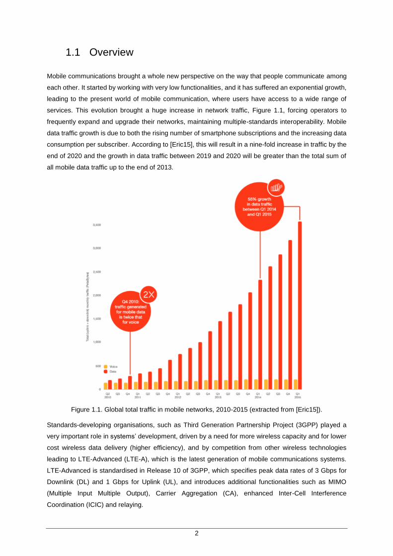
services. This evolution brought a huge increase in network traffic, Figure 1.1, forcing operators to
frequently expand and upgrade their networks, maintaining multiple-standards interoperability. Mobile
data traffic growth is due to both the rising number of smartphone subscriptions and the increasing data
consumption per subscriber. According to [Eric15], this will result in a nine-fold increase in traffic by the
end of 2020 and the growth in data traffic between 2019 and 2020 will be greater than the total sum of
all mobile data traffic up to the end of 2013.
Figure 1.1. Global total traffic in mobile networks, 2010-2015 (extracted from [Eric15]).
Standards-developing organisations, such as Third Generation Partnership Project (3GPP) played a
very important role in systems’ development, driven by a need for more wireless capacity and for lower
cost wireless data delivery (higher efficiency), and by competition from other wireless technologies
leading to LTE-Advanced (LTE-A), which is the latest generation of mobile communications systems.
LTE-Advanced is standardised in Release 10 of 3GPP, which specifies peak data rates of 3 Gbps for
Downlink (DL) and 1 Gbps for Uplink (UL), and introduces additional functionalities such as MIMO
(Multiple Input Multiple Output), Carrier Aggregation (CA), enhanced Inter-Cell Interference
Coordination (ICIC) and relaying.
3
In order to satisfy consumer usage growth, mobile operators must significantly increase their network
capacity to provide mobile broadband to the masses. However, in an intensifying competitive
marketplace, high saturation levels, rapid technological changes and declining voice revenue, operators
are challenged with the deployment of traditional BS (Base Stations) as the cost is high, the return is
not high enough. Average Revenue Per User (ARPU) is affecting mobile operators’ profitability. They
become more and more cautious about the Total Cost of Ownership (TCO) of their network in order to
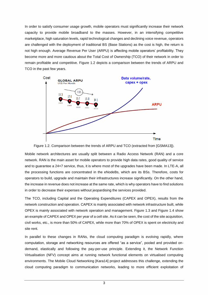
remain profitable and competitive. Figure 1.2 depicts a comparison between the trends of ARPU and
TCO in the past few years.
Figure 1.2. Comparison between the trends of ARPU and TCO (extracted from [GSMA13]).
Mobile network architectures are usually split between a Radio Access Network (RAN) and a core
network. RAN is the main asset for mobile operators to provide high data rates, good quality of service
and to guarantee a 24×7 service, thus, it is where most of the upgrades have been made. In LTE-A, all
the processing functions are concentrated in the eNodeBs, which are its BSs. Therefore, costs for
operators to build, upgrade and maintain their infrastructures increase significantly. On the other hand,
the increase in revenue does not increase at the same rate, which is why operators have to find solutions
in order to decrease their expenses without jeopardising the services provided.
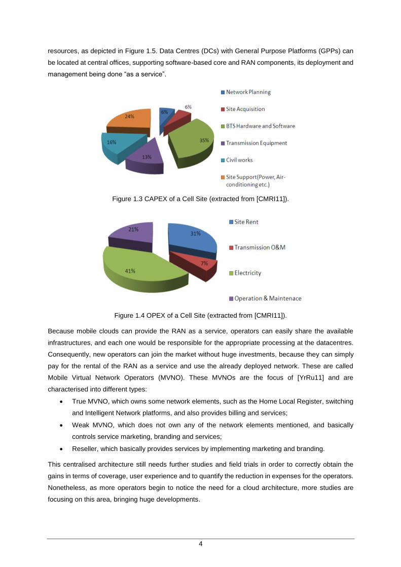
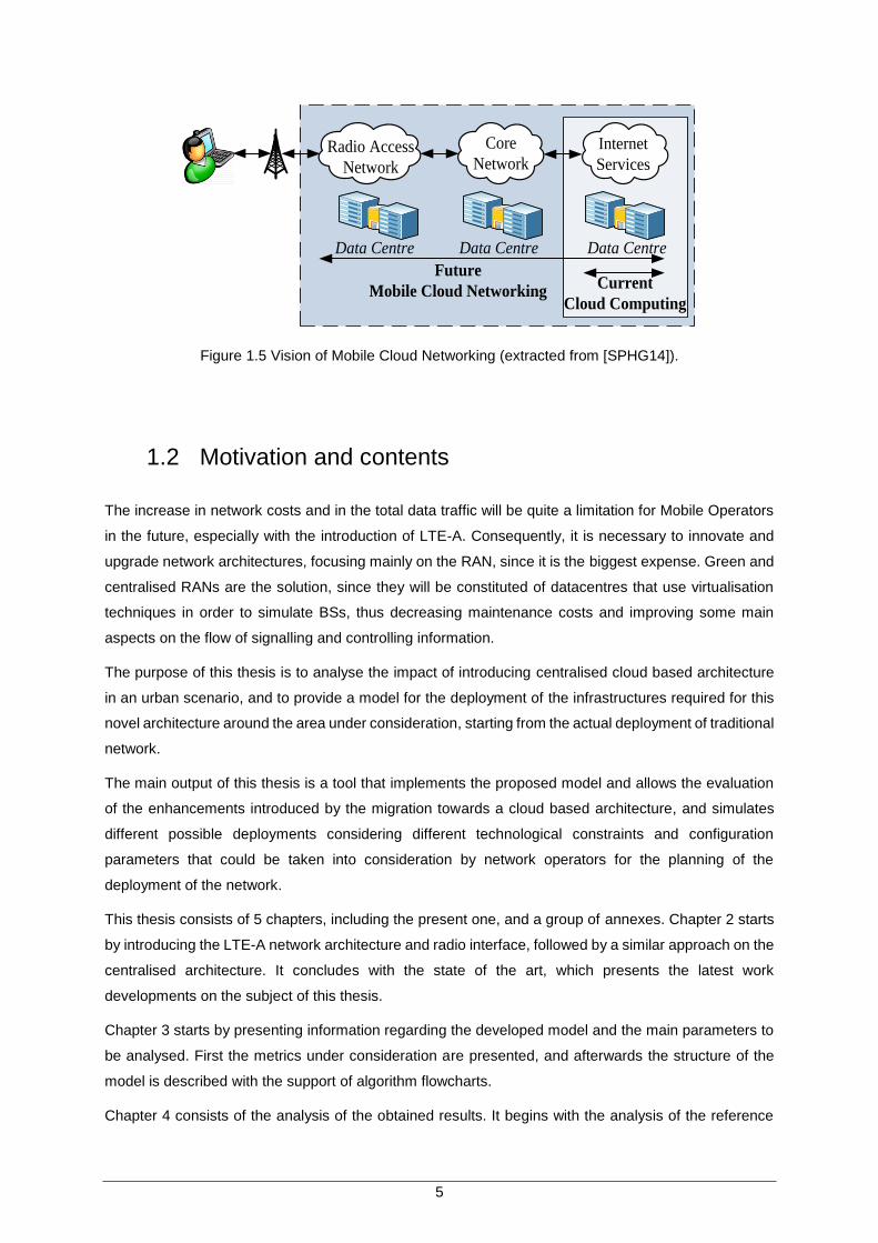
The TCO, including Capital and the Operating Expenditures (CAPEX and OPEX), results from the
network construction and operation. CAPEX is mainly associated with network infrastructure built, while
OPEX is mainly associated with network operation and management. Figure 1.3 and Figure 1.4 show
an example of CAPEX and OPEX per year of a cell site. As it can be seen, the cost of the site acquisition,
civil works, etc., is more than 50% of CAPEX, while more than 70% of OPEX is spent on electricity and
site rent.
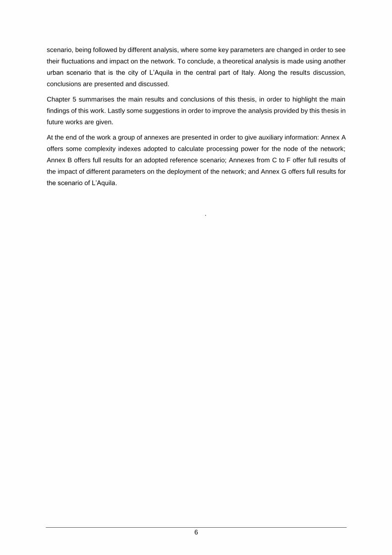
In parallel to these changes in RANs, the cloud computing paradigm is evolving rapidly, where
computation, storage and networking resources are offered “as a service”, pooled and provided on-
demand, elastically and following the pay-per-use principle. Extending it, the Network Function
Virtualisation (NFV) concept aims at running network functional elements on virtualised computing
environments. The Mobile Cloud Networking [Kara14] project addresses this challenge, extending the
cloud computing paradigm to communication networks, leading to more efficient exploitation of
4
resources, as depicted in Figure 1.5. Data Centres (DCs) with General Purpose Platforms (GPPs) can
be located at central offices, supporting software-based core and RAN components, its deployment and
management being done “as a service”.
Figure 1.3 CAPEX of a Cell Site (extracted from [CMRI11]).
Figure 1.4 OPEX of a Cell Site (extracted from [CMRI11]).
Because mobile clouds can provide the RAN as a service, operators can easily share the available
infrastructures, and each one would be responsible for the appropriate processing at the datacentres.
Consequently, new operators can join the market without huge investments, because they can simply
pay for the rental of the RAN as a service and use the already deployed network. These are called
Mobile Virtual Network Operators (MVNO). These MVNOs are the focus of [YrRu11] and are
characterised into different types:
True MVNO, which owns some network elements, such as the Home Local Register, switching
and Intelligent Network platforms, and also provides billing and services;
Weak MVNO, which does not own any of the network elements mentioned, and basically
controls service marketing, branding and services;
Reseller, which basically provides services by implementing marketing and branding.
This centralised architecture still needs further studies and field trials in order to correctly obtain the
gains in terms of coverage, user experience and to quantify the reduction in expenses for the operators.
Nonetheless, as more operators begin to notice the need for a cloud architecture, more studies are
focusing on this area, bringing huge developments.
5
Figure 1.5 Vision of Mobile Cloud Networking (extracted from [SPHG14]).
1.2 Motivation and contents
The increase in network costs and in the total data traffic will be quite a limitation for Mobile Operators
in the future, especially with the introduction of LTE-A. Consequently, it is necessary to innovate and
upgrade network architectures, focusing mainly on the RAN, since it is the biggest expense. Green and
centralised RANs are the solution, since they will be constituted of datacentres that use virtualisation
techniques in order to simulate BSs, thus decreasing maintenance costs and improving some main
aspects on the flow of signalling and controlling information.
The purpose of this thesis is to analyse the impact of introducing centralised cloud based architecture
in an urban scenario, and to provide a model for the deployment of the infrastructures required for this
novel architecture around the area under consideration, starting from the actual deployment of traditional
network.
The main output of this thesis is a tool that implements the proposed model and allows the evaluation
of the enhancements introduced by the migration towards a cloud based architecture, and simulates
different possible deployments considering different technological constraints and configuration
parameters that could be taken into consideration by network operators for the planning of the
deployment of the network.
This thesis consists of 5 chapters, including the present one, and a group of annexes. Chapter 2 starts
by introducing the LTE-A network architecture and radio interface, followed by a similar approach on the
centralised architecture. It concludes with the state of the art, which presents the latest work
developments on the subject of this thesis.
Chapter 3 starts by presenting information regarding the developed model and the main parameters to
be analysed. First the metrics under consideration are presented, and afterwards the structure of the
model is described with the support of algorithm flowcharts.
Chapter 4 consists of the analysis of the obtained results. It begins with the analysis of the reference
Radio Access
Network
Internet
Services
Future
Mobile Cloud Networking
Core
Network
Current
Cloud Computing
Data Centre Data Centre Data Centre
6
scenario, being followed by different analysis, where some key parameters are changed in order to see
their fluctuations and impact on the network. To conclude, a theoretical analysis is made using another
urban scenario that is the city of L’Aquila in the central part of Italy. Along the results discussion,
conclusions are presented and discussed.
Chapter 5 summarises the main results and conclusions of this thesis, in order to highlight the main
findings of this work. Lastly some suggestions in order to improve the analysis provided by this thesis in
future works are given.
At the end of the work a group of annexes are presented in order to give auxiliary information: Annex A
offers some complexity indexes adopted to calculate processing power for the node of the network;
Annex B offers full results for an adopted reference scenario; Annexes from C to F offer full results of
the impact of different parameters on the deployment of the network; and Annex G offers full results for
the scenario of L’Aquila.
.

7
Chapter 2
Basic Concepts and State of
the Art
2 Basic concepts and state of the art
This chapter provides firstly a background on the fundamental concepts of LTE, SDN and Virtualisation,
including LTE’s network architecture and radio interface, a synopsis of SDN and an introduction to NFV
and Cloud-RAN. Then, a brief discussion of optimisation of capacity and load balancing in cellular
networks follows. The last part of this chapter is dedicated to an analysis of the state of the art.
8
2.1 LTE aspects
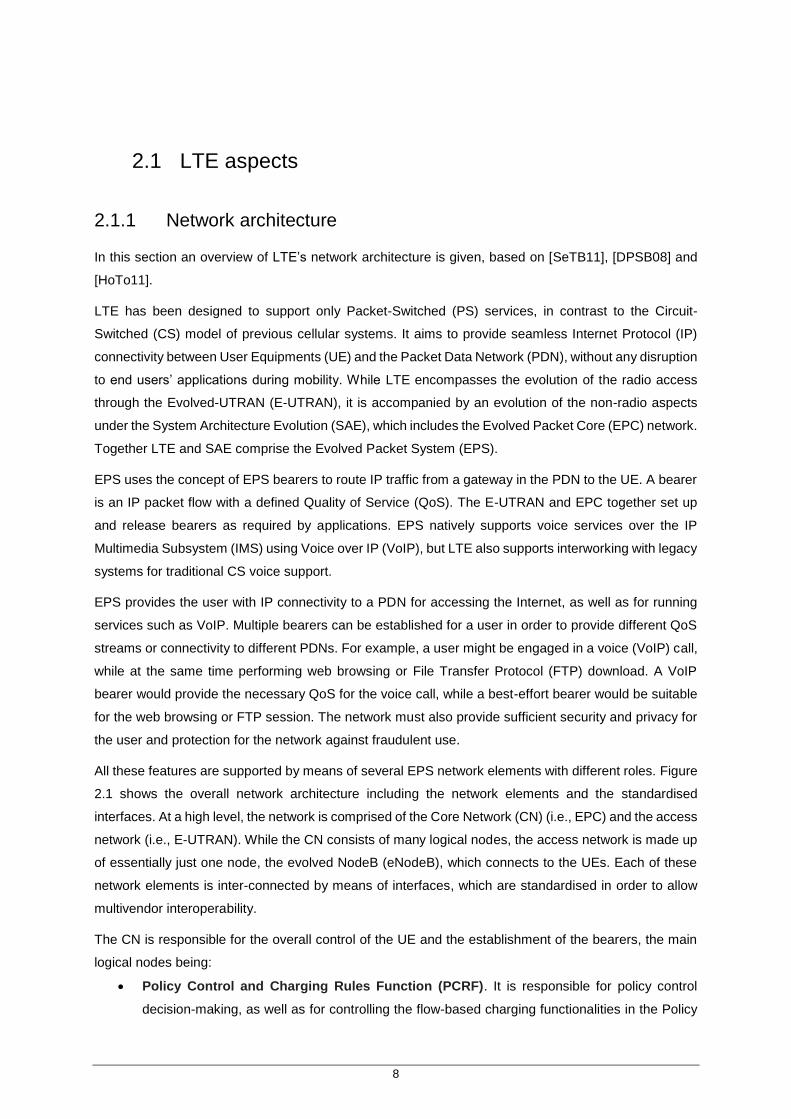
2.1.1 Network architecture
In this section an overview of LTE’s network architecture is given, based on [SeTB11], [DPSB08] and
[HoTo11].
LTE has been designed to support only Packet-Switched (PS) services, in contrast to the Circuit-
Switched (CS) model of previous cellular systems. It aims to provide seamless Internet Protocol (IP)
connectivity between User Equipments (UE) and the Packet Data Network (PDN), without any disruption
to end users’ applications during mobility. While LTE encompasses the evolution of the radio access
through the Evolved-UTRAN (E-UTRAN), it is accompanied by an evolution of the non-radio aspects
under the System Architecture Evolution (SAE), which includes the Evolved Packet Core (EPC) network.
Together LTE and SAE comprise the Evolved Packet System (EPS).
EPS uses the concept of EPS bearers to route IP traffic from a gateway in the PDN to the UE. A bearer
is an IP packet flow with a defined Quality of Service (QoS). The E-UTRAN and EPC together set up
and release bearers as required by applications. EPS natively supports voice services over the IP
Multimedia Subsystem (IMS) using Voice over IP (VoIP), but LTE also supports interworking with legacy
systems for traditional CS voice support.
EPS provides the user with IP connectivity to a PDN for accessing the Internet, as well as for running
services such as VoIP. Multiple bearers can be established for a user in order to provide different QoS
streams or connectivity to different PDNs. For example, a user might be engaged in a voice (VoIP) call,
while at the same time performing web browsing or File Transfer Protocol (FTP) download. A VoIP
bearer would provide the necessary QoS for the voice call, while a best-effort bearer would be suitable
for the web browsing or FTP session. The network must also provide sufficient security and privacy for
the user and protection for the network against fraudulent use.
All these features are supported by means of several EPS network elements with different roles. Figure
2.1 shows the overall network architecture including the network elements and the standardised
interfaces. At a high level, the network is comprised of the Core Network (CN) (i.e., EPC) and the access
network (i.e., E-UTRAN). While the CN consists of many logical nodes, the access network is made up
of essentially just one node, the evolved NodeB (eNodeB), which connects to the UEs. Each of these
network elements is inter-connected by means of interfaces, which are standardised in order to allow
multivendor interoperability.
The CN is responsible for the overall control of the UE and the establishment of the bearers, the main
logical nodes being:
Policy Control and Charging Rules Function (PCRF). It is responsible for policy control
decision-making, as well as for controlling the flow-based charging functionalities in the Policy
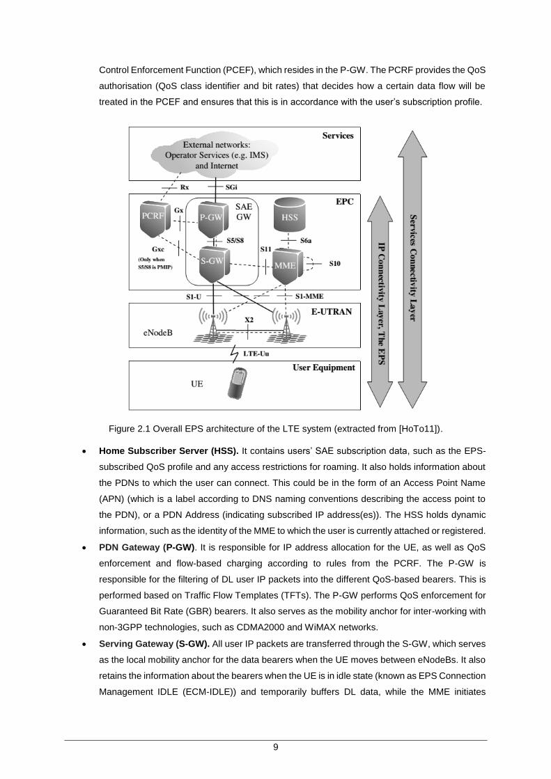
9
Control Enforcement Function (PCEF), which resides in the P-GW. The PCRF provides the QoS
authorisation (QoS class identifier and bit rates) that decides how a certain data flow will be
treated in the PCEF and ensures that this is in accordance with the user’s subscription profile.
Figure 2.1 Overall EPS architecture of the LTE system (extracted from [HoTo11]).
Home Subscriber Server (HSS). It contains users’ SAE subscription data, such as the EPS-
subscribed QoS profile and any access restrictions for roaming. It also holds information about
the PDNs to which the user can connect. This could be in the form of an Access Point Name
(APN) (which is a label according to DNS naming conventions describing the access point to
the PDN), or a PDN Address (indicating subscribed IP address(es)). The HSS holds dynamic
information, such as the identity of the MME to which the user is currently attached or registered.
PDN Gateway (P-GW). It is responsible for IP address allocation for the UE, as well as QoS
enforcement and flow-based charging according to rules from the PCRF. The P-GW is
responsible for the filtering of DL user IP packets into the different QoS-based bearers. This is
performed based on Traffic Flow Templates (TFTs). The P-GW performs QoS enforcement for
Guaranteed Bit Rate (GBR) bearers. It also serves as the mobility anchor for inter-working with
non-3GPP technologies, such as CDMA2000 and WiMAX networks.
Serving Gateway (S-GW). All user IP packets are transferred through the S-GW, which serves
as the local mobility anchor for the data bearers when the UE moves between eNodeBs. It also
retains the information about the bearers when the UE is in idle state (known as EPS Connection
Management IDLE (ECM-IDLE)) and temporarily buffers DL data, while the MME initiates
10
paging of the UE to re-establish the bearers. In addition, the S-GW performs some
administrative functions in the visited network, such as collecting information for charging (e.g.,
the volume of data sent to or received from the user) and legal interception. It also serves as
the mobility anchor for inter-working with other 3GPP technologies, such as GPRS and UMTS.
Mobility Management Entity (MME). It is the control node that processes the signalling
between the UE and the CN. The protocols running between the UE and the CN are known as
the Non-Access Stratum (NAS) protocols. The functions accomplished by the MME are related
to bearer management, connection management an inter-working with other networks.
The access network consists of a network of eNodeBs, normally interconnected to each other by means
of an interface known as X2 and to the EPC by means of the S1 interface. The E-UTRAN is responsible
for the radio related functions, like Radio Resource Management, header compression, security and
connectivity to EPC. Radio Resource Management consists of radio bearer control, radio admission
control, radio mobility control, scheduling and dynamic allocation of resources to UEs in both UL and
DL. Header compression helps to ensure an efficient use of the radio interface by compressing the IP
packet headers, which could otherwise represent a significant overhead, especially for small packets
such as VoIP. Regarding security, all data sent over the radio interface is encrypted. Connectivity to the
EPC consists of the signalling towards the MME and the bearer path towards the S-GW.
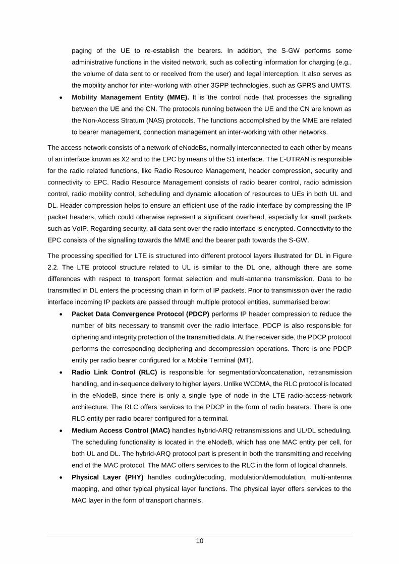
The processing specified for LTE is structured into different protocol layers illustrated for DL in Figure
2.2. The LTE protocol structure related to UL is similar to the DL one, although there are some
differences with respect to transport format selection and multi-antenna transmission. Data to be
transmitted in DL enters the processing chain in form of IP packets. Prior to transmission over the radio
interface incoming IP packets are passed through multiple protocol entities, summarised below:
Packet Data Convergence Protocol (PDCP) performs IP header compression to reduce the
number of bits necessary to transmit over the radio interface. PDCP is also responsible for
ciphering and integrity protection of the transmitted data. At the receiver side, the PDCP protocol
performs the corresponding deciphering and decompression operations. There is one PDCP
entity per radio bearer configured for a Mobile Terminal (MT).
Radio Link Control (RLC) is responsible for segmentation/concatenation, retransmission
handling, and in-sequence delivery to higher layers. Unlike WCDMA, the RLC protocol is located
in the eNodeB, since there is only a single type of node in the LTE radio-access-network
architecture. The RLC offers services to the PDCP in the form of radio bearers. There is one
RLC entity per radio bearer configured for a terminal.
Medium Access Control (MAC) handles hybrid-ARQ retransmissions and UL/DL scheduling.
The scheduling functionality is located in the eNodeB, which has one MAC entity per cell, for
both UL and DL. The hybrid-ARQ protocol part is present in both the transmitting and receiving
end of the MAC protocol. The MAC offers services to the RLC in the form of logical channels.
Physical Layer (PHY) handles coding/decoding, modulation/demodulation, multi-antenna
mapping, and other typical physical layer functions. The physical layer offers services to the
MAC layer in the form of transport channels.
11
Figure 2.2 LTE protocol architecture (DL) (extracted from [DPSB08]).
2.1.2 Radio interface
This section addresses the radio interface for LTE-Advanced, being based on [HoTo11], [DaPS11],
[SeTB11] and [DPSB08].
LTE uses 2 different multiple access schemes: for DL, it is Orthogonal Frequency Division Multiple
Access (OFDMA), and for UL, it is Single Carrier – Frequency Division Multiple Access (SC-FDMA).
The LTE DL transmission scheme is based on Orthogonal Frequency Division Multiplexing (OFDM).
OFDM is an attractive DL transmission scheme for several reasons. Due to the relatively long OFDM
symbol time in combination with a cyclic prefix, OFDM provides a high degree of robustness against
channel frequency selectivity. Although signal corruption due to a frequency-selective channel can, in
principle, be handled by equalisation at the receiver side, the complexity of the equalisation starts to
become unattractively high for implementation in an MT at bandwidths above 5 MHz. Therefore, OFDM
with its inherent robustness to frequency-selective fading is attractive for DL, especially when combined
with spatial multiplexing. Additional benefits with OFDM include the fact that flexible bandwidth
allocations are easily supported by OFDM, at least from a baseband perspective, by varying the number
of OFDM subcarriers used for transmission. Note, however, that the support of multiple spectrum
12
allocations also require flexible RF filtering, an operation to which the exact transmission scheme is
irrelevant. Nevertheless, maintaining the same baseband-processing structure, regardless of the
bandwidth, eases terminal implementation. Another advantage of the use of OFDM is the fact that
broadcast/multicast transmission, where the same information is transmitted from multiple BSs, is
straightforward with OFDM.
For LTE UL, single-carrier transmission based on DFT-spread OFDM (DFTS-OFDM) is used. The use
of single-carrier modulation in UL is motivated by the lower peak-to-average ratio of the transmitted
signal compared to multi-carrier transmission, such as OFDM. The smaller the peak-to-average ratio of
the transmitted signal, the higher the average transmission power can be for a given power amplifier.
Therefore, single-carrier transmission allows for more efficient usage of the power amplifier, which
translates into an increased coverage. This is especially important for the power-limited terminal. At the
same time, the equalisation required to handle corruption of the single-carrier signal due to frequency-
selective fading is less of an issue in UL due to fewer restrictions in signal-processing resources at the
BS compared to the MT.
The high-level time-domain structure for LTE transmission is frame of length 10 ms consisting of ten
equally size subframes of length 1 ms.
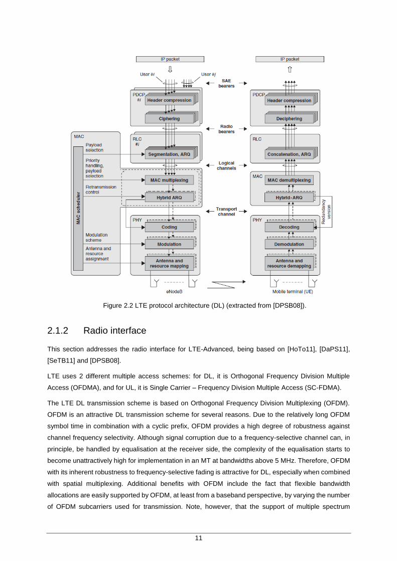
LTE-A benefits from the frequency domain scheduling, which is the dynamic allocation of resources in
the frequency domain, based on Resource Blocks (RBs). An RB consists of a group of 12 sub-carriers,
which occupy 180 kHz in the frequency domain, and 7 or 6 OFDM symbols in the time domain,
depending on if the normal CP or the extended one is being used, respectively. The minimum resource
unit is the resource element that consists of one sub-carrier during one OFDM symbol, which implies
that an RB has 84 (12 sub-carriers × 7 OFDM symbols) or 72 (12 sub-carriers × 6 OFDM symbols)
resource elements per slot in the time domain. Figure 2.3 illustrates the DL resource allocation process.
Figure 2.3 Resource allocation in OFDMA (extracted from [HoTo11]).
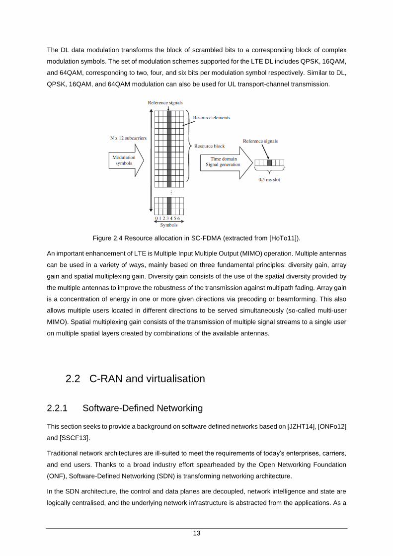
Resource allocation in UL is performed in a similar way to DL, but RBs are allocated to one user
consecutively in the frequency domain, as shown in Figure 2.4. The maximum bandwidth that can be
allocated is 20 MHz, nonetheless there has to be some margin for the guard bands, so the useful
channel bandwidth is smaller.
13
The DL data modulation transforms the block of scrambled bits to a corresponding block of complex
modulation symbols. The set of modulation schemes supported for the LTE DL includes QPSK, 16QAM,
and 64QAM, corresponding to two, four, and six bits per modulation symbol respectively. Similar to DL,
QPSK, 16QAM, and 64QAM modulation can also be used for UL transport-channel transmission.
Figure 2.4 Resource allocation in SC-FDMA (extracted from [HoTo11]).
An important enhancement of LTE is Multiple Input Multiple Output (MIMO) operation. Multiple antennas
can be used in a variety of ways, mainly based on three fundamental principles: diversity gain, array
gain and spatial multiplexing gain. Diversity gain consists of the use of the spatial diversity provided by
the multiple antennas to improve the robustness of the transmission against multipath fading. Array gain
is a concentration of energy in one or more given directions via precoding or beamforming. This also
allows multiple users located in different directions to be served simultaneously (so-called multi-user
MIMO). Spatial multiplexing gain consists of the transmission of multiple signal streams to a single user
on multiple spatial layers created by combinations of the available antennas.
2.2 C-RAN and virtualisation
2.2.1 Software-Defined Networking
This section seeks to provide a background on software defined networks based on [JZHT14], [ONFo12]
and [SSCF13].
Traditional network architectures are ill-suited to meet the requirements of today’s enterprises, carriers,
and end users. Thanks to a broad industry effort spearheaded by the Open Networking Foundation
(ONF), Software-Defined Networking (SDN) is transforming networking architecture.
In the SDN architecture, the control and data planes are decoupled, network intelligence and state are
logically centralised, and the underlying network infrastructure is abstracted from the applications. As a
14
result, enterprises and carriers gain unprecedented programmability, automation, and network control,
enabling them to build highly scalable, flexible networks that readily adapt to changing business needs.
SDN focuses on four key features: separation of the control plane from the data plane; a centralised
controller and view of the network; open interfaces between the devices in the control plane (controllers)
and those in the data plane; and programmability of the network by external applications.
In traditional networks, the control and data planes are combined in a network node. The control plane
is responsible for configuration of the node and programming the paths to be used for data flows. Once
the paths have been determined they are pushed down to the data plane. Data forwarding at the
hardware level is thus based on control information. In this traditional approach, once the forwarding
policy has been defined, the only way to make an adjustment to the policy is via changes to the
configuration of the devices. This is a really restrictive constraint for network operators who are keen to
scale their networks in response to changing traffic demands.
In the SDN approach, control is moved out of the individual network nodes and into the separate,
centralised controller. SDN switches are controlled by a network operating system (NOS) that collects
information using well defined application programming interface (API) and manipulates their forwarding
plane, providing an abstract model of the network topology to the SDN controller hosting the
applications. Therefore, the controller can exploit the complete knowledge of the network to optimise
flow management and support service-user requirements of scalability and flexibility. For example,
bandwidth can be dynamically allocated into the data plane from the application.
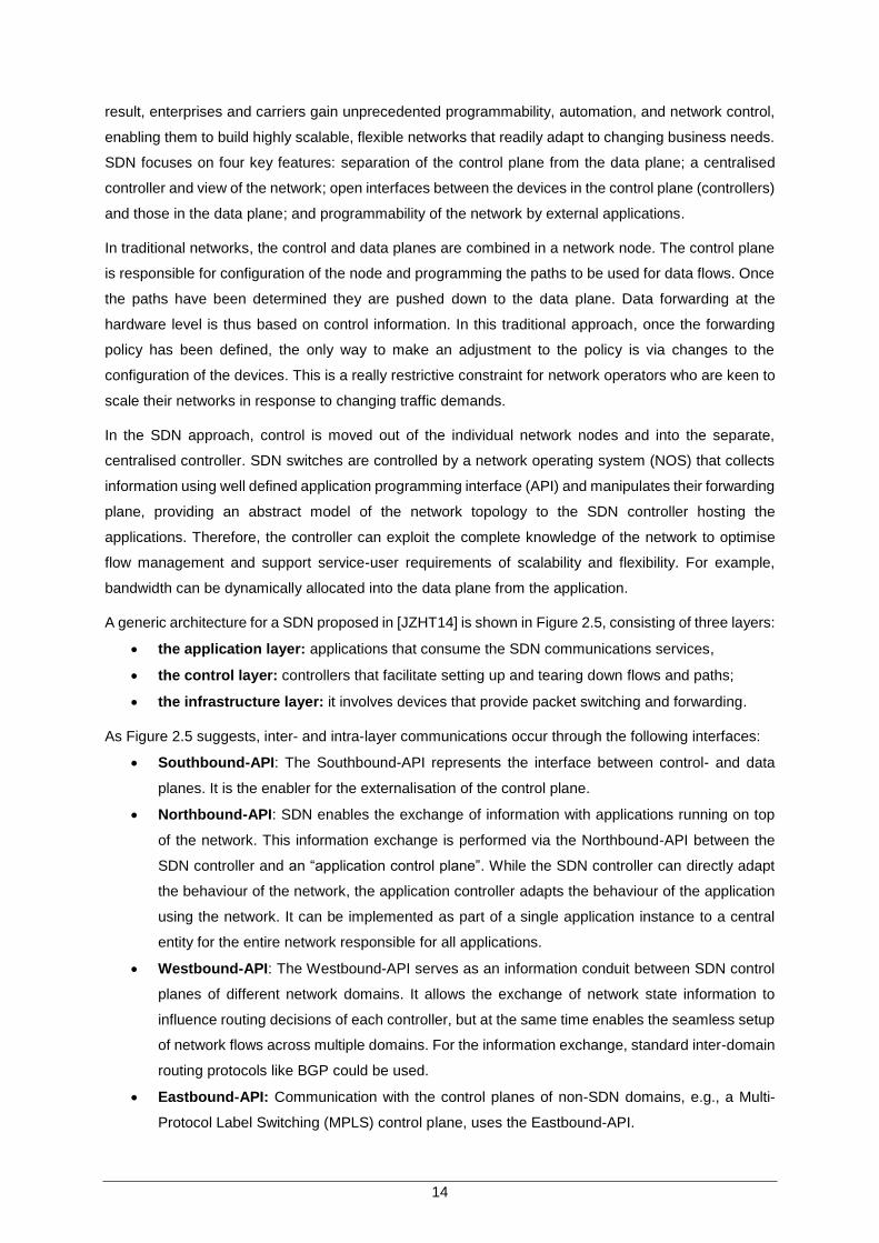
A generic architecture for a SDN proposed in [JZHT14] is shown in Figure 2.5, consisting of three layers:
the application layer: applications that consume the SDN communications services,
the control layer: controllers that facilitate setting up and tearing down flows and paths;
the infrastructure layer: it involves devices that provide packet switching and forwarding.
As Figure 2.5 suggests, inter- and intra-layer communications occur through the following interfaces:
Southbound-API: The Southbound-API represents the interface between control- and data
planes. It is the enabler for the externalisation of the control plane.
Northbound-API: SDN enables the exchange of information with applications running on top
of the network. This information exchange is performed via the Northbound-API between the
SDN controller and an “application control plane”. While the SDN controller can directly adapt
the behaviour of the network, the application controller adapts the behaviour of the application
using the network. It can be implemented as part of a single application instance to a central
entity for the entire network responsible for all applications.
Westbound-API: The Westbound-API serves as an information conduit between SDN control
planes of different network domains. It allows the exchange of network state information to
influence routing decisions of each controller, but at the same time enables the seamless setup
of network flows across multiple domains. For the information exchange, standard inter-domain
routing protocols like BGP could be used.
Eastbound-API: Communication with the control planes of non-SDN domains, e.g., a Multi-
Protocol Label Switching (MPLS) control plane, uses the Eastbound-API.
15
Figure 2.5 Generic SDN architecture (extracted from [JZHT14]).
A standard communications interface defined between control and forwarding layers of an SDN
architecture, called OpenFlow, has been developed by ONF. OpenFlow allows direct access to and
manipulation of the forwarding plane of network devices, such as switches and routers. With OpenFlow,
the path of network packets through the network of switches can be determined by software running on
multiple routers. A number of network switch and router vendors have announced intent to support
OpenFlow standard.
2.2.2 Network functions virtualisation
This section addresses Network Functions Virtualisation (NFV) aspects and is based on [HSMA14],
[LiYu14] and [ETSI12].
The virtualisation technology has emerged as a way to decouple software applications from the
underlying hardware, and enable software to run in a virtualised environment. In a virtual environment,
hardware is emulated, and the operating system (OS) runs over the emulated hardware as if it is running
on its own bare metal resources. Using this procedure, multiple virtual machines can share available
resources and run simultaneously on a single physical machine.
NFV aims to transform the way that network operators architect networks by evolving standard IT
virtualisation technology to consolidate many network equipment types onto industry standard high
volume servers, switches and storage, which could be located in Datacentres, Network Nodes and end
user premises. It involves the implementation of network functions in software that can run on a range
of industry standard server hardware, and that can be moved to, or instantiated in, various locations in
the network as required, without the need for installation of new equipment.
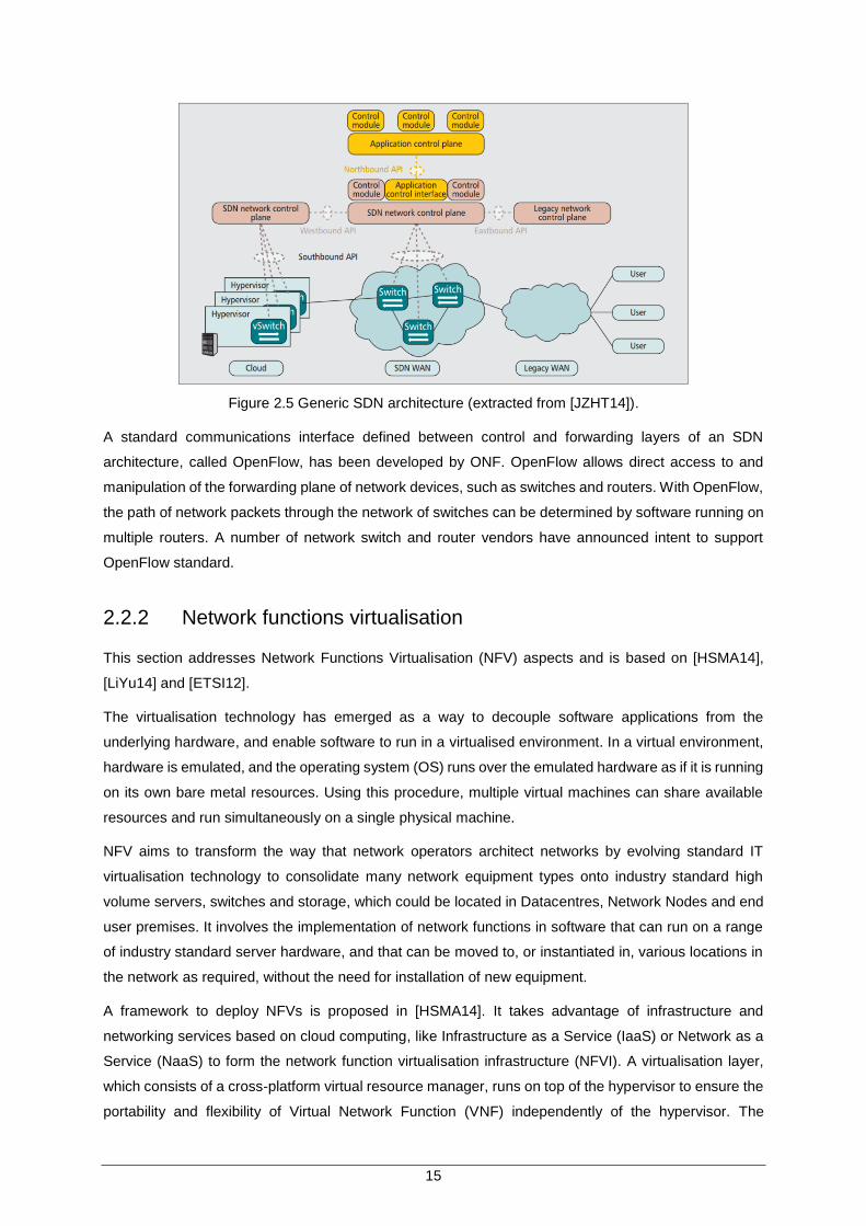
A framework to deploy NFVs is proposed in [HSMA14]. It takes advantage of infrastructure and
networking services based on cloud computing, like Infrastructure as a Service (IaaS) or Network as a
Service (NaaS) to form the network function virtualisation infrastructure (NFVI). A virtualisation layer,
which consists of a cross-platform virtual resource manager, runs on top of the hypervisor to ensure the
portability and flexibility of Virtual Network Function (VNF) independently of the hypervisor. The
16
hypervisor is the software that runs and manages physical resources and provides the virtual
environment on which the guest virtual machines are executed. OpenStack, Eucalyptus, oVirt,
OpenNebula, and Nimbula are examples of cross-platform virtual layers. The virtual machine hosts a
VNF and its Element Management System (EMS). Each VNF instance has its own private EMS to
reduce complexity when migrating an existing VNF or initiating a new one. Operations and business
support systems with VNF infrastructure description entities are deployed in a centralised form, which
provides uniformity of VNF software images and minimises database fragmentation. The Virtual
Resources Manager, the VNF Manager, and the Orchestrator form a centralised controller. The resulting
architecture is shown in Figure 2.6.
Figure 2.6. Basic NFV Framework (extracted from [Damo13]).
NFV goals can be achieved using non-SDN mechanisms, relying on the techniques currently in use in
many datacentres. But approaches relying on the separation of the control and data forwarding planes
as proposed by SDN can enhance performance, simplify compatibility with existing deployments, and
facilitate operation and maintenance procedures. NFV is able to support SDN, by providing the
infrastructure upon which the SDN software can be run. Furthermore, NFV aligns closely with the SDN
objectives to use commodity servers and switches.
2.2.3 Cloud Radio Access Network
In this section, an overview on Cloud Radio Access Network (C-RAN) is given based on [CCYS14] and
[HDGK13].
Cloud computing technology has emerged as a promising solution for providing high energy efficiency
together with gigabit data rates across software defined wireless communication networks, in which the
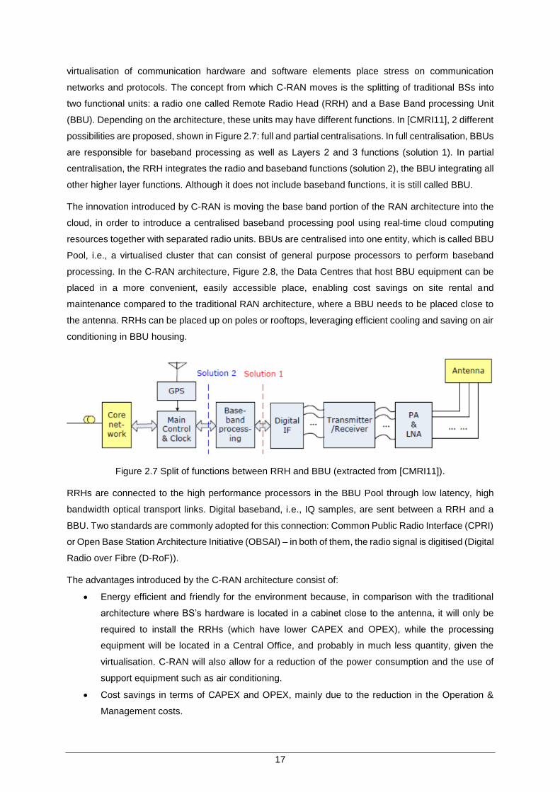
17
virtualisation of communication hardware and software elements place stress on communication
networks and protocols. The concept from which C-RAN moves is the splitting of traditional BSs into
two functional units: a radio one called Remote Radio Head (RRH) and a Base Band processing Unit
(BBU). Depending on the architecture, these units may have different functions. In [CMRI11], 2 different
possibilities are proposed, shown in Figure 2.7: full and partial centralisations. In full centralisation, BBUs
are responsible for baseband processing as well as Layers 2 and 3 functions (solution 1). In partial
centralisation, the RRH integrates the radio and baseband functions (solution 2), the BBU integrating all
other higher layer functions. Although it does not include baseband functions, it is still called BBU.
The innovation introduced by C-RAN is moving the base band portion of the RAN architecture into the
cloud, in order to introduce a centralised baseband processing pool using real-time cloud computing
resources together with separated radio units. BBUs are centralised into one entity, which is called BBU
Pool, i.e., a virtualised cluster that can consist of general purpose processors to perform baseband
processing. In the C-RAN architecture, Figure 2.8, the Data Centres that host BBU equipment can be
placed in a more convenient, easily accessible place, enabling cost savings on site rental and
maintenance compared to the traditional RAN architecture, where a BBU needs to be placed close to
the antenna. RRHs can be placed up on poles or rooftops, leveraging efficient cooling and saving on air
conditioning in BBU housing.
Figure 2.7 Split of functions between RRH and BBU (extracted from [CMRI11]).
RRHs are connected to the high performance processors in the BBU Pool through low latency, high
bandwidth optical transport links. Digital baseband, i.e., IQ samples, are sent between a RRH and a
BBU. Two standards are commonly adopted for this connection: Common Public Radio Interface (CPRI)
or Open Base Station Architecture Initiative (OBSAI) – in both of them, the radio signal is digitised (Digital
Radio over Fibre (D-RoF)).
The advantages introduced by the C-RAN architecture consist of:
Energy efficient and friendly for the environment because, in comparison with the traditional
architecture where BS’s hardware is located in a cabinet close to the antenna, it will only be
required to install the RRHs (which have lower CAPEX and OPEX), while the processing
equipment will be located in a Central Office, and probably in much less quantity, given the
virtualisation. C-RAN will also allow for a reduction of the power consumption and the use of
support equipment such as air conditioning.
Cost savings in terms of CAPEX and OPEX, mainly due to the reduction in the Operation &
Management costs.
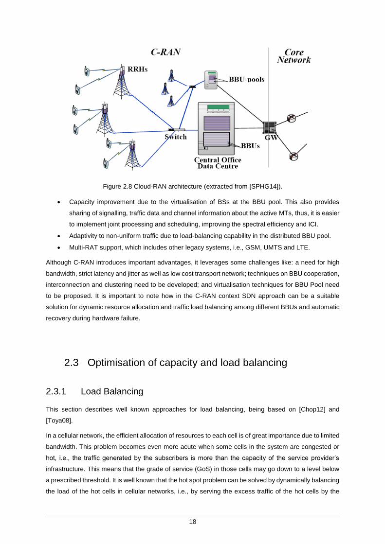
18
Figure 2.8 Cloud-RAN architecture (extracted from [SPHG14]).
Capacity improvement due to the virtualisation of BSs at the BBU pool. This also provides
sharing of signalling, traffic data and channel information about the active MTs, thus, it is easier
to implement joint processing and scheduling, improving the spectral efficiency and ICI.
Adaptivity to non-uniform traffic due to load-balancing capability in the distributed BBU pool.
Multi-RAT support, which includes other legacy systems, i.e., GSM, UMTS and LTE.
Although C-RAN introduces important advantages, it leverages some challenges like: a need for high
bandwidth, strict latency and jitter as well as low cost transport network; techniques on BBU cooperation,
interconnection and clustering need to be developed; and virtualisation techniques for BBU Pool need
to be proposed. It is important to note how in the C-RAN context SDN approach can be a suitable
solution for dynamic resource allocation and traffic load balancing among different BBUs and automatic
recovery during hardware failure.
2.3 Optimisation of capacity and load balancing
2.3.1 Load Balancing
This section describes well known approaches for load balancing, being based on [Chop12] and
[Toya08].
In a cellular network, the efficient allocation of resources to each cell is of great importance due to limited
bandwidth. This problem becomes even more acute when some cells in the system are congested or
hot, i.e., the traffic generated by the subscribers is more than the capacity of the service provider’s
infrastructure. This means that the grade of service (GoS) in those cells may go down to a level below
a prescribed threshold. It is well known that the hot spot problem can be solved by dynamically balancing
the load of the hot cells in cellular networks, i.e., by serving the excess traffic of the hot cells by the
19
cooler cells in the system. Many channel assignment and dynamic load-balancing schemes have been
proposed in the past for efficient use of the frequency spectrum and to handle the hot spot problem from
the voice applications viewpoint.
The hot spot problem exists not only for voice applications but for wireless data networks as well. The
performance (e.g., in terms of throughput) of a wireless data network with centralised control (e.g.,
Wireless Local Area Networks (WLAN) or other cellular data services, such as Cellular Digital Packet
Data (CDPD)) can be improved by transferring users from overloaded BSs (or access points) to lightly
or moderately loaded ones. Similar to the call blocking probability, which is a performance metric for
voice in circuit switching, the improvement that can be achieved in throughput of a WLAN when a
dynamic load-balancing scheme is employed will depend on several criteria, such as traffic level,
available resources, and QoS requirements.
Regarding traditional voice applications, there are three main channel assignment strategies proposed
in the literature. The first one is the Fixed Channel Assignment (FCA) strategy, wherein each cell is
allocated a predetermined set of voice channels. If all the channels in a cell are occupied, any new calls
or handover requests within the cell will be rejected. In variants of the FCA strategy, a cell is allowed to
borrow channels from a neighbouring cell if all of its channels are already occupied. The Mobile
Switching Centre (MSC) supervises such borrowing procedures, and ensures that the borrowing of a
channel will not affect any of the calls already in progress in the cell that is lending. Simplicity is one of
the main advantages of such a scheme, along with frequency reuse maximisation, as opposed to the
other schemes that have complex procedures.
The second one is the Dynamic Channel Assignment (DCA) strategy, in which voice channels are not
permanently allocated to the cells. Every time a call request is made, the serving BS requests a channel
from the MSC, instead. The switch then allocates a channel to the requesting cell following an algorithm
that takes the likelihood of future call blocking within the cell into account, as well as the frequency of
use of the candidate, the reuse distance of the channel, and other cost functions. Although DCA
schemes improve the call blocking probability of the system substantially, for high traffic intensity, the
computational load on the system increases greatly.
The third type is Hybrid Channel Assignment (HCA), which is a blend of the concepts of fixed and
dynamic channel assignment schemes. This basically means there are channels in a global pool for use
in case there is a shortage in addition to the fixed set of channels assigned to each cell. To conclude,
although the objective of all the schemes is better utilisation of the available channels, causing reduced
call blocking probability, most of the schemes do not consider the non-uniformity of channel demand,
which is the variation of channel demand from time to time and/or area to area.
Many interesting dynamic load-balancing schemes have been proposed for an efficient use of limited
bandwidth and to increase the capacity of congested cells or hot spots. The dynamic load balancing
schemes proposed in the literature can be broadly classified into two groups: strategies based on
channel borrowing from cooler cells (lightly loaded), such as simple borrowing, Channel Borrowing
Without Locking (CBWL), and Load Balancing with Selective Borrowing (LBSB); strategies based on
traffic transfer to cooler cells, such as directed retry, and hierarchical macro cell overlay systems.

20
In simple borrowing, every cell is assigned a fixed set of channels and a separate set of channels that
are allowed to be borrowed by the neighbouring congested cells. When a channel is borrowed, the co-
channels within the reuse distance are locked to avoid co-channel interference.
In CBWL, the use of borrowed channels with reduced transmission power is proposed, when the set of
available channels in a cell gets exhausted. This is done to avoid interference with other co-channels.
Taking advantage of transmission power control, however, to induce handover into less loaded cells
and reducing it, may decrease the link capacity for others, who still remain in the cell. There are two
types of CBWL: without channel arrangement (CBWLnR) and with channel rearrangement (CBWLCR).
In CBWLnR, only the new call requests within the fraction of cellular area in which borrowed channels
can be used (this area is limited due to reduced transmission power over the borrowed channels) are
granted service using a borrowed channel. However, in CBWLCR, even if the new call request is not in
the channel-borrowing area, it can still get service if there is at least one active user within the channel-
borrowing area; in this case, the active user will borrow a channel from a neighbouring cell and start
transmission at a reduced power, and the channel released by that user will be assigned to the new
user requesting service.
In selective channel borrowing, load balancing is achieved by a structured borrowing mechanism where
a hot cell can borrow a fixed number of channels only from adjacent cells in the next outer ring. In this
way, unused channels of the cold cells are moved to the hot spot area. This mechanism reduces the
amount of interference between the borrower cell and the co-channel cells of the lender.
In the directed retry scheme, the traffic load is shared in the overlap of the neighbouring cells. There is
no concept of borrowing channels from the neighbouring cells, however, the subscribers who can
communicate with more than one BS are moved from the congested cell to a neighbouring cell.
In the hierarchical macro cell overlay system with microcells and overlaid macro cells, high traffic areas
are covered by microcells while overlaying macro cells cover low-traffic areas and provide overflow
groups of channels for clusters of microcells. In other words, the excess traffic of the microcells is served
by the overlaying macro cells. As a consequence, macro cell overlays inherently achieve dynamic load
balancing by transferring the otherwise blocked microcell users to the macro cells.
Recently, there has been a lot of interest in the usage of relays and relaying techniques to expand
coverage and capacity in cellular networks. Relaying is a cooperative communication concept based on
replacement of direct communication link between source and destination with several shorter links
using network terminals called relays. Researchers have looked at the problem of load balancing from
the perspective of relaying and have proposed schemes to induce user handover from heavily loaded
cells into adjacent cells that may be lightly loaded.
Integrated cellular and ad hoc relay (iCAR) and Pervasive Ad-Hoc Relaying for Cellular Systems
(PARCelS) were the first two load balancing schemes introduced for balancing the load among cells
through relaying. In iCAR, low cost limited mobility, ad-hoc relay stations (ARSs) are placed in hot spots
for relaying traffic out of the hot spots. This strategy is still costly and not flexible enough to handle the
highly dynamic load situation in 3G networks.
21
PARCelS uses mobile nodes for relaying. When a BS is congested, MTs search best routes to other
non-congested cells. Route information is forwarded to BSs for selection. This strategy requires
considerable routing overhead in MTS and does not take advantage of the presence of powerful BSs.
In addition, both schemes do not take into account the load balancing among relaying nodes which
could greatly affect the load balancing performance.
2.3.2 Optimisation of capacity
Optimisation of network capacity is a key challenge to cope with the boost in mobile data traffic that is
expected in the next years and to benefit from the growing market. Several metrics define the capacity
of the network and several strategies have been proposed in order to optimise capacity. In general, the
optimisation of network capacity cannot be considered as an independent aspect from other network
features concerns, like load balancing or coverage maximisation. Every proposed different strategy
involves a different relationship between these aspects and capacity optimisation.
Regarding the relationship between load balancing and capacity optimisation, some schemes have also
been introduced to increase capacity in cellular networks. Mobile Assisted Call Admission (MACA), is a
dynamic load balancing scheme proposed to improve call blocking probability performance in cellular
networks with the idea of forwarding the excess traffic of a ”hot” cell to its ”cooler” neighbouring cells via
mobile agents in the network [XiMC00]. For the purpose of forwarding the call, either relay channel can
be used, in-band (i.e., cellular band) or out-of-band (i.e., ISM-band or any other band other than cellular
band) channels. In the case of in-band MACA, a portion of the fixed channels assigned to each cell is
saved for forwarding calls, whereas, in out-of-band MACA, the MTs use channels from a frequency band
other than the cellular band, such as the ISM-band to forward calls.
In Multihop Cellular Networks (MCN), the ranges of BSs and MTs are reduced, and users within the
same cell are able to communicate with each other over multi-hops, while on the other hand, users in
different cells need to forward their traffic via BSs. The objective in this scheme is to increase network
capacity by replacing single-hop communication by multi-hops between BSs and MTs [LiHs00].
In Unified Cellular and Ad hoc Network (UCAN), instead of improving the call blocking probability, the
use of ad hoc connections to enhance a mobile user’s access to the 3G cellular infrastructure is
proposed. If the throughput is low (i.e., the direct wireless link from the BS to MS is bad), a multi-hop
link from the mobile user to the BS is formed via other mobile users in the system that have better
channel quality [LRSL03].
Coverage and capacity optimisation (CCO) has been initially addressed in Release 9 of 3GPP
specification, which has attracted plenty of attention to increase the corresponding Key Performance
Indicators (KPIs). Several approaches follow the goal of optimising capacity acting on the adjustment of
the antennas parameters, like azimuth orientation and tilt, at the same time varying network coverage.
In [AWVK11], an algorithm designed for an offline network planning environment is provided. The
proposed solution is based on a mathematical optimisation approach, and four optimisation functions
are determined: two based on cell-specific performance measures and two on network-side ones. Self-
22
Organising Networks (SONs) may benefit from optimisation solutions designed for a dynamic context.
In SONs, a wireless network coverage and capacity are optimised by monitoring channel quality to
identify BS coverage holes and to eliminate unnecessary overlapping coverage areas. BSs can
dynamically manipulate parameters, such as antenna tilt and reference power offsets, to compensate
for lapses in coverage and to ensure adequate capacity.
In [LuSB11], a model for SON optimisation of coverage and capacity is presented. The outputs are
optimised radio configuration parameters, which may include DL transmit power, DL reference signal
power offset and antenna tilt. So, the optimisation aims at maximising network capacity and ensuring
that there is an appropriate overlapping area between adjacent cells. The optimal parameter setting is
acquired by cooperatively adjusting antenna tilt and pilot power among the related cells.
In [ERXM13], the optimisation procedure is carried out by considering time-variant optimisation
parameters that are automatically adapted with respect to changes in the network. In the proposed
solution, periodic or aperiodic detection of degraded system performance automatically triggers
optimisation procedures that autonomously improve the performance by (re-)configuration of basic
control parameters, namely, transmission power, antenna tilt, and transmitter activity (switch on/off).
Since maximisation of coverage and maximisation of capacity, generally, are trade-off tasks [NGMN08],
they consider a typical multiobjective optimisation problem. To cope with the contradicting objectives,
they develop a traffic light-related decision scheme that optimises Multi-Tier Network (MTN) coverage
and capacity, either jointly or in a hierarchical manner, if significant performance degradation needs to
be resolved. The optimisation model proposed comprises three key components: the objective function
represents the KPI metrics that will be maximised by tuning according control parameters, i.e., the
optimisation variables; the optimisation constraints model system dependence relations and system
restrictions, mostly in a technical sense; traffic-related input parameters describing spatial radio
conditions for different system configurations and the distribution of user rate demand.
In [ZSYZ13], a novel hybrid two layer optimisation framework is proposed to enhance network capacity
and coverage, where on the top layer a network entity of eCoordinator is implemented to ensure overall
network coverage by optimising the antenna tilt and capacity-coverage weight of each cell in a
centralised manner, and on the bottom one individual eNB optimises cell-specific capacity and coverage
by tuning its pilot power in a distributed manner. A heuristic algorithm is developed for the eCoordinator
operation at large time granularity and the Genetic Programming (GP) approach is exploited for the eNB
operation at small time granularity, for the purpose of tracking overall network performance as well as
adapting to network dynamics.
A completely different approach to the capacity optimisation problem is represented by acting on BS
placement. In [MoNa00], the Combination Algorithm for Total Optimisation (CAT) is proposed to identify
optimal positions for BSs. In the proposed solution, users are modelled as a set of control points that
represent the capacity and coverage requirements a set of feasible BS location is given avoiding
problems deriving from the fact that network operators cannot locate BSs in arbitrary locations, such as
protected buildings, difficult geographical locations and so on. The basic idea relies on analysing all
possible BSs in the given set. The optimum combination is the subset with the highest metric (i.e. the
23
greatest number of adequately supported users). For a given number of control nodes and BSs an
optimisation algorithm deploys a minimum number of BSs to satisfy the operator’s overall requirements.
The problem of coverage optimisation can lead to the well-known geometrical problem of the Discrete
Unit Disk Cover (DUDC), which is an NP problem as highlighted in [FoPT81]. This problem has been
studied extensively due to its wide applications in wireless networks and several Polynomial Time
Approximation Schemes have been proposed. During years, different solutions with different
approximation factors have been developed and actually the best known ones are [FrLo12] and
[MuRa10]. In [FrLo12], they propose an approximation that is the lowest known approximation factor for
a DUDC approximation algorithm with a tractable running time. In [MuRa10], they propose the best
Polynomial Time Approximation Schemes known for DUDC, which is based on local search that takes
O(m257n) time for a 2-approximation solution.
2.4 State of the art
In [NGMN13], a more in-depth analysis of the architecture of the C-RAN can be found. In this paper,
different deployment cases for C-RAN are analysed, such as Large/Medium Scale C-RAN, Small Scale
C-RAN using legacy site room, Indoor Coverage, Super Hot Spot Coverage and Railway/Subway
coverage. It also presents the key functionalities and possible solutions for the C-RAN implementation,
for both the fronthaul and the architecture of the network elements.
RRHs must be associated with the BBUs depending on the traffic at a certain period of time. Thus, a
good algorithm to describe the switching schemes between RRHs and BBUs is required. In [NaWK12],
an example of an algorithm is made that explains how this switching is done, according to metrics such
as processing power and RRH localisation. With the help of some simulations, it is concluded that the
number of required BBUs can be reduced between 26% and 47%.
In [NMWK12], an analysis on statistical multiplexing gain as a function of cell layout is performed, based
on the variation of population between day and night in the Tokyo metropolitan area. The analysis shows
that the number of BBUs can be reduced by 75% compared to the traditional RAN architecture.
[WeGP13] describes a simulation model that is capable of capturing the effects from data traffic, user
distribution, and radio transmissions. With simulations, they have shown that in typical scenarios, the
compute resource utilisation is limited to about 80% of the theoretical maximum, which is mainly caused
by the channel conditions. They also evaluated how the multiplexing gain increases when more sectors
are aggregated in a single MSS-BBU. While the combination of five sectors already saves 9 %, the
aggregation of 57 sectors saves more than a quarter of the compute resources. Finally, they showed
that the user distribution has a strong influence on the utilisation of the compute resources.
In [ChHC14], solutions on how to optimise new RAN deployments in terms of minimising TCO are
proposed. This involves optimal distribution of office and residential cells in order to reduce the number
of required BBUs for a BBU pool and the optimal share of C-RAN with RRHs versus traditional BSs at
24
different cost factors. They investigate the statistical multiplexing gain that can be achieved in C-RAN,
using analytical and modelling approaches. For the analysed traffic profile, they both show that the
optimal gain can be obtained connecting 20-30% of office BSs and 70-80% of residential BSs to the
BBU Pool. The statistical multiplexing gain reaching up to 1.6 can be achieved. Moreover, they show
that if the cost factor (the ratio between the cost of one BBU and the cost of one kilometre of fibre
deployment) is 3 or higher, it is beneficial to deploy C-RAN with RRHs in order to minimise TCO. Results
also show that the advantage is higher when looking at smaller areas (100 km2) compared to larger
ones (400 km2). C-RAN is considered to be beneficial for urban deployments with densely placed cells.
Since in C-RAN the baseband processing of multiple cells is carried out in the centralised BBU pool, the
overall utilisation rate can be improved. The required baseband processing capacity of the pool is
expected to be smaller than the sum of capacities of single BSs. [MLXX12] proposes a spectrum sharing
scheme for LTE eNB virtualisation with multi-eNBs and multi-VOs systems. Extensive simulations were
performed to evaluate the improved efficiency of the spectrum resource utilisation and the end user
performance. With eNB virtualisation, the resources can be utilised in a more efficient manner by
multiple VOs, thus improving system performance, especially for nGBR services. They investigate the
optimal parameters settings for NV, such as sharing intervals and safety margins. An optimum setting
can be found as a trade-off between user performance and processing effort, as well as signalling
overhead. They also present a dynamic load balancing scheme that can lead to a significant gain of
user performance by offloading the excessive traffic from high loaded eNBs to low loaded ones.
In [BPKK12], a framework for Cloud RAN is proposed. The proposed framework has two objectives:
partitioning the set of BSs into groups that are simultaneously processed on a shared homogeneous
compute platform for a given statistical guarantee; scheduling the set of BSs allocated to a platform in
order to meet their real-time processing requirements. This partitioning and scheduling framework saves
up to 19% of the compute resources for a probability of failure of one in 100 million.
[ZZHS13] shows how power allocation is a key technique that can significantly improve RAN
performance. The proposed idea is that UL and DL powers should be controlled to avoid signal
interference. The power control technique can minimise the transmitted power of each MT in the premise
of ensuring each user’s communication quality so as to mitigate interference and enhance network
capacity. They established an optimisation model that takes network capacity as the objective function,
and solved the globally optimal solution of the model, which was a group of transmitted power of MTs
via the Artificial Fish Swarm Algorithm (AFSA). Numerical results show that the power allocation
algorithm proposed in the paper can enormously enhance network capacity compared to the existing
Non-cooperative Power control Game and Pricing (NPGP) algorithm.
The virtualisation technology is a promising solution for higher resource utilisation, improved system
performance, and lower investment capitals for mobile operators. In [LiTi13], the work is focused on
allocating wireless resources among multiple Virtual Mobile Operators (VMOs). A bankruptcy game
based dynamic wireless resource allocation approach among multiple VMOs is proposed and
investigated. An LTE virtualisation framework is adopted and the minimum radio resource allocation unit
is taken as the physical RB. Wireless spectrum resources are abstracted to a resource pool that is
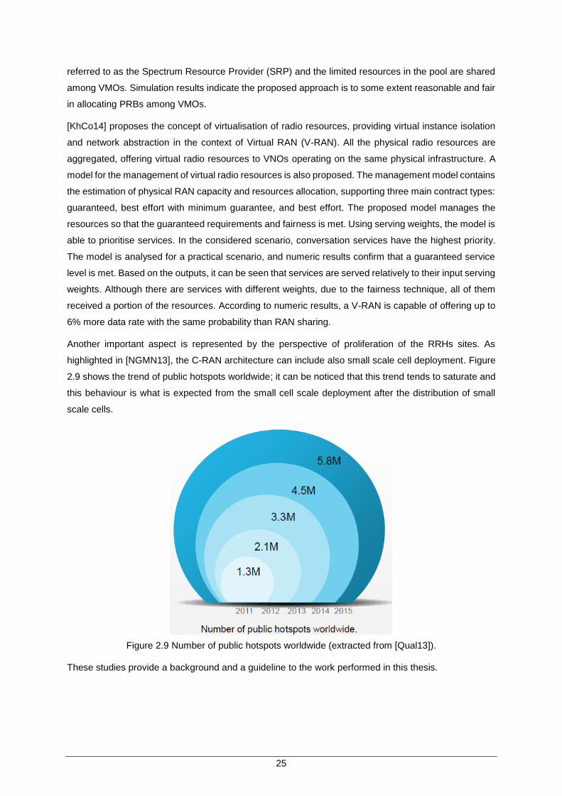
25
referred to as the Spectrum Resource Provider (SRP) and the limited resources in the pool are shared
among VMOs. Simulation results indicate the proposed approach is to some extent reasonable and fair
in allocating PRBs among VMOs.
[KhCo14] proposes the concept of virtualisation of radio resources, providing virtual instance isolation
and network abstraction in the context of Virtual RAN (V-RAN). All the physical radio resources are
aggregated, offering virtual radio resources to VNOs operating on the same physical infrastructure. A
model for the management of virtual radio resources is also proposed. The management model contains
the estimation of physical RAN capacity and resources allocation, supporting three main contract types:
guaranteed, best effort with minimum guarantee, and best effort. The proposed model manages the
resources so that the guaranteed requirements and fairness is met. Using serving weights, the model is
able to prioritise services. In the considered scenario, conversation services have the highest priority.
The model is analysed for a practical scenario, and numeric results confirm that a guaranteed service
level is met. Based on the outputs, it can be seen that services are served relatively to their input serving
weights. Although there are services with different weights, due to the fairness technique, all of them
received a portion of the resources. According to numeric results, a V-RAN is capable of offering up to
6% more data rate with the same probability than RAN sharing.
Another important aspect is represented by the perspective of proliferation of the RRHs sites. As
highlighted in [NGMN13], the C-RAN architecture can include also small scale cell deployment. Figure
2.9 shows the trend of public hotspots worldwide; it can be noticed that this trend tends to saturate and
this behaviour is what is expected from the small cell scale deployment after the distribution of small
scale cells.
Figure 2.9 Number of public hotspots worldwide (extracted from [Qual13]).
These studies provide a background and a guideline to the work performed in this thesis.

26
27
Chapter 3
Model Development and
Implementation
3 Model Development and Implementation
A description of the model used in this thesis is provided in this chapter, starting with its metrics and
overview and proceeding with a more detailed analysis of its implementation. The chapter ends with a
brief assessment of the model.
28
3.1 Description of the problem
The problem addressed in this thesis concerns the optimal deployment of RRHs and BBU pools in an
urban scenario in which traditional BSs are already deployed. As highlighted in the next sections,
concentrating computational capacity in BBUs introduces a new segment in the traditional RAN
architecture. This implies that time elaboration constraints provided by specifications for tasks
accomplished by eNodeBs must incorporate also the time for the transportation of data through the
fronthaul segment.
The budget of time for transportation represents a key aspect for the optimisation of the deployment,
because it has a direct impact on the maximum length of the links between RRHs and BBUs. Regarding
this aspect, one provides a solution that holds for different constraints of delay in order to tolerate
evolution of technologies and at the same time restrictions of the constraints for the future radio access
technologies.
Designing a solution for an urban scenario raises an important requirement: not all the locations that
could be considered optimal for the BBU pools positions should be able to host infrastructures required
for a BBU pool, due to the fact that network operators cannot locate equipment in arbitrary locations,
such as protected buildings, difficult geographical locations and so on. The adopted approach to avoid
this problem is to consider as the set of feasible positions for the BBUs the set of locations of the BSs.
Based on these considerations, the problem is to find which BSs’ positions can be elected as possible
BBU pools’ positions, given a constraint of distance between BBU and RRH, and minimising the number
of BBU pools location in order to reduce costs of investments for operators. This problem can be
interpreted in a geometrical way and leads to the well-known problem of Discrete Unit Disk Coverage,
which is known to be NP-complete [FoPT81]. This problem has been studied extensively due to its wide
applications in wireless networks and series of constant factor approximation algorithms have been
proposed. In the next sections, one provides some heuristic approaches to this problem.
Another important aspect taken into consideration in designing the C-RAN deployment is the load
balancing between BBU pools. Given the optimal BBU positions, one needs to understand the
clusterisation policy to connect each RRH to a BBU in order to respect delay constraint and at the same
time balance the load (in terms of required capacity or processing power) between BBUs. To do this, a
technique that associates RRHs that can be connected to more than one BBU to the one that is less
utilised has been developed. For what concerns load calculation, our approach assumes the worst case
in which each RRH requires all resources available.
As highlighted in [NGMN13], a C-RAN architecture can include also small scale cell deployment, and
focusing on this fact, one provide a proliferation algorithm that can forecast the growth of RRHs in the
urban scenario. This is an important aspect in addressing the problem of optimal deployment, in order
to evaluate the variation on capacity requirements and processing power for the BBU pools.
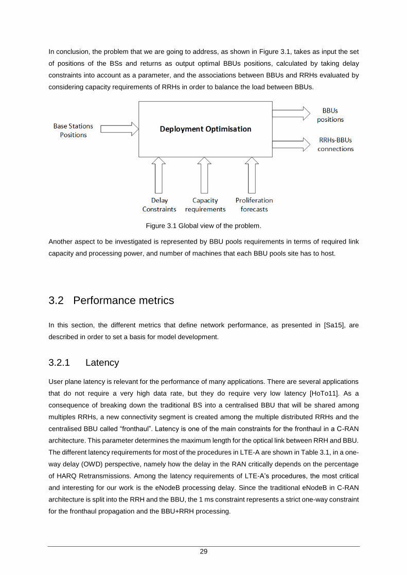
29
In conclusion, the problem that we are going to address, as shown in Figure 3.1, takes as input the set
of positions of the BSs and returns as output optimal BBUs positions, calculated by taking delay
constraints into account as a parameter, and the associations between BBUs and RRHs evaluated by
considering capacity requirements of RRHs in order to balance the load between BBUs.
Figure 3.1 Global view of the problem.
Another aspect to be investigated is represented by BBU pools requirements in terms of required link
capacity and processing power, and number of machines that each BBU pools site has to host.
3.2 Performance metrics
In this section, the different metrics that define network performance, as presented in [Sa15], are
described in order to set a basis for model development.
3.2.1 Latency
User plane latency is relevant for the performance of many applications. There are several applications
that do not require a very high data rate, but they do require very low latency [HoTo11]. As a
consequence of breaking down the traditional BS into a centralised BBU that will be shared among
multiples RRHs, a new connectivity segment is created among the multiple distributed RRHs and the
centralised BBU called “fronthaul”. Latency is one of the main constraints for the fronthaul in a C-RAN
architecture. This parameter determines the maximum length for the optical link between RRH and BBU.
The different latency requirements for most of the procedures in LTE-A are shown in Table 3.1, in a one-
way delay (OWD) perspective, namely how the delay in the RAN critically depends on the percentage
of HARQ Retransmissions. Among the latency requirements of LTE-A’s procedures, the most critical
and interesting for our work is the eNodeB processing delay. Since the traditional eNodeB in C-RAN
architecture is split into the RRH and the BBU, the 1 ms constraint represents a strict one-way constraint
for the fronthaul propagation and the BBU+RRH processing.
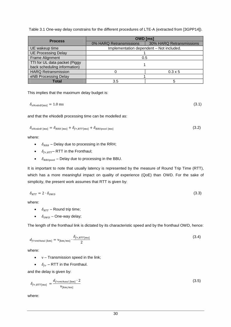
30
Table 3.1 One-way delay constrains for the different procedures of LTE-A (extracted from [3GPP14]).
Process OWD [ms]
0% HARQ Retransmissions 30% HARQ Retransmissions
UE wakeup time Implementation dependent – Not included.
UE Processing Delay 1
Frame Alignment 0.5
TTI for UL data packet (Piggy back scheduling information)
1
HARQ Retransmission 0 0.3 x 5
eNB Processing Delay 1
Total 3.5 5
This implies that the maximum delay budget is:
𝛿𝑒𝑁𝑜𝑑𝑒𝐵 [ms] = 1.0 ms (3.1)
and that the eNodeB processing time can be modelled as:
𝛿𝑒𝑁𝑜𝑑𝑒𝐵 [ms] = 𝛿𝑅𝑅𝐻 [ms] + 𝛿𝑓𝑟,𝑅𝑇𝑇[ms] + 𝛿𝐵𝐵𝑈𝑝𝑜𝑜𝑙 [ms] (3.2)
where:
𝛿𝑅𝑅𝐻 – Delay due to processing in the RRH;
𝛿𝑓𝑟,𝑅𝑇𝑇– RTT in the Fronthaul;
𝛿𝐵𝐵𝑈𝑝𝑜𝑜𝑙 – Delay due to processing in the BBU.
It is important to note that usually latency is represented by the measure of Round Trip Time (RTT),
which has a more meaningful impact on quality of experience (QoE) than OWD. For the sake of
simplicity, the present work assumes that RTT is given by:
𝛿𝑅𝑇𝑇 = 2 ∙ 𝛿𝑂𝑊𝐷 (3.3)
where:
𝛿𝑅𝑇𝑇 – Round trip time;
𝛿𝑂𝑊𝐷 – One-way delay;
The length of the fronthaul link is dictated by its characteristic speed and by the fronthaul OWD, hence:
𝑑𝑓𝑟𝑜𝑛𝑡ℎ𝑎𝑢𝑙 [km] = ν[km/ms] ∙𝛿𝑓𝑟,𝑅𝑇𝑇[ms]
2
(3.4)
where:
ν – Transmission speed in the link;
𝛿𝑓𝑟 – RTT in the Fronthaul.
and the delay is given by:
𝛿𝑓𝑟,𝑅𝑇𝑇[ms] =𝑑𝑓𝑟𝑜𝑛𝑡ℎ𝑎𝑢𝑙 [km] ∙ 2
ν[km/ms]
(3.5)
where:
31
ν – Transmission speed in the link;
𝛿𝑓𝑟 – RTT in the Fronthaul.
Assuming that the fronthaul link is based on D-RoF technology implemented over fibre resources, the
time for the optical link propagation spans for the actual technologies from 10 km up to 40 km [Pizz13],
and assuming that the velocity in the fibre is 200 000 km/s, one obtains that the value for the fronthaul
propagation delay spans from 100 µs to 400 µs. Globally, one obtains values spanning from 600 µs (for
longer optical connections) up to 900 µs, Table 3.2.
Table 3.2 Delay constraints for the fronthaul propagation and the BBU+RRH processing.
Fronthaul Propagation [µs] BBU + RRH processing [µs]
Min. Max. Min. Max.
100 400 600 900
It is important to mention that some delays were left out of the equations, which could significantly reduce
this value. Some examples of extra delays not considered are those caused by active equipment for
transmission, such as the ones used for Wavelength Division Multiplexing (WDM) systems and
equipment for CPRI compression. Moreover, is important to highlight that the purpose of this work is to
investigate the behaviour of the model for future delay constraints, so one considers also different delay
constraints, in order to tolerate future evolution of RAN requirements.
3.2.2 Processing Power
The BBU pool is implemented on a virtualised environment, which enables the use of virtualisation
techniques in order to create multiple instances of a VBS in a single hardware machine. In order to
achieve an efficient load balancing of the traffic, the processing power has to be quantified.
The total processing power used by a BBU-pool is measured in Giga operations per second (Gops) and
can be expressed as:
𝑃𝑝𝑜𝑜𝑙 [Gops] = ∑ 𝑃𝐵𝐵𝑈,𝑛 [Gops]
𝑁
𝑖=1
+ 𝑃𝑓𝑖𝑥𝑒𝑑 [Gops] (3.6)
where:
𝑃𝑝𝑜𝑜𝑙 - BBU pool processing power;
𝑃𝐵𝐵𝑈,𝑛 - required processing power per BBU;
𝑃𝑓𝑖𝑥𝑒𝑑 - fixed processing power required for scheduling and signalling functions, independent of
the number of BBUs.
In terms of percentage, it can be written as:
𝑃𝑝𝑜𝑜𝑙 [%] =100 ∙ 𝑃𝑝𝑜𝑜𝑙 [Gops]
𝑃𝑝𝑜𝑜𝑙,max [Gops]
(3.7)
32
where:
𝑃𝑝𝑜𝑜𝑙 [%] – percentage of processing power;
𝑃𝑝𝑜𝑜𝑙 [Gops] – actual processing power
𝑃𝑝𝑜𝑜𝑙,max [Gops] – maximum processing power
A method to compute the required processing power of a BS, for both DL and UL, is proposed in
[DDGF12]. The total processing power required by a BBU, as described in (3.8), involves the sum of all
the processing efforts required before starting the communication with the core network. This includes
the processing power for the Packet Data Convergence Protocol (PDCP) (responsible for data
ciphering/deciphering and compression/decompression), the RLC and MAC functions, the scheduler
functions, the S1 termination functions and the physical layer functions.
𝑃𝑡𝑜𝑡𝑎𝑙 [Gops] = 𝑃𝑠𝑐ℎ𝑒𝑑𝑢𝑙𝑒𝑟 [Gops] + 𝑃𝑅𝐿𝐶−𝑀𝐴𝐶 [Gops] + 𝑃𝑃𝐷𝐶𝑃−𝑐𝑦𝑝ℎ𝑒𝑟𝑖𝑛𝑔 [Gops] + 𝑃𝑆1𝑡𝑒𝑟𝑚𝑖𝑛𝑎𝑡𝑖𝑜𝑛 [Gops]
+ 𝑃𝑃𝐷𝐶𝑃−𝑐𝑜𝑚𝑝𝑟𝑒𝑠𝑠𝑖𝑜𝑛 [Gops] + 𝑃𝑃𝐻𝑌𝑢𝑠𝑒𝑟 [Gops]
(3.8)
where:
𝑃𝑠𝑐ℎ𝑒𝑑𝑢𝑙𝑒𝑟 is a function of the number of radio bearers and the resource allocation algorithm;
𝑃𝑅𝐿𝐶−𝑀𝐴𝐶 is a function of the S1 data rate and the RLC mode used to perform the data transfer;
𝑃𝑃𝐷𝐶𝑃−𝑐𝑦𝑝ℎ𝑒𝑟𝑖𝑛𝑔 is a function of the S1 data rate and the RLC mode used to perform data transfer;
𝑃𝑆1𝑡𝑒𝑟𝑚𝑖𝑛𝑎𝑡𝑖𝑜𝑛 is a function of the S1 data rate;
𝑃𝑃𝐷𝐶𝑃−𝑐𝑜𝑚𝑝𝑟𝑒𝑠𝑠𝑖𝑜𝑛 is a function of the S1 data rate and the type of header compression used.
The present work focuses on the physical functions, because they can be quantified using [DDGF12]. It
is assumed that the BBU performs all the baseband functions, the RRH being left with the radio ones.
Furthermore, the processing power required for power amplification and overhead is not considered,
because it is not relevant for the purpose of this thesis.
The processing power required by the physical functions for the DL case is given by the following
expression (for the UL case, some functions may not exist):
𝑃𝑃𝐻𝑌𝑢𝑠𝑒𝑟,𝐷𝐿 [Gops] = 𝐴1𝑃𝐷𝑃𝐷 + 𝐴2𝑃𝐹𝑖𝑙𝑡𝑒𝑟 + 𝐴3𝑃𝐶𝑃𝑅𝐼 + 𝐴4𝑃𝑂𝐹𝐷𝑀 + 𝐴5𝑃𝐹𝐷,𝑙𝑖𝑛 + 𝐴6𝑃𝐹𝐷,𝑛𝑙𝑖𝑛 + 𝐴7𝑃𝐹𝐸𝐶 (3.9)
where:
𝑃𝐷𝑃𝐷 – Digital Pre-Distortion;
𝑃𝐹𝑖𝑙𝑡𝑒𝑟 – Up/down sampling and filtering;
𝑃𝐶𝑃𝑅𝐼 – Link to backbone network;
𝑃𝑂𝐹𝐷𝑀 – FTT and OFDM specific functions;
𝑃𝐹𝐷,𝑙𝑖𝑛𝑒𝑎𝑟 – Frequency domain functions with a linear dependency;
𝑃𝐹𝐷,𝑛𝑙𝑖𝑛 – Frequency domain functions with a non-linear dependency;
𝑃𝐹𝐸𝐶 – Forward Error Correction functions;
𝐴𝑥 – Complexity associated with each function, given in Gops (see Annex A).
The processing powers in (3.9) can be computed through:
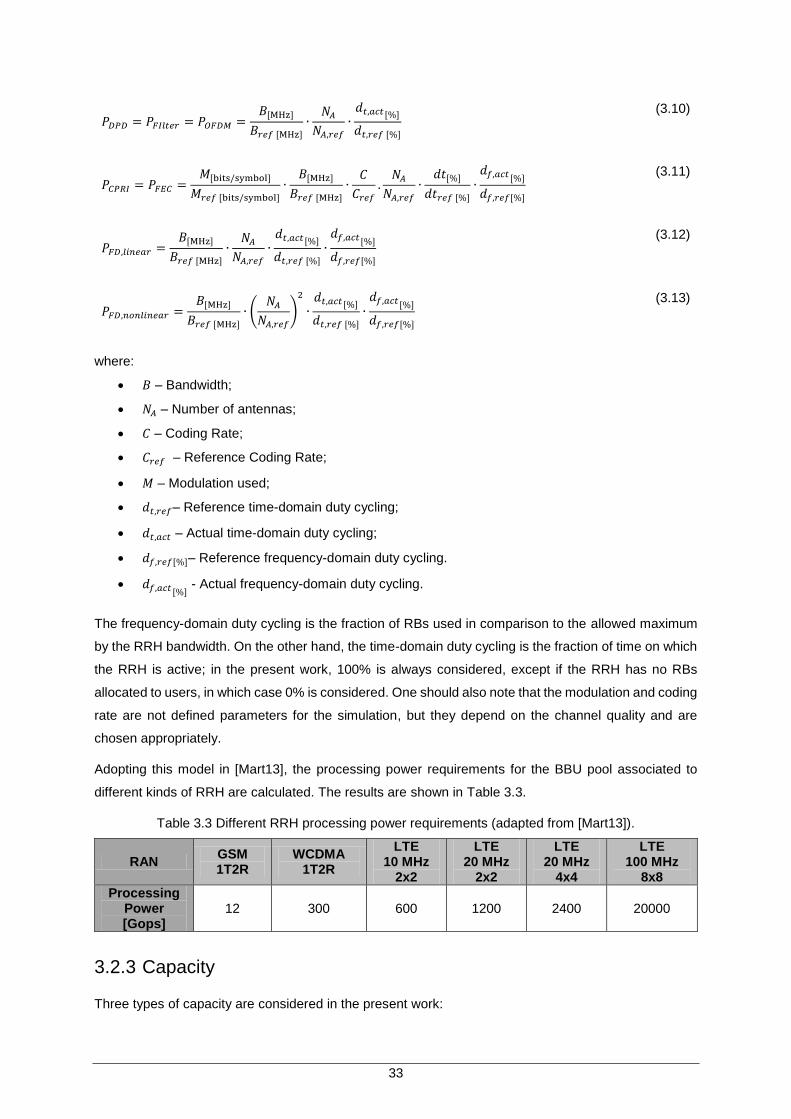
33
𝑃𝐷𝑃𝐷 = 𝑃𝐹𝐼𝑙𝑡𝑒𝑟 = 𝑃𝑂𝐹𝐷𝑀 =𝐵[MHz]
𝐵𝑟𝑒𝑓 [MHz]
∙𝑁𝐴
𝑁𝐴,𝑟𝑒𝑓
∙𝑑𝑡,𝑎𝑐𝑡[%]
𝑑𝑡,𝑟𝑒𝑓 [%]
(3.10)
𝑃𝐶𝑃𝑅𝐼 = 𝑃𝐹𝐸𝐶 =𝑀[bits/symbol]
𝑀𝑟𝑒𝑓 [bits/symbol]
∙𝐵[MHz]
𝐵𝑟𝑒𝑓 [MHz]
∙𝐶
𝐶𝑟𝑒𝑓
.𝑁𝐴
𝑁𝐴,𝑟𝑒𝑓
∙𝑑𝑡[%]
𝑑𝑡𝑟𝑒𝑓 [%]
∙𝑑𝑓,𝑎𝑐𝑡 [%]
𝑑𝑓,𝑟𝑒𝑓[%]
(3.11)
𝑃𝐹𝐷,𝑙𝑖𝑛𝑒𝑎𝑟 =𝐵[MHz]
𝐵𝑟𝑒𝑓 [MHz]
∙𝑁𝐴
𝑁𝐴,𝑟𝑒𝑓
∙𝑑𝑡,𝑎𝑐𝑡[%]
𝑑𝑡,𝑟𝑒𝑓 [%]
∙𝑑𝑓,𝑎𝑐𝑡[%]
𝑑𝑓,𝑟𝑒𝑓[%]
(3.12)
𝑃𝐹𝐷,𝑛𝑜𝑛𝑙𝑖𝑛𝑒𝑎𝑟 =𝐵[MHz]
𝐵𝑟𝑒𝑓 [MHz]
∙ (𝑁𝐴
𝑁𝐴,𝑟𝑒𝑓
)
2
∙𝑑𝑡,𝑎𝑐𝑡 [%]
𝑑𝑡,𝑟𝑒𝑓 [%]
∙𝑑𝑓,𝑎𝑐𝑡[%]
𝑑𝑓,𝑟𝑒𝑓[%]
(3.13)
where:
𝐵 – Bandwidth;
𝑁𝐴 – Number of antennas;
𝐶 – Coding Rate;
𝐶𝑟𝑒𝑓 – Reference Coding Rate;
𝑀 – Modulation used;
𝑑𝑡,𝑟𝑒𝑓– Reference time-domain duty cycling;
𝑑𝑡,𝑎𝑐𝑡 – Actual time-domain duty cycling;
𝑑𝑓,𝑟𝑒𝑓[%]– Reference frequency-domain duty cycling.
𝑑𝑓,𝑎𝑐𝑡 [%] - Actual frequency-domain duty cycling.
The frequency-domain duty cycling is the fraction of RBs used in comparison to the allowed maximum
by the RRH bandwidth. On the other hand, the time-domain duty cycling is the fraction of time on which
the RRH is active; in the present work, 100% is always considered, except if the RRH has no RBs
allocated to users, in which case 0% is considered. One should also note that the modulation and coding
rate are not defined parameters for the simulation, but they depend on the channel quality and are
chosen appropriately.
Adopting this model in [Mart13], the processing power requirements for the BBU pool associated to
different kinds of RRH are calculated. The results are shown in Table 3.3.
Table 3.3 Different RRH processing power requirements (adapted from [Mart13]).
RAN GSM 1T2R
WCDMA 1T2R
LTE 10 MHz
2x2
LTE 20 MHz
2x2
LTE 20 MHz
4x4
LTE 100 MHz
8x8
Processing Power [Gops]
12 300 600 1200 2400 20000
3.2.3 Capacity
Three types of capacity are considered in the present work:
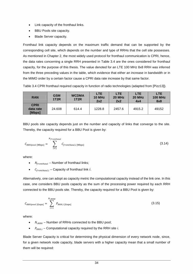
34
Link capacity of the fronthaul links.
BBU Pools site capacity.
Blade Server capacity.
Fronthaul link capacity depends on the maximum traffic demand that can be supported by the
corresponding cell site, which depends on the number and type of RRHs that the cell site possesses.
As mentioned in Chapter 2, the most widely used protocol for fronthaul communication is CPRI, hence,
the data rates concerning a single RRH presented in Table 3.4 are the ones considered for fronthaul
capacity, for the purpose of this thesis. The value denoted for an LTE 100 MHz 8x8 RRH was inferred
from the three preceding values in the table, which evidence that either an increase in bandwidth or in
the MIMO order by a certain factor cause a CPRI data rate increase by that same factor.
Table 3.4 CPRI fronthaul required capacity in function of radio technologies (adapted from [Pizz13]).
RAN GSM 1T2R
WCDMA 1T2R
LTE 10 MHz
2x2
LTE 20 MHz
2x2
LTE 20 MHz
4x4
LTE 100 MHz
8x8
CPRI data rate [Mbps]
24.608 614.4 1228.8 2457.6 4915.2 49152
BBU pools site capacity depends just on the number and capacity of links that converge to the site.
Thereby, the capacity required for a BBU Pool is given by:
𝐶𝐵𝐵𝑈𝑝𝑜𝑜𝑙 [Mbps] = ∑ 𝐶𝑓𝑟𝑜𝑛𝑡ℎ𝑎𝑢𝑙,𝑖 [Mbps]
𝑁𝑓𝑟𝑜𝑛𝑡ℎ𝑎𝑢𝑙
𝑖=1
(3.14)
where:
𝑁𝑓𝑟𝑜𝑛𝑡ℎ𝑎𝑢𝑙 – Number of fronthaul links;
𝐶𝑓𝑟𝑜𝑛𝑡ℎ𝑎𝑢𝑙,𝑖 – Capacity of fronthaul link i.
Alternatively, one can adopt as capacity metric the computational capacity instead of the link one. In this
case, one considers BBU pools capacity as the sum of the processing power required by each RRH
connected to the BBU pools site. Thereby, the capacity required for a BBU Pool is given by:
𝐶𝐵𝐵𝑈𝑝𝑜𝑜𝑙 [Gops] = ∑ 𝑃𝑅𝑅𝐻,𝑖 [Gops]
𝑁𝑐𝑅𝑅𝐻
𝑖=1
(3.15)
where:
𝑁𝑐𝑅𝑅𝐻 – Number of RRHs connected to the BBU pool;
𝑃𝑅𝑅𝐻,𝑖 – Computational capacity required by the RRH site i.
Blade Server Capacity is critical for determining the physical dimension of every network node, since,
for a given network node capacity, blade servers with a higher capacity mean that a small number of
them will be required:
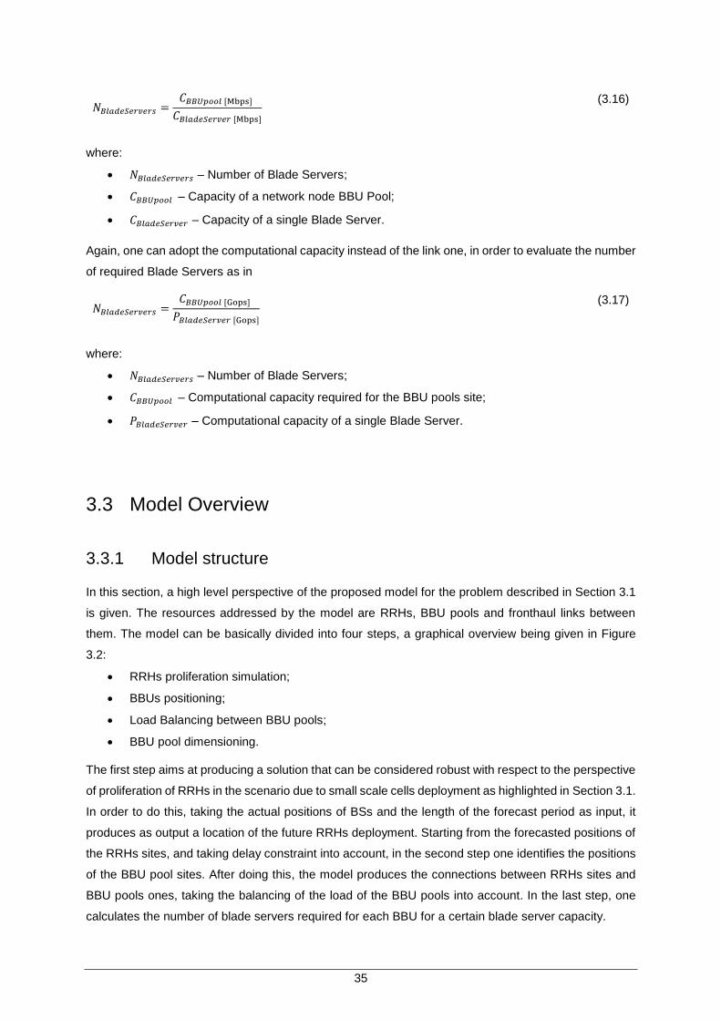
35
𝑁𝐵𝑙𝑎𝑑𝑒𝑆𝑒𝑟𝑣𝑒𝑟𝑠 =𝐶𝐵𝐵𝑈𝑝𝑜𝑜𝑙 [Mbps]
𝐶𝐵𝑙𝑎𝑑𝑒𝑆𝑒𝑟𝑣𝑒𝑟 [Mbps]
(3.16)
where:
𝑁𝐵𝑙𝑎𝑑𝑒𝑆𝑒𝑟𝑣𝑒𝑟𝑠 – Number of Blade Servers;
𝐶𝐵𝐵𝑈𝑝𝑜𝑜𝑙 – Capacity of a network node BBU Pool;
𝐶𝐵𝑙𝑎𝑑𝑒𝑆𝑒𝑟𝑣𝑒𝑟 – Capacity of a single Blade Server.
Again, one can adopt the computational capacity instead of the link one, in order to evaluate the number
of required Blade Servers as in
𝑁𝐵𝑙𝑎𝑑𝑒𝑆𝑒𝑟𝑣𝑒𝑟𝑠 =𝐶𝐵𝐵𝑈𝑝𝑜𝑜𝑙 [Gops]
𝑃𝐵𝑙𝑎𝑑𝑒𝑆𝑒𝑟𝑣𝑒𝑟 [Gops]
(3.17)
where:
𝑁𝐵𝑙𝑎𝑑𝑒𝑆𝑒𝑟𝑣𝑒𝑟𝑠 – Number of Blade Servers;
𝐶𝐵𝐵𝑈𝑝𝑜𝑜𝑙 – Computational capacity required for the BBU pools site;
𝑃𝐵𝑙𝑎𝑑𝑒𝑆𝑒𝑟𝑣𝑒𝑟 – Computational capacity of a single Blade Server.
3.3 Model Overview
3.3.1 Model structure
In this section, a high level perspective of the proposed model for the problem described in Section 3.1
is given. The resources addressed by the model are RRHs, BBU pools and fronthaul links between
them. The model can be basically divided into four steps, a graphical overview being given in Figure
3.2:
RRHs proliferation simulation;
BBUs positioning;
Load Balancing between BBU pools;
BBU pool dimensioning.
The first step aims at producing a solution that can be considered robust with respect to the perspective
of proliferation of RRHs in the scenario due to small scale cells deployment as highlighted in Section 3.1.
In order to do this, taking the actual positions of BSs and the length of the forecast period as input, it
produces as output a location of the future RRHs deployment. Starting from the forecasted positions of
the RRHs sites, and taking delay constraint into account, in the second step one identifies the positions
of the BBU pool sites. After doing this, the model produces the connections between RRHs sites and
BBU pools ones, taking the balancing of the load of the BBU pools into account. In the last step, one
calculates the number of blade servers required for each BBU for a certain blade server capacity.
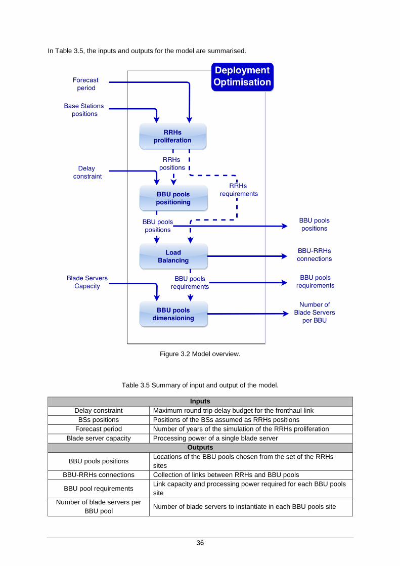
36
In Table 3.5, the inputs and outputs for the model are summarised.
Figure 3.2 Model overview.
Table 3.5 Summary of input and output of the model.
Inputs
Delay constraint Maximum round trip delay budget for the fronthaul link
BSs positions Positions of the BSs assumed as RRHs positions
Forecast period Number of years of the simulation of the RRHs proliferation
Blade server capacity Processing power of a single blade server
Outputs
BBU pools positions Locations of the BBU pools chosen from the set of the RRHs
sites
BBU-RRHs connections Collection of links between RRHs and BBU pools
BBU pool requirements Link capacity and processing power required for each BBU pools
site
Number of blade servers per
BBU pool Number of blade servers to instantiate in each BBU pools site
37
3.3.2 RRHs proliferation
As highlighted in Section 3.1, the C-RAN architecture can include also small scale cell deployment, and
focusing on this fact, one needs to provide a proliferation algorithm that can forecast the growth of RRHs
in the urban scenario. The idea of the proposed algorithm is to take as input the actual RRHs sites
positions and the length of the temporal window of the forecast expressed in terms of number of years,
and produce a corresponding growth of the number of RRHs.
During the growth simulation, one assumes that the first portion of the trend is represented by large
scale cell deployment, while the second one takes small scale cell deployment. In order to take this
aspect into account, the algorithm instantiates during the first two years large cell sites of class 1, 2 or
3 with the corresponding capacity requirements as in Section 3.2.3 and processing power as illustrated
in Section 3.2.2. The choice of the class of the site is based on the region in which it is instantiated:
urban area, suburban area or rural area. The second portion of the trend, starting from the third year of
forecast, will instantiate only small scale cells.
Another important aspect that the proliferation algorithm takes into consideration is that more dense
urban areas in the scenario are expected to have a higher growth with respect to rural and suburban
ones, resulting in an unchanged density distribution of sites. In order to obtain this, one has constructed
the Probability Distribution Function of the distances to the reference point, and proceeded to an
extraction of elements conditioned by this probability function. By acting in this way, one obtains that the
probability to extract an element in a denser area is greater than the one in a less dense area. To obtain
the location of the RRH site to instantiate, one proceeds to the extraction of each site by calculating the
two nearest sties and adding to the collection of sites the centroid of this three points. In Figure 3.3, the
proposed algorithm for the proliferation of RRHs is shown.
3.3.3 BBU pools positioning
As depicted in Figure 3.2 the stage of BBU positioning takes as input the positions of the BSs and
computes the number and positions of the BBU pools, taking only the delay constraint into account, in
terms of maximum distances between RRH and BBU pool.
The datacentres placement is crucial to perform an efficient traffic management. It is expected that
RRHs connect to the nearest available datacentre due to the fronthaul latency constraints, hence, one
presumes that there will be a higher load in datacentres located near densest areas, i.e., where the data
traffic and number of RRHs is higher. Therefore, a careful planning of this placement must be performed.
The localisation of the RRHs is also quite significant for the load balancing. It is much more efficient for
neighbour RRHs to be processed in the same BBU-pool, since an external communication between
different BBU-pools will not be required, greatly improving handover, and joint scheduling and
processing. For the operators, this is quite easy to implement, since the RRHs locations are well known,
and thus, it is possible to create neighbours lists for each RRH, containing specific information regarding
which RRHs are closest.
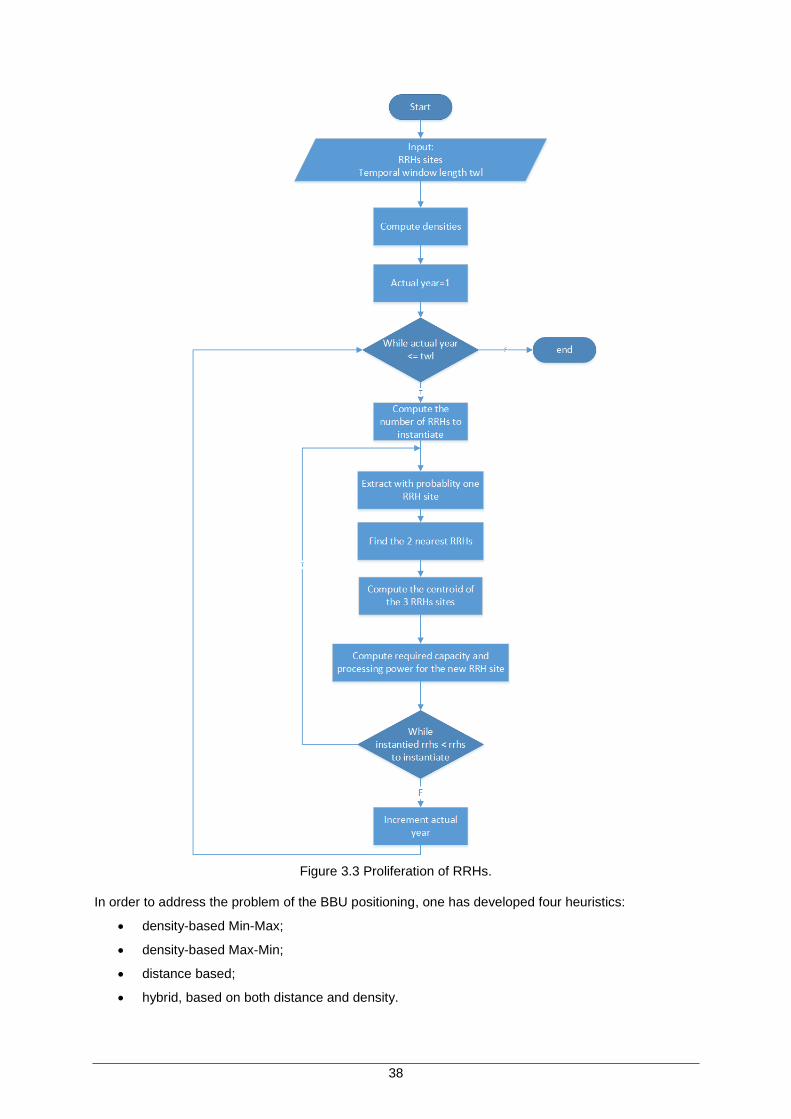
38
Figure 3.3 Proliferation of RRHs.
In order to address the problem of the BBU positioning, one has developed four heuristics:
density-based Min-Max;
density-based Max-Min;
distance based;
hybrid, based on both distance and density.
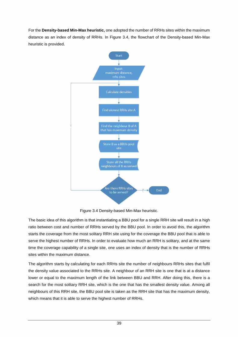
39
For the Density-based Min-Max heuristic, one adopted the number of RRHs sites within the maximum
distance as an index of density of RRHs. In Figure 3.4, the flowchart of the Density-based Min-Max
heuristic is provided.
Figure 3.4 Density-based Min-Max heuristic.
The basic idea of this algorithm is that instantiating a BBU pool for a single RRH site will result in a high
ratio between cost and number of RRHs served by the BBU pool. In order to avoid this, the algorithm
starts the coverage from the most solitary RRH site using for the coverage the BBU pool that is able to
serve the highest number of RRHs. In order to evaluate how much an RRH is solitary, and at the same
time the coverage capability of a single site, one uses an index of density that is the number of RRHs
sites within the maximum distance.
The algorithm starts by calculating for each RRHs site the number of neighbours RRHs sites that fulfil
the density value associated to the RRHs site. A neighbour of an RRH site is one that is at a distance
lower or equal to the maximum length of the link between BBU and RRH. After doing this, there is a
search for the most solitary RRH site, which is the one that has the smallest density value. Among all
neighbours of this RRH site, the BBU pool site is taken as the RRH site that has the maximum density,
which means that it is able to serve the highest number of RRHs.
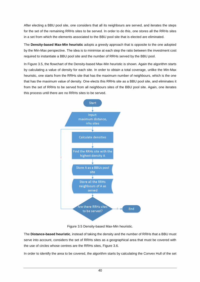
40
After electing a BBU pool site, one considers that all its neighbours are served, and iterates the steps
for the set of the remaining RRHs sites to be served. In order to do this, one stores all the RRHs sites
in a set from which the elements associated to the BBU pool site that is elected are eliminated.
The Density-based Max-Min heuristic adopts a greedy approach that is opposite to the one adopted
by the Min-Max perspective. The idea is to minimise at each step the ratio between the investment cost
required to instantiate a BBU pool site and the number of RRHs served by the BBU pool.
In Figure 3.5, the flowchart of the Density-based Max-Min heuristic is shown. Again the algorithm starts
by calculating a value of density for each site. In order to obtain a total coverage, unlike the Min-Max
heuristic, one starts from the RRHs site that has the maximum number of neighbours, which is the one
that has the maximum value of density. One elects this RRHs site as a BBU pool site, and eliminates it
from the set of RRHs to be served from all neighbours sites of the BBU pool site. Again, one iterates
this process until there are no RRHs sites to be served.
Figure 3.5 Density-based Max-Min heuristic.
The Distance-based heuristic, instead of taking the density and the number of RRHs that a BBU must
serve into account, considers the set of RRHs sites as a geographical area that must be covered with
the use of circles whose centres are the RRHs sites, Figure 3.6.
In order to identify the area to be covered, the algorithm starts by calculating the Convex Hull of the set
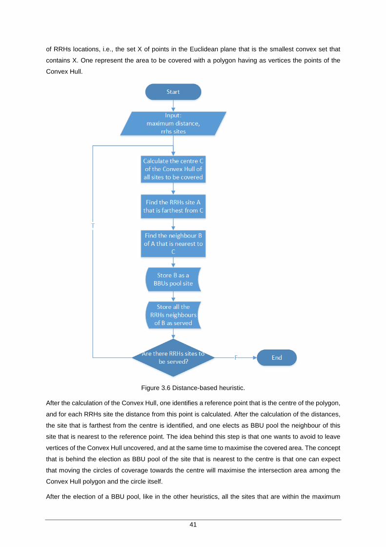
41
of RRHs locations, i.e., the set X of points in the Euclidean plane that is the smallest convex set that
contains X. One represent the area to be covered with a polygon having as vertices the points of the
Convex Hull.
Figure 3.6 Distance-based heuristic.
After the calculation of the Convex Hull, one identifies a reference point that is the centre of the polygon,
and for each RRHs site the distance from this point is calculated. After the calculation of the distances,
the site that is farthest from the centre is identified, and one elects as BBU pool the neighbour of this
site that is nearest to the reference point. The idea behind this step is that one wants to avoid to leave
vertices of the Convex Hull uncovered, and at the same time to maximise the covered area. The concept
that is behind the election as BBU pool of the site that is nearest to the centre is that one can expect
that moving the circles of coverage towards the centre will maximise the intersection area among the
Convex Hull polygon and the circle itself.
After the election of a BBU pool, like in the other heuristics, all the sites that are within the maximum
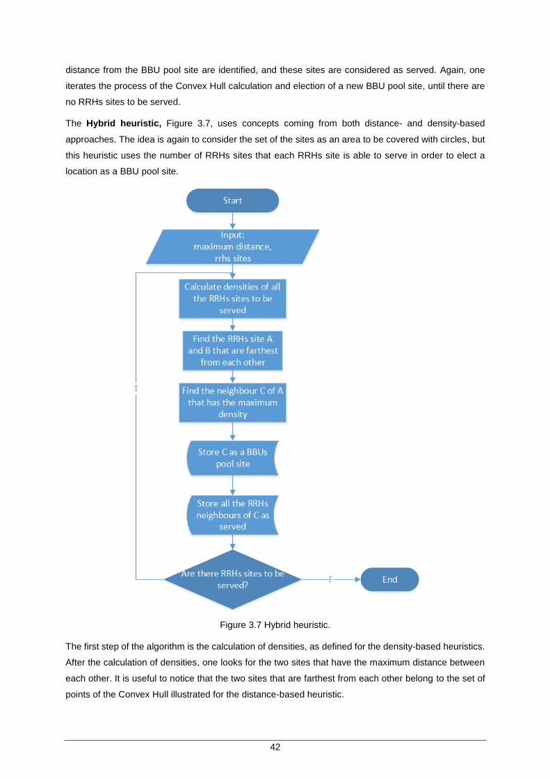
42
distance from the BBU pool site are identified, and these sites are considered as served. Again, one
iterates the process of the Convex Hull calculation and election of a new BBU pool site, until there are
no RRHs sites to be served.
The Hybrid heuristic, Figure 3.7, uses concepts coming from both distance- and density-based
approaches. The idea is again to consider the set of the sites as an area to be covered with circles, but
this heuristic uses the number of RRHs sites that each RRHs site is able to serve in order to elect a
location as a BBU pool site.
Figure 3.7 Hybrid heuristic.
The first step of the algorithm is the calculation of densities, as defined for the density-based heuristics.
After the calculation of densities, one looks for the two sites that have the maximum distance between
each other. It is useful to notice that the two sites that are farthest from each other belong to the set of
points of the Convex Hull illustrated for the distance-based heuristic.
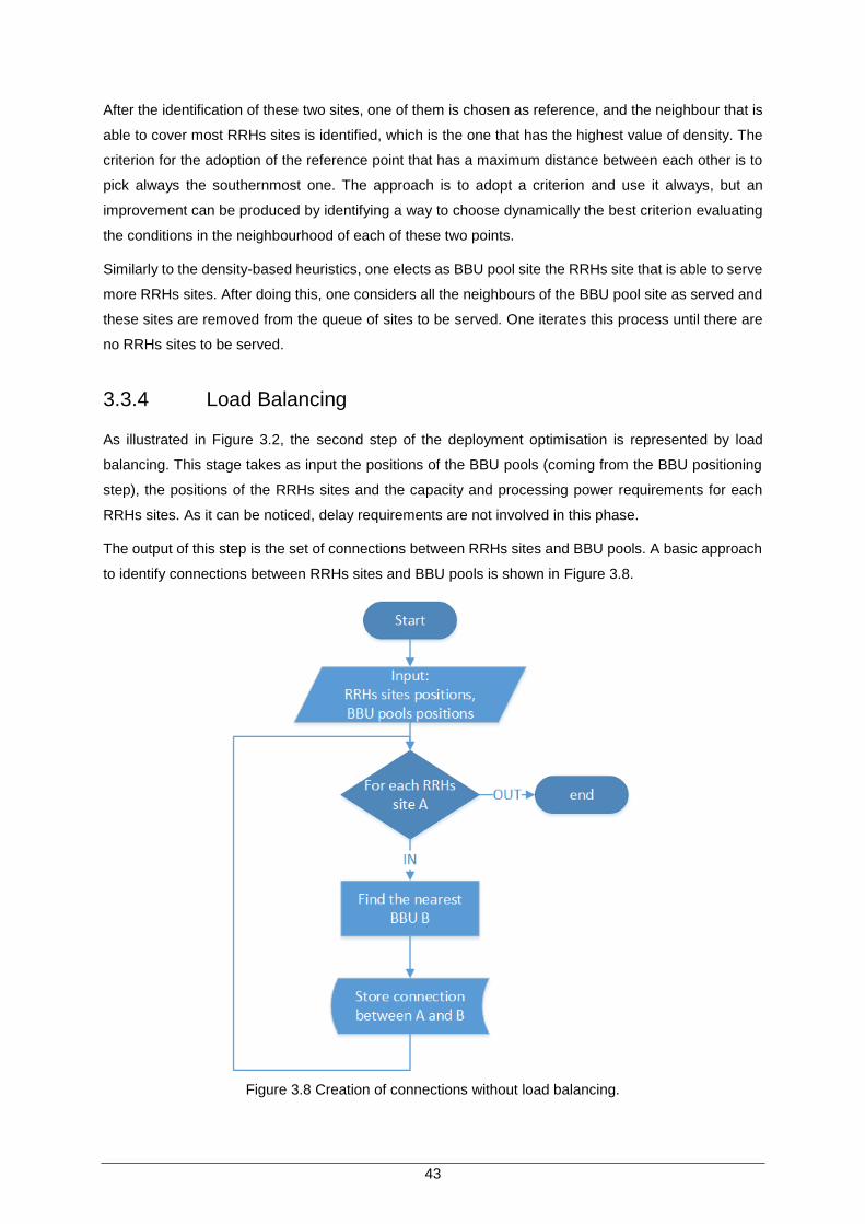
43
After the identification of these two sites, one of them is chosen as reference, and the neighbour that is
able to cover most RRHs sites is identified, which is the one that has the highest value of density. The
criterion for the adoption of the reference point that has a maximum distance between each other is to
pick always the southernmost one. The approach is to adopt a criterion and use it always, but an
improvement can be produced by identifying a way to choose dynamically the best criterion evaluating
the conditions in the neighbourhood of each of these two points.
Similarly to the density-based heuristics, one elects as BBU pool site the RRHs site that is able to serve
more RRHs sites. After doing this, one considers all the neighbours of the BBU pool site as served and
these sites are removed from the queue of sites to be served. One iterates this process until there are
no RRHs sites to be served.
3.3.4 Load Balancing
As illustrated in Figure 3.2, the second step of the deployment optimisation is represented by load
balancing. This stage takes as input the positions of the BBU pools (coming from the BBU positioning
step), the positions of the RRHs sites and the capacity and processing power requirements for each
RRHs sites. As it can be noticed, delay requirements are not involved in this phase.
The output of this step is the set of connections between RRHs sites and BBU pools. A basic approach
to identify connections between RRHs sites and BBU pools is shown in Figure 3.8.
Figure 3.8 Creation of connections without load balancing.
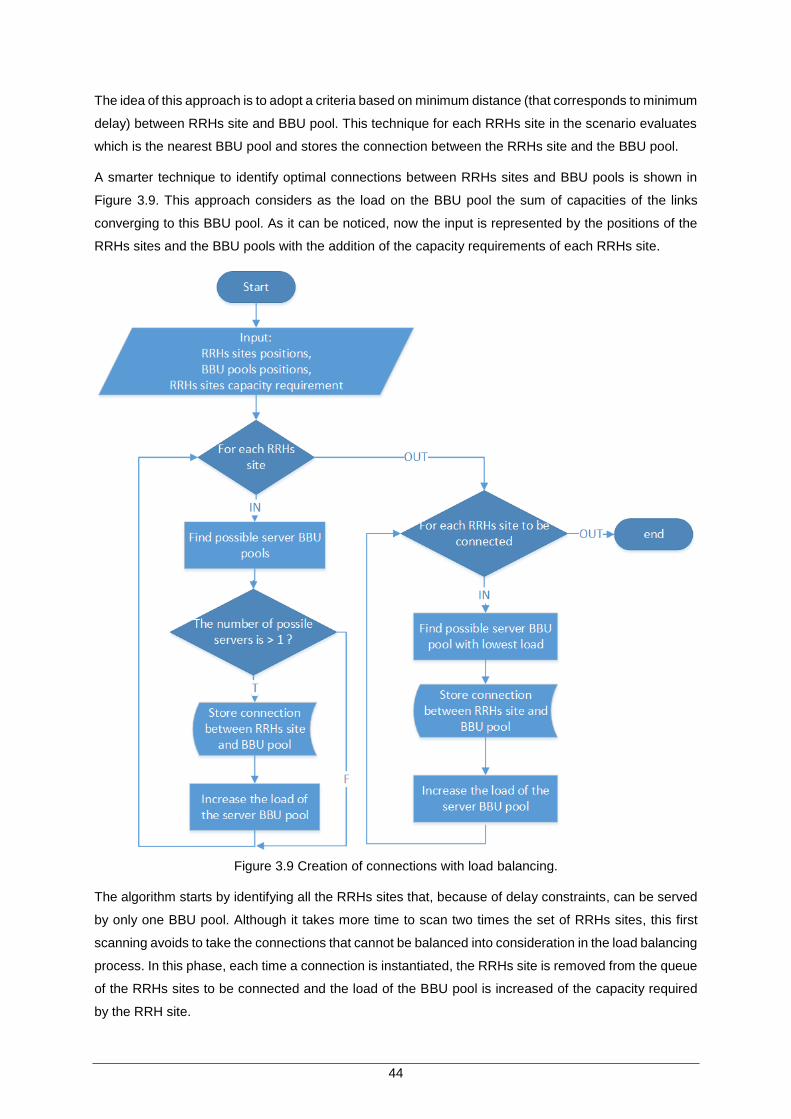
44
The idea of this approach is to adopt a criteria based on minimum distance (that corresponds to minimum
delay) between RRHs site and BBU pool. This technique for each RRHs site in the scenario evaluates
which is the nearest BBU pool and stores the connection between the RRHs site and the BBU pool.
A smarter technique to identify optimal connections between RRHs sites and BBU pools is shown in
Figure 3.9. This approach considers as the load on the BBU pool the sum of capacities of the links
converging to this BBU pool. As it can be noticed, now the input is represented by the positions of the
RRHs sites and the BBU pools with the addition of the capacity requirements of each RRHs site.
Figure 3.9 Creation of connections with load balancing.
The algorithm starts by identifying all the RRHs sites that, because of delay constraints, can be served
by only one BBU pool. Although it takes more time to scan two times the set of RRHs sites, this first
scanning avoids to take the connections that cannot be balanced into consideration in the load balancing
process. In this phase, each time a connection is instantiated, the RRHs site is removed from the queue
of the RRHs sites to be connected and the load of the BBU pool is increased of the capacity required
by the RRH site.
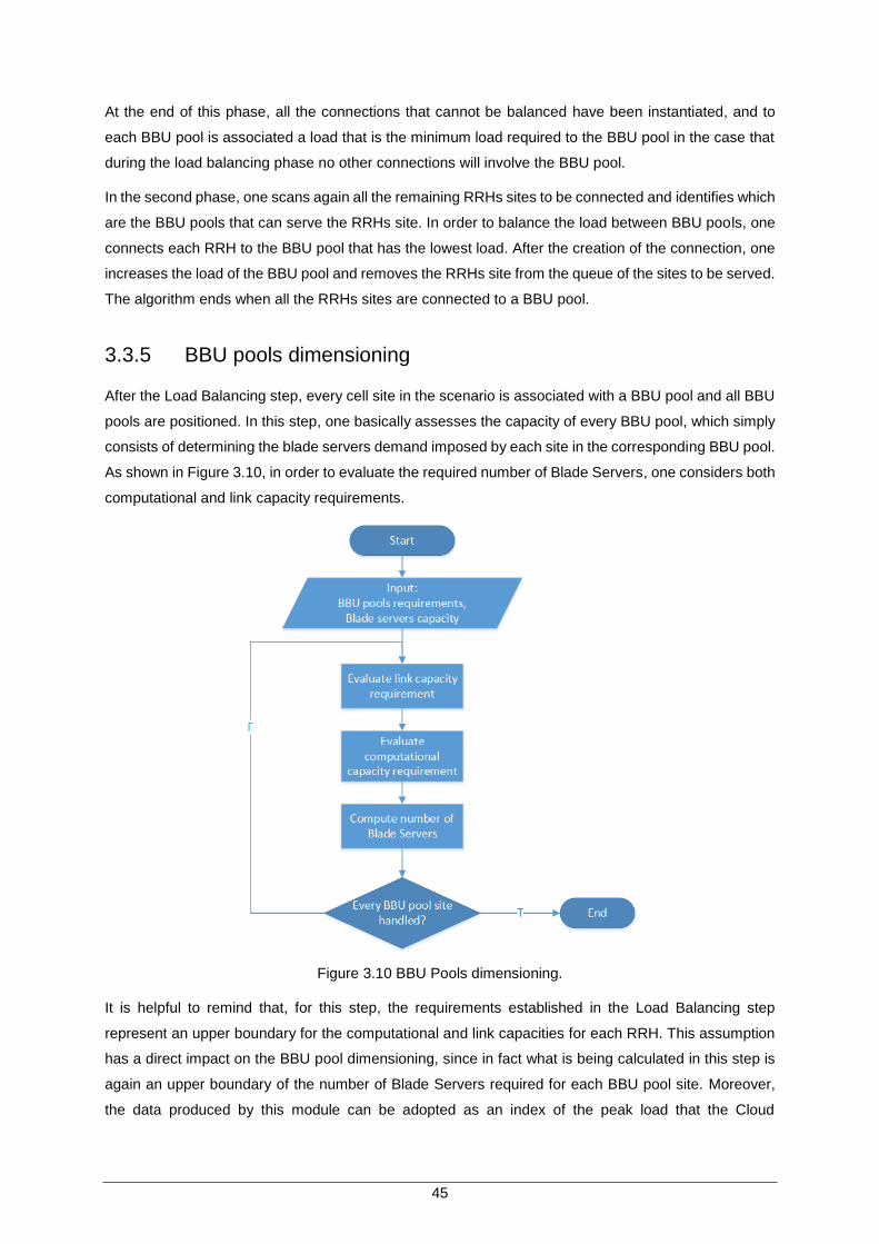
45
At the end of this phase, all the connections that cannot be balanced have been instantiated, and to
each BBU pool is associated a load that is the minimum load required to the BBU pool in the case that
during the load balancing phase no other connections will involve the BBU pool.
In the second phase, one scans again all the remaining RRHs sites to be connected and identifies which
are the BBU pools that can serve the RRHs site. In order to balance the load between BBU pools, one
connects each RRH to the BBU pool that has the lowest load. After the creation of the connection, one
increases the load of the BBU pool and removes the RRHs site from the queue of the sites to be served.
The algorithm ends when all the RRHs sites are connected to a BBU pool.
3.3.5 BBU pools dimensioning
After the Load Balancing step, every cell site in the scenario is associated with a BBU pool and all BBU
pools are positioned. In this step, one basically assesses the capacity of every BBU pool, which simply
consists of determining the blade servers demand imposed by each site in the corresponding BBU pool.
As shown in Figure 3.10, in order to evaluate the required number of Blade Servers, one considers both
computational and link capacity requirements.
Figure 3.10 BBU Pools dimensioning.
It is helpful to remind that, for this step, the requirements established in the Load Balancing step
represent an upper boundary for the computational and link capacities for each RRH. This assumption
has a direct impact on the BBU pool dimensioning, since in fact what is being calculated in this step is
again an upper boundary of the number of Blade Servers required for each BBU pool site. Moreover,
the data produced by this module can be adopted as an index of the peak load that the Cloud
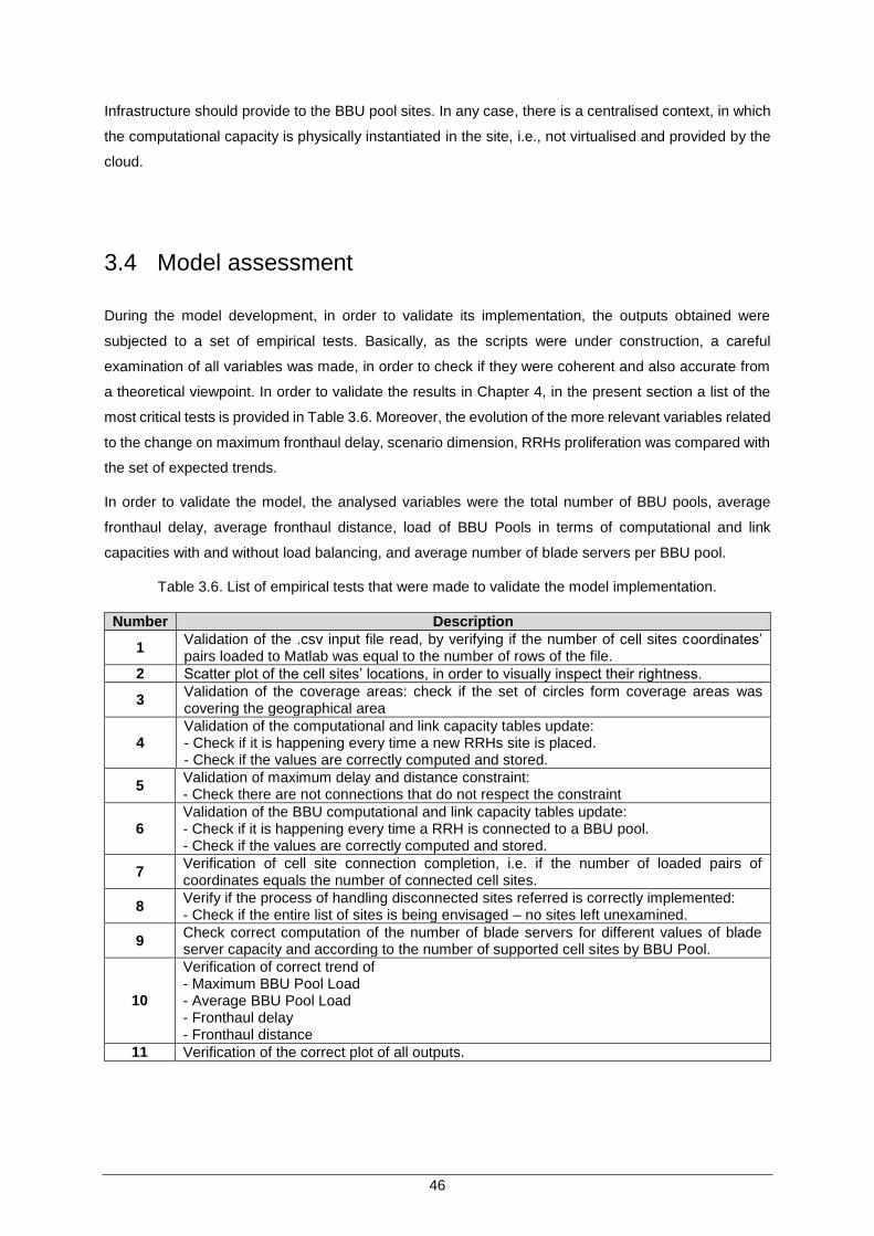
46
Infrastructure should provide to the BBU pool sites. In any case, there is a centralised context, in which
the computational capacity is physically instantiated in the site, i.e., not virtualised and provided by the
cloud.
3.4 Model assessment
During the model development, in order to validate its implementation, the outputs obtained were
subjected to a set of empirical tests. Basically, as the scripts were under construction, a careful
examination of all variables was made, in order to check if they were coherent and also accurate from
a theoretical viewpoint. In order to validate the results in Chapter 4, in the present section a list of the
most critical tests is provided in Table 3.6. Moreover, the evolution of the more relevant variables related
to the change on maximum fronthaul delay, scenario dimension, RRHs proliferation was compared with
the set of expected trends.
In order to validate the model, the analysed variables were the total number of BBU pools, average
fronthaul delay, average fronthaul distance, load of BBU Pools in terms of computational and link
capacities with and without load balancing, and average number of blade servers per BBU pool.
Table 3.6. List of empirical tests that were made to validate the model implementation.
Number Description
1 Validation of the .csv input file read, by verifying if the number of cell sites coordinates’ pairs loaded to Matlab was equal to the number of rows of the file.
2 Scatter plot of the cell sites’ locations, in order to visually inspect their rightness.
3 Validation of the coverage areas: check if the set of circles form coverage areas was covering the geographical area
4 Validation of the computational and link capacity tables update: - Check if it is happening every time a new RRHs site is placed. - Check if the values are correctly computed and stored.
5 Validation of maximum delay and distance constraint: - Check there are not connections that do not respect the constraint
6 Validation of the BBU computational and link capacity tables update: - Check if it is happening every time a RRH is connected to a BBU pool. - Check if the values are correctly computed and stored.
7 Verification of cell site connection completion, i.e. if the number of loaded pairs of coordinates equals the number of connected cell sites.
8 Verify if the process of handling disconnected sites referred is correctly implemented: - Check if the entire list of sites is being envisaged – no sites left unexamined.
9 Check correct computation of the number of blade servers for different values of blade server capacity and according to the number of supported cell sites by BBU Pool.
10
Verification of correct trend of - Maximum BBU Pool Load - Average BBU Pool Load - Fronthaul delay - Fronthaul distance
11 Verification of the correct plot of all outputs.
47
Chapter 4
Results Analysis
4 Results Analysis
This chapter presents the considered scenario along with the associated results and respective analysis.
Thus, the scenario is defined in Section 4.1; in Section 4.2 a comparison between some BBU positioning
algorithms is provided. The results for the RAN are presented in Sections 4.3 to 4.8, respectively.
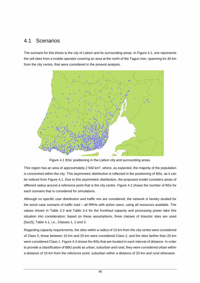
48
4.1 Scenarios
The scenario for this thesis is the city of Lisbon and its surrounding areas. In Figure 4.1, one represents
the cell sites from a mobile operator covering an area at the north of the Tagus river, spanning for 40 km
from the city centre, that were considered in the present analysis.
Figure 4.1 BSs’ positioning in the Lisbon city and surrounding areas.
This region has an area of approximately 2 500 km2, where, as expected, the majority of the population
is concentred within the city. This asymmetric distribution is reflected in the positioning of BSs, as it can
be noticed from Figure 4.1. Due to this asymmetric distribution, the proposed model considers areas of
different radius around a reference point that is the city centre. Figure 4.2 shows the number of BSs for
each scenario that is considered for simulations.
Although no specific user distribution and traffic mix are considered, the network is hereby studied for
the worst case scenario of traffic load – all RRHs with active users, using all resources available. The
values shown in Table 3.3 and Table 3.4 for the fronthaul capacity and processing power take this
situation into consideration; based on these assumptions, three classes of trisector sites are used
[Sa15], Table 4.1, i.e., Classes 1, 2 and 3.
Regarding capacity requirements, the sites within a radius of 10 km from the city centre were considered
of Class 3, those between 10 km and 25 km were considered Class 2, and the sites farther than 25 km
were considered Class 1. Figure 4.3 shows the BSs that are located in each interval of distance. In order
to provide a classification of BBU pools as urban, suburban and rural, they were considered urban within
a distance of 10 km from the reference point, suburban within a distance of 20 km and rural otherwise.
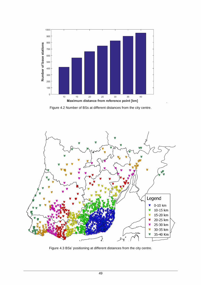
49
.
Figure 4.2 Number of BSs at different distances from the city centre.
Figure 4.3 BSs’ positioning at different distances from the city centre.
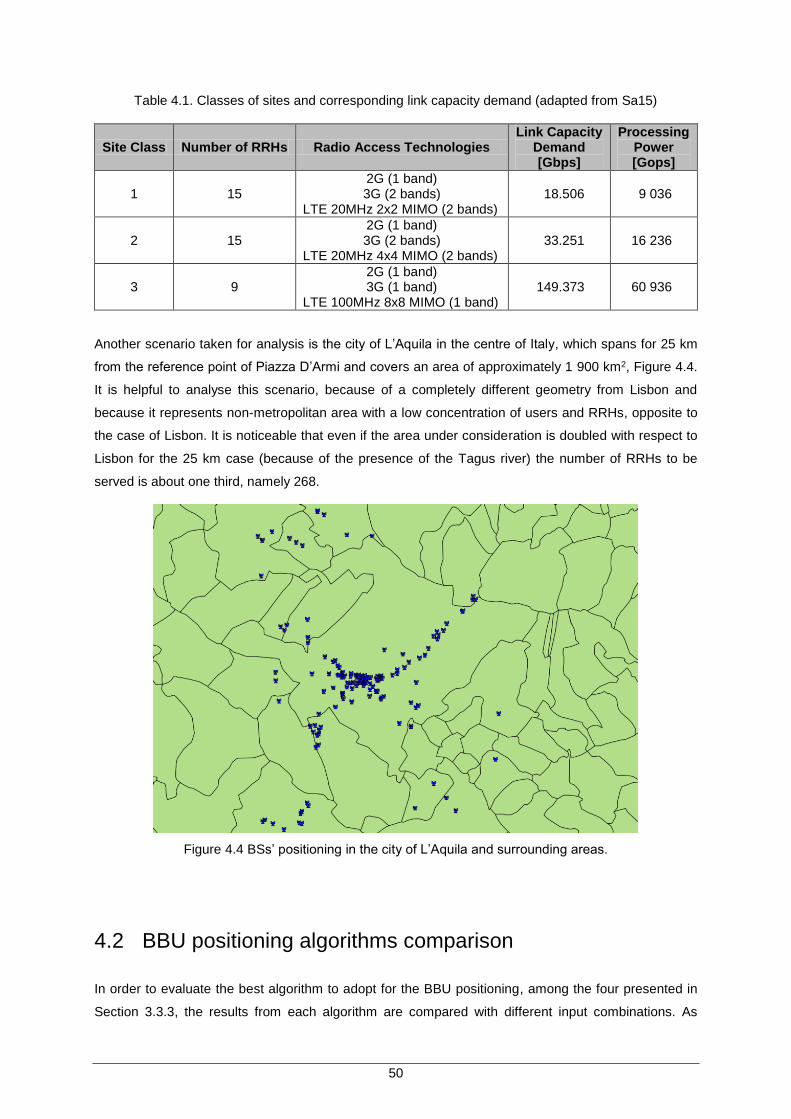
50
Table 4.1. Classes of sites and corresponding link capacity demand (adapted from Sa15)
Site Class Number of RRHs Radio Access Technologies Link Capacity
Demand [Gbps]
Processing Power [Gops]
1 15 2G (1 band) 3G (2 bands)
LTE 20MHz 2x2 MIMO (2 bands) 18.506 9 036
2 15 2G (1 band) 3G (2 bands)
LTE 20MHz 4x4 MIMO (2 bands) 33.251 16 236
3 9 2G (1 band) 3G (1 band)
LTE 100MHz 8x8 MIMO (1 band) 149.373 60 936
Another scenario taken for analysis is the city of L’Aquila in the centre of Italy, which spans for 25 km
from the reference point of Piazza D’Armi and covers an area of approximately 1 900 km2, Figure 4.4.
It is helpful to analyse this scenario, because of a completely different geometry from Lisbon and
because it represents non-metropolitan area with a low concentration of users and RRHs, opposite to
the case of Lisbon. It is noticeable that even if the area under consideration is doubled with respect to
Lisbon for the 25 km case (because of the presence of the Tagus river) the number of RRHs to be
served is about one third, namely 268.
Figure 4.4 BSs’ positioning in the city of L’Aquila and surrounding areas.
4.2 BBU positioning algorithms comparison
In order to evaluate the best algorithm to adopt for the BBU positioning, among the four presented in
Section 3.3.3, the results from each algorithm are compared with different input combinations. As
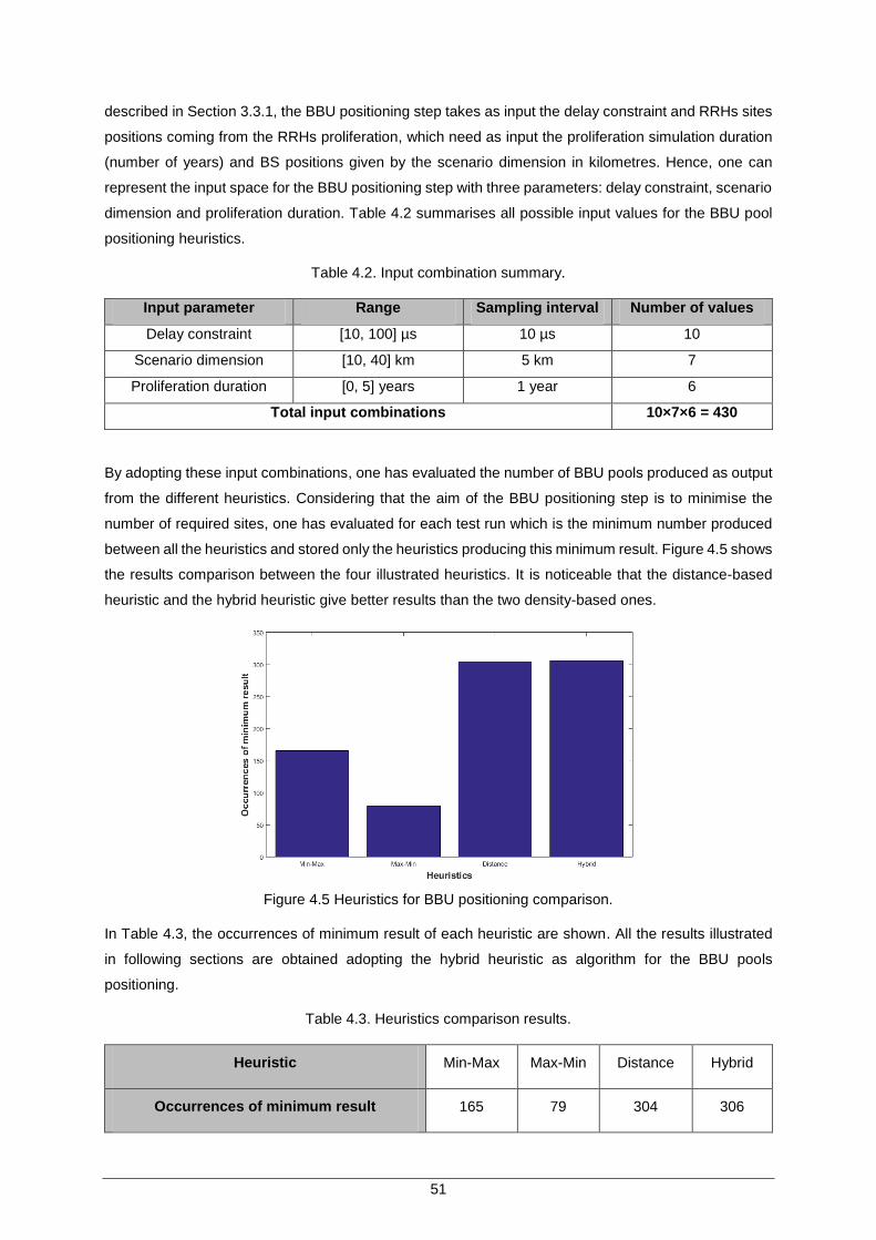
51
described in Section 3.3.1, the BBU positioning step takes as input the delay constraint and RRHs sites
positions coming from the RRHs proliferation, which need as input the proliferation simulation duration
(number of years) and BS positions given by the scenario dimension in kilometres. Hence, one can
represent the input space for the BBU positioning step with three parameters: delay constraint, scenario
dimension and proliferation duration. Table 4.2 summarises all possible input values for the BBU pool
positioning heuristics.
Table 4.2. Input combination summary.
Input parameter Range Sampling interval Number of values
Delay constraint [10, 100] µs 10 µs 10
Scenario dimension [10, 40] km 5 km 7
Proliferation duration [0, 5] years 1 year 6
Total input combinations 10×7×6 = 430
By adopting these input combinations, one has evaluated the number of BBU pools produced as output
from the different heuristics. Considering that the aim of the BBU positioning step is to minimise the
number of required sites, one has evaluated for each test run which is the minimum number produced
between all the heuristics and stored only the heuristics producing this minimum result. Figure 4.5 shows
the results comparison between the four illustrated heuristics. It is noticeable that the distance-based
heuristic and the hybrid heuristic give better results than the two density-based ones.
Figure 4.5 Heuristics for BBU positioning comparison.
In Table 4.3, the occurrences of minimum result of each heuristic are shown. All the results illustrated
in following sections are obtained adopting the hybrid heuristic as algorithm for the BBU pools
positioning.
Table 4.3. Heuristics comparison results.
Heuristic Min-Max Max-Min Distance Hybrid
Occurrences of minimum result 165 79 304 306
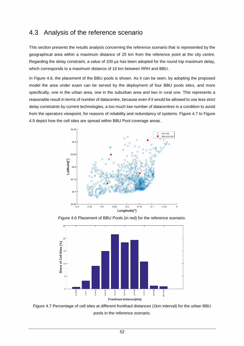
52
4.3 Analysis of the reference scenario
This section presents the results analysis concerning the reference scenario that is represented by the
geographical area within a maximum distance of 25 km from the reference point at the city centre.
Regarding the delay constraint, a value of 100 µs has been adopted for the round trip maximum delay,
which corresponds to a maximum distance of 10 km between RRH and BBU.
In Figure 4.6, the placement of the BBU pools is shown. As it can be seen, by adopting the proposed
model the area under exam can be served by the deployment of four BBU pools sites, and more
specifically, one in the urban area, one in the suburban area and two in rural one. This represents a
reasonable result in terms of number of datacentre, because even if it would be allowed to use less strict
delay constraints by current technologies, a too much low number of datacentres is a condition to avoid
from the operators viewpoint, for reasons of reliability and redundancy of systems. Figure 4.7 to Figure
4.9 depict how the cell sites are spread within BBU Pool coverage areas.
Figure 4.6 Placement of BBU Pools (in red) for the reference scenario.
Figure 4.7 Percentage of cell sites at different fronthaul distances (1km interval) for the urban BBU
pools in the reference scenario.
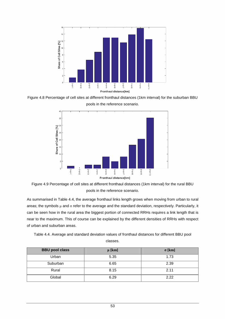
53
Figure 4.8 Percentage of cell sites at different fronthaul distances (1km interval) for the suburban BBU
pools in the reference scenario.
Figure 4.9 Percentage of cell sites at different fronthaul distances (1km interval) for the rural BBU
pools in the reference scenario.
As summarised in Table 4.4, the average fronthaul links length grows when moving from urban to rural
areas; the symbols μ and σ refer to the average and the standard deviation, respectively. Particularly, it
can be seen how in the rural area the biggest portion of connected RRHs requires a link length that is
near to the maximum. This of course can be explained by the different densities of RRHs with respect
of urban and suburban areas.
Table 4.4. Average and standard deviation values of fronthaul distances for different BBU pool
classes.
BBU pool class μ [km] σ [km]
Urban 5.35 1.73
Suburban 6.65 2.39
Rural 8.15 2.11
Global 6.29 2.22
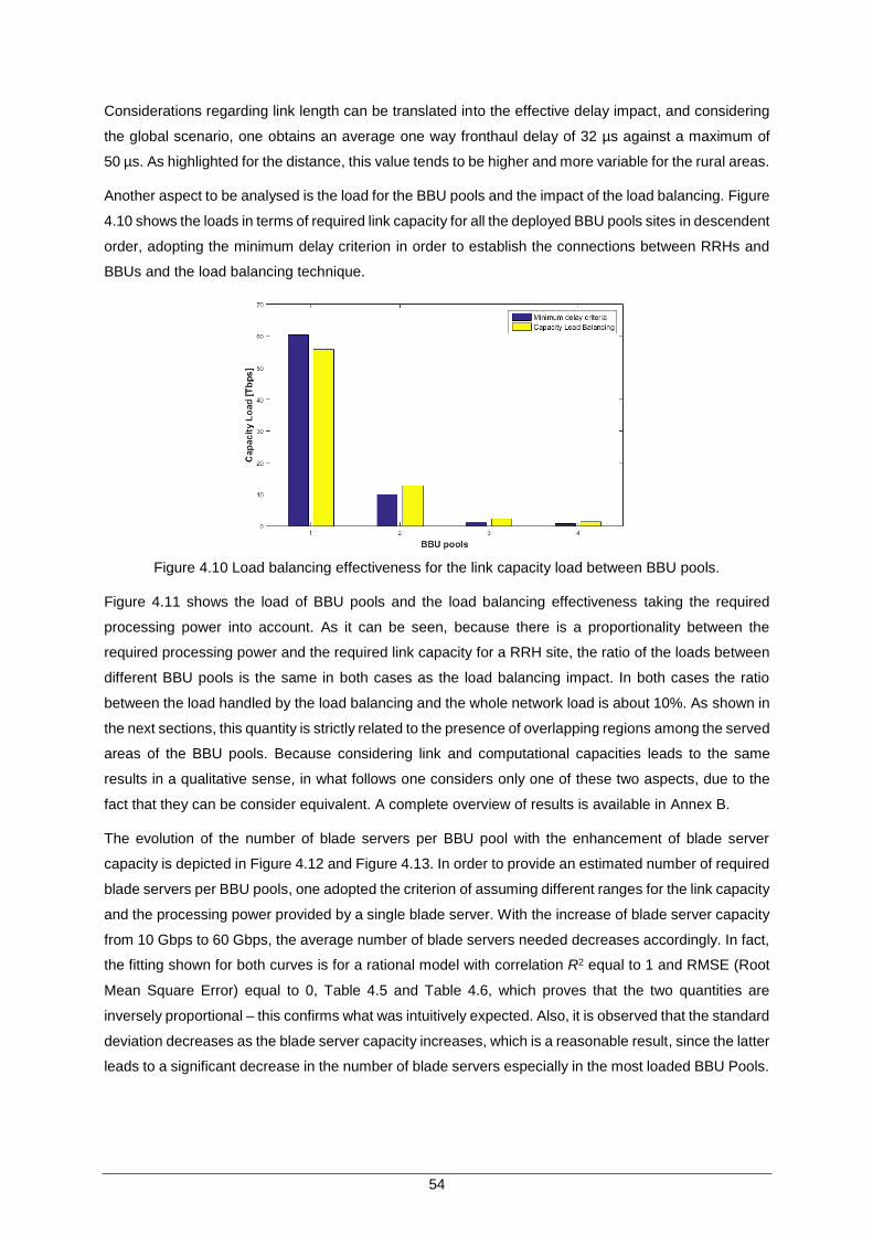
54
Considerations regarding link length can be translated into the effective delay impact, and considering
the global scenario, one obtains an average one way fronthaul delay of 32 µs against a maximum of
50 µs. As highlighted for the distance, this value tends to be higher and more variable for the rural areas.
Another aspect to be analysed is the load for the BBU pools and the impact of the load balancing. Figure
4.10 shows the loads in terms of required link capacity for all the deployed BBU pools sites in descendent
order, adopting the minimum delay criterion in order to establish the connections between RRHs and
BBUs and the load balancing technique.
Figure 4.10 Load balancing effectiveness for the link capacity load between BBU pools.
Figure 4.11 shows the load of BBU pools and the load balancing effectiveness taking the required
processing power into account. As it can be seen, because there is a proportionality between the
required processing power and the required link capacity for a RRH site, the ratio of the loads between
different BBU pools is the same in both cases as the load balancing impact. In both cases the ratio
between the load handled by the load balancing and the whole network load is about 10%. As shown in
the next sections, this quantity is strictly related to the presence of overlapping regions among the served
areas of the BBU pools. Because considering link and computational capacities leads to the same
results in a qualitative sense, in what follows one considers only one of these two aspects, due to the
fact that they can be consider equivalent. A complete overview of results is available in Annex B.
The evolution of the number of blade servers per BBU pool with the enhancement of blade server
capacity is depicted in Figure 4.12 and Figure 4.13. In order to provide an estimated number of required
blade servers per BBU pools, one adopted the criterion of assuming different ranges for the link capacity
and the processing power provided by a single blade server. With the increase of blade server capacity
from 10 Gbps to 60 Gbps, the average number of blade servers needed decreases accordingly. In fact,
the fitting shown for both curves is for a rational model with correlation R2 equal to 1 and RMSE (Root
Mean Square Error) equal to 0, Table 4.5 and Table 4.6, which proves that the two quantities are
inversely proportional – this confirms what was intuitively expected. Also, it is observed that the standard
deviation decreases as the blade server capacity increases, which is a reasonable result, since the latter
leads to a significant decrease in the number of blade servers especially in the most loaded BBU Pools.
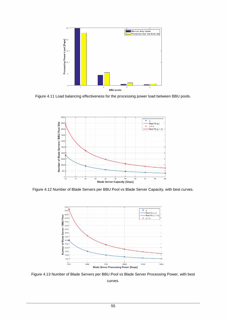
55
Figure 4.11 Load balancing effectiveness for the processing power load between BBU pools.
Figure 4.12 Number of Blade Servers per BBU Pool vs Blade Server Capacity, with best curves.
Figure 4.13 Number of Blade Servers per BBU Pool vs Blade Server Processing Power, with best
curves.
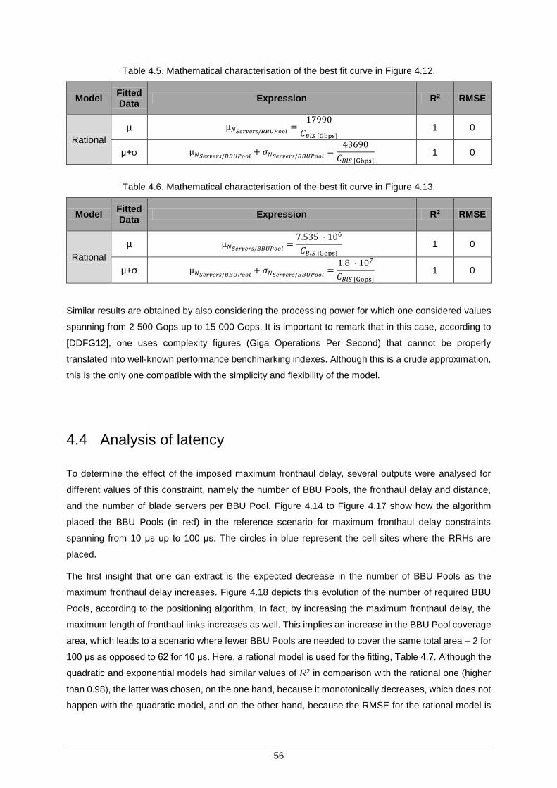
56
Table 4.5. Mathematical characterisation of the best fit curve in Figure 4.12.
Model Fitted Data
Expression R2 RMSE
Rational
µ µ𝑁𝑆𝑒𝑟𝑣𝑒𝑟𝑠/𝐵𝐵𝑈𝑃𝑜𝑜𝑙=
17990
𝐶𝐵𝑙𝑆 [Gbps]
1 0
µ+σ µ𝑁𝑆𝑒𝑟𝑣𝑒𝑟𝑠/𝐵𝐵𝑈𝑃𝑜𝑜𝑙+ 𝜎𝑁𝑆𝑒𝑟𝑣𝑒𝑟𝑠/𝐵𝐵𝑈𝑃𝑜𝑜𝑙
=43690
𝐶𝐵𝑙𝑆 [Gbps]
1 0
Table 4.6. Mathematical characterisation of the best fit curve in Figure 4.13.
Model Fitted Data
Expression R2 RMSE
Rational
µ µ𝑁𝑆𝑒𝑟𝑣𝑒𝑟𝑠/𝐵𝐵𝑈𝑃𝑜𝑜𝑙=
7.535 · 106
𝐶𝐵𝑙𝑆 [Gops]
1 0
µ+σ µ𝑁𝑆𝑒𝑟𝑣𝑒𝑟𝑠/𝐵𝐵𝑈𝑃𝑜𝑜𝑙+ 𝜎𝑁𝑆𝑒𝑟𝑣𝑒𝑟𝑠/𝐵𝐵𝑈𝑃𝑜𝑜𝑙
=1.8 · 107
𝐶𝐵𝑙𝑆 [Gops]
1 0
Similar results are obtained by also considering the processing power for which one considered values
spanning from 2 500 Gops up to 15 000 Gops. It is important to remark that in this case, according to
[DDFG12], one uses complexity figures (Giga Operations Per Second) that cannot be properly
translated into well-known performance benchmarking indexes. Although this is a crude approximation,
this is the only one compatible with the simplicity and flexibility of the model.
4.4 Analysis of latency
To determine the effect of the imposed maximum fronthaul delay, several outputs were analysed for
different values of this constraint, namely the number of BBU Pools, the fronthaul delay and distance,
and the number of blade servers per BBU Pool. Figure 4.14 to Figure 4.17 show how the algorithm
placed the BBU Pools (in red) in the reference scenario for maximum fronthaul delay constraints
spanning from 10 μs up to 100 μs. The circles in blue represent the cell sites where the RRHs are
placed.
The first insight that one can extract is the expected decrease in the number of BBU Pools as the
maximum fronthaul delay increases. Figure 4.18 depicts this evolution of the number of required BBU
Pools, according to the positioning algorithm. In fact, by increasing the maximum fronthaul delay, the
maximum length of fronthaul links increases as well. This implies an increase in the BBU Pool coverage
area, which leads to a scenario where fewer BBU Pools are needed to cover the same total area – 2 for
100 μs as opposed to 62 for 10 μs. Here, a rational model is used for the fitting, Table 4.7. Although the
quadratic and exponential models had similar values of R2 in comparison with the rational one (higher
than 0.98), the latter was chosen, on the one hand, because it monotonically decreases, which does not
happen with the quadratic model, and on the other hand, because the RMSE for the rational model is
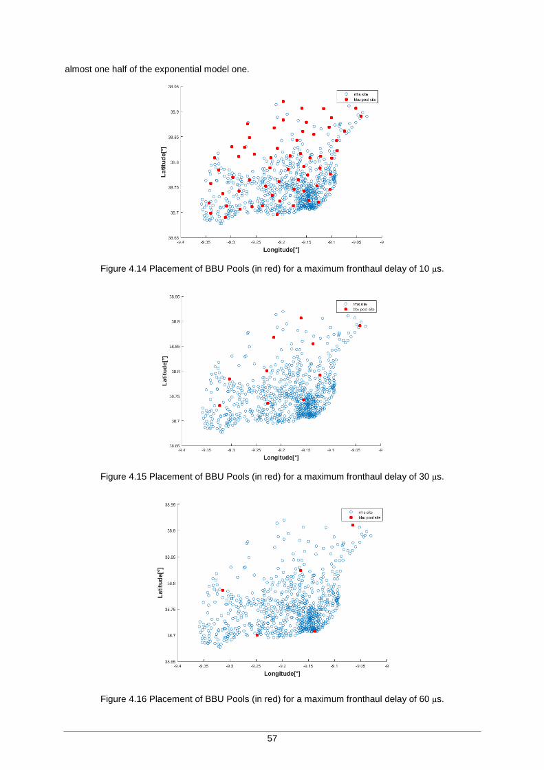
57
almost one half of the exponential model one.
Figure 4.14 Placement of BBU Pools (in red) for a maximum fronthaul delay of 10 μs.
Figure 4.15 Placement of BBU Pools (in red) for a maximum fronthaul delay of 30 μs.
Figure 4.16 Placement of BBU Pools (in red) for a maximum fronthaul delay of 60 μs.
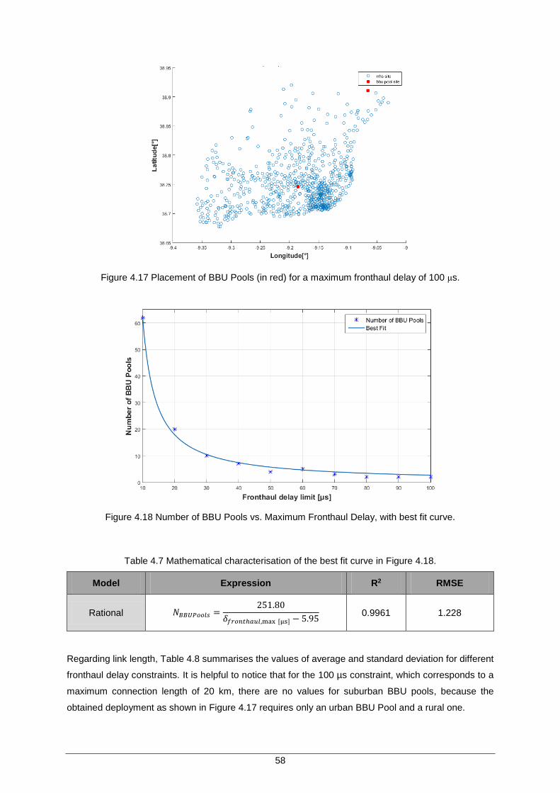
58
Figure 4.17 Placement of BBU Pools (in red) for a maximum fronthaul delay of 100 μs.
Figure 4.18 Number of BBU Pools vs. Maximum Fronthaul Delay, with best fit curve.
Table 4.7 Mathematical characterisation of the best fit curve in Figure 4.18.
Model Expression R2 RMSE
Rational 𝑁𝐵𝐵𝑈𝑃𝑜𝑜𝑙𝑠 =251.80
𝛿𝑓𝑟𝑜𝑛𝑡ℎ𝑎𝑢𝑙,max [µs] − 5.95 0.9961 1.228
Regarding link length, Table 4.8 summarises the values of average and standard deviation for different
fronthaul delay constraints. It is helpful to notice that for the 100 µs constraint, which corresponds to a
maximum connection length of 20 km, there are no values for suburban BBU pools, because the
obtained deployment as shown in Figure 4.17 requires only an urban BBU Pool and a rural one.
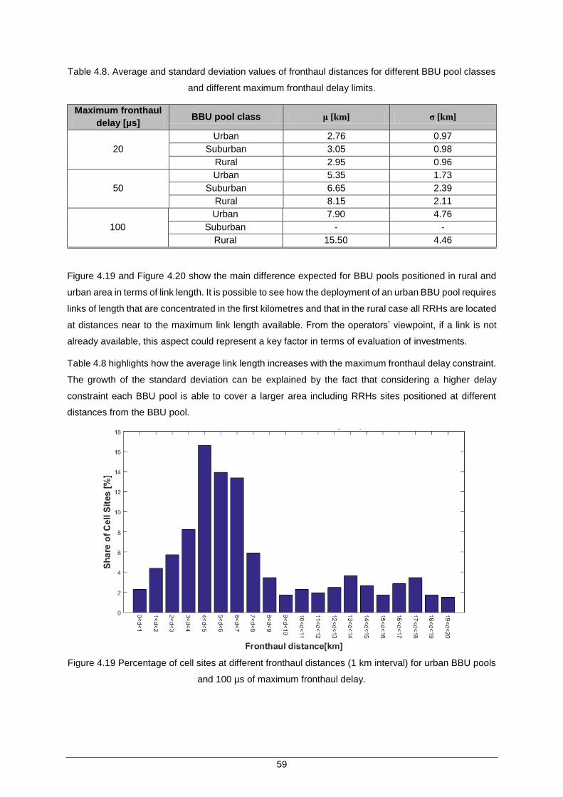
59
Table 4.8. Average and standard deviation values of fronthaul distances for different BBU pool classes
and different maximum fronthaul delay limits.
Maximum fronthaul
delay [µs] BBU pool class μ [km] σ [km]
20
Urban 2.76 0.97
Suburban 3.05 0.98
Rural 2.95 0.96
50
Urban 5.35 1.73
Suburban 6.65 2.39
Rural 8.15 2.11
100
Urban 7.90 4.76
Suburban - -
Rural 15.50 4.46
Figure 4.19 and Figure 4.20 show the main difference expected for BBU pools positioned in rural and
urban area in terms of link length. It is possible to see how the deployment of an urban BBU pool requires
links of length that are concentrated in the first kilometres and that in the rural case all RRHs are located
at distances near to the maximum link length available. From the operators’ viewpoint, if a link is not
already available, this aspect could represent a key factor in terms of evaluation of investments.
Table 4.8 highlights how the average link length increases with the maximum fronthaul delay constraint.
The growth of the standard deviation can be explained by the fact that considering a higher delay
constraint each BBU pool is able to cover a larger area including RRHs sites positioned at different
distances from the BBU pool.
Figure 4.19 Percentage of cell sites at different fronthaul distances (1 km interval) for urban BBU pools
and 100 µs of maximum fronthaul delay.
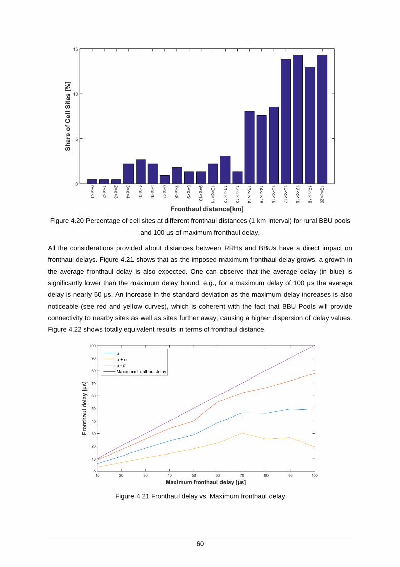
60
Figure 4.20 Percentage of cell sites at different fronthaul distances (1 km interval) for rural BBU pools
and 100 µs of maximum fronthaul delay.
All the considerations provided about distances between RRHs and BBUs have a direct impact on
fronthaul delays. Figure 4.21 shows that as the imposed maximum fronthaul delay grows, a growth in
the average fronthaul delay is also expected. One can observe that the average delay (in blue) is
significantly lower than the maximum delay bound, e.g., for a maximum delay of 100 μs the average
delay is nearly 50 μs. An increase in the standard deviation as the maximum delay increases is also
noticeable (see red and yellow curves), which is coherent with the fact that BBU Pools will provide
connectivity to nearby sites as well as sites further away, causing a higher dispersion of delay values.
Figure 4.22 shows totally equivalent results in terms of fronthaul distance.
Figure 4.21 Fronthaul delay vs. Maximum fronthaul delay
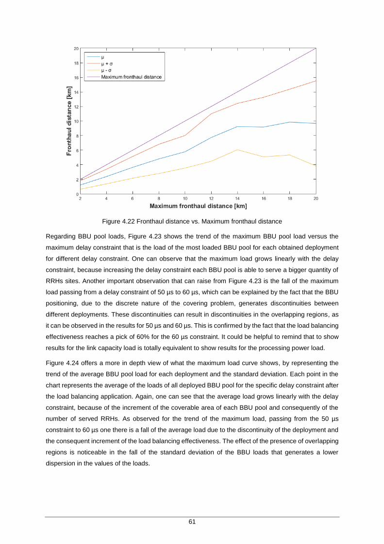
61
Figure 4.22 Fronthaul distance vs. Maximum fronthaul distance
Regarding BBU pool loads, Figure 4.23 shows the trend of the maximum BBU pool load versus the
maximum delay constraint that is the load of the most loaded BBU pool for each obtained deployment
for different delay constraint. One can observe that the maximum load grows linearly with the delay
constraint, because increasing the delay constraint each BBU pool is able to serve a bigger quantity of
RRHs sites. Another important observation that can raise from Figure 4.23 is the fall of the maximum
load passing from a delay constraint of 50 µs to 60 µs, which can be explained by the fact that the BBU
positioning, due to the discrete nature of the covering problem, generates discontinuities between
different deployments. These discontinuities can result in discontinuities in the overlapping regions, as
it can be observed in the results for 50 µs and 60 µs. This is confirmed by the fact that the load balancing
effectiveness reaches a pick of 60% for the 60 µs constraint. It could be helpful to remind that to show
results for the link capacity load is totally equivalent to show results for the processing power load.
Figure 4.24 offers a more in depth view of what the maximum load curve shows, by representing the
trend of the average BBU pool load for each deployment and the standard deviation. Each point in the
chart represents the average of the loads of all deployed BBU pool for the specific delay constraint after
the load balancing application. Again, one can see that the average load grows linearly with the delay
constraint, because of the increment of the coverable area of each BBU pool and consequently of the
number of served RRHs. As observed for the trend of the maximum load, passing from the 50 µs
constraint to 60 µs one there is a fall of the average load due to the discontinuity of the deployment and
the consequent increment of the load balancing effectiveness. The effect of the presence of overlapping
regions is noticeable in the fall of the standard deviation of the BBU loads that generates a lower
dispersion in the values of the loads.
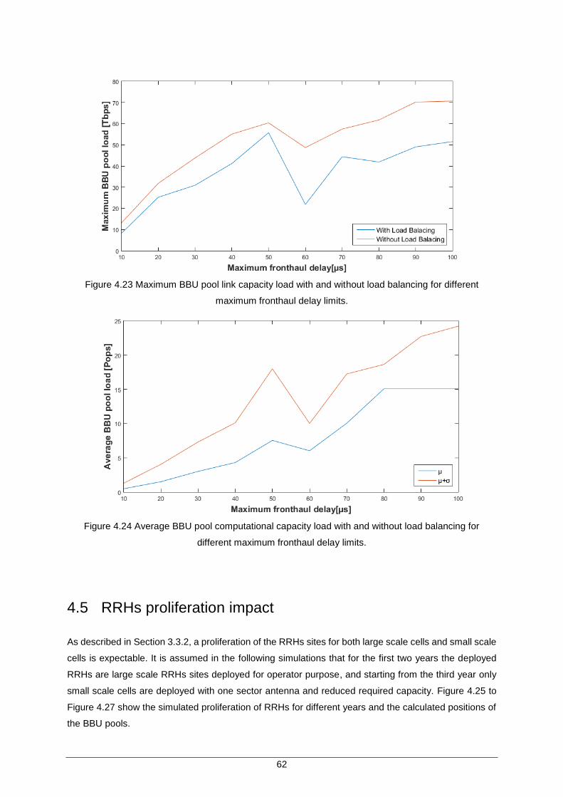
62
Figure 4.23 Maximum BBU pool link capacity load with and without load balancing for different
maximum fronthaul delay limits.
Figure 4.24 Average BBU pool computational capacity load with and without load balancing for
different maximum fronthaul delay limits.
4.5 RRHs proliferation impact
As described in Section 3.3.2, a proliferation of the RRHs sites for both large scale cells and small scale
cells is expectable. It is assumed in the following simulations that for the first two years the deployed
RRHs are large scale RRHs sites deployed for operator purpose, and starting from the third year only
small scale cells are deployed with one sector antenna and reduced required capacity. Figure 4.25 to
Figure 4.27 show the simulated proliferation of RRHs for different years and the calculated positions of
the BBU pools.
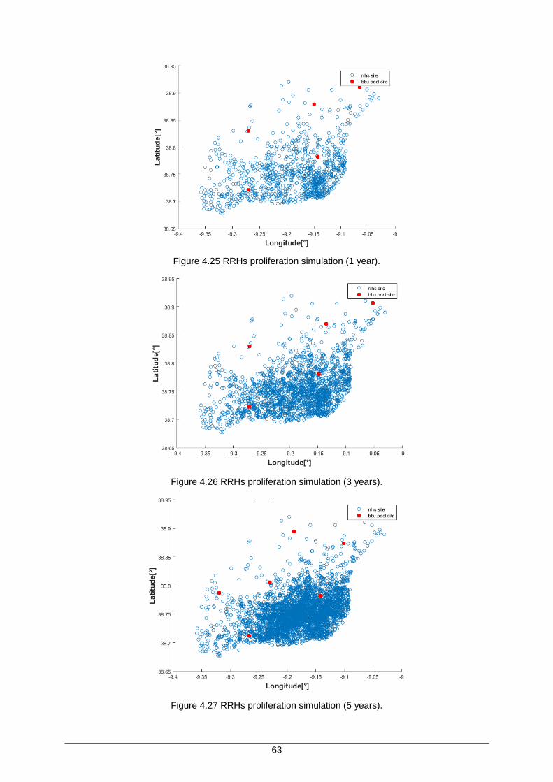
63
Figure 4.25 RRHs proliferation simulation (1 year).
Figure 4.26 RRHs proliferation simulation (3 years).
Figure 4.27 RRHs proliferation simulation (5 years).
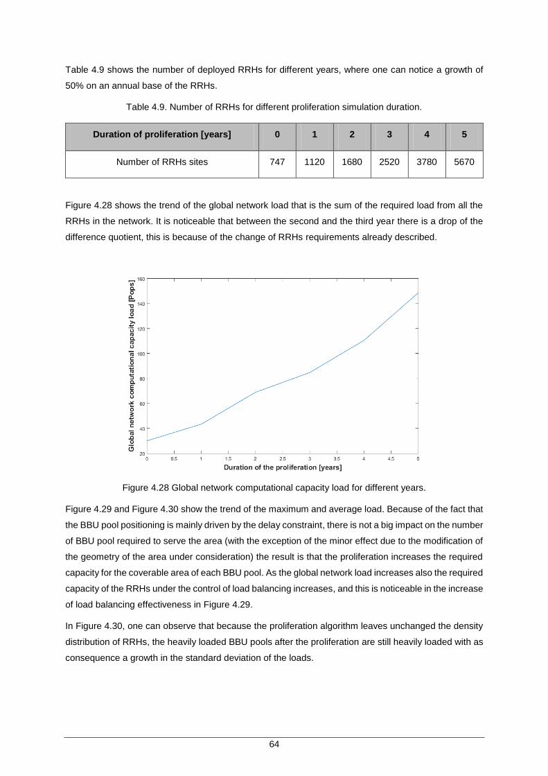
64
Table 4.9 shows the number of deployed RRHs for different years, where one can notice a growth of
50% on an annual base of the RRHs.
Table 4.9. Number of RRHs for different proliferation simulation duration.
Duration of proliferation [years] 0 1 2 3 4 5
Number of RRHs sites 747 1120 1680 2520 3780 5670
Figure 4.28 shows the trend of the global network load that is the sum of the required load from all the
RRHs in the network. It is noticeable that between the second and the third year there is a drop of the
difference quotient, this is because of the change of RRHs requirements already described.
Figure 4.28 Global network computational capacity load for different years.
Figure 4.29 and Figure 4.30 show the trend of the maximum and average load. Because of the fact that
the BBU pool positioning is mainly driven by the delay constraint, there is not a big impact on the number
of BBU pool required to serve the area (with the exception of the minor effect due to the modification of
the geometry of the area under consideration) the result is that the proliferation increases the required
capacity for the coverable area of each BBU pool. As the global network load increases also the required
capacity of the RRHs under the control of load balancing increases, and this is noticeable in the increase
of load balancing effectiveness in Figure 4.29.
In Figure 4.30, one can observe that because the proliferation algorithm leaves unchanged the density
distribution of RRHs, the heavily loaded BBU pools after the proliferation are still heavily loaded with as
consequence a growth in the standard deviation of the loads.
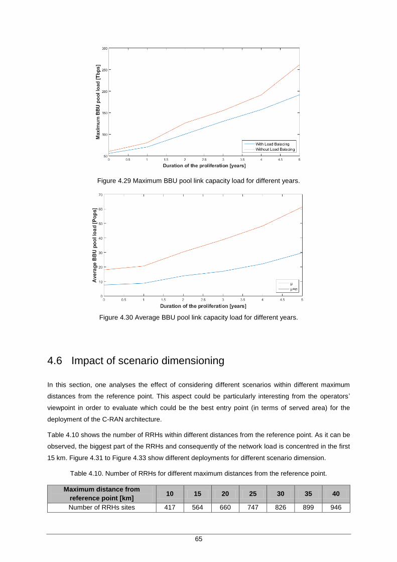
65
Figure 4.29 Maximum BBU pool link capacity load for different years.
Figure 4.30 Average BBU pool link capacity load for different years.
4.6 Impact of scenario dimensioning
In this section, one analyses the effect of considering different scenarios within different maximum
distances from the reference point. This aspect could be particularly interesting from the operators’
viewpoint in order to evaluate which could be the best entry point (in terms of served area) for the
deployment of the C-RAN architecture.
Table 4.10 shows the number of RRHs within different distances from the reference point. As it can be
observed, the biggest part of the RRHs and consequently of the network load is concentred in the first
15 km. Figure 4.31 to Figure 4.33 show different deployments for different scenario dimension.
Table 4.10. Number of RRHs for different maximum distances from the reference point.
Maximum distance from
reference point [km] 10 15 20 25 30 35 40
Number of RRHs sites 417 564 660 747 826 899 946
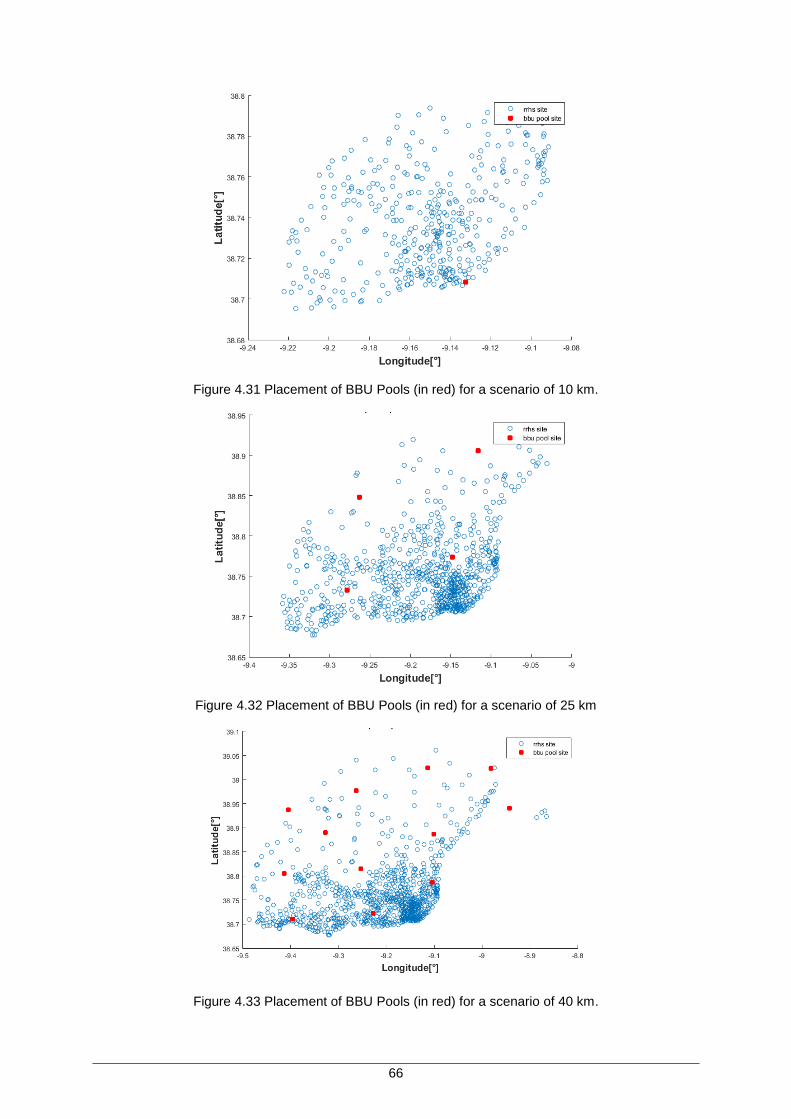
66
Figure 4.31 Placement of BBU Pools (in red) for a scenario of 10 km.
Figure 4.32 Placement of BBU Pools (in red) for a scenario of 25 km
Figure 4.33 Placement of BBU Pools (in red) for a scenario of 40 km.
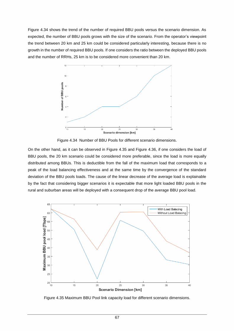
67
Figure 4.34 shows the trend of the number of required BBU pools versus the scenario dimension. As
expected, the number of BBU pools grows with the size of the scenario. From the operator’s viewpoint
the trend between 20 km and 25 km could be considered particularly interesting, because there is no
growth in the number of required BBU pools. If one considers the ratio between the deployed BBU pools
and the number of RRHs, 25 km is to be considered more convenient than 20 km.
Figure 4.34 Number of BBU Pools for different scenario dimensions.
On the other hand, as it can be observed in Figure 4.35 and Figure 4.36, if one considers the load of
BBU pools, the 20 km scenario could be considered more preferable, since the load is more equally
distributed among BBUs. This is deductible from the fall of the maximum load that corresponds to a
peak of the load balancing effectiveness and at the same time by the convergence of the standard
deviation of the BBU pools loads. The cause of the linear decrease of the average load is explainable
by the fact that considering bigger scenarios it is expectable that more light loaded BBU pools in the
rural and suburban areas will be deployed with a consequent drop of the average BBU pool load.
Figure 4.35 Maximum BBU Pool link capacity load for different scenario dimensions.
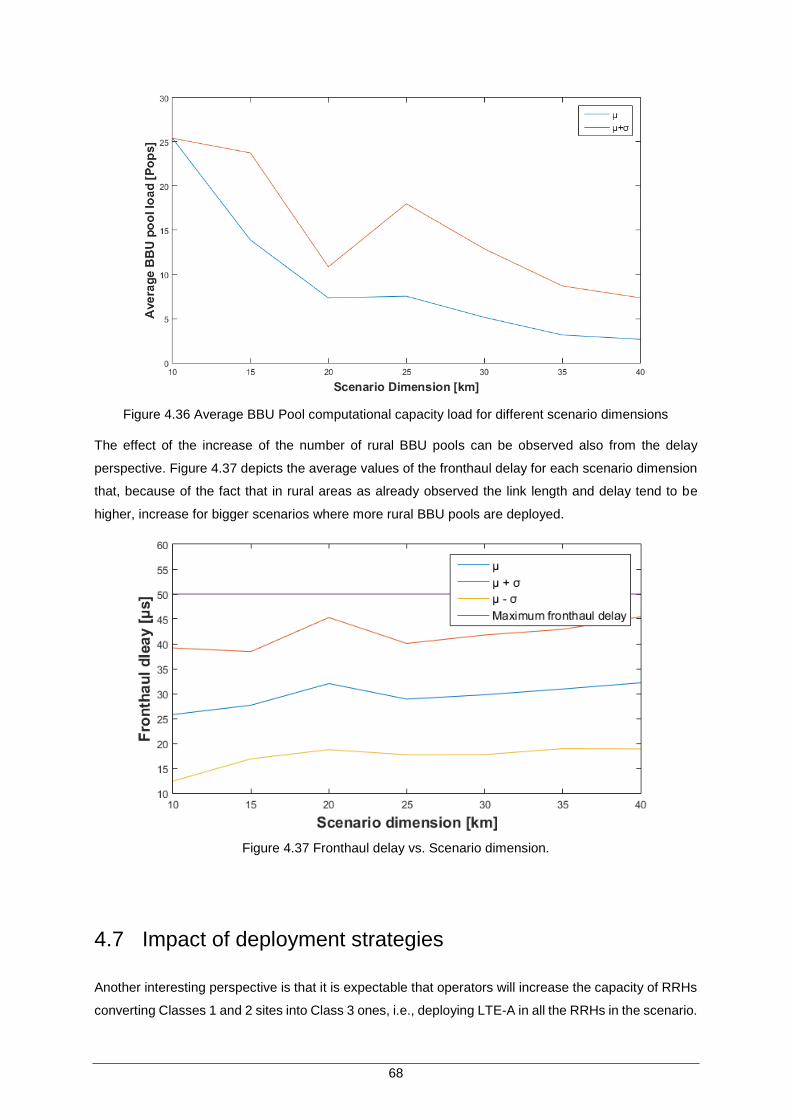
68
Figure 4.36 Average BBU Pool computational capacity load for different scenario dimensions
The effect of the increase of the number of rural BBU pools can be observed also from the delay
perspective. Figure 4.37 depicts the average values of the fronthaul delay for each scenario dimension
that, because of the fact that in rural areas as already observed the link length and delay tend to be
higher, increase for bigger scenarios where more rural BBU pools are deployed.
Figure 4.37 Fronthaul delay vs. Scenario dimension.
4.7 Impact of deployment strategies
Another interesting perspective is that it is expectable that operators will increase the capacity of RRHs
converting Classes 1 and 2 sites into Class 3 ones, i.e., deploying LTE-A in all the RRHs in the scenario.
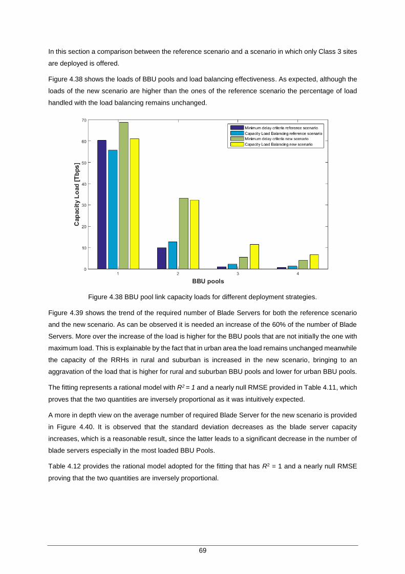
69
In this section a comparison between the reference scenario and a scenario in which only Class 3 sites
are deployed is offered.
Figure 4.38 shows the loads of BBU pools and load balancing effectiveness. As expected, although the
loads of the new scenario are higher than the ones of the reference scenario the percentage of load
handled with the load balancing remains unchanged.
Figure 4.38 BBU pool link capacity loads for different deployment strategies.
Figure 4.39 shows the trend of the required number of Blade Servers for both the reference scenario
and the new scenario. As can be observed it is needed an increase of the 60% of the number of Blade
Servers. More over the increase of the load is higher for the BBU pools that are not initially the one with
maximum load. This is explainable by the fact that in urban area the load remains unchanged meanwhile
the capacity of the RRHs in rural and suburban is increased in the new scenario, bringing to an
aggravation of the load that is higher for rural and suburban BBU pools and lower for urban BBU pools.
The fitting represents a rational model with R2 = 1 and a nearly null RMSE provided in Table 4.11, which
proves that the two quantities are inversely proportional as it was intuitively expected.
A more in depth view on the average number of required Blade Server for the new scenario is provided
in Figure 4.40. It is observed that the standard deviation decreases as the blade server capacity
increases, which is a reasonable result, since the latter leads to a significant decrease in the number of
blade servers especially in the most loaded BBU Pools.
Table 4.12 provides the rational model adopted for the fitting that has R2 = 1 and a nearly null RMSE
proving that the two quantities are inversely proportional.
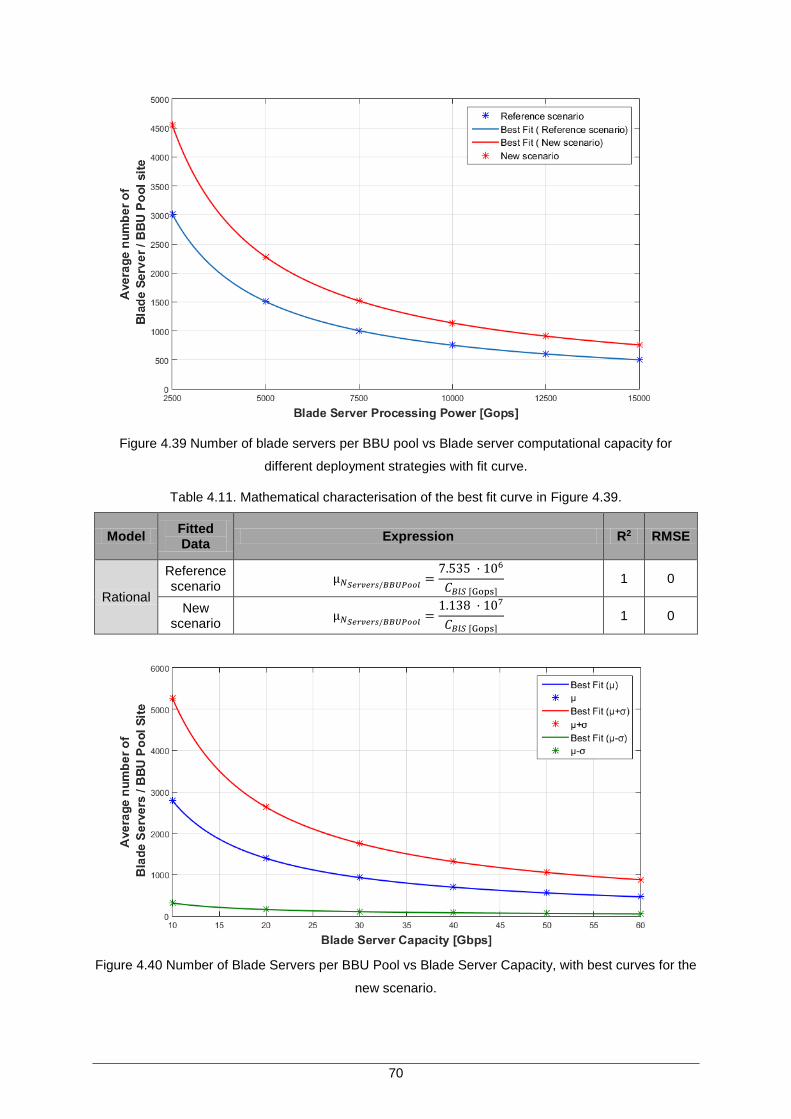
70
Figure 4.39 Number of blade servers per BBU pool vs Blade server computational capacity for
different deployment strategies with fit curve.
Table 4.11. Mathematical characterisation of the best fit curve in Figure 4.39.
Model Fitted Data
Expression R2 RMSE
Rational
Reference scenario
µ𝑁𝑆𝑒𝑟𝑣𝑒𝑟𝑠/𝐵𝐵𝑈𝑃𝑜𝑜𝑙=
7.535 · 106
𝐶𝐵𝑙𝑆 [Gops]
1 0
New scenario
µ𝑁𝑆𝑒𝑟𝑣𝑒𝑟𝑠/𝐵𝐵𝑈𝑃𝑜𝑜𝑙=
1.138 · 107
𝐶𝐵𝑙𝑆 [Gops]
1 0
Figure 4.40 Number of Blade Servers per BBU Pool vs Blade Server Capacity, with best curves for the
new scenario.
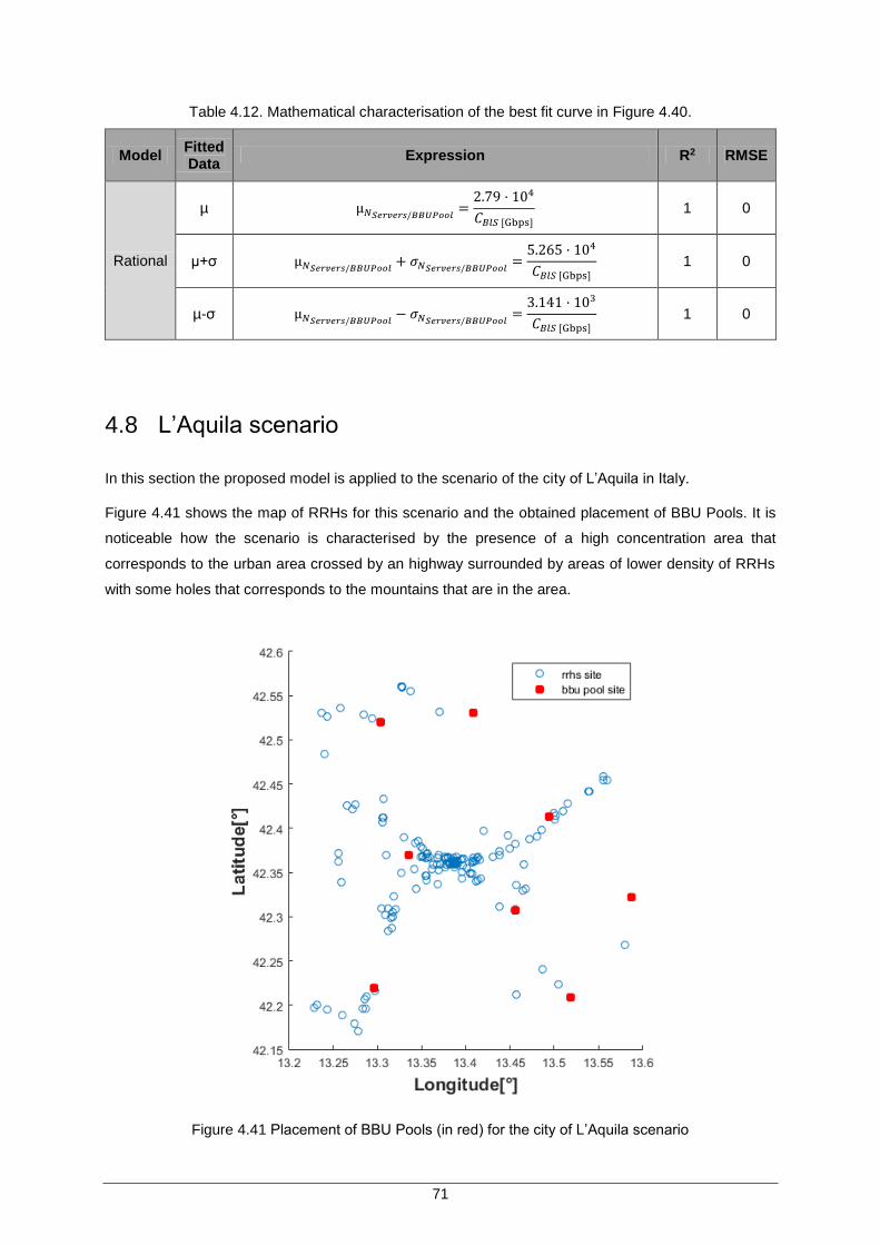
71
Table 4.12. Mathematical characterisation of the best fit curve in Figure 4.40.
Model Fitted Data
Expression R2 RMSE
Rational
µ µ𝑁𝑆𝑒𝑟𝑣𝑒𝑟𝑠/𝐵𝐵𝑈𝑃𝑜𝑜𝑙=
2.79 · 104
𝐶𝐵𝑙𝑆 [Gbps]
1 0
µ+σ µ𝑁𝑆𝑒𝑟𝑣𝑒𝑟𝑠/𝐵𝐵𝑈𝑃𝑜𝑜𝑙+ 𝜎𝑁𝑆𝑒𝑟𝑣𝑒𝑟𝑠/𝐵𝐵𝑈𝑃𝑜𝑜𝑙
=5.265 · 104
𝐶𝐵𝑙𝑆 [Gbps]
1 0
µ-σ µ𝑁𝑆𝑒𝑟𝑣𝑒𝑟𝑠/𝐵𝐵𝑈𝑃𝑜𝑜𝑙− 𝜎𝑁𝑆𝑒𝑟𝑣𝑒𝑟𝑠/𝐵𝐵𝑈𝑃𝑜𝑜𝑙
=3.141 · 103
𝐶𝐵𝑙𝑆 [Gbps]
1 0
4.8 L’Aquila scenario
In this section the proposed model is applied to the scenario of the city of L’Aquila in Italy.
Figure 4.41 shows the map of RRHs for this scenario and the obtained placement of BBU Pools. It is
noticeable how the scenario is characterised by the presence of a high concentration area that
corresponds to the urban area crossed by an highway surrounded by areas of lower density of RRHs
with some holes that corresponds to the mountains that are in the area.
Figure 4.41 Placement of BBU Pools (in red) for the city of L’Aquila scenario
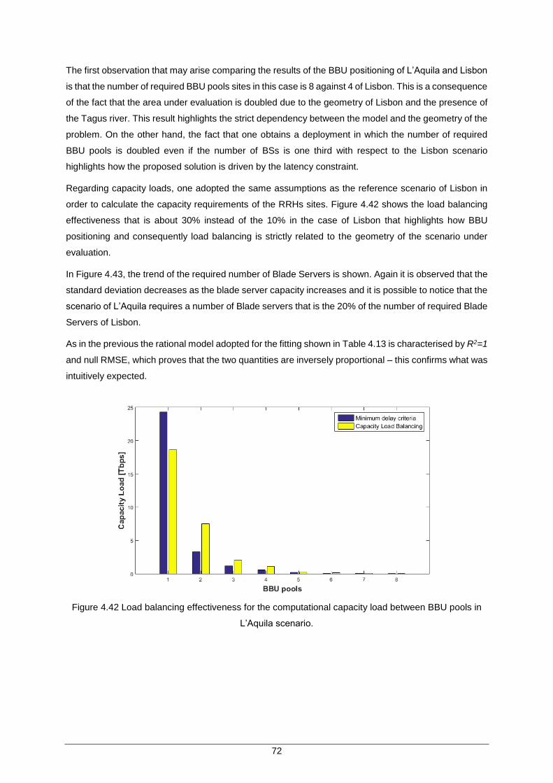
72
The first observation that may arise comparing the results of the BBU positioning of L’Aquila and Lisbon
is that the number of required BBU pools sites in this case is 8 against 4 of Lisbon. This is a consequence
of the fact that the area under evaluation is doubled due to the geometry of Lisbon and the presence of
the Tagus river. This result highlights the strict dependency between the model and the geometry of the
problem. On the other hand, the fact that one obtains a deployment in which the number of required
BBU pools is doubled even if the number of BSs is one third with respect to the Lisbon scenario
highlights how the proposed solution is driven by the latency constraint.
Regarding capacity loads, one adopted the same assumptions as the reference scenario of Lisbon in
order to calculate the capacity requirements of the RRHs sites. Figure 4.42 shows the load balancing
effectiveness that is about 30% instead of the 10% in the case of Lisbon that highlights how BBU
positioning and consequently load balancing is strictly related to the geometry of the scenario under
evaluation.
In Figure 4.43, the trend of the required number of Blade Servers is shown. Again it is observed that the
standard deviation decreases as the blade server capacity increases and it is possible to notice that the
scenario of L’Aquila requires a number of Blade servers that is the 20% of the number of required Blade
Servers of Lisbon.
As in the previous the rational model adopted for the fitting shown in Table 4.13 is characterised by R2=1
and null RMSE, which proves that the two quantities are inversely proportional – this confirms what was
intuitively expected.
Figure 4.42 Load balancing effectiveness for the computational capacity load between BBU pools in
L’Aquila scenario.
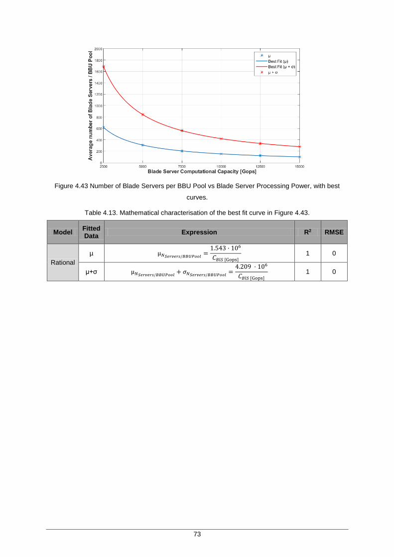
73
Figure 4.43 Number of Blade Servers per BBU Pool vs Blade Server Processing Power, with best
curves.
Table 4.13. Mathematical characterisation of the best fit curve in Figure 4.43.
Model Fitted Data
Expression R2 RMSE
Rational
µ µ𝑁𝑆𝑒𝑟𝑣𝑒𝑟𝑠/𝐵𝐵𝑈𝑃𝑜𝑜𝑙=
1.543 · 106
𝐶𝐵𝑙𝑆 [Gops]
1 0
µ+σ µ𝑁𝑆𝑒𝑟𝑣𝑒𝑟𝑠/𝐵𝐵𝑈𝑃𝑜𝑜𝑙+ 𝜎𝑁𝑆𝑒𝑟𝑣𝑒𝑟𝑠/𝐵𝐵𝑈𝑃𝑜𝑜𝑙
=4.209 · 106
𝐶𝐵𝑙𝑆 [Gops]
1 0

74
75
Chapter 5
Conclusions
5 Conclusions
This chapter finalises this work by summarising the main conclusions obtained and pointing out aspects
to be developed in future work.
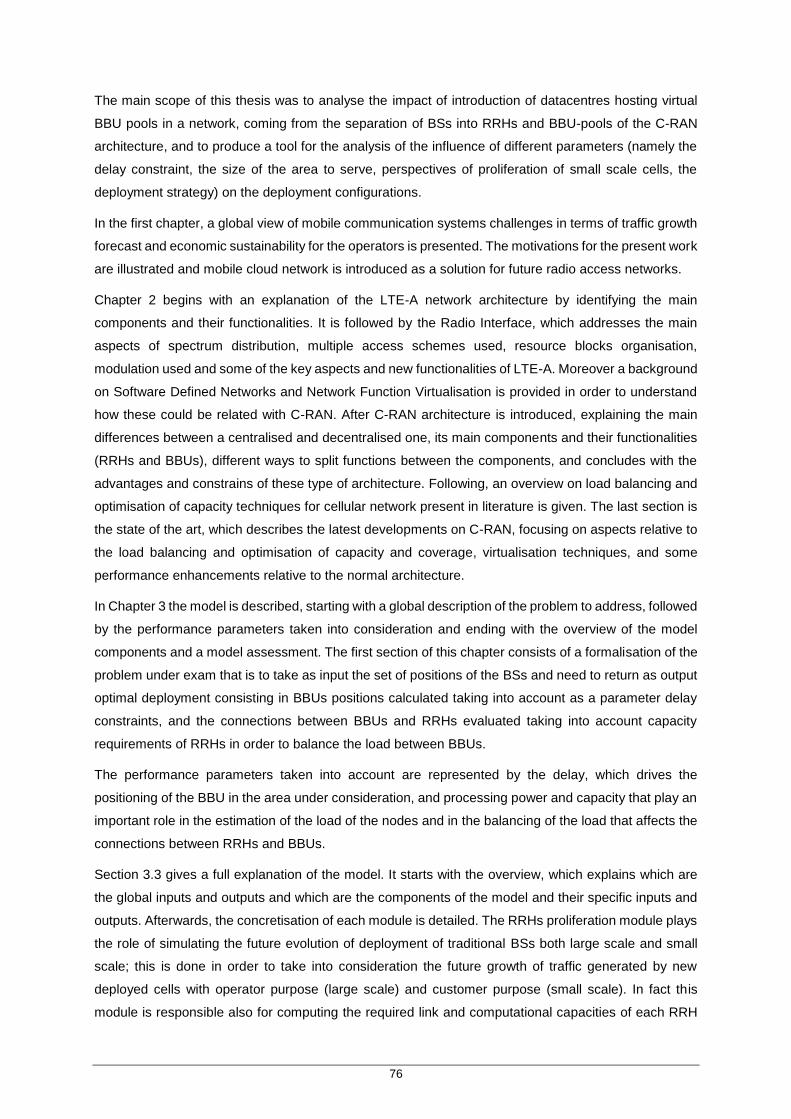
76
The main scope of this thesis was to analyse the impact of introduction of datacentres hosting virtual
BBU pools in a network, coming from the separation of BSs into RRHs and BBU-pools of the C-RAN
architecture, and to produce a tool for the analysis of the influence of different parameters (namely the
delay constraint, the size of the area to serve, perspectives of proliferation of small scale cells, the
deployment strategy) on the deployment configurations.
In the first chapter, a global view of mobile communication systems challenges in terms of traffic growth
forecast and economic sustainability for the operators is presented. The motivations for the present work
are illustrated and mobile cloud network is introduced as a solution for future radio access networks.
Chapter 2 begins with an explanation of the LTE-A network architecture by identifying the main
components and their functionalities. It is followed by the Radio Interface, which addresses the main
aspects of spectrum distribution, multiple access schemes used, resource blocks organisation,
modulation used and some of the key aspects and new functionalities of LTE-A. Moreover a background
on Software Defined Networks and Network Function Virtualisation is provided in order to understand
how these could be related with C-RAN. After C-RAN architecture is introduced, explaining the main
differences between a centralised and decentralised one, its main components and their functionalities
(RRHs and BBUs), different ways to split functions between the components, and concludes with the
advantages and constrains of these type of architecture. Following, an overview on load balancing and
optimisation of capacity techniques for cellular network present in literature is given. The last section is
the state of the art, which describes the latest developments on C-RAN, focusing on aspects relative to
the load balancing and optimisation of capacity and coverage, virtualisation techniques, and some
performance enhancements relative to the normal architecture.
In Chapter 3 the model is described, starting with a global description of the problem to address, followed
by the performance parameters taken into consideration and ending with the overview of the model
components and a model assessment. The first section of this chapter consists of a formalisation of the
problem under exam that is to take as input the set of positions of the BSs and need to return as output
optimal deployment consisting in BBUs positions calculated taking into account as a parameter delay
constraints, and the connections between BBUs and RRHs evaluated taking into account capacity
requirements of RRHs in order to balance the load between BBUs.
The performance parameters taken into account are represented by the delay, which drives the
positioning of the BBU in the area under consideration, and processing power and capacity that play an
important role in the estimation of the load of the nodes and in the balancing of the load that affects the
connections between RRHs and BBUs.
Section 3.3 gives a full explanation of the model. It starts with the overview, which explains which are
the global inputs and outputs and which are the components of the model and their specific inputs and
outputs. Afterwards, the concretisation of each module is detailed. The RRHs proliferation module plays
the role of simulating the future evolution of deployment of traditional BSs both large scale and small
scale; this is done in order to take into consideration the future growth of traffic generated by new
deployed cells with operator purpose (large scale) and customer purpose (small scale). In fact this
module is responsible also for computing the required link and computational capacities of each RRH

77
based on the purpose and the position (it is assumed that cells deployed in rural areas will require lower
performance with respect to cells deployed in urban area).
The BBU positioning module aims to identify the positions of the BBU pools sites starting from the set
of the positions of the BSs. One important assumption is adopted during the evaluation and is that in an
urban scenario not all the locations that could be considered optimal for the BBU pools positions should
be able to host infrastructures required for a BBU pool due to the fact that network operators cannot
locate equipment in arbitrary locations, such as protected buildings, difficult geographical locations and
so on. The approach that one adopted to avoid this problem was to consider as set of feasible positions
for the BBUs the set of the locations of the BSs itself. The key parameter for the BBU positioning is
represented by the delay. The deployment of the BBU is identified under the constraint that all the RRHs
in the scenario must be able to connect to a BBU with a resulting fronthaul delay lower than the maximum
fronthaul delay provided as input of the problem. Because of the problem that the BBU positioning
address is demonstrated to be NP-Complete, one proposes four heuristics that adopt different criteria
that are: density-based Min-Max heuristic; density-based Max-Min; distance based heuristic; hybrid
heuristic based on both distance and density.
The load balancing module identifies the connections between RRHs sites and BBU pools. A basic
approach is to adopt a criterion based on minimum distance (that corresponds to minimum delay)
between RRHs site and BBU pool. This technique for each RRH site in the scenario evaluates which is
the nearest BBU pool and creates a connection between the RRHs site and the BBU pool. We provide
another technique that takes into consideration also the load on the BBU pool generated by the RRH
connection and instantiate connections connecting a RRH to the less loaded BBU pool within a
maximum fronthaul distance obtained from the maximum fronthaul delay constraint. We adopt as index
of the load on the BBU pool the sum of the capacities of the links converging to the BBU pool or
alternatively the processing power of the nodes connected to the BBU Pool.
The BBU pools dimensioning module assesses the capacity of every BBU pool, which simply consists
of determining the blade servers demand imposed by each site in the corresponding BBU Pool. The
data produced by this module can be adopted as an index of the peak load that the Cloud Infrastructure
should provide to the BBU pool sites. In any case, they hold for a centralised context in which the
computational capacity is physically instantiated in the site and not virtualised and provide by the cloud.
Chapter 4 starts by providing a description of the scenario used in this thesis, which is the city of Lisbon
and its surrounding areas. Three classes of sites were defined, each one with its own fronthaul link
capacity and computational power requirements; this distinction is used in order to evaluate the loads
of the BBU pools and to aggravate the capacity demand to be supported by the set of BBU Pools for
different deployment strategies. Furthermore, the range of values for maximum fronthaul delays used in
simulation were defined, and the ranges for the capacity for blade servers in BBU Pools. Moreover the
scenario of the city of L’Aquila, which is used to provide a comparison of results for a totally different
scenario, is described.
Before the analysis of results, a comparison between the algorithms illustrated in Chapter 3 for the BBU
positioning is proposed. The criterion adopted for the comparison is the minimum number of deployed
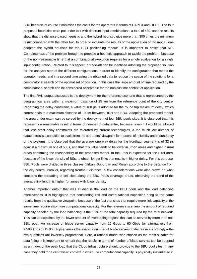
78
BBU because of course it minimises the costs for the operators in terms of CAPEX and OPEX. The four
proposed heuristics were put under test with different input combinations, a total of 430, and the results
show that the distance based heuristic and the hybrid heuristic give more than 300 times the minimum
result compared with the other two. In order to evaluate the results of the application of the model, one
adopted the hybrid heuristic for the BBU positioning module. It is important to notice that NP-
Completeness of the problem brought to propose a heuristic approach to tackle the problem, because
of the non-reasonable time that a combinatorial execution requires for a single evaluation for a single
input configuration. Related to this aspect, a trade-off can be identified adopting the proposed solution
for the analysis step of the different configurations in order to identify the configuration that meets the
operator needs, and in a second time using the obtained data to reduce the space of the solutions for a
combinatorial search of the optimal set of position. In this case the large amount of time required by the
combinatorial search can be considered acceptable for the non-runtime context of application.
The first RAN output discussed is the deployment for the reference scenario that is represented by the
geographical area within a maximum distance of 25 km from the reference point of the city centre.
Regarding the delay constraint, a value of 100 µs is adopted for the round trip maximum delay, which
corresponds to a maximum distance of 10 km between RRH and BBU. Adopting the proposed model,
the area under exam can be served by the deployment of four BBU pools sites. It is observed that this
represents a reasonable result in terms of number of datacentre, because, even if it would be allowed
that less strict delay constraints are tolerated by current technologies, a too much low number of
datacentres is a condition to avoid from the operators’ viewpoint for reasons of reliability and redundancy
of the systems. It is observed that the average one way delay for the fronthaul segment is of 32 µs
against a maximum one of 50µs, and that this value tends to be lower in urban areas and higher in rural
areas confirming the reasonability of the proposed model. In fact, this is expected for the rural area,
because of the lower density of BSs, to obtain longer links that results in higher delay. For this purpose,
BBU Pools were divided in three classes (Urban, Suburban and Rural) according to the distance from
the city centre. Parallel, regarding fronthaul distance, a few considerations were also drawn on what
concerns the spreading of cell sites along the BBU Pools coverage areas, observing the trend of the
average link length is higher for zones with lower density
Another important output that was studied is the load on the BBU pools and the load balancing
effectiveness. It is highlighted that considering link and computational capacities bring to the same
results from the qualitative viewpoint, because of the fact that sites that require more link capacity at the
same time require also more computational capacity. For the reference scenario the amount of required
capacity handled by the load balancing is the 10% of the total capacity required by the total network.
This can be explained by the lower amount of overlapping regions that can be served by more than one
BBU pool. An increase of blade server capacity from 10 Gbps to 60 Gbps (or alternatively from
2 500 Tops to 15 000 Tops) causes the average number of blade servers to decrease accordingly – the
two quantities are inversely proportional. Here, a rational model was chosen as the most suitable for
data fitting. It is important to remark that the results in terms of number of blade servers can be adopted
as an index of the peak load that the Cloud Infrastructure should provide to the BBU pool sites. In any
case they hold for a centralised context in which the computational capacity is physically instantiated in
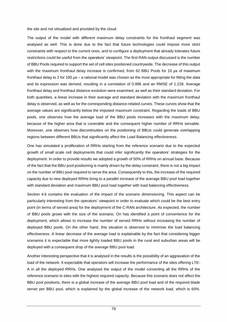
79
the site and not virtualised and provided by the cloud.
The output of the model with different maximum delay constraints for the fronthaul segment was
analysed as well. This is done due to the fact that future technologies could impose more strict
constraints with respect to the current ones, and to configure a deployment that already tolerates future
restrictions could be useful from the operators’ viewpoint. The first RAN output discussed is the number
of BBU Pools required to support the set of cell sites positioned countrywide. The decrease of this output
with the maximum fronthaul delay increase is confirmed, from 62 BBU Pools for 10 μs of maximum
fronthaul delay to 2 for 100 μs – a rational model was chosen as the most appropriate for fitting the data
and its expression was derived, resulting in a correlation of 0.996 and an RMSE of 1.228. Average
fronthaul delay and fronthaul distance evolution were examined, as well as their standard deviation. For
both quantities, a linear increase in their average and standard deviation with the maximum fronthaul
delay is observed, as well as for the corresponding distance-related curves. These curves show that the
average values are significantly below the imposed maximum constraint. Regarding the loads of BBU
pools, one observes how the average load of the BBU pools increases with the maximum delay,
because of the higher area that is coverable and the consequent higher number of RRHs servable.
Moreover, one observes how discontinuities on the positioning of BBUs could generate overlapping
regions between different BBUs that significantly affect the Load Balancing effectiveness.
One has simulated a proliferation of RRHs starting from the reference scenario due to the expected
growth of small scale cell deployments that could infer significantly the operators’ strategies for the
deployment. In order to provide results we adopted a growth of 50% of RRHs on annual base. Because
of the fact that the BBU pool positioning is mainly driven by the delay constraint, there is not a big impact
on the number of BBU pool required to serve the area. Consequently to this, the increase of the required
capacity due to new deployed RRHs bring to a parallel increase of the average BBU pool load together
with standard deviation and maximum BBU pool load together with load balancing effectiveness.
Section 4.6 contains the evaluation of the impact of the scenario dimensioning. This aspect can be
particularly interesting from the operators’ viewpoint in order to evaluate which could be the best entry
point (in terms of served area) for the deployment of the C-RAN architecture. As expected, the number
of BBU pools grows with the size of the scenario. On has identified a point of convenience for the
deployment, which allows to increase the number of served RRHs without increasing the number of
deployed BBU pools. On the other hand, this situation is observed to minimise the load balancing
effectiveness. A linear decrease of the average load is explainable by the fact that considering bigger
scenarios it is expectable that more lightly loaded BBU pools in the rural and suburban areas will be
deployed with a consequent drop of the average BBU pool load.
Another interesting perspective that it is analysed in the results is the possibility of an aggravation of the
load of the network. It expectable that operators will increase the performance of the sites offering LTE-
A in all the deployed RRHs. One analysed the output of the model converting all the RRHs of the
reference scenario to sites with the highest required capacity. Because this scenario does not affect the
BBU pool positions, there is a global increase of the average BBU pool load and of the required blade
server per BBU pool, which is explained by the global increase of the network load, which is 60%.
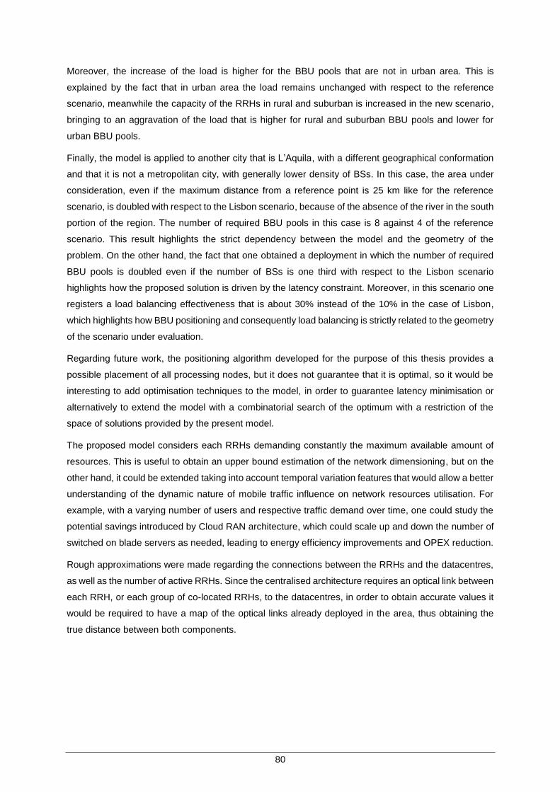
80
Moreover, the increase of the load is higher for the BBU pools that are not in urban area. This is
explained by the fact that in urban area the load remains unchanged with respect to the reference
scenario, meanwhile the capacity of the RRHs in rural and suburban is increased in the new scenario,
bringing to an aggravation of the load that is higher for rural and suburban BBU pools and lower for
urban BBU pools.
Finally, the model is applied to another city that is L’Aquila, with a different geographical conformation
and that it is not a metropolitan city, with generally lower density of BSs. In this case, the area under
consideration, even if the maximum distance from a reference point is 25 km like for the reference
scenario, is doubled with respect to the Lisbon scenario, because of the absence of the river in the south
portion of the region. The number of required BBU pools in this case is 8 against 4 of the reference
scenario. This result highlights the strict dependency between the model and the geometry of the
problem. On the other hand, the fact that one obtained a deployment in which the number of required
BBU pools is doubled even if the number of BSs is one third with respect to the Lisbon scenario
highlights how the proposed solution is driven by the latency constraint. Moreover, in this scenario one
registers a load balancing effectiveness that is about 30% instead of the 10% in the case of Lisbon,
which highlights how BBU positioning and consequently load balancing is strictly related to the geometry
of the scenario under evaluation.
Regarding future work, the positioning algorithm developed for the purpose of this thesis provides a
possible placement of all processing nodes, but it does not guarantee that it is optimal, so it would be
interesting to add optimisation techniques to the model, in order to guarantee latency minimisation or
alternatively to extend the model with a combinatorial search of the optimum with a restriction of the
space of solutions provided by the present model.
The proposed model considers each RRHs demanding constantly the maximum available amount of
resources. This is useful to obtain an upper bound estimation of the network dimensioning, but on the
other hand, it could be extended taking into account temporal variation features that would allow a better
understanding of the dynamic nature of mobile traffic influence on network resources utilisation. For
example, with a varying number of users and respective traffic demand over time, one could study the
potential savings introduced by Cloud RAN architecture, which could scale up and down the number of
switched on blade servers as needed, leading to energy efficiency improvements and OPEX reduction.
Rough approximations were made regarding the connections between the RRHs and the datacentres,
as well as the number of active RRHs. Since the centralised architecture requires an optical link between
each RRH, or each group of co-located RRHs, to the datacentres, in order to obtain accurate values it
would be required to have a map of the optical links already deployed in the area, thus obtaining the
true distance between both components.

81
Annex A
Processing Power Complexity
Tables
Annex A. Processing Power Complexity Tables
Auxiliary values for the calculation of the Processing Power per RRH are shown in this appendix.
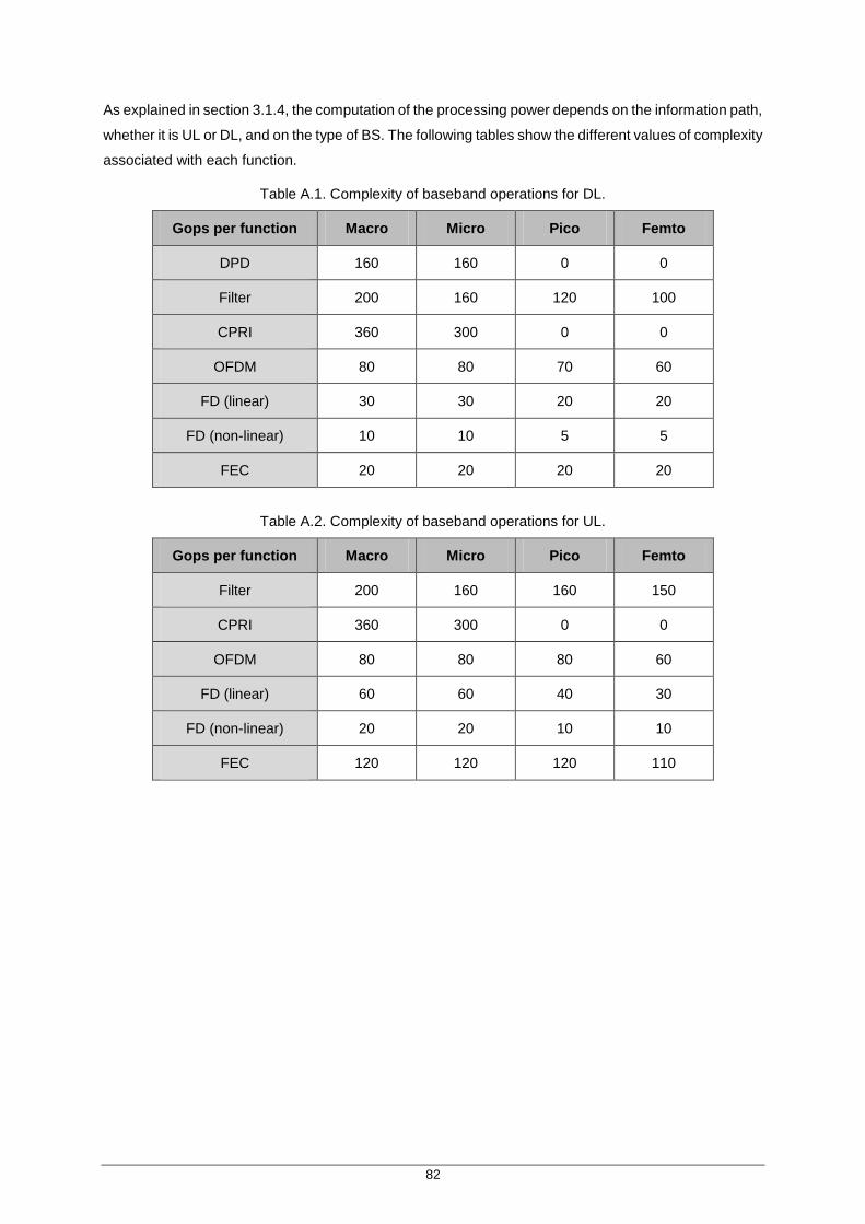
82
As explained in section 3.1.4, the computation of the processing power depends on the information path,
whether it is UL or DL, and on the type of BS. The following tables show the different values of complexity
associated with each function.
Table A.1. Complexity of baseband operations for DL.
Gops per function Macro Micro Pico Femto
DPD 160 160 0 0
Filter 200 160 120 100
CPRI 360 300 0 0
OFDM 80 80 70 60
FD (linear) 30 30 20 20
FD (non-linear) 10 10 5 5
FEC 20 20 20 20
Table A.2. Complexity of baseband operations for UL.
Gops per function Macro Micro Pico Femto
Filter 200 160 160 150
CPRI 360 300 0 0
OFDM 80 80 80 60
FD (linear) 60 60 40 30
FD (non-linear) 20 20 10 10
FEC 120 120 120 110
83
Annex B
Full results for the reference
scenario
Annex B. Full results for the reference scenario
Additional results for the reference scenario omitted in the text.
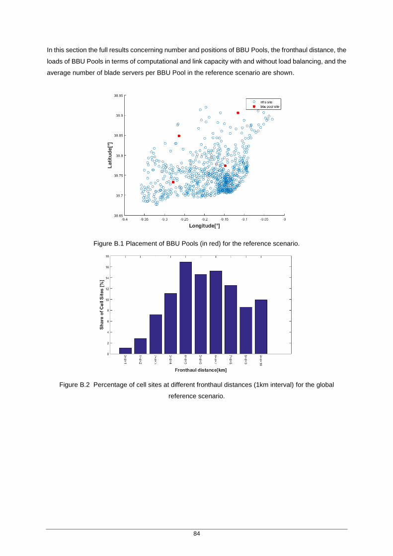
84
In this section the full results concerning number and positions of BBU Pools, the fronthaul distance, the
loads of BBU Pools in terms of computational and link capacity with and without load balancing, and the
average number of blade servers per BBU Pool in the reference scenario are shown.
Figure B.1 Placement of BBU Pools (in red) for the reference scenario.
Figure B.2 Percentage of cell sites at different fronthaul distances (1km interval) for the global
reference scenario.
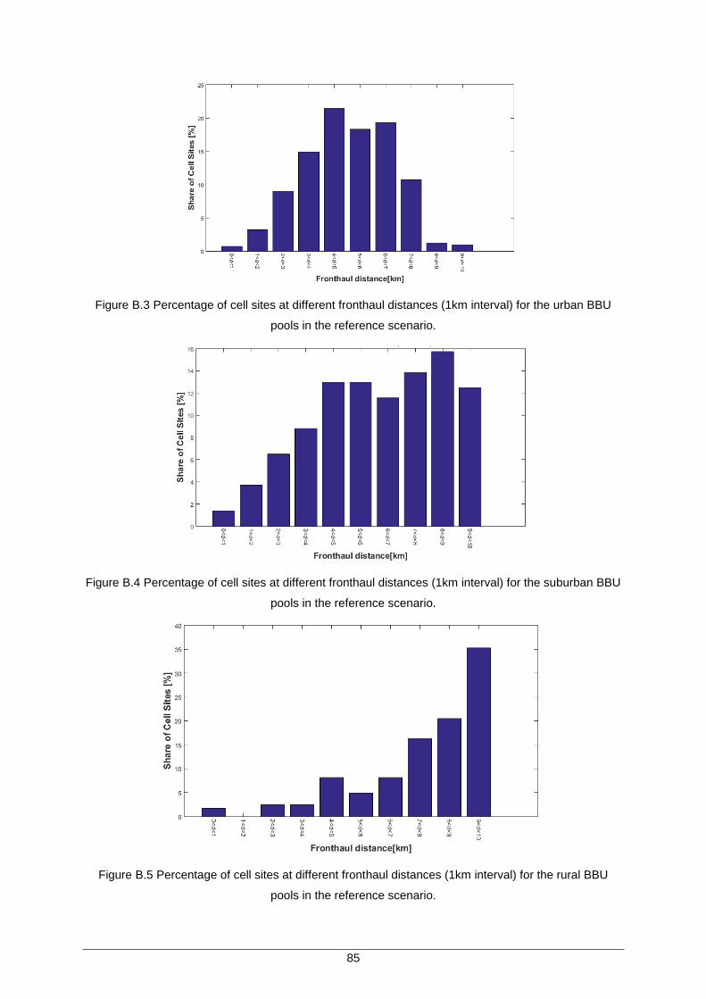
85
Figure B.3 Percentage of cell sites at different fronthaul distances (1km interval) for the urban BBU
pools in the reference scenario.
Figure B.4 Percentage of cell sites at different fronthaul distances (1km interval) for the suburban BBU
pools in the reference scenario.
Figure B.5 Percentage of cell sites at different fronthaul distances (1km interval) for the rural BBU
pools in the reference scenario.
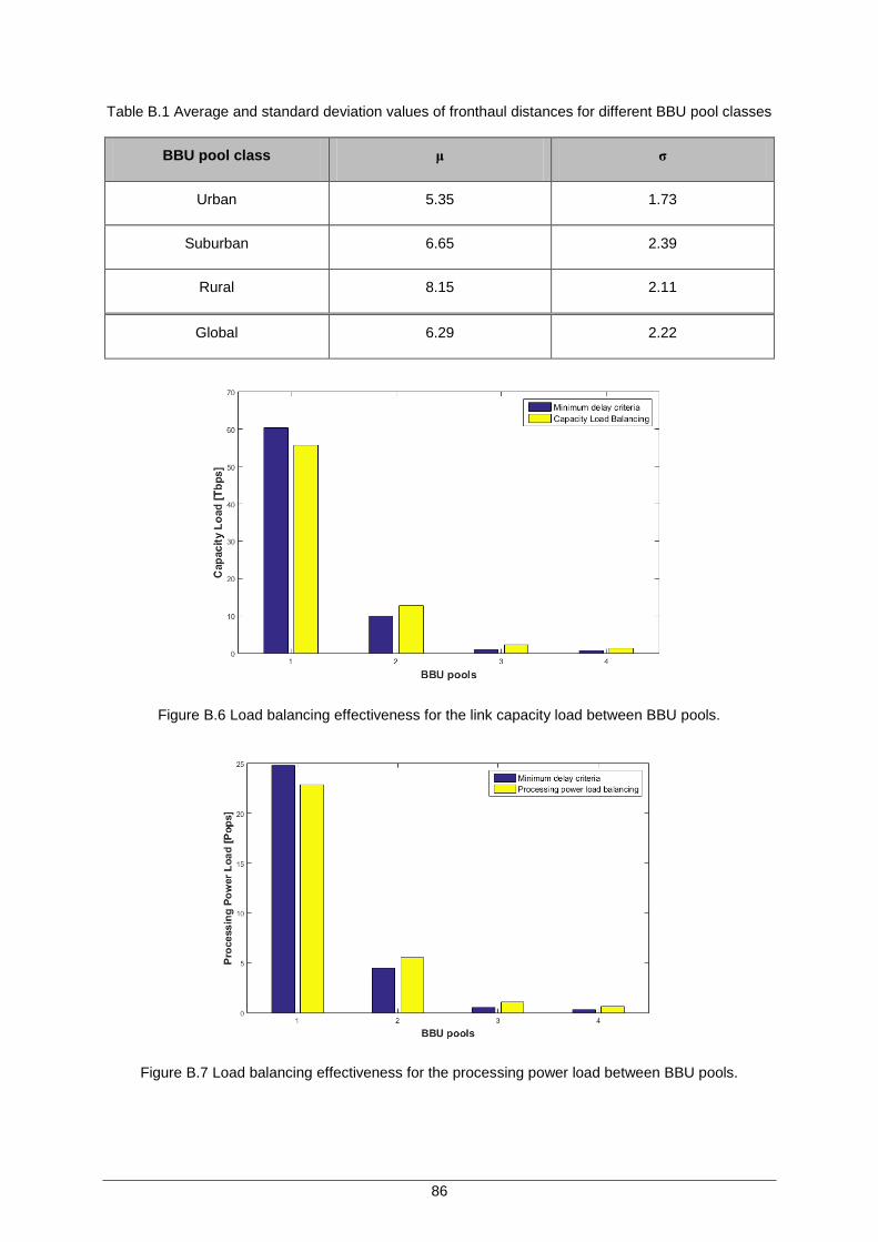
86
Table B.1 Average and standard deviation values of fronthaul distances for different BBU pool classes
BBU pool class μ σ
Urban 5.35 1.73
Suburban 6.65 2.39
Rural 8.15 2.11
Global 6.29 2.22
Figure B.6 Load balancing effectiveness for the link capacity load between BBU pools.
Figure B.7 Load balancing effectiveness for the processing power load between BBU pools.
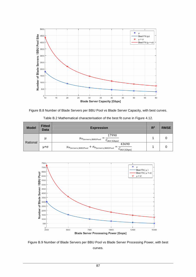
87
Figure B.8 Number of Blade Servers per BBU Pool vs Blade Server Capacity, with best curves.
Table B.2 Mathematical characterisation of the best fit curve in Figure 4.12.
Model Fitted Data
Expression R2 RMSE
Rational
µ µ𝑁𝑆𝑒𝑟𝑣𝑒𝑟𝑠/𝐵𝐵𝑈𝑃𝑜𝑜𝑙=
17990
𝐶𝐵𝑙𝑆 [Gbps]
1 0
µ+σ µ𝑁𝑆𝑒𝑟𝑣𝑒𝑟𝑠/𝐵𝐵𝑈𝑃𝑜𝑜𝑙+ 𝜎𝑁𝑆𝑒𝑟𝑣𝑒𝑟𝑠/𝐵𝐵𝑈𝑃𝑜𝑜𝑙
=43690
𝐶𝐵𝑙𝑆 [Gbps]
1 0
Figure B.9 Number of Blade Servers per BBU Pool vs Blade Server Processing Power, with best
curves.
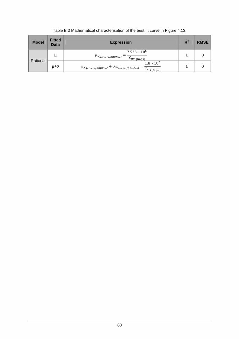
88
Table B.3 Mathematical characterisation of the best fit curve in Figure 4.13.
Model Fitted Data
Expression R2 RMSE
Rational
µ µ𝑁𝑆𝑒𝑟𝑣𝑒𝑟𝑠/𝐵𝐵𝑈𝑃𝑜𝑜𝑙=
7.535 · 106
𝐶𝐵𝑙𝑆 [Gops]
1 0
µ+σ µ𝑁𝑆𝑒𝑟𝑣𝑒𝑟𝑠/𝐵𝐵𝑈𝑃𝑜𝑜𝑙+ 𝜎𝑁𝑆𝑒𝑟𝑣𝑒𝑟𝑠/𝐵𝐵𝑈𝑃𝑜𝑜𝑙
=1.8 · 107
𝐶𝐵𝑙𝑆 [Gops]
1 0
89
Annex C
Full results for latency
constraint variation
Annex C. Full results for latency constraint variation
Additional results for the latency constraint variation omitted in the text.
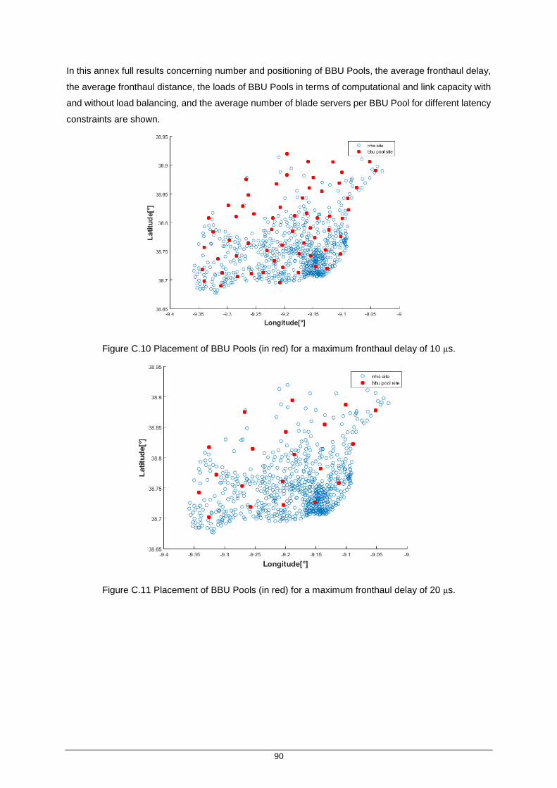
90
In this annex full results concerning number and positioning of BBU Pools, the average fronthaul delay,
the average fronthaul distance, the loads of BBU Pools in terms of computational and link capacity with
and without load balancing, and the average number of blade servers per BBU Pool for different latency
constraints are shown.
Figure C.10 Placement of BBU Pools (in red) for a maximum fronthaul delay of 10 μs.
Figure C.11 Placement of BBU Pools (in red) for a maximum fronthaul delay of 20 μs.
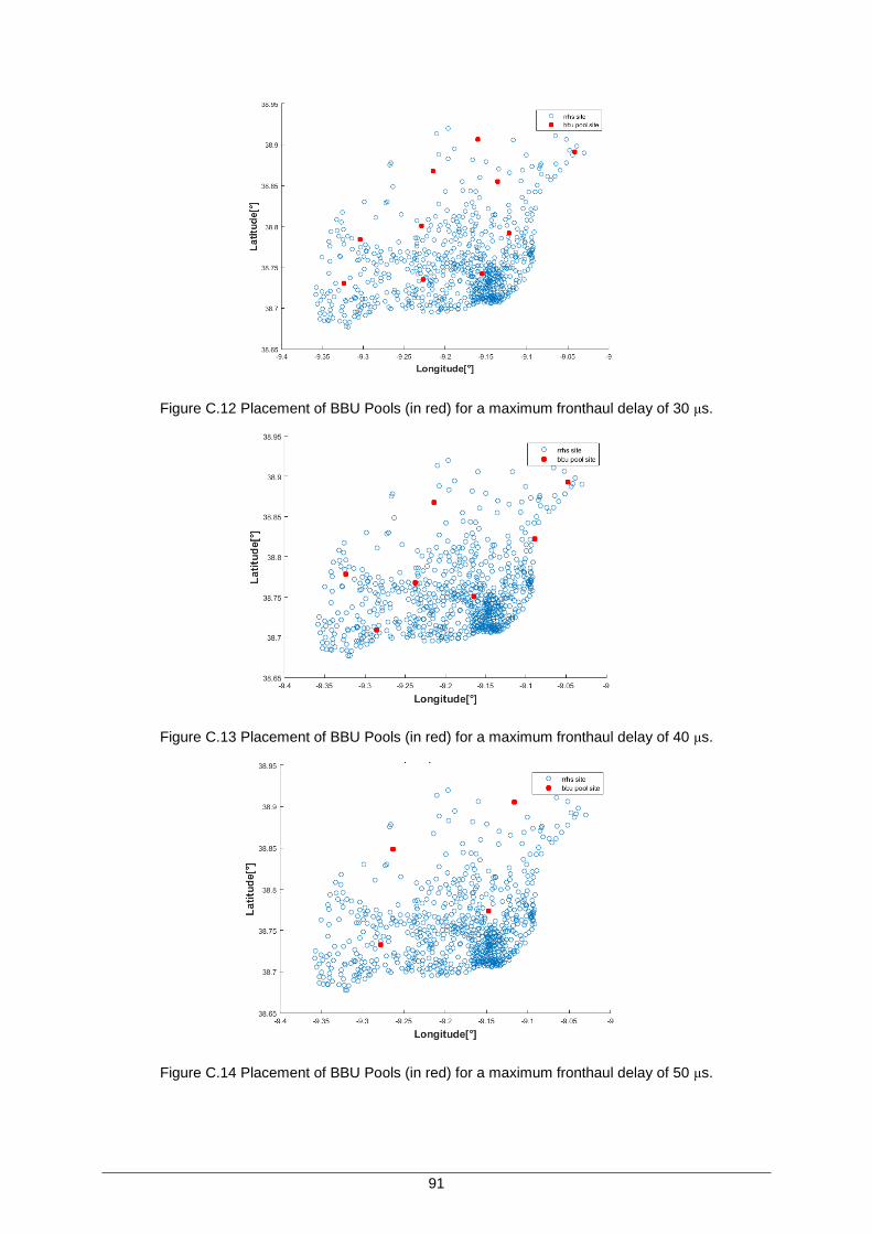
91
Figure C.12 Placement of BBU Pools (in red) for a maximum fronthaul delay of 30 μs.
Figure C.13 Placement of BBU Pools (in red) for a maximum fronthaul delay of 40 μs.
Figure C.14 Placement of BBU Pools (in red) for a maximum fronthaul delay of 50 μs.
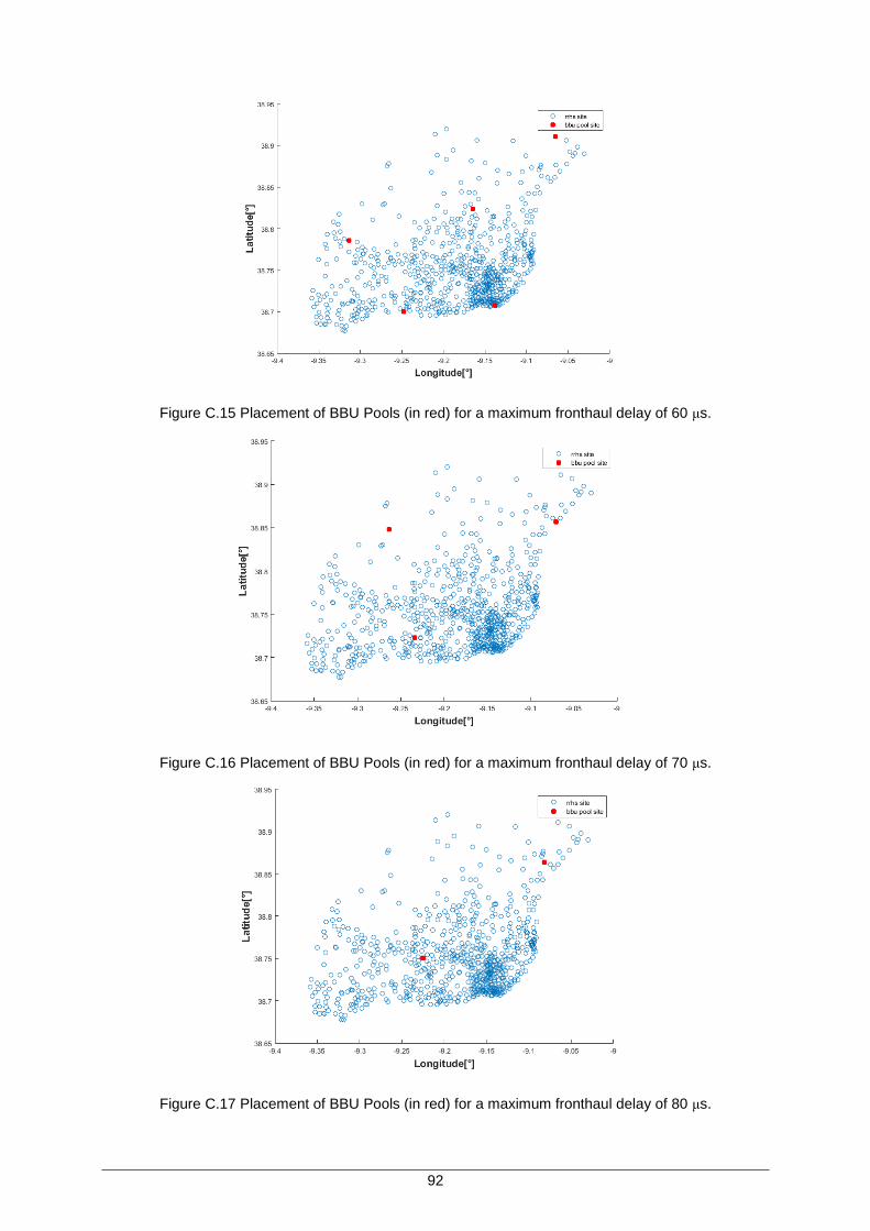
92
Figure C.15 Placement of BBU Pools (in red) for a maximum fronthaul delay of 60 μs.
Figure C.16 Placement of BBU Pools (in red) for a maximum fronthaul delay of 70 μs.
Figure C.17 Placement of BBU Pools (in red) for a maximum fronthaul delay of 80 μs.
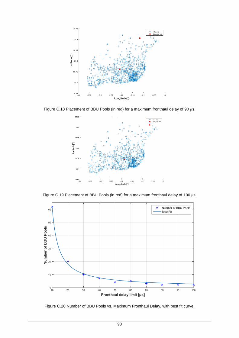
93
Figure C.18 Placement of BBU Pools (in red) for a maximum fronthaul delay of 90 μs.
Figure C.19 Placement of BBU Pools (in red) for a maximum fronthaul delay of 100 μs.
Figure C.20 Number of BBU Pools vs. Maximum Fronthaul Delay, with best fit curve.
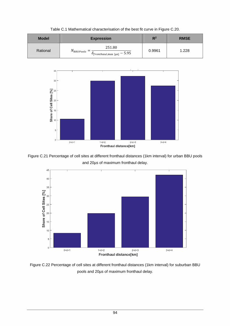
94
Table C.1 Mathematical characterisation of the best fit curve in Figure C.20.
Model Expression R2 RMSE
Rational 𝑁𝐵𝐵𝑈𝑃𝑜𝑜𝑙𝑠 =251.80
𝛿𝑓𝑟𝑜𝑛𝑡ℎ𝑎𝑢𝑙,max [µs] − 5.95 0.9961 1.228
Figure C.21 Percentage of cell sites at different fronthaul distances (1km interval) for urban BBU pools
and 20µs of maximum fronthaul delay.
Figure C.22 Percentage of cell sites at different fronthaul distances (1km interval) for suburban BBU
pools and 20µs of maximum fronthaul delay.
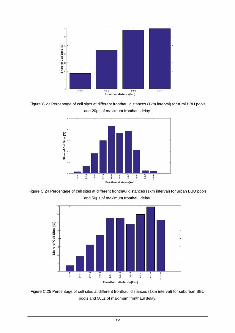
95
Figure C.23 Percentage of cell sites at different fronthaul distances (1km interval) for rural BBU pools
and 20µs of maximum fronthaul delay.
Figure C.24 Percentage of cell sites at different fronthaul distances (1km interval) for urban BBU pools
and 50µs of maximum fronthaul delay.
Figure C.25 Percentage of cell sites at different fronthaul distances (1km interval) for suburban BBU
pools and 50µs of maximum fronthaul delay.
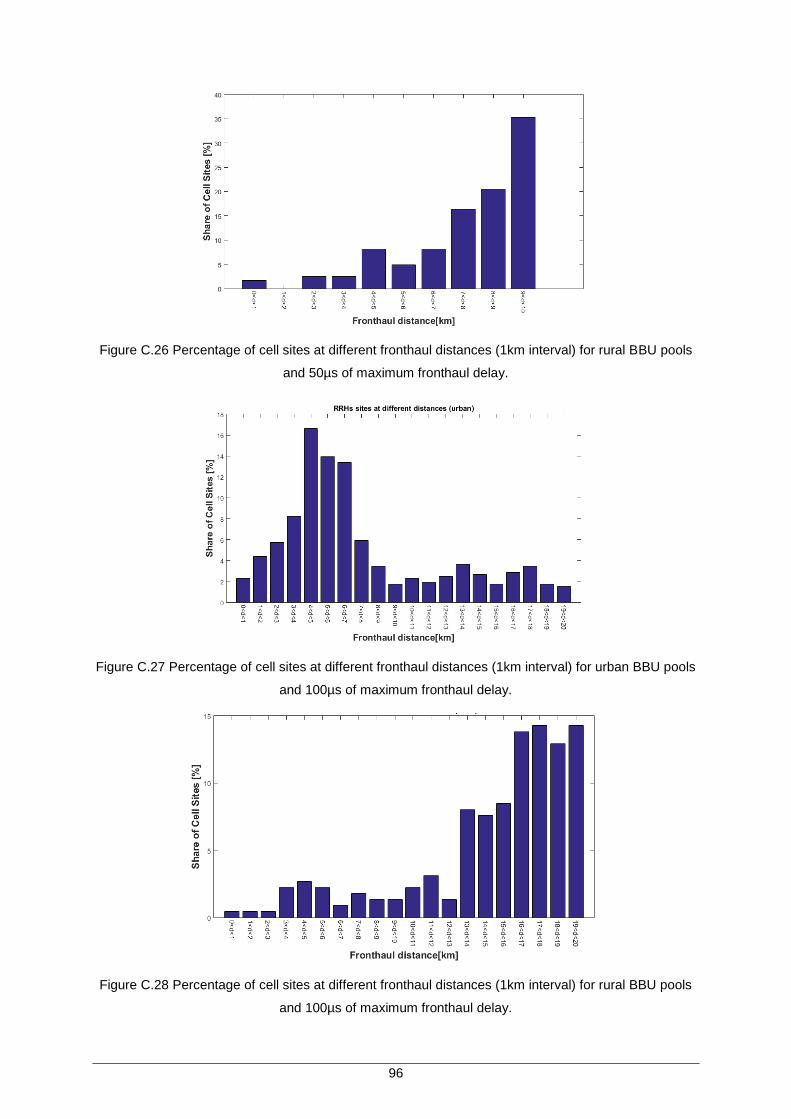
96
Figure C.26 Percentage of cell sites at different fronthaul distances (1km interval) for rural BBU pools
and 50µs of maximum fronthaul delay.
Figure C.27 Percentage of cell sites at different fronthaul distances (1km interval) for urban BBU pools
and 100µs of maximum fronthaul delay.
Figure C.28 Percentage of cell sites at different fronthaul distances (1km interval) for rural BBU pools
and 100µs of maximum fronthaul delay.
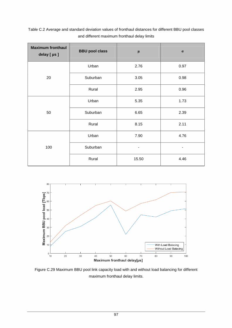
97
Table C.2 Average and standard deviation values of fronthaul distances for different BBU pool classes
and different maximum fronthaul delay limits
Maximum fronthaul
delay [ µs ] BBU pool class μ σ
20
Urban 2.76 0.97
Suburban 3.05 0.98
Rural 2.95 0.96
50
Urban 5.35 1.73
Suburban 6.65 2.39
Rural 8.15 2.11
100
Urban 7.90 4.76
Suburban - -
Rural 15.50 4.46
Figure C.29 Maximum BBU pool link capacity load with and without load balancing for different
maximum fronthaul delay limits.
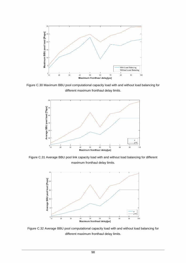
98
Figure C.30 Maximum BBU pool computational capacity load with and without load balancing for
different maximum fronthaul delay limits.
Figure C.31 Average BBU pool link capacity load with and without load balancing for different
maximum fronthaul delay limits.
Figure C.32 Average BBU pool computational capacity load with and without load balancing for
different maximum fronthaul delay limits.
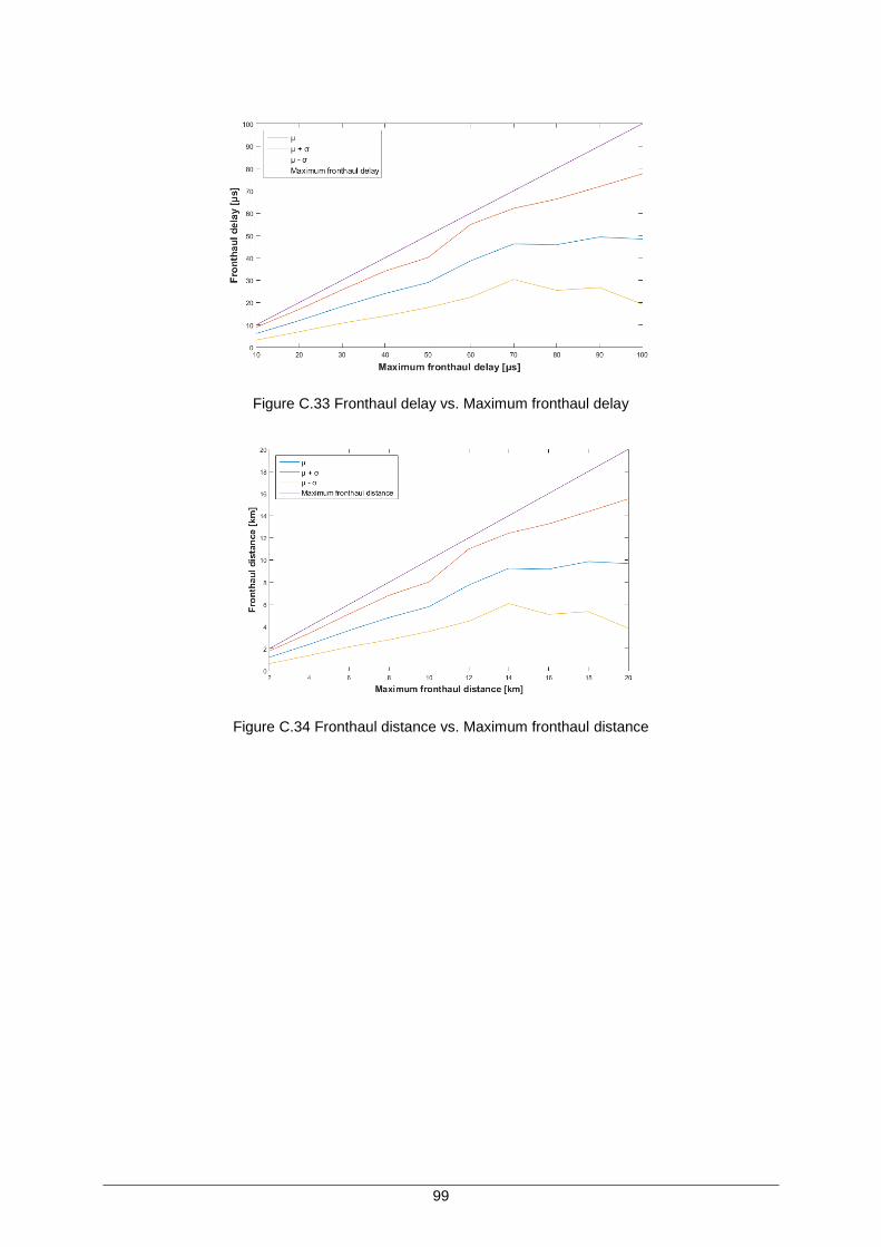
99
Figure C.33 Fronthaul delay vs. Maximum fronthaul delay
Figure C.34 Fronthaul distance vs. Maximum fronthaul distance

100
101
Annex D
Full results for RRHs
proliferation
Annex D. Full results for RRHs proliferation
Additional results for RRHs proliferation impact.
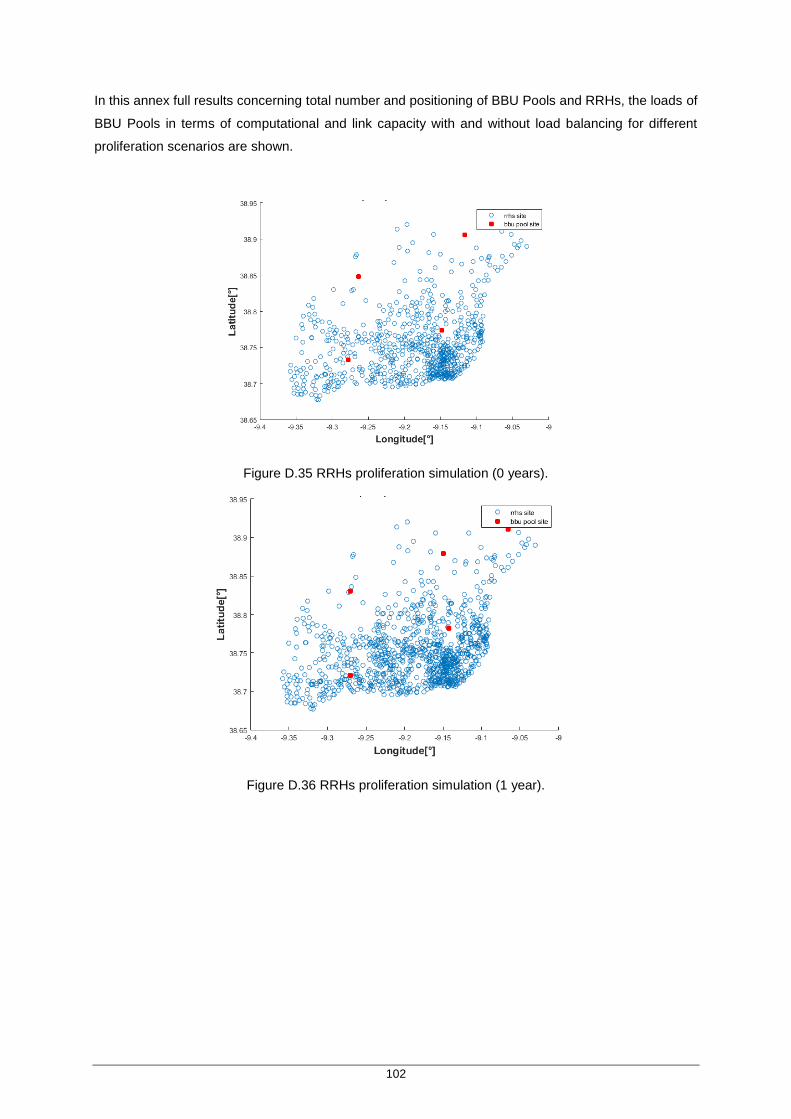
102
In this annex full results concerning total number and positioning of BBU Pools and RRHs, the loads of
BBU Pools in terms of computational and link capacity with and without load balancing for different
proliferation scenarios are shown.
Figure D.35 RRHs proliferation simulation (0 years).
Figure D.36 RRHs proliferation simulation (1 year).
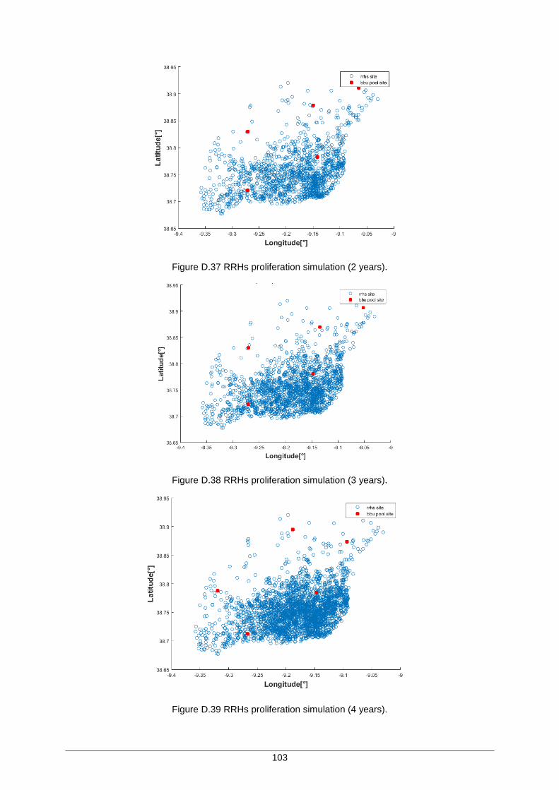
103
Figure D.37 RRHs proliferation simulation (2 years).
Figure D.38 RRHs proliferation simulation (3 years).
Figure D.39 RRHs proliferation simulation (4 years).
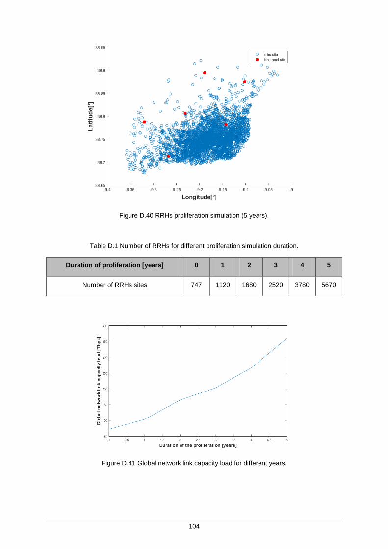
104
Figure D.40 RRHs proliferation simulation (5 years).
Table D.1 Number of RRHs for different proliferation simulation duration.
Duration of proliferation [years] 0 1 2 3 4 5
Number of RRHs sites 747 1120 1680 2520 3780 5670
Figure D.41 Global network link capacity load for different years.
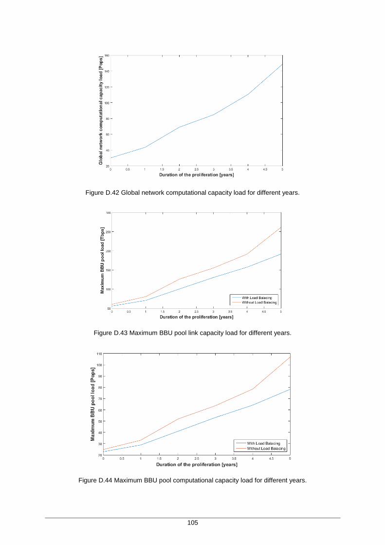
105
Figure D.42 Global network computational capacity load for different years.
Figure D.43 Maximum BBU pool link capacity load for different years.
Figure D.44 Maximum BBU pool computational capacity load for different years.
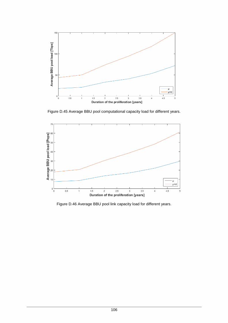
106
Figure D.45 Average BBU pool computational capacity load for different years.
Figure D.46 Average BBU pool link capacity load for different years.
107
Annex E
Full results for scenario
dimensioning
Annex E. Full results for scenario dimensioning
Auxiliary results for the evaluation of the impact of the scenario dimensioning.
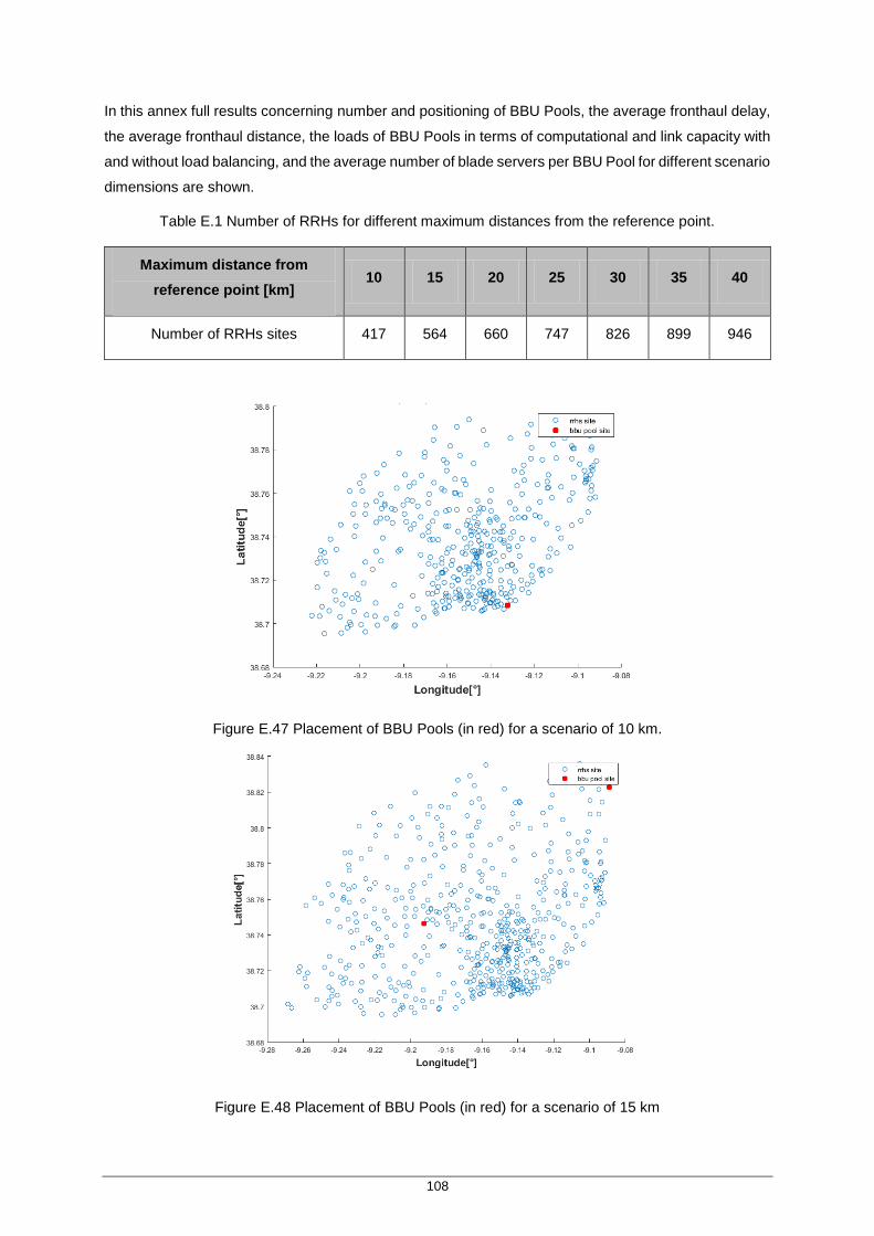
108
In this annex full results concerning number and positioning of BBU Pools, the average fronthaul delay,
the average fronthaul distance, the loads of BBU Pools in terms of computational and link capacity with
and without load balancing, and the average number of blade servers per BBU Pool for different scenario
dimensions are shown.
Table E.1 Number of RRHs for different maximum distances from the reference point.
Maximum distance from
reference point [km] 10 15 20 25 30 35 40
Number of RRHs sites 417 564 660 747 826 899 946
Figure E.47 Placement of BBU Pools (in red) for a scenario of 10 km.
Figure E.48 Placement of BBU Pools (in red) for a scenario of 15 km
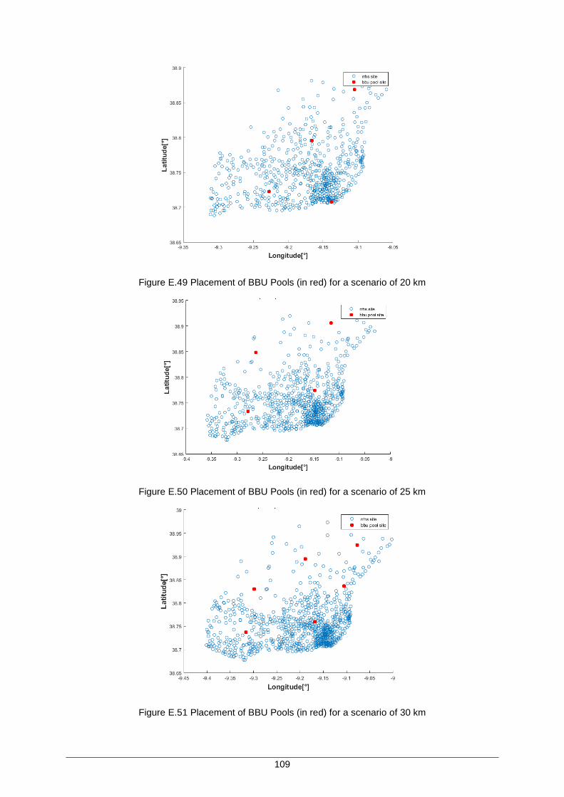
109
Figure E.49 Placement of BBU Pools (in red) for a scenario of 20 km
Figure E.50 Placement of BBU Pools (in red) for a scenario of 25 km
Figure E.51 Placement of BBU Pools (in red) for a scenario of 30 km
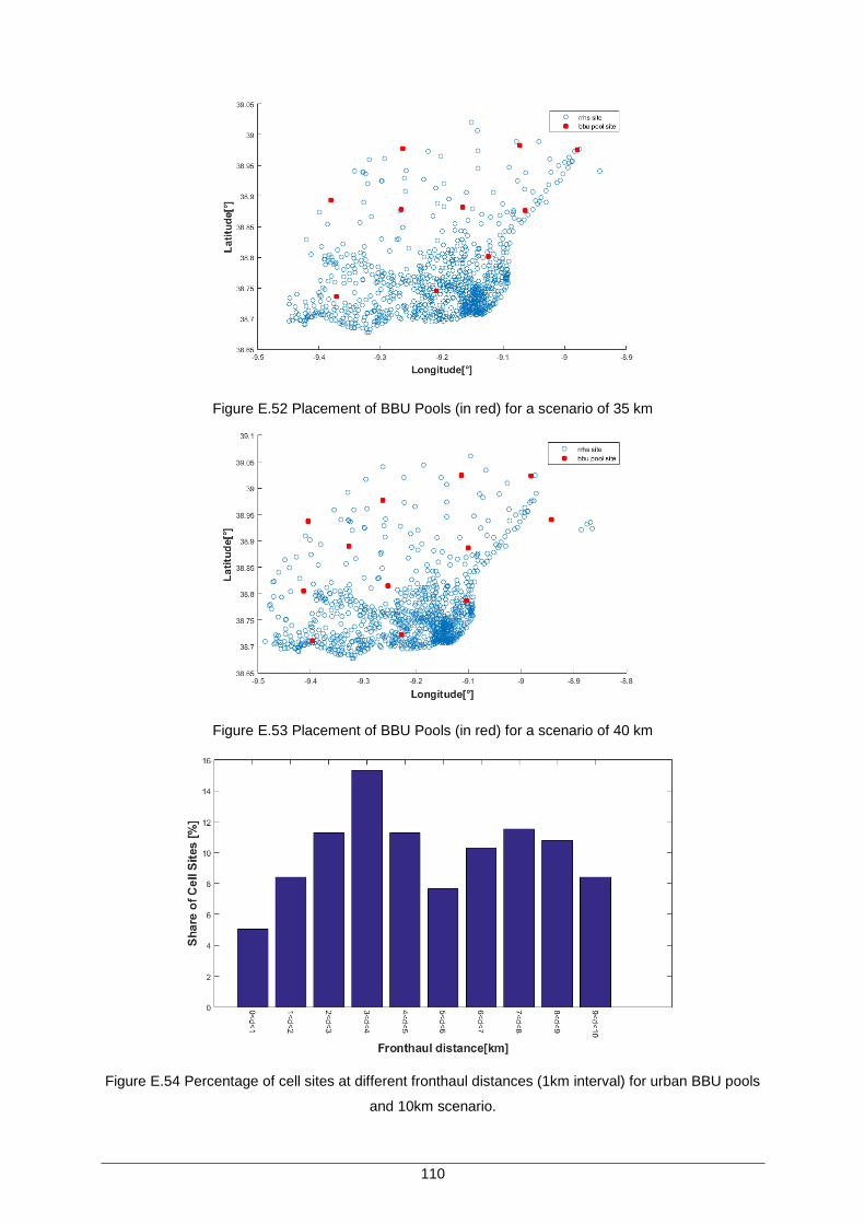
110
Figure E.52 Placement of BBU Pools (in red) for a scenario of 35 km
Figure E.53 Placement of BBU Pools (in red) for a scenario of 40 km
Figure E.54 Percentage of cell sites at different fronthaul distances (1km interval) for urban BBU pools
and 10km scenario.
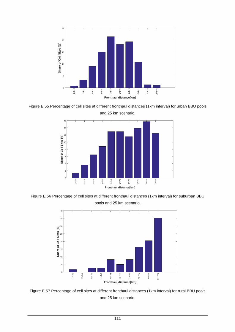
111
Figure E.55 Percentage of cell sites at different fronthaul distances (1km interval) for urban BBU pools
and 25 km scenario.
Figure E.56 Percentage of cell sites at different fronthaul distances (1km interval) for suburban BBU
pools and 25 km scenario.
Figure E.57 Percentage of cell sites at different fronthaul distances (1km interval) for rural BBU pools
and 25 km scenario.
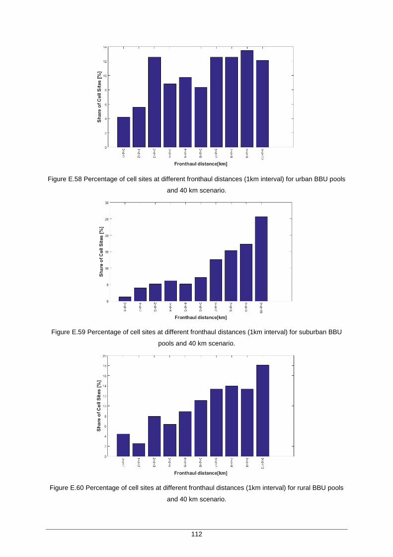
112
Figure E.58 Percentage of cell sites at different fronthaul distances (1km interval) for urban BBU pools
and 40 km scenario.
Figure E.59 Percentage of cell sites at different fronthaul distances (1km interval) for suburban BBU
pools and 40 km scenario.
Figure E.60 Percentage of cell sites at different fronthaul distances (1km interval) for rural BBU pools
and 40 km scenario.
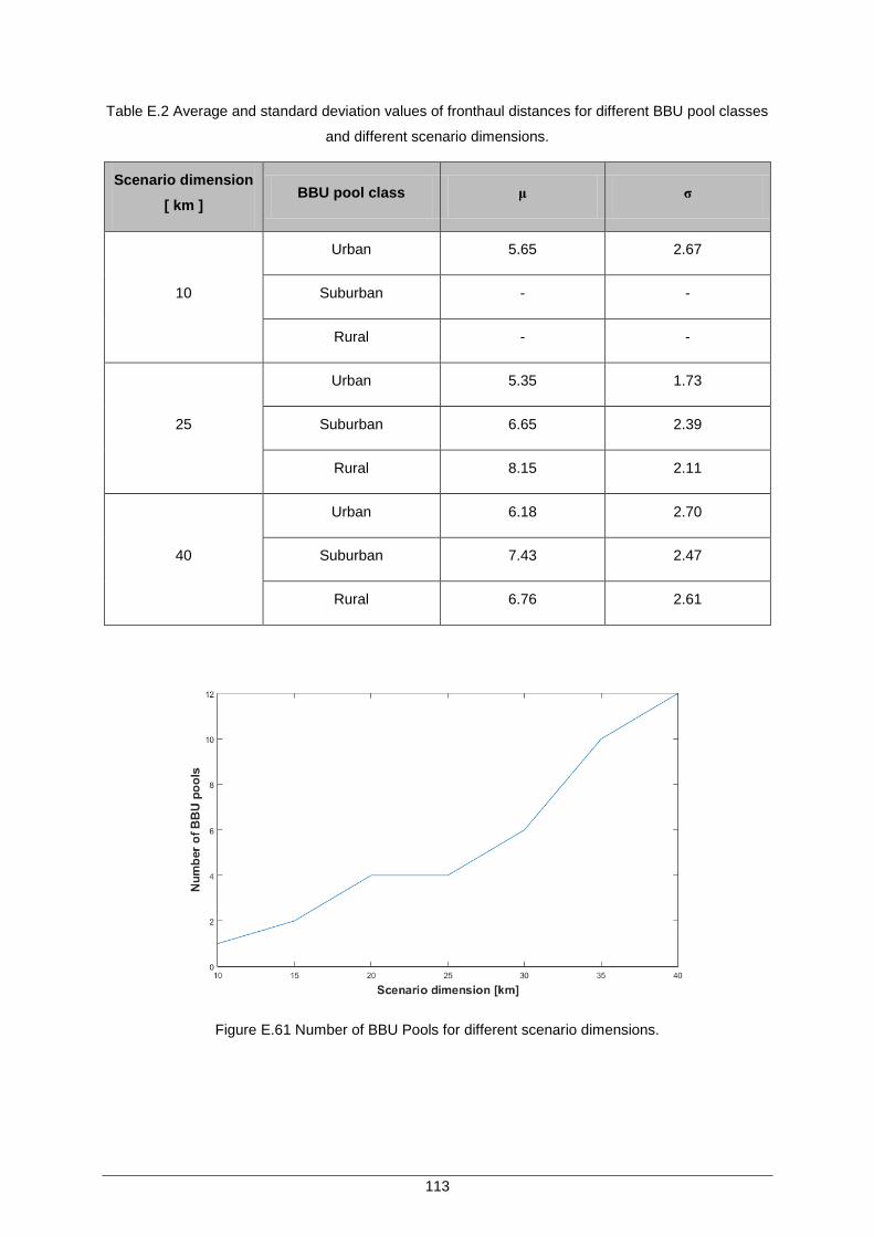
113
Table E.2 Average and standard deviation values of fronthaul distances for different BBU pool classes
and different scenario dimensions.
Scenario dimension
[ km ] BBU pool class μ σ
10
Urban 5.65 2.67
Suburban - -
Rural - -
25
Urban 5.35 1.73
Suburban 6.65 2.39
Rural 8.15 2.11
40
Urban 6.18 2.70
Suburban 7.43 2.47
Rural 6.76 2.61
Figure E.61 Number of BBU Pools for different scenario dimensions.
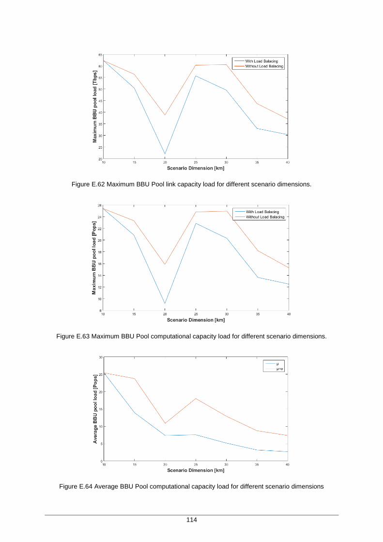
114
Figure E.62 Maximum BBU Pool link capacity load for different scenario dimensions.
Figure E.63 Maximum BBU Pool computational capacity load for different scenario dimensions.
Figure E.64 Average BBU Pool computational capacity load for different scenario dimensions
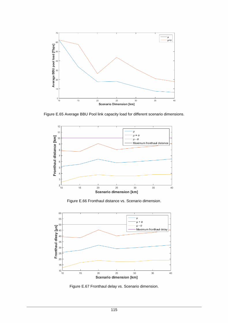
115
Figure E.65 Average BBU Pool link capacity load for different scenario dimensions.
Figure E.66 Fronthaul distance vs. Scenario dimension.
Figure E.67 Fronthaul delay vs. Scenario dimension.

116

117
Annex F
Full results for the impact of
deployment strategies
Annex F. Full results for the impact of deployment strategies
Auxiliary results for the evaluation of the impact of the deployment strategy.
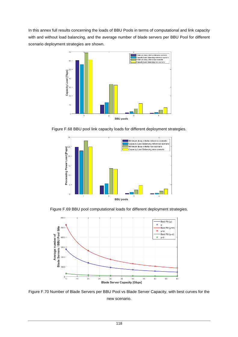
118
In this annex full results concerning the loads of BBU Pools in terms of computational and link capacity
with and without load balancing, and the average number of blade servers per BBU Pool for different
scenario deployment strategies are shown.
Figure F.68 BBU pool link capacity loads for different deployment strategies.
Figure F.69 BBU pool computational loads for different deployment strategies.
Figure F.70 Number of Blade Servers per BBU Pool vs Blade Server Capacity, with best curves for the
new scenario.
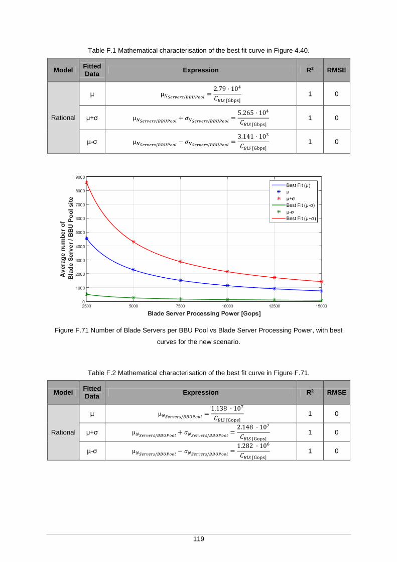
119
Table F.1 Mathematical characterisation of the best fit curve in Figure 4.40.
Model Fitted Data
Expression R2 RMSE
Rational
µ µ𝑁𝑆𝑒𝑟𝑣𝑒𝑟𝑠/𝐵𝐵𝑈𝑃𝑜𝑜𝑙=
2.79 · 104
𝐶𝐵𝑙𝑆 [Gbps]
1 0
µ+σ µ𝑁𝑆𝑒𝑟𝑣𝑒𝑟𝑠/𝐵𝐵𝑈𝑃𝑜𝑜𝑙+ 𝜎𝑁𝑆𝑒𝑟𝑣𝑒𝑟𝑠/𝐵𝐵𝑈𝑃𝑜𝑜𝑙
=5.265 · 104
𝐶𝐵𝑙𝑆 [Gbps]
1 0
µ-σ µ𝑁𝑆𝑒𝑟𝑣𝑒𝑟𝑠/𝐵𝐵𝑈𝑃𝑜𝑜𝑙− 𝜎𝑁𝑆𝑒𝑟𝑣𝑒𝑟𝑠/𝐵𝐵𝑈𝑃𝑜𝑜𝑙
=3.141 · 103
𝐶𝐵𝑙𝑆 [Gbps]
1 0
Figure F.71 Number of Blade Servers per BBU Pool vs Blade Server Processing Power, with best
curves for the new scenario.
Table F.2 Mathematical characterisation of the best fit curve in Figure F.71.
Model Fitted Data
Expression R2 RMSE
Rational
µ µ𝑁𝑆𝑒𝑟𝑣𝑒𝑟𝑠/𝐵𝐵𝑈𝑃𝑜𝑜𝑙=
1.138 · 107
𝐶𝐵𝑙𝑆 [Gops]
1 0
µ+σ µ𝑁𝑆𝑒𝑟𝑣𝑒𝑟𝑠/𝐵𝐵𝑈𝑃𝑜𝑜𝑙+ 𝜎𝑁𝑆𝑒𝑟𝑣𝑒𝑟𝑠/𝐵𝐵𝑈𝑃𝑜𝑜𝑙
=2.148 · 107
𝐶𝐵𝑙𝑆 [Gops]
1 0
µ-σ µ𝑁𝑆𝑒𝑟𝑣𝑒𝑟𝑠/𝐵𝐵𝑈𝑃𝑜𝑜𝑙− 𝜎𝑁𝑆𝑒𝑟𝑣𝑒𝑟𝑠/𝐵𝐵𝑈𝑃𝑜𝑜𝑙
=1.282 · 106
𝐶𝐵𝑙𝑆 [Gops]
1 0
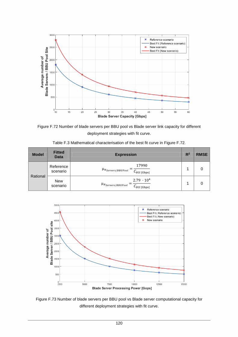
120
Figure F.72 Number of blade servers per BBU pool vs Blade server link capacity for different
deployment strategies with fit curve.
Table F.3 Mathematical characterisation of the best fit curve in Figure F.72.
Model Fitted Data
Expression R2 RMSE
Rational
Reference scenario
µ𝑁𝑆𝑒𝑟𝑣𝑒𝑟𝑠/𝐵𝐵𝑈𝑃𝑜𝑜𝑙=
17990
𝐶𝐵𝑙𝑆 [Gbps]
1 0
New scenario
µ𝑁𝑆𝑒𝑟𝑣𝑒𝑟𝑠/𝐵𝐵𝑈𝑃𝑜𝑜𝑙=
2.79 · 104
𝐶𝐵𝑙𝑆 [Gbps]
1 0
Figure F.73 Number of blade servers per BBU pool vs Blade server computational capacity for
different deployment strategies with fit curve.
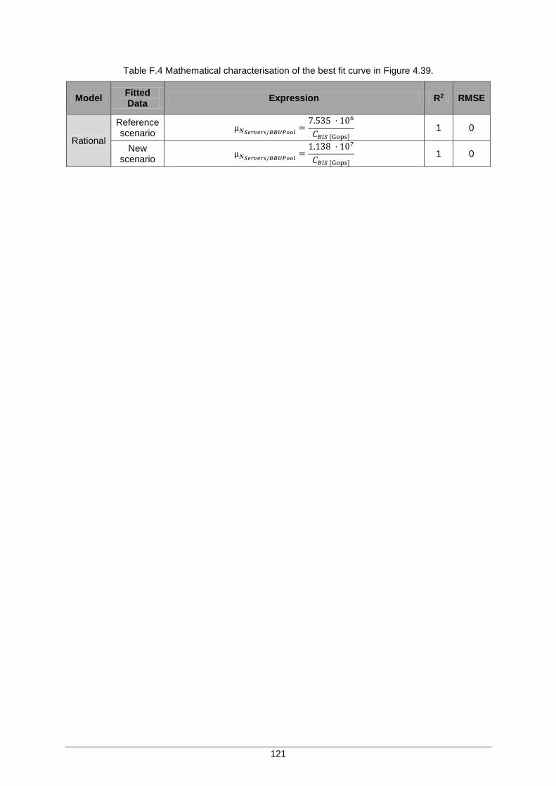
121
Table F.4 Mathematical characterisation of the best fit curve in Figure 4.39.
Model Fitted Data
Expression R2 RMSE
Rational
Reference scenario
µ𝑁𝑆𝑒𝑟𝑣𝑒𝑟𝑠/𝐵𝐵𝑈𝑃𝑜𝑜𝑙=
7.535 · 106
𝐶𝐵𝑙𝑆 [Gops]
1 0
New scenario
µ𝑁𝑆𝑒𝑟𝑣𝑒𝑟𝑠/𝐵𝐵𝑈𝑃𝑜𝑜𝑙=
1.138 · 107
𝐶𝐵𝑙𝑆 [Gops]
1 0

122
7
123
Annex G
Full results for L’Aquila
scenario
Annex G. Full results for L’Aquila scenario
Full results for the scenario of the city of L’Aquila.
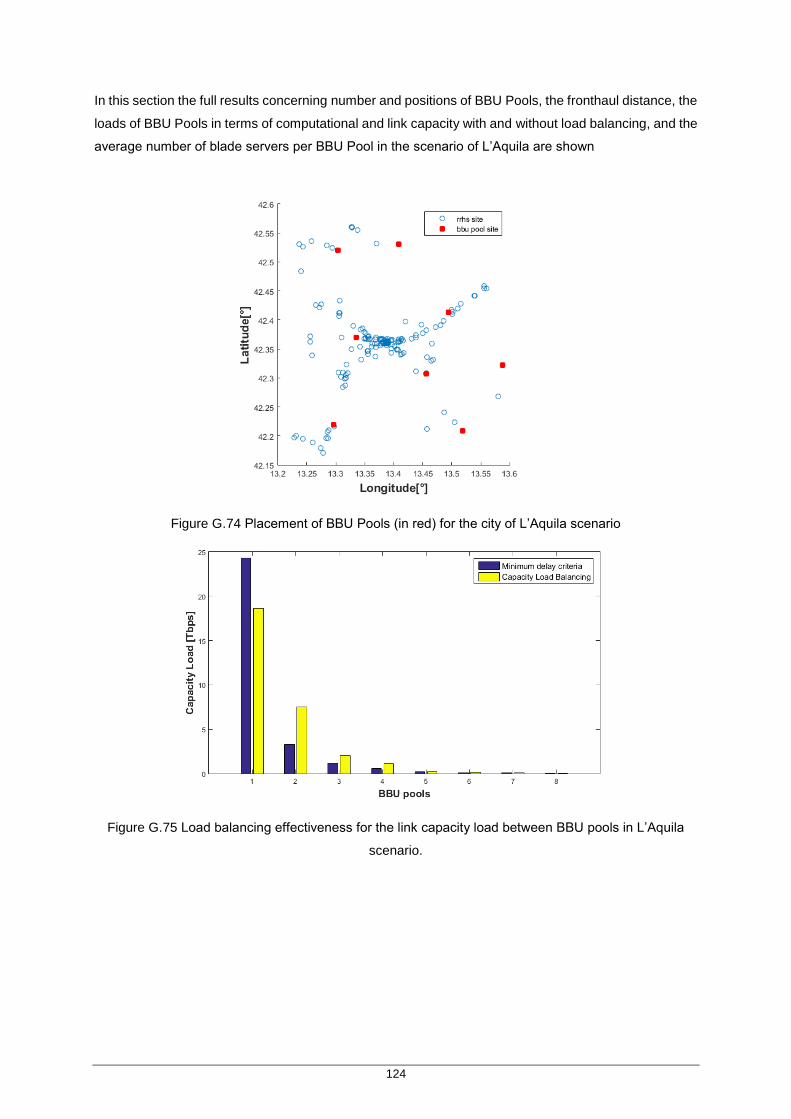
124
In this section the full results concerning number and positions of BBU Pools, the fronthaul distance, the
loads of BBU Pools in terms of computational and link capacity with and without load balancing, and the
average number of blade servers per BBU Pool in the scenario of L’Aquila are shown
Figure G.74 Placement of BBU Pools (in red) for the city of L’Aquila scenario
Figure G.75 Load balancing effectiveness for the link capacity load between BBU pools in L’Aquila
scenario.
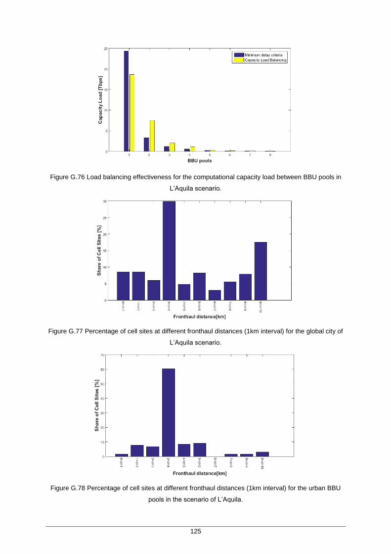
125
Figure G.76 Load balancing effectiveness for the computational capacity load between BBU pools in
L’Aquila scenario.
Figure G.77 Percentage of cell sites at different fronthaul distances (1km interval) for the global city of
L’Aquila scenario.
Figure G.78 Percentage of cell sites at different fronthaul distances (1km interval) for the urban BBU
pools in the scenario of L’Aquila.
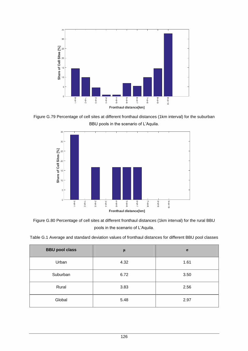
126
Figure G.79 Percentage of cell sites at different fronthaul distances (1km interval) for the suburban
BBU pools in the scenario of L’Aquila.
Figure G.80 Percentage of cell sites at different fronthaul distances (1km interval) for the rural BBU
pools in the scenario of L’Aquila.
Table G.1 Average and standard deviation values of fronthaul distances for different BBU pool classes
BBU pool class μ σ
Urban 4.32 1.61
Suburban 6.72 3.50
Rural 3.83 2.56
Global 5.48 2.97
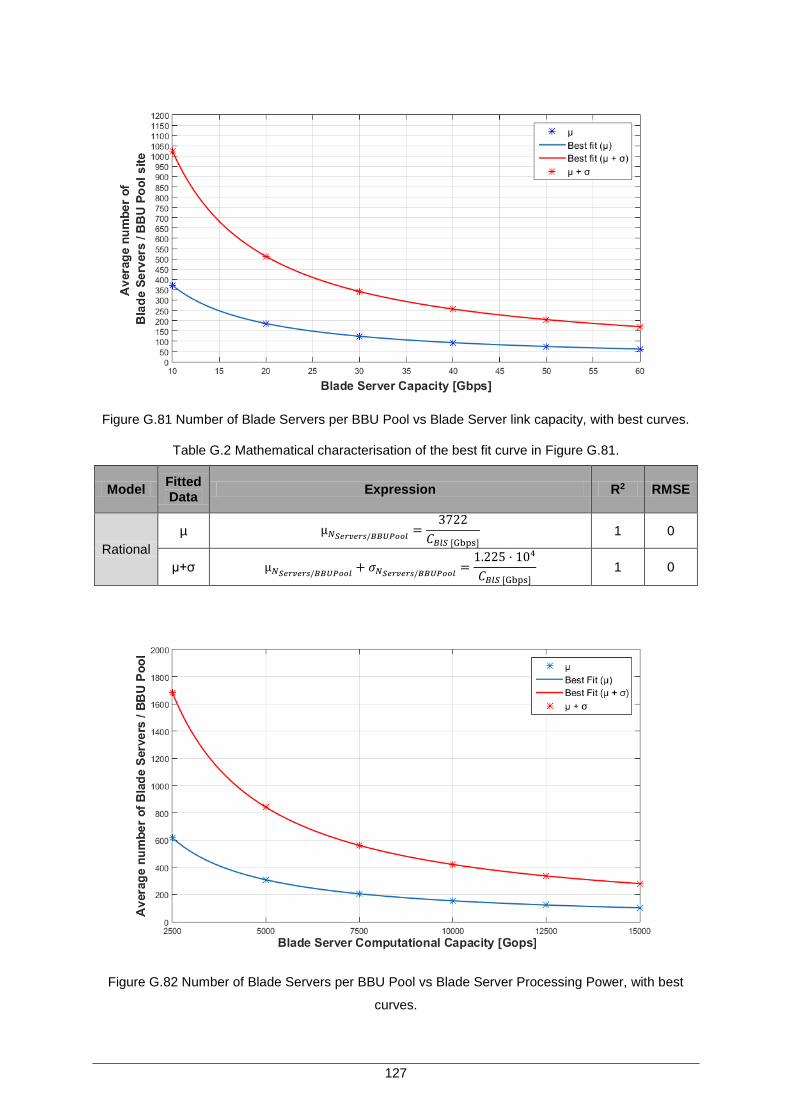
127
Figure G.81 Number of Blade Servers per BBU Pool vs Blade Server link capacity, with best curves.
Table G.2 Mathematical characterisation of the best fit curve in Figure G.81.
Model Fitted Data
Expression R2 RMSE
Rational
µ µ𝑁𝑆𝑒𝑟𝑣𝑒𝑟𝑠/𝐵𝐵𝑈𝑃𝑜𝑜𝑙=
3722
𝐶𝐵𝑙𝑆 [Gbps]
1 0
µ+σ µ𝑁𝑆𝑒𝑟𝑣𝑒𝑟𝑠/𝐵𝐵𝑈𝑃𝑜𝑜𝑙+ 𝜎𝑁𝑆𝑒𝑟𝑣𝑒𝑟𝑠/𝐵𝐵𝑈𝑃𝑜𝑜𝑙
=1.225 · 104
𝐶𝐵𝑙𝑆 [Gbps]
1 0
Figure G.82 Number of Blade Servers per BBU Pool vs Blade Server Processing Power, with best
curves.
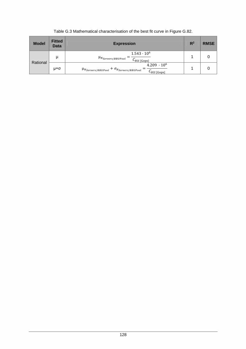
128
Table G.3 Mathematical characterisation of the best fit curve in Figure G.82.
Model Fitted Data
Expression R2 RMSE
Rational
µ µ𝑁𝑆𝑒𝑟𝑣𝑒𝑟𝑠/𝐵𝐵𝑈𝑃𝑜𝑜𝑙=
1.543 · 106
𝐶𝐵𝑙𝑆 [Gops]
1 0
µ+σ µ𝑁𝑆𝑒𝑟𝑣𝑒𝑟𝑠/𝐵𝐵𝑈𝑃𝑜𝑜𝑙+ 𝜎𝑁𝑆𝑒𝑟𝑣𝑒𝑟𝑠/𝐵𝐵𝑈𝑃𝑜𝑜𝑙
=4.209 · 106
𝐶𝐵𝑙𝑆 [Gops]
1 0
129
References
References
[3GPP14] 3GPP, Technical Specification Group Radio Access Network, Feasibility study for evolved
Universal Terrestrial Radio Access (UTRA) and Universal Terrestrial Radio Access
Network (UTRAN), Report TR 25.912, V12.0.0, Sep. 2014
(http://www.3gpp.org/ftp/Specs/html-info/25912.htm).
[Alme13] Almeida,D., Inter-cell Interference Impact on LTE Performance in Urban Scenarios, M.Sc.
Thesis, IST, Technical University of Lisbon, Lisbon, Portugal, 2013.
[AWVK11] Awada,A., Wegmann,B., Viering,I. and Klein,A., “A Mathematical Model for User Traffic in
Coverage and Capacity Optimisation of a Cellular Network”, in Proc. of VTC’11 – 73rd IEEE
Vehicular Technology Conference, Budapest, Hungary, May 2011.
[BPKK12] Bhaumik,S., Preeth Chandrabose,S., Kashyap Jataprolu,M., Kumar,G., Muralidhar,A.,
Polakos,P., Srinivasan,V. and Woo,T., “CloudIQ: a framework for processing base stations
in a data center”, in Proc. of Mobicom’12 - 18th annual international conference on Mobile
computing and networking, Istanbul, Turkey, Aug. 2012.
[CCYS14] Checko,A., Christiansen,H.L., Yan,Y., Scolari,L., Kardaras,G., Berger,M.S. and
Dittmann,L., "Cloud RAN for Mobile Networks - a Technology Overview", IEEE
Communications Surveys & Tutorials, Vol. 17, No. 1, Sep. 2014, pp. 405-426.
[ChHC14] Checko,A., Holm,H. and Christiansen,H., "Optimizing small cell deployment by the use of
C-RANs", in Proc. of EW’14 - 20th European Wireless Conference, Barcelona, Spain, May
2014.
[Chop12] Chopra,A., Association Control based Load Balancing in Wireless Cellular Networks using
Preamble Sequences, M.Sc. Thesis, Victoria University of Wellington, Wellington, New
Zealand, 2012.
[CMRI11] China Mobile Research Institute, C-RAN: The Road towards Green Radio RAN, White
Paper, 2011 (http://labs.chinamobile.com/cran/wp-content/uploads/CRAN_white_paper
_v2_5_EN.pdf)
[Damo13] Damouny,N., Inside NFV, SDN & the Emerging Network, online article, June 2014
(http://www.eetimes.com/author.asp?section_id=36&doc_id=1320009).
[DaPS11] Dahlman,E., Parkvall,S. and Sköld,J., 4G LTE/LTE-Advanced for Mobile Broadband,
Elsevier, Oxford, UK, 2011.
[DDGF12] Desset,C., Debaillie,B., Giannini,V. and Fehske,A., "Flexible power modelling of LTE base
stations", in Proc. of WCNC’12 - IEEE Wireless Communications and Networking
130
Conference, Shanghai, China, Apr. 2012.
[DPSB08] Dahlman,E., Parkvall,S., Skold,J. and Beming,P., 3G Evolution: HSPA and LTE for Mobile
Broadband (2nd Edition), Elsevier, Oxford, UK, 2008.
[Eric15] Ericsson, Ericsson Mobility Report, Public Consultation, Stockholm, Sweden, June 2015
(http://www.ericsson.com/mobility-report).
[ERXM13] Engels,A., Reyer,M., Xiang,X., Mathar,R., Jietao,Z., Hongcheng,Z., "Autonomous Self-
Optimization of Coverage and Capacity in LTE Cellular Networks", IEEE Transactions on
Vehicular Technology, Vol. 62, No. 5, June 2013, pp. 1989-2004.
[ETSI12] ETSI, Network Functions Virtualisation: An Introduction, Benefits, Enablers, Challenges &
Call for Action, White Paper, 2012 (https://portal.etsi.org/nfv/nfv_white_paper.pdf)
[FoPT81] Fowler,R.J., Paterson,M.S. and Tanimoto,S.L., “Optimal packing and covering in the plane
are NP-complete”, Information processing letters, Vol. 12, No. 3, June 1981, pp. 133-137.
[FrLo12] Fraser,R. and López-Ortiz,A., “The Within-Strip Discrete Unit Disk Cover Problem”, in Proc.
of CCCG’12 – 24th Canadian Conference on Computational Geometry, Charlottetown,
Canada, Aug. 2012.
[GSMA13] GSMA, The Mobile Economy 2013, Report, 2013
(http://www.gsmamobileeconomy.com/GSMA%20Mobile%20Economy%202013.pdf)
[HDGK13] Haberland,B., Derakhshan,F., Grob-Lipski,H., Klotsche,R., Rehm,W., Schefczik,P. and
Soellner,M., "Radio base stations in the cloud," Bell Labs Technical Journal, Vol. 18, No.1,
June 2013, pp. 129-152.
[HoTo11] Holma,H. and Toskala,A., LTE for UMTS: Evolution to LTE Advanced (2nd Edition), John
Wiley & Sons, Chichester, UK, 2011.
[HSMA14] Hawilo,H., Shami,A., Mirahmadi,M. and Asal,R., “NFV: state of the art, challenges, and
implementation in LZLL next generation mobile networks (vEPC)”, IEEE Network
Magazine, Vol. 28, No. 6, Nov. 2014, pp. 18-26.
[JZHT14] Jarschel,M., Zinner,T., Hossfeld,T., Tran-Gia,P. and Kellerer,W., "Interfaces, attributes,
and use cases: A compass for SDN," IEEE Communications Magazine , Vol. 52, No. 6 ,
June 2014, pp. 210-217.
[Kara14] Karagiannis,G., Jamakovic,A., Edmonds,A., Parada,C., Metsch,T., Pichon,D., and
Bohnert,T.M., "Mobile Cloud Networking: Virtualisation of Cellular Networks", in Proc. of
ICT’14 - 21st International Conference on Telecommunications, Lisbon, Portugal, May
2014.
[KhCo14] Khatibi,S. and Correia,L.M., “Modelling of Virtual Radio Resource Management for Cellular
Heterogeneous Access Networks”, in Proc. of PIMRC’14 – 25thIEEE Annual International
Symposium on Personal, Indoor, and Mobile Radio Communication, Washington, DC,
USA, Sep. 2014.
131
[LiHs00] Lin,Y.D. and Hsu,Y.C., ”Multihop cellular: A new architecture for wireless communication”,
in Proc. of INFOCOM’00 – 19th Annual Joint Conference of the IEEE Computer and
Communications Societies , Tel Aviv, Israel, Mar. 2000.
[LiTi13] Liu,B. and Tian, H., "A Bankruptcy Game-Based Resource Allocation Approach among
Virtual Mobile Operators", IEEE Communications Letters, Vol. 17, No. 7, July 2013, pp.
1420-1423.
[LiYu14] Liang,C. and Yu,F.R., "Wireless Network Virtualisation: A Survey, Some Research Issues
and Challenges", IEEE Communications Surveys & Tutorials, Vol. 17, No.1, Aug. 2014, pp.
358-380.
[LRSL03] Luo,H., Ramjee,R., Sinha,P., Li,L. and Lu,S., ”UCAN: A Unified Cellular and Ad-hoc
Network Architecture,” in Proc. of MOBICOM’03 – 9th Annual International Conference on
Mobile Computing and Networking, San Diego, CA, USA, Sep. 2003.
[LuSB11] Luketic,I., Simunic,D. and Blajic,T., "Optimization of coverage and capacity of Self-
Organizing Network in LTE", in Proc. of MIPRO’11 - 34th International Convention, Opatija,
Croatia, May 2011.
[MLXX12] Ming,L., Liang,Z., Xi,L., Xiaona,L., Zaki,Y., Timm-Giel,A. and Gorg,C., "Investigation of
Network Virtualization and Load Balancing Techniques in LTE Networks", in Proc. of
VTC’12 – 75th IEEE Vehicular Technology Conference, Yokohama, Japan, May 2012.
[Mart13] Martins,P., Analysis of Wireless Cloud Implementation in LTE-Advanced, M.Sc. Thesis,
IST, Technical University of Lisbon, Lisbon, Portugal, 2013.
[MoNa00] Molina,A., Nix,A.R. and Athanasiadou,G.E., "Cellular network capacity planning using the
combination algorithm for total optimisation", in Proc. of VTC’00 – 51st IEEE Vehicular
Technology Conference, Tokyo, Japan, May 2000.
[MuRa10] Mustafa,N.H. and Ray,S. “Improved results on geometric hitting set problems”, Discrete &
Computational Geometry, Vol. 44, No. 4, 2010, pp. 883-895.
[NaWK12] Namba,S., Warabino,T. and Kaneko,S., “BBU-RRH switching schemes for centralized
RAN”, in Proc. of CHINACOM’12 – 7thInternational ICST Conference on Communications
and Networking in China, Kun Ming, China, Aug. 2012.
[NGMN08] NGMN, NGMN Use Cases related to Self Organising Network, Overall Description, Report,
2008 (http://www.ngmn.org/uploads/media/NGMN_Use_Cases_related_to_Self_
Organising_Network__Overall_Description.pdf).
[NGMN13] NGMN, Suggestions on potential solutions to C-RAN, Report, 2013
(https://www.ngmn.org/uploads/media/NGMN_CRAN_Suggestions_on_Potential_Solutio
ns_to_CRAN.pdf)
[NMWK12] Namba,S., Matsunaka,T., Warabino,T., Kaneko,S. and Kishi,Y., "Colony-RAN architecture
for future cellular network", in Proc. of 21st Future Network & Mobile Summit, Berlin,
132
Germany, July 2012.
[ONFo12] Open Networking Foundation, Software-Defined Networking: The New Norm for Networks,
White Paper, 2012 (https://www.opennetworking.org/images/stories/downloads/sdn-
resources/white-papers/wp-sdn-newnorm.pdf).
[Pizz13] Pizzinat,A., Chanclou,P., Le Clech,F., Reedeker,T.L., Lagadec,Y., Saliou,F. and Galli,P.,
"Optical fibre solution for mobile fronthaul to achieve Cloud Radio Access Network" in Proc.
of 22th IEEE Future Network and Mobile Summit, Lisbon, Portugal, July 2013.
[Qual13] Qualcomm, IEEE802.11ac: The Next Evolution of Wi-Fi, Technical Report, San Diego,
California, USA, 2011 (http://www.qualcomm.com/media/documents/ieee80211ac-next-
evolution-wi-fi).
[Sa15] Sa,M., Performance Analysis of Software Defined Networks in LTE-A, M.Sc. Thesis, IST,
Technical University of Lisbon, Lisbon, Portugal, 2015
[SeTB11] Sesia,S., Toufik,I. and Baker,I., LTE - The UMTS Long Term Evolution: From Theory to
Practice (2nd Edition), John Wiley & Sons, Chichester, UK, 2011.
[SPHG14] Ferreira,L.S., Pichon,D., Hatefi,A., Gomes,A., Dimitrova,D., Braun,T., Karagiannis,G.,
Karimzadeh,M., Branco,M. and Correia,L.M., "An architecture to offer cloud-based radio
access network as a service", in Proc. of EuCNC’14 – 23rd European Conference on
Networks and Communications, Bologna, Italy, June 2014.
[SSCF13] Sezer,S., Scott-Hayward,S., Chouhan,P.K., Fraser,B., Lake,D., Finnegan,J. and Rao,N.,
"Are we ready for SDN? Implementation challenges for software-defined networks”, IEEE
Communications Magazine, Vol. 51, No. 7, July 2013, pp. 36-43.
[ToYa08] Tonguz,O.K. and Yanmaz,E., “The Mathematical Theory of Dynamic Load Balancing in
Cellular Networks”, IEEE Transactions on Mobile Computing, Vol.7, No.12, Dec. 2008,
pp.1504-1518.
[WeGP13] Werthmann,T., Grob-Lipski,H. and Proebster,M., "Multiplexing gains achieved in pools of
baseband computation units in 4G cellular networks", in Proc. of PIMRC’13 - 24th IEEE
International symposium on Personal Indoor and Mobile Radio Communications, London,
United Kingdom, Sep. 2013.
[XiMC00] Xiaoxin,W., Mukherjee,B. and Chan,S.-H.G., “MACA-an efficient channel allocation
scheme in cellular networks”, in Proc. of GLOBECOM’00 – 19th Global Telecommunications
Conference, San Francisco, CA, USA, Nov. 2000.
[ZSYZ13] Zhang,J., Sun,C., Yi,Y. and Zhuang,H., “A hybrid framework for capacity and coverage
optimization in self-organizing LTE networks”, in Proc. of PIMRC’13 - 24th IEEE
International symposium on Personal Indoor and Mobile Radio Communications, London,
United Kingdom, Sep. 2013.
[ZZHS13] Zhanjun,L., Zhichao,Z., Huan,D. and Shiyan,Z., "A power allocation algorithm maximizing

133
system capacity in radio access networks", in Proc. of ICNC’13 - 9th International
Conference on Natural Computation, Shenyang, China, July 2013.