Non equilibrium thermodynamics of protein organization · concernenti i trasportatori ABC, che sono...
107
POUR L'OBTENTION DU GRADE DE DOCTEUR ÈS SCIENCES acceptée sur proposition du jury: Prof. V. Savona, président du jury Prof. P. De Los Rios, directeur de thèse Prof. D. Marenduzzo, rapporteur Prof. G. Tiana, rapporteur Prof. F. Naef, rapporteur Non equilibrium thermodynamics of protein organization THÈSE N O 8507 (2018) ÉCOLE POLYTECHNIQUE FÉDÉRALE DE LAUSANNE PRÉSENTÉE LE 13 AVRIL 2018 À LA FACULTÉ DES SCIENCES DE BASE LABORATOIRE DE BIOPHYSIQUE STATISTIQUE PROGRAMME DOCTORAL EN PHYSIQUE Suisse 2018 PAR Alberto Stefano SASSI
Transcript of Non equilibrium thermodynamics of protein organization · concernenti i trasportatori ABC, che sono...
POUR L'OBTENTION DU GRADE DE DOCTEUR ÈS SCIENCES
acceptée sur proposition du jury:
Prof. V. Savona, président du juryProf. P. De Los Rios, directeur de thèse
Prof. D. Marenduzzo, rapporteurProf. G. Tiana, rapporteurProf. F. Naef, rapporteur
Non equilibrium thermodynamics of protein organization
THÈSE NO 8507 (2018)
ÉCOLE POLYTECHNIQUE FÉDÉRALE DE LAUSANNE
PRÉSENTÉE LE 13 AVRIL 2018
À LA FACULTÉ DES SCIENCES DE BASE
LABORATOIRE DE BIOPHYSIQUE STATISTIQUE
PROGRAMME DOCTORAL EN PHYSIQUE
Suisse2018
PAR
Alberto Stefano SASSI


Ovviamente,per Elisa.


AcknowledgementsI prefer to use the italian language for this part.I miei ringraziamenti vanno innanzitutto a Paolo, il mio supervisore. È stato disponibile enon ha esitato a darci delle responsabilità fin dai primi giorni. La sua fiducia, disponibilitàe ottimismo sono stati uno stimolo positivo per l’attività di ricerca. Un discorso simile(con forse qualche riserva sull’ottimismo) va fatto per Alessandro. In secondo luogo, citengo a dire che ho avuto dei compagni di laboratorio fantastici. Ringrazio calorosamenteDuccio e Andrea, con i quali ho passato più tempo che con chiunque altro, e anche Salvo,Stefano e Alessio.Mando un grosso abbraccio al gruppo losannese, agli amici di infanzia, i compagni di liceoe di università, ai miei splendidi cugini e agli zii, che purtroppo non vedo tanto spessoquanto vorrei. La compagnia di tutti loro è stata preziosa per questi quattro anni. Infine,ringrazio di cuore Giulia e mamma e papà. Hanno saputo mostrare positività anche inmomenti difficili e mi hanno sempre sostenuto. Non ci sono parole adeguate per esprimerela mia gratitudine nei loro confronti.
Lausanne, 23 January 2018 A. S.
v


AbstractThree quarters of the thesis will be devoted to the discussion of non equilibrium systems.We show how certain biological systems cannot be described by standard thermodynamics.The reason is that the energy consumption due to the hydrolysis of ATP imposes to thesystems a directionality and therefore a chemical flux that is different from zero. Morespecifically, we will apply the formalism to molecular chaperones, that are proteins involvedin a plethora of biological processes, with a particular in-depth analysis on the mechanismsof protein unfolding and refolding mediated by the two families of chaperones Hsp70and GroEL. Moreover, with the same mathematical tools, we will provide a qualitativedescription of some phenomena regarding the Atp-binding cassette transporters, that areimportant membrane protein complexes used to translocate small molecules in and out ofthe cell.In the remaining quarter we will analyze the deformation of a polymer chain when it ispulled by an external force. We will explain how it is possible to quantify the orientationalong the force and the shrinking along the other directions. It will be also shown that thetransverse section shrinks isotropically once the orientation along the force is complete.The main quantities that are used to identify the shape and the orientation of a polymerchain can all be written as a function of a universal quantity that is independent, in first ap-proximation, by the number of monomers, by the rigidity, and even by the volume exclusion.
Key words: non equilibrium physics | molecular chaperones | ABC transporters | polymertheory
vii

SommarioTre quarti della tesi saranno dedicati alla trattazione di sistemi di non equilibrio. Si mostracome alcuni sistemi biologici non possono essere descritti con gli strumenti della termodi-namica standard. Il motivo è che il consumo di energia dovuto all’idrolisi di ATP impone alsistema una direzionalità e perciò un flusso chimico che è diverso da zero. Più precisamente,si applicherà il formalismo ai chaperone molecolari, che sono proteine impiegate in un grannumero di processi biologici, con particolare riguardo al meccanismo di dispiegamento eripiegamento mediato dalle due famiglie di chaperone Hsp70 e GroEL. Inoltre, con glistessi strumenti matematici, sarà fornita una descrizione qualitativa di alcuni fenomeniconcernenti i trasportatori ABC, che sono importanti proteine di membrana usate pertrasportare piccole molecole all’interno e all’esterno della cellula.Nel rimanente quarto della tesi verrà analizzata la deformazione di una catena polimericaquando è sottoposta ad una forza di tensione esterna. Si spiegherà come è possibilequantificare l’orientazione lungo la forza e l’assottigliamento lungo le altre direzioni. Simostrerà, inoltre, che la sezione trasversa viene ridotta in modo isotropico ona volta chel’orientazione verso la forza è completata. Le principali grandezze che sono usate peridentificare la forma e l’orientazione di una catena polimerica possono essere tutte scrittecome funzioni di una quantità universale che è indipendente, in prima approssimazione,dal numero di monomeri, dalla rigidità, e persino dal volume escluso.
Parole chiave: fisica di non equilibrio | chaperone molecolari | trasportatori ABC | teoriadei polimeri
ix


ContentsAcknowledgements v
Abstract (English/Français/Deutsch) vii
List of figures xii
List of tables xiv
1 Introduction 1
2 Basic principles on non equilibrium systems 52.1 Non locality of non equilibrium systems . . . . . . . . . . . . . . . . . . . . 52.2 Stationary states in biochemical systems . . . . . . . . . . . . . . . . . . . . 62.3 Entropy flow and entropy production . . . . . . . . . . . . . . . . . . . . . . 82.4 Stationary state solution . . . . . . . . . . . . . . . . . . . . . . . . . . . . . 92.5 The source of the non equilibrium . . . . . . . . . . . . . . . . . . . . . . . 112.6 Michaelis-Menten kinetics . . . . . . . . . . . . . . . . . . . . . . . . . . . . 11
3 Molecular Chaperones 133.1 Hsp70 . . . . . . . . . . . . . . . . . . . . . . . . . . . . . . . . . . . . . . . 14
3.1.1 Entropic pulling . . . . . . . . . . . . . . . . . . . . . . . . . . . . . 153.1.2 Rate model for refolding . . . . . . . . . . . . . . . . . . . . . . . . . 163.1.3 Role of the cochaperones in the binding affinity . . . . . . . . . . . . 223.1.4 Binding with JDP and hydrolysis . . . . . . . . . . . . . . . . . . . . 243.1.5 The expansion of rhodanese . . . . . . . . . . . . . . . . . . . . . . . 263.1.6 Brief summary . . . . . . . . . . . . . . . . . . . . . . . . . . . . . . 37
3.2 Chaperonin . . . . . . . . . . . . . . . . . . . . . . . . . . . . . . . . . . . . 373.2.1 General description . . . . . . . . . . . . . . . . . . . . . . . . . . . . 373.2.2 Out-of-equilibrium stabilization of the functional state . . . . . . . . 393.2.3 Brief summary . . . . . . . . . . . . . . . . . . . . . . . . . . . . . . 50
3.3 Conclusions . . . . . . . . . . . . . . . . . . . . . . . . . . . . . . . . . . . . 50
4 Atp-binding cassette transporters 534.1 Introduction . . . . . . . . . . . . . . . . . . . . . . . . . . . . . . . . . . . . 53
4.1.1 Importers . . . . . . . . . . . . . . . . . . . . . . . . . . . . . . . . . 53
xi
Contents
4.1.2 Exporters . . . . . . . . . . . . . . . . . . . . . . . . . . . . . . . . . 544.2 The model . . . . . . . . . . . . . . . . . . . . . . . . . . . . . . . . . . . . . 564.3 Conclusions . . . . . . . . . . . . . . . . . . . . . . . . . . . . . . . . . . . . 59
5 Shape of a stretched polymer 615.1 State of the art . . . . . . . . . . . . . . . . . . . . . . . . . . . . . . . . . . 625.2 Exact Computation of
⟨R2
e
⟩and
⟨R2
g
⟩. . . . . . . . . . . . . . . . . . . . . 67
5.3 Inertia tensor and asphericity . . . . . . . . . . . . . . . . . . . . . . . . . . 685.4 Universal behaviors . . . . . . . . . . . . . . . . . . . . . . . . . . . . . . . . 735.5 Conclusions . . . . . . . . . . . . . . . . . . . . . . . . . . . . . . . . . . . . 76
6 Concluding remarks 77
A Appendix 79A.1 Hsp70 . . . . . . . . . . . . . . . . . . . . . . . . . . . . . . . . . . . . . . . 79
A.1.1 Rate constants in the model with rhodanese . . . . . . . . . . . . . . 79A.2 Chaperonin . . . . . . . . . . . . . . . . . . . . . . . . . . . . . . . . . . . . 79
A.2.1 Rate constants in the model . . . . . . . . . . . . . . . . . . . . . . . 79A.3 ABC transporters . . . . . . . . . . . . . . . . . . . . . . . . . . . . . . . . 80
A.3.1 Explicit expression for the exchange rates . . . . . . . . . . . . . . . 80A.3.2 Master equations for the rate model . . . . . . . . . . . . . . . . . . 80A.3.3 Asymptotic results . . . . . . . . . . . . . . . . . . . . . . . . . . . . 81A.3.4 Rates in the model . . . . . . . . . . . . . . . . . . . . . . . . . . . . 81
Bibliography 88
Curriculum Vitae 89
xii
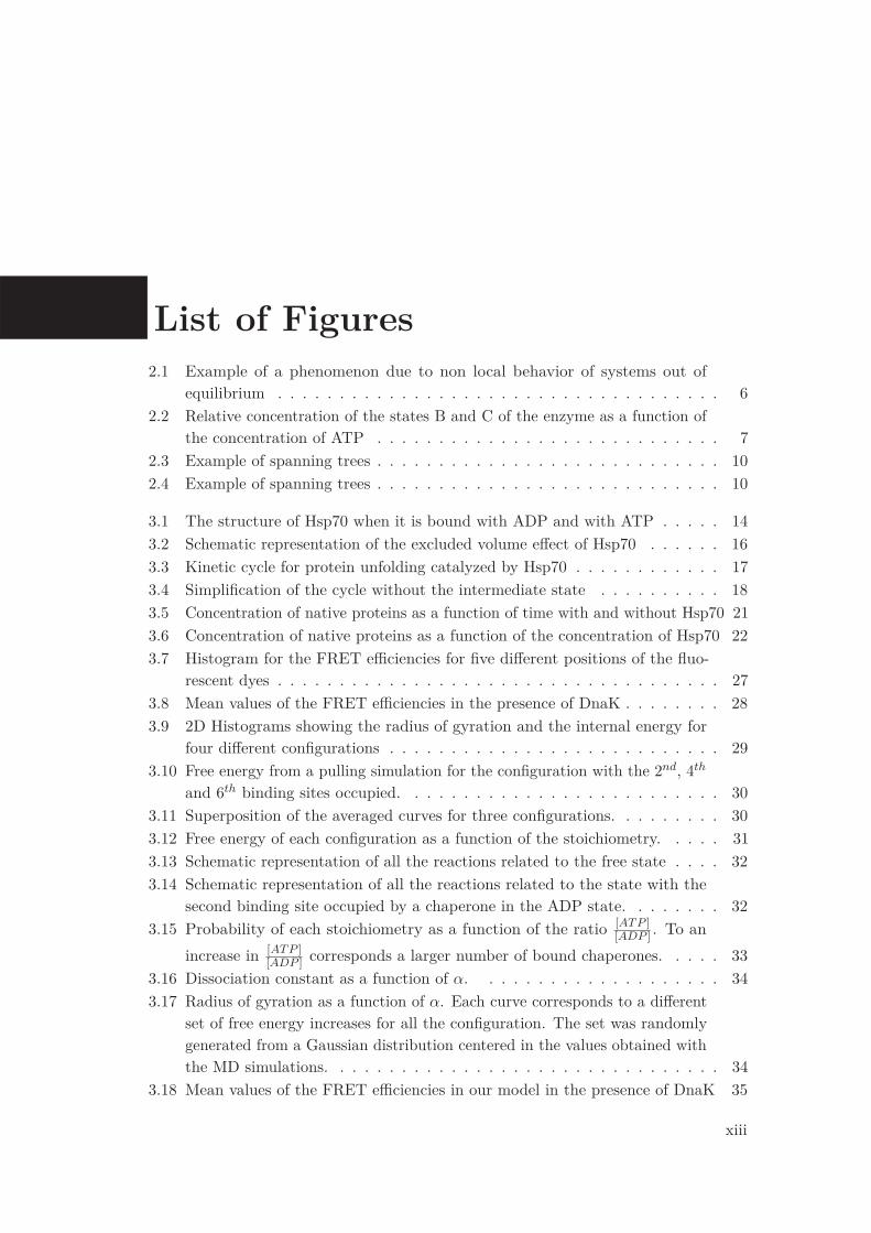
List of Figures2.1 Example of a phenomenon due to non local behavior of systems out of
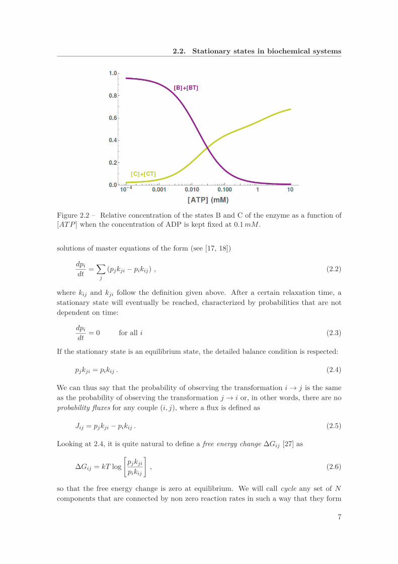
equilibrium . . . . . . . . . . . . . . . . . . . . . . . . . . . . . . . . . . . . 62.2 Relative concentration of the states B and C of the enzyme as a function of
the concentration of ATP . . . . . . . . . . . . . . . . . . . . . . . . . . . . 72.3 Example of spanning trees . . . . . . . . . . . . . . . . . . . . . . . . . . . . 102.4 Example of spanning trees . . . . . . . . . . . . . . . . . . . . . . . . . . . . 10
3.1 The structure of Hsp70 when it is bound with ADP and with ATP . . . . . 143.2 Schematic representation of the excluded volume effect of Hsp70 . . . . . . 163.3 Kinetic cycle for protein unfolding catalyzed by Hsp70 . . . . . . . . . . . . 173.4 Simplification of the cycle without the intermediate state . . . . . . . . . . 183.5 Concentration of native proteins as a function of time with and without Hsp70 213.6 Concentration of native proteins as a function of the concentration of Hsp70 223.7 Histogram for the FRET efficiencies for five different positions of the fluo-
rescent dyes . . . . . . . . . . . . . . . . . . . . . . . . . . . . . . . . . . . . 273.8 Mean values of the FRET efficiencies in the presence of DnaK . . . . . . . . 283.9 2D Histograms showing the radius of gyration and the internal energy for
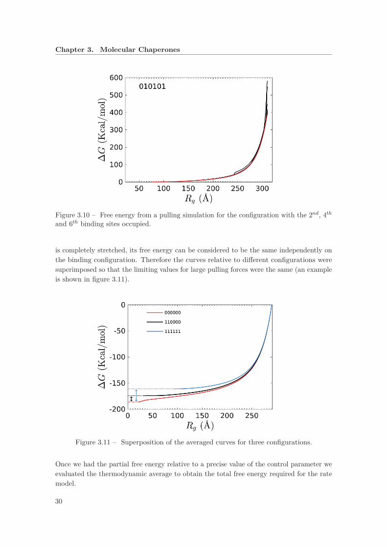
four different configurations . . . . . . . . . . . . . . . . . . . . . . . . . . . 293.10 Free energy from a pulling simulation for the configuration with the 2nd, 4th
and 6th binding sites occupied. . . . . . . . . . . . . . . . . . . . . . . . . . 303.11 Superposition of the averaged curves for three configurations. . . . . . . . . 303.12 Free energy of each configuration as a function of the stoichiometry. . . . . 313.13 Schematic representation of all the reactions related to the free state . . . . 323.14 Schematic representation of all the reactions related to the state with the
second binding site occupied by a chaperone in the ADP state. . . . . . . . 323.15 Probability of each stoichiometry as a function of the ratio [ATP ]
[ADP ] . To anincrease in [ATP ]
[ADP ] corresponds a larger number of bound chaperones. . . . . 333.16 Dissociation constant as a function of α. . . . . . . . . . . . . . . . . . . . 343.17 Radius of gyration as a function of α. Each curve corresponds to a different
set of free energy increases for all the configuration. The set was randomlygenerated from a Gaussian distribution centered in the values obtained withthe MD simulations. . . . . . . . . . . . . . . . . . . . . . . . . . . . . . . . 34
3.18 Mean values of the FRET efficiencies in our model in the presence of DnaK 35
xiii

List of Figures
3.19 Effectiveness (purple) as a function of α, together with its numerator (green)and denominator (orange). . . . . . . . . . . . . . . . . . . . . . . . . . . . . 36
3.20 Structure of GroEL. Figure taken from [1]. . . . . . . . . . . . . . . . . . . 383.21 Schematic representation of the different conformations of MDH . . . . . . 403.22 Enzymatic activity of MDH as a function of time . . . . . . . . . . . . . . . 413.23 Recovery of MDH activity with the help of GroELS, added in the system at
5 different times . . . . . . . . . . . . . . . . . . . . . . . . . . . . . . . . . 423.24 Enzymatic activity of MDH as a function of time in the presence and in the
absence of GroEL . . . . . . . . . . . . . . . . . . . . . . . . . . . . . . . . . 423.25 MDH activity as a function of time, for different values of ADP . . . . . . . 443.26 Reactivation of MDH when GroELS is added at different times . . . . . . . 463.27 Enzymatic activity of MDH as a function of time . . . . . . . . . . . . . . . 473.28 MDH activity as a function of time for different concentrations of ADP. . . 483.29 Nonequilibrium free energy of the native ensemble plotted as a function of
the energy available in the form of ATP . . . . . . . . . . . . . . . . . . . . 483.30 Fraction of native MDH as a function of the difference in free energy between
native and misfolded ensembles . . . . . . . . . . . . . . . . . . . . . . . . . 49
4.1 The structure of an ABC importer, together with a binding protein . . . . . 544.2 Fluorescence of ethidium as a function of time . . . . . . . . . . . . . . . . . 554.3 Simplified version of the kinetic cycle of an ABC transporter in the model
presented . . . . . . . . . . . . . . . . . . . . . . . . . . . . . . . . . . . . . 564.4 The concentration of molecules inside the cell is shown as a function of time 584.5 Contour plot showing the ratio ω corresponding to values of α and stot. . . 59
5.1 Superposition of random chains . . . . . . . . . . . . . . . . . . . . . . . . . 645.2 Comparison of the force vs extension curve in the case with and without
rigidity . . . . . . . . . . . . . . . . . . . . . . . . . . . . . . . . . . . . . . . 665.3 Projection of the first eigenvector to the force, for five different values of N 695.4 Renormalized eigenvalue λ1 as a function of the force, for five different values
of N . . . . . . . . . . . . . . . . . . . . . . . . . . . . . . . . . . . . . . . . 705.5 Renormalized eigenvalue λ2 as a function of the force, for five different values
of N . . . . . . . . . . . . . . . . . . . . . . . . . . . . . . . . . . . . . . . . 705.6 Renormalized eigenvalue λ3 as a function of the force, for five different values
of N . . . . . . . . . . . . . . . . . . . . . . . . . . . . . . . . . . . . . . . . 715.7 Ratio between the two smaller eigenvalues as a function of the force, for five
different values of N . . . . . . . . . . . . . . . . . . . . . . . . . . . . . . . 715.8 Asphericity as a function of γ for different values of N . . . . . . . . . . . . 725.9 Derivative of the asphericity as a function of γ for different values of N . . 725.10 Asphericity as a function of η for different models . . . . . . . . . . . . . . . 745.11 Projection of the first and the second eigenvalues . . . . . . . . . . . . . . . 75
xiv
List of TablesRate constants for the expansion of rhodanese . . . . . . . . . . . . . . . . . . . . 79Rate constants for the refolding mediated by GroELS . . . . . . . . . . . . . . . 79Rate constants for ABC transporter system . . . . . . . . . . . . . . . . . . . . . 81
xv

1 Introduction
Besides its intrinsic scientific appeal and its indisputable importance in many biologicalprocesses, the topic of protein organization and dynamics has an ever growing intereston the theoretical physics perspective. There are several reasons for this fact, we willjust mention the ones that directly motivated our work. First, like other macromolecules,proteins can be seen as mesoscopic systems, which means1 that even though they areformed by a large number of components, they are subjected to non negligible fluctuations[2]. When they are unfolded, the can be modeled with the tools of polymer physics [3, 4]and several conformational properties can be studied, like the scaling laws that regulatethe relation between the end-to-end vector and the number of monomers or the responseto confinement and other external constraints [5]. On the other hand, when they arefunctional they often take part to processes in which the thermal fluctuations not onlyare non negligible, but they are the real driving force that makes the system work. Themost evident example are the molecular motors, that are important biological systemsdistinguished by the peculiarity that they use chemical energy and thermal fluctuationsto perform mechanical work [6, 7]. Moreover, proteins represent a case study for somegroundbreaking accomplishments in modern statistical physics, like the fluctuation theorem[8] and the important equalities obtained by Jarzynski and Crooks [9, 10], concerning nonequilibrium transformations between two states at the same temperature. Second, the paththrough which a protein assumes its native configuration is also interesting on the point ofview of theoretical physics: in order to be functional, it has to reach a complex tertiarystructure that in many cases is univocally determined by its amino acids sequence [11].This leads to the development of statistical methods that are devised to infer the contactsbetween amino acids on the sole basis of the protein sequence, like co-evolutionary analysis[12, 13]. In addition, protein folding is an intriguing challenge that can be investigatedby means of molecular dynamics simulations (MD)[14]. Third, and this is probably themost important reason for our field, proteins are involved in several cellular mechanisms inwhich there is a continuous energy consumption. Here, the word continuous is particularlysignificant: what we want to highlight is that the systems under our consideration do not
1We recognize that here we are not giving a very formal definition, but we hope it is sufficient to explainour point.
1

Chapter 1. Introduction
simply gain a certain amount of energy in order to overcome a kinetic barrier, or escapefrom a metastable state, so that they can reach more easily the equilibrium state. Onthe contrary, we are focusing on those systems that are found in states that would not bepopulated without the support of an energetic source. As a consequence, these systemscannot be described with the formalism of the statistical physics of equilibrium [15, 16, 17].However, it would be a mistake to conclude that for this reason they are necessarily timedependent. Indeed, after a relaxation time they can be found in non equilibrium steadystates (NESS), with the main relevant quantities that are constant in time but do notcorrespond to a minimum in the free energy[17, 18]. An example of systems of this kind isa metallic bar that is kept at different temperatures at its extremities [2]: after a certaininterval, there is a net flux of heat along the bar that does not change in time and thatwould start decreasing as soon as the temperature gradient is removed. There are thusessentially two different kinds of non equilibrium states. One is a transient state, which mayor may not converge to an equilibrium state after a given time, and the other is the NESS,which does not depend on time and requires the constant supply of external energy. Thecell itself can be considered a non equilibrium system. The difference with respect to themetallic bar is that the thermodynamic force is not generated by a temperature gradientbut rather by a chemical gradient. The main source of energy in the cell is provided byATP [19]. The reaction of hydrolysis has a standard free energy ΔG0 � −32.6 kJ/mol[20]. However, in the cell there is a continuous production of ATP, so that in physiologicalconditions the ratio between the concentration of ATP and the one of ADP is kept atvalues of the order of 10 [21].
Among the different mechanisms taking place in the cell, we were particularly interestedin the one of protein folding. It is mostly accepted in the biological community thatmany proteins are capable of spontaneously assuming the functional structure in vitro[11]. However, it is fair to argue that the experimental conditions that are normallyused to perform in vitro experiments do not match the real cellular environment [22]. Inphysiological conditions there are indeed several factors, like heat or chemical stresses, thatcan represent an obstacle to the folding process. Therefore, protein folding is helped bymolecular chaperones, which are ATP consuming systems that interact with the exposedhydrophobic residues of unfolded and misfolded substrates [1, 23]. We will discuss two ofthem: the 70-kilodalton heat shock protein (Hsp70) and the bacterial chaperonin GroEL.For Hsp70 we start with a more abstract approach, by showing the theoretical constraintsthat the rate constants follow when the chaperone is able to efficiently enhance the refoldingprocess. We then move to a model that is closer to experiments, trying to reproduce theresults obtained in the group of Ben Schuler [24]. They used the technique of Försterenergy transfer spectroscopy (FRET) to show that denaturated rhodanese was expandedby Hsp70 in the presence of ATP. With a combination of MD simulations and a rate model2
we showed how it was possible to relate the substrate expansion to the energy consumption,as well as to obtain FRET efficiencies that are in agreement with the experiments.In the case of GroEL the problem was tackled in a different way. Above all, we could work
2The MD simulations were devised and implemented by S. Assenza and A. Barducci.
2

closely with the group of Pierre Goloubinoff, from the University of Lausanne, so that wewere able devise with them the experiments that are more relevant for our message. Weused as substrate an enzyme that is functional at 25 ◦C but it misfolds and it is susceptibleto aggregation at 37 ◦C. However, GroEL, together with its co-chaperone GroES and ATP,was able to recover the functional activity at 37 ◦C, suggesting that molecular chaperonescan stabilize the native state even when it does not correspond to a minimum in free energyin equilibrium conditions.
Even if it is less advanced in the development, we also want to discuss our application ofthe methods to ABC transporters. We show analytically that the free energy availablebecause of the supply of ATP in the cell constitutes a higher bond to the maximal efficiencyof the transporters defined as the ratio between the concentration of molecules on the twosides of the cell membrane. We also reproduce an experiment with exporters in which aconcentration gradient in the wrong direction was artificially imposed. In the absence ofATP, an uptake was detected. However, as soon as ATP was injected into the system, theefflux was recovered.
The last part will be only weakly related to the others, but still definitely inherent tothe main message. We study the deformation of a polymer chain when it is stretchedby an external force, that is a situation that is often encountered both in experiment[25] and in some biological phenomena, like protein translocation [26, 16]. With bothanalytical calculations and numerical simulations, we show that the transverse section ofthe ellipsoid which best approximates the polymer starts shrinking isotropically after theorientation. In addition, we show that the important quantities like the projection of theeigenvectors on the direction of the force and the asphericity can be written in terms of auniversal parameter, corresponding to the force contribution to the free energy of the system.
The next chapter will be devoted to a brief summary of the main results in non equilibriumphysics, with a particular emphasis on their application to biochemical cycles. In chapter3 we will discuss the application of the formalism to molecular chaperones. More precisely,in the first part we will focus on Hsp70 and in the second part on GroEL. In chapter 4we will explain how the energy is used by the Atp-binding cassette transporter (ABC) inorder to mediate the uptake and the efflux of small molecules through cell membranes. Inthe last chapter we will describe the shape and the orientation of a polymer subjected toan external tension.
3

2 Basic principles on non equilib-rium systems
In this chapter we want to summarize some of the most important results concerningnon equilibrium systems. In the particular case of biochemical cycles, the source of nonequilibrium is usually a chemostat, that is an external agent which stimulates the injectionof a particular type of molecules into the system and the ejection of another type. Inthe biological processes that we will consider in this thesis, the chemostat is usually theregeneration system of ATP. As we will describe below, the presence of a chemostatimplies that some of the rules that are usually valid for equilibrium systems, like thedetailed balance, are broken. The main consequence is the emergence of fluxes of reactions,and chemical cycles that are followed in a preferential direction. In any case, the maincharacteristic of non equilibrium systems, which is also the reason of the obstacles for theirsystematic statistical description, is their non locality. While for two equilibrium states thedifference in free energy provides, in principle, a sufficient indication of the way the twostates will be populated after a given relaxation time, in non equilibrium the rate constantsof the whole system are important to define the final distribution. We will give somemore details on this aspect, then we will discuss the main properties of non equilibriumbiochemical cycles, with a particular attention to their steady state solutions.
2.1 Non locality of non equilibrium systems
Before going into the formal description, we want to show an example in which theuniqueness of non equilibrium systems is evident.Consider an enzyme which can be found in three different states A, B and C. Whentransforming from B to C and vice versa, the enzyme must always pass through state A(see figure 2.1, left).We assume that, in the absence of ATP and ADP, B is more stable than C, but thetransformation between C and A is much faster than the one between B and A. We alsoassume that in state B and C the enzyme can bind ATP. In addition, the hydrolysis alwaysleads to a transformation from B, or C, to A (see figure 2.1, right). Both the bindingwith ATP and the hydrolysis have the same rates for B and for C. Therefore the only
5

Chapter 2. Basic principles on non equilibrium systems
Figure 2.1 – (left) Scheme for the enzyme in equilibrium. The state B and C can bothtransform reversibly to state A. B is favored in equilibrium, even if C has faster rates ofreaction. (right) Scheme for the enzyme out of equilibrium. As soon as the interactionwith the nucleotide is introduced, state C becomes more populated than state B.
asymmetries are given by the fact that the rates between A and C are faster than the ratesbetween A and B, even though the equilibrium constant, defined for a generic reactionfrom i to j as
Kij = kijkji, (2.1)
where kij and kji are the rates from i to j and from j to i respectively, is lower for A ↔ C
than for A ↔ B. The system is kept out of equilibrium by a chemostat which continuouslyremoves ADP and injects new ATP into the system. In figure 2.2 we plot the relativeconcentration of state C and state B as a function of the concentration of ATP, keepingfixed the concentration of ADP.As we can see, C is significantly stabilized with respect to B for large values of [ATP ].This stabilization is only due to the fact that the transformations between A and C arefaster than the ones between A and B, even though the reaction constants would fostera stabilization of the state B instead of C in equilibrium. Therefore, we can concludethat the NESS has the peculiarity of being non local, meaning that the kinetics of acomponent of the biochemical network can have a significant influence on the whole systemand considering the values of the equilibrium constants is not sufficient anymore.
2.2 Stationary states in biochemical systems
We can now recall some basic principles on biochemical systems. When we consider asystem with M components with probabilities pi (i = 1, ...,M), the probabilities are
6
2.2. Stationary states in biochemical systems
Figure 2.2 – Relative concentration of the states B and C of the enzyme as a function of[ATP ] when the concentration of ADP is kept fixed at 0.1mM .
solutions of master equations of the form (see [17, 18])
dpidt
=∑j
(pjkji − pikij) , (2.2)
where kij and kji follow the definition given above. After a certain relaxation time, astationary state will eventually be reached, characterized by probabilities that are notdependent on time:
dpidt
= 0 for all i (2.3)
If the stationary state is an equilibrium state, the detailed balance condition is respected:
pjkji = pikij . (2.4)
We can thus say that the probability of observing the transformation i → j is the sameas the probability of observing the transformation j → i or, in other words, there are noprobability fluxes for any couple (i, j), where a flux is defined as
Jij = pjkji − pikij . (2.5)
Looking at 2.4, it is quite natural to define a free energy change ΔGij [27] as
ΔGij = kT log[pjkjipikij
], (2.6)
so that the free energy change is zero at equilibrium. We will call cycle any set of Ncomponents that are connected by non zero reaction rates in such a way that they form
7
Chapter 2. Basic principles on non equilibrium systems
a single closed loop. We can reorder the components of the cycle so that component iis connected with component i + 1 with the only exception of component N , which isconnected with component 1 by construction. The implication of 2.4 is that the product ofthe reaction rates following a cycle in one direction is equal to the one that is obtain in theopposite direction1, that is
γ =N∏i
ki,i+1ki+1,i
= 1 , (2.7)
where we have imposed kN,N+1 = kN,1. The parameter γ is the affinity coefficient and it isrelated to the free energy of a cycle ξ by the relation
ΔGξ ≡∑i∈ξ
ΔGi,i+1 = kT ln γξ . (2.8)
As we said, if the system is not in contact with a chemostat, the stationary state is anequilibrium state. Otherwise, after the relaxation time the system is in a non equilibriumstationary state (NESS) with a net flux
Jij ≡ pjkji − pikij �= 0 . (2.9)
We can define the entropy as [17]
S = −k∑i
pi ln pi . (2.10)
2.3 Entropy flow and entropy production
Let us now assume that the rates do not depend on time and that the master equationsare linear. Computing the derivative of this expression with respect to time we obtain
dS
dt= −k
∑i
dpidt
(ln pi + 1) = −k∑i
dpidt
ln pi , (2.11)
where we have used the normalization condition on the probabilities:∑i
pi = 1 . (2.12)
1We can convince ourselves by simply multiplying and dividing for the product of the probabilities ofthe cycle.
8
2.4. Stationary state solution
Using the Master equation for pi and playing a bit with the sums, we have
dS
dt= − k
∑i,j
(kijpi − kjipj) ln pi =
− k
2
⎛⎝∑
i,j
(kijpi − kjipj) ln pi −∑i,j
(kijpi − kjipj) ln pj
⎞⎠ = (2.13)
− k
2
⎛⎝∑
i,j
(kijpi − kjipj) ln(pipj
)⎞⎠ ,
by multiplying and dividing inside the logarithm for(kij
kji
), we can separate the derivative
of S with respect to time in two contributions:
dS
dt= −k2
∑i,j
(kijpi−kjipj) ln(kijkji
)+ k
2∑i,j
(kijpi−kjipj) ln(pikijpjkji
)≡ Sf +Sp . (2.14)
The first term is called entropy flow and the second term is the entropy production. Notethat by construction we always have
Sp ≥ 0 . (2.15)
In the stationary state the two terms must be equal in absolute value and with oppositesign so that
dS
dt= 0 . (2.16)
In the particular case of equilibrium both terms are zero, since the detailed balance issatisfied for every branch of the reaction network. The entropy production can be used toquantify how far the system is from the equilibrium conditions. Using the definition in(2.9) we can write it as the sum of products between the flux and the difference in freeenergy [27] for every transformation:
Sp = 12∑i,j
JijΔGij . (2.17)
2.4 Stationary state solution
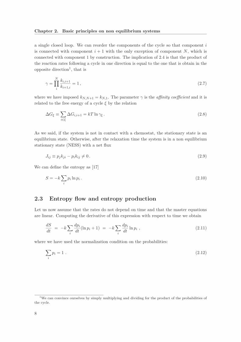
Let us now go back to the stationary state. There is very synthetic way to write thesolution of the stationary state, in the case of linear systems [18]. We represent the systemas a graph G whose components are the vertices. Two vertices are connected if betweenthe corresponding components the rate is different from zero.A spanning tree of the graph is a portion of the graph with the following properties:
9
Chapter 2. Basic principles on non equilibrium systems
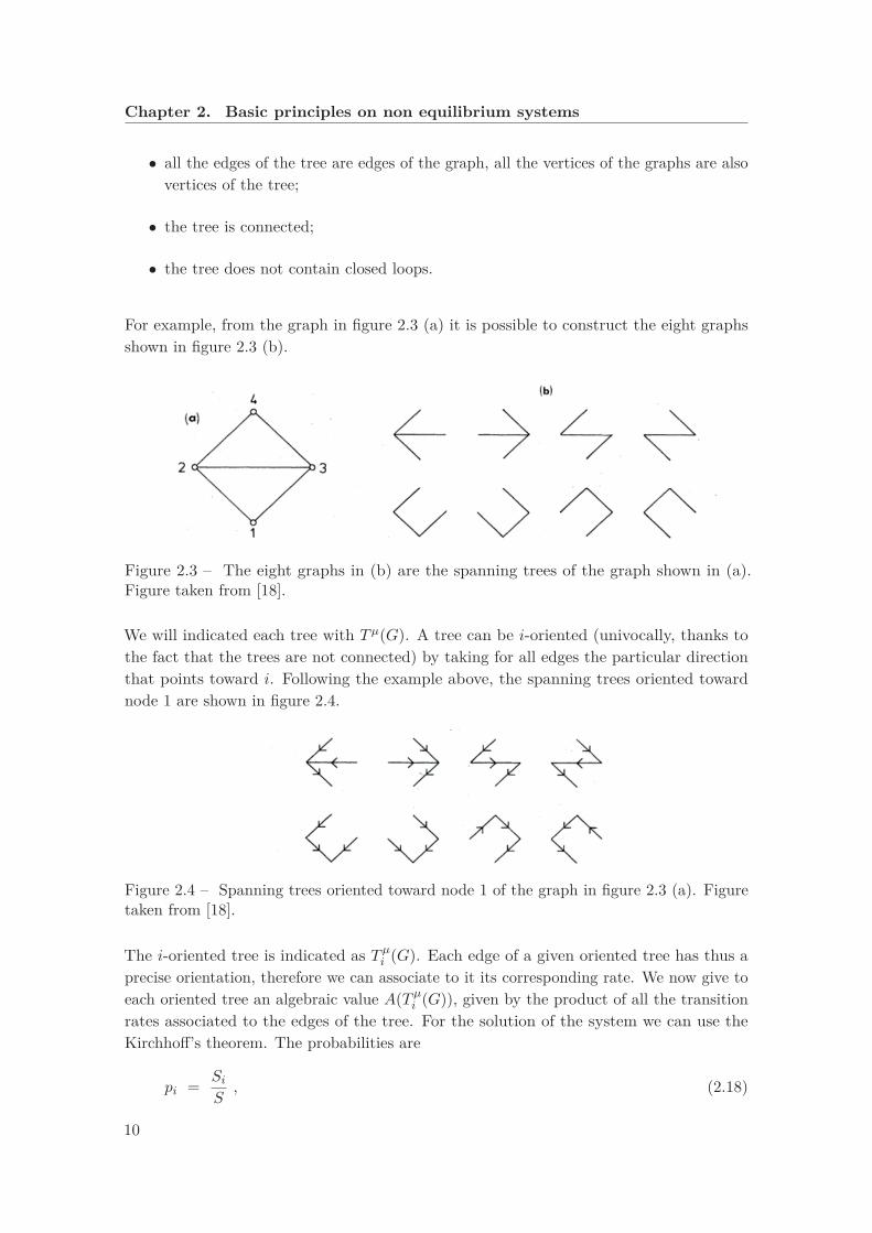
• all the edges of the tree are edges of the graph, all the vertices of the graphs are alsovertices of the tree;
• the tree is connected;
• the tree does not contain closed loops.
For example, from the graph in figure 2.3 (a) it is possible to construct the eight graphsshown in figure 2.3 (b).
Figure 2.3 – The eight graphs in (b) are the spanning trees of the graph shown in (a).Figure taken from [18].
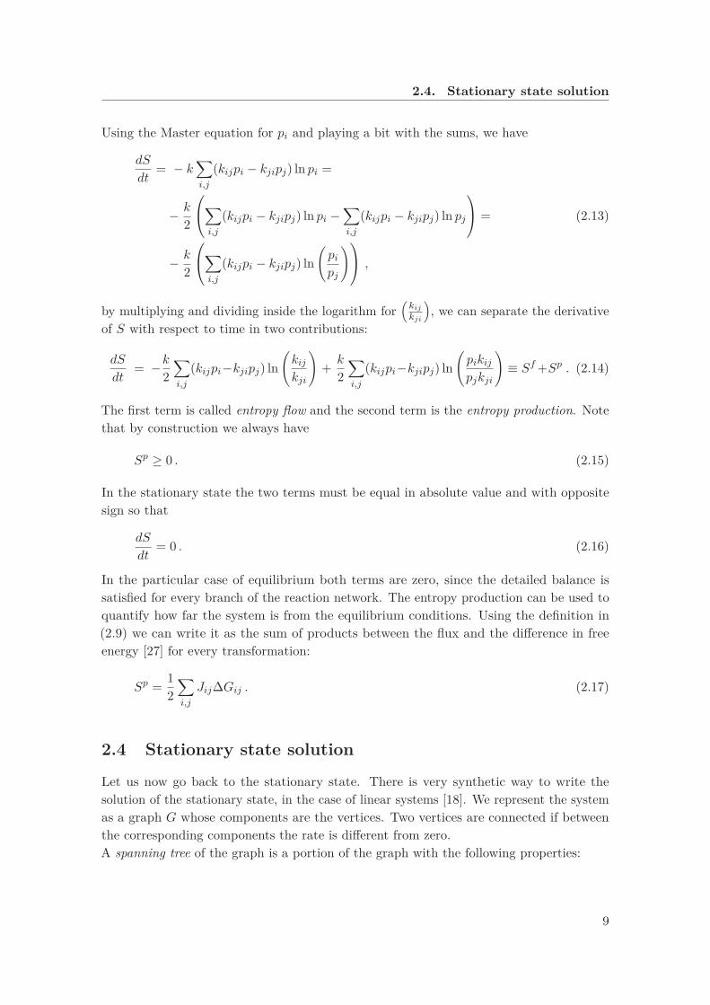
We will indicated each tree with Tμ(G). A tree can be i-oriented (univocally, thanks tothe fact that the trees are not connected) by taking for all edges the particular directionthat points toward i. Following the example above, the spanning trees oriented towardnode 1 are shown in figure 2.4.
Figure 2.4 – Spanning trees oriented toward node 1 of the graph in figure 2.3 (a). Figuretaken from [18].
The i-oriented tree is indicated as Tμi (G). Each edge of a given oriented tree has thus a
precise orientation, therefore we can associate to it its corresponding rate. We now give toeach oriented tree an algebraic value A(Tμ
i (G)), given by the product of all the transitionrates associated to the edges of the tree. For the solution of the system we can use theKirchhoff’s theorem. The probabilities are
pi = SiS, (2.18)
10
2.5. The source of the non equilibrium
with
Si =∑μ
A(Tμi (G)) (2.19)
and
S =∑i
Si . (2.20)
2.5 The source of the non equilibrium
We have shown that the equilibrium regime is determined by a condition on the rateconstants. Thermodynamics impose those constraints on whatever system can be consideredisolated, and thus which does not exchange heat or particles with the environment. Whenthis is not the case, it is usually possible to identify those rates that are influenced byexternal agents. An example that we will frequently use is the tuning of the effectiveexchange rates, in reactions that involve the hydrolysis of ATP. Systems like molecularchaperones have conformations that can vary according to the nucleotide that is bound.The protein, or the enzyme, can release a nucleotide and bind a new one. However, in mostcases the concentration of ATP and ADP in physiological is large enough that the proteinis almost never found in the absence of nucleotide (often referred to as the apo-state).Therefore, it is possible to define effective rate constants that take into account, at thesame time, both the release and the rebinding. If the rates of binding and unbinding ofATP and ADP are kT+, kT−, kD+ and kD− respectively, the effective rate constants ofexchange are
kexTD = kT−kD+
kD+ + [ATP ][ADP ]kT+
,
kexDT = kD−[ATP ][ADP ] kT+
kD+ + [ATP ][ADP ]kT+
. (2.21)
In this way the dependency on the actual energy source, that is the ratio between ATP andADP, can be written explicitly. All the rate constants must be chosen in such a way that,when the ratio is equal to the ratio that we would have in the absence of a regeneratingsystem for ATP, the constraint of formula 2.7 is satisfied.
2.6 Michaelis-Menten kinetics
We now consider a very simple and well-known example of enzyme kinetics [17]. Supposethere is a substrate S that can bind with an enzyme E and be converted into product P:
E + S � ES → E + P . (2.22)
11
Chapter 2. Basic principles on non equilibrium systems
We assume that kf is the binding rate, kr is the unbinding rate and kc is the rate for thereaction that converts the substrate into the product. In the stationary state, since thetotal concentration of enzyme [E0] = [E] + [ES] does not change in time, we must have
[ES] = [E][S]kfkr. (2.23)
Therefore we can write
[E] = [E0]1 + kf
kr[S]. (2.24)
The rate of the production of P is given by
d[P ]dt
= [ES]kc . (2.25)
Using equation 2.23 and 2.24 we obtain
d[P ]dt
= [S] kc[E0][S] + kr
kf
≡ [S]Vmax
[S] +Kd, (2.26)
where we have defined the maximum reaction velocity Vmax and the dissociation constantfor the enzyme-substrate complex Kd. We can see that in the case the concentration ofthe substrate is much lower than the dissociation constant, there is a linear dependency ofthe rate of formation of the product from the concentration [S]. Formula 2.26 is calledMichaelis-Menten equation [17].
12

3 Molecular Chaperones
Introduction
The vast majority of works involving the problem of protein folding usually give for grantedthe so called Anfinsen’s dogma [11], that is a postulate according to which a proteinsequence determines univocally the tertiary structure of the native state, a conformationthat can be reached spontaneously, that is unique and kinetically accessible. However,the free energy landscape relative to the tertiary structure of a protein is rugged andproteins are prone to be kinetically trapped in non functional states, corresponding tolocal minima in the free energy. A cell is a very crowded environment and in physiologicalconditions it is often not possible for the protein to spontaneously cross the kinetic barrierin relevant time scales. Moreover, in the case of extraordinary conditions such as thermalor chemical stresses, it is not even assured that the functional, or native state is actuallythe state of the absolute minimum in the free energy. Proteins that are misfolded, namelythat are not in their functional state, apart from the obvious issue of not being able toperform their biological task, could also form cytotoxic aggregates [28] responsible formany diseases, such as Alzheimer and Parkinson [29]. Thankfully, the folding is usuallysupervised by a particular class of specialized proteins called chaperones, that are definedas proteins that provoke a conformational change in a substrate without taking part in itsfinal structure [1]. Among the variety of chaperone families, many of them are heat-shockproteins (Hsps) because for historical reasons they have been initially associated to thefactor that strongly enhances their expression, which is the sudden increase in temperature(heat shock) responsible for the unfolding [30]. Even though heat shock proteins have beenunder study for more than three decades and there has been an overwhelming improvementin the understanding of the field, there are still many questions that at present remainunanswered. For example, it is unclear the precise mechanism that drives the substrateto the folded state: do chaperones actively catalyze protein unfolding or they are ratherpassive holding machines that are able to prevent aggregation during the folding process?Moreover, it is well known that ATP is consumed during the process, but it is a matterof debate how the energy of ATP hydrolysis is actually used. Is it possible for molecularchaperones to stabilize client proteins that would not be stable in equilibrium? In this work,
13
Chapter 3. Molecular Chaperones
we will try to answer some of these questions with the help of non equilibrium statisticalphysics.
3.1 Hsp70
Hsp70 is a very abundant chaperone family that is involved in protein folding together withother very important cellular functions, as protein translocation across cell membranes[16, 31] and protein degradation [32]. In the Hsp70 system the heat shock protein isusually helped by other proteins called cochaperones: a J domain protein (JDP), whichcarries the substrate to the complex and stimulates the hydrolysis [33, 34], and a nucleotideexchange factor [35] (NEF), responsible for the release of ADP after the hydrolysis and thesubsequent binding of a new molecule of ATP. Despite the remarkable versatility of Hsp70,its sequence is pretty conserved, mostly because the specificity is usually guaranteed bythe cochaperones [33, 35].
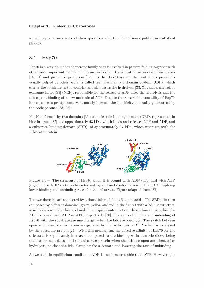
Hsp70 is formed by two domains [36]: a nucleotide binding domain (NBD, represented inblue in figure [37]), of approximately 43 kDa, which binds and releases ATP and ADP, anda substrate binding domain (SBD), of approximately 27 kDa, which interacts with thesubstrate protein.
Figure 3.1 – The structure of Hsp70 when it is bound with ADP (left) and with ATP(right). The ADP state is characterized by a closed conformation of the SBD, implyinglower binding and unbinding rates for the substrate. Figure adapted from [37].
The two domains are connected by a short linker of about 5 amino acids. The SBD is in turncomposed by different domains (green, yellow and red in the figure) with a lid-like structure,which can assume either a closed or an open conformation, depending on whether theNBD is bound with ADP or ATP, respectively [38]. The rates of binding and unbinding ofHsp70 with the substrate are much larger when the lids are open [36]. The switch betweenopen and closed conformation is regulated by the hydrolysis of ATP, which is catalysedby the substrate protein [21]. With this mechanism, the effective affinity of Hsp70 for thesubstrate is significantly increased compared to the binding without nucleotides, beingthe chaperone able to bind the substrate protein when the lids are open and then, afterhydrolysis, to close the lids, clamping the substrate and lowering the rate of unbinding.
As we said, in equilibrium conditions ADP is much more stable than ATP. However, the
14

3.1. Hsp70
cell is a system that is strongly out of equilibrium, and in physiological conditions wecan have a ratio α = [ATP ]
[ADP ] ∈ (1, 10). Previously [21], it was shown that the switchingbetween a configuration with large binding rates and one with small binding rates can leadto an ultra-affinity, that is an effective affinity between the chaperone and the substratethat is much larger than the affinity for the ATP or the ADP state of Hsp70 and thisphenomenon is possible only when the system is out of equilibrium. This result wouldsuggest that the binding is indeed the step in the reaction cycle that is most affected bythe energy consumption and α is thus a parameter that quantifies how far the system isfrom equilibrium. This section will be divided in two. In the first part we will consider asimple model with a single binding site and derive some constraints on the rate constantsnecessary for the catalysis of the unfolding. Afterwards, we will work on a model withseveral binding sites, focusing on the particular case of rhodanese, motivated by someexperimental data [24]. Before starting we want to give an intuitive explanation on themechanism used by Hsp70 for the unfolding of the substrate.
3.1.1 Entropic pulling
Here we want to give a qualitative description of the mechanism that Hsp70 uses for thetranslocation and the unfolding of substrate proteins. We consider the translocation as anexample because it allows a simpler representation, but a similar approach can be used forthe unfolding[16, 15]. The idea is that thermal fluctuations induce the substrate to increaseits freedom by reducing the effects of the excluded volume. Let us model the translocatingsubstrate as a Gaussian chain and consider the case in which the chain is constrained tostay above a fixed rigid surface 1. In the last chapter of the thesis the shape of a randomchain will be discussed, here we just anticipate that the end-to-end vector, that is thedistance between the first and the last monomer of the chain, is normally distributed whenthere is no interaction between the monomers. However, it is possible to show that in thepresence of a constraint that prohibit the monomers to be in a certain region, the form ofthe distribution is different. In our example the monomers are not allowed to be in theregion in which z < 0. In this case, the distribution of the end to end vector Re becomes
P (Re) = ωRz exp[−3
2R2
e
Nb2
], (3.1)
where N is the number of monomers in the chain that have already crossed the membrane,ω is a constant and Rz is the z-component of Re. If a chain with N monomers has A0possible conformations in free space, then in the presence of the membrane it will have anumber A of possible conformations where
A = A0N∫ +∞
−∞dz
∫ +∞
−∞dy
∫ +∞
0dz P (Re) . (3.2)
1This calculation can be found in [16]
15

Chapter 3. Molecular Chaperones
Now we assume that at the end of the chain an Hsp70 is bound. Therefore, when weintegrate over z we must consider the volume that is forbidden by the chaperone (see figure3.2):
A70 = A0N∫ +∞
−∞dz
∫ +∞
−∞dy
∫ +∞
R70dz P (Re) = A exp
[− 3R2
702Nb2
]. (3.3)
As a consequence, the free energy gained by the addition of one chaperone is
ΔF = −kbT (ln [A70] − ln [A]) = 3R270
2Nb2 , (3.4)
and we can see that the increment is inversely proportional to the number of monomers N .We can conclude that to minimize ΔF the chain is enhanced to increase the number ofmonomers that cross the membrane.
Figure 3.2 – Schematic representation of the excluded volume effect of Hsp70. The numberof conformations that are forbidden is lower in the presence (B) with respect to the absence(A) of Hsp70. This picture is taken from [16].
This mechanism is called entropic pulling. Even though we presented it for the translocation,the same mechanism can be applied to the chaperone-mediated unfolding and disaggregation.The role of the surface is played in this case by the misfolded protein itself or by theaggregate, that can be modeled as rigid spheres. Hsp70 can specifically bind to exposedhydrophobic regions in the substrate sequence that are not hidden in the inner part of thesubstrate/aggregate. In this way, the excluded volume interaction between the chaperoneand the substrate or the aggregate stimulates an increase in the number of monomers thatform the portion of the chain that is exposed and thus that is not misfolded anymore.
3.1.2 Rate model for refolding
In this section we want to derive the constraints that the rate constants must respect sothat the chaperones can properly do their work as unfoldase. In order to model a processof refolding catalysed by Hsp70, we had to make some assumptions. We assumed thateach protein can be found in one of four conformational states, that are coarse grainedensembles of all the possible configurations (a similar approach has been used, for example,
16

3.1. Hsp70
in [39]): the protein can be native (N), partially folded (X), misfolded (M) or unfolded (U)(see figure 3.3).
Figure 3.3 – Initial kinetic cycle, with four different conformational states for the protein.Under some assumptions it can be reduced to a simpler cycle, without the unfolded state(the second from the left).
The native state N is a state that is completely folded and we assume, for this reason, thatalmost all the hydrophobic residues are hidden in the inner regions and it is impossiblefor the chaperone to bind the protein [40]. The partially folded state is an intermediatestep in the process of refolding. In proteins in state X a large number of amino acids arecorrectly arranged, but some of them are not and, as a consequence, there is still a certainnumber of exposed hydrophobic residues to which the chaperone can bind. The misfoldedstate is a non-functional state with non native hydrogen bonds and a certain number ofexposed hydrophobic residues. It corresponds to a local minimum in the free energy and itis separated by a high energy barrier from the native state. The unfolded state has fewcontacts among the amino acids and the majority of the hydrophobic residues are exposed.We also assumed that the unfolded state is very unstable and thus the rates of misfoldingand refolding from state U are large. We can show that, under these hypotheses, theunfolded state can be left out of the cycle and the state M can be connected directly withthe state X, but with new effective rates that are a function of the rates from U to X andto M.
17

Chapter 3. Molecular Chaperones
The concentrations of this system are determined by the following rate equations:
˙[M ] = [U ]kum + [Mc]kmcm − [M ](kmu + kmmc)˙[Mc] = [M ]kmmc + [Uc]kucmc − [Mc](kmcm + kmcuc)˙[U ] = [M ]kmu + [Uc]kucu + [X]kxu − [U ](kum + kuuc + kux)˙[Uc] = [U ]kuuc + [Mc]kmcuc + [Xc]kxcuc − [Uc](kucu + kucmc + kucxc) (3.5)˙[X] = [U ]kux + [Xc]kxcx + [N ]knx − [X](kxu + kxxc + kxn)˙[Xc] = [X]kxxc + [Uc]kucxc − [Xc](kxcx + kxcuc)˙[N ] = [X]kxn − [N ]knx .
Note that we are assuming that the concentration of free chaperones [c] is large enough thatit can be considered constant. Therefore, the rates that we have written for the bindingreactions must be interpreted as the product between the actual binding rates and theconcentration of free chaperones, for example kmmc = [c]k0
mmc where k0mmc is the binding
rate and kmmc has dimension s−1. The total concentration of the substrate [St] is fixed:
[M ] + [Mc] + [U ] + [Uc] + [X] + [Xc] + [N ] = [St] . (3.6)
The steady state is obtained by imposing on all the concentrations to be constant in time:
˙[M ] = ˙[Mc] = ˙[U ] = ˙[Uc] = ˙[X] = ˙[Xc] = ˙[N ] = 0 . (3.7)
If we now assume that the rates kum, kux, kucmc and kucxc are much larger than all theother rates, then we can pass from a cycle of the form of figure 3.3 to a cycle of the formof figure 3.4.
Figure 3.4 – Kinetic cycle used in this work, after the simplification.
Intuitively, a simplification of this kind is possible because the proteins spend few timein the unfolded state and once they unfold they rapidly refold or misfold again. The
18
3.1. Hsp70
concentrations of the new cycle are solutions of the following system:
0 = [X]kxm + [Mc]kmcm − [M ](kmx + kmmc)0 = [M ]kmmc + [Xc]kxcmc − [Mc](kmcm + kmcxc)0 = [M ]kmx + [Xc]kxcx + [N ]knx − [X](kxm + kxxc + kxn)0 = [X]kxxc + [Mc]kmcxc − [Xc](kxcx + kxcmc)0 = [X]kxn − [N ]knx ,
(3.8)
where we have defined
kmx = kmukuxkux + kum
kxm = kxukumkux + kum
kmcxc = kmcuckucxckucxc + kucmc
kxcmc = kucmckxcuckxcuc + kmcuc
.
(3.9)
Once the simplification on state U has been done, the remaining states are connected inthe kinetic cycle shown in figure 3.4.When a misfolded protein refolds, it necessarily passes through the intermediate state Xbefore reaching the native state N. Hsp70s are able to catalyse the reaction M ↔ X viathe path M ↔ Mc ↔ Xc ↔ X, but for a complete refolding they must leave the clientprotein and the reaction X ↔ N is always spontaneous.
As we said, Hsp70 is always helped by the cochaperones. Here, the effects of the cochap-erones are implicitly taken into account via a modulation of the rate constants. Thehydrolysis of ATP is stimulated by the combined interaction of Hsp70 with JDP and theclient protein: when they are both bound with Hsp70, the hydrolysis is much faster thanin the presence of either the substrate or the J protein alone: while JDP and substrate canstimulate the hydrolysis of 2-5 fold, when they both interact with Hsp70 at the same timethe hydrolysis can be increased of up to three orders of magnitude. [33, 41, 42, 43]. At afirst sight, this is slightly counter-intuitive. As we will better explain later, our guess isthat the chaperone in the ATP state can have two different conformations and only in oneof them it stimulates the hydrolysis. The J-protein and the substrate are responsible forthe stabilization of that conformation with respect to the other. In this way, it is possibleto explain the particularly large enhancement of the ATP hydrolysis.A consequence of this phenomenon is that the catalysis of the hydrolysis must depend onthe conformation of the substrate. Indeed, if the interaction with JDP depends on theconformation of the client protein, as we can expect, then it is reasonable to assume thatalso the hydrolysis of ATP is stimulated at a different amount by proteins that are in stateM or in state X. In the next section we will discuss how it is possible to write an effective
19
Chapter 3. Molecular Chaperones
binding affinity that takes into account the hydrolysis of ATP and the interaction betweenchaperone, substrate and cochaperone.
The mechanism by which the switch between the different conformational states of Hsp70influences its interaction with the client protein will be discussed later and here we collectin one state all the configurations of Hsp70. The rates of the hydrolysis of ATP are includedin the effective rates of binding with Hsp70, kmmc and kxxc. Therefore, with Mc and Xc
we indicate the misfolded and partially folded proteins when they are bound with Hsp70,independently on the conformation of Hsp70 and the nucleotide that is bound to it.
We consider a system in which the concentrations are low, so that aggregation can beneglected. Intuitively, if the rates toward X following a path that include the bindingare faster, the concentration of native proteins relative to the concentration of misfoldedproteins must be larger with Hsp70, compared to a system in the absence of chaperones.More formally, we define the affinity coefficient for this particular system:
γ = kxm kmmc kmcxc kxcxkmx kxxc kxcmc kmcm
. (3.10)
The concentrations in the stationary state can be calculated by solving 3.8. The result canbe used to obtain the ratio between the concentrations of the two states with respect tothe same ratio in the case of spontaneous refolding (without Hsp70):
[N ]ch[M ]ch
= [N ]0[M ]0
(1 + C(γ − 1)) , (3.11)
where
C = kxxckxcmckmcm
kxxckxcmckmcm + kxcmckmcmkxm + kxmkxcx(kmcm + kmcxc), (3.12)
is a positive constant, [N ]0 and [M ]0 are the concentrations of native protein in the absenceof chaperones and [N ]ch and [M ]ch are the corresponding concentrations for a system withchaperones. We can see that, as soon as γ > 1, the native state is stabilized with respectto the misfolded state in the presence of Hsp70:
[N ]ch[M ]ch
>[N ]0[M ]0
. (3.13)
However, the fact that the relative concentration is increased does not mean that theabsolute concentration [N ] is also increased. For the general case, the necessary conditionon the rate constants in order to have [N ]ch > [N ]0 can be written as
γ > 1 + γ[kmx
kxcx+ kmx
kmcxc
]+ kmx
[ 1kxcmc
+ 1kmcm
], (3.14)
and we thus confirm the fact that it is necessary to have γ > 1. In [21] it has been shownthat the role of the hydrolysis of ATP is to tune the effective affinity of Hsp70 for the
20
3.1. Hsp70
substrate. If we assume that the energy of the hydrolysis is used only to perform this task,then the condition γ > 1 implies that, for an improvement of the refolding in the steadystate, it is necessary to increase the affinity for proteins in state M of a larger amount thanfor proteins in state X, because that would be the only way to increase γ, that dependson the ratio kmmc/kxxc. Note that γ = 1 is not necessarily a signal of equilibrium, butit rather implies that, if there is hydrolysis, the affinity is increased of the same amountfor the reaction M ↔ Mc and X ↔ Xc. Playing a bit with the algebra and using thedefinition of γ, we can rewrite the inequality as
γ [τmx − τmcx] > τxcmc + τmcm + τmx (3.15)
where
τmcx = τmcxc
[1 + τxcx
τxcmc
]+ τxcx (3.16)
is the time needed for the reaction Mc → Xc → X to occur and τij = k−1ij . Since γ is
always positive, the condition can be satisfied only if τmx > τmcx, namely if the refoldingin the presence of Hsp70 is faster than the spontaneous refolding, as we should expect. Ifthis condition is not satisfied, the concentration [N ]ch will not be larger than [N ]0 in anytime interval, even during the transient state.
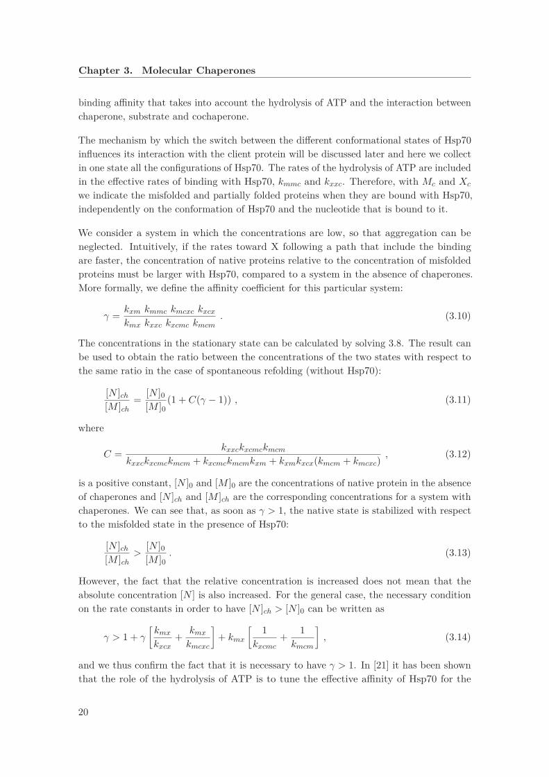
In figure 3.5 we show the concentration of native proteins [N ] normalized by the totalconcentration [ST ] in three different conditions.
Figure 3.5 – Concentration of native proteins as a function of time in the absence of Hsp70(black), in the presence of Hsp70 but in equilibrium conditions (blue) and in the presenceof Hsp70 in non equilibrium conditions (red).
We can see that the presence of Hsp70 in non equilibrium conditions (red curve) not onlystimulates a faster refolding, but also leads to a larger concentration of native proteinsin the stationary state with respect to the case in which the chaperones are absent (blue
21
Chapter 3. Molecular Chaperones
curve). On the contrary, if γ = 1 (black curve), even though during the transient state alarger concentration is possible, the yield of native protein in the stationary state is alwayslarger without Hsp70.
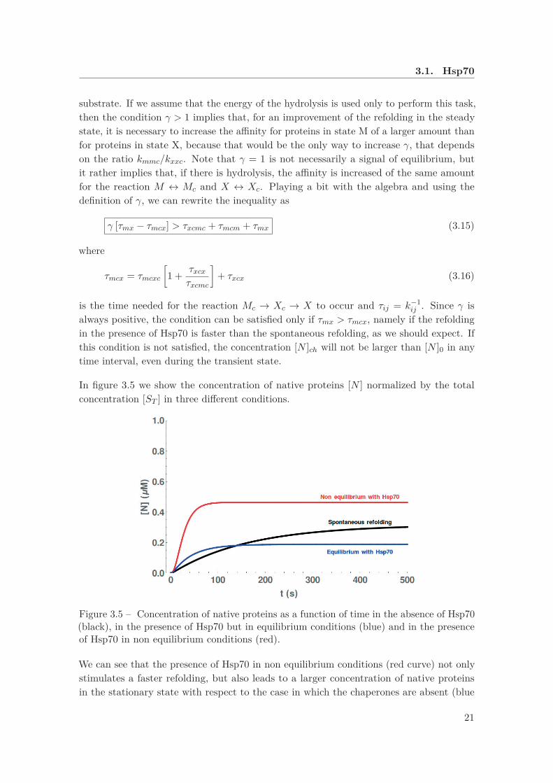
Even though the hydrolysis of ATP is mainly used to increase the effective affinity for thesubstrate protein, it is worth to mention that the affinity must not be too large, becauseHsp70 needs to release the substrate protein in order to allow it to spontaneously refold.In figure 3.6 we plot the relative concentration of native protein in the stationary state asa function of the concentration of Hsp70 in the system. As we can see, if the concentrationof chaperones is too large, the yield of native proteins becomes lower than in the case ofspontaneous refolding (orange line).
Figure 3.6 – Concentration of native proteins as a function of the concentration of Hsp70(green). The light green region represents the improvement in the yield of native proteinsdue to the presence of Hsp70.
3.1.3 Role of the cochaperones in the binding affinity
Since in our model we have not taken into account explicitly the conformation of thechaperone, as well as the nucleotide that is bound to it, we want to give some details onthe dependence of the binding affinity from the hydrolysis of ATP. In order to do so, thereis the need of a brief discussion about J-domain proteins.
Hsp70 never works alone: even though sometimes it can function without the nucleotideexchange factor, up to now it has never been shown to work in the absence of a J-domainprotein (JDP) as cochaperone [33]. Hsp70 is a very conserved protein, but at the same timeit has to interact with a plethora of very different client proteins [33]. JDP is the proteinthat mediates this interaction with the substrate [34], having a much larger diversity in itsprotein binding domains. On the other hand, the J-domain, that is used to catalyze the
22
3.1. Hsp70
ATPase activity of Hsp70, is quite conserved among different JDPs. The mechanism bywhich the J-domain stimulates the hydrolysis of ATP is still a matter of debate.We want to study in more detail how JDP influences the binding affinity between thechaperone and the substrate. JDP has two binding sites, located in the C-terminaldomain of its two monomers. We assume that the client protein binds separately to eachdomain. Therefore, we can define two states, SJ1 and SJ2, the first one representing theconfiguration with only one monomer of JDP bound to the client protein, the second onethe configuration with both monomers attached to it. The binding reaction is
S + J � SJ1 � SJ2 . (3.17)
In the steady state, we have
[SJ1] = nkonkoff
[S][J ] , (3.18)
and
[SJ2] = (n− 1)konkoff
[SJ1] = n(n− 1)konkonk2off
[S][J ] . (3.19)
where koff is the rate of unbinding (the same for the two domains), n is the number ofavailable binding sites, kon is the binding rate at a precise site for the first domain andkon is the binding rate for the second, that is larger because, after the first monomerbinds, JDP is localized in the neighborhood of the client protein. If we define the totalconcentration of client proteins bound with JDP as
[SJ ] = [SJ1] + [SJ2] , (3.20)
we end up with the following relation:
[SJ ] = nkonkoff
(1 + (n− 1)kon
koff
)[S][J ] . (3.21)
Hsp70 can interact with the substrate either when it is free or when it is bound withJDP, with approximately the same binding rate. However, the hydrolysis is stimulated atdifferent amounts by SJ and S. We will call HT and HD the Hsp70 in the ATP and ADPstate respectively. Let us assume that the Hsp70 can bind with SJ only when it is in theATP state. Then we have
[SJHT ] =k0jk
kkj[SJ ][HT ] ≡ 1
Kd[SJ ][HT ] , (3.22)
where k0jk and kkj are the rate constants for the reaction SJ +HT � SJHT and Kd = kkj
k0jk
the dissociation constant of SJHT . It is considered to be approximately equal to thedissociation constant of the bound state without JDP, indicated as SHT . Since the
23

Chapter 3. Molecular Chaperones
reaction of synthesis is negligible, the interchange between the ATP and the ADP statesare determined by the rates of hydrolysis and of exchange:
[SJHD] = kjhkex
[SJHT ] = kjhkexKd
[SJ ][HT ] , (3.23)
where kex is the rate of exchange from ADP to ATP and kjh is the rate of hydrolysis in thepresence of SJ . Moreover, we are assuming that the hydrolysis is the leading contributionin the reaction HT → HD, being much faster than the exchange from ATP to ADP. Thetotal concentration of the complex formed by the three proteins is given by
[SJK] = [SJHT ] + [SJHD] = 1Kd
(1 + kjh
kex
)[SJ ][HT ] . (3.24)
If we now plug 3.21 into 3.24, we obtain
[SJK] = konkoff
n
Kd
(1 + kjh
kex
)(1 + (n− 1)kon
koff
)[J ][S][HT ] ≡ 1
Ked
[S][HT ] . (3.25)
where we have defined the effective dissociation constant as
Ked =
[konkoff
n
Kd
(1 + kjh
kex
)(1 + (n− 1)kon
koff
)[J ]
]−1
. (3.26)
We can see that the dissociation constant is decreased by an increase in either the concen-tration of JDP or in the rate of hydrolysis.
As we said, the binding rate of the chaperone with the free substrate is not very differentfrom the one in the presence of JDP. However, in the absence of JDP the hydrolysis ofATP is much slower[33]. Therefore, the steady state is given by the following relation:
[SHT ] = 1Kd
(1 + ksh
kex
)[S][HT ] � 1
Kd[S][HT ] , (3.27)
where ksh is the rate of hydrolysis in the absence of the J-domain. The last equality in 3.27follows from the fact that ksh kex. The total concentration of the bound state StotK isthe sum of the two contributions:
[StotK] = [SJK] + [SHT ] =(
1Ke
d
+ 1Kd
)[S][HT ] . (3.28)
3.1.4 Binding with JDP and hydrolysis
We have just seen how the hydrolysis can change the effective binding affinity between thechaperone and the substrate. The fact that JDP stimulates the hydrolysis in cooperationwith the substrate, that is supported by experimental observation [34], up to now in this
24
3.1. Hsp70
work has just been given for granted. We now want to implement a model that can explainthis behavior.
We assume that the chaperone can be found in one of two conformational states, A andB, with a free energy difference ΔGAB. Let us also assume that the chaperone is ableto stimulate the ATP hydrolysis only when it is in the state with larger free energy (sayA) whereas it does not work as ATPase when it is in the other state (B). The state thatstimulates the hydrolysis has a large affinity for the J-domain protein, whereas the otherstate barely interact with it. We will call kh,max the rate of hydrolysis stimulated by Hsp70.In the absence of J and S, the effective rate of hydrolysis is equal to kh,max multiplied bythe probability that Hsp70 is in the higher energy state:
kh,eff = exp (−βΔG)1 + exp (−βΔG) kh,max . (3.29)
For the free Hsp70, the difference in free energy is about 7 kT and thus
kh,eff � 10−3 kh,max . (3.30)
The binding of substrate or JDP leads to a state characterized by a lower difference in freeenergy with respect to state A. Suppose that the chaperone can bind with the cochaperoneor with the substrate and when they are both bound they can also interact with oneanother. The expression of the effective rate must be modified:
kh,eff =exp (−βΔG)
(1 + [J ]
KjcA
+ [S]Ksc
A+ [J ]
KjcA
[S]Ksc
A
ρloc
Kjs
)(
1 + [J ]Kjc
B
+ [S]Ksc
B+ [J ]
KjcB
[S]Ksc
B
ρloc
Kjs
)+ exp (−βΔG)
(1 + [J ]
KjcA
+ [S]Ksc
A+ [J ]
KjcA
[S]Ksc
A
ρloc
Kjs
) kh,max ,
(3.31)
where KuvI is the dissociation constant of state UV (where U and V can be JDP (J),
substrate (S) or Hsp70 (C) ) when Hsp70 is in conformation I (either A or B). In principle,we should add the terms corresponding to the other possible three body interactions, thatare when protein and JDP interact before they are both bound to Hsp70. However, theyare not particularly relevant for the effect that we are going to show, so we will omit them.ρloc is the local concentration, the number of binding sites of S that are available to theJDP when they are both bound with Hsp70, over the volume that can be reached by JDPwithout unbinding from Hsp70 (same order of magnitude of its radius of gyration). If wewrite 3.31 in the following way:
kh,eff = exp (−βΔG) D
F + exp (−βΔG)D kh,max , (3.32)
with
D =(
1 + [J ]Kjc
A
)(1 + [S]
KscA
)+ [J ]Kjk
A
[S]Ksc
A
(ρlocKjs
− 1), (3.33)
25
Chapter 3. Molecular Chaperones
and
F =(
1 + [J ]Kjc
B
)(1 + [S]
KscB
)+ [J ]Kjk
B
[S]Ksc
B
(ρlocKjs
− 1), (3.34)
we can see that D and F are the sum of a contribution given by the product of the termsthat we would have with either only J or only S and a contribution with the couplingbetween J and S. It is now time to make some estimates2. The local concentration ρloccan be around 1 − 10mM . Substrate and JDP are usually in concentrations of the order of1μM . The dissociation constants for the binding between the substrate and the chaperoneis also of the order of the micromolar, while for the interaction between S and JDP we canassume Kjs ∼ 10−2μM . We can also assume Kjc
A ∼ 1μM , whereas in first approximationthere is no binding between JDP and Hsp70 in state B. Considering that we have
exp [−ΔG] ∼ 10−3 , (3.35)
we can see that, when there are either JDP alone or the substrate alone in the system, onlyF is relevant in the denominator of formula 3.32. Therefore in the absence of cooperationbetween JDP and S the rate of hydrolysis can be improved of a factor
z = 1 + [J ]Kjc
A
, (3.36)
which is the order of unity. According to the observation, the addition of JDP alonecan lead to an increase in the rate of hydrolysis of up to 5-fold [36, 43]. However, in thepresence of both the substrate and JDP the second term in the denominator of 3.32 is notnegligible anymore. We have indeed
exp (−βΔG)D ∼ 102 − 103 . (3.37)
This is in agreement with the general opinion that the rate of hydrolysis is increased by upto 103 times in the presence of both the substrate and the cochaperone.
3.1.5 The expansion of rhodanese
Until now we have considered a model with a single binding site. However, in many casesthe substrate is bound at the same time by more than one chaperone and in general asubstrate protein can be bound in more than one region along its amino acid sequence[24, 44]. The other problem of the previous model is that even though it gives a qualitativedescription of the conditions for Hsp70 to work in the most efficient way, it is not able todirectly relate the effect of the chaperone to the substrate with the amount of energy thatcan be used. Indeed, this is only possible when the change in conformation of the chaperoneitself is taken into account. We decided to focus on the substrate protein rhodanese, which
2The values that will be chosen are all in agreement with those reported in the article of Mayer, Hu andTomita [40].
26

3.1. Hsp70
has been proven to expand under the influence of Hsp70 by Schuler and co-workers [24].In 2014, they measured the expansion of denaturated rhodanese in the absence and inthe presence of DnaK, that is a particular family of prokaryotic Hsp70, its cochaperoneDnaJ, that is a J-domain protein, and ATP using a method called Förster resonanceenergy transfer spectroscopy (FRET). This technique is based on the fact that an excitedchromophore, the donor, can transfer energy to another chromophore, the acceptor, viaa nonradiative dipole-dipole coupling [45]. The efficiency of this transfer of energy goeswith the inverse of the sixth power of the distance between the two chromophores [45, 46].Therefore, with a measurement of the transfer efficiency it is possible to deduce with goodaccuracy the distance between the chromophores.In the experiment, they attached two fluorescent dyes in two positions along the sequenceof the substrate protein and measured the transfer efficiency. The idea is that when thesubstrate protein expands the distance between the dyes increases and thus there is a netdrop in the transfer efficiency.
As we can see in figure 3.7, the presence of chaperones provokes a decrease in the efficiencythat is indicative of an expansion of the substrate.
Figure 3.7 – Histogram for the FRET efficiencies for five different positions of the fluorescentdyes, in the absence (left) and in the presence (right) of DnaK and DnaJ. The histogramsfor the native state are shown in gray. Figure adapted from [24].
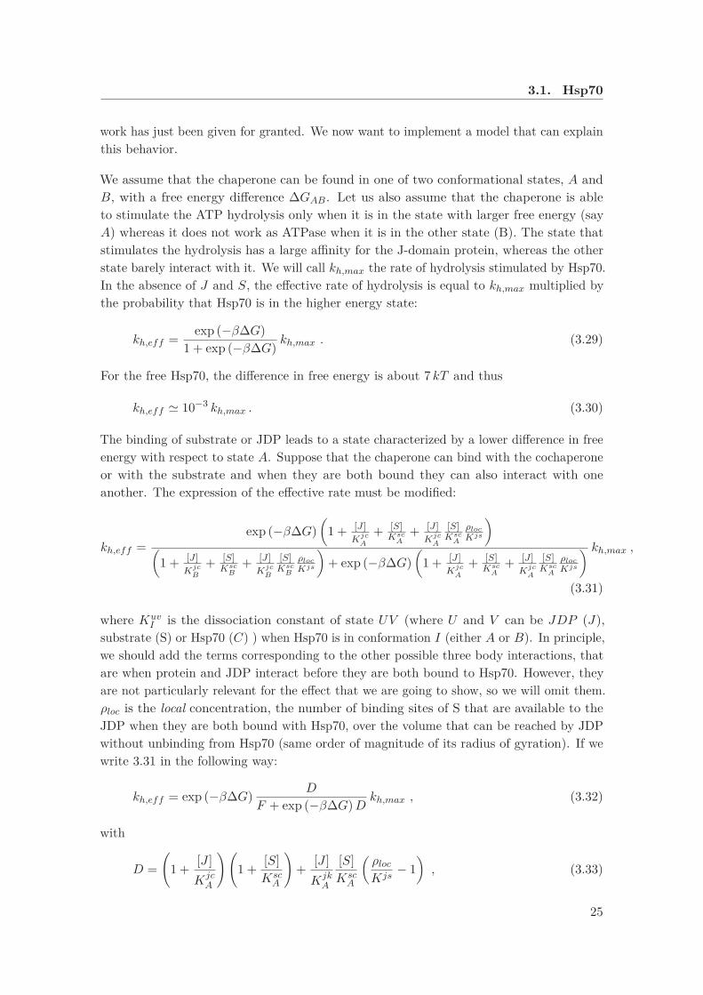
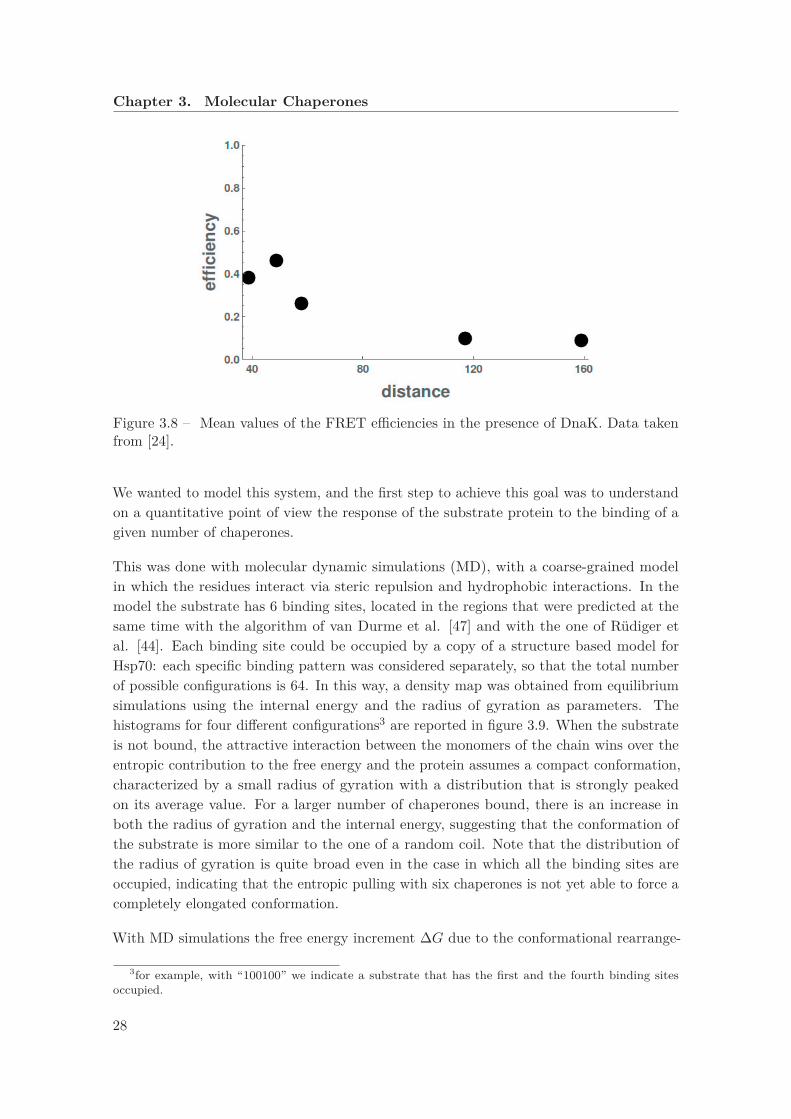
The mean values of the FRET efficiency for a system in the presence of chaperones isplotted in figure 3.8. We will soon discuss the validity of our model by a comparison of ourprediction with these data.
27
Chapter 3. Molecular Chaperones
Figure 3.8 – Mean values of the FRET efficiencies in the presence of DnaK. Data takenfrom [24].
We wanted to model this system, and the first step to achieve this goal was to understandon a quantitative point of view the response of the substrate protein to the binding of agiven number of chaperones.
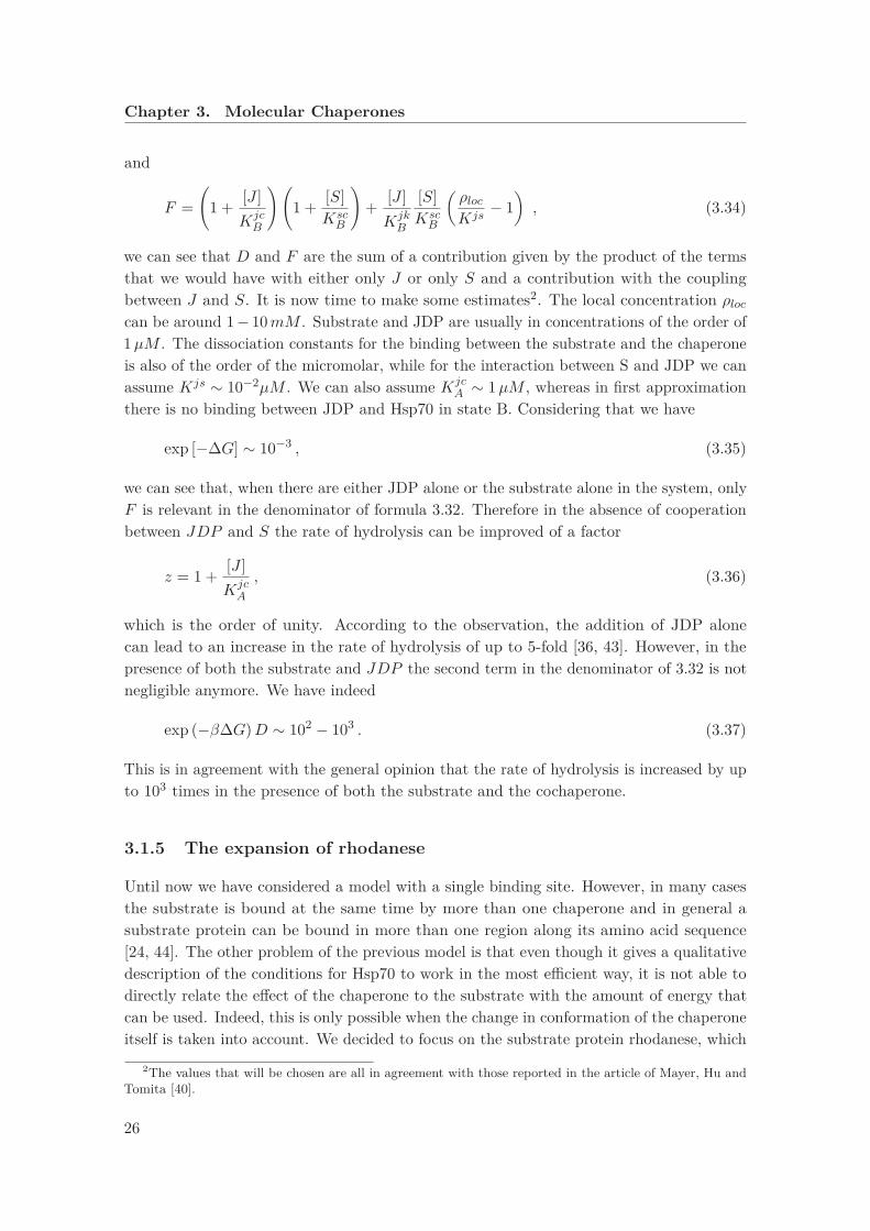
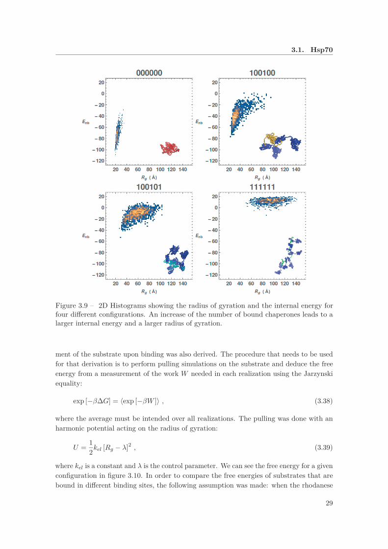
This was done with molecular dynamic simulations (MD), with a coarse-grained modelin which the residues interact via steric repulsion and hydrophobic interactions. In themodel the substrate has 6 binding sites, located in the regions that were predicted at thesame time with the algorithm of van Durme et al. [47] and with the one of Rüdiger etal. [44]. Each binding site could be occupied by a copy of a structure based model forHsp70: each specific binding pattern was considered separately, so that the total numberof possible configurations is 64. In this way, a density map was obtained from equilibriumsimulations using the internal energy and the radius of gyration as parameters. Thehistograms for four different configurations3 are reported in figure 3.9. When the substrateis not bound, the attractive interaction between the monomers of the chain wins over theentropic contribution to the free energy and the protein assumes a compact conformation,characterized by a small radius of gyration with a distribution that is strongly peakedon its average value. For a larger number of chaperones bound, there is an increase inboth the radius of gyration and the internal energy, suggesting that the conformation ofthe substrate is more similar to the one of a random coil. Note that the distribution ofthe radius of gyration is quite broad even in the case in which all the binding sites areoccupied, indicating that the entropic pulling with six chaperones is not yet able to force acompletely elongated conformation.
With MD simulations the free energy increment ΔG due to the conformational rearrange-
3for example, with “100100” we indicate a substrate that has the first and the fourth binding sitesoccupied.
28
3.1. Hsp70
Figure 3.9 – 2D Histograms showing the radius of gyration and the internal energy forfour different configurations. An increase of the number of bound chaperones leads to alarger internal energy and a larger radius of gyration.
ment of the substrate upon binding was also derived. The procedure that needs to be usedfor that derivation is to perform pulling simulations on the substrate and deduce the freeenergy from a measurement of the work W needed in each realization using the Jarzynskiequality:
exp [−βΔG] = 〈exp [−βW ]〉 , (3.38)
where the average must be intended over all realizations. The pulling was done with anharmonic potential acting on the radius of gyration:
U = 12kel [Rg − λ]2 , (3.39)
where kel is a constant and λ is the control parameter. We can see the free energy for a givenconfiguration in figure 3.10. In order to compare the free energies of substrates that arebound in different binding sites, the following assumption was made: when the rhodanese
29
Chapter 3. Molecular Chaperones
Figure 3.10 – Free energy from a pulling simulation for the configuration with the 2nd, 4thand 6th binding sites occupied.
is completely stretched, its free energy can be considered to be the same independently onthe binding configuration. Therefore the curves relative to different configurations weresuperimposed so that the limiting values for large pulling forces were the same (an exampleis shown in figure 3.11).
Figure 3.11 – Superposition of the averaged curves for three configurations.
Once we had the partial free energy relative to a precise value of the control parameter weevaluated the thermodynamic average to obtain the total free energy required for the ratemodel.
30

3.1. Hsp70
In figure 3.12 ΔG is plotted as a function of the number of bound chaperones n, for eachconfiguration. The increment in free energy corresponding to the addition of one chaperone
Figure 3.12 – Free energy of each configuration as a function of the stoichiometry.
is taken into account in the value of the dissociation constant:
Kd(i, j) → K0d(i, j) exp [−ΔΔGi,j ] , (3.40)
where Kd(i, j) is the dissociation constant for the binding reaction between state i and statej, K0
d(i, j) is the dissociation constant for the isolated binding site (without consideringthe change in conformation of the whole substrate) and ΔΔGi,j is the relative incrementin free energy. Experimental evidence suggests that the unbinding rate of Hsp70 from largeproteins is similar to the one from single peptides, whereas the binding rate can be up totwo orders of magnitude smaller [24, 38, 48]. Therefore, the rate that must be different forthe protein and for the single peptide is the binding rate.
We can now focus on the thermodynamics of the binding interaction between Hsp70 and thesubstrate protein, addressing in particular how the binding of the chaperones is influencedby the amount of energy that is available in the form of ATP. In an article of Barducciand De Los Rios [21] the dependence of the binding affinity on the non equilibrium regimeinduced by the hydrolysis of ATP was discussed in the case of single binding sites. Inthat work it was explained how chaperones can achieve an effective binding affinity forthe client peptide that is larger than the affinity that they would have in the ADP or inthe ATP state and this ultra-affinity is only possible if the system is out-of equilibrium.Here, we need to do a step further and consider as a substrate a protein with the sixbinding sites that have been mentioned above. We implemented a rate model in whicheach state corresponds to a single configuration, identified by the positions of all the boundchaperones in the ATP and in the ADP state. Therefore, since each of the six binding sitescan be free, bound with a chaperone in the ATP or in the ADP state, we have in total
31
Chapter 3. Molecular Chaperones
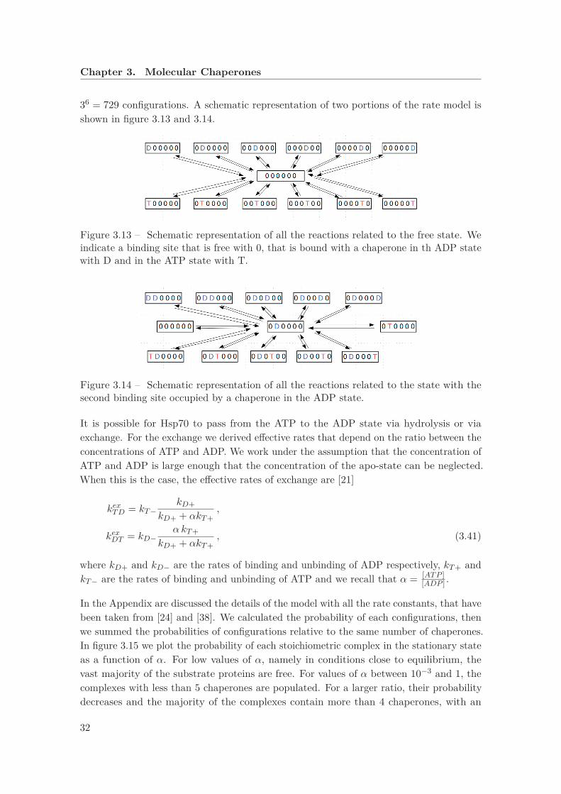
36 = 729 configurations. A schematic representation of two portions of the rate model isshown in figure 3.13 and 3.14.
Figure 3.13 – Schematic representation of all the reactions related to the free state. Weindicate a binding site that is free with 0, that is bound with a chaperone in th ADP statewith D and in the ATP state with T.
Figure 3.14 – Schematic representation of all the reactions related to the state with thesecond binding site occupied by a chaperone in the ADP state.
It is possible for Hsp70 to pass from the ATP to the ADP state via hydrolysis or viaexchange. For the exchange we derived effective rates that depend on the ratio between theconcentrations of ATP and ADP. We work under the assumption that the concentration ofATP and ADP is large enough that the concentration of the apo-state can be neglected.When this is the case, the effective rates of exchange are [21]
kexTD = kT−kD+
kD+ + αkT+,
kexDT = kD−αkT+
kD+ + αkT+, (3.41)
where kD+ and kD− are the rates of binding and unbinding of ADP respectively, kT+ andkT− are the rates of binding and unbinding of ATP and we recall that α = [ATP ]
[ADP ] .
In the Appendix are discussed the details of the model with all the rate constants, that havebeen taken from [24] and [38]. We calculated the probability of each configurations, thenwe summed the probabilities of configurations relative to the same number of chaperones.In figure 3.15 we plot the probability of each stoichiometric complex in the stationary stateas a function of α. For low values of α, namely in conditions close to equilibrium, thevast majority of the substrate proteins are free. For values of α between 10−3 and 1, thecomplexes with less than 5 chaperones are populated. For a larger ratio, their probabilitydecreases and the majority of the complexes contain more than 4 chaperones, with an
32

3.1. Hsp70
average number between 5 and 6. It is possible to define an effective dissociation constant
Figure 3.15 – Probability of each stoichiometry as a function of the ratio [ATP ][ADP ] . To an
increase in [ATP ][ADP ] corresponds a larger number of bound chaperones.
Kd as
Kd =[ 6
〈n〉 − 1]
[DnaK] , (3.42)
where 〈n〉 is the average number of occupied binding sites. In figure 3.16 we report thedissociation constant divided by its value in equilibrium as a function of α.In [21] the rate of hydrolysis was used to quantify the degree of non equilibrium. Here, wedecided to use the parameter α, since it is more directly related to the energy that thechemostat can inject into the system.In equilibrium conditions Kd is equal to the dissociation constant of a chaperone in ADPstate. When the concentration of ATP is larger, the dissociation constant is well belowthat value, as predicted in [21]. The red region in the figure is the ultra-affinity region,namely the gain in affinity caused by the non equilibrium.
A direct measure of the expansion of rhodanese is provided by the radius of gyration.The average value was measured in the equilibrium MD simulation for each configuration.We then calculated the average over all the configurations weighting each term with theconcentrations obtained with the rate model. When calculating the main quantities of
33
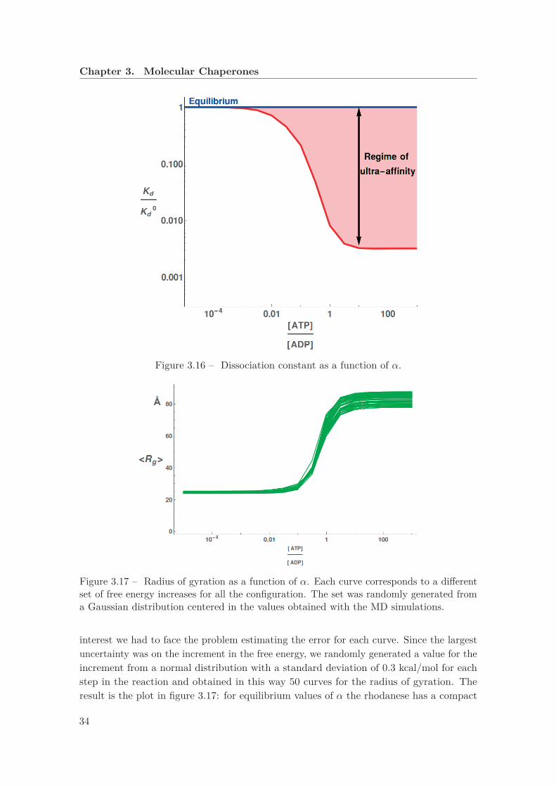
Chapter 3. Molecular Chaperones
Figure 3.16 – Dissociation constant as a function of α.
Figure 3.17 – Radius of gyration as a function of α. Each curve corresponds to a differentset of free energy increases for all the configuration. The set was randomly generated froma Gaussian distribution centered in the values obtained with the MD simulations.
interest we had to face the problem estimating the error for each curve. Since the largestuncertainty was on the increment in the free energy, we randomly generated a value for theincrement from a normal distribution with a standard deviation of 0.3 kcal/mol for eachstep in the reaction and obtained in this way 50 curves for the radius of gyration. Theresult is the plot in figure 3.17: for equilibrium values of α the rhodanese has a compact
34
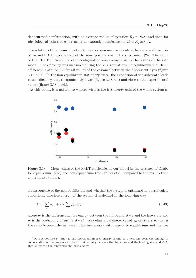
3.1. Hsp70
denaturated conformation, with an average radius of gyration Rg � 25Å, and then forphysiological values of α it reaches an expanded conformation with Rg � 80Å.
The solution of the chemical network has also been used to calculate the average efficienciesof virtual FRET dyes placed at the same positions as in the experiment [24]. The valueof the FRET efficiency for each configuration was averaged using the results of the ratemodel. The efficiency was measured during the MD simulations. In equilibrium the FRETefficiency is around 0.8 for all values of the distance between the fluorescent dyes (figure3.18 blue). In the non equilibrium stationary state, the expansion of the substrate leadsto an efficiency that is significantly lower (figure 3.18 red) and close to the experimentalvalues (figure 3.18 black).At this point, it is natural to wonder what is the free energy gain of the whole system as
Figure 3.18 – Mean values of the FRET efficiencies in our model in the presence of DnaK,for equilibrium (blue) and non equilibrium (red) values of α, compared to the result of theexperiments (black).
a consequence of the non equilibrium and whether the system is optimized in physiologicalconditions. The free energy of the system Ω is defined in the following way
Ω =∑i
pigi +RT∑i
pi ln pi (3.43)
where gi is the difference in free energy between the ith bound state and the free state andpi is the probability of such a state 4. We define a parameter called effectiveness, θ, that isthe ratio between the increase in the free energy with respect to equilibrium and the free
4Do not confuse gi, that is the increment in free energy taking into account both the change inconformation of the protein and the intrinsic affinity between the chaperone and the binding site, and ΔGi,that is instead the conformational free energy.
35

Chapter 3. Molecular Chaperones
energy that is available in the form of ATP:
θ = Ω − Ωeq
6 ln[
ααeq
] , (3.44)
where αeq is the ratio between the concentration of ATP and ADP in equilibrium conditionsand the number 6 is due to the fact that there are in total six binding sites, therefore inprinciple the hydrolysis of six ATP molecules could take place at the same time. In figure
Figure 3.19 – Effectiveness (purple) as a function of α, together with its numerator (green)and denominator (orange).
3.19 we plot the effectiveness (purple), together with its numerator (green), that is the freeenergy difference with respect to equilibrium, and its denominator (orange), the free energyavailable in the form of ATP. The increase of the free energy of the system reaches a plateauwhen the ratio α is close to the one of physiological conditions (α ∈ (1, 10)). Therefore, wecan conclude that the physiological conditions are in an interval of parameters such thatthe improvement in the binding affinity is achieved at an optimal energetic cost.
36
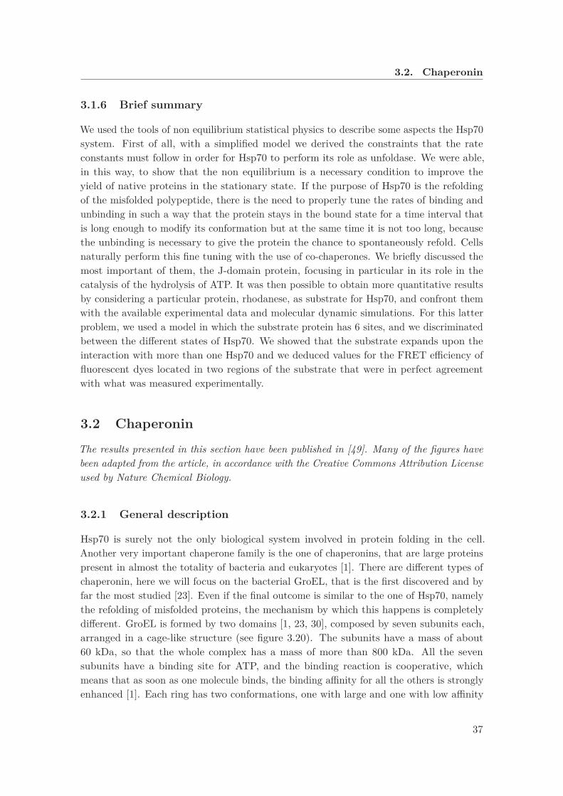
3.2. Chaperonin
3.1.6 Brief summary
We used the tools of non equilibrium statistical physics to describe some aspects the Hsp70system. First of all, with a simplified model we derived the constraints that the rateconstants must follow in order for Hsp70 to perform its role as unfoldase. We were able,in this way, to show that the non equilibrium is a necessary condition to improve theyield of native proteins in the stationary state. If the purpose of Hsp70 is the refoldingof the misfolded polypeptide, there is the need to properly tune the rates of binding andunbinding in such a way that the protein stays in the bound state for a time interval thatis long enough to modify its conformation but at the same time it is not too long, becausethe unbinding is necessary to give the protein the chance to spontaneously refold. Cellsnaturally perform this fine tuning with the use of co-chaperones. We briefly discussed themost important of them, the J-domain protein, focusing in particular in its role in thecatalysis of the hydrolysis of ATP. It was then possible to obtain more quantitative resultsby considering a particular protein, rhodanese, as substrate for Hsp70, and confront themwith the available experimental data and molecular dynamic simulations. For this latterproblem, we used a model in which the substrate protein has 6 sites, and we discriminatedbetween the different states of Hsp70. We showed that the substrate expands upon theinteraction with more than one Hsp70 and we deduced values for the FRET efficiency offluorescent dyes located in two regions of the substrate that were in perfect agreementwith what was measured experimentally.
3.2 Chaperonin
The results presented in this section have been published in [49]. Many of the figures havebeen adapted from the article, in accordance with the Creative Commons Attribution Licenseused by Nature Chemical Biology.
3.2.1 General description
Hsp70 is surely not the only biological system involved in protein folding in the cell.Another very important chaperone family is the one of chaperonins, that are large proteinspresent in almost the totality of bacteria and eukaryotes [1]. There are different types ofchaperonin, here we will focus on the bacterial GroEL, that is the first discovered and byfar the most studied [23]. Even if the final outcome is similar to the one of Hsp70, namelythe refolding of misfolded proteins, the mechanism by which this happens is completelydifferent. GroEL is formed by two domains [1, 23, 30], composed by seven subunits each,arranged in a cage-like structure (see figure 3.20). The subunits have a mass of about60 kDa, so that the whole complex has a mass of more than 800 kDa. All the sevensubunits have a binding site for ATP, and the binding reaction is cooperative, whichmeans that as soon as one molecule binds, the binding affinity for all the others is stronglyenhanced [1]. Each ring has two conformations, one with large and one with low affinity
37

Chapter 3. Molecular Chaperones
Figure 3.20 – Structure of GroEL. Figure taken from [1].
for ATP. The binding of a nucleotide stabilizes the former with respect to the latter. Theway the nucleotides are used to tune the affinity for the client protein is the opposite ofthe one of Hsp70 [50, 51], because the ADP state has lower affinity than the ATP state[1, 23], therefore the hydrolysis stimulates the unbinding rather than the binding reaction.The cage also has a cover, a protein called GroES, formed by seven subunits of about10 kDa. GroES is responsible to close the cage after the substrate protein has entered[1]. We will often indicate the whole complex GroEL/GroES by simply writing GroELS.The precise mechanism of refolding is still a matter of animate discussions: we can saythat the models that by now have more popularity in the chaperones community areessentially three: Anfinsen cage (AC), active folding (AF) and iterative annealing (IA).According to the AC model, as the name suggests, GroEL does nothing but protectingthe substrate protein from aggregation, leaving it in an environment that is suitable forfolding, even though the protein refolds at the same rates that it would have in the caseof a spontaneous refolding in conditions in which there is not the obstacle of aggregation.Therefore, the role of GroEL would be to deplete the misfolded state in order to reducethe mean speed of the aggregation process. However, several experiments have shown thatit is possible for GroEL to accelerate the refolding, instead of just increasing the yield ofthe functional conformation once the stationary state has been reached [52, 53]. The replyof the supporters of the AC model is that the aggregation might be a reversible process: ifthis is the case, the apparent acceleration of the refolding can be explained as the result ofthe rescue of proteins from aggregates. In an article published in Pnas [54], Apetri andHorwich monitored the folding of Rubisco in different conditions. They did confirm thatthere was an acceleration of the refolding in the presence of GroEL. However, they alsoshowed that Rubisco was able to spontaneously refold when the aggregation was obstructedby the presence of bovine serum albumin (BSA). Moreover, they showed that when theyused the maltose binding protein (MBP) as a substrate the refolding had the same speedwhen it was spontaneous and when it was helped by the chaperonin, providing that theyartificially created the conditions necessary to avoid aggregation. They thus concludedthat the role of GroEL was to protect the substrate proteins from reversible aggregationand that the chaperone was not able to actively enhance their conformational remodeling.
38

3.2. Chaperonin
The strongest argument against the AC model lies in the fact that GroEL has been shownto successfully stimulate protein refolding even at concentrations of the substrate that areso low that the aggregation can be neglected [52, 55]. This is the main reason why modelspostulating an active role of GroEL in the refolding process have been proposed [23, 1].
In the AF model the hydrophilic walls of the chaperonin participate to the folding of thesubstrate protein via steric repulsion [56, 1]. The reduced available volume inside the cagefavors the formation of the bonds required for the tertiary structure of the native state.The role of confinement in protein folding has been demonstrated with MD simulationsby Baumketner and co-workers [57]. The power of the AF model is that it is able toexplain why the refolding is accelerated even for very small concentration of substrateproteins, which indicates a low probability of aggregation, and even when GroELS isin sub-stoichiometric amount. In 2014 Gupta and co-workers [52] demonstrated withfluorescence resonance energy transfer spectroscopy (FRET) that GroEL can accelerate therefolding of a mutant of the maltose binding protein at concentrations as low as 100 pM,arguing for this reason that the AF is likely the most promising model, since aggregationis not a relevant factor at those concentrations.
Another possible explanation, non necessarily in conflict with the previous one, is theiterative annealing (IA). According to this model, GroEL stimulates the unfolding of themisfolded proteins and gives them a chance to properly refold spontaneously, either insideor outside the cage, and this can be accomplished after several binding/release cycles. Linand co-workers [53] used FRET spectroscopy to show how a misfolded substrate unfoldsin the presence of GroEL and ATP. As a substrate they used Ribulose-1,5-bisphosphatecarboxylase/oxygenase (known as RuBisCO), which is an abundant enzyme involved in theprocess of carbon fixation[58], that after denaturation is found in misfolded conformationsthat are susceptible to aggregation even at 25 ◦C. The unfolding time of misfolded RuBisCOis longer than the average time in which it is bound with GroEL [53, 59], therefore theyconcluded that the transformation that leads to a recovery of the functional state happensvia several cycles of binding and release and it is thus unlikely that the active refoldingcould be the only process by which the functional state is recovered.
3.2.2 Out-of-equilibrium stabilization of the functional state
Rather than trying to validate or disprove any model, we wanted to deepen a conceptthat is maybe slightly undervalued by part of the chaperone community, that is the out-of-equilibrium intrinsic nature of the chaperone systems and GroELS in particular. Wewanted to show that even in some stress conditions in which the functional conformationof the substrate does not correspond to a minimum in the free energy landscape, and thusit is not the one that is favored in equilibrium, it is possible for the GroELS system tostabilize the functional conformation in a non equilibrium steady state (NESS). We devisedthis work in collaboration with the group of Goloubinoff in the University of Lausanne,which also performed all the experiments, and with Alessandro Barducci in the University
39
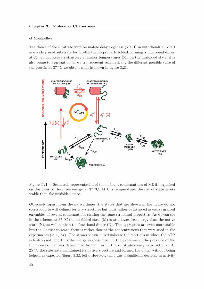
Chapter 3. Molecular Chaperones
of Montpellier.
The choice of the substrate went on malate dehydrogenase (MDH) in mitochondria. MDHis a widely used substrate for GroEL that is properly folded, forming a functional dimer,at 25 ◦C, but loses its structure at higher temperatures [55]. In the misfolded state, it isalso prone to aggregation. If we try represent schematically the different possible state ofthe protein at 37 ◦C we obtain what is shown in figure 3.21.
Figure 3.21 – Schematic representation of the different conformations of MDH, organizedon the basis of their free energy at 37 ◦C. At this temperature, the native state is lessstable than the misfolded state.
Obviously, apart from the native dimer, the states that are shown in the figure do notcorrespond to well defined tertiary structures but must rather be intended as coarse grainedensembles of several conformations sharing the same structural properties. As we can seein the scheme, at 37 ◦C the misfolded state (M) is at a lower free energy than the nativestate (N), as well as than the functional dimer (D). The aggregates are even more stablebut the kinetics to reach them is rather slow at the concentrations that were used in theexperiments (< 1μM). The arrows shown in red indicate the reactions in which the ATPis hydrolyzed, and thus the energy is consumed. In the experiment, the presence of thefunctional dimer was determined by monitoring the substrate’s enzymatic activity. At25 ◦C the substrate maintained its native structure and formed the dimer without beinghelped, as expected (figure 3.22, left). However, there was a significant decrease in activity
40

3.2. Chaperonin
at 37 ◦C, as we can see in figure 3.22(right). If only GroELS was added, the denaturationstill occurred at the same rate and the activity was not recovered (blue data). On thecontrary, when ATP and a regeneration system were present5, a clear reactivation wasmeasured and MDH remained stable for more than 2 hours (red data).
Figure 3.22 – (left) Enzymatic activity of MDH at 25 ◦C as a function of time, for differentexperimental set-ups. (right) Enzymatic activity of MDH at 37 ◦C as a function of time,for different experimental set-ups. For both the blue and the red curve GroELS was addedafter 160 min, but only for the red curve there was also an addition of ATP.
To determine which fraction of the substrate was not possible to recover because it wastrapped in irreversible aggregations, an experiment was performed in which GroELS andATP where added at different times. The aggregation started to be significant after a quitelarge time (see figure 3.23, left), suggesting that the irreversible aggregation was a slowprocess.As a consequence, unless we assume that there is a reversible aggregation that is fastenough to compete with the refolding process and thus to slow the net refolding rate, wemust conclude that the conformational rearrangement of the substrate protein is activelyenhanced by GroELS. In figure 3.23(right) we show how the different conformations aredistribute once the stationary state is reached, for different value of the time in whichGroELS and ATP are added to the system. Note that the native monomer is included inthe non-recoverable fraction, since native MDH monomers need to form dimers in orderto be functional and thus to contribute to the enzymatic activity. In the presence ofchaperones and ATP, the native state could be maintained for a long time (figure 3.24,left), or it could be recovered if at the initial time MDH was denaturated (figure 3.24,right). However, upon the addiction of apyrase, an enzyme known to massively catalyze
5Which means that the ATP concentration could be considered constant for the time scales underconsideration.
41
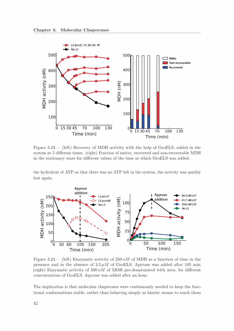
Chapter 3. Molecular Chaperones
Figure 3.23 – (left) Recovery of MDH activity with the help of GroELS, added in thesystem at 5 different times. (right) Fraction of native, recovered and non-recoverable MDHin the stationary state for different values of the time at which GroELS was added.
the hydrolysis of ATP so that there was no ATP left in the system, the activity was quicklylost again.
Figure 3.24 – (left) Enzymatic activity of 250nM of MDH as a function of time in thepresence and in the absence of 3.5μM of GroELS. Apyrase was added after 105 min.(right) Enzymatic activity of 500nM of MDH pre-denaturated with urea, for differentconcentrations of GroELS. Apyrase was added after an hour.
The implication is that molecular chaperones were continuously needed to keep the func-tional conformations stable, rather than behaving simply as kinetic means to reach them
42

3.2. Chaperonin
from the misfolded state. The free energy ΔGh that is available thanks to the hydrolysisof ATP is given by
ΔGh = kbT ln[
[ATP ]kh[ADP ][Pi]ksy
]= kbT ln
[ [ATP ][ADP ][Pi]
]−kbT ln
[[ATP ]eq
[ADP ]eq[Pi]eq
], (3.45)
where with kh and ksy we indicate the rates of hydrolysis and synthesis and with thesubscript eq we indicate concentrations in equilibrium. Note that in equilibrium conditionswe have ΔGh = 0, as we should expect, since the detailed balance is satisfied:
[ATP ]eqkh − [ADP ]eq[Pi]eqksy = 0 . (3.46)
We can see that the free energy is a function of the ratio between the concentration of ATPand ADP. As a consequence, a part from being lower for lower concentrations of ATP, it alsodecreases if the concentration of ATP does not change while we increase the concentrationof ADP. Without the use of the free energy, a more intuitive explanation is that if thereis overabundance of ADP with respect to ATP there will be too many chaperones in theADP state and the kinetic cycle will not be effectively followed in the right direction. Thisphenomenon is shown in figure 3.25 (right), where the enzymatic activity of MDH at 37 ◦Cis plotted as a function of time for different values of the concentration of ADP, while theATP was kept at a concentration of 400μM . We can see that in a first stage GroELS isable to successfully refold the misfolded MDH, which recovers its activity. However, sincethis experiment was performed without a regeneration system of ATP, after a certain timethe energy supplied starts decreasing until the system is found in equilibrium, where as weknow the substrate is mostly misfolded and thus the enzymatic activity is very low.
Refolding processes of this kind can be rationalized with a rate model. In this case anon linear approach is needed, because both the dimerization and the aggregation areprocesses that depend on multiplications of two concentrations. We assumed that onlyproteins in the intermediate or misfolded state can bind to the chaperone. This assumptionis substained by experimental observations showing that a substrate in the native statehas a negligible affinity for GroEL [52]. We also assumed that proteins in misfolded orintermediate state can form aggregates irreversibly. Moreover, proteins that are already inaggregates can aggregate with other non native proteins. However, we did not discriminatebetween aggregates composed of different numbers of proteins. The chemical network is
43

Chapter 3. Molecular Chaperones
Figure 3.25 – MDH activity as a function of time, for different values of ADP. Theconcentration of ATP was kept at an initial value of 400μM (with the exclusion of theblack curve), but the experiments were performed without a regeneration system of ATP.
regulated by the following system of equations:
d[D]dt
= − 2kDN [D] + 2kND[N ]2
d[N ]dt
= − kNI [N ] − 2kND[N ]2 + 2kDN [D] + kIN [I]
d[I]dt
= − (kIN + kIM ) [I] + kNI [N ] + kMI [M ]+
− kagg ([M ] + 2[I] + [A]) [I] + koffI [CI] − konI [C][I]d[M ]dt
= − kMI [M ] + kIM [I] − kagg (2[M ] + [I] + [A]) [M ]+
+ koffM [CM ] − konM [C][M ]d[A]dt
= 2kagg([M ][I] + [M ]2 + [I]2
)+ kagg ([M ] + [I]) [A] (3.47)
d[CI]dt
= −(koffI + kCIM
)[CI] + konI [C][I] + kCMI [CM ]
d[CM ]dt
= −(koffM + kCMI
)[CM ] + konM [C][M ] + kCIM [CI]
d[C]dt
= − konI [C][I] − konM [C][M ] + koffI [CI] + koffM [CM ] .
The notation is the following:
44
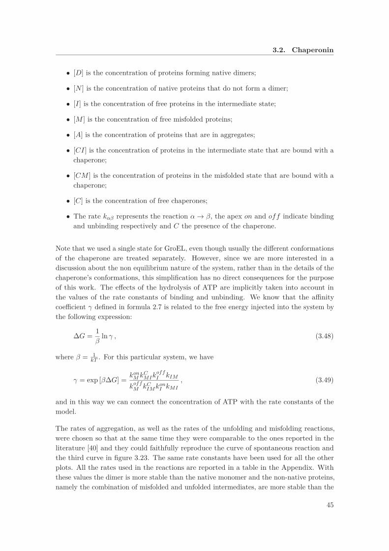
3.2. Chaperonin
• [D] is the concentration of proteins forming native dimers;
• [N ] is the concentration of native proteins that do not form a dimer;
• [I] is the concentration of free proteins in the intermediate state;
• [M ] is the concentration of free misfolded proteins;
• [A] is the concentration of proteins that are in aggregates;
• [CI] is the concentration of proteins in the intermediate state that are bound with achaperone;
• [CM ] is the concentration of proteins in the misfolded state that are bound with achaperone;
• [C] is the concentration of free chaperones;
• The rate kαβ represents the reaction α → β, the apex on and off indicate bindingand unbinding respectively and C the presence of the chaperone.
Note that we used a single state for GroEL, even though usually the different conformationsof the chaperone are treated separately. However, since we are more interested in adiscussion about the non equilibrium nature of the system, rather than in the details of thechaperone’s conformations, this simplification has no direct consequences for the purposeof this work. The effects of the hydrolysis of ATP are implicitly taken into account inthe values of the rate constants of binding and unbinding. We know that the affinitycoefficient γ defined in formula 2.7 is related to the free energy injected into the system bythe following expression:
ΔG = 1β
ln γ , (3.48)
where β = 1kT . For this particular system, we have
γ = exp [βΔG] = konM kCMIk
offI kIM
koffM kCIMkonI kMI
, (3.49)
and in this way we can connect the concentration of ATP with the rate constants of themodel.
The rates of aggregation, as well as the rates of the unfolding and misfolding reactions,were chosen so that at the same time they were comparable to the ones reported in theliterature [40] and they could faithfully reproduce the curve of spontaneous reaction andthe third curve in figure 3.23. The same rate constants have been used for all the otherplots. All the rates used in the reactions are reported in a table in the Appendix. Withthese values the dimer is more stable than the native monomer and the non-native proteins,namely the combination of misfolded and unfolded intermediates, are more stable than the
45
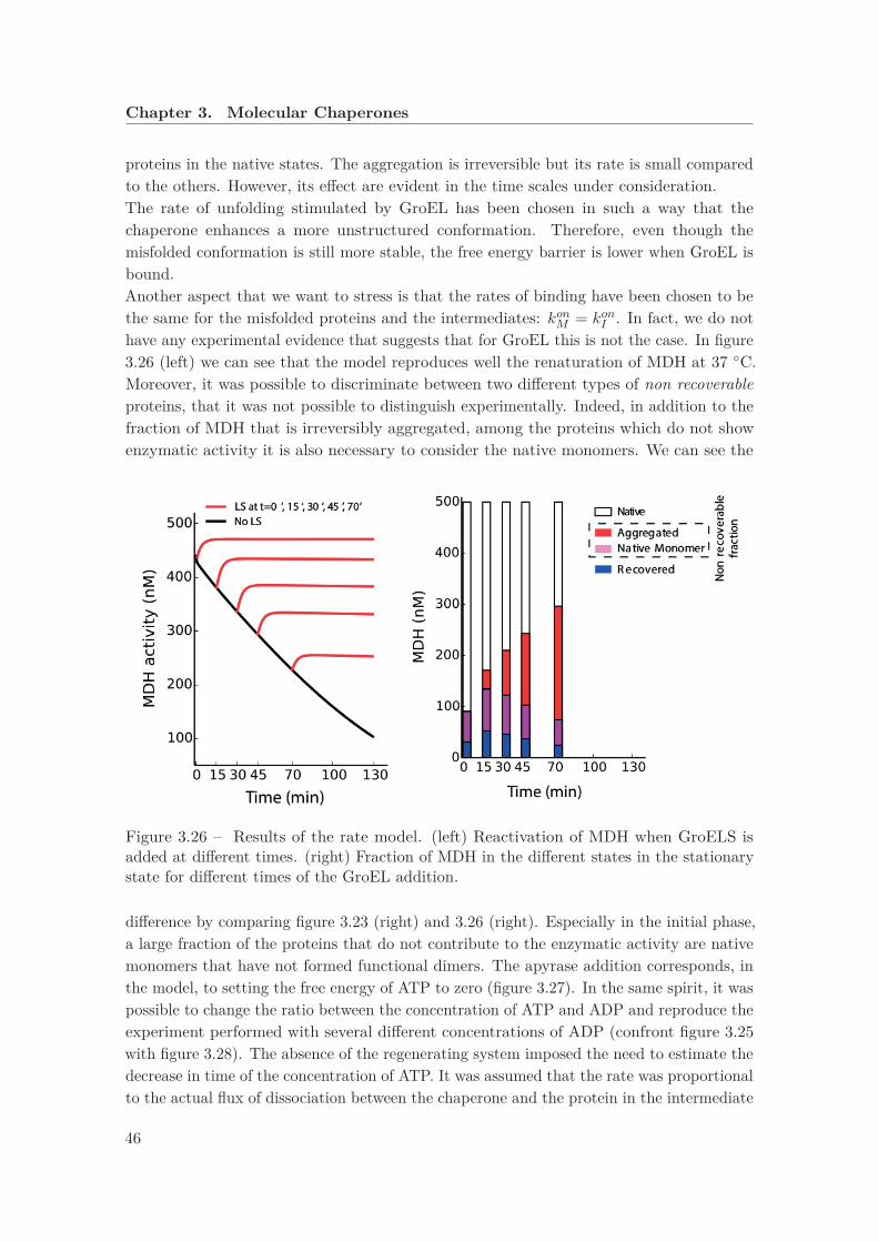
Chapter 3. Molecular Chaperones
proteins in the native states. The aggregation is irreversible but its rate is small comparedto the others. However, its effect are evident in the time scales under consideration.The rate of unfolding stimulated by GroEL has been chosen in such a way that thechaperone enhances a more unstructured conformation. Therefore, even though themisfolded conformation is still more stable, the free energy barrier is lower when GroEL isbound.Another aspect that we want to stress is that the rates of binding have been chosen to bethe same for the misfolded proteins and the intermediates: konM = konI . In fact, we do nothave any experimental evidence that suggests that for GroEL this is not the case. In figure3.26 (left) we can see that the model reproduces well the renaturation of MDH at 37 ◦C.Moreover, it was possible to discriminate between two different types of non recoverableproteins, that it was not possible to distinguish experimentally. Indeed, in addition to thefraction of MDH that is irreversibly aggregated, among the proteins which do not showenzymatic activity it is also necessary to consider the native monomers. We can see the
Figure 3.26 – Results of the rate model. (left) Reactivation of MDH when GroELS isadded at different times. (right) Fraction of MDH in the different states in the stationarystate for different times of the GroEL addition.
difference by comparing figure 3.23 (right) and 3.26 (right). Especially in the initial phase,a large fraction of the proteins that do not contribute to the enzymatic activity are nativemonomers that have not formed functional dimers. The apyrase addition corresponds, inthe model, to setting the free energy of ATP to zero (figure 3.27). In the same spirit, it waspossible to change the ratio between the concentration of ATP and ADP and reproduce theexperiment performed with several different concentrations of ADP (confront figure 3.25with figure 3.28). The absence of the regenerating system imposed the need to estimate thedecrease in time of the concentration of ATP. It was assumed that the rate was proportionalto the actual flux of dissociation between the chaperone and the protein in the intermediate
46
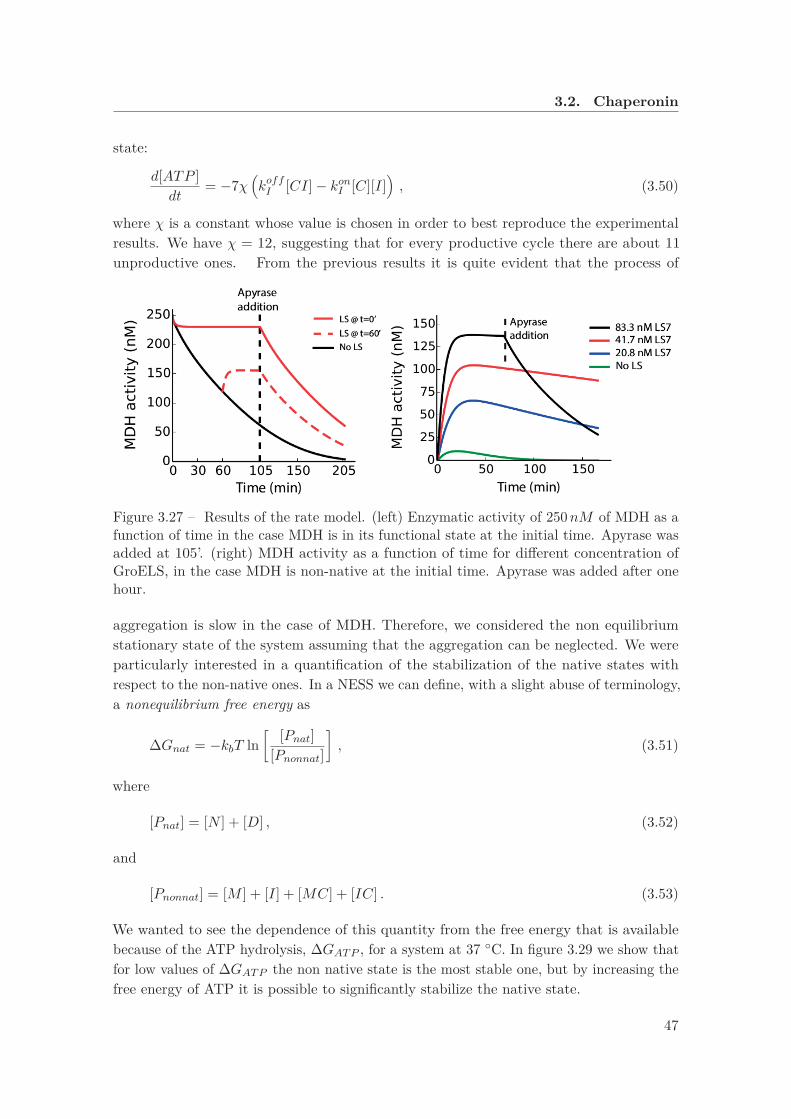
3.2. Chaperonin
state:
d[ATP ]dt
= −7χ(koffI [CI] − konI [C][I]
), (3.50)
where χ is a constant whose value is chosen in order to best reproduce the experimentalresults. We have χ = 12, suggesting that for every productive cycle there are about 11unproductive ones. From the previous results it is quite evident that the process of
Figure 3.27 – Results of the rate model. (left) Enzymatic activity of 250nM of MDH as afunction of time in the case MDH is in its functional state at the initial time. Apyrase wasadded at 105’. (right) MDH activity as a function of time for different concentration ofGroELS, in the case MDH is non-native at the initial time. Apyrase was added after onehour.
aggregation is slow in the case of MDH. Therefore, we considered the non equilibriumstationary state of the system assuming that the aggregation can be neglected. We wereparticularly interested in a quantification of the stabilization of the native states withrespect to the non-native ones. In a NESS we can define, with a slight abuse of terminology,a nonequilibrium free energy as
ΔGnat = −kbT ln[ [Pnat]
[Pnonnat]
], (3.51)
where
[Pnat] = [N ] + [D] , (3.52)
and
[Pnonnat] = [M ] + [I] + [MC] + [IC] . (3.53)
We wanted to see the dependence of this quantity from the free energy that is availablebecause of the ATP hydrolysis, ΔGATP , for a system at 37 ◦C. In figure 3.29 we show thatfor low values of ΔGATP the non native state is the most stable one, but by increasing thefree energy of ATP it is possible to significantly stabilize the native state.
47

Chapter 3. Molecular Chaperones
Figure 3.28 – Results of the rate model. MDH activity as a function of time for differentconcentrations of ADP. The system was considered to be without a regenerating system,so that the concentration of ATP decreases over time.
Figure 3.29 – Results of the rate model in the NESS. The nonequilibrium free energy ofthe native ensemble is plotted as a function of the energy that is available in the form ofATP.
48

3.2. Chaperonin
The equilibrium stability of the native state can be tuned by changing, for example, therate constant of misfolding. We define the free energy difference between the native andnon native ensemble:
ΔGeqnat = −kbT ln
[[Pnat]eq
[Pnonnat]eq
], (3.54)
which we can see as a quantitative estimation of the stress factors that inhibit a spontaneousrefolding of the substrate. We were interested to see in which interval of ΔGeq
nat therewas a stronger non equilibrium stabilization of the functional state. In figure 3.30 we plotthe fraction of native MDH as a function of ΔGeq
nat. The gray region represents the gainin native structure due to the energy consumption of the ATP hydrolysis. For energiesgaps larger than 5 kcal/mol the substrate is so prone to the misfolded state that even inthe presence of GroELS it is not possible to stabilize the native state. On the contrary,when ΔGeq
nat < 2 kcal/mol the functional state is stable also in equilibrium. For values ofthe free energy inside that interval GroELS is able to use the non equilibrium regime tosignificantly increase the yield of native proteins.
Figure 3.30 – Results of the rate model in the NESS. Fraction of native MDH as a functionof the difference in free energy between native and misfolded ensembles.
49
Chapter 3. Molecular Chaperones
3.2.3 Brief summary
We wanted to demonstrate that GroELS can stabilize the functional conformation of agiven substrate protein even under stress conditions such that it would be normally foundin a misfolded state. The substrate that was used, the enzyme MDH, was inactive at 37◦C. However, in the presence of GroELS and ATP the enzymatic activity was recovered,but only as long as ATP was available. The experimental results were reproduced by arate model that includes aggregation, even though it turned out to be slow enough to beneglected in a first approximation. With an analysis of the non equilibrium stationarystate we showed the dependence of the refolding activity of GroELS from the free energyof ATP and from the intrinsic stability of the substrate in equilibrium conditions.
3.3 Conclusions
Despite the great interest that chaperone systems have among biologists, there are stillvery few works in which thermodynamics and statistical physics are used to investigatetheir mechanism. With our work we tried to give our contribution to fill this gap. Thanksto the constant effort directed to the characterization of the structure and the dynamics ofchaperone systems, lasted more than three decades, there are some general facts that arenow universally accepted:
• There are particular conditions in which proteins are not capable to reach theirfunctional structure by themselves.
• In these cases they can be helped, in some way, by molecular chaperones.
• In order to take part in the refolding process (regardless of what they actually do)chaperones must consume ATP.
Unfortunately, many questions concerning the facts just mentioned are still unansweredtoday. There is no general consensus on whether the aggregation is the only obstacle toproper folding in stress conditions or proteins can actually be more stable in a misfoldedstate independently of aggregation. It is still unclear how chaperones favor the refoldingof their substrate: do they actively stimulates the refolding? Do they just break thenon-native bonds leaving the protein the chance to refold spontaneously? Do they ratherjust prevent aggregation? Moreover, there is still the lack of an accepted model that isable to explain precisely how the hydrolysis of ATP is stimulated and in some cases thereis not even an agreement on its consequence on the chaperone dynamics [1, 23].Since our main goal was to determine what could be understood by simply consideringbasic thermodynamic principles, inevitably we had to abandon the level of molecular detailthat is often used. However, we managed, in this way, to use an approach that could lead tomore general results, that are true independently of the precise mechanism and sometimeseven of the chaperone system under study. For example it was possible to deduce some
50

3.3. Conclusions
constraint on the rate constants, as well as to demonstrate that the hydrolysis of ATP isnot just a contingent step in a complicated series of molecular transformation but rather anecessity that naturally follows from the rules of non equilibrium thermodynamics.Despite that, we also obtained some results that correctly reproduce the experimentalobservations, both in the case the GroELS system and in the case of Hsp70.
51

4 Atp-binding cassette transporters
4.1 Introduction
In order to move through the cell membrane, small molecules usually need the help ofspecific membrane proteins called transporters. The Atp-binding cassette transporters(ABC) are one of the most abundant family of transporters [60, 61, 62]; they use the energyof ATP to drive the transport of several molecules, like lipids, sugars, sterols and vitamins.Moreover, they are of particular interest for biomedical applications, since it has beendemonstrated [63, 64] that they can mediate the efflux of chemotherapeutic drugs from thecell, promoting in this way the multidrug resistance. ABC can be exporters or importers,but until now it has not been found any transporter that is able to perform both tasks[61]. The exporters are present in eukaryotes and prokaryotes, whereas the importers canonly be found in prokaryotes [20, 65].ABC are formed by two transmembrane domains (TMD, in yellow and cyan in figure 4.1),which are less conserved because they need to specifically bind to members of the hugevariety of available substrate molecules, and two nucleotide binding domains (NBD, inpurple and green in figure 4.1), more conserved, with the binding sites for ATP or ADP [66].The crucial point of the mechanism of ABCs is the allosteric interaction between the NBDand the TMD, that is usually described with the so called ATP-switch model [61, 67]. In themodel, the TMD can assume mainly two conformations: outward or inward facing. Experi-mental evidence suggests that for the majority of transporters when ATP is bound with theNBD the outward facing conformation is preferred, whereas when the ADP is bound theinward facing conformation is dominant [65, 67]. Therefore, the hydrolysis of ATP and theexchange are the reactions that enhance the conformational change in the ABC transporter.
4.1.1 Importers
In importers, the substrate is usually carried to the complex by a substrate binding protein(SBP) [68, 69]. For example, in the maltose uptake performed by the transporter MalFGK
53

Chapter 4. Atp-binding cassette transporters
Figure 4.1 – The structure of an ABC importer, together with a binding protein (red).Figure taken from [66].
an important role is played by the maltose-binding protein expressed from the gene malE[70], which in addition to bringing the substrate to the transporter also stimulates the hy-drolysis of ATP. Another very well known system in which the binding protein is extremelyimportant is the BtuCD in E. coli, that assists the import of vitamin B12 with the help of thebinding protein BtuF [71]. Usually, the loaded SBD interacts with the transporter when thelatter is in a conformation that would not be optimal for the binding of the substrate alone,and then it stimulates the conformational change required to increase the binding affinity[65]. The PBD, the ATP and the substrate are also responsible for the closing of the NBDthat stimulates the hydrolysis of ATP [70, 72]. After the hydrolysis of ATP, the ABC re-turns in the inward facing conformation [73], where it remains until the substrate is released.
4.1.2 Exporters
The exporters behave in a different way: the allosteric interaction between the TMD andthe NBD is similar to the one of the importers, but in this case the substrate binds whenthe ABC is inward facing and unbinds when it is outward facing, therefore the reactioncycle is followed in the opposite direction with respect to the importers. The exporterswork without the need of SBP. The binding of the substrate molecule to an inward facing
54
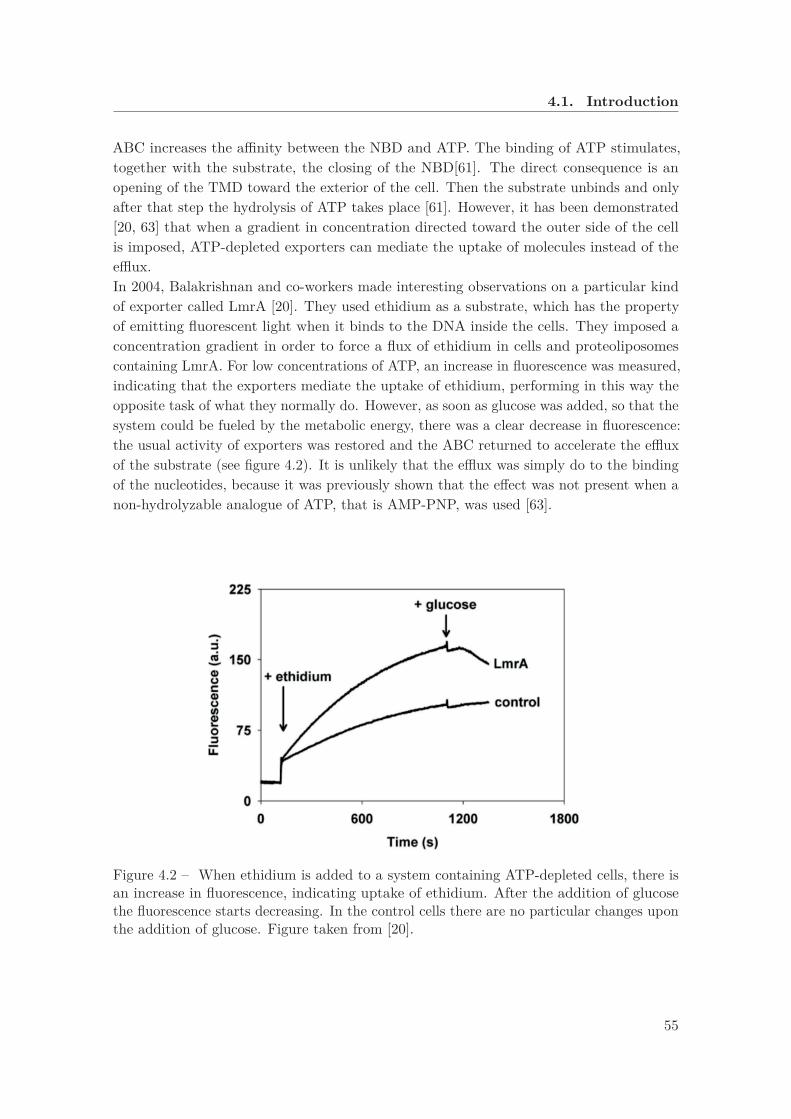
4.1. Introduction
ABC increases the affinity between the NBD and ATP. The binding of ATP stimulates,together with the substrate, the closing of the NBD[61]. The direct consequence is anopening of the TMD toward the exterior of the cell. Then the substrate unbinds and onlyafter that step the hydrolysis of ATP takes place [61]. However, it has been demonstrated[20, 63] that when a gradient in concentration directed toward the outer side of the cellis imposed, ATP-depleted exporters can mediate the uptake of molecules instead of theefflux.In 2004, Balakrishnan and co-workers made interesting observations on a particular kindof exporter called LmrA [20]. They used ethidium as a substrate, which has the propertyof emitting fluorescent light when it binds to the DNA inside the cells. They imposed aconcentration gradient in order to force a flux of ethidium in cells and proteoliposomescontaining LmrA. For low concentrations of ATP, an increase in fluorescence was measured,indicating that the exporters mediate the uptake of ethidium, performing in this way theopposite task of what they normally do. However, as soon as glucose was added, so that thesystem could be fueled by the metabolic energy, there was a clear decrease in fluorescence:the usual activity of exporters was restored and the ABC returned to accelerate the effluxof the substrate (see figure 4.2). It is unlikely that the efflux was simply do to the bindingof the nucleotides, because it was previously shown that the effect was not present when anon-hydrolyzable analogue of ATP, that is AMP-PNP, was used [63].
Figure 4.2 – When ethidium is added to a system containing ATP-depleted cells, there isan increase in fluorescence, indicating uptake of ethidium. After the addition of glucosethe fluorescence starts decreasing. In the control cells there are no particular changes uponthe addition of glucose. Figure taken from [20].
55
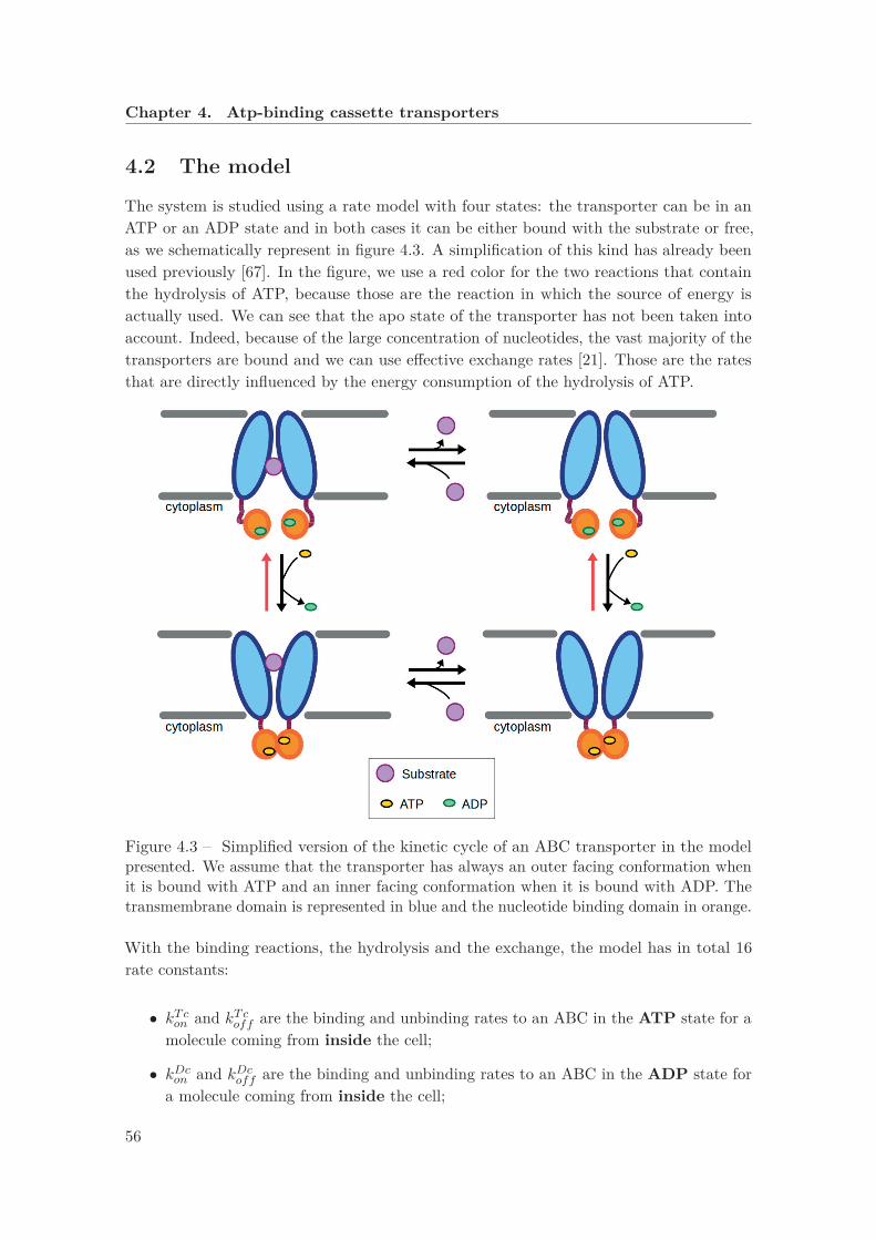
Chapter 4. Atp-binding cassette transporters
4.2 The model
The system is studied using a rate model with four states: the transporter can be in anATP or an ADP state and in both cases it can be either bound with the substrate or free,as we schematically represent in figure 4.3. A simplification of this kind has already beenused previously [67]. In the figure, we use a red color for the two reactions that containthe hydrolysis of ATP, because those are the reaction in which the source of energy isactually used. We can see that the apo state of the transporter has not been taken intoaccount. Indeed, because of the large concentration of nucleotides, the vast majority of thetransporters are bound and we can use effective exchange rates [21]. Those are the ratesthat are directly influenced by the energy consumption of the hydrolysis of ATP.
Figure 4.3 – Simplified version of the kinetic cycle of an ABC transporter in the modelpresented. We assume that the transporter has always an outer facing conformation whenit is bound with ATP and an inner facing conformation when it is bound with ADP. Thetransmembrane domain is represented in blue and the nucleotide binding domain in orange.
With the binding reactions, the hydrolysis and the exchange, the model has in total 16rate constants:
• kTcon and kTc
off are the binding and unbinding rates to an ABC in the ATP state for amolecule coming from inside the cell;
• kDcon and kDc
off are the binding and unbinding rates to an ABC in the ADP state fora molecule coming from inside the cell;
56

4.2. The model
• kTton and kTt
off are the binding and unbinding rates to an ABC in the ATP state for amolecule coming from outside the cell;
• kDton and kDt
off are the binding and unbinding rates to an ABC in the ADP state fora molecule coming from outside the cell;
• kh and ks are the rates of hydrolysis and synthesis in the absence of the substrate;
• ksh and kss are the rates of hydrolysis and synthesis in the presence of the substrate;
• keTD and keDT are the exchange rates from ATP to ADP and from ATP to ADPrespectively, when the substrate is not bound;
• ke,sTD and ke,sDT are the exchange rates when the substrate is bound.
They are not independent, because they must respect the constraints imposed by thethermodynamics of equilibrium. In equilibrium the concentration of the molecules inside(indicated as c) is equal to the concentration of the molecules outside the cell (indicated asc). Therefore, the equilibrium conditions are
γeq =[c]eq kTc
on ksh k
Dtoff ks
[t]eq kDton k
ss k
Tcoff kh
=kTcon k
sh k
Dtoff ks
kDton k
ss k
Tcoff kh
= 1 , (4.1)
γeq =[t]eq kTt
on ksh k
Dtoff ks
[t]eq kDton k
ss k
Ttoff kh
=kTton k
sh k
Dtoff ks
kDton k
ss k
Ttoff kh
= 1 , (4.2)
γeq =[c]eq kTc
on ksh k
Dcoff ks
[c]eq kDcon k
ss k
Tcoff kh
=kTcon k
sh k
Dcoff ks
kDcon k
ss k
Tcoff kh
= 1 , (4.3)
where with [c]eq and [t]eq we indicate concentrations in equilibrium.In our simplified model, the only difference between importers and exporters is the choiceof the parameters that is influenced by the presence of the substrate molecule: in the caseof importers the parameter is the hydrolysis rate, whereas in the case of exporters it is thebinding of ATP [65, 61]. To the rate model we associate a system of master equations (seeAppendix). The numerical solution with the parameters valid for the exporters was used toplot the concentration [c] of molecules inside the cell as a function of time. Imitating thesteps followed in the experiment with ethidium that we previously described, we startedwith a concentration of ATP that was similar to the one of thermodynamic equilibrium.The concentration of molecules inside the cell increased as expected. We then changedthe value of the ratio α = [ATP ]
[ADP ] at a time t = 1200s, in order to reproduce the effect ofthe addition of ATP. As we can see in figure 4.4, for t > 1200 there is a decrease in theconcentration of substrate inside the cell, indicating that the flux of molecules is directedoutward, as it should, since we were using the parameters of exporters.We then considered the non equilibrium stationary state. In our system the NESS is
57

Chapter 4. Atp-binding cassette transporters
Figure 4.4 – The concentration of molecules inside the cell is shown as a function oftime. For t < 1200s equilibrium value [ATP ]/[ADP ] � 10 is used. For t > 1200s we used[ATP ]/[ADP ] = 10.
only due to a net flux of hydrolysis of ATP, whereas the total concentration of substratemolecules is fixed once for all and we assume that there are no exchanges of substratemolecules with the surrounding. Therefore, for the stationary state we imposed
Jc = 0 , (4.4)
where the flux Jc is defined as
Jc = [c]([T ]kTc
on + [D]kDcon
)−
([TS]kTc
off + [DS]kDcoff
). (4.5)
In figure 4.5 we show two phase diagrams in which the ratio ω = [c][t] is shown as a function
of α = [ATP ][ADP ] and [stot] in the case of exporters (left) and importers (right). We can see
that an increase in α leads to an increase in the chemical gradient between the two sidesof the membrane. This effect is larger for smaller values of the total concentration of thesubstrate molecules and if they are in large excess the transporters can not work properly,leaving the ratio ω close to 1. It is interesting to see some asymptotic behaviors: first ofall, we can determine a limiting case for optimal hydrolysis rate and optimal binding ratefrom the inner side of the cell. Indeed, in these conditions we have:
ω →A
[ADP ]eq
[ATP ]eq+B
A [ADP ][ATP ] +B
, (4.6)
where A and B are two positive constants (see Appendix). Here, with [ADP ]eq and [ATP ]eqwe indicate the concentrations in equilibrium conditions, that are valid for an isolatedsystem after the relaxation time. The implication of 4.6 is that the following inequality
58

4.3. Conclusions
Figure 4.5 – Contour plot showing the ratio ω = [c][t] corresponding to values of α = [ATP ]
[ADP ]and [stot] = [c] + [t], in the case of exporters (left) and importers (right).
holds:
ω ≤ [ADP ]eq[ATP ][ATP ]eq[ADP ] . (4.7)
The inequality 4.7 gives a boundary to the possible concentration gradient that can beachieved with a given amount of available free energy. Note that it is a thermodynamiclimit that is valid regardless of the intrinsic properties of the ABC system. If instead weassume that the available energy is infinite, that is
[ATP ][ADP ] → ∞ , (4.8)
we have the following asymptotic behavior
ω →kTtonk
Dcoff
kTtoffk
Dcon
. (4.9)
Therefore, in that case the efficiency of the transporter is uniquely determined by thebinding rates, that are the time limiting steps in the reaction.
4.3 Conclusions
The non equilibrium thermodynamic formalism is particularly fit for the description of themechanisms of the ABC transporters, in which the prominent role of the ATP consumptionhas been highlighted even during experiments [20]. We have shown that the requirementfor the energy consumption is not a simple mechanistic tool, but rather a constraint thatnaturally comes from basic principles of thermodynamics. With our coarse-grained modelit has been possible to reproduce qualitatively an experimental result. It has been done
59

Chapter 4. Atp-binding cassette transporters
starting from a simple assumption that was already made in other works [67], namely thatin the case of exporters the substrate is able to stimulate the exchange by interacting withthe NBD [61], whereas in the case of importers it is rather the hydrolysis of ATP to beaccelerated. In addition, we obtained the phase diagrams for importers and exporters. Inboth cases, the transporters work in a more efficient way for large concentrations of ATPand for low concentrations of substrate molecules.
60
5 Shape of a stretched polymer
The main results presented in this chapter have been published in [74]. Many of the figureshave been adapted from the article, in accordance with the Creative Commons AttributionLicense used by Physical Review Letters.
Introduction
In the previous chapters we have discussed the mechanisms and the interactions that leadpolymer chains to reach their functional state, characterized by a very complex and uniquetertiary structure. Now we would like to study their conformation when they are insteadin an unfolded state.The shape of a polymer chain is strongly dependent both on the intrinsic characteristicsof the chain, like the rigidity and all the interactions among its monomers, and on theproperties of the solvent. Roughly speaking, we can say that the main classification ofdifferent types of polymers is determined on the basis of how much the monomers areattracted to the molecules of the solvent with respect to their interaction with one another.The parameter that is commonly used for this classification is the second virial coefficient,defined as follows [5]:
v =∫d3r (1 − exp [−βU(r)]) , (5.1)
where U(r) is the energy necessary to bring two monomers to a distance r from very faraway and β = (kT )−1 is the thermal energy. When v < 0 the attractive interaction amongthe monomers is stronger and therefore the polymer tends to assume a more compactshape. When v > 0 the monomers tend to stay far from one another and the solvent isusually called good. If the monomers repel each other as if they were hard spheres thevirial coefficient is precisely the excluded volume. When instead v = 0, the molecules ofthe solvent perfectly compensate the interaction among the monomers and the polymerbehaves as an ideal chain. We are in the regime of θ-solvent. This condition is of particularinterest because the polymer chain can be treated with the same formalism that is used
61
Chapter 5. Shape of a stretched polymer
for the random walk. When this is possible, the chain is usually called freely-jointed chain(FJC).
In this chapter we will discuss some results regarding the conformational shape of a polymerchain when it is pulled by an external force, a condition that is often encountered both invivo, for example in protein translocation across the cell membrane [26, 16], and in vitro,e.g. in pulling experiments performed with optical or magnetic tweezers [75]. We will showthat the transverse section of the ellipsoid that approximates the polymer chain shrinksisotropically after the orientation. We will then show that there is a new model independentbehavior of some main quantities when they are written in terms of the contribution of theforce to the free energy.
Next section will be devoted to a brief summary of the main results in polymer physics. Inthe following section we will derive the end to end vector and the radius of gyration for aFJC under tension. In section three we will study the polymer shape in more details, withthe inertia tensor and its eigenvalues. We will also show the exact value of the asphericityas a function of the force. In section four we will extend the discussion to models that aredifferent from the FJC, discussing also some universal behavior that is valid for modelswith rigidities and excluded volume.
5.1 State of the art
The simplest way to model a polymer chain is to assume that each monomer behavesindependently of all the others and has a fixed length. In order to study the shape of thechain in three dimensions the quantity that comes more natural to define is the end-to-endvector
Re ≡N∑i=1
ri , (5.2)
where ri is a tangent vector corresponding to the i-th monomer and N is the number ofmonomers. A well known result of polymer physics is that the probability distribution ofRe for a polymer of N monomers of length b is a normal distribution:
P (Re) =( 3
2πNb2)3/2
exp[−3
2R2
e
Nb2
]. (5.3)
As a consequence, using spherical coordinates it is easy to show that the distribution ofthe distance Re is
P (Re) = 4πR2e
( 32πNb2
)3/2exp
[−3
2R2
e
Nb2
]. (5.4)
62
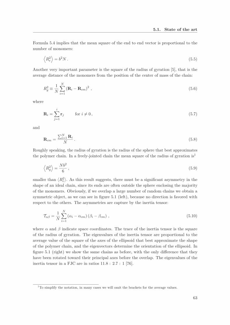
5.1. State of the art
Formula 5.4 implies that the mean square of the end to end vector is proportional to thenumber of monomers:
⟨R2
e
⟩= b2N . (5.5)
Another very important parameter is the square of the radius of gyration [5], that is theaverage distance of the monomers from the position of the center of mass of the chain:
R2g ≡ 1
N
N∑i=1
(Ri − Rcm)2 , (5.6)
where
Ri =i∑
j=1rj for i �= 0 , (5.7)
and
Rcm =∑N
i=1 Ri
N. (5.8)
Roughly speaking, the radius of gyration is the radius of the sphere that best approximatesthe polymer chain. In a freely-jointed chain the mean square of the radius of gyration is1
⟨R2
g
⟩= Nb2
6 , (5.9)
smaller than⟨R2
e
⟩. As this result suggests, there must be a significant asymmetry in the
shape of an ideal chain, since its ends are often outside the sphere enclosing the majorityof the monomers. Obviously, if we overlap a large number of random chains we obtain asymmetric object, as we can see in figure 5.1 (left), because no direction is favored withrespect to the others. The asymmetries are capture by the inertia tensor:
Tαβ = 1N
N∑i=1
(αi − αcm) (βi − βcm) , (5.10)
where α and β indicate space coordinates. The trace of the inertia tensor is the squareof the radius of gyration. The eigenvalues of the inertia tensor are proportional to theaverage value of the square of the axes of the ellipsoid that best approximate the shapeof the polymer chain, and the eigenvectors determine the orientation of the ellipsoid. Infigure 5.1 (right) we show the same chains as before, with the only difference that theyhave been rotated toward their principal axes before the overlap. The eigenvalues of theinertia tensor in a FJC are in ratios 11.8 : 2.7 : 1 [76].
1To simplify the notation, in many cases we will omit the brackets for the average values.
63
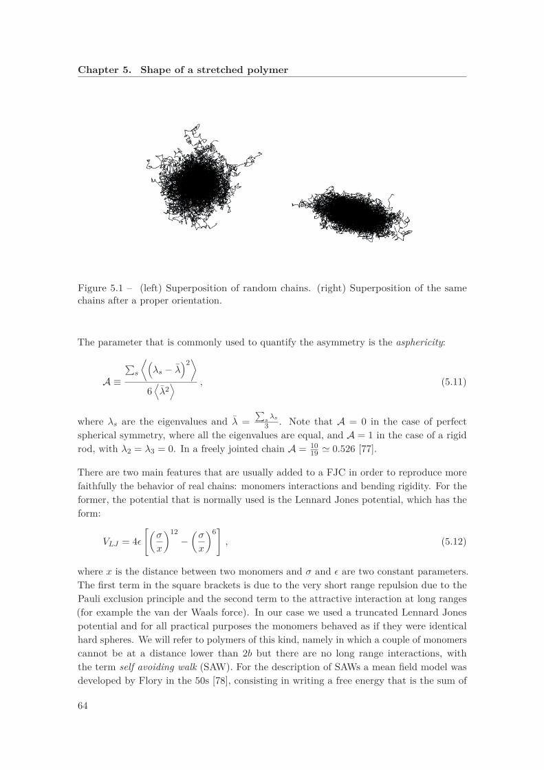
Chapter 5. Shape of a stretched polymer
Figure 5.1 – (left) Superposition of random chains. (right) Superposition of the samechains after a proper orientation.
The parameter that is commonly used to quantify the asymmetry is the asphericity:
A ≡
∑s
⟨(λs − λ
)2⟩
6⟨λ2
⟩ , (5.11)
where λs are the eigenvalues and λ =∑
sλs
3 . Note that A = 0 in the case of perfectspherical symmetry, where all the eigenvalues are equal, and A = 1 in the case of a rigidrod, with λ2 = λ3 = 0. In a freely jointed chain A = 10
19 � 0.526 [77].
There are two main features that are usually added to a FJC in order to reproduce morefaithfully the behavior of real chains: monomers interactions and bending rigidity. For theformer, the potential that is normally used is the Lennard Jones potential, which has theform:
VLJ = 4ε[(σ
x
)12−
(σ
x
)6], (5.12)
where x is the distance between two monomers and σ and ε are two constant parameters.The first term in the square brackets is due to the very short range repulsion due to thePauli exclusion principle and the second term to the attractive interaction at long ranges(for example the van der Waals force). In our case we used a truncated Lennard Jonespotential and for all practical purposes the monomers behaved as if they were identicalhard spheres. We will refer to polymers of this kind, namely in which a couple of monomerscannot be at a distance lower than 2b but there are no long range interactions, withthe term self avoiding walk (SAW). For the description of SAWs a mean field model wasdeveloped by Flory in the 50s [78], consisting in writing a free energy that is the sum of
64

5.1. State of the art
the entropic term that we would have even in the Gaussian regime and a term that takesinto account the hard sphere repulsion in the same way it would treat it for a gas confinedin a volume w ∼ R3, where R is the size of the chain:
F = aR2
N+ bN
2
R3 , (5.13)
where a and b are two constant parameters. Minimizing the free energy with respect to Rwe obtain the scaling law
R ∼ N3/5 . (5.14)
Given the simplicity of the model, the critical exponent ν = 35 = 0.6 has a remarkable
accuracy, since the correct exponent is ν � 0.588 [5]. Self avoiding polymers are on averagemore elongated than FJCs: the ratios between the eigenvalues are [79] 14.05 : 2.96 : 1 andthe asphericity is A � 0.55.
For the bending rigidity a correlation between neighboring tangent vectors is introduced,usually with a potential of the form
V = −Bb
N−1∑i=1
ri · ri+1 = −Bb
N−1∑i=1
cos θi , (5.15)
where B is a constant parameter and θi is the angle between ri and ri+1. This is known asthe Kratky-Porod model. In most cases the cosine is expanded and an harmonic potentialis used:
V = kN−1∑i=1
θ2i , (5.16)
where k is a new parameter that from now on will be called bending constant. Thecorrelation between tangent vectors can be quantified using the persistence length [5] :
lp = − 1ln [〈cos θi〉]
. (5.17)
Note that in our case, since the monomers are considered to be identical, lp is just a numberthat does not depend on the position along the chain. It can be shown that the persistencelength is related to the bending constant via the relation
lp � 2bkkbT
. (5.18)
Concerning polymer stretching, there are some known result we need to recall. We willshow in the next section that when a FJC is subjected to an external force f = f ez its
65

Chapter 5. Shape of a stretched polymer
mean extension is
〈Rz〉 = NbL(γ) ez , (5.19)
where
L(γ) ≡ coth(γ) − 1/γ (5.20)
is the Langevin function and
γ ≡ βfb . (5.21)
However, if the bending rigidity is taken into account, the force vs extension relationbecomes [80]
flpkbT
= Rz
L+ 1
4(1 − Rz
L
)2 − 14 , (5.22)
where L is the contour length. In figure 5.2 we compare the curve relative to the formulawe just wrote with the Langevin function.
Figure 5.2 – Comparison of the force vs extension curve in the case with (red) and withoutrigidity (blue).
66
5.2. Exact Computation of⟨R2
e
⟩and
⟨R2
g
⟩
5.2 Exact Computation of 〈R2e〉 and
⟨R2g
⟩
The force applied to the polymer chain corresponds to an internal energy E = −f · Re andthus to a Boltzmann factor
exp [−βE] = exp [βf · Re] = exp[
N∑i=1βf · ri
]=
N∏i=1
exp [βf · ri] . (5.23)
Therefore, the force is coupled separately with each tangent vector and we can calculatethe partition function for a single tangent vector, that is [81]
q(βfb) =∫dr exp(βf · ri)δ (|ri| − b) =
= 4πb2 sinh(βfb)/βfb , (5.24)
where we used a Dirac delta to impose a constraint on the length of the tangent vector.The partition function of the whole system is just qN . We now assume that a force isoriented along the z axis. Using the partition function, we can derive the known result ofthe mean extension
〈Re〉 = NbL(γ) ez , (5.25)
In the same way 2, it is possible to calculate the variances of the three components of Re,that are
σ2x = σ2
y = Nb2g , (5.26)σ2z = Nb2a , (5.27)
where g ≡ L/γ and a ≡ 1 − 2g − L2. The end to end vector is a combination of variablesthat are independent and identically distributed, therefore it follows the central limittheorem and its mean square is given by
⟨R2
e
⟩= 〈Re〉2 + σ2 = Nb2(1 − L2) +N2b2L2 . (5.28)
As we can see, the end to end vector is the sum of two contributions, modulated by theterm L2. For low forces, the unstretched FJC dominates, whereas as the force increasesthe end to end vector becomes similar to the one of a rigid rod, that is Re � Nb. The forceat which the second component becomes larger than the first one is
f = kT
b
3√N + 1
. (5.29)
The expression of the end to end vector can be used for the derivation of the radius ofgyration. First of all, we note that it can be written in terms of the distance between
2This derivation, like many others in this chapter, has been published in [74].
67
Chapter 5. Shape of a stretched polymer
couples of monomer along the chain:
⟨R2
g
⟩=
⟨1N
N∑i=1
(Ri − Rcm)2⟩
=
=⟨
12N2
∑i,j
(Ri − Rj)2⟩
= (5.30)
= 1N2
∑j>i
⟨(Ri − Rj)2
⟩.
The average distance between two position vectors is equal to the end to end vector of thesubchain between them. Therefore, we can calculate it using 5.28. With this method weobtain
⟨R2
g
⟩= 1
6Nb2 + 1
12N2b2L2 . (5.31)
Note that even in the case of the radius of gyration the two regimes are weighted by L2.
The increase in the radius of gyration for larger forces does not give any information aboutthe directionality of the elongation. Obviously, we expect that when the forces are largeenough the elongation takes place only in one preferred direction and beyond a certainthreshold there should be a shrinking in the section orthogonal to the force. In order togive a more insightful description we need to use the inertia tensor.
5.3 Inertia tensor and asphericity
We implemented a FJC for different values of N and different forces using Monte Carlosimulations (MC). For each chain we calculated the inertia tensor and its eigenvaluesand eigenvectors. There are essentially two scales of the force that must be considered.When the force is small, the polymer is slightly deformed even though it is not orientedin the same direction as the force. As soon as the force becomes large enough to orientthe polymer in its direction there is an elongation in that direction and a shrinking inthe other two. The orientation can be represented with the projection of the force onthe eigenvectors. In figure 5.3 we can see that the eigenvector v1 relative to the largesteigenvalue starts at random orientation, with projection 〈cosψ1〉 = 0.5, where ψ1 is theangle between v1 and f , and then it rotates until it is parallel to the force.
68
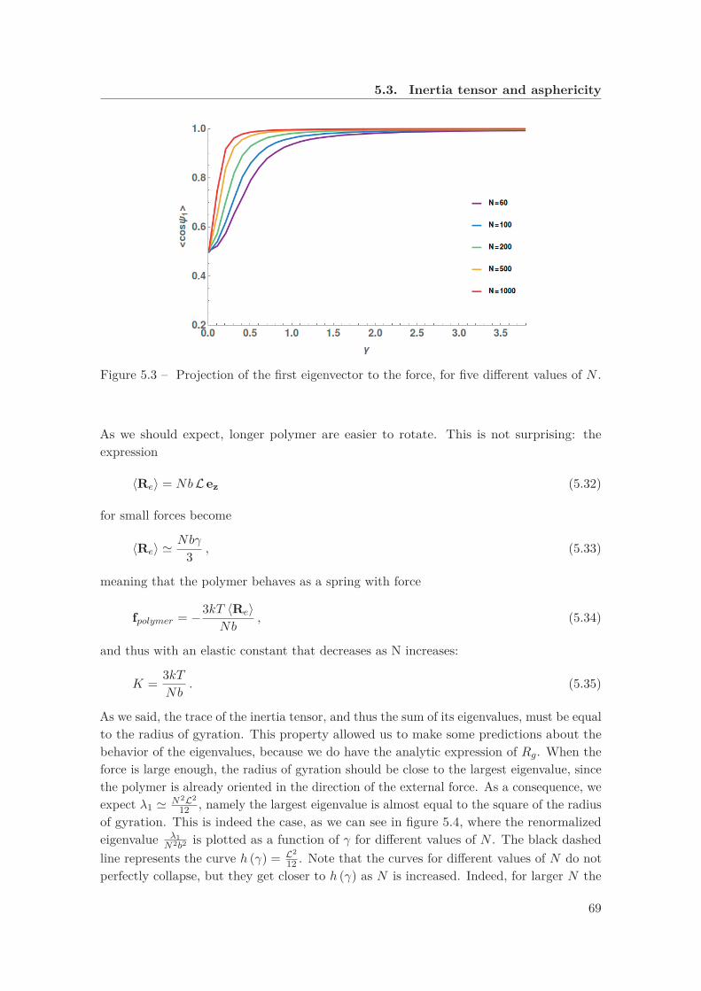
5.3. Inertia tensor and asphericity
Figure 5.3 – Projection of the first eigenvector to the force, for five different values of N .
As we should expect, longer polymer are easier to rotate. This is not surprising: theexpression
〈Re〉 = NbL ez (5.32)
for small forces become
〈Re〉 � Nbγ
3 , (5.33)
meaning that the polymer behaves as a spring with force
fpolymer = −3kT 〈Re〉Nb
, (5.34)
and thus with an elastic constant that decreases as N increases:
K = 3kTNb
. (5.35)
As we said, the trace of the inertia tensor, and thus the sum of its eigenvalues, must be equalto the radius of gyration. This property allowed us to make some predictions about thebehavior of the eigenvalues, because we do have the analytic expression of Rg. When theforce is large enough, the radius of gyration should be close to the largest eigenvalue, sincethe polymer is already oriented in the direction of the external force. As a consequence, weexpect λ1 � N2L2
12 , namely the largest eigenvalue is almost equal to the square of the radiusof gyration. This is indeed the case, as we can see in figure 5.4, where the renormalizedeigenvalue λ1
N2b2 is plotted as a function of γ for different values of N . The black dashedline represents the curve h (γ) = L2
12 . Note that the curves for different values of N do notperfectly collapse, but they get closer to h (γ) as N is increased. Indeed, for larger N the
69

Chapter 5. Shape of a stretched polymer
critical force at which the rod-like behavior becomes dominant is smaller.
Figure 5.4 – Renormalized eigenvalue λ1 as a function of the force, for five different valuesof N . The black dashed line is the curve h(γ) = L2
12 .
In the same regime, the other two eigenvalues should instead depend on the force in thesame way as the variances of the end to end vector in the directions orthogonal to theforce, which means λ2,3 ∼ NL/γ. If we consider figure 5.5 and 5.6, we can see that thereis an initial increase in the value of the mean eigenvalues for small forces.
Figure 5.5 – Renormalized eigenvalue λ2 as a function of the force, for five different valuesof N . The black dashed line is the curve h(γ) = 0.1L
γ .
This regime indicates forces that are low enough that the polymer is not well oriented,therefore the elongation takes place in a random direction, increasing, on a statistical pointof view, all the eigenvalues. After the orientation, the stretching is directed along themajor axis of the ellipsoid, and the smaller eigenvalues decrease as predicted. Fitting withcurves of the form λi = ciNL/γ, we obtained the parameters c2 = 0.1 and c3 = 0.034 for
70

5.3. Inertia tensor and asphericity
the second and the third eigenvalue respectively. As the results suggest, for large forces
Figure 5.6 – Renormalized eigenvalue λ3 as a function of the force, for five different valuesof N . The black dashed line is the curve h(γ) = 0.034L
γ .
the ratio between the two smaller eigenvalues reaches a plateau that is independent on theforce but that is different from the case at zero force (figure 5.7).
Figure 5.7 – Ratio between the two smaller eigenvalues as a function of the force, for fivedifferent values of N .
With the MC is also possible to calculate the asphericity as a function of γ and N . However,we calculated its expression analytically using the same method that was used for the
71

Chapter 5. Shape of a stretched polymer
radius of gyration 3. The exact formula is the following:
A = 1 − 72ag + 36g2 + 24NgL2
36a2 + 80ag + 112g2 + 4L2 (11a+ 10g)N + 5N2L4 . (5.36)
We show the curve in figure 5.8. The derivative of the asphericity with respect to γ is a
Figure 5.8 – Asphericity as a function of γ for different values of N .
measure on the sensibility of the polymer chain to a change in the external force. As wecan see in figure 5.9, the maximum of this value is at lower forces for larger N.
Figure 5.9 – Derivative of the asphericity as a function of γ for different values of N . Blackdots correspond to f = 3
N+1 .
We indicated with black dots the values corresponding to the critical force at which the
3the whole calculation can be found in the supplementary information of [74].
72

5.4. Universal behaviors
rod-like behavior starts being dominant with respect to the one of unbiased Gaussian chain:f = 3√
N+1 . As we should expect, it is very close to the maximum.
What we found interesting of formula (5.36) were the two asymptotic behaviors, that are
A � 1 − 245NγL , (5.37)
for large forces and
A � 1019 + 25
1083Nγ2 , (5.38)
for small forces. The reason why we found the result interesting is that for low forces wehave Nγ2 ∼ NγL. Therefore, both the asymptotic behaviors depend on the combinationη ≡ NγL, which is nothing but the contribution of the force to the free energy, sinceNγL = f · 〈Re〉 /kbT . This suggested that the whole asphericity could be written, in firstapproximation, as a function of the sole parameter η. Indeed, after a bit of algebra andkeeping only the leading terms, we have
A � 120 + 60η + 5η2
228 + 84η + 5η2 . (5.39)
5.4 Universal behaviors
When we obtained formula (5.39) we found it natural to investigate whether the result wassomehow more general and applicable to other models or it was instead limited to the veryspecific case of FJC. Models with excluded volume or rigidity were too complicated to betreated analytically. We implemented molecular dynamics (MD) simulations for models inwhich the rigidity of the polymer and the excluded volume are taken into account. In figure5.10 we plot the asphericity as a function of η for different parameters of the rigidity, withand without volume exclusion and with N = 103. We can see that in first approximationthere is a collapse onto the same curve for models in which the excluded volume is takeninto account (E) and in which it is not (P), and for every value of the rigidity. To be precise,for very small values of the force there is a small difference between the self-avoiding walk(SAW) and the other models since the latter is slightly more elongated. Increasing theforce, the effect of the excluded volume becomes less important and the SAW is even closerto the other models. Therefore, we can conclude that in a θ-solvent it is possible to inferthe asphericity of a polymer from its end to end vector, that is the accessible quantity inpulling experiments.
A similar result can be found for the projection of the eigenvectors on the direction of theforce. As we have previously pointed out, for large forces the mean largest eigenvalue goes
73

Chapter 5. Shape of a stretched polymer
Figure 5.10 – (main) Asphericity as a function of η for different models. (inset) Zoom forsmall values of the force. The black curve corresponds to equation 5.39. Image taken from[74].
as
λ1 � (NLb)2
12 . (5.40)
We must now find the projection of the vector λ1v1 on the xy plane. We can do this bytaking the contribution to the radius of gyration that are orthogonal to the force, that are
1(N + 1)2
∑j>i
⟨(Xj −Xi)2
⟩+
⟨(Yj − Yi)2
⟩� 1
3Nb2g , (5.41)
and subtract the part of the two smaller eigenvalues, that has been discussed above. Inthis way we obtain
(λ1v1 · x) x + (λ1v1 · y) y � Nb2g
(13 − c2 − c3
)� Nb2g
5 . (5.42)
Therefore the mean value of sinψ1 is
〈sinψ1〉 �√Nb2g
5λ1�
√12
5NγL =√
125η . (5.43)
The behavior of the eigenvalues suggested an analogy with the electric dipole, when it isimmersed in a constant electric field. Here, we are slightly giving up the mathematicalrigor, since the analogy makes sense only if the dipole is already partially oriented in thecorrect direction, otherwise its orientation would be completely flipped, differently fromthe case of the polymer. However, a part from this detail, we think that it is useful to
74

5.4. Universal behaviors
better understand the physical meaning of some quantities. Imagine an electric dipole withdipole moment:
d = αRe
kT(5.44)
subjected to a force f due to the electric field. The projection of the dipole in the directionof the force will be
〈cosψ1〉 � 11 − e−αη
− 1αη, (5.45)
and thus in the orthogonal direction
〈sinψ1〉 �√
2αη. (5.46)
With a comparison between the two expressions for 〈sinψ1〉, we obtain
α � 0.83 . (5.47)
With a more involving calculation, it is also possible to show that
〈cosψ2〉 = 〈cosψ3〉 = I1(αη)sinh(αη) , (5.48)
where I1 is the modified Bessel function of the first kind. We plotted formula 5.45 and5.48 together with the results of the simulations, in figure 5.11.
Figure 5.11 – Projection of the first (main) and the second (inset) eigenvalues. The legendof the points is the same as in the figure for the asphericity. Plot taken from [74].
First of all, we have the confirmation that the collapse that was shown for the asphericity
75
Chapter 5. Shape of a stretched polymer
is also valid for the projections of the eigenvector. Moreover, the curves that were derivedwith the dipole analogy fit in an excellent way the simulations, even for rather small valuesof η.
5.5 Conclusions
We studied the response of a polymer chain under the influence of an external pullingforce. Starting from the distribution of the end to end vector, it has been possible to deriveanalytically both the expression of the radius of gyration and the one of the asphericity inthe case of a FJC. Using numerical simulations performed with MD and MC methods, wealso obtained the average eigenvalues and eigenvectors of the inertia tensor, that give ussome more detailed information about the orientation and the shrinking of the polymerchain. The first result that we found particularly intriguing is the fact that the lowereigenvalues do not have a monotonic dependence from the force, but they rather increasefor small forces, they reach a maximum and then after the polymer is significantly orientedthey start decreasing as intuitively one should expected. This behavior is less pronouncedfor longer polymers, since they are easier to orient along the direction of the force. Moreimportantly, once the polymer is oriented the transverse section shrinks isotropically withthe lower eigenvalues that reach a new constant value that is different from the one at zeroforce. The turning point of our work was when we realized that the analytical formulafor the asphericity could be written, keeping only the leading terms, as a function ofthe sole parameter η ≡ NγL. After this discovery, it immediately became natural towonder whether other quantities could also be written in terms of the same parameter.We thus showed that the average projections of the eigenvectors on the direction of theforce corresponding to different numbers of monomers collapsed onto the same curve whenplotted as a function of η. Moreover, we realized that it was more universal than what weexpected, since it the result could be extended to polymer models that are more complicatedthan the FJC.
76
6 Concluding remarks
In this work we used methods of statistical physics to model biological systems.We wanted to illustrate how the physics of non equilibrium can be a useful tool for thedescription of those biological processes that intrinsically contain a directionality. We did itby choosing the emblematic example of the molecular chaperones, with particular attentionto their role in protein folding. The concept that the path through which the proteins areable to reach their functional structure is accessible in equilibrium is quite deeply rooted inthe scientific community [11]. For this reason, the requirement of molecular chaperones instress conditions has often been considered as a temporary necessity to avoid aggregation orin some cases to simply accelerate the refolding process [1, 54]. Our goal was to challengethis position, promoting the idea that there are situations in which the native conformationof the proteins is not the most thermodynamically stable, but that even in those cases itis possible for them to recover their functional structure, at the condition that a certainamount of energy is continuously supplied to the system, keeping it out of equilibrium.
We started with a more abstract approach, with a calculation that allowed to derive theconstraints that the parameters follow in an Hsp70 system that stimulates the unfoldingof misfolded proteins. From these constraints the importance of the non equilibrium wasimplied by the requirement for the affinity coefficient to be larger than one. Still withHsp70, we then proceeded with a model that is closer to experiments. Motivated by theFRET experiments performed on denaturated rhodanese in the group of Ben Schuler [24],we showed the dependence on the energy due to the hydrolysis of ATP of the expansionof rhodanese under the influence of Hsp70. In addition, our model was able to faithfullyreproduce the average values of FRET efficiency.In a similar fashion, we showed that GroEL could rescue misfolded proteins even ata temperature at which they could not refold spontaneously. More importantly, theconservation of the native conformation was possible only in the constant presence ofATP. Indeed, as soon as adenosine diphosphatase was added, the enzymatic activity of thesubstrate proteins dropped drastically. These results could be nicely explained with theuse of very simple non equilibrium models.
77
Chapter 6. Concluding remarks
The third system that we found intriguing for its relation to non equilibrium physics isthe one of the ABC transporters. Our research in that field is more recent than in theothers discussed in the thesis, and so we could say that it is still somehow work in progress.However we could demonstrate that their necessity of ATP follows naturally from basicthermodynamic considerations. Moreover, we reproduced qualitatively the experiment inwhich a concentration gradient is imposed to the exporters, in the absence of ATP. Theinitial uptake of the substrate molecule is substitute by the efflux as soon as ATP is addedin the system.
Finally, we described the deformation of a polymer chain when it is under the effect of anexternal pulling force. The polymer is expanded in random directions for low forces, asthe increase in the lower eigenvalues suggests. Afterwards, when the polymer is oriented,the transverse section start shrinking isotropically, with the ratio between the two lowereigenvalues that reaches a new constant value that is different from the one at zero force.We think that our analysis can provide not only some speculations of purely theoreticalinterest (which, for the sake of the argument, would be fine as well), but also predictionsthat can be tested in experiments. For example, we demonstrated that a parameter like theasphericity can be inferred from the knowledge of the end to end vector, that is a quantitythat can be directly measured or even tuned in single molecule experiments, performedwith techniques like optical or magnetic tweezers, or atomic force microscopy.
78

A Appendix
A.1 Hsp70
A.1.1 Rate constants in the model with rhodanese
We assumed that the concentration of chaperones was [Hsp70] = 10μM and the concen-tration of nucleotides [ATP ] + [ADP ] = 1mM . The rate constants were similar to theones of the [40] and [38]. We report them in the table,
kh = 6 · 10−4 s−1 ksh = 1.8 s−1
kTon = 1.2M−1 s−1 kDon = 11.7 · 10−3M−1 s−1
kToff = 2.31 s−1 kDoff = 2.5 · 10−3M−1 s−1
kD− = 1.4 · 10−3 s−1 kT− = 1.33 · 10−4 s−1
kD+ = 0.27 s−1 kT+ = 0.13 s−1
ks,D− = (1/δ)kD− ks,T− = δ kT−
ks,D+ = δ kD+ ks,T+ = (1/δ)kT+
The parameter δ � 1.7 was a correction necessary in order to have γ = 1 in equilibrium.
A.2 Chaperonin
A.2.1 Rate constants in the model
In the model the rate constants in the following table were used.
79
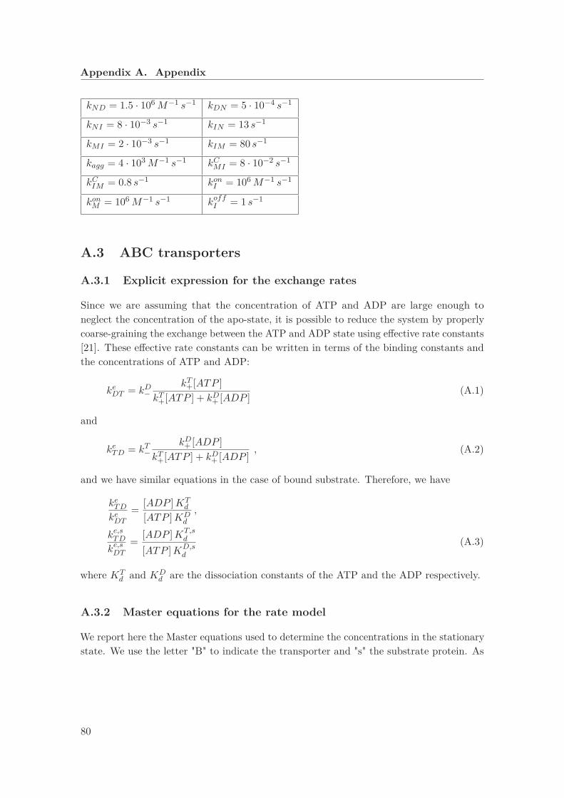
Appendix A. Appendix
kND = 1.5 · 106M−1 s−1 kDN = 5 · 10−4 s−1
kNI = 8 · 10−3 s−1 kIN = 13 s−1
kMI = 2 · 10−3 s−1 kIM = 80 s−1
kagg = 4 · 103M−1 s−1 kCMI = 8 · 10−2 s−1
kCIM = 0.8 s−1 konI = 106M−1 s−1
konM = 106M−1 s−1 koffI = 1 s−1
A.3 ABC transporters
A.3.1 Explicit expression for the exchange rates
Since we are assuming that the concentration of ATP and ADP are large enough toneglect the concentration of the apo-state, it is possible to reduce the system by properlycoarse-graining the exchange between the ATP and ADP state using effective rate constants[21]. These effective rate constants can be written in terms of the binding constants andthe concentrations of ATP and ADP:
keDT = kD−kT+[ATP ]
kT+[ATP ] + kD+ [ADP ](A.1)
and
keTD = kT−kD+ [ADP ]
kT+[ATP ] + kD+ [ADP ], (A.2)
and we have similar equations in the case of bound substrate. Therefore, we have
keTD
keDT
= [ADP ]KTd
[ATP ]KDd
,
ke,sTD
ke,sDT
= [ADP ]KT,sd
[ATP ]KD,sd
(A.3)
where KTd and KD
d are the dissociation constants of the ATP and the ADP respectively.
A.3.2 Master equations for the rate model
We report here the Master equations used to determine the concentrations in the stationarystate. We use the letter "B" to indicate the transporter and "s" the substrate protein. As
80
A.3. ABC transporters
usual, "T" and "D" indicate ATP and ADP respectively.
d[BT ]dt
= − [BT ][[c]kTc
on + [t]kTton + kh + keTD
]+ [BTs]
[kTcoff + kTt
off
]+
+ [BD] [kx + keDT ]d[BTs]dt
= − [BTs][kTcoff + kTt
off + ksh + k(s,e)TD
]+ [BT ]
[[c]kTc
on + [t]kTton
]+
+ [BDs][ksx + k(s,e)
DT
]d[BD]dt
= − [BD][[c]kDc
on + [t]kDton + kx + keDT
]+ [BDs]
[kDcoff + kDt
off
]+
+ [BD] [kx + keDT ] (A.4)d[BDs]dt
= − [BDs][kDcoff + kDt
off + ksx + k(s,e)DT
]+ [BD]
[[c]kDc
on + [t]kDton
]+
+ [BDs][kss + k(s,e)
TD
].
When we want to consider the NESS, we impose
d[BT ]dt
= d[BTs]dt
= d[BD]dt
= d[BDs]dt
= 0 , (A.5)
as usual.
A.3.3 Asymptotic results
The constants that appear in 4.6 are
A = kTtoffk
s,D− ks,T+
B = kDtoffk
s,T− ks,D+ . (A.6)
A.3.4 Rates in the model
For the rate model we used parameters that were in agreement with the prediction ofSenior and Gadsby [82]. We report them in the following table.
81
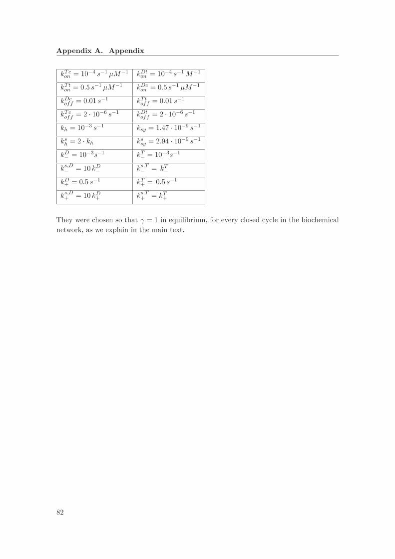
Appendix A. Appendix
kTcon = 10−4 s−1 μM−1 kDt
on = 10−4 s−1M−1
kTton = 0.5 s−1 μM−1 kDc
on = 0.5 s−1 μM−1
kDcoff = 0.01 s−1 kTt
off = 0.01 s−1
kTcoff = 2 · 10−6 s−1 kDt
off = 2 · 10−6 s−1
kh = 10−3 s−1 ksy = 1.47 · 10−9 s−1
ksh = 2 · kh kssy = 2.94 · 10−9 s−1
kD− = 10−3s−1 kT− = 10−3s−1
ks,D− = 10 kD− ks,T− = kT−
kD+ = 0.5 s−1 kT+ = 0.5 s−1
ks,D+ = 10 kD+ ks,T+ = kT+
They were chosen so that γ = 1 in equilibrium, for every closed cycle in the biochemicalnetwork, as we explain in the main text.
82
Bibliography
[1] M. Hayer-Hartl, A. Bracher, and F. Hartl, “The groel–groes chaperonin machine: Anano-cage for protein folding,” Trends in Biochemical Sciences, vol. 41, pp. 62–76,2015.
[2] X. Zhang, H. Qian, and M. Qian, “Stochastic theory of nonequilibrium steady statesand its applications,” Physics Reports, vol. 510, p. 1–86, 2012.
[3] H. Hofmann, A. Soranno, K. G. A. Borgia, D. Nettels, and B. Schuler, “Polymerscaling laws of unfolded and intrinsically disordered proteins quantified with singlemolecule spectroscopy,” Proc. Nat. Acad. Sci, vol. 109, pp. 16155–16160, 2012.
[4] P. Gennes, Scaling Concepts in Polymer Physics. Cornell University Press, 1979.
[5] M. Rubinstein and R. Colby, Polymer Physics. Oxford University Press, 2003.
[6] C.Bustamante, Y. Chemla, N. Forde, and D. Izhaky, “Mechanical processes in bio-chemistry,” Annu. Rev. Biochem., vol. 73, pp. 705–748, 2004.
[7] R. Astumian and M. Bier, “Fluctuation driven ratchets: Molecular motors,” Phys.Rev. Lett., vol. 72, pp. 1766–1769, 1994.
[8] D. Evans, E. Cohen, and G. Morriss, “Probability of second law violations in shearingsteady states,” Phys. Rev. Lett., vol. 71, p. 2401, 1993.
[9] D. Collin, F. Ritort, C. Jarzynski, S. B. Smith, I. T. Jr, and C. Bustamante, “Nonequi-librium equality for free energy differences,” Phys. Rev. Lett., vol. 78, pp. 2690–2690,1997.
[10] D. Collin, F. Ritort, C. Jarzynski, S. B. Smith, I. T. Jr, and C. Bustamante, “Verifica-tion of the crooks fluctuation theorem and recovery of rna folding free energies,” NatMed., vol. 437, p. 231–234, 2005.
[11] C. Anfinsen, “Principles that govern the folding of protein chains,” Science, vol. 181,pp. 223–230, 1973.
[12] F. Morcos, A. Pagnani, B. Lunt, A. Bertolino, D. Marks, C. Sander, R. Zecchina,J. Onuchic, T. Hwa, and M. Weigt, “Direct-coupling analysis of residue coevolutioncaptures native contacts across many protein families,” eLife, vol. 6, p. e23471, 2017.
83
Bibliography
[13] D. Malinverni, A. Lopez, P. D. L. Rios, G. Hummer, and A. Barducci, “Modeling hsp70-hsp40 interaction by multi-scale molecular simulations and coevolutionary sequenceanalysis,” eLife, vol. 6, p. e23471, 2017.
[14] M. Karplus and J. McCammon, “Molecular dynamics simulations of biomolecules,”Nat. Struct. Mol. Biol., vol. 9, pp. 646–652, 2002.
[15] P. Goloubinoff and P. D. L. Rios, “The mechanism of hsp70 chaperones: (entropic)pulling the models together,” Trends. Biochem. Sci., vol. 32, p. 372–380, 2007.
[16] P. D. L. Rios, A. Ben-Zvi, O. Slutsky, A. Azem, and P. Goloubinoff, “Hsp70 chaperonesaccelerate protein translocation and the unfolding of stable protein aggregates byentropic pulling,” Proc. Natl. Acad. Sci., vol. 103, p. 6166–6171, 2005.
[17] H.Ge, M.Qian, and H.Qian, “Stochastic theory of nonequilibrium steady states. partii: Applications in chemical biophysics,” Physics Report, vol. 510, pp. 87–118, 2012.
[18] J. Schnakenberg, “Network theory of microscopic and macroscopic behavior of masterequation systems,” Rev. Mod. Phys., vol. 48, pp. 571–585, 1976.
[19] B. Alberts, A. Johnson, J. Lewis, M. Raff, K. Roberts, and P. Walter, MolecularBiology of the Cell. Garland Science, 2007.
[20] L. Balakrishnan, H. Venter, R. Shilling, and H. van Veen, “Reversible transport bythe atp-binding cassette multidrug export pump lmra,” J. Biol. Chem., vol. 279,pp. 11273–11280, 2004.
[21] P. D. L. Rios and A. Barducci, “Hsp70 chaperones are non-equilibrium machines thatachieve ultra-affinity by energy consumption,” eLife, vol. 3, p. e02218, 2014.
[22] K. Hingorani and L. Gierasch, “Comparing protein folding in vitro and in vivo:Foldability meets the fitness challenge,” Curr Opin Struct Biol., vol. 0, pp. 81–90,2014.
[23] D. Thirumalai and G. Lorimer, “Chaperonin-mediated protein folding,” Annu. Rev.Biophys., vol. 30, p. 245–69, 2001.
[24] R. Kellner, H. Hofmann, A. Barducci, B. Wunderlich, D. Nettels, and B. Schuler,“Single-molecule spectroscopy reveals chaperone-mediated expansion of substrateprotein,” Proc. Natl. Acad. Sci., vol. 111, pp. 13355–13360, 2014.
[25] K. Neuman and A. Nagy, “Single-molecule force spectroscopy: optical tweezers,magnetic tweezers and atomic force microscopy,” Nature Methods, vol. 5, pp. 491–505,2008.
[26] W. Chirico, M. Waters, and G. Blobel, “70k heat shock related proteins stimulateprotein translocation into microsomes,” Nature, vol. 332, pp. 805–810, 1988.
84

Bibliography
[27] G. Lebon, D. Jou, and J. Casas-Vázquez, Understanding Non-equilibrium Thermody-namics. Springer, 2008.
[28] C. Dobson, “Protein folding and misfolding,” Nature, vol. 426, pp. 884–890, 2003.
[29] C. Ross and M. Poirier, “Protein aggregation and neurodegenerative disease,” NatMed., vol. 10, pp. S10–S17, 2004.
[30] B. Bukau and H. Horwich, “The hsp70 and hsp60 chaperone machines,” Cell, vol. 92,p. 351–366, 1998.
[31] M. Pilon and R. Schekman, “Protein translocation: How hsp70 pulls it off,” Cell,vol. 97, p. 679–682, 1999.
[32] M.R..Fernández, Gragera, L. Ibarrola, Q. Gallardo, and M.Valpuesta, “Hsp70 - amaster regulator in protein degradation,” FEBS Lett., vol. 591, pp. 2648–2660, 1999.
[33] H. Kampinga and E.A.Craig, “The hsp70 chaperone machinery: J proteins as driversof functional specificity,” Nat. Rev., vol. 11, pp. 579–592, 2010.
[34] T. Laufen, M. Mayer, C. Beisel, D. Klostermeier, A. Mogk, J. Reinstein, and B. Bukau,“Mechanism of regulation of hsp70 chaperones by dnaj cochaperones,” Proc. Natl.Acad. Sci., vol. 96, p. 5452–5457, 1999.
[35] J. Rauch and J. Gestwicki, “Binding of human nucleotide exchange factors to heatshock protein 70 (hsp70) generates functionally distinct complexes in vitro,” J. Biol.Chem., vol. 289, p. 1402–1414, 2014.
[36] M. Mayer, “Hsp70 chaperone dynamics and molecular mechanism,” Trends in Bio-chemical Sciences, vol. 38, pp. 223–230, 2013.
[37] A. Zhuravleva, E. Clerico, and L. Gierasch, “An interdomain energetic tug-of-warcreates the allosterically active state in hsp70 molecular chaperones,” J. Biol. Chem.,vol. 151, pp. 1296–1307, 2012.
[38] M. Mayer and B. Bukau, “Hsp70 chaperones: Cellular functions and molecularmechanism,” Cell Mol Life Sci., vol. 62, pp. 670–684, 2005.
[39] R. Tehver and D. Thirumalai, “Kinetic model for the coupling between allosterictransitions in groel and substrate protein folding and aggregation,” J. Mol. Biol.,vol. 377, pp. 1279–1295, 2008.
[40] B. Hu, M. Mayer, and M. Tomita, “Modeling hsp70-mediated protein folding,” Biophys.J., vol. 91, pp. 496–507, 2006.
[41] A. Karzai and R. McMacken, “A bipartite signaling mechanism involved in dna-j medi-ated activation of the e. coli dna-k protein,” J. Biol. Chem., vol. 271, p. 11236–11246,1995.
85
Bibliography
[42] F. Rodriguez, F. Arsène-Ploetze, W. Rist, S. Ruediger, J. Schneider-Mergener,M. Mayer, and B. Bukau, “Molecular basis for regulation of the heat shock transcrip-tion factor σ32 by the dnak and dnaj chaperones,” Molecular Cell, vol. 32, pp. 347–358,2008.
[43] R. Kityk, J. Kopp, and M. Mayer, “Molecular mechanism of j-domain-triggered atphydrolysis by hsp70 chaperones,” Molecular Cell, vol. 69, pp. 227–237, 2018.
[44] S. Rüdiger, L. Germerot, J. Schneider-Mergener, and B. Bukau, “Substrate specificityof the dnak chaperone determined by screening cellulose-bound peptide libraries,”EMBO J., vol. 16, pp. 1501–1507, 1997.
[45] C. dos Remedios and P. Moens, “Fluorescence resonance energy transfer spectroscopyis a reliable ruler for measuring structural changes in proteins: dispelling the problemof the unknown orientation factor,” J. Struct. Biol., vol. 115, pp. 175–185, 1995.
[46] P. D. L. Rios, A. Ben-Zvi, O. Slutsky, A. Azem, and P. Goloubinoff, “Single-moleculefret spectroscopy and the polymer physics of unfolded and intrinsically disorderedproteins,” Annu. Rev. Biophys., vol. 45, p. 207–231, 2016.
[47] J. V. Durme, S. Maurer-Stroh, R. Gallardo, H. Wilkinson, F. Rousseau, andJ. Schymkowitz, “Accurate prediction of dnak-peptide binding via homology modellingand experimental data,” Plos, vol. 5, pp. e1000475–e1000475, 2009.
[48] D. Schmid, A. Baici, H. Gehring, and P. Christen, “Kinetics of molecular chaperoneaction,” Science, vol. 263, pp. 971–973, 1994.
[49] P. Goloubinoff, A. Sassi, B. Fauvet, A. Barducci, and P. D. L. Rios, “Chaperonesconvert the energy from atp into the non equilibrium stabilisation of native proteins,”Nat. Chem. Biol., vol. 14, pp. 388–395, 2018.
[50] N. Ranson, D. Clare, G. Farr, D. Houldershaw, A. Horwich, and H. R. Saibil, “Allostericsignalling of atp hydrolysis in groel-groes complexes,” Nat Struct Mol Biol., vol. 13,p. 147–152, 2006.
[51] M. Preuss and A. Miller, “The affinity of the groel/groes complex for peptides underconditions of protein folding,” FEBS, vol. 466, pp. 75–79, 2000.
[52] A. Gupta, S. Haldar, G. Mili, F. Hartl, and M. Hayer-Hartl, “Active cage mechanismof chaperonin-assisted protein folding demonstrated at single-molecule level,” J. Mol.Biol., vol. 426, pp. 2739–2754, 2014.
[53] Z. Lin, J. Puchalla, D. Shoup, and H. Rye, “Repetitive protein unfolding by thetrans ring of the groel-groes chaperonin complex stimulates folding,” J. Biol. Chem.,vol. 288, p. 30944 –30955, 2013.
[54] A. Apetri and A. Horwich, “Chaperonin chamber accelerates protein foldingthrough passive action of preventing aggregation,” Proc. Natl. Acad. Sci., vol. 105,p. 17351–17355, 2008.
86

Bibliography
[55] D. Hartman, B. Surin, N. Dixon, N. Hoogenraad, and P. Hoj, “Substoichiometricamounts of the molecular chaperones groel and groes prevent thermal denaturationand aggregation of mammalian mitochondrial malate dehydrogenase in vitro,” Proc.Natl. Acad. Sci., vol. 90, p. 2276–2280, 1993.
[56] A.Brinker, G. Michael, J.K.Dean, J.Naylor, F.U.Hartl, and M.Hayer-Hartl, “Modelinghsp70-mediated protein folding,” Biophys. J., vol. 107, p. 223–233, 2001.
[57] A. Baumketner, A. Jewett, and J. Shea, “Effects of confinement in chaperonin assistedprotein folding: Rate enhancement by decreasing the roughness of the folding energylandscape,” J. Mol. Biol., vol. 332, p. 701–713, 2003.
[58] U. Feller, I. Anders, and T. Mae, “Rubiscolytics: fate of rubisco after its enzymaticfunction in a cell is terminated,” J. Exper. Bot., vol. 59, p. 1615–1624, 2008.
[59] U. Feller, I. Anders, and T. Mae, “Groel-groes cycling: Atp and nonnative polypeptidedirect alternation of folding-active rings,” Cell, vol. 97, pp. 325–338, 1999.
[60] B. Holland, S. Cole, K. Kuchler, and C. Higgins, ABC Proteins: From Bacteria toMan. Academic Press, 2015.
[61] C. Higgins and K. Linton, “The atp switch model for abc transporters,” Nat. Struct.Mol. Biol., vol. 10, pp. 918–926, 2004.
[62] C. Higgins, “Abc transporters: physiology, structure and mechanism – an overview,”Res. Microbiol., vol. 152, p. 205–210, 2001.
[63] S. Velamakanni, Y. Yao, D. Gutmann, and H. van Veen, “Multidrug transport bythe abc transporter sav1866 from staphylococcus aureus,” Biochemistry, vol. 47,p. 9300–9308, 2008.
[64] R. Shilling, H. Venter, S. Velamakanni, A. Bapna, B. Woebking, S. Shahi, andH. van Veen, “New light on multidrug binding by an atp-binding-cassette transporter,”TRENDS in Pharmacological Sciences, vol. 27, pp. 195–204, 2006.
[65] R. Dawson and K. P. Locher, “Structure of a bacterial multidrug abc transporter,”Nature, vol. 443, pp. 180–185, 2006.
[66] K. Hollenstein, D. Frei, and K. Locher, “Structure of an abc transporter in complexwith its binding protein,” Nature, vol. 446, pp. 213–216, 2007.
[67] D. Rees, E. Johnson, and O. Lewinson, “Abc transporters: the power to change,”Nature, vol. 10, pp. 218–227, 2009.
[68] O. Lewinson, A. Lee, K. Locher, and D. Rees, “A distinct mechanism for the abctransporter btucd-btuf revealed by the dynamics of complex formation,” Nat. Struct.Mol. Biol., vol. 17, p. 332–338, 2010.
87
Bibliography
[69] L. Bishop, R. Agbayani, S. Ambudkar, P. Maloney, and G. Ames, “Reconstitution of abacterial periplasmic permease in proteoliposomes and demonstration of atp hydrolysisconcomitant with transport,” Proc. Natl. Acad. Sci., vol. 18, pp. 6953–6957, 1989.
[70] A. Davidson, H. Shuman, and H. Nikaido, “Mechanism of maltose transport inescherichia coli: transmembrane signaling by periplasmic binding proteins,” Pnas,vol. 89, pp. 2360–2364, 1992.
[71] E. Borths, B. Poolman, R. Hvorup, K. Locher, and D. Rees, “In vitro functionalcharacterization of btucd-f, the escherichia coli abc transporter for vitamin b12 uptake,”Biochemistry, vol. 44, pp. 16301–16309, 2005.
[72] M. Oldham and J. Chen, “Crystal structure of the maltose transporter in a pretranslo-cation intermediate state,” Science, vol. 332, pp. 1202–1205, 2011.
[73] S.Wilkens, “Structure and mechanism of abc transporters,” F1000Prime Reports,vol. 7, p. 14, 2015.
[74] A. Sassi, S. Assenza, and P. D. L. Rios, “Shape of a stretched chain,” Phys. Rev. Lett.,vol. 119, p. 037801, 2017.
[75] J. Moffitt, Y. Chemla, S. Smith, and C. Bustamante, “Recent advances in opticaltweezers,” Annu. Rev. Biochem., vol. 77, pp. 205–228, 2008.
[76] J. Rudnick and G. Gaspari, “Elements of the random walk,” Library of Congress,2004.
[77] J. Rudnick and G. Gaspari, “The aspherity of random walks,” J. Phys. A: Math. Gen.,vol. 19, pp. L191–L193, 1986.
[78] P. J. Flory, “Principles of polymer chemistry,” Cornell University Press, 1953.
[79] S. Sciutto, “The shape of self-avoiding walks,” J. Phys. A: Math. Gen., vol. 29,p. 5455–5473, 1996.
[80] J. Marko and E. Siggia, “Stretching dna,” Macromolecules, vol. 28, pp. 8759–8770,1995.
[81] R. Neumann, “Nonequivalence of the stress and strain ensembles in describing polymer-chain elasticity,” Phys. Rev. A, vol. 31, pp. 3516–3517, 1985.
[82] A. Senior and D. Gadsby, “Atp hydrolysis cycles and mechanism in p-glycoproteinand cftr,” Seminars in Cancer Biology, vol. 8, pp. 143–150, 1997.
88
Alberto SassiMSc in Physics
BSP 519 Rte de la SorgeCH-1015 Lausanne
Switzerland� +41 21 69 38347
Education2014–2018 PhD in Theoretical Biophysics, École Polytechnique Fédérale de Lausanne,
Lausanne.Thesis title: Non equilibrium thermodynamics of protein organization
2012–2014 MSc degree in Physics, École Polytechnique Fédérale de Lausanne, Lausanne.Thesis title: Asymmetries in 3-dimensional unbranched polymer chains
2009–2012 BSc degree in Physics, University of Turin, Turin.
Professional ExperiencesLaboratory of Statistical Biophysics, École Polytéchnique Fédérale de Lausanne
� Implementation of Monte Carlo simulations of polymer chains in a good solvent;� Theoretical models of non equilibrium thermodynamics applied to chaperone systems;� Theoretical models of non equilibrium thermodynamics applied to ABC transporters;
LanguagesItalian NativeEnglish Very goodFrench Good
Skills� Programming in C++ and Mathematica;� Numerical methods for the solution of non-linear equations;� Basic knowledge in cell biology;� Basic knowledge in protein folding and chaperone systems;
Publications� A.S. Sassi, S. Assenza, and P. De Los Rios, Shape of a Stretched Polymer, Phys. Rev. Lett. 119,
037801 (2017);� P. Goloubinoff, A.S. Sassi, B. Fauvet, A. Barducci and P. De Los Rios, Chaperones convert the
energy from ATP into the non-equilibrium stabilisation of native proteins, Nat. Chem. Biol.,
89

publishing (2018);
Oral Presentations� Active unfolding of RNA by chaperones, Swiss Soft Day 2015, Fribourg;� DEAD-box proteins actively unfold RNA, FisMat 2015, Palermo;� Molecular chaperones as cellular non-equilibrium machines, Physics of Living Systems Seminar,
2017, Lausanne;
Teaching Experiences� 2014-2015, Teaching assistant in the course Mathematical methods for physicists, BSc course
for physicists;� 2015-2016 and 2016-2017, Teaching assistant in the course Classical electrodynamics, BSc course
for physicists;� 2014-2015, Teaching assistant in the course General physics I, BSc course for chemists;� 2015-2016 and 2016-2017, Teaching assistant in the course Analytical Mechanics, BSc course for
physicists.
References� Prof Paolo De Los Rios, École Polytéchnique Fédérale de Lausanne, Institute of
Physics, +41 21 69 30510, [email protected]� Dr. Alessandro Barducci, Centre de Biochimie Structurale de Montpellier, CNRS,+33 467 4179 11, [email protected]
90