THÈSE

Pour obtenir le grade de

DOCTEUR DE L’UNIVERSITÉ DE GRENOBLESpécialité : Mathématiques-informatique

Arrêté ministériel du 25 mai 2016

Présentée par

Gilles Daviet

Thèse dirigée par Florence Bertails-Descoubes

préparée au sein de l’ équipe-projet Bipop, Inria et Laboratoire Jean Kuntzmannet de l’école doctorale “Mathématiques, Sciences et Technologies del’Information, Informatique”

Modèles et algorithmespour la simulation du contact frottantdans les matériaux complexesApplication aux milieux fibreux et granulaires

Thèse soutenue publiquement le 15 décembre 2016,

devant le jury composé de :

Dr Georges-Henri CottetProfesseur des universités, Université Grenoble Alpes, Président

Dr Robert BridsonAdjunct Professor, University of British Columbia et

Senior Principal Researcher for Visual Effects, Autodesk, Rapporteur

Dr Ioan IonescuProfesseur des Universités, Université Paris 13, Rapporteur

Dr Jean-Marie AubryHDR, Visual Effects Researcher, Double Negative Visual Effects, Examinateur

Dr Pierre-Yves LagréeDirecteur de recherche, Institut d’Alembert, CNRS, Examinateur

Dr Pierre SaramitoDirecteur de recherche, Laboratoire Jean Kuntzmann, CNRS, Examinateur

Dr Florence Bertails-DescoubesChargée de Recherche, Inria Rhône-Alpes, Directrice de thèse

Remerciements

En premier lieu, je tiens bien sûr à remercier les rapporteurs et examinateurs de cette thèse, enparticulier pour leur patience quand à la lecture de ce manuscrit — qui, reconnaissons le, com-porte quelques sections pouvant s’avérer arides. Je remercie également le labex PERSYVAL-Lab1

de m’avoir octroyé la bourse m’ayant finalement permis d’effectuer cette thèse, après une demi-douzaine de refus auprès d’organismes variés — et évidemment, Florence et Pierre, pour ne pasavoir désespéré malgré lesdits refus. Merci en outre à Pierre pour m’avoir initié à la simulationdes fluides complexes, et Florence, pour m’avoir recueilli tout fraîchement sorti de l’Ensimag etm’avoir donné goût à ce domaine bien spécifique de l’animation pour l’informatique graphique,puis m’avoir porté en tant qu’ingénieur de recherche et doctorant. Je remercie l’équipe Bipopet l’Inria de m’avoir accueilli près de six ans, et tous ceux, permanents ou non-permanents, quej’ai pu rencontré dans ce cadre, et qui m’ont transmis quelques intuitions quand à la mécaniquedu contact, l’optimisation, ou d’autres sujets moins scientifiques. Merci en particulier aux précé-dents doctorants de Bipop et de la Tour pour leur rôle de modèles exemplaires : Florent, dontle manuscrit aura été une source d’informations inestimable ; Alexandre, Romain, Sofia, mesco-bureaux m’ayant préparé à la Rédaction, vraisemblablement avec succès. Merci égalementà mes anciens collègues de Weta Digital, qui ont largement contribué à élargir mes horizonsculturels et scientifiques.

Car cette thèse n’aurait pu s’achever sans les moments de détente qui l’ont entrecoupé, jeremercie les InuIts (et apparentés) pour les sorties à Grenoble et ailleurs, les randonnées etautres bivouacs — et parmi eux mes illustres prédécesseurs thésards, pour m’avoir encouragé àcontinuer dans cette voie et pour la richesse de leurs discussions, en particulier en fin de Fam’s.

Finalement, je remercie ma famille, non seulement pour son support inconditionnel maispour avoir initié ma curiosité scientifique et mon goût pour la programmation (à travers le GW-BASIC !), sans lesquels je n’aurais sans doute jamais entrepris de telles études. Plus que tout,merci à Anaïs, qui m’aura supporté et encouragé tout au long de cette thèse, et m’aura accom-pagné au bout du monde.

1 This work has been partially supported by the LabEx PERSYVAL-Lab (ANR-11-LABX-0025-01) funded by the Frenchprogram Investissement d’avenir

3

Contents

Remerciements 3

Contents 5

Nomenclature 11

Introduction 15

0.1 Motivation . . . . . . . . . . . . . . . . . . . . . . . . . . . . . . . . . . . . . . . . . . . . 150.1.1 Granular materials . . . . . . . . . . . . . . . . . . . . . . . . . . . . . . . . . . 150.1.2 Dynamics of hair and fur . . . . . . . . . . . . . . . . . . . . . . . . . . . . . . 160.1.3 Target applications . . . . . . . . . . . . . . . . . . . . . . . . . . . . . . . . . . 16

0.2 Contacts and dry friction . . . . . . . . . . . . . . . . . . . . . . . . . . . . . . . . . . . 180.2.1 Impacts . . . . . . . . . . . . . . . . . . . . . . . . . . . . . . . . . . . . . . . . . 180.2.2 Dry friction . . . . . . . . . . . . . . . . . . . . . . . . . . . . . . . . . . . . . . . 190.2.3 Other friction laws . . . . . . . . . . . . . . . . . . . . . . . . . . . . . . . . . . 210.2.4 Discrete simulation of complex materials with frictional contacts . . . . . . 22

0.3 Continuum modeling of dry friction . . . . . . . . . . . . . . . . . . . . . . . . . . . . 230.3.1 Yield-stress flows . . . . . . . . . . . . . . . . . . . . . . . . . . . . . . . . . . . 230.3.2 Frictional yield surfaces . . . . . . . . . . . . . . . . . . . . . . . . . . . . . . . 230.3.3 Shearing granular flows . . . . . . . . . . . . . . . . . . . . . . . . . . . . . . . 250.3.4 Other complex materials . . . . . . . . . . . . . . . . . . . . . . . . . . . . . . . 26

0.4 Synopsis . . . . . . . . . . . . . . . . . . . . . . . . . . . . . . . . . . . . . . . . . . . . . 26

I Numerical treatment of friction in discrete contact mechanics 29

1 Mathematical structure of Coulomb friction 31

1.1 Coulomb’s friction law . . . . . . . . . . . . . . . . . . . . . . . . . . . . . . . . . . . . . 311.1.1 Second-Order Cone . . . . . . . . . . . . . . . . . . . . . . . . . . . . . . . . . . 311.1.2 Disjunctive formulation of the Signorini-Coulomb conditions . . . . . . . . 321.1.3 Alart–Curnier function . . . . . . . . . . . . . . . . . . . . . . . . . . . . . . . . 33

1.2 Implicit Standard Materials . . . . . . . . . . . . . . . . . . . . . . . . . . . . . . . . . . 341.2.1 Generalized Standard Materials . . . . . . . . . . . . . . . . . . . . . . . . . . 341.2.2 Implicit Standard Materials . . . . . . . . . . . . . . . . . . . . . . . . . . . . . 35

1.3 Application to Drucker–Prager plasticity . . . . . . . . . . . . . . . . . . . . . . . . . . 381.3.1 Symmetric tensors . . . . . . . . . . . . . . . . . . . . . . . . . . . . . . . . . . 381.3.2 Drucker–Prager yield surface . . . . . . . . . . . . . . . . . . . . . . . . . . . . 391.3.3 Dilatancy and non-associated Drucker–Prager flow rule . . . . . . . . . . . 401.3.4 Bipotential and reformulations of the Drucker–Prager flow rule . . . . . . . 411.3.5 Viscoplasticity . . . . . . . . . . . . . . . . . . . . . . . . . . . . . . . . . . . . . 44

2 Modeling contacts within the Discrete Element Method 47

2.1 A few mechanical models for rigid and deformable bodies in finite dimension . . 472.1.1 Rigid-body dynamics . . . . . . . . . . . . . . . . . . . . . . . . . . . . . . . . . 472.1.2 Lumped system . . . . . . . . . . . . . . . . . . . . . . . . . . . . . . . . . . . . 51

5

CONTENTS

2.1.3 Lagrangian mechanics . . . . . . . . . . . . . . . . . . . . . . . . . . . . . . . . 522.1.4 Discussion . . . . . . . . . . . . . . . . . . . . . . . . . . . . . . . . . . . . . . . 54

2.2 Contacts . . . . . . . . . . . . . . . . . . . . . . . . . . . . . . . . . . . . . . . . . . . . . 552.2.1 Continuous-time equations of motion with contacts . . . . . . . . . . . . . . 562.2.2 Time integration . . . . . . . . . . . . . . . . . . . . . . . . . . . . . . . . . . . . 572.2.3 Collision detection . . . . . . . . . . . . . . . . . . . . . . . . . . . . . . . . . . 60

2.3 Discrete Coulomb Friction Problem . . . . . . . . . . . . . . . . . . . . . . . . . . . . . 612.3.1 Reduced formulation . . . . . . . . . . . . . . . . . . . . . . . . . . . . . . . . . 612.3.2 Fixed-point algorithms and existence criterion . . . . . . . . . . . . . . . . . 62

3 Solving the Discrete Coulomb Friction Problem 67

3.1 Global strategies . . . . . . . . . . . . . . . . . . . . . . . . . . . . . . . . . . . . . . . . 673.1.1 Pyramidal friction cone . . . . . . . . . . . . . . . . . . . . . . . . . . . . . . . 673.1.2 Complementarity functions . . . . . . . . . . . . . . . . . . . . . . . . . . . . . 683.1.3 Optimization-based methods . . . . . . . . . . . . . . . . . . . . . . . . . . . . 69

3.2 Interior-point methods . . . . . . . . . . . . . . . . . . . . . . . . . . . . . . . . . . . . . 703.2.1 Second-Order Cone Programs . . . . . . . . . . . . . . . . . . . . . . . . . . . 703.2.2 Discussion . . . . . . . . . . . . . . . . . . . . . . . . . . . . . . . . . . . . . . . 71

3.3 First-order proximal methods . . . . . . . . . . . . . . . . . . . . . . . . . . . . . . . . 713.3.1 Proximal operator . . . . . . . . . . . . . . . . . . . . . . . . . . . . . . . . . . . 713.3.2 Projected Gradient Descent . . . . . . . . . . . . . . . . . . . . . . . . . . . . . 733.3.3 Primal–dual proximal methods . . . . . . . . . . . . . . . . . . . . . . . . . . . 74

3.4 Splitting methods . . . . . . . . . . . . . . . . . . . . . . . . . . . . . . . . . . . . . . . . 783.4.1 Operator splitting . . . . . . . . . . . . . . . . . . . . . . . . . . . . . . . . . . . 783.4.2 Convergence properties . . . . . . . . . . . . . . . . . . . . . . . . . . . . . . . 793.4.3 Performance . . . . . . . . . . . . . . . . . . . . . . . . . . . . . . . . . . . . . . 803.4.4 Discussion . . . . . . . . . . . . . . . . . . . . . . . . . . . . . . . . . . . . . . . 82

4 A Robust Gauss–Seidel Solver and its Applications 83

4.1 Hybrid Gauss–Seidel algorithm . . . . . . . . . . . . . . . . . . . . . . . . . . . . . . . 834.1.1 SOC Fischer-Burmeister function . . . . . . . . . . . . . . . . . . . . . . . . . . 834.1.2 Analytical solver . . . . . . . . . . . . . . . . . . . . . . . . . . . . . . . . . . . . 854.1.3 Full algorithm . . . . . . . . . . . . . . . . . . . . . . . . . . . . . . . . . . . . . 88

4.2 Application to hair dynamics . . . . . . . . . . . . . . . . . . . . . . . . . . . . . . . . . 894.2.1 Hair simulation in Computer Graphics . . . . . . . . . . . . . . . . . . . . . . 914.2.2 Full-scale simulations . . . . . . . . . . . . . . . . . . . . . . . . . . . . . . . . . 924.2.3 Friction solvers comparisons . . . . . . . . . . . . . . . . . . . . . . . . . . . . 944.2.4 Limitations . . . . . . . . . . . . . . . . . . . . . . . . . . . . . . . . . . . . . . . 97

4.3 Application to cloth simulation . . . . . . . . . . . . . . . . . . . . . . . . . . . . . . . 984.3.1 Nodal algorithm . . . . . . . . . . . . . . . . . . . . . . . . . . . . . . . . . . . . 984.3.2 Results . . . . . . . . . . . . . . . . . . . . . . . . . . . . . . . . . . . . . . . . . . 1004.3.3 Limitations . . . . . . . . . . . . . . . . . . . . . . . . . . . . . . . . . . . . . . . 100

4.4 Inverse modeling with frictional contacts . . . . . . . . . . . . . . . . . . . . . . . . . 1014.4.1 Linear case . . . . . . . . . . . . . . . . . . . . . . . . . . . . . . . . . . . . . . . 1014.4.2 Nonlinear case . . . . . . . . . . . . . . . . . . . . . . . . . . . . . . . . . . . . . 103

II Continuum simulation of granular materials 107

5 Continuum simulation of granular flows 109

5.1 Continuum models . . . . . . . . . . . . . . . . . . . . . . . . . . . . . . . . . . . . . . . 1095.1.1 Inelastic yield-stress fluids . . . . . . . . . . . . . . . . . . . . . . . . . . . . . . 1105.1.2 Elasto-plastic models . . . . . . . . . . . . . . . . . . . . . . . . . . . . . . . . . 111

5.2 Spatial discretization strategies . . . . . . . . . . . . . . . . . . . . . . . . . . . . . . . 112

6

Contents

5.2.1 Continuous conservation equations . . . . . . . . . . . . . . . . . . . . . . . . 1125.2.2 Mesh-based discretization . . . . . . . . . . . . . . . . . . . . . . . . . . . . . . 1135.2.3 Particle-based discretization . . . . . . . . . . . . . . . . . . . . . . . . . . . . . 1155.2.4 Hybrid methods . . . . . . . . . . . . . . . . . . . . . . . . . . . . . . . . . . . . 116

5.3 Our approach . . . . . . . . . . . . . . . . . . . . . . . . . . . . . . . . . . . . . . . . . . 1175.3.1 Design goals . . . . . . . . . . . . . . . . . . . . . . . . . . . . . . . . . . . . . . 1175.3.2 Outline of this second part . . . . . . . . . . . . . . . . . . . . . . . . . . . . . 118

6 Dense granular flows 119

6.1 Constitutive equations . . . . . . . . . . . . . . . . . . . . . . . . . . . . . . . . . . . . . 1196.1.1 Unilateral incompressibility . . . . . . . . . . . . . . . . . . . . . . . . . . . . . 1196.1.2 Friction . . . . . . . . . . . . . . . . . . . . . . . . . . . . . . . . . . . . . . . . . 120

6.2 Creeping flow . . . . . . . . . . . . . . . . . . . . . . . . . . . . . . . . . . . . . . . . . . 1226.2.1 Steady-state and boundary conditions . . . . . . . . . . . . . . . . . . . . . . 1226.2.2 Variational formulation . . . . . . . . . . . . . . . . . . . . . . . . . . . . . . . 1236.2.3 Cadoux algorithm . . . . . . . . . . . . . . . . . . . . . . . . . . . . . . . . . . . 124

6.3 Discretization using finite-elements . . . . . . . . . . . . . . . . . . . . . . . . . . . . . 1266.3.1 Discretization of the symmetric tensor fields . . . . . . . . . . . . . . . . . . 1266.3.2 Discretization of the (bi)linear forms . . . . . . . . . . . . . . . . . . . . . . . 1286.3.3 Discretization of the Drucker–Prager flow rule . . . . . . . . . . . . . . . . . 1286.3.4 Considerations on R† . . . . . . . . . . . . . . . . . . . . . . . . . . . . . . . . . 1316.3.5 Final discrete system . . . . . . . . . . . . . . . . . . . . . . . . . . . . . . . . . 132

6.4 Solving the discrete problem . . . . . . . . . . . . . . . . . . . . . . . . . . . . . . . . . 1336.4.1 Discrete Cadoux fixed-point algorithm . . . . . . . . . . . . . . . . . . . . . . 1336.4.2 Dual problem . . . . . . . . . . . . . . . . . . . . . . . . . . . . . . . . . . . . . 1346.4.3 Solving the minimization problems . . . . . . . . . . . . . . . . . . . . . . . . 135

6.5 Results . . . . . . . . . . . . . . . . . . . . . . . . . . . . . . . . . . . . . . . . . . . . . . 1366.5.1 Model problems . . . . . . . . . . . . . . . . . . . . . . . . . . . . . . . . . . . . 1366.5.2 Flow around a cylinder . . . . . . . . . . . . . . . . . . . . . . . . . . . . . . . . 1396.5.3 Extension to inertial flows: discharge of a silo . . . . . . . . . . . . . . . . . 1406.5.4 Performance . . . . . . . . . . . . . . . . . . . . . . . . . . . . . . . . . . . . . . 143

7 Dry granular flows 149

7.1 Spatially continuous model . . . . . . . . . . . . . . . . . . . . . . . . . . . . . . . . . . 1497.1.1 Constitutive equations . . . . . . . . . . . . . . . . . . . . . . . . . . . . . . . . 1497.1.2 Energy considerations . . . . . . . . . . . . . . . . . . . . . . . . . . . . . . . . 1507.1.3 Semi-implicit integration . . . . . . . . . . . . . . . . . . . . . . . . . . . . . . 1527.1.4 Discrete-time equations . . . . . . . . . . . . . . . . . . . . . . . . . . . . . . . 153

7.2 Discretization using finite elements . . . . . . . . . . . . . . . . . . . . . . . . . . . . . 1557.2.1 Space compability criterion . . . . . . . . . . . . . . . . . . . . . . . . . . . . . 1557.2.2 Piecewise-constant discretization . . . . . . . . . . . . . . . . . . . . . . . . . 1567.2.3 Results . . . . . . . . . . . . . . . . . . . . . . . . . . . . . . . . . . . . . . . . . . 160

7.3 Material Point Method . . . . . . . . . . . . . . . . . . . . . . . . . . . . . . . . . . . . . 1627.3.1 Application to our variational formulation . . . . . . . . . . . . . . . . . . . . 1637.3.2 Grid–particles transfers . . . . . . . . . . . . . . . . . . . . . . . . . . . . . . . 1637.3.3 Shape functions . . . . . . . . . . . . . . . . . . . . . . . . . . . . . . . . . . . . 1657.3.4 Numerical resolution . . . . . . . . . . . . . . . . . . . . . . . . . . . . . . . . . 1677.3.5 Overview of a time-step . . . . . . . . . . . . . . . . . . . . . . . . . . . . . . . 169

7.4 Extensions . . . . . . . . . . . . . . . . . . . . . . . . . . . . . . . . . . . . . . . . . . . . 1697.4.1 Rigid body coupling and frictional boundaries . . . . . . . . . . . . . . . . . 1707.4.2 Anisotropy . . . . . . . . . . . . . . . . . . . . . . . . . . . . . . . . . . . . . . . 172

7.5 Results . . . . . . . . . . . . . . . . . . . . . . . . . . . . . . . . . . . . . . . . . . . . . . 1737.5.1 Model problems . . . . . . . . . . . . . . . . . . . . . . . . . . . . . . . . . . . . 1747.5.2 Complex scenarios . . . . . . . . . . . . . . . . . . . . . . . . . . . . . . . . . . 176

7

CONTENTS

7.5.3 Performance . . . . . . . . . . . . . . . . . . . . . . . . . . . . . . . . . . . . . . 1787.5.4 Limitations . . . . . . . . . . . . . . . . . . . . . . . . . . . . . . . . . . . . . . . 179

7.6 Discussion . . . . . . . . . . . . . . . . . . . . . . . . . . . . . . . . . . . . . . . . . . . . 180

8 Granular flows inside a fluid 181

8.1 Related work . . . . . . . . . . . . . . . . . . . . . . . . . . . . . . . . . . . . . . . . . . . 1818.1.1 Modeling . . . . . . . . . . . . . . . . . . . . . . . . . . . . . . . . . . . . . . . . 1828.1.2 Numerical simulations . . . . . . . . . . . . . . . . . . . . . . . . . . . . . . . . 184

8.2 Two-phase model . . . . . . . . . . . . . . . . . . . . . . . . . . . . . . . . . . . . . . . . 1868.2.1 Base equations . . . . . . . . . . . . . . . . . . . . . . . . . . . . . . . . . . . . . 1868.2.2 Stresses and buoyancy . . . . . . . . . . . . . . . . . . . . . . . . . . . . . . . . 1868.2.3 Drag force . . . . . . . . . . . . . . . . . . . . . . . . . . . . . . . . . . . . . . . 1888.2.4 Mixture conservation equations . . . . . . . . . . . . . . . . . . . . . . . . . . 1898.2.5 Dimensionless equations . . . . . . . . . . . . . . . . . . . . . . . . . . . . . . . 1918.2.6 Particular cases . . . . . . . . . . . . . . . . . . . . . . . . . . . . . . . . . . . . 193

8.3 Numerical resolution of the two-phase equations . . . . . . . . . . . . . . . . . . . . 1958.3.1 Time discretization . . . . . . . . . . . . . . . . . . . . . . . . . . . . . . . . . . 1958.3.2 Variational formulation . . . . . . . . . . . . . . . . . . . . . . . . . . . . . . . 1968.3.3 Discrete system . . . . . . . . . . . . . . . . . . . . . . . . . . . . . . . . . . . . 1978.3.4 Spatial discretization . . . . . . . . . . . . . . . . . . . . . . . . . . . . . . . . . 198

8.4 Results . . . . . . . . . . . . . . . . . . . . . . . . . . . . . . . . . . . . . . . . . . . . . . 1998.4.1 Rayleigh-Taylor instability . . . . . . . . . . . . . . . . . . . . . . . . . . . . . . 1998.4.2 Sedimentation . . . . . . . . . . . . . . . . . . . . . . . . . . . . . . . . . . . . . 1998.4.3 Regimes . . . . . . . . . . . . . . . . . . . . . . . . . . . . . . . . . . . . . . . . . 2008.4.4 Limitations . . . . . . . . . . . . . . . . . . . . . . . . . . . . . . . . . . . . . . . 2028.4.5 Conclusion . . . . . . . . . . . . . . . . . . . . . . . . . . . . . . . . . . . . . . . 203

Conclusion 205

9.1 Key remarks and summary of contributions . . . . . . . . . . . . . . . . . . . . . . . . 2059.2 Perspectives . . . . . . . . . . . . . . . . . . . . . . . . . . . . . . . . . . . . . . . . . . . 206

Appendices 209

A Convex analysis 211

A.1 Operations on convex functions . . . . . . . . . . . . . . . . . . . . . . . . . . . . . . . 211A.1.1 Fundamental definitions . . . . . . . . . . . . . . . . . . . . . . . . . . . . . . . 211A.1.2 Subdifferential of a function . . . . . . . . . . . . . . . . . . . . . . . . . . . . 211A.1.3 Convex conjugate . . . . . . . . . . . . . . . . . . . . . . . . . . . . . . . . . . . 213

A.2 Normal and convex cones . . . . . . . . . . . . . . . . . . . . . . . . . . . . . . . . . . . 214A.2.1 Normal cone . . . . . . . . . . . . . . . . . . . . . . . . . . . . . . . . . . . . . . 214A.2.2 Operations on normal cones . . . . . . . . . . . . . . . . . . . . . . . . . . . . 215A.2.3 Convex cones . . . . . . . . . . . . . . . . . . . . . . . . . . . . . . . . . . . . . 217

A.3 Constrained optimization . . . . . . . . . . . . . . . . . . . . . . . . . . . . . . . . . . . 218A.3.1 Optimality conditions . . . . . . . . . . . . . . . . . . . . . . . . . . . . . . . . 219A.3.2 Lagrange multipliers . . . . . . . . . . . . . . . . . . . . . . . . . . . . . . . . . 220

B Discrete Coulomb Friction Problem solvers 227

B.1 Newton SOC Fischer–Burmeister function . . . . . . . . . . . . . . . . . . . . . . . . . 227B.1.1 SOC Fischer–Burmeister derivatives . . . . . . . . . . . . . . . . . . . . . . . . 227B.1.2 Optimistic Newton algorithm . . . . . . . . . . . . . . . . . . . . . . . . . . . . 228

B.2 Suggested variants of the Projected Gradient Descent algorithm . . . . . . . . . . . 228B.3 Convergence of the out-of-order Gauss–Seidel algorithm . . . . . . . . . . . . . . . . 229

C Supplemental justifications related to Drucker–Prager constraints 233

8

Contents

C.1 Constraints on quadrature points . . . . . . . . . . . . . . . . . . . . . . . . . . . . . . 233C.2 Frictional boundaries . . . . . . . . . . . . . . . . . . . . . . . . . . . . . . . . . . . . . . 234

C.2.1 Signorini condition . . . . . . . . . . . . . . . . . . . . . . . . . . . . . . . . . . 234C.2.2 Tangential reaction . . . . . . . . . . . . . . . . . . . . . . . . . . . . . . . . . . 234C.2.3 Reverse inclusion . . . . . . . . . . . . . . . . . . . . . . . . . . . . . . . . . . . 235

Bibliography 237

Abstract – Résumé 252

9

Nomenclature

Abbreviations

ADMM Alternating Direction Method of Multipliers (Section 3.3.3)

AMA Alternating Minimization Algorithm (Section 3.3.3)

DCFP Discrete Coulomb Friction Problem (Section 2.3)

DEM Discrete-Element Modeling (Section 0.2.4)

FEM Finite-Element Modeling (Section 5.2.2)

FLIP FLuid-Implicit Particle method (Section 5.2.4)

GSM Generalized Standard Material (Section 1.2.1)

ISM Implicit Standard Material (Section 1.2.2)

MPM Material Point Method (Section 5.2.4)

NSCD Non-Smooth Contact Dynamics (Section 3.4)

PIC Particle-in-Cell method (Section 5.2.4)

SOC Second-Order Cone (Definition 1.1)

SOCP Second-Order Cone Program (Section 3.2)

SOCQP Second-Order-Cone Quadratic program (Section 2.3.2)

SOR Successive Over-Relaxations (Section 3.4.3)

DP Drucker–Prager (yield surface, Section 0.3.2)

MC Mohr–Coulomb (yield surface, Section 0.3.2

Constants

Bi Bingham number

Fr Froude number

Re Reynolds number

St Stokes number

d Dimension of the simulation space (usually 2 or 3)

α (Chapter 8 only) Scaled density difference, α :=ρg−ρ f

ρ f

ε (Chapter 8 only) Ratio of scales, ε := Dg/L

e i ith component of the canonical basis of an Euclidean space

In Identity tensor of dimension n (n might be ommitted)

ιd Unit normal tensor for the scalar product S2d → R, σ,τ 7→ 1

2 ·σ : τ·sd Dimension of the space Sd of symmetric tensors with d rows and columns, sd =

12 d(d+1)

11

CONTENTS

Ω Simulation domain (for continuum mechanics) or rigid-body

BD Part of the boundary of Ω with Dirichlet boundary conditions

BN Part of the boundary of Ω with Neumann boundary conditions

∆t Timestep size

ζ Dilatancy coefficient (in the context of granular flows)

η Dynamic viscosity

g Gravity vector

µ Coefficient of friction

n Normal vector (for a given contact point)

φmax Maximal volume fraction

ρ Volumetric mass

σS Shear yield stress

τc Tensile yield stress

c Cohesion coefficient

Dg Average diameter of the grains

L Characteristic length

Differential operators

∇ · τ Divergence of a vector or tensor field τ

∂ f∂ x Partial derivative or subdifferential of a function f w.r.t. a single varibale x

DφDt Total or material derivative of a field φ , c.f. Section 5.2.1

∇ f Gradient of a function (or of a vector or scalar field) f

W(v) Skew-symmetric part of the gradient of a vector field v, W(v) := 12∇v− 1

2 (∇v)⊺

D(v) Symmetric part of the gradient of a vector field v, D(v) := 12∇v+ 1

2 (∇v)⊺

∂ f Subdifferential of a function f (Definition A.6)

Functions

IC Characteristics function of the set C (Definition A.8)

δij Kronecker delta

δ Dirac delta function

fAC Alart–Curnier function, defined in Equations (1.6, 1.27)

fBK Kynch batch flux density function, defined in Section 8.1.1

fDS De Saxcé function, defined in Equation (1.29)

fDS Fischer–Burmeister function, defined in Section 4.1.1

Mathematical operators

⟨u, v⟩ Dot product of vectors u and v

τ : σ Twice-contracted tensor product. For rank-2 tensors, τ : σ =∑

i, j τi jσ ji

τ⊗σ Tensor (outer) product of τ and σ

12

Contents

u ∧ v Cross product of 3D vectors u and v

ΠC Orthogonal projection on a set (Corollary A.6)

M Mass or stiffness matrix

W Delassus operator

adj Adjugate matrix (transpose of cofactor matrix)

atan2 A two-arguments arctangent function that is robust to edge cases 2

L·M Average values of a field at a discontinuity

f ⋆ Convex conjugate of a function (Definition A.7)

Conv Convex hull of a set

Dev Deviatoric (traceless) part of a tensor

diag (Block-)diagonal matrix obtained by diagonal concatenation of several coefficients orblocks

dom Effective domain of a function (Definition A.3)

epi Epigraph of a function (Definition A.2)

Im Image of a linear operator

relint Relative interior of a set

J·K Jump (difference in values) of a field at a discontinuity

Ker Kernel of a linear operator

·N Normal part of a vector (w.r.t. n) or tensor (w.r.t. ιd)

C Closure of the set C

prox Proximal operator (Definition 3.1)

Span Set spanned by linear combinations of a set of vectors

·T Tangential part of a vector (w.r.t. n) or tensor (w.r.t. ιd)

Tr Trace of a tensor

Bd Boundary of a set

int Interior of a set

I1(σ) First invariant of a tensor σ, I1(σ) := Trσ

J2(σ) Second invariant of the deviatoric part of a tensor σ, J2(σ) := Trσ2

Sets and spaces

Kµ Second-Order Cone (SOC) of aperture µ (Definition 1.1)

Tµ,σSTruncated SOC of aperture µ and base section σS (Section 1.3.2)

H1(Ω) Sobolev space W 1,2 of square integrable functions with square-integrable derivativesover a domain Ω

H10(Ω) Subspace of H1(Ω) satisfying homogeneous Dirichlet boundary conditions

L2(Ω) Space of square integrable functions over a domain Ω

Th ⊂ L2(Ω)sd Discrete space of symmetric tensor fields

2See https://en.wikipedia.org/wiki/Atan2

13

CONTENTS

Vh(0) ⊂ H10(Ω)

d Discrete space of velocity fields

[a, b] ⊂ R Closed interval

]a, b[⊂ R Open interval

NC Normal cone to a set C (Definition A.9)

K Polar cone to a set K (Definition A.11)

Cµ Set of velocity–force solutions to the Signorini–Coulomb frictional contact law (Sec-tion 1.1.2)

DP Set of strain–stress solutions to the non-associated Drucker–Prager rheology (Section 1.3.3)

R R∪ −∞,+∞Variables (discrete mechanics)

λ Lagrange multipliers associated to holonomic constraints

q Generalized coordinates

r Contact reaction forces

u Relative velocities of contacting objects

u Relative velocities after de Saxcé change of variable (Section 1.2.2)

v Generalized velocities

Variables (granular flows)

β Scaled mass field, β := αφ+ 1

ǫ Strain rate tensor, ǫ := D(u)

ǫ Strain tensor

ηeff Effective viscosity field

γ Affine combination of the strain rate tensor with positive divergence

λ Opposite of contact stress tensor

φ Volume fraction field

π Product fraction field, π := φ(1−φ)σ Stress tensor

u Velocity field

ξ Effective drag field

(T j) Basis of the discrete space of symmetric tensors Th

(T j) Shape functions (basis scalar fields) for stresses and strains

(Vi) Basis of the discrete velocity space Vh(0)

(ωvi ) Shape functions (basis scalar fields) for stresses and strains velocities

14

Introduction

Complex materials can be defined as large collections of discrete constituents; rigid bodies, slen-der elastic objects, or anything in between. In this work, we are particularly interested in thecase where the interactions between the different constituents are mainly driven by dry fric-tional contact, and more specifically, where the Coulomb friction law holds. As the Coulombmodel is a macroscopic approximation of the fine-scale interactions occurring between contact-ing surfaces, our study will be restricted to systems whose constituents are above a critical size,around 100µm. Moreover, we will focus on materials with no fixed structure — the differentconstituents are free to reorganize themselves at will, and their relative motion will only be im-peded by frictional contact (and possibly cohesive) forces. Natural examples of such systemsinclude the likes of sand and scree, but also animal fur and human hair; manufactured examplescan be as diverse as dry food troves or ball (and more rarely coin) pools.

Being able to numerically reproduce the dynamics of such complex systems is important fora wide range of applications. For instance, geotechnical communities are particularly interestedin the avalanching behavior of soil or gravel, while cosmetology researchers would like to assessthe impact of care products on the motion of human hair. Moreover, the last decades have seenthe rise of a strong demand for realism in digital special effects for feature films; the visualrichness of the motion of fur, hair, or granular media have thus driven the increasing interest ofthe Computer Graphics community in the dynamics of complex materials.

0.1 Motivation

The numerical methods advocated in this dissertation were mostly motivated by two particularcases of complex materials, fiber assemblies and granular medias.

0.1.1 Granular materials

Granular materials (see, e.g., Andreotti et al. 2011 for a comprehensive description) commonlyrefer to a large collection of small solid grains larger than 100 µm in size — which typically

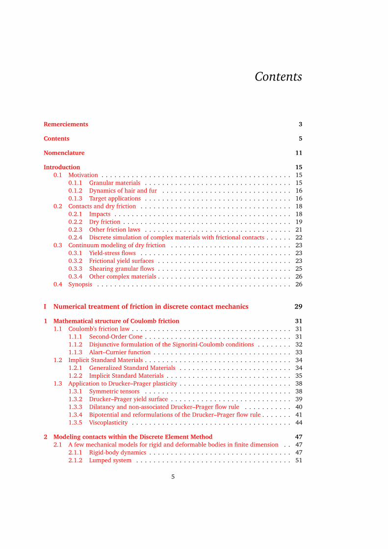
(a) (b) (c)

Figure 0.1: Fur, herbs, and sand are examples of natural complex materials. Thehourglass on the right illustrates the different dynamical regimes that canbe exhibited by granular materials: liquid (above the outlet), gaseous(below the outlet), and solid (the core of the heap in the bottom com-partment).

15

INTRODUCTION

distinguishes them from powders, made of much smaller grains. Considering this limit size,grain-grain interactions in dry granulars are mainly dictated by contact and dry friction, whileair–grain interactions can be neglected. The case of immersed materials, for which interactionswith the surrounding fluid can no longer be neglected, will also be treated in Chapter 8. Cohesionbetween grains may furthermore be considered, typically in the case of wet materials.

Being ubiquitous in outdoor environments, materials made of such grains have been heavilystudied by the mechanical and geotechnical communities in the last century. They have also seenapplications in a wide range of industries, including Computer Graphics. Indeed, despite theirapparent simplicity, granular materials — even when constituted of rigid grains — are capableof exhibiting visually very rich dynamics. In particular, contacts and friction in such materialsallow them to switch between three distinct regimes:

• a solid regime, when the material is maintained at rest by dry friction — for instance thecore of the sand dune in Figure 0.1(b);

• a flowing regime, in which the material behaves like a liquid — consider the flow at theoutlet of the hourglass from Figure 0.1(c), or the avalanching behavior on the outer layerof a dune;

• a gaseous regime, when the grains are mostly separated and only interact through sparseimpacts — the flow below the hourglass’ outlet, or the projections made by an impact ona granular bed.

All of these regimes (and the transitions between them) have to be properly modeled in orderto produce visually convincing simulations.

0.1.2 Dynamics of hair and fur

Fibrous materials feature constituents with one dimension much longer than the other ones.Driven by industrial applications, particular cases of fibrous materials have also been the sub-ject of extensive research. For instance, the flow of polymer suspensions is critical to injectionmolding, and the tire engineering community is deeply interested in the study of the cords’ wearby repeated small deformations. In contrast, the large-deformation dynamics of assemblies ofslender elastic rods subject to frictional contacts, as is the case of hair and fur, have historicallyseen less interest. Yet, industrial applications such as cosmetology and digital virtual effects haverecently put the spotlight on such complex materials (Ward et al. 2007).

A human head of hair consists of about 150, 000 individual strands, which are very elon-gated, with a diameter of about 100µm for a potential length of dozens of centimeters. Con-versely, animal fur such as in Figure 0.1(a) may contain millions of (generally shorter) strands.The relative importance of contact forces compared to other interactions, such as air drag orelectostatic forces, is not well known. However, it is a certainty that contacts and friction playa huge role in the appearance of hair and fur, and proper handling of these interactions is ofutmost importance for Computer Graphics applications. Indeed, frictional contacts maintain thevolume of the groom, and thus the silhouette of the virtual character. Dry friction is furthermoreresponsible for the persistence of intricate patterns at rest, and ignoring it can lead to an uncan-nily tidy appearance. Despite these considerations, the work that we will present in Chapter 4was among the first to attempt to properly capture dry friction in hair simulations.

0.1.3 Target applications

In this dissertation, we will not attempt to quantitatively reproduce the behavior of the simulatedmaterials in tightly controlled settings. Instead, we will be interested in capturing the qualitativecharacteristics of their large-scale dynamics.

This choice is partly motivated by applications to Computer Graphics, which we will discuss inmore details below. Independently of the peculiarities of this industry, we believe that convincingsimulations should be based on sound physics; when possible, we will also attempt to capture inour simulations the macroscopic laws that are experimentally observed to govern the materials.

16

0.1. Motivation

(a) Hair dynamics, Chapter 4 (b) Granular pressure, Chapter 6

(c) Dry granular flows, Chapter 7 (d) Immersed avalanches, Chapter 8

Figure 0.2: A few snapshots of simulations from this manuscript

Moreover, we will not solely focus on Computer Graphics; for instance, Chapters 6 and 8, inwhich we will study only 2D model problems, have no direct graphical application, and mightbe of greater interest to the mechanical engineering community.

Computer Graphics As already mentioned, a significant part of this work will be focused ondevising simulation methods that are viable for Computing Graphics. A peculiarity of this ap-plication is that it strives to capture the emerging features that are created by the motion ofthe individual constituents. Indeed, while some of these features may not be significant for themacroscopic mechanical properties of the material (a few grains projected in the air will notaffect the pressure inside a granular medium), they largely contribute to the visual richness ofthe overall phenomenon and would be extremely tedious to animate by hand. This overarchinggoal can thus be quite different from that of the mechanical engineering communities, so thesimulation approaches will also be evaluated using different criteria. We list below a few of thevirtues that numerical methods targeted at Computer Graphics should meet.

• realism, but not accuracy. While the human mind is good at pointing out things that “feeloff”, it is a poor judge about whether a simulated is physically accurate or not, especiallyas part of a heavily stylized movie. As such, we want to be able to capture qualitativefeatures of our complex materials (for instance, the distinct regimes of granulars), but donot necessarily want to solve our equations to a high precision.

• artifacts-free. The resulting simulations must be free of disturbing visual artifacts, such asflickering, popping, privileged directions or creeping. Proper modeling of dry friction is nec-essary to avoid the latter pitfall, and care has to be taken for the underlying discretizationnever to be visible.

• controllability. While physical realism is a good thing, being pleasant to the client’s eye is aprime requirement for any Computer Graphics simulation. If a gravity-defying hair wisp isrequired to achieve the desired look, then the numerical method should be able to handleit. Here, we will not worry too much about this aspect. However, we will prefer modelsbased on measurable physical parameters, and shall ensure that implementation detailssuch as a “number of solver iterations” do not affect too much the simulated physics. In

17

INTRODUCTION

(A)

(B)

x A = x B

n

Figure 0.3: Two bodies (A) and (B) are in contact when two points of their respec-tive surfaces, x A and x B, coalesce. The resulting contact normal, n, isarbitrarily defined to point towards A.

Chapter 4, we will also try to infer some of those physical parameters from the geometryof the material.

• computational efficiency. As providing a good set of control parameters is a hard problem(see also Sigal et al. 2015), a trial-and-error process is often required for artists to ob-tain a satisfying look. To make this process less painful, the numerical method should bereasonably efficient, and simulations for most shots should be able to finish overnight.

0.2 Contacts and dry friction

Proper modeling of invidual constituents (for instance, in the case of fibrous materials, choosingan adequate mechanical model for individual fibers) is obviously of primary importance forcomputing the dynamics of any complex material. However, we will not discuss this topic in thisdissertation, and will simply rely on existing models from the literature. We will instead focuson the modeling and simulation of contacts and dry friction inside the material. We providebelow a brief introduction to these physical phenomena, and present the modeling choices thatwill underpin the remainder of this dissertation.

0.2.1 Impacts

We assume the distinct constituents of our complex material to be large enough that they canbe considered to never overlap. Impacts happen when two previously disjoint objects comeinto contact; that is, when their (initially positive) relative distance drops to zero. Assumingsufficient smoothness of their boundaries, the two bodies will then share a normal directionalong the contacting surfaces, and further relative motion of each pair of contacting points willbe restricted to the half-space spanned by this normal. The simplest scenario, where two locallysmooth and convex bodies (A) and (B) come into contact, is illustrated in Figure 0.3. Let x A(t)and x B(t) denote the position over time, for each object, of the surface point that will take partin the contact. The gap function, h(t) := x A(t) − x B(t), gives the relative position of thosecontacting points. The condition that objects (A) and (B) should not overlap can be written as⟨h(t),n⟩ ≥ 0, where n is the normal to (B) at x B and ⟨·, ·⟩ denotes the usual scalar product. Thetwo objects are in contact at instant t if h(t) = 0; as long as this is the case, the normal relativevelocity, uN(t) :=

dhdt ,n

, should remain positive. Note that u can be discontinuous at the time

of impact; however, following Moreau (1988), we will assume locally bounded variations ofthe relative velocity u, i.e., the existence of a left-limit u(t−) and a right-limit u(t+) at everyinstant t.

At the onset of contact, a finitely-elastic body will compress, storing potential energy in theprocess, then restitute this energy in a second phase. Note that the amount of restituted energydoes not depend on the “hardness” of the material, but rather on its internal structure; if thisamount is high enough, the objects may end up separating themselves. If the elastic body isvery stiff, these compression and decompression phases may happen on a time scale which ismuch lower than that of the studied system dynamics (Cadoux 2009, Section 1.1.1). In order

18

0.2. Contacts and dry friction

to avoid having to explicitly simulate this fine time scale, one may simply model the impact asan instantaneous jump of the relative normal velocities; several models have been proposed forthis purpose. The simplest of them, the empirical Newton impact law, simply states that thepost-impact normal velocity should be opposed and proportional to the pre-impact one, with amaterial-dependent restitution coefficient. On our simple example, this means that uN(t

+i ) =−ξuN(t

−i ) ≥ 0, t i denotes the time of impact and where 0 ≤ ξ ≤ 1 is the restitution coefficient.

Note that this naive law may yield incorrect results in the presence of simultaneous contacts, andfor instance will fail to reproduce the alternation in the contact points of a rigid block rockingon the ground; see (Brogliato 1999) for more discussion about impact laws.

In this work, we will focus on the simplest case of purely inelastic impacts — the energywill be instantaneously dissipated by the system. We shall thus enforce the post-impact normalvelocity, uN(t

+i ), to always be null, and refer to (Cadoux 2009, Section 1.1.5) and (Smith et al.

2012) for suggestions about how the numerical framework used throughout this dissertationmay be adapted to handle Newton-like impacts.

Signorini conditions Physically, the inter-penetration of the two objects is prevented by theonset of a contact-force, r . In the absence of friction and cohesion, this force should be colinearto the contact normal, i.e., r = r Nn with r N ≥ 0. Now, suppose that the two objects are incontact at time t, i.e., hN(t) = 0. We have already stated the following conditions:

1. The normal relative velocity should be positive as long as the points are in contact, i.e.,hN = 0 =⇒ uN ≥ 0.

2. If t is a time of impact, the post-impact normal velocity, uN(t+), should vanish.

3. The normal contact force should be positive, and vanish when hN > 0.

The Signorini conditions are constructed by considering each contact in isolation, or moreprecisely, by assuming that the shock due to an impact does not propagate to other contacts.This is consistent with our choice of a purely inelastic impact law, which already forbids energyrestitution. In the more general setting of a Newton impact law, this means that the pre-impactvelocities are computed independently for each contact point, or again that the work of thenormal contact force at already existing contacts should not be strictly positive, i.e., uN(t

−) =0 =⇒ uN(t

+)r N(t+)≤ 0. Another characterization of this hypothesis is that if t is not a time of

impact for the considered contact, then the contact force should locally be of bounded variationsat t, i.e., should possess both left and right limits. Note that this strategy is unable to correctlymodel the famous Newton craddle, as the impacted balls would be incorrectly predicted to sticktogether (see Smith et al. 2012, Figure 3, bottom).

Combining this new implication with the three previous ones, we get that

uN(t+)≥ 0

r N(t+) = 0 if uN(t

+)> 0r N(t

+)≥ 0 if uN(t+) = 0

(1)

which together are known as the Signorini conditions. Remember however that these velocity-level conditions apply only when the objects are in contact at instant t, i.e., when hN(t) = 0.

The Signorini conditions are more commonly written in a more compact manner, making theuse of complementarity notation and dropping the time variable, as

0≤ uN ⊥ r N ≥ 0,

where the uN ⊥ r N notation means that the two variables should be orthogonal, i.e., r N uN = 0.

0.2.2 Dry friction

The set of inequalities commonly referred to as the Coulomb friction law is actually the result ofobservations made by several authors and over the span of many centuries (Besson 2007). The

19

INTRODUCTION

nr

ϕα

α

g

Figure 0.4: Euler observed that as long as the angle α of an inclined plane remainsbelow the friction angle ϕ = arctanµS , the ratio of the tangential tonormal components of the contact force r will remain below µS , and thebody (gray) cannot not slide.

discovery of the proportionality between the maximal tangential friction force and the normalload, as well as the irrelevance of the apparent contact surface area, are attributed to Leonardde Vinci at the end of the fifteenth century, and independently to Guillaume Amontons twohundred years later. Leonhard Euler distinguishes the static (or sticking) regime, when there isno relative motion between the two objects, from the dynamic regime, when one object is slidingon top of the other. Euler also introduced the notation µS for the static friction coefficient, i.e.,the maximum ratio between the tangential and normal components of the reaction force, andrelated this coefficient to the maximum angle ϕ at which a mass may rest on an inclined planewithout sliding as µS = tanϕ (see Figure 0.4).

In his famed manuscript, Théorie des machines simples: en ayant égard au frottement de leursparties et à la roideur des cordages, Coulomb (1781) compiled the results of several experiments,validating previous theories and noting that in the dynamic regime, the friction coefficient wasindependent of the sliding velocity. He also observed that for most materials, the static frictioncoefficient, µS , was higher than the dynamic one, µD. Overall, Coulomb observed the relation-ship between the normal and tangential forces as obeying

‖r T‖ ≤ µS r N if uT = 0 (static regime)

‖r T‖= µDr N if uT 6= 0 (dynamic regime),(2)

where the ·T denotes the tangential part of the reaction force and relative velocity vectors, e.g.,r T = r − r Nn. Incidentally, the proportionality of friction to the applied load was initiallypostulated by Amontons to be the result of the upper object having to elevate itself above thefine-scale irregularities of the contact surface. However, investigations in the twentieth centuryshowed that this relationship is actually caused by an increase of the microscopic-level contactarea when a higher normal load is applied (Bowden and Tabor 1950).

In this work, we will not distinguish between the static and dynamic friction coefficients.Indeed, the main characteristics of Coulomb friction, such as the existence of a sliding thresholdthat depends on the applied normal load, can already be captured without making this distinc-tion, and we did not judge the gain in realism brought by the introduction of a distinct slidingfriction coefficient worth the significant associated increase in mathematical complexity3. Tak-ing into account the fact that the tangential friction force must oppose the sliding velocity, wewill thus consider the Coulomb friction law as defined by the disjunction (3),

‖r T‖ ≤ µr N if uT = 0§ ‖r T‖= µr N

r T = −αuT, α ∈ R+ if uT 6= 0.(3)

3In discrete-time numerical algorithms, the friction coefficient can always be updated explicitly at each timestepdepending on the status of each contact point.

20

0.2. Contacts and dry friction

µrN

−µrN

uT

rT

(a) Multi-valued (solid, blue) and reg-ularized (dashed, orange) 2D frictionlaws

−µrN

µrN

∆xT

rT

(b) Hysteresis cycles modeled by Dahl’s frictionlaw. ∆x T denotes the relative tangential dis-placement, ∆x T =

∫uTdt

Figure 0.5: Some alternative friction laws: regularized (left) and Dahl’s (right)

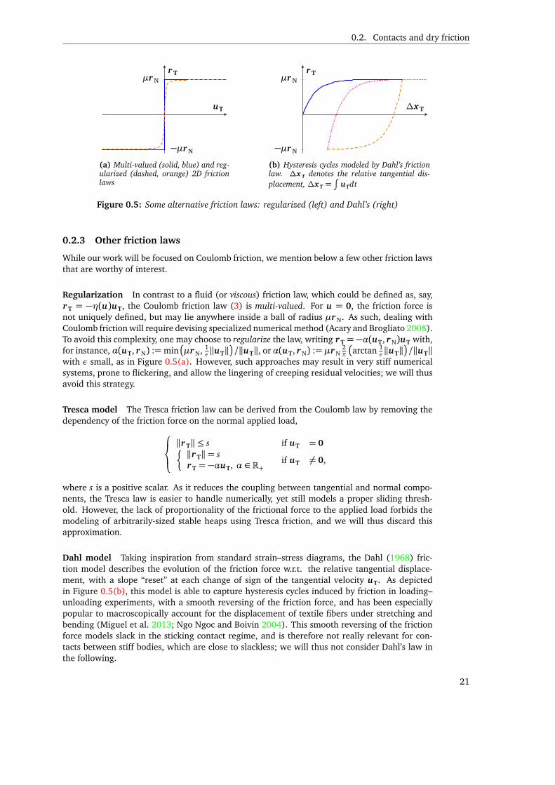
0.2.3 Other friction laws

While our work will be focused on Coulomb friction, we mention below a few other friction lawsthat are worthy of interest.

Regularization In contrast to a fluid (or viscous) friction law, which could be defined as, say,r T = −η(u)uT, the Coulomb friction law (3) is multi-valued. For u = 0, the friction force isnot uniquely defined, but may lie anywhere inside a ball of radius µr N. As such, dealing withCoulomb friction will require devising specialized numerical method (Acary and Brogliato 2008).To avoid this complexity, one may choose to regularize the law, writing r T = −α(uT, r N)uT with,for instance, α(uT, r N) :=min

µr N, 1

ε‖uT‖/‖uT‖, or α(uT, r N) := µr N

2π

arctan 1

ε‖uT‖/‖uT‖

with ε small, as in Figure 0.5(a). However, such approaches may result in very stiff numericalsystems, prone to flickering, and allow the lingering of creeping residual velocities; we will thusavoid this strategy.

Tresca model The Tresca friction law can be derived from the Coulomb law by removing thedependency of the friction force on the normal applied load,

‖r T‖ ≤ s if uT = 0§ ‖r T‖= sr T = −αuT, α ∈ R+ if uT 6= 0,

where s is a positive scalar. As it reduces the coupling between tangential and normal compo-nents, the Tresca law is easier to handle numerically, yet still models a proper sliding thresh-old. However, the lack of proportionality of the frictional force to the applied load forbids themodeling of arbitrarily-sized stable heaps using Tresca friction, and we will thus discard thisapproximation.

Dahl model Taking inspiration from standard strain–stress diagrams, the Dahl (1968) fric-tion model describes the evolution of the friction force w.r.t. the relative tangential displace-ment, with a slope “reset” at each change of sign of the tangential velocity uT. As depictedin Figure 0.5(b), this model is able to capture hysteresis cycles induced by friction in loading–unloading experiments, with a smooth reversing of the friction force, and has been especiallypopular to macroscopically account for the displacement of textile fibers under stretching andbending (Miguel et al. 2013; Ngo Ngoc and Boivin 2004). This smooth reversing of the frictionforce models slack in the sticking contact regime, and is therefore not really relevant for con-tacts between stiff bodies, which are close to slackless; we will thus not consider Dahl’s law inthe following.

21

INTRODUCTION

Figure 0.6: With Discrete Element Modeling, constituents are simulated individually,and all interactions between neighboring bodies must be taken into ac-count.

Rolling friction Rolling friction is induced by the deformation of a wheel near its contact pointwith the ground, and is responsible for energy dissipation that is not captured by the tangentialCoulomb friction law (3). Indeed, Equation (3) implies that the work of the friction force isnon-zero only when sliding occurs. However, in the remainder of this dissertation we will focuson stiff materials and relatively small applied loads, and will thus neglect rolling friction.

0.2.4 Discrete simulation of complex materials with frictional contacts

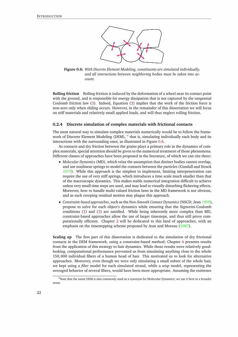
The most natural way to simulate complex materials numerically would be to follow the frame-work of Discrete Element Modeling (DEM), 4 that is, simulating individually each body and itsinteractions with the surrounding ones, as illustrated in Figure 0.6.

As contacts and dry friction between the grains plays a primary role in the dynamics of com-plex materials, special attention should be given to the numerical treatment of those phenomena.Different classes of approaches have been proposed in the literature, of which we can cite three:

• Molecular Dynamics (MD), which relax the assumption that distinct bodies cannot overlap,and use nonlinear springs to model the contacts between the particles (Cundall and Strack1979). While this approach is the simplest to implement, limiting interpenetration canrequire the use of very stiff springs, which introduces a time scale much smaller than thatof the macroscopic dynamics. This makes stable numerical integration difficult to achieveunless very small time steps are used, and may lead to visually disturbing flickering effects.Moreover, how to handle multi-valued friction laws in the MD framework is not obvious,and as such creeping residual motion may plague this approach.

• Constraint-based approaches, such as the Non-Smooth Contact Dynamics (NSCD; Jean 1999),propose to solve for each object’s dynamics while ensuring that the Signorini-Coulombconditions (1) and (3) are satisfied. While being inherently more complex than MD,constraint-based approaches allow the use of larger timesteps, and thus still prove com-putationally efficient. Chapter 2 will be dedicated to this kind of approaches, with anemphasis on the timestepping scheme proposed by Jean and Moreau (1987).

Scaling up The first part of this dissertation is dedicated to the simulation of dry frictionalcontacts in the DEM framework, using a constraint-based method; Chapter 4 presents resultsfrom the application of this strategy to hair dynamics. While those results were relatively good-looking, computational performance prevented us from simulating anything close to the whole150, 000 individual fibers of a human head of hair. This motivated us to look for alternativeapproaches. Moreover, even though we were only simulating a small subset of the whole hair,we kept using a fiber model for each simulated strand, while a wisp model, representing theaveraged behavior of several fibers, would have been more appropriate. Assuming the existence

4Note that the name DEM is also commonly used as a synonym for Molecular Dynamics; we use it here in a broadersense.

22

0.3. Continuum modeling of dry friction

of such a model, we could as well take this approach one step further, and simulate the wholematerial using continuum mechanics.

As a first step towards the simulation of very large complex materials, the second part of thisdissertation embraces this strategy, but focuses on large systems made of simpler constituents:granular materials consisting only of rigid grains. Devising a similar macroscopic simulationmethod for fibrous media such as hair remained out of the reach of this thesis.

Using a continuum approach for granular materials makes sense, as they can be extremelylarge systems – a cubic meter of sand contains close to a trillion individual grains. We see imme-diately that simulating every grain as in the DEM framework, and taking into account each of itsinteractions with its neighbors, is not tractable, especially on standard computers. Moreover, thescale of inhomogeneities in granular materials is usually much smaller than the material itself.For these reasons, several constitutive laws have already been proposed in the literature to modelthe macroscopic behavior of granulars. The next section introduces fundamental concepts forthe continuum modeling of dry frictional contact in granular materials.

0.3 Continuum modeling of dry friction

When the discrete constituents are sufficiently small w.r.t. the scale at which a phenomenon isstudied for the material to appear spatially homogeneous, averaging processes may be used tointuit constitutive equations (or rheologies) on macroscopic quantities such as stress and strain.

0.3.1 Yield-stress flows

For instance, the presence of large molecules in so-called Bingham plastics such as mayonnaisemanifest itself at the macroscopic scale by the onset of a yield stress σS . This means that irre-versible deformations of the material will occur, i.e., the plastic strain rate ǫ will be non-zero,only once the norm of the deviatoric stress, |Devσ|, has reached the critical value σS . Suchmaterials may remain indefinitely stuck in various shapes, in contrast to Newtonian fluids whichwill always, albeit potentially slowly, go back to a flat shape. Note that different choices can beused for the definition of the norm | · | in the above expression, yielding slightly different rhe-ologies, but an objectivity criterion should always be satisfied: one must ensure that the normis invariant to changes in the reference frame. The Bingham model is classically defined us-ing the second invariant of the deviatoric part of the stress tensor, J2(σ) := 1

2 Tr (Devσ)2, with|Devσ| :=pJ2(σ). This definition ensures the objectivity of the model.

Such plastic phenomena are commonly described with a yield surface, that is, a functionF , objective w.r.t. the stress tensor, such that the material remains solid while F(σ) < 0, andF(σ) = 0 corresponds to the flowing regime where irreversible deformation occurs. The yieldsurface for the Bingham model is given FBI(σ) :=

pJ2(σ)−σS .

0.3.2 Frictional yield surfaces

Granular materials also exhibit a yield stress, as demonstrated by their ability to form heaps thatdo not (systematically) collapse over time. However, just like Coulomb friction featured a slidingthreshold proportional to the normal applied load, the yield stress of dry granular materials isobserved to depend on the normal (or mean) stress, i.e., the internal pressure.

Mohr–Coulomb criterion The Mohr–Coulomb (MC) criterion is the continuum mechanicsgeneralization of Euler’s inclined plane experiment, and consider the maximum angle ϕ (theso-called rest angle) that the slope of a granular heap can make without starting to avalanche(Figure 0.7, left). Let us first consider the 2D case, and let σϕ and τϕ denote the normal andshear stresses acting on an inclined plane of angle ϕ. By analogy with Euler’s criterion, thestability of the granular heap up to an angle ϕ means that the material’s yield condition can be

23

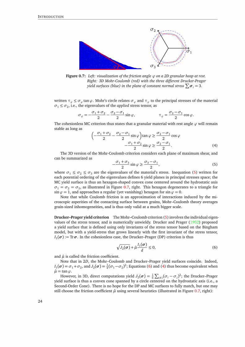
INTRODUCTION

ϕ

σ1

σ2

σ3

Figure 0.7: Left: visualization of the friction angle ϕ on a 2D granular heap at rest.Right: 3D Mohr-Coulomb (red) with the three different Drucker-Prageryield surfaces (blue) in the plane of constant normal stress

∑σi = 3.

written τϕ ≤ σϕ tanϕ. Mohr’s circle relates σϕ and τϕ to the principal stresses of the materialσ1 ≤ σ2, i.e., the eigenvalues of the applied stress tensor, as

σϕ = −σ1 +σ2

2− σ2 −σ1

2sinϕ, τϕ =

σ2 −σ1

2cosϕ.

The cohesionless MC criterion thus states that a granular material with rest angle ϕ will remainstable as long as

−σ1 +σ2

2− σ2 −σ1

2sinϕ

tanϕ ≥ σ2 −σ1

2cosϕ

−σ1 +σ2

2sinϕ ≥ σ2 −σ1

2. (4)

The 3D version of the Mohr-Coulomb criterion considers each plane of maximum shear, andcan be summarized as

−σ1 +σ3

2sinϕ ≥ σ3 −σ1

2, (5)

where σ1 ≤ σ2 ≤ σ3 are the eigenvalues of the material’s stress. Inequation (5) written foreach potential ordering of the eigenvalues defines 6 yield planes in principal stresses space; theMC yield surface is thus an hexagon-shaped convex cone centered around the hydrostatic axisσ1 = σ2 = σ3, as illustrated in Figure 0.7, right. This hexagon degenerates to a triangle forsinϕ = 1, and approaches a regular (yet vanishing) hexagon for sinϕ = 0.

Note that while Coulomb friction is an approximation of interactions induced by the mi-croscopic asperities of the contacting surface between grains, Mohr–Coulomb theory averagesgrain-sized inhomogeneities, and is thus only valid at a much bigger scale.

Drucker–Prager yield criterion The Mohr–Coulomb criterion (5) involves the individual eigen-values of the stress tensor, and is numerically unwieldy. Drucker and Prager (1952) proposeda yield surface that is defined using only invariants of the stress tensor based on the Binghammodel, but with a yield-stress that grows linearly with the first invariant of the stress tensor,I1(σ) := Trσ. In the cohesionless case, the Drucker–Prager (DP) criterion is thus

ÆJ2(σ) + µ

I1(σ)

d≤ 0, (6)

and µ is called the friction coefficient.Note that in 2D, the Mohr–Coulomb and Drucker–Prager yield surfaces coincide. Indeed,

I1(σ) = σ1+σ2, and J2(σ) =14 (σ1−σ2)

2; Equations (6) and (4) thus become equivalent whenµ= tanϕ.

However, in 3D, direct computations yield J2(σ) =16

∑i 6= j(σi − σ j)

2; the Drucker–Prageryield surface is thus a convex cone spanned by a circle centered on the hydrostatic axis (i.e., aSecond-Order Cone). There is no hope for the DP and MC surfaces to fully match, but one maystill choose the friction coefficient µ using several heuristics (illustrated in Figure 0.7, right):

24

0.3. Continuum modeling of dry friction

• µ= 2p

3 sinϕ3−sinϕ , so that DP circumscribes MC;

• µ= sinϕq1+ 1

3 sin2ϕ, so that DP inscribes MC;

• µ= 2p

3 sinϕ3+sinϕ , so that DP interpolates MC at middle vertices.

Choice between these different values is application-dependent. For instance, risk-assessmentsimulations may want to use the inscribed surface, so that the predicted run-out length of anavalanche with DP will always overestimate the one using MC.

Cohesion and tensile strength The Drucker–Prager model can be extended to the modelingof cohesive materials, modifying the yield surface as (Alejano and Bobet 2012)

FDPµ,c(σ) := µ

I1(σ)

d− c +

ÆJ2(σ). (7)

A slightly more complex yield surface, the so-called Drucker–Prager yield surface with tensioncut-off, may also be of interest for materials such as concrete. The cut-off dictates that thematerial will break when the mean tensile stress exceeds a critical value cτc ,

FDPµ,c,cτc

(σ) :=maxI1(σ)− dcτc , FDP

µ,c(σ)

. (8)

The cut-off stress will influence the set of admissible stresses set only when there holds simul-taneously I1(σ) ≥ dcτc and µI1(σ) ≤ dc, which means µcτc ≤ c; the original Drucker–Prageryield surface is retrieved when µcτc ≥ c. For this reason, we will prefer parameterizing the yieldsurface (9) with a shear yield stress, σS := c − µcτc , rather than with the cohesion coefficient c.In the following, we will thus write the Drucker–Prager yield surface with tension cut-off as

FDPµ,σS ,cτc

(σ) :=max

I1(σ)− dcτc , µI1(σ)− dcτc

d−σS +

ÆJ2(σ)

. (9)

Note that the Bingham yield surface is recovered when cτc = +∞.

Other yield surfaces Both the Mohr–Coulomb and Drucker–Prager yield surfaces are nons-mooth; the normal to the surface is not uniquely defined everywhere, in particular for σ = 0

in the cohesionless case. As we will see in Chapter 1, this complicates the definition of a flowrule, that is, we will not be able to unambiguously express the direction of plastic displacementas a function of the stress tensor. ‘ Mast (2013) presents different strategies to circumvent thisdifficulty, such as using a smooth cap for the Drucker–Prager cone, or prescribing the flow to bealong the hydrostatic axis when σ = 0. Another interesting option that they explore is the use ofthe Matzuo–Nakai yield surface, which is smooth everywhere and better matches the hexagonalshape of the Mohr–Coulomb surface that the Drucker–Prager law.

0.3.3 Shearing granular flows

The “GDR MiDi” group (GDR MiDi 2004) studied dense granular shearing flows, and proposeda new constitutive law that was able to match experiments quantitatively, the so-called µ(I)rheology (Jop et al. 2006). Based on the Drucker–Prager yield criterion, this rheology suggeststo vary the friction coefficient with the inertial number I ,

I(ǫ,σ) :=

pJ2(ǫ)DgÆ

I1(σ)/(dρg),

where ǫ is the strain rate, Dg the average diameter of grains, and ρg their density. This dimen-sionless number relates the fluctuation of the velocity at the grain scale to that of the macroscopicflow. When I = 0, the material behaves like a solid, and for very high values of I , the materialbecomes akin to a gas; in between lies the dense flowing regime.

25

INTRODUCTION

Shear-hardening friction The higher the inertial number, the more energy will be dissipatedby grain–grain interactions, and the higher the friction coefficient should be. Jop et al. (2006)propose the following expression:

µ(I) = µS +µD −µS

I0/I + 1,

with µD ≥ µS and where I0 is a material-dependent constant. In contrast to discrete frictionlaws which are usually taken to be slip-weakening (e.g., Coulomb friction when µS > µD), theµ(I) rheology is thus shear-hardening.

Note that the µ(I) rheology does not influence the rest angle of the material; at rest, I = 0and µ(I) = µS .

Dilatancy In a similar manner, the volume fraction of grains φ, that is, the fraction of spaceoccupied by the granular material, can be affected by the shear rate; when this translates intoan augmentation of the flow volume, this phenomenon is known as dilatancy. In dense shearingflow, the volume fraction has been observed to decrease with the inertial number (GDR MiDi2004). Roux and Radjai (1998) define the dilatancy angle ψ from the ratio between the volu-metric and shear strain rates, 1

d I1(ǫ) tanψ = J2(ǫ). They relate this angle to a critical volumefraction φc as ψ(φ) = ψ0(φ −φc), so that positive dilatancy occurs above the critical volumefraction, but shear tends to compress the material when φ < φmax.

0.3.4 Other complex materials

This section has made clear that devising macroscopic laws for granular materials, even whenassuming perfectly rigid and spherical grains, was already complex. Continuum modeling of as-semblies of elastic and anisotropic objects such as fibers would require much more sophisticatedmodels, and was thus left out of the scope of this dissertation.

0.4 Synopsis

This dissertation will be divided in two parts. The first one will be mostly dedicated to Coulombfriction, going from the modeling to the numerical resolution of frictional contacts between dis-crete bodies. Note that the first three chapters will consist mostly in a walk through standardmodels and numerical methods from the literature, which Chapter 4 will present original con-tributions.

• Chapter 1 will first look at the mathematical structure of Signorini–Coulomb conditions,presenting a few useful reformulations and showing where such law can fit in standardplasticity theory. Structural similarities with Drucker–Prager flows will be made explicit.

• Chapter 2 will go through standard modeling of contacts in discrete mechanical systems.The Moreau–Jean scheme will be presented, and we will show that each timestep can bereduced to one or more instances of a canonical problem, which we will call a DiscreteCoulomb Friction Problem (DCFP).

• Chapter 3 will be dedicated to numerical algorithms for solving the DCFP, discussing theirrelative relevance for particular problem structures.

• Chapter 4 will present an original variant of the Gauss–Seidel algorithm that proved toperform very well on Computer Graphics applications, such as hair dynamics, hair inversemodeling, and cloth dynamics.

The second part will be focused on the continuum simulation of granular materials. Takingadvantage of the similarities between the Coulomb friction law and the Drucker–Prager yieldsurface, we will show how the numerical methods devised for discrete mechanics can still berelevant in the continuum limit.

26

0.4. Synopsis

• Chapter 5 will serve as an introduction to numerical methods in continuum mechanics,and the different strategies use for the simulation of granular materials.

• Chapter 6 will present our proposed numerical method for the simulation of dense, drygranular flows, which will relax the classical incompressibility assumption and take profitof the DCFP formalism.

• Chapter 7 will extend this method to more general flows with varying volume fraction ofgrains. A discretization scheme and numerical resolution strategy focused on improvingrelevance to Computer Graphics applications will also be presented.

• Finally, Chapter 8 will discuss the extension to granular flows in which the interactions witha surrounding fluid cannot be neglected. Once again, we will show that the dynamics ofsuch flows can be numerically solved as a sequence of DCFP.

Software and Publications

The numerical methods presented throughout this dissertation have been accompanied by thedevelopment of associated simulation programs. Some of them have been released as open-source: a sparse block matrix linear algebra library featuring a few DCFP solvers5 and a granularsimulation software6 based on the Material Point Method framework of Chapter 7. The approachproposed in the first part of this manuscript has also been implemented in industrial settings,both for cosmetology and visual effects applications.

Moreover, some of the contributions presented in this dissertation have already been pub-lished. These publications are listed below, together with pointers to the corresponding parts ofthis manuscript.

Peer-reviewed journals

G. Daviet and F. Bertails-Descoubes (2016a). “A Semi-Implicit Material Point Method for theContinuum Simulation of Granular Materials”. In: ACM Transactions on Graphics. SIGGRAPH’16 Technical Papers 35.4, p. 13. DOI: 10.1145/2897824.2925877 (Chapter 7)G. Daviet and F. Bertails-Descoubes (2016b). “Nonsmooth simulation of dense granular flowswith pressure-dependent yield stress”. In: Journal of Non-Newtonian Fluid Mechanics 234, pp. 15–35. ISSN: 0377-0257. DOI: http://dx.doi.org/10.1016/j.jnnfm.2016.04.006 (Chap-ter 6)A. Derouet-Jourdan, F. Bertails-Descoubes, G. Daviet, et al. (2013). “Inverse dynamic hair model-ing with frictional contact”. In: ACM Transactions on Graphics 32.6, pp. 1–10. ISSN: 0730-0301.DOI: 10.1145/2508363.2508398 (Chapter 4, Section 4.4.1)G. Daviet, F. Bertails-Descoubes, and L. Boissieux (2011). “A hybrid iterative solver for robustlycapturing Coulomb friction in hair dynamics”. In: ACM Transactions on Graphics 30.6, pp. 1–12.ISSN: 0730-0301. DOI: 10.1145/2070781.2024173 (Chapter 4, Sections 4.1 and 4.2)F. Bertails-Descoubes et al. (2011). “A nonsmooth Newton solver for capturing exact Coulombfriction in fiber assemblies”. In: ACM Transactions on Graphics 30 (1), 6:1–6:14. ISSN: 0730-0301. DOI: http://doi.acm.org/10.1145/1899404.1899410 (Chapter 3, Section 3.1.2)

Technical reports

R. Casati et al. (2016). Inverse Elastic Cloth Design with Contact and Friction. Research Re-port. Inria Grenoble Rhône-Alpes, Université de Grenoble. URL: https://hal.archives-ouvertes.fr/hal-01309617 (Chapter 4, Section 4.4.2)O. Bonnefon and G. Daviet (2011). Quartic formulation of Coulomb 3D frictional contact. Anglais.Tech. rep. INRIA - Laboratoire Jean Kuntzmann. URL: http://hal.archives-ouvertes.fr/inria-00553859/en/ (Chapter 4, Section 4.1.2)

5bogus: http://gdaviet.fr/code/bogus6Sand6: http://bipop.inrialpes.fr/~gdaviet/code/sand6

27

INTRODUCTION

Poster

G. Daviet, F. Bertails-Descoubes, and R. Casati (2015). “Fast cloth simulation with implicit con-tact and exact coulomb friction”. In: Proceedings of the 14th ACM SIGGRAPH / EurographicsSymposium on Computer Animation - SCA ’15. DOI: 10.1145/2786784.2795139 (Chapter 4,Section 4.3)

28

Part I

Numerical treatment of friction in discrete

contact mechanics

29

1 Mathematical structure of Coulomb friction

In this chapter, we present a few equivalent formulations of the Coulomb law that will proveuseful for the construction of numerical algorithms. Most of the properties compiled below stemfrom the works of Pierre Alart and Géry de Saxcé in the early 1990’s, and rely upon convexanalysis tools that were largely developed by Jean Jacques Moreau and R. Tyrrell Rockafellar inthe 1960’s. We refer the reader to Appendix A for a brief introduction to this theory, and theenunciation of a few properties of convex cones, subdifferentials and convex conjugates that wewill make frequently use of. Note that this chapter is quite heavy on notations, and not fullyrequired to follow the remainder of this dissertation — the equivalences established here willbe appropriately referred to in the following chapters. The casual reader may choose to readSections 1.1 and 1.3.1–1.3.3, and skip the remaining derivations.

1.1 Coulomb’s friction law

1.1.1 Second-Order Cone

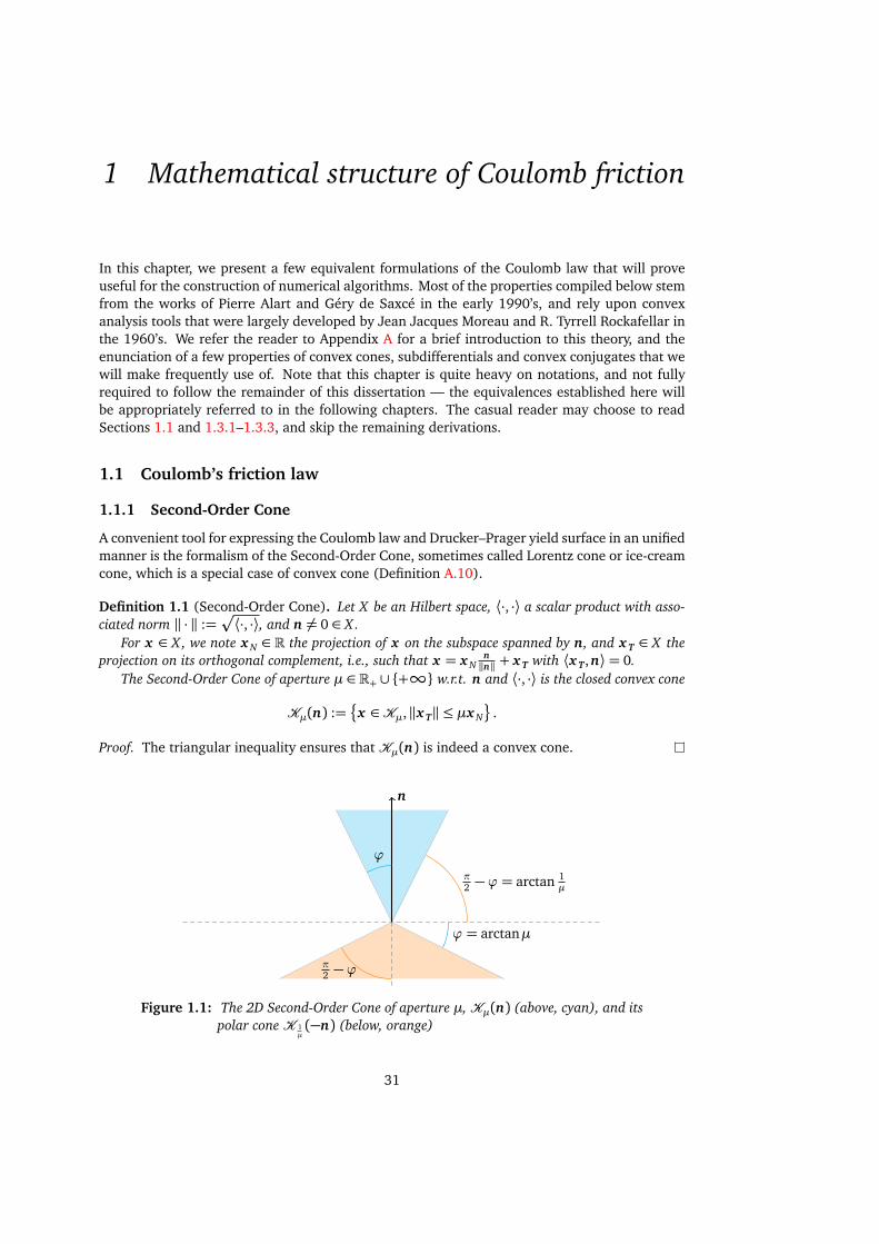
A convenient tool for expressing the Coulomb law and Drucker–Prager yield surface in an unifiedmanner is the formalism of the Second-Order Cone, sometimes called Lorentz cone or ice-creamcone, which is a special case of convex cone (Definition A.10).

Definition 1.1 (Second-Order Cone). Let X be an Hilbert space, ⟨·, ·⟩ a scalar product with asso-ciated norm ‖ · ‖ :=

p⟨·, ·⟩, and n 6= 0 ∈ X .For x ∈ X , we note x N ∈ R the projection of x on the subspace spanned by n, and x T ∈ X the

projection on its orthogonal complement, i.e., such that x = x Nn‖n‖ + x T with ⟨x T,n⟩= 0.

The Second-Order Cone of aperture µ ∈ R+ ∪ +∞ w.r.t. n and ⟨·, ·⟩ is the closed convex cone

Kµ(n) :=x ∈Kµ,‖x T‖ ≤ µx N

.

Proof. The triangular inequality ensures that Kµ(n) is indeed a convex cone.

n

ϕ

ϕ = arctanµ

π2 −ϕ = arctan 1

µ

π2 −ϕ

Figure 1.1: The 2D Second-Order Cone of aperture µ,Kµ(n) (above, cyan), and itspolar cone K 1

µ(−n) (below, orange)

31

1. MATHEMATICAL STRUCTURE OF COULOMB FRICTION

(A)

(B)

nu

(a) Take-off

(A)

(B)

n Kµr

(b) Sticking

(A)

(B)

n Kµ

u

r

(c) Sliding

Figure 1.2: The three cases of the disjunctive Coulomb frictional contact law

An interesting property of the class of Second-Order Cones is that it is closed w.r.t. duality,that is, the dual cone to a SOC is also a SOC. Indeed, direct geometric computations illustratedin Figure 1.1 yield that:

Property 1.1. The dual cone to the Second-Order Cone Kµ(n) is K 1µ(n), the Second Order Cone

of aperture 1µ .

1.1.2 Disjunctive formulation of the Signorini-Coulomb conditions

The Signorini (1) and Coulomb friction (3) conditions can be combined into a slightly morecompact set of three cases, illustrated in Figure 1.2, which we will refer to as the disjunctive for-mulation of the Coulomb contact law (Cadoux 2009). In the take-off case, the two objects areseparating and the reaction force vanishes; the sticking case holds when there is no relative mo-tion; finally, the sliding corresponds to saturated friction and purely tangential relative motion.More formally, the relative velocity u and the contact force r should satisfy one of the followingcases:

r = 0 and uN > 0, (take-off)or r ∈Kµ(n) and u = 0, (sticking)

or§

r ∈ BdKµ(n)r T = −αuT, α ∈ R+ and

§uN = 0uT 6= 0,

(sliding)(1.1)

where Kµ is defined w.r.t. the usual scalar product in Rd . In the following, we will denote byCµ(n) ⊂ Rd ×Rd the set of velocity–force pairs satisfying the Signorini-Coulomb condition,

(u, r ) ∈ Cµ(n) ⇐⇒ u and r satisfy (1.1) ⇐⇒ u and r satisfy (1) and (3).

For the sake of simplicity, we will also stop writing systematically the contact normal n relative towhich the normal cone and the Coulomb law solution set are defined. That is, when the precisedirection of the contact normal is of no relevance, we will write Kµ instead of Kµ(n) and Cµinstead of Cµ(n).

An analogous formulation may be derived by expressing the disjunction on r instead of u,

(u, r ) ∈ Cµ ⇐⇒

uN ≥ 0 and r = 0

or u = 0 and r ∈ intKµor

§uN = 0uT = −αr T, α ∈ R+ and r ∈ BdKµ \ 0

(1.2)

In Section 4.1.2 we will show that for a system with a single contact and a linear relationshipbetween u and r , we can find an analytical solution to the Signorini-Coulomb conditions byenumerating the cases of Equation (1.1). However, as soon as we have to deal with multiplecontacts, the disjunctive formulations become cumbersome to work with. Indeed, for a systemsystem with n contact points, one would have to check for the existence of a solution in eachof the 3n cases — the cost of such an enumeration would quickly become prohibitive. This

32

1.1. Coulomb’s friction law

Kµ

n

Figure 1.3: The projection at the heart of the Alart–Curnier formulation

motivates the search for alternative expressions of these conditions, i.e., ones that would lendthemselves to numerical optimization methods.

1.1.3 Alart–Curnier function

Using the notion of normal cone (see Definition A.9), we can rewrite the Signorini and Coulombfriction conditions into a pair of root-finding problems.

Indeed, computing the normal cones of R+, the set of positive reals, and B d (a) ⊂ Rd , theball of radius max(0, a) centered at 0, yield

NR+(x) =

; if x < 00 if x > 0R− if x = 0,

(1.3)

and

NB d (a)(x ) =

; if ‖x‖> a0 if ‖x‖< aαx , α ∈ R+ if ‖x‖= a and a > 0Rd if ‖x‖= a and a = 0.

(1.4)

Studying each case of those expressions confirms that they correspond to those of the Sig-norini and Coulomb friction laws. We thus get the equivalences

(1) ⇐⇒ uN ∈ −NR+(r N),

(3) ⇐⇒ uT ∈ −NB d−1(µr N)(r T).

Finally, we can use Corollary A.6 to express the normal cone inclusions as fixed points of orthog-onal projections, and obtain the functional formulation of the Coulomb contact law introducedby Alart and Curnier (1991),

(u, r ) ∈ Cµ ⇐⇒ fAC(u, r ) = 0 (1.5)

with, for any ξ ∈ R∗+

,

fAC : Rd ×Rd → Rd

(u, r ) 7→

ΠR+(r N − ξuN)

ΠB d−1(µr N)(r T − ξuT)

− r .

(1.6)

The effect of the tangential and normal projections in Equation 1.6 is illustrated in Figure 1.3;note that their result is always inKµ. Now, given a kinematic relationship between u and r , onecould express the search of solutions satisfying the Coulomb law as a root-finding problem, or asa minimization problem on the norm of fAC. Note however that the orthogonal projections are

33

1. MATHEMATICAL STRUCTURE OF COULOMB FRICTION

not differentiable everywhere, making fAC a nonsmooth function, and thus requiring a carefuldesign of the minimization algorithm.

While being an effective tool for the resolution of practical problems, the Alart–Curnier func-tion yields little insight into the mathematical structure of the Coulomb contact law. One maywonder if we could retrieve more information from the theory of plasticity, which is what wewill discuss in the following section.

1.2 Implicit Standard Materials

1.2.1 Generalized Standard Materials

In its simplest form, the theory of Generalized Standard Materials (GSM) relates the evolutionof a strain-like variable, ǫ ∈ X , and a stress-like variable, σ ∈ Y , where X and Y are reflexiveBanach spaces, dual for the bilinear form ⟨·, ·⟩. Considering an isothermal system described by ǫand another internal variable γ, its evolution should satisfy (see, e.g., Saramito 2015, chapter 5)

σ ∈ ρ∂ E∂ ǫ(ǫ,γ) +

∂D∂ ǫ(ǫ, γ)

0 ∈ ρ∂ E∂ γ(ǫ,γ) +

∂D∂ γ(ǫ, γ)

with E and D proper closed convex functions, ρ is the density of the material, and ǫ := dǫdt . E is

called the Helmotz free-energy function, and D the dissipation potential.Still following Saramito (2015, chapter 5), we can decompose the strain ǫ as an elastic part,

ǫe, and a plastic part, ǫp. Assuming locally small deformations, we write ǫ = ǫe + ǫp. Wefurthermore consider that the free energy depends only on ǫe, and the potential of dissipationonly on ǫp. Writing again our equations for γ := ǫe, we get

σ ∈ ∂D∂ ǫ − ǫe

(ǫ − ǫe)

0 ∈ ρ ∂ E∂ ǫe(ǫe)−

∂D∂ ǫ − ǫe

(ǫ − ǫe),

or equivalently,

σ ∈ ∂D∂ ǫp(ǫp)

σ ∈ ρ ∂ E∂ ǫe(ǫe).

(1.7)

(1.8)

Note the purely plastic case is recovered for E = I0, as Equation (1.8) then boils down toǫe = 0.

Using Theorem A.2, we can also write Equation (1.7) as the so-called flow rule,

ǫp ∈∂D⋆∂σ(σ). (1.9)

We are interested in the particular case of yield-stress materials, where analogously to ourCoulomb contact force r that must lie in Kµ, the stress σ must belong to an admissible set. LetC := σ, F(σ) ≤ 0 be this set of admissible stresses, with F(σ) = 0 the yield isosurface. Theflow rule (1.9) is said to be associated if it is derived from Hill’s maximum power principle (seee.g., de Saxcé and Bousshine 2002), which imposes

σ = argminτ∈C

− τ, ǫp

.

From the optimality condition of Theorem A.6, a flow rule will thus be associated if and only ifǫp ∈ NC(σ), and therefore D = IC

⋆.

34

1.2. Implicit Standard Materials

Remark The flow rule (1.9) is often written as

ǫp ∈∂D⋆∂σ(σ) ⇐⇒ ǫp ∈ α

∂ F

∂σ(σ) and

F(σ)≤ 0

α= 0 if F(σ)< 0

α ∈ R+ if F(σ) = 0

⇐⇒ ǫp ∈ α∂ F

∂σ(σ) and 0≥ F(σ)⊥ α≥ 0

where α is called the plastic multiplier, or consistency parameter. The equivalence – underregularity conditions for F – is granted by Property (A.16).

Coulomb law In our multibody contact setting, −r plays the role of σ and u that of ǫp. Asa first attempt to fit Coulomb friction in the GSM framework, we can define an associated flowrule from the admissible set for the contact force, −r ∈ −Kµ. Since Kµ is a convex cone,Theorem A.4 states that the flow rule u ∈ N−Kµ(−r ) will be equivalent to Kµ ∋ r ⊥ u ∈ K 1

µ.

This means that the power dissipated through the friction force, ⟨u, r ⟩, will always be zero; this isphysically absurd, unless µ= 0. We therefore conclude that Coulomb friction cannot be modeledwith an associated flow rule. Actually, de Saxcé and Feng (1998) showed that attempting tofit the Coulomb contact law inside the GSM framework is vain, and that Rockafellar’s cyclicmonotonicity criterion asserts that one cannot find a dissipation potential D such that (u, r ) ∈Cµ ⇐⇒ −r ∈ ∂D(u). Instead, they introduce the Implicit Standard Material framework, asuperset of GSM in which the dissipation potential may depend on the strain-rate-like variables.

1.2.2 Implicit Standard Materials

The theory of Implicit Standard Materials (ISM) was introduced by de Saxcé and Feng (1991),and extended in (Berga and de Saxcé 1994; de Saxcé 1992; de Saxcé and Feng 1998). As thestandard notion of dissipation potential is not adapted to the modeling of Coulomb’s law, theyintroduce the weaker notion of bipotentials, which they define as follows:

Definition 1.2 (Bipotential). A function b : X × Y → R is called a bipotential if

1. b is convex and closed w.r.t. each of its two parameters, and

2. b satisfies a Fenchel-Young-like inequality, that is

b(ǫ,σ)≥ ⟨ǫ,σ⟩ ∀ǫ,σ ∈ X × Y. (1.10)

This definition allows for a weaker, unilateral version of Theorem A.2,

Property 1.2. If b is a bipotential, then

b(ǫ,σ) = ⟨ǫ,σ⟩ =⇒ ǫ ∈ ∂ b

∂σ(ǫ,σ) and σ ∈ ∂ b

∂ ǫ(ǫ,σ).

Proof. Combining the left-hand-side with the inequality (1.10) yields

b(ǫ,τ)− b(ǫ,σ)≥ ⟨ǫ,τ⟩ − ⟨ǫ,σ⟩ ∀τ ∈ Y, i.e.,

b(ǫ,τ)≥ b(ǫ,σ) + ⟨ǫ,τ−σ⟩ ∀τ ∈ Y,

which by definition of the subdifferential means ǫ ∈ ∂ b∂σ (ǫ,σ). The second inclusion, σ ∈

∂ b∂ ǫ (ǫ,σ), can be derived in a similar manner.

35

1. MATHEMATICAL STRUCTURE OF COULOMB FRICTION

This motivates the Implicit Standard Material approach, which replaces Equations (1.7)and (1.9) from GSM with

σ ∈ ∂ b

∂ ǫp(ǫp,σ)

ǫp ∈∂ b

∂σ(ǫp,σ).

(1.11)

(1.12)

One can readily see that for b(ǫ,σ) = D(ǫ) +D⋆(σ), we fall back to the GSM case and thereciprocal of Property 1.2 is also true. In the general case, the reverse implication will have tobe checked manually to ensure that Equations (1.11) and (1.12) are equivalent.

Coulomb law In the framework of ISM, de Saxcé and Feng (1991) constructed a bipotentialb(u,−r ) such that Equations (1.11) and (1.12) are equivalent to the Coulomb contact law (1.1).

In order to heuristically construct such a bipotential, we can make the following considera-tions:

• The force r should lie in Kµ• The relative velocity u should lie in K∞ = R+ ×Rd−1

• The energy dissipation should be consistent with Coulomb’s law, meaning

b(u,−r ) = −⟨u, r ⟩= −⟨uT,nT⟩= µr N‖uT‖ (1.13)

The simplest function satisfying those rules is indeed the one proposed by de Saxcé and Feng(1991),

b(u,−r ) = I−Kµ(−r ) +IK∞(u) +µ‖uT‖r N. (1.14)

Property 1.3. b defined as in (1.14) is a bipotential.

Proof. The closed, convex nature of b w.r.t. each variable is immediate as b is the sum of suchfunctions. Now, for u ∈K∞ and r ∈Kµ, we have to show that

b(u,−r )≥ −⟨u, r ⟩ i.e.,

µ‖uT‖r N ≥ −uNr N − ⟨uT, r T⟩ .Using the Cauchy-Schwartz inequality and the fact that r ∈Kµ,

−⟨uT, r T⟩ ≤ ‖uT‖‖r T‖ ≤ µr N‖uT‖.Finally, uN ≥ 0 and r N ≥ 0, yielding 0≥ −uNr N and thus concluding the proof.

De Saxcé change of variable Now, let us show that with b defined as per (1.14), Equa-tions (1.11) and (1.12) are equivalent to (u, r ) ∈ Cµ. Still following de Saxcé and Feng, wefirst state an intermediate result; let us introduce the auxiliary variable u, deduced from u asu := u +µ‖uT‖n.

This change of variable u 7→ u, illustrated in Figure 1.4 and which we will refer to as the deSaxcé change of variable, maps the half-space K∞ to the Second-Order Cone K 1

µ, with

(uN ≥ 0 ⇐⇒ u +µ‖uT‖n ∈K 1

µand

uN = 0 ⇐⇒ u +µ‖uT‖n ∈ BdK 1µ.

We get the following equivalences, which will prove very useful for the conception of numer-ical algorithms.

36

1.2. Implicit Standard Materials

nKµ

K 1µ r

u

u

Figure 1.4: De Saxcé change of variable u 7→ u in the sliding case of Coulombfriction. More generally, this change of variable maps the half-spaceK∞to the dual cone K 1

µ

Property 1.4. The Coulomb contact law (1.1) can be expressed in a compact manner on the vari-ables r and u as

(u, r ) ∈ Cµ ⇐⇒ u ∈ −NKµ r ⇐⇒ r ∈ −NK 1µ

u ⇐⇒ K 1µ∋ u ⊥ r ∈Kµ,

where the ⊥ notation is referring to the usual Rd orthogonality.

Proof. Let us prove the first equivalence. Property A.14 gives us the expression of NKµ ,

u ∈ −NKµ(r ) ⇐⇒

r ∈Kµu = 0 if r ∈ intKµu ∈K 1

µif r = 0

u ∈ BdK 1µ∩ r⊥ if r ∈ BdKµ \ 0

⇐⇒

r ∈Kµu = 0 if r ∈ intKµu ∈K∞ if r = 0

u ∈ BdK∞ and uT = −αr T, α ∈ R+ if r ∈ BdKµ \ 0We recognize the disjunctive formulation of the Coulomb law on r , Equation (1.2), and concludethat u ∈ −NKµ(r ) ⇐⇒ (u, r ) ∈ Cµ. Then, the other equivalences are direct applications ofTheorem A.4, noting that −Kµ =K 1

µ.

We therefore want our candidate bipotential to satisfy u ∈ ∂I−Kµ(−r ) ⇐⇒ u ∈ − ∂ b∂ r (u,−r ).

This will be the case if we choose b as b(u,−r ) = I−Kµ(−r ) +µ‖uT‖r N + f (u).

Property 1.5 (Bipotential for Coulomb law). The bipotential b defined as in Equation (1.14)models the Coulomb contact law, i.e.,

b(u,−r ) = −⟨u, r ⟩ ⇐⇒ r = − ∂ b

∂ u(u,−r ) ⇐⇒ u = −∂ b

∂ r(u,−r ) ⇐⇒ (u, r ) ∈ Cµ

Proof. From Properties 1.2 and 1.3, we know that

b(u,−r ) = −⟨u, r ⟩ =⇒ r = − ∂ b

∂ u(u,−r ) and u = −∂ b

∂ r(u,−r ).

As the regularity conditions of Corollary A.1 on the subdifferential of a sum are satisfied, we get

u ∈ −∂ b

∂ r(u,−r ) ⇐⇒ u ∈

∂I−Kµ(−r )− µ‖uT‖n

⇐⇒ u ∈ −N−Kµ using Property A.9

⇐⇒ (u, r ) ∈ Cµ. using Property 1.4

37

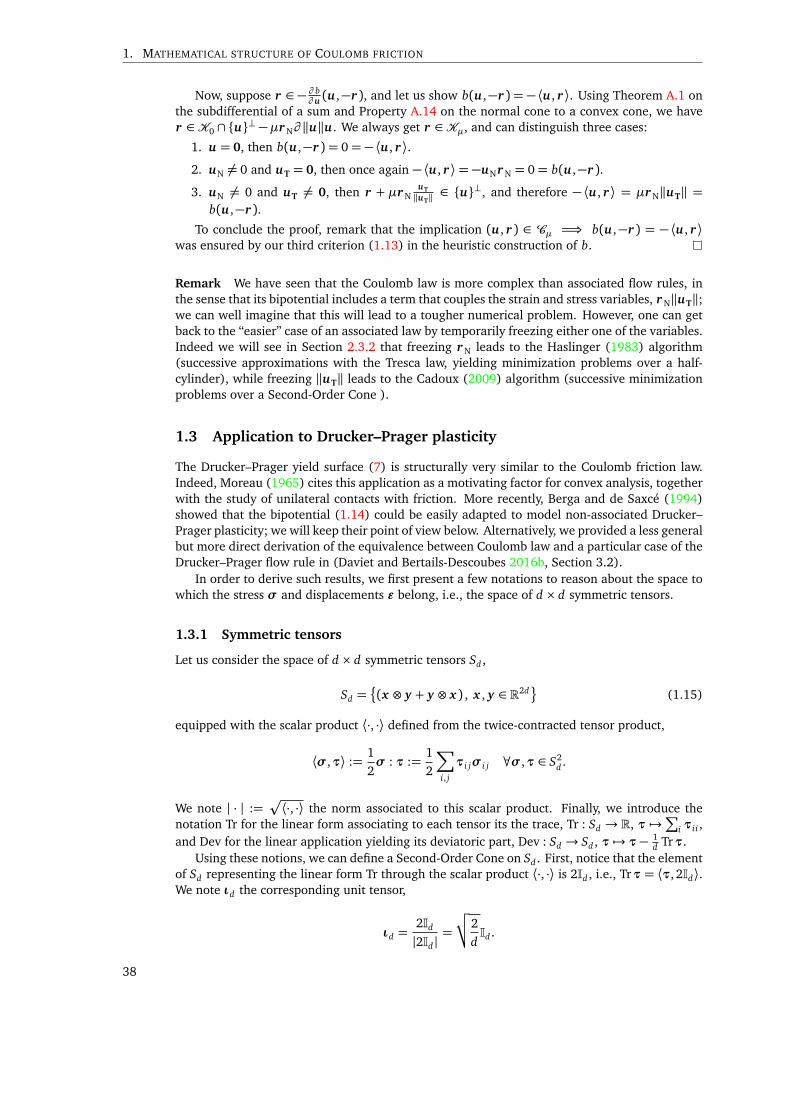
1. MATHEMATICAL STRUCTURE OF COULOMB FRICTION

Now, suppose r ∈ − ∂ b∂ u (u,−r ), and let us show b(u,−r ) = −⟨u, r ⟩. Using Theorem A.1 on

the subdifferential of a sum and Property A.14 on the normal cone to a convex cone, we haver ∈K0 ∩ u⊥ −µr N∂ ‖u‖u. We always get r ∈Kµ, and can distinguish three cases:

1. u = 0, then b(u,−r ) = 0= −⟨u, r ⟩.2. uN 6= 0 and uT = 0, then once again −⟨u, r ⟩= −uNr N = 0= b(u,−r ).

3. uN 6= 0 and uT 6= 0, then r + µr NuT

‖uT‖ ∈ u⊥, and therefore −⟨u, r ⟩ = µr N‖uT‖ =b(u,−r ).

To conclude the proof, remark that the implication (u, r ) ∈ Cµ =⇒ b(u,−r ) = −⟨u, r ⟩was ensured by our third criterion (1.13) in the heuristic construction of b.

Remark We have seen that the Coulomb law is more complex than associated flow rules, inthe sense that its bipotential includes a term that couples the strain and stress variables, r N‖uT‖;we can well imagine that this will lead to a tougher numerical problem. However, one can getback to the “easier” case of an associated law by temporarily freezing either one of the variables.Indeed we will see in Section 2.3.2 that freezing r N leads to the Haslinger (1983) algorithm(successive approximations with the Tresca law, yielding minimization problems over a half-cylinder), while freezing ‖uT‖ leads to the Cadoux (2009) algorithm (successive minimizationproblems over a Second-Order Cone ).

1.3 Application to Drucker–Prager plasticity

The Drucker–Prager yield surface (7) is structurally very similar to the Coulomb friction law.Indeed, Moreau (1965) cites this application as a motivating factor for convex analysis, togetherwith the study of unilateral contacts with friction. More recently, Berga and de Saxcé (1994)showed that the bipotential (1.14) could be easily adapted to model non-associated Drucker–Prager plasticity; we will keep their point of view below. Alternatively, we provided a less generalbut more direct derivation of the equivalence between Coulomb law and a particular case of theDrucker–Prager flow rule in (Daviet and Bertails-Descoubes 2016b, Section 3.2).

In order to derive such results, we first present a few notations to reason about the space towhich the stress σ and displacements ǫ belong, i.e., the space of d × d symmetric tensors.

1.3.1 Symmetric tensors

Let us consider the space of d × d symmetric tensors Sd ,

Sd =(x ⊗ y + y ⊗ x ) , x , y ∈ R2d

(1.15)

equipped with the scalar product ⟨·, ·⟩ defined from the twice-contracted tensor product,

⟨σ,τ⟩ :=1

2σ : τ :=

1

2

∑

i, j

τi jσi j ∀σ,τ ∈ S2d .

We note | · | :=p⟨·, ·⟩ the norm associated to this scalar product. Finally, we introduce the

notation Tr for the linear form associating to each tensor its the trace, Tr : Sd → R, τ 7→∑i τii ,

and Dev for the linear application yielding its deviatoric part, Dev : Sd → Sd , τ 7→ τ− 1d Trτ.

Using these notions, we can define a Second-Order Cone on Sd . First, notice that the elementof Sd representing the linear form Tr through the scalar product ⟨·, ·⟩ is 2Id , i.e., Trτ = ⟨τ, 2Id⟩.We note ιd the corresponding unit tensor,

ιd =2Id|2Id |

=

√√2

dId .

38

1.3. Application to Drucker–Prager plasticity

n

Tµ,σSϕ = arctanµ

σS

Figure 1.5: The 2D truncated Second-Order Cone Tµ,σS

Then, it can be readily seen that Tr (Devτ) = 0, and that any symmetric tensor τ can be decom-posed as the orthogonal sum τ = ⟨τ, ιd⟩ ιd + Devτ. We can therefore extend the notation ofnormal part and tangential part to the space of symmetric tensors with, for τ ∈ Sd ,

τN = ⟨τ, ιd⟩ τT = Devτ.

In the following, we will reuse the notation Kµ for the Second-Order Cone on the space ofsymmetric tensors defined w.r.t. ⟨·, ·⟩ and the linear form Tr,

Kµ(ιd) := σ ∈ Sd , |σT| ≤ µσN=§σ ∈ Sd , |Devσ| ≤ µp

2dTrσ

ª

1.3.2 Drucker–Prager yield surface

In order to study the Drucker–Prager yield surface in this framework, we have to express theinvariants I1(σ) and J2(σ) as functions of the normal and tangential parts of the stress tensorσ. We have directly I1(σ) = Trσ =

p2dσN, and

J2(σ) =1

2Tr(Devσ)2

=

1

2

∑

i

∑

j

(Devσ)i j

2

!= |Devσ|2

= |σT|2

The Drucker–Prager yield surface with tension cut-off is defined by Equation (9),

FDPµ,σS ,cτc

(σ) =max

I1(σ)− dcτc , µI1(σ)− dcτc

d−σS +

ÆJ2(σ)

=maxp

2d (σN −τc) ,µ (σN −τc)−σS + |σT|

using the notation µ :=q

2d µ and τc =

qd2cτc . We have thus the equivalence

FDPµ,σS ,cτc

(σ)≤ 0 ⇐⇒§τc −σN ≥ 0µ (τc −σN) +σS ≥ ‖σT‖.

In the case σS = 0, we retrieve a set of of admissible stresses similar in structure to that ofthe Coulomb friction, a translation of the SOC Kµ:

FDPµ,c(σ)≤ 0 ⇐⇒ (τcιd −σ) ∈Kµ.

In the general case, for σS ≥ 0, the set of admissible stresses is instead a translation of atruncated Second-Order Cone Tµ,σS

,

Tµ,σS:= σ ∈ Sd ,σN ≥ 0 and |σT| ≤ τc +µσN , (1.16)

39

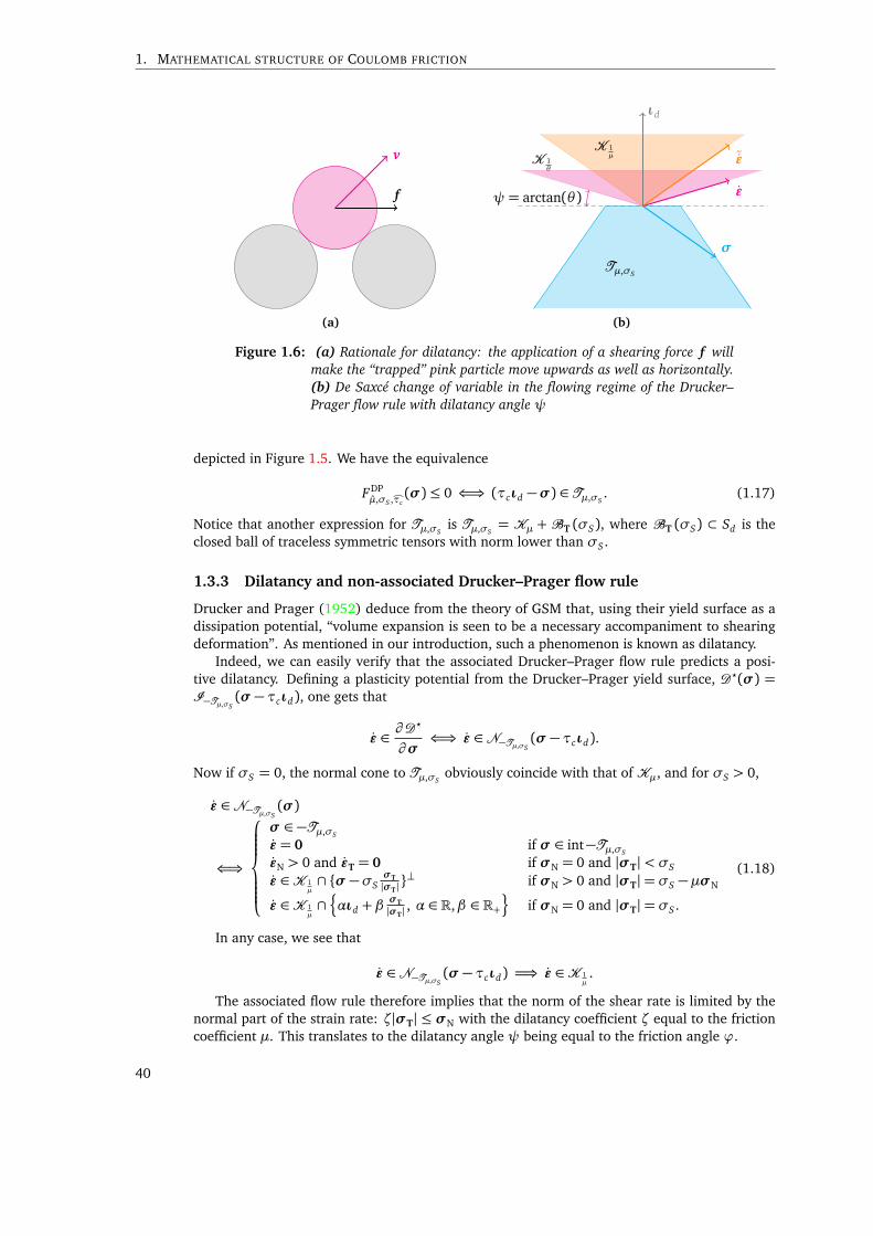
1. MATHEMATICAL STRUCTURE OF COULOMB FRICTION

f

v

(a)

ιd

σ

ǫ

˜ǫ

Tµ,σS

K 1µK 1

θ

ψ = arctan(θ )

(b)

Figure 1.6: (a) Rationale for dilatancy: the application of a shearing force f willmake the “trapped” pink particle move upwards as well as horizontally.(b) De Saxcé change of variable in the flowing regime of the Drucker–Prager flow rule with dilatancy angle ψ

depicted in Figure 1.5. We have the equivalence

FDPµ,σS ,cτc

(σ)≤ 0 ⇐⇒ (τcιd −σ) ∈ Tµ,σS. (1.17)

Notice that another expression for Tµ,σSis Tµ,σS

= Kµ +BT (σS), where BT (σS) ⊂ Sd is theclosed ball of traceless symmetric tensors with norm lower than σS .

1.3.3 Dilatancy and non-associated Drucker–Prager flow rule

Drucker and Prager (1952) deduce from the theory of GSM that, using their yield surface as adissipation potential, “volume expansion is seen to be a necessary accompaniment to shearingdeformation”. As mentioned in our introduction, such a phenomenon is known as dilatancy.

Indeed, we can easily verify that the associated Drucker–Prager flow rule predicts a posi-tive dilatancy. Defining a plasticity potential from the Drucker–Prager yield surface, D⋆(σ) =I−Tµ,σS

(σ −τcιd), one gets that

ǫ ∈ ∂D⋆

∂σ⇐⇒ ǫ ∈ N−Tµ,σS

(σ −τcιd).

Now if σS = 0, the normal cone to Tµ,σSobviously coincide with that of Kµ, and for σS > 0,

ǫ ∈ N−Tµ,σS(σ)

⇐⇒

σ ∈ −Tµ,σS

ǫ = 0 if σ ∈ int−Tµ,σS

ǫN > 0 and ǫT = 0 if σN = 0 and |σT|< σS

ǫ ∈K 1µ∩ σ −σS

σT

|σT|⊥ if σN > 0 and |σT|= σS −µσN

ǫ ∈K 1µ∩¦αιd + β

σT

|σT| , α ∈ R,β ∈ R+©

if σN = 0 and |σT|= σS .

(1.18)

In any case, we see that

ǫ ∈ N−Tµ,σS(σ −τcιd) =⇒ ǫ ∈K 1

µ.

The associated flow rule therefore implies that the norm of the shear rate is limited by thenormal part of the strain rate: ζ|σT| ≤ σN with the dilatancy coefficient ζ equal to the frictioncoefficient µ. This translates to the dilatancy angle ψ being equal to the friction angle ϕ.

40

1.3. Application to Drucker–Prager plasticity

Dilatancy makes physical sense; indeed, a grain initially stuck between others, as in Fig-ure 1.6(a), will first have to go upwards before being able to perform any lateral motion. How-ever, we see from the above computation that a lower friction coefficient will mean a lowerdilatancy, which is not necessarily intuitive. Actually, experiments on granular materials dis-proved this postulate, and the dilatancy was observed to be significantly lower than predictedby the associated flow rule (see e.g., Vermeer 1998). Moreover, the same argument that weused to reject an associated flow rule for the Coulomb friction law can be made again: for acohesionless material, σS = τc = 0, the rate of energy dissipated through the plastic strain rate,ǫ : σ, would be always zero.

Overall, this motivates keeping the dilatancy angle ψ, or equivalently our dilatancy coeffi-cient θ , as a independent parameter of the model. Noting that ǫ ∈K 1

ζ⇐⇒ ǫ+(µ− ζ) |ǫT|ιd ∈

K 1µ, we will follow Berga and de Saxcé (1994) and use the non-associated flow rule defined by

ǫ + (µ− ζ) |ǫT|ιd ∈ N−Tµ,σS(σ −τcιd). (1.19)

For the material to be stable, plastic displacements need to dissipate energy, which meansǫ : σ ≥ 0 for all admissible stresses σ. This implies 0≤ ζ ≤ µ, or in terms of angles, 0≤ψ ≤ φ.Note that for ζ = µ, we retrieve the associated case; however, for ζ < µ we leave the GSMframework and obtain an Implicit Standard Material. For ζ = 0, and a cohesionless material,we retrieve the non-associated Coulomb friction flow rule. Finally, for ζ = µ = 0, σS > 0 andτc = +∞, we obtain the incompressible Bingham yield surface (an infinite cylinder around thehydrostatic axis) with associated flow rule; for τc = 0, we get unilateral incompressibility, that is,plastic expansion is allowed but not compression. More generally, we will see in the followingsection that the flow rule (1.19) enforces a maximum dissipation principle on the deviatoriccomponent of the stress.

In order to lighten notations, we will denote by DP (µ,σS ,τc ,ζ) the set of (ǫ,−σ) ∈ Sd ×Sd

such that the flow rule (1.19) is satisfied. We put the “minus” in front of the stress variablein order to be consistent with our definition of the Coulomb friction solution set Cµ. Indeedwe recognize from Property 1.4 that Cµ ∼ DP (µ, 0, 0, 0), the only difference being that theformer is defined on vector spaces, while the later is defined on tensor spaces. As such, theflow rule (1.19) naturally motivates the introduction of another version of the de Saxcé changeof variable presented in Property 1.4, and illustrated in Figure 1.6(b).

Property 1.6. With the change of variable ǫ 7→ ˜ǫ := ǫ+(µ− ζ) |ǫT|, the Drucker–Prager flow rulemay be written as

(ǫ,−σ) ∈ DP (µ,σS ,τc ,ζ) ⇐⇒ ˜ǫ ∈ N−Tµ,σS(σ −τcιd).

When there are no ambiguities, we will omit the parameters which are taken to be zero, e.g.,,DP (µ,τc) = DP (µ, 0,τc , 0). Indeed, a non-zero τc do not fundamentally change the natureof the solution set, so we will often discard it.

1.3.4 Bipotential and reformulations of the Drucker–Prager flow rule

Using the bipotential framework, we will show that DP (µ,σS ,τc ,ζ) is fully characterized bythe disjunctive formulation (1.20),

σT = (σS +µ(τc −σN))ǫT

|ǫT|if ǫT 6= 0

|σT| ≤ (σS +µ(τc −σN)) if ǫT = 0

0≤ τc −σN ⊥ ǫN − ζ|ǫT| ≥ 0.

(1.20)

We mentioned in the previous paragraph that for σS = τc = ζ = 0, we retrieved a flow rulesimilar to that of the Coulomb contact law; that is, Cµ ∼ DP (µ). This motivates looking for abipotential with a structure similar to Equation (1.14), but adapted to our new version of the deSaxcé change of variable from Property 1.6.

41

1. MATHEMATICAL STRUCTURE OF COULOMB FRICTION

Property 1.7 (Bipotential for the Drucker–Prager flow rule). The function b : Sd × Sd → R,

b(ǫ,σ) = I−Tµ,σS(σ −τcιd) +IK 1

θ

(ǫ) +τc ǫN +σS |ǫT|+ (µ− ζ) (τc −σN) |ǫT|

is a bipotential modeling the non-associated Drucker–Prager flow rule (1.19). That is,

(ǫ,−σ) ∈ DP (µ,σS ,τc ,ζ) ⇐⇒ b(ǫ,σ) = ⟨ǫ,σ⟩⇐⇒ ǫ ∈ ∂ b

∂σ(ǫ,σ) ⇐⇒ σ ∈ ∂ b

∂ ǫ(ǫ,σ)

⇐⇒ the disjunctive formulation (1.20) is satisfied.

Proof. It follows from the definition ofDP and the Drucker–Prager flow rule (1.19) that (ǫ,σ) ∈DP (µ,σS ,τc ,ζ) ⇐⇒ ǫ ∈ ∂ b

∂σ (ǫ,σ).Let us now show that b is a bipotential. b is the sum of convex functions w.r.t. σ and ǫ,

and is therefore is convex w.r.t. each variable; indeed, we supposed that µ ≥ ζ, and σN ≤ τc

everywhere on the effective domain of b. Moreover, for any σ and ǫ in the effective domain ofb, we have ǫN ≥ ζ|ǫT|, and σT ≤ µ(τc −σN) +σS , therefore

⟨ǫ,σ⟩= ǫNσN + ⟨ǫT,σT⟩ ≤ ǫNτc + ǫN(σN −τc) + |ǫT||σT|≤ ǫNτc + ζ|ǫT|(σN −τc) + |ǫT| (µ(τc −σN) +σS)

≤ τc ǫN +σS |ǫT|+ (µ− ζ)(τc −σN)|ǫT|≤ b(ǫ,σ).

Therefore, b is a bipotential.From Property 1.2, this means that we only have to show that

(ǫ,σ) ∈ DP (µ,σS ,τc ,ζ) =⇒ b(ǫ,σ) = ⟨ǫ,σ⟩(1.20) =⇒ b(ǫ,σ) = ⟨ǫ,σ⟩(1.20) ⇐⇒ σ ∈ ∂ b

∂ ǫ(ǫ,σ),

(1.21)

(1.22)

(1.23)

to obtain the complete equivalence chain of Property 1.7. We can first check in each case ofthe expression of the normal cone of Tµ,σS

given in Equation (1.18) that the implication (1.21)holds. Let ˜ǫ denote the de Saxcé change of variable from Property 1.6 and σ := σ − τcιd . Theflow rule (1.19) means ˜ǫ ∈ N−Tµ,σS

(σ), and then either:

1. σ ∈ int−Tµ,σS, then ˜ǫ = ǫ = 0, therefore b(ǫ,σ) = ⟨ǫ,σ⟩= 0

2. σT < σS and σN = 0, then ǫT = 0 and b(ǫ,σ) = ǫNτc = ⟨ǫ,σ⟩3. σN > 0 and |σT|= σS −µσN, then

˜ǫ, σ

=

­˜ǫ, σ −σS

σT

|σT|·+σS

­˜ǫ,σT

|σT|·= σS |ǫT|

and⟨ǫ,σ⟩= ˜ǫ, σ+τc ǫN − ⟨(µ− θ )|ǫ|ιd , σ⟩

= σS |ǫT|+τc ǫN − (µ− θ )σN|ǫT|= b(ǫ,σ).

4. σN = 0 and |σT|= σS , then once again˜ǫ, σ

= σS |ǫT|, and

⟨ǫ,σ⟩= ˜ǫ, σ+τc ǫN − ⟨(µ− θ )|ǫ|ιd , σ⟩= σS |ǫT|+τc ǫN = b(ǫ,σ).

Now, let us treat the right-hand side of the equivalence chain. First, we show the equiva-lence (1.23),

(1.20) ⇐⇒ σ ∈ ∂ b

∂ ǫ(ǫ,σ).

42

1.3. Application to Drucker–Prager plasticity

Indeed,

σ ∈ ∂ b

∂ ǫ(ǫ,σ) ⇐⇒ σ ∈ NK 1

ζ

(ǫ) + (σS − (µ− ζ)) σN∂ |ǫT|∂ ǫ

⇐⇒

ǫ ∈K 1ζ

σ ∈ (σS − (µ− ζ)σN)ǫT

|ǫT|−Kθ ∩ ǫ⊥ if ǫT 6= 0

σ ∈BT ((σS − (µ− ζ)σN))−Kθ ∩ ǫ⊥ if ǫT = 0.

(1.24)

Now, for any τ ∈ Sd , τ− ζτNτT

|τT| ∈ −Kζ ⇐⇒ τ ∈ −K0, so for ǫ ∈K 1ζ,

τ− ζτNτT

|τT|∈ −Kζ ∩ ǫ⊥ ⇐⇒ τ ∈ −K0 and τN(ǫN − ζ|ǫT|).

Moreover, τ ∈ −Kζ ∩ ǫ⊥ implies that τT is colinear with ǫT (with ǫT eventually zero).Using these results in Equation (1.24), we get

σ ∈ ∂ b

∂ ǫ(ǫ,σ) ⇐⇒

ǫ ∈K 1ζ

σN ≤ 0

0= σN(ǫN − ζ|ǫT|)σT = (σS −µσN)

ǫT

|ǫT|if ǫT 6= 0

σT ∈BT ((σS −µσN)) if ǫT = 0

⇐⇒ (1.20).

It now only remains to verify (1.21), i.e., that the disjunctive formulation (1.20) implies thatb(ǫ,σ) = ⟨ǫ,σ⟩. Indeed, if ǫ and σ satisfy (1.20), we have

⟨ǫT,σT⟩= (σS +µ(τc −σN)) |ǫT|ǫNσN = σN(ǫN − ζ|ǫT|) + σNζ|ǫT|+τc ǫN = (σN −τc)ζ|ǫT|+τc ǫN,

so b(ǫ,σ) = ⟨ǫT,σT⟩+ ǫNσN.

Convex conjugate of the truncated SOC characteristic function Property 1.7 implicitly givesan expression for the subdifferential of ITµ,σS

⋆. Indeed, considering the Drucker–Prager flow rulefor µ= ζ and τc = 0, we get

σ ∈ ∂I−Tµ,σS

⋆(ǫ) ⇐⇒ ǫ ∈ N−Tµ,σS

(σ)

⇐⇒ σ ∈ ∂ b

∂ ǫ(ǫ,σ) ⇐⇒ σ ∈ ∂

IK 1

µ

+σS |σT|

.

As moreover I−Tµ,σS

⋆(0) =

IK 1

µ

+σS |σT|= 0, we deduce the equality (Moreau 1966–1967,

Proposition 10.j)

I−Tµ,σS

⋆ = IK 1µ

+σS |σT|. (1.25)

Maximum dissipation principle The first two equations of the disjunctive formulation (1.20)may be rewritten in an equivalent manner as σT ∈ NBT(σS+(τc−σN)µ)

(ǫT), which we recognizefrom Theorem A.6 as the optimality conditions of the optimization problem

maxτ∈BT(σS+(τc−σN)µ)

⟨τ, ǫT⟩.

In other words,σT maximizes the dissipated energy over the set of admissible deviatoric stresses.

43

1. MATHEMATICAL STRUCTURE OF COULOMB FRICTION

Complementarity functions We can use the disjunctive formulation (1.20) to define an ex-tension of the Alart–Curnier complementarity function (1.6) whose roots will coincide with thesolutions of the Drucker–Prager flow rule,

(ǫ,−σ) ∈ DP (µ,σS ,τc ,ζ) ⇐⇒ fAC(ǫ,−σ) = 0 (1.26)

with, for any ξ ∈ R∗+

,

fAC : Sd × Sd → Sd

(ǫ,−σ) 7→ΠR+(τc −σN − ξ (ǫN − θ |ǫT|))

ΠBT(σS+µ(τc−σN))(−σT − ξǫT)

+σ −τcιd .

(1.27)

In both the disjunctive formulation (1.20) and the Alart–Curnier formulation (1.27), a non-zero dilatancy significantly complicates the model, yielding a nonlinear complementarity prob-lem on the normal components of ǫ and σ. However, this coefficient has not as much influenceon the structure of the bipotential. This motivates tackling problems with non-zero dilatancywith methods derived from the bipotential framework, for instance using the de Saxcé change ofvariable. As such, we can define the De Saxcé complementarity function fDS satisfying

(ǫ,−σ) ∈ DP (µ,σS ,τc ,ζ) ⇐⇒ fDS(ǫ,−σ) = 0 (1.28)

with, for any ξ ∈ R∗+

,

fDS : Sd × Sd → Sd

(ǫ,−σ) 7→ ΠTµ,σS

τcιd −σ − ξ˜ǫ

+σ −τcιd

(1.29)

and ˜ǫ defined as the de Saxcé change of variable of Property 1.6, ˜ǫ := ǫ + (µ− ζ)|ǫT|ιd .

1.3.5 Viscoplasticity

Starting again from the GSM equations, we can model viscoplasticity by waiving the assumptionthat D depends only on the plastic displacement ǫp, and writing instead D = V (ǫ) + Dp(ǫp).Equations (1.7–1.8) become

σ ∈ ∂ V∂ ǫ(ǫ) +

∂Dp

∂ ǫp(ǫp)

σ ∈ ∂ V∂ ǫ(ǫ) +ρ

∂ E∂ ǫe(ǫe).

With the viscous dissipation potential V (ǫ) = ηN ǫ2N +ηT ǫ

2T, we get

σ = σe + (ηT ǫ + (ηN −ηT ) ǫNιd)

σe ∈∂Dp

∂ ǫp(ǫp)

σe ∈ ρ∂ E∂ ǫe(ǫe).

We can once again generalize this equations to the framework of Implicit Standard Materialsby allowing Dp to depend on σe as well as on ǫp. Our full visco-elasto-plastic model then reads

σ = σe +ηT

ǫe + ǫp

+ (ηN −ηT )

ǫe + ǫp

Nιd

σe ∈∂ b

∂ ǫp(ǫp,σe)

σe ∈ ρ∂ E∂ ǫe(ǫe).

(1.30)

In this thesis, we will restrict ourselves to the case where E = I0, i.e., the viscoplastic casewhere ǫe = 0, and will choose b to be the Drucker–Prager bipotential defined in Property 1.7.

44

1.3. Application to Drucker–Prager plasticity

Summary

In this first technical chapter, we have derived several equivalent formulations of the Signorini–Coulomb contact law (1–3) and of the non-associated Drucker–Prager flow rule with dilatancy (1.19),which shall prove useful for their numerical resolution. We have seen that these laws do not fitinto the framework of Generalized Standard Materials, but can be described using the morecomprehensive theory of Implicit Standard Materials.

Other cones In this chapter, we studied the nature of laws that were intrinsically linked to theSecond-Order Cone (SOC). It is natural to wonder if and how the equivalences that we obtainedwould translate for other kind of convex cones; for instance, the Mohr-Coulomb yield surface.

As a first step, we can define the p-order cone of aperture µ, K (p)µ , as

K (p)µ :=x ∈ Rd ,µx N ≥ ‖x T‖p

.

For p = 1 or p = +∞, the p-order cone becomes a pyramid, which yields a popular way ofapproximating the Coulomb law in numerical solvers, as in e.g., (Klarbring 1987). Its dualcone is given by (K (p)µ )

⋆= K (q)1

µ

, with q such that 1p +

1q = 1. The de Saxcé change of variable

must then be adapted to u(p) := u + µ‖uT‖qn so that the p-order Coulomb friction law reads

u(p) ∈ −NK (p)µ(r ), or equivalently K (q)1

µ

∋ u(p) ⊥ r ∈ K (p)µ .

Remaining equations The set of equations that we obtained is not sufficient to fully determinea dynamical system. For the discrete contact mechanics, we have two variables, u and r , but onlyone equation linking them. Similarly, our visco-elasto-plastic model (1.30) boasts four variables(σ t ,σe, ǫp and ǫe), but only three equations. We therefore need one more relationship; it willbe provided the so-called conservation equations, which describe how a local stress affects theglobal motion of the dynamical system.

In the next chapter, we will see how to integrate the Coulomb contact law within the frame-work of Discrete-Element Modeling. Starting from chapter 6, we will go back to our viscoplasticmodel (1.30), and apply it to the context of Finite-Element Modeling of granular flows.

45

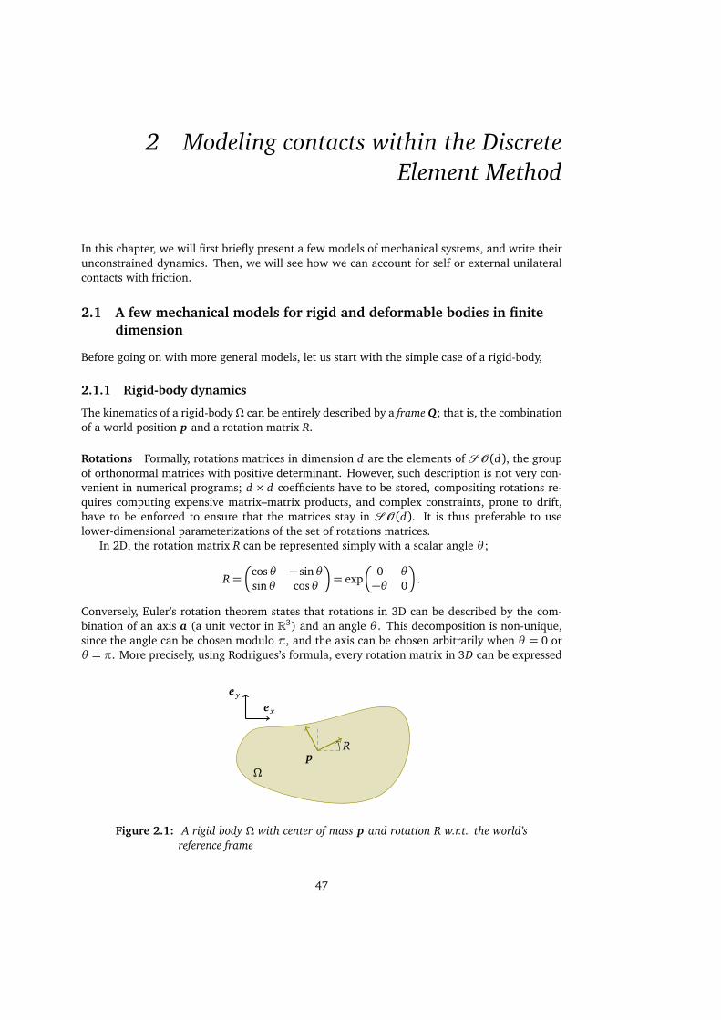
2 Modeling contacts within the DiscreteElement Method

In this chapter, we will first briefly present a few models of mechanical systems, and write theirunconstrained dynamics. Then, we will see how we can account for self or external unilateralcontacts with friction.

2.1 A few mechanical models for rigid and deformable bodies in finite

dimension

Before going on with more general models, let us start with the simple case of a rigid-body,

2.1.1 Rigid-body dynamics

The kinematics of a rigid-body Ω can be entirely described by a frame Q; that is, the combinationof a world position p and a rotation matrix R.

Rotations Formally, rotations matrices in dimension d are the elements of S O (d), the groupof orthonormal matrices with positive determinant. However, such description is not very con-venient in numerical programs; d × d coefficients have to be stored, compositing rotations re-quires computing expensive matrix–matrix products, and complex constraints, prone to drift,have to be enforced to ensure that the matrices stay in S O (d). It is thus preferable to uselower-dimensional parameterizations of the set of rotations matrices.

In 2D, the rotation matrix R can be represented simply with a scalar angle θ ;

R=

cosθ − sinθsinθ cosθ

= exp

0 θ

−θ 0

.

Conversely, Euler’s rotation theorem states that rotations in 3D can be described by the com-bination of an axis a (a unit vector in R3) and an angle θ . This decomposition is non-unique,since the angle can be chosen modulo π, and the axis can be chosen arbitrarily when θ = 0 orθ = π. More precisely, using Rodrigues’s formula, every rotation matrix in 3D can be expressed

Rp

Ω

e x

e y

Figure 2.1: A rigid body Ω with center of mass p and rotation R w.r.t. the world’sreference frame

47

2. MODELING CONTACTS WITHIN THE DISCRETE ELEMENT METHOD

as R = exp[e∧], where [e∧] is the skew-symmetric matrix corresponding to the application ofthe cross product e ∧ ·,

[e∧] :=

0 −ez e y

ez 0 −e x

−e y e x 0

.

The angle of the rotation R is then θ = ‖e‖, and the axis is e‖e‖ (or any unit vector when e = 0).

Alternatively, the set of 3D rotations can be parameterized by the three angles of the successiverotations around each axis of an orthogonal basis — the so-called Euler angles. However, whilevery compact, those representations are not much more satisfying for a numerical implemen-tation; they require numerous trigonometric operations which are computationally expensiveand may accumulate errors, and compositing rotations is still non-trivial. Euler angles are alsosubject to gimbal-locking, that is, in certain configurations they may loose a degree of freedom.

A better way of representing the matrix R in a compact yet well-defined manner is throughthe mean of a unit quaternion q ∈H1,H1 = q := [w, x , y, z] := w+ x i + y j + x z, (w, x , y, z) ∈R4,‖q‖ = 1 with i, j and k square roots of −1. Numerous texts have been written about therelationship between unit quaternions, matrix exponentials and rotations, we refer the reader toe.g., (Cadoux 2009, Appendix C) for a concise introduction focused on their application to rigid-body dynamics. In practice, a unit quaternion q can also be seen as the combination of an angleθ and a unit direction vector a. Indeed, q =

cos( θ2 ); sin( θ2 )a

is unitary and reciprocally, every

unit quaternion can be decomposed in such a way: for instance, θ = 2 atan2(‖[x , y, z]⊺‖, w),and a =

[x ,y,z]⊺

‖[x ,y,z]⊺‖ if sinθ 6= 0, or any other unit vector otherwise. The decomposition is thereforenot unique, but the rotation defined by the axis–angle couple is unique.

Now, the major advantage of using quaternions instead of rotation matrices or their angle–axis representation is that operations on quaternions are well-suited for numerical computations.Indeed,H1 is a group for the canonical quaternion product · × ·, and q1 × q2 coincide with thecomposition of the rotations represented by q1 and q2. At the same time, it is much cheaperand precise to compute than a matrix–matrix product, and less prone to numerical drift (eventhough the resulting quaternion must be kept unitary). Moreover, the applicationH1×R3→ R3,(q , p) 7→ r such that

[0; r ] = q⋆ × [0; p]× q with ([w, x , y, z]⊺)⋆ := [w,−x ,−y,−z]⊺

coincide with the application of the rotation R(q) represented by the quaternion q to the vectorp, i.e., r = R(q)p. Compared to Rodrigues formula, this does not involve any trigonometricoperation, and is therefore much cheaper to compute numerically. Finally, unit quaternionscan also be expressed as the exponential (w.r.t. the quaternion product) of a purely imaginaryquaternion,

cos(θ

2); sin(

θ

2)a

= exp[0;

θ

2a], (2.1)

which naturally links them to the solutions of first-order linear differential equations, and yieldsan insight on their integration through time.

Equations of motions Without loss of generality, we will assume that our kinematic frameQ = (p;q) is positioned at the center of mass of the rigid body. Let also v and ω be the linearand angular velocity of Ω at its center of mass; the time derivative of the frame Q := (p;q)

can be expressed as Q := (v ;ω). Indeed, dp

dt = v , and since the velocity at any point x of Ω

may be computed as v(x ) = v +ω ∧ (x − p), it holds that dR(q)dt x = ω ∧ (R(q)x ), which leads

to dR(q)dt = [ω]∧R(q). This identity transpose to the quaternion framework as a 4-dimensional

first-order linear differential equation, dq

dt =12 [0;ω] × q . Note that if the direction of ω is

constant between t0 and t, i.e., ω(t) = θ (t)a, using (2.1) the solution in time is simply givenby q(t) = [cos θ (t)2 ; sin θ (t)

2 a]× q(t0), with θ (t) such that θ (t0) = 0 and dθdt = θ .

48

2.1. A few mechanical models for rigid and deformable bodies in finite dimension

Supposing a Galilean frame of reference, Newton’s second law over a elementary volume dx

around x reads

ρ(x )dv(x )

dtdx = g(x ,v(x ), t)dx , (2.2)

where g if the volumetric force applied at each point of Ω, and ρ(x ) is the density of the rigidbody. As dv(x )

dt = v + dωdt ∧ (x − p)+ω∧ (ω∧ (x − p)), integrating over Ω yields the conservation

of linear momentum equation,

mdp

dt= g (Q, Q, t) :=

∫

Ω

g(t, x ,v(x ))dx , (2.3)

and applying the vector product (x − p) ∧ · to each side of Equation (2.2) before integratingyields the conservation of angular momentum equation,

I(Q)dω

dt+ω∧ (I(Q)ω) = l(Q, Q, t) :=

∫

Ω

(x − p)∧ g(t, x ,v(x ))dx , (2.4)

where m is the mass and I the inertia matrix of Ω computed as

m=

∫

Ω

ρ(x )dx

I(q) = Tr(T (q))I3 − T (q)

T (q) =

∫

Ω

ρ(x )(x − p)⊗ (x − p)dx .

We see that the inertia matrix I(q), which is computed in the world’s coordinate system, de-pends of the orientation of the frame Q. However, it can easily be deduced from the computationof the inertia matrix I|Q in the frame attached to the rigid body, I(q) = R(q) I|Q R(q)⊺.

Finally, we can group the conservation equations (2.3–2.4) into a single one,

M(Q)dQ

dt= f (Q, Q, t), (2.5)

with M(Q) :=

mI3 00 I(q)

and f (Q, Q, t) :=

g (Q, Q, t)

l(Q, Q, t)−ω∧ (I(Q)ω)

.

Multiple bodies Now that we know how to model the dynamics of a single rigid-body, we canextend our equations to handle more complex objects, such as articulate bodies. Let (Ωi) be aset of N ∈ N rigid-bodies with frames (Qi). Concatenating the degrees of freedom, velocitiesand forces as Q := [Q1; . . . ;QN ], f := [ f 1; . . . ; f N ] and assembling the N mass matrices MI intoa single block-diagonal matrix M := diag(M1, . . . , MN ), the dynamics of the whole system maybe written as

M(Q)

dQ

dt= f (Q, Q, t) + f cst

C(Q) = 0.

where C : (R3 × R4)m → Rn is a function defining constraints on the system, and f csti is the

sum of the forces applied on the body i through the constraints. Now, D’Alembert’s principle1

states that the work of the constraint forces f csti vanishes during a virtual displacement δQ (

that is, an infinitesimal displacement such that the constraints are still satisfied, i.e., such that

1Traité de dynamique, Jean le Rond d’Alembert, 1743

49

2. MODELING CONTACTS WITHIN THE DISCRETE ELEMENT METHOD

Ωi−1

p i

Ωi+1

Li θi

αi−1,i := θi − θi−1

Figure 2.2: An articulated rigid-body chain. Degrees-of-freedom are (p i ,θi), andjoints are modeled by holonomic constraints.

δQ ∈ Ker ∂ C∂Q (Q)). This means that f cst ∈ Ker ∂ C

∂Q (Q)⊥= Im

∂ C∂Q (Q)

⊺, so the dynamics can be

written again as

M(Q)

dQ

dt= f (Q, Q, t) +

∂ C

∂Q(Q)

⊺λ

C(Q) = 0

(2.6)

with λ ∈ Rn.

For instance, one may enforce that two bodies share the same center of mass by takingC = (p1 − p2), which will lead to f cst = (λ;−λ) with λ in R3.

Chain of rigid segments As an illustrative example, we can attempt to model a 2D flexiblechain of N inextensible segments of length 2Li and width ri ≪ Li with frames given by Qi =

(p i ,θi), as in Figure 2.2. The end points ofΩi are given by p i±Le(θi), with e(θ ) := (cosθ ; sinθ ).The velocity of the point of abscissa s on the ith segment is vi(s) = v i+sωe(θ+ π2 ). By homogene-ity with the 3D equations, we will reuse the notation x ∧ y for the determinant of two vectorsin R2, x ∧ y := det (x , y).

Assuming that the first link is clamped at the world’s frame origin, and that the chain’s endis free to move, our nonlinear constraint function C could be defined as

C(Q) =

p1p1 + L1 cosθ1 − p2 + L2 cosθ2

· · ·pN−1 + LN−1 cosθN−1 − pN + LN cosθN

.

Next, assuming a constant density ρi over the volume of the ith segment, the mass of eachcylinder is mi = 2ρi Li ri . In 2D, the inertia matrix Ii boils down to a single scalar coefficient, inour case

Ii = ρi ri

∫ Li

−Li

(se(θi))∧ (se(θi +π

2)) =

1

3mi L

2i .

Finally, we assume that the volumetric force (actually, lineic in our slender case) can bedecomposed into the following contributions:

• The gravity, which we will assume along the y axis. ggi = −ρi ri ge y , and l

gi = 0.

• A viscous air friction term opposing the velocity at each point of the rod, ga(x ) = −ηv(x ),

50

2.1. A few mechanical models for rigid and deformable bodies in finite dimension

p i−1

p i

p i+1

p i+2

p i+3

Figure 2.3: N-tuple pendulum modeled with point passes. Degrees of freedom arelimited to the positions (p i), and each element’s length is maintained byan holonomic constraint ‖p i+1 − p i |= 2Li .

yielding

g ai = −η

∫ Li

s=−Li

vi(x )ds = 2Liηv i

lai = −η

∫ Li

s=−Li

(x (s)− p i)∧ vi(x (s))ds

= −η∫ Li

s=−Li

se(θi)∧ (ωi(se(θi)))ds

= −2

3L3

iωi .

• The force derived from a bending energy E bi, j , which, assuming a Hookean torsion spring,

is quadratic in the bending angle αi, j := θ j − θi between adjacent rods: E bi, j := 1

2 Kα2i, j .

The bending energy E bi, j therefore causes the jth element to induce a torque Kαi, j on the

ith element. Writing the total bending force and torque applied by the ith element at thelink between the ith and (i + 1)th elements gives

0=

∫ L

−L

gbi→i+1(s)ds

−Kαi,i+1 =

∫ L

−L

(s− L)e(θi)∧ gbi→i+1(s)ds =

∫ L

−L

se(θi)∧ gbi→i+1(s)ds,

from which we deduce g bi = 0 and

l bi = −K

α(i−1),i −αi,(i+1)

= −K (2θi − θi−1 − θi+1) .

To summarize, the dynamics of our articulated chain are governed by a second-order ordinarydifferential equation with a banded, symmetric positive semi-definite mass-matrix, non-linearin Q. The force f is linear in Q and Q, and the constraints are non-linear in Q.

2.1.2 Lumped system

Another popular way of modeling deformable objects is to consider them as a set of point atwhich all of the body’s mass is concentrated, possibly with constraints on their relative positions.That is, writing ρi(x ) = δ(x − p i), where δ denotes the Dirac distribution such that for any fieldf over Ω,

∫Ω

f(x )δ(y)dx = f(y). We see immediately that with such a mass distribution, Ii = 0

and l i = 0; therefore, we need only concern ourselves with the evolution of the position of linearvelocity variables p i and v i , and can discard q i and ωi . The mass matrix M is then constant,diagonal and positive definite, simplifying greatly the numerical integration of the dynamical

51

2. MODELING CONTACTS WITHIN THE DISCRETE ELEMENT METHOD

system. However, this approach is not without drawbacks; the discretization of the physicalmodel might be less accurate, and the forces and constraints will often be nonlinear.

A N -tuple pendulum can be modeled in this framework by positioning the point masses atthe links between consecutive elements, as well as at the start and end points of the chain (Fig-ure 2.3). For our chain of N elements, we therefore have (N +1) point masses with coordinates(p i), with the constraint that for 1 ≤ i ≤ 0, ‖p i+1 − p i‖ = Li . The mass associated to the ith

node is then mi := ρ(ri−1 Li−1+ ri Li) (with the convention L−1 = 0). Note that this model is notequivalent to the chain of rigid-bodies presented in the previous section; the kinetic energy ofan individual slender rod is m

2

v2 + 1

3 L2ω2i

, while that of the corresponding two-masses system

would be m2

v2 + L2ω2

i

. Our goal here is simply to give an insight about the structure of the

resulting equations; for the rigid-body chain version of the N -tuple pendulum, only the value(but not the structure) of the inertia matrix and air friction torque would have to be modified.

Now, the forces acting on the node p i are the sum of:1. the gravity contribution, f

gi = −mi ge y .

2. the force induced by air friction, f ai = −(Li−1 + Li)ηv i .

3. the bending force derived from the bending energy E bi, j =

12 Kθ 2

i, j ,

f bi = −α⊺(i−2),(i−1)

∂ α(i−2),(i−1)

∂ p i−α⊺

(i−1),i

∂ α(i−1),i

∂ p i−α⊺i,(i+1)

∂ αi,(i+1)

∂ p i

αi,i+1 = sin−1

‖y i,i+1‖4Li−1 Li

y i,i+1

‖y i,i+1‖y i, j := (p i − p i−1)∧ (p i+1 − p i),

which is nonlinear in Q.In brief, the lumped system boasts a diagonal, positive-definite mass matrix, but suffers fromhighly nonlinear constraints and forces.

2.1.3 Lagrangian mechanics

In the two previous approaches, modeling any complex system led to the introduction of con-straints, which might seriously complicate the process of solving the dynamics differential equa-tion. In contrast, Lagrangian mechanics opens the way for using alternative sets of coordinates.In particular, one may choose to directly parameterize the manifold of admissible kinematic vari-ables with so-called reduced coordinates, which will eventually lead to a constraint-free system.For the sake of simplicity, we only consider this case below.

We consider a non-conservative dynamical system described by a set of m ∈ N kinematic vari-ables q and its time-derivative v := dq

dt , the so-called generalized velocity. Assuming that q arereduced coordinates, any infinitesimal change δq yields a virtual displacement δx=

∑∂ x∂ q iδq i .

Expressing Newtons’ second law of motion for any of those virtual displacements gives∫

s∈Ω

∂ x

∂ q(t, s ,q)

⊺ρ(s)

dv

dt(t, s ,q , v)ds =

∫

s∈Ω

∂ x

∂ q(t, s ,q)

⊺g(t,x(t, s ,q),v(t, s ,q , v))ds

where g is the external force applied at each point of Ω. Moreover, we have also∫

s∈Ωρ(s)

dv

dt(t, s ,q , v)

∂ x

∂ q(t, s ,q)ds

=

∫

s∈Ωρ(s)

d

dt

v(t, s ,q , v)

∂ x

∂ q(t, s ,q)

− v(t, s ,q , v)

d

dt

∂ x

∂ q(t, s ,q)

ds

=

∫

s∈Ωρ(s)

d

dt

v(t, s ,q , v)

∂ v

∂ v(t, s ,q , v)

− v(t, s ,q , v)

∂ v

∂ q(t, s ,q , v)

ds

=1

2

∫

s∈Ωρ(s)

d

dt

∂ v2

∂ v(t, s ,q , v)− ∂ v2

∂ q(t, s ,q , v)

ds .

52

2.1. A few mechanical models for rigid and deformable bodies in finite dimension

Li

αi−1

αi

αi+1 αi+2

Figure 2.4: With the Lagrangian approach and reduced coordinates, the angles (αi)

between successive elements are the sole degrees of freedom for our 2Darticulated chain, and no supplemental constraint is necessary. However,the position of each segment depends on the angle at all prior joints,yielding a dense numerical system.

Introducing the kinetic energy E c of the system,

E c(t,q , v) :=1

2

∫

s∈Ωρ(s)v2(t, s ,q , v)ds ,

we obtain the Euler–Lagrange dynamics equation2,

d

dt

∂ E c

∂ v(t,q , v)− ∂ E

c

∂ q(t,q , v) =

∫

s∈Ω

∂ x

∂ q(t, s ,q)

⊺g(t, s ,q , v)ds . (2.7)

It is convenient to express forces that can be derived from potentials as such; for instance, alarge class of systems can be written as

d

dt

∂ E c

∂ v(t,q , v)− ∂ E

c

∂ q(t,q , v) +

∂ E p

∂ q(q) = −∂D

∂ v(q , v) (2.8)

where E p is the potential energy of the system and D is a dissipation potential.E c being generally quadratic w.r.t. v , expressing the derivatives and integral of Equation (2.7)

leads to

M(t,q)dv

dt= f (t,q , v)

where M(t,q) is symmetric positive semi-definite, with Mi j =∫Ωρ(s) ∂ 2v

∂ v i∂ v j(t, s ,q , v)ds , and

the generalized force f groups terms from internal, external and inertial forces. The expressionof the dynamics of the system in the reduced coordinates q is therefore similar to that of theunconstrained dynamics equation (2.5) in the framework of Section 2.1.1. However, as we willnow see on our 2D articulated chain example, the mass-matrix M(t,q) will not necessarily besparse anymore.

Articulated chain Let q = (αi) ∈ RN , with αi the angle between the (i − 1)th and the ith

segments, and with α0 defined w.r.t. to the clamping angle θ0 which we will assume to be 0.The generalized velocity is v = (ωi), with ωi =

dαidt .

Potential energy The potential energy is the sum of two terms, the bending energy E b and thecontribution of gravity E g . We have E b

i−1,i(q) =12 Kα2

i , and therefore

∂ E b

∂ q(q) =

∑

i

∂ E bi−1,i

∂ q(q) = Kq⊺.

2First established by Joseph Louis Lagrange from the principle of least action in 1756, then from D’Alembert principlein 1788.

53

2. MODELING CONTACTS WITHIN THE DISCRETE ELEMENT METHOD

The potential energy associated to the gravity is more complex. The position of the point atabscissa s of the ith element can be recovered from a recursive formula xi(s) = xi−1(Li−1) + (s+Li)(Π

ij=0R(α j))e x . and the clamping condition x0 = 0. We can therefore evaluate

E g(q) =∑

i

ρi ri

∫ Li

−Li

xi(s), e y

ds =

∑

i

mi

xi(0), e y

,

and the gravity generalized force, − ∂ E g

∂ q (q), can then be computed using

∂ xi(s)

∂ q j(q) =

( Π

j−1k=1R(αk)

R(α j +

π

2)xi(s)− x j(−L j)

if j ≤ i

0 if j > i

Air friction The generalized force f a due to air friction derives from the dissipation potential

D(q , v) :=η

2

∑

i

∫ Li

−Li

v2i (s)ds,

where vi(s) can be once again be computed using a recursive formula,

vi(s) = vi−1(L) + (s+ L)

i∑

j=1

ωi

!e

π

2+

i∑

j=1

α j

!. (2.9)

The expression the friction force is then

f a = −∂D(q , v)

∂ v= −η

∑

i

∫ Li

−Li

∂ xi

∂ q(s)⊺

vi(s)ds,

Inertia Finally, it remains to consider the derivatives of the kinetic energy E c w.r.t. the gener-alized positions and velocity. We have

E c =1

2

∑

i

∫ Li

−Li

v2i (s)ds =

1

2

∑

i

mi

v2

i (0) +1

3L2

iω2i

.

We see from Equation (2.9) that vN (0) depends linearly on all the velocity components (ωi);indeed,

∂ vN (0)

∂ωi= (s+ L)e

π

2+

N∑

j=1

α j

!+ 2L

N−1∑

k=i

e

π

2+

k∑

j=1

α j

!.

Therefore, ∀i, j ∈ [1, N]2,

∂ 2v2N (0)

∂ωi∂ω j=

∂ vN (0)

∂ωi

∂ vN (0)

∂ω j

⊺

and we deduce that the mass matrix M(t,q) is generally dense.

2.1.4 Discussion

While being far from exhaustive, we illustrated a few different approaches for deriving the equa-tions of motion of a mechanical system with kinematic constraints. The logical follow-up ques-tion is then: which one should we use ? There is no definitive answer, but we can compare thedifferent approaches on selected criterions.

54

2.2. Contacts

To this aim, let us remark that all previous derivations can be coalesced into a single canonicalset of equations,

M(t,q)dv

dt= f (t,q , v) +

∂ C

∂ q(t,q)

⊺λ

C(t,q) = 0

where q is a set a generalized coordinates, and v a set of generalized velocities. However,the structure of the mass-matrix M , the properties of force f , and the kinematic constraints Cshowed substantial variations depending on the nature of coordinates.

Modeling capacity Reduced coordinates may not always be adequate. For once, not everysystem can be described with solely holonomic constraints, and even then, finding a constraint-free parametrization is a hard problem — such is the case of inextensible shells (Casati 2015).Note, however that the Lagrangian approach does not prescribe the use of reduced coordinates;it is entirely possible, using again D’Alembert’s principle, to add supplemental constraints to theLagrange equation of motion (2.7), yielding an “intermediate” set of coordinates. However, theLagrange equation (2.7) does require that the velocity variable v be the derivative in time of theposition variable. For instance, this prohibits using a quaternion for the position variable and anangular velocity as the velocity variable, like we did for rigid bodies.

Conversely, point masses are a very rough discretization of a mechanical system, and mightnot model correctly some physical quantities, such as the angular momentum in our 2D exam-ple. Getting more faithful to the continuous model then means adding more point masses andconstraints, making the equations more expensive to solve numerically.

Numerical integration In the presence of holonomic constraints, the equations of motion boildown to an index-3 differential algebraic equation (DAE). Numerical integration of such equa-tions have been extensively studied in the literature, we point the reader to (Haddouni 2015)for a recent review.

On the one hand, the absence of additional constraints is obviously a huge advantage of theLagrangian approach with reduced coordinates, as it allows the use of much simpler integrators.However, in practice supplemental constraints may be required to allow artistic control of thesimulation, and deriving a new reduced kinematic model for each new scene is not practical —it is safer to devise a numerical integrator that can handle kinematic constraints anyway.

On the other hand, the main advantage of the point-masses method is that the mass matrixwill always be diagonal and positive-definite, and thus trivial to inverse; on the contrary, slender3D structures may have vanishing inertia terms when modeled with the Lagrangian of articulatedrigid-body approach. Moreover, the mass matrix of reduced-coordinates models can be dense,leading to more expensive computations.

Another important point deals with the structure of the internal forces; having them dependlinearly on the kinematic variables may greatly simplify the numerical integration process, aswe shall see later. In our 2D example, we saw that all three forces were linear for the chain ofrigid-bodies, while the bending force was nonlinear of the point-masses discretization, and bothgravity and air friction forces were nonlinear for the reduced coordinates model. One may thuschoose one or the other model depending on the respective influence of each force term.

2.2 Contacts

For the sake of simplicity, we first consider a system without kinematic constraints. Using anykind of coordinates, the equation of motion may be written as

M(t,q)dv

dt= f (t,q , v) + f c , f c :=

∫

s∈Ω

∂ v

∂ v(t, s ,q)

⊺gc(s)ds ,

where gc is a supplemental force density due to the contacts.

55

2. MODELING CONTACTS WITHIN THE DISCRETE ELEMENT METHOD

2.2.1 Continuous-time equations of motion with contacts

First, let us discretize our contact surface as a finite number n of contact points (c i), at whichthe contact normal is well-defined. Generating this set is a non trivial task, and the chosenprocess will largely influence the numerical resolution of the system’s dynamics; however, weconsider it as out of the scope of this thesis. Let u i denote the relative velocity at the ith contactpoint. If the ith contact is between two points of our mechanical system (self contact), then thereexist s i,1 and s i,2 such that u i(t,q , v) = v(t, s i,1,q , v)− v(t, s i,2,q , v). Otherwise, the contactis between a point of our system and an external object (external contact), and u i(t,q , v) =

v(t, s i,1,q , v)− w ext(t), where w ext(t) is the velocity of the external object at c i . Let u = (u i).The contact force density gc can be then be expressed as a sum of n punctual forces (r i),

gc =∑

i r iδ(x − c i). We get

f c =

n∑

i=1

∂ v

∂ v(t, s i,1,q)

⊺r i if i is a self contact

∂ v

∂ v(t, s i,1,q)− v

v(t, s i,2,q)

⊺r i if i is an external contact

=

∂ u

∂ v(t,q)

⊺r .

We will assume that u is an affine function of v ; that is, u(t,q) := H(t,q)v + w (t) withH(t,q) = ∂ u

∂ v (t,q). Our equations of motion with unilateral contact can then be summarized as

M(t,q)dv

dt= f (t,q , v) +H(t,q)⊺r

u = H(t,q)v + w (t)

u i , r i satisfy the contact law for 1≤ i ≤ n.

(2.10)

First, we can treat the case of frictionless contacts, or more generally, an associated contactlaw with the convex cone K as the set of admissible forces. The contact law is then K⋆ ∋ u i ⊥r i ∈ K , and we can rewrite system (2.10) as the differential inclusion

M(t,q)dv

dt− f (t,q , v) ∈ −H(t,q)⊺NK⋆(Hi(q)u i + w i(t)).

Under a regularity assumption, for instance, ∃v such that u(t,q , v) ∈ int(K⋆)n, we can useProperty A.12 on the subdifferential of the precomposition with an affine map to write equiva-lently our dynamics equation with unilateral contact as

M(t,q)dv

dt− f (t,q , v) ∈ −NC(q ,t)(v), (2.11)

with the admissible velocity set V (q , t) := v , H(t,q)v + w (t) ∈ (K⋆)n. The associated contactlaw can therefore be modeled with the addition of a dissipation potential D(t,q , v) = IV (q ,t)(v)

to the equations of motion.This form of the equations highlights a difficulty in the definition of dv

dt : as the right-hand-sideof (2.11) may be unbounded and non-differentiable w.r.t. v , q , or t, v might be discontinuous.This is physically intuitive: considering the inelastic impact of a body falling on the ground attime t, its vertical velocity goes instantaneously from a non-zero value at t− to zero at t+. Thesymbol dv

dt should instead be understood as a function defined almost everywhere on a timeinterval [T0, T1], such that

v(t) = v(T0) +

∫ t

T0

dv

dtdt ∀t ∈ [T0, T1].

Equation (2.11) can then be cast as a measure differential inclusion. We will not worry here aboutthe existence of solutions in time to such inclusions, as we will promptly resort to a time-steppingscheme which alleviates most concerns (see e.g., Moreau 1999).

56

2.2. Contacts

Going back to the Coulomb frictional contact law, our equations of motions read

M(t,q)dv

dt= f (t,q , v) + H(t,q)⊺r

u = H(t,q)v + w (t)

(u i , r i) ∈ Cµ i∀1≤ i ≤ n,

(2.12)

where dvdt is still to be understood in the sense mentioned above. The Coulomb law does not

derive from a dissipation potential, but the equation of motions can still be written once againas a differential inclusion,

M(t,q)dv

dt− f (t,q , v) ∈ −H(t,q)⊺N

ΠK 1µi

(u), (2.13)

where u = (u i) = (u i +µi‖(u i)T‖n i) is the contact-wise de Saxcé change of variable defined inProperty 1.4.

2.2.2 Time integration

We now consider the problem of finding solution in time to our equations of motion with uni-lateral contacts. Several algorithms have been developed; we again refer to (Haddouni 2015,chapter 2) for a complete review on this topic.

We can cite two large class of methods. First, event-driven schemes decouple the nonsmoothevents (such as impacts), which happen at a countable set of instants (t i), from the smoothdynamics which hold in every interval between those instants. The main advantage of thisapproach is the ability to use arbitrarily-high order integration schemes between the nonsmoothevents, reaching tight error tolerances at a reasonable computational cost. However, there arealso drawbacks:

• A infinite number of events may occur in a finite time interval; this is known as a Zenophenomenon, and is observed in mechanical systems as simple as rigid ball bouncing onthe ground with a restitution coefficient in ]0,1[ (Brogliato 1999);

• Simultaneous nonsmooth events require special care;

• Numerically, detecting events requires the introduction of several thresholds — saying thatfor instance, two objects will no longer be considered in contact when the gap betweenthem exceeds a certain value. Tuning this threshold parameters is difficult to automate.

A second kind of integration method is usually preferred in practice for systems in which alarge number of events may occur, such as large multi-body systems : time-stepping methods,which integrate the equation of motion over a time interval [tk, tk+1 = tk +∆t] regardless ofwhether or not nonsmooth events occur during the timestep.

Time-stepping methods suppose prior knowledge of the contacts that are going to be ac-tive during the timestep; in practice, this means using proximity-based or continuous-time col-lision detection methods, which we will discuss in the next section. Then, the Moreau–Jean(1987, Moreau 1988) time-stepping algorithm discretizes the continuous-time measure differ-ential equation (2.13) by enforcing that the end-of-step velocity v k+1 — or the correspondingrelative velocity, uk+1 — satisfies the contact constraints.

Velocity-level constraints Consider the ith contact predicted to happen during a timestep[tk, tk +∆t], and let hi(t) denote the gap function, that is, the difference in position at timet of the two points that are going to come into contact at t c

i ∈ [tk, tk+1], as illustrated in Fig-ure 2.5.

For a large ∆t , hiN(tk) might be far from zero, that is, the two points of the future contact

may still be far away from each other. However, the velocity constraint that we formulated inthe continuous case reads uk+1

iN ≥ 0, which would prevent the two points to get any closer.

57

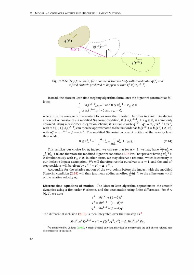
2. MODELING CONTACTS WITHIN THE DISCRETE ELEMENT METHOD

q(tk)

q(tCi )

n ihi(tk)

q(tk+1)

Figure 2.5: Gap function hi for a contact between a body with coordinates q(t) anda fixed obstacle predicted to happen at time tC

i ∈]tk, tk+1].

Instead, the Moreau-Jean time-stepping algorithm formulates the Signorini constraint as fol-lows: ¨

hi(tk+1)iN = 0 and 0≤ uk+1

iN ⊥ r iN ≥ 0

or hi(tk+1)iN > 0 and r iN = 0,

where r is the average of the contact forces over the timestep. In order to avoid introducinga new set of constraints, a modified Signorini condition, 0 ≤ hi(t

k+1) ⊥ r iN ≥ 0, is commonlyenforced. Using a first-order integration scheme, it is usual to write q k+1−q k =∆t(αv k+1+αv k)

with α ∈ [0,1]; hi(tk+1) can then be approximated to the first order as hi(t

k+1) = hi(tk)+∆t u

αi ,

with uαi = αuk+1 + (1 − α)uk. The modified Signorini constraint written at the velocity levelthen reads

0≤ uk+1iN +

1−αα

ukiN +

1

α∆thk

iN ⊥ r iN ≥ 0. (2.14)

This restricts our choice for α; indeed, we can see that for α < 1, we may have 1−αα uk

iN +1α∆t

hkiN < 0, and therefore the modified Signorini condition (2.14) will not prevent having uk+1

iN >

0 simultaneously with r iN > 0. In other terms, we may observe a rebound, which is contrary toour inelastic impact assumption. We will therefore restrict ourselves to α = 1, and the end-of-step positions will be given by q k+1 = q k +∆t v

k+1.Accounting for the relative motion of the two points before the impact with the modified

Signorini condition (2.14) will then just mean adding an offset 1∆t

h(tk) to the affine term w i(t)of the relative velocity u i .

Discrete-time equations of motion The Moreau-Jean algorithm approximates the smoothdynamics using a first-order ϑ-scheme, and the acceleration using finite differences. For ϑ ∈[0, 1], we note

tϑ = ϑtk+1 + (1− ϑ)tk

vϑ = ϑv k+1 + (1− ϑ)v k

qϑ = ϑq k+1 + (1− ϑ)q k

The differential inclusion (2.13) is then integrated over the timestep as 3

M(tϑ,qϑ)(v k+1 − v k)− f (tϑ,qϑ, vϑ) =∆t H(tϑ,qϑ)⊺r .

3As mentioned by Cadoux (2009), f might depend on v and may thus be nonsmooth; the end-of-step velocity maybe considered in this case.

58

2.2. Contacts

Enforcing holonomic constraints to be satisfied at tϑ, our discrete equations of motion read

M(tϑ,qϑ)v k+1 − v k

∆t= f (tϑ,qϑ, vϑ) +H(tϑ,qϑ)⊺r +

∂ C

∂ q(tϑ,qϑ)

⊺λ

C(tϑ,qϑ) = 0

u = H(tϑ,qϑ)v k+1 + w (tϑ) +1

∆th(tk)

(u i , r i) ∈ Cµ i∀1≤ i ≤ n.

(2.15)

Linearized dynamics Solving the implicit nonlinear system (2.15) can then be decomposedas a sequence of problems with explicit mass matrix, internal forces and constraints Jacobiansusing a quasi-Newton algorithm; see, e.g., (Jean 1999; Kaufman, Tamstorf, et al. 2014).

Indeed, let the sequence (v k,l ,q k,l) be recursively defined as the solution of the problem(2.16),

q k,l+1 = q k +∆t vk,l+1

M l v k,l+1 − v k,l

∆t= f (tϑ,qϑ,l , vϑ,l)−M l v k,l − v k

∆t+ H l,⊺r + G l,⊺λ

M l := M l − ϑ∆t∂ f

∂ v(tϑ,qϑ,l , vϑ,l)− ϑ∆2

t

∂ f

∂ q(tϑ,qϑ,l , vϑ,l)

G l v k,l+1 = G l v k,l − C(qϑ,l)

u = H l v k,l+1 + w (tϑ) +1

∆th(tk)

(u i , r i) ∈ Cµ i∀1≤ i ≤ n,

(2.16)

with M l := M(tϑ,qϑ,l), H l := H(tϑ,qϑ,l), G l := ∂ Cq(tϑ,qϑ,l), qϑ,l := ϑq k,l + (1− θ )q k, vϑ,l :=ϑv k,l + (1 − θ )v k, and (v k,0,q k,0) = (v k,q k). Then any value towards which this sequenceconverges will be a solution of the equations of motion (2.15). If f derives from potentials,then M should remain symmetric; however M may non-remain positive semi-definite for largevalues of ∆t . Other approximations should then be used to estimate the Hessian, for instancethe Gauss–Newton method for quadratic potentials.

In practice, this algorithm can be costly; even if the solution at iteration l is a good initialguess for the solution at l + 1, solving each subproblem may require expensive preprocessingsteps. The algorithm is thus (2.16) often truncated to its first step, yielding the so-called lin-earized equations of motion. We will actually adopt this strategy for all of our applications.However, in the presence of highly nonlinear forces, this might worsen the stability or energyconservation properties of the time-stepping scheme (Kaufman, Tamstorf, et al. 2014).

Limitations The time-stepping approach also suffers from limitations. First, it is a low-ordermethod, and thus requires small timesteps to approximate the continuous solution, even whenno nonsmooth events occur. Note that Acary (2009) proposed a first method for improvingthe order of accuracy of the Moreau time-stepping scheme, which performed well on academicexamples.

Then, in the above formulation, the contact constraints are formulated on the velocity, andmay be subject to numerical drift. If hiN(t) becomes negative, then once again we may haveuk+1

iN r iN > 0, and observe a rebound. On the other hand, if we clamp hiN(t) to positive values,the unilateral contact constraints may be violated.

Finally, as already mentioned, an important limitation of the time-stepping algorithm is thatall contacts that may occur during the timestep must be predicted, which is hard problem, as weare going to see in the next section.

59

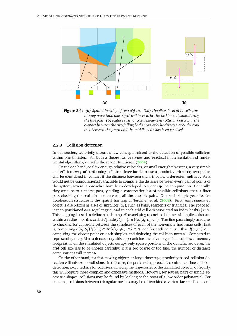
2. MODELING CONTACTS WITHIN THE DISCRETE ELEMENT METHOD

(a)

v1∆t

v2∆t

(b)

Figure 2.6: (a) Spatial hashing of two objects. Only simplices located in cells con-taining more than one object will have to be checked for collisions duringthe fine pass. (b) Failure case for continuous-time collision detection: thecontact between the two falling bodies can only be detected once the con-tact between the green and the middle body has been resolved.

2.2.3 Collision detection

In this section, we briefly discuss a few concepts related to the detection of possible collisionswithin one timestep. For both a theoretical overview and practical implementation of funda-mental algorithms, we refer the reader to Ericson (2004).

On the one hand, or slow enough relative velocities, or small enough timesteps, a very simpleand efficient way of performing collision detection is to use a proximity criterion; two pointswill be considered in contact if the distance between them is below a detection radius r. As itwould not be computationally tractable to compute the distance between every pair of points ofthe system, several approaches have been developed to speed-up the computation. Generally,they amount to a coarse pass, yielding a conservative list of possible collisions, then a finerpass checking the real distance between all the possible pairs. One such simple yet effectiveacceleration structure is the spatial hashing of Teschner et al. (2003). First, each simulatedobject is discretized as a set of simplices (Si), such as balls, segments or triangles. The space R3

is then partitioned as a regular grid, and to each grid cell c is associated an index hash(c) ∈ N.This mapping is used to define a hash-mapH associating to each cell the set of simplices that arewithin a radius r of this cell: H [hash(c)] = i ∈ N, d(Si , c)< r . The fine pass simply amountsto checking for collisions between the simplices of each of the non-empty hash-map cells; thatis, computing d(Si , S j) ∀(i, j) ∈ H (k), i 6= j, ∀k ∈ N, and for each pair such that d(Si , S j) < r,computing the closest point on each simplex and deducing the collision normal. Compared torepresenting the grid as a dense array, this approach has the advantage of a much lower memoryfootprint when the simulated objects occupy only sparse portions of the domain. However, thegrid cell size has to be chosen carefully; if it is too coarse or too fine, the number of distancecomputations will increase.

On the other hand, for fast-moving objects or large timesteps, proximity-based collision de-tection will miss some collisions. In this case, the preferred approach is continuous-time collisiondetection, i.e., checking for collisions all along the trajectories of the simulated objects; obviously,this will require more complex and expensive methods. However, for several pairs of simple ge-ometric shapes, collisions may be found by looking at the roots of a low-order polynomial. Forinstance, collisions between triangular meshes may be of two kinds: vertex–face collisions and

60

2.3. Discrete Coulomb Friction Problem

edge–edge collisions. Assuming a constant rigid motion for each triangle over the timestep, bothcorrespond to the roots of a cubic polynomial. Brochu et al. (2012) proposed a geometrically-exact detection method for such intersections, avoiding the rounding errors associated with thepolynomial root-finding approach.

Yet, in order to compute the collisions along a trajectory, we first need to know the trajectory.Which we don’t, since the trajectory will be influenced by the contact forces, and obviously, tocompute the contact forces, we first need to know the contact points. We therefore need tocompromise, and will use unconstrained velocity (the solution of the unconstrained equationsof motion ) to define the trajectory that will be used for continuous-time collision detection.However, some contacts may not be predicted before the resolution of other collisions. Forinstance, consider two thin bodies A and B, with B above A, falling on the ground G at thesame speed. If ∆t is big enough, they might impact the ground during the same time step; thecontinuous-time collision detection process will then predict the contacts A/G and B/G, but notthe contact A/B, and the two bodies may end up in the same place. Such situations are likely tohappen in the simulation of layered cloth, and may require sophisticated heuristics.

Another solution, if the computational cost is deemed acceptable, would be to perform acollision detection step at each iteration of the algorithm (2.16).

2.3 Discrete Coulomb Friction Problem

Let us refer to the system of equations that we have to solve at each step of the algorithm (2.16)as a Discrete Coulomb Friction Problem (DCFP), and let us write it using a lighter notation as

M v = f + C⊺λ+ H⊺r

C v = k

u = Hv + w

(u i , r i) ∈ Cµ i∀1≤ i ≤ n,

(2.17)

where the unknowns are v ∈ Rm, u ∈ Rnd , λ ∈ Rc and r ∈ Rnd . Moreover, M will be assumedto be symmetric, positive definite, and the rows of C will generally be assumed to be linearlyindependent (that is, unless otherwise mentioned there are no redundant equality constraints).

2.3.1 Reduced formulation

We can eliminate the variable v from the DCFP (2.17), and obtain

Pλ + B⊺r + c = 0

Bλ + W r + b = u

(u i , r i) ∈ Cµ i∀1≤ i ≤ n.

(2.18)

withW := HM−1HT P := C M−1C T B := HM−1C T

b := HM−1 f + w c := C M−1 f − k.

The symmetric, positive semi-definite matrix W is often referred to as the Delassus operator.When the rows of C are linearly independent, C is surjective, therefore P is invertible and

we can go one step further, writing system (2.18) with r and u as the only unknowns,

u = W r + b

(u i , r i) ∈ Cµ i∀1≤ i ≤ n.

(2.19)

with W :=W − BP−1B⊺ and b := b− BP−1c.While this formulation is short and convenient, in practice we will often avoid computing the

W matrix explicitly. First, the inverse of M may be dense; this will be the case for cloth, or finite-element models, among others. In this case, W and P will be dense, and therefore expensive to

61

2. MODELING CONTACTS WITHIN THE DISCRETE ELEMENT METHOD

compute and less likely to fit into main memory. It is also rarely a good idea to compute W , asP−1 will often be dense and the double-inversion might lead to tremendous numerical errors.

However, for multi-body systems, M is a block-diagonal matrix; if the size of the diagonalblocks is reasonable, they can be easily factorized, for instance using a QLDL⊺Q⊺ factorization 4,and it may become fruitful to explicitly compute the Delassus operator. Even then, W might becostly to assemble. We argue in (Daviet, Bertails-Descoubes, and Boissieux 2011) that it is impor-tant to exploit the block structure of M and H to accelerate the computation. Our bogus (Daviet2013) C++ template library provides an easy way to perform efficient linear algebra operationswith sparse block matrices, including a parallelized matrix–matrix multiplication routine. De-spite this, our results for hair simulations (presented in the next chapter, Table 4.2) show that asignificant portion of the total time for solving the DCFP (2.17) was spent assembling the Delas-sus matrix W , and (Daviet, Bertails-Descoubes, and Boissieux 2011, Figure 6) implies a scalingwith the square of the number of contacts, both in time and memory consumption.

More generally, a trade-off has to be made between a higher preprocessing and memorycost, or a higher solver cost. Some of the algorithms that we will present in Chapter 3 willrequire an explicit computation of W , others will just require being able to perform matrix–vector multiplications with W , some will use completely different formulations; their relativeperformance is application-dependent.

2.3.2 Fixed-point algorithms and existence criterion

Still following from the fact that the Coulomb friction law does not derive from a potential, theDCFP (2.17) cannot be formulated as a convex optimization problem. However, (2.17) can becharacterized as the fixed-point of sequences of such problems; we just need to temporarily fixeither u i or r i in the coupling term of the bipotential (1.14), µi r iN‖u iT‖.

As the minimization of convex functions is a well-studied problem, for which numerous effi-cient algorithms have been devised, this iterative strategy may prove fruitful in practice. More-over, this characterization of (2.17) as a fixed-point was used by Cadoux (2009) to state a suffi-cient criterion for the existence existence of solutions, which we will recall in Theorem 2.1.

Haslinger algorithm First, let us fix the normal force r iN. Consider the function hs (which isno-longer a bipotential) derived from (1.14) as

hs(u i ,−r i) = I−Kµi(−r i) +IK∞(u i) + si‖u iT‖.

A velocity–force couple satisfying r i ∈ −∂ hs(u i) will be a solution to the Coulomb friction prob-lem if and only if si = µi r iN. Now, we recognize from Equation (1.25) the expression of theconvex conjugate of IT0,si

, that this, IK∞(u i) + si‖u iT‖ = IT0,si

⋆(u i) (note that T0,siis simply a

semi-infinite cylinder of radius si). This means, using Theorem A.2,

r i ∈ −∂ hs(u i) ⇐⇒ r i ∈ −∂IT0,si

⋆(u i) ⇐⇒ u i ∈ −NT0,s

(r i).

As the optimality conditions of the quadratic minimization problem under cylindrical con-straints (2.20),

minλ∈Rc ,r∈ΠT0,si

1

2(λ⊺, r ⊺)

P B⊺

B W

λ

r

+ (λ⊺, r ⊺)

c

b

, (2.20)

are, from Theorem (A.6),

Pλ + B⊺r + c = 0

Bλ + W r + b = u

u i ∈ −NT0,si(r i) ∀i,

4That is, a Cholesky factorization where the square-root of the diagonal is not explicitly computed for better numer-ical precision, and with a reordering step to reduce the fill-in of the triangular matrix L. The SimplicialLDLT classof the Eigen (Guennebaud, Jacob, et al. 2010) C++ library provides an implementation of this factorization.

62

2.3. Discrete Coulomb Friction Problem

we deduce that the solution of the minimization problem (2.20) will be the solution of thedual form of the DCFP (2.18) if and only if s := (si) = (µi r iN). This leads to the fixed-pointalgorithm introduced by Haslinger (1983), which consists in iteratively solving the minimizationproblem (2.20)5 for a given parameter value s k, then computing s k+1 from the optimal solution,and looping again.

However, the objective function of (2.20) is not strictly convex, and therefore the problemmay have more than one solution. The fixed-point iteration is thus ill-defined, and studying itsconvergence would be tricky. In contrast, Cadoux (2009) formulated an algorithm that does notsuffer from this drawback, by freezing instead the velocity part of the bipotential coupling term.

Cadoux algorithm Let us now consider the function derived from the bipotential by fixing u

in the coupling term,

cs(u i ,−r i) := I−Kµi(−r i) +IK∞(u i) + si r iN.

The equivalence (u i , r i) ∈ Cµi⇐⇒ u i ∈ ∂ cs

∂−r i(−r i) will hold if and only if si = µi‖u iT‖. Now,

direct computations yield that u i ∈ ∂ cs∂−r i(−r i) ⇐⇒ u i + sin i ∈ −NKµi

(r i). The solution of theDCFP (2.18) will therefore be given by the solution of the minimization problem (2.21),

q(s) := minλ∈Rc ,r∈ΠKµi

1

2(λ⊺, r ⊺)

P B⊺

B W

λ

r

+ (λ⊺, r ⊺)

c

b+ s

, (2.21)

when s = (µi‖u iT‖n i), with u :=W r + Bλ+ b

We will refer to problems such as (2.21), where a quadratic objective function is minimizedsubject to SOC constraints, as Second-Order Cone Quadratic Programs (SOCQP). A fixed-pointalgorithm can then be obtained by computing s k+1 from the solution λk to the problem param-eterized by s k as s k+1 = (µi‖uk

iT‖).At first sight, the gain over the Haslinger algorithm is not obvious; the solution to the min-

imization problem (2.21) is still not unique. Cadoux (2009, Theorem 3.5) proves the well-definition of the fixed-point update from a duality argument, using Fenchel’s duality theorem (A.3)to show that the velocity v corresponding to the optimum of (2.21) is the solution of a strictlyconvex minimization problem, meaning that v and thus u are uniquely defined for each s . Here,we will show this well-definition by directly constructing the primal problem from the optimalitycondition of the dual (2.21).

Expressing W and P in the optimality conditions of (2.21), we can get back to a system inthe same unknowns as our original DCFP (2.17),

M v = f + C⊺λ+ H⊺r

C v = k

u = Hv + w

K 1µi∋ u i + s in i ⊥ r i ∈Kµi

∀i = 1 . . . n.

(2.22)

Since system (2.22) derives from the optimality conditions of a convex problem, we we will referto (2.22) as a convexified DCFP. Now, discarding the relative velocity variable u, system (2.22)can be written equivalently as

M v = f + C⊺λ+ H⊺r

λ ∈ −N0Rc (C v − k)

r ∈ −NΠK 1µi

(Hv + w + s).

5Actually, the original Haslinger algorithm solves the Fenchel primal of (2.20).

63

2. MODELING CONTACTS WITHIN THE DISCRETE ELEMENT METHOD

Moreover, from Corollary A.4 to the Property A.12 on the subdifferential of a precompositionwith an affine map, we have always

C⊺N0Rc (C v − k) +H⊺NΠK 1µi

(Hv + w + s) ⊂NV (s)(v)

with V (s) :=n

v ∈ Rm, C v = k and (Hv + w + s) ∈ ΠK 1µi

o, and equality is achieved under the

regularity condition (H (s)),

∃v ∈ Rm, C v = k and (Hv + w + s) ∈ intΠK 1µi

. (H (s))

This means that all the solutions to (2.22) must satisfy (2.23),

M v − f ∈ −NV (s)(v) (2.23)

and that they coincide when the condition (H (s)) is satisfied. Finally, we recognize (2.23) asthe optimality conditions of the strictly convex minimization problem (2.24),

p(s) := minv∈V (s)

1

2v⊺M v − v⊺ f . (2.24)

Summarizing, the velocity v reconstructed from a solution (λ, r ) of the dual SOCQP (2.21)as v = M−1 ( f + C⊺λ+ H⊺r ) will always be a solution of the primal SOCQP (2.24), and if v isa solution to the primal (2.24), then the condition (H (s)) suffices to ensure the existence of asolution (λ, r ) to (2.21).

Property 2.1 (Cadoux fixed-point algorithm). We introduce the mapping s : Rnd → Rnd , (u i) 7→(µi‖u iT‖n i). Let v(s) denote the optimum of the strictly-convex primal SOCQP (2.24), and u : v 7→u := Hv + w . Then, if V (0) 6= ;, the mapping F : Rnd → Rnd , F := s u v is well-defined onIm s ⊃ Im F, and under the condition H (0), any fixed-point of F will correspond to a solution ofthe DCFP (2.17).

The sequence s0 := s u(v0), s k+1 := F(s k) will be referred to as the Cadoux fixed pointalgorithm.

Proof. Notice that ∀i ∈ 1 . . . n, s(u)i ∈ K0; this means that for any s in the image of s, ∀z ∈ΠK 1

µi, (z + s) ∈ K 1

µiand ∀z ∈ intΠK 1

µi, (z + s) ∈ intK 1

µi. Therefore, for all s ∈ Im s, V (s) ⊂

V (0), andH (0) =⇒ H (s).If V (0) 6= ;, the primal SOCQP (2.24) is thus feasible for any s ∈ Im s, and as it is strictly-

convex it admits a unique solution. v is therefore well-defined on Im s, and so is F .Now, let s be a fixed-point of F . Under the condition H (0), H (s) is satisfied and there-

fore v(s) will correspond to a solution (λ, r ) of the dual SOCQP (2.21) at s . As s = F(s) =(µi‖u iT‖n i), (λ, r ) is also a solution of the dual for of the DCFP (2.17).

Cadoux (2009) also investigated other update rules for s , for instance using a Newton orquasi-Newton iteration instead of a fixed-point one. Those more complex rules were not foundto perform significantly better in practice, and we will not consider them here.

In practice v(s) may be computed either from the solution to the primal SOCQP (2.24), orfrom the dual (2.21). The primal has the advantage of boasting strict convexity, but is subject toa more complex constraint, as it involves the linear application H on top of the SOC. For somevalues of s , p(s) might admit a solution while q(s) does not; however, an approximate solutionfor q(s)might suffice to keep the algorithm going. Actually, it is often a good idea to truncate theresolution of the intermediate SOCQP, using heuristics to refine error tolerance as the fixed-pointalgorithm converges, to increase the computational performance of the algorithm as a whole.

Cadoux (2009) proves furthermore — in the case without equality constraints, but the gen-eralization is easy — the following theorem about the existence of solutions:

64

2.3. Discrete Coulomb Friction Problem

Theorem 2.1 (Cadoux existence criterion). If V (0) 6= ;, then the mapping F introduced in Prop-erty 2.1 admits a fixed-point s . If H (s), or a fortiori if H (0) is satisfied, then the DCFP (2.17)admits a solution.

Note that Theorem 2.1 gives a sufficient existence condition, but not a necessary one. Forinstance, Cadoux (2009, Theorem 3.20) states that a solution to DCFP (2.17) will exist as soonas the fixed-point s is such that the constraints for which s i = 0 satisfy a qualification condition.

Anistescu regularization Using the regularized contact law proposed by Anitescu (2005)amounts to approximating the DCFP (2.17) with the convexified DCFP

M v = f + C⊺λ+ H⊺r

C v = k

u = Hv + w

K 1µi∋ u i ⊥ r i ∈Kµi

∀i = 1 . . . n,

which corresponds to the optimality conditions of our couple of dual SOCQP at s = 0. Using theDrucker–Prager analogy (Section 1.3.3), this corresponds to adding a dilatancy with coefficient1µ to the Coulomb friction law, i.e., in plasticity terms, using an associated flow rule. Mazharet al. (2015) argue that numerical simulations using this regularization are still able to matchexperimental data on several complex examples. However we can readily see that the approxi-mation becomes rougher for higher values of the friction coefficient or of the tangential relativevelocity, and cause the objects to separate instead of sliding.

Summary

In this chapter, we have seen that the equations of motion of a large class of mechanical systemssubject to holonomic kinematic constraints and unilateral contact with Coulomb friction can beintegrated in time by solving a sequence of problems structurally similar to the Discrete CoulombFriction Problem (2.17). The DCFP itself can then be solved as a sequence of Second-Order ConeQuadratic Programs, using either the primal (2.24) or dual (SOCQP (2.21) formulation.

In the following chapter, we will present numerical algorithms for solving either:

• the original DCFP (2.17);

• the convexified DCFP (2.22), or the corresponding primal (2.24) and dual (2.21) SOCQP.

65

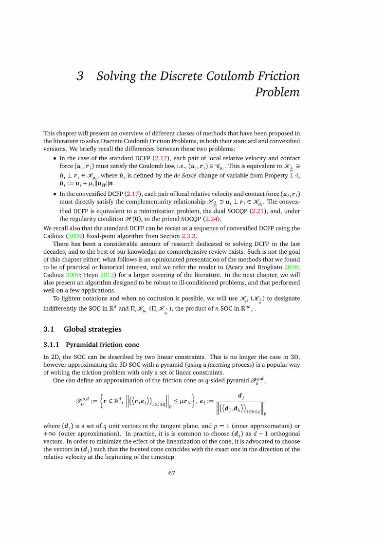
3 Solving the Discrete Coulomb FrictionProblem

This chapter will present an overview of different classes of methods that have been proposed inthe literature to solve Discrete Coulomb Friction Problems, in both their standard and convexifiedversions. We briefly recall the differences between these two problems:

• In the case of the standard DCFP (2.17), each pair of local relative velocity and contactforce (u i , r i)must satisfy the Coulomb law, i.e., (u i , r i) ∈ Cµi

. This is equivalent toK 1µi∋

u i ⊥ r i ∈ Kµi, where u i is defined by the de Saxcé change of variable from Property 1.4,

u i := u i +µi‖u iT‖n.

• In the convexified DCFP (2.17), each pair of local relative velocity and contact force (u i , r i)

must directly satisfy the complementarity relationship K 1µi∋ u i ⊥ r i ∈ Kµi

. The convex-

ified DCFP is equivalent to a minimization problem, the dual SOCQP (2.21), and, underthe regularity conditionH (0), to the primal SOCQP (2.24).

We recall also that the standard DCFP can be recast as a sequence of convexified DCFP using theCadoux (2009) fixed-point algorithm from Section 2.3.2.

There has been a considerable amount of research dedicated to solving DCFP in the lastdecades, and to the best of our knowledge no comprehensive review exists. Such is not the goalof this chapter either; what follows is an opinionated presentation of the methods that we foundto be of practical or historical interest, and we refer the reader to (Acary and Brogliato 2008;Cadoux 2009; Heyn 2013) for a larger covering of the literature. In the next chapter, we willalso present an algorithm designed to be robust to ill-conditioned problems, and that performedwell on a few applications.

To lighten notations and when no confusion is possible, we will use Kµ (K 1µ) to designate

indifferently the SOC in Rd and ΠiKµi(ΠiK 1

µi), the product of n SOC in Rnd , .

3.1 Global strategies

3.1.1 Pyramidal friction cone

In 2D, the SOC can be described by two linear constraints. This is no longer the case in 3D,however approximating the 3D SOC with a pyramid (using a facetting process) is a popular wayof writing the friction problem with only a set of linear constraints.

One can define an approximation of the friction cone as q-sided pyramid P p,dµ ,

P p,dµ :=

§r ∈ Rd ,

r , e j

1≤ j≤q

p≤ µr N

ª, e j :=

d j

d j ,dk

1≤k≤q

p

where (d j) is a set of q unit vectors in the tangent plane, and p = 1 (inner approximation) or+∞ (outer approximation). In practice, it is is common to choose (d j) as d − 1 orthogonalvectors. In order to minimize the effect of the linearization of the cone, it is advocated to choosethe vectors in (d j) such that the faceted cone coincides with the exact one in the direction of therelative velocity at the beginning of the timestep.

67

3. SOLVING THE DISCRETE COULOMB FRICTION PROBLEM

e2

e1

Figure 3.1: Horizontal section of the inner (red, dashed) and outer (red, dotted)approximations with two basis vectors of the 3D Coulomb cone (blue).

The faceted problem can then be solved using a variety of methods; we will not detail them,as our main goal will be to solve the problem in 3D (or more) with the exact cone. We referto (Erleben 2013) for a recent review such algorithms. In a non-exhaustive manner, we canmention:

• the Lemke algorithm used by Klarbring (1987), a direct method with good convergenceproperties, but which may become expensive for large systems;

• a conjugate-gradient algorithm on a sequence of minimization problems (Renouf and Alart2005);

• the staggered projection approach (Kaufman, Sueda, et al. 2008), popular in ComputerGraphics, which solves for the normal and tangential components in an iterative manner;

• an interior-point method (Trinkle et al. 1997);

• the Gauss-Seidel splitting algorithm (e.g., Raous et al. 1988, Jean 1999, Erleben 2007),which we will detail in Section (3.4).

This faceting approach also possesses weaknesses; for instance, Renouf, Acary, et al. (2005)argue that this approximation may lead to significant errors in the resulting trajectories.

Moreover, while the structure of the individual constraints is indeed simpler, their number isdrastically increased (the simplest approximation, a 4-sided pyramid, already requires 4 linearconstraints and 2 dual variables, instead of a single quadratic constraint and a single dual vari-able for the exact cone). The constraints also become more prone to switching between activeand inactive states (the number of faces is increased), which might degrade the overall con-vergence of the solver algorithm. Overall, the faceted problem might therefore not be simplernor faster to solve than the original one1, and the pertinence of this approximation should becarefully evaluated.

For these reasons, in the remainder of this chapter we will focus on the original, non-linearized problem defined with forces inside a SOC.

3.1.2 Complementarity functions

A natural way of solving the reduced dual formulation (2.19) is to express Coulomb law asa the root of a complementarity function, for instance the Alart–Curnier function (1.6) or theDe Saxcé (1.29) complementarity functions. In the next chapter, we will also present anothercomplementarity function, based on a adaptation of the Fischer–Burmeister function to the SOCalgebra (Fukushima et al. 2002). Note that while the De Saxcé complementarity function caneasily be adapted to solve the convexified DCFP rather than the DCFP (by simply not performingthe eponymous change of variable), it is not as simple in the case of the Alart–Curnier function.

1Rockafellar (1993) famously said that “the great watershed in optimization isn’t between linearity and nonlinearity,but convexity and nonconvexity”.

68

3.1. Global strategies

In a general manner, let f : Rnd×Rnd → Rnd be such that f (u, r ) = r ⇐⇒ (u i , r i) ∈ Cµi∀i.

Then finding a solution to (2.19) amounts to finding r ∈ Rnd such that

f (W r + b, r ) = r . (3.1)

As it now involves solely the force variable r , a variety of algorithms may be used to to finda solution to (3.1); however, remember that f is in general non-convex, non-contracting, andnon-smooth.

Using a simple fixed-point iteration r k+1 = f (W r k+ b, r k) is tempting, and has been used inthe case of a single contact (e.g., Feng et al. 2005) 2 , but the convergence is not always satisfyingfor larger systems in practice. As the points at which f is non-differentiable are generally sparse,a better solution is to use a Newton algorithm3 on the function g (Alart and Curnier 1991;Dumont 2012), g : Rnd → Rnd , r 7→ f (W r + b, r )− r . Each step is defined as the solution to alinear system,

J kg

r k+1 − r k

= −αkg (r k)

where J kg ∈ ∂ g(r k) is any element of the subdifferential of g at r k, and αk is an optional damping

term that can be computed using a line-search based on the error function ‖g‖2.

Drawbacks The left-hand-side matrix of the linear system that must be solved at each step,

∂ g

∂ r(r k) = W

∂ f

∂ u(W r k + b) +

∂ f

∂ r(r k)− IRnd ,

may not be invertible. A failsafe is required when one cannot find a step increment, for instancea gradient-descent or fixed-point iteration. In any case, the cost of solving this linear systemgrows quickly with the number of contacts, making the cost of this algorithm prohibitive forvery large systems.

Moreover, we have observed in (Bertails-Descoubes et al. 2011) that while a Newton algo-rithm on the Alart-Curnier formulation yields good results for a system with a small number ofcontacts, the success rate of the algorithm drops quickly when a conditioning parameter, µ nd

m ,grows beyond 1. Indeed, in such cases the number of rows of H exceeds its number of columns,and the number of vanishing eigenvalues of W increases. Moreover, criterion H (s) implies alink between the surjectivity of H and the existence of a solution to the DCFP; as the relativerank of H degrades, so does the probability that this existence criterion is satisfied.

3.1.3 Optimization-based methods

Since the convexified DCFP can be recast as either the primal (2.24) or dual (2.21) SOCQP, itis natural to attempt to use optimization-based algorithms to solve this problem. Moreover, as aSOCQP consists in the minimization of a convex function over a convex feasible set, theoreticalconvergence properties can generally be derived.

In the following sections, we will present three kinds of optimization-based methods: interior-point methods, proximal algorithms, and splitting algorithms. The latter family of methods canbe interpreted as block-coordinate-descent algorithms, i.e., partial minimization over a smallnumber of variables in turn.

Optimization-based methods can be leveraged to solve the original DCFP thanks to theCadoux fixed-point algorithm defined in Property 2.1. Alternatively, we will see in the followingthat some optimization-based algorithms (e.g., projected gradient descent or Gauss–Seidel) canbe repurposed to directly solve the original DCFP. However, both strategies induce the loss ofany theoretical convergence property.

2When f is a projection function, i.e., f ∼ ΠC (r − ρu), as is the case for the Alart-Curnier and De Saxcé comple-mentarity function, the fixed-point algorithm can be interpreted as a slight variation of a proximal algorithm; see Fenget al. 2005 and Section 3.3 below.

3Quasi-Newton methods on complementarity functions are rarely observed to perform well in practice.

69

3. SOLVING THE DISCRETE COULOMB FRICTION PROBLEM

3.2 Interior-point methods

Interior-point methods have become extremely popular in optimization communities in the lastdecades, thanks to their superlinear convergence on many problems (Potra and Wright 2000).

At their core, they replace the characteristic function IC associated to the constraint C witha logarithmic barrier function, IC ,β , such that limβ→0IC ,β = IC . If the feasible set C is definedas C = x , F(x ) ≤ 0, one may take IC ,β (x ) := −β log (−F(x )). The interior-point methodthen performs a Newton algorithm on the modified optimization problem, while simultaneouslydriving β to 0 in the process.

Note that high values for β will tend to make the successive iterates stay in the “center” ofthe feasible set. Iterates will thus follow an interior path to reach the solution, even when thisoptimal point lies on the boundary of the constraint, which is where the interior-point method’sname come from. This is in contrast to most other kinds of methods (pivoting, active-set, prox-imal, . . . ) which tend instead to follow the boundary of the constraint.

3.2.1 Second-Order Cone Programs

A particular case for which several efficient solvers4 have been devised is Second Order ConePrograms (SOCP), that is, minimizing a linear objective function under equality and SOC con-straints. Our convexified DCFP corresponds to the optimality conditions of a (primal or dual)SOCQP, and this class of problem can easily be recast as SOCP, as shown in Cadoux (2009)(more generally, quadratic optimization problems with quadratic constraints are a subclass ofSOCP, see e.g., E. Andersen and K. Andersen 2013). The trick is in the transformation of thequadratic objective function into a linear objective function with a SOC constraint. Indeed, theproblem

minx∈C

1

2x ⊺M x + x ⊺b

is equivalent to (min

x∈C ,t∈Rt + x ⊺b

2t ≥ x T M x .(3.2)

Given a square root L of M (for instance, its Cholesky factorization), Problem (3.2) becomes

minx∈C ,t∈R

t + x ⊺b

L⊺x = z

2t ≥ ‖z‖2.

The constraint t ≥ ‖z‖2 can then be recognized as the rotated cone constraint (1, t, z) ∈ RK ,i.e., 2 × 1 × t ≥ ‖z‖2. Rotated cone constraints are handled by most SOCP solvers, or can berecast as standard SOC constraints.

The SOCP corresponding to the primal SOCQP (2.24) is therefore

minv∈Rm,t∈R t − v⊺ f

z = L⊺v

k = C v

u = Hv + x + s

u i ∈K 1µi

∀i = 1 . . . n

(1, t, z) ∈ RK ,

(3.3)

4Including several out-of-the-box commercial packages, such as CPLEX, MOSEK, Gurobi, . . .

70

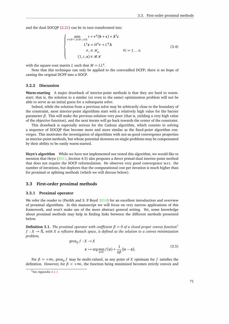
3.3. First-order proximal methods

and the dual SOCQP (2.21) can be in turn transformed into

minr∈Rnd ,λ∈Rc ,t∈R

t + r ⊺(b+ s) +λ⊺c

L⊺z = H⊺r + C⊺λ

r i ∈Kµi∀i = 1 . . . n

(1, t, z) ∈ RK

(3.4)

with the square-root matrix L such that M = LL⊺.Note that this technique can only be applied to the convexified DCFP; there is no hope of

casting the original DCFP into a SOCP.

3.2.2 Discussion

Warm-starting A major drawback of interior-point methods is that they are hard to warm-start; that is, the solution to a similar (or even to the same) optimization problem will not beable to serve as an initial guess for a subsequent solve.

Indeed, while the solution from a previous solve may be arbitrarily close to the boundary ofthe constraint, most interior-point algorithms start with a relatively high value for the barrierparameter β . This will make the previous solution very poor (that is, yielding a very high valueof the objective function), and the next iterate will go back towards the center of the constraint.

This drawback is especially serious for the Cadoux algorithm, which consists in solvinga sequence of SOCQP that become more and more similar as the fixed-point algorithm con-verges. This motivates the investigation of algorithms with not-as-good convergence propertiesas interior-point methods, but whose potential slowness on single problems may be compensatedby their ability to be easily warm-started.

Heyn’s algorithm While we have not implemented nor tested this algorithm, we would like tomention that Heyn (2013, Section 4.5) also proposes a direct primal-dual interior-point methodthat does not require the SOCP reformulation. He observes very good convergence w.r.t. thenumber of iterations, but deplores that the computational cost per iteration is much higher thanfor proximal or splitting methods (which we will discuss below).

3.3 First-order proximal methods

3.3.1 Proximal operator

We refer the reader to (Parikh and S. P. Boyd 2014) for an excellent introduction and overviewof proximal algorithms. In this manuscript we will focus on very narrow applications of thisframework, and won’t make use of the more abstract general setting. Yet, some knowledgeabout proximal methods may help in finding links between the different methods presentedbelow.

Definition 3.1. The proximal operator with coefficient β > 0 of a closed proper convex function5

f : X → R, with X a reflexive Banach space, is defined as the solution to a convex minimizationproblem,

proxβ f : X → X

x 7→ arg minz∈X

f (z) +1

2β‖x − z‖. (3.5)

For β = +∞, proxβ f may be multi-valued, as any point of X optimum for f satisfies thedefinition. However, for β < +∞, the function being minimized becomes strictly convex and

5See Appendix A.1.1

71

3. SOLVING THE DISCRETE COULOMB FRICTION PROBLEM

xprox2 f (x )

−∇ f (x )

z

f (z)

f (z) + 12‖z − x‖2

Figure 3.2: Geometrical evaluation of the proximal operator and relationship witha gradient descent step

coercive, and therefore from Theorem A.5, the proximal operator is uniquely defined. As βgoes towards 0, the minimization problem becomes more and more skewed towards the pointat which the operator is evaluated. Alternatively, as illustrated in Figure 3.2, evaluating theproximal operator proxβ f (x ) may be seen as moving x towards the minimum of f ; the lowerβ , the smaller the step size. More precisely, Parikh and S. P. Boyd (2014, Section 3.3) point outthat when f is twice-differentiable,

proxβ f (x ) = x − β(∇ f )(x 0) + o(β). (3.6)

The fixed-point algorithm defined by the induction x k+1 := proxβ f (x k) can be thus be seen asa modified gradient descent step. Corroborating this interpretation, it can be shown that x 0 ∈ Xis a minimum for f on X if and only if proxβ f (x 0) = x 0, i.e., if and only if x 0 is a fixed-point ofthe proximal operator (Parikh and S. P. Boyd 2014, Section 2.3).

An interesting property of the proximal operator manifests itself when f = IC , the charac-teristic function of C ⊂ X , a proper, closed, convex subset of X (Definition A.8). Then

proxβ IC(x ) = argminz∈C

1

2β‖x − z‖= ΠC(x ),

the orthogonal projection on C . This interpretation of the orthogonal projection as a special caseof a proximal operator translates to the optimality conditions of convex optimization problems.Recall (Remark A.3) that the optimality condition for the minimization problem (A.4),

minx∈X

f (x ) +IC(x ) (A.4)

reads, when f is differentiable on C , and for any α ∈ R∗+

,

ΠC (x 0 −α(∇ f )(x 0)) = x 0;

a similar but more general optimality condition can be stated on proximal operators (Parikh andS. P. Boyd 2014, Section 4.2).

Property 3.1. The optimality conditions of the minimization problem

minx∈X

f (x ) + g(x )

with f and g proper closed convex and f differentiable on dom g are

proxβ g (x 0 −α(∇ f )(x 0)) = x 0 , α ∈ R∗+

.

Any fixed-point of the sequence induced by x k+1 := proxβ gx k −α(∇ f )(x k)

will thus yield

a minimum of f + g over X . When (∇ f ) is Lipschitz with constant L, this fixed-point algorithmwill converge as O(1/k) for β ∈]0, 1

L ] (Parikh and S. P. Boyd 2014) — though it is only practical aslong as evaluating proxβ g is simple enough. The projected gradient descent method, presentedbelow, will thus appear as a special case of fixed-point algorithms on a proximal operator whereg = IC .

72

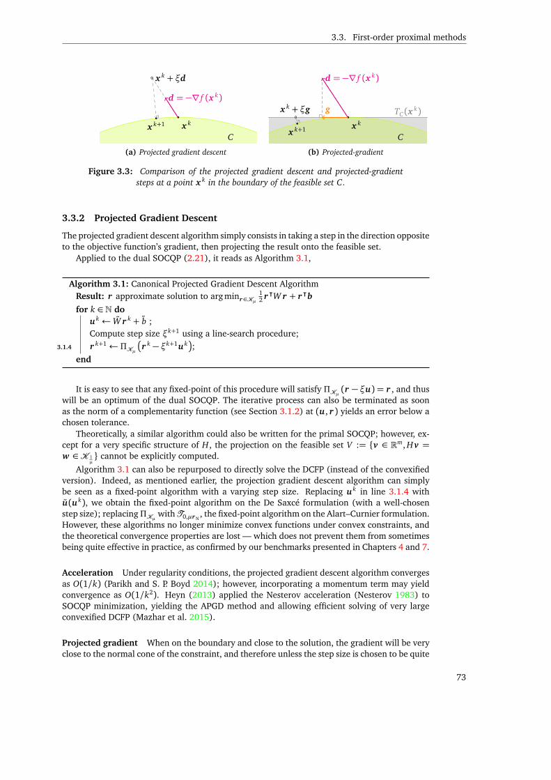
3.3. First-order proximal methods

Cx k

d = −∇ f (x k)

x k + ξd

x k+1

(a) Projected gradient descent

C

TC(xk)

x k

d = −∇ f (x k)

gx k + ξg

x k+1

(b) Projected-gradient

Figure 3.3: Comparison of the projected gradient descent and projected-gradientsteps at a point x k in the boundary of the feasible set C.

3.3.2 Projected Gradient Descent

The projected gradient descent algorithm simply consists in taking a step in the direction oppositeto the objective function’s gradient, then projecting the result onto the feasible set.

Applied to the dual SOCQP (2.21), it reads as Algorithm 3.1,

Algorithm 3.1: Canonical Projected Gradient Descent AlgorithmResult: r approximate solution to arg minr∈Kµ

12 r ⊺W r + r ⊺b

for k ∈ N do

uk ← W r k + b ;Compute step size ξk+1 using a line-search procedure;

3.1.4 r k+1← ΠKµr k − ξk+1uk

;

end

It is easy to see that any fixed-point of this procedure will satisfy ΠKµ (r − ξu) = r , and thuswill be an optimum of the dual SOCQP. The iterative process can also be terminated as soonas the norm of a complementarity function (see Section 3.1.2) at (u, r ) yields an error below achosen tolerance.

Theoretically, a similar algorithm could also be written for the primal SOCQP; however, ex-cept for a very specific structure of H, the projection on the feasible set V := v ∈ Rm, Hv =

w ∈K 1µ cannot be explicitly computed.

Algorithm 3.1 can also be repurposed to directly solve the DCFP (instead of the convexifiedversion). Indeed, as mentioned earlier, the projection gradient descent algorithm can simplybe seen as a fixed-point algorithm with a varying step size. Replacing uk in line 3.1.4 withu(uk), we obtain the fixed-point algorithm on the De Saxcé formulation (with a well-chosenstep size); replacingΠKµ withT0,µr N

, the fixed-point algorithm on the Alart–Curnier formulation.However, these algorithms no longer minimize convex functions under convex constraints, andthe theoretical convergence properties are lost — which does not prevent them from sometimesbeing quite effective in practice, as confirmed by our benchmarks presented in Chapters 4 and 7.

Acceleration Under regularity conditions, the projected gradient descent algorithm convergesas O(1/k) (Parikh and S. P. Boyd 2014); however, incorporating a momentum term may yieldconvergence as O(1/k2). Heyn (2013) applied the Nesterov acceleration (Nesterov 1983) toSOCQP minimization, yielding the APGD method and allowing efficient solving of very largeconvexified DCFP (Mazhar et al. 2015).

Projected gradient When on the boundary and close to the solution, the gradient will be veryclose to the normal cone of the constraint, and therefore unless the step size is chosen to be quite

73

3. SOLVING THE DISCRETE COULOMB FRICTION PROBLEM

big, the projected position will be very close to the original position (Figure 3.3). The projected-gradient algorithm alleviates this problem by first projecting the gradient onto the tangent coneTC to the constraint C ⊂ X ,

TC(x ) := y ∈ X , ∃ε > 0, ∀0< t < ε, (x + t y) ∈ C.

Algorithm 3.2: Projected-Gradient Algorithmfor k ∈ N do

uk ← W r k + b ;3.2.3 g k+1← ΠTKµ (r

k)uk;

Compute step size ξk+1 using a line-search procedure;r ← ΠKµ

r k − ξk+1g k+1

;

end

If the projection tangent cone is hard to compute, it can be approximated by performinganother projection on the feasible set C . Line 3.2.3 is then replaced with two steps,

x ← ΠKµ (r −g );

g ← x − r ;

Other variants Many other variants of the projected-gradient and projected gradient descentexist. We can mention the Spectral Projected-Gradient (SPG) method, with was observed towork well on convexified DCFP by Tasora (2013). In Appendix B.2, we propose a Nesterov-accelerated, line-search free variant of this algorithm, which we coined ASPG and that per-formed consistently well on our problems (both convexified and standard). Algorithm B.2 isimplemented in the bogus library, along with the APGD method, canonical algorithms, and aprojected-gradient variant augmented with a simple conjugation step.

3.3.3 Primal–dual proximal methods

Primal–dual proximal methods are a class of first-order minimization algorithms that work bysplitting the objective function, and iterating on both the primal variable (in our case, the ve-locity v) and the dual variable (the forces r ). The methods presented below were not observedto converge very well on our DCFP without requiring significant manual tuning of the step sizeparameters, and we therefore won’t use them in practice. However, their popularity in compu-tational fluid mechanics make them worthy of interest.

Alternating Directions Method of Multipliers ADMM is another way of minimizing sepa-rable problems, introduced by Glowinski and Marroco (1975) for non-differentiable continuumflow problems and made popular by Fortin and Glowinski (1983) under the name of AugmentedLagrangian algorithm. ADMM has also been recently introduced to the Computer Graphics sim-ulation community by Narain, Overby, et al. (2016), though in a slightly different setting.

The minimization of f (v) + g(Hv + w ) is written as

minu=Hv+w

f (v) + g(u)

The Lagrangian associated to this minimization problem is

L = f (v) + g(u) + r ⊺(u − Hv − w ),

74

3.3. First-order proximal methods

and the augmented Lagrangian with parameter γ is

Lγ = f (v) + g(u) + r ⊺(u − Hv − w ) +γ

2‖Hv + w − u‖2.

We are looking for a saddle-point of Lγ. Minimizing over the first two variables v and u inturn, and taking a gradient step to maximize λ, we obtain Algorithm 3.3,

Algorithm 3.3: Alternating Directions Method of Multipliersfor k ∈ N do

3.3.2 v k+1 ← argminv Lγ(v , uk, r k) ;3.3.3 uk+1 ← arg minuLγ(v k+1, u, r k)(v k+1 + r k);

r k+1 ← r k − γ(Hv + w − u);end

Now, Line 3.3.3 can easily be written as a proximal operator:

uk+1 := argminu

g(u) +γ

2‖Hv k+1 + w − u − r k

γ‖

= prox 1γ

g(Hv k+1 + w − 1

γr k)

The first step, Line 3.3.2, is more tricky, but can be dealt with by linearizing the quadratic termaround v k and adding a new quadratic regularization term, (Parikh and S. P. Boyd 2014, Section4.4.2),

γ

2‖Hv + w − uk‖2 ∼ γ Hv k + w − uk, Hv

+β

2‖v − v k‖

∼ β2‖v − v k +

γ

βH⊺Hv k + w − uk

‖2.

This yields the linearized ADMM algorithm, with Line 3.3.2 replaced by

v k+1← argminv

f (v) +β

2‖v − v k +

γ

βH⊺Hv k + w − uk

− 1

βH⊺r k‖2

= prox 1β

f

v k +1

βH⊺r k − γ

βH⊺Hv k + w − uk

= prox 1β

f

v k +1

βH⊺r k − γ Hv k + w − uk

(3.7)

The ADMM algorithm 3.3 can also be interpreted as an integral controller, where r is thecontrol u the state, and the goal is to achieve u = Hv + w (Parikh and S. P. Boyd 2014).

ADMM on primal formulation Now, let us consider our primal SOCQP (without linear con-straints for now). We have f (v) = 1

2 v⊺M v − v⊺ f , and g(u) := IK 1µ

(u). Therefore

prox 1β

f (x ) = argminv

1

2v⊺M v − v⊺ f +

β

2‖v − x‖2

= argminv

1

2v⊺(M + βI)v − v⊺( f + βx )

= (M + βI)−1( f + βx )

prox 1γ

g(y) = ΠK 1µ

(y).

75

3. SOLVING THE DISCRETE COULOMB FRICTION PROBLEM

The linearized ADMM algorithm on the primal SOCQP thus becomes Algorithm 3.4,

Algorithm 3.4: Linearized ADMM for SOCQPfor k ∈ N do

v k+1 ← (M + βI)−1f + βv k + H⊺

r k − γ Hv k + w − uk

;

uk+1 ← ΠK 1µ

Hv k+1 + w − 1

γ r k;

r k+1 ← r k − γ(Hv k+1 + w − uk+1);end

We can easily verify that any fixed point (v , u, r ) of this algorithm satisfies

M v = f + H⊺r

u = Hv + w

r ∈ −NK 1µ

u

and is thus a solution of the primal SOCQP without linear constraints.

The Alternating Minimization Algorithm (AMA, see Goldstein et al. 2014) is obtained bysuppressing the quadratic term in the expression of the Lagrangian when minimizing w.r.t. v ,that is, replacing Line 3.3.2 with

v k+1← argminv

f (v)− r k, Hv

Applied to our SOCQP, we obtain Algorithm 3.5,

Algorithm 3.5: AMA for SOCQPfor k ∈ N do

v k+1 ← M−1( f + H⊺r k) ;

uk+1 ← ΠK 1µ

Hv k+1 + w − 1

γ r k;

r k+1 ← r k − γ(Hv k+1 + w − uk+1);end

In contrast to the original ADMM algorithm, AMA may be ill-defined when M is only positivesemi-definite. Both algorithms can be easily extended to handle linear constraints; for ADMM,we get Algorithm 3.6,

Algorithm 3.6: Linearized ADMM for SOCQP with linear constraintsfor k ∈ N do

v k+1 ←(M + βI)−1

f + βv k + H⊺

r k − γ1

Hv k + w − uk

+ C⊺

λk − γ2

C v k − k

;

uk+1 ← ΠK 1µ

Hv k+1 + w − 1

γ1r k;

r k+1 ← r k − γ1(Hv k+1 + w − uk+1);λk+1 ← λk − γ2(C v k+1 − k);

end

Like the projected-gradient algorithm on the dual SOCQP, this algorithm requires solving ateach iteration a linear systems with M (or M + βI) as left-hand-side. However, the constraintprojection is here done on K 1

µ, instead of Kµ for the projected gradient. One may also attempt

to directly solve the original DCFP by replacing the term w in each step with the expressionw + s(Hv + w ); however, once again the theoretical convergence properties are then lost.

Starting from dual SOCQP we can also define an AMA algorithm that will only require onemultiplication by M at each iteration.

76

3.3. First-order proximal methods

AMA on dual formulation We write the dual SOCQP (2.21) without linear constraints as

minz=H⊺r

1

2z⊺M−1z + z⊺M−1 f

︸ ︷︷ ︸f (z)

+ r ⊺w +IKµ(r )︸ ︷︷ ︸g(r )

.

Writing the AMA on this formulation yields Algorithm 3.7,

Algorithm 3.7: AMA on dual formulationfor k ∈ N do

zk+1 ← arg minz f (z)− z, v k

;3.7.3 r k+1 ← arg minr g(r ) +

H⊺r , v k

+γ2‖zk+1 − H⊺r‖2;

v k+1 ← v k + γ(H⊺r − z);end

The first minimization is straightforward;

zk+1 = arg minz

1

2zT M−1z + z⊺

M−1 f − v k

= M(v k − f ).

However the second step has to be reworked. Linearizing once again the quadratic part, wereplace Line 3.7.3 with

r k+1← arg minr

g(r ) +H⊺r , v k

+ γ

H⊺r k − z, H⊺r

+β

2‖r − r k‖2

= arg minr

g(r ) +β

2‖r − r k +

1

βHv k + γ

H⊺r k − z

‖2

= arg minr∈Kµ

β

2‖r − r k +

1

βw +

1

βHv k + γ

H⊺r k − zk+1

‖2

= ΠKµ

r k − 1

β

w + H

v k + γ

H⊺r k − z

.

We see easily that any fixed-point (v , z, r ) of this linearized version of Algorithm 3.7 satisfies

M v = z + f

z = H⊺r

Hv + w ∈ −NKµ(r ),

and thus is also a solution of the convexified DCFP. Once again, this algorithm can be extendedto handle linear constraints, by driving the auxiliary variable z to satisfy z = H⊺r + C⊺λ. Weobtain Algorithm 3.8,

Algorithm 3.8: Linearized AMA on dual formulation with linear constraintsfor k ∈ N do

zk+1 ← M v k + f ;

3.8.3 r k+1 ← ΠKµr k − 1

β1

w + H

v k + γ

H⊺r k + C⊺λk − zk+1

;

λk+1 ← λk − 1β2

−k + Cv k + γ

H⊺r k + C⊺λk − zk+1

;

v k+1 ← v k + γ(H⊺r k+1 + C⊺λk+1 − zk+1);end

Just like with the primal formulation, one can directly solve the original DCFP by replacingw on line 3.8.3 with w + s(Hv + w ).

77

3. SOLVING THE DISCRETE COULOMB FRICTION PROBLEM

Variants Goldstein et al. 2014 also define Nesterov-like accelerated versions of those algo-rithms. Other variants of such separation schemes exist, such as the Arrow–Hurwitz algorithm(which is itself an extension the Uzawa algorithm to the proximal setting):

for k ∈ N do

r k+1 ← -prox 1γ

g⋆−r k + γ

Hv k + w

;

v k+1 ← prox 1β

f (v k + 1β H⊺r k+1);

end

which for our primal SOCQP is written

Algorithm: Arrow–Hurwitz algorithm for SOCQP

for k ∈ N do

r k+1 ← ΠKµr k − γ Hv k + w

;

v k+1 ← (M + βI)−1( f + βv k + H⊺r k+1);end

Compared to our original ADMM algorithm, the constraint projection is done on the forcesr instead of on the relative velocities u; the Arrow-Hurwitz degrades to a projected gradientdescent algorithm (without line search) when β = 0. The popular Chambolle and Pock (2010)algorithm is an accelerated version of the Arrow–Hurwitz algorihm.

The bogus library (Daviet 2013), implements the accelerated ADMM from (Goldstein et al.2014) and a preconditioned and accelerated version of the AMA on the dual SOCQP. In practice,our early tests were not very satisfying; fine-tuning of the coefficients β and γ was require toachieve fast convergence.

3.4 Splitting methods

3.4.1 Operator splitting

The most popular way to solve the dual formulation of the DCFP (2.19) is to use a splittingmethod: that is, treating one part of the operator W implicitly, and another part explicitly. Inpractice, this means decomposing W as W =W1 +W2, and iterating as

uk+1 =W1r k+1 +W2r k + C⊺λk + b

(uk+1i , r k+1

i ) ∈ Cµ i∀1≤ i ≤ n.

Pλk+1 = c − B⊺r k+1.

(3.8)

(3.9)

(3.10)

a fixed-point for (r ,λ) is reached, that is (r k+1,λk+1) = (r k,λk).Obviously, W1 and W2 should be chosen so that the resulting problem (3.8 – 3.9) is easier to

solve than the original DCFP. The convexified DCFP can also be solved in this manner, replacingthe Coulomb law condition (3.9) with K 1

µi∋ uk+1

i ⊥ r k+1i ∈Kµi

.

In practice, W has a sparse block structure composed of d × d blocks (WOJ ), 1 ≤ i, j ≤ n,where each block (Wi j) describe the interaction between the ith and jth contacts (that is, therelative velocity change at i when a force increment is applied at j). W can thus be decomposedas the sum of a block-diagonal matrix WD := (Wii), a lower part WL := (Wi, j)i> j and an upperpart WU := (Wi, j)i< j .

Choosing W1 = D and W2 = L + U yields the Jacobi algorithm; equation (3.8) becomesseparable, and result in n d-dimensional problems that can be solved in parallel:

uk+1i =Wii r

k+1i +

∑

j 6=i

Wi, j rkj + C⊺λk + b

(uk+1i , r k+1

i ) ∈ Cµ i.

78

3.4. Splitting methods

Choosing W1 = D + L and W2 = U , we obtain the Gauss–Seidel algorithm, which boasts betterconvergence but loses parallelism; the d-dimensional local problems now have to be solved inorder:

uk+1i =Wii r

k+1i +

∑

j<i

Wi, j rk+1j +

∑

j>i

Wi, j rkj + C⊺λk + b

(uk+1i , r k+1

i ) ∈ Cµ i.

In both cases, solving our global problem can thus be reduced to solving a sequence of localproblems (or one-contact problems),

u i =Wii r i + bi

(u i , r i) ∈ Cµi,

(3.11)

where Wii is a d × d, positive semi-definite matrix.This one-contact problem is much easier to solve than the original one; indeed, for d = 2 or

d = 3, we can construct an analytical solver, as we will show in Chapter 4.Splitting methods have been used on contact-related problems for several decades. Raous

et al. (1988) applied them to the statics of an elastic body under frictional contact, and mentionprevious uses in the frictionless case. However, their huge popularity nowadays is largely due tothe advent of the Nonsmooth Contact Dynamics (NSCD) method (Jean 1999; Jean and Moreau1992; Jourdan et al. 1998), which proposed to compute the dynamics of Discrete Element Mod-els with frictional contacts using the Gauss–Seidel algorithm and an efficient one-contact solver.

3.4.2 Convergence properties

Interpretation as block-coordinate descent When solving the convexified DCFP, the localproblem (3.11) becomes ¨

u i =Wii r i + bi

u i ∈ −NKµi(r i),

(3.12)

which from Theorem A.6 we recognize as the optimality conditions of the minimization problem

arg minr i∈Kµi

1

2r⊺

i Wii r i + r⊺

i bi = argminr i∈Kµi

Ji(r i), (3.13)

where Ji(r i) := 12 r ⊺W r+r ⊺b is defined by freezing every component of r except for r i . As such,

successively solving the local problems (3.12) amounts to iteratively minimizing the quadraticobjective function J(r ) := 1

2 r ⊺W r+r ⊺b w.r.t. each contact force r i; the Gauss–Seidel algorithmcan thus be seen as a block-coordinate descent method.

If Wii is symmetric, positive-definite for all i, then each local problem admits a unique so-lution, and the objective function will monotonically decrease to its optimal value (Grippo andSciandrone 2000).

Proximal modification However, Wii may only be positive semi-definite, and in this case theminimization problem (3.13) will be ill-posed. However, we can modify it slightly as

arg minr i∈Kµi

1

2r ⊺W r + r ⊺b+

β

2‖r k

i − r i‖2 = prox 1β

Ji(rki )

with β > 0. Any fixed-point of the proximal operator will be optimal for Ji , and therefore afixed-point of the modified Gauss–Seidel algorithm will still be a solution of the dual SOCQP.Grippo and Sciandrone (2000) show that this fixed-point will always be reached for W symmetricpositive semi-definite.

79

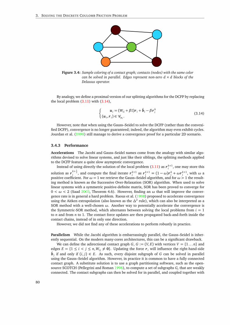
3. SOLVING THE DISCRETE COULOMB FRICTION PROBLEM

Figure 3.4: Sample coloring of a contact graph; contacts (nodes) with the same colorcan be solved in parallel. Edges represent non-zero d × d blocks of theDelassus operator.

By analogy, we define a proximal version of our splitting algorithms for the DCFP by replacingthe local problem (3.11) with (3.14),

u i = (Wii + βI)r i + bi − β r k

i

(u i , r i) ∈ Cµi.

(3.14)

However, note that when using the Gauss–Seidel to solve the DCFP (rather than the convexi-fied DCFP), convergence is no longer guaranteed; indeed, the algorithm may even exhibit cycles.Jourdan et al. (1998) still manage to derive a convergence proof for a particular 2D scenario.

3.4.3 Performance

Accelerations The Jacobi and Gauss–Seidel names come from the analogy with similar algo-rithms devised to solve linear systems, and just like their siblings, the splitting methods appliedto the DCFP feature a quite slow asymptotic convergence.

Instead of using directly the solution of the local problem (3.11) as r k+1i , one may store this

solution as rk+ 1

2

i , and compute the final iterate r k+1i as r k+1

i = (1 −ω)r ki +ωr k+1

i , with ω apositive coefficient. Forω = 1 we retrieve the Gauss–Seidel algorithm, and forω> 1 the result-ing method is known as the Successive Over-Relaxation (SOR) algorithm. When used to solvelinear systems with a symmetric positive-definite matrix, SOR has been proved to converge for0 < ω < 2 (Saad 2003, Theorem 4.6). However, finding an ω that will improve the conver-gence rate is in general a hard problem. Raous et al. (1988) proposed to accelerate convergenceusing the Aitken extrapolation (also known as the ∆2 rule), which can also be interpreted as aSOR method with a well-chosen ω. Another way to potentially accelerate the convergence isthe Symmetric-SOR method, which alternates between solving the local problems from i = 1to n and from n to 1. The contact force updates are then propagated back-and-forth inside thecontact chains, instead of in only one direction.

However, we did not find any of these accelerations to perform robustly in practice.

Parallelism While the Jacobi algorithm is embarrassingly parallel, the Gauss–Seidel is inher-ently sequential. On the modern many-cores architectures, this can be a significant drawback.

We can define the adirectional contact graph G, G := (V, E) with vertices V = 1 . . . n andedges E = 1 ≤ i < j ≤ n, Wi j 6= 0. Updating the force r i will influence the right-hand-sideb j if and only if (i, j) ∈ E. As such, every disjoint subgraph of G can be solved in parallelusing the Gauss–Seidel algorithm. However, in practice it is common to have a fully connectedcontact graph. A substitute solution is to use a graph partitioning software, such as the open-source SCOTCH (Pellegrini and Roman 1996), to compute a set of subgraphs Gi that are weaklyconnected. The contact subgraphs can then be solved for in parallel, and coupled together with

80

3.4. Splitting methods

an outer Jacobi algorithm. Hopefully, the loss of convergence speed will not be too dramatic;however, the more contacts subgraphs are being used, the more degraded the convergence,as the algorithm ultimately becomes a pure Jacobi. Another solution, implemented in bogus,is to use a coloring approach, illustrated in Figure 3.4. When the contact graph has a grid-like structure, it is possible to color each node with a checkerboard-like pattern. Then at eachGauss–Seidel iteration, all the white nodes can be solved in parallel, then all the black nodescan be solved in parallel; this is the so-called red-black Gauss–Seidel algorithm. It is possible togeneralize this approach to arbitrary contact graphs using more colors; however, computing anoptimal coloring is a NP-hard task. A greedy algorithm can be easily implemented: each contactis considered in turn, and is either: (i) assigned one of the existing colors if it has no edge to anyof the contacts in this color, or (ii) assigned a new color. However, such an algorithm will oftenlead to a lot of colors with very few contacts, making the overall algorithm very sequential onceagain. Moreover, computing the partitioning or coloring can be costly, and contacts have thento be reordered to preserve good memory locality; the gain from the recovered parallelism maynot suffice to outbalance the cost of the preprocessing cost.

Another approach has been explored by Tonge et al. (2012). Each pair of contacting bodiesis considered independently of the other ones, resulting in nB distinct velocity vectors for anobject in contact with nB bodies. The nB velocity vectors are prescribed to remain consistentusing fixed-joint constraints. The algorithm then iterates between solving for each contactingpair (which can been done in parallel) and enforcing the fixed-joint constraints (for which theyprovide an analytical formula). This results in a very GPU-friendly method, allowing the authorsto solve systems with several thousands of contacts in real-time.

Overall, we found that the most efficient solution for a number of cores that is very smallw.r.t. the number of contacts is the most naive one: the set of all contacts is statically assignedto a small number of threads, and each thread is allowed to process its contacts without anysynchronization with the others. This might lead to race conditions when one thread is writing agiven contact force at the same time as another one is reading it; the reading thread may get backthe first components of the force at iteration k+ 1, and the last components at iteration k6. Yetwe have not found this to be a problem in practice, and observed instead a good scaling w.r.t. thenumber of threads. Actually, the randomness induced by the scheduling of the threads was foundto sometimes improve the convergence of the global algorithm. The major downside, due to thisrandomness, is that the algorithm is no longer deterministic, and may produce significantlydifferent results each time that it is run on a given DCFP (using the proximal version somewhatreduces this variance).

Delassus operator A fundamental requisite to achieve satisfying performance is the abilityto efficiently evaluate the local problem’s right-hand-side bi , which means multiplying d rowsof the Delassus operator W with the current aggregate force vector r . Using row-major block-compressed-storage (BSR) for W yields good performance, but requires explicitly assemblingand storing W ; as mentioned in Section 2.3.1, this can be costly both in time and memory, andprohibitive if the inverse mass matrix M−1 is dense. Moreover, even when M is the identitymatrix, HH⊺ may be much more expensive to store than H.

On the other hand, computing the ith block-row–vector product Wi[·]r = (HM−1H⊺)i[·]ranalytically for each contact would be very light on memory, but incur a huge runtime cost. Agood middle ground, when M is block-diagonal, is to consider an intermediate vector z ∈ Rm

storing at each-instant the matrix–vector product M−1H⊺r . In this case, M−1H⊺ possesses thesame block structure as HT , and can be precomputed. Updating z when a contact force r i

changes then becomes very cheap. Indeed, it simply amounts to d scale–add operations on thecolumns of M−1H⊺. As the rows of H (and therefore the columns of H⊺) are usually quite sparse,this operation is inexpensive. Then, the right-hand-side bi can be deduced from z by once again

6Note that reading and writing aligned double-precision floats is usually atomic on modern architectures, so thisapproach will not be subject to intra-component corruption.

81

3. SOLVING THE DISCRETE COULOMB FRICTION PROBLEM

a cheap multiplication with d rows of H. Overall, the inner loop of the Gauss–Seidel algorithmbecomes:

for 1≤ i ≤ n do

bi ← bi + Hi[·]z −Wii rki ;

Set r k+1i as solution of local problem (3.11) ;

z ← z + (M−1H⊺)[·]i(r k+1i − r k

i ) ;end

where only the diagonal blocks Wii have now to be precomputed.When H is stored using BSR, and when its rows are quite-sparse, this algorithm remains very

efficient, and is also implemented in the bogus library. It is however more prone to data raceswhen synchronization-free parallelism is used; for this reason, we periodically recompute z fromscratch.

Whether one or the other of these two algorithms performs best when factoring into accountthe cost of computing W into account is application-dependent. In practice we usually explicitlycompute W for Discrete Element Models (or generally systems with a high number of degrees offreedom w.r.t. the number of contacts), and use the matrix-free variation for continuum models(the second part of this dissertation). Note that Kaufman, Tamstorf, et al. (2014) recommendsavoiding computing explicitly the Delassus operator for non-linear DEM; this seems sensible, asa sequence of DCFP with varying W but improving initial guesses has then to be solved, whichmean relatively less work for the solver w.r.t. the matrix assembly time.

3.4.4 Discussion

On the one hand, despite all the above theoretical drawbacks (slow or lack of convergence,sequentiality, computation of W ), the Gauss–Seidel algorithm actually performs very well inpractice. This will be confirmed by the results presented over the course of the next chapters,such as in Section 4.2.3. As long as the local contact problems can be solved reliably, the globalalgorithm is very robust, and quickly lowers the error below a tolerance that is acceptable for alot of purposes.

Jean (1999) states that the local problems can usually be solved using 3 or less iterations ofthe Newton method on the Alart–Curnier function. We have not found this to be always the case,especially on reduced-coordinates flexible models, and have observed that failure of convergencein the local solver may quickly escalate to divergence of the global solver. This has motivatedthe conception of a very robust local solver, to which is dedicated the following chapter.

On the other hand, the Gauss–Seidel algorithm is not adapted for problems where the in-verse M−1 of the DCFP matrix is dense, or for massively parallel architectures. In this case, weadvocate instead using proximal methods. The following chapters will show that one variantof the projected gradient descent, APSG (Algorithm B.2), performs generally well. The DualAMA (Algorithm 3.8) is also worthy of interest as it does not require explicitly solving any linearsystem. However, achieving satisfying practical performance would first require devising betterheuristics for choosing the step sizes.

82

4 A Robust Gauss–Seidel Solver and itsApplications

The first section of this chapter present a few modifications over the canonical Gauss–Seidelalgorithm allowing to tackle problems which cause divergence of most standard implementa-tions. The resulting algorithm performed well on a wide range of problems, was often fasterthan proximal or interior-points methods, and was faster and more robust than standard GSapproaches.

The last three section are dedicated to applications of this algorithm; the first one, realisticsimulation hair dynamics, being the one that motivated building this solver in the first place.

Our hybrid solver (Section 4.1) was originally published in (Daviet, Bertails-Descoubes, andBoissieux 2011), in the context of hair dynamics (Section 4.2), then leveraged for the inversedesign of hair (Section 4.4), and, more recently, for cloth dynamics (Section 4.3).

4.1 Hybrid Gauss–Seidel algorithm

As mentioned earlier, our applications — especially hair dynamics with reduced coordinate mod-els (see Section 4.2) — caused regular failures of the local solvers commonly in use in the litera-ture: Newton methods or fixed-point iterations over the Alart–Curnier or De Saxcé complemen-tarity functions. These local failures could then escalate to global divergence of the frictionalcontact solver, leading to visible popping or complete blowup of the simulation.

Our first objective was thus to devise a very robust solver for the local problem (3.11).

4.1.1 SOC Fischer-Burmeister function

One first idea is to try new complementarity functions that could be more suitable for root-findingprocedures than the Alart-Curnier or De Saxcé functions.

First, we may want to look back at the scalar case, and consider the linear complemen-tarity problem 0 ≤ u ⊥ r ≥ 0. This scalar complementarity problem can be expressed asthe normal cone inclusion u ∈ −NR+(r), and thus as the zero of a complementarity functionf : (u, r) 7→ ΠR+(r − ξu)− r, which looks somewhat similar to our Alart–Curnier and De Saxcéfunctions. However, for root-finding purposes this projection-based complementarity functionis usually discarded in favor of the Fischer–Burmeister complementarity function (Burmeister1985; Fischer 1992),

fFB :

¨R2 −→ R(u, r) 7−→ pu2 + r2 − u− r.

The Fischer–Burmeister function is indeed “smoother”; it is only non-differentiable for u =r = 0 (while the projection is not-differentiable for r = −ξu) and its Jacobian has been shownto be regular under reasonable conditions (Fischer 1992). Newton algorithms over the Fischer–Burmeister function have been proved to perform quite well in practice (e.g., Munson et al.2001; Silcowitz et al. 2009).

Finding an analogous well-behaved complementarity function for SOC problems would there-fore be of interest, and the Fischer–Burmeister has fortunately been extended to SOC comple-

83

4. A ROBUST GAUSS–SEIDEL SOLVER AND ITS APPLICATIONS

mentarity problems by Fukushima et al. (2002). Indeed,

K1 ∋ x ⊥ y ∈K1 ⇐⇒ f KFB (x , y) = 0,

f KFB : Rd ×Rd → Rd

(x , y) 7→ (u u + r r )12 − x − y

(4.1)

where the square-root is also defined w.r.t. the bilinear operator · · : Rd ×Rd → Rd ,

x y 7→

x ⊺y

x N yT + yNx T

.

The vectorial space Rd equipped with standard addition and the “” product defines a Jordan(i.e., commutative, but generally not associative) algebra. The well-definition of the SOC f KFBfunction will be asserted in a following paragraph.

Now, remember from Property 1.4 that the Coulomb law can be expressed equivalently as

(u, r ) ∈ Cµ ⇐⇒ K 1µ∋ u ⊥ r ∈K 1

µ

where u = u +µ‖uT‖ is defined from the De Saxcé change of variable. For µ > 0, we introducetwo new changes of variable,

r :=µr N

r T

u := ρ

uN

µuT

(4.2)

where ρ is a scalar introduced for conditioning purposes (Here as r is an impulse and u avelocity, therefore ρ should be a mass ). Then,

K 1µ∋ u ⊥ r ∈K 1

µ⇐⇒ K1 ∋ u ⊥ r ∈K1

and thus from Equation (4.1),

f KFB (u, r ) = 0 ⇐⇒ (u, r ) ∈ Cµ. (4.3)

This new complementarity function for Coulomb friction is only valid for µ > 0, but sincefor µ = 0 Coulomb’s law degenerates to a scalar complementarity problem, in this case we canuse the original, scalar Fischer–Burmeister function. The SOC f KFB function can also be triviallyadapted to convexified DCFP, as it is sufficient to use the original velocity u instead of the DeSaxcé change of variable u in Equation (4.2).

Unlike what we claimed in (Daviet, Bertails-Descoubes, and Boissieux 2011), the SOC Fischer–Burmeister function has already been applied (and discarded as not efficient) by Cadoux (2009)inside a quasi-Newton algorithm. We proposed instead to use a Newton algorithm, and obtainedsatisfying results.

Numerical evaluation Computing the SOC f KFB function involves taking the square-root of avector of Rd w.r.t. the bilinear operator · ·; one may wonder about the well-definedness of thisoperation, and its ease of computation.

The association of the vector space Rd with the bilinear operator forms a R-algebra, tightlyassociated to the SOC K1 through two notable properties:

• ∀x ∈K1, there exists a unique z ∈K1 s.t. z z = x ; we note z = x12 ;

• ∀x ∈ Rd , x x ∈K1.

As K1 is a convex cone, we deduce that ∀x , y ∈ Rd ×Rd , x x + y y ∈ K1 and thus the SOCFischer–Burmeister function is well-defined.

84

4.1. Hybrid Gauss–Seidel algorithm

Moreover, any vector x ∈ Rd can be decomposed as x = λ1v1 +λ2v2, where

λi = x N + (−1)i‖x T‖

v i =1

2

1; (−1)i

x T

‖x T‖

if x T 6= 0

1; (−1)ie

if x T = 0

(4.4)

(4.5)

where e is any unit vector in Rd−1. λ1 and λ2 are called the eigenvectors of x , and v1 and v2

are the associated eigenvalues. If x ∈ K1, λ1 and λ2 will both be positive; we can thus definez :=

pλ1v1+

pλ2v2, and check that z z = x . This yields an easy access to the square-root of

any element of K1, and thus to the SOC Fischer–Burmeister function f KFB .

Newton algorithm The f KFB function is Lipschitz-continuous, as is the gradient of its squarednorm, (∂ f KFB )

⊺ f KFB , suggesting good conditions for a Newton minimization algorithm on ΨFB :=12‖ f KFB (u(r ), r )‖2. Moreover, f KFB is strongly semismooth (D. Sun and J. Sun 2005), justify-ing performing directly a nonsmooth root-finding Newton algorithm (Qi and J. Sun 1993) onf KFB (u(r ), r ) = 0, as this avoids computing the second derivative of f KFB .

The Newton algorithm implemented in the bogus library is a simplification of the one thatwe suggested originally (Daviet, Bertails-Descoubes, and Boissieux 2011, Appendix A.2), and isgiven in Appendix B.1.2; the derivatives of f KFB are provided in Appendix B.1.1.

We observed that on average, using the SOC Fischer–Burmeister complementarity functionmade the Gauss–Seidel algorithm perform slightly better than using the Alart–Curnier formula-tion (see Table 4.3). However, this was still not sufficient to achieve convergence for every localproblem. Damping the Newton algorithms (by performing a line-search) improves their robust-ness, at the cost of being much slower in the general case, and still failing sometimes. Moreprecisely, on our hair problems the undamped Fischer–Burmeister Newton (Algorithm B.1) wasmuch more robust that the undamped Alart–Curnier Newton, and slightly less robust but muchfaster that the undamped Alart–Curnier Newton with line-search (Table 4.3 below).

Building failsafes with different combinations of root-finding algorithms on complementarityfunctions did not yield significantly better results. Instead, we have chosen to conceive a failsafeusing a radically different approach, solving the one-contact problem analytically.

4.1.2 Analytical solver

The idea of solving the one-contact friction problems analytically is not new. In 2D, it wasmentioned by Klarbring (1990), and used inside a Gauss–Seidel algorithm by Jean (1999). In3D however, this method appears to be surprisingly less popular, and we could not find anyevidence of previous usage in numerical codes.

Analytical solvers attempt to solve problem (3.11) by trying to find a solution in each caseof the disjunctive formulation (1.1). Here we will assume that W is symmetric positive-definite;if not, we can simply use the proximal variant (Section 3.4.2) of the Gauss–Seidel algorithm toalleviate this difficulty.

The enumerative algorithm proceeds as follow:

1. We first check the easiest case, take-off. If bN ≥ 0, then it is sufficient to choose r = 0 andu = b for u and r to satisfy Coulomb’s law.

2. Then, we check the sticking case, i.e., u = 0. This means finding r ∈ Kµ such thatW r + b = 0. As W is positive-definite, this amounts to checking that W−1b ∈ −Kµ.

3. Finally, the sliding case is the hard one, as we will see in the next paragraph.

85

4. A ROBUST GAUSS–SEIDEL SOLVER AND ITS APPLICATIONS

Sliding case We try to find a solution to the sliding case of the one-contact problem,

0

−αr T

=W r + b α ∈ R+

‖r T‖= µr N.(4.6)

In 2D, the second row of (4.6) imposes r T = ±µr N. Plugging this into the first equation,we get (WNN ± µWTN)r N = −bN, and it suffices to check if any of the two possibilities yields apositive α.

For the 3D case, we remark in (Bonnefon and Daviet 2011) that the null normal velocitycondition uN = 0 together with the cone boundary condition ‖r T‖ = µr N state that r shouldlie in the intersection of a plane and a hollow cone, which is an ellipse. This ellipse can beparameterized by a polar angle θ , and plugging-in the uT = −αr T equation allows to reduce thepotential values of θ to the roots of a quartic polynomial, which can be enumeratively checked.Alternatively, we propose also in (Bonnefon and Daviet 2011) to look for the solutions to thesliding case in the roots of another degree-four polynomial on α. This second polynomial mayhave a worse conditioning, but its coefficients are simpler to compute. Indeed, let us decomposeW as

W :=

WNN W ⊺TNWTN WTT

We define

T := WTT − 1WNN

WTNW⊤TN A := Tr T −W ⊺TNbT C := det T −W ⊺TNB

bT := bT

bN− WTN

WNNB := (adj T ) bT D :=

WNNµ

2

where adj T designate the adjugate of T , that is, the transpose of its cofactor matrix. The solu-tions of the sliding problem (4.6) must then satisfy P(α) = 0, with

P(α) = α4 + 2Aα3 +2C+A2 −Db2

T

α2 + 2

CA−Db

⊺

TBα+C2 −DB2. (4.7)

Convexified DCFP The same approach can be used for the local problems of the convexifiedDCFP. The enumerative algorithm becomes:

1. (“take-off” case) If b ∈K 1µ, then take r = 0.

2. (“sticking” case) If W−1b ∈ −Kµ, take r = −W−1b.

3. (“sliding” case) Check for solutions satisfying Equation (4.8),

BdK 1µ∋W r + b ⊥ r ∈ BdKµ. (4.8)

Once again, we will be able to obtain 3D solutions by analyzing the roots of a quartic poly-nomial.

First, suppose that µ is zero, then r ∈ BdK0 =⇒ r T = 0 and therefore r =− bN

WNN;0

isa solution since bN < 0 ( otherwise we would have b ∈ K∞ and therefore be in the “take-off”case).

Now we assume that µ > 0. We are looking for solutions where r N and uN are non zero,as u = 0 and r = 0 already correspond to “take-off” and “sliding” cases. Such solutions mustsatisfy

u = W r + b

‖r T‖ = µr N

‖uT‖ = 1µuN

∃α > 0 s.t. uT = −αr T.

(4.9)

86

4.1. Hybrid Gauss–Seidel algorithm

In the 2D case, this means r T = ±µr N. We can successively look for a solution in both cases;with s := sign(r T), this amounts to solving

WNN + 2µsWTN +µ2WTTr N = −(bN +µsbT) (4.10)

and checking that the resulting r N and uN are both positive.Now let us consider the 3D case, and write (eN, eT1

, eT2) the canonical basis of R3. Writing

Equation (4.9) with cylindrical coordinates yields

u = W r + b

r = reN +µ

cosθeT1

+ sinθeT2

u = uµeN −

cosθeT1

+ sinθeT2

u> 0 , r > 0.

(4.11)

The first line of (4.11) reads

u

µ

cosθsinθ

− r

µ cosθWNT1

+µ sinθWNT2+WNN

µ cosθWT1T1+µ sinθWT1T2

+WNT1

µ cosθWT1T2+µ sinθWT2T2

+WNT2

= b. (4.12)

We can eliminate u by plugging the first row into the second and third ones,

r

−cos2 θWNT1

+ cosθ sinθWNT2+cosθWT1T1

+ sinθWT1T2

µ+

cosθWNNµ +WNT1

−cosθ sinθWNT1+ sin2 θWNT2

+cosθWT1T2

+ sinθWT2T2

µ+

sinθWNNµ +WNT2

= bT +1

µbN,

cosθsinθ

then eliminate r by subtracting these two equations scaled by respectively bT2+

bN sinθµ and

bT1+

bN cosθµ , to obtain the necessary condition (4.13),

0= µbT1

WNT1− bT2

WNT2− bNWT1T1

+ bNWT2T2

cosθ sinθ

− bT2WT1T2

− bT1WT2T2

µ2 + bT1

WNN − bNWNT1

sinθ

−bT2WNT1

− bNWT1T2

cos2 θµ+

bT1

WNT2− bNWT1T2

sin2 θµ

−bT2WT1T1

− bT1WT1T2

µ2 + bT2

WNN − bNWNT2

cosθ

−bT2WNT1

− bT1WNT2

µ.

(4.13)

Using the half-angle change of variable t = tan θ2 , we obtain a degree-4 polynomial in t

whose roots yield a superset of the solutions to Equation (4.9). We then just need to look forany of the at most 4 roots that satisfies the original equation.

For the sake of completeness, we include below the expression of the coefficients of thispolynomial, obtained thanks to the Sage1 computer algebra system. Let

A :=bT1

WT1,T2− bT2

WT1,T1

µ2 + bNWN,T2

− bT2WN,N

B :=bNWT1,T2

+ bT1WN,T2

− T2bT2WN,T1

µ

C := 2

bT1WT2,T2

− bT2WT1,T2

µ2 − bNWN,T1

+ bT1WN,N

D := 2bN

WT1,T1

−WT2,T2

− bT1WN,T1

+ bT2WN,T2

µ

E := −6bNWT1,T2

− bT1WN,T2

µ,

then Equation (4.13) becomes equivalent to P(t) = 0 with

P(t) := (B − A)t4 + (C + D)t3 + Et2 + (C − D)t + A+ B. (4.14)

1https://www.sagemath.org

87

4. A ROBUST GAUSS–SEIDEL SOLVER AND ITS APPLICATIONS

Quartic solvers We need an efficient and precise way of finding the roots of the quartic poly-nomials from the sliding cases, (4.7) and (4.14). There exists a few analytical algorithms forfinding the roots of a quartic polynomial, the first one being attributed to Lodovico Ferrari in1540. Such algorithms are complex, as they involve accounting for a lot of potential cases; luck-ily, open-source implementations have been written, for instance in the GNU Scientific Library(GSL)2. If a perfectly analytical solution is not required, one may also use a general purposepolynomial root-finding algorithm, such as the famous Netlib routine rpoly3, or compute theeigenvalues of the companion matrix. Despite performing more floating point operations, theselatter solutions are often faster in practice, thanks to a lower number of conditionals.

Hybrid local solver Using our new analytical solver inside the Gauss–Seidel algorithm provedto be quite robust, but once again did not fully eliminate the simulation failures (see Table 4.3).The main drawback of the enumerative solver is that, in cases where no solution is found, noapproximate solution is computed either, as would be the case for iterative solvers. Even if aproblem is very close to have a solution (say, for instance that bN is slightly below 0 due tonumerical errors and no solution is found in either the sliding or sticking case), the analyticalsolver will simply state that no solution exists. In contrast, in this same scenario, a Newton solverwould simply return a zero force vector and yield a very small residual. One solution could be toadd tolerances when checking for each case in the enumerative algorithm; but that would justamount to slightly postponing the difficulty. We found that one more satisfying solution was tocombine the two different approaches, enumerative and iterative, thus benefitting from the bestof both strategies.

In (Daviet, Bertails-Descoubes, and Boissieux 2011), we computed the quartic’s roots analyt-ically using the GSL’s algorithm. As this was quite slow, we used the enumerative solver only asa failsafe for the Fischer–Burmeister Newton algorithm. In bogus, a slightly different approachis used: the enumerative solver is first used, computing the quartic’s roots as the eigenvalues ofthe polynomial’s companion matrix. For this, we use Eigen’s built-in solver (Guennebaud, Jacob,et al. 2010), which proved to be quite fast. Then, the Newton solver is unconditionally applied.The computed eigenvalues might not be extremely precise, but will still be close enough to thesolution so that the Newton algorithm will only need a very low number of iterations (usually 0or 1) to bring the error below the required tolerance. If no solution is found by the enumerativealgorithm, then the Newton algorithm is simply started from the previous iteration solution.

Both approaches work well in practice, proving themselves both more robust and more effi-cient than any non-hybrid solution. From a practical point of view, however, the second strategymay be more convenient to implement.

4.1.3 Full algorithm

Now that we have a robust and efficient one-contact solver, let us focus on the global Gauss–Seidel algorithm. At each iteration, the canonical algorithm solves the local problem for eachcontact. However, we observe that the speed of convergence of the local forces is highly inhomo-geneous; some contacts will reach their final value after a few iterations, with others will requiredozens of them. For this reason, we would rather focus our computing power on the contactsthat are slow to converge.

Sleeping heuristics Radjai et al. (1998) observe that the intensity of the contact forces insidea granular media follows a bimodal distribution. They describe the emergence of force chains,that is, a percolating load-bearing structure consisting of sticking contacts with high forces, andlocal dissipative regions where the forces are much smaller and where sliding occurs. Using thisinsight, we want to focus on getting the force chains right; the dissipative regions, being localand having less influence on the force network, should require less iterations to converge. We

2https://www.gnu.org/software/gsl/3http://netlib.sandia.gov/port/prop.upd/rpoly.f

88

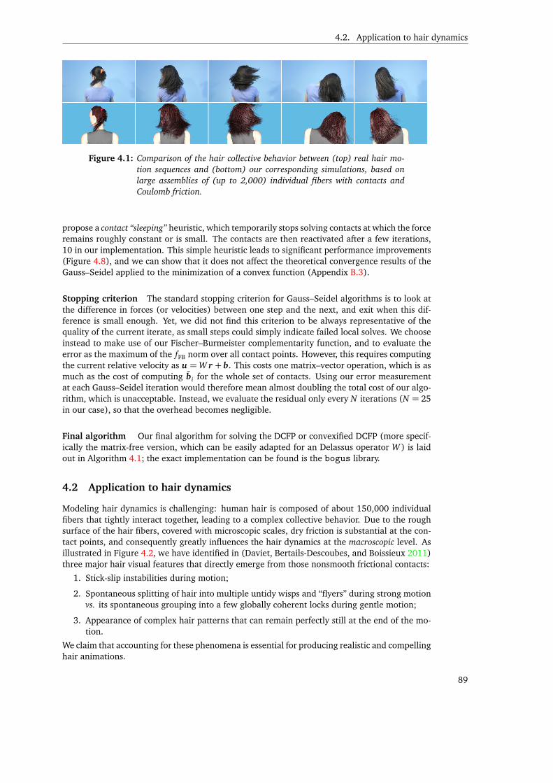
4.2. Application to hair dynamics

Figure 4.1: Comparison of the hair collective behavior between (top) real hair mo-tion sequences and (bottom) our corresponding simulations, based onlarge assemblies of (up to 2,000) individual fibers with contacts andCoulomb friction.

propose a contact “sleeping” heuristic, which temporarily stops solving contacts at which the forceremains roughly constant or is small. The contacts are then reactivated after a few iterations,10 in our implementation. This simple heuristic leads to significant performance improvements(Figure 4.8), and we can show that it does not affect the theoretical convergence results of theGauss–Seidel applied to the minimization of a convex function (Appendix B.3).

Stopping criterion The standard stopping criterion for Gauss–Seidel algorithms is to look atthe difference in forces (or velocities) between one step and the next, and exit when this dif-ference is small enough. Yet, we did not find this criterion to be always representative of thequality of the current iterate, as small steps could simply indicate failed local solves. We chooseinstead to make use of our Fischer–Burmeister complementarity function, and to evaluate theerror as the maximum of the fFB norm over all contact points. However, this requires computingthe current relative velocity as u =W r + b. This costs one matrix–vector operation, which is asmuch as the cost of computing bi for the whole set of contacts. Using our error measurementat each Gauss–Seidel iteration would therefore mean almost doubling the total cost of our algo-rithm, which is unacceptable. Instead, we evaluate the residual only every N iterations (N = 25in our case), so that the overhead becomes negligible.

Final algorithm Our final algorithm for solving the DCFP or convexified DCFP (more specif-ically the matrix-free version, which can be easily adapted for an Delassus operator W ) is laidout in Algorithm 4.1; the exact implementation can be found is the bogus library.

4.2 Application to hair dynamics

Modeling hair dynamics is challenging: human hair is composed of about 150,000 individualfibers that tightly interact together, leading to a complex collective behavior. Due to the roughsurface of the hair fibers, covered with microscopic scales, dry friction is substantial at the con-tact points, and consequently greatly influences the hair dynamics at the macroscopic level. Asillustrated in Figure 4.2, we have identified in (Daviet, Bertails-Descoubes, and Boissieux 2011)three major hair visual features that directly emerge from those nonsmooth frictional contacts:

1. Stick-slip instabilities during motion;

2. Spontaneous splitting of hair into multiple untidy wisps and “flyers” during strong motionvs. its spontaneous grouping into a few globally coherent locks during gentle motion;

3. Appearance of complex hair patterns that can remain perfectly still at the end of the mo-tion.

We claim that accounting for these phenomena is essential for producing realistic and compellinghair animations.

89

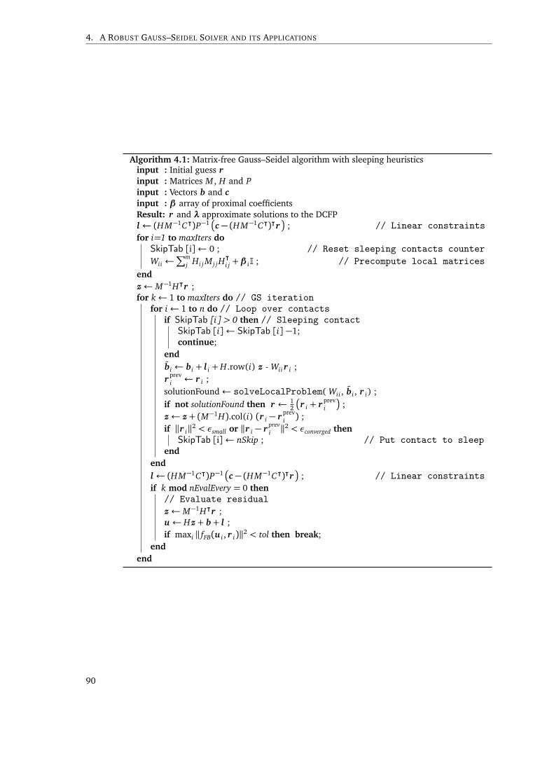
4. A ROBUST GAUSS–SEIDEL SOLVER AND ITS APPLICATIONS

Algorithm 4.1: Matrix-free Gauss–Seidel algorithm with sleeping heuristicsinput : Initial guess r

input : Matrices M , H and Pinput : Vectors b and c

input : β array of proximal coefficientsResult: r and λ approximate solutions to the DCFPl ← (HM−1C⊺)P−1

c − (HM−1C⊺)⊺r

; // Linear constraints

for i=1 to maxIters do

SkipTab [i]← 0 ; // Reset sleeping contacts counter

Wii ←∑m

j Hi j M j jH⊺

i j +β iI ; // Precompute local matrices

end

z← M−1H⊺r ;for k← 1 to maxIters do // GS iteration

for i← 1 to n do // Loop over contactsif SkipTab [i] > 0 then // Sleeping contact

SkipTab [i]← SkipTab [i] −1;continue;

end

bi ← bi + l i + H.row(i) z - Wii r i ;r

previ ← r i ;

solutionFound← solveLocalProblem( Wii , bi , r i) ;if not solutionFound then r ← 1

2

r i + r

previ

;

z← z + (M−1H).col(i) (r i − rprevi ) ;

if ‖r i‖2 < εsmall or ‖r i − rprevi ‖2 < εconverged then

SkipTab [i]← nSkip ; // Put contact to sleepend

end

l ← (HM−1C⊺)P−1c − (HM−1C⊺)⊺r

; // Linear constraints

if k mod nEvalEvery = 0 then

// Evaluate residual

z← M−1H⊺r ;u ← Hz + b+ l ;if maxi ‖ fFB(u i , r i)‖2 < tol then break;

end

end

90

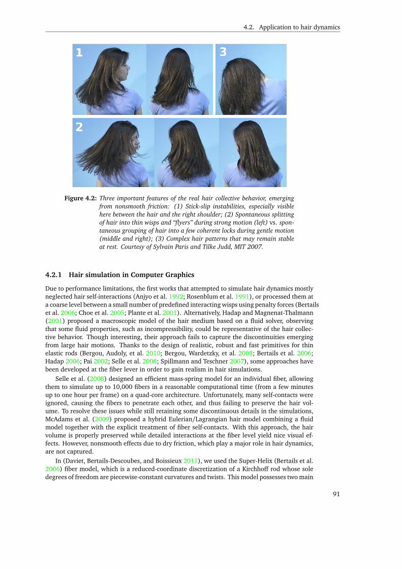
4.2. Application to hair dynamics

Figure 4.2: Three important features of the real hair collective behavior, emergingfrom nonsmooth friction: (1) Stick-slip instabilities, especially visiblehere between the hair and the right shoulder; (2) Spontaneous splittingof hair into thin wisps and “flyers” during strong motion (left) vs. spon-taneous grouping of hair into a few coherent locks during gentle motion(middle and right); (3) Complex hair patterns that may remain stableat rest. Courtesy of Sylvain Paris and Tilke Judd, MIT 2007.

4.2.1 Hair simulation in Computer Graphics

Due to performance limitations, the first works that attempted to simulate hair dynamics mostlyneglected hair self-interactions (Anjyo et al. 1992; Rosenblum et al. 1991), or processed them ata coarse level between a small number of predefined interacting wisps using penalty forces (Bertailset al. 2006; Choe et al. 2005; Plante et al. 2001). Alternatively, Hadap and Magnenat-Thalmann(2001) proposed a macroscopic model of the hair medium based on a fluid solver, observingthat some fluid properties, such as incompressibility, could be representative of the hair collec-tive behavior. Though interesting, their approach fails to capture the discontinuities emergingfrom large hair motions. Thanks to the design of realistic, robust and fast primitives for thinelastic rods (Bergou, Audoly, et al. 2010; Bergou, Wardetzky, et al. 2008; Bertails et al. 2006;Hadap 2006; Pai 2002; Selle et al. 2008; Spillmann and Teschner 2007), some approaches havebeen developed at the fiber lever in order to gain realism in hair simulations.

Selle et al. (2008) designed an efficient mass-spring model for an individual fiber, allowingthem to simulate up to 10,000 fibers in a reasonable computational time (from a few minutesup to one hour per frame) on a quad-core architecture. Unfortunately, many self-contacts wereignored, causing the fibers to penetrate each other, and thus failing to preserve the hair vol-ume. To resolve these issues while still retaining some discontinuous details in the simulations,McAdams et al. (2009) proposed a hybrid Eulerian/Lagrangian hair model combining a fluidmodel together with the explicit treatment of fiber self-contacts. With this approach, the hairvolume is properly preserved while detailed interactions at the fiber level yield nice visual ef-fects. However, nonsmooth effects due to dry friction, which play a major role in hair dynamics,are not captured.

In (Daviet, Bertails-Descoubes, and Boissieux 2011), we used the Super-Helix (Bertails et al.2006) fiber model, which is a reduced-coordinate discretization of a Kirchhoff rod whose soledegrees of freedom are piecewise-constant curvatures and twists. This model possesses two main

91

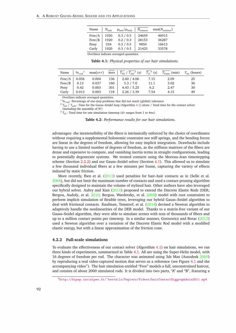
4. A ROBUST GAUSS–SEIDEL SOLVER AND ITS APPLICATIONS

Name Nrods µhair/µbody Ncontacts max(Ncontacts)

Free/A 1920 0.3 / 0.5 24659 46915Free/B 1920 0.2 / 0.3 28153 36287Pony 334 0.3 / 0.5 9850 16613Curly 1920 0.3 / 0.5 21425 33578

Overlines indicate averaged quantities.

Table 4.1: Physical properties of our hair simulations.

Name %>tol1 max(er r) iters TGS / Tsolv

2 (s) Td t3 (s) Tframe (min) Ttot (hours)

Free/A 0.056 0.004 136 2.60 / 4.06 7.15 2.09 25Free/B 0.13 0.037 160 5.3 / 7.0 11.1 3.02 36Pony 0.42 0.003 301 4.43 / 5.25 6.2 2.47 30Curly 0.013 0.003 118 2.26 / 3.39 7.54 4.15 49

Overlines indicate averaged quantities.1 %>tol: Percentage of one-step problems that did not reach (global) tolerance2 TGS / Tsolv: Time for the Gauss–Seidel loop (Algorithm 4.1) alone / Total time for the contact solver

(including the assembly of W )3 Td t : Total time for one simulation timestep (d t ranges from 1 to 4ms)

Table 4.2: Performance results for our hair simulations.

advantages: the inextensibility of the fibers is intrinsically enforced by the choice of coordinateswithout requiring a supplemental holonomic constraint nor stiff springs, and the bending forcesare linear in the degrees of freedom, allowing for easy implicit integration. Drawbacks includehaving to use a limited number of degrees of freedom, as the stiffness matrices of the fibers aredense and expensive to compute, and vanishing inertia terms in straight configurations, leadingto potentially degenerate systems. We treated contacts using the Moreau-Jean timesteppingscheme (Section 2.2.2) and our Gauss–Seidel solver (Section 4.1). This allowed us to simulatea few thousand individual fibers at a few minutes per frame, capturing the variety of effectsinduced by static friction.

More recently, Iben et al. (2013) used penalties for hair–hair contacts as in (Selle et al.2008), but did not limit the maximum number of contacts and used a contact-pruning algorithmspecifically designed to maintain the volume of stylized hair. Other authors have also leveragedour hybrid solver. Aubry and Xian (2015) proposed to extend the Discrete Elastic Rods (DER;Bergou, Audoly, et al. 2010; Bergou, Wardetzky, et al. 2008) model with root constraints toperform implicit simulation of flexible trees, leveraging our hybrid Gauss–Seidel algorithm todeal with frictional contacts. Kaufman, Tamstorf, et al. (2014) devised a Newton algorithm toadaptively handle the nonlinearities of the DER model. Thanks to a matrix-free variant of ourGauss–Seidel algorithm, they were able to simulate scenes with tens of thousands of fibers andup to a million contact points per timestep. In a similar manner, Gornowicz and Borac (2015)used a Newton algorithm over a variation of the Discrete Elastic Rod model with a modifiedelastic energy, but with a linear approximation of the friction cone.

4.2.2 Full-scale simulations

To evaluate the effectiveness of our contact solver (Algorithm 4.1) on hair simulations, we ranthree kinds of experiments, summarized in Table 4.1. All are using the Super-Helix model, with16 degrees of freedom per rod. The character was animated using 3ds Max (Autodesk 2009)by reproducing a real video-captured motion that serves as a reference (see Figure 4.1 and theaccompanying video4). The hair simulation entitled “Free” models a full, unconstrained haircut,and consists of about 2000 simulated rods. It is divided into two parts, “A” and “B”, featuring a

4http://bipop.inrialpes.fr/~bertails/Papiers/Videos/hairContactSiggraphAsia2011.mp4

92

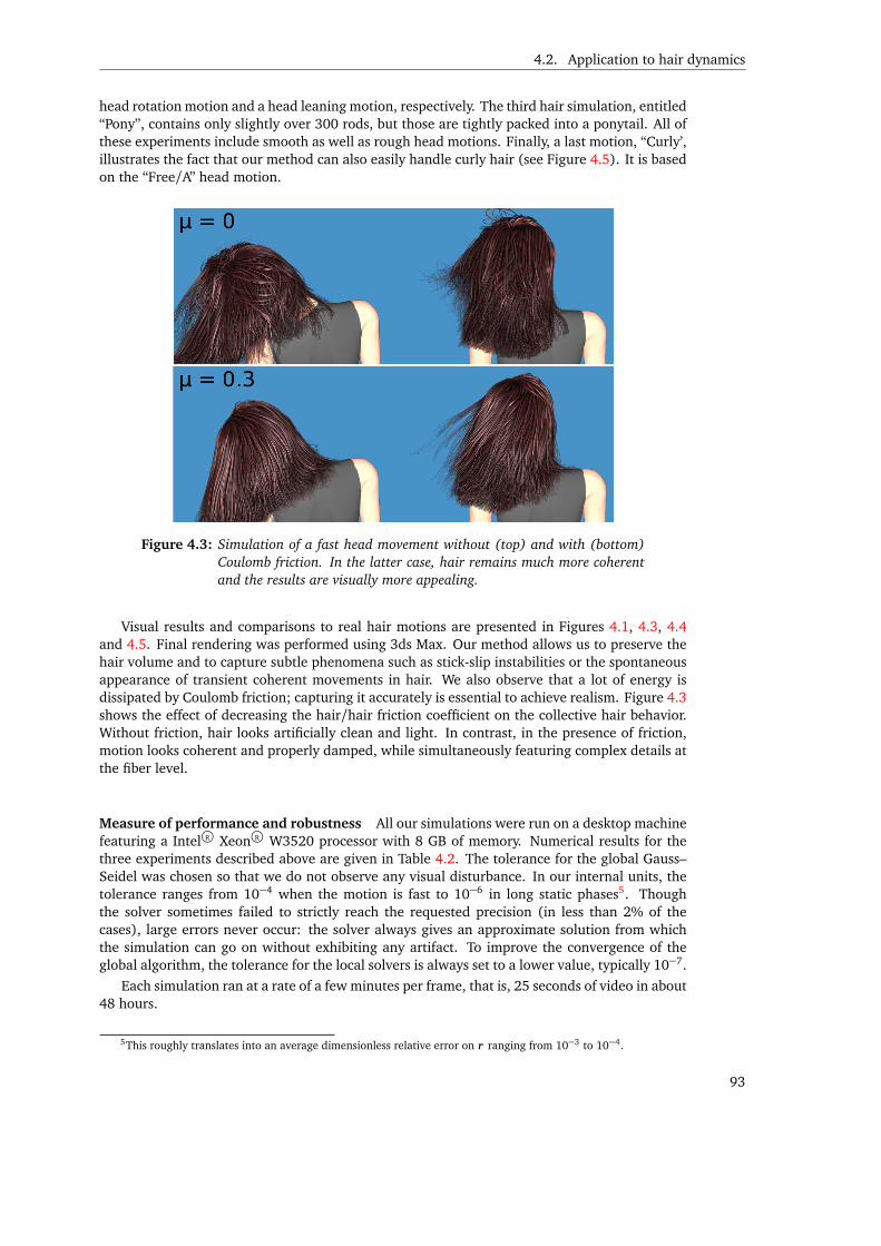
4.2. Application to hair dynamics

head rotation motion and a head leaning motion, respectively. The third hair simulation, entitled“Pony”, contains only slightly over 300 rods, but those are tightly packed into a ponytail. All ofthese experiments include smooth as well as rough head motions. Finally, a last motion, “Curly’,illustrates the fact that our method can also easily handle curly hair (see Figure 4.5). It is basedon the “Free/A” head motion.

Figure 4.3: Simulation of a fast head movement without (top) and with (bottom)Coulomb friction. In the latter case, hair remains much more coherentand the results are visually more appealing.

Visual results and comparisons to real hair motions are presented in Figures 4.1, 4.3, 4.4and 4.5. Final rendering was performed using 3ds Max. Our method allows us to preserve thehair volume and to capture subtle phenomena such as stick-slip instabilities or the spontaneousappearance of transient coherent movements in hair. We also observe that a lot of energy isdissipated by Coulomb friction; capturing it accurately is essential to achieve realism. Figure 4.3shows the effect of decreasing the hair/hair friction coefficient on the collective hair behavior.Without friction, hair looks artificially clean and light. In contrast, in the presence of friction,motion looks coherent and properly damped, while simultaneously featuring complex details atthe fiber level.

Measure of performance and robustness All our simulations were run on a desktop machinefeaturing a Intel R© Xeon R© W3520 processor with 8 GB of memory. Numerical results for thethree experiments described above are given in Table 4.2. The tolerance for the global Gauss–Seidel was chosen so that we do not observe any visual disturbance. In our internal units, thetolerance ranges from 10−4 when the motion is fast to 10−6 in long static phases5. Thoughthe solver sometimes failed to strictly reach the requested precision (in less than 2% of thecases), large errors never occur: the solver always gives an approximate solution from whichthe simulation can go on without exhibiting any artifact. To improve the convergence of theglobal algorithm, the tolerance for the local solvers is always set to a lower value, typically 10−7.

Each simulation ran at a rate of a few minutes per frame, that is, 25 seconds of video in about48 hours.

5This roughly translates into an average dimensionless relative error on r ranging from 10−3 to 10−4.

93

4. A ROBUST GAUSS–SEIDEL SOLVER AND ITS APPLICATIONS

Figure 4.4: Our simulations (right) capture the complex patterns emerging fromstatic friction in real hair (left).

Figure 4.5: Our method can also handle curly hair. Note how the volume of thehairstyle is preserved throughout the simulation, and how static frictionis properly captured near the top of the head.

4.2.3 Friction solvers comparisons

We compared our method against a variety of frictional contact solvers,

• MFB: Our Newton method based on the modified Fischer-Burmeister formulation. It canbe used either as a global solver or as a local solver within a Gauss–Seidel loop.

• PAC and DAC: Respectively pure and damped Newton methods based on the Alart-Curnierformulation used in (Bertails-Descoubes et al. 2011). Both can be used as either global orlocal solvers.

• Duriez08: Local solver from Duriez (2008), which consists of successive iterations of theapproach from Duriez et al. (2006) embedded in a fixed point loop. Unlike the original

94

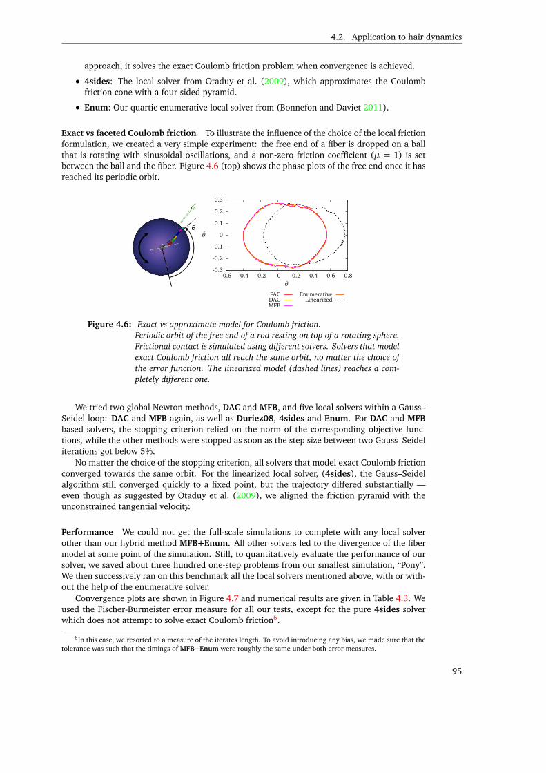
4.2. Application to hair dynamics

approach, it solves the exact Coulomb friction problem when convergence is achieved.

• 4sides: The local solver from Otaduy et al. (2009), which approximates the Coulombfriction cone with a four-sided pyramid.

• Enum: Our quartic enumerative local solver from (Bonnefon and Daviet 2011).

Exact vs faceted Coulomb friction To illustrate the influence of the choice of the local frictionformulation, we created a very simple experiment: the free end of a fiber is dropped on a ballthat is rotating with sinusoidal oscillations, and a non-zero friction coefficient (µ = 1) is setbetween the ball and the fiber. Figure 4.6 (top) shows the phase plots of the free end once it hasreached its periodic orbit.

-0.3

-0.2

-0.1

0

0.1

0.2

0.3

-0.6 -0.4 -0.2 0 0.2 0.4 0.6 0.8θ

θ

PACDACMFB

EnumerativeLinearized

Figure 4.6: Exact vs approximate model for Coulomb friction.Periodic orbit of the free end of a rod resting on top of a rotating sphere.Frictional contact is simulated using different solvers. Solvers that modelexact Coulomb friction all reach the same orbit, no matter the choice ofthe error function. The linearized model (dashed lines) reaches a com-pletely different one.

We tried two global Newton methods, DAC and MFB, and five local solvers within a Gauss–Seidel loop: DAC and MFB again, as well as Duriez08, 4sides and Enum. For DAC and MFB

based solvers, the stopping criterion relied on the norm of the corresponding objective func-tions, while the other methods were stopped as soon as the step size between two Gauss–Seideliterations got below 5%.

No matter the choice of the stopping criterion, all solvers that model exact Coulomb frictionconverged towards the same orbit. For the linearized local solver, (4sides), the Gauss–Seidelalgorithm still converged quickly to a fixed point, but the trajectory differed substantially —even though as suggested by Otaduy et al. (2009), we aligned the friction pyramid with theunconstrained tangential velocity.

Performance We could not get the full-scale simulations to complete with any local solverother than our hybrid method MFB+Enum. All other solvers led to the divergence of the fibermodel at some point of the simulation. Still, to quantitatively evaluate the performance of oursolver, we saved about three hundred one-step problems from our smallest simulation, “Pony”.We then successively ran on this benchmark all the local solvers mentioned above, with or with-out the help of the enumerative solver.

Convergence plots are shown in Figure 4.7 and numerical results are given in Table 4.3. Weused the Fischer-Burmeister error measure for all our tests, except for the pure 4sides solverwhich does not attempt to solve exact Coulomb friction6.

6In this case, we resorted to a measure of the iterates length. To avoid introducing any bias, we made sure that thetolerance was such that the timings of MFB+Enum were roughly the same under both error measures.

95

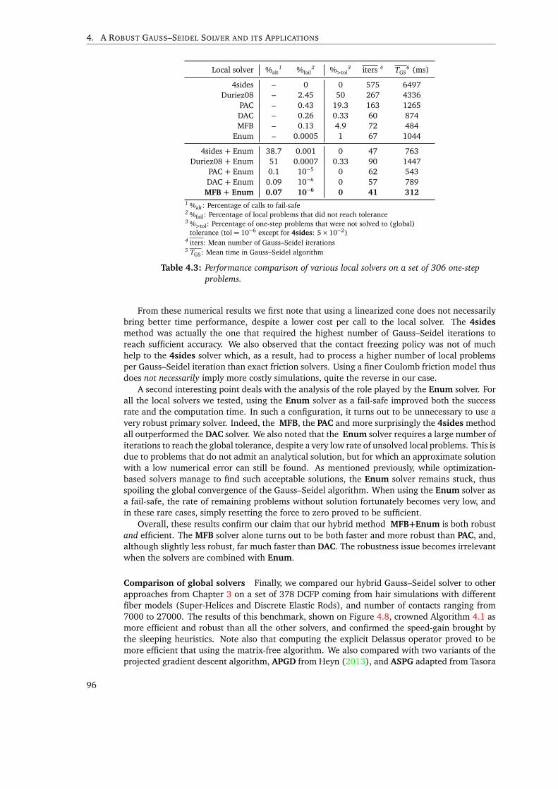
4. A ROBUST GAUSS–SEIDEL SOLVER AND ITS APPLICATIONS

Local solver %alt1 %fail

2 %>tol3 iters 4 TGS

6 (ms)

4sides – 0 0 575 6497Duriez08 – 2.45 50 267 4336

PAC – 0.43 19.3 163 1265DAC – 0.26 0.33 60 874MFB – 0.13 4.9 72 484

Enum – 0.0005 1 67 1044

4sides + Enum 38.7 0.001 0 47 763Duriez08 + Enum 51 0.0007 0.33 90 1447

PAC + Enum 0.1 10−5 0 62 543DAC + Enum 0.09 10−6 0 57 789MFB + Enum 0.07 10−6 0 41 312

1 %alt: Percentage of calls to fail-safe2 %fail: Percentage of local problems that did not reach tolerance3 %>tol: Percentage of one-step problems that were not solved to (global)

tolerance (tol= 10−6 except for 4sides: 5× 10−2)4 iters: Mean number of Gauss–Seidel iterations5 TGS: Mean time in Gauss–Seidel algorithm

Table 4.3: Performance comparison of various local solvers on a set of 306 one-stepproblems.

From these numerical results we first note that using a linearized cone does not necessarilybring better time performance, despite a lower cost per call to the local solver. The 4sides

method was actually the one that required the highest number of Gauss–Seidel iterations toreach sufficient accuracy. We also observed that the contact freezing policy was not of muchhelp to the 4sides solver which, as a result, had to process a higher number of local problemsper Gauss–Seidel iteration than exact friction solvers. Using a finer Coulomb friction model thusdoes not necessarily imply more costly simulations, quite the reverse in our case.

A second interesting point deals with the analysis of the role played by the Enum solver. Forall the local solvers we tested, using the Enum solver as a fail-safe improved both the successrate and the computation time. In such a configuration, it turns out to be unnecessary to use avery robust primary solver. Indeed, the MFB, the PAC and more surprisingly the 4sides methodall outperformed the DAC solver. We also noted that the Enum solver requires a large number ofiterations to reach the global tolerance, despite a very low rate of unsolved local problems. This isdue to problems that do not admit an analytical solution, but for which an approximate solutionwith a low numerical error can still be found. As mentioned previously, while optimization-based solvers manage to find such acceptable solutions, the Enum solver remains stuck, thusspoiling the global convergence of the Gauss–Seidel algorithm. When using the Enum solver asa fail-safe, the rate of remaining problems without solution fortunately becomes very low, andin these rare cases, simply resetting the force to zero proved to be sufficient.

Overall, these results confirm our claim that our hybrid method MFB+Enum is both robustand efficient. The MFB solver alone turns out to be both faster and more robust than PAC, and,although slightly less robust, far much faster than DAC. The robustness issue becomes irrelevantwhen the solvers are combined with Enum.

Comparison of global solvers Finally, we compared our hybrid Gauss–Seidel solver to otherapproaches from Chapter 3 on a set of 378 DCFP coming from hair simulations with differentfiber models (Super-Helices and Discrete Elastic Rods), and number of contacts ranging from7000 to 27000. The results of this benchmark, shown on Figure 4.8, crowned Algorithm 4.1 asmore efficient and robust than all the other solvers, and confirmed the speed-gain brought bythe sleeping heuristics. Note also that computing the explicit Delassus operator proved to bemore efficient that using the matrix-free algorithm. We also compared with two variants of theprojected gradient descent algorithm, APGD from Heyn (2013), and ASPG adapted from Tasora

96

4.2. Application to hair dynamics

Duriez08

4sides

Enum

DAC

MFB+Enum

Number of Gauss−Seidel iterations

0 %

25 %

50 %

75 %

100 %

25 100 200 500 1000 2000

Figure 4.7: Percentage of one-step problems (Y axis) requiring more than a givennumber of Gauss–Seidel iterations (X axis) to converge, for various localsolvers. Our hybrid method (solid red) induces better global convergencethan previous approaches.

100 101 102 1030

0.2

0.4

0.6

0.8

1

Solve time w.r.t fastest solver

Perce

ntprob

lemss

olved

GSMatrix-free GSNo-sleep GSCadoux/GS

ASPGCadoux/ASPG

APGD

Figure 4.8: Performance profiles for a variety of solvers on our hair simulationbenchmark — percentage of problems that each solver was able to solveunder a multiple x of the time taken by the fastest solver for this prob-lem. The line x = 1 gives the solvers that were the most often the fastest,while y = 1 shows the most robust ones.

(2013) as per Algorithm B.2. Finally, GS and ASPG were also compared to their SOCQP variantsinside a Cadoux fixed-point loop.

4.2.4 Limitations

Even though our hair simulations appear more convincing than those generated by previousmethods, they do not perfectly match the real movement depicted in the reference videos. This ispartly due to inaccuracies in the hair styling process and to the difficulty of precisely identifyingthe true physical parameters. The next section will present a first step towards reducing thisinaccuracy by deducing the groom rest parameters from an input geometry.

Another reason is related to the actual complexity of hair interactions. While Coulomb fric-tion is a key ingredient, further effects such as anisotropic friction, adhesion, or electrostatics arelikely to influence the hair motion, depending on the hair state (clean, dirty, wet) and externalconditions (dry or wet atmosphere). Moreover, air–hair friction becomes preponderant duringenergetic motions, and a full simulation the surrounding air would be necessary to properlycapture the intricate dynamics of this tightly coupled system.

97

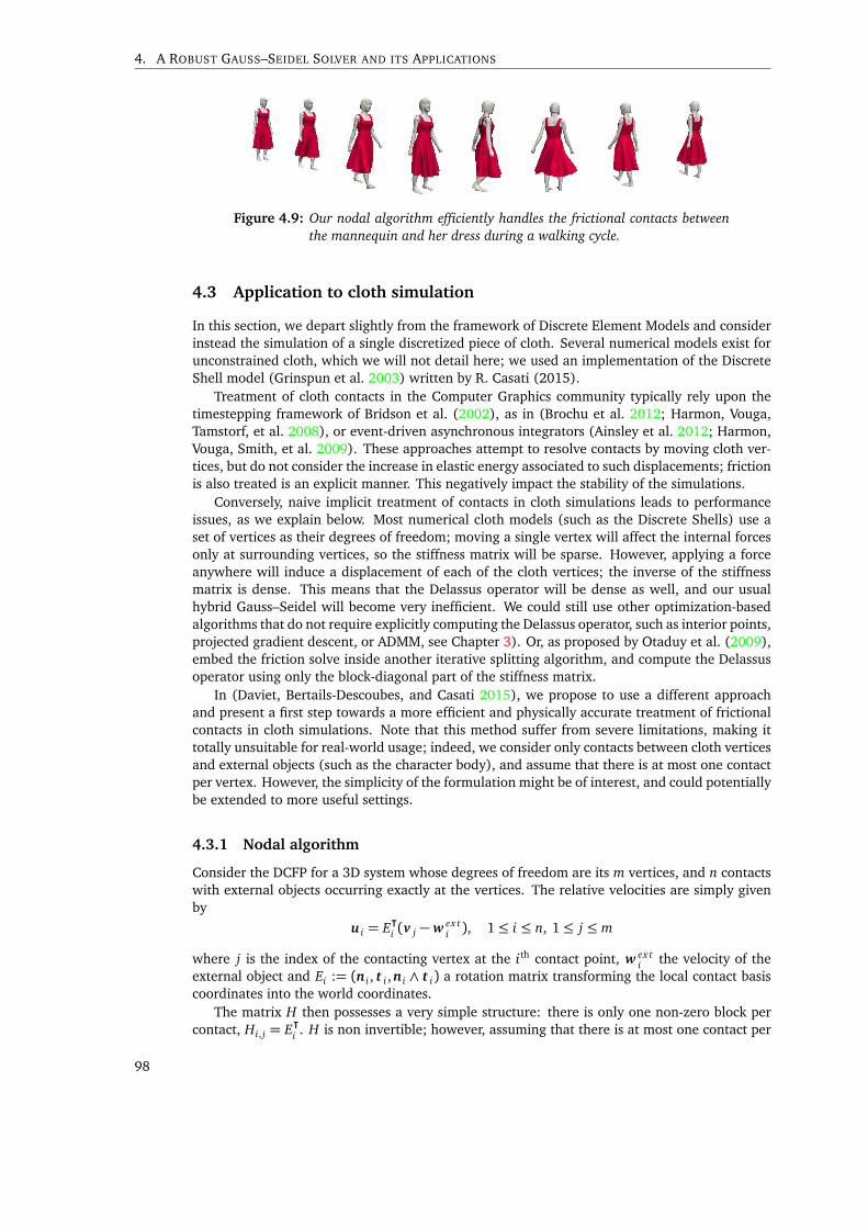
4. A ROBUST GAUSS–SEIDEL SOLVER AND ITS APPLICATIONS

Figure 4.9: Our nodal algorithm efficiently handles the frictional contacts betweenthe mannequin and her dress during a walking cycle.

4.3 Application to cloth simulation

In this section, we depart slightly from the framework of Discrete Element Models and considerinstead the simulation of a single discretized piece of cloth. Several numerical models exist forunconstrained cloth, which we will not detail here; we used an implementation of the DiscreteShell model (Grinspun et al. 2003) written by R. Casati (2015).

Treatment of cloth contacts in the Computer Graphics community typically rely upon thetimestepping framework of Bridson et al. (2002), as in (Brochu et al. 2012; Harmon, Vouga,Tamstorf, et al. 2008), or event-driven asynchronous integrators (Ainsley et al. 2012; Harmon,Vouga, Smith, et al. 2009). These approaches attempt to resolve contacts by moving cloth ver-tices, but do not consider the increase in elastic energy associated to such displacements; frictionis also treated is an explicit manner. This negatively impact the stability of the simulations.

Conversely, naive implicit treatment of contacts in cloth simulations leads to performanceissues, as we explain below. Most numerical cloth models (such as the Discrete Shells) use aset of vertices as their degrees of freedom; moving a single vertex will affect the internal forcesonly at surrounding vertices, so the stiffness matrix will be sparse. However, applying a forceanywhere will induce a displacement of each of the cloth vertices; the inverse of the stiffnessmatrix is dense. This means that the Delassus operator will be dense as well, and our usualhybrid Gauss–Seidel will become very inefficient. We could still use other optimization-basedalgorithms that do not require explicitly computing the Delassus operator, such as interior points,projected gradient descent, or ADMM, see Chapter 3). Or, as proposed by Otaduy et al. (2009),embed the friction solve inside another iterative splitting algorithm, and compute the Delassusoperator using only the block-diagonal part of the stiffness matrix.

In (Daviet, Bertails-Descoubes, and Casati 2015), we propose to use a different approachand present a first step towards a more efficient and physically accurate treatment of frictionalcontacts in cloth simulations. Note that this method suffer from severe limitations, making ittotally unsuitable for real-world usage; indeed, we consider only contacts between cloth verticesand external objects (such as the character body), and assume that there is at most one contactper vertex. However, the simplicity of the formulation might be of interest, and could potentiallybe extended to more useful settings.

4.3.1 Nodal algorithm

Consider the DCFP for a 3D system whose degrees of freedom are its m vertices, and n contactswith external objects occurring exactly at the vertices. The relative velocities are simply givenby

u i = E⊺i (v j − w ex ti ), 1≤ i ≤ n, 1≤ j ≤ m

where j is the index of the contacting vertex at the ith contact point, w ex ti the velocity of the

external object and Ei := (n i , t i ,n i ∧ t i) a rotation matrix transforming the local contact basiscoordinates into the world coordinates.

The matrix H then possesses a very simple structure: there is only one non-zero block percontact, Hi, j = E⊺i . H is non invertible; however, assuming that there is at most one contact per

98

4.3. Application to cloth simulation

vertex, we can easily extend it into a square 3m× 3m block-diagonal matrix G,

Gi,i :=

E⊺i if vertex i is in contact

I otherwise .(4.15)

The DCFP can then be equivalently written using this matrix G as finding v , u, r , all in R3m, suchthat

M v = f + G⊺r

u = Gv − Gw ex t

(u i , r i) ∈ Cµiif vertex i is in contact

r i = 0 otherwise .

(4.16)

Now, G is orthonormal, and can be easily inverted as G−1 = G⊺. We can thus eliminate v insystem (4.16) and write its first line as

MG⊺u + w ex t

= f + G⊺r .

Multiplying both sides by G, we obtain system (4.17)

GMG⊺︸ ︷︷ ︸W

u + G(MG⊺w ex t − f )︸ ︷︷ ︸b

= r

(u i , r i) ∈ Cµiif vertex i is in contact

r i = 0 otherwise .

(4.17)

System (4.17) is very similar to the dual formulation of the DCFP (2.19), where the role of u andr have been reversed. However, the matrix W is now sparse, and we can therefore solve (4.17)using our Gauss–Seidel algorithm by either

• transforming (4.17) as a sequence of convexified DCFP, using a variation of the Cadouxfixed-point algorithm (see Daviet, Bertails-Descoubes, and Casati 2015), or;

• if Wii is invertible, writing the inverse local linear relationship, u i = W−1ii (r i − bi) and

using our original one-contact solvers, or;

• devising a new hybrid local solver for Coulomb friction with reversed linear relationshipbetween the force and relative velocity. The Fischer–Burmeister Newton algorithm can betrivially adapted, and a corresponding quartic polynomial has been derived by a studentin our group, L. Toran — but has not been published yet.

One can also take advantage of the orthonormality of the matrix G by performing a pro-jected gradient descent algorithm on the primal formulation. Indeed, the feasible set of eachintermediate primal SOCQP of the Cadoux algorithm is

C(s) = v ∈ R3m, Gv + w ex t + s ∈ K := K1 × . . .× Km

Ki :=

K 1µi

if i is in contact

Rd otherwise

∀1≤ i ≤ m

and the projection on C(s) is now easy to compute:

y = ΠC(s)(v) ⇐⇒ v − y ∈ NC(s)(y)

⇐⇒ ⟨v − y , z − y⟩ ≤ 0 ∀z ∈ C(s)

⇐⇒ v − y , G⊺

u − s − w ex t

− y≤ 0 ∀u ∈ K

⇐⇒ Gv − Gy , u − Gy + s + w ex t

≤ 0 ∀u ∈ K

⇐⇒ (Gy + s + w ex t) ∈ NK(Gv + s + w ex t)

⇐⇒ y = GTΠK

Gv + s + w ex t

− s − w ex t

.

99

4. A ROBUST GAUSS–SEIDEL SOLVER AND ITS APPLICATIONS

µ= 0

t = 40 ms t = 100 ms t = 200 ms

µ= 0.2

µ= 0.5

Figure 4.10: When the friction coefficient µ is high enough (bottom), the clothfalling onto the bunny no longer slides away.

Dual Nodal algorithm

Scene m1 n2 Build Solve Build Solve

Bunny 6500 169 2.25 0.017 0.02 0.074Skirt 5208 741 76.7 0.23 0.074 0.14Dress 6060 1086 157 0.19 0.077 0.048

Times are in seconds.1 Number of cloth vertices.2 Average number of contacts.

Table 4.4: Performance comparison between the standard dual algorithm (with ex-plicit Delassus operator) and the nodal algorithm for solving body–clothcontacts.

4.3.2 Results

Capturing dry friction We first want to ensure that our algorithm is indeed capable of cap-turing the effects of Coulomb friction. We run a simple simulation consisting of a square pieceof cloth falling onto the Stanford bunny (Figure 4.10). While the friction coefficient is low,the cloth is slipping down under its own weight; however, for higher values of this coefficient,friction maintains the cloth stuck atop the bunny.

Performance We compared the cost of solving the DCFP using the standard (dual) Gauss–Seidel algorithm with the dense Delassus operator versus running our nodal algorithm (using theCadoux fixed-point algorithm and our hybrid Gauss–Seidel for each intermediate SOCQP). Ta-ble 4.4 summarize our results for three test cases: the cloth-on-bunny simulation of Figure 4.10,the walk of a mannequin wearing a dress of as in Figure 4.9), and a similar motion with a skirt.When taking into account the cost of computing the Delassus operator, the nodal algorithm ranabout two orders of magnitude faster than the naive dual method.

4.3.3 Limitations

Our naive nodal algorithm allowed for a significant speed-up w.r.t. solving the standard DCFPon simple simulations, such as that of Figure 4.9 where the dress is contacting only with theunderlying body . As the body mesh does not have sharp features, dealing only with contacts

100

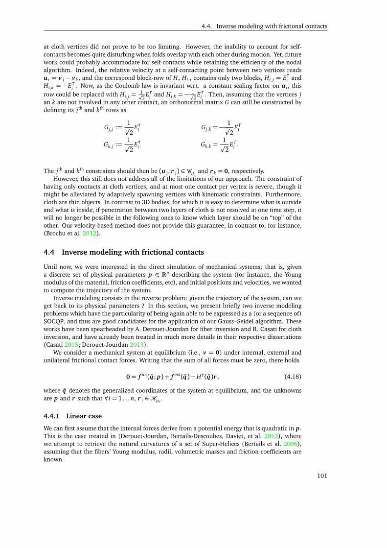
4.4. Inverse modeling with frictional contacts

at cloth vertices did not prove to be too limiting. However, the inability to account for self-contacts becomes quite disturbing when folds overlap with each other during motion. Yet, futurework could probably accommodate for self-contacts while retaining the efficiency of the nodalalgorithm. Indeed, the relative velocity at a self-contacting point between two vertices readsu i = v j − v k, and the correspond block-row of H, Hi·, contains only two blocks, Hi, j = E⊺i andHi,k = −ET

i . Now, as the Coulomb law is invariant w.r.t. a constant scaling factor on u i , thisrow could be replaced with Hi, j =

1p2

E⊺i and Hi,k = − 1p2

ETi . Then, assuming that the vertices j

an k are not involved in any other contact, an orthonormal matrix G can still be constructed bydefining its jth and kth rows as

G j, j :=1p2

E⊺i G j,k = −1p2

ETi

Gk, j :=1p2

E⊺i Gk,k =1p2

ETi .

The jth and kth constraints should then be (u j , r j) ∈ Cµ jand r k = 0, respectively.

However, this still does not address all of the limitations of our approach. The constraint ofhaving only contacts at cloth vertices, and at most one contact per vertex is severe, though itmight be alleviated by adaptively spawning vertices with kinematic constraints. Furthermore,cloth are thin objects. In contrast to 3D bodies, for which it is easy to determine what is outsideand what is inside, if penetration between two layers of cloth is not resolved at one time step, itwill no longer be possible in the following ones to know which layer should be on “top” of theother. Our velocity-based method does not provide this guarantee, in contrast to, for instance,(Brochu et al. 2012).

4.4 Inverse modeling with frictional contacts

Until now, we were interested in the direct simulation of mechanical systems; that is, givena discrete set of physical parameters p ∈ Rp describing the system (for instance, the Youngmodulus of the material, friction coefficients, etc), and initial positions and velocities, we wantedto compute the trajectory of the system.

Inverse modeling consists in the reverse problem: given the trajectory of the system, can weget back to its physical parameters ? In this section, we present briefly two inverse modelingproblems which have the particularity of being again able to be expressed as a (or a sequence of)SOCQP, and thus are good candidates for the application of our Gauss–Seidel algorithm. Theseworks have been spearheaded by A. Derouet-Jourdan for fiber inversion and R. Casati for clothinversion, and have already been treated in much more details in their respective dissertations(Casati 2015; Derouet-Jourdan 2013).

We consider a mechanical system at equilibrium (i.e., v = 0) under internal, external andunilateral frictional contact forces. Writing that the sum of all forces must be zero, there holds

0= f int(q ; p) + f ext(q) +H⊺(q)r , (4.18)

where q denotes the generalized coordinates of the system at equilibrium, and the unknownsare p and r such that ∀i = 1 . . . n, r i ∈Kµi

.

4.4.1 Linear case

We can first assume that the internal forces derive from a potential energy that is quadratic in p.This is the case treated in (Derouet-Jourdan, Bertails-Descoubes, Daviet, et al. 2013), wherewe attempt to retrieve the natural curvatures of a set of Super-Helices (Bertails et al. 2006),assuming that the fibers’ Young modulus, radii, volumetric masses and friction coefficients areknown.

101

4. A ROBUST GAUSS–SEIDEL SOLVER AND ITS APPLICATIONS

Figure 4.11: Outline of our hair inverse modeling strategy. (a) Input hair geom-etry, here a capture from Herrera et al. (2012). (b) Conversion to amechanical fiber model, here a set of Super-Helices. (c) Without inver-sion, the hair sags at the beginning of the simulation, and the groom islost. (d) Using our inversion procedure, the groom stays in place andbehaves naturally once the head starts moving. Character model c©L.Boissieux.

This addresses an important problem in the visual effects industry: when creating a digi-tal double of a live performing actor, artists (or sufficiently-advanced software) will sculpt thegroom so that it matches a reference photography. One can “easily” transform each of thegroom’s strands into the rest configuration of an animatable fiber (e.g., a Super-Helix, as inDerouet-Jourdan, Bertails-Descoubes, and Thollot 2013). However, once the simulation is runwith gravity, the fibers will fall from their rest configuration and significant sagging will be ob-served, ruining the similarity between the digital groom and its physical reference (Figure 4.11).One could simply consider fibers one by one, and find a set of rest curvatures and twists so thattheir deformed configuration under gravity matches the input groom (see e.g., Derouet-Jourdan,Bertails-Descoubes, and Thollot 2010). Then, no sagging will occur when the simulation is run.However, such an inversion procedure will explain all deformations, including those due to con-tacts (such as hair resting upon a shoulder) as merely stemming from large rest curvatures,which will inevitably lead to weird dynamics. To avoid such artifacts, one must consider thewhole groom and take contacts into account when looking for the rest parameters.

Inversion strategy In the linear case, the inverse problem (4.18) boils down to finding p ∈ Rp

and r ∈ Rnd such that

0= f ext + Kp + H⊺r , r ∈ ΠKµi. (4.19)

Even when K is symmetric positive definite, problem (4.19) is under-determined; we can alwaysfind a solution for which r = 0, but this might not be the only one.

To circumvent this problem, we define a target parameter set p0 ∈ Rp from physical consid-erations, and minimize the distance between our retrieved parameter p and p0. Our problembecomes

minp∈Rp

1

2‖p − p0‖2 = min

r∈ΠKµi

1

2‖K−1

H⊺r + f ext

+ p0‖2

= minr∈ΠKµi

1

2r ⊺W r + r T b+

1

2‖K−1 f ext + p0‖,

with W = HK−2H⊺ and b = HK−2 f ex t + K−1p0

, whose optimality conditions satisfy a problem

structurally similar to the convexified DCFP (2.22),

K2v = f ex t + Kp0 + H⊺r

u = Hv

K 1µi∋ u i ⊥ r i ∈Kµi

∀i = 1 . . . n.(4.20)

As we saw in Section 2.3.2, problem (4.20) always admits a solution in v and can be solvedeither as a primal or dual SOCQP. p can then be deduced from a solution to (4.20) as p =

−K−1H⊺r + f ext

= p0 − Kv .

102

4.4. Inverse modeling with frictional contacts

(a) (b) (c) (d)

Figure 4.12: An application of inverse cloth modeling. (a) An artist creates a skirtmodel by sculpting its rest pose under gravity. (b) Without inverse mod-eling, the simulated cloth sags and falls from the hips of the character.(c) Inverse modeling ensures that friction at the hips suffices to main-tain the cloth at its original position. (d) The recovered cloth behavesnaturally when external forces (wind) are applied. Skirt and charactermodels c©L. Boissieux.

Application to inverse hair modeling The above framework for taking frictional contacts intoaccount within the inversion procedure requires defining a set of target parameters p0, and threepossibilities can be considered:• Using directly the input curvatures from the deformed configurations;

• Using the curvature computed at the end of each input curve; this assumes that eachfiber possesses relatively constant natural curvatures, and that the fiber’s end is the least-deformed portion.

• Using a vanishing target curvatures, assuming that the fibers are naturally straight.Each of these strategies yields a different balance between the influence of the contact forcesand that of the natural curliness, and we have not found any of them to work better than theothers overall. Instead, we suggest to try each of them for any input, and manually compare theresults.

The resulting SOCQP will also often have a singular W matrix, which means underdetermi-nation of the contact forces. In practice, we propose to regularize the minimization problem byadding a penalization term ǫIRnd to W , preventing the inversion procedure to consider unlikelyhuge contact forces. This strategy allowed us to find plausible parameters for input geometrieswith hundreds of fibers and thousands of contacts, at a cost similar to that of a single simu-lation step. The hair recovered from the inversion procedure could then either be simulatedunmodified, or further edited using physically-based grooming techniques.

4.4.2 Nonlinear case

In (Casati et al. 2016), we proposed a first attempt to solve the inverse problem (4.18) with anonlinear dependency of the forces w.r.t. the parameters p. This is the case for the DiscreteElastic Shell model (Grinspun et al. 2003), when the parameters to recover are the positions ofthe vertices of the rest shape.

We assume that all non-contact forces derive from a potential energy E p(q , p), i.e.,

f int(q ; p) + f ex t(q) = −∂ Ep

∂ q(q , p).

We introduce the equilibrium function F : Rm ×Rp → Rm,

F : (q , p) 7→ ∂ E p

∂ q(q , p)−ΠC

∂ E p

∂ q(q , p)

103

4. A ROBUST GAUSS–SEIDEL SOLVER AND ITS APPLICATIONS

where C = H(q)⊺ΠKµi, such that

F(q , p) = 0 ⇐⇒ ∂ E p

∂ q(q , p) ∈ H(q)⊺ΠKµi

.

The inverse problem (4.18) is thus equivalent to finding p such that F(q , p) = 0. Just like forthe dynamics (Section 4.3), we assume that the degrees of freedom q of the dynamical modelare the positions of the shell vertices, and that contacts occur only at those points. This meansthat the projection on C simply amounts to projections on rotated SOC, and is thus trivial tocompute.

Draping function Without diving too deeply into the algorithmic details, we then recast (4.18)as the minimization problem

minp∈Rp

J(p) :=1

2‖Φ(p)− q‖2 (4.21)

where Φ : Rp → Rm is a so-called draping function, which associates to a parameter p an equilib-rium coordinate q , i.e., such that F(q , p) = 0. For instance, Φ can be defined locally through theimplicit function theorem7. One solution to evaluate Φ would be to perform a full simulation,but that would be too costly. Instead, let us now show how we can evaluate Φ as the solution toan optimization problem.

As∀x ∈ R3,−NK 1µ

(x ) ⊂Kµ, a sufficient condition to obtain F(q , p) = 0, and thus q = Φ(p),

is to have ∂ E p

∂ q (q , p) ∈ −H(q)TNΠK 1µi

(H(q)(q− q)); the condition also becomes necessary when

Φ(p) = q , i.e., when p is a solution to the inverse problem. Under our nodal contact assumptionH(q) is surjective, so we can apply the Corollary A.3 to Property A.12 on the subdifferential ofthe precomposition with an affine map and obtain an equivalent condition,

∂ E p

∂ q(q , p) ∈ −NV (q) (4.22)

with V =n

q ∈ Rm, H(q − q) ∈ ΠK 1µi

o. We recognize this last inclusion as defining a (local)

minimum of an optimization problem,

minq∈VE p(q , p). (4.23)

Evaluating the draping function Φ(p) therefore amounts to finding a local minimum of an opti-mization problem under SOC constraints, which can be cast as a sequence of convexified DCFP:

∂ 2Ec

∂ 2q(q k, p)

q k+1 − q k

= −∂ Ec

∂ q(q k, p) + H(q)⊺r

u = H(q)(q k+1 − q)

K 1µi∋ u i ⊥ r i ∈Kµi

∀i = 1 . . . n.

(4.24)

In practice, we penalize the objective function with a proximal regularization term 12λ‖q−q‖2

in order to ensure that the Hessian in (4.24) remains reasonably positive, and avoid finding localminima that are too far away from the target position. λ is then progressively increased as theoverall algorithm converges.

7This definition does not hold in the presence of contacts, as F is no longer differentiable, but we can still define Φalgorithmically.

104

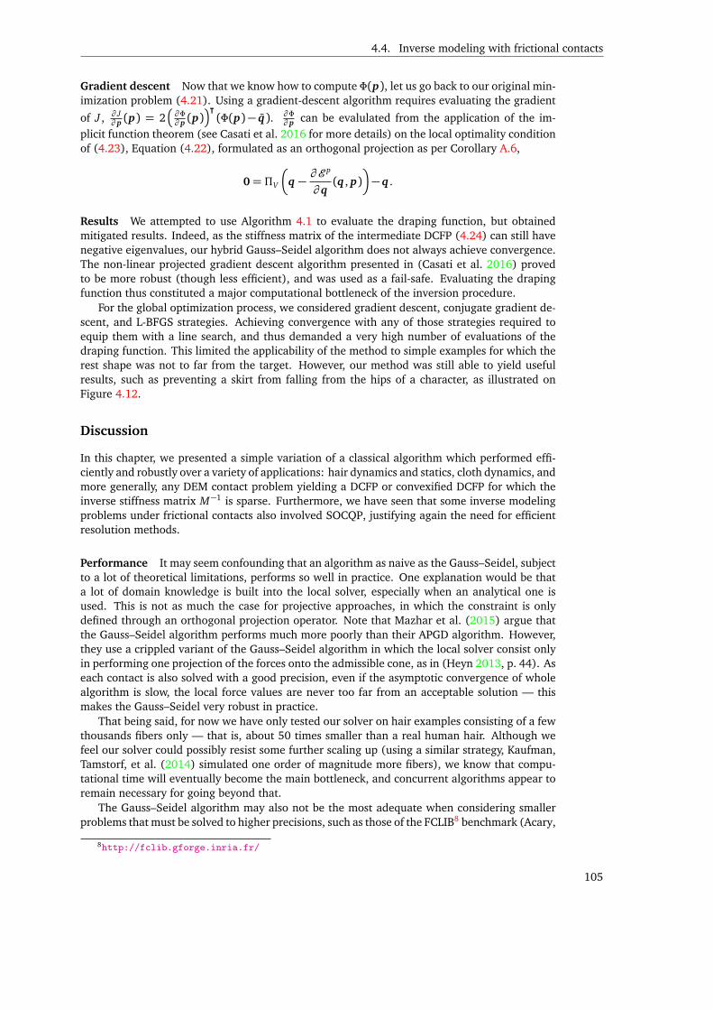
4.4. Inverse modeling with frictional contacts

Gradient descent Now that we know how to compute Φ(p), let us go back to our original min-imization problem (4.21). Using a gradient-descent algorithm requires evaluating the gradient

of J , ∂ J∂ p (p) = 2

∂Φ∂ p (p)

⊺(Φ(p)− q). ∂Φ

∂ p can be evalulated from the application of the im-plicit function theorem (see Casati et al. 2016 for more details) on the local optimality conditionof (4.23), Equation (4.22), formulated as an orthogonal projection as per Corollary A.6,

0= ΠV

q − ∂ E

p

∂ q(q , p)

− q .

Results We attempted to use Algorithm 4.1 to evaluate the draping function, but obtainedmitigated results. Indeed, as the stiffness matrix of the intermediate DCFP (4.24) can still havenegative eigenvalues, our hybrid Gauss–Seidel algorithm does not always achieve convergence.The non-linear projected gradient descent algorithm presented in (Casati et al. 2016) provedto be more robust (though less efficient), and was used as a fail-safe. Evaluating the drapingfunction thus constituted a major computational bottleneck of the inversion procedure.

For the global optimization process, we considered gradient descent, conjugate gradient de-scent, and L-BFGS strategies. Achieving convergence with any of those strategies required toequip them with a line search, and thus demanded a very high number of evaluations of thedraping function. This limited the applicability of the method to simple examples for which therest shape was not to far from the target. However, our method was still able to yield usefulresults, such as preventing a skirt from falling from the hips of a character, as illustrated onFigure 4.12.

Discussion

In this chapter, we presented a simple variation of a classical algorithm which performed effi-ciently and robustly over a variety of applications: hair dynamics and statics, cloth dynamics, andmore generally, any DEM contact problem yielding a DCFP or convexified DCFP for which theinverse stiffness matrix M−1 is sparse. Furthermore, we have seen that some inverse modelingproblems under frictional contacts also involved SOCQP, justifying again the need for efficientresolution methods.

Performance It may seem confounding that an algorithm as naive as the Gauss–Seidel, subjectto a lot of theoretical limitations, performs so well in practice. One explanation would be thata lot of domain knowledge is built into the local solver, especially when an analytical one isused. This is not as much the case for projective approaches, in which the constraint is onlydefined through an orthogonal projection operator. Note that Mazhar et al. (2015) argue thatthe Gauss–Seidel algorithm performs much more poorly than their APGD algorithm. However,they use a crippled variant of the Gauss–Seidel algorithm in which the local solver consist onlyin performing one projection of the forces onto the admissible cone, as in (Heyn 2013, p. 44). Aseach contact is also solved with a good precision, even if the asymptotic convergence of wholealgorithm is slow, the local force values are never too far from an acceptable solution — thismakes the Gauss–Seidel very robust in practice.

That being said, for now we have only tested our solver on hair examples consisting of a fewthousands fibers only — that is, about 50 times smaller than a real human hair. Although wefeel our solver could possibly resist some further scaling up (using a similar strategy, Kaufman,Tamstorf, et al. (2014) simulated one order of magnitude more fibers), we know that compu-tational time will eventually become the main bottleneck, and concurrent algorithms appear toremain necessary for going beyond that.

The Gauss–Seidel algorithm may also not be the most adequate when considering smallerproblems that must be solved to higher precisions, such as those of the FCLIB8 benchmark (Acary,

8http://fclib.gforge.inria.fr/

105

4. A ROBUST GAUSS–SEIDEL SOLVER AND ITS APPLICATIONS

100 101 102 103 1040

0.2

0.40.6

0.81

Solve time w.r.t fastest solverPerce

ntprob

lemss

olved

GSCadoux/GS

ASPGCadoux/ASPG

APGD

Figure 4.13: Performance profiles for a variety of solvers on the FCLIB benchmark— percentage of problems that each solver was able to solve under amultiple x of the time taken by the fastest solver for this problem. Theline x = 1 gives the solvers that were the most often the fastest, whiley = 1 shows the most robust ones.

Brémond, et al. 2014). The FCLIB-0.2 collection is a set of thousands of DCFP in reduced for-mulation (2.19) and without linear constraints, generated by four different kinds of simulations(stacks of rigid boxes, unstructured capsules and rigid-body chains). All problems feature lessthan on thousand degrees of freedom and contact points. Figure 4.13 shows performance pro-files for different solvers on an arbitrary subset of 2500 problems. On this benchmark, the pro-jected gradient variants, and especially ASPG (Algorithm B.2), performed much better than ourGauss–Seidel algorithm. This in part due to the fact that the combination of sleeping heuristicsand naive parallelization may hamper convergence on problems with low number of contacts,as the algorithm becomes more alike to Jacobi.

Continuum mechanics Alternatively, one may renounce attempting to solve for each frictionalcontact force, and instead simulate the macroscopic interactions between the fibers using acontinuum model. This is the strategy that we are going to adopt in the second part of thisdissertation, though for much simpler systems consisting only of rigid spherical grains. WhileDCFP solvers (Chapter 3) have been initially devised to work on problems arising from con-tacts between discrete bodies (Chapter 2), we will see that, exploiting the similarity betweenthe Coulomb and non-associated Drucker–Prager laws (Chapter 1), they can actually be usedfor a wider range of applications, including some problems from continuum mechanics. In somecases, we will once again be able to leverage the hybrid Gauss–Seidel algorithm presented inthis chapter.

106

Part II

Continuum simulation of granular

materials

107

5 Continuum simulation of granular flows

We already mentioned in our introduction that several attempts have been made to model theaveraged behavior of granular materials. In particular, we mentioned the Mohr–Coulomb andDrucker–Prager yield surfaces, which restrict the set of admissible stresses inside granulars totake into account that:

• Granular materials offer a much higher resistance to compression than to stretching. Infact, materials like dry sand can freely dilate, but their compression Young modulus is veryhigh (hundreds of MPa).

• Due to the Coulombic nature of the friction between grains, the resistance of granularmaterials to shearing increases with the local pressure.

In the following, we review a few methods that have been used in the literature to performnumerical simulations of granular materials modeled as continua.

Notation We will generally denote values will italic Greek (usually for tensors and scalars) orroman (for vectors and scalars) letters, and fields with the corresponding upright symbols. Forinstance, we shall write u = u(x , t) the value of the velocity field at x ∈ Ω and at instant t, andσ = σ(x , t) the value of the stress field.

5.1 Continuum models

As the numerical simulation of granular continua has found a wide range of applications, fromthe small-strain study of soils to the prediction of the run-out of avalanches, it is natural thatdifferent point of views have been taken in the literature.

Most of the contitutive models devised for this purpose fit in the framework of Implicit Stan-dard Materials (ISM) presented in Chapter 1, and boil down to (omitting potential hardeningvariables),

ǫ = ǫe + ǫp

σ ∈ ρ ∂ E∂ ǫe(ǫe)

σ ∈ ∂ b

∂ ǫp(ǫp,σ),

(5.1)

(5.2)

(5.3)

where E is the free-energy function and b is a bipotential (Definition 1.2). In the case of Gen-eralized Standard Materials (GSM), b is simply defined through a dissipation potential D asb(ǫp,σ) := D(ǫp) + D⋆(σ). However, different bodies of research have considered differentexpressions for E and b in the context of granular continua.

A first class of methods (flow-oriented) is motivated by the liquid regime of granulars, thusthe modeling of very large deformations, and derive from the standard framework of yield stressfluids. The grains are generally assumed to be perfectly rigid, so that the material is inelastic,leading to visco-plastic models.

Another class of methods (elasticity-oriented) has been historically focused on the study ofsoils and the solid behavior of granulars, in the fashion of the elasto-plastic “Cam Clay” model(Vermeer 1998).

109

5. CONTINUUM SIMULATION OF GRANULAR FLOWS

5.1.1 Inelastic yield-stress fluids

The flow-oriented approach consists in adapting the standard framework of inelastic yield-stressfluids to account for the pressure-dependency observed in granular materials.

Incompressible yield stress fluids Fluids such as toothpaste behave like a solid at rest, butcan flow once an external load is applied. Like Newtonian fluids, they remain inelastic andincompressible. In the framework of GSM, this means that the free-energy function is chosen asE = I0Sd

, so that Equation (5.2) implies ǫe = 0. Moreover, the dissipation potential must besuch that D(γI) = I0(γ), so that Equation (5.3) enforces Tr ǫ = 0, i.e., ∇ · u= 0.

However, in contrast to Newtonian fluids, the dissipation potential is nonsmooth w.r.t. thetangential strain Dev ǫ. The simplest constitutive law for incompressible yield-stress fluid is theBingham rheology, of which we already presented an inviscid version in Section 0.3.1. Thisrheology derives from a simple yet nonsmooth visco-plastic dissipation potential DBi,

DBi(Dev ǫ) := η(Dev ǫ)2 +σS |Dev ǫ|,and can be written using a disjunctive formulation as

Devσ = ηDev ǫ +σS

Dev ǫ

|Dev ǫ| if Dev ǫ 6= 0

|Devσ| ≤ σS if Dev ǫ = 0.(5.4)

This can be seen as the combination of a Newtonian viscosity with the inelastic associatedflow rule deriving from the yield surface FBi(σ) := |Devσ| −σS .

The Bingham rheology (5.4) is a particular case of the Herschel-Buckley rheology, which iswidely used for concrete or crude oil flows. Such industrial applications have made incompress-ible Bingham flows the subject of a very large body of research, and several numerical methodshave been devised to handle to nonsmoothness of the rheology in an implicit manner; we referto (Saramito and Wachs 2016) for a comprehensive review. Such methods can be classified intotwo main categories:• Regularizing methods, which employ diverse numerical artifacts to smooth out the sin-

gularities of the rheology (see, e.g., (Frigaard and Nouar 2005) for a review). The mainbenefit of a regularizing strategy is the use of classical numerical schemes dedicated to dif-ferential equations. While some regularizing methods have been shown to converge to thetrue solution even in the ill-conditioned inviscid case (Bouchut, Eymard, et al. 2014), thislimit cannot be realized numerically, and the regularization may predict yielding wherenone should occur (Frigaard and Nouar 2005).

• Nonsmooth methods, the first of which being Augmented Lagrangian methods (such asArrow–Hurwitz or ADMM) based on the framework of (Fortin and Glowinski 1983), asused by Saramito and Roquet (2001). This class of methods is able to correctly predict theyielded and unyielded zones, but historically suffered from slow numerical convergence inpractice. Recently however, several authors have focused on improving the convergencerate of non-regularizing approaches. Bleyer et al. (2015) proposed a method for Herschel–Bulkley fluids based on a SOCP reformulation, which they claim benefits from much fasterconvergence properties than Augmented Lagrangian methods. Saramito (2016) used aNewton algorithm on a complementarity function to solve for the steady-state of yieldstress flows without Newtonian viscosity, and also observed improved convergence overthe Augmented Lagrangian algorithm. Concurrently and in a similar fashion to our work,Treskatis et al. (2016) proposed the use of a Nesterov-accelerated proximal method on thedual minimization problem.

Granular materials Several works have focused on extending these numerical methods tothe simulation of the non-associated Drucker–Prager or µ(I) 1 rheologies in 2D, inheriting in

1See Section 0.3.3.

110

5.1. Continuum models

the process the incompressibility constraint of Bingham flows (Chambon et al. 2011; Chauchatand Médale 2014; Ionescu et al. 2015; Lagrée et al. 2011; Staron et al. 2014). In ComputerGraphics, Y. Zhu and Bridson (2005) used a similar approach for the simulation of 3D granularflows, enriching an incompressible flow solver with special treatment for zones below the yieldstress.

However, incompressiblity of the flow means that the pressure field will only be definedup to a constant, and the usual zero-average condition will lead to the appearance of negativepressure values. This choice may prove unfortunate in certain configurations, such as in thewake of an obstacle, where special care has to be taken to ensure that the rheology remainswell-defined (Chauchat and Médale 2014). Even then, using an incompressible flow model doesnot allow to capture the asymmetry of the pressure field experimentally observed by Seguin etal. (2016). Moreover, Barker et al. (2015) showed that the incompressible µ(I) rheology isinstable for a wide range of parameters; they suggest that this instability may be alleviatedby modeling the transitions between the different regimes of the granular material, and thusallowing dilation. In a very recent work, Heyman et al. (2016) also argue that relaxing theincompressibility constraint can resolve these stability issues.

In contrast, Narain, Golas, et al. (2010) proposed a flow-oriented approach that does notpreclude the expansion of the material, and allows transitions between the solid, liquid andgaseous regimes. However, their approach was hampered by their use of a staggered time-integration procedure and a quite-rough approximation of the yield surface.

5.1.2 Elasto-plastic models

Another important body of research considers the plastic deformation of an elastic body. Theseapproaches have been originally devised to study the behavior of metals outside of their elasticrange, but can accommodate a much wider range of constitutive relationships, including that ofgranular materials (Vermeer 1998).

In contrast to flow-oriented approaches, these methods allow elastic displacement, and splitthe strain tensor into an elastic part ǫe and a plastic part ǫp, using either additive or multiplicativeplasticity theory. Using the terminology of the ISM framework, the bipotential b is usually chosento be inviscid, and is defined from a yield surface, — i.e., a function F such that the set ofadmissible stresses is defined by F(σ) ≤ 0 — and a flow rule. Associated flow rules remainwithin the framework of GSM and are obtained by choosing the dissipation potential D suchthat D⋆ = Iτ,F(τ)≤0. In this case, Remark 1.2.1 states that Equation (5.3) can be writtenequivalently as (5.5),

ǫp ∈ α∂ F

∂σ(σ) and 0≥ F(σ)⊥ α≥ 0. (5.5)

Non-associated flow rules are also commonly used to model granular continua, and can be de-vised by replacing (5.3) with (5.6),

ǫp ∈ α∂ G

∂σ(σ) and 0≥ F(σ)⊥ α≥ 0, (5.6)

where the plastic potential G differs from F . The strains and stress at every point of the materialare either computed explicitly — for instance by projecting the stresses onto the inside of theyield surface — or implicitly, using a so-called return-mapping algorithm (Simo and Hughes2000), which usually takes the form of a root-finding Newton algorithm. Note that the non-associated Drucker–Prager flow rule, which we presented in the framework of ISM in Chapter 1,can also be written as (5.6). In this case, G is simply deduced from F by replacing the frictioncoefficient µ with the dilatancy coefficient ζ.

Mast (2013) compares different yield surfaces and flow rules (associated Drucker–Prager,Bingham or non-associated Natzuo–Makai), and proposes both implicit and explicit methods fortheir simulation. As for Drucker–Prager the plastic potential G is not differentiable at the “tip” ofthe cone of admissible stresses, ∂ G

∂σ may contain several elements, which complicates the return-mapping algorithm. Mast (2013, Section 3.6) proposes to use a two-surface approximation of

111

5. CONTINUUM SIMULATION OF GRANULAR FLOWS

the yield-surface to alleviate this difficulty. Klar et al. (2016) argue that in the case of dry sand,the projection on the Drucker–Prager yield surface should be orthogonal to the hydrostatic axisσ1 = σ2 = σ3. This corresponds indeed to an unassociated Drucker–Prager flow-rule with nulldilatancy, as the projection is then analogous to that defining the Alart–Curnier complementar-ity function, as illustrated in Figure 1.3. Dunatunga and Kamrin (2015) explicitly models thetransition between the gaseous and dense regimes based on the local volume fraction of grains,and restrict the use of the elasto-plastic flow rule to the latter regime.

This class of methods inherently model more complete physics, as it accounts for the mea-surable elasticity of the macroscopic material while flow-based methods do not. However, itsuffers from the fact the compression Young modulus of granular materials made of rigid grainsis very high, which leads to extremely stiff numerical systems; moreover, the time-scale of theelastic response is generally much lower than that of the plastic deformation, and not necessarilyrelevant for our applications. Using explicit integration schemes then requires taking very smalltimesteps, and implicit integration yields ill-conditioned, hard to solve systems. In practice, sev-eral works artificially lower the Young modulus for numerical efficiency purposes, weakeningthe physical correctness argument.

5.2 Spatial discretization strategies

While the above dichotomy focused on the constitutive law of the material (elastoplastic vsviscoplastic), we can also sort the different granular simulation methods following the strategythat they use to discretize the so-called conservation equations, which we first recall below.

5.2.1 Continuous conservation equations

The evolution of the material state in time is driven by two conservation equations. Let ρ denotethe density of the material and u its velocity, then the conservation of mass reads

∂ ρ

∂ t+∇ · [ρu] = 0, (5.7)

and the conservation of momentum (in conservative form) is

∂ ρu

∂ t+∇ · ρu⊗ u−σtot

= fex t , (5.8)

where σ tot is the total stress tensor and fex t the total density of external forces. These equationsare derived from the application of basic physical principles over elementary volumes; we referthe interested reader to (Saramito 2013) for more details.

The momentum conservation equation (or momentum balance) (5.8) is typically written un-der another, non-conservative form, using the identity

∇ · [ρu⊗ u] =∇ · [ρu]u+ (ρu · ∇)u (see Remark 5.1)

= −∂ ρ∂ t

u+ρ (u · ∇)u using (5.7). (5.9)

Then using (5.9) inside the momentum balance (5.8), we get the non-conservative form,

ρ

∂ u

∂ t+ (u · ∇)u

−∇ ·σtot = fex t . (5.10)

Remark 5.1. We use the classical notation (u ·∇)v, where u is a vector field (a “velocity”) and v ascalar or vector field, to denote the quantity (∇v)u, that is, the variation of v when traveling alongthe streamlines of the velocity field u.

To further simplify notation, we can also introduce the notion of total derivative.

112

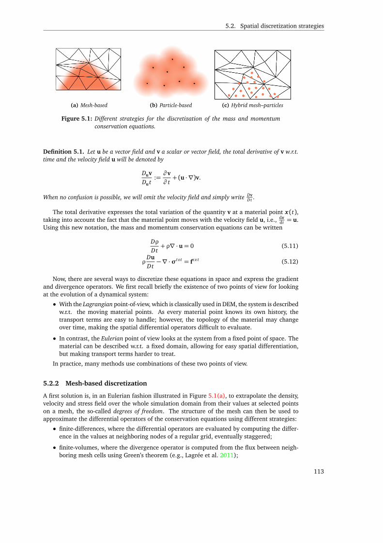
5.2. Spatial discretization strategies

(a) Mesh-based (b) Particle-based (c) Hybrid mesh–particles

Figure 5.1: Different strategies for the discretization of the mass and momentumconservation equations.

Definition 5.1. Let u be a vector field and v a scalar or vector field, the total derivative of v w.r.t.time and the velocity field u will be denoted by

Duv

Du t:=∂ v

∂ t+ (u · ∇)v.

When no confusion is possible, we will omit the velocity field and simply write DvDt .

The total derivative expresses the total variation of the quantity v at a material point x (t),taking into account the fact that the material point moves with the velocity field u, i.e., dx

dt = u.Using this new notation, the mass and momentum conservation equations can be written

Dρ

Dt+ ρ∇ · u= 0

ρDu

Dt−∇ ·σtot = fex t

(5.11)

(5.12)

Now, there are several ways to discretize these equations in space and express the gradientand divergence operators. We first recall briefly the existence of two points of view for lookingat the evolution of a dynamical system:

• With the Lagrangian point-of-view, which is classically used in DEM, the system is describedw.r.t. the moving material points. As every material point knows its own history, thetransport terms are easy to handle; however, the topology of the material may changeover time, making the spatial differential operators difficult to evaluate.

• In contrast, the Eulerian point of view looks at the system from a fixed point of space. Thematerial can be described w.r.t. a fixed domain, allowing for easy spatial differentiation,but making transport terms harder to treat.

In practice, many methods use combinations of these two points of view.

5.2.2 Mesh-based discretization

A first solution is, in an Eulerian fashion illustrated in Figure 5.1(a), to extrapolate the density,velocity and stress field over the whole simulation domain from their values at selected pointson a mesh, the so-called degrees of freedom. The structure of the mesh can then be used toapproximate the differential operators of the conservation equations using different strategies:

• finite-differences, where the differential operators are evaluated by computing the differ-ence in the values at neighboring nodes of a regular grid, eventually staggered;

• finite-volumes, where the divergence operator is computed from the flux between neigh-boring mesh cells using Green’s theorem (e.g., Lagrée et al. 2011);

113

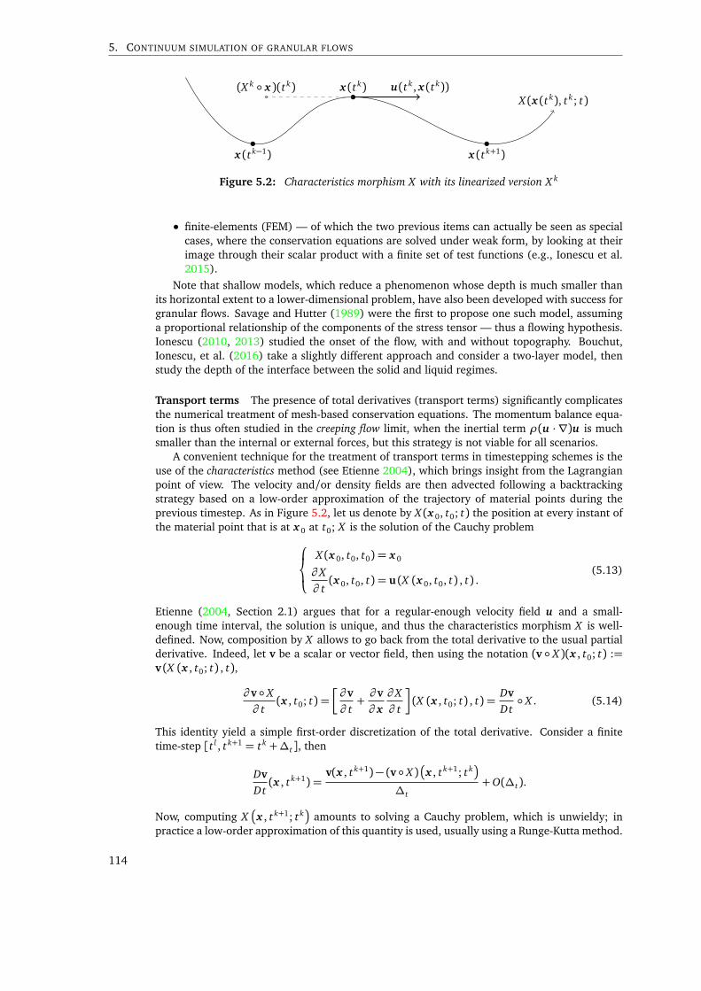
5. CONTINUUM SIMULATION OF GRANULAR FLOWS

x (tk−1)

x (tk)

x (tk+1)

u(tk, x (tk))(X k x )(tk)X (x (tk), tk; t)

Figure 5.2: Characteristics morphism X with its linearized version X k

• finite-elements (FEM) — of which the two previous items can actually be seen as specialcases, where the conservation equations are solved under weak form, by looking at theirimage through their scalar product with a finite set of test functions (e.g., Ionescu et al.2015).

Note that shallow models, which reduce a phenomenon whose depth is much smaller thanits horizontal extent to a lower-dimensional problem, have also been developed with success forgranular flows. Savage and Hutter (1989) were the first to propose one such model, assuminga proportional relationship of the components of the stress tensor — thus a flowing hypothesis.Ionescu (2010, 2013) studied the onset of the flow, with and without topography. Bouchut,Ionescu, et al. (2016) take a slightly different approach and consider a two-layer model, thenstudy the depth of the interface between the solid and liquid regimes.

Transport terms The presence of total derivatives (transport terms) significantly complicatesthe numerical treatment of mesh-based conservation equations. The momentum balance equa-tion is thus often studied in the creeping flow limit, when the inertial term ρ(u · ∇)u is muchsmaller than the internal or external forces, but this strategy is not viable for all scenarios.

A convenient technique for the treatment of transport terms in timestepping schemes is theuse of the characteristics method (see Etienne 2004), which brings insight from the Lagrangianpoint of view. The velocity and/or density fields are then advected following a backtrackingstrategy based on a low-order approximation of the trajectory of material points during theprevious timestep. As in Figure 5.2, let us denote by X (x 0, t0; t) the position at every instant ofthe material point that is at x 0 at t0; X is the solution of the Cauchy problem

X (x 0, t0, t0) = x 0

∂ X

∂ t(x 0, t0, t) = u (X (x 0, t0, t) , t) .

(5.13)

Etienne (2004, Section 2.1) argues that for a regular-enough velocity field u and a small-enough time interval, the solution is unique, and thus the characteristics morphism X is well-defined. Now, composition by X allows to go back from the total derivative to the usual partialderivative. Indeed, let v be a scalar or vector field, then using the notation (v X )(x , t0; t) :=v (X (x , t0; t) , t),

∂ v X

∂ t(x , t0; t) =

∂ v

∂ t+∂ v

∂ x

∂ X

∂ t

(X (x , t0; t) , t) =

Dv

Dt X . (5.14)

This identity yield a simple first-order discretization of the total derivative. Consider a finitetime-step [t l , tk+1 = tk +∆t], then

Dv

Dt(x , tk+1) =

v(x , tk+1)− (v X )x , tk+1; tk

∆t+O(∆t).

Now, computing Xx , tk+1; tk

amounts to solving a Cauchy problem, which is unwieldy; in

practice a low-order approximation of this quantity is used, usually using a Runge-Kutta method.

114

5.2. Spatial discretization strategies

At the first order,

Dv

Dt(x , tk+1) =

v(x , tk+1)− vX k(x ), tk

∆t+O(∆t), X k(x ) := x −∆tu

k(x , tk). (5.15)

Note that this requires being able to locate arbitrary points in the mesh, which can be costlyand require using a dedicated spatial index structure. In a similar manner, one may evolve themesh after each timestep, moving its nodes along the velocity field in a Lagrangian manner andthus yielding an explicit access to the characteristics morphism X . However, for flows incurringlarge displacements, as is often the case with granular materials, the mesh can quickly becomedegenerate and require remeshing.

Other approaches discretize directly the transport operators – possibly without resorting totimestepping scheme — in the Eulerian framework, but have to take special care to ensure energyand mass conservation yet prevent overshooting (the advected quantities should be physicallyadmissible, for instance the density should remain positive). Saramito (2013, Section 4.10) il-lustrates that centered methods, such as finite-differences or continuous finite-elements, lead toparasitic oscillations on transport equations. Conversely, upwind discontinuous Galerkin meth-ods (a finite-element method which can be interpreted as an arbitrary-degree generalization offinite-volumes, and which we will discuss briefly in Section 7.2.2) have been shown to possessgood stability properties when discretizing transport terms (Pietro and Ern 2011). Specializedmethods have also been devised for convection-dominated equations such as the mass conser-vation (5.7), for instance the WENO schemes (Shu 2009).

Note that when considering an incompressible flow with a spatially constant initial density,the mass conservation equation becomes trivial, as the density simply remains constant throughtime. This makes mesh-based approaches especially suited for simulating granular materials asincompressible yield-stress flows. However, if the portion of space occupied by the material ismoving, one still has either to deform the mesh (e.g., Ionescu et al. 2015), or advect a bound-ary (e.g., Lagrée et al. 2011).

Visualization For Computer Graphics applications, the ultimate goal is to produce a set ofgrain samples that can be rendered. While it is easy to sample a density field at each individualframe, doing so in a temporally consistent manner is a hard problem; this drawback has alsocontributed to spark interest in particle-based approaches.

5.2.3 Particle-based discretization

Smoothed Particle Hydrodynamics (SPH) methods take a different approach, and remove theneed for any structured mesh by making further use of the Lagrangian point of view. The materialis discretized as a finite set of particles that represent clumps of material rather than individualgrains. The velocity, stress and density fields are then discretized as the sum of smooth, compact,radially-symmetric kernels centered on those particles, as in Figure 5.1(b).

As such, the results are intrinsically free from grid artifacts. Moreover, this approach makesthe transport terms trivial to discretize. Indeed, solving the mass conservation equations justamounts to moving the particles. Using an implicit Euler integration rule and denoting by x k

p(t)

and v kp(t) the position and velocity of the pth particle at time tk, this means

x k+1p = x k

p +∆t vkp.

The particles also yield a direct access to the characteristics morphism (5.13), and the velocity’stotal derivative in the momentum balance equation can thus be simply discretized as

Du

Dt(x p(t

k+1), tk+1) =v p(t

k+1)− v p(tk)

∆t+O(∆t).

115

5. CONTINUUM SIMULATION OF GRANULAR FLOWS

Several authors have applied SPH to granular simulation (Alduán and Otaduy 2011; Alduánet al. 2009; Chambon et al. 2011; Ihmsen et al. 2013; Lenaerts and Dutré 2009). However, suchmethods typically require more degrees of freedom (particles) than mesh-based methods. Evalu-ating the differential operators require keeping track of each pair of neighboring particles, whichcan be costly. Enforcing constraints on the density is usually done with predictive-corrective ap-proaches, requiring a lot of iterations with slow convergence.

5.2.4 Hybrid methods

Hybrid methods, illustrated on Figure 5.1(c), attempt to strike a compromise between the twoaforementioned approaches. They still use particles for the representation of the material state— thus allowing easy handling of the transport terms, but augment them with a backgroundmesh to help with the computation of differential operators and the internal forces. At eachstep, the new velocities are computed on the mesh, and then transferred to the particles.

The main difficulty of this approach thus lies in the particles-to-mesh and mesh-to-particlestransfers; they should conserve energy, yet be stable. The first method of this kind, the Particle-in-Cell (PIC; Harlow 1963) method, used finite-differences on a regular grid for the mesh-basedportion, and simple interpolation for transferring the velocities both ways.

We assume that the jth component of a field g j at any point in space can be evaluated byextrapolating its values gi, j at the degrees of freedom (y i) using the shape functions ωv

i, j , i.e.,

g j(x , tk) =∑

i g ki, jω

vi, j(x ). A any timestep tk, PIC transfers the velocities of the particles to the

grid as a weighted average,

up 7→g,ki, j =

∑p mpω

vi, j(x

kp)v

kp, j∑

p mpωvi, j(x

kp)

, (5.16)

where mp denotes the mass of the pth particle.The total velocity derivative can then be approximated to the first order as

Du

Dt(x , tk+1) =

u(x , tk+1)− up 7→g(x , tk)

∆t+O(∆t).

Finally, particles gets their velocities from the newly computed velocity field,

v k+1p = u(x k

p, tk+1) (5.17)

are moved using a semi-implicit Euler step,

x k+1p = x k

p +∆t vk+1p . (5.18)

However, this strategy was found to quickly dissipate kinetic energy. This led to the intro-duction of the FLuid-Implicit-Particle (FLIP) method (Brackbill and Ruppel 1986); instead oftransferring the velocities from the grid to the particles, the particle velocities are updated usingthe difference in grid velocity from the previous to the current timestep. That is, Equation (5.17),is replaced with (5.19),

v k+1p = v k

p +ux k

p, tk+1− up 7→g

x k

p, tk

(5.19)

While this second velocity update rule leads to a much better conservation of kinetic energy,FLIP suffers from being prone to instabilities, losing the high-frequency filtering properties of PIC(Jiang, Schroeder, Selle, et al. 2015). In practice, a weighted average of the PIC and FLIP updaterules is generally used. More recently, Jiang, Schroeder, Selle, et al. (2015) introduced the AffineParticle-in-Cell method (APIC). In this case, the grid-to-particles transfer use the original PICrule (5.17), but an additional term, modeling the velocity gradients, is added to the particle-to-grid velocity transfers (5.16). This approach boasts a much better energy conservation than PIC,while preserving its stability and filtering properties.

116

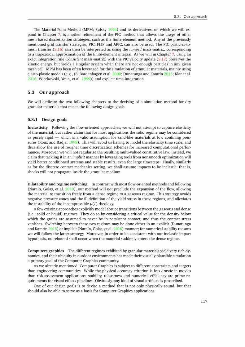
5.3. Our approach

The Material-Point Method (MPM; Sulsky 1994) and its derivatives, on which we will ex-pand in Chapter 7, is another refinement of the PIC method that allows the usage of othermesh-based discretization strategies, such as the finite-element method. Any of the previouslymentioned grid transfer strategies, PIC, FLIP and APIC, can also be used. The PIC particles-to-mesh transfer (5.16) can then be interpreted as using the lumped mass-matrix, correspondingto a trapezoidal approximation of the finite-element integral. As we will in Chapter 7, using anexact integration rule (consistent mass-matrix) with the PIC velocity update (5.17) preserves thekinetic energy, but yields a singular system when there are not enough particles in any givenmesh cell. MPM has been often leveraged for the simulation of granular materials, mainly usingelasto-plastic models (e.g., (S. Bardenhagen et al. 2000; Dunatunga and Kamrin 2015; Klar et al.2016; Wieckowski, Youn, et al. 1999)) and explicit time-integration.

5.3 Our approach

We will dedicate the two following chapters to the devising of a simulation method for drygranular materials that meets the following design goals.

5.3.1 Design goals

Inelasticity Following the flow-oriented approaches, we will not attempt to capture elasticityof the material, but rather claim that for most applications the solid regime may be consideredas purely rigid — which is a valid assumption for sand-like materials at low confining pres-sures (Roux and Radjai 1998). This will avoid us having to model the elasticity time scale, andthus allow the use of rougher time discretization schemes for increased computational perfor-mance. Moreover, we will not regularize the resulting multi-valued constitutive law. Instead, weclaim that tackling it in an implicit manner by leveraging tools from nonsmooth optimization willyield better conditioned systems and stable results, even for large timesteps. Finally, similarlyas for the discrete contact mechanics setting, we shall assume impacts to be inelastic, that is,shocks will not propagate inside the granular medium.

Dilatability and regime switching In contrast with most flow-oriented methods and following(Narain, Golas, et al. 2010), our method will not preclude the expansion of the flow, allowingthe material to transition freely from a dense regime to a gaseous regime. This strategy avoidsnegative pressure zones and the ill-definition of the yield stress in these regions, and alleviatesthe instability of the incompressible µ(I) rheology.

A few existing approaches explicitly model abrupt transitions between the gaseous and dense(i.e., solid or liquid) regimes. They do so by considering a critical value for the density belowwhich the grains are assumed to never be in persistent contact, and thus the contact stressvanishes. Switching between these two regimes may be done either in an explicit (Dunatungaand Kamrin 2015) or implicit (Narain, Golas, et al. 2010) manner; for numerical stability reasonswe will follow the latter strategy. Moreover, in order to be consistent with our inelastic impacthypothesis, no rebound shall occur when the material suddenly enters the dense regime.

Computers graphics The different regimes exhibited by granular materials yield very rich dy-namics, and their ubiquity in outdoor environments has made their visually plausible simulationa primary goal of the Computer Graphics community.

As we already mentioned, Computer Graphics is subject to different constraints and targetsthan engineering communities. While the physical accuracy criterion is less drastic in moviesthan risk-assessment applications, stability, robustness and numerical efficiency are prime re-quirements for visual effects pipelines. Obviously, any kind of visual artifacts is proscribed.

One of our design goals is to devise a method that is not only physically sound, but thatshould also be able to serve as a basis for Computer Graphics applications.

117

5. CONTINUUM SIMULATION OF GRANULAR FLOWS

5.3.2 Outline of this second part

In Chapter 6, we will first consider dense granular materials, that is, materials that are alreadytightly packed together and cannot be compacted anymore. We will relax this assumption inChapter 7, and consider the unconstrained flow of granular materials, but assume that the in-teractions with the surrounding fluid are negligible (which is the case for large-enough grainsin the air). Finally, in Chapter 8 we will relax this second assumption, and model fully coupledflows such as powders in the air or immersed avalanches.

118

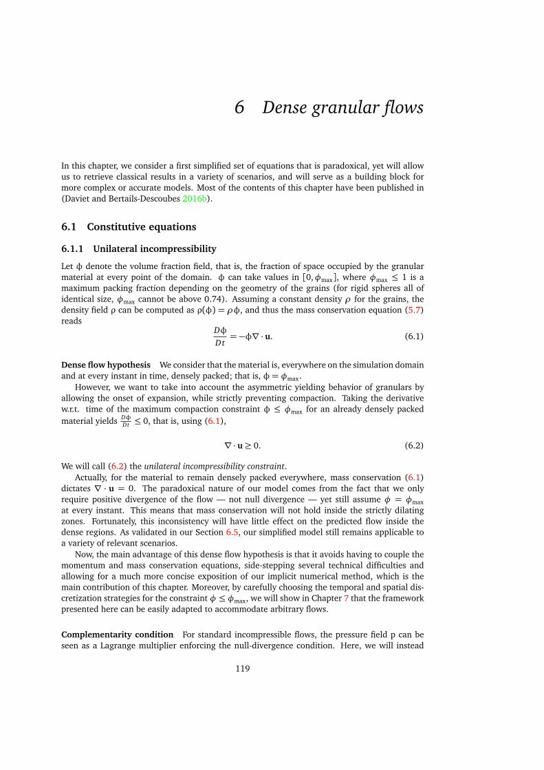
6 Dense granular flows

In this chapter, we consider a first simplified set of equations that is paradoxical, yet will allowus to retrieve classical results in a variety of scenarios, and will serve as a building block formore complex or accurate models. Most of the contents of this chapter have been published in(Daviet and Bertails-Descoubes 2016b).

6.1 Constitutive equations

6.1.1 Unilateral incompressibility

Let φ denote the volume fraction field, that is, the fraction of space occupied by the granularmaterial at every point of the domain. φ can take values in [0,φmax], where φmax ≤ 1 is amaximum packing fraction depending on the geometry of the grains (for rigid spheres all ofidentical size, φmax cannot be above 0.74). Assuming a constant density ρ for the grains, thedensity field ρ can be computed as ρ(φ) = ρφ, and thus the mass conservation equation (5.7)reads

Dφ

Dt= −φ∇ · u. (6.1)

Dense flow hypothesis We consider that the material is, everywhere on the simulation domainand at every instant in time, densely packed; that is, φ= φmax.

However, we want to take into account the asymmetric yielding behavior of granulars byallowing the onset of expansion, while strictly preventing compaction. Taking the derivativew.r.t. time of the maximum compaction constraint φ ≤ φmax for an already densely packedmaterial yields Dφ

Dt ≤ 0, that is, using (6.1),

∇ · u≥ 0. (6.2)

We will call (6.2) the unilateral incompressibility constraint.Actually, for the material to remain densely packed everywhere, mass conservation (6.1)

dictates ∇ · u = 0. The paradoxical nature of our model comes from the fact that we onlyrequire positive divergence of the flow — not null divergence — yet still assume φ = φmax

at every instant. This means that mass conservation will not hold inside the strictly dilatingzones. Fortunately, this inconsistency will have little effect on the predicted flow inside thedense regions. As validated in our Section 6.5, our simplified model still remains applicable toa variety of relevant scenarios.

Now, the main advantage of this dense flow hypothesis is that it avoids having to couple themomentum and mass conservation equations, side-stepping several technical difficulties andallowing for a much more concise exposition of our implicit numerical method, which is themain contribution of this chapter. Moreover, by carefully choosing the temporal and spatial dis-cretization strategies for the constraint φ ≤ φmax, we will show in Chapter 7 that the frameworkpresented here can be easily adapted to accommodate arbitrary flows.

Complementarity condition For standard incompressible flows, the pressure field p can beseen as a Lagrange multiplier enforcing the null-divergence condition. Here, we will instead

119

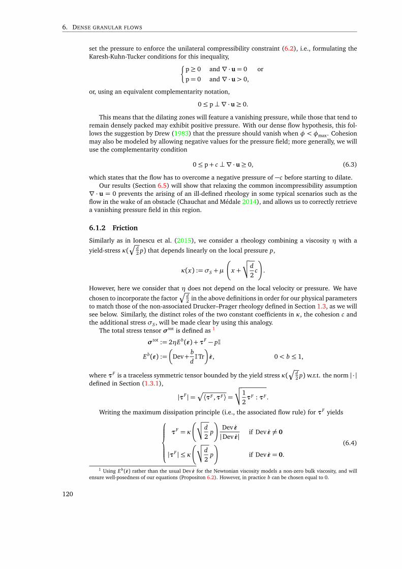
6. DENSE GRANULAR FLOWS

set the pressure to enforce the unilateral compressibility constraint (6.2), i.e., formulating theKaresh-Kuhn-Tucker conditions for this inequality,

p≥ 0 and ∇ · u= 0 or

p= 0 and ∇ · u> 0,

or, using an equivalent complementarity notation,

0≤ p⊥∇ · u≥ 0.

This means that the dilating zones will feature a vanishing pressure, while those that tend toremain densely packed may exhibit positive pressure. With our dense flow hypothesis, this fol-lows the suggestion by Drew (1983) that the pressure should vanish when φ < φmax. Cohesionmay also be modeled by allowing negative values for the pressure field; more generally, we willuse the complementarity condition

0≤ p+ c ⊥∇ · u≥ 0, (6.3)

which states that the flow has to overcome a negative pressure of −c before starting to dilate.Our results (Section 6.5) will show that relaxing the common incompressibility assumption

∇ · u = 0 prevents the arising of an ill-defined rheology in some typical scenarios such as theflow in the wake of an obstacle (Chauchat and Médale 2014), and allows us to correctly retrievea vanishing pressure field in this region.

6.1.2 Friction

Similarly as in Ionescu et al. (2015), we consider a rheology combining a viscosity η with a

yield-stress κ(q

d2 p) that depends linearly on the local pressure p,

κ(x) := σS +µ

x +

√√d

2c

.

However, here we consider that η does not depend on the local velocity or pressure. We have

chosen to incorporate the factorq

d2 in the above definitions in order for our physical parameters

to match those of the non-associated Drucker–Prager rheology defined in Section 1.3, as we willsee below. Similarly, the distinct roles of the two constant coefficients in κ, the cohesion c andthe additional stress σS , will be made clear by using this analogy.

The total stress tensor σtot is defined as 1

σtot := 2ηE b(ǫ) +τF − pI

E b(ǫ) :=

Dev+b

dITrǫ, 0< b ≤ 1,

where τF is a traceless symmetric tensor bounded by the yield stress κ(q

d2 p) w.r.t. the norm | · |

defined in Section (1.3.1),

|τF |=Æ⟨τF ,τF ⟩=

√√1

2τF : τF .

Writing the maximum dissipation principle (i.e., the associated flow rule) for τF yields

τF = κ

√√d

2p

Dev ǫ

|Dev ǫ| if Dev ǫ 6= 0

|τF | ≤ κ√√d

2p

if Dev ǫ = 0.

(6.4)

1 Using Eb(ǫ) rather than the usual Dev ǫ for the Newtonian viscosity models a non-zero bulk viscosity, and willensure well-posedness of our equations (Propositon 6.2). However, in practice b can be chosen equal to 0.

120

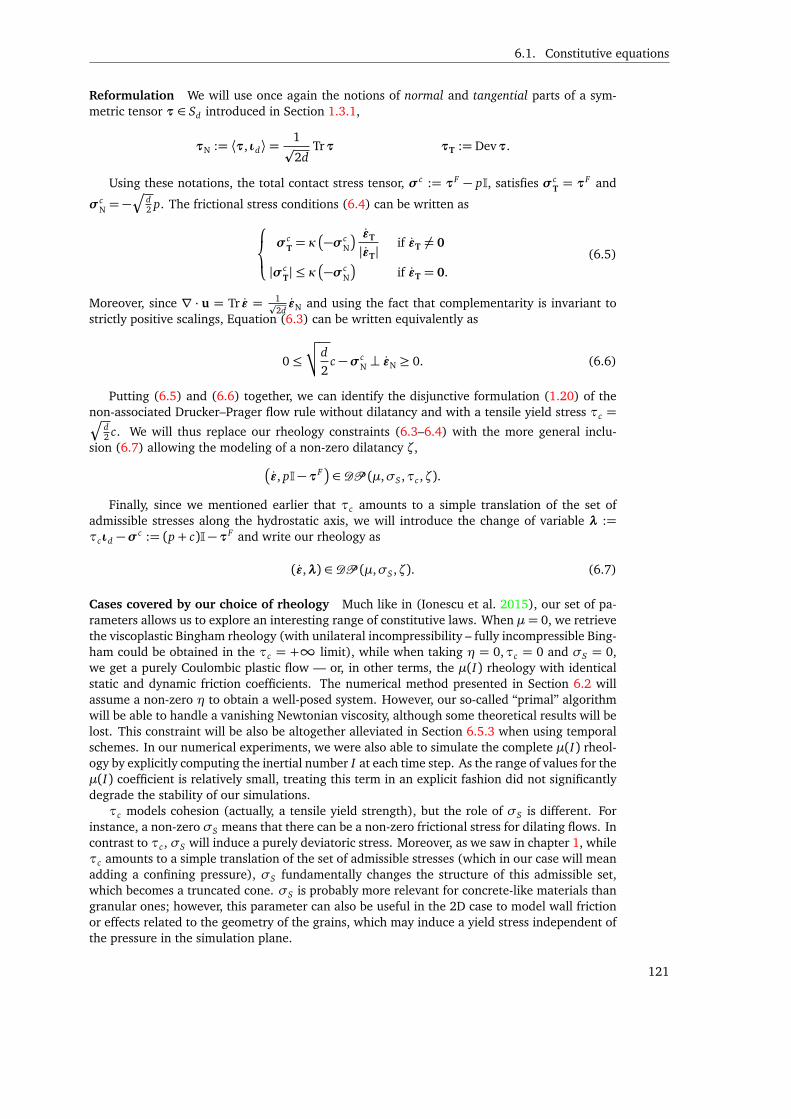
6.1. Constitutive equations

Reformulation We will use once again the notions of normal and tangential parts of a sym-metric tensor τ ∈ Sd introduced in Section 1.3.1,

τN := ⟨τ, ιd⟩=1p2d

Trτ τT := Devτ.

Using these notations, the total contact stress tensor, σc := τF − pI, satisfies σcT= τF and

σcN = −

qd2 p. The frictional stress conditions (6.4) can be written as

σc

T= κ

−σcN

ǫT

|ǫT|if ǫT 6= 0

|σcT| ≤ κ −σc

N

if ǫT = 0.

(6.5)

Moreover, since ∇ · u = Tr ǫ = 1p2dǫN and using the fact that complementarity is invariant to

strictly positive scalings, Equation (6.3) can be written equivalently as

0≤√√d

2c −σc

N ⊥ ǫN ≥ 0. (6.6)

Putting (6.5) and (6.6) together, we can identify the disjunctive formulation (1.20) of thenon-associated Drucker–Prager flow rule without dilatancy and with a tensile yield stress τc =q

d2 c. We will thus replace our rheology constraints (6.3–6.4) with the more general inclu-

sion (6.7) allowing the modeling of a non-zero dilatancy ζ,ǫ, pI−τF

∈ DP (µ,σS ,τc ,ζ).

Finally, since we mentioned earlier that τc amounts to a simple translation of the set ofadmissible stresses along the hydrostatic axis, we will introduce the change of variable λ :=τcιd −σc := (p+ c)I−τF and write our rheology as

(ǫ,λ) ∈ DP (µ,σS ,ζ). (6.7)

Cases covered by our choice of rheology Much like in (Ionescu et al. 2015), our set of pa-rameters allows us to explore an interesting range of constitutive laws. When µ= 0, we retrievethe viscoplastic Bingham rheology (with unilateral incompressibility – fully incompressible Bing-ham could be obtained in the τc = +∞ limit), while when taking η = 0,τc = 0 and σS = 0,we get a purely Coulombic plastic flow — or, in other terms, the µ(I) rheology with identicalstatic and dynamic friction coefficients. The numerical method presented in Section 6.2 willassume a non-zero η to obtain a well-posed system. However, our so-called “primal” algorithmwill be able to handle a vanishing Newtonian viscosity, although some theoretical results will belost. This constraint will be also be altogether alleviated in Section 6.5.3 when using temporalschemes. In our numerical experiments, we were also able to simulate the complete µ(I) rheol-ogy by explicitly computing the inertial number I at each time step. As the range of values for theµ(I) coefficient is relatively small, treating this term in an explicit fashion did not significantlydegrade the stability of our simulations.τc models cohesion (actually, a tensile yield strength), but the role of σS is different. For

instance, a non-zero σS means that there can be a non-zero frictional stress for dilating flows. Incontrast to τc , σS will induce a purely deviatoric stress. Moreover, as we saw in chapter 1, whileτc amounts to a simple translation of the set of admissible stresses (which in our case will meanadding a confining pressure), σS fundamentally changes the structure of this admissible set,which becomes a truncated cone. σS is probably more relevant for concrete-like materials thangranular ones; however, this parameter can also be useful in the 2D case to model wall frictionor effects related to the geometry of the grains, which may induce a yield stress independent ofthe pressure in the simulation plane.

121

6. DENSE GRANULAR FLOWS

6.2 Creeping flow

In this first section we assume that the flow is slow enough for its inertia to be neglected, andsolve for its steady state. While inertial effects are generally significant for granular flows, thiscase remains relevant since the structure of the equations for each timestep of the fully dynamiccase will be similar (see Section 6.5.3).

6.2.1 Steady-state and boundary conditions

Let us consider a domain Ω ⊂ Rd and decompose its boundary as BdΩ := BD∪BN , with Dirichletboundary conditions on BD and homogeneous Neumann on BN ,

u= uD on BD

E b D(u)nΩ = 0 on BN

(6.8a)

(6.8b)

where nΩ is the outward-pointing normal to Ω on each point of its boundary.Moreover, let σext gather all external stresses applied onto the Neumann boundary of the

domain. We thus have

−λnΩ = (σext − cI)nΩ on BN . (6.9)

We assume that the sole external force is the action of gravity whose orientation is given bythe “down” unit vector e g . Writing the conservation of momentum (5.12) for the steady-stategives

−∇ ·

2ηE bε− λ︸ ︷︷ ︸=σtot−cI

= ρge g + ∇c︸︷︷︸0

on Ω. (6.10)

From Equations (6.9) and (6.10), we see that the cohesion term c simply modifies the exter-nal stress term σext; it the following, we will gather both of those terms into σext and ignore c.

Dimensionless equations Let L be a characteristic dimension of the flow. We define U :=pg L as the characteristic velocity and P := ρg L the characteristic pressure of the flow. We

consider dimensionless differential operators defined through ∇ := L∇. We furthermore intro-duce two dimensionless numbers, the Reynolds number Re := ρU L

η and the Bingham number

Bi := σS

ρg L =σS

P .

Considering the dimensionless quantities u := 1U u, ˜ε := D(u) = L

U ǫ, λ := 1Pλ, and uD :=

1U uD, Equations (6.8 – 6.10) can be made dimensionless as

−∇ ·

2

ReE b ˜ε− λ

= e g on Ω

u= uD on BD

E bD(u)nΩ = 0 on BN

−λnΩ = σext nΩ on BN ,

(6.11)

with the dimensionless rheology

(˜ε, λ) ∈ DP (µ, Bi,ζ). (6.12)

From now on we shall use the dimensionless quantities and omit the tildes.

122

6.2. Creeping flow

6.2.2 Variational formulation

Let H1(Ω)d be the usual Sobolev space containing square-integrable functions from Ω ⊂ Rd toRd , with square-integrable gradients. As in (Saramito 2015, Appendix A), we introduce theaffine subspace V (uD) of H1(Ω)d for which the Dirichlet boundary condition (6.8a) is satisfied,i.e.,

V (uD) := u ∈ H1(Ω)d ; u= uD on BD.V (0) is therefore the vector subspace of H1(Ω)d for which the homogeneous Dirichlet boundarycondition u|BD

= 0 is satisfied. Let also T (Ω) be the space of square-integrable symmetric tensorfields on Ω.

Proposition 6.1. A weak form of System (6.11 – 6.12) amounts to finding u ∈ V (uD), λ ∈ T (Ω),and γ ∈ T (Ω), such that

a(u,v) = b(λ,v) + l(v) ∀v ∈ V (0)

m(γ,τ) = b(τ,u) ∀τ ∈ T (Ω)

(γ,λ) ∈ DP (µ, Bi,ζ),

(6.13a)

(6.13b)

(6.13c)

where ∀x,y ∈ H1(Ω)d and ∀σ,τ ∈ T (Ω), a(x , y) and m(σ,τ) are the symmetric positive-definitebilinear forms on H1(Ω)d × H1(Ω)d and T (Ω)× T (Ω), respectively,

a(x,y) :=2

Re

∫

Ω

Dev D(x) : Dev D(y) +b

d(∇ · x) (∇ · y)

m(σ,τ) =

∫

Ω

σ : τ,

b(τ,x) is the bilinear form on T (Ω)× H1(Ω)d ,

b(τ,x) =

∫

Ω

D(x) : τ,

and l(x) is the linear form on H1(Ω)d ,

l(x) =

∫

Ω

e g ,x

−∫

BN

σext nΩ

, x.

Proof. First, let us consider the stress boundary condition (6.9). One solution would be to en-force it strongly, by constraining λ to the subspace of T (Ω) which satisfy (6.9). However, thismay lead to difficulties in the discretization of the DP (µ, Bi,ζ) rheology. In our proposed imple-mentation, we choose instead to model, in the integration of the term ∇·σtot over Ω, a possiblynon-zero jump JσtotK= −λ|BN

−σext of the stress on BN .Let us now derive the variational formulation for System (6.11). We assume u ∈ V (uD) and

λ ∈ T (Ω), and let v ∈ V (0) be a test function. Multiplying both sides of the first line of (6.11)by v and integrating over Ω yields

−∫

Ω

­∇ ·

2

ReE b D(u)−λ

, v

·+

∫

BN

JσtotKnΩ,v

=

∫

Ω

e g ,v

. (6.14)

Using the Green formula with the Neumann (6.8b) and homogeneous Dirichlet (6.8a) bound-ary conditions for u,

123

6. DENSE GRANULAR FLOWS

a(u,v) =2

Re

∫

Ω

Dev D(u) : Dev D(v) +b

d(∇ · v) (∇ · u)

=

∫

Ω

2

ReE b D(u) : D(v)

= −∫

Ω

­∇ ·

2

ReE b D(u)

,v·

(6.15)

and ∫

Ω

⟨∇ · λ,v⟩+∫

BN

JσtotKnΩ,v

= −

∫

BN

σextnΩ,v

− b(λ,v). (6.16)

By combining (6.14 – 6.16) and the definition of l, we retrieve (6.13a). Let us now focus on therheology DP (µ, Bi,ζ) given in (6.12), which contains inequalities that cannot be put directlyunder weak form. To circumvent this difficulty, we introduce an auxiliary variable γ ∈ T (Ω) thatweakly satisfies γ= D(u), i.e.,

∫

Ω

D(u) : τ=

∫

Ω

γ : τ ∀τ ∈ T (Ω), (6.17)

which is exactly equation (6.13b). We can thus express the rheology DP (µ, Bi,ζ) under theweak form as (6.13b —6.13c).

Remark Note that we do not include any additional equation ensuring the well-posedness ofour system, such as the zero-average pressure condition which is commonly used for Stokesflows. Indeed, for a given velocity field, the DP (µ, Bi,ζ) rheology imposes the value of λ in theyielded regions, serving as an intrinsic boundary condition for the stress field inside the rigidzones.

6.2.3 Cadoux algorithm

In this section, we adapt the algorithm of Cadoux (2009) to show that solutions to our variationalproblem (6.13a–6.13c) can be characterized as the fixed-point of a sequence of strictly convexand well-posed minimization problems.

Proposition 6.2. Let s ∈ L2(Ω), let us useK 1µ

as a short-hand for τ ∈ T (Ω),τ(x ) ∈K 1µ(x )

a.e. on Ω.Under the regularity condition (H (s)),

∃u ∈ V (uD), D(u) + sιd ∈ intK 1µ, (H (s))

and assuming Re< +∞, the minimization problem

q(s) := minu∈C(s)

J(u)

J(u) :=1

2a(u,u)− l(u) + Bi g(D(u))

g(γ) := 2

∫

Ω

|γT|

C(s) := u ∈ V (uD),D(u) + sιd ∈K 1µ

(6.18)

(6.19)

admits a unique solution which satisfies

a(u,v) = b(λ,v) + l(v) ∀v ∈ V (0)

m(γ,τ) = b(τ,u) ∀τ ∈ T (Ω)

γ+ sιd ∈ −NTµ,Bi(λ).

(6.20)

124

6.2. Creeping flow

Remark 6.1. We readily deduce from Property 1.6 and Equation (6.20) that a solution u(s) tothe minimization problem (6.18) such that s = (µ− ζ) |γT| will yield a solution to our originalvariational problem (6.13a–6.13c). We can therefore define an operator F : L2(Ω) → L2(Ω),s 7→ (µ− ζ) |D(u(s))T|, with u : s 7→ argminu∈C(s) J(u), so that any fixed-point of F will yield asolution to (6.13a–6.13c). Note that when µ= ζ, the fixed-point will be reached in a single step.

Proof. As from Korn’s inequality J is coercive and strictly convex, and under (H (s)) the feasibleset is not empty, Theorem (A.5) ensures that there exists a unique solution u to (6.18), whichusing Theorem A.6 can be characterized by

0 ∈ ∂ J(u) +NC(s)(u). (6.21)

D(·) : H1(Ω)d → T (Ω) and ·|BD: H1(Ω)d → L2(BD)

d are linear operators from and to Hilbertspaces (trace theorem), we can thus use Corollary A.4 to Property A.12 on the normal cone to aprecomposition by an affine map. Under the regularity condition (H (s)),

NC(s)(u) = D(·)⊺NK 1µ

(D(u) + sιd) + (·|BD)⊺N0(u|BD

− uD) (6.22)

where D(·)⊺ denotes the adjoint operator to D(·) for the usual scalar products of H1(Ω)d andT (Ω). Using once again Property A.12, we have also

∂ J(u) = a(u, ·)− l + Bi D(·)⊺∂ g(D(u)), (6.23)

where ∂ g is also defined w.r.t. the usual scalar product of T (Ω),∫Ω(· : ·). Replacing (6.23)

and (6.22) into (6.21), taking the scalar product with a test function v ∈ V (0) and noticing that

V (0) = Ker(·|BD) =

Im (·|BD

)⊺⊥

, we get

(6.21) ⇐⇒

a(u,v) = l(v) +D(·)⊺λ,v

H1 ∀v ∈ V (0)

γ= D(u)

λ ∈ −Bi∂ g(γ)−NK 1µ

(γ+ sιd).(6.24)

Let us reformulate the last inclusion. We recognize from Section 1.3 and Equation (1.25)that for τ ∈ Sd ,

Bi(|τT|) +IK 1µ

(τ) = I−Tµ,Bi

⋆(τ). (6.25)

Using once again the notation Tµ,Bi as a shorthand for τ ∈ T (Ω),τ(x ) ∈ Tµ(x ),Bi a.e., we getfrom Property A.5 on subdifferentials in function spaces that

−NTµ,Bi(−σ) =

¦τ ∈ T (Ω),τ(x ) ∈ N−Tµ(x ),Bi

(σ(x )) a.e. on Ω©

=¦τ ∈ T (Ω),σ(x ) ∈ ∂I−Tµ,Bi

⋆(τ(x )) a.e.©

(Theorem A.2)

=

§τ ∈ T (Ω),σ(x ) ∈ ∂

Bi(| ·T |) +IK 1

µ

(−τ(x )) a.e.

ªusing (6.25)

=

§τ ∈ T (Ω),σ(x ) ∈

Bi∂ (| ·T |) +NK 1

µ

(τ(x )) a.e.

ª

=

§τ ∈ T (Ω),σ ∈ Bi∂ g(τ) +NK 1

µ

(τ)

ª.

Note that the “2” in the definition of g is indeed retrieved in the last equality, as the scalarproduct and subdifferential on T (Ω) are defined w.r.t. the “· : ·” scalar product on Sd , while thesubdifferential of | · | on Sd is defined using the ⟨·, ·⟩= 1

2 · : · scalar product.Hence, noticing that γT = (γ+ sιd)T, we get the equivalence

−λ ∈ Bi∂ (∫ | ·T |)(γ) +NK 1

µ

(γ+ sιd) ⇐⇒ γ+ sιd ∈ −NTµ,Bi(λ). (6.26)

125

6. DENSE GRANULAR FLOWS

Finally, using thatD(·)⊺λ,v

H1 = ⟨D(v),λ⟩L2

= b(λ,v) and (6.26) to rewrite the first andlast line of (6.24), respectively, we get that

(6.21) ⇐⇒

a(u,v) = b(λ,v) + l(v) ∀v ∈ V (0)

m(γ,τ) = b(τ,u) ∀τ ∈ T (Ω)

γ+ sιd ∈ −NTµ,Bi(λ).

(6.27)

The F operator, as defined is Remark 6.1, allows us to define a Cadoux-like fixed-point algo-rithm.

Remark 6.2. We used the coercivity of the bilinear form “a” to ensure the existence of a solution toeach feasible optimization problem, and thus the well-posedness of the fixed-point algorithm. Thiscondition is sufficient but not necessary, and in practice the method could be still be attempted forRe= +∞.

Existence of a solution to the variational problem ? In the discrete case, Cadoux (2009)proves the existence of a fixed-point for the F operator under the hypothesis H (s) by demon-strating the continuity and boundedness of F and applying the Brouwer fixed-point theorem.In our continuous case, one can also show relatively easily (at least for Bi = 0) that the func-tion q : L2(Ω)→ R defined from the minimization problem (6.18) is continuous on S+ := s ∈L2(Ω), s ≥ 0 a.e. on Ω, and that the application u : S+ → H1(Ω)d , associating to s ∈ S+ theunique solution to the minimization problem (6.18), is continuous and bounded on S+. SinceF = f u, with f : H1(Ω)d → S+, u 7→ (µ − ζ)|D(u)T|, the existence of a solution to our flowproblem under the hypothesisH (s) would be ensured by the existence of a fixed-point to u f .This application looks indeed like a good candidate; u f is continuous and bounded on H1(Ω)d ,and the Rellich theorem states that its injection on L2(Ω)

d is compact. However, the continuityof u f w.r.t. the L2-norm does not seem obvious.

6.3 Discretization using finite-elements

In this section, we propose to discretize the variational problem (6.13a–6.13c) in such a waythat the characterization of the solution as a fixed-point of a sequence of convex minimizationproblems (Remark 6.1) will still hold in the discrete case.

Moreover, we will see that the discrete version of the variational problem will have the samestructure as the Discrete Coulomb Friction Problem (DCFP) that we studied in Chapters 2–4,allowing us to leverage similar algorithms.

6.3.1 Discretization of the symmetric tensor fields

For the discretization of the space T (Ω), we shall make use of Lagrange FEM, which means thatall symmetric tensor fields will be expressed as the extrapolation over Ω of their values at ndegrees of freedom (y i) ∈ Rnd .

Let Qh be a subspace of L2(Ω) with dimension n ∈ N, andωτi

1≤i≤n

a basis of Qh such that

ωτi (y j) = δi, j . Let (S j)1≤ j≤sdbe a basis of Sd , with sd := dim Sd =

12 d(d − 1). We may build a

finite subspace Th ⊂ T (Ω) from the basis (Tk)1≤k≤sd n defined as

Tsd (i−1)+ j :=ωτi S j for 1≤ i ≤ n, 1≤ j ≤ sd .

Then ∀τh ∈ Th, ∃τ := (τk) ∈ Rnsd such that

τh =∑

1≤i≤n1≤ j≤sd

τsd (i−1)+ jTsd (i−1)+ j =

∑

1≤i≤n

τh(y i)ωτi ,

τh(y i) =∑

1≤ j≤sd

τsd (i−1)+ jS j ∀1≤ i ≤ n.

126

6.3. Discretization using finite-elements

Choice of basis for Sd We want to leverage the analogy between the Drucker–Prager flow rule,which is expressed on tensors in Sd , and the Coulomb frictional contact law, which is expressedon vectors inRd . As such, will now construct a basis of Sd such that the properties of the “normal”and “tangential” parts are preserved.

Definition 6.1. Let us introduce the morphism χ ,

χ : Rsd → Sd

(a; b, c) 7→

b cc −b

+ a I if d = 2

(a; b, c, d, e, f ) 7→

b− cp

3d e

d −b− cp3

f

e f 2cp3

+p

2p3

a I if d = 3.

The morphism χ satisfies the following two properties:

Property 6.1. χ is an orthonormal isomorphism between the two Euclidean spaces (Rsd ; ·⊺·) and(Sd ; ⟨·, ·⟩). This means

∀(x , y) ∈ Rsd ×Rsd x ⊺y = ⟨χ(x ),χ(y)⟩ , (6.28)

where x ⊺y is the usual scalar product on Rm, m≥ 1 and ⟨σ,τ⟩= σ:τ2 is our scalar product on Sd .

Property 6.2. Let (·)N and (·)T designate the normal and tangential parts of vectors and symmetrictensors as introduced in Chapter 1;

n := (1,0, . . . , 0) ∈ Rsd x N := n⊺x x T := x − x Nn ∀x ∈ Rm

ιd :=

√√d

2I ∈ Sd τN := ⟨ιd ,τ⟩ τT := τ−τNιd = Devτ ∀τ ∈ Sd .

Then ∀x ∈ Rm,¨[χ(x )]N = x N[χ(x )]T

= ‖x T‖.(6.29a)

(6.29b)

It follows immediately from (6.29a–6.29b) that σ ∈ T (Sd )

µ,Bi ⇐⇒ χ−1(σ) ∈ T (Rsd )

µ,Bi . As χ isorthogonal (Property 6.1), the inclusion in normal cones is also preserved. Finally, by linearityof χ ,

γ+ (µ− ζ)|γT|ιd ∈ −NT (Sd )µ,Bi(σ)

⇐⇒ χ1γ+ (µ− ζ)|γT|ιd

∈ −NT (Rsd )µ,Bi(χ−1(σ))

⇐⇒ χ−1(γ) + (µ− ζ) χ−1(γ)

T

n ∈ −NT (Rsd )µ,Bi(χ−1(σ)).

We will thus be able to write the Drucker–Prager flow rule indifferently on symmetric tensors oron their image inRsd by the orthonormal isomorphism χ−1, and, with a slight abuse of notations,use the equivalence

(γ,λ) ∈ DP (µ, Bi,ζ) ⇐⇒ χ−1(γ),χ−1(λ)

∈ DP (µ, Bi,ζ). (6.30)

Going back to the discretization of our symmetric tensor fields, the equivalence (6.30) mo-tivates choosing S j := χ(e j) as the basis for Sd , where (e j)1≤ j≤sd

is the canonical basis of Rsd .Our global basis for Th becomes

Tsd (i−1)+ j :=ωτi χ(e j) for 1≤ i ≤ n, 1≤ j ≤ sd .

127

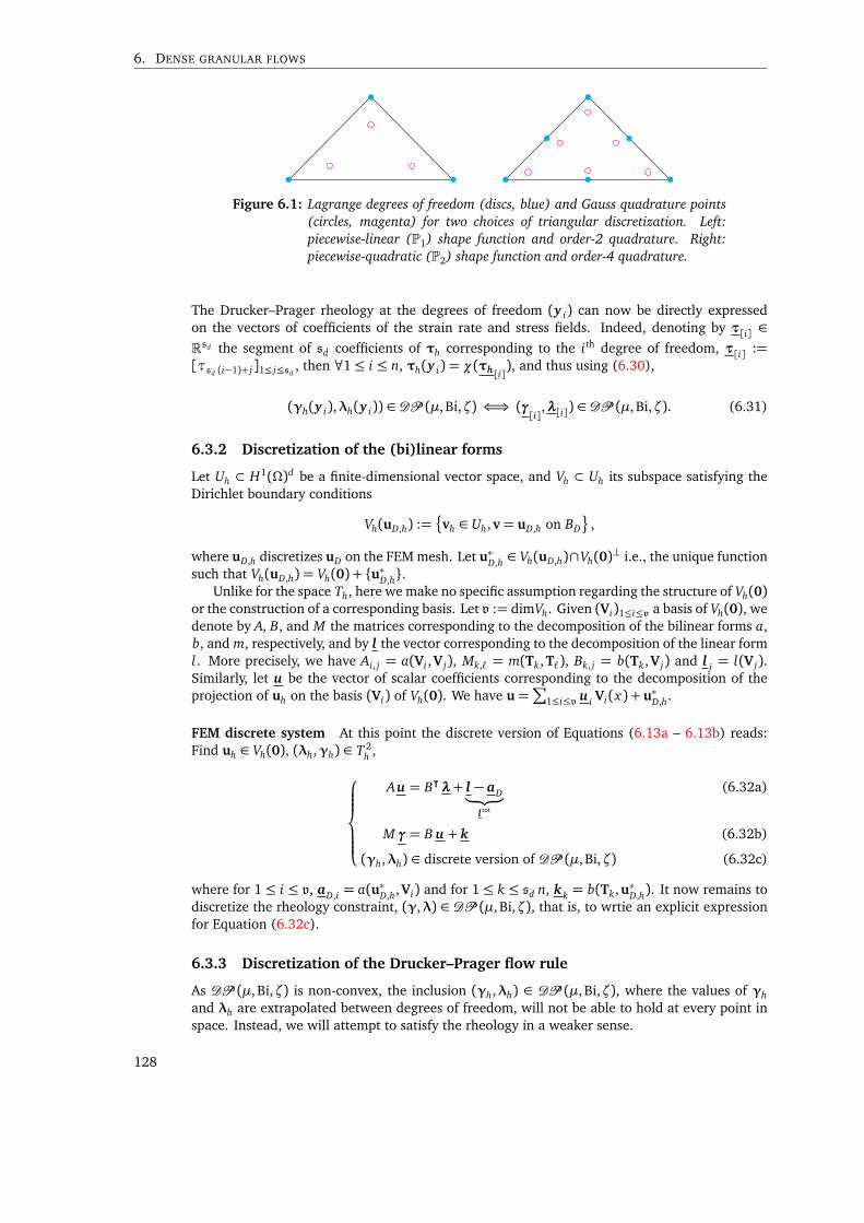
6. DENSE GRANULAR FLOWS

Figure 6.1: Lagrange degrees of freedom (discs, blue) and Gauss quadrature points(circles, magenta) for two choices of triangular discretization. Left:piecewise-linear (P1) shape function and order-2 quadrature. Right:piecewise-quadratic (P2) shape function and order-4 quadrature.

The Drucker–Prager rheology at the degrees of freedom (y i) can now be directly expressedon the vectors of coefficients of the strain rate and stress fields. Indeed, denoting by τ

[i] ∈Rsd the segment of sd coefficients of τh corresponding to the ith degree of freedom, τ

[i] :=[τ

sd (i−1)+ j]1≤ j≤sd, then ∀1≤ i ≤ n, τh(y i) = χ(τh

[i]), and thus using (6.30),

(γh(y i),λh(y i)) ∈ DP (µ, Bi,ζ) ⇐⇒ (γ[i]

,λ[i]) ∈ DP (µ, Bi,ζ). (6.31)

6.3.2 Discretization of the (bi)linear forms

Let Uh ⊂ H1(Ω)d be a finite-dimensional vector space, and Vh ⊂ Uh its subspace satisfying theDirichlet boundary conditions

Vh(uD,h) :=vh ∈ Uh,v= uD,h on BD

,

where uD,h discretizes uD on the FEM mesh. Let u∗D,h ∈ Vh(uD,h)∩Vh(0)⊥ i.e., the unique function

such that Vh(uD,h) = Vh(0) + u∗D,h.Unlike for the space Th, here we make no specific assumption regarding the structure of Vh(0)

or the construction of a corresponding basis. Let v := dimVh. Given (Vi)1≤i≤v a basis of Vh(0), wedenote by A, B, and M the matrices corresponding to the decomposition of the bilinear forms a,b, and m, respectively, and by l the vector corresponding to the decomposition of the linear forml. More precisely, we have Ai, j = a(Vi ,V j), Mk,ℓ = m(Tk,Tℓ), Bk, j = b(Tk,V j) and l j = l(V j).Similarly, let u be the vector of scalar coefficients corresponding to the decomposition of theprojection of uh on the basis (Vi) of Vh(0). We have u=

∑1≤i≤v u i Vi(x) + u∗D,h.

FEM discrete system At this point the discrete version of Equations (6.13a – 6.13b) reads:Find uh ∈ Vh(0), (λh,γh) ∈ T 2

h ,

Au = B⊺λ+ l − aD︸ ︷︷ ︸l tot

M γ= B u + k

(γh,λh) ∈ discrete version of DP (µ, Bi,ζ)

(6.32a)

(6.32b)

(6.32c)

where for 1 ≤ i ≤ v, aD,i = a(u∗D,h,Vi) and for 1 ≤ k ≤ sd n, kk = b(Tk,u∗D,h). It now remains todiscretize the rheology constraint, (γ,λ) ∈ DP (µ, Bi,ζ), that is, to wrtie an explicit expressionfor Equation (6.32c).

6.3.3 Discretization of the Drucker–Prager flow rule

As DP (µ, Bi,ζ) is non-convex, the inclusion (γh,λh) ∈ DP (µ, Bi,ζ), where the values of γh

and λh are extrapolated between degrees of freedom, will not be able to hold at every point inspace. Instead, we will attempt to satisfy the rheology in a weaker sense.

128

6.3. Discretization using finite-elements

Remember from Chapter 1 that the Drucker–Prager flow rule can be expressed as a root-finding problem, for instance on the De Saxcé complementarity function (1.29),

(γ,λ) ∈ DP (µ, Bi,ζ) ⇐⇒ fDS(γ,λ) = 0.

We can thus write a weak form of (6.32c) as∫

Ω

fDS(γh,λh) : τh = 0 ∀τh ∈ Th ,

which amounts to saying that the projection of fDS(γh,λh) on Th should vanish.If fDS were piecewise-polynomial, we could reduce these integrals to the evaluation of the

integrand at a discrete number of quadrature points (x q), and thus discretize the constraint as

fDS(γh(x q),λh(x q)) = 0 ∀q. (6.33)

Obviously, fDS is not piecewise-polynomial, but we we shall still restrict ourselves to a discretenumber of points x q at which to enforce (γh(x q),λh(x q) ∈ DP (µ, Bi,ζ) — in a sense, sayingthat a “projection” of fDS onto a polynomial space should be zero. The remaining question iswhat makes a good choice for this set of points (x q). In the following we shall see that thischoice has a direct impact on the final form of the numerical system that must be solved, andthus on both the physical relevance of the discrete problem and the computational performanceof solving methods.

Discretization on Qh’s Lagrange degrees of freedom One obvious choice for (x )q is to con-sider the n degrees of freedom (y i) which served to define the (ωτ)i basis and thus the finite-dimensional spaces Qh and Th. Indeed, let τh ∈ Th such that τ(y i) = 0 ∀1≤ i ≤ n, then τh = 0.From (6.31), replacing (6.32c) with

γ[i]

,λ[i]

∈ DP (µi , Bii ,ζi) for 1≤ i ≤ n.

thus means that any τ f ∈ Th interpolating fDS(γh,λh) at the degrees of freedom satisfies τh = 0.With this choice of discretization for the constraint, the discrete system (6.32a–6.32c) looks

a lot like a DCFP, with one notable difference: the presence of the M matrix. Since A and M arepositive-definite, we may eliminate the velocity variable u from (6.32a), and then get a linearrelationship between λ and γ from (6.32b), γ∝Wλ where W = M−1BA−1B⊺. Continuing theDCFP analogy, the “Delassus” operator W of (6.32a–6.32c) is generally not symmetric, as M andBA−1B⊺ do not necessarily commute. This lack of symmetry is problematic; indeed, consider thecase µ= ζ, the discrete problem reduces to

Wλ+ b ∈ −NTµ,Bi(λ),

with b a constant vector in Rnd . As W is asymetric, this does not correspond to the optimalityconditions of a convex minimization problem; more generally, the Cadoux algorithm that wedevised in the continuous case can no longer be applied.

The discrete system (6.32) therefore lacks a fundamental symmetry property, which is keynot only to guarantee physical consistency of our model, but also to the design of efficient nu-merical solvers. From a physical point of view, such an asymmetry in our discrete frictionalcontact law typically implies that the maximum dissipation principle cannot be satisfied, mean-ing that some anisotropy is artificially introduced through the discretization. From a purelynumerical point of view, symmetry of the Delassus operator is not necessarily a prerequisiteto common numerical solvers, but in our case it proves to be highly desirable for coming upwith a tractable solving method. Indeed, among scalable solvers for DCFP, we basically havethe choice between operator-splitting algorithms (Section (3.4)), and optimization-based algo-rithms (Sections 3.2 and 3.3). On the one hand, as mentioned above the asymmetric nature of

129

6. DENSE GRANULAR FLOWS

W disqualifies the interpretation of as the fixed-point of a sequence of minimization problems,and thus optimization-based methods have to be discarded. On the other hand, the Gauss–Seidelsplitting algorithm does not require W to be symmetric (except for the interpretation as blockcoordinate-descent), yet for efficiency purposes it requires the explicit knowledge of W or a atleast a very cheap way to compute matrix-vector products with A−1B⊺. In our case A−1 is dense,and so is W , making the Gauss–Seidel algorithm intractable, especially for the large systems thatwe are going to have to deal with. For these reasons, we choose to discretize our constraints onan alternative set of points (x )q that will allow us to eliminate the matrix M and thus retrievesymmetry of W . This way we shall both recover physical consistency of our model, and benefitfrom efficient optimization-based solving methods.

Discretization on Gauss quadrature points As we are using a Lagrange FEM discretizationof the space T (Ω) with polynomial interpolating bases, each integral Mk,ℓ =

∫Tk : Tℓ can be

computed exactly using Gaussian quadrature of order 2r, where r is the degree of the piece-wise polynomials in Th. That is, Mk,ℓ =

∑q wq

Tk(x q) : Tℓ(x q)

where the (x q), 1≤ q ≤ nQ are

the so-called Gauss quadrature points and (wq) ∈ RnQ are their corresponding weights. Similarly,let σh ∈ Th such that σh(x q) = 0 ∀1≤ q ≤ nQ; then ∀τh ∈ Th,

∫Ωσh : τh = 0. Hence, enforcing

(γh(x q),λh(x q)) ∈ DP (µ, Bi,ζ) ∀1≤ q ≤ nQ

implies that any function τh ∈ Th interpolating fDS(γh,λh) at the quadrature points (x q) mustbe zero.

As shown below, defining (x )q, the set of points at which the constraint is enforced, as theset of quadrature points (x q) allows us to retrieve a symmetric Delassus operator.

Recall that for τ a symmetric tensor field in T (Ω), τh ∈ Th corresponds to its discretizedversion interpolating the values at the n degrees of freedom (y i), with τ(y i) = χ(τ[i]). Let R be

thesd nQ × sd n

matrix mapping τ to the interpolated values τ at the quadrature points (x q).

That is, R is such that τ = Rτ, with τ := (τ[q])1≤q≤nQ

:= χ−1τ(x q)

. The matrix R contains

nQ× n square blocks Rq, j of size sd × sd with Rq,p =ωτi (x q) Isd

for all 1≤ q ≤ nQ and 1≤ i ≤ n.This translates into the following coefficient-wise expression

R(q−1)sd+p,(i−1)sd+ j =ωτi (x q)δp, j for 1≤ p,ℓ≤ sd . (6.34)

Proposition 6.3. Let λ := Rλ, and let R† denote the Moore–Penrose pseudoinverse of R. ThenEquations (6.13a — 6.13c) can be discretized as:Find u ∈ Rv, λ, γ ∈ RnQ sd ,

Au = B⊺R†λ+ l tot

γ= R†,⊺B u + R†,⊺k

(γ[q]

, λ[q]) ∈ DP (µ, Bi,ζ) ∀1≤ q ≤ nQ.

(6.35a)

(6.35b)

(6.35c)

γ defined as in (6.35b) is such that for 1 ≤ q ≤ nQ, γ[q]= 2wqγh(x q). The corresponding

proof is given in Appendix C.1. This time we have obtained in (6.35) a system which preservesthe symmetry of the new Delassus operator W = R†,⊺ B A−1 B⊺ R†; we will be able to express thesolutions to (6.35a–6.35c) as a sequence of convex minimization problems, which are discreteversion of (6.18).

Indeed, the convexified version of (6.35a–6.35c), i.e., with µ= ζ, reduces to

Au − l tot ∈ −BT R†NK 1µ

R†,⊺ (B u + k)

. (6.36)

130

6.3. Discretization using finite-elements

Under the hypothesis ∃u ∈ Rv, (R†,⊺ (B u + k)) ∈ intK 1µ, the convexified problem (6.36) reads

as the optimality conditions of the minimization problem

minu∈C

J(u),

J(u) :=1

2u⊺Au + u⊺l + Bi

nQ∑

q=1

γ(u)qT

γ(u) := R†,⊺ B u + R†,⊺ k

C :=¦

u ∈ Rv, γ(u) ∈K 1µ

©.

(6.37)

Problem (6.37) corresponds to a discretization of the continuous minimization problem (6.18)where the Dirichlet boundary conditions are enforced intrinsically and the strain rate D(u) isevaluated at the Gauss quadrature points. Indeed,

∑

q

‖γ(u)qT‖=∑

q

|2wqγh(x q)T|= 2∑

q

wq|ΠTh(D(uh)T)(x q)| ∼ 2

∫

Ω

|D(uh)T|.

One remaining difficulty stems from the presence of the matrix R†, which in the general casecould substantially increase the cost of solving the system. We present in below a few cases forwhich this difficulty vanishes.

6.3.4 Considerations on R†

The first observation is that if the quadrature points (x q) were to coincide with the degrees offreedom (y i), R would boil down to the identity matrix and the operator R† would not induce anyadditional cost. This is actually always the case for a piecewise constant (P0) approximation, forwhich both the degrees of freedom and the Gauss quadrature points are located at the barycenterof each element.

Trapezoidal quadrature rule For higher-order polynomial basis functions, having the (x )qcoincide with the (y)i amounts to computing m(γ,τ) using a trapezoidal integration rule. Ob-viously, such an approximation induces a loss of precision — the integral being exact only forfunctions that are linear between the degrees of freedom. This means that the order of con-vergence will not increase with that of the basis functions, and using high-order discretizationspace (P2 or higher-order polynomials) would be wasteful. However, for piecewise linear (P1)polynomials, we found this approximation to be acceptable, and used it in practice.

Mixed finite elements In the case of piecewise-polynomial discontinuous basis functions, de-grees of freedom are not shared between adjacent elements. When considering such a discretiza-tion of the space T (Ω), the matrix R becomes block-diagonal, and consequently its pseudo-inverse has a similar structure and is easy to compute. The additional cost induced by thepresence of the linear operator R† in Problem (6.35) is therefore once again negligible.

Factorization of the B matrix If the discrete velocity space Vh(0) is such that D(uh) is piecewise-polynomial of order less than that of Th, then the same quadrature rule can be used to computethe bilinear form b. That is, b(Tk,V j) =

∑q wq(Tk)(x q) : D(V j)(x q), and thus B = R⊺H, with H

a nQ sd × v matrix given by

H(q−1)sd+p, j := 2wq

χ−1

D(V j)

(x q)

p

.

131

6. DENSE GRANULAR FLOWS

Proof.

(R⊺H)i sd+k, j =

nQ∑

q=1

sd∑

p=1

R(q−1)sd+p,(i−1)sd+kH(q−1)sd+p, j

=

nQ∑

q=1

sd∑

p=1

2wqαi(x q)δkp

χ−1

D(V j)(x q)

p

=

nQ∑

q=1

2wqαi(x q)χ(ek), D(V j)(x q)

=

nQ∑

q=1

wqT(i−1)sd+k(x q) : D(V j)(x q) = b(T(i−1)sd+k,V j) = B(i−1)sd+k, j .

In this case, a discrete version of (6.13a–6.13c) can be written simply as:Find u ∈ Rv, λ, γ ∈ RnQ sd ,

Au = H⊺λ+ l tot

γ= H u + k

(γ[q]

, λ[q]) ∈ DP (µ, Bi,ζ) ∀1≤ q ≤ nQ,

wherekq sd+p := 2wq

χ−1

D(u∗D,h)(x q)

p

,

and the pseudo-inverse needs not be computed. However, note that unlike the previous methodswhich can be used in conjunction with black-box finite-element libraries, this approach requiresbeing able to modify the assembly of matrice corresponding to the “b” bilinear form.

6.3.5 Final discrete system

For brevity of notation and since there are no more ambiguities, from now on we shall drop thedecorations of the variables, i.e., we shall consider Problem (6.35) written as:Find u ∈ Rv, λ,γ ∈ RnQ sd ,

Au = B⊺R†λ+ l

γ= R†,⊺ B u + R†,⊺ k

(γi ,λi) ∈ DP (µi , Bii ,ζi) ∀1≤ i ≤ nQ.

(6.38)

Under this form, the similarity of (6.38) with the DCFP (2.17) is clear. There remains onlytwo differences:

• The constraint is more general; we may have to adapt our DCFP solvers to handle thedilatancy ζ and a truncated SOC when Bi> 0;

• In contrast with DEM methods where the global stiffness matrix was block-diagonal, andsimilarly to the case of cloth dynamics, here A is sparse but with a dense inverse.

Discussion on the discretization strategy At no point have we attempted to study the rateof convergence of our finite-element discretization; in particular, we did not specify any inf-sup-like condition. It is probable that one should be required; consider homogeneous Dirichletboundary conditions, then our unilateral incompressibility constraint becomes equivalent to fullincompressibility. To mitigate this consideration, in our Results section we present convergence

132

6.4. Solving the discrete problem

tests on simple Bingham Poiseuille flows for which we have an analytical solution, and observeconvergence of the velocity solution in L2- and H1-norms.

The discrete setting will also allow us to formulate stronger existence properties than for thecontinuous problem, using the criterion from of Cadoux (2009).

6.4 Solving the discrete problem

In this section, we are concerned with the numerical resolution of System (6.38).

6.4.1 Discrete Cadoux fixed-point algorithm

We have already hinted in the previous section that the solutions to System (6.38) can be char-acterized as the fixed points of a sequence of minimization problems structurally similar to Prob-lem (6.37); we demonstrate this assertion below.

Indeed, let S denote the subspace of RnQ sd with vanishing tangential components, S = s ∈RnQ sd , s iT = 0 ∀1 ≤ i ≤ nQ, and S+ the positive subset of S, S+ = s ∈ S, s iN ≥ 0 ∀1 ≤ i ≤ nQ.For any s ∈ S, consider the minimization problem (6.39),

q(s) := minu∈C(s)

J(u),

J(u) :=1

2u⊺Au + u⊺l + Bi

nQ∑

i=1

‖γ(u)iT‖

γ(u) := R†,⊺ B u + R†,⊺ k

C(s) :=¦

u ∈ Rv,γ(u) + s ∈K 1µ

©.

(6.39)

Proceeding as in the discrete DEM (Section 2.3.2) or continuous FEM (Section 6.2.3) cases,we can show that any u ∈ Rv satisfying (6.40),

Au − l ∈ −BT R†NK 1

µ

(γ(u) + s) + Bi∂ ‖ ·T ‖ (γ(u))

(6.40)

is a solution of (6.39). This sufficient condition is also necessary whenH (s) holds,

∃u ∈ Rv,γ(u) + s ∈ intK 1µ. (H (s))

Moreover, Equation (6.40) can be equivalently rewritten as

Au = B⊺R†λ+ l

γ= R†,⊺ B u + R†,⊺ k

λi ∈ −NK 1µi

γi + s i

− Bi∂ ‖ ·T ‖γi

∀1≤ i ≤ nQ.

(6.41)

Using once again Equation (1.25) to rewrite the last line of (6.41),

λi ∈ −NK 1µi

γi + s i

− Bi∂ ‖ ·T ‖γi

⇐⇒ λi ∈ −∂I−Tµi ,Bi

⋆ γi + s i

⇐⇒ γi + s i ∈ N−Tµi ,Bi(−λ),

and recalling the definition (1.19) of the Drucker–Prager flow rule, one can check that Equa-tion (6.40) coincide with System (6.38) when s iN = (µ−ζ)‖γ(u)iT‖ for any 1≤ i ≤ nQ. In otherwords, we can once again solve our discrete flow problem (6.38) using a fixed point algorithm.

133

6. DENSE GRANULAR FLOWS

Property 6.3 (Cadoux fixed-point algorithm). Let u : S+ → Rv be a function associating to eachs ∈ S+ a solution to the minimization problem (6.39), i.e., u(s) ∈ C(s) and J(u(s)) = q(s). Lets : Rv→ S+ such that ∀u ∈ Rv, ∀1≤ i ≤ nQ, s(u)iN = (µ− ζ)‖γ(u)iT‖.

The Cadoux fixed-point algorithm, induced by s k+1 := s u(s k) and an initial guess s0 ∈ S+,will be well-defined as long as C(0) 6= 0 and Re< +∞.

Moreover, let s be a fixed-point of su satisfyingH (s); then the minimization problem q(s) de-fined in (6.39) admits a unique solution, and its optimality conditions (6.41) realize a solution (u,λ, γ) of the discrete flow problem (6.38).

Indeed, if C(0) is non-empty, then all the minimization problems in the sequence generatedby the fixed-point algorithm are feasible. If Re < +∞, the objective function is strictly convexand coercive, hence each intermediate problem admits a unique solution, and the function u iswell-defined.

The following existence property can also be directly adapted from (Cadoux 2009, Theorem3.19).

Property 6.4 (Cadoux existence criterion). If C(0) is non-empty, then the Cadoux fixed pointalgorithm defined in Property 6.3 admits a fixed-point s .

Indeed, while Cadoux (2009) did not treat the case Bi> 0, as the strict convexity, coercivityand continuity of J are preserved, his analysis holds nevertheless without modifications.

Homogeneous Dirichlet boundary conditions Let us emphasize once again that this exis-tence criterion is only sufficient, and not necessary. In the case µ = 0, the strong hypothesisH (0) amounts to the existence of a velocity field with strictly positive divergence everywhere– this requires outwards Dirichlet boundary conditions, or a Neumann boundary. The weakerhypothesis in Property 6.4 only requires that there exists a velocity field with nowhere strictlynegative divergence. Homogeneous Dirichlet boundary conditions only satisfy the latter, weakercriterion C(0) 6= ;. However we can always exhibit a trivial solution in u,λ; for µ = 0, it cor-responds to the incompressible Stokes solution, and for µ > 0, to the null velocity solution,u = 0.

Proof. Let us use our original notations, with the underline to differentiate the concatenatedcoefficient vectors from the discretized fields. By construction, we have k = 0. Moreover, thehomogeneous Dirichlet condition imposes

∫Ω∇ · uh =

∫∂Ω

uD,h · nΩ = 0. As the rheology requires∇ · uh ≥ 0, velocity solutions must have null divergence, which means (R†,⊺Bu)N = 0.

In the case µ= 0, s := 0 is a fixed-point of su, and the primal feasibility condition u ∈ C(0)boils down to (R†,⊺Bu)N = 0. The optimality condition reads

−∇J ∈ NC(0)u = (Ker(R†,⊺B)N)⊥ = Im(R†,⊺B)⊺N ,

so there exists λ ∈ RnQsd with ∇J = BT R†λ and λT = 0.In the case µ > 0, u ∈ C(0) boils down to R†,⊺Bu = 0. This means that the solution u(0) of

the primal problem at s = 0 satisfies ‖(B⊺R†u)T‖ = 0, and therefore s := 0 is a fixed point ofs u. The optimality condition yields ∃λ ∈ RnQsd , ∇J = BT R†λ.

In both cases, we define λ∗h := λh+∆pιd , with ∆p constant over all discretization points. Byconstruction, λ− λ∗ ∈ Ker BT R†. We can choose ∆p such that λ∗ ∈ Kµ; for µ = 0, it suffices totake∆p := −mini λiN, and for µ > 0, ∆p := −mini(λiN− 1

µ‖λiT‖). We have then Au− l =∇J =

BT R†λ∗, and it can be easily verified that in both cases γ⊺λ∗ = 0.

6.4.2 Dual problem

If the matrix A is invertible (which, once again, is achieved as soon as Re < +∞) then thevelocity variable u can be eliminated in System (6.41), so that the latter system can be writtenequivalently as

134

6.4. Solving the discrete problem

γ=W λ+ b

γi + s i ∈ −NTµi ,Bi(λi) ∀1≤ i ≤ nQ,

(6.42)

where W := R†,⊺BA−1B⊺R† and b := R†,⊺k + BA−1l

. As W is symmetric positive semi-definite,

we recognize (6.42) as the optimality conditions of the minimization problem (6.43),

minλ∈Tµ,Bi

1

2λ⊺Wλ+ (b+ s)⊺λ. (6.43)

Problem (6.43) is the dual (in the sense of Fenchel) of the primal minimization problem (6.39).The Cadoux fixed-point algorithm defined in Property 6.3 can thus be iterated by solving theintermediate problems under either primal or dual form; the next section is dedicated to thenumerical resolution of those minimization problems.

6.4.3 Solving the minimization problems

Problems (6.39) and (6.43) are very close to SOCQP (and actually are SOCQP when Bi = 0);for the primal, the difference is just a modification of the objective function (which is no longerquadratic), and for the dual, only the constraint is modified by replacing the SOC with a trun-cated SOC. It is therefore likely that the algorithms presented in Chapter 3 for solving SOCQPcan be easily adapted to our flow problems. However, remember that the inverse of our matrixA is dense, therefore we will not be able to use the Gauss–Seidel solver. Moreover, as we tar-get relatively large meshes, we will not consider performing directly root-finding methods oncomplementarity functions. This leaves us with two strategies, interior-points (Section 3.2) andproximal algorithms (Section 3.3).

Interior points When Bi = 0 the SOCP formulations of the primal and dual problems givenin Section 3.2 can directly be used. Moreover, when Bi > 0, our modified minimization prob-lems (6.39) and (6.43) can still be put under SOCP form.

Indeed, the “Bi” part of our primal objective function can again be transformed into a linearcontribution with SOC constraints using a trick similar to that of the quadratic part. Indeed,minx∈Rnd

∑i ‖x i‖ can be rewritten as minr∈Rn r i

such that r i ≥ ‖x i‖ ∀i. Let L be a square-rootof A, i.e., A= LL⊺, then a solution of the primal minimization problem (6.39) can be found bysolving the SOCP

minu∈Rv,t∈R,r∈RnQ

t + Bi

nQ∑

i=1

r i − u⊺l

z = L⊺u

R⊺γ= Bu + k + R⊺s

γi ∈K 1µi

∀i = 1 . . . nQ

(r i ,γiT) ∈K1 ∀i = 1 . . . nQ

(1, t, z) ∈ RK .

(6.44)

The objective function of the dual minimization problem has not changed, however the con-straint on λ is no longer conical. Yet this constraint can still be expressed using two SOC con-straints:

λ ∈ Tµ,Bi ⇐⇒

λ= λK +λB

λK i ∈Kµi∀1≤ i ≤ nQ

λB iT ≤ Bi and λB iN = 0 ∀1≤ i ≤ nQ

135

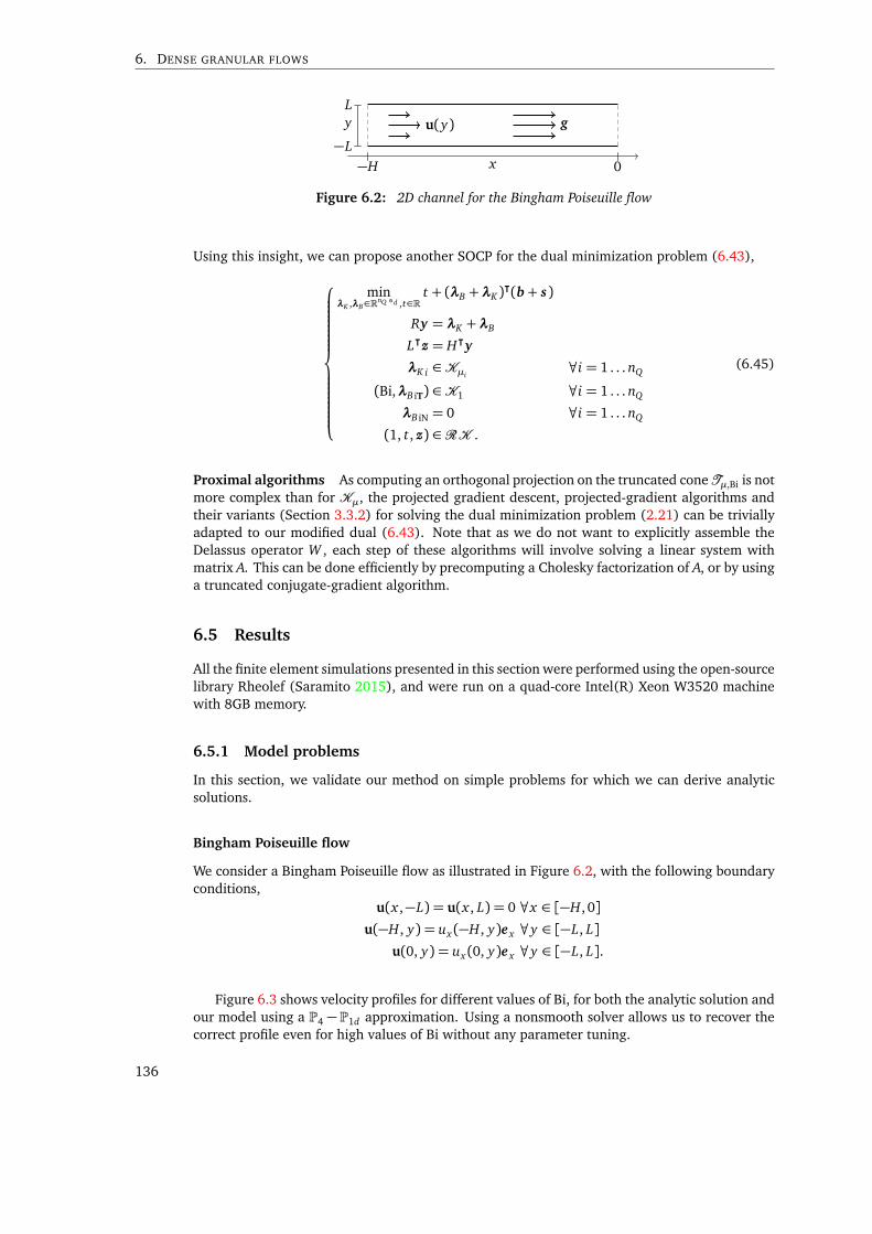
6. DENSE GRANULAR FLOWS

−H x 0

−L

yL

u(y) g

Figure 6.2: 2D channel for the Bingham Poiseuille flow

Using this insight, we can propose another SOCP for the dual minimization problem (6.43),

minλK ,λB∈RnQ sd ,t∈R

t + (λB +λK)⊺(b+ s)

Ry = λK +λB

L⊺z = H⊺y

λK i ∈Kµi∀i = 1 . . . nQ

(Bi,λB iT) ∈K1 ∀i = 1 . . . nQ

λB iN = 0 ∀i = 1 . . . nQ

(1, t, z) ∈ RK .

(6.45)

Proximal algorithms As computing an orthogonal projection on the truncated cone Tµ,Bi is notmore complex than for Kµ, the projected gradient descent, projected-gradient algorithms andtheir variants (Section 3.3.2) for solving the dual minimization problem (2.21) can be triviallyadapted to our modified dual (6.43). Note that as we do not want to explicitly assemble theDelassus operator W , each step of these algorithms will involve solving a linear system withmatrix A. This can be done efficiently by precomputing a Cholesky factorization of A, or by usinga truncated conjugate-gradient algorithm.

6.5 Results

All the finite element simulations presented in this section were performed using the open-sourcelibrary Rheolef (Saramito 2015), and were run on a quad-core Intel(R) Xeon W3520 machinewith 8GB memory.

6.5.1 Model problems

In this section, we validate our method on simple problems for which we can derive analyticsolutions.

Bingham Poiseuille flow

We consider a Bingham Poiseuille flow as illustrated in Figure 6.2, with the following boundaryconditions,

u(x ,−L) = u(x , L) = 0 ∀x ∈ [−H, 0]

u(−H, y) = ux(−H, y)e x ∀y ∈ [−L, L]

u(0, y) = ux(0, y)e x ∀y ∈ [−L, L].

Figure 6.3 shows velocity profiles for different values of Bi, for both the analytic solution andour model using a P4 − P1d approximation. Using a nonsmooth solver allows us to recover thecorrect profile even for high values of Bi without any parameter tuning.

136

6.5. Results

0 0.2 0.4 0.6 0.8 10

0.1

0.2

0.3

0.4

0.5

y/L

ux

Bi= 0

Bi= 0.5Bi= 0.9

0.9 0.95 10

0.5

1

1.5

2·10−4

y/L

Bi= 0.9

Bi= 0.99

Bi= 1.0

Figure 6.3: Comparison of the steady velocity profiles ux(−H/2, y) between our nu-merical model using a P2−P1d approximation (marks), and the analyticBingham Poiseuille flow (lines). Plots for high values of Bi (right) arezoomed in compared to plots for lower Bi values (left).

Convergence of spatial discretization We study how the error between our method and theanalytic solutions for Bi = 0.5 and Bi = 0.9 decreases as we uniformly refine a mesh withinitial characteristic edge length h0. Results for various FEM approximation orders are shown inFigure 6.4. Convergence was observed for all approximation orders, and we found that P2 −P1

and P2−P1d achieved a good ratio of convergence speed versus computational cost. Conversely,the higher-order approximation P3−P2d performed relatively poorly on the finer meshes, whichwe interpret as being the result of numerically more complex quadrature rules. P4 − P1d , withhigh-order velocities but low-order stresses, yielded consistently the best results, at the cost of avery large A matrix.

Bagnold profiles

We consider the flow of a granular layer of height H = 1 on a rough infinite inclined plane withangle α, as described in (Lagrée et al. 2011) and illustrated in Figure 6.5. We assume the flowto be slow enough to neglect inertial terms.

The conservation of momentum on the longitudinal x-axis and perpendicular y-axis reads

∂

∂ y

η∂ ux

∂ y+ τx y

= − sinα

∂ p

∂ y= − cosα.

Integrating the second equation with the condition that the pressure should be zero at thetop of the granular layer, i.e., p(H) = 0, gives p= (1− y) cosα.

We consider the case of an avalanching flow with ∂ ux∂ y > 0 for y < 1. This means that the

friction is saturated, therefore τx y = µ(1− y) cos(α). We get

∂

∂ yη∂ ux

∂ y= − sinα+µ cosα.

A Neumann boundary condition at the interface ∂ ux∂ y (1) = 0 imposes ∂

∂ yη∂ ux∂ y < 0, which

means µ < tanα.

137

6. DENSE GRANULAR FLOWS

0 2 410−6

10−4

10−2

2

1

Bi = 0.5

‖ux−u

ref

x‖ ∞

P1 − P0 P2 − P0 P2 − P1

P2 − P1d P4 − P1d P3 − P2d

0 2 410−7

10−5

10−3

2

1

Bi = 0.9

0 2 4

10−4

10−3

10−2

2

1

log2 h0 − log2 h

‖ux−u

ref

x‖ H

1

0 2 4

10−4

10−2

2

1

log2 h0 − log2 h

Figure 6.4: L∞-norm (top) and H1-norm (bottom) convergence plots for variousFEM approximation orders, for Bi = 0.5 (left) and Bi = 0.9 (right).ure f

x denotes the analytic solution.

x

0

yH

u(y) g

α

Figure 6.5: Flow on an infinite inclined plane

For spatially constant (Newtonian) η and µ, we get ∂ ux∂ y =

1−yη sinα− (µ cosα), and ux(y) is

quadratic. In order to retrieve the typical 32 power of the Bagnold profile, we can instead choose

η(y) := |D(u)|= 12∂ ux∂ y , which gives the analytic expressions

∂ ux

∂ y=Æ

2 sinα− (µ cosα) (1− y)12

ux(y) =2

3

Æ2 sinα− (µ cosα)

1− (1− y)

32

.

We simulated this model on a square patch using the algorithm presented in Section 6.2.The value of σext on the upstream and downstream boundaries was computed using the analyticsolution. In order to handle the non-constantη, we used a fixed-point algorithm which happenedto converge very fast in practice — a dozen or so of iterations.

138

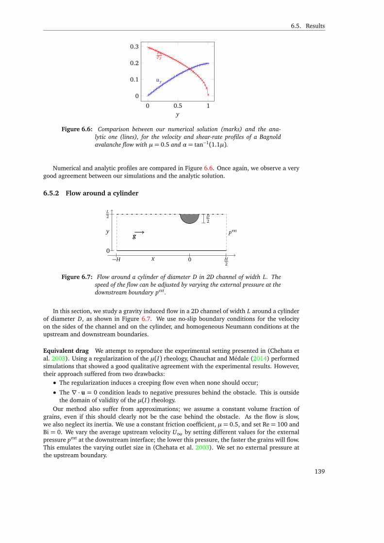
6.5. Results

0 0.5 1

0

0.1

0.2

0.3

y

uy

∂ u∂ y

Figure 6.6: Comparison between our numerical solution (marks) and the ana-lytic one (lines), for the velocity and shear-rate profiles of a Bagnoldavalanche flow with µ= 0.5 and α= tan−1(1.1µ).

Numerical and analytic profiles are compared in Figure 6.6. Once again, we observe a verygood agreement between our simulations and the analytic solution.

6.5.2 Flow around a cylinder

D2

−H x 0 H2

0

y

L2

gpext

Figure 6.7: Flow around a cylinder of diameter D in 2D channel of width L. Thespeed of the flow can be adjusted by varying the external pressure at thedownstream boundary pext.

In this section, we study a gravity induced flow in a 2D channel of width L around a cylinderof diameter D, as shown in Figure 6.7. We use no-slip boundary conditions for the velocityon the sides of the channel and on the cylinder, and homogeneous Neumann conditions at theupstream and downstream boundaries.

Equivalent drag We attempt to reproduce the experimental setting presented in (Chehata etal. 2003). Using a regularization of the µ(I) rheology, Chauchat and Médale (2014) performedsimulations that showed a good qualitative agreement with the experimental results. However,their approach suffered from two drawbacks:• The regularization induces a creeping flow even when none should occur;

• The ∇ · u = 0 condition leads to negative pressures behind the obstacle. This is outsidethe domain of validity of the µ(I) rheology.

Our method also suffer from approximations; we assume a constant volume fraction ofgrains, even if this should clearly not be the case behind the obstacle. As the flow is slow,we also neglect its inertia. We use a constant friction coefficient, µ= 0.5, and set Re= 100 andBi = 0. We vary the average upstream velocity U∞ by setting different values for the externalpressure pext at the downstream interface; the lower this pressure, the faster the grains will flow.This emulates the varying outlet size in (Chehata et al. 2003). We set no external pressure atthe upstream boundary.

139

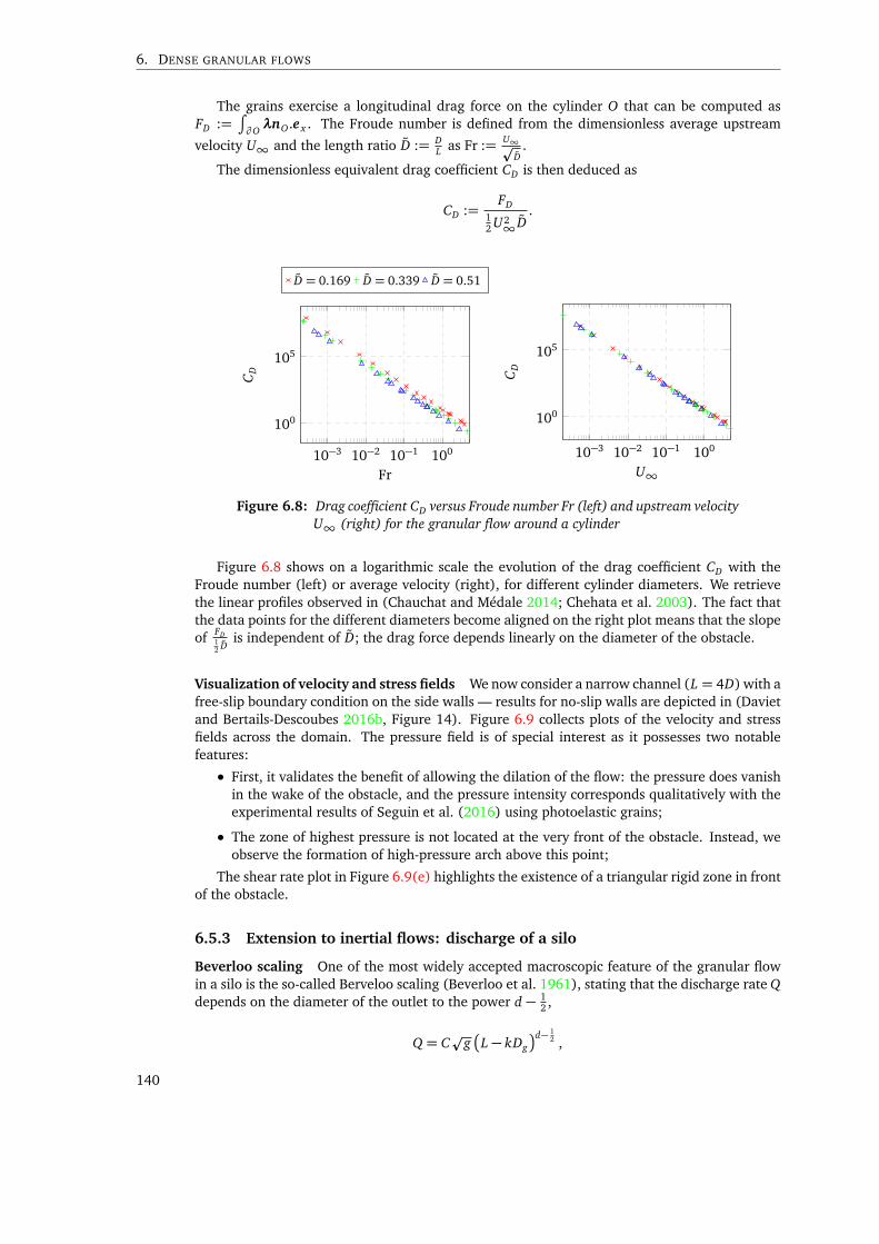
6. DENSE GRANULAR FLOWS

The grains exercise a longitudinal drag force on the cylinder O that can be computed asFD :=

∫∂OλnO.e x . The Froude number is defined from the dimensionless average upstream

velocity U∞ and the length ratio D := DL as Fr := U∞p

D.

The dimensionless equivalent drag coefficient CD is then deduced as

CD :=FD

12 U2∞ D

.

10−3 10−2 10−1 100

100

105

Fr

CD

D = 0.169 D = 0.339 D = 0.51

10−3 10−2 10−1 100

100

105

U∞

CD

Figure 6.8: Drag coefficient CD versus Froude number Fr (left) and upstream velocityU∞ (right) for the granular flow around a cylinder

Figure 6.8 shows on a logarithmic scale the evolution of the drag coefficient CD with theFroude number (left) or average velocity (right), for different cylinder diameters. We retrievethe linear profiles observed in (Chauchat and Médale 2014; Chehata et al. 2003). The fact thatthe data points for the different diameters become aligned on the right plot means that the slopeof FD

12 D

is independent of D; the drag force depends linearly on the diameter of the obstacle.

Visualization of velocity and stress fields We now consider a narrow channel (L = 4D) with afree-slip boundary condition on the side walls — results for no-slip walls are depicted in (Davietand Bertails-Descoubes 2016b, Figure 14). Figure 6.9 collects plots of the velocity and stressfields across the domain. The pressure field is of special interest as it possesses two notablefeatures:

• First, it validates the benefit of allowing the dilation of the flow: the pressure does vanishin the wake of the obstacle, and the pressure intensity corresponds qualitatively with theexperimental results of Seguin et al. (2016) using photoelastic grains;

• The zone of highest pressure is not located at the very front of the obstacle. Instead, weobserve the formation of high-pressure arch above this point;

The shear rate plot in Figure 6.9(e) highlights the existence of a triangular rigid zone in frontof the obstacle.

6.5.3 Extension to inertial flows: discharge of a silo

Beverloo scaling One of the most widely accepted macroscopic feature of the granular flowin a silo is the so-called Berveloo scaling (Beverloo et al. 1961), stating that the discharge rate Qdepends on the diameter of the outlet to the power d − 1

2 ,

Q = Cp

gL − kDg

d− 12 ,

140

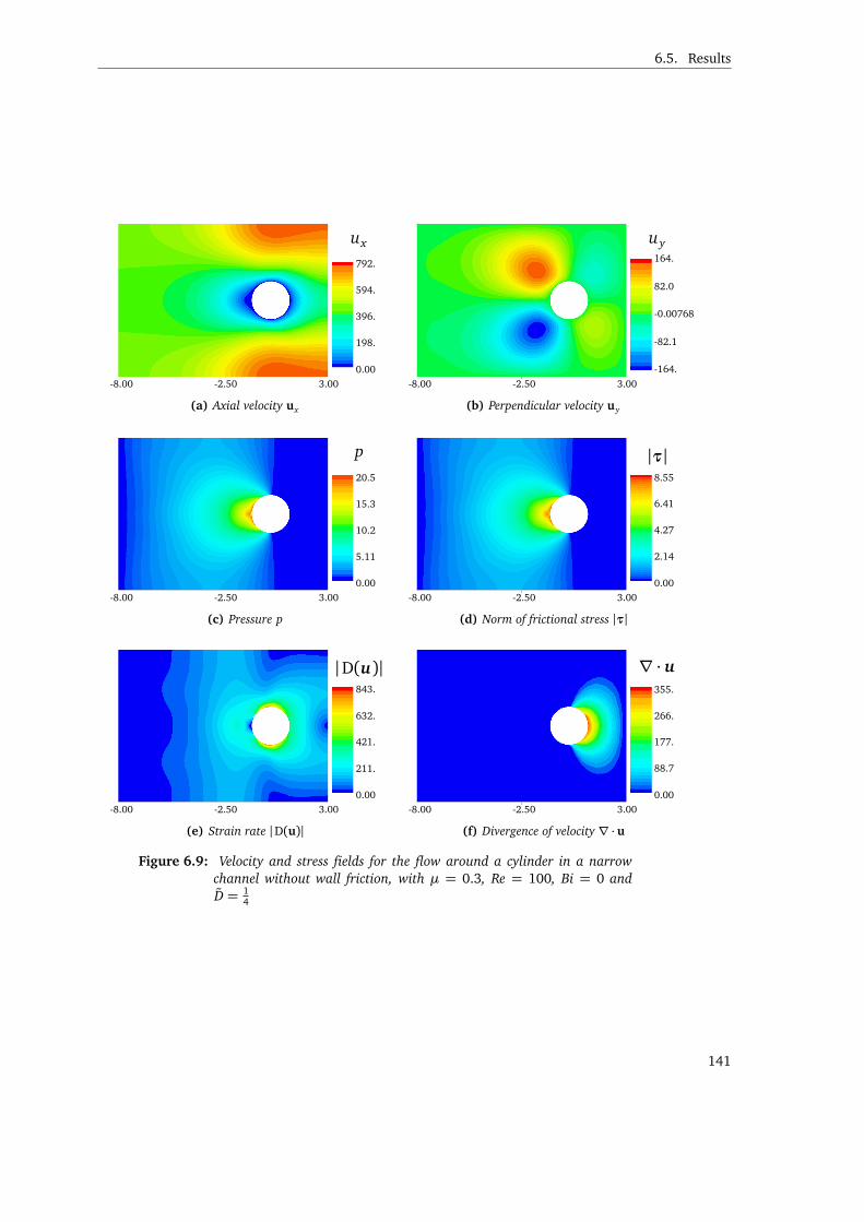
6.5. Results

0.00

198.

396.

594.

792.

ux

-8.00 -2.50 3.00

(a) Axial velocity ux

-164.

-82.1

-0.00768

82.0

164.

uy

-8.00 -2.50 3.00

(b) Perpendicular velocity uy

0.00

5.11

10.2

15.3

20.5

p

-8.00 -2.50 3.00

(c) Pressure p

0.00

2.14

4.27

6.41

8.55

|τ|

-8.00 -2.50 3.00

(d) Norm of frictional stress |τ|

0.00

211.

421.

632.

843.

|D(u)|

-8.00 -2.50 3.00

(e) Strain rate |D(u)|

0.00

88.7

177.

266.

355.

∇ · u

-8.00 -2.50 3.00

(f) Divergence of velocity ∇ · u

Figure 6.9: Velocity and stress fields for the flow around a cylinder in a narrowchannel without wall friction, with µ = 0.3, Re = 100, Bi = 0 andD = 1

4

141

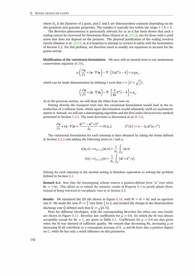
6. DENSE GRANULAR FLOWS

where Dg is the diameter of a grain, and C and k are dimensionless constants depending on thesilo geometry and granular properties. The number k typically lies within the range 1< k < 3.

The Beverloo phenomenon is particularly relevant for us as it has been shown that such ascaling cannot be recovered for Newtonian flows (Staron et al. 2012), nor for flows with a yieldstress that does not depend on the pressure. The physical justification of the scaling involvesinertia (Mankoc et al. 2007), so it is hopeless to attempt to retrieve it solely with the formulationof Section 6.2. For this problem, we therefore need to modify our equations to account for thegrains inertia.

Modification of the variational formulation We now add an inertial term to our momentumconservation equation (6.10),

ρ

∂ u

∂ t+ (u · ∇)u

−∇ · 2ηE bε− λ

= ρge g ,

which can be made dimensionless by defining t such that t = LU t =

ÇLg t,

∂ u

∂ t+ (u · ∇)u

− ∇ ·

2

ReE b ˜ε− λ

= e g .

As in the previous section, we will drop the tildes from now on.Putting directly the transport term into the variational formulation would lead to the in-

troduction of a trilinear form, which upon discretization would ultimately yield an asymmetricmatrix A. Instead, we will use a timestepping algorithm and the first-order characteristics methodpresented in Section 5.2.2. The total derivative is discretized as in (5.15),

∂ u

∂ t+ (u · ∇)u= uk+1 − uk X k

∆t+O(∆t), X k(x ) := x −∆tu

k(x , tk).

The variational formulation for each timestep is then obtained by taking the forms definedin Section 6.2.2 and adding the following terms to l and a,

a(u,v) :=a(6.2.2)(u,v) +1

∆t

∫

Ω

⟨u,v⟩

l(v) :=l(6.2.2)(v) +1

∆t

∫

Ω

uk X k,v

.

Solving for each timestep in the inertial setting is therefore equivalent to solving the problemdefined in Section 6.2.

Remark 6.3. Note that the timestepping scheme ensures a positive-definite form “a” even whenRe = +∞. This allows us to extend the existence results of Property 6.4 to purely plastic flows,instead of being restricted to viscoplastic ones as in Section 6.2.

Results We simulated the 2D silo shown in Figure 6.10, with W = H = 8L and an aperturesize D. We made the ratio D := D

L vary from 12 to 2, and studied the change in the dimensionless

discharge rate Q defined such that Q :=p

g L32 Q.

Plots for different rheologies, with the corresponding Beverloo fits when one was found,are shown in Figure 6.11. Beverloo law coefficients for µ = 0.6, for which the fit was alwaysacceptable except for Re = 1, are given in Table 6.1. Coefficients for µ = 0.4 are also givenwhen the fit was deemed of sufficient quality. We remark that decreasing Re, increasing µ orincreasing Bi all contribute to a consequent increase of k. µ and Bi have also a positive impacton C , while Re has only a small influence on this parameter.

142

6.5. Results

H

W2

D2

x

y g

Figure 6.10: Geometry of a half-silo of height H, width W and aperture size D

Re= 100 Re= 1000 Re= 10Bi= 0 Bi= 0.1 Bi= 0

µ C 1.70 1.44 1.77 2.00k 0 0.96 0 3.34

µ= 0.4 C 1.54 1.52 1.54 1.48k 0.87 2.49 0.38 3.07

µ= 0.5 C 1.35 1.43 1.35 1.33k 0.83 3.20 0.22 3.56

Table 6.1: Beverloo law coefficents obtained for µ = 0.6 and µ = 0.4, for differentBi and Re values. The values for k are given assuming L = 11.2Dg .

Extension to the µ(I) rheology The µ(I) (see Section 0.3.3) rheology is classically integratedinto dynamics solvers by explicitly evaluating the value of the equivalent viscosity ηeff at eachtimestep (Lagrée et al. 2011).

In our case, we only have to explicitly evaluate the friction coefficient µ(I) instead of ηeff.Since µ(I) can only take values in [µS ,µD] whereas ηeff takes values in R+, our approach has afew benefits:

• We do not have to clamp the value of ηeff, and can have fully rigid zones where the shearrate is strictly zero (which means an infinite ηeff);

• The loss of stability of the time-integration scheme due to this explicit term is much lessdramatic;

• While fully implicit approaches are possible (Ionescu et al. 2015), our explicit update ruleremains much simpler — and cheaper.

While the simulation frameworks are quite different — we do not take into account the airphase and use a non-zero (Re= 100) Newtonian viscosity, we nevertheless attempted to recreatea simulation from (Staron et al. 2014, Fig 4), using the same physical parameters (D = 11.2Dg ,I0 = 0.4, µS = 0.32, µD = 0.6).

The results are shown in Figure 6.12 ; the match on the C coefficient of the Beverloo lawis surprisingly good (both methods give C = 1.48), however we retrieve a coefficient k that issignificantly smaller (0.52 vs 0.73). Velocity profiles along the vertical and horizontal sectionsdescribed in (Staron et al. 2014) are also presented in Figure 6.12.

6.5.4 Performance

We now study the computational performance for the problem of Section 6.2 – the dynamics caseis just a sequence of such problems. In the following, PG will denote the canonical Projected-Gradient algorithm, APGD the Accelerated Projected Gradient Descent from Heyn (2013) —which is roughly similar to the FISTA* algorithm advocated in(Treskatis et al. 2016), ASPG theAccelerated Spectral Projected Gradient (Algorithm B.2), and IP the Interior-Point algorithmfrom the commercial package MOSEK (E. Andersen, Roos, et al. 2003).

In order to make as fair a comparison as possible, to evaluate the current error at each fixed-point iteration we have chosen not to use a residual based on a projection operator — which

143

6. DENSE GRANULAR FLOWS

0.5 1 1.5 20

2

4

6

Q

µ= 0 µ= 0.1 µ= 0.2µ= 0.3 µ= 0.4 µ= 0.5

(a) Re= 100, Bi= 0

0.5 1 1.5 20

2

4

6

(b) Re= 100, Bi= 0.1

0.5 1 1.5 20

2

4

6

Q

(c) Re= 100, Bi= 0.2

0.5 1 1.5 20

2

4

6

(d) Re= 1000, Bi= 0

0.5 1 1.5 20

2

4

6

L

Q

(e) Re= 10, Bi= 0

0.5 1 1.5 20

2

4

6

L

(f) Re= 1, Bi= 0

Figure 6.11: Dimensionless discharge rate Q versus silo outlet diameter L for anddifferent rheologies. When µ is small, we cannot get a reasonable fit; inthe case of the Newtonian flow, the discharge rate is closer to a linearlaw. Bi mainly influences the k parameter of the law but does sufficesto obtain a fit. Large values of Re tend to linearize the discharge ratefor small µ, smaller values make it quadratic.

144

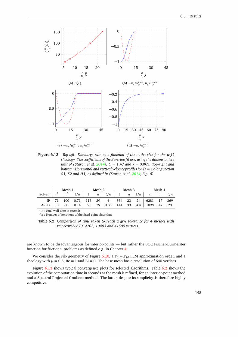
6.5. Results

5 10 15 20

50

100

150

DDg

D

(D D

g)

3 2Q

(a) µ(I)

0 15 30 45

−1

−0.5

0

DDg

y

(b) −ux/umaxx , uy/u

maxy

0 15 30 45

−1

−0.5

0

DDg

y

(c) −ux/umaxx , uy/u

maxy

0 15 30 45 60 75 90

−1

−0.8

−0.6

−0.4

−0.2

DDg

x

(d) −ux/umaxx

Figure 6.12: Top-left: Discharge rate as a function of the outlet size for the µ(I)rheology. The coefficients of the Beverloo fit are, using the dimensionlessunit of (Staron et al. 2014), C = 1.47 and k = 0.063. Top-right andbottom: Horizontal and vertical velocity profiles for D = 1 along sectionS1, S2 and H1, as defined in (Staron et al. 2014, Fig. 6)

Mesh 1 Mesh 2 Mesh 3 Mesh 4

Solver t1 n2 t/n t n t/n t n t/n t n t/n

IP 71 100 0.71 116 29 4 564 23 24 6281 17 369ASPG 13 88 0.14 69 79 0.88 144 33 4.4 1098 47 23

1 t : Total wall time in seconds.2 n : Number of iterations of the fixed-point algorithm.

Table 6.2: Comparison of time taken to reach a give tolerance for 4 meshes withrespectively 670, 2703, 10403 and 41509 vertices.

are known to be disadvantageous for interior-points — but rather the SOC Fischer-Burmeisterfunction for frictional problems as defined e.g. in Chapter 4.

We consider the silo geometry of Figure 6.10, a P2 − P1d FEM approximation order, and arheology with µ= 0.5, Re= 1 and Bi= 0. The base mesh has a resolution of 640 vertices.

Figure 6.13 shows typical convergence plots for selected algorithms. Table 6.2 shows theevolution of the computation time in seconds as the mesh is refined, for an interior-point methodand a Spectral Projected Gradient method. The latter, despite its simplicity, is therefore highlycompetitive.

145

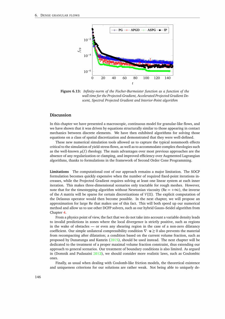
6. DENSE GRANULAR FLOWS

0 20 40 60 80 100 120 140

10−6

10−4

10−2

tf F

B

PG APGD ASPG IP

Figure 6.13: Infinity-norm of the Fischer-Burmeister function as a function of thewall time for the Projected-Gradient, Accelerated Projected Gradient De-scent, Spectral Projected Gradient and Interior-Point algorithm

Discussion

In this chapter we have presented a macroscopic, continuous model for granular-like flows, andwe have shown that it was driven by equations structurally similar to those appearing in contactmechanics between discrete elements. We have then exhibited algorithms for solving thoseequations on a class of spatial discretization and demonstrated that they were well-defined.

These new numerical simulation tools allowed us to capture the typical nonsmooth effectscritical to the simulation of yield-stress flows, as well as to accommodate complex rheologies suchas the well-known µ(I) rheology. The main advantages over most previous approaches are theabsence of any regularization or clamping, and improved efficiency over Augmented Lagrangianalgorithms, thanks to formulations in the framework of Second Order Cone Programming.

Limitations The computational cost of our approach remains a major limitation. The SOCPformulation becomes quickly expensive when the number of required fixed-point iterations in-creases, while the Projected Gradient requires solving at least one linear system at each inneriteration. This makes three-dimensional scenarios only tractable for rough meshes. However,note that for the timestepping algorithm without Newtonian viscosity (Re = +∞), the inverseof the A matrix will be sparse for certain discretizations of V (Ω). The explicit computation ofthe Delassus operator would then become possible. In the next chapter, we will propose anapproximation for large Re that makes use of this fact. This will both speed up our numericalmethod and allow us to use other DCFP solvers, such as our hybrid Gauss–Seidel algorithm fromChapter 4.

From a physics point of view, the fact that we do not take into account a variable density leadsto invalid predictions in zones where the local divergence is strictly positive, such as regionsin the wake of obstacles — or even any shearing region in the case of a non-zero dilatancycoefficient. Our simple unilateral compressibility condition ∇ · u ≥ 0 also prevents the materialfrom recompacting after dilatation; a condition based on the current volume fraction, such asproposed by Dunatunga and Kamrin (2015), should be used instead. The next chapter will bededicated to the treatment of a proper maximal volume fraction constraint, thus extending ourapproach to general scenarios. Our treatment of boundary conditions is also limited. As arguedin (Domnik and Pudasaini 2012), we should consider more realistic laws, such as Coulombicones.

Finally, as usual when dealing with Coulomb-like friction models, the theoretical existenceand uniqueness criterions for our solutions are rather weak. Not being able to uniquely de-

146

6.5. Results

termine the stress field for a given velocity solution is problematic for assessing the stress onstructures. However, as the flowing and dilating regions enforce boundary conditions for thestress inside the rigid zones, we did not find this under-determination to be problematic for ourtest scenarios.

147

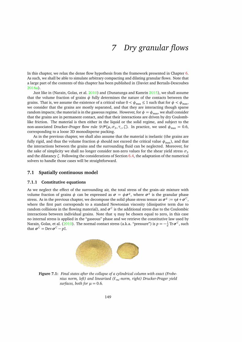
7 Dry granular flows

In this chapter, we relax the dense flow hypothesis from the framework presented in Chapter 6.As such, we shall be able to simulate arbitrary compacting and dilating granular flows. Note thata large part of the contents of this chapter has been published in (Daviet and Bertails-Descoubes2016a).

Just like in (Narain, Golas, et al. 2010) and (Dunatunga and Kamrin 2015), we shall assumethat the volume fraction of grains φ fully determines the nature of the contacts between thegrains. That is, we assume the existence of a critical value 0< φmax ≤ 1 such that for φ < φmax,we consider that the grains are mostly separated, and that they are interacting though sparserandom impacts; the material is in the gaseous regime. However, forφ = φmax, we shall considerthat the grains are in permanent contact, and that their interactions are driven by dry Coulomb-like friction. The material is then either in the liquid or the solid regime, and subject to thenon-associated Drucker–Prager flow rule DP (µ,σS ,τc ,ζ). In practice, we used φmax = 0.6,corresponding to a loose 3D monodisperse packing.

As in the previous chapter, we shall also assume that the material is inelastic (the grains arefully rigid, and thus the volume fraction φ should not exceed the critical value φmax), and thatthe interactions between the grains and the surrounding fluid can be neglected. Moreover, forthe sake of simplicity we shall no longer consider non-zero values for the shear yield stress σS

and the dilatancy ζ. Following the considerations of Section 6.4, the adaptation of the numericalsolvers to handle those cases will be straightforward.

7.1 Spatially continuous model

7.1.1 Constitutive equations

As we neglect the effect of the surrounding air, the total stress of the grain–air mixture withvolume fraction of grains φ can be expressed as σ = φσg , where σg is the granular phasestress. As in the previous chapter, we decompose the solid phase stress tensor as σg := ηǫ+σC ,where the first part corresponds to a standard Newtonian viscosity (dissipative term due torandom collisions in the flowing material), and σC is the additional stress due to the Coulombicinteractions between individual grains. Note that η may be chosen equal to zero, in this caseno internal stress is applied in the “gaseous” phase and we retrieve the constitutive law used byNarain, Golas, et al. (2010). The normal contact stress (a.k.a. “pressure”) is p = − 1

d TrσC , suchthat σC = DevσC − pI.

Figure 7.1: Final states after the collapse of a cylindrical column with exact (Frobe-nius norm, left) and linearized (ℓ∞-norm, right) Drucker-Prager yieldsurfaces, both for µ= 0.6.

149

7. DRY GRANULAR FLOWS

Just like in the previous chapter, we consider a Drucker–Prager yield criterion with frictioncoefficient µ and cohesion c, that is, a pressure-dependent yield stress µ(p + c). However, fol-lowing Narain, Golas, et al. (2010), the pressure no longer enforces a positive divergence of theflow, but the maximal volume fraction constraint φ ≤ φmax. That is, we replace Equation (6.3)with the complementarity relationship

0≤ p+ c ⊥ φmax −φ ≥ 0. (7.1)

The maximum dissipation principle states that in the yielded regime, friction should be sat-urated and the frictional stress tensor should be colinear to the deviatoric part of the strain rate.The deviatoric part of σC should thus satisfy one of the two regimes,

DevσC = µ (p+ c)

Dev ǫ

|Dev ǫ| if Dev ǫ 6= 0 (yielded)

|DevσC | ≤ µ(p+ c) if Dev ǫ = 0 (unyielded).(7.2)

Note that in contrast with (Narain, Golas, et al. 2010), we will not linearize the | · | norm inEquation (7.2), thus avoiding the disturbing geometrical artifacts inherent to their method (Fig-ure 7.1).

Remark 7.1. When φ < φmax, Equation (7.1) imposes p+ c = 0, and thus Equation (7.2) dictatesthat the frictional stress should vanish, which is expected. However, the mixture pressure will be−φc in the gaseous zones; if c > 0, the grains will thus tend to attract each other even though thecontacts are broken, which is unwanted. For this reason, the cohesion field c should also satisfyφ < φmax =⇒ c = 0. This may create spatial discretization issues, as we will see later.

7.1.2 Energy considerations

Let us study the conditions for which the flow rule defined by Equation (7.1–7.2) and the con-servation equations (5.7,5.10) lead to a dissipative system, as is expected from a granular ma-terial. We have already performed a similar study in the supplemental document to (Daviet andBertails-Descoubes 2016a) for the discrete-time version of the rheology. We propose here to lookat the continuous-time setting instead, by leveraging an analogy with impacts in discrete contactmechanics.

Local dissipativity of contact stress Let us consider a material point x (t) of the domain, withφ(t) := φ(x (t), t). We will see that both the inelastic impacts hypothesis and the criterion fromRemark 7.1, that cohesion should vanish in non-dense zones, are critical to ensure that the workof the contact stress is always and everywhere dissipative.

The density of energy dissipation by the contact stress is given by (−φ(t)σC(t)) : ǫ(t). Forthe system to be locally dissipative, it suffices that φσC : ǫ ≥ 0, or, a fortiori, that

¨DevσC : Dev(φD(u))≥ 0

TrσC Tr(φD(u))≥ 0.

(7.3a)

(7.3b)

The implication (7.1–7.2) =⇒ (7.3a) is trivial; either Dev(φD(u)) = 0, or Dev(φD(u)) 6= 0and DevσC = µ (p+ c) Devγ

|Devγ| with p+ c ≥ 0.Now, (7.3b) can be written equivalently as (pφ∇ · u) ≤ 0, or again, using the mass conser-

vation equation (6.1), p DφDt ≥ 0. Using an analogy with discrete mechanics, we argue below that

this inequality shall hold if the consideration made in Remark 7.1 is satisfied.The maximal volume fraction constraint, φmax −φ(t) ≥ 0, can be seen as analogous to the

normal part of the gap function in contact mechanics. The instant at which φ reaches φmax

constitutes an impact, and the time-derivative of the gap function (the normal relative velocity

150

7.1. Spatially continuous model

for discrete contacts, DφDt (x ) here) will be discontinuous. However, this derivative will retain

both a left and a right limit at every instant.

Pursuing the analogy with nonsmooth discrete mechanics, we interpret our inelastic im-pacts hypothesis as preventing rebounds; that is, if φ reach φmax at time t, then we shall haveDφDt (x (t), t+) = 0. Moreover, just like we did to construct the Signorini conditions, we assume

that shocks do not propagate. Therefore, if t is not a time of impact for the material point x (t),then the contact pressure p(t) := p(x (t), t), should possess both left and right limits.

The volume fraction and its derivative have thus to satisfy one of the following four cases,

φ(t)< φmax

or φ(t) = φmax andDφ

Dt(x (t), t−)> 0 and

Dφ

Dt(x (t), t+) = 0

or φ(t) = φmax andDφ

Dt(x (t), t) = 0

or φ(t) = φmax andDφ

Dt(x (t), t−)> 0 and

Dφ

Dt(x (t), t+) = 0.

(7.4a)

(7.4b)

(7.4c)

(7.4d)

Case (7.4a) corresponds to the gaseous regime, case (7.4b) to an impact, case (7.4c) to persistentcontact and case (7.4d) to the onset of dilation.

Let us show that, under the hypothesis of Remark 7.1, i.e., that φ < φmax =⇒ c = 0, thenp Dφ

Dt ≥ 0. This is obvious when DφDt = 0, let us consider the remaining cases.

• Case (7.4a). The complementarity condition (7.1) requires p = −c = 0.

• Case (7.4b) at t−. Left-continuity of DφDt means that there exists t0 such that ∀s ∈ [t0, t[,

DφDt (s) < 0, and thus φ(s) < φmax, meaning c(s) = 0. Left-continuity of c imposes in turn

that c(t−) = 0, and condition (7.1) that p(t−)≥ 0. We deduce (p DφDt )(x , t−)≥ 0.

• Case (7.4d) at t+. As t is not a time of impact, by analogy with discrete mechanics weassume right-continuity of p. There exists t0 such that ∀s ∈]t, t0], φ(s) < φmax, thusc(s) = p(s) = 0, and p(t+) = 0. Once again (p Dφ

Dt )(x (t), t+) = 0.

Global dissipativity For the sake of simplicity, we shall consider a domain Ω with homoge-neous Dirichlet boundary conditions.

We can decompose the total energy of the system as the sum of its potential and kineticenergies, i.e., E t = E p + E c , with

E p := −∫

Ω

ρφ ⟨x, g ⟩ E c :=

∫

Ω

1

2ρφ ⟨u,u⟩ .

Since we are using homogeneous Dirichlet boundary conditions, their evolution follows

dE p

dt= −ρ

∫

Ω

∂φ

∂ t⟨x, g ⟩= ρ

∫

Ω

∇ · [φu] ⟨x, g ⟩

= −ρ∫

Ω

φ ⟨u,g⟩+ρ∫

BdΩ

φ ⟨u,nΩ⟩ ⟨x ,g⟩︸ ︷︷ ︸

=0

,

151

7. DRY GRANULAR FLOWS

t = t0

t > t0

φ(x 0, t0)

u(t)

φ(x 0, t0; t)φ(x 0, t)

Figure 7.2: Eulerian (in red) and Lagrangian (in blue) points of view for studyingthe change in volume fraction of a compressible fluid.

anddE c

dt=

∫

Ω

ρφ

­Du

Dt,u·

=

∫

Ω

η ⟨∇ · [φε],u⟩+ ∇ · φσC,u+ρφ ⟨g ,u⟩

=ρ

∫

Ω

φ ⟨u,g⟩ −η∫

Ω

φε : ε

︸ ︷︷ ︸≥0

−∫

Ω

φσC : ε

+

∫

BdΩ

φu,ηε+σC

nΩ

︸ ︷︷ ︸=0

.

Therefore dE t

dt ≤ −∫ΩφσC : ε. Provided the local dissipativity of the contact stress that we

discussed in the previous paragraph, the overall material is thus also dissipative.

7.1.3 Semi-implicit integration

Unlike in Chapter 6, our rheology involves the volume fraction field φ; the mass conservationand momentum balance equations are now fully coupled. Moreover, as we are using an inelasticmodel — i.e., in the infinite compression Young modulus limit — numerical stability considera-tions impose using an integration scheme with some degree of implicity.

We propose using a two-step semi-implicit algorithm. At the kth timestep,

1. we first solve the momentum balance equation (5.10) using the current volume fractionfield φk, and deduce the end-of-step velocity and stress fields uk+1 and σk+1;

2. we then solve the mass conservation equation (5.7) using the end-of-step velocities uk+1

and deduce φk+1.

However, note that Step 1. requires finding uk+1 and σk+1 such that the end-of-step velocityconstraints are satisfied, and in particular, the end-of-step maximum volume fraction constraint,φk+1 ≤ φmax. Yet φk+1 is only computed at Step 2.! We must therefore replace the maximumvolume fraction constraint in Step 1. with an approximation of φk+1 that can be computedusing only φk and uk+1, and is much cheaper to evaluate than solving the full mass conservationequation. The following section is dedicated to this choice of approximation.

Remark 7.2. Our algorithm could be made fully implicit by keeping iterating between the two stepsuntil a fixed point for the volume fraction and velocity fields is reached.

Maximum volume fraction The mass conservation equation (5.7) describes how the volumefraction changes in time. Yet, as depicted in Figure 7.2, there are two ways to express this

152

7.1. Spatially continuous model

change. On the one hand, the Eulerian point of view looks at the change of φ at a fixed locationin space x 0, which is given by the derivative ∂φ

∂ t evaluated at x 0. We have

φ(x 0, t) = φ(x 0, t0) +

∫ t

t0

∂φ

∂ t(x 0, s)ds

= φ(x 0, t0)−∫ t

t0

∇ · [φu] (x 0, s)ds, using (5.7).

On the other hand, the Lagrangian point of view follows grains as they move through space.The volume fraction at such a tracked point is given by φ(x 0, t0; t) := φ(X (x 0, t0; t), t), whereX (x 0, t0; t) is the characteristics function defined by the Cauchy problem (5.13). Using the chainderivation rule w.r.t. time (5.14) and the mass conservation equation (5.7), we get

∂ φ

∂ t(x 0, t0; t) =

Dφ

Dt(X (x 0, t0; t), t) = −φ∇ · u (X (x 0, t0; t), t) .

We thus have

φ(x 0, t0; t) = φ(x 0, t0; t0) +

∫ t

t0

∂φ

∂ t(x 0, t0, s)ds

= φ(x 0, t0)−∫ t

t0

(φ∇ · u) (X (x 0, t0; s), s)ds.

(7.5)

The maximum volume fraction constraint, φ ≤ φmax, can be expressed at every instant andevery point of the simulation domain using either the Eulerian or Lagrangian point of views.Studying the rate of change eventually leads to conditions on ∇ · [φu] or φ∇ · u, respectively.Both conditions are equivalent in the spatially continuous case, however they will yield differentdiscretizations. A simple physical consideration will drive our choice: at the grain scale, thecontact forces oppose the relative velocity of the particles; at the macroscopic scale, we can thusexpect that the pressure will oppose the (opposite of) the divergence of the flow. Hence, we willuse the Lagrangian point of view to discretize the maximum volume fraction constraint.

First-order approximation With the Lagrangian framework of Equation (7.5), we linearize

the constraint φk+1 ≤ φmax on a time interval [tk, tk+1 := tk +∆t] as

φk −∆tφ

k∇ · uk+1 ≤

φmax. Equation (7.1) can thus be approximated at the first order as

0≤ φk∇ · uk+1 +βk ⊥ pk+1 + ck ≥ 0, (7.6)

where βk := φmax−φk

∆tis a scalar field expressing the maximum rate at which the material can

compress during ∆t .

7.1.4 Discrete-time equations

We now perform a few mathematical manipulations that will reveal a problem structure similarto that of the previous chapter. To lighten the notations, we will omit the k + 1 superscript;unless otherwise mentioned, the fields are evaluated at the end of the time-step.

As mentioned in Remark 7.1, the frictional contact stress field DevσC vanishes when thematerial is not at maximum compaction, and in particular where there is no granular matter(φk = 0). One may thus rewrite (7.2) equivalently as

DevσC = µ

p+ ck

φk Dev ε

|φk Dev ε| if φk Dev ε 6= 0

|DevσC | ≤ µ(p+ ck) if φk Dev ε= 0.

(7.7)

153

7. DRY GRANULAR FLOWS

We now consider the friction coefficient µ :=q

2d µ, and the symmetric tensor fields λ :=

ckI − σC and γ := φε + β

d I. We have φk∇ · u + β = Trγ, φk Dev ε = Dev(γ), and µλN =

µq

2d

qd2 ck − TrσCp

2d

= µ(ck + p), so that Equations (7.6)–(7.7) reread

Devλ= −µλNDevγ

|Devγ| if Devγ 6= 0

|Devλ| ≤ µλN if Devγ= 0

0≤ γN ⊥ λN ≥ 0.

(7.8)

We recognize the disjunctive formulation (1.20) of the non-associated Drucker–Prager flow ruleexpressed on γ and λ,

γ and λ satisfy (7.8) ⇐⇒ (γ,λ) ∈ DP (µ).

Conservation of momentum Replacing the expression of λ into the momentum conservationequation (5.10), the discrete time momentum balance equation that we will have to solve atStep 1. of our semi-implicit integration algorithm reads

ρφk Du

Dt−∇ · ηφk D(u)−φkλ

= ρφkg +∇ φkck

. (7.9)

The total derivative remains to be discretized, but the method for doing so will be tightlylinked to our choice of spatial discretization. For now, we will assume that Du

Dt can be approxi-mated at the first order as

Du

Dt=

1

∆t

u− u(uk)

+O(∆t),

with the mapping u to be defined later.

Variational formulation Similarly as in Chapter 6, the momentum conservation equation (7.9)with the non-associated Drucker-Prager flow rule can be put under variational form. Let V de-note the subspace of H1(Ω)d satisfying the homogeneous Dirichlet boundary conditions, and letT ⊂ L2(Ω)

s

d a subspace of square-integrable symmetric tensor fields on Ω.

Proposition 7.1. The first step of out semi-implicit integration scheme amounts to finding u ∈ V ,γ,λ ∈ T 2 such that

m(u,v) + a(u,v) = b(λ,v) + l(v) ∀v ∈ T

s(γ,τ) = b(τ,u) + k(τ) ∀τ ∈ T

(γ,τ) ∈ DP (µ),(7.10)

where the bilinear forms a, b, m and linear forms l,k are given by

m(u,v) :=ρ

∆t

∫

Ω

φk ⟨u,v⟩ s(γ,τ) :=

∫

Ω

γ : τ

a(u,v) := η

∫

Ω

φk D(u) : D(v) b(τ,u) :=

∫

Ω

φkτ : D(u)

l(v) := ρ

∫

Ω

φk

g +

u(uk)

∆t

k(τ) :=

∫

Ω

maxφmax −φk, 0

∆t

Trτ

d.

Proof. One can see easily that the second line of 7.10 is just the definition of γ put under weakform. Multiplying the conservation of momentum (7.9) by a test function v, one gets

ρ

∆t

∫

Ω

φk ⟨u,v⟩ −η∫

Ω

∇ · φk D(u),v= −

∫

Ω

∇ · φkλ,v+ρ

∫

Ω

φk

g +

u(uk)

∆t

.

154

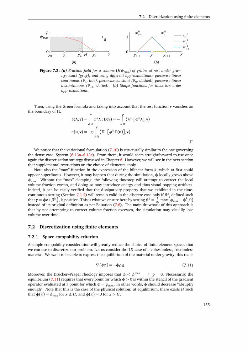
7.2. Discretization using finite elements

0

φmaxφ

H yy0 y1 y2 y3

g

(a)

0

1

y

ω0i−1 ω0

i

yi−1 yi yi+1

ω1i+

ω1i−

ω1i

(b)

Figure 7.3: (a) Fraction field for a volume (Hφmax) of grains at rest under grav-ity; exact (gray), and using different approximations: piecewise-linearcontinuous (P1, line), piecewise-constant (P0, dashed), piecewise-lineardiscontinuous (P1d , dotted). (b) Shape functions for those low-orderapproximations.

Then, using the Green formula and taking into account that the test function v vanishes onthe boundary of Ω,

b(λ,v) =

∫

Ω

φkλ : D(v) = −∫

Ω

∇ · φkλ,v

a(u,v) = −η∫

Ω

∇ · φk D(u),v.

We notice that the variational formulation (7.10) is structurally similar to the one governingthe dense case, System (6.13a–6.13c). From there, it would seem straightforward to use onceagain the discretization strategy discussed in Chapter 6. However, we will see in the next sectionthat supplemental restrictions on the choice of elements apply.

Note also the “max” function in the expression of the bilinear form k, which at first couldappear superfluous. However, it may happen that during the simulation, φ locally grows aboveφmax. Without the “max” clamping, the following timestep will attempt to correct the localvolume fraction excess, and doing so may introduce energy and thus visual popping artifacts.Indeed, it can be easily verified that the dissipativity property that we exhibited in the time-continuous setting (Section 7.1.2) will remain valid in the discrete case only if β k, defined suchthat γ= φǫ+β k I

d , is positive. This is what we ensure here by setting β k = 1∆t

maxφmax −φk, 0

instead of its original definition as per Equation (7.6). The main drawback of this approach isthat by not attempting to correct volume fraction excesses, the simulation may visually losevolume over time.

7.2 Discretization using finite elements

7.2.1 Space compability criterion

A simple compability consideration will greatly reduce the choice of finite-element spaces thatwe can use to discretize our problem. Let us consider the 1D case of a cohesionless, frictionlessmaterial. We want to be able to express the equilibrium of the material under gravity; this reads

∇ [φp] = −φρg. (7.11)

Moreover, the Drucker–Prager rheology imposes that φ < φmax =⇒ p = 0. Necessarily, theequilibrium (7.11) requires that every point for which φ> 0 is within the stencil of the gradientoperator evaluated at a point for which φ= φmax. In other words, φ should decrease “abruptlyenough”. Note that this is the case of the physical solution: at equilibrium, there exists H suchthat φ(x) = φmax for x ≤ H, and φ(x) = 0 for x > H.

155

7. DRY GRANULAR FLOWS

More formally, let Vh and Th be subspaces of V ⊂ H1(R) and T ⊂ L2(R). The complementaritycondition (7.1) suggests using the same discretization space for the volume fraction and stressfields, so we will assume φ ∈ T . Consider the linear form lh on Vh, lh(vh) :=

∫Ωφhvh, and the

bilinear form on Th × Vh bh(ph,vh) :=∫Ω∇ [ph]vh. Let Λ(φh) ⊂ Th be the linear subspace of the

pressure fields that are non-zero only at mesh nodes where φh = φmax . Then if lh 6= 0Vh

and∀ph ∈ Λ(φh), b(ph, lh) = 0, the equilibrium under gravity cannot be achieved.

Let us see if this criterion is satisfied for a few simple velocity–pressure spaces and the sce-nario depicted in Figure 7.3(a). We will restrict ourselves to low-order approximations (Fig-ure 7.3(b)):

• (piecewise-constant) P0 := Span(ω0i ), with ω0

i (x) := 1 for x i ≤ x ≤ x i+1 and zero else-where;

• (piecewise-linear) P1 := Span(ω1i ), with ω1

i (x) :=max(0, 1− |x − x i |);• (piecewise-linear discontinuous) P1d := Span(ω1

i+,ω1i−), with ω1

i+(x) := ω1i (x) for x i ≤

x ≤ x i+1 and zero elsewhere; ω1i−(x) :=ω1

i (x) for x i−1 ≤ x ≤ x i and zero elsewhere.

Th piecewise-constant Let us choose φ = ω00 +ω

01 + βω

02 with 0 < β < 1

2 and where ω0i is

the constant unitary function over the ith element.Then Λ = Span

q0

0, q01

, and thus bh(ph,vh) = 0 for any vh vanishing on [x0, x2]. The ex-

istence of a test function vh with positive integral on [x2, x3] yet vanishing for x ≤ x2 wouldprevent the existence of an equilibrium solution.

For Vh = P1, we have lh(ω13) > 0, and bh(ph,ω1

3) = 0. The pair P1 − P0 is inconsistent.Similarly for Vh = P1d , we have lh(ω

13−) > 0, while bh(ph,ω1

3−) = 0. This can be generalized tohigher orders.

However, the compatibility criterion does not prohibit the P0–P0 pair.

Th piecewise-linear We now choose φ = ω10 + ω

11 + βω

12 with 1

2 < β < 1. This meansΛ = Span(ω1

0,ω11), and thus again, bh(ph,vh) = 0 for any vh vanishing on [x0, x2].

For Vh = P0, lh(ω02)> 0 and bh(ph,ω0

2) = 0. Again for Vh = P1, lh(ω13)> 0 and bh(ph,ω1

3) =

0. For Vh = P1d , lh(ω13−)> 0 and b(ph,ω1

3−) = 0. Idem for higher orders.

Th piecewise-linear discontinuous Let φ =ω10++ω

11−+ω

11++ω

12−+βω

12+ with 0< β < 1.

This means Λ = Spanω1

0+,ω11−,ω1

1+,ω12−, and once again, bh(ph,vh) = 0 for any vh vanishing

on [x0, x2].For Vh = P1 or Vh = P1d , lh(vh)> 0 and bh(ph,vh) = 0 for vh :=ω2

3 or vh :=ω23−, respectively.

However the compatibility criterion does not prohibit P0 velocities.

Wrapping up This incompatiblity seems to arise from the fact that we are using the samediscretization space for both the pressure and volume fraction fields; using a higher-order volumefraction would yield a sharper interface, and would allow this interface to stay within the rangeof the gradient operator stencil. However, in this case the maximal volume fraction constraintwould not be able to be satisfied for every degree of freedom of the volume fraction field. InSection 7.3, we will propose to use particles to discretize the volume fraction field, and thusobtain unconditionally sharp interfaces. Alternatively, we can use one of the few discretizationspaces that were found to not violate the compatibility criterion, such as the P0–P0 pair, to whichthe next subsection is dedicated.

7.2.2 Piecewise-constant discretization

In a manner similar to that of finite-volume methods, we consider only the average value (i.e.,the value at the barycenter) of each mesh cell. Discontinuous velocity spaces are theoreticallytricky to handle, are they are not subspaces of H1(Ω)d ; we refer the reader to (Pietro and Ern2011).

156

7.2. Discretization using finite elements

Discontinuous Green formula We assume that the discrete mesh Ωh can be decomposed as aset of disjoint polyhedras (Ki), and denote by Ppd(Ωh) the space of piecewise-polynomials thatare of order less than p on each element Ki . Let Fi denote the set of all interior faces of Ωh,which we augment with an arbitrary orientation: for any F ∈ Fi , we number as K F

1 and K F2 the

adjacent cells, and define the normal nF as pointing towards K F2 , i.e., nF = nK F

1 = −nK F2 .

For any field v ∈ Ppd(Ωh), for any internal face F and for x ∈ F we denote by vi(x ), i = 1or 2 the value at x of the restriction v to K F

i , v|Ki(x ). We can then define the jump and average

operators on Fi as

JvK := v1 − v2 LvM :=1

2(v1 + v2).

These operators allow us to define a Stokes-like theorem for discontinuous fields. Let v ∈ V0,then ∫

BdΩh

v,nΩ

=∑

K∈Ωh

∫

Bd K

v,nK

−∑

F∈Fi

∫

F

¬v1,nK F

1

¶+¬v2,nK F

2

¶

=∑

K∈Ωh

∫

K

∇ · v−∑

F∈Fi

∫

F

JvK,nF

.

Let Vp = Pp(Ωh)d , and Tp = Pp(Ωh)

sd . Applying our discontinuous Stokes formula to theproduct τv, with τ ∈ Tp and v ∈ Vh, and using the identity JτvK= JτK LvM+ LτM JvK , we get

∫

BdΩh

v,τnΩ

+∑

F∈Fi

∫

F

JvK, LτMnF

−∑

K∈Ωh

∫

K

D(v) : τ=

∑

K∈Ωh

∫

K

⟨∇ · τ,v⟩ −∑

F∈Fi

∫

F

LvM, JτKnF

.

For the sake of brevity, we can extend the jump and average operators on Fa := Fi ∪ BdΩh asJvK|BdΩh

= v and LvM|BdΩh= v, and rewrite this last equation (the discontinuous Green formula)

as

∑

F∈Fa

∫

F

JvK, LτMnF

−∑

K∈Ωh

∫

K

D(v) : τ=∑

K∈Ωh

∫

K

⟨∇ · τ,v⟩ −∑

F∈Fi

∫

F

LvM, JτKnF

. (7.12)

The left-hand-side of (7.12) can be interpreted as a weak expression of D(u) (with homogeneousDirichlet boundary conditions), and the right-hand-side as a weak expression of ∇ · τ.

Discrete variational formulation The bilinear forms m and s from the variational formulationgiven in Proposition 7.1 do not involve any spatial derivative, and can thus be left unmodified.The discontinuous Green formula (7.12) yields a discretization of the bilinear form b which canbe easily verified to be consistent when the velocity solution is continuous, i.e., when JuK = 0

on Fi,

bh(u,τ) = −∑

F∈Fa

∫

F

JvK, LφτMnF

+∑

K∈Ωh

∫

K

φD(v) : τ. (7.13)

Obviously, the rightmost term in (7.13) vanishes when considering piecewise constant polyno-mials, and thus bh reduces to a sum of interfacial transfer terms.

The discretization of viscosity term, which involves a second-order derivative of the velocity,is more complex. The order of the polynomials in P0 is too low to allow the application ofstandard discontinuous Galerkin methods, such as the Symmetric Interior Penalty method (Pietroand Ern 2011, Section 4.2). Instead, we discretize our viscosity form a from Proposition 7.1

157

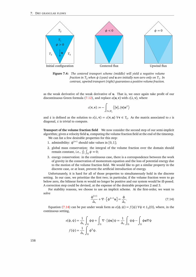
7. DRY GRANULAR FLOWS

T1

φ > 0

T2

T3 T4u

Initial configuration

φ < 0

Centered flux

φ = 0

Upwind flux

Figure 7.4: The centered transport scheme (middle) will yield a negative volumefraction in T2 when φ (cyan) and u are initially non-zero only on T1. Incontrast, upwind transport (right) guarantees a positive volume fraction.

as the weak derivative of the weak derivative of u. That is, we once again take profit of ourdiscontinuous Green formula (7.12), and replace a(u,v) with c(ε,v), where

c(τ,v) := −∫

F∈Fa

JvK, LτMnF

and ε is defined as the solution to s(ε,τ) = c(τ,u) ∀τ ∈ Th. As the matrix associated to s isdiagonal, ε is trivial to compute.

Transport of the volume fraction field We now consider the second step of our semi-implicitalgorithm; given a velocity field u, computing the volume fraction field at the end of the timestep.

We can list a few desirable properties for this step:

1. admissibility: φk+1 should take values in [0, 1];

2. global mass conservation: the integral of the volume fraction over the domain shouldremain constant, i.e., ∂

∂ t

∫Ωφ = 0;

3. energy conservation: in the continuous case, there is a correspondence between the workof gravity in the conservation of momentum equation and the loss of potential energy dueto the motion of the volume fraction field. We would like to get a similar property in thediscrete case, or at least, prevent the artificial introduction of energy.

Unfortunately, it is hard for all of those properties to simultaneously hold in the discretesetting. In our case, we prioritize the first two; in particular, if the volume fraction were to gobelow zero, the bilinear form m would no longer be positive and our system would be ill-posed.A correction step could be devised, at the expense of the desirable properties 2 and 3.

For stability reasons, we choose to use an implicit scheme. At the first-order, we want tosolve

φk+1

∆t+∇ · φk+1u

=φ

∆t. (7.14)

Equation (7.14) can be put under weak form as e(φ,ψ) = f (ψ) ∀ψ ∈ L2(Ω), where, in thecontinuous setting,

e(φ,ψ) =1

∆t

∫

Ω

φψ+

∫

Ω

∇ · [φu]ψ=1

∆t

∫

Ω

ψφ−∫

Ω

φu∇ψ

f (ψ) =1

∆t

∫

Ω

φkψ.

158

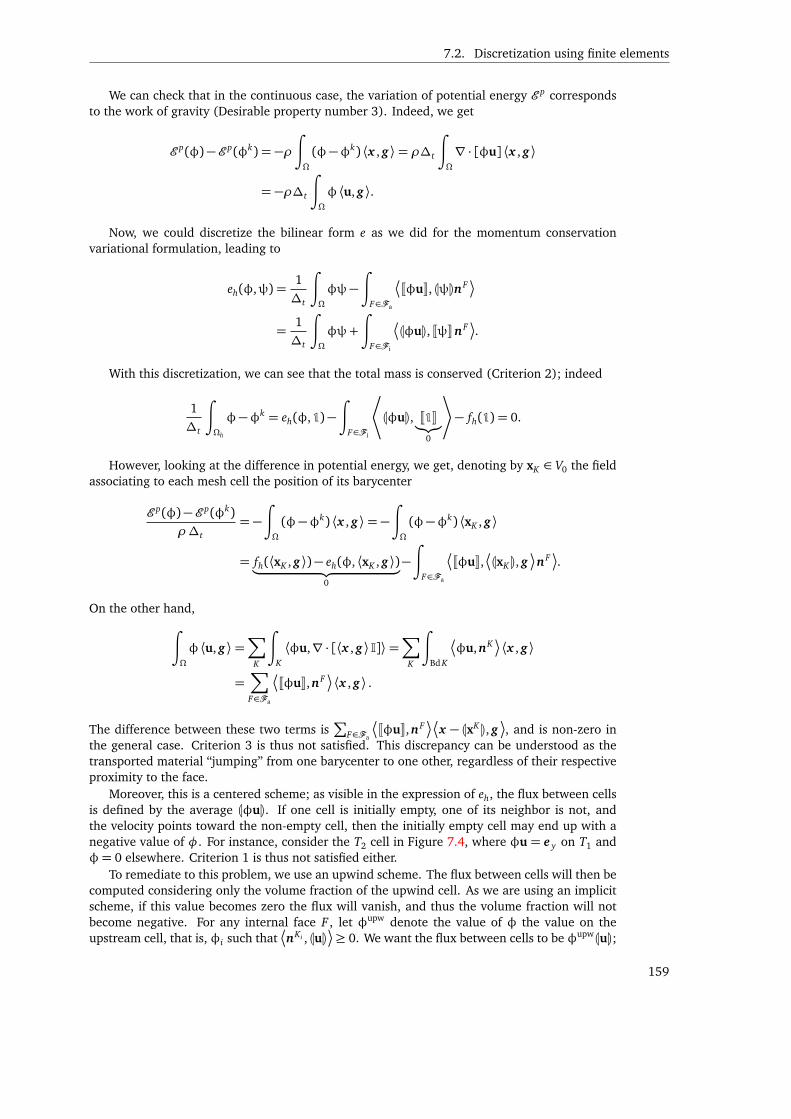
7.2. Discretization using finite elements

We can check that in the continuous case, the variation of potential energy E p correspondsto the work of gravity (Desirable property number 3). Indeed, we get

E p(φ)−E p(φk) = −ρ∫

Ω

(φ−φk) ⟨x , g ⟩= ρ∆t

∫

Ω

∇ · [φu] ⟨x , g ⟩

= −ρ∆t

∫

Ω

φ ⟨u, g ⟩.

Now, we could discretize the bilinear form e as we did for the momentum conservationvariational formulation, leading to

eh(φ,ψ) =1

∆t

∫

Ω

φψ−∫

F∈Fa

JφuK, LψMnF

=1

∆t

∫

Ω

φψ+

∫

F∈Fi

LφuM, JψKnF

.

With this discretization, we can see that the total mass is conserved (Criterion 2); indeed

1

∆t

∫

Ωh

φ−φk = eh(φ,1)−∫

F∈Fi

*LφuM, J1K︸︷︷︸

0

+− fh(1) = 0.

However, looking at the difference in potential energy, we get, denoting by xK ∈ V0 the fieldassociating to each mesh cell the position of its barycenter

E p(φ)−E p(φk)

ρ∆t= −

∫

Ω

(φ−φk) ⟨x , g ⟩= −∫

Ω

(φ−φk) ⟨xK , g ⟩

= fh(⟨xK , g ⟩)− eh(φ, ⟨xK , g ⟩)︸ ︷︷ ︸0

−∫

F∈Fa

JφuK,

LxKM, g

nF.

On the other hand,

∫

Ω

φ ⟨u, g ⟩=∑

K

∫

K

⟨φu,∇ · [⟨x , g ⟩ I]⟩=∑

K

∫

Bd K

φu,nK

⟨x , g ⟩

=∑

F∈Fa

JφuK,nF

⟨x , g ⟩ .

The difference between these two terms is∑

F∈Fa

JφuK,nF

x − LxKM, g

, and is non-zero in

the general case. Criterion 3 is thus not satisfied. This discrepancy can be understood as thetransported material “jumping” from one barycenter to one other, regardless of their respectiveproximity to the face.

Moreover, this is a centered scheme; as visible in the expression of eh, the flux between cellsis defined by the average LφuM. If one cell is initially empty, one of its neighbor is not, andthe velocity points toward the non-empty cell, then the initially empty cell may end up with anegative value of φ. For instance, consider the T2 cell in Figure 7.4, where φu = e y on T1 andφ= 0 elsewhere. Criterion 1 is thus not satisfied either.

To remediate to this problem, we use an upwind scheme. The flux between cells will then becomputed considering only the volume fraction of the upwind cell. As we are using an implicitscheme, if this value becomes zero the flux will vanish, and thus the volume fraction will notbecome negative. For any internal face F , let φupw denote the value of φ the value on theupstream cell, that is, φi such that

nKi , LuM

≥ 0. We want the flux between cells to be φupwLuM;

159

7. DRY GRANULAR FLOWS

the upwind bilinear form eupw can thus be obtained as

eupwh (φ,ψ) = eh(φ,ψ) +

∑

Fi

JφKφupwLuM− LφuM,nF

JψK

= eh(φ,ψ) +1

2

∑

Fi

JφK

LuM,nF− 1

2

JuK,n f

JψK

=1

∆t

∫

Ω

φψ+

∫

F∈Fi

JψK

LφMLuM,nF

+

1

2JφK

LuM,nF

.

With a similar reasoning to that of the centered case, we can verify that the upwind discretiza-tion verify Criterion 2 on the total mass conservation. However, energy conservation is not betterthan for the centered discretization. Criterion 1 and 2 being our priorities, we still choose to usethe upwind bilinear form and take φk+1 as the solution of eupw

h (φ,ψ) = l(ψ) ∀ψ ∈ P0(Ωh).

Inertial terms Finally, it remains to deal with the velocity advection term (u·∇)u in the conser-vation of momentum equation. As the velocities are discontinuous, the characteristics methodcannot be used (the morphism X is no longer locally invertible). Pietro and Ern (2011, Chapter6) demonstrate that discretizing implicitly the transport trilinear form t(w,u,v),

t(w,u,v) := −∫

Ω

⟨(w · ∇)u,v⟩ ,

using to the so-called Temam modification preserves the kinetic energy of the system. However,this modification is only valid for incompressible flows, and yields an asymmetric system; it istherefere not applicable in our case. In the end, we simply used an explicit version of the upwindtransport scheme described in the previous paragraph, which we found yielded in practice a goodcompromise between stability and conservation of kinetic energy. Thus, we define u(uk) in thecomputation of the l linear form from Property 7.1 such that

∫

Ωh

u(uk), v

:=

∫

Ωh

uk, v

− th(uk,uk,v)

th(w,u,v) := −∑

F∈Fi

­JuK,

LwM,nF

LvM+

1

2

LwM,nF JvK

·.

Final discrete system The final form of the variational formulation from Property 7.1 afterP0–P0 discretization is thus:Find u ∈ Rv, λ,γ ∈ Rnsd ,

(M + C⊺S−1C)u = B⊺λ+ l

Sγ= Bu + k

(γ,λ) ∈ DP (µ),(7.15)

where M and S are diagonal, positive matrices. As all the integrals of the variational formulationvanish on empty mesh cells, we can only consider those in which the volume fraction is non-zero,and thus M is positive-definite. This has also the advantage of drastically reducing the size ofthe numerical system in some scenarios. Alternatively, we can take into account the presence ofa light phase in the computation of the density in each cell, as in (Lagrée et al. 2011). In bothcases, System (7.15) can be then solved in the exact same manner as for our dense flows; seeSection 6.4.

7.2.3 Results

We attempted to validate our piecewise-constant discretization strategy by looking at some em-pirical laws reported in the literature. Just like in the dense case, the finite-element discretizationwas done with the Rheolef library (Saramito 2015).

160

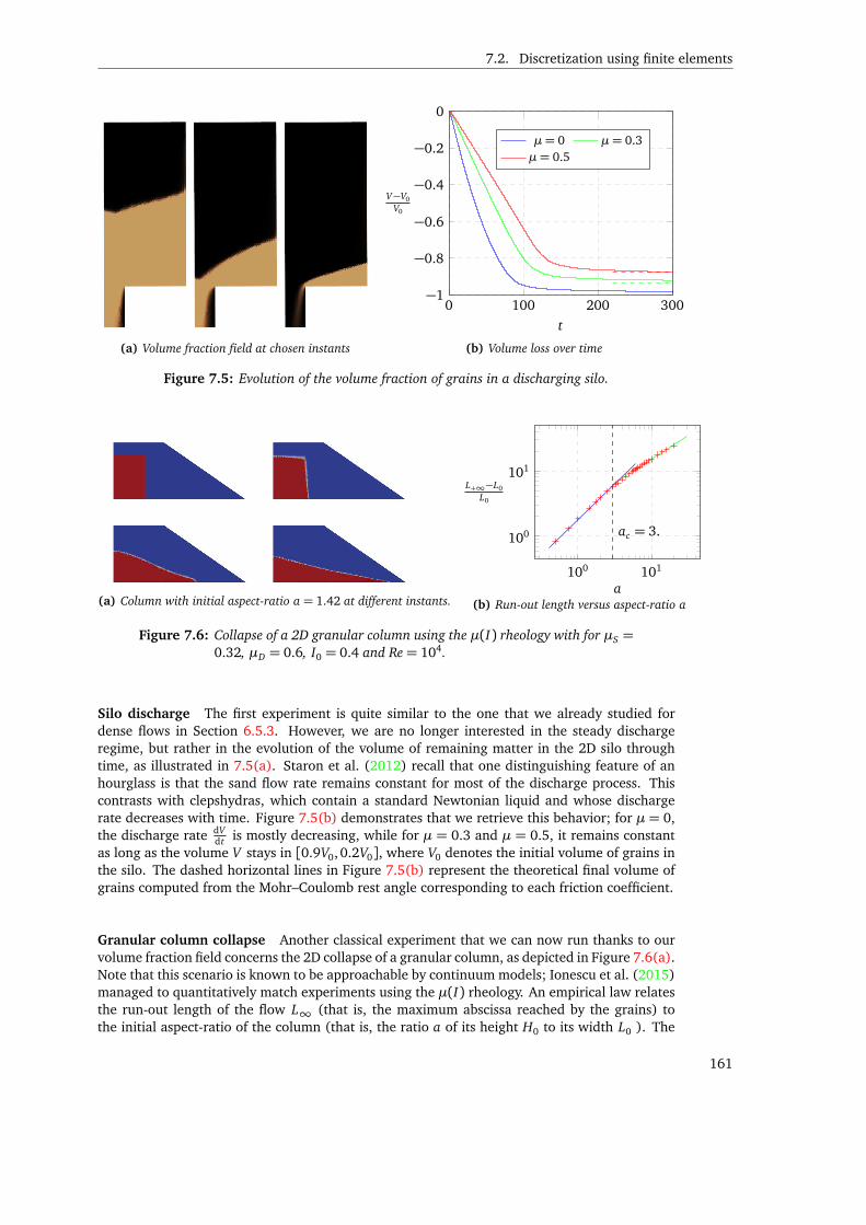
7.2. Discretization using finite elements

(a) Volume fraction field at chosen instants

0 100 200 300−1

−0.8

−0.6

−0.4

−0.2

0

t

V−V0V0

µ= 0 µ= 0.3µ= 0.5

(b) Volume loss over time

Figure 7.5: Evolution of the volume fraction of grains in a discharging silo.

(a) Column with initial aspect-ratio a = 1.42 at different instants.

100 101

100

101

ac = 3.

a

L+∞−L0

L0

(b) Run-out length versus aspect-ratio a

Figure 7.6: Collapse of a 2D granular column using the µ(I) rheology with for µS =

0.32, µD = 0.6, I0 = 0.4 and Re= 104.

Silo discharge The first experiment is quite similar to the one that we already studied fordense flows in Section 6.5.3. However, we are no longer interested in the steady dischargeregime, but rather in the evolution of the volume of remaining matter in the 2D silo throughtime, as illustrated in 7.5(a). Staron et al. (2012) recall that one distinguishing feature of anhourglass is that the sand flow rate remains constant for most of the discharge process. Thiscontrasts with clepshydras, which contain a standard Newtonian liquid and whose dischargerate decreases with time. Figure 7.5(b) demonstrates that we retrieve this behavior; for µ = 0,the discharge rate dV

dt is mostly decreasing, while for µ = 0.3 and µ = 0.5, it remains constantas long as the volume V stays in [0.9V0, 0.2V0], where V0 denotes the initial volume of grains inthe silo. The dashed horizontal lines in Figure 7.5(b) represent the theoretical final volume ofgrains computed from the Mohr–Coulomb rest angle corresponding to each friction coefficient.

Granular column collapse Another classical experiment that we can now run thanks to ourvolume fraction field concerns the 2D collapse of a granular column, as depicted in Figure 7.6(a).Note that this scenario is known to be approachable by continuum models; Ionescu et al. (2015)managed to quantitatively match experiments using the µ(I) rheology. An empirical law relatesthe run-out length of the flow L∞ (that is, the maximum abscissa reached by the grains) tothe initial aspect-ratio of the column (that is, the ratio a of its height H0 to its width L0 ). The

161

7. DRY GRANULAR FLOWS

Figure 7.7: A steel ball impacts a granular bed. Unlike previous approaches, ourfully resolved (non-linearized) Drucker-Prager rheology allows us to re-trieve a perfectly round crater.

experiments of Lajeunesse et al. (2005) led to the distinction of two regimes:

L∞ − L0

L0(a)∝

¨a if a < ac

a23 if a > ac ,

with ac ∼ 3. The numerical simulations of Staron and Hinch (2005), using DEM, and Lagrée etal. (2011), using the µ(I) rheology, yielded similar scaling laws, although with different criticalaspect ratios, ac ∼ 2 and 7. Several other authors have performed similar experiments bothexperimentally and numerically, see (Dunatunga and Kamrin 2015, Table 3) for a summary oftheir results. Using our method with the physical parameters from Lagrée et al. (2011), weobtained the scaling law plotted in Figure 7.6(b):

L∞ − L0

L0(a)∼

1.82a1.1 if a < 3

2.8a0.73 if a > 3.

The exponents that we obtained in both regimes seem to be a bit on the high side, though theyremain within the range of reported values in the numerical simulation literature, especiallywhen taking into account the results of (Mast et al. 2014). Note that at the characteristic sizeschosen for our spatial and temporal discretization, the choice of the advection scheme for thevolume fraction and velocity fields retains a non-negligible influence on the final scaling law.

Discussion This fully mesh-based discretization strategy suffers from several drawbacks. Weobserve diffusion of the volume fraction field over time, as a lot of cells retain slightly-above-zero volume fraction even once the bulk of the material has moved away. The explicit transportscheme for the inertial term also prohibits taking large timesteps, making the simulation processquite slow. In the next section we propose to use a different strategy and resort to an hybridmethod, which will discretize the volume fraction field using a set of particles. These particleswill also be used to transport other quantities, such as the inertial terms.

7.3 Material Point Method

The basic idea behind MPM is to consider that the whole mass of the material is condensed ata finite number of material points. The volume fraction field φ can therefore be expressed asφ(x , t) =

∑p Vpδ(x − x p(t)), where δ is the Dirac distribution, and Vp, x p are the volume and

position of the pth particle, respectively. The total volume of granular reads Vtot =∫Ωφ(t) =∑

p Vp.This representation is particularly adapted to the FEM formalism, where quantities are eval-

uated in weak-form, by multiplying them by a test function and integrating over a domain. Forinstance, for v ∈ L2(Ω), we have

∫Ωφ(t)v =

∑p Vpv(x p(t)). In this sense, the Material Point

Method can be seen as a quadrature rule for which the quadrature points are given by the par-ticles positions, and the corresponding weights by the particles volumes.

162

7.3. Material Point Method

Related work The MPM method was introduced by Sulsky (1994) for the simulation of history-dependent elastic materials. Storing information on particles made tracking the position of eachmaterial point through time trivial, avoiding solving complex transport equations.

MPM was quickly recognized as relevant for the simulation of granular materials. Wieck-owski, Youn, et al. (1999) proposed a first explicit algorithm for the integration of an elasto-plastic material subject to the non-associated Drucker–Prager flow rule 1 in 2D, and recentlyextended it to the 3D setting (Wieckowski and Pawlak 2015). S. Bardenhagen et al. (2000)proposed to use MPM for simulating the dynamics of many 2D deformable grains with slidingand rolling contacts. Konagai and Johansson (2001) coupled the Mohr–Coulomb yield criterionwith a nodal finite-difference scheme to simulate 2D granular flows. More recently, Mast et al.(2014) performed 2D granular column collapse simulations using MPM with the Matzuo–Nakaiyield surface. Dunatunga and Kamrin (2015) proposed a MPM method with two distinct regimesdepending on whether the volume fraction is above or below a critical value, again for 2D flows.

Stomakhin, Schroeder, Chai, et al. (2013) popularized MPM to the Computer Graphics com-munity, coupling this method with an elasto-plastic model to produce visually-striking snowsimulations. This gave rise to a variety of related methods modeling a wide range of physi-cal phenomenons, such as visco-elasto-plastic foams (Ram et al. 2015; Yue et al. 2015), phasechanges (Stomakhin, Schroeder, Jiang, et al. 2014), granular materials (e.g., concurrently to thework presented below, Klar et al. 2016), and more (Jiang, Schroeder, Teran, et al. 2016). Klaret al. (2016) follow the approach of Wieckowski, Youn, et al. (1999) with one notable difference:while both prevent plastic compression, Klar et al. (2016) allow plastic expansion, performingAlart–Curnier-like projections onto the Drucker–Prager set of admissible stresses.

Most MPM methods are explicit (Dunatunga and Kamrin 2015; Wieckowski, Youn, et al.1999; Yue et al. 2015), or semi-implicit with respect to the elastic energy, but not w.r.t. theplasticity (Ram et al. 2015; Stomakhin, Schroeder, Chai, et al. 2013). Klar et al. (2016) and Mastet al. (2014) propose to use a “return-mapping” algorithm to perform semi-implicit integrationtaking into account the plasticity. In practice, this means a Newton algorithm prone to fallinginto local minima. In contrast, our semi-implicit integration procedure will leverage our DCFPsolvers that showed good empirical convergence.

Extensions of MPM using different discretization strategies for the volume fraction field havealso been proposed; for instance, the Generalized Interpolation Material Point Method (GIMP;S. G. Bardenhagen and Kober 2004) use arbitrary indicator functions for the particles.

7.3.1 Application to our variational formulation

Taking advantage of the expression of φ as a sum of Dirac distributions, we can now rewrite thebilinear and linear forms from the variational formulation of Property 7.1 as:

m(u,v) :=∑

p

ρ

∆tVp

¬u(x k

p),v(xkp)¶

s(γ,τ) :=

∫

Ω

γ : τ

a(u,v) :=∑

p

VpηD(u)(x kp) : D(v)(x k

p) b(τ,u) :=∑

p

Vpτ(xkp) : D(u)(x k

p)

l(v) :=∑

p

ρVp

u(uk)

∆t+ g

,v(x k

p)

k(τ) :=

∫

Ω

φmax

∆t

I

d: τ−

∑

p

Vp

∆t

I

d: τ(xp)

and where x kp denotes the position of the pthth particle at timestep k.

7.3.2 Grid–particles transfers

In the context of MPM, the semi-implicit integration algorithm reads as follow:

1which is expressed as the association of the Drucker–Prager yield surface with a plastic incompressibility criterion,that is, ǫp ∈ NBT(−µσN)

(σT)

163

7. DRY GRANULAR FLOWS

1. solve the variational formulation (7.10), where the advected velocity field u(uk) is recon-structed from the particles;

2. deduce the new particle velocities v k+1p from the velocity field uk+1, and move the particles

accordingly.Two steps remain to be defined; first, the computation of u(uk) (particles-to-grid transfer),

and the computation of the particles velocities (grid-to-particle transfer). We mentioned in Sec-tion 5.2.4 different strategies for doing these transfers, such as PIC and FLIP. Both of those meth-ods compute up 7→g := u(uk) at each mesh node as a weighted interpolation of the velocities ofthe surrounding particles, as per Equation (5.16). As we are using the FEM formalism however,the natural way to compute up 7→g would be to solve

∆t

ρm(up 7→g ,v) =

∫

Ω

φ ⟨u,v⟩=∑

p

Vp

¬v k

p,v(x kp)¶

,

leading to a linear system Mu p 7→g = v , where

Mi, j :=∑

p

Vp

¬Vi(x

kp),V j(x

kp)¶

and v i :=∑

p Vpv kpVi(x

kp). M is called the consistent mass matrix.

In contrast, the standard PIC/FLIP update (5.16) can be understood as solving a diagonalsystem Mu p 7→g = v , with

Mi, j :=∑

p

Vp

Vi(x

k + p),1δ

ji (7.16)

Assume that ∀x ∈ Ω,∑

V j(x ) = 1Rd , as is the case for standard Lagrange FEM. ThenMi, j =

∑j Mi, j , and M is called the diagonalized or lumped mass matrix. Alternatively, M can

be understood as the result of using a trapezoidal approximation of the integral in the bilinearform m.

Computing up 7→g using M instead of M yields much better kinetic energy conservation, alle-viating the main drawback of PIC (Burgess et al. 1992). Indeed, the kinetic energy discrepancy isO(∆t |u|) for the consistent mass matrix, instead of O(|u|) for the lumped mass matrix. However,we can see from the interpretation of the particles as quadrature points that M will be indefiniteif there are not enough particles in one given mesh cell. Using the consistent mass matrix istherefore rarely possible in practice.

Moreover, FLIP is not convenient in our case. Indeed, consider a particular falling on a flatgranular bed; we want the particle to stop as soon as it reaches the ground. As the granularbed is not moving, the velocity delta (uk+1−uk) will be zero inside the ground; the FLIP updaterule (5.19) will thus not modify the falling particle’s velocity, and this particle will dive insidethe ground. Using a weighted PIC/FLIP update rule does not fully correct this problem.

Instead, we will opt for the strategy recently proposed by Jiang, Schroeder, Selle, et al.(2015), the Affine Particle-in-Cell (APIC) method. The original PIC velocity update rule (5.17) isthen used; in our falling particle scenario, this means that the particle velocity will become equalto the ground velocity (0) as soon as it reaches it. The kinetic energy loss due to the lumped-massmatrix is alleviated by storing information about the velocity gradient on the particles, and usingthis information during the particle-to-grid transfer step. Instead of computing the velocity atmesh nodes as a weighted average of particle velocities, they are computed as the weighted ofaverage of the node velocities as seen by the particles.

The exact procedure depends on the shape functions chosen for the velocity field; in the caseof d-linear shape functions, with Vd (i−1)+k =ω

vi ek, the expression boils down to

u p 7→g = M−1vAPIC

vAPIC3(i−1)+k =

∑

p

Vp(vkp,kω

vi (x

kp) + ck

p,k(y i − x kp))

(7.17)

(7.18)

164

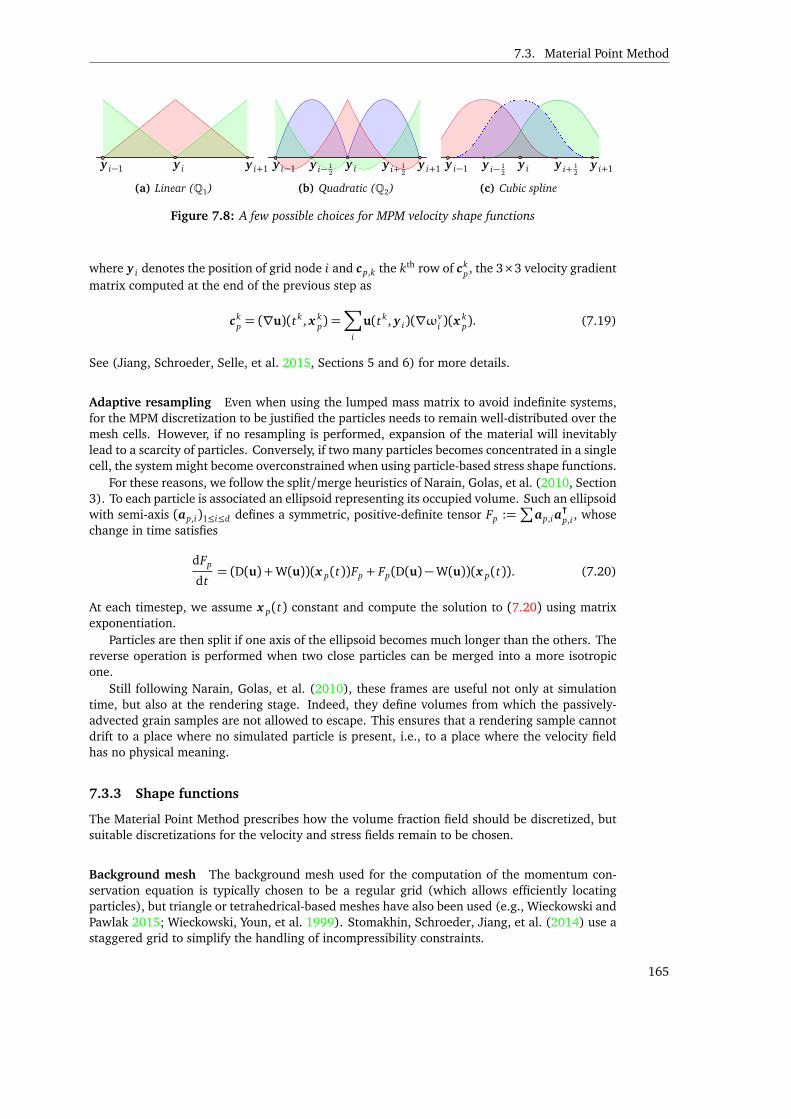
7.3. Material Point Method

y i y i+1y i−1

(a) Linear (Q1)

y i y i+1y i−1 y i− 12

y i+ 12

(b) Quadratic (Q2)

y i y i+1y i−1 y i− 12

y i+ 12

(c) Cubic spline

Figure 7.8: A few possible choices for MPM velocity shape functions

where y i denotes the position of grid node i and cp,k the kth row of ckp, the 3×3 velocity gradient

matrix computed at the end of the previous step as

ckp = (∇u)(tk, x k

p) =∑

i

u(tk, y i)(∇ωvi )(x

kp). (7.19)

See (Jiang, Schroeder, Selle, et al. 2015, Sections 5 and 6) for more details.

Adaptive resampling Even when using the lumped mass matrix to avoid indefinite systems,for the MPM discretization to be justified the particles needs to remain well-distributed over themesh cells. However, if no resampling is performed, expansion of the material will inevitablylead to a scarcity of particles. Conversely, if two many particles becomes concentrated in a singlecell, the system might become overconstrained when using particle-based stress shape functions.

For these reasons, we follow the split/merge heuristics of Narain, Golas, et al. (2010, Section3). To each particle is associated an ellipsoid representing its occupied volume. Such an ellipsoidwith semi-axis (ap,i)1≤i≤d defines a symmetric, positive-definite tensor Fp :=

∑ap,ia

⊺

p,i , whosechange in time satisfies

dFp

dt= (D(u) +W(u))(x p(t))Fp + Fp(D(u)−W(u))(x p(t)). (7.20)

At each timestep, we assume x p(t) constant and compute the solution to (7.20) using matrixexponentiation.

Particles are then split if one axis of the ellipsoid becomes much longer than the others. Thereverse operation is performed when two close particles can be merged into a more isotropicone.

Still following Narain, Golas, et al. (2010), these frames are useful not only at simulationtime, but also at the rendering stage. Indeed, they define volumes from which the passively-advected grain samples are not allowed to escape. This ensures that a rendering sample cannotdrift to a place where no simulated particle is present, i.e., to a place where the velocity fieldhas no physical meaning.

7.3.3 Shape functions

The Material Point Method prescribes how the volume fraction field should be discretized, butsuitable discretizations for the velocity and stress fields remain to be chosen.

Background mesh The background mesh used for the computation of the momentum con-servation equation is typically chosen to be a regular grid (which allows efficiently locatingparticles), but triangle or tetrahedrical-based meshes have also been used (e.g., Wieckowski andPawlak 2015; Wieckowski, Youn, et al. 1999). Stomakhin, Schroeder, Jiang, et al. (2014) use astaggered grid to simplify the handling of incompressibility constraints.

165

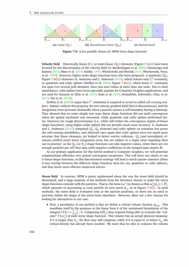
7. DRY GRANULAR FLOWS

y i y i+1y i−1

(a) Linear (Q1)

y i y i+1y i−1

(b) Discontinuous linear (Q1d)

y i y i+1y i−1

(c) Particle-based

Figure 7.9: A few possible choices for MPM stress shape functions

Velocity field Historically, linear (P1) or multi-linear (Q1) elements (Figure 7.8(a)) have beenfavored for the discretization of the velocity field (S. Bardenhagen et al. 2000; Dunatunga andKamrin 2015; Mast et al. 2014; Sulsky 1994; Wieckowski and Pawlak 2015; Wieckowski, Youn,et al. 1999). However, higher-order shape functions have also been proposed: d-quadratic (Q2;Figure 7.8(b)) elements (S. Andersen and L. Andersen 2010), which feature only C0 continuity,or quadratic and cubic splines (Steffen et al. 2008; Figure 7.8(c)), which boast C1 continuitybut span over several grid elements, have non-zero values at more than one node. Due to theirsmoothness, cubic splines have been especially popular for Computer Graphics applications, andare used for instance in (Klar et al. 2016; Ram et al. 2015; Stomakhin, Schroeder, Chai, et al.2013; Yue et al. 2015).

Steffen et al. (2008) argue that C1 continuity is required to avoid so-called cell-crossing arti-facts. Indeed, without this property, the test velocity gradient field D(v) is discontinuous, and theintegration error increases drastically when a particle crosses a cell-boundary during a timestep.They showed that on some simple test cases linear shape functions did not yield convergencewhen the spatial resolution was increased, while quadratic and cubic splines performed bet-ter. However, for rough discretizations (i.e., while still within the convergence regime of linearshape functions), using higher-order splines did not provide much more accuracy. S. Andersenand L. Andersen (2010) compared Q1, Q2 elements and cubic splines on scenarios less pronethe cell-crossing instabilities, and observed once again that cubic splines were not much moreaccurate that linear elements, yet helped to better resolve collisions. Q2 (and serendipity) el-ements yielded much lower integration error, but are subject to a major issue impeding theiruse in practice: as the Q2 (or P2) shape functions can take negative values, when there are notenough particles per cell they may yield negative coefficients in the lumped mass matrix M .

As our primary application for this hybrid method is Computer Graphics, we will prioritizecomputational efficiency over spatial convergence properties. This will drive our choice to used-linear shape functions, as this discretization strategy will lead to much sparser matrices (thereis less overlap between the different shape functions than for, say, quadratic or cubic splines),and thus much more efficient numerical solvers.

Stress field In contrast, MPM is pretty opinionated about the way the stress field should bediscretized, and a large majority of the methods from the literature choose to make the stressshape functions coincide with the particles. That is, the basis (ωτ) is chosen so thatωτq (x p) = δ

pq ,

which amounts to associating to each particle its own stress σp, as in Figure 7.9(c). In mostmethods, the stress field is evaluated only at the particle positions, so there are no need toprecisely define the shape of the stress basis elsewhere. However, there are a few reasons forlooking for alternatives in our case.

• First, a peculiarity of our method is that we define a critical volume fraction φmax. Thismanifests itself by the presence in the linear form k of the variational formulation of theintegral V (τ) :=

∫Ω

Id : τ. Computing k(Tp) thus requires being able to evaluate the “vol-

ume” V (ωτp) of each stress shape function. This volume has an actual physical meaning:if it is larger than Vp, the flow may still compress, while if it is equal to or below Vp, thecritical density has already been reached. We must thus be able to evaluate the volume

166

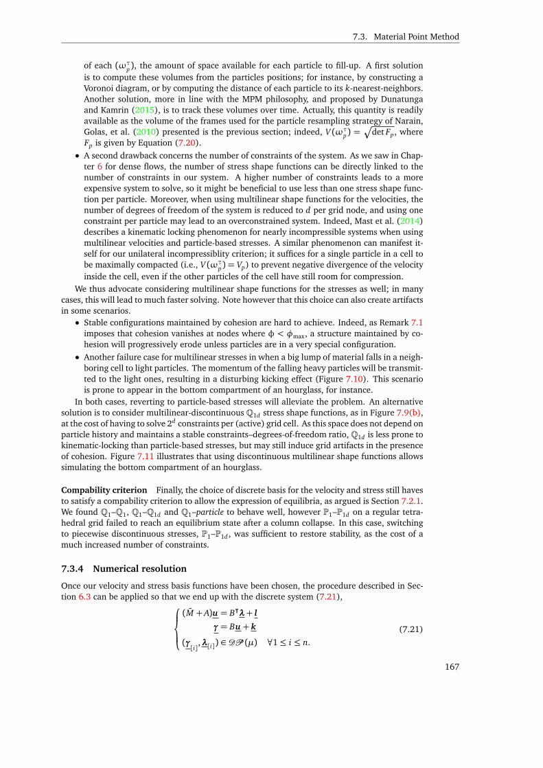
7.3. Material Point Method

of each (ωτp), the amount of space available for each particle to fill-up. A first solutionis to compute these volumes from the particles positions; for instance, by constructing aVoronoi diagram, or by computing the distance of each particle to its k-nearest-neighbors.Another solution, more in line with the MPM philosophy, and proposed by Dunatungaand Kamrin (2015), is to track these volumes over time. Actually, this quantity is readilyavailable as the volume of the frames used for the particle resampling strategy of Narain,Golas, et al. (2010) presented is the previous section; indeed, V (ωτp) =

Ædet Fp, where

Fp is given by Equation (7.20).

• A second drawback concerns the number of constraints of the system. As we saw in Chap-ter 6 for dense flows, the number of stress shape functions can be directly linked to thenumber of constraints in our system. A higher number of constraints leads to a moreexpensive system to solve, so it might be beneficial to use less than one stress shape func-tion per particle. Moreover, when using multilinear shape functions for the velocities, thenumber of degrees of freedom of the system is reduced to d per grid node, and using oneconstraint per particle may lead to an overconstrained system. Indeed, Mast et al. (2014)describes a kinematic locking phenomenon for nearly incompressible systems when usingmultilinear velocities and particle-based stresses. A similar phenomenon can manifest it-self for our unilateral incompressiblity criterion; it suffices for a single particle in a cell tobe maximally compacted (i.e., V (ωτp) = Vp) to prevent negative divergence of the velocityinside the cell, even if the other particles of the cell have still room for compression.

We thus advocate considering multilinear shape functions for the stresses as well; in manycases, this will lead to much faster solving. Note however that this choice can also create artifactsin some scenarios.• Stable configurations maintained by cohesion are hard to achieve. Indeed, as Remark 7.1

imposes that cohesion vanishes at nodes where φ < φmax, a structure maintained by co-hesion will progressively erode unless particles are in a very special configuration.

• Another failure case for multilinear stresses in when a big lump of material falls in a neigh-boring cell to light particles. The momentum of the falling heavy particles will be transmit-ted to the light ones, resulting in a disturbing kicking effect (Figure 7.10). This scenariois prone to appear in the bottom compartment of an hourglass, for instance.

In both cases, reverting to particle-based stresses will alleviate the problem. An alternativesolution is to consider multilinear-discontinuous Q1d stress shape functions, as in Figure 7.9(b),at the cost of having to solve 2d constraints per (active) grid cell. As this space does not depend onparticle history and maintains a stable constraints–degrees-of-freedom ratio, Q1d is less prone tokinematic-locking than particle-based stresses, but may still induce grid artifacts in the presenceof cohesion. Figure 7.11 illustrates that using discontinuous multilinear shape functions allowssimulating the bottom compartment of an hourglass.

Compability criterion Finally, the choice of discrete basis for the velocity and stress still havesto satisfy a compability criterion to allow the expression of equilibria, as argued is Section 7.2.1.We found Q1–Q1, Q1–Q1d and Q1–particle to behave well, however P1–P1d on a regular tetra-hedral grid failed to reach an equilibrium state after a column collapse. In this case, switchingto piecewise discontinuous stresses, P1–P1d , was sufficient to restore stability, as the cost of amuch increased number of constraints.

7.3.4 Numerical resolution

Once our velocity and stress basis functions have been chosen, the procedure described in Sec-tion 6.3 can be applied so that we end up with the discrete system (7.21),

(M + A)u = B⊺λ+ l

γ= Bu + k

(γ[i]

,λ[i]) ∈ DP (µ) ∀1≤ i ≤ n.

(7.21)

167

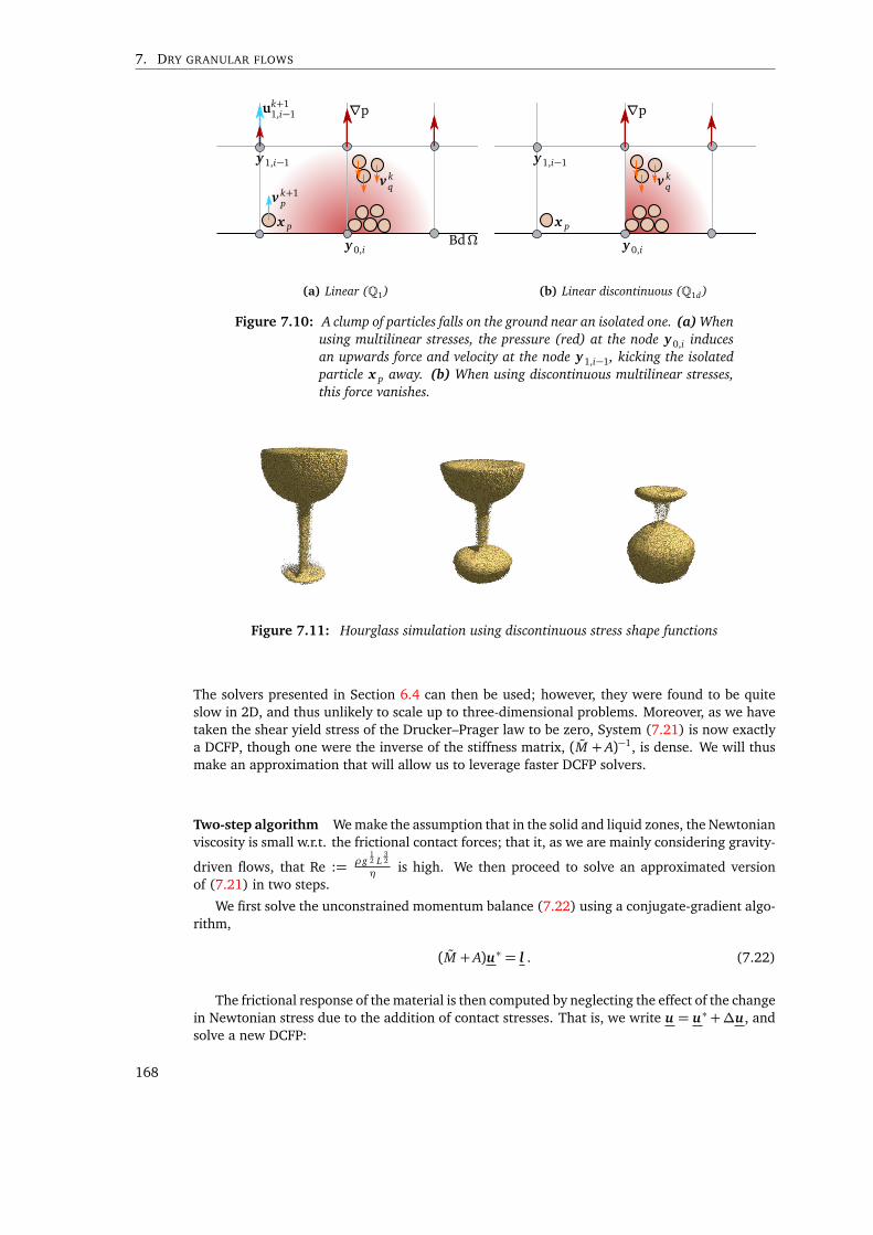
7. DRY GRANULAR FLOWS

y0,i

y1,i−1

x p

v kq

BdΩ

uk+11,i−1

v k+1p

∇p

(a) Linear (Q1)

y0,i

y1,i−1

x p

v kq

∇p

(b) Linear discontinuous (Q1d)

Figure 7.10: A clump of particles falls on the ground near an isolated one. (a) Whenusing multilinear stresses, the pressure (red) at the node y0,i inducesan upwards force and velocity at the node y1,i−1, kicking the isolatedparticle x p away. (b) When using discontinuous multilinear stresses,this force vanishes.

Figure 7.11: Hourglass simulation using discontinuous stress shape functions

The solvers presented in Section 6.4 can then be used; however, they were found to be quiteslow in 2D, and thus unlikely to scale up to three-dimensional problems. Moreover, as we havetaken the shear yield stress of the Drucker–Prager law to be zero, System (7.21) is now exactlya DCFP, though one were the inverse of the stiffness matrix, (M + A)−1, is dense. We will thusmake an approximation that will allow us to leverage faster DCFP solvers.

Two-step algorithm We make the assumption that in the solid and liquid zones, the Newtonianviscosity is small w.r.t. the frictional contact forces; that it, as we are mainly considering gravity-

driven flows, that Re := ρg12 L

32

η is high. We then proceed to solve an approximated versionof (7.21) in two steps.

We first solve the unconstrained momentum balance (7.22) using a conjugate-gradient algo-rithm,

(M + A)u∗ = l . (7.22)

The frictional response of the material is then computed by neglecting the effect of the changein Newtonian stress due to the addition of contact stresses. That is, we write u = u∗ +∆u, andsolve a new DCFP:

168

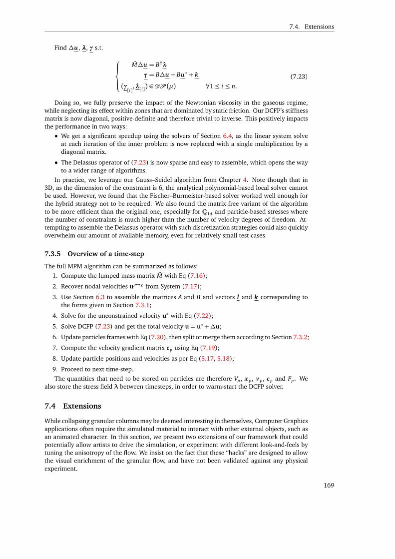
7.4. Extensions

Find ∆u, λ, γ s.t.

M∆u = B⊺λ

γ= B∆u + Bu∗ + k

(γ[i]

,λ[i]) ∈ DP (µ) ∀1≤ i ≤ n.

(7.23)

Doing so, we fully preserve the impact of the Newtonian viscosity in the gaseous regime,while neglecting its effect within zones that are dominated by static friction. Our DCFP’s stiffnessmatrix is now diagonal, positive-definite and therefore trivial to inverse. This positively impactsthe performance in two ways:

• We get a significant speedup using the solvers of Section 6.4, as the linear system solveat each iteration of the inner problem is now replaced with a single multiplication by adiagonal matrix.

• The Delassus operator of (7.23) is now sparse and easy to assemble, which opens the wayto a wider range of algorithms.

In practice, we leverage our Gauss–Seidel algorithm from Chapter 4. Note though that in3D, as the dimension of the constraint is 6, the analytical polynomial-based local solver cannotbe used. However, we found that the Fischer–Burmeister-based solver worked well enough forthe hybrid strategy not to be required. We also found the matrix-free variant of the algorithmto be more efficient than the original one, especially for Q1d and particle-based stresses wherethe number of constraints is much higher than the number of velocity degrees of freedom. At-tempting to assemble the Delassus operator with such discretization strategies could also quicklyoverwhelm our amount of available memory, even for relatively small test cases.

7.3.5 Overview of a time-step

The full MPM algorithm can be summarized as follows:

1. Compute the lumped mass matrix M with Eq (7.16);

2. Recover nodal velocities up 7→g from System (7.17);

3. Use Section 6.3 to assemble the matrices A and B and vectors l and k corresponding tothe forms given in Section 7.3.1;

4. Solve for the unconstrained velocity u∗ with Eq (7.22);

5. Solve DCFP (7.23) and get the total velocity u= u∗ +∆u;

6. Update particles frames with Eq (7.20), then split or merge them according to Section 7.3.2;

7. Compute the velocity gradient matrix cp using Eq (7.19);

8. Update particle positions and velocities as per Eq (5.17, 5.18);

9. Proceed to next time-step.

The quantities that need to be stored on particles are therefore Vp, x p, v p, cp and Fp. Wealso store the stress field λ between timesteps, in order to warm-start the DCFP solver.

7.4 Extensions

While collapsing granular columns may be deemed interesting in themselves, Computer Graphicsapplications often require the simulated material to interact with other external objects, such asan animated character. In this section, we present two extensions of our framework that couldpotentially allow artists to drive the simulation, or experiment with different look-and-feels bytuning the anisotropy of the flow. We insist on the fact that these “hacks” are designed to allowthe visual enrichment of the granular flow, and have not been validated against any physicalexperiment.

169

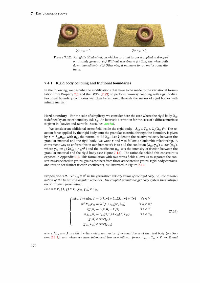
7. DRY GRANULAR FLOWS

(a) µRB = 0 (b) µRB > 0

Figure 7.12: A slightly tilted wheel, on which a constant torque is applied, is droppedon a sandy ground. (a) Without wheel-sand friction, the wheel fallsdown immediately. (b) Otherwise, it manages to roll on for some dis-tance.

7.4.1 Rigid body coupling and frictional boundaries

In the following, we describe the modifications that have to be made to the variational formu-lation from Property 7.1 and the DCFP (7.23) to perform two-way coupling with rigid bodies.Frictional boundary conditions will then be imposed through the means of rigid bodies withinfinite inertia.

Hard boundary For the sake of simplicity, we consider here the case where the rigid body ΩRB

is defined by an exact boundary, BdΩRB. An heuristic derivation for the case of a diffuse interfaceis given in (Daviet and Bertails-Descoubes 2016a).

We consider an additional stress field inside the rigid body, −λRB ∈ TRB ⊂ L2(ΩRB)sd . The re-

action force applied by the rigid body onto the granular material through the boundary is givenby r = λRBnRB, with nRB the normal to BdΩRB. Let v denote the relative velocity between thegranular material and the rigid body; we want r and v to follow a Coulombic relationship. Aconvenient way to enforce this in our framework is to add the condition (λRB,γRB) ∈ DP (µRB),where γRB := 1

2

vn⊺RB + nRBv⊺

and the coefficient µRB sets the intensity of friction between the

granular material and the rigid body (see Figure 7.12). The rationale behind this constraint isexposed in Appendix C.2. This formulation with two stress fields allows us to separate the con-straints associated to grains–grains contacts from those associated to grains–rigid-body contacts,and thus to set distinct friction coefficients, as illustrated in Figure 7.12.

Proposition 7.2. Let vRB ∈ R6 be the generalized velocity vector of the rigid body, i.e., the concate-nation of the linear and angular velocities. The coupled granular–rigid body system then satisfiesthe variational formulation:

Find u ∈ V , (λ,γ) ∈ T, (λRB,γRB) ∈ TRB,

m(u,v) + a(u,v) = b(λ,v) + bRB(λRB,v) + l(v) ∀v ∈ V

w ⊺MRBvRB = w T f + cRB(w ,λRB) ∀w ∈ R6

s(γ,u) = b(τ,u) + k(τ) ∀τ ∈ T

s(γRB,u) = bRB(τ,u) + cRB(τ, vRB) ∀τ ∈ TRB

(γ,λ) ∈ DP (µ)(γRB,λRB) ∈ DP (µRB)

(7.24)

where MRB and f are the inertia matrix and vector of external forces of the rigid body (see Sec-tion 2.1.1), and where we have introduced two new bilinear forms, bRB : TRB × V → R and

170

7.4. Extensions

cRB : TRB ×R6→ R,

bRB(τ,u) :=1

2

∫

BdΩRB

un⊺RB + nRBu

⊺

: τ

cRB(τ, vRB) := −1

2

∫

BdΩRB

J(vRB)n

⊺RB + nRBJ(vRB)

⊺

: τ,

with J(vRB) the velocity field spawned by a rigid body with linear and angular velocities vRB andcenter of mass x RB,

J(vRB)(x ) = J

v linRB

vangRB

(x ) = v lin

RB+ v

angRB ∧ (x − x RB).

Discretizing System (7.24) once again yields a DCFP, which can be solved as usual.

Proof. By definition v= u− J(vRB), so the weak definition of γRB as per the fourth line of (7.24)is consistent.

We will now justify that the terms bRB(λRB,v) and cRB(λr b, w ) added to the momentum con-servation equations of the granular material and rigid body (i.e., the first two lines of (7.24)) docorrespond to the interaction between the two media.

We recall the identity, for any symmetric tensor τ ∈ Sd , and for (v ,n) ∈ Rd ×Rd ,

v⊺τn =∑

i

v i

∑

j

τi jn j =∑

i, j

v in jτi, j = τ : v ⊗ n =1

2τ : (v ⊗ n + n ⊗ v) . (7.25)

The force f C and torque LC applied onto the rigid body by the granular material are givenby (Batty et al. 2007):

f C =

∫

ΩRB

∇ · [−λRB] LC =

∫

ΩRB

(x − x RB)∧∇ · [−λRB] .

For any r ∈ R3, there holds

r T f C = r T

∫

ΩRB

∇ · [−λRB] = −∫

BdΩRB

r TλRBnRB

= −∫

BdΩRB

1

2λRB : (nRB ⊗ r + r ⊗ nRB) using (7.25)

r T LC = r T

∫

ΩRB

(x − x RB)∧∇ · [−λRB] = −∫

ΩRB

r T [x − x RB]∧∇ ·λRB

=

∫

ΩRB

[x − x RB]∧ r

⊺∇ ·λRB

=

∫

BdΩRB

[x − x RB]∧ r

⊺λRBnRB −

∫

ΩRB

D([x − x RB]∧ r ) : λRB

︸ ︷︷ ︸=0

=

∫

BdΩRB

1

2λRB :

nRB ⊗

[x − x RB]∧ r

+[x − x RB]∧ r

⊗ nRB

using (7.25)

= −∫

BdΩRB

1

2λRB : (nRB ⊗ (r ∧ [x − x RB]) + (r ∧ [x − x RB])⊗ nRB) ,

171

7. DRY GRANULAR FLOWS

(a)

u

(b) (c)

Figure 7.13: Rationale for our handling of anisotropy. (a) (b) A shear flow inducesa privileged orientation. (c) Aligned particles yield anisotropic macro-scopic friction: reduced in the horizontal direction, more intense in thevertical one.

which means, ∀w ∈ R6,

w ⊺

f C

LC

= cRB(λRB, w ),

and hence justifies the second line of (7.24).Concerning the momentum conservation of the granular material, using (7.25),

b(λRB,v) =

∫

BdΩRB

⟨λRBnRB,v⟩,

which does correspond to the force applied by the rigid body onto the granular material throughthe boundary.

7.4.2 Anisotropy

Many granular materials are composed of anisotropic grains that are thinner along one direction.This is typically the case for corn flakes, or, more common in the Computer Graphics imaginary,piles of gold coins (see Figure 7.23). It is noteworthy that anisotropy at the grain scale doesplay a role on the collective granular behavior. Indeed, while there is no reason to favor anyparticular direction when the grains are randomly oriented, when all their normals are alignedthe macroscopic friction becomes anisotropic: it has much less dissipative effect when grains aresliding on top of each other, rather than when their relative displacement is along their commonnormal (see Figure 7.13 for an illustration).

However, remember that each one of our particles does not represent a single grain, but acollection of them, and thus it may contain different orientations. Rather than mapping a normalto each particle, we should instead store a probability distribution function (PDF) ψ(n). Forefficiency purposes we store only its second moment, the symmetric tensor ν2 =

∫S2 nn⊺ψ(n)dn.

In the following, we propose a way to model the influence of ν2 on our DP (µ) rheology, thenconstruct an heuristic evolution equation for this tensor.

Modification of DP (µ) Anisotropy can be included in the rheology by simply replacing thenorm | · | with the norm | · |A associated to the scalar product ⟨·, ·⟩A := 1

2 (· :A ) : (A : ·), whereA is a fourth-order symmetric tensor. In order for the maximum dissipation principle to remainsatisfied, γ should also be replaced withA : γ on the first line of Equation (7.8).

We choose to construct A such as A : τ = NτN , i.e., Ai jkℓ = NikNℓ j , where the symmetrictensor N is deduced from the normal orientation tensor ν2 following N−1 = (1 − α)I + dαν2,where 0 ≤ α ≤ 1 is a dimensionless coefficient parameterizing the amount of anisotropy in thefrictional law. Using this formula, the effective friction coefficient will remain equal to µ forisotropic orientations (the d eigenvalues of ν2 equal to 1

d ). If all the normals are oriented in thesame direction (a single non-zero eigenvalue equal to 1), the effective friction coefficient will be(1+ (d − 1)α)2µ in the normal direction, and (1−α)2µ in the tangential ones.

172

7.5. Results

Instead of modifying our friction solver, we can introduce the linear operator N : λ 7→Trλ

d I+ N DevλN , make the changes of variable λ = Nλ, γ = Nγ and replace the DCFP (7.23)

with

M∆u = B⊺N−1λ

γ= N−1B∆u + N−1Bu∗ + k

(γ[i]

,λ[i]) ∈ DP (µ) ∀1≤ i ≤ n.

It now remains to describe how the second moment of the orientation normal PDF, ν2,changes in time.

Evolution of ν2 The evolution of the orientation of rigid ellipsoids in a shearing Newtonianflow has been described by Jeffery (1922). Integrating it over the unit sphere of all possibleorientations (see e.g., Folgar and Tucker 1984) yields the evolution of the second moment tensorπ2 of the orientation PDF,

Dπ2

Dt=W(u)π2 +π2 W(u) + ℓ(D(u)π2 +π2 D(u)− 2 D(u) : π4) (7.26)

where 0≤ ℓ≤ 1 is a coefficient describing the elongation of the ellipsoid, ℓ= L/W−1L/W+1 , and π4 the

fourth moment of the orientation PDF. The parameter ℓ affects the tendency of the ellipsoids toalign with the flow. Note that this evolution equation does not directly apply to our problem:

• Jeffery’s equation consider the velocity of a surrounding Newtonian fluid. In our case, thevelocity field u is that of the granular matter itself.

• This model is only valid for dilute suspensions. Many authors have postulated laws forextending it to higher particle concentrations (e.g., Folgar and Tucker (1984) added anadditional dissipative term modeling random collisions between particles in the semi-concentrated regime).

We will nonetheless take inspiration from this evolution equation and propose the followingalgorithm for the evolution of our normal orientation tensor ν2, which yields good enough resultsfor our purposes — for high values of ℓ, flat particles in a shearing flow do tend to become parallelto each other, which corresponds to the expected behavior (see Figures 7.13 and 7.15).

1. Deduce π2(t) from ν2(t) as π2 =1

d−1 P(I− D)P⊺, where P and D are given by the eigendecomposition of ν2.

2. Explicitly compute π2(t +∆t) using Equation (7.26) and the quadratic approximation ofthe π4 tensor, π4 ∼ π2 ⊗π2 — the outer tensor product of π2 with itself.

3. Deduce ν2(t +∆t) from π2(t +∆t), and normalize it using ν2← ν2‖ν2‖1

.

7.5 Results

We used this hybrid framework to perform 3D simulations of granular materials. Rendering wasdone following the method of Narain, Golas, et al. (2010), yielding several samples for eachsimulation particle, but using rasterization instead of ray-tracing. All simulation code, includingthe finite-element discretization, relied on a purposely-built library, that has since then beenreleased as open-source2. Unless otherwise mentioned, trilinear shape functions were used forthe stresses. The DCFP were solved using the bogus library. As usual, all our simulations andbenchmarks were run on Intel R© Xeon R© quad-core workstations.

2http://bipop.inrialpes.fr/~gdaviet/code/sand6

173

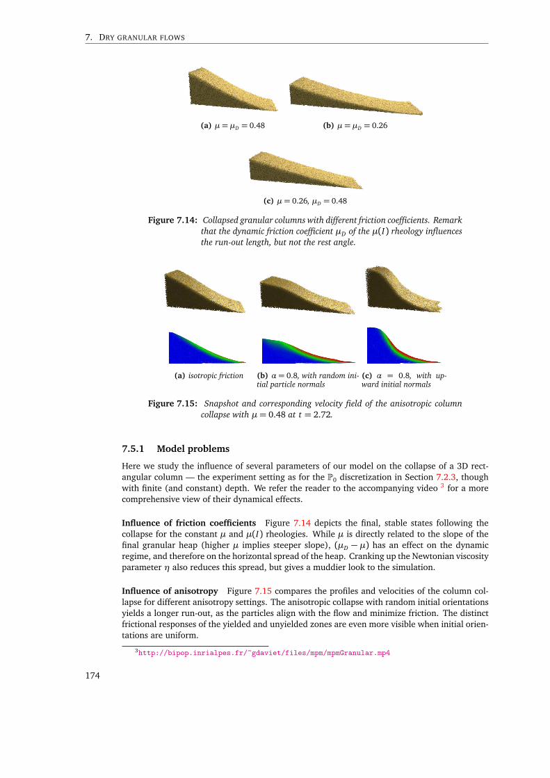
7. DRY GRANULAR FLOWS

(a) µ= µD = 0.48 (b) µ= µD = 0.26

(c) µ= 0.26, µD = 0.48

Figure 7.14: Collapsed granular columns with different friction coefficients. Remarkthat the dynamic friction coefficient µD of the µ(I) rheology influencesthe run-out length, but not the rest angle.

(a) isotropic friction (b) α= 0.8, with random ini-tial particle normals

(c) α = 0.8, with up-ward initial normals

Figure 7.15: Snapshot and corresponding velocity field of the anisotropic columncollapse with µ= 0.48 at t = 2.72.

7.5.1 Model problems

Here we study the influence of several parameters of our model on the collapse of a 3D rect-angular column — the experiment setting as for the P0 discretization in Section 7.2.3, thoughwith finite (and constant) depth. We refer the reader to the accompanying video 3 for a morecomprehensive view of their dynamical effects.

Influence of friction coefficients Figure 7.14 depicts the final, stable states following thecollapse for the constant µ and µ(I) rheologies. While µ is directly related to the slope of thefinal granular heap (higher µ implies steeper slope), (µD − µ) has an effect on the dynamicregime, and therefore on the horizontal spread of the heap. Cranking up the Newtonian viscosityparameter η also reduces this spread, but gives a muddier look to the simulation.

Influence of anisotropy Figure 7.15 compares the profiles and velocities of the column col-lapse for different anisotropy settings. The anisotropic collapse with random initial orientationsyields a longer run-out, as the particles align with the flow and minimize friction. The distinctfrictional responses of the yielded and unyielded zones are even more visible when initial orien-tations are uniform.

3http://bipop.inrialpes.fr/~gdaviet/files/mpm/mpmGranular.mp4

174

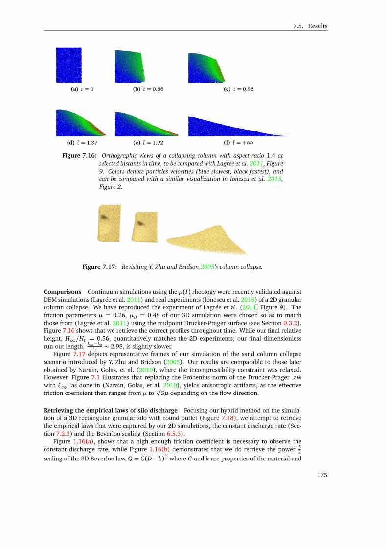
7.5. Results

(a) t = 0 (b) t = 0.66 (c) t = 0.96

(d) t = 1.37 (e) t = 1.92 (f) t = +∞

Figure 7.16: Orthographic views of a collapsing column with aspect-ratio 1.4 atselected instants in time, to be compared with Lagrée et al. 2011, Figure9. Colors denote particles velocities (blue slowest, black fastest), andcan be compared with a similar visualization in Ionescu et al. 2015,Figure 2.

Figure 7.17: Revisiting Y. Zhu and Bridson 2005’s column collapse.

Comparisons Continuum simulations using the µ(I) rheology were recently validated againstDEM simulations (Lagrée et al. 2011) and real experiments (Ionescu et al. 2015) of a 2D granularcolumn collapse. We have reproduced the experiment of Lagrée et al. (2011, Figure 9). Thefriction parameters µ = 0.26, µD = 0.48 of our 3D simulation were chosen so as to matchthose from (Lagrée et al. 2011) using the midpoint Drucker-Prager surface (see Section 0.3.2).Figure 7.16 shows that we retrieve the correct profiles throughout time. While our final relativeheight, H∞/H0 = 0.56, quantitatively matches the 2D experiments, our final dimensionlessrun-out length, L∞−L0

L0∼ 2.98, is slightly slower.

Figure 7.17 depicts representative frames of our simulation of the sand column collapsescenario introduced by Y. Zhu and Bridson (2005). Our results are comparable to those laterobtained by Narain, Golas, et al. (2010), where the incompressibility constraint was relaxed.However, Figure 7.1 illustrates that replacing the Frobenius norm of the Drucker-Prager lawwith ℓ∞, as done in (Narain, Golas, et al. 2010), yields anisotropic artifacts, as the effectivefriction coefficient then ranges from µ to

p5µ depending on the flow direction.

Retrieving the empirical laws of silo discharge Focusing our hybrid method on the simula-tion of a 3D rectangular granular silo with round outlet (Figure 7.18), we attempt to retrievethe empirical laws that were captured by our 2D simulations, the constant discharge rate (Sec-tion 7.2.3) and the Beverloo scaling (Section 6.5.3).

Figure 1.16(a), shows that a high enough friction coefficient is necessary to observe theconstant discharge rate, while Figure 1.16(b) demonstrates that we do retrieve the power 5

2

scaling of the 3D Beverloo law, Q = C(D− k)52 where C and k are properties of the material and

175

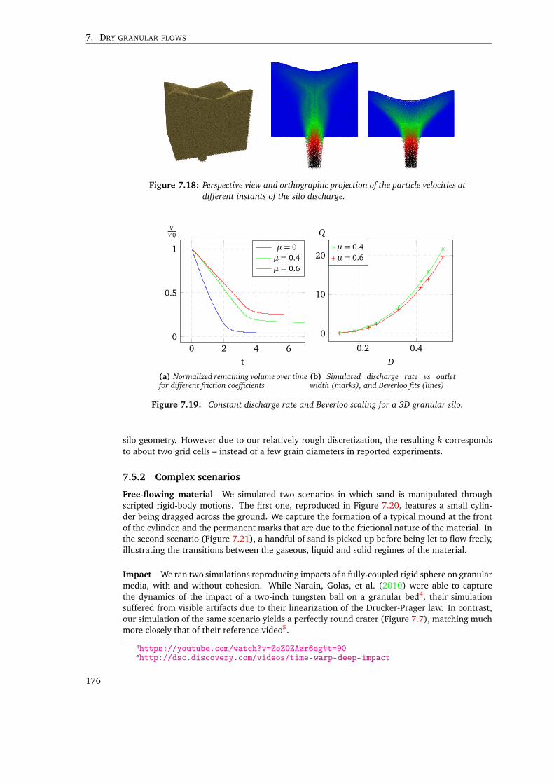
7. DRY GRANULAR FLOWS

Figure 7.18: Perspective view and orthographic projection of the particle velocities atdifferent instants of the silo discharge.

0 2 4 60

0.5

1

t

VV0

µ= 0µ= 0.4µ= 0.6

(a) Normalized remaining volume over timefor different friction coefficients

0.2 0.4

0

10

20

D

Q

µ= 0.4µ= 0.6

(b) Simulated discharge rate vs outletwidth (marks), and Beverloo fits (lines)

Figure 7.19: Constant discharge rate and Beverloo scaling for a 3D granular silo.

silo geometry. However due to our relatively rough discretization, the resulting k correspondsto about two grid cells – instead of a few grain diameters in reported experiments.

7.5.2 Complex scenarios

Free-flowing material We simulated two scenarios in which sand is manipulated throughscripted rigid-body motions. The first one, reproduced in Figure 7.20, features a small cylin-der being dragged across the ground. We capture the formation of a typical mound at the frontof the cylinder, and the permanent marks that are due to the frictional nature of the material. Inthe second scenario (Figure 7.21), a handful of sand is picked up before being let to flow freely,illustrating the transitions between the gaseous, liquid and solid regimes of the material.

Impact We ran two simulations reproducing impacts of a fully-coupled rigid sphere on granularmedia, with and without cohesion. While Narain, Golas, et al. (2010) were able to capturethe dynamics of the impact of a two-inch tungsten ball on a granular bed4, their simulationsuffered from visible artifacts due to their linearization of the Drucker-Prager law. In contrast,our simulation of the same scenario yields a perfectly round crater (Figure 7.7), matching muchmore closely that of their reference video5.

4https://youtube.com/watch?v=ZoZ0ZAzr6eg#t=905http://dsc.discovery.com/videos/time-warp-deep-impact

176

7.5. Results

Figure 7.20: Letters drawn by dragging a stick in the sand. Right: a typical moundgrows at the front of the stick.

Figure 7.21: Picking-up sand and letting it flow away.

(a) Trilinear stress shape functions and cohesion decay

(b) Particle-based stress shape functions without cohesion decay

Figure 7.22: A sphere impacting a sand tower initially standing up thanks to a highcohesion coefficient.

177

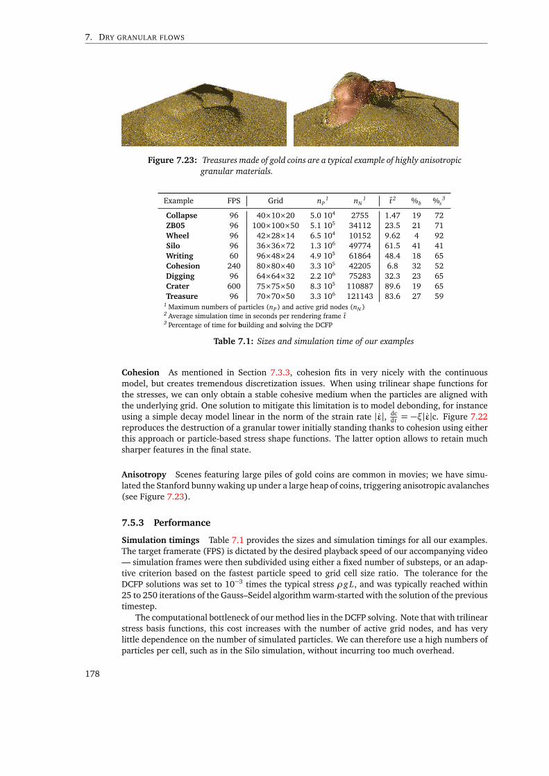
7. DRY GRANULAR FLOWS

Figure 7.23: Treasures made of gold coins are a typical example of highly anisotropicgranular materials.

Example FPS Grid nP1 nN

1 t2 %b %s3

Collapse 96 40×10×20 5.0 104 2755 1.47 19 72ZB05 96 100×100×50 5.1 105 34112 23.5 21 71Wheel 96 42×28×14 6.5 104 10152 9.62 4 92Silo 96 36×36×72 1.3 106 49774 61.5 41 41Writing 60 96×48×24 4.9 105 61864 48.4 18 65Cohesion 240 80×80×40 3.3 105 42205 6.8 32 52Digging 96 64×64×32 2.2 106 75283 32.3 23 65Crater 600 75×75×50 8.3 105 110887 89.6 19 65Treasure 96 70×70×50 3.3 106 121143 83.6 27 59

1 Maximum numbers of particles (nP ) and active grid nodes (nN )2 Average simulation time in seconds per rendering frame t3 Percentage of time for building and solving the DCFP

Table 7.1: Sizes and simulation time of our examples

Cohesion As mentioned in Section 7.3.3, cohesion fits in very nicely with the continuousmodel, but creates tremendous discretization issues. When using trilinear shape functions forthe stresses, we can only obtain a stable cohesive medium when the particles are aligned withthe underlying grid. One solution to mitigate this limitation is to model debonding, for instanceusing a simple decay model linear in the norm of the strain rate |ε|, dc

dt = −ξ|ε|c. Figure 7.22reproduces the destruction of a granular tower initially standing thanks to cohesion using eitherthis approach or particle-based stress shape functions. The latter option allows to retain muchsharper features in the final state.

Anisotropy Scenes featuring large piles of gold coins are common in movies; we have simu-lated the Stanford bunny waking up under a large heap of coins, triggering anisotropic avalanches(see Figure 7.23).

7.5.3 Performance

Simulation timings Table 7.1 provides the sizes and simulation timings for all our examples.The target framerate (FPS) is dictated by the desired playback speed of our accompanying video— simulation frames were then subdivided using either a fixed number of substeps, or an adap-tive criterion based on the fastest particle speed to grid cell size ratio. The tolerance for theDCFP solutions was set to 10−3 times the typical stress ρg L, and was typically reached within25 to 250 iterations of the Gauss–Seidel algorithm warm-started with the solution of the previoustimestep.

The computational bottleneck of our method lies in the DCFP solving. Note that with trilinearstress basis functions, this cost increases with the number of active grid nodes, and has verylittle dependence on the number of simulated particles. We can therefore use a high numbers ofparticles per cell, such as in the Silo simulation, without incurring too much overhead.

178

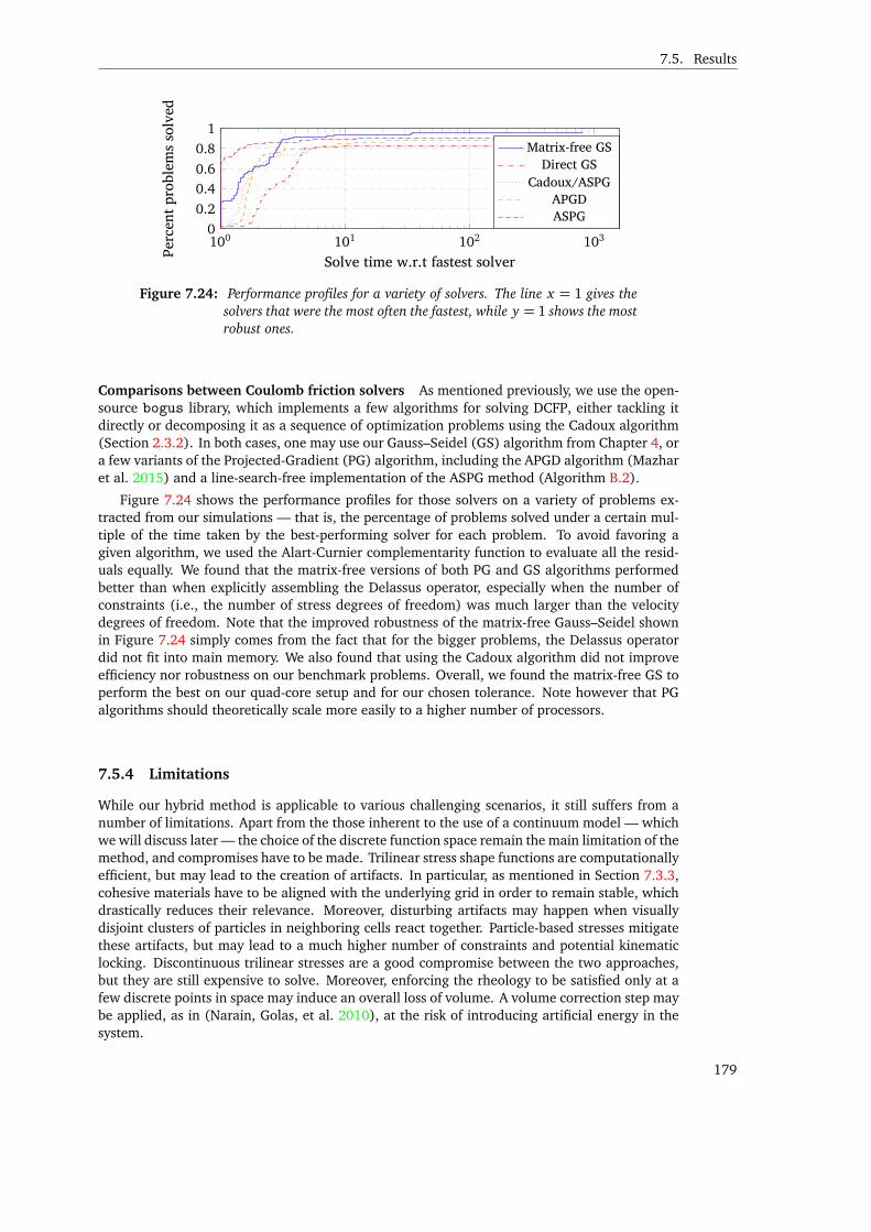
7.5. Results

100 101 102 1030

0.2

0.40.6

0.81

Solve time w.r.t fastest solverPerce

ntprob

lemss

olved

Matrix-free GSDirect GS

Cadoux/ASPGAPGDASPG

Figure 7.24: Performance profiles for a variety of solvers. The line x = 1 gives thesolvers that were the most often the fastest, while y = 1 shows the mostrobust ones.

Comparisons between Coulomb friction solvers As mentioned previously, we use the open-source bogus library, which implements a few algorithms for solving DCFP, either tackling itdirectly or decomposing it as a sequence of optimization problems using the Cadoux algorithm(Section 2.3.2). In both cases, one may use our Gauss–Seidel (GS) algorithm from Chapter 4, ora few variants of the Projected-Gradient (PG) algorithm, including the APGD algorithm (Mazharet al. 2015) and a line-search-free implementation of the ASPG method (Algorithm B.2).

Figure 7.24 shows the performance profiles for those solvers on a variety of problems ex-tracted from our simulations — that is, the percentage of problems solved under a certain mul-tiple of the time taken by the best-performing solver for each problem. To avoid favoring agiven algorithm, we used the Alart-Curnier complementarity function to evaluate all the resid-uals equally. We found that the matrix-free versions of both PG and GS algorithms performedbetter than when explicitly assembling the Delassus operator, especially when the number ofconstraints (i.e., the number of stress degrees of freedom) was much larger than the velocitydegrees of freedom. Note that the improved robustness of the matrix-free Gauss–Seidel shownin Figure 7.24 simply comes from the fact that for the bigger problems, the Delassus operatordid not fit into main memory. We also found that using the Cadoux algorithm did not improveefficiency nor robustness on our benchmark problems. Overall, we found the matrix-free GS toperform the best on our quad-core setup and for our chosen tolerance. Note however that PGalgorithms should theoretically scale more easily to a higher number of processors.

7.5.4 Limitations

While our hybrid method is applicable to various challenging scenarios, it still suffers from anumber of limitations. Apart from the those inherent to the use of a continuum model — whichwe will discuss later — the choice of the discrete function space remain the main limitation of themethod, and compromises have to be made. Trilinear stress shape functions are computationallyefficient, but may lead to the creation of artifacts. In particular, as mentioned in Section 7.3.3,cohesive materials have to be aligned with the underlying grid in order to remain stable, whichdrastically reduces their relevance. Moreover, disturbing artifacts may happen when visuallydisjoint clusters of particles in neighboring cells react together. Particle-based stresses mitigatethese artifacts, but may lead to a much higher number of constraints and potential kinematiclocking. Discontinuous trilinear stresses are a good compromise between the two approaches,but they are still expensive to solve. Moreover, enforcing the rheology to be satisfied only at afew discrete points in space may induce an overall loss of volume. A volume correction step maybe applied, as in (Narain, Golas, et al. 2010), at the risk of introducing artificial energy in thesystem.

179

7. DRY GRANULAR FLOWS

7.6 Discussion

In this chapter, we presented an extension of the numerical method of Chapter 6 that is appli-cable to general granular flows with varying volume fraction of grains. We saw that in order toobtain a symmetric system, the maximal volume fraction constraint has to be discretized usingthe Lagrangian point of view — i.e., looking at positions that are moving with the grains. Themain difficulty in our approach consists in finding appropriate discretization spaces for the ve-locity, stress and volume fraction fields; we proposed two different choices, piecewise-constantdiscretization or the Material Point Method with low-order velocities and stresses. However,both of those choices suffer from limitations; finding better discretization spaces remain one ofour priority for future work. Despite this, our method was still able to capture qualitative char-acteristics of granular flows, and to reduce the visual artifacts of previous approaches such as(Narain, Golas, et al. 2010) at a roughly similar computational cost. Moreover, in contrast to thecited approach, our numerical method derives from a proper, consistent, variational formulationrather than an ad-hoc sequence of corrective steps. This will allow us to accommodate the morecomplex case of diphasic flows in the next chapter.

The continuous model itself is also subject to several limitations; due to our continuum ap-proximation of granulars, the range of possible simulations is restricted to homogeneous ma-terials where all grains share common features, such as their size. Our method is thus notappropriate for simulating polydisperse media with various grain shapes. Moreover, being amacroscopic law, our DP (µ) rheology cannot model specific arrangements of grains, such asthe formation of arches clogging the silo outlet. Our definition of a constant maximal volumefraction is also flawed; it is well known that different packings are possible over time for a givengranular medium, exhibiting different volume fractions. Moreover, Roux and Radjai (1998) statethat the packing volume fraction has an influence on the dilatancy angle; our model is unable tocapture this phenomenon. Finally, our equations are based on an inelastic impact assumption,while a non-zero restitution coefficient might be necessary to properly model some classes ofgranular flows.

A last limitation, which we are going to address in the next chapter, is that we completely ig-nored the presence of a fluid around the grains. While the influence of air on large-enough grainsis negligible, this hypothesis prevents us from tackling interesting scenarios, such as immersedavalanches.

180

8 Granular flows inside a fluid

This chapter is dedicated to the simulation of a granular material inside a Newtonian fluid. Incontrast with the previous chapter, the surrounding fluid is no longer considered to be muchlighter than the grains. Our main objective is to capture the qualitative influence of the sur-rounding fluid on the dynamics of the granular material; for instance, looking at the dynamicsof an ash cloud, or at how water will affect the avalanching behavior of a column of sand. How-ever, we still want said avalanche to eventually come to rest. For this reason, we still assumethe existence of a critical volume fraction of grains φmax such that when φ reaches φmax, thegrains interact together through dry frictional contact, and obey the non-associated Drucker–Prager flow rule. We also suppose that no mass transfer occurs between the two phases (i.e., nochemical reaction).

Even more than in the dry case, immersed granular materials can exhibit different regimes,depending for instance on whether the inertia of the grains or that of the fluid is preponderant(Topin, Monerie, et al. 2012); we will attempt to capture this behavior in our continuum simula-tions. As we will see, the ratio of the particle size w.r.t. the domain will be of utmost importance.To the best of our knowledge, the method presented in this chapter is the first to combine fully-coupled two-phase equations for immersed granular flows with implicit, nonsmooth treatmentof the Drucker–Prager rheology. An interesting property of our method is that it will ultimatelylead to equations very similar to that of the dry case discussed in Chapter 7. The main differenceswill be the presence of a second velocity field (the fluctuation, modeling the velocity differencebetween the two phases), and linear constraints enforcing the conservation of the local volumeof matter.

Notations Quantities associated with the granular phase will be denoted with a “g” subscript(e.g., ug will be the velocity field of the grains ) while those associated with the surrounding fluidwill be denoted with a “f”. As in the previous chapters, φ will denote the grain volume fraction,and we will assume that the fluid occupies the entirety of the volume where there are no grains.That is, the density of the granular phase will be ρg(φ) = ρgφ, and the density of the fluid phasewill be ρ f (φ) = ρ f (1−φ). The total density of the mixture will thus be ρ(φ) = ρ f (φ)+ρg(φ). Wealso define two velocities for the mixture: the mass-averaged velocity, um, such that ρ(φ)um =

ρg(φ)ug + ρ f (φ)u f , and the volume-averaged velocity, uv := φug + (1−φ)u f .

8.1 Related work

As the behavior of dry granular materials has yet to be fully understood, it is not surprising thatno general model exists for immersed granular materials. However, they have been the subjectof extensive studies in the second-half of the last century, in a variety of domains. Differentmodels for different applications evolved largely in parallel, but cross-pollinated over time.

The study of the influence of dispersed grains in a Newtonian fluid goes as far as Einstein(1906), who postulated that the effective viscosity ηeff of a slurry — a dilute suspension ofspherical particles — followed the law ηeff(φ) = η f (1 +

52φ), where η f is the viscosity of the

pure Newtonian fluid, and φ the volume fraction of particles.Several applications have motivated subsequent work on related problems. In rough chrono-

logical order, we can mention:

181

8. GRANULAR FLOWS INSIDE A FLUID

• Civil engineering and soil mechanics, with the work of Terzaghi (1936) on the reductionof the effective stress in a saturated porous material; later, with the poroelasticity theoryof Biot (1955);

• Sedimentation and consolidation, of practical interest for the mining industry, with theseminal work of Kynch (1952);

• Fluidized granular beds, of special importance in chemical engineering, following Jackson(1963);

• Particulate gravity currents — that is, gravity-induced flows that mostly spread in thehorizontal direction, such as avalanches (Parker et al. 1986);

• Sediment transport in river beds (Hanes and Bowen 1985);

• Finally, Computer Graphics (Lenaerts and Dutré 2009; Rungjiratananon et al. 2008).

To construct our numerical model, we will mainly follow the ideas of Jackson (2000). How-ever, we propose below to walk through the different approaches that have been explored forthe continuum simulation of grains in a Newtonian fluid.

8.1.1 Modeling

Kynch batch flux density Batch sedimentation study the gravity-induced settling process ofinitially dilute particles in a tank. Concha and Bürger (2002) relate the advances of sedimen-tation theory from the early works of Kynch (1952), who postulated that the evolution of thevolume fraction of sediments in a horizontally homogeneous vertical tank obeyed a 1D equation,

∂φ

∂ t+∂ fBK(φ)

∂ z= 0,

where fBK is called the Kynch batch flux density function. As mass conservation states that∂φ∂ t = − ∂φuz

∂ z , this is equivalent to saying that the vertical velocity depends only on the localvolume fraction of sediments. An underlying assumption is that the volume fraction of grainsis monotonically decreasing with altitude. Richardson and Zaki (1954) proposed an expressionfor the batch flux function, leading the vertical velocity to decrease with the volume fraction offluid,

uz(φ) = w∞(1−φ)ν, (8.1)

where w∞ denotes the settling velocity of a single particle, and the exponent ν is generallyobserved to be greater than 3. Michaels and Bolger (1962) refined this expression to ensurethat the vertical velocity vanishes at the bottom of the tank, where the particles have alreadyreached a critical volume fraction φmax and cannot be compacted anymore. They use

uz(φ) = w∞(1−φ

φmax)ν.

Full two-phase models In parallel, Jackson (1963) started the study of fluidized granular bedsby modeling this phenomenon as the interactions between two continua. However, he did notinclude any stress preventing compression of the granular phase, and his model was found to beunstable, disagreeing with observations. Anderson and Jackson (1967) derived the governingequations of the two continua using an averaging process. In particular, they demonstratedthe necessity of including a generalized buoyancy contribution in the momentum transfer termbetween the two phases. They modeled the drag applied by the fluid on the particles usingtwo terms: one term opposing the relative velocity of the two phases, determined from thesedimentation experiments of Richardson and Zaki (1954); and a second term opposing theacceleration between the two phases, a so-called virtual mass. Their work has ultimately led tothe popular two-phase framework presented in (Jackson 2000).

182

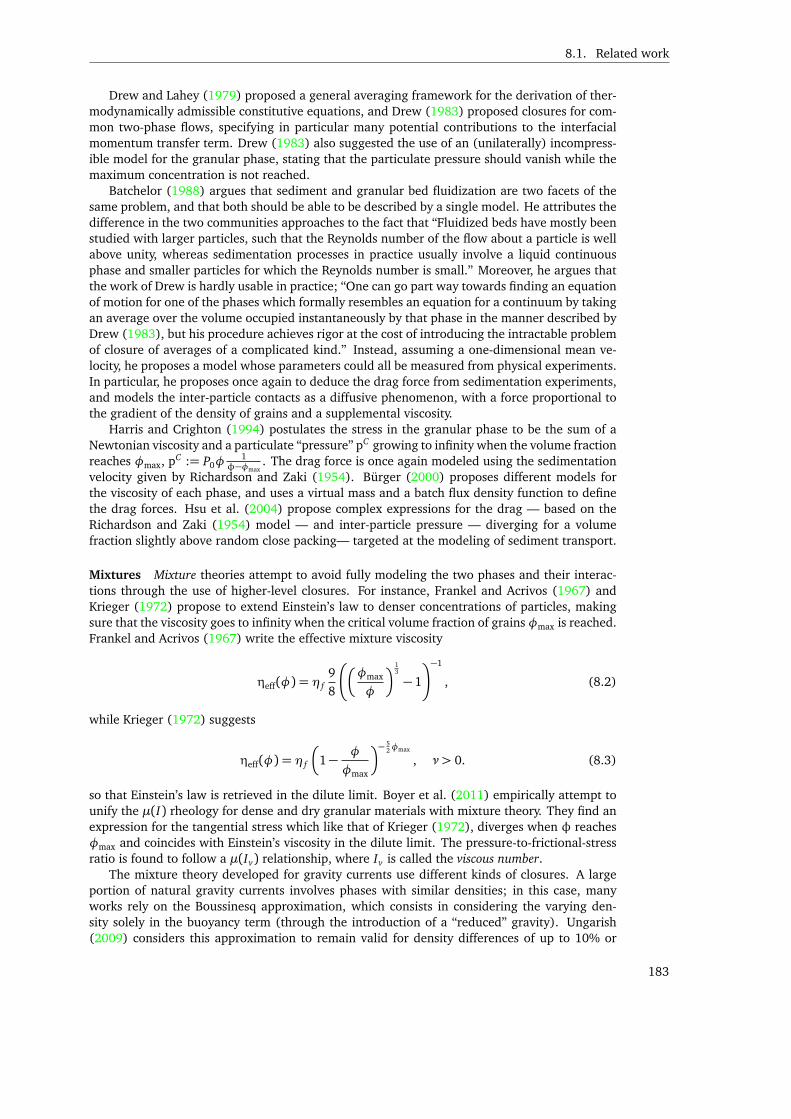
8.1. Related work

Drew and Lahey (1979) proposed a general averaging framework for the derivation of ther-modynamically admissible constitutive equations, and Drew (1983) proposed closures for com-mon two-phase flows, specifying in particular many potential contributions to the interfacialmomentum transfer term. Drew (1983) also suggested the use of an (unilaterally) incompress-ible model for the granular phase, stating that the particulate pressure should vanish while themaximum concentration is not reached.

Batchelor (1988) argues that sediment and granular bed fluidization are two facets of thesame problem, and that both should be able to be described by a single model. He attributes thedifference in the two communities approaches to the fact that “Fluidized beds have mostly beenstudied with larger particles, such that the Reynolds number of the flow about a particle is wellabove unity, whereas sedimentation processes in practice usually involve a liquid continuousphase and smaller particles for which the Reynolds number is small.” Moreover, he argues thatthe work of Drew is hardly usable in practice; “One can go part way towards finding an equationof motion for one of the phases which formally resembles an equation for a continuum by takingan average over the volume occupied instantaneously by that phase in the manner described byDrew (1983), but his procedure achieves rigor at the cost of introducing the intractable problemof closure of averages of a complicated kind.” Instead, assuming a one-dimensional mean ve-locity, he proposes a model whose parameters could all be measured from physical experiments.In particular, he proposes once again to deduce the drag force from sedimentation experiments,and models the inter-particle contacts as a diffusive phenomenon, with a force proportional tothe gradient of the density of grains and a supplemental viscosity.

Harris and Crighton (1994) postulates the stress in the granular phase to be the sum of aNewtonian viscosity and a particulate “pressure” pC growing to infinity when the volume fractionreaches φmax, pC := P0φ

1φ−φmax

. The drag force is once again modeled using the sedimentationvelocity given by Richardson and Zaki (1954). Bürger (2000) proposes different models forthe viscosity of each phase, and uses a virtual mass and a batch flux density function to definethe drag forces. Hsu et al. (2004) propose complex expressions for the drag — based on theRichardson and Zaki (1954) model — and inter-particle pressure — diverging for a volumefraction slightly above random close packing— targeted at the modeling of sediment transport.

Mixtures Mixture theories attempt to avoid fully modeling the two phases and their interac-tions through the use of higher-level closures. For instance, Frankel and Acrivos (1967) andKrieger (1972) propose to extend Einstein’s law to denser concentrations of particles, makingsure that the viscosity goes to infinity when the critical volume fraction of grainsφmax is reached.Frankel and Acrivos (1967) write the effective mixture viscosity

ηeff(φ) = η f9

8

φmax

φ

13

− 1

−1

, (8.2)

while Krieger (1972) suggests

ηeff(φ) = η f

1− φ

φmax

− 52φmax

, ν > 0. (8.3)

so that Einstein’s law is retrieved in the dilute limit. Boyer et al. (2011) empirically attempt tounify the µ(I) rheology for dense and dry granular materials with mixture theory. They find anexpression for the tangential stress which like that of Krieger (1972), diverges when φ reachesφmax and coincides with Einstein’s viscosity in the dilute limit. The pressure-to-frictional-stressratio is found to follow a µ(Iv) relationship, where Iv is called the viscous number.

The mixture theory developed for gravity currents use different kinds of closures. A largeportion of natural gravity currents involves phases with similar densities; in this case, manyworks rely on the Boussinesq approximation, which consists in considering the varying den-sity solely in the buoyancy term (through the introduction of a “reduced” gravity). Ungarish(2009) considers this approximation to remain valid for density differences of up to 10% or

183

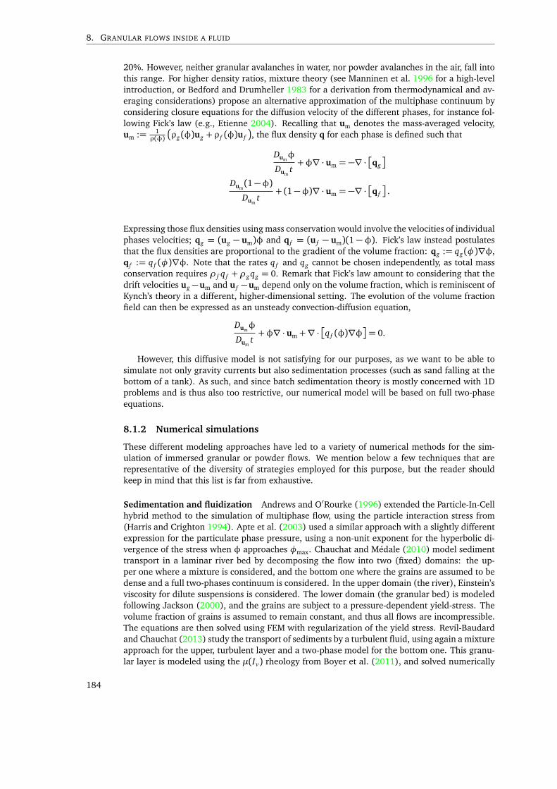
8. GRANULAR FLOWS INSIDE A FLUID

20%. However, neither granular avalanches in water, nor powder avalanches in the air, fall intothis range. For higher density ratios, mixture theory (see Manninen et al. 1996 for a high-levelintroduction, or Bedford and Drumheller 1983 for a derivation from thermodynamical and av-eraging considerations) propose an alternative approximation of the multiphase continuum byconsidering closure equations for the diffusion velocity of the different phases, for instance fol-lowing Fick’s law (e.g., Etienne 2004). Recalling that um denotes the mass-averaged velocity,um := 1

ρ(φ)

ρg(φ)ug + ρ f (φ)u f

, the flux density q for each phase is defined such that

Dumφ

Dumt+φ∇ · um = −∇ ·

qg

Dum(1−φ)Dum

t+ (1−φ)∇ · um = −∇ ·

q f

.

Expressing those flux densities using mass conservation would involve the velocities of individualphases velocities; qg = (ug − um)φ and q f = (u f − um)(1 − φ). Fick’s law instead postulatesthat the flux densities are proportional to the gradient of the volume fraction: qg := qg(φ)∇φ,q f := q f (φ)∇φ. Note that the rates q f and qg cannot be chosen independently, as total massconservation requires ρ f q f +ρgqg = 0. Remark that Fick’s law amount to considering that thedrift velocities ug −um and u f −um depend only on the volume fraction, which is reminiscent ofKynch’s theory in a different, higher-dimensional setting. The evolution of the volume fractionfield can then be expressed as an unsteady convection-diffusion equation,

Dumφ

Dumt+φ∇ · um +∇ ·

q f (φ)∇φ

= 0.

However, this diffusive model is not satisfying for our purposes, as we want to be able tosimulate not only gravity currents but also sedimentation processes (such as sand falling at thebottom of a tank). As such, and since batch sedimentation theory is mostly concerned with 1Dproblems and is thus also too restrictive, our numerical model will be based on full two-phaseequations.

8.1.2 Numerical simulations

These different modeling approaches have led to a variety of numerical methods for the sim-ulation of immersed granular or powder flows. We mention below a few techniques that arerepresentative of the diversity of strategies employed for this purpose, but the reader shouldkeep in mind that this list is far from exhaustive.

Sedimentation and fluidization Andrews and O′Rourke (1996) extended the Particle-In-Cellhybrid method to the simulation of multiphase flow, using the particle interaction stress from(Harris and Crighton 1994). Apte et al. (2003) used a similar approach with a slightly differentexpression for the particulate phase pressure, using a non-unit exponent for the hyperbolic di-vergence of the stress when φ approaches φmax. Chauchat and Médale (2010) model sedimenttransport in a laminar river bed by decomposing the flow into two (fixed) domains: the up-per one where a mixture is considered, and the bottom one where the grains are assumed to bedense and a full two-phases continuum is considered. In the upper domain (the river), Einstein’sviscosity for dilute suspensions is considered. The lower domain (the granular bed) is modeledfollowing Jackson (2000), and the grains are subject to a pressure-dependent yield-stress. Thevolume fraction of grains is assumed to remain constant, and thus all flows are incompressible.The equations are then solved using FEM with regularization of the yield stress. Revil-Baudardand Chauchat (2013) study the transport of sediments by a turbulent fluid, using again a mixtureapproach for the upper, turbulent layer and a two-phase model for the bottom one. This granu-lar layer is modeled using the µ(Iv) rheology from Boyer et al. (2011), and solved numerically

184

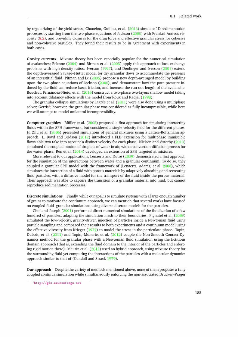
8.1. Related work

by regularizing of the yield stress. Chauchat, Guillou, et al. (2013) simulate 1D sedimentationprocesses by starting from the two-phase equations of Jackson (2000) with Frankel–Acrivos vis-cosity (8.2), and providing closures for the drag force and effective granular stress for cohesiveand non-cohesive particles. They found their results to be in agreement with experiments inboth cases.

Gravity currents Mixture theory has been especially popular for the numerical simulationof avalanches; Etienne (2004) and Birman et al. (2005) apply this approach to lock-exchangeproblems with high density ratios. Iverson (1997), and Denlinger and Iverson (2001) extendthe depth-averaged Savage–Hutter model for dry granular flows to accommodate the presenceof an interstitial fluid. Pitman and Le (2005) propose a new depth-averaged model by buildingupon the two-phase equations of Jackson (2000), and demonstrate how the pore pressure in-duced by the fluid can reduce basal friction, and increase the run-out length of the avalanche.Bouchut, Fernández-Nieto, et al. (2016) construct a two-phase two-layers shallow model takinginto account dilatancy effects with the model from Roux and Radjai (1998).

The granular collapse simulations by Lagrée et al. (2011) were also done using a multiphasesolver, Gerris1; however, the granular phase was considered as fully incompressible, while herewe will attempt to model unilateral incompressibility.

Computer graphics Müller et al. (2005) proposed a first approach for simulating interactingfluids within the SPH framework, but considered a single velocity field for the different phases.H. Zhu et al. (2006) presented simulations of general mixtures using a Lattice-Boltzmann ap-proach. L. Boyd and Bridson (2012) introduced a FLIP extension for multiphase immiscibleflows able two take into account a distinct velocity for each phase. Nielsen and Østerby (2013)simulated the coupled motion of droplets of water in air, with a convection-diffusion process forthe water phase. Ren et al. (2014) developed an extension of SPH targeted at mixtures.

More relevant to our applications, Lenaerts and Dutré (2009) demonstrated a first approachfor the simulation of the interactions between water and a granular continuum. To do so, theycoupled a granular SPH model with the framework of (Lenaerts, Adams, et al. 2008), whichsimulates the interaction of a fluid with porous materials by adaptively absorbing and recreatingfluid particles, with a diffusive model for the transport of the fluid inside the porous material.Their approach was able to capture the transition of a granular material into mud, but cannotreproduce sedimentation processes.

Discrete simulations Finally, while our goal is to simulate systems with a large enough numberof grains to motivate the continuum approach, we can mention that several works have focusedon coupled fluid–granular simulations using diverse discrete models for the particles.

Choi and Joseph (2001) performed direct numerical simulations of the fluidization of a fewhundred of particles, adapting the simulation mesh to their boundaries. Pignatel et al. (2009)simulated the low-velocity, gravity-driven injection of particles inside a Newtonian fluid usingparticle sampling and compared their results to both experiments and a continuum model usingthe effective viscosity from Krieger (1972) to model the stress in the particulate phase. Topin,Dubois, et al. (2011) and Topin, Monerie, et al. (2012) couple the Non-Smooth Contact Dy-namics method for the granular phase with a Newtonian fluid simulation using the fictitiousdomain approach (that is, extending the fluid domain to the interior of the particles and enforc-ing rigid motion there). Maurin et al. (2015) used an hybrid approach, using mixture theory forthe surrounding fluid yet computing the interactions of the particles with a molecular dynamicsapproach similar to that of (Cundall and Strack 1979).

Our approach Despite the variety of methods mentioned above, none of them proposes a fullycoupled continua simulation while simultaneously enforcing the non-associated Drucker–Prager

1http://gfs.sourceforge.net

185

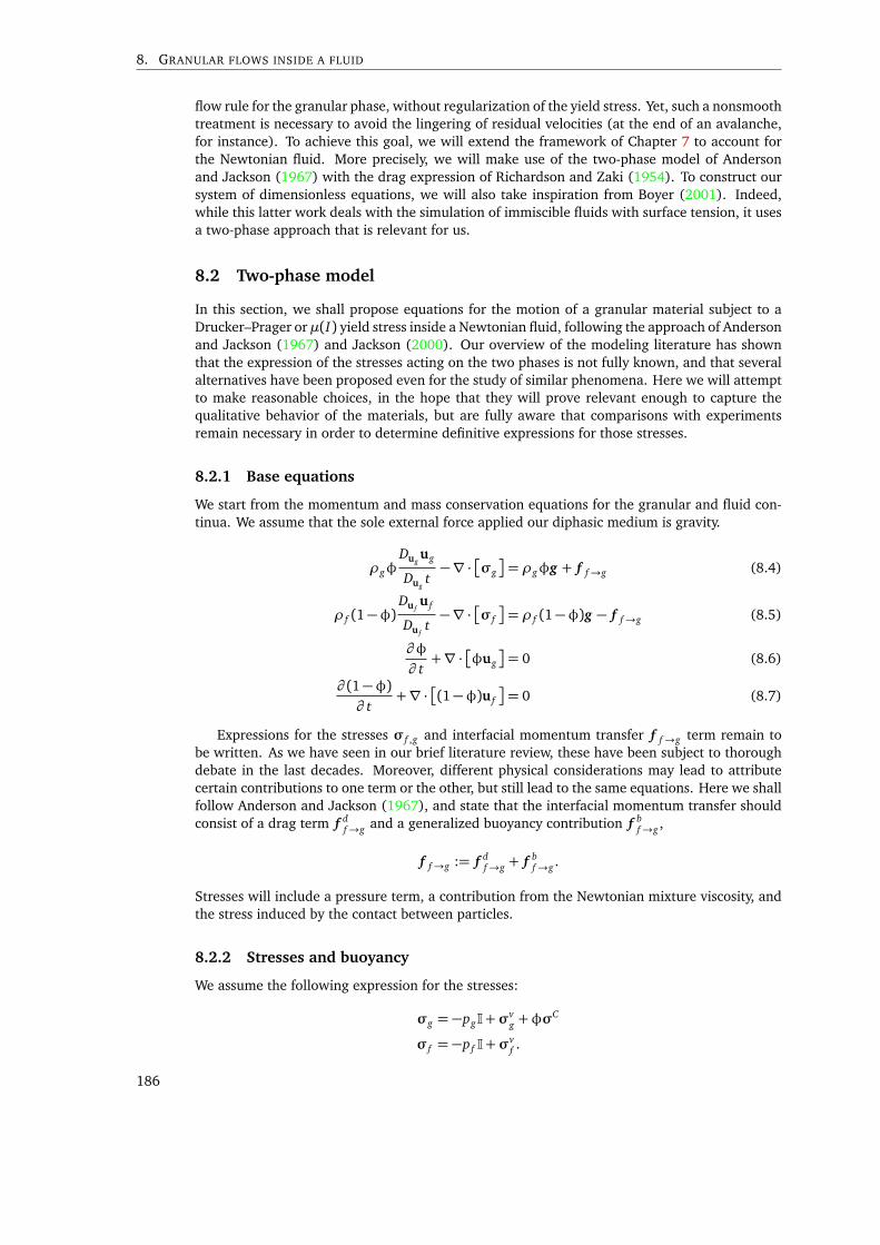
8. GRANULAR FLOWS INSIDE A FLUID

flow rule for the granular phase, without regularization of the yield stress. Yet, such a nonsmoothtreatment is necessary to avoid the lingering of residual velocities (at the end of an avalanche,for instance). To achieve this goal, we will extend the framework of Chapter 7 to account forthe Newtonian fluid. More precisely, we will make use of the two-phase model of Andersonand Jackson (1967) with the drag expression of Richardson and Zaki (1954). To construct oursystem of dimensionless equations, we will also take inspiration from Boyer (2001). Indeed,while this latter work deals with the simulation of immiscible fluids with surface tension, it usesa two-phase approach that is relevant for us.

8.2 Two-phase model

In this section, we shall propose equations for the motion of a granular material subject to aDrucker–Prager or µ(I) yield stress inside a Newtonian fluid, following the approach of Andersonand Jackson (1967) and Jackson (2000). Our overview of the modeling literature has shownthat the expression of the stresses acting on the two phases is not fully known, and that severalalternatives have been proposed even for the study of similar phenomena. Here we will attemptto make reasonable choices, in the hope that they will prove relevant enough to capture thequalitative behavior of the materials, but are fully aware that comparisons with experimentsremain necessary in order to determine definitive expressions for those stresses.

8.2.1 Base equations

We start from the momentum and mass conservation equations for the granular and fluid con-tinua. We assume that the sole external force applied our diphasic medium is gravity.

ρgφDug

ug

Dugt−∇ · σg

= ρgφg + f f→g

ρ f (1−φ)Du f

u f

Du ft−∇ · σ f

= ρ f (1−φ)g − f f→g

∂φ

∂ t+∇ · φug

= 0

∂ (1−φ)∂ t

+∇ · (1−φ)u f

= 0

(8.4)

(8.5)

(8.6)

(8.7)

Expressions for the stresses σ f ,g and interfacial momentum transfer f f→g term remain tobe written. As we have seen in our brief literature review, these have been subject to thoroughdebate in the last decades. Moreover, different physical considerations may lead to attributecertain contributions to one term or the other, but still lead to the same equations. Here we shallfollow Anderson and Jackson (1967), and state that the interfacial momentum transfer shouldconsist of a drag term f d

f→g and a generalized buoyancy contribution f bf→g ,

f f→g := f df→g + f b

f→g .

Stresses will include a pressure term, a contribution from the Newtonian mixture viscosity, andthe stress induced by the contact between particles.

8.2.2 Stresses and buoyancy

We assume the following expression for the stresses:

σg = −pgI+σvg +φσ

C

σ f = −p f I+σvf .

186

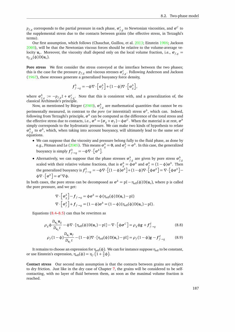
8.2. Two-phase model

p f ,g corresponds to the partial pressure in each phase, σvf ,g to Newtonian viscosities, and σC to

the supplemental stress due to the contacts between grains (the effective stress, in Terzaghi’sterms).

Our first assumption, which follows (Chauchat, Guillou, et al. 2013; Einstein 1906; Jackson2000), will be that the Newtonian viscous forces should be relative to the volume-average ve-locity uv. Moreover, the viscosity shall depend only on the local volume fraction, i.e., σ f ,g =

η f ,g(φ)D(uv).

Pore stress We first consider the stress conveyed at the interface between the two phases;this is the case for the pressure p f ,g and viscous stresses σv

f ,g . Following Anderson and Jackson(1967), these stresses generate a generalized buoyancy force density,

f bf→g = −φ∇ ·

σb

f

+ (1−φ)∇ ·

σb

g

,

where σbf ,g := −p f ,gI + σv

f ,g . Note that this is consistent with, and a generalization of, theclassical Archimede’s principle.

Now, as mentioned by Bürger (2000), σbf ,g are mathematical quantities that cannot be ex-

perimentally measured, in contrast to the pore (or interstitial) stress σb, which can. Indeed,following from Terzaghi’s principle, σb can be computed as the difference of the total stress andthe effective stress due to contacts, i.e., σb = (σg +σ f )−φσC . When the material is at rest, σb

simply corresponds to the hydrostatic pressure. We can make two kinds of hypothesis to relateσb

f ,g to σb, which, when taking into account buoyancy, will ultimately lead to the same set ofequations.

• We can suppose that the viscosity and pressure belong fully to the fluid phase, as done bye.g., Pitman and Le (2005). This means σb

g = 0, and σbf = σb. In this case, the generalized

buoyancy is simply f bf→g = −φ∇ ·

σb.

• Alternatively, we can suppose that the phase stresses σbf ,g are given by pore stress σb

f ,g

scaled with their relative volume fractions, that is σbg = φσ

b and σbf = (1−φ)σb. Then

the generalized buoyancy is f bf→g = −φ∇·

(1−φ)σb

+(1−φ)∇·φσb

=∇·φσb

−φ∇ · σb

= σv∇φ.

In both cases, the pore stress can be decomposed as σb = pI− ηeff(φ)D(uv), where p is calledthe pore pressure, and we get:

∇ ·σb

g

− f f→g = φσ

b = φ (ηeff(φ)D(uv)− pI)

∇ ·σb

f

+ f f→g = (1−φ)σb = (1−φ) (ηeff(φ)D(uv)− pI) .

Equations (8.4–8.5) can thus be rewritten as

ρgφDug

ug

Dugt−φ∇ · [ηeff(φ)D(uv)− pI]−∇ · φσC

= ρgφg + f d

f→g

ρ f (1−φ)Du f

u f

Du ft− (1−φ)∇ · [ηeff(φ)D(uv)− pI] = ρ f (1−φ)g − f d

f→g

(8.8)

(8.9)

It remains to choose an expression for ηeff(φ). We can for instance suppose ηeff to be constant,or use Einstein’s expression, ηeff(φ) = η f

1+ 5

2φ.

Contact stress Our second main assumption is that the contacts between grains are subjectto dry friction. Just like in the dry case of Chapter 7, the grains will be considered to be self-contacting, with no layer of fluid between them, as soon as the maximal volume fraction isreached.

187

8. GRANULAR FLOWS INSIDE A FLUID

p

pC

pC

pC

Figure 8.1: Two kinds of competing normal stresses acting on the particles: the porepressure p and the effective stress due to contacts pC = − 1

d Trσc

As in the dry case, we will want the grains volume fraction φ, contact stress σC , and strainrate ǫg , to follow the maximal volume fraction constraint with non-associated Drucker–Pragerflow rule, i.e.,

0≤ pC ⊥ φmax −φ ≥ 0

DevσC = µpCDev ǫg

|Dev ǫg |if Dev ǫg 6= 0 (yielded)

|DevσC | ≤ µpC if Dev ǫg = 0 (unyielded),

(8.10)

where pC := − 1d TrσC .

This solid-contacts assumption also means that the stress due to contacts between grainswill be propagated at grain–grain interfaces only, and exist solely inside the granular phase. Assuch, there is no associated buoyancy force. This is confirmed by a simple thought experiment:consider a dry, compact heap of rigid grains at rest, supporting a given mass m. Modifying theintensity of the contact forces between the grains, for instance by changing m, will not affect theair phase nor the interstitial pressure p.

Remark 8.1. We can already remark that as illustrated on Figure 8.1, the normal component ofthe total stress of the mixture will be the sum of two terms, p and pC = − 1

d TrσC . Now, as per theDrucker–Prager criterion (8.10), increasing pC increases the yield stress of the material; for a givenapplied load, the pore pressure p will thus have a weakening effect.

8.2.3 Drag force

Our third core hypothesis will be to consider grains that are thin enough, or with velocity (w.r.t.the surrounding fluid) small enough that Stokes’ drag law apply. That is, we consider the case

where the grain-level Reynolds number, Reg :=ρ f W Dg

η f, where Dg is the diameter of the grains

and W a characteristic relative velocity, is small. This choice has been made by numerous au-thors, e.g., (Anderson and Jackson 1967; Bürger 2000; Chauchat and Médale 2010; Harris andCrighton 1994; Pitman and Le 2005) , while others consider the drag force to be quadratic in therelative velocity (Batchelor 1988; Chauchat, Guillou, et al. 2013; Drew 1983). We will stick withsimple linear drag, knowing that in any case we can account for the nonlinearity by explicitlyadjusting the drag coefficient in the numerical method, and remember that we may overestimatethe relative velocity in the analysis below.

188

8.2. Two-phase model

We will thus express the drag force as f df→g = −ξ(φ)w, where w is the relative velocity

between the two phases, w := ug − u f , and ξ is a scalar function of the volume fraction. In the

two-phase literature, ξ(φ) is commonly deduced from sedimentation experiments, for instanceusing the empirical law of Richardson and Zaki (1954), such as in (Chauchat, Guillou, et al.2013). The quasistatic conservation of momentum for the sedimenting particles is written as

0= φ(ρg −ρ f )g − ξ(φ)uz(φ),

yielding

ξ(φ) =φ(ρg −ρ f )g

uz(φ).

Equation (8.1) gives uz(φ) = w∞(1−φ)ν; let us compute the value of w∞ under the hypothesisReg ≤ 1. Let w denote the relative velocity of a single spherical grain falling through the fluid.Stokes’ law state that the intensity of the drag on the particle is −3πη f Dg w, meaning that the

equilibrium is reached for (ρg −ρ f )(43π

Dg

2

3)g = 3πη f Dg w, i.e.,

w∞ =(ρg −ρ f )gD2

g

18η f.

Overall, we conclude

ξ(φ) = η f18

D2g

φ(1−φ)−ν.

Note that this expression increases monotonically with the volume fraction of grains, whichat first may appear strange, as one expects the average drag force to decrease for denser objects.However, this weakening of the drag force is due to a smaller relative velocity, as the fluid islugged by the higher density of grains, rather than a decrease in the friction coefficient. Notealso that this expression makes ξ grow to infinity when the fluid vanishes, thus requiring therelative velocity w to vanish for purely granular materials. As our maximal volume fractionconstraint requires φ ≤ φmax < 1, we need not worry about this degenerate case, however.Other closures are possible; for instance, Chauchat and Médale (2010) use the so-called Carman–Kozeny relationship. For now, we will not assume a precise expression for ξ, but simply writethat

f df→g = −φ(1−φ)ξ(φ)w, (8.11)

and remember that ξ(φ) in Pa.s.m−2 is similar in order of magnitude to gρg−ρ f

w∞(1−φ)ν+1 =η f

D2g

18(1−φ)ν+1 .

Summary of our hypothesis At this point, we have made the following hypothesis:• no mass is transferred between the two phases;

• the Newtonian viscous stress is proportional to D(uv);

• the linear Stokes drag law applies;

• the contacts between grains are subject to dry friction and occur when φ= φmax < 1.

8.2.4 Mixture conservation equations

The conservation equations (8.4–8.7) written with the phase velocities are not very convenient;Boyer (2001) propose to express them instead as functions of two other velocity variables, thevolume-average velocity uv and the relative velocity w. This choice does have some nice proper-ties; the Newtonian viscosity is already expressed as a function of uv, and uv is the only velocityvariable that is divergence-free. Indeed, summing Equations (8.6) and (8.7), we get

∇ · uv = −∂ 1

∂ t= 0. (8.12)

However, using uv also requires Boyer (2001) to deal with rather inconvenient inertial terms.Here, we will choose instead to use um and w as our velocity variables.

189

8. GRANULAR FLOWS INSIDE A FLUID

Notations Following Etienne (2004), we introduce the scaled density difference

α :=ρg −ρ f

ρ f.

Note that ρg/ρ f = (α + 1). Let β(φ) := (1 + αφ), so that the total density of the mixture isgiven by ρ(φ) = φρg + (1−φ)ρ f = β(φ)ρ f . Let π(φ) := φ(1−φ).

The total mass conservation of the mixture, obtained by summing (8.6) scaled byρg and (8.7)scaled by ρ f , reads

∂β

∂ t+∇ · [βum] = 0. (8.13)

Finally, note that phase and volume-averaged velocities can also be expressed as function ofthe mass-averaged and relative velocities:

ug = um +(1−φ)β

w u f = um − (α+ 1)φ

βw

uv = um −απ

βw

Mixture momentum conservation To obtain the conservation equation for the total momen-tum of the mixture, we just have to sum Equations (8.8) and (8.9). It is simpler to consider theconservative expression2 for the inertial terms,

φDug

ug

Dugt=∂φug

∂ t+∇ · φug ⊗ ug

(1−φ)Du f

u f

Du ft=∂ (1−φ)ug

∂ t+∇ · (1−φ)u f ⊗ u f

.

Remark first that

ρgφug ⊗ ug +ρ f (1−φ)u f ⊗ u f

= ρ f

(α+ 1)φug ⊗ um + (1−φ)u f ⊗ um

+ρ f

(α+ 1)φug ⊗ (ug − um) + (1−φ)u f ⊗ (u f − um)

= ρ f

βum ⊗ um + (α+ 1)

φ(1−φ)β

ug ⊗w− (α+ 1)φ(1−φ)

βu f ⊗w

= ρ f

βum ⊗ um + (α+ 1)

π

βw⊗w

.

Therefore,

ρgφDug

ug

Dugt+ρ f (1−φ)

Du fu f

Du ft

= ρ f

∂βum

∂ t+ (βum · ∇)um +

*∇ · [βum]︸ ︷︷ ︸− ∂β∂ t

,um

++ (α+ 1)∇ ·

π

βw⊗w

= ρ f

β

Dumum

Dumt+ (α+ 1)∇ ·

π

βw⊗w

.

The conservation equation for the total momentum of the mixture thus reads

ρ f

β

Dumum

Dumt+ (α+ 1)∇ ·

π

βw⊗w

+∇p−∇ ·

ηeff D(um −α

π

βw)

−∇ · φσC

= ρ f βg (8.14)2see Section 5.2.1

190

8.2. Two-phase model

Fluctuation momentum conservation Another interesting linear combination of the momen-tum conservation consists in taking the difference of (8.8) scaled by ρ f (1−φ), and (8.9) scaledby φρg . Processing term by term, we have• Inertial terms:

ρgρ f πDug

ug

Dugt−ρgρ f π

Du fu f

Du ft= ρgρ f π

∂w

∂ t+ (ug · ∇)ug − (u f · ∇)u f

= ρgρ f π

∂w

∂ t+Lu f ,gM · ∇

w− (w · ∇)Lu f ,gM

,

with Lu f ,gM :=u f + ug

2= um +

1− 2φ−αφ2β

w;

• Mixture stress:−ρ f π∇ ·

σb+ρgπ∇ ·

σb= ρ f απ∇ ·

σb

;

• Drag force:ρ f (1−φ) f d

f→g +ρgφ f df→g = ρ f β f d

f→g = −ρ f βπξw;

• Gravity:ρ f (1−φ)φρg g −ρgφρ f (1−φ)g = 0.

The conservation of the fluctuation momentum, where we have divided each term by (1−φ)ρ f3,

thus reads

(α+ 1)ρ fφ

∂w

∂ t+Lu f ,gM · ∇

w+ (w · ∇)Lu f ,gM

+βφξw

−αφ∇p+αφ∇ ·ηeff D(um −α

π

βw)

−∇ · φσC

= 0. (8.15)

Remark The velocity transport terms in Equations (8.14) and (8.15) seem relatively unwieldy,and, as we will see in the next section, may not be negligible for certain applications. However,their expression will be drastically simplified when using a timestepping algorithm with an ex-plicit velocity-advection scheme, such as the characteristics method or particle-based transport.

8.2.5 Dimensionless equations

Characteristic quantities To get an idea of the respective importance of the different terms inEquation (8.14)and (8.15), we need to define characteristic values for our variables. There areseveral ways to do this, and none will hold for the whole range of regimes that can be exhibitedby our two-phase material. As we will mostly be studying gravity-driven flows, we define thecharacteristic mixture velocity as U :=

pg L, where L is a characteristic length of the studied

phenomenon. For the same reason, we choose P := ρ f g L as the characteristic pore pressure,(α+1)P = ρg g L as the characteristic contact stress, T = L

U as the characteristic time. Finally, atthe risk of overestimating W , we define the characteristic relative velocity as the sedimentationvelocity of a single grain, w∞.

The dimensionless variables will be denoted with a tilde in the equations below, but we willquickly drop their decoration to lighten notation. We also introduce dimensionless versions ofthe effective viscosity and drag fields,

ηeff = η f ηeff ξ= gρg −ρ f

w∞Ξηeff,

where the dimensionless number Ξ denotes the order of magnitude of the geometry dependentterm in ξ, i.e., Ξ ∼ ξ w∞

ρg−ρ fg ∼ (1−φ)−ν−1 when using the Richardson and Zaki (1954) closure.

Note that as ν is usually taken to be greater than 3, the choice of Ξ will be highly dependent onthe target volume fraction.

3We supposed that φmax < 1 and thus φ= 1 is never reached

191

8. GRANULAR FLOWS INSIDE A FLUID

Mixture momentum conservation The dimensionless version of (8.14) is, after division byρ f ,

1

L

βU2 Dum

Dt+ (α+ 1)UW ∇ ·

π

βw⊗ w

− (α+ 1)g∇ · φσC

+ g∇p− η f

ρ f L2∇ ·

ηeffD(Uum −Wα

π

βw)

= gβe g .

This motivates the introduction of two dimensionless number; the Reynolds number of the fluid,Re, and a Stokes number, St, relating the importance of the mixture kinetic energy to the dissi-pation by drag forces:

Re :=ρ f U L

η fSt :=

W

U=(ρg −ρ f )gD2

g

18Uη f=ρg U D2

g

18Lη f.

The relationship between these dimensionless numbers is given by ratios of density and length,

St=α+ 1

18

ρ f U D2g

Lη f=α+ 1

18ReDg

L

2

=α+ 1

18ε2Re,

where ε :=Dg

L denotes the ratio of the grains diameter to the characteristic simulation length.Dividing our equation by g(α+1), we get the dimensionless momentum conservation equa-

tion for the mixture,

β

α+ 1

Dum

Dt+ St2∇ ·

π

βw⊗ w

− ∇ · φσC

− 1

α+ 1∇ ·

ηeff

ReD(um − Stα

π

βw)− pI

=

β

α+ 1e g . (8.16)

Fluctuation momentum conservation Rewriting (8.15) using our dimensionless variablesyield

(α+ 1)ρ fφW

L

U∂ w

∂ t+ U I(um, w) +W I(

1− 2φ−αφ2β

w, w)+βφg

ρg −ρ f

w∞ΞW ξw

= αφ

gρ f∇p− η f

L2∇ ·

ηeff D(U um −αW

π

βw)

+ (α+ 1)ρ f g∇ · φσC

,

where I(v,w) := (v · ∇)w+ (w · ∇)v. Dividing both sides by ρg g, and remarking that W U/L =Stg, we get

φSt∂ w

∂ t+ I(um, w) + StI(

1− 2φ−αφ2β

w, w)+αβ

α+ 1φΞξw

=αφ

α+ 1

∇p− 1

Re∇ ·

ηeffD(um −αSt

π

βw)

+ ∇ · φσC

. (8.17)

Mass conservation The dimensionless mass conservation equations read:

∇ ·um − St

απ

βw

= 0

∂β

∂ t− ∇ · [βum] = 0.

(8.18)

(8.19)

Alternatively, Equation (8.19) can be replaced with (8.20),

∂φ

∂ t− ∇ · φug

= 0, (8.20)

where ug := 1U ug .

192

8.2. Two-phase model

8.2.6 Particular cases

Equilibrium First, let us look at static equilibrium, which means um =w= 0. The dimension-less conservation equations read simply

−∇ · φσC+

1

α+ 1∇p=

β

α+ 1e g

−∇ · φσC=αφ

α+ 1∇p,

from which we deduce easily

∇p= e g

−∇ · φσC=αφ

α+ 1e g .

Hence, up to a constant field, the pore pressure satisfies p = ρ f gz, and corresponds to theexpected hydrostatic pressure. We also have −∇· φσg

= φαρ f g = φρg g −φ∇p; the contact

force thus oppose the action of gravity on the grains reduced by the buoyancy force given byArchimede’s principle. Again, this is the expected result.

Incompressible flow The divergence-free condition for the volume-averaged velocity uv isexpressed by Equation (8.18).

In the limit case where St= 0, the mass-averaged velocity um becomes also divergence-free.In a similar fashion, if Ξ = +∞, then (8.17) imposes w = 0 and then once again the flowbecomes incompressible.

Single phase limit If we consider that the surrounding fluid is massless and inviscid, α= +∞,and β

α+1 = φ. Moreover, if the grains are small enough w.r.t. the characteristic length, i.e.,ε << 1, then St

α+1 << 1.Overall, the mixture momentum conservation equation (8.16) becomes

φDug

ug

Dugt− ∇ · φσC

= φe g ,

which is the equation that we used for the dry case in Chapter 7 in the case of a vanishingNewtonian granular viscosity. However, in the vanishing grain size limit St will also get close tozero, and the flow will be incompressible, thus departing from the single phase equations.

Orders of magnitude We now look at the order of magnitude of the different terms in thedimensionless conservation equations for different physical parameters. Numbers of specialinterest are St2 — the importance of the w transport term in the mixture momentum balanceequation, St

Re =αε2

18 — the viscosity term on w, and StΞ

and St2

Ξ– the inertial terms in the fluctuation

equations.Since as we already mentioned, we know that we overestimate w, and since when using the

Richardson-Zaki closure the term βΞξwill be greater that 1 for most regimes, St< 10−1 appearsto be a satisfying criterion for neglecting all inertial forces in w.

• We first consider sand grains in water, for which ρ f ∼ 103kg.m−3, ρg ∼ 2.5× 103kg.m−3,

and η f ∼ 10−3Pa.s. We have Re = 3 × 106 L32 , α ∼ 1 and St = 105 L

32 ε2 = 105D2

g L−12 .

This scaling means that when the size of the particles doubles, the size of the domain hasto be multiplied by 16 to recover the same ratio for the mass-averaged and fluctuationvelocities, and by 256 to get a similar influence for the inertial terms in w. For grains ofdiameter Dg = 1mm, getting St < 0.1 requires L > 1m. However, for Dg = 1cm, we musthave L > 10km. As St

Re << 1 as soon as L > 10Dg , the viscous forces on w can be neglectedin both of those scenarios.

193

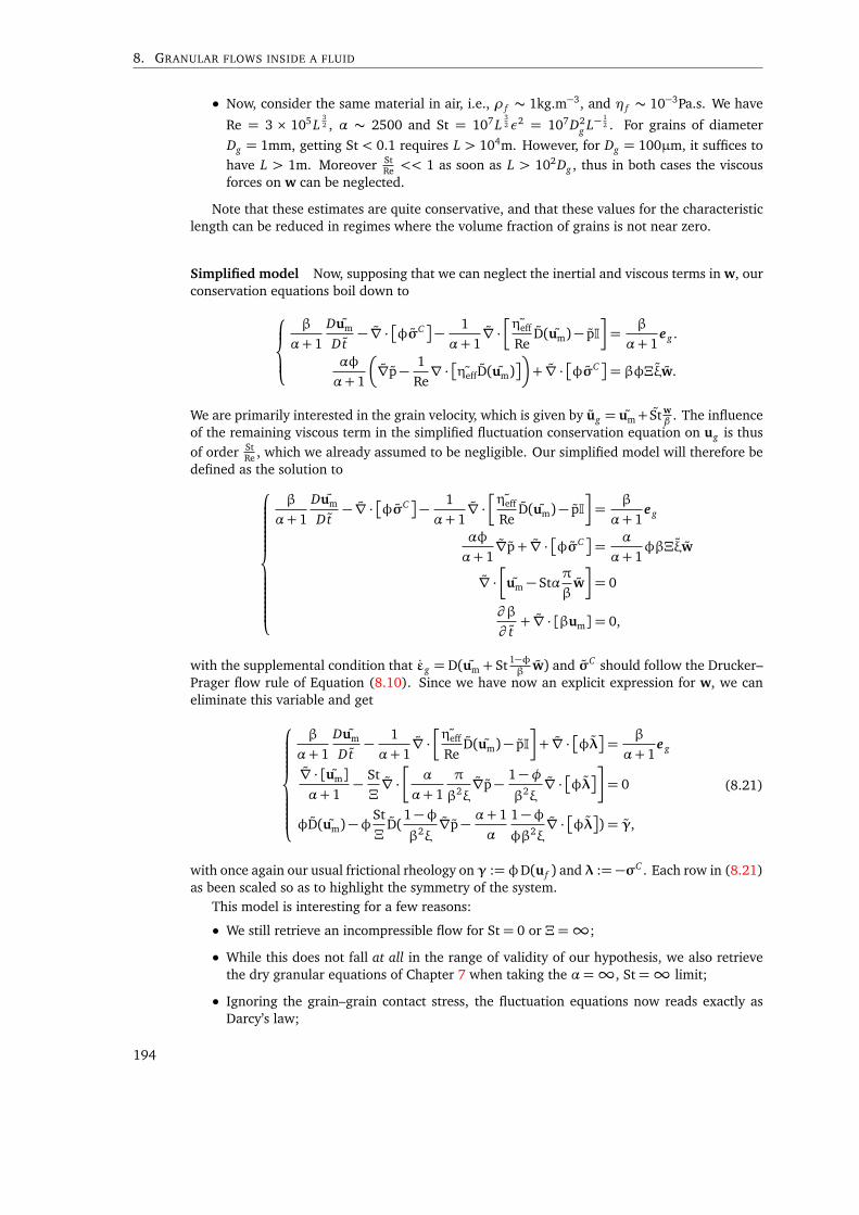
8. GRANULAR FLOWS INSIDE A FLUID

• Now, consider the same material in air, i.e., ρ f ∼ 1kg.m−3, and η f ∼ 10−3Pa.s. We have

Re = 3 × 105 L32 , α ∼ 2500 and St = 107 L

32 ε2 = 107D2

g L−12 . For grains of diameter

Dg = 1mm, getting St < 0.1 requires L > 104m. However, for Dg = 100µm, it suffices tohave L > 1m. Moreover St

Re << 1 as soon as L > 102Dg , thus in both cases the viscousforces on w can be neglected.

Note that these estimates are quite conservative, and that these values for the characteristiclength can be reduced in regimes where the volume fraction of grains is not near zero.

Simplified model Now, supposing that we can neglect the inertial and viscous terms in w, ourconservation equations boil down to

β

α+ 1

Dum

Dt− ∇ · φσC

− 1

α+ 1∇ ·

ηeff

ReD(um)− pI

=

β

α+ 1e g .

αφ

α+ 1

∇p− 1

Re∇ · ηeffD(um)

+ ∇ · φσC

= βφΞξw.

We are primarily interested in the grain velocity, which is given by ug = um+ St wβ . The influence

of the remaining viscous term in the simplified fluctuation conservation equation on ug is thusof order St

Re , which we already assumed to be negligible. Our simplified model will therefore bedefined as the solution to

β

α+ 1

Dum

Dt− ∇ · φσC

− 1

α+ 1∇ ·

ηeff

ReD(um)− pI

=

β

α+ 1e g

αφ

α+ 1∇p+ ∇ · φσC

=

α

α+ 1φβΞξw

∇ ·um − Stα

π

βw

= 0

∂β

∂ t+ ∇ · [βum] = 0,

with the supplemental condition that εg = D(um + St 1−φβ

w) and σC should follow the Drucker–Prager flow rule of Equation (8.10). Since we have now an explicit expression for w, we caneliminate this variable and get

β

α+ 1

Dum

Dt− 1

α+ 1∇ ·

ηeff

ReD(um)− pI

+ ∇ · φλ= β

α+ 1e g

∇ · [um]

α+ 1− St

Ξ∇ ·

α

α+ 1

π

β2ξ∇p− 1−φ

β2ξ∇ · φλ

= 0

φD(um)−φSt

ΞD(

1−φβ2ξ

∇p− α+ 1

α

1−φφβ2ξ

∇ · φλ) = γ,

(8.21)

with once again our usual frictional rheology on γ := φD(u f ) and λ := −σC . Each row in (8.21)as been scaled so as to highlight the symmetry of the system.

This model is interesting for a few reasons:

• We still retrieve an incompressible flow for St= 0 or Ξ =∞;

• While this does not fall at all in the range of validity of our hypothesis, we also retrievethe dry granular equations of Chapter 7 when taking the α=∞, St=∞ limit;

• Ignoring the grain–grain contact stress, the fluctuation equations now reads exactly asDarcy’s law;

194

8.3. Numerical resolution of the two-phase equations

• Still ignoring grain-grain interactions, the system we have to solve is deeply similar to thatof near-incompressible flows, i.e., a penalized Navier-Stokes problem,

β

α+ 1

Dum

Dt− 1

α+ 1∇ ·

ηeff

ReD(um)− pI

=

β

α+ 1e g

∇ · [um]

α+ 1− α

α+ 1

St

Ξ∇ ·

π

β2ξ∇p

= 0

∂β

∂ t+ ∇ · [βum] = 0.

The reduced diphasic model (8.21) is very similar to the single phase model of Chapter 7,except that the degrees of freedom are now the combination of the mass-averaged velocity um

and the pressure p. It could be solved in a similar fashion, but one would have to be wary that thestiffness matrix is no longer guaranteed to be positive-definite, and that another term, comingfrom the nonlinear Laplacian of λ in the definition of γ, contributes to the Delassus operator.Since w does not need to be discretized, this reduced problem could be cheaper to solve thanthe original one, and may still be able to capture a wide range of phenomena. Following theapproach of the dry case, the simplified model can also be shown to be dissipative. Despite thesepotential advantages, in the following section we will go back to the general case and propose anumerical method to solve our original equations. Adapting this method to the simplified modelshould be straightforward.

8.3 Numerical resolution of the two-phase equations

We consider our original dimensionless system of four equations — the two conservation equa-tions, (8.16) and (8.17), and the two mass conservation equations (8.18) and (8.20) — plus ourfrictional rheology constraint (8.10). We now drop the tildes to lighten notations.

8.3.1 Time discretization

Just like in the dry case presented in Chapter 7, we will use a semi-implicit timestepping scheme,that first solves the momentum conservation equations, then advect the volume fraction field.That is, we will first solve equations (8.16), (8.17) subject to the volume-averaged incompress-ibility (8.18) and the frictional rheology (8.10) to get end-of-step values for u,w, p and σC , thensolve the volume fraction transport equation (8.20) using these new velocities.

Frictional contacts Once again, we thus have to linearize the end-of-step maximal volumefraction constraint, following

(φ(t +∆t)≤ φmax)∼ (φk +φk∆t D(ug)≤ φmax).

Just as in Chapter 7, we thus define

γ := φk D(ug) +φmax −φ∆t

I

dand λ := −σC , (8.22)

such that our frictional rheology constraint is expressed as (γ,λ) ∈ DP (µ).

Material velocity derivatives We suppose that the material derivative for the velocity of eachphase can be approximated to the first order as

Du f ,gu f ,g

Du f ,gt=

uk+1f ,g − u f ,g(u

kf ,g)

∆t+O(∆t).

195

8. GRANULAR FLOWS INSIDE A FLUID

For instance, u can be computed using the characteristics morphism, or by recovering the velocityfrom particles in the case of hybrid schemes.

Using this approximation, we can get simpler expressions for the inertial terms of the mixtureand fluctuation momentum conservation equations. Indeed,

φ(α+ 1)Dug

ug

Dugt+ (1−φ)

Du fu f

Du ft∼ 1

∆t

βum − (α+ 1)φug(u

kg)− (1−φ)u f (u

kf )

Dugug

Dugt−

Du fu f

Du ft∼ 1

∆t

St w+ u f (u

kf )− ug(u

kg)

.

Using this insight, we rewrite our momentum conservation equations as

β

α+ 1

um

∆t+∇ · [φλ]− 1

α+ 1∇ ·

ηeff

ReD(um − Stα

π

βw)− pI

=β

α+ 1e g +

1

∆t

φug(u

kg) +

1−φα+ 1

u f (ukf )

(8.23)

φ

St

∆t+αβ

α+ 1Ξξ

w− αφ

α+ 1

∇p− 1

Re∇ ·

ηeff D(um −αSt

π

βw)

+∇ · [φλ] = φ

∆t

ug(u

kg)− u f (u

kf )

(8.24)

8.3.2 Variational formulation

We first perform a change of variable which will allow us to obtain a symmetric system, andintroduce the velocity field w :=

pSt 1−φ

βw. The velocity of each phase can be reconstructed

from um and w as ug = um +p

Stw and u f = um − (α+ 1)p

St φ

1−φ w.Let us consider a simulation domain Ω, with, for the sake of simplicity, homogeneous Dirich-

let boundary conditions. Let as usual V denote a subspace of H1(Ω)d satisfying the boundaryconditions, and T (Ω)∼ L2(Ω)

sd be the space of square-integrable symmetric tensor fields on Ω.Our two-phase flow is described by the solution to the following variational formulation:

Find um, w ∈ V 2, p ∈ L2(Ω) and γ,λ ∈ T 2 such that

a(um,v) + e(w,v) − b(p,v) − g(λ,v) = l(v) ∀v ∈ Ve(um,z) + r(w,z) − c(p,z) − h(λ,z) = f (z) ∀z ∈ V−b(q,um) − c(q, w) = 0 ∀q ∈ L2(Ω)

−g(τ,um) − h(τ, w) + m(γ,τ) = k(τ) ∀τ ∈ T(γ,λ) ∈ DP (µ).

where a = a1 + a2, r = r1 + r2,

a1(u,v) :=1

∆t

∫

Ω

β

α+ 1⟨u,v⟩ a2(u,v) :=

1

(α+ 1)Re

∫

Ω

ηeff D(u) : D(v)

r1(w,z) :=

∫

Ω

φβ

1−φ

St

∆t+αβ

α+ 1Ξξ

r2(w,z) :=

St

Re

α2

α+ 1

∫

Ω

ηeff D(φw) : D(φz)

e(w,z) := −αp

St

α+ 1

∫

Ω

ηeff

ReD(φw) : D(v) m(γ,τ) :=

∫

Ω

γ : τ

b(p,v) :=1

α+ 1

∫

Ω

p∇ · z c(p,z) :=αp

St

α+ 1

∫

Ω

φ ⟨∇p,z⟩

g(τ,u) :=

∫

Ω

φτ : D(u) h(τ,u) :=p

St

∫

Ω

φτ : D(w)

196

8.3. Numerical resolution of the two-phase equations

l(v) :=

∫

Ω

β

α+ 1

e g ,v

+

1

∆t

∫

Ω

¬(α+ 1)φug(u

kg) + (1−φ)u f (u

kf ),v

¶

k(τ) :=

∫

Ω

φmax −φ∆t

Trτ

d

f (z) :=

pSt

∆t

∫

Ω

φ¬ug(u

kg)− u f (u

kf ),z

¶.

Proof. Scaling the fluctuation momentum conservation equation (8.24) byp

St, dividing thevolume-averaged incompressibility (8.18) by (α + 1) and transcribing the definition of w intothem, we obtain:

φβ

1−φ

St

∆t+αβ

α+ 1Ξξ

w− αφ

α+ 1

pSt∇p− 1

Re∇ · ηeff D(

pStum −αStφw)

+p

St∇ · [φλ] =pStφ

∆t

ug(u

kg)− u f (u

kf )

,

1

α+ 1∇ · um −

pSt

α

α+ 1∇ · [φw] = 0,

which, put under weak form and using Green formulas, correspond to the second and third linesof our variational formulation. The first and fourth line are obtained through a similar process onthe mixture momentum conservation equation (8.24) and the definition of γ, Equation (8.22).

8.3.3 Discrete system

Choosing adequate discrete spaces for our variables, and expressing the constraints on quadra-ture points as we did in Chapters 6 and (7), we ultimately obtain a system which has the form:

Au + E⊺w = l + B⊺p + G⊺λ

Eu + Rw = f + C⊺p + H⊺λ

0= Bu + C w

γ= k + Gu + Hw

(λ[i],γ[i]) ∈ DP (µ) ∀i.

(8.25)

System (8.25) is a DCFP, with linear constraints and whose degrees of freedom are given by thecouple (u, w ). Concatenating the system matrices as

A :=

A E⊺

E R

H :=

G, H

C :=

B, C

,

System (8.25) can be rewritten in a more familiar manner as

Au; w

=

l

f

+ C⊺p + H⊺λ

Cu; w

= 0

γ= k + Hu; w

(λ[i],γ[i]) ∈ DP (µ) ∀i.

(8.26)

The matrix A is always symmetric positive-definite, and discretizing the fluctuation field onlywhere φ > 0 — which is sensible, as w should vanish elsewhere — R is also positive-definite;therefore A is symmetric positive-positive as well.

197

8. GRANULAR FLOWS INSIDE A FLUID

Numerical resolution Chapters 3 and 4 were dedicated to solving numerically the DCFP withlinear constraints. However, notice that System 8.26 features two peculiarities that restrict thechoice of numerical solvers.

• First, the inverse of the stiffness matrix, A−1, is dense. This difficulty can be dealt with byeither using the numerical algorithms proposed in Chapter 6, or making the high Reynoldshypothesis of Chapter 7 and using the two-steps algorithm of Section 7.3.4.

• The matrix C is not surjective — the pressure field is simply defined up to a constant —and thus the Schur complement of the linear constraints may not be invertible, discardingsome of the methods that we proposed to deal with linear constraints in a DCFP. If the dis-cretization spaces for the velocities and pressure, Vh and Qh, satisfy an inf-sup criterion, thisproblem can be solved by enforcing a supplemental zero-average constraint for the pres-sure p. Otherwise, we can assume that slightly relaxing the incompressibility constraint ofthe volume-averaged velocity is acceptable, and penalize the pressure variable.

In practice, as we put more of an emphasis on solving efficiency rather than on the precisionof the fluid velocity field, we use the two-step approximate algorithm together with the relaxationof the incompressibility constraints.

That is, we first solve a Stokes-like problem, with either the zero-average constraint or a pe-nalization strategy, depending on whether our choice for Vh and Qh satisfies the inf-sup condition,to obtain a candidate velocity

u; w

∗, e.g.,

A E⊺ −BT

E R −C T

−B −C 1

1⊺

u∗

w ∗

p

κ

=

l

f

0

0

or

A E⊺ −BT

E R −C T

−B −C −cI

u∗

w ∗

p

=

l

f

0

,

where κ is the Lagrange multiplier associated to the zero-pressure average condition.Then, we solve a lumped DCFP to get the velocity increment satisfying the frictional con-

straints,

˜A∆u; w

= C⊺p + H⊺λ

C∆u; w

= −cp

γ= Hu; w

+ k + H

u; w

∗

(λ[i],γ[i]) ∈ DP (µ) ∀i,

(8.27)

where ˜A = diag(A1, R1) is the concatenation of the lumped mass matrices for the mixture andfluctuation inertia. In practice, we use the matrix-free Gauss–Seidel algorithm presented inChapter 4, where the linear constraints are accounted for every few iterations by solving thesymmetric positive-definite system

(C ˜A−1C⊺ + cI)p = −C ˜A−1HTλk.

8.3.4 Spatial discretization

In the previous paragraph we assumed that suitable discretization spaces for the velocity, pres-sure, grain volume fraction and stress fields had been chosen. We did not pursue this investiga-tion in details yet, and simply adapted the discretization strategies devised for the dense case.We considered either:

• Piecewise-constant approximations on a triangular mesh for the velocity, volume fraction,and stress field, with a piecewise-linear pressure field. As in Section 7.2.2, advection ofthe volume fraction and velocity fields was done using an upwind scheme.

• MPM discretization of the volume fraction field, as in Section 7.3, with trilinear velocitiesand trilinear, trilinear-discontinuous, or particle-based stresses. For the sake of simplicity

198

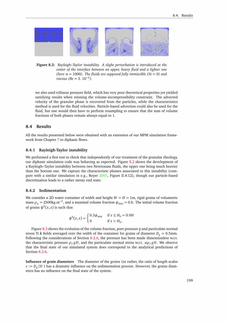
8.4. Results

Figure 8.2: Rayleigh–Taylor instability. A slight perturbation is introduced at thecenter of the interface between an upper, heavy fluid and a lighter one(here α = 1000). The fluids are supposed fully immiscible (St = 0) andviscous (Re= 3. 10−2).

we also used trilinear pressure field, which has very poor theoretical properties yet yieldedsatisfying results when relaxing the volume-incompressibility constraint. The advectedvelocity of the granular phase is recovered from the particles, while the characteristicsmethod is used for the fluid velocities. Particle-based advection could also be used for thefluid, but one would then have to perform resampling to ensure that the sum of volumefractions of both phases remain always equal to 1.

8.4 Results

All the results presented below were obtained with an extension of our MPM simulation frame-work from Chapter 7 to diphasic flows.

8.4.1 Rayleigh-Taylor instability

We performed a first test to check that independently of our treatment of the granular rheology,our diphasic simulation code was behaving as expected. Figure 8.2 shows the development ofa Rayleigh–Taylor instability between two Newtonian fluids, the upper one being much heavierthan the bottom one. We capture the characteristic plumes associated to this instability (com-pare with a similar simulation in e.g., Boyer 2001, Figure II.4.12), though our particle-baseddiscretization leads to a rather messy end state.

8.4.2 Sedimentation

We consider a 2D water container of width and height W = H = 1m, rigid grains of volumetricmass ρg = 2500kg.m−3, and a maximal volume fraction φmax = 0.6. The initial volume fractionof grains φ0(x , z) is such that

φ0(x , z) =

0.3φmax if z ≤ H0 = 0.9H

0 if z > H0.

Figure 8.3 shows the evolution of the volume fraction, pore pressure p and particulate normalstress Trλ fields averaged over the width of the container for grains of diameter Dg = 0.5mm.Following the considerations of Section 8.2.6, the pressure has been made dimensionless w.r.t.the characteristic pressure ρ f gH, and the particulate normal stress w.r.t. αρ f gH. We observethat the final state of our simulated system does correspond to the analytical predictions ofSection 8.2.6.

Influence of grain diameters The diameter of the grains (or rather, the ratio of length scalesε := Dg/H ) has a dramatic influence on the sedimentation process. However, the grains diam-eters has no influence on the final state of the system.

199

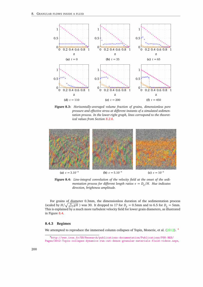
8. GRANULAR FLOWS INSIDE A FLUID

0 0.2 0.4 0.6 0.8 10

0.5

1

z(a) t = 0

0 0.2 0.4 0.6 0.8 10

0.5

1

z(b) t = 35

0 0.2 0.4 0.6 0.8 10

0.5

1

z(c) t = 65

0 0.2 0.4 0.6 0.8 10

0.5

1

z(d) t = 110

0 0.2 0.4 0.6 0.8 10

0.5

1

z(e) t = 200

0 0.2 0.4 0.6 0.8 10

0.5

1

z(f) t = 450

Figure 8.3: Horizontally-averaged volume fraction of grains, dimensionless porepressure and effective stress at different instants of a simulated sedimen-tation process. In the lower-right graph, lines correspond to the theoret-ical values from Section 8.2.6.

(a) ε= 3.10−4 (b) ε= 5.10−4 (c) ε= 10−3

Figure 8.4: Line-integral convolution of the velocity field at the onset of the sedi-mentation process for different length ratios ε = Dg/H. Hue indicatesdirection, brightness amplitude.

For grains of diameter 0.3mm, the dimensionless duration of the sedimentation process(scaled by H/

Æαα+1 gH ) was 30. It dropped to 17 for Dg = 0.5mm and to 6.5 for Dg = 5mm.

This is explained by a much more turbulent velocity field for lower grain diameters, as illustratedin Figure 8.4.

8.4.3 Regimes

We attempted to reproduce the immersed column collapses of Topin, Monerie, et al. (2012). 4

4http://www.irsn.fr/EN/Research/publications-documentation/Publications/PSN-RES/Pages/2012-Topin-collapse-dynamics-run-out-dense-granular-materials-fluid-videos.aspx,

200

8.4. Results

Figure 8.5: Snapshots at identical instants of the collapse of a granular column inthree different fluids: air (top), water (middle), and viscous (bottom).Colors indicate the particle and fluid velocities, on the same scale (blueis slowest, white fastest).

We consider a 2D granular column of aspect-ratio a = 8, with grains of diameter Dg = 1mmand volumetric mass ρg = 2600kg.m−3. The column width is W = 11.5Dg . Topin, Monerie,et al. (2012) couple the NSCD method with a fluid simulation; we use instead the µ(I) rheologyto model the frictional contacts, with µS = 0.32, µD = 0.6. Three choices are considered for thesurrounding fluid:

1. air: ρ f = 1kg.m−3 and η f = 10−5Pa.s;

2. water: ρ f = 1000kg.m−3 and η f = 10−3Pa.s;

3. viscous: ρ f = 1000kg.m−3 and η f = 1Pa.s.

Topin, Monerie, et al. (2012) observe that each of these choices yield a different collapseregime, which they coin respectively grain-inertial, fluid-inertial, and viscous. In the latter case,the collapse is simply slowed-down by the fluid, and the run-out length is much shorter thanin the dry (i.e., grain-inertial) case. However, in the fluid-inertial regime, the kinetic energyinitially transferred from the grains to the fluid is transferred back to the grains in the later stageof the collapse, maintaining an horizontal velocity for a much longer time than in the two otherregimes. As such, the final run-out length in the fluid-inertial regime can surpass that of the drycase.

While our experiments, reproduced in Figure 8.5, allow us to retrieve the grain-inertial andfluid-inertial regimes for the choices of parameters (1.) and (2.), choice (3.) remains mostly inthe fluid-inertial regime; albeit much slower than the collapse in water, the collapse in the viscousfluid achieve a barely shorter run-out length. While initially surprising, this can be explained bylooking at the characteristic numbers of our model.

Indeed, in the later stage of the collapse, the grains can be either slowed down or driven bythe drag forces, depending on which of the contact stress or pore pressure is preponderant. Thetotal normal stress of the mixture is p+Trφλ; the fact that the velocity is mostly horizontal, andthus that the grains are not collapsing under their own weight, means that the total normal stressis higher there than in the front of the avalanche. When the grains are weakly contacting, and

http://www.irsn.fr/EN/Research/publications-documentation/Publications/PSN-RES/Pages/2012-Topin-collapse-dynamics-run-out-dense-granular-materials-fluid-videos-bis.aspx

201

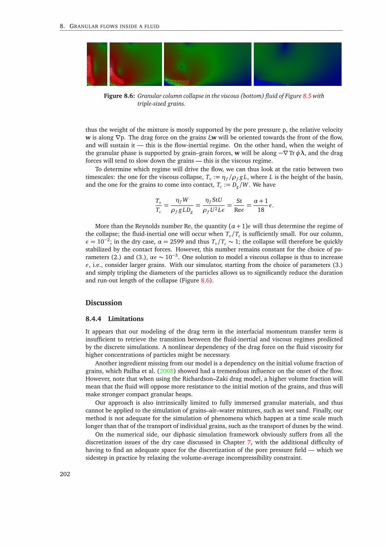
8. GRANULAR FLOWS INSIDE A FLUID

Figure 8.6: Granular column collapse in the viscous (bottom) fluid of Figure 8.5 withtriple-sized grains.

thus the weight of the mixture is mostly supported by the pore pressure p, the relative velocityw is along ∇p. The drag force on the grains ξw will be oriented towards the front of the flow,and will sustain it — this is the flow-inertial regime. On the other hand, when the weight ofthe granular phase is supported by grain–grain forces, w will be along −∇Trφλ, and the dragforces will tend to slow down the grains — this is the viscous regime.

To determine which regime will drive the flow, we can thus look at the ratio between twotimescales: the one for the viscous collapse, Tv := η f /ρ f g L, where L is the height of the basin,and the one for the grains to come into contact, Tc := Dg/W . We have

Tv

Tc=

η f W

ρ f g LDg=η f StU

ρ f U2 Lε=

St

Reε=α+ 1

18ε.

More than the Reynolds number Re, the quantity (α+1)ε will thus determine the regime ofthe collapse; the fluid-inertial one will occur when Tv/Tc is sufficiently small. For our column,ε = 10−2; in the dry case, α = 2599 and thus Tv/Tc ∼ 1; the collapse will therefore be quicklystabilized by the contact forces. However, this number remains constant for the choice of pa-rameters (2.) and (3.), αε ∼ 10−3. One solution to model a viscous collapse is thus to increaseε, i.e., consider larger grains. With our simulator, starting from the choice of parameters (3.)and simply tripling the diameters of the particles allows us to significantly reduce the durationand run-out length of the collapse (Figure 8.6).

Discussion

8.4.4 Limitations

It appears that our modeling of the drag term in the interfacial momentum transfer term isinsufficient to retrieve the transition between the fluid-inertial and viscous regimes predictedby the discrete simulations. A nonlinear dependency of the drag force on the fluid viscosity forhigher concentrations of particles might be necessary.

Another ingredient missing from our model is a dependency on the initial volume fraction ofgrains, which Pailha et al. (2008) showed had a tremendous influence on the onset of the flow.However, note that when using the Richardson–Zaki drag model, a higher volume fraction willmean that the fluid will oppose more resistance to the initial motion of the grains, and thus willmake stronger compact granular heaps.

Our approach is also intrinsically limited to fully immersed granular materials, and thuscannot be applied to the simulation of grains–air–water mixtures, such as wet sand. Finally, ourmethod is not adequate for the simulation of phenomena which happen at a time scale muchlonger than that of the transport of individual grains, such as the transport of dunes by the wind.

On the numerical side, our diphasic simulation framework obviously suffers from all thediscretization issues of the dry case discussed in Chapter 7, with the additional difficulty ofhaving to find an adequate space for the discretization of the pore pressure field — which wesidestep in practice by relaxing the volume-average incompressibility constraint.

202

8.4. Results

8.4.5 Conclusion

Despite all those drawbacks, our approach is still able to recover the qualitative dynamics ofimmersed granular flows in different regimes. We are able to capture the duality of the fluidrole, which may either lubricate the flow or dampen it, following the relative importance ofthe pore pressure and contact forces. Moreover, we were able to cast the numerical problemthat must be solved at each timestep as a standard DCFP with linear constraints, allowing us toleverage once again the large body of research devoted to such systems.

Future work will be focused on better understanding the role of the drag function ξ, whichdiscriminates between the inertial and viscous regime. Moreover, as already mentioned for thedry case, the search for better discretization spaces constitutes an important research directionfor us.

203

Conclusion

This dissertation focused on the simulation of complex materials featuring a large number of in-elastic contacts with friction. Our main argument is that dealing with these contacts using meth-ods derived from nonsmooth analysis is an efficient alternative to seemingly simpler elasticity-or regularization-based strategies. Indeed, nonsmooth methods allow to decouple the time scaleof the macroscopic phenomenon from that of the contact dynamics themselves, the latter beingoften much smaller for stiff materials and of little practical interest. For instance, one avoidshaving to explicitly simulate the compression and decompression phases after an impact, andcan thus get away with much larger timesteps.

We have also seen that continuum-based simulation methods can provide an efficient man-ner of simulating very large systems with small inhomogeneities, while still allowing to capturequalitative flow characteristics. Moreover, some numerical methods that have been developedfor discrete mechanics can be translated in a straightforward manner to continuum materials. Inparticular, granular materials may be simulated either at the grain level with the Coulomb fric-tion law or in a macroscopic fashion using the non-associated Drucker–Prager flow rule. Bothapproaches can leverage the exact same numerical solvers — even though the latter constitu-tive law is expressed on tensorial rather than vectorial quantities. This legitimizes further thefocus that we have put on devising a robust an efficient solver for Discrete Coulomb FrictionProblems (DCFP).

Finally, we have advocated in very different settings the use of hybrid methods, which cantake insight from distinct point of views to alleviate the drawbacks of each of them. We havehighlighted the benefits of combining an optimization-based approach with an analytical one forsolving local problems arising when using splitting methods on DCFP. Similarly, we have seenthat using simultaneously mesh-based and particle-based discretization strategies can simplifythe treatment of both temporal and spatial differential operators.

9.1 Key remarks and summary of contributions

We recall below with more details the main points that we brought up over the course of thisthesis, and emphasize the original contributions that we have introduced.

Following the works of Alart and de Saxcé, Chapter 1 presented the Signorini–Coulomb fric-tional contact law and the non-associated Drucker–Prager flow rule with tension cut-off in anunified manner. It included different ways of characterizing their sets of solutions, either withnormal cone inclusions or as roots of complementarity functions. In Chapter 2, we recalled theMoreau–Jean timestepping algorithm, which allows to compute the dynamics of a mechanicalsystem with bilateral constraints and unilateral contact with friction as a sequence of DCFP. Wepresented the Cadoux fixed-point algorithm, which yields both a criterion for the existence ofsolutions to a DCFP, and a practical way of solving this problem as a sequence of convexifiedDCFP (i.e., equivalently, as quadratic minimization problems under conical constraints). Chap-ter 3 then outlined standard algorithms for solving DCFP and convexified DCFP. Our first orig-inal contribution was presented in Chapter 4, and consisted in improving a numerical methodfor solving DCFP, targeted at ill-conditioned problems with a high number of contacts and forwhich reaching very high precision was not a requirement. To this aim, we proposed to equipthe Gauss–Seidel algorithm with a hybrid local solver combining a novel Newton algorithm onthe SOC Fischer–Burmeister function, and an enumerative analytical solver. We derived the ex-

205

CONCLUSION

pressions of the coefficients of the quartic polynomial that has to be solved for both DCFP andconvexified DCFP. We showed how this algorithm was relevant for applications to the direct andinverse simulation of hair and cloth, and provided benchmarks confirming its good practicalperformance. However, we noted that on smaller problems, a variant of the projected gradientdescent algorithm which we coined Accelerated Spectral Projected Gradient descent (ASPG) alsoperformed very well in practice. We also proposed a primal-dual algorithm “Dual AMA” requiringonly multiplications by the stiffness matrix, but which failed to demonstrate consistent-enoughconvergence. These different solvers have been released as part of an open-source library devel-oped alongside this thesis, bogus (Daviet 2013).

The second part of this dissertation built on our second contribution, presented in Chapter 6,a numerical strategy allowing to cast continuum granular flows problems into the frameworkof DCFP. Inspired by the work of Cadoux (2009), we showed how finding the solution to thenon-associated Drucker–Prager flow rule over a continuous domain amounted once again to asequence of minimization problems over a SOC in the space of symmetric tensor fields. How-ever, we were only able to state a very weak existence criterion. We then demonstrated thatby carefully choosing the basis for the discretization of the strain and stress fields, the discreteflow equations amounted to solving a DCFP (although with higher-dimensional constraints),and that we were able to leverage the solvers designed for standard discrete contact mechanics.We showed that this approach allowed us to capture qualitative features of dense granular flows(some of which being hard to achieve with standard methods, such as the vanishing pressurefield in the wake of an obstacle), then extended our method to more general flows in Chapters 7and 8. In particular, we proposed in Chapter 7 an approximation thanks to which our methodproved to be efficient-enough for Computer Graphics applications, allowing us to significantly re-duce visual artifacts w.r.t. a state-of-the-art method at a similar computational cost. However, wenoted that the choice of suitable discretization spaces remained a notable difficulty. On the otherhand, the soundness of our method allowed for an easy generalization to more complex settings,be it anisotropic friction, two-way coupling with rigid bodies, or interactions with a surroundingfluid. This last point was the subject of our third main contribution, presented in Chapter 8.Starting from the framework of Jackson (2000), we proposed a two-phase, two-velocity modelfor the coupled simulation of a Drucker–Prager granular material with a Newtonian fluid. Themain interesting feature of our approach is that, once again, we are able to cast the flow dynam-ics as a DCFP— though, in contrast to the single-phase case, one that includes linear equalityconstraints. While limited at the moment, we presented a first few steps towards the qualitativevalidation of this model, including the capture of the different dynamical regimes governing thecollapse of an immersed granular column reported in the literature.

9.2 Perspectives

Each step of our numerical method could probably be substantially improved: the choice of dis-cretization spaces, the coupling between the transport and momentum conservation equations,the algorithm for solving the DCFP, et cætera. One of our initial goals that was finally excludedfrom the scope of this thesis was the devising of a massive parallelization strategy taking profitof modern many-cores architectures. We have good hope that the proximal-based approachessuch as ASPG or Dual AMA could scale quite well, even though sparse matrix–vector productis not the most parallelization-friendly routine. Indeed, our first tests in this domain indicatedthat for regular grids, the variance in the number of non-zeros blocks per row in the DCFP’smatrices was quite small, and that storage schemes such as NVIDIA R© cuSPARSE’s HYB format1

were particularly relevant in this case.From a modeling point of view, we showed that it was possible to express the flow of a

granular material, even inside a Newtonian fluid, in a compact, consistent manner and with-out any regularization, as a sequence of numerical problems with a well-known structure. Wedemonstrated that this approach was able to capture some qualitative features of granular flows

1http://docs.nvidia.com/cuda/cusparse/#hybrid-format-hyb

206

9.2. Perspectives

that have been reported in the literature. Despite these first encouraging results, priority forfuture work should be put towards additional validation w.r.t. experimental data or DEM sim-ulations, and towards studying the influence of the several dimensionless numbers than appearin our diphasic model. Moreover, extending the numerical method of Chapter 8 to 3D simu-lations remains to be done before contemplating applications to Computer Graphics — whichcould include reproducing underwater sand avalanches or the dynamics of volcanic ash duringan eruption.

Finally, while we were able to simulate the dynamics of fibrous materials consisting of a fewthousand strands, larger systems still elude our DEM strategy. Moreover, air drag greatly influ-ences the dynamics of hair, and modeling the coupled dynamics of air and hair would probablyenhance realism. As coupling a fluid solver with hundreds of thousands of very fine DEM fiberswould be extremely costly, continuum modeling of this interaction would seem more appro-priate. An interesting research direction would thus be to attempt to extend our macroscopicnumerical method to the simulation of hair and fur; however, several key ingredients of suchmedia would still remain to be modeled. First, the bending elasticity of the fibers. One couldimagine writing a macroscopic bending energy based on the total derivative the fibers’ tangentsfield, or computing stresses on a discrete number of fiber samples in a MPM fashion. Stretchingenergy would probably have to be modeled in a similar manner, as the material cannot be approx-imated macroscopically as inextensible. Fibrous materials are also generally very anisotropic;the basic considerations that we laid down for coin-shaped grains in Chapter 7 would have tobe generalized, and the distribution of fiber orientations should influence a much wider rangeof parameters, from the drag coefficient to the maximal volume fraction. Finally, our granularmodel cannot capture the natural entanglement of human hair, which induces a kind of normal(instead of shearing) friction. Applying Dahl’s frictional model to this phenomenon would be aninteresting starting point. Continuum modeling of slender, elastic fiber assemblies would thusrequire the introduction of several additional hypothesis and closures. Before attempting suchan undertaking, it is therefore essential to get a good understanding of the simpler diphasicgranular model.

207

Appendices

209

A Convex analysis

In this section we recall a few fundamental results from convex analysis, stemming for a largepart from the early works of Jean-Jacques Moreau and R. Tyrrell Rockafellar. In the following,we mainly refer to the monograph “Fonctionnelles convexes”, as it lists several results in verygeneral settings — e.g., without assumption of finite dimension, even though here we will restrictourselves to Banach or Hilbert spaces.

A.1 Operations on convex functions

A.1.1 Fundamental definitions

Let X be a reflexive Banach space on R. Let R := R∪−∞,+∞ denote the extended-real set,and f : X → R.

Definition A.1. f is said to be convex if

f (αx + (1−α)z)≤ α f (x ) + (1−α) ∀x , z,α ∈ X × X×]0, 1[

where the addition is extended to R with the commutative convention (−∞) + (+∞) = +∞. fis said to be strictly convex if the above definition holds with strict inequality for all x 6= z.

Definition A.2 (Epigraph). The epigraph of f is the set epi f := (x ,α) ∈ X ×R, f (x )≤ α. Itholds that f is convex if and only if epi f is convex.

Definition A.3 (Effective domain). The effective domain of f is the set dom f := x ∈ X , f (x )< +∞.f is said to be proper if dom f 6= ; and ∀x ∈ X , f (x )> −∞.

Definition A.4 (Closed function). f is said to be closed if epi f is closed.

Definition A.5. [Lower semi-continuity] f is said to be lower semi-continuous at x 0 ∈ X if for allε ∈ R∗

+, there exists a neighborhood V of x 0 such that ∀x ∈ V, f (x )≥ f (x 0))− ε.

Property A.1. The following propositions are equivalent (Moreau 1966–1967, paragraph 4.a):

1. f is closed

2. f is lower semi-continuous on X

3. ∀α ∈ R, the set x ∈ X , f (x )≤ α is closed.

Property A.2. Any proper closed convex function f is continuous on the interior of its effectivedomain (Moreau 1966–1967, paragraph 5.f).

A.1.2 Subdifferential of a function

Let Y be the topological dual space of X (the space of continuous linear forms y : X → R), withthe bilinear form ⟨·, ·⟩ : X × Y → R such that Y can be identified to ⟨·, y⟩ , y ∈ Y and X to⟨x , ·⟩ , x ∈ X .

211

A. CONVEX ANALYSIS

Definition A.6 (Subdifferential). If there exists x 0 ∈ X and y ∈ Y such that

∀x ∈ X , f (x )≥ f (x 0) + ⟨x − x 0, y⟩then f is said to be subdifferentiable at x 0 and y is a subgradient of f at x 0. We denote by ∂ f (x 0)

the subdifferential of f at x 0, defined as the set of all subgradients at f at x 0.

Remark A.1. If f is proper, ∂ f (X \ dom f ) = ;.It follows from Definition A.6 that:

Property A.3 (Minimum of a convex function). The global minimum of f is attained at x 0 ∈ Xif and only if 0 ∈ ∂ f (x 0). Moreover, if f is strictly convex, this global minimum is attained at atmost one point.

Proof. 0 ∈ ∂ f (x 0) ⇐⇒ f (x )≥ f (x 0) ∀x ∈ X , which is the definition of a global minimum. Toprove the second assertion, suppose that f is strictly convex and attains its global minimum attwo different points x 1 6= x 2. Then f ( 1

2 (x 1 + x 2)) <12 ( f (x 1) + f (x 2)) = f (x 1), which yields a

contradiction.

The following property suggests that the subdifferential can be seen as a generalization ofthe concept of the gradient of a convex function at points where it is not differentiable.

Property A.4. Let f be a proper convex function on X, continuous at x 0 ∈ dom( f ). The followingstatements are equivalent (Moreau 1966–1967, paragraphs 10.f and 10.g)

• f is Gâteaux-differentiable at x 0 with gradient (∇ f )(x 0) ∈ Y , i.e.,

limα→0+

f (x 0 +αx )− f (x 0)

α= ⟨x , (∇ f )(x 0)⟩ ∀x ∈ X ;

• ∂ f (x 0) = (∇ f )(x 0).Remark A.2. If f is Fréchet-differentiable, then it is continuous and Gâteaux-differentiable as well,and the gradients from both definitions coincide. The converse is not true; intuitively Fréchet ensuresthat the differential is well-defined along all continuous paths converging to x 0, while Gâteauxconsiders only straight lines.

Sum of differentials It always hold that ∂ f + ∂ g ⊂ ∂ ( f + g), but some regularity (a.k.a.qualification) conditions are required for the equality to be achieved. Moreau (1966–1967,Proposition 10.7) states the following theorem:

Theorem A.1 (Subdifferential of a sum). For f and g convex X → R, if there exists x 0 ∈ dom f ∩dom g such that either f or g is continuous at x 0, then ∂ ( f + g) = ∂ f + ∂ g on X .

As a proper convex function is continuous on the interior of its effective domain (Prop-erty A.2), it follows:

Corollary A.1. Let f and g be convex functions X → R, with f closed and proper. If (int dom f )∩dom g 6= ;, then ∂ ( f + g) = ∂ f + ∂ g on X .

Special cases The following property will prove useful in continuum mechanics.

Property A.5 (Subdifferential in function spaces). Let Ω be a subset of Rd , d ∈ N, and let L2(Ω)

denote the space of square-integrable functions on Ω. Let ⟨·, ·⟩ be a scalar product on Rn, n ∈ N; weequip the space V := L2(Ω)

n with the scalar product ⟨·, ·⟩V ,

⟨u,v⟩V :=

∫

Ω

⟨u(x ),v(x )⟩dx ∀(u,v) ∈ V 2.

212

A.1. Operations on convex functions

Finally, consider a function g : V → R, u 7→ ∫Ω

f (u(x ))dx , where f : Rn→ R. The subdifferentialof g is given by, for any u ∈ V ,

∂ g(u) = v ∈ V,v(x ) ∈ ∂ f (u(x )) a.e. on Ω .

Proof. V is an Hilbert space, thus ∂ g ⊂ V . Let u,v ∈ V 2, Ω+v

:= x ∈ Ω,v(x ) ∈ ∂ f (u(x )) andΩ−v

:= Ω − Ω+v

. By definition of the subdifferential, x ∈ Ω+v⇐⇒ ∀z ∈ Rd , f (z)− f (u(x )) ≥

⟨v(x ), z − u(x )⟩.For any w ∈ V , we thus have

g(w)− g(u) =

∫

Ω+v

f (w(x ))− f (u(x )) +

∫

Ω−v

f (w(x ))− f (u(x ))

≥∫

Ω+v

⟨v(x ),w(x )− u(x )⟩+∫

Ω−v

f (w(x ))− f (u(x )).

As f takes its values in R, Ω−v

being of measure zero implies that g(w)− g(x)≥ ⟨v,w− u⟩V , andthus v ∈ ∂ g(u). Reciprocally, suppose that Ω−

vis not of measure zero. By definition of this set,

for all x ∈ Ω−v

there exists zx ∈ Rd such that f (zx )− f (u(x ))< ⟨v(x ), zx − u(x )⟩. Let us definew ∈ V as

w(x ) :=§

zx on a relatively compact subset of Ω−v

with strictly positive measureu(x ) elsewhere.

Then g(w)− g(u) =∫Ω−

v

zx − f (u(x ))<∫Ω−

v

⟨v(x ), zx − u(x )⟩= ⟨v,w− u⟩V , i.e., v 6∈ ∂ g(u).

Finally, we state a property of subdifferentials that will not be directly useful in this disserta-tion, but allows the easy extension of results derived for a scalar constraint to larger dimensionalones. The proof is given for a finite-dimensional space in (Hiriart-Urruty and Lemaréchal 1993,VI, Corollary 4.3.2), and extended to infinite sequences in (Hiriart-Urruty and Lemaréchal 1993,VI, Theorem 4.4.2).

Property A.6 (Subdifferential of a maximum). Let fi , i = 1 . . . n be a finite number of convexfunctions on X . Then the subdifferential of their point-wise maximum a point x 0 is the convex hullof the subdifferentials of the fi that are active at x 0, i.e.,

∂ (max( fi))(x 0) = Conv⋃

j∈J

∂ f j with J := j, f j(x 0) =maxi

fi(x 0)).

A.1.3 Convex conjugate

Definition A.7 (Convex conjugate). The convex conjugate (or Fenchel–Legendre transform) of fis the application

f ⋆ :Y → Ry 7→ sup

x∈X(⟨x , y⟩ − f (x )) .

Moreau (1966–1967, paragraphs 6.b and 6.d) gives two fundamental properties:

Property A.7. The convex conjugate of f is always convex and closed. If f is proper, convex andclosed, then it is equal to its biconjugate, i.e., f = f ⋆⋆.

Theorem A.2 (Subnormality). It always hold that f (x )+ f ⋆(y)≥ ⟨x , y⟩ (Fenchel-Young inequal-ity). Moreover, if f is proper, closed and convex, then

y ∈ ∂ f (x ) ⇐⇒ f (x ) + f ⋆(y) = ⟨x , y⟩ ⇐⇒ x ∈ ∂ f ⋆(y).

213

A. CONVEX ANALYSIS

Proof. From the definition of the convex conjugate, ∀x , y ∈ X × Y ,

f (x ) + f ⋆(y) = f (x ) + supz∈X(⟨z, y⟩ − f (z))

≥ f (x ) + (⟨x , y⟩ − f (x )) = ⟨x , y⟩Then,

f (x ) + f ⋆(y) = ⟨x , y⟩ ⇐⇒ f ⋆(y) = ⟨x , y⟩ − f (x )

⇐⇒ ⟨z, y⟩ − f (z)≤ ⟨x , y⟩ − f (x ) ∀z ∈ X

⇐⇒ f (x ) + ⟨z − x , y⟩ ≤ f (z) ∀z ∈ X

⇐⇒ y ∈ ∂ f (x )

The second part of the equivalence stems from f ⋆⋆ = f (Property A.7).

We transcribe below a slightly weakened version of the Fenchel duality theorem as given in(Borwein and Luke 2011, theorem 1.2),

Theorem A.3 (Fenchel duality). Let X and E be Banach spaces, with E⋆ the dual of E. Let L be abounded linear map.

Then the extrema of the optimization problems (A.1) and (A.2),

p = infx∈X

f (x ) + g(Lx )

d = supz∈E⋆− f ⋆(L⊺z)− g⋆(−z)

(A.1)

(A.2)

satisfy weak duality, i.e., p ≥ d.Moreover if f and g are convex and if there exists x ∈ L dom f such that g is finite and contin-

uous at x 0, strong duality holds: p = d, and if they are finite, then the dual problem (A.2) attainsits maximum.

Corollary A.2. Extension to affine maps; L in the theorem above is replaced by A : x 7→ Lx + e,and the optimization problems (A.1) and (A.2) with

p = infx∈X

f (x ) + (g A)(x )

d = supz∈E⋆− f ⋆(L⊺z)− g⋆(−z)− ⟨e, z⟩

Weak duality always hold, and strong duality is achieved when f and g are convex and there existsx ∈ Adom f such that g is finite and continuous at x 0.

Proof. By application of the theorem to ge : z 7→ g(z + e); indeed ge(Lx ) = g A(x ), and(⋆ge)(−z) = (⋆g)(−z) + ⟨e, z⟩.

A.2 Normal and convex cones

A.2.1 Normal cone

Definition A.8 (Characteristic function). The characteristic function IC of a set C ⊂ X is definedas vanishing on C and taking infinite values outside of C,

IC :=

0 if x ∈ C

+∞ if x 6∈ C .

From epiIC = C ×R+ and domIC = C it follows:

• IC is convex if and only if C is convex.

214

A.2. Normal and convex cones

• IC is not empty if and only if C is proper.

• IC is closed if and only if C is closed.

Definition A.9 (Normal cone). Let C be a convex subset of X . The normal cone to C at x 0 ∈ X isdefined as

NC(x 0) =

y ∈ Y, ⟨x − x 0, y⟩ ≤ 0 ∀x ∈ C if x 0 ∈ C

; if x 0 6∈ C

As it can easily be seen that for any point x 0 in C , 0 ∈ NC(x 0), we have the equivalence:

Property A.8. 0 ∈ NC(x ) ⇐⇒ x ∈ C

Property A.9. If C is not empty, there holds NC = ∂IC .

Proof. As IC is proper, from Remark A.1 we have x 0 6∈ C ⇐⇒ ∂IC(x 0) = ; = NC(x 0). Forx 0 ∈ C , Definition A.6 reads

y ∈ ∂IC(x 0) ⇐⇒ IC(x )≥ IC(x 0) + ⟨x − x 0, y⟩ ∀x ∈ X

⇐⇒ IC(x )≥ ⟨x − x 0, y⟩ ∀x ∈ X

⇐⇒ 0≥ ⟨x − x 0, y⟩ ∀x ∈ C

⇐⇒ y ∈ NC(x 0)

We deduce immediately that the expression of the normal cone at an interior point.

Property A.10. x ∈ int C =⇒ NC(x ) = 0.Proof. For x ∈ int C , there exists a closed ball with strictly positive radius centered at x on whichIC is constant. ThereforeIC is continuous and Gâteaux-differentiable at x , with (∇IC)(x 0) = 0.Properties A.4 and A.9 conclude the proof.

A.2.2 Operations on normal cones

Property A.11 (Normal cone to an intersection). For any two subsets C1 and C2 of X , NC1∩C2⊃

NC1+NC2

.Moreover, if C1 and C2 are convex, with C1 closed and (int C1)∩C2 6= ;, thenNC1∩C2

=NC1+NC2

.

Proof. If C1 and C2 are empty, the inclusion is trivial. Otherwise, we have IC1∩C2= IC1

+ IC2,

therefore with Property A.9,

NC1∩C2= ∂

IC1+IC2

⊃ ∂IC1+ ∂IC2

=NC1+NC2

.

Now, if C1 and C2 are convex with C1 closed and (int C1) ∩ C2 6= 0, the regularity conditions ofCorollary A.1 on the subdifferential of a sum are satisfied, and the equality holds.

Corollaries of the following property will often prove useful for the practical computation ofnormal cones.

Property A.12 (Subdifferential of the precomposition by an affine map). Let X and E be Hilbertspaces, and A an affine map from X to E, i.e., A(x ) = Lx + e with L linear and e ∈ E. We note L⊺

the linear adjoint of L. Let f be a convex function on E. There holds, for all x ∈ X ,

∂ ( f A)(x ) ⊃ L⊺∂ f (A(x )).

Moreover, if f is proper and closed, and ∃x 0 ∈ dom( f A) such that f is continuous at A(x 0), thenfor all x ∈ X ,

∂ ( f A)(x ) = L⊺∂ f (A(x )).

215

A. CONVEX ANALYSIS

Proof. First, let y ∈ L⊺∂ f (A(x 0)). There exists g ∈ E such that y = L⊺g and

f (z)≥ f (A(x 0)) + ⟨z − A(x 0), g ⟩ ∀z ∈ E.

In particular,

f (A(x ))≥ f (A(x 0)) + ⟨A(x )− A(x 0), g ⟩ ∀x ∈ X .

Since ⟨A(x )− A(x 0), g ⟩= ⟨Lx − Lx 0, g ⟩= ⟨x − x 0, L⊺g ⟩,f (A(x ))≥ f (A(x 0)) + ⟨x − x 0, y⟩ ∀x ∈ X ,

which means that y ∈ ∂ ( f A)(x 0).Now, let us prove the reverse inclusion under our supplemental regularity conditions. Let

y ∈ ∂ ( f A)(x 0), and let x ∗ ∈ dom( f A), which is not empty under our hypothesis. Then,∀x ∈ Ker L,

f (A(x ∗ + x ))≥ f (A(x 0)) + ⟨x ∗ + x − x 0, y⟩−⟨x , y⟩ ≥ f (A(x 0))− f (A(x ∗)) + ⟨x ∗ − x 0, y⟩ .

As the right-hand side is finite, for the inequality to hold for all x ∈ Ker L, we must have y ∈(Ker L)⊥ = Im L⊺, i.e., ∃g ∈ E, y = L⊺g . Going back to the definition of the subdifferential, wemust also have

f (A(x ))≥ f (A(x 0)) + ⟨x − x 0, L⊺g ⟩ ∀x ∈ X

f (A(x ))≥ f (A(x 0)) + ⟨A(x )− A(x 0), g ⟩ ∀x ∈ X

f (z)≥ f (A(x 0)) + ⟨z − A(x 0), g ⟩ ∀z ∈ Im A

( f +IIm A)(z)≥ ( f +IIm A)(A(x 0)) + ⟨z − A(x 0), g ⟩ ∀z ∈ E,

which means g ∈ ∂ ( f +IIm A)(A(x 0)). Under our regularity conditions, we can apply Theo-rem A.1 and get equivalently g ∈ ∂ f (A(x 0))+∂IIm A(A(x 0)). As ∂IIm A(A(x 0)) =NIm A(A(x 0)) =

Ker L⊺, we gety ∈ L⊺ (∂ f (A(x 0)) + Ker L⊺) = L⊺∂ f (A(x 0)).

We can get the following corollary by choosing f = IC in the above property:

Corollary A.3. Let C be a closed convex subset of E such that int C ∩ Im A 6= 0. Then the normalcone to Γ := x ∈ X , A(x ) ∈ C is

NΓ (x ) = L⊺NC(A(x ))

The extension to linear constraints stated below will also prove useful for mechanical systems.

Corollary A.4. Let A : X → E be an affine map defined as in Property A.12, i.e., A : x 7→ Lx+e, B :X → F a linear operator from X to F Hilbert space, and for any f ∈ F, V ( f ) := x ∈ X , Bx = f .Let C be a closed convex subset of E, then the normal cone to Γ ( f ) := x ∈ V ( f ), A(x ) ∈ Csatisfies

NΓ ( f )(x ) ⊃ L⊺NC(A(x )) + B⊺N0F (Bx − f ),

with equality under the regularity condition

int C ∩ A(V ( f )) 6= ;. (A.3)

Proof. The inclusion being trivial, we focus on the equality. The regularity condition (A.3) re-quires that V ( f ) is not empty; let v f ∈ V ( f ), then V ( f ) = V (0F ) + v f .

V (0F ) = Ker B is a linear subspace of X and is therefore a Hilbert space. As the regularitycondition (A.3) can be written

int C ∩ LV (0F ) + e + Lv f

6= ;

216

A.2. Normal and convex cones

we can apply Corollary A.3 to the linear map A0 : V (0F )→ E, x 7→ Lx + (e+ Lv f ), and get thatthe normal cone to Γ0( f ) ⊂ V (0F ) := x ∈ V (0F ), A0(x ) ∈ C is

NΓ0( f )(x ) = L⊺NC(A0(x )).

Now, suppose y ∈ NΓ ( f )(x ). Necessarily x ∈ Γ ( f ), and thus x − v f ∈ V (0F ). Moreover, wecan decompose y as y = y |V (0F )

+ y⊥, with y |V (0F )∈ V (0F ) and y⊥ ∈ Im B⊺. Therefore,

∀z ∈ Γ ( f ), ⟨y , z − x ⟩ ≤ 0

∀z ∈ Γ0( f ),y , z − (x − v f )

≤ 0

∀z ∈ Γ0( f ),y |V (0F )

, z − (x − v f )≤ 0,

and necessarily y ∈ NΓ0(x − v f )+ B⊺N0F (Bx − f ). As the reverse inclusion always holds fromProperty A.11 on the normal cone to an intersection and Corollary A.3 applied to the linearconstraint, we get

NΓ ( f )(x ) = L⊺NC(A0(x − v f )) + B⊺N0F (Bx − f )

= L⊺NC(A(x )) + B⊺N0F (Bx − f ).

A.2.3 Convex cones

The name normal cone is coined from the fact that its belong to the class of convex cones, whichpossesses interesting properties w.r.t. the convex conjugate.

Definition A.10 (Convex cone). A subset K ⊂ X is a convex cone if

x , y ∈ K2 =⇒ (αx + β y) ∈ K , ∀α,β ∈ R2+

.

Property A.13. There holds:

1. For any x ∈ C ⊂ X , NC(x ) is a convex cone.

2. If K is a convex cone, then 0 ∈ K ⇐⇒ K 6= ;.Definition A.11 (Dual and polar cones). The polar cone of C ⊂ X is the set

C := y ∈ Y, ⟨x , y⟩ ≤ 0 ∀x ∈ C .

The dual cone of C is then defined as the negative of the polar cone, C⋆ := −C.

Property A.14 (Normal cone to a convex cone). If K is a convex cone, then

NK(x ) =

; if x 6∈ K

K ∩ x⊥ if x ∈ K .

Proof. The first case holds for any normal cone (Property A.8). Let us prove the second one.First, we choose x ∈ K and y ∈ NK(x ), i.e., ∀x ∈ K , ⟨z − x , y⟩ ≤ 0. Since 0 ∈ K , ⟨0− x , y⟩ ≤

0, and since 2x ∈ K as well, ⟨x , y⟩ ≤ 0, therefore ⟨x , y⟩= 0, i.e., y ∈ x⊥.Moreover, ∀z ∈ K , (x + z) ∈ K , meaning that ∀z ∈ K , ⟨z, y⟩ ≤ 0, i.e., y ∈ K. Necessarily,

we therefore have NK(x ) ⊂ K ∩ x⊥. Let us now prove that the inclusion is not strict. Lety ∈ K∩x⊥, and z ∈ K . Then ⟨z − x , y⟩= ⟨z, y⟩−⟨x , y⟩ ≤ 0 from the definitions of the polarcone and of the orthogonal subspace. Since this is true ∀z ∈ K , y ∈ NK(x ). Therefore, ∀x ∈ K ,NK(x ) = K ∩ x⊥.

Property A.15. For K a non-empty convex cone, (IK)⋆ = IK

217

A. CONVEX ANALYSIS

Proof. Following from the definition of the convex conjugate,

IK⋆(y) = sup

x∈X(⟨x , y⟩ − IK(x ))

= supx∈K(⟨x , y⟩)

As K is a cone, (0x ) ∈ K and therefore IK⋆(y) ≥ 0. Moreover if ∃x 0 ∈ K , ⟨x 0, y⟩ > 0, then

∀β ∈ R+, we can choose α= β

⟨x 0,y⟩ so that (αx 0) ∈ K and ⟨αx 0, y⟩ ≥ β , i.e., IK⋆(y) = +∞.

This means

IK⋆(y) =

§+∞ if ∃x ∈ K , ⟨x , y⟩> 00 otherwise

=

§+∞ if x 6∈ K

0 otherwise= IK .

Corollary A.5. A non-empty closed convex cone K is the dual (resp., polar) cone of its dual (resp.,polar) cone, i.e., K⋆⋆ = K and K = K.

Proof.x ∈ K ⇐⇒ x ∈ NK(0) using Property A.14

⇐⇒ x ∈ ∂IK(0) using Property A.9

⇐⇒ x ∈ ∂IK⋆(0) using Property A.15

⇐⇒ 0 ∈ ∂IK⋆⋆(x ) using Theorem A.2

⇐⇒ 0 ∈ ∂IK(x ) using Property A.7

⇐⇒ 0 ∈ NK(x ) using Property A.9

⇐⇒ x ∈ K using Property A.8.

Theorem A.4 (Conic complementarity). For K a non-empty closed convex cone, there holds

y ∈ NK(x ) ⇐⇒ K ∋ x ⊥ y ∈ K ⇐⇒ x ∈ NK(y)

where the “· ⊥ ·” is used to mean ⟨·, ·⟩= 0.

Proof. From Theorem A.2 and Properties A.9 and A.15,

y ∈ NK(x ) ⇐⇒ y ∈ ∂IK(x )

⇐⇒ IK(x ) +IK⋆(y) = ⟨x , y⟩

⇐⇒ IK(x ) +IK(y) = ⟨x , y⟩The equality is only possible on the effective domain of the left-hand side, on which IK(x ) +

IK(y) is constant and equal to zero. This means

IK(x ) +IK(y) = ⟨x , y⟩ ⇐⇒ x ∈ K and y ∈ K and ⟨x , y⟩= 0

Then, the rightmost equivalence follows from Corollary A.5.

A.3 Constrained optimization

We consider the minimization problem

p =minx∈C

f (x ) (A.4)

with f closed and convex, and C a closed convex subset of X .

218

A.3. Constrained optimization

Note that the constrained minimization problem (A.4) is equivalent to the unconstrainedone (A.5),

p =minx∈X( f +IC)(x ) (A.5)

We first recall a sufficient condition for the existence of a solution to problem (A.5) (see e.g.,Barbu and Precupanu 2012, p. 72, Theorem 2.11, Proposition 2.10 and Remark 2.13).

Theorem A.5 (Existence of a solution). Let f : X → R be convex and lower semi-continuous, andC ⊂ X is convex and closed. If the minimization problem (A.4) is feasible, that is dom f ∩ C 6= ;,and f is coercive on C, that is,

limx∈C ,‖x‖→+∞

f (x ) = +∞,

then f attains its global minimum on C.

A.3.1 Optimality conditions

We now derive sufficient conditions for checking that a point x 0 ∈ X is a solution to (A.4), i.e.,x 0 ∈ C and f (x 0) = p.

Theorem A.6 (Fundamental theorem of convex optimization). Suppose f a proper closed convexfunction on X and C a closed convex subset of X , such that f is real-valued and continuous on C.The optimality condition of (A.4) reads

∂ f (x 0)∩−NC(x 0) 6= 0.

If f is moreover Gâteaux-differentiable on C, the optimality condition becomes

(∇ f )(x 0) ∈ −NC(x 0).

Proof. First, if C is empty the problem is not feasible, NC is always empty and the equivalenceis trivial. Let us now assume C not empty. From Property A.3, the optimality condition of (A.5)and therefore of (A.4) is 0 ∈ ∂ g(x 0).

We can apply Theorem A.1 to get ∂ g = ∂IC + ∂ f . Expressing ∂IC with Property A.9, thismeans 0 ∈ ∂ f (x 0) +NC(x 0). If f is Gâteaux-differentiable at x 0, Property A.4 states that itssubdifferential contains only its gradient, so the optimality condition becomes 0 ∈ (∇ f )(x 0)+NC(x 0).

Corollary A.6. If X is an Hilbert space, then for x , y ,α ∈ X × X ×R∗+

,

y ∈ NC(x ) ⇐⇒ ΠC (x +αy) = x

where ΠC denotes the orthogonal projection on the closed convex subset C of X ,

ΠC(z) = argminx∈C

1

2⟨z − x , z − x ⟩

Proof. For any z ∈ X , let fz(x ) := 12 ⟨z − x , z − x ⟩, which a real-valued, closed, convex, and

differentiable function on X .Applying Theorem A.6 to the minimization of fz on C , we get

x 0 = ΠC (z) ⇐⇒ ∇ fz(x 0) ∈ −NC(x 0) ⇐⇒ x 0 − z ∈ −NC(x 0).

For z := x 0 +αy with α ∈ R+∗ , this reduces to

x 0 = ΠC (x 0 +αy) ⇐⇒ αy ∈ NC(x 0) ⇐⇒ y ∈ NC(x 0).

219

A. CONVEX ANALYSIS

Remark A.3. Combining Theorem A.6 with Corollary A.6, the optimality condition of (A.4) becomes

ΠC (x 0 −α(∇ f )(x 0)) = x 0 , α ∈ R∗+

,

yielding the rationale for the Projected Gradient Descent algorithm.

Corollary A.7 (Karush–Kuhn–Tucker conditions). The optimality conditions of the minimizationproblem

minx∈K

f (x )

with K is a closed convex cone, and f a proper closed convex function on X and real-valued, contin-uous and Gâteaux-differentiable on K, are

K ∋ x 0 ⊥ (∇ f )(x 0) ∈ K⋆

and are called the first-order Karush–Kuhn–Tucker conditions.

Proof. This is a direct application of Theorem A.6 combined with the equivalences from Prop-erty A.9 and Theorem A.4:

(∇ f )(x 0) ∈ −NK(x 0) ⇐⇒ (∇ f )(x 0) ∈ −∂IK(x 0) ⇐⇒ K ∋ x 0 ⊥ (∇ f )(x 0) ∈ K⋆

A.3.2 Lagrange multipliers

A last application concerns the structure of the normal cone at the boundary of an implicitly-defined convex set.

Property A.16 (Normal cone at the boundary). Consider a set C defined as C := x ∈ X , F(x )≤0 with F a proper closed convex function on X , continuous on C. For x 0 ∈ Bd C, there alwaysholds

NC(x 0) ⊃ αg , g ∈ ∂ F(x 0), α ∈ R+, (A.6)

and equality is achieved if inf F < 0. It this later case, we also have the equivalence F(x ) = 0 ⇐⇒x 0 ∈ Bd C, so that for any x 0 such that F(x )< 0, NC(x 0) = 0.Proof. C is convex (from the convexity of F) and closed (Property A.1). Moreover, as F is con-tinuous on C , F(x )< 0 =⇒ x ∈ int C and therefore x ∈ Bd C =⇒ F(x ) = 0.

We can easily show that αg , g ∈ ∂ F(x 0) α ∈ R+ ⊂ NC(x 0). Indeed, let x 0 ∈ Bd C andg ∈ ∂ F(x 0). This means

F(x )≥ F(x 0) + ⟨x − x 0, y⟩ ∀x ∈ X

0≥ ⟨x − x 0, y⟩ ∀x , F(x )≤ 0

and therefore y ∈ NC(x 0).Now assume inf F < 0, and let us prove the converse inclusion. Let y ∈ NC(x 0); if y = 0,

we have ∃g ∈ ∂ F(x 0),0 g = y as ∂ F(x 0) is not empty (Moreau 1966–1967, paragraph 10.c).Now, let us assume y 6= 0, and consider the constrained optimization problem

minx∈C−⟨x , y⟩. (A.7)

From Theorem A.6, x 0 satisfies the optimality condition of (A.7). Now, suppose that the mini-mum is also reached at x ∈ int C; this means y ∈ NC(x ) = 0 from Property A.10, which is acontradiction. Therefore, ∀x ∈ int C , −⟨x , y⟩> −⟨x 0, y⟩. As x 0 ∈ Bd C , we get

x ∈ int C =⇒ F(x )< F(x 0)︸ ︷︷ ︸0

=⇒ ⟨x − x 0, y⟩< 0

220

A.3. Constrained optimization

or equivalently

⟨x − x 0, y⟩ ≥ 0 =⇒ F(x )≥ F(x 0). (A.8)

Let use denote byHy (x 0) the half-space

Hy (x 0) := x ∈ X , ⟨x − x 0, y⟩ ≥ 0 .Then Equation (A.8) means that x 0 satisfies the optimality conditions of the minimization prob-lem

minx∈Hy (x 0)

F(x ),

which are, using Property (A.3) then Theorem A.1 (F is continuous and both terms are convexand finite at x 0),

0 ∈ ∂F +IHy (x 0)

(x 0) = ∂ F(x 0) +NHy (x 0)

(x 0)

0 ∈ ∂ F(x 0) + −αy ,α ∈ R+ .As we supposed that inf F < 0, 0 6∈ ∂ F(x 0), and therefore ∃α ∈ R+ and g ∈ ∂ F(x 0) such thaty = αg .

It remains to show that x ∈ int C =⇒ F(x ) < 0. Suppose F(x ) = 0. As inf F < 0,0 6∈ ∂ F(x 0), and we can find a non-zero element y ∈ ∂ F , which is non-empty. From the dualityof X and Y , there exists x ∈ X , ⟨x , y⟩ > 0. For every ε > 0, let x ε = x 0 +

ε‖x‖ x ; ‖x 0 − x ε‖ ≤ ε

and F(x ε)> 0, i.e., x 0 ∈ Bd C .

The qualification hypothesis inf F < 0 is not necessary, however the equality would thenrequire supplemental constraints on the structure of ∂ F . Intuitively, we require F to go to zerowith a strictly positive slope in all directions; the problem is indeed similar to that of the existenceof Lagrange Multipliers, which require a surjective differential for the application of the ImplicitFunction Theorem.

An example of a function for which inclusion (A.6) is strict while the subdifferential isnowhere equal to 0 is

F : R→ R, x 7→§

x2 if x ≤ 0x if x > 0.

Indeed, ∂ F(0) = [0,1] while ∂IC = R.Conversely, an example for which min F = 0 yet the equality holds is the case of affine

equality constraints:

Property A.17. Suppose A : X → E, x 7→ Lx + e an affine map between two Hilbert spaces. LetF : x 7→ ‖A(x )‖, and C := x ∈ X , F(x ) = 0. Then for x 0 such that A(x 0) = 0,

NC(x 0) = Im L⊺ = αg , g ∈ ∂ F(x 0), α ∈ R+.Proof. First, suppose y ∈ NC(x 0). ∀x ∈ C , ⟨x − x 0, y⟩ ≤ 0. As A(x 0) = 0, F(x ) = 0 ⇐⇒A(x ) − A(x 0) = 0 ⇐⇒ L(x − x 0) = 0. Therefore, y must obey that ∀x ∈ Ker L, ⟨x , y⟩ ≤ 0,which means y ∈ (Ker L)⊥. We thus have NC(x 0) ⊂ Im L⊺.

Now, let us prove that

Im L⊺ ⊂ αg , g ∈ ∂ F(x 0), α ∈ R+,which will achieve the demonstration, the converse inclusion being granted by Property A.16.Property A.12 states that we always have ∂ F(x 0) ⊃ L⊺∂ ‖ · ‖(A(x 0)). Since A(x 0) = 0, usingTheorem (A.2),

g ∈ ∂ ‖ · ‖(A(x 0)) ⇐⇒ 0 ∈ ∂ ‖ · ‖⋆(g ).Direct computations yield ‖ · ‖⋆ = IB(0,1), the characteristic function of the unit closed ballcentered at 0. This means

g ∈ ∂ ‖ · ‖(A(x 0)) ⇐⇒ 0 ∈ NB(0,1)(g ) ⇐⇒ ‖g‖ ≤ 1.

221

A. CONVEX ANALYSIS

It results that ∂ F(x 0) ⊃ L⊺B(0, 1). Then, for all y ∈ Im L⊺, ∃α ∈ R+, y = L⊺αg with ‖g‖ ≤ 1,and in particular, (L⊺g ) ∈ ∂ F(x 0).

Property A.18 (KKT multiplier). Let C := x ∈ X , F(x )≤ 0 and A(x ) = 0 with F convex, closedand continuous on C, and A an affine map, A : X → E, x 7→ Lx + e. We consider the optimizationproblem (A.4),

minx∈C

f (x ), (A.4)

for f closed, convex, continuous and real-valued on C.If there exists x ∈ X such that A(x ) = 0 and F(x ) < 0, then the optimality conditions of (A.4)

read

; 6= ∂ f (x 0)∩ (−λ∂ F(x 0) + L⊺r )

0= A(x 0)

0≤ F(x 0)⊥ λ ≥ 0.

(A.9)

λ ∈ R is the Karush–Kuhn–Tucker multiplier associated to the constraint F(x ) ≤ 0, and r ∈ E⋆ isthe vector of Lagrange multipliers associated to the constraint A(x ) = 0.

Proof. Property A.6 gives the optimality condition ∂ f (x 0)∩NC 6= 0. Let us expressNC =NCA∩CF,

CA := A(x ) = 0, CF := F(x )≤ 0.Our hypothesis, ∃x , A(x ) = 0 and F(x ) < 0, implies that CA ∩ int CF 6= ;; we can therefore

use the Corollary A.1 on the subdifferential of a sum, and obtain with Property A.9 thatNCA∩CF=

NCA+NCF

.NCA

is straightforward to compute, and Property A.16 gives us the expression of the normalcone NCF

(x 0),

NCA(x 0) =

§ ; if A(x 0) 6= 0

Im L⊺ if A(x 0) = 0

NCF(x 0) =

; if F(x 0)> 00 if F(x 0)< 0λg , λ ∈ R+, g ∈ ∂ F(x 0) if F(x 0) = 0.

Remark A.4. Property A.18 can easily be extended to the case of multiple constraints thanks toProperty A.6, with F := maxi=1...n Fi(x ). The optimality conditions are then, for f Gâteaux-differentiable, and in the absence of linear constraints,

(∇ f )(x 0) =

n∑

i=1

λig i , g i ∈ ∂ Fi

Rn− ∋ (Fi(x 0))⊥ (λi) ∈ Rn

+.

Theorem A.7 (Lagrange duality). With the notations of Property A.18, let p be the minimum ofthe constrained minimization problem (A.4),

p =minx∈C

f (x ). (A.4)

Under the qualification hypothesis of A.18, if there exists x 0 ∈ C such that p = f (x 0) , thenthere exists (λ0, r 0) ∈ R+ × E such that the tuple (x 0,λ0, r 0) is a saddle points of the LagrangianL (x ,λ, r ),

L (x ,λ, r ) := f (x ) +λF(x ) + ⟨r , A(x )⟩ .That is, (λ0, r 0) is a solution to the dual maximization problem,

d = maxr∈E,λ≥0

J(λ, r ), J(λ, r ) :=minx∈X(L (x ,λ, r )) . (A.10)

222

A.3. Constrained optimization

with J(λ0, r 0) =L (x 0,λ0, r 0).Moreover, p = d, and if (λ0, r 0) ∈ R+×E⋆ is a solution to the dual problem (A.10), any solution

x 0 ∈ X to the primal problem (A.4) must satisfy d = J(λ0, r 0) =L (x 0,λ0, r 0).

Proof. First, let us show that J is concave (i.e., −J is convex). For α ∈]0,1[,

αJ(λ1, r 1) + (1−α)J(λ2, r 2) =minx∈X(αL (x ,λ1, r 1)) +min

x∈X((1−α)L (x ,λ2, r 2))

≥minx∈X(αL (x ,λ1, r 1) + (1−α)L (x ,λ2, r 2))

≥minx∈XL (x ,αλ1 + (1−α)λ2,αr 1 + (1−α)r 2)

≥ J(αλ1 + (1−α)λ2,αr 1 + (1−α)r 2)

This means that we can use Property A.6 to get an optimality condition for the dual prob-lem (A.10),

; 6= −∂ (−J)(λ, r ) 6= NR+(λ)× 0E⋆

. (A.11)

Suppose that (x 0) is a solution to the primal problem (A.4). From Property (A.18), thismeans that there exists (λ0, r 0) such that

; 6= ∂ f (x 0)∩ (−λ0∂ F(x 0) + L⊺r 0)

0= A(x 0)

0≤ F(x 0)⊥ λ0 ≥ 0.

(A.9)

The first equation ensures that x 0 is a solution to the minimization problem J(λ0, r 0), i.e.,J(λ0, r 0) =L (x 0,λ0, r 0). It remains to show that (λ0, r 0) satisfies the optimality condition (A.11)of the dual problem.

As J is a minimum over x ∈ X , ∀λ, r ∈ R× E,

J(λ, r )≤L (x 0,λ, r )

≤ F(x 0) +λF(x 0) + ⟨r , A(x 0)⟩≤ J(x 0) + (λ−λ0)F(x 0) + ⟨r − r 0, A(x 0)⟩

which by definition means that (F(x 0), A(x 0)) ∈ −∂ (−J). We can easily check from the condi-tions (A.9) that (F(x 0), A(x 0)) ∈ NR+(λ0)× 0E⋆ , meaning that the optimality conditions of thedual problem (A.10) are satisfied.

Notice that λ0F(x 0) = 0 and ⟨r 0, A(x 0)⟩ = 0, i.e., L (x 0,λ0, r 0) = f (x 0), and thereforep = d.

We have proved that if there exists a solution to the primal problem (A.4), then p = d.This is actually always true, as we will show below; but for now, assume that p = d, and letus show that, for (λ0, r 0) solution to the dual problem (A.10), any primal solution x 0 is suchthat L (λ0, r 0, x 0) = J(λ0, r 0). Indeed, as x 0 ∈ CF , L (x 0,λ0, r 0) = f (x 0) + λ0F(x 0), withλ0F(x 0)≤ 0. Therefore

d = J(λ0, r 0)≤L (x 0,λ0, r 0)≤ f (x 0) = p = d,

from which we deduce that L (x 0,λ0, r 0) = J(λ0, r 0).In the remainder of this proof, we show that p = d regardless of the existence of a primal

solution. It always hold that

d = maxλ≥0,r∈E

minx∈XL (x ,λ, r )≤ max

λ≥0,r∈Eminx∈CL (x ,λ, r )≤ max

λ≥0,r∈Eminx∈C

f (x )≤ p.

We therefore have to show that p ≤ d. Let us introduce the affine map A : X → X × E, x 7→x

A(x )+e

, and the characteristic function g : X × E→ R, (x , y) 7→ ICF×0E.

223

A. CONVEX ANALYSIS

We can use Fenchel’s duality theorem (A.3) to get that

p = infx∈X

f (x ) + g Ag

= sup

y∈Y,r∈E⋆J f (r , y),

J f (r , y) = − f ⋆(y + L⊺r )− g⋆(−y ,−r )− ⟨e, r ⟩= sup

y∈Y,r∈E⋆− sup

x∈X(⟨x , y + L⊺r ⟩ − f (x ))− g⋆(−y ,−r )− ⟨e, r ⟩

= supy∈Y,r∈E⋆

− supx∈X(⟨x , y⟩+ ⟨A(x ), r ⟩ − f (x ))− g⋆(−y ,−r )

= supy∈Y,r∈E⋆

infx∈X(⟨x , y⟩+ ⟨A(x ), r ⟩+ f (x ))− g⋆(y , r ).

As p is a supremum, we need only consider the set of y , r for which g⋆(y , r )< +∞. Let usexpress g⋆:

g⋆(y , r ) = supx∈X ,z∈E

⟨y , x ⟩ − ICF(x ) + ⟨r , z⟩ − I0E

(z)

= supx∈X

⟨y , x ⟩ − ICF(x )

+ sup

r∈E

⟨r , z⟩ − I0E(z)

= − infx∈CF

(−⟨y , x ⟩) .The optimality condition for infx∈CF

(−⟨y , x ⟩) is ∃x 0 ∈ X , y ∈ NCF(x 0). Moreover, if g⋆(y , r )

is finite but the optimum is non attained, then ∀ε > 0, the penalized optimization problem

qε(y) = minx∈CF

(−⟨y , x ⟩+ ε‖x‖) (A.12)

attains its minimum, and limε→0+ qε(y) = −g⋆(y , r ). Indeed, the function hε : X → R,

hε : x 7→ −⟨y , x ⟩+ ε‖x‖is convex, lower semi-continuous and coercive on a reflexive Banach space, and therefore, fromTheorem A.5, attains its minimum on CF . Moreover ∀δ > 0, ∃x 0 ∈ CF , ⟨x 0, y⟩ > g⋆(y , r )− δ,therefore ∃ε0 such that ∀ε < ε0, ⟨x 0, y⟩−ε‖x 0‖> g⋆(y , r )−δ. i.e., limε→0+(qε(y)+ g⋆(y , r ))<

δ. Since there also holds qε ≥ −g⋆(y , r ), limε→0+(qε(y) + g⋆(y)) = 0.Let us denote by V the subset of Y for which g⋆(y , r ) is finite. For any y ∈ V , for any ε > 0,

we note x ε the element of CF at which the optimal value of qε is reached. We have

−g⋆(y , r )≤ limε→0+

⟨x ε,−y⟩ ≤ limε→0+

(⟨x ε,−y⟩+ ε‖x ε‖) = limε→0+

qε(y) = −g⋆(y , r ),

therefore limε→0+ ε‖x ε‖= 0. As for all yε ∈B(y ,ε),

limε→0+

(⟨x ε,−y⟩+ ε‖x ε‖)≥ limε→0+

x ε,−yε

≥ limε→0+

(⟨x ε,−y⟩ − ε‖x ε‖) ,

we deduce thatlimε→0+

x ε,−yε

= limε→0+

(⟨x ε,−y⟩) = −g⋆(y , r ).

Now, the optimality condition of (A.12) is ∃x ε ∈ X , y ∈ B(0,ε) +NCF(x ε). Going back to

our original problem, we can now write that ∀y ∈ V , ∀r ∈ E⋆,

J f (y , r ) = limε→0+

infx∈X(⟨x , y⟩+ ⟨A(x ), r ⟩+ f (x ))− x ε, yε

yε ∈ NCF

(x ε)

= limε→0+

infx∈X

x − x ε, yε

+x , y − yε

+ ⟨A(x ), r ⟩+ f (x )

yε ∈ NCF

(x ε)

≤ limε→0+

infx∈X

x − x ε, yε

+ ε‖x‖+ ⟨A(x ), r ⟩+ f (x )

yε ∈ NCF

(x ε)

From Property A.16, we know that

NCF(x ) = y ∈ Y, y = αg , g ∈ ∂ F(x ) and 0≤ α⊥ F(x )≥ 0 .

224

A.3. Constrained optimization

Therefore, for yε ∈ NCF(x ε), and ∀x ∈ X ,

x − x ε, yε

= ⟨x − x ε,αg ⟩+αF(x ε)≤ αF(x )

as g ∈ ∂ F(x ε), and then

J f (y , r )≤ limε→0+

supα∈R+

infx∈X(αF(x ) + ε‖x‖+ ⟨A(x ), r ⟩+ f (x ))

≤ supα∈R+

infx∈X(αF(x ) + ⟨A(x ), r ⟩+ f (x ))

≤ supα∈R+

J(α, r ).

We conclude that

p = supy∈Y,r∈E⋆

J f (y , r ) = supy∈V,r∈E⋆

J f (y , r )≤ supr∈E⋆

supα∈R+

J(α, r )≤ d.

225

B Discrete Coulomb Friction Problem solvers

B.1 Newton SOC Fischer–Burmeister function

B.1.1 SOC Fischer–Burmeister derivatives

Let us recall that for any pair of vectors (r , u) ∈ Rd ×Rd , the vector z2 := r r + u u is in theSOC K1, and its square root can be computed as z =

pλ1v1 +

pλ2v2,

w := r N r T + uNuT

λi = ‖r‖2 + ‖u‖2 + (−1)i‖2w‖

v i =1

2

1; (−1)i

w

‖w‖

if w 6= 0

1; (−1)ie

if w = 0.

The SOC Fischer–Burmeister function can thus be evaluated as f KFB (r , u) =pλ1v1+

pλ2v2−

r − u. To compute the gradient of f KFB , let us recall two properties of the SOC algebra (Chenand Tseng 2005, Property 1):• If x ∈ intK1, x is invertible1 and x−1 ∈ intK1;

• x ∈ R×Rd−1 is invertible ⇐⇒ det x = x 2N − ‖x T‖2 6= 0.

Since we always have z ∈ K1 and det z =pλ1λ2, we get z invertible ⇐⇒ z ∈ intK1 ⇐⇒

λ1λ2 6= 0. We can then distinguish three cases We have (Chen and Tseng 2005, Proposition 1):• If λ2 = 0, then r = u = 0, and thus f KFB (r , u) = 0; we have already found a solution to

our problem.

• Otherwise, if λ1 = 0, then z ∈ BdK1 \0, and we can arbitrarily choose one element of thegeneralized Jacobian of f KFB . We take2:

∂ f KFB

∂ r(r , u) =

r Nq

r 2N + u2

N

− 1

!I and

∂ f KFB

∂ u(r , u) =

uNq

r 2N + u2

N

− 1

!I.

• Otherwise, we have z ∈ intK1, and both z−1 and the Jacobian of f KFB are uniquely defined.For x ∈ Rd , let us denote Lx the d × d matrix that satisfies ∀y ∈ Rd Lx y = x y .

Lz−1 =1pλ1λ2

zN −z⊤

T

−zT

pλ1λ2

zNId−1 +

zTz⊤T

zN

.

Then∂ f KFB

∂ r(r , u) = I− Lz−1 L r and

∂ f KFB

∂ u(r , u) = I− Lz−1 Lu .

Finally, using the chain rule,

d f KFB

dr(r ) =

∂ f KFB

∂ r(r , u)

d r

dr+∂ f KFB

∂ u(r , u)

d u

d u

d u

du

du

dr.

Note that d udu is not strictly defined when uT = 0, because ‖uT‖ is not differentiable at 0. We can

however take any element of its generalized Jacobian, such as Id .1With respect to the Jordan product, i.e., ∃y s.t. x y = y x = [1,0].2 r 2

N + u2N > 0. Otherwise we would have r N = uN = 0, which would mean that zT = 0 and either z = 0 or

z ∈ intK1.

227

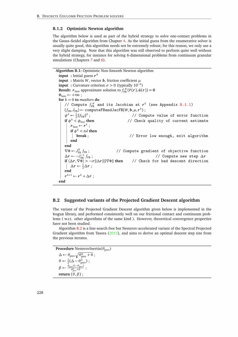
B. DISCRETE COULOMB FRICTION PROBLEM SOLVERS

B.1.2 Optimistic Newton algorithm

The algorithm below is used as part of the hybrid strategy to solve one-contact problems inthe Gauss–Seidel algorithm from Chapter 4. As the initial guess from the enumerative solver isusually quite good, this algorithm needs not be extremely robust; for this reason, we only use avery slight damping. Note that this algorithm was still observed to perform quite well withoutthe hybrid strategy, for instance for solving 6-dimensional problems from continuum granularsimulations (Chapters 7 and 8).

Algorithm B.1: Optimistic Non-Smooth Newton algorithminput : Initial guess r 0

input : Matrix W , vector b, friction coefficient µinput : Curvature criterion σ > 0 (typically 10−2)Result: r best approximate solution to f KFB (r (r ), u(r )) = 0

Φbest← +∞ ;for k = 0 to maxIters do

// Compute f KFB and its Jacobian at r k (see Appendix B.1.1)

( fFB, JFB)← computeFBandJacFB(W, b,µ, r k) ;φk ← 1

2‖ fFB‖2 ; // Compute value of error function

if φk < φbest then // Check quality of current estimater best← r k ;if φk < tol then

break ; // Error low enough, exit algorithmend

end

∇Φ← J⊺FB fFB ; // Compute gradient of objective function

∆r ←−J−1FB fFB ; // Compute new step ∆r

if ⟨∆r ,∇Φ⟩> −σ‖∆r‖‖∇Φ‖ then // Check for bad descent direction

∆r ← 12∆r ;

end

r k+1← r k +∆r ;end

B.2 Suggested variants of the Projected Gradient Descent algorithm

The variant of the Projected Gradient Descent algorithm given below is implemented in thebogus library, and performed consistently well on our frictional contact and continuum prob-lems ( w.r.t. other algorithms of the same kind ). However, theoretical convergence propertieshave not been studied.

Algorithm B.2 is a line-search free but Nesterov-accelerated variant of the Spectral ProjectedGradient algorithm from Tasora (2013), and aims to derive an optimal descent step size fromthe previous iterates.

Procedure NesterovInertia(θprev)

∆← θprev

qθ 2

prev + 4 ;

θ ← 12 (∆− θ 2

prev) ;

β ← θprev(1−θprev)

θ 2prev+θ

;

return (θ ,β) ;

228

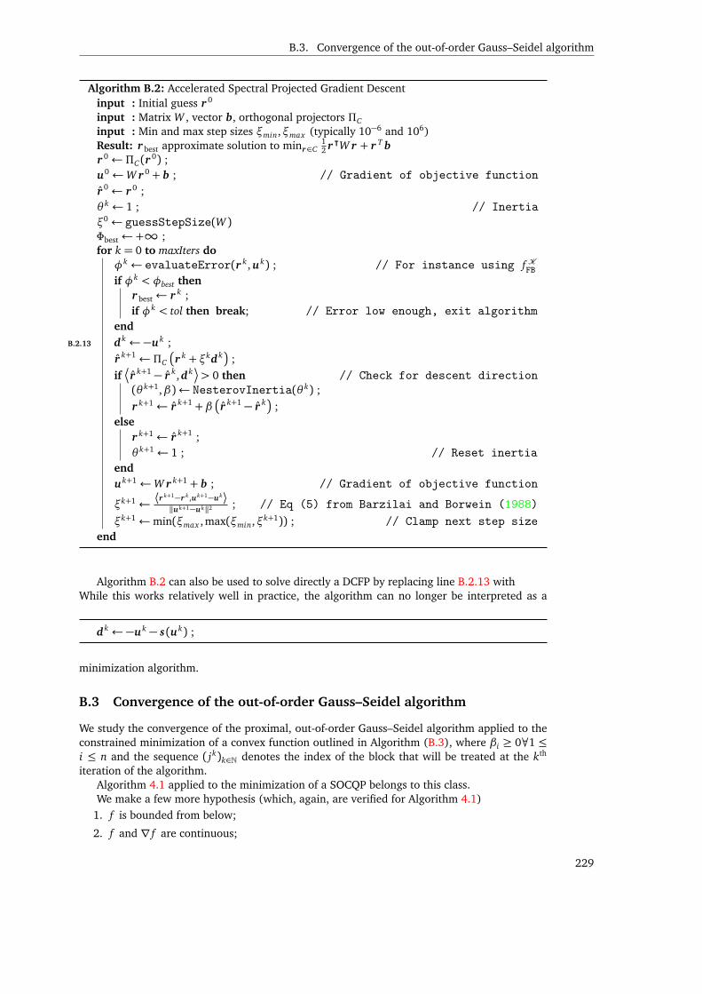
B.3. Convergence of the out-of-order Gauss–Seidel algorithm

Algorithm B.2: Accelerated Spectral Projected Gradient Descentinput : Initial guess r 0

input : Matrix W , vector b, orthogonal projectors ΠC

input : Min and max step sizes ξmin,ξmax (typically 10−6 and 106)Result: r best approximate solution to minr∈C

12 r ⊺W r + r T b

r 0← ΠC(r0) ;

u0←W r 0 + b ; // Gradient of objective function

r 0← r 0 ;θ k ← 1 ; // Inertia

ξ0← guessStepSize(W )Φbest← +∞ ;for k = 0 to maxIters do

φk ← evaluateError(r k, uk) ; // For instance using f KFBif φk < φbest then

r best← r k ;if φk < tol then break; // Error low enough, exit algorithm

end

B.2.13 dk ←−uk ;

r k+1← ΠC

r k + ξkdk

;

ifr k+1 − r k,dk

> 0 then // Check for descent direction

(θ k+1,β)← NesterovInertia(θ k) ;

r k+1← r k+1 + βr k+1 − r k

;

else

r k+1← r k+1 ;θ k+1← 1 ; // Reset inertia

end

uk+1←W r k+1 + b ; // Gradient of objective function

ξk+1← ⟨rk+1−r k ,uk+1−uk⟩‖uk+1−uk‖2 ; // Eq (5) from Barzilai and Borwein (1988)

ξk+1←min(ξmax , max(ξmin,ξk+1)) ; // Clamp next step size

end

Algorithm B.2 can also be used to solve directly a DCFP by replacing line B.2.13 withWhile this works relatively well in practice, the algorithm can no longer be interpreted as a

dk ←−uk − s(uk) ;

minimization algorithm.

B.3 Convergence of the out-of-order Gauss–Seidel algorithm

We study the convergence of the proximal, out-of-order Gauss–Seidel algorithm applied to theconstrained minimization of a convex function outlined in Algorithm (B.3), where βi ≥ 0∀1 ≤i ≤ n and the sequence ( jk)k∈N denotes the index of the block that will be treated at the kth

iteration of the algorithm.Algorithm 4.1 applied to the minimization of a SOCQP belongs to this class.We make a few more hypothesis (which, again, are verified for Algorithm 4.1)

1. f is bounded from below;

2. f and ∇ f are continuous;

229

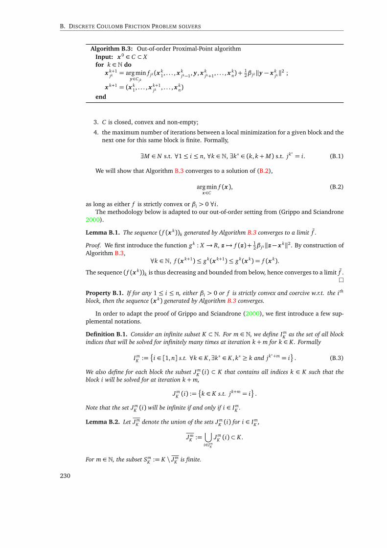
B. DISCRETE COULOMB FRICTION PROBLEM SOLVERS

Algorithm B.3: Out-of-order Proximal-Point algorithmInput: x 0 ∈ C ⊂ Xfor k ∈ N do

x k+1jk = arg min

y∈C jk

f jk(x k1, . . . , x k

jk−1, y , x kjk+1, . . . , x k

n) +12β jk‖y − x k

jk‖2 ;

x k+1 = (x k1, . . . , x k+1

jk , . . . , x kn)

end

3. C is closed, convex and non-empty;

4. the maximum number of iterations between a local minimization for a given block and thenext one for this same block is finite. Formally,

∃M ∈ N s.t. ∀1≤ i ≤ n, ∀k ∈ N, ∃k∗ ∈ (k, k+M) s.t. jk∗ = i. (B.1)

We will show that Algorithm B.3 converges to a solution of (B.2),

arg minx∈C

f (x ), (B.2)

as long as either f is strictly convex or βi > 0 ∀i.The methodology below is adapted to our out-of-order setting from (Grippo and Sciandrone

2000).

Lemma B.1. The sequence ( f (x k))k generated by Algorithm B.3 converges to a limit f .

Proof. We first introduce the function gk : X → R, z 7→ f (z)+ 12β jk‖z− x k‖2. By construction of

Algorithm B.3,∀k ∈ N, f (x k+1)≤ gk(x k+1)≤ gk(x k) = f (x k).

The sequence ( f (x k))k is thus decreasing and bounded from below, hence converges to a limit f .

Property B.1. If for any 1 ≤ i ≤ n, either βi > 0 or f is strictly convex and coercive w.r.t. the ith

block, then the sequence (x k) generated by Algorithm B.3 converges.

In order to adapt the proof of Grippo and Sciandrone (2000), we first introduce a few sup-plemental notations.

Definition B.1. Consider an infinite subset K ⊂ N. For m ∈ N, we define ImK as the set of all block

indices that will be solved for infinitely many times at iteration k+m for k ∈ K. Formally

ImK :=

i ∈ [1, n] s.t. ∀k ∈ K ,∃k∗ ∈ K , k∗ ≥ k and jk∗+m = i

. (B.3)

We also define for each block the subset JmK (i) ⊂ K that contains all indices k ∈ K such that the

block i will be solved for at iteration k+m,

JmK (i) :=

k ∈ K s.t. jk+m = i

.

Note that the set JmK (i) will be infinite if and only if i ∈ Im

K .

Lemma B.2. Let JmK denote the union of the sets Jm

K (i) for i ∈ ImK ,

JmK :=

⋃

i∈ImK

JmK (i) ⊂ K .

For m ∈ N, the subset SmK := K \ Jm

K is finite.

230

B.3. Convergence of the out-of-order Gauss–Seidel algorithm

Proof. Suppose this was not the case, then the integer sequence

jk+m

k∈SmK⊂ [1, n] has a limit

point i∗ which is also in ImK as it satisfies Equation B.3. By definition of i∗ there exists k∗ ∈ Sm

K

such that jk∗+m = i∗, which means k∗ ∈ JmK (i

∗)∩ SmK = ;, which is a contradiction.

We should now be able to prove Proposition B.1.

Proof. Let us denote by B ⊂ [1, n] the set for which βi = 0.

Existence of a limit point First, let us show that from (x k)k∈N we can extract a convergingsubsequence. From Lemma B.1, we have limk∈N f (x k) = limk∈N gk(x k+1) = f , therefore ∀1 ≤i ≤ n, limk∈N βi‖x k − x k+1‖= 0. Each block x k

i for which i 6∈ B thus admits a limit; let us define

x i :=

lim x k

i if i 6∈ B

0 if i ∈ B.

The function g : z 7→ f (z) + βi2 ‖z − x‖2 is coercive on X and g(x k) → f , therefore (x k)k∈N is

bounded. Hence there exists a subsequence (x k)k∈K that converges to x ∈ C , and by continuityof f , f (x ) = limk∈N f (x K) = f . Necessarily, x i = x i ∀i 6∈ B.

Convergence of translated subsequences For m ∈ N, we define the predicate Π(m),

Π(m) := limk∈K

x k+m = x

Π(0) hold by definition of K; now we suppose that Π(m) is true, and we will show that thisimplies Π(m+ 1).

For any i ∈ Im+1k ∩ B, by definition the set Jm+1

K (i) ⊂ K is infinite and thus (x k+m)k∈Jm+1K (i)→

x . We can use (Grippo and Sciandrone 2000, Proposition 4) by identifying their yk with(x k+m)k∈Jm+1

K (i) and their vk with (x k+m+1)k∈Jm+1K (i). We get

limk∈Jm+1

K (i)‖x k+m

i − x k+m+1i ‖= 0

and therefore from Π(m),

limk∈Jm+1

K (i)x k+m+1

i = x i . (B.4)

Moreover, Equation (B.4) also holds for any i ∈ Im+1k \ B since (x k

i )k∈N → x i = x i . Now bydefinition of Jm+1

K (i) and Algorithm B.3, ∀i ∈ Im+1k , ∀ℓ 6= i, ∀k ∈ Jm+1

K (i), x k+mℓ= x k+m+1

ℓ. Thus

we get also from Π(m) that ∀i ∈ Im+1k ,

limk∈Jm+1

K (i)x k+m+1

l = limk∈Jm+1

K (i)x k+m

l = x l ∀l 6= i. (B.5)

Putting together (B.4) and (B.5), we get

limk∈Jm+1

K (i)x k+m+1 = x .

This being true for any i ∈ Im+1k , we deduce that

limk∈Jm+1

K

x k+m+1 = x

and with Lemma B.2,limk∈K

x k+m+1 = x

which proves Π(m+1). By induction Π(m) holds for all m ∈ N, which means that (x k)k∈N→ x .

231

B. DISCRETE COULOMB FRICTION PROBLEM SOLVERS

Property B.2. Under the hypothesis of Property B.1, the limit x of the sequence of iterates (x k)

from Algorithm B.3 is a critical point of the minimization problem (B.2).

Again, let us first introduce an useful definition.

Definition B.2 ( Successor function ). Given Assumption B.1, we can define for each block 1 ≤i ≤ n the function

succi :

¨N −→ Nk 7−→ min

k∗ ∈ (k, k+M), jk∗ = i

which indicates the next iteration at which a given block will be minimized over.

Proof. For any 1≤ i ≤ n, the sequence (succi(k))k∈N is infinite and thus

limk∈N

x succi(k) = x . (B.6)

Moreover by construction of Algorithm B.3, (∇i gk)(x succi(k)) ∈ −NCi

(xsucci(k)i ), i.e.,

¬(∇i g

k)(x succi(k)), z − xsucci(k)i

¶≥ 0 ∀z ∈ Ci .

This means¬(∇i f k)(x succi(k)) + βi(x

succi(k)i − x

succi(k)−1i ), z − x

succi(k)i

¶≥ 0 ∀z ∈ Ci

Taking into account Equation B.6 and the continuity assumption on ∇i f ,

⟨(∇i f )(x ), y − x i⟩ ≥ 0 ∀y ∈ Ci

i.e., (∇i f )(x ) ∈ −NCi(x i). As this is true for any 1≤ i ≤ n, x is an optimal point of Problem B.2.

232

C Supplemental justifications related toDrucker–Prager constraints

C.1 Constraints on quadrature points

The goal of this section is to justify Proposition 6.3, that Equations (6.13a — 6.13c) can bediscretized as System (6.35).

Proof. First, it is noteworthy that the matrix M may be factorized as M = RT diag(S)R, wherediag(S) is a diagonal matrix of size sd nQ mapping to each quadrature point q the diagonal weightblock Sq,q := 2 wq I

sd. That is, the diagonal coefficients of S are given by

S(q−1)sd+k = 2 wq for 1≤ k ≤ sd and 1≤ q ≤ nQ.

Indeed, for all 1 ≤ i, j ≤ n and for all 1 ≤ k,ℓ ≤ n let r(i, k) := (i − 1)sd + k and c( j,ℓ) :=( j − 1)sd + ℓ. Using the quadrature rule, we have

Mr,c =

nQ∑

q=1

wq

Tr(i,k)(x q) : Tc( j,ℓ)(x q)

= 2

nQ∑

q=1

wq

¬ωτi (x q)χ(ek),ω

τj (x q)χ(e l)

¶

= 2

nQ∑

q=1

wqωτi (x q)ω

τj (x q)

e⊺

keℓ

from (6.28)

= 2

nQ∑

q=1

wq

ωτi (x q)ω

τj (x q)δk,ℓ

= 2

nQ∑

q=1

sd∑

p=1

wq

ωτi (x q)ω

τj (x q)δk,pδp,l

=

nQ∑

q=1

sd∑

p=1

S(q−1)sd+p

R(q−1)sd+p,r(i,k)R(q−1)sd+p,c( j,ℓ)

from (6.34),

which we recognize as the product M = R⊺ diag(S)R.Furthermore, since M is invertible, we have rank(M) = sd n. From the rank inequality on

product of matrices, we get

rank(M)≤min (rank(diag(S)), rank(R))≤ rank(R),

meaning that the rank of R is equal to its number of columns sd n. The pseudoinverse R† cantherefore be computed as R† = (R⊺R)−1R⊺, and R† plays the role of a left inverse, i.e., we haveR† R= I.

We thus have R†λ = R† Rλ = λ, so (6.35a) is directly equivalent to (6.32a). Moreover,since for any strictly positive scalar ξ, (γ,λ) ∈ DP (µ, Bi,ζ) ⇐⇒ (ξγ,λ) ∈ DP (µ, Bi,ζ), the

233

C. SUPPLEMENTAL JUSTIFICATIONS RELATED TO DRUCKER–PRAGER CONSTRAINTS

system is not affected by a multiplication of the left-hand-side of (6.35b) with the matrix diag(S).Multiplying then both sides of (6.35b) by R⊺, we get

R⊺ diag(S)γ= R⊺R†,⊺B u + R⊺R†,⊺k

Since R⊺R†,⊺ =R† R

⊺= I, we retrieve (6.32b).

Finally, as λ[q] = χ

−1(λ(x q)) and γ[q]= χ−1(γ(x q)), we have (6.35c) ⇐⇒

γ(x q),λ(x q) ∈

DP (µ, Bi,ζ), that is, we ensure that ∀τ ∈ Th the integral (6.33) is zero.

C.2 Frictional boundaries

Suppose that (γRB,λRB) ∈ DP µRB, with γRB := 12

vn⊺RB + nRBv⊺

, and ‖nRB‖= 1.

The force induced by a stress σ through a plane with normal n is computed as σn; thereaction force induced by the material on the frictional boundary is therefore r = λRBnRB. In thefollowing, we investigate the relationship between r and v, the relative velocity of the boundaryw.r.t. the granular material.

C.2.1 Signorini condition

First, remark that TrγRB = ⟨v,nRB⟩= vN,

r N =1

3(TrλRB) + (DevλRB) : (nRBn

⊺RB)

and(DevλRB) : (nRBn

⊺RB)≤ 2 |DevλRB||nRBn

⊺RB|

≤ µRBp6

TrλRB ×2p2

≤ µRBp3

TrλRB .

Therefore, 1−p3µRB

3

TrλRB ≤ r N ≤

1+p

3µRB

3

TrλRB .

For µRB <1p3, we thus have

0≤ TrγRB ⊥ TrλRB ≥ 0 =⇒ 0≤ vN ⊥ r N ≥ 0 ,

i.e., the Signorini condition is satisfied.

C.2.2 Tangential reaction

Notice that

Dev(γRB)nRB =1

2v+ (

1

2− 1

3) ⟨v,nRB⟩nRB

=1

2vT +

2

3vNn .

Sliding case First suppose that vT 6= 0, therefore DevγRB 6= 0, and DP µRB imposes thatDevλRB = −αDevγRB,α > 0. Since r = 1

3 TrλRBn +DevλRBn, we can identify that

r T = −1

2αvT

i.e. the tangential friction force is opposed to the tangential relative velocity. Now, let us show

that r lies on the boundary of the second-order cone of apertureq

32µRB, i.e., ‖r T‖=

q32µRBr N.

234

C.2. Frictional boundaries

From the Signori condition, vN > 0 implies r N = 0, and therefore TrλRB = 0. This means

|DevλRB|= 0, and consequently ‖r T‖. Our relation ‖r T‖=q

32µRBr N is trivially satisfied.

We now have to study the case vN = 0. DevλRB = −αDevγRB means that

‖r T‖= ‖DevλRBn‖= |DevλRBn| ‖DevγRBnRB‖|DevγRB|

.

Since v.nRB = 0,

‖Dev(γRB)nRB‖=1

2‖vT‖

and

|Dev(γRB)|2 = |γRB|2 = |vn⊺RB|2 −

1

4|vn⊺RB − nRBv⊺|2

=1

2‖v‖2 − 1

4‖v∧ nRB‖2 =

1

2‖v‖2 − 1

4‖vT‖2

=1

4‖vT‖2 = ‖Dev(γRB)nRB‖2 .

This means

‖r T‖= |DevλRB|=µRBp

6TrλRB =

√√3

2µRBr N .

The sliding case thus satisfies the Coulomb law with coefficientq

32µRB.

Sticking When v = 0, we cannot conclude without more information about the relationshipbetween λRB and γRB. Indeed, we can only verify that

‖r T‖ ≤ ‖DevλRBn‖ ≤ p2|DevλRB|

≤ µRBp3

TrλRB ≤p

3µRB

1−p3µRB

r N

i.e the reaction force has to lie inside a second-order cone of aperturep

3µRB1−p3µRB

.

This last bound does not correspond to the one derived for the sliding case (except whenµRB = 0), but nevertheless models a coupling between the tangential and normal reaction forces.

C.2.3 Reverse inclusion

For any (v, r ) ∈ Cq 32µ(nRB)— i.e., satisfying the 3D Coulomb law with friction coefficient

q32µ

— we can construct a symmetric tensor λRB such that (γRB,λRB) ∈ DP (µ). Indeed, let

λRB :=r Tn⊺RB + nRBr

⊺

T

+ r NI

We have

TrλRB = 3r N =p

6

√√3

2r N

λRBnRB = r T + nRB(r N) = r

Dev(λRB)nRB = r T

|Dev(λRB)|=r Tn

⊺RB + nRB(r − r NnRB)

⊺

= ‖r T‖It can be easily verified that for any case of the Cq 3

2µ(nRB) disjunctive formulation satisfied

by r and v, the corresponding case of DP (µ) is satisfied by (γRB,λRB).

235

Bibliography

Acary, V. and B. Brogliato (2008). Numerical methods for nonsmooth dynamical systems. English.Vol. 35. Lecture Notes in Computational and Applied Mechanics. Springer.

Acary, V. (2009). Toward higher order event–capturing schemes and adaptive time–step strategiesfor nonsmooth multibody systems. Research Report RR-7151, p. 31. URL: https://hal.inria.fr/inria-00440771.

Acary, V., M. Brémond, T. Koziara, and F. Pérignon (2014). FCLIB: a collection of discrete 3DFrictional Contact problems. Technical Report RT-0444. INRIA, p. 34. URL: https://hal.inria.fr/hal-00945820.

Ainsley, S., E. Vouga, E. Grinspun, and R. Tamstorf (2012). “Speculative Parallel AsynchronousContact Mechanics”. In: ACM Trans. Graph. 31.6, 151:1–151:8. ISSN: 0730-0301. DOI: 10.1145/2366145.2366170.

Alart, P. and A. Curnier (1991). “A mixed formulation for frictional contact problems prone toNewton like solution methods”. In: Computer Methods in Applied Mechanics and Engineering92.3, pp. 353–375. ISSN: 0045-7825. DOI: 10.1016/0045-7825(91)90022-x.

Alduán, I. and M. A. Otaduy (2011). “SPH Granular Flow with Friction and Cohesion”. In: Pro-ceedings of the 2011 ACM SIGGRAPH/Eurographics Symposium on Computer Animation. SCA’11. Vancouver, British Columbia, Canada: ACM, pp. 25–32. ISBN: 978-1-4503-0923-3. DOI:10.1145/2019406.2019410.

Alduán, I., A. Tena, and M. A. Otaduy (2009). “Simulation of high-resolution granular media”.In: Proc. of Congreso Español de Informática Gráfica. Vol. 1. 4.

Alejano, L. R. and A. Bobet (2012). “Drucker–Prager Criterion”. In: Rock Mechanics and RockEngineering 45.6, pp. 995–999. ISSN: 1434-453X. DOI: 10.1007/s00603-012-0278-2.

Andersen, E. and K. Andersen (2013). MOSEK modeling manual.Andersen, E., C. Roos, and T. Terlaky (2003). “On implementing a primal-dual interior-point

method for conic quadratic optimization”. In: Mathematical Programming 95.2, pp. 249–277. ISSN: 1436-4646. DOI: 10.1007/s10107-002-0349-3.

Andersen, S. and L. Andersen (2010). “Analysis of spatial interpolation in the material-pointmethod”. In: Computers & Structures 88.7-8, pp. 506–518. ISSN: 0045-7949. DOI: 10.1016/j.compstruc.2010.01.004.

Anderson, T. B. and R. Jackson (1967). “Fluid Mechanical Description of Fluidized Beds. Equa-tions of Motion”. In: Industrial & Engineering Chemistry Fundamentals 6.4, pp. 527–539. ISSN:1541-4833. DOI: 10.1021/i160024a007.

Andreotti, B., Y. Forterre, and O. Pouliquen (2011). Granular media: between fluid and solid.Cambridge University Press.

Andrews, M. and P. O′Rourke (1996). “The multiphase particle-in-cell (MP-PIC) method fordense particulate flows”. In: International Journal of Multiphase Flow 22.2, pp. 379–402.ISSN: 0301-9322. DOI: 10.1016/0301-9322(95)00072-0.

Anitescu, M. (2005). “Optimization-based simulation of nonsmooth rigid multibody dynamics”.In: Math. Program. 105.1, pp. 113–143. ISSN: 1436-4646. DOI: 10.1007/s10107-005-0590-7.

Anjyo, K., Y. Usami, and T. Kurihara (1992). “A Simple Method for Extracting the Natural Beautyof Hair”. In: Computer Graphics Proceedings (Proceedings of the ACM SIGGRAPH’92 confer-ence), pp. 111–120.

237

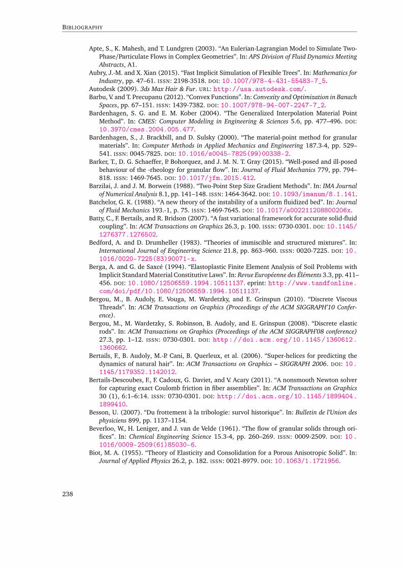
BIBLIOGRAPHY

Apte, S., K. Mahesh, and T. Lundgren (2003). “An Eulerian-Lagrangian Model to Simulate Two-Phase/Particulate Flows in Complex Geometries”. In: APS Division of Fluid Dynamics MeetingAbstracts, A1.

Aubry, J.-M. and X. Xian (2015). “Fast Implicit Simulation of Flexible Trees”. In: Mathematics forIndustry, pp. 47–61. ISSN: 2198-3518. DOI: 10.1007/978-4-431-55483-7_5.

Autodesk (2009). 3ds Max Hair & Fur. URL: http://usa.autodesk.com/.Barbu, V. and T. Precupanu (2012). “Convex Functions”. In: Convexity and Optimization in Banach

Spaces, pp. 67–151. ISSN: 1439-7382. DOI: 10.1007/978-94-007-2247-7_2.Bardenhagen, S. G. and E. M. Kober (2004). “The Generalized Interpolation Material Point

Method”. In: CMES: Computer Modeling in Engineering & Sciences 5.6, pp. 477–496. DOI:10.3970/cmes.2004.005.477.

Bardenhagen, S., J. Brackbill, and D. Sulsky (2000). “The material-point method for granularmaterials”. In: Computer Methods in Applied Mechanics and Engineering 187.3-4, pp. 529–541. ISSN: 0045-7825. DOI: 10.1016/s0045-7825(99)00338-2.

Barker, T., D. G. Schaeffer, P. Bohorquez, and J. M. N. T. Gray (2015). “Well-posed and ill-posedbehaviour of the -rheology for granular flow”. In: Journal of Fluid Mechanics 779, pp. 794–818. ISSN: 1469-7645. DOI: 10.1017/jfm.2015.412.

Barzilai, J. and J. M. Borwein (1988). “Two-Point Step Size Gradient Methods”. In: IMA Journalof Numerical Analysis 8.1, pp. 141–148. ISSN: 1464-3642. DOI: 10.1093/imanum/8.1.141.

Batchelor, G. K. (1988). “A new theory of the instability of a uniform fluidized bed”. In: Journalof Fluid Mechanics 193.-1, p. 75. ISSN: 1469-7645. DOI: 10.1017/s002211208800206x.

Batty, C., F. Bertails, and R. Bridson (2007). “A fast variational framework for accurate solid-fluidcoupling”. In: ACM Transactions on Graphics 26.3, p. 100. ISSN: 0730-0301. DOI: 10.1145/1276377.1276502.

Bedford, A. and D. Drumheller (1983). “Theories of immiscible and structured mixtures”. In:International Journal of Engineering Science 21.8, pp. 863–960. ISSN: 0020-7225. DOI: 10.1016/0020-7225(83)90071-x.

Berga, A. and G. de Saxcé (1994). “Elastoplastic Finite Element Analysis of Soil Problems withImplicit Standard Material Constitutive Laws”. In: Revue Européenne des Éléments 3.3, pp. 411–456. DOI: 10.1080/12506559.1994.10511137. eprint: http://www.tandfonline.com/doi/pdf/10.1080/12506559.1994.10511137.

Bergou, M., B. Audoly, E. Vouga, M. Wardetzky, and E. Grinspun (2010). “Discrete ViscousThreads”. In: ACM Transactions on Graphics (Proceedings of the ACM SIGGRAPH’10 Confer-ence).

Bergou, M., M. Wardetzky, S. Robinson, B. Audoly, and E. Grinspun (2008). “Discrete elasticrods”. In: ACM Transactions on Graphics (Proceedings of the ACM SIGGRAPH’08 conference)27.3, pp. 1–12. ISSN: 0730-0301. DOI: http://doi.acm.org/10.1145/1360612.1360662.

Bertails, F., B. Audoly, M.-P. Cani, B. Querleux, et al. (2006). “Super-helices for predicting thedynamics of natural hair”. In: ACM Transactions on Graphics – SIGGRAPH 2006. DOI: 10.1145/1179352.1142012.

Bertails-Descoubes, F., F. Cadoux, G. Daviet, and V. Acary (2011). “A nonsmooth Newton solverfor capturing exact Coulomb friction in fiber assemblies”. In: ACM Transactions on Graphics30 (1), 6:1–6:14. ISSN: 0730-0301. DOI: http://doi.acm.org/10.1145/1899404.1899410.

Besson, U. (2007). “Du frottement à la tribologie: survol historique”. In: Bulletin de l’Union desphysiciens 899, pp. 1137–1154.

Beverloo, W., H. Leniger, and J. van de Velde (1961). “The flow of granular solids through ori-fices”. In: Chemical Engineering Science 15.3-4, pp. 260–269. ISSN: 0009-2509. DOI: 10.1016/0009-2509(61)85030-6.

Biot, M. A. (1955). “Theory of Elasticity and Consolidation for a Porous Anisotropic Solid”. In:Journal of Applied Physics 26.2, p. 182. ISSN: 0021-8979. DOI: 10.1063/1.1721956.

238

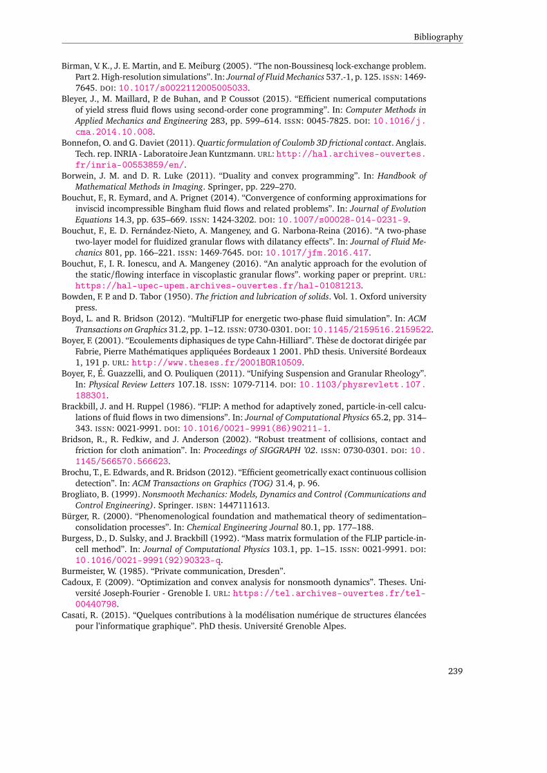
Bibliography

Birman, V. K., J. E. Martin, and E. Meiburg (2005). “The non-Boussinesq lock-exchange problem.Part 2. High-resolution simulations”. In: Journal of Fluid Mechanics 537.-1, p. 125. ISSN: 1469-7645. DOI: 10.1017/s0022112005005033.

Bleyer, J., M. Maillard, P. de Buhan, and P. Coussot (2015). “Efficient numerical computationsof yield stress fluid flows using second-order cone programming”. In: Computer Methods inApplied Mechanics and Engineering 283, pp. 599–614. ISSN: 0045-7825. DOI: 10.1016/j.cma.2014.10.008.

Bonnefon, O. and G. Daviet (2011). Quartic formulation of Coulomb 3D frictional contact. Anglais.Tech. rep. INRIA - Laboratoire Jean Kuntzmann. URL: http://hal.archives-ouvertes.fr/inria-00553859/en/.

Borwein, J. M. and D. R. Luke (2011). “Duality and convex programming”. In: Handbook ofMathematical Methods in Imaging. Springer, pp. 229–270.

Bouchut, F., R. Eymard, and A. Prignet (2014). “Convergence of conforming approximations forinviscid incompressible Bingham fluid flows and related problems”. In: Journal of EvolutionEquations 14.3, pp. 635–669. ISSN: 1424-3202. DOI: 10.1007/s00028-014-0231-9.

Bouchut, F., E. D. Fernández-Nieto, A. Mangeney, and G. Narbona-Reina (2016). “A two-phasetwo-layer model for fluidized granular flows with dilatancy effects”. In: Journal of Fluid Me-chanics 801, pp. 166–221. ISSN: 1469-7645. DOI: 10.1017/jfm.2016.417.

Bouchut, F., I. R. Ionescu, and A. Mangeney (2016). “An analytic approach for the evolution ofthe static/flowing interface in viscoplastic granular flows”. working paper or preprint. URL:https://hal-upec-upem.archives-ouvertes.fr/hal-01081213.

Bowden, F. P. and D. Tabor (1950). The friction and lubrication of solids. Vol. 1. Oxford universitypress.

Boyd, L. and R. Bridson (2012). “MultiFLIP for energetic two-phase fluid simulation”. In: ACMTransactions on Graphics 31.2, pp. 1–12. ISSN: 0730-0301. DOI: 10.1145/2159516.2159522.

Boyer, F. (2001). “Ecoulements diphasiques de type Cahn-Hilliard”. Thèse de doctorat dirigée parFabrie, Pierre Mathématiques appliquées Bordeaux 1 2001. PhD thesis. Université Bordeaux1, 191 p. URL: http://www.theses.fr/2001BOR10509.

Boyer, F., É. Guazzelli, and O. Pouliquen (2011). “Unifying Suspension and Granular Rheology”.In: Physical Review Letters 107.18. ISSN: 1079-7114. DOI: 10.1103/physrevlett.107.188301.

Brackbill, J. and H. Ruppel (1986). “FLIP: A method for adaptively zoned, particle-in-cell calcu-lations of fluid flows in two dimensions”. In: Journal of Computational Physics 65.2, pp. 314–343. ISSN: 0021-9991. DOI: 10.1016/0021-9991(86)90211-1.

Bridson, R., R. Fedkiw, and J. Anderson (2002). “Robust treatment of collisions, contact andfriction for cloth animation”. In: Proceedings of SIGGRAPH ’02. ISSN: 0730-0301. DOI: 10.1145/566570.566623.

Brochu, T., E. Edwards, and R. Bridson (2012). “Efficient geometrically exact continuous collisiondetection”. In: ACM Transactions on Graphics (TOG) 31.4, p. 96.

Brogliato, B. (1999). Nonsmooth Mechanics: Models, Dynamics and Control (Communications andControl Engineering). Springer. ISBN: 1447111613.

Bürger, R. (2000). “Phenomenological foundation and mathematical theory of sedimentation–consolidation processes”. In: Chemical Engineering Journal 80.1, pp. 177–188.

Burgess, D., D. Sulsky, and J. Brackbill (1992). “Mass matrix formulation of the FLIP particle-in-cell method”. In: Journal of Computational Physics 103.1, pp. 1–15. ISSN: 0021-9991. DOI:10.1016/0021-9991(92)90323-q.

Burmeister, W. (1985). “Private communication, Dresden”.Cadoux, F. (2009). “Optimization and convex analysis for nonsmooth dynamics”. Theses. Uni-

versité Joseph-Fourier - Grenoble I. URL: https://tel.archives-ouvertes.fr/tel-00440798.

Casati, R. (2015). “Quelques contributions à la modélisation numérique de structures élancéespour l’informatique graphique”. PhD thesis. Université Grenoble Alpes.

239

BIBLIOGRAPHY

Casati, R., G. Daviet, and F. Bertails-Descoubes (2016). Inverse Elastic Cloth Design with Contactand Friction. Research Report. Inria Grenoble Rhône-Alpes, Université de Grenoble. URL:https://hal.archives-ouvertes.fr/hal-01309617.

Chambolle, A. and T. Pock (2010). “A First-Order Primal-Dual Algorithm for Convex Problemswith Applications to Imaging”. In: J Math Imaging Vis 40.1, pp. 120–145. ISSN: 1573-7683.DOI: 10.1007/s10851-010-0251-1.

Chambon, G., R. Bouvarel, D. Laigle, and M. Naaim (2011). “Numerical simulations of granularfree-surface flows using smoothed particle hydrodynamics”. In: Journal of Non-NewtonianFluid Mechanics 166.12-13, pp. 698–712. ISSN: 0377-0257. DOI: 10.1016/j.jnnfm.2011.03.007.

Chauchat, J., S. Guillou, D. Pham Van Bang, and K. Dan Nguyen (2013). “Modelling sedimentation-consolidation in the framework of a one-dimensional two-phase flow model”. In: Journal ofHydraulic Research 51.3, pp. 293–305. ISSN: 1814-2079. DOI: 10.1080/00221686.2013.768798.

Chauchat, J. and M. Médale (2010). “A three-dimensional numerical model for incompress-ible two-phase flow of a granular bed submitted to a laminar shearing flow”. In: ComputerMethods in Applied Mechanics and Engineering 199.9-12, pp. 439–449. ISSN: 0045-7825. DOI:10.1016/j.cma.2009.07.007.

— (2014). “A three-dimensional numerical model for dense granular flows based on the mu(I)rheology”. In: Journal of Computational Physics 256, pp. 696–712. ISSN: 0021-9991. DOI:10.1016/j.jcp.2013.09.004.

Chehata, D., R. Zenit, and C. R. Wassgren (2003). “Dense granular flow around an immersedcylinder”. In: Physics of Fluids 15.6, p. 1622. ISSN: 1070-6631. DOI: 10.1063/1.1571826.

Chen, J.-S. and P. Tseng (2005). “An unconstrained smooth minimization reformulation of thesecond-order cone complementarity problem”. In: Math. Program. 104 (2), pp. 293–327.ISSN: 0025-5610. DOI: 10.1007/s10107-005-0617-0.

Choe, B., M. Choi, and H.-S. Ko (2005). “Simulating complex hair with robust collision handling”.In: Proceedings of the 2005 ACM SIGGRAPH/Eurographics symposium on Computer animation.SCA ’05. Los Angeles, California: ACM, pp. 153–160. ISBN: 1-59593-198-8. DOI: http://doi.acm.org/10.1145/1073368.1073389.

Choi, H. G. and D. D. Joseph (2001). “Fluidization by lift of 300 circular particles in planePoiseuille flow by direct numerical simulation”. In: Journal of Fluid Mechanics 438. ISSN:1469-7645. DOI: 10.1017/s0022112001004177.

Concha, F. and R. Bürger (2002). “A century of research in sedimentation and thickening”. In:Kona 20, pp. 38–70.

Coulomb, C.-A. (1781). Théorie des machines simples: en ayant égard au frottement de leurs partieset à la roideur des cordages.

Cundall, P. A. and O. D. L. Strack (1979). “A discrete numerical model for granular assemblies”.In: Géotechnique 29.1, pp. 47–65. ISSN: 1751-7656. DOI: 10.1680/geot.1979.29.1.47.

Dahl, P. R. (1968). A solid friction model. Tech. rep. The Aerospace Corporation.Daviet, G. (2013). So-bogus, a C++ linear algebra and solvers library for sparse block matrices.

http://gdaviet.fr/code/bogus.Daviet, G. and F. Bertails-Descoubes (2016a). “A Semi-Implicit Material Point Method for the

Continuum Simulation of Granular Materials”. In: ACM Transactions on Graphics. SIGGRAPH’16 Technical Papers 35.4, p. 13. DOI: 10.1145/2897824.2925877.

— (2016b). “Nonsmooth simulation of dense granular flows with pressure-dependent yieldstress”. In: Journal of Non-Newtonian Fluid Mechanics 234, pp. 15–35. ISSN: 0377-0257. DOI:http://dx.doi.org/10.1016/j.jnnfm.2016.04.006.

Daviet, G., F. Bertails-Descoubes, and L. Boissieux (2011). “A hybrid iterative solver for robustlycapturing Coulomb friction in hair dynamics”. In: ACM Transactions on Graphics 30.6, pp. 1–12. ISSN: 0730-0301. DOI: 10.1145/2070781.2024173.

Daviet, G., F. Bertails-Descoubes, and R. Casati (2015). “Fast cloth simulation with implicit con-tact and exact coulomb friction”. In: Proceedings of the 14th ACM SIGGRAPH / EurographicsSymposium on Computer Animation - SCA ’15. DOI: 10.1145/2786784.2795139.

240

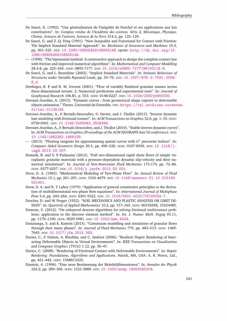
Bibliography

De Saxcé, G. (1992). “Une généralisation de l’inégalité de Fenchel et ses applications aux loisconstitutives”. In: Comptes rendus de l’Académie des sciences. Série 2, Mécanique, Physique,Chimie, Sciences de l’univers, Sciences de la Terre 314.2, pp. 125–129.

De Saxcé, G. and Z.-Q. Feng (1991). “New Inequality and Functional for Contact with Friction:The Implicit Standard Material Approach”. In: Mechanics of Structures and Machines 19.3,pp. 301–325. DOI: 10.1080/08905459108905146. eprint: http://dx.doi.org/10.1080/08905459108905146.

— (1998). “The bipotential method: A constructive approach to design the complete contact lawwith friction and improved numerical algorithms”. In: Mathematical and Computer Modelling28.4-8, pp. 225–245. ISSN: 0895-7177. DOI: 10.1016/s0895-7177(98)00119-8.

De Saxcé, G. and L. Bousshine (2002). “Implicit Standard Materials”. In: Inelastic Behaviour ofStructures under Variable Repeated Loads, pp. 59–76. DOI: 10.1007/978-3-7091-2558-8_4.

Denlinger, R. P. and R. M. Iverson (2001). “Flow of variably fluidized granular masses acrossthree-dimensional terrain: 2. Numerical predictions and experimental tests”. In: Journal ofGeophysical Research 106.B1, p. 553. ISSN: 0148-0227. DOI: 10.1029/2000jb900330.

Derouet-Jourdan, A. (2013). “Dynamic curves : from geometrical shape capture to deformableobjects animation.” Theses. Université de Grenoble. URL: https://tel.archives-ouvertes.fr/tel-01135185.

Derouet-Jourdan, A., F. Bertails-Descoubes, G. Daviet, and J. Thollot (2013). “Inverse dynamichair modeling with frictional contact”. In: ACM Transactions on Graphics 32.6, pp. 1–10. ISSN:0730-0301. DOI: 10.1145/2508363.2508398.

Derouet-Jourdan, A., F. Bertails-Descoubes, and J. Thollot (2010). “Stable inverse dynamic curves”.In: ACM Transactions on Graphics (Proceedings of the ACM SIGGRAPH Asia’10 conference). DOI:10.1145/1882262.1866159.

— (2013). “Floating tangents for approximating spatial curves with G1 piecewise helices”. In:Computer Aided Geometric Design 30.5, pp. 490–520. ISSN: 0167-8396. DOI: 10.1016/j.cagd.2013.02.007.

Domnik, B. and S. P. Pudasaini (2012). “Full two-dimensional rapid chute flows of simple vis-coplastic granular materials with a pressure-dependent dynamic slip-velocity and their nu-merical simulations”. In: Journal of Non-Newtonian Fluid Mechanics 173-174, pp. 72–86.ISSN: 0377-0257. DOI: 10.1016/j.jnnfm.2012.03.001.

Drew, D. A. (1983). “Mathematical Modeling of Two-Phase Flow”. In: Annual Review of FluidMechanics 15.1, pp. 261–291. ISSN: 1545-4479. DOI: 10.1146/annurev.fl.15.010183.001401.

Drew, D. A. and R. T. Lahey (1979). “Application of general constitutive principles to the deriva-tion of multidimensional two-phase flow equations”. In: International Journal of MultiphaseFlow 5.4, pp. 243–264. ISSN: 0301-9322. DOI: 10.1016/0301-9322(79)90024-7.

Drucker, D. and W. Prager (1952). “SOIL MECHANICS AND PLASTIC ANALYSIS OR LIMIT DE-SIGN”. In: Quarterly of Applied Mathematics 10.2, pp. 157–165. ISSN: 0033569X, 15524485.

Dumont, S. (2012). “On enhanced descent algorithms for solving frictional multicontact prob-lems: application to the discrete element method”. In: Int. J. Numer. Meth. Engng 93.11,pp. 1170–1190. ISSN: 0029-5981. DOI: 10.1002/nme.4424.

Dunatunga, S. and K. Kamrin (2015). “Continuum modelling and simulation of granular flowsthrough their many phases”. In: Journal of Fluid Mechanics 779, pp. 483–513. ISSN: 1469-7645. DOI: 10.1017/jfm.2015.383.

Duriez, C., F. Dubois, A. Kheddar, and C. Andriot (2006). “Realistic Haptic Rendering of Inter-acting Deformable Objects in Virtual Environments”. In: IEEE Transactions on Visualizationand Computer Graphics (TVCG) 1.12, pp. 36–47.

Duriez, C. (2008). “Rendering of Frictional Contact with Deformable Environments”. In: HapticRendering: Foundations, Algorithms and Applications. Natick, MA, USA: A. K. Peters, Ltd.,pp. 421–442. ISBN: 1568813325.

Einstein, A. (1906). “Eine neue Bestimmung der Moleküldimensionen”. In: Annalen der Physik324.2, pp. 289–306. ISSN: 1521-3889. DOI: 10.1002/andp.19063240204.

241

BIBLIOGRAPHY

Ericson, C. (2004). Real-time collision detection. CRC Press.Erleben, K. (2007). “Velocity-based shock propagation for multibody dynamics animation”. In:

ACM Transaction on Graphics 26.2.Erleben, K. (2013). “Numerical methods for linear complementarity problems in physics-based

animation”. In: ACM SIGGRAPH 2013 Courses on - SIGGRAPH’13. DOI: 10.1145/2504435.2504443.

Etienne, J. (2004). “Simulation numérique d’écoulements gravitaires à fortes différences de den-sité : application aux avalanches”. Thèse de doctorat dirigée par Saramito, Pierre et Hopfin-ger, Emil Mathématiques appliquées Grenoble, INPG 2004. PhD thesis, 163 p. URL: http://www.theses.fr/2004INPG0066.

Feng, Z.-Q., P. Joli, J.-M. Cros, and B. Magnain (2005). “The bi-potential method applied to themodeling of dynamic problems with friction”. In: Comput Mech 36.5, pp. 375–383. ISSN:1432-0924. DOI: 10.1007/s00466-005-0663-8.

Fischer, A. (1992). “A special newton-type optimization method”. In: Optimization 24.3-4, pp. 269–284. ISSN: 1029-4945. DOI: 10.1080/02331939208843795.

Folgar, F. and C. L. Tucker (1984). “Orientation Behavior of Fibers in Concentrated Suspen-sions”. In: Journal of Reinforced Plastics and Composites 3, pp. 98–119. DOI: 10.1177/073168448400300201.

Fortin, M. and R. Glowinski (1983). Augmented Lagrangian Methods: Applications to the Numeri-cal Solution of Boundary-Value Problems (Studies in Mathematics and Its Applications). ElsevierScience Ltd. ISBN: 0444866809.

Frankel, N. A. and A. Acrivos (1967). “On the viscosity of a concentrated suspension of solidspheres”. In: Chem. Eng. Sci. 22, pp. 847–852.

Frigaard, I. and C. Nouar (2005). “On the usage of viscosity regularisation methods for visco-plastic fluid flow computation”. In: Journal of Non-Newtonian Fluid Mechanics 127.1, pp. 1–26. ISSN: 0377-0257. DOI: 10.1016/j.jnnfm.2005.01.003.

Fukushima, M., Z.-Q. Luo, and P. Tseng (2002). “Smoothing Functions for Second-Order-ConeComplementarity Problems”. In: SIAM Journal on Optimization 12 (2), pp. 436–460. ISSN:1052-6234. DOI: http://dx.doi.org/10.1137/S1052623400380365.

GDR MiDi (2004). “On dense granular flows”. In: The European Physical Journal E 14.4, pp. 341–365. ISSN: 1292-895X. DOI: 10.1140/epje/i2003-10153-0.

Glowinski, R. and A. Marroco (1975). “Sur l’approximation, par éléments finis d’ordre un, etla résolution, par pénalisation-dualité d’une classe de problèmes de Dirichlet non linéaires”.fre. In: ESAIM: Mathematical Modelling and Numerical Analysis 9.R2, pp. 41–76. URL: http://eudml.org/doc/193269.

Goldstein, T., B. O’Donoghue, S. Setzer, and R. Baraniuk (2014). “Fast Alternating DirectionOptimization Methods”. In: SIAM Journal on Imaging Sciences 7.3, pp. 1588–1623. ISSN:1936-4954. DOI: 10.1137/120896219.

Gornowicz, G. and S. Borac (2015). “Efficient and Stable Approach to Elasticity and Collisionsfor Hair Animation”. In: Proceedings of the 2015 Symposium on Digital Production. DigiPro’15. Los Angeles, California: ACM, pp. 41–49. ISBN: 978-1-4503-3718-2. DOI: 10.1145/2791261.2791271.

Grinspun, E., A. N. Hirani, M. Desbrun, and P. Schröder (2003). “Discrete Shells”. In: Proceedingsof the 2003 ACM SIGGRAPH/Eurographics Symposium on Computer Animation. SCA ’03. SanDiego, California: Eurographics Association, pp. 62–67. ISBN: 1-58113-659-5.

Grippo, L. and M. Sciandrone (2000). “On the convergence of the block nonlinear Gauss–Seidelmethod under convex constraints”. In: Operations Research Letters 26.3, pp. 127–136. ISSN:0167-6377. DOI: 10.1016/s0167-6377(99)00074-7.

Guennebaud, G., B. Jacob, et al. (2010). Eigen v3, a C++ template library for linear algebra.http://eigen.tuxfamily.org.

Hadap, S. (2006). “Oriented strands - dynamics of stiff multi-body system”. In: ACM SIGGRAPH- EG Symposium on Computer Animation (SCA’06). ACM-EG SCA, pp. 91–100.

Hadap, S. and N. Magnenat-Thalmann (2001). “Modeling Dynamic Hair as a Continuum”. In:Computer Graphics Forum 20.3. Proceedings of Eurographics’01, pp. 329–338.

242

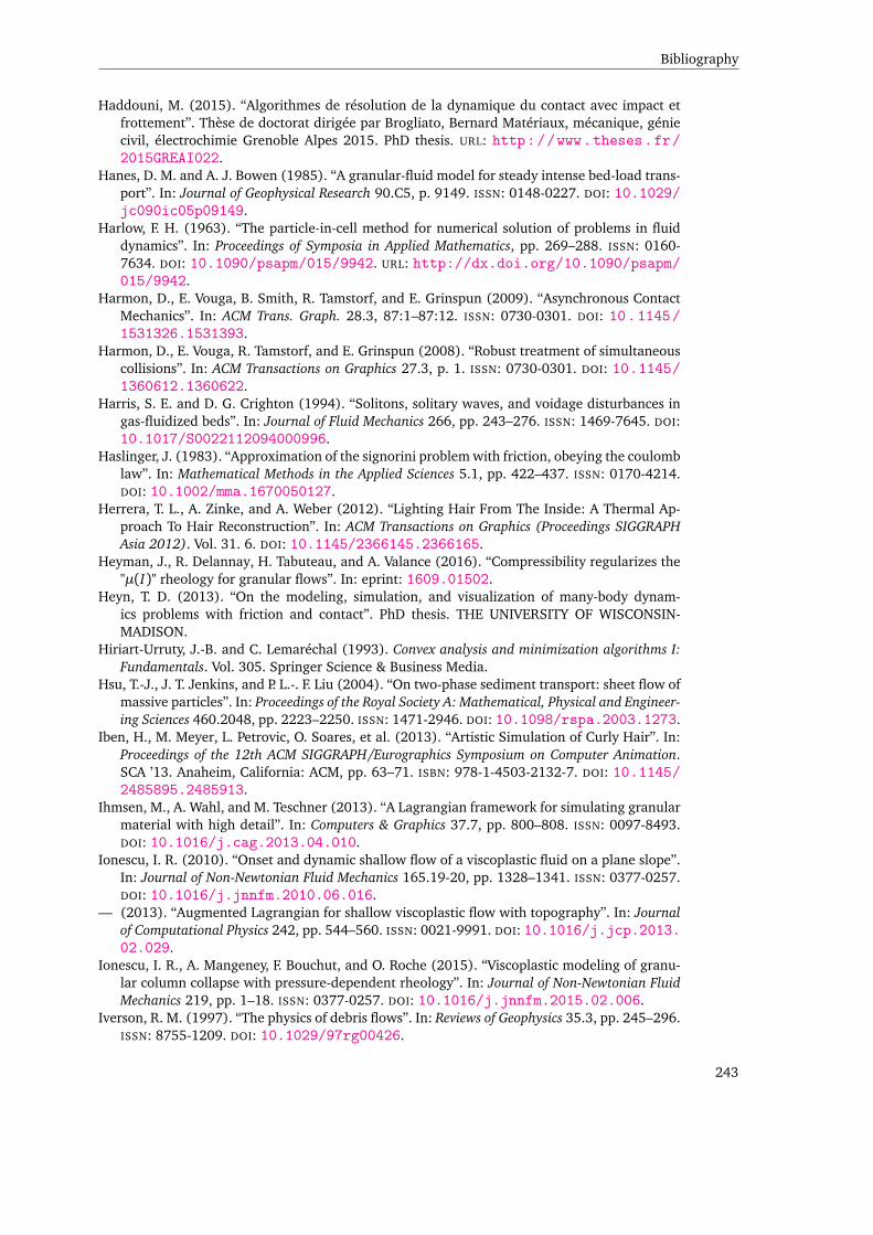
Bibliography

Haddouni, M. (2015). “Algorithmes de résolution de la dynamique du contact avec impact etfrottement”. Thèse de doctorat dirigée par Brogliato, Bernard Matériaux, mécanique, géniecivil, électrochimie Grenoble Alpes 2015. PhD thesis. URL: http://www.theses.fr/2015GREAI022.

Hanes, D. M. and A. J. Bowen (1985). “A granular-fluid model for steady intense bed-load trans-port”. In: Journal of Geophysical Research 90.C5, p. 9149. ISSN: 0148-0227. DOI: 10.1029/jc090ic05p09149.

Harlow, F. H. (1963). “The particle-in-cell method for numerical solution of problems in fluiddynamics”. In: Proceedings of Symposia in Applied Mathematics, pp. 269–288. ISSN: 0160-7634. DOI: 10.1090/psapm/015/9942. URL: http://dx.doi.org/10.1090/psapm/015/9942.

Harmon, D., E. Vouga, B. Smith, R. Tamstorf, and E. Grinspun (2009). “Asynchronous ContactMechanics”. In: ACM Trans. Graph. 28.3, 87:1–87:12. ISSN: 0730-0301. DOI: 10.1145/1531326.1531393.

Harmon, D., E. Vouga, R. Tamstorf, and E. Grinspun (2008). “Robust treatment of simultaneouscollisions”. In: ACM Transactions on Graphics 27.3, p. 1. ISSN: 0730-0301. DOI: 10.1145/1360612.1360622.

Harris, S. E. and D. G. Crighton (1994). “Solitons, solitary waves, and voidage disturbances ingas-fluidized beds”. In: Journal of Fluid Mechanics 266, pp. 243–276. ISSN: 1469-7645. DOI:10.1017/S0022112094000996.

Haslinger, J. (1983). “Approximation of the signorini problem with friction, obeying the coulomblaw”. In: Mathematical Methods in the Applied Sciences 5.1, pp. 422–437. ISSN: 0170-4214.DOI: 10.1002/mma.1670050127.

Herrera, T. L., A. Zinke, and A. Weber (2012). “Lighting Hair From The Inside: A Thermal Ap-proach To Hair Reconstruction”. In: ACM Transactions on Graphics (Proceedings SIGGRAPHAsia 2012). Vol. 31. 6. DOI: 10.1145/2366145.2366165.

Heyman, J., R. Delannay, H. Tabuteau, and A. Valance (2016). “Compressibility regularizes the"µ(I)" rheology for granular flows”. In: eprint: 1609.01502.

Heyn, T. D. (2013). “On the modeling, simulation, and visualization of many-body dynam-ics problems with friction and contact”. PhD thesis. THE UNIVERSITY OF WISCONSIN-MADISON.

Hiriart-Urruty, J.-B. and C. Lemaréchal (1993). Convex analysis and minimization algorithms I:Fundamentals. Vol. 305. Springer Science & Business Media.

Hsu, T.-J., J. T. Jenkins, and P. L.-. F. Liu (2004). “On two-phase sediment transport: sheet flow ofmassive particles”. In: Proceedings of the Royal Society A: Mathematical, Physical and Engineer-ing Sciences 460.2048, pp. 2223–2250. ISSN: 1471-2946. DOI: 10.1098/rspa.2003.1273.

Iben, H., M. Meyer, L. Petrovic, O. Soares, et al. (2013). “Artistic Simulation of Curly Hair”. In:Proceedings of the 12th ACM SIGGRAPH/Eurographics Symposium on Computer Animation.SCA ’13. Anaheim, California: ACM, pp. 63–71. ISBN: 978-1-4503-2132-7. DOI: 10.1145/2485895.2485913.

Ihmsen, M., A. Wahl, and M. Teschner (2013). “A Lagrangian framework for simulating granularmaterial with high detail”. In: Computers & Graphics 37.7, pp. 800–808. ISSN: 0097-8493.DOI: 10.1016/j.cag.2013.04.010.

Ionescu, I. R. (2010). “Onset and dynamic shallow flow of a viscoplastic fluid on a plane slope”.In: Journal of Non-Newtonian Fluid Mechanics 165.19-20, pp. 1328–1341. ISSN: 0377-0257.DOI: 10.1016/j.jnnfm.2010.06.016.

— (2013). “Augmented Lagrangian for shallow viscoplastic flow with topography”. In: Journalof Computational Physics 242, pp. 544–560. ISSN: 0021-9991. DOI: 10.1016/j.jcp.2013.02.029.

Ionescu, I. R., A. Mangeney, F. Bouchut, and O. Roche (2015). “Viscoplastic modeling of granu-lar column collapse with pressure-dependent rheology”. In: Journal of Non-Newtonian FluidMechanics 219, pp. 1–18. ISSN: 0377-0257. DOI: 10.1016/j.jnnfm.2015.02.006.

Iverson, R. M. (1997). “The physics of debris flows”. In: Reviews of Geophysics 35.3, pp. 245–296.ISSN: 8755-1209. DOI: 10.1029/97rg00426.

243

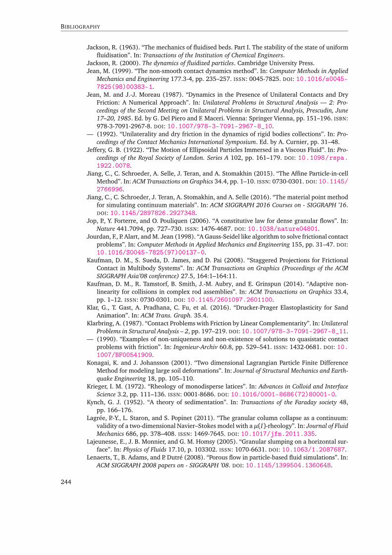
BIBLIOGRAPHY

Jackson, R. (1963). “The mechanics of fluidised beds. Part I. The stability of the state of uniformfluidisation”. In: Transactions of the Institution of Chemical Engineers.

Jackson, R. (2000). The dynamics of fluidized particles. Cambridge University Press.Jean, M. (1999). “The non-smooth contact dynamics method”. In: Computer Methods in Applied

Mechanics and Engineering 177.3-4, pp. 235–257. ISSN: 0045-7825. DOI: 10.1016/s0045-7825(98)00383-1.

Jean, M. and J.-J. Moreau (1987). “Dynamics in the Presence of Unilateral Contacts and DryFriction: A Numerical Approach”. In: Unilateral Problems in Structural Analysis — 2: Pro-ceedings of the Second Meeting on Unilateral Problems in Structural Analysis, Prescudin, June17–20, 1985. Ed. by G. Del Piero and F. Maceri. Vienna: Springer Vienna, pp. 151–196. ISBN:978-3-7091-2967-8. DOI: 10.1007/978-3-7091-2967-8_10.

— (1992). “Unilaterality and dry friction in the dynamics of rigid bodies collections”. In: Pro-ceedings of the Contact Mechanics International Symposium. Ed. by A. Curnier, pp. 31–48.

Jeffery, G. B. (1922). “The Motion of Ellipsoidal Particles Immersed in a Viscous Fluid”. In: Pro-ceedings of the Royal Society of London. Series A 102, pp. 161–179. DOI: 10.1098/rspa.1922.0078.

Jiang, C., C. Schroeder, A. Selle, J. Teran, and A. Stomakhin (2015). “The Affine Particle-in-cellMethod”. In: ACM Transactions on Graphics 34.4, pp. 1–10. ISSN: 0730-0301. DOI: 10.1145/2766996.

Jiang, C., C. Schroeder, J. Teran, A. Stomakhin, and A. Selle (2016). “The material point methodfor simulating continuum materials”. In: ACM SIGGRAPH 2016 Courses on - SIGGRAPH ’16.DOI: 10.1145/2897826.2927348.

Jop, P., Y. Forterre, and O. Pouliquen (2006). “A constitutive law for dense granular flows”. In:Nature 441.7094, pp. 727–730. ISSN: 1476-4687. DOI: 10.1038/nature04801.

Jourdan, F., P. Alart, and M. Jean (1998). “A Gauss-Seidel like algorithm to solve frictional contactproblems”. In: Computer Methods in Applied Mechanics and Engineering 155, pp. 31–47. DOI:10.1016/S0045-7825(97)00137-0.

Kaufman, D. M., S. Sueda, D. James, and D. Pai (2008). “Staggered Projections for FrictionalContact in Multibody Systems”. In: ACM Transactions on Graphics (Proceedings of the ACMSIGGRAPH Asia’08 conference) 27.5, 164:1–164:11.

Kaufman, D. M., R. Tamstorf, B. Smith, J.-M. Aubry, and E. Grinspun (2014). “Adaptive non-linearity for collisions in complex rod assemblies”. In: ACM Transactions on Graphics 33.4,pp. 1–12. ISSN: 0730-0301. DOI: 10.1145/2601097.2601100.

Klar, G., T. Gast, A. Pradhana, C. Fu, et al. (2016). “Drucker-Prager Elastoplasticity for SandAnimation”. In: ACM Trans. Graph. 35.4.

Klarbring, A. (1987). “Contact Problems with Friction by Linear Complementarity”. In: UnilateralProblems in Structural Analysis – 2, pp. 197–219. DOI: 10.1007/978-3-7091-2967-8_11.

— (1990). “Examples of non-uniqueness and non-existence of solutions to quasistatic contactproblems with friction”. In: Ingenieur-Archiv 60.8, pp. 529–541. ISSN: 1432-0681. DOI: 10.1007/BF00541909.

Konagai, K. and J. Johansson (2001). “Two dimensional Lagrangian Particle Finite DifferenceMethod for modeling large soil deformations”. In: Journal of Structural Mechanics and Earth-quake Engineering 18, pp. 105–110.

Krieger, I. M. (1972). “Rheology of monodisperse latices”. In: Advances in Colloid and InterfaceScience 3.2, pp. 111–136. ISSN: 0001-8686. DOI: 10.1016/0001-8686(72)80001-0.

Kynch, G. J. (1952). “A theory of sedimentation”. In: Transactions of the Faraday society 48,pp. 166–176.

Lagrée, P.-Y., L. Staron, and S. Popinet (2011). “The granular column collapse as a continuum:validity of a two-dimensional Navier–Stokes model with a µ(I)-rheology”. In: Journal of FluidMechanics 686, pp. 378–408. ISSN: 1469-7645. DOI: 10.1017/jfm.2011.335.

Lajeunesse, E., J. B. Monnier, and G. M. Homsy (2005). “Granular slumping on a horizontal sur-face”. In: Physics of Fluids 17.10, p. 103302. ISSN: 1070-6631. DOI: 10.1063/1.2087687.

Lenaerts, T., B. Adams, and P. Dutré (2008). “Porous flow in particle-based fluid simulations”. In:ACM SIGGRAPH 2008 papers on - SIGGRAPH ’08. DOI: 10.1145/1399504.1360648.

244

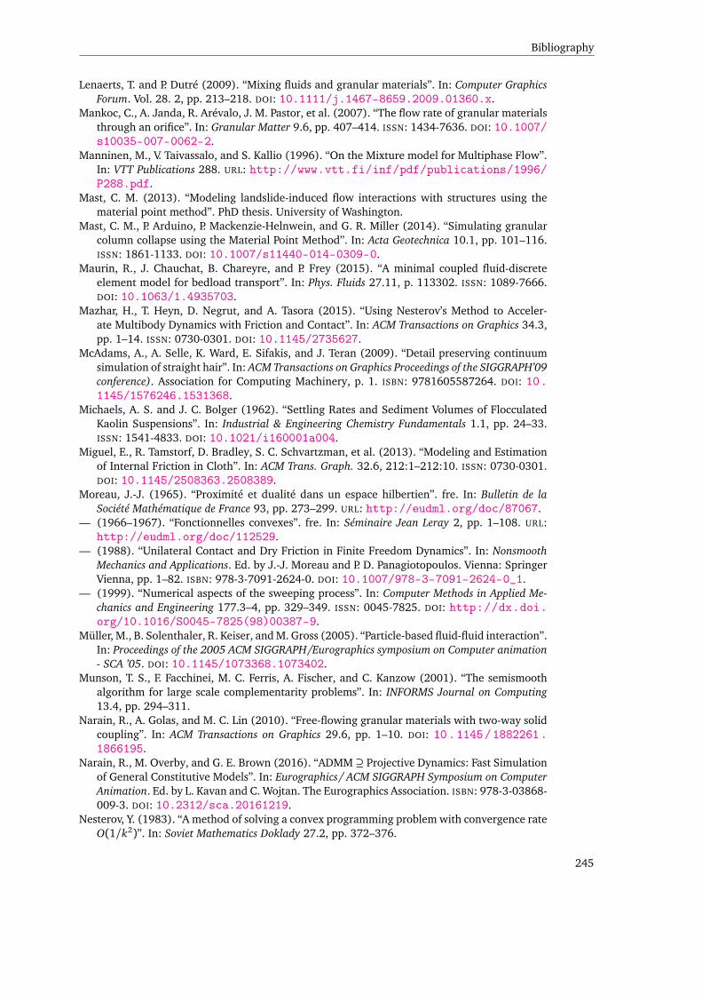
Bibliography

Lenaerts, T. and P. Dutré (2009). “Mixing fluids and granular materials”. In: Computer GraphicsForum. Vol. 28. 2, pp. 213–218. DOI: 10.1111/j.1467-8659.2009.01360.x.

Mankoc, C., A. Janda, R. Arévalo, J. M. Pastor, et al. (2007). “The flow rate of granular materialsthrough an orifice”. In: Granular Matter 9.6, pp. 407–414. ISSN: 1434-7636. DOI: 10.1007/s10035-007-0062-2.

Manninen, M., V. Taivassalo, and S. Kallio (1996). “On the Mixture model for Multiphase Flow”.In: VTT Publications 288. URL: http://www.vtt.fi/inf/pdf/publications/1996/P288.pdf.

Mast, C. M. (2013). “Modeling landslide-induced flow interactions with structures using thematerial point method”. PhD thesis. University of Washington.

Mast, C. M., P. Arduino, P. Mackenzie-Helnwein, and G. R. Miller (2014). “Simulating granularcolumn collapse using the Material Point Method”. In: Acta Geotechnica 10.1, pp. 101–116.ISSN: 1861-1133. DOI: 10.1007/s11440-014-0309-0.

Maurin, R., J. Chauchat, B. Chareyre, and P. Frey (2015). “A minimal coupled fluid-discreteelement model for bedload transport”. In: Phys. Fluids 27.11, p. 113302. ISSN: 1089-7666.DOI: 10.1063/1.4935703.

Mazhar, H., T. Heyn, D. Negrut, and A. Tasora (2015). “Using Nesterov’s Method to Acceler-ate Multibody Dynamics with Friction and Contact”. In: ACM Transactions on Graphics 34.3,pp. 1–14. ISSN: 0730-0301. DOI: 10.1145/2735627.

McAdams, A., A. Selle, K. Ward, E. Sifakis, and J. Teran (2009). “Detail preserving continuumsimulation of straight hair”. In: ACM Transactions on Graphics Proceedings of the SIGGRAPH’09conference). Association for Computing Machinery, p. 1. ISBN: 9781605587264. DOI: 10.1145/1576246.1531368.

Michaels, A. S. and J. C. Bolger (1962). “Settling Rates and Sediment Volumes of FlocculatedKaolin Suspensions”. In: Industrial & Engineering Chemistry Fundamentals 1.1, pp. 24–33.ISSN: 1541-4833. DOI: 10.1021/i160001a004.

Miguel, E., R. Tamstorf, D. Bradley, S. C. Schvartzman, et al. (2013). “Modeling and Estimationof Internal Friction in Cloth”. In: ACM Trans. Graph. 32.6, 212:1–212:10. ISSN: 0730-0301.DOI: 10.1145/2508363.2508389.

Moreau, J.-J. (1965). “Proximité et dualité dans un espace hilbertien”. fre. In: Bulletin de laSociété Mathématique de France 93, pp. 273–299. URL: http://eudml.org/doc/87067.

— (1966–1967). “Fonctionnelles convexes”. fre. In: Séminaire Jean Leray 2, pp. 1–108. URL:http://eudml.org/doc/112529.

— (1988). “Unilateral Contact and Dry Friction in Finite Freedom Dynamics”. In: NonsmoothMechanics and Applications. Ed. by J.-J. Moreau and P. D. Panagiotopoulos. Vienna: SpringerVienna, pp. 1–82. ISBN: 978-3-7091-2624-0. DOI: 10.1007/978-3-7091-2624-0_1.

— (1999). “Numerical aspects of the sweeping process”. In: Computer Methods in Applied Me-chanics and Engineering 177.3–4, pp. 329–349. ISSN: 0045-7825. DOI: http://dx.doi.org/10.1016/S0045-7825(98)00387-9.

Müller, M., B. Solenthaler, R. Keiser, and M. Gross (2005). “Particle-based fluid-fluid interaction”.In: Proceedings of the 2005 ACM SIGGRAPH/Eurographics symposium on Computer animation- SCA ’05. DOI: 10.1145/1073368.1073402.

Munson, T. S., F. Facchinei, M. C. Ferris, A. Fischer, and C. Kanzow (2001). “The semismoothalgorithm for large scale complementarity problems”. In: INFORMS Journal on Computing13.4, pp. 294–311.

Narain, R., A. Golas, and M. C. Lin (2010). “Free-flowing granular materials with two-way solidcoupling”. In: ACM Transactions on Graphics 29.6, pp. 1–10. DOI: 10.1145/1882261.1866195.

Narain, R., M. Overby, and G. E. Brown (2016). “ADMM ⊇ Projective Dynamics: Fast Simulationof General Constitutive Models”. In: Eurographics/ ACM SIGGRAPH Symposium on ComputerAnimation. Ed. by L. Kavan and C. Wojtan. The Eurographics Association. ISBN: 978-3-03868-009-3. DOI: 10.2312/sca.20161219.

Nesterov, Y. (1983). “A method of solving a convex programming problem with convergence rateO(1/k2)”. In: Soviet Mathematics Doklady 27.2, pp. 372–376.

245

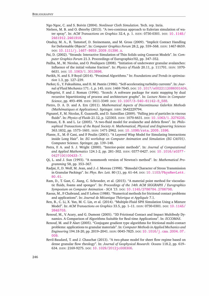
BIBLIOGRAPHY

Ngo Ngoc, C. and S. Boivin (2004). Nonlinear Cloth Simulation. Tech. rep. Inria.Nielsen, M. B. and O. Østerby (2013). “A two-continua approach to Eulerian simulation of wa-

ter spray”. In: ACM Transactions on Graphics 32.4, p. 1. ISSN: 0730-0301. DOI: 10.1145/2461912.2461918.

Otaduy, M. A., R. Tamstorf, D. Steinemann, and M. Gross (2009). “Implicit Contact Handlingfor Deformable Objects”. In: Computer Graphics Forum 28.2, pp. 559–568. ISSN: 1467-8659.DOI: 10.1111/j.1467-8659.2009.01396.x.

Pai, D. (2002). “Strands: Interactive Simulation of Thin Solids using Cosserat Models”. In: Com-puter Graphics Forum 21.3. Proceedings of Eurographics’02, pp. 347–352.

Pailha, M., M. Nicolas, and O. Pouliquen (2008). “Initiation of underwater granular avalanches:Influence of the initial volume fraction”. In: Physics of Fluids 20.11, p. 111701. ISSN: 1070-6631. DOI: 10.1063/1.3013896.

Parikh, N. and S. P. Boyd (2014). “Proximal Algorithms.” In: Foundations and Trends in optimiza-tion 1.3, pp. 127–239.

Parker, G., Y. Fukushima, and H. M. Pantin (1986). “Self-accelerating turbidity currents”. In: Jour-nal of Fluid Mechanics 171.-1, p. 145. ISSN: 1469-7645. DOI: 10.1017/s0022112086001404.

Pellegrini, F. and J. Roman (1996). “Scotch: A software package for static mapping by dualrecursive bipartitioning of process and architecture graphs”. In: Lecture Notes in ComputerScience, pp. 493–498. ISSN: 1611-3349. DOI: 10.1007/3-540-61142-8_588.

Pietro, D. A. D. and A. Ern (2011). Mathematical Aspects of Discontinuous Galerkin Methods(Mathématiques et Applications). Springer. ISBN: 3642229794.

Pignatel, F., M. Nicolas, É. Guazzelli, and D. Saintillan (2009). “Falling jets of particles in viscousfluids”. In: Physics of Fluids 21.12, p. 123303. ISSN: 1070-6631. DOI: 10.1063/1.3276235.

Pitman, E. B. and L. Le (2005). “A two-fluid model for avalanche and debris flows”. In: Philo-sophical Transactions of the Royal Society A: Mathematical, Physical and Engineering Sciences363.1832, pp. 1573–1601. ISSN: 1471-2962. DOI: 10.1098/rsta.2005.1596.

Plante, E., M.-P. Cani, and P. Poulin (2001). “A Layered Wisp Model for Simulating Interactionsinside Long Hair”. In: EG workshop on Computer Animation and Simulation (EG CAS’01).Computer Science. Springer, pp. 139–148.

Potra, F. A. and S. J. Wright (2000). “Interior-point methods”. In: Journal of Computationaland Applied Mathematics 124.1-2, pp. 281–302. ISSN: 0377-0427. DOI: 10.1016/s0377-0427(00)00433-7.

Qi, L. and J. Sun (1993). “A nonsmooth version of Newton’s method”. In: Mathematical Pro-gramming 58, pp. 353–367.

Radjai, F., D. Wolf, M. Jean, and J.-J. Moreau (1998). “Bimodal Character of Stress Transmissionin Granular Packings”. In: Phys. Rev. Lett. 80 (1), pp. 61–64. DOI: 10.1103/PhysRevLett.80.61.

Ram, D., T. Gast, C. Jiang, C. Schroeder, et al. (2015). “A material point method for viscoelas-tic fluids, foams and sponges”. In: Proceedings of the 14th ACM SIGGRAPH / EurographicsSymposium on Computer Animation - SCA ’15. DOI: 10.1145/2786784.2786798.

Raous, M., P. Chabrand, and F. Lebon (1988). “Numerical methods for frictional contact problemsand applications”. In: Journal de Mécanique Théorique et Appliquée 7.1.

Ren, B., C. Li, X. Yan, M. C. Lin, et al. (2014). “Multiple-Fluid SPH Simulation Using a MixtureModel”. In: ACM Transactions on Graphics 33.5, pp. 1–11. ISSN: 0730-0301. DOI: 10.1145/2645703.

Renouf, M., V. Acary, and G. Dumont (2005). “3D Frictional Contact and Impact Multibody Dy-namics. A Comparison of Algorithms Suitable for Real-time Applications”. In: ECCOMAS.

Renouf, M. and P. Alart (2005). “Conjugate gradient type algorithms for frictional multi-contactproblems: applications to granular materials”. In: Computer Methods in Applied Mechanics andEngineering 194.18-20, pp. 2019–2041. ISSN: 0045-7825. DOI: 10.1016/j.cma.2004.07.009.

Revil-Baudard, T. and J. Chauchat (2013). “A two-phase model for sheet flow regime based ondense granular flow rheology”. In: Journal of Geophysical Research: Oceans 118.2, pp. 619–634. ISSN: 2169-9275. DOI: 10.1029/2012jc008306.

246

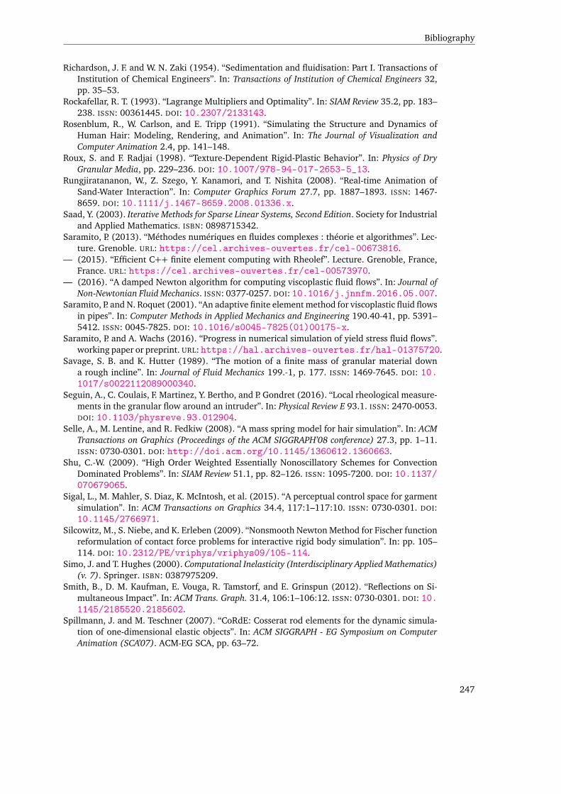
Bibliography

Richardson, J. F. and W. N. Zaki (1954). “Sedimentation and fluidisation: Part I. Transactions ofInstitution of Chemical Engineers”. In: Transactions of Institution of Chemical Engineers 32,pp. 35–53.

Rockafellar, R. T. (1993). “Lagrange Multipliers and Optimality”. In: SIAM Review 35.2, pp. 183–238. ISSN: 00361445. DOI: 10.2307/2133143.

Rosenblum, R., W. Carlson, and E. Tripp (1991). “Simulating the Structure and Dynamics ofHuman Hair: Modeling, Rendering, and Animation”. In: The Journal of Visualization andComputer Animation 2.4, pp. 141–148.

Roux, S. and F. Radjai (1998). “Texture-Dependent Rigid-Plastic Behavior”. In: Physics of DryGranular Media, pp. 229–236. DOI: 10.1007/978-94-017-2653-5_13.

Rungjiratananon, W., Z. Szego, Y. Kanamori, and T. Nishita (2008). “Real-time Animation ofSand-Water Interaction”. In: Computer Graphics Forum 27.7, pp. 1887–1893. ISSN: 1467-8659. DOI: 10.1111/j.1467-8659.2008.01336.x.

Saad, Y. (2003). Iterative Methods for Sparse Linear Systems, Second Edition. Society for Industrialand Applied Mathematics. ISBN: 0898715342.

Saramito, P. (2013). “Méthodes numériques en fluides complexes : théorie et algorithmes”. Lec-ture. Grenoble. URL: https://cel.archives-ouvertes.fr/cel-00673816.

— (2015). “Efficient C++ finite element computing with Rheolef”. Lecture. Grenoble, France,France. URL: https://cel.archives-ouvertes.fr/cel-00573970.

— (2016). “A damped Newton algorithm for computing viscoplastic fluid flows”. In: Journal ofNon-Newtonian Fluid Mechanics. ISSN: 0377-0257. DOI: 10.1016/j.jnnfm.2016.05.007.

Saramito, P. and N. Roquet (2001). “An adaptive finite element method for viscoplastic fluid flowsin pipes”. In: Computer Methods in Applied Mechanics and Engineering 190.40-41, pp. 5391–5412. ISSN: 0045-7825. DOI: 10.1016/s0045-7825(01)00175-x.

Saramito, P. and A. Wachs (2016). “Progress in numerical simulation of yield stress fluid flows”.working paper or preprint. URL: https://hal.archives-ouvertes.fr/hal-01375720.

Savage, S. B. and K. Hutter (1989). “The motion of a finite mass of granular material downa rough incline”. In: Journal of Fluid Mechanics 199.-1, p. 177. ISSN: 1469-7645. DOI: 10.1017/s0022112089000340.

Seguin, A., C. Coulais, F. Martinez, Y. Bertho, and P. Gondret (2016). “Local rheological measure-ments in the granular flow around an intruder”. In: Physical Review E 93.1. ISSN: 2470-0053.DOI: 10.1103/physreve.93.012904.

Selle, A., M. Lentine, and R. Fedkiw (2008). “A mass spring model for hair simulation”. In: ACMTransactions on Graphics (Proceedings of the ACM SIGGRAPH’08 conference) 27.3, pp. 1–11.ISSN: 0730-0301. DOI: http://doi.acm.org/10.1145/1360612.1360663.

Shu, C.-W. (2009). “High Order Weighted Essentially Nonoscillatory Schemes for ConvectionDominated Problems”. In: SIAM Review 51.1, pp. 82–126. ISSN: 1095-7200. DOI: 10.1137/070679065.

Sigal, L., M. Mahler, S. Diaz, K. McIntosh, et al. (2015). “A perceptual control space for garmentsimulation”. In: ACM Transactions on Graphics 34.4, 117:1–117:10. ISSN: 0730-0301. DOI:10.1145/2766971.

Silcowitz, M., S. Niebe, and K. Erleben (2009). “Nonsmooth Newton Method for Fischer functionreformulation of contact force problems for interactive rigid body simulation”. In: pp. 105–114. DOI: 10.2312/PE/vriphys/vriphys09/105-114.

Simo, J. and T. Hughes (2000). Computational Inelasticity (Interdisciplinary Applied Mathematics)(v. 7). Springer. ISBN: 0387975209.

Smith, B., D. M. Kaufman, E. Vouga, R. Tamstorf, and E. Grinspun (2012). “Reflections on Si-multaneous Impact”. In: ACM Trans. Graph. 31.4, 106:1–106:12. ISSN: 0730-0301. DOI: 10.1145/2185520.2185602.

Spillmann, J. and M. Teschner (2007). “CoRdE: Cosserat rod elements for the dynamic simula-tion of one-dimensional elastic objects”. In: ACM SIGGRAPH - EG Symposium on ComputerAnimation (SCA’07). ACM-EG SCA, pp. 63–72.

247

BIBLIOGRAPHY

Staron, L. and E. J. Hinch (2005). “Study of the collapse of granular columns using two-dimensionaldiscrete-grain simulation”. In: Journal of Fluid Mechanics 545.-1, p. 1. ISSN: 1469-7645. DOI:10.1017/s0022112005006415.

Staron, L., P.-Y. Lagrée, and S. Popinet (2012). “The granular silo as a continuum plastic flow:The hour-glass vs the clepsydra”. In: Physics of Fluids 24, 103301. ISSN: 1070-6631. DOI:10.1063/1.4757390.

— (2014). “Continuum simulation of the discharge of the granular silo”. In: The European Phys-ical Journal E 37.1. ISSN: 1292-895X. DOI: 10.1140/epje/i2014-14005-6.

Steffen, M., R. M. Kirby, and M. Berzins (2008). “Analysis and reduction of quadrature errors inthe material point method (MPM)”. In: Int. J. Numer. Meth. Engng 76.6, pp. 922–948. ISSN:1097-0207. DOI: 10.1002/nme.2360.

Stomakhin, A., C. Schroeder, L. Chai, J. Teran, and A. Selle (2013). “A material point methodfor snow simulation”. In: ACM Transactions on Graphics 32.4, pp. 1–10. DOI: 10.1145/2461912.2461948.

Stomakhin, A., C. Schroeder, C. Jiang, L. Chai, et al. (2014). “Augmented MPM for phase-changeand varied materials”. In: ACM Transactions on Graphics 33.4, pp. 1–11. ISSN: 0730-0301.DOI: 10.1145/2601097.2601176.

Sulsky, D. (1994). “A particle method for history-dependent materials”. In: Computer Methodsin Applied Mechanics and Engineering 118, pp. 179–196. DOI: 10.1016/0045-7825(94)00033-6.

Sun, D. and J. Sun (2005). “Strong Semismoothness of the Fischer-Burmeister SDC and SOCComplementarity Functions”. In: Math. Program. 103.3, pp. 575–581. ISSN: 1436-4646. DOI:10.1007/s10107-005-0577-4.

Tasora, A. (2013). “Efficient simulation of contacts, friction and constraints using a modifiedspectral projected gradient method”. In: Poster Proceedings of WSCG 2013, pp. 69–72.

Terzaghi, K. (1936). “The Shearing Resistance of Saturated Soils”. In: Proc. 1st InternationalConference on Soil Mechanics and Foundation Engineering.

Teschner, M., B. Heidelberger, M. Müller, D. Pomeranerts, and M. Gross (2003). “Optimized Spa-tial Hashing for Collision Detection of Deformable Objects”. In: Vision, Modeling, Visualization(VMV 2003), pp. 47–54.

Tonge, R., F. Benevolenski, and A. Voroshilov (2012). “Mass splitting for jitter-free parallel rigidbody simulation”. In: ACM Transactions on Graphics 31.4, pp. 1–8. ISSN: 0730-0301. DOI:10.1145/2185520.2185601.

Topin, V., F. Dubois, Y. Monerie, F. Perales, and A. Wachs (2011). “Micro-rheology of dense par-ticulate flows: Application to immersed avalanches”. In: Journal of Non-Newtonian Fluid Me-chanics 166.1-2, pp. 63–72. ISSN: 0377-0257. DOI: 10.1016/j.jnnfm.2010.10.006.

Topin, V., Y. Monerie, F. Perales, and F. Radjaï (2012). “Collapse Dynamics and Runout of DenseGranular Materials in a Fluid”. In: Physical Review Letters 109.18. ISSN: 1079-7114. DOI:10.1103/physrevlett.109.188001.

Treskatis, T., M. A. Moyers-González, and C. J. Price (2016). “An accelerated dual proximal gradi-ent method for applications in viscoplasticity”. In: Journal of Non-Newtonian Fluid Mechanics.ISSN: 0377-0257. DOI: 10.1016/j.jnnfm.2016.09.004.

Trinkle, J. C., J.-S. Pang, S. Sudarsky, and G. Lo (1997). “On Dynamic Multi-Rigid-Body ContactProblems with Coulomb Friction”. In: Z. angew. Math. Mech. 77.4, pp. 267–279. ISSN: 1521-4001. DOI: 10.1002/zamm.19970770411.

Ungarish, M. (2009). An introduction to gravity currents and intrusions. CRC Press.Vermeer, P. A. (1998). “Non-Associated Plasticity for Soils, Concrete and Rock”. In: Physics of Dry

Granular Media, pp. 163–196. DOI: 10.1007/978-94-017-2653-5_10.Ward, K., F. Bertails, T.-Y. Kim, S. Marschner, et al. (2007). “A Survey on Hair Modeling: Styling,

Simulation, and Rendering”. In: IEEE Transactions on Visualization and Computer Graphics(TVCG) 13.2, pp. 213–34. URL: http://www-evasion.imag.fr/Publications/2007/WBKMCL07.

Wieckowski, Z. and M. Pawlak (2015). “Material point method in three-dimensional problemsof granular flow”. In: 6th European Conference on Computational Fluid Dynamics.

248

Bibliography

Wieckowski, Z., S.-K. Youn, and J.-H. Yeon (1999). “A particle-in-cell solution to the silo discharg-ing problem”. In: International Journal for Numerical Methods in Engineering 45.9, pp. 1203–1225. ISSN: 1097-0207. DOI: 10.1002/(sici)1097-0207(19990730)45:9<1203::aid-nme626>3.0.co;2-c.

Yue, Y., B. Smith, C. Batty, C. Zheng, and E. Grinspun (2015). “Continuum Foam”. In: ACMTransactions on Graphics 34.5, pp. 1–20. ISSN: 0730-0301. DOI: 10.1145/2751541.

Zhu, H., X. Liu, Y. Liu, and E. Wu (2006). “Simulation of miscible binary mixtures based on latticeBoltzmann method”. In: Computer Animation and Virtual Worlds 17.3-4, pp. 403–410. ISSN:1546-427X. DOI: 10.1002/cav.143.

Zhu, Y. and R. Bridson (2005). “Animating sand as a fluid”. In: ACM Transactions on Graphics24.3, pp. 965–972. DOI: 10.1145/1073204.1073298.

249

AbstractThis dissertation focuses on the numerical simulation of mechanical systems consisting

of a large number of discrete pieces interacting with each other through contacts and dryfriction. Examples of such systems — for instance, sand or human hair — are common innatural environments; being able to predict their dynamics is therefore of great importancefor diverse applications ranging from geotechnical considerations to engaging visual effectsfor feature films.

A major difficulty that complicates the numerical simulation of such complex systemsstems from the nonsmoothness of their dynamics. For instance, from a macroscopic viewpoint,the velocity of the individual constituents may exhibit instantaneous jumps when impactsoccur. The first part of this manuscript will be dedicated to the establishment of efficientalgorithms for the numerical simulation of discrete mechanical systems subject to contacts andCoulomb friction. We advocate using a Gauss–Seidel algorithm with a hybrid local solver, andshow that this strategy performs robustly in the challenging context of virtual hair simulation.

The second part of this dissertation will focus on much bigger systems, consisting of mil-lions or billions of grains. As computing every force between pairs of contacting grains quicklybecomes intractable, we embrace a continuum viewpoint instead. We show how the numeri-cal methods devised for the simulation of discrete mechanical systems can be adapted to thesimulation of flows governed by the Drucker–Prager rheology — a constitutive relationshipbetween the material’s stress and strain rate that macroscopically models the action of fric-tional contact forces. This approach allows us to capture qualitative features of granular flowsthat have been observed experimentally. Finally, we propose a new numerical model for thecoupled simulation of a granular continuum with a surrounding fluid, and show that onceagain, we are able to leverage efficient algorithms from discrete contact mechanics to solvethe resulting equations.

RésuméCette thèse traite de la simulation numérique de systèmes composés de nombreux objets

distincts, et dont le principal mécanisme d’interaction consiste en des contacts inélastiquesavec frottement solide. On trouve de nombreuses occurrences de tels systèmes dans la na-ture, par exemple sous la forme de sable ou d’une chevelure humaine ; aussi la reproduc-tion numérique de leur dynamique trouve des applications diverses, allant de considérationsgéotechniques à la production d’effets spéciaux réalistes pour le cinéma.

Une difficulté majeure pour la simulation de tels systèmes concerne la non-régularité deleur dynamique ; à une échelle de temps macroscopique, on observe par exemple des sautsdans les vitesses des constituants lors d’impacts. La première partie de ce manuscrit est ainsidédiée à la conception d’algorithmes efficaces permettant de prendre en compte les contactsavec frottement de Coulomb lors de la simulation de systèmes mécaniques discrets. La méth-ode que nous proposons, basée sur un algorithme de type Gauss–Seidel avec stratégie hybride,s’avère robuste et perfomante sur le problème délicat de la simulation virtuelle de chevelures.

La second partie de ce manuscrit est consacrée à l’étude de systèmes à une échelle beau-coup plus grande, au delà du million de grains. Puisque le calcul de toutes les forces decontacts pour chaque paire de grains s’avérerait trop coûteux, on adopte un point de vuemacroscopique en utilisant le formalisme des milieux continus. On propose ainsi d’adapter lesméthodes développées pour la simulation de systèmes discrets à la résolution de la rhéologiedite de Drucker–Prager, une relation entre la contrainte et le cisaillement du matériau exp-rimant l’influence moyennée des forces de frottement. On montre que cette approche nouspermet de retrouver le comportement qualitatif de matériaux granulaires secs observé expéri-mentalement. Finalement, nous proposons un nouveau modèle numérique pour l’étude desdynamiques couplées d’un matériau granulaire immergé dans un fluide Newtonien, et mon-trons une nouvelle fois que les algorithmes développés pour la mécanique discrète s’avèrentégalement pertinents dans le cas continu.