Modeling of Flatness-Based Control with Disturbance ... · Modeling of Flatness-Based Control with...
9
Modeling of Flatness-Based Control with Disturbance Observer-Based Parameter Estimation for PMSM Drive S. Sriprang* 1,2,3 , B. Nahid-Mobarakeh 1 , N. Takorabet 1 , P. Thounthong 2,3 , S. Pierfederici 6 , P. Kumam 4 , N. Bizon 5 and P. Mungporn 2 1 GREEN Lab., Université de Lorraine, 2 Vancouver-les-Nancy, Lorraine 54516, France 2 Renewable Energy Research Centre (RERC), Thai-French Innovation Institute (TFII) 3 Department of Teacher Training in Electrical Engineering (TE), Faculty of Technical Education King Mongkut's University of Technology North Bangkok, 1518, Pracharat 1 Rd., Bangkok 10800, Thailand * Corresponding author: [email protected], [email protected] 4 Department of Mathematics, King Mongkut's University of Technology Thonburi, Bangkok, Thailand 5 Faculty of Electronics, Communications and Computers, University of Pitesti, Arges 110040, Pitesti, Romania 6 LEMTA Lab., Université de Lorraine, 2 Vancouver-les-Nancy, Lorraine 54516, France Abstract: - This paper presents a modeling of nonlinear control with parameters identification for the permanent magnet synchronous motor (PMSM) drive. A resistance in series with an inductance and the conduction losses in semiconductor switching devices of inverters represented by vtq (=Rs*iq) as well as the torque load TL are going to be estimated by observer method based on extended Luenberger observer (LOB). The simulation and experimental results show the proposed control provides the rapid response and flat of the current control loop for the PMSM drive system. Moreover, the observer approach precisely estimates both vtq and TL, and the converging time is less than 0.1 sec. The test bench was implemented by small-scale PMSM 1 kW, 3,500 rpm, 6 ampere rated to validate the proposed control approach. Key-Words: - Disturbance observer (DOB), SPMSM, Flatness-based control modeling, Extended Luenberger Observer 1 Introduction Currently, Permanent-Magnet Synchronous Machines (PMSMs) have been widely used in many applications such as robotics, numerical controls, and electric vehicles, etc., since they have the significant advantages like high power ratio, small volume, and simple structure. Moreover, with the development of a full electric aircraft, PMSMs are the appropriate player for the electrical propulsion system in aviation. Although there are many advantages of PMSMs, it is still challenging to control them getting high performance for all operating conditions. It is due to a nonlinear multivariable system and subjected to unknown parameters uncertainty of them that nonlinear control approaches are more reasonable than linear control. To get around this problem, many researchers have proposed diverse control design methods, e.g., adaptive control [1], neural network control [2], nonlinear feedback linearization control [3], disturbance-observer-based control [4], model predictive control [5], fuzzy-logic-based controller [6], robust control [7] and the combination of these concepts [8]. One of the nonlinear control systems adapted to control PMSM is the flatness-based control system [9]-[10]. As the flatness-based control is a model-based control, the performance of the controller relies on the accuracy of the machine parameters such as the stator resistance Rs, load torque disturbance TL, etc. However, these are difficult to measure directly, so state observer method is often utilized to estimate these parameters. Many parameter estimation methods have been investigated in the literature review, and one of the observer methods is Extended Luenberger Observer (ELO) that has advantages over conventional observers such as independence from mathematical model accuracy, robustness, and good dynamic performance [11]. Also, only observer gains need to be tuned, and the tuning process is not complicated because the gains are determined by the desired observer. In this paper, flatness-based control is going to utilize to control PMSM, and also an observer approach is introduced to improve the performance of the proposed control. In the following sections, a detailed theoretical analysis of the proposed method is presented. Finally, practical implementation results based on the dSPACE 1104 DSP system are shown to confirm its correctness. WSEAS TRANSACTIONS on ELECTRONICS S. Sriprang, B. Nahid-Mobarakeh, N. Takorabet, P. Thounthong, S. Pierfederici, P. Kumam, N. Bizon, P. Mungporn E-ISSN: 2415-1513 19 Volume 10, 2019
Transcript of Modeling of Flatness-Based Control with Disturbance ... · Modeling of Flatness-Based Control with...
Modeling of Flatness-Based Control with Disturbance Observer-Based
Parameter Estimation for PMSM Drive
S. Sriprang*1,2,3, B. Nahid-Mobarakeh1, N. Takorabet1, P. Thounthong2,3, S. Pierfederici6,
P. Kumam4, N. Bizon5 and P. Mungporn2 1GREEN Lab., Université de Lorraine, 2 Vancouver-les-Nancy, Lorraine 54516, France 2Renewable Energy Research Centre (RERC), Thai-French Innovation Institute (TFII)
3Department of Teacher Training in Electrical Engineering (TE), Faculty of Technical Education King Mongkut's University of Technology North Bangkok, 1518, Pracharat 1 Rd., Bangkok 10800, Thailand
* Corresponding author: [email protected], [email protected] 4Department of Mathematics, King Mongkut's University of Technology Thonburi, Bangkok, Thailand 5Faculty of Electronics, Communications and Computers, University of Pitesti, Arges 110040, Pitesti, Romania
6LEMTA Lab., Université de Lorraine, 2 Vancouver-les-Nancy, Lorraine 54516, France
Abstract: - This paper presents a modeling of nonlinear control with parameters identification for the
permanent magnet synchronous motor (PMSM) drive. A resistance in series with an inductance and the
conduction losses in semiconductor switching devices of inverters represented by vtq (=Rs*iq) as well as the
torque load TL are going to be estimated by observer method based on extended Luenberger observer (LOB).
The simulation and experimental results show the proposed control provides the rapid response and flat of the
current control loop for the PMSM drive system. Moreover, the observer approach precisely estimates both vtq
and TL, and the converging time is less than 0.1 sec. The test bench was implemented by small-scale PMSM 1
kW, 3,500 rpm, 6 ampere rated to validate the proposed control approach.
Key-Words: - Disturbance observer (DOB), SPMSM, Flatness-based control modeling, Extended Luenberger Observer
1 Introduction Currently, Permanent-Magnet Synchronous
Machines (PMSMs) have been widely used in many
applications such as robotics, numerical controls,
and electric vehicles, etc., since they have the
significant advantages like high power ratio, small
volume, and simple structure. Moreover, with the
development of a full electric aircraft, PMSMs are
the appropriate player for the electrical propulsion
system in aviation. Although there are many
advantages of PMSMs, it is still challenging to
control them getting high performance for all
operating conditions. It is due to a nonlinear
multivariable system and subjected to unknown
parameters uncertainty of them that nonlinear
control approaches are more reasonable than linear
control. To get around this problem, many
researchers have proposed diverse control design
methods, e.g., adaptive control [1], neural network
control [2], nonlinear feedback linearization control
[3], disturbance-observer-based control [4], model
predictive control [5], fuzzy-logic-based controller
[6], robust control [7] and the combination of these
concepts [8]. One of the nonlinear control systems
adapted to control PMSM is the flatness-based
control system [9]-[10]. As the flatness-based
control is a model-based control, the performance of
the controller relies on the accuracy of the machine
parameters such as the stator resistance Rs, load
torque disturbance TL, etc. However, these are
difficult to measure directly, so state observer
method is often utilized to estimate these
parameters. Many parameter estimation methods
have been investigated in the literature review, and
one of the observer methods is Extended
Luenberger Observer (ELO) that has advantages
over conventional observers such as independence
from mathematical model accuracy, robustness, and
good dynamic performance [11]. Also, only
observer gains need to be tuned, and the tuning
process is not complicated because the gains are
determined by the desired observer. In this paper,
flatness-based control is going to utilize to control
PMSM, and also an observer approach is introduced
to improve the performance of the proposed control.
In the following sections, a detailed theoretical
analysis of the proposed method is presented.
Finally, practical implementation results based on
the dSPACE 1104 DSP system are shown to
confirm its correctness.
WSEAS TRANSACTIONS on ELECTRONICS
S. Sriprang, B. Nahid-Mobarakeh, N. Takorabet, P. Thounthong,
S. Pierfederici, P. Kumam, N. Bizon, P. Mungporn
E-ISSN: 2415-1513 19 Volume 10, 2019
2 Proposed Control Design
2.1 Modeling of the PMSM/inverter
PMSM
1S 3S 5S
2S 4S 6S
Ai
Bi
Ci
Encoderm
m
BUSCChopS
BreakR
PIM(7MBR15SA-120)BUSiBUSV
BUSv
BUSi
R
S
T
Control algorithm
PWM1-7
ADCADC
Incremental
Encoder
380 V
Bra
kin
g C
ho
pp
er
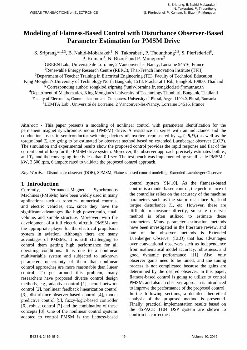
Fig. 1 A three-phase inverter is driving the PMSM
where VBUS, iBUS, iA, and iC are DC bus voltage, the
input inverter current, the motor phase current,
respectively.
Fig. 1 shows a system configuration of a three-phase
inverter connected to the PMSM. The sinusoidal
pulse-width modulation technique (SPWM) is
applied to inverter to achieve a sinusoidal output
voltage with minimal undesired harmonics. The
classic rotor reference frame of the PMSM is [9]-
[12]:
1)( d d q q
ds
did R Led t L
v i i (1)
1)( q q d d
qs
diqR L
e e md t Lv i i (2)
)(1
Lme TBTJtd
md
(3)
Where
)( ( )q m q d deT L Lp i Ψ i (4)
me p (5)
vd and vq are the d, q axis voltages, id and iq are the
d, q axis stator currents, Ld and Lq are the d, q axis
inductances, Rs and Ψm are the resistance (or system
losses) and the magnet’s flux linkage, respectively;
and ωe, ωm, p, Te, TL, B, J are electrical angular
frequency, mechanical angular frequency, number
of pole pairs, electromagnetic torque, load torque,
viscosity, and inertia, respectively.
2.2 Flatness-based Control design For the first is to analyze the flatness-based control
that is mentioned by [9], to utilize for PMSM
control. As Ls = Lq = Ld is defined for non-salient
machine. Flat outputs y = [id iq ωm]T, control
variable u = [vd vq iq]T, and state variable x = [id iq
ωm]T are assigned respectively. Then, the state
variables x can be written as x = [φ1(y1) φ2(y2)
φ3(y3)]T. From (1), (2), and (3), the control variable
u can be calculated from the flatness output y and its
time derivatives (called inverse dynamics):
dqsedsds vyyyiLiRiLu ),,( 21111 (6)
2
2 1 2 2 )( , ,
s q s q e s d e m
qv
u L i R i L i Ψ
y y y
(7)
qCOMmmfLm iyyΨpBTJu ),(/)( 3333
(8)
dtd
iK1
iK2
+
-
+
+
+
Eq.7
dv
dtd
1K
2K
+
-
+
+
+
Speed Control lawdt
d
iK1
iK2
+
-
+
+
+
Current Control law
Eq.6
qv
di
qCOMi
qi
Eq.8REF
m
qREFiCOMqMAXi
qMINi
3y
1y
2y
dREFi
dCOMi
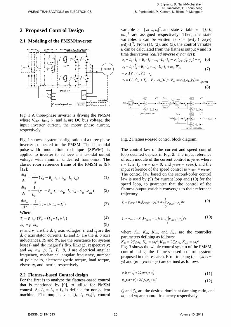
Fig. 2 Flatness-based control block diagram.
The control law of the current and speed control
loop detailed depicts in Fig. 2. The input reference
of each module of the current control is yiREF, where
i = 1, 2, (y1REF = id = 0, and y2REF = iqCOM), and the
input reference of the speed control is y3REF = ωCOM.
The control law based on the second-order control
law is used by (9) for current loop and (10) for the
speed loop, to guarantee that the control of the
flatness output variable converges to their reference
trajectory.
t
dyyKyyKyyiiREFiiiREFiiREFi
021 (9)
t
dyyKyyKyyREFREFREF
0
33233133 (10)
where K1i, K2i, K1ω, and K2ω are the controller
parameters defining as follows:
K1i = 2ζ1ω1, K2i = ω12, K1ω = 2ζ3ω3, K2ω = ω3
2
Fig. 3 shows the whole control system of the PMSM
control using the flatness-based control system
proposed in this research. Error tracking (e1 = yiREF −
yi) and (e2 = y3REF – y3) are defined as follows
2
1111
2
12)( ees
iq (11)
2
3233
2
22)(
eesq (12)
ζ1 and ζ3, are the desired dominant damping ratio, and
ω1 and ω3 are natural frequency respectively.
WSEAS TRANSACTIONS on ELECTRONICS
S. Sriprang, B. Nahid-Mobarakeh, N. Takorabet, P. Thounthong,
S. Pierfederici, P. Kumam, N. Bizon, P. Mungporn
E-ISSN: 2415-1513 20 Volume 10, 2019
SPWM
PWM1-6
Controller
aV
bV
cV
tT 32
i
i1P
32T
v
vP
Park’s Transformation
p
qi
di
di
qi
tqv
0dCOMi
tqv
LestT
m
qi
qv
qv
di
dv
qREFi
LestT
m
REF
ELO
e
Ai
Ci
Bi
BUSv
m
1S
2S
3S
4S
5S
6S
Gate
DriveFlatness-based
Current Control
Flatness-based
Speed Control
maxqi
minqi
-
-
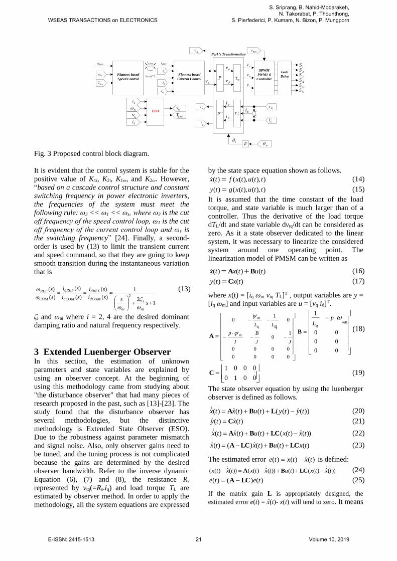
Fig. 3 Proposed control block diagram.
It is evident that the control system is stable for the
positive value of K1i, K2i, K1ω, and K2ω. However,
“based on a cascade control structure and constant
switching frequency in power electronic inverters,
the frequencies of the system must meet the
following rule: ω3 << ω1 << ωs, where ω3 is the cut
off frequency of the speed control loop, ω1 is the cut
off frequency of the current control loop and ωs is
the switching frequency” [24]. Finally, a second-
order is used by (13) to limit the transient current
and speed command, so that they are going to keep
smooth transition during the instantaneous variation
that is
12
1
)(
)(
)(
)(
)(
)(2
sssi
si
si
si
s
s
ni
i
ni
dCOM
dREF
qCOM
qREF
COM
REF
(13)
ζi and ωni where i = 2, 4 are the desired dominant
damping ratio and natural frequency respectively.
3 Extended Luenberger Observer In this section, the estimation of unknown
parameters and state variables are explained by
using an observer concept. At the beginning of
using this methodology came from studying about
"the disturbance observer" that had many pieces of
research proposed in the past, such as [13]-[23]. The
study found that the disturbance observer has
several methodologies, but the distinctive
methodology is Extended State Observer (ESO).
Due to the robustness against parameter mismatch
and signal noise. Also, only observer gains need to
be tuned, and the tuning process is not complicated
because the gains are determined by the desired
observer bandwidth. Refer to the inverse dynamic
Equation (6), (7) and (8), the resistance Rs
represented by vtq(=Rs.iq) and load torque TL are
estimated by observer method. In order to apply the
methodology, all the system equations are expressed
by the state space equation shown as follows.
)),(),(()( ttutxftx (14)
)),(),(()( ttutxgty (15)
It is assumed that the time constant of the load
torque, and state variable is much larger than of a
controller. Thus the derivative of the load torque
dTL/dt and state variable dvtq/dt can be considered as
zero. As it a state observer dedicated to the linear
system, it was necessary to linearize the considered
system around one operating point. The
linearization model of PMSM can be written as
)()()( tutxtx BA (16)
)()( txty C (17)
where x(t) = [iq ωm vtq TL]T , output variables are y =
[iq ωm] and input variables are u = [vq id]T.
0000
0000
10
01
0
JJ
B
J
p
qLL
m
q
m
A
00
00
00
1
0mq
pL
B (18)
0010
0001C (19)
The state observer equation by using the luenberger
observer is defined as follows.
))(ˆ)(()()(ˆ)(ˆ tytytutxtx LBA (20)
)(ˆ)(ˆ txty C (21)
))(ˆ)(()()(ˆ)(ˆ txtxtutxtx LCBA (22)
)()()(ˆ)()(ˆ txtutxtx LCBLCA (23)
The estimated error )(ˆ)()( txtxte is defined:
))(ˆ)(()())(ˆ)(())(ˆ)(( txtxtutxtxtxtx LCBA (24)
)()()( tete LCA (25)
If the matrix gain L is appropriately designed, the
estimated error e(t) = x̂(t)- x(t) will tend to zero. It means
WSEAS TRANSACTIONS on ELECTRONICS
S. Sriprang, B. Nahid-Mobarakeh, N. Takorabet, P. Thounthong,
S. Pierfederici, P. Kumam, N. Bizon, P. Mungporn
E-ISSN: 2415-1513 21 Volume 10, 2019
that the estimated states x̂(t) approach the actual
states x(t).
Block diagram for Luenberger observer is shown in
Fig. 3. The observability matrix (Qb) (18), (19) has
rank 4. It is full rank, and the system is
completely observable. It is realized by choosing
the value of the gain matrix L so that (A − LC)
eigenvalues approach (−200 − 200 − 33 − 60)T.
Those values have been tuned experimentally to
obtain better performances as possible. For the
operating point, at speed (n) = 1500 rpm ωm0 =
157.0796 rad/sec, and id(0) = 0, the matrix L is
obtained by (26). For this estimation, even if the
system has been linearized around one operating
point, it has been experimentally verified that the
estimation was converging in the speed range 0-
1500 rpm with no change of the value of the matrix
L. The closed-loop system pole locations can be
arbitrarily placed if and only if the system is
controllable.
11.088-0
0423.720-
230.9174395.357
18.811-260
L (26)
4 Stability and Control Conclusion In this section, the stability of the flatness-based
control including the extended Luenberger observer
is going to be explained. The control conclusion and
stability of the flatness-based control was mentioned
by [24] that the stability of the control systems was
guaranteed. For the stability of the ELO is explained
by the design controllers and observers using state-
space (or time-domain) methods. For the LTI
(Linear Time-Invariant) systems are written as
follows.
)()()( tButAxtx (27)
)()()( tDutCxty (28)
The first step is to analyze whether the open-loop
system (without any control) is stable. The
eigenvalues of the system matrix, A, (equivalent to
the poles of the transfer function) determine the
stability. The eigenvalues of the A matrix are the
values of s where det(sI - A) = 0. It is important to
note that a system must be completely controllable
and observable to allow the flexibility to place all
the closed-loop system poles arbitrarily. A system is
controllable if there exists a control input, u(t), that
transfers any state of the system to zero in finite
time. It is able be shown that the LTI system (27) is
controllable if and only if its controllability matrix,
Qc, has full rank or det(Qc) ≠ 0 (i.e. if rank(Qc) = n
where n is the number of states ).
BABAABBQ2 1|...||| n
c (29)
Meanwhile, The system is observable if and only if
the observability matrix, Qb, has full rank or det(Qb)
≠ 0 (i.e. if rank(Qb) = n where n is the number of
states).
1n
2
CA
CA
CA
C
Q
.
.
.b
(30)
Controllability and observability are dual concepts.
A system (A,B) is controllable if and only if a
system (A',C,B',D) is observable. This fact will be
useful when designing an observer. Ackermann's
formula can also be employed to place the roots of
the observer characteristic equation at the desired
locations [25]. Consider the observer gain matrix.
T
nLLL ]...[ 21L (31)
and the desired observer characteristic equation
011
1 ...)(
nn
nq (32)
The β's are selected to meet given performance
specifications for the observer. The observer gain
matrix is then computed via
T
bq ]10...0[)( 1 QAL (33)
where Qb is the observability matrix and
IAAAA01
1
1...)(
n
n
nq (34)
4 Simulation and Experimental Result
4.1 Laboratory Setup The main PMSM parameters are presented in Table 1,
and the flatness-based controller parameters are
defined in Table 2. The laboratory setup showing in
Fig. 4 composed of a 6-pole, 1-kW PMSM coupled
with a 0.25-kW Separate Excited DC motor that was
served as a power supply for a purely resistive load.
The stator windings of the PMSM were fed by a 3-
kW, 3Φ DC–AC voltage-source inverter (VSI) that
was operated at a switching frequency of 10 kHz.
WSEAS TRANSACTIONS on ELECTRONICS
S. Sriprang, B. Nahid-Mobarakeh, N. Takorabet, P. Thounthong,
S. Pierfederici, P. Kumam, N. Bizon, P. Mungporn
E-ISSN: 2415-1513 22 Volume 10, 2019
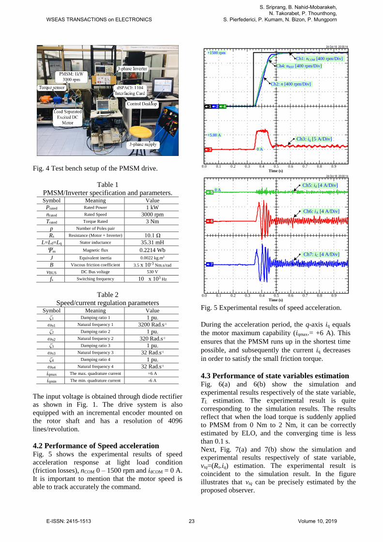
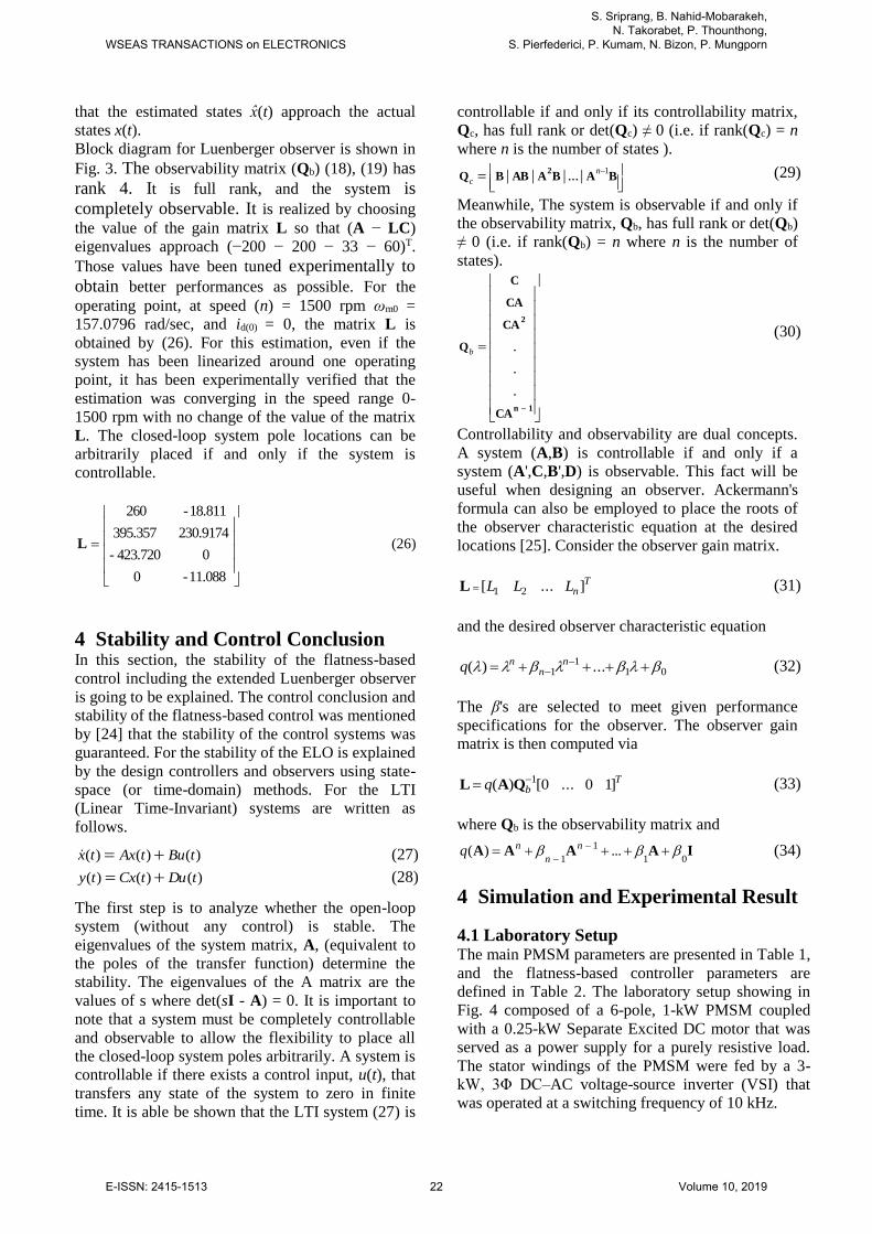
Fig. 4 Test bench setup of the PMSM drive.
Table 1
PMSM/Inverter specification and parameters. Symbol Meaning Value
Prated Rated Power 1 kW
nrated Rated Speed 3000 rpm
Trated Torque Rated 3 Nm
p Number of Poles pair
Rs Resistance (Motor + Inverter) 10.1 Ω
L=Ld=Lq Stator inductance 35.31 mH
Ψm Magnetic flux 0.2214 Wb
J Equivalent inertia 0.0022 kg.m2
B Viscous friction coefficient 3.5 x 10⁻³ Nm.s/rad
vBUS DC Bus voltage 530 V
fs Switching frequency 10 x 103 Hz
Table 2
Speed/current regulation parameters Symbol Meaning Value
ζ1 Damping ratio 1 1 pu.
ωn1 Natural frequency 1 3200 Rad.s-1
ζ2 Damping ratio 2 1 pu.
ωn2 Natural frequency 2 320 Rad.s-1
ζ3 Damping ratio 3 1 pu.
ωn3 Natural frequency 3 32 Rad.s-1
ζ4 Damping ratio 4 1 pu.
ωn4 Natural frequency 4 32 Rad.s-1
iqmax The max. quadrature current +6 A
iqmin The min. quadrature current -6 A
The input voltage is obtained through diode rectifier
as shown in Fig. 1. The drive system is also
equipped with an incremental encoder mounted on
the rotor shaft and has a resolution of 4096
lines/revolution.
4.2 Performance of Speed acceleration Fig. 5 shows the experimental results of speed
acceleration response at light load condition
(friction losses), nCOM 0 – 1500 rpm and idCOM = 0 A.
It is important to mention that the motor speed is
able to track accurately the command.
0.0 0.1 0.2 0.3 0.4 0.5 0.6 0.7 0.8 0.9Time (s)
-1600
-1200
-800
-400
0
400
800
1200
1600
24 Oct 18 20:00:14
Ch2: n [400 rpm/Div]
+1500 rpm
+5.00 A
0 A
Ch4: nREF [400 rpm/Div]
Ch3: iq [5 A/Div]
2
3
41
Ch1: nCOM [400 rpm/Div]
24 Oct 18 20:00:14
Ch6: iA [4 A/Div]
Ch7: iC [4 A/Div]
Ch5: id [4 A/Div]0 A
0.0 0.1 0.2 0.3 0.4 0.5 0.6 0.7 0.8 0.9Time (s)
-14
-10
-6
-2
2
5
6
7
Fig. 5 Experimental results of speed acceleration.
During the acceleration period, the q-axis iq equals
the motor maximum capability (iqmax.= +6 A). This
ensures that the PMSM runs up in the shortest time
possible, and subsequently the current iq decreases
in order to satisfy the small friction torque.
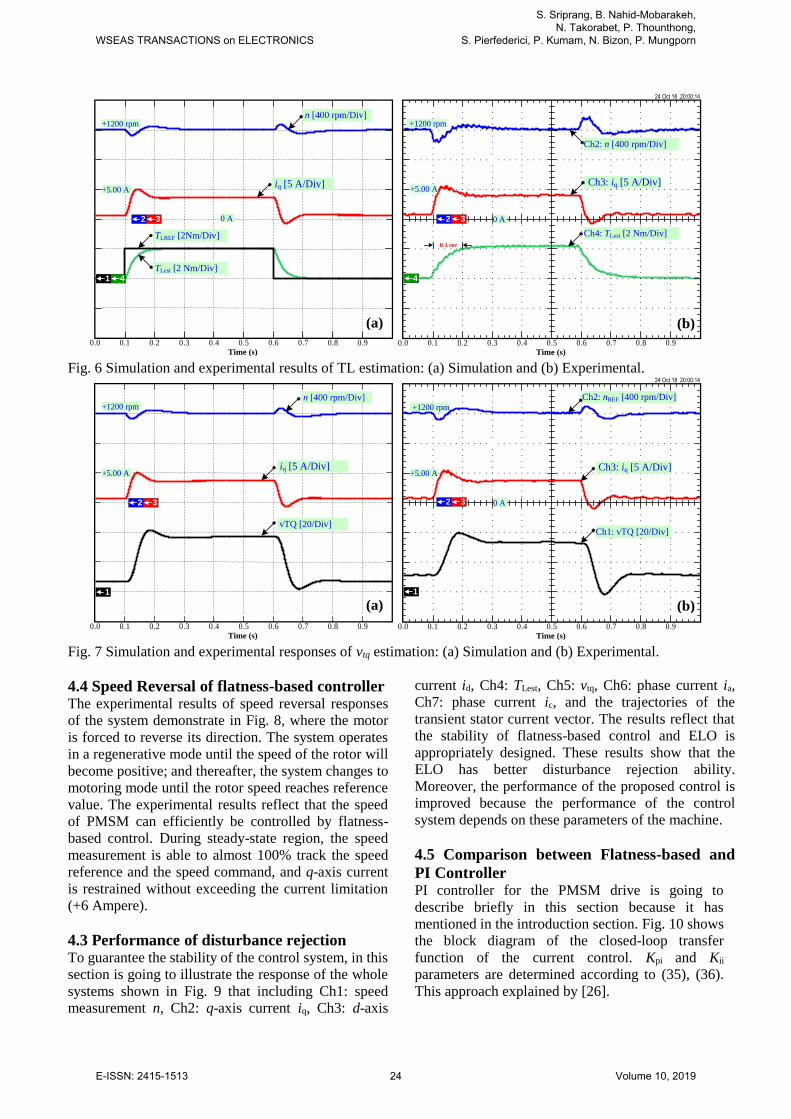
4.3 Performance of state variables estimation Fig. 6(a) and 6(b) show the simulation and
experimental results respectively of the state variable,
TL estimation. The experimental result is quite
corresponding to the simulation results. The results
reflect that when the load torque is suddenly applied
to PMSM from 0 Nm to 2 Nm, it can be correctly
estimated by ELO, and the converging time is less
than 0.1 s.
Next, Fig. 7(a) and 7(b) show the simulation and
experimental results respectively of state variable,
vtq=(Rs.iq) estimation. The experimental result is
coincident to the simulation result. In the figure
illustrates that vtq can be precisely estimated by the
proposed observer.
WSEAS TRANSACTIONS on ELECTRONICS
S. Sriprang, B. Nahid-Mobarakeh, N. Takorabet, P. Thounthong,
S. Pierfederici, P. Kumam, N. Bizon, P. Mungporn
E-ISSN: 2415-1513 23 Volume 10, 2019
0.0 0.1 0.2 0.3 0.4 0.5 0.6 0.7 0.8 0.9Time (s)
-1600
-1200
-800
-400
0
400
800
1200
1600
+5.00 A
0 A
n [400 rpm/Div]
iq [5 A/Div]
TLest [2 Nm/Div]
TLREF [2Nm/Div]
+1200 rpm
2 3
41
0.0 0.1 0.2 0.3 0.4 0.5 0.6 0.7 0.8 0.9Time (s)
-1600
-1200
-800
-400
0
400
800
1200
1600
24 Oct 18 20:00:14
+1200 rpm
+5.00 A
0 A
Ch2: n [400 rpm/Div]
Ch3: iq [5 A/Div]
Ch4: TLest [2 Nm/Div]
2 3
4
0.1 sec
Fig. 6 Simulation and experimental results of TL estimation: (a) Simulation and (b) Experimental.
0.0 0.1 0.2 0.3 0.4 0.5 0.6 0.7 0.8 0.9Time (s)
-1600
-1200
-800
-400
0
400
800
1200
1600
1
n [400 rpm/Div]
iq [5 A/Div]
vTQ [20/Div]
2 3
+5.00 A
+1200 rpm
0.0 0.1 0.2 0.3 0.4 0.5 0.6 0.7 0.8 0.9Time (s)
-1600
-1200
-800
-400
0
400
800
1200
1600
24 Oct 18 20:00:14
+1200 rpm
+5.00 A
0 A
Ch2: nREF [400 rpm/Div]
Ch3: iq [5 A/Div]
Ch1: vTQ [20/Div]
2 3
1
Fig. 7 Simulation and experimental responses of vtq estimation: (a) Simulation and (b) Experimental.
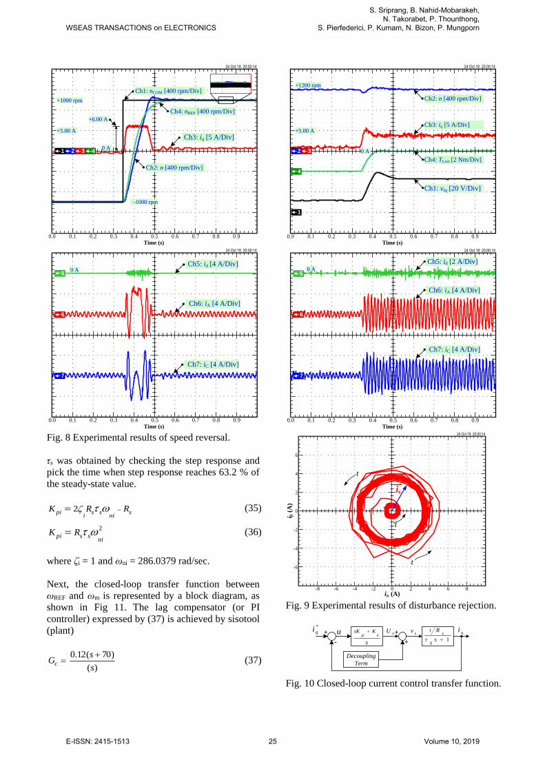
4.4 Speed Reversal of flatness-based controller The experimental results of speed reversal responses
of the system demonstrate in Fig. 8, where the motor
is forced to reverse its direction. The system operates
in a regenerative mode until the speed of the rotor will
become positive; and thereafter, the system changes to
motoring mode until the rotor speed reaches reference
value. The experimental results reflect that the speed
of PMSM can efficiently be controlled by flatness-
based control. During steady-state region, the speed
measurement is able to almost 100% track the speed
reference and the speed command, and q-axis current
is restrained without exceeding the current limitation
(+6 Ampere).
4.3 Performance of disturbance rejection To guarantee the stability of the control system, in this
section is going to illustrate the response of the whole
systems shown in Fig. 9 that including Ch1: speed
measurement n, Ch2: q-axis current iq, Ch3: d-axis
current id, Ch4: TLest, Ch5: vtq, Ch6: phase current ia,
Ch7: phase current ic, and the trajectories of the
transient stator current vector. The results reflect that
the stability of flatness-based control and ELO is
appropriately designed. These results show that the
ELO has better disturbance rejection ability.
Moreover, the performance of the proposed control is
improved because the performance of the control
system depends on these parameters of the machine.
4.5 Comparison between Flatness-based and
PI Controller PI controller for the PMSM drive is going to
describe briefly in this section because it has
mentioned in the introduction section. Fig. 10 shows
the block diagram of the closed-loop transfer
function of the current control. Kpi and Kii
parameters are determined according to (35), (36).
This approach explained by [26].
(a) (b)
(a) (b)
WSEAS TRANSACTIONS on ELECTRONICS
S. Sriprang, B. Nahid-Mobarakeh, N. Takorabet, P. Thounthong,
S. Pierfederici, P. Kumam, N. Bizon, P. Mungporn
E-ISSN: 2415-1513 24 Volume 10, 2019
24 Oct 18 20:00:14
+1000 rpm
+5.00 A
0 A
0.0 0.1 0.2 0.3 0.4 0.5 0.6 0.7 0.8 0.9Time (s)
-1600
-1200
-800
-400
0
400
800
1200
1600
Ch2: n [400 rpm/Div]
Ch4: nREF [400 rpm/Div]
Ch3: iq [5 A/Div]
2 41
Ch1: nCOM [400 rpm/Div]
3
-1000 rpm
+6.00 A
24 Oct 18 20:00:14
0 A
0.0 0.1 0.2 0.3 0.4 0.5 0.6 0.7 0.8 0.9Time (s)
-14
-10
-6
-2
2
Ch6: iA [4 A/Div]
Ch7: iC [4 A/Div]
Ch5: id [4 A/Div]
5
6
7
Fig. 8 Experimental results of speed reversal.
τs was obtained by checking the step response and
pick the time when step response reaches 63.2 % of
the steady-state value.
sni
ssi
pi RRK 2 (35)
2
nisspi RK (36)
where ζi = 1 and ωni = 286.0379 rad/sec.
Next, the closed-loop transfer function between
ωREF and ωm is represented by a block diagram, as
shown in Fig 11. The lag compensator (or PI
controller) expressed by (37) is achieved by sisotool
(plant)
)(
)70(12.0
s
sGc
(37)
0.0 0.1 0.2 0.3 0.4 0.5 0.6 0.7 0.8 0.9Time (s)
-1600
-1200
-800
-400
0
400
800
1200
1600
24 Oct 18 20:00:14
+1200 rpm
+5.00 A
0 A
Ch2: n [400 rpm/Div]
Ch1: vtq [20 V/Div]
2 3
4
1
Ch3: iq [5 A/Div]
Ch4: TLest [2 Nm/Div]
24 Oct 18 20:00:14
Ch6: iA [4 A/Div]
Ch7: iC [4 A/Div]
Ch5: id [2 A/Div]0 A
0.0 0.1 0.2 0.3 0.4 0.5 0.6 0.7 0.8 0.9Time (s)
-14
-10
-6
-2
2
5
6
7
24 Oct 18 20:00:14
i (A)
i (
A)
is
t
t
t
-8 -6 -4 -2 0 2 4 6 8
-6
-4
-2
0
2
4
6
i (
A)
Fig. 9 Experimental results of disturbance rejection.
qi+
-
u*
qi
s
iipiKsK
1
1
ss
Rs
qU +
+
Decoupling
Term
qv
Fig. 10 Closed-loop current control transfer function.
WSEAS TRANSACTIONS on ELECTRONICS
S. Sriprang, B. Nahid-Mobarakeh, N. Takorabet, P. Thounthong,
S. Pierfederici, P. Kumam, N. Bizon, P. Mungporn
E-ISSN: 2415-1513 25 Volume 10, 2019
qi+
-
u*
mcG
1)/(
1
ss
RL
*
qi
TK+ -
BJs
1eT
LT
m
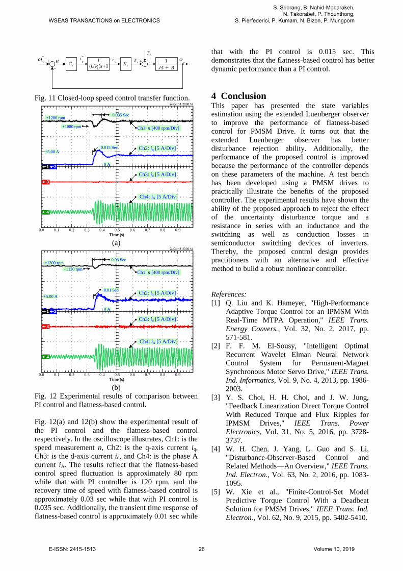
Fig. 11 Closed-loop speed control transfer function.
0.0 0.1 0.2 0.3 0.4 0.5 0.6 0.7 0.8 0.9Time (s)
-1600
-1200
-800
-400
0
400
800
1200
1600
24 Oct 18 20:00:14
+5.00 A
0 A2
4
1
3
Ch1: n [400 rpm/Div]
Ch2: iq [5 A/Div]
+1200 rpm
Ch3: id [5 A/Div]
Ch4: iA [5 A/Div]
+1080 rpm
0.035 Sec
0.015 Sec
(a)
0.0 0.1 0.2 0.3 0.4 0.5 0.6 0.7 0.8 0.9Time (s)
-1600
-1200
-800
-400
0
400
800
1200
1600
24 Oct 18 20:00:14
+5.00 A
0 A2
4
1
3
Ch1: n [400 rpm/Div]
Ch2: iq [5 A/Div]
+1200 rpm
Ch3: id [5 A/Div]
Ch4: iA [5 A/Div]
+1120 rpm
0.03 Sec
0.01 Sec
(b)
Fig. 12 Experimental results of comparison between
PI control and flatness-based control.
Fig. 12(a) and 12(b) show the experimental result of
the PI control and the flatness-based control
respectively. In the oscilloscope illustrates, Ch1: is the
speed measurement n, Ch2: is the q-axis current iq,
Ch3: is the d-axis current id, and Ch4: is the phase A
current iA. The results reflect that the flatness-based
control speed fluctuation is approximately 80 rpm
while that with PI controller is 120 rpm, and the
recovery time of speed with flatness-based control is
approximately 0.03 sec while that with PI control is
0.035 sec. Additionally, the transient time response of
flatness-based control is approximately 0.01 sec while
that with the PI control is 0.015 sec. This
demonstrates that the flatness-based control has better
dynamic performance than a PI control.
4 Conclusion This paper has presented the state variables
estimation using the extended Luenberger observer
to improve the performance of flatness-based
control for PMSM Drive. It turns out that the
extended Luenberger observer has better
disturbance rejection ability. Additionally, the
performance of the proposed control is improved
because the performance of the controller depends
on these parameters of the machine. A test bench
has been developed using a PMSM drives to
practically illustrate the benefits of the proposed
controller. The experimental results have shown the
ability of the proposed approach to reject the effect
of the uncertainty disturbance torque and a
resistance in series with an inductance and the
switching as well as conduction losses in
semiconductor switching devices of inverters.
Thereby, the proposed control design provides
practitioners with an alternative and effective
method to build a robust nonlinear controller.
References:
[1] Q. Liu and K. Hameyer, "High-Performance
Adaptive Torque Control for an IPMSM With
Real-Time MTPA Operation," IEEE Trans.
Energy Convers., Vol. 32, No. 2, 2017, pp.
571-581.
[2] F. F. M. El-Sousy, "Intelligent Optimal
Recurrent Wavelet Elman Neural Network
Control System for Permanent-Magnet
Synchronous Motor Servo Drive," IEEE Trans.
Ind. Informatics, Vol. 9, No. 4, 2013, pp. 1986-
2003.
[3] Y. S. Choi, H. H. Choi, and J. W. Jung,
"Feedback Linearization Direct Torque Control
With Reduced Torque and Flux Ripples for
IPMSM Drives," IEEE Trans. Power
Electronics, Vol. 31, No. 5, 2016, pp. 3728-
3737.
[4] W. H. Chen, J. Yang, L. Guo and S. Li,
"Disturbance-Observer-Based Control and
Related Methods—An Overview," IEEE Trans.
Ind. Electron., Vol. 63, No. 2, 2016, pp. 1083-
1095.
[5] W. Xie et al., "Finite-Control-Set Model
Predictive Torque Control With a Deadbeat
Solution for PMSM Drives," IEEE Trans. Ind.
Electron., Vol. 62, No. 9, 2015, pp. 5402-5410.
WSEAS TRANSACTIONS on ELECTRONICS
S. Sriprang, B. Nahid-Mobarakeh, N. Takorabet, P. Thounthong,
S. Pierfederici, P. Kumam, N. Bizon, P. Mungporn
E-ISSN: 2415-1513 26 Volume 10, 2019
[6] Y. C. Chang, C. H. Chen, Z. C. Zhu and Y. W.
Huang, "Speed Control of the Surface-Mounted
Permanent-Magnet Synchronous Motor Based
on Takagi–Sugeno Fuzzy Models," IEEE
Trans. Power Electron., Vol. 31, No. 9, 2016,
pp. 6504-6510.
[7] R. Cai, R. Zheng, M. Liu and M. Li, "Robust
Control of PMSM Using Geometric Model
Reduction and μ-synthesis," IEEE Trans. Ind.
Electron., Vol. PP, No. 99, 2018, pp. 1-1.
[8] H. Li, J. Wang, H. K. Lam, Q. Zhou and H. Du,
"Adaptive Sliding Mode Control for Interval
Type-2 Fuzzy Systems," IEEE Trans. Syst.,
Man, Cybern., Syst., Vol. 46, No. 12, 2016, pp.
1654-1663.
[9] P. Thounthong et al., “Model based control of
permanent magnet AC servo motor drives,” in
Proc. Electrical Machines and Systems
(ICEMS), 2016, pp. 1-6.
[10] H. Sira-Ramírez, J. Linares-Flores, C. García-
Rodríguez and M. A. Contreras-Ordaz, "On the
Control of the Permanent Magnet Synchronous
Motor: An Active Disturbance Rejection
Control Approach," IEEE Trans. Control Syst.
Technol., Vol. 22, No. 5, 2014, pp. 2056-2063.
[11] M. Yang, X. Lang, J. Long and D. Xu, "Flux
Immunity Robust Predictive Current Control
With Incremental Model and Extended State
Observer for PMSM Drive," ” IEEE Trans.
Power Electron., Vol. 32, No. 12, 2017, pp.
9267-9279.
[12] P. Pillay and R. Krishnan, "Control
characteristics and speed controller design for a
high performance permanent magnet
synchronous motor drive," IEEE Trans. Power
Electron., Vol. 5, No. 2, 1990, pp. 151-159.
[13] L. Wang, J. Jatskevich and H. W. Dommel,
"Re-examination of Synchronous Machine
Modeling Techniques for Electromagnetic
Transient Simulations," IEEE Trans. Power
Syst., Vol. 22, No. 3, 2007, pp. 1221-1230.
[14] N. Matsui, T. Makino and H. Satoh,
"Autocompensation of torque ripple of direct
drive motor by torque observer," IEEE Trans.
Ind. Appl., Vol. 29, No. 1, 1993, pp. 187-194.
[15] J. Solsona, M. I. Valla and C. Muravchik,
"Nonlinear control of a permanent magnet
synchronous motor with disturbance torque
estimation," IEEE Trans. Energy Convers.,
Vol. 15, No. 2, 2000, pp. 163-168.
[16] Y. A. R. I. Mohamed, "Design and
Implementation of a Robust Current-Control
Scheme for a PMSM Vector Drive With a
Simple Adaptive Disturbance Observer," IEEE
Trans. Ind. Electron., Vol. 54, No. 4, 2007, pp.
1981-1988.
[17] Y. Zhang, C. M. Akujuobi, W. H. Ali, C. L.
Tolliver and L. S. Shieh, "Load Disturbance
Resistance Speed Controller Design for
PMSM," IEEE Trans. Ind. Electron., Vol. 53,
No. 4, 2006, pp. 1198-1208.
[18] W. Deng, C. Xia, Y. Yan, Q. Geng and T. Shi,
"Online Multiparameter Identification of
Surface-Mounted PMSM Considering Inverter
Disturbance Voltage," IEEE Trans. Energy
Convers., Vol. 32, No. 1, 2017, pp. 202-212.
[19] S. Diao, D. Diallo, Z. Makni, C. Marchand and
J. F. Bisson, "A Differential Algebraic
Estimator for Sensorless Permanent-Magnet
Synchronous Machine Drive," IEEE Trans.
Energy Convers., Vol. 30, No. 1, 2015, pp. 82-
89.
[20] F. Tinazzi and M. Zigliotto, "Torque
Estimation in High-Efficency IPM
Synchronous Motor Drives," IEEE Trans.
Energy Convers., Vol. 30, No. 3, 2015, pp.
983-990.
[21] Y. Sangsefidi, S. Ziaeinejad, A. Mehrizi-Sani,
H. Pairodin-Nabi and A. Shoulaie, "Estimation
of Stator Resistance in Direct Torque Control
Synchronous Motor Drives," IEEE Trans.
Energy Convers., Vol. 30, No. 2, 2015, pp.
626-634.
[22] G. Wang et al., "Enhanced Position Observer
Using Second-Order Generalized Integrator for
Sensorless Interior Permanent Magnet
Synchronous Motor Drives," IEEE Trans.
Energy Convers., Vol. 29, No. 2, 2014, pp.
486-495.
[23] H. Renaudineau, J. P. Martin, B. Nahid-
Mobarakeh and S. Pierfederici, "DC–DC
Converters Dynamic Modeling With State
Observer-Based Parameter Estimation," IEEE
Trans. Power Electron., Vol. 30, No. 6, 2015,
pp. 3356-3363.
[24] Thounthong, P., S. Pierfederici, et al.,
"Analysis of Differential Flatness-Based
Control for a Fuel Cell Hybrid Power Source,"
IEEE Trans. Energy Convers., Vol. 25, No. 2,
2010, pp. 909-920.
[25] Dorf, R. C. and R. H. Bishop, Modern control
systems, 12th ed., Publishing Pearson, 2011,
pp. 847–850.
[26] Sheng-Ming Yang and Kuang-Wei Lin,
"Automatic Control Loop Tuning for
Permanent-Magnet AC Servo Motor Drives,"
IEEE Trans. ind. Electron., Vol. 63, Vo. 3,
2016, pp. 1499-1506.
WSEAS TRANSACTIONS on ELECTRONICS
S. Sriprang, B. Nahid-Mobarakeh, N. Takorabet, P. Thounthong,
S. Pierfederici, P. Kumam, N. Bizon, P. Mungporn
E-ISSN: 2415-1513 27 Volume 10, 2019