Mathematical modelling for the transmission ofdengue: symmetry and traveling wave analysis

Felipo Bacani1, Stylianos Dimas2, Igor Leite Freire2, Norberto Anibal Maidana2 and Mariano Torrisi3

1Instituto de Cincias Exatas e Aplicadas,Universidade Federal de Ouro Preto - UFOP

Rua Trinta e Seis, Loanda, 35931− 008 Joao Monlevade, MG - BrazilE-mail: fbacani@decea.ufop.br

2 Centro de Matematica, Computacao e CognicaoUniversidade Federal do ABC - UFABC

Rua Santa Adelia, 166, Bairro Bangu, 09.210− 170Santo Andre, SP - Brasil

E-mails: s.dimas@ufabc.edu.br, igor.freire@ufabc.edu.br/igor.leite.freire@gmail.com,norberto.maidana@ufabc.edu.br

3Dipartimento di Matematica e Informatica, Universita Degli Studi di Catania,Viale Andrea Doria, 6, 95125 Catania, Italia;

E-mails: torrisi@dmi.unict.it / m.torrisi12@gmail.com

Abstract

In this paper we propose some mathematical models for the transmission of dengue using asystem of reaction-diffusion equations. The mosquitoes are divided into infected, uninfected andaquatic subpopulations, while the humans, which are divided into susceptible, infected and recov-ered, are considered homogeneously distributed in space and with a constant total population. Wefind Lie point symmetries of the models and we study theirs temporal dynamics, which provides usthe regions of stability and instability, depending on the values of the basic offspring and the basicreproduction numbers. Also, we calculate the possible values of the wave speed for the mosquitoesinvasion and dengue spread and compare them with those found in the literature.

2010 AMS Mathematics Classification numbers: 34D20, 35B35, 76M60, 92Bxx

Key words: mathematical modelling, dengue, Lie symmetries, qualitative analysis, appliedmathematics

1

arX

iv:1

708.

0127

7v1

[m

ath.

AP]

3 A

ug 2

017

1 Introduction

The Aedes aegypti mosquito is a well known vector for the transmission of diseases to humanssuch as dengue and Zika, to name a few. Until 2015 these mosquitoes were mostly related to thetransmission of dengue. However, evidence suggests that after 2014 FIFA World Cup tournament,Zika virus arrived at South America, finding in Brazil an ideal habitat to grow: a tropical climate,significantly higher population density and an efficient vector for transmission: Aedes aegypti [1, 4].Zika usually causes mild symptoms in most people infected by it. In spite of everything, new datagathered since the end of 2015 from women that got infected – while they where on the last monthsof their pregnancy – supported the suspicion that Zika is related to microcephaly, a medical conditionwhere the baby’s brain does not develop properly.

To the best of our knowledge no mathematical models of Zika have been proposed or validatedso far [10]. On the contrary, things are quite different with dengue. For dengue, Aedes mosquito isthe primary vector of transmission, and therefore, the study of its dynamics is very important as itpermits the determination of the efficacy of different ways of controlling the mosquitoes populations.Furthermore, as a mosquito becomes a carrier of the virus only by biting an already infected human,the transmission can be fully understood only by taking also into account the human populations.On the other hand, for Zika, this is only one of the possible ways of transmission since it can alsobe transmitted through other ways [10]. Nevertheless, the study of dengue’s transmission may beuseful not only for its own sake, but it can also enlighten and provide insights and inspiration to themathematical understanding of Zika too.

Our paper is concerned with the mathematical modelling for transmission of dengue. In section 2we propose Malthusian models taking into account a division of human population into three groups(SIR classification): susceptible, infectious and recovered, while the mosquitoes are divided into femalewinged non-infected and infected, and aquatic sub-populations.

To have a picture of some mathematical features of the biological constitutive parameters of themodels considered we look for some point symmetries of the models in section 3. Next, in the section 4we consider the temporal dynamics of the models. This enables us to determine the equilibrium pointsof the systems and determine whether these points are stable or not. In section 5, using the invarianceunder space and time translations, we determine the wave speed for the mosquitoes’ invasion anddispersion. To determine these values we made use of the data used in [13]. Finally, discussions andconclusions are presented in section 6.

2 The models

We start by introducing the models for transmission of dengue relating humans and Aedes aegyptimosquitoes dynamics.

The human population is divided into three sub-populations: susceptible, infected and recoveredindividuals at a time t and a position x. The corresponding density functions are denoted by h(x, t),I(x, t) and r(x, t), respectively. By N(x, t) we designate the total human population, that is N(x, t) =h(x, t) + I(x, t) + r(x, t).

The mosquitoes’ population is also divided into three: winged non-infected u(x, t) and infectedw(x, t) and aquatic v(x, t). The latter population includes the eggs, larvae and pupae stages of Aedeslife cycle. The total winged mosquito population is denoted by M(x, t).

The biological parameters used in our models are presented on the Table 1.

2

Table 1: Biological parameters used for modelling.

Parameter Biological meaning

ν advection coefficient

r0 intrinsic oviposition rate

k1 carrying capacity regarding the winged mosquitoes form

k2 carrying capacity regarding the aquatic mosquitoes form

γ rate of maturation from the aquatic form of mosquitoes to winged form

µ1 mortality rate of the winged mosquito sub-population

µ2 mortality rate of the aquatic mosquito sub-population

µ3 mortality rate of human population

β1 transmission coefficient from humans to mosquitoes

β2 transmission coefficient from mosquitoes to humans

σ recovery rate from disease

D diffusion coefficient, which may depend on the winged population

2.1 Previous models

Here we recall previous models that influenced this study.

2.1.1 Aedes aegypti population models

As in the model proposed in [16], here we consider only two sub-populations: the winged form,comprised of mature female mosquitoes, and an aquatic sub-population, including eggs, larvae and pu-pae. The spatial density of the winged population is M(x, t) = u(x, t) and the aquatic sub-populationis v(x, t). The rate of maturation from the aquatic form to the winged one, denoted by γ, is saturedby the carrying capacity k1, given by γv(x, t)

(1− u(x, t)/k1

).

On the other hand, the rate of oviposition is proportional to the density of female mosquitoes,but it is also dependent on the availability of breeders, given by r0u(x, t)

(1− v(x, t)/k2

). Therefore,

considering the parameters (ν, µ1, µ2, k1, k2, r0) and the diffusion D = D(u), one has the followingmathematical model for the vital dynamics and dispersal process of mosquitoes:

ut = (D(u) ux)x︸ ︷︷ ︸diffusion

−transport︷︸︸︷ν ux + γ v

(1− u

k1

)− µ1u︸ ︷︷ ︸

birth/death

,

vt =

oviposition︷ ︸︸ ︷r0

(1− v

k2

)M −

lost eggs/eclosion︷ ︸︸ ︷(µ2 + γ)v .

(1)

Assuming that D(u) = D is a constant, under the suitable non-dimensional transformation

u =u

k1, v =

v

k2, t = t · r0, x =

x√D/r0

µ1 =µ1

r0, µ2 =

µ2

r0, γ =

γ

r0, ν =

ν√r0D

, k =k1

k2, (2)

one can transform system (1) intout = uxx − νux +

γ

kv(1− u)− µ1u,

vt = k(1− v)u− (µ2 + γ)v.

(3)

3

If one assumes nonlinear effects in the diffusion (in section 2.2 we shall revisit this point) of the typeD(u) ∼ up, it is induced a nonlinear effect on the transport. Then it may be of interest the additionof nonlinear effects in both diffusion and transport. These nonlinear effects can be considered in (3)by making the changes uxx 7→ (upux)x and νux 7→ 2νuqux, respectively, where p and q are arbitraryparameters. Additionally, if one removes the species’ self-regulation term uv in (3) and add (γ/k)u(for further details, see [8]), one removes the mosquitoes’ saturation. Thus, the following model isobtained:

ut = (upux)x − 2νuqux +γ

kv + (

γ

k− µ1)u,

vt = ku+ (k − µ2 − γ)v.

(4)

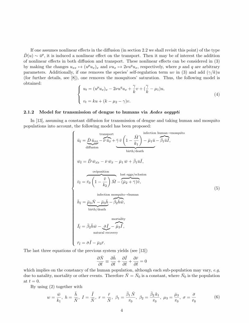
2.1.2 Model for transmission of dengue to humans via Aedes aegypti

In [13], assuming a constant diffusion for transmission of dengue and taking human and mosquitopopulations into account, the following model has been proposed:

ut = D uxx︸ ︷︷ ︸diffusion

−transport︷︸︸︷ν ux + γ v

(1− M

k1

)− µ1u︸ ︷︷ ︸

birth/death

−

infection human→mosquito︷ ︸︸ ︷β1uI,

wt = D wxx − ν wx − µ1 w + β1uI,

vt =

oviposition︷ ︸︸ ︷r0

(1− v

k2

)M −

lost eggs/eclosion︷ ︸︸ ︷(µ2 + γ)v,

ht = µ3N − µ3h︸ ︷︷ ︸birth/death

−

infection mosquito→human︷ ︸︸ ︷β2hw,

It = β2hw − σI︸︷︷︸natural recovery

−

mortality︷︸︸︷µ3I ,

rt = σI − µ3r.

(5)

The last three equations of the previous system yields (see [13])

∂N

∂t≡ ∂h

∂t+∂I

∂t+∂r

∂t= 0

which implies on the constancy of the human population, although each sub-population may vary, e.g,due to natality, mortality or other events. Therefore N = N0 is a constant, where N0 is the populationat t = 0.

By using (2) together with

w =w

k1, h =

h

N, I =

I

N, r =

r

N, β1 =

β1 N

r0, β2 =

β2 k1

r0, µ3 =

µ3

r0, σ =

σ

r0

(6)

4

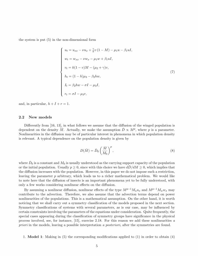
the system is put (5) in the non-dimensional form

ut = uxx − νux + γkv (1−M)− µ1u− β1uI,

wt = wxx − νwx − µ1w + β1uI,

vt = k(1− v)M − (µ2 + γ)v,

ht = (1− h)µ3 − β2hw,

It = β2hw − σI − µ3I,

rt = σI − µ3r,

(7)

and, in particular, h+ I + r = 1.

2.2 New models

Differently from [16, 13], in what follows we assume that the diffusion of the winged population isdependent on the density M . Actually, we make the assumption D ∝ Mp, where p is a parameter.Nonlinearities in the diffusion may be of particular interest in phenomena in which population densityis relevant. A typical dependence on the population density is given by

D(M) = D0

(M

M0

)p, (8)

where D0 is a constant and M0 is usually understood as the carrying support capacity of the populationor the initial population. Usually p ≥ 0, since with this choice we have dD/dM ≥ 0, which implies thatthe diffusion increases with the population. However, in this paper we do not impose such a restriction,leaving the parameter p arbitrary, which leads us to a richer mathematical problem. We would liketo note here that the diffusion of insects is an important phenomena yet to be fully understood, withonly a few works considering nonlinear effects on the diffusion.

By assuming a nonlinear diffusion, nonlinear effects of the type Mp−1Muux and Mp−1Mwwx maycontribute to the advection. Therefore, we also assume that the advection terms depend on powernonlinearities of the populations. This is a mathematical assumption. On the other hand, it is worthnoticing that we shall carry out a symmetry classification of the models proposed in the next section.Symmetry classifications of systems with several parameters, as is our case, may be influenced bycertain constraints involving the parameters of the equations under consideration. Quite frequently, thespecial cases appearing during the classification of symmetry groups have significance in the physicalprocess involved, see, for instance, [15], exercise 2.18. For this reason we add these nonlinearities apriori in the models, leaving a possible interpretation a posteriori, after the symmetries are found.

1. Model 1: Making in (5) the corresponding modifications applied to (1) in order to obtain (4)

5

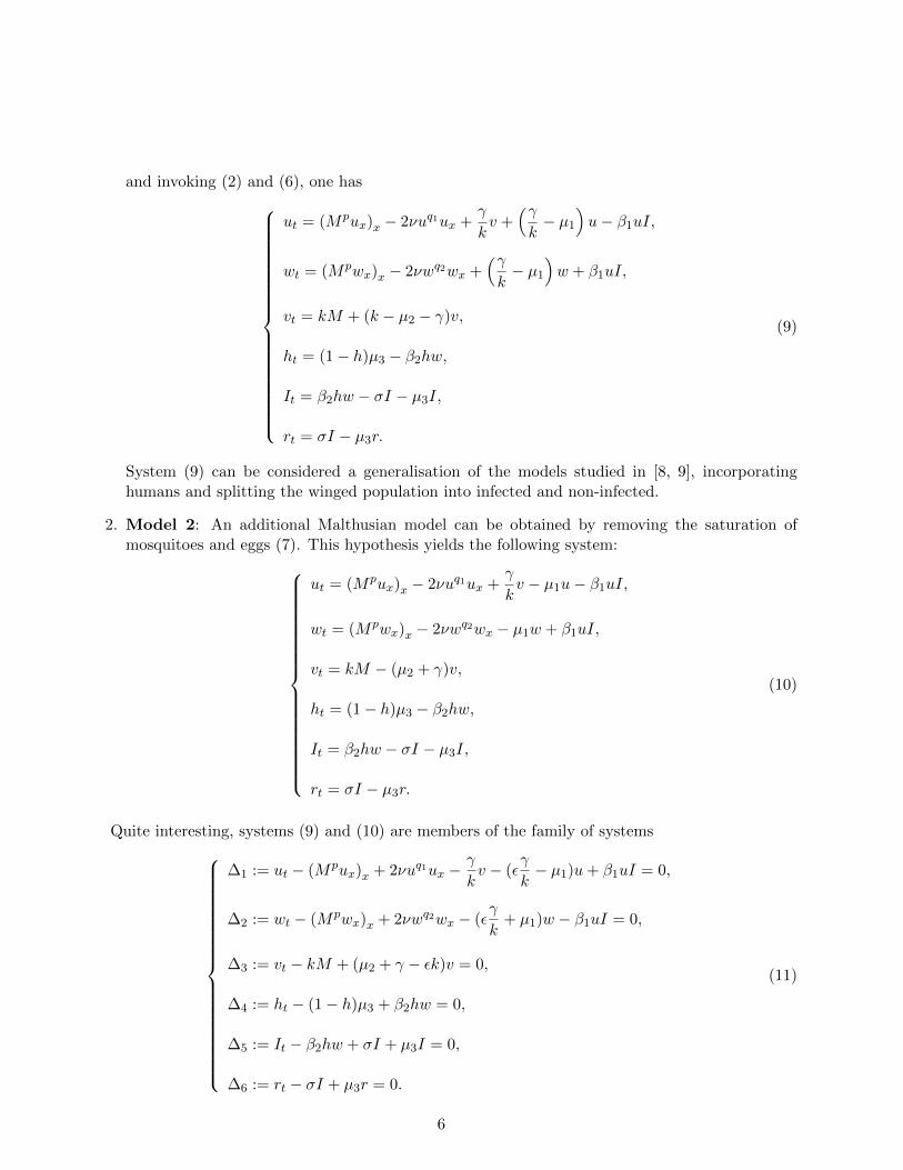
and invoking (2) and (6), one has

ut = (Mpux)x − 2νuq1ux +γ

kv +

(γk− µ1

)u− β1uI,

wt = (Mpwx)x − 2νwq2wx +(γk− µ1

)w + β1uI,

vt = kM + (k − µ2 − γ)v,

ht = (1− h)µ3 − β2hw,

It = β2hw − σI − µ3I,

rt = σI − µ3r.

(9)

System (9) can be considered a generalisation of the models studied in [8, 9], incorporatinghumans and splitting the winged population into infected and non-infected.

2. Model 2: An additional Malthusian model can be obtained by removing the saturation ofmosquitoes and eggs (7). This hypothesis yields the following system:

ut = (Mpux)x − 2νuq1ux +γ

kv − µ1u− β1uI,

wt = (Mpwx)x − 2νwq2wx − µ1w + β1uI,

vt = kM − (µ2 + γ)v,

ht = (1− h)µ3 − β2hw,

It = β2hw − σI − µ3I,

rt = σI − µ3r.

(10)

Quite interesting, systems (9) and (10) are members of the family of systems

∆1 := ut − (Mpux)x + 2νuq1ux −γ

kv − (ε

γ

k− µ1)u+ β1uI = 0,

∆2 := wt − (Mpwx)x + 2νwq2wx − (εγ

k+ µ1)w − β1uI = 0,

∆3 := vt − kM + (µ2 + γ − εk)v = 0,

∆4 := ht − (1− h)µ3 + β2hw = 0,

∆5 := It − β2hw + σI + µ3I = 0,

∆6 := rt − σI + µ3r = 0.

(11)

6

3 Lie symmetries of the system (11)

In this section we investigate point symmetries of the system (11). As already mentioned, suchanalysis in mathematical models with several parameters usually reveals those who are really impor-tant. In our case, it may enlighten our knowledge on the biological parameters and this is of interestfor mathematical studies of some system of type (11). Moreover they are useful to understand how themathematical structure of the system could be modified in order to improve the fitting of the modelwith the real phenomenon.

Although it may not have biological meaning for all values of ε, system (11) contains both systems(9) and (10) as members, and from the point of view of Lie symmetries the effort for determining theinvariance group of either (9) or (10) is the same of (11). Therefore, here, we focus our attention in(11).

We shall proceed in the following way: first we give a short overview on Lie point symmetries andthen, we find symmetries of (11).

3.1 Lie point symmetries

Definition 1. A continuous one-parameter (local) Lie group of transformations is a family G

Tε :=

x∗ = x∗(x, t, u, w, v, h, I, r, ε), t∗ = t∗(x, t, u, w, v, h, I, r, ε),u∗ = u∗(x, t, u, w, v, h, I, r, ε), w∗ = w∗(x, t, u, w, v, h, I, r, ε),v∗ = v∗(x, t, u, w, v, h, I, r, ε), h∗ = h∗(x, t, u, w, v, h, I, r, ε),I∗ = I∗(x, t, u, w, v, h, I, r, ε), r∗ = r∗(x, t, u, w, v, h, I, r, ε),

(12)

which is locally a C∞-diffeomorphism in a subset S ⊆ R2+6 with coordinates (x, t, u, w, v, h, I, r),depending analytically on the parameter ε in a neighbourhood D ⊆ R of ε = 0 and reduces to theidentity transformation when ε = 0. A Lie point symmetry for the system (11) is a transformation(12) leaving (11) invariant.

By expanding with respect to ε around 0 we get the linear form of (12)

x∗ = x+ εξ(x, t, u, w, v, h, I, r) +O(ε2), t∗ = t+ ετ(x, t, u, w, v, h, I, r) +O(ε2),

u∗ = u+ εη1(x, t, u, w, v, h, I, r) +O(ε2), w∗ = w + εη2(x, t, u, w, v, h, I, r) +O(ε2),

v∗ = v + εη3(x, t, u, w, v, h, I, r) +O(ε2), h∗ = h+ εη4(x, t, u, w, v, h, I, r) +O(ε2),

I∗ = I + εη5(x, t, u, w, v, h, I, r) +O(ε2), r∗ = r + εη6(x, t, u, w, v, h, I, r) +O(ε2),

(13)

where

ξ(x, t, u, w, v, h, I, r) :=∂x∗

∂ε|ε=0 , τ(x, t, u, w, v, h, I, r) :=

∂t∗

∂ε|ε=0 ,

η1(x, t, u, w, v, h, I, r) :=∂u∗

∂ε|ε=0 , η2(x, t, u, w, v, h, I, r) :=

∂w∗

∂ε|ε=0 ,

η3(x, t, u, w, v, h, I, r) :=∂v∗

∂ε|ε=0 , η4(x, t, u, w, v, h, I, r) :=

∂h∗

∂ε|ε=0 ,

η5(x, t, u, w, v, h, I, r) :=∂I∗

∂ε|ε=0 , η6(x, t, u, w, v, h, I, r) :=

∂r∗

∂ε|ε=0 ,

7

allows us to introduce the vector field

X = ξ(x, t, u, w, v, h, I, r)∂

∂x+ τ(x, t, u, w, v, h, I, r)

∂

∂t+ η1(x, t, u, w, v, h, I, r)

∂

∂u

+η2(x, t, u, w, v, h, I, r)∂

∂w+ η3(x, t, u, w, v, h, I, r)

∂

∂v+ η4(x, t, u, w, v, h, I, r)

∂

∂h

+η5(x, t, u, w, v, h, I, r)∂

∂I+ η6(x, t, u, w, v, h, I, r)

∂

∂r.

(14)

This operator is usually called infinitesimal generator of the transformation or infinitesimal gener-ator of the Lie point symmetry. Then, given a transformation (13), it is possible to obtain the corre-sponding generator (14). Vice-versa, given a generator of the type (14), it is possible to obtain its trans-formation using the exponential map, that is, the transformation is given by (x, t, u, w, v, h, I, r) 7→(eεXx, eεXt, eεXu, eεXw, eεXv, eεXh, eεXI, eεXr).

In order to obtain the symmetries of system (11) one should extend the operator (14) up to secondorder and then apply the invariance condition (see the well known references [3, 11, 12, 15] for furtherdetails) that reads:

X(2)∆1 = 0∣∣∣∆=0

, X(2)∆2 = 0∣∣∣∆=0

, X(1)∆3 = 0∣∣∣∆=0

,

X(1)∆4 = 0∣∣∣∆=0

, X(1)∆5 = 0∣∣∣∆=0

, X(1)∆6 = 0∣∣∣∆=0

,

(15)

where ∆ := (∆1, ∆2, ∆3, ∆4, ∆5, ∆6)T , being X(1) and X(2) the first and the second extensions ofgenerator X, respectively.

By using the symbolic package SYM for Mathematica R© deloped by SD, see [5, 6], we obtain from(15) the determining system (see again [3, 11, 12, 15] for further details). The solutions of such a systemprovide the components ξ, τ, η1, η2, η3, η4, η5, η6 of the generator (14). The Principal Lie Algebra LP ,i.e, those symmetries leaving the system invariant for all parameters, is spanned by X = ∂x, T = ∂t,which correspond to the generators of translations in space and time.

Table 2: Some symmetries of the system (11). A more complete list of symmetries of (11) is presented inthe chapter 4 of the references [2]. The biological parameters β1, β2, ν, µ3 and σ are non-negatives, while thenonlinearities p, q1 and q2 may assume any real value.

Case β1 p β2 ν q1, q2 µ3 σ Extensions with respect to LP1 ∀ 0 0 ∀ 0 ∀ ∀ X2 = u∂u + w∂w + v∂v2 ∀ ∀ 0 ∀ p/2 ∀ ∀ X3 = p x ∂x + 2 (u∂u + w∂w + v∂v)3 ∀ ∀ 0 0 ∀ ∀ ∀ X3 = p x ∂x + 2 (u∂u + w∂w + v∂v)4 0 0 6= 0 0 ∀ ∀ ∀ X4 = (u+ w)∂u + v∂v5 0 0 6= 0 0 ∀ ∀ ∀ X5 = w∂u − w∂w6 0 ∀ 0 ∀ ∀ ∀ ∀ X∞ = f∂I + g∂r (f, g) is a solution of ∆5 = 0, ∆6 = 07 0 0 0 0 ∀ ∀ ∀ X∞ = f1∂u + f2∂w + f3∂v + f4∂h + f5∂I + f6∂r, (f1, · · · , f6) is a solution of ∆ = 0

As usually occurs in empirical mathematical models, the search for solutions of the determiningsystem, or more precisely, the search for the symmetries, is quite complex as they depend on thebiological parameters β1, β2, ν, µ3, σ, jointly with values ensuring nonlinearities p, q1 and q2. A morecomplete list of symmetries of (11) would take a considerable amount of space and is decomposed inseveral cases and sub-cases, much of them without biological relevance nor meaning. Hence we opt toshow only some of them. On Table 2 we present some extensions of the Principal Lie Algebra. In thereference [2] the reader can find several pages reporting the classification of symmetries of (11).

8

3.2 A case of biological relevance

A case of biological relevance occurs when β1β2σ 6= 0, which implies that the interaction betweenmosquitoes and humans is present, as well as there are infected humans recovering from the disease.Moreover, we also consider µ3 = 0, a condition expressing the fact that no human dies, which mayoccur if a short period of time is considered. Therefore, considering a linear combination of thegenerators of the Principal Lie Algebra given by cX + T = c∂x + ∂t, from the invariant form method(see [3], page 197) we obtain the following invariants: z = x− ct and

u = Φ1(z), w = Φ2(z), v = Φ3(z), h = Φ4(z), I = Φ5(z), r = Φ6(z), (16)

where the dependence on (x, t) was omitted.

Substitution of (16) into (11) reads

−cΦ′1 = (Φ1 + Φ2)p Φ′′1 + p (Φ1 + Φ2)p−1(Φ′1 + Φ′2)Φ′1 − 2ν(Φ1)q1Φ′1 + γkΦ3

+(εγk − µ1

)Φ1 − β1Φ1Φ5,

−cΦ′2 = (Φ1 + Φ2)p Φ′′2 + p (Φ1 + Φ2)p−1(Φ′1 + Φ′2)Φ′2 − 2ν(Φ2)q2Φ′2+(εγk − µ1

)Φ2 + β1Φ1Φ5,

−cΦ′3 = k (Φ1 + Φ2) + (εk − µ2 − γ)Φ3,−cΦ′4 = −β2Φ2Φ4,−cΦ′5 = β2Φ2Φ4 − σΦ5,−cΦ′6 = σΦ5.

(17)

4 Spatial homogeneity

In what follows we make the assumption that ε = 0. This enables us to compare some of our resultswith those obtained in [16]. It will be of great importance in our analysis the following quantities: thebasic offspring number

Q0 =γ

µ1(γ + µ2)(18)

and the basic reproduction number

R0 =β1β2h

∗u∗

µ1σ. (19)

The latter depends explicitly on the densities of susceptible mosquitoes u∗ and humans h∗. If we donot choose ε = 0, Q0 might depend on this parameter, which would not allow us to proceed to acomparison with the results of [16].

4.1 Preliminaries

At this point it will be useful to recall some facts on the theory of ordinary differential equations.To begin with, let U ⊆ Rn, I ⊆ R, u : I → U and f : U → Rm be, a connected open set, an interval,a smooth function such that u(t0) = u0, where t0 ∈ I, and a vector field, respectively. Consider thesystem of ordinary differential equations with initial condition

u′(t) = f(u),

u(t0) = u0.(20)

9

If u0 is such that f(u0) = 0, then u ≡ u0 is said to be an equilibrium point of the system (20). Inparticular, it is also a solution of the system, called equilibrium solution.

A solution u of the system (20) is said to be stable if, for every ε > 0, there is a δ = δ(ε) suchthat for any other solution of (20) w for which ‖u− w‖ < δ at t = t0, satisfies the further inequality‖u− w‖ < ε for t ≥ t0. Otherwise, the solution u is said to be unstable.

If u0 is an equilibrium point of f : U → Rm, then u0 is called asymptotically stable to f if, forany ε > 0, there is δ > 0 such that, for any u ∈ U and any t > t0, φt(u) → u0, when t → t0 and‖u− u0‖ < δ implies ‖φt(u)− u0‖ < ε, where, for each t, φt(u) = φ(t, u) and φ : R× U → Rm is theflux through u, that is, ∂tφ(t, u) = f(φ(t, u)).

In what follows, f : U ⊆ Rn → Rm is a vector field, u0 ∈ U is a point, Jf (u0) is the Jacobianmatrix of f evaluated at u0. The next three propositions can be found in [7], pages 195, 198 and 49,respectively.

Proposition 1. Let u0 ∈ U be a point such that f(u0) = 0. If all eigenvalues of Jf (u0) have negativereal part, then u0 is an asymptotically stable point to f .

Proposition 2. Let u0 be an equilibrium point of f . If Jf (u0) has an eigenvalue with positive realpart, then u0 is an unstable point.

Proposition 3. If f is linear, u0 is an equilibrium point of f and all eigenvalues of Jf (u0) have realpart negative or 0, then u0 is a stable point.

4.2 Temporal dynamics

We now consider the temporal dynamics, or temporal conditons of the stability, of the system (11).This condition is necessary for the spatial condition which determine the mosquitoes invasion.

Assuming that µ3 = 0 and ux = uxx = wx = wxx = 0, system (10) becomes

du

dt=γ

kv − µ1u− β1uI,

dw

dt= −µ1w + β1uI,

dv

dt= k(u+ w)− (µ2 + γ)v,

dh

dt= −β2hw,

dI

dt= β2hw − σI,

dr

dt= σI.

(21)

The equilibrium points of the system (21) are given by w∗ = 0, I∗ = 0, r∗ = 1− h∗, 0 ≤ h∗ ≤ 1,and

u∗ =γ

kµ1v∗, v∗ =

k

γ + µ2u∗. (22)

10

Equations (22) can be equivalently rewritten as the system

A

[u∗

v∗

]=

[00

], A =

[−1 γ/(kµ1)

k/(γ + µ2) −1

]. (23)

A quick calculation shows that det(A) = 1− γ(γ+µ2)µ1

= 1−Q0.

In view of the latter equation, system (23) will have unique solution if and only if det(A) 6= 0,which is equivalent to Q0 6= 1. Provided that such a condition holds, we have the following set ofequilibrium points:

E0 = {(u∗, w∗, v∗, h∗, I∗, r∗) = (0, 0, 0, h∗, 0, 1− h∗), 0 ≤ h∗ ≤ 1}. (24)

On the other hand, if one assumes that Q0 = 1, then the system (23) loses the uniqueness ofsolutions. Consequently, the equilibrium points of (21) belong to the region

E1 =

{(u∗, w∗, v∗, h∗, I∗, r∗) =

(v∗γ

kµ1, 0, v∗, h∗, 0, 1− h∗

), 0 ≤ h∗ ≤ 1, v∗ > 0

}. (25)

Remark 1. If we had not assumed ε = 0, then the system (23) would have been

Aε

[u∗

v∗

]=

[00

], Aε =

[−1 γ

kµ1−εγk

µ2+γ−εk −1

](26)

and det(Aε) = 1− kγ(kµ1−εγ)(γ+µ2−εk) =: 1−Qε. Then the values of the basic offspring number depend

on ε and, in order to compare with the results of [16], we must take ε = 0.

4.3 Jacobian matrices and eigenvalues in the dynamics of humans and mosquitoes

Let p = (0, 0, 0, h∗, 0, 1−h∗) ∈ E0. The Jacobian matrix associated to the system (21) at p is givenby

J(p) =

−µ1 0 γ/k 0 0 00 −µ1 0 0 0 0k k −(γ + µ2) 0 0 00 −β2h

∗ 0 0 0 00 β2h

∗ 0 0 −σ 00 0 0 0 σ 0

. (27)

The eigenvalues of (27) are 0 and the roots of the polynomial

P1(λ) = λ2 + λ(γ + µ1 + µ2) + µ1(1−Q0)(γ + µ2), (28)

are

λ1,2 =1

2

[−(γ + µ1 + µ2)±

√(γ + µ1 + µ2) 2 + 4µ1(Q0 − 1) (γ + µ2)

]. (29)

On the other hand, the Jacobian matrix associated to the system (21) evaluated at a point q =(v∗γ/(kµ1), 0, v∗, h∗, 0, 1− h∗) ∈ E1 is

J(q) =

−µ1 0 γ/k 0 −γβ1v∗/kµ1 0

0 −µ1 0 0 γβ1v∗/kµ1 0

k k −(γ + µ2) 0 0 00 −β2h∗ 0 0 0 00 β2h

∗ 0 0 −σ 00 0 0 0 σ 0

, (30)

11

whose eigenvalues are 0 and, in addition, the roots of the polynomials

P2(λ) = λ2 + λ (γ + µ1 + µ2) + µ1(1−Q0) (γ + µ2) = λ(λ+ (γ + µ1 + µ2)),

P3(λ) = λ2 + λ (µ1 + σ) + µ1σ(1−R0).(31)

In P2(λ) above, we made use the fact that Q0 = 1 in the region E1.Our first results regarding the equilibrium points can now be announced.

Theorem 1. Let p ∈ E0 and Q0, where E0 and Q0 are given in (24) and (18), respectively. If Q0 > 1,then the equilibrium point p is unstable.

Proof. Let p ∈ E0 and J(p) given by (27). Assuming Q0 > 1, it follows from (29) that λ1 > 0. Thus,by Proposition 2, we have proved the theorem in question.

Theorem 2. Let Q0 = 1 and q ∈ E1 and R0, where E1 and R0 are given in (25) and (19), respectively.If R0 > 1, then the equilibrium point q is unstable.

Proof. Consider the polinomial P3(λ) given by (31). A straightforward calculation shows that

λ =1

2

[−(σ + µ1)±

√(σ + µ1)2 + 4σµ1(R0 − 1)

]> 0

under the hypothesis of the theorem. This implies that the matrix (30) has at least one eigenvaluewith positive real part and again, the result is a consequence of Proposition 2.

4.4 Analysis of the mosquitoes population

Seeing that in both equilibrium regions E0 and E1 we have I∗ = 0, which implies in the absenceof infected humans, the first three equations of (21) have a dynamics independent of that of humans.Moreover, if I = 0, then w = 0 and we shall therefore pay attention to the following subsystem of(21):

du

dt=γ

kv − µ1u,

dv

dt= ku− (µ2 + γ)v.

(32)

Proceeding as in the previous sections, we have the following set of equilibrium points (restrictingto a bidimensional space with coordinates (u, v)):

E′ = {(γv∗/(kµ1), v∗), v∗ ≥ 0}. (33)

A featured point of E′ is e0 = (0, 0), which can only be achieved provided that Q0 6= 1. Otherwise,if Q0 = 1 and e ∈ E′, then e 6= e0. In what follows, we denote by e any point of E′ different from e0.

The Jacobian associated to (32) evaluated at e0 and e ∈ E′ are, respectively, given by

J(e0) = J(e) =

[−µ1 γ/kk −(γ + µ2)

], (34)

whose characteristic polynomial and eigenvalues are, respectively,

P(λ) = λ2 + λ (γ + µ1 + µ2)− µ1(γ + µ1)(Q0 − 1), (35)

12

λ∗1,2 =1

2

[−(γ + µ1 + µ2)±

√(γ + µ1 + µ2)2 + 4µ1(γ + µ1)(Q0 − 1)

]. (36)

Now we present the main results concerning qualitative aspects of system (32). We begin with twoauxiliary lemmas.

Lemma 1. If Q0 < 1, then the real part of the roots λ∗1,2 (36) are negative.

Proof. By the Routh–Hurwitz criteria (see [14], Appendix B), the real part of the roots of the polino-mial (35) are negative if all coefficients of the polinomial are positive. Once γ, µ1 and µ2 are positive,then γ + µ1 + µ2 > 0. Since Q0 ∈ (0, 1), then µ1(γ + µ1)(1−Q0) > 0 and the results follows.

Lemma 2. If Q0 > 1, then the roots λ∗1,2 (36) are non-zero and have opposite signs.

Proof. If Q0 > 1, then√

(γ + µ1 + µ2)2 + 4µ1(γ + µ1)(Q0 − 1) > (γ + µ1 + µ2). This inequalityimplies

λ∗1 = 12

[−(γ + µ1 + µ2)−

√(γ + µ1 + µ2)2 + 4µ1(γ + µ1)(Q0 − 1)

]< −2(γ + µ1 + µ2) < 0,

λ∗2 = 12

[−(γ + µ1 + µ2) +

√(γ + µ1 + µ2)2 + 4µ1(γ + µ1)(Q0 − 1)

]> 0.

Theorem 3. The equilibrium point e0 = (0, 0) of the system (32) is asymptotically stable if Q0 < 1and unstable if Q0 > 1.

Proof. If Q0 < 1, it follows from Lemma 1 that all eigenvalues (34) have negative real part and theasymptotic stability follows from Proposition 1.

On the other hand, if Q0 > 1, by Lemma 2 we have λ∗2 > 0, which implies that (34) has aneigenvalue with positive real part. From Proposition 2, e0 is an unstable point of (32).

Theorem 4. Let e ∈ E′, where E′ is given by (33). Then e is an stable equilibrium point of thesystem (32).

Proof. If Q0 = 1, then the eigenvalues λ∗1,2 of (34) are given by λ∗1 = 0 and λ∗2 = −(γ + µ1 + µ2) < 0.Then the result follows from Proposition 3.

5 Wave speed during the spatial mosquitoes’ invasion

Here we determine the wave speed during the spatial invasion of mosquitoes, which we would liketo compare with analogous results obtained in [13]. For this reason, in addition to the hypothesisε = 0, we shall not consider nonlinearities in the diffusion as well as in the advection, that is, weconsider p = q1 = q2 = 0 in (11). It will be of great importance in our analysis the basic offspringnumber (18) and the basic reproduction rate (19). In dimensional variables, they are given by

Q0 =γ

γ + µ2× r0

µ1, R0 =

β1Nh∗

µ1× β2k1u

∗

σ. (37)

From the hypothesis on p, q1, q2 and ε, and the fact that we shall determine the wave speed duringthe mosquitoes’ invasion, it is sufficient to study system (17) with these conditions.

13

v∗

u∗

u∗ = γv∗

kµ1

Figure 1: An illustration of the stability in the bidimensional case for Q0 = 1 (Theorem 4).

5.1 Equilibrium points of system (17) with p = q1 = q2 = ε = 0

Defining auxiliary functions Ψ1(z) := Φ′1(z), Ψ2(z) := Φ2(z), system (17) can be transformed into

Φ′1 = Ψ1,

Ψ′1 = (2ν − c)Ψ1 −γ

kΦ3 + µ1Φ1 + β1Φ1Φ5,

Φ′2 = Ψ2,Ψ′2 = (2ν − c)Ψ2 + µ1Φ2 − β1Φ1Φ5

Φ′3 = −kc

(Φ1 + Φ2) +(µ2 + γ)

cΦ3,

Φ′4 =β2

cΦ2Φ4,

Φ′5 = −β2

cΦ2Φ4 +

σ

cΦ5,

Φ′6 = −σc

Φ5.

(38)

Recalling that h+ I + r = 1, the set of equilibrium points of (38) is given by

E0 = {(Φ∗1,Ψ∗1,Φ∗2,Ψ∗2,Φ∗3,Φ∗4,Φ∗5, Φ∗6) = (0, 0, 0, 0, 0, h∗, 0, 1− h∗), h∗ ∈ [0, 1]} (39)

if Q0 6= 1, and by

E1 =

{(Φ∗1,Ψ

∗1,Φ

∗2,Ψ

∗2,Φ

∗3,Φ

∗4,Φ

∗5, Φ

∗6

)=

(0,v∗γ

kµ1, 0, 0, v∗, h∗, 0, 1− h∗

), v∗ > 0, h∗ ∈ [0, 1]

}(40)

provided that Q0 = 1.The Jacobian associated to (38) at a point p ∈ E0 and a point q ∈ E1 are, respectively,

J(p) =

0 1 0 0 0 0 0 0µ1 2ν − c 0 0 −γ/k 0 0 00 0 0 1 0 0 0 00 0 µ1 2ν − c 0 0 0 0k/c 0 k/c 0 −(γ + µ2)/c 0 0 00 0 −(β2h

∗)/c 0 0 0 0 00 0 (β2h

∗)/c 0 0 0 σ/c 00 0 0 0 0 0 σ/c 0

(41)

14

and

J(q) =

0 1 0 0 0 0 0 0µ1 2ν − c 0 0 −γ/k 0 (γβ1v

∗)/kµ1 00 0 0 1 0 0 0 00 0 µ1 2ν − c 0 0 −(γβ1v

∗)/kµ1 0k/c 0 k/c 0 −(γ + µ2)/c 0 0 00 0 −β2h

∗/c 0 0 0 0 00 0 β2h

∗/c 0 0 0 σ/c 00 0 0 0 0 0 σ/c 0

. (42)

5.2 Method for determining the wave speed

Our procedure for determining the wave speed follows closely that employed in [13, 16] for deter-mining c: let J be (41) or (42). Denoting by P(λ, c) the corresponding characteristic polynomial, wedetermine the critical points of P(·, c). Since both (41) and (42) have 2 columns with all entries 0 itfollows that the characteristic polynomial can be factored into two polynomials of degree three. Inorder to assure a third order degree polynomial P(λ, c) has only real roots, one must impose that atleast one of the roots of P(λ, c) is negative and the constant c must be chosen such that P(λ, c) hasat least one positive root.

So, in order to achieve the aforementioned requirements, one should impose the following condi-tions:

P(0, c) > 0, limλ→±∞

P(λ, c) = ±∞. (43)

To assure the existence of c such that P(λ, c) has at least one positive real root, one must imposethat for a fixed c > Cmin, the following conditions holds

λ+ > 0,dP(λ, c)

dλ

∣∣∣∣λ=0

< 0, (44)

where

λ+ = max

{λ :

∂ P(λ, c)

∂λ= 0

}, Cmin = {c : P(λ+, c) = 0} . (45)

5.3 Wave speed for mosquitoes’ invasion

The eigenvalues of (41) are λ1 = λ2 = 0, λ3 = −σ/c and roots of the following polynomials:

P0(λ, c) = λ2 − λ(2ν − c)− µ1,

P1(λ, c) = λ3 + λ2

((c− 2ν) +

γ + µ2

c

)− λ

((2ν − c) (γ + µ2)

c+ µ1

)+µ1 (γ + µ2) (Q0 − 1)

c,

(46)where Q0 is given by (18).

Once the discriminant of P0(λ, c) in (46) satisfies (2ν − c)2 + 4µ1 > 0 for any values of c, ν andµ1, this implies that its roots are always real numbers.

With respect to P1(λ, c) in (46), assuming thatQ0 > 1, a condition already obtained in the previoussection in order to describe the mosquitoes’ invasion, we have P1(0, c) = [µ1 (γ + µ2) (Q0 − 1)]/c > 0for any c > 0. Moreover, we have P1(λ, c)→ ±∞ when λ→ ±∞.

15

It follows from (46) that the critical points of P1(·, c) are

λ± =1

3

−(−(2ν − c) +γ + µ2

c

)±

√(−(2ν − c) +

γ + µ2

c

)2

+ 3

((γ + µ2) (2ν − c)

c+ µ1

) ,It is reasonable to assume that the traveling wave should prevail on the wind if it is opposite to

it, that is, one should impose that 2ν − c > 0, from which we conclude that λ+ > 0 and

dP1(λ, c)

dλ

∣∣∣∣∣λ=0

= −(

(γ + µ2) (2ν − c)c

+ µ1

)< 0.

The polynomial P1 satisfies the conditions of the method employed to find out the wave speed. Hence,we use this polynomial to find the wave speed of mosquitoes’ invasion. The procedure to obtain theminimum wave speed is illustrated in Figure 2.

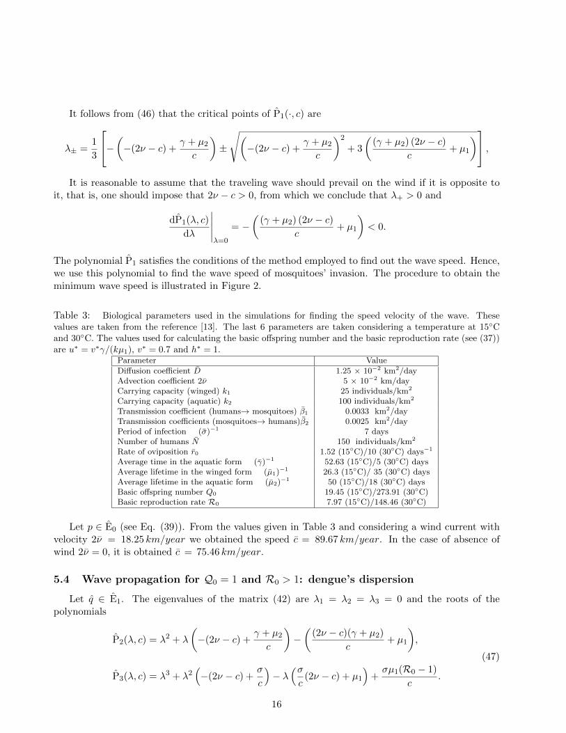
Table 3: Biological parameters used in the simulations for finding the speed velocity of the wave. Thesevalues are taken from the reference [13]. The last 6 parameters are taken considering a temperature at 15◦Cand 30◦C. The values used for calculating the basic offspring number and the basic reproduction rate (see (37))are u∗ = v∗γ/(kµ1), v∗ = 0.7 and h∗ = 1.

Parameter Value

Diffusion coefficient D 1.25 × 10−2 km2/dayAdvection coefficient 2ν 5 × 10−2 km/dayCarrying capacity (winged) k1 25 individuals/km2

Carrying capacity (aquatic) k2 100 individuals/km2

Transmission coefficient (humans→ mosquitoes) β1 0.0033 km2/dayTransmission coefficients (mosquitoes→ humans)β2 0.0025 km2/dayPeriod of infection (σ)−1 7 daysNumber of humans N 150 individuals/km2

Rate of oviposition r0 1.52 (15◦C)/10 (30◦C) days−1

Average time in the aquatic form (γ)−1 52.63 (15◦C)/5 (30◦C) daysAverage lifetime in the winged form (µ1)−1 26.3 (15◦C)/ 35 (30◦C) daysAverage lifetime in the aquatic form (µ2)−1 50 (15◦C)/18 (30◦C) daysBasic offspring number Q0 19.45 (15◦C)/273.91 (30◦C)Basic reproduction rate R0 7.97 (15◦C)/148.46 (30◦C)

Let p ∈ E0 (see Eq. (39)). From the values given in Table 3 and considering a wind current withvelocity 2ν = 18.25 km/year we obtained the speed c = 89.67 km/year. In the case of absence ofwind 2ν = 0, it is obtained c = 75.46 km/year.

5.4 Wave propagation for Q0 = 1 and R0 > 1: dengue’s dispersion

Let q ∈ E1. The eigenvalues of the matrix (42) are λ1 = λ2 = λ3 = 0 and the roots of thepolynomials

P2(λ, c) = λ2 + λ

(−(2ν − c) +

γ + µ2

c

)−(

(2ν − c)(γ + µ2)

c+ µ1

),

P3(λ, c) = λ3 + λ2(−(2ν − c) +

σ

c

)− λ

(σc

(2ν − c) + µ1

)+σµ1(R0 − 1)

c.

(47)

16

λ

P

1(λ, c)

λ+

c < Cmin

c = Cmin

c > Cmin

Figure 2: The figure shows the result of the procedure above for obtaining the minimum wave speed for thewave. Using the values of Table 3 it was found the non-dimensional value Cmin = 0.69 for the polynomialP1(λ, c) given in (46), corresponding to an equilibrium point p ∈ E0 (39).

Proceeding as in the last subsection, we intend to determine restrictions on the biological parametersinvolved in (37) in order to have Q0 = 1 and R0 > 1.

Taking (37) into account and since u∗ = v∗γ/(kµ1), we have

R0 =β1Nh

∗

µ1× β2

σ× v∗γ

µ1. (48)

According to Table 3, the lowest possible value to Q0 is achieved at 15◦C. Even for this choice,maintained the values of the biological parameters, Q0 is significantly greater than 1. A natural wayfor decreasing Q0 without affecting the basic reproduction rates (48) would be increasing the value ofµ2. Then, considering the values of γ−1, µ−1

1 and r0 given on Table 3 and imposing that Q0 = 1, onefinds

µ2 = 0.74. (49)

Fixing v∗ = 0.7 and h∗ = 1, if ν = 0 we would obtain c = 24.08 km/year, while if 2ν =18.25 km/year, we would get c = 38.72 km/year.

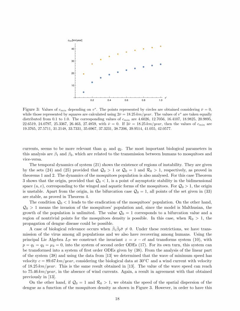
Figure 3 shows the distribution of velocities cmin as a function of v∗. We can observe an increasingof the wave speed when the densities of mosquitoes population increases.

6 Discussion and Conclusion

In this paper we derived two Malthusian models for analysing the transmission of dengue betweenhumans and mosquitoes. These models can be viewed as members of the system (11), and some Liesymmetries are listed on Table 2.

Our results on symmetry analysis show that the transmission coefficients from human to mosquitoesβ1 and mosquitoes to humans β2 and the wind current 2ν, are quite relevant in the manifestation ofsymmetries other than the translations.

With respect to the power nonlinearities, the most dominant from the point of view of symmetriesis p. The powers q1 and q2 are relatively important while ν, that is related to the existence of wind

17

●

●

●

●●

●●

●●

●

■

■

■

■■

■■

■■

■

0.2 0.4 0.6 0.8 1.0v*

10

20

30

40

cmin[km/year]

Figure 3: Values of cmin depending on v∗. The points represented by circles are obtained considering ν = 0,while those represented by squares are calculated using 2ν = 18.25 km/year. The values of v∗ are taken equallydistributed from 0.1 to 1.0. The corresponding values of cmin are 4.6026, 12.7056, 16.4107, 18.9825, 20.9895,22.6519, 24.0797, 25.3367, 26.463, 27.4859, with ν = 0. If 2ν = 18.25 km/year, then the values of cmin are19.3765, 27.5711, 31.2148, 33.7331, 35.6967, 37.3231, 38.7206, 39.9514, 41.055, 42.0577.

currents, seems to be more relevant than q1 and q2. The most important biological parameters inthis analysis are β1 and β2, which are related to the transmission between humans to mosquitoes andvice-versa.

The temporal dynamics of system (21) shows the existence of regions of instability. They are givenby the sets (24) and (25) provided that Q0 > 1 or Q0 = 1 and R0 > 1, respectively, as proved intheorems 1 and 2. The dynamics of the mosquitoes population is also analysed. For this case Theorem3 shows that the origin, provided that Q0 < 1, is a point of asymptotic stability in the bidimensionalspace (u, v), corresponding to the winged and aquatic forms of the mosquitoes. For Q0 > 1, the originis unstable. Apart from the origin, in the bifurcation case Q0 = 1, all points of the set given in (33)are stable, as proved in Theorem 4.

The condition Q0 < 1 leads to the eradication of the mosquitoes’ population. On the other hand,Q0 > 1 means the invasion of the mosquitoes’ population and, since the model is Malthusian, thegrowth of the population is unlimited. The value Q0 = 1 corresponds to a bifurcation value and aregion of nontrivial points for the mosquitoes density is possible. In this case, when R0 > 1, thepropagation of dengue disease could be possible.

A case of biological relevance occurs when β1β2σ 6= 0. Under these restrictions, we have trans-mission of the virus among all populations and we also have recovering among humans. Using theprincipal Lie Algebra LP we construct the invariant z = x − ct and transforms system (10), withp = q1 = q2 = µ3 = 0, into the system of second order ODEs (17). For its own turn, this system canbe transformed into a system of first order ODEs given by (38). From the analysis of the linear partof the system (38) and using the data from [13] we determined that the wave of minimum speed hasvelocity c = 89.67 km/year, considering the biological data at 30◦C and a wind current with velocityof 18.25 km/year. This is the same result obtained in [13]. The value of the wave speed can reachto 75.46 km/year, in the absence of wind currents. Again, a result in agreement with that obtainedpreviously in [13].

On the other hand, if Q0 = 1 and R0 > 1, we obtain the speed of the spatial dispersion of thedengue as a function of the mosquitoes density as shown in Figure 3. However, in order to have this

18

situation we should have a mortality rate given by (49), which seems to be unrealistic. Biologicallyspeaking, the situation Q0 = 1 would correspond to a high mosquitoes mortality. From mathematicalviewpoint, condition Q0 = 1 implies bifurcation points, which brings changes in the stability of thesystem (38) and hence, hardly describes a real situation.

Acknowledgements

The authors are grateful to FAPESP, grant n 2014/05024-8, for financial support. F. Bacani isthankful to CNPq, grant n 141081/2014-7, for the scholarship provided. I. L. Freire is grateful toCNPq for the grant n 308941/2013-6. M. Torrisi has been supported by Gruppo Nazionale per laFisica Matematica of Instituto Nazionale di Alta Matematica (Italy)

References

[1] J-W Ai, Y. Zhang and W. Zhang, Zika virus outbreak: ‘a perfect storm’, Emerging Microbes andInfections, (2016), DOI: 10.1038/emi.2016.42.

[2] F. Bacani, Tratamento de modelos para a dinamica populacional do Aedes aegypti via simetriasde Lie, PhD thesis in Applied Mathematics, State University of Campinas, (2016) – in Portuguese.

[3] G. W. Bluman and S. Kumei, Symmetries and Differential Equations, Applied MathematicalSciences 81, Springer, New York, (1989).

[4] D. Butler, Zika and birth defects: what we know and what we don?t, Nature News, (2016), avail-able at http://www.nature.com/news/zika-and-birth-defects-what-we-know-and-what-we-don-t-1.19596. Access made on June 15th 2016.

[5] S. Dimas, D. Tsoubelis, SYM: A new symmetry-finding package for Mathematica, in: Proceedingsof the 10th International Conference in Modern Group Analysis, Larnaca, Cyprus, 24–30 October2004, 2004, pp. 64–70.

[6] S. Dimas, D. Tsoubelis, A new heuristic algorithm for solving overdetermined systems of PDEs inMathematica, in: 6th International Conference on Symmetry in Nonlinear Mathematical Physics,Kiev, Ukraine, 20–26 June 2005, 2005.

[7] C. I. Doering and A. O. Lopes, Equacoes diferenciais ordinarias, IMPA, (2010) – in Portuguese.

[8] I. L. Freire and M. Torrisi, Symmetry methods in mathematical modeling Aedes aegypti dispersaldynamics, Nonlin. Anal. RWA, vol. 14, 1300–1307, (2013).

[9] I. L. Freire and M. Torrisi, Similarity solutions for systems arising from an Aedes aegypti model,Commun. Nonlin. Sci. Numer. Simul., vol. 19, 872–879, (2014).

[10] C. R. Howard, Aedes mosquitoes and Zika virus infection: an A to Z of emergence, EmergingMicrobes and Infections, (2016), DOI:10.1038/emi.2016.37.

[11] N. H. Ibragimov, CRC Handbook of Lie group analysis of differential equations, vol. 1, CRCPress, (1994).

19

[12] N. H. Ibragimov, Elementary Lie Group Analysis and Ordinary Differential Equations, JohnWiley and Sons, Chirchester (1999).

[13] N. A. Maidana and H. M. Yang, Describing the geographic spread of dengue disease by travelingwaves, Math. Biosci., vol. 215, 64–77, (2008).

[14] J. D. Murray, Mathematical biology, Springer, 3th edition, (2002).

[15] P. J. Olver, Applications of Lie groups to differential equations, Springer-Verlag, 1st, edition,(1986).

[16] L. T. Takahashi, N. A. Maidana, W. C. Ferreira Jr., P. Pulino and H. M. Yang, Mathematicalmodels for the Aedes aegypti dispersal dynamics: traveling waves by wind and wind, Bull. Math.Biol., vol. 67, 509–528, (2005).

20