1

Martian cloud climatology and life cycle extracted from Mars Express

OMEGA spectral images

André Szantai*, Joachim Audouard+, Francois Forget*, Kevin S. Olsen+, Brigitte Gondetx, Ehouarn

Millour*, Jean-Baptiste Madeleine*, Alizée Pottier+*, Yves Langevinx, Jean-Pierre Bibring

x

* Laboratoire de Météorologie Dynamique/IPSL, Sorbonne Université, École Normale supérieure / PSL Research

University, École polytechnique, CNRS, Paris, France.

+ Laboratoire Atmosphères, Milieux, Observations spatiales, (CNRS/UVSQ/IPSL), Guyancourt, France x Institut d'Astrophysique Spatiale, (CNRS, Université Paris 11), Orsay, France.

Corresponding author: André Szantai: szantai@lmd.polytechnique.fr

Keywords : Mars climate, Mars atmosphere, clouds, Mars Express, OMEGA.

Abstract

A Martian water-ice cloud climatology has been extracted from OMEGA data covering 7 Martian years (MY 26-

32). We derived two products, the Reversed Ice Cloud Index (ICIR) and the Percentage of Cloudy Pixels (PCP),

indicating the mean cloud thickness and nebulosity over a regular grid (1° longitude × 1° latitude × 1° Ls × 1 h

Local Time) adapted for comparisons with data from high-resolution Martian Global Climate Models (GCMs).

The ICIR has been shown to be a proxy of the water-ice column.

The PCP confirms the existence and location of the main cloud structures mapped with the ICIR, but also gives a

more accurate image of the cloud cover. We observed a denser cloud coverage over Hellas Planitia, the Lunae

Planum region and over large volcanoes (Tharsis volcanoes, Olympus and Elysium Montes) in the aphelion belt.

For the first time, thanks to the fact that Mars Express is not in Sun-synchronous orbit, we can explore the clouds

diurnal cycle at a given season by combining the seven years of observations. However, because of the excentric

orbit, the temporal coverage remains limited. To study the diurnal cloud life cycle, we averaged the data over

larger regions: from specific topographic features (covering a few degrees in longitude and latitude) up to large

climatic bands (covering all longitudes). We found that in the tropics (25°S – 25°N) around northern summer

solstice, the diurnal thermal tide modulates the abundance of clouds, which is reduced around noon (Local

Time). At northern midlatitudes (35°N – 55°N), clouds corresponding to the edge of the north polar hood are

2

observed mainly in the morning and around noon during northern winter (Ls = 260° – 30°). Over Chryse

Planitia, low lying morning fogs dissipate earlier and earlier in the afternoon during northern winter. Over

Argyre, clouds are present over all daytime during two periods, around Ls = 30° and 160°.

1. Introduction

Understanding the water cycle of current and past Martian climate and weather remains an objective of planetary

climate research. The major components of the Martian water cycle are water vapor, water-ice clouds and

surface water deposits, which include the perennial polar caps, frost deposition and sublimation, and near

subsurface processes (diffusion, adsorption, desorption, condensation and sublimation in the pores of the soil).

This study focuses on the life cycle of water-ice clouds, and, more specifically, on their diurnal cycle. It is based

on an extensive use of data from the OMEGA imaging spectrometer onboard Mars Express, from which only a

small subset has been used for cloud studies previously (Langevin et al., 2007 ; Madeleine et al., 2012). Mars

Express has been in operation around Mars over the second longest period after Mars Odyssey, starting in 2004

and is still operational in 2019.

White spots near the limb of the planet have been observed with terrestrial telescopes since the 19th century and

were suspected to be clouds. Based on telescopic observations of clouds between 1924 and 1971, Smith and

Smith (1972) identified the main features of the seasonal cloud life cycle, in particular over major volcanoes

(Olympus Mons, Elysium Mons) and the Hellas basin.

On images from the Mariner 6 and 7 spacecrafts, which made a short flyby, some features could be identified as

water-ice clouds (Peale, 1973). The nature of water-ice clouds was unambiguously confirmed with the

spectrometer onboard Mariner 9, the first Martian artificial satellite (Curran et al., 1973).

Mariner 9, the Viking 1 and 2 orbiters and their successors have observed cloud features of various types and at

different scales, and enabled their description. These include clouds associated to major volcanoes (in the Tharsis

area, and Elysium Mons), low-level fogs and hazes (in particular in Valles Marineris), the polar hoods (clouds

above the polar caps and at their edges during the corresponding fall, winter and spring seasons) and the aphelion

belt (a large cloudy area that forms during the northern spring and summer, mainly in the tropics,) (French et al.,

1981 ; Kahn, 1984) .

3

Abundant observations from various instruments onboard Mars Global Surveyor (MGS), Mars Odyssey (ODY)

and Mars Reconnaissance Orbiter (MRO) spacecrafts combined with the reprocessing of older satellite data from

Vikings and Mariner-9 led to a precise characterization of the location of clouds and their annual cycle in the

2000s (Wang and Ingersoll, 2002 ; Tamppari et al., 2003 ; Liu et al., 2003 ; Smith, 2004).

However, unlike Mars Express, put into orbit in December 2003, MGS, ODY and MRO were placed on

heliosynchronous orbits. As a consequence, they always cover the (non-polar) surface of Mars at the same

Martian local time, approximately 2-3 h and 13-15 h local time (LT). Therefore, they are not suited for the

characterization of the diurnal lifecycle of clouds. In this paper, we present the complete climatology of clouds

as observed by the OMEGA (Observatoire pour la Minéralogie, l’Eau les Glaces et l’Activité) imaging

spectrometer onboard Mars Express. The major objective is the determination of the lifecycle of Martian water-

ice clouds. The presence and thickness of the ice clouds is estimated in each pixel of the spectral image by

measuring the difference in reflectance between two wavelengths located on one edge of the 3.1 µm water ice

absorption band. This indicator is then binned onto a regular grid in longitude, latitude, solar longitude (Ls) and

local time to provide a mean cloud index covering one Martian day and one Martian year, to be used as reference

climatology. In each bin it is completed by an estimation of the percentage of cloudy pixels, related to the cloud

cover.

In Section 2 of this article we describe the OMEGA original data and the method for the derivation of spectral

image-based and gridded indicators characteristic of water-ice clouds, and also some of their limitations.

The construction of a representative yearly cloud climatology, using data covering several consecutive Martian

years (MY 26 to 32), is based on the assumption that the current climate does not change much from one year to

another. Previous observations, mainly from satellites, have shown its validity (Smith, 2004, 2009 ; Hale et al.

2011). A major limitation to this assumption is the occurrence of global dust storms (GDSs), which take place

every few Martian years. A GDS occurred during the northern winter of MY 28. It had a significant impact on

surface and tropospheric temperatures, atmospheric dust content, integrated water vapor and clouds.

In the following section we analyze the two OMEGA-derived water-ice cloud indicators, the reversed ice cloud

index and the percentage of cloudy pixels. We compare this ice cloud index to two other climatological datasets,

the integrated water ice optical thickness derived from the Thermal Emission Spectrometer (TES) onboard MGS

(Smith, 2004) and model predictions of the water-ice column retrieved from the Martian Climate Database

4

(MCD) (Millour et al., 2018) derived from the Martian Global Climate Model (MGCM) of the LMD (Forget et

al., 1999 ; Navarro et al., 2014).

In Section 4, we determine the daily cloud life cycle over a series of selected geographical areas. Selected daily

cloud life cycles are interpreted in the context of Martian atmospheric physics and dynamics with the help of the

LMD MGCM.

The resulting 4D OMEGA-derived cloud products are formatted into an accessible database. In conclusion, a

possible application is the comparison with the coming generation of high-resolution general circulation models

in order to investigate small-scale processes.

2. Data and Methodology

2.1 Original OMEGA data

The OMEGA instrument provides spectral image cubes along an orbit at wavelengths between 0.38 and 5.1 µm.

In practice, several 2D images of variable width (powers of 2 pixels, from 16 to 128 pixels) are taken along a

part of an orbit ; a spectrum at 352 wavelengths in 3 channels, the visible (VIS: 0.38 - 1.05 µm ), the “C” (1.0 -

2.77 µm ) and “L” (2.65 - 5.1 µm ) near-infrared channels is extracted for each pixel. The technical

characteristics and the performance of the instrument was described by Bibring et al. (2004) in an ESA special

publication.

Detection of water ice is based on the identification of corresponding absorption lines in the spectrum. Langevin

et al. (2007) first applied this principle for the detection of water ice in the south polar region by calculating the

depth of a water ice absorption band near 1.5 µm. However, the water ice absorption band at 3.1 µm was found

to be better adapted to the detection of water-ice clouds (Langevin et al. 2007), especially in the tropics and at

mid-latitudes. In a study using a small number of OMEGA spectral images, Madeleine et al. (2012) detected and

identified 4 types of water-ice clouds: morning hazes, topographically controlled hazes, cumulus clouds and

thick hazes.

The objective of the present study is to detect and characterize water-ice clouds from all available OMEGA

spectral images, i.e. covering almost 6 Martian years (14/01/2004 – 27/04/2014: from MY 26, Ls=333.1° to MY

32, Ls=122.4°) and to build a daily and yearly cloud climatology mapped on a regular spatio-temporal grid.

Since this last date, the OMEGA instrument has been activated only along a very small number of orbits, and the

quality of the resulting data was insufficient to be included in this study.

5

2.2 Definition of the ice cloud index

The original ice cloud index ICI (Langevin et al. 2007, Madeleine et al. 2012) is representative of the slope on

the edge of the 3.1 µm water ice absorption band. It is defined by the following relation:

ICI = R3.38

/ R3.52

(1)

with R3.38

and R3.52

: reflectances at 3.38 and 3.52 µm respectively.

This simple definition has been preferred to indexes based on a difference of radiances or on a relation involving

another continuum reflectance on the other side of the water ice absorption band (close to 3.0 µm), because of

other possible absorption of atmospheric or surface components. This definition was used in previous and

current studies using OMEGA data (Langevin et al., 2007 ; Madeleine et al., 2012 ; Audouard et al., 2014b,

Olsen et al., 2019).

In the current study we prefer to use the reversed ice cloud index ICIR:

ICIR = 1 – ICI (2)

which enables an easier identification of clouds (the more clouds / the denser / the thicker the clouds, the higher

the ICIR).

In a first step, an ice cloud index value is calculated for each pixel of orbits with all types of scans (nadir, along-

track, across-track and inert/ limb scan). Pixels considered as inconsistent are removed from further processing

when:

- their incidence and emergence value (w.r.t. the Mars surface ellipsoid) are too high (incidence >= 85° or

emergence >= 50°) ;

- they are in the first and last lines of an image ;

- their signal/noise ratio is too low (SNR < 20) or infinite ;

- they belong to portions of identified orbit files of width of 128 pixels with corrupted values ;

- their ICIR is too low (ICIR < -1) or infinite.

Complementary selection tests include:

- the removal of orbit files with a large spacecraft distance from the reference surface of the planet (distance >

7000 km) ;

- the removal of all orbit files during the MY 28 global dust storm (orbits 4436 to 4739 ; Ls = 261.9 - 312°), in

order to build the standard cloud climatology (Wang and Richardson, 2013 ; Montabone et al., 2015).

6

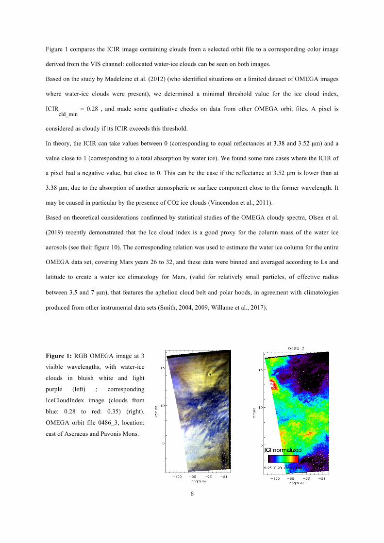
Figure 1 compares the ICIR image containing clouds from a selected orbit file to a corresponding color image

derived from the VIS channel: collocated water-ice clouds can be seen on both images.

Based on the study by Madeleine et al. (2012) (who identified situations on a limited dataset of OMEGA images

where water-ice clouds were present), we determined a minimal threshold value for the ice cloud index,

ICIRcld_min

= 0.28 , and made some qualitative checks on data from other OMEGA orbit files. A pixel is

considered as cloudy if its ICIR exceeds this threshold.

In theory, the ICIR can take values between 0 (corresponding to equal reflectances at 3.38 and 3.52 µm) and a

value close to 1 (corresponding to a total absorption by water ice). We found some rare cases where the ICIR of

a pixel had a negative value, but close to 0. This can be the case if the reflectance at 3.52 µm is lower than at

3.38 µm, due to the absorption of another atmospheric or surface component close to the former wavelength. It

may be caused in particular by the presence of CO2 ice clouds (Vincendon et al., 2011).

Based on theoretical considerations confirmed by statistical studies of the OMEGA cloudy spectra, Olsen et al.

(2019) recently demonstrated that the Ice cloud index is a good proxy for the column mass of the water ice

aerosols (see their figure 10). The corresponding relation was used to estimate the water ice column for the entire

OMEGA data set, covering Mars years 26 to 32, and these data were binned and averaged according to Ls and

latitude to create a water ice climatology for Mars, (valid for relatively small particles, of effective radius

between 3.5 and 7 µm), that features the aphelion cloud belt and polar hoods, in agreement with climatologies

produced from other instrumental data sets (Smith, 2004, 2009, Willame et al., 2017).

Figure 1: RGB OMEGA image at 3

visible wavelengths, with water-ice

clouds in bluish white and light

purple (left) ; corresponding

IceCloudIndex image (clouds from

blue: 0.28 to red: 0.35) (right).

OMEGA orbit file 0486_3, location:

east of Ascraeus and Pavonis Mons.

7

2.3 Generation of the 4D ice cloud index database

In order to build a daily and yearly cloud climatology, a 4D cloud database is defined with the following grid

characteristics:

Longitude ΔLON = 1° ; latitude ΔLAT = 1° ; solar longitude ΔLs = 5° ; local time ΔLT = 1 h.

These values are of the same order of magnitude as current high-resolution global climate models (e.g. Pottier et

al., 2017), and allow relatively short computation times for the generation of the 4D database.

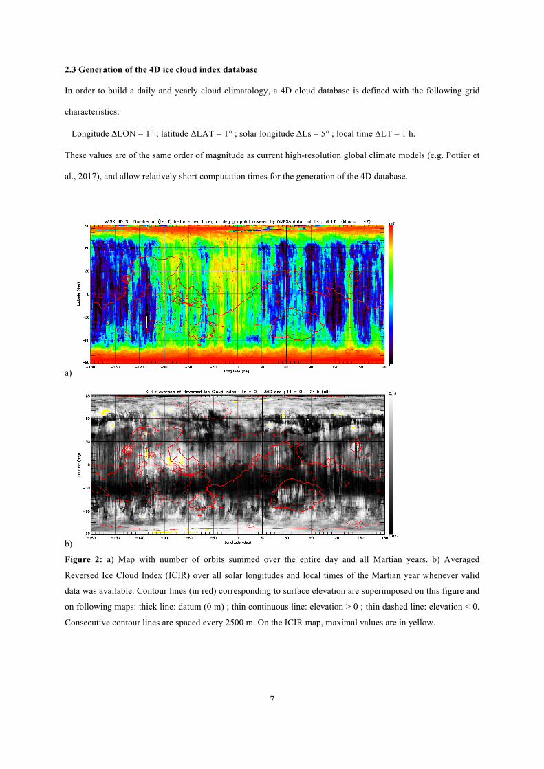
a)

b)

Figure 2: a) Map with number of orbits summed over the entire day and all Martian years. b) Averaged

Reversed Ice Cloud Index (ICIR) over all solar longitudes and local times of the Martian year whenever valid

data was available. Contour lines (in red) corresponding to surface elevation are superimposed on this figure and

on following maps: thick line: datum (0 m) ; thin continuous line: elevation > 0 ; thin dashed line: elevation < 0.

Consecutive contour lines are spaced every 2500 m. On the ICIR map, maximal values are in yellow.

8

All the quality-controlled pixels are then binned onto this 4D grid, i.e., they are counted and their ICIR averaged

at each gridpoint. Figure 2 shows maps of the number of orbits per square degree used for the ICIR calculation,

and the temporally averaged values of the ice cloud index. At this stage, one may note the good spatial coverage

over the planet and also identify large cloud structures: the aphelion belt and the polar cloud belts / polar hood

edges. Note also that some regions are more often covered by the satellite : the polar regions and the northern

latitudes between 100°W and 15°E, around Chryse Planitia.

2.4 Definition and calculation of the percentage of cloudy pixels

For each 4-dimensional gridpoint, we define the percentage of cloudy pixels PCP with the following relation:

PCP = 100 x Ncloudy

/ Nall

(3)

with Nall, Ncloudy: number of pixels of any type (cloudy or non-cloudy), respectively of cloudy type.

The percentage of cloudy pixels is an indicator of the cloud coverage of a gridpoint to illustrate the kilometer

scale nebulosity and cloud fraction resulting from the effect of gravity waves and convection. It can be useful for

comparison or use in general circulation models aiming at taking into account this subgrid scale nebulosity

(Pottier et al. 2015). The map on Figure 3 shows the value of the PCP for each 1° x 1° gridpoint averaged over

the day and the Martian year whenever data was available. Not surprisingly, the areas representing the cloud

cover (Fig. 3) are basically the same as those covered by the ICIR (on Fig. 2).

Figure 3: map of the average percentage of cloudy pixels (PCP) over the Martian day and year.

2.5 Uncertainty estimation of the Ice Cloud Index

9

The error bar on the ICIR is also calculated for each 4D gridpoint, or bin. It is the quadratic sum of the

uncertainty related to the measure by the OMEGA instrument for N observations (pixels) used for the gridpoint

and the 3-standard deviation of the ICIR values of the N observations (σICIR). It is given by the following

formula (derived from Audouard et al., 2014a):

δICIR_bin =1N

ΔICIRi2

i=1

N∑( )+σ ICIR_bin

2#

$%&

'(

12

(4)

The first standard deviation term reflects the impact of the uncertainties on the ICIR related to the original

measurements, i.e. the reflectance values at 3.38 µm and 3.52 µm used to calculate the ICIR. They include in

particular the instrumental noise on OMEGA spectels. The second term reflects the variability of the ICIR pixel

values used to calculate the average (reversed) ice cloud index value on the 4D grid. The impact of this

uncertainty term will be illustrated in Section 3.2.

2.6 General results about the 4D databases

The overall coverage of the 4D grid by OMEGA data is small: 1.06% (i.e. about 2% of the possible daytime

gridoints). With such a limited coverage, it is difficult to find spatial gridpoints having a long series of daily

ICIR profiles at a fixed Ls (Table 1), or yearly profiles at a fixed local time.

Climatic(zone Daily(number Number(of(longest Latitude Solar(longitude Longitude

(N(or(S) of(observations daily(ICI(series (degrees) Ls((degrees) (degrees)

Polar 95°

(65°(B(90°) 100°

MidBlatitude 46°(B(41°S 80° 30°W

(25°(B(65°) 46°(B(49°N 280° 136°E

Tropical 25°(B((18°S 55° 78°W

(0°(B(25°) 10°(B(11°N 80° 21°W

17°(B(22°N 150° 21°W

14(h 6 86°(B(89°N

5(h 10

4(h 16

Table 1: longest series of daily ICIR observations (4D gridpoints) in different climatic zones

10

Table 1 shows that OMEGA observations cover at best 4 h a day in the tropics (33% of daytime), and 14 h a day

in the polar region (58% of the duration of the Martian day, during the midnight sun period). Similarly, ICIR

annual profile series are short: at a specific local time they cover at best 17 Ls instants among 72 in the polar

regions (23.6% of the Martian year) and 6 Ls instants in the tropics (8.3%).

This limited daily and annual data coverage for a single gridpoint led us to define larger spatial regions over

which ICIR and PCP values are integrated and averaged. Based on a visual identification of the cloudy regions at

various periods of the Martian year, we could define large regions of interest of different type and extension,

delimited by their longitude and latitude, with a name corresponding to the main topographic (or climatic)

feature. The characteristics of the selected Region Of Interest (ROI) are listed in Table 2.

These regions of interest, where water-ice clouds have been observed, are the following:

- large climatic zones:

* tropical (25° S - 25° N). In the tropics, the aphelion belt is the dominant large scale cloud structure during

northern spring and summer.

* mid-latitudes (25° N – 55° N ; 55° S – 25° S). The poleward part of midlatitude areas undergo an annual

cycle related to the advance and retreat of the polar hoods (Tamppari et al., 2008, Benson et al., 2010 ; Benson et

al., 2011). The equatorward part is impacted by the aphelion belt around the northern summer solstice period.

* polar regions (65° N – 89° N ; 65° S – 89° S). These regions are covered over more than half of the Martian

year by a polar hood, which has its largest extension around the winter solstice. However this period also

corresponds largely to nighttime at those latitudes and thus these regions are not observable except on the

equatorward edge of the polar hood.

- large impact craters: Hellas, Argyre ;

- around individual volcanoes: Olympus Mons, Elysium Mons, Arsia Mons, and groups of volcanoes: Tharsis

volcanoes (Ascraeus, Pavonis and Arsia Mons). Clouds are abundant over major volcanoes mainly during

northern spring and summer. Clouds are also present in lesser amount over Arsia Mons around northern winter

solstice (Benson et al., 2003 ; Benson et al., 2006).

- regions in the northern hemisphere where water ice or clouds have been observed or could be present: Lunae

Planum, South-East Tharsis, Valles Marineris (Benson et al., 2003), Tempe Terra, Syrtis Major

11

- a region in the southern hemisphere where clouds have been observed: the cloud bridge zone, connecting the

aphelion belt with the cloud belt around the South Pole or the edge of the south polar hood.

   Name  of  the  region Latitude Longitude Correlation Percentage  of     of  interest (degrees) (degrees  E) ICIR  vs.  MCD  WIC Cloudy  pixels         Ls=[60-­‐120°] Ls=[60-­‐120°] 1 Olympus  Mons 10  N    ;    30  N -­‐145  ;  -­‐125 0,736 58 2 Alba  Patera 30  N    ;    50  N -­‐125  ;  -­‐105 0,666 21 3 Arsia  Mons -­‐15  S  ;        0  N -­‐130  ;  -­‐115 0,814 78 4 Elysium  Mons 15  N    ;    35  N 135  ;    155 0,747 54 5 Tharsis  Montes -­‐15  S  ;    20  N -­‐125  ;  -­‐100 0,471 75 6 Tharsis  South-­‐East -­‐20  S  ;    10  N -­‐105  ;    -­‐80 0,707 75 7 Tempe  Terra 30  N    ;    50  N -­‐90    ;    -­‐55 0,713 8 8 Chryse  Planitia 20  N    ;    50  N -­‐60    ;    -­‐30 0,625 22 9 Lunae  Planum 0  N      ;    25  N -­‐70    ;    -­‐40 0,325 80 10 Arabia  Terra  West 10  N    ;    40  N -­‐35    ;      10 0,608 21 11 Syrtis  Major 0  N      ;    35  N 55    ;      80 0,355 50 12 Valles  Marineris  2 -­‐15  S  ;    -­‐5  S -­‐90    ;    -­‐45 0,422 65 13 SH  Cloud  bridge -­‐35  S  ;  -­‐20  S -­‐150  ;    -­‐60 0,549 18 14 Tyrrhena  Terra -­‐10  S  ;      0  N 70      ;      85 0,525 57 15 Argyre  Planitia -­‐55  S  ;  -­‐35  S -­‐65    ;    -­‐25 0,305 53 16 Hellas  Planitia -­‐55  S  ;  -­‐25  S 40      ;  105 0,838 70 17 Tropics  25S  –  25N -­‐25  S  ;  25  N -­‐180  ;    180 0,601 44 18 Midlatitudes  25N  –  55N 25  N    ;    55  N -­‐180  ;    180 0,489 5 19 Midlatitudes  25S  –  55S -­‐55  S  ;  -­‐25  S -­‐180  ;    180 0,732 24 20 N  Polar  65N  –  89N 65  N    ;    89  N -­‐180  ;    180 -­‐0,056 26 21 S  Polar  65S  –  89S  -­‐89  S  ;  -­‐65  S -­‐180  ;    180 X X

Table 2: characteristics of the regions of interest. Correlation between the OMEGA ICIR and the WaterIceCol

from the MCD (values above 0.6 are in bold), and percentage of cloudy 4D gridpoints (i.e. that have an ICIR

above the threshold value of 0.28) around the Northern summer solstice period.

These selected spatial regions of interest will be used in Section 4 to determine the diurnal cloud life cycle.

3. Seasonal ICIR and PCP maps

3.1 Seasonal mapping of water-ice clouds

Geographical maps of clouds can be derived from 4D ICIR and PCP datasets by averaging data over time, i.e.

over selected periods of the Martian day and year. Figure 4 shows examples of ICIR and PCP maps centered on

the solstices (Ls = 90 and 270°) and averaged over 90 degrees of solar longitude.

The aphelion belt, including large volcanoes (Olympus and Elysium Mons, the Tharsis volcanoes and Alba

Patera) and Arabia Terra, Hellas Planitia, the north polar hood edge and the southern polar cloud belt stand out

12

as major cloudy areas around the northern summer solstice (Fig. 4a). No other outstanding cloud feature is

present in between, i.e. in the tropics and mid-latitudes (below 35° N) during the period around the northern

winter solstice (Fig. 4b). In comparison to the ICIR figures, the PCP Figures 4c and 4d filter out smaller and less

prominent cloud structures while retaining only the main ones.

Note that the same major cloud features are present on the overall map of the ICIR covering the whole day and

the whole year (Fig. 2b), but appear with less contrast. The contours of cloudy areas on such maps are impacted

by the limited number, or absence, of OMEGA orbits covering the Martian surface. The main effect is vertical

striping in the tropical and mid-latitude areas. In some cases, diagonal stripes due to unusual (non-nadir) pointing

modes or peculiar orbits may also be present.

a)

b)

(continued on next page)

13

c)

d)

Figure 4: average ICIR around Ls = 90° (a: top) and 270° (b) ; average PCP around Ls = 90° (c) and 270° (d:

bottom).

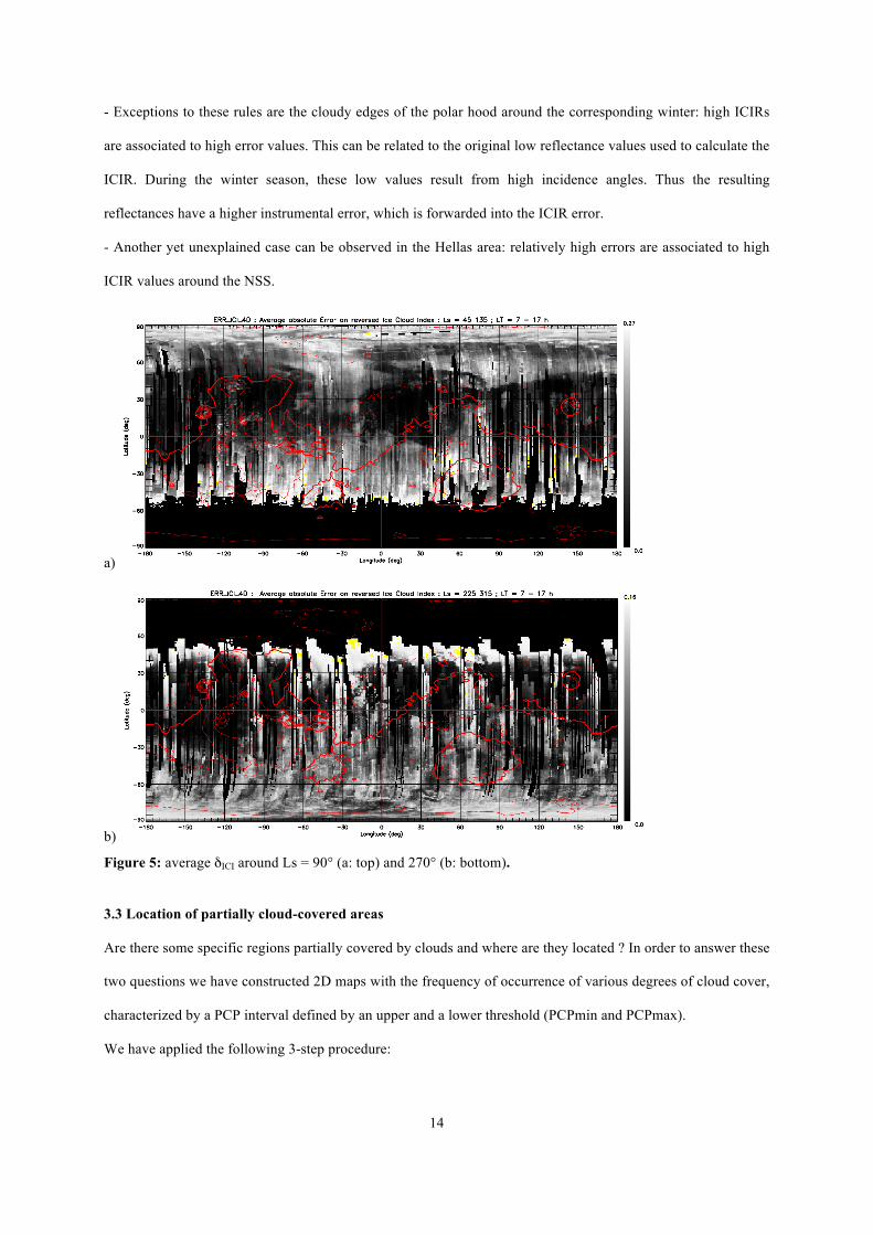
3.2 Uncertainty estimation of ICIR data

As mentioned in Section 2.5, we also calculated δICI, the related uncertainty on the ICIR variable, on the same

4D grid. Figure 5a and 5b represent δICI values averaged around the solstice periods (northern summer: Ls = 45 –

135°, labeled NSS ; southern summer: Ls = 225 – 315°, labeled SSS) and during daytime (LT = 7 – 17 h). These

figures can be compared visually to the corresponding ICIR fields (Fig. 4a and 4b).

From the visual comparison with these figure pairs, we can note the following relations:

- The higher the ICIR values, the lower their error. This is clearly visible specifically for the aphelion belt around

the NSS.

- Conversely, the lower the ICIR values, the higher their error. This can be observed in particular at southern

latitudes (around 30° S), and in the northern plains where areas around 60° N have low reflectances (around the

NSS).

14

- Exceptions to these rules are the cloudy edges of the polar hood around the corresponding winter: high ICIRs

are associated to high error values. This can be related to the original low reflectance values used to calculate the

ICIR. During the winter season, these low values result from high incidence angles. Thus the resulting

reflectances have a higher instrumental error, which is forwarded into the ICIR error.

- Another yet unexplained case can be observed in the Hellas area: relatively high errors are associated to high

ICIR values around the NSS.

a)

b)

Figure 5: average δICI around Ls = 90° (a: top) and 270° (b: bottom).

3.3 Location of partially cloud-covered areas

Are there some specific regions partially covered by clouds and where are they located ? In order to answer these

two questions we have constructed 2D maps with the frequency of occurrence of various degrees of cloud cover,

characterized by a PCP interval defined by an upper and a lower threshold (PCPmin and PCPmax).

We have applied the following 3-step procedure:

15

1) For each 5° Ls bin, we define:

* 1< PCP =< 5%: very small cloud cover

* 5 < PCP =< 50%: (not too small) minority of clouds

* 50 < PCP =< 95%: (not too large) majority of clouds

* 95 < PCP =< 100%: (almost) total cloud cover.

* 1 < PCP =< 100%: presence of clouds in any amount (extremely low values of PCP, below 1%, are not taken

into account).

2) For each 2D (spatial) location, we count the number of (temporal) occurrence of the corresponding PCP

values between the upper and lower bounds, i.e. the number of gridpoints: NGP(PCPmin

, PCPmax

).

3) The frequency of occurrence is the ratio between the number of occurrences observed over a specific PCP

interval and the total number of cloudy occurrences. It can be expressed as a percentage by the following

formula:

foccurrence(PCPmin,PCPmax) = 100 . NGP(PCPmin,PCPmax) / NGP(1%, 100%) (5)

The maps of Fig. 6a to 6d represent 4 levels of cloud coverage expressed by the frequency of occurrence,

observed around the NSS and during daytime (LT = 7 – 17 h).

The highest cloudiness, with a PCP close to 100%, can be observed over a limited number of regions (Fig. 6d),

namely:

- the aphelion belt over the Tharsis rise (150°W – 40°W), including the Tharsis volcanoes, Olympus Mons and

Alba Patera,

- Elysium Mons,

- Arabia Terra and Syrtis Major,

- the Hellas basin.

Along two latitudinal bands, around 55°N and 30°S (with Hellas excluded), only reduced partial cloud coverage

(PCP < 50%) can be observed, or no cloud at all.

In the regions covered by the North polar cloud cover, by the edge of the South polar hood, and by a large part of

the aphelion belt, all densities of cloud coverage can be observed (from 1% to 100%). Only two regions have a

peculiar configuration:

16

- the Hellas basin, completely covered by clouds (Fig. 6d), is surrounded by a thin ring of partial cloud cover

(Fig. 6a-c),

- an area on the eastern part of the Tharsis rise and the western part of Lunae Planum (around 10°N, 75°W)

where partial cloud cover is absent and which is visible as a dark hole on figures 6a-c. In this area, we found

only a complete cloud cover (PCP > 95%).

A similar comparison (not shown) has been conducted around the southern summer solstice period (Ls = 225 –

315°). Only two large, cloudy areas can be observed, the reduced southern polar hood (70°S – 90°S) and the

southern edge of the northern polar hood (35°N – 60°N). Cloud coverage frequencies of all types, with a PCP

between 5% and 100% are located over the same parts of these cloudy areas. Cases of PCP between 1% and 5%

are also present over the same areas but are less frequent.

a)

b)

(continued on next page)

17

c)

d)

Figure 6: frequency of occurrence of 4 types of cloud cover during Ls = 45° - 135° and daytime (LT = 7 – 17h).

(a) Very small (1% < PCP =< 5%) ; (b) minority of clouds (5% < PCP =< 50%) ; (c) majority of clouds (50% <

PCP =< 95%) ; (d) total cloud cover (PCP > 95%). Maximal values are in yellow.

4. Comparison of ICIR data with TES observations and MCD model predictions

4.1 Comparison of ICIR data with TES optical thickness mapped climatology

In order to validate the ICIR as a climatological product, we compared it to the water ice optical depth derived

from TES data. The water ice optical depth ( τTES_wice) is one of the products of the TES mapped climatology

(Smith, 2004). TES-derived data have been remapped for each Martian year (from MY 24 to 27) onto a regular

grid: longitude ΔLON = 7.5° ; latitude ΔLAT = 3° and solar longitude ΔLs = 5°. We selected data from the

hybrid year MY 24 (the beginning of MY 24 is missing and is replaced by the beginning of MY 25 ; a major

dust storm - not taken into account - occurred during the last third of MY 25), around 14h LT for latitudes < 80°

and at nadir.

18

For this comparison, the original ICIR data was reprocessed and adapted to the TES mapped climatology grid,

with a specific selection of 4D gridpoints at 14 h LT corresponding approximately to the observation time of

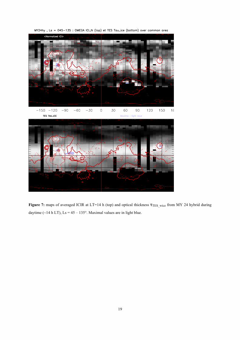
TES, and a limitation below 75° latitude. Fig. 7 shows that the high, averaged ICIR values are collocated with

high τTES_wice around the northern summer solstice period. Some differences can be observed at high northern

latitudes and on the northern edge of the Hellas Basin, where ICIR values are high, whereas τTES_wice values are

relatively low. The ICIR 2D map has a noisier aspect than the τTES_wice map. A possible explanation of the

reduced cloudiness at higher latitudes could be the biased estimation of the optical depth obtained from very low

TES-derived temperature values.

2D histograms of ICIR and τTES_wice (Fig.8) show a linear trend and possibly indicate a physical relation

between both variables, with an intermediate correlation value (0.53) for the complete TES dataset (limited to

78° in latitude), but much higher values for known cloudy areas and periods (0.83 for the aphelion belt) (Fig 8b).

19

Figure 7: maps of averaged ICIR at LT=14 h (top) and optical thickness τTES_wice from MY 24 hybrid during

daytime (~14 h LT), Ls = 45 – 135°. Maximal values are in light blue.

20

Figure 8: 2D histograms of ICIR vs τTES_wice for all latitudes below 78° and all seasons (left), and in the

tropics (-27° < lat < 27°) during Northern summer (Ls = 45 – 135°) (right) at the TES climatological resolution

(ΔLON = 7.5° ; ΔLAT = 3°)

4.2 Comparison with water-ice column and integrated optical thickness from the Mars Climate Database

The Mars Climate Database version 5.3 (Millour et al., 2018) is a database of meteorological fields computed

using runs of the LMD Global Climate Model (GCM) of the Martian atmosphere (see Forget et al. (1999), for

general settings, Navarro et al. (2014) for details on modeling the water cycle, and Pottier et al. (2017) and

references therein for a detailed description of the latest version).

A key aspect of the GCM is that it uses a prescribed dust scenario (i.e. imposed columnar dust opacity at all

locations and time). In practice, such forcings are implemented after analysis of a variety of dust observations

from MY 24 to MY 31 (Montabone et al., 2015), or using a climatological dust scenario derived from theses

observations (Millour et al. 2018). The MCD thus provides fields calculated using various dust scenarios. For the

comparisons presented in this paper, we used the MCD (version 5.3) climatological scenario, corresponding to

21

our best guess of a typical Mars year, i.e., a Mars year without any global planet encircling dust storm. We first

chose the water-ice column variable for the comparison with the OMEGA Ice Cloud Index.

The water-ice column (WaterIceCol) from the MCD is extracted on the same 4D grid (1° longitude x 1° latitude

x 5° Ls x 1 h LT) as the ICIR and PCP, and is compared to these OMEGA-derived variables. In a first stage, we

averaged the water-ice column over the same daily and yearly time period in order to compare 2D daytime and

seasonal maps.

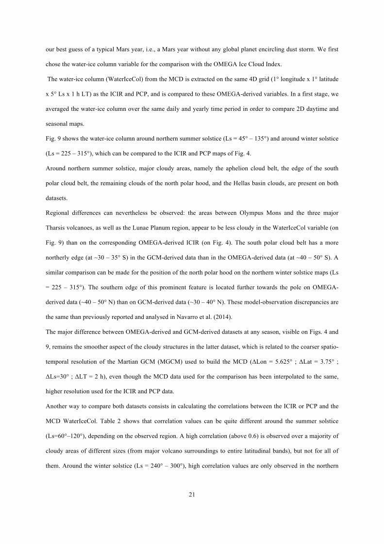
Fig. 9 shows the water-ice column around northern summer solstice (Ls = 45° – 135°) and around winter solstice

(Ls = 225 – 315°), which can be compared to the ICIR and PCP maps of Fig. 4.

Around northern summer solstice, major cloudy areas, namely the aphelion cloud belt, the edge of the south

polar cloud belt, the remaining clouds of the north polar hood, and the Hellas basin clouds, are present on both

datasets.

Regional differences can nevertheless be observed: the areas between Olympus Mons and the three major

Tharsis volcanoes, as well as the Lunae Planum region, appear to be less cloudy in the WaterIceCol variable (on

Fig. 9) than on the corresponding OMEGA-derived ICIR (on Fig. 4). The south polar cloud belt has a more

northerly edge (at ~30 – 35° S) in the GCM-derived data than in the OMEGA-derived data (at ~40 – 50° S). A

similar comparison can be made for the position of the north polar hood on the northern winter solstice maps (Ls

= 225 – 315°). The southern edge of this prominent feature is located further towards the pole on OMEGA-

derived data (~40 – 50° N) than on GCM-derived data (~30 – 40° N). These model-observation discrepancies are

the same than previously reported and analysed in Navarro et al. (2014).

The major difference between OMEGA-derived and GCM-derived datasets at any season, visible on Figs. 4 and

9, remains the smoother aspect of the cloudy structures in the latter dataset, which is related to the coarser spatio-

temporal resolution of the Martian GCM (MGCM) used to build the MCD (ΔLon = 5.625° ; ΔLat = 3.75° ;

ΔLs=30° ; ΔLT = 2 h), even though the MCD data used for the comparison has been interpolated to the same,

higher resolution used for the ICIR and PCP data.

Another way to compare both datasets consists in calculating the correlations between the ICIR or PCP and the

MCD WaterIceCol. Table 2 shows that correlation values can be quite different around the summer solstice

(Ls=60°–120°), depending on the observed region. A high correlation (above 0.6) is observed over a majority of

cloudy areas of different sizes (from major volcano surroundings to entire latitudinal bands), but not for all of

them. Around the winter solstice (Ls = 240° – 300°), high correlation values are only observed in the northern

22

hemisphere, mainly in areas covered by the edge of the north polar hood. In areas with less than 10% cloud

cover (i.e. in the tropics and midlatitudes of the southern hemisphere), correlation values are very low (below

0.4).

The ICIR and WaterIceCol are physically related to the presence of water ice particles, therefore high correlation

values are expected and generally observed when clouds are present. Low correlation values are observed when

no, or very few, clouds are present (especially during northern winter), and the ICIR may not be very significant.

It can also indicate that the WaterIceCol variable does not reproduce observed cloudiness correctly, possibly in

relation with lower spatio-temporal resolution of the underlying GCM used to build the MCD. This could be in

particular the case over the Lunae Planum, Syrtis Major and Argyre areas around the northern summer solstice.

a)

b)

Figure 9: maps of average MCD water-ice column (WaterIceCol) a) between Ls = 45° and 135°, and b) between

Ls = 225° and 315°, both during daytime (7 – 17 h LT).

5. The cloud Seasonal and Diurnal cycle at global scale and over selected regions

23

The temporal evolution of several geographical regions listed in Table 2 is described in this section. After a

description of the global seasonal cycle, we focus on the regions where there is sufficient data to describe the

cloud life cycle at least during a part of the Martian year.

5.1 The seasonal cycle of morning, noon and afternoon clouds

The cloud seasonal cycle along a Martian year is traditionally represented by a 2D diagram as a function of solar

longitude (Ls) and latitude, after averaging over all longitudes and time of a Martian day, whenever data is

available. Such diagrams were extracted from TES data (τTES_wice) (Smith, 2004), from SPICAM data (τwice)

(Willame et al., 2017) and from MGCM data (τwice and WaterIceCol) (Montmessin et al., 2004 ; Navarro et al.

2014, Pottier et al., 2017). These diagrams show the main cloud structures at planetary scales, e.g. the aphelion

belt during northern spring and summer, the north polar hood during extended autumn and winter, and the south

polar hood during reduced southern autumn and winter. We extracted the same type of figures covering a limited

period of daytime (4 Martian hours). Figure 10 shows the ICIR in the morning (6 – 10 h LT), around local noon

(10 – 14 h LT) and in the afternoon (14 – 18 h LT). The three main cloud structures are also present here. But

although OMEGA data does not cover the southern hemisphere in the morning during northern summer (Ls = 80

– 170°), a major difference is outstanding between morning and afternoon hours on one side, and the period

around noon: the ICIR values are lower, indicating a reduced cloud coverage in the aphelion belt region.

24

a)

b)

c)

Figure 10: reversed ice cloud index (ICIR) averaged over all longitudes and over 4-hour periods. a) 6 – 10 h LT,

b) 10 – 14 h LT, c) 14 – 18 h LT.

5.2 Clouds over the tropical plains.

Here we limit the region of interest to latitudes between 25°S and 25°N, and longitude between 90°W and

120°E, i.e. located between the major volcanoes of the Tharsis bulge and Elysium Mons. Figures 11a shows the

observed ICIR variable, 11b the MCD-predicted WaterIceCol shown over all gridpoints. One can see that:

- A few clouds are present in the morning after Ls ~ 30°.

25

- Around summer solstice (Ls = 50°-150°), the cloudiness is reduced at 12 h, before increasing again in the

afternoon.

- Between Ls = 200° and 270°, there are less and less clouds, and the clouds dissipate earlier and earlier in

the afternoon. The seasonal behavior is well known (it can be explained by the increase in atmospheric

temperature, due to growing dust loading and decreasing distance to the Sun). However the diurnal cycle seem

different in the observations and in the model.

Figure 11c shows the percentage of cloud cover in the same coordinates. It is extensive during the largest part of

the northern spring and summer (Ls = 30 – 150°). This corresponds mainly to the aphelion cloud belt. Maximal

PCP values of 100% are obtained during this period, corresponding to complete dense cloud coverage of at least

a part of the area.

26

a)

b)

c)

Figure 11: diurnal cycle of the Ice Cloud Index (a: top), MCD Water-ice column at all instants (b: middle) and

Percentage of Cloudy Pixels (c: bottom) over the tropical zone (25°S – 25°N ; 90° W – 120° E) during one

Martian year. Light gray corresponds to missing values. Dark gray for c) corresponds to a PCP equal to 0 %.

With the help of complementary data from the MCD and the LMD MGCM, the evolution of the clouds and the

minimal cloudiness can be explained by the propagation of the diurnal thermal tide which induces a temperature

anomaly that controls the condensation/sublimation of the cloud ice (Fig. 12).

Almost similar results are obtained when all the longitudes, also covering the Tharsis area and the large

volcanoes, are taken into account in the average calculation of the ICIR. This indicates that there is no major

longitudinal effect on average cloudiness between the 90°W – 120°E zone “between major volcanoes”, and the

complementary longitudinal band, which covers in particular cloudy areas around Elysium Mons and major

volcanoes of the Tharsis ridge including Olympus Mons, as shown on Figure 4a.

27

Figure 12: MGCM diurnal cloud ice density in the tropics at the beginning of summer (Ls = 90° - 120°).

5.3 Northern midlatitudes (35° N – 55° N ; all longitudes):

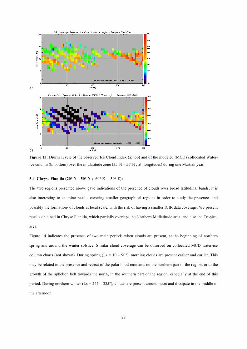
In this midlatitude band, clouds are present at the end of autumn and during winter (Ls = 250 – 360°) (Fig 13a ;

see also Fig. 4b). Observed clouds (after Ls = 310°) are mainly present in the morning and around noon. The

cloudiness decreases at the end of the afternoon. Lower ICIR values are found at the beginning of northern

spring (Ls = 0 – 50°), mainly in the morning. Similar trends can be observed on the MCD water-ice column map,

but with fewer clouds during spring and summer in the afternoon (Ls = 45 – 150°) (Fig. 13b). The observed

clouds must correspond to the northern polar hood, present during winter, with remnants retreating towards the

pole at the beginning of spring.

28

a)

b)

Figure 13: Diurnal cycle of the observed Ice Cloud Index (a: top) and of the modeled (MCD) collocated Water-

ice column (b: bottom) over the midlatitude zone (35°N – 55°N ; all longitudes) during one Martian year.

5.4 Chryse Planitia (20° N – 50° N ; -60° E – -30° E):

The two regions presented above gave indications of the presence of clouds over broad latitudinal bands; it is

also interesting to examine results covering smaller geographical regions in order to study the presence -and

possibly the formation- of clouds at local scale, with the risk of having a smaller ICIR data coverage. We present

results obtained in Chryse Planitia, which partially overlaps the Northern Midlatitude area, and also the Tropical

area.

Figure 14 indicates the presence of two main periods when clouds are present, at the beginning of northern

spring and around the winter solstice. Similar cloud coverage can be observed on collocated MCD water-ice

column charts (not shown). During spring (Ls = 10 – 90°), morning clouds are present earlier and earlier. This

may be related to the presence and retreat of the polar hood remnants on the northern part of the region, or to the

growth of the aphelion belt towards the north, in the southern part of the region, especially at the end of this

period. During northern winter (Ls = 245 – 335°), clouds are present around noon and dissipate in the middle of

the afternoon.

29

This time the MGCM suggests that the clouds are low-lying fogs (Fig. 15a). As on Earth they form near the

surface during the night as the surface cools and are maximal in the morning. They only dissipate a little in the

afternoon when the surface heated by the sun is warm enough to heat the atmosphere. This is why the fog

thickness is minimum in the afternoon. Above 30 km, the MGCM predicts the formation of a cloud that is very

thin and should be invisible to OMEGA. Nevertheless it provides an example of high cloud controlled by

thermal tides but with a maximum of condensation during the day and dissipation during the night (Fig. 15b).

Figure 14: diurnal cycle of the Ice Cloud Index over the Chryse Planitia region (20°N – 50°N ; -60°E – -30°E )

during one Martian year.

a)

b)

Figure 15: MCD Global Climate Model predictions - winter fog in Chryse region (Ls = 270° – 300°): mean

water ice content (kg/kg) (a: top). Temperature diurnal anomaly (K) (b: bottom). The time at which fog

dissipates (~16 h LT) is indicated by the arrow.

30

5.5 Argyre (55° S – 35° S ; -65° E – -25° E):

On Fig. 16, two major periods of significant cloudiness can be observed during the southern winter, around Ls =

45° and 135°. Between these periods, around winter solstice (Ls = 90°), cloudiness is reduced. The water vapor

inflow from the north polar region tends to be reduced by the important cloud formation in the aphelion belt

which limits the southward transport of water vapor. During both cloud peaks, clouds can be present during a

large part of daytime. The MGCM also confirms the presence of clouds at 12 h LT during these peaks (Fig. 17).

In southern spring and summer, clouds are absent, or strongly reduced, during all of the day.

Figure 16: diurnal cycle of the Ice Cloud Index over the Argyre Planitia region (55°S – 35°S ; -65°E – 25°E )

during one Martian year.

Latitude (degrees)

Ls (degrees)

Figure 17: MGCM prediction of water-ice column (kg/m2) at -45° E (central longitude of the Argyre region), at

12h LT. The latitude of the center of Argyre Planitia is ~50°S.

5.6 The Southern Hemisphere cloud bridge (35° S – 20° S ; -150° E – -60° E):

This region has been defined and selected because it is located between two major areas of cloudiness during

northern spring and summer, the aphelion belt and the southern polar hood. Clouds and hazes have been reported

31

in this region, in relation with occasional southward transport of water vapor (Benson et al., 2010 ; Mateshvili et

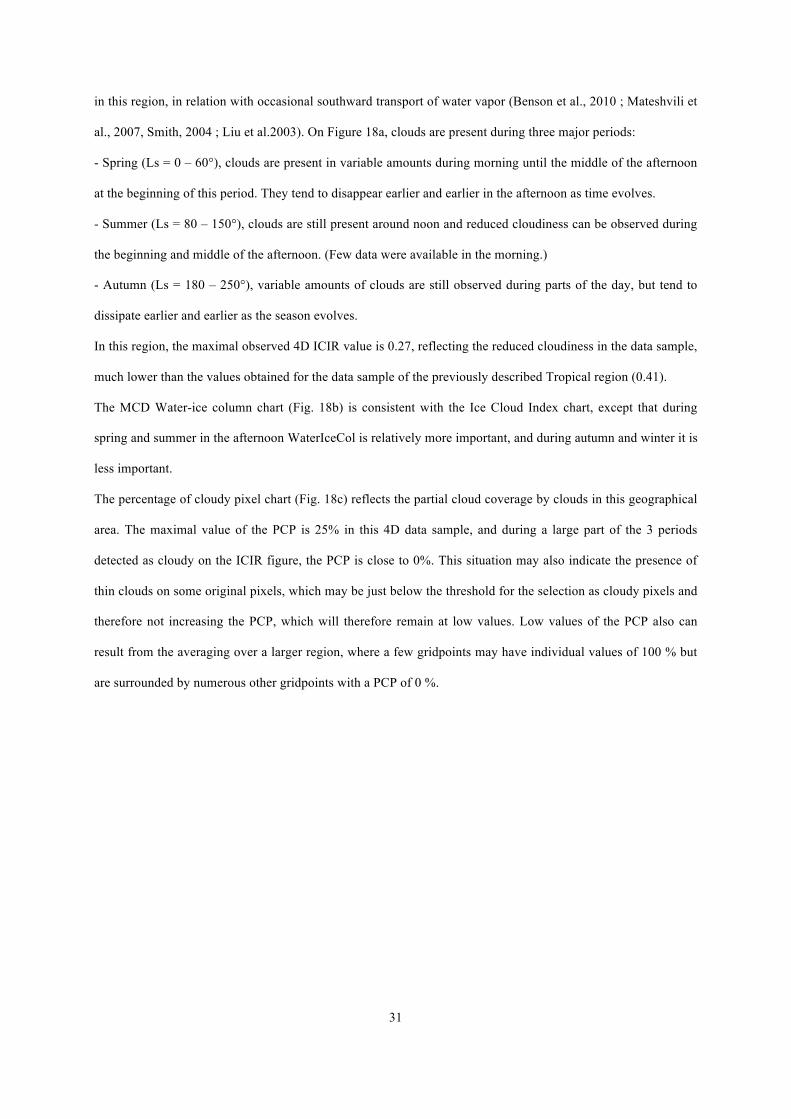
al., 2007, Smith, 2004 ; Liu et al.2003). On Figure 18a, clouds are present during three major periods:

- Spring (Ls = 0 – 60°), clouds are present in variable amounts during morning until the middle of the afternoon

at the beginning of this period. They tend to disappear earlier and earlier in the afternoon as time evolves.

- Summer (Ls = 80 – 150°), clouds are still present around noon and reduced cloudiness can be observed during

the beginning and middle of the afternoon. (Few data were available in the morning.)

- Autumn (Ls = 180 – 250°), variable amounts of clouds are still observed during parts of the day, but tend to

dissipate earlier and earlier as the season evolves.

In this region, the maximal observed 4D ICIR value is 0.27, reflecting the reduced cloudiness in the data sample,

much lower than the values obtained for the data sample of the previously described Tropical region (0.41).

The MCD Water-ice column chart (Fig. 18b) is consistent with the Ice Cloud Index chart, except that during

spring and summer in the afternoon WaterIceCol is relatively more important, and during autumn and winter it is

less important.

The percentage of cloudy pixel chart (Fig. 18c) reflects the partial cloud coverage by clouds in this geographical

area. The maximal value of the PCP is 25% in this 4D data sample, and during a large part of the 3 periods

detected as cloudy on the ICIR figure, the PCP is close to 0%. This situation may also indicate the presence of

thin clouds on some original pixels, which may be just below the threshold for the selection as cloudy pixels and

therefore not increasing the PCP, which will therefore remain at low values. Low values of the PCP also can

result from the averaging over a larger region, where a few gridpoints may have individual values of 100 % but

are surrounded by numerous other gridpoints with a PCP of 0 %.

32

a)

b)

c)

Figure 18: diurnal cycle of the Ice Cloud Index (a: top), MCD Water-ice column (b: middle) and Percentage of

Cloudy Pixels (c: bottom) over the Southern Hemisphere cloud bridge region (35°S – 20°S ; -150°E – -60°E)

during one Martian year. The color scale is strongly non-linear for c).

5.7 Other regions:

Among the 19 non-polar regions of interest, those for which sufficient data are available to characterize a

fraction of the diurnal cycle at least during some parts of the Martian year are the three ones which have the

largest spatial extension and cover all longitudes, namely the Tropics and Midlatitudes N and S (see the list on

Table 2). Smaller regions, namely Tharsis South-East, Tempe Terra, Chryse Planitia, Lunae Planum, Valles

Marineris, Southern Hemisphere cloud bridge, Tyrrhenea Terra, Argyre and Hellas Planitia are included (or

overlap largely) in the three regions with the largest extension. Small regions give less information about the

diurnal (and annual) cloud life cycle, but this information is consistent with that of the large regions in most

cases.

33

Volcanoes (Olympus, Arsia, Elysium Mons and Alba Patera) are known to be covered or surrounded by clouds.

Corresponding regions cover even smaller surfaces, their ICIR values indicate the presence of clouds at some

periods of the day and the year but are not in sufficient number to show a diurnal cycle. Their ICIR values are

compatible with those of the three largest regions, with the exception of the Alba Patera region where fewer

clouds are observed than in the largely overlapping Midlatitude N (25° – 55° N) region during winter.

6. Conclusion

Our high-resolution 4D gridded data products, the Reversed Ice Cloud Index and the Percentage of Cloudy

Pixels, are valuable indicators for detecting and characterizing Martian water-ice clouds, although the dataset is

sparsely populated (~2% of all daytime 4D grid-points). The ICIR and the PCP are complementary products

representing the cloudiness (presence of clouds and abundance) in two different ways:

- The ICIR is a general indicator of cloudiness. It is a better extractor of thin clouds at pixel scale, especially

from pixels with values just above the threshold used for the calculation of the PCP. Note that the gridded ICIR

can take values below this threshold because it results from an average of pixels that can be cloudy or not. It has

been shown to be a very good proxy for the mass of the water-ice column

- The PCP gives subgrid scale information that may be useful for GCMs.: It can be the indicator of partial cloud

coverage of a grid cell (in our case of 1° x 1°). It is less adapted for the detection of individual thin clouds at

pixel scale than the ICIR, and such clouds are eliminated by the threshold-based selection prior to the PCP

calculation.

The estimation of the uncertainty on the ICIR calculation depends on the error estimation on the reflectance

values used to calculate the ICIR at pixel scale and on the variability of the ICIR originating from different

pixels (and possibly different orbits) at the level of the grid cell. Highest uncertainty values are obtained in

regions of low reflectance values, mainly located at high latitudes under low solar illumination (i.e. at high

incidence angles), and in regions of low albedo of the surface whenever clouds are present or not (such as Syrtis

Major, and the dark latitudinal band around 60°N). We made a qualitative description of the uncertainty of the

gridded ICIR calculation. A more complete examination could help to determine whether the main factor of

uncertainty is due to instrumental error or to the variability of meteorological situation (observed locally between

34

data from the same orbit, or between data from several overlapping orbits). Neither did we investigate the

uncertainty estimation of the PCP. These complementary studies were beyond the scope of this article.

When integrated over a large time period of the day and the year, 2D maps can show the spatial cloud coverage

of the planet over (part of) a season. The major cloud structures are similar to those observed in TES optical

thickness data and those derived from the water-ice column of the Mars Climate Database.

When integrated over a specific period and larger area (covering more than one grid cell), the ICIR can also

show the daily evolution of cloudiness. As an example, we found that the diurnal cycle in the tropics is

characterized by important cloudiness in the morning, decreasing until noon, and increasing again in the

afternoon ; this can be explained with model simulation outputs as resulting from a thermal tide.

The current 4D database covers only a small fraction of the Martian cloud climatology. A consequence of the

sampling imposed by the satellite orbit and the instrument availability is the visible difference of aspect of the

temporal charts of the water-ice column when all instants are integrated (Fig. 11b is smooth) and when only a

temporal sample is available and integrated (Fig. 13b and 18b, with the sampling of corresponding ICIR data, is

more rugged). We do not now yet if this sample is a good representation of the complete diurnal and annual

cloud life cycle. An argument in favor of its representativeness is that the Martian climate observed by

instruments from other satellite or Earth-based telescopes indicate that at least at the annual and interannual scale

(with the exception of global dust storms) the Martian climate shows little variability, less than the terrestrial

climate.

Another open question is how well do the ICIR and PCP represent the water-ice clouds. The ICIR corresponds to

the absorption of small (micrometer to millimeter-sized) water ice particles, which compose Martian (water ice)

clouds but can also be produced by thin frost. At this stage we did not attempt to discriminate clouds and frost

and in this text we considered that the ICIR is only an indicator of clouds. This assumption is likely justified in a

large majority of cases, although water ice frost has occasionally been observed in some sites and during some

periods of the day and the year on the surface.

The ICIR and PCP appear to be representative of the cloud cover when compared to other cloud-related datasets.

Qualitative agreement can be observed in cloudy areas with optical thickness from TES (τTES _wice) and with the

water-ice column from the MCD. Acceptable correlations at global scale (for TES data) and regional scales (for

35

MCD data) indicate quite logically that a relation exists in cloudy areas between the ICIR on one side, and the

τTES _wice and the WaterIceCol on the other side.

The four main 4D variables derived from OMEGA, the ICIR, the PCP, the uncertainty on the ICIR and the

number of Mars Express OMEGA orbit files used at each gridpoint were uploaded to the ESA Planetary Science

Archive at open.esa.int/esa-planetary-science-archive/, conforming to the Planetary Data System (version 4)

requirements. Non-heliosynchronous satellites, namely MAVEN (Mars Atmosphere and Volatile Evolution

mission), ExoMars / Trace Gas Orbiter, and the upcoming Emirates Mars Mission (Amiri et al., 2018), may

potentially provide complementary information and data on water-ice clouds at various local times of the

Martian day in the near future.

Aknowledgement

This work has received funding from the European Union's Horizon 2020 Programme (H2020-Compet-08-2014)

under grant agreement UPWARDS-633127. Michael Smith has provided the TES mapped climatology data, part

of the validation.

References

Amiri, S., McGrath, M., Al Awadhi, M., Almatroushi, H., Sharaf, O., AlDhafri, S., AlRais, A., Wali, M.,

AlShamsi, Z., AlQasim, I., AlHarmoodi, K., Ferrington, N., Withnell, P., Reed, H., AlTeneiji, N., Landin, B.

and AlShamsi, M. (2018). Emirates Mars Mission (EMM) 2020 Overview. 42nd COSPAR Scientific

Assembly, 14-22 July 2018, Pasadena, California. COSPAR Meeting, 42, B4.2-2-18.

Audouard, J., Poulet, F., Vincendon, M., Bibring, J.-P., Forget, F., Langevin, Y., and Gondet, B. (2014a). Mars

surface thermal inertia and heterogeneities from OMEGA/MEX. Icarus, 233:194–213.

Audouard, J., Poulet, F., Vincendon, M., Milliken, R., Jouglet, D., Bibring, J.-P., Gondet, B., and Langevin, Y.

(2014b). Water in the Martian regolith from OMEGA/Mars Express. J. Geophys. Res., 119(E16):1969–1989.

Benson, J. L., Bonev, B. P., James, P. B., Shan, K. J., Cantor, B. A., and Caplinger, M. A. (2003). The seasonal

36

behavior of water ice clouds in the Tharsis and Valles Marineris regions of Mars: Mars Orbiter Camera

observa tions. Icarus, 165:34–52.

Benson, J. L., James, P. B., Cantor, B. A., and Remigio, R. (2006). Interannual variability of water ice clouds

over major martian volcanoes observed by MOC. Icarus, 184:365–371.

Benson, J. L., Kass, D. M., and Kleinböhl, A. (2011). Mars’ north polar hood as observed by the Mars Climate

Sounder. J. Geophys. Res., 116:E03008.

Benson, J. L., Kass, D. M., Kleinböhl, A., McCleese, D. J., Schofield, J. T., and Taylor, F. W. (2010). Mars’

south polar hood as observed by the Mars Climate Sounder. J. Geophys. Res., 115:E12015.

Bibring, J.-P., Soufflot, A., Berthé, M., Langevin, Y., Gondet, B., Drossart, P., Bouyé, M., Combes, M., Puget,

P., Semery, A., Bellucci, G., Formisano, V., Moroz, V., Kottsov, V., Bonello, G., Erard, S., Forni, O.,

Gendrin, A., Manaud, N., Poulet, F., Poulleau, G., Encrenaz, T., Fouchet, T., Melchiori, R., Altieri, F.,

Ignatiev, N., Titov, D., Zasova, L., Coradini, A., Capacionni, F., Cerroni, P., Fonti, S., Mangold, N., Pinet,

P., Schmitt, B., Sotin, C., Hauber, E., Hoffmann, H., Jaumann, R., Keller, U., Arvidson, R., Mustard, J., and

Forget, F. (2004). OMEGA: Observatoire pour la Minéralogie, l’Eau, les Glaces et l’Activité, pages 37–49.

ESA SP-1240: Mars Express: the Scientific Payload.

Curran, R. J., Conrath, B. J., Hanel, R. A., Kunde, V. G., and Pearl, J. C. (1973). Mars: Mariner 9 spectroscopic

evidence for H2O ice clouds. Science, 182:381–383.

Forget, F., Hourdin, F., Fournier, R., Hourdin, C., Talagrand, O., Collins, M., Lewis, S. R., Read, P. L., and

Huot, J.-P. (1999). Improved general circulation models of the Martian atmosphere from the surface to above

80 km. J. Geophys. Res., 104:24,155–24,176.

French, R. G., Gierasch, P. J., Popp, B. D., and Yerdon, R. J. (1981). Global patterns in cloud forms on Mars.

Icarus, 45:468–493.

Hale, A. S., Tamppari, L. K., Bass, D. S., and Smith, M. D. (2011). Martian water ice clouds: A view from Mars

Global Surveyor Thermal Emission Spectrometer. Journal of Geophysical Research (Planets), 116:E04004.

Kahn, R. (1984). The spatial and seasonal distribution of Martian clouds and some meteorological implications.

37

J. Geophys. Res., 89:6671–6688.

Langevin, Y., Bibring, J.-P., Montmessin, F., Forget, F., Vincendon, M., Douté, S., Poulet, F., and Gondet, B.

(2007). Observations of the south seasonal cap of Mars during recession in 2004-2006 by the OMEGA

visible/near-infrared imaging spectrometer on board Mars Express. J. Geophys. Res., 112:E08S12.

Liu, J., Richardson, M. I., and Wilson, R. J. (2003). An assessment of the global, seasonal, and interannual

spacecraft record of Martian climate in the thermal infrared. Journal of Geophysical Research (Planets),

108:8–1.

Madeleine, J.-B., Forget, F., Spiga, A., Wolff, M. J., Montmessin, F., Vincendon, M., Jouglet, D., Gondet, B.,

Bibring, J.-P., Langevin, Y., and Schmitt, B. (2012). Aphelion water-ice cloud mapping and property

retrieval using the OMEGA imaging spectrometer onboard Mars Express. J. Geophys. Res.,

117(E16):E00J07.

Mateshvili, N., Fussen, D., Vanhellemont, F., Bingen, C., Dekemper, E., Loodts, N., and Tetard, C. (2009).

Water ice clouds in the Martian atmosphere: Two Martian years of SPICAM nadir UV measurements. Planet.

Space Sci., 57:1022–1031.

Millour, E., Forget, F., Spiga, A., Vals, M., Zakharov, V., Montabone, L., Lefevre, F., Montmessin, F.,

Chaufray, J.-Y., Lopez-Valverde, M., Gonzalez-Galindo, F., Lewis, S., Read, P., Desjean, M.-C., Cipriani,

F., and MCD/GCM Development Team (2018). The Mars Climate Database (version 5.3). In From Mars

Express to ExoMars Scientific Workshop, 27 - 28 February, ESA-ESAC Madrid, Spain, 2 pp.

Montabone, L., Forget, F., Millour, E., Wilson, R. J., Lewis, S. R., Cantor, B., Kass, D., Kleinböhl, A.,

Lemmon, M. T., Smith, M. D., and Wolff, M. J. (2015). Eight-year climatology of dust optical depth on

Mars. Icarus, 251:65– 95.

Montmessin, F., Forget, F., Rannou, P., Cabane, M., and Haberle, R. M. (2004). Origin and role of water ice

clouds in the Martian water cycle as inferred from a general circulation model. Journal of Geophysical

Research (Planets), 109:E10004.

Navarro, T., Madeleine, J.-B., Forget, F., Spiga, A., Millour, E., Montmessin, F., and Määttanen, A. (2014).

38

Global Climate Modeling of the Martian water cycle with improved microphysics and radiatively active

water ice clouds. Journal of Geophysical Research (Planets), 119:1479–1495.

Olsen, K. S., Forget, F., Madeleine, J.-B., Szantai, A., Audouard, J., Geminale, A., Altieri, F., Bellucci, G.,

Oliva, F., Montabone, L., and Wolff, M. J. (2018). The distributions of retrieved properties from water-ice

clouds in the Martian atmosphere using the OMEGA imaging spectrometer. Icarus (accepted; this issue).

Peale, S. J. (1973). Water and the Martian W cloud. Icarus, 18:497–501.

Pottier, A., Montmessin, F., Forget, F., Wolff, M., Navarro, T., Millour, E., Madeleine, J.-B., Spiga, A.,

Bertrand, T. ( 2015). Water ice clouds on Mars: a study of partial cloudiness with a global climate model and

MARCI data. EGU General Assembly Conference Abstracts 17, 1751.

Pottier, A., Forget, F., Montmessin, F., Navarro, T., Spiga, A., Millour, E., Szantai, A., and Madeleine, J.-B.

(2017). Unraveling the martian water cycle with high-resolution global climate simulations. Icarus, 291:82–

106.

Smith, M. D. (2009). THEMIS observations of Mars aerosol optical depth from 2002-2008. Icarus, 202: 444-

452. Doi: 10.1016/j.icarus.2009.03.027

Smith, M. D. (2004). Interannual variability in TES atmospheric observations of Mars during 1999-2003. Icarus,

167:148–165.

Smith, S. A. and Smith, B. A. (1972). Diurnal and seasonal behavior of discrete white clouds on Mars. Icarus,

16:509–521.

Tamppari, L. K., Smith, M. D., Bass, D. S., and Hale, A. S. (2008). Water-ice clouds and dust in the north polar

region of Mars using MGS TES data. Planet. Space Sci., 56:227–245.

Tamppari, L. K., Zurek, R. W., and Paige, D. A. (2003). Viking-era diurnal water-ice clouds. J. Geophys. Res.,

108:9–1.

Vincendon, M., Pilorget, C., Gondet, B., Murchie, S., and Bibring, J.-P. (2011). New near-IR observations of

mesospheric CO2 and H2O clouds on Mars. Journal of Geophysical Research (Planets), 116:E00J02.

39

Wang, H. and Ingersoll, A. P. (2002). Martian clouds observed by Mars Global Surveyor Mars Orbiter Camera.

J. Geophys. Res., 107:8–1.

Wang, H. and Richardson, M. I. (2013). The origin, evolution and trajectory of large dust storms on Mars during

Mars years 24-30 (1999-2011). Icarus, 251:112–127.

Willame, Y., Vandaele, A.-C., Depiesse, C., Lefevre, F., Letocart, V., Gillotay, D. and Montmessin, F. (2017).

Retrieving cloud, dust and ozone abundances in the Martian atmosphere using SPICAM/UV nadir spectra.

Planet. Space Sci., 142, 9-25.