
Maintenance modelling, simulation and performance ... · Maintenance modelling, simulation and...
222
Thèse de doctorat de l’UTT Hui SHANG Maintenance Modelling, Simulation and Performance Assessment for Railway Asset Management Spécialité : Optimisation et Sûreté des Systèmes 2015TROY0022 Année 2015
Transcript of Maintenance modelling, simulation and performance ... · Maintenance modelling, simulation and...
Thèse de doctorat
de l’UTT
Hui SHANG
Maintenance Modelling, Simulation and Performance Assessment
for Railway Asset Management
Spécialité : Optimisation et Sûreté des Systèmes
2015TROY0022 Année 2015
THESE
pour l’obtention du grade de
DOCTEUR de l’UNIVERSITE DE TECHNOLOGIE DE TROYES
Spécialité : OPTIMISATION ET SURETE DES SYSTEMES
présentée et soutenue par
Hui SHANG
le 25 septembre 2015
Maintenance Modelling, Simulation and Performance Assessment for Railway Asset Management
JURY
M. R. LENGELLÉ PROFESSEUR DES UNIVERSITES Président M. J. ANDREWS PROFESSOR Directeur de thèse M. C. BÉRENGUER PROFESSEUR DES UNIVERSITES Directeur de thèse M. N. BRINZEI MAITRE DE CONFERENCES Examinateur M. P. DEHOMBREUX PROFESSEUR ORDINAIRE Rapporteur M. B. GUYOT INGENIEUR DOCTEUR Examinateur M. O. SÉNÉCHAL PROFESSEUR DES UNIVERSITES Rapporteur

Acknowledgements
I would like to express my gratitude to all those who helped me during my doctoral studiesand the writing of this thesis. My deepest gratitude goes first to my supervisors ProfessorChristophe Bérenguer and Professor John Andrews, for their constantly encouragement andguidance of my research. I learn from them not only the research methods and knowledge,but also the attitude to life and research: they are rigorous in their researches, encyclopaedicin their reading. I also want to thank Professor Nicolas Lefebvre who gave me a lot of helpduring my PhD.
A special thank goes to Prof. Lengelle , Prof. Dehombreux, Prof. Senechal, Prof.Brinzei and Dr. Guyot who kindly agreed to serve as reviewer (rapporteur) or exam-iner(examinateur) in my Ph.D defence committee.
I wish to express my gratitude to China Scholarship Council (CSC) and University ofTechnology of Troyes (UTT) for the financial support during these four years.
Thanks the secretaries of the pôle ROSAS Ms. Marie-José Rousselet, Ms. VeroniqueBanse and Ms. Bernadette Andre, and the secretaries of the doctoral school: Ms. IsabelleLeclercq, Ms. Pascale Denis and Ms. Therese Kazarian, and the secretaries in Gipsa-labfor their help throughout my PhD study.
I want to thank my friends in UTT (Xiaowei LV, Yugang Li, Hongchang Han and hiswife, Wenjin Zhu, Guoliang Zhu, Tian Wang, Huan Wang and Zhenming Yue and otherfriends) for their valuable supports and aids, and all my friends in France (Yingying Wang,Xunqian Ying, Xingling Tang, Dandan Yao and Xiao Fan, Kai Li) , in UK (Yang Zhang,Miranda and Shan) and in China, they give me a lot of helps when I was struggling withthe troubles. Special thank Mengyi Zhang in Université de Reims for supporting me all thetime.
Last but not least, I offer sincere thanks to my parents and all my family members, fortheir loving considerations and great confidence in me all through these years.
Hui SHANGJuly, 2015

Maintenance modelling, simulation and performance assessment for railwayasset management
Abstract:The aim of this thesis research work is to propose maintenance models for railwaysinfrastructures that can help to make better maintenance decisions in the more constrainedenvironment that the railway industry has to face, e.g. increased traffic loads, faster deterio-ration, longer maintenance planning procedures, shorter maintenance times. The proposedmaintenance models are built using Coloured Petri nets; they are animated through MonteCarlo simulations to estimate the performance of the considered maintenance policies interms of cost and availability. The maintenance models are developed both at the compo-nent and network levels, and several different maintenance problems are considered. At therail component level, maintenance policies with different level of monitoring information(level of gradual deterioration vs binary working state) are compared to show the benefitsof gathering monitoring information on the deterioration level. The effect of preventivemaintenance delays is also investigated for both condition-based inspection policies andperiodic inspection policies on a gradually deteriorating component. At the line level, amaintenance policy based on a two-level inspection procedure is first investigated. Then,considering the case when the deterioration process depends on the operation modes(normal vs limited speed), a maintenance optimization problem is solved to determine anoptimal tuning of the repair delay and speed restriction.
Keywords: Railroads–Track - Maintenance and repair, Railroads–Track - Deterio-ration, Condition-based maintenance, Petri nets, Reliability, Systems availability, Systemsafety, Engineering inspection, Simulation methods

Modélisation, simulation et évaluation de performances de la maintenancedes infrastructures ferroviaires
Résume: Les travaux présentés dans ce manuscrit visent à développer des modèles decoût/performances pour améliorer les décisions de maintenance sur les infrastructuresferroviaires exploitées dans un environnement de plus en plus contraint: trafic accru,détérioration accélérée, temps de maintenance réduits. Les modèles de maintenanceproposés sont construits à base de réseaux de Petri colorés ; ils sont animés par simulationde Monte Carlo pour estimer les performances (en termes de coût et de disponibilité) despolitiques de maintenance considérées. Ils sont développés aux niveaux "composant"et "réseau", et plusieurs problèmes de maintenance différents sont étudiés. Au niveau"composant" (rail), des politiques de maintenance mettant en jeu différents niveauxd’information de surveillance sont comparées pour montrer l’intérêt de surveiller ladétérioration graduelle du composant. L’effet de l’existence d’un délai de maintenanceest également étudié pour les politiques conditionnelle et périodique. Au niveau système(ligne), une maintenance mettant en jeu différents types d’inspections complémentaires(automatique ou visuelle) est d’abord étudiée. On s’intéresse ensuite au cas de figure oùl’évolution de la détérioration dépend du mode d’utilisation et de la charge de la voie : leproblème de maintenance étudié vise alors à définir un réglage optimal des paramètresd’exploitation de la voie (vitesse limite) et de maintenance (délai d’intervention).
Les mots clé: Voies ferrées-Entretien et réparations; Voies ferrées-Détérioration;Maintenance conditionnelle; Réseaux de Petri; Fiabilité; Disponibilité (systèmes); Con-trôle technique; Méthodes de Simulation

Contents
I INTRODUCTION 1
1 Introduction 31.1 Importance and necessity of railway asset maintenance . . . . . . . . . . . 3
1.1.1 Effects of failures on railway . . . . . . . . . . . . . . . . . . . . . 31.1.2 Existing railway maintenance . . . . . . . . . . . . . . . . . . . . 41.1.3 Challenges of railway assets maintenance . . . . . . . . . . . . . . 6
1.1.3.1 Faster deteriorations . . . . . . . . . . . . . . . . . . . . 61.1.3.2 Longer planning procedure . . . . . . . . . . . . . . . . 61.1.3.3 Shorter maintenance time . . . . . . . . . . . . . . . . . 7
1.1.4 Conclusion . . . . . . . . . . . . . . . . . . . . . . . . . . . . . . 71.2 Motivations and objectives . . . . . . . . . . . . . . . . . . . . . . . . . . 7
1.2.1 Inspection capability . . . . . . . . . . . . . . . . . . . . . . . . . 81.2.2 Delayed repairs . . . . . . . . . . . . . . . . . . . . . . . . . . . . 81.2.3 Maintenance and operation configurations . . . . . . . . . . . . . . 8
1.3 Structure of the thesis . . . . . . . . . . . . . . . . . . . . . . . . . . . . . 9
II BACKGROUND 11
2 Railway system description and asset maintenance introduction 132.1 Introduction . . . . . . . . . . . . . . . . . . . . . . . . . . . . . . . . . . 132.2 Example of a railway section . . . . . . . . . . . . . . . . . . . . . . . . . 142.3 Railway assets . . . . . . . . . . . . . . . . . . . . . . . . . . . . . . . . . 15
2.3.1 Track . . . . . . . . . . . . . . . . . . . . . . . . . . . . . . . . . 162.3.2 Switches & Crossing . . . . . . . . . . . . . . . . . . . . . . . . . 172.3.3 Point machine . . . . . . . . . . . . . . . . . . . . . . . . . . . . 18
2.4 Railway assets failures and maintenance . . . . . . . . . . . . . . . . . . . 192.4.1 Track geometry faults and maintenance . . . . . . . . . . . . . . . 19
2.4.1.1 Track geometry quality measurements . . . . . . . . . . 192.4.1.2 Track gauge spread . . . . . . . . . . . . . . . . . . . . 212.4.1.3 Track top and twist . . . . . . . . . . . . . . . . . . . . 222.4.1.4 Track buckle . . . . . . . . . . . . . . . . . . . . . . . . 24
2.4.2 Rail faults and maintenance . . . . . . . . . . . . . . . . . . . . . 252.4.3 Inspections for track . . . . . . . . . . . . . . . . . . . . . . . . . 262.4.4 Point machine failures . . . . . . . . . . . . . . . . . . . . . . . . 26
2.5 Conclusion for the maintenance modelling of railway infrastructure . . . . 27
viii Contents
3 Deterioration/failure and maintenance models for railway application: stateof the art 293.1 Introduction . . . . . . . . . . . . . . . . . . . . . . . . . . . . . . . . . . 293.2 Failure modelling . . . . . . . . . . . . . . . . . . . . . . . . . . . . . . . 30
3.2.1 Deterministic deterioration model . . . . . . . . . . . . . . . . . . 303.2.2 Stochastic deterioration modelling . . . . . . . . . . . . . . . . . . 31
3.2.2.1 Component lifetime models . . . . . . . . . . . . . . . 313.2.2.2 P-F interval and delay time concept . . . . . . . . . . . . 313.2.2.3 Models for deterioration . . . . . . . . . . . . . . . . . . 33
3.3 Inspection policy . . . . . . . . . . . . . . . . . . . . . . . . . . . . . . . 343.4 Maintenance policy . . . . . . . . . . . . . . . . . . . . . . . . . . . . . . 35
3.4.1 Maintenance effects . . . . . . . . . . . . . . . . . . . . . . . . . 353.4.2 Maintenance policies for single component . . . . . . . . . . . . . 363.4.3 Maintenance modelling for multi-component . . . . . . . . . . . . 36
3.5 Railway risk modelling . . . . . . . . . . . . . . . . . . . . . . . . . . . . 383.6 Conclusion for the existing failures and maintenance models for railway
assets management . . . . . . . . . . . . . . . . . . . . . . . . . . . . . . 38
4 Modelling tools 414.1 Introduction . . . . . . . . . . . . . . . . . . . . . . . . . . . . . . . . . . 414.2 Probabilistic models for deterioration/ failure modelling . . . . . . . . . . . 41
4.2.1 Lifetime distribution . . . . . . . . . . . . . . . . . . . . . . . . . 414.2.1.1 Exponential distribution . . . . . . . . . . . . . . . . . . 424.2.1.2 Weibull distribution . . . . . . . . . . . . . . . . . . . . 42
4.2.2 Stochastic processes . . . . . . . . . . . . . . . . . . . . . . . . . 434.2.2.1 Counting process . . . . . . . . . . . . . . . . . . . . . 434.2.2.2 Gamma process . . . . . . . . . . . . . . . . . . . . . . 44
4.3 Petri Nets . . . . . . . . . . . . . . . . . . . . . . . . . . . . . . . . . . . 454.3.1 Basic Petri Nets . . . . . . . . . . . . . . . . . . . . . . . . . . . . 464.3.2 Stochastic Petri Nets . . . . . . . . . . . . . . . . . . . . . . . . . 46
4.3.2.1 Time in SPN . . . . . . . . . . . . . . . . . . . . . . . . 474.3.3 Colored Petri Nets . . . . . . . . . . . . . . . . . . . . . . . . . . 47
4.3.3.1 Concepts of CPN . . . . . . . . . . . . . . . . . . . . . 484.3.3.2 Marking process in CPN . . . . . . . . . . . . . . . . . 484.3.3.3 Hierarchical modelling in CPN . . . . . . . . . . . . . . 50
4.3.4 CPN tool . . . . . . . . . . . . . . . . . . . . . . . . . . . . . . . 514.3.5 Component maintenance model using CPN tool . . . . . . . . . . . 52
4.3.5.1 Assumptions of the model . . . . . . . . . . . . . . . . . 524.3.5.2 CPN model description . . . . . . . . . . . . . . . . . . 534.3.5.3 Simulation results . . . . . . . . . . . . . . . . . . . . . 55
4.4 Conclusion for the modelling tool . . . . . . . . . . . . . . . . . . . . . . 58
Contents ix
III COMPONENT MAINTENANCE MODELLING 59
5 Comparison of failure models for maintenance optimization 615.1 Introduction . . . . . . . . . . . . . . . . . . . . . . . . . . . . . . . . . . 615.2 Assumptions for deterioration model and lifetime model . . . . . . . . . . 63
5.2.1 Gradual deterioration model . . . . . . . . . . . . . . . . . . . . . 635.2.1.1 Condition-based maintenance policy . . . . . . . . . . . 645.2.1.2 Periodic preventive maintenance policy . . . . . . . . . . 64
5.2.2 Lifetime distribution model . . . . . . . . . . . . . . . . . . . . . 655.2.2.1 Periodic preventive maintenance policy . . . . . . . . . . 66
5.2.3 Performance evaluations . . . . . . . . . . . . . . . . . . . . . . . 675.3 CPN models . . . . . . . . . . . . . . . . . . . . . . . . . . . . . . . . . . 67
5.3.1 CPN model for deterioration model . . . . . . . . . . . . . . . . . 675.3.1.1 Deterioration CPN model . . . . . . . . . . . . . . . . . 685.3.1.2 Condition-based mainteannce CPN model . . . . . . . . 685.3.1.3 Periodic preventive maintenance CPN model for deteri-
oration process . . . . . . . . . . . . . . . . . . . . . . . 695.3.2 CPN model for lifetime model . . . . . . . . . . . . . . . . . . . . 70
5.3.2.1 CPN model describing failure time . . . . . . . . . . . . 705.3.2.2 CPN model for periodic preventive maintenance . . . . . 71
5.4 Monte Carlo simulations . . . . . . . . . . . . . . . . . . . . . . . . . . . 715.4.1 Parameters used in simulations . . . . . . . . . . . . . . . . . . . . 725.4.2 Simulation convergence . . . . . . . . . . . . . . . . . . . . . . . 745.4.3 Simulation results of deterioration process model . . . . . . . . . . 75
5.4.3.1 Simulation results of condition-based maintenance ofGamma process . . . . . . . . . . . . . . . . . . . . . . 75
5.4.3.2 Simulation results of periodic preventive maintenancefor Gamma process deterioration model . . . . . . . . . 77
5.4.4 Simulation results of lifetime model . . . . . . . . . . . . . . . . . 785.4.5 Comparison of lifetime model and deterioration model . . . . . . . 79
5.5 Conclusion for the comparison of failure models . . . . . . . . . . . . . . . 80
6 Delayed repair for railway track maintenance 836.1 Introduction . . . . . . . . . . . . . . . . . . . . . . . . . . . . . . . . . . 836.2 Track maintenance modelling assumptions . . . . . . . . . . . . . . . . . . 84
6.2.1 Modelling assumptions . . . . . . . . . . . . . . . . . . . . . . . . 846.2.2 Performance evaluation . . . . . . . . . . . . . . . . . . . . . . . . 87
6.3 Track CPN models . . . . . . . . . . . . . . . . . . . . . . . . . . . . . . 876.3.1 Deterioration part of CPN model . . . . . . . . . . . . . . . . . . . 876.3.2 CPN model of inspection schemes . . . . . . . . . . . . . . . . . . 896.3.3 CPN model of delayed maintenance . . . . . . . . . . . . . . . . . 89
6.4 Numerical results . . . . . . . . . . . . . . . . . . . . . . . . . . . . . . . 916.4.1 Simulation convergence . . . . . . . . . . . . . . . . . . . . . . . 91
6.4.1.1 Converged simulation time . . . . . . . . . . . . . . . . 92
x Contents
6.4.1.2 Number of simulations for a finite simulation time . . . . 956.4.2 Repair delay for periodic inspection . . . . . . . . . . . . . . . . . 96
6.4.2.1 Long-term average maintenance cost for periodic in-spection . . . . . . . . . . . . . . . . . . . . . . . . . . 97
6.4.2.2 Short-term average maintenance cost for periodic in-spection . . . . . . . . . . . . . . . . . . . . . . . . . . 97
6.4.3 Repair delay for condition-based inspection . . . . . . . . . . . . . 986.4.3.1 Long-term average maintenance cost for Condition-
based inspection . . . . . . . . . . . . . . . . . . . . . . 996.4.3.2 Short-term maintenance cost for condition-based inspec-
tion . . . . . . . . . . . . . . . . . . . . . . . . . . . . . 1046.4.4 Comparison of inspection policies . . . . . . . . . . . . . . . . . . 105
6.5 Conclusions for the delayed repairs . . . . . . . . . . . . . . . . . . . . . . 107
IV MAINTENANCE MODELLING FOR A RAILWAY SECTION 109
7 Maintenance modelling for a railway section: limited maintenance resources 1117.1 Introduction . . . . . . . . . . . . . . . . . . . . . . . . . . . . . . . . . . 1117.2 Modelling assumptions . . . . . . . . . . . . . . . . . . . . . . . . . . . . 112
7.2.1 Assumptions for the component . . . . . . . . . . . . . . . . . . . 1127.2.2 Region and network assumptions . . . . . . . . . . . . . . . . . . 113
7.3 CPN model for the railway network . . . . . . . . . . . . . . . . . . . . . 1147.3.1 Modelling framework . . . . . . . . . . . . . . . . . . . . . . . . 1147.3.2 Track component CPN model . . . . . . . . . . . . . . . . . . . . 115
7.3.2.1 Track deterioration and inspection process model . . . . 1157.3.2.2 Track component maintenance requirement . . . . . . . . 1167.3.2.3 Tamper maintenance model . . . . . . . . . . . . . . . . 1177.3.2.4 Stoneblower maintenance model . . . . . . . . . . . . . 118
7.3.3 Region CPN model . . . . . . . . . . . . . . . . . . . . . . . . . . 1187.3.3.1 Machine utility model . . . . . . . . . . . . . . . . . . . 120
7.3.4 Network CPN model . . . . . . . . . . . . . . . . . . . . . . . . . 1227.4 Simulation results . . . . . . . . . . . . . . . . . . . . . . . . . . . . . . . 1227.5 Conclusion for the limited resource maintenance . . . . . . . . . . . . . . 124
8 Maintenance of a railway section: two-level inspection policies 1258.1 Introduction . . . . . . . . . . . . . . . . . . . . . . . . . . . . . . . . . . 1258.2 Modelling assumptions . . . . . . . . . . . . . . . . . . . . . . . . . . . . 126
8.2.1 Component assumptions . . . . . . . . . . . . . . . . . . . . . . . 1268.2.1.1 Component degradation and maintenance . . . . . . . . . 1268.2.1.2 Component working model . . . . . . . . . . . . . . . . 128
8.2.2 System operation and accident assumptions . . . . . . . . . . . . . 1288.2.3 Performance evaluation . . . . . . . . . . . . . . . . . . . . . . . . 129
8.3 CPN model for the railway section . . . . . . . . . . . . . . . . . . . . . . 130
Contents xi
8.3.1 Modelling framework . . . . . . . . . . . . . . . . . . . . . . . . 1308.3.2 Component CPN model . . . . . . . . . . . . . . . . . . . . . . . 131
8.3.2.1 Component deterioration CPN Model . . . . . . . . . . . 1318.3.2.2 Component working CPN Model . . . . . . . . . . . . . 1318.3.2.3 Component inspection CPN Model . . . . . . . . . . . . 1328.3.2.4 Component maintenance CPN Model . . . . . . . . . . . 132
8.3.3 System inspection CPN model . . . . . . . . . . . . . . . . . . . . 1338.3.4 System operation and accident CPN model . . . . . . . . . . . . . 134
8.4 Simulation results . . . . . . . . . . . . . . . . . . . . . . . . . . . . . . . 1358.4.1 Simulation convergence . . . . . . . . . . . . . . . . . . . . . . . 1368.4.2 System performance evaluations . . . . . . . . . . . . . . . . . . . 137
8.5 Conclusion for two-level inspection policies . . . . . . . . . . . . . . . . . 138
9 Maintenance optimization for a railway section: delayed maintenance vs speedrestriction 1399.1 Introduction . . . . . . . . . . . . . . . . . . . . . . . . . . . . . . . . . . 1399.2 Modelling assumptions . . . . . . . . . . . . . . . . . . . . . . . . . . . . 141
9.2.1 Track component deterioration and maintenance . . . . . . . . . . 1419.2.1.1 Track deterioration . . . . . . . . . . . . . . . . . . . . 1419.2.1.2 Component maintenance . . . . . . . . . . . . . . . . . 142
9.2.2 Section maintenance planning . . . . . . . . . . . . . . . . . . . . 1429.3 Performance evaluation . . . . . . . . . . . . . . . . . . . . . . . . . . . . 144
9.3.1 Single objective evaluation . . . . . . . . . . . . . . . . . . . . . . 1449.3.2 Multiple-objective evaluation . . . . . . . . . . . . . . . . . . . . 145
9.4 CPN models . . . . . . . . . . . . . . . . . . . . . . . . . . . . . . . . . . 1469.4.1 CPN model for railway section . . . . . . . . . . . . . . . . . . . . 1469.4.2 Component CPN model . . . . . . . . . . . . . . . . . . . . . . . 1479.4.3 Component maintenance CPN model for grouping strategy . . . . . 1489.4.4 Maintenance planning CPN model . . . . . . . . . . . . . . . . . . 149
9.5 Simulation results . . . . . . . . . . . . . . . . . . . . . . . . . . . . . . . 1509.5.1 Convergence . . . . . . . . . . . . . . . . . . . . . . . . . . . . . 1509.5.2 Results for the grouping policy . . . . . . . . . . . . . . . . . . . . 1509.5.3 Results for the non-grouping policy . . . . . . . . . . . . . . . . . 1539.5.4 Comparison of grouping and non-grouping policies . . . . . . . . . 154
9.6 Conclusion for the delayed maintenance with speed restriction . . . . . . . 155
V CONCLUSION & PERSPECTIVE 157
A Résumé en Français 163
B Tables of track faults and maintenance in UK standard 185
C CPN models for inspection and train density in Chapter9 187
xii Contents
References 189
Part I
INTRODUCTION:PROBLEM STATEMENT, OBJECTIVES AND MOTIVATION

Chapter 1
Introduction
Contents1.1 Importance and necessity of railway asset maintenance . . . . . . . . . 3
1.1.1 Effects of failures on railway . . . . . . . . . . . . . . . . . . . . . 3
1.1.2 Existing railway maintenance . . . . . . . . . . . . . . . . . . . . 4
1.1.3 Challenges of railway assets maintenance . . . . . . . . . . . . . . 6
1.1.4 Conclusion . . . . . . . . . . . . . . . . . . . . . . . . . . . . . . 7
1.2 Motivations and objectives . . . . . . . . . . . . . . . . . . . . . . . . . 7
1.2.1 Inspection capability . . . . . . . . . . . . . . . . . . . . . . . . . 8
1.2.2 Delayed repairs . . . . . . . . . . . . . . . . . . . . . . . . . . . . 8
1.2.3 Maintenance and operation configurations . . . . . . . . . . . . . . 8
1.3 Structure of the thesis . . . . . . . . . . . . . . . . . . . . . . . . . . . . 9
1.1 Importance and necessity of railway asset maintenance
SNCF (Société nationale des chemins de fer français) maintains and monitors around30,000 km of track in France, and around 15,500 trains run on this huge network carry-ing 126.9 million passengers per year[50]. According to the statistics on the website ofworld bank, Network Rail controls more than 16,000 km length of track and carries 2.75million passenger journeys per weekday [160]. In China, the railway network expands toreach 66,298 km and more than 12,000 km are the high speed passenger dedicated lines[131].
For these large scale transport system, safety and availability are the most basic and im-portant requirements since the failures on the railway system may lead to traffic disorders,and even disasters.
1.1.1 Effects of failures on railway
Railway assets and infrastructures play an important role in railway safety and service. Thefailures of the railway assets may cause emergency maintenance, hence the traffic stops,and even lead to accidents.
4 Chapter 1. Introduction
The first unexpected event due to the railway asset failure is the traffic stop whichleads to train delays and traffic disruption. For example, a rail breakage occurred in 2006,results in a track circuit failure and traffic stop for 6 hours at Urchfont and 10 hours atKennington in UK [149]. According to the report of Office of Rail Regulation, around16,000 infrastructure incidents arose and they were associated with 1.7 million minutes oftrain delays in 2013[129]. Open data on the website of SNCF indicates that there werearound 37 safety incidents due to the track faults, such as the twist, broken rail and so onduring 2013/2014. These incidents did not cause railway accidents but they resulted inheavy maintenance on the railway section [50].
Another consequence due to the failure is the accident which may damage the otherinfrastructures and ruin the environment. For example, the derailment of a freight trainhappens near Gloucester station in 2013 damaged the signal cables for 4 miles, as well as4 level-crossing and 2 bridges [153]. A freight train derailed in North-west London in Oc-tober 2013 due to a track twist fault; even though there is no injuries reported, the accidentdamaged the overhead line electrification, and the maintenance at the accident locationforced the stop of the passenger and freight service for 6 days [152]. A serious accidentmay lead to injuries and fatalities that are the most unexpected disaster in the railway op-eration. Several passengers trains derailments in UK during 2000-2010 are reported by theRail Accident investigation Branch, including a derailment in Grayrigg due to a fault ofpoint machine leading to injuries in 2007 [150]; the derailment at Potters Bar leading to theconsequence of fatalities [80, 158], the accident investigation reports for them mentionedthat the inspection failed in identifying the defects. Let us mention as well a derailmentreported due to the lack of maintenance at the right location: it happened in Leeds in 2000which not only leaded to fatalities and injuries but also to the permanent speed restrictionand replacement for more than 1 year [128]. In France, an accident due to the track faulthappened in Bertigny/Orgy in July 2013, a train derailed and crashed to the station due tothe loose of rail connection and resulted in 7 fatalities and nearly 200 injuries; in addition,investigation report pointed out that the regular inspections are carried out for the devicesbut it seemed the failure was not detected and maintained in time [26].
During 1991-2001, around 23.7% of derailments were caused by the track faults [143]and 10% of the derailments occurred due to both of the defective track and vehicle condi-tion in UK [105].Therefore, it is important to carry out the inspection and maintenance toreduce the potential railway failures and enhance the safety and availability of the railwayline.
1.1.2 Existing railway maintenance
Maintenance of railway asset contributes by a high proportion to the total railway expen-diture. Netherlands railway company spent e250 million for 4,500km of track in 2006[54]. In the financial Report of SNCF, e746 millions is spent for the upgrades to the sta-tions and buildings including track renewal, replacement of the communication system andso on [175]. Network Rail has spent £391.8 million for track maintenance during 2013-2014[121].
Three types of maintenances are carried out for railway assets:
1.1. Importance and necessity of railway asset maintenance 5
• preventive maintenance, which is planned to be carried out to prevent the failures,including time-based or condition-based strategies;
• corrective maintenance, which is performed after the failure is detected to recoverthe function of railway devices, sometimes which is unplanned;
• renewal/replacement, which replaces all the devices or components in the railwaysection.
Renewal costs the most of railway expenditure: cost of track renewal in Netherlands in2006 represented more than 70% of the overall maintenance cost. In order to ensure thesafety and at the same time perform an economic maintenance, maintenance strategies arestudied to improve the maintenance decision and schedule a cost-effective maintenancestrategy for railway system within the safety constraints. Railway infrastructure ownersmake efforts to optimise maintenance scheduling for a cost-effective maintenance strate-gies: The renewal strategies considers the type of rails [73] or the number of failures [8, 9].Reliability-centred maintenance (RCM) is introduced to the safety critical infrastructurein 2000 [178] and some researches discuss the applications of RCM on the railway sub-systems, such as point machines and signalling devices [31, 99, 106, 138]. Risk-basedmaintenance (RBM) is another maintenance strategy for the railway assets [144]. Thesetwo maintenance strategies have similar steps but they have differences:
• Different events are analysed: RCM considers the functions and functional failures;RBM considers the hazardous events (or functions) and their corresponding func-tions. Since RBM and RCM may concern about different events, the system can bedivided into different subsystems.
• RBM needs to consider the integrated risk (Risk=FrequencyŒConsequence); RCMconsiders the probability of failures.
• RBM needs to firstly satisfy the acceptable risk level and then optimize maintenancecost and availability. RCM considers failures probability and try to make mainte-nance plans to minimize maintenance cost and maximize system availability.
• For safety-related or safety-critical system, RBM is needed; for the system which isnot related to safety, we can just use RCM.
RCM needs to carry out HAZOP, FMECA (FMEA), and FTA, etc before making mainte-nance decision. Risk-based maintenance also needs to consider the failure modes and theireffects so it also carries out the techniques such as FMEA, HAZOP and FTA. Before weset up RBM, we need to implement RCM in some extents.
Under these maintenance frameworks, preventive maintenance is scheduled to improvethe system reliability and safety; it can be carried out depending on time or the detectedstates since the preventive maintenance on railway is not as expensive as the track renewal.
Some researches focus on improving the monitoring techniques (monitoring the volt-ages and pressure for Point machine or using ultrasonic inspection for rail cracks) to detectmore hidden defects which is more cheaper than the preventive maintenance or renewaland helps to make decisions for preventive maintenance [133].
6 Chapter 1. Introduction
1.1.3 Challenges of railway assets maintenance
More and more people choose trains for long distance journeys. Network Rail’s data showsthat the growth of passenger journeys increase from 1 billion in 2002/2003 to 1.5 billionin 2012/2013. They believe that the rail capacity should have to increase 25% if 2% roadtraffic changes to rail [160]. The clients want to arrive to the destination as quickly aspossible; in addition, they want to take the trains within a shorter waiting time.
Thus, effective maintenance scheduling and execution on railway need to consider theconflict between the maintenance actions and the operation requirements. In the future, thisconflict will become more and more important since the railway system may be developedin order to facilitate faster trains, more trains per hours, longer operating time and higherpunctuality.
1.1.3.1 Faster deteriorations
According to the route utilization strategy report of Network Rail, in the next 10 years, onlyin the east midland, the speed of most of the passenger trains will increase from 110 mph(177km/h) to 125 mph (200km/h). Network Rail sets the aims that for the long distancehigh speed train, in the next ten years, the journey time will reduce by 1%-6% [120]. TGVran with the maximum speed of 500km/h for a test of the high speed rail in 2007 andit is possible to run the TGV trains at the average speed of 320-350km/h in the regularoperation[176]. China built high speed railway in these years, the maximum speed on thehigh speed railway line can reach to 400 km/h for the testing commissions.
Some studies reveal that the track quality deterioration rate depends on the train speed,thus the higher speed in the high speed railway line may lead to a faster deterioration rate.In China, most of the trains running on the high speed line keep their maximum speed at250km/h[131].
Not only the high speed but also the heavier loads on the lines may lead to fastertrack deterioration rate. In the report of Efficiency of Network Rail, the traffic statisticsindicates that there are 10% more trains kilometers in the year 2014/5 than in the year2004/5 [121]. China railways was running over 1,330 pairs of high-speed trains a day onboth this dedicated network and on upgraded conventional lines in 2014 summer which ismore than in the same period in 2013[131].
These higher speed and heavier loads may accelerate the deterioration of track accord-ing to the researches in [51, 96], and thus it may require to plan more maintenance orinspections on the running lines.
1.1.3.2 Longer planning procedure
Given the complex railway operation procedures, maintenance planning is a complex ne-gotiation procedure. In some cases, a complete track renewal work may take 28 hours, andit takes the adjacent lines to be closed [119]. These railway line closures are always sched-uled at night during the train traffic stops or during weekend when there are less passengers.However, rescheduling maintenance and planning emergency maintenance is difficult, itmust be agreed with the railway companies and the clients several months ahead. In the
1.2. Motivations and objectives 7
other hand, since the maintenance is a noisy task, sometimes it should be agreed with theresidences being affected. In the future, more trains, companies, residences and passengersare involved into the network operations and hence the maintenance implementation needto coordinate the schedules and the negotiation process may lead to a longer repair delaytime.
1.1.3.3 Shorter maintenance time
The third challenge for the railway asset maintenance is the shorter track possession time(which is the downtime for maintenance).
The increasing capability of the railway line requires more trains running on the lines.With the development of the ERTMS (The European Railway Trains Management System),the concept of moving block is introduced to the train control principle, which reduces thedistance between two trains [49]. According to Hunyadi’s report[83], the headway (theinterval between two trains) is shorter thanks to the new signalling system for the highspeed trains and they plan to have a peak capacity of 18 trains per hour and direction.However, increasing speed and shorter headway sometimes cannot satisfy the passengerstravelling requirements, and hence a longer operation time is needed, for example, moretrains runs during weekend or some long distance trains are scheduled to run at night. As aresult, the operation period may pre-empt the regular scheduled maintenance period whichused to be planned to occupy the track for the whole night or weekend.
1.1.4 Conclusion
Maintenance is important to prevent the railway accidents hence to make sure trains run-ning safely and enhance the passengers and working crews’ safety. Since the maintenancemay disrupt the railway operation and cost a large amount of money, the infrastructureconductors or companies make effort on the cost-effective maintenance decision making tosave money and improve the availability without affecting the safety.
1.2 Motivations and objectives
To answer the practical needs and solve some of the maintenance problems presented in theprevious section, it is necessary to have at our disposal maintenance models allowing theevaluation and optimisation of the maintenance policies for an improved maintenance de-cision making. Since it is a complex task to consider the details of deterioration, inspectionand maintenance together and the operation for a multi-component system, the analyticalsolution seems not a good idea for developing these maintenance models; it is important todevelop structured models and solve the problems by simulations.
Most of the maintenance models in the literature depends on the Markov assumptions,but the limitation of the Markov assumptions cannot satisfy the maintenance modellingrequirement in railway system, we are thus interested in having a tool to help maintenancedecision making; with this tool, we should be able to take into account the deterioration,maintenance and operation for the complex system more easily.
8 Chapter 1. Introduction
The major objective of this thesis is to evaluate the maintenance strategies for the rail-way system and estimate the hazardous event probability for the maintenance optimization.
The thesis aims to study the following problems in railway maintenance:
1. maintenance and scheduling effects for different types of collected data;
2. effect of delayed repair, during the waiting time, the component is still working;
3. maintenance strategies and operation configuration when the operation affects thefailure process.
1.2.1 Inspection capability
Different maintenance policies can be planned for the component depending on the inspec-tion data. Sometimes the data just indicate the working or failed states; in some cases,the inspection has limitation for the defects identification, which also needs supplementinspections; some inspection techniques can show the health in details. With the detailedinspection data, condition-based preventive maintenance can be planned otherwise age-based preventive maintenance is performed.
If the inspection cannot identify all of the defective states, a supplement inspection needto be considered. Multi-inspection for multiple failure modes [198] and the inspectionfor two kinds of deterioration process [195] are discussed based on delay time concept;they focus on the maintenance cost optimization. In this thesis,we want to assess somemulti-level inspection policies for multiple component system considering the operationand accident scenarios.
1.2.2 Delayed repairs
As mentioned in Section 1.1.3.2, it is a long waiting and negotiating procedure for theasset maintenance in railway system. In addition, due to the long distance travelling andthe limited number of repair machines, we cannot implement maintenance once we detectthe failures or the defects. In this work, we want to study the effect of the preventivemaintenance delay on the condition-based maintenance for railway track component.
1.2.3 Maintenance and operation configurations
In some maintenance models for railway section, speed restriction is considered, however,they do not concern about the effect of the speed restriction on the deterioration [5, 144].In [219], the effect of speed restriction on the deterioration is considered and a model isbuilt to study the train delays on a railway section.
The operation configuration affects the loads on the tracks. If we implements speedrestriction as a kind of degraded operation for a section, the lower speed and less trainpassages slow down the deterioration. On the other hand, the restriction may reduce thebenefit,thus it is interesting to find a joint tuning of speed restriction and repair delays.
1.3. Structure of the thesis 9
1.3 Structure of the thesis
After this introduction Part I, the thesis is organized as follows:Part II consists in three small chapters to introduce the research background and the
tools using in the thesis: Chapter 2 introduces a traditional railway region as an example; aballasted track system and an example of point machines are described, and the failures andthe corresponding maintenance methods are introduced. Chapter 3 reviews the literatureon the failure models, existing inspection and maintenance modelling for single componentsystem or multi-component system. Chapter 4 introduces some mathematics tools used inthe thesis, especially, we introduce the concept, formal definitions and modelling rules ofColored Petri net and give an example of CPN to show the ability of Colored Petri Net.
Part III focus on the maintenance modelling for the single component system. Chapter5 compares the maintenance strategies based on two kinds of stochastic failure descriptions,which describe the same physical failure process. Chapter 6 investigates the effects ofrepair delays on condition-based maintenance; the effect of the periodic inspection policiesand condition-based inspection policies are compared.
Since the railway network is a multi-component system, it is not enough to considerthe maintenance modelling for single component system. Therefore, Part IV describes themaintenance model for a series track section. Chapter 7 shows a maintenance model con-sidering the limitation of maintenance machines in a railway network. Chapter 8 gives amulti-component maintenance for railway asset management and risk analysis consideringthe imperfect inspection scheduling. Chapter 9 models the railway network, the compo-nents in the network suffer to the gradual track deterioration depending on the speed andthe number of trains, a cost function and an unavailability function are used to evaluate theperformance of the section. Part V is a general conclusion for the thesis.

Part II
BACKGROUND:RAILWAY SYSTEM AND MAINTENANCE, LITERATURE REVIEW

Chapter 2
Railway system description and assetmaintenance introduction
Contents2.1 Introduction . . . . . . . . . . . . . . . . . . . . . . . . . . . . . . . . . 132.2 Example of a railway section . . . . . . . . . . . . . . . . . . . . . . . . 142.3 Railway assets . . . . . . . . . . . . . . . . . . . . . . . . . . . . . . . . 15
2.3.1 Track . . . . . . . . . . . . . . . . . . . . . . . . . . . . . . . . . 16
2.3.2 Switches & Crossing . . . . . . . . . . . . . . . . . . . . . . . . . 17
2.3.3 Point machine . . . . . . . . . . . . . . . . . . . . . . . . . . . . 18
2.4 Railway assets failures and maintenance . . . . . . . . . . . . . . . . . 192.4.1 Track geometry faults and maintenance . . . . . . . . . . . . . . . 19
2.4.2 Rail faults and maintenance . . . . . . . . . . . . . . . . . . . . . 25
2.4.3 Inspections for track . . . . . . . . . . . . . . . . . . . . . . . . . 26
2.4.4 Point machine failures . . . . . . . . . . . . . . . . . . . . . . . . 26
2.5 Conclusion for the maintenance modelling of railway infrastructure . . 27
2.1 Introduction
Railway assets play an important role for the railway transportation. The condition ofthe assets contribute to the railway safety and maintenance. As mentioned in Chapter 1,railway companies spend thousands of money on the track maintenance to decrease thenumber of accidents every year. In order to plan the maintenance to satisfy the safety andeconomic requirement, maintenance modelling is important.
In this thesis, we want to study the effect of multiple inspection on railway sectionmaintenance and the effect of delayed preventive maintenance on the railway section per-formance to help us to optimize the maintenance strategies and then to make decision.Therefore, not only the failure modes and corresponding maintenance for railway assets,but also the general operation for a railway section are needed to be considered for therailway section modelling. In this section, we introduce an example of a railway section inUK, to give a general idea about the train operation rules for a railway section. In order to
14 Chapter 2. Railway system description and asset maintenance introduction
make a better decision for the railway assets, a ballasted track system is introduced in thischapter, to present the structure and function of the ballasted track, the failures which maylead to the accidents and the corresponding maintenance and inspection methods.
The chapter is organized as follows: Section 2.2 describes a railway section as anexample which consists of plain line, switches and crossings (S& C), points machines andsignalling devices. The general operation rule of the section and the functions of the assetsare introduced.
Section 2.4 presents the representation of track quality, track geometry faults and railfaults. The corresponding maintenance methods and inspections for each failure mode aredescribed in order to help us to specify the modelling problems mentioned in Chapter 1.
In Section 2.5, we outline the maintenance specifications according to our motivationand the system description for this thesis.
2.2 Example of a railway section
An example of a railway section is introduced in this section to give some general ideasabout the general operation rules of railway system.
platform
platform
platform
Fast down
Fast up
slow up
slow down
Leagrave station
platform
platform
platform
Harlington Staion
Signal with TPWS Plain line signal
Plain line section
Signal block for train separation one train in one block
A B C D
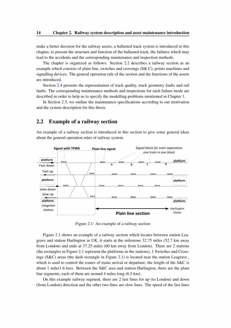
Figure 2.1: An example of a railway section
Figure 2.1 shows an example of a railway section which locates between station Lea-grave and station Harlington in UK, it starts at the milestone 32.75 miles (52.7 km awayfrom London) and ends at 37.25 miles (60 km away from London). There are 2 stations(the rectangles in Figure 2.1 represent the platforms in the stations), 1 Switches and Cross-ings (S&C) areas (the dash rectangle in Figure 2.1) is located near the station Leagrave ,which is used to control the routes of trains arrival or departure; the length of the S&C isabout 1 mile(1.6 km). Between the S&C area and station Harlington, there are the plainline segments, each of them are around 4 miles long (6.5 km).
On this example railway segment, there are 2 fast lines for up (to London) and down(from London) direction and the other two lines are slow lines. The speed of the fast lines
2.3. Railway assets 15
is from 90 mph (144.9 km/h) to 110mph (177.1km/h) ; the speed of the slow lines is from70 (112.7 km/h) to 90 mph(144.9 km/h).
The speed at the S&C is limited from 15 mph to 50 mph (24.15-80.5 km/h) whena train needs to change the railway line. Figure 2.1 shows the signals lamps with TrainProtection Warning System (TPWS), which are fitted at the entrance of each S&C areato prevent Signal Passed at Danger(SPAD). According to the structure of S&C in Figure2.1, each train may pass different routes at S&C, which contains different number of pointmachines. Independent of the route assigned to the train, the train will pass TPWS at eachS&C entrance. For this part of section, there are 12 pairs of point machines are installed inthe S&C area.
In this study a train is assumed to travel in one direction, i.e. up or down, but it canchange between fast lines and slow lines. Therefore S&C can be only used for trains tochange lines in the same direction. Signals without TPWS are installed on the plain lineto separate running trains to prevent the train collision accident, the section between twosignals is called “a signal block". 4-aspects signals are adopted to control the traffic (redmeans “stop", green is ok, yellow means caution and double yellow is caution and trainsshould stop); permanent speed restriction(PSR), temporary speed restriction (TSR) andpermissible maximum speed are indicated at the entry of each signal block.
In practice, the speeds in the adjacent blocks are not independent: for example, if thesignal at the entry of block C (in Figure 2.1) is double yellow, and thus the signal for blockB is yellow and for D is red. In order to simplify the operation of system, we assume thatthe speed of each train at different signal blocks are independent and it does not need toconsider the existence of another train on the running line.
2.3 Railway assets
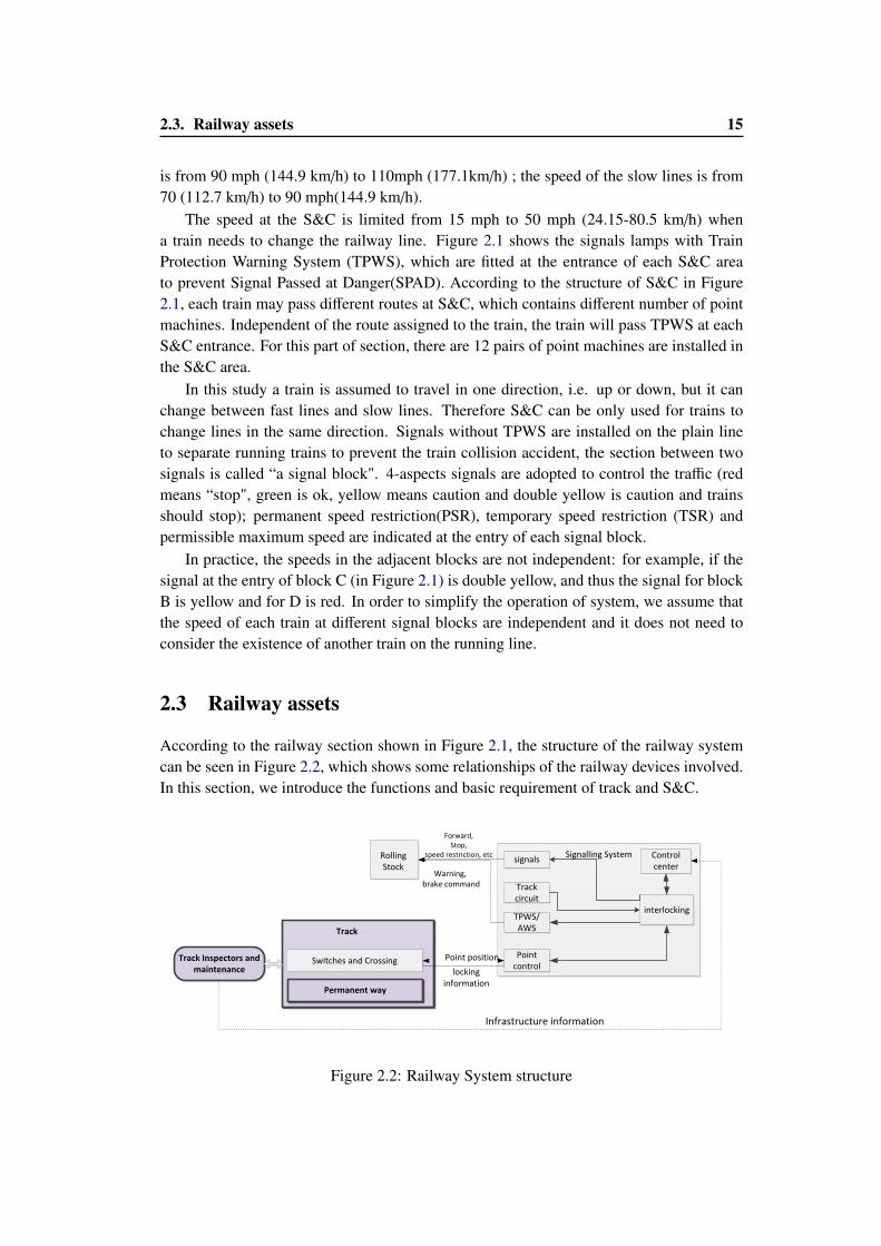
According to the railway section shown in Figure 2.1, the structure of the railway systemcan be seen in Figure 2.2, which shows some relationships of the railway devices involved.In this section, we introduce the functions and basic requirement of track and S&C.
Track
Switches and Crossing
Control center
interlocking
signals
Track circuit
Point control
TPWS/AWS
Track Inspectors and maintenance
Signalling SystemRolling Stock
Permanent way
Forward,Stop,
speed restriction, etc
Warning, brake command
locking
information
Point position
Infrastructure information
Figure 2.2: Railway System structure
16 Chapter 2. Railway system description and asset maintenance introduction
Figure 2.2 shows the major devices of signalling system: control centre, interlockingsystem, signals, track circuit, point machines and the protection system which containstrain protection warning system (TPWS) and automatic warning system (AWS). Track cir-cuit is used to identify the railway block occupied by a train and it is also a means ofbroken rail detection. The signal devices (including the 4-aspect signal lamps, track circuitand point machines) are assumed to be controlled by the interlocking system. Consideringthe time tables and the occupation of the railway line, control centre arranges a route andthe permissible speed (including permanent speed restriction (PSR), temporary speed re-striction (TSR) and maximum speed) for the coming train and then the interlocking systemsends the signal commands to signals, point movement commands to the point machinesand the moving authorities to the protection system.
In the following sections, we present some details of track, S&C and point machines.Track is the railway asset which the trains travel on. S&C can be considered as a specialtype of track, which contains movable and fixed rail. The movable rails are controlled bythe point machines and the point control commands come from the signalling system. Thepoint machine has to move the switch rail to the right position and maintain the correcttrack gauge in order to make sure a train can pass through safely.
2.3.1 Track
Track is one of the railway assets which support trains, it should maintain its gauge, cant,cross level and alignment of rails within the limits to make sure train can go through safely,these are the critical geometry parameters of track.
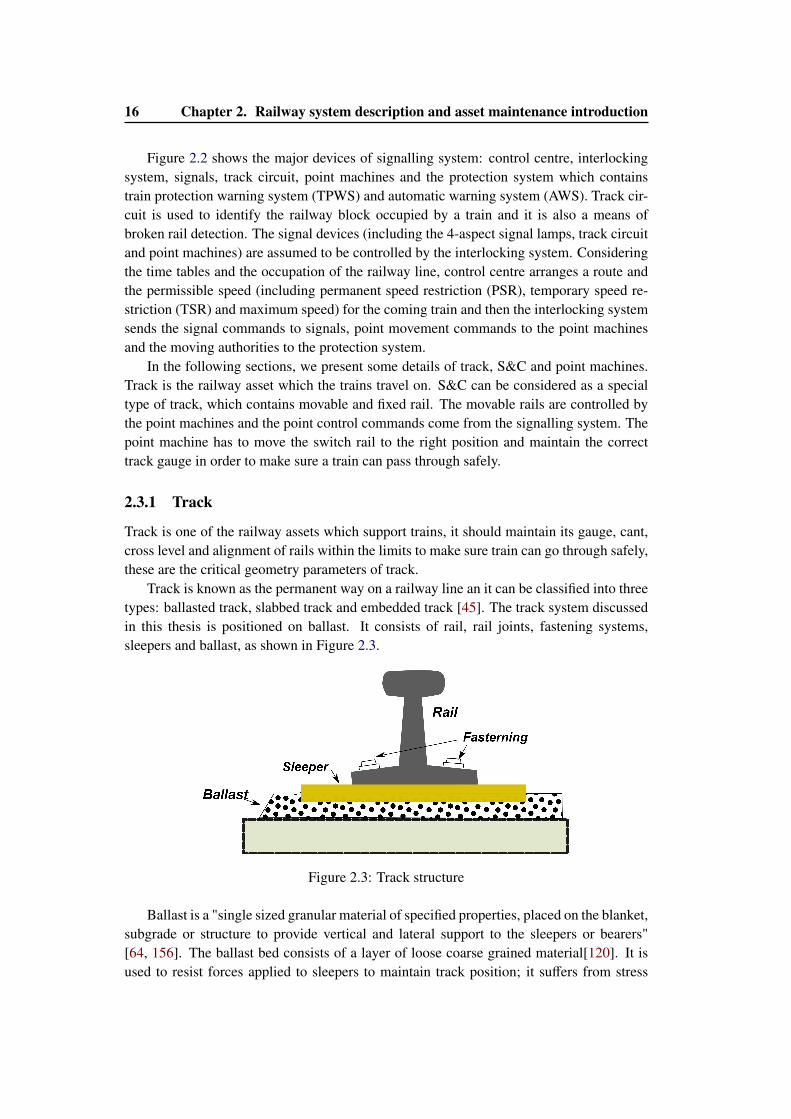
Track is known as the permanent way on a railway line an it can be classified into threetypes: ballasted track, slabbed track and embedded track [45]. The track system discussedin this thesis is positioned on ballast. It consists of rail, rail joints, fastening systems,sleepers and ballast, as shown in Figure 2.3.
Figure 2.3: Track structure
Ballast is a "single sized granular material of specified properties, placed on the blanket,subgrade or structure to provide vertical and lateral support to the sleepers or bearers"[64, 156]. The ballast bed consists of a layer of loose coarse grained material[120]. It isused to resist forces applied to sleepers to maintain track position; it suffers from stress
2.3. Railway assets 17
Wheels
Rail
Rail head
Rail gauge
Rail foot
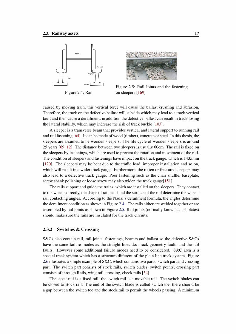
Figure 2.4: RailFigure 2.5: Rail Joints and the fasteningon sleepers [169]
caused by moving train, this vertical force will cause the ballast crushing and abrasion.Therefore, the track on the defective ballast will subside which may lead to a track verticalfault and then cause a derailment; in addition the defective ballast can result in track losingthe lateral stability, which may increase the risk of track buckle [103].
A sleeper is a transverse beam that provides vertical and lateral support to running railand rail fastening [64]. It can be made of wood (timber), concrete or steel. In this thesis, thesleepers are assumed to be wooden sleepers. The life cycle of wooden sleepers is around25 years [69, 12]. The distance between two sleepers is usually 60cm. The rail is fixed onthe sleepers by fastenings, which are used to prevent the rotation and movement of the rail.The condition of sleepers and fastenings have impact on the track gauge, which is 1435mm[120]. The sleepers may be bent due to the traffic load, improper installation and so on,which will result in a wider track gauge. Furthermore, the rotten or fractured sleepers mayalso lead to a defective track gauge. Poor fastening such as the chair shuffle, baseplate,screw shank polishing or loose screw may also widen the track gauge[151].
The rails support and guide the trains, which are installed on the sleepers. They contactto the wheels directly, the shape of rail head and the surface of the rail determine the wheel-rail contacting angles. According to the Nadal’s derailment formula, the angles determinethe derailment condition as shown in Figure 2.4 . The rails either are welded together or areassembled by rail joints as shown in Figure 2.5. Rail joints (normally known as fishplates)should make sure the rails are insulated for the track circuits.
2.3.2 Switches & Crossing
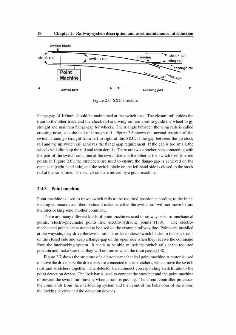
S&Cs also contain rail, rail joints, fastenings, bearers and ballast so the defective S&Cshave the same failure modes as the straight lines do: track geometry faults and the railfaults. However some additional failure modes need to be considered. S&C area is aspecial track system which has a structure different of the plain line track system. Figure2.6 illustrates a simple example of S&C, which contains two parts: switch part and crossingpart. The switch part consists of stock rails, switch blades, switch points; crossing partconsists of through Rails, wing rail, crossing, check rails [54].
The stock rail is a fixed rail; the switch rail is a movable rail. The switch blades canbe closed to stock rail. The end of the switch blade is called switch toe, there should bea gap between the switch toe and the stock rail to permit the wheels passing. A minimum
18 Chapter 2. Railway system description and asset maintenance introduction
Point
Machine
check rail
check rail
stock rail switch rail
switch blade
crossingwing rail
through rail
Switch part Crossing part
Figure 2.6: S&C structure
flange-gap of 100mm should be maintained at the switch toes. The closure rail guides thetrain to the other track and the check rail and wing rail are used to guide the wheel to gostraight and maintain flange-gap for wheels. The triangle between the wing rails is calledcrossing nose, it is the end of through rail. Figure 2.6 shows the normal position of theswitch; trains go straight from left to right at this S&C, if the gap between the up stockrail and the up switch rail achieves the flange-gap requirement. If the gap is too small, thewheels will climb up the rail and train derails. There are two stretcher bars connecting withthe pair of the switch rails, one at the switch toe and the other at the switch heel (the redpoints in Figure 2.6); the stretchers are used to ensure the flange-gap is achieved on theopen side (right hand side) and the switch blade on the left hand side is closed to the stockrail at the same time. The switch rails are moved by a point machine.
2.3.3 Point machine
Point machine is used to move switch rails to the required position according to the inter-locking commands and then it should make sure that the switch rail will not move beforethe interlocking send another command.
There are many different kinds of point machines used in railway: electro-mechanicalpoints, electro-pneumatic points and electro-hydraulic points [179]. The electro-mechanical points are assumed to be used on the example railway line. Points are installedat the wayside, they drive the switch rails in order to close switch blades to the stock railson the closed side and keep a flange-gap on the open side when they receive the commandfrom the interlocking system. It needs to be able to lock the switch rails at the requiredposition and make sure that they will not move when the train passes[138].
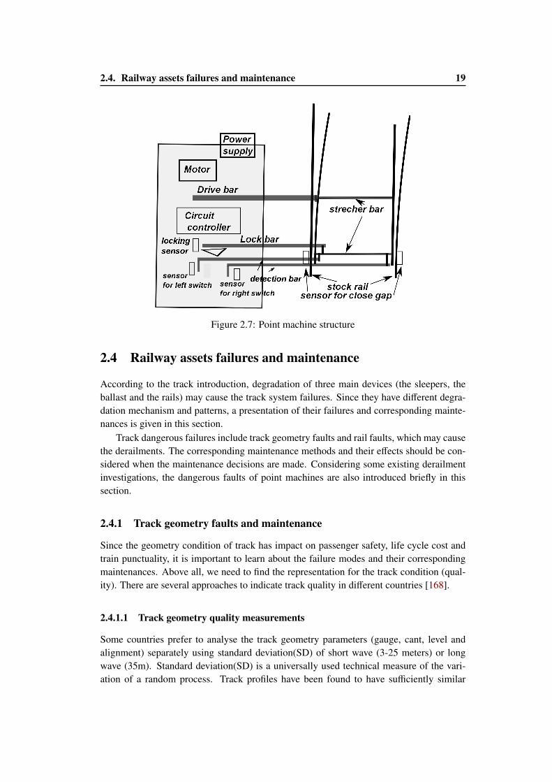
Figure 2.7 shows the structure of a eletronic-mechanical point machine.A motor is usedto move the drive bars; the drive bars are connected to the stretchers, which move the switchrails and stretchers together. The detector bars connect corresponding switch rails to thepoint detection device. The lock bar is used to connect the stretcher and the point machineto prevent the switch rail moving when a train is passing. The circuit controller processesthe commands from the interlocking system and then control the behaviour of the motor,the locking devices and the detection devices.
2.4. Railway assets failures and maintenance 19
Figure 2.7: Point machine structure
2.4 Railway assets failures and maintenance
According to the track introduction, degradation of three main devices (the sleepers, theballast and the rails) may cause the track system failures. Since they have different degra-dation mechanism and patterns, a presentation of their failures and corresponding mainte-nances is given in this section.
Track dangerous failures include track geometry faults and rail faults, which may causethe derailments. The corresponding maintenance methods and their effects should be con-sidered when the maintenance decisions are made. Considering some existing derailmentinvestigations, the dangerous faults of point machines are also introduced briefly in thissection.
2.4.1 Track geometry faults and maintenance
Since the geometry condition of track has impact on passenger safety, life cycle cost andtrain punctuality, it is important to learn about the failure modes and their correspondingmaintenances. Above all, we need to find the representation for the track condition (qual-ity). There are several approaches to indicate track quality in different countries [168].
2.4.1.1 Track geometry quality measurements
Some countries prefer to analyse the track geometry parameters (gauge, cant, level andalignment) separately using standard deviation(SD) of short wave (3-25 meters) or longwave (35m). Standard deviation(SD) is a universally used technical measure of the vari-ation of a random process. Track profiles have been found to have sufficiently similar
20 Chapter 2. Railway system description and asset maintenance introduction
statistical properties to random processes to enable a measure of the magnitude of track ir-regularities to be obtained from the standard deviation of the vertical and horizontal profiledata. This form of analysis provides track quality indices [64]:
σ =
√1m
Σ(a1 − a)2 (2.1)
σ is the standard deviation; a1 is the actual measures; a represents the average of themeasures; m is the number of measurements.
Some countries describe track quality with a synthesis indicator which includes all ofthe track geometry parameters (gauge, cant, level and twist). Track Quality Index(TQI)is used to indicate the track quality in China, Zimbabwe and so on. The general TQI isdefined in Equation 2.2:
T QI =
n∑i=1
aiδi (2.2)
δi is the track geometry parameters, such as the gauge, cants, level and alignment. ai is thecoefficient parameters. In China, Equation 2.2 is specified to be Equation 2.3, there are 7parameters (not only including the gauge, level, alignment and twist, but also SDs of eachrail surface for both left rail and right rail ) in the equation, and δi denotes the standarddeviation of the geometry parameters [191].
T QIchina =
7∑i=1
δi (2.3)
In Sweden, TQI is changed to be Equation 2.4 [56]:
T QIsweden = 150 − 100(δLL
δT H_LL− 2
δAC
δT H_AC)/3 (2.4)
δLL is the the average of the standard deviations of left and right profile;δAC is standarddeviations of the combined alignment and cross level. δT H_LL and δT H_AC represent thecomfort threshold of the parameters.
The above track quality representation focus on the track geometry and profile, butsometimes, track maintenance needs to consider the condition of the devices and henceSadeghi et al describe track quality considering both the geometry condition and the de-vices condition with Track Geometry Indicator (TGI) and Track Structure Indicator (TSI):[166].
TGI =2UI + T I + 6AI + GI
10(2.5)
TS I = (BCI, S CI,RCI) = 0.5CI(low) + 0.35CI(mid) + 0.15CI(high) (2.6)
Track Geometry Index (TGI) is similar to TQI, taking into account twist (TI), alignment(AI), gauge (GI) and unevenness (UI); these four parameters are calculated by the standarddeviation of the measured result.
TSI is used to indicate the average condition of the track structure. BCI, S CI and RCIare ballast, sleeper and rail condition indices and CI(low), CI(mid) and CI(high) are the
2.4. Railway assets failures and maintenance 21
lowest, medium and highest amounts for the condition indices of ballast, sleeper and railrespectively.
Furthermore, J synthetic coefficient is used in Polish railway which also considers thegauge, vertical, horizontal and twist parameters together [17]. Key Performance Indicator(KPI) is another track quality indicator which combines the plain line, switch and crossing,maintenances together [203].
According to the best practical experience, CEN standards adopt standard deviationsto indicate the track quality. In order to guarantee the safety, EN standard EN 13848-5requires three maintenance levels for the track geometry faults in order to guarantee therailway safety [55]:
• Immediate Action Limit (IAL): if the standard deviation exceeds this value, it re-quires taking measures to reduce the risk of derailment to an acceptable level. Thiscan be done either by closing the line, reducing speed or by correction of track ge-ometry.
• Intervention Limit (IL): the value, which, if exceeded, requires corrective mainte-nance in order that the immediate action limit shall not be reached before the nextinspection.
• Alert Limit (AL): the value requires that the track geometry condition is analysedand considered in the planned maintenance operations.
Even though EN13848-5 recommends three maintenance levels for track geometryfaults, there is not the mandated values for these geometry parameters; thus infrastruc-tures conductors have their own optimized maintenance thresholds considering the cost,the availability, the human sources and usages of maintenance machines.
In the following sections, the major geometry track faults, rail faults and their corre-sponding maintenance are presented.
2.4.1.2 Track gauge spread
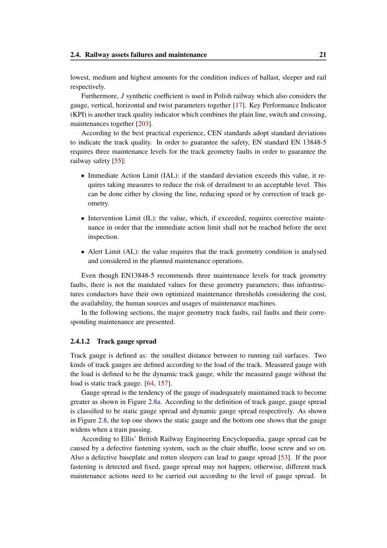
Track gauge is defined as: the smallest distance between to running rail surfaces. Twokinds of track gauges are defined according to the load of the track. Measured gauge withthe load is defined to be the dynamic track gauge, while the measured gauge without theload is static track gauge. [64, 157].
Gauge spread is the tendency of the gauge of inadequately maintained track to becomegreater as shown in Figure 2.8a. According to the definition of track gauge, gauge spreadis classified to be static gauge spread and dynamic gauge spread respectively. As shownin Figure 2.8, the top one shows the static gauge and the bottom one shows that the gaugewidens when a train passing.
According to Ellis’ British Railway Engineering Encyclopaedia, gauge spread can becaused by a defective fastening system, such as the chair shuffle, loose screw and so on.Also a defective baseplate and rotten sleepers can lead to gauge spread [53]. If the poorfastening is detected and fixed, gauge spread may not happen; otherwise, different trackmaintenance actions need to be carried out according to the level of gauge spread. In
22 Chapter 2. Railway system description and asset maintenance introduction
(a) Overhead view of track gauge spread
Wheel
Gauge
Gauge Spread
(b) Static track gauge and dynamic gaugespread
Figure 2.8: Track gauge spread
practice, we can carry out the following maintenance to control gauge spread:
Tie bar: a rod used to maintain the track gauge temporarily; in somecases, the mean time of tie-bar failure is around 60 days .
Spot-resleepering: replacement of the sleepers at the defective location.Track renewal: a term of maintenance work for a track segment consisting
of the rail replacement, sleepers replacement, ballast replace-ment and so on.
According to the requires in EN13848-5, gauge spread can be divided into 3 levels.For example, in UK, the standard static track gauge is 1435 mm and the tolerant dynamictrack gauge is 1465 mm. Therefore, level 1 of gauge spread defines to be at the range of1435-1465 mm; for this low gauge spread, the defect can be controlled by speed restrictionor restrain controls including tie-bar and spot re-sleepering. If the dynamic gauge exceeds1465mm (medium gauge spread), speed restriction and restrain controls should be carriedout to control the defects. If the gauge spread is high (the loaded gauge is over 1480mm),the line should be closed and the track should be renewed.
2.4.1.3 Track top and twist
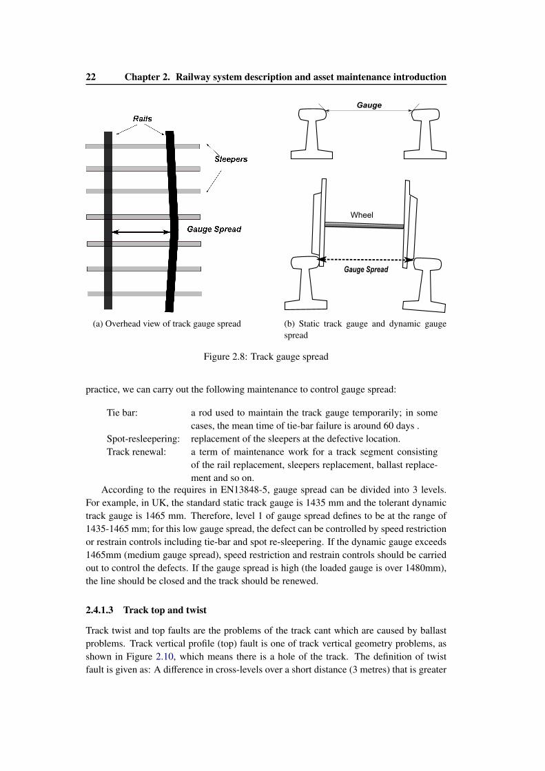
Track twist and top faults are the problems of the track cant which are caused by ballastproblems. Track vertical profile (top) fault is one of track vertical geometry problems, asshown in Figure 2.10, which means there is a hole of the track. The definition of twistfault is given as: A difference in cross-levels over a short distance (3 metres) that is greater
2.4. Railway assets failures and maintenance 23
TwistRail
Rail
short wave length (b)x
cant(x)cant(x-b)
Figure 2.9: Track twist
Track TopCant(x)
x
Rail
Rail
Figure 2.10: Track top fault
than a predetermined amount . As shown in Figure 2.9, the bold black lines represent thetracks, and the twist can be calculated as cant(x)-cant(x-b)[54], where cant is the differencein level between the rail head centres.
Twist can be caused by the uncontrolled poor ballast condition. There are 3 levels oftwists. A tamping can be carried out to control twist and top. For example, if the twistis between 1 in 126 and 1 in 199, the maintenance should be carried out in 10 days, andbetween 1 in 91 and 1 in 125, the track should be maintain in 36 hours. For worse situations,immediate line closure is needed.
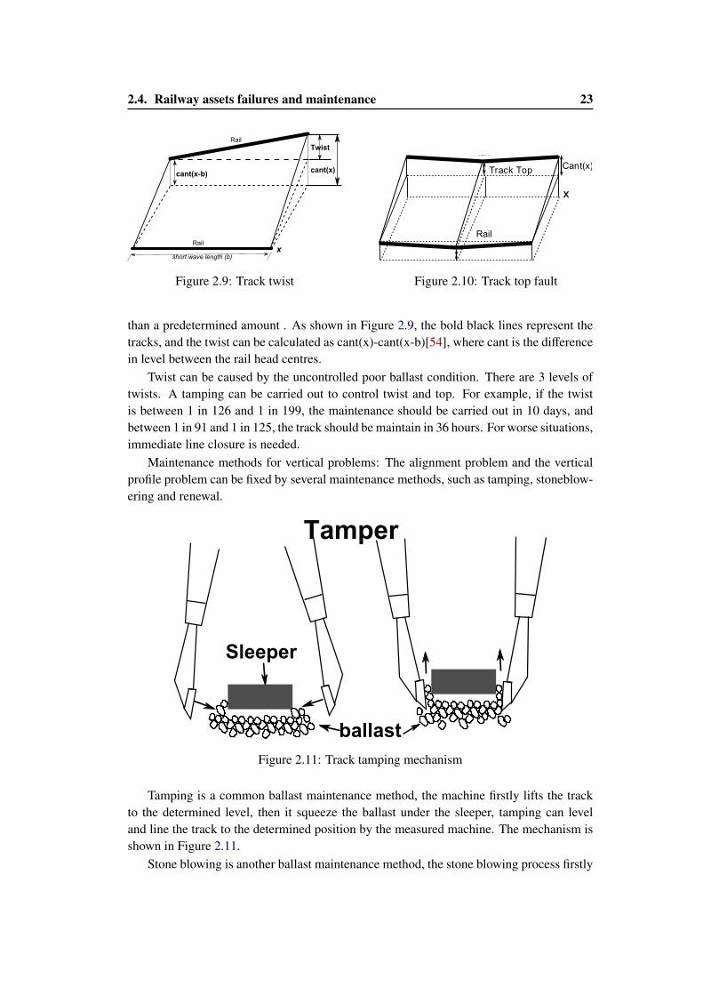
Maintenance methods for vertical problems: The alignment problem and the verticalprofile problem can be fixed by several maintenance methods, such as tamping, stoneblow-ering and renewal.
Tamper
Sleeper
ballast
Figure 2.11: Track tamping mechanism
Tamping is a common ballast maintenance method, the machine firstly lifts the trackto the determined level, then it squeeze the ballast under the sleeper, tamping can leveland line the track to the determined position by the measured machine. The mechanism isshown in Figure 2.11.
Stone blowing is another ballast maintenance method, the stone blowing process firstly
24 Chapter 2. Railway system description and asset maintenance introduction
lifts the sleeper to create a void, then the stone blower tube fits the grades into the void,when the sleeper is lowered onto the added stones, the process is completed as shown inFigure 2.12.
BALLASTS
SLEEPER
RAIL
Figure 2.12: Stone-blowing mechanism
Since the mechanical of tamping tool may damage the ballast, tamping makes newcontact point of the grades which may break down after the traffic loads. Compared tothe tamping, the ballast damage with the stoneblower is insignificant. Thus, the need forcleaning and replacing ballast is postponed. This effect is amplified by the fact that tampingis required more often than stoneblowing. Since stone blowing uses a consistent materialfor geometry adjustment, the geometry correction lasts longer with stoneblowing than withtamping. However, stoneblower cannot lift the wooden sleeper adequately and it cannot beused for S&C [44].
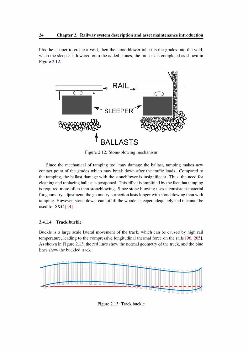
2.4.1.4 Track buckle
Buckle is a large scale lateral movement of the track, which can be caused by high railtemperature, leading to the compressive longitudinal thermal force on the rails [96, 205].As shown in Figure 2.13, the red lines show the normal geometry of the track, and the bluelines show the buckled track.
Figure 2.13: Track buckle
2.4. Railway assets failures and maintenance 25
Buckle can be fixed by slewing the track when the buckle is slight. In the case ofsignificant buckle, the traffic should be stopped and the renewal should be carried out assoon as possible.
2.4.2 Rail faults and maintenance
According to the rail fault location on the track, Rail fault can be classified into two types[155]:
• Broken rail joint: if the breakage exists at the fish-plated joint or at the welded joint,it is defined as broken rail joint,
• Broken rail: if the breakage occurs more than 1.8m away from joint, it is broken rail.
Broken rail and rail joint can be caused by rolling contact fatigue and different kinds of railcracks inside the rail.
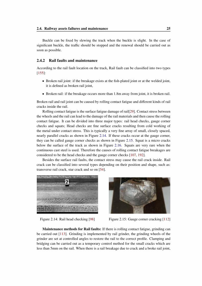
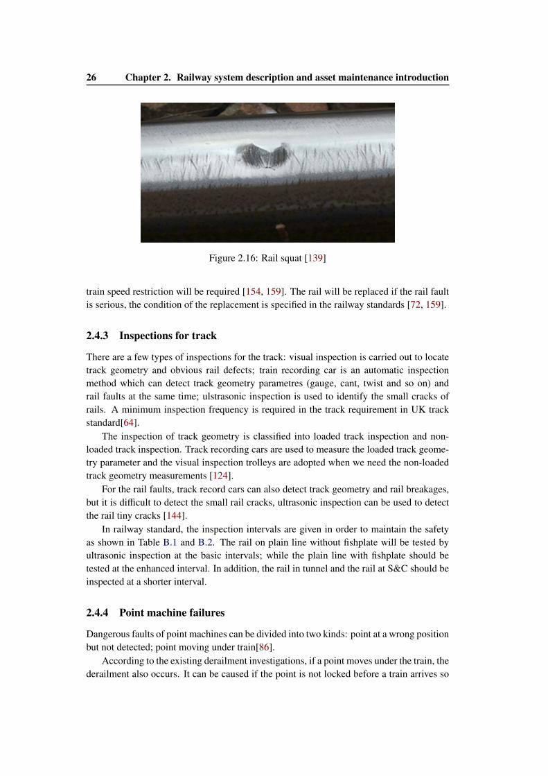
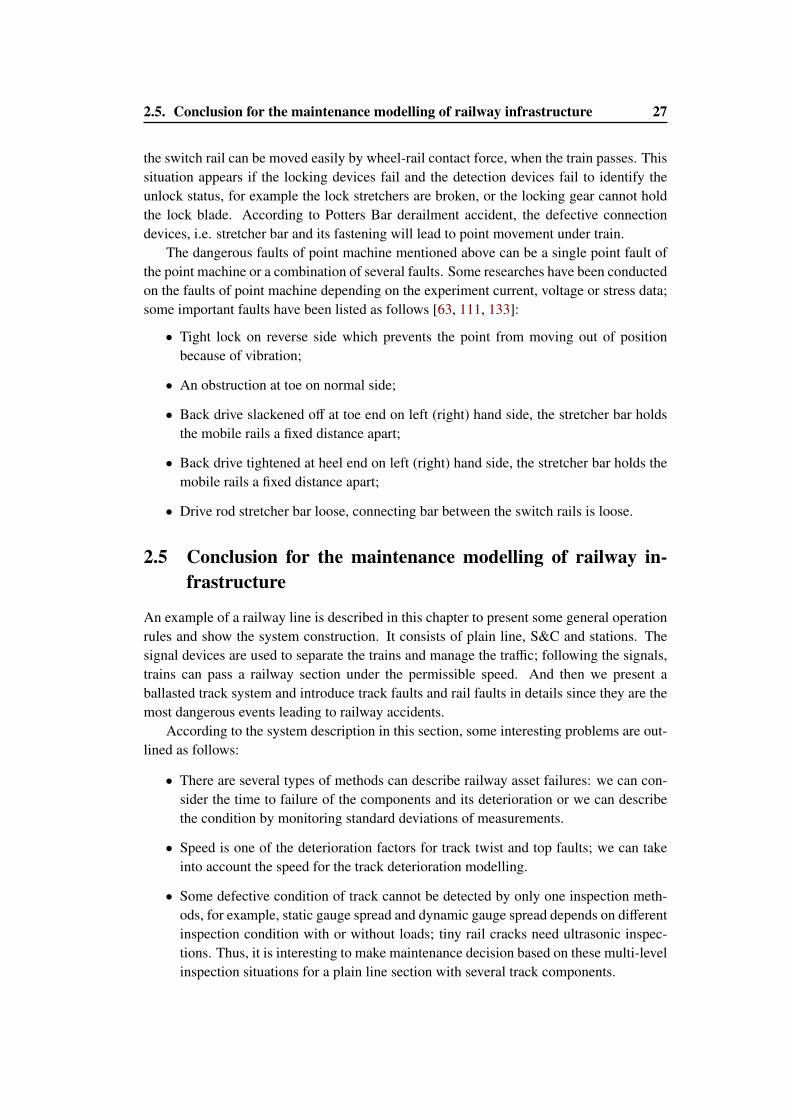
Rolling contact fatigue is the surface fatigue damage of rail[29]. Contact stress betweenthe wheels and the rail can lead to the damage of the rail materials and then cause the rollingcontact fatigue. It can be divided into three major types: rail head checks, gauge cornerchecks and squats; Head checks are fine surface cracks resulting from cold working ofthe metal under contact stress. This is typically a very fine array of small, closely spaced,nearly parallel cracks as shown in Figure 2.14. If these cracks occur at the gauge corner,they can be called gauge corner checks as shown in Figure 2.15. Squat is a micro cracksbelow the surface of the track as shown in Figure 2.16. Squats are very rare when thecontinuous cast steel is used. Therefore the causes of rolling contact fatigue breakages areconsidered to be the head checks and the gauge corner checks [107, 192].
Besides the surface rail faults, the contact stress may cause the rail crack inside. Railcrack can be classified into several types depending on their position and shape, such as:transverse rail crack, star crack and so on [54].
Figure 2.14: Rail head checking [98] Figure 2.15: Gauge corner cracking [112]
Maintenance methods for Rail faults: If there is rolling contact fatigue, grinding canbe carried out [113]. Grinding is implemented by rail grinder, the grinding wheels of thegrinder are set at controlled angles to restore the rail to the correct profile. Clamping andbridging can be carried out as a temporary control method for the small cracks which areless than 5mm on the rail. When there is a rail breakage due to crack and a broke rail joint,
26 Chapter 2. Railway system description and asset maintenance introduction
Figure 2.16: Rail squat [139]
train speed restriction will be required [154, 159]. The rail will be replaced if the rail faultis serious, the condition of the replacement is specified in the railway standards [72, 159].
2.4.3 Inspections for track
There are a few types of inspections for the track: visual inspection is carried out to locatetrack geometry and obvious rail defects; train recording car is an automatic inspectionmethod which can detect track geometry parametres (gauge, cant, twist and so on) andrail faults at the same time; ulstrasonic inspection is used to identify the small cracks ofrails. A minimum inspection frequency is required in the track requirement in UK trackstandard[64].
The inspection of track geometry is classified into loaded track inspection and non-loaded track inspection. Track recording cars are used to measure the loaded track geome-try parameter and the visual inspection trolleys are adopted when we need the non-loadedtrack geometry measurements [124].
For the rail faults, track record cars can also detect track geometry and rail breakages,but it is difficult to detect the small rail cracks, ultrasonic inspection can be used to detectthe rail tiny cracks [144].
In railway standard, the inspection intervals are given in order to maintain the safetyas shown in Table B.1 and B.2. The rail on plain line without fishplate will be tested byultrasonic inspection at the basic intervals; while the plain line with fishplate should betested at the enhanced interval. In addition, the rail in tunnel and the rail at S&C should beinspected at a shorter interval.
2.4.4 Point machine failures
Dangerous faults of point machines can be divided into two kinds: point at a wrong positionbut not detected; point moving under train[86].
According to the existing derailment investigations, if a point moves under the train, thederailment also occurs. It can be caused if the point is not locked before a train arrives so
2.5. Conclusion for the maintenance modelling of railway infrastructure 27
the switch rail can be moved easily by wheel-rail contact force, when the train passes. Thissituation appears if the locking devices fail and the detection devices fail to identify theunlock status, for example the lock stretchers are broken, or the locking gear cannot holdthe lock blade. According to Potters Bar derailment accident, the defective connectiondevices, i.e. stretcher bar and its fastening will lead to point movement under train.
The dangerous faults of point machine mentioned above can be a single point fault ofthe point machine or a combination of several faults. Some researches have been conductedon the faults of point machine depending on the experiment current, voltage or stress data;some important faults have been listed as follows [63, 111, 133]:
• Tight lock on reverse side which prevents the point from moving out of positionbecause of vibration;
• An obstruction at toe on normal side;
• Back drive slackened off at toe end on left (right) hand side, the stretcher bar holdsthe mobile rails a fixed distance apart;
• Back drive tightened at heel end on left (right) hand side, the stretcher bar holds themobile rails a fixed distance apart;
• Drive rod stretcher bar loose, connecting bar between the switch rails is loose.
2.5 Conclusion for the maintenance modelling of railway in-frastructure
An example of a railway line is described in this chapter to present some general operationrules and show the system construction. It consists of plain line, S&C and stations. Thesignal devices are used to separate the trains and manage the traffic; following the signals,trains can pass a railway section under the permissible speed. And then we present aballasted track system and introduce track faults and rail faults in details since they are themost dangerous events leading to railway accidents.
According to the system description in this section, some interesting problems are out-lined as follows:
• There are several types of methods can describe railway asset failures: we can con-sider the time to failure of the components and its deterioration or we can describethe condition by monitoring standard deviations of measurements.
• Speed is one of the deterioration factors for track twist and top faults; we can takeinto account the speed for the track deterioration modelling.
• Some defective condition of track cannot be detected by only one inspection meth-ods, for example, static gauge spread and dynamic gauge spread depends on differentinspection condition with or without loads; tiny rail cracks need ultrasonic inspec-tions. Thus, it is interesting to make maintenance decision based on these multi-levelinspection situations for a plain line section with several track components.
28 Chapter 2. Railway system description and asset maintenance introduction
• Preventive maintenance for railway asset cannot maintain the component as good asnew; the effects after maintenance may depend on the number of implemented repairactions or the maintenance methods, or on the asset materials.
• According to some railway standards, delayed preventive maintenance is allowed inrailway maintenance, for example, the maintenance of track twist can be schedulesin one month.
• The example in Section 2.2 describes a railway section and some operation rules init. The maintenance rules of track faults also require operation co-ordination, such asline closure, speed restrictions. To ensure the safety, the traffic needs to slow downin the defective section or to stop beyond the section.
In order to solve these problems, some existing models for the deteriorations, inspec-tions and maintenance policies are introduced in Chapter 3 to learn from some relatedexisting researches on railway maintenance in the literature.

Chapter 3
Deterioration/failure andmaintenance models for railway
application: state of the art
Contents3.1 Introduction . . . . . . . . . . . . . . . . . . . . . . . . . . . . . . . . . 293.2 Failure modelling . . . . . . . . . . . . . . . . . . . . . . . . . . . . . . 30
3.2.1 Deterministic deterioration model . . . . . . . . . . . . . . . . . . 30
3.2.2 Stochastic deterioration modelling . . . . . . . . . . . . . . . . . . 31
3.3 Inspection policy . . . . . . . . . . . . . . . . . . . . . . . . . . . . . . . 343.4 Maintenance policy . . . . . . . . . . . . . . . . . . . . . . . . . . . . . 35
3.4.1 Maintenance effects . . . . . . . . . . . . . . . . . . . . . . . . . 35
3.4.2 Maintenance policies for single component . . . . . . . . . . . . . 36
3.4.3 Maintenance modelling for multi-component . . . . . . . . . . . . 36
3.5 Railway risk modelling . . . . . . . . . . . . . . . . . . . . . . . . . . . 383.6 Conclusion for the existing failures and maintenance models for railway
assets management . . . . . . . . . . . . . . . . . . . . . . . . . . . . . . 38
3.1 Introduction
In this thesis, we want to work on the maintenance modelling for railway assets. Regardingto the system description in Chapter 2, we can describe the health of track by standarddeviation of the short wave measurements; infrastructure conductors have their freedom toset the preventive maintenance threshold but they should follow the mandated correctivemaintenance threshold in the standards. In addition, inspections for the track condition arecarried out depending on different track types, materials and operation modes.
The existing models for deteriorations, inspection and maintenance are presented inthis section, especially the models for railway applications.
There are several kinds of description for failure processes which have different char-acteristic in the modelling. Some maintenance strategies are not suitable for some special
30Chapter 3. Deterioration/failure and maintenance models for railway application:
state of the art
failure processes. We review the existing researches in the literature which work on thedeteriorations, maintenance modelling and optimization, especially the researches on therailway industry.
In section 3.2, we summarize the existing failure models in order to help us to learnabout the properties of the deteriorations and their application. Section 3.3 summarizessome inspection policies in the literature. Section 3.4 reviews the maintenance policies forthe single component and for the multiple component. In section 3.5, Applications of Faulttree and Petri Net in risk analysis are reviewed.
3.2 Failure modelling
Railway systems consist of several kinds of devices, they suffer of several kinds of fail-ures, such as the aging behaviours, the wearing on the rail surface, the shocks which maycause rail breakages and so on. In this section, we want to investigate some existing failuremodels; depending on the different failure models, different maintenance policies can beadopted on the system, and then these policies have different effects on the system perfor-mances, such as maintenance cost, system risks and system availability.
3.2.1 Deterministic deterioration model
Some researchers have been concerned in the relationship between the factors (such asloads, speed, materials, temperature and so on) and the deterioration. The deterministicdeterioration models describe the average deterioration according to the environment, ma-teriel and operation in railway asset failure researches.
Kish et al. describe track buckle using a linear equation, which reveals that the trackbuckle index depends on Young’s Module, rail temperature and train speed [96]. Similarly,another linear equation is proposed to predict the rolling contact fatigue index of the railsaccording to the stress and the radius of the rail[51].
In order to model the significant deterioration evolutions of track deterioration, a gen-eral form of a power function is used to describe the deterioration condition of track. Trafficload and train speed are considered to be the main factors of these deteriorations. A trackdeterioration index can be calculated by a power function of the tonnage of the line, theaxle load and the train speed of the line [220]. Another deterioration model of switchesand crossing is an extension of the power function for a plain line, it also depends on thetonnage, the speed, the switch angle and the solid quality [221].
Sadeghi et al. suppose a track deterioration model considering the environment factorsof the track, Track Quality Indices (TQI) are used in [166, 167], which is an integer rep-resentation of track quality. However, the index cannot show the relationship between thedeterioration and maintenances. Westgeest et al. propose a regression model containingKPIs to describe degradation of track geometry depending on the local circumstances andthe Key Performance Indication(KPI) maintenance models, where KPI is used to describethe track quality with a certain length [203]. The linear regression model which is obtainedby regression analysis according to the observation data was used to relate the deteriorationto the tonnage, tamping, subsoil and switches.[4]
3.2. Failure modelling 31
These deterministic models describe the relationship between the factors (environment,physical characters and structure) and deterioration. Even though the evolution againsttime can be described in these models, they lack of ability to model the variations of theevolution since the deterioration increments are determined and cannot model the varieddeteriorations behaviours probability.
3.2.2 Stochastic deterioration modelling
Stochastic deterioration models are adopted to describe the uncertain behaviours and statesbased on time. In contrast, the deterministic model, the state or condition at time t is notknown and we can only predict the probability of the occurrence of the states.
3.2.2.1 Component lifetime models
Lifetime distributions offer a first solution to model the probabilistic failure behaviour ofan item. They only consider the binary states of the system and describe the probabilityof the failure occurrences at time t, to this extent they cannot be considered strictly asdeterioration models, but some of them can nevertheless captures ageing properties throughan increasing failure rate of the item resulting from its deterioration.
The most simple lifetime model is the exponential distribution because the failure rateat any time is the same and it is memoryless. But it cannot model a distribution with anincreased or decreased failure rate. Weibull distribution (as shown in Equation 3.1) is usedwidely to describe the deterioration of the ballast [5, 7, 146, 28] , the aging behaviour ofsignalling devices[9], the residual life function of rail defect [113] and the occurrence ofthe rail defect at time t [137], because Weibull distribution can represent many kinds ofshapes by choosing different parameters, and hence many different ageing behaviours.
F(t) = 1 − exp(−(tη
)β) (3.1)
There are two parameters in Weibull distribution. β is the shape parameter and η is thescale parameter. When β = 1, Weibull distribution turns to be exponential distribution.According to the paper [11], using a Weibull distribution with two parametres is a betterway to model the failure process of track with tampering in the railway.
As already outlined, with the lifetime distribution models, we can predict the failureprobability at time t, however, we cannot get more detailed information from them formaintenance decision making.
3.2.2.2 P-F interval and delay time concept
We can only consider two states in the lifetime model: failed or worked; in some cases,before the devices fail, the devices have abnormal states between good and failure, whichcan be detected by inspections. These defective states help to schedule the inspection andpreventive maintenance and thus we can take these states into account for the maintenance.
To describe the defective states and the corresponding maintenance, two similar failureprocess models are introduced in the literature:
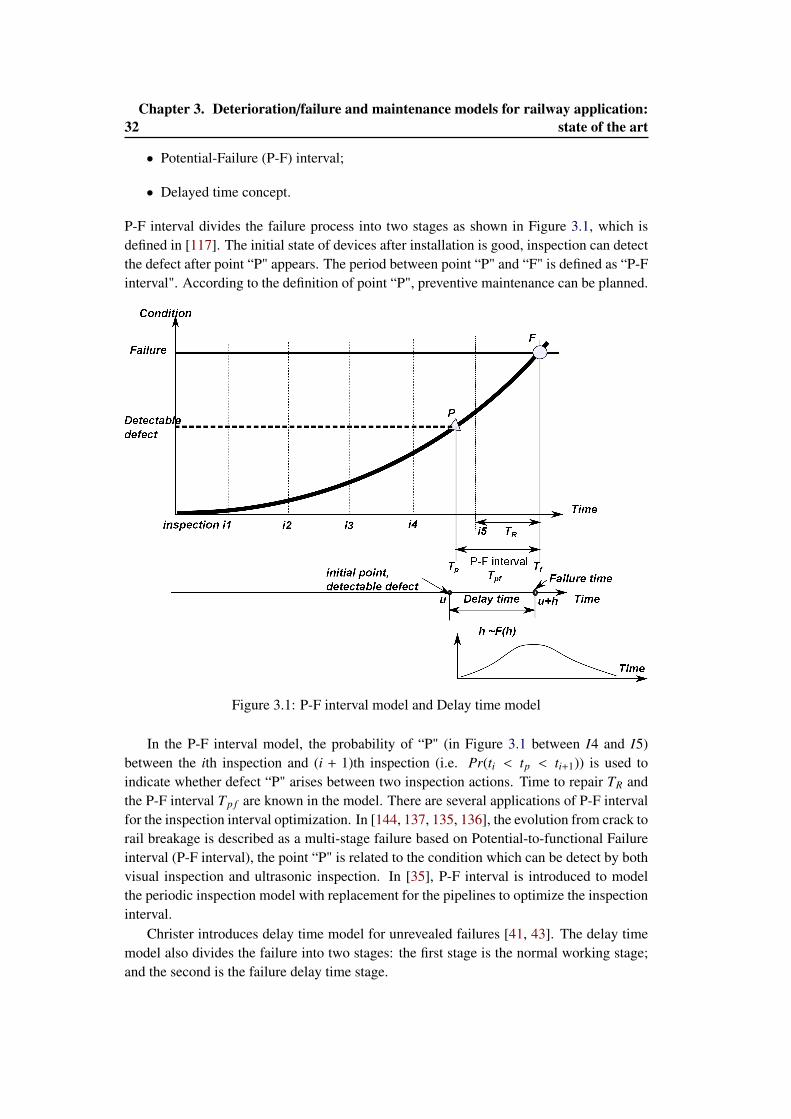
32Chapter 3. Deterioration/failure and maintenance models for railway application:
state of the art
• Potential-Failure (P-F) interval;
• Delayed time concept.
P-F interval divides the failure process into two stages as shown in Figure 3.1, which isdefined in [117]. The initial state of devices after installation is good, inspection can detectthe defect after point “P" appears. The period between point “P" and “F" is defined as “P-Finterval". According to the definition of point “P", preventive maintenance can be planned.
Time
initial point,
detectable defect
Figure 3.1: P-F interval model and Delay time model
In the P-F interval model, the probability of “P" (in Figure 3.1 between I4 and I5)between the ith inspection and (i + 1)th inspection (i.e. Pr(ti < tp < ti+1)) is used toindicate whether defect “P" arises between two inspection actions. Time to repair TR andthe P-F interval Tp f are known in the model. There are several applications of P-F intervalfor the inspection interval optimization. In [144, 137, 135, 136], the evolution from crack torail breakage is described as a multi-stage failure based on Potential-to-functional Failureinterval (P-F interval), the point “P" is related to the condition which can be detect by bothvisual inspection and ultrasonic inspection. In [35], P-F interval is introduced to modelthe periodic inspection model with replacement for the pipelines to optimize the inspectioninterval.
Christer introduces delay time model for unrevealed failures [41, 43]. The delay timemodel also divides the failure into two stages: the first stage is the normal working stage;and the second is the failure delay time stage.
3.2. Failure modelling 33
In Figure 3.1 the label u means the initial point of the defects and h means the delaytime to failure and follows a distribution F(h). If there are inspections during[u, u + h],the defect can be observed and the maintenance activities can be carried out to prevent thefailures. If the defective point u arrives with a rate λ, the expected number of failures canbe calculated as: E(N f (t)) =
∫ t0 λF(h)dh
Christer et al. demonstrate that if the initial state arrival has the Markov property,delay time concept and semi-Markov model has the same results, while if the arrival is notMarkovian, the semi-Markov model may lead to the wrong estimation of the maintenancecost, but delay time concept can be used in this situation regardless of the Markov property[42]. The differences between P-F interval and delay time concept are discussed in [197,194].
The delay time model is useful for optimising inspection planning according to theinitial point arrival time; furthermore, some extensions such as three-stages delay timemodels, nested-inspection policies are introduced to fit the practical situations[13, 104,195, 201, 210, 58, 130].
3.2.2.3 Models for deterioration
With the development of inspection technology, more data are available than before. Thesecollected data cannot only indicate the binary state or the three stages process but alsoreveal the exact condition of the monitored system. To describe the evolution indicated bythe monitoring and to use them in maintenance decision making purpose, models for thedeterioration process are needed.
Some damages are due to discrete events such as shocks: if the damage size is constant,Poisson process can be used to model the deterioration process, Shafiee et al. consider thetrack deterioration depending on the usages which follows a non-homogeneous PoissonProcess [171]; if the damage size is random, Compound Poisson Process can be used [14,90, 62, 78, 180].
If we consider the aging process, wearing process and other continuous processbetween two maintenances, we need to describe the gradual deterioration. Quirogaet al proposed a stochastic model for track geometry deterioration. The deteriorationprocess assumes that the evolution between two tamping is exponentially distributed(Ae(bn(t−tn)),where bn follows a normal distribution bn ∼ LN(µb(n), σ2
b(n))), tnis the timeof the last tamping and the measurement noise is εn(t) ∼ N(0, σ2
ε), A is denoted the stateafter tamping [148, 147]. Meier et al propose a Gamma process to describe the track geom-etry deterioration[114]. VanNoortwijk summarize the application and maintenance modelsbased on Gamma process [182]. In [183, 184], the gradual deterioration based on a Gammaprocess is compared to the corresponding lifetime model. Vale et al. propose track deteri-oration model based on Dagum probabilistic distribution for condition-based maintenance[181].
If two failure modes, both of which follows a Gamma process, are considered for themaintenance, a bivariate Gamma process is proposed[115]. If the environments factorsare taken into account for the deterioration, the parameters of Gamma process (such asthe shape parameter α) needs to change and represent the impact of the factors on the
34Chapter 3. Deterioration/failure and maintenance models for railway application:
state of the art
deterioration process [48, 47, 84].
3.3 Inspection policy
Inspections are used to identify the component or system condition/state. In practice, sev-eral kinds of inspections are possible, depending on the monitoring time, the inspection canbe classified to be the continuous monitoring and the discrete inspection; depending on thecapability, inspections are classified to be perfect and imperfect (full inspection or partialinspection).
Based on the deterioration process, a perfect inspection can be also described as astochastic process. In some cases, the imperfect inspection is modelled by introducing acombination of real measured condition and a noise, for example, another process com-bined by the original deterioration process with a normally distributed measurement errors[91].
Some researches introduce the detection probability p to indicate the inspectioncapability[210, 211]. In [20], Berrade et al assume the inspection is imperfect: a prob-ability of positive responses for failure and a probability of the false alarms are introducedto model the inspection results.
With the P-F interval and the delay time model , defective states are introduced to dividethe failure process to be detectable and undetectable. They can model the non-Markovianassumptions for the defect arrivals. The inspection may incorrectly identify the errors orthey may ignore the errors, these two situations are represented by a probability p and qbefore and after the initial point arrives in delay time model [59].
The safety critical equipments consists of several parts, partial inspections for someparts and the full inspection is scheduled for the whole equipments; in addition, the de-pendent failures are also considered in the model. Pascual et al. propose a ρβ diagnosecoverage model for the complex safety system, ρ indicates the defect detected probabilityby partial inspection and β is used to represent the dependent failure [134].
If there is the continuous monitoring, the component state can be modelled as a revealedfailure[18, 37].
Inspection performance interval for discrete inspection is another issue in the modellingsince the different inspection schemes lead to different maintenance strategies and resultsdifferent effects of maintenances. Regularly, we plan the periodic inspection to monitorcomponent states, and the inspection intervals are the maintenance decision variables [177].
Age-based or time dependent inspection policies are discussed in the literature [33].According to the collective data, inspection can be planned according to the previous stateor the time: Golmakani et al. apply an age based inspection policy for the condition basedmaintenance [67, 68].
Once the devices suffer to different failure modes which can be detected by differentinspection methods, multi-level inspections are scheduled for the devices, the optimizationfor the nest inspection planning are discussed based on delay time concept [193, 195, 196,199]. Ferreira et al propose a decision model to optimize the periodic inspection intervalbased on delay time concept for multiple evaluation indices[58].
3.4. Maintenance policy 35
An inspection scheme depending on the cumulative distribution of Q value of trackgeometry quality is proposed, taking into account the inspection interval and the tampinghorizon after inspections to find an optimized inspection interval and frequency [10].
If the observed track quality data can indicate the component state, periodic or non-periodic inspections can be scheduled. The observed states by periodic inspection canbe modeled as a semi-regenerative process [114]. Based on the precise inspection data,inspection interval can be scheduled as non-periodic according to the observed states [32,71, 16, 212, 215, 97].
3.4 Maintenance policy
With inspection for unrevealed failures, renewal or corrective maintenance are carried outto prevent the component failures and to maintain the system in an acceptable operatingcondition. In the railway system, we need to make decision for maintenance, in [74], adecision making process is proposed. There are thousands of maintenance policies, some ofthem are suitable for general applications, while some of them are proposed for the specialsystem. Wang summarizes the major maintenance policies and gives their advantages anddisadvantages [188].
3.4.1 Maintenance effects
Similar to inspection models, maintenance actions can be classified into three types accord-ing to their effects: perfect maintenance, imperfect maintenance and minimal maintenance[163]. After a perfect maintenance (replacement or renewal), the component is fixed to theoriginal new state. An imperfect maintenance cannot repair the component to be "as goodas new" but better than the minimal repair. A minimal repair is a kind of repair which fixescomponent to a state as bad as old, under which it can continue work but it is not goodenough for a long time.
The maintenance effects are the key issue in maintenance modelling because they mayintroduce different deterioration models, they can lead to the limited opportunity of mainte-nances. In order to describe the maintenance effects, several methods are considered.Phamet al. introduce the imperfect maintenance models between 1985 to 1996 [142].
If the failure models focus on the lifetime, virtual age is a method to describe theimperfect maintenance [52]. Virtual age model is suitable for the components which sufferfrom an aging process, it assumes that the maintenance can either reduce the virtual agesas a proportional to the value before maintenance or reduce the increment of the virtual age[94, 141]. The rail grinding effect is described by a reduced amount of virtual age model[113].
Some imperfect maintenance actions may change the failure rate after the maintenance[38, 81]. Both repairable and unrepairable failure modes are considered in [206], they as-sumed that the hazard rate of the maintainable mode increases as a consequence of thedeterioration of the unrepairable failure mode. Wang et al consider the imperfect mainte-nance represented by decreased functional time and increased the maintenance time [189].
36Chapter 3. Deterioration/failure and maintenance models for railway application:
state of the art
3.4.2 Maintenance policies for single component
Several kinds of maintenance policies are discussed in the literature, such as reliability-centred maintenance [138], risk-based maintenance[100, 82], time-based maintenance,age-based maintenance and condition-based maintenance. The probability to implementeither one of these strategy depends on the level of information available on the system.[3]. The choice of a maintenance strategy is also a strategy for a company.
If the monitoring data can just indicate the working state (OK or failed), time-based orage-based maintenance can be scheduled based on the failure time analysis [3, 126]. Theproblem of time-based or age-based maintenance (ABM) is to find out a optimized mainte-nance interval TM to get a minimal maintenance cost. For the replacement strategies in rail-way maintenance, Antoni et al compare age-based replacement to a replacement strategybased on the number of failures for the signalling devices, which follows a Weibull life-time distribution, one of the replacement is age-based, another one is carried out dependingon the number of defects [8]. Shafiee et al propose a maintenance policy considering theusage and they compare the age-usage policy to the age-based policy, and the numericalresults show that the combination policy (i.e.age-usage maintenance policy) can reduce theservice cost [171]. A Proportional hazard model is used to describe the aging process withincreasing rate of single component[110]. Age-based maintenance is extended to discussthe minimal repair for a system which has two types of failures [89]; Huynh et al. alsoconsider age-based minimal repair for the competing failure modes [85].
Condition-based maintenance (CBM) can be performed if the inspection can collect thedeterioration state of the component [71, 70, 200]. The preventive maintenance thresholdcan be one of the maintenance decision variables, which can implicitly predict the lifetimeof the equipments. In 1995, Fararooy propose a condition-base maintenance for the "trainstop" devices next to the signal lamps by monitoring the air pressure[57]. Condition-basedmaintenance strategies are also adopted to consider the maintenance for the combined fail-ure process [27, 36, 216] and the failure process exposed to a dynamic environments[209].
3.4.3 Maintenance modelling for multi-component
All of the issues mention in the previous sections such as the deterioration model, theinspection and maintenance model can be applied to a multi-component system. In order tomodel a multi-component system, we need to consider the system structure, the interactionbetween the components, the common effects of environments on the components and soon; all of these issues are summarized as the structural dependence, economic dependenceand stochastic dependence [46, 123].
In the literature, some researches consider the dependence between components. Themost basic stochastic dependence in the multi-component modelling is the common causefailures (CCF), a basic model divides the component with common failure to be two part,one is part represents the independent failure and another one is the dependent failure,then the system is re-constructed according to the settings [6, 163]. α factor and β factormodels are two important extensions for the common cause failures. In the recent years,lèvy copulas is used to describe the stochastic dependence for the deterioration models [92,
3.4. Maintenance policy 37
102]. Some researches considers the components in the system are structural dependencies,for instance, effect of maintenance for a series system with correlated failure [190] and aredundancy for a series-parallel system [127].
Grouped maintenance takes advantage of economic dependence for multi-componentsystem. Block replacement is one of the grouping policy which implements a preventivemaintenance for all the component in a block group. Since the time tracking for the com-ponent is complicated and difficult, Li et al introduce a modified age-based replacement[101]; with the bivariate stochastic process, a condition-based block replacement is pro-posed for the dependent failures without knowing the correlation. Castanier et al. discussthe condition-based maintenance grouping for a series system and they show that a newthreshold for the system can reduce the long-term maintenance cost [34]. An age-basedgrouping for multi-series system is proposed to optimize the group preventive interval[170]. In [2], they summarize some existing researches about the opportunistic mainte-nance in order to save system downtime and maintenance cost. A condition-based group-ing for opportunistic maintenance is discussed in [208]. In some cases, the planned fixedgrouping needs to be adjusted according to the environments or operation context, Bouvardet al. propose a dynamic maintenance grouping decision model for the vehicles based onthe monitoring information[23].
There are two kinds of opportunistic maintenance considered for railway asset main-tenance: one is the combination of components in the same railway track segment; theother one is the combination of component renewal in adjacent track section. Luis et al.[28] concludes the opportunistic maintenance model to combine the component renewal inadjacent track section.
The maintenance modelling for multi-component mentioned above considers struc-tural dependence, economic dependence and stochastic dependence; however these are notenough for the railway network maintenance strategies, the allocation of the maintenanceactivities and the arrangement of crews should be taken into account, as well as the op-eration of the trains. Therefore, it is interesting to find an optimal maintenance strategyfor a global railway network, concerning system functions, failures, railway operationsand maintenance configurations. Some global maintenance schedules are proposed for therailway network in [125, 132, 116]. There is a preventive railway scheduling for a routinemaintenance work and the major preventive maintenance activities, in order to save the costof the preventive maintenance [140, 164] and the whole system downtime [77], the main-tenance activities are wished to be carried out as much close as possible[25], but in thisresearch it is the scheduling for one segment jobs. And then there is an optimal schedulingof a railway region taking the residual life of the devices and the travelling time of theteams into account[207]; and two scenarios of the segments of the track are considered toimprove the maintenance models[145].
Since we need to consider the functions, failures and maintenance configurations forthe railway maintenance modelling, it is important to pay attention to the model the failureswhich may lead to the accident, and hence the railway network maintenance model mayneed to describe the possible risks.
38Chapter 3. Deterioration/failure and maintenance models for railway application:
state of the art
3.5 Railway risk modelling
Safety is important for railway system, in order to guarantee the risk of the system at anacceptable level, risk modelling is required to evaluate the accident frequency and conse-quences. In railway industry, Safety Risk Model (SRM) is used to estimate system risk,SRM consists of Fault Tree Analysis (FTA) and Event Tree Analysis (ETA). Fault tree es-timates accident frequency considering system failure logic [118]. It calculates top eventfrequency or probability using minimal cut sets. Basic events in fault tree describe the com-ponent failures; they can model revealed repairable failure, revealed un-repairable failureand unrevealed repairable failure with periodic inspection [6]. The above failure models forbasic event are not enough to consider the effects of maintenances on risk as these modelscannot describe multi-level repairs or inspections in details.
Petri nets are used in the railway risk model due to their capability to describe concur-rent events in accident scenarios [214]. Petri nets estimate accident frequency or probabil-ity by thousands of Monte Carlo simulations. Colored Petri nets(CPN) are a kind of highlevel Petri nets. They introduce colored set into the Petri nets, so it is possible to build anobject-oriented Petri net model for complex systems.
Malhotra et al introduced an automatic way to convert fault trees to Petri nets [108].Vernez et al gave an overview of accident modelling using Petri nets; they introduced theconversion process of safety concepts to Petri net structures[185]. Nivolianitou proposedto build a scenario-based Petri Net model with Unified Modelling Language(UML) [19].The Petri net model converted from a fault tree can show direct causes of an accident, it isa good way to obtain all possible accident contributions in the model. However it does notdescribe the failure process of a system or interactions between components.
Several studies include modelling railway accidents, with a focus on the collision onthe railway line, and only adopting simple repair activities in the models. Ghazel usedstochastic Petri net for the level crossing collision risk assessment [65]. Wei et al proposedthe Petri net models for the collision at a station and at a level crossing[213, 214]. Thefailure model does not considers the details of component degradation and the preventivemaintenance strategies. Petri net model for maintenance modelling needs to be consideredin this study to describe several levels of failures and kinds of inspection and repairs in themodel.
3.6 Conclusion for the existing failures and maintenance mod-els for railway assets management
In this chapter, some existing failure models, inspection models, maintenance models andrisk modelling in the literature are reviewed.
Chapter 2 presents some interesting problems of railway maintenance. In this chapter,we learn some existing works related to the problems identified in Section 2.5:
• lifetime distribution can be used to model the data only indicates the time to failure;stochastic process is a way to model the component deterioration;
3.6. Conclusion for the existing failures and maintenance models for railway assetsmanagement 39
• The deterministic models are used to model the deterioration based on different en-vironment factors, physical factors and system structure;
• Inspection capacity can be modelled by several methods: they assume that differentcondition stages to model the inspection capacity.
• Condition-based maintenance can be performed for the component or system ac-cording to the observed health condition; in addition, condition-based inspection canbe applied to the system.
However, the solutions of the existing models need to be extended to model the follow-ing details for the problems in this thesis:
• The condition-based maintenance models existing do not consider the preventiverepair delays: during this delay time, component is still working and the deteriorationcontinuous which may lead to the accident.
• Multi-level inspection models based on the delay time concept are introduced for amulti-component system to optimize the inspection intervals. However, the multi-level inspection models for railway assets need to consider the system structure andthe accident scenarios.
• A gradual deterioration model is needed, which depends on some environment andoperation factors, such as the speed, the loads and so on. Thus, the deteriorationmodel links the system operation and maintenance.
Thus, we work on the maintenance modelling for railway assets which considers thetrack health deterioration based on the operation factors; the multi-level inspection andmaintenance models including accident scenarios; and a delayed preventive maintenancemodel for the track component.
Before we present our maintenance models developed in this thesis, some importantmathematical modelling tools and Coloured Petri Nets are presented in Chapter 4, whichare useful for the modelling framework considered in this thesis.

Chapter 4
Modelling tools
Contents4.1 Introduction . . . . . . . . . . . . . . . . . . . . . . . . . . . . . . . . . 414.2 Probabilistic models for deterioration/ failure modelling . . . . . . . . . 41
4.2.1 Lifetime distribution . . . . . . . . . . . . . . . . . . . . . . . . . 414.2.2 Stochastic processes . . . . . . . . . . . . . . . . . . . . . . . . . 43
4.3 Petri Nets . . . . . . . . . . . . . . . . . . . . . . . . . . . . . . . . . . . 454.3.1 Basic Petri Nets . . . . . . . . . . . . . . . . . . . . . . . . . . . . 464.3.2 Stochastic Petri Nets . . . . . . . . . . . . . . . . . . . . . . . . . 464.3.3 Colored Petri Nets . . . . . . . . . . . . . . . . . . . . . . . . . . 474.3.4 CPN tool . . . . . . . . . . . . . . . . . . . . . . . . . . . . . . . 514.3.5 Component maintenance model using CPN tool . . . . . . . . . . . 52
4.4 Conclusion for the modelling tool . . . . . . . . . . . . . . . . . . . . . . 58
4.1 Introduction
To evaluate the maintenance strategies performance and operation risk for the railway sys-tems, it is necessary to have at one’s disposal models for the deterioration/failure of therailway infrastructure and its components, for the inspection/ maintenance policies and forthe system operation. In this chapter, the concepts and properties of some probabilisticmathematics models for the failure process are introduced, including both of the probabil-ity distributions and the stochastic processes.
In addition, since we want to model the maintenance process using Petri Net, the formaldefinitions and properties of Colored Petri Net and the interface of CPN Tool are presented.A CPN model for a component maintenance is described as an example to show the capac-ity of CPN tool.
4.2 Probabilistic models for deterioration/ failure modelling
4.2.1 Lifetime distribution
A lifetime distribution is denoted as F(t), it only considers that the system state is binary:worked or failed. It calculates the probability that the failure occurs before time t. Let T
42 Chapter 4. Modelling tools
indicates the failure time, then we have:
F(t) = Pr(T ≤ t) (4.1)
And, the failure rate , the probability that the component fails after it works during (0,t]. Itis a conditional probability:
λ(t) =Pr(t ≤ T ≤ t + ∆t|T ≥ t)
Pr(T ≥ t)(4.2)
Unavailability is the probability that the component will not work at time t, which isdenoted as Q(t), the opposite of unavailability is availability A(t).
4.2.1.1 Exponential distribution
Exponential distribution is the most common life time distribution. The probability func-tion is written as:
F(t) = 1 − e−λt (4.3)
The failure rate in exponential lifetime distribution is a constant λ.In the classic reliability theory, exponential distribution is discussed in details to cal-
culate the unavailability, failure frequency of the components, for example, in Fault tree.In reliability and risk assessment [6, 163], the formulas are given to calculate the unavail-ability of the revealed failures and unrevealed failures. If the time to repair also followsa exponential distribution with parameter τ, the stationary unavailability of the revealedfailure is given as Equation 4.4:
Q =λ
λ + τ(4.4)
If the failure is unrevealed and the inspection is carried out with the period θ to identifythe failures, the average unavailability is calculated as Equation 4.5:
Qavg ≈ λ(θ
2+ τ) (4.5)
Since exponential distribution is memoryless with a constant failure rate λ, it cannotmodel the fatigue, wear and aging of the component, exponential distribution has limitationto be used in mechanical degradation. Although exponential distribution cannot be usedto describe the deterioration states of the mechanical components, it can be used as anapproximate failure distribution model for components to estimate the failure probability.
4.2.1.2 Weibull distribution
Weibull Distribution is widely used to model the mechanical failure and so on because it iscapability to model different kinds of failure time distribution.
The probability density function is:
f (t, η, β) =
β
η(
tη
)β−1e−( tη )β t ≥ 0
0 t < 0(4.6)
4.2. Probabilistic models for deterioration/ failure modelling 43
The cumulative function is:
F(t) =
1 − e−( tη )β t ≥ 0
0 t < 0(4.7)
The failure rate function for the Weibull distribution is written as
λ(t) =β
η(
tη
)β−1 (4.8)
β is the shape parameter, which has effect on the Weibull failure rate function; η is thescale parameter and it has effect of the stretching out of probability function density.
Regarding to Equation 4.8, if β = 1, it is an exponential distribution with the failurerate 1
η ; if β ≥ 1, the degradation accelerates depending on time; if β ≤ 1, the failure ratefunction decreases by time.
4.2.2 Stochastic processes
A stochastic process is a collection of the random variables, in this thesis, the randomvariables are the states of system which are denoted as X(t), t ∈ T , where T is time indexset [163].
4.2.2.1 Counting process
A counting process is a special stochastic process, the variable is N(t) which is defined asthe number of failures during (0, t].
A counting process has independent and stationary increments. Poisson process and theextended Poisson process are well known counting processes considered in maintenancemodelling.
4.2.2.1.1 Poisson process Poisson process is one of the most useful jump process formaintenance engineering which has the same jump size but has random interarrival timebetween two jumps.
Homogeneous Poisson Process (HPP) is a counting process in which the interarrivaltime between the events are exponential distributed with a constant arrival rate λ [165]:
Pr(N(t + s) − N(s) = n) =(λt)n
n!e−λt (4.9)
The mean number of failures during (t, t + τ] is : E(N(t)) = λτ, and var(N(t)) = λτ.Homogeneous Poisson Process is one of the models for perfect maintenance .
If the arrival rate is not a constant but a time dependent function, Non-HomogeneousPoisson Process is used to describe the process [163]:
Pr(N(t + h) − P(N(t) = 1) = λ(t)h + o(h) (4.10)
NHPP is used to describe the minimal repair in the literature since the interarrival timebetween two events are shorter and shorter depending on time.
44 Chapter 4. Modelling tools
4.2.2.1.2 Compound Poisson Process Poisson process is usually used to model theshocks or the deterioration with the same increments size. It is interesting in considering thedeterioration process which has random increment size, thus Compound Poisson processis introduced in this situation.
The Compound Poisson Process is defined in Equation 4.11.
Xt =
Nt∑k=1
Yk, t ∈ R (4.11)
Nt is a Poisson Process, (Yk)k≥1 denote a random variable with probability distributiony(dx), independent to the Poisson process (Nt)t∈R+
.The Compound Poisson Process has the expectation E(Xt) = λtE(Y1). The character-
istic function of the increment XT − Xt has the property as Equation 4.12:
E[exp(iα(XT − Xt))] = exp(λ(T − t)∫ ∞−∞
(eixα − 1)y(dx)) (4.12)
for all 0 ≤ t0 ≤ t1... ≤ tn, we have
E[n∏
k=1
(eiαk(Xtk−Xtk−1))] =
n∏k=1
E[eiα(Xtk−Xtk−1)] (4.13)
It shows that the Compound Poisson Process Xt has the independent increments as thestandard Poisson process [93].
According to the definition of Compound Poisson Process, they only have a finite num-ber of jumps on any interval. However, Compound Poisson Process can just model thedeterioration process with a finite number of jumps; if we want to model a deteriorationprocess with infinite jumps, we need to adopt other lèvy processes which have infinitejumps, such as Gamma process.
4.2.2.2 Gamma process
Gamma Process is one of the lèvy process. In the review of J.M.van Noortwijk [182], hementions that Gamma process has the following properties:
• X(0) = 0 with probability 1;
• X(t) has independent increments. X(t+∆t)−X(t) ∼ Γ(α(t+∆t)−α(t), β) for all ∆t > 0,where X has a Gamma distribution with shape parameter α and scale parameter β:
fα(∆t),β(x) =1
Γ(α(∆t))βα(∆t)xα(∆t)−1e−βx (4.14)
α is the shape parameter and β is the scale parameter. If the shape function α(∆t)is defined to be a linear function, for instance, α(∆t) = α∆t, the Gamma process is astationary process, which means the increment of the process for any time period has thesame distribution.
4.3. Petri Nets 45
Tδ is used to indicate the time when the state exceeds the threshold δ, The distributionof Tδ that the process reaches the predetermined state δ is written as:
FTδ(t) = Pr(Tδ ≤ t) = Pr(X(t) ≥ δ) =Γ(αt, δβ)
Γ(αt)(4.15)
The mean value of the deterioration for time t equals E(X) = αtβ . The variance is VAR = αt
β2 .For Gamma process, X(Tδ) , δ. If δ1 and δ2 denote two condition levels, and we know
δ1 − δ2 , XTδ1−Tδ2 . The survival function for (Tδ1 −Tδ2) is given in [18]. An approximationis proposed as Equation 4.16 [85].
FTδ1−Tδ2 (t) ' FTδ1−δ2−
12β
(t) (4.16)
Although Gamma process can be approximately modelled by Compound Poisson pro-cess, but it is not an efficient way. In the simulation, we sample Gamma increments fortime period ∆t using its independent increment property: Γ(α(t + ∆t) − α(t), β).
4.3 Petri Nets
In this thesis we work on the maintenance modelling for railway assets. According to theexisting researches, Markov process is one of the methods considering states for the mod-elling. However, the problem we want to study may not be appropriate to use Markovchains or semi-Markov process to solve: one of the problems that we want to study isthe effect of delayed preventive maintenance, which is not a Markovian process. Further-more, in the railway system modelling, accident scenarios or system operation needs to beconsidered.
As mentioned in Section 3.5, Petri nets are a powerful tool of risk modelling. Somepapers show that Petri Net is able to model the degradation processes in a comprehensiveway and their repairs, including logistics aspect. Fouathia et al used Petri nets to modelon-demand and spurious failures in the power supply substation system, considering pe-riodic inspections[61, 60]. Chang et al used Generalized Stochastic Petri Net (GSPN) fora serial-parallel automatic manufacturing system, considering scheduled preventive main-tenance for different levels of failures[39, 40]. One of the limitations of them is that theyadopted exponential distribution to describe the degradation of component. Hosseini etal [79, 78] used Stochastic Petri Net (SPN) model to model a system with aging failuresand Poisson failures, they also studied optimal detection time and maintenance mode forcondition-based maintenance. Volovoi [186, 187] introduced aging token to model thedegradation of repairable complex system, that is particularly suited for system reliabilitymodelling with non-exponentially distributed firing time. Rana et al [162] converted thenon-exponential process with mixed Erlang process or hyper geometric process to severalexponential distribution, this mapping process does not need to introduce the aging tokensin the model. Zille et al propose PN models to describe the multi-component maintenanceprocess for multiple failure modes[217, 218]. Therefore, Petri net is proved to be a relevanttool to model the failure process of component with different maintenance strategies.
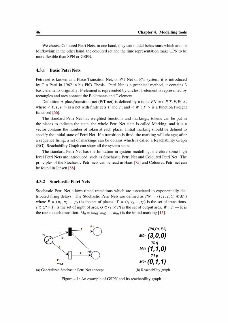
46 Chapter 4. Modelling tools
We choose Coloured Petri Nets, in one hand, they can model behaviours which are notMarkovian; in the other hand, the coloured set and the time representation make CPN to bemore flexible than SPN or GSPN.
4.3.1 Basic Petri Nets
Petri net is known as a Place-Transition Net, or P/T Net or P/T system, it is introducedby C.A.Petri in 1962 in his PhD Thesis. Petri Net is a graphical method, it contains 3basic elements originally: P-element is represented by circles; T-element is represented byrectangles and arcs connect the P-elements and T-element.
Definition:A place/transition net (P/T net) is defined by a tuple PN =< P,T, F,W >,where < P,T, F > is a net with finite sets P and T , and < W : F > is a function (weightfunction) [66].
The standard Petri Net has weighted functions and markings; tokens can be put inthe places to indicate the state, the whole Petri Net state is called Marking, and it is avector contains the number of token at each place. Initial marking should be defined tospecify the initial state of Petri Net. If a transition is fired, the marking will change; aftera sequence firing, a set of markings can be obtains which is called a Reachability Graph(RG). Reachability Graph can show all the system states.
The standard Petri Net has the limitation in system modelling, therefore some highlevel Petri Nets are introduced, such as Stochastic Petri Net and Coloured Petri Net. Theprinciples of the Stochastic Petri nets can be read in Haas [75] and Coloured Petri net canbe found in Jensen [88].
4.3.2 Stochastic Petri Nets
Stochastic Petri Net allows timed transitions which are associated to exponentially dis-tributed firing delays. The Stochastic Petri Nets are defined as PN = (P,T, I,O,W,M0)where P = (p1, p2, ..., pp) is the set of places. T = (t1, t2, ..., tT ) is the set of transitions.I ⊂ (P × T ) is the set of input of arcs, O ⊂ (T × P) is the set of output arcs. W : T → R isthe rate to each transition. M0 = (m01,m02, ...,m0p) is the initial marking [15].
(a) Generalized Stochastic Petri Net concept
(3,0,0)
(1,1,0)
(0,1,1)
T0
T1
M0:
M1:
M2:
(P0,P1,P2)
(b) Reachability graph
Figure 4.1: An example of GSPN and its reachability graph
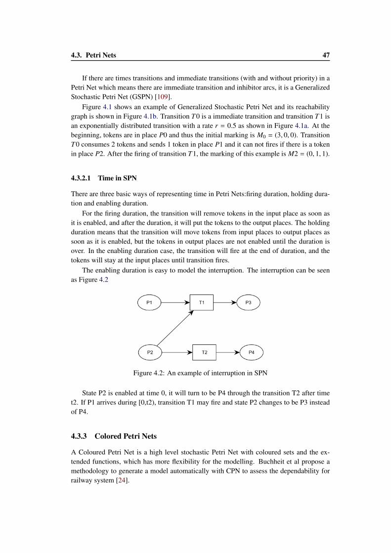
4.3. Petri Nets 47
If there are times transitions and immediate transitions (with and without priority) in aPetri Net which means there are immediate transition and inhibitor arcs, it is a GeneralizedStochastic Petri Net (GSPN) [109].
Figure 4.1 shows an example of Generalized Stochastic Petri Net and its reachabilitygraph is shown in Figure 4.1b. Transition T0 is a immediate transition and transition T1 isan exponentially distributed transition with a rate r = 0.5 as shown in Figure 4.1a. At thebeginning, tokens are in place P0 and thus the initial marking is M0 = (3, 0, 0). TransitionT0 consumes 2 tokens and sends 1 token in place P1 and it can not fires if there is a tokenin place P2. After the firing of transition T1, the marking of this example is M2 = (0, 1, 1).
4.3.2.1 Time in SPN
There are three basic ways of representing time in Petri Nets:firing duration, holding dura-tion and enabling duration.
For the firing duration, the transition will remove tokens in the input place as soon asit is enabled, and after the duration, it will put the tokens to the output places. The holdingduration means that the transition will move tokens from input places to output places assoon as it is enabled, but the tokens in output places are not enabled until the duration isover. In the enabling duration case, the transition will fire at the end of duration, and thetokens will stay at the input places until transition fires.
The enabling duration is easy to model the interruption. The interruption can be seenas Figure 4.2
Figure 4.2: An example of interruption in SPN
State P2 is enabled at time 0, it will turn to be P4 through the transition T2 after timet2. If P1 arrives during [0,t2), transition T1 may fire and state P2 changes to be P3 insteadof P4.
4.3.3 Colored Petri Nets
A Coloured Petri Net is a high level stochastic Petri Net with coloured sets and the ex-tended functions, which has more flexibility for the modelling. Buchheit et al propose amethodology to generate a model automatically with CPN to assess the dependability forrailway system [24].
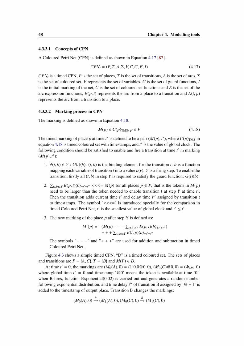
48 Chapter 4. Modelling tools
4.3.3.1 Concepts of CPN
A Coloured Petri Net (CPN) is defined as shown in Equation 4.17 [87].
CPNt = (P,T, A,Σ,V,C,G, E, I) (4.17)
CPNt is a timed CPN, P is the set of places, T is the set of transitions, A is the set of arcs, Σ
is the set of coloured set, V represents the set of variables. G is the set of guard functions, Iis the initial marking of the net, C is the set of coloured set functions and E is the set of thearc expression functions, E(p, t) represents the arc from a place to a transition and E(t, p)represents the arc from a transition to a place.
4.3.3.2 Marking process in CPN
The marking is defined as shown in Equation 4.18.
M(p) ∈ C(p)TMS, p ∈ P (4.18)
The timed marking of place p at time t∗ is defined to be a pair (M(p), t∗), where C(p)TMS inequation 4.18 is timed coloured set with timestamps, and t∗ is the value of global clock. Thefollowing condition should be satisfied to enable and fire a transition at time t′ in marking(M(p), t∗):
1. ∀(t, b) ∈ Y : G(t)〈b〉. (t, b) is the binding element for the transition t. b is a functionmapping each variable of transition t into a value b(v). Y is a firing step. To enable thetransition, firstly all (t, b) in step Y is required to satisfy the guard function: G(t)〈b〉.
2.∑
(t,b)∈Y E(p, t)〈b〉+t′+t′′ <<<= M(p) for all places p ∈ P, that is the tokens in M(p)need to be larger than the token needed to enable transition t at step Y at time t′.Then the transition adds current time t′ and delay time t′′ assigned by transition tto timestamps. The symbol "<<<=" is introduced specially for the comparison intimed Coloured Petri Net, t′ is the smallest value of global clock and t∗ ≤ t′.
3. The new marking of the place p after step Y is defined as:
M′(p) = (M(p) − − −∑
(t,b)∈Y E(p, t)〈b〉+t′+t′′)+ + +
∑(t,b)∈Y E(t, p)〈b〉+t′+t′′
The symbols "− − −" and "+ + +" are used for addition and subtraction in timedColoured Petri Net.
Figure 4.3 shows a simple timed CPN. “D” is a timed coloured set. The sets of placesand transitions are P = {A,C},T = {B} and M(P) ∈ D.
At time t′ = 0, the markings are (M0(A), 0) = (1‘0.0@0, 0), (M0(C)@0, 0) = (ΦMS , 0)where global time t∗ = 0 and timestamp ’@0’ means the token is available at time ‘0’.when B fires, function Exponential(0.02) is carried out and generates a random numberfollowing exponential distribution, and time delay t′′ of transition B assigned by ’@ + 1’ isadded to the timestamp of output place. Transition B changes the markings:
(M0(A), 0)B−→ (M1(A), 0), (M0(C), 0)
B−→ (M1(C), 0)
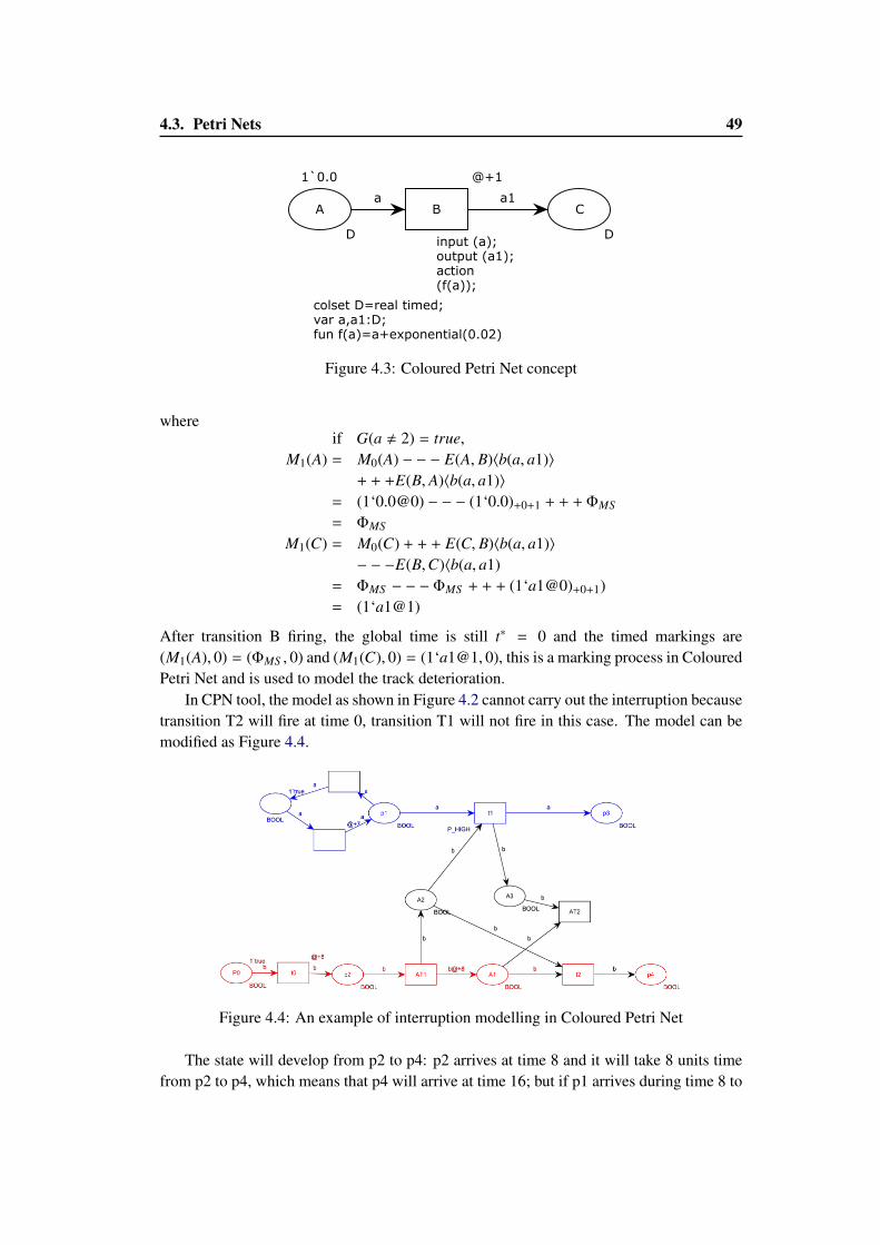
4.3. Petri Nets 49
colset D=real timed;var a,a1:D;fun f(a)=a+exponential(0.02)
A
D
B C
D
a a1
1`0.0
input (a);output (a1);action(f(a));
@+1
Figure 4.3: Coloured Petri Net concept
whereif G(a , 2) = true,
M1(A) = M0(A) − − − E(A, B)〈b(a, a1)〉+ + +E(B, A)〈b(a, a1)〉
= (1‘0.0@0) − − − (1‘0.0)+0+1 + + + ΦMS
= ΦMS
M1(C) = M0(C) + + + E(C, B)〈b(a, a1)〉− − −E(B,C)〈b(a, a1)
= ΦMS − − − ΦMS + + + (1‘a1@0)+0+1)= (1‘a1@1)
After transition B firing, the global time is still t∗ = 0 and the timed markings are(M1(A), 0) = (ΦMS , 0) and (M1(C), 0) = (1‘a1@1, 0), this is a marking process in ColouredPetri Net and is used to model the track deterioration.
In CPN tool, the model as shown in Figure 4.2 cannot carry out the interruption becausetransition T2 will fire at time 0, transition T1 will not fire in this case. The model can bemodified as Figure 4.4.
Figure 4.4: An example of interruption modelling in Coloured Petri Net
The state will develop from p2 to p4: p2 arrives at time 8 and it will take 8 units timefrom p2 to p4, which means that p4 will arrive at time 16; but if p1 arrives during time 8 to
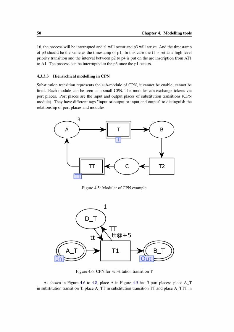
50 Chapter 4. Modelling tools
16, the process will be interrupted and t1 will occur and p3 will arrive. And the timestampof p3 should be the same as the timestamp of p1. In this case the t1 is set as a high levelpriority transition and the interval between p2 to p4 is put on the arc inscription from AT1to A1. The process can be interrupted to the p3 once the p1 occurs.
4.3.3.3 Hierarchical modelling in CPN
Substitution transition represents the sub-module of CPN, it cannot be enable, cannot befired. Each module can be seen as a small CPN. The modules can exchange tokens viaport places. Port places are the input and output places of substitution transitions (CPNmodule). They have different tags "input or output or input and output" to distinguish therelationship of port places and modules.
C
A
3
B
T2TT
TT
T
T
TT
T
Figure 4.5: Modular of CPN example
A_T
In
B_T
Out
D_T
TT
1
T1
tt tt@+5
In Out
Figure 4.6: CPN for substitution transition T
As shown in Figure 4.6 to 4.8, place A in Figure 4.5 has 3 port places: place A_Tin substitution transition T, place A_TT in substitution transition TT and place A_TTT in
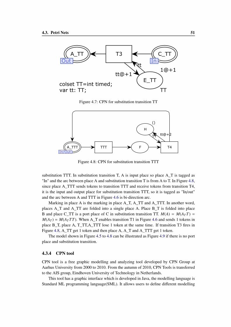
4.3. Petri Nets 51
colset TT=int timed;var tt: TT;
E_TT
TT
1@+1
A_TT
Out
C_TT
In
T3
tt
tt@+1
InOut
Figure 4.7: CPN for substitution transition TT
F
H
A_TTT
In/OutIn/Out
TTT T4
()
tt tt@+2TT
Figure 4.8: CPN for substitution transition TTT
substitution TTT. In substitution transition T, A is input place so place A_T is tagged as"In" and the arc between place A and substitution transition T is from A to T. In Figure 4.8,since place A_TTT sends tokens to transition TTT and receive tokens from transition T4,it is the input and output place for substitution transition TTT, so it is tagged as "In/out"and the arc between A and TTT in Figure 4.6 is bi-direction arc.
Marking in place A is the marking in place A_T, A_TT and A_TTT. In another word,places A_T and A_TT are folded into a single place A. Place B_T is folded into placeB and place C_TT is a port place of C in substitution transition TT. M(A) = M(AT T ) =
M(AT ) = M(AT TT ). When A_T enables transition T1 in Figure 4.6 and sends 1 tokens inplace B_T, place A, T_TT,A_TTT lose 1 token at the same time. If transition T3 fires inFigure 4.8, A_TT get 1 token and then place A, A_T and A_TTT get 1 token.
The model shown in Figure 4.5 to 4.8 can be illustrated as Figure 4.9 if there is no portplace and substitution transition.
4.3.4 CPN tool
CPN tool is a free graphic modelling and analyzing tool developed by CPN Group atAarhus University from 2000 to 2010. From the autumn of 2010, CPN Tools is transferredto the AIS group, Eindhoven University of Technology in Netherlands.
This tool has a graphic interface which is developed in Java, the modelling language isStandard ML programming language(SML). It allows users to define different modelling
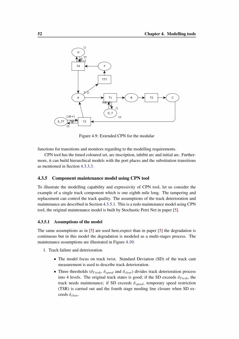
52 Chapter 4. Modelling tools
CA B T2
3`()
F
H
()
TT
TTT
T4
tttt@+2
D_T
()
TT
T1
tt
tt@+5
E_TT
()@+1
TT
T3tttt@+1
Figure 4.9: Extended CPN for the modular
functions for transitions and monitors regarding to the modelling requirements.CPN tool has the timed coloured set, arc inscription, inhibit arc and initial arc. Further-
more, it can build hierarchical models with the port places and the substitution transitionsas mentioned in Section 4.3.3.3.
4.3.5 Component maintenance model using CPN tool
To illustrate the modelling capability and expressivity of CPN tool, let us consider theexample of a single track component which is one eighth mile long. The tampering andreplacement can control the track quality. The assumptions of the track deterioration andmaintenance are described in Section 4.3.5.1. This is a redo maintenance model using CPNtool, the original maintenance model is built by Stochastic Petri Net in paper [5].
4.3.5.1 Assumptions of the model
The same assumptions as in [5] are used here,expect than in paper [5] the degradation iscontinuous but in this model the degradation is modeled as a multi-stages process. Themaintenance assumptions are illustrated in Figure 4.10:
1. Track failure and deterioration.
• The model focus on track twist. Standard Deviation (SD) of the track cantmeasurement is used to describe track deterioration.
• Three thresholds (δTresh, δspeed and δclose) divides track deterioration processinto 4 levels. The original track states is good; if the SD exceeds δTresh, thetrack needs maintenance; if SD exceeds δspeed, temporary speed restriction(TSR) is carried out and the fourth stage needing line closure when SD ex-ceeds δclose.
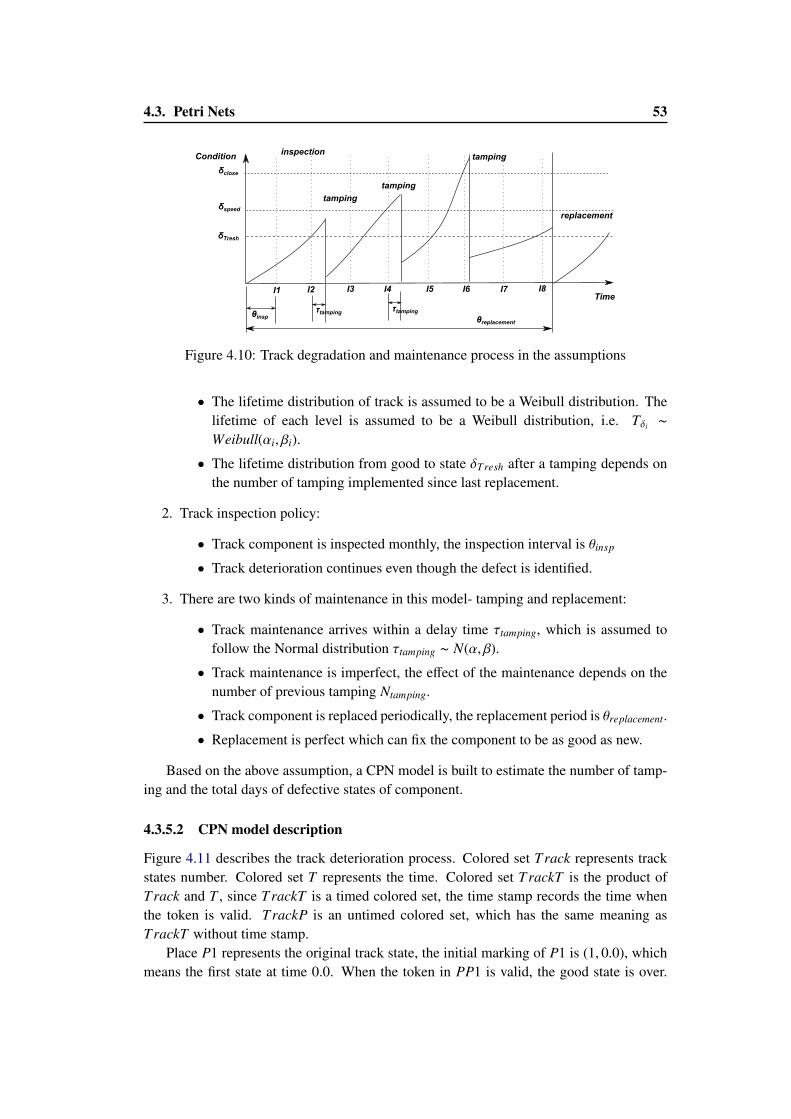
4.3. Petri Nets 53
Condition
Time
δTresh
δspeed
δclose
I1
θinspτtamping τtamping
θreplacement
tamping
replacement
inspection
I2 I3 I4 I5 I6 I7 I8
tamping
tamping
Figure 4.10: Track degradation and maintenance process in the assumptions
• The lifetime distribution of track is assumed to be a Weibull distribution. Thelifetime of each level is assumed to be a Weibull distribution, i.e. Tδi ∼
Weibull(αi, βi).
• The lifetime distribution from good to state δTresh after a tamping depends onthe number of tamping implemented since last replacement.
2. Track inspection policy:
• Track component is inspected monthly, the inspection interval is θinsp
• Track deterioration continues even though the defect is identified.
3. There are two kinds of maintenance in this model- tamping and replacement:
• Track maintenance arrives within a delay time τtamping, which is assumed tofollow the Normal distribution τtamping ∼ N(α, β).
• Track maintenance is imperfect, the effect of the maintenance depends on thenumber of previous tamping Ntamping.
• Track component is replaced periodically, the replacement period is θreplacement.
• Replacement is perfect which can fix the component to be as good as new.
Based on the above assumption, a CPN model is built to estimate the number of tamp-ing and the total days of defective states of component.
4.3.5.2 CPN model description
Figure 4.11 describes the track deterioration process. Colored set Track represents trackstates number. Colored set T represents the time. Colored set TrackT is the product ofTrack and T , since TrackT is a timed colored set, the time stamp records the time whenthe token is valid. TrackP is an untimed colored set, which has the same meaning asTrackT without time stamp.
Place P1 represents the original track state, the initial marking of P1 is (1, 0.0), whichmeans the first state at time 0.0. When the token in PP1 is valid, the good state is over.
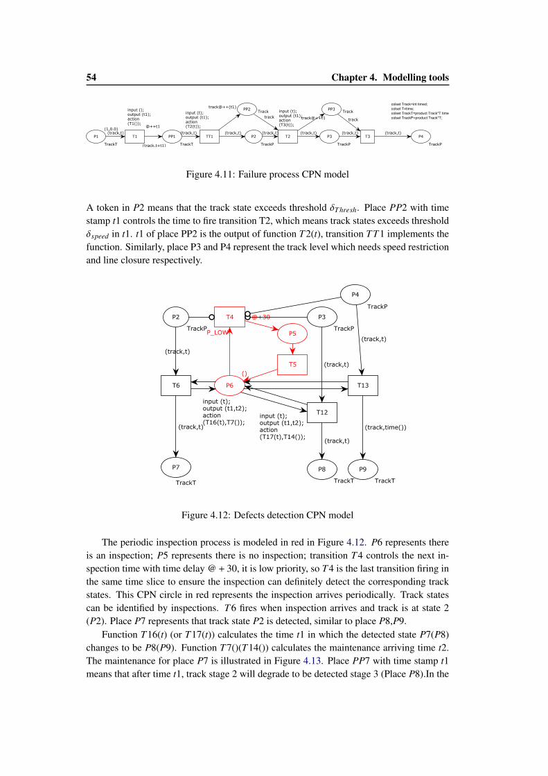
54 Chapter 4. Modelling tools
P1
TrackT
(1,0.0)
P2
TrackP
P3
TrackP
P4
TrackP
PP1
TrackT
PP2Track
PP3Track
T1
@++t1
input ();output (t1);action(T1());
T2
input (t);output (t1);action(T3(t));
T3TT1
input (t);output (t1);action(T2(t));
(track,t) (track,t) (track,t) (track,t) (track,t)
(track,t+t1)
(track,t) (track,t)
track@++(t1)
track track@++t1 track
colset Track=int timed;
colset T=time;
colset TrackT=product Track*T timed;
colset TrackP=product Track*T;
Figure 4.11: Failure process CPN model
A token in P2 means that the track state exceeds threshold δThresh. Place PP2 with timestamp t1 controls the time to fire transition T2, which means track states exceeds thresholdδspeed in t1. t1 of place PP2 is the output of function T2(t), transition TT1 implements thefunction. Similarly, place P3 and P4 represent the track level which needs speed restrictionand line closure respectively.
P2
TrackP
P3
TrackP
P4
TrackP
P6
()
P5
P7
TrackT
P8
TrackT
P9
TrackT
T4
P_LOW
T5
T6
input (t);output (t1,t2);action(T16(t),T7());
T12input (t);output (t1,t2);action(T17(t),T14());
T13
@+30
(track,t)
(track,t)
(track,t)
(track,t)
(track,t)
(track,time())
Figure 4.12: Defects detection CPN model
The periodic inspection process is modeled in red in Figure 4.12. P6 represents thereis an inspection; P5 represents there is no inspection; transition T4 controls the next in-spection time with time delay @ + 30, it is low priority, so T4 is the last transition firing inthe same time slice to ensure the inspection can definitely detect the corresponding trackstates. This CPN circle in red represents the inspection arrives periodically. Track statescan be identified by inspections. T6 fires when inspection arrives and track is at state 2(P2). Place P7 represents that track state P2 is detected, similar to place P8,P9.
Function T16(t) (or T17(t)) calculates the time t1 in which the detected state P7(P8)changes to be P8(P9). Function T7()(T14()) calculates the maintenance arriving time t2.The maintenance for place P7 is illustrated in Figure 4.13. Place PP7 with time stamp t1means that after time t1, track stage 2 will degrade to be detected stage 3 (Place P8).In the

4.3. Petri Nets 55
other hand, after t2, the stage 2 defect will be fixed to be acceptable state (place P10). t1and t2 decide which transitions will fire (transition T7 and T16). If t2 is smaller than t1,transition T7 fires and the track state change to P10. Place P10 represents the track stateis not as good as new but it is better than P2. Place P11 records the number of previoustamping in this track section. The time stamp of PP10 means the ending time of this state.The ending time is sampled by function T8(n), n is the number of tamping. If the token inPlace PP10 is valid, track state deteriorates to be P2.
P2
TrackP
P7
TrackT
P11
INT
0
P10
TrackT
P8
TrackT
PP7
Track
PP10
TrackT
PPP7
Track
T6
input (t);output (t1,t2);action(T16(t),T7());
T7
T8
input (n);output (t1);action(T8(n));
T16
input (t);output (t1,t2);action(T17(t),T14());
T8_2
input (t);output (t1);action(T2(t));
(track,t)
(track,t)
(track,t)
(track,0.0)
(track,t)
n
(track,t) (track,t)
n
track@++t1
track
(track+1,t)@++t1
(track,t)
(track,t1)
track@++t2
track
nn+1
Figure 4.13: Defects repair CPN model
The track component is assumed to be replaced periodically. Figure 4.14 shows theperiodic replacement. Transition T11 is high priority so it will fire before other transitionsassociated to place P1, then it puts token to place PP0 and set the replacement time to be36500; Place P12 are used to control transition T11 not to fire for a second time beforereplacement.
Transition T9 means that the replacement is carried out, then replacement restores trackto be new (place P1) and resets the number of tamping to be 0 (the value of token in placeP11). All the arcs from place P2,P3,P4,PP1,P10 and PP10 are reset arcs, these arcs canreset all these places to be empty, and the enable bind element of T10 is: P13 and P11 arenot empty no matter there is a token in P2,P3,P4,PP1,P10 and PP10.
4.3.5.3 Simulation results
Figure 4.15 shows the intervention convergence depends on the number of simulations overa simulation horizon of 180 years. The number of intervention converges if the number ofsimulation is larger than 20000, we run 25000 simulations to get the maintenance results.
There are some differences between this CPN model and the SPN model in [5]: InAndrews’s paper, T2 (the time from state δTresh to state δspeed), T3 (the time from state
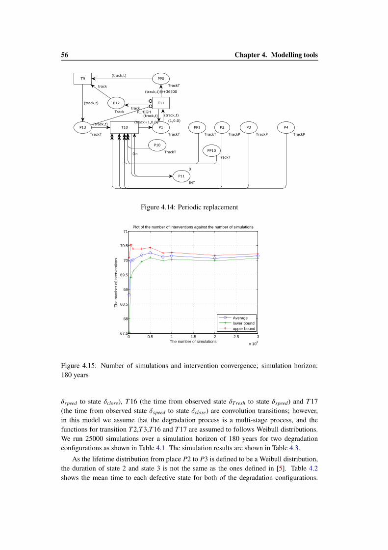
56 Chapter 4. Modelling tools
P1
TrackT
(1,0.0)
P2
TrackP
P3
TrackP
P4
TrackP
P12
Track
P13
TrackT
PP0
TrackT
P11
INT
0
P10
TrackT
PP1
TrackT
PP10
TrackT
T11
P_HIGH
T9
T10
track
(track,t)
(track,t)(track+1,0.0)
(track,t)(track,t)
track
(track,t)@+36500
(track,t)
n0
Figure 4.14: Periodic replacement
0 0.5 1 1.5 2 2.5 3
x 104
67.5
68
68.5
69
69.5
70
70.5
71
The
num
ber
of in
terv
entio
ns
The number of simulations
Plot of the number of interventions against the number of simulations
Averagelower boundupper bound
Figure 4.15: Number of simulations and intervention convergence; simulation horizon:180 years
δspeed to state δclose), T16 (the time from observed state δTresh to state δspeed) and T17(the time from observed state δspeed to state δclose) are convolution transitions; however,in this model we assume that the degradation process is a multi-stage process, and thefunctions for transition T2,T3,T16 and T17 are assumed to follows Weibull distributions.We run 25000 simulations over a simulation horizon of 180 years for two degradationconfigurations as shown in Table 4.1. The simulation results are shown in Table 4.3.
As the lifetime distribution from place P2 to P3 is defined to be a Weibull distribution,the duration of state 2 and state 3 is not the same as the ones defined in [5]. Table 4.2shows the mean time to each defective state for both of the degradation configurations.
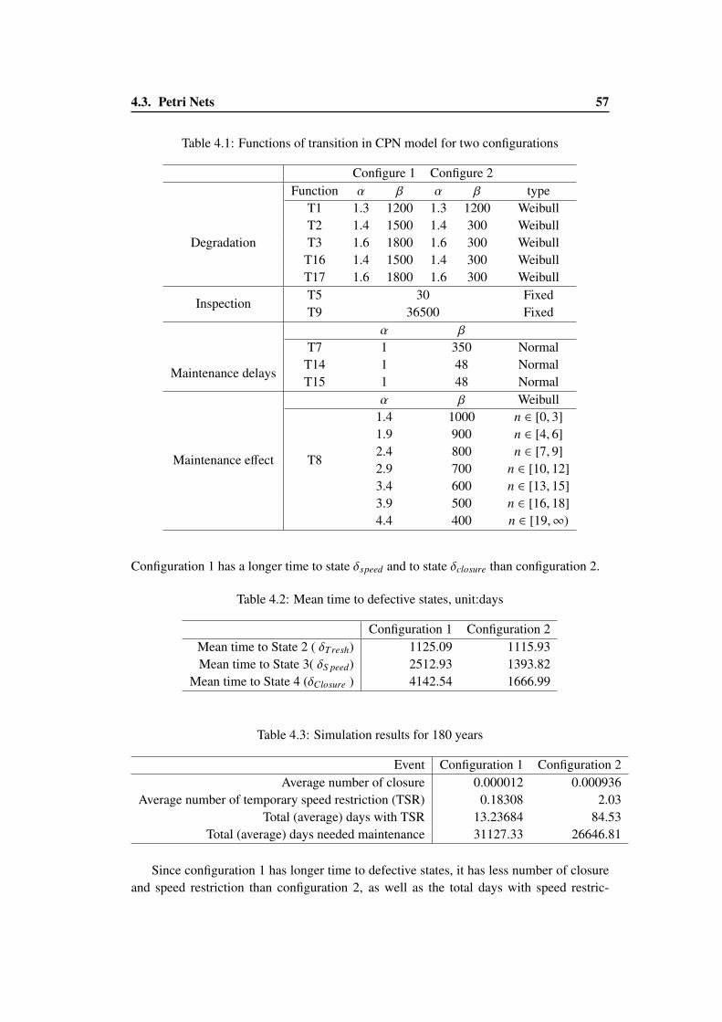
4.3. Petri Nets 57
Table 4.1: Functions of transition in CPN model for two configurations
Configure 1 Configure 2Function α β α β type
Degradation
T1 1.3 1200 1.3 1200 WeibullT2 1.4 1500 1.4 300 WeibullT3 1.6 1800 1.6 300 Weibull
T16 1.4 1500 1.4 300 WeibullT17 1.6 1800 1.6 300 Weibull
InspectionT5 30 FixedT9 36500 Fixed
α β
Maintenance delays
T7 1 350 NormalT14 1 48 NormalT15 1 48 Normal
Maintenance effect T8
α β Weibull1.4 1000 n ∈ [0, 3]1.9 900 n ∈ [4, 6]2.4 800 n ∈ [7, 9]2.9 700 n ∈ [10, 12]3.4 600 n ∈ [13, 15]3.9 500 n ∈ [16, 18]4.4 400 n ∈ [19,∞)
Configuration 1 has a longer time to state δspeed and to state δclosure than configuration 2.
Table 4.2: Mean time to defective states, unit:days
Configuration 1 Configuration 2Mean time to State 2 ( δTresh) 1125.09 1115.93Mean time to State 3( δS peed) 2512.93 1393.82
Mean time to State 4 (δClosure ) 4142.54 1666.99
Table 4.3: Simulation results for 180 years
Event Configuration 1 Configuration 2Average number of closure 0.000012 0.000936
Average number of temporary speed restriction (TSR) 0.18308 2.03Total (average) days with TSR 13.23684 84.53
Total (average) days needed maintenance 31127.33 26646.81
Since configuration 1 has longer time to defective states, it has less number of closureand speed restriction than configuration 2, as well as the total days with speed restric-
58 Chapter 4. Modelling tools
tion.Total days need maintenance is around 85 years for configuration 1 which means thataround 47% time of the track are used with a defective state and 73 years for configura-tion 2 which is around 40% time in 180 years. However, the configurations are based onsome assumptions which might not be the actual data, and hence the period,during whichcomponent needs maintenance, is not an actual case in practice.
The simulation results for both configurations show that CPN tools can model themulti-stages failure and with different degradation configuration, we can have the differ-ent estimations for performance evaluation.
4.4 Conclusion for the modelling tool
In this chapter, we introduce some useful mathematics models, which are adopted in themaintenance models in the following chapters.
The concepts of Petri Nets are introduced for the basic knowledge of the modelling. Wereview several timed marking mechanisms and find out the equivalent models for differenttime duration mechanism.
The formal definition and marking process of Coloured Petri Net are reviewed since inthis chapter we adopt CPN tools to model the maintenance process in railway system.
In addition, we work on a published example, which worked out using SPN, to showhow CPN modelling and simulations can be implemented to analyse the performance ofthe maintenance policy on single track component. The number of maintenance actionsand the duration between two component states are collected by the simulations, whichcan be used to estimated system performance evaluation indices, such as maintenance costand system unavailability.
Part III
COMPONENT MAINTENANCEMODELLING

Chapter 5
Comparison of failure models formaintenance optimization
Contents5.1 Introduction . . . . . . . . . . . . . . . . . . . . . . . . . . . . . . . . . 615.2 Assumptions for deterioration model and lifetime model . . . . . . . . . 63
5.2.1 Gradual deterioration model . . . . . . . . . . . . . . . . . . . . . 63
5.2.2 Lifetime distribution model . . . . . . . . . . . . . . . . . . . . . 65
5.2.3 Performance evaluations . . . . . . . . . . . . . . . . . . . . . . . 67
5.3 CPN models . . . . . . . . . . . . . . . . . . . . . . . . . . . . . . . . . 675.3.1 CPN model for deterioration model . . . . . . . . . . . . . . . . . 67
5.3.2 CPN model for lifetime model . . . . . . . . . . . . . . . . . . . . 70
5.4 Monte Carlo simulations . . . . . . . . . . . . . . . . . . . . . . . . . . 715.4.1 Parameters used in simulations . . . . . . . . . . . . . . . . . . . . 72
5.4.2 Simulation convergence . . . . . . . . . . . . . . . . . . . . . . . 74
5.4.3 Simulation results of deterioration process model . . . . . . . . . . 75
5.4.4 Simulation results of lifetime model . . . . . . . . . . . . . . . . . 78
5.4.5 Comparison of lifetime model and deterioration model . . . . . . . 79
5.5 Conclusion for the comparison of failure models . . . . . . . . . . . . . 80
5.1 Introduction
Railway track maintenance decisions are made based on the track condition. Since trackfaults are non self-announcing, inspections are carried out regularly to collect the trackcondition measures in order to supervise the track quality. Regarding to the inspectiontechniques, we sometimes have different types of condition data. The first type of data justindicates the binary health states of the track - worked or failed. With the development ofinspection devices, we can collect more precise condition data to show more details of thetrack quality; for example, we can use the standard deviation for a certain number of trackcondition data to indicates the health of the track for a certain length. Based on these twokinds of inspection data, two failure models are adopted to describe the track deterioration
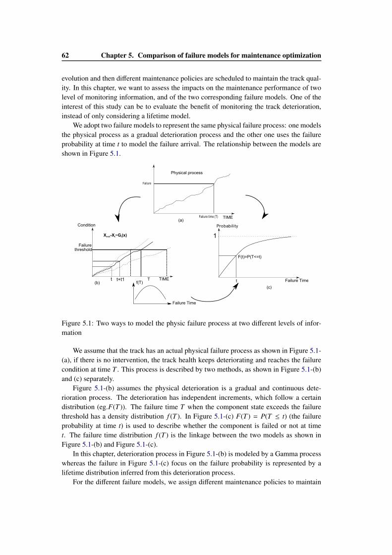
62 Chapter 5. Comparison of failure models for maintenance optimization
evolution and then different maintenance policies are scheduled to maintain the track qual-ity. In this chapter, we want to assess the impacts on the maintenance performance of twolevel of monitoring information, and of the two corresponding failure models. One of theinterest of this study can be to evaluate the benefit of monitoring the track deterioration,instead of only considering a lifetime model.
We adopt two failure models to represent the same physical failure process: one modelsthe physical process as a gradual deterioration process and the other one uses the failureprobability at time t to model the failure arrival. The relationship between the models areshown in Figure 5.1.
threshold
f(T)
Physical process
Probability
Failure TimeT
Failure Time
t
F(t)=P(T<=t)
(b)(c)
(a)Condition
Failure
Failure time (T) TIME
Xt+t1-Xt~Gt(x)
t t+t1 TIME
1
Failure
Figure 5.1: Two ways to model the physic failure process at two different levels of infor-mation
We assume that the track has an actual physical failure process as shown in Figure 5.1-(a), if there is no intervention, the track health keeps deteriorating and reaches the failurecondition at time T . This process is described by two methods, as shown in Figure 5.1-(b)and (c) separately.
Figure 5.1-(b) assumes the physical deterioration is a gradual and continuous dete-rioration process. The deterioration has independent increments, which follow a certaindistribution (eg.F(T )). The failure time T when the component state exceeds the failurethreshold has a density distribution f (T ). In Figure 5.1-(c) F(T ) = P(T ≤ t) (the failureprobability at time t) is used to describe whether the component is failed or not at timet. The failure time distribution f (T ) is the linkage between the two models as shown inFigure 5.1-(b) and Figure 5.1-(c).
In this chapter, deterioration process in Figure 5.1-(b) is modeled by a Gamma processwhereas the failure in Figure 5.1-(c) focus on the failure probability is represented by alifetime distribution inferred from this deterioration process.
For the different failure models, we assign different maintenance policies to maintain
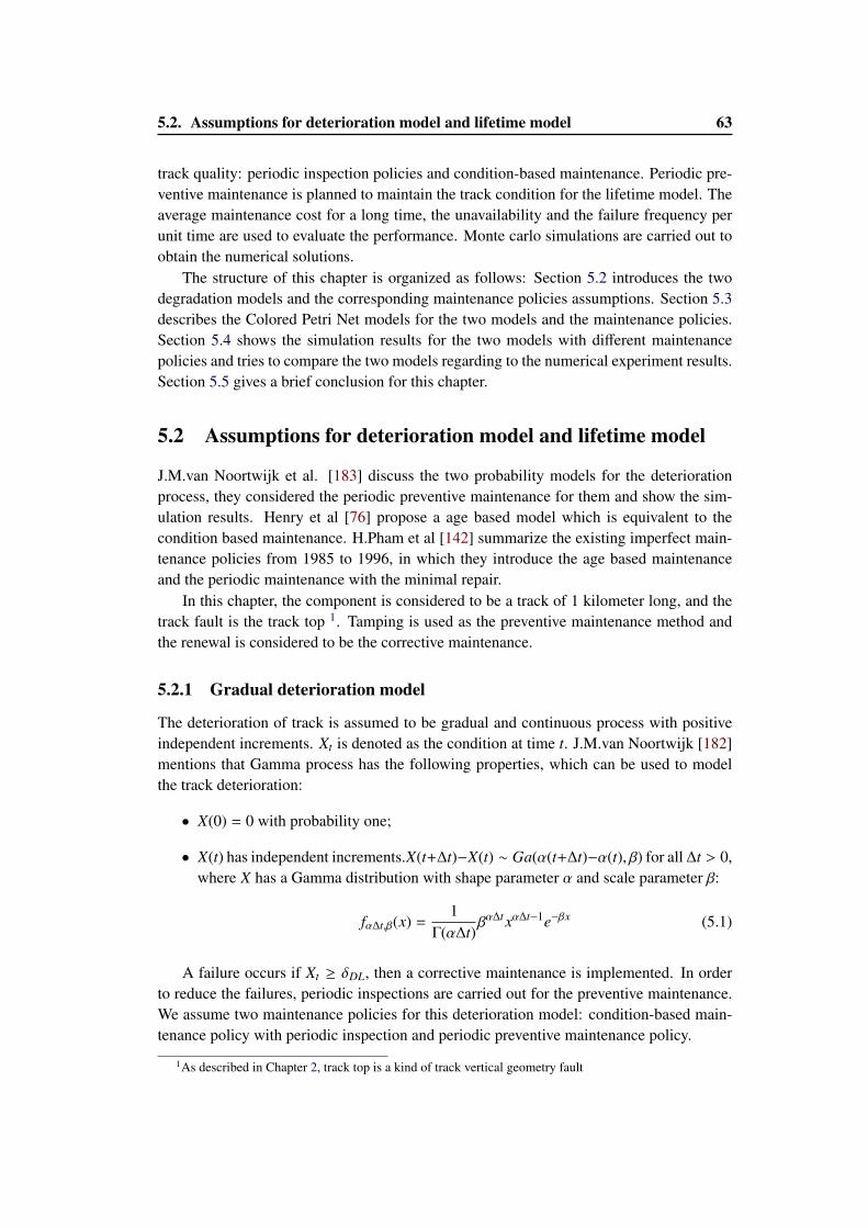
5.2. Assumptions for deterioration model and lifetime model 63
track quality: periodic inspection policies and condition-based maintenance. Periodic pre-ventive maintenance is planned to maintain the track condition for the lifetime model. Theaverage maintenance cost for a long time, the unavailability and the failure frequency perunit time are used to evaluate the performance. Monte carlo simulations are carried out toobtain the numerical solutions.
The structure of this chapter is organized as follows: Section 5.2 introduces the twodegradation models and the corresponding maintenance policies assumptions. Section 5.3describes the Colored Petri Net models for the two models and the maintenance policies.Section 5.4 shows the simulation results for the two models with different maintenancepolicies and tries to compare the two models regarding to the numerical experiment results.Section 5.5 gives a brief conclusion for this chapter.
5.2 Assumptions for deterioration model and lifetime model
J.M.van Noortwijk et al. [183] discuss the two probability models for the deteriorationprocess, they considered the periodic preventive maintenance for them and show the sim-ulation results. Henry et al [76] propose a age based model which is equivalent to thecondition based maintenance. H.Pham et al [142] summarize the existing imperfect main-tenance policies from 1985 to 1996, in which they introduce the age based maintenanceand the periodic maintenance with the minimal repair.
In this chapter, the component is considered to be a track of 1 kilometer long, and thetrack fault is the track top 1. Tamping is used as the preventive maintenance method andthe renewal is considered to be the corrective maintenance.
5.2.1 Gradual deterioration model
The deterioration of track is assumed to be gradual and continuous process with positiveindependent increments. Xt is denoted as the condition at time t. J.M.van Noortwijk [182]mentions that Gamma process has the following properties, which can be used to modelthe track deterioration:
• X(0) = 0 with probability one;
• X(t) has independent increments.X(t+∆t)−X(t) ∼ Ga(α(t+∆t)−α(t), β) for all ∆t > 0,where X has a Gamma distribution with shape parameter α and scale parameter β:
fα∆t,β(x) =1
Γ(α∆t)βα∆t xα∆t−1e−βx (5.1)
A failure occurs if Xt ≥ δDL, then a corrective maintenance is implemented. In orderto reduce the failures, periodic inspections are carried out for the preventive maintenance.We assume two maintenance policies for this deterioration model: condition-based main-tenance policy with periodic inspection and periodic preventive maintenance policy.
1As described in Chapter 2, track top is a kind of track vertical geometry fault
64 Chapter 5. Comparison of failure models for maintenance optimization
5.2.1.1 Condition-based maintenance policy
The scenarios of the periodic inspection policies are illustrated in Figure 5.2 and the detailsof the assumptions are listed as follows:
Figure 5.2: Scenarios of periodic inspection policy
1. The inspections are carried out periodically with an interval θinsp. i is the index ofthe inspection; Ii means the ith inspection, and Xi represents the observed states bythe ith inspection.
2. There are two thresholds for the maintenance:
• If Xi ≥ δDL, a corrective maintenance is carried out immediately, eg. I3 inFigure 5.2. It can restore the track to be a condition Xcm which means the stateafter the corrective maintenance is as good as new.
• If Xi ≥ δII , a preventive maintenance is implemented, eg, I2 in figure 5.2.
• The preventive maintenance is imperfect. The preventive maintenance can fixthe component to the state Xpm > 0.0 which means the state after the preventivemaintenance is not as good as new .
3. There is no delays for the two levels of maintenances. It takes Dcm for one correctivemaintenance action and Dpm for one preventive maintenance action as the downtime.
The preventive maintenance threshold δII and the Inspection interval θinsp are the main-tenance decision variables to optimize the maintenance configuration.
5.2.1.2 Periodic preventive maintenance policy
A periodic preventive maintenance is scheduled for the deterioration process, the inspectionof which cannot identify the condition details and only detected the failure states.
The maintenance scenarios can be seen in Figure 5.3.
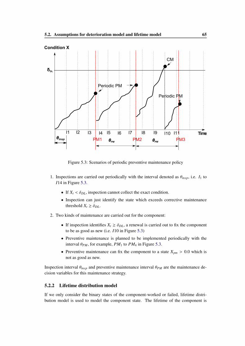
5.2. Assumptions for deterioration model and lifetime model 65
δDL
Condition X
PM1 PM2 PM3
I1 I2 I3 I5I4 I6 I7 I8 I9 I10 I11 Time
Periodic PM
CM
Periodic PM
θinsp θPM θPM
Figure 5.3: Scenarios of periodic preventive maintenance policy
1. Inspections are carried out periodically with the interval denoted as θinsp, i.e. I1 toI14 in Figure 5.3.
• If Xt < δDL, inspection cannot collect the exact condition.
• Inspection can just identify the state which exceeds corrective maintenancethreshold Xt ≥ δDL.
2. Two kinds of maintenance are carried out for the component:
• If inspection identifies Xt ≥ δDL, a renewal is carried out to fix the componentto be as good as new (i.e. I10 in Figure 5.3)
• Preventive maintenance is planned to be implemented periodically with theinterval θPM, for example, PM1 to PM4 in Figure 5.3.
• Preventive maintenance can fix the component to a state Xpm > 0.0 which isnot as good as new.
Inspection interval θinsp and preventive maintenance interval θPM are the maintenance de-cision variables for this maintenance strategy.
5.2.2 Lifetime distribution model
If we only consider the binary states of the component-worked or failed, lifetime distri-bution model is used to model the component state. The lifetime of the component is
66 Chapter 5. Comparison of failure models for maintenance optimization
denoted as TδDL , which means the time when the component condition exceeds the fail-ure threshold δDL. The probability of the component which fails during (0, t] is defined asFTδDL
(t) = Pr(t ≥ TδDL).Since the failure model and the deterioration model are used to represent the same
physical deterioration process, for the same failure condition δDL, the lifetime distributionis calculated as Equation 5.2, to be consistent with the deterioration process [182]:
FTδDL(t) = Pr(t ≥ TδDL) =
Υ(αt, βδDL)Γ(αt)
(5.2)
For the lifetime distribution model, the inspections are only able to identify two statesof the components: working or failed. Since the lifetime model cannot give the componentcondition to the decision maker, the maintenance can only be scheduled according to theusage time or component age.
5.2.2.1 Periodic preventive maintenance policy
Periodic maintenance policy for the lifetime model proposes a two level maintenance policyfor the track component, as shown in Figure 5.3.
Since the failure is unrevealed, inspection is needed to detect the component failure.The details of the periodic maintenance policy for the lifetime model are assumed as fol-lows:
1. Inspection is carried out periodically with the interval θinsp regardless of the correc-tive maintenance.
2. Two levels of maintenances are scheduled for the component
• Preventive maintenance are planned for the component; it is implemented peri-odically, with the interval denoted as θT . The interval θT is a constant indepen-dent to the component failure history.
• Preventive maintenance is imperfect, after the nth preventive maintenance thecomponent is fixed to the virtual age Vn. We assume that the virtual age is equalto a constant value, Vn = y, n = 1, 2, ... .
• The lifetime distribution after the nth preventive maintenance is obtained ac-cording to the actual age Xn [95]:
Fn(t) = F2(t) = Pr(Xn ≤ x|Vn−1 = y) =F(t + y) − F(y)
1 − F(y)(5.3)
• If the ith inspection identifies the component failure, a corrective maintenanceis carried out.
• Corrective maintenance is perfect. After the corrective maintenance, the virtualage of the component is Vm = 0. m is the index of corrective maintenance.
For this maintenance policy, the decision variables are the preventive maintenance in-terval θPM and the inspection interval θinsp.
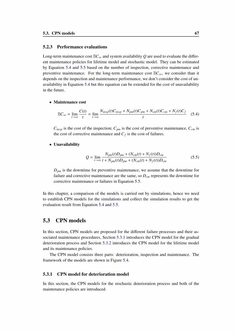
5.3. CPN models 67
5.2.3 Performance evaluations
Long-term maintenance cost EC∞ and system availability Q are used to evaluate the differ-ent maintenance policies for lifetime model and stochastic model. They can be estimatedby Equation 5.4 and 5.5 based on the number of inspection, corrective maintenance andpreventive maintenance. For the long-term maintenance cost EC∞, we consider than itdepends on the inspection and maintenance performance, we don’t consider the cost of un-availability in Equation 5.4 but this equation can be extended for the cost of unavailabilityin the future.
• Maintenance cost
EC∞ = limt→∞
C(t)t
= limt→∞
Ninsp(t)Cinsp + Npm(t)Cpm + Ncm(t)Ccm + N f (t)C f
t(5.4)
Cinsp is the cost of the inspection; Cpm is the cost of preventive maintenance, Ccm isthe cost of corrective maintenance and C f is the cost of failures.
• Unavailability
Q = limt→∞
Npm(t)Dpm + (Ncm(t) + N f (t))Dcm
t + Npm(t)Dpm + (Ncm(t) + N f (t))Dcm(5.5)
Dpm is the downtime for preventive maintenance, we assume that the downtime forfailure and corrective maintenance are the same, so Dcm represents the downtime forcorrective maintenance or failures in Equation 5.5.
In this chapter, a comparison of the models is carried out by simulations, hence we needto establish CPN models for the simulations and collect the simulation results to get theevaluation result from Equation 5.4 and 5.5.
5.3 CPN models
In this section, CPN models are proposed for the different failure processes and their as-sociated maintenance procedures, Section 5.3.1 introduces the CPN model for the gradualdeterioration process and Section 5.3.2 introduces the CPN model for the lifetime modeland its maintenance policies.
The CPN model consists three parts: deterioration, inspection and maintenance. Theframework of the models are shown in Figure 5.4.
5.3.1 CPN model for deterioration model
In this section, the CPN models for the stochastic deterioration process and both of themaintenance policies are introduced.
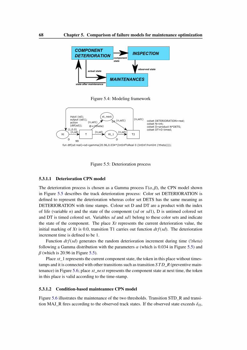
68 Chapter 5. Comparison of failure models for maintenance optimization
COMPONENT
DETERIORATIONINSPECTION
MAINTENANCES
component
state
observed stateactual state
state after maintenance
Figure 5.4: Modeling framework
colset DETERIORATION=real;colset N=int;colset D=product N*DETS;colset DT=D timed;
fun dtf(sd:real)=sd+gamma(20.96,0.034*(IntInfToReal 0 (IntInf.fromInt (!theta))));
Xt
D
(1,0.0)
Xt_1
D
xt_next
DT
T
@+(!theta)
input (sd);output (sd1);action(dtf(sd));
99
T2(n,sd) (n,sd)
(n,sd1)(n,sd1)
(n,sd)
(n,sd1)
Figure 5.5: Deterioration process
5.3.1.1 Deterioration CPN model
The deterioration process is chosen as a Gamma process Γ(α, β), the CPN model shownin Figure 5.5 describes the track deterioration process: Color set DETERIORATION isdefined to represent the deterioration whereas color set DETS has the same meaning asDETERIORATION with time stamps. Colour set D and DT are a product with the indexof life (variable n) and the state of the component (sd or sd1), D is untimed colored setand DT is timed colored set. Variables sd and sd1 belong to these color sets and indicatethe state of the component. The place Xt represents the current deterioration value, theinitial marking of Xt is 0.0, transition T1 carries out function dt f (sd). The deteriorationincrement time is defined to be 1.
Function dt f (sd) generates the random deterioration increment during time (!theta)following a Gamma distribution with the parameters α (which is 0.034 in Figure 5.5) andβ (which is 20.96 in Figure 5.5).
Place xt_1 represents the current component state, the token in this place without times-tamps and it is connected with other transitions such as transition S T D_R (preventive main-tenance) in Figure 5.6; place xt_next represents the component state at next time, the tokenin this place is valid according to the time-stamp.
5.3.1.2 Condition-based mainteannce CPN model
Figure 5.6 illustrates the maintenance of the two thresholds. Transition STD_R and transi-tion MAJ_R fires according to the observed track states. If the observed state exceeds δII ,
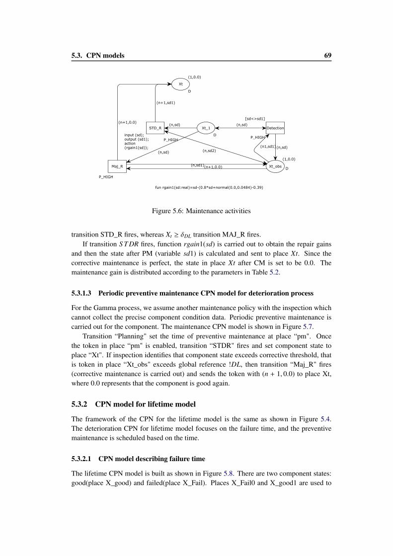
5.3. CPN models 69
fun rgain1(sd:real)=sd-(0.8*sd+normal(0.0,0.0484)-0.39)
Xt_obsD
(1,0.0)
Xt_1
D
Xt
D
(1,0.0)
Detection
[sd<>sd1]
P_HIGH
STD_R
P_HIGH
Maj_R
P_HIGH
(n,sd)(n1,sd1)(n,sd2)
(n,sd)(n,sd)
(n+1,sd1)
(n+1,0.0)
(n,sd)
(n,sd1)(n+1,0.0)
input (sd);output (sd1);action(rgain1(sd));
Figure 5.6: Maintenance activities
transition STD_R fires, whereas Xt ≥ δDL transition MAJ_R fires.If transition S T DR fires, function rgain1(sd) is carried out to obtain the repair gains
and then the state after PM (variable sd1) is calculated and sent to place Xt. Since thecorrective maintenance is perfect, the state in place Xt after CM is set to be 0.0. Themaintenance gain is distributed according to the parameters in Table 5.2.
5.3.1.3 Periodic preventive maintenance CPN model for deterioration process
For the Gamma process, we assume another maintenance policy with the inspection whichcannot collect the precise component condition data. Periodic preventive maintenance iscarried out for the component. The maintenance CPN model is shown in Figure 5.7.
Transition “Planning" set the time of preventive maintenance at place “pm". Oncethe token in place “pm" is enabled, transition “STDR" fires and set component state toplace “Xt". If inspection identifies that component state exceeds corrective threshold, thatis token in place “Xt_obs" exceeds global reference !DL, then transition “Maj_R" fires(corrective maintenance is carried out) and sends the token with (n + 1, 0.0) to place Xt,where 0.0 represents that the component is good again.
5.3.2 CPN model for lifetime model
The framework of the CPN for the lifetime model is the same as shown in Figure 5.4.The deterioration CPN for lifetime model focuses on the failure time, and the preventivemaintenance is scheduled based on the time.
5.3.2.1 CPN model describing failure time
The lifetime CPN model is built as shown in Figure 5.8. There are two component states:good(place X_good) and failed(place X_Fail). Places X_Fail0 and X_good1 are used to
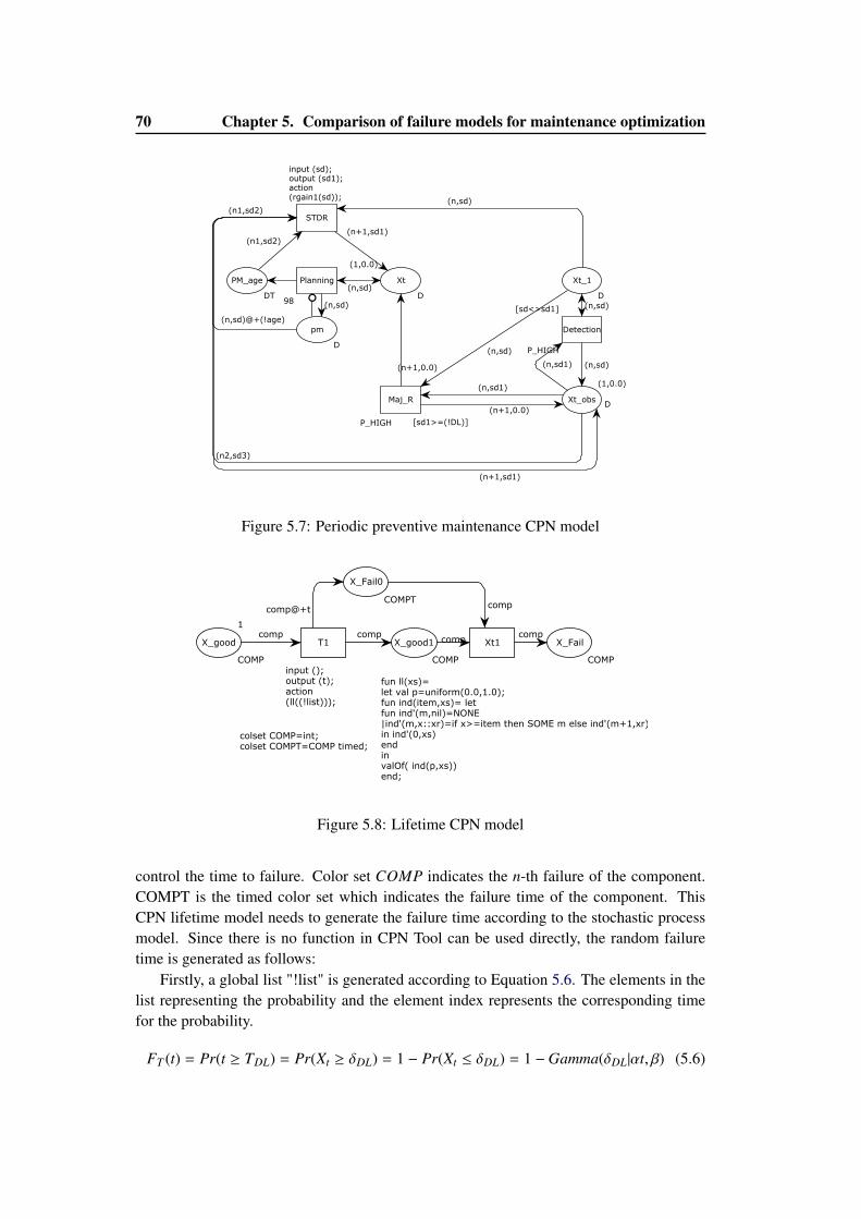
70 Chapter 5. Comparison of failure models for maintenance optimization
Xt
D
(1,0.0)
Xt_obsD
(1,0.0)
Xt_1
D
PM_age
DT
pm
D
Detection
[sd<>sd1]
P_HIGH
Maj_R
[sd1>=(!DL)]P_HIGH
Planning
98
STDR
input (sd);output (sd1);action(rgain1(sd));
(n,sd)
(n,sd)
(n,sd1)(n+1,0.0)
(n,sd)
(n,sd1)
(n+1,0.0)
(n,sd)
(n,sd)@+(!age)
(n,sd)
(n1,sd2)(n+1,sd1)
(n1,sd2)(n,sd)
(n+1,sd1)
(n2,sd3)
Figure 5.7: Periodic preventive maintenance CPN model
fun ll(xs)=let val p=uniform(0.0,1.0);fun ind(item,xs)= let fun ind'(m,nil)=NONE|ind'(m,x::xr)=if x>=item then SOME m else ind'(m+1,xr)in ind'(0,xs)endinvalOf( ind(p,xs))end;
colset COMP=int;colset COMPT=COMP timed;
X_good
COMP
1
X_good1
COMP
X_Fail0
COMPT
X_Fail
COMP
T1
input ();output (t);action(ll((!list)));
Xt1comp comp
comp@+tcomp
compcomp
Figure 5.8: Lifetime CPN model
control the time to failure. Color set COMP indicates the n-th failure of the component.COMPT is the timed color set which indicates the failure time of the component. ThisCPN lifetime model needs to generate the failure time according to the stochastic processmodel. Since there is no function in CPN Tool can be used directly, the random failuretime is generated as follows:
Firstly, a global list "!list" is generated according to Equation 5.6. The elements in thelist representing the probability and the element index represents the corresponding timefor the probability.
FT (t) = Pr(t ≥ TDL) = Pr(Xt ≥ δDL) = 1 − Pr(Xt ≤ δDL) = 1 −Gamma(δDL|αt, β) (5.6)
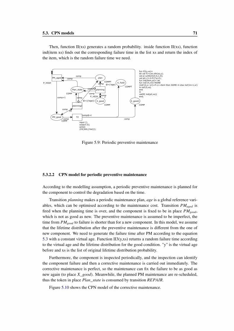
5.3. CPN models 71
Then, function II(xs) generates a random probability. inside function II(xs), functionind(item xs) finds out the corresponding failure time in the list xs and return the index ofthe item, which is the random failure time we need.
fun ll3(y,xs)=let val f1=List.nth(xs,y);val p=uniform(0.0,1.0);val p2=(1.0-f1)*p+f1;fun ind(item,xs)= let fun ind'(m,nil)=NONE|ind'(m,x::xr)=if x>=item then SOME m else ind'(m+1,xr)in ind'(0,xs)endinvalOf( ind(p2,xs))end;
X_good
COMP
1
X_good1
COMP
X_Fail0
COMPT
plan
COMPT
Plan_state
COMP
PM_good
COMP
planning
@+(!age)
P_HIGH
PM_aged
P_HIGH
T2
input ();output (t);action(ll3(300,(!list)));
planning2
@+((!age))
99
comp
comp
comp
comp
comp
comp+1
comp
comp@+t
comp
comp
comp
comp
Figure 5.9: Periodic preventive maintenance
5.3.2.2 CPN model for periodic preventive maintenance
According to the modelling assumption, a periodic preventive maintenance is planned forthe component to control the degradation based on the time.
Transition planning makes a periodic maintenance plan, age is a global reference vari-ables, which can be optimised according to the maintenance cost. Transition PMaged isfired when the planning time is over, and the component is fixed to be in place PMgood,which is not as good as new. The preventive maintenance is assumed to be imperfect, thetime from PMgood to failure is shorter than for a new component. In this model, we assumethat the lifetime distribution after the preventive maintenance is different from the one ofnew component. We need to generate the failure time after PM according to the equation5.3 with a constant virtual age. Function II3(y,xs) returns a random failure time accordingto the virtual age and the lifetime distribution for the good condition. "y" is the virtual agebefore and xs is the list of original lifetime distribution probability.
Furthermore, the component is inspected periodically, and the inspection can identifythe component failure and then a corrective maintenance is carried out immediately. Thecorrective maintenance is perfect, so the maintenance can fix the failure to be as good asnew again (to place X_good). Meanwhile, the planned PM maintenance are re-scheduled,thus the token in place Plan_state is consumed by transition REPAIR.
Figure 5.10 shows the CPN model of the corrective maintenance.
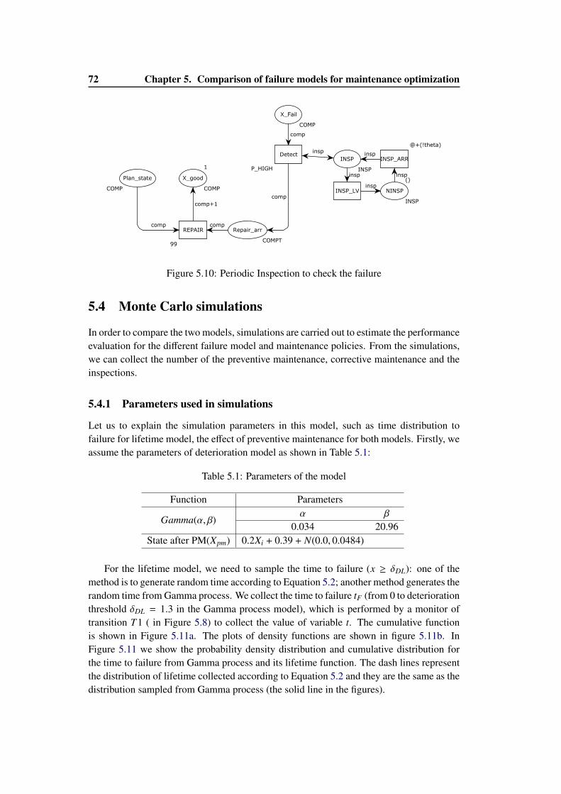
72 Chapter 5. Comparison of failure models for maintenance optimization
X_good
COMP
1
X_Fail
COMP
INSP
INSP
NINSP
INSP
()Plan_state
COMP
Repair_arr
COMPT
INSP_LV
INSP_ARR
@+(!theta)
Detect
P_HIGH
REPAIR
99
insp
insp
insp
insp
comp
insp
comp
comp+1
comp
comp
Figure 5.10: Periodic Inspection to check the failure
5.4 Monte Carlo simulations
In order to compare the two models, simulations are carried out to estimate the performanceevaluation for the different failure model and maintenance policies. From the simulations,we can collect the number of the preventive maintenance, corrective maintenance and theinspections.
5.4.1 Parameters used in simulations
Let us to explain the simulation parameters in this model, such as time distribution tofailure for lifetime model, the effect of preventive maintenance for both models. Firstly, weassume the parameters of deterioration model as shown in Table 5.1:
Table 5.1: Parameters of the model
Function Parameters
Gamma(α, β)α β
0.034 20.96State after PM(Xpm) 0.2Xi + 0.39 + N(0.0, 0.0484)
For the lifetime model, we need to sample the time to failure (x ≥ δDL): one of themethod is to generate random time according to Equation 5.2; another method generates therandom time from Gamma process. We collect the time to failure tF (from 0 to deteriorationthreshold δDL = 1.3 in the Gamma process model), which is performed by a monitor oftransition T1 ( in Figure 5.8) to collect the value of variable t. The cumulative functionis shown in Figure 5.11a. The plots of density functions are shown in figure 5.11b. InFigure 5.11 we show the probability density distribution and cumulative distribution forthe time to failure from Gamma process and its lifetime function. The dash lines representthe distribution of lifetime collected according to Equation 5.2 and they are the same as thedistribution sampled from Gamma process (the solid line in the figures).
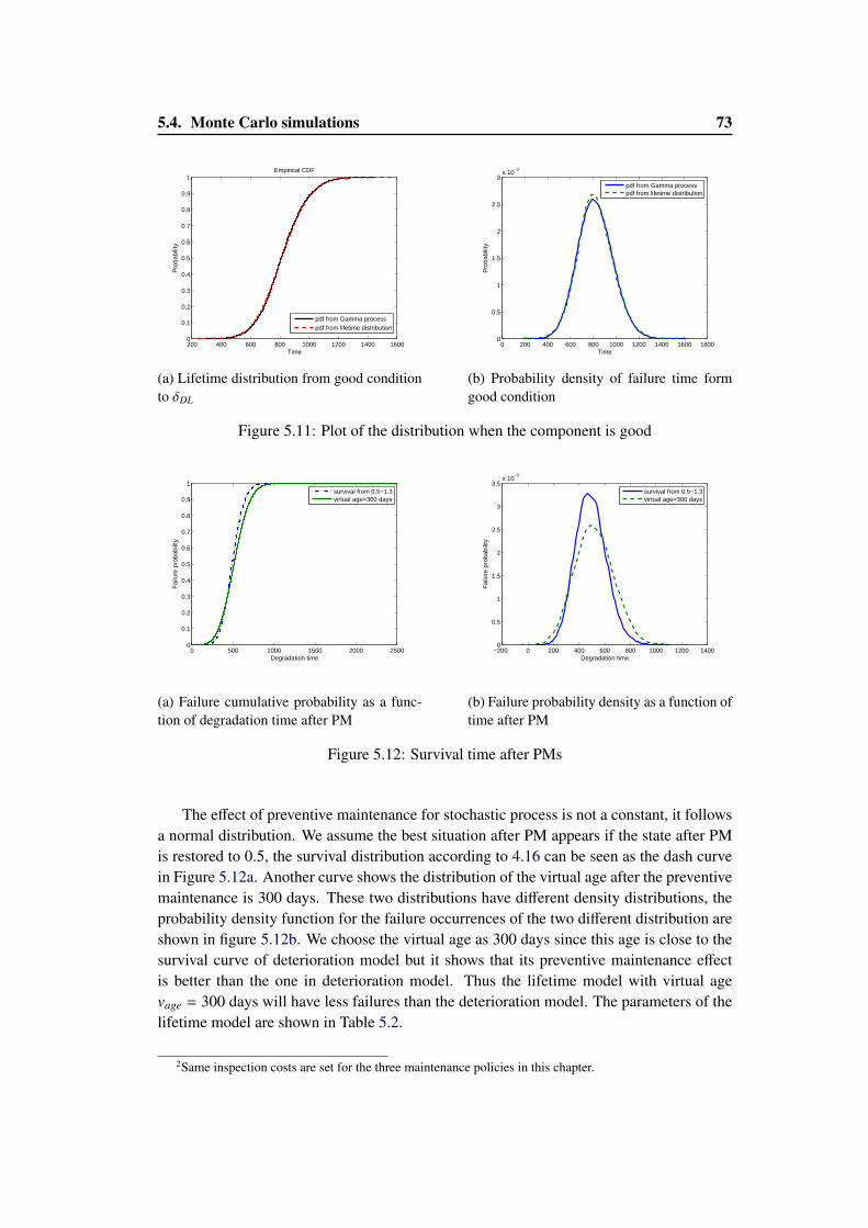
5.4. Monte Carlo simulations 73
200 400 600 800 1000 1200 1400 16000
0.1
0.2
0.3
0.4
0.5
0.6
0.7
0.8
0.9
1
Time
Pro
babi
lity
Empirical CDF
pdf from Gamma processpdf from lifetime distribution
(a) Lifetime distribution from good conditionto δDL
0 200 400 600 800 1000 1200 1400 1600 18000
0.5
1
1.5
2
2.5
3x 10
−3
Time
Pro
babi
lity
pdf from Gamma processpdf from lifetime distribution
(b) Probability density of failure time formgood condition
Figure 5.11: Plot of the distribution when the component is good
0 500 1000 1500 2000 25000
0.1
0.2
0.3
0.4
0.5
0.6
0.7
0.8
0.9
1
Degradation time
Fai
lure
pro
babi
lity
survival from 0.5−1.3virtual age=300 days
(a) Failure cumulative probability as a func-tion of degradation time after PM
−200 0 200 400 600 800 1000 1200 14000
0.5
1
1.5
2
2.5
3
3.5x 10
−3
Degradation time
Fai
lure
pro
babi
lity
survival from 0.5−1.3virtual age=300 days
(b) Failure probability density as a function oftime after PM
Figure 5.12: Survival time after PMs
The effect of preventive maintenance for stochastic process is not a constant, it followsa normal distribution. We assume the best situation after PM appears if the state after PMis restored to 0.5, the survival distribution according to 4.16 can be seen as the dash curvein Figure 5.12a. Another curve shows the distribution of the virtual age after the preventivemaintenance is 300 days. These two distributions have different density distributions, theprobability density function for the failure occurrences of the two different distribution areshown in figure 5.12b. We choose the virtual age as 300 days since this age is close to thesurvival curve of deterioration model but it shows that its preventive maintenance effectis better than the one in deterioration model. Thus the lifetime model with virtual agevage = 300 days will have less failures than the deterioration model. The parameters of thelifetime model are shown in Table 5.2.
2Same inspection costs are set for the three maintenance policies in this chapter.
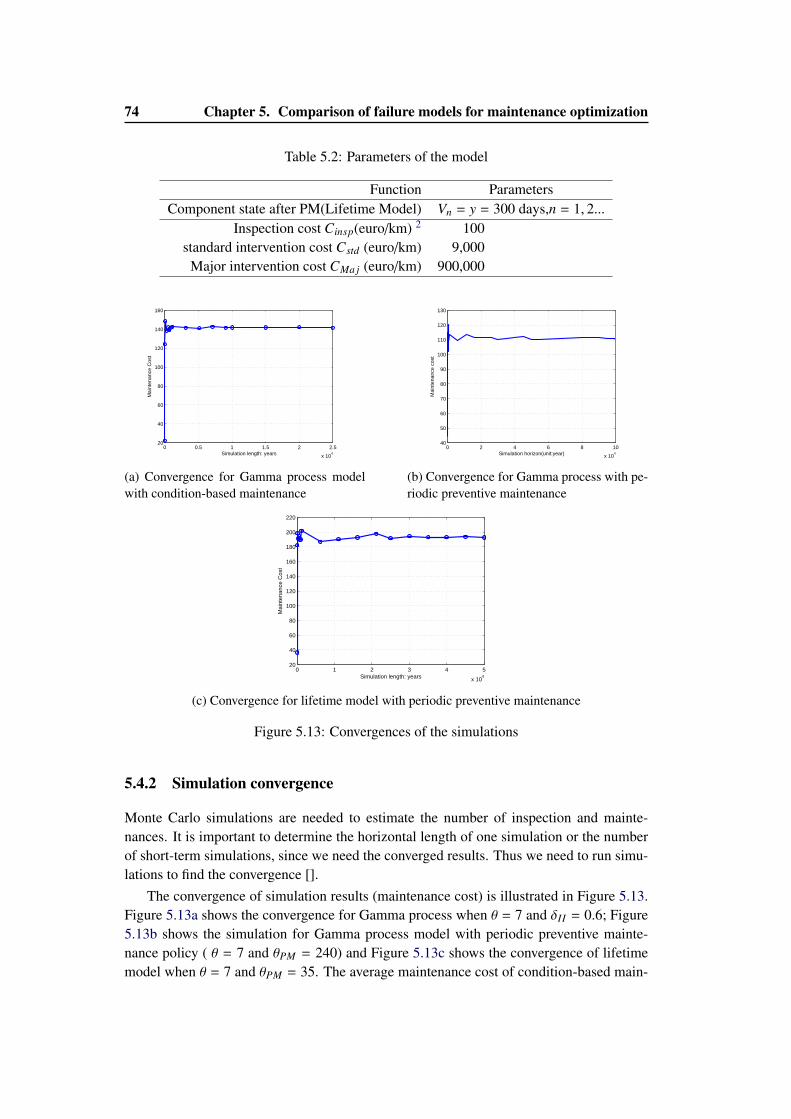
74 Chapter 5. Comparison of failure models for maintenance optimization
Table 5.2: Parameters of the model
Function ParametersComponent state after PM(Lifetime Model) Vn = y = 300 days,n = 1, 2...
Inspection cost Cinsp(euro/km) 2 100standard intervention cost Cstd (euro/km) 9,000
Major intervention cost CMa j (euro/km) 900,000
0 0.5 1 1.5 2 2.5
x 104
20
40
60
80
100
120
140
160
Simulation length: years
Mai
nten
ance
Cos
t
(a) Convergence for Gamma process modelwith condition-based maintenance
0 2 4 6 8 10
x 104
40
50
60
70
80
90
100
110
120
130
Simulation horizon(unit:year)
Mai
nten
ance
cos
t
(b) Convergence for Gamma process with pe-riodic preventive maintenance
0 1 2 3 4 5
x 104
20
40
60
80
100
120
140
160
180
200
220
Simulation length: years
Mai
nten
ance
Cos
t
(c) Convergence for lifetime model with periodic preventive maintenance
Figure 5.13: Convergences of the simulations
5.4.2 Simulation convergence
Monte Carlo simulations are needed to estimate the number of inspection and mainte-nances. It is important to determine the horizontal length of one simulation or the numberof short-term simulations, since we need the converged results. Thus we need to run simu-lations to find the convergence [].
The convergence of simulation results (maintenance cost) is illustrated in Figure 5.13.Figure 5.13a shows the convergence for Gamma process when θ = 7 and δII = 0.6; Figure5.13b shows the simulation for Gamma process model with periodic preventive mainte-nance policy ( θ = 7 and θPM = 240) and Figure 5.13c shows the convergence of lifetimemodel when θ = 7 and θPM = 35. The average maintenance cost of condition-based main-
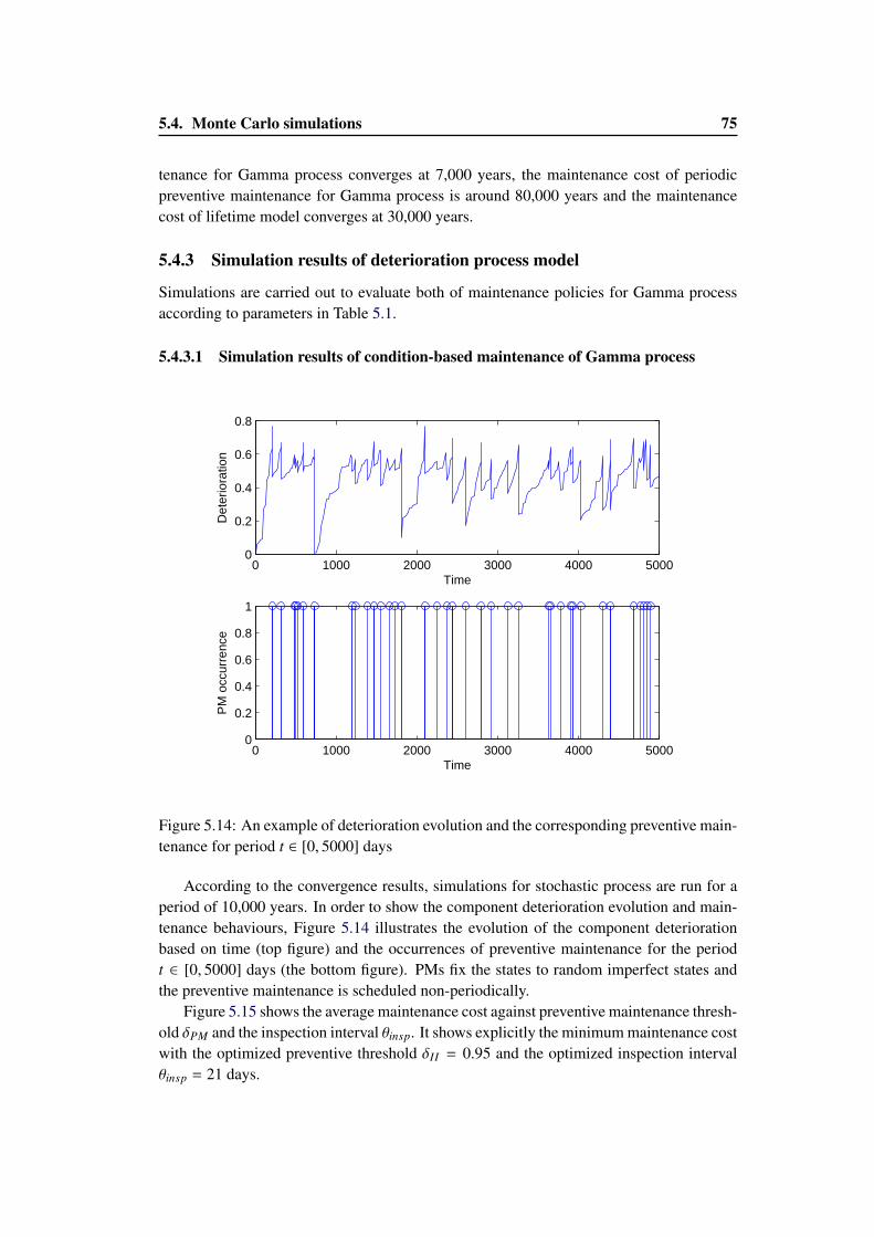
5.4. Monte Carlo simulations 75
tenance for Gamma process converges at 7,000 years, the maintenance cost of periodicpreventive maintenance for Gamma process is around 80,000 years and the maintenancecost of lifetime model converges at 30,000 years.
5.4.3 Simulation results of deterioration process model
Simulations are carried out to evaluate both of maintenance policies for Gamma processaccording to parameters in Table 5.1.
5.4.3.1 Simulation results of condition-based maintenance of Gamma process
0 1000 2000 3000 4000 50000
0.2
0.4
0.6
0.8
Time
Det
erio
ratio
n
0 1000 2000 3000 4000 50000
0.2
0.4
0.6
0.8
1
Time
PM
occ
urre
nce
Figure 5.14: An example of deterioration evolution and the corresponding preventive main-tenance for period t ∈ [0, 5000] days
According to the convergence results, simulations for stochastic process are run for aperiod of 10,000 years. In order to show the component deterioration evolution and main-tenance behaviours, Figure 5.14 illustrates the evolution of the component deteriorationbased on time (top figure) and the occurrences of preventive maintenance for the periodt ∈ [0, 5000] days (the bottom figure). PMs fix the states to random imperfect states andthe preventive maintenance is scheduled non-periodically.
Figure 5.15 shows the average maintenance cost against preventive maintenance thresh-old δPM and the inspection interval θinsp. It shows explicitly the minimum maintenance costwith the optimized preventive threshold δII = 0.95 and the optimized inspection intervalθinsp = 21 days.
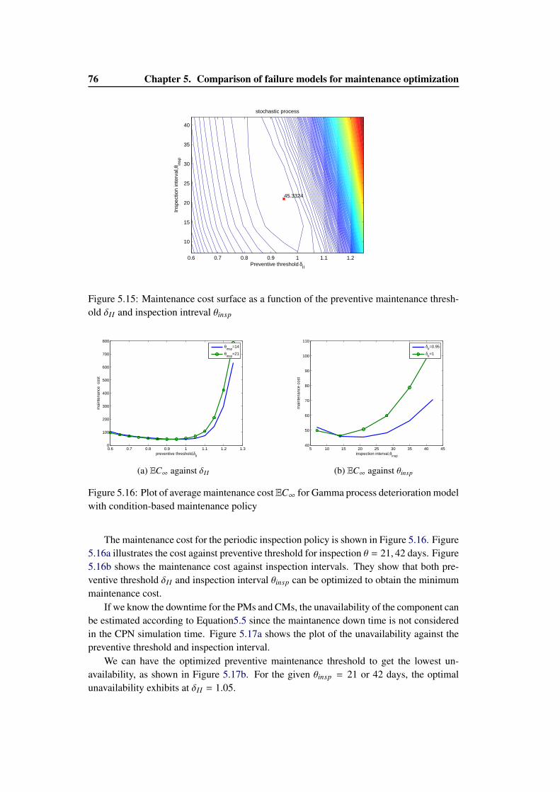
76 Chapter 5. Comparison of failure models for maintenance optimization
Preventive threshold δII
Insp
ectio
n in
terv
al,θ
insp
stochastic process
45.3324
0.6 0.7 0.8 0.9 1 1.1 1.2
10
15
20
25
30
35
40
Figure 5.15: Maintenance cost surface as a function of the preventive maintenance thresh-old δII and inspection intreval θinsp
0.6 0.7 0.8 0.9 1 1.1 1.2 1.30
100
200
300
400
500
600
700
800
preventive threshold,δII
mai
nten
ance
cos
t
θ
insp=14
θinsp
=21
(a) EC∞ against δII
5 10 15 20 25 30 35 40 4540
50
60
70
80
90
100
110
inspection interval,θinsp
mai
nten
ance
cos
t
δ
II=0.95
δII=1
(b) EC∞ against θinsp
Figure 5.16: Plot of average maintenance cost EC∞ for Gamma process deterioration modelwith condition-based maintenance policy
The maintenance cost for the periodic inspection policy is shown in Figure 5.16. Figure5.16a illustrates the cost against preventive threshold for inspection θ = 21, 42 days. Figure5.16b shows the maintenance cost against inspection intervals. They show that both pre-ventive threshold δII and inspection interval θinsp can be optimized to obtain the minimummaintenance cost.
If we know the downtime for the PMs and CMs, the unavailability of the component canbe estimated according to Equation5.5 since the maintanence down time is not consideredin the CPN simulation time. Figure 5.17a shows the plot of the unavailability against thepreventive threshold and inspection interval.
We can have the optimized preventive maintenance threshold to get the lowest un-availability, as shown in Figure 5.17b. For the given θinsp = 21 or 42 days, the optimalunavailability exhibits at δII = 1.05.

5.4. Monte Carlo simulations 77
0.40.6
0.81
1.21.4
0
20
40
600
0.05
0.1
0.15
0.2
Preventive threshold δII
Inspection interval,θinsp
Sys
tem
una
vaila
bilit
y
(a) Mesh plot of unavailability against δII andθinsp
0.5 0.6 0.7 0.8 0.9 1 1.1 1.2 1.30.03
0.04
0.05
0.06
0.07
0.08
0.09
Preventive threshold δPM
Una
vaila
bilit
y Q
avg
θ=21θ=42
(b) Plot of the unavailability against δII
Figure 5.17: System unavailability of condition-based maintenance for Gamma processdeterioration model
5.4.3.2 Simulation results of periodic preventive maintenance for Gamma processdeterioration model
According to the convergence results for the periodic preventive maintenance for Gammaprocess deterioration model in Figure 5.13b, simulation converges around 80,000 years;in order to get a more converged results, simulations of 100,000 years are carried out forestimate the average maintenance cost and system unavailability of periodic preventivemaintenance policy for Gamma process.
Figure 5.18 shows the maintenance cost of the periodic maintenance for Gamma pro-cess deterioration model. The optimal maintenance cost is around 53.34 when θinsp = 63days and θPM = 180 days as shown in Figure 5.18a. Figure 5.18b shows the averagemaintenance cost against preventive interval θPM.
Inspection interval, θinsp
Pre
vent
ive
thre
shol
dθP
M
Maintenance cost of stochastic process with periodic preventive maintenance
53.3438
10 20 30 40 50 60 70 80
150
200
250
300
350
400
(a) Maintenance cost against PM interval andinspection interval
100 150 200 250 300 350 400 4500
100
200
300
400
500
600
700
800
preventive interval,θPM
mai
nten
ance
cos
t
θinsp
=14
θinsp
=21
(b) Maintenance cost against intervention in-terval
Figure 5.18: Maintenance cost of periodic preventive maintenance for Gamma processdeterioration model
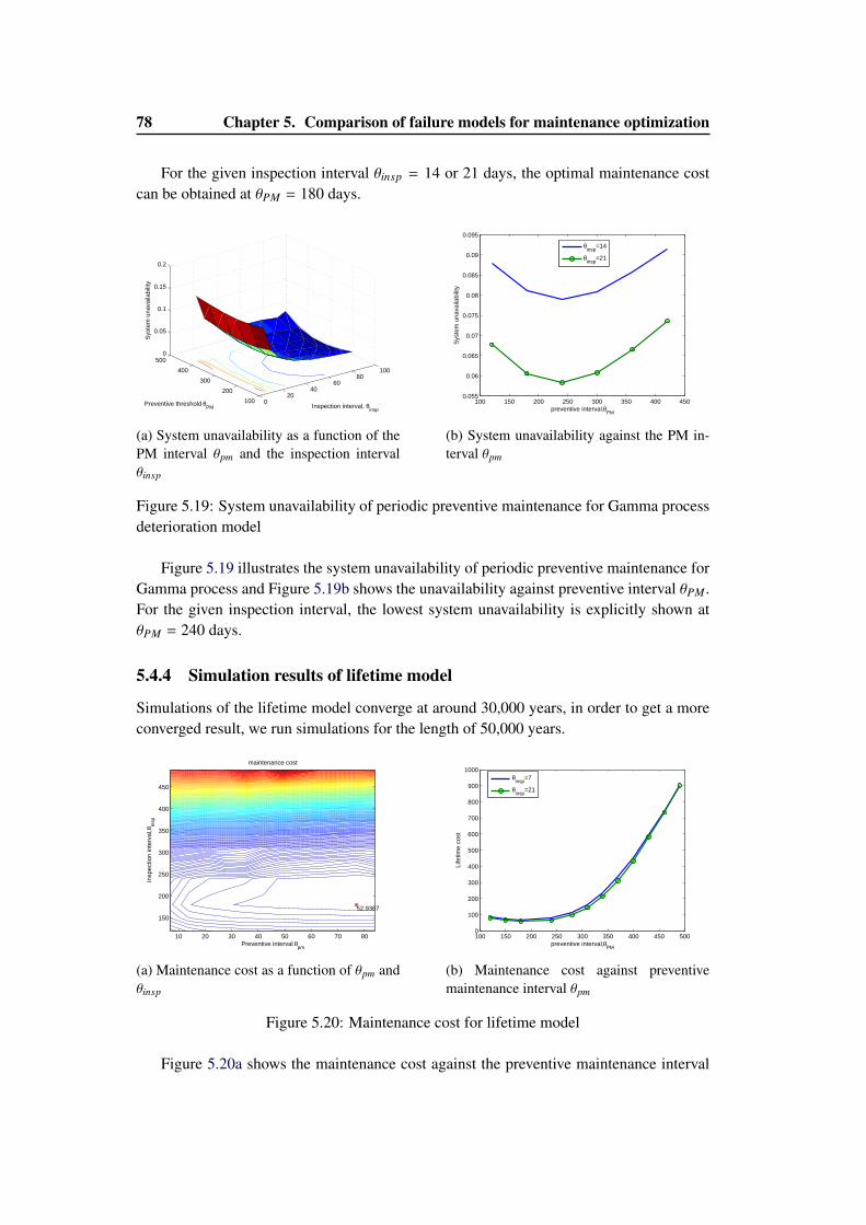
78 Chapter 5. Comparison of failure models for maintenance optimization
For the given inspection interval θinsp = 14 or 21 days, the optimal maintenance costcan be obtained at θPM = 180 days.
020
4060
80100
100
200
300
400
5000
0.05
0.1
0.15
0.2
Inspection interval, θinsp
Preventive threshold θPM
Sys
tem
una
vaila
bilit
y
(a) System unavailability as a function of thePM interval θpm and the inspection intervalθinsp
100 150 200 250 300 350 400 4500.055
0.06
0.065
0.07
0.075
0.08
0.085
0.09
0.095
preventive interval,θPM
Sys
tem
una
vaila
bilit
y
θinsp
=14
θinsp
=21
(b) System unavailability against the PM in-terval θpm
Figure 5.19: System unavailability of periodic preventive maintenance for Gamma processdeterioration model
Figure 5.19 illustrates the system unavailability of periodic preventive maintenance forGamma process and Figure 5.19b shows the unavailability against preventive interval θPM.For the given inspection interval, the lowest system unavailability is explicitly shown atθPM = 240 days.
5.4.4 Simulation results of lifetime model
Simulations of the lifetime model converge at around 30,000 years, in order to get a moreconverged result, we run simulations for the length of 50,000 years.
Preventive interval θpm
Insp
ectio
n in
terv
al,θ
insp
maintenance cost
52.9367
10 20 30 40 50 60 70 80
150
200
250
300
350
400
450
(a) Maintenance cost as a function of θpm andθinsp
100 150 200 250 300 350 400 450 5000
100
200
300
400
500
600
700
800
900
1000
preventive interval,θPM
Life
time
cost
θ
insp=7
θinsp
=21
(b) Maintenance cost against preventivemaintenance interval θpm
Figure 5.20: Maintenance cost for lifetime model
Figure 5.20a shows the maintenance cost against the preventive maintenance interval
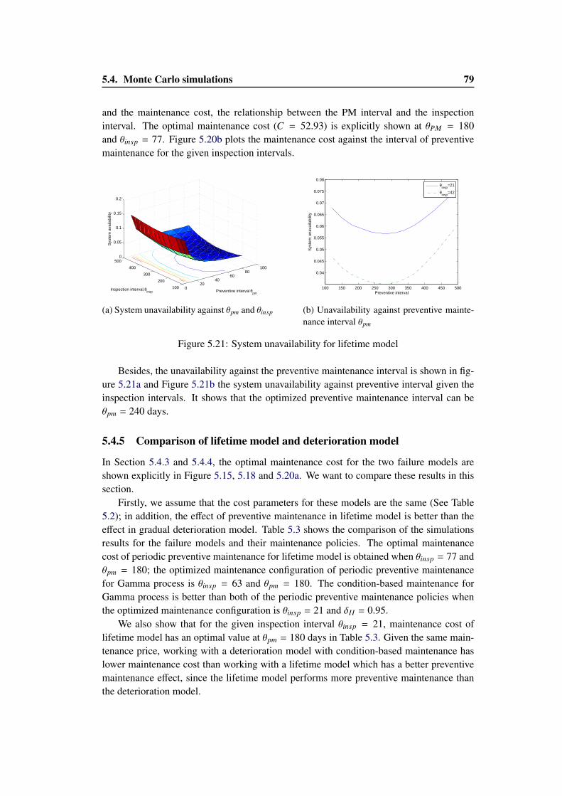
5.4. Monte Carlo simulations 79
and the maintenance cost, the relationship between the PM interval and the inspectioninterval. The optimal maintenance cost (C = 52.93) is explicitly shown at θPM = 180and θinsp = 77. Figure 5.20b plots the maintenance cost against the interval of preventivemaintenance for the given inspection intervals.
020
4060
80100
100
200
300
400
5000
0.05
0.1
0.15
0.2
Preventive interval θpm
Inspection interval,θinsp
Sys
tem
ava
ilabi
lity
(a) System unavailability against θpm and θinsp
100 150 200 250 300 350 400 450 500
0.04
0.045
0.05
0.055
0.06
0.065
0.07
0.075
0.08
Preventive interval
Sys
tem
una
vaila
bilit
y
θ
insp=21
θinsp
=42
(b) Unavailability against preventive mainte-nance interval θpm
Figure 5.21: System unavailability for lifetime model
Besides, the unavailability against the preventive maintenance interval is shown in fig-ure 5.21a and Figure 5.21b the system unavailability against preventive interval given theinspection intervals. It shows that the optimized preventive maintenance interval can beθpm = 240 days.
5.4.5 Comparison of lifetime model and deterioration model
In Section 5.4.3 and 5.4.4, the optimal maintenance cost for the two failure models areshown explicitly in Figure 5.15, 5.18 and 5.20a. We want to compare these results in thissection.
Firstly, we assume that the cost parameters for these models are the same (See Table5.2); in addition, the effect of preventive maintenance in lifetime model is better than theeffect in gradual deterioration model. Table 5.3 shows the comparison of the simulationsresults for the failure models and their maintenance policies. The optimal maintenancecost of periodic preventive maintenance for lifetime model is obtained when θinsp = 77 andθpm = 180; the optimized maintenance configuration of periodic preventive maintenancefor Gamma process is θinsp = 63 and θpm = 180. The condition-based maintenance forGamma process is better than both of the periodic preventive maintenance policies whenthe optimized maintenance configuration is θinsp = 21 and δII = 0.95.
We also show that for the given inspection interval θinsp = 21, maintenance cost oflifetime model has an optimal value at θpm = 180 days in Table 5.3. Given the same main-tenance price, working with a deterioration model with condition-based maintenance haslower maintenance cost than working with a lifetime model which has a better preventivemaintenance effect, since the lifetime model performs more preventive maintenance thanthe deterioration model.
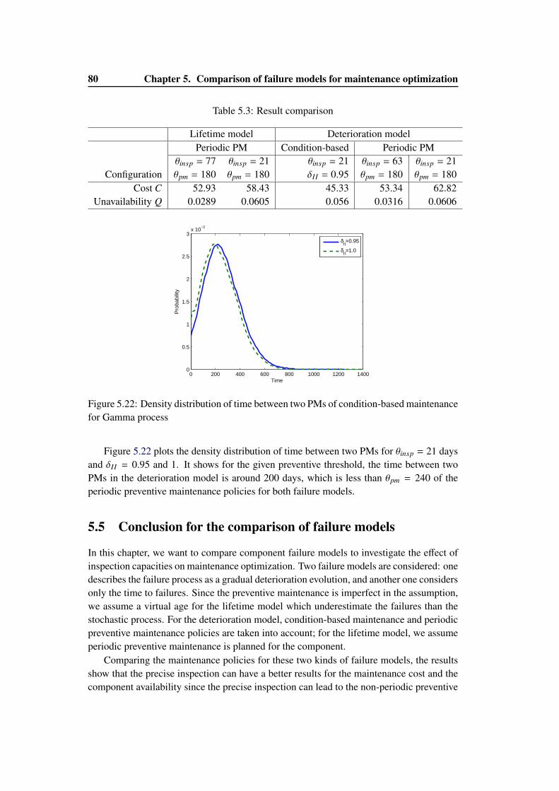
80 Chapter 5. Comparison of failure models for maintenance optimization
Table 5.3: Result comparison
Lifetime model Deterioration modelPeriodic PM Condition-based Periodic PM
Configurationθinsp = 77 θinsp = 21 θinsp = 21 θinsp = 63 θinsp = 21θpm = 180 θpm = 180 δII = 0.95 θpm = 180 θpm = 180
Cost C 52.93 58.43 45.33 53.34 62.82Unavailability Q 0.0289 0.0605 0.056 0.0316 0.0606
0 200 400 600 800 1000 1200 14000
0.5
1
1.5
2
2.5
3x 10
−3
Time
Pro
babi
lity
δ
II=0.95
δII=1.0
Figure 5.22: Density distribution of time between two PMs of condition-based maintenancefor Gamma process
Figure 5.22 plots the density distribution of time between two PMs for θinsp = 21 daysand δII = 0.95 and 1. It shows for the given preventive threshold, the time between twoPMs in the deterioration model is around 200 days, which is less than θpm = 240 of theperiodic preventive maintenance policies for both failure models.
5.5 Conclusion for the comparison of failure models
In this chapter, we want to compare component failure models to investigate the effect ofinspection capacities on maintenance optimization. Two failure models are considered: onedescribes the failure process as a gradual deterioration evolution, and another one considersonly the time to failures. Since the preventive maintenance is imperfect in the assumption,we assume a virtual age for the lifetime model which underestimate the failures than thestochastic process. For the deterioration model, condition-based maintenance and periodicpreventive maintenance policies are taken into account; for the lifetime model, we assumeperiodic preventive maintenance is planned for the component.
Comparing the maintenance policies for these two kinds of failure models, the resultsshow that the precise inspection can have a better results for the maintenance cost and thecomponent availability since the precise inspection can lead to the non-periodic preventive
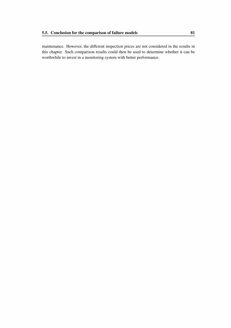
5.5. Conclusion for the comparison of failure models 81
maintenance. However, the different inspection prices are not considered in the results inthis chapter. Such comparison results could then be used to determine whether it can beworthwhile to invest in a monitoring system with better performance.

Chapter 6
Delayed repair for railway trackmaintenance
Contents6.1 Introduction . . . . . . . . . . . . . . . . . . . . . . . . . . . . . . . . . 836.2 Track maintenance modelling assumptions . . . . . . . . . . . . . . . . 84
6.2.1 Modelling assumptions . . . . . . . . . . . . . . . . . . . . . . . . 84
6.2.2 Performance evaluation . . . . . . . . . . . . . . . . . . . . . . . . 87
6.3 Track CPN models . . . . . . . . . . . . . . . . . . . . . . . . . . . . . . 876.3.1 Deterioration part of CPN model . . . . . . . . . . . . . . . . . . . 87
6.3.2 CPN model of inspection schemes . . . . . . . . . . . . . . . . . . 89
6.3.3 CPN model of delayed maintenance . . . . . . . . . . . . . . . . . 89
6.4 Numerical results . . . . . . . . . . . . . . . . . . . . . . . . . . . . . . 916.4.1 Simulation convergence . . . . . . . . . . . . . . . . . . . . . . . 91
6.4.2 Repair delay for periodic inspection . . . . . . . . . . . . . . . . . 96
6.4.3 Repair delay for condition-based inspection . . . . . . . . . . . . . 98
6.4.4 Comparison of inspection policies . . . . . . . . . . . . . . . . . . 105
6.5 Conclusions for the delayed repairs . . . . . . . . . . . . . . . . . . . . 107
6.1 Introduction
Railway network is a large-scale network which carries thousands of trains and passengersevery day. Maintenance machines are allocated in several depots and they need to travel tothe locations of the defective assets and the machines and crews are not always availablefor the maintenance. Once there is a identified asset defect, if it is not critical and does notexceed the extreme threshold, the railway section keeps open to allow trains passing.
Therefore, preventive maintenance for the railway asset cannot be performed imme-diately after the defects are detected. During the waiting time for preventive repairs, therailway section still allows the traffic and hence suffers to the same deterioration processwhich possibly results in the asset degrading to a critical state which leads to a correctivemaintenance even to an accident.
84 Chapter 6. Delayed repair for railway track maintenance
Castro et al discuss the repair policies for a single unit component which allows repairperforming in a repair window [37]. The component works for period T and a continuesinspection works for the component. If defects are detected during the repair window, thecomponent is repaired; otherwise, no repair is scheduled and the component is down if thecomponent state reaches N. System reward is the performance evaluation and the length ofthe repair window is the maintenance decision variable. They calculate the system rewardsbased on the alternative renewal process [37]. Meier-Hirmer et al. [114] describes the trackdeterioration as a Gamma process Γ(α, β), a periodic inspection is scheduled to measurethe deterioration details. The preventive maintenance are assumed to arrive in a delaytime which may be longer than the periodic inspection interval; during the delay time,component keep deteriorates. They propose a Markov Chain to estimate the maintenancecost.
In this chapter, we want to assess the effect of the delay on the maintenance perfor-mance to see if it is necessary to take this delay into account in the decision procedure tomake a better maintenance strategy for the track system. A maintenance model is neededto solve the problem. Since the system state not only depends on the last observed state butalso more previous states according to the length of the delays, the deterioration process isnot a Markov chain. Instead of constructing a Markov Chain introduced in [114], we pro-pose a model based on Coloured Petri Net to estimate the long-term average maintenancecost.
The model in this chapter is presented in conference Safeprocess 2015 [173].This chapter is organized as followed: Section 6.2 lists the assumptions of track de-
terioration and maintenance. Section 6.3 illustrates the Colored Petri Net model for theassumptions. Section 6.4 shows the simulation results and section 6.5 give a brief conclu-sion.
6.2 Track maintenance modelling assumptions
In this chapter, the component deterioration is assumed to be a Gamma process: Xτ+∆τ −
Xτ ∼ Γ(α∆τ, β). Delayed repairs for condition based maintenance and periodic inspectionare modeled. The preventive maintenance threshold, inspection interval and the repairdelays are optimized to get the minimum maintenance cost.
6.2.1 Modelling assumptions
The delayed maintenance policies considers a single unit component. Track top fault (de-scribed in Chapter 2), the vertical geometry fault of track is assumed to be the failure.Tamping is assumed to be the preventive maintenance method and the stoneblowering isthe corrective maintenance. Track condition information, .i.e. standard deviation for 35mlong is collected by track recording car.
The assumptions of the model in this work are as follows:
• The component is assumed to be a track of 1 kilometre long.
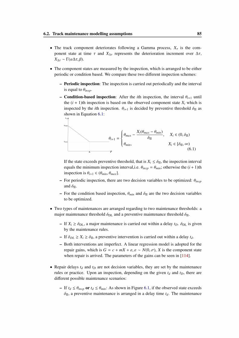
6.2. Track maintenance modelling assumptions 85
• The track component deteriorates following a Gamma process, Xτ is the com-ponent state at time τ and X∆τ represents the deterioration increment over ∆τ,X∆τ ∼ Γ(α∆τ, β).
• The component states are measured by the inspection, which is arranged to be eitherperiodic or condition based. We compare these two different inspection schemes:
– Periodic inspection: The inspection is carried out periodically and the intervalis equal to θinsp.
– Condition-based inspection: After the ith inspection, the interval θi+1 untilthe (i + 1)th inspection is based on the observed component state Xi which isinspected by the ith inspection. θi+1 is decided by preventive threshold δII asshown in Equation 6.1:
θi+1 =
θmax −
Xi(θmax − θmin)δII
, Xi ∈ (0, δII)
θmin, Xi ∈ [δII,∞)(6.1)
If the state exceeds preventive threshold, that is Xi ≤ δII, the inspection intervalequals the minimum inspection interval,i.e. θinsp = θmin; otherwise the (i + 1)thinspection is θi+1 ∈ (θmin, θmax].
– For periodic inspection, there are two decision variables to be optimized: θinsp
and δII.
– For the condition based inspection, θmin and δII are the two decision variablesto be optimized.
• Two types of maintenances are arranged regarding to two maintenance thresholds: amajor maintenance threshold δDL and a preventive maintenance threshold δII.
– If Xi ≥ δDL, a major maintenance is carried out within a delay tD. δDL is givenby the maintenance rules.
– If δDL ≥ Xi ≥ δII, a preventive intervention is carried out within a delay td.
– Both interventions are imperfect. A linear regression model is adopted for therepair gains, which is G = c + mX + ε, ε ∼ N(0, σ), X is the component statewhen repair is arrived. The parameters of the gains can be seen in [114].
• Repair delays td and tD are not decision variables, they are set by the maintenancerules or practice. Upon an inspection, depending on the given td and tD, there aredifferent possible maintenance scenarios:
– If td ≤ θinsp or td ≤ θmin: As shown in Figure 6.1, if the observed state exceedsδII, a preventive maintenance is arranged in a delay time td. The maintenance
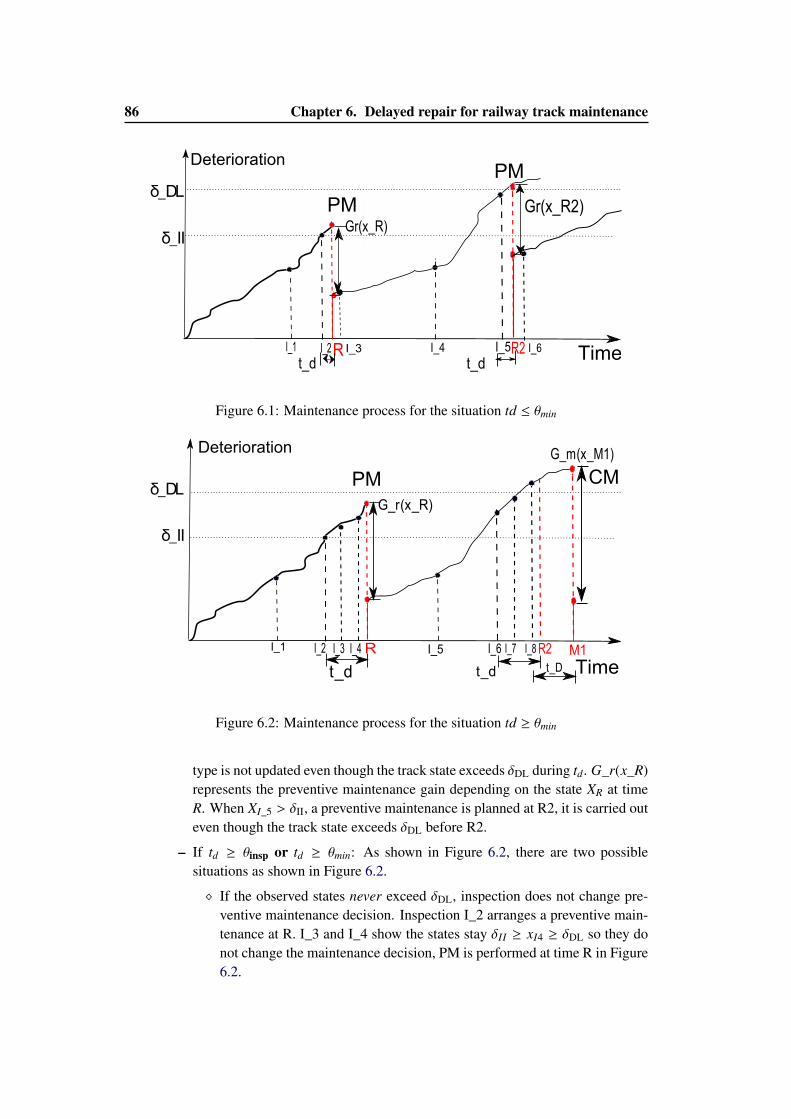
86 Chapter 6. Delayed repair for railway track maintenance
δ_DL
δ_II
PM
PM
I_1 I_2 I_3Rt_d
Gr(x_R)
I_4 I_5
t_dI_6R2
Gr(x_R2)
Deterioration
Time
Figure 6.1: Maintenance process for the situation td ≤ θmin
δ_DL
δ_II
I_1 I_2 I_3 I_4R
t_d
G_r(x_R)
I_5 I_6
t_d
I_7 I_8R2
G_m(x_M1)
t_D
M1
Deterioration
Time
PM CM
Figure 6.2: Maintenance process for the situation td ≥ θmin
type is not updated even though the track state exceeds δDL during td. G_r(x_R)represents the preventive maintenance gain depending on the state XR at timeR. When XI_5 > δII, a preventive maintenance is planned at R2, it is carried outeven though the track state exceeds δDL before R2.
– If td ≥ θinsp or td ≥ θmin: As shown in Figure 6.2, there are two possiblesituations as shown in Figure 6.2.
� If the observed states never exceed δDL, inspection does not change pre-ventive maintenance decision. Inspection I_2 arranges a preventive main-tenance at R. I_3 and I_4 show the states stay δII ≥ xI4 ≥ δDL so they donot change the maintenance decision, PM is performed at time R in Figure6.2.
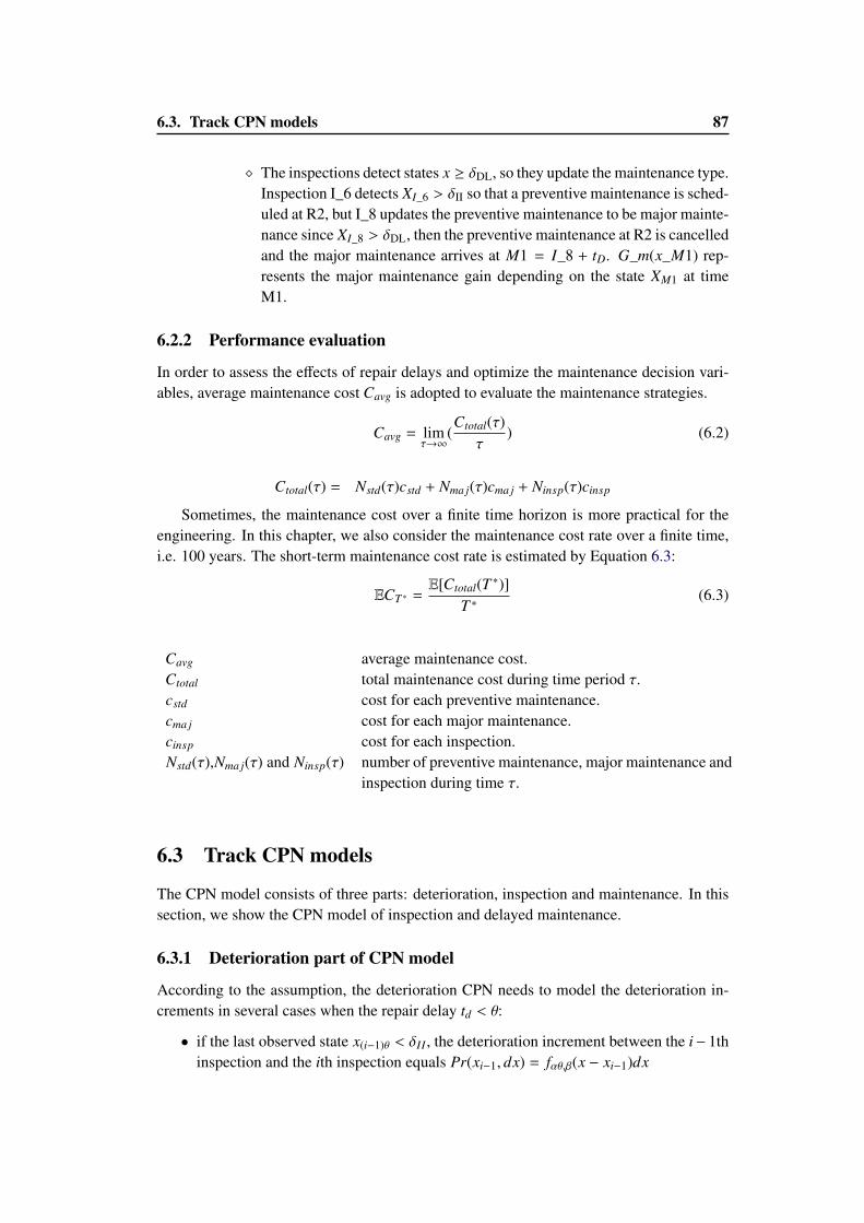
6.3. Track CPN models 87
� The inspections detect states x ≥ δDL, so they update the maintenance type.Inspection I_6 detects XI_6 > δII so that a preventive maintenance is sched-uled at R2, but I_8 updates the preventive maintenance to be major mainte-nance since XI_8 > δDL, then the preventive maintenance at R2 is cancelledand the major maintenance arrives at M1 = I_8 + tD. G_m(x_M1) rep-resents the major maintenance gain depending on the state XM1 at timeM1.
6.2.2 Performance evaluation
In order to assess the effects of repair delays and optimize the maintenance decision vari-ables, average maintenance cost Cavg is adopted to evaluate the maintenance strategies.
Cavg = limτ→∞
(Ctotal(τ)
τ) (6.2)
Ctotal(τ) = Nstd(τ)cstd + Nma j(τ)cma j + Ninsp(τ)cinsp
Sometimes, the maintenance cost over a finite time horizon is more practical for theengineering. In this chapter, we also consider the maintenance cost rate over a finite time,i.e. 100 years. The short-term maintenance cost rate is estimated by Equation 6.3:
ECT ∗ =E[Ctotal(T ∗)]
T ∗(6.3)
Cavg average maintenance cost.Ctotal total maintenance cost during time period τ.cstd cost for each preventive maintenance.cma j cost for each major maintenance.cinsp cost for each inspection.Nstd(τ),Nma j(τ) and Ninsp(τ) number of preventive maintenance, major maintenance and
inspection during time τ.
6.3 Track CPN models
The CPN model consists of three parts: deterioration, inspection and maintenance. In thissection, we show the CPN model of inspection and delayed maintenance.
6.3.1 Deterioration part of CPN model
According to the assumption, the deterioration CPN needs to model the deterioration in-crements in several cases when the repair delay td < θ:
• if the last observed state x(i−1)θ < δII , the deterioration increment between the i− 1thinspection and the ith inspection equals Pr(xi−1, dx) = fαθ,β(x − xi−1)dx
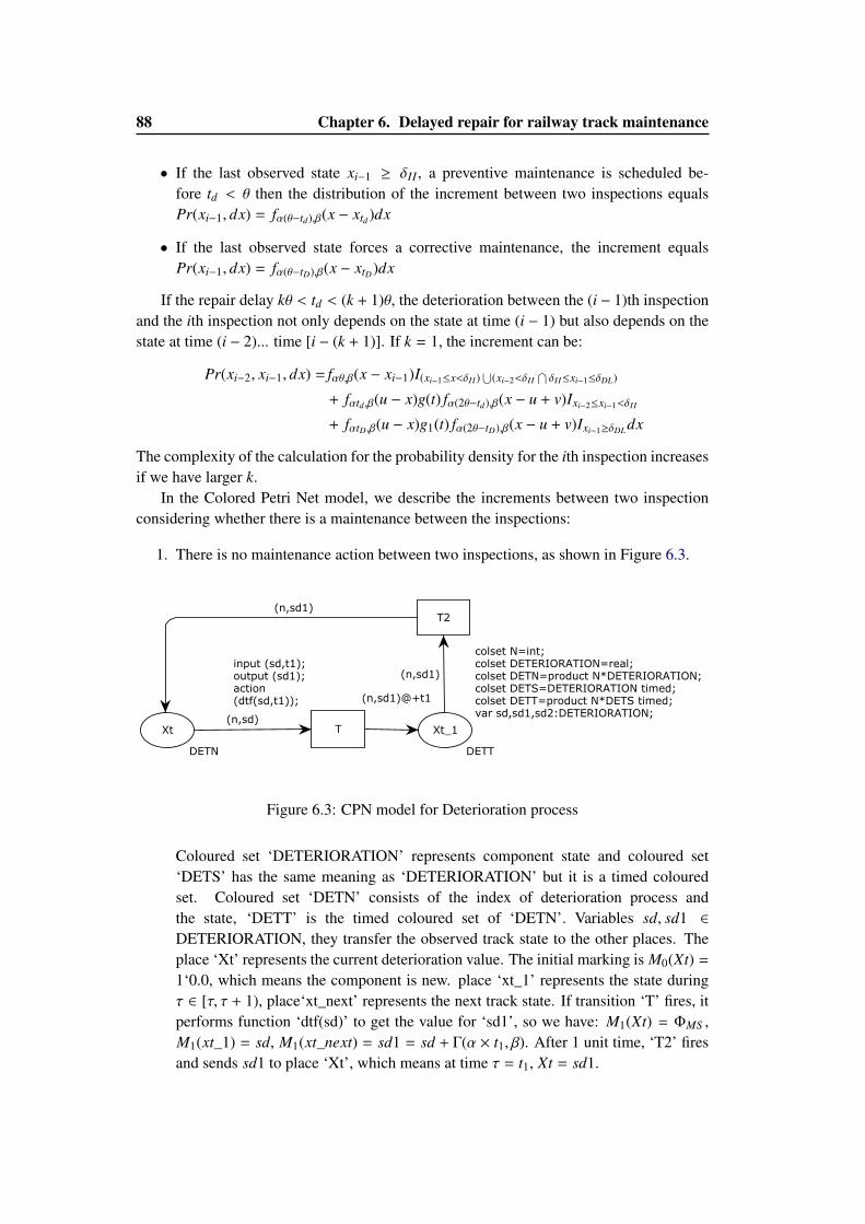
88 Chapter 6. Delayed repair for railway track maintenance
• If the last observed state xi−1 ≥ δII , a preventive maintenance is scheduled be-fore td < θ then the distribution of the increment between two inspections equalsPr(xi−1, dx) = fα(θ−td),β(x − xtd )dx
• If the last observed state forces a corrective maintenance, the increment equalsPr(xi−1, dx) = fα(θ−tD),β(x − xtD)dx
If the repair delay kθ < td < (k + 1)θ, the deterioration between the (i − 1)th inspectionand the ith inspection not only depends on the state at time (i − 1) but also depends on thestate at time (i − 2)... time [i − (k + 1)]. If k = 1, the increment can be:
Pr(xi−2, xi−1, dx) = fαθ,β(x − xi−1)I(xi−1≤x<δII )⋃
(xi−2<δII⋂δII≤xi−1≤δDL)
+ fαtd ,β(u − x)g(t) fα(2θ−td),β(x − u + v)Ixi−2≤xi−1<δII
+ fαtD,β(u − x)g1(t) fα(2θ−tD),β(x − u + v)Ixi−1≥δDLdx
The complexity of the calculation for the probability density for the ith inspection increasesif we have larger k.
In the Colored Petri Net model, we describe the increments between two inspectionconsidering whether there is a maintenance between the inspections:
1. There is no maintenance action between two inspections, as shown in Figure 6.3.
colset N=int;colset DETERIORATION=real;colset DETN=product N*DETERIORATION;colset DETS=DETERIORATION timed;colset DETT=product N*DETS timed;var sd,sd1,sd2:DETERIORATION;
Xt
DETN
Xt_1
DETT
T
input (sd,t1);output (sd1);action(dtf(sd,t1));
T2
(n,sd)
(n,sd1)@+t1
(n,sd1)
(n,sd1)
Figure 6.3: CPN model for Deterioration process
Coloured set ‘DETERIORATION’ represents component state and coloured set‘DETS’ has the same meaning as ‘DETERIORATION’ but it is a timed colouredset. Coloured set ‘DETN’ consists of the index of deterioration process andthe state, ‘DETT’ is the timed coloured set of ‘DETN’. Variables sd, sd1 ∈
DETERIORATION, they transfer the observed track state to the other places. Theplace ‘Xt’ represents the current deterioration value. The initial marking is M0(Xt) =
1‘0.0, which means the component is new. place ‘xt_1’ represents the state duringτ ∈ [τ, τ + 1), place‘xt_next’ represents the next track state. If transition ‘T’ fires, itperforms function ‘dtf(sd)’ to get the value for ‘sd1’, so we have: M1(Xt) = ΦMS ,M1(xt_1) = sd, M1(xt_next) = sd1 = sd + Γ(α × t1, β). After 1 unit time, ‘T2’ firesand sends sd1 to place ‘Xt’, which means at time τ = t1, Xt = sd1.
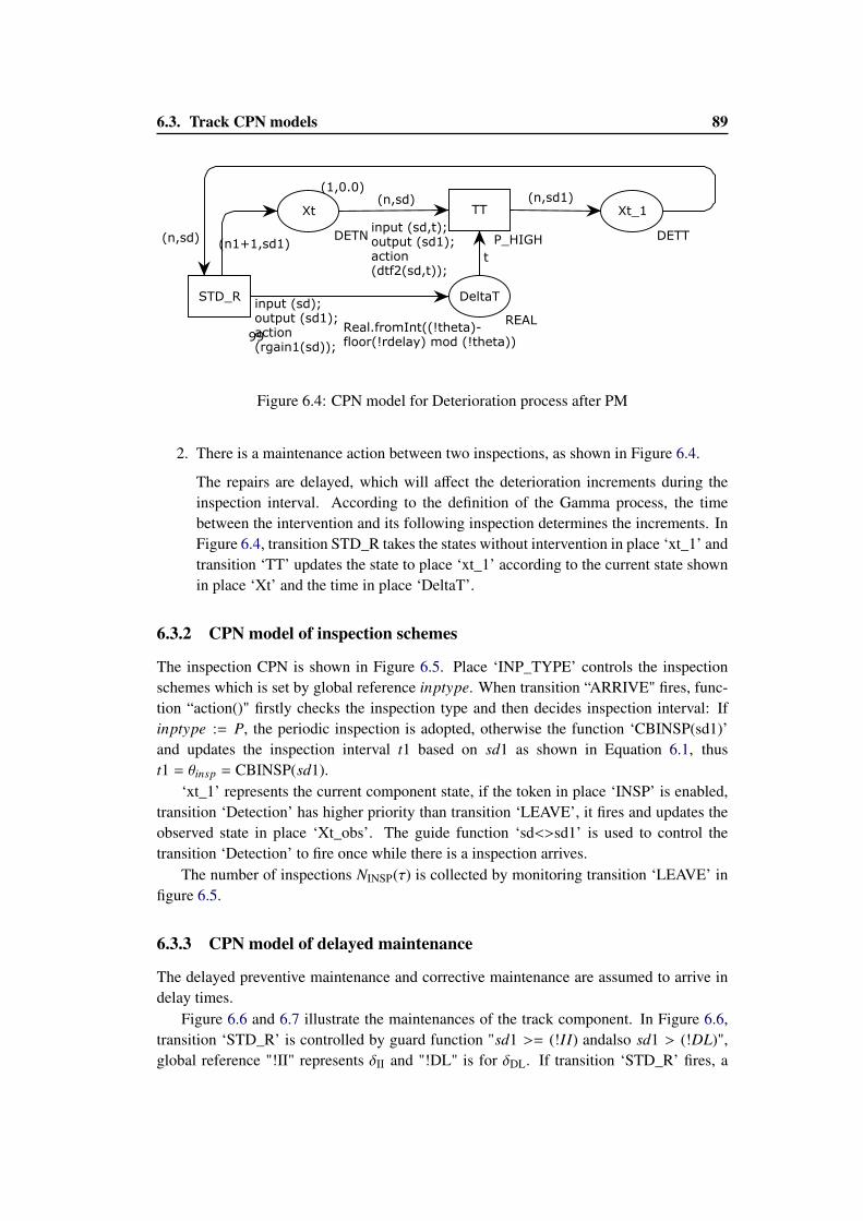
6.3. Track CPN models 89
Xt
DETN
(1,0.0)
Xt_1
DETT
DeltaT
REAL
STD_Rinput (sd);output (sd1);action(rgain1(sd));
99
TT
input (sd,t);output (sd1);action(dtf2(sd,t));
P_HIGH(n,sd)(n1+1,sd1)
(n,sd)
t
(n,sd1)
Real.fromInt((!theta)-floor(!rdelay) mod (!theta))
Figure 6.4: CPN model for Deterioration process after PM
2. There is a maintenance action between two inspections, as shown in Figure 6.4.
The repairs are delayed, which will affect the deterioration increments during theinspection interval. According to the definition of the Gamma process, the timebetween the intervention and its following inspection determines the increments. InFigure 6.4, transition STD_R takes the states without intervention in place ‘xt_1’ andtransition ‘TT’ updates the state to place ‘xt_1’ according to the current state shownin place ‘Xt’ and the time in place ‘DeltaT’.
6.3.2 CPN model of inspection schemes
The inspection CPN is shown in Figure 6.5. Place ‘INP_TYPE’ controls the inspectionschemes which is set by global reference inptype. When transition “ARRIVE" fires, func-tion “action()" firstly checks the inspection type and then decides inspection interval: Ifinptype := P, the periodic inspection is adopted, otherwise the function ‘CBINSP(sd1)’and updates the inspection interval t1 based on sd1 as shown in Equation 6.1, thust1 = θinsp = CBINSP(sd1).
‘xt_1’ represents the current component state, if the token in place ‘INSP’ is enabled,transition ‘Detection’ has higher priority than transition ‘LEAVE’, it fires and updates theobserved state in place ‘Xt_obs’. The guide function ‘sd<>sd1’ is used to control thetransition ‘Detection’ to fire once while there is a inspection arrives.
The number of inspections NINSP(τ) is collected by monitoring transition ‘LEAVE’ infigure 6.5.
6.3.3 CPN model of delayed maintenance
The delayed preventive maintenance and corrective maintenance are assumed to arrive indelay times.
Figure 6.6 and 6.7 illustrate the maintenances of the track component. In Figure 6.6,transition ‘STD_R’ is controlled by guard function "sd1 >= (!II) andalso sd1 > (!DL)",global reference "!II" represents δII and "!DL" is for δDL. If transition ‘STD_R’ fires, a
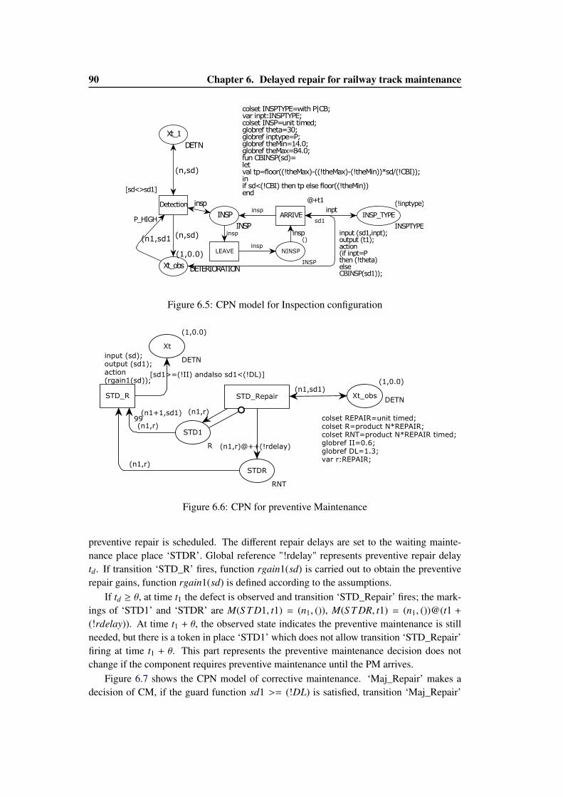
90 Chapter 6. Delayed repair for railway track maintenance
colset INSPTYPE=with P|CB;var inpt:INSPTYPE;colset INSP=unit timed;globref theta=30;globref inptype=P;globref theMin=14.0;globref theMax=84.0;fun CBINSP(sd)=letval tp=floor((!theMax)-((!theMax)-(!theMin))*sd/(!CBI));in if sd<(!CBI) then tp else floor((!theMin))end
INSP
INSP
NINSP
INSP
()
Xt_obs DETERIORATION
Xt_1
DETN
LEAVE
ARRIVE
@+t1
input (sd1,inpt);output (t1);action(if inpt=Pthen (!theta)elseCBINSP(sd1));
Detection
[sd<>sd1]
P_HIGH
insp
insp
insp
inspinsp
(n,sd)
(n,sd)
(n1,sd1
sd1INSP_TYPE
INSPTYPE
inpt(!inptype)
(1,0.0)
Figure 6.5: CPN model for Inspection configuration
colset REPAIR=unit timed;colset R=product N*REPAIR;colset RNT=product N*REPAIR timed;globref II=0.6;globref DL=1.3;var r:REPAIR;
Xt
DETN
(1,0.0)
Xt_obsDETN
(1,0.0)
STDR
RNT
STD1
R
STD_Repair
[sd1>=(!II) andalso sd1<(!DL)]
STD_R
input (sd);output (sd1);action(rgain1(sd));
99
(n1,sd1)
(n1,r)@++(!rdelay)
(n1,r)
(n1+1,sd1) (n1,r)
(n1,r)
Figure 6.6: CPN for preventive Maintenance
preventive repair is scheduled. The different repair delays are set to the waiting mainte-nance place place ‘STDR’. Global reference "!rdelay" represents preventive repair delaytd. If transition ‘STD_R’ fires, function rgain1(sd) is carried out to obtain the preventiverepair gains, function rgain1(sd) is defined according to the assumptions.
If td ≥ θ, at time t1 the defect is observed and transition ‘STD_Repair’ fires; the mark-ings of ‘STD1’ and ‘STDR’ are M(S T D1, t1) = (n1, ()), M(S T DR, t1) = (n1, ())@(t1 +
(!rdelay)). At time t1 + θ, the observed state indicates the preventive maintenance is stillneeded, but there is a token in place ‘STD1’ which does not allow transition ‘STD_Repair’firing at time t1 + θ. This part represents the preventive maintenance decision does notchange if the component requires preventive maintenance until the PM arrives.
Figure 6.7 shows the CPN model of corrective maintenance. ‘Maj_Repair’ makes adecision of CM, if the guard function sd1 >= (!DL) is satisfied, transition ‘Maj_Repair’

6.4. Numerical results 91
Xt
DETN
(1,0.0)
Xt_obsDETN
(1,0.0)
MAJR
RNT
STD1
R
Maj1
R
Maj_Repair
[sd1>=(!DL)]
Maj_R
input (sd);output (sd1);action(Mgain(sd));
99
(n1,sd1)
(n1,r)@++(!Mdelay)
(n1+1,sd1)
(n1,r)
(n1,r)
(n1,r)
Figure 6.7: CPN for corrective maintenance
fires, a token is sent to place ‘Maj1’ which means the component needs CM and a token issent to place ‘MAJR’ which stores the repair arrival time sampled by function Mgain(sd).Similar to transition ‘STD_R’ , transition ‘Maj_R’ fires if token in ‘MAJR’ is enabled. IfPM delay is larger than inspection interval and a major maintenance is needed during thedelay time. This maintenance updating process is realized by the reset arc from ‘STD1’ totransition ‘Maj_Repair’.
The number of preventive maintenance actions NSTD(τ) is collected by monitoring thetransition ‘STD_R’, the number of major maintenance actions NMAJ(τ) is collected bymonitoring the transition ‘Maj_R’.
6.4 Numerical results
Monte Carlo Simulations are needed to:
• investigate how the delay td affects the maintenance performance;
• find the optimal maintenance decision value for delayed maintenance strategies.
Simulations are carried out according to the maintenance cost parameters as shown in Table6.1. The maintenance price is not exactly the real price used in the real railway system; insome researches, the preventive maintenance action price is assumed to be several thousandeuros and the corrective maintenance or the renewal price is assumed to be several hundredthousand euros.
6.4.1 Simulation convergence
We run simulations for one maintenance configuration to find the simulation convergence.The simulation are configured as: θinsp = 15, δII = 0.6,td = 1.0.
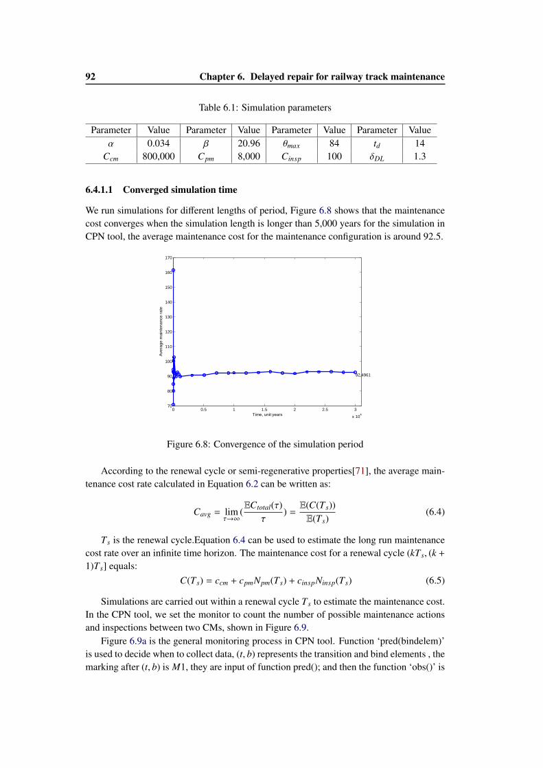
92 Chapter 6. Delayed repair for railway track maintenance
Table 6.1: Simulation parameters
Parameter Value Parameter Value Parameter Value Parameter Valueα 0.034 β 20.96 θmax 84 td 14
Ccm 800,000 Cpm 8,000 Cinsp 100 δDL 1.3
6.4.1.1 Converged simulation time
We run simulations for different lengths of period, Figure 6.8 shows that the maintenancecost converges when the simulation length is longer than 5,000 years for the simulation inCPN tool, the average maintenance cost for the maintenance configuration is around 92.5.
0 0.5 1 1.5 2 2.5 3
x 104
70
80
90
100
110
120
130
140
150
160
170
Time, unit:years
Ave
rage
mai
nten
ance
rat
e
92.4961
Figure 6.8: Convergence of the simulation period
According to the renewal cycle or semi-regenerative properties[71], the average main-tenance cost rate calculated in Equation 6.2 can be written as:
Cavg = limτ→∞
(ECtotal(τ)
τ) =E(C(Ts))E(Ts)
(6.4)
Ts is the renewal cycle.Equation 6.4 can be used to estimate the long run maintenancecost rate over an infinite time horizon. The maintenance cost for a renewal cycle (kTs, (k +
1)Ts] equals:C(Ts) = ccm + cpmNpm(Ts) + cinspNinsp(Ts) (6.5)
Simulations are carried out within a renewal cycle Ts to estimate the maintenance cost.In the CPN tool, we set the monitor to count the number of possible maintenance actionsand inspections between two CMs, shown in Figure 6.9.
Figure 6.9a is the general monitoring process in CPN tool. Function ‘pred(bindelem)’is used to decide when to collect data, (t, b) represents the transition and bind elements , themarking after (t, b) is M1, they are input of function pred(); and then the function ‘obs()’ is
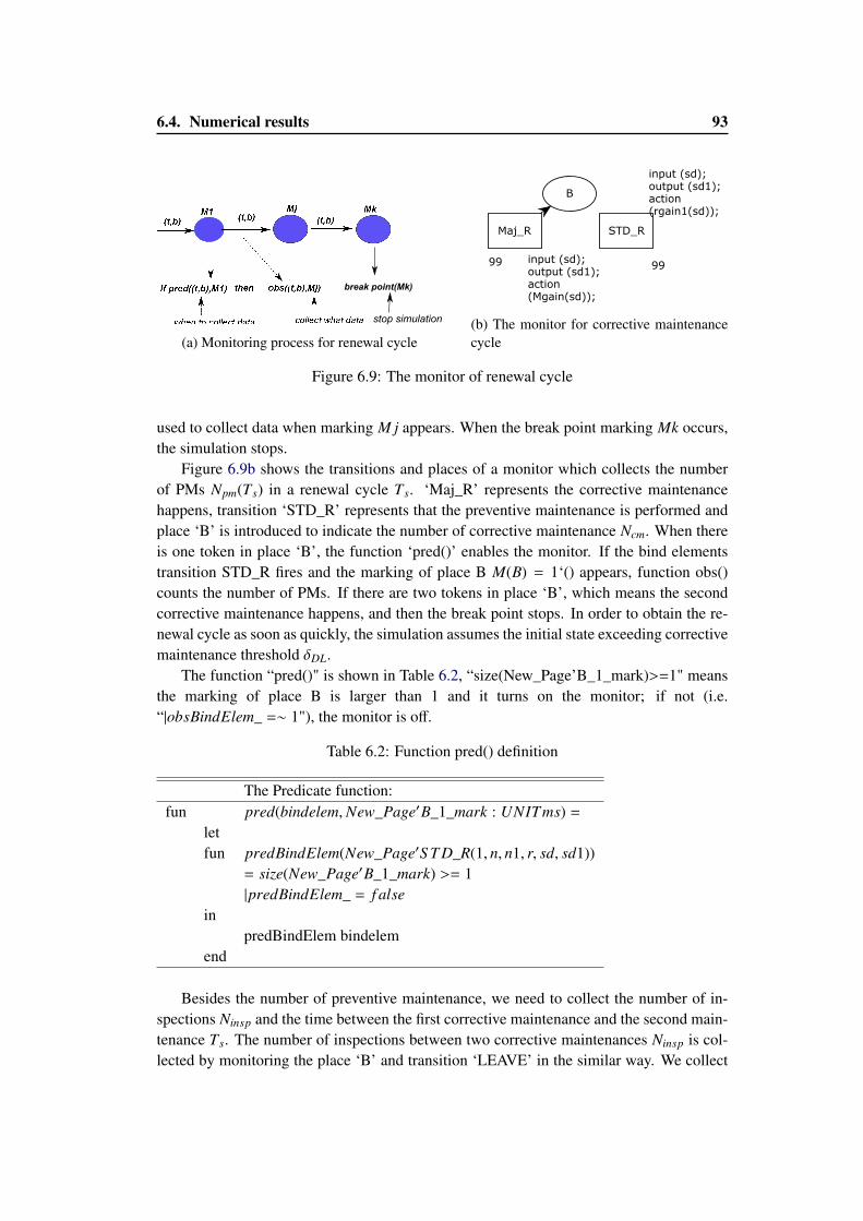
6.4. Numerical results 93
break point(Mk)
stop simulation
(a) Monitoring process for renewal cycle
B
STD_R
input (sd);output (sd1);action(rgain1(sd));
99
Maj_R
input (sd);output (sd1);action(Mgain(sd));
99
(b) The monitor for corrective maintenancecycle
Figure 6.9: The monitor of renewal cycle
used to collect data when marking M j appears. When the break point marking Mk occurs,the simulation stops.
Figure 6.9b shows the transitions and places of a monitor which collects the numberof PMs Npm(Ts) in a renewal cycle Ts. ‘Maj_R’ represents the corrective maintenancehappens, transition ‘STD_R’ represents that the preventive maintenance is performed andplace ‘B’ is introduced to indicate the number of corrective maintenance Ncm. When thereis one token in place ‘B’, the function ‘pred()’ enables the monitor. If the bind elementstransition STD_R fires and the marking of place B M(B) = 1‘() appears, function obs()counts the number of PMs. If there are two tokens in place ‘B’, which means the secondcorrective maintenance happens, and then the break point stops. In order to obtain the re-newal cycle as soon as quickly, the simulation assumes the initial state exceeding correctivemaintenance threshold δDL.
The function “pred()" is shown in Table 6.2, “size(New_Page’B_1_mark)>=1" meansthe marking of place B is larger than 1 and it turns on the monitor; if not (i.e.“|obsBindElem_ =∼ 1"), the monitor is off.
Table 6.2: Function pred() definition
The Predicate function:fun pred(bindelem,New_Page′B_1_mark : UNITms) =
letfun predBindElem(New_Page′S T D_R(1, n, n1, r, sd, sd1))
= size(New_Page′B_1_mark) >= 1|predBindElem_ = f alse
inpredBindElem bindelem
end
Besides the number of preventive maintenance, we need to collect the number of in-spections Ninsp and the time between the first corrective maintenance and the second main-tenance Ts. The number of inspections between two corrective maintenances Ninsp is col-lected by monitoring the place ‘B’ and transition ‘LEAVE’ in the similar way. We collect
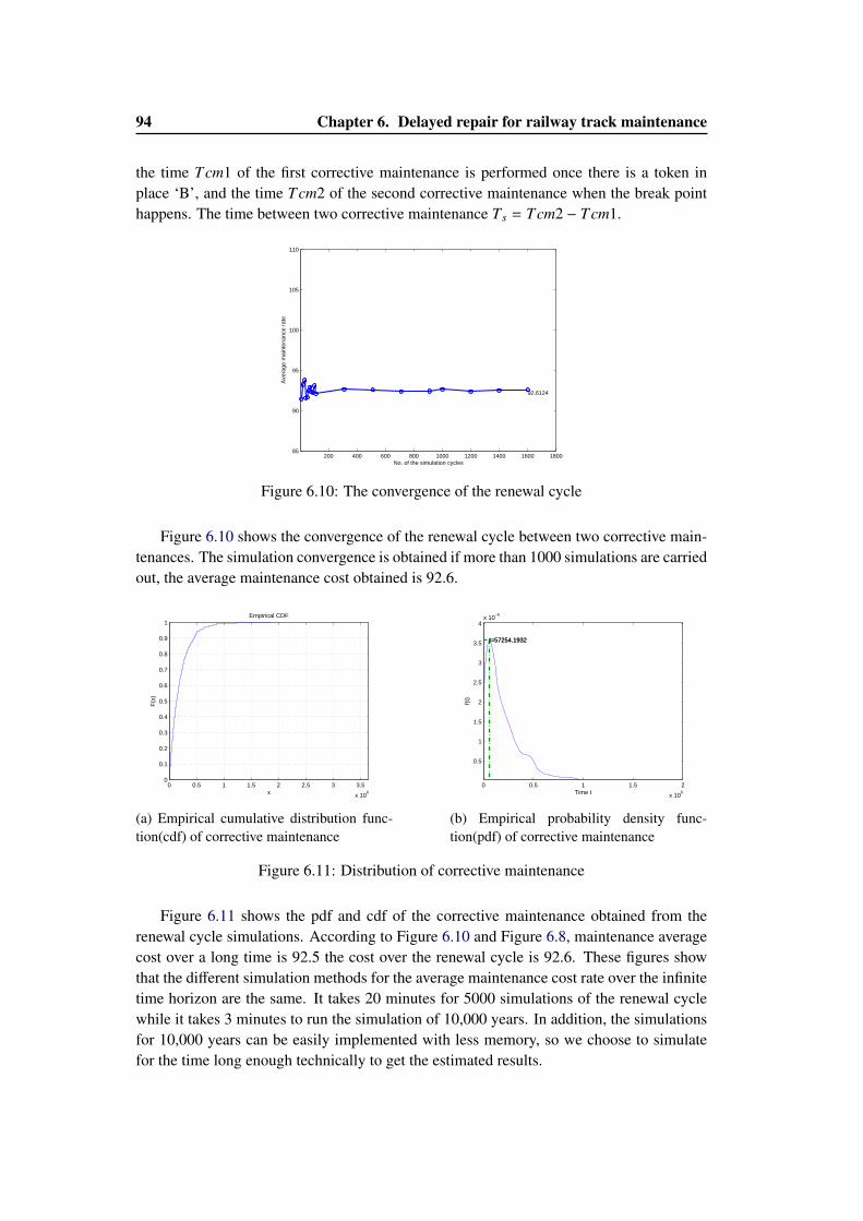
94 Chapter 6. Delayed repair for railway track maintenance
the time Tcm1 of the first corrective maintenance is performed once there is a token inplace ‘B’, and the time Tcm2 of the second corrective maintenance when the break pointhappens. The time between two corrective maintenance Ts = Tcm2 − Tcm1.
200 400 600 800 1000 1200 1400 1600 180085
90
95
100
105
110
No. of the simulation cycles
Ave
rage
mai
nten
ance
rat
e
92.6124
Figure 6.10: The convergence of the renewal cycle
Figure 6.10 shows the convergence of the renewal cycle between two corrective main-tenances. The simulation convergence is obtained if more than 1000 simulations are carriedout, the average maintenance cost obtained is 92.6.
0 0.5 1 1.5 2 2.5 3 3.5
x 106
0
0.1
0.2
0.3
0.4
0.5
0.6
0.7
0.8
0.9
1
x
F(x
)
Empirical CDF
(a) Empirical cumulative distribution func-tion(cdf) of corrective maintenance
0 0.5 1 1.5 2
x 106
0.5
1
1.5
2
2.5
3
3.5
4x 10
−6
Time t
f(t)
t=57254.1932t=57254.1932
(b) Empirical probability density func-tion(pdf) of corrective maintenance
Figure 6.11: Distribution of corrective maintenance
Figure 6.11 shows the pdf and cdf of the corrective maintenance obtained from therenewal cycle simulations. According to Figure 6.10 and Figure 6.8, maintenance averagecost over a long time is 92.5 the cost over the renewal cycle is 92.6. These figures showthat the different simulation methods for the average maintenance cost rate over the infinitetime horizon are the same. It takes 20 minutes for 5000 simulations of the renewal cyclewhile it takes 3 minutes to run the simulation of 10,000 years. In addition, the simulationsfor 10,000 years can be easily implemented with less memory, so we choose to simulatefor the time long enough technically to get the estimated results.
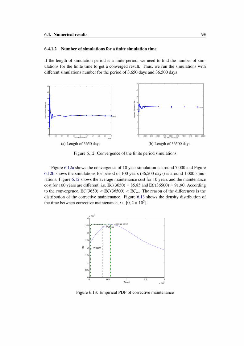
6.4. Numerical results 95
6.4.1.2 Number of simulations for a finite simulation time
If the length of simulation period is a finite period, we need to find the number of sim-ulations for the finite time to get a converged result. Thus, we run the simulations withdifferent simulations number for the period of 3,650 days and 36,500 days
0 0.2 0.4 0.6 0.8 1 1.2 1.4 1.6 1.8 2
x 104
70
75
80
85
90
95
100
105
110
No. of the simulations
Ave
rage
mai
nten
ance
rat
e
85.8504
(a) Length of 3650 days
0 1000 2000 3000 4000 5000 6000 7000 8000 9000 1000070
75
80
85
90
95
100
105
110
No. of the simulations
Ave
rage
mai
nten
ance
rat
e
91.8995
(b) Length of 36500 days
Figure 6.12: Convergence of the finite period simulations
Figure 6.12a shows the convergence of 10 year simulation is around 7,000 and Figure6.12b shows the simulations for period of 100 years (36,500 days) is around 1,000 simu-lations. Figure 6.12 shows the average maintenance cost for 10 years and the maintenancecost for 100 years are different, i.e. EC(3650) = 85.85 and EC(36500) = 91.90. Accordingto the convergence, EC(3650) < EC(36500) < EC∞. The reason of the differences is thedistribution of the corrective maintenance. Figure 6.13 shows the density distribution ofthe time between corrective maintenance, t ∈ [0, 2 × 10⁵].
0 0.5 1 1.5 2
x 105
0
0.5
1
1.5
2
2.5
3
3.5
4x 10
−6
Time t
f(t)
← t=57254.1932← t=36500
← t=3650
Figure 6.13: Empirical PDF of corrective maintenance
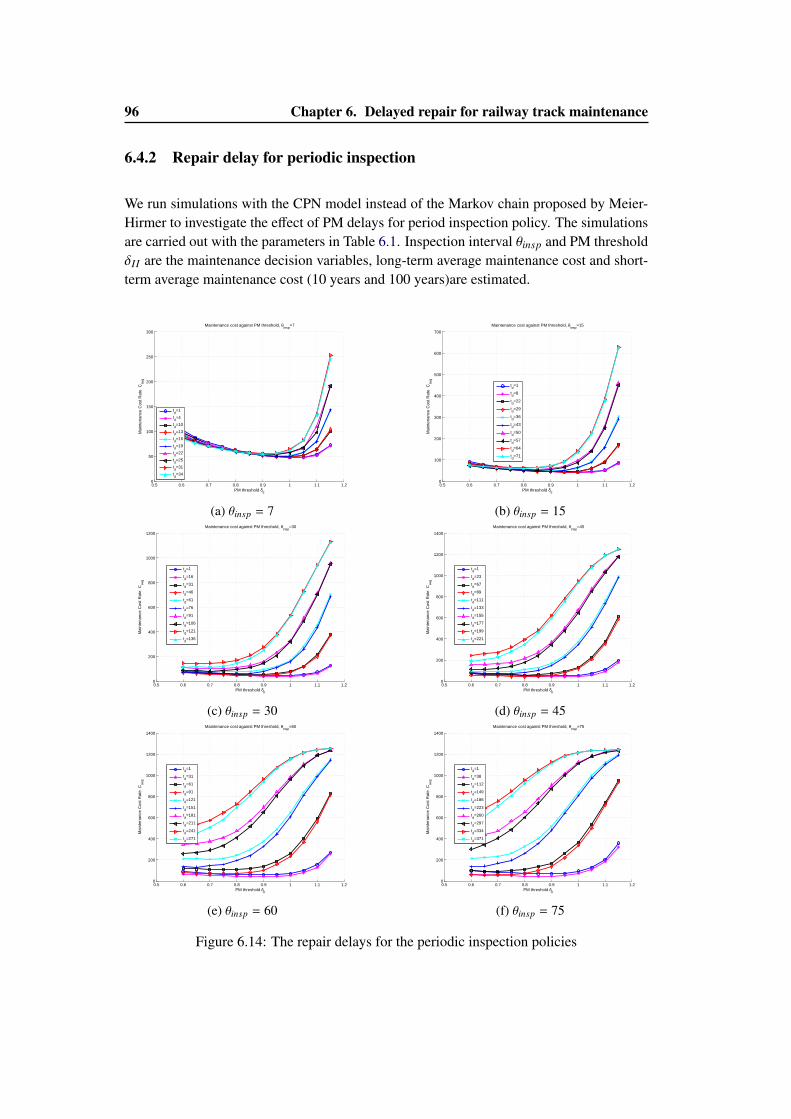
96 Chapter 6. Delayed repair for railway track maintenance
6.4.2 Repair delay for periodic inspection
We run simulations with the CPN model instead of the Markov chain proposed by Meier-Hirmer to investigate the effect of PM delays for period inspection policy. The simulationsare carried out with the parameters in Table 6.1. Inspection interval θinsp and PM thresholdδII are the maintenance decision variables, long-term average maintenance cost and short-term average maintenance cost (10 years and 100 years)are estimated.
0.5 0.6 0.7 0.8 0.9 1 1.1 1.20
50
100
150
200
250
300
PM threshold δII
Mai
nten
ance
Cos
t Rat
e C
avg
Maintenance cost against PM threshold, θinsp
=7
td=1
td=4
td=10
td=13
td=16
td=19
td=22
td=25
td=31
td=34
(a) θinsp = 7
0.5 0.6 0.7 0.8 0.9 1 1.1 1.20
100
200
300
400
500
600
700
PM threshold δII
Mai
nten
ance
Cos
t Rat
e C
avg
Maintenance cost against PM threshold, θinsp
=15
td=1
td=8
td=22
td=29
td=36
td=43
td=50
td=57
td=64
td=71
(b) θinsp = 15
0.5 0.6 0.7 0.8 0.9 1 1.1 1.20
200
400
600
800
1000
1200
PM threshold δII
Mai
nten
ance
Cos
t Rat
e C
avg
Maintenance cost against PM threshold, θinsp
=30
td=1
td=16
td=31
td=46
td=61
td=76
td=91
td=106
td=121
td=136
(c) θinsp = 30
0.5 0.6 0.7 0.8 0.9 1 1.1 1.20
200
400
600
800
1000
1200
1400
PM threshold δII
Mai
nten
ance
Cos
t Rat
e C
avg
Maintenance cost against PM threshold, θinsp
=45
td=1
td=23
td=67
td=89
td=111
td=133
td=155
td=177
td=199
td=221
(d) θinsp = 45
0.5 0.6 0.7 0.8 0.9 1 1.1 1.20
200
400
600
800
1000
1200
1400
PM threshold δII
Mai
nten
ance
Cos
t Rat
e C
avg
Maintenance cost against PM threshold, θinsp
=60
td=1
td=31
td=61
td=91
td=121
td=151
td=181
td=211
td=241
td=271
(e) θinsp = 60
0.5 0.6 0.7 0.8 0.9 1 1.1 1.20
200
400
600
800
1000
1200
1400
PM threshold δII
Mai
nten
ance
Cos
t Rat
e C
avg
Maintenance cost against PM threshold, θinsp
=75
td=1
td=38
td=112
td=149
td=186
td=223
td=260
td=297
td=334
td=371
(f) θinsp = 75
Figure 6.14: The repair delays for the periodic inspection policies
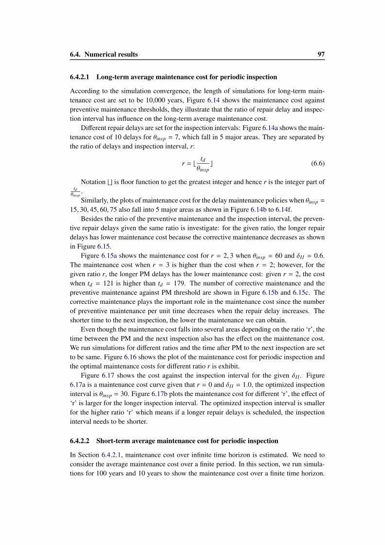
6.4. Numerical results 97
6.4.2.1 Long-term average maintenance cost for periodic inspection
According to the simulation convergence, the length of simulations for long-term main-tenance cost are set to be 10,000 years, Figure 6.14 shows the maintenance cost againstpreventive maintenance thresholds, they illustrate that the ratio of repair delay and inspec-tion interval has influence on the long-term average maintenance cost.
Different repair delays are set for the inspection intervals: Figure 6.14a shows the main-tenance cost of 10 delays for θinsp = 7, which fall in 5 major areas. They are separated bythe ratio of delays and inspection interval, r:
r = btdθinspc (6.6)
Notation bc is floor function to get the greatest integer and hence r is the integer part oftdθinsp
.Similarly, the plots of maintenance cost for the delay maintenance policies when θinsp =
15, 30, 45, 60, 75 also fall into 5 major areas as shown in Figure 6.14b to 6.14f.Besides the ratio of the preventive maintenance and the inspection interval, the preven-
tive repair delays given the same ratio is investigate: for the given ratio, the longer repairdelays has lower maintenance cost because the corrective maintenance decreases as shownin Figure 6.15.
Figure 6.15a shows the maintenance cost for r = 2, 3 when θinsp = 60 and δII = 0.6.The maintenance cost when r = 3 is higher than the cost when r = 2; however, for thegiven ratio r, the longer PM delays has the lower maintenance cost: given r = 2, the costwhen td = 121 is higher than td = 179. The number of corrective maintenance and thepreventive maintenance against PM threshold are shown in Figure 6.15b and 6.15c. Thecorrective maintenance plays the important role in the maintenance cost since the numberof preventive maintenance per unit time decreases when the repair delay increases. Theshorter time to the next inspection, the lower the maintenance we can obtain.
Even though the maintenance cost falls into several areas depending on the ratio ‘r’, thetime between the PM and the next inspection also has the effect on the maintenance cost.We run simulations for different ratios and the time after PM to the next inspection are setto be same. Figure 6.16 shows the plot of the maintenance cost for periodic inspection andthe optimal maintenance costs for different ratio r is exhibit.
Figure 6.17 shows the cost against the inspection interval for the given δII . Figure6.17a is a maintenance cost curve given that r = 0 and δII = 1.0, the optimized inspectioninterval is θinsp = 30. Figure 6.17b plots the maintenance cost for different ‘r’, the effect of‘r’ is larger for the longer inspection interval. The optimized inspection interval is smallerfor the higher ratio ‘r’ which means if a longer repair delays is scheduled, the inspectioninterval needs to be shorter.
6.4.2.2 Short-term average maintenance cost for periodic inspection
In Section 6.4.2.1, maintenance cost over infinite time horizon is estimated. We need toconsider the average maintenance cost over a finite period. In this section, we run simula-tions for 100 years and 10 years to show the maintenance cost over a finite time horizon.
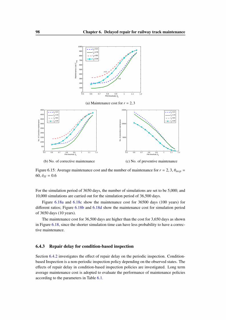
98 Chapter 6. Delayed repair for railway track maintenance
0.5 0.6 0.7 0.8 0.9 1 1.1 1.20
100
200
300
400
500
600
700
800
900
1000
PM threshold, δII
Mai
nten
ance
cos
t Cav
g
r=3 →
← r=2
td=121
td=179
td=181
td=239
(a) Maintenance cost for r = 2, 3
0.5 0.6 0.7 0.8 0.9 1 1.1 1.20
500
1000
1500
2000
2500
3000
3500
4000
4500
PM threshold, δII
No.
of C
orre
ctiv
e m
aint
enan
ce
td=121
td=179
td=181
td=239
(b) No. of corrective maintenance
0.5 0.6 0.7 0.8 0.9 1 1.1 1.20
5000
10000
15000
PM threshold, δII
No.
of p
reve
ntiv
e m
aint
enan
ce
td=121
td=179
td=181
td=239
(c) No. of preventive maintenance
Figure 6.15: Average maintenance cost and the number of maintenance for r = 2, 3, θinsp =
60, δII = 0.6
For the simulation period of 3650 days, the number of simulations are set to be 5,000; and10,000 simulations are carried out for the simulation period of 36,500 days.
Figure 6.18a and 6.18c show the maintenance cost for 36500 days (100 years) fordifferent ratios; Figure 6.18b and 6.18d show the maintenance cost for simulation periodof 3650 days (10 years).
The maintenance cost for 36,500 days are higher than the cost for 3,650 days as shownin Figure 6.18, since the shorter simulation time can have less probability to have a correc-tive maintenance.
6.4.3 Repair delay for condition-based inspection
Section 6.4.2 investigates the effect of repair delay on the periodic inspection. Condition-based Inspection is a non-periodic inspection policy depending on the observed states. Theeffects of repair delay in condition-based inspection policies are investigated. Long termaverage maintenance cost is adopted to evaluate the performance of maintenance policiesaccording to the parameters in Table 6.1.
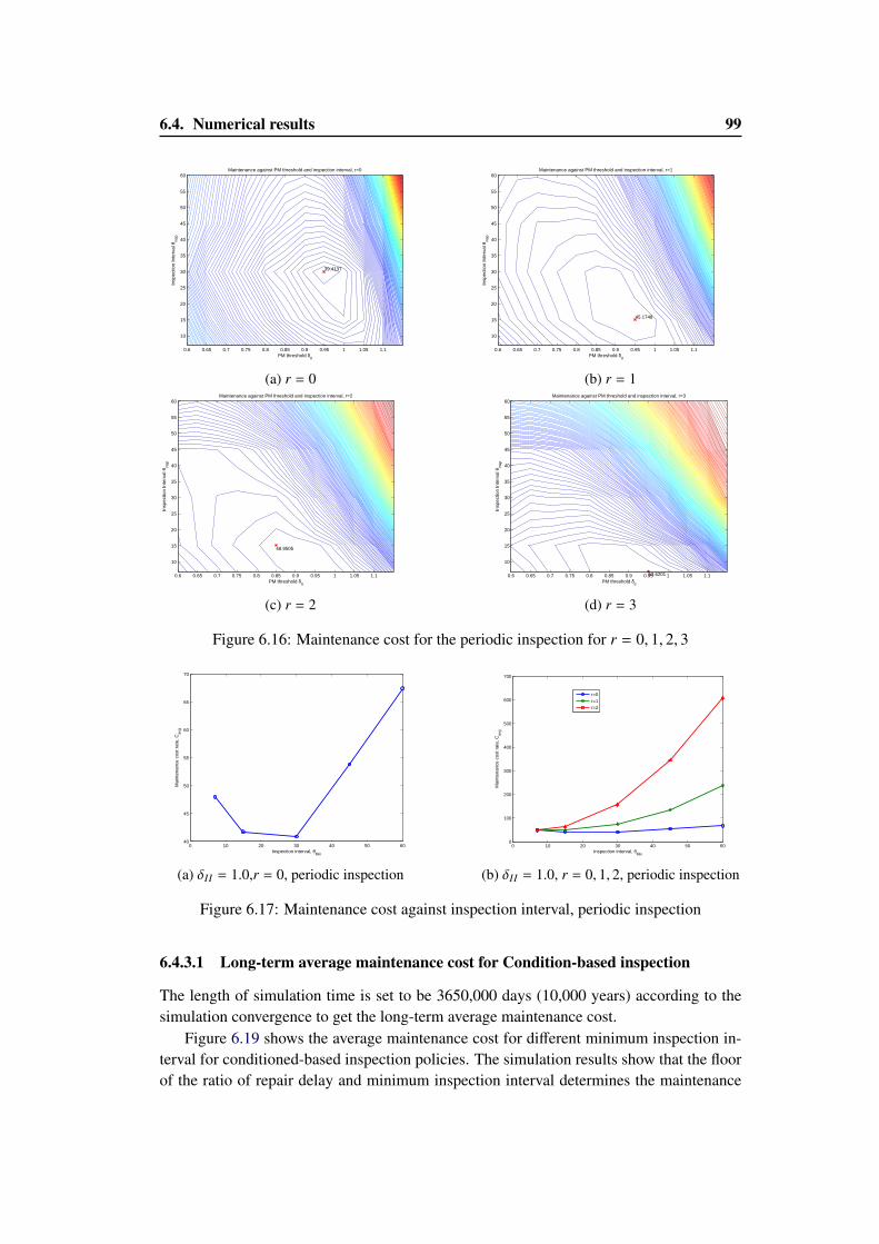
6.4. Numerical results 99
39.4137
PM threshold δII
Insp
ectio
n In
terv
al θ
insp
Maintenance against PM threshold and inspection interval, r=0
0.6 0.65 0.7 0.75 0.8 0.85 0.9 0.95 1 1.05 1.1
10
15
20
25
30
35
40
45
50
55
60
(a) r = 0
45.1748
PM threshold δII
Insp
ectio
n In
terv
al θ
insp
Maintenance against PM threshold and inspection interval, r=1
0.6 0.65 0.7 0.75 0.8 0.85 0.9 0.95 1 1.05 1.1
10
15
20
25
30
35
40
45
50
55
60
(b) r = 1
48.9505
PM threshold δII
Insp
ectio
n In
terv
al θ
insp
Maintenance against PM threshold and inspection interval, r=2
0.6 0.65 0.7 0.75 0.8 0.85 0.9 0.95 1 1.05 1.1
10
15
20
25
30
35
40
45
50
55
60
(c) r = 2
53.6201
PM threshold δII
Insp
ectio
n In
terv
al θ
insp
Maintenance against PM threshold and inspection interval, r=3
0.6 0.65 0.7 0.75 0.8 0.85 0.9 0.95 1 1.05 1.1
10
15
20
25
30
35
40
45
50
55
60
(d) r = 3
Figure 6.16: Maintenance cost for the periodic inspection for r = 0, 1, 2, 3
0 10 20 30 40 50 6040
45
50
55
60
65
70
Inspection interval, θMin
Mai
nten
ance
cos
t rat
e, C
avg
(a) δII = 1.0,r = 0, periodic inspection
0 10 20 30 40 50 600
100
200
300
400
500
600
700
Inspection interval, θMin
Mai
nten
ance
cos
t rat
e, C
avg
r=0r=1r=2
(b) δII = 1.0, r = 0, 1, 2, periodic inspection
Figure 6.17: Maintenance cost against inspection interval, periodic inspection
6.4.3.1 Long-term average maintenance cost for Condition-based inspection
The length of simulation time is set to be 3650,000 days (10,000 years) according to thesimulation convergence to get the long-term average maintenance cost.
Figure 6.19 shows the average maintenance cost for different minimum inspection in-terval for conditioned-based inspection policies. The simulation results show that the floorof the ratio of repair delay and minimum inspection interval determines the maintenance
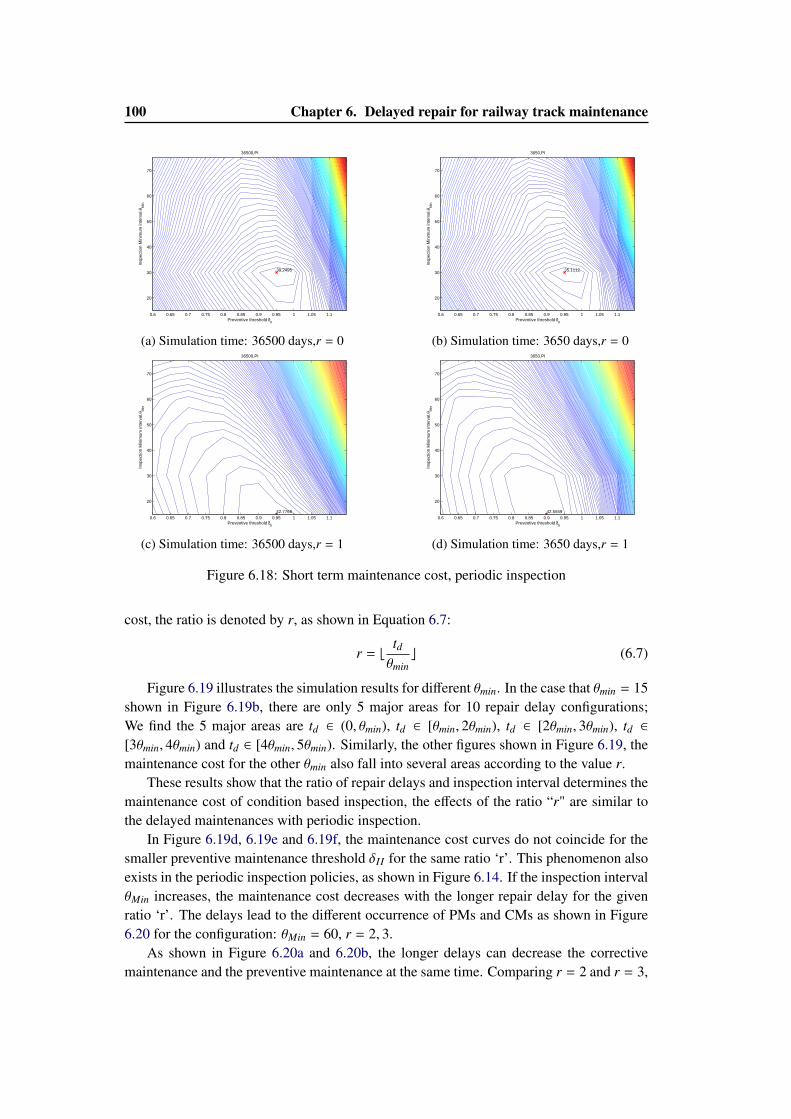
100 Chapter 6. Delayed repair for railway track maintenance
Preventive threshold δII
Insp
ectio
n M
inim
um in
terv
al,θ
Min
36500,PI
39.2495
0.6 0.65 0.7 0.75 0.8 0.85 0.9 0.95 1 1.05 1.1
20
30
40
50
60
70
(a) Simulation time: 36500 days,r = 0
Preventive threshold δII
Insp
ectio
n M
inim
um in
terv
al,θ
Min
3650,PI
35.1112
0.6 0.65 0.7 0.75 0.8 0.85 0.9 0.95 1 1.05 1.1
20
30
40
50
60
70
(b) Simulation time: 3650 days,r = 0
Preventive threshold δII
Insp
ectio
n M
inim
um in
terv
al,θ
Min
36500,PI
42.77690.6 0.65 0.7 0.75 0.8 0.85 0.9 0.95 1 1.05 1.1
20
30
40
50
60
70
(c) Simulation time: 36500 days,r = 1
Preventive threshold δII
Insp
ectio
n M
inim
um in
terv
al,θ
Min
3650,PI
42.55590.6 0.65 0.7 0.75 0.8 0.85 0.9 0.95 1 1.05 1.1
20
30
40
50
60
70
(d) Simulation time: 3650 days,r = 1
Figure 6.18: Short term maintenance cost, periodic inspection
cost, the ratio is denoted by r, as shown in Equation 6.7:
r = btdθminc (6.7)
Figure 6.19 illustrates the simulation results for different θmin. In the case that θmin = 15shown in Figure 6.19b, there are only 5 major areas for 10 repair delay configurations;We find the 5 major areas are td ∈ (0, θmin), td ∈ [θmin, 2θmin), td ∈ [2θmin, 3θmin), td ∈[3θmin, 4θmin) and td ∈ [4θmin, 5θmin). Similarly, the other figures shown in Figure 6.19, themaintenance cost for the other θmin also fall into several areas according to the value r.
These results show that the ratio of repair delays and inspection interval determines themaintenance cost of condition based inspection, the effects of the ratio “r" are similar tothe delayed maintenances with periodic inspection.
In Figure 6.19d, 6.19e and 6.19f, the maintenance cost curves do not coincide for thesmaller preventive maintenance threshold δII for the same ratio ‘r’. This phenomenon alsoexists in the periodic inspection policies, as shown in Figure 6.14. If the inspection intervalθMin increases, the maintenance cost decreases with the longer repair delay for the givenratio ‘r’. The delays lead to the different occurrence of PMs and CMs as shown in Figure6.20 for the configuration: θMin = 60, r = 2, 3.
As shown in Figure 6.20a and 6.20b, the longer delays can decrease the correctivemaintenance and the preventive maintenance at the same time. Comparing r = 2 and r = 3,
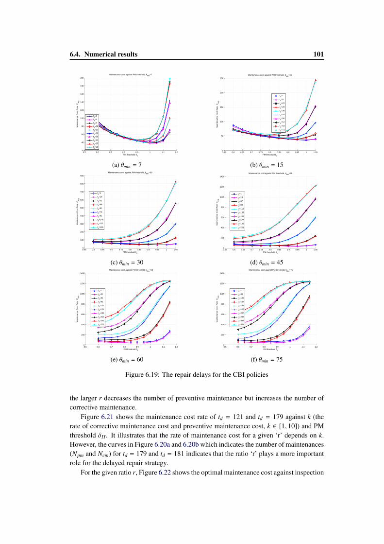
6.4. Numerical results 101
0.5 0.6 0.7 0.8 0.9 1 1.1 1.220
40
60
80
100
120
140
160
180
200
PM threshold δII
Mai
nten
ance
Cos
t Rat
e C
avg
Maintenance cost against PM threshold, θMin
=7
td=1
td=4
td=7
td=10
td=13
td=16
td=19
td=22
td=25
td=28
(a) θmin = 7
0.55 0.6 0.65 0.7 0.75 0.8 0.85 0.9 0.95 1 1.050
50
100
150
200
250
PM threshold δII
Mai
nten
ance
Cos
t Rat
e C
avg
Maintenance cost against PM threshold, θMin
=15
td=1
td=8
td=22
td=29
td=36
td=43
td=50
td=57
td=64
td=71
(b) θmin = 15
0.55 0.6 0.65 0.7 0.75 0.8 0.85 0.9 0.95 1 1.050
100
200
300
400
500
600
700
800
900
PM threshold δII
Mai
nten
ance
Cos
t Rat
e C
avg
Maintenance cost against PM threshold, θMin
=30
td=1
td=16
td=31
td=46
td=61
td=76
td=91
td=106
td=121
td=136
(c) θmin = 30
0.55 0.6 0.65 0.7 0.75 0.8 0.85 0.9 0.95 1 1.050
200
400
600
800
1000
1200
1400
PM threshold δII
Mai
nten
ance
Cos
t Rat
e C
avg
Maintenance cost against PM threshold, θMin
=45
td=1
td=23
td=67
td=89
td=111
td=133
td=155
td=177
td=199
td=221
(d) θmin = 45
0.5 0.6 0.7 0.8 0.9 1 1.1 1.20
200
400
600
800
1000
1200
1400
PM threshold δII
Mai
nten
ance
Cos
t Rat
e C
avg
Maintenance cost against PM threshold, θMin
=60
td=1
td=31
td=61
td=91
td=121
td=151
td=181
td=211
td=241
td=271
(e) θmin = 60
0.5 0.6 0.7 0.8 0.9 1 1.1 1.20
200
400
600
800
1000
1200
1400
PM threshold δII
Mai
nten
ance
Cos
t Rat
e C
avg
Maintenance cost against PM threshold, θMin
=75
td=1
td=38
td=112
td=149
td=186
td=223
td=260
td=297
td=334
td=371
(f) θmin = 75
Figure 6.19: The repair delays for the CBI policies
the larger r decreases the number of preventive maintenance but increases the number ofcorrective maintenance.
Figure 6.21 shows the maintenance cost rate of td = 121 and td = 179 against k (therate of corrective maintenance cost and preventive maintenance cost, k ∈ [1, 10]) and PMthreshold δII . It illustrates that the rate of maintenance cost for a given ‘r’ depends on k.However, the curves in Figure 6.20a and 6.20b which indicates the number of maintenances(Npm and Ncm) for td = 179 and td = 181 indicates that the ratio ‘r’ plays a more importantrole for the delayed repair strategy.
For the given ratio r, Figure 6.22 shows the optimal maintenance cost against inspection

102 Chapter 6. Delayed repair for railway track maintenance
0.6 0.65 0.7 0.75 0.8 0.85 0.9 0.95 10.5
1
1.5
2
2.5
3
3.5
4
4.5x 10
�3
PM threshold
Avera
ge n
um
ber
of
Pre
ventive M
ain
tenance
td=121
td=179
td=181
td=239
td=179
td=239
(a) Number of PMs, CBI
0.6 0.65 0.7 0.75 0.8 0.85 0.9 0.95 10
0.2
0.4
0.6
0.8
1
1.2
1.4x 10
¡ 3
PM threshold
Avera
ge n
um
ber
of
Corr
ective M
ain
tenance
td=121
td=179
td=181
td=239
td=239
r=2,td=179
r=3
(b) Number of CMs, CBI
Figure 6.20: Maintenance number for different time give the ratio
0.6
0.7
0.8
0.9
1
0
5
101
1.5
2
2.5
PM thresholdk=ccm/cpm
C(t
d=
12
1)/
C(t
d=
17
9)
Figure 6.21: The effect of the maintenance prices for a given ‘r’
interval θMin and the PM threshold δII . When r = 0, we can obtain the lowest maintenancecost (EC = 37.65) when θMin = 30 and δII = 1.0 in Figure 6.22a. When r = 1, the optimalmaintenance cost (EC = 40.64) exhibits at θMin = 15 and δII = 0.95 in Figure 6.22b.Figure 6.22c and 6.22d are the maintenance cost for r = 2 and r = 3.
Figure 6.23 shows the cost against inspection interval given that δII = 1.0. The curver = 0 exhibits a minimum cost around θmin = 30 as shown in Figure 6.23a; for r = 1 theminimum cost is around θmin = 15 and for r = 2 is around θmin = 7 as shown in Figure6.23b. The larger r can get the minimum cost at a smaller inspection interval θmin.
According to the results of Monte Carlo simulations, we find that the larger r leadsto more corrective maintenance as shown in Figure 6.24 and more inspections in the CBIpolicies and hence the higher maintenance cost.
Figure 6.24a shows the probability of the time between two PMs for different r (r =
14, 29, 44, 59, 74) when θMin = 15 . The longer ‘r’ contributes less number of PMs while
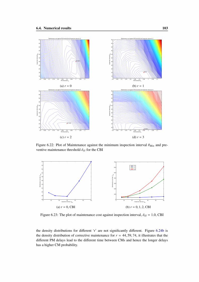
6.4. Numerical results 103
37.6528
PM threshold δII
Insp
ectio
n In
terv
al θ
Min
Maintenance cost against PM threshold and Inspection interval,r=0
0.6 0.65 0.7 0.75 0.8 0.85 0.9 0.95 1 1.05 1.1
10
15
20
25
30
35
40
45
50
55
60
(a) r = 0
40.64
PM threshold δII
Insp
ectio
n In
terv
al θ
Min
Maintenance cost against PM threshold and Inspection interval,r=1
0.6 0.65 0.7 0.75 0.8 0.85 0.9 0.95 1 1.05 1.1
10
15
20
25
30
35
40
45
50
55
60
(b) r = 1
44.7144
PM threshold δII
Insp
ectio
n In
terv
al θ
Min
Maintenance cost against PM threshold and Inspection interval,r=2
0.6 0.65 0.7 0.75 0.8 0.85 0.9 0.95 1 1.05 1.1
10
15
20
25
30
35
40
45
50
55
60
(c) r = 2
44.8812
PM threshold δII
Insp
ectio
n In
terv
al θ
Min
Maintenance cost against PM threshold and Inspection interval,r=3
0.6 0.65 0.7 0.75 0.8 0.85 0.9 0.95 1 1.05 1.1
10
15
20
25
30
35
40
45
50
55
60
(d) r = 3
Figure 6.22: Plot of Maintenance against the minimum inspection interval θMin and pre-ventive maintenance threshold δII for the CBI
0 10 20 30 40 50 6036
38
40
42
44
46
48
50
52
54
56
Inspection interval, θMin
Mai
nten
ance
cos
t rat
e, C
avg
(a) r = 0, CBI
0 10 20 30 40 50 600
100
200
300
400
500
600
700
Inspection interval, θMin
Mai
nten
ance
cos
t rat
e, C
avg
r=0r=1r=2
(b) r = 0, 1, 2, CBI
Figure 6.23: The plot of maintenance cost against inspection interval, δII = 1.0, CBI
the density distributions for different ‘r’ are not significantly different. Figure 6.24b isthe density distribution of corrective maintenance for r = 44, 59, 74, it illustrates that thedifferent PM delays lead to the different time between CMs and hence the longer delayshas a higher CM probability.
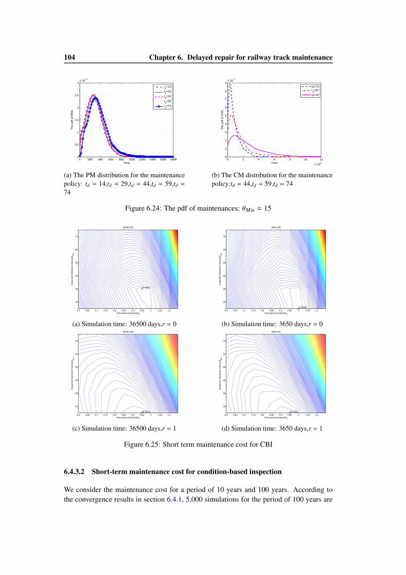
104 Chapter 6. Delayed repair for railway track maintenance
0 200 400 600 800 1000 1200 1400 1600 18000
0.5
1
1.5
2
2.5
3x 10
−3
Time
The
of P
Ms
td=14
td=29
td=44
td=59
td=74
(a) The PM distribution for the maintenancepolicy: td = 14,td = 29,td = 44,td = 59,td =
74
0 2 4 6 8 10 12
x 104
0
1
2
3
4
5
6
7
8
9x 10
−5
Time
The
of C
Ms
td=74td=59
td=44
(b) The CM distribution for the maintenancepolicy:td = 44,td = 59,td = 74
Figure 6.24: The pdf of maintenances: θMin = 15
Preventive threshold δII
Insp
ectio
n M
inim
um in
terv
al,θ
Min
36500,CBI
37.8587
0.6 0.65 0.7 0.75 0.8 0.85 0.9 0.95 1 1.05 1.1
20
30
40
50
60
70
(a) Simulation time: 36500 days,r = 0
Preventive threshold δII
Insp
ectio
n M
inim
um in
terv
al,θ
Min
3650,CBI
33.84220.6 0.65 0.7 0.75 0.8 0.85 0.9 0.95 1 1.05 1.1
20
30
40
50
60
70
(b) Simulation time: 3650 days,r = 0
Preventive threshold δII
Insp
ectio
n M
inim
um in
terv
al,θ
Min
36500,CBI
39.90130.6 0.65 0.7 0.75 0.8 0.85 0.9 0.95 1 1.05 1.1
20
30
40
50
60
70
(c) Simulation time: 36500 days,r = 1
Preventive threshold δII
Insp
ectio
n M
inim
um in
terv
al,θ
Min
3650,CBI
35.62830.6 0.65 0.7 0.75 0.8 0.85 0.9 0.95 1 1.05 1.1
20
30
40
50
60
70
(d) Simulation time: 3650 days,r = 1
Figure 6.25: Short term maintenance cost for CBI
6.4.3.2 Short-term maintenance cost for condition-based inspection
We consider the maintenance cost for a period of 10 years and 100 years. According tothe convergence results in section 6.4.1, 5,000 simulations for the period of 100 years are
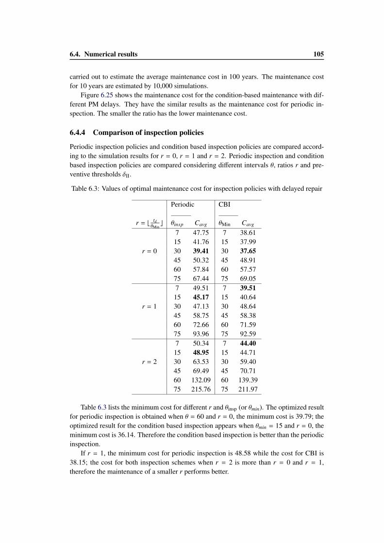
6.4. Numerical results 105
carried out to estimate the average maintenance cost in 100 years. The maintenance costfor 10 years are estimated by 10,000 simulations.
Figure 6.25 shows the maintenance cost for the condition-based maintenance with dif-ferent PM delays. They have the similar results as the maintenance cost for periodic in-spection. The smaller the ratio has the lower maintenance cost.
6.4.4 Comparison of inspection policies
Periodic inspection policies and condition based inspection policies are compared accord-ing to the simulation results for r = 0, r = 1 and r = 2. Periodic inspection and conditionbased inspection policies are compared considering different intervals θ, ratios r and pre-ventive thresholds δII.
Table 6.3: Values of optimal maintenance cost for inspection policies with delayed repair
Periodic CBI
r = btdθMinc θinsp Cavg θMin Cavg
r = 0
7 47.75 7 38.6115 41.76 15 37.9930 39.41 30 37.6545 50.32 45 48.9160 57.84 60 57.5775 67.44 75 69.05
r = 1
7 49.51 7 39.5115 45.17 15 40.6430 47.13 30 48.6445 58.75 45 58.3860 72.66 60 71.5975 93.96 75 92.59
r = 2
7 50.34 7 44.4015 48.95 15 44.7130 63.53 30 59.4045 69.49 45 70.7160 132.09 60 139.3975 215.76 75 211.97
Table 6.3 lists the minimum cost for different r and θinsp (or θmin). The optimized resultfor periodic inspection is obtained when θ = 60 and r = 0, the minimum cost is 39.79; theoptimized result for the condition based inspection appears when θmin = 15 and r = 0, theminimum cost is 36.14. Therefore the condition based inspection is better than the periodicinspection.
If r = 1, the minimum cost for periodic inspection is 48.58 while the cost for CBI is38.15; the cost for both inspection schemes when r = 2 is more than r = 0 and r = 1,therefore the maintenance of a smaller r performs better.
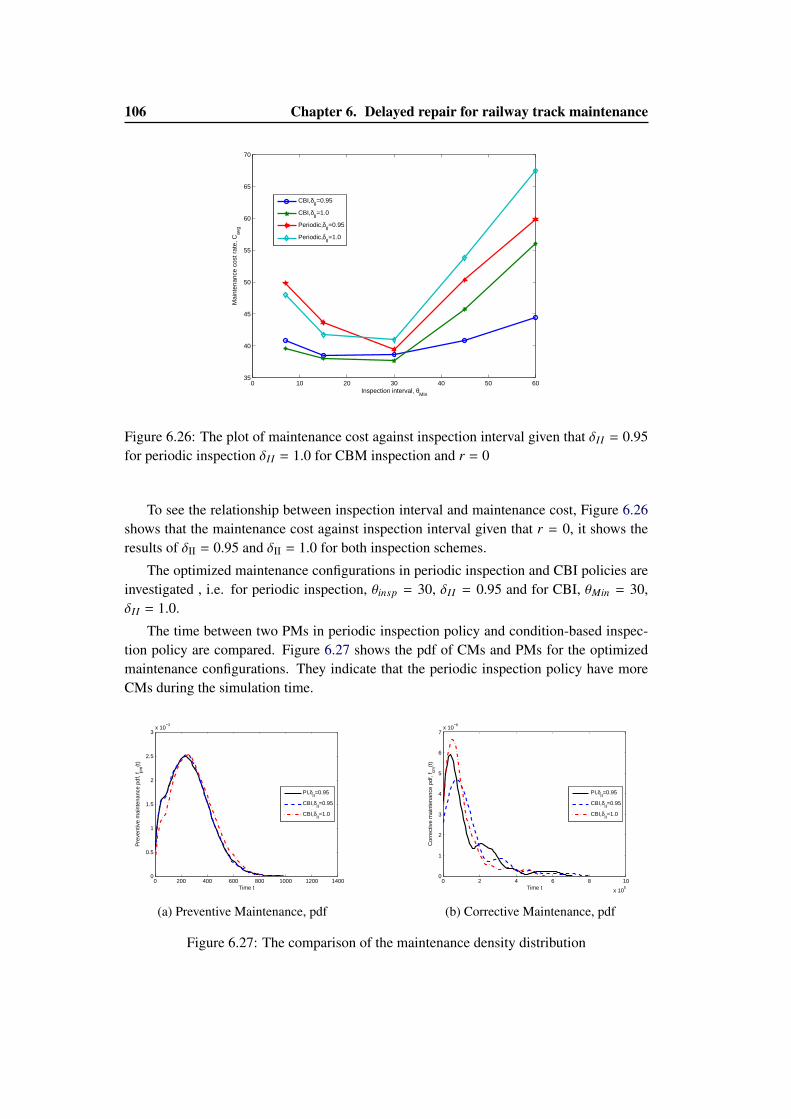
106 Chapter 6. Delayed repair for railway track maintenance
0 10 20 30 40 50 6035
40
45
50
55
60
65
70
Inspection interval, θMin
Mai
nten
ance
cos
t rat
e, C
avg
CBI,δII=0.95
CBI,δII=1.0
Periodic,δII=0.95
Periodic,δII=1.0
Figure 6.26: The plot of maintenance cost against inspection interval given that δII = 0.95for periodic inspection δII = 1.0 for CBM inspection and r = 0
To see the relationship between inspection interval and maintenance cost, Figure 6.26shows that the maintenance cost against inspection interval given that r = 0, it shows theresults of δII = 0.95 and δII = 1.0 for both inspection schemes.
The optimized maintenance configurations in periodic inspection and CBI policies areinvestigated , i.e. for periodic inspection, θinsp = 30, δII = 0.95 and for CBI, θMin = 30,δII = 1.0.
The time between two PMs in periodic inspection policy and condition-based inspec-tion policy are compared. Figure 6.27 shows the pdf of CMs and PMs for the optimizedmaintenance configurations. They indicate that the periodic inspection policy have moreCMs during the simulation time.
0 200 400 600 800 1000 1200 14000
0.5
1
1.5
2
2.5
3x 10
−3
Time t
Pre
vent
ive
mai
nten
ance
, fpm
(t)
PI,δII=0.95
CBI,δII=0.95
CBI,δII=1.0
(a) Preventive Maintenance, pdf
0 2 4 6 8 10
x 105
0
1
2
3
4
5
6
7x 10
−6
Time t
Cor
rect
ive
mai
nten
ance
, fcm
(t)
PI,δII=0.95
CBI,δII=0.95
CBI,δII=1.0
(b) Corrective Maintenance, pdf
Figure 6.27: The comparison of the maintenance density distribution
6.5. Conclusions for the delayed repairs 107
6.5 Conclusions for the delayed repairs
Delayed repair is a specific problem in railway maintenance. The delays may eventuallylead to accidents and hence cost much more money in maintenance. In order to makea better maintenance decision, it is necessary to take these delays into account for trackmaintenance.
The deterioration process with the delayed repair cannot be modeled by a simpleMarkov Chain, even though we can construct a Markov Chain for the delayed repair modelproposed in the literature.
Therefore we propose a timed Coloured Petri Net model which can assess the main-tenance strategies and optimize the maintenance decision. The CPN model adopts thecoloured sets and their corresponding variables to describe the component states; the mark-ing process can represent the possible deterioration evolution. The deterioration processbetween two inspection is considered and modelled for three scenarios: whithout mainte-nance, within PM and within CM. Either periodic inspection strategies or condition-basedinspection strategies is performed to collect the component states for maintenance deci-sions.
Monte Carlo simulations are carried out to estimate the maintenance performance. Ac-cording to the simulation results, the ratio of repair delays and minimum inspection intervalaffects the cost of condition-based inspection, which is similar to the delayed maintenancewith periodic inspection. The smaller r, the better is the performance of condition-basedinspection strategies. For a given ratio r, the longer repair delay leads to more correctivemaintenance but the ratio ‘r’ still plays an important role. We can optimize θinsp and δII
for both inspection schemes to obtain the optimal maintenance cost. Periodic inspection iscompared to CBI policies: the results indicate that CBI inspection is better than the periodicinspection for a given ratio r.
Short-term maintenance cost for 10 years and 100 years are estimated from simulations,the maintenance cost is lower than the maintenance cost over the infinite time horizon, sincethe short time cannot include the corrective maintenance when the time between them islonger than the short time (i.e. 10 years and 100 years).

Part IV
MAINTENANCE MODELLINGFOR A RAILWAY SECTION

Chapter 7
Maintenance modelling for a railwaysection: limited maintenance
resources
Contents7.1 Introduction . . . . . . . . . . . . . . . . . . . . . . . . . . . . . . . . . 1117.2 Modelling assumptions . . . . . . . . . . . . . . . . . . . . . . . . . . . 112
7.2.1 Assumptions for the component . . . . . . . . . . . . . . . . . . . 112
7.2.2 Region and network assumptions . . . . . . . . . . . . . . . . . . 113
7.3 CPN model for the railway network . . . . . . . . . . . . . . . . . . . . 1147.3.1 Modelling framework . . . . . . . . . . . . . . . . . . . . . . . . 114
7.3.2 Track component CPN model . . . . . . . . . . . . . . . . . . . . 115
7.3.3 Region CPN model . . . . . . . . . . . . . . . . . . . . . . . . . . 118
7.3.4 Network CPN model . . . . . . . . . . . . . . . . . . . . . . . . . 122
7.4 Simulation results . . . . . . . . . . . . . . . . . . . . . . . . . . . . . . 1227.5 Conclusion for the limited resource maintenance . . . . . . . . . . . . . 124
7.1 Introduction
Railway system can be seen a large scale network which consists of regions and compo-nents. When making maintenance decisions for the railway network, it is necessary to builda model for the entire multi-component system to estimate the maintenance cost, the totaldowntime and analyse the risk since the component failures and maintenance may dependon the states of the region, the states of the other components and the maintenance abilityof the network [146]. The limitation of maintenance resources, such as the limited num-ber of maintenance machines and the limited maintenance teams, which has effect on themaintenance decision making and hence the system performance, are needed to be takeninto account in railway network maintenance modelling.
The CPN model built in Section 4.3.5 is a model for single-unit system, the failureprocess of the system is divided into several stages. The model shows how the CPN tool
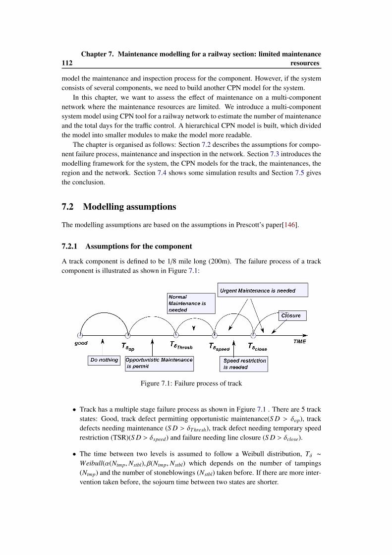
112Chapter 7. Maintenance modelling for a railway section: limited maintenance
resources
model the maintenance and inspection process for the component. However, if the systemconsists of several components, we need to build another CPN model for the system.
In this chapter, we want to assess the effect of maintenance on a multi-componentnetwork where the maintenance resources are limited. We introduce a multi-componentsystem model using CPN tool for a railway network to estimate the number of maintenanceand the total days for the traffic control. A hierarchical CPN model is built, which dividedthe model into smaller modules to make the model more readable.
The chapter is organised as follows: Section 7.2 describes the assumptions for compo-nent failure process, maintenance and inspection in the network. Section 7.3 introduces themodelling framework for the system, the CPN models for the track, the maintenances, theregion and the network. Section 7.4 shows some simulation results and Section 7.5 givesthe conclusion.
7.2 Modelling assumptions
The modelling assumptions are based on the assumptions in Prescott’s paper[146].
7.2.1 Assumptions for the component
A track component is defined to be 1/8 mile long (200m). The failure process of a trackcomponent is illustrated as shown in Figure 7.1:
Figure 7.1: Failure process of track
• Track has a multiple stage failure process as shown in Fgiure 7.1 . There are 5 trackstates: Good, track defect permitting opportunistic maintenance(S D > δop), trackdefects needing maintenance (S D > δThresh), track defect needing temporary speedrestriction (TSR)(S D > δspeed) and failure needing line closure (S D > δclose).
• The time between two levels is assumed to follow a Weibull distribution, Tδ ∼Weibull(α(Ntmp,Nstbl), β(Ntmp,Nstbl) which depends on the number of tampings(Ntmp) and the number of stoneblowings (Nstbl) taken before. If there are more inter-vention taken before, the sojourn time between two states are shorter.
7.2. Modelling assumptions 113
• There is a periodic inspection with inspection interval θ to identify track states, theinspection takes ε time. If there is a maintenance for the component, inspection iscarried out after the maintenance.
• There are two maintenance priorities: normal maintenance requirement and urgentmaintenance requirement:
– If track deterioration exceeds δThresh, the track component needs a normalmaintenance.
– If track deterioration exceeds δspeed or δclose, the track component needs anurgent maintenance.
– The urgent maintenance requirement has a higher priority than normal mainte-nance requirement and hence the maintenance task is carried out for the trackcomponent needing urgent maintenance prior to the others.
Two kinds of maintenance are considered in this chapter: Tamping and stoneblowering.Tampers and stoneblowers can be used respectively for the maintenance.
• Tamping is preferable to stoneblowering. If a stoneblower is used for the track com-ponent, a tamper can no longer be used.
• Stoneblower can be used for the track component if Tlimit has passed since mainte-nance is required for the track; or there is an urgent maintenance requirement for thecomponent.
• Both of the maintenances can restore track state to be as good as new.
• The machine (both of tampers and stoneblowers) arriving time is assumed to followNormal distribution τ ∼ N(θ, δ).
7.2.2 Region and network assumptions
In a region, there are Nt track components, the maintenance procedure in the region are setas follows:
• If there are urgent maintenances needed in the region, the urgent maintenance isperformed firstly.
• The available machines are allowed to work for the defective tracks in the region atthe same time.
The network has Nr regions and each region has Nt track components, the maintenancerules for the network are as follows:
• There are Mtamper tampers and Mstoneblower stoneblowers in this network.
• Maintenance performed by one machine can only be performed within a region. Themaintenance machines are allocated randomly for the regions which have the samemaintenance priority.
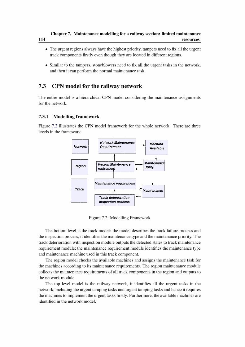
114Chapter 7. Maintenance modelling for a railway section: limited maintenance
resources
• The urgent regions always have the highest priority, tampers need to fix all the urgenttrack components firstly even though they are located in different regions.
• Similar to the tampers, stoneblowers need to fix all the urgent tasks in the network,and then it can perform the normal maintenance task.
7.3 CPN model for the railway network
The entire model is a hierarchical CPN model considering the maintenance assignmentsfor the network.
7.3.1 Modelling framework
Figure 7.2 illustrates the CPN model framework for the whole network. There are threelevels in the framework.
Figure 7.2: Modelling Framework
The bottom level is the track model: the model describes the track failure process andthe inspection process, it identifies the maintenance type and the maintenance priority. Thetrack deterioration with inspection module outputs the detected states to track maintenancerequirement module; the maintenance requirement module identifies the maintenance typeand maintenance machine used in this track component.
The region model checks the available machines and assigns the maintenance task forthe machines according to its maintenance requirements. The region maintenance modulecollects the maintenance requirements of all track components in the region and outputs tothe network module.
The top level model is the railway network, it identifies all the urgent tasks in thenetwork, including the urgent tamping tasks and urgent tamping tasks and hence it requiresthe machines to implement the urgent tasks firstly. Furthermore, the available machines areidentified in the network model.
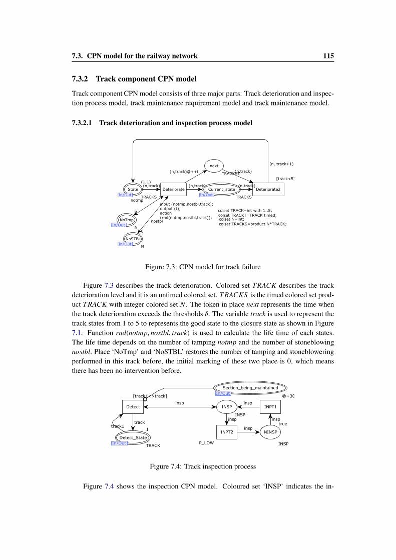
7.3. CPN model for the railway network 115
7.3.2 Track component CPN model
Track component CPN model consists of three major parts: Track deterioration and inspec-tion process model, track maintenance requirement model and track maintenance model.
7.3.2.1 Track deterioration and inspection process model
colset TRACK=int with 1..5;
colset N=int;
colset TRACKS=product N*TRACK;
colset TRACKT=TRACK timed;
next
TRACKST
Current_state
In/OutTRACKS
State
In/OutTRACKS
(1,1)
NoSTBL
In/OutN
0
NoTmp
In/OutN
0
Deteriorate
input (notmp,nostbl,track);output (t);action(rnd(notmp,nostbl,track));
Deteriorate2
[track<5]
(n,track)(n,track)@++t
(n,track)
(n, track+1)
nostbl
notmp
(n,track)(n,track)
Figure 7.3: CPN model for track failure
Figure 7.3 describes the track deterioration. Colored set TRACK describes the trackdeterioration level and it is an untimed colored set. TRACKS is the timed colored set prod-uct TRACK with integer colored set N. The token in place next represents the time whenthe track deterioration exceeds the thresholds δ. The variable track is used to represent thetrack states from 1 to 5 to represents the good state to the closure state as shown in Figure7.1. Function rnd(notmp, nostbl, track) is used to calculate the life time of each states.The life time depends on the number of tamping notmp and the number of stoneblowingnostbl. Place ‘NoTmp’ and ‘NoSTBL’ restores the number of tamping and stonebloweringperformed in this track before, the initial marking of these two place is 0, which meansthere has been no intervention before.
INSP
INSP
NINSP
INSP
true
Section_being_maintained
In/Out
Detect_State
In/OutTRACK
1
Detect
[track1<>track]
INPT1
@+30
INPT2
P_LOW
insp
insp
insp
insp
insptrack
track1
Figure 7.4: Track inspection process
Figure 7.4 shows the inspection CPN model. Coloured set ‘INSP’ indicates the in-
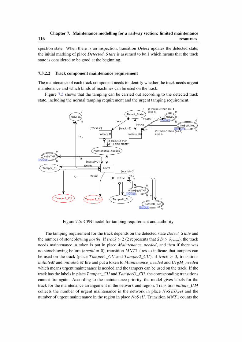
116Chapter 7. Maintenance modelling for a railway section: limited maintenance
resources
spection state. When there is an inspection, transition Detect updates the detected state,the initial marking of place Detected_S tate is assumed to be 1 which means that the trackstate is considered to be good at the beginning.
7.3.2.2 Track component maintenance requirement
The maintenance of each track component needs to identify whether the track needs urgentmaintenance and which kinds of machines can be used on the track.
Figure 7.5 shows that the tamping can be carried out according to the detected trackstate, including the normal tamping requirement and the urgent tamping requirement.
Detect_State
TRACK
1
NoSTBL
N
0
Maintenance_needed
Tamper_CU
TamperU_CUTamper1_CU Tamper2_CU
NoSeTMP
In/OutN
0
NoSecUTMP
In/OutN
0
NoTMPU_Net
In/OutN
0
NoSeU_Net
In/OutN
0
NoSeU
In/OutN
0
initiate UM
[track>3]
MNT1
[nostbl=0]
MNT2
[nostbl=0]
initiate M
[track>2]
track
nostbl
nostbl
nn+1
n+1
n
n
if track>3 then (n+1) else n
n+1
n
if track>3 then (n+1) else n
ntrack
if track>2 then 1`() else empty
Figure 7.5: CPN model for tamping requirement and authority
The tamping requirement for the track depends on the detected state Detect_S tate andthe number of stoneblowing nostbl. If track > 2 (2 represents that S D > δTresh), the trackneeds maintenance, a token is put in place Maintenance_needed, and then if there wasno stoneblowing before (nostbl = 0), transition MNT1 fires to indicate that tampers canbe used on the track (place Tamper1_CU and Tamper2_CU); if track > 3, transitionsinitiateM and initiateUM fire and put a token to Maintenance_needed and UrgM_neededwhich means urgent maintenance is needed and the tampers can be used on the track. If thetrack has the labels in place Tamper_CU and TamperU_CU, the corresponding transitionscannot fire again. According to the maintenance priority, the model gives labels for thetrack for the maintenance arrangement in the network and region. Transition initiate_UMcollects the number of urgent maintenance in the network in place NoS EUNet and thenumber of urgent maintenance in the region in place NoS eU. Transition MNT1 counts the
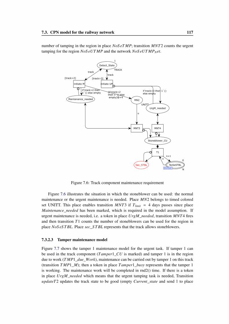
7.3. CPN model for the railway network 117
number of tamping in the region in place NoS eT MP; transition MNT2 counts the urgenttamping for the region NoS eUT MP and the network NoS eUT MPNet.
Detect_State
TRACK
1
Maintenance_needed
UrgM_needed
Stoneblower_CU
MN2
UNITT
NoSeSTBL
In/OutN
0
Sec_STBL
initiate UM
[track>3]
MNT4MNT3
T1
initiate M
[track>2]
track
if track>3 then 1`() else empty
u
n+1n
track
if track>2 then 1`() else empty (if track>2
then 1`() else empty)@+4
Figure 7.6: Track component maintenance requirement
Figure 7.6 illustrates the situation in which the stoneblower can be used: the normalmaintenance or the urgent maintenance is needed. Place MN2 belongs to timed coloredset UNITT. This place enables transition MNT3 if Tlimit = 4 days passes since placeMaintenance_needed has been marked, which is required in the model assumption. Ifurgent maintenance is needed, i.e. a token in place UrgM_needed, transition MNT4 firesand then transition T1 counts the number of stoneblowers can be used for the region inplace NoS eS T BL. Place sec_S T BL represents that the track allows stoneblowers.
7.3.2.3 Tamper maintenance model
Figure 7.7 shows the tamper 1 maintenance model for the urgent task. If tamper 1 canbe used in the track component (Tamper1_CU is marked) and tamper 1 is in the regiondue to work (T MP1_due_Work), maintenance can be carried out by tamper 1 on this track(transition T MP1_M); then a token in place Tamper1_busy represents that the tamper 1is working. The maintenance work will be completed in rnd2() time. If there is a tokenin place UrgM_needed which means that the urgent tamping task is needed, TransitionupdateT2 updates the track state to be good (empty Current_state and send 1 to place
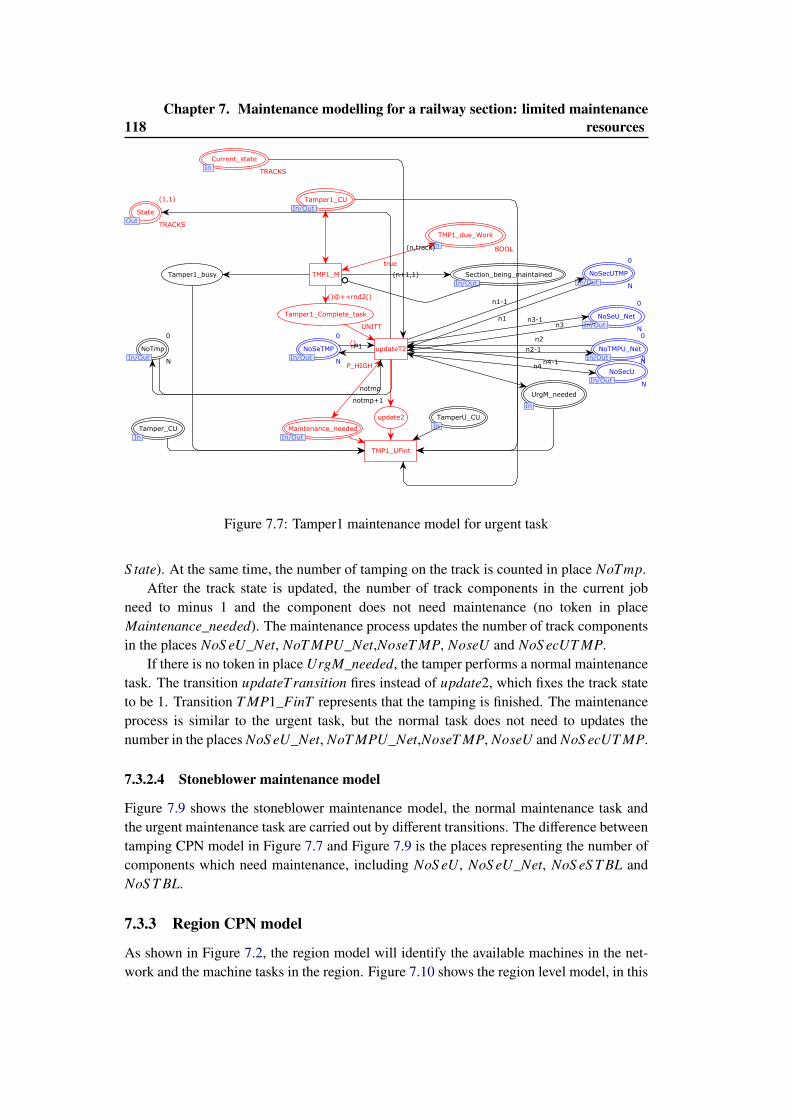
118Chapter 7. Maintenance modelling for a railway section: limited maintenance
resources
Tamper1_busy
Tamper1_Complete_task
UNITT
update2 TamperU_CU
In
TMP1_due_Work
InBOOL
Tamper1_CU
In/Out
Tamper_CU
In
State
OutTRACKS
(1,1)
NoSeTMP
In/OutN
0
Maintenance_needed
In/Out
Section_being_maintained
In/Out
NoSecUTMP
In/OutN
0
UrgM_needed
In
NoSeU_Net
In/OutN
0
NoTmp
In/OutN
0
NoTMPU_Net
In/OutN
0
Current_state
InTRACKS
NoSecU
In/OutN
0
TMP1_M
updateT2
P_HIGH
TMP1_UFint
()
()@++rnd2()
true
n1n3
nn-1
n3-1
n2-1
n2
n1-1
(n+1,1)
(n,track)
n4n4-1
notmp
notmp+1
Figure 7.7: Tamper1 maintenance model for urgent task
S tate). At the same time, the number of tamping on the track is counted in place NoTmp.After the track state is updated, the number of track components in the current job
need to minus 1 and the component does not need maintenance (no token in placeMaintenance_needed). The maintenance process updates the number of track componentsin the places NoS eU_Net, NoT MPU_Net,NoseT MP, NoseU and NoS ecUT MP.
If there is no token in place UrgM_needed, the tamper performs a normal maintenancetask. The transition updateTransition fires instead of update2, which fixes the track stateto be 1. Transition T MP1_FinT represents that the tamping is finished. The maintenanceprocess is similar to the urgent task, but the normal task does not need to updates thenumber in the places NoS eU_Net, NoT MPU_Net,NoseT MP, NoseU and NoS ecUT MP.
7.3.2.4 Stoneblower maintenance model
Figure 7.9 shows the stoneblower maintenance model, the normal maintenance task andthe urgent maintenance task are carried out by different transitions. The difference betweentamping CPN model in Figure 7.7 and Figure 7.9 is the places representing the number ofcomponents which need maintenance, including NoS eU, NoS eU_Net, NoS eS T BL andNoS T BL.
7.3.3 Region CPN model
As shown in Figure 7.2, the region model will identify the available machines in the net-work and the machine tasks in the region. Figure 7.10 shows the region level model, in this

7.3. CPN model for the railway network 119
Update
Tamper1_busy
Tamper1_Complete_task
UNITT
TMP1_due_Work
InBOOL
Tamper1_CU
In/Out
Tamper_CU
In
State
OutTRACKS
(1,1)
NoSeTMP
In/OutN
0
Maintenance_needed
In/Out
Section_being_maintained
In/Out
NoTmp
In/OutN
0
Current_state
InTRACKS
TMP1_FinT
UpdateTransition
TMP1_M
()@++rnd2()
()
true
(n+1,1)
nn-1
notmp
notmp+1
(n,track)
Figure 7.8: Tamper1 maintenance model for normal maintenance task
Update
STBL_busy
Tamper1_Complete_task
UNITT
update2
QTBL_due_Work
InBOOL
In
STBL_CU
In/OutIn/Out
STBL_NoSe_CurrentJob
In/OutN
In/Out
State
OutTRACKS
(1,1)
Out
NoSeSTBL
In/OutN
0
In/Out
Maintenance_needed
In/OutIn/Out
Section_being_maintained
In/OutIn/Out
NoSecU
In/OutN
0
In/Out
UrgM_needed
InIn
NoSeU_Net
In/OutN
0
In/Out
NoSTBL
In/OutN
0
In/Out
Next_state
InTRACKS
In
STBL_FinT
UpdateTransition
STBL_M
updateT2
P_HIGH
TMP1_UFint
()
()@++rnd2()
()
true
track1
n n-1
(n+1,1)
nn-1
n1
n-1
n3nnotmpn-1
n3-1notmp+1
n
n1-1
(n,track)
Figure 7.9: Stoneblower maintenance model
model, substitution transition TRACK contains the models presented in Figure 7.5, 7.6,4.12 and 7.9.
Substitution transition T MP1_Utility and S T BL_Utility are used to model two tam-pers and stoneblowers working tasks in the region. The substitution transition can be seenin Figure 7.11. The region model sends information to the network, i.e. the number of
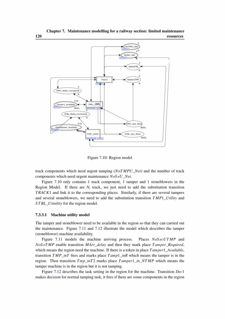
120Chapter 7. Maintenance modelling for a railway section: limited maintenance
resources
Stoneblower_Available
In/OutBOOL
true
STBL_Utility
MACHINE_Utility
TMP1_NoSe_CurrentJob
0
N
Tamper1_Available
In/Out
true
BOOL
TMP1_Utility
MACHINE_Utility
Track1
TRACK
NoSecUTMP
0
N
TMP1_due_Work
BOOL
true
NoTMPU_Net
In/Out
0
N
NoSeU_Net
In/Out
0
N
NoSeSTBL
0
N
STBL_due_Work
BOOL
STBL_NoSe_CurrentJob
0
N
Figure 7.10: Region model
track components which need urgent tamping (NoT MPU_Net) and the number of trackcomponents which need urgent maintenance NoS eU_Net.
Figure 7.10 only contains 1 track component, 1 tamper and 1 stoneblowers in theRegion Model. If there are Nt track, we just need to add the substitution transitionTRACK1 and link it to the corresponding places. Similarly, if there are several tampersand several stoneblowers, we need to add the substitution transition T MP1_Utility andS T BL_Utinility for the region model.
7.3.3.1 Machine utility model
The tamper and stoneblower need to be available in the region so that they can carried outthe maintenance. Figure 7.11 and 7.12 illustrate the model which describes the tamper(stoneblower) machine availability.
Figure 7.11 models the machine arriving process. Places NoS ecUT MP andNoS eT MP enable transition MArr_delay and then they mark place Tamper_Required,which means the region need the machine. If there is a token in place Tamper1_Available,transition T MP_inT fires and marks place Tamp1_inR which means the tamper is in theregion. Then transition Tmp_inT2 marks place Tamper1_in_NT MP which means thetamper machine is in the region but it is not tamping.
Figure 7.12 describes the task setting in the region for the machine. Transition Dec1makes decision for normal tamping task, it fires if there are some components in the region
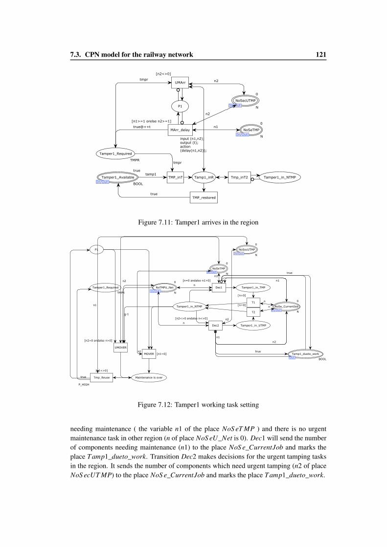
7.3. CPN model for the railway network 121
Tamper1_in_NTMPTamp1_inR
Tamper1_Required
TMPR
P1
NoSecUTMP
In/OutN
0
NoSeTMP
In/OutN
0
Tamper1_Available
In/OutBOOL
true
Tmp_inT2
UMArr
[n2<>0]
TMP_inT
TMP_restored
MArr_delay
[n1>=1 orelse n2>=1]
input (n1,n2);output (t);action(delay(n1,n2));
true@++t
tmpr
tmpr
n1
true
tamp1
n2
n2
Figure 7.11: Tamper1 arrives in the region
Tamper1_in_NTMP
Tamper1_in_TMP
NoSe_CurrentJob
In/OutN
0
Tamper1_in_UTMP
Maintenance is over
Tamper1_Required
TMPR
P1 NoSecUTMP
In/OutN
0
NoSeTMP
In/OutN
0
NoTMPU_Net
In/OutN
0
Tamp1_dueto_work
OutBOOL
Dec1
[n=0 andalso n1>0]
Dec2
[n2<>0 andalso n<>0]
UMOVER
[n2=0 andalso n>0]
MOVER [n1=0]
T1
[n=0]
T2
[n=0]
Tmp_Reuse
[n1<>0]
P_HIGH
n
n2
true
n
n1n2
n2
n1
n
n
n1
n1 true
true
nn-1
n
n1
Figure 7.12: Tamper1 working task setting
needing maintenance ( the variable n1 of the place NoS eT MP ) and there is no urgentmaintenance task in other region (n of place NoS eU_Net is 0). Dec1 will send the numberof components needing maintenance (n1) to the place NoS e_CurrentJob and marks theplace Tamp1_dueto_work. Transition Dec2 makes decisions for the urgent tamping tasksin the region. It sends the number of components which need urgent tamping (n2 of placeNoS ecUT MP) to the place NoS e_CurrentJob and marks the place Tamp1_dueto_work.
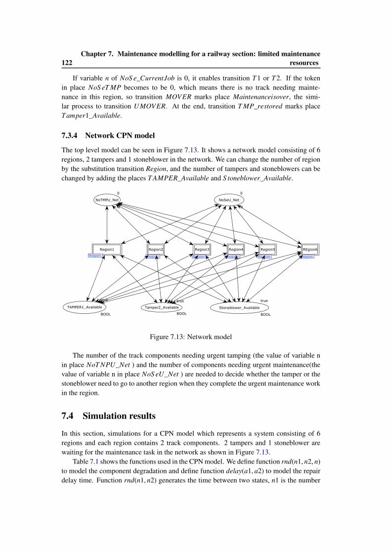
122Chapter 7. Maintenance modelling for a railway section: limited maintenance
resources
If variable n of NoS e_CurrentJob is 0, it enables transition T1 or T2. If the tokenin place NoS eT MP becomes to be 0, which means there is no track needing mainte-nance in this region, so transition MOVER marks place Maintenanceisover, the simi-lar process to transition UMOVER. At the end, transition T MP_restored marks placeTamper1_Available.
7.3.4 Network CPN model
The top level model can be seen in Figure 7.13. It shows a network model consisting of 6regions, 2 tampers and 1 stoneblower in the network. We can change the number of regionby the substitution transition Region, and the number of tampers and stoneblowers can bechanged by adding the places T AMPER_Available and S toneblower_Available.
NoSeU_Net
N
0
TAMPER1_Available
BOOL
true
NoTMPU_Net
N
0
Tamper2_Available
BOOL
true
Stoneblower_Available
BOOL
true
Region1
RegionRegion
Region2
RegionRegion
Region3
RegionRegion
Region4
RegionRegion
Region5
RegionRegion
REgion6
RegionRegion
Figure 7.13: Network model
The number of the track components needing urgent tamping (the value of variable nin place NoT NPU_Net ) and the number of components needing urgent maintenance(thevalue of variable n in place NoS eU_Net ) are needed to decide whether the tamper or thestoneblower need to go to another region when they complete the urgent maintenance workin the region.
7.4 Simulation results
In this section, simulations for a CPN model which represents a system consisting of 6regions and each region contains 2 track components. 2 tampers and 1 stoneblower arewaiting for the maintenance task in the network as shown in Figure 7.13.
Table 7.1 shows the functions used in the CPN model. We define function rnd(n1, n2, n)to model the component degradation and define function delay(a1, a2) to model the repairdelay time. Function rnd(n1, n2) generates the time between two states, n1 is the number
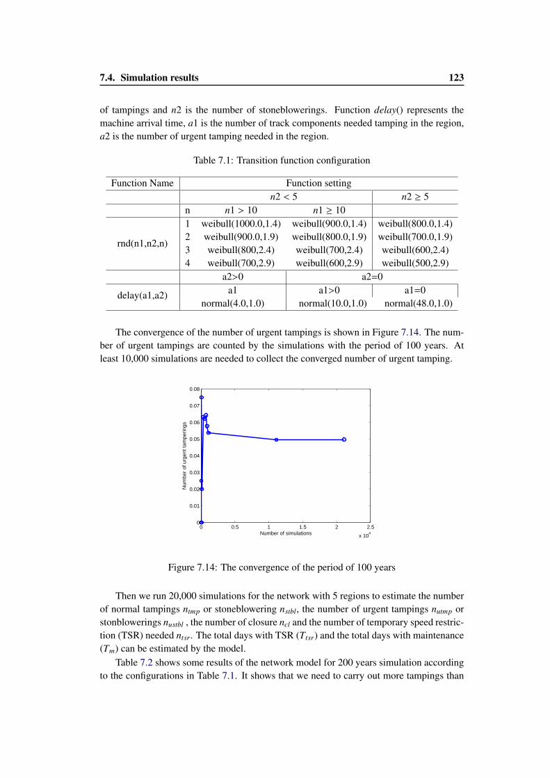
7.4. Simulation results 123
of tampings and n2 is the number of stoneblowerings. Function delay() represents themachine arrival time, a1 is the number of track components needed tamping in the region,a2 is the number of urgent tamping needed in the region.
Table 7.1: Transition function configuration
Function Name Function setting
rnd(n1,n2,n)
n2 < 5 n2 ≥ 5n n1 > 10 n1 ≥ 101 weibull(1000.0,1.4) weibull(900.0,1.4) weibull(800.0,1.4)2 weibull(900.0,1.9) weibull(800.0,1.9) weibull(700.0,1.9)3 weibull(800,2.4) weibull(700,2.4) weibull(600,2.4)4 weibull(700,2.9) weibull(600,2.9) weibull(500,2.9)
delay(a1,a2)
a2>0 a2=0a1 a1>0 a1=0
normal(4.0,1.0) normal(10.0,1.0) normal(48.0,1.0)
The convergence of the number of urgent tampings is shown in Figure 7.14. The num-ber of urgent tampings are counted by the simulations with the period of 100 years. Atleast 10,000 simulations are needed to collect the converged number of urgent tamping.
0 0.5 1 1.5 2 2.5
x 104
0
0.01
0.02
0.03
0.04
0.05
0.06
0.07
0.08
Number of simulations
Num
ber
of u
rgen
t tam
perin
gs
Figure 7.14: The convergence of the period of 100 years
Then we run 20,000 simulations for the network with 5 regions to estimate the numberof normal tampings ntmp or stoneblowering nstbl, the number of urgent tampings nutmp orstonblowerings nustbl , the number of closure ncl and the number of temporary speed restric-tion (TSR) needed ntsr. The total days with TSR (Ttsr) and the total days with maintenance(Tm) can be estimated by the model.
Table 7.2 shows some results of the network model for 200 years simulation accordingto the configurations in Table 7.1. It shows that we need to carry out more tampings than
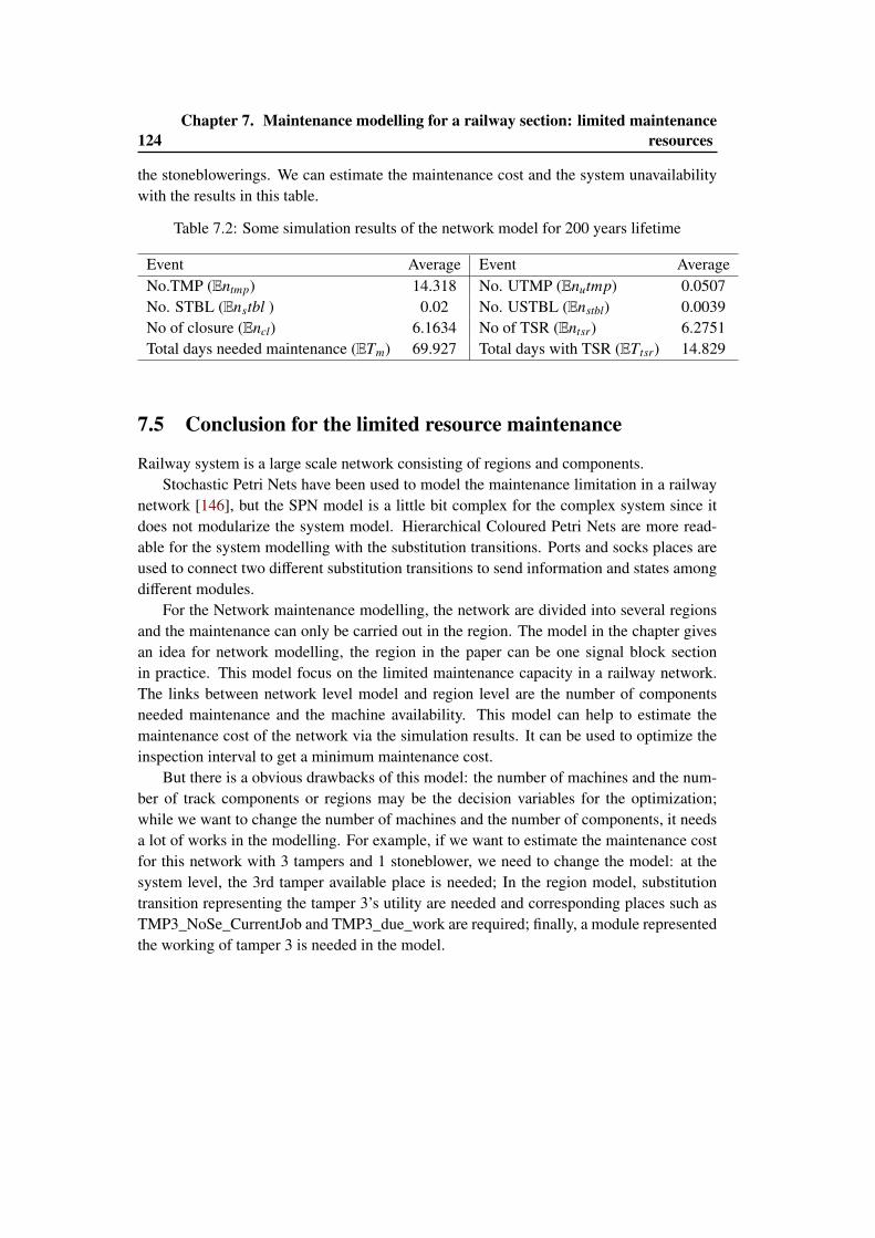
124Chapter 7. Maintenance modelling for a railway section: limited maintenance
resources
the stoneblowerings. We can estimate the maintenance cost and the system unavailabilitywith the results in this table.
Table 7.2: Some simulation results of the network model for 200 years lifetime
Event Average Event AverageNo.TMP (Entmp) 14.318 No. UTMP (Enutmp) 0.0507No. STBL (Enstbl ) 0.02 No. USTBL (Enstbl) 0.0039No of closure (Encl) 6.1634 No of TSR (Entsr) 6.2751Total days needed maintenance (ETm) 69.927 Total days with TSR (ETtsr) 14.829
7.5 Conclusion for the limited resource maintenance
Railway system is a large scale network consisting of regions and components.Stochastic Petri Nets have been used to model the maintenance limitation in a railway
network [146], but the SPN model is a little bit complex for the complex system since itdoes not modularize the system model. Hierarchical Coloured Petri Nets are more read-able for the system modelling with the substitution transitions. Ports and socks places areused to connect two different substitution transitions to send information and states amongdifferent modules.
For the Network maintenance modelling, the network are divided into several regionsand the maintenance can only be carried out in the region. The model in the chapter givesan idea for network modelling, the region in the paper can be one signal block sectionin practice. This model focus on the limited maintenance capacity in a railway network.The links between network level model and region level are the number of componentsneeded maintenance and the machine availability. This model can help to estimate themaintenance cost of the network via the simulation results. It can be used to optimize theinspection interval to get a minimum maintenance cost.
But there is a obvious drawbacks of this model: the number of machines and the num-ber of track components or regions may be the decision variables for the optimization;while we want to change the number of machines and the number of components, it needsa lot of works in the modelling. For example, if we want to estimate the maintenance costfor this network with 3 tampers and 1 stoneblower, we need to change the model: at thesystem level, the 3rd tamper available place is needed; In the region model, substitutiontransition representing the tamper 3’s utility are needed and corresponding places such asTMP3_NoSe_CurrentJob and TMP3_due_work are required; finally, a module representedthe working of tamper 3 is needed in the model.
Chapter 8
Maintenance of a railway section:two-level inspection policies
Contents8.1 Introduction . . . . . . . . . . . . . . . . . . . . . . . . . . . . . . . . . 1258.2 Modelling assumptions . . . . . . . . . . . . . . . . . . . . . . . . . . . 126
8.2.1 Component assumptions . . . . . . . . . . . . . . . . . . . . . . . 126
8.2.2 System operation and accident assumptions . . . . . . . . . . . . . 128
8.2.3 Performance evaluation . . . . . . . . . . . . . . . . . . . . . . . . 129
8.3 CPN model for the railway section . . . . . . . . . . . . . . . . . . . . . 1308.3.1 Modelling framework . . . . . . . . . . . . . . . . . . . . . . . . 130
8.3.2 Component CPN model . . . . . . . . . . . . . . . . . . . . . . . 131
8.3.3 System inspection CPN model . . . . . . . . . . . . . . . . . . . . 133
8.3.4 System operation and accident CPN model . . . . . . . . . . . . . 134
8.4 Simulation results . . . . . . . . . . . . . . . . . . . . . . . . . . . . . . 1358.4.1 Simulation convergence . . . . . . . . . . . . . . . . . . . . . . . 136
8.4.2 System performance evaluations . . . . . . . . . . . . . . . . . . . 137
8.5 Conclusion for two-level inspection policies . . . . . . . . . . . . . . . . 138
8.1 Introduction
The failures of a repairable component can be classified in revealed (or self-announcing)and unrevealed. Track faults in railway system are non-revealed: we need to carry outthe inspections to make sure that the component is good enough for the train passage.The maintenance and corresponding traffic control are planned according to the inspectionresults in order to avoid a railway accident.
The inspection ability influences the maintenance planning and hence have effect onthe maintenance cost, system unavailability and so on. In order to describe the inspectionability in failure process, Christer et al propose the “Delayed time" concept [41] ; Wangproposes an inspection model for a component which suffers from two kinds of defects andtwo inspection methods are set to the two defects separately [195]. Another similar model

126 Chapter 8. Maintenance of a railway section: two-level inspection policies
“P-F" failure process has been introduced for reliability centred maintenance (RCM)[117],Podofillini et.al propose a Markov model for the rail breakage assuming there are two levelsinspection for the failure process[144].
Gauge spread, a kind of track fault, can be classified to be static gauge spread or dy-namic gauge spread as described in Section 2.4.1.2. Two kinds of inspection measurementsare set for these two kinds of gauge spread. We assume that the visual inspection can in-spect the track and identify the static gauge spread whereas the train recording car canidentify the loaded (dynamic) gauge spread. This chapter aims to propose a CPN modelfor the maintenance policy with a two-level inspection procedure to investigate the inspec-tion planning.1
The structure of the chapter is as follows: Section 8.2 describe the system, includingthe deterioration process, maintenance rules, operation and risk condition. Section 8.3introduces the CPN model for the system, the framework and the details of the CPN modelsaccording to the framework. The simulation results are shown in Section 8.4 to show thatthe effect of the inspection policy. Section 8.5 gives a brief conclusion.
8.2 Modelling assumptions
In this study, we work on a plain line section consisting of 8 track components. These trackcomponents suffer from gauge spread. The study concerns about the system maintenancecost and the availability, as well as the derailment frequency.
8.2.1 Component assumptions
At the component level, component degradation and its maintenance strategy with inspec-tion policies are presented in this section.
8.2.1.1 Component degradation and maintenance
In this chapter, a multi-stage deterioration model is adopted to describe the process of gaugespread. The deterioration distribution for each stage is assumed to follow a exponentialdistribution Exp(λi). Corresponding repairs are carried out for each observed deteriorationstages.
The model of maintained component is shown in Figure 8.1. The component degra-dation process is divided into k stages, this process is shown in the grey rectangle area inFigure 8.1. The time distribution of each level is assumed to be an exponential distributionwith rate λi, when the component deteriorates to level k, it may cause an accident.
Each level can be identified by inspections INS Pi, then the component state is ob-served and a corresponding repair Mi controls the observed deterioration. Unfortunately,the repair arrives in a delay time and the component keeps degrading when this defectivecomponent is waiting for the repairs, hence the arriving repair may not fix the defects. Thecomponent deterioration and the corresponding maintenance and control methods are as-sumed as shown in Table 8.1. At the component level, derailments may happen due to the
1The work in this chapter has been presented in ESREL2014 [172]
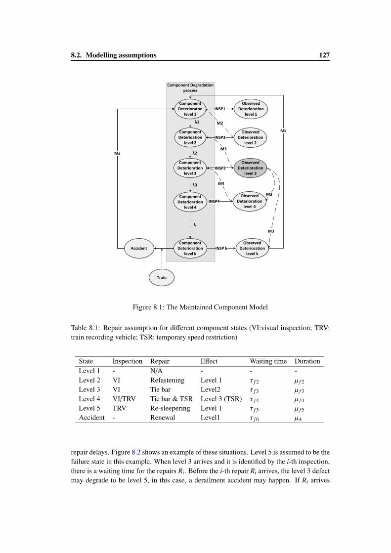
8.2. Modelling assumptions 127
Component Deterioraton
level 1
Component Deterioration
level 3
Component Deterioration
level k
Observed Deterioration
level 3
Observed Deterioration
level 2
Observed Deterioration
level k
INSP3
INSP k
λ1
λ
Mk
Accident
Ma
Observed Deterioration
level 1INSP1
Component Deterioation
level 2INSP2
M2
M3
Train
Component Degradation process
M3
λ2
Component Deterioration
level 4
λ3
Observed Deterioration
level 4INSP4
M3
M4
Figure 8.1: The Maintained Component Model
Table 8.1: Repair assumption for different component states (VI:visual inspection; TRV:train recording vehicle; TSR: temporary speed restriction)
State Inspection Repair Effect Waiting time DurationLevel 1 - N/A - - -Level 2 VI Refastening Level 1 τ f 2 µ f 2
Level 3 VI Tie bar Level2 τ f 3 µ f 3
Level 4 VI/TRV Tie bar & TSR Level 3 (TSR) τ f 4 µ f 4
Level 5 TRV Re-sleepering Level 1 τ f 5 µ f 5
Accident - Renewal Level1 τ f 6 µA
repair delays. Figure 8.2 shows an example of these situations. Level 5 is assumed to be thefailure state in this example. When level 3 arrives and it is identified by the i-th inspection,there is a waiting time for the repairs Ri. Before the i-th repair Ri arrives, the level 3 defectmay degrade to be level 5, in this case, a derailment accident may happen. If Ri arrives
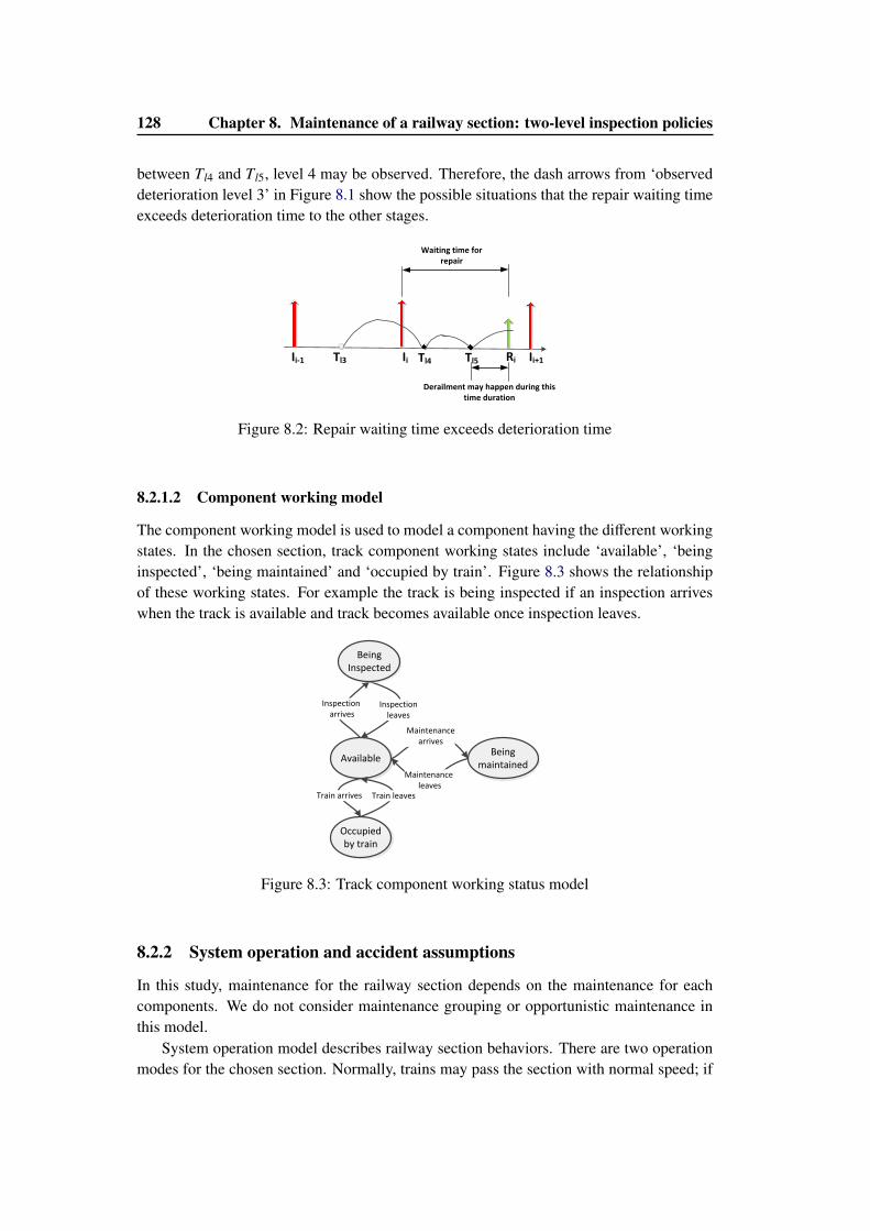
128 Chapter 8. Maintenance of a railway section: two-level inspection policies
between Tl4 and Tl5, level 4 may be observed. Therefore, the dash arrows from ‘observeddeterioration level 3’ in Figure 8.1 show the possible situations that the repair waiting timeexceeds deterioration time to the other stages.
IiTl3 Tl4Ii-1 Ii+1
Waiting time for repair
RiTl5
Derailment may happen during this time duration
Figure 8.2: Repair waiting time exceeds deterioration time
8.2.1.2 Component working model
The component working model is used to model a component having the different workingstates. In the chosen section, track component working states include ‘available’, ‘beinginspected’, ‘being maintained’ and ‘occupied by train’. Figure 8.3 shows the relationshipof these working states. For example the track is being inspected if an inspection arriveswhen the track is available and track becomes available once inspection leaves.
Available
Inspection arrives
Inspection leaves
Being Inspected
Being maintained
Maintenancearrives
Maintenance leaves
Occupied by train
Train arrives Train leaves
Figure 8.3: Track component working status model
8.2.2 System operation and accident assumptions
In this study, maintenance for the railway section depends on the maintenance for eachcomponents. We do not consider maintenance grouping or opportunistic maintenance inthis model.
System operation model describes railway section behaviors. There are two operationmodes for the chosen section. Normally, trains may pass the section with normal speed; if
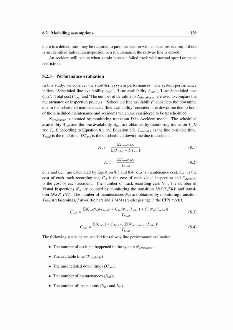
8.2. Modelling assumptions 129
there is a defect, train may be required to pass the section with a speed restriction; if thereis an identified failure, an inspection or a maintenance, the railway line is closed.
An accident will occurs when a train passes a failed track with normal speed or speedrestriction.
8.2.3 Performance evaluation
In this study, we consider the short-term system performances. The system performanceindices ‘Scheduled line availability Asch’, ‘Line availability Auns’, ‘Line Scheduled costCsch’, ‘Total cost Cuns’ and ‘The number of derailments Nderailment’ are used to compare themaintenance or inspection policies. ‘Scheduled line availability’ considers the downtimedue to the scheduled maintenances, ‘line availability’ considers the downtime due to bothof the scheduled maintenance and accidents which are considered to be unscheduled.
Nderailment is counted by monitoring transition D in Accident model. The scheduledavailability Asch and the line availability Auns are obtained by monitoring transition T_Dand Ti_E according to Equation 8.1 and Equation 8.2. Tavailable is the line available time,Ttotal is the total time, DTuns is the unscheduled down time due to accident.
Asch =ETavailable
E[Ttotal − DTuns](8.1)
Auns =ETavailable
Ttotal(8.2)
Csch and Cuns are calculated by Equation 8.3 and 8.4. CM is maintenance cost, Ctrv is thecost of each track recording car, Cvi is the cost of each visual inspection and CAccident
is the cost of each accident. The number of track recording cars Ntrv, the number ofVisual Inspections Nvi are counted by monitoring the transition INS P_TRV and transi-tion INS P_INT . The number of maintenances NM are obtained by monitoring transitionTmms(refastening), T Mms (tie bar) and T MMs (re-sleepering) in the CPN model.
Csch =E[CMNM(Ttotal) + CtrvNtrv(Ttotal) + CviNvi(Ttotal)]
Ttotal(8.3)
Cuns =E[Csch] + CAccidentE[Nderailment(Ttotal)]
Ttotal(8.4)
The following statistics are needed for railway line performance evaluation:
• The number of accident happened in the system Nderailment.
• The available time (Tavailable)
• The unscheduled down time (DTuns).
• The number of maintenances (NM);
• The number of inspections (Ntrv and Nvi)
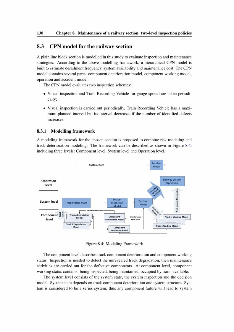
130 Chapter 8. Maintenance of a railway section: two-level inspection policies
8.3 CPN model for the railway section
A plain line block section is modelled in this study to evaluate inspection and maintenancestrategies. According to the above modelling framework, a hierarchical CPN model isbuilt to estimate derailment frequency, system availability and maintenance cost. The CPNmodel contains several parts: component deterioration model, component working model,operation and accident model.
The CPN model evaluates two inspection schemes:
• Visual inspection and Train Recording Vehicle for gauge spread are taken periodi-cally;
• Visual inspection is carried out periodically, Train Recording Vehicle has a maxi-mum planned interval but its interval decreases if the number of identified defectsincreases.
8.3.1 Modelling framework
A modeling framework for the chosen section is proposed to combine risk modeling andtrack deterioration modeling. The framework can be described as shown in Figure 8.4,including three levels: Component level, System level and Operation level.
Track n Working Model
………………………...
Track System State
Track n Degradation Model
………………………...
ComponentMaintenance Model
ComponentInspection Model
Decision Model
Track 1 Degradation Model
MaintenanceDdecision
Accident Model
System Inspection
Model
Railway System Operation
Component maintenance
System state
Track 1 Working Model
Maintenance
decision
Trac
k st
ate
s
System level
Component level
Line cl
osure
or speed
restr
ictio
n
Trac
k o
ccu
pie
d in
form
atio
n
Operation level
Figure 8.4: Modeling Framework
The component level describes track component deterioration and component workingstatus. Inspection is needed to detect the unrevealed track degradation, then maintenanceactivities are carried out for the defective components. At component level, componentworking status contains: being inspected, being maintained, occupied by train, available.
The system level consists of the system state, the system inspection and the decisionmodel. System state depends on track component deterioration and system structure. Sys-tem is considered to be a series system, thus any component failure will lead to system
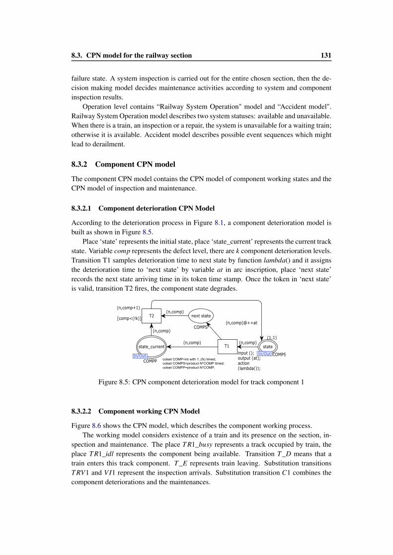
8.3. CPN model for the railway section 131
failure state. A system inspection is carried out for the entire chosen section, then the de-cision making model decides maintenance activities according to system and componentinspection results.
Operation level contains “Railway System Operation" model and “Accident model".Railway System Operation model describes two system statuses: available and unavailable.When there is a train, an inspection or a repair, the system is unavailable for a waiting train;otherwise it is available. Accident model describes possible event sequences which mightlead to derailment.
8.3.2 Component CPN model
The component CPN model contains the CPN model of component working states and theCPN model of inspection and maintenance.
8.3.2.1 Component deterioration CPN Model
According to the deterioration process in Figure 8.1, a component deterioration model isbuilt as shown in Figure 8.5.
Place ‘state’ represents the initial state, place ‘state_current’ represents the current trackstate. Variable comp represents the defect level, there are k component deterioration levels.Transition T1 samples deterioration time to next state by function lambda() and it assignsthe deterioration time to ‘next state’ by variable at in arc inscription, place ‘next state’records the next state arriving time in its token time stamp. Once the token in ‘next state’is valid, transition T2 fires, the component state degrades.
next state
COMPS
state_current
In/OutCOMPP
state
In/Out COMPS
(1,1)
T1
input ();output (at);action(lambda());
T2[comp<(!k)]
(n,comp)
(n,comp)@++at
(n,comp)
(n,comp+1)
(n,comp)
(n,comp)
colset COMP=int with 1..(!k) timed;
colset COMPS=product N*COMP timed;
colset COMPP=product N*COMP;
Figure 8.5: CPN component deterioration model for track component 1
8.3.2.2 Component working CPN Model
Figure 8.6 shows the CPN model, which describes the component working process.The working model considers existence of a train and its presence on the section, in-
spection and maintenance. The place TR1_busy represents a track occupied by train, theplace TR1_idl represents the component being available. Transition T_D means that atrain enters this track component. T_E represents train leaving. Substitution transitionsTRV1 and VI1 represent the inspection arrivals. Substitution transition C1 combines thecomponent deteriorations and the maintenances.
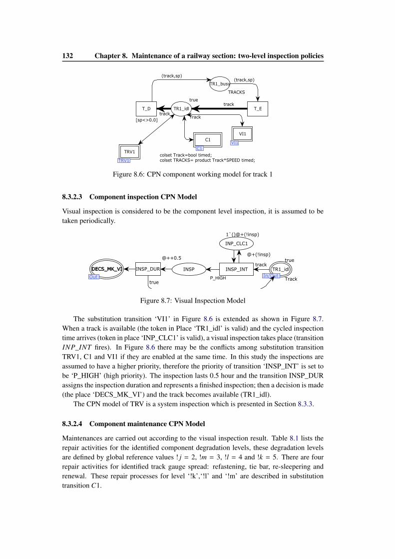
132 Chapter 8. Maintenance of a railway section: two-level inspection policies
colset Track=bool timed;colset TRACKS= product Track*SPEED timed;
TR1_idl
Track
true
TR1_busy
TRACKS
T_ET_D
[sp<>0.0]
C1
C1
VI1
VI1
TRV1
TRV1
track
track
(track,sp)(track,sp)
Figure 8.6: CPN component working model for track 1
8.3.2.3 Component inspection CPN Model
Visual inspection is considered to be the component level inspection, it is assumed to betaken periodically.
INP_CLC1
1`()@+(!insp)
INSP TR1_idl
In/OutTrack
true
In/Out
DECS_MK_VIDECS_MK_VIDECS_MK_VI
Out
INSP_INTINSP_DUR
@++0.5@+(!insp)
track
trueOut P_HIGH
Figure 8.7: Visual Inspection Model
The substitution transition ‘VI1’ in Figure 8.6 is extended as shown in Figure 8.7.When a track is available (the token in Place ‘TR1_idl’ is valid) and the cycled inspectiontime arrives (token in place ‘INP_CLC1’ is valid), a visual inspection takes place (transitionINP_INT fires). In Figure 8.6 there may be the conflicts among substitution transitionTRV1, C1 and VI1 if they are enabled at the same time. In this study the inspections areassumed to have a higher priority, therefore the priority of transition ‘INSP_INT’ is set tobe ‘P_HIGH’ (high priority). The inspection lasts 0.5 hour and the transition INSP_DURassigns the inspection duration and represents a finished inspection; then a decision is made(the place ‘DECS_MK_VI’) and the track becomes available (TR1_idl).
The CPN model of TRV is a system inspection which is presented in Section 8.3.3.
8.3.2.4 Component maintenance CPN Model
Maintenances are carried out according to the visual inspection result. Table 8.1 lists therepair activities for the identified component degradation levels, these degradation levelsare defined by global reference values ! j = 2, !m = 3, !l = 4 and !k = 5. There are fourrepair activities for identified track gauge spread: refastening, tie bar, re-sleepering andrenewal. These repair processes for level ‘!k’,‘!l’ and ‘!m’ are described in substitutiontransition C1.
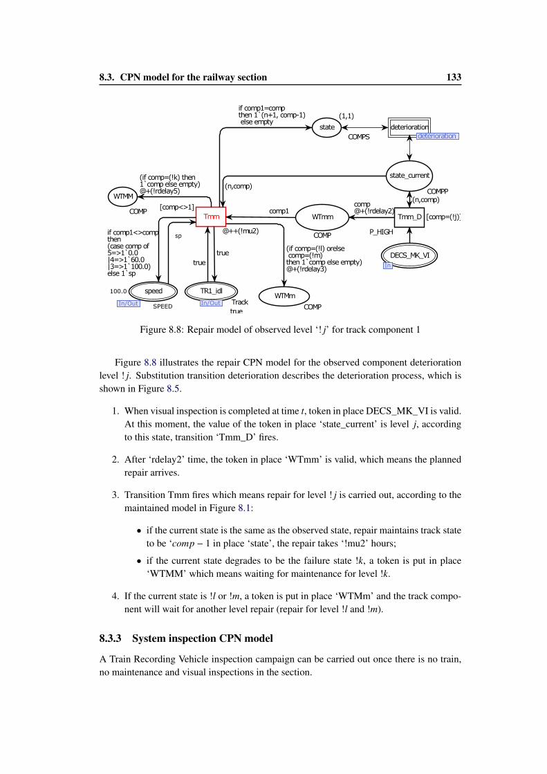
8.3. CPN model for the railway section 133
globref k=5;globref l=4;globref m=3;globref j=2;globref rdelay2=15;globref rdelay3=10;globref rdelay5=2;colset COMP=int with 1..(!k) timed;colset COMPP=product N*COMP;colset COMPS=product N*COMP timed;
WTMm
COMP
state_current
COMPP
WTmm
COMP
state
(1,1)
COMPS
TR1_idl
In/Out
true
Track
WTMM
COMP
speed
In/Out
100.0
SPEED
DECS_MK_VI
In
Tmm
[comp<>1]
@++(!mu2)
Tmm_D [comp=(!j)]
P_HIGH
deteriorationdeterioration
(if comp=(!l) orelse comp=(!m) then 1 comp else empty)@+(!rdelay3)
(n,comp)
comp1comp@+(!rdelay2)
(n,comp)
if comp1=comp then 1 (n+1, comp-1) else empty
true
true
if comp1<>comp then (case comp of5=>1 0.0|4=>1 60.0|3=>1 100.0)else 1 sp
sp
(if comp=(!k) then 1 comp else empty)@+(!rdelay5)
deterioration
In/Out In/Out
In
Figure 8.8: Repair model of observed level ‘! j’ for track component 1
Figure 8.8 illustrates the repair CPN model for the observed component deteriorationlevel ! j. Substitution transition deterioration describes the deterioration process, which isshown in Figure 8.5.
1. When visual inspection is completed at time t, token in place DECS_MK_VI is valid.At this moment, the value of the token in place ‘state_current’ is level j, accordingto this state, transition ‘Tmm_D’ fires.
2. After ‘rdelay2’ time, the token in place ‘WTmm’ is valid, which means the plannedrepair arrives.
3. Transition Tmm fires which means repair for level ! j is carried out, according to themaintained model in Figure 8.1:
• if the current state is the same as the observed state, repair maintains track stateto be ‘comp − 1 in place ‘state’, the repair takes ‘!mu2’ hours;
• if the current state degrades to be the failure state !k, a token is put in place‘WTMM’ which means waiting for maintenance for level !k.
4. If the current state is !l or !m, a token is put in place ‘WTMm’ and the track compo-nent will wait for another level repair (repair for level !l and !m).
8.3.3 System inspection CPN model
A Train Recording Vehicle inspection campaign can be carried out once there is no train,no maintenance and visual inspections in the section.
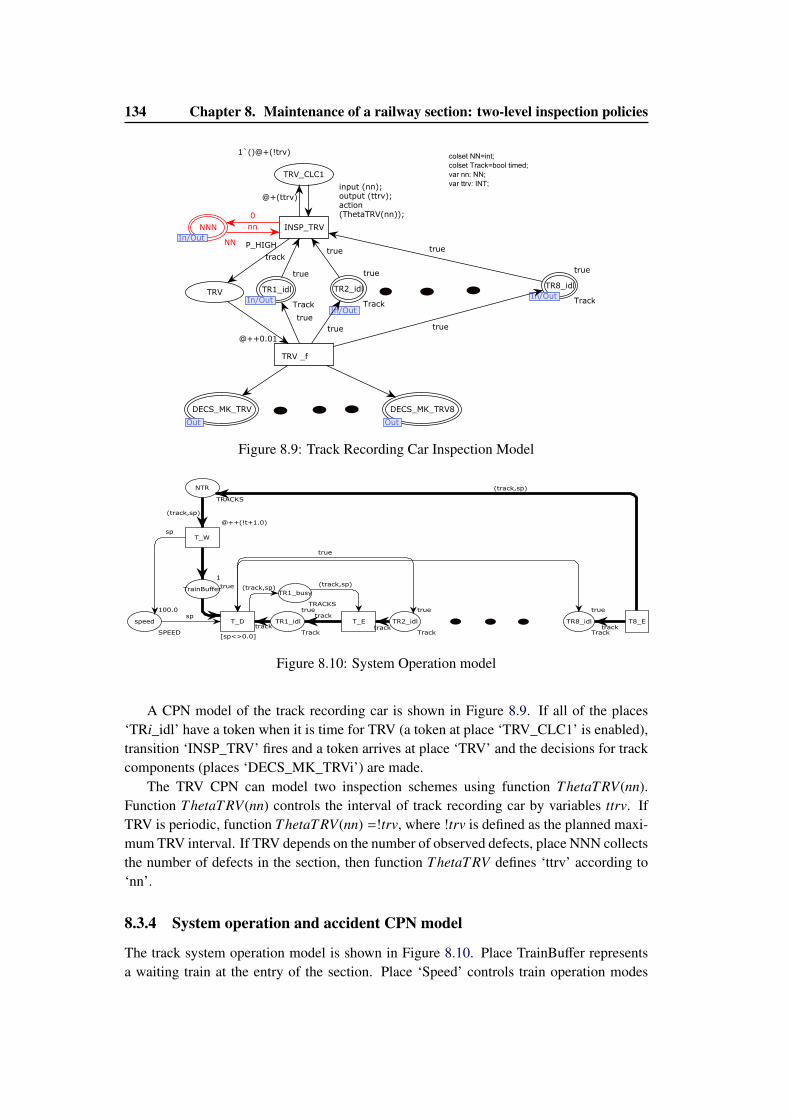
134 Chapter 8. Maintenance of a railway section: two-level inspection policies
TRV_CLC1
1`()@+(!trv)
TRV TR2_idl
In/OutTrack
true
TR8_idl
In/OutTrack
true
DECS_MK_TRV8
Out
TR1_idl
In/OutTrack
true
DECS_MK_TRV
Out
NNN
In/OutNN
INSP_TRV
input (nn);output (ttrv);action(ThetaTRV(nn));
P_HIGH
TRV _f
@++0.01
@+(ttrv)
true
truetrue
truetrack
true
nn
0
colset NN=int;
colset Track=bool timed;
var nn: NN;
var ttrv: INT;
Figure 8.9: Track Recording Car Inspection Model
TR1_idl
Track
true
NTR
TRACKS
TrainBuffer
1
TR1_busy
TRACKS
speed
SPEED
100.0
TR2_idl
Track
true
TR8_idl
Track
true
T_ET_D
[sp<>0.0]
T_W
@))+8t)1.0(
T8_Etrack
track
+track,sp(
+track,sp( +track,sp(
sp
sp
track
true
track
+track,sp(
true
Figure 8.10: System Operation model
A CPN model of the track recording car is shown in Figure 8.9. If all of the places‘TRi_idl’ have a token when it is time for TRV (a token at place ‘TRV_CLC1’ is enabled),transition ‘INSP_TRV’ fires and a token arrives at place ‘TRV’ and the decisions for trackcomponents (places ‘DECS_MK_TRVi’) are made.
The TRV CPN can model two inspection schemes using function ThetaTRV(nn).Function ThetaTRV(nn) controls the interval of track recording car by variables ttrv. IfTRV is periodic, function ThetaTRV(nn) =!trv, where !trv is defined as the planned maxi-mum TRV interval. If TRV depends on the number of observed defects, place NNN collectsthe number of defects in the section, then function ThetaTRV defines ‘ttrv’ according to‘nn’.
8.3.4 System operation and accident CPN model
The track system operation model is shown in Figure 8.10. Place TrainBuffer representsa waiting train at the entry of the section. Place ‘Speed’ controls train operation modes
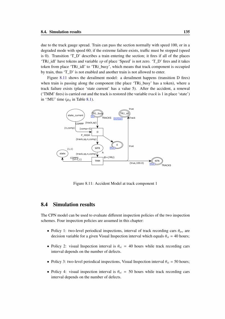
8.4. Simulation results 135
due to the track gauge spread. Train can pass the section normally with speed 100, or in adegraded mode with speed 60; if the extreme failure exists, traffic must be stopped (speedis 0). Transition ‘T_D’ describes a train entering the section; it fires if all of the places‘TRi_idl’ have tokens and variable sp of place ‘Speed’ is not zero. ‘T_D’ fires and it takestoken from place ‘TRi_idl’ to ‘TRi_busy’, which means that track component is occupiedby train, thus ‘T_D’ is not enabled and another train is not allowed to enter.
Figure 8.11 shows the derailment model: a derailment happens (transition D fires)when train is passing along the component (the place ‘TRi_busy’ has a token), where atrack failure exists (place ‘state current’ has a value 5). After the accident, a renewal(‘TMM’ fires) is carried out and the track is restored (the variable track is 1 in place ‘state’)in ‘!MU’ time (µA in Table 8.1).
state
COMPS
(1,1)
state_current
COMPP
WFR
A
TR1_idl
In/Out Track
true
TR1_busy
InTRACKS
NTR
OutTRACKS
E
Out
D
[comp=5]
P_HIGH
TMM
@+(!MU)(n+1,1)
(track,sp,n,comp)
(track,sp,n,comp)
(n,comp)
(track,sp)
(true,100.0)
true
Figure 8.11: Accident Model at track component 1
8.4 Simulation results
The CPN model can be used to evaluate different inspection policies of the two inspectionschemes. Four inspection policies are assumed in this chapter:
• Policy 1: two-level periodical inspections, interval of track recording cars θtrv aredecision variable for a given Visual Inspection interval which equals θvi = 40 hours;
• Policy 2: visual Inspection interval is θvi = 40 hours while track recording carsinterval depends on the number of defects.
• Policy 3: two-level periodical inspections, Visual Inspection interval θvi = 50 hours;
• Policy 4: visual inspection interval is θvi = 50 hours while track recording carsinterval depends on the number of defects.

136 Chapter 8. Maintenance of a railway section: two-level inspection policies
In this study, we want to estimate the system performance for 1 year (8760 hours) withthe inspection policies mention above. For these inspection policies, the planned TrainRecording Vehicle (TRV) interval ranges from 5 to 2000 hours. The parameters for main-tenance are shown in Table 8.2. Since we have no actual failure data for gauge spread, theparameters in this table are our assumptions.
Table 8.2: Simulation parametres
State Failure rate Effect Waiting time (hours) Duration (hours)Level 1 λ1 = 0.002 - -Level 2 λ2 = 0.002 Level 1 τ f 2 = 15 µ f 2 = 1Level 3 λ3 = 0.002 Level2 τ f 3 = 10 µ f 3 = 4Level 4 λ4 = 0.002 Level 3 (TSR) τ f 4 = 5 µ f 4 = 4Level 5 λ5 = 0.002 Level 1 τ f 5 = 2 µ f 5 = 10Accident - Level1 τ f 6 = 0 µA = 70
8.4.1 Simulation convergence
20000 simulations with a simulation length of 8760 hours (1 year) are carried out to checkhow many simulations are required to observe a convergence in the results. A plot of theaverage line availability against the number of simulations is shown in Figure 8.12. The
0 0.2 0.4 0.6 0.8 1 1.2 1.4 1.6 1.8 2
x 104
0.739
0.74
0.741
0.742
0.743
0.744
0.745
0.746
0.747
0.748
0.749
Line
sch
edul
ed a
vaila
bilit
y
No of simulation
Plot of average scheduled line availability against the number of simulations
AverageHigh boundLow bound
Figure 8.12: The number of simulation against the availability(simulation horizon: 8760hours (1 year))
middle curve is the average availability result, the curve below it and above it are the 99%confidence results. It shows the simulation converges at around 2000 simulations. If thenumber of simulations is less than 2000, the results have larger deviations. Therefore, atleast 2000 simulations are needed to get the solution of CPN model; in this study, we run10000 simulations for the simulation length of 8760 hours.
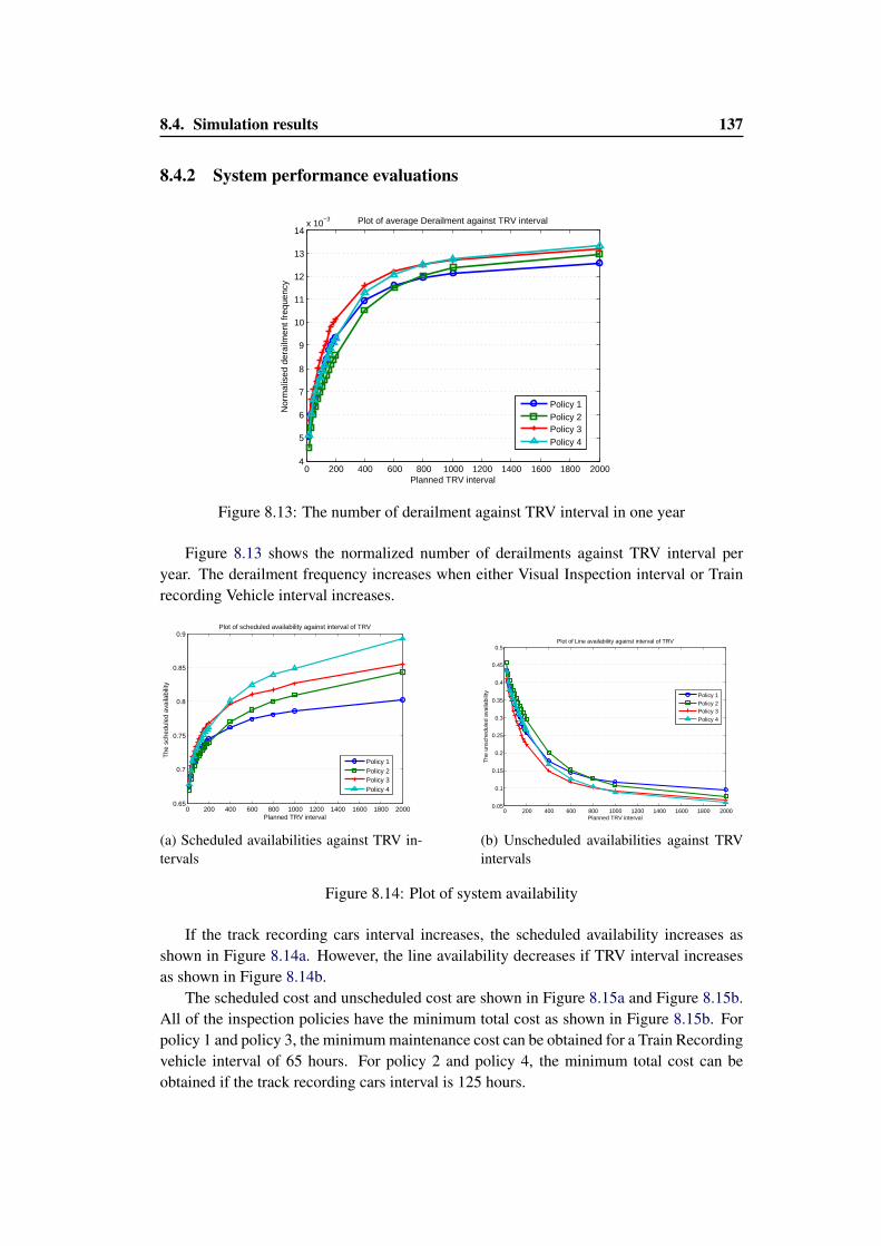
8.4. Simulation results 137
8.4.2 System performance evaluations
0 200 400 600 800 1000 1200 1400 1600 1800 20004
5
6
7
8
9
10
11
12
13
14x 10
−3
Nor
mal
ised
der
ailm
ent f
requ
ency
Planned TRV interval
Plot of average Derailment against TRV interval
Policy 1Policy 2Policy 3Policy 4
Figure 8.13: The number of derailment against TRV interval in one year
Figure 8.13 shows the normalized number of derailments against TRV interval peryear. The derailment frequency increases when either Visual Inspection interval or Trainrecording Vehicle interval increases.
0 200 400 600 800 1000 1200 1400 1600 1800 20000.65
0.7
0.75
0.8
0.85
0.9
Planned TRV interval
The
sch
edul
ed a
vaila
bilit
y
Plot of scheduled availability against interval of TRV
Policy 1Policy 2Policy 3Policy 4
(a) Scheduled availabilities against TRV in-tervals
0 200 400 600 800 1000 1200 1400 1600 1800 20000.05
0.1
0.15
0.2
0.25
0.3
0.35
0.4
0.45
0.5
The
uns
ched
uled
ava
ilabi
lity
Planned TRV interval
Plot of Line availability against interval of TRV
Policy 1Policy 2Policy 3Policy 4
(b) Unscheduled availabilities against TRVintervals
Figure 8.14: Plot of system availability
If the track recording cars interval increases, the scheduled availability increases asshown in Figure 8.14a. However, the line availability decreases if TRV interval increasesas shown in Figure 8.14b.
The scheduled cost and unscheduled cost are shown in Figure 8.15a and Figure 8.15b.All of the inspection policies have the minimum total cost as shown in Figure 8.15b. Forpolicy 1 and policy 3, the minimum maintenance cost can be obtained for a Train Recordingvehicle interval of 65 hours. For policy 2 and policy 4, the minimum total cost can beobtained if the track recording cars interval is 125 hours.
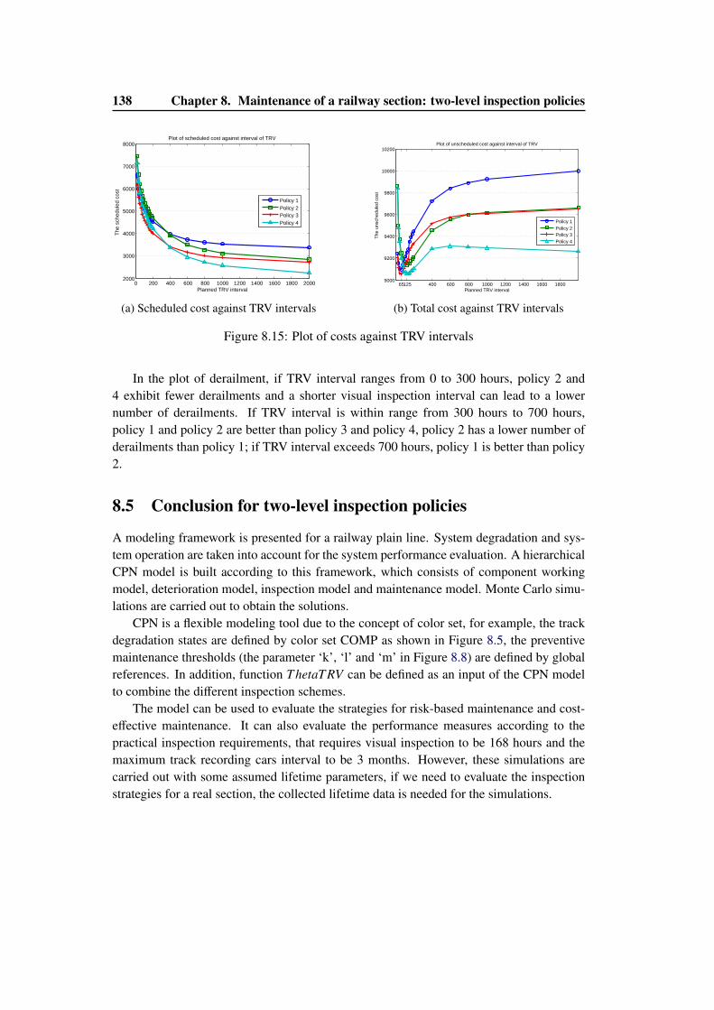
138 Chapter 8. Maintenance of a railway section: two-level inspection policies
0 200 400 600 800 1000 1200 1400 1600 1800 20002000
3000
4000
5000
6000
7000
8000
The
sch
edul
ed c
ost
Planned TRV interval
Plot of scheduled cost against interval of TRV
Policy 1Policy 2Policy 3Policy 4
(a) Scheduled cost against TRV intervals
65125 400 600 800 1000 1200 1400 1600 18009000
9200
9400
9600
9800
10000
10200
The
uns
ched
uled
cos
t
Planned TRV interval
Plot of unscheduled cost against interval of TRV
Policy 1Policy 2Policy 3Policy 4
(b) Total cost against TRV intervals
Figure 8.15: Plot of costs against TRV intervals
In the plot of derailment, if TRV interval ranges from 0 to 300 hours, policy 2 and4 exhibit fewer derailments and a shorter visual inspection interval can lead to a lowernumber of derailments. If TRV interval is within range from 300 hours to 700 hours,policy 1 and policy 2 are better than policy 3 and policy 4, policy 2 has a lower number ofderailments than policy 1; if TRV interval exceeds 700 hours, policy 1 is better than policy2.
8.5 Conclusion for two-level inspection policies
A modeling framework is presented for a railway plain line. System degradation and sys-tem operation are taken into account for the system performance evaluation. A hierarchicalCPN model is built according to this framework, which consists of component workingmodel, deterioration model, inspection model and maintenance model. Monte Carlo simu-lations are carried out to obtain the solutions.
CPN is a flexible modeling tool due to the concept of color set, for example, the trackdegradation states are defined by color set COMP as shown in Figure 8.5, the preventivemaintenance thresholds (the parameter ‘k’, ‘l’ and ‘m’ in Figure 8.8) are defined by globalreferences. In addition, function ThetaTRV can be defined as an input of the CPN modelto combine the different inspection schemes.
The model can be used to evaluate the strategies for risk-based maintenance and cost-effective maintenance. It can also evaluate the performance measures according to thepractical inspection requirements, that requires visual inspection to be 168 hours and themaximum track recording cars interval to be 3 months. However, these simulations arecarried out with some assumed lifetime parameters, if we need to evaluate the inspectionstrategies for a real section, the collected lifetime data is needed for the simulations.
Chapter 9
Maintenance optimization for arailway section: delayed
maintenance vs speed restriction
Contents9.1 Introduction . . . . . . . . . . . . . . . . . . . . . . . . . . . . . . . . . 1399.2 Modelling assumptions . . . . . . . . . . . . . . . . . . . . . . . . . . . 141
9.2.1 Track component deterioration and maintenance . . . . . . . . . . 141
9.2.2 Section maintenance planning . . . . . . . . . . . . . . . . . . . . 142
9.3 Performance evaluation . . . . . . . . . . . . . . . . . . . . . . . . . . . 1449.3.1 Single objective evaluation . . . . . . . . . . . . . . . . . . . . . . 144
9.3.2 Multiple-objective evaluation . . . . . . . . . . . . . . . . . . . . 145
9.4 CPN models . . . . . . . . . . . . . . . . . . . . . . . . . . . . . . . . . 1469.4.1 CPN model for railway section . . . . . . . . . . . . . . . . . . . . 146
9.4.2 Component CPN model . . . . . . . . . . . . . . . . . . . . . . . 147
9.4.3 Component maintenance CPN model for grouping strategy . . . . . 148
9.4.4 Maintenance planning CPN model . . . . . . . . . . . . . . . . . . 149
9.5 Simulation results . . . . . . . . . . . . . . . . . . . . . . . . . . . . . . 1509.5.1 Convergence . . . . . . . . . . . . . . . . . . . . . . . . . . . . . 150
9.5.2 Results for the grouping policy . . . . . . . . . . . . . . . . . . . . 150
9.5.3 Results for the non-grouping policy . . . . . . . . . . . . . . . . . 153
9.5.4 Comparison of grouping and non-grouping policies . . . . . . . . . 154
9.6 Conclusion for the delayed maintenance with speed restriction . . . . . 155
9.1 Introduction
Track vertical geometry faults due to poor ballast condition can be adjusted by track tamp-ing or stoneblowering. Several researches study on the track failure evolution and theypoint out that the track quality depends on some factors such as speed, tonnage (MGT),maintenance histories and materials [11, 166, 203, 221].
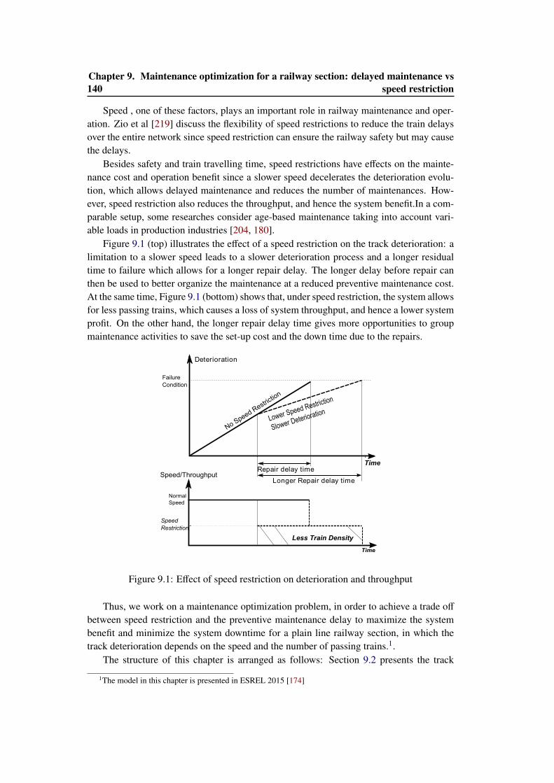
140Chapter 9. Maintenance optimization for a railway section: delayed maintenance vs
speed restriction
Speed , one of these factors, plays an important role in railway maintenance and oper-ation. Zio et al [219] discuss the flexibility of speed restrictions to reduce the train delaysover the entire network since speed restriction can ensure the railway safety but may causethe delays.
Besides safety and train travelling time, speed restrictions have effects on the mainte-nance cost and operation benefit since a slower speed decelerates the deterioration evolu-tion, which allows delayed maintenance and reduces the number of maintenances. How-ever, speed restriction also reduces the throughput, and hence the system benefit.In a com-parable setup, some researches consider age-based maintenance taking into account vari-able loads in production industries [204, 180].
Figure 9.1 (top) illustrates the effect of a speed restriction on the track deterioration: alimitation to a slower speed leads to a slower deterioration process and a longer residualtime to failure which allows for a longer repair delay. The longer delay before repair canthen be used to better organize the maintenance at a reduced preventive maintenance cost.At the same time, Figure 9.1 (bottom) shows that, under speed restriction, the system allowsfor less passing trains, which causes a loss of system throughput, and hence a lower systemprofit. On the other hand, the longer repair delay time gives more opportunities to groupmaintenance activities to save the set-up cost and the down time due to the repairs.
Deterioration
Failure
Condition
Lower Speed Restriction
Slower Deterioration
No Speed R
estrictio
n
Speed/ThroughputRepair delay time
Longer Repair delay time
Normal
Speed
Speed
Restriction
Less Train Density
Time
Time
Figure 9.1: Effect of speed restriction on deterioration and throughput
Thus, we work on a maintenance optimization problem, in order to achieve a trade off
between speed restriction and the preventive maintenance delay to maximize the systembenefit and minimize the system downtime for a plain line railway section, in which thetrack deterioration depends on the speed and the number of passing trains.1.
The structure of this chapter is arranged as follows: Section 9.2 presents the track
1The model in this chapter is presented in ESREL 2015 [174]
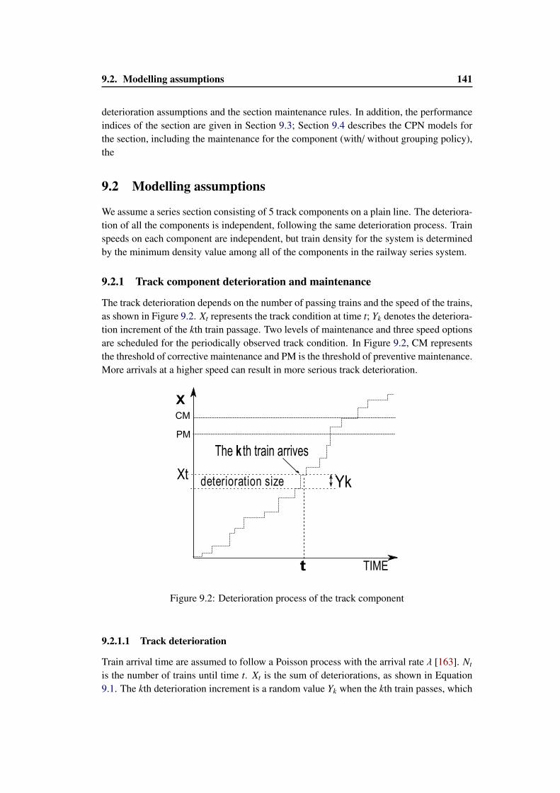
9.2. Modelling assumptions 141
deterioration assumptions and the section maintenance rules. In addition, the performanceindices of the section are given in Section 9.3; Section 9.4 describes the CPN models forthe section, including the maintenance for the component (with/ without grouping policy),the
9.2 Modelling assumptions
We assume a series section consisting of 5 track components on a plain line. The deteriora-tion of all the components is independent, following the same deterioration process. Trainspeeds on each component are independent, but train density for the system is determinedby the minimum density value among all of the components in the railway series system.
9.2.1 Track component deterioration and maintenance
The track deterioration depends on the number of passing trains and the speed of the trains,as shown in Figure 9.2. Xt represents the track condition at time t; Yk denotes the deteriora-tion increment of the kth train passage. Two levels of maintenance and three speed optionsare scheduled for the periodically observed track condition. In Figure 9.2, CM representsthe threshold of corrective maintenance and PM is the threshold of preventive maintenance.More arrivals at a higher speed can result in more serious track deterioration.
X
The k th train arrives
deterioration size
t TIME
Yk
PM
CM
Xt
Figure 9.2: Deterioration process of the track component
9.2.1.1 Track deterioration
Train arrival time are assumed to follow a Poisson process with the arrival rate λ [163]. Nt
is the number of trains until time t. Xt is the sum of deteriorations, as shown in Equation9.1. The kth deterioration increment is a random value Yk when the kth train passes, which
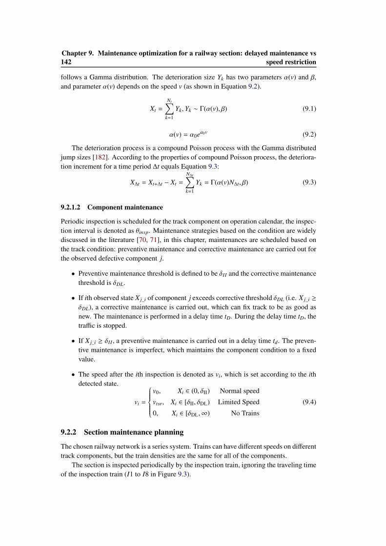
142Chapter 9. Maintenance optimization for a railway section: delayed maintenance vs
speed restriction
follows a Gamma distribution. The deterioration size Yk has two parameters α(v) and β,and parameter α(v) depends on the speed v (as shown in Equation 9.2).
Xt =
Nt∑k=1
Yk,Yk ∼ Γ(α(v), β) (9.1)
α(v) = α0ea0v (9.2)
The deterioration process is a compound Poisson process with the Gamma distributedjump sizes [182]. According to the properties of compound Poisson process, the deteriora-tion increment for a time period ∆t equals Equation 9.3:
X∆t = Xt+∆t − Xt =
N∆t∑k=1
Yk = Γ(α(v)N∆t, β) (9.3)
9.2.1.2 Component maintenance
Periodic inspection is scheduled for the track component on operation calendar, the inspec-tion interval is denoted as θinsp. Maintenance strategies based on the condition are widelydiscussed in the literature [70, 71], in this chapter, maintenances are scheduled based onthe track condition: preventive maintenance and corrective maintenance are carried out forthe observed defective component j.
• Preventive maintenance threshold is defined to be δII and the corrective maintenancethreshold is δDL.
• If ith observed state X j_i of component j exceeds corrective threshold δDL (i.e. X j_i ≥
δDL), a corrective maintenance is carried out, which can fix track to be as good asnew. The maintenance is performed in a delay time tD. During the delay time tD, thetraffic is stopped.
• If X j_i ≥ δII , a preventive maintenance is carried out in a delay time td. The preven-tive maintenance is imperfect, which maintains the component condition to a fixedvalue.
• The speed after the ith inspection is denoted as vi, which is set according to the ithdetected state.
vi =
v0, Xi ∈ (0, δII) Normal speed
vtsr, Xi ∈ [δII, δDL) Limited Speed
0, Xi ∈ [δDL,∞) No Trains
(9.4)
9.2.2 Section maintenance planning
The chosen railway network is a series system. Trains can have different speeds on differenttrack components, but the train densities are the same for all of the components.
The section is inspected periodically by the inspection train, ignoring the traveling timeof the inspection train (I1 to I8 in Figure 9.3).
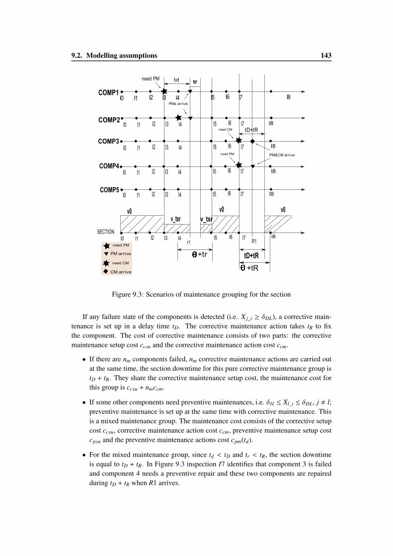
9.2. Modelling assumptions 143
I0 I1 I2 I3 I4 I5 I6 I7 I8
I0 I1 I2 I3 I4 I5 I6 I7 I8
I8I0 I1 I2 I3 I4 I5 I6 I7
I0 I1 I2 I3 I4 I5 I6 I7
I0 I1 I2 I3 I4 I5 I6 I7
COMP1
COMP2
COMP3
COMP4
COMP5
I0 I1 I2 I3 I4 I5 I6 I7
SECTION
td
tD+tR
r1 R1
+tr
v0
v_tsrv0 v0
+tR
need PM
PMs arrive
need PM
need CM
PM&CM arrive
need PM
PM arrive
need CM
CM arrive
tr
v_tsr
tD+tR
I8
I8
I8
Figure 9.3: Scenarios of maintenance grouping for the section
If any failure state of the components is detected (i.e. X j_i ≥ δDL), a corrective main-tenance is set up in a delay time tD. The corrective maintenance action takes tR to fixthe component. The cost of corrective maintenance consists of two parts: the correctivemaintenance setup cost ccsu and the corrective maintenance action cost ccm.
• If there are nm components failed, nm corrective maintenance actions are carried outat the same time, the section downtime for this pure corrective maintenance group istD + tR. They share the corrective maintenance setup cost, the maintenance cost forthis group is ccsu + nmccm.
• If some other components need preventive maintenances, i.e. δII ≤ Xl_i ≤ δDL, j , l;preventive maintenance is set up at the same time with corrective maintenance. Thisis a mixed maintenance group. The maintenance cost consists of the corrective setupcost ccsu, corrective maintenance action cost ccm, preventive maintenance setup costcpsu and the preventive maintenance actions cost cpm(td).
• For the mixed maintenance group, since td < tD and tr < tR, the section downtimeis equal to tD + tR. In Figure 9.3 inspection I7 identifies that component 3 is failedand component 4 needs a preventive repair and these two components are repairedduring tD + tR when R1 arrives.
144Chapter 9. Maintenance optimization for a railway section: delayed maintenance vs
speed restriction
At time ti, if X j_i ≥ δII , a preventive maintenance is set up in a delay time td. Duringtd, if the following inspection only identifies defects but no failures, all the defective com-ponents are repaired at time ti + td. This is a pure preventive maintenance group, as shownin Figure 9.3, I3 identifies component 1 needs preventive maintenance, then a preventivemaintenance is scheduled at time I3 + td, inspection I4 identifies that the component 2 alsoneeds a preventive maintenance, thus the preventive maintenance for component 4 is car-ried out at time I3 + td and it does not need to wait for another delay time td. Preventivemaintenance needs a down time tr.
The cost of preventive maintenance includes the setup cost cpsu and the cost of eachpreventive maintenance action cpm(td). cpm(td) depends on the longest repair delay timein the group, that is td for component 1 at time I3 in Figure 9.3. The longer td the lowermaintenance cost as shown in Equation 9.5. If td ∈ (0,T ∗), the preventive maintenanceaction cost depends on the repair delay time td, if td ≥ T ∗, the preventive maintenanceaction cost equals a minimum repair value cpmin .
cpm(td) =
Atd + B td ∈ (0,T ∗)
cpmin td ∈ [T ∗,∞)(9.5)
There are three traffic density configurations according to the minimum train speed inthe section: If all observed states are normal X j_i ≤ δII , the train density is λ0. If componentj is defective (X j_i ≥ δII), during td, the speed at j component is v j = vtsr and the speed forthe other normal component equals vl = v0, l , j, the train density for the section is λtrain
in Equation 9.6 until the following inspection confirms that all the components are normal.
λtrain =vtsr
v0λ0 (9.6)
When the maintenance action is performed, the system is closed, that is I3 to I5 in Figure9.3. If component j is failed (X j_i ≥ δII), the section is closed and the density is 0.
9.3 Performance evaluation
In this section, the performance evaluation indices are introduced. For the single objective,we can compare the system benefit or the system unavailability for the evaluation; for themultiple-objectives, we adopt the Pareto front.
9.3.1 Single objective evaluation
System benefit and system unavailability are used to evaluate the system performance.System unavailability is equal to Equation 9.7:
Qavg = limt→∞
[Ncsu(t) + Nmix(t)](tD + tR) + Npsu(t)trt
(9.7)
9.3. Performance evaluation 145
System benefit is the system gain minus the system maintenance cost:
EB∞ = EG∞ − EC∞ (9.8)
The average maintenance cost rate (EC∞) and system gain rate (EG∞) per time unit on aninfinite time span are:
EC∞ = limt→∞
C(t)t
(9.9)
EG∞ = limt→∞
Ntrain(t)ctrain
t(9.10)
where ctrain is the gain for each train passage.Maintenance cost includes maintenance setup cost and maintenance action cost.
C(t) =
Ncsu(t)∑m=1
(ccsu + nmccm)︸ ︷︷ ︸Pure corrective maintenance group
+
Npsu(t)∑n=1
(cpsu + nncpm)︸ ︷︷ ︸Pure preventive maintenance group
+
Nmix(t)∑h=1
(ccsu + ncm_hccm + cpsu + npm_hcpm)︸ ︷︷ ︸Mix maintenances group
+Ninsp(t)cinsp
=[Ncsu(t) + Nmix(t)]ccsu + (Npsu(t)∑
n=1
nn +
Nmix(t)∑h=1
npm_h)cpm
+ [Npsu(t) + Nmix(t)]cpsu + (Ncsu(t)∑m=1
nm +
Nmix(t)∑h=1
ncm_h)ccm + Ninsp(t)cinsp
(9.11)
In order to evaluate these quantities, we need to build a simulation model to collect thenumber of trains Ntrain, the number of inspections Ninsp, the number of maintenance setups(Nmix, Ncsu and Npsu), the number of maintenance actions (Ncm and Npm).
9.3.2 Multiple-objective evaluation
The multiple objective problem evaluates the system performance considering the systembenefit and unavailability at the same time, Pareto front is adopted [30, 122]; we need tofind the solution set (vtsr, td) to satisfy:
if and only if there is no (v∗tsr, t∗d) ∈ (V,Td)
B(vtsr, td) ≥ B(v∗tsr, t∗d) (9.12)
Q(vtsr, td) ≤ Q(v∗tsr, t∗d) (9.13)
The solution set (vtsr, td) is called strict Pareto front. If B(vtsr, td) > B(v∗tsr, t∗d) and
Q(vtsr, td) < Q(v∗tsr, t∗d), the solution set is called weak Pareto front.
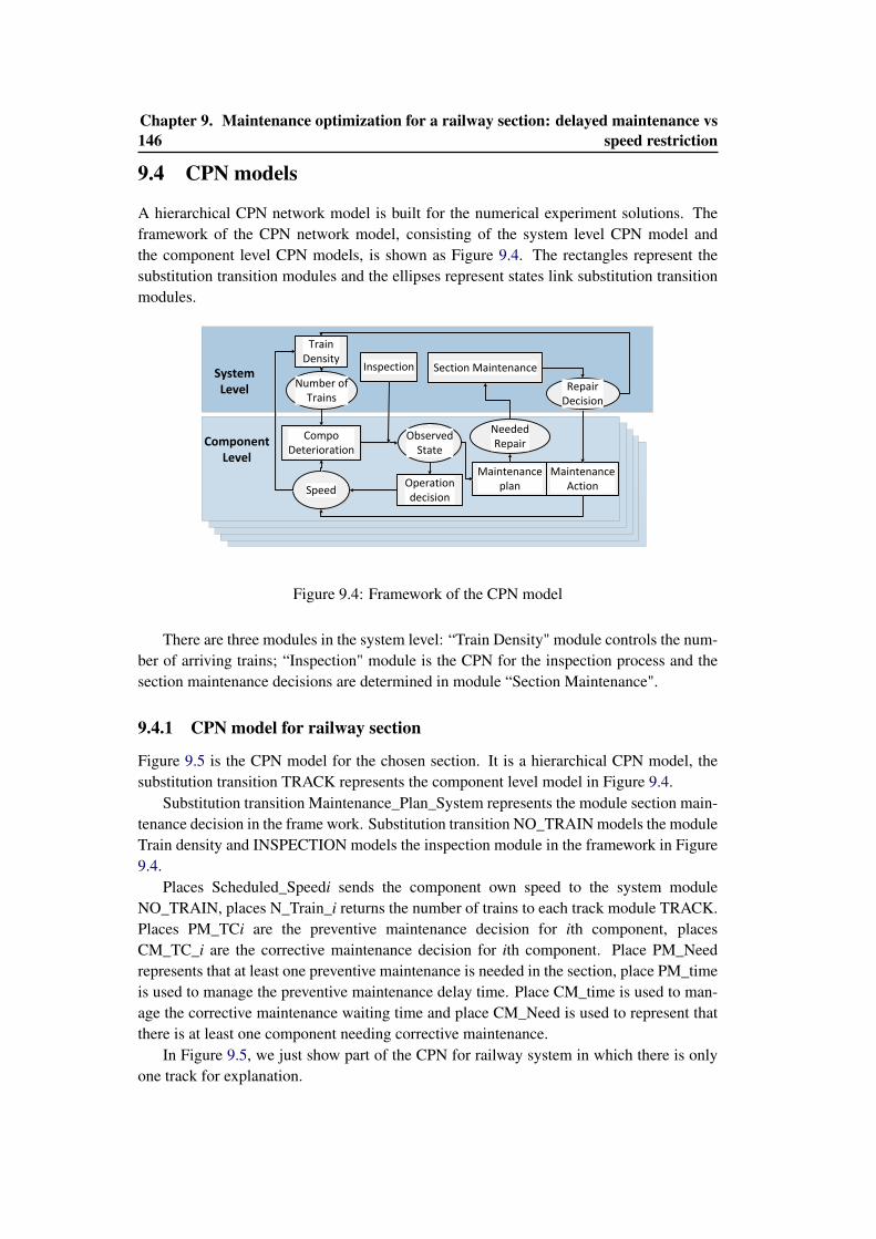
146Chapter 9. Maintenance optimization for a railway section: delayed maintenance vs
speed restriction
9.4 CPN models
A hierarchical CPN network model is built for the numerical experiment solutions. Theframework of the CPN network model, consisting of the system level CPN model andthe component level CPN models, is shown as Figure 9.4. The rectangles represent thesubstitution transition modules and the ellipses represent states link substitution transitionmodules.
Train Density
CompoDeterioration
Observed State
Speed
Inspection Section Maintenance
Maintenance plan
Maintenance ActionOperation
decision
Number of Trains
System Level
Component Level
Needed Repair
Repair Decision
Figure 9.4: Framework of the CPN model
There are three modules in the system level: “Train Density" module controls the num-ber of arriving trains; “Inspection" module is the CPN for the inspection process and thesection maintenance decisions are determined in module “Section Maintenance".
9.4.1 CPN model for railway section
Figure 9.5 is the CPN model for the chosen section. It is a hierarchical CPN model, thesubstitution transition TRACK represents the component level model in Figure 9.4.
Substitution transition Maintenance_Plan_System represents the module section main-tenance decision in the frame work. Substitution transition NO_TRAIN models the moduleTrain density and INSPECTION models the inspection module in the framework in Figure9.4.
Places Scheduled_Speedi sends the component own speed to the system moduleNO_TRAIN, places N_Train_i returns the number of trains to each track module TRACK.Places PM_TCi are the preventive maintenance decision for ith component, placesCM_TC_i are the corrective maintenance decision for ith component. Place PM_Needrepresents that at least one preventive maintenance is needed in the section, place PM_timeis used to manage the preventive maintenance delay time. Place CM_time is used to man-age the corrective maintenance waiting time and place CM_Need is used to represent thatthere is at least one component needing corrective maintenance.
In Figure 9.5, we just show part of the CPN for railway system in which there is onlyone track for explanation.
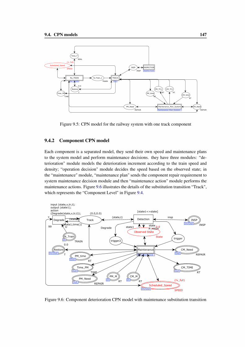
9.4. CPN models 147
INSP
INSP
N_Train_1
TRAIN
Time_T
REAL
Restore
T
0.0
Time_PM
TIME
Scheduled_Speed
SPEED
(!v_full)
PM_Need
REPAIR
PM_time
RT
PM_TC1
RT
CM_time
RT
CM_Need
REPAIR
CM_TC1
RT
TRACK
TC1
INSPECTION
INSPECTION
No_TRAIN
No_TRAIN
Maintenance_Plan_System
Maintenance_Plan_System
Figure 9.5: CPN model for the railway system with one track component
9.4.2 Component CPN model
Each component is a separated model, they send their own speed and maintenance plansto the system model and perform maintenance decisions. they have three modules: “de-terioration" module models the deterioration increment according to the train speed anddensity; “operation decision" module decides the speed based on the observed state; inthe “maintenance" module, “maintenance plan" sends the component repair requirement tosystem maintenance decision module and then “maintenance action" module performs themaintenance actions. Figure 9.6 illustrates the details of the substitution transition “Track",which represents the “Component Level" in Figure 9.4.
triggertrigger2
Observed State
State
0.0
PM_M
InRT
In
Track
Degrade
(0.0,0.0)
Scheduled_Speed
In/OutSPEED
(!v_full)
Time_PM
OutTIME
Out
INSP
In/OutINSP
In/Out
Restore
In/OutT
0.0
In/Out
N_Train
InTRAIN
PM_Need
OutREPAIR
PM_time
OutRT
Out
CM_Need
OutREPAIR
Out
CM_TIME
OutRT
Out
CM_M
InRT
In
Detection
[state1<>state]
P_HIGH
Degrade
input (state,v,tr,t);output (state1);action(Degrade(state,v,tr,t));
99
Maintenance
MaintenanceMaintenance
(state,t)
(state1,time())state1
state
(state,t)v insp
tr
In
In/Out
Out
Figure 9.6: Component deterioration CPN model with maintenance substitution transition
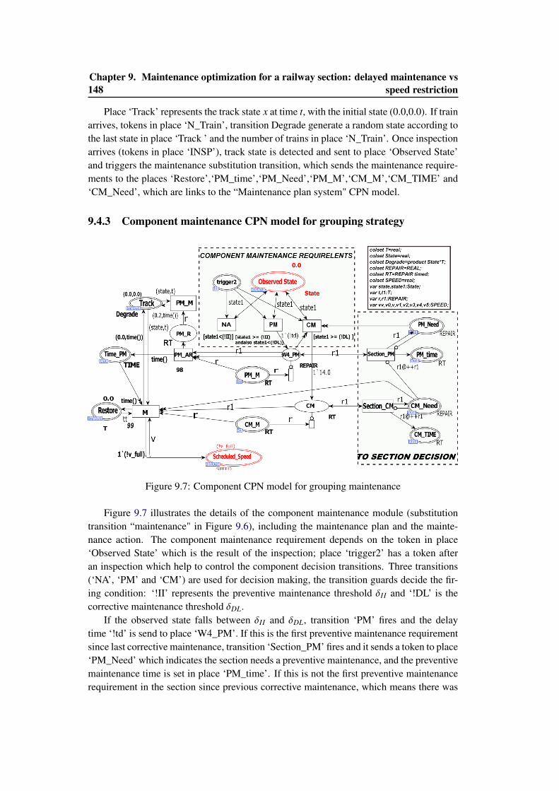
148Chapter 9. Maintenance optimization for a railway section: delayed maintenance vs
speed restriction
Place ‘Track’ represents the track state x at time t, with the initial state (0.0,0.0). If trainarrives, tokens in place ‘N_Train’, transition Degrade generate a random state according tothe last state in place ‘Track ’ and the number of trains in place ‘N_Train’. Once inspectionarrives (tokens in place ‘INSP’), track state is detected and sent to place ‘Observed State’and triggers the maintenance substitution transition, which sends the maintenance require-ments to the places ‘Restore’,‘PM_time’,‘PM_Need’,‘PM_M’,‘CM_M’,‘CM_TIME’ and‘CM_Need’, which are links to the “Maintenance plan system" CPN model.
9.4.3 Component maintenance CPN model for grouping strategy
Figure 9.7: Component CPN model for grouping maintenance
Figure 9.7 illustrates the details of the component maintenance module (substitutiontransition “maintenance" in Figure 9.6), including the maintenance plan and the mainte-nance action. The component maintenance requirement depends on the token in place‘Observed State’ which is the result of the inspection; place ‘trigger2’ has a token afteran inspection which help to control the component decision transitions. Three transitions(‘NA’, ‘PM’ and ‘CM’) are used for decision making, the transition guards decide the fir-ing condition: ‘!II’ represents the preventive maintenance threshold δII and ‘!DL’ is thecorrective maintenance threshold δDL.
If the observed state falls between δII and δDL, transition ‘PM’ fires and the delaytime ‘!td’ is send to place ‘W4_PM’. If this is the first preventive maintenance requirementsince last corrective maintenance, transition ‘Section_PM’ fires and it sends a token to place‘PM_Need’ which indicates the section needs a preventive maintenance, and the preventivemaintenance time is set in place ‘PM_time’. If this is not the first preventive maintenancerequirement in the section since previous corrective maintenance, which means there was
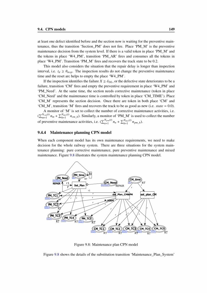
9.4. CPN models 149
at least one defect identified before and the section now is waiting for the preventive main-tenance, thus the transition ‘Section_PM’ does not fire. Place ‘PM_M’ is the preventivemaintenance decision from the system level. If there is a valid token in place ‘PM_M’ andthe tokens in place ‘W4_PM’, transition ‘PM_AR’ fires and consumes all the tokens inplace ‘W4_PM’. Transition ‘PM_M’ fires and recovers the track state to be 0.2.
This model also considers the situation that the repair delay is longer than inspectioninterval, i.e. td ≥ θinsp. The inspection results do not change the preventive maintenancetime and the reset arc helps to empty the place ‘W4_PM’.
If the inspection identifies the failure X ≥ δDL, or the defective state deteriorates to be afailure, transition ‘CM’ fires and empty the preventive requirement in place ‘W4_PM’ and‘PM_Need’. At the same time, the section needs corrective maintenance (token in place‘CM_Need’ and the maintenance time is controlled by token in place ‘CM_TIME’). Place‘CM_M’ represents the section decision. Once there are token in both place ‘CM’ and‘CM_M’, transition ‘M’ fires and recovers the track to be as good as new (i.e. state = 0.0).
A monitor of ‘M’ is set to collect the number of corrective maintenance activities, i.e.(∑Ncsu(t)
m=1 nm +∑Nmix(t)
h=1 ncm_h). Similarly, a monitor of ‘PM_M’ is used to collect the number
of preventive maintenance activities, i.e. (∑Npsu(t)
n=1 nn +∑Nmix(t)
h=1 npm_h).
9.4.4 Maintenance planning CPN model
When each component model has its own maintenance requirements, we need to makedecision for the whole railway system. There are three situations for the system main-tenance planning: pure corrective maintenance, pure preventive maintenance and mixedmaintenance. Figure 9.8 illustrates the system maintenance planning CPN model.
PM_timeIn
RT
CM_TC4Out
RT
CM_TC1Out
RT
CM_TC5Out RT
PM_TC3Out
RT
CM_TC3Out
RT
PM_TC4Out RT
CM_timeIn RT
PM_NeedIn/Out
REPAIR
PM_TC1Out
RT
PM_TC2Out RT
CM_TC2Out
RT
PM_TC5Out RT
CM_NeedIn/Out REPAIRSet_Plan
set_Plan_CM&PM
P_HIGH
set_plan_CM
r
rr
r
r
r
r
r
r
r
r1
rr
r
r
r
r
rr
r
r
r1
r
rr r
Figure 9.8: Maintenance plan CPN model
Figure 9.8 shows the details of the substitution transition ‘Maintenance_Plan_System’
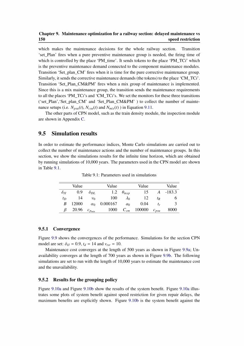
150Chapter 9. Maintenance optimization for a railway section: delayed maintenance vs
speed restriction
which makes the maintenance decisions for the whole railway section. Transition‘set_Plan’ fires when a pure preventive maintenance group is needed, the firing time ofwhich is controlled by the place ‘PM_time’. It sends tokens to the place ‘PM_TCi’ whichis the preventive maintenance demand connected to the component maintenance modules.Transition ‘Set_plan_CM’ fires when it is time for the pure corrective maintenance group.Similarly, it sends the corrective maintenance demands (the tokens) to the place ‘CM_TCi’.Transition ‘Set_Plan_CM&PM’ fires when a mix group of maintenance is implemented.Since this is a mix maintenance group, the transition sends the maintenance requirementsto all the places ‘PM_TCi’s and ‘CM_TCi’s. We set the monitors for these three transitions(‘set_Plan’,‘Set_plan_CM’ and ‘Set_Plan_CM&PM’ ) to collect the number of mainte-nance setups (i.e. Npsu(t), Ncsu(t) and Nmix(t) ) in Equation 9.11.
The other parts of CPN model, such as the train density module, the inspection moduleare shown in Appendix C.
9.5 Simulation results
In order to estimate the performance indices, Monte Carlo simulations are carried out tocollect the number of maintenance actions and the number of maintenance groups. In thissection, we show the simulations results for the infinite time horizon, which are obtainedby running simulations of 10,000 years. The parameters used in the CPN model are shownin Table 9.1.
Table 9.1: Parameters used in simulations
Value Value Value ValueδII 0.9 δDL 1.2 θinsp 15 A -183.3tD 14 v0 100 λ0 12 tR 6B 12000 α0 0.000167 a0 0.04 tr 3β 20.96 cpmin 1000 Ccm 100000 cpsu 8000
9.5.1 Convergence
Figure 9.9 shows the convergences of the performance. Simulations for the section CPNmodel are set: δII = 0.9, td = 14 and vtsr = 10.
Maintenance cost converges at the length of 500 years as shown in Figure 9.9a; Un-availability converges at the length of 700 years as shown in Figure 9.9b. The followingsimulations are set to run with the length of 10,000 years to estimate the maintenance costand the unavailability.
9.5.2 Results for the grouping policy
Figure 9.10a and Figure 9.10b show the results of the system benefit. Figure 9.10a illus-trates some plots of system benefit against speed restriction for given repair delays, themaximum benefits are explicitly shown. Figure 9.10b is the system benefit against the
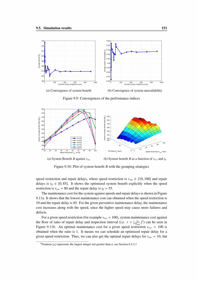
9.5. Simulation results 151
0 200 400 600 800 1000450
460
470
480
490
500
510
520
530
Simultion history length(unit: year)
Ave
rage
Ben
efit
EB
∞
(a) Convergence of system benefit
0 200 400 600 800 10000.056
0.057
0.058
0.059
0.06
0.061
0.062
0.063
0.064
0.065
Simultion history length(unit: year)
Ave
rage
sys
tem
una
vaila
bilit
y Q
(b) Convergence of system unavailability
Figure 9.9: Convergences of the performance indices
10 20 30 40 50 60 70 80 90 100300
350
400
450
500
550
600
650
700
750
800
Sys
tem
Ave
rage
Ben
efit
Rat
e (E
B∞
)
Speed Restriction( vtsr
: km/h)
td=20td=40td=50td=70td=80
(a) System Benefit B against vtsr
020
4060
80100
0
50
100300
400
500
600
700
800
900
Speed Restriction( vtsr
: km/h)PM delay (td: days)
Sys
tem
Ave
rage
Ben
efit
Rat
e (E
B∞
)
(b) System benefit B as a function of vtsr and td
Figure 9.10: Plot of system benefit B with the grouping strategies
speed restriction and repair delays, where speed restriction is vstr ∈ [10, 100] and repairdelays is td ∈ [0, 85]. It shows the optimized system benefit explicitly when the speedrestriction is vtsr = 80 and the repair delay is td = 55.
The maintenance cost for the system against speeds and repair delays is shown in Figure9.11a. It shows that the lowest maintenance cost can obtained when the speed restriction is10 and the repair delay is 85. For the given preventive maintenance delay, the maintenancecost increases along with the speed, since the higher speed may cause more failures anddefects.
For a given speed restriction (for example vtsr = 100), system maintenance cost againstthe floor of ratio of repair delay and inspection interval (i.e. r = b
tdθinspc2) can be seen in
Figure 9.11b. An optimal maintenance cost for a given speed restriction vtsr = 100 isobtained when the ratio is 1. It means we can schedule an optimized repair delay for agiven speed restriction. Thus, we can also get the optimal repair delays for vtsr = 10, but
2Notation bac represents the largest integer not greater than a, see Section 6.4.2.1
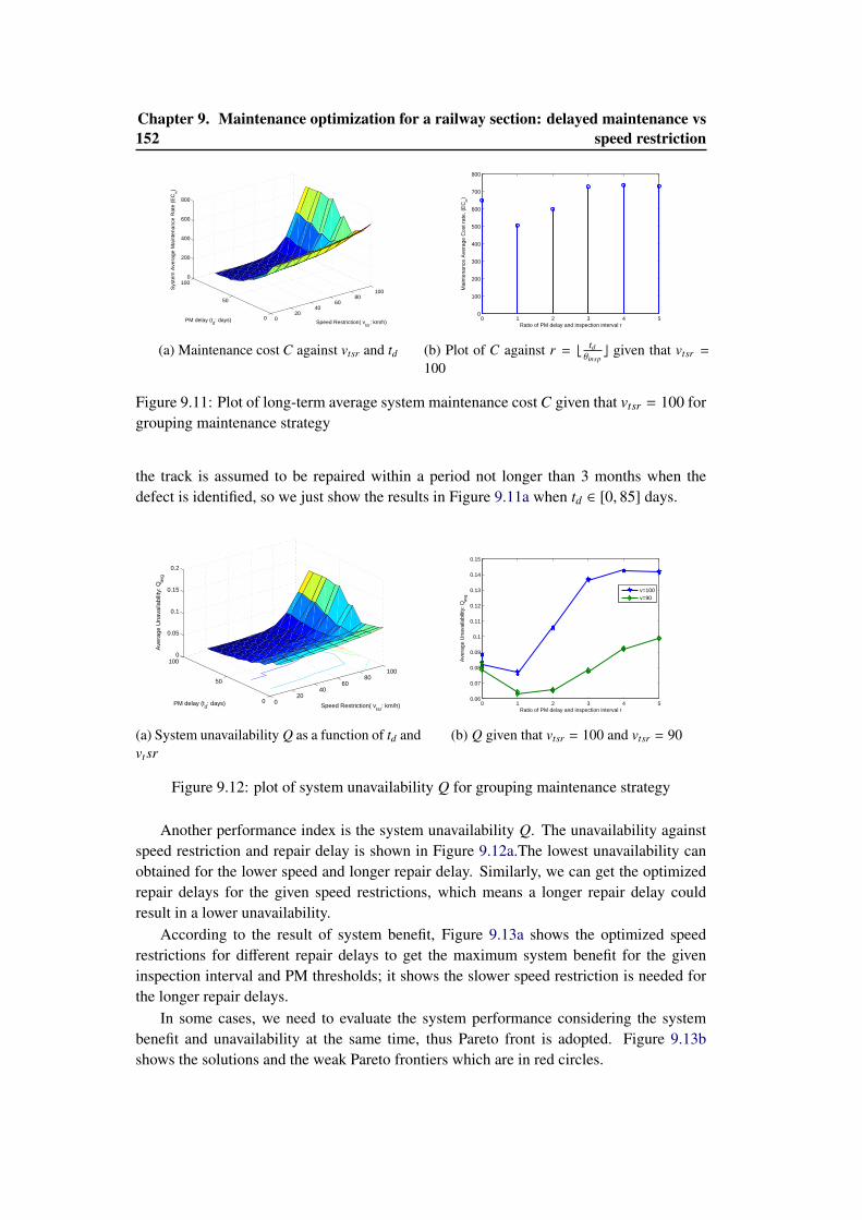
152Chapter 9. Maintenance optimization for a railway section: delayed maintenance vs
speed restriction
020
4060
80100
0
50
1000
200
400
600
800
Speed Restriction( vtsr
: km/h)PM delay (td: days)
Sys
tem
Ave
rage
Mai
nten
ance
Rat
e (E
C∞
)
(a) Maintenance cost C against vtsr and td
0 1 2 3 4 50
100
200
300
400
500
600
700
800
Ratio of PM delay and inspection interval r
Mai
nten
ance
Ave
rage
Cos
t rat
e, (
EC
∞)
(b) Plot of C against r = btdθinspc given that vtsr =
100
Figure 9.11: Plot of long-term average system maintenance cost C given that vtsr = 100 forgrouping maintenance strategy
the track is assumed to be repaired within a period not longer than 3 months when thedefect is identified, so we just show the results in Figure 9.11a when td ∈ [0, 85] days.
020
4060
80100
0
50
1000
0.05
0.1
0.15
0.2
Speed Restriction( vtsr
: km/h)PM delay (td: days)
Ave
rage
Una
vaila
bilit
y: Q
avg
(a) System unavailability Q as a function of td andvt sr
0 1 2 3 4 50.06
0.07
0.08
0.09
0.1
0.11
0.12
0.13
0.14
0.15
Ratio of PM delay and inspection interval r
Ave
rage
Una
vaila
bilit
y: Q
avg
v=100v=90
(b) Q given that vtsr = 100 and vtsr = 90
Figure 9.12: plot of system unavailability Q for grouping maintenance strategy
Another performance index is the system unavailability Q. The unavailability againstspeed restriction and repair delay is shown in Figure 9.12a.The lowest unavailability canobtained for the lower speed and longer repair delay. Similarly, we can get the optimizedrepair delays for the given speed restrictions, which means a longer repair delay couldresult in a lower unavailability.
According to the result of system benefit, Figure 9.13a shows the optimized speedrestrictions for different repair delays to get the maximum system benefit for the giveninspection interval and PM thresholds; it shows the slower speed restriction is needed forthe longer repair delays.
In some cases, we need to evaluate the system performance considering the systembenefit and unavailability at the same time, thus Pareto front is adopted. Figure 9.13bshows the solutions and the weak Pareto frontiers which are in red circles.
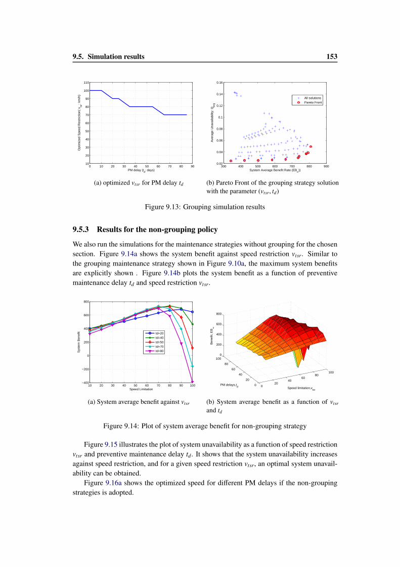
9.5. Simulation results 153
0 10 20 30 40 50 60 70 80 9010
20
30
40
50
60
70
80
90
100
110
PM delay (td: days)
Opt
imiz
ed S
peed
Res
tric
tion(
vts
r: km
/h)
(a) optimized vtsr for PM delay td
300 400 500 600 700 800 9000.02
0.04
0.06
0.08
0.1
0.12
0.14
0.16
System Average Benefit Rate (EB∞))
Ave
rage
Una
vaila
bilit
y: Q
avg
All solutionsPareto Front
(b) Pareto Front of the grouping strategy solutionwith the parameter (vtsr, td)
Figure 9.13: Grouping simulation results
9.5.3 Results for the non-grouping policy
We also run the simulations for the maintenance strategies without grouping for the chosensection. Figure 9.14a shows the system benefit against speed restriction vtsr. Similar tothe grouping maintenance strategy shown in Figure 9.10a, the maximum system benefitsare explicitly shown . Figure 9.14b plots the system benefit as a function of preventivemaintenance delay td and speed restriction vtsr.
10 20 30 40 50 60 70 80 90 100−400
−200
0
200
400
600
800
Sys
tem
Ben
efit
Speed Limitation
td=20td=40td=50td=70td=80
(a) System average benefit against vtsr
020
4060
80100
0
20
40
60
80
1000
200
400
600
800
Speed limitation,vtsr
PM delays,td
Ben
efit,
EB
∞
(b) System average benefit as a function of vtsr
and td
Figure 9.14: Plot of system average benefit for non-grouping strategy
Figure 9.15 illustrates the plot of system unavailability as a function of speed restrictionvtsr and preventive maintenance delay td. It shows that the system unavailability increasesagainst speed restriction, and for a given speed restriction vtsr, an optimal system unavail-ability can be obtained.
Figure 9.16a shows the optimized speed for different PM delays if the non-groupingstrategies is adopted.
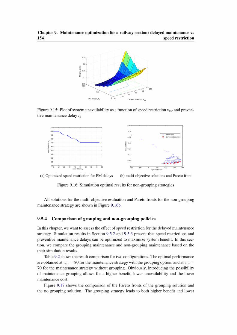
154Chapter 9. Maintenance optimization for a railway section: delayed maintenance vs
speed restriction
020
4060
80100
0
50
1000.05
0.1
0.15
0.2
0.25
Speed limitation, vtsr
PM delays, td
Una
vaila
bilit
y
Figure 9.15: Plot of system unavailability as a function of speed restriction vtsr and preven-tive maintenance delay td
0 10 20 30 40 50 60 70 80 9010
20
30
40
50
60
70
80
90
100
110
repair delays,td
spee
d lim
itatio
n, v
tsr
(a) Optimized speed restriction for PM delays
−400 −200 0 200 400 600 8000
0.05
0.1
0.15
0.2
0.25
0.3
0.35
System Benefit
Una
vaila
bilit
y
All solutionDominated solution
(b) multi-objective solutions and Pareto front
Figure 9.16: Simulation optimal results for non-grouping strategies
All solutions for the multi-objective evaluation and Pareto fronts for the non-groupingmaintenance strategy are shown in Figure 9.16b.
9.5.4 Comparison of grouping and non-grouping policies
In this chapter, we want to assess the effect of speed restriction for the delayed maintenancestrategy. Simulation results in Section 9.5.2 and 9.5.3 present that speed restrictions andpreventive maintenance delays can be optimized to maximize system benefit. In this sec-tion, we compare the grouping maintenance and non-grouping maintenance based on thetheir simulation results.
Table 9.2 shows the result comparison for two configurations. The optimal performanceare obtained at vtsr = 80 for the maintenance strategy with the grouping option, and at vtsr =
70 for the maintenance strategy without grouping. Obviously, introducing the possibilityof maintenance grouping allows for a higher benefit, lower unavailability and the lowermaintenance cost.
Figure 9.17 shows the comparison of the Pareto fronts of the grouping solution andthe no grouping solution. The grouping strategy leads to both higher benefit and lower
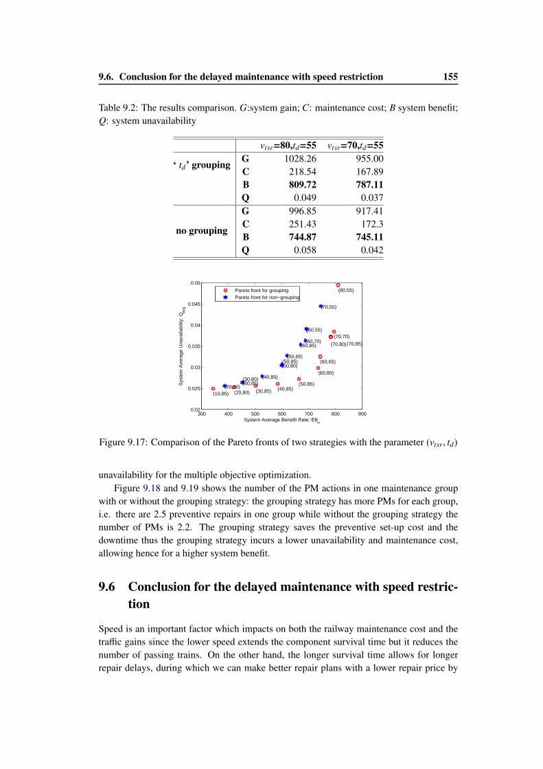
9.6. Conclusion for the delayed maintenance with speed restriction 155
Table 9.2: The results comparison. G:system gain; C: maintenance cost; B system benefit;Q: system unavailability
‘ td’ grouping
vtsr=80,td=55 vtsr=70,td=55G 1028.26 955.00C 218.54 167.89B 809.72 787.11Q 0.049 0.037
no grouping
G 996.85 917.41C 251.43 172.3B 744.87 745.11Q 0.058 0.042
300 400 500 600 700 800 9000.02
0.025
0.03
0.035
0.04
0.045
0.05
(80,55)
(60,65)
(70,70)
(20,80)
(60,80)
(70,80)
(10,85) (30,85) (40,85)(50,85)
(70,85)
(60,55)
(70,55)
(50,65)
(60,70)
(20,80)
(30,80)
(50,80)
(30,85)(40,85)
(50,85)
(60,85)
System Average Benefit Rate: EB∞
Sys
tem
Ave
rage
Una
vaila
bilit
y: Q
avg
Pareto front for groupingPareto front for non−grouping
Figure 9.17: Comparison of the Pareto fronts of two strategies with the parameter (vtsr, td)
unavailability for the multiple objective optimization.Figure 9.18 and 9.19 shows the number of the PM actions in one maintenance group
with or without the grouping strategy: the grouping strategy has more PMs for each group,i.e. there are 2.5 preventive repairs in one group while without the grouping strategy thenumber of PMs is 2.2. The grouping strategy saves the preventive set-up cost and thedowntime thus the grouping strategy incurs a lower unavailability and maintenance cost,allowing hence for a higher system benefit.
9.6 Conclusion for the delayed maintenance with speed restric-tion
Speed is an important factor which impacts on both the railway maintenance cost and thetraffic gains since the lower speed extends the component survival time but it reduces thenumber of passing trains. On the other hand, the longer survival time allows for longerrepair delays, during which we can make better repair plans with a lower repair price by
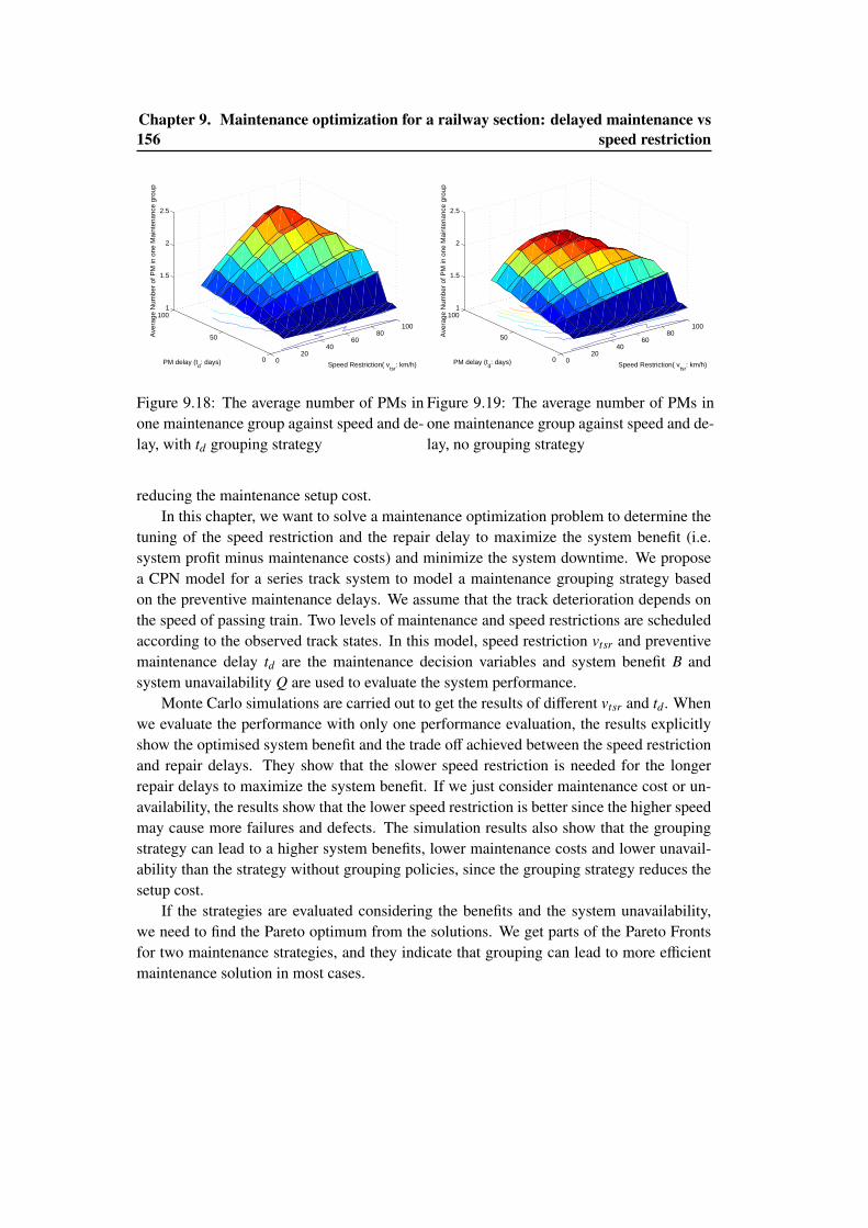
156Chapter 9. Maintenance optimization for a railway section: delayed maintenance vs
speed restriction
020
4060
80100
0
50
1001
1.5
2
2.5
Speed Restriction( vtsr
: km/h)PM delay (td: days)
Ave
rage
Num
ber
of P
M in
one
Mai
nten
ance
gro
up
Figure 9.18: The average number of PMs inone maintenance group against speed and de-lay, with td grouping strategy
020
4060
80100
0
50
1001
1.5
2
2.5
Speed Restriction( vtsr
: km/h)PM delay (td: days)
Ave
rage
Num
ber
of P
M in
one
Mai
nten
ance
gro
up
Figure 9.19: The average number of PMs inone maintenance group against speed and de-lay, no grouping strategy
reducing the maintenance setup cost.In this chapter, we want to solve a maintenance optimization problem to determine the
tuning of the speed restriction and the repair delay to maximize the system benefit (i.e.system profit minus maintenance costs) and minimize the system downtime. We proposea CPN model for a series track system to model a maintenance grouping strategy basedon the preventive maintenance delays. We assume that the track deterioration depends onthe speed of passing train. Two levels of maintenance and speed restrictions are scheduledaccording to the observed track states. In this model, speed restriction vtsr and preventivemaintenance delay td are the maintenance decision variables and system benefit B andsystem unavailability Q are used to evaluate the system performance.
Monte Carlo simulations are carried out to get the results of different vtsr and td. Whenwe evaluate the performance with only one performance evaluation, the results explicitlyshow the optimised system benefit and the trade off achieved between the speed restrictionand repair delays. They show that the slower speed restriction is needed for the longerrepair delays to maximize the system benefit. If we just consider maintenance cost or un-availability, the results show that the lower speed restriction is better since the higher speedmay cause more failures and defects. The simulation results also show that the groupingstrategy can lead to a higher system benefits, lower maintenance costs and lower unavail-ability than the strategy without grouping policies, since the grouping strategy reduces thesetup cost.
If the strategies are evaluated considering the benefits and the system unavailability,we need to find the Pareto optimum from the solutions. We get parts of the Pareto Frontsfor two maintenance strategies, and they indicate that grouping can lead to more efficientmaintenance solution in most cases.
Part V
CONCLUSION & PERSPECTIVE

Conclusion and perspectives
General conclusions
Nowadays, more and more people choose to travel by train and hence railway assets need tobe checked and maintained to prevent accidents and ensure safety. However, maintenancefor railway assets lead to traffic stops and passengers disturbances, it also costs a lot ofmoney. Railway networks consist of thousands of components and different operationmodes; in addition, it is difficult to perform a maintenance which makes the traffic stop.All of the above factors lead not only to the necessity, but also to the complexity of themaintenance modelling. Most of the maintenance models in railway industry are assumedto be Markovian, along with the increase of input information, a more flexible modellingtool need to be used for the maintenance modelling. In this thesis, we are interesting inhaving a tool to help maintenance decision making for the failure process which may notsatisfy Markov properties (for example, the delay repair model), and should be able todescribe maintenance and operation for a multi-component system. Coloured Petri Net isone of the tools which can cover the above modelling requirements.
Works in the thesis
Part III works on the maintenance modelling for single component. Chapter 5 com-pares maintenance for lifetime distribution failure model and gradually deterioration failuremodel. Colour sets can model the observed component health data which represents thedeterioration evolution. The CPN models for both failure descriptions are used to repre-sent the same failure process, while different maintenance strategies are planned dependingon the inspection data. Simulation results show that for the gradual deterioration model,inspection interval and preventive threshold are the maintenance decision variables whichcan be optimized to obtain the optimal maintenance cost; while for the lifetime model, pre-ventive maintenance intervals are the maintenance variable. In addition, since the modelscan represents the inspection ability, thus the results can also indicates the more details wecan collect from inspection, the lower cost the maintenance takes. Chapter 6 focuses ondelay maintenance modelling based component condition. If the repair arrives in a delaytime, the process is not Markov (Semi-Markov) anymore. Coloured Petri Net models arebuilt to describe this deterioration process to investigate the effect of the delay on mainte-nance cost by the timed colour set representing the repair delays. Reset arcs are used toupdate the maintenance decision. Numerical results show that the floor of ratio of repairdelay and the inspection interval has influence on the maintenance cost; a larger ratio maylead to higher maintenance cost since it may lead to more corrective maintenances.
In Part IV, we are interested in the maintenance modelling for a multi-component rail-way section where the inspection capacity may affect the maintenance decision or the de-layed repair may lead to degraded operation on the running line. Chapter 8 assume thatthere are limitations of the inspection, which cannot detect the defective state under some
160
condition and hence a supplementary inspection is needed. Since accident scenarios aretaken into account, the model can also evaluate the risk of the system. Chapter 9 considersthe maintenance for a track section based on the collected health data. The deteriorationof the component depends on the train speed and the number of passing trains, and themaintenance for defective trains arrive in a delay time. We built a CPN model to solve amaintenance optimization problem to determine the tuning of the speed restriction and therepair delay to maximize the system benefit (i.e. system profit minus maintenance costs)and minimize the system downtime. Since the preventive maintenance is carried out in adelay time, a grouping strategies for the delayed repairs are compared to the non-groupingstrategy.
According to the models built in this thesis, CPN shows its modelling flexibility: withthe transition and timed colour set, CPN can describe the behaviours of system by time, andit allows to model the details of health data using variables and colour sets. The prioritiesof the transition can model the events sequences. Furthermore, substitution transitions helpus to build a hierarchical model which is more readable than Stochastic Petri Net.
Limitations of the models
In this thesis, we assume that the deterioration distribution and the maintenance gains areknown, the parameters used in the simulation are not obtained from the real data. How-ever, in practice, data analysis should be carried out before these maintenance modelling toestimate the modelling parameters.
The model will be large if we need to model a complex system. The CPN modelfor one component which is monitored by periodic inspections and maintained by two-level maintenance based on the observed condition in Chapter 6 consists of 14 places,12 transitions and 44 arcs. The CPN for a series track section which consists of 5 trackcomponents in Chapter 9 consists of more than 180 places , more than 100 transitions andseveral hundreds of arcs. But in the real world, the number of the components in the railwaynetwork is far more than the quantity in this Petri Net model, the complex system structureand operation options undoubtedly will need more transition and places in the modelling.
The simulation process is long to get the probability of rare events. Using Petri Net orCPN, the probability estimation relies on Monte Carlo simulations. The simulation timedepends on the length of the simulation cycles, the number of simulation cycles and thenumber of transition firing steps. The simulation time for one parameter configuration inthis thesis varies from several minutes to dozens of minutes, so it may take several hoursto several days for the simulations to optimize the maintenance decision variables.
The multi-component models in Chapters 7, 8 and 9 are more readable than the modelbased on Stochastic Petri Net, however, it is not an easy job to change the number ofcomponents, the number of machines involved in the section. For another section with adifferent number of component, the system level, section level and operation level CPNmodel need to be changed correspondingly.
161
Perspectives
The maintenance models proposed in this thesis are assumed for only one failure modesand a simple series system with a simple operation principle. However, some other aspectsneed to be taken into account in the maintenance modelling, such as multiple failure modes,the interaction between failures, a faster simulation or estimation method.
Combination of petri net and fault tree
Coloured Petri Net need a longer time for the performance evaluation but it can modelthe dynamic behaviours of the component. In contrast to Petri Net, fault tree is faster tocalculate the top event probability using the logic gates but it is not powerful in modelingthe dynamics behaviours. Therefore, it may be a good idea to combine these two methodsfor the risk assessments. Bobbio et al. propose a parametric fault tree with a high levelpetri net [22, 21] to model the partial repair and global repair. Moreover, repairable faulttree is a similar concept proposed for the repair grouping [161].
Multi-components with multiple states
Even though the substitution transitions help to divided system CPN model into differentsmall modules, region modules and system modules could be different for two system con-sisting of different quantities of components. Wang et al. propose a kind of CPN modelwhere the places represents the different states, tokens representing different components[202]. The CPN can be used to model the system consisting of different kinds of com-ponents involves in dynamic operation scheduling and different kinds of maintenance andinspection requirements.
Opportunistic maintenance modelling
For the multi-component system, besides preventive maintenance, opportunistic mainte-nance is another type of maintenance before failures. It is adopted in order to save thedowntime due to the frequent maintenance. It will be interesting to optimize the thresholdof opportunistic maintenance to minimize the downtime and the average maintenance cost.

Appendix A
Résumé en Français
Introduction
La SNCF (Société nationale des chemins de fer français) maintient et surveille 30000 kmde voies en France tous les jours, et près de 15 500 trains circulent sur ce vaste réseau detransport, ce qui correspond à 126 900 000 passagers par an [50]. Selon les statistiques dusite de la Banque Mondiale, Network Rail contrôle plus de 16000 km de longueur de lavoie et réalise 2,75 millions de voyages de passagers chaque jour.
De l’importance de l’entretien de infrastructures ferroviaires
Les infrastructure ferroviaires jouent un rôle important dans la sécurité et le service ferrovi-aire. Les défaillances d’actifs ferroviaires peuvent provoquer une maintenance d’urgence,entraînant l’arrêt de la circulation : ces défaillances peuvent aussi dans le pire des casconduire à des accidents.
Sur la période 1991-2001, environ 23,7 % des déraillements ont été causés par desdéfauts de la voie [143] et 10 % des déraillements se sont produits en raison à la fois de lavoie défectueuse et l’état du véhicule et autour de 65 % des déraillements se produisant surla ligne ont été dus à des défauts de la voie [105]. Par conséquent, il est important de mettreen place des procédures d’entretien et de maintenance pour de réduire les défaillancesferroviaires et pour garantir la sécurité et la disponibilité du réseau ferré.
La maintenance des actifs et infrastructures ferroviaires contribue par une forte propor-tion aux dépenses totales des compagnies ferroviaires. Le coût de l’entretien ferroviaireaux Pays-Bas a dépassé e250 millions d’euros en 2006 [54]. Dans le rapport financier dela SNCF, e746 millions sont dépensés pour les mises à niveau des gares et des bâtimentsy compris le renouvellement de la voie, le remplacement du système de communication etainsi de suite [175] . Network Rail a dépensé £391, 8 millions de pounds pour l’entretiende la voie au cours de 2013 à 2014 [121].
Afin d’assurer la sécurité et en même temps réaliser un entretien économique, desstratégies de maintenance sont étudiées pour améliorer la décision de l’entretien et pourplanifier une stratégie de maintenance pour le système "réseau ferré" tout en respectant lescontraintes de sécurité.
Dans l’avenir, le contexte de l’exploitation ferroviaire va devenir de plus en plus con-traint: la vitesse augmente, le trafic est accru, donc la détérioration s’accélère et, de plus,le temps disponible pour les opérations de maintenance se réduit.
164 Appendix A. Résumé en Français
Motivation et objectifs
La maintenance préventive est importante pour prévenir les accidents de chemin de fer etpar conséquent pour assurer la sécurité des passagers et des équipages de travail. Commela maintenance peut perturber le fonctionnement normal des chemins de fer et coûter unegrosse somme d’argent, les sociétés gestionnaires des infrastructure ferroviaires essaientde sauver le coût d’entretien et d’améliorer la disponibilité sans affecter la sécurité.
Comme la tâche de modélisation de la détérioration, de l’inspection et de l’entretiens’avère très complexe, en particulier pour un système multi-composant, il n’est souvent paspossible d’avoir une solution analytique pour la prise de décision. Nous nous sommes doncintéressé au développement d’un outil d’aide à la prise de décision de maintenance basésur la simulation ; avec cet outil, nous pouvons ainsi prendre en compte la détérioration, lamaintenance et l’exploitation pour un système complexe plus facilement.
Le principal objectif de cette thèse est de contribuer au développement d’outils de mod-élisation et de simulation pour l’évaluation des performances des stratégies de maintenancepour le système de chemin de fer et d’estimer la probabilité d’événement dangereux.
La thèse vise à étudier les problèmes suivants dans la modélisation de la maintenancedes infrastructures ferroviaires :
1. comment comparer des politiques de maintenance pour différents niveaud’information surveillance ?
2. comment quantifier l’effet de délais de maintenance, sachant pendant le tempsd’attente de maintenance, les composants sont toujours utilisés et donc continuentde se dégrader ?
3. comment établir conjointement une stratégie de maintenance et un plan d’utilisationopérationnelle d’une infrastructure lorsque le mode d’utilisation d’un composant af-fecte sa détérioration ?
Capacité d’inspection Plusieurs politiques d’entretien peuvent être planifiées pour unmême composant en fonction des données d’inspection disponibles. Dans certains cas,l’inspection de routine peut présenter des limitations pour l’identification des défauts, et ils’avère nécessaire de programmer des inspections supplémentaires pour pouvoir prendreen connaissance de cause une décision de maintenance qui assurer un coût d’entretien etune sécurité optimales.
Délais de maintenance Il existe souvent une longue attente et de la procédure de négo-ciation pour le maintien des actifs dans le système de chemin de fer. En outre, en raison dutrajet jusqu’au point de maintenance et du nombre limité de machines de réparation, nousne pouvons pas mettre en oeuvre l’entretien immédiatement une fois que nous détectonsles défaillances ou les défauts.
Maintenance vs mode d’utilisation La configuration de fonctionnement et d’utilisationdu réseau affectent les charges sur les voies. Si on met en oeuvre une limitation de vitesse
165
comme une sorte de fonctionnement dégradé pour une section, la vitesse inférieure et moinsde passages de trains ralentissent la détérioration. Mais, d’autre part, la restriction peutréduire le bénéfice, il est donc intéressant de trouver compromis entre restriction de vitesseet délai de réparation.
Structure de la thèse
Les travaux sont organisés en cinq parties: introduction générale et motivation des travauxdans la première partie, l’état de l’art et les descriptions du système dans la deuxièmepartie, les modèles au niveau “composant" dans la troisième partie et les modèles au niveau“système" dans la quatrième partie.
La partie II est constituée de trois petits chapitres pour introduire le contexte de larecherche et les outils utilisés dans cette thèse:
• Le Chapitre 2 présente un exemple type d’une section de voie ferrée, un système devoies ballastées, les défaillances de la voie et les méthodes d’entretien correspon-dants.
• Le Chapitre 3 donne un bref aperçu de la littérature sur les modèles de défaillance,les politiques d’inspection et de maintenance sur les infrastructures ferroviaires.
• Le Chapitre 4 introduit les outils mathématiques utilisés dans cette thèse. En parti-culier, nous présentons le concept et les règles de modélisation de réseaux de Petricoloré (CPN). Un exemple de CPN est donnée pour montrer la capacité du réseau dePetri coloré.
La Partie III présente les modèles de coût/performances au niveau “composant":
• Le Chapitre 5 compare des politiques de maintenance mettant en jeu différentsniveaux d’information de surveillance.
• Le Chapitre 6 étudie les effets des délais de maintenance pour les politiquesd’inspection périodiques et différentes politiques d’inspection conditionnelle sontcomparées.
Le réseau de chemin de fer est un système multi-composant, il ne suffit pas d’envisagerla modélisation de la maintenance pour un seul composant. Donc, la Partie IV décrit lemodèle de maintenance pour un réseau de chemin de fer:
• Le Chapitre 7 présente un modèle de maintenance pour un réseau ferroviaire comptetenu de la limitation de ressource de maintenance.
• Le Chapitre 8 propose un modèle de performance de maintenance mettant en jeudifférents types d’inspections complémentaires.
• Le Chapitre 9 vise à définir un réglage optimal de vitesse limite et dedélai d’intervention, l’évolution de détérioration de composant dépend du moded’utilisation.
Partie V donne une conclusion générale pour cette thèse.
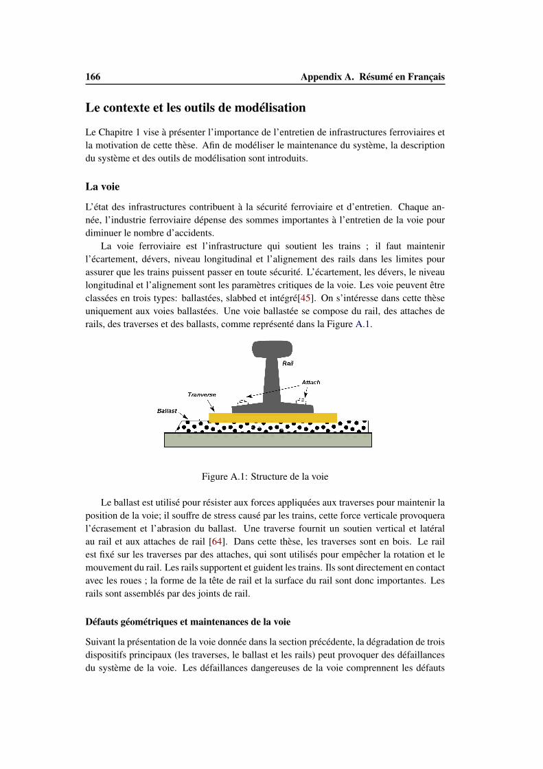
166 Appendix A. Résumé en Français
Le contexte et les outils de modélisation
Le Chapitre 1 vise à présenter l’importance de l’entretien de infrastructures ferroviaires etla motivation de cette thèse. Afin de modéliser le maintenance du système, la descriptiondu système et des outils de modélisation sont introduits.
La voie
L’état des infrastructures contribuent à la sécurité ferroviaire et d’entretien. Chaque an-née, l’industrie ferroviaire dépense des sommes importantes à l’entretien de la voie pourdiminuer le nombre d’accidents.
La voie ferroviaire est l’infrastructure qui soutient les trains ; il faut maintenirl’écartement, dévers, niveau longitudinal et l’alignement des rails dans les limites pourassurer que les trains puissent passer en toute sécurité. L’écartement, les dévers, le niveaulongitudinal et l’alignement sont les paramètres critiques de la voie. Les voie peuvent êtreclassées en trois types: ballastées, slabbed et intégré[45]. On s’intéresse dans cette thèseuniquement aux voies ballastées. Une voie ballastée se compose du rail, des attaches derails, des traverses et des ballasts, comme représenté dans la Figure A.1.
Figure A.1: Structure de la voie
Le ballast est utilisé pour résister aux forces appliquées aux traverses pour maintenir laposition de la voie; il souffre de stress causé par les trains, cette force verticale provoqueral’écrasement et l’abrasion du ballast. Une traverse fournit un soutien vertical et latéralau rail et aux attaches de rail [64]. Dans cette thèse, les traverses sont en bois. Le railest fixé sur les traverses par des attaches, qui sont utilisés pour empêcher la rotation et lemouvement du rail. Les rails supportent et guident les trains. Ils sont directement en contactavec les roues ; la forme de la tête de rail et la surface du rail sont donc importantes. Lesrails sont assemblés par des joints de rail.
Défauts géométriques et maintenances de la voie
Suivant la présentation de la voie donnée dans la section précédente, la dégradation de troisdispositifs principaux (les traverses, le ballast et les rails) peut provoquer des défaillancesdu système de la voie. Les défaillances dangereuses de la voie comprennent les défauts
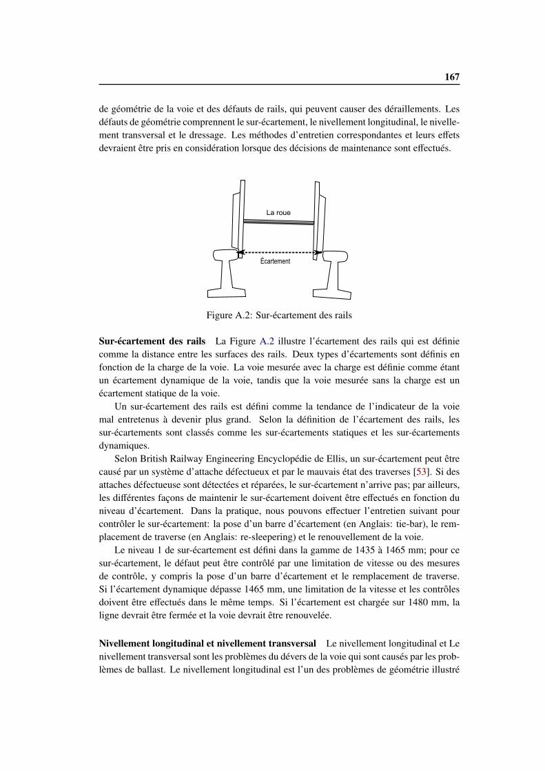
167
de géométrie de la voie et des défauts de rails, qui peuvent causer des déraillements. Lesdéfauts de géométrie comprennent le sur-écartement, le nivellement longitudinal, le nivelle-ment transversal et le dressage. Les méthodes d’entretien correspondantes et leurs effetsdevraient être pris en considération lorsque des décisions de maintenance sont effectués.
La roue
Écartement
Figure A.2: Sur-écartement des rails
Sur-écartement des rails La Figure A.2 illustre l’écartement des rails qui est définiecomme la distance entre les surfaces des rails. Deux types d’écartements sont définis enfonction de la charge de la voie. La voie mesurée avec la charge est définie comme étantun écartement dynamique de la voie, tandis que la voie mesurée sans la charge est unécartement statique de la voie.
Un sur-écartement des rails est défini comme la tendance de l’indicateur de la voiemal entretenus à devenir plus grand. Selon la définition de l’écartement des rails, lessur-écartements sont classés comme les sur-écartements statiques et les sur-écartementsdynamiques.
Selon British Railway Engineering Encyclopédie de Ellis, un sur-écartement peut êtrecausé par un système d’attache défectueux et par le mauvais état des traverses [53]. Si desattaches défectueuse sont détectées et réparées, le sur-écartement n’arrive pas; par ailleurs,les différentes façons de maintenir le sur-écartement doivent être effectués en fonction duniveau d’écartement. Dans la pratique, nous pouvons effectuer l’entretien suivant pourcontrôler le sur-écartement: la pose d’un barre d’écartement (en Anglais: tie-bar), le rem-placement de traverse (en Anglais: re-sleepering) et le renouvellement de la voie.
Le niveau 1 de sur-écartement est défini dans la gamme de 1435 à 1465 mm; pour cesur-écartement, le défaut peut être contrôlé par une limitation de vitesse ou des mesuresde contrôle, y compris la pose d’un barre d’écartement et le remplacement de traverse.Si l’écartement dynamique dépasse 1465 mm, une limitation de la vitesse et les contrôlesdoivent être effectués dans le même temps. Si l’écartement est chargée sur 1480 mm, laligne devrait être fermée et la voie devrait être renouvelée.
Nivellement longitudinal et nivellement transversal Le nivellement longitudinal et Lenivellement transversal sont les problèmes du dévers de la voie qui sont causés par les prob-lèmes de ballast. Le nivellement longitudinal est l’un des problèmes de géométrie illustré
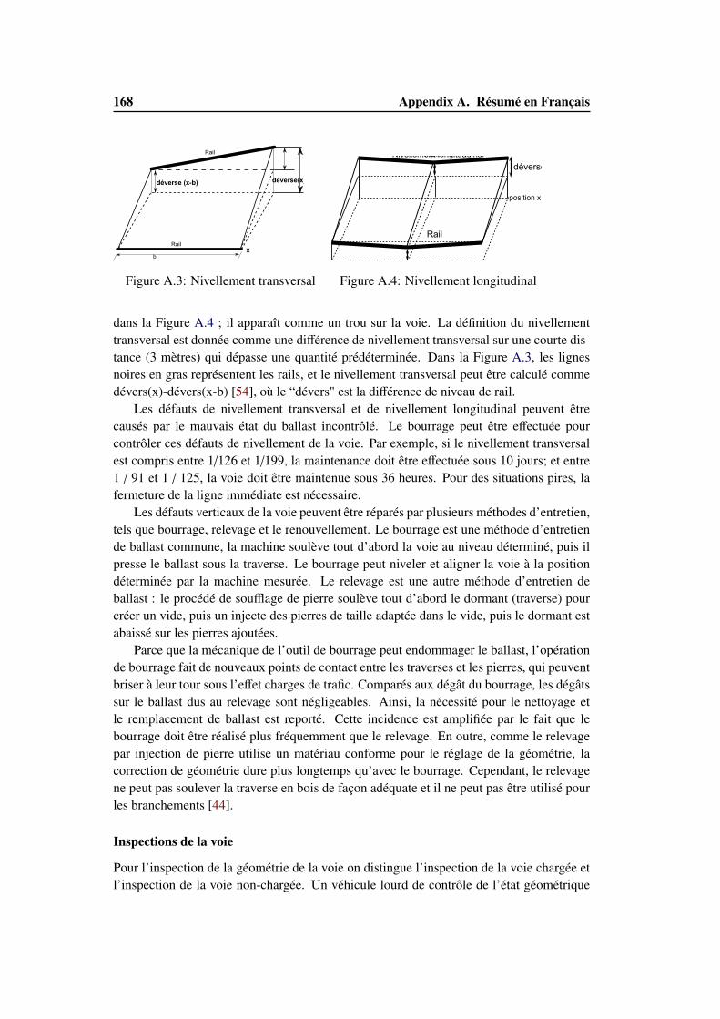
168 Appendix A. Résumé en Français
Rail
Rail
b
x
déverse(x)déverse (x-b)
Figure A.3: Nivellement transversal
position x
Rail
Rail
Nivellement longituadinal
déverse
Figure A.4: Nivellement longitudinal
dans la Figure A.4 ; il apparaît comme un trou sur la voie. La définition du nivellementtransversal est donnée comme une différence de nivellement transversal sur une courte dis-tance (3 mètres) qui dépasse une quantité prédéterminée. Dans la Figure A.3, les lignesnoires en gras représentent les rails, et le nivellement transversal peut être calculé commedévers(x)-dévers(x-b) [54], où le “dévers" est la différence de niveau de rail.
Les défauts de nivellement transversal et de nivellement longitudinal peuvent êtrecausés par le mauvais état du ballast incontrôlé. Le bourrage peut être effectuée pourcontrôler ces défauts de nivellement de la voie. Par exemple, si le nivellement transversalest compris entre 1/126 et 1/199, la maintenance doit être effectuée sous 10 jours; et entre1 / 91 et 1 / 125, la voie doit être maintenue sous 36 heures. Pour des situations pires, lafermeture de la ligne immédiate est nécessaire.
Les défauts verticaux de la voie peuvent être réparés par plusieurs méthodes d’entretien,tels que bourrage, relevage et le renouvellement. Le bourrage est une méthode d’entretiende ballast commune, la machine soulève tout d’abord la voie au niveau déterminé, puis ilpresse le ballast sous la traverse. Le bourrage peut niveler et aligner la voie à la positiondéterminée par la machine mesurée. Le relevage est une autre méthode d’entretien deballast : le procédé de soufflage de pierre soulève tout d’abord le dormant (traverse) pourcréer un vide, puis un injecte des pierres de taille adaptée dans le vide, puis le dormant estabaissé sur les pierres ajoutées.
Parce que la mécanique de l’outil de bourrage peut endommager le ballast, l’opérationde bourrage fait de nouveaux points de contact entre les traverses et les pierres, qui peuventbriser à leur tour sous l’effet charges de trafic. Comparés aux dégât du bourrage, les dégâtssur le ballast dus au relevage sont négligeables. Ainsi, la nécessité pour le nettoyage etle remplacement de ballast est reporté. Cette incidence est amplifiée par le fait que lebourrage doit être réalisé plus fréquemment que le relevage. En outre, comme le relevagepar injection de pierre utilise un matériau conforme pour le réglage de la géométrie, lacorrection de géométrie dure plus longtemps qu’avec le bourrage. Cependant, le relevagene peut pas soulever la traverse en bois de façon adéquate et il ne peut pas être utilisé pourles branchements [44].
Inspections de la voie
Pour l’inspection de la géométrie de la voie on distingue l’inspection de la voie chargée etl’inspection de la voie non-chargée. Un véhicule lourd de contrôle de l’état géométrique
169
doit avoir une charge verticale et pouvoir mesurer des mesures dynamiques de la géométrieet l’inspection visuelle sont adoptées lorsque nous avons besoin des mesures statiques dela géométrie de la voie [124].
Une voiture de mesure peut détecter un défaut de géométrie de la voie ou une rupturede rail, mais il est difficile de détecter les petites fissures ferroviaires ; l’inspection parultrasons peut être utilisé pour détecter les minuscules fissures des rails [144].
Dans la norme ferroviaire, les intervalles de contrôle sont donnés afin de maintenirla sécurité. Par exemple, l’inspection par ultrasons teste le rail sur la ligne simple à desintervalles de base; le rail sur un aiguillage doit être testé à des intervalles plus courts.
Réseaux de Petri colorés
Nous travaillons sur la modélisation de l’entretien des actifs ferroviaires. Selon lesrecherches existantes, les processus de Markov constituent l’une des méthodes qui prennenten compte différents états pour la modélisation. Toutefois, les problèmes que nous voulonsétudier peuvent ne pas être adaptés à l’utilisation de chaînes de Markov ou semi-Markovprocessus: ainsi par exemple, l’un des problèmes que nous voulons étudier est l’effet dela maintenance préventive retardée, qui n’est pas modélisable par un processus de Markov.En outre, dans la modélisation du système de chemin de fer, des scénarios d’accidents oule fonctionnement du système -pas nécessairement markoviens- doivent être pris en con-sidération.
Nous choisissons donc de développer nos modèles avec des Réseaux de Petri colorés.D’une part, ils peuvent modéliser des comportements qui ne sont pas de Markov; d’autrepart, les ensembles colorés et la représentation de temps font des CPN des outils de mod-élisation plus souples.
Un réseau de Petri coloré (CPN) est défini comme représenté dans l’Equation A.1 [87].
CPNt = (P,T, A,Σ,V,C,G, E, I) (A.1)
CPNt est CPN avec temps, P est l’ensemble de “places", T est l’ensemble de transitions,A l’ensemble de arcs, Σ est l’ensemble de couleurs, V est l’ensemble de variables. Gest l’ensemble de fonctions, I est le marquage initial , C est l’ensemble de fonctionsd’ensembles colorés et E est l’ensemble de fonctions d’arcs.
Nous utilisons l’outil de CPN pour la modélisation. Cet outil dispose d’une interfacegraphique qui est développé en Java, le langage de modélisation est langage de program-mation standard ML (SML). Il permet aux utilisateurs de définir différentes fonctions demodélisation pour les transitions et moniteurs concernant les exigences en matière de mod-élisation. L’outil de CPN a l’ensemble coloré, inscription à l’arc, inhiber l’arc et arc initial.En outre, il peut construire des modèles hiérarchiques avec les ports et les transitions desubstitution.
170 Appendix A. Résumé en Français
Comparaison des modèles de défaillance pour l’optimisation dela maintenance
Les décisions d’entretien de la voie de chemin de fer sont prises en fonction de l’étatde la voie. Comme les défauts de voie ne sont pas auto-décelables, des inspections sonteffectuées régulièrement pour recueillir les mesures d’état de la voie afin de surveiller laqualité de la voie. En ce qui concerne les techniques d’inspection, il faut parfois différentstypes de données d’état. Un type de données indique simplement les états de santé binairesde la voie - fonctionnel ou en panne. Avec le développement des dispositifs d’inspection,nous pouvons recueillir des données précises sur l’état, contenant plus de détails sur laqualité de la voie, par exemple, nous pouvons utiliser la déviation standard pour un certainnombre de données sur l’état de la voie pour caractériser l’état de santé de la voie sur unecertaine longueur. Sur la base de ces deux types différents de données d’inspection, deuxmodèles de défaillance sont adoptés pour décrire l’évolution de la détérioration des voies,puis plusieurs politiques d’entretien sont prévues pour maintenir la qualité de la voie. Nousvoulons accéder aux impacts de ces deux modèles de défaillance.
Hypothèses concernant les modèles d’information à deux niveaux
Modélisation de la fiabilité basée sur la détérioration graduelle
Une défaillance se produit si Xt ≥ δDL ; alors, une maintenance corrective est mise enoeuvre. Afin de réduire les défaillances, des inspections périodiques sont effectuées pourla maintenance préventive. Les détails sur les hypothèses sont répertoriés comme suit:
1. Les inspections sont menées périodiquement avec un intervalle θInsp. i est l’indicede l’inspection; Ii signifie l’i ème inspection, et Xi représente les états observés parl’i ème inspection.
2. Il y a deux seuils pour la maintenance:
• Si Xi ≥ δDL, une maintenance corrective est effectuée immédiatement. Il peutrestaurer la voie à une condition Xcm, ce qui signifie que l’état après la mainte-nance corrective est comme neuf.
• Si Xi ≥ δII , une maintenance préventive est mise en oeuvre.
• La maintenance préventive est imparfaite. La maintenance préventive peutramener le composant à l’état de Xh > 0.0, ce qui signifie que l’état aprèsl’entretien préventif n’est pas aussi bon que neuf.
3. Il n’existe pas de délais pour les deux niveaux de maintenance. La maintenancecorrective (resp. préventive) nécessite d’immobilier le système pour un temps d’arrêtDTcm (resp. DTh).
Le seuil de la maintenance préventive δII et l’intervalle d’inspection θInsp sont les vari-ables de décision de maintenance, à régler pour optimiser le coût de maintenance.
171
Modélisation de type "durée de vie"
Si on ne considère que les états binaires du composant maintenu -fonctionnel ou en panne,le modèle de distribution de la durée de vie est utilisée pour modéliser son état de santé.La durée de vie du composant est notée TδDL , qui représente l’instant où la condition ducomposant dépasse le seuil de défaillance δDL. La probabilité de défaillance du composantsur (0, t] est défini comme FTδDL
(t) = Pr(t ≥ TδDL).Parce que le modèle de loi de durée de vie et le modèle de fiabilité basé sur la détériora-
tion sont utilisés pour représenter le même processus de détérioration physique ’ie la même"réalité terrain"), pour la même condition de défaillance δDL, la répartition de la durée devie est calculée par l’équation A.2 [182]:
FTδDL(t) = Pr(t ≥ TδDL) =
Υ(αt, βδDL)Γ(αt)
(A.2)
La politique de maintenance périodique pour le modèle de loi de durée de vie proposeune politique de maintenance à deux niveaux pour le composant de voie :
Comme la défaillance n’est pas auto-décelable, une inspection est nécessaire pour dé-tecter la défaillance d’un composant. Les détails de la politique d’entretien périodique pourle modèle de durée de vie sont présentés comme suit:
1. L’inspection est effectuée périodiquement à l’intervalle θinsp.
2. Deux niveaux de maintenance sont programmés pour le composant:
• Un entretien préventif est prévue pour le composant, il est mis en oeuvre péri-odiquement, avec l’intervalle noté θT . L’intervalle θT est une constante in-dépendante de l’histoire de la défaillance d’un composant.
• La maintenance préventive est imparfaite ; après la n ème maintenance préven-tive, l’âge virtuel du composant est fixé à Vn. Nous supposons que l’âge virtuelest égal à une valeur constante, Vn = y, n = 1, 2, ... .
• La distribution de la durée de vie après la n e la maintenance préventive estobtenu selon l’âge réel Xn[95]:
Fn(t) = F2(t) = Pr(Xn ≤ x|Vn−1 = y) =(F(t + y) − F(y))
1 − F(y)(A.3)
• Si la i ème inspection identifie la défaillance d’un composant, une maintenancecorrective est effectuée.
• La maintenance corrective est parfaite. Après la maintenance corrective, l’âgevirtuel du composant estVm = 0.m est l’indice de la maintenance corrective.
Comparaison de résultats des modèles
Deux modèles de réseaux de Petri coloré sont construits pour la comparaison. Un premiermodèle décrit le processus de défaillance comme une évolution de la détérioration gradu-elle, et un autre considère "seulement" le temps de défaillance. Parce que la maintenance
172 Appendix A. Résumé en Français
préventive est imparfaite par hypothèse, nous supposons un âge virtuel pour le modèle dedurée de vie qui conduit à sous-estimer le risque de défaillance par rapport au modèle dedégradation stochastique.
En comparant les politiques de maintenance pour ces deux types des modèles, les résul-tats montrent que l’inspection précise peut avoir mener à de meilleurs résultats pour le coûtd’entretien et de la disponibilité des composants, parce que l’inspection précise permet demieux planifier la maintenance préventive non périodique.
Délais de maintenance pour un composant de la voie ferrée
La voie ferrée transporte des milliers de trains et de passagers tous les jours. Des machinesd’entretien sont affectées à plusieurs dépôts : elles ne sont pas immédiatement disponiblessur le lieu où doit se faire la maintenance et elles ont besoin de se rendre à l’emplacementdes actifs défectueux ; par ailleurs, les machines de maintenance et les équipages ne sontpas toujours disponibles pour l’entretien. Lorsqu’une dégradation d’actif est identifié, sielle est pas critique et ne dépasse pas le seuil extrême, la section de voie est maintenueouverte pour permettre aux trains de circuler.
Par conséquent, l’entretien préventif pour un élément de voie ne peut pas être effec-tuée immédiatement après la détection d’un défauts.. Pendant le temps d’attente pour lesréparations préventives, la section de chemin de fer permet encore le trafic et souffre dumême processus de détérioration qui résulte peut-être dans la dégradation de l’actif à unétat critique qui conduit à une maintenance corrective, même à un accident.
Nous voulons évaluer l’effet de délai de maintenance pour voir si il est nécessaire deprendre ce délai en considération dans la procédure de décision pour mettre en oeuvreune meilleure stratégie de maintenance pour l’infrastructure ferroviaire. Un modèle demaintenance est nécessaire pour résoudre le problème. Dans la mesure où l’état du systèmene dépend pas seulement du dernier état observé mais aussi des états précédents selon lalongueur des retards, le processus de détérioration n’est pas une chaîne de Markov. Aulieu de construire une chaîne de Markov comme introduit dans[114], nous proposons unmodèle basé sur les réseaux de Petri colorés pour estimer le coût moyen d’entretien sur unhorizon infini.
Hypothèses sur la maintenance avec retard pour un composant
Les politiques de maintenance avec retard proposées dans ce travail considèrent un com-posant unique. On suppose que la défaillance résulte d’un défaut de géométrie verticale.La bourrage est supposé être la méthode de la maintenance préventive et la relevage estla maintenance corrective. L’information sur l’état de la voie est mesurée par un train desurveillance automatique.
Les hypothèses de modélisation retenues dans ce travail sont les suivantes:
• Le composant est supposé être un élément de voie de de 1 km de long.
• Le composant se détériore suivant à un processus Gamma, Xτ est l’état du composantau moment τ et X∆τ représente l’augmentation de la détérioration sur ∆τ, X∆τ ∼
173
Γ(α∆τ, β).
• Les états de composant sont mesurés par l’inspection, qui est agencé pour être soitpériodique, soit basé sur l’état. Nous comparons ces deux régimes de contrôle dif-férents:
– Inspection périodique: l’inspection est effectuée périodiquement, etl’intervalle est égal à θinsp.
– Inspection conditionnelle: Après la ième inspection, l’intervalle θi+1 jusqu’à(i+1)ème inspection est basé sur l’état observé du composant Xi qui est inspectépar la ième inspection. θi+1 est décidé par le seuil préventif δII comme indiquédans l’équation A.4:
θi+1 =
θmax −
Xi(θmax − θmin)δII
, Xi ∈ (0, δII)
θmin, Xi ∈ [δII,∞)(A.4)
Si l’état dépasse le seuil préventive, qui est Xi ≤ δII, l’intervalle d’inspection estégale à l’intervalle d’inspection minimum,i.e. θinsp = θmin; sinon l’(i + 1)èmeinspection est θi+1 ∈ (θmin, θmax].
– Pour l’inspection périodique, il y a deux variables de décision à optimiser: θinsp
and δII.
– Pour l’inspection conditionnelle, θmin and δII sont les deux variables de décisionà considérer.
• Deux types de maintenance sont envisageables, relativement à deux seuils de main-tenance: un seuil d’intervention majeur δDL et un seuil de maintenance préventiveδII.
– Si Xi ≥ δDL, un entretien majeur est réalisé dans un délai tD. δDL est donné parles règles de maintenance.
– Si δII ≥ Xi ≥ δII, une intervention préventive est réalisée dans un délai td.
– Les deux interventions sont imparfaites. Un modèle de régression linéaire estadopté pour les gains de réparation, qui est G = c + mX + ε, ε ∼ N(0, σ), X estl’état du composant lorsque la réparation est effectuée.
• Les délais de réparation td et tD ne sont pas des variables de décision, ils sont fixéspar les règles ou pratiques d’entretien sur le terrain, ou par les experts métiers.Lors d’une inspection, en fonction de la donnée td et tD, il y a différents scénariosd’entretien possibles:
– Si td ≤ θinsp ou td ≤ θmin: si l’état observé dépasse δII, un entretien préventifest disposé dans un temps de retard td. Le type d’entretien ne sont pas mis àjour, même si l’état de la piste dépasseδDL pendent td.
– Si td ≥ θinsp or td ≥ θmin:
174 Appendix A. Résumé en Français
� Si les états observés ne dépassent jamais δDL, l’inspection ne change pasla décision de la maintenance préventive.
� Les inspections détectent des états x ≥ δDL : le type d’entretien est alorsmis à jour.
Comparaison de politiques d’inspection
Les politiques d’inspection périodique et les politiques d’inspection conditionnelle sontcomparées sur la base de résultats de simulation pour r = 0, r = 1 et r = 2. Une in-spection périodique et les politiques d’inspection conditionnelle (CBI) sont comparées enenvisageant différents intervalles θ, ratios r et seuils préventifs δII.
Si r = 1, le coût minimum pour l’inspection périodique est 48,58 tandis que le coûtpour la CBI est 38.15; le coût pour les deux régimes d’inspection quand r = 2 est plusélevé que pour r = 0 et r = 1, donc le maintien d’un petit r plus performant.
Pour voir la relation entre les intervalles d’inspection et le coût de la maintenance,les résultats montrent que le coût d’entretien contre intervalle d’inspection étant donné quer = 0, il montre les résultats de δII = 0, 95 et δII = 1, 0 pour les deux systèmes d’inspection.
Les configurations de maintenance optimisés dans les politiques d’inspection péri-odiques et d’inspection conditionnelle sont étudiés, soit pour l’inspection périodique,θinspecteur = 30, δII = 0, 95 et pour CBI, θmin = 30 , δII = 1.0.
Le temps entre les deux PMs de la politique d’inspection périodique et politiqued’inspection basée sur l’état sont comparées. Le pdf de la CMs et PMs pour les configura-tions de maintenance optimisés indiquent que la politique d’inspection périodique présenteplus de CMs pendant le temps de simulation.
Modèle de maintenance avec deux niveaux d’inspection pour uneLigne
On considère dans cette section qu’il existe deux types de défaillances pour le composantréparable, l’un d’eux est auto-décelable, l’autre non. Les défauts de voie n’étant pas auto-décelable, nous devons effectuer les inspections pour nous assurer que le composant estassez bon pour le passage du train. L’entretien et le contrôle de la circulation correspondantsont prévus selon les résultats de l’inspection afin d’éviter tout incident ou accident.
La capacité d’inspection influe sur la planification de la maintenance et a doncnaturellement un effet sur le coût de l’entretien, l’indisponibilité du système et ainside suite. Afin de décrire la capacité d’inspection dans le processus global de défail-lance/maintenance, Christer et al proposent de concept de “ delay time " [41]; Wang pro-pose un modèle d’inspection pour un composant qui souffre de deux sortes de défauts etdeux méthodes d’inspection sont mis à la deux défauts séparément [195] . Un autre mod-èle similaire “ PF "processus est introduite par Podofillini et.al qui proposent un modèle deMarkov pour les défauts de rail en supposant qu’il y a deux niveaux d’inspection pour leprocessus d’échec [144] .
175
Un sur-écartement (type de défaut de voie déjà évoqué plus haut) peut être classé endeux catégories : le sur-écartement statique et le sur-écartement dynamique. Deux types demesures de contrôle différents sont établis pour ces deux catégories différentes. Nous sup-posons que l’inspection visuelle peut inspecter la voie et d’identifier l’écartement statiqueet la voiture de mesure peut identifier le sur-écartement dynamique. Nous voulons proposerun modèle CPN de l’inspection à deux niveaux pour étudier plus finement la planificationdes inspections de différentes nature et capacité.
Hypothèses de maintenance pour deux niveaux de inspection
Le modèle CPN peut être utilisé pour évaluer les politiques d’inspection différentes desdeux programmes d’inspection. Quatre politiques d’inspection sont supposés:
• Politique 1: inspections périodiques à deux niveaux ; inspection visuelle avec inter-valle θvi = 40 unités et voiture de mesure passée à intervalle variable;
• Politique 2: l’inspection visuelle intervalle θvi = 40 unités tandis que l’intervalle dela voiture de mesure dépend du nombre de défauts.
• Politique 3: inspections périodiques à deux niveaux ; inspection visuelle avec inter-valle θvi = 50 unités et voiture de mesure passée à intervalle variable;;
• Politique 4: l’intervalle pour l’inspection visuelle est θvi = 50 unités tandis quel’intervalle de la voiture de mesure dépend du nombre de défauts.
Pour ces politiques d’inspection, l’intervalle de voiture de mesure prévue varie de 5 à 2000unités. Les paramètres de la maintenance sont supposées être: τ f 2 = 15, µ f 2 = 1,τ f 3 = 10,µ f 3 = 4, τ f 4 = 5, µ f 4 = 4, τ f 5 = 2, µ f 5 = 10, τ f 6 = 0, µA = 70.
Les résultats de modèles de deux niveaux inspection
Dans cette étude, nous considérons les performances du système à court terme. L’indicede performance du système ‘disponibilité de la ligne programmée Asch’, ‘disponibilité enligne Auns’, ‘ le coût Prévu de Ligne Csch’, ‘le coût total Cuns’ et ‘Le nombre de placesdisponibles Nderailment’ sont utilisés pour comparer ces quatre politiques d’inspection.
Nderailment est compté en surveillant la transition D dans le modèle d’accident. Ladisponibilité prévue Asch et de la disponibilité de la ligne Auns sont obtenues par la surveil-lance de la transition T_D and Ti_E selon l’équation A.5 et A.6. Tavailable est la ligne dutemps disponible, Ttotal est la durée totale, DTuns est le temps d’arrêt non programmé.
Asch =Tavailable
Ttotal − DTuns(A.5)
Auns =Tavailable
Ttotal(A.6)
Csch and Cuns sont calculés par l’équation A.7 et A.8. CM est le coût de la maintenance,Ctrv est le coût de voiture de mesure (TRV), Cvi est le coût d’inspection visuelle et CAccident
176 Appendix A. Résumé en Français
est le coût d’ accident. Le nombre de voiture de mesure Ntrv, le nombre des inspectionsvisuelles Nvi sont comptées par la transition INS P_TRV et INS P_INT . Le nombre demaintenances NM est compté par la transition Tmms(refastening), T Mms (la pose d’unbarre d’écartement,“ tie-bar" en Anglais) and T MMs (le replacement de traverse) dans lemodèle de CPN.
Csch = CMNM + CtrvNtrv + CviNvi (A.7)
Cuns = Csch + CAccidentNderailment (A.8)
Selon les résultats du nombre de déraillements normalisé par l’intervalle de TRV par an,la fréquence du déraillement augmente lorsque l’intervalle d’inspection visuelle ou de lavoiture de mesure augmente. Si l’intervalle de voiture de mesure augmente, la disponibilitéprévue augmente ; cependant, la disponibilité globale de la ligne diminue si l’intervalleTRV augmente.
En ce qui concerne le coût prévu et le coût imprévu, toutes les politiques d’inspectionmontrent l’existence coût total minimum. Pour la politique 1 et la politique 3, le coûtde maintenance minimum peut être obtenu pour un intervalle de voiture de mesure de 65unités. Pour les politiques 2 et 4, le coût total minimum peut être obtenu si l’intervalle devoiture de mesure est de 125 unités.
En ce qui concerne les déraillements, si l’intervalle de voiture de mesure varie de 0à 300 heures , les politiques 2 et 4 présentent moins de déraillements et un intervalled’inspection visuelle plus courte peut conduire à une diminution du nombre de déraille-ments. Si l’intervalle de voiture de mesure se situe entre 300 et 700 heures, les politiques1 et 2 sont meilleures que les politiques 3 et 4, la politique 2 a un nombre de déraillementsinférieur à celui de la politique 1. Si l’intervalle de voiture de mesure dépasse 700 heures,la politique 1 est meilleure que la politique 2.
Modèle de maintenance pour une section de voie avec limitationde vitesse
Les défauts de géométrie verticale de la voie dus à un mauvais état de ballast peuvent êtreréglés par des opérations de bourrage ou de relevage. Différents travaux de recherche ontétudié l’évolution de la dégradation de la voie et ils soulignent que la qualité de la voiedépend de certains facteurs tels que la vitesse, le tonnage (MGT),l’historique de l’entretienet des matériaux [11, 166, 203, 221].
La vitesse de train joue un rôle important dans la maintenance et l’exploitation ferrovi-aire. Zio et al [219] discutent de la flexibilité des limitations de vitesse afin de réduire lesretards de train sur l’ensemble du réseau parce que la limitation de vitesse peut augmenterla sécurité des chemins de fer, mais peut aussi causer des retards.
Les limitations de vitesse ont des effets non seulement sur la sécurité et les temps detrajet, mais aussi sur les coûts de maintenance et sur les gains d’exploitation. En effet, unediminution de vitesse ralentit l’évolution de la détérioration qui permet l’entretien différéet réduit le nombre de maintenances. Cependant, les limitations de vitesse réduisent égale-ment les flux de voyageurs et de marchandises, et ainsi les gains. On se retrouve donc
177
face à un compromis que certains travaux on déjà abordé dans le cadre de recherche surla politique de maintenance basée sur l’âge en fonction de la vitesse de production dansl’industrie de la production [204][180].
La limitation de la vitesse conduit à un processus de dégradation plus lente et à untemps résiduel avant défaillances plus long qui permet un temps plus long avant réparation.La possibilité d’un délai de réparation plus long permet de mieux organiser la maintenanceà un coût de maintenance préventive réduite. Dans le même temps, le système avec lalimitation de vitesse laisse passer moins trains, conduisant à la perte de débit de systèmed’où à un gain moindre du système. D’autre part, le retard de réparation plus longue donneplus de possibilités pour grouper les activités de maintenance et d’économiser ainsi le coûtde mise en place et le temps d’arrêt en raison des réparations.
Ainsi, nous travaillons sur un problème d’optimisation de la maintenance, afin de par-venir à un compromis entre limitation de vitesse et le retard d’entretien préventif afin demaximiser les avantages du système et de réduire le temps d’indisponibilité du systèmepour une section de la ligne ferroviaire plaine, dans laquelle la détérioration de la voiedépend de la la vitesse et le nombre de trains qui passent.
Hypothèses de système
Nous considérons une section "série" composée de 5 composants de la voie sur une lignesimple. La détérioration de l’ensemble des composants est indépendante, et suit le mêmeprocessus de dégradation. La vitesse des trains sur chaque composant sont également in-dépendantes, tandis que la densité des trains dépend de la valeur minimale de densité dansla section.
Détérioration des composants
La détérioration de la voie dépend du nombre de trains qui passent et la vitesse des trains.Deux niveaux de maintenance et trois options de vitesse sont prévues pour l’état de la voieobservée périodiquement. Des trains plus nombreux et une vitesse plus élevée des trainspeuvent entraîner la détérioration de la voie plus sérieuse.
Détérioration de la voie L’arrivée du train est supposé être un processus de Poisson avecle taux d’arrivée λ [163]. Nt est le nombre de trains jusqu’à t.
Xt représente l’état de la voie (soit la somme des détériorations) à l’instant t dansl’Equation A.9. Le k-ème incrément de détérioration est une valeur aléatoire yk lorsquele k-ème train passe, qui suit une distribution Gamma. La taille de la détérioration yk adeux paramètres α(v) et β, et le paramètre α(v) dépend de la vitesse v (comme indiqué dansl’équation A.10 ).
Xt =
Nt∑k=1
Yk,Yk ∼ Γ(α(v), β) (A.9)
α(v) = α0ea0v (A.10)

178 Appendix A. Résumé en Français
Le processus de dégradation est un processus de Poisson composé avec les tailles desaut Gamma distribués [182]. Selon les propriétés du processus de Poisson composé,l’incrément de détérioration pour une période de temps ∆t est égal à l’équation A.11
X∆t = Xt+∆t − Xt =
N∆t∑k=1
Yk = Γ(α(v)N∆t, β) (A.11)
Maintenance d’un composant
Une inspection périodique est prévue pour le composant de la voie sur le calendrier del’opération, l’intervalle d’inspection est notée θInsp. Les stratégies de maintenance baséesur la condition sont largement discutés dans la littérature [71, 70], les maintenances icisont programmées sur la base de l’état de la voie: La maintenance préventive et la main-tenance corrective sont effectuées pour le composant j, en fonction de la dégradation ob-servée.
• Seuil de maintenance préventive est défini comme δII et le seuil de la maintenancecorrective est δDL.
• Si i-ème état observé X j_i du composant j dépasse correctives seuil δDL ( X j_i ≥ δDL),un maintenance corrective est réalisée, qui peut fixer la bonne voie pour être aussibon que nouveau. a maintenance est effectuée dans un temps de retard tD. Pendantle temps de retard tD, la circulation de trafic est arrêtée.
• Si X j_i ≥ δII , un entretien préventif est effectué dans un délai td. La maintenancepréventive est imparfaite, ce qui ramène l’état du composant à une valeur fixe.
• La vitesse après ième inspection est notée comme vi, qui est fixée en fonction de laième état détecté.
vi =
v0, Xi ∈ (0, δII) Vitesse normale
vtsr, Xi ∈ [δII, δDL) Vitesse limité
0, Xi ∈ [δDL,∞) Trafic arrêté
(A.12)
La planification de la maintenance de ligne
La structure choisie pour la section de voie considérée est celle d’un système en série. Lestrains peuvent avoir des vitesses différentes sur les différents éléments de la voie, mais ladensité de train est la même pour tous les composants.
La ligne est régulièrement inspectée par le train de l’inspection, en ignorant le tempsde déplacement du train d’inspection.
Si X j_i ≥ δDL), une maintenance corrective est mise en place avec un délai tD. L’actionde maintenance corrective prend une durée tR pour réparer le composant. Le coût de lamaintenance corrective est composé de deux parties: le coût d’installation de maintenancecorrective ccsu et le coût unitaire d’un travail de maintenance corrective ccm.
179
• Si il y a nm composants en pannes,nm actions de maintenance correctives sont effec-tuées dans le même temps, la section des temps d’arrêt pour ce groupe de mainte-nance corrective pur est td + tR. Ils partagent le coût d’installation de maintenancecorrective, le coût d’entretien de ce groupe est de cCS U + nmccm.
• Si certains autres composants doivent subir des maintenances préventives, soit δII ≤
Xl_i ≤ δDL, j , l. La maintenance préventive est mise en place en même temps quela maintenance corrective. Ceci est un groupe de maintenance "mixte" (préventifet correctif). Le coût de maintenance comprend le coût de mise en oeuvre de lamaintenance correctives ccsu , le coût de l’action de maintenance corrective ccm, lecoût de mise en oeuvre de la maintenance préventive cpsu et les coûts des actions demaintenance préventive ch(td).
• Pour le groupe de maintenance mixte, comme on a td < td et tr < tR, l’indisponibilitéde la voie est équivalente à td + tR.
Au moment de ti, si X j_i ≥ δII , un entretien préventif est mis en place avec un délaitd. Pendant td, si l’inspection suivante identifie uniquement des détériorations mais aucunedéfaillance, tous les composants détériorés sont réparés au moment ti + td. Ceci est ungroupe de maintenance préventive pur. La maintenance préventive a besoin d’un tempsd’arrêttr.
Le coût de la maintenance préventive comprend le coût d’installation cpsu et le coût dechaque action de maintenance préventive ch(td). ch(td) dépend le plus de temps de retardde réparation dans le groupe, qui est td. Plus td est élevé, plus le coût d’entretien plus faiblecomme indiqué dans l’équation A.13. Si td ∈ (0,T ∗), le coût de l’action de maintenancepréventive dépend sur le retard de temps de réparation td, si td ≥ T ∗, le coût de l’action demaintenance préventive équivaut à une valeur minimale de réparation cpmin .
cpm(td) =
Atd + B td ∈ (0,T ∗)
cpmin td ∈ [T ∗,∞)(A.13)
Il existe trois configurations de densité de trafic en fonction de la vitesse minium d’untrain dans la section: Si tous les états observés sont bons X j_i ≤ δII , la densité de train estλ0.Si le composant j est détérioré (X j_i ≥ δII), pendant td, la vitesse sur ce composant j estv j = vtsr et la vitesse pour l’autre composant normale est égale à vl = v0, l , j, la densité detrain pour la ligne est λtrain
vtsrv0λ0. Lorsque le travail de maintenance est exécuté, le système
est fermé. Si composant j est en panne (X j_i ≥ δII), la section est fermée et la densité detrain est égale à 0.
Évaluation de la performance
Différents indices d’évaluation de performance sont introduits. Pour une évaluation mono-objectif, nous pouvons comparer le profit du système ou l’indisponibilité du système; pourune évaluation multi-objectif, nous adoptons une approche de type "front de Pareto".
180 Appendix A. Résumé en Français
Évaluation de le profit et le disponibilité
Le profit du système et l’indisponibilité du système sont utilisés pour évaluer la perfor-mance du système. L’indisponibilité du système est donnée par l’équation A.14:
Qavg = limt→∞
[Ncsu(t) + Nmix(t)](tD + tR) + Npsu(t)trt
(A.14)
Le profit du système est le gain du système, moins le coût de la maintenance du sys-tème:
EB∞ = EG∞ − EC∞ (A.15)
Le taux moyen des coûts de maintenance (EC∞) et le taux de gain du système (EG∞) surune durée de temps infini sont:
EC∞ = limt→∞
C(t)t
(A.16)
EG∞ = limt→∞
Ntrain(t)ctrain
t(A.17)
Le coût de maintenance se compose du coût de mise en oeuvre et des coûts d’opération demaintenance.
C(t) =
Ncsu(t)∑m=1
(ccsu + nmccm)︸ ︷︷ ︸Pure corrective maintenance group
+
Npsu(t)∑n=1
(cpsu + nncpm)︸ ︷︷ ︸Pure preventive maintenance group
+
Nmix(t)∑h=1
(ccsu + ncm_hccm + cpsu + npm_hcpm)︸ ︷︷ ︸Mix maintenances group
+Ninsp(t)cinsp
=[Ncsu(t) + Nmix(t)]ccsu + (Npsu(t)∑
n=1
nn +
Nmix(t)∑h=1
npm_h)cpm
+ [Npsu(t) + Nmix(t)]cpsu + (Ncsu(t)∑m=1
nm +
Nmix(t)∑h=1
ncm_h)ccm + Ninsp(t)cinsp
(A.18)
Afin d’évaluer ces quantités, nous avons besoin de construire un modèle de simulationpour collecter le nombre de trains Ntrain, le nombre d’inspections Ninsp, le nombre de miseen oeuvre de maintenance (Nmix, Ncsu and Npsu), le nombre d’inspections maintenanceactions (Ncm and Npm).
Évaluation multi-objectif
Le problème d’évaluation multi-objectif vise à évaluer la performance du système comptetenu du bénéfice rapporté par le système et son indisponibilité dans le même temps. Uneapproche basée sur le front de Pareto est adoptée [30] [122]; nous devons ainsi trouver lasolution (vtsr, td) pour satisfaire:
si et seulement si il n’y a pas (v∗tsr, t∗d) ∈ (V,Td)
B(vtsr, td) ≥ B(v∗tsr, t∗d) (A.19)
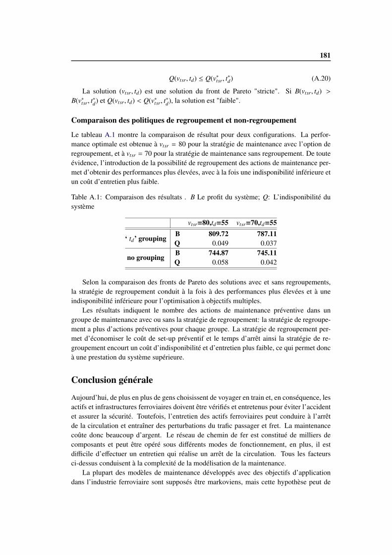
181
Q(vtsr, td) ≤ Q(v∗tsr, t∗d) (A.20)
La solution (vtsr, td) est une solution du front de Pareto "stricte". Si B(vtsr, td) >
B(v∗tsr, t∗d) et Q(vtsr, td) < Q(v∗tsr, t
∗d), la solution est "faible".
Comparaison des politiques de regroupement et non-regroupement
Le tableau A.1 montre la comparaison de résultat pour deux configurations. La perfor-mance optimale est obtenue à vtsr = 80 pour la stratégie de maintenance avec l’option deregroupement, et à vtsr = 70 pour la stratégie de maintenance sans regroupement. De touteévidence, l’introduction de la possibilité de regroupement des actions de maintenance per-met d’obtenir des performances plus élevées, avec à la fois une indisponibilité inférieure etun coût d’entretien plus faible.
Table A.1: Comparaison des résultats . B Le profit du système; Q: L’indisponibilité dusystème
vtsr=80,td=55 vtsr=70,td=55
‘ td’ groupingB 809.72 787.11Q 0.049 0.037
no groupingB 744.87 745.11Q 0.058 0.042
Selon la comparaison des fronts de Pareto des solutions avec et sans regroupements,la stratégie de regroupement conduit à la fois à des performances plus élevées et à uneindisponibilité inférieure pour l’optimisation à objectifs multiples.
Les résultats indiquent le nombre des actions de maintenance préventive dans ungroupe de maintenance avec ou sans la stratégie de regroupement: la stratégie de regroupe-ment a plus d’actions préventives pour chaque groupe. La stratégie de regroupement per-met d’économiser le coût de set-up préventif et le temps d’arrêt ainsi la stratégie de re-groupement encourt un coût d’indisponibilité et d’entretien plus faible, ce qui permet doncà une prestation du système supérieure.
Conclusion générale
Aujourd’hui, de plus en plus de gens choisissent de voyager en train et, en conséquence, lesactifs et infrastructures ferroviaires doivent être vérifiés et entretenus pour éviter l’accidentet assurer la sécurité. Toutefois, l’entretien des actifs ferroviaires peut conduire à l’arrêtde la circulation et entraîner des perturbations du trafic passager et fret. La maintenancecoûte donc beaucoup d’argent. Le réseau de chemin de fer est constitué de milliers decomposants et peut être opéré sous différents modes de fonctionnement, en plus, il estdifficile d’effectuer un entretien qui réalise un arrêt de la circulation. Tous les facteursci-dessus conduisent à la complexité de la modélisation de la maintenance.
La plupart des modèles de maintenance développés avec des objectifs d’applicationdans l’industrie ferroviaire sont supposés être markoviens, mais cette hypothèse peut de
182 Appendix A. Résumé en Français
moins en moins être acceptée en pratique. Pour pouvoir prendre en compte l’augmentationdes information de surveillance disponible, un outil de modélisation plus souple doit êtredéveloppé pour la modélisation de la maintenance. Dans cette thèse, nous nous intéres-sons à contribuer au développement d’un outil de modélisation, d’évaluation des per-formances et d’aide à la décision en maintenance, en pensant aux processus de défail-lance/maintenance qui ne peuvent pas satisfaire les propriétés de Markov (par exemple, lemodèle de réparation avec délais), et en cherchant à décrire l’entretien et l’exploitation pourdes systèmes multi-composants. Les réseaux de Petri colorés sont l’un des outils qui peutcouvrir les besoins de modélisation ci-dessus et que nous avons retenu pour nos travaux.
Travaux dans la thèse
Partie III:Les modèles de maintenance au niveau composant
La Partie III travaille sur la modélisation de maintenance au niveau “ composant".Le Chapitre 5 compare la maintenance pour le processus de défaillance modélisé par
une distribution de durée de vie d’une part, et par un modèle de fiabilité basé sur l’évolutionde détérioration graduelle, d’autre part. Les ensembles de couleurs du RdP colorés peu-vent modéliser les données sur l’état de santé des composants observés qui représentel’évolution de la détérioration. Les modèles CPN pour les deux descriptions de défail-lance sont utilisés pour représenter le même processus de détérioration/défaillance, tandisque différentes stratégies d’entretien sont prévues en fonction des données d’inspection.Les résultats des simulations montrent une baisse du coût de maintenance lorsqu’on prendla décision de maintenance sur des données d’inspection plus riches en information.
Le Chapitre 6 met l’accent sur la modélisation de la maintenance conditionnelle avecdélai. Si la réparation arrive avec un délai fixe, le processus ne peut pas être Markov(semi-Markov). Des modèles de réseaux de Petri colorés sont construits pour décrire ce processusde détérioration pour voir l’effet du retard sur le coût d’entretien par le jeu de couleurschronométré représentant les délais de réparation. Les arcs réinitialisé sont utilisés pourmettre à jour la décision de maintenance dans le modèle. Les résultats numériques montrentque le rapport r entre le délai de réparation et l’intervalle d’inspection a une influence surle coût de l’entretien: un grand r peut conduire à l’augmentation du coût de maintenance,car il peut conduire à plus de maintenances correctives.
Partie IV:les modèles de maintenance pour une voie
Dans la Partie IV, nous nous intéressons à la modélisation de la maintenance pour unevoie de chemin de fer à plusieurs composants en considérant deux problème : la capac-ité d’inspection peut influer sur la décision de maintenance et la réparation retardés peutconduire à un fonctionnement dégradé sur la voie.
Le Chapitre 8 suppose qu’il existe des limites de l’inspection, qui ne peut pas détecterl’état défectueux sous certaines conditions et, partant, une inspection complémentaire estnécessaire. Parce que les scénarios d’accidents sont prises en compte, le modèle peutégalement évaluer le risque du système.
183
Le Chapitre 9 considère la maintenance pour une voie sur la base des données sur l’étatde santé recueillies en ligne. La détérioration du composant dépend de la vitesse du train etle nombre de trains qui passent, et la maintenance pour les éléments de voie défectueux ar-rive avec un délai. Nous avons construit un modèle RdP colorés pour résoudre un problèmed’optimisation de la maintenance pour déterminer conjointement le réglage de la limitationde vitesse et le délai de réparation afin de maximiser les gains d’exploitation du systèmeet de minimiser les temps d’arrêt du système. Tenant compte du fait que la maintenancepréventive est réalisée avec un délai, une stratégie de maintenance avec regroupement pourdes réparations retardées est envisagée et comparée à la stratégie sans regroupement.
Selon les modèles construits dans cette thèse, les réseaux de Petri colorés montrentleur souplesse de modélisation: Avec la transition et les couleur sets chronométré, lesRdP colorés peuvent décrire les comportements de système par le temps, et il permettentde modéliser les détails de données sur la santé en utilisant des variables et des jeux decouleurs. Les priorités de la transition peuvent modéliser les séquences d’événements. Enoutre, les transitions de substitution nous aident à construire un modèle hiérarchique quiest plus lisible que ceux obtenus par exemple avec des réseaux de Petri stochastiques.
Limitations des modèles
Dans cette thèse, nous supposons que la distribution de détérioration et les gains de main-tenance sont connus, les paramètres utilisés dans la simulation ne sont pas obtenus à partirdes données réelles. Cependant, dans la pratique, l’analyse des données doit être effectuéeavant ces modélisation de maintenance.
Le modèle développé sera de grande taille si nous avons besoin de modéliser un sys-tème complexe. Le modèle de CPN pour un composant qui est contrôlé par des inspectionspériodiques et maintenu par l’entretien à deux niveaux basé sur la condition observée auchapitre 6 se compose de 14 places, 12 transitions et 44 arcs. Le CPN pour une ligneen série dans le chapitre 9 se compose de plus de 180 places, plus de 100 transitions etplusieurs centaines d’arcs. Mais dans le monde réel, le nombre de composants dans leréseau de chemin de fer est beaucoup plus que la quantité dans ce modèle de CPN, lastructure et le fonctionnement du système vont sans aucun doute nécessiter de plus de tran-sition et de lieux dans la modélisation : il sera donc nécessaire d’étudier la possibilité d’unpassage à l’échelle pour les approches proposées.
Avec les réseaux de Petri ou SPN ou CPN, l’estimation des probabilités dépend dessimulations des Monte Carlo . Le temps de simulation dépend de la durée des cycles desimulation, le nombre de cycles de simulation et le nombre de tirages de transitions. Ilfaut plusieurs minutes ou dizaines de minutes pour les simulations d’une configurationdes paramètres, donc il peut prendre plusieurs heures à plusieurs jours pour optimiser lesvariables de décision de maintenance. Ici encore, la possibilité d’un passage à l’échelledevra être étudiée.
Les modèles de voie dans les Chapitres 7, 8 et 9 sont plus lisibles que les réseaux dePetris Stochastiques, cependant, ce n’est toujours pas une tâche facile de changer le nombrede composants, le nombre de machines dans les modèles. Pour une section comprenant unnombre différent de composants, il faut modifier les modèle de CPN au niveau composant,
184 Appendix A. Résumé en Français
au niveau ligne et au niveau fonctionnement.
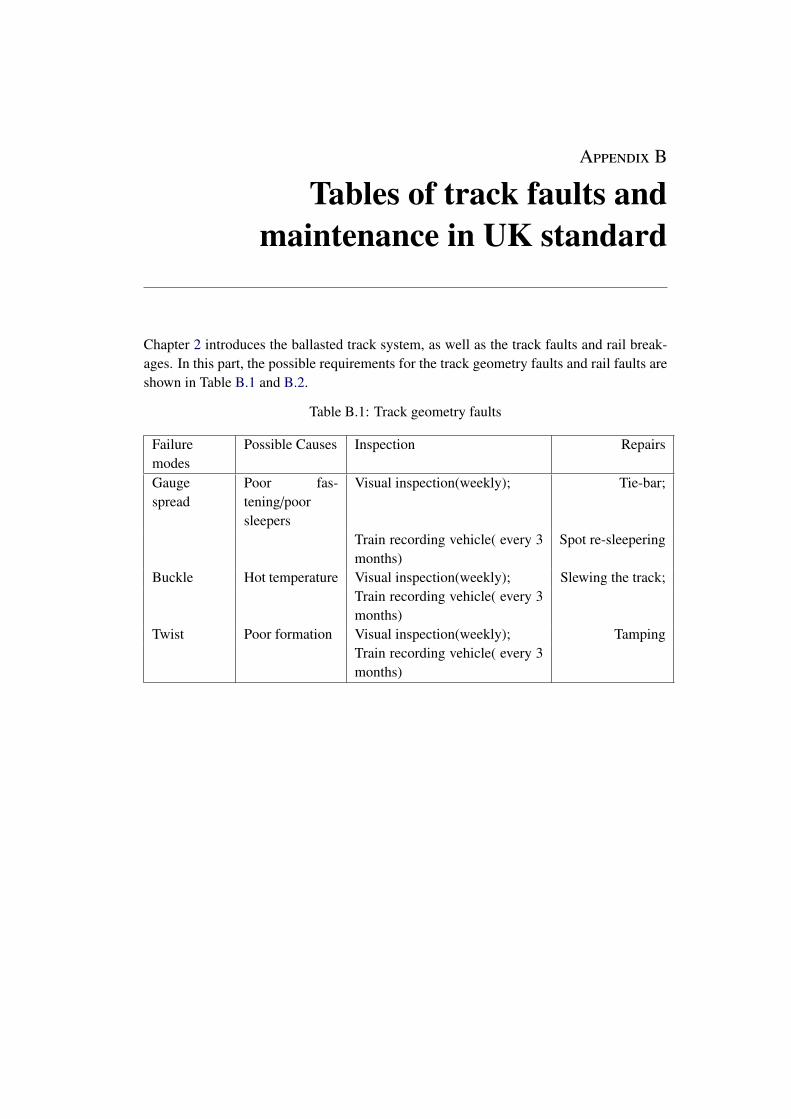
Appendix B
Tables of track faults andmaintenance in UK standard
Chapter 2 introduces the ballasted track system, as well as the track faults and rail break-ages. In this part, the possible requirements for the track geometry faults and rail faults areshown in Table B.1 and B.2.
Table B.1: Track geometry faults
Failuremodes
Possible Causes Inspection Repairs
Gaugespread
Poor fas-tening/poorsleepers
Visual inspection(weekly); Tie-bar;
Train recording vehicle( every 3months)
Spot re-sleepering
Buckle Hot temperature Visual inspection(weekly); Slewing the track;Train recording vehicle( every 3months)
Twist Poor formation Visual inspection(weekly); TampingTrain recording vehicle( every 3months)
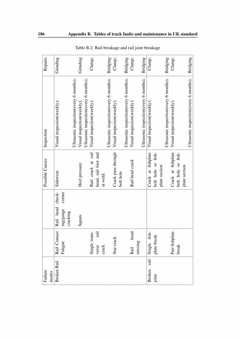
186 Appendix B. Tables of track faults and maintenance in UK standard
Table B.2: Rail breakage and rail joint breakageFa
ilure
mod
esPo
ssib
leC
ause
sIn
spec
tion
Rep
airs
Bro
ken
Rai
lR
ail
Con
tact
Fatig
ueR
ail
head
chec
k-in
g/ga
uge
corn
ercr
acki
ng
Side
wea
rV
isua
lins
pect
ion(
wee
kly)
;G
rind
ing
Ultr
ason
icin
spec
tion(
ever
y6
mon
ths)
;Sq
uats
Hee
lpre
ssur
eV
isua
lins
pect
ion(
wee
kly)
;G
rind
ing
Ultr
ason
icin
spec
tion(
ever
y6
mon
ths)
;Si
ngle
tran
s-ve
rse
rail
crac
k
Rai
lcr
ack
atra
ilhe
ad,
rail
foot
and
atw
eld;
Vis
uali
nspe
ctio
n(w
eekl
y);
Cla
mp;
Ultr
ason
icin
spec
tion(
ever
y6
mon
ths)
;B
ridg
ing
Star
crac
kC
rack
pass
thro
ugh
bolt
hole
Vis
uali
nspe
ctio
n(w
eekl
y);
Cla
mp;
Ultr
ason
icin
spec
tion(
ever
y6
mon
ths)
;B
ridg
ing
Rai
lhe
adm
issi
ngR
ailh
ead
crac
kV
isua
lins
pect
ion(
wee
kly)
;C
lam
p;
Ultr
ason
icin
spec
tion(
ever
y6
mon
ths)
;B
ridg
ing
Bro
ken
rail
join
tSi
ngle
fish-
plat
ebr
eak
Cra
ckat
fishp
late
bolt
hole
orfis
h-pl
ate
sect
ion
Vis
uali
nspe
ctio
n(w
eekl
y);
Cla
mp;
Ultr
ason
icin
spec
tion(
ever
y6
mon
ths)
;B
ridg
ing
Pair
fishp
late
brea
kC
rack
atfis
hpla
tebo
ltho
leor
fish-
plat
ese
ctio
n
Vis
uali
nspe
ctio
n(w
eekl
y);
Cla
mp;
Ultr
ason
icin
spec
tion(
ever
y6
mon
ths)
;B
ridg
ing
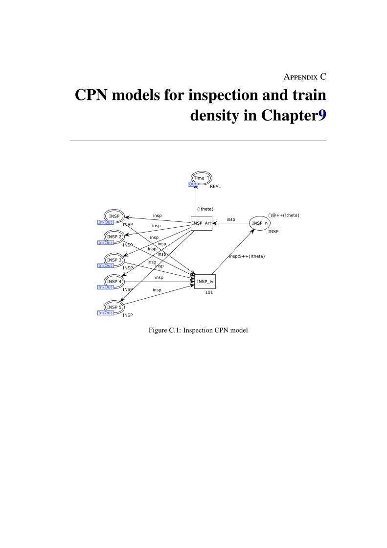
Appendix C
CPN models for inspection and traindensity in Chapter9
INSP_n
INSP
()@++(!theta)
INSP 2
In/OutINSP
In/Out
INSP
In/OutINSP
In/Out
Time_T
OutREAL
INSP 3
In/OutINSP
In/Out
INSP 4
In/OutINSP
In/Out
INSP 5
In/OutINSP
In/Out
INSP_Arr
INSP_lv
101
insp
insp@++(!theta)insp
insp
insp
insp
(!theta)
insp
insp
insp
insp
insp
insp
Out
Figure C.1: Inspection CPN model
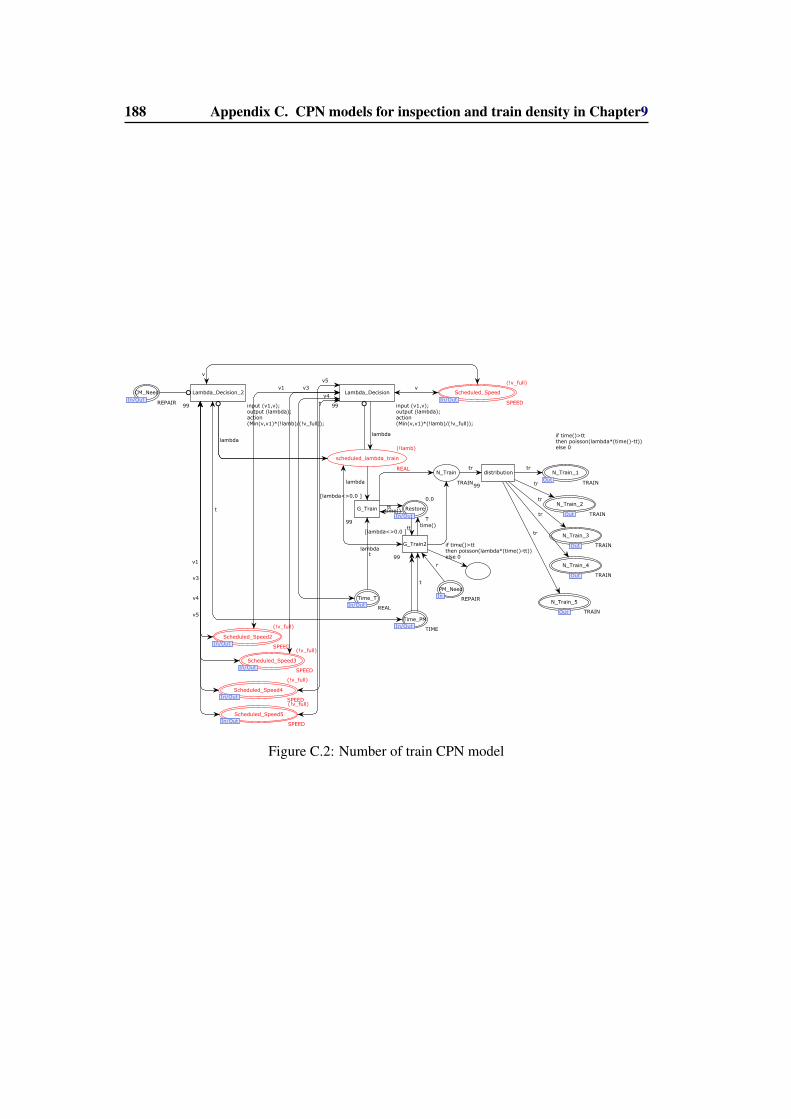
188 Appendix C. CPN models for inspection and train density in Chapter9
N_Train
TRAIN
scheduled_lambda_train
REAL
(!lamb)
Restore
In/OutT
0.0
In/Out
Time_PM
In/OutTIME
In/Out
Time_T
In/OutREAL
In/Out
PM_Need
InREPAIR
In
N_Train_2
Out TRAINOut
Scheduled_Speed
In/OutSPEED
(!v_full)
In/Out
Scheduled_Speed2
In/OutSPEED
(!v_full)
In/Out
N_Train_1
OutTRAIN
Out
CM_Need
In/OutREPAIR
In/Out
N_Train_3
Out TRAINOut
Scheduled_Speed3
In/OutSPEED
(!v_full)
In/Out
Scheduled_Speed4
In/OutSPEED
(!v_full)
In/Out
N_Train_4
Out TRAINOut
N_Train_5
Out TRAINOut
Scheduled_Speed5
In/OutSPEED
(!v_full)
In/Out
Lambda_Decision_2
input (v1,v);output (lambda);action(Min(v,v1)*(!lamb)/(!v_full));
99
Lambda_Decision
input (v1,v);output (lambda);action(Min(v,v1)*(!lamb)/(!v_full));
99
distribution
99
G_Train
[lambda<>0.0 ]
99
G_Train2
[lambda<>0.0 ]
99
if time()>tt then poisson(lambda*(time()-tt)) else 0
lambda
tr
if time()>tt then poisson(lambda*(time()-tt)) else 0
lambda
lambdalambda
time()
t
t
t
t
tt
r
tr
v
v
v1
v1
tt
time()
tr
v3
v3
tr
tr
v4
v4
tr
v5
v5
Figure C.2: Number of train CPN model
References
[1] (2003). Summary of the Potters Bar Investigation Board Recommendations and sub-sequent actions taken. (Not cited.)
[2] Ab-Samat, H. and Kamaruddin, S. (2014). Opportunistic maintenance (OM) as a newadvancement in maintenance approaches. J. Qual. Maint. Eng., 20(2):98–121. (Citedon page 37.)
[3] Ahmad, R. and Kamaruddin, S. (2012). An overview of time-based and condition-based maintenance in industrial application. Comput. Ind. Eng., 63(1):135–149. (Citedon page 36.)
[4] Andrade, A. R. and Teixeira, P. F. (2012). A Bayesian model to assess rail trackgeometry degradation through its life-cycle. Res. Transp. Econ., 36(1):1–8. (Citedon page 30.)
[5] Andrews, J. (2013). A modelling approach to railway track asset management. Proc.Inst. Mech. Eng. Part F J. Rail Rapid Transit, 227(1):56–73. (Cited on pages 8, 31, 52,55 and 56.)
[6] Andrews, J. and Moss, T. R. (2002). Fault Tree Analysis. In Reliab. risk Assess., pages201–300. Wiley-Blackwell, London, 2nd editio edition. (Cited on pages 36, 38 and 42.)
[7] Andrews, J., Prescott, D., and De Rozières, F. (2014). A stochastic model for railwaytrack asset management. Reliab. Eng. Syst. Saf., 130:76–84. (Cited on page 31.)
[8] Antoni, M. (2009). The ageing of signalling equipment and the impact on maintenancestrategy. 2009 Int. Conf. Comput. Ind. Eng., 2:1179–1184. (Cited on pages 5 and 36.)
[9] Antoni, M., Zilber, N., Lejette, F., and Meier-Hirmer, C. (2009). The ageing of sig-nalling equipment and the impact on maintenance strategies. In Safety, Reliab. RiskAnal. Theory, Methods Appl. - Proc. Jt. ESREL SRA-Europe Conf., volume 4, pages3231–3236, SNCF Infrastructure, Maintenance Engineering, Paris, France. (Cited onpages 5 and 31.)
[10] Arasteh khouy, I., Larsson-Kråik, P.-O., Nissen, A., Juntti, U., and Schunnesson, H.(2014). Optimization of track geometry inspection interval. Proc. Inst. Mech. Eng. PartF J. Rail Rapid Transit, 228(5):546–556. (Cited on page 35.)
[11] Audley, M. and Andrews, J. (2013). The effects of tamping on railway track geometrydegradation. Proc. Inst. Mech. Eng. Part F J. Rail Rapid Transit, 227(4):376–391. (Citedon pages 31, 139 and 176.)
[12] Australian Rail Track Corporation (2009). Steel Sleepers-Usage and Installation Stan-dards. Technical report, Australian Rail Track Corporation. (Cited on page 17.)

190 References
[13] Aven, T. and Castro, I. (2009). A delay-time model with safety constraint. Reliab.Eng. Syst. Saf., 94(2):261–267. (Cited on page 33.)
[14] Aven, T. and Castro, I. T. (2008). A minimal repair replacement model with twotypes of failure and a safety constraint. Eur. J. Oper. Res., 188(2):506–515. (Cited onpage 33.)
[15] Balbo, G. (2007). Introduction to generalized stochastic petri nets. In Formal methodsfor performance evaluation, pages 83–131. Springer. (Cited on page 46.)
[16] Barker, C. and Newby, M. (2009). Optimal non-periodic inspection for a multivariatedegradation model. Reliab. Eng. Syst. Saf., 94(1):33–43. (Cited on page 35.)
[17] Berawi, A. R. B., Delgado, R., Calçada, R., and Vale, C. (2010). Evaluating TrackGeometrical Quality through Different Methodologies. Int. J. Technol., 1:38–47. (Citedon page 21.)
[18] Bérenguer, C., Grall, A., Dieulle, L., and Roussignol, M. (2003). Maintenance policyfor a continuously monitored deteriorating system. Probab. Eng. Informational Sci.,17(02):235–250. (Cited on pages 34 and 45.)
[19] Bernardi, S., Campos, J., and Merseguer, J. (2011). Timing-Failure Risk Assessmentof UML Design Using Time Petri Net Bound Techniques. IEEE Trans. Ind. Informatics,7(1):90–104. (Cited on page 38.)
[20] Berrade, M. D., Cavalcante, C. A., and Scarf, P. A. (2012). Maintenance schedulingof a protection system subject to imperfect inspection and replacement. Eur. J. Oper.Res., 218(3):716–725. (Cited on page 34.)
[21] Bobbio, A. and Codetta R., D. (2004). Parametric fault trees with dynamic gates andrepair boxes. In Annu. Symp. Reliab. Maint. 2004 - RAMS, pages 459–465. IEEE. (Citedon page 161.)
[22] Bobbio, A., Franceschinis, G., Gaeta, R., and Portinale, L. (2003). Parametric FaultTree for the Dependability Analysis of Redundant Systems and Its High-Level Petri NetSemantics. IEEE Trans. Softw. Eng., 29(3):270–287. (Cited on page 161.)
[23] Bouvard, K., Artus, S., Bérenguer, C., and Cocquempot, V. (2011). Condition-based dynamic maintenance operations planning & grouping. Application to commer-cial heavy vehicles. Reliab. Eng. Syst. Saf., 96(6):601–610. (Cited on page 37.)
[24] Buchheit, G., Malasse, O., Brinzei, N., and Ammad, N. (2013). Dependability assess-ment of large railway systems. In 2013 Proc. Annu. Reliab. Maintainab. Symp., pages1–6. IEEE. (Cited on page 47.)
[25] Budai, G., Huisman, D., and Dekker, R. (2005). Scheduling preventive railway main-tenance activities. J. Oper. Res. Soc., 57(9):1035–1044. (Cited on page 37.)
References 191
[26] Bureau d’enquêtes sur les accidents de transport Terrestre (2014). Rapport d’étapesur le déraillement du train Intercites n 3657 le 12 juillet 2013 à Brétigny-sur-Orge (91).Technical report, Ministère de l’Écologie, du DÉveloppement durable et de l’Énergie.(Cited on page 4.)
[27] Caballé, N., Castro, I., Pérez, C., and Lanza-Gutiérrez, J. (2015). A condition-basedmaintenance of a dependent degradation-threshold-shock model in a system with multi-ple degradation processes. Reliab. Eng. Syst. Saf., 134:98–109. (Cited on page 36.)
[28] Caetano, L. F. and Teixeira, P. F. (2014). Optimisation model to schedule railwaytrack renewal operations: a life-cycle cost approach. Struct. Infrastruct. Eng., pages1–13. (Cited on pages 31 and 37.)
[29] Cannon, D. F., Edel, K., Grassie, S. L., and Sawley, K. (2003). Rail defects : anoverview. Fatigue Fract Engng Mater Struct, 26:865–886. (Cited on page 25.)
[30] Caramia, M. and Dell’Olmo, P. (2008). Multi-objective management in freight logis-tics: Increasing capacity, service level and safety with optimization algorithms. SpringerScience & Business Media. (Cited on pages 145 and 180.)
[31] Carretero, J., Pérez, J. M., García-Carballeira, F., Calderón, A., Fernández, J., Gar-cÄsía, J. D., Lozano, A., Cardona, L., Cotaina, N., and Prete, P. (2003). Applying RCMin large scale systems: a case study with railway networks. Reliab. Eng. Syst. Saf.,82(3):257–273. (Cited on page 5.)
[32] Castanier, B., Bérenguer, C., and Grall, A. (2003). A sequential condition-based re-pair/replacement policy with non-periodic inspections for a system subject to continuouswear. Appl. Stoch. Model. Bus. Ind., 19(4):327–347. (Cited on page 35.)
[33] Castanier, B., Grall, A., and Bérenguer, C. (2001). A stochastic model for hy-brid maintenance policies evaluation and optimization. Int. J. Reliab. Qual. Saf. Eng.,08(03):233–248. (Cited on page 34.)
[34] Castanier, B., Grall, A., and Bérenguer, C. (2005). A condition-based maintenancepolicy with non-periodic inspections for a two-unit series system. Reliab. Eng. Syst.Saf., 87(1):109–120. (Cited on page 37.)
[35] Castanier, B. and Rausand, M. (2006). Maintenance optimization for subsea oilpipelines. Int. J. Press. Vessel. Pip., 83(4):236–243. (Cited on page 32.)
[36] Castro, I., Caballé, N., and Pérez, C. (2013). A condition-based maintenance for asystem subject to multiple degradation processes and external shocks. Int. J. Syst. Sci.,46(9):1692–1704. (Cited on page 36.)
[37] Castro, I. and Sanjuán, E. (2008). An optimal maintenance policy for repairablesystems with delayed repairs. Oper. Res. Lett., 36(5):561–564. (Cited on pages 34and 84.)
192 References
[38] Castro, I. T. (2009). A model of imperfect preventive maintenance with dependentfailure modes. Eur. J. Oper. Res., 196(1):217–224. (Cited on page 35.)
[39] Chang, C.-K. and Hsiang, C.-L. (2010). An optimal maintenance policy based ongeneralized stochastic Petri nets and periodic inspection. Asian J. Control, 12(3):364–376. (Cited on page 45.)
[40] Chang, C.-K. and Hsiang, C.-L. (2011). Using generalized stochastic Petri nets forpreventive maintenance optimization in automated manufacturing systems. J. Qual.,18(2):117–135. (Cited on page 45.)
[41] Christer, A. H. (1999). Developments in delay time analysis for modelling plantmaintenance. J. Oper. Res. Soc., 50(11):1120–1137. (Cited on pages 32, 125 and 174.)
[42] Christer, A. H. (2001). The robustness of the semi-Markov and delay time single-component inspection models to the Markov assumption. IMA J. Manag. Math.,12(1):75–88. (Cited on page 33.)
[43] Christer, A. H. and Lee, C. (2000). Refining the delay-time-based PM inspectionmodel with non-negligible system downtime estimates of the expected number of fail-ures. Int. J. Prod. Econ., 67:77–85. (Cited on page 32.)
[44] Claisse, P. and Calla, C. (2006). Rail ballast: conclusions from a historical perspec-tive. Proc. ICE - Transp., 159(2):69–74. (Cited on pages 24 and 168.)
[45] De Man, A. (2002). Dynatrack: A survey of dynamic railway track properties andtheir quality. (Cited on pages 16 and 166.)
[46] Dekker, R., Wildeman, R. E., and Duyn Schouten, F. A. (1997). A review of multi-component maintenance models with economic dependence. Math. Methods Oper. Res.,45(3):411–435. (Cited on page 36.)
[47] Deloux, E., Castanier, B., and Bérenguer, C. (2009a). An adaptive condition-basedmaintenance policy with environmental factors. In Risk Decis. Anal. Maint. Optim.Flood Manag., pages 137–148. Delft University Press. (Cited on page 34.)
[48] Deloux, E., Castanier, B., and Bérenguer, C. (2009b). Predictive maintenance policyfor a gradually deteriorating system subject to stress. Reliab. Eng. Syst. Saf., 94(2):418–431. (Cited on page 34.)
[49] Dhahbi, S., Abbas-Turki, A., Hayat, S., and El Moudni, A. (2011). Study of the high-speed trains positioning system: European signaling system ERTMS/ETCS. In 20114th Int. Conf. Logist. LOGISTIQUA’2011, pages 468–473. (Cited on page 7.)
[50] Direction Sécurité & Qualité de Service Ferroviaire. SNCF open DATA. (Cited onpages 3, 4 and 163.)
[51] Dirks, B. and Enblom, R. (2011). Prediction model for wheel profile wear and rollingcontact fatigue. Wear, 271(1-2):210–217. (Cited on pages 6 and 30.)
References 193
[52] Doyen, L. and Gaudoin, O. (2004). Classes of imperfect repair models based onreduction of failure intensity or virtual age. Reliab. Eng. Syst. Saf., 84(1):45–56. (Citedon page 35.)
[53] Ellis, I. (2006). Ellis’ British Railway Engineering Encyclopaedia. Lulu Enterprises,UK Ltd, London, 2nd editio edition. (Cited on pages 21 and 167.)
[54] Esveld, C. (2001). Modern Railway Track. MRT-productions Zaltbommel, secondedition. (Cited on pages 4, 17, 23, 25, 163 and 168.)
[55] European Comittee for Standardization (CEN) (2008). EN 13848-5:Railway appli-cations. Track. Track geometry quality. Geometric quality levels. Plain line. (Cited onpage 21.)
[56] Famurewa, S. M., Stenström, C., Asplund, M., Galar, D., and Kumar, U.(2014). Composite indicator for railway infrastructure management. J. Mod. Transp.,22(4):214–224. (Cited on page 20.)
[57] Fararooy, S. and Allan, J. (1995). Condition-based Maintenance of Railway signallingEquipment. In Int. Conf. Electr. Railw. a United Eur., 405, pages 27–30, Amsterdam,Netherlands. IET. (Cited on page 36.)
[58] Ferreira, R. J., de Almeida, A. T., and a.V. Cavalcante, C. (2009). A multi-criteriadecision model to determine inspection intervals of condition monitoring based on delaytime analysis. Reliab. Eng. Syst. Saf., 94(5):905–912. (Cited on pages 33 and 34.)
[59] Flage, R. (2014). A delay time model with imperfect and failure-inducing inspections.Reliab. Eng. Syst. Saf., 124:1–12. (Cited on page 34.)
[60] Fouathia, O. (2005). petri net based monte carlo simultiaon for modeling and anlysisthe relibaility of distribution substation facilities in belgian power system. In 18th Int.Conf. Eletr. Distrib., volume 4, Turin. (Cited on page 45.)
[61] Fouathia, O., Maun, J.-C., Labeau, P.-E., and Wiot, D. (2005). Cost-optimizationmodel for the planning of the renewal, inspection, and maintenance of substation facili-ties in Belgian power transmission system. In Adv. Saf. Reliab. - Proc. Eur. Saf. Reliab.Conf. ESREL 2005, volume 1, pages 631–637, Université Libre de Bruxelles, Bruxelles,Belgium. (Cited on page 45.)
[62] Frostig, E. and Kenzin, M. (2009). Availability of inspected systems subject to shocks- A matrix algorithmic approach. Eur. J. Oper. Res., 193(1):168–183. (Cited on page 33.)
[63] García Márquez, F. P., Pedregal Tercero, D. J., and Schmid, F. (2007). UnobservedComponent models applied to the assessment of wear in railway points: A case study.Eur. J. Oper. Res., 176(3):1703–1712. (Cited on page 27.)
[64] GC/RT 5021 issue 5 (2011). Track System Requirements . (Cited on pages 16, 17,20, 21, 26 and 166.)
194 References
[65] Ghazel, M. (2009). Using Stochastic Petri Nets for Level-Crossing Collision RiskAssessment. IEEE Trans. Intell. Transp. Syst., 10(4):668–677. (Cited on page 38.)
[66] Girault, C. and Valk, R. (2001). Petri Nets for System Engineering: A Guide toModeling, Verification, and Applications. Springer-Verlag New York, Inc. (Cited onpage 46.)
[67] Golmakani, H. R. and Fattahipour, F. (2011). Age-based inspection scheme forcondition-based maintenance. J. Qual. Maint. Eng., 17(1):93–110. (Cited on page 34.)
[68] Golmakani, H. R. and Moakedi, H. (2012). Optimal nonperiodic inspection schemefor a multicomponent repairable system with failure interaction using A * search algo-rithm. Int. J. Adv. Manuf. Technol., 67(5-8):1325–1336. (Cited on page 34.)
[69] Goossens, H. (2010). Maintenance of High Speed Lines. Technical Report Septem-ber, international union of railways. (Cited on page 17.)
[70] Grall, A., Bérenguer, C., and Dieulle, L. (2002a). A condition-based maintenancepolicy for stochastically deteriorating systems. Reliab. Eng. Syst. Saf., 76(2):167–180.(Cited on pages 36, 142 and 178.)
[71] Grall, A., Dieulle, L., Berenguer, C., and Roussignol, M. (2002b). Continuous-timepredictive-maintenance scheduling for a deteriorating system. IEEE Trans. Reliab.,51(2):141–150. (Cited on pages 35, 36, 92, 142 and 178.)
[72] Grassie, S. L. (2005). Rolling contact fatigue on the British railway system : treat-ment. Wear, 258(March 2004):1310–1318. (Cited on page 26.)
[73] Grimes, G. A. and Barkan, C. P. L. (2006). Cost-effectiveness of railway infrastruc-ture renewal maintenance. J. Transp. Eng., 132(8):601–608. (Cited on page 5.)
[74] Guler, H. (2012). Decision Support System for Railway Track Maintenance and Re-newal Management. J. Comput. Civ. Eng., 27(3):292–306. (Cited on page 35.)
[75] Haas, P. (2004). Stochastic Petri Nets for Modelling and Simulation. In Proc. 2004Winter Simul. Conf. 2004., volume 1, pages 95–106. IEEE. (Cited on page 46.)
[76] Henry, A. J. and Nachlas, J. A. (2012). An equivalent age model for condition-basedmaintenance. In 2012 Proc. Annu. Reliab. Maintainab. Symp., pages 1–6. IEEE. (Citedon page 63.)
[77] Higgins, A., Ferreira, L., and Lake, M. (1999). Scheduling rail track maintenanceto minimise overall delays. In 14th Int. Symp. Transp. Traffic Theory, pages 1–8,Jerusalem, Israel. (Cited on page 37.)
[78] Hosseini, M., Kerr, R., and Randall, R. (2000). An inspection model with minimaland major maintenance for a system with deterioration and Poisson failures. IEEE Trans.Reliab., 49(1):88–98. (Cited on pages 33 and 45.)
References 195
[79] Hosseini, M., Kerr, R., and Randall, R. B. (1999). Hybrid maintenance model withimperfect inspection for a system with deterioration and Poisson failure. J. Oper. Res.Soc., 50(12):1229–1243. (Cited on page 45.)
[80] HSE Potters Bar Investigation Board (2003). Train Derailment at Potters Bar 10 May2002. Technical Report May, Health& Safety Executive. (Cited on page 4.)
[81] Hu, H., Cheng, G., Duan, Q., Wu, W., and Xu, C. (2009). Delay time model basedon imperfect maintenance. Hsi-An Chiao Tung Ta Hsueh/Journal Xi’an Jiaotong Univ.,43(6):103–107. (Cited on page 35.)
[82] Hudson, B. G. (2006). Risk-based maintenance. Pet. Technol. Q., 11(5):37–38,41–42,44–45. (Cited on page 36.)
[83] Hunyadi, B. (2011). Capacity evaluation for ERTMS ( European Rail Traffic Man-agement System ) Level 2 operation on HS2. Technical Report October, BombardierInc. (Cited on page 7.)
[84] Huynh, K. T., Barros, A., and Bérenguer, C. (2012a). Adaptive condition-based main-tenance decision framework for deteriorating systems operating under variable environ-ment and uncertain condition monitoring. Proc. Inst. Mech. Eng. Part O J. Risk Reliab.,226(6):602–623. (Cited on page 34.)
[85] Huynh, K. T., Castro, I., Barros, A., and Bérenguer, C. (2012b). Modeling age-basedmaintenance strategies with minimal repairs for systems subject to competing failuremodes due to degradation and shocks. Eur. J. Oper. Res., 218(1):140–151. (Cited onpages 36 and 45.)
[86] INNOTRACK (2008). D3 . 3 . 1- List of key parameters for switch and crossingmonitoring. Technical report, innovative track systems. (Cited on page 26.)
[87] Jensen, K. and Kristensen, L. (2009). Colored Petri Net–Modelling and validation ofconcurrent systems. Springer-Verlag Berlin. (Cited on pages 48 and 169.)
[88] Jensen, K., Kristensen, L. M., Wells, L., Michael, L., and Lisa, K. (2007). ColouredPetri Nets and CPN Tools for modelling and validation of concurrent systems. Int. J.Softw. Tools Technol. Transf., 9(3-4):213–254. (Cited on page 46.)
[89] Jhang, J. and Sheu, S. (1999). Opportunity-based age replacement policy with mini-mal repair. Reliab. Eng. Syst. Saf., 64(3):339–344. (Cited on page 36.)
[90] Junca, M. and Sanchez-Silva, M. (2013). Optimal Maintenance Policy for a Com-pound Poisson Shock Model. IEEE Trans. Reliab., 62(1):66–72. (Cited on page 33.)
[91] Kallen, M. and van Noortwijk, J. (2005). Optimal maintenance decisions under im-perfect inspection. Reliab. Eng. Syst. Saf., 90(2-3):177–185. (Cited on page 34.)
[92] Kallsen, J. and Tankov, P. (2006). Characterization of dependence of multidimen-sional Lévy processes using Lévy copulas. J. Multivar. Anal., 97(7):1551–1572. (Citedon page 36.)
196 References
[93] Kao, E. P. C. (1997). An Introduction to Stochastic Processes. Duxbury Press, 1stedition. (Cited on page 44.)
[94] Kijima, M. (1989). Some Results for Repairable Systems with General Repair. J.Appl. Probab., 26(1):89–102. (Cited on page 35.)
[95] Kijima, M., Morimura, H., and Suzuki, Y. (1988). Periodical replacement problemwithout assuming minimal repair. Eur. J. Oper. Res., 37(2):194–203. (Cited on pages 66and 171.)
[96] Kish, A. and W.Clark, D. (2009). Track Buckling Derailment Prevention Through riskbased train speed reduction. In AREMA 2009 Annu. Conf. Expo., pages 1–21. (Cited onpages 6, 24 and 30.)
[97] Kitagawa, T., Yuge, T., and Yanagi, S. (2014). Optimal maintenance policy for a one-shot system with minimal repair and non-periodic inspection intervals. In RQD 2014 -Proc. - 20th ISSAT Int. Conf. Reliab. Qual. Des., pages 198–202. International Societyof Science and Applied Technologies. (Cited on page 35.)
[98] Krull, R., Hintze, H., Luke, M., Thomas, M., Pohl, R., and Rühe, S. (2002). Eddycur-rent Detection of Head Checks on the Gauge Corners of Rails: Recent Results. NDT.net,7(6):1. (Cited on page 25.)
[99] Lee, K.-m., Shin, D., Lee, J.-h., and Kim, Y.-g. (2007). Study on the system contrac-ture for the preventive maintenance of the train control system using RCM. In Proceed-ing Int. Conf. Electr. Mach. Syst., pages 1919–1922. (Cited on page 5.)
[100] Li, G. and Shi, D. (2011). Risk-based maintenance schedule of transmission lineusing multi-objective evolutionary algorithm. In PEAM 2011 - Proc. 2011 IEEEPower Eng. Autom. Conf., volume 1, pages 413–416, College of Electrical Engineer-ing (CEEE), Huazhong University of Science and Technology (HUST), Wuhan, China.(Cited on page 36.)
[101] Li, H. (2005). Stochastic Comparison of Age-Dependent Block Replacement Poli-cies. Methodol. Comput. Appl. Probab., 7(4):473–488. (Cited on page 37.)
[102] Li, H., Dieulle, L., and Deloux, E. (2015). Condition-based maintenance poli-cies for multi-component systems with Lévy copulas dependence. In Saf. Reliab.Methodol. Appl. - Proc. Eur. Saf. Reliab. Conf. ESREL 2014, pages 1281–1288. CRCPress/Balkema. (Cited on page 36.)
[103] Lim, W. L. (2004). Mechanics of Railway Ballast Behaviour. Phd thesis, TheUniversity of Nottingham. (Cited on page 17.)
[104] Lipi, T. F., Lim, J.-H., Zuo, M. J., and Wang, W. (2011). A condition- and age-basedreplacement model using delay time modelling. Proc. Inst. Mech. Eng. Part O J. RiskReliab., 226(2):221–233. (Cited on page 33.)
References 197
[105] Lupton, J. (2003). derailment mitigation-categorisation of past derailments. Tech-nical report, Railway Safety and Standard Board, London. (Cited on pages 4 and 163.)
[106] Macchi, M., Garetti, M., Centrone, D., Fumagalli, L., and Piero Pavirani, G. (2012).Maintenance management of railway infrastructures based on reliability analysis. Re-liab. Eng. Syst. Saf., 104(null):71–83. (Cited on page 5.)
[107] Magel, E. E. (2011). Rolling contact Fatigue: A Comprehensive Review. Technicalreport, U.S. Department of Transportation Federal Railroad Administration, Washing-ton. (Cited on page 25.)
[108] Malhotra, M. and Trivedi, K. (1995). Dependability modeling using Petri-nets. IEEETrans. Reliab., 44(3):428–440. (Cited on page 38.)
[109] Marsan, M. A., Balbo, G., Conte, G., Donatelli, S., and Franceschinis, G. (1994).Modelling with generalized stochastic Petri nets. John Wiley & Sons, Inc. (Cited onpage 47.)
[110] Martorell, S. (1999). Age-dependent reliability model considering effects of mainte-nance and working conditions. Reliab. Eng. Syst. Saf., 64(1):19–31. (Cited on page 36.)
[111] McHutchon, M., Staszewski, W., and Schmid, F. (2005). Signal Processing for Re-mote Condition Monitoring of Railway Points. Strain, 41(2):71–85. (Cited on page 27.)
[112] McWilliams, R. and Eberius, E. (2014). Measuring With Eddy Current: GaugeCorner Cracking and the Magic Wear Rate. (Cited on page 25.)
[113] Meier-Hirmer, C. and Poulighy, P. (2009). Impact of preventive grinding on main-tenance costs and determination of an optimal grinding cycle. In Safety, Reliab. RiskAnal. Theory, Methods Appl. - Proc. Jt. ESREL SRA-Europe Conf., volume 4, pages3183–3189, SNCF, Infrastructure, Maintenance Engineering, Paris, France. (Cited onpages 25, 31 and 35.)
[114] Meier-Hirmer, C., Riboulet, G., Sourget, F., and Roussignol, M. (2009). Mainte-nance optimization for a system with a gamma deterioration process and interventiondelay: application to track maintenance. Proc. Inst. Mech. Eng. Part O J. Risk Reliab.,223(3):189–198. (Cited on pages 33, 35, 84, 85 and 172.)
[115] Mercier, S., Meier-hirmer, C., and Roussignol, M. (2012). Bivariate Gamma wearprocesses for track geometry modelling , with application to intervention scheduling.Struct. Infrastruct. Eng. Maintenance, Manag. Life-Cycle Des. Performance,, 8(4):357–366. (Cited on page 33.)
[116] M.Lake, L.Ferreira, and M.Murray (2000). Minimising cost in scheduling railwaytrack maintenance. In Int. Conf. Comput. Railw., volume 7, pages 895–902. (Cited onpage 37.)
198 References
[117] Moubray, J. (1997). Proactive Maintenance 2: Predictive Tasks. In Reliab. Maint.,pages 144–169. Industrial Press, Inc, New York, 2nd edition. (Cited on pages 32and 126.)
[118] Muttram, R. I. (2002). Railway Safety’s Safety Risk Model. Proc. Inst. Mech. Eng.Part F J. Rail Rapid Transit, 216(2):71–79. (Cited on page 38.)
[119] Network Rail (2009). CP4 Delivery Plan 2009: More trains, more seats- BetterJourneys. Technical report, Network Rail, London. (Cited on page 6.)
[120] Network Rail (2011). Route Specifications 2011 - East Midlands. (Cited on pages 6,16 and 17.)
[121] Network Rail (2014). Efficiency Summary. Technical report, Network Rail, London.(Cited on pages 4, 6 and 163.)
[122] Ngatchou, P., Zarei, A., and El-Sharkawi, A. (2005). Pareto Multi Objective Opti-mization. In Proc. 13th Int. Conf. on, Intell. Syst. Appl. to Power Syst., pages 84–91.IEEE. (Cited on pages 145 and 180.)
[123] Nicolai, R. P. and Dekker, R. (2007). A review of multi-component maintenancemodels. In Proc. Eur. Saf. Reliab. Conf. 2007, ESREL 2007 - Risk, Reliab. Soc. Saf.,volume 1, pages 289–296. (Cited on page 36.)
[124] Nielsen, J., Berggren, E., Lölgen, T., Müller, R., Stallaert, B., and Pesqueux, L.(2013). Overview of Methods for Measurement of Track Irregularities Important forGround-Borne Vibration. Technical report, International Union of Railways (UIC).(Cited on pages 26 and 169.)
[125] Nissen, A. (2009). LCC-analysis for Switches and Crossings âAS a case study fromthe Swedish railway network. Int. J. COMADEM, pages 1–13. (Cited on page 37.)
[126] Nodem, F. D., Gharbi, A., and Kenné, J.-P. (2011). Preventive maintenance andreplacement policies for deteriorating production systems subject to imperfect repairs.Int. J. Prod. Res., 49(12):3543–3563. (Cited on page 36.)
[127] Nourelfath, M., Châtelet, E., and Nahas, N. (2012). Joint redundancy and imperfectpreventive maintenance optimization for series-parallel multi-state degraded systems.Reliab. Eng. Syst. Saf., 103:51–60. (Cited on page 37.)
[128] Office of Rail Regulation (2006). Train Derailment at Hatfield: A Final Reportby the Independent Investigation Board. Technical report, Office of Rail Regulation,London. (Cited on page 4.)
[129] Office of Rail Regulation (2013). Network Rail Monitor-Quarter 2 (Periods 5 - 7) ofYear 5 of CP4. Technical Report October, Office of Rail Regulation, London. (Cited onpage 4.)
References 199
[130] Okumura, S. (1997). An inspection policy for deteriorating processes using delay-time concept. Int. Trans. Oper. Res., 4(5-6):365–375. (Cited on page 33.)
[131] Ollivier, G., Bullock, R., Jin, Y., and Zhou, N. (2014). High-Speed Railways inChina: A Look at Traffic. (Cited on pages 3 and 6.)
[132] Oyama, T. and Miwa, M. (2006). Mathematical Modeling Analyses for Obtainingan Optimal Railway Track Maintenance Schedule. Japan J.Indust. Appl.Math.,, 23:207–224. (Cited on page 37.)
[133] Oyebande, B. and Renfrew, A. (2002). Condition monitoring of railway electricpoint machines. In Electr. Power Appl. IEE Proceedings-, volume 149, pages 465–473.IET. (Cited on pages 5 and 27.)
[134] Pascual, R., Louit, D., and Jardine, A. (2010). Optimal inspection intervals forsafety systems with partial inspections. J. Oper. Res. Soc., 62(12):2051–2062. (Citedon page 34.)
[135] Patra, A. P. and Kumar, U. (2010). Availability analysis of railway track circuits.Proc. Inst. Mech. Eng. Part F J. Rail Rapid Transit, 224(3):169–177. (Cited on page 32.)
[136] Patra, A. P., Kumar, U., and Kråik, P.-O. L. (2010). Availability target of the railwayinfrastructure: An analysis. In Proc. - Annu. Reliab. Maintainab. Symp., pages 1–6.IEEE. (Cited on page 32.)
[137] Patra, A. P., Kumar, U., and Larsson-Kråik, P.-O. (2009). Assessment and improve-ment of railway track safety. In Proc. - 9th Int. Heavy Haul Conf. "Heavy Haul Innov.Dev., pages 91–98, Luleå Railway Research Center, SE-97187, Luleå, Sweden. (Citedon pages 31 and 32.)
[138] Pedregal, D. J., García, F. P., and Schmid, F. (2004). RCM2 predictive maintenanceof railway systems based on unobserved components models. Reliab. Eng. Syst. Saf.,83(1):103–110. (Cited on pages 5, 18 and 36.)
[139] Peng, D. and Jones, R. (2013). Finite Element Method Study on the Squats GrowthSimulation. Appl. Math., 04(05):29–38. (Cited on page 26.)
[140] Peng, F., Kang, S., Li, X., and Ouyang, Y. (2011). A Heuristic Approach to the Rail-road Track Maintenance Scheduling Problem. Comput. Civ. Infrastruct. Eng., 26:129–145. (Cited on page 37.)
[141] Pérez Ramírez, P. A. and Utne, I. B. (2013). Decision support for life extensionof technical systems through virtual age modelling. Reliab. Eng. Syst. Saf., 115:55–69.(Cited on page 35.)
[142] Pham, H. and Wang, H. (1996). Imperfect maintenance. Eur. J. Oper. Res.,94(3):425–438. (Cited on pages 35 and 63.)
200 References
[143] Pocock, J. (2006). Cost Effective Reduction of Derailment Risk (D7175-07), issue1. Technical report, Railway Safety & Standard Board, London. (Cited on pages 4and 163.)
[144] Podofillini, L., Zio, E., and Vatn, J. r. (2006). Risk-informed optimisation of railwaytracks inspection and maintenance procedures. Reliab. Eng. Syst. Saf., 91(1):20–35.(Cited on pages 5, 8, 26, 32, 126, 169 and 174.)
[145] Pouryousef, H., Teixeira, P., and Sussman, J. (2010). Track maintenance schedulingand its interactions with operations Dedicated and mixed high-speed rail (HSR) scenar-ios. In Proc. 2010 Jt. Rail Conf., pages 317–326. ASME. (Cited on page 37.)
[146] Prescott, D. and Andrews, J. (2012). A Railway Track Ballast Maintenance andInspection Model for Multiple Track Sections. In 11th Int. Probabilistic Saf. Assess.Manag. Conf. Annu. Eur. Saf. Reliab. Conf., volume 1, pages 41–50, University of Not-tingham, Nottingham, United Kingdom. (Cited on pages 31, 111, 112 and 124.)
[147] Quiroga, L. and Schnieder, E. (2010). A heuristic approach to railway track mainte-nance scheduling. WIT Trans. Built Environ., 114:687–699. (Cited on page 33.)
[148] Quiroga, L., Wegele, S., and Schnieder, E. (2009). Benefit of railway infrastruc-ture diagnosis systems on its availability. In 2nd IFAC Work. dependable Control Dis-cret. Syst., pages 146–150, Technical University of Braunschweig, Institute for Traf-fic Safety and Automation Engineering, Braunschweig, Germany, Langer Kamp 8, D-38106 Braunschweig, Germany. (Cited on page 33.)
[149] Rail Accident Investigation Branch (2006). Broken Rails at Urchfont and Kenning-ton following the passage of a freight train 5 January 2006. Technical report, RailAccident Investigation Branch. (Cited on page 4.)
[150] Rail Accident Investigation Branch (2007). Derailment at Grayrigg 23 February2007. Technical report, Rail Accident Investigation Branch, Derby. (Cited on page 4.)
[151] Rail Accident Investigation Branch (2011). Derailment of an engineering train be-tween Gloucester Road and Earl’s Court stations on London Underground 12 May 2010.Technical Report May 2010, Rail Accident Investigation Branch. (Cited on page 17.)
[152] Rail Accident Investigation Branch (2013a). Derailment at Primrose Hill / CamdenRoad West Junction 15 October 2013. Technical report, Rail Accident InvestigationBranch, Derby. (Cited on page 4.)
[153] Rail Accident Investigation Branch (2013b). Rail Accident Report-Freight train de-railment near Gloucester 15 October 2013. Technical report, Rail Accident InvestigationBranch, Derby. (Cited on page 4.)
[154] Rail Safety & Standards Board (1998). Track Standards Manual - Section 2 :Rails(5019). Rail Safety & Standards Board. (Cited on page 26.)
References 201
[155] Rail Safety & Standards Board (2002). Rails and Rail Joints GC/RT5022. RailSafety and Standards Board. (Cited on page 25.)
[156] Railway Safety & Standard Board (1995). Track Standards Manual - Section 5 :Rail Support Systems. Railway Safety & Standard Board. (Cited on page 16.)
[157] Railway Safety & Standard Board (2001). Rail Fastenings and Supports GC/RT5024 issue 1. (Cited on page 21.)
[158] Railway Safety & Standard Board (2002). Potters Bar derailment: report and rec-ommendations. Technical Report May, Railway Safety & Standard Board. (Cited onpage 4.)
[159] Railway Safety & Standard Board (2006). Management and understanding of rollingcontact fatigue Literature Review. Technical report, Railway Safety & Standard Board.(Cited on page 26.)
[160] Railway Technical Web Pages (2014). Railway statistics for Britain. (Cited onpages 3 and 6.)
[161] Raiteri, D., Franceschinis, G., Iacono, M., and Vittorini, V. (2004). Repairable faulttree for the automatic evaluation of repair policies. In Int. Conf. Dependable Syst. Net-works, 2004, pages 659–668. IEEE. (Cited on page 161.)
[162] Rana, A., Verma, A., and Srividya, A. (2011). Use of petrinets for solution of a sterngland optimal inspection interval problem. Int. J. Syst. Assur. Eng. Manag., 2(2):183–192. (Cited on page 45.)
[163] Rausand, M. and Høyland, A. (2004). System reliability theory models, statisticalmethods, and applications. Wiley-Interscience, Hoboken, NJ, 2 edition. (Cited onpages 35, 36, 42, 43, 141 and 177.)
[164] Ribeiro, I. and Cal, R. (2010). Application of a maintenance model for optimizingtamping on ballasted tracks : the influence of the model constraints. In 2nd Int. Conf.Eng. Optim., pages 1–8, Lisbon,Portugal. (Cited on page 37.)
[165] Ross, S. M. (2007). Introduction to Probability Models. Academic Press, 10thedition. (Cited on page 43.)
[166] Sadeghi, J. and Askarinejad, H. (2010). Development of improved railway trackdegradation models. Struct. Infrastruct. Eng., 6(6):675–688. (Cited on pages 20, 30,139 and 176.)
[167] Sadeghi, J. and Askarinejad, H. (2011). Development of track condition assessmentmodel based on visual inspection. Struct. Infrastruct. Eng. Maint. , Manag. , Life-CycleDes. Perform., 7(12):895–905. (Cited on page 30.)
[168] Sadeghi, J., Fathali, M., and Boloukian, N. (2009). Development of a new trackgeometry assessment technique incorporating rail cant factor. Proc. Inst. Mech. Eng.Part F J. Rail Rapid Transit, 223:255–263. (Cited on page 19.)
202 References
[169] Schön, W., Larraufie, G., Moëns, G., and Poré, J. (2013). Signalisation et automa-tismes ferroviaires: Tome 1. La vie du Rail. (Cited on page 17.)
[170] Shafiee, M. and Finkelstein, M. (2015). An optimal age-based group maintenancepolicy for multi-unit degrading systems. Reliab. Eng. Syst. Saf., 134(2015):230–238.(Cited on page 37.)
[171] Shafiee, M., Patriksson, M., and Chukova, S. (2014). An optimal age-usage mainte-nance strategy containing a failure penalty for application to railway tracks. Proc. Inst.Mech. Eng. Part F J. Rail Rapid Transit, 0(0):1–11. (Cited on pages 33 and 36.)
[172] Shang, H. and Bérenguer, C. (2015a). A Colored Petri Net model for railway trackmaintenance with two-level inspection. In Saf. Reliab. Methodol. Appl. - Proc. Eur.Saf. Reliab. Conf. ESREL 2014, pages 1227–1235. CRC Press/Balkema. (Cited onpage 126.)
[173] Shang, H. and Bérenguer, C. (2015b). Delayed maintenance model for deterioratingtrack using Coloured Petri Net. In 9th IFAC Symp. Fault Detect. Superv. Saf. Tech.Process. 2015, page 6, Paris. (Cited on page 84.)
[174] Shang, H., Bérenguer, C., and Andrews, J. (2015). Delayed maintenance modelingwith speed restriction for railway section. In Saf. Reliab. Methodol. Appl. - Proc. Eur.Saf. Reliab. Conf. ESREL 2015, page 8, London. Taylor & Francis. (Cited on page 140.)
[175] SNCF (2014). 2014 Financial Report. Technical report, SNCF, PARIS. (Cited onpages 4 and 163.)
[176] SNCF (2015). Le Train à Grande Vitesse. (Cited on page 6.)
[177] Taghipour, S., Banjevic, D., and Jardine, A. K. (2010). Periodic inspection opti-mization model for a complex repairable system. Reliab. Eng. Syst. Saf., 95(9):944–952.(Cited on page 34.)
[178] The RAIL consortium (2000). RAIL: Reliability centred maintenance(RCM) Ap-proach for Infrastructure and Logistics of railway operation-Complete Guide for RailMethodology. Technical report, The RAIL consortium. (Cited on page 5.)
[179] Theeg, G.; Vlasenko, S. (2009). Railway Signalling & Interlocking. Eurailpress, 1edition. (Cited on page 18.)
[180] Tinga, T. (2010). Application of physical failure models to enable usage and loadbased maintenance. Reliab. Eng. Syst. Saf., 95(10):1061–1075. (Cited on pages 33, 140and 177.)
[181] Vale, C. and Ribeiro, I. M. (2014). Railway condition-based maintenance modelwith stochastic deterioration. J. Civ. Eng. Manag., pages 1–7. (Cited on page 33.)
[182] van Noortwijk, J. (2009). A survey of the application of Gamma processes in main-tenance. Reliab. Eng. Syst. Saf., 94:2–21. (Cited on pages 33, 44, 63, 66, 142, 171and 178.)
References 203
[183] van Noortwijk, J. and Frangopol, D. M. (2004). Two probabilistic life-cyclemaintenance models for deteriorating civil infrastructures. Probabilistic Eng. Mech.,19(4):345–359. (Cited on pages 33 and 63.)
[184] van Noortwijk, J., van der Weide, J., Kallen, M., and Pandey, M. (2007). Gammaprocesses and peaks-over-threshold distributions for time-dependent reliability. Reliab.Eng. Syst. Saf., 92(12):1651–1658. (Cited on page 33.)
[185] Vernez, D., Buchs, D., and Pierrehumbert, G. (2003). Perspectives in the use ofcoloured Petri nets for risk analysis and accident modelling. Saf. Sci., 41(5):445–463.(Cited on page 38.)
[186] Volovoi, V. (2004). Modeling multiphased missions using stochastic Petri nets withaging tokens. In Proc. Annu. Reliab. Maintainab. Symp. , pp. 232-236. (Cited onpage 45.)
[187] Volovoi, V. (2007). System-level maintenance policies via stochastic petri nets withaging tokens. In 2007 Proc. - Annu. Reliab. Maintainab. Symp. RAMS, pages 89–94,Georgia Tech., Atlanta, United States. (Cited on page 45.)
[188] Wang, H. (2002). A survey of maintenance policies of deteriorating systems. Eur.J. Oper. Res., 139(3):469–489. (Cited on page 35.)
[189] Wang, H. and Pham, H. (1999). Some maintenance models and availability withimperfect maintenance in production systems. Ann. Oper. Res., 91:305–318. (Cited onpage 35.)
[190] Wang, H. and Pham, H. (2006). Availability and maintenance of series systems sub-ject to imperfect repair and correlated failure and repair. Eur. J. Oper. Res., 174(3):1706–1722. (Cited on page 37.)
[191] Wang, Q., Li, Z., Xu, S., Xiao, G., Sun, S., and Zhang, X. (2006). Evaluating TrackGeometrical Quality through Different Methodologies. In Saf. Reliab. Manag. Risk,pages 979–984, London. Taylor & Francis Group. (Cited on page 20.)
[192] Wang, Q. J. and Chung, Y.-W., editors (2013). Encyclopedia of Tribology. SpringerUS, Boston, MA. (Cited on page 25.)
[193] Wang, W. (2000). A model of multiple nested inspections at different intervals.Comput. Oper. Res., 27:539–558. (Cited on page 34.)
[194] Wang, W. (2008). Delay time modeling. In D.N.P. Murthy, A. K. E., editor, ComplexSyst. Maint. Handb., chapter 14, pages 345–370. Springer. (Cited on page 33.)
[195] Wang, W. (2009). An inspection model for a process with two types of inspectionsand repairs. Reliab. Eng. Syst. Saf., 94(2):526–533. (Cited on pages 8, 33, 34, 125and 174.)
204 References
[196] Wang, W. (2011). An inspection model based on a three-stage failure process. Re-liab. Eng. Syst. Saf., 96(7):838–848. (Cited on page 34.)
[197] Wang, W. (2012). An overview of the recent advances in delay-time-based mainte-nance modelling. Reliab. Eng. Syst. Saf. (Cited on page 33.)
[198] Wang, W., Banjevic, D., and Pecht, M. (2010). A multi-component and multi-failure mode inspection model based on the delay time concept. Reliab. Eng. Syst.Saf., 95(8):912–920. (Cited on page 8.)
[199] Wang, W., Carr, M. J., Chow, T. W. S., Member, S., and Pecht, M. G. (2012a).A Two-Level Inspection Model With Technological Insertions. IEEE Trans. Reliab.,61(2):479–490. (Cited on page 34.)
[200] Wang, W., Scarf, P., and Smith, M. (2012b). On the application of a model ofcondition-based maintenance. J. Oper. Res. Soc., 51(11):1218–1227. (Cited on page 36.)
[201] Wang, Y., Cheng, G., Hu, H., and Wu, W. (2012c). Development of a risk-basedmaintenance strategy using FMEA for a continuous catalytic reforming plant. J. LossPrev. Process Ind., 25(6):958–965. (Cited on page 33.)
[202] Wang, Z. (2014). Coloured stochastic Petri nets modelling for the reliability andmaintenance analysis of multi-state multi-unit systems. J. Manuf. Technol. Manag.,25(4):476–490. (Cited on page 161.)
[203] Westgeest, F. P., Dekker, R., and Fischer, R. H. (2012). Predicting rail geometry de-terioration by regression models. In ESREL 2012-Advances Safety, Reliab. Risk Manag.,pages 926–933. Taylor & Francis Group. (Cited on pages 21, 30, 139 and 176.)
[204] Yang, Z., Djurdjanovic, D., and Ni, J. (2007). Maintenance scheduling for a man-ufacturing system of machines with adjustable throughput. IIE Trans., 39(12):1111–1125. (Cited on pages 140 and 177.)
[205] Zarembski, A. M. and W, J. (2006). Managing Risk on the Railway Infrastructure.In World Congr. Railw. Res. 2006, pages 1–18. (Cited on page 24.)
[206] Zequeira, R. and Bérenguer, C. (2006). Periodic imperfect preventive maintenancewith two categories of competing failure modes. Reliab. Eng., 91(4):460–468. (Citedon page 35.)
[207] Zhang, H.-Y. and Zhang, Y. (2012). Chemical supply chain Petri Net modelling andrisk warning. In Proceeding 2012 Int. Conf. Inf. Manag. Innov. Manag. Ind. Eng. ICIII2012, volume 2, pages 293–296, Automation Department of, Beijing Technology andBusiness University, Beijing, China. (Cited on page 37.)
[208] Zhang, Z., Wu, S., and Li, B. (2011). A condition-based and opportunistic main-tenance model for a two-unit deteriorating system. 2011 Int. Conf. Qual. Reliab. Risk,Maintenance, Saf. Eng., pages 590–595. (Cited on page 37.)
References 205
[209] Zhao, J., Chan, A., and Burrow, M. (2009a). A genetic-algorithm-based approachfor scheduling the renewal of railway track components. Proc. Inst. Mech. Eng. Part FJ. Rail Rapid Transit, 223(6):533–541. (Cited on page 36.)
[210] Zhao, J., Chan, A., Roberts, C., and Madelin, K. (2007). Reliability evaluation andoptimisation of imperfect inspections for a component with multi-defects. Reliab. Eng.Syst. Saf., 92:65–73. (Cited on pages 33 and 34.)
[211] Zhao, J., Miao, S., and Zhang, S. (2009b). An integrated model for optimizing main-tenance and inspection of potential failures. In 2009 8th Int. Conf. Reliab. Maintainab.Saf., 1, pages 626–629. IEEE. (Cited on page 34.)
[212] Zhao, X., Fouladirad, M., Bérenguer, C., and Bordes, L. (2009c). Nonperiodicinspection/replacement policy for monotone deteriorating system with covariates. InIFAC Proc. Vol., pages 1617–1622. (Cited on page 35.)
[213] Zheng, W., Mueller, J. R., Slovak, R., and Schnieder, E. (2010). Function modellingand risk analysis of automated level crossing based on national statistical data. In CAR2010 - 2010 2nd Int. Asia Conf. Informatics Control. Autom. Robot., volume 2, pages281–284, School of Electrical and Infonnation Engineering, Beijing Jiaotong University,Beijing, China. (Cited on page 38.)
[214] Zheng, W. and Xu, H.-Z. (2009). Modeling and safety analysis of Maglev train over-speed protection based on stochastic Petri nets. Tiedao Xuebao/Journal China Railw.Soc., 31(4):59–64. (Cited on page 38.)
[215] Zhu, W., Fouladirad, M., and Bérenguer, C. (2012). Condition-based maintenancefor a deteriorating system subject to random shocks and environmental changes. In 11thInt. Probabilistic Saf. Assess. Manag. Conf. Annu. Eur. Saf. Reliab. Conf. 2012, PSAM11ESREL 2012, volume 1, pages 153–162. (Cited on page 35.)
[216] Zhu, W., Fouladirad, M., and Bérenguer, C. (2015). Condition-based maintenancepolicies for a combined wear and shock deterioration model with covariates. Comput.Ind. Eng., 85:268–283. (Cited on page 36.)
[217] Zille, V., Bérenguer, C., Grall, A., and Despujols, A. (2010). Simulation of Main-tained Multi-Component Systems for Dependability Assessment. In Faulin, Javier andJuan, Angel A. and Martorell, Sebastián and Ramírez-Márquez, J.-E., editor, Simul.Methods Reliab. Availab. Complex Syst., Springer Series in Reliability Engineering,chapter 25, pages 1–22. Springer London, London. (Cited on page 45.)
[218] Zille, V., Bérenguer, C., Grall, A., and Despujols, A. (2011). Modelling multicom-ponent systems to quantify reliability centred maintenance strategies. Proc. Inst. Mech.Eng. Part O J. Risk Reliab., 225(2):141–160. (Cited on page 45.)
[219] Zio, E., Marella, M., and Podofillini, L. (2007). Importance measures-based prioriti-zation for improving the performance of multi-state systems: application to the railwayindustry. Reliab. Eng. Syst. Saf., 92(10):1303–1314. (Cited on pages 8, 140 and 176.)
206 References
[220] Zwanenburg, W.-J. (2008). A model for the life expectancy of railway switches andcrossings for maintenance and renewal planning in asset management systems. Comput.Railw. XI, 103:765–773. (Cited on page 30.)
[221] Zwanenburg, W.-J. (2009). Modelling Degradation Processes of Switches & Cross-ings for Maintenance & Renewal Planning on the Swiss Railway Network. PhD thesis,Delft University of Technology. (Cited on pages 30, 139 and 176.)
Modélisation, simulation et évaluation de performances de la maintenance des infrastructures ferroviaires Les travaux présentés dans ce manuscrit visent à développer des modèles de coût/performances pour améliorer les décisions de maintenance sur les in-frastructures ferroviaires exploitées dans un envi-ronnement de plus en plus contraint: trafic accru, détérioration accélérée, temps de maintenance réduits. Les modèles de maintenance proposés sont cons-truits à base de réseaux de Petri colorés ; ils sont animés par simulation de Monte Carlo pour estimer les performances (en termes de coût et de disponibi-lité) des politiques de maintenance considérées. Ils sont développés aux niveaux "composant" et "ré-seau", et plusieurs problèmes de maintenance diffé-rents sont étudiés. Au niveau "composant" (rail), des politiques de maintenance mettant en jeu différents niveaux d'information de surveillance sont comparées pour montrer l'intérêt de surveiller la détérioration gra-duelle du composant. L'effet de l'existence d'un délai de maintenance est également étudié pour les politiques conditionnelle et périodique. Au niveau système (ligne), une maintenance mettant en jeu différents types d'inspections complémen-taires (automatique ou visuelle) est d'abord étudiée. On s'intéresse ensuite au cas de figure où l'évolution de la détérioration dépend du mode d'utilisation et de la charge de la voie : le problème de maintenance étudié vise alors à définir un réglage optimal des paramètres d'exploitation de la voie (vitesse limite) et de maintenance (délai d'intervention). Mots clés : voies ferrées, entretien et réparations - voies ferrées, détérioration - maintenance condi-tionnelle - Petri, réseaux de - fiabilité - disponibilité (systèmes) - sécurité des systèmes - contrôle tech-nique - simulation, méthodes de.
Hui SHANGDoctorat : Optimisation et Sûreté des Systèmes
Année 2015
Maintenance Modelling, Simulation and Performance Assessment for Railway Asset Management The aim of this thesis research work is to propose maintenance models for railways infrastructures that can help to make better maintenance decisions in the more constrained environment that the rail-way industry has to face, e.g. increased traffic loads, faster deterioration, longer maintenance planning procedures, shorter maintenance times. The proposed maintenance models are built using Coloured Petri nets; they are animated through Mon-te Carlo simulations to estimate the performance of the considered maintenance policies in terms of cost and availability. The maintenance models are devel-oped both at the component and network levels, and several different maintenance problems are consid-ered. At the rail component level, maintenance policies with different level of monitoring information (level of gradual deterioration vs binary working state) are compared to show the benefits of gathering moni-toring information on the deterioration level. The effect of preventive maintenance delays is also in-vestigated for both condition-based inspection poli-cies and periodic inspection policies on a gradually deteriorating component. At the line level, a maintenance policy based on a two-level inspection procedure is first investigated. Then, considering the case when the deterioration process depends on the operation modes (normal vs limited speed), a maintenance optimization problem is solved to determine an optimal tuning of the re-pair delay and speed restriction. Keywords: railroads, track, maintenance and repair – railroads, track, deterioration - Petri nets - condi-tion-based maintenance - reliability - system safety - engineering inspection - simulation methods – systems availability.
Ecole Doctorale "Sciences et Technologies"
Thèse réalisée en partenariat entre :