1

M2 de Biophysique Moléculaire et Cellulaire

Cours N°3: Analyse Bidimensionnelle d’Images de

Particules Isolées

URL: http://www.impmc.jussieu.fr

Nicolas BOISSET et Slavica JONIC

Département de Biologie Structurale de l’IMPMC

Institut de minéralogie et de physique des milieux condensés

CNRS UMR 7590, Universités Paris 6, Paris 7, IPGP

140 Rue de Lourmel, 75015 Paris

Tel. (S. JONIC): 01 44 27 72 05

• Numérisation de l’image, cameras CCD

• Sélection des particules et normalisation du contraste

• Alignement

• Classification des images

2

Numérisation de l’ image

Les détecteurs CCD ont révolutionné la cristallographie X, et

commencent a pouvoir remplacer les films photographiques

pour certaines applications de la cryoMET.

Numérisation de l’image : Une partie d’un cours donné par

Helen Saibil et Elena Orlova au cours EMBO 2003.

EMBO Practical Course on EMBO Practical Course on

Image processing for Image processing for cryocryo EMEM

Lecture 4Lecture 4

H. Saibil

Sept 2003

0

1.0

2.0

Optical D

ensity

Beam intensity

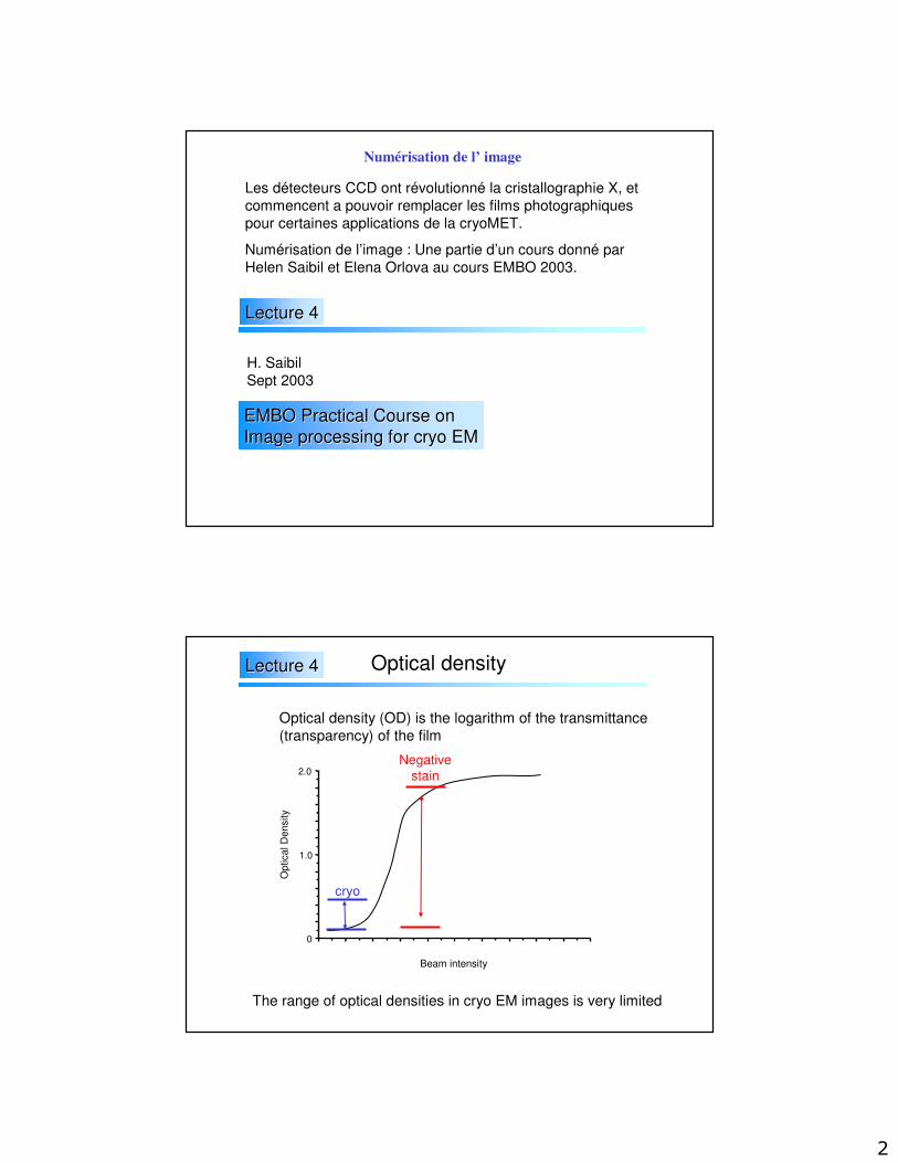
Optical density (OD) is the logarithm of the transmittance

(transparency) of the film

Optical density

The range of optical densities in cryo EM images is very limited

cryo

Negative

stain

Lecture 4Lecture 4

3

Spot scanning (Joyce-Loebl/Perkin Elmer) - incredibly slow and

accurate. Can do 5 µm, spot formed by microscope objective lens, transmittance measured relative to a reference beam. 8h to scan a

negative at high resolution. Isotropic in xy resolution - lens moved by

accurate stepper motors. Huge.

Drum – (Optronics, Heidelberg Tango) Optics good, mechanics not

as good, relatively quick, no reference beam

CCD – (Zeiss SCAI, Nikon Coolscan) Very quick and less accurate.

Patch or strip of CCD elements moves relative to film, resolution

different in x and y; some geometrical distortion; more noisy

measurement; amplitude loss at high resolution

Film scannersLecture 4Lecture 4

Zeiss SCAI

Nikon Coolscan

Lecture 4Lecture 4

4

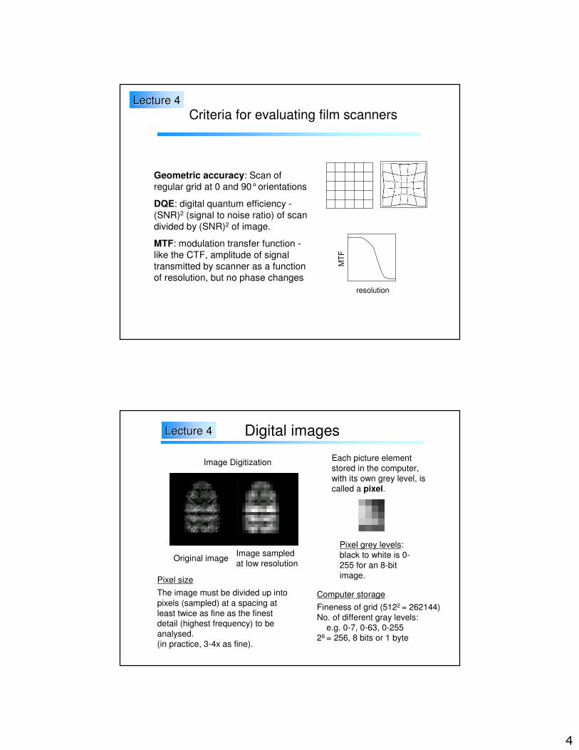
Geometric accuracy: Scan of

regular grid at 0 and 90°orientations

DQE: digital quantum efficiency -

(SNR)2 (signal to noise ratio) of scan

divided by (SNR)2 of image.

MTF: modulation transfer function -

like the CTF, amplitude of signal

transmitted by scanner as a function

of resolution, but no phase changes

Criteria for evaluating film scanners

resolution

MT

F

Lecture 4Lecture 4

Digital images

Image Digitization

Original imageImage sampled

at low resolution

Pixel grey levels:

black to white is 0-

255 for an 8-bit

image.

Computer storage

Fineness of grid (5122 = 262144)

No. of different gray levels:

e.g. 0-7, 0-63, 0-255

28 = 256, 8 bits or 1 byte

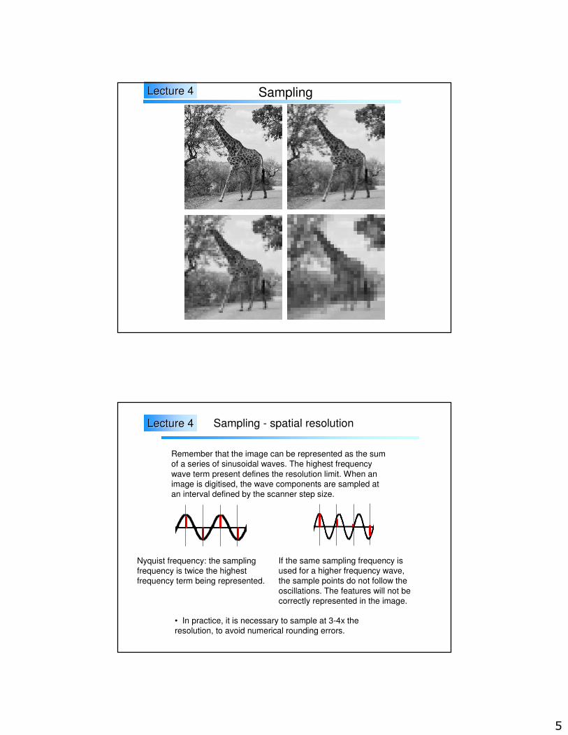
Pixel size

The image must be divided up into

pixels (sampled) at a spacing at

least twice as fine as the finest

detail (highest frequency) to be

analysed.

(in practice, 3-4x as fine).

Each picture element

stored in the computer,

with its own grey level, is

called a pixel.

Lecture 4Lecture 4

5

SamplingLecture 4Lecture 4

Sampling - spatial resolution

Nyquist frequency: the sampling

frequency is twice the highest

frequency term being represented.

If the same sampling frequency is

used for a higher frequency wave,

the sample points do not follow the

oscillations. The features will not be

correctly represented in the image.

Remember that the image can be represented as the sum

of a series of sinusoidal waves. The highest frequency

wave term present defines the resolution limit. When an

image is digitised, the wave components are sampled at

an interval defined by the scanner step size.

• In practice, it is necessary to sample at 3-4x the

resolution, to avoid numerical rounding errors.

Lecture 4Lecture 4

6

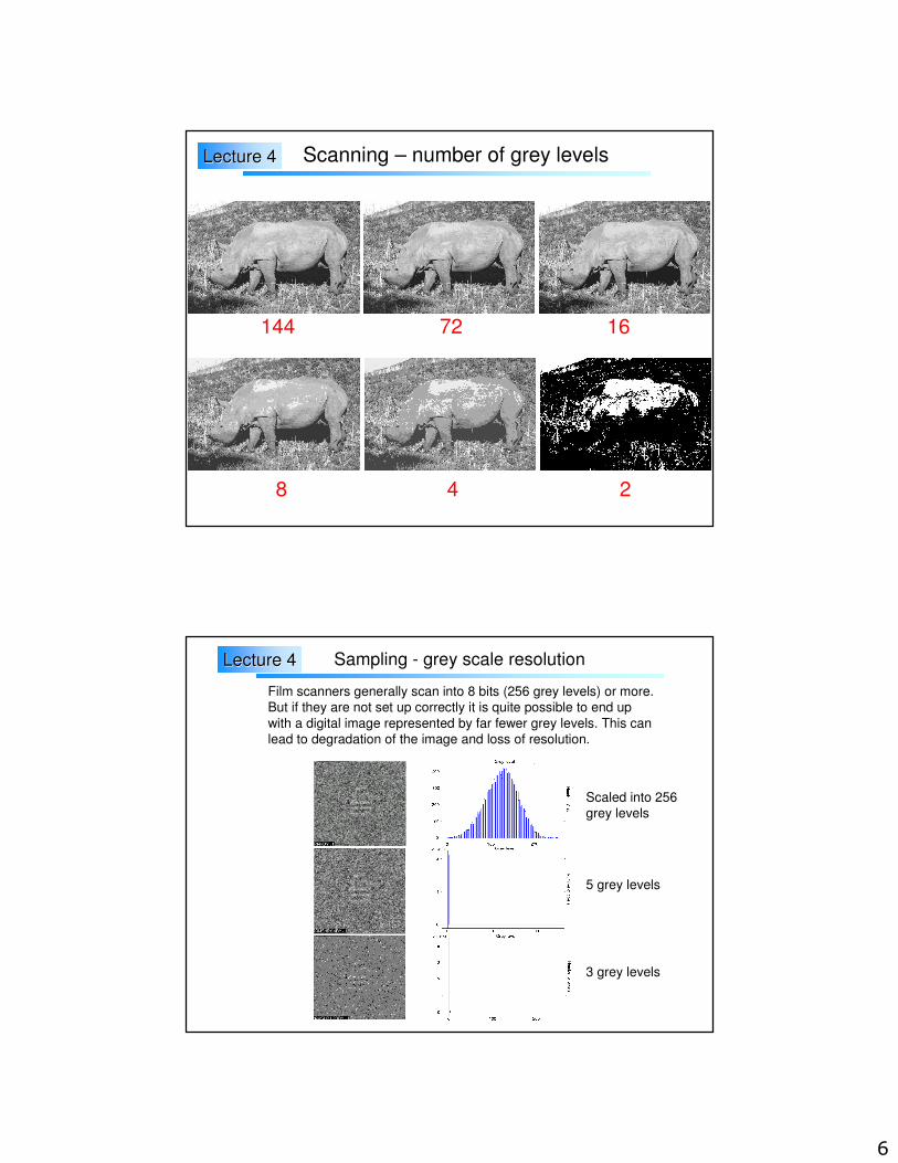
Scanning – number of grey levels

144 72 16

8 4 2

Lecture 4Lecture 4

Sampling - grey scale resolution

Film scanners generally scan into 8 bits (256 grey levels) or more.

But if they are not set up correctly it is quite possible to end up

with a digital image represented by far fewer grey levels. This can

lead to degradation of the image and loss of resolution.

Scaled into 256

grey levels

5 grey levels

3 grey levels

Lecture 4Lecture 4

7

Statistical noise in low electron dose images

Electron

beam

Photographic film

or detector

Random pattern

of incident

electrons

108 90 103

102 95 114

94 105 89

1025 1007 980

967 984 1016

1010 1046 964

N = 100 electrons

per unit areaN = 1000 electrons

per unit area

electron dose = average (N) ± √N

√N / N = 10% √N / N = 3.3%

The signal to noise ratio improves by a factor of √N as the electron dose increases. However, for beam-sensitive specimens the dose must be

kept low to avoid radiation damage to the specimen. Electrons can

transfer energy to the specimen, breaking bonds and causing mass loss

in biological molecules. For analysis, we assume that the image is the

sum of the structure information plus random noise.

Lecture 4Lecture 4

Noise reduction by averaging

Averages of 2 5 10 25 200 images

Raw

images

Lecture 4Lecture 4

8

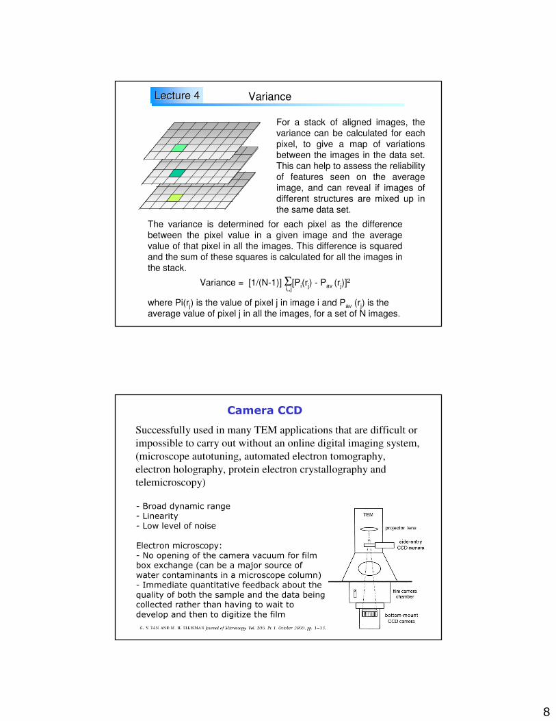
Variance

For a stack of aligned images, the

variance can be calculated for each

pixel, to give a map of variations

between the images in the data set.

This can help to assess the reliability

of features seen on the average

image, and can reveal if images of

different structures are mixed up in

the same data set.

The variance is determined for each pixel as the difference

between the pixel value in a given image and the average

value of that pixel in all the images. This difference is squared

and the sum of these squares is calculated for all the images in

the stack.

Variance = [1/(N-1)] Σ[Pi(rj) - Pav (rj)]2

where Pi(rj) is the value of pixel j in image i and Pav (rj) is the

average value of pixel j in all the images, for a set of N images.

i,,j

Lecture 4Lecture 4

Camera CCD

Successfully used in many TEM applications that are difficult or

impossible to carry out without an online digital imaging system,

(microscope autotuning, automated electron tomography,

electron holography, protein electron crystallography and

telemicroscopy)

- Broad dynamic range- Linearity- Low level of noise

Electron microscopy:- No opening of the camera vacuum for film box exchange (can be a major source of water contaminants in a microscope column)- Immediate quantitative feedback about the quality of both the sample and the data being collected rather than having to wait todevelop and then to digitize the film

9

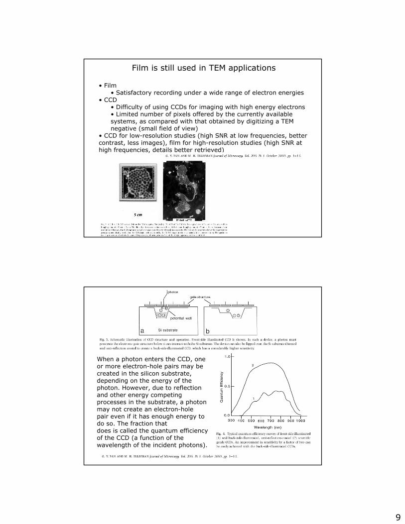
Film is still used in TEM applications

• Film• Satisfactory recording under a wide range of electron energies

• CCD• Difficulty of using CCDs for imaging with high energy electrons• Limited number of pixels offered by the currently available systems, as compared with that obtained by digitizing a TEM negative (small field of view)

• CCD for low-resolution studies (high SNR at low frequencies, better contrast, less images), film for high-resolution studies (high SNR at high frequencies, details better retrieved)

When a photon enters the CCD, one or more electron-hole pairs may be created in the silicon substrate, depending on the energy of the photon. However, due to reflection and other energy competing processes in the substrate, a photon may not create an electron-holepair even if it has enough energy to do so. The fraction thatdoes is called the quantum efficiency of the CCD (a function of the wavelength of the incident photons).

10

Electron-hole pairs are also created in CCDs due to thermal excitations, causing dark noise in the CCD. Dark noise accumulates with time, but can be reduced by cooling the CCD. Dark noise reduces by 50% for every ~7°C drop in temperature in silicon. At -30°C, dark noise can be reduced to a level of a few electron-hole pairs per pixel per second in a CCD.

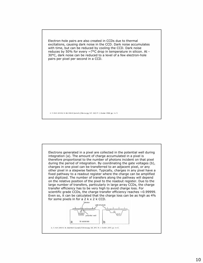
Electrons generated in a pixel are collected in the potential well during integration (a). The amount of charge accumulated in a pixel is therefore proportional to the number of photons incident on that pixel during the period of integration. By coordinating the gate voltages (b), charges in one pixel can be transferred to an adjacent pixel, or any other pixel in a stepwise fashion. Typically, charges in any pixel have a fixed pathway to a readout register where the charge can be amplified and digitized. The number of transfers along the pathway will depend on the relative position of the pixel to the readout register. Due to the large number of transfers, particularly in large array CCDs, the charge transfer efficiency has to be very high to avoid charge loss. For scientific grade CCDs, the charge transfer efficiency reaches ~0.99999. Even so, it can be calculated that the charge loss can be as high as 4% for some pixels in for a 2 k x 2 k CCD.

11

As ionizing particles, electrons with enough energy can also create electron-hole pairs in a CCD. Thus, CCDs can also be used for direct electron imaging. However, one incident electron generally creates too many electron-hole pairs in a CCD given the energy range typically involved in TEM. For example, a 100 keV electron will create in the order of 27 k electron-hole pairs in silicon. A 24 µm x 24 µm CCD pixel can have a full well capacity as high as ~500 k well electrons, whereas a 15 µm x 15 µm pixel has only about 80 k. Therefore, direct detection would result in an imaging system with a very high sensitivity but a very low dynamic range (e.g., a saturation level of 45 incident electrons at 100 keV (Roberts et al., 1982)). At higher electron energies, the dynamic range will be even lower. More importantly, the radiation damage to the CCD by the energetic electrons is a serious problem even at 100 keV. CCD imaging characteristics change markedly as a function of cumulative electron dose on the CCD (Roberts et al., 1982).

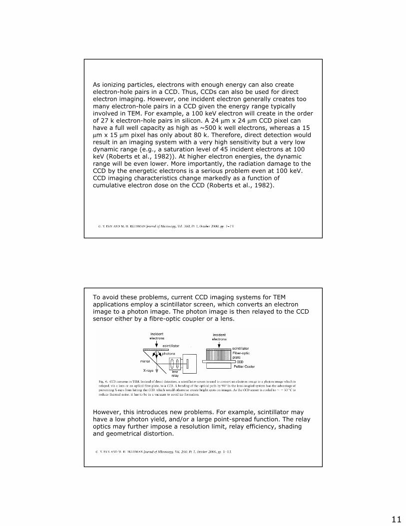
To avoid these problems, current CCD imaging systems for TEM applications employ a scintillator screen, which converts an electron image to a photon image. The photon image is then relayed to the CCD sensor either by a fibre-optic coupler or a lens.

However, this introduces new problems. For example, scintillator may have a low photon yield, and/or a large point-spread function. The relay optics may further impose a resolution limit, relay efficiency, shading and geometrical distortion.

12

At present, the resolution of a CCD imaging system for TEM is limited to a large degree by the scintillator screen used. As expected, the dimension of the point-spread function increases drastically with electron energy. Even at 100 keV, the diameter of the point-spread function is in the order of 50 µm, whereas the pixel size of large format CCDs useful for electron microscopy is 24 µm or smaller. This means that the point spread function of the scintillator will cover several CCD pixels, therefore reducing the effective array size of the CCD. For example, a 1 k x 1 k CCD may only provide 500 x 500 independent pixels. The situation worsens rapidly with increasing energies.

Two remedies are apparent for this large point-spread function problem: (1) using a thinner scintillator screen, and (2) using a reducing optical relay. Both, however, lower the sensitivity of the imaging system.

CCD camera characterization

Parameters : resolution, sensitivity, linearity, dynamic range, detection quantum efficiency (DQE) and fixed-pattern noise. Some of these are interdependent, and it is possible and sometimes practiced to improve one at the expense of others.

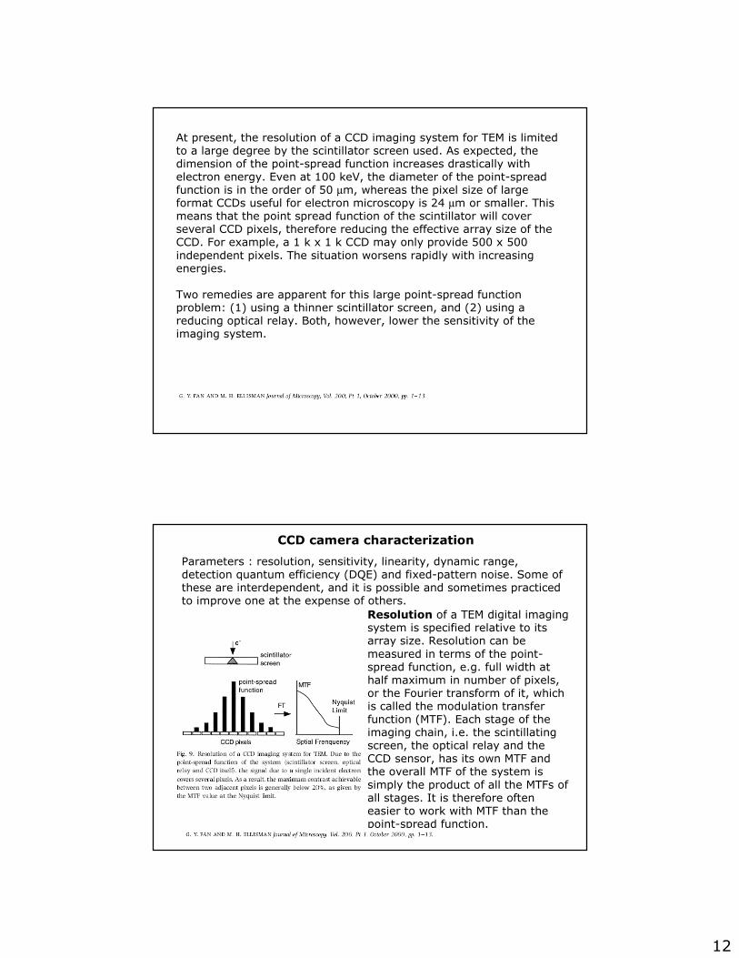
Resolution of a TEM digital imaging system is specified relative to its array size. Resolution can be measured in terms of the point-spread function, e.g. full width at half maximum in number of pixels, or the Fourier transform of it, which is called the modulation transfer function (MTF). Each stage of the imaging chain, i.e. the scintillating screen, the optical relay and the CCD sensor, has its own MTF and the overall MTF of the system is simply the product of all the MTFs of all stages. It is therefore often easier to work with MTF than the point-spread function.

13

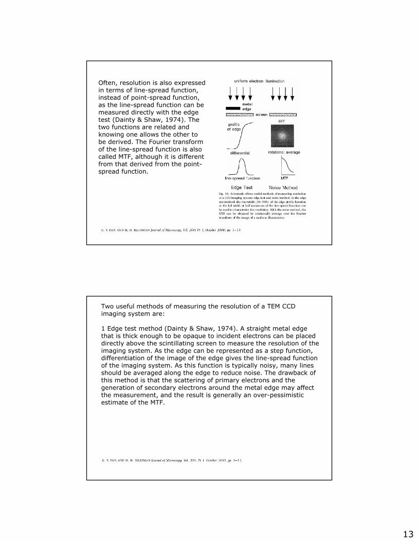
Often, resolution is also expressed in terms of line-spread function, instead of point-spread function, as the line-spread function can be measured directly with the edge test (Dainty & Shaw, 1974). The two functions are related and knowing one allows the other to be derived. The Fourier transform of the line-spread function is also called MTF, although it is different from that derived from the point-spread function.

Two useful methods of measuring the resolution of a TEM CCD imaging system are:

1 Edge test method (Dainty & Shaw, 1974). A straight metal edge that is thick enough to be opaque to incident electrons can be placed directly above the scintillating screen to measure the resolution of the imaging system. As the edge can be represented as a step function, differentiation of the image of the edge gives the line-spread function of the imaging system. As this function is typically noisy, many lines should be averaged along the edge to reduce noise. The drawback of this method is that the scattering of primary electrons and the generation of secondary electrons around the metal edge may affect the measurement, and the result is generally an over-pessimistic estimate of the MTF.

14

2. Noise method (Rabbani et al., 1987; De Ruijter & Weiss,1992). This method is based on the Fourier analysis of images of a uniform electron illumination. Due to the fluctuation of the number of electrons landing on a pixel, a uniform illumination actually represents a white noise input, which has a constant power spectrum over all Fourier frequencies. This constant spectrum will be attenuated by the MTF of the imaging system, so the Fourier transform of the image of a uniform illumination gives the MTF of the system. Because no special set-up or specimen is required to perform the measurement, this method is very easy to perform and can be done at any time. However, the accuracy of this method is influenced by the stochastic scattering of electrons in the scintillating screen, and the random generation and further scattering of photons in the scintillating screen. These random processes add noise to the image. As the added noise contains all Fourier frequencies, including high spatial frequencies, this method tends to give an over-optimistic estimate of the MTF. Simulations indicate that the discrepancy is smaller for scintillator screens that do not have a support substrate, such as a thin-foil screen (Fan et al., 1994).

Sensitivity: This is the minimum detectable signal in terms of thenumber of incident electrons.

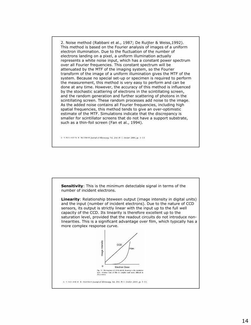
Linearity: Relationship bteween output (image intensity in digital units) and the input (number of incident electrons). Due to the nature of CCD sensors, its output is strictly linear with the input up to the full well capacity of the CCD. Its linearity is therefore excellent up to the saturation level, provided that the readout circuits do not introduce non-linearities. This is a significant advantage over film, which typically has amore complex response curve.

15

Dynamic range : The ratio of the saturation level over the noise floor.

Detection quantum efficiency (DQE) : DQE characterizes the noise performance of an imaging system, and is defined as (Herrmann & Krahl, 1982):

where (SNR)o and (SNR)i are the signal-to-noise ratio at the output and input, respectively.

Supposing one incident electron causes a pixel intensity increase, on the average, of g digital units, which can be greater or smaller than 1. Witha uniform electron illumination, the average number of electrons per pixel, N, can be calculated from the image mean, M, by

and for a Poisson process:

The standard deviation (σ) of the image can also be measured, so (SNR)o can be calculated easily:

This gives:

16

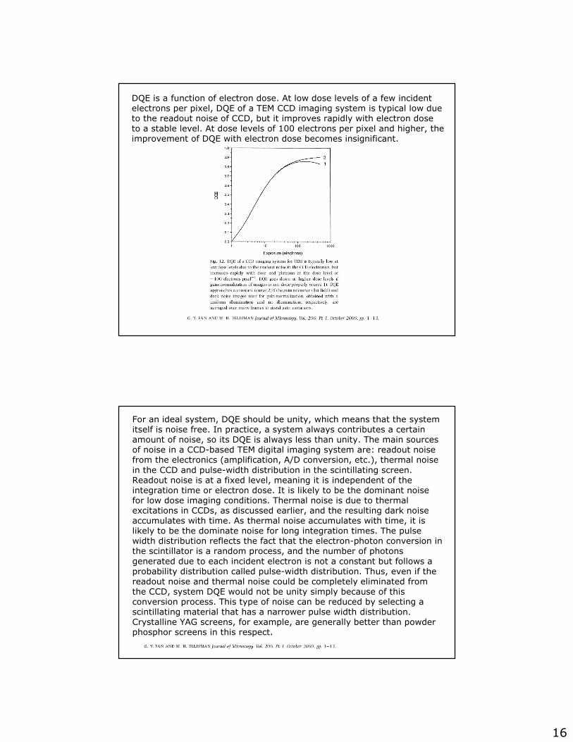
DQE is a function of electron dose. At low dose levels of a few incident electrons per pixel, DQE of a TEM CCD imaging system is typical low due to the readout noise of CCD, but it improves rapidly with electron dose to a stable level. At dose levels of 100 electrons per pixel and higher, the improvement of DQE with electron dose becomes insignificant.

For an ideal system, DQE should be unity, which means that the system itself is noise free. In practice, a system always contributes a certain amount of noise, so its DQE is always less than unity. The main sources of noise in a CCD-based TEM digital imaging system are: readout noisefrom the electronics (amplification, A/D conversion, etc.), thermal noise in the CCD and pulse-width distribution in the scintillating screen. Readout noise is at a fixed level, meaning it is independent of the integration time or electron dose. It is likely to be the dominant noise for low dose imaging conditions. Thermal noise is due to thermalexcitations in CCDs, as discussed earlier, and the resulting dark noise accumulates with time. As thermal noise accumulates with time, it is likely to be the dominate noise for long integration times. The pulse width distribution reflects the fact that the electron-photon conversion in the scintillator is a random process, and the number of photons generated due to each incident electron is not a constant but follows a probability distribution called pulse-width distribution. Thus, even if the readout noise and thermal noise could be completely eliminated from the CCD, system DQE would not be unity simply because of this conversion process. This type of noise can be reduced by selecting a scintillating material that has a narrower pulse width distribution. Crystalline YAG screens, for example, are generally better than powder phosphor screens in this respect.

17

Fixed-pattern noise:

Another unique aspect of large format CCD imaging systems is that, owing to the large number of pixels contained in a CCD sensor, some defects are unavoidable even in the highest grade CCDs. These defects include individual or groups of pixels having an abnormal response, i.e. they may have a higher level of dark noise, or may be brighter or dimmer than the rest of the pixels under a uniform illumination. These give rise to a fixed-patternnoise in an image. In addition, the non-uniformity in the scintillatorscreen, defects in the fibre-optic coupler (which often form chicken-wire patterns) or vignetting of the lens relay also contribute to the fixed-pattern noise. Fortunately, this problem can be very effectively corrected by a simple gain-normalization procedure.

This involves acquiring a dark noise image (with no illumination), denoted by D, and an image of a uniform illumination, denoted byG, which are used as the gain reference (sometimes called flat-field). Then a raw image, denoted by Ir, can be gain-normalized toyield the correct image, denoted by I, by applying a pixel-wiseoperation given by:

where C is a constant and should be set to be the mean of (G - D) to preserve image intensity. To avoid fluctuations in the dark noise image and in the gain reference, both D and G should be averagedover many frames before using. Not doing so will degrade the DQEof the system, particularly at high electron dose (Ishizuka, 1993).

18

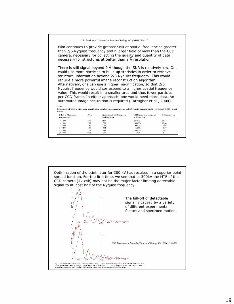
SNR of the CCD data is better than the SNR of the photographic film data at low spatial frequencies. At 2/5 Nyquist frequency the SNR between the two datasets is equivalent and at higher spatial frequencies the SNR of film data is better than the SNR of CCD data. The analysis showed the same trend regardless of defocus values or microscope magnification.

MTF shows the same behavior for different dosages, ranging from 450 to 1500 counts/pixel corresponding to a specimen dose, ~9–30 electrons/A², typically used for imaging ice embedded single particles.

A 9 Å single particle reconstruction from 4kx4k CCD captured images on a 200 kV electron cryomicroscope (the first time that a structure of a non-crystalline sample was determined at sub-nanometer resolution using CCD camera)

19

Film continues to provide greater SNR at spatial frequencies greater than 2/5 Nyquist frequency and a larger field of view than the CCD camera, necessary for collecting the quality and quantity of data necessary for structures at better than 9 Å resolution.

There is still signal beyond 9 Å though the SNR is relatively low. One could use more particles to build up statistics in order to retrieve structural information beyond 2/5 Nyquist frequency. This would require a more powerful image reconstruction algorithm. Alternatively, one can use a higher magnification, so that 2/5 Nyquist frequency would correspond to a higher spatial frequency value. This would result in a smaller area and thus fewer particles per CCD frame. In either approach, one would need more data. An automated image acquisition is required (Carragher et al., 2004).

Optimization of the scintillator for 300 kV has resulted in a superior point spread function. For the first time, we see that at 300kV the MTF of the CCD camera (4k x4k) may not be the major factor limiting detectable signal to at least half of the Nyquist frequency.

The fall-off of detectablesignal is caused by a variety of different experimental factors and specimen motion.

20

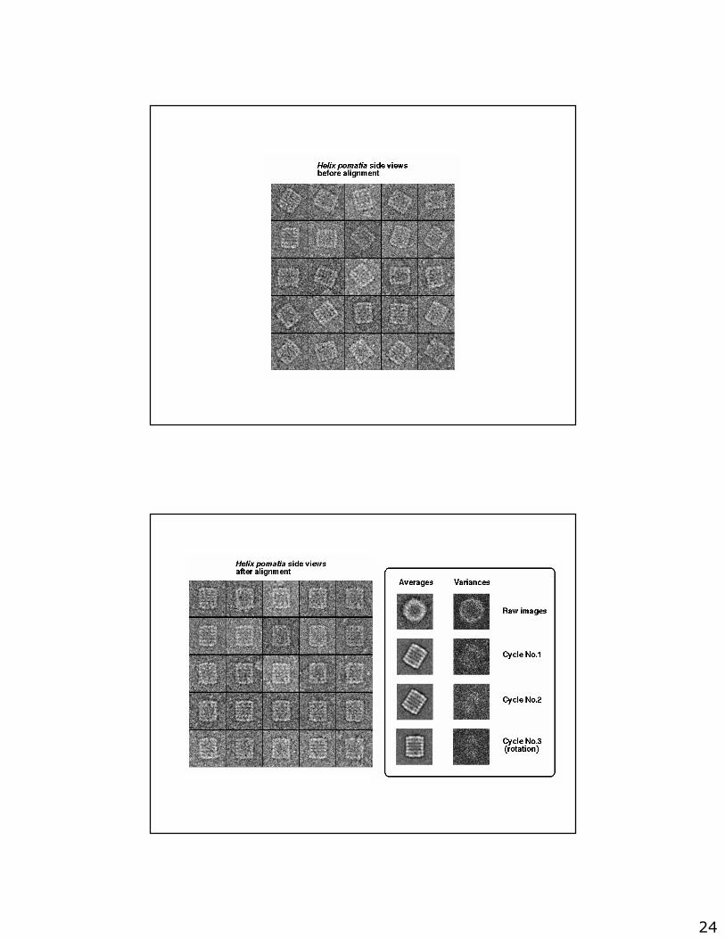
Sélection des particules (Helix pomatia)

Normalisation du contraste

Soustraction de la moyenne et division par l’écart type

21

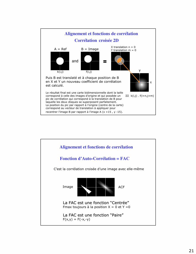
Alignement et fonctions de corrélation

Corrélation croisée 2D

A = Ref B = Image

and =

Puis B est translaté et à chaque position de B en X et Y un nouveau coefficient de corrélation est calculé.

Le résultat final est une carte bidimensionnelle dont la taille correspond à celle des images d’origine et qui possède un pic de corrélation qui correspond à la translation de B pour laquelle les deux disques se superposent parfaitement.La position du pic par rapport à l’origine (centre de la carte)correspond au vecteur de translation à appliquer pourrecentrer l’image B par rapport à l’image A (x +15 , y -15).

y

X

ΣΣ k(i,j) . f(i+n,j+m)

k(i,j) f(i,j)

X translation n = 0 Y translation m = 0

Alignement et fonctions de corrélation

Fonction d’Auto-Corrélation = FAC

C’est la corrélation croisée d’une image avec elle-même

Image ACF

La FAC est une fonction La FAC est une fonction ““CentrCentrééee””Fmax toujours à la position X = 0 et Y =0

La FAC est une fonction La FAC est une fonction ““PairePaire””F(x,y) = F(-x,-y)

22

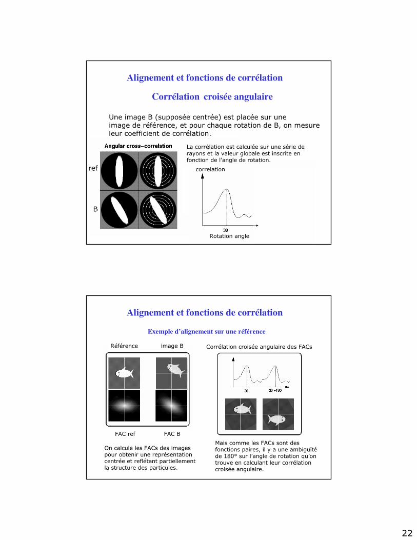
Corrélation croisée angulaire

Une image B (supposée centrée) est placée sur une image de référence, et pour chaque rotation de B, on mesureleur coefficient de corrélation.

Alignement et fonctions de corrélation

ref

B

Rotation angle

correlation

La corrélation est calculée sur une série de rayons et la valeur globale est inscrite en fonction de l’angle de rotation.

Exemple d’alignement sur une référence

Référence image B

FAC ref FAC B

Corrélation croisée angulaire des FACs

Mais comme les FACs sont des fonctions paires, il y a une ambiguïtéde 180° sur l’angle de rotation qu’on trouve en calculant leur corrélation croisée angulaire.

On calcule les FACs des imagespour obtenir une représentation centrée et reflétant partiellementla structure des particules.

Alignement et fonctions de corrélation

23

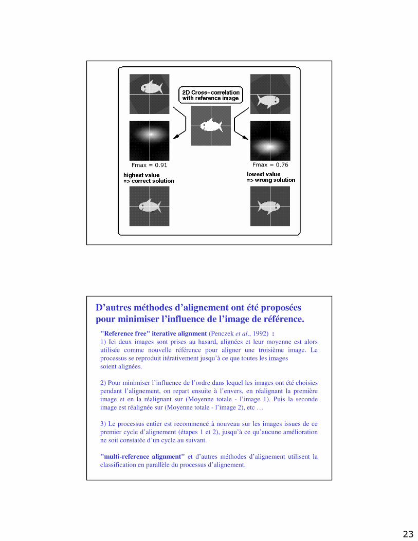
Fmax = 0.91 Fmax = 0.76

D’autres méthodes d’alignement ont été proposées

pour minimiser l’influence de l’image de référence.

"Reference free" iterative alignment (Penczek et al., 1992) :

1) Ici deux images sont prises au hasard, alignées et leur moyenne est alors

utilisée comme nouvelle référence pour aligner une troisième image. Le

processus se reproduit itérativement jusqu’à ce que toutes les images

soient alignées.

2) Pour minimiser l’influence de l’ordre dans lequel les images ont été choisies

pendant l’alignement, on repart ensuite à l’envers, en réalignant la première

image et en la réalignant sur (Moyenne totale - l’image 1). Puis la seconde

image est réalignée sur (Moyenne totale - l’image 2), etc …

3) Le processus entier est recommencé à nouveau sur les images issues de ce

premier cycle d’alignement (étapes 1 et 2), jusqu’à ce qu’aucune amélioration

ne soit constatée d’un cycle au suivant.

"multi-reference alignment" et d’autres méthodes d’alignement utilisent la

classification en parallèle du processus d’alignement.

24

25

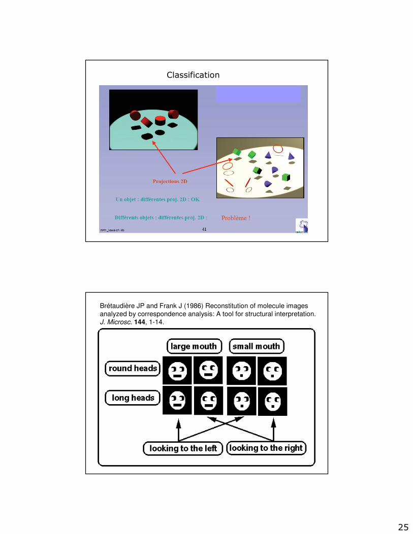
Classification

Brétaudière JP and Frank J (1986) Reconstitution of molecule images

analyzed by correspondence analysis: A tool for structural interpretation.

J. Microsc. 144, 1-14.

26

Image No1

Image No80

Pixel 1 Pixel 2754

x ij

27

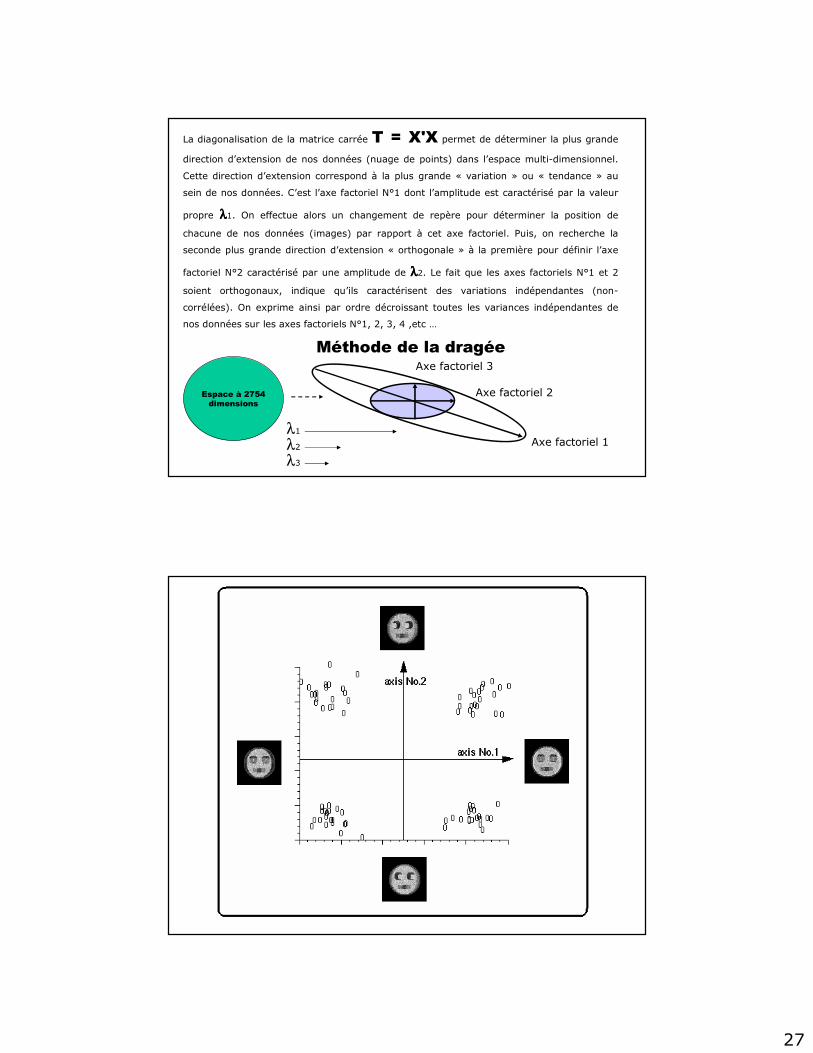
Méthode de la dragée

Espace à 2754

dimensions

λ2

λ3

λ1Axe factoriel 1

Axe factoriel 2

Axe factoriel 3

La diagonalisation de la matrice carrée T = X'X permet de déterminer la plus grande

direction d’extension de nos données (nuage de points) dans l’espace multi-dimensionnel.

Cette direction d’extension correspond à la plus grande « variation » ou « tendance » au

sein de nos données. C’est l’axe factoriel N°1 dont l’amplitude est caractérisé par la valeur

propre λλλλ1. On effectue alors un changement de repère pour déterminer la position de

chacune de nos données (images) par rapport à cet axe factoriel. Puis, on recherche la

seconde plus grande direction d’extension « orthogonale » à la première pour définir l’axe

factoriel N°2 caractérisé par une amplitude de λλλλ2. Le fait que les axes factoriels N°1 et 2

soient orthogonaux, indique qu’ils caractérisent des variations indépendantes (non-

corrélées). On exprime ainsi par ordre décroissant toutes les variances indépendantes de

nos données sur les axes factoriels N°1, 2, 3, 4 ,etc …

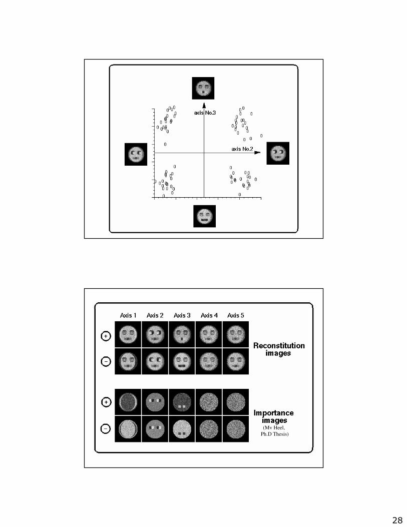
28

(Mv Heel,

Ph.D Thesis)

29

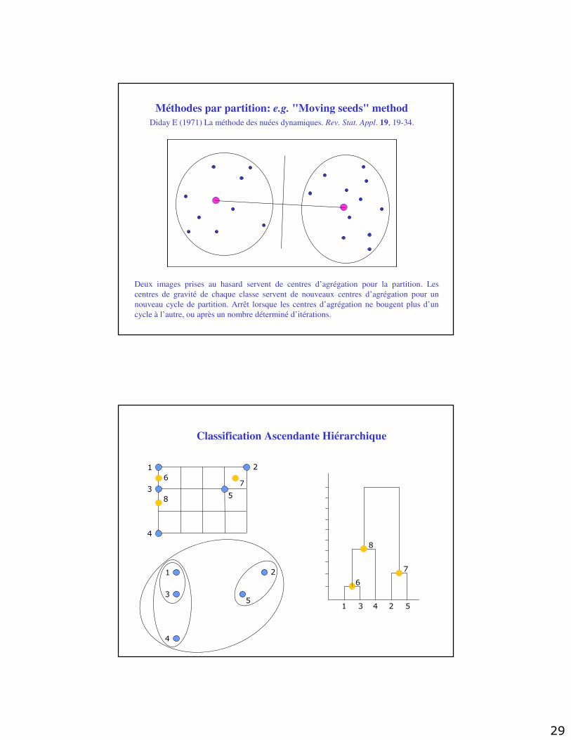
Méthodes par partition: e.g. "Moving seeds" method

Diday E (1971) La méthode des nuées dynamiques. Rev. Stat. Appl. 19, 19-34.

Deux images prises au hasard servent de centres d’agrégation pour la partition. Les

centres de gravité de chaque classe servent de nouveaux centres d’agrégation pour un

nouveau cycle de partition. Arrêt lorsque les centres d’agrégation ne bougent plus d’un

cycle à l’autre, ou après un nombre déterminé d’itérations.

Classification Ascendante Hiérarchique

1 2

3

4

5

1 2

3

4

51 3

6

6

52

7

7

4

8

8

30

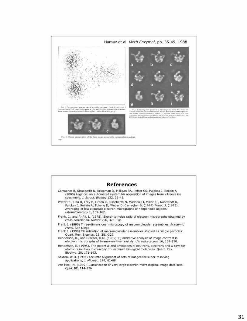
Harauz et al. Meth Enzymol, pp. 35-49, 1988

Hétérogénéité

31

Harauz et al. Meth Enzymol, pp. 35-49, 1988

ReferencesCarragher B, Kisseberth N, Kriegman D, Milligan RA, Potter CS, Pulokas J, Reilein A

(2000) Leginon: an automated system for acquisition of images from vitreous ice specimens. J. Struct. Biology 132, 33-45.

Potter CS, Chu H, Frey B, Green C, Kisseberth N, Madden TJ, Miller KL, Nahrstedt K, Pulokas J, Reilein A, Tcheng D, Weber D, Carragher B. (1999) Frank, J. (1975). Averaging of low exposure electron micrographs of nonperiodic objects. Ultramicroscopy 1, 159-162.

Frank, J., and Al-Ali, L. (1975). Signal-to-noise ratio of electron micrographs obtained by cross-correlation. Nature 256, 376-378.

Frank J. (1996) Three-dimensional microscopy of macromolecular assemblies. Academic Press, San Diego.

Frank J. (1990) Classification of macromolecular assemblies studied as 'single particles'. Quart. Rev. Biophys. 23, 281-329.

Henderson, R., and Glaeser, R.M. (1985). Quantitative analysis of image contrast in electron micrographs of beam-sensitive crystals. Ultramicroscopy 16, 139-150.

Henderson, R. (1995). The potential and limitations of neutrons, electrons and X-rays for atomic resolution microscopy of unstained biological molecules. Quart. Rev. Biophys. 28, 171-193.

Saxton, W.O. (1994) Accurate alignment of sets of images for super-resolving applications, J. Microsc. 174, 61-68.

van Heel, M. (1989). Classification of very large electron microscopical image data sets. Optik 82, 114-126