LABORATOIRE

INFORMATIQUE, SIGNAUX ET SYSTÈMESDE SOPHIA ANTIPOLIS

UMR 6070

PENALIZED AND RESPONSE-ADAPTIVE OPTIMAL DESIGNS

WITH APPLICATION TO DOSE-FINDING

Luc Pronzato

Equipe SYSTEMES

Rapport de rechercheISRN I3S/RR–2008-16–FR

Septembre2008

Laboratoire d’Informatique de Signaux et Systèmes de Sophia Antipolis - UNSA-CNRS2000, rte.des Lucioles – Les Algorithmes – Bât Euclide B – B.P. 121 – 06903 Sophia-Antipolis Cedex – France

Tél.: 33 (0)4 92 94 27 01 – Fax: 33 (0)4 92 94 28 98 – www.i3s.unice.frUMR6070

RÉSUMÉ :On considère la planifcation adaptative d’une expérience optimale avec une contrainte de coût, en régression nonlinéaire et

pour un modèle de type Bernoulli, avec une application aux essais cliniques. La convergence forte et la normalité asymptotiquedes estimateurs est démontrée pour une planification sur un domaine expérimental fini, lorsque le coût moyen est imposé (etle plan d’expérience converge vers le plan optimum sous contrainte de coût) et lorsque l’objectif est de minimiser le coût. Unexemple avec un modèle binaire bivarié est présenté.

MOTS CLÉS:Plans d’expériences adaptatifs; Plans d’expériences optimaux; Planification d’expériences pénalisée; Planification d’expériences

avec contraintes; Essais cliniques; Modèle binaire bivarié; Convergence; Normalité asymptotique

ABSTRACT:Adaptive optimal design with a cost constraint is considered, both for nonlinear regression and Bernoulli type experiments,

with application in clinical trials. The strong consistency and asymptotic normality of the estimators is proved for designs overa finite space, both when the cost level is fixed, and the adaptive design converges to an optimum constrained design, and whenthe objective is to minimize the cost. An example with a bivariate binary model is given.

KEY WORDS :Adaptive design; Optimal experimental design; Penalized experimental design; Constrained experimental design; Dose find-

ing; Bivariate binary model; Consistency; Asymptotic normality

Penalized and response-adaptive optimal designs

with application to dose-finding∗

Luc Pronzato

Laboratoire I3S, CNRS/Universite de Nice-Sophia Antipolis

Bat Euclide, Les Algorithmes

2000 route des lucioles, BP 121

06903 Sophia Antipolis cedex, France

pronzato@i3s.unice.fr

September 8, 2008

Abstract Adaptive optimal design with a cost constraint is considered, both for nonlinear regression

and Bernoulli type experiments, with application in clinical trials. The strong consistency and asymptotic

normality of the estimators is proved for designs over a finite space, both when the cost level is fixed, and

the adaptive design converges to an optimum constrained design, and when the objective is to minimize

the cost. An example with a bivariate binary model is given.

Key words: Adaptive design; Optimal experimental design; Penalized experimental design; Con-

strained experimental design; Dose finding; Bivariate binary model; Consistency; Asymptotic normality∗This work was partly accomplished while the author was invited at the Isaac Newton Institute for Mathematical

Sciences, Cambridge, UK. The support of the Newton Institute and of CNRS are gratefully acknowledged.

1

1 Introduction and motivations

In the papers [5, 6] the authors make a stimulating step towards a clear formalization of the necessary

compromise between individual and collective ethics in experimental design for dose-finding studies. The

idea is to use a penalty function that accounts for poor efficacy and for toxicity, and to construct a

penalized D-optimal design (or cost-constrained D-optimal design, the cost being defined through the

penalty function, see [9, Chap. 4]). Using a parametric model for the dose/efficacy-toxicity responses

(Gumbel or Cox model as in [5] or a bivariate probit model as in [6]), the Fisher information matrix

can be calculated and optimal designs can be obtained through (now standard) algorithmic methods.

This shows a neat advantage over more standard approaches. Indeed, D-optimal design alone (and its

extensions to Bayesian, minimax and adaptive variants) favors collective ethics in the sense that future

patients will benefit from the information collected in the trials, but it neglects individual ethics in the

sense that the patients enroled in the trials may receive doses with low efficacy or high toxicity. In

contrast, dose-finding approaches based on up-and-down [20] or bandit methods [14] focuss on individual

ethics by determining the best dose associated with some predefined criterion (e.g., the probability of

efficacy and no toxicity) but may result in a poor learning from the trial and thus in poorly adapted

dosage regimen for future individuals. By a suitable tuning of the penalty function, the approach used in

[5, 6] makes a clear compromise between the efficient treatment of individuals in the trial (by preventing

the use of doses with low efficacy or high toxicity) and the precise estimation of the model parameters

(accompanied with measures of statistical accuracy), to be used for making efficient decisions for future

treatments. As such, it has a great potential in combining traditional phase I and phase II clinical trials

into a single one, thereby accelerating the drug development process.

The aim of the present paper is to build on this approach and improve it in two directions.

First, the penalized optimal design problem formulated in [5, 6] does not allow flexibility in setting

the balance between the information gained (in terms of precision of parameter estimation) and the cost

of the experiment (in terms of poor success for the patients enroled in the trial). Here we shall promote

another formulation for optimal design under a cost constraint, for which a scalar tuning parameter

2

sets the compromise between information and cost. We show that, for suitable penalty functions, by

increasing the weight set on the penalty one guarantees that all doses in the experiment have a small cost

(and concentrate around the optimal dose when this one is unique). This permits to avoid the extreme

doses generally suggested by experimental design for parameter estimation.

Second, whereas [5, 6] advocate the use of adaptive experimental design, the convergence of the

procedure (strong consistency of the estimator of the model parameters and convergence of the design

to the optimal one) is left as an open issue. This difficulty is usually overcome by considering an initial

experiment (non adaptive) that grows in size when the total number of observations increases. Although

this number is often severely limited in practise, we think it would be reassuring to know that for a given

initial experiment, adaptive design guarantees suitable asymptotic convergence properties. Using simple

arguments, we show that this is indeed the case when the design space is finite, which forms a rather

natural assumption in the context of clinical trials. Our results concern penalized D-optimal design

but also cover the case, more classical, of fully adaptive D-optimal design. The asymptotic distribution

of the parameter estimator is shown to be normal, with variance-covariance matrix given by inverse of

the usual information matrix, similarly to the non-adaptive case. Moreover, we show that, for suitable

penalty functions, when the weight given to the cost for bad treatment increases with the number of

patients enroled, the doses allocated converge to the optimal one while the parameters are still estimated

consistently.

The results presented are of rather general applicability and, although this work has been motivated

by considerations in the context of clinical trials, we show that they also cover the case of least-squares

estimation in nonlinear regression models, for which there exist even less consistency results than for

maximum likelihood estimation when the design is adaptive. In particular, the results of Sect. 3 and 4

form a major improvement over those in [26] where only linear regression models were considered.

Penalized optimal design for a fixed value of the model parameters (locally optimal design) is consid-

ered in Sect. 2. We show in particular that a scalar penalty coefficient can be used to make a suitable

compromise between learning (gaining information) and optimization (targeting the optimal dose), and

3

eventually force the design points to concentrate around the optimal one. Adaptive penalized D-optimal

design is introduced at the end of this section, its asymptotic properties are investigated in the rest of

the paper under the assumption that the design space is finite. Sect. 3 concerns the case where the

penalty coefficient is bounded. We show that when both the design and the coefficient are adapted to the

current estimated value of the model parameters, one guarantees the strong consistency and asymptotic

normality of the parameter estimator and the strong convergence of the design to the optimal one. Both

least-squares estimation in nonlinear regression and maximum-likelihood estimation in Bernoulli-type

experiments are considered. In Sect. 4, the penalty coefficient is allowed to grow to infinity. We show

that when the increase is not too fast, the strong consistency and asymptotic normality of the parameter

estimator are preserved, while at the same time the design asymptotically concentrates around points of

minimum cost. Some simulation results with a bivariate dose-response model are presented in Sect. 5.

Finally, Sect. 6 concludes and suggests several directions for further developments. The proofs of lemmas

and theorems are collected in an Appendix.

2 Penalized D-optimal design

2.1 Models, designs and constraints

Let X , a compact subset of Rd, denote the admissible domain for the experimental variables x (design

points) and θ ∈ Rp denote the (p-dimensional) vector of parameter of interest in a parametric model

generating the log-likelihood l(Y, x; θ) for the observation Y at the design point x. We shall always

suppose that θ ∈ Θ, a compact subset of Rp. For N independent observations Y = (Y1, . . . , YN ) at

X = (x1, . . . , xN ) the log-likelihood at θ is l(Y,X; θ) =∑N

i=1 l(Yi, xi; θ). Let M(X, θ) denote the

corresponding Fisher information matrix,

M(X, θ) = −IEθ

∂2l(Y,X; θ)

∂θ∂θ>

=

N∑

i=1

µ(xi, θ) .

4

When N(xi) denotes the number of observations made at x = xi, we get the following normalized

information matrix per observation

M(ξ, θ) =1N

M(X, θ) =K∑

i=1

N(xi)N

µ(xi, θ) ,

where K is the number of distinct design points and ξ is the design measure (a probability measure on

X ) that puts mass N(xi)/N at xi. Following the usual approximate design approach, we shall relax the

constraints on design measures and consider ξ as any element of Ξ, the set of probability measures on X ,

so that

M(ξ, θ) =∫

Xµ(x, θ) ξ(dx) .

In a regression model with independent and homoscedastic observations satisfying IEθ(Y |x, θ) =

η(x, θ), with η(x, θ) differentiable with respect to θ for any x, we have

µ(x, θ) = I ∂η(x, θ)∂θ

∂η(x, θ)∂θ>

(1)

with I =∫

[ϕ′(t)/ϕ(t)]2 ϕ(t) dt the Fisher information for location, where ϕ(·) is the probability density

function of the observation errors and ϕ′(·) its derivative.

In a dose-response problem with single response Y ∈ 0, 1 (efficacy or toxicity response at the dose

x for instance) and ProbY = 1|x, θ = π(x, θ) we have

l(Y, x; θ) = Y log[π(x, θ)] + (1− Y ) log[1− π(x, θ)] (2)

so that, assuming π(x, θ) differentiable with respect to θ for any x,

µ(x, θ) =∂π(x, θ)

∂θ

∂π(x, θ)∂θ>

1π(x, θ)[1− π(x, θ)]

. (3)

Bivariate extensions, where both efficacy and toxicity responses are observed at a dose x, are considered

in [5] (Gumbel and Cox models) and [6] (bivariate probit model). See also Example 2 below and Sect. 5.

Besides a few additional technical difficulties, the main difference with the single response case is the fact

that µ(x, θ) may have rank larger than one, so that less than p support points in ξ may suffice to estimate

θ consistently. The same situation occurs for regression models when dim(η) > 1 so that (1) may have

rank larger than one. We shall always assume that µ(x, θ) is bounded on X .

5

In its now traditional form, local optimal design consists in determining a measure ξ∗ that maximizes

a concave function Ψ(·) of the Fisher information matrix M(ξ, θ) for a given value of θ. We assume that

Ψ(·) is monotone for the Loewner ordering (therefore, Ψ(aM) is a non-decreasing function of a ∈ R+

for any non-negative definite matrix M) and shall pay special attention to local D-optimal design, for

which Ψ(M) = log detM. The extension to other global optimality criteria, such as [trace(M−1)]−1

for instance, can be obtained by following a similar route. The denomination ‘local’ in local optimal

design comes from the fact that in nonlinear situations M(ξ, θ) depends on θ and the optimal design

thus depends on the value θ that is chosen. Extensions to minimax and Bayesian (or average optimal

designs) are also considered in [6] (see also [23, 8, 29, 30, 1]). A natural and widely used approach to

face the problem of dependency into the unknown value of θ is adaptive design. In its simplest form

(one-step adaptive locally optimal) the design points x1, x2 . . . , xN , xN+1, . . . associated with a sequence

of observations are chosen sequentially, the determination of the point xN+1 being based on the value

θN estimated from the N previous observations. The asymptotic properties of estimators and designs

obtained via this procedure will be investigated in Sect. 3 and 4.

In many circumstances, besides the optimality criterion ψ(ξ) = Ψ[M(ξ, θ)], it is desirable to introduce

a constraint of the form Φ(ξ, θ) ≤ C for the design measure. In dose-finding problems, the introduction of

such a constraint allows one to take individual ethical concerns into account. For instance, when both the

efficacy and toxicity responses are observed, one can relate Φ(ξ, θ) to the probability of success (efficacy

and no toxicity) for a given dose, as done in [5, 6]. See also Example 2. We suppose that the cost function

Φ(ξ, θ) is linear in ξ, that is

Φ(ξ, θ) =∫

Xφ(x, θ) ξ(dx) ,

and that φ(x, θ) is bounded on X . The extension to nonlinear constraints is considered, e.g., in [4] and [9,

Chap. 4]. Also, we shall restrict our attention to the case where a single — scalar — constraint is present,

some of the issues caused by the presence of several constraints are addressed in the same references. See

also Sect. 6. Matrices are denoted by bold capital letters and we denote by ‖A‖ the usual norm of A,

‖A‖ = [trace(A>A)]1/2 = (∑

i,jA2i,j)1/2.

6

2.2 Two equivalent formulations for maximizing information per cost-unit

Suppose that φ(x, θ) > 0 for all x ∈ X . The approach used in [5, 6] formulates the problem as follows.

Problem P1(θ): maximize the total information for N observations, that is, maximize Ψ[NM(ξ, θ)]

with respect to N and ξ ∈ Ξ satisfying the total cost constraint

NΦ(ξ, θ) = N

∫

Xφ(x, θ) ξ(dx) ≤ C .

For any ξ, the optimal value of N is N∗(ξ) = C/Φ(ξ, θ) so that an optimal measure ξ∗ ∈ Ξ for P1(θ)

maximizes Ψ(C M(ξ, θ)/Φ(ξ, θ)].

Denote now ν = Nξ, which is a mesure on X not normalized to 1; we have∫X ν(dx) = N which

becomes a free variable. P1(θ) is then equivalent to the maximization of Ψ[M(ν, θ)] under the constraint

Φ(ν, θ) ≤ C. The constraint is saturated at the optimum, i.e. Φ(ν∗, θ) = C, which we can thus set as an

active constraint. Imposing Φ(ν, θ) = C and defining ξ′(dx) = ν(dx)φ(x, θ)/C we obtain∫X ξ′(dx) = 1

and

M(ν, θ) =∫

Xµ(x, θ) ν(dx) =

∫

XC

µ(x, θ)φ(x, θ)

ξ′(dx) = M′(ξ′, θ) .

The constraint design problem P1(θ) is thus equivalent to a standard unconstrained one, with µ(x, θ)

simply replaced by C µ(x, θ)/φ(x, θ). Call P2(θ) this problem.

Problem P2(θ): maximize Ψ[M′(ξ, θ)] with respect to ξ ∈ Ξ.

The equivalence between P1(θ) and P2(θ) is further evidenced by considering the necessary and

sufficient conditions for optimality expressed by the Equivalence Theorem, see [19] for D-optimality and,

e.g., [31] for a general formulation. For P1(θ) with ψ(ξ) = log det[M(ξ, θ)/Φ(ξ, θ)], the measure ξ∗ is

optimal if and only if

∀x ∈ X , trace[µ(x, θ)M−1(ξ∗, θ)] ≤ pφ(x, θ)Φ(ξ∗, θ)

(4)

(note that the condition does not depend on the normalization constant∫X ξ∗(dx)). For P2(θ) with

7

ψ(ξ′) = log detM′(ξ′, θ), ξ′∗ is optimal in Ξ if and only if

∀x ∈ X , C trace[µ(x, θ)φ(x, θ)

M′−1(ξ′∗, θ)]≤ p (5)

(note that M′ is proportional to C which thus cancels out). The two conditions are equivalent: (5) can

be written as (4) by setting ξ∗(dx) = C ξ′∗(dx)/φ(x, θ).

One should note that the value of C plays no role in the definition of optimal designs for P1(θ),

P2(θ). For the dose-response problem considered in [5, 6] this has the important consequence that the

prohibition of excessively low (with poor efficacy) or high (with high toxicity) doses can only be obtained

by an ad-hoc modification of the penalty function φ(x, θ). Indeed, this is the only way to modify the

optimal design and hopefully to change its support. This can be contrasted with the solution of the

constrained design problem that we present in the next section and then consider in all the rest of the

paper.

2.3 Maximizing information per observation under a cost constraint

A direct formulation of the optimal design problem under constraint is as follows.

Problem P3(θ): maximize Ψ[M(ξ, θ)] with respect to ξ ∈ Ξ under the constraint Φ(ξ, θ) ≤ C.

We say that a design measure ξ ∈ Ξ is θ-admissible if Φ(ξ, θ) ≤ C and we suppose that a strictly

θ-admissible measure exists in Ξ (Φ(ξ, θ) < C for some ξ ∈ Ξ). A necessary and sufficient condition for

the optimality of a θ-admissible ξ∗ ∈ Ξ is the existence of λ∗ ≥ 0 such that λ∗ [C − Φ(ξ∗, θ)] = 0 with

ξ∗ = ξ∗(λ∗) maximizing the design criterion Lθ(ξ, λ∗) = Ψ[M(ξ, θ)] + λ∗ [C − Φ(ξ, θ)] (the Lagragian of

the problem) with respect to ξ ∈ Ξ. Moreover, the Lagrange coefficient λ∗ minimizes Lθ[ξ∗(λ), λ] with

respect to λ ∈ R+. When Ψ(·) = log det(·), the necessary and sufficient condition for the optimality of a

θ-admissible ξ∗ ∈ Ξ becomes

∃λ∗ ≥ 0 such that

λ∗ [C − Φ(ξ∗, θ)] = 0

∀x ∈ X , trace[µ(x, θ)M−1(ξ∗, θ)] ≤ p + λ∗ [φ(x, θ)− Φ(ξ∗, θ)] .

(6)

8

In practice, ξ∗ can be determined by maximizing

Hθ(ξ, λ) = Ψ[M(ξ, θ)]− λ Φ(ξ, θ) (7)

for an increasing sequence (λi) of Lagrange coefficients λ, starting at λ0 = 0 and stopping at the first

λi such that the associated optimal design ξ∗ satisfies Φ(ξ∗, θ) ≤ C, see, e.g., [24] (for C large enough,

the unconstrained optimal design for Ψ(·) is optimal for the constrained problem). The parameter λ

can thus be used to set the tradeoff between the maximization of Ψ[M(ξ, θ)] (gaining information) and

minimization of Φ(ξ, θ) (reducing cost). Notice that maximizing Hθ(ξ, λ) for λ ≥ 0 is equivalent to

maximizing (1− γ)Ψ[M(ξ, θ)] + γ [−Φ(ξ, θ)] with γ = λ/(1 + λ) ∈ [0, 1). Also, when Ψ(M) = log detM,

there is an obvious relation between the maximization of (7) and the solution of a problem in the form

P1(θ). Indeed, one can write Hθ(ξ, λ) = log det[M(ξ, θ)/Φ′(ξ, θ)] with Φ′(ξ, θ) = exp[(λ/p)Φ(ξ, θ)] (which,

however, is not linear in ξ).

Similarly to the case of unconstrained optimal design with a strictly concave criterion, the optimal

matrix M(ξ∗, θ) is unique when the function Ψ(·) is strictly concave on the set of positive definite matrices.

Indeed, suppose that there exist two optimal designs ξ∗1 , ξ∗2 in Ξ for P3(θ) such that M(ξ∗1 , θ) 6= M(ξ∗2 , θ).

The optimality of ξ∗1 and ξ∗2 implies Ψ[M(ξ∗1 , θ)] = Ψ[M(ξ∗2 , θ)] and Φ(ξ∗1 , θ) = Φ(ξ∗2 , θ) = C. Therefore

the Lagrange multipliers λ of both solutions coincide, see (6), and ξ∗1 , ξ∗2 maximize (7) for this λ, that is,

maxξ∈Ξ Hθ(ξ, λ) = Hθ(ξ∗1 , λ) = Hθ(ξ∗2 , λ). Take now any α in (0, 1) and consider ξ = (1−α)ξ∗1 +αξ∗2 ∈ Ξ.

From the strict concavity of Ψ(·) and the linearity in ξ of Φ(ξ, θ), we obtain Hθ(ξ, λ) > (1−α)Hθ(ξ∗1 , λ)+

α Hθ(ξ∗2 , λ) = Hθ(ξ∗1 , λ) = Hθ(ξ∗2 , λ), which contradicts the optimality of ξ∗1 , ξ∗2 . The optimal information

matrix is thus unique (but the optimal design measure ξ∗ is not necessarily).

Let ξ∗(λ) denote an optimal design for Hθ(ξ, λ) given by (7). One can easily check that both

ΨM[ξ∗(λ), θ] and Φ[ξ∗(λ), θ] are non-increasing functions of λ. Three questions (at least) naturally

arise concerning the tradeoff between maximization of Ψ[M(ξ, θ)] and minimization of Φ(ξ, θ).

• (i) How fast does the cost Φ(ξ, θ) decrease when λ increases?

• (ii) How big is the loss of information (decrease of Ψ[M(ξ, θ)]) when Φ(ξ, θ) decreases?

9

• (iii) Can we force the costs φ(xi, θ) to decrease for all support points xi of the optimal design ξ∗(λ)

by increasing λ?

Suppose that µ(x, θ) and φ(x, θ) are continuous in x ∈ X , with X a compact subset of Rd, and define

φ∗θ = minx∈X

φ(x, θ) , x∗ = x∗(θ) = arg minx∈X

φ(x, θ) . (8)

We do not assume for the moment that x∗ is unique (but at least one such point exists in X ). For any

ξ ∈ Ξ, we also define

∆θ(ξ) = Φ(ξ, θ)− φ∗θ .

Only the case of D-optimality is considered and we denote by ξ∗D a D-optimal design that maxi-

mizes log detM(ξ, θ) with respect to ξ ∈ Ξ. We assume that ∆θ(ξ∗D) > 0 (otherwise ξ∗D maximizes

log detM(ξ, θ)− λΦ(ξ, θ) for any λ ≥ 0) and that log detM(ξ∗D, θ) > 0 (otherwise M(ξ, θ) is singular for

any ξ ∈ Ξ). We then have the following results concerning the three questions above. The proof is given

in Appendix.

Proposition 1 Let ξ∗ = ξ∗(λ) be an optimal design that maximises Hθ(ξ, λ) given by (7) with respect

to ξ ∈ Ξ, with Ψ(M) = log detM. It satisfies

(i) ∆θ(ξ∗) ≤ p/λ;

(ii) for any ξ such that ∆θ(ξ) > 0, any a > 0 and any λ ≥ a/∆θ(ξ),

log detM(ξ∗, θ) ≥ log detM(ξ, θ) + p loga/[λ∆θ(ξ)] − a , (9)

moreover, λmin[M(ξ∗, θ)] > δ/(p + λ[φθ − φ∗θ]) for some positive constant δ, with φθ = maxx∈X φ(x, θ);

(iii) any support point x of ξ∗ satisfies

φ(x, θ)− φ∗θ ≤ 2∆θ(ξλ) trace[µ(x, θ)M−1(ξλ, θ)] , ∀ ξλ ∈ Ξ such that ∆θ(ξλ) ≥ p/λ . (10)

Property (i) shows the guaranteed cost-reduction obtained when λ is increased and (ii) shows that

λmin[M(ξ∗, θ)] decreases not faster than 1/λ. A similar property will be obtained in Sect. 4 for adap-

tive design with an increasing sequence of penalty coefficients λk; it is a central argument for obtaining

10

the strong consistency and asymptotic normality of estimators, see Theorem 4 and Corollary 2. No-

tice that taking ξ = ξ∗D in (9) ensures detM(ξ∗, θ) ≥ det[M(ξ∗D, θ) exp(−a/p)] for λ = a/∆θ(ξ∗D) and

log detM(ξ∗, θ) ≥ log detM(ξ∗D, θ) + p log[∆θ(ξ∗)/∆θ(ξ∗D)] for any λ ≥ 0 (take a = λ∆θ(ξ∗)).

Property (iii) shows that, for suitable penalty functions, the support of an optimal design for P3(θ)

depends on C or, equivalently, that the support of an optimal design for (7) depends on λ. When x∗ is

unique, (iii) implies that if

there exist designs ξλ ∈ Ξ such that ∆θ(ξλ) ≥ p/λ and

∀ε > 0 , lim supλ→∞

sup‖x−x∗‖>ε

2∆θ(ξλ) trace[µ(x, θ)M−1[ξλ, θ)]φ(x, θ)− φ∗θ

< 1 , (11)

then the supporting points of ξ∗ converge to x∗ as λ →∞. The choice of suitable designs ξλ is central for

testing if (11) is satisfied. Designs formed by points neighboring x∗ are good candidates, see Examples 1

and 2. Notice that, when rank[µ(x, θ)] < p, for (11) to be satisfied the ξλ’s must necessarily have support

points that approach x∗ as λ → ∞. Indeed, suppose that it is not the case. It means that there exists

γ > 0 such that, for all λ larger than some λ0, the support points x(i)λ of ξλ satisfy ‖x(i)

λ − x∗‖ > γ.

Replace X by X ′ = X \ B(x∗, γ) ∪ x∗, that is, remove the ball B(x∗, γ) = x : ‖x − x∗‖ ≤ γ from X

but keep x∗. Then, ξλ is a design measure on X ′ for λ > λ0 and (11) would indicate that the optimal

design ξ∗ on X ∗ is the delta measure δ∗x, which is impossible since the optimal information matrix must

have full rank. The same is true if the designs ξλ have one support point at x∗ and the others outside

the ball B(x∗, γ) for λ larger than some λ0. Finally, note that the support points of ξ∗(λ′) for λ′ > λ

must also satisfy (10) for the same ξλ (since ∆θ(ξλ) > p/λ′).

For dose-response problems, the property (11) has the important consequence that excessively high or

low doses can be prohibited by choosing C small enough or, equivalently, λ large enough. Its effectiveness

very much depends on the choice of the penalty function, and in particular on its local behavior around

x∗. Contrary to what intuition might suggest, it requires the cost function φ(·, θ) to be sufficiently flat

around x∗. Indeed, in that case a design ξ supported in the neighborhood of x∗ can at the same time have

a small cost Φ(ξ, θ) and be dispersed enough to carry significant information through log detM(ξ, θ). This

11

is illustrated by examples below. The first one is simple enough to make the optimal designs calculable

explicitly.

2.4 Examples

Example 1

We take

µ(x) =

1

x

x2

(1 x x2

)=

1 x x2

x x2 x3

x2 x3 x4

,

X = [−1, 1], Ψ(·) = log det(·) and consider different penalty functions φ(x), symmetric with respect to

x = 0 (nothing depends on θ in this example and we thus omit the dependence in θ in the notation). For

all cases considered, the optimal designs ξ∗ are symmetric and take the form

ξ∗ =

−z 0 z

1−α2 α 1−α

2

, (12)

where the first row gives the support points and the second their respective weights. This gives detM(ξ∗) =

α(1− α)2z6. The D-optimal design ξ∗D corresponds to z = 1 and α = 1/3.

For φ(x) = 1 + x2q, q integer, the optimal designs for problems P1 and P2 correspond to α =

minq/[3(q − 1)], 1/2 and z = min[3/(2q − 3)]1/2q, 1 (note that z < 1 only for q ≥ 4). The costs

φ(x) = 1+x2 +x4 and φ(x) = 1/(1−x2) respectively give the optimal designs defined by α = 3/5, z = 1

and α = 5/9, z =√

3/5.

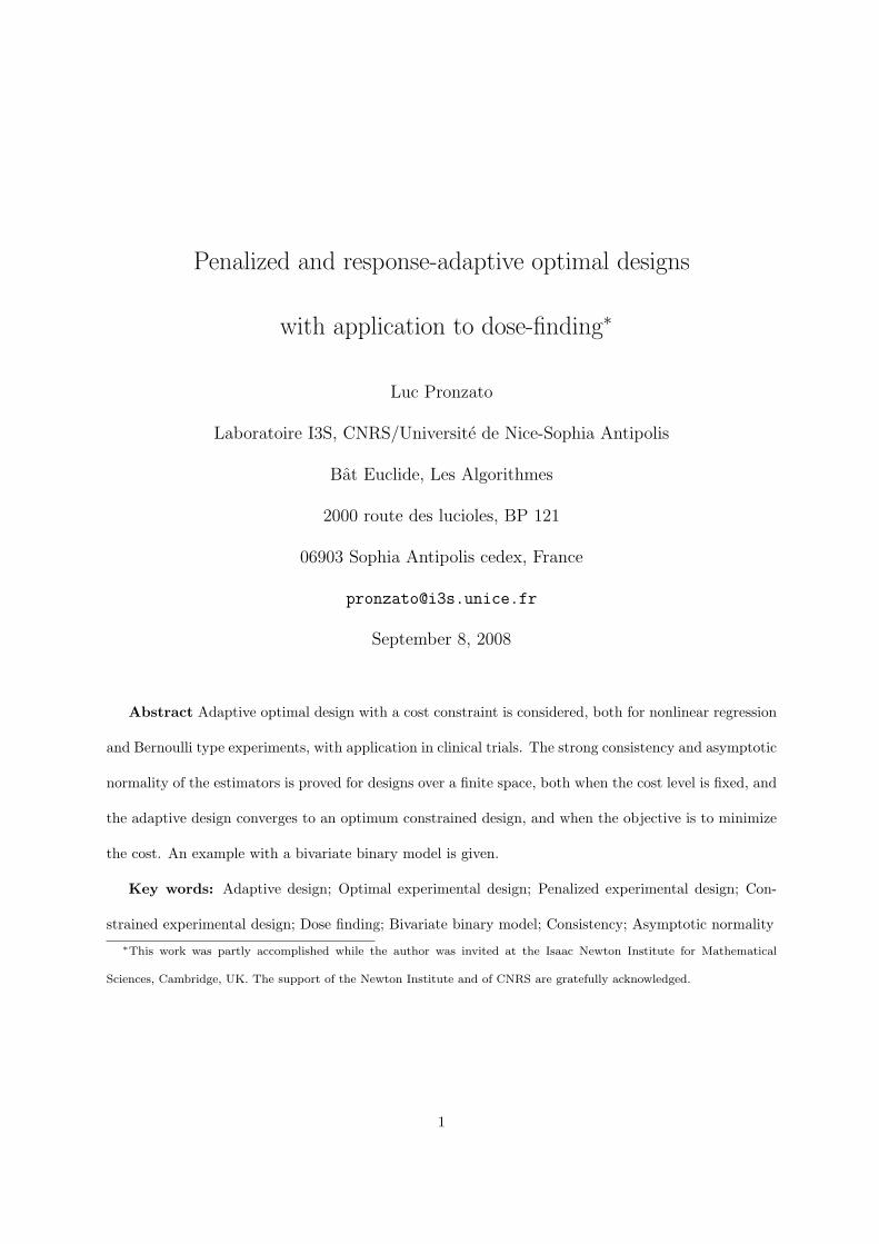
The optimal designs ξ∗ for P3 obtained for various choices for φ(·) are given in Table 1, together with

the optimal value λ∗(C) of the Lagrange coefficient associated with C. When there is no solution, it

means that λ∗(C) = ∞. When there is one, then Φ(ξ∗) = C.

In order to check if the support of ξ∗ concentrates around x∗ = 0 when λ increases (without computing

12

ξ∗), we use (10) with the design

ξλ = ξλ(γ) =

−γ 0 γ

1/3 1/3 1/3

.

For φ(x) = x2q we get ∆(ξλ) = 2γ2q/3 and (10) then gives x2q ≤ [4γ2q/3] trace[µ(x)M−1(ξλ)]. Noticing

that trace[µ(γ t)M−1(ξλ)] = P (t) = 3(1 − 3/2t2 + 3/2t4) independently of γ (a property of D-optimal

design for polynomial regression), we obtain that a support point x of ξ∗ must satisfy t2q ≤ 4P (t)/3, with

t = x/γ. For q = 3 we obtain t ≤ [1+(1+β1/3)2]1/2/β1/6 with β = 4+2√

2, that is t . 2.2252. For q = 4,

we get t ≤ √2. Since we need to have ∆(ξλ) ≥ p/λ = 3/λ, we take γ = [9/(2λ)]1/(2q) (which corresponds

to α = 1 and ξλ = ξλ in the proof of Proposition 1-(ii)). It gives x ≤ xmax with xmax ' 2.860 λ−1/6

for q = 3 and xmax =√

2[9/(2λ)]1/8 ' 1.707 λ−1/8 for q = 4. When q = 1, 2 all t are admissible and

xmax = ∞. We obtain in a similar way xmax = ∞ for φ(x) = 1 + x2 + x4.

Next case illustrates that it is the local behavior of φ(x) around the minimum x∗ that influences the

support of ξ∗ when λ tends to infinity. Take φ(x) = 1/(1 − x2), which tends to infinity for x tending

to ±1 but is equal to 1 + x2 + x4 + O(x6) around x∗ = 0. Condition (10) then writes φ(γt) − φ(0) =

γ2t2/(1 − γ2t2) ≤ 2∆(ξλ)P (t) = (4/3)γ2P (t)/(1 − γ2). The bound obtained for t now depends on γ;

the best bound (minimum) for x is xmax ' 0.9649, obtained at γ ' 0.7385, and ∆(ξλ) ≥ p/λ imposes

λ & 3.7516. Therefore, we only learn from (10) that the support of ξ∗ is included in [−0.9649, 0.9649]

for λ large enough. This is consistent with the behavior of the support points −z, z of ξ∗ as λ tends to

infinity, which do not converge to zero (limλ→∞ z = 1/√

3, see Table 1). ¤

Next example is taken from [5] and concerns a problem with bivariate binary responses.

Example 2 : Cox model for efficacy-toxicity response.

For Y (respectively Z) the binary indicator of efficiency (resp. of toxicity) at dose x for a model with

parameters θ, we write ProbY = y, Z = z|x, θ = πyz(x, θ), Y, y, Z, z ∈ 0, 1, with

π11(x, θ) =ea11+b11 x

1 + ea01+b01 x + ea10+b10 x + ea11+b11 x

π10(x, θ) =ea10+b10 x

1 + ea01+b01 x + ea10+b10 x + ea11+b11 x

13

φ(x) C λ∗(C) α z

1 + x2 5/3 ≤ C 0 1/3 1

1 < C ≤ 5/3 5−3C(C−1)(2−C) 2− C 1

C ≤ 1 ∞ — no solution —

1 + x4 5/3 ≤ C 0 1/3 1

4/3 ≤ C ≤ 5/3 5−3C(C−1)(2−C) 2− C 1

1 < C ≤ 4/3 3/[2(C − 1)] 2/3 [3(C − 1)]1/4

C ≤ 1 ∞ — no solution —

1 + x6 5/3 ≤ C 0 1/3 1

3/2 ≤ C ≤ 5/3 5−3C(C−1)(2−C) 2− C 1

1 < C ≤ 3/2 1/(C − 1) 1/2 [2(C − 1)]1/6

C ≤ 1 ∞ — no solution —

1 + x8 5/3 ≤ C 0 1/3 1

14/9 ≤ C ≤ 5/3 5−3C(C−1)(2−C) 2− C 1

1 < C ≤ 14/9 3/[4(C − 1)] 4/9 [9(C − 1)/5]1/8

C ≤ 1 ∞ — no solution —

1 + x2 + x4 7/3 ≤ C 0 1/3 1

1 < C ≤ 7/3 7−3C(C−1)(3−C) (3− C)/2 1

C ≤ 1 ∞ — no solution —

1/(1− x2) 1 < C 2C(C−1)

C3C−2

(3C−2)1/2

(3C)1/2

C ≤ 1 ∞ — no solution —

Table 1: Optimal designs ξ∗ for problem P3 in Example 1, see (12).14

π01(x, θ) =ea01+b01 x

1 + ea01+b01 x + ea10+b10 x + ea11+b11 x

π00(x, θ) =(1 + ea01+b01 x + ea10+b10 x + ea11+b11 x

)−1

and θ = (a11, b11, a10, b10, a01, b01)>. The log-likelihood function of a single observation (Y,Z) at dose

x is then l(Y, Z, x; θ) = Y Z log π11(x, θ) + Y (1 − Z) log π10(x, θ) + (1 − Y )Z log π01(x, θ) + (1 − Y )(1 −

Z) log π00(x, θ) and elementary calculations show that the contribution to the Fisher information matrix

is

µ(x, θ) =∂p>(x, θ)

∂θ

(P−1(x, θ) + [1− π11(x, θ)− π10(x, θ)− π01(x, θ)]−111>

) ∂p(x, θ)∂θ>

where p(x, θ) = [π11(x, θ), π10(x, θ), π01(x, θ)]>, P(x, θ) = diagp(x, θ) and 1 = (1, 1, 1)>. Note that

µ(x, θ) is generally of rank 3. As in [5], we take θ = (3, 3, 4, 2, 0, 1)> and X the finite set x(1), . . . , x(11)

where the doses x(i) are equally spaced in the interval [−3, 3]. We choose a cost function related to the

probability π10(x, θ) of efficacy and no toxicity and take

φ(x, θ) = π−110 (x, θ)− [max

xπ10(x, θ)]−12 . (13)

The Optimal Safe Dose (OSD) minimizing φ(x, θ), is x(5) = −0.6. Using the condition (10) with the

test designs ξλ,1, giving weights (1 − α)/2, α and (1 − α)/2 at x(4), x(5) and x(6) respectively, and ξλ,2,

giving weights 1− β and β at x(4) and x(5) respectively, we obtain that the support of ξ∗(λ) is included

in x(4), x(5), x(6) for α & 0.9993 and β & 0.4508, showing that the optimal designs concentrate on three

doses around the optimal one when λ is large enough. The D-optimal design (corresponding to λ = 0), is

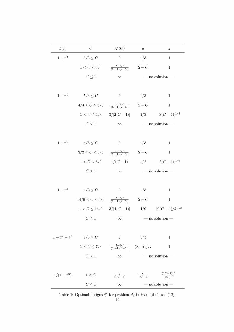
supported on x(1), x(4), x(5) and x(10), with associated weights 0.3318, 0.3721, 0.1259 and 0.1701. Figure

1 presents the optimal designs ξ∗(λ) for λ varying between 0 and 100 along the horizontal axis. The

weight associated with each x(i) on the vertical axis is proportional to the thickness of the plot.

The figure indicates that for λ & 75 the optimum designs are supported on x(4) and x(6) only, with

weights approximately 1/2 each, that is, all patients in the trial receive a dose close to the optimal one,

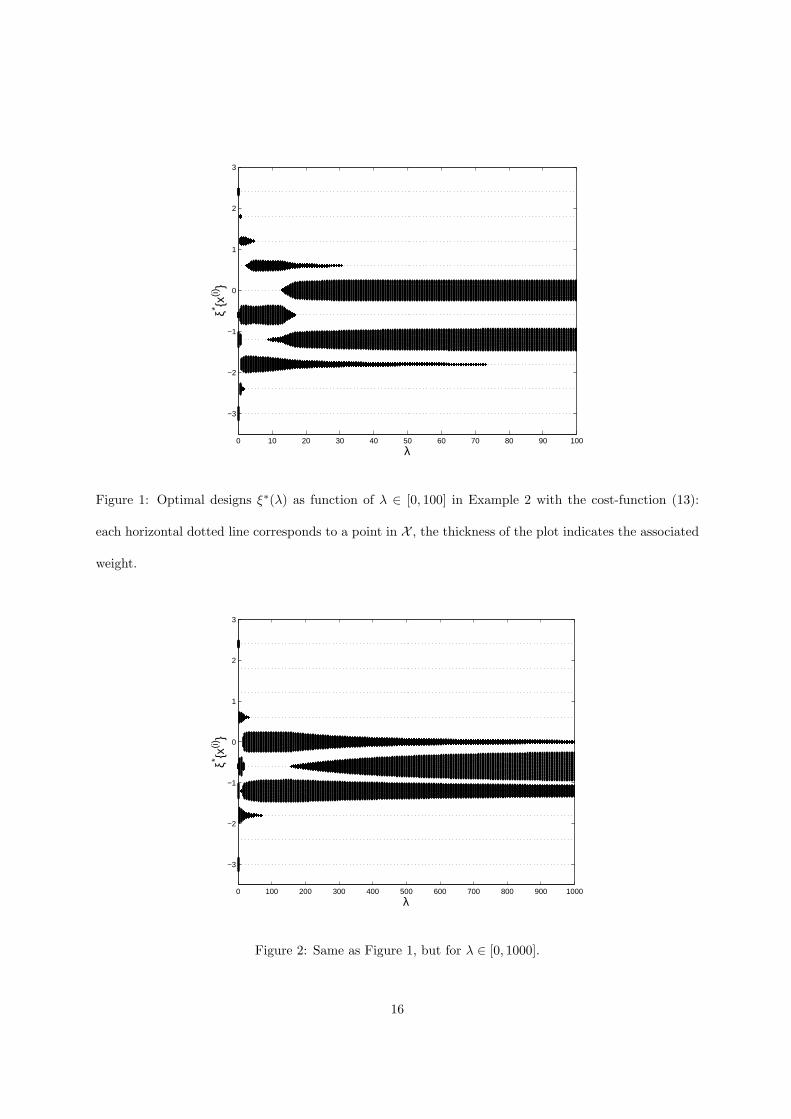
x(5). However, none receives the optimal dose. The situations changes for larger values of λ, see Figure

2 where the optimal design is supported on x(4), x(5), x(6) for λ & 160 and the weight of the optimal

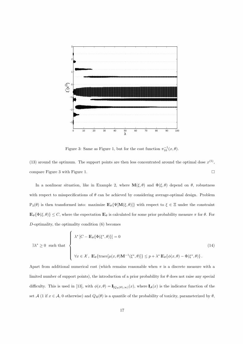
dose x(5) increases with λ. Consider now the cost function φ(x, θ) = π−110 (x, θ), which is less flat than

15

0 10 20 30 40 50 60 70 80 90 100

−3

−2

−1

0

1

2

3

λ

ξ* x(i)

Figure 1: Optimal designs ξ∗(λ) as function of λ ∈ [0, 100] in Example 2 with the cost-function (13):

each horizontal dotted line corresponds to a point in X , the thickness of the plot indicates the associated

weight.

0 100 200 300 400 500 600 700 800 900 1000

−3

−2

−1

0

1

2

3

λ

ξ* x(i)

Figure 2: Same as Figure 1, but for λ ∈ [0, 1000].

16

0 10 20 30 40 50 60 70 80 90 100

−3

−2

−1

0

1

2

3

λ

ξ* x(i)

Figure 3: Same as Figure 1, but for the cost function π−110 (x, θ).

(13) around the optimum. The support points are then less concentrated around the optimal dose x(5),

compare Figure 3 with Figure 1. ¤

In a nonlinear situation, like in Example 2, where M(ξ, θ) and Φ(ξ, θ) depend on θ, robustness

with respect to misspecifications of θ can be achieved by considering average-optimal design. Problem

P3(θ) is then transformed into: maximize IEθΨ[M(ξ, θ)] with respect to ξ ∈ Ξ under the constraint

IEθΦ(ξ, θ) ≤ C, where the expectation IEθ is calculated for some prior probability measure π for θ. For

D-optimality, the optimality condition (6) becomes

∃λ∗ ≥ 0 such that

λ∗ [C − IEθΦ(ξ∗, θ)] = 0

∀x ∈ X , IEθtrace[µ(x, θ)M−1(ξ∗, θ)] ≤ p + λ∗ IEθφ(x, θ)− Φ(ξ∗, θ) .

(14)

Apart from additional numerical cost (which remains reasonable when π is a discrete measure with a

limited number of support points), the introduction of a prior probability for θ does not raise any special

difficulty. This is used in [13], with φ(x, θ) = II[QR(θ),∞)(x), where IIA(x) is the indicator function of the

set A (1 if x ∈ A, 0 otherwise) and QR(θ) is a quantile of the probability of toxicity, parameterized by θ,

17

corresponding to the maximum acceptable probability of toxicity (note that IEθφ(x, θ) = πQR(θ) ≤ x,

the prior probability that x exceeds QR).

Another, rather common, approach for facing the issue of dependence of the optimum design in θ is

to design the experiment sequentially. By alternating between estimation based on previous observations

and determination of the next design point where to observe, one may hope that the empirical design

measure will progressively adapt to the correct (true) value of the model parameters. Adaptive design

is briefly introduced in the next section, the asymptotic properties of designs and estimators obtained in

this way are considered into details in the rest of the paper. An example (continuation of Example 2) is

presented in Sect. 5.

2.5 Adaptive penalized D-optimal design

In fully-adaptive D-optimal design, next design point after N observations is taken as

xN+1 = argmaxx∈X

trace[µ(x, θN )M−1(ξN , θN )] , (15)

where θN ∈ Θ ⊂ Rp is the current estimated value for θ (based on x1, Y1, . . . , xN , YN ) and ξN =

(1/N)∑N

i=1 δxi (with δz the delta measure that puts mass 1 at z) is the current empirical design measure

(leaving aside some initialisation issues: we simply assume that x1, . . . , xp are such that M(ξp, θ) is

nonsingular for any θ ∈ Θ). Note that (15) can only be considered as an algorithm for choosing design

points, in the sense that M(ξN , θ) is not the Fisher information matrix for parameters θ due to the

sequential construction of the design (we shall see, however, in Sect. 3 that when X is finite, from the

same repeated sampling principle as in [36], one can still use M(ξN , θ) to characterize the precision of

the estimation of θ as N →∞).

For constrained D-optimal design we take xN+1 as

xN+1 = arg maxx∈X

trace[µ(x, θN )M−1(ξN , θN )]− λN φ(x, θN )

. (16)

Since (15) can be considered as a special case of (16), only the latter will be considered in the following.

This means that the results in Sect. 3 also cover the case of classical (unconstrained) sequential D-

18

optimal design (15) for which λN = 0 for all N . This also includes the constrained problems P1(θ),

P2(θ) considered in [5, 6], which can be formulated as standard D-optimal design problems, see Sect. 2.2.

One can notice the similarity between (16) and the construction used in [26] for optimizing a parametric

function, the parameters of which being estimated by least-squares in a linear regression model.

When θN is frozen to a fixed value θ and λN is constant, the iterations (15) and (16) correspond to

one step of a steepest-ascent vertex-direction algorithm with step-length 1/N at step N . Convergence

to an optimal design measure is proved in [38] for iterations given by (15) and in [26] for (16) (using a

general argument developed in [37]).

The fact that θN is estimated in adaptive design makes the proof of convergence a much more compli-

cated issue for which few results are available: [10, 36, 25] concern a particular example with least-squares

estimation; [16] is specific of Bayesian estimation by posterior mean and does not use a fully sequential

design of the form (15); [21] and [3] require the introduction of a subsequence of non-adaptive design

points to ensure consistency of the estimator and [2] requires that the size of the initial experiment (non-

adaptive) grows with the increase in size of the total experiment. Intuitively, the almost sure convergence

of θN to some θ∞ would be enough to imply the convergence of ξN to an optimal design measure for θ∞

(this will be shown in Theorem 3) and, conversely, convergence of ξN to a design ξ∞ such that M(ξ∞, θ)

is non-singular for any θ would be enough in general to make an estimator consistent. It is thus the

interplay between estimation and design iterations (which implies that each design point depends on

previous observations) that creates difficulties. As shown in the next sections, those difficulties disappear

when X is a finite set (notice that the assumption that X is finite is seldom limitative since practical

considerations often impose such a restriction on possible choices for the design points; this can be con-

trasted with the much less natural assumption that would consist in considering the feasible parameter

set as finite).

Two situations will be considered concerning the choice of the sequence (λN ) in (16), respectively in

Sect. 3 and 4. In the first one, the objective is to obtain an optimal design for problem P3(θ). We shall

then adapt λN to θN and take λN = λ∗N = λ∗(θN ), the optimal Lagrange coefficient for P3(θN ). The

19

second situation corresponds to the case where (λN ) forms an increasing sequence, which gives more and

more importance to the constraint in the construction of the design. When φ(x, θ) has a single minimum,

by letting the Lagrange coefficient λN increase with N one may hope to be able to force the design to

concentrate at the minimizer of φ associated with the true value of θ (that is, for clinical trials, to focuss

more and more on individual ethics by allocating treatments with increasing efficiency).

The results presented in the next sections rely on simple arguments based on three ideas. First, the

sequence (θN ) in (16) is taken as any sequence of vectors in Θ. The asymptotic design properties obtained

within this framework will thus also apply when θN corresponds to some estimator of θ in Θ. Second,

when X is finite we obtain a lower bound on the sampling rate of a subset of points of X associated with

a nonsingular information matrix. Third, we show that this bound guarantees the strong consistency

of the estimator of θ, both for least-squares estimation in nonlinear regression and maximum-likelihood

estimation for Bernoulli trials. With a few additional technicalities, this yields almost sure convergence

results for the adaptive designs constructed via (16).

3 Asymptotic properties of adaptive design with bounded penalty

The results in this section and the next one apply to a wide range of situations and we try to keep the

presentation general enough. However, to avoid unnecessary complications we only treat the univariate

case where µ(x, θ) has rank one, and write

µ(x, θ) = fθ(x)f>θ (x)

with fθ(x) a p-dimensional vector, as it is the case in (1, 3). The extension to the multivariate case does

not raise particular difficulties. We shall use the following assumptions on the design space X , vector

f(x, θ), constraint function φ(x, θ) and Lagrange coefficients λN .

HX -(i): The design space X is finite, X = x(1), x(2), . . . , x(K).

HX -(ii): infθ∈Θ λmin

[∑Ki=1 fθ(x(i))f>θ (x(i))

]> γ > 0.

Hφ-(i): 0 ≤ φ(x, θ) < φ , ∀x ∈ X and θ ∈ Θ.

20

Hλ-(i): 0 ≤ λN < λ < ∞ , ∀N .

When λN = λ∗N = λ∗(θN ), the optimal Lagrange coefficient for problem P3(θN ), and θN ∈ Θ, the

following condition guarantees that Hλ-(i) is satisfied.

Hλ-(i’): There exists C ′ < C such that ∀θ ∈ Θ, ∃ξ(θ) ∈ Ξ with Φ[ξ(θ), θ] < C ′ and M[ξ(θ), θ] has full

rank.

We first obtain a lower bound on the sampling rate of nonsingular designs, which will be the cor-

nerstone for proving the consistency and asymptotic normality of estimators. The proof is given in

Appendix.

Lemma 1 Let (θN ) be an arbitrary sequence in Θ used to generate design points according to (16), with

an initialisation such that M(ξN , θ) is non-singular for all θ in Θ and all N ≥ p. Let rN,i = rN (x(i))

denote the number of times x(i) appears in the sequence x1, . . . , xN , i = 1, . . . , K, and consider the

associated order statistics rN,1:K ≥ rN,2:K ≥ · · · ≥ rN,K:K . Define

q∗ = maxj : there exists α > 0 such that lim infN→∞

rN,j:K/N > α .

Then, HX -(i), HX -(ii), Hφ-(i) and Hλ-(i) imply q∗ ≥ p. When the sequence (θN ) is random, the statement

holds with probability one.

3.1 Consistency of estimators

3.1.1 Least-squares estimation in nonlinear regression

Consider a regression model with observations

Yi = Y (xi) = η(xi, θ) + εi , (17)

with θ in the interior of Θ, a compact subset of Rp, xi ∈ X ⊂ Rd, and εi a sequence of independently

and identically distributed random variables with IEε1 = 0 and IEε21 = σ2 < ∞ (with σ = 1 without

loss of generality). We assume that the model response η(x, θ) is differentiable with respect to θ ∈ int(Θ)

for any x ∈ X .

21

Denote

SN (θ) =N∑

k=1

[Y (xk)− η(xk, θ)]2 (18)

and let θNLS = arg minθ∈Θ SN (θ) be the least-squares (LS) estimator of θ. The contribution of the design

point x to the information matrix is then µ(x, θ) = fθ(x) f>θ (x) with

fθ(x) =∂η(x, θ)

∂θ.

The results can easily be extended to non stationary errors and weighted least-squares. In the case of

maximum-likelihood estimation, the contribution of x to the Fisher information matrix only differs by a

multiplicative constant, see (1).

Define

DN (θ, θ) =N∑

k=1

[η(xk, θ)− η(xk, θ)]2 . (19)

Next theorem shows that the consistency of the LS estimator is a consequence of DN (θ, θ) tending to

infinity fast enough for ‖θ − θ‖ ≥ δ > 0. The fact that the design space X is finite makes the minimum

rate of increase of DN (θ, θ) required for consistency quite slow. The result is valid whether the xk’s are

non-random constants or are generated via a sequential design algorithm such as (16).

Theorem 1 Let (xi) be a non-random design sequence on a finite set X . If DN (θ, θ) given by (19)

satisfies

for all δ > 0 ,

[inf

‖θ−θ‖≥δDN (θ, θ)

]/(log log N) →∞ , N →∞ , (20)

then θNLS

a.s.→ θ as N →∞ (almost sure convergence). The result remains valid for (xi) a random sequence

on X finite when (20) holds almost surely.

The proof is given in [27] and is based on Lemma 1 in [35]. Note that the condition (20) is much

less restrictive than the classical one for strong consistency of LS estimation in nonlinear regression

(DN (θ, θ) = O(N) for θ 6= θ), see [18]. It is also less restrictive than the condition obtained in [21] for

sequential design.

Consider the following identifiability assumption on the regression model (17).

22

HX -(iii): For all δ > 0 there exists ε(δ) > 0 such that for any subset i1, . . . , ip of distinct elements

of 1, . . . , K,

inf‖θ−θ‖≥δ

p∑

j=1

[η(x(ij), θ)− η(x(ij), θ)]2 > ε(δ) .

For any sequence (θN ) used in (16), the conditions of Lemma 1 ensure the existence of N1 and α > 0

such that rN,j:K > αN for all N > N1 and all j = 1, . . . , p. Under the additional assumption HX -(iii)

we thus obtain that DN (θ, θ) given by (19) satisfies inf‖θ−θ‖≥δ DN (θ, θ) > αNε(δ), N > N1. Therefore,

θNLS

a.s.→ θ (N →∞) from Theorem 1. Since this holds for any sequence (θN ) in Θ, it is true in particular

when θNLS is substituted for θN in (16).

3.1.2 Maximum-likelihood estimation in Bernoulli trials

Consider now the case of dose-response experiments with

Y ∈ 0, 1 , with ProbY = 1|xi, θ = π(xi, θ) . (21)

We suppose that Θ is a compact subset of Rp, that θ, the ‘true’ value of θ that generates the observations,

lies in the interior of Θ, and that π(x, θ) ∈ (0, 1) for any θ ∈ Θ and x ∈ X . We also assume that π(x, θ)

is differentiable with respect to θ ∈ int(Θ) for any x ∈ X .

The log-likelihood for the observation Y at the design point x is given by (2) and the contribution of

the point x to the Fisher information matrix is (3), which we can write µ(x, θ) = fθ(x)f>θ (x) with

fθ(x) =1√

π(x, θ)[1− π(x, θ)]∂π(x, θ)

∂θ. (22)

Let θNML denote the Maximum-Likelihood (ML) estimator of θ, θN

ML = arg maxθ∈Θ LN (θ), with LN (θ) =

∑Ni=1 l(Yi, xi; θ), see (2). It satisfies the following.

Lemma 2 If for any δ > 0

lim infN→∞

inf‖θ−θ‖≥δ

[LN (θ)− LN (θ)] > 0 almost surely ,

then θNML

a.s.→ θ as N →∞.

23

The proof is identical to that of Lemma 1 in [35]. We then obtain a property similar to Theorem 1, see

[27].

Theorem 2 Let (xi) be a non-random design sequence on a finite set X . Assume that

DN (θ, θ) =N∑

i=1

π(xi, θ) log[π(xi, θ)π(xi, θ)

]+ [1− π(xi, θ)] log

[1− π(xi, θ)1− π(xi, θ)

](23)

satisfies (20). Then, θNML

a.s.→ θ as N → ∞ in the model (21). The same is true for (xi) a random

sequence such that (20) holds almost surely.

Consider the following identifiability assumption for the Bernoulli model.

HX -(iii’): For all δ > 0 there exists ε(δ) > 0 such that for any subset i1, . . . , ip of distinct elements

of 1, . . . , K,

inf‖θ−θ‖≥δ

p∑

j=1

[π(x(ij), θ)− π(x(ij), θ)

]2

> ε(δ) .

Defining g(a, b) = a log(a/b) + (1 − a) log[(1 − a)/(1 − b)], a, b ∈ (0, 1), we can easily check that, for

any fixed a ∈ (0, 1), g(a, b) > 2(a − b)2 with g(a, a) = 0, so that each term of the sum (23) is positive.

Also, HX -(iii’) implies that

inf‖θ−θ‖≥δ

p∑

j=1

π(x(ij), θ) log[π(x(ij), θ)π(x(ij), θ)

]+ [1− π(x(ij), θ)] log

[1− π(x(ij), θ)1− π(x(ij), θ)

]> ε(δ) > 0 .

for any δ > 0 and any subset i1, . . . , ip of 1, . . . , K. Similarly to the case of LS estimation in nonlinear

regression, but using now Theorem 2 instead of Theorem 1, we thus obtain that under the conditions of

Lemma 1 and with the additional assumption HX -(iii’) the ML estimator satisfies θNML

a.s.→ θ, N → ∞,

when θNML is substituted for θN in (16).

3.2 Asymptotic optimality of adaptive penalized D-optimal design

We consider the adaptive design algorithm (16) with λN = λ∗N = λ∗(θN ), the optimal Lagrange coefficient

for P3(θN ). Define

H ∗θ = max

ξ∈Ξ

log detM(ξ, θ) + λ∗(θ) [C − Φ(ξ, θ)]

. (24)

24

By asymptotic optimality we mean that the empirical design measure ξN is such that θN a.s.→ θ and

Hθ(ξN ) = log detM(ξN , θ) + λ∗(θ) [C − Φ(ξN , θ)] a.s.→ H ∗θ , N →∞ . (25)

Since M(ξ∗, θ) is unique, see Sect. 2.3, (25) is equivalent to M(ξN , θ) a.s.→ M[ξ∗(θ), θ], N → ∞, that

is, ξN tends to be optimal for P3(θ). We state this property below as a theorem (the proof is given in

Appendix). The following assumptions are used.

HX -(iv): For any subset i1, . . . , ip of distinct elements of 1, . . . ,K,

λmin

p∑

j=1

fθ(x(ij))f >θ (x(ij))

≥ γ > 0 .

Hf -(i): For all x in X , fθ(x) is a continuous function of θ in the interior of Θ.

Hφ-(ii): For all x in X , φ(x, θ) is a continuous function of θ in the interior of Θ.

Theorem 3 Suppose that in the regression model (17) (respectively, in the Bernoulli model (21)) the

design points for N > p are generated sequentially according to (16), where λN = λ∗(θN ), the optimal

Lagrange coefficient for P3(θN ), with θN = θNLS (respectively, θN = θN

ML). Suppose, moreover, that the

first p design points are such that the information matrix is nonsingular for any θ ∈ Θ. Then, under

HX -(i), HX -(ii), HX -(iii) (respectively, HX -(iii’)), HX -(iv), Hλ-(i’), Hφ-(i), Hφ-(ii) and Hf -(i) we have

θNLS

a.s.→ θ (respectively, θNML

a.s.→ θ) and M(ξN , θ) a.s.→ M[ξ∗(θ), θ], N → ∞, with ξ∗(θ) an optimal design

for P3(θ).

One may notice that Theorem 3 also applies in the case where the sequence (λN ) is not adapted to θN

but is simply controlled so as to satisfy a suitable compromise between designing for precise estimation

of θ and cost-minimization, and satisfies λNa.s.→ λ, N →∞, for some λ.

3.3 Asymptotic normality of estimators

Under a fixed design (penalized D-optimal for instance) the information matrix can be considered as a

large sample approximation for the variance-covariance matrix of the estimator, thus allowing straightfor-

ward statistical inference from the trial. The situation is more complicated for adaptive designs and has

25

been intensively discussed in the literature. Intuitively, the usual asymptotic normality of θN (N →∞)

should hold when the sequence (xN ) is such that θN is strongly consistent and M(ξN , θ) converges to a

nonsingular matrix. The theorem below shows that this is indeed the case in the present situation. One

may refer e.g. to [32, 12, 11, 39] for statistical inference in dose-finding problems when using up-and-down

[20] or bandit methods [14], randomized Polya-urn [7] etc. In contrast with those approaches, a guaran-

teed level of precision for the estimation of the model parameters can easily be imposed by choosing the

targeted cost C in Problem P3(θ) or the value of λ in (7), see Proposition 1. Our result is a corollary of

the lemma below (its proof is given in Appendix), which uses the following regularity assumption for the

model.

Hf -(ii): For all x in X , the components of fθ(x) are continuously differentiable with respect to θ in

some open neighborhood of θ.

Lemma 3 Assume that Hf -(ii) is satisfied, that the design points belong to a finite set, see HX -(i), and

are such that

lim infN→∞

τNλmin[M(ξN , θ)] > Λ > 0 a.s.

for some sequence (τN ) satisfying limN→∞ τN/N1/4 = 0. Then, if θNML

a.s.→ θ (N →∞) in the Bernoulli

model (21), we also have

√N M1/2(ξN , θN

ML)(θNML − θ) d→ ω ∼ N (0, I) , N →∞ . (26)

The same is true in the regression model (17): when θNLS

a.s.→ θ we also have

√N M1/2(ξN , θN

LS)(θNLS − θ) d→ ω ∼ N (0, I) , N →∞ , (27)

under the additional condition limN→∞ τN N−δ/(2+δ) = 0 for some δ such that IE|ε1|2+δ < ∞.

Note that when limN→∞ τN/N1/4 = 0, the condition limN→∞ τN N−δ/(2+δ) = 0 for regression models

is not restrictive when moments IE|ε1|α exist for α > 8/3. One may also notice that, compared to [35],

we do not require that τNM(ξN , θ) tends to some positive definite matrix, and compared to [22, 21] we

do not require the existence of a non-random matrix CN such that CNM1/2(ξN , θ)p→ I, N → ∞. On

26

the other hand, we need that λmin[M(ξN , θ)] decreases more slowly than N−1/4. The lemma applies to

more general designs than (15, 16). In particular, adaptive rules on a finite design space that have a non

degenerate limiting distribution ξ∞ (such that detM(ξ∞, θ) 6= 0) satisfy the conditions of the lemma

with τN ≡ 1. This is the case in particular for up-and-down methods in clinical trials, see Sect. 5.

Under the conditions of Theorem 3, there exist N0 and α > 0 such that, for all N > N0 we have

λmin[M(ξN , θ)] > αγ, with γ as in HX -(iv). We can thus take τN ≡ 1 in Lemma 3 and obtain the

following property, which indicates that it is legitimate (asymptotically) to characterize the precision of

the estimation by the inverse information matrix M−1(ξN , θN ) when using the adaptive design scheme

(16) on a finite design set X .

Corollary 1 Under the conditions of Theorem 3, and assuming that, moreover, Hf -(ii) is satisfied, the

ML estimator in the model (21) satisfies (26) and the LS estimator in the model (17) satisfies (27).

4 Asymptotic properties of adaptive design with increasing penalty

We consider now the case where the sequence (λN ) of Lagrange coefficients in (16) is unbounded and

satisfies

Hλ-(ii): (λN ) is a non-decreasing positive sequence and limN→∞ λN = ∞.

Replacing Hλ-(i) by Hλ-(ii) in the assumptions of Sect. 3, we obtain the following lower bound on the

sampling rate of nonsingular designs. The proof is given in Appendix.

Lemma 4 Let (θN ) be an arbitrary sequence in Θ used to generate design points according to (16), with

an initialisation such that M(ξN , θ) is non-singular for all θ in Θ and all N ≥ p. Let rN,j:K be defined

as in Lemma 1, j = 1, . . . ,K, and define

q∗ = maxj : there exists α > 0 such that lim infN→∞

λN rN,j:K/N > α .

Then, HX -(i), HX -(ii), Hφ-(i) and Hλ-(ii) imply q∗ ≥ p. When the sequence (θN ) is random, the

statement holds with probability one.

27

4.1 Consistency of estimators

As in Sect. 3.1, we consider the consistency of the LS and ML estimators in regression and dose-response

experiments respectively, but now in the case where (λN ) is an unbounded increasing sequence of penalty

coefficients. We show that strong consistency is ensured provided that this sequence tends to infinity

slowly enough.

4.1.1 Least-squares estimation in nonlinear regression

For any sequence (θN ) used in (16), the conditions of Lemma 4 ensure the existence of N1 and α > 0

such that rN,j:K > αN/λN for all N > N1 and all j = 1, . . . , p. Under the additional assumption HX -(iii)

we thus obtain that DN (θ, θ) given by (19) satisfies

1log log N

inf‖θ−θ‖≥δ

DN (θ, θ) >αNε(δ)

λN log log N, N > N1 .

Therefore, if (λN log log N)/N → 0 when N → ∞, θNLS

a.s.→ θ from Theorem 1. Since this holds for any

sequence (θN ) in Θ, it is true in particular when θNLS is substituted for θN in (16).

4.1.2 Maximum-likelihood estimation in Bernoulli trials

The situation is similar to previous one. Using now Theorem 2 instead of Theorem 1, we obtain that

under the conditions of Lemma 4 and with the additional assumption HX -(iii’) the ML estimator satisfies

θNML

a.s.→ θ, N →∞, when θNML is substituted for θN in (16) with (λN log log N)/N → 0 when N →∞.

4.2 Convergence to minimum-cost design and asymptotic normality

The following theorem shows that using the following assumptions

Hλ-(iii): the sequence (λN ) is such that λN/N is non-increasing with (λN log log N)/N → 0, N →∞;

Hφ-(iii): φ(x, θ) has a unique global minimizer x∗: ∀β > 0, ∃ε > 0 such that φ(x, θ) < φ(x∗, θ) + ε

implies ‖x− x∗‖ < β;

28

in complement of Hλ-(ii), the adaptive design algorithm (16) is such that (xN ) tends to accumulate

at the point of minimum cost for θ. The proof is given in Appendix.

Theorem 4 Suppose that in the regression model (17) (respectively, in the Bernoulli model (21)) the

design points for N > p are generated sequentially according to (16), where λN satisfies Hλ-(ii) and Hλ-

(iii). Suppose, moreover, that the first p design points are such that the information matrix is nonsingular

for any θ ∈ Θ. Then, under HX -(i), HX -(ii), HX -(iii) (respectively, HX -(iii’)), HX -(iv), Hφ-(i), Hφ-(ii),

and Hf -(i) we have θNLS

a.s.→ θ (respectively, θNML

a.s.→ θ) and

Φ(ξN , θ) a.s.→ φ∗θ = minx∈X

φ(x, θ) , N →∞ . (28)

If, moreover, Hφ-(iii) is satisfied, then

ξNw→ δx∗ almost surely , N →∞ , (29)

with w→ denoting the weak convergence of probability measures and δx∗ the delta measure at x∗ =

argminx∈X φ(x, θ).

The property (29) does not imply that the xk’s generated by (16) converge to x∗. However, when X

is obtained by the discretization of a compact set X ′ and (11) is satisfied at θ = θ for design measures

on X ′, then the points xN will gather around x∗ as N →∞, see Example 2. Convergence results similar

to those in Theorem 4 are obtained in [26] for LS estimation in a linear regression model, without the

assumption that X is finite, but under more restrictive conditions than Hλ-(ii), Hλ-(iii) on the growth

rate of the sequence (λN ).

Under the conditions of Theorem 4, there exist N0 and α > 0 such that, for all N > N0, λmin[M(ξN , θ)] >

αγ/λN , with γ as in HX -(iv). We use again Lemma 3, with now τN = λN and obtain the following.

Corollary 2 Under the conditions of Theorem 4 and assuming that, moreover, Hf -(ii) is satisfied and

limN→∞ λN/N1/4 = 0, the ML estimator in the Bernoulli model (21) satisfies (26). Also, the LS estima-

tor in the regression model (17) satisfies (27) under the additional assumption limN→∞ λN N−δ/(2+δ) = 0

for some δ such that IE|ε1|2+δ < ∞.

29

5 Example

As an illustration of the behavior of the adaptive scheme (16), we continue Example 2 and present some

simulation results (using the value θ = (3, 3, 4, 2, 0, 2)>). For comparison, we use the up-and-down rule

of [17] (which is also considered in [5]), defined by

xN+1 =

maxx(iN−1), x(1) if ZN = 1 ,

x(iN ) if YN = 1 and ZN = 0 ,

minx(iN+1), x(11) if YN = 0 and ZN = 0 ,

(30)

where the index iN ∈ 1, . . . , 11 is defined by x(iN ) = xN and (YN , ZN ) denotes the observation for xN .

The stationary allocation distribution ξu&d is log-concave, see [17], and is approximately given by

ξu&d(θ) '

x(1) x(2) x(3) x(4) x(5) x(6) x(7) x(8)

1.70 10−3 2.12 10−2 0.146 0.426 0.345 5.88 10−2 1.90 10−3 1.13 10−5

(the total weight on x(9), x(10), x(11) is less than 10−7). Note that the mode is at x(4), one dose below the

OSD x(5).

We consider trials on 36 patients, organized in a similar way as in [5]: the allocation for the first 10

patients uses the up-and-down rule above, starting with the lowest dose x(1); after the 10th patient, the

up-and-down rule is still used until the first observed toxicity (ZN = 1); we then switch to the adaptive

design rule (16), with the restriction that we do not allow allocation at a dose one step higher than

the maximum level tested so far (following recommendations for practical implementation, see [5]). The

parameters are estimated by maximum likelihood (the log-likelihood∑

i l(Yi, Zi, xi; θ) being regularized

by the addition of the term 0.01 ‖θ‖2, which amounts to maximum a posteriori estimation with the normal

prior N (0, 50 I)). We use the cost function φ(x, θ) = π−110 (x, θ), with minimum value at the OSD x(5),

φ(x(5), θ) ' 1.2961.

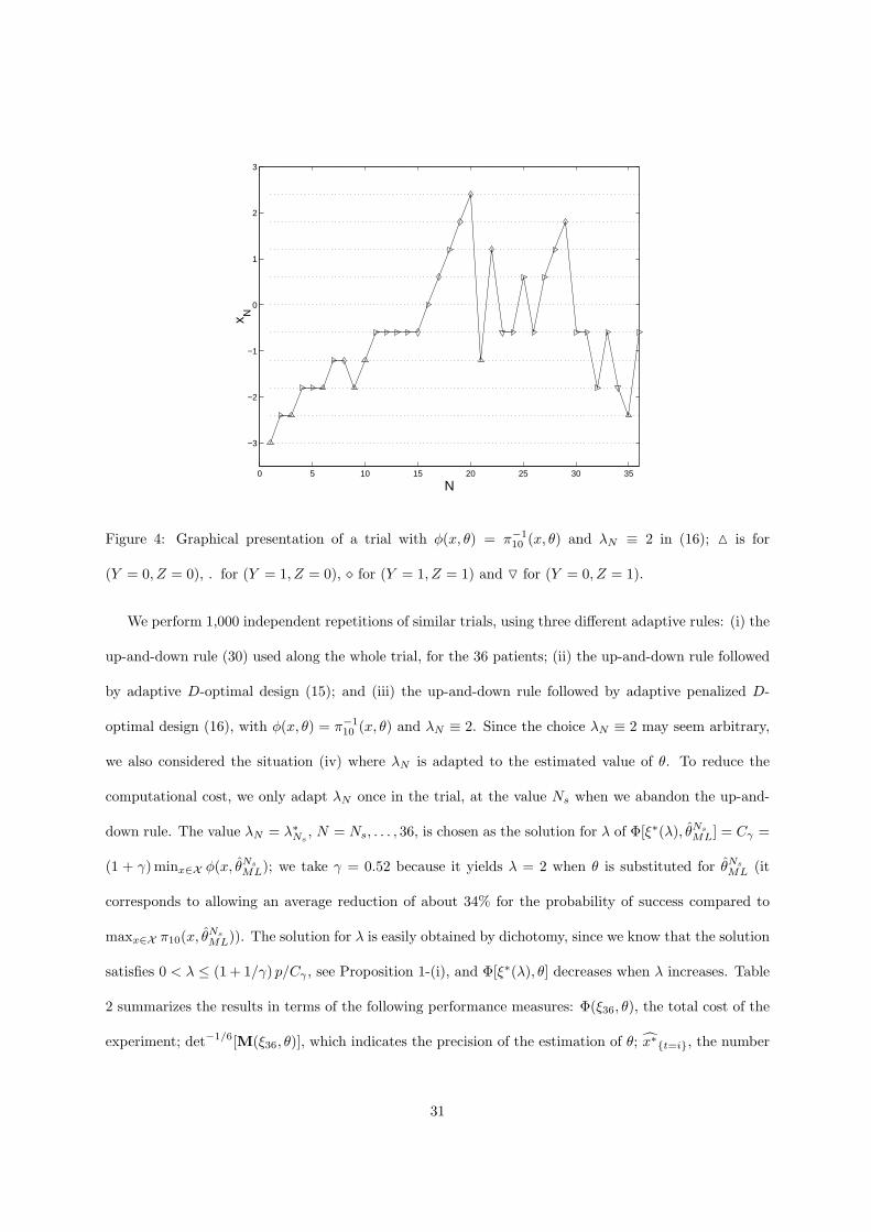
Figure 4 shows the progress of a typical trial with λN ≡ 2. The symbols indicate the values of the

observations at the given points: M for (Y = 0, Z = 0), . for (Y = 1, Z = 0), ¦ for (Y = 1, Z = 1) and

O for (Y = 0, Z = 1). The up-and-down rule is used until N = 15 where toxicity is observed. The next

dose should have been x(4) but the adaptive design rule (16) selects x(6) instead.

30

0 5 10 15 20 25 30 35

−3

−2

−1

0

1

2

3

N

x N

Figure 4: Graphical presentation of a trial with φ(x, θ) = π−110 (x, θ) and λN ≡ 2 in (16); M is for

(Y = 0, Z = 0), . for (Y = 1, Z = 0), ¦ for (Y = 1, Z = 1) and O for (Y = 0, Z = 1).

We perform 1,000 independent repetitions of similar trials, using three different adaptive rules: (i) the

up-and-down rule (30) used along the whole trial, for the 36 patients; (ii) the up-and-down rule followed

by adaptive D-optimal design (15); and (iii) the up-and-down rule followed by adaptive penalized D-

optimal design (16), with φ(x, θ) = π−110 (x, θ) and λN ≡ 2. Since the choice λN ≡ 2 may seem arbitrary,

we also considered the situation (iv) where λN is adapted to the estimated value of θ. To reduce the

computational cost, we only adapt λN once in the trial, at the value Ns when we abandon the up-and-

down rule. The value λN = λ∗Ns, N = Ns, . . . , 36, is chosen as the solution for λ of Φ[ξ∗(λ), θNs

ML] = Cγ =

(1 + γ) minx∈X φ(x, θNs

ML); we take γ = 0.52 because it yields λ = 2 when θ is substituted for θNs

ML (it

corresponds to allowing an average reduction of about 34% for the probability of success compared to

maxx∈X π10(x, θNs

ML)). The solution for λ is easily obtained by dichotomy, since we know that the solution

satisfies 0 < λ ≤ (1 + 1/γ) p/Cγ , see Proposition 1-(i), and Φ[ξ∗(λ), θ] decreases when λ increases. Table

2 summarizes the results in terms of the following performance measures: Φ(ξ36, θ), the total cost of the

experiment; det−1/6[M(ξ36, θ)], which indicates the precision of the estimation of θ; x∗t=i, the number

31

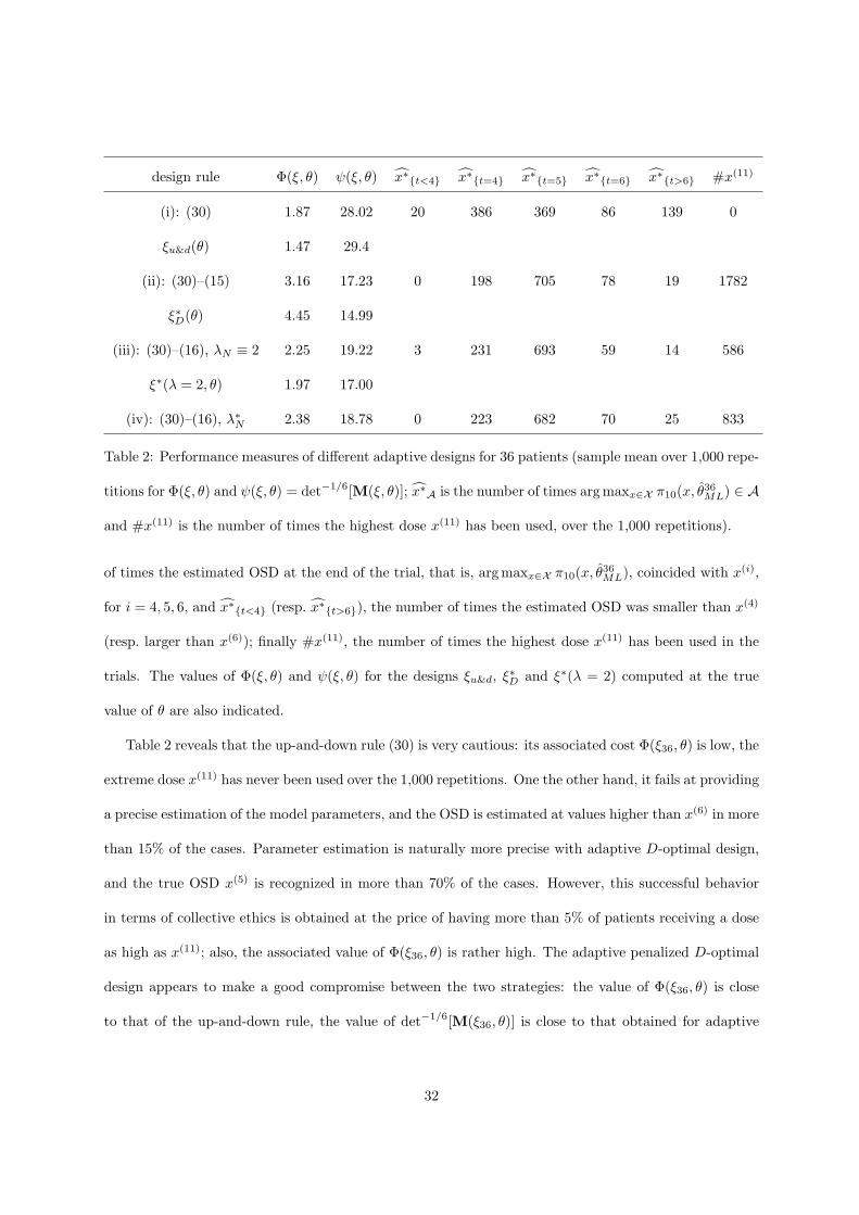
design rule Φ(ξ, θ) ψ(ξ, θ) x∗t<4 x∗t=4 x∗t=5 x∗t=6 x∗t>6 #x(11)

(i): (30) 1.87 28.02 20 386 369 86 139 0

ξu&d(θ) 1.47 29.4

(ii): (30)–(15) 3.16 17.23 0 198 705 78 19 1782

ξ∗D(θ) 4.45 14.99

(iii): (30)–(16), λN ≡ 2 2.25 19.22 3 231 693 59 14 586

ξ∗(λ = 2, θ) 1.97 17.00

(iv): (30)–(16), λ∗N 2.38 18.78 0 223 682 70 25 833

Table 2: Performance measures of different adaptive designs for 36 patients (sample mean over 1,000 repe-

titions for Φ(ξ, θ) and ψ(ξ, θ) = det−1/6[M(ξ, θ)]; x∗A is the number of times arg maxx∈X π10(x, θ36ML) ∈ A

and #x(11) is the number of times the highest dose x(11) has been used, over the 1,000 repetitions).

of times the estimated OSD at the end of the trial, that is, arg maxx∈X π10(x, θ36ML), coincided with x(i),

for i = 4, 5, 6, and x∗t<4 (resp. x∗t>6), the number of times the estimated OSD was smaller than x(4)

(resp. larger than x(6)); finally #x(11), the number of times the highest dose x(11) has been used in the

trials. The values of Φ(ξ, θ) and ψ(ξ, θ) for the designs ξu&d, ξ∗D and ξ∗(λ = 2) computed at the true

value of θ are also indicated.

Table 2 reveals that the up-and-down rule (30) is very cautious: its associated cost Φ(ξ36, θ) is low, the

extreme dose x(11) has never been used over the 1,000 repetitions. One the other hand, it fails at providing

a precise estimation of the model parameters, and the OSD is estimated at values higher than x(6) in more

than 15% of the cases. Parameter estimation is naturally more precise with adaptive D-optimal design,

and the true OSD x(5) is recognized in more than 70% of the cases. However, this successful behavior

in terms of collective ethics is obtained at the price of having more than 5% of patients receiving a dose

as high as x(11); also, the associated value of Φ(ξ36, θ) is rather high. The adaptive penalized D-optimal

design appears to make a good compromise between the two strategies: the value of Φ(ξ36, θ) is close

to that of the up-and-down rule, the value of det−1/6[M(ξ36, θ)] is close to that obtained for adaptive

32

D-optimal design. It recognized x(5) as the OSD in about 70% of the cases and only 1.6% of the patients

received the dose x(11) when λN ≡ 2 (2.3% when λN is adapted). Of course, other choices of λ would set

other compromises. Note that the estimation of the OSD is more cautious for adaptive penalized design

than for the up-and-down rule, in the sense that its estimation at x(6) or a higher dose occurs much less

frequently.

In order to limit more severely the number of patients that receive very high doses, we finally consider

a compromise strategy that implements a smoother (and less arbitrary) transition between up-and-down

and adaptive penalized D-optimal design. To better illustrate the potential interest of letting λN increase

in (16), we consider longer trials, with NT = 240 patients enroled. Define x∗∗(θ) = arg minx∈R φ(x, θ)

and h(x, θ) = ∂φ(x, θ)/∂x|x=x∗∗(θ). From the implicit function theorem,

∇θx∗∗(θ) =

dx∗∗(θ)dθ

= −[∂h(x, θ)

∂x |x=x∗∗(θ)

]−1∂h(x, θ)

∂θ |x=x∗∗(θ)

and, when using the up-and-down rule (30) the estimator θNML asymptotically satisfies

√NV

−1/2N [x∗∗(θN

ML)− x∗∗(θ)] d→ z ∼ N (0, 1) , N →∞ ,

where VN = [∇θx∗∗(θN

ML)]>M−1(ξN , θNML)[∇θx

∗∗(θNML)]. Based on that, we decide to switch from the

up-and-down rule to the adaptive one when√

VN/N < x(2) − x(1), the interval between two consecutive

doses. If Ns is the index of the patient for which the rule changes, we take λNs as the solution for λ

of Φ[ξ∗(λ), θNs

ML] = Cγ = (1 + γ)minx∈X φ(x, θNs

ML) with γ = 0.5 (thus targeting 33% of decrease with

respect to the maximum of π10(x, θNs

ML)). The value of λNTat the end of the trial is chosen as the solution

for λ of the same equation with γ = 0.1 (allowing only 9% of decrease with respect to the maximum

of π10(x, θNs

ML)). In between λN increases at a logarithmic rate, that is, λN = λNs [1 + a log(N/Ns)],

N = Ns, . . . , NT , with a = (λNT /λNs − 1)/ log(NT /Ns). When uncertainty on the OSD is large, that

is when√

VN/N > [x(2) − x(1)]/2, we also restrict the allocations at high doses by adapting the design

space, taken as XN = x(1), . . . , x(iN ) at step N : the maximum dose x(iN ) allowed in (16) is never more

than one step higher than previous dose and is smaller than previous dose if toxicity was observed. The

results obtained for 150 repetitions of the experiment are summarized in Table 3 (the results obtained

33

Φ(ξ, θ) ψ(ξ, θ) x∗t<4 x∗t=4 x∗t=5 x∗t=6 x∗t>6 #x(11)

(30) 1.54 29.04 0 21 116 11 2 0

(30)–(16), λN 1.52 27.87 0 13 135 1 1 40

Table 3: Performance measures of adaptive design (16) with increasing λN for 240 patients (sam-

ple mean over 150 repetitions for Φ(ξ, θ) and ψ(ξ, θ) = det−1/6[M(ξ, θ)]; x∗A is the number of times

argmaxx∈X π10(x, θ200ML) ∈ A and #x(11) is the number of times the highest dose x(11) has been used,

over the 150 repetitions).

when the up-and-down rule (30) is used for the 240 patients are also indicated). One may notice the

precise estimation of the OSD for the adaptive penalized design compared to the up-and-down rule (it

even does slightly better than the up-and-down rule both in terms of Φ(ξ, θ) and det−1/6[M(ξ, θ)]). At

the same time, only about 0.11% of the patients received the maximal dose x(11). Also note that, from

the results of Sect. 4.2, instead of setting NT = 240 in advance, the decision to stop the trial could be

based on the value of VN . ¤

6 Conclusion and further developments

We have shown that constrained optimal design can be formulated in a way that allows a clear compromise

between gaining information and minimizing a cost. We have also shown that the optimal design can be

constructed sequentially and proved the strong consistency and asymptotic normality of the estimator of

the model parameters in such adaptive designs. The dose-finding example with bivariate binary responses

has illustrated the potential of adaptive penalized D-optimal design to set compromises between individual

and collective ethics. Further developments and numerical studies are required to define suitable rules for

selecting cost functions and for choosing the value (or the sequence of values) for the penalty coefficients

λN . Relating λN to the precision of the estimation of the OSD is a possible option to investigate in dose-

finding problems. We mention below some extensions of this work, some straightforward, others more

challenging, and indicate a motivating objective concerning the design of non-stationary dose-finding

34

experiments preserving individual ethics.

Bayesian estimation The extension of the results presented to Bayesian estimators should not raise

particular difficulties, especially since consistency is usually easier to obtained than for LS or ML esti-

mation using martingales properties, see, e.g., [16]. A straightforward modification of (16) is to replace

M(ξN , θN ) by [M−1(ξN , θN ) + Ω/N ]−1, with Ω the prior covariance matrix for the model parameters.

Multiple constraints The results obtained in Sect. 3 and 4 easily generalize to the presence of several

constraints, that is, when problem P3(θ) is transformed into:

maximize log detM(ξ, θ) with respect to ξ ∈ Ξ under the constraints Φ(ξ, θ) ≤ Ci , i = 1, . . . , m .

A Lagrange coefficient is then associated with each constraint and the design algorithm (16) becomes

xN+1 = argmaxx∈X

trace[µ(x, θN )M−1(ξN , θN )]−

m∑

i=1

λ(i)N φi(x, θN )

.

When the λ(i)N ’s are controlled to increase to infinity, define ρ

(j)N = λ

(j)N /

∑i λ

(i)N and suppose that a

limit ρj exists for each ρ(j)N , j = 1, . . . , m. Then, if all cost functions φi(·, θ) are bounded on X , the

asymptotic behaviors of the design and estimators are the same as in Sect. 4 for λN =∑

i λ(i)N and

φ(x, θ) =∑

j ρjφj(x, θ). Also, the developments of Sect. 3 remain valid when the λ(i)N ’s are kept constant,

or when they are adapted to θN , that is, when they correspond to the optimal coefficients in the solution

of P3(θN ). Note, however, that the presence of several constraints makes this optimal solution more

difficult to determine (it can no longer be obtained by solving a series of unconstrained problems with an

increasing sequence of coefficients, contrary to the single constraint case).

Finite horizon The results of Sect. 4 indicate that, when λN increases to infinity at suitable speed,

the design converges to the delta measure located at the optimum. In clinical trials, this means that more

and more patients receive doses close to the optimal one (and none receives extreme doses if the penalty

function satisfies (11)). This is an asymptotic result, however, and approaching the optimal solution over

a finite horizon is a challenging task. In the case of LS estimation in linear regression, design strategies are

35

suggested in [28] that are shown to be close to the optimum control (stochastic dynamic programming)

solution. Is is then tempting to replace the Bernoulli model by a regression type model (observation Yk

at design point xk has mean value π(xk, θ) and variance π(xk, θ)[1− π(xk, θ)]), as suggested in [34], with

a linear parametrization, and then try to apply the finite-horizon results of [28].

Non stationary clinical trials Strong consistency of the estimator is obtained in Sect. 4 when the

penalty coefficient λN in (16) tends to infinity. Moreover, when the growth of λN is not too fast, the

estimator is asymptotically normal. This means that, although the design is non-stationary in the sense

that patients enrolled in the trial receive better and better treatments, the information collected at the

end of the experiment can be used to set future treatments. In particular, the minimum effective and

maximum tolerated doses can be estimated and confidence intervals can be given. At the same time, the

fact that patients receive unequal treatments in the trial raises ethical issues: there is no randomization, a

new patient tends to receive a better treatment than patients previously treated (since when λN increases,

the design points tend to get closer to the optimal dose). This emphasizes the importance of constructing

a fair rule for choosing the increasing sequence (λN ). Trying to give equal probabilities of success at

patients PN and PN+1 when patient PN is treated first seems to be an honest ambition, and the increase

of λN could then be used to compensate for the late treatment of patient PN+1. This requires a model

for the evolution of the probability of success as a function of the delay in treatment, to be combined

with a suitable characterization of the improvement of treatment that can be expected when increasing

λN .

Appendix

Proof of Proposition 1.

(i) Since ξ∗ is optimal we have for all x ∈ X , trace[µ(x, θ)M−1(ξ∗, θ)] ≤ p + λ [φ(x, θ)−Φ(ξ∗, θ)], see

(6). This is true in particular at a x∗ defined by (8) and trace[µ(x∗, θ)M−1(ξ∗, θ)] ≥ 0 gives the result.

(ii) For any a > 0, take λ ≥ a/∆θ(ξ) and define ξ = (1 − α)ξ + αδx∗ with δx∗ the delta measure at

36

a point x∗ satisfying (8) and α = 1 − a/[λ∆θ(ξ)]. This gives Φ(ξ, θ) − φ∗θ = a/λ and log detM(ξ, θ) ≥

p log(1− α) + log detM(ξ, θ). Therefore,

log detM(ξ∗, θ)− λ[Φ(ξ∗, θ)− φ∗θ] ≥ log detM(ξ, θ)− λ[Φ(ξ, θ)− φ∗θ]

≥ p log a− a− p log ∆θ(ξ) + log detM(ξ, θ)− p log λ .

Since Φ(ξ∗, θ) ≥ φ∗θ, the result follows.

When φ(x, θ) is bounded by φθ, the optimality of ξ∗ implies that for all x ∈ X , trace[µ(x, θ)M−1(ξ∗, θ)] ≤

B = p + λ (φθ − φ∗θ). Write µ(x, θ) = F>θ (x)Fθ(x) with F>θ (x) = [f1,θ(x), . . . , fm,θ(x)] and fi,θ(x) a p-

dimensional vector, i = 1, . . . , m. From the inequality trace[µ(x, θ)M−1(ξ∗, θ)] ≤ B we obtain that

f>i,θ(x)M−1(ξ∗, θ)fi,θ(x) ≤ B, i = 1, . . . ,m. We have

λmin[M(ξ∗, θ)] = λ−1max[M

−1(ξ∗, θ)] = [ max‖u‖=1

u>M−1(ξ∗, θ)u]−1 .

Consider the optimization problem defined by: maximize u>A>Au with respect to A and u respectively

in Rn×p and Rp, n ≤ p, subject to the constraints ‖u‖ = 1 and f>i,θ(x)A>Afi,θ(x) ≤ B, ∀x ∈ X and

∀i = 1, . . . ,m. The optimal solution is obtained for A = v> ∈ Rp such that |f>i,θ(x)v| ≤ √B, ∀x ∈ X ,

∀i = 1, . . . ,m, and b = v>v is maximal. For x varying in X the fi,θ(x)’s span Rp (since a nonsingular

information matrix exists). Therefore, there exists a positive constant δ such that the optimal value for

b is bounded by B/δ, so that λmin[M(ξ∗, θ)] > δ/B.

(iii) Since trace[µ(x, θ)M−1(ξ∗, θ)] ≤ p + λ [φ(x, θ) − Φ(ξ∗, θ)] for all x ∈ X when ξ∗ is optimal,

and∫X

trace[µ(x, θ)M−1(ξ∗, θ)]− λφ(x, θ)

ξ∗(dx) = p−λ Φ(ξ∗, θ), we have trace[µ(x, θ)M−1(ξ∗, θ)] =

p+λ [φ(x, θ)−Φ(ξ∗, θ)] at any x support point of ξ∗. Suppose that λ is large enough so that there exists a

design ξλ ∈ Ξ satisfying ∆θ(ξλ) ≥ p/λ. We proceed as in (ii) and construct a design ξλ = (1−α)ξλ +αδx∗

with α = 1 − p/[λ∆θ(ξλ)] so that Φ(ξλ, θ) − φ∗θ = p/λ. With the same notation as in (ii), we can write

trace[µ(x, θ)M−1(ξλ, θ)] =∑m

i=1 f>i,θ(x)M−1(ξλ, θ)fi,θ(x). We then follow the same approach as in [15]

and define H(ξ∗, ξ, θ) = M1/2(ξ∗, θ)M−1(ξ, θ)M1/2(ξ∗, θ). We obtain

trace[µ(x, θ)M−1(ξλ, θ)] =m∑

i=1

f>i,θ(x)M−1/2(ξ∗, θ)H(ξ∗, ξλ, θ)M−1/2(ξ∗, θ)fi,θ(x)

37

≥ λmin[H(ξ∗, ξλ, θ)] trace[µ(x, θ)M−1(ξ∗, θ)]

= λmin[H(ξ∗, ξλ, θ)] p + λ [φ(x, θ)− Φ(ξ∗, θ)]

≥ λmin[H(ξ∗, ξλ, θ)]

p + λ [φ(x, θ)− Φ(ξλ, θ)]

= λmin[H(ξ∗, ξλ, θ)] λ [φ(x, θ)− φ∗θ]

where we used the property ∆θ(ξ∗) ≤ p/λ = ∆θ(ξλ), see (i). Therefore,

trace[µ(x, θ)M−1(ξλ, θ)] ≥ (1− α)trace[µ(x, θ)M−1(ξλ, θ)] ≥ p λmin[H(ξ∗, ξλ, θ)] [φ(x, θ)− φ∗θ]∆θ(ξλ)

. (31)

The last step consists in deriving a lower bound on λmin[H(ξ∗, ξλ, θ)] that does not depend on ξ∗. We

have

trace[H−1(ξ∗, ξλ, θ)

]=

∫

Xtrace

[µ(x, θ)M−1(ξ∗, θ)

]ξλ(dx)

and thus from the optimality of ξ∗,

trace[H−1(ξ∗, ξλ, θ)

]≤ p + λ

∫

X[φ(x, θ)− Φ(ξ∗, θ)] ξλ(dx)

= p + λ[Φ(ξλ, θ)− Φ(ξ∗, θ)

]≤ p + λ

[Φ(ξλ, θ)− φ∗θ

]= 2p .

Therefore, λmin[H(ξ∗, ξλ, θ)] ≥ 1/(2p), which, together with (31), concludes the proof.

Proof of Lemma 1. First note that q∗ ≥ 1 since X is finite. Suppose that p ≥ 2 and q∗ < p. We show

that this leads to a contradiction.

For any N we can write

M(ξN , θ) =1N

N∑

k=1

fθ(xk)f>θ (xk)

=1N

q∗∑

i=1

rN,i:K fθ(x(iN ))f>θ (x(iN )) +1N

∑

xk 6∈XN (q∗)

fθ(xk)f>θ (xk) , (32)

where iN is the index (depending on N) of a design point appearing rN,i:K times in x1, . . . , xN and

XN (q∗) = x(1N ), . . . , x(q∗N ) is the set of such points for i ≤ q∗. Let MN (θ) denote the first matrix on

the right-hand side of (32). For any x(iN ) ∈ XN (q∗) we have

f>θ (x(iN ))M−1(ξN , θ)fθ(x(iN )) ≤ f>θ (x(iN ))M−N (θ)fθ(x(iN )) =

N

rN,i:K,

38

with M−N (θ) any g-inverse of MN (θ). Therefore, from the definition of q∗, there exists N1 such that

for all i ≤ q∗ , N > N1 and θ ∈ Θ , f>θ (x(iN ))M−1(ξN , θ)fθ(x(iN ))− λN φ(x(iN ), θ) ≤ 1α

. (33)

Let βN = rN,(q∗+1):K/N . Showing that lim infN→∞ βN ≥ β for some β > 0 will contradict the definition

of q∗.

Define

M(1)N (θ) =

q∗∑

i=1

fθ(x(iN ))f>θ (x(iN )) , M(2)N (θ) =

K∑

i=1

fθ(x(iN ))f>θ (x(iN )) . (34)

We have (1−βN )M(1)N (θ)+βN M(2)

N (θ)−M(ξN , θ) ∈M≥, where M≥ is the set of symmetric nonnegative

definite p× p matrices. For any u ∈ Rp,

u>M−1(ξN , θ)u ≥ u>[(1− βN )M(1)N (θ) + βN M(2)

N (θ)]−1u

= maxz∈Rp

2z>u− z>[(1− βN )M(1)N (θ) + βN M(2)

N (θ)]z

≥ maxz∈N [M

(1)N (θ)]

2z>u− z>[(1− βN )M(1)N (θ) + βN M(2)

N (θ)]z

with N (M) = v : Mv = 0 the null-space of the matrix M. Direct calculations then give

u>M−1(ξN , θ)u ≥ 1βN

u>[M(2)N (θ)]−1 [I−PN (θ)]u (35)

with I the p-dimensional identity matrix and PN (θ) the projector

PN (θ) = M(1)N (θ)

[M(1)

N (θ)[M(2)N (θ)]−1M(1)

N (θ)]−

M(1)N (θ)[M(2)

N (θ)]−1 .

Note that the right-hand side of (35) is zero when u ∈ M[M(1)N (θ)] (i.e., when u = M(1)

N (θ)v for some

v ∈ Rp). When u = fθ(x(iN )) for some i ∈ q∗ + 1, . . . , K we can construct a lower bound for this term,

of the form A/βN with A constant. Indeed, from (34) and HX -(ii),

for all θ ∈ Θ and v ∈ Rp , v>

M(1)

N (θ) +K∑

i=q∗+1

fθ(x(iN ))f>θ (x(iN ))

v > γ ‖v‖2

so that for all θ ∈ Θ and z ∈ N [M(1)N (θ)],

maxi=q∗+1,...,K

[z>fθ(x(iN ))]2 >γ

K − q∗‖z‖2 . (36)

39

Take z = zθ,iN= [M(2)

N (θ)]−1[I−PN (θ)]fθ(x(iN )) for some i ∈ q∗+1, . . . , K, so that zθ,iN∈ N [M(1)

N (θ)]

and f>θ (x(iN ))[M(2)N (θ)]−1 [I−PN (θ)] fθ(x(iN )) = z>θ,iN

fθ(x(iN )) = z>θ,iNM(2)

N (θ)zθ,iN . We obtain

maxi=q∗+1,...,K

f>θ (x(iN ))[M(2)N (θ)]−1 [I−PN (θ)] fθ(x(iN )) = max

i,j=q∗+1,...,Kz>θ,iN

M(2)N (θ)zθ,jN

= maxi,j=q∗+1,...,K

z>θ,iNfθ(x(jN )) ,

and thus from (36),

for all θ ∈ Θ , maxi=q∗+1,...,K

f>θ (x(iN ))[M(2)N (θ)]−1 [I−PN (θ)] fθ(x(iN )) >

(γ

K − q∗

)1/2

maxi=q∗+1,...,K

‖zθ,i∗N ‖ .

Let i∗N denote the argument of the maximum on the left-hand side, for which we have, z>θ,i∗Nfθ(x(i∗N )) =

z>θ,i∗NM(2)

N (θ)zθ,i∗N ≤ K L ‖zθ,i∗N ‖2 with L = maxx∈X , θ∈Θ ‖fθ(x)‖2. This finally gives: for all θ ∈ Θ,

maxi=q∗+1,...,K f>θ (x(iN ))[M(2)N (θ)]−1 [I−PN (θ)] fθ(x(iN )) > γ/[LK(K − q∗)], and thus, from (35) and

Hφ-(i),

for all θ ∈ Θ , maxi=q∗+1,...,K

f>θ (x(iN ))M−1(ξN , θ)fθ(x(iN ))− λN φ(x(iN ), θ)

>

1βN

γ

LK(K − q∗)− λφ .

(37)

Together with (33), it gives: N > N1 and βN < β∗ = γα/[LK(K − q∗)(1 + αλφ)] ⇒ xN+1 /∈ XN (q∗) in

the sequence (16). Define

β∗N =

∑Ki=q∗+1 rN,i:K

(K − q∗)N,

so that βN ≥ β∗N ≥ βN/(K − q∗). Also, when N > N1, (∑q∗

i=1 rN,i:K)/N > q∗α, and therefore β∗N <

(1− q∗α)/(K − q∗). By construction, βN < β∗ and N > N1 imply

βN+1 ≥ β∗N+1 =Nβ∗N (K − q∗) + 1(K − q∗)(N + 1)

= β∗N +1

N + 1

(1

K − q∗− β∗N

)

> β∗N +1

N + 1q∗α

K − q∗≥ βN

K − q∗+

1N + 1

q∗αK − q∗

.

By induction, this lower bound on βN+k increases with k,

βN+k >βN

K − q∗+

q∗αK − q∗

k∑

i=1

1N + i

,

until βN+k becomes larger that β∗. Suppose that the threshold β∗ is crossed downwards at N2 > N1, i.e.,

βN2−1 ≥ β∗ and βN2 < β∗. This implies βN2 = βN2−1(N2 − 1)/N2 and thus β∗(N2 − 1)/N2 ≤ βN2 < β∗,

40

so that βN2 tends to β∗ when N2 → ∞. We thus obtain lim infN→∞ βN ≥ β = β∗/(K − q∗), showing

that q∗ ≥ p, which concludes the proof.

Proof of Theorem 3. We have already seen that the conditions of Lemma 1 with HX -(iii) (respectively,

HX -(iii’)) imply θNLS

a.s.→ θ (respectively, θNML

a.s.→ θ) as N →∞. All what we need to obtain the asymptotic

optimality of ξN is thus a continuity property of the form: for all ε > 0, there exists β > 0 such that

[‖θN − θ‖ < β for all N larger than some N0] implies lim infN→∞Hθ(ξN ) > H ∗θ− ε. We show that this

is indeed true under the additional assumptions HX -(iv), Hφ-(ii) and Hf -(i).

First note that λ∗(θ) = arg minλ≥0 maxξ∈Ξ log detM(ξ, θ) + λ [C − Φ(ξ, θ)] is continuous in θ as

the argument of the minimum of a convex function (given by the maximum of convex functions) that is

continuous in θ. Therefore, ∀ε0, ∃β1 such that ‖θ− θ‖ < β1 ⇒ |λ∗(θ)− λ∗(θ)| < ε0. Also, Hf -(i), Hφ-(ii)

and HX -(i) imply: ∀ε0, ∃β2 such that ‖θ − θ‖ < β2 ⇒ maxx∈X ‖fθ(x) − fθ(x)‖ < ε0 and ∃β3 such that

‖θ − θ‖ < β3 ⇒ maxx∈X |φ(x, θ)− φ(x, θ)| < ε0.

From Lemma 1, there exits N1 and α > 0 such that for all N > N1, rN,j:K > αN , j = 1, . . . , q∗, with

q∗ > p, and thus from HX -(iv), λmin[M(ξN , θ)] > αγ. Direct calculations then give

maxx∈X

max‖θ−θ‖<β2

|f>θ (x)M−1(ξN , θ)fθ(x)− f >θ (x)M−1(ξN , θ)fθ(x)| < Bε0

for ε0 small enough and N > N1, with B depending on α, γ and f = maxx∈X ‖fθ(x)‖.

Therefore, for all ε0 small enough, we can take β = minβ1, β2, β3 and obtain, for all N > N1 and

‖θN − θ‖ < β in (16),

f >θ (xN+1)M−1(ξN , θ)fθ(xN+1)− λ∗(θ)φ(xN+1, θ)

> f>θN (xN+1)M−1(ξN , θN )fθN (xN+1)− λ∗(θN )φ(xN+1, θ

N )− ε0(B + λ + φ)− ε20

= maxx∈X

[f>θN (x)M−1(ξN , θN )fθN (x)− λ∗(θN )φ(x, θN )

]− ε0(B + λ + φ)− ε20

> maxx∈X

[f >θ (x)M−1(ξN , θ)fθ(x)− λ∗(θ)φ(x, θ)

]− 2ε0(B + λ + φ) .

For a given ε, take ε0 = ε/(B + λ + φ) and β as above, and suppose that there exists δ > 0 such that

Hθ(ξN ) < H ∗θ − δ − ε (38)

41

for all N larger than some N2, with Hθ(ξN ) and H ∗θ

respectively given by (25) and (24). From the

concavity of the design criterion, this implies

maxx∈X

[f >θ (x)M−1(ξN , θ)fθ(x)− λ∗(θ)φ(x, θ)

]> p− λ∗(θ)Φ(ξN , θ) + ε + δ

and thus

f >θ (xN+1)M−1(ξN , θ)fθ(xN+1)− λ∗(θ)φ(xN+1, θ) > p− λ∗(θ)Φ(ξN , θ) + δ (39)

for all N > maxN1, N2, N0 when ‖θN − θ‖ < β for all N > N0. Direct calculations give

Hθ(ξN+1)−Hθ(ξN ) = log

[1 +

f >θ

(xN+1)M−1(ξN , θ)fθ(xN+1)N

]− p log

(1 +

1N

)

+λ∗(θ)N + 1

[Φ(ξN , θ)− φ(xN+1, θ)] (40)

and thus from (39),

Hθ(ξN+1)−Hθ(ξN ) > log

[1 +

f >θ

(xN+1)M−1(ξN , θ)fθ(xN+1)N

]− p log

(1 +

1N

)

+p + δ − f >

θ(xN+1)M−1(ξN , θ)fθ(xN+1)

N + 1.

Since f >θ

(xN+1)M−1(ξN , θ)fθ(xN+1) is bounded by f2/(αγ), we obtain that Hθ(ξN+1)−Hθ(ξN ) > δ/(2N)

for N large enough, which implies that Hθ(ξN ) → ∞ as N → ∞, in contradiction with Hφ-(i), Hλ-(i’)

and Hf -(i), see the definition of Hθ(ξ) in (25).

Therefore, for any ε > 0, ‖θN − θ‖ < β for all N > N0 implies the existence of a subsequence ξNt such

that lim supt→∞Hθ(ξNt) ≥ H ∗θ− ε. From (40), for all δ > 0 there exists N3 such that for all N > N3,

Hθ(ξN+1) > Hθ(ξN )−δ. Also, from the developments just above, there exists N4 such that for all N > N4,

(38) implies Hθ(ξN+1) > Hθ(ξN ). Take any Nt > max(N0, N3, N4) satisfying Hθ(ξNt) > H ∗θ− ε− δ, we

obtain Hθ(ξN ) > H ∗θ− ε− 2δ , for all N > Nt. Since δ is arbitrary, lim infN→∞Hθ(ξN ) ≥ H ∗

θ− ε, which

concludes the proof.

Proof of Lemma 3. We consider the case of LS estimation in the regression model (17). The proof is

similar (but simpler) for ML estimation in the model (21) and we shall only indicate the adaptations that

are required.

42

A first-order series development of the gradient of the LS criterion (18) around θ gives

∇θSN (θNLS) = 0 = ∇θSN (θ) +∇2

θSN (θN )(θNLS − θ) , (41)

where ∇θSN (θ) = −2∑N

k=1 εkfθ(xk), ∇2θSN (θ) is the (Hessian) matrix of second-order derivatives of

SN (θ), given by

∇2θSN (θ) = 2N M(ξN , θ)− 2

N∑

k=1

[Yk − η(xk, θ)]∂fθ(xk)

∂θ>,

and θN = (1− γN )θ + γN θNLS , γN ∈ (0, 1), with θN measurable, see [18].

We first try to bound ‖θNLS − θ‖. We have (1/N)∇2

θSN (θ) = 2M(ξN , θ) + 2A(ξN , θ, θ)− 2BN (ξN , θ),

with

A(ξN , θ, θ) =1N

N∑

k=1

[η(xk, θ)− η(xk, θ)]∂fθ(xk)

∂θ>and BN (ξN , θ) =

1N

N∑

k=1

εk∂fθ(xk)

∂θ>.

From Hf -(ii), there exist A1 > 0 and A2 > 0 such that supx∈X sup‖θ−θ‖≤δ |η(x, θ) − η(x, θ)| < A1δ and

supx∈X sup‖θ−θ‖≤δ ‖∂fθ(x)/∂θ>‖ < A2. This implies limδ→0 sup‖θ−θ‖≤δ ‖A(ξN , θ, θ)‖ = 0. We also have

sup‖θ−θ‖≤δ

‖B(ξN , θ)‖ <∑

x∈X

∣∣∣∑Nk=1, xk=x εk

∣∣∣rN (x)

A2rN (x)

N(42)

where rN (x) denotes the number of times x appears in the sequence x1, . . . , xN . Either rN (x) is bounded

or rN (x) tends to infinity (but remains smaller than N), in any case limN→∞ sup‖θ−θ‖≤δ

∥∥B(ξN , θ, θ)∥∥ = 0

a.s. We have similarly M(ξN , θ)−M(ξN , θ) =∑

x∈X [rN (x)/N ] [fθ(x)f>θ (x)− fθ(x)f >θ

(x)], and therefore

limδ→0 sup‖θ−θ‖≤δ ‖M(ξN , θ) − M(ξN , θ)‖ = 0. Since θNLS

a.s.→ θ, N → ∞, we obtain that there exists

a.s. N0 such that for all N > N0, λmin[∇2θSN (θN )/N ] > Λ/τN . From the series development (41), it

implies ‖θNLS − θ‖ < [τN/(Λ

√N)] ‖∇θSN (θ)‖/√N . We have ∇θSN (θ)/

√N = −2

∑x∈X vN (x), where

vN (x) = ζN (x)αN (x)fθ(x) with ζN (x) = (∑N

k=1, xk=x εk)/√

rN (x) and αN (x) =√

rN (x)/N < 1, there-

fore ‖∇θSN (θ)‖/√N < 2f∑

x∈X |ζN (x)| with f = maxx∈X ‖fθ(x)‖ and ζN (x) = Op(1) (that is, ζN (x)

is bounded in probability) for all x. We thus obtain ‖θNLS − θ‖ < (2f τNωN )/(Λ

√N) for N > N0 with

ωN =∑

x∈X |ζN (x)| = Op(1).

Now, for N large enough we have ‖M−1(ξN , θ)A(ξN , θ, θ)‖ < (2τN/Λ)‖A(ξN , θ, θ)‖ and therefore

‖M−1(ξN , θ)A(ξN , θN , θ)‖ < (4A1A2f/Λ2) (τ2NωN/

√N)

p→ 0, N → ∞ (since τ2N/√

N → 0 and ωN =

43

Op(1)). Also, ‖M−1(ξN , θ)B(ξN , θ)‖ < (2τN/Λ)‖B(ξN , θ)‖ for N large enough, which implies that

sup‖θ−θ‖≤δ

∥∥M−1(ξN , θ)B(ξN , θ)∥∥ < (2A2/Λ) (τNωN/

√N), see (42), and ‖M−1(ξN , θ)B(ξN , θN )‖ p→ 0,

N → ∞. Moreover, ‖M−1(ξN , θ)M(ξN , θ)− I‖ = ‖M−1(ξN , θ)[M(ξN , θ)−M(ξN , θ)]‖ and, for N large

enough, ‖M−1(ξN , θ)M(ξN , θ) − I‖ < (2τN/Λ) supx∈X ‖fθ(x)f>θ (x) − fθ(x)f >θ

(x)‖. Since ‖fθ(x)f>θ (x) −

fθ(x)f >θ

(x)‖2 = ‖fθ(x)− fθ(x)‖4 + 2[fθ(x)− fθ(x)]>fθ(x)2 + 4‖fθ(x)− fθ(x)‖2[fθ(x)− fθ(x)]>fθ(x) and

supx∈X sup‖θ−θ‖≤δ ‖fθ(x) − fθ(x)‖ < A2δ, there exists A3 > 0 such that for δ small enough we have

supx∈X sup‖θ−θ‖≤δ ‖fθ(x)f>θ (x) − fθ(x)f >θ

(x)‖ < A3δ. We thus obtain ‖M−1(ξN , θ)M(ξN , θN ) − I‖ <

(4A3f/Λ2)(τ2NωN/

√N)

p→ 0, N →∞ and finally ‖M−1/2(ξN , θ)[∇2θSN (θN )/N ]M−1/2(ξN , θ)− 2I‖ p→ 0,

so that (41) gives

[2 + op(1)]√

NM1/2(ξN , θ)(θNLS − θ) = −M−1/2(ξN , θ)∇θSN (θ)/

√N , N →∞ . (43)

We show now that M−1/2(ξN , θ)∇θSN (θ)/√

N is asymptotically normal.

Denote by Fk the σ-field generated by Y1, . . . , Yk. Notice that from the adaptive construction of

the design, xk is Fk−1-measurable. Take any u ∈ Rp with ‖u‖ = 1 and consider

RN = − 12√

Nu>M−1/2(ξN , θ)∇θSN (θ) =

N∑

k=1

ζNk

where ζNk = εkzNk/√

N with zNk = u>M−1/2(ξN , θ)fθ(xk). Using [33, Th. 1, p. 541], to prove that

RNd→ r ∼ N (0, s2) it is enough to show that, for any γ ∈ (0, 1),

N∑

k=1

Prob|ζNk| > γ|Fk−1 p→ 0 (44)

N∑

k=1

IEζNk II(|ζNk| ≤ 1)|Fk−1 p→ 0 (45)

N∑

k=1

VarζNk II(|ζNk| ≤ γ)|Fk−1 p→ s2 (46)

as N → ∞, with II(·) the indicator function. First consider (44). Define tNk = Prob|ζNk| > γ|Fk−1 =

∫|ε|>γ

√N/|zNk| dF (ε) with F (·) the probability distribution of the errors in the model (17). Since |zNk| ≤

fλ−1/2min M(ξN , θ) < f

√2τN/

√Λ for N large enough (a.s.), with f = maxx∈X ‖fθ(x)‖, we get tNk <

∫|ε|>γρ

√N/τN

dF (ε) < (γρ)−(2+δ)(τN/N)1+δ/2∫|ε|>γρ

√N/τN

|ε|2+δ dF (ε), where ρ =√

Λ/(f√

2). Since

44

limN→∞ τN N−δ/(2+δ) = 0 and IE|ε1|2+δ < ∞, NtNk → 0 as N → ∞ and (44) is satisfied. Con-

sider (45) and define t′Nk = IEζNk II(|ζNk| ≤ 1)|Fk−1 = (zNk/√

N)∫|ε|≤√N/|zNk| ε dF (ε), so that

|t′Nk| = (|zNk|/√

N)∣∣∣∫|ε|>√N/|zNk| ε dF (ε)

∣∣∣ (since IEε1 = 0). Therefore, for N large enough, |t′Nk| ≤

(1/ρ)√

τN/N∫|ε|>ρ

√N/τN

|ε| dF (ε) < ρ−(2+δ)(τN/N)1+δ/2∫|ε|>ρ

√N/τN

|ε|2+δ dF (ε), which implies that

N |t′Nk| → 0 as N → ∞ and (45) is satisfied. We proceed in a similar way for (46) and define

t′′Nk = VarζNk II(|ζNk| ≤ γ)|Fk−1 = (z2Nk/N)

[∫|ε|≤γ

√N/|zNk| ε

2 dF (ε)−(∫|ε|≤γ

√N/|zNk| ε dF (ε)

)2].

Since IEε21 = 1, we obtain

∑k t′′Nk = (1/N)

∑k z2

Nk + QN where, for N large enough, QN sat-

isfies |QN | < τN/(Nρ2)∑

k

[∫|ε|>γ

√N/|zNk| ε

2 dF (ε) +(∫|ε|>γ

√N/|zNk| |ε| dF (ε)

)2]

(using IEε1 = 0).

Therefore, for N large enough, |QN | < (τN/ρ2)[∫|ε|>γρ

√N/τN

ε2 dF (ε) +(∫|ε|>γρ

√N/τN

|ε| dF (ε))2

]<

γ−δρ−(2+δ))(τ1+δ/2N /Nδ/2)

[∫|ε|>γρ

√N/τN

|ε|2+δ dF (ε) +(∫|ε|>γρ

√N/τN

|ε|1+δ/2 dF (ε))2

]→ 0 as N →

∞. Moreover, (1/N)∑

k z2Nk = u>u = 1 and we have thus proved that RN

d→ r ∼ N (0, 1) as N → ∞.

Since this is true for any u, we have M−1/2(ξN , θ)∇θSN (θ)/√

Nd→ v ∼ N (0, 4I), and therefore from

(43),√

NM1/2(ξN , θ)(θNLS − θ) d→ w ∼ N (0, I) , N → ∞. Since ‖M−1(ξN , θ)M(ξN , θN

LS) − I‖ p→ 0 as

N →∞, we obtain the announced result (27).

Consider now ML estimation in the model (21). We substitute LN (θ) for SN (θ) is the series develop-

ment (41) (with the difference that LN (θ) is now maximum at θNML). Denoting πk = π(xk, θ) and πk =

π(xk, θ), we have LN (θ) =∑

k Yk log πk+(1−Yk) log(1−πk), ∇θLN (θ) =∑

k(Yk−πk)/√

πk(1− πk)fθ(xk)

and ∇2θLN (θ)/N = −M(ξN , θ) + AN (ξN , θ, θ) + BN (ξN , θ, θ), where fθ(x) is given by (22),

AN (ξN , θ, θ) =1N

N∑

k=1

πk − πk√πk(1− πk)

Qk(xk, θ) and BN (ξN , θ, θ) =1N

N∑

k=1

Zk

√πk(1− πk)√πk(1− πk)

Qk(xk, θ) ,

with

Qk(xk, θ) =1√

πk(1− πk)

[∂2πk

∂θ∂θ>+ (2πk − 1)fθ(xk)f>θ (xk)

]and Zk =

Yk − πk√πk(1− πk)

.

Notice that IEZk = 0 and IEZ2k = 1. Similarly to the case of LS estimation, we obtain that

exists a.s. N0 such that, for all N > N0, λmin[−∇2θLN (θN )/N ] > 1/(2τN ), where θN is now a

point between θ and θNML. This implies that ‖θN

ML − θ‖ < cτNωN/√

N for some constant c and

ωN = Op(1). We consider then ‖M−1(ξN , θ)∇2θLN (θ)/N + I‖ and obtain, since limN→∞ τN/N1/4 = 0,

45

‖M−1/2(ξN , θ)[∇2θLN (θN )/N ]M−1/2(ξN , θ)+I‖ p→ 0, N →∞. This gives [1+op(1)]

√NM1/2(ξN , θ)(θN

ML−

θ) = M−1/2(ξN , θ)∇θLN (θ)/√

N , N →∞. We consider finally RN = (1/√

N)u>M−1/2(ξN , θ)∇θLN (θ)

for some vector u with norm 1, and write RN =∑

k ζN,k with now ζN,k = Zku>M−1/2(ξN , θ)fθ(xk)/√

N .

The properties (44, 45, 46) directly follow from the fact that Zk is bounded, |Zk| < maxx∈X max([1 −

π(x, θ)]/π(x, θ))1/2, (π(x, θ)/[1− π(x, θ)])1/2 for all k. The rest of the proof is similar to the case of LS

estimation.

Proof of Lemma 4. First note that lim infN→∞ rN,1:K/N > 1/K since X is finite, so that q∗ ≥ 1. Suppose

that p ≥ 2 and q∗ < p, we show that we arrive at a contradiction. The proof follows the same lines as for

Lemma 1.

The property (33) is replaced by

for all i ≤ q∗ , N > N1 and θ ∈ Θ , f>θ (x(iN ))M−1(ξN , θ)fθ(x(iN ))− λN φ(x(iN ), θ) ≤ λN

α. (47)

Define ρN as ρN = λNβN , with βN = rN,(q∗+1):K/N as in Lemma 1. We show that lim infN→∞ ρN ≥ ρ

for some ρ > 0, which contradicts the definition of q∗.

The property (37) becomes

for all θ ∈ Θ , maxi=q∗+1,...,K

f>θ (x(iN ))M−1(ξN , θ)fθ(x(iN ))− λN φ(x(iN ), θ)

>

1βN

γ

LK(K − q∗)− λN φ .

Together with (47), it gives N > N1 and ρN < ρ∗ = γα/[LK(K−q∗)(1+αφ)] ⇒ xN+1 /∈ XN (q∗). Define

ρ∗N = λN

∑Ki=q∗+1 rN,i:K

(K − q∗)N,

so that ρN ≥ ρ∗N ≥ ρN/(K−q∗). Also, when N > N1,∑q∗

i=1 rN,i:K > q∗αN/λN , so that∑K

i=q∗+1 rN,i:K <

N(1− q∗α/λN ) and ρ∗N < λN (1− q∗α/λN )/(K − q∗). By construction, ρN < ρ∗ and N > N1 imply

ρN+1 ≥ ρ∗N+1 = λN+1Nρ∗N (K − q∗)/λN + 1

(K − q∗)(N + 1)=

λN+1

λNρ∗N +

λN+1

N + 1

(1

K − q∗− ρ∗N

λN

)

>λN+1

λN

[ρ∗N +

1N + 1

q∗αK − q∗

]≥ ρ∗N +

1N + 1

q∗αK − q∗

≥ ρN

K − q∗+

1N + 1

q∗αK − q∗

.

The end of the proof is strictly identical to that of Lemma 1. By induction, the lower bound on ρN+k

increases with k,

ρN+k >ρN

K − q∗+

q∗αK − q∗

k∑

i=1

1N + i

,

46

until ρN+k becomes larger that ρ∗ and lim infN→∞ ρN > ρ = ρ∗/(K − q∗), which shows that q∗ ≥ p and

concludes the proof.

Proof of Theorem 4. We have already seen that the conditions of Lemma 4 with HX -(iii) (respectively,

HX -(iii’)) imply θNLS

a.s.→ θ (respectively, θNML

a.s.→ θ) as N →∞. Therefore, what we first need to show is

that for all δ > 0, there exist some N0 > 0 and β > 0 such that ‖θN − θ‖ < β for all N > N0 implies

lim supN→∞ Φ(ξN , θ) < φ∗θ

+ δ. This will prove (28).

As in the proof of Theorem 3, Hf -(i), Hφ-(ii) and HX -(i) imply: ∀ε0, ∃β1, β2 such that ‖θ− θ‖ < β1 ⇒

maxx∈X ‖fθ(x)− fθ(x)‖ < ε0 and ‖θ − θ‖ < β2 ⇒ maxx∈X |φ(x, θ)− φ(x, θ)| < ε0. Also, from Lemma 4,

there exits N1 and α > 0 such that for all N > N1, rN,j:K > αN/λN , j = 1, . . . , q∗, with q∗ > p, and

thus from HX -(iv), λmin[M(ξN , θ)] > αγ/λN . Direct calculations give

maxx∈X

max‖θ−θ‖<β1

|f>θ (x)M−1(ξN , θ)fθ(x)− f >θ (x)M−1(ξN , θ)fθ(x)| < BλN ε0

for ε0 small enough and N > N1, with B depending on α, γ and f = maxx∈X ‖fθ(x)‖.

Therefore, for all ε0 small enough, we can take β = minβ1, β2 and obtain, for all N > N1 and

‖θN − θ‖ < β in (16),

f >θ (xN+1)M−1(ξN , θ)fθ(xN+1)− λNφ(xN+1, θ)

> f>θN (xN+1)M−1(ξN , θN )fθN (xN+1)− λNφ(xN+1, θ

N )− ε0(B + 1)λN

= maxx∈X

[f>θN (x)M−1(ξN , θN )fθN (x)− λNφ(x, θN )

]− ε0(B + 1)λN

> maxx∈X

[f >θ (x)M−1(ξN , θ)fθ(x)− λNφ(x, θ)

]− 2ε0(B + 1)λN . (48)

Suppose now that exists δ > 0 such that lim infN→∞ Φ(ξN , θ) > φ∗θ

+ δ, that is, there exists N2 such

that

Φ(ξN , θ) > φ∗θ + δ (49)

for all N > N2. This implies

f >θ (x∗)M−1(ξN , θ)fθ(x∗)− λNφ(x∗, θ) > −λNφ(x∗, θ) > λN

[δ − Φ(ξN , θ)

], N > N2 ,

47

with x∗ such that φ(x∗, θ) = minx∈X φ(x, θ), and therefore,

maxx∈X

[f >θ (x)M−1(ξN , θ)fθ(x)− λNφ(x, θ)

]> λN

[δ − Φ(ξN , θ)

], N > N2 .

For ε = δ/2, take ε0 = ε/[2(B + 1)] and β as above and define

Gθ(ξN , λN ) =1

λNlog detM(ξN , θ) + [C − Φ(ξN , θ)] . (50)

From (40, 48), we obtain

Gθ(ξN+1, λN )−Gθ(ξN , λN ) >1

λNlog

[1 +

f >θ

(xN+1)M−1(ξN , θ)fθ(xN+1)N

]− p

λNlog

(1 +

1N

)

+δ

2(N + 1)− 1

N + 1f >θ

(xN+1)M−1(ξN , θ)fθ(xN+1)λN

,

for ‖θN − θ‖ < β and N > maxN1, N2. Since λmin[M(ξN , θ)] > αγ/λN for N > N1, we also have

f >θ

(xN+1)M−1(ξN , θ)fθ(xN+1) < f2λN/(λγ), with f = maxx∈X ‖fθ(x)‖. Since λN → ∞ from Hλ-(ii)

and λN/N → 0 from Hλ-(iii) when N → ∞, for any constant D < 1 there exists N3 such that for all

N > N3,

log

[1 +

f >θ

(xN+1)M−1(ξN , θ)fθ(xN+1)N

]> D

f >θ

(xN+1)M−1(ξN , θ)fθ(xN+1)N + 1

and

p

λNlog

(1 +

1N

)<

δ

4(N + 1).

This gives

Gθ(ξN+1, λN )−Gθ(ξN , λN ) >δ

4(N + 1)+ (D − 1)

f >θ

(xN+1)M−1(ξN , θ)fθ(xN+1)(N + 1)λN

>1

N + 1

[δ

4+ (D − 1)

f2

αγ

]>

δ

8(N + 1)

for N > maxN1, N2, N3 and ‖θN − θ‖ < β when choosing D > 1− δαγ/(8f2). Consider now

Gθ(ξN+1, λN+1)−Gθ(ξN , λN ) =[

1λN+1

− 1λN

]log detM(ξN+1, θ) + Gθ(ξN , λN+1)−Gθ(ξN , λN ) .

For N large enough and ‖θN − θ‖ < β, it satisfies

Gθ(ξN+1, λN+1)−Gθ(ξN , λN ) >

[1

λN+1− 1

λN

]log detM(ξN+1, θ) +

δ

8(N + 1).

48

Denote L∗ = maxξ∈Ξ log detM(ξ, θ). Since λN is non-decreasing from Hλ-(ii) and λN/N is non-increasing

from Hλ-(iii), we get

Gθ(ξN+1, λN+1)−Gθ(ξN , λN ) >δ

8(N + 1)−

[1

λN− 1

λN+1

]L∗ ≥ δ

8(N + 1)− L∗

λN (N + 1)>

δ

16(N + 1)

for N large enough, in contradiction with the fact that Gθ(ξ, λ) is bounded for λ > 1, see (50).

Therefore, for all δ > 0 we can find a β such that ‖θN − θ‖ < β for all N > N0 implies that

there exists a subsequence ξNt such that lim inft→∞ Φ(ξNt , θ) < φ∗θ

+ δ. First note that Hφ-(i) implies

Φ(ξN+1, θ)−Φ(ξN , θ) = 1/(N + 1) [φ(xN+1, θ)−Φ(ξN , θ)] < φ/(N + 1) so that there exists N4 such that

Φ(ξN+1, θ) < Φ(ξN , θ) + δ/2 for all N > N4. Also, from the developments above, there exists N5 such

that for N > N5, ‖θN − θ‖ < β and Φ(ξN , θ) > φ∗θ

+ δ imply Gθ(ξN+1, λN+1) > Gθ(ξN , λN ). Moreover,

since λmin[M(ξN , θ)] > αγ/λN for all N > N1, we have p log(αγ) − p log λN < log detM(ξN , θ) < L∗

and thus

| log detM(ξN , θ)|λN

<δ

4(51)

for N larger than some N6. Take any Nt > max(N0, N4, N5, N6) and such that Φ(ξNt , θ) ≤ φ∗θ

+ δ.

We show that Φ(ξN , θ) < φ∗θ

+ 2δ for all N > Nt until the next N ′ such that Φ(ξN ′ , θ) ≤ φ∗θ

+ δ.

We have Φ(ξNt+1, θ) < φ∗θ

+ (3/2)δ. If Φ(ξNt+1, θ) ≤ φ∗θ

+ δ we take N ′ = Nt + 1. Suppose that

Φ(ξNt+1, θ) > φ∗θ

+ δ. Then, Gθ(ξNt+2, λNt+2) > Gθ(ξNt+1, λNt+1) and, from the definition of Gθ(ξ, λ)

and (51), Φ(ξNt+2, θ) < Φ(ξNt+1, θ) + δ/2 < φ∗θ

+ 2δ. If Φ(ξNt+2, θ) ≤ φ∗θ

+ δ we take N ′ = Nt + 2.

Otherwise, we have Gθ(ξNt+3, λNt+3) > Gθ(ξNt+2, λNt+2) > Gθ(ξNt+1, λNt+1) and thus Φ(ξNt+3, θ) <

Φ(ξNt+1, θ) + δ/2 < φ∗θ

+ 2δ. By induction, Φ(ξN , θ) < φ∗θ

+ 2δ for all N > Nt. This concludes the proof

of (28).

Define BN (β) = xi : ‖xi − x∗‖ > β , i = 1, . . . , N and denote by bN (β) the number of elements

of BN (β). Assume that there exists β > 0 such that lim supN→∞ bN (β)/N > γ > 0. From Hφ-(iii),

this implies that there exists ε > 0 such that lim supN→∞ Φ(ξN , θ) − φ∗θ

> γε, which contradicts (28).

Therefore, for all β > 0, limN→∞ bN (β)/N = 0 which gives (29).

49

References

[1] K. Chaloner and K. Larntz. Optimal Bayesian design applied to logistic regression experiments.

Journal of Statistical Planning and Inference, 21:191–208, 1989.

[2] P. Chaudhuri and P.A. Mykland. Nonlinear experiments: optimal design and inference based likeli-

hood. Journal of the American Statistical Association, 88(422):538–546, 1993.

[3] P. Chaudhuri and P.A. Mykland. On efficiently designing of nonlinear experiments. Statistica Sinica,

5:421–440, 1995.

[4] D. Cook and V.V. Fedorov. Constrained optimization of experimental design (invited discussion

paper). Statistics, 26:129–178, 1995.

[5] V. Dragalin and V. Fedorov. Adaptive designs for dose-finding based on efficacy-toxicity response.

Journal of Statistical Planning and Inference, 136:1800–1823, 2006.

[6] V. Dragalin, V. Fedorov, and Y. Wu. Adaptive designs for selecting drug combinations based on

efficacy-toxicity response. Journal of Statistical Planning and Inference, 138:352–373, 2008.

[7] S. Durham, N. Flournoy, and W. Li. A sequential design for maximizing the probability of a favorable

response. Can. Journal Statist., 26:479–495, 1998.

[8] V.V. Fedorov. Convex design theory. Math. Operationsforsch. Statist., Ser. Statistics, 11(3):403–413,

1980.

[9] V.V. Fedorov and P. Hackl. Model-Oriented Design of Experiments. Springer, Berlin, 1997.

[10] I. Ford and S.D. Silvey. A sequentially constructed design for estimating a nonlinear parametric

function. Biometrika, 67(2):381–388, 1980.

[11] A. Giovagnoli. Asymptotic properties of biased coin designs for treatment allocation. In A. Di

Bucchianico, H. Lauter, and H.P. Wynn, editors, mODa’7 – Advances in Model–Oriented Design

50

and Analysis, Proceedings of the 7th Int. Workshop, Heeze (Netherlands), pages 81–88, Heidelberg,

June 2004. Physica Verlag.

[12] A. Giovagnoli and N. Pintacuda. Properties of frequancy distributions induced by general ‘up-and-

down’ methods for estimating quantiles. Journal of Statistical Planning and Inference, 74:51–63,

1998.

[13] L.M. Haines, I. Perevozskaya, and W.F. Rosenberger. Bayesian optimal designs in Phase I clinical

trials. Biometrics, 59:591–600, 2003.

[14] J. Hardwick and Q. Stout. Optimizing a unimodal response function for binary variables. In A. Atkin-

son, B. Bogacka, and A. Zhigljavsky, editors, Optimum Design 2000, chapter 18, pages 195–210.

Kluwer, Dordrecht, 2001.

[15] R. Harman and L. Pronzato. Improvements on removing non-optimal support points in D-optimum

design algorithms. Statistics & Probability Letters, 77:90–94, 2007.

[16] I. Hu. On sequential designs in nonlinear problems. Biometrika, 85(2):496–503, 1998.

[17] A. Ivanova. A new dose-finding design for bivariate outcomes. Biometrics, 59:1001–1007, 2003.

[18] R.I. Jennrich. Asymptotic properties of nonlinear least squares estimation. Annals of Math. Stat.,

40:633–643, 1969.

[19] J. Kiefer and J. Wolfowitz. The equivalence of two extremum problems. Canadian Journal of

Mathematics, 12:363–366, 1960.

[20] E.E. Kpamegan and N. Flournoy. An optimizing up-and-down design. In A. Atkinson, B. Bogacka,

and A. Zhigljavsky, editors, Optimum Design 2000, chapter 19, pages 211–224. Kluwer, Dordrecht,

2001.

[21] T.L. Lai. Asymptotic properties of nonlinear least squares estimates in stochastic regression models.

Annals of Statistics, 22(4):1917–1930, 1994.

51

[22] T.L. Lai and C.Z. Wei. Least squares estimates in stochastic regression models with applications to

identification and control of dynamic systems. Annals of Statistics, 10(1):154–166, 1982.

[23] V.B. Melas. Optimal designs for exponential regressions. Math. Operationsforsch. und Statist., Ser.

Statistics, 9:753–768, 1978.

[24] J. Mikulecka. On a hybrid experimental design. Kybernetika, 19(1):1–14, 1983.

[25] W.G. Muller and B.M. Potscher. Batch sequential design for a nonlinear estimation problem. In V.V.

Fedorov, W.G. Muller, and I.N. Vuchkov, editors, Model-Oriented Data Analysis II, Proceedings 2nd

IIASA Workshop, St Kyrik (Bulgaria), May 1990, pages 77–87. Physica Verlag, Heidelberg, 1992.

[26] L. Pronzato. Adaptive optimisation and D-optimum experimental design. Annals of Statistics,

28(6):1743–1761, 2000.

[27] L. Pronzato. One-step ahead adaptive D-optimal design on a finite design space is asymptotically

optimal. Technical Report I3S/RR-2008-14-FR, 22 pages, Laboratoire I3S, CNRS–Universite de

Nice-Sophia Antipolis, 06903 Sophia Antipolis, France, 2008. http://www.i3s.unice.fr/~mh/RR/

rapports.html, submitted.

[28] L. Pronzato and E. Thierry. Sequential experimental design and response optimisation. Statistical

Methods and Applications, 11(3):277–292, 2003.

[29] L. Pronzato and E. Walter. Robust experiment design via stochastic approximation. Mathematical

Biosciences, 75:103–120, 1985.

[30] L. Pronzato and E. Walter. Robust experiment design via maximin optimization. Mathematical

Biosciences, 89:161–176, 1988.

[31] F. Pukelsheim. Optimal Experimental Design. Wiley, New York, 1993.

[32] W.F. Rosenberger, N. Flournoy, and S.D. Durham. Asymptotic normality of maximum likelihood

estimators for multiparameter response-driven designs. Journal of Statistical Planning and Inference,

60:69–76, 1997.

52

[33] A.N. Shiryaev. Probability. Springer, Berlin, 1996.

[34] J. Volaufova, S.M. Redmann, Jr., and L. LaMotte. Is logistic regression the best for binomial

response? In Tatra Mountains Mathematical Publications, volume 26, pages 237–246, 2003.

[35] C.F.J. Wu. Asymptotic theory of nonlinear least squares estimation. Annals of Statistics, 9(3):501–

513, 1981.

[36] C.F.J. Wu. Asymptotic inference from sequential design in a nonlinear situation. Biometrika,

72(3):553–558, 1985.

[37] C.F.J. Wu and H.P. Wynn. The convergence of general step–length algorithms for regular optimum

design criteria. Annals of Statistics, 6(6):1273–1285, 1978.

[38] H.P. Wynn. The sequential generation of D-optimum experimental designs. Annals of Math. Stat.,

41:1655–1664, 1970.

[39] Y. Yi and X. Wang. Asymptotically efficient estimation in response adaptive trials. Journal of

Statistical Planning and Inference, 138:2899–2905, 2008.

53