
Introduction to density-functional theory Introduction to density-functional theory First...
30
Introduction to density-functional theory Introduction to density-functional theory Emmanuel Fromager Institut de Chimie de Strasbourg - Laboratoire de Chimie Quantique - Université de Strasbourg /CNRS M2 lecture, Strasbourg, France. Institut de Chimie, Strasbourg, France Page 1
Transcript of Introduction to density-functional theory Introduction to density-functional theory First...
Introduction to density-functional theory
Introduction to density-functional theory
Emmanuel Fromager
Institut de Chimie de Strasbourg - Laboratoire de Chimie Quantique -Université de Strasbourg /CNRS
M2 lecture, Strasbourg, France.
Institut de Chimie, Strasbourg, France Page 1
Introduction to density-functional theory
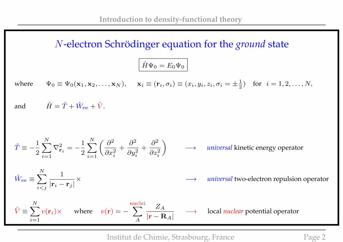
N -electron Schrödinger equation for the ground state
HΨ0 = E0Ψ0
where Ψ0 ≡ Ψ0(x1,x2, . . . ,xN ), xi ≡ (ri, σi) ≡ (xi, yi, zi, σi = ± 12
) for i = 1, 2, . . . , N,
and H = T + Wee + V .
T ≡ −1
2
N∑i=1
∇2ri
= −1
2
N∑i=1
(∂2
∂x2i
+∂2
∂y2i
+∂2
∂z2i
)−→ universal kinetic energy operator
Wee ≡N∑i<j
1
|ri − rj |× −→ universal two-electron repulsion operator
V ≡N∑i=1
v(ri)× where v(r) = −nuclei∑A
ZA
|r−RA|−→ local nuclear potential operator
Institut de Chimie, Strasbourg, France Page 2
Introduction to density-functional theory
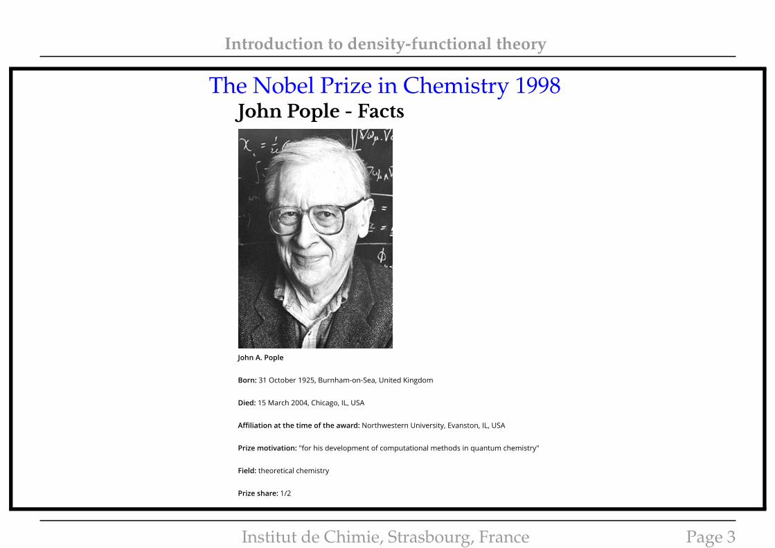
The Nobel Prize in Chemistry 1998
Share this:
(http://www.addthis.com/bookmark.php?v=300&winname=addthis&pub=nobelprize&source=tbx-300&lng=en-US&s=google_plusone_share&url=http%3A%2F
%2Fwww.nobelprize.org%2Fnobel_prizes%2Fchemistry%2Flaureates%2F1998%2Fpople-facts.html&title=John%20Pople%20-%20Facts&ate=AT-nobelprize/-/-/5376334291852234/2&frommenu=1&uid=537633427bfb5966&ct=1&pre=http%3A%2F%2Fwww.nobelprize.org%2Fnobel_prizes%2Fchemistry%2Flaureates%2F1998%2Fkohn-facts.html&tt=0&captcha_provider=nucaptcha)
0
Share this:
The Nobel Prize in Chemistry 1998
Walter Kohn, John Pople
John Pople - Facts
ShareShare
ShareMore Share
John A. Pople
Born: 31 October 1925, Burnham-on-Sea, United Kingdom
Died: 15 March 2004, Chicago, IL, USA
Affiliation at the time of the award: Northwestern University, Evanston, IL, USA
Prize motivation: "for his development of computational methods in quantum chemistry"
Field: theoretical chemistry
Prize share: 1/2
Share
John Pople - Facts http://www.nobelprize.org/nobel_prizes/chemistry/laureates/...
1 of 2 16/05/14 17:48Institut de Chimie, Strasbourg, France Page 3
Introduction to density-functional theory
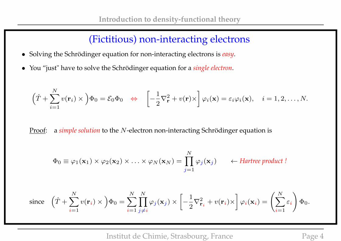
(Fictitious) non-interacting electrons• Solving the Schrödinger equation for non-interacting electrons is easy.
• You “just" have to solve the Schrödinger equation for a single electron.
(T +
N∑i=1
v(ri)×)
Φ0 = E0Φ0 ⇔[−
1
2∇2
r + v(r)×]ϕi(x) = εiϕi(x), i = 1, 2, . . . , N.
Proof: a simple solution to the N -electron non-interacting Schrödinger equation is
Φ0 ≡ ϕ1(x1)× ϕ2(x2)× . . .× ϕN (xN ) =
N∏j=1
ϕj(xj) ← Hartree product !
since(T +
N∑i=1
v(ri)×)
Φ0 =N∑i=1
N∏j 6=i
ϕj(xj)×[−
1
2∇2
ri+ v(ri)×
]ϕi(xi) =
(N∑i=1
εi
)Φ0.
Institut de Chimie, Strasbourg, France Page 4
Introduction to density-functional theory
(Real) interacting many-electron problem
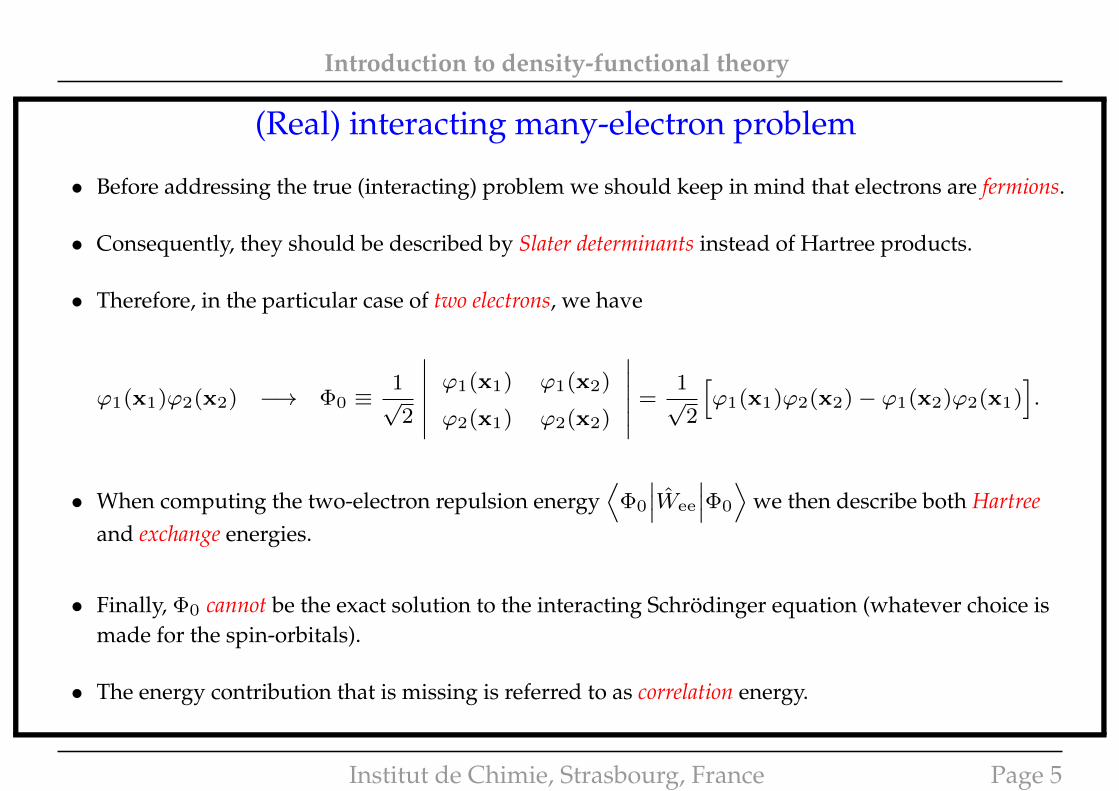
• Before addressing the true (interacting) problem we should keep in mind that electrons are fermions.
• Consequently, they should be described by Slater determinants instead of Hartree products.
• Therefore, in the particular case of two electrons, we have
ϕ1(x1)ϕ2(x2) −→ Φ0 ≡1√
2
∣∣∣∣∣∣ ϕ1(x1) ϕ1(x2)
ϕ2(x1) ϕ2(x2)
∣∣∣∣∣∣ =1√
2
[ϕ1(x1)ϕ2(x2)− ϕ1(x2)ϕ2(x1)
].
• When computing the two-electron repulsion energy⟨
Φ0
∣∣∣Wee
∣∣∣Φ0
⟩we then describe both Hartree
and exchange energies.
• Finally, Φ0 cannot be the exact solution to the interacting Schrödinger equation (whatever choice ismade for the spin-orbitals).
• The energy contribution that is missing is referred to as correlation energy.
Institut de Chimie, Strasbourg, France Page 5
Introduction to density-functional theory
Mapping the interacting problem onto a non-interacting one
• Is it possible to extract the exact (interacting) ground-state energy from a non-interacting system ?
• If yes, then it would lead to a huge simplification of the problem.
• Nevertheless, the question sounds a bit weird since the two-electron repulsion is completely ignoredin a non-interacting system.
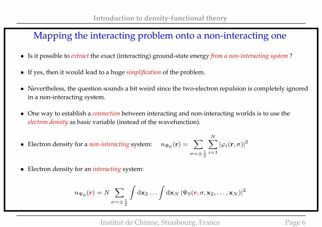
• One way to establish a connection between interacting and non-interacting worlds is to use theelectron density as basic variable (instead of the wavefunction).
• Electron density for a non-interacting system: nΦ0(r) =
∑σ=± 1
2
N∑i=1
|ϕi(r, σ)|2
• Electron density for an interacting system:
nΨ0(r) = N
∑σ=± 1
2
∫dx2 . . .
∫dxN |Ψ0(r, σ,x2, . . . ,xN )|2
Institut de Chimie, Strasbourg, France Page 6
Introduction to density-functional theory
Mapping the interacting problem onto a non-interacting one
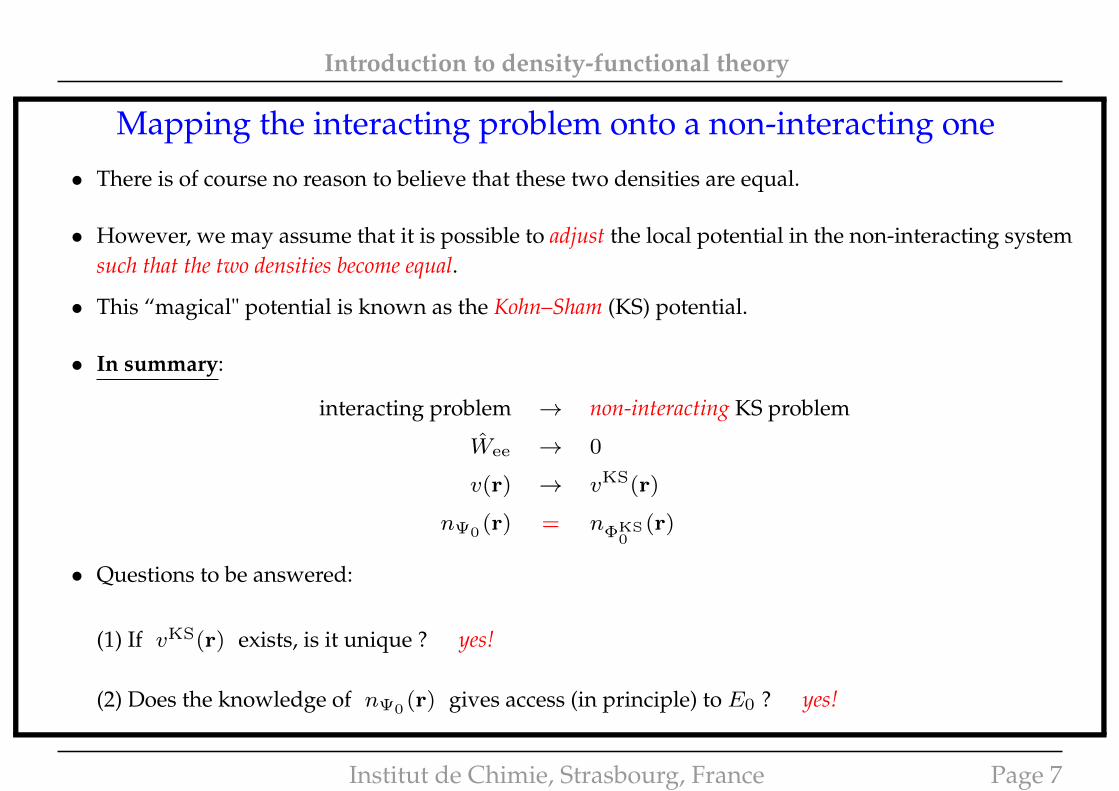
• There is of course no reason to believe that these two densities are equal.
• However, we may assume that it is possible to adjust the local potential in the non-interacting systemsuch that the two densities become equal.
• This “magical" potential is known as the Kohn–Sham (KS) potential.
• In summary:
interacting problem → non-interacting KS problem
Wee → 0
v(r) → vKS(r)
nΨ0 (r) = nΦKS0
(r)
• Questions to be answered:
(1) If vKS(r) exists, is it unique ? yes!
(2) Does the knowledge of nΨ0(r) gives access (in principle) to E0 ? yes!
Institut de Chimie, Strasbourg, France Page 7
Introduction to density-functional theory
The Nobel Prize in Chemistry 1998
This website uses cookies to improve user experience. By using our website you consent to all cookies inaccordance with our Cookie Policy.
I UNDERSTAND
Share this: 6
The Nobel Prize in Chemistry 1998
Walter Kohn, John Pople
Walter Kohn - Facts
WorkThe structures of molecules and the way they react with one another depends on the movement of electrons and their
distribution in space, which is determined by the laws of quantum mechanics. However, quantum mechanics requires
very complicated calculations for complex systems such as molecules. In 1964 Walter Kohn laid the foundation for a
theory that stated it was not necessary to account for every electron's movement. Instead, one could look at the
average density of electrons in the space. This presented new opportunities for calculations involving chemical
structures and reactions.
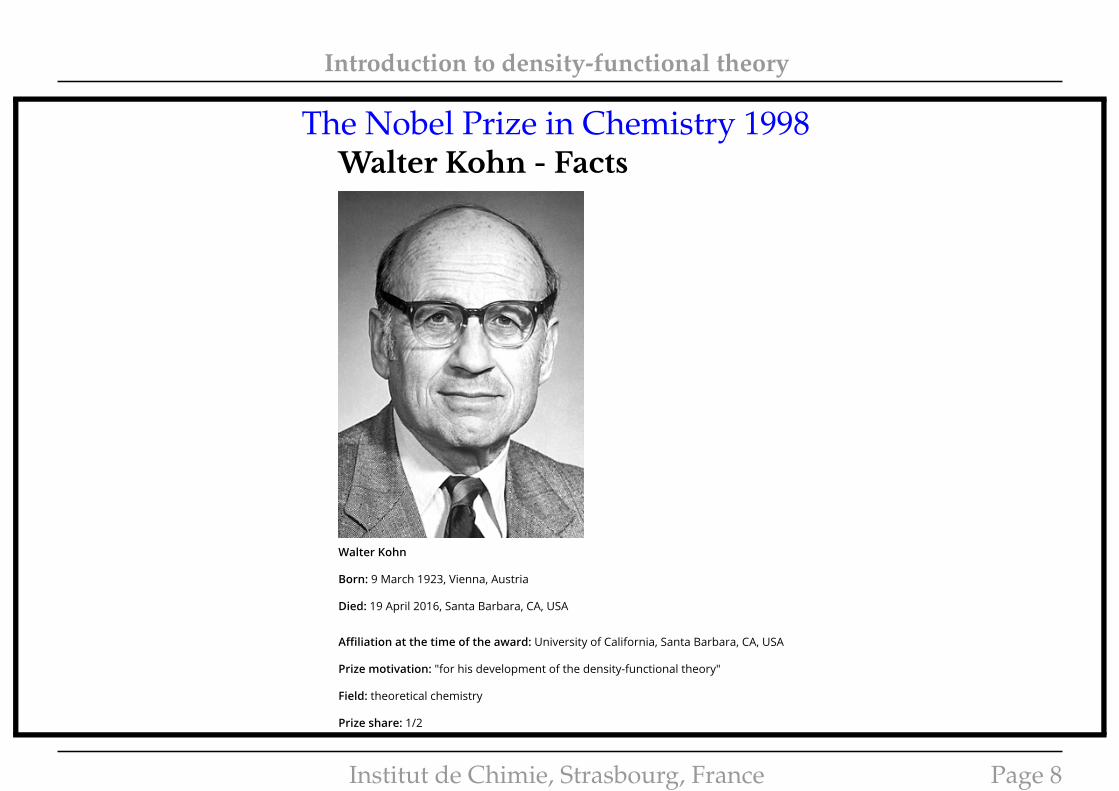
Walter Kohn
Born: 9 March 1923, Vienna, Austria
Died: 19 April 2016, Santa Barbara, CA, USA
Affiliation at the time of the award: University of California, Santa Barbara, CA, USA
Prize motivation: "for his development of the density-functional theory"
Field: theoretical chemistry
Prize share: 1/2
Walter Kohn - Facts https://www.nobelprize.org/nobel_prizes/chemistry/laureates/...
1 of 2 23/02/2017, 10:24
Institut de Chimie, Strasbourg, France Page 8
Introduction to density-functional theory
Two things to remember before we start ...
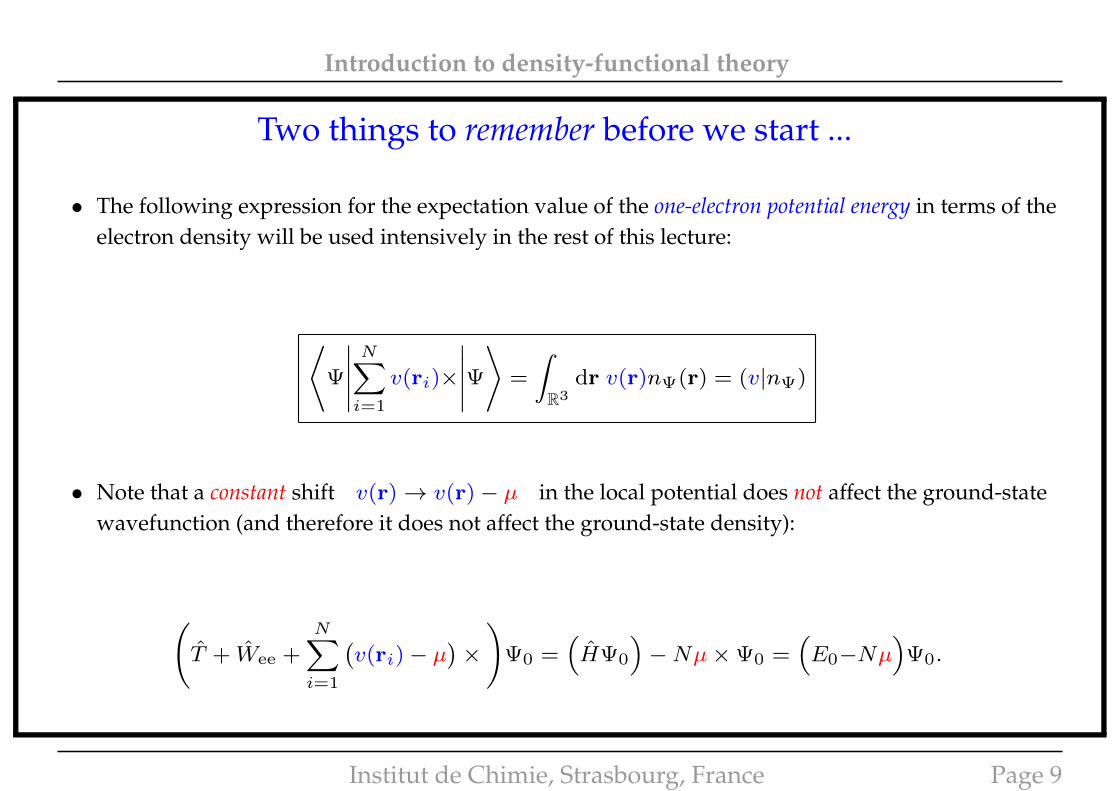
• The following expression for the expectation value of the one-electron potential energy in terms of theelectron density will be used intensively in the rest of this lecture:
⟨Ψ
∣∣∣∣∣N∑i=1
v(ri)×
∣∣∣∣∣Ψ⟩
=
∫R3
dr v(r)nΨ(r) = (v|nΨ)
• Note that a constant shift v(r)→ v(r)− µ in the local potential does not affect the ground-statewavefunction (and therefore it does not affect the ground-state density):
(T + Wee +
N∑i=1
(v(ri)− µ
)×)
Ψ0 =(HΨ0
)−Nµ×Ψ0 =
(E0−Nµ
)Ψ0.
Institut de Chimie, Strasbourg, France Page 9
Introduction to density-functional theory
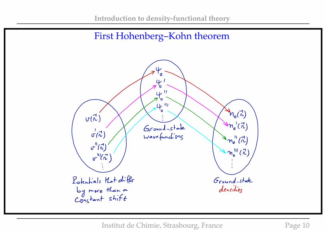
First Hohenberg–Kohn theorem
4
¥
.run ,i "
jet ) wavefunctionsno
"C I )
v"
cryno "ci ,r' " Ci ) .
'
i.
i
Potentials that differ Ground -state
by more than a densitiesConstant shift
Institut de Chimie, Strasbourg, France Page 10
Introduction to density-functional theory
First Hohenberg–Kohn theorem
• Note that v → Ψ0 → E0
→ n0 = nΨ0
• HK1: Hohenberg and Kohn∗ have shown that, in fact, the ground-state electron density fullydetermines (up to a constant) the local potential v. Therefore
n0 → v → Ψ0 → E0
• In other words, the ground-state energy is a functional of the ground-state density: E0 = E[n0].
Proof (part 1):
Let us consider two potentials v and v′ that differ by more than a constant, which means that v(r)− v′(r)
varies with r. In the following, we denote Ψ0 and Ψ′0 the associated ground-state wavefunctions withenergies E0 and E′0, respectively.
∗P. Hohenberg and W. Kohn, Phys. Rev. 136, B864 (1964).
Institut de Chimie, Strasbourg, France Page 11
Introduction to density-functional theory
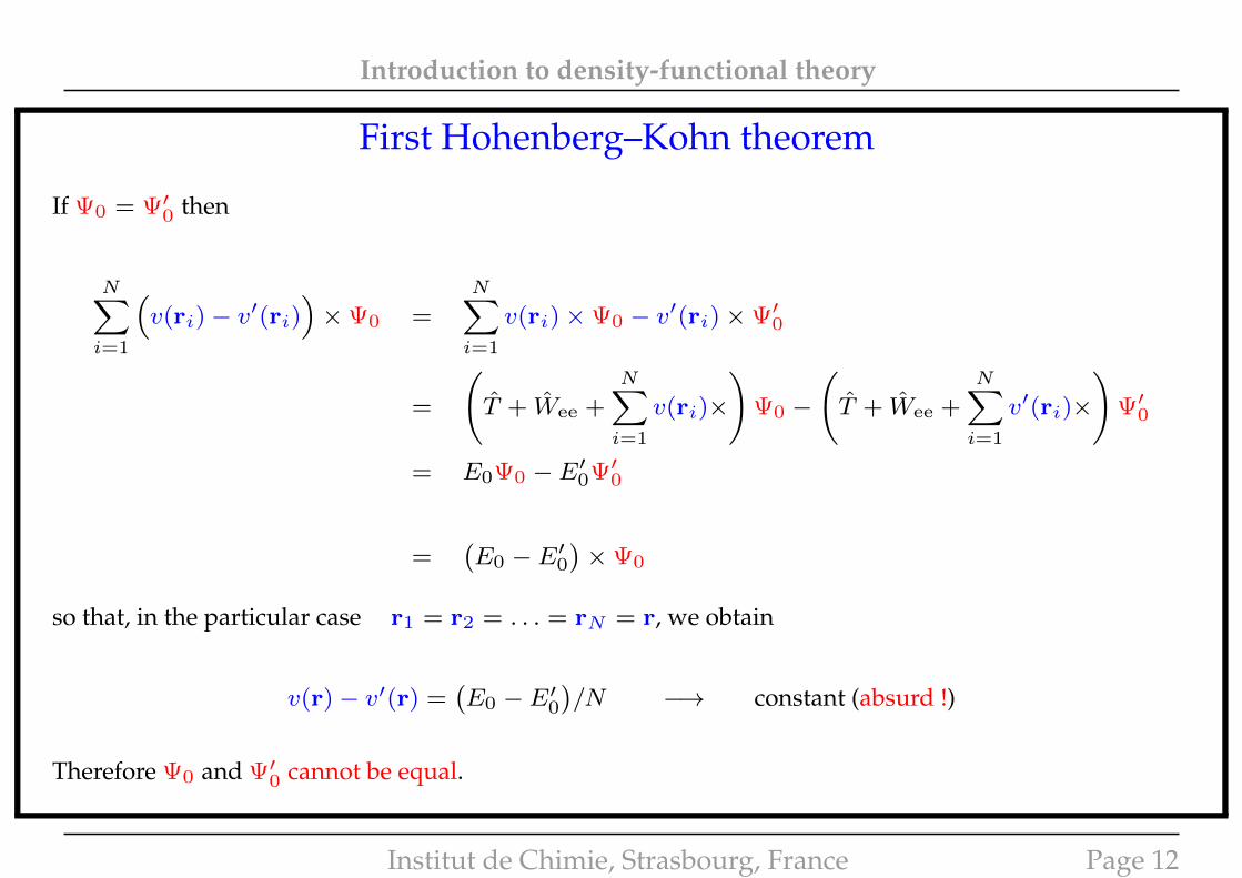
First Hohenberg–Kohn theorem
If Ψ0 = Ψ′0 then
N∑i=1
(v(ri)− v′(ri)
)×Ψ0 =
N∑i=1
v(ri)×Ψ0 − v′(ri)×Ψ′0
=
(T + Wee +
N∑i=1
v(ri)×)
Ψ0 −(T + Wee +
N∑i=1
v′(ri)×)
Ψ′0
= E0Ψ0 − E′0Ψ′0
=(E0 − E′0
)×Ψ0
so that, in the particular case r1 = r2 = . . . = rN = r, we obtain
v(r)− v′(r) =(E0 − E′0
)/N −→ constant (absurd !)
Therefore Ψ0 and Ψ′0 cannot be equal.
Institut de Chimie, Strasbourg, France Page 12
Introduction to density-functional theory
First Hohenberg–Kohn theorem
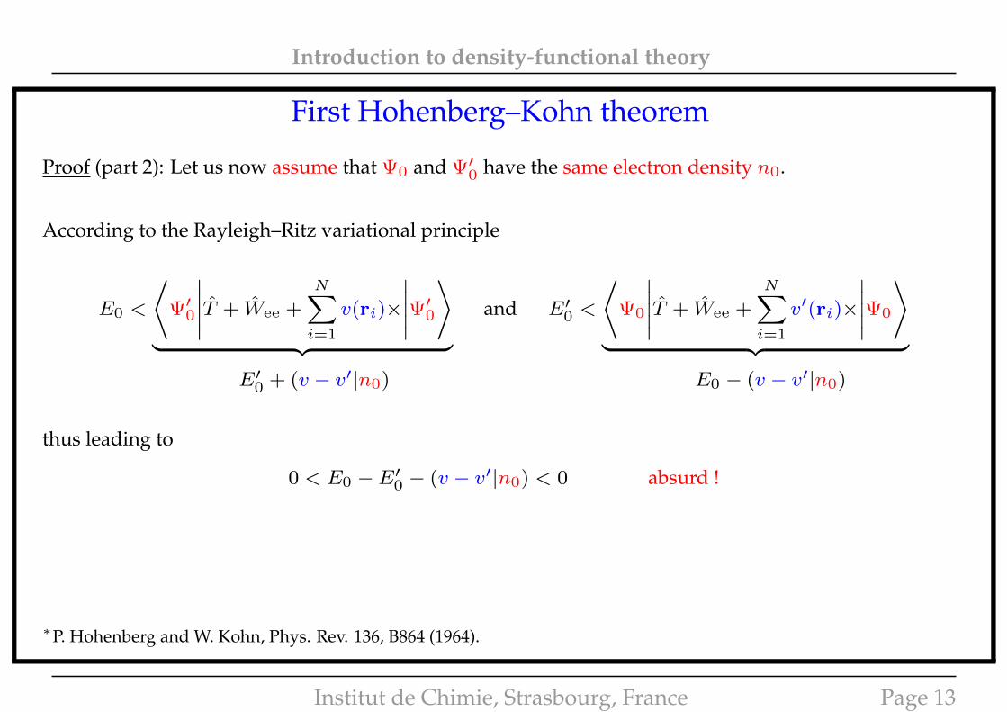
Proof (part 2): Let us now assume that Ψ0 and Ψ′0 have the same electron density n0.
According to the Rayleigh–Ritz variational principle
E0 <
⟨Ψ′0
∣∣∣∣∣T + Wee +
N∑i=1
v(ri)×
∣∣∣∣∣Ψ′0⟩
︸ ︷︷ ︸ and E′0 <
⟨Ψ0
∣∣∣∣∣T + Wee +
N∑i=1
v′(ri)×
∣∣∣∣∣Ψ0
⟩︸ ︷︷ ︸
E′0 + (v − v′|n0) E0 − (v − v′|n0)
thus leading to
0 < E0 − E′0 − (v − v′|n0) < 0 absurd !
∗P. Hohenberg and W. Kohn, Phys. Rev. 136, B864 (1964).
Institut de Chimie, Strasbourg, France Page 13
Introduction to density-functional theory
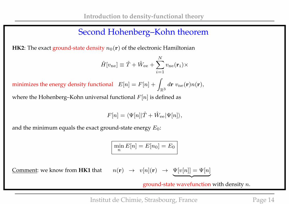
Second Hohenberg–Kohn theorem
HK2: The exact ground-state density n0(r) of the electronic Hamiltonian
H[vne] ≡ T + Wee +N∑i=1
vne(ri)×
minimizes the energy density functional E[n] = F [n] +
∫R3dr vne(r)n(r),
where the Hohenberg–Kohn universal functional F [n] is defined as
F [n] = 〈Ψ[n]|T + Wee|Ψ[n]〉,
and the minimum equals the exact ground-state energy E0:
minnE[n] = E[n0] = E0
Comment: we know from HK1 that n(r) → v[n](r) → Ψ[v[n]] = Ψ[n]︸ ︷︷ ︸ground-state wavefunction with density n.
Institut de Chimie, Strasbourg, France Page 14
Introduction to density-functional theory
Second Hohenberg–Kohn theorem
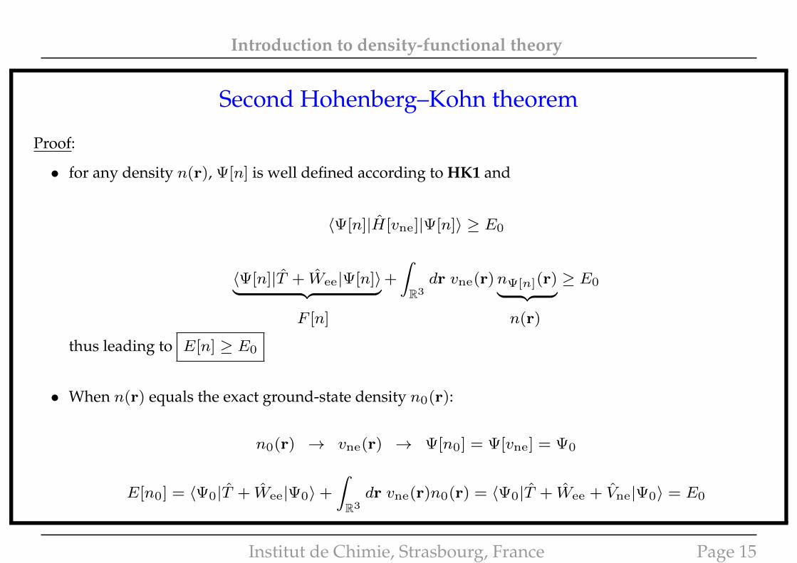
Proof:
• for any density n(r), Ψ[n] is well defined according to HK1 and
〈Ψ[n]|H[vne]|Ψ[n]〉 ≥ E0
〈Ψ[n]|T + Wee|Ψ[n]〉︸ ︷︷ ︸+
∫R3dr vne(r)nΨ[n](r)︸ ︷︷ ︸ ≥ E0
F [n] n(r)
thus leading to E[n] ≥ E0
• When n(r) equals the exact ground-state density n0(r):
n0(r) → vne(r) → Ψ[n0] = Ψ[vne] = Ψ0
E[n0] = 〈Ψ0|T + Wee|Ψ0〉+
∫R3dr vne(r)n0(r) = 〈Ψ0|T + Wee + Vne|Ψ0〉 = E0
Institut de Chimie, Strasbourg, France Page 15
Introduction to density-functional theory
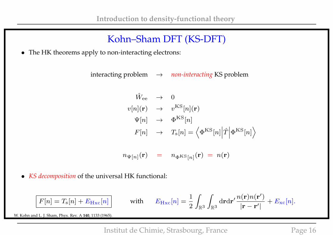
Kohn–Sham DFT (KS-DFT)• The HK theorems apply to non-interacting electrons:
interacting problem → non-interacting KS problem
Wee → 0
v[n](r) → vKS[n](r)
Ψ[n] → ΦKS[n]
F [n] → Ts[n] =⟨
ΦKS[n]∣∣∣T ∣∣∣ΦKS[n]
⟩nΨ[n](r) = nΦKS[n](r) = n(r)
• KS decomposition of the universal HK functional:
F [n] = Ts[n] + EHxc[n] with EHxc[n] =1
2
∫R3
∫R3
drdr′n(r)n(r′)|r− r′|
+ Exc[n].
W. Kohn and L. J. Sham, Phys. Rev. A 140, 1133 (1965).
Institut de Chimie, Strasbourg, France Page 16
Introduction to density-functional theory
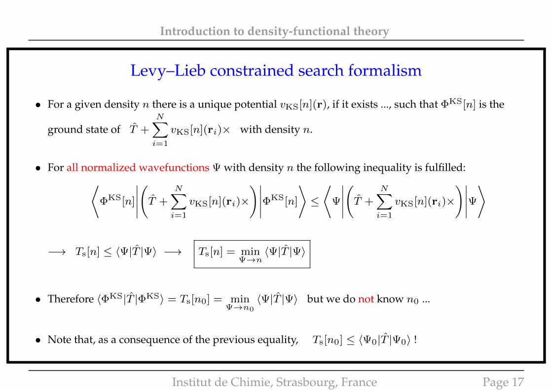
Levy–Lieb constrained search formalism
• For a given density n there is a unique potential vKS[n](r), if it exists ..., such that ΦKS[n] is the
ground state of T +
N∑i=1
vKS[n](ri)× with density n.
• For all normalized wavefunctions Ψ with density n the following inequality is fulfilled:⟨ΦKS[n]
∣∣∣∣∣(T +
N∑i=1
vKS[n](ri)×)∣∣∣∣∣ΦKS[n]
⟩≤⟨
Ψ
∣∣∣∣∣(T +
N∑i=1
vKS[n](ri)×)∣∣∣∣∣Ψ
⟩
−→ Ts[n] ≤ 〈Ψ|T |Ψ〉 −→ Ts[n] = minΨ→n
〈Ψ|T |Ψ〉
• Therefore 〈ΦKS|T |ΦKS〉 = Ts[n0] = minΨ→n0
〈Ψ|T |Ψ〉 but we do not know n0 ...
• Note that, as a consequence of the previous equality, Ts[n0] ≤ 〈Ψ0|T |Ψ0〉 !
Institut de Chimie, Strasbourg, France Page 17
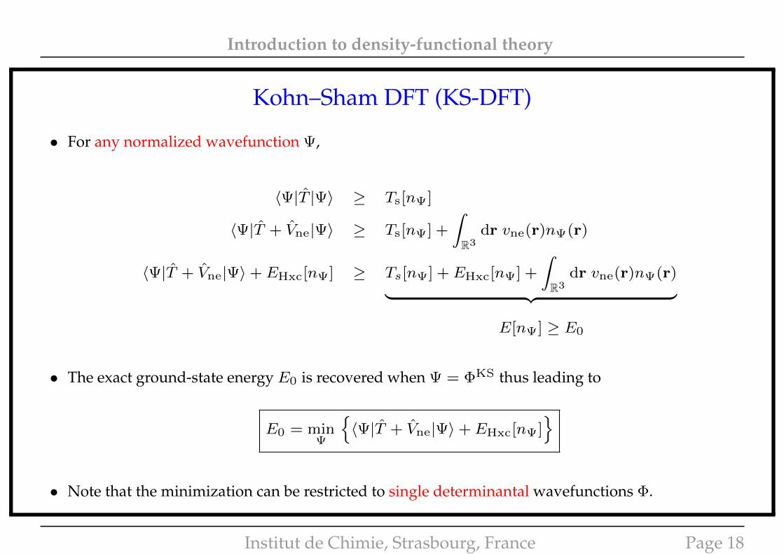
Introduction to density-functional theory
Kohn–Sham DFT (KS-DFT)
• For any normalized wavefunction Ψ,
〈Ψ|T |Ψ〉 ≥ Ts[nΨ]
〈Ψ|T + Vne|Ψ〉 ≥ Ts[nΨ] +
∫R3
dr vne(r)nΨ(r)
〈Ψ|T + Vne|Ψ〉+ EHxc[nΨ] ≥ Ts[nΨ] + EHxc[nΨ] +
∫R3
dr vne(r)nΨ(r)︸ ︷︷ ︸E[nΨ] ≥ E0
• The exact ground-state energy E0 is recovered when Ψ = ΦKS thus leading to
E0 = minΨ
{〈Ψ|T + Vne|Ψ〉+ EHxc[nΨ]
}
• Note that the minimization can be restricted to single determinantal wavefunctions Φ.
Institut de Chimie, Strasbourg, France Page 18
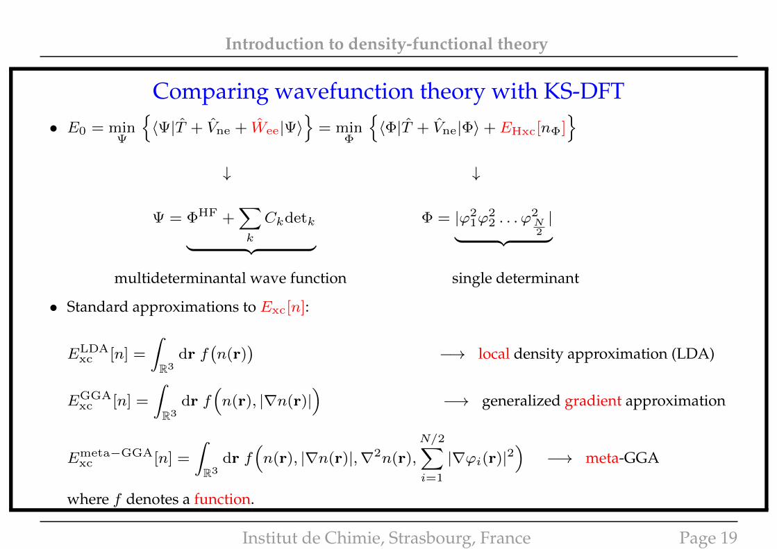
Introduction to density-functional theory
Comparing wavefunction theory with KS-DFT• E0 = min
Ψ
{〈Ψ|T + Vne + Wee|Ψ〉
}= min
Φ
{〈Φ|T + Vne|Φ〉+ EHxc[nΦ]
}↓ ↓
Ψ = ΦHF +∑k
Ckdetk︸ ︷︷ ︸Φ = |ϕ2
1ϕ22 . . . ϕ
2N2
|︸ ︷︷ ︸multideterminantal wave function single determinant
• Standard approximations to Exc[n]:
ELDAxc [n] =
∫R3
dr f(n(r)
)−→ local density approximation (LDA)
EGGAxc [n] =
∫R3
dr f(n(r), |∇n(r)|
)−→ generalized gradient approximation
Emeta−GGAxc [n] =
∫R3
dr f(n(r), |∇n(r)|,∇2n(r),
N/2∑i=1
|∇ϕi(r)|2)−→ meta-GGA
where f denotes a function.
Institut de Chimie, Strasbourg, France Page 19
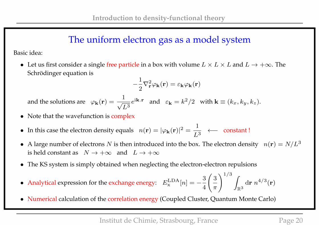
Introduction to density-functional theory
The uniform electron gas as a model systemBasic idea:
• Let us first consider a single free particle in a box with volume L× L× L and L→ +∞. TheSchrödinger equation is
−1
2∇2
rϕk(r) = εkϕk(r)
and the solutions are ϕk(r) =1√L3
eik.r and εk = k2/2 with k ≡ (kx, ky , kz).
• Note that the wavefunction is complex
• In this case the electron density equals n(r) = |ϕk(r)|2 =1
L3←− constant !
• A large number of electrons N is then introduced into the box. The electron density n(r) = N/L3
is held constant as N → +∞ and L→ +∞
• The KS system is simply obtained when neglecting the electron-electron repulsions
• Analytical expression for the exchange energy: ELDAx [n] = −
3
4
(3
π
)1/3 ∫R3
dr n4/3(r)
• Numerical calculation of the correlation energy (Coupled Cluster, Quantum Monte Carlo)
Institut de Chimie, Strasbourg, France Page 20
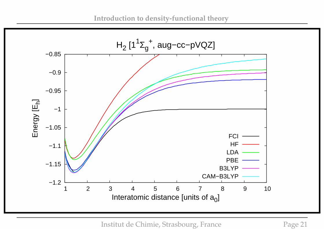
Introduction to density-functional theory
−1.2
−1.15
−1.1
−1.05
−1
−0.95
−0.9
−0.85
1 2 3 4 5 6 7 8 9 10
Ene
rgy
[Eh]
Interatomic distance [units of a0]
H2 [11Σg+, aug−cc−pVQZ]
FCIHF
LDAPBE
B3LYPCAM−B3LYP
Institut de Chimie, Strasbourg, France Page 21
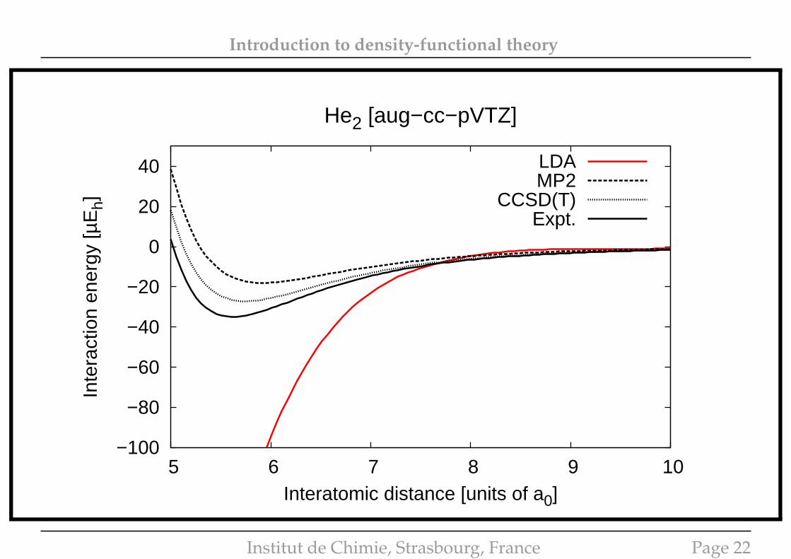
Introduction to density-functional theory
−100
−80
−60
−40
−20
0
20
40
5 6 7 8 9 10
Inte
ract
ion
ener
gy [µ
Eh]
Interatomic distance [units of a0]
He2 [aug−cc−pVTZ]
LDAMP2
CCSD(T)Expt.
Institut de Chimie, Strasbourg, France Page 22
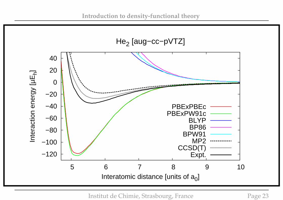
Introduction to density-functional theory
−120
−100
−80
−60
−40
−20
0
20
40
5 6 7 8 9 10
Inte
ract
ion
ener
gy [µ
Eh]
Interatomic distance [units of a0]
He2 [aug−cc−pVTZ]
PBExPBEcPBExPW91c
BLYPBP86
BPW91MP2
CCSD(T)Expt.
Institut de Chimie, Strasbourg, France Page 23
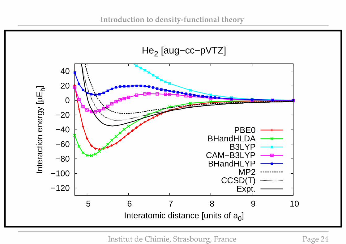
Introduction to density-functional theory
−120
−100
−80
−60
−40
−20
0
20
40
5 6 7 8 9 10
Inte
ract
ion
ener
gy [µ
Eh]
Interatomic distance [units of a0]
He2 [aug−cc−pVTZ]
PBE0BHandHLDA
B3LYPCAM−B3LYPBHandHLYP
MP2CCSD(T)
Expt.
Institut de Chimie, Strasbourg, France Page 24
Introduction to density-functional theory
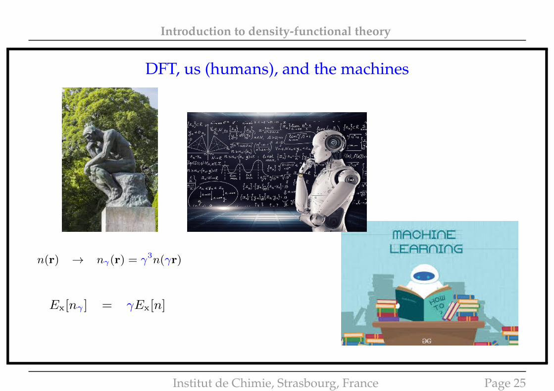
DFT, us (humans), and the machinesExact scaling relations for Ts [n] and Ex[n]
We want to see how (some) universal density functionals are a↵ected by theuniform coordinate scaling.
We start with the simplest one, namely the Hartree functional EH[n].
EXERCISE
Show that the following scaling relation is fulfilled,
EH[n� ] = �EH[n].
It can also be shown that the non-interacting kinetic energy and exact exchangeenergy functionals fulfill the following scaling relations:
Ts [n� ] = �2Ts [n] ,
Ex[n� ] = �Ex[n].EXERCISE
For that purpose, write the variational principle for the KS Hamiltonian
T +PN
i=1 vKS[n](ri)⇥, consider trial wavefunctions with density n [we denote
! n] and conclude that Ts [n] = min !n
h |T | i. Deduce that �KS� [n] = �KS[n� ].
Emmanuel Fromager (UdS) EUR: Theory of extended systems 4 / 6
Uniform coordinate scaling in wavefunctions and densities
Let � > 0 be a scaling factor.
Applying a uniform coordinate scaling consists in multiplying each spacecoordinate by �:
r ⌘ (x, y, z) ! �r ⌘ (�x, �y, �z)
dr = dxdydz ! �3dr
Uniform coordinate scaling applied to the density:
n(r) ! n�(r) = �3n(�r)
Uniform coordinate scaling applied to an N -electron wavefunction [spin isuna↵ected by the scaling]:
(r1, r2, . . . , rN ) ! �(r1, r2, . . . , rN ) = �3N2 (�r1, �r2, . . . , �rN )
Emmanuel Fromager (UdS) EUR: Theory of extended systems 2 / 6Institut de Chimie, Strasbourg, France Page 25
Introduction to density-functional theory
ARTICLE
Bypassing the Kohn-Sham equations with machinelearningFelix Brockherde1,2, Leslie Vogt 3, Li Li 4, Mark E. Tuckerman3,5,6, Kieron Burke4,7 & Klaus-Robert Müller1,8,9
Last year, at least 30,000 scientific papers used the Kohn–Sham scheme of density functional
theory to solve electronic structure problems in a wide variety of scientific fields. Machine
learning holds the promise of learning the energy functional via examples, bypassing the need
to solve the Kohn–Sham equations. This should yield substantial savings in computer
time, allowing larger systems and/or longer time-scales to be tackled, but attempts to
machine-learn this functional have been limited by the need to find its derivative. The present
work overcomes this difficulty by directly learning the density-potential and energy-density
maps for test systems and various molecules. We perform the first molecular dynamics
simulation with a machine-learned density functional on malonaldehyde and are able to
capture the intramolecular proton transfer process. Learning density models now allows the
construction of accurate density functionals for realistic molecular systems.
DOI: 10.1038/s41467-017-00839-3 OPEN
1Machine Learning Group, Technische Universität Berlin, Marchstraße 23, 10587 Berlin, Germany. 2Max-Planck-Institut für Mikrostrukturphysik, Weinberg 2,06120 Halle, Germany. 3 Department of Chemistry, New York University, New York, NY 10003, USA. 4Department of Physics and Astronomy, University ofCalifornia, Irvine, CA 92697, USA. 5 Courant Institute of Mathematical Science, New York University, New York, NY 10003, USA. 6NYU-ECNU Center forComputational Chemistry at NYU Shanghai, 3663 Zhongshan Road North, Shanghai 200062, China. 7 Department of Chemistry, University of California,Irvine, CA 92697, USA. 8Department of Brain and Cognitive Engineering, Korea University, Anam-dong, Seongbuk-gu, Seoul 136-713, Republic of Korea.9Max-Planck-Institut für Informatik, Stuhlsatzenhausweg, 66123 Saarbrücken, Germany. Correspondence and requests for materials should be addressed toM.E.T. (email:[email protected]) or to K.B. (email:[email protected]) or to K.-R.M. (email:[email protected])
NATURE COMMUNICATIONS |8: �872� |DOI: 10.1038/s41467-017-00839-3 |www.nature.com/naturecommunications 1
28/11/2019 18(01Bypassing the Kohn-Sham equations with machine learning | Nature Communications
Page 1 of 42https://www.nature.com/articles/s41467-017-00839-3
Help us improve our products. Sign up to take part.
Article
Open Access
Published: 11 October 2017
Bypassing the Kohn-Sham equations withmachine learning
Felix Brockherde, Leslie Vogt, Li Li, Mark E. Tuckerman , Kieron Burke & Klaus-Robert
Müller
Nature Communications 8, Article number: 872 (2017)
10k Accesses
132 Citations
150 Altmetric
Metrics
Abstract
Last year, at least 30,000 scientific papers used the Kohn–Sham scheme of densityfunctional theory to solve electronic structure problems in a wide variety ofscientific fields. Machine learning holds the promise of learning the energyfunctional via examples, bypassing the need to solve the Kohn–Sham equations.This should yield substantial savings in computer time, allowing larger systems
Institut de Chimie, Strasbourg, France Page 26
Introduction to density-functional theory
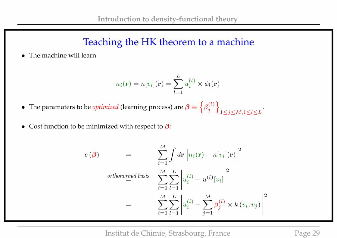
Teaching the HK theorem to a machine
• One can teach the functional Ts[n] to a machine.
• But then it needs to find the value of δTs[n]/δn(r) by itself ...
• ... in order to determine n0 variationally from vne.
• What about learning the map v → n[v] directly ?∗
• If we have vne, the machine will tell us directly what n0 = n[vne] is.
• We can also teach the machine how to compute the energy E[n0] = Ts[n0] + EHxc[n0] + (vne|n0).
∗Brockherde, Felix, Vogt, Leslie, Li ,Li, Tuckerman, Mark E, Burke, Kieron and Muller, Klaus-Robert, Nature Communications 8, 872 (2017).
Institut de Chimie, Strasbourg, France Page 27
Introduction to density-functional theory
Teaching the HK theorem to a machine
• Expansion of densities in an orthonormal basis of functions {φl(r)}1≤l≤L:
n[v](r) =
L∑l=1
u(l)[v]× φl(r).
• Kernel Ridge Regression (KRR) method:
u(l)[v] =
M∑j=1
β(l)j × k (v, vj)
k(v, vi) = exp
−∫dr∣∣∣v(r)− vi(r)
∣∣∣22σ2
where {vj}1≤j≤M are the potentials the machine will learn from.
Brockherde, Felix, Vogt, Leslie, Li ,Li, Tuckerman, Mark E, Burke, Kieron and Muller, Klaus-Robert, Nature Communications 8, 872 (2017).
Institut de Chimie, Strasbourg, France Page 28
Introduction to density-functional theory
Teaching the HK theorem to a machine• The machine will learn
ni(r) = n[vi](r) =
L∑l=1
u(l)i × φl(r)
• The paramaters to be optimized (learning process) are β ≡{β
(l)j
}1≤j≤M,1≤l≤L
.
• Cost function to be minimized with respect to β:
e (β) =
M∑i=1
∫dr∣∣∣ni(r)− n[vi](r)
∣∣∣2orthonormal basis
=
M∑i=1
L∑l=1
∣∣∣∣∣u(l)i − u
(l)[vi]
∣∣∣∣∣2
=
M∑i=1
L∑l=1
∣∣∣∣∣u(l)i −
M∑j=1
β(l)j × k (vi, vj)
∣∣∣∣∣2
Institut de Chimie, Strasbourg, France Page 29
Introduction to density-functional theory
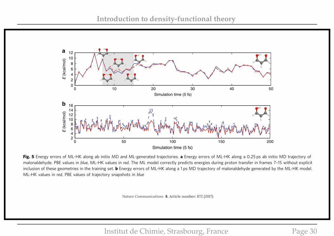
is the average of tautomer atomic positions. For the test set, weuse snapshots from a computationally expensiveBorn–Oppenheimer ab initio MD trajectory at 300 K. Figure 5ashows that the ML-HK map is able to predict DFT energiesduring a proton transfer event (MAE of 0.27 kcal/mol) despitebeing trained on classical geometries that did not include theseintermediate points.
We show, finally, that the ML-HK map can also be used togenerate a stable MD trajectory for malonaldehyde at 300 K(Fig. 5b). In principle, analytic gradients could be obtained for
each timestep, but for this first proof-of-concept trajectory, afinite-difference approach was used to determine atomic forces.The ML-HK-generated trajectory samples the same molecularconfigurations as the ab inito MD simulation (see Fig. 6 andSupplementary Table 1) with a mean absolute energy error of0.77 kcal/mol, but it typically underestimates the energy for out-of-plane molecular fluctuations at the extremes of the classicaltraining set (maximum error of 5.7 kcal/mol, see SupplementaryFig. 4). Even with the underestimated energy values, however, theatomic forces are sufficiently large to return the molecule to the
–0.0165
–0.0105
–0.0045
0.0015
0.0075
0.0135
nPBE − nLDA nPBEb − nPBE nPBEb − nML
nPBEb − nML
–0.0004700–0.0003845–0.0002991–0.0002136–0.0001282–0.00004270.00004270.00012820.00021360.00029910.00038450.0004700
a b c
d e f
−0.015
−0.010
−0.005
0.000
0.005
0.010
0.015nPBE
nLDA − nPBE
nPBE − nPBEb
nPBEb − nML
0.00
0.08
0.16
0.24
0.32
0.40
Fig. 4 The precision of our density predictions using the Fourier basis for the molecular plane of benzene. The plots show a the difference between thevalence density of benzene when using PBE and LDA functionals at the PBE-optimized geometry. b Error introduced by using the Fourier basisrepresentation. c Error introduced by the nML[v] density fitting (a–c on same color scale). d The total PBE valence density. e The density differences along a1D cut of a–c. f The density error introduced with the ML-HK map (same data but different scale, as in c)
0 10 20 30 40 50Simulation time (5 fs)
02468
1012
E (
kcal
/mol
)E
(kc
al/m
ol)
a
0 50 100 150 200
Simulation time (5 fs)
2468
10121416b
Fig. 5 Energy errors of ML-HK along ab initio MD and ML-generated trajectories. a Energy errors of ML-HK along a 0.25 ps ab initio MD trajectory ofmalonaldehyde. PBE values in blue, ML-HK values in red. The ML model correctly predicts energies during proton transfer in frames 7–15 without explicitinclusion of these geometries in the training set. b Energy errors of ML-HK along a 1 ps MD trajectory of malonaldehyde generated by the ML-HK model.ML-HK values in red, PBE values of trajectory snapshots in blue
NATURE COMMUNICATIONS | DOI: 10.1038/s41467-017-00839-3 ARTICLE
NATURE COMMUNICATIONS |8: �872� |DOI: 10.1038/s41467-017-00839-3 |www.nature.com/naturecommunications 7
28/11/2019 18(01Bypassing the Kohn-Sham equations with machine learning | Nature Communications
Page 1 of 42https://www.nature.com/articles/s41467-017-00839-3
Help us improve our products. Sign up to take part.
Article
Open Access
Published: 11 October 2017
Bypassing the Kohn-Sham equations withmachine learning
Felix Brockherde, Leslie Vogt, Li Li, Mark E. Tuckerman , Kieron Burke & Klaus-Robert
Müller
Nature Communications 8, Article number: 872 (2017)
10k Accesses
132 Citations
150 Altmetric
Metrics
Abstract
Last year, at least 30,000 scientific papers used the Kohn–Sham scheme of densityfunctional theory to solve electronic structure problems in a wide variety ofscientific fields. Machine learning holds the promise of learning the energyfunctional via examples, bypassing the need to solve the Kohn–Sham equations.This should yield substantial savings in computer time, allowing larger systems
Institut de Chimie, Strasbourg, France Page 30


![A Facet‐Specific Quantum Dot Passivation Strategy for Colloid Management … · 2019-03-18 · a PbS(100) surface using density functional theory (DFT) calcu-lations.[42,43] The](https://static.fdocuments.fr/doc/165x107/5eb1ecef7cf416399f1880ee/a-facetaspecific-quantum-dot-passivation-strategy-for-colloid-management-2019-03-18.jpg)