VALERI: a network of sites and a methodology for the validation of medium spatial resolution land satellite products

Frédéric Baret1, Marie Weiss2, Denis Allard3, Sébastien Garrigue1,

Marc Leroy4, Hervé Jeanjean5, R. Fernandes, R. Myneni, J. Privette, J. Morisette Hervé Bohbot6, Roland Bosseno7, Gérard Dedieu8, Carlos Di Bella9, Benoit Duchemin, Marisa Espana10, Valery Gond11, Xing Fa Gu1, Dominique Guyon12, Camille Lelong13,

Philippe Maisongrande8, Eric Mougin8, Tiit Nilson14, Frank Veroustraete15, Roxana Vintilla16 1INRA-CSE, Agroparc, 84914 Avignon, France 2NOVELTIS, Ramonville Saint Agne, France 3INRA, Biométrie, Agroparc, Avignon, France 4MEDIAS-France, Toulouse, France 5CNES, Toulouse, France 6CEFE, Montpellier, France 7IRD, INRA-CSE, Agroparc, Avignon, France 8CESBIO, Toulouse, France 9INTA, Castelar, Buones Aeres, Argentina 10 Universidad Michoacana de San Nicolas de Hidalgo, Morelia, Mexico 11CIRAD, Laboratoire Régionale de Télédétection, Cayenne, French Guyana 12INRA bioclimatologie, Domaine de la grande ferrade, France 13CIRAD, maison de la télédétection, Montpellier, France 14Tartu Observatory, Tartu, Estonia 15VITO, Mol, Belgium. 16ICPA, Bucharest, Romania ABSTRACT - Validation is mandatory to quantify the reliability of satellite biophysical products that are now routinely generated by a range of sensors. This paper presents the VALERI project dedicated to the validation of the products derived from medium resolution satellite sensors (www. avignon.inra.fr/valeri/). It describes the sites used, and the methodology developed to get the high spatial resolution map of the biophysical variables considered, i.e. LAI, fAPAR and fCover that can be estimated from ground level gap fraction measurements. Sites were selected to represent , with the other validation projects, the large variation of biomes and conditions observed over the Earth’s surface. Each site is about 3×3 km² in size and should be flat and relatively homogeneous at the medium resolution scale. For each site, the methodology used to generate the high spatial resolution biophysical variable maps is described. It is mainly based on concurent use of local gound measurements and a high spatial resolution satellite image, generally SPOT-HRV. Local ground measurements should be representative of an elementary sampling unit (ESU) that has approximately the same size as a SPOT-HRV multispectral pixel. The ground measurements mainly consist of gap fraction measurements achieved with LAI-2000 measurements or hemispherical photographs. The ESUs are selected over the whole 3×3 km² site in order to sample the vegetation types observed and to allow the derivation of variograms. A transfer function is subsequently established over the ESUs to relate the ground measurements of the biophysical variables with those of the high spatial resolution satellite image. Finally, co-kriging is applied to generate the high spatial resolution map of the biophysical variables over the 3×3 km² area. The methodology presented in this paper can serve as a basis for validating medium resolution satellite products. Finally these methodological aspects are discussed and conclusions drawn on the limitations and prospects of beforementioned validation activity. Key-words: remote sensing, biophysical variable, validation, kriging, upscaling, transfer function

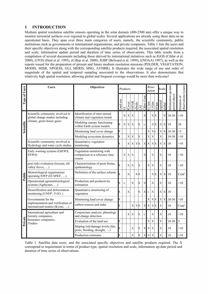
1 INTRODUCTION Medium spatial resolution satellite sensors operating in the solar domain (400-2500 nm) offer a unique way to monitor terrestrial surfaces over regional to global scales. Several applications are already using these data on an operational basis. They span over three main categories of users, namely, the scientific community, public institutions such as governments or international organisations, and private companies. Table 1 lists the users and their specific objectives along with the corresponding satellite products required, the associated spatial resolution and scale, information update period and duration of time series of observations. This table results from a compilation of several documents including those derived by international initiatives such as IGOS (Cihlar et al. 2000), GTOS (Heal et al. 1995), (Cilhar et al. 2000), IGBP (Belward et al. 1999), ((NOAA) 1997), as well as the reports issued for the preparation of present and future medium resolution missions (POLDER, VEGETATION, MODIS, MISR, NPOESS, GLI, MERIS, MSG, AVHRR). It illustrates the wide range of use and order of magnitude of the spatial and temporal sampling associated to the observations. It also demonstrates that relatively high spatial resolution, allowing global and frequent coverage would be more than welcome!

Products Reso-lution Scale

Typ

e of

Use

rs

Users Objectives

Land

use

V

I fC

over

fA

PAR

al

bedo

LA

I C

hlor

. Con

t. 0.

1 km

1.

0 km

10

km

re

gion

al

glob

al

Info

rmat

ion

up-d

ate

perio

d (d

ays)

Dur

atio

n of

ob

serv

atio

ns (y

ears

)

Identification of inter-annual climate and vegetation trends X X X X X X X 10-30 >10

Modeling canopy functioning within Earth system models X X X X X x X X X X 10 10

Monitoring land cover change X X X x X X 10-30 >5

Scientific community involved in global change studies including climate, green house gases

Modeling ecosystem dynamics X X X X X X X 10-30 >10

Scie

ntifi

c

Scientific community involved in Hydrology and water cycle studies

Quantitative vegetation monitoring X X X X X X X X X X X 10 >10

Early warning systems (GIEWS, FEWS)

Vegetation monitoring with comparison to a reference time course

X X X X X X 10 >10

pest risks evaluation (locusta, rift valley fiever, …)

Characterization of pests biotas, epidemiology X X X X X X X 10 >10

Meteorological organisations operating NWP (ECMWF, …)

Definition of the surface scheme X X X X X X X X 10 Cont1.

Operationnal agrométéorological systems (Agrhymet, …)

Production and productivity estimation X x X X X X X 10 >10

Desertification and deforestation monitoring (UNEP / FAO, )

Quantitative monitoring of vegetation X X X X x X X X 10

Monitoring land cover change X X X X X X 10-30 >10

Publ

ic

Governments for the implementation and verification of international treaties (Kyoto, …) carbon sources and sinks X X X X X X X X X 10 Cont1.

Conjoncture analysis: phenology and change detection X X X x X X 10 >10

Evaluation of the land use X X X X 10-30 5 Maping risk/damage levels (fire, pests, flooding, drought, …) X X X X X X X 10 >10

Priv

ate

International agriculture and forestry companies, Insurance companies, Traders

Production estimates X X X X X X X 10 >10

Table 1. Satellite data users, and the associated specific objectives and satellite products required. The X correspond to requirement in terms of product type, spatial resolution and scale, information up-date period and duration of time series of observations.

Table 1 shows that the duration of observations required is either continuous for operational meteorological services, or requires past time series of 5 to more than 10 years. Such long term studies are required to build a reference accounting for climate fluctuations, or to detect changes when the trend is subtle (Myneni et al. 1997). The expected period for information updates is around 10 to 30 days, mainly governed by vegetation dynamics that can be very fast for some biomes and seasons (Gond et al. 1999) The same conculsion has been drawn by several groups in charge of global observational strategy such as the Global Terrestrial Observating System group in one of its report focusing on the carbon cycle (Cilhar et al. 2000). To fulfill these conditions, three requirements have to be combined:

• to ensure the continuity of satellite observations. This is actually the case since the first launch of AVHRR in 1981, with a multiplicity of sensors since 1997 with ATSR, POLDER/ADEOS, VEGETATION, SEAWIFS, MODIS, MISR and soon MERIS. For the future, the space agencies are planning to launch new sensors to ensure the observations continuity.

• to develop algorithms allowing the derivation of biophysica products in a consistent way from the past, current and future satellite sensors. The products should also be assessed with respect to their uncertainties that will vary with the sensor or combination of sensors used. There is currently no consensus on an algorithm and they thus have to be evaluated and compared. It is possible that for some specific applications, process models will assimilate directly the radiance values. However, in this case, the validation of the intermediate products is also mandatory to make sure that the models used and the assimilation procedure are properly implemented and pertinent.

• to validate the products and provide estimates of uncertainties. The validation is the process of assessing by independent means the accuracy of data products derived from the system outputs (Justice et al. 1998). This will provide the confidence intervals that is mandatory in a number of applications, including those based on the assimilation approach.

As satellite products, both quantitative (the biophysical variables such as fAPAR, fCover, albedo, chlorophyll content and LAI) and qualitative or relative information (VI and classification) are required:

• Land use : Classification techniques applied for land use mapping will not be discussed here since it is not the main focus of this paper. However, we can note that the use of seasonality derived from a biophysical variable time course can improve the classification process

• Vegetation indices (VI): a large variety of vegetation indices have been designed to monitor vegetation amount while minimizing the effect of confounding factors such as soil background, atmosphere, or geometry of observation. They consist of relatively simple combinations of reflectance observed in few wavebands. However, in most cases, they are not strictly linked to a particular biophysical variable, and can not be considered as true biophysical variables. However, good relationships are generally found between fAPAR, fCover, LAI and a VI within restricted conditions. Except when assigning a precise meaning to the ‘vegetation amount’ that vegetation indices are targeting, vegetation indices can not be properly optimized, neither rigorously evaluated or validated. For this reason, it is preferable to characterize vegetation amount by a given biophysical variable. The cover fraction, fCover, is a good candidate since it is relatively easy to estimate as compared to LAI, highly scale independent, and independent of illumination conditions such as albedo or fAPAR.

• Albedo: is the main term for energy balance models of the Earth’s surface. It corresponds to the amount of energy scattered by the surface in all upward directions and integrated over the whole spectrum (Jacob et al. 2002). Albedo depends on the irradiance conditions as well as location (latitude) and date considered. It is generally decomposed into white and black sky quantities.

• fCover: the cover fraction simply describes the amount of vegetation. It is also generally related to the green parts of the canopies. This variable intervenes in a range of processes, and governs the partition between soil and vegetation contribution for emissivity, temperature and evaporation. It does not depend on latitude and date as opposed to fAPAR and albedo.

• fAPAR: the fraction of photosynthetic active radiation absorbed by a canopy is used as main input in net primary production models describing photosynthesis and thus the carbon budget. Only the green parts which are the only ones directly involved in photosynthesis processes should be considered. fAPAR is generally integrated over the diurnal course and thus, similarly to the albedo, it depends on the irradiance conditions as well as location (latitude) and date considered.

• LAI: the leaf area index is the main driver of most canopy functioning and SVAT models since it represents the acual size of the interface between the canopy and the atmosphere. The leaf area index should be defined here as the area of the green leaves (one sided) per unit of horizontal soil (Privette et al. 2001).

• Chlorophyll content: This biophysical variable computed at the leaf or canopy levels is linked to the nitrogen status that strongly influences photosynthesis and respiration processes. It can be considered as the terrestrial counterpart to chlorophyll concentration in oceanic phytoplankton.

This brief description of the products required by users of medium resolution satellite data users, stresses the importance of biophysical variables such as fCover, fAPAR, LAI and albedo that can ultimately replace the current use of vegetation indices. The spatial resolution required ranges between 0.1 to 10 km, although there are not too many strong arguments to specify a specific value. These figures come partly from the analysis of the current applications of medium resolution sensors. However, they strictly depend on the use considered, as well as on the spatial heterogeneity of the landscapes and the non linearity between reflectance and the biophysical variable considered (Becker and Li 1995). From this point of view, the scale effect will be quite important for LAI, and chlorophyll content (Weiss et al. 2000b), marginal for fAPAR and fCover (Malingreau and Belward 1992) (De Fries et al. 1997, Weiss et al. 2000b), and neglectable for albedo which is directly linked to a radiation flux quantity that is measured from satellite reflectances. This study focuses on the validation activity in the framework of several projects that are currently developed (Justice et al. 2000). (Justice et al. 1998, Privette et al. 1998, Justice et al. 2000, Morissette et al. 2000, Weiss et al. 2000a, Privette et al. 2001, Baret et al. 2002, Chen et al. 2002, Duchemin et al. 2002, Liang et al. 2002, Tian et al. 2002a, b, Weiss et al. 2002). They are coordinated within the Commitee on Earth Observation Satellites (CEOS) by the Working group on Calibration and Validation (WGCV), sub-group on Land Product Validation (LPV) in order to get consistent approaches and to use in a synergistic way the data gathered by individual teams. The validation projects aim at providing high spatial resolution maps (order of 10-50 m) of the biophysical variables of interest over a network of sites covering a wide range of vegetation types and conditions.This high spatial resolution map could then be exploited by agregation of the data to the proper satellite resolution to provide the independent ground truth for the validation. This paper will focus on the first results of the VALERI project (Validation of LAnd European Remote sensing Instruments). We will propose a methodology that should be considered as the state of art for to get the high spatial resolution map of the biophysical products. We will therefore not address directly the final step of the validation exercise that consists to compare biophysical values agregated at the scale of the medium spatial resolution sensors and derived from ground measurements to those of the corresonding satellite products. This paper describes the network of sites, the methodology illustrated by actual results. As a matter of fact, the methodology has evolved since the beginning of the project in 2000. The methodology presented here after is now stabilized and considered to be mature enough to be applied on a routine basis for such validation activity. VALERI mostly focused on products that can be derived from simple gap fraction measurements, i.e. fCover, fAPAR and LAI. THE NETWORK OF SITES The selected sites must fulfill a number of criteria to enable the provision of accurate estimates of biophysical variables from ground measurements. Size: The spatial resolution of the sensors considered ranges from few hundred of meters (MODIS, MERIS) to a few kilometers (MSG) with most of the sensors being around 1 km² (AVHRR, VEGETATION, SEAWIFS). Therefore, the validation sites must cover at least a 3×3 km² square. A larger size would be ideal for even coarser resolution sensors such as POLDER. However, the corresponding resources required for characterizing such a large site would too high. As an alternative, products derived from POLDER can be evaluated by comparison with other sensors products or over quite spatially homogeneous areas. Homogeneity: it should be relatively homogeneous, i.e. the biophysical variable value as well as the corresponding radiometric values may change only marginaly when shifting the position of a 1km² pixel within the 3×3 km² square. Topography: the area should be relatively flat to simplify the interpretation both of the ground measurements and the satellite data. Biome type: the selection of sites is made in order to sample the variability of biomes and conditions encountered over the Earth’s surface. Obviously this is also governed by the availability of local support for the measurements. Furthermore, the VALERI activity is coordinated with that of other validation initiatives such as that NASA’s MODLAND, CCRS LAI validation activity (Chen et al. 2002), (Privette et al. 1998), (Morissette et al. 2000) through the CEOS.

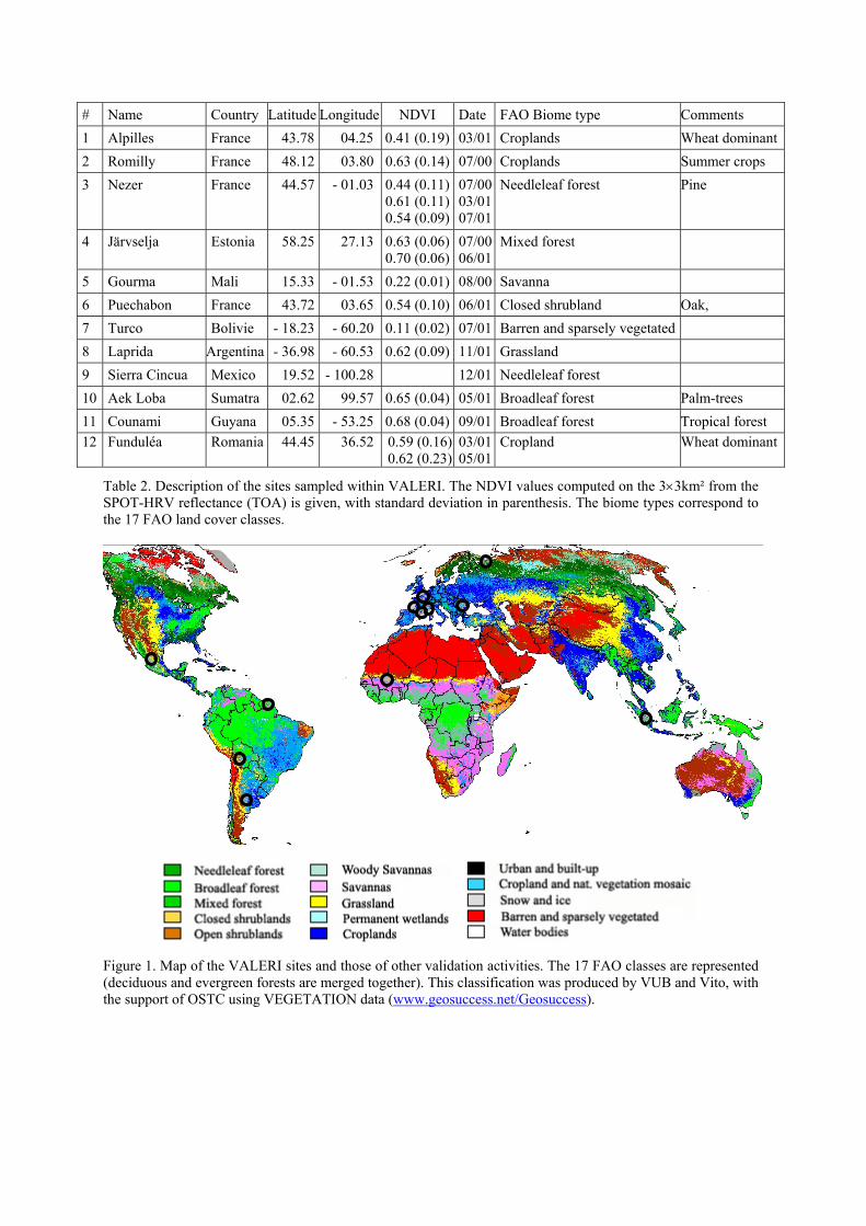
# Name Country Latitude Longitude NDVI Date FAO Biome type Comments 1 Alpilles France 43.78 04.25 0.41 (0.19) 03/01 Croplands Wheat dominant2 Romilly France 48.12 03.80 0.63 (0.14) 07/00 Croplands Summer crops 3 Nezer France 44.57 - 01.03 0.44 (0.11)

0.61 (0.11)0.54 (0.09)

07/0003/0107/01

Needleleaf forest Pine

4 Järvselja Estonia 58.25 27.13 0.63 (0.06)0.70 (0.06)

07/0006/01

Mixed forest

5 Gourma Mali 15.33 - 01.53 0.22 (0.01) 08/00 Savanna 6 Puechabon France 43.72 03.65 0.54 (0.10) 06/01 Closed shrubland Oak, 7 Turco Bolivie - 18.23 - 60.20 0.11 (0.02) 07/01 Barren and sparsely vegetated 8 Laprida Argentina - 36.98 - 60.53 0.62 (0.09) 11/01 Grassland 9 Sierra Cincua Mexico 19.52 - 100.28 12/01 Needleleaf forest 10 Aek Loba Sumatra 02.62 99.57 0.65 (0.04) 05/01 Broadleaf forest Palm-trees 11 Counami Guyana 05.35 - 53.25 0.68 (0.04) 09/01 Broadleaf forest Tropical forest 12 Funduléa Romania 44.45 36.52 0.59 (0.16)

0.62 (0.23)03/0105/01

Cropland Wheat dominant

Table 2. Description of the sites sampled within VALERI. The NDVI values computed on the 3×3km² from the SPOT-HRV reflectance (TOA) is given, with standard deviation in parenthesis. The biome types correspond to the 17 FAO land cover classes.

Figure 1. Map of the VALERI sites and those of other validation activities. The 17 FAO classes are represented (deciduous and evergreen forests are merged together). This classification was produced by VUB and Vito, with the support of OSTC using VEGETATION data (www.geosuccess.net/Geosuccess).

FAO Cover Classes VALERI sites Total sites % Total sites % FAO ClassesNeedleleaf forest 2 13 24.1 5.7 Broadleaf forest 2 7 13.0 10.5 Mixed forest 1 22 40.7 4.3 Closed shrublands 1 1 1.9 1.8 Open shrublands 0 1 1.9 12.4 Woody savannas 0 1 1.9 7.0 Savannas 1 2 3.7 6.4 Grassland 1 2 3.7 7.6 Permanent wetlands 0 0 0.0 0.9 Croplands 3 4 7.4 9.6 Cropland and natural vegetation mosaic 0 0 0.0 9.6 Barren and sparsely vegetated 1 1 1.9 12.7 TOTAL 12 54 100.0 88.5

Table 3. Number of sites sampled per biome type. The VALERI sites and the sites from the other initiatives are separated. “% Total sites” is the number of sites sampled (VALERI and others) for each biome class divided by the total number of sites sampled over all the biome classes. The fraction of land area represented by each class is also given for comparison (data coming from (Loveland et al. 2000).

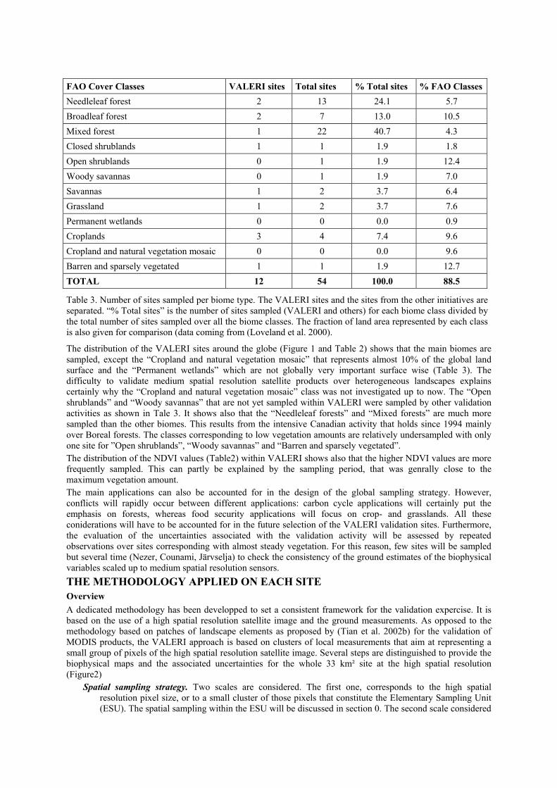
The distribution of the VALERI sites around the globe (Figure 1 and Table 2) shows that the main biomes are sampled, except the “Cropland and natural vegetation mosaic” that represents almost 10% of the global land surface and the “Permanent wetlands” which are not globally very important surface wise (Table 3). The difficulty to validate medium spatial resolution satellite products over heterogeneous landscapes explains certainly why the “Cropland and natural vegetation mosaic” class was not investigated up to now. The “Open shrublands” and “Woody savannas” that are not yet sampled within VALERI were sampled by other validation activities as shown in Tale 3. It shows also that the “Needleleaf forests” and “Mixed forests” are much more sampled than the other biomes. This results from the intensive Canadian activity that holds since 1994 mainly over Boreal forests. The classes corresponding to low vegetation amounts are relatively undersampled with only one site for ”Open shrublands”, “Woody savannas” and “Barren and sparsely vegetated”. The distribution of the NDVI values (Table2) within VALERI shows also that the higher NDVI values are more frequently sampled. This can partly be explained by the sampling period, that was genrally close to the maximum vegetation amount. The main applications can also be accounted for in the design of the global sampling strategy. However, conflicts will rapidly occur between different applications: carbon cycle applications will certainly put the emphasis on forests, whereas food security applications will focus on crop- and grasslands. All these coniderations will have to be accounted for in the future selection of the VALERI validation sites. Furthermore, the evaluation of the uncertainties associated with the validation activity will be assessed by repeated observations over sites corresponding with almost steady vegetation. For this reason, few sites will be sampled but several time (Nezer, Counami, Järvselja) to check the consistency of the ground estimates of the biophysical variables scaled up to medium spatial resolution sensors. THE METHODOLOGY APPLIED ON EACH SITE Overview A dedicated methodology has been developped to set a consistent framework for the validation expercise. It is based on the use of a high spatial resolution satellite image and the ground measurements. As opposed to the methodology based on patches of landscape elements as proposed by (Tian et al. 2002b) for the validation of MODIS products, the VALERI approach is based on clusters of local measurements that aim at representing a small group of pixels of the high spatial resolution satellite image. Several steps are distinguished to provide the biophysical maps and the associated uncertainties for the whole 33 km² site at the high spatial resolution (Figure2)

Spatial sampling strategy. Two scales are considered. The first one, corresponds to the high spatial resolution pixel size, or to a small cluster of those pixels that constitute the Elementary Sampling Unit (ESU). The spatial sampling within the ESU will be discussed in section 0. The second scale considered

is the whole 3×3 km² site that will be termed ‘WS’ in the following. The spatial sampling strategy here consists to determine the optimal number and location of ESUs to get a good representation of the WS. A high spatial resolution image will be used in the process of extending the ESU measurements to the WS.

Measurements of the biophysical variables over the ESU. Two issues have to be discussed here: the measurement method, which is generally local, and the associated spatial sampling strategy within an ESU.

Scaling-up to the whole 33 km² site. In order to take advantage of all available information, co-located kriging is applied (Goovaerts 1997). This allows to both account for the measurement points and for the high spatial resolution image. The co-located kriging requires a secondary variable, in this case the radiometric information, to be linearly related to the variable of interest (here a biophysical variable). For this reason, a transfer function is developed over the ensemble of ESUs to relate the biophysical variable to the high spatial resolution radiometric data.

Figure 2.: Scheme describing the strategy used to derive the biophysical maps at high spatial resolution from the combination of the individual ground measurements (the yellow spots) performed over the Elementary Sampling Units (ESUs) and the high spatial resolution satellite images over the whole 33 km² site (WS). The medium spatial resolution satellite pixel is represented in faded colors.

Spatial sampling strategy for the whole 3×3 km² site The objective here is to set the minimum number of ESUs at the optimal location to get both (i) a good description of the geostatistics of the biophysical variable considered over the WS, and (ii) to establish robust relationships between the measured biophysical variables and the corresponding high spatial resolution radiometric values over an ensemble of ESUs. For these reasons, the WS area is divided into nine 1 km² squares, to get a better scattering of the ESUs over the WS, improving the estimation of the geostatiscal characteristics at

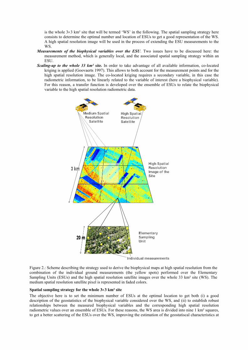
this scale. Subsequently, in each 1 km² square, 3 to 5 ESUs are considered. Their location is chosen to globally sample equally in proportion all the cover types present in the WS and within one cover type, as well as their variability. In addition, two constraints have to be accounted for: first the ESUs have to be close to an access (road, path, …) for more conveniency, but far enough from a landscape boundary to minimize the possible contamination of the radiometry of the considered ESU due to the misregistration between the GPS geolocated ESU and the corresponding high spatial resolution image. Second, the ESUs should also be spread spatially equal within the 1km² square to improve the geostatistical variables estimation. Furthermore, the 1 km² square that is located at the centre of the WS should be more densely sampled (between 5 to 7 ESUs) for a better description of the geostatistics for the medium range lags. This proposed scheme leads to a total number of 30 to 50 ESUs to sample the whole 3×3 km² site. Considering the size of ESUs (20×20 m²), the sampling rate of the WS ranges between 0.13% and 0.22%. Depending on the type of instruments used for the local measurements of the biophysical variables, and the difficulty to access the ESUs, the required manpower is between 4 man-days (2 teams of 2 people for one day) to 32 man-days. Ideally the measurement period should not exceed one week, otherwise the vegetation might significantly evolve. Once the high resolution image is acquired, the representativity of the sampling is evaluated based on the simple NDVI distribution. It is not statistically consistent to directly compare the two NDVI histograms because the number of pixels is drastically different between that of the ESUs (between 30 to 50) and that of the WS (22500 in case of a 3x3km SPOT image). Therefore, the proposed technique consists in comparing the NDVI cumulative frequency of the two distributions by:

1. Computing the cumulative frequency of the NDVI values of the 30 to 50 ESUs. 2. Applying a given translation to all of the 50 pixels (modulo the size of the image). 3. Computing the cumulative NDVI frequency of the new set of translated pixels. 4. Repeating steps 2 and 3, 199 times with 199 random values of the translation vectors.

This provides a total population of N=199+1(actual) cumulative frequency on which a statistical test at acceptance probability 1 %95=−α is applied: for a given NDVI level, if the actual ESU density function is in between two limits defined by the 5 ( 5.2 =Nα ) highest and lowest values of the 200 cumulative frequencies, the hypothesis that WS and ESUs NDVI distributions are equivalent is accepted. Otherwise it is rejected. Results obtained for the 2001 Puechabon site (Figure 3 left) show that the sampling was really good since it corresponds to a VALERI-MODLAND joint campaign with a lot of manpower and many ESUs sampled. Conversely, for the Alpilles site (Figure 3 right), the actual cumulative frequency is very close to the 5 lowest distributions, particularly for NDVI values between 0.3 and 0.5, as well as between 0.6 and 1. The sampling appears therefore not representative. However, the land cover shows that the surface that were not covered by vegetations were significant and were obviously not sampled by ESUs (roads, senescent wheat, bare soil, …). Therefore, it should be more sound to discard in the sampling strategy these areas where the green LAI is known to be 0 (roads, houses, …).by applying masks on the images for such land cover types.

Figure 3. Illustration of the test applied to verify the representativeness of the ESUs. The figure on the left correponds to the Alpilles site. That on the right corresponds to Puechabon site. If the NDVI distribution (the dots) are in between the 5 minimum and maximum distributions, then the sampling for ESU is considered to be representative.

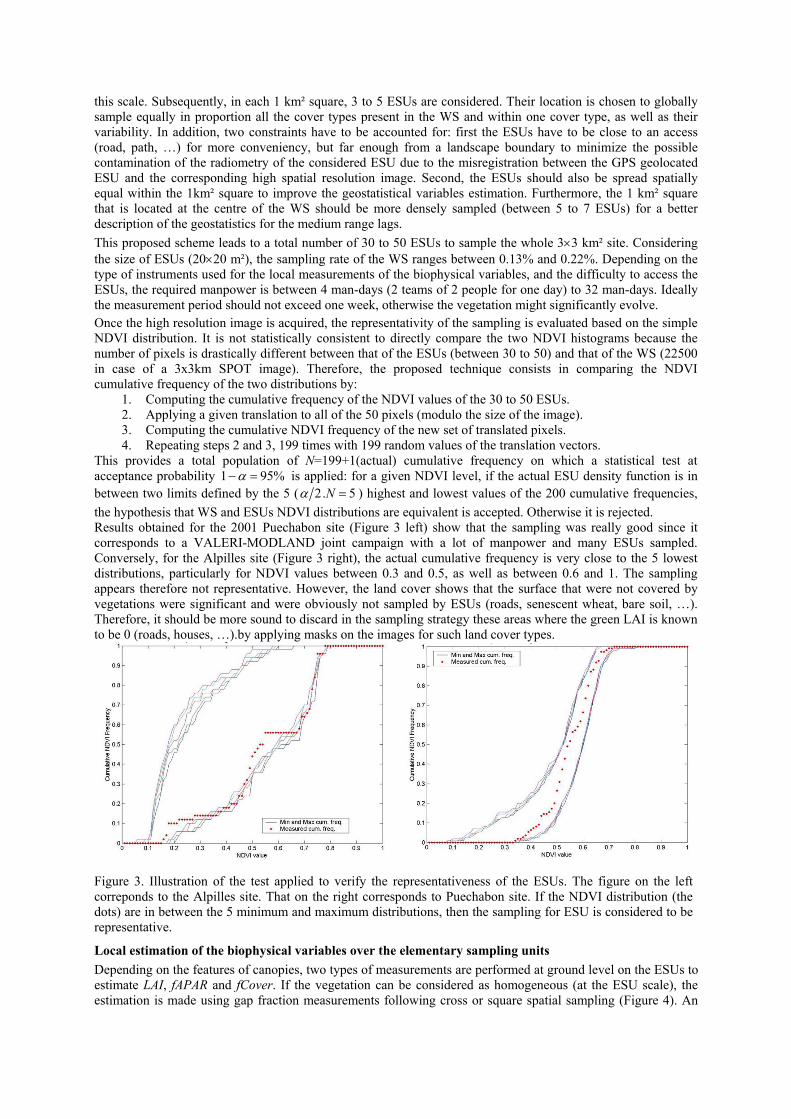
Local estimation of the biophysical variables over the elementary sampling units Depending on the features of canopies, two types of measurements are performed at ground level on the ESUs to estimate LAI, fAPAR and fCover. If the vegetation can be considered as homogeneous (at the ESU scale), the estimation is made using gap fraction measurements following cross or square spatial sampling (Figure 4). An

alternative sampling scheme (transect in figure 4) is used when the vegetation is heterogeneously distributed within the ESU. Gap fraction measurements. The gap fraction is an integrated canopy structural quantity. The vertical gap fraction corresponds directly to the complement to unity of the cover fraction (fCover). The gap fraction in the sun direction provides a direct estimation of instantaneous fAPAR (Baret et al. 1993). However, dynamic vegetation models often require estimates of fAPAR integrated over the day. This can be achieved by estimating both the black-sky fAPAR (directional fAPAR) and the white sky fAPAR (diffuse fAPAR for a given sky luminance distribution often assumed isotropic) similarly to what is proposed for albedo (Martonchik 1994). Then, the daily integrated value can be derived from the knowledge of the variation of the diffuse fraction along the day, the sun position course and the corresponding incoming radiance. Finally, gap fraction measurements allow to estimate the LAI of canopies with an asumption about the spatial organisation of the vegetation elements. This principle is exploited by the LAI2000 instrument to estimate LAI that provides an estimate of effective LAI, i.e. assuming all the elements being green and randomly distributed. The same principle can be also applied to hemispherical photographs (e.g. (Chen et al. 1991), (Leblanc et al. 2002). The use of color hemispherical photographs reduces the uncertainty associated to the green fraction estimation that is often significant for forest canopies (Fernandes et al. 2002). Hemispherical photography provides also information on the clumpiness through the gap size distribution (Chen and Cilhar 1995). This is the reason why hemispherical photographs are progressively replacing LAI2000 devices within the VALERI project. Furthermore, hemispherical photographs can be used in the case of low vegetation canopies by taking downwards looking photographs. They can also be used in more variable illumination conditions, particularly when looking upwards, which makes the measurements more flexible as compared to LAI2000. The latter requires stable diffuse illumination conditions. A dedicated software was developped to process these color photographs with emphasis on green element classification and processing of series of photographs (EYE-CAN). A more detailed review of the LAI estimation from gap fraction measurements is given by (Weiss et al. 2003) with special attention to the hemispherical photographs technique.

20 m

Square Cross Transect

20 m

Square Cross Transect

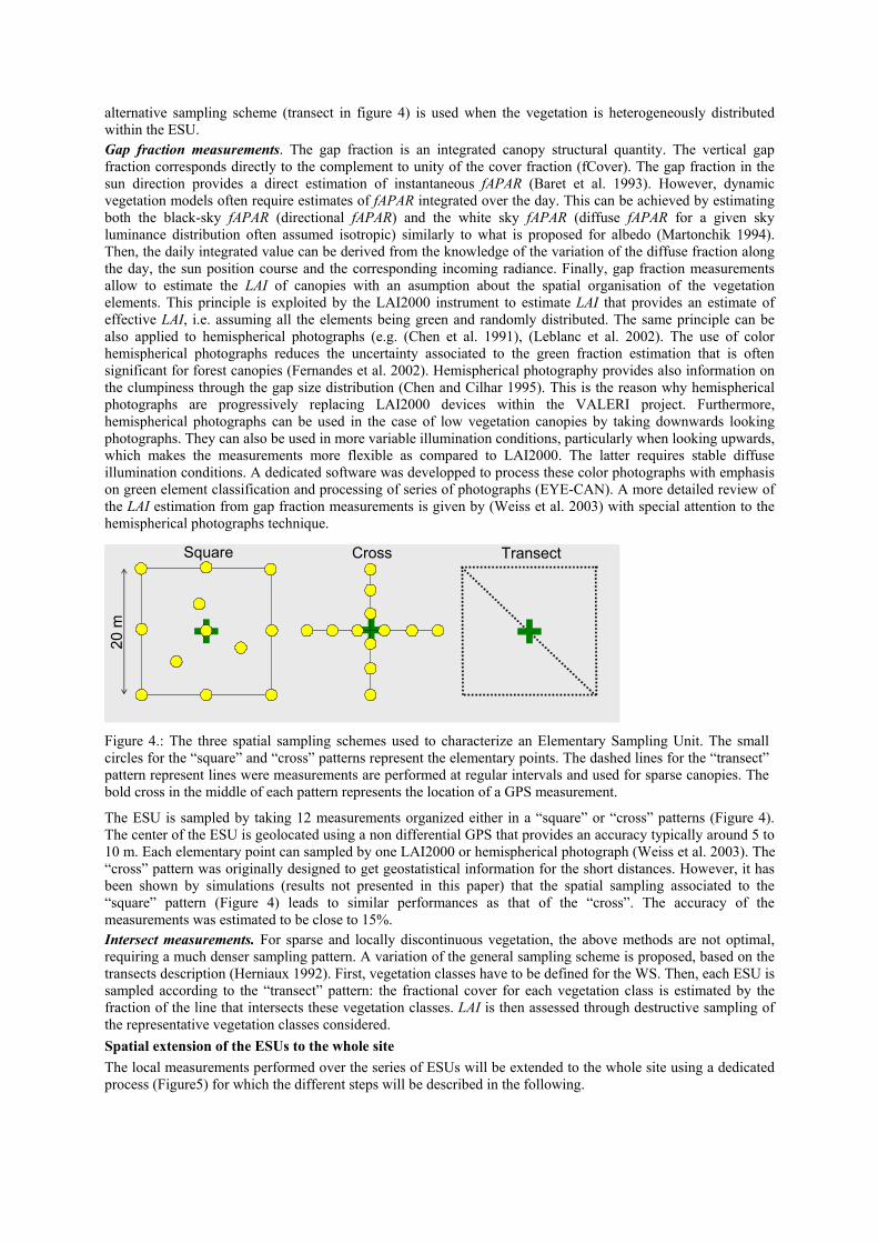
Figure 4.: The three spatial sampling schemes used to characterize an Elementary Sampling Unit. The small circles for the “square” and “cross” patterns represent the elementary points. The dashed lines for the “transect” pattern represent lines were measurements are performed at regular intervals and used for sparse canopies. The bold cross in the middle of each pattern represents the location of a GPS measurement.

The ESU is sampled by taking 12 measurements organized either in a “square” or “cross” patterns (Figure 4). The center of the ESU is geolocated using a non differential GPS that provides an accuracy typically around 5 to 10 m. Each elementary point can sampled by one LAI2000 or hemispherical photograph (Weiss et al. 2003). The “cross” pattern was originally designed to get geostatistical information for the short distances. However, it has been shown by simulations (results not presented in this paper) that the spatial sampling associated to the “square” pattern (Figure 4) leads to similar performances as that of the “cross”. The accuracy of the measurements was estimated to be close to 15%. Intersect measurements. For sparse and locally discontinuous vegetation, the above methods are not optimal, requiring a much denser sampling pattern. A variation of the general sampling scheme is proposed, based on the transects description (Herniaux 1992). First, vegetation classes have to be defined for the WS. Then, each ESU is sampled according to the “transect” pattern: the fractional cover for each vegetation class is estimated by the fraction of the line that intersects these vegetation classes. LAI is then assessed through destructive sampling of the representative vegetation classes considered. Spatial extension of the ESUs to the whole site The local measurements performed over the series of ESUs will be extended to the whole site using a dedicated process (Figure5) for which the different steps will be described in the following.

Vm

Local measurementsover ESUs

R High Res. Image

F :TransferFunction

Vt=F(R)High Res. Image

ColocatedKriging

Vk

High Res. Image

Input data

Geostatistics

HighResolutionValidationProducts

TransferFunction

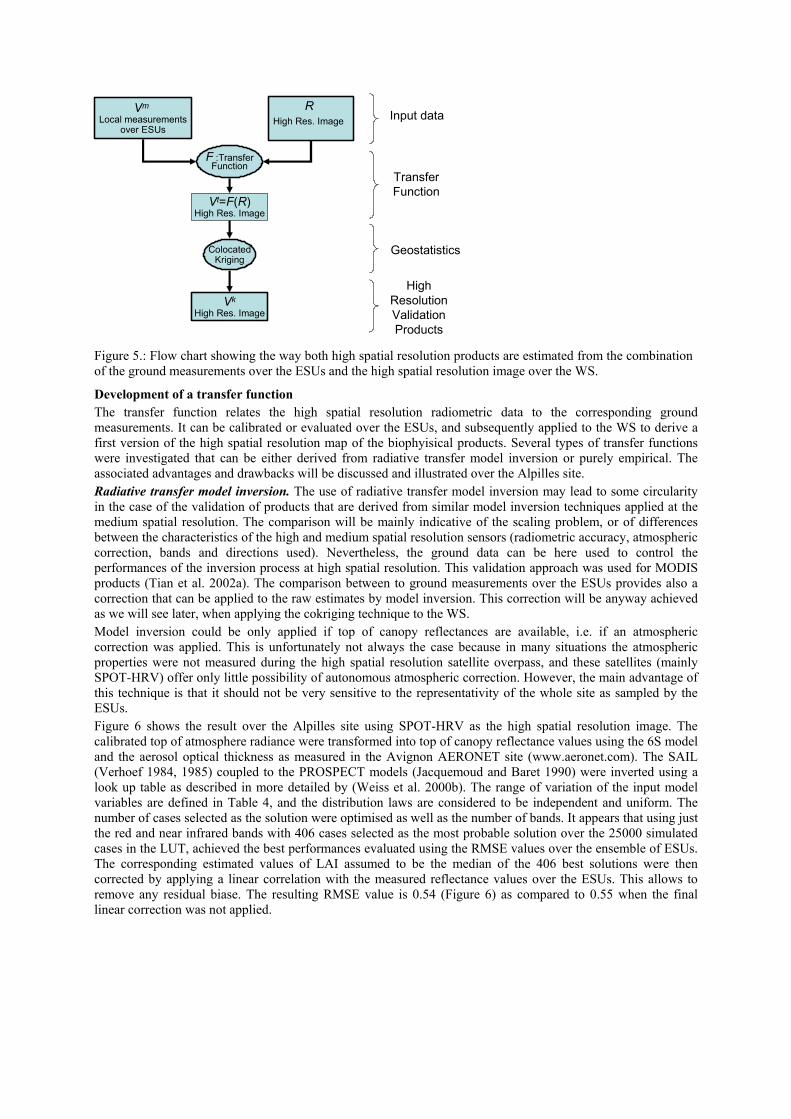
Figure 5.: Flow chart showing the way both high spatial resolution products are estimated from the combination of the ground measurements over the ESUs and the high spatial resolution image over the WS.

Development of a transfer function The transfer function relates the high spatial resolution radiometric data to the corresponding ground measurements. It can be calibrated or evaluated over the ESUs, and subsequently applied to the WS to derive a first version of the high spatial resolution map of the biophyisical products. Several types of transfer functions were investigated that can be either derived from radiative transfer model inversion or purely empirical. The associated advantages and drawbacks will be discussed and illustrated over the Alpilles site. Radiative transfer model inversion. The use of radiative transfer model inversion may lead to some circularity in the case of the validation of products that are derived from similar model inversion techniques applied at the medium spatial resolution. The comparison will be mainly indicative of the scaling problem, or of differences between the characteristics of the high and medium spatial resolution sensors (radiometric accuracy, atmospheric correction, bands and directions used). Nevertheless, the ground data can be here used to control the performances of the inversion process at high spatial resolution. This validation approach was used for MODIS products (Tian et al. 2002a). The comparison between to ground measurements over the ESUs provides also a correction that can be applied to the raw estimates by model inversion. This correction will be anyway achieved as we will see later, when applying the cokriging technique to the WS. Model inversion could be only applied if top of canopy reflectances are available, i.e. if an atmospheric correction was applied. This is unfortunately not always the case because in many situations the atmospheric properties were not measured during the high spatial resolution satellite overpass, and these satellites (mainly SPOT-HRV) offer only little possibility of autonomous atmospheric correction. However, the main advantage of this technique is that it should not be very sensitive to the representativity of the whole site as sampled by the ESUs. Figure 6 shows the result over the Alpilles site using SPOT-HRV as the high spatial resolution image. The calibrated top of atmosphere radiance were transformed into top of canopy reflectance values using the 6S model and the aerosol optical thickness as measured in the Avignon AERONET site (www.aeronet.com). The SAIL (Verhoef 1984, 1985) coupled to the PROSPECT models (Jacquemoud and Baret 1990) were inverted using a look up table as described in more detailed by (Weiss et al. 2000b). The range of variation of the input model variables are defined in , and the distribution laws are considered to be independent and uniform. The number of cases selected as the solution were optimised as well as the number of bands. It appears that using just the red and near infrared bands with 406 cases selected as the most probable solution over the 25000 simulated cases in the LUT, achieved the best performances evaluated using the RMSE values over the ensemble of ESUs. The corresponding estimated values of LAI assumed to be the median of the 406 best solutions were then corrected by applying a linear correlation with the measured reflectance values over the ESUs. This allows to remove any residual biase. The resulting RMSE value is 0.54 (Figure 6) as compared to 0.55 when the final linear correction was not applied.

Table 4

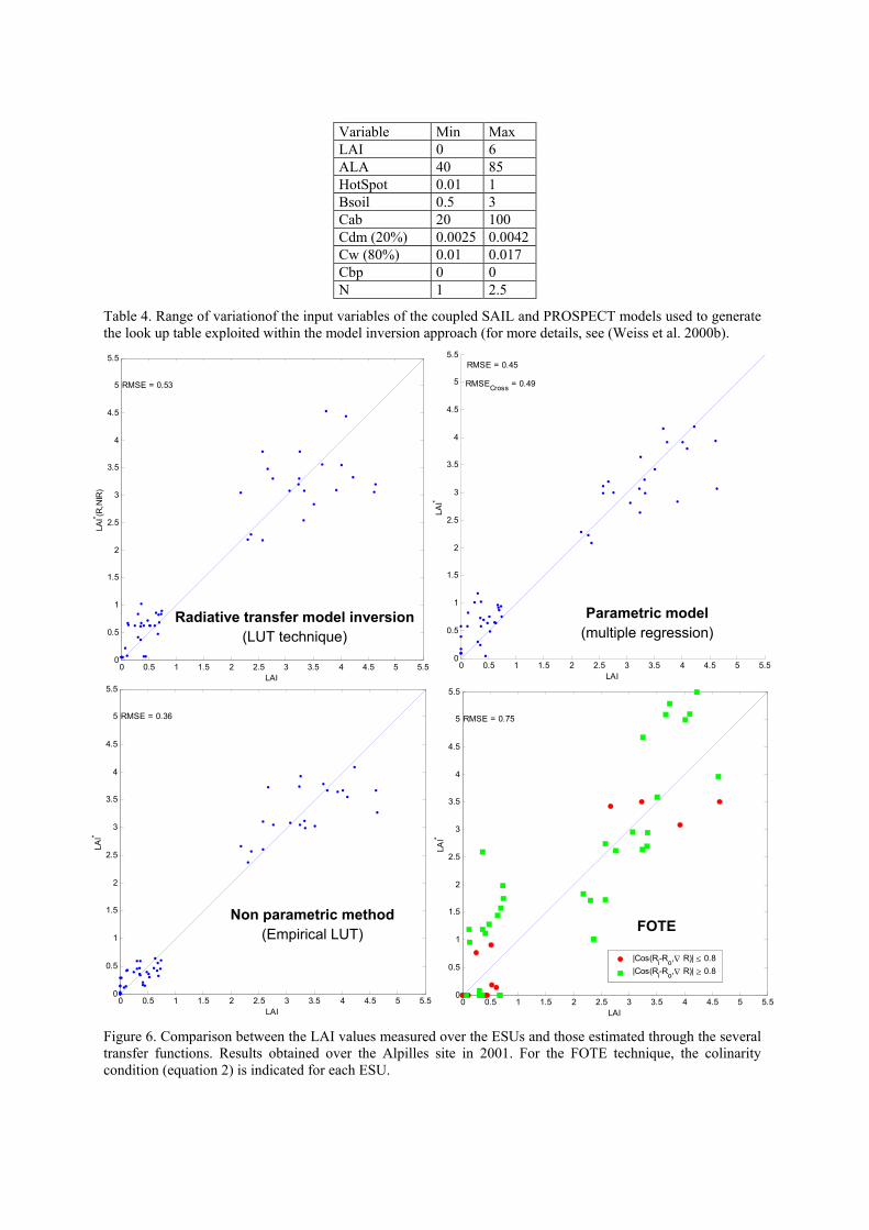
Variable Min Max LAI 0 6 ALA 40 85 HotSpot 0.01 1 Bsoil 0.5 3 Cab 20 100 Cdm (20%) 0.0025 0.0042Cw (80%) 0.01 0.017 Cbp 0 0 N 1 2.5

Table 4. Range of variationof the input variables of the coupled SAIL and PROSPECT models used to generate the look up table exploited within the model inversion approach (for more details, see (Weiss et al. 2000b).

0 0.5 1 1.5 2 2.5 3 3.5 4 4.5 5 5.50

0.5

1

1.5

2

2.5

3

3.5

4

4.5

5

5.5

RMSE = 0.53

LAI

LAI* (R

,NIR

)

0 0.5 1 1.5 2 2.5 3 3.5 4 4.5 5 5.50

0.5

1

1.5

2

2.5

3

3.5

4

4.5

5

5.5RMSE = 0.45

RMSECross = 0.49

LAI

LAI*

0 0.5 1 1.5 2 2.5 3 3.5 4 4.5 5 5.50

0.5

1

1.5

2

2.5

3

3.5

4

4.5

5

5.5

RMSE = 0.36

LAI

LAI*

0 0.5 1 1.5 2 2.5 3 3.5 4 4.5 5 5.50

0.5

1

1.5

2

2.5

3

3.5

4

4.5

5

5.5

RMSE = 0.75

LAI

LAI*

|Cos(Ri-Ro,∇ R)| ≤ 0.8|Cos(Ri-Ro,∇ R)| ≥ 0.8

Parametric model (multiple regression)

Radiative transfer model inversion(LUT technique)

Non parametric method (Empirical LUT) FOTE

Figure 6. Comparison between the LAI values measured over the ESUs and those estimated through the several transfer functions. Results obtained over the Alpilles site in 2001. For the FOTE technique, the colinarity condition (equation 2) is indicated for each ESU.

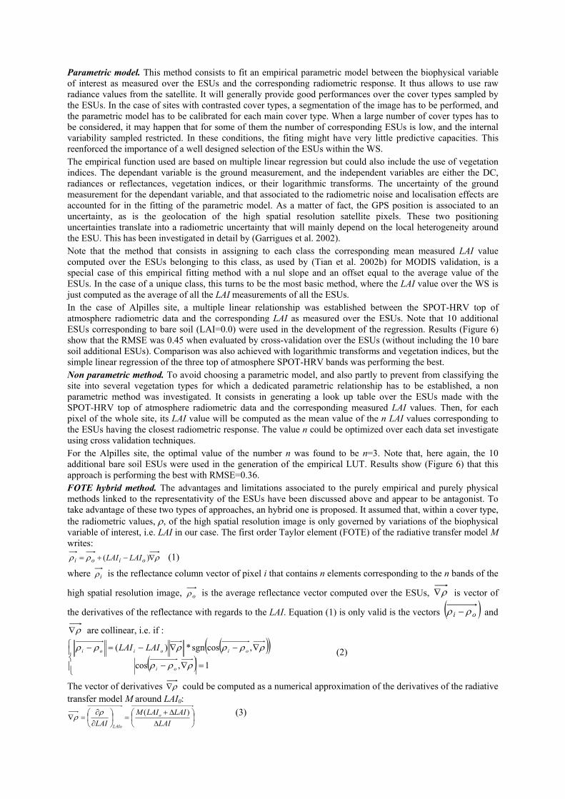
Parametric model. This method consists to fit an empirical parametric model between the biophysical variable of interest as measured over the ESUs and the corresponding radiometric response. It thus allows to use raw radiance values from the satellite. It will generally provide good performances over the cover types sampled by the ESUs. In the case of sites with contrasted cover types, a segmentation of the image has to be performed, and the parametric model has to be calibrated for each main cover type. When a large number of cover types has to be considered, it may happen that for some of them the number of corresponding ESUs is low, and the internal variability sampled restricted. In these conditions, the fiting might have very little predictive capacities. This reenforced the importance of a well designed selection of the ESUs within the WS. The empirical function used are based on multiple linear regression but could also include the use of vegetation indices. The dependant variable is the ground measurement, and the independent variables are either the DC, radiances or reflectances, vegetation indices, or their logarithmic transforms. The uncertainty of the ground measurement for the dependant variable, and that associated to the radiometric noise and localisation effects are accounted for in the fitting of the parametric model. As a matter of fact, the GPS position is associated to an uncertainty, as is the geolocation of the high spatial resolution satellite pixels. These two positioning uncertainties translate into a radiometric uncertainty that will mainly depend on the local heterogeneity around the ESU. This has been investigated in detail by (Garrigues et al. 2002). Note that the method that consists in assigning to each class the corresponding mean measured LAI value computed over the ESUs belonging to this class, as used by (Tian et al. 2002b) for MODIS validation, is a special case of this empirical fitting method with a nul slope and an offset equal to the average value of the ESUs. In the case of a unique class, this turns to be the most basic method, where the LAI value over the WS is just computed as the average of all the LAI measurements of all the ESUs. In the case of Alpilles site, a multiple linear relationship was established between the SPOT-HRV top of atmosphere radiometric data and the corresponding LAI as measured over the ESUs. Note that 10 additional ESUs corresponding to bare soil (LAI=0.0) were used in the development of the regression. Results (Figure 6) show that the RMSE was 0.45 when evaluated by cross-validation over the ESUs (without including the 10 bare soil additional ESUs). Comparison was also achieved with logarithmic transforms and vegetation indices, but the simple linear regression of the three top of atmosphere SPOT-HRV bands was performing the best. Non parametric method. To avoid choosing a parametric model, and also partly to prevent from classifying the site into several vegetation types for which a dedicated parametric relationship has to be established, a non parametric method was investigated. It consists in generating a look up table over the ESUs made with the SPOT-HRV top of atmosphere radiometric data and the corresponding measured LAI values. Then, for each pixel of the whole site, its LAI value will be computed as the mean value of the n LAI values corresponding to the ESUs having the closest radiometric response. The value n could be optimized over each data set investigate using cross validation techniques. For the Alpilles site, the optimal value of the number n was found to be n=3. Note that, here again, the 10 additional bare soil ESUs were used in the generation of the empirical LUT. Results show (Figure 6) that this approach is performing the best with RMSE=0.36. FOTE hybrid method. The advantages and limitations associated to the purely empirical and purely physical methods linked to the representativity of the ESUs have been discussed above and appear to be antagonist. To take advantage of these two types of approaches, an hybrid one is proposed. It assumed that, within a cover type, the radiometric values, ρ, of the high spatial resolution image is only governed by variations of the biophysical variable of interest, i.e. LAI in our case. The first order Taylor element (FOTE) of the radiative transfer model M writes:

ρρρ ∇−+= )( oioi LAILAI (1)

where iρ is the reflectance column vector of pixel i that contains n elements corresponding to the n bands of the

high spatial resolution image, oρ is the average reflectance vector computed over the ESUs, ρ∇ is vector of

the derivatives of the reflectance with regards to the LAI. Equation (1) is only valid is the vectors ( )oi ρρ − and

ρ∇ are collinear, i.e. if :

( )( )( )

=∇−

∇−∇−=−

1,cos

,cossgn*)(

ρρρ

ρρρρρρ

oi

oioioi LAILAI (2)

The vector of derivatives ρ∇ could be computed as a numerical approximation of the derivatives of the radiative transfer model M around LAI0:

∆∆+

=

∂∂

=∇LAI

LAILAIMLAI

o

LAIo

)(ρρ (3)

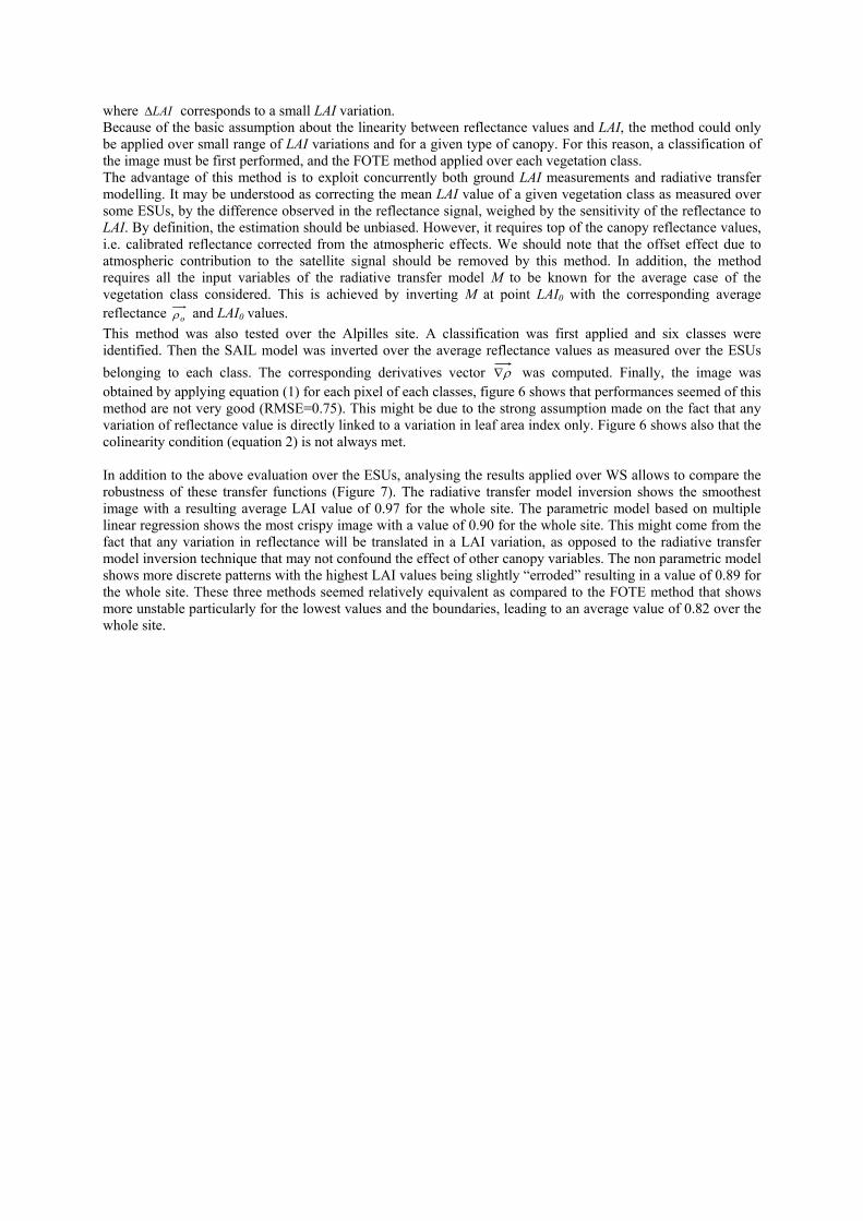
where LAI∆ corresponds to a small LAI variation. Because of the basic assumption about the linearity between reflectance values and LAI, the method could only be applied over small range of LAI variations and for a given type of canopy. For this reason, a classification of the image must be first performed, and the FOTE method applied over each vegetation class. The advantage of this method is to exploit concurrently both ground LAI measurements and radiative transfer modelling. It may be understood as correcting the mean LAI value of a given vegetation class as measured over some ESUs, by the difference observed in the reflectance signal, weighed by the sensitivity of the reflectance to LAI. By definition, the estimation should be unbiased. However, it requires top of the canopy reflectance values, i.e. calibrated reflectance corrected from the atmospheric effects. We should note that the offset effect due to atmospheric contribution to the satellite signal should be removed by this method. In addition, the method requires all the input variables of the radiative transfer model M to be known for the average case of the vegetation class considered. This is achieved by inverting M at point LAI0 with the corresponding average reflectance oρ and LAI0 values. This method was also tested over the Alpilles site. A classification was first applied and six classes were identified. Then the SAIL model was inverted over the average reflectance values as measured over the ESUs belonging to each class. The corresponding derivatives vector ρ∇ was computed. Finally, the image was obtained by applying equation (1) for each pixel of each classes, figure 6 shows that performances seemed of this method are not very good (RMSE=0.75). This might be due to the strong assumption made on the fact that any variation of reflectance value is directly linked to a variation in leaf area index only. Figure 6 shows also that the colinearity condition (equation 2) is not always met. In addition to the above evaluation over the ESUs, analysing the results applied over WS allows to compare the robustness of these transfer functions (Figure 7). The radiative transfer model inversion shows the smoothest image with a resulting average LAI value of 0.97 for the whole site. The parametric model based on multiple linear regression shows the most crispy image with a value of 0.90 for the whole site. This might come from the fact that any variation in reflectance will be translated in a LAI variation, as opposed to the radiative transfer model inversion technique that may not confound the effect of other canopy variables. The non parametric model shows more discrete patterns with the highest LAI values being slightly “erroded” resulting in a value of 0.89 for the whole site. These three methods seemed relatively equivalent as compared to the FOTE method that shows more unstable particularly for the lowest values and the boundaries, leading to an average value of 0.82 over the whole site.

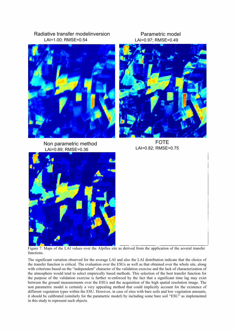
Parametric model Radiative transfer modelinversionLAI=1.00; RMSE=0.54 LAI=0.97; RMSE=0.49

FOTE

Figure 7. Maps of the LAI values over the Alpilles site as derived from the application of the several transfer functions.

The significant variation observed for the average LAI and also the LAI distribution indicate that the choice of the transfer function is critical. The evaluation over the ESUs as well as that obtained over the whole site, along with criterions based on the “independent” character of the validation exercise and the lack of characterization of the atmosphere would tend to select empirically based methods. This selection of the best transfer function for the purpose of the validation exercise is further re-enforced by the fact that a significant time lag may exist between the ground measurements over the ESUs and the acquisition of the high spatial resolution image. The non parametric model is certainly a very appealing method that could implicitly account for the existence of different vegetation types within the ESU. However, in case of sites with bare soils and low vegetation amounts, it should be calibrated (similarly for the parametric model) by including some bare soil “ESU” as implemented in this study to represent such objects.

LAI=0.82; RMSE=0.75 Non parametric methodLAI=0.89; RMSE=0.36

Colocated kriging Although the use of the transfer function allows to get a high spatial resolution image, the performances of the whole process highly depend on the accuracy of the transfer function. In case of poor transfer functions, or even in case of unavailable high spatial resolution satellite image, simple kriging techniques allow to get a back-up solution for the generation of the required high spatial resolution map of the biophysical variable. Colocated kriging technique allows to balance within a single formalism between these two extreme solutions for the generation of the high spatial resolution map of the biophysical variable (de Beaufort 2000). Colocated kriging technique is designed to estimate the value of a primary variable at any point in space from the knowledge of the measured values sampled over a limited number of points, and from the knowledge of the value of a secondary variable that is known at any point of the area investigated and that is linearly related to the primary variable (Goovaerts 1997). In our case, the primary variable is the biophysical variable of interest, V, that is measured over a limited number of ESUs. The secondary variable, R, is derived from the high spatial resolution image thanks to the transfer function V(R). This way, the secondary variable should be linearly related to the primary variable and is an unbiased estimate of V knowing R. The kriged value V of the biophysical variable Vi at pixel i is built as a linear combination of the measured values V and the secondary variable V(R):

i

),(ˆ1

ii

n

jj

iji RVVV ⋅+⋅= ∑

=

δλ (2)

where n is the number of ESUs sampled within the cover type considered, Vj is the biophysical variable measured at the ESU j, and the weights λi

j and δI . These weights are the solution of a linear system derived by minimizing the variance of the prediction error under the assumption of unbiasedness of the prediction error [ ] 0ˆ =− ii VVE that leads to the constraint (Wackernagel 1995):

11

=+∑=

i

n

j

ij δλ (3)

Note that the simple kriging technique correspond to δi=0, and the single use of the transfer function corresponds to λi

j=0. The weights λij and δi depend on the variogram of V established over the ESUs, the sampling pattern,

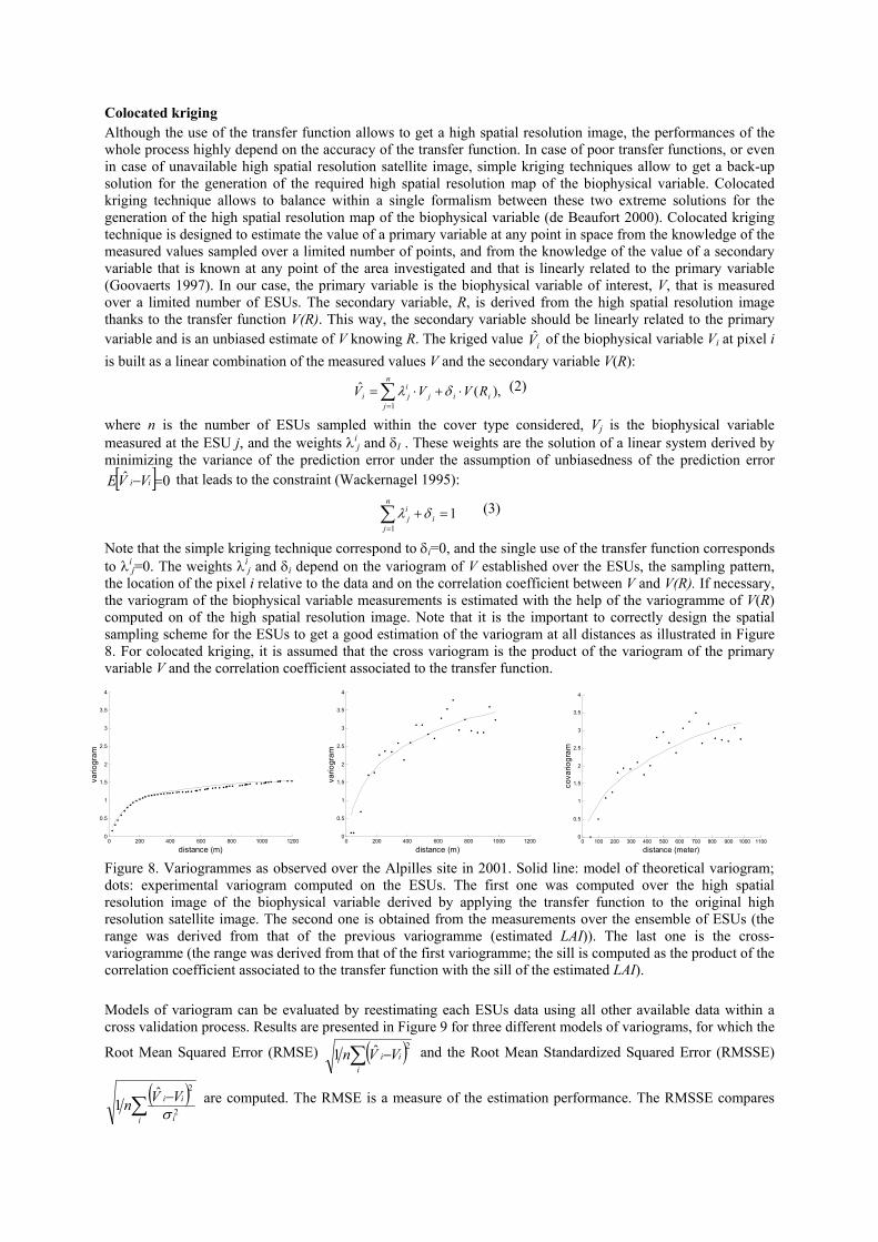
the location of the pixel i relative to the data and on the correlation coefficient between V and V(R). If necessary, the variogram of the biophysical variable measurements is estimated with the help of the variogramme of V(R) computed on of the high spatial resolution image. Note that it is the important to correctly design the spatial sampling scheme for the ESUs to get a good estimation of the variogram at all distances as illustrated in Figure 8. For colocated kriging, it is assumed that the cross variogram is the product of the variogram of the primary variable V and the correlation coefficient associated to the transfer function.

0 200 400 600 800 1000 12000

0.5

1

1.5

2

2.5

3

3.5

4

vario

gram

distance (m)0 200 400 600 800 1000 1200

0

0.5

1

1.5

2

2.5

3

3.5

4

vario

gram

distance (m)0 100 200 300 400 500 600 700 800 900 1000 1100

0

0.5

1

1.5

2

2.5

3

3.5

4

cova

riogr

am

distance (meter) Figure 8. Variogrammes as observed over the Alpilles site in 2001. Solid line: model of theoretical variogram; dots: experimental variogram computed on the ESUs. The first one was computed over the high spatial resolution image of the biophysical variable derived by applying the transfer function to the original high resolution satellite image. The second one is obtained from the measurements over the ensemble of ESUs (the range was derived from that of the previous variogramme (estimated LAI)). The last one is the cross-variogramme (the range was derived from that of the first variogramme; the sill is computed as the product of the correlation coefficient associated to the transfer function with the sill of the estimated LAI). Models of variogram can be evaluated by reestimating each ESUs data using all other available data within a cross validation process. Results are presented in Figure 9 for three different models of variograms, for which the

Root Mean Squared Error (RMSE) ( )2ˆ1 ∑ −i

ii VVn and the Root Mean Standardized Squared Error (RMSSE)

( )∑ −i i

ii VVn 2

2ˆ1 σ

are computed. The RMSE is a measure of the estimation performance. The RMSSE compares

the squared error with the kriging variance given by the model. Results show that the exponential and spherical variograms lead to very similar performances, whereas the Kbessel variogram leads to less good prediction and over-optimistic kriging variance. Hence this model should be discarded.

Figure 9. Comparison of the performances of three variogramme models (Exponential, Spherical and KBessel) applied on biophysical measurements over the ESUs as observed during Alpilles 2001. The evaluation is achieved by cross validation. RMSE is the root mean square error and RMSSE is the root mean standardized squared error.

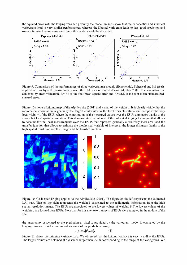
Figure 10 shows a kriging map of the Alpilles site (2001) and a map of the weight δ. It is clearly visible that the radiometric information is generally the largest contributor to the local variable estimation, except in the very local vicinity of the ESUs where the contribution of the measured values over the ESUs dominates thanks to the strong but local spatial correlation. This demonstrates the interest of the colocated kriging technique that allows to account for the local measurements over the ESUS that represent generally a relatively local area, and the transfer function that allows to estimate the biophysical variable of interest at the longer distances thanks to the high spatial resolution satellite image and the transfer function.

0

1

0.2

0.4

0.6

0.8

0

8

2

4

6

0

1

0.2

0.4

0.6

0.8

0

8

2

4

6

Figure 10. Co-located kriging applied to the Alpilles site (2001). The figure on the left represents the estimated LAI map. That on the right represents the weight δ associated to the radiometric information from the high spatial resolution image. The ESUs are associated to the lowest values of weights δ The lowest values of the weights δ are located near ESUs. Note that for this site, two transects of ESUs were sampled in the middle of the site. the uncertainty associated to the prediction at pixel i, provided by the variogram model is evaluated by the kriging variance. It is the minimized variance of the prediction error,

( )iii VVVar −= ˆ2σ . (4)

Figure 11 shows the kringing variance map. We observed that the kriging variance is strictly null at the ESUs. The largest values are obtained at a distance larger than 250m corresponding to the range of the variograms. We

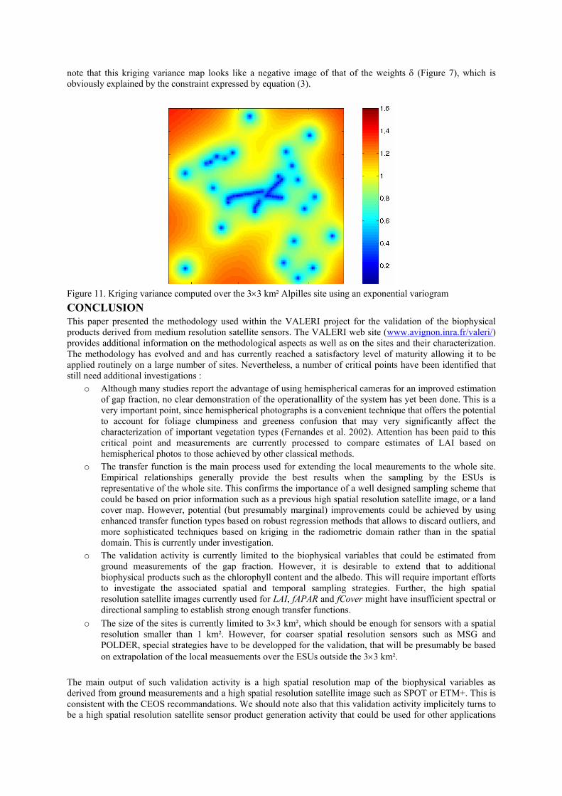
note that this kriging variance map looks like a negative image of that of the weights δ (Figure 7), which is obviously explained by the constraint expressed by equation (3).

Figure 11. Kriging variance computed over the 3×3 km² Alpilles site using an exponential variogram CONCLUSION This paper presented the methodology used within the VALERI project for the validation of the biophysical products derived from medium resolution satellite sensors. The VALERI web site (www.avignon.inra.fr/valeri/) provides additional information on the methodological aspects as well as on the sites and their characterization. The methodology has evolved and and has currently reached a satisfactory level of maturity allowing it to be applied routinely on a large number of sites. Nevertheless, a number of critical points have been identified that still need additional investigations :

o Although many studies report the advantage of using hemispherical cameras for an improved estimation of gap fraction, no clear demonstration of the operationallity of the system has yet been done. This is a very important point, since hemispherical photographs is a convenient technique that offers the potential to account for foliage clumpiness and greeness confusion that may very significantly affect the characterization of important vegetation types (Fernandes et al. 2002). Attention has been paid to this critical point and measurements are currently processed to compare estimates of LAI based on hemispherical photos to those achieved by other classical methods.

o The transfer function is the main process used for extending the local meaurements to the whole site. Empirical relationships generally provide the best results when the sampling by the ESUs is representative of the whole site. This confirms the importance of a well designed sampling scheme that could be based on prior information such as a previous high spatial resolution satellite image, or a land cover map. However, potential (but presumably marginal) improvements could be achieved by using enhanced transfer function types based on robust regression methods that allows to discard outliers, and more sophisticated techniques based on kriging in the radiometric domain rather than in the spatial domain. This is currently under investigation.

o The validation activity is currently limited to the biophysical variables that could be estimated from ground measurements of the gap fraction. However, it is desirable to extend that to additional biophysical products such as the chlorophyll content and the albedo. This will require important efforts to investigate the associated spatial and temporal sampling strategies. Further, the high spatial resolution satellite images currently used for LAI, fAPAR and fCover might have insufficient spectral or directional sampling to establish strong enough transfer functions.

o The size of the sites is currently limited to 3×3 km², which should be enough for sensors with a spatial resolution smaller than 1 km². However, for coarser spatial resolution sensors such as MSG and POLDER, special strategies have to be developped for the validation, that will be presumably be based on extrapolation of the local measuements over the ESUs outside the 3×3 km².

The main output of such validation activity is a high spatial resolution map of the biophysical variables as derived from ground measurements and a high spatial resolution satellite image such as SPOT or ETM+. This is consistent with the CEOS recommandations. We should note also that this validation activity implicitely turns to be a high spatial resolution satellite sensor product generation activity that could be used for other applications

than just the validation of medium resolution satellite sensors. A consistent processing of the whole data gathered over the ensemble of sites could lead to enhance the description of the relationships between canopy radiometric response and the corresponding biophysical variables for a range of vegetation types and states. Apart from the high spatial resolution biophysical map product, the validation exercise should also include the agregation process used to validate the medium resolution satellite sensor products. This agregation process is not straightforward when considering the associated uncertainties. Block kriging as proposed by (de Beaufort 2000) could be used to take advantage from the data available and processing already achieved. However, other sources of uncertainties have to be accounted for, including the registration errors of the medium resolution satellite sensor images that could be very significant in case of heterogeneous landscapes. Further investigations are currently directed towards the agregation problem that represents the ultimate step of the validation process. As stated earlier, medium resolution satellite validation activity should benefit from the contribution of worldwide distributed validation projects among which VALERI is contributing to. Concurrent use of the several validation projects will provide more reliable results. However, this requires a minimum of consistency between individual validation projects, both for the site selection and the methodological aspects, but also for the accessibility of the data and the documentation of the format used. This re-enforces the role of the Commitee on Earth Observation Satellites (CEOS) by the Working group on Calibration and Validation (WGCV), sub-group on Land Product Validation (LPV) to reach a sufficient consensus on the validation activity. Aknowledgements. We would like to thank CNES for suporting this activity, J. Privette for his chairing of the CEOS Land Product Validation group facilitating the contact and consistency with other validation activities, Boston university, particularly R. Myneni and Y. Knyazikhin for the very fruitful discussions that allowed to mature the methodology. We would like also to thank very much all those who participated to the field campaigns, and particularly N. Bruguier, R. Olivier, J.F. Hanocq, O. Marloie, B. Combal, O. Bajoles, N. Rochdi, C. Lazar, L. Prévot, L. de Beaufort, R. Cardenas, J.L. Roujan, G. Smith, S. Rambal, Freddy Loza de la Cruz, Rufian Villca Carex, Justina Mollo de Villca. P. Hiernaux, L. Jarlan, F. Lavenu, G. Marty, P. Mazzega, Y. Tracol, B. Ruelle, S. Weber, O. Ngwété et R. Santé.

References Baret, F., B. Andrieu, J. C. Folmer, J. F. Hanocq, and C. Sarrouy. 1993. Gap fraction measurement from

hemispherical infrared photography and its use to evaluate PAR interception efficiency. Pages 359-372 in C. Varlet-Grancher, R. Bonhomme, and H. Sinoquet, editors. Crop structure and microclimate: characterization and applications. INRA edition, Paris (France).

Becker, F., and Z. L. Li. 1995. Surface temperature and emissivity at various scales: definition, measurement and related problems. Remote Sensing Reviews 12:225-253.

Belward, A. S., J. E. Estes, and K. D. Kline. 1999. The IGBP-DIS global 1 km land cover data set: a project overview. photogrammetric engineering and remote sensing 65:1013-1020.

Chen, J. M., T. A. Black, and R. S. Adams. 1991. Evaluation of hemispherical photography for determining plant area index and geometry of forest stand. Agricultural and Forest Meteorology 56:129-143.

Chen, J. M., and J. Cilhar. 1995. Plant canopy gap-size analysis theory for improving optical measurements of leaf area index. Applied Optics 34:6211-6222.

Chen, J. M., G. Pavlic, L. Brown, J. Cihlar, S. Leblanc, H. P. White, R. J. Hall, D. R. Peddle, D. J. King, J. A. Trofymov, E. Swift, J. Van der Sanden, and P. K. E. Pellika. 2002. Derivation and validation of Canada wide coarse resolution leaf area index maps using high resolution satellite imagery and ground masurements. Remote Sensing of Environment 80:165-184.

Cihlar, J., S. Denning, F. Ahern, O. Arino, A. Belward, F. Bretherton, W. Cramer, G. Dedieu, C. Field, R. Francey, R. Gommes, J. Gosz, K. Hibbard, T. Igarashi, P. Kabat, R. Olson, S. Plummer, I. Rasool, M. Raupach, R. Scholes, J. Townshend, R. Valentini, and D. Wickland. 2000. IGOS-P: Carbon cycle observation theme: terrestrial and atmospheric componants. IGOS-P.

Cilhar, J., A. S. Denning, and J. Gosz. 2000. Global terrestrial carbon observation: requirements, present status and next steps. Report of a synthesis workshop GTOS-23, GTOS, Ottawa (Canada).

de Beaufort, L. 2000. Définition d'une méthode de cartographie d'indice foliaire destinée à la validation des produits de capteurs à large champ. mémoire de fin d'études INRA Bioclimatologie, Avignon.

De Fries, R. S., J. R. Townshend, and O. S. Los. 1997. Scaling land cover heterogeneity for global atmosphere-biosphere models. Pages 231-246 in D. A. Quattrochi and M. F. Goodrich, editors. Scales in Remote Sensing and GIS. CRC Press, Boca Raton, Florida, USA.

Duchemin, B., B. B., G. Dedieu, M. Leroy, and P. Maisongrande. 2002. Normalisation of directional effects in 10-day global syntheses derived VEGETATION/SPOT I. Validation of an operational method on actual data sets. Remote Sensing of Environment 81.

Fernandes, R., H. P. White, S. Leblanc, H. Mc Nairn, J. M. Chen, and R. J. Hall. 2002. Examination of error propagation in relationships between leaf area index and spectral indices from Landsat TM and ETM. draft.

Garrigue, S., D. Allard, F. Baret, and M. Weiss. 2003. Influence of the Positioning uncertaities on the radiometric values associated to ground measurement units. Remote Sensing of Environment in preparation.

Gond, V., D. G. G. de Pury, F. Veroustraete, and R. Ceulemans. 1999. Seasonal variation in leaf area index, leaf chlorophyll, and water content; scaling up to estimate fAPAR and carbon balance in a multilayer, multispecies temperate forest. Tree Physiology 19:673-679.

Goovaerts, P. 1997. Geostatistics for Natural Ressources Evaluation. Oxford University Press, Oxford (UK). Heal, O. W., J.-C. Menaut, and W. Steffen. 1995. Towards a Global Terrestrial Observing System (GTOS):

Detecting and Monitoring Change in Terrestrial Ecosystems,. Report 26, IGBP. Herniaux. 1992. Jacob, F., M. Weiss, A. Olioso, and A. French. 2002. Assessing the narrowband to broadband conversion to

estimate visible, near infrared and shortwave apparent albedo from airborne POLDER. Agronomie 22:537-546.

Jacquemoud, S., and F. Baret. 1990. PROSPECT: A model of leaf optical properties spectra. RSE 34:75-91. Justice, C., A. Belward, J. Morisette, P. Lewis, J. Privette, and F. Baret. 2000. Developments in the validation of

satellite sensor products for the study of the land surface. International Journal of Remote Sensing 21. Justice, C. O., D. Starr, D. Wickland, J. Privette, and T. Suttles. 1998. EOS land validation coordination: an

update. Earth Observer 10:55–60. Leblanc, S., R. Fernandes, and J. M. Chen. 2002. Recent advancements in optical field leaf area index, foliage

heterogeneity, and foliage angular distribution measurements. in IGARSS 02. Liang, S., C. J. Shuey, A. L. Russ, H. Fang, M. Chen, C. L. Walthall, C. S. T. Daughtry, and E. R. J. Hunt. 2002.

Norrowband to broad band conversions of land surface albedo: II. Validation. Remote Sensing of Environment 84.

Loveland, T. R., B. C. Reed, J. F. Brown, D. O. Ohen, Z. Zhu, L. Yang, and J. W. Merchant. 2000. Development of a global land cover characteristics database and IGBP DISCover from 1 km AVHRR data. International Journal of Remote Sensing 21:1303-1330.

Malingreau, J. P., and A. S. Belward. 1992. Scale considerations in vegetation monitoring using AVHRR data. International Journal of Remote Sensing. 13:2289-2307.

Martonchik, J. V. 1994. Retrieval of surface directional reflectance properties using ground level multiangle measurements. Remote Sensing of Environment 50:303-316.

Morissette, J., J. Privette, C. Justice, and D. Starr. 2000. MODIS land validation activities: status and review. in IGARS'2000, Honolulu.

Myneni, R. B., C. D. Keeling, C. J. Tucker, G. Asrar, and R. R. Nemani. 1997. Increased plant growth in the Northern high latitudes from 1981-1991. Nature 386:698-702.

(NOAA), N. O. a. A. A. 1997. Climate Measurement Requirements for the National Polar-orbiting Operational Environmental Satellite System (NPOESS). Office of Research and Applications, National Environmental Satellite, Data, and Information Service, National Oceanic and Atmospheric Administration.

Privette, J., R. Myneni, J. Morissette, and C. Justice. 1998. Global validation of EOS and FPAR products. The Earth Observer 10:39-42.

Privette, J. L., J. Morisette, F. Baret, S. T. Gower, and R. B. Myneni. 2001. Summary of the International Workshop on LAI Product Validation. Earth Observer 13:18-22.

Tian, Y., C. E. Woodcock, Y. Wang, J. Privette, N. V. Shabanov, L. Zhou, Y. Zhang, W. Buermann, J. Dong, B. Veikkanen, T. Häme, K. Andersson, M. Ozdogan, Y. Knyazikhin, and R. B. Myneni. 2002a. Multiscale analysis and validation of the MODIS LAI product I. Uncertainty assessment. Remote Sensing of Environment 83:414-430.

Tian, Y., C. E. Woodcock, Y. Wang, J. Privette, N. V. Shabanov, L. Zhou, Y. Zhang, W. Buermann, J. Dong, B. Veikkanen, T. Häme, K. Andersson, M. Ozdogan, Y. Knyazikhin, and R. B. Myneni. 2002b. Multiscale analysis and validation of the MODIS LAI product II. Sampling strategy. Remote Sensing of Environment 83:431-441.

Verhoef, W. 1984. Light scattering by leaf layers with application to canopy reflectance modeling: the SAIL model. Remote. Sens. Environ. 16:125-141.

Verhoef, W. 1985. Earth observation modeling based on layer scattering matrices. Remote Sens. Environ. 17:165-178.

Wackernagel, H. 1995. Multivariate geostatistics, an introduction with applications. Springer Verlag. Weiss, M., F. Baret , M. Leroy, O. Hautecoeur, C. Bacour, L. Prévot, and N. Bruguier. 2002. Validation of neural

net techniques to estimate canopy biophysical variables from remote sensing data. Agronomie 22:547-554.

Weiss, M., F. Baret, M. Leroy, O. Hautecoeur, L. Prévot, and N. Bruguier. 2000a. Validation of neural network techniques for the estimation of canopy biophysical variables from VEGETATION data. in VEGETATION preparatory programme. Final meeting. G. Saint, Belgirate (Italy).

Weiss, M., F. Baret, R. Myneni, A. Pragnère, and Y. Knyazikhin. 2000b. Investigation of a model inversion technique for the estimation of crop charcteristics from spectral and directional reflectance data. Agronomie 20:3-22.

Weiss, M., F. Baret, and G. J. Smith 2003. Review of methods and devices used to estimate LAI from gap fraction measurements. Agricultural and Forest Meteorology submitted (September 2002).