UNIVERSITÉ DE MONTRÉAL

INFINITE-DIMENSIONAL MODELLING AND CONTROL OF A MEMSDEFORMABLE MIRROR WITH APPLICATIONS IN ADAPTIVE OPTICS

AMIR BADKOUBEH-HAZAVEDÉPARTEMENT DE GÉNIE ÉLECTRIQUEÉCOLE POLYTECHNIQUE DE MONTRÉAL

THÈSE PRÉSENTÉE EN VUE DE L’OBTENTIONDU DIPLÔME DE PHILOSOPHIÆ DOCTOR

(GÉNIE ÉLECTRIQUE)AOÛT 2015

c© Amir Badkoubeh-Hazave, 2015.

UNIVERSITÉ DE MONTRÉAL

ÉCOLE POLYTECHNIQUE DE MONTRÉAL

Cette thèse intitulée :

INFINITE-DIMENSIONAL MODELLING AND CONTROL OF A MEMSDEFORMABLE MIRROR WITH APPLICATIONS IN ADAPTIVE OPTICS

présentée par : BADKOUBEH-HAZAVE Amiren vue de l’obtention du diplôme de : Philosophiæ Doctora été dûment acceptée par le jury d’examen constitué de :

M. SAYDY Lahcen, Ph. D., présidentM. ZHU Guchuan, Ph. D., membre et directeur de rechercheM. DELFOUR Michel, Ph. D., membreM. PARANJAPE Aditya, Ph. D., membre externe

iii

DEDICATION

You are not a drop in the ocean.You are the entire ocean, in a drop. . . .

Rumi

iv

ACKNOWLEDGEMENTS

This work would not have been possible without the help, support, and suggestions ofmy advisor, Professor Guchuan Zhu. I am indebted to Dr. Zhu not only for his academic andresearch support, but also for his advices on writing style, problem solving, critical thinking,and professional mentorship. It has been an honor to be his first graduate Ph.D. Student.

I would like to express the deepest appreciation to Dr. Jun Zheng from the Division ofFoundation Courses of Southwest Jiaoton University of China. The mathematic rigor of thefinal design would not have been possible without the collaboration of Dr. Jun.

I would like to thank my committee members, professor Lahcen Saydy, and Roland Mal-hamé from Department of Electrical Engineering, Polytechnique Montréal, professor MichelDelfour from Département de mathématiques et de statistique, Université de Montréal, andProfessor Aditya Paranjape from Indian Institute of Technology Bombay in Mumbai for theirtime on reviewing my thesis and attending my defense session, and also for their commentsand suggestions.

I also would like to thank Professor Charless Audit from The Department of Mathematicsand Statistics of McGill University for his insightful discussions, and suggestions on thisresearch.

In addition, I would like to acknowledge the financial support of NSERC (Natural Scienceand Engineering Research Council of Canada) and ReSMiQ (Regroupement Stratégique enMicroélectronique du Québec). I benefited immensely from working as teaching assistant forProfessor Roland Malhamé and Professor Richard Gourdeau. I also thank Professor LahcenSaydy for all his advices during my Ph.D. and for transferring my first request for a Ph.D.position to Professor Zhu.

I enjoyed the company of my office mates and sharing the office with them. Perhaps in afew years, I would not remember all the details of this thesis, but I am sure I cannot forgettrue friends, in particular Guissepe Costanzo.

Last but not least, I also would like to thank my family for their continuous support.Especially my parents who cultivated the enthusiasm for knowledge in me.

v

RÉSUMÉ

Le contrôle de déformation est un problème émergent dans les micro structures intelli-gentes. Une des applications type est le contrôle de la déformation de miroirs dans l’optiqueadaptative dans laquelle on oriente la face du miroir selon une géométrie précise en utili-sant une gamme de micro-vérins afin d’éliminer la distortion lumineuse. Dans cette thèse, leproblème de la conception du contrôle du suivi est considéré directement avec les modèlesdécrits par des équations aux dérivées partielles définies dans l’espace de dimension infinie.L’architecture du contrôleur proposée se base sur la stabilisation par retour des variables etle suivi des trajectoires utilisant la théorie des systèmes différentiellement plats. La combi-naison de la commande par rétroaction et la planification des trajectoires permet de réduirela complexité de la structure du contrôleur pour que ce dernier puisse être implémentée dansles microsystèmes avec les techniques disponibles de nos jours. Pour aboutir à une architec-ture implémentable dans les applications en temps réel, la fonction de Green est considéréecomme une fonction de test pour concevoir le contrôleur et pour représenter les trajectoiresde référence dans la planification de mouvements.

vi

ABSTRACT

Deformation control is an emerging problem for micro-smart structures. One of its excit-ing applications is the control of deformable mirrors in adaptive optics systems, in which themirror face-sheet is steered to a desired shape using an array of micro-actuators in order toremove light distortions. This technology is an enabling key for the forthcoming extremelylarge ground-based telescopes. Large-scale deformable mirrors typically exhibit complex dy-namical behaviors mostly due to micro-actuators distributed in the domain of the systemwhich in particular complicates control design.

A model of this device may be described by a fourth-order in space/second-order in timepartial differential equation for the mirror face-sheet with Dirac delta functions located inthe domain of the system to represent the micro-actuators. Most of control design methodsdealing with partial differential equations are performed on lumped models, which oftenleads to high-dimensional and complex feedback control structures. Furthermore, controldesigns achieved based on partial differential equation models correspond to boundary controlproblems.

In this thesis, a tracking control scheme is designed directly based on the infinite-dimensionalmodel of the system. The control scheme is introduced based on establishing a relationshipbetween the original nonhomogeneous model and a target system in a standard boundarycontrol form. Thereby, the existing boundary control methods may be applicable. For thecontrol design, we apply the tool of differential flatness to a partial differential equation sys-tem controlled by multiple actuators, which is essentially a multiple-input multiple-outputpartial differential equation problem. To avoid early lumping in the motion planning, we usethe properties of the Green’s function of the system to represent the reference trajectories.A finite set of these functions is considered to establish a one-to-one map between the inputspace and output space. This allows an implementable scheme for real-time applications.Since pure feedforward control is only applicable for perfectly known, and stable systems,feedback control is required to account for instability, model uncertainties, and disturbances.Hence, a stabilizing feedback is designed to stabilize the system around the reference trajec-tories. The combination of differential flatness for motion planning and stabilizing feedbackprovides a systematic control scheme suitable for the real-time applications of large-scaledeformable mirrors.

vii

TABLE OF CONTENTS

DEDICATION . . . . . . . . . . . . . . . . . . . . . . . . . . . . . . . . . . . . . . . iii

ACKNOWLEDGEMENTS . . . . . . . . . . . . . . . . . . . . . . . . . . . . . . . . iv

RÉSUMÉ . . . . . . . . . . . . . . . . . . . . . . . . . . . . . . . . . . . . . . . . . . v

ABSTRACT . . . . . . . . . . . . . . . . . . . . . . . . . . . . . . . . . . . . . . . . vi

TABLE OF CONTENTS . . . . . . . . . . . . . . . . . . . . . . . . . . . . . . . . . vii

LIST OF FIGURES . . . . . . . . . . . . . . . . . . . . . . . . . . . . . . . . . . . . x

LIST OF SYMBOLS AND ABBREVIATIONS . . . . . . . . . . . . . . . . . . . . . xi

CHAPTER 1 INTRODUCTION . . . . . . . . . . . . . . . . . . . . . . . . . . . . 11.1 Deformable Mirrors in the Context of Adaptive Optics systems . . . . . . . . 11.2 Finite- versus Infinite-Dimensional Model . . . . . . . . . . . . . . . . . . . . 21.3 PDE-Based Tracking Control of Euler-Bernoulli Beams . . . . . . . . . . . . 31.4 The Main Challenge in PDE-Based Deformation Control of Micro-Mirrors . 41.5 Motivation and Objective . . . . . . . . . . . . . . . . . . . . . . . . . . . . 41.6 Treatment Approach and the Contributions . . . . . . . . . . . . . . . . . . 51.7 Dissertation Organization . . . . . . . . . . . . . . . . . . . . . . . . . . . . 6

CHAPTER 2 A SYNOPSIS OF INFINITE-DIMENSIONAL LINEAR SYSTEMS CON-TROL THEORY . . . . . . . . . . . . . . . . . . . . . . . . . . . . . . . . . . . . 72.1 Linear Systems on Infinite-dimensional Spaces . . . . . . . . . . . . . . . . . 72.2 Strongly Continuous Semigroups . . . . . . . . . . . . . . . . . . . . . . . . . 82.3 Infinitesimal Generators . . . . . . . . . . . . . . . . . . . . . . . . . . . . . 122.4 Abstract Differential Equations . . . . . . . . . . . . . . . . . . . . . . . . . 132.5 Contraction Semigroup . . . . . . . . . . . . . . . . . . . . . . . . . . . . . . 142.6 Semigroups and Solutions of PDEs . . . . . . . . . . . . . . . . . . . . . . . 162.7 Stability . . . . . . . . . . . . . . . . . . . . . . . . . . . . . . . . . . . . . . 172.8 Inhomogeneous Abstract Differential Equations and Stabilization . . . . . . 192.9 Boundary Controlled PDEs . . . . . . . . . . . . . . . . . . . . . . . . . . . 202.10 Well-Posedness . . . . . . . . . . . . . . . . . . . . . . . . . . . . . . . . . . 22

viii

2.11 Controllability . . . . . . . . . . . . . . . . . . . . . . . . . . . . . . . . . . . 23

CHAPTER 3 ADAPTIVE OPTICS SYSTEMS . . . . . . . . . . . . . . . . . . . . 243.1 Introduction . . . . . . . . . . . . . . . . . . . . . . . . . . . . . . . . . . . . 243.2 Adaptive Optics . . . . . . . . . . . . . . . . . . . . . . . . . . . . . . . . . . 243.3 Structure of Adaptive Optics Systems . . . . . . . . . . . . . . . . . . . . . . 263.4 MEMS-Actuated Deformable Mirror Modelling . . . . . . . . . . . . . . . . . 263.5 Simplifying Assumptions on the Model . . . . . . . . . . . . . . . . . . . . . 293.6 Lumped Model and Finite-Dimensional Control Design . . . . . . . . . . . . 30

3.6.1 Control Design of Lumped System . . . . . . . . . . . . . . . . . . . 303.6.2 Simulation Study . . . . . . . . . . . . . . . . . . . . . . . . . . . . . 323.6.3 Summary and Discussion . . . . . . . . . . . . . . . . . . . . . . . . . 34

CHAPTER 4 CONTROL DESIGN: FLATNESS-BASED DEFORMATION CONTROLOF EULER-BERNOULLI BEAMS WITH IN-DOMAIN ACTUATION . . . . . 374.1 Notation . . . . . . . . . . . . . . . . . . . . . . . . . . . . . . . . . . . . . . 374.2 Basic Properties of the Considered System . . . . . . . . . . . . . . . . . . . 38

4.2.1 System Modeling . . . . . . . . . . . . . . . . . . . . . . . . . . . . . 384.2.2 Well-Posedness and Controllability of the Model . . . . . . . . . . . . 414.2.3 Green’s Functions for Euler-Bernoulli Beams . . . . . . . . . . . . . . 44

4.3 The First Design: Mapping In-domain Actuation into Boundary Control . . 464.3.1 Mapping In-domain Actuation into Boundary Control . . . . . . . . . 464.3.2 Feedback Stabilization . . . . . . . . . . . . . . . . . . . . . . . . . . 504.3.3 Decomposition of Reference Trajectories and Formal Series-Based Mo-

tion Planning . . . . . . . . . . . . . . . . . . . . . . . . . . . . . . . 514.4 The Second Control Design: In-domain Actuation Design via Boundary Con-

trol Using Regularized Input Functions . . . . . . . . . . . . . . . . . . . . . 564.4.1 Relating In-domain Actuation to Boundary Control . . . . . . . . . . 574.4.2 Well-posedness of Cauchy Problems . . . . . . . . . . . . . . . . . . . 604.4.3 Feedback Control and Stability of the Inhomogeneous System . . . . 614.4.4 Motion Planning and Feedforward Control . . . . . . . . . . . . . . . 63

4.5 Summary . . . . . . . . . . . . . . . . . . . . . . . . . . . . . . . . . . . . . 68

CHAPTER 5 SIMULATION STUDIES OF IN-DOMAIN CONTROLLED EULER-BERNOULLI BEAMS . . . . . . . . . . . . . . . . . . . . . . . . . . . . . . . . . 695.1 Numerical implementation . . . . . . . . . . . . . . . . . . . . . . . . . . . . 695.2 Numerical Results of the First Design . . . . . . . . . . . . . . . . . . . . . . 71

ix

5.3 Simulation Results for the Second Design . . . . . . . . . . . . . . . . . . . . 745.4 Discussion . . . . . . . . . . . . . . . . . . . . . . . . . . . . . . . . . . . . . 77

CHAPTER 6 CONCLUSION AND RECOMMENDATION . . . . . . . . . . . . . . 816.1 Main Contributions . . . . . . . . . . . . . . . . . . . . . . . . . . . . . . . . 816.2 Recommendations and Future Work . . . . . . . . . . . . . . . . . . . . . . . 83

BIBLIOGRAPHY . . . . . . . . . . . . . . . . . . . . . . . . . . . . . . . . . . . . . 84

x

LIST OF FIGURES

3.1 A typical example of how AO systems can make very sharp images. . 253.2 Illustration of AO principle in the context of astronomical telescope. . 253.3 Schematic representation of open-loop AO with closed-loop DM control. 263.4 Cross sectional schematics of continuous and segmented deformable

mirrors. . . . . . . . . . . . . . . . . . . . . . . . . . . . . . . . . . . 273.5 Schematic representation of the MEMS-DM. . . . . . . . . . . . . . . 283.6 Two Snapshots of the beam from the initial state to steady-state. . . 353.7 Control effort generated on each actuator points. . . . . . . . . . . . 363.8 The error between the desired and actual trajectory. . . . . . . . . . . 364.1 Schematic of the deformable microbeam. . . . . . . . . . . . . . . . . 385.1 Stabilized System. . . . . . . . . . . . . . . . . . . . . . . . . . . . . 715.2 Deformation control: (a) reference trajectory; (b) beam deflection; (c)

tracking error. . . . . . . . . . . . . . . . . . . . . . . . . . . . . . . . 725.3 Simulation results for 3 actuators . . . . . . . . . . . . . . . . . . . . 735.4 Green’s function of the beam for ξ = 0.1, 0.2, · · · , 0.9. . . . . . . . . 745.5 Deformation control for time-domain design with Green’s function de-

composition: (a) desired shape; (b) beam deflection; (c) tracking error; 755.6 Control signals for the first design . . . . . . . . . . . . . . . . . . . . 765.7 Effect of number of actuators . . . . . . . . . . . . . . . . . . . . . . 785.8 Control signals for the second design . . . . . . . . . . . . . . . . . . 795.9 Set-point control: (b) system response; (c) regulation error. . . . . . . 80

xi

LIST OF SYMBOLS AND ABBREVIATIONS

AO Adaptive OpticsARE Algebraic Riccati EquationDM Deformable MirrorDOF Degree of FreedomFFT Fast Fourier TransformLQR Linear-Quadratic RegulatorMEMS Microelectromechanical SystemsMIMO Multiple-Input Multiple-OutputODE Ordinary Differential EquationPDE Partial Differential EquationRBF Radial-Based Functions1D One-Dimensional2D Two-DimensionalC0-semigroup Strongly Continuous SemigroupR The field of all real numbersC The filed of all complex numbersRn The n−dimentional Euclidean spaceΩ A nonempty open subset of Rn

∂Ω The boundary of ΩΩ The closure of ΩL(X,Z) Set of continuous linear map L between two Hilbert spaces Z and XH A Hilbert spaceLp(Ω) p-integrable functionsCm(Ω) The space of m-times boundedly continuously differentiable function

from Ω into HHm(Ω) The Sobolev space of order mwx The derivatives of w(x, t) with respect to xwt The derivatives of w(x, t) with respect to tS(t) C0-semigroupD(A) Domain of the operator AΣ(A,B) The dynamic system with the system matrix A and the input operator

B

δ(x, ξ) Dirac delta function, or impulse function concentrated at the point ξ

xii

G(x, ξ) Green’s functionϕ(x, ξ) Blob function centered at the point ξG(x, ξ) Regularized Green’s function

1

CHAPTER 1

INTRODUCTION

We begin this chapter by introducing the deformable mirrors in the context of adaptiveoptics, AO, and the necessity to deal with the infinite-dimensional control of this device inthis context. In Section 1.3 we review the pertinent control methods in this realm. Sec-tion 1.4 explains the challenges associated with partial differential equation, PDE, basedcontrol designs for the deformable mirrors. Then, Section 1.5, and 1.6 outline the motiva-tion, objectives, and our treatment strategy in this research work. The original contributionsof this work are also summarized in Section 1.6. We conclude this chapter by mentioning theorganization of this thesis in Section 1.7.

1.1 Deformable Mirrors in the Context of Adaptive Optics systems

Deformable mirrors are key elements for enhancing the performance of optical systemsand have been used in many different applications including: free space laser communications[105], [100], retinal imaging [33], biological microscopy [96], and ground-based telescopes[20, 31]. However, despite many similarities, each of these applications has unique featureswhich requires specific insights into the system and specialized techniques. In this research,we mainly focus on the application of deformable mirrors in ground-based telescopes.

The deformable mirrors in this context are intended to remove the distortion of light dueto earth atmosphere turbulence. Because atmospheric turbulence is a dynamic phenomenon,the adaptive optics system needs to be sufficiently fast. The sampling times in this applicationcan amount to 0.5 [ms]. Given this sampling time, the high frequency modes of the deformablemirrors can be excited, and thus these devices cannot be considered as static systems [83, 44].Hence, the control methods developed in other applications based on static models of adeformable mirror, the so-called open-loop control, cannot meet this requirement [108, 98,21, 85, 100, 36, 32].

On the other hand, the design methods for dynamic control of this device leading toa control structure that requires a considerable number of on-chip sensors for the imple-mentation of closed-loop control are not applicable to microsystems with currently availabletechnologies [44, 6, 59, 83, 77].

Another vital issue is the precision. The high resolution performance of an adaptive opticssystem is strongly tied to the precise control of its deformable mirror. The displacement

2

range of a deformable mirrors surface is in micro-meters, and thus an acceptable trackingerror should be at least ten times smaller than this range. According to this level of precision,the controller must be developed based on a very precise and a high resolution model [22,23, 38, 86, 99, 107].

1.2 Finite- versus Infinite-Dimensional Model

Most ordinary differential equation systems describing physical phenomenon are finite-dimensional approximations of distributed parameter systems. Hence, for very high resolutioncontrol applications the study of distributed parameter systems, such as control of systemsgoverned by partial differential equations, are of intrinsic interest.

One of the major issues related to approximating a system in finite-dimensional space isthat the neglected dynamics might lead to unexpected excitation of truncated modes, andconversely the truncated modes might undesirably contribute to feedback data. In eithercase, the performance of the closed-loop system may be deteriorated, or, at some points, thesystem may even be destabilized [14, 81]. Furthermore, the increase of modeling accuracy willlead to high-dimensional and complex feedback control structures, requiring a considerablenumber of on-chip sensors for the implementation. This raises serious technological challengesfor the design, fabrication, and operation of microsystems. Therefore, it is of great interestto directly deal with the control of the exact PDE models.

However, even treatment of some very basic problems of partial differential equation sys-tems, such as heat equations and wave equations, demands a rich background on mathemati-cal foundations, such as functional analysis. For instance, a small alteration on the boundaryvalues could drastically alter the nature of the problem. As a result, the study of partialdifferential equation systems in the context of infinite-dimensional space has been treateddifferently on a case-by-case basis and remains an open field for engineering applications.

In this research, we consider the partial differential equation model of a deformable mirroractuated with Microelectromechanical systems, MEMS. In this work, we refer to this deviceas MEMS-actuated deformable mirror, or deformable mirror for short. In the model, thedynamics of small transversal displacement of the membrane surface may be described bya fourth-order in space and second-order in time partial differential equation, called Timo-shenko thin plate equation [101, 106, 48]. The MEMS actuators are considered as pointwiseactuators represented by Dirac delta functions located in the domain of the system.

By exploiting the symmetry of the domain, the problem of a 2-dimensional plate equationcan be reduced to the Cartesian product of two decoupled 1-dimensional systems of Euler-Bernoulli beam equations [16, 17]. Hence, the main focus of the control design will be on

3

tracking control of an Euler-bernoulli PDE with in-domain Dirac delta functions as controlinputs.

1.3 PDE-Based Tracking Control of Euler-Bernoulli Beams

One of the most popular methods for the tracking control of PDEs is to approximatethe PDE by a system of lumped ordinary differential equations, ODE, through the spatialdiscretization of differential operator [18, 15, 19, 24, 67, 66, 84]. Subsequently, various controlmethods developed for ODE systems can be directly applied. The problems associated withthe approximation of the model mentioned earlier may arise in these methods. Regardlessof implementation aspects, we formally review the steps in designs based on a lumped ODEmodel of a PDE system in Chapter 3.

Moreover, many methods originally developed for nonlinear control of finite-dimensionalsystems are successfully generalized to control infinite-dimensional systems. This, for in-stance, includes Lyapunov-based techniques, [71, 68, 5], backstepping [57, 56, 58, 55], anddifferential flatness for inversion-based trajectory planning and feed-forward control [40, 82,81, 97, 64]. Furthermore, tracking control is a result of combinations of these approaches[78].

The feedback stabilization of an Euler- Bernoulli beam has been considered in many differ-ent sources (see, e.g., [5, 26, 25]). For instance, feedback stabilization using a backsteppingapproach is considered in [79, 56] which provides a systematic approach for the design ofexponentially stabilizing state feedback controllers. Stabilization by strain and shear forceboundary feedback using dissipative concepts is addressed in Chapter 4 of [71]. Stabilizationof Euler-Bernoulli beams using one in-domain point-wise feedback force has been examinedin [5, 4, 3, 25].

The problem of trajectory planning, i.e. the design of an open-loop control to real-ize prescribed spatial-temporal output paths, using differential flatness which is originallydeveloped for the control of finite-dimensional nonlinear systems, [57, 41, 42, 97, 76, 64],has further been successfully extended to a variety of infinite-dimensional systems (see e.g.,[82, 79, 97, 76, 64, 65]).

Differential flatness implies that the system states and the control inputs can be parame-terized in terms of a flat, or a so-called basic output, and its time-derivatives up to a certainproblem dependent order. By prescribing appropriate trajectories for the flat output, thefull-state and input trajectories can be directly evaluated without integration of any differen-tial equation. This implies that a system is differentially flat if the flat output has the samenumber of components as the number of system inputs, [42, 41, 39, 64, 65]. This is the key

4

concept in generalizing differential flatness for multi-input multi-output PDEs.The underlying idea of flatness, i.e. the existence of a one-to-one correspondence between

trajectories of systems, has also been adapted successfully to some PDE systems (see, e.g.,[52, 65, 73, 79, 90, 94, 74]).

In differential flatness designs, the system states and system inputs can be parameterizedby the flat output in terms of infinite power series representations of the system. Then, seriescoefficients can be obtained by solving recursive equations on time-derivatives of the basicoutput, which has to be chosen from a certain smooth function, namely Gevrey function.Recent works on the flatness concept has mainly dealt with its extension to trajectory plan-ning for boundary controlled PDE systems in a single spatial coordinate [82, 80]. Trackingcontrol using a combination of flatness and backstepping for parabolic and bi-harmonic PDEswith actuators located on the boundary to stabilize the system along prescribed trajectorieshas been addressed in [78, 79]. It is, however, very challenging to apply this tool to systemscontrolled by multiple in-domain actuators.

1.4 The Main Challenge in PDE-Based Deformation Control of Micro-Mirrors

In standard PDE systems, unbounded control operators are typically located on theboundaries of the system, whereas in the PDE model of deformable mirrors the unboundedcontrol operators are distributed in the domain of the system. This makes PDE-based controldesigns of deformable mirrors drastically different from the standard boundary controlledPDE designs. Particularly, finding a one-to-one correspondence between the control spaceand the system’s state space is not obvious since the dimension of the control space is finite,while that of the state space is infinite.

1.5 Motivation and Objective

The main motivation of this work is to develop a high-precision and real-time applica-ble control structure for large-scale deformable mirrors in order to reduce the complexityintroduced by closed-loop control at the level of every actuator.

To meet this end, the objective of this dissertation is to develop a control law directlybased on the partial differential equation model of the system to archive high-precision perfor-mance. To mitigate the complexity of the controller, we consider a combination of feedbackstabilization and feed-forward motion planing controllers. Minimizing the requirement ofsensory data in order to steer the surface mirror asymptotically along reference trajectoriesis also the other objective of this control design. To achieve real-time implementation, aninversion-based trajectory planing is performed based on the Green’s functions of the system

5

that can be calculated a priori.

1.6 Treatment Approach and the Contributions

The problem posed above will be tackled as follows. First, we introduce a dynamic modelfor a MEMS-actuated deformable mirror described by a set of partial differential equationswith unbounded control operators in the domain of the system. Then, we introduce thecontrol scheme based on establishing a relationship between the original nonhomogeneousmodel and a target system in a standard boundary control form. Then, an asymptotictracking control is achieved by combining feedback stabilization and feed-forward motionplaning allowing the system to follow prescribed output trajectories.

To facilitate the motion planing and real-time implementation of the scheme, the Green’sfunctions of the system employed in the design. A finite set of these functions is consideredto establish a one-to-one map between the input space and output space.

The original contributions of the present work are as follows:First, this work addresses a scheme for control of deformable mirrors that requires only

to close few feedback control loops, typically one for 1-dimensional devices. Consequently,the implementation and operation of such devices will be drastically simplified.

Second, the design is directly preformed with the partial differential equation model ofthe system. Hence, there are no neglected dynamics to sacrifice the performance. The onlytruncation is required at the level of controller implementation.

Third, we extend the tool of flat systems for tracking control of a PDE system con-trolled by multiple in-domain actuators, which is essentially a multiple-input multiple-output(MIMO) problem. To the best of the author’s knowledge, design scheme without requiringearly truncations for tracking control of this type of PDE systems have not yet been reportedIn the open literature.

Finally, to enable this extension, we introduce a Green’s function-based control design.A finite set of Green’s functions of the system is used to establish a one-to-one map betweenthe input and the output of the system. Using the Green’s functions also enables a simpleand computationally tractable implementation of the proposed control scheme. As the staticGreen’s function used in trajectory planning can be computed a priori, the developed schemefacilitates real-time implementations. This will have an important impact on the operationof large-scale deformable mirrors.

The other contributions of this research work are also reported in the following journaland refereed conference papers:

The work reported in [13] explains the problem of dynamic control of a MEMS deformable

6

mirror in the context of adaptive optics. This paper also demonstrates the essential steps forPDE control designs based on the early lumped system.

The paper [8] deals with the application of differential flat systems on a simple modelof heat propagation along a bar, which is the same model used throughout Chapter 2 todemonstrate the properties of infinite-dimensional linear systems.

The paper [7, 9, 10, 11, 12] address the tracking control design directly on in-domaincontrolled Euler-Bernoulli beam equations, which form the main results of Chapter 4.

1.7 Dissertation Organization

The rest of this dissertation is organized as follow:Chapter 2 outlines the required background on infinite-dimensional systems control the-

ory. Hence, we just refer to the theorems and definitions from this chapter in the designrepresented in Chapter 4. Thus, the design chapter which explains the original work of thisthesis will be succinct.

Chapter 3 presents a background of adaptive optics systems and how the problem canbe posed as a tracking control problem. In this chapter, we also present a dynamic model ofthe deformable mirror. At the end of this chapter, we carry out a case study to show typicalsteps in the designs based on a finite-dimensional approximation of the model.

Chapter 4 presents the main results of this thesis: the control design based on an infinite-dimensional model of the considered system. This chapter entails two designs. In the firstdesign, we formally establish a map between the in-domain controlled system and a boundarycontrolled system. The developed map holds for some special test functions which meansthe approach is valid in a very weak sense. To rectify this caveat, we solve the problem byusing the technique of lifting to transform the target system, which is controlled by boundaryactuators, to an inhomogeneous PDE driven by sufficiently smooth functions generated byapplying blob functions to approximate the delta functions.

Chapter 5 discusses the numerical implementation of the model and presents the simula-tion results of the designs from Chapter 4.

We conclude this dissertation in Chapter 6 by providing a summary, drawing conclusionsbased on the results, and suggestions for future developments.

7

CHAPTER 2

A SYNOPSIS OF INFINITE-DIMENSIONAL LINEAR SYSTEMSCONTROL THEORY

Many problems arising in control systems are described in infinite-dimensional spaces. Forexample, systems governed by partial differential equations and delay systems are infinite-dimensional. In this thesis, we are interested in tracking control of a partial differentialequation model of the system understudy directly in infinite-dimensional space. Hence, thischapter is devoted to providing a background on infinite-dimensional systems.

In this chapter, we first introduce the concept of strongly continuous semigroup, or C0-semigroup for short, the generators of a C0-semigroup, and the solution of PDEs. Then,we introduce the prerequisites theorems for the stability, well-posedness, and controllabilityanalysis of PDE systems in an abstract form. In Section 2.9, we introduce the well-knownform of boundary control for PDE systems. Through an example on an Euler-Bernoulli beamequation, we demonstrate the two concepts of boundary control and in-domain control canbe exchangeable by introducing a proper map. Our coverage in this chapter is driven not bya desire to achieve generality, but rather to gather the prerequisites for the control design andtools for theoretical studies of the system understudy presented in the following chapters.

2.1 Linear Systems on Infinite-dimensional Spaces

From the state space theory of linear time-invariant systems, we know that ordinarydifferential equations can be written in the following abstract form:

x(t) = Ax(t) +Bu(t), x(0) = x0 (2.1a)

y(t) = Cx(t), (2.1b)

where x(t) ∈ Rn is the system state, u(t) ∈ Rm is the input, and y ∈ Rp is the output. Thematrix A ∈ Rn×n is the system matrix, B ∈ Rm×n is the input operator, and C ∈ Rp×n isthe output operator. From the theory of ordinary differential equations, the state evolutionof this system can be represented as:

x(t) = eAtx0 +∫ t

0eA(t−τ)Bu(τ)dτ, t > 0, (2.2)

8

where eAt is the matrix exponential defined as:

eAt =∞∑n=0

Antn

n! . (2.3)

However, there are many cases where the system is defined in infinite-dimensional spaces.In this section, we show how systems described by partial differential equations can be writ-ten in the same form by using the concept of operators in infinite-dimensional state spaces.Nonetheless, “In contrast of finite-dimensional systems, presenting the properties of infinite-dimensional systems such as well-posedness, controllability, stability, etc. in a general frame-work of abstract form is far from being the end of the story,” as pointed out in [27].

Since the question of existence and uniqueness of solutions to partial differential equationsis more difficult than that for ordinary differential equations, we focus first on homogeneouspartial differential equations. Thus, we begin by introducing the solution operator, and thenwe show how to rewrite a partial differential equation as an abstract differential equation inthe form of (2.1). Then, we present the notion of input-output map and stability analysisfor inhomogeneous systems. We conclude this chapter by introducing the well-known formof boundary control PDEs, well-posedness, and controllability for PDE systems.

2.2 Strongly Continuous Semigroups

To show the importance of continuous semigroups for generalizing the concept of thematrix exponential eAt and the concept of a solution on abstract spaces to infinite dimensionalequations, we start with the following example from [29].

Example 2.1 Consider a metal bar of length L with following initial conditions and bound-ary values [29]:

∂w(x, t)∂t

= ∂2w(x, t)∂x2 (2.4a)

w(x, 0) = w0(x) (2.4b)∂w(0, t)∂x

= 0 = ∂w(L, t)∂x

, (2.4c)

where w(x, t) represents the temperature at the position x ∈ [0, L] at time t ≥ 0 and w0(x)represents the initial temperature profile. The boundary conditions state the isolated bar thatis no heat flow at the boundaries.

In order to find a solution to (2.4), we try out a solution of the form w(x, t) = f(t)g(x);this method of solution is called separation of variables [63]. Substituting this form of solution

9

in (2.4) and using the boundary conditions, we obtain:

f(t)g(x) = αne(−n2π2t) cos(nπx), (2.5)

where αn ∈ R or C and n ∈ N. By the linearity of the PDE (2.4), we have:

wN(x, t) =N∑n=0

αne(−n2π2t) cos(nπx). (2.6)

The function in (2.6) satisfies the PDE and the boundary conditions, but does not verify theinitial conditions.

The corresponding initial condition derived from (2.6) wN(x, 0) = ∑Nn=0 an cos(nπx) is a

Fourier polynomial. Note that every function q in L2(0, L), the space of square-integrablefunctions in (0, L), can be represented by its Fourier series [29]:

q(ξ) =∞∑n=0

αncos(nπξ). (2.7)

This series converges in L2 for:α0 =

∫ 1

0q(ξ)dξ, (2.8)

andαn = 2

∫ 1

0q(ξ) cos(nπξ)dξ, n = 1, 2, · · · . (2.9)

If w0 ∈ L2(0, 1), then we can find αn as the corresponding Fourier coefficients and

wN(x, t) =N∑n=0

αne(−n2φ2t) cos(nπx). (2.10)

The the solution to (2.4) w(·, t) is an element in L2(0, 1) since e−n2π2t ≤ 1 for t ≥ 0. It alsosatisfies the initial conditions by construction. However, as interchanging infinite summationand differentiation is not always possible, it is not clear whether this function satisfies thePDE (2.4) in this example. Nevertheless, the mapping w0 7→ w(·, t) defines an operator,which would assign to an initial condition its corresponding solution at time t, provided w isthe solution [29].

This example motivates the generalization of the concept of the matrix exponential eAt

on abstract space and show the necessity for clarifying the concept of solution to infinite-dimensional equations on abstract spaces.

10

We denote by X a real or complex separable Hilbert space, with inner product 〈·, ·〉X andnorm ‖ · ‖X =

√〈·, ·〉X . By L(x) we denote the class of linear bounded operators from X to

X.

Definition 2.1 [29] Let X be a Hilbert space. S(t)t>0 is called a strongly continuous semi-group, or for short C0-semigroup, if the following holds:

1. For all t ≥ 0, S(t)is a bounded linear operator on X, i.e., S(t) ∈ L(X);

2. S(0) = I;

3. S(t+ τ) = S(t)S(τ) for all t, τ > 0;

4. For all x0 ∈ X, we have that ‖S(t)x0 − x0‖X converges to zero, when t → 0, i.e.,t 7→ S(t) is strongly continuous at zero.

X is called the state space, and the elements of X are called states. A trivial exampleof a strongly continuous semigroup is the matrix exponential. That is, let A be an n × n

matrix, the matrix-valued function S(t) = eAt defines a C0-semigroup on the Hilbert spaceRn.

Example 2.2 [49] Let φn, n ≥ 1 be an orthogonal basis of the separable Hilbert space X,and let λn, n ≥ 1 be a sequence of complex numbers. Then,

S(t)x =∞∑n=1

eλnt〈x, φn〉φn (2.11)

is a bounded linear operator if and only if eRe(λn)t, n ≥ 1 is a bounded sequence in R.Under this assumption, we have

‖S(t)‖ ≤ eωt, ω ∈ R. (2.12)

Furthermore,

S(t+ s)x =∞∑n=1

eλn(t+s)〈x, φn〉φn, (2.13)

which can be written as:

S(t)S(s)x =∞∑n=1

eλnt〈S(s)x, φn〉φn =∞∑n=1

eλnteλns〈S(s)x, φn〉φn = S(t+ s)x. (2.14)

11

Clearly S(0) = I, and the strong continuity follows from the following calculation:

‖S(t)x− x‖2 =∞∑n=1|eλnt − 1||〈x, φn〉|2 (2.15)

=N∑n=1|eλnt − 1||〈x, φn〉|2 +

∞∑n=N+1

|eλnt − 1||〈x, φn〉|2 (2.16)

≤ sup1≤n≤N

|eλnt − 1|2N∑n=1|〈x, φn〉|2 + k

∞∑n=N+1

|〈x, φn〉|2. (2.17)

For any ε > 0 there exist an N ∈ R such that

∞∑n=N+1

|〈x, φn〉|2 <ε

2k , (2.18)

and we can choose t0 ≤ 1 such that sup1≤n≤N |eλnt0 − 1|2 ≤ ε2‖x‖2 . Thus, for t ∈ [0, t0] we

have:‖S(t)x− x‖2 ≤ ε

2‖x‖2

N∑n=1|〈x, φn〉|2 + k

ε

2k ≤ ε, (2.19)

which shows that S(t)t≥0 is strongly continuous. Thus, (2.11) defines a C0-semigroup if andonly if eRe(λn)t, n ≥ 1 is a bounded sequence in R which is the case for t > 0 if and only ifsupn≥1Reλn <∞.

As mentioned before, any exponential of a matrix defines a strong continuous semigroup.In fact, semigroups share many properties with theses exponential functions.

Theorem 2.1 [29] A strongly continuous semigroup S(t)t≥0 on the Hilbert space X has thefollowing properties:

1. ‖ S(t) ‖ is bounded on every finite sub-interval of [0,∞);

2. The mapping t 7→ S(t) is strongly continuous on the interval [0,∞);

3. For all x ∈ X we have that 1t

∫ t0 S(s)xds→ x as t→ 0;

4. If ω0 = inft>0(1t

log ‖ S(t) ‖), t→ 0 then ω0 <∞;

5. For every ω > ω0, there exists a constant Mω such that for every t ≤ 0 we have‖ S(t) ‖≤Mωe

ωt.

The constant ω0 is called the growth bound of the semigroup.

12

2.3 Infinitesimal Generators

If A is an n× n matrix, then the semigroup (eAt)t≥0 is directly linked to A via

A =(d

dteAt)|t=0. (2.20)

Next we associate in a similar way an operator A to a C0-semigroup S(t)t≥0.

Definition 2.2 [29] Let S(t)t≥0 be a C0-semigroup on Hilbert space X. If the followinglimit exists

limt→0

S(t)x0 − x0

t, (2.21)

then we say that x0 is an element of the domain of A, or x0 ∈ D(A), and we define Ax0 as

Ax0 = limt→0

S(t)x0 − x0

t. (2.22)

We call A the infinitesimal generator of the strongly continuous semigroup S(t)t≥0.

The following theorem shows that for every x0 ∈ D(A) the function t 7→ S(t)x0 is differ-entiable. In fact, this theorem link a strongly continuous semigroup uniquely to an abstractdifferential equation.

Theorem 2.2 , [29], Let S(t)t≥0 be a strongly continuous semigroup on Hilbert space X withinfinitesimal generator A. Then, the following results hold:

1. For x0 ∈ D(A) and t ≥ 0 we have S(t)x0 ∈ D(A);

2. ddt

(S(t)x0) = AS(t)x0 for x0 ∈ D(A), t ≥ 0;

3. dn

dtn(S(t)x0) = AnS(t)x0 = S(t)Anx0 for x0 ∈ D(An), t ≥ 0;

4. S(t)x0 − x0 =∫ t

0 S(s)Ax0ds for x0 ∈ D(A);

5.∫ t

0 S(s)x0ds ∈ D(A) and A∫ t

0 S(s)x0ds = S(t)x − x for all x ∈ X, and D(A) is densein X.

This theorem implies in particular that for every x0 ∈ D(A) the function x defined byx(t) = S(t)x0 satisfies the abstract differential equation x = Ax(t). It implies though thatevery strongly continuous semigroup has a unique generator. It is not hard to show thatevery generator belongs to a unique semigroup.

13

2.4 Abstract Differential Equations

Theorem 2.2 shows that for x0 ∈ D(A) the function x(t) = S(t)x0 is a solution to theabstract differential equation

x(t) = Ax(t), x(0) = x0 (2.23)

Definition 2.3 [49] A differentiable function x : [0,∞) → X is called a classical solutionof (2.23) if for all t ≥ 0 we have x(t) ∈ D(A) and Equation (2.23) is satisfied.

It is not hard to show that the classic solution is uniquely determined for x0 ∈ D(A).

Definition 2.4 [49] A continuous function x : [0,∞)→ X is called a mild or weak solutionof (2.23) if

∫ t0 x(s)ds ∈ D(A), x(0) = x0 and

x(t)− x(0) = A∫ t

0x(τ)dτ, for all t ≥ 0. (2.24)

Furthermore, the mild solution is also uniquely determined.Finally, we return to the PDE of Example 2.1. We constructed a C0-semigroup and

showed that the semigroup solves an abstract differential equation. A natural question ishow this abstract differential equation is related to the PDE (2.4). The mild solution x

of (2.4) takes at every time t values in an Hilbert space X. For the PDE (2.4) we choseX = L2(0, 1). Thus, x(t) is a function of ξ ∈ [0, 1]. Writing down the abstract differentialequation using both variables, we obtain:

∂w(x, t)∂t

= Aw(x, t). (2.25)

Comparing this with (2.23) A must be equal to ∂2w(x,t)∂x2 . Since for x0 ∈ D(A) the mild solution

is a classical solution, the boundary condition must be a part of the domain of A. Hence,the operator A associated to the PDE (2.4) is given by:

Aw = d2w

dx2 , (2.26)

with

D(A) = w ∈ L2(0, 1)|w, dwdx

are absolutely continuous, (2.27)

d2w

dx2 ∈ L2(0, 1) and dw(0, t)

dx= 0 = dw(L, t)

dx.

14

2.5 Contraction Semigroup

We realized from the previous sections that every C0-semigroup possesses an infinitesimalgenerator. In this section, we are interested in other implication that is which operator Agenerates a C0-semigroup. In physical problems, one usually does not start with a semigroup,but with a PDE. This section answers the question how to get from a PDE to an operatorA and from the operator A to the semigroup.

The answer to this question is given by Hille-Yosida Theorem [19], which provides thenecessary and sufficient condition for A to be the infinitesimal generator of a semigroup.However, in practice often an equivalent theorem which is called the Lumer-Phillips Theo-rem is used [30, 71]. This theorem gives the answer in a special case, namely contractionsemigroups. Hence, we limit our investigation of which operator A generates a C0-semigroupto this special case.

Definition 2.5 [29] Let (S(t))t≥0 be a C0-semigroup on the Hilbert space X. (S(t))t≥0 iscalled contraction semigroup, if ‖S(t)z‖ ≤ ‖z‖ for every t ≥ 0.

Definition 2.6 [29] A linear operator A : D(A) ⊂ X 7→ X is called dissipative, if

Re〈Ax, x〉 ≤ 0, x ∈ D(A). (2.28)

Definition 2.7 [29] A linear operator A : D(A) ⊂ X 7→ X is called closed dissipativeoperator, if the range of αI − A, ran(αI − A) is closed for all α > 0.

Theorem 2.3 (Lumer-Phillips’s Theorem) [29] Let A be a linear operator with domain D(A)on a Hilbert space X. Then A is the infinitesimal generator of a contraction semigroup(S(t)t≤0) on X if and only if A is dissipative and ran(I − A) = X.

The following theorem gives another simple characterization of generators of contractionsemigroups.

Theorem 2.4 [29] Let A be a linear, densely defined, and closed operator on a Hilbert spaceX. Then A is the infinitesimal generator of a contraction semigroup (S(t)t≤0) on X ifand only if A and the adjoint of A, denoted by A∗ and defined later in Definition 2.8, aredissipative.

Remark 2.1 Instead of assuming that A∗ is dissipative, it is sufficient to assume that A∗

has no eigenvalues on the positive real axis.

Next we apply this theorem to Example 2.1 [49].

15

Example 2.3 For the heated bar in Example 2.1, We obtained the following operator:

Ah =∂2h

∂2ξwith, (2.29a)

D(A) =h ∈ L2(0, 1), ∂

2h

∂2ξ∈ L2(0, 1), ∂h

∂ξ(0) = 0 = ∂h

∂ξ(1). (2.29b)

Next we show that A generates a contraction semigroup on L2(0, 1). A is dissipative, as

〈h,Ah〉+ 〈h,Ah〉 =∫ 1

0h(ξ)∂

2h

∂2ξ(ξ) + ∂2h

∂2ξ(ξ)h(ξ)dξ

=(h(ξ)∂h

∂ξ(ξ) + ∂h

∂ξ(ξ)h(ξ)

)|10 −2

∫ 1

0

∂h

∂ξ(ξ)∂h

∂ξ(ξ)

= 0− 2∫ 1

0

∥∥∥∥∥∂h∂ξ (ξ)∥∥∥∥∥

2

dξ ≤ 0, (2.30a)

where we have used the boundary conditions. It remains to show that the range of (I − A)equals L2(0, 1), i.e., for every f ∈ L2(0, 1) we have to find an h ∈ D(A) such that (I−A)h =f . Let f ∈ L2(0, 1) and define

h(ξ) = α cosh(ξ)−∫ ξ

0sinh(ξ − τ)f(τ)dτ, (2.31)

whereα = 1

sinh(1)

∫ 1

0cosh(1− τ)f(τ)dτ. (2.32)

Now directly we can see that h is an element of L2(0, 1) and is absolutely continuous. Fur-thermore, its derivative is given by

dh

dξ= α sinh(ξ)−

∫ ξ

0cosh(ξ − τ)f(τ)dτ. (2.33)

This function is also absolutely continuous and satisfies the boundary conditions. Further-more,

d2h

dξ2 = α cosh(ξ)− f(ξ)−∫ ξ

0sinh(ξ − τ)f(τ)dτ = −f(ξ) + h(ξ). (2.34)

Thus h ∈ D(A) and (I − A)h = f . This proves that for every f ∈ L2(0, 1) there existsan h ∈ D(A) such that (I − A)h = f . Thus, according to the Lumer-Phillips’s theorem, Agenerates a contraction semigroup.

Now it remains to find out what is the form of this semigroup. There are two ways ofapproaching this question. First, we can directly solve the PDE to which operator A is

16

associated. For instance, in Example 2.1, we can directly solve the PDE, e.g., by using theseparation of variables method [63, 91].

Another way is starting from the operator A and solving the eigenfunction equation. Forinstance in Example 2.1, we can solve the eigenfunction equation, Aφn = λnφn, which yields:

φn(x) =

1, λ0 = 0;√

2 cos(nπx), λn = −n2π2, n ∈ N.(2.35)

Therefore, the solution to z(t) = Az(t), with z(0) = φn, is given by:

z(t) = eλntφn, (2.36)

which must be equal to S(t)φn. Sine φn, n ∈ N ∪ 0 is an orthonormal basis, we knowthat

z0 =∞∑n=0〈z0, φn〉φn. (2.37)

Hence

S(t)z0 = S(t)( ∞∑n=0〈z0, φn〉φn

)=∞∑n=0〈z0, φn〉S(t)φn =

∞∑n=0〈z0, φn〉eλntφn. (2.38)

Thus, we found that the semigroup evaluated at z0 is equal to this infinite sum.

Remark 2.2 (2.38) is a formal form of a semigroup. If we write down each elements suchthat for the inner product and λ, the final equation becomes a tedious expression.

2.6 Semigroups and Solutions of PDEs

We have shown thus far that for any z0 ∈ D(A), the solution z(t) := S(t)z0 is the solutionto

z(t) = Az(t), z(0) = z0. (2.39)

However, for a general z0, Az(t) has no meaning nor does z(t). To generalize the definitionof a solution for a general z0, we have to first introduce the adjoint of A.

Definition 2.8 [49] Let A be a densely defined operator with domain D(A). The domain ofA∗, D(A∗), is defined as consisting of those w ∈ X for which there exists a z ∈ X such that

〈w,Az〉 = 〈v, z〉 ∀z ∈ D(A). (2.40)

17

If w ∈ D(A∗), then A∗ is defined asA∗w = v. (2.41)

A∗ is called the adjoint of A.

Definition 2.9 The operator A is called positive, if A is self-adjoint, A = A∗.

Now we can define the concept of weak solutions.

Proposition 1 [49] Let z0 ∈ X, and define z(t) = S(t)z0. Then for every w ∈ D(A∗), thefollowing holds

d

dt〈w, z(t)〉 = 〈A∗w, z(t)〉. (2.42)

This implies that z(t) := S(t)z0 is a weak solution of z(t) = Az(t), z(0) = z0.

This is exactly the concept of the weak or mild solution in PDEs.

2.7 Stability

One of the most important aspects of systems theory is the stability, which is strictlyrelated to the design of feedback controls. For infinite-dimensional systems there are differentnotions of stability such as strong stability, polynomial stability, and exponential stability.We restrict the discourse of this section to the exponential stability and show that the strongstability is weaker than the exponential stability.

Definition 2.10 Exponential stability: [27] The C0-semigroup (S(t)t≥1) on the Hilbert spaceX is exponentially stable if there exists positive constants M and α such that

‖ S(t) ‖≤Me−αt for t > 0. (2.43)

The constant α is called the decay rate, and the supremum over all possible values of α is thestability margin of S(t); this is minus its growth bound as introduced in Theorem 2.1.

If S(t) is exponentially stable, then the solution to the abstract Cauchy problem

x(t) = Ax(t), t ≥ 0, x(0) = x0, (2.44)

tends to zero exponentially.

Definition 2.11 Strong stability: [27] The C0-semigroup (S(t)t≥1) on the Hilbert space X isstrongly stable if for all z0 ∈ X

limt→+∞

S(t)z0 = 0. (2.45)

18

It is evident that the exponential stability always implies the strong stability, but theconverse is not true.

The following theorem sorts conditions that guarantee the exponentially stability forinfinite-dimensional systems.

Theorem 2.5 [29] Suppose that A is the infinitesimal generator of the C0-semigroup S(t)on the Hilbert space X. Then the following statements are equivalent

— S(t) is exponentially stable.— For all z0 ∈ X we have that S(t)z0 ∈ L2((0,∞);X).— There exists a positive operator P ∈ L(X), such that

〈Ax, Px〉+ 〈Px,Ax〉 ≤ −〈x, x〉, for all x ∈ D(A). (2.46)

Equation (2.46) is called a Lyapunov equation. This Lyapunov equation is being writtendifferently in different literature.

One of the important concepts in finite-dimensional system theory is the relationshipbetween the stability of the system and no poles in the right half plane. Indeed, for finite-dimensional systems, one usually examines the exponential stability via the spectrum of theoperator. However, there are examples of unstable semigroups for which the infinitesimalgenerator A has no spectrum in the set s ∈ C | Re(s) ≥ 0. Hence, in general, we cannotconclude the stability by only looking at the spectrum of A.

Example 2.4 Consider a n×n Jordan matrix with minus half on the diagonal and all oneson the upper diagonal:

A =

−1/2 1 0 · · · 00 . . . . . . ...... . . . 10 . . . 0 −1/2

(2.47)

The exponential of this matrix is given by:

e−t2 te−

t2 · · · tn−1

(n−1)!e− t

2

0 . . . . . . ...... . . . . . . te−

t2

0 . . . 0 e−t2

(2.48)

It clearly shows that all the eigenvalues of this operator are in the left hand-side.

19

Applying a vector all consisting of one, the first row will be:

eAnt

1...1

=

e−t/2(1 + t+ t2

2! + · · ·+ tn−1

(n−1)!)0...

=

e−t/2et

0...

(2.49)

For a large value of n the series approximates the Taylor series of et. Hence, it is ex-ponentially growing. This counter example shows that even though all the spectrums of thissemigroup are non-negative, the system may not be stable. Although this is not a rigorousproof, it is one of the counter examples showing that the eigenvalues or the spectrums of Ado not determine the growth of the semigroup.

To determine the exponential stability of infinite-dimensional systems, we can resort to thefollowing theorem.

Theorem 2.6 [29] The semigroup S(t) is exponentially stable if and only if

sups∈C|Re(s)>0

‖ (sI − A)−1 ‖<∞. (2.50)

This theorem shows not only the resolvent should exist but also it should be bounded. Thistheorem is the natural generalization of no poles in the right hand plane for finite-dimensionalsystems.

2.8 Inhomogeneous Abstract Differential Equations and Stabilization

In the previous sections, we studied homogenous infinite-dimensional systems. However,for control theoretical questions, it is important to add an input to the differential equation.We add an input to the system and define input-output dynamics very similar to those existin finite-dimensional system theory in the state-space form :

z(t) = Az(t) +Bu(t), z(0) = z0 (2.51a)

y(t) = Cz(t) +Du(t). (2.51b)

First we define what we mean by a solution to the dynamic system (2.51). We denote thedynamic system (2.51a) by Σ(A,B), and assume that

— A generates a C0-semigroup (S(t))t≥0 on the Hilbert space X.— B ∈ L(U,X).

20

To find the form of the solution, we multiply the differential equation (2.51a) by S(t1 − t),and bring z to the left-hand side to obtain:

S(t1 − t)z(t)− S(t1 − t)Az(t) = S(t1 − t)Bu(t). (2.52)

The left-hand side equals

d

dt[S(t1 − t)z(t)] = S(t1 − t)Bu(t). (2.53)

Hence, ∫ t1

0S(t1 − t)Bu(t)dt = [S(t1 − t)z(t)]t10 = z(t1)− S(t1)z(0). (2.54)

The existence of the solution to (2.51a) in the form of (2.54) is given in the following theorem.

Theorem 2.7 [27] Consider the abstract differential equation

z(t) = Az(t) +Bu(t), z(0) = z0 (2.55)

where A generates the C0-semigroup (S(t))t≥0 on Hilbert space X, let t ∈ [0, τ ] B ∈ L(U,X),and u ∈ C1((0, τ);U). Then a (weak) solution to (2.55) is given by

z(t) = S(t)z0 +∫ t

0S(t− τ)Bu(τ)dτ. (2.56)

If u is continuously differentiable and z0 ∈ D(A), then it is the classical solution.

For an inhomogeneous system, the stabilization problem amounts to finding a feedback,u = Fz which stabilizes the system Σ(A,B). In other words, the operator A+BF generatesa stable semigroup.

2.9 Boundary Controlled PDEs

Essentially, there exist two types of PDE control schemes depending on how the controlaction is involved in the system: in-domain control with the actuators located in the interiorof the system, and boundary control with the actuators located only on the boundaries.Boundary control of PDEs received more attention than the in-domain control [58]. In thetraditional developed area of PDEs, boundary control is considered to be more realistic.For example, in case of fluid flow, actuation is normally expected at the walls of the flow.Moreover, because the actuators and sensors are exercised at spatial points, the input and

21

output operators are unbounded. As a result, considering unbounded operators in the domainof the system may introduce severe mathematical difficulties. Therefore, boundary pointsare much more suitable to place the actuators and sensors.

Nonetheless, evolution of micro-devices such as MEMS has brought about many realis-tic applications for the in-domain PDE control. One of the best examples is the MEMSdeformable mirror control.

There is an extensive literature on boundary control of PDE [58, 19]. Typically onecan find a thorough chapter on boundary control in most of the books in the field of PDEsystems. In this section, we show that in a certain sense these two forms, namely boundaryand in-domain control, might be made interchangeable using a proper map.

First, we explain the idea behind this reformulation through an example from [26, 71].This example shows that the problem of boundary control and interior control is nothing buta matter of mathematical formulation. We construct our argument through the example ofa flexible arm with a revolute joint and strain force feedback as a single point input in thedomain of the system.

Example 2.5 Consider a simplified linear dynamic model for the transversal vibration of aflexible arm given by, [26, 71, 72]:

ytt(x, t) + yxxxx(x, t) = −kxyxxt, x ∈ (0, 1), t > 0, (2.57a)

y(0, t) = yxx(0, t) = 0, (2.57b)

yxx(1, t) = yxxx(1, t) = 0, (2.57c)

y(x, 0) = y0(x), yt(x, 0) = y1(x), x ∈ (0, 1), (2.57d)

where y(x, t) denotes the transverse displacement of the arm at time t and position x alongthe arm length direction. The feedback control yxxt is the velocity of the bending strain andcan be directly implemented using a motor driver of velocity reference type. This is a in-domain control form in which the control is a singular point in the domain of the system. Totransfer this system to a standard boundary form, a new variable is introduced as follows:

y(x, t) = wxx(1− x, t). (2.58)

Using this change of variables, (2.57) can be transferred into the following boundary control

22

form:

wtt(x, t) + wxxxx(x, t) = 0, x ∈ (0, 1), t > 0, (2.59a)

w(0, t) = wx(0, t) = 0, (2.59b)

wxx(1, t) = 0, (2.59c)

wxx(1, t) = kwt(t, 1), (2.59d)

Hence via a simple manipulation, we can reformulate this PDE with in-domain control intoa PDE with boundary control. However, the price to pay is that y has to be smooth, here atleast of C2. This issue illustrates an important aspect of working with PDEs that of definingthe proper space for the system.

Another example in this regards can be found in [19], Chapter 4, in which a generalHyperbolic boundary PDE is transferred into a in-domain form, and the notion of space anddual space for both system is explained.

2.10 Well-Posedness

A PDE is called well-posed, in the sense of Hadamard [27], if:— a solution exists;— the solution is unique;— the solution depends continuously on the data, the initial conditions, and the boundary

conditions.Existence and uniqueness involve boundary conditions. Hence, the study of well-posednessvaries from one PDE to the other. We just conclude this section with Theorem 2.8 whichis an essential theorem to prove the well-posedness of PDE systems with unbounded inputoperators. Before that, we first introduce the definition of admissible control operators.

Definition 2.12 [27] The control operator B in abstract system (2.51a), Σ(A,B), is calledadmissible for S(t) on X if ∀T > 0 and ∀z ∈ D(A∗), there exists a constant CT > 0 suchthat ∫ T

0‖B∗S(t)z(t)‖2

U dt ≤ CT ‖z‖2X , (2.60)

where B∗ ∈ L(D(A∗);U) is the adjoint of B.

An operator B satisfying the admissibility condition defined above is also called regularfor S(t) on X.

Theorem 2.8 [27] The inhomogeneous abstract system (2.51a), Σ(A,B), is well-posed if Ais skew-adjoint, i.e. S∗ = −S, and B is admissible for the space.

23

2.11 Controllability

In contrast to the case of linear finite-dimensional control systems, there are many typesof controllability for infinite-dimensional system. Four essential types of controllability inthis regards are: exact controllability, approximate controllability, trajectory controllability,and null controllability [27].

We are interested in the exact controllability. The exact controllability property is thepossibility to steer the state of the system from any initial data to any target by choosingthe control as a function of time in an appropriate way. The exact controllability implies theother types of controllability. However, the converse is not true in general.

There is no general framework for controllability assessment of infinite-dimensional sys-tem. However, it should be noted that for linear system (2.51a) with bounded control operatorB in Hilbert spaces, many profound results are already known in earlier literatures [51, 50].

Theorem 4.15 of [29] states that if A generates a C0-semigroup in a Hilbert space and B isa bounded operator and the control space is finite dimensional, then the linear system (2.51a)is not exactly controllable in [0; t] for any finite t > 0. On the other hand, the following usefultheorem provides an essential property for systems in which B is unbounded:

Theorem 2.9 [50] System (2.51a) is exactly controllable in [0; t] for any finite t > 0 if Agenerates a stable C0-semigroup and B is unbounded but admissible.

Hence, the controllability for the linear system Σ(A,B) with unbounded operator B canbe derived from well-posedness and stability analysis. We refer to [51] for recent considerationon this respect, and [47, 46] for the controllability of Euler-Bernoulli beams with unboundedinput.

24

CHAPTER 3

ADAPTIVE OPTICS SYSTEMS

3.1 Introduction

Adaptive Optics (AO) is a technology used in optic systems to correct wavefront aberra-tions and the loss of image quality. One of the very exciting applications of this technology isin extremely large ground-based telescopes that are currently under development in Europeand North America [31]. The goal of this chapter is to present an overview of the AO tech-nique in the context of ground-based telescopes, and then formulate the problem as a controlproblem to be treated in the sequel. This chapter examines the following topics: the structureof adaptive optics systems in ground-based telescopes; deformable mirrors modelling; and afinite-dimensional approximation solution for deformation control of this device.

3.2 Adaptive Optics

The term adaptive optics (AO) refers to optical systems that adapt in real time to com-pensate distortions of light introduced along the propagation path from the source point tothe receiver [36]. This definition opens up two fertile areas of research: first, identifying thedistortion and defining the reference shape; second, real time compensation for the distortingeffect. The present research is focused on investigating the latter problem as a real timecontrol problem.

Among the most important applications of AO we can find free space laser communi-cations [105], [100], retinal imaging [33, 37], biological microscopy [96] , optical fabrication[34], and ground-based telescopes [87]. However, despite many similarities, each particularapplication has unique features which require its own insight to the system and special-ized techniques. Hence, this research work is mainly focused on the application of AO inground-based telescopes.

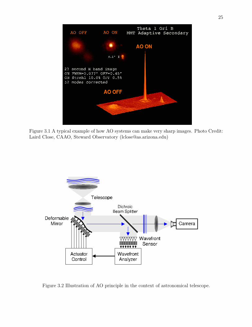
In the context of ground-based telescopes, as shown in Fig 3.1, AO is used to correctaberrations of celestial light due to turbulence of earth atmosphere to achive a crisp imagerather than a hazy one. Figure 3.2 shows a typical setup of AO in astronomical telescopes.

25

Figure 3.1 A typical example of how AO systems can make very sharp images. Photo Credit:Laird Close, CAAO, Steward Observatory (lclose@as.arizona.edu)

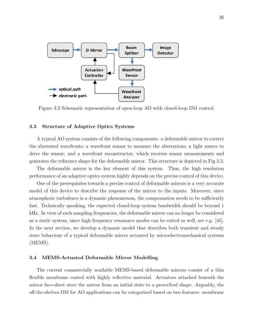
Figure 3.2 Illustration of AO principle in the context of astronomical telescope.

26

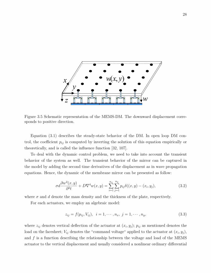
Figure 3.3 Schematic representation of open-loop AO with closed-loop DM control.

3.3 Structure of Adaptive Optics Systems

A typical AO system consists of the following components: a deformable mirror to correctthe aberrated wavefronts; a wavefront sensor to measure the aberrations; a light source todrive the sensor; and a wavefront reconstructor, which receives sensor measurements andgenerates the reference shape for the deformable mirror. This structure is depicted in Fig 3.3.

The deformable mirror is the key element of this system. Thus, the high resolutionperformance of an adaptive optics system highly depends on the precise control of this device.

One of the prerequisites towards a precise control of deformable mirrors is a very accuratemodel of this device to describe the response of the mirror to the inputs. Moreover, sinceatmospheric turbulence is a dynamic phenomenon, the compensation needs to be sufficientlyfast. Technically speaking, the expected closed-loop system bandwidth should be beyond 1kHz. In view of such sampling frequencies, the deformable mirror can no longer be consideredas a static system, since high frequency resonance modes can be exited as well, see e.g. [45].In the next section, we develop a dynamic model that describes both transient and steadystate behaviour of a typical deformable mirror actuated by microelectromechanical systems(MEMS).

3.4 MEMS-Actuated Deformable Mirror Modelling

The current commercially available MEMS-based deformable mirrors consist of a thinflexible membrane coated with highly reflective material. Actuators attached beneath themirror face-sheet steer the mirror from an initial state to a prescribed shape. Arguably, theoff-the-shelves DM for AO applications can be categorized based on two features: membrane

27

mirror and technology of actuators.In terms of membrane mirror, DMs are divided into two commonplace categories: continu-

ous face-sheet mirrors and segmented mirrors. Figure 3.4 shows the cross sectional schematicsof the main components of the continuous (left) and segmented (right) deformable mirrorfrom Boston Micro Machine (BMC).

Figure 3.4 Cross sectional schematics of the main components of BMC’s continuous (left) andsegmented (right) MEMS deformable mirrors. Picture courtesy of Michael Feinberg, BMM,(mrf@bostonmicromachines.com).

Continuous membrane mirrors have optimal fill factor and no diffraction effects. Hence,this type of mirrors are used when high power dissipation is an issue, e.g., laser micromachin-ing, and when high-order corrections are needed, e.g., astronomy. However, they have limiteddeformation range, are slower than segmented mirrors, and suffer from crosstalk [31, 36].Therefore, more elaborated control algorithms are required to overcome these drawbacks.

In terms of actuators, two ubiquitous technologies are: piezo-stack DMs and Micro ElectroMechanical System (MEMS) DMs. MEMS-DMs are the most popular one because of theirsimple structural geometry, flexible operation, and easy fabrication from standard and well-understood materials [54]. Electrostatic actuation is also the dominant scheme used forMEMS deformable mirrors in adaptive optics applications [109, 32, 75, 111, 95].

In this work, we use a relatively simple model for MEMS-actuated continuous facesheetDM displacement based on the thin plate theory [102]. Henceforward, we use the term DMto refer to this type of deformable mirrors, unless otherwise mentioned.

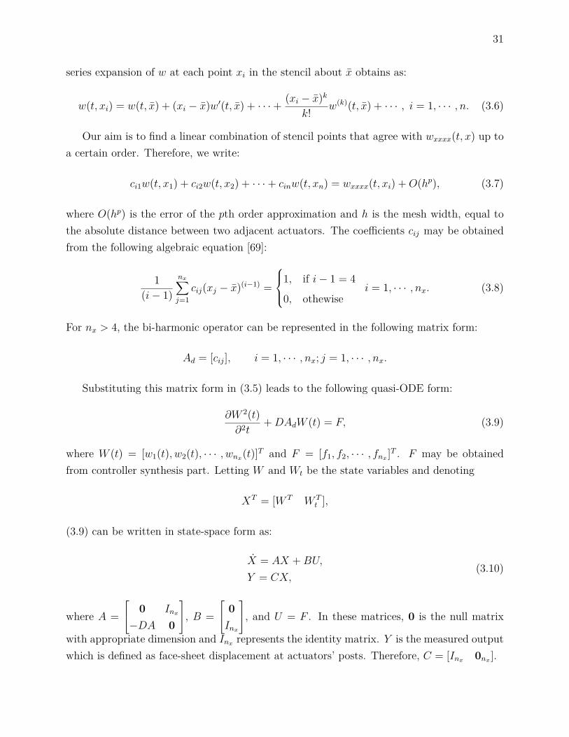
The considered DM, as shown in Fig. 3.5, consists of two coupled mechanical subsystems:a continuous flexible membrane facesheet and an array of N by N micro-actuators connectedto the facesheet via rigid posts, all integrated together on a common silicon substrate usingmicro fabrication technology.

When the DM is in static equilibrium, forces due to the actuators acting on the mirror arebalanced by restoring forces due to flexure of the membrane. If the rigid posts are relativelysmall, the membrane is of uniform thickness, and the displacement is small relatively to the

28

thickness of membrane, then we may ignore longitudinal displacement, which yields:

D∇4w(x, y) =nx∑j=1

ny∑i=1

pijδ((x, y)− (xi, yj)), (3.1)

where w(x, y) denotes the transversal displacement, or deflection, of the membrane mirrorat position (x, y) in the same direction of z (see Fig. 3.5), ∇4 =

(∂w4

∂4x+ 2 ∂w4

∂2x∂2y+ ∂w4

∂4y

)is

the 2-D biharmonic operator, or squared Laplacian operator, D denotes flexural rigidity ofthe face-sheet, pij denotes the point load, force per unite area, on the facesheet due to theactuator located at (xi, yj); δ((x, y)− (xi, yj)) denotes the Dirac Delta function concentratedat (xi, yj) point; nx, and ny denote the number of actuators along x-axis and y-axis.

( , )w x y

zx y

wFigure 3.5 Schematic representation of the MEMS-DM. The downward displacement corre-sponds to positive direction.

Equation (3.1) describes the steady-state behavior of the DM. In open loop DM con-trol, the coefficient pij is computed by inverting the solution of this equation empirically ortheoretically, and is called the influence function [32, 107].

To deal with the dynamic control problem, we need to take into account the transientbehavior of the system as well. The transient behavior of the mirror can be captured inthe model by adding the second time derivatives of the displacement as in wave propagationequations. Hence, the dynamic of the membrane mirror can be presented as follow:

σd∂w2(x, y)

∂2t+D∇4w(x, y) =

nx∑i=1

ny∑j=1

pijδ((x, y)− (xi, yj), (3.2)

where σ and d denote the mass density and the thickness of the plate, respectively.For each actuators, we employ an algebraic model:

zij = f(pij, Vij), i = 1, · · · , nx, j = 1, · · · , ny, (3.3)

where zij denotes vertical deflection of the actuator at (xi, yj); pij as mentioned denotes theload on the facesheet; Vij denotes the “command voltage“ applied to the actuator at (xi, yj),and f is a function describing the relationship between the voltage and load of the MEMSactuator to the vertical displacement and usually considered a nonlinear ordinary differential

29

equation (see, e.g., [75, 111]). Since the actuators are firmly attached to the membranefacesheet, coupling conditions will be:

w(xi, yj) = zij, i = 1, · · · , nx, j = 1, · · · , ny. (3.4)

As a result, the governing model for this device may be represented by the partial dif-ferential equation (3.2) coupled with nx × ny nonlinear ordinary differential equations of theMEMS actuators. This is not a easy model to start our control design. Hence, we addresssome simplifying assumptions, in the following section, to reduce the complexity of the model.

3.5 Simplifying Assumptions on the Model

To reduce the complexity of the model, we start with the MEMS actuators of the system.The dynamics of MEMS actuators which represent the relationship between input voltagesand vertical displacements as represented in (3.3) are highly nonlinear (see, e.g., [75, 111]).However, if we assume that the actuators are operating in a stable domain [95], and alsotheir dynamics is sufficiently faster than that of the membrane mirror, then we can ignorethe nonlinear dynamics of the actuators. Furthermore, since the focus of this research workis on the shape control of deformable mirrors, considering Dirac delta functions to describethe behaviour of the actuators in the domain of the PDE system is a reasonable assumption.This assumption is sufficient for our control development, especially because the dimensionof the rigid posts is much smaller than that of the membrane mirror. Hence, they can beconsidered as point-wise actuators. As a result, the coupled PDE-ODE model of the devicecan be reduced to a PDE system with in-domain point-wise control inputs represented byDirac delta functions.

Mathematically speaking, in order to have this model controllable, the system shouldhave a unique solution. To address this issue, we have to associate a set of proper boundaryconditions to the model. The boundary conditions have to describe the physical behaviourof the structure. We assume the membrane mirror is suspended at two ends and supportedat two other ends. Note that this suspended-supported boundary conditions are standardconditions for plate and beam equations that facilitate well-posedness and controllabilitystudies of the model and also describe well the structure of a large-scale deformable mirror.These boundary conditions describe a rectangle segment of the membrane mirror which isterminated with the frame at two sides, and two other sides are suspended on holding rigidposts. We prove the well-posedness and the controllability of the model based on this set ofboundary conditions in Chapter 4.

Furthermore, DM deflection is typically measured relative to a “bias” deflection, obtained

30

when a bias voltage is applied simultaneously to all the actuators. We take this physicalproperty into account by assigning initial conditions to the displacement and the rate ofdisplacement of membrane mirror.

Moreover, by assuming a fully symmetric distribution of the actuators in x-y plane, theplate equation of the large-scale deformable mirror model (3.1) can be reduced to the Carte-sian product of two decoupled 1-dimensional systems of Euler-Bernoulli beam equations[16, 17]. Hence, considering this assumption, we limit the control design to one row of actu-ators located along the x-axis and suppose that the mass of the device is normalized to oneunit.

3.6 Lumped Model and Finite-Dimensional Control Design

In this section, we present a simple simulation study based on a finite-dimensional ap-proximation of the model. In this study, a finite element approximation of the model isconsidered on space which results in a set of lumped ordinary differential equations. Then,a linear-quadratic tracking, LQT, scheme is applied to develop the control law for trackingreference trajectories. This design formally shows the essential steps in control designs basedon lumped model. The results of this section has been published in [13].

3.6.1 Control Design of Lumped System

For this design, we consider the beam equation model of the system with one row ofactuators located along the x-axis as:

wtt(t, x) +Dwxxxx(t, x) = −nx∑i=1

piδ(x− xi). (3.5)

where wtt and wxxxx represent the second time derivatives and the fourth space derivativesof w(x, t). The goal of the control design is to find pi to steer the beam along referencetrajectories. Note that the open-loop approaches for deformable mirrors aim at finding astatic pi, the so-called influence functions. However, in closed-loop control schemes, pi iscomputed dynamically.

To carry out the control design, we discretize wxxxx on space. More specifically, weapproximate the fourth time space derivatives of w based on a linear combination of theactuators as stencil points. Then, we may apply an optimal quadratic tracking control todrive the quasi-ODE system resulting from space discretization. Assuming that w(t, x) issufficiently smooth in space, i.e., at least n times continuously differentiable, the Taylor

31

series expansion of w at each point xi in the stencil about x obtains as:

w(t, xi) = w(t, x) + (xi − x)w′(t, x) + · · ·+ (xi − x)kk! w(k)(t, x) + · · · , i = 1, · · · , n. (3.6)

Our aim is to find a linear combination of stencil points that agree with wxxxx(t, x) up toa certain order. Therefore, we write:

ci1w(t, x1) + ci2w(t, x2) + · · ·+ cinw(t, xn) = wxxxx(t, xi) +O(hp), (3.7)

where O(hp) is the error of the pth order approximation and h is the mesh width, equal tothe absolute distance between two adjacent actuators. The coefficients cij may be obtainedfrom the following algebraic equation [69]:

1(i− 1)

nx∑j=1

cij(xj − x)(i−1) =

1, if i− 1 = 4

0, othewisei = 1, · · · , nx. (3.8)

For nx > 4, the bi-harmonic operator can be represented in the following matrix form:

Ad = [cij], i = 1, · · · , nx; j = 1, · · · , nx.

Substituting this matrix form in (3.5) leads to the following quasi-ODE form:

∂W 2(t)∂2t

+DAdW (t) = F, (3.9)

where W (t) = [w1(t), w2(t), · · · , wnx(t)]T and F = [f1, f2, · · · , fnx ]T . F may be obtainedfrom controller synthesis part. Letting W and Wt be the state variables and denoting

XT = [W T W Tt ],

(3.9) can be written in state-space form as:

X = AX +BU,

Y = CX,(3.10)

where A = 0 Inx

−DA 0

, B = 0Inx

, and U = F . In these matrices, 0 is the null matrix

with appropriate dimension and Inx represents the identity matrix. Y is the measured outputwhich is defined as face-sheet displacement at actuators’ posts. Therefore, C = [Inx 0nx ].

32

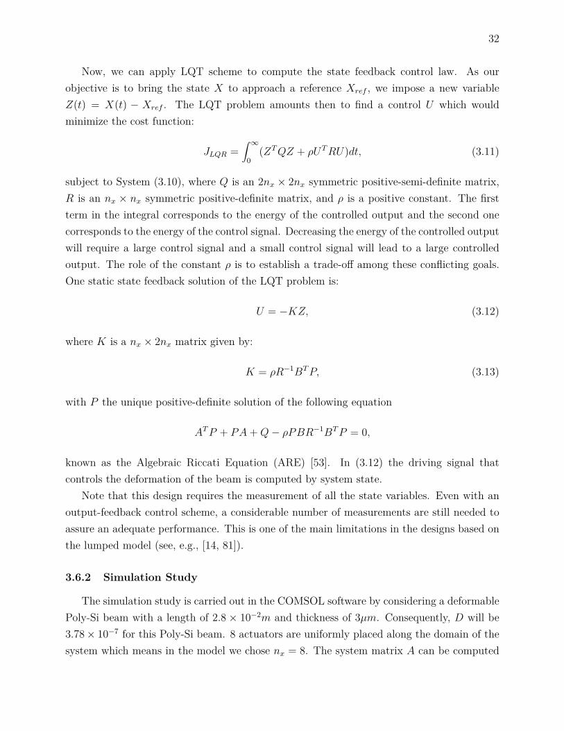
Now, we can apply LQT scheme to compute the state feedback control law. As ourobjective is to bring the state X to approach a reference Xref , we impose a new variableZ(t) = X(t) − Xref . The LQT problem amounts then to find a control U which wouldminimize the cost function:

JLQR =∫ ∞

0(ZTQZ + ρUTRU)dt, (3.11)

subject to System (3.10), where Q is an 2nx × 2nx symmetric positive-semi-definite matrix,R is an nx × nx symmetric positive-definite matrix, and ρ is a positive constant. The firstterm in the integral corresponds to the energy of the controlled output and the second onecorresponds to the energy of the control signal. Decreasing the energy of the controlled outputwill require a large control signal and a small control signal will lead to a large controlledoutput. The role of the constant ρ is to establish a trade-off among these conflicting goals.One static state feedback solution of the LQT problem is:

U = −KZ, (3.12)

where K is a nx × 2nx matrix given by:

K = ρR−1BTP, (3.13)

with P the unique positive-definite solution of the following equation

ATP + PA+Q− ρPBR−1BTP = 0,

known as the Algebraic Riccati Equation (ARE) [53]. In (3.12) the driving signal thatcontrols the deformation of the beam is computed by system state.

Note that this design requires the measurement of all the state variables. Even with anoutput-feedback control scheme, a considerable number of measurements are still needed toassure an adequate performance. This is one of the main limitations in the designs based onthe lumped model (see, e.g., [14, 81]).

3.6.2 Simulation Study

The simulation study is carried out in the COMSOL software by considering a deformablePoly-Si beam with a length of 2.8 × 10−2m and thickness of 3µm. Consequently, D will be3.78× 10−7 for this Poly-Si beam. 8 actuators are uniformly placed along the domain of thesystem which means in the model we chose nx = 8. The system matrix A can be computed

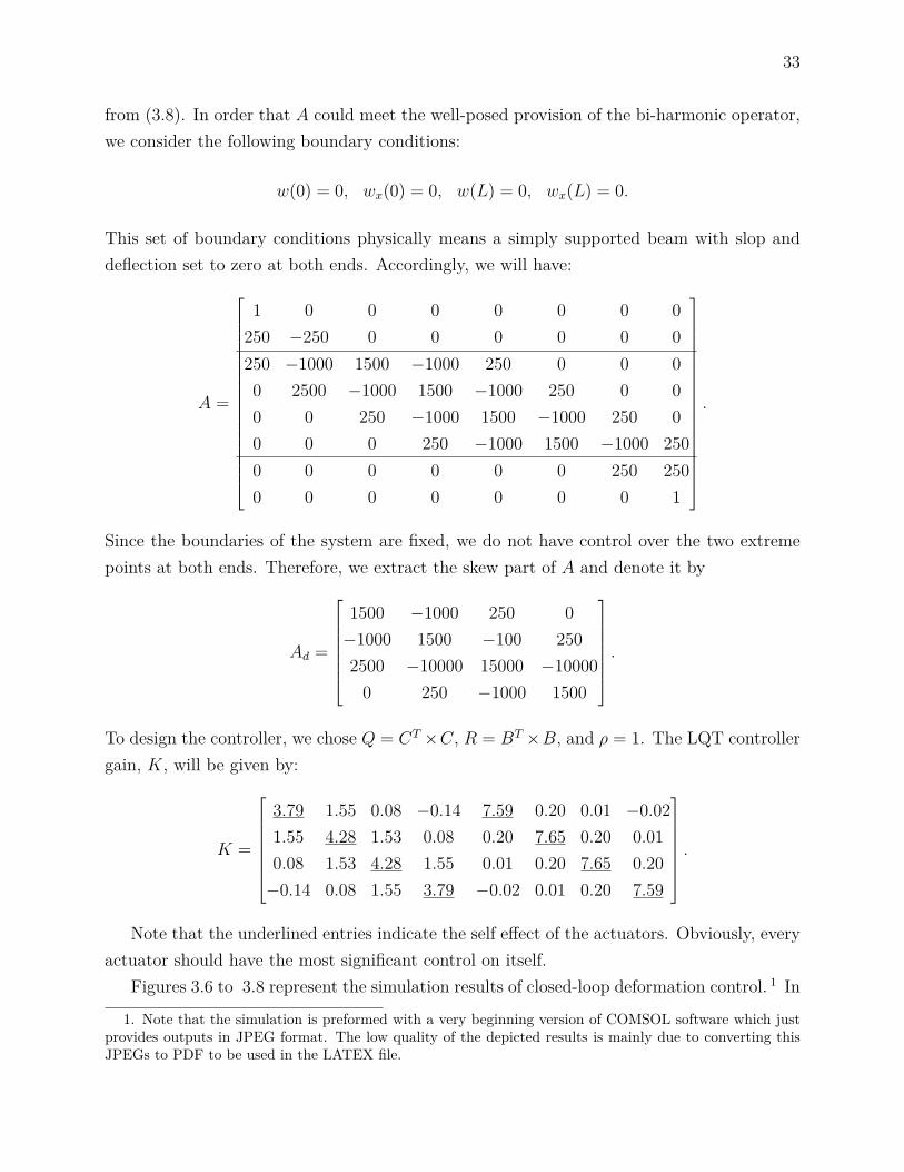
33

from (3.8). In order that A could meet the well-posed provision of the bi-harmonic operator,we consider the following boundary conditions:

w(0) = 0, wx(0) = 0, w(L) = 0, wx(L) = 0.

This set of boundary conditions physically means a simply supported beam with slop anddeflection set to zero at both ends. Accordingly, we will have:

A =

1 0 0 0 0 0 0 0250 −250 0 0 0 0 0 0250 −1000 1500 −1000 250 0 0 00 2500 −1000 1500 −1000 250 0 00 0 250 −1000 1500 −1000 250 00 0 0 250 −1000 1500 −1000 2500 0 0 0 0 0 250 2500 0 0 0 0 0 0 1

.

Since the boundaries of the system are fixed, we do not have control over the two extremepoints at both ends. Therefore, we extract the skew part of A and denote it by

Ad =

1500 −1000 250 0−1000 1500 −100 2502500 −10000 15000 −10000

0 250 −1000 1500

.

To design the controller, we chose Q = CT ×C, R = BT ×B, and ρ = 1. The LQT controllergain, K, will be given by:

K =

3.79 1.55 0.08 −0.14 7.59 0.20 0.01 −0.021.55 4.28 1.53 0.08 0.20 7.65 0.20 0.010.08 1.53 4.28 1.55 0.01 0.20 7.65 0.20−0.14 0.08 1.55 3.79 −0.02 0.01 0.20 7.59

.

Note that the underlined entries indicate the self effect of the actuators. Obviously, everyactuator should have the most significant control on itself.

Figures 3.6 to 3.8 represent the simulation results of closed-loop deformation control. 1 In

1. Note that the simulation is preformed with a very beginning version of COMSOL software which justprovides outputs in JPEG format. The low quality of the depicted results is mainly due to converting thisJPEGs to PDF to be used in the LATEX file.

34

simulation, The desired shape, as shown in Fig. 3.6, is described by W = −10−6 sin( 2π2.8x)ex.

It can be seen that the system tracks the reference shape with an acceptable tracking error,shown in Fig. 3.8, and the controller drives the beam to the steady-state mode within areasonable time (Fig. 3.6). It is worth noting that the simulation is carried out in a normalizedcoordinate. Therefore, the time scale is also normalized. The maximum amplitude of thecontrol signal is approximately 8 × 10−6 ( Fig. 3.7) which is a affordable displacement fora MEMS actuator to operate in a stable region. However, in order to avoid the undesiredovershot in actuation, one should consider more sophisticated control techniques, such asconstrained quadratic control.

3.6.3 Summary and Discussion

In this chapter, we presented the adaptive optics in the context of ground-based telescopesand introduced a dynamic partial differential equation model for deformable mirrors. Acontroller is designed based on a finite-dimension approximation of the PDE model. Thedesign formally presented the typical steps in control designs based on approximating PDEmodels to ordinary differential equations. However, this approach requires at least as manysensors as actuators to implement the closed-loop control which is not implementable withthe currently available fabrication technologies of DMs.

In addition, the neglected dynamics due to reducing the system to a finite-dimensionalmodel may deteriorate the performance or even destabilize the system, known as the spillovereffect in PDE control systems. Thus, a high order approximation is often required in thedesign for assuring system stability, which in turn might lead to complex control structures.These issues raise serious technological challenges in the design, fabrication, and operationof microsystems. Therefore, it is of great interest to directly deal with the control of PDEmodels from both theoretical and practical viewpoints.

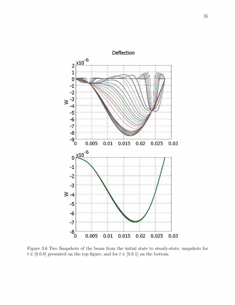
35

Figure 3.6 Two Snapshots of the beam from the initial state to steady-state; snapshots fort ∈ [0 0.8] presented on the top figure, and for t ∈ [0.8 1] on the bottom.

36

Figure 3.7 Control effort generated on each actuator points, two first and two last actuatorsare fixed to comply with boundary condition.

Figure 3.8 The error between the desired and actual trajectory.

37

CHAPTER 4

CONTROL DESIGN: FLATNESS-BASED DEFORMATION CONTROL OFEULER-BERNOULLI BEAMS WITH IN-DOMAIN ACTUATION

This chapter addresses the main results of this research. In this chapter, we start by pre-senting an Euler-Bernoulli model of the deformable beam described by a fourth-order partialdifferential equation, and discussing the well-posedness and controllability of the model.Then, in Section 4.2.3, we develop the Green’s function of the system which will be employedlater in the control algorithm design. We start the design in Section 4.3 by establishing aformal map between the in-domain controlled system and a standard boundary-controlledmodel. Based on this map, we develop a control strategy, which is a combination of feedbackstabilization and differential flatness-based feed-forward motion planing. This part formallyshows a way to deal with the tracking control problem of in-domain controlled PDE systems.However, the map holds only for some special test functions. Thus, since we limit the testfunctions to some convenient ones, the original PDE is satisfied in a very weak sense, butnot in the usual one. To cope with this problem, we develop another design in Section 4.4.In this design instead of trying to establish such an equivalence, we approximate the solutionof the original system by that of a target system driven by regularized inputs in the steadystate. To do this, we use the technique of lifting to transform the target system, which iscontrolled by boundary actuators, to an inhomogeneous PDE driven by sufficiently smoothfunctions generated by applying blobs, used to approximate the Dirac delta functions. Thiswould allow establishing a relationship between the original system and the target systemin a usual weak sense. Theorem 4.6 entails this issue. Moreover, the transient behavior,the stability of the closed-loop system, and the regulation error dynamics are addressed inTheorem 4.8 and Corollary 1.

4.1 Notation

For the purpose of clarity, we recall the notations, most of which are defined in Chapter 2.Let R be the field of all real numbers. For n ≥ 1, Rn denotes the n-dimensional Euclidean

space with norm ‖x‖ and inner product 〈x, y〉 for all x and y in Rn. Let Ω be a nonemptyopen subset of Rn. Denoting by ∂Ω the boundary of Ω, then Ω = Ω∪ ∂Ω is the closure of Ω.Given a continuous linear map L between two Hilbert space and letting H be a Hilbert space,Lp(Ω), p > 0, will be the normed linear space of all equivalent classes of Lebesgue-measurable

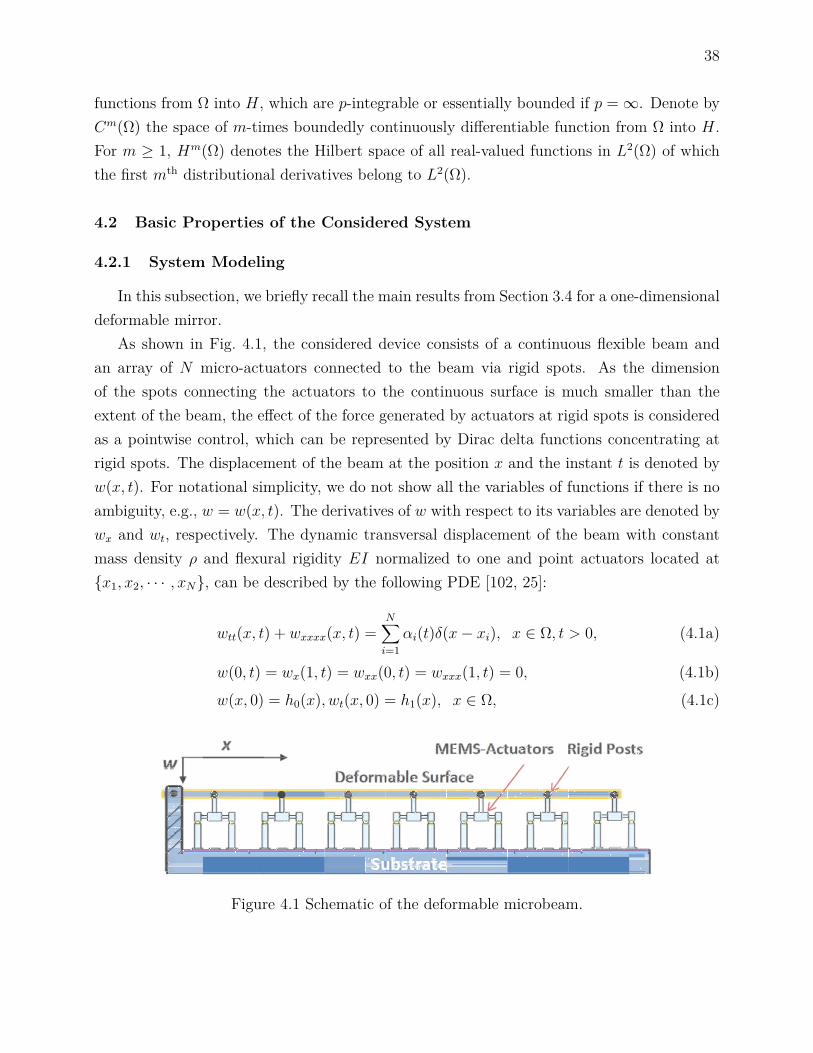
38

functions from Ω into H, which are p-integrable or essentially bounded if p =∞. Denote byCm(Ω) the space of m-times boundedly continuously differentiable function from Ω into H.For m ≥ 1, Hm(Ω) denotes the Hilbert space of all real-valued functions in L2(Ω) of whichthe first mth distributional derivatives belong to L2(Ω).

4.2 Basic Properties of the Considered System

4.2.1 System Modeling

In this subsection, we briefly recall the main results from Section 3.4 for a one-dimensionaldeformable mirror.

As shown in Fig. 4.1, the considered device consists of a continuous flexible beam andan array of N micro-actuators connected to the beam via rigid spots. As the dimensionof the spots connecting the actuators to the continuous surface is much smaller than theextent of the beam, the effect of the force generated by actuators at rigid spots is consideredas a pointwise control, which can be represented by Dirac delta functions concentrating atrigid spots. The displacement of the beam at the position x and the instant t is denoted byw(x, t). For notational simplicity, we do not show all the variables of functions if there is noambiguity, e.g., w = w(x, t). The derivatives of w with respect to its variables are denoted bywx and wt, respectively. The dynamic transversal displacement of the beam with constantmass density ρ and flexural rigidity EI normalized to one and point actuators located atx1, x2, · · · , xN, can be described by the following PDE [102, 25]:

wtt(x, t) + wxxxx(x, t) =N∑i=1

αi(t)δ(x− xi), x ∈ Ω, t > 0, (4.1a)

w(0, t) = wx(1, t) = wxx(0, t) = wxxx(1, t) = 0, (4.1b)

w(x, 0) = h0(x), wt(x, 0) = h1(x), x ∈ Ω, (4.1c)

Figure 4.1 Schematic of the deformable microbeam.

39

where x is a normalized variable spanned over the domain Ω = (0, 1), δ(x − xi) is theDirac mass concentrated at the point xi ∈ Ω, denoting the actuation spots, and αi : t 7→ R,i = 1, . . . , N , are the control signals. h0 and h1 represent the initial values of the displacementand its time-derivative associated with the beam. The boundary condition (4.1b) means thatthe beam is simply supported at x = 0 and the shear hinged at x = 1. Without loss ofgenerality, we assume that 0 < x1 < x2 < · · · < xN < 1.

Remark 4.1 The boundary conditions given in (4.1b) capture well the property of the struc-ture that is suspended at the left end and supported by a vertically moving actuator at theright end. Note that for other bending schemes, such as clamped-clamped and clamped-freeconfigurations, the boundary conditions are different, which may lead to different feedbackstabilization strategies [25]. Nevertheless, the system architecture and the procedure for feed-forward control design remain the same.

Remark 4.2 The considered problem can also be modeled as a serially connected beam [25].Indeed, these two models are equivalent in the sense that they lead to the same abstract linearsystem in variational form (see, e.g., [92, 25, 60, 62, 61]).

Remark 4.3 Electrostatic actuation is one of the dominant schemes used for MEMS de-formable mirrors [107, 32]. However, the dynamics of electrostatic MEMS are highly nonlin-ear and performance enhancement of such devices is a challenging topic (see, e.g., [75, 111]).In this research, we concentrate on shape control of deformable mirrors while ignoring thedynamics of the actuators, which is supposed to be sufficiently faster than the dynamics of thestructure. Moreover, we suppose that the actuators are working in the stable operation range[95]. In fact, considering the dynamics of the actuators will lead to a coupled PDE-ODEcontrol problem.

The control objective is to steer the beam displacement, w(x, t), to follow a desired formdescribed by wd(x, t) via in-domain pointwise actuation.

The model given in (4.1) is a nonstandard PDE due to the in-domain pointwise actuation,represented by Dirac functions, on the right-hand side of (4.1a). Thus, the classical definitionof derivative cannot be applied. Therefore, we will invoke the weak derivative notion of asolution to this model in the weak sense [89].

Specifically, (4.1) does not admit strong solutions in the classic sense for w ∈ C4([0 T ]×Ω\xi1≤i≤N)⋂C3([0 T ]× Ω) because of the unbounded Delta dirac functions on the right-hand-side of (4.1a). However, in practice, there exist functions that satisfy this differentialequation, except they are not sufficiently smooth. A typical example of this type of situationsis the impulse response of a (finite- or infinite-dimensional) system, which is indeed physically

40

meaningful, although it is only differentiable up to a finite order. Such functions are calledweak or generalized solutions to the corresponding differential equation.

The weak solution of a PDE can be defined by means of weak derivative in the theoryof distributions [89]. To find the weak derivatives, the system is multiplied by a sufficientlysmooth function with a compact support, called test function. Then, integrating over thedomain results in a sufficiently smooth function coming from the rough distribution. Applyingintegration by part and Green’s formula, up to a certain problem-dependent order, willenable the definition of the derivatives of distributions. To this end, we start by defining theconvergence on C∞0 (Ω).

Definition 4.1 Let Ω be a domain in R(n ≥ 1). A sequence ϕj of functions belonging toC∞0 (Ω) converges to ϕ ∈ C∞0 (Ω), if

(i) there exists K ⊂ Ω such that supp(ϕj − ϕ) ⊂ K for every j, and

(ii) limj→∞ ∂αϕj(x) = ∂αϕ(x) uniformly on K for each multi-index α.

The linear space C∞0 (Ω) having the above properties is called fundamental space, denoted byD(Ω). The space of all linear continuous functionals on D(Ω), denoted by D ′(Ω), is calledthe space of (Schwartz) distributions on Ω, which is the dual of D(Ω) (see, e.g., Chapter 1of [2] for more properties of D(Ω) and D ′(Ω)).

Denote the set Φ by

Φ =φ ∈ H2(0, 1);φ(0) = φx(1) = 0

. (4.2)

In the following definition, we define a weak solution of (4.1).

Definition 4.2 Let T > 0 and αi ∈ L2(0, T ) for i = 1, 2, ..., N . Let h0 ∈ Φ, h1 ∈ L2(0, 1). Aweak solution to the Cauchy problem (4.1) is a function w ∈ C([0, T ]; Φ)∩C1([0, T ];L2(0, 1)),satisfying

w(x, 0) = h0(x), x ∈ (0, 1),

41

such that, for every v ∈ C1([0, T ]; Φ), one has for almost every τ ∈ [0, T ]∫ 1

0wt(x, τ)v(x, τ)dx−

∫ 1

0h1(x)v(x, 0)dx

−∫ τ

0

∫ 1

0wt(x, t)vt(x, t)dxdt

+∫ τ

0

∫ 1

0wxx(x, t)vxx(x, t)dxdt

=N∑i=1

∫ τ

0

∫ 1

0αi(t)δ(x− xi)v(x, t)dxdt. (4.3)

For every v ∈ C1([0, T ]; Φ), the function w(x, t) given by 4.3 is a weak solution for thesystem. In the next section, we study the uniqueness of this solution through well-posednessanalysis of the model.

4.2.2 Well-Posedness and Controllability of the Model

In the investigation of the well-posedness of the considered system, we employ the formu-lation of Cauchy problem for abstract linear control systems, which enables the applicationof the framework of semigroup theory [27, 29, 104]. More specifically, in this framework theassessment of well-posedness amounts to showing that if the system is defined on an appro-priate Hilbert space, then by Riesz’ representation theorem there exists a unique solution tothe problem (see, e.g., Page 52 of [89] and Chapter 1 of Part II in [19]).

Let X = Φ × L2(0, 1), where Φ is defined in (4.2), be a Hilbert space equipped withappropriate inner product and norm. We define the subspace D(A) ⊂ X by:

D(A) =

(w, v) ∈ [Φ ∩H4(0, 1)]× Φ | wxx(0, t) = wxxx(1, t) = 0

(4.4)

with the corresponding operator A : D(A)→ X defined as:

A

wv

= v

−wxxxx

, (4.5)

where the derivative with respect to x are calculated in the dual space of D(A), denoted byD′(A), with respect to the pivot space X.

Denoted by S(t), t ∈ [0,+∞), the semigroup generated by A and by S∗(t) the semigroupgenerated by A∗, the adjoint of A. It can be shown that D′(A∗), the dual of D(A∗) withrespect to the space X, satisfies [104]

D(A∗) ⊂ X ⊂ D′(A∗). (4.6)

42

Moreover, the control operator B : RN 7→ D′(A∗) is defined as:

Br = 0∑N

i=1 riδ(x− xi)

, ∀r ∈ RN . (4.7)

With the above notations we can translate System (4.1) into the equivalent Cauchy prob-lem described by an abstract linear control system of the following form:

y = Ay +Bu, y(0) = y0, (4.8)

where y =(w wt

)T∈ X is the state vector, u : [0, T ] → U is the control signal, U = R is

the control space, and y0 =(h0 h1

)Tis the initial condition.

Note that the control operator B in (4.8) is not continuous nor bounded in classical sense.Hence, we are interested in the set of operators for which all the weak solutions of System(4.8) for u(t) given in L2((0, T );U) and y0 given in X are continuous X-valued functions, asdefined in Definition 2.12.

We start by giving a formal definition of a solution to (4.8). Let τ ∈ [0, T ] and ϕ : [0, τ ]→X. We take the inner product in X of (4.8) with ϕ and perform integration on [0, τ ]. Usingintegration by part together with (4.8), we obtain formally:

〈y(τ), ϕ(τ)〉X − 〈y0, ϕ(0)〉X =∫ τ

0〈y(t), ϕ+ A∗ϕ(t)〉Xdt+

∫ τ

0〈u(t), B∗ϕ(t)〉Udt. (4.9)

Taking ϕ = S∗(τ − t)z(τ), for ∀z(τ) ∈ X, we have ϕ(t) + A∗ϕ(t) = 0, which leads to:

〈y(τ), z(τ)〉X − 〈y0, S∗(τ)z(τ)〉X =∫ τ

0〈u(t), B∗S∗(τ − t)z(τ)〉Udt, ∀τ ∈ [0, T ],∀z(τ) ∈ X.

(4.10)

Definition 4.3 Let T > 0, y0 ∈ X, and u ∈ L2((0, T );U). A weak solution to the Cauchyproblem (4.8) associated with (4.1) is defined by (4.10) with the regularity y ∈ C([0, T ];X).

Based on this definition of solutions, we introduce the following theorem for the well-posedness of the Cauchy problem of abstract linear control systems of the form defined in(4.8) (see Theorem 2.37 in [27], Page 53), and a proposition from [5] that we use later toprove the uniqueness of the solution.

Theorem 4.1 Let T > 0. Then for every y0 ∈ X and every u ∈ L2((0, T );U), the Cauchyproblem (4.8) has a unique solution y if A is a generator of a strongly continuous semigroupS(t) and B is admissible for S(t) on X.

43

Theorem 4.2 (Proposition 2.1 [5]) If y0 = (w0, w1) ∈ X, then for the problem (4.8) wehave:

‖ ϕ(ξ, ·) ‖2H1(0,T )≤ C

(‖ w0 ‖2

H2(0,1) + ‖ w1 ‖2L2(0,1)

), (4.11)

where C is a positive constant which depends only on ξ and T .

The following theorem states the well-posedness property of (4.1) presented in the abstractform (4.8).

Theorem 4.3 Let T > 0 and denote α(t) = (αi(t), . . . , αN(t)). Then for every y0 =(w0, w1) ∈ X and every u(t) = α(t) ∈ L2((0, T );U), the Cauchy problem (4.8) associatedto (4.1) has a unique solution y ∈ C([0, T ];X) defined by (4.10).

Proof. SinceA is skew-adjoint, by Stone’s theorem [27], it generates a strongly continuoussemigroup of isometries S(t) on X. Hence, based on Theorem 4.1, it is sufficient to showthat the control operator B expressed by (4.7) is admissible for S(t) on X.

According to (4.7), the operator B∗ : D(A∗) 7→ RN is given by:

B∗

wv

=N∑i=1

v(ξi), ∀wv

∈ D(A∗). (4.12)

This implies that

B∗S∗(t)w0

w1

=N∑i=1

ϕt(ξi), ∀w0

w1

∈ D(A∗). (4.13)

According to Theorem 4.2 and Equation (4.13), we deduce that for all T > 0, there exists aconstant CT > 0 such that

∫ T

0

∥∥∥∥∥∥B∗S∗(t)w0

w1

∥∥∥∥∥∥2

dt ≤CT

∥∥∥∥∥∥w0

w1

∥∥∥∥∥∥2

X

, ∀

w0

w1

∈ D(A∗). (4.14)

This implies that the operator B is regular for S(t) on X. From Theorem 4.1, we canconclude then on the existence and the uniqueness of the solution to the Cauchy problem (4.8)associated to System (4.1).

Remark 4.4 The well-posedness of a similar system with only one in-domain input has beenshown in [5] (Proposition 3.1). In such a case, B : R 7→ D′(A∗). Therefore, Theorem 4.3can be seen as a direct extension of this result.

For the controllability of the system from Chapter 2, we have:

44

Theorem 4.4 System (4.8) is exactly controllable in [0;T ] for any finite y0 ≥ 0 if A gener-ates a stable C0-semigroup and B is unbounded but admissible.

Proof. The admissibility of the unbounded operators B is shown in the well-posedenss study.Hence, showing the stability of C0-semigroup generator A will complete the proof. This issueis addressed in Section 4.4.3.

4.2.3 Green’s Functions for Euler-Bernoulli Beams

One of the main contribution of this work is to leverage the Green’s function in thedesign. It is shown that a finite set of the Green’s functions of the system can be used toapproximate desired trajectories. Therefore, an exact invertible and finite-dimensional inputto output map can be obtained without invoking any truncations. It also facilitates the realtime implementation of the design since the decomposition of desired trajectories can beassessed a priori.

This subsection recalls some basic notation, properties, and results related to the Green’sfunction, which will be employed later in control algorithm development. The Green’s func-tion is a basic tool in the study of PDEs and there exists a rich literature on this topic(see e.g., [91]). In this research, we are particularly interested in the static Green’s functioncorresponding to the steady-state beam equation, which will be used in our design.

Consider a generic form of steady-state equation corresponding to the beam equation(4.1) with an arbitrary excitation function, f(x):

wxxxx(x) = f(x), x ∈ Ω, (4.15a)

w(0) = wx(1) = wxx(0) = wxxx(1) = 0. (4.15b)

For a point-wise actuation scheme described by System (4.1), the source term is of the form∑Ni=1 αiδ(x − xi), where αi, i = 1, · · · , N , represent the steady-state actuation signals. The

static Green’s function, or the Green’s function for short, corresponding to (4.15), denoted byG(x, ξ), is the solution to such an equation for f(x) = δ(x− ξ), x, ξ ∈ Ω, with homogeneousboundary conditions.

The Green’s function G(x, ξ) can be calculated by measuring the response of the systemat point x for the pressure applied at the point ξ. Therefore, it can be seen as the impulseresponse of the system, which is an essential and important property for system analysis.Based on the principle of superposition for linear systems, the solution to the steady-state

45

beam equation (4.15) can be expressed in terms of the Green’s function as:

w(x) =∫

ΩG(x, ξ)f(ξ)dξ. (4.16)

Obviously, the domain of the Green’s function is determined by the original system.When the actuator makes vertical movement at the point x = ξ, based on the continuity

condition, the displacement, the rotation, and the bending force from the left and rightside of this point are identical. That is G(x, ξ−) = G(x, ξ+), Gx(x, ξ−) = Gx(x, ξ+), andGxx(x, ξ−) = Gxx(x, ξ+). Meanwhile, this movement will generate a shear force, representedby the jump Gxxx(x, ξ+) − Gxxx(x, ξ−) = 1 [25]. Solving (4.15a) and applying continuity,jump, an boundary conditions (4.15b), we obtain the Green’s function for System (4.15),which is given by

G(x, ξ) =

(−x

3

6 + xξ

(1− ξ

2

)), 0 ≤ x < ξ;(

−ξ3

6 + ξx(

1− x

2

)), ξ ≤ x ≤ 1.

(4.17)

The Green’s function is used for two different purposes in our design. First, this functionis used to construct test functions in the development of a map between the in-domain andboundary data. Secondly, the property given in (4.16) is employed to generate referencetrajectories in motion planning. As shown latter in Section 4.3.3, motion planning for theconsidered 4th-order beam equitation requires that the base functions must have a continuous3th-order derivative on space at the actuation points (see (4.42d)). However, the Green’sfunction given in (4.17) is only of H2 over Ω. A solution for overcoming this problem is theuse of regularized Green’s functions that are sufficiently smooth.

Different from the Green’s function that is the response to the Delta dirac input, aregularized Green’s function, denoted by G, is generated by using a cutoff function, alsocalled blob, as the input to the system. Driving the steady state equation (4.15) by a blob ofthe following form [28]:

ϕδ(x− ξ) = 3δ4((x− ξ)2 + δ2)5/2 , (4.18)

where δ is a small scaling parameter, the corresponding regularized Green’s function is givenby:

G(x, ξ) = 112((x− ξ)2 + δ2

)3/2+ Ax3 +Bx2 + Cx+D, (4.19)

46

where

A =(2(ξ − 1)2 + 3δ2)(ξ − 1)4((ξ − 1)2 + δ2)3/2 , (4.20a)

B =− (δ2 + 2ξ2)/(4(δ2 + ξ2)1/2), (4.20b)

C =(δ2 + 2ξ2)/(4(δ2 + ξ2)(1/2))− ((2(ξ − 1)2 + 2δ2)

× (ξ − 1) + δ2(ξ − 1))/(8((ξ − 1)2 + δ2)3/2)

+ (((ξ − 1)2 + δ2)1/2(ξ − 1))/4, (4.20c)

D =− (δ2 + ξ2)3/2/12. (4.20d)

Note that for ∀δ > 0, the blob given in (4.18) satisfies∫ ∞−∞

ϕδ(x)dx = 1. (4.21)

It can also be shown that the regularized Green’s function generated by the blob defined in(4.18) gives an approximation of the Green’s function with O(δ2/x2) and G converges to Gas δ → 0 [28].

4.3 The First Design: Mapping In-domain Actuation into Boundary Control

The control scheme presented in this section consists in first mapping the original nonho-mogeneous model into a target system in a standard boundary control form. The system hasa finite number of actuators which means the control space is of finite dimensions whereas thedegree of freedom (DOF) of the system is of infinite dimensions. This underactuated propertyof the system is solved by splitting reference trajectories into a finite set of sub-trajectoriesbased on an essential property of the Green’s functions. The technique of flatness-basedtrajectory planning can then be readily applied to boundary controls introduced in the for-mulation of the target system. A standard closed-loop feedback control is used to stabilize thesystem around the desired trajectories. The combination of feedback stabilization and feed-forward motion planning results in an asymptotic tracking control law allowing the systemto follow prescribed trajectories.

4.3.1 Mapping In-domain Actuation into Boundary Control

To circumvent the complexity introduced by unbounded in-domain actuators in themodel (4.1), we start by introducing a formal map that will transform this nonstandardproblem into a standard boundary control form to which existing stabilization and controlmethods may be applied. To this end, we consider the following target system described by

47

a homogenous initial-boundary value PDE:

utt(x, t) + uxxxx(x, t) = 0, x ∈ Ω, t > 0, (4.22a)

u(0, t) = ux(1, t) = uxx(0, t) = 0, t > 0, (4.22b)

uxxx(1, t) = g(t), t > 0, (4.22c)

u(x, 0) = h0(x), ut(x, 0) = h1(x), x ∈ Ω, (4.22d)

where g(t) is the control placed on the boundary and the other variables are defined in (4.1).Our aim is to find a relationship that maps the effect of the actuation signals appearing onthe right-hand side of (4.1a) to the boundary control g(t) in (4.22c), representing a shearforce. Note that (4.22) is an abstract mathematical model used in control design, which doesnot describe the physical system operated by multiple interior actuators.

Our goal is to ensure that Systems (4.1) and (4.22) have an identical weak solution. Theweak solution to Systems (4.1) is introduced in Section 4.2. The weak solution to (4.22)can be obtained by repeating the same procedure. We multiply (4.22) by a test functionv ∈ C1([0, T ]; Φ), where Φ is defined in (4.2). Then, the weak solution in integral form canbe derived by integration over [0, τ ] × Ω, with τ ∈ [0, T ]. We can then obtain the followingequations using integration by parts twice on the term wtt(x, t)v(x, t), and Green’s formula[48] two times on the term wxxxx(x, t)v(x, t):

〈ut(x, t), vt(x, t)〉(τ,Ω) + 〈uxx(x, t), vxx(x, t)〉(τ,Ω)

−∫

Ω(h1(x)v(x, 0)− ut(x, τ)v(x, τ)

+u(x, τ)vt(x, τ)) dx+∫ τ

0

∫∂Ωvx(x, t)uxxx(x, t)dωdt

−∫ τ

0

∫∂Ωvxx(x, t)uxx(x, t)dωdt = 0, (4.23)

where〈f(x, t), g(x, t)〉(τ,Ω) =

∫ τ

0

∫Ωf(x, t)g(x, t)dxdt (4.24)

denotes a spatio-temporal inner product, and dω denotes the integration variable on theboundary where x = 0 and x = 1 are the boundary points for this system. By applying the

48

boundary conditions given in (4.22c), and (4.22b), we have:

〈ut(x, t), vt(x, t)〉(τ,Ω) + 〈uxx(x, t), vxx(x, t)〉(τ,Ω)

−∫

Ω(h1(x)v(x, 0)− ut(x, τ)v(x, τ)

+u(x, τ)vt(x, τ)) dx+∫ τ

0

∫∂Ωv(x, t)g(t)dωdt = 0. (4.25)

Finally, a sufficient condition for which Systems (4.1) and (4.61) have an identical weaksolution can be obtained by subtracting (4.25) from (4.3):

∫∂Ωv(x, t)g(t)dω −

N∑i=1

∫Ωαi(t)v(x, t)δ(x− xi)dx = 0. (4.26)

To find a closed-form expression for g(t), we choose a test function of the form:

v(x) =N∑j=1

G(x, ξj), (4.27)

where G(x, ξj), j = 1, · · · , N , are computed from (4.17).Note that a wide class of functions can be considered as a candidate for test functions, for

example a function formed by the eigenfunctions of the system. The reason that the Green’sfunction is chosen as a test function comes primarily from the fact that it leads to a simplesolution while guaranteeing the solvability of the map between the boundary value and theactual actuation signals, as shown below.

By substituting (4.27) into (4.26) and using the basic property of Dirac delta functions,we can rearrange (4.26) in terms of g(t) as

g(t) =N∑j=1

∑Ni=1 αi(t)G(xi, ξj)

Γ(ξj), (4.28)

whereΓ =

N∑m=1

∫∂ΩG(x, ξj)dω. (4.29)

Hence, the map between the in-domain control signals and the corresponding boundaryvalues can be expressed by:

G(x1, ξ1) . . . G(xN , ξ1)

... . . . ...G(x1, ξN) . . . G(xN , ξN)

α1(t)...

αN(t)

= Γ

g1(t)...

gN(t)

, (4.30)

49

withg(t) =

N∑j=1

gj(t) = 1Γ

N∑j=1

N∑i=1

G(xi, ξj)αi(t). (4.31)

Clearly, (4.30) and (4.31) bridge the nonhomogeneous PDE system (4.1) with the standardboundary control form (4.22). This will allow the use of existing methods to deal with thePDE controlled on the boundary and then applying the results back to the original in-domainactuation signals by inverting (4.30). Note that (4.30) is a static map whose invertibility canbe assessed a priori. This shows the simplicity of the proposed approach.

Theorem 4.5 The map given in (4.30) is invertible if the test functions as chosen v(x) =∑Nj=1G(x, ξj), ξj, j = 1, . . . , N , are all distinguished, and G(x, ξj) is of the form

G(x, ξj) =

−x

3

6 + xξj

(1− ξj

2

), 0 ≤ x < ξj;

−ξ3j

6 + ξjx(

1− x

2

), ξj ≤ x ≤ 1.

(4.32)

Note that G(x, ξj) given in (4.32) is the static Green’s function of the beam equationparameterized by ξj. It is easy to check that G(x, ξj) is a positive, monotonically increasingfunction and G(x, ξi) 6= G(x, ξj), ∀ξi 6= ξj and x ∈ (0, 1].

Proof. First, being the fundamental static solution of the beam equation (4.1) corre-sponding to the input δ(x− ξj), G(x, ξj) is in Φ. We need then to proof that the matrix inthe left-hand-side of (4.30) formed by Green’s functions corresponding to distinguished ξjs,denoted by [G(xi, ξj)]N×N , is invertible. If, otherwise, [G(xi, ξj)]N×N is not invertible, then itis of rank less than N . Without loss of generality, assume that there exist N − 1 constants,k1, k2, ..., kN−1, such that

G(x1, ξN) =N−1∑i=1

kiG(x1, ξi), (4.33a)

G(x2, ξN) =N−1∑i=1

kiG(x2, ξi), (4.33b)

... (4.33c)

G(xN , ξN) =N−1∑i=1

kiG(xN , ξi). (4.33d)

The above equations show that

G(x, ξN) =N−1∑i=1

kiG(x, ξi) (4.34)

50

has N different positive solutions x1, x2, · · · xN , xi ∈ (0, 1), i = 1, . . . , N .We consider two cases:

(i) If N > 3, since ξi, i = 1, . . . , N, are distinguished, G(x, ξj), i = 1, . . . , N, are all differentfrom each other. Hence

G(x, ξN) 6≡ k1G(x, ξ1) + k2G(x, ξ2) + · · ·+ kN−1G(x, ξN−1). (4.35)

Note that G(x, ξj), j = 1, . . . , N, are of order at most 3, then (4.34) has at most 3 differentsolutions in R, which is a contradiction.(ii) If N ≤ 3, it is easy to check that (4.34) has a solution x = 0, and a pair of solutionsx = x0 and x = −x0 near the origin 0. By the assumption, (4.34) has N different positivesolutions, then it must be N = 1, which leads to a contradiction with the non-invertibleproperty of G(x1, ξ1) 6= 0.

Remark 4.5 Note that the map given in (4.30) holds only for some particular test functions.Thus, since we limit the test functions to some convenient ones, the original PDE is satisfiedin a very weak sense, but not in the usual one. This caveat is addressed in the next designpresented in Section 4.4.

4.3.2 Feedback Stabilization

According to the method of energy multiplier, the target system (4.22) is exponentiallystable if the following condition holds on the boundary (see, e.g., [25] and Theorem 2.3 of[5]):

g(t) = wxxx(1, t) = kgwt(1, t), (4.36)

where kg > 0 is a real-valued constant.It can be seen from (4.31) that one of the in-domain control signal can be uniquely defined

by the stabilizing feedback (4.36) and the other gjs. For notational simplicity, we assign thestabilizing feedback to gN and hence:

gN(t) = kgwt(1, t)−N−1∑j=1

gj(t). (4.37)

In fact, Equation (4.37) constrains the system trajectory to a stable region, yet the remainingN − 1 degrees-of-freedom of the system can be used to implement feed-forward control fortracking reference trajectories.

51

4.3.3 Decomposition of Reference Trajectories and Formal Series-Based MotionPlanning

To design the feed-forward controls gj, j = 1, . . . , N − 1, we use the technique of motionplanning developed in [58]. In this technique the formal power series is used to parameterizethe system inputs and states by a so-called flat output and its time-derivatives.

Assume that the reference trajectory is of the following form:

wd(x, t) =N−1∑j=1

wjd(x, t) =N−1∑j=1

βjG(x, ξj)φj(t), (4.38)

where βj is a constant, G(x, ξj) is the regularized Green’s function of System (4.15), and φj(t)is a smooth function evolving through time from zero to one. In order that the referencetrajectory given in (4.38) be feasible, φj(t) must respect the physical restrictions on controlauthority, such as rising time.

The motivation of such a decomposition lies on the fact that the Green’s function intrin-sically meets boundary conditions and the physical properties of the system. In addition,this form of reference trajectory will not only allow achieving the solvability but also becomputationally traceable. The parameter βj can be derived from (4.38) as shown below.

Based on (4.38), the desired profile in steady-state can be expressed as

wd(x) =N−1∑j=1

βjG(x, ξj). (4.39)

Taking N − 1 distinguished points along wd(x) and arranging (4.39) in a matrix form, weget:

β1...

βN−1

=

G(x1, ξ1) · · · G(xN−1, ξ1)

... . . . ...G(x1, ξN−1) · · · G(xN−1, ξN−1)

−1

wd(x1)...

wd(xN−1)

. (4.40)

Similar to the map of (4.30), the invertibility of the square matrix in (4.40) can be verifieda priori.

Motion planing amounts then to taking wjd(xk, t) ∈ C∞ as the desired output of thesystem at xk and to generating the full-state trajectory uj(x, t). The control signal can bedirectly computed from the full-state trajectory, which should force the output uj(xk, t) totrack the reference output wjd(xk, t).

Consider a configuration in which the reference output and the actuator are co-locatedat the same point xj, for j = 1, · · · , N − 1. The system dynamics corresponding to the input

52

gj are then of the following form:

ujtt(x, t) + ujxxxx(x, t) = 0, (4.41a)

uj(0, t) = ujx(1, t) = ujxx(0, t) = 0, (4.41b)

ujxxx(1, t) = gj(t). (4.41c)

In the presence of stabilizing feedback loop, the motion planing design can be processwith zero-initial conditions. We are interested in finding the control signal gj(t) so that thetrajectory of the beam (4.41) at xj meets the following constrains:

uj(xj, t) = wjd(xj, t) = βjG(xj, ξj)φj(t), (4.42a)

ujx(xj, t) = wjd,x(xj, t) = βjGx(xj, ξj)φj(t), (4.42b)

ujxx(xj, t) = wjd,xx(xj, t) = βjGxx(xj, ξj)φj(t), (4.42c)

ujxxx(xj, t) = wjd,xxx(xj, t) = βjGxxx(xj, ξj)φj(t). (4.42d)

To solve this, we consider the method of formal power series [58]. By using the formalpower series to approximate the solution of the system for a excitation at point xj, thefull-state trajectory of the system can be expressed as:

uj(x, t) =∞∑k=0

ak(t)(x− xj)k

k! , (4.43)

weighted by time varying coefficients ak(t). It can be shown by a direct computation that:

ak+4(t) = −ak(t), ∀k ≥ 0, (4.44)

with

a0(t) = P0(xj)φj(t), a1(t) = P1(xj)φj(t), (4.45)

a2(t) = P2(xj)φj(t), a3(t) = P3(xj)φj(t), (4.46)

where P0(xj), P1(xj), P2(xj), and P3(xj) computed from reference trajectory wdj (x, t) and its

53

first, second, and third spatial derivatives are given by:

P0(xj) = δ3

12 + A(xj)6 x3

j + B(xj)2 x2

j + C(xj)xj +D(xj), (4.47a)

P1(xj) =A(xj)2 x2

j +B(xj)xj + c(xj), (4.47b)

P2(xj) =δ

4 + A(xj)xj +B(xj), (4.47c)

P3(xj) =A(xj), (4.47d)

where A, B, C, and D are:

A =(2(ξ − 1)2 + 3δ2)(ξ − 1)4((ξ − 1)2 + δ2)3/2 , (4.48a)

B =− (δ2 + 2ξ2)/(4(δ2 + ξ2)1/2), (4.48b)

C =(δ2 + 2ξ2)/(4(δ2 + ξ2)(1/2))− ((2(ξ − 1)2 + 2δ2)

× (ξ − 1) + δ2(ξ − 1))/(8((ξ − 1)2 + δ2)3/2)

+ (((ξ − 1)2 + δ2)1/2(ξ − 1))/4, (4.48c)

D =− (δ2 + ξ2)3/2/12. (4.48d)

Therefore,

a4k = (−1)ka(2k)0 = (−1)kP0(xj)φ(2k)

j (t), (4.49a)

a4k+1 = (−1)kP1(xj)φ(2k)j (t), (4.49b)

a4k+2 = (−1)kP2(xj)φ(2k)j (t), (4.49c)

a4k+3 = (−1)kP3(xj)φ(2k)j (t). (4.49d)

The full-state trajectory becomes:

uj(x, t) =∞∑k=0

3∑n=0

(−1)kPn(x− xj)4k+n

(4k + n)! φ(2k)j (t). (4.50)

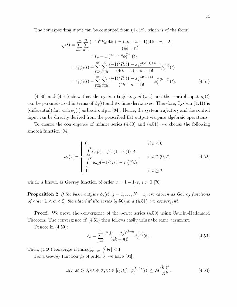
54

The corresponding input can be computed from (4.41c), which is of the form:

gj(t) =∞∑k=0

3∑n=0

(−1)kPn(4k + n)(4k + n− 1)(4k + n− 2)(4k + n)!

× (1− xj)4k+n−3φ(2k)j (t)

= P3φj(t) +∞∑k=1

3∑n=0

(−1)kPn(1− xj)4(k−1)+n+1

(4(k − 1) + n+ 1)! φ(2k)j (t)

= P3φj(t)−∞∑k=0

3∑n=0

(−1)kPn(1− xj)4k+n+1

(4k + n+ 1)! φ(2(k+1))j (t). (4.51)

(4.50) and (4.51) show that the system trajectory uj(x, t) and the control input gj(t)can be parameterized in terms of φj(t) and its time derivatives. Therefore, System (4.41) is(differential) flat with φj(t) as basic output [94]. Hence, the system trajectory and the controlinput can be directly derived from the prescribed flat output via pure algebraic operations.

To ensure the convergence of infinite series (4.50) and (4.51), we choose the followingsmooth function [94]:

φj(t) =

0, if t ≤ 0∫ t

0exp(−1/(τ(1− τ)))εdτ∫ T

0exp(−1/(τ(1− τ)))εdτ

, if t ∈ (0, T )

1, if t ≥ T

(4.52)

which is known as Gevrey function of order σ = 1 + 1/ε, ε > 0 [70].

Proposition 2 If the basic outputs φj(t), j = 1, . . . , N − 1, are chosen as Gevrey functionsof order 1 < σ < 2, then the infinite series (4.50) and (4.51) are convergent.

Proof. We prove the convergence of the power series (4.50) using Cauchy-HadamardTheorem. The convergence of (4.51) then follows easily using the same argument.

Denote in (4.50):

bk =3∑

n=0

Pn(x− xj)4k+n

(4k + n)! φ(2k)j (t). (4.53)

Then, (4.50) converges if lim supk→∞ k

√|bk| < 1.

For a Gevrey function φj of order σ, we have [94]:

∃K,M > 0,∀k ∈ N,∀t ∈ [t0, t1],∣∣∣φ(k+1)j (t)

∣∣∣ ≤M(k!)σKk

. (4.54)

55

Thus, for 0 < xj < 1 and x ∈ [0, 1], bk can be majorized as:

|bk| <∣∣∣∣∣

3∑n=0

Pn(4k + n)!φ

(2k)j (t)

∣∣∣∣∣<

∣∣∣∣∣3∑

n=0

Pn(4k + n)!M

((2k)!)σK2k

∣∣∣∣∣ . (4.55)

Therefore:

lim supk→∞

k√bk = lim sup

k→∞

3∑n=0

4K2 (MPn)1/k ((2k)!)σ/k

((4k + n)!)1/k

< lim supk→∞

1K2

(((2k)!)1/2k)2σ

(((4k)!)1/4k)4 . (4.56)

Applying Stirling’s formaula k√k! ' (k/e) yields:

lim supk→∞

k√bk ≤

4e4−2σ

K2 lim supk→∞

(2k)2σ

(4k)4 . (4.57)

Since

lim supk→∞

(2k)2σ

(4k)4 =

0, σ < 2;116 , σ = 2;∞, σ > 2,

(4.58)

we can conclude by Cauchy-Hadamard Theorem that the radius of convergence of (4.50) isinfinity for σ < 2 and 4K2 for σ = 2. The series (4.50) diverges if σ > 2.

Remark 4.6 In general, the Gevrey bounds are unknown, but can be estimated followingthe way presented in [35]. Furthermore, a symmetric function in the transient phase can beconsidered to improve convergency analysis [35].

Remark 4.7 For numerical implementations, (4.51) needs to be truncated to finite terms.An upper bound on truncation errors can be directly computed using the property of Gevreyfunction given in (4.52) [93].

Finally, substituting g1, . . . , gN−1 computed from (4.51) together with gN computed from(4.37) into (4.30), the in-domain actuation signals αi, i = 1, · · · , N , can be uniquely deter-mined by the pure algebraic solution of (4.30).

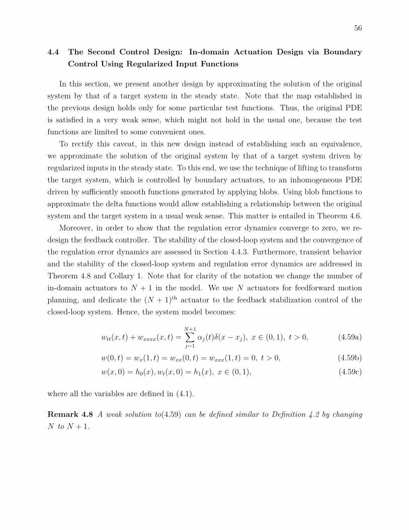
56

4.4 The Second Control Design: In-domain Actuation Design via BoundaryControl Using Regularized Input Functions

In this section, we present another design by approximating the solution of the originalsystem by that of a target system in the steady state. Note that the map established inthe previous design holds only for some particular test functions. Thus, the original PDEis satisfied in a very weak sense, which might not hold in the usual one, because the testfunctions are limited to some convenient ones.

To rectify this caveat, in this new design instead of establishing such an equivalence,we approximate the solution of the original system by that of a target system driven byregularized inputs in the steady state. To this end, we use the technique of lifting to transformthe target system, which is controlled by boundary actuators, to an inhomogeneous PDEdriven by sufficiently smooth functions generated by applying blobs. Using blob functions toapproximate the delta functions would allow establishing a relationship between the originalsystem and the target system in a usual weak sense. This matter is entailed in Theorem 4.6.

Moreover, in order to show that the regulation error dynamics converge to zero, we re-design the feedback controller. The stability of the closed-loop system and the convergence ofthe regulation error dynamics are assessed in Section 4.4.3. Furthermore, transient behaviorand the stability of the closed-loop system and regulation error dynamics are addressed inTheorem 4.8 and Collary 1. Note that for clarity of the notation we change the number ofin-domain actuators to N + 1 in the model. We use N actuators for feedforward motionplanning, and dedicate the (N + 1)th actuator to the feedback stabilization control of theclosed-loop system. Hence, the system model becomes:

wtt(x, t) + wxxxx(x, t) =N+1∑j=1

αj(t)δ(x− xj), x ∈ (0, 1), t > 0, (4.59a)

w(0, t) = wx(1, t) = wxx(0, t) = wxxx(1, t) = 0, t > 0, (4.59b)

w(x, 0) = h0(x), wt(x, 0) = h1(x), x ∈ (0, 1), (4.59c)

where all the variables are defined in (4.1).

Remark 4.8 A weak solution to(4.59) can be defined similar to Definition 4.2 by changingN to N + 1.

57

4.4.1 Relating In-domain Actuation to Boundary Control

For the feedforward motion planning with N actuators located in the domain, we considerthe dynamics of the desired trajectory as follow:

wdtt(x, t) + wdxxxx(x, t) =N∑j=1

αj(t)δ(x− xj), x ∈ (0, 1), t > 0, (4.60a)

wd(0, t) = wdx(1, t) = wdxx(0, t) = wdxxx(1, t) = 0, t > 0, (4.60b)

wd(x, 0) = wdt (x, 0) = 0, x ∈ (0, 1). (4.60c)

The weak solution of (4.60) can be defined in a similar way as Definition 4.2. Note that it isshown later that the initial conditions given in (4.1c) will be captured by the regulation errordynamics. Therefore, feedforward control design can be carried out based on System (4.60)with zero-initial conditions.

Due to the fact that the model given in (4.60) is driven by unbounded inputs, we willapply a sequence of blobs ϕ(x − xj) to approximate δ(x − xj) in the sense of distributions.We will then show that in steady state, wd can be approximated by a sufficiently smoothfunction. More specifically, we consider first the following boundary controlled PDE:

utt(x, t) + uxxxx(x, t) = 0, x ∈ (0, 1), t > 0, (4.61a)

u(0, t) = ux(1, t) = uxx(0, t) = 0, t > 0, (4.61b)

uxxx(1, t) = g(t), t > 0, (4.61c)

u(x, 0) = ut(x, 0) = 0, x ∈ (0, 1), (4.61d)

where g(t) = ∑Nj=1 gj(t). Without special statements, we assume that gj(t) ∈ C3([0,+∞))

and gj(0) = gj(0) = 0 for j = 1, 2, ..., N . Note that the motivation behind considering(4.61) as a target system is that it allows leveraging the techniques of boundary controlfor feedforward control design while avoiding early truncations of dynamic model and/orcontroller structure.

Definition 4.4 Let T > 0. A weak solution to the Cauchy problem (4.61) is a functionu ∈ C([0, T ]; Φ) ∩ C1([0, T ];L2(0, 1)) satisfying

u(x, 0) = ut(x, 0) = 0, x ∈ (0, 1),

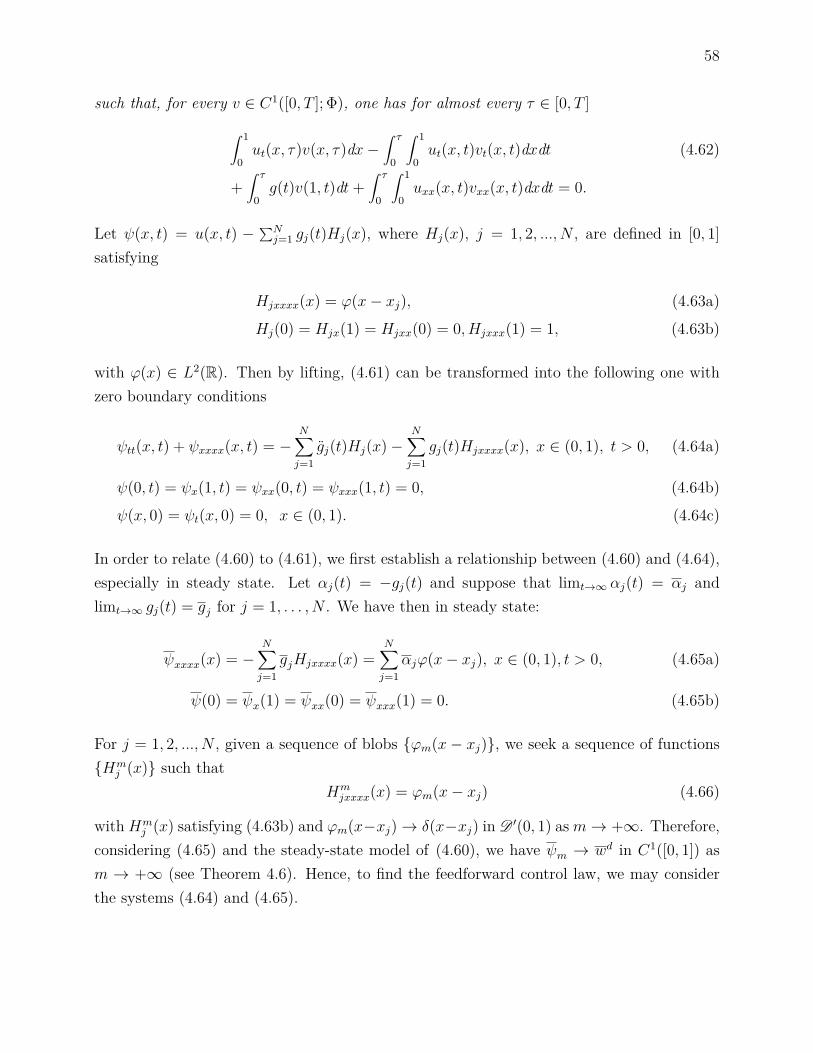
58

such that, for every v ∈ C1([0, T ]; Φ), one has for almost every τ ∈ [0, T ]∫ 1

0ut(x, τ)v(x, τ)dx−

∫ τ

0

∫ 1

0ut(x, t)vt(x, t)dxdt (4.62)

+∫ τ

0g(t)v(1, t)dt+

∫ τ

0

∫ 1

0uxx(x, t)vxx(x, t)dxdt = 0.

Let ψ(x, t) = u(x, t) − ∑Nj=1 gj(t)Hj(x), where Hj(x), j = 1, 2, ..., N , are defined in [0, 1]

satisfying

Hjxxxx(x) = ϕ(x− xj), (4.63a)

Hj(0) = Hjx(1) = Hjxx(0) = 0, Hjxxx(1) = 1, (4.63b)

with ϕ(x) ∈ L2(R). Then by lifting, (4.61) can be transformed into the following one withzero boundary conditions

ψtt(x, t) + ψxxxx(x, t) = −N∑j=1

gj(t)Hj(x)−N∑j=1

gj(t)Hjxxxx(x), x ∈ (0, 1), t > 0, (4.64a)

ψ(0, t) = ψx(1, t) = ψxx(0, t) = ψxxx(1, t) = 0, (4.64b)

ψ(x, 0) = ψt(x, 0) = 0, x ∈ (0, 1). (4.64c)

In order to relate (4.60) to (4.61), we first establish a relationship between (4.60) and (4.64),especially in steady state. Let αj(t) = −gj(t) and suppose that limt→∞ αj(t) = αj andlimt→∞ gj(t) = gj for j = 1, . . . , N . We have then in steady state:

ψxxxx(x) = −N∑j=1

gjHjxxxx(x) =N∑j=1

αjϕ(x− xj), x ∈ (0, 1), t > 0, (4.65a)

ψ(0) = ψx(1) = ψxx(0) = ψxxx(1) = 0. (4.65b)

For j = 1, 2, ..., N , given a sequence of blobs ϕm(x − xj), we seek a sequence of functionsHm

j (x) such thatHmjxxxx(x) = ϕm(x− xj) (4.66)

withHmj (x) satisfying (4.63b) and ϕm(x−xj)→ δ(x−xj) in D ′(0, 1) asm→ +∞. Therefore,

considering (4.65) and the steady-state model of (4.60), we have ψm → wd in C1([0, 1]) asm → +∞ (see Theorem 4.6). Hence, to find the feedforward control law, we may considerthe systems (4.64) and (4.65).

59

Lemma 1 [1] Let ϕm(x) ∈ L2(R) be defined by

ϕm(x) = 1π

sinmxx

. (4.67)

Then ϕm(x) has the following properties:

(i)∫ +∞

−∞ϕm(x)dx =

∫ +∞

−∞

1π

sinmxx

dx = 1.

(ii) ϕm(x)→ δ(x) in D ′(R) as m→∞.

By taking ϕm given in (4.67) as the input to (4.66), we get

Hmj (x) =1

6x3 − 1

2x+∫ x

0

∫ z

1

∫ y

0

∫ t

1ϕm(s− xj)dsdtdydz.

Theorem 4.6 Let ϕm(x) be defined as in Lemma 1. Assume that αj(t) = −gj(t) tends toαj = −gj as t→∞ for all j = 1, 2, ..., N . Denote by ψmj and by wdj the steady-state solutionsof System (4.60) and System (4.64), respectively. Then ψmj → wdj in C1([0, 1]) as m→ +∞for j = 1, 2, ..., N .

Proof. In the steady state, we have

ψm

jxxxx(x) = −gjHmjxxxx(x) = αjϕm(x− xj), (4.68a)

ψm

j (0) = ψm

jx(1) = ψm

jxx(0) = ψm

jxxx(1) = 0, (4.68b)

and

wdjxxxx(x) = αjδ(x− xj), (4.69a)

wdj (0) = wdjx(1) = wdjxx(0) = wdjxxx(1) = 0. (4.69b)

Taking v(x) ∈ D(0, 1) as a test function and integrating by parts, we get∫ 1

0

(ψm

jx(x)− wdjx(x))vxxx(x)dx = αj

∫ 1

0(ϕm(x− xj)− δ(x− xj)) v(x)dx.

Since ϕm(x− xj)→ δ(x− xj) in the sense of distributions as m→ +∞ and vxxx ∈ D(0, 1),it follows that ψmjx → wdjx in the sense of distributions as m → +∞ for j = 1, 2, ..., N .Furthermore, as ψmjx ∈ L1(0, 1) and wdjx ∈ L1(0, 1), we have ψmjx → wdjx a.e. in (0, 1) (seeLemma 3.31 of [2], page 74). Then by the continuity of ψmjx and wdjx, we conclude that ψ

m

jx →wdjx pointwisely in (0, 1). Therefore ψmj → wdj in C1([0, 1]) as m→ +∞ for j = 1, 2, ..., N .

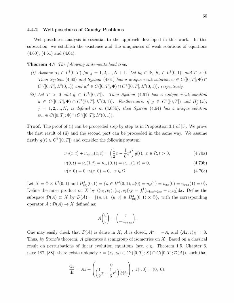
60

4.4.2 Well-posedness of Cauchy Problems

Well-posedness analysis is essential to the approach developed in this work. In thissubsection, we establish the existence and the uniqueness of weak solutions of equations(4.60), (4.61) and (4.64).

Theorem 4.7 The following statements hold true:

(i) Assume αj ∈ L2(0, T ) for j = 1, 2, ..., N + 1. Let h0 ∈ Φ, h1 ∈ L2(0, 1), and T > 0.Then System (4.60) and System (4.61) has a unique weak solution w ∈ C([0, T ]; Φ) ∩C1([0, T ];L2(0, 1)) and wd ∈ C([0, T ]; Φ) ∩ C1([0, T ];L2(0, 1)), respectively.

(ii) Let T > 0 and g ∈ C2([0, T ]). Then System (4.61) has a unique weak solutionu ∈ C([0, T ]; Φ) ∩ C1([0, T ];L2(0, 1)). Furthermore, if g ∈ C3([0, T ]) and Hm

j (x),j = 1, 2, ..., N , is defined as in (4.63b), then System (4.64) has a unique solutionψm ∈ C([0, T ]; Φ) ∩ C1([0, T ];L2(0, 1)).

Proof. The proof of (i) can be proceeded step by step as in Proposition 3.1 of [5]. We provethe first result of (ii) and the second part can be proceeded in the same way. We assumefirstly g(t) ∈ C3([0, T ]) and consider the following system:

νtt(x, t) + νxxxx(x, t) =(1

2x−16x

3)g(t), x ∈ Ω, t > 0, (4.70a)

ν(0, t) = νx(1, t) = νxx(0, t) = νxxx(1, t) = 0, (4.70b)

ν(x, 0) = 0, νt(x, 0) = 0, x ∈ Ω. (4.70c)

Let X = Φ× L2(0, 1) and H4(0)(0, 1) = u ∈ H4(0, 1);u(0) = ux(1) = uxx(0) = uxxx(1) = 0.

Define the inner product on X by 〈(u1, v1), (u2, v2)〉X =∫ 10 (u1xxu2xx + v1v2)dx. Define the

subspace D(A) ⊂ X by D(A) = (u, v); (u, v) ∈ H4(0)(0, 1) × Φ, with the corresponding

operator A : D(A)→ X defined as:

A

(u

v

)=(

v

−uxxxx

).

One may easily check that D(A) is dense in X, A is closed, A∗ = −A, and 〈Az, z〉X = 0.Thus, by Stone’s theorem, A generates a semigroup of isometries on X. Based on a classicalresult on perturbations of linear evolution equations (see, e.g., Theorem 1.5, Chapter 6,page 187, [88]) there exists uniquely z = (z1, z2) ∈ C1([0, T ];X) ∩ C([0, T ];D(A)), such that

dzdt = Az +

0(12x−

16x

3)g(t)

, z(·, 0) = (0, 0),

61

which implies that (4.70) has a unique solution ν = z1 ∈ C([0, T ];H4(0)(0, 1)) ∩ C1([0, T ]; Φ)

in the usual sense. Particularly, ν ∈ C([0, T ]; Φ) ∩ C1([0, T ];L2(0, 1)) is a weak solution. Adirect computation shows that u = ν −

(12x−

16x

3)g(t) is a solution of (4.61) in the usual

sense and, in particular, it is a weak solution.Now for g ∈ C1([0, T ]), let gn ∈ C3([0, T ]) such that gn → g in C1([0, T ]). Consider

un = νn −(

12x−

16x

3)gn(t), where νn is the solution of (4.70) corresponding to the data

gn(t). Then arguing as above and taking limit as in Chapter 2 of [? ], we may obtain theexistence and the uniqueness of a weak solution of (4.64).

4.4.3 Feedback Control and Stability of the Inhomogeneous System

The validity of the proposed scheme requires a suitable closed-loop control that guaranteesthe stability of the original inhomogeneous system. As the (N + 1)th actuator is dedicatedto stabilizing control, (4.59) can be written as

wtt(x, t) + wxxxx(x, t)− αN+1(t)δ(x− xN+1) =N∑j=1

αj(t)δ(x− xj), x ∈ (0, 1), t > 0. (4.71)

Suppose further that the feedback control is taken as [5, 25]

αN+1(t) = −kwt (xN+1, t) , (4.72)

where k is a positive-valued constant. Then in closed-loop, (4.71) becomes

wtt(x, t) + wxxxx(x, t) + kwt (x, t) δ(x− xN+1) =N∑j=1

αj(t)δ(x− xj), x ∈ (0, 1), t > 0.

(4.73)

Let D(A) = (w, v); (w, v) ∈ [H2(0, 1) ∩ (H4(0, x1) ∪ H4(x1, x2) ∪ · · · ∪ H4(xN , xN+1) ∪H4(xN+1, 1))] × H2(0, 1), w(0) = wx(1) = wxx(0) = wxxx(1) = 0, v(0) = vx(1) = 0 and X

be defined as in the proof of Theorem 4.8. Let T > 0 and αj ∈ L2(0, T ) for j = 1, ..., N .Assume (h0, h1) ∈ X. To address the stability of System (4.73) with the boundary conditions(4.1b) and initial conditions (4.1c), we consider the corresponding linear control system underabstract form:

z = Az +Bα, t > 0, (4.74a)

z(0) = z0 = (h0, h1)T , (4.74b)

62

where z = (w, v)T , α = (α1, · · · , αN)T , A : D(A)→ X is defined as:

A

(w

v

)=(

v

−wxxxx − kvδ(x− xN+1)

), (4.75)

with v = wt, and B : RN → D′(A∗) is defined as:

(Bα)y =(

0∑Nj=1 αjδ(x− xj)

)Ty, ∀ y ∈ D(A∗), (4.76)

where A∗ is the adjoint of A. It can be directly verified that A is dissipative [5].Thus, A generates a strongly continuous semigroup S(t) on X. The semigroup S∗(t),

generated by A∗, equals to S(t). Note that B∗ : D(A∗)→ RN is defined by

B∗y = (y2(x1), . . . , y2(xN))T ,∀y =(y1

y2

)∈ D(A∗). (4.77)

Let U = RN . Then, the solution of the Cauchy problem (4.74) can be defined as follows (see[? ], Definition 2.36, p53):

〈z(τ), yτ 〉X = 〈z0, S∗(τ)yτ 〉X +∫ τ

0〈α(t), B∗S∗(τ − t)yτ 〉Udt, ∀ τ ∈[0, T ],∀ yτ∈X. (4.78)

One may verify, as in Chapter 2 of [? ], that the solution defined by (4.78) is also a weaksolution of (4.73) under the form given in Definition 4.2.

Theorem 4.8 Assume αj ∈ L∞(0,+∞), j = 1, . . . , N . For xN+1 = 1, there exist positiveconstants C1, C2, and λ such that for any t ≥ 0, there holds:

‖z(t)‖X ≤ C1e−λt‖z0‖X + C2 max

j‖αj‖L∞(0,+∞). (4.79)

Proof. The proof generalization of Theorem 2.37 in [? ] for multiple-output system. First,the admissible property of B can be obtained from the proof of Theorem 4.1. Moreover, S(t)generated by A defined in (4.75) is an exponentially stable C0-semigroup onX if xN+1 ∈ (0, 1)is a rational number with coprime factorization, in particular for xN+1 = 1 (see, e.g., [5, 25]),i.e. there exist two positive constants C1 and λ, such that

‖S(t)‖ ≤ C1e−λt, ∀ t ≥ 0.

As S(t) = S∗(t), then using the same arguments as in the proof of Theorem 2.37 in [? ],we can conclude that all the constants in (4.79) are independent of t.

63

Now consider the regulation error defined as e(x, t) = w(x, t)−wd(x). Denoting ∆αj(x, t) =αj(x, t)−αj(x), j = 1, . . . , N , then from (4.73), (4.59b), (4.59c), and the steady-state modelof (4.60), the regulation error dynamics satisfy

ett(x, t) + exxxx(x, t) + ket (x, t) δ(x− xN+1) =N∑j=1

∆αj(t)δ(x− xj), x ∈ (0, 1), t > 0,

(4.80a)

e(0, t) = ex(1, t) = exx(0, t) = exxx(1, t) = 0, t > 0, (4.80b)

e(x, 0) = e0(x) = h0(x)− wd(x),

et(x, 0) = e1(x) = h1(x), x ∈ (0, 1). (4.80c)

Obviously, the regulation error dynamics are in an identical form as (4.73) with the sametype of boundary conditions. We can then consider the solution of System (4.80) defined inthe same form given by (4.78) with ze = (e, et) and z0

e = (e0, e1).

Corollary 1 Assume that all the conditions in Theorem 4.8 are fulfilled and z0e ∈ X. Then

there exist positive constants C1, C2, and λ, independent of t, such that for any t ≥ 0, thereholds:

‖ze(t)‖X ≤ C1e−λt‖z0

e‖X + C2 maxj‖∆αj‖L∞(0,+∞). (4.81)

Moreover, if limt→∞∆αj = 0 for all j = 1, . . . , N , then limt→∞ e(x, t) = 0, ∀x ∈ (0, 1).

Remark 4.9 This stabilization feedback also complete the proof of Theorem 4.4.

The feedforward control satisfying the conditions for closed-loop stability and regulationerror convergence can be obtained through motion planning, as presented in the next section.

4.4.4 Motion Planning and Feedforward Control

According to the principle of superposition for linear systems, we consider in feedforwardcontrol design the dynamics of System (4.61) corresponding to the input gj(t), which are ofthe following form:

ujtt(x, t) + ujxxxx(x, t) = 0, (4.82a)

uj(0, t) = ujx(1, t) = ujxx(0, t) = 0, (4.82b)

ujxxx(1, t) = gj(t), (4.82c)

uj(x, 0) = ujt(x, 0) = 0. (4.82d)

64

The required control signal gj(t) should be designed so that the output of System (4.82)follows a prescribed function udj (xj, t) and that the conditions in Theorem 4.8 and Corollary 1are fulfilled.

Motion planning becomes then to take udj (xj, t) as the desired output and to generatethe full-state trajectory of the subsystem uj(x, t), which is carried out in this work usingflatness-based motion planning (see, e.g., [43, 78, 79, 81, 94]). To solve this problem, weapply a standard Laplace transform-based procedure. Henceforth, we denote by f(x, s) theLaplace transform of a function f(x, t) with respect to time variable. Then, in the Laplacedomain, the transformed equations are given by

ujxxxx(x, s)− q4(s)uj(x, s) = 0, (4.83a)

uj(0, s) = ujx(1, s) = ujxx(0, s) = 0, (4.83b)

uj(xj, s) = udj (xj, s), (4.83c)

where q4(s) = −s2. The general solution of (4.83a) can be expressed as

uj(x, s) = aj(s)C1(x, s) + bj(s)S1(x, s) + cj(s)C2(x, s) + dj(s)S2(x, s), (4.84)

where

C1(x, s) = (cosh(q(s)x) + cos(q(s)x))/2, (4.85a)

C2(x, s) = (cosh(q(s)x)− cos(q(s)x))/2q2(s), (4.85b)

S1(x, s) = (sinh(q(s)x) + sin(q(s)x))/2q(s), (4.85c)

S2(x, s) = (sinh(q(s)x)− sin(q(s)x))/2q3(s) (4.85d)

are the basic solutions to (4.83a).To determine the coefficients aj(s), bj(s), cj(s), and dj(s), we use the property C1x =

q4(s)S2, C2x = S1, S1x = C1, S2x = C2, and apply the boundary values given in (4.83b) anduj(xj, s) = udj (xj, s). We obtain:

aj = cj = 0,

bj(s)S1(xj, s) + dj(s)S2(xj, s) = udj (xj, s),

ujx(1, s) = bj(s)C1(1, s) + dj(s)C2(1, s) = 0.

We can write then

R(s)bjdj

=udj (xj, s)

0

,

65

where

R(s) =S1(xj, s) S2(xj, s)C1(1, s) C2(1, s)

.Now bj and dj can be computed as

bjdj

= R−1(s)udj (xj, s)

0

= adj(R(s))det(R(s))

udj (xj, s)0

.Letting

udj (xj, s) = det(R(s)

)yj(s), (4.86)

it follows thatuj(x, s) = (C2(1, s)S1(x, s)− C1(1, s)S2(x, s))yj(s). (4.87)

Note that yj(s)↔ yj(t) is the so-called basic output, or flat output. In order to transfer thefull-state trajectory and the control input from frequency domain to time domain, we use theTaylor expansion of trigonometric and hyperbolic functions in (4.85a)-(4.85d) with respectto x. The full-state trajectory uj(x, s) in (4.87) can be written in the form

uj(x, s) =(1

2x−16x

3)yj(s) (4.88)

+∞∑n=1

(n∑k=0

x4k+1

(4k + 1)!(4(n−k) + 2)! −n∑k=0

x4k+3

(4k + 3)!(4(n−k))!

)q4n(s)yj(s).

Thus, in time domain the full-state trajectory with zero initial values is given by

uj(x, t) =(1

2x−16x

3)yj(t) (4.89)

+∞∑n=1

(n∑k=0

x4k+1

(4k + 1)!(4(n−k) + 2)! −n∑k=0

x4k+3

(4k + 3)!(4(n−k))!

)(−1)ny(2n)

j (t).

Now let yj(t) = yjφj(t), where φj(t) is a smooth function evolving from 0 to 1. Then,Equation (4.89) becomes

uj(x, t) =yj(1

2x−16x

3)φj(t) (4.90)

+ yj

∞∑n=1

(n∑k=0

x4k+1

(4k + 1)!(4(n−k) + 2)! −n∑k=0

x4k+3

(4k + 3)!(4(n−k))!

)(−1)nφ(2n)

j (t).

66

The corresponding input can be computed from (4.82c), which is of the form

gj(t) = −yjφj(t) + yj

∞∑n=1

(n∑k=1

1(4k − 2)!(4(n−k) + 2)! −

n∑k=0

1(4k)!(4(n−k))!

)(−1)nφ(2n)

j (t).

(4.91)

For set-point control, we need an appropriate class of trajectories enabling a rest-to-rest evolution of the system. A convenient choice for this purpose is Gevrey functions asintroduced in (4.52)

For the convergence of (4.90) and (4.91), we have

Proposition 3 If φj(t) in the basic output yj(t) = yjφj(t) is chosen as a Gevrey function oforder 1 < σ < 2, then the infinite series (4.90) and (4.91) are convergent.

Proof. Denote in (4.89):

bn =(

n∑k=0

x4k+1

(4k + 1)!(4(n−k) + 2)!

−n∑k=0

x4k+3

(4k + 3)!(4(n−k))!

)(−1)nφ(2n)

j (t). (4.92)

Then, (4.90) converges if lim supn→∞ n

√|bn| < 1. The proof can be proceed similarly to that

of Proposition 2.The convergence of (4.91) then follows easily using the same argument.

Now let

Pj(x) =12x−

16x

3, (4.93a)

Ij,m(x) =∫ x

0

∫ z

1

∫ y

0

∫ t

1ϕm(s− xj)dsdtdydz, (4.93b)

Φj,n(x) =(

n∑k=0

x4k+1

(4k + 1)!(4(n−k) + 2)! −x4k+3

(4k + 3)!(4(n−k))!

)(−1)n, (4.93c)

Ψj,n(1) =(

n∑k=1

1(4k − 2)!(4(n−k) + 2)! −

n∑k=0

1(4k)!(4(n−k))!

)(−1)n. (4.93d)

Set ∑Nj=1 ψ

mj (x, t) = ψm(x, t),m > 0. By the definition of ψ(x, t), we obtain

ψmj (x, t) = yjIj,m(x)φj(t) + yj

∞∑n=1

(Φj,n(x) + Ψj,n(1)Pj(x)−Ψj,n(1)Ij,m(x)

)φ

(2n)j (t). (4.94)

67

To compute Ij,m(x), we note that

ϕm(x− xj) = 1π

∞∑k=1

(−1)k+1m2k−1

(2k − 1)! (x− xj)2k−2.

Therefore,

Ij,m(x) = 1π

∞∑k=1

(−1)k+1m2k−1

(2k − 1)

((x− xj)2k+2

(2k + 2)!

− (1− xj)2k−1x3

6((2k − 1)!) −x2kj x

2

2(2k)! −(1− xj)2k+1x

(2k + 1)!

+x2kj x

(2k)! + (1− xj)2k−1x

2(2k − 1)! −x2k+2j

(2k + 2)!

). (4.95)

Claim 1 Ij,m(x) given in (4.95) is convergent for all x, xj ∈ (0, 1) with respect to any fixedm.

Proof. Consider the first series in (4.95). Fixingm > 0, for x, xj ∈ (0, 1), j = 1, 2, . . . , N ,we have ∣∣∣∣∣(−1)k+1m2k−1

(2k − 1)(x− xj)2k+2

(2k + 2)!

∣∣∣∣∣ ≤ m2k−1

(2k − 1)! .

Since limn→∞1

n√n! = 0, it follows that for any a > 0

limn→∞

n

√an

n! = a limn→∞

1n√n!

= 0.

Thus ∑∞k=0m2k−1

(2k−1)! is convergent. We conclude that the first series in (4.95) is uniformlyconvergent. The convergence of the other terms in (4.95) can be proved in the same way.

Based on Claim 1, the series in the right hand side of (4.94) are convergent and ψmj (x, t)can be expanded by (4.94) and (4.95). Moreover, for gj(t) given in (4.91), ψmj (x, t) tends toψm

j (x) = yjIj,m(x) as t→∞. Note that for fixed x, the radius of convergence of ψj,m on mis ∞. Thus, we can let m→ +∞.

To complete the control design, we need to determine the amplitude of flat outputs yj,j = 1, . . . , N , from the desired shape wd(x) that may not necessarily be a solution of thesteady-state beam equation (4.69). To that end, we use the Green’s functions, G(x, ξ), of(4.69), as denoted in (4.17).

68

Due to the principle of superposition for linear systems, the solution to (4.69), wd(x), canbe expressed as

wd(x) =∫ 1

0

N∑j=1

G(x, ξ)αjδ(x− ξj)dξ =N∑j=1

G(x, ξj)αj.

Now taking N points on wd(x) and letting wd(xj) = wd(xi = j), j = 1, . . . , N , yieldG(x1, ξ1) . . . G(xN , ξ1)

... . . . ...G(x1, ξN) . . . G(xN , ξN)

α1...αN

=

wd(x1)

...wd(xN)

, (4.96)

which represents a steady-state input to output map. Based on Theorem 4.5, the map givenin (4.96) is invertible for all xj, ξj ∈ (0, 1), j = 1, . . . , N , and xi 6= xj, ξi 6= ξj, if i 6= j.

As αj = −gj and limt→∞ gj(t) = gj = −yj for all j = 1, . . . , N , we obtain from (4.96)that

y1...yN

=

G(x1, ξ1) . . . G(xN , ξ1)

... . . . ...G(x1, ξN) . . . G(xN , ξN)

−1

wd(x1)...

wd(xN)

. (4.97)

4.5 Summary

In this chapter, we presented two control designs for an Euler-Bernoulli model of thedeformable beam.

In the first design, we formally established a map between the in-domain controlled modelof the system and a standard boundary-controlled PDE model. Based on that map, wedeveloped a control strategy, which is a combination of feedback stabilization and differentialflatness-based feed-forward motion planing. However, since the map holds only for someparticular test functions, the original PDE is satisfied in a very weak sense.

To cope with this problem in the second design, we approximate the solution of the originalsystem by that of a target system in the steady state. To do this, we use the technique oflifting to transform the target system to an inhomogeneous PDE driven by sufficiently smoothfunctions generated by applying blobs. This would allow establishing a relationship betweenthe original system and the target system in a usual weak sense.

In the next chapter, we verify the validity of both designs through numerical simulationstudies.

69

CHAPTER 5

SIMULATION STUDIES OF IN-DOMAIN CONTROLLEDEULER-BERNOULLI BEAMS

This chapter presents the simulation results of the designs presented in the previouschapter. We begin the chapter by explaining the numerical implementation and the numericalstability of the simulated model Section 5.1. Then, in Section 5.2, Section 5.3, we presentthe simulation results for the first and the second design. We conclude the chapter withdiscussion on results in Section 5.4.

As we will show in the simulation study if the desired curve is not a solution of thecorresponding static beam equation, the regulation error with respect to this curve will ingeneral not identically vanish. Therefore, to make the performance evaluation meaningful,we propose in the second set of simulation study to first interpolate the desired curve by theGreen’s functions of the static beam equation and then to evaluate the regulation error ofthe controller with respect to the corresponding steady-state solution of the beam.

In the evaluation of interpolation accuracy, we consider 3 setups with different numberof actuators and use the L1−norm as a measure of interpolation errors. We also show thecontrol effort corresponding to different setups to provide a better characterization of themicro-beam efficiency.

5.1 Numerical implementation

In this section, we expain how a beam equation described by a fourth-order in spaceand second-order in time partial differential equation can be numerically implemented inMATLAB. It is worth mentioning that the unstable dynamics of this equation is one of themost challenging parts in performing the numerical implementation.

We explain the numerical implementation in three folds: first, the approximation of thesecond-order time derivative operator; then the numerical approximation of the forth-orderspatial differentiation operator, or the bi-harmonic operator; and eventually the integrationof the nonstandard boundary conditions to the numerical approximation of the bi-harmonicoperator.

For the time evolution, we convert the second-order-in-time system in (4.1) into a first-

70

order-in-time system by introducing a dummy variable, u(x, t), as:

wt(x, t) = u(x, t), (5.1a)

ut(x, t) = wxxxx(x, t) + f(x, t). (5.1b)

We use a general notation in this part. For instance, we use f(x, t) for inputs instead ofshowing the exact term. Then, we can rewrite the system in the following matrix form:

X = AX + Pn (5.2)

where A = 0 Inx

−DA 0

, Pn = 0Fnx

, and Fnx is nonzero on the location of the point-wise

actuators of the system. In these matrices, 0 is the null matrix with appropriate dimension,Inx represents the identity matrix, and DA is the approximation of biharmonic operator.

Now we are dealing with a first-order in time system. Hence, we can use the the leap frogformula for computing time derivative. As stated in Chapter 10 of [103], leap frog approxi-mation of time evolution is numerically stable for first-order in time systems. A method iscalled numerically unstable in the sense that small errors are amplified unboundedly, in fact,exponentially.

In matrix A, the term DA is the approximation of bi-harmonic operator with associatedboundary conditions. For this approximation, we use Chebyshev spectral differentiation [103]to approximate the fourth-order-spatial derivatives of bi-harmonic operator.

The Chebyshev spectral function uses Fast Fourier Transform (FFT) to approximatethe derivatives. For the boundary conditions, interpolant method is used. In this method,the additional equations are augmented to the system to enforce the nonstandard boundaryconditions. For instance, the term (1−x3) can be multiplied to enforce the condition uxxx(1) =0, please see Chapter 14 of [103] for more details.

The convergence of the numerical method is checked by varying the time step ∆t in theinterval [10−3, 10−6] and the mesh-density M for Chebyshev approximation between 40 and80.

Note that the dynamics of this system are inherently unstable because there is no damp-ening term in the Euler-Bernoulli PDE equation. Therefore, regardless of numerical stability,one may find the numerical results are growing on time. To harvest the best result, we runthe system with stabilizing feedback together.

We first start by implementing System (4.1) with 3 actuators in the domain located atx = 0.25, 0.5, 0.75 with initial conditions h0(x, 0) = −3×10−3e−400(x−0.8)2 and h1(x, 0) = 0.To comply with the limitation of micro-actuators, we assume downward displacement for the

71

system. Moreover, for the validation of the linear model of the beam, the displacement isat the order of micro meter for a beam length of a few centimeter. The deflection and thelength of the beam, as well as the time, are all represented in normalized coordinates.

As an undamped beam is unstable in open-loop, the controller tuning is started by deter-mining a suitable value of the closed-loop control gain k. Figure 5.1 shows the stabilizationof the beam by applying the feedback control derived from (4.37) to g1 at x = 0.25 whileg2 and g3 are set to 0. As illustrated in Fig. 5.1, the stabilizing feedback damped the beamrapidly.

Figure 5.1 Stabilized System.

Then, to try the trajectory tracking behavior, we chose the basic outputs φj(t) as Gevreyfunctions of the same order. The desired reference trajectory generated from (4.38) is depictedin Fig. 5.2(a). Note that to meet the convergence condition given in Proposition 2, the orderis set to σ = 1.11. g1, g2, and g3 are computed from (4.51) and (4.37), respectively. α1,α2, and α3 are then computed from (4.30) and are illustrated in Fig. 5.3(a). As shown inFig. 5.2(b), the system is smoothly transferred from the initial profile to the desired one.The error between the system output and the reference trajectory is depicted in Fig. 5.2(c).Figure 5.3(b) shows system outputs at x = 0.5 and x = 0.75.

The simulation results though far shows the proper numerical implementation. The sys-tem stabilized well around the reference trajectories. The numerical computation also showsstable implementation despite initial values and in-domain inputs.

5.2 Numerical Results of the First Design

In this section, we examine the simulation result of the first control scheme presented inSection 4.3.3. The static Green’s functions of the system are used for spacial decomposing

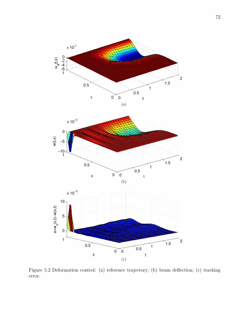
72

(a)

00.5

11.5

2

0

0.5

1−10

−5

0

x 10−3

tx

w(t

,x)

(b)

00.5

11.5

2

0

0.5

1

0

5

10

x 10−3

tx

e=

wd(x

,t)−

w(x

,t)

(c)

Figure 5.2 Deformation control: (a) reference trajectory; (b) beam deflection; (c) trackingerror.

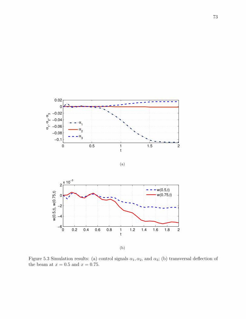
73

0 0.5 1 1.5 2

−0.1

−0.08

−0.06

−0.04

−0.02

0

0.02

t

α1,

α2,

α3

α1

α2

α3

(a)

0 0.2 0.4 0.6 0.8 1 1.2 1.4 1.6 1.8 2−6

−4

−2

0

2x 10

−3

t

w(0

.5,t),

w(0

.75,t)

w(0.5,t)

w(0.75,t)

(b)

Figure 5.3 Simulation results: (a) control signals α1, α2, and α3; (b) transversal deflection ofthe beam at x = 0.5 and x = 0.75.

74

of the reference trajectories. Figure 5.4 shows the Green’s function G(x, ξ) for ξ = 0.1,0.2, · · · , 0.9 as a basis to decompose the given reference trajectories. The lowest curve isthe Green’s function for ξ = 0.1 and the others correspond to ξ in increasing order.

We considered a system with 10 actuators uniformly distributed in the domain.In the simulation study, we consider the deformation control in which the desired shape

is given by

wd(x, t) = −10−3φ(t)(e−100(x−0.4)2

+ 2e−100(x−0.6)2+ 3e−400(x−0.7)2)

, x ∈ (0, 1), (5.3)

where φj(t) is the Gevrey function of order σ = 1.11 as derived from the convergence studyof the controller. The desired shape is depicted in Fig. 5.5(a).

The feedforward controls are computed from (4.51) and the feedback law is given in (4.37).Accordingly, the in-domain control signals, α1, · · · , α10, are derived from (4.30), illustratedin Fig. 5.6(a) and Fig. 5.6(b). As shown in Fig. 5.5(b) and Fig. 5.5(c), these control signalssteer the deflection of the beam along the given reference trajectory with reasonable trackingerrors. Nevertheless, we can observe that the steady-state error in the interval [0.5, 0.7]is significantly bigger than that of the other positions. The reason is that the referencetrajectory has an important peak at the position 0.8 that draws the beam downward. Thisis due to the physical constraint of the device and indicates that for improving the overalltracking accuracy, more actuators are desirable.

0 0.2 0.4 0.6 0.8 10

0.1

0.2

0.3

x

G(x

,ξ1),

... ,

G(x

,ξ9)

Figure 5.4 Green’s function of the beam for ξ = 0.1, 0.2, · · · , 0.9.

5.3 Simulation Results for the Second Design

In this section we evaluate the performance of the second design from Section 4.4.In this study, we consider the deformation control in which the desired shape is given in

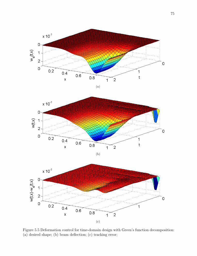
75

(a)

(b)

(c)

Figure 5.5 Deformation control for time-domain design with Green’s function decomposition:(a) desired shape; (b) beam deflection; (c) tracking error;

76

(a)

(b)

Figure 5.6 Control signals: (a) α1-α5; (b) α6-α10.

77

steady-state form by:

wd(x) = −10−3(e−100(x−0.4)2

+ 2e−100(x−0.6)2+ 3e−400(x−0.7)2)

, x ∈ (0, 1), (5.4)

as shown in Fig. 5.7(a).In order to obtain an exponential closed-loop convergence, the actuator for feedback

stabilization is located at the position xN+1 = 1. To evaluate the effect of the number ofactuators to interpolation accuracy, measured by ‖wd(x) − wd(x)‖L1(0,1), and control effort,we considered 3 setups with, respectively, 8, 12, and 16 actuators evenly distributed in thedomain. It can be seen from Fig. 5.7 that the setup with 8 actuators exhibits an importantinterpolation error and the one with 16 actuators requires a high control effort in spite of ahigh interpolation accuracy. The setup with 12 actuators provides an appropriate trade-offbetween the interpolation accuracy and the required control effort, which is used in controlalgorithm validation.

For this simulation study, we use a MATLAB Toolbox for dynamic Euler-Bernoulli beamssimulation provided in Chapter 14 of [110]. With this Toolbox, the simulation accuracy canbe adjusted by choosing the number of modes used in implementation. In the simulation,we implement System (4.59) The corresponding feedforward control signals with α1, . . . , α12,that steer the beam to deform are illustrated in Fig. 5.8. The evolution of beam shapes andthe regulation error are depicted in Fig. 5.9. It can be seen that the beam is deformed to thedesired shape and the regulation error vanishes along the whole beam, which confirms theexpected performance of the developed control scheme.

5.4 Discussion

The simulation results demonstrate the validity of the designs. In both designs, thecontroller was able to steer the system along prescribed trajectories with a feasible controleffort for the MEMS actuators and with a acceptable range of tracking errors. However, sincethe first design is valid in a very weak sense, in real implementation the outcome might notmatch that of the simulation study. Nonetheless, this caveat is rectified in the second design.

As we realized from simulation study, if the desired curve is not a solution of the corre-sponding static beam equation, the regulation error with respect to this curve will in generalnot identically vanish. Therefore, to make the performance evaluation meaningful, we haveproposed in the second set of simulation study to first interpolate the desired curve by theGreen’s functions of the static beam equation and then to evaluate the regulation error ofthe controller with respect to the corresponding steady-state solution of the beam.

In the evaluation of interpolation accuracy, we have considered 3 setups with different

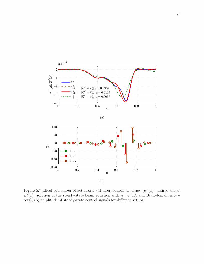
78

0 0.2 0.4 0.6 0.8 1−4

−3

−2

−1

0

x 10−3

x

wd(x),wd(x)

wd

wd16

wd12

wd8

‖wd− wd

8‖1 = 0.0346

‖wd − wd12‖1 = 0.0139

‖wd− wd

16‖1 = 0.0037

(a)

0 0.2 0.4 0.6 0.8 1−150

−100

−50

0

50

100

x

α

α1−8

α1−12

α1−16

(b)

Figure 5.7 Effect of number of actuators: (a) interpolation accuracy (wd(x): desired shape;wdn(x): solution of the steady-state beam equation with n =8, 12, and 16 in-domain actua-tors); (b) amplitude of steady-state control signals for different setups.

79

0 2 4 6 8 10−80

−60

−40

−20

0

20

40

60

t

α 1, ...,

α12

α

1

α2

α3

α4

α5

α6

α7

α8

α9

α10

α11

α12

Figure 5.8 Feedforward control signals: α1, . . . , α12.

number of actuators and have adopted the L1−norm of interpolation errors. We also haveshown the control effort corresponding to different setups to provide a better characterizationof the micro-beam efficiency.

Eventually, using the Green’s function not only makes the algorithm computationallytraceable but also is a very promising choice for real time implementation. As the staticGreen’s function used in trajectory planning can be computed off-line, the developed schemefacilitates real-time implementations. As a result, the basic flat output for differential flatnessmethod can be computed directly by an inverse static matrix calculation. This complexityreduction will have an important impact on the real time implementation for large scaledeformable mirrors.

80

(a)

(b)

Figure 5.9 Set-point control: (b) system response; (c) regulation error.

81

CHAPTER 6

CONCLUSION AND RECOMMENDATION

High precision and real time control of deformable mirrors is an enabling key of forth-coming extremely large ground-based telescopes. In this regards, this thesis addressed asystematic deformation control scheme for MEMS-actuated deformable mirrors in the con-text of astronomical telescopes.

To meet the high precision requirement, the design is directly carried out using the partialdifferential equation model of the system. To avoid early lumping in the motion planning,we use the properties of the Green’s function of the system to represent the reference tra-jectories. A finite set of these functions is considered to establish a one-to-one map betweenthe input space and output space. This allows an implementable scheme for real-time ap-plications. The only truncation is at the level of implementation of the controller. As aresult, there are no neglected dynamics to compromise the performance of the controller.To account for instability, model uncertainties, and disturbances, a stabilizing feedback isdesigned to stabilize the system around the reference trajectories. The presented controlscheme is a combination of differential flatness for feedforward motion planning and stabi-lizing feedback controllers, leading to a simple structure requiring only one measurementpoint on the boundary. Nonetheless, the feedforward control is inherently unrobust due themethod of open-loop trajectory planning, which depends heavily on the model. Adding moresensors is a way to improve the robustness. However, this is not a viable option for currentstate-of-the-art microsystems.

The presented scheme is particularly suitable for micro-systems for which the design, fab-rication, and operation with a high number of on-chip sensors represent a serious technologicalchallenge.

Below, we summarize the main contributions of this work.

6.1 Main Contributions

The objective of this dissertation was to develop a high-precision and real-time imple-mentable control structure in order to mitigate the complexity introduced by closed-loopcontrol at the level of every actuator in MEMS deformable mirrors.

We approached the problem as follow: first, we introduced the dynamics of a MEMS-actuated deformable mirror described by a set of partial differential equations with un-

82

bounded control operators in the domain of the system. Then, for the deformation controlof this device we developed two control designs. In the first design, we established a mapbetween the in-domain controlled system and a standard boundary controlled model. Basedon that, we developed a control strategy, which is a combination of feedback stabilizationand differential flatness-based feed-forward motion planing. This scheme shows a way todeal with the tracking control problem of in-domain PDE systems. However, the map holdsonly for some particular test functions. Thus, the original PDE is satisfied in a very weaksense. To cope with this caveat, in the second design instead of trying to establish such anequivalence, we approximated the solution of the original system by that of a target systemin the steady-state mode. To this end, we used the technique of lifting to transform thetarget system, which is controlled by boundary actuators, to an inhomogeneous PDE drivenby sufficiently smooth functions generated by applying blobs. This would allow establishinga relationship between the original system and the target system in a usual weak sense.

The control schemes developed in this work require just one displacement feedback datafrom a boundary point for one-row-actuator mirror. The feedback loop can be directlyprovided using an interferometer sensor on an inactive actuator of the mirror.

The benefits of this approach can be listed as:First, this work addresses a systematic scheme for the control of deformable mirrors. That

is the scheme can be directly generalized for different boundary condition configurations of thesystem. The system architecture and the procedure for feed-forward control design remainthe same, but only the feedback stabilization law should be reconsidered according to newboundary conditions.

Second, the proposed control scheme requires only to close few feedback control loops,typically one for 1D devices. Consequently, the implementation and operation of such deviceswill be drastically simplified.

Third, the design is directly performed with the partial differential equation model ofthe system. Hence, there is no neglected dynamics to sacrifice the performance. The onlytruncation requires at the level of the controller implementation.

Fourth, the presented scheme can be considered as an extension of the flat systems to asystem controlled by multiple actuators, which is essentially a multiple-input multiple-output(MIMO) problem. To the best of the author’s knowledge, a treatment without requiring earlytruncations for tracking control of this type of PDE systems has not yet been reported Inthe context of PDE-based control designs.

Finally, we introduced a Green’s function-based decomposition scheme that enables asimple and computationally tractable implementation of the proposed control. As the staticGreen’s function used in trajectory planning can be computed offline, the developed scheme

83

facilitates real-time implementations. This will have an important impact on the operationof large-scale deformable mirrors.

6.2 Recommendations and Future Work

The next step of this research work may be to examine the performance of the purposedmethod on a physical set-up. A simple way of testing the approach is to use a segmenteddeformable mirror between a light source and a continuous deformable mirror to introducea distortion. Then, using a wavefront sensor, e.g. Shack-Hartmann sensor, one is ableto validate the performance of the control scheme on the continuous mirror to correct thedistortion.

The mentioned devices are all tested individually in the laboratory of Adaptive Opticsduring this PhD research. The remaining part is to establish the adaptive optic loop asexplained in Chapter 2. A real time communication protocol such as TCP/IP requires toestablish the realtime data exchange in electronic loop. For the optic loop, identifying thefeasible distance between the devices requires an optics expert’s insight.

Further perspectives of the theory presented in this work is to extend this control schemeto a plate equation, or in other words to a case of more than one row of actuators. One mayconsider this extension, similarly to Chapter 9 of [17], by decomposing the plate into twodifferent beam equations. Then, for each set of equations the proposed control scheme maybe applicable.

Deformation control of deformable mirrors has many different applications and a list ofthose applications is provided in the introduction of this manuscript. Since the proposedcontrol is a systematic design, it can directly be exploited for other applications with a goodinsight to requirements associated to that particular application.

The proposed control scheme may concern other in-domain controlled PDE systems. Forinstance, one initial generalization example could be the well-known case of heating up andcooling down certain materials along a specific profile that requires multiple actuators actingin different temperatures at different instance of time.

84

BIBLIOGRAPHY

[1] M. Abramowitz and I. A. Stegun. Handbook of Mathematical Functions. Dover Publi-cations, New York, 1972.

[2] R. A. Adams and J. F. Fournier. Sobolev Spaces. Academic press, New York, 2ndedition, 2003.

[3] K. Ammari and M. Mehrenberger. Study of the nodal feedback stabilization of astring-beams network. J. Appl Math Comput, 36:441–458, 2011.

[4] K. Ammari, D. Mercier, V. Regnier, and J. Valein. Spectral analysis and stabilizationof a chain of serially connected Euler-Bernoulli beam and strings. Communications onPure and Applied Analysis, 11(2):785–807, 2012.

[5] K. Ammari and M. Tucsnak. Stabilization of Bernoulli-Euler beams by means of apointwise feedback force. SIAM J. Control Optimal, 39(4):1160–1181, 2000.

[6] T. Anderson, O. Garpinger, M. Owner-Petersen, F. Svahn, and A. Ardegerg. Vovelconcept for large deformable mirrors. Optical Engineering, 45(7):73001–1–13, 2006.

[7] A. Badkoubeh, J. Zheng, and G. Zhu. Flatness-based deformation control of an Euler-Bernoulli beam with in-domain actuation. Submitted to Automatica, 2014.

[8] A. Badkoubeh and G. Zhu. Tracking control of a linear parabolic PDE with in-domain point actuators. International Journal of Electrical and Electronics Engineer-ing, 5(11):11–25, 2011.

[9] A. Badkoubeh and G. Zhu. Deformation control of a 1-dimensional microbeam within-domain actuation. In IEEE 51st Annual Conference on Decision and Control, CDC,Maui, Hawaii, Dec. 2012.

[10] A. Badkoubeh and G. Zhu. Flatness-based deformation control of a 1-dimensionalmicrobeam with in-domain actuation. In Annual Conference of the IEEE IndustrialElectronics Society, Montreal, QC, Canada, Oct. 2012.

[11] A. Badkoubeh and G. Zhu. A Green’s function-based design for deformation controlof a microbeam with in-domain actuation. Journal of Dynamic Systems, Measurment,and Control, 136(11), Oct 2013.

[12] A. Badkoubeh and G. Zhu. A Green’s function-based design for deformation controlof a microbeam with in-domain actuation. In American Control Conference, ACC,Washington, DC, USA, June 2013. IEEE. Awarded the best paper of the session.

85

[13] A. Badkoubeh, G. Zhu, and R. Beguenane. Open-loop adapive opics wih closed-loopconrol of deformable mirror. In International Symposium on Optomechatronic Tech-nologies, ISOT, pages 1–6, Toronto, ON, Canada, Oct 2010. IEEE.

[14] M.J. Balas. Finite-dimentional control of disturbuted parameter systems by galerkinapproximation of infinite dimentional controllers. Journal of Mathematical Analysisand Applications, 114:17–36, 1986.

[15] H. T. Banks, R. C. H. Del Rosario, and R. C. Smith. Reduced order model feedbackcontrol design: Numerical implementation in a thin shell model. IEEE Trans. Auto.Contr, 45(7):1312–1324, 2000.

[16] H. T. Banks, R. C. H. del Rosario, and H. T. Tran. Proper orthogonal decomposition-based control of transverse beam vibration: Experimental implementation. IEEETrans. Contr. Syst. Technol., 10(5):717–726, 2012.

[17] H. T. Banks, R. C. Smith, and Y. Wang. Smart Material Structures: Modeling, Esti-mation and Control. John Wiley & Sons, Chichester, 1996.

[18] H. T. Banks, Ralph C. Smith, D. E. Brown, R. J. Silcox, and Vern L. Metcalf. Exper-imental confirmation of a PDE-based approach to design of feedback controls. SIAMJ. Control and Optimization, 35(4):1263–1296, 1997.

[19] A. Bensoussan, G. Da Prato, M. Delfour, and S. K. Mitter. Representation and Controlof Infinite-Dimensional Systems. Birkhauser, Boston, 2006.

[20] T. G. Bifano, R. K. Mali, J. K. Dorton, J. Perreault, N. Vandelli, M. N. Horenstein,and D. A. Castanon. Continuous-membrane surface-micromachined silicon deformablemirror. J. of Opt. Eng., 36(5):1354–1360, 1997.

[21] T. G. Bifano, R. K. Mali, J. K. Dorton, J. Perreault, N. Vandelli, M. N. Horenstein,and D. A. Castanon. Continuous-membrane surface-micromachined silicon deformablemirror. J. of Opt. Eng., 36(5):1354–1360, 1997.

[22] C. Blain, O. Guyon, C. Bradley, and O. Lardière. Fast iterative algorithm (FIA) forcontrolling MEMS deformable mirrors: principle and laboratory demonstration. OpticsExpress, 19(22):21271–21294, 2011.

[23] C. Bonato, S. Bonora, A. Chiuri, P. Mataloni, G. Milani, G. Vallone, and P. Villoresi.Phase control of a path-entangled photon state by a deformable membrane mirror. J.Opt. Soc. Am. B, 27(6):A175–A180, 2010.

[24] J. Borggaard, J. Burns, E. Cliff, and S. Schreck (ed.). Computational Methods forOptimal Design and Control. Birkhauser, Boston, 1998.

[25] G. Chen, M. C. Delfour, A.M. Krall, and G. Payre. Modeling, stabilization and controlof serially connected beams. SIAM J. Control and Optimization, 25(3):526–546, 1987.

86

[26] G. Chen, S G. Krantz, D. L. Russell, C. E. Wayne, H. H. West, and M. P. Coleman.Analysis, designs, and behavior of dissipative joints for coupled beam. SIAM J. Appl.Math., 49(6):1665–1693, 1989.

[27] J. M. Coron. Control and Nonlinearity. American Mathematical Society, 2007.[28] R. Cortez. Numerical methods based on regularized -distributions. Technical report,

The University of North Carolina, 2005.[29] R. F. Curtain and H. J. Zwart. An Introduction to Infinite-Dimensional Linear System

Theory, volume 12 of Texts in Applied Mathematics. Springer-Verlag, NY, 1995.[30] C. Dafermos and M. Slemrod. Asymptotic behavior of solutions of nonlinear contraction

semigroups. J. Funct. Anal., 13(3):97–106, 1973.[31] R. G. Dekany, M. C. Britton, D. T. Gavel, B. L. Ellerbroek, G. Herriot, C. E. Max,

and J.-P. Veran. Adaptive optics requirements definition for tmt. Proceedings of theSPIE: Conference on Advancements in Adaptive Optics, 5490:879–890, 2004.

[32] A. Diouf, A. P. Legendre, J. B. Stewart, T. G. Bifano, and Y. Lu. Open-loop shapecontrol for continuous microelectromechanical system deformable mirror. App. Opt.,pages 148–154, 2010.

[33] N. Doble and D. R. Williams. The application of MEMS technology for adaptive opticsin vision science. IEEE Journal of Selected topics in Quantum Electronics, 10(3):629–636, 2004.

[34] N. Doble and D. R. Williams. The application of MEMS technology for adaptive opticsin vision science. IEEE Journal of Selected topics in Quantum Electronics, 10(3):629–636, 2004.

[35] W. B. Dunbar, N. Petit, P. Rouchon, and Ph. Martin. Motion planning for a nonlinearStefan problem. ESAIM: Control, Optimisation and Calculus of Variations, 9:275–296,August 2003.

[36] B. L. Ellerbroek and C. R. Vogel. Inverse problems in astronomical adaptive optics.Inverse Problems, 25(063001):1–41, 2009.

[37] E. J. Fernandez and P. Artal. Membrane deformable mirror for adaptive optics: Per-formance limits in visual optics. Optic Express, 11(9):1056–1069, 2003.

[38] A. Ferreira and S. S. Aphale. A survey of modeling and control techniques for micro-and nanoelectromechanical systems. IEEE Trans. Syst., Man, Cybern., C, 41:350–364,2011.

[39] M. Fliess, Rouchon H., and Rudolph P. A distributed parameter approach to thecontrol of a tubular reactor: a multi variable case. In Proc. of the 37th Conference onDecision and Control, 1998.

87

[40] M. Fliess, J. Lévine, P. Martin, and P. Rouchon. Flatness and defect of nonlinearsystem introductory theory and examples. International Journal of Control, 61:1327–1361, 1995.

[41] M. Fliess, J. Lévine, P. Martin, and P. Rouchon. Flatness and defect of nonlinearsystems: Introductory theory and examples. Int. J. of Control, 61:1327–1361, 1995.

[42] M. Fliess, J. Lévine, P. Martin, and P. Rouchon. A Lie-Bäcklund approach to equiva-lence and flatness of nonlinear systems. 44(5):922–937, 1999.

[43] M. Fliess, Ph. Martin, N. Petit, and P. Rouchon. Active restoration of a signal byprecompensation technique. In the 38th IEEE Conf. on Decision and Control, pages1007–1011, Phoenix, AZ, Dec. 1999.

[44] R. Fraanje, P. Massioni, and M. Verhaejen. A decomposition approach to distributedcontrol of dynamic deformable mirrors. Int. J. of Optomechatronics, 4(3):269–284,Septamber 2010.

[45] R. Fraanje, P. Massioni, and M. Verhaejen. A decomposition approach to distributedcontrol of dynamic deformable mirrors. Int. J. of Optomechatronics, 4(3):269–284,2010.

[46] B. Z. Guo and Y. H. Luo. Controllability and stability of a second-order hyperbolicsystem with collocated sensor actuator. System and Control Letters, 46(5):45–65, 2002.

[47] B. Z. Guo and G. Q. Xu. Riesz bases and exact controllability of c0-groups with onedimensional input operators. System and Control Letters, 52:221–232, 2004.

[48] W. Han and B. D. Reddy. Plasticity: Mathematical Theory and Numerical Analysis.Springer, New York, 1999.

[49] B. Jacob and H. Zwart. Linear Port-Hamiltonian Systems on Infinite-dimensionalSpaces. Birkhauser, 2012.

[50] B. Jocob and H. Zwart. Equivalent conditions for stabilizability of in6nite-dimensionalsystems with admissible control operators. SIAM Journal of Control Optim., 37:1419–1455, 1999.

[51] B. Jocob and H. Zwart. Exact controllability of c0groups with one dimensional inputoperators. Advance in Mathematical Systems Theory, Basel:221–242, 2001.

[52] A. Kharitonov and O. Sawodny. Optimal flatness based control for heating processesin the glass industry. In Proc. of the 43rd IEEE Conference on Decision and Control,pages 2435–2440, Atlantis, Bahamas, 2004.

[53] D. E. Kirk. Optimal Control Theory: an Introduction. Prentice-Hall, New Jersey, 1970.

88

[54] G. T. A. Kovacs. Micromachined Transducers Sourcebook. McGraw-Hill, New York,1998.

[55] M. Krstić. Delay Compensation for Nonlinear, Adaptive, and PDE Systems. Birkhuser,2009.

[56] M. Krstic, B. Guo, A. Balogh, and A. Smyshlyev. Control of a tip-force destablizedshear beam by observer-based boundary feedback. SIAM J. Control Optim, 47(2):553–574, 2008.

[57] M. Krstić, I. Kanellakopoulos, and P.V. Kokotović. Nonlinear and Adaptative ControlDesign. John Wiley & Sons Ltd, New York, 1995.

[58] M. Krstić and A. Smyshlyaev. Boundary Control of PDEs: A Course on BacksteppingDesigns. SIAM, 2008.

[59] J. Kulakarni, R. D’Andrea, and B. Brandl. Application of disturbuted control tech-niques to the adaptive secondary mirror of cornell’s large atacama telescope. In Proc.SPIE, volume 750, Hi, USA, 2003.

[60] J.E. Lagnese, G. Leugering, and E.J.P.G. Schmidt. Modelling and Controllability ofnetworks of Thin Beam, System Modelling and Optimization. Lecture Notes in COntroland Information Science. Springer, 1992.

[61] J.E. Lagnese, G. Leugering, and E.J.P.G. Schmidt. Control of plannar networks oftimoshenko beams. SIAM J. Control Optim., 31:780–811, 1993.

[62] J.E. Lagnese, G. Leugering, and E.J.P.G. Schmidt. Modelling of dynamic networks ofthin thermoelastic beams. Math. Methods Applied Science, 16:327–358, 1993.

[63] G. L. Lamb. Introductory Application of Partial Differential Equations. John Wileyand Sons, Inc., New York, 1995.

[64] B. Laroche, Ph. Martin, and P. Rouchon. Motion planning for a class of partial dif-ferential equations with boundary control. In Proc. of the 37th IEEE Conference onDecision and Control, pages 3494–3497, Tampa, FL, USA, 1998.

[65] B. Laroche, Ph. Martin, and P. Rouchon. Motion planning for the heat equation.International Journal of Robust Nonlinear Control, 10:629–643, 2000.

[66] I. Lasiecka. Mathematical Control Theory of Coupled PDEs. SIAM, Philadelpia, 2002.

[67] I. Lasiecka and R. Triggiani. Control Theory for Partial Differential Equations: Volume1 and Volume 2. Cambridge Universioty Press, Cambridge, UK, 2000.

[68] P. Le Gall, C. Prieur, and L. Rosier. Output feedback stabilization of a clamped-freebeam. International Jouranal of Control, 80(8):1201–1216, 2007.

89

[69] R. J. LeVeque. Finite Difference Method for Ordinary and Partial Differential Equa-tions Steady-state and Time-Dependent Problems. SIAM, Philadelphia, 1955.

[70] Jean Lévine. Analysis and Control of Nonlinear Systems: A Flatness-based Approach.Springer-Verlag, Berlin, 2009.

[71] Z. Luo, B. Guo, and O. Morgul. Stability and Stabilization of Infinite DimensionalSystems with Applications. Springer, London, 1999.

[72] Z. H. Luo, N. Kitamura, and B. Z. Guo. Shear force feedback control of flexible robotarms. IEEE Trans. on Robot. Auto., 11(5):760–765, 1995.

[73] A. F. Lynch and J. Rudolph. Flatness-based boundary control of a class of quasilinearparabolic distributed parameter systems. Int. J. of Control, 75(15), 2005.

[74] A. F. Lynch and J. Rudolph. Flatness-based boundary control of a class of quasilinearparabolic distributed parameter systems. International Journal of Control, 75(15),2005.

[75] D. H. S. Maithripala, J. M. Berg, and W. P. Dayawansa. Control of an electrostaticMEMS using static and dynamic output feedback. ASME J. of Dyn. Syst., Meas. andContr., 127:443–450, 2005.

[76] Ph. Martin, R. M. Murray, and P. Rouchon. Flat systems, equivalence and trajectorygeneration. Cds technical report, CDS, Caltech, CA, 2003.

[77] P. Massioni and M. Vehaegen. Disturbiuted control for identical dynamically coupledsystems: A decomposition approach. IEEE Trans. on Automatic Control, 54(4):124–135, 2009.

[78] T. Meurer. Control of Higher-Dimensional PDEs: Flatness and Backstepping Designs.Springer, Berlin, 2013.

[79] T. Meurer and A. Kugi. Tracking control for boundary controlled parabolic PDEs withvarying parameters: Combining backstepping and differential flatness. Automatica,45(5):1182–1194, 2009.

[80] T. Meurer and A. Kugi. Motion planning for piezo-actuated flexible structures: Mod-eling, design, and experiment. IEEE Trans. Contr. Syst. Technol., 2012.

[81] T. Meurer, D. Thull, and A. Kugi. Flatness-based tracking control of a piezoactuatedEuler-Bernoulli beam with non-collocated output feedback: Theory and experiments.International Journal of Control, 81(3):473–491, 2008.

[82] T. Meurer and M. Zeitz. Feedforward and feedback tracking control of nonlineardiffusion-convection-reaction systems using summability methods. Ind. Eng. Chem.Res., 44(8):2532–2548, 2005.

90

[83] D. Miller and S. Grocott. Robust control of the multiple mirror telescope adaptivesecondary mirror. Opt. Eng., 38(8):1267–1287, 1999.

[84] K. Morris. Control of systems governed by partial differential equations. In William S.Levine, editor, The Control Systems Handbook: Control System Advanced Methods,Chapter 67, pages 1–37. CRC Press, 2nd edition, 2010.

[85] K. Morzinski, K. Harpsoe, D. Gavel, and S. Ammons. The open-loop control of MEMS:Modeling and experimental results. In Proc.of SPIE Conf. on MEMS Adaptive Optics,volume 6467, pages 645–654, CA, USA, 2007.

[86] K. Morzinski, K. Harpsoe, D. Gavel, and S. Ammons. The open-loop control of MEMS:Modeling and experimental results. In Proc. of SPIE Conf. on MEMS Adaptive Optics,volume 6467, pages 645–654, CA, USA, 2007.

[87] M. E. Motamedi (editor). MOEMS: Micro-Opto-Electro-Mechanical Systems. SPIEPress, 2005.

[88] A. Pazy. Semigroups of Linear Operators and Applications to Partial Differential Equa-tions. Applied Mathematical Sciences. 1983.

[89] M. Pederson. Functional Analysis in Applied Mathematics and Engineering. Chapmanand Hall CRC, 2000.

[90] N. Petit, P. Rouchon, J. M. Boueih, F. Guerin, and P. Pinvidic. Control of an industrialpolymerization reactor using flatness. International Journal of Control, 12(5):659–665,2002.

[91] Andrei D. Polyanin. Handbook of Linear Partial Differential Equations for Engineersand Scientists. Chapman & Hall/CRC, New York, 2002.

[92] R. Rebarber. Exponential stability of coupled beam with dissipative joints: A frequencydomain approach. SIAM J. Control and Optimization, 33(1):1–28, 1995.

[93] L. Rodino. Linear Partial Differential Operators in Gevrey Spaces. World Scientific,River Edge, NJ, 1993.

[94] J. Rudolph. Flatness Based Control of Distributed Parameter Systems. Shaker-Verlag,Aachen, 2003.

[95] S. D. Senturia. Microsystem Design. Kluwer Academic Publishers, Norwell, MA, 2002.

[96] L. Sherman, J. Y. Ye, O. Albert, and T. B. Norris. Adaptive correction of depth-induced aberrations in multiphoton scanning microscopy using a deformable mirror.Journal of Microscopy, 206(1):65–71, 2002.

[97] H. Sira-Ramirez and S. K. Agrawal. Differential Flat Systems. Marcel Dekker Inc.,NY, 2004.

91

[98] J. B. Stewart, A. Diouf, Y. Zhou, and T. G. Bifano. Open-loop control of a MEMSdeformable mirror for large-amplitude wavefront control. J. of the Optical Society ofAmerica, 24(12):3827–3833, 2007.

[99] J. B. Stewart, A. Diouf, Y. Zhou, and T. G. Bifano. Open-loop control of a MEMSdeformable mirror for large-amplitude wavefront control. J. Opt. Soc. Am. A, 24:3827–3833, 2007.

[100] R. R. A. Syms. Principles of free-space optical microelectromechanical systems. Proc.of the I MECH E Part C J. of Mech. Eng. Science, 222(1):1–18, 2008.

[101] S. Timoshenko and S. Woinowsky. Theory of Plates and Shells. MacGraw-Hill, NY,2nd edition, 1959.

[102] S. Timoshenko and S. Woinowsky. Theory of Plates and Shells. MacGraw-Hill BookCompany, NY, 2nd edition, 1959.

[103] L. N. Trefethen. Spectral Method in MATLAB. SIAM, Philadelphia, 2000.

[104] M. Tucsnak and G. Weiss. Observation and Control for Operator Semigroups.Birkhauser Verlag AG, Basel, 2009.

[105] R. K. Tyson. Adaptive Optic Engineering Handbook. Marcel Dekker, NY, 2000.

[106] E. Ventsel and T. Krauthammer. Thin Plate and Shells: Theory, Analysis, and Appli-cations. Marcel Dekker, 2001.

[107] C. R. Vogel and Q. Yang. Modelling, simulation, and open-loop control of a continousfacesheet MEMS deformable mirror. J. of Opt. Soc. Am., 23(5):1074–1081, 2006.

[108] C. R. Vogel and Q. Yang. Modelling, simulation, and open-loop control of a continousfacesheet MEMS deformable mirror. J. of Opt. Soc. Am., 24(12):3827–3833, 2007.

[109] C. R. Vogel and Q. Yang. Modelling, simulation, and open-loop control of a continousfacesheet MEMS deformable mirror. J. of Opt. Soc. Am., 24(12):3827–3833, 2007.

[110] B. Yang. Stress, Strain, and Structural Dynamics: an Interactive Handbook of Formu-las, Solutions, and MATLAB Toolboxes. Elsevier Academic Press, Burlington, 2005.

[111] G. Zhu. Electrostatic MEMS: Modelling, control, and applications. In J. Lévine andPh. Mullhaupt, editors, Advances in the Theory of Control, Signals and Systems withPhysical Modeling, volume 407 of Lecture Notes in Control and Information Sciences,pages 113–123. Springer-Verlag, Berlin, 2011.