
Indexing and Knowledge Discovery of Gaussian Mixture Models … · 2018-01-31 · Indexing and...
164
Indexing and Knowledge Discovery of Gaussian Mixture Models and Multiple-Instance Objects Dissertation an der Fakult¨ at f¨ ur Mathematik, Informatik und Statistik der Ludwig–Maximilians–Universit¨ at M¨ unchen eingereicht von Linfei Zhou Shandong, China
Transcript of Indexing and Knowledge Discovery of Gaussian Mixture Models … · 2018-01-31 · Indexing and...
Indexing and Knowledge Discovery of Gaussian Mixture
Models and Multiple-Instance Objects
Dissertation
an der Fakultat fur Mathematik, Informatik und Statistik
der Ludwig–Maximilians–Universitat Munchen
eingereicht von
Linfei Zhou
Shandong, China

1. Gutachter: Prof. Dr. Christian Bohm
2. Gutachter: Prof. Dr. Peng Cui
Tag der Einreichung: 18 August 2017
Tag der mundlichen Prufung: 31 January 2018

Contents
Abstract xiii
Zusammenfassung xv
1 Introduction 1
1.1 Knowledge Discovery in Databases . . . . . . . . . . . . . . . . . . . . . . 1
1.2 Representation of Complex Data . . . . . . . . . . . . . . . . . . . . . . . 3
1.3 Similarity and Dissimilarity Measures . . . . . . . . . . . . . . . . . . . . . 6
1.3.1 Measures for Feature Vectors . . . . . . . . . . . . . . . . . . . . . 6
1.3.2 Measures for Distributions . . . . . . . . . . . . . . . . . . . . . . . 7
1.4 Indexing Structures . . . . . . . . . . . . . . . . . . . . . . . . . . . . . . . 10
1.4.1 Index of Feature Vectors . . . . . . . . . . . . . . . . . . . . . . . . 10
1.4.2 Index of Distributions . . . . . . . . . . . . . . . . . . . . . . . . . 15
1.4.3 Analysis of Index . . . . . . . . . . . . . . . . . . . . . . . . . . . . 17
1.5 Performance Evaluation . . . . . . . . . . . . . . . . . . . . . . . . . . . . 18
1.5.1 Classification and Regression . . . . . . . . . . . . . . . . . . . . . . 18
1.5.2 Clustering . . . . . . . . . . . . . . . . . . . . . . . . . . . . . . . . 19
1.5.3 Indexing . . . . . . . . . . . . . . . . . . . . . . . . . . . . . . . . . 22
1.6 Contributions and Structure of the Thesis . . . . . . . . . . . . . . . . . . 22
2 Gaussian Component Based Index for GMM 27
2.1 Introduction . . . . . . . . . . . . . . . . . . . . . . . . . . . . . . . . . . . 28

iv CONTENTS
2.2 Related Work . . . . . . . . . . . . . . . . . . . . . . . . . . . . . . . . . . 30
2.2.1 Similarity Measures for Gaussian Mixture Models . . . . . . . . . . 30
2.2.2 Index of Gaussian Mixture Models . . . . . . . . . . . . . . . . . . 31
2.3 Formal Definitions . . . . . . . . . . . . . . . . . . . . . . . . . . . . . . . 32
2.4 Index GMM by Gaussian Components . . . . . . . . . . . . . . . . . . . . 34
2.4.1 Problem Definition and Motivation . . . . . . . . . . . . . . . . . . 35
2.4.2 Index Tree for Gaussian Components . . . . . . . . . . . . . . . . . 36
2.4.3 Refinement Strategy . . . . . . . . . . . . . . . . . . . . . . . . . . 39
2.4.4 Time Complexity . . . . . . . . . . . . . . . . . . . . . . . . . . . . 43
2.5 Experimental Evaluation . . . . . . . . . . . . . . . . . . . . . . . . . . . . 44
2.5.1 Data Sets . . . . . . . . . . . . . . . . . . . . . . . . . . . . . . . . 44
2.5.2 Experiments on Synthetic Data . . . . . . . . . . . . . . . . . . . . 46
2.5.3 Experiments on Real-world Data . . . . . . . . . . . . . . . . . . . 50
2.6 Conclusions . . . . . . . . . . . . . . . . . . . . . . . . . . . . . . . . . . . 52
3 Infinite Euclidean Distance 55
3.1 Introduction . . . . . . . . . . . . . . . . . . . . . . . . . . . . . . . . . . . 56
3.2 Related Work . . . . . . . . . . . . . . . . . . . . . . . . . . . . . . . . . . 58
3.2.1 Data Representations . . . . . . . . . . . . . . . . . . . . . . . . . . 58
3.2.2 Similarity Measures . . . . . . . . . . . . . . . . . . . . . . . . . . . 59
3.2.3 Indexes . . . . . . . . . . . . . . . . . . . . . . . . . . . . . . . . . 60
3.3 Methods . . . . . . . . . . . . . . . . . . . . . . . . . . . . . . . . . . . . . 61
3.3.1 Gaussian Mixture Models . . . . . . . . . . . . . . . . . . . . . . . 61
3.3.2 Infinite Euclidean Distance for Distributions . . . . . . . . . . . . . 62
3.4 Experimental Evaluations . . . . . . . . . . . . . . . . . . . . . . . . . . . 64
3.4.1 Data Sets . . . . . . . . . . . . . . . . . . . . . . . . . . . . . . . . 65
3.4.2 Query performance . . . . . . . . . . . . . . . . . . . . . . . . . . . 66
3.4.3 Classification on NBA data . . . . . . . . . . . . . . . . . . . . . . 67
3.4.4 Clustering on Weather Data . . . . . . . . . . . . . . . . . . . . . . 68

CONTENTS v
3.5 Conclusions . . . . . . . . . . . . . . . . . . . . . . . . . . . . . . . . . . . 71
4 Novel Indexing Strategy and Similarity Measures for GMM 73
4.1 Introduction . . . . . . . . . . . . . . . . . . . . . . . . . . . . . . . . . . . 74
4.2 Related Work . . . . . . . . . . . . . . . . . . . . . . . . . . . . . . . . . . 75
4.2.1 Similarity Measures . . . . . . . . . . . . . . . . . . . . . . . . . . . 75
4.2.2 Indexes . . . . . . . . . . . . . . . . . . . . . . . . . . . . . . . . . 77
4.3 Formal Definitions . . . . . . . . . . . . . . . . . . . . . . . . . . . . . . . 77
4.4 Normalized Transformation . . . . . . . . . . . . . . . . . . . . . . . . . . 79
4.4.1 Motivation . . . . . . . . . . . . . . . . . . . . . . . . . . . . . . . . 79
4.4.2 Normalized Indexing Strategy . . . . . . . . . . . . . . . . . . . . . 81
4.4.3 Normalized Similarity Measures . . . . . . . . . . . . . . . . . . . . 82
4.5 Experimental Evaluation . . . . . . . . . . . . . . . . . . . . . . . . . . . . 83
4.5.1 Data Sets . . . . . . . . . . . . . . . . . . . . . . . . . . . . . . . . 83
4.5.2 Effectiveness of queries in GCI . . . . . . . . . . . . . . . . . . . . . 84
4.5.3 Effectiveness of normalized similarity measures . . . . . . . . . . . . 85
4.6 Conclusions . . . . . . . . . . . . . . . . . . . . . . . . . . . . . . . . . . . 90
5 Similarity Measures for Multiple-Instance Learning 91
5.1 Introduction . . . . . . . . . . . . . . . . . . . . . . . . . . . . . . . . . . . 92
5.2 Related Work . . . . . . . . . . . . . . . . . . . . . . . . . . . . . . . . . . 93
5.2.1 Instance Space Based Paradigm . . . . . . . . . . . . . . . . . . . . 93
5.2.2 Embedded Space Based Paradigm . . . . . . . . . . . . . . . . . . . 94
5.2.3 Bag Space Based Paradigm . . . . . . . . . . . . . . . . . . . . . . 94
5.3 Formal Definitions . . . . . . . . . . . . . . . . . . . . . . . . . . . . . . . 95
5.4 Joint Gaussian Based Measures . . . . . . . . . . . . . . . . . . . . . . . . 95
5.4.1 Density of Instances . . . . . . . . . . . . . . . . . . . . . . . . . . 95
5.4.2 Joint Gaussian Measures . . . . . . . . . . . . . . . . . . . . . . . . 98
5.5 Experimental Evaluations . . . . . . . . . . . . . . . . . . . . . . . . . . . 102
vi Contents
5.5.1 Data Sets . . . . . . . . . . . . . . . . . . . . . . . . . . . . . . . . 102
5.5.2 Parameter Setting . . . . . . . . . . . . . . . . . . . . . . . . . . . 104
5.5.3 Effectiveness . . . . . . . . . . . . . . . . . . . . . . . . . . . . . . . 104
5.6 Conclusions . . . . . . . . . . . . . . . . . . . . . . . . . . . . . . . . . . . 109
6 Indexing Multiple-Instance Objects 111
6.1 Introduction . . . . . . . . . . . . . . . . . . . . . . . . . . . . . . . . . . . 111
6.2 Related Work . . . . . . . . . . . . . . . . . . . . . . . . . . . . . . . . . . 114
6.2.1 Similarity Measures for MI objects . . . . . . . . . . . . . . . . . . 114
6.2.2 Index . . . . . . . . . . . . . . . . . . . . . . . . . . . . . . . . . . . 115
6.3 Index MI Objects . . . . . . . . . . . . . . . . . . . . . . . . . . . . . . . . 116
6.3.1 Time Complexity . . . . . . . . . . . . . . . . . . . . . . . . . . . . 117
6.4 Experimental Evaluations . . . . . . . . . . . . . . . . . . . . . . . . . . . 118
6.4.1 Data Sets . . . . . . . . . . . . . . . . . . . . . . . . . . . . . . . . 118
6.4.2 Effectiveness . . . . . . . . . . . . . . . . . . . . . . . . . . . . . . . 119
6.4.3 Efficiency . . . . . . . . . . . . . . . . . . . . . . . . . . . . . . . . 120
6.5 Conclusions . . . . . . . . . . . . . . . . . . . . . . . . . . . . . . . . . . . 122
7 Conclusions and Future Work 127
7.1 Knowledge Discovery Using GMM . . . . . . . . . . . . . . . . . . . . . . . 127
7.2 Multiple-Instance Learning . . . . . . . . . . . . . . . . . . . . . . . . . . . 128
Acknowledgments 140

List of Figures
1.1 Demonstration of KDD Process. . . . . . . . . . . . . . . . . . . . . . . . . 2
1.2 Demonstration of clustering algorithms on Iris data. . . . . . . . . . . . . . 4
1.3 Demonstration of different data types. . . . . . . . . . . . . . . . . . . . . 5
1.4 Demonstration of Manhattan distance and Euclidean distance. . . . . . . . 7
1.5 Demonstration of Hausdorff distance between two MI objects X and Y . . . 8
1.6 Demonstration of PIM between MI objects X and Y . . . . . . . . . . . . 9
1.7 Demonstration of a K-D tree of two-dimensional points. . . . . . . . . . . 10
1.8 Demonstration of an R-tree for two-dimensional rectangles. . . . . . . . . . 11
1.9 Demonstration of an VP-tree. . . . . . . . . . . . . . . . . . . . . . . . . . 13
1.10 Demonstration of a M-tree. . . . . . . . . . . . . . . . . . . . . . . . . . . 14
1.11 Demonstration of a Gauss-tree. . . . . . . . . . . . . . . . . . . . . . . . . 15
1.12 Demonstration of the PCR of an object stored in U-tree. . . . . . . . . . . 16
1.13 Structure of this thesis. . . . . . . . . . . . . . . . . . . . . . . . . . . . . . 23
2.1 Illustration of retrieval systems for GMM-modeled objects. . . . . . . . . . 29
2.2 GMM G0 in a two-dimensional space. . . . . . . . . . . . . . . . . . . . . . 33
2.3 Comparison of time costs for the MBR calculation and the full GMM cal-
culation. . . . . . . . . . . . . . . . . . . . . . . . . . . . . . . . . . . . . . 36
2.4 Demonstration of an index tree of GCI for Gaussian components. . . . . . 43
2.5 Comparison of run-time between GCI, PRQ and the linear scan on synthetic
data. . . . . . . . . . . . . . . . . . . . . . . . . . . . . . . . . . . . . . . . 47
viii List of Figures
2.6 Refined percentages of GCI and PRQ on synthetic data. . . . . . . . . . . 48
2.7 Results of 1-most-likely queries when varying the parameters of GCI. . . . 50
2.8 Results of approximate 1-most-likely queries using GCI on CorelDB data. . 52
3.1 Weather statistic of Munich Airport. . . . . . . . . . . . . . . . . . . . . . 57
3.2 1-Nearest Neighbour query results of IED and GQFD on synthetic data
using VP-tree. . . . . . . . . . . . . . . . . . . . . . . . . . . . . . . . . . . 66
3.3 Multidimensional scaling plot of 15 players using different similarity measures. 69
3.4 Clustering results of Weather data. . . . . . . . . . . . . . . . . . . . . . . 70
4.1 Demonstration of a node P of GCI for univariate GMM. . . . . . . . . . . 80
4.2 Normalized Transformation of a Gaussian component in an univariate space. 81
4.3 Demonstration of the normalized node P ′ of GCI for univariate GMM. . . 82
4.4 Number of refined GMM in GCI when varying the number of stored GMM. 85
4.5 Classification accuracies on SR data. . . . . . . . . . . . . . . . . . . . . . 86
4.6 1-NN classification accuracies on AR data. . . . . . . . . . . . . . . . . . 87
4.7 1-NN classification accuracies on three real-world data sets. . . . . . . . . . 88
4.8 Evaluations of k-medoids clustering results on three real-world data sets. . 89
5.1 Density of instances of a one-dimensional MI object. . . . . . . . . . . . . . 98
5.2 Demostration of JGS and JGD between MI objects U ,V in a two-dimensional
space. . . . . . . . . . . . . . . . . . . . . . . . . . . . . . . . . . . . . . . 100
5.3 Classification accuracies on Musk data. . . . . . . . . . . . . . . . . . . . . 104
5.4 Demonstration of four MI objects A,B, C,D in Syn1. . . . . . . . . . . . . 105
6.1 Demonstration of the motivation for similarity definitions. . . . . . . . . . 113
6.2 Time cost of similarity calculations on synthetic data. . . . . . . . . . . . . 120
6.3 Time cost of 1-NN queries using linear scan on synthetic data. . . . . . . . 121
6.4 Acceleration ratio of 1-NN queries using indexes on synthetic data. . . . . 122

List of Tables
1.1 Demonstration of a confusion matrix. . . . . . . . . . . . . . . . . . . . . . 20
2.1 Search accuracy of PRQ on synthetic data. . . . . . . . . . . . . . . . . . . 49
2.2 Results of experiments on real-world data. . . . . . . . . . . . . . . . . . . 51
3.1 Eight NBA players that play most ’like’ Jordan . . . . . . . . . . . . . . . 68
3.2 Sub-dataset: three levels of NBA players . . . . . . . . . . . . . . . . . . . 68
3.3 Clustering results of Weather data . . . . . . . . . . . . . . . . . . . . . . . 71
5.1 Overview of similarity measures for MIL . . . . . . . . . . . . . . . . . . . 96
5.2 Real-world data sets . . . . . . . . . . . . . . . . . . . . . . . . . . . . . . 103
5.3 σ of real-world data sets . . . . . . . . . . . . . . . . . . . . . . . . . . . . 106
5.4 Reports of distances on Syn1 data . . . . . . . . . . . . . . . . . . . . . . 107
5.5 Classification results of k-NN on real-world data sets (k=10) . . . . . . . . 108
5.6 Optimal accuracies on benchmark tasks . . . . . . . . . . . . . . . . . . . . 110
6.1 Classification results of k-NN on real-world data sets (k=10) . . . . . . . . 125
6.2 Clustering results of k-medoids . . . . . . . . . . . . . . . . . . . . . . . . 125

x List of Tables

List of Abbreviations
EM Expectation-Maximization
EMD Earth Mover’s Distance
FM F-Measure
GCI Gaussian Component based Index
GMM Gaussian Mixture Models
GQFD Gaussian Quadratic Form Distance
IED Infinite Euclidean Distance
JGD Joint Gaussian Distance
JGS Joint Gaussian Similarity
KDD Knowledge Discovery in Databases
KL Kullback-Leibler
MBR Minimum Bounding Rectangle
MI Multiple-Instance
MIL Multiple-Instance Learning
MP Matching Probability
NMI Normalized mutual information
PCR Probabilistically Constrained Regions
PDF Probability Distribution Functions
PIM Probabilistic Integral Metric

xii List of Abbreviations
PRQ Probabilistic Ranking Query
SMD Sum of Minimum Distance
VP Vantage-Point

Abstract
Due to the increasing quantity and variety of generated and stored data, the manual
and automatic analysis becomes a more and more challenging task in many modern
applications, like biometric identification and content-based image retrieval. In this thesis,
we consider two very typical, related inherent structures of objects: Multiple-Instance
(MI) objects and Gaussian Mixture Models (GMM). In both approaches, each object is
represented by a set. For MI, each object is a set of vectors from a multi-dimensional space.
For GMM, each object is a set of multi-variate Gaussian distribution functions, providing
the ability to approximate arbitrary distributions in a concise way. Both approaches are
very powerful and natural as they allow to express (1) that an object is additively composed
from several components or (2) that an object may have several different, alternative kinds
of behavior. Thus we can model e.g. an image which may depict a set of different things
(1). Likewise, we can model a sports player who has performed differently at different
games (2). We can use GMM to approximate MI objects and vice versa. Both ways of
approximation can be appealing because GMM are more concise whereas for MI objects
the single components are less complex.
A similarity measure quantifies similarities between two objects to assess how much
alike these objects are. On this basis, indexing and similarity search play essential roles in
data mining, providing efficient and/or indispensable supports for a variety of algorithms
such as classification and clustering. This thesis aims to solve challenges in the indexing
and knowledge discovery of complex data using MI objects and GMM.
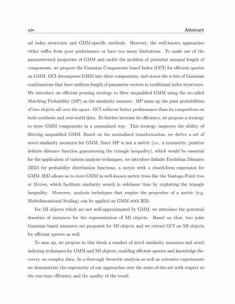
For the indexing of GMM, there are several techniques available, including univer-
xiv Abstract
sal index structures and GMM-specific methods. However, the well-known approaches
either suffer from poor performance or have too many limitations. To make use of the
parameterized properties of GMM and tackle the problem of potential unequal length of
components, we propose the Gaussian Components based Index (GCI) for efficient queries
on GMM. GCI decomposes GMM into their components, and stores the n-lets of Gaussian
combinations that have uniform length of parameter vectors in traditional index structures.
We introduce an efficient pruning strategy to filter unqualified GMM using the so-called
Matching Probability (MP) as the similarity measure. MP sums up the joint probabilities
of two objects all over the space. GCI achieves better performance than its competitors on
both synthetic and real-world data. To further increase its efficiency, we propose a strategy
to store GMM components in a normalized way. This strategy improves the ability of
filtering unqualified GMM. Based on the normalized transformation, we derive a set of
novel similarity measures for GMM. Since MP is not a metric (i.e., a symmetric, positive
definite distance function guaranteeing the triangle inequality), which would be essential
for the application of various analysis techniques, we introduce Infinite Euclidean Distance
(IED) for probability distribution functions, a metric with a closed-form expression for
GMM. IED allows us to store GMM in well-known metric trees like the Vantage-Point tree
or M-tree, which facilitate similarity search in sublinear time by exploiting the triangle
inequality. Moreover, analysis techniques that require the properties of a metric (e.g.
Multidimensional Scaling) can be applied on GMM with IED.
For MI objects which are not well-approximated by GMM, we introduce the potential
densities of instances for the representation of MI objects. Based on that, two joint
Gaussian based measures are proposed for MI objects and we extend GCI on MI objects
for efficient queries as well.
To sum up, we propose in this thesis a number of novel similarity measures and novel
indexing techniques for GMM and MI objects, enabling efficient queries and knowledge dis-
covery on complex data. In a thorough theoretic analysis as well as extensive experiments
we demonstrate the superiority of our approaches over the state-of-the-art with respect to
the run-time efficiency and the quality of the result.

Zusammenfassung
Angesichts der steigenden Quantitat und Vielfalt der generierten und gespeicherten
Daten werden manuelle und automatisierte Analysen in vielen modernen Anwendungen
eine zunehmend anspruchsvolle Aufgabe, wie z.B. biometrische Identifikation und
inhaltbasierter Bildzugriff. In dieser Arbeit werden zwei sehr typische und relevante
inharente Strukturen von Objekten behandelt: Multiple-Instance-Objects (MI) und
Gaussian Mixture Models (GMM). In beiden Anwendungsfallen wird das Objekt in
Form einer Menge dargestellt. Bei MI besteht jedes Objekt aus einer Menge von
Vektoren aus einem multidimensionalen Raum. Bei GMM wird jedes Objekt durch
eine Menge von multivariaten normalverteilten Dichtefunktionen reprasentiert. Dies
bietet die Moglichkeit, beliebige Wahrscheinlichkeitsverteilungen in kompakter Form zu
approximieren. Beide Ansatze sind sehr leistungsfahig, denn sie basieren auf einfachsten
Ideen: (1) entweder besteht ein Objekt additiv aus mehreren Komponenten oder (2)
ein Objekt hat unterschiedliche alternative Verhaltensarten. Dies ermoglicht es uns z.B.
ein Bild zu reprasentieren, welches unterschiedliche Objekte und Szenen zeigt (1). In
gleicher Weise konnen wir einen Sportler modellieren, der bei verschiedenen Wettkampfen
unterschiedliche Leistungen gezeigt hat (2). Wir konnen MI-Objekte durch GMM
approximieren und auch der umgekehrte Weg ist moglich. Beide Vorgehensweisen konnen
sehr ansprechend sein, da GMM im Vergleich zu MI kompakter sind, wogegen in MI-
Objekten die einzelnen Komponenten weniger Komplexitat aufweisen.
Ein Ahnlichkeitsmaßdient der Quantifikation der Gemeinsamkeit zwischen zwei
Objekten. Darauf basierend spielen Indizierung und Ahnlichkeitssuche eine wesentliche

xvi Zusammenfassung
Rolle fur die effiziente Implementierung von einer Vielzahl von Klassifikations- und
Clustering-Algorithmen im Bereich des Data Minings. Ziel dieser Arbeit ist es, die
Herausforderungen bei Indizierung und Wissensextraktion von komplexen Daten unter
Verwendung von MI Objekten und GMM zu bewaltigen.
Fur die Indizierung der GMM stehen verschiedene universelle und GMM-spezifische
Indexstrukuren zur Verfugung. Jedoch leiden solche bekannten Ansatze unter schwacher
Leistung oder zu vielen Einschrankungen. Um die parametrisieren Eigenschaften der
GMM auszunutzen und dem Problem der moglichen ungleichen Komponentenlange
entgegenzuwirken, prasentieren wir das Verfahren Gaussian Components based Index
(GCI), welches effizienten Abfrage auf GMM ermoglicht. GCI zerlegt dabei ein GMM
in Parameterkomponenten und speichert alle moglichen Kombinationen mit einheitlicher
Vektorlange in traditionellen Indexstrukturen. Wir stellen ein effizientes Pruningverfahren
vor, um ungeeignete GMM unter Verwendung der sogenannten Matching Probability
(MP) als Ahnlichkeitsmaßauszufiltern. MP errechnet die Summe der gemeinsamen
Wahrscheinlichkeit zweier Objekte aus dem gesamten Raum. CGI erzielt bessere
Leistung als konkurrierende Verfahren, sowohl in Bezug auf synthetische, als auch auf
reale Datensatze. Um ihre Effizienz weiter zu verbessern, stellen wir eine Strategie
zur Speicherung der GMM-Komponenten in normalisierter Form vor. Diese Strategie
verbessert die Fahigkeit zum Ausfiltern ungeeigneter GMM. Daruber hinaus leiten wir,
basierend auf dieser Transformation, neuartige Ahnlichkeitsmaße fur GMM her.
Da MP keine Metrik (d.h. eine symmetrische, positiv definite Distanzfunktion, die die
Dreiecksungleichung garantiert) ist, dies jedoch unentbehrlich fur die Anwendung mehrerer
Analysetechniken ist, fuhren wir Infinite Euclidean Distance (IED) ein, ein Metrik mit
geschlossener Ausdrucksform fur GMM. IED erlaubt die Speicherung der GMM in Metrik-
Baumen wie z.B. Vantage-Point Trees oder M-Trees, die die Ahnlichkeitssuche in sublinear
Zeit mit Hilfe der Dreiecksungleichung erleichtert. Außerdem konnen Analysetechniken,
die die Eigenschaften einer Metrik erfordern (z.B. Multidimensional Scaling), auf GMM
mit IED angewandt werden.
Fur MI-Objekte, die mit GMM nicht in außreichender Qualitat approximiert werden

Zusammenfassung xvii
konnen, stellen wir Potential Densities of Instances vor, um MI-Objekte zu reprasentieren.
Darauf beruhend werden zwei auf multivariater Gaußverteilungen basierende Maße fur MI-
Objekte eingefuhrt. Außerdem erweitern wir GCI fur MI-Objekte zur effizienten Abfragen.
Zusammenfassend haben wir in dieser Arbeit mehrere neuartige Ahnlichkeitsmaße
und Indizierungstechniken fur GMM- und MI-Objekte vorgestellt. Diese ermoglichen
effiziente Abfragen und die Wissensentdeckung in komplexen Daten. Durch eine
grundliche theoretische Analyse und durch umfangreiche Experimente demonstrieren wir
die Uberlegenheit unseres Ansatzes gegenuber anderen modernen Ansatzen bezuglich ihrer
Laufzeit und Qualitat der Resultate.

xviii Zusammenfassung

Chapter 1
Introduction
“Processed data is information. Processed information is knowledge.
Processed knowledge is wisdom.”
Ankala V. Subbarao
Nowadays, data are being generated at a dramatic pace across a wide variety of fields,
such as banking, manufacturing, marketing and monitoring [1]. Advances in storage capac-
ity and digital data gathering equipments enable possible massive datasets and resources.
Extracting meaningful information from the data is hindered by its size and complexity,
which brings the challenges for indexing and searching through the growing data and raises
an urgent need for the development of computational theories to assist humans. The notion
of finding useful information from data has been given a variety of names, including data
analysis, data dredging, knowledge extraction, information discovery, etc [2], among which
Knowledge Discovery in Databases (KDD) emphasizes that knowledge is the end product
of a data-driven discovery [3].
1.1 Knowledge Discovery in Databases
Extracting useful information and knowledge from huge amount of data is essential for
many modern applications ranging from business intelligence [4], market analysis [5], risk

2 1. Introduction
control [6], etc. As the process shown in Figure 1.1, KDD consists of a sequence of following
steps to find and interpret patterns from data.
• Data selection and preprocessing. Selecting target datasets, or focusing on subsets
of variables, and cleaning data.
• Data transformation. According to the goal of the task, finding useful features for
the representation of the data and using dimensionality reduction or transformation
methods to transfer the data into forms appropriate for the following mining methods.
• Data mining. Searching for data patterns in a particular representational form using
intelligent methods.
• Interpretation and evaluation. Identifying the truly understandable patterns on base
of some interestingness measures which includes pattern value, combining validity,
novelty, usefulness and simplicity.
Data Warehouse
Target Data
Transformed Data
Patterns
Selection & Preprocessing
Transformation
Data Mining
Interpretation & Evaluation
Applications
Knowledge
Understanding
Integration
Raw Data
Figure 1.1: Demonstration of KDD Process. The figure is modified from J. Han and M.
Kamber [2].
1.2 Representation of Complex Data 3
The mined knowledge is presented to users by visualization and knowledge repre-
sentation techniques to guide the procedure of KDD and improve the performance of
applications.
Here KDD refers to the overall process of discovering useful information from data, and
data mining, however, is only a particular step that consists of data analysis and discovery
algorithms in this process. There are several major data mining algorithms have been
developed, including regression, classification, clustering, association rules, etc.
Regression analysis is a classical statistical process to estimate relations between vari-
ables, and it is widely used for prediction and forecasting [12]. Many techniques have
been developed, such as Linear Regression, Multiple Regression [13] and Support Vector
Machine [14]. Classification is the problem of identifying to which of a set of categories an
object belongs, on basis of a training set of objects with category membership information.
Techniques like regression [15], decision trees [16], neural network [17], etc. can be used to
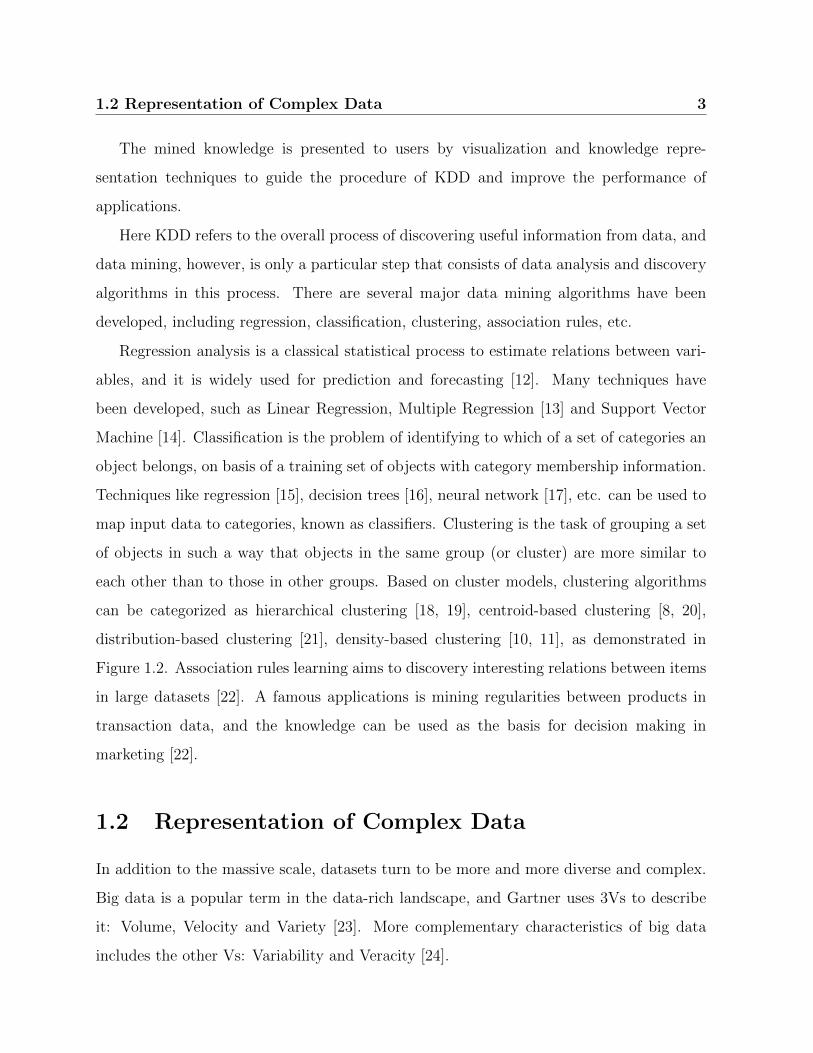
map input data to categories, known as classifiers. Clustering is the task of grouping a set
of objects in such a way that objects in the same group (or cluster) are more similar to
each other than to those in other groups. Based on cluster models, clustering algorithms
can be categorized as hierarchical clustering [18, 19], centroid-based clustering [8, 20],
distribution-based clustering [21], density-based clustering [10, 11], as demonstrated in
Figure 1.2. Association rules learning aims to discovery interesting relations between items
in large datasets [22]. A famous applications is mining regularities between products in
transaction data, and the knowledge can be used as the basis for decision making in
marketing [22].
1.2 Representation of Complex Data
In addition to the massive scale, datasets turn to be more and more diverse and complex.
Big data is a popular term in the data-rich landscape, and Gartner uses 3Vs to describe
it: Volume, Velocity and Variety [23]. More complementary characteristics of big data
includes the other Vs: Variability and Veracity [24].
4 1. Introduction
4 4.5 5 5.5 6 6.5 7 7.5 80
1
2
3
4
5
6
7
8
Sepal Length
Pet
al L
eng
th
(a) Ground Truth
4 4.5 5 5.5 6 6.5 7 7.5 80
1
2
3
4
5
6
7
8
Sepal Length
Pet
al L
eng
th(b) K-Means
4 4.5 5 5.5 6 6.5 7 7.5 80
1
2
3
4
5
6
7
8
Sepal Length
Pet
al L
eng
th
(c) EM
4 4.5 5 5.5 6 6.5 7 7.5 80
1
2
3
4
5
6
7
8
Sepal Length
Pet
al L
eng
th
(d) DBSCAN
Figure 1.2: Demonstration of clustering algorithms on Iris data [7]. (a) Ground truth of
three classes of Iris data, only two attributes are used here. (b) As a centroid model, K-
Means algorithm [8] represents each cluster by a single mean vector. It assumes equal-sized
clusters. (c) Clusters are modeled using statistical distributions, here for example, Gaussian
distribution. The parameters of the model are estimated using Expectation-Maximization
algorithm [9]. (d) Density models defines clusters as connected dense regions in the data
space, such as DBSCAN [10] and OPTICS [11]. Here the parameters of DBSCAN are set
to ε = 0.4 and MinPts = 10, and gray diamonds indicate noise in the clustering result.

1.2 Representation of Complex Data 5
• Volume. Big data observes and tracks what happens anywhere, and it does not
sample.
• Variety. The data types are various and complex.
• Velocity. Big data is often available in real-time.
• Variability. The data sets are inconsistency.
• Veracity. The quality of captured data can vary greatly.
Aside high-dimensional numerical features, many datasets are collected in non-numerical
forms and/or with inherent structures. Figure 1.3 demonstrates several forms of complex
data. As shown in Figure 1.3(a), a categorical feature and two numerical features are
included in these data objects. Each of the possible values of categorical variables is
referred to as a level (e.g., here referred to as the gender). Figure 1.3(b) shows an example
of time-series data, which is a series of data points indexed in time order [25]. Most
commonly, a time series is a sequence taken at equally spaced points in time. Multiple-
Instance (MI) data is shown in Figure 1.3(c), where each data object is a set of individual
instances.
M
M
W
(a) Mixed-type (b) Time-series (c) MI
Data object A
Data object B
Data object C
Figure 1.3: Demonstration of different data types.
6 1. Introduction
1.3 Similarity and Dissimilarity Measures
To search for similar objects and to analysis on the basis of similarities, we need similarity
measures or dissimilarity measure for objects. A similarity measure is a real-valued function
that quantifies the similarity between data objects. The value of a similarity is higher when
objects are more alike, while the value of the dissimilarity is lower. Usually similarities are
the inverses of dissimilarities. Most of the dissimilarity measures are distance functions
when they meet the following definition.
Definition 1. (Distance function) Given an nonempty set of objects P, a mapping d :
P ×P −→ R+ is a distance function when the following properties always hold for any
object X ,Y ,Z ∈P.
• identity of indiscernibles: d(X ,Y) = 0⇔ X = Y
• symmetry: d(X ,Y) = d(Y ,X )
A distance function is a metric if it additionally fulfills the triangle inequality:
d(X ,Y) + d(Y ,Z) ≥ d(X ,Z)
1.3.1 Measures for Feature Vectors
Many distance functions have been proposed for numeric variables, for instance, Euclidean
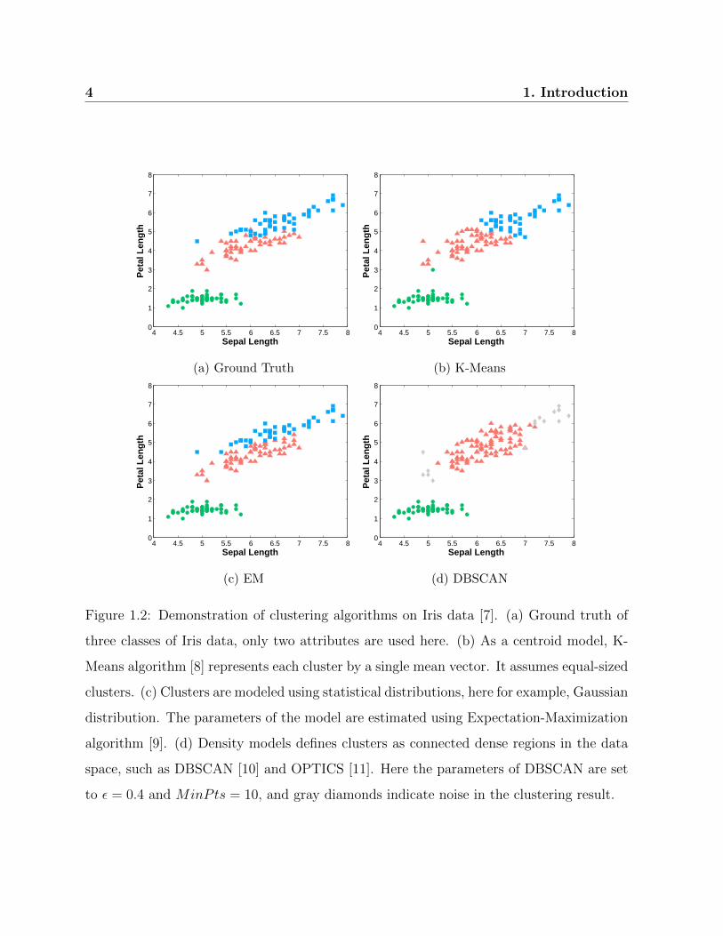
distance, Manhattan distance and Chebyshev distance. Figure 1.4 illustrates two well-
known distance functions: Manhattan distance and Euclidean distance. In this figure, the
blue dot line indicates the Manhattan distance (4.02 km) from 368 W23rd St. New York
to 590 Madison Ave. New York, and the black solid line shows the Euclidean distance
(2.98 km) between two locations.
Turning to other kinds of variables (e.g. binary variables), various measures are avail-
able, including simple matching coefficient [26], Jaccard index [27], etc. The choice of
a particular measure to capture the essential differences between objects depends on the
1.3 Similarity and Dissimilarity Measures 7
Figure 1.4: Demonstration of Manhattan distance and Euclidean distance. The screenshot
is taken from maps.google.com.
application and other factors, such as the distribution of data points and computational
considerations.
1.3.2 Measures for Distributions
To measure the (dis)similarities between distributions or sets of vectors (instances), var-
ious similarity measures have been proposed, ranging from relatively simple and efficient
proposals to more sophisticated ones. Here we introduce two main categories of them.
The first one uses prototype instances for each object together with previous introduced
measures. The second one uses the complete information about the structure of objects.
For measure based on prototype vectors, different hierarchical schemes have been
proposed. Sum of Minimum Distance (SMD) sums up the minimum distances between
the instances of two objects, and returns the average value as the distance for the sets [28].
Chamfer distance shares the same schemes with SMD [29]. Hausdorff distance is the
greatest of all distances from an instance in one set to the closest instance in the other
set [30]. Given two objects X = ximi=1 and Y = yjnj=1, the three distances can be
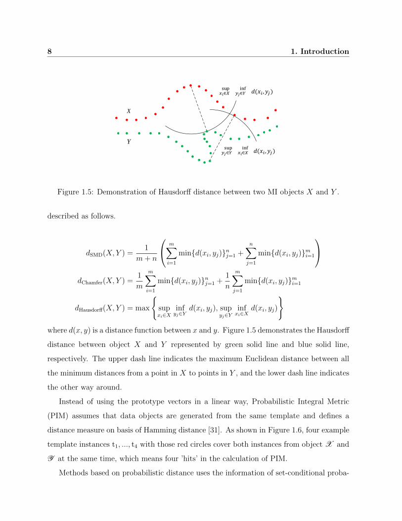
8 1. Introduction
X
Y
Figure 1.5: Demonstration of Hausdorff distance between two MI objects X and Y .
described as follows.
dSMD(X, Y ) =1
m+ n
m∑
i=1
mind(xi, yj)nj=1 +n∑
j=1
mind(xi, yj)mi=1
dChamfer(X, Y ) =1
m
m∑
i=1
mind(xi, yj)nj=1 +1
n
m∑
j=1
mind(xi, yj)mi=1
dHausdorff(X, Y ) = max
supxi∈X
infyj∈Y
d(xi, yj), supyj∈Y
infxi∈X
d(xi, yj)
where d(x, y) is a distance function between x and y. Figure 1.5 demonstrates the Hausdorff
distance between object X and Y represented by green solid line and blue solid line,
respectively. The upper dash line indicates the maximum Euclidean distance between all
the minimum distances from a point in X to points in Y , and the lower dash line indicates
the other way around.
Instead of using the prototype vectors in a linear way, Probabilistic Integral Metric
(PIM) assumes that data objects are generated from the same template and defines a
distance measure on basis of Hamming distance [31]. As shown in Figure 1.6, four example
template instances t1, ..., t4 with those red circles cover both instances from object X and
Y at the same time, which means four ’hits’ in the calculation of PIM.
Methods based on probabilistic distance uses the information of set-conditional proba-

1.3 Similarity and Dissimilarity Measures 9
Instances of
Instances of
t2
t4
t1
t3
Figure 1.6: Demonstration of PIM between MI objects X and Y [31].
bility density functions. One of the main disadvantages of the probabilistic based methods
is the numerical integration. It restricts their usefulness in many applications, especially
for some real-time situations. Given two Probability Distribution Functions (PDF) f
and g, the Bhattacharyya measure [32] and Kullback-Leibler (KL) divergence [33] can be
described as follows.
dBhatta(f, g) = −log
∫ √p(x|f)p(x|g)dx
dKL(f ||g) =
∫p(x|f)
p(x|f)
p(x|g)dx
Under some assumptions regarding to the form of the distributions, the expression can
be evaluated analytically. For example, the KL divergence of two Gaussian distributions
f ′ and g′ has a closed-form expression:
dKL(f ′||g′) =1
2
(log|Σg′||Σf ′ |
+ Tr(Σ−1g′ Σf ′)−D + (µf ′ − µg′)TΣ−1
g′ (µf ′ − µg′))
10 1. Introduction
where µf ′ and µg′ are the means, and Σf ′ and Σg′ are the covariance matrices of f ′ and g′
in a D-dimensional space, respectively.
1.4 Indexing Structures
The goal of indexing structures is to facilitate the efficient similarity search of databases,
and the applications include content based image and video retrieval [34], time series
indexing [35], biometric identification [36], etc. Similarity search relates to some similarity
measures between objects, for example, a query for the most similar feature vector given
a reference feature vector.
1.4.1 Index of Feature Vectors
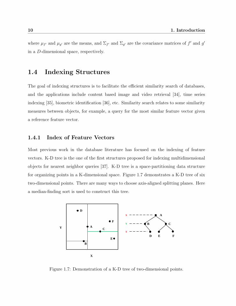
Most previous work in the database literature has focused on the indexing of feature
vectors. K-D tree is the one of the first structures proposed for indexing multidimensional
objects for nearest neighbor queries [37]. K-D tree is a space-partitioning data structure
for organizing points in a K-dimensional space. Figure 1.7 demonstrates a K-D tree of six
two-dimensional points. There are many ways to choose axis-aligned splitting planes. Here
a median-finding sort is used to construct this tree.
A
B
D
E
C
F
A
B
D
C
E F
X
Y
X
X
Y
Figure 1.7: Demonstration of a K-D tree of two-dimensional points.

1.4 Indexing Structures 11
R1
R2
R3
R4
R5
R6R7
R8
R9
R10
R11
R12
R13 R14
R15
R18
R19
R1 R2
R3 R4 R5 R6 R7
R16
R17
R13 R14 R15 R16 R17 R18 R19 R8 R9 R10 R11 R12
Root
Figure 1.8: Demonstration of an R-tree for two-dimensional rectangles. Different colors
indicate the different levels of rectangles in the tree, and all leaf nodes are at the same red
level.

12 1. Introduction
R-tree [38] is a widely used index for multiple dimensional data. The key idea is to
group nearby objects and represent them with the Minimum Bounding Rectangle (MBR)
in the next higher level of the tree. A query object that does not intersect the MBR also
cannot intersect any of the contained objects, thus a MBR can be used to decide whether
or not to search inside a subtree. Figure 1.8 shows an example of an R-tree. At the leaf
level, each rectangle describes a single object, and at the higher levels the aggregation
of an increasing number of objects are included. The queries start at the root and only
interested subtrees are accessed.
R*-tree [39] is one of the most successful variants of R-tree. When a node overflows in R-
tree, it is split into two new nodes. In R*-tree, however, a portion of the entries of that node
are removed and reinserted, allowing them to find a more appropriated location. R*-tree
has slightly higher construction cost than R-tree because of the strategy of reinsertion, but
it minimizes both overlaps and coverage. Lower overlaps mean that, on the data query and
insertion, less branches of the tree need to be expanded. A minimized coverage improves
pruning performance by excluding whole pages for the query.
For indexing high-dimensional data, both R-tree and R*-tree are not competent due
to the overlap problem. Thus X-tree [40] emphasizes the prevention of overlaps in the
bounding boxes and utilizes the concept of supernodes based on R-tree. Its split algorithm
and supernodes keep the directory as hierarchical as possible and at the same time avoid
split which would result in a high degree of overlap in the directory. SS-tree [41] uses
ellipsoid bounding regions in a lower dimensional space after the transformation of the
nodes. SS+ tree [42] has a tigher bounding sphere for each node than SS-tee, and makes
use of the clustering property of data as the split method. SR-tree [43] is an extension
of R*-tree and SS-tree, combining the utilization of bounding rectangles and bounding
spheres, which improves the performance on nearest queries by reducing both the diameter
and volume of regions.
Vantage-Point (VP)-tree is a metric tree that designed for objects in metric spaces.
It partitions data points into two parts by distances between these points to the vantage
point, and VP-tree only take metric as the distance function. Each node in a VP-tree
1.4 Indexing Structures 13
contains an input point and a radius r. The points inside the circle are the left children,
while those outside the circle are the right children.
VP
Q
P1
Root
τ VP
P1, d(VP, P1)
P2, d(VP, P2)
P2
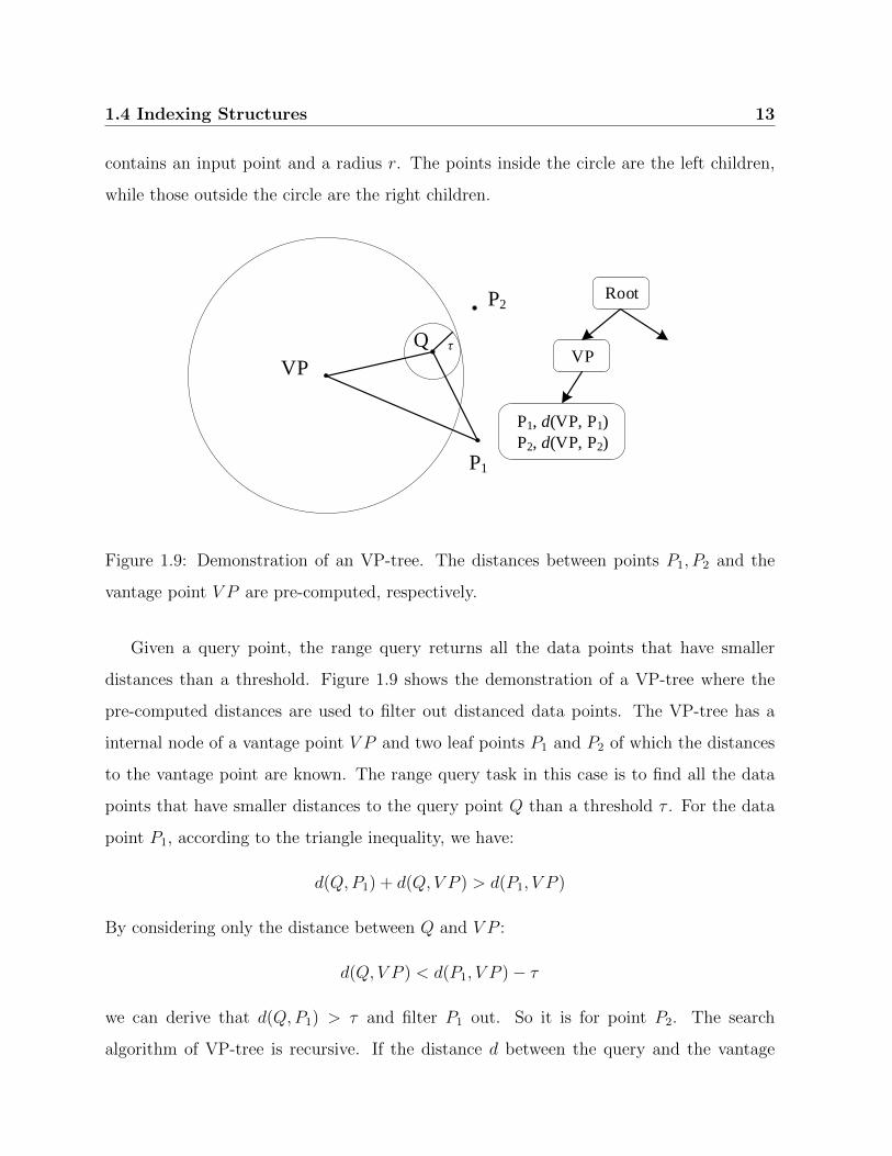
Figure 1.9: Demonstration of an VP-tree. The distances between points P1, P2 and the
vantage point V P are pre-computed, respectively.
Given a query point, the range query returns all the data points that have smaller
distances than a threshold. Figure 1.9 shows the demonstration of a VP-tree where the
pre-computed distances are used to filter out distanced data points. The VP-tree has a
internal node of a vantage point V P and two leaf points P1 and P2 of which the distances
to the vantage point are known. The range query task in this case is to find all the data
points that have smaller distances to the query point Q than a threshold τ . For the data
point P1, according to the triangle inequality, we have:
d(Q,P1) + d(Q, V P ) > d(P1, V P )
By considering only the distance between Q and V P :
d(Q, V P ) < d(P1, V P )− τ
we can derive that d(Q,P1) > τ and filter P1 out. So it is for point P2. The search
algorithm of VP-tree is recursive. If the distance d between the query and the vantage

14 1. Introduction
point is smaller than the radius r then we search the subtree of the node, otherwise recurse
to the subtree of nodes that contain points that locate outside the circle of r.
O1 O2
O1 O4 O3 O6 O4 O8
o1
o2
o3
o6
o7
o4
o5
O1 O3 O2 O4
O2 O7
o8
Figure 1.10: Demonstration of a M-tree [44]. Blue circles indicate non-leaf nodes and red
circles represent leaf nodes.
M-tree [44] is another metric tree that relies on the triangle inequality for efficient
queries. As shown in Figure 1.10, M-tree has a similar structure like R-tree, and it could
also have large overlaps. There are four components in M-tree: objects, routing objects, leaf
nodes and non-leaf nodes. An object includes the feature vector of a data point, identifier,
and the distance between the data point and its parent. A routing object consists of
the feature vector of a routing point, a covering radius, a pointer to its children and the
distance to its parent. A non-leaf node includes a set of routing objects and a pointer to
its parent while a leaf node includes a set of objects and also a pointer to its parent.
1.4 Indexing Structures 15
1.4.2 Index of Distributions
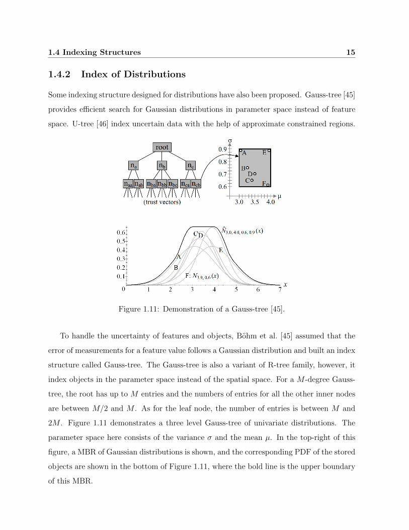
Some indexing structure designed for distributions have also been proposed. Gauss-tree [45]
provides efficient search for Gaussian distributions in parameter space instead of feature
space. U-tree [46] index uncertain data with the help of approximate constrained regions.
Figure 1.11: Demonstration of a Gauss-tree [45].
To handle the uncertainty of features and objects, Bohm et al. [45] assumed that the
error of measurements for a feature value follows a Gaussian distribution and built an index
structure called Gauss-tree. The Gauss-tree is also a variant of R-tree family, however, it
index objects in the parameter space instead of the spatial space. For a M -degree Gauss-
tree, the root has up to M entries and the numbers of entries for all the other inner nodes
are between M/2 and M . As for the leaf node, the number of entries is between M and
2M . Figure 1.11 demonstrates a three level Gauss-tree of univariate distributions. The
parameter space here consists of the variance σ and the mean µ. In the top-right of this
figure, a MBR of Gaussian distributions is shown, and the corresponding PDF of the stored
objects are shown in the bottom of Figure 1.11, where the bold line is the upper boundary
of this MBR.

16 1. Introduction
l2+
l2-
l1- l1+
URq
Figure 1.12: Demonstration of the PCR of an object stored in U-tree [46]. The red
box q represents for a prob-range query where qualified objects have higher appearance
probabilities than a given threshold.
U-tree is designed for range queries on multi-dimensional PDF, and Probabilistically
Constrained Regions (PCR) is introduced to assist prob-range search. The PCR of an
object takes a parameter p ∈ [0, 0.5] which is the probability of the uncertain data appears
in this region. As shown in Figure 1.12, the dashed line-encircled region UR is the
uncertainty region of an object o, and the grey area decided by four lines l1−, l1+, l2−
and l2+ is the PCR of the object at probability p. Take line l1+ for example, it divides
UR into two parts: the left part and the right part, and the appearance probability in the
right part (the shadowed part) is p. Similarly, the left part of UC partitioned by line l1−
has a probability of p as well. Having PCR, we can prune un-qualified objects without
computing the accurate appearance probabilities. Assuming that the parameter p is set
to 0.3 in Figure 1.12, and the red box q represents a range query with threshold τq = 0.8.
Since q is disjoint with the left part of UR (divided by line l1+), it is not possible that the
object o have a higher appearance probability than τp in the range query. Thus we can
safely exclude the object for this query. U-tree can be applied to objects with arbitrary
distributions, however, its efficiency deteriorates for mixture models.

1.4 Indexing Structures 17
1.4.3 Analysis of Index
Insertion, deletion and update are critical operations for the corresponding index struc-
tures. They heavily determine the structures and the achievable performance. Take
insertion for example, the general steps are shown as follows.
• Search a suitable data page (or node) P for the data object Oi.
• Insert Oi into page P .
• If the number of data objects stored in P exceeds the maximum number, then split
P into two pages by some strategies.
• Replace the previous description of P in its parent by the new one.
• If the parent page of P exceed its capacity, then split it.
• If the root need to be split, then grow the height of the tree by 1, split the root and
create a new one that parents the split pages.
Different splitting and merging strategies produce different index structures.
Space Utilization
Space utilization indicates the utilization rate of data pages in the index. Higher storage
utilization will generally reduce the query cost as the height of the tree will be kept low.
Take R-tree for example, let M be the maximum capacity of nodes, every split node will
generate 2M − (M + 1) = M − 1 empty entries, thus node splitting may propagate to low
storage utilization.
Overlap
The overlap of index structures means more than one branch of the tree needs to be
expanded on data query or insertion. As shown in Figure 1.8, directory rectangle R6 and

18 1. Introduction
R7 (blue dash rectangles) are overlap, and bounding rectangle R9 and R10 (red solid line
rectangles) are shared.
The overlap leads to the traversal of a larger number of index paths, which increases
the number of accessed index pages. The overlap between directory rectangles should be
minimized.
1.5 Performance Evaluation
Evaluation is the structured interpretation and giving of meaning to predicted or actual
impacts of proposals or results. It is an essential part of the model development process,
with the intention of improving the value or effectiveness of the proposal. In this thesis,
classification and clustering is used for the evaluation of our novel similarity measures.
Similarity measures that are more meaningful and suitable for objects achieve better
classification and clustering results than the others.
1.5.1 Classification and Regression
To avoid over-fitting, it is not acceptable to evaluate model performance with the data
used for training. Hold-out validation splits original datasets into two parts, training sets
and testing sets. The training sets are used to build models and the testing sets are used
to assess the performance of the models, which provides a test platform for the selecting of
the best-performing model and tuning parameters. When only a limited amount of data
is available, cross-validation can be used to divide a dataset into k subsets of equal size.
k models are built and each time one of the subsets is left from training and is used as
the test set. There are several criteria to evaluate and compare the performance of built
models.
1.5 Performance Evaluation 19
Root Mean Squared Error
Root Mean Squared Error (RMSE) is a popular formula to measure the error rate of a
regression model. RMSE sums up the squared differences of predicted targets and actual
targets, and returns the root of the mean value. The formula is shown as follows.
RMSE =
√∑ni=1(pi − ai)2
n
where n is the number of predicted units, p and a are the predicted targets and actual
targets, respectively.
Relative Squared Error
Unlike RMSE, Relative Squared Error (RSE) can be compared between models whose
errors are measured in the different units. The formula of RSE is shown as follows.
RSE =
∑ni=1(pi − ai)2
∑ni=1(a− ai)2
where a is the mean of all actual targets a.
Confusion Matrix
A confusion matrix shows the number of correct and incorrect predictions made by clas-
sification models compared to the actual targets. The matrix is N × N , where N is the
number of classes. The following table shows a 2× 2 confusion matrix, where A,B,C and
D are the frequencies of data objects in different categories. Take A for example, it is the
number of positive data objects that are classified as positive ones.
1.5.2 Clustering
The objective functions of clustering formalize the goal of attaining high intra-cluster sim-
ilarities and low inter-cluster similarities. Good scores on an objective function, however,
does not necessarily translate into good effectiveness in applications. Clustering evaluation

20 1. Introduction
Table 1.1: Demonstration of a confusion matrix.
Target
Positive Negative
ModelPositive A B Positive Predictive A/(A+B)
Negative C D Negative Predictive D/(C+D)
True Positive False PositiveAccuracy = (A+D)/(A+B+C+D)
A/(A+C) D/(B+D)
provides evidence whether data contains non-random structures, ranks alternative cluster-
ings with regards to their quality, and determines the ideal number of clusters. Given N
data objects and a set of clusters Ω = ω1, ω2, ...ωK and a set of classes C = c1, c2, ...cM,where ωi represents the data objects of the i-th cluster and cj represents data objects with
the j-th class label, we introduce three widely-used external criteria of clustering quality
as follows.
Purity
Purity is a simple and transparent evaluation measure of extent to which clusters contains
a single class. Each cluster is assigned to the class that is most frequent in the cluster, and
then we measure the mean of the accuracy of this assignment. Purity can be defined as:
Purity(Ω, C) =1
N
K∑
i=1
maxj∈[1,M ]
|ωi ∩ cj|
where | · | indicates the cardinality of a set.
Purity ranges from 0 to 1 and does not penalise having many clusters. A highest value
of 1 is possible by putting each data object in its own cluster.

1.5 Performance Evaluation 21
Normalized Mutual Information
Mutual information is an information theoretic measure of how much information is shared
between a cluster and a ground truth. It can detect a non-linear similarity between two
clusters. Given two clusters Ω and C, mutual information can be defined as:
I(Ω, C) =K∑
i=1
M∑
j=1
|ωi ∩ cj|N
logN |ωi ∩ cj||ωi||cj|
Derived from thinking of mutual information as an analogue to covariance, Normalized mu-
tual information (NMI) [47] that is calculated similarly to the Person correlation coefficient
is defined as follows.
NMI(Ω, C) =I(Ω, C)√H(Ω)H(C)
where H(Ω) and H(C) are the entropies of the cluster Ω and the ground truth C, respec-
tively. The formula of H(Ω) is given by:
H(Ω) = −K∑
i=1
|ωi|N
log|ωi|N
Like purity, the range of NMI is [0, 1], and the higher the value, the better performance
of the clustering result is. NMI can be used for the comparison of clusterings with different
number of clusters.
F-Measure
Precision, Recall and F-Measure (FM) are often used in pattern recognition, information
retrieval and binary classification. They can also be used for the evaluation of clustering
by viewing the assignments of data objects as a series of decisions.
As shown in Table 1.1, True Positive (TP) assigns two objects to the same cluster
when they belong to the same cluster in ground truth, and False Positive (FP) assigns two
objects that come from different clusters in the ground truth to the same cluster. As for
False Negative (FN), it fails to assign two same-labeled data objects into the same cluster.

22 1. Introduction
The definitions of precision and recall are shown as follows.
Precision =TP
TP + FP
Recall =TP
TP + FN
Thus we can calculate FM by using the following formula.
FMβ =(β2 + 1)Presion×Recallβ2Presion+Recall
where β ≥ 0. Increasing β allocates an increasing amount of weight to recall in the final
FM. When β > 1, FM penalizes FN more strongly than FP.
1.5.3 Indexing
A query operation takes a physical query plan, executes the plan and returns the result.
The goal of an index is to compute query results as fast as possible. There are many
possible ways to estimate query cost, for instance, disk accesses and CPU time.
Disk access is relatively easy to estimate. Typically the number of block transfers
from/to disk is used as the measure on basis of a simplifying assumption, each block
transfer has the same cost. CPU time is the amount of time for which a CPU is used for
the query processing. The CPU time is measured in clock ticks or seconds.
1.6 Contributions and Structure of the Thesis
This thesis aims to study the indexing and similarity search of complex data represented as
Multiple-Instance (MI) objects and Gaussian Mixture Models (Gaussian Mixture Models
(GMM)), and to support knowledge discovery with specific designed similarity measures.
Extensive experiments are performed to demonstrate the effectiveness and efficiency of the
proposed technologies. The major contributions and the general structure of this thesis as
shown in Figure 1.13.
Chapter 2 introduces a dynamic index structure for GMM, Gaussian Component based
Index (GCI) [48]. GCI decomposes GMM into the single, pairs, or n-lets of Gaussian

1.6 Contributions and Structure of the Thesis 23
Gaussian
Component based
Index
(Chapter 2)
Infinite Euclidean
Distance
(Chapter 3)
Normalized
Transformation
(Chapter 4)
Gaussian
Mixture
Models
Matching
Probability
Normalized GCI
(Chapter 4)
Previous
Similarity
Measures
Set of Normalized
Similarity Measures
(Chapter 4)
Application of Index
Using Metric Tree
(Chapter 3)Metric Tree
Multiple
Instance
Objects
Joint Gaussian
Similarity
(Chapter 5)
Joint Gaussian
Distance
(Chapter 5)
Instance Based
Index
(Chapter 6)
Application of Index
Using Metric Tree
(Chapter 6)
Metric Tree
Multiple Instance
Learning
(Chapter 6)
Figure 1.13: Structure of this thesis.

24 1. Introduction
components, stores these components into well studied index trees such as R-tree and
Gauss-Tree, and refines the corresponding GMM in a conservative but tight way. GCI
supports both k-most-likely queries and probability threshold queries by means of Matching
Probability, and also provides an approximate way to get a balance between the efficiency
and accuracy of the queries. Extensive experimental evaluations of GCI demonstrate a
considerable speed-up of similarity search on both synthetic and real-world data sets.
Chapter 3 generalizes Euclidean distance to GMM and derive the closed-form expression
called Infinite Euclidean Distance (IED) [49]. Our metric enables efficient and accurate
similarity calculations. For the analysis of complex data, we model two real-world data
sets, NBA player statistic and the weather data of airports into GMM, and we compare the
performance of IED to previous similarity measures on both classification and clustering
tasks. Experimental evaluations demonstrate the efficiency and effectiveness of GMM with
IED on the analysis of complex data.
Chapter 4 proposes a novel technique Normalized Transformation that reorganizes the
index structure to account for different numbers of components in GMM [50]. In addition,
Normalized Transformation enables us to derive a set of similarity measures on the basis
of existing ones that have close-form expression. Extensive experiments demonstrate the
effectiveness of proposed technique for GCI and the performance of the novel similarity
measures for clustering and classification.
Chapter 5 introduces two joint Gaussian based measures for Multiple-Instance Learning
(MIL), Joint Gaussian Similarity (JGS) and Joint Gaussian Distance (JGD), which require
no prior knowledge of relations between the labels of MI objects and their instances [51].
JGS is a measure of similarity while JGD is a metric of which the properties are necessary
for many techniques like clustering and embedding. JGS and JGD take all the information
into account and many traditional machine learning methods can be introduced to MIL.
Extensive experimental evaluations on various real-world data demonstrate the effective-
ness of both measures, and better performances than state-of-the-art MIL algorithms on
benchmark tasks.
Chapter 6 uses JGS and JGD for the indexing of MI objects [52]. For JGS, we propose

1.6 Contributions and Structure of the Thesis 25
the Instance based Index for querying MI objects. For JGD, metric trees can be directly
used as the index because of its metric properties. Extensive experimental evaluations on
various synthetic and real-world data sets demonstrate the effectiveness and efficiency of
the similarity measures and the performance of the corresponding index structures.
Chapter 7 concludes the thesis and discusses about the possible future work.

26 1. Introduction

Chapter 2
Gaussian Component Based Index
for GMM
“Things get done only if the data we gather can inform and inspire those in
a position to make a difference.”
Mike Schmoker
In this chapter, we propose GCI, a novel technique for the indexing of GMM on basis
of component combinations. Parts of this chapter have been published in:
Linfei Zhou, Bianca Wackersreuther, Frank Fiedler, Claudia Plant, Christian
Bohm. Gaussian Component Based Index for GMMs. IEEE 16th International
Conference on Data Mining, ICDM 2016, December 12-15, 2016, Barcelona,
Spain.
where Linfei Zhou was mostly responsible for the development of main concepts, imple-
mented main algorithms and wrote the most parts of the paper. Bianca Wackersreuther and
Frank Fiedler helped with the implementation and experimental design. Christian Bohm
and Claudia Plant supervised the project and proposed the initial idea of decomposition.
All co-authors contributed to the discussion, paper writing and revising.

28 2. Gaussian Component Based Index for GMM
2.1 Introduction
Information extraction systems capable of handling uncertain data objects is an actively
investigated research field. Many modern applications such as speaker recognition, content-
based image and video retrieval, biometric identification and stock market analysis can be
supported by the representation of uncertain data [53, 54, 55].
Instead of using the exact positions of a feature vector, PDF are assigned to each
uncertain data object for the representation. As a general class of PDF, GMM consist of a
weighted sum of univariate or multivariate Gaussian distributions, allowing a concise but
exact representation of the uncertain data object [56]. A typical example of using objects
represented by GMM is managing multimedia data. A 90 minutes movie contains about
130,000 images, and requires a large storage capacity as well as enormous computational
efforts for the content-based retrieval. Nevertheless, storing the movie as GMM will
dramatically reduce resource consumption. As shown in Figure 2.1, features are extracted
from original data objects (the frame images of the movie) to estimate GMM, which
represent the objects precisely by parameters.
Besides the modeling of uncertainty, the efficiency of similarity search on uncertain data
is another important aspect. Several dynamic index structures designed for uncertain data
have been proposed, for instance, Gauss-tree [45] and U-tree [46]. However, these existing
index techniques either cannot handle GMM or have too many constraints. Although a
bottom-up hierarchical tree has been proposed specifically for data objects represented by
GMM[57], it is only usable for static data sets due to the lack of convenient insertion and
deletion functions. Dynamic index structures for GMM are yet to be developed and tested.
A competitive candidate for such a structure has the properties to guarantee the query
accuracy and to keep high efficiency in similarity calculations and pruning steps.
As we will demonstrate, GCI proposed in this chapter is highly efficient, because it has
a tight pruning strategy and enables a closed-form calculation for GMM. The tight pruning
strategy avoids unnecessary expensive calculations while it keeps the query accuracy. The
closed-form expression of the similarity calculation is intrinsically valuable for computation,
2.1 Introduction 29
Original data objects
FeaturesGMM-modeled
objects
Image Color histogram
Audio Frequency spectrum
G1=g11, g12, g13, g14
G2=g21, g22
Root
P1 P2 P3
P11 P12 P21 P22 P31 P32
Ranking List
Threshold τ
Gaussian Component based Index
gij
Refinement
Gi=gi1, , gij,
gij
......
......
GQ= gQj,
......
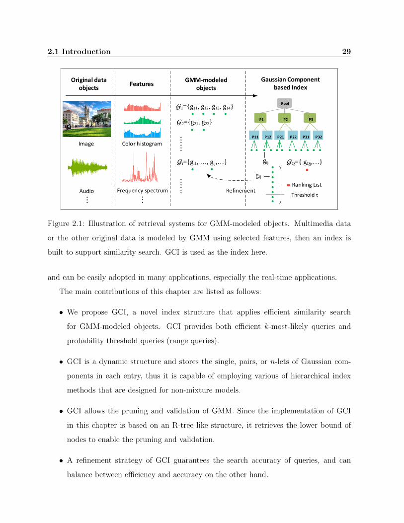
Figure 2.1: Illustration of retrieval systems for GMM-modeled objects. Multimedia data
or the other original data is modeled by GMM using selected features, then an index is
built to support similarity search. GCI is used as the index here.
and can be easily adopted in many applications, especially the real-time applications.
The main contributions of this chapter are listed as follows:
• We propose GCI, a novel index structure that applies efficient similarity search
for GMM-modeled objects. GCI provides both efficient k-most-likely queries and
probability threshold queries (range queries).
• GCI is a dynamic structure and stores the single, pairs, or n-lets of Gaussian com-
ponents in each entry, thus it is capable of employing various of hierarchical index
methods that are designed for non-mixture models.
• GCI allows the pruning and validation of GMM. Since the implementation of GCI
in this chapter is based on an R-tree like structure, it retrieves the lower bound of
nodes to enable the pruning and validation.
• A refinement strategy of GCI guarantees the search accuracy of queries, and can
balance between efficiency and accuracy on the other hand.

30 2. Gaussian Component Based Index for GMM
The rest of this chapter is organized as follows. In Section 2.2, we survey previous work
on similarity measures and index methods for GMM. Section 2.3 gives the definitions of
GMM and Matching Probability (MP) which is a similarity measure for GMM. Section 2.4
describes the principle of GCI which indexes GMM by the single, pairs, or n-lets of Gaussian
components. Section 2.5 shows experimental studies on both synthetic and real-world data
sets for verifying the effectiveness and efficiency of GCI. The final section, Section 2.6,
concludes this chapter with a summary and outlines the directions of future work.
2.2 Related Work
In this section we present a discussion on similarity measures and index techniques for
GMM in previous work.
2.2.1 Similarity Measures for Gaussian Mixture Models
A fundamental concept to measure the difference between two PDF is the KL divergence,
also called the discrimination information [33]. The KL divergence is always non-negative
and has a closed-form expression for two Gaussian distributions. However, no such ex-
pression for two GMM exists. Hence, the KL divergence of two GMM is determined by
approximations, such as Monte-Carlo sampling, matching based approximation, product
approximation and variation approximation [58, 59].
Another class of similarity measures with closed-form expressions for GMM have been
proposed. Helen et al. [60] have suggested the squared Euclidean distance, which integrates
the squared differences of two GMM over the whole feature space. Sfikas et al. [61] have
presented the C2 distance and the Bhattacharyya-based distance for GMM, and the former
is more effective than the latter. The normalized L2 distance has been proposed by Jensen
et al. [62] in the similarity search of music. Beside, two similarity measures that support
component-wise calculations have been introduced. The first one is MP [45], which is the
matching probability of two PDF that correspond to the same object. The second measure

2.2 Related Work 31
is Gaussian Quadratic Form Distance (GQFD) [63], which is designed for content-based
image retrieval systems. Although both MP and GQFD have closed-form expressions for
GMM, we select MP as the similarity measure for GMM in this chapter, since it is widely
used in papers as well as the technique chosen for comparison in this study [45, 64, 65].
2.2.2 Index of Gaussian Mixture Models
For the index of GMM, there are several techniques available, including universal index
structures designed for uncertain data and GMM-specific methods. However, none of them
has the competency to obtain high efficiency and guarantee accuracy.
U-tree [46] provides a probability threshold retrieval on general multi-dimensional
uncertain data. It pre-computes a finite number of PCR which are possible appearance
regions with fixed probabilities, and uses them to prune unqualified objects. Although
U-tree works well with single PDF, its effectiveness deteriorates for mixture models such
as GMM. The reason behind this is that it is difficult for PCR to represent mixture models,
especially when the component numbers increase.
Rougui et al. [57] have designed a bottom-up hierarchical tree and an iterative grouping
tree for GMM-modeled speaker retrieval systems. Both approaches provide only two index
levels, and are lack of a convenient insertion and deletion strategy. Furthermore, they can
not guarantee reliable query results. Haegler et al. have published SUDN [64], an index to
perform similarity search on non-axis parallel GMM. SUDN introduces a rotation strategy
to transform non-axis parallel GMM into approximate diagonal GMM. Then the linear
scan, rather than any hierarchical structure, is applied to sort these approximate GMM in
a descending order and complete queries afterwards.
Gauss-tree [45] utilizes the characteristic of Gaussian distributions for efficient queries
and uses MP as the similarity measure. It provides both the k-most likely queries and the
range queries for Gaussian distributions. Instead of index Gaussian curves as spatial objects
in feature spaces, Gauss-tree searches the parameter space of the means and variances of
the Gaussian distributions. Probabilistic Ranking Query (PRQ) [65] extends Gauss-tree

32 2. Gaussian Component Based Index for GMM
for the index of GMM. However, PRQ can not guarantee the query accuracy since it
assumes that all the Gaussian components of candidates have relatively high MP with
query objects, which is not common in general cases.
2.3 Formal Definitions
In this section, we summarize the formal notations of GMM and MP. A GMM is a prob-
abilistic model that represents the probability distribution of observations. The definition
of GMM is shown as follows.
Definition 2. (Gaussian Mixture Models) Let x ∈ Rd be a variable in a d-dimensional
space, x = (x1, x2, ..., xd). A Gaussian Mixture Model G is the weighted sum of m Gaussian
distributions, and defined as:
G(x) =∑
1≤i≤m
wi · Ni(x) (2.1)
where∑
1≤i≤mwi = 1, ∀i ∈ [1,m], wi ≥ 0, and Ni(x) is the density function of a Gaussian
distribution with a covariance matrix Σi:
Ni(x) =1√
(2π)d|Σi|exp
(−1
2(x− µi)TΣ−1
i (x− µi))
When Σi is a diagonal matrix, Ni(x) can be reformulated as:
Ni(x) =∏
1≤l≤d
1√2πσ2
i,l
exp
(−(xl − µi,l)2
2σ2i,l
)
where σi,l is the l-th element on the diagonal of Σi.
As we can see in Definition 2, a GMM can be represented by a set of components,
each of which is composed of a mean vector µ ∈ Rd and a covariance matrix Σ ∈ Rd×d.
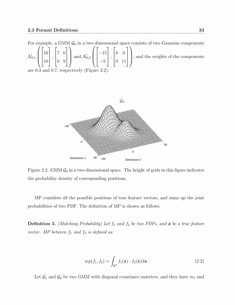
2.3 Formal Definitions 33
For example, a GMM G0 in a two-dimensional space consists of two Gaussian components
N0,1
10
10
,
7 0
0 9
and N0,2
−15
−5
,
8 0
0 11
, and the weights of the components
are 0.3 and 0.7, respectively (Figure 2.2).
−50
0
50 −50
0
50
Dimension 2
G0
Dimension 1
Figure 2.2: GMM G0 in a two-dimensional space. The height of grids in this figure indicates
the probability density of corresponding positions.
MP considers all the possible positions of true feature vectors, and sums up the joint
probabilities of two PDF. The definition of MP is shown as follows.
Definition 3. (Matching Probability) Let f1 and f2 be two PDFs, and x be a true feature
vector. MP between f1 and f2 is defined as:
mp(f1, f2) =
∫
Rdf1(x) · f2(x)dx (2.2)
Let G1 and G2 be two GMM with diagonal covariance matrices, and they have m1 and
34 2. Gaussian Component Based Index for GMM
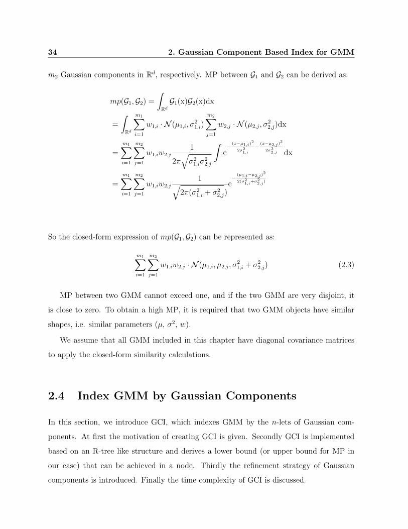
m2 Gaussian components in Rd, respectively. MP between G1 and G2 can be derived as:
mp(G1,G2) =
∫
RdG1(x)G2(x)dx
=
∫
Rd
m1∑
i=1
w1,i · N (µ1,i, σ21,i)
m2∑
j=1
w2,j · N (µ2,j, σ22,j)dx
=
m1∑
i=1
m2∑
j=1
w1,iw2,j1
2π√σ2
1,iσ22,j
∫e−
(x−µ1,i)2
2σ21,i
−(x−µ2,j)
2
2σ22,j dx
=
m1∑
i=1
m2∑
j=1
w1,iw2,j1√
2π(σ21,i + σ2
2,j)e−
(µ1,i−µ2,j)2
2(σ21,i
+σ22,j
)
So the closed-form expression of mp(G1,G2) can be represented as:
m1∑
i=1
m2∑
j=1
w1,iw2,j · N (µ1,i, µ2,j, σ21,i + σ2
2,j) (2.3)
MP between two GMM cannot exceed one, and if the two GMM are very disjoint, it
is close to zero. To obtain a high MP, it is required that two GMM objects have similar
shapes, i.e. similar parameters (µ, σ2, w).
We assume that all GMM included in this chapter have diagonal covariance matrices
to apply the closed-form similarity calculations.
2.4 Index GMM by Gaussian Components
In this section, we introduce GCI, which indexes GMM by the n-lets of Gaussian com-
ponents. At first the motivation of creating GCI is given. Secondly GCI is implemented
based on an R-tree like structure and derives a lower bound (or upper bound for MP in
our case) that can be achieved in a node. Thirdly the refinement strategy of Gaussian
components is introduced. Finally the time complexity of GCI is discussed.

2.4 Index GMM by Gaussian Components 35
2.4.1 Problem Definition and Motivation
Let D = GiNi=1 be a database of N GMM-modeled objects in a d-dimensional space Rd,
and Gi consists of mi Gaussian components. For a given query object GQ, a k-most-likely
query is to find k database objects which have the highest MP with GQ, while a probability
threshold query is to find database objects that have a higher MP with GQ than a given
threshold T .
Index structures, besides the linear scan, are essential techniques to support the queries.
Similarity measures for GMM, such as MP, are expensive to calculate, especially when
GMM have large numbers of Gaussian components, which is prevalent in getting an
accurate estimation of real-world data. An intuitive index structure for GMM should
have the competency to prune those unqualified objects and to validate objects that have
high probabilities to be the final candidates. However, since mixture models, for example
GMM, can have unequal numbers of components, traditional index techniques such as
U-tree and Gauss-tree cannot be directly applied on them.
To tackle the problem, we create a special index tree with the single, pairs, or n-lets of
Gaussian components which have the same length, and refine potential GMM candidates
in a conservative but tight way. In the pruning step, the index tree works as a filter by
calculating MP between the query object and the tree nodes, instead of calculating MP
between GMM (referred to as full GMM calculation). In addition, we have a separate array
structure to store and access GMM whenever necessary, which we regard as refinement.
In this way, we can employ various of existing index methods that are designed for non-
mixture models, for instance, Gauss-tree and U-tree, and heuristic strategies can be applied
for the refinement. The index structure of GMM in Figure 2.1 demonstrates the basic idea
of GCI.
In this chapter, we implement GCI based on an R-tree like structure of Gaussian
components, since R-tree is the most widely used and well understood index tree. It is
worth noting that the similarity measure used to build the tree is MP instead of Euclidean
distance. Figure 2.3 shows the run-time of the full GMM calculation and the calculation of

36 2. Gaussian Component Based Index for GMM
MP between the query component and MBR, which is referred to as the MBR calculation.
It is obvious that the MBR calculation has stable run-time when the number of components
increases, whereas the run-time of the full GMM calculation grows polynomially. The
advantage of GCI is avoiding unnecessary expensive calculations (full GMM calculations)
on basis of cheap calculations (MBR calculations). The fabrication process of GCI is given
in the following part of this section.
1 2 3 4 5 6 70
20
40
60
80
100
Component number in each GMM
Tim
e co
st (
ms)
MBRfull GMM
Figure 2.3: Comparison of time costs for the MBR calculation and the full GMM
calculation. The solid green line shows the average run-time of 10,000 MP calculations
between GMM over 100 runs, while the red dash line shows that of 10,000 calculations
between the query component and MBRs.
2.4.2 Index Tree for Gaussian Components
In the index tree of Gaussian components, we store the n-lets of Gaussian components
combinations in each entry. For a GMM Gi with mi components, there are (min
) possible
combinations to store.
Taking a GMM G1 that has four Gaussian components g1,1, g1,2, g1,3, g1,4 for example,
(42) Gaussian pairs will be stored in a 2-lets index tree: g1,1, g1,2, g1,1, g1,3, g1,1, g1,4,

2.4 Index GMM by Gaussian Components 37
g1,2, g1,3, g1,2, g1,4, g1,3, g1,4, where the first pair corresponds to:
(w1,1, µ1,1, σ21,1︸ ︷︷ ︸
g1,1
, w1,2, µ1,2, σ21,2︸ ︷︷ ︸
g1,2
,m1,G1)
In the case of mi < n, the Gaussian components combination will be supplemented with
zero-weight components.
After preparing these Gaussian components, we organize them into the R-tree like struc-
ture. The dimension of data stored in the tree is (2d+1)×n+1. For a query processing, we
need the conservative approximation of MP between the query GQ and entries (the single,
pairs, or n-lets of Gaussian components) stored in a node P = [wp, wp; µp, µp; σ2p, σ
2p; ...; mp, mp].
Since all Gaussian components are independent, it is sufficient to provide the conservative
approximation of MP between a query component gQ ∈ GQ and a single Gaussian compo-
nent gx ∈ P . According to Eq. 2.3, MP between gQ and gx can be represented as:
mp(gQ, gx) = wQwx1√
2π(σ2Q + σ2
x)e−
(µQ−µx)2
2(σ2Q
+σ2x)
The maximum mp(gQ, gx) for gQ in the node P is given as:
maxwx∈[wp,wp],µx∈[µp,µp],σ2
x∈[σ2p,σ
2p],mx∈[mp,mp]
mp(gQ, gx)
Determining mp(gQ, gx) in each dimension, we get the closed-form expression of the ap-
proximation by lemma 2.4.1.
Lemma 2.4.1. For entries stored in a node P , the maximum MP between the single
Gaussian component gx of them and a query component gQ can be computed by the following
function:
mp(gQ, gx) =
mpwp,mp
mpµp if µQ < µp
mpµp if µQ > µp
mpµQ if µp ≤ µQ ≤ µp
mpσ2p
if σ2Q < (µx − µQ)2 − σ2
p
mpσ2p
if σ2Q > (µx − µQ)2 − σ2
p
mp((µQ−µx)2−σ2Q) for other σ2
Q
(2.4)

38 2. Gaussian Component Based Index for GMM
where the subscripts of mp indicate the conditions of mp(gQ, gx) reaching its maximum.
Proof. The derivatives of mp(gQ, gx) with respect to wx and mx are greater than zero, so
mp(gQ, gx) reaches the maximum when wx = wp and mx = mp.
The derivative of mp(gQ, gx) with respect to µx is
∂mp
∂µx=
wQwx√2π(σ2
Q + σ2x)e−
(µQ−µx)2
2(σ2Q
+σ2x)µQ − µxσ2Q + σ2
x
Since ∂mp∂µx
< 0 when µQ < µp, mp(gQ, gx) = mpµp . Likewise mp(gQ, gx) = mpµp when
µQ > µp, and mp(gQ, gx) = mpµQ when µp ≤ µQ ≤ µp.
The derivative of mp(gQ, gx) with respect to σ2x is
∂mp
∂σ2x
=wQwxe
−(µQ−µx)
2
2(σ2Q
+σ2x)
2√
2π(σ2x + σ2
Q)5/2
((µQ − µx)2 − σ2
Q − σ2x
)
If σ2Q < (µx− µQ)2− σ2
p, we get ∂mp∂σ2x> 0, thus mp(gQ, gx) = mp
σ2p. Similarly, mp(gQ, gx) =
mpσ2p
when σ2Q > (µx − µQ)2 − σ2
p, and mp(gQ, gx) = mpσ2Q
when (µx − µQ)2 − σ2p ≤ σ2
Q ≤(µx − µQ)2 − σ2
p.
With the above equations and formularies, we have a tight and closed-form expression
for the MBR calculation in the index tree for Gaussian components, which has a similar
insertion and deletion strategy as R-tree. As for the insertion, if a new entry fits into
one node exactly, the entry is assigned to this node. When an entry does not fit into any
existing node, the upper bounds of MP, mp(gQ, gx), are calculated to locate a proper node
to assign the entry. When a node exceeds its capacity, two entries with the highest lower
bound and the lowest higher bound are set as seeds for two new nodes, respectively. The
other entries are assigned to the new nodes afterwards. If a node has less entries than a
pre-setting value after the deletion, the node will be removed and all entries of it will be
reinserted.
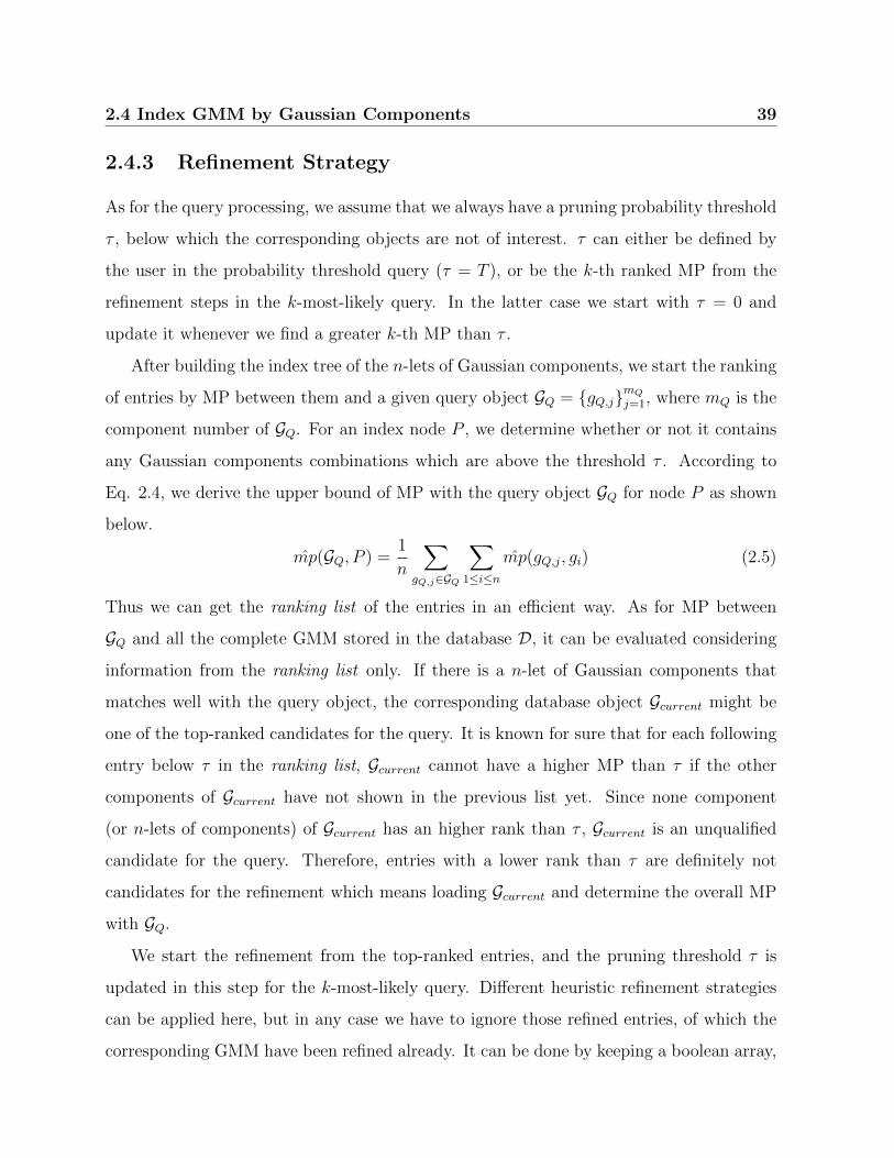
2.4 Index GMM by Gaussian Components 39
2.4.3 Refinement Strategy
As for the query processing, we assume that we always have a pruning probability threshold
τ , below which the corresponding objects are not of interest. τ can either be defined by
the user in the probability threshold query (τ = T ), or be the k-th ranked MP from the
refinement steps in the k-most-likely query. In the latter case we start with τ = 0 and
update it whenever we find a greater k-th MP than τ .
After building the index tree of the n-lets of Gaussian components, we start the ranking
of entries by MP between them and a given query object GQ = gQ,jmQj=1, where mQ is the
component number of GQ. For an index node P , we determine whether or not it contains
any Gaussian components combinations which are above the threshold τ . According to
Eq. 2.4, we derive the upper bound of MP with the query object GQ for node P as shown
below.
mp(GQ, P ) =1
n
∑
gQ,j∈GQ
∑
1≤i≤n
mp(gQ,j, gi) (2.5)
Thus we can get the ranking list of the entries in an efficient way. As for MP between
GQ and all the complete GMM stored in the database D, it can be evaluated considering
information from the ranking list only. If there is a n-let of Gaussian components that
matches well with the query object, the corresponding database object Gcurrent might be
one of the top-ranked candidates for the query. It is known for sure that for each following
entry below τ in the ranking list, Gcurrent cannot have a higher MP than τ if the other
components of Gcurrent have not shown in the previous list yet. Since none component
(or n-lets of components) of Gcurrent has an higher rank than τ , Gcurrent is an unqualified
candidate for the query. Therefore, entries with a lower rank than τ are definitely not
candidates for the refinement which means loading Gcurrent and determine the overall MP
with GQ.
We start the refinement from the top-ranked entries, and the pruning threshold τ is
updated in this step for the k-most-likely query. Different heuristic refinement strategies
can be applied here, but in any case we have to ignore those refined entries, of which the
corresponding GMM have been refined already. It can be done by keeping a boolean array,
40 2. Gaussian Component Based Index for GMM
or using a hashing method to store them in an ignore list if there are too many GMM.
In this chapter we use a intuitive refinement method which refines entries whenever their
ranks are higher than τ and the corresponding GMM are not on the ignore list. For those
entries blow the updated τ , we can safely exclude them. This strategy is simple and clear,
and no other extra criteria are needed.
The refinement strategy in this chapter can also support approximate queries by re-
placing Eq. 2.5 with the following equation.
mp(GQ, P ) =1
n
∑
gQ,j∈G∗Q
∑
1≤i≤n
mp(gQ,j, gi)
where G∗Q is a set of selected Gaussian components from GQ, and it is chosen by the sorted
weights of components, since the component with a higher weight might play a more
important role in MP between GMM.
The pseudo code in Algorithm 1 shows GCI for the k-most-likely query, and the
probability threshold query is shown in Algorithm 2. The two pseudo codes are similar
except that the latter one maintains an unknown number of possible candidates for queries.
To illustrate the processing of GCI, we generate a synthetic data set that consists of
eleven data objects (available in the synthetic data sets of Section 2.5). Each object is
represented by a two-component GMM in a two-dimensional data space. We store ten of
these objects in the index tree of Gaussian components and take the left one as a query
object. Since here we only store a single component in each entry, we have twenty leafs
(ID 0∼19) in total. Setting the minimum number of entries in each node as three and the
maximum as eight, we get an index tree for Gaussian components as shown in Figure 2.4.
There are three nodes (Node 1, 2 and 3) in level one, and one node (Node 0) in level two.
Setting τ = 0 in the beginning of a 1-most-likely query, three times of MBR calculations
are carried out from the root, and the descending order of them is: Node 2 (mp = 0.03),
Node 1 (mp = 1.9 × 10⁻¹⁷) and Node 3 (mp = 1 × 10⁻²⁵). Since the child nodes of Node
2 are data pages, we start refining the entries in Node 2. All these entries belong to four
GMM, which means we have to perform four times of full GMM calculations. After this
refinement step, the threshold τ is updated to 0.0024. Entries stored in Node 1 and Node

2.4 Index GMM by Gaussian Components 41
Algorithm 1: k-most-likely Objects Query
Data: int k, Node root, Query Object GQResult: PriorityQueue results
1 PriorityQueue results = new PriorityQueue() ; /* Ascending */
2 PriorityQuene activePages = new PriorityQueue() ; /* Descending */
3 activePages.put(root, MAX REAL);
4 τ = 0;
5 while activePages.isNotEmpty() &
results.getFirstMP()<activePages.getFirstMP() do
6 P = activePages.getFirstPage;
7 activePages.removeFirstPage();
8 if P .isDataPage() then
9 Entry E = P .data;
10 if mp(E,GQ) > τ then
11 Gcurrent = E.getGMM;
12 results.put(Gcurrent, mp(Gcurrent,GQ));
13 if results.size> k then
14 results.removeFirst;
15 τ = results.getFirstMP();
16 else
17 children = P .getChildren();
18 while children.hasMoreElements() do
19 child = children.getNextElement();
20 probability = mp(GQ, child);
21 activePages.put(child,probability);

42 2. Gaussian Component Based Index for GMM
Algorithm 2: Probability Threshold Query
Data: T , Node root, Query Object GQResult: PriorityQueue results
1 PriorityQueue results = new PriorityQueue() ; /* Ascending */
2 PriorityQuene activePages = new PriorityQueue() ; /* Descending */
3 activePages.put(root, MAX REAL);
4 τ = T ;
5 while activePages.isNotEmpty() &
results.getFirstMP()<activePages.getFirstMP() do
6 P = activePages.getFirstPage;
7 activePages.removeFirstPage();
8 if P .isDataPage() then
9 Entry E = P .data;
10 if mp(E,GQ) > τ then
11 Gcurrent = E.getGMM;
12 if mp(Gcurrent,GQ) > τ then
13 results.put(Gcurrent, mp(Gcurrent,GQ));
14 else
15 children = P .getChildren();
16 while children.hasMoreElements() do
17 child = children.getNextElement();
18 probability = mp(GQ, child);
19 activePages.put(child,probability);
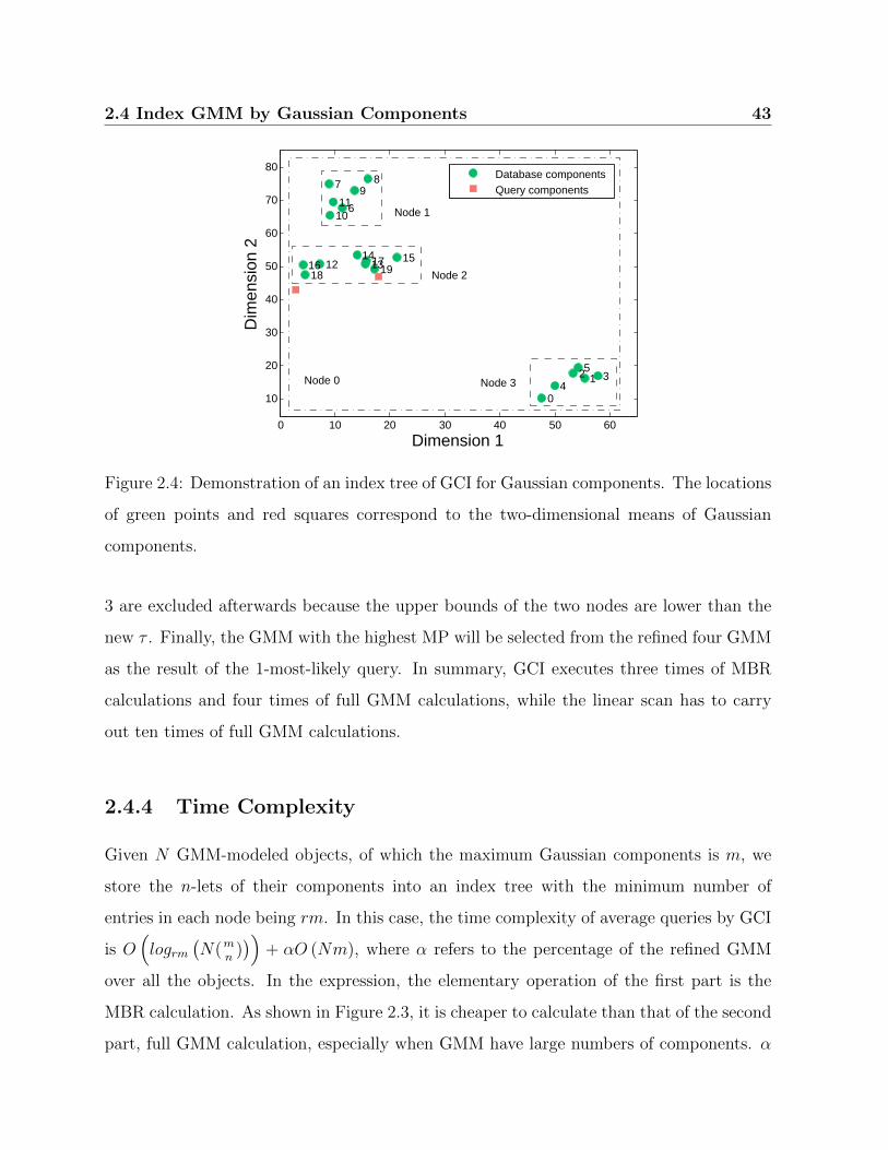
2.4 Index GMM by Gaussian Components 43
0 10 20 30 40 50 60
10
20
30
40
50
60
70
80
0
24
6
8
10
1214
1618
1 35
79
11
131517
19
Dimension 1
Dim
ensi
on 2
Database componentsQuery components
Node 0
Node 2
Node 3
Node 1
Figure 2.4: Demonstration of an index tree of GCI for Gaussian components. The locations
of green points and red squares correspond to the two-dimensional means of Gaussian
components.
3 are excluded afterwards because the upper bounds of the two nodes are lower than the
new τ . Finally, the GMM with the highest MP will be selected from the refined four GMM
as the result of the 1-most-likely query. In summary, GCI executes three times of MBR
calculations and four times of full GMM calculations, while the linear scan has to carry
out ten times of full GMM calculations.
2.4.4 Time Complexity
Given N GMM-modeled objects, of which the maximum Gaussian components is m, we
store the n-lets of their components into an index tree with the minimum number of
entries in each node being rm. In this case, the time complexity of average queries by GCI
is O(logrm
(N(m
n)))
+ αO (Nm), where α refers to the percentage of the refined GMM
over all the objects. In the expression, the elementary operation of the first part is the
MBR calculation. As shown in Figure 2.3, it is cheaper to calculate than that of the second
part, full GMM calculation, especially when GMM have large numbers of components. α

44 2. Gaussian Component Based Index for GMM
varies in (0, 1], and it is related to data distributions and the settings of the employed
index tree. In the worst case, i.e. all the entries in the index tree of components have to
be refined, the second part of the time complexity will be equal to that of the linear scan:
O (Nm).
2.5 Experimental Evaluation
In this section, we provide the practical evaluations of GCI, comparing to PRQ [65] and the
linear scan. We choose PRQ because it is the only dynamic GMM-specific index structure
to the best of our knowledge. We first conduct experiments on synthetic data to investigate
how the three approaches perform when varying the dimensionality of the data, the number
of GMM components or objects, and k in k-most-likely queries1. Since PRQ is yield to
storing only single Gaussian components, GCI uses the same setting for the comparison.
Besides, GCI is evaluated with the varied number of components stored in the index entry.
Additionally, we evaluate the performance of the approximate queries provided by GCI.
Experiments on real-world data sets are also performed to evaluate the effectiveness and
efficiency of GCI.
GCI and PRQ share the same index tree of Gaussian components, and the minimum
and maximum entry numbers of each node in this tree are 10 and 50, respectively. All the
experiments arse implemented with Java 1.7, and executed on a regular workstation PC
with 3.4 GHz dual core CPU equipped with 32 GB RAM. For all the experiments, we use
the ten-fold cross validation and report the average results over 100 runs.
2.5.1 Data Sets
Synthetic data sets2 are generated by randomly choosing mean values between 0 and 100
and standard deviations between 0 and 5 for each Gaussian component. The weights are
1The probability threshold queries have the similar performance with the k-most-likely queries, thus
the experiments of the former are not included in this chapter due to the limited space.2https://drive.google.com/open?id=0B3LRCuPdnX1BaXJra2VSVTZLU1E

2.5 Experimental Evaluation 45
randomly assigned, and sum up to one within each GMM.
As for the real-world data sets, since we are not interested in tuning the modeling of data
objects into its optimum, the numbers of Gaussian components in GMM are determined
by the rule of thumb instead of the Bayesian Information Criterion. The Expectation-
Maximization algorithm3 is used to learn GMM from the data objects.
Classificacao Nacional de Atividade Economica4 (CNAE) is a set of text documents of
Brazilian companies. We estimate 20-component GMM from it.
The Audio data set consists of selected speeches from ten speakers in Open Speech Data
Corpus5. The ten speakers are Aaron, Abdul Moiz, Afshad, Afzal, Akahansson, Alexander
Drachmann, Afred Strauss, Andy, Anna Karpelevich and Anniepoo. Every wav file is split
into ten fragments which are then transformed into frequency domains by Fast Fourier
Transform, and used to generate ten-component GMM.
Amsterdam Library of Object Images6 (ALOI) is a collection of images taking under
various light conditions and rotation angles. Here we use the 1000-level histogram of each
picture to train an univariate GMM, which has eight components. CorelDB data7 is another
image data set from the Corel image database. We use the grey histogram information of
each image to general ten-component GMM.
Weather Underground8 collects the historical weather data of the world. We use the
daily weather data of 907 airports in Europe from year 2005 to 2014. The selected features
of the Airports Weather data are temperature, humidity, sea level pressure, visibility
distance and wind speed, and the average values of each day are used. For each airport, a
ten-component GMM is estimated.
3Implementation provided by WEKA at http://weka.sourceforge.net/doc.dev/weka/clusterers/
EM.html.4https://archive.ics.uci.edu/ml/datasets/CNAE-95 http://www.repository.voxforge1.org/downloads/SpeechCorpus/Trunk/Audio/Main/16kHz_
16bit/6http://aloi.science.uva.nl/7https://sites.google.com/site/dctresearch/Home/content-based-image-retrieval8https://www.wunderground.com/history
46 2. Gaussian Component Based Index for GMM
The NBA players data9 provides all the performance statistics of every player in the
history. We collect 1,023,731 game logs of 2444 players till 2014, and build a GMM with
20 components for each player using his 15 statistical data, including MIN, FGM, FGA,
3FGM, FTM, FTA, OREB, DREB, REB, AST, STL, BLK, TO, PF and PFS10.
2.5.2 Experiments on Synthetic Data
We compare the query times and average accuracies of GCI, PRQ and the linear scan, and
analyze the performance of GCI when varying its settings.
We start with experiments by scaling the data dimension d, the Gaussian components
number m of GMM, the object number N and k in k-most-likely queries.
As shown in Figure 2.5, GCI generally achieves the least run-time comparing to the
other approaches. In Figure 2.5(a), both the linear scan and GCI have a linear relation
with the data dimension, but the latter is much placid than the former. PRQ has a rather
stable time cost with the increase of the data dimension. In Figure 2.5(b), GCI has a
linear dependency with the component number of GMM. The linear scan completes the
queries in polynomial time, sharing the same trend with the full GMM calculations shown
in Figure 2.3. PRQ shows a similar trend with the linear scan, but costs slightly less run-
time. Figure 2.5(c) shows that with the increase of the object number, GCI is more and
more efficient than the linear scan and PRQ, except that it costs slightly more time than
the linear scan when the object number is ten. When varying k in k-most-likely queries,
the linear scan has a stable run-time cost, while that of GCI and PRQ increase linearly,
but GCI still costs less run-time than the linear scan (Figure 2.5(d)).
The percentages of refined GMM (referred to as refined percentages) are shown in
Figure 2.6, where GCI always has a lower refined percentage than PRQ, except for Figure
2.6(c). Both GCI and PRQ have stable refined percentages with the increase of the data
dimension (Figure 2.6(a)). GCI keeps the same trend when increasing the component
number of each GMM, while the refined percentage of PRQ decreases to a stable level
9http://stats.nba.com/players/10Glossary is available at http://stats.nba.com/help/glossary.

2.5 Experimental Evaluation 47
(a) (b)
(c) (d)
Figure 2.5: Comparison of run-time between GCI, PRQ and the linear scan on synthetic
data. 1-most-likely queries are applied in (a), (b) and (c). In (a), the number of Gaussian
components in each GMM is fixed as ten and the object number is 100. The data dimension
in (b) is two and the object number is 100. In (c) the data dimension is two and the
components in each GMM is ten. The synthetic data set used in (d) has 100 GMM with
ten Gaussian components in a two-dimensional space.
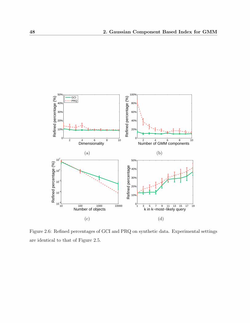
48 2. Gaussian Component Based Index for GMM
2 4 6 8 100
10%
20%
30%
40%
50%
Dimensionality
Ref
ined
per
cent
age
(%)
GCIPRQ
(a)
2 4 6 8 100
20%
40%
60%
80%
100%
Number of GMM components
Ref
ined
per
cent
age
(%)
(b)
10 100 1000 1000010
−6
10−4
10−2
100
102
Number of objects
Ref
ined
per
cent
age
(%)
(c)
1 3 5 7 9 11 13 15 17 190
10%
20%
30%
40%
50%
k in k−most−likely query
Ref
ined
per
cent
age
(d)
Figure 2.6: Refined percentages of GCI and PRQ on synthetic data. Experimental settings
are identical to that of Figure 2.5.

2.5 Experimental Evaluation 49
Table 2.1: Search accuracy of PRQ on synthetic data.
index Data dimension Component # Object # k-most-likely
i d = i m = i N = 10i k = 2i− 1
1 0.135 0.000 0.490 0.085
2 0.070 0.079 0.110 0.253
3 0.110 0.076 0.000 0.419
4 0.117 0.074 0.000 0.538
5 0.174 0.118 0.558
6 0.124 0.143 0.527
7 0.119 0.125 0.549
8 0.178 0.131 0.588
9 0.183 0.094 0.600
10 0.102 0.097 0.591
when there are more than four components in each GMM (Figure 2.6(b)). Figure 2.6(c)
shows the decrease of the refined percentages of GCI and PRQ when we have an increasing
number of objects in the data set. The refined percentages of the two methods increase
with k in k-most-likely queries in Figure 2.6(d), corresponding to the trend of the run-time
costs as shown in Figure 2.5(d). It is notable that GCI and the linear scan guarantee the
search accuracy which reaches 100%, while PRQ gets a very low accuracy as shown in
Table 2.1.
GCI can not only store more than one single Gaussian component in each entry, but
also support approximate queries to obtain better efficiency. Each GMM in the database
is decomposed into Gaussian components and the n-lets of the components are stored in
the index tree of GCI. For each approximate query, the Gaussian components of the query
object are sorted by the weights, and only the top-ranked components are used for applying
the query. Taking the synthetic data set used in Figure 2.5(d) for example, we keep k in
k-most-likely queries to one, but vary the number of components n in each entry as well
as the percentage of used Gaussian components for the query. The time cost for building
the index tree achieves its maximum when storing only one single Gaussian component in

50 2. Gaussian Component Based Index for GMM
each entry, and fluctuates within a narrow range with the increase of n (Figure 2.7(a)).
The query time and the refined percentage of GCI share the same trend, and the lowest
three points are n = 1, 2, 5 (Figure 2.7(a) and (b)). The query time shows an approximate
linear relation with the percentage of used component for the query (Figure 2.7(c)). In
correspondence with that, the query accuracy slightly decreases with the query percentage,
and its variance increases at the same time (Figure 2.7(d)).
(a)
1 2 3 4 5 6 7 8 9 100.5
0.6
0.7
0.8
0.9
1Accuracy
Component number of each entry
Acc
urac
y
0
20
40
60
80
100
Ref
ined
per
cent
age
(%)
Refined percentage
(b)
(c)
100% 80% 60% 40% 20%0.8
0.85
0.9
0.95
1
1.05Accuracy
Percentage of used components in each query object
Acc
urac
y
0
10
20
Ref
ined
per
cent
age
(%)
Refined percentage
(d)
Figure 2.7: Results of 1-most-likely queries on the synthetic data used in Figure 2.5 (d)
when varying the parameters of GCI. The synthetic data set has 100 GMM, each of which
has ten Gaussian components in a two-dimensional space.
2.5.3 Experiments on Real-world Data
Moving to experiments on the real-world data sets, we measure the time cost, the refined
percentage and the number of accessed node in the index tree, and evaluate the performance
of approximate queries of GCI on CorelDB data.
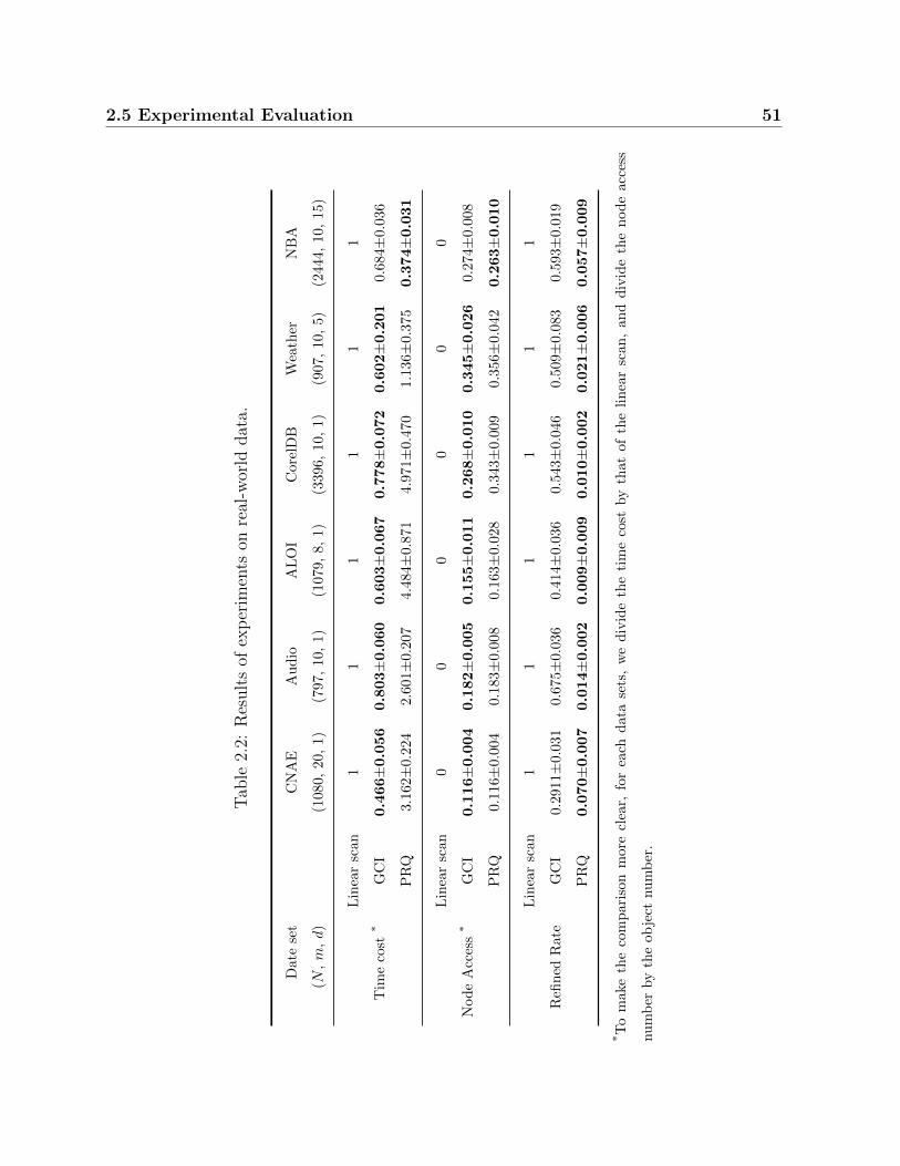
2.5 Experimental Evaluation 51
Tab
le2.
2:R
esult
sof
exp
erim
ents
onre
al-w
orld
dat
a.
Dat
ese
tC
NA
EA
ud
ioA
LO
IC
ore
lDB
Wea
ther
NB
A
(N,m
,d)
(108
0,20
,1)
(797,
10,
1)
(1079,
8,
1)
(3396,
10,
1)
(907,
10,
5)
(2444,
10,
15)
Lin
ear
scan
11
11
11
Tim
eco
st*
GC
I0.466±0.056
0.803±0.060
0.603±0.067
0.778±0.072
0.602±0.201
0.6
84±
0.0
36
PR
Q3.
162±
0.224
2.6
01±
0.2
07
4.4
84±
0.8
71
4.9
71±
0.4
70
1.1
36±
0.3
75
0.374±0.031
Lin
ear
scan
00
00
00
Nod
eA
cces
s*
GC
I0.116±0.004
0.182±0.005
0.155±0.011
0.268±0.010
0.345±0.026
0.2
74±
0.0
08
PR
Q0.
116±
0.004
0.1
83±
0.0
08
0.1
63±
0.0
28
0.3
43±
0.0
09
0.3
56±
0.0
42
0.263±0.010
Lin
ear
scan
11
11
11
Refi
ned
Rat
eG
CI
0.29
11±
0.031
0.6
75±
0.0
36
0.4
14±
0.0
36
0.5
43±
0.0
46
0.5
09±
0.0
83
0.5
93±
0.0
19
PR
Q0.070±0.007
0.014±0.002
0.009±0.009
0.010±0.002
0.021±0.006
0.057±0.009
*T
om
ake
the
com
par
ison
mor
ecl
ear,
for
each
data
sets
,w
ed
ivid
eth
eti
me
cost
by
that
of
the
lin
ear
scan
,an
dd
ivid
eth
en
od
eacc
ess
nu
mb
erby
the
obje
ctnu
mb
er.
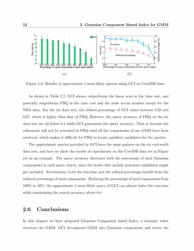
52 2. Gaussian Component Based Index for GMM
(a)
100% 80% 60% 40% 20%0.5
0.6
0.7
0.8
0.9
1
Accuracy
Percentage of used components in each query object
Acc
urac
y
0
20
40
60
80
100
Ref
ined
per
cent
age
(%)
Refined percentage
(b)
Figure 2.8: Results of approximate 1-most-likely queries using GCI on CorelDB data.
As shown in Table 2.2, GCI always outperforms the linear scan in the time cost, and
generally outperforms PRQ in the time cost and the node access number except for the
NBA data. For the six data sets, the refined percentage of GCI varies between 0.29 and
0.67, which is higher than that of PRQ. However, the query accuracy of PRQ on the six
data sets are all below 0.1 while GCI guarantees the query accuracy. That is because the
refinement will not be activated in PRQ until all the components of one GMM have been
retrieved, which makes it difficult for PRQ to locate qualified candidates for the queries.
The approximate queries provided by GCI have the same pattern on the six real-world
data sets, and here we show the results of experiments on the CorelDB data set in Figure
2.8 as an example. The query accuracy decreases with the percentage of used Gaussian
components in each query object, since the nodes that include potential candidates might
get excluded. Nevertheless, both the run-time and the refined percentage benefit from the
reduced percentage of used components. Reducing the percentage of used components from
100% to 20%, the approximate 1-most-likely query of GCI can almost halve the run-time
while maintaining the search accuracy above 0.8.
2.6 Conclusions
In this chapter we have proposed Gaussian Component based Index, a dynamic index
structure for GMM. GCI decomposes GMM into Gaussian components and stores the

2.6 Conclusions 53
single, pairs or n-lets of them in well developed index techniques. GCI provides the k-
most-likely queries, the probability threshold queries and the approximate queries. The
implementation of GCI in this chapter is based on an R-tree like structure, where the
conservative bound of MP enables the efficient pruning process while it guarantees the
query accuracy. Besides, a refinement strategy is introduced to exclude unnecessary
expensive full GMM calculations.
The extensive experiments on both the synthetic data sets and the real-world data sets
demonstrate the effectiveness and efficiency of GCI. GCI outperforms the linear scan as
well as PRQ which is the only existing dynamic index structure for GMM. The advantage of
GCI expands with the increase of the data dimension, the component number of GMM and
the number of GMM-modeled objects. Specifically, storing different numbers of Gaussian
components in each index entry, GCI enables a solution for some special applications which
need the faster building of the index. As for the approximate queries, GCI can make a
good balance between efficiency and accuracy when varying the percentage of used query
components which are chosen by the sorted weights.
For future work, the enrichment of the refinement strategy is a promising direction. New
criteria to exclude potential unqualified objects in tighter ways will improve the efficiency
of GCI. Moreover, similarity measures with metric properties for GMM is an interesting
topic for both the index and the subsequent analysis.

54 2. Gaussian Component Based Index for GMM
Chapter 3
Infinite Euclidean Distance
“Most of the world will make decisions by either guessing or using their gut.
They will be either lucky or wrong.”
Suhail Doshi
In this chapter, we propose IED, a novel metric for probability distribution functions
and it has a closed-form expression for GMM. Parts of this chapter have been published
in:
Linfei Zhou, Wei Ye, Claudia Plant, Christian Bohm. Knowledge Discovery of
Complex Data Using Gaussian Mixture Models. 18th International Conference
on Big Data Analytics and Knowledge Discovery, DaWaK 2017, August 28-31,
2017, Lyon, France.
where Linfei Zhou was mostly responsible for the development of main concepts, imple-
mented main algorithms and wrote the most parts of the paper. Wei Ye helped with the
design of experiment part. Christian Bohm and Claudia Plant supervised the project. All
co-authors contributed to the discussion, paper writing and revising.
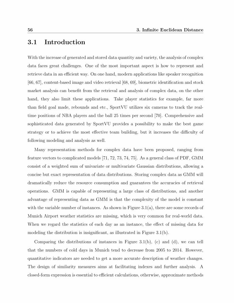
56 3. Infinite Euclidean Distance
3.1 Introduction
With the increase of generated and stored data quantity and variety, the analysis of complex
data faces great challenges. One of the most important aspect is how to represent and
retrieve data in an efficient way. On one hand, modern applications like speaker recognition
[66, 67], content-based image and video retrieval [68, 69], biometric identification and stock
market analysis can benefit from the retrieval and analysis of complex data, on the other
hand, they also limit these applications. Take player statistics for example, far more
than field goal made, rebounds and etc., SportVU utilizes six cameras to track the real-
time positions of NBA players and the ball 25 times per second [70]. Comprehensive and
sophisticated data generated by SportVU provides a possibility to make the best game
strategy or to achieve the most effective team building, but it increases the difficulty of
following modeling and analysis as well.
Many representation methods for complex data have been proposed, ranging from
feature vectors to complicated models [71, 72, 73, 74, 75]. As a general class of PDF, GMM
consist of a weighted sum of univariate or multivariate Gaussian distributions, allowing a
concise but exact representation of data distributions. Storing complex data as GMM will
dramatically reduce the resource consumption and guarantees the accuracies of retrieval
operations. GMM is capable of representing a large class of distributions, and another
advantage of representing data as GMM is that the complexity of the model is constant
with the variable number of instances. As shown in Figure 3.1(a), there are some records of
Munich Airport weather statistics are missing, which is very common for real-world data.
When we regard the statistics of each day as an instance, the effect of missing data for
modeling the distribution is insignificant, as illustrated in Figure 3.1(b).
Comparing the distributions of instances in Figure 3.1(b), (c) and (d), we can tell
that the numbers of cold days in Munich tend to decrease from 2005 to 2014. However,
quantitative indicators are needed to get a more accurate description of weather changes.
The design of similarity measures aims at facilitating indexes and further analysis. A
closed-form expression is essential to efficient calculations, otherwise, approximate methods
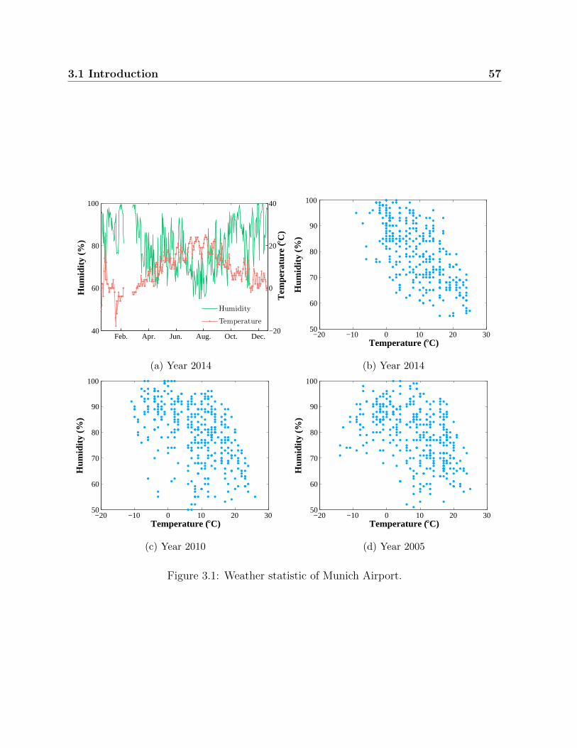
3.1 Introduction 57
Feb. Apr. Jun. Aug. Oct. Dec.40
60
80
100
Hum
idit
y (%
)
−20
0
20
40
Tem
pera
ture
(°C
)
Humidity
Temperature
(a) Year 2014
−20 −10 0 10 20 3050
60
70
80
90
100
Temperature (°C)
Hum
idit
y (%
)
(b) Year 2014
−20 −10 0 10 20 3050
60
70
80
90
100
Temperature (°C)
Hum
idit
y (%
)
(c) Year 2010
−20 −10 0 10 20 3050
60
70
80
90
100
Temperature (°C)
Hum
idit
y (%
)
(d) Year 2005
Figure 3.1: Weather statistic of Munich Airport.

58 3. Infinite Euclidean Distance
like Monte-Carlo sampling are needed, which results in time consuming and/or inaccurate.
What is more, since GMM might have different numbers of Gaussian components in them,
traditional indexes designed for fixed-length vectors can not be applied here. For those
indexes that are based on similarity measures, for instance, M-tree [44] and VP-tree [76],
the properties of metric (e.g., triangle inequality) are required for the similarity measure
to guarantee the effectiveness and efficiency queries. As we will demonstrate, the main
contributions of this chapter are:
• We generalize Euclidean distance to IED on PDF, prove its metric properties and
derive the closed-form expression for GMM.
• Our experimental evaluations on both synthetic and real-world data sets demonstrate
the effectiveness and efficiency of IED and the better performances than previous
similarity measures for GMM.
The rest of this chapter is organized as follows. In Section 3.2, we survey the previous
work. Section 3.3 gives the basic definition of GMM, and introduces IED, a metric with
closed-form expression for GMM. Section 3.4 shows the experimental studies for verifying
the efficiency and effectiveness of the proposed similarity measure. Section 3.5 summarizes
the chapter.
3.2 Related Work
This section gives a survey and discussion of previous work on Multiple-Instance Learning,
similarity measures and indexes for GMM.
3.2.1 Data Representations
For objects with inherent structures, MI is a natural way to describe them. First motivated
by the problem of drug activity predictions, MIL deals with MI objects that are sets (or
bags) of instances [77]. MIL algorithms can be grouped into three categories, the instance

3.2 Related Work 59
space based paradigm, the bag space based paradigm and the embedded space based
paradigm [78], the last of which maps MI objects into new feature spaces.
Many mapping methods have been proposed to represent the data of instances, in-
cluding feature vectors and complex models. The vocabulary based mapping clusters
all instances from all bags into k clusters (vocabularies), and then uses the histogram
information, i.e., the counts of instances that belong to these clusters, to obtain a k-
dimensional feature vector for each bag [72, 78, 79]. The instance based mapping models
instances as a feature. For example, DD-SVM (Diverse Density SVM) [80] uses instance
prototypes that obtained according to DD measure, while MILES [81] chooses one of
instances as the feature. The model based mapping trains each bag to a model, for instance,
each bag is represented by a k-component mixture model (EM-clustering [73], PPMM [82],
miFV [74]), a Gaussian distribution [83], a graph in miGraph [75], a joint optimization
concept [84] and so on.
Having the ability to approximate arbitrary distributions, GMM can achieve a more
accurate representation of data than the feature vectors and other models, and it is a
concise model as well [56].
3.2.2 Similarity Measures
Similarity measures for GMM can be grouped into two categories, having closed-form ex-
pressions for GMM or not. For measures that have no closed-form expressions, Monte Carlo
sampling or other approximation approaches are applied, which may be time consuming
or imprecise.
KL divergence [85] is a common way to measure the distance between two PDF. It
has a closed-form expression for Gaussian distributions, but no such expression for GMM
exists.
To compute the distance between GMM by KL divergence, several approximation
methods have been proposed. For two GMM, a commonly used approximation for KL
divergence between them is Gaussian approximation. It replaces two GMM with two

60 3. Infinite Euclidean Distance
Gaussian distributions, whose means and covariance matrices depend on those of GMM.
Another popular way is to use the minimum KL divergence of Gaussian components that
are included in two GMM. Moreover, Hershey et al. [59] have proposed the product of
Gaussian approximation and the variation approximation, but the former tends to greatly
underestimate the KL divergence between GMM while the latter does not satisfy the
positivity property. Besides, Goldberger et al. [58] have proposed the matching based KL
divergence (KLm) and the unscented transformation based KL divergence (KLt). KLm
works well when the Gaussian elements are far apart, but it cannot handle the overlapping
situations which are very common in real-world data sets. KLt solves the overlapping
problem based on a non-linear transformation. Cui et al. [86] have compared the six
approximation methods for KL divergence with Monte Carlo sampling, where the variation
approximation achieves the best result quality, while KLm give a comparable result with
a much faster speed.
Besides the approximation similarity methods for GMM, several methods with closed-
form expressions have been proposed. Helen et al. [60] have described a squared Euclidean
distance (SE), which integrates the squared differences over the whole feature space. Sfikas
et al. [61] have presented a KL divergence based distance C2 for GMM. Jensen et al. [62]
used a normalized L2 (NL2) distance to measure the similarity of GMM in mel-frequency
cepstral coefficients from songs. Beecks et al. have proposed GQFD for modeling image
similarity in image databases [63]. However, only GQFD fulfills the properties of metric
on condition that a proper setting of parameters is given.
3.2.3 Indexes
For the indexes of GMM, there are several techniques available, including universal index
structures designed for uncertain data and GMM-specific methods.
U-tree provides a probability threshold retrieval on general multi-dimensional uncertain
data [46]. It pre-computes a finite number of PCR) which are possible appearance regions
with fixed probabilities, and uses them to prune unqualified objects. Although U-tree works
3.3 Methods 61
well with single PDF, its effectiveness deteriorates for mixture models such as GMM. The
reason behind this is that it is difficult for PCR to represent mixture models, especially
when the component numbers increase.
Rougui et al. [57] have designed a bottom-up hierarchical tree and an iterative grouping
tree for GMM-modeled speaker retrieval systems. Both approaches provide only two index
levels, and are lack of a convenient insertion and deletion strategy. Furthermore, they can
not guarantee reliable query results.
Instead of indexing curves as spatial objects in feature spaces, PRQ technique [65]
and Gaussian Component based Index [48] search the parameter space of the means and
variances of GMM. However, PRQ can not guarantee the query accuracy since it assumes
that all the Gaussian components of candidates have relatively high matching probabilities
with query objects, which is not common in general cases. For both indexes, their prune
strategies are highly effected by the distributions of Gaussian components.
Similarity measures that have the properties of metric can easily be supported by metric
trees like M-tree [44] and VP-tree [76]. Otherwise, special designed structures are needed
to guarantee efficient queries.
3.3 Methods
In this section, firstly we summarize the formal notations for GMM, then we introduce
IED for distributions and give the proof of its metric properties. Finally we derive the
closed-form expression of IED for GMM.
3.3.1 Gaussian Mixture Models
A GMM is a probabilistic model that represents the probability distribution of observations.
The definition is shown as follows.
Definition 4. (Gaussian Mixture Models) Let x ∈ RD be a variable in a D-dimensional
space, x = (x1, x2, ..., xD). A Gaussian Mixture Model G is the weighted sum of m Gaussian
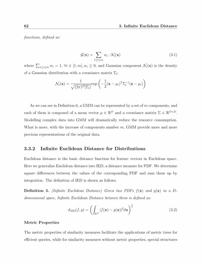
62 3. Infinite Euclidean Distance
functions, defined as:
G(x) =∑
1≤i≤m
wi · Ni(x) (3.1)
where∑
1≤i≤mwi = 1, ∀i ∈ [1,m], wi ≥ 0, and Gaussian component Ni(x) is the density
of a Gaussian distribution with a covariance matrix Σi:
Ni(x) =1√
(2π)D|Σi|exp
(−1
2(x− µi)TΣ−1
i (x− µi))
As we can see in Definition 6, a GMM can be represented by a set of m components, and
each of them is composed of a mean vector µ ∈ RD and a covariance matrix Σ ∈ RD×D.
Modelling complex data into GMM will dramatically reduce the resource consumption.
What is more, with the increase of components number m, GMM provide more and more
precious representations of the original data.
3.3.2 Infinite Euclidean Distance for Distributions
Euclidean distance is the basic distance function for feature vectors in Euclidean space.
Here we generalize Euclidean distance into IED, a distance measure for PDF. We determine
square differences between the values of the corresponding PDF and sum them up by
integration. The definition of IED is shown as follows.
Definition 5. (Infinite Euclidean Distance) Given two PDFs f(x) and g(x) in a D-
dimensional space, Infinite Euclidean Distance between them is defined as:
dIED(f, g) =
(∫
RD|f(x)− g(x)|2dx
) 12
(3.2)
Metric Properties
The metric properties of similarity measures facilitate the applications of metric trees for
efficient queries, while for similarity measures without metric properties, special structures
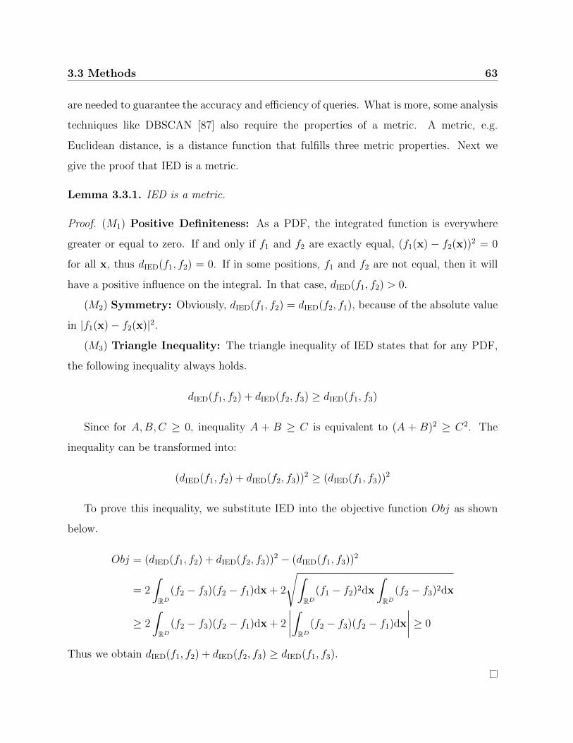
3.3 Methods 63
are needed to guarantee the accuracy and efficiency of queries. What is more, some analysis
techniques like DBSCAN [87] also require the properties of a metric. A metric, e.g.
Euclidean distance, is a distance function that fulfills three metric properties. Next we
give the proof that IED is a metric.
Lemma 3.3.1. IED is a metric.
Proof. (M1) Positive Definiteness: As a PDF, the integrated function is everywhere
greater or equal to zero. If and only if f1 and f2 are exactly equal, (f1(x) − f2(x))2 = 0
for all x, thus dIED(f1, f2) = 0. If in some positions, f1 and f2 are not equal, then it will
have a positive influence on the integral. In that case, dIED(f1, f2) > 0.
(M2) Symmetry: Obviously, dIED(f1, f2) = dIED(f2, f1), because of the absolute value
in |f1(x)− f2(x)|2.
(M3) Triangle Inequality: The triangle inequality of IED states that for any PDF,
the following inequality always holds.
dIED(f1, f2) + dIED(f2, f3) ≥ dIED(f1, f3)
Since for A,B,C ≥ 0, inequality A + B ≥ C is equivalent to (A + B)2 ≥ C2. The
inequality can be transformed into:
(dIED(f1, f2) + dIED(f2, f3))2 ≥ (dIED(f1, f3))2
To prove this inequality, we substitute IED into the objective function Obj as shown
below.
Obj = (dIED(f1, f2) + dIED(f2, f3))2 − (dIED(f1, f3))2
= 2
∫
RD(f2 − f3)(f2 − f1)dx + 2
√∫
RD(f1 − f2)2dx
∫
RD(f2 − f3)2dx
≥ 2
∫
RD(f2 − f3)(f2 − f1)dx + 2
∣∣∣∣∫
RD(f2 − f3)(f2 − f1)dx
∣∣∣∣ ≥ 0
Thus we obtain dIED(f1, f2) + dIED(f2, f3) ≥ dIED(f1, f3).

64 3. Infinite Euclidean Distance
Closed-form Expression
Firstly we derive the closed-form expression for the inner product of GMM. Let G1 and
G2 be two GMM with diagonal covariance matrices, and they have m1 and m2 Gaussian
components, respectively. Let x be a feature vector in the space RD. The inner product
of G1 and G2 can be derived as:
〈G1,G2〉 =
∫
RD
m1∑
i=1
w1,i · N (µ1,i, σ21,i)
m2∑
j=1
w2,j · N (µ2,j, σ22,j)dx
=
m1∑
i=1
m2∑
j=1
w1,iw2,j
D∏
l=1
1
2π√σ2
1,i,lσ22,j,l
∫e−
(x−µ1,i,l)2
2σ21,i,l
−(x−µ2,j,l)
2
2σ22,j,l dx
=
m1∑
i=1
m2∑
j=1
w1,iw2,j
D∏
l=1
e−
(µ1,i,l−µ2,j,l)2
2(σ21,i,l
+σ22,j,l
)
√2π(σ2
1,i,l + σ22,j,l)
(3.3)
where σ1,i,l and σ2,j,l are the l-th diagonal elements of Σ1,i and Σ2,j, respectively.
The relation of the inner product to IED is:
dIED(G1,G2) =√〈G1,G1〉+ 〈G2,G2〉 − 2〈G1,G2〉 (3.4)
A closed-form expression is intrinsically valuable for computations. It saves extra efforts
to get a good approximation by avoiding simulation methods, like Monte Carlo sampling,
which may cause a significant increase in computation time and the loss of precision.
Therefore, closed-form expressions are well received in many applications, especially in
real-time applications. It is worth noting that only for GMM that have diagonal covariance
matrices, IED for GMM has a closed-form expression, so are the other similarity measures
to the best of our knowledge.
3.4 Experimental Evaluations
In this section, we provide experimental evaluations on both synthetic and real-world data
sets to show the efficiency and effectiveness of complex data analysis using GMM and the
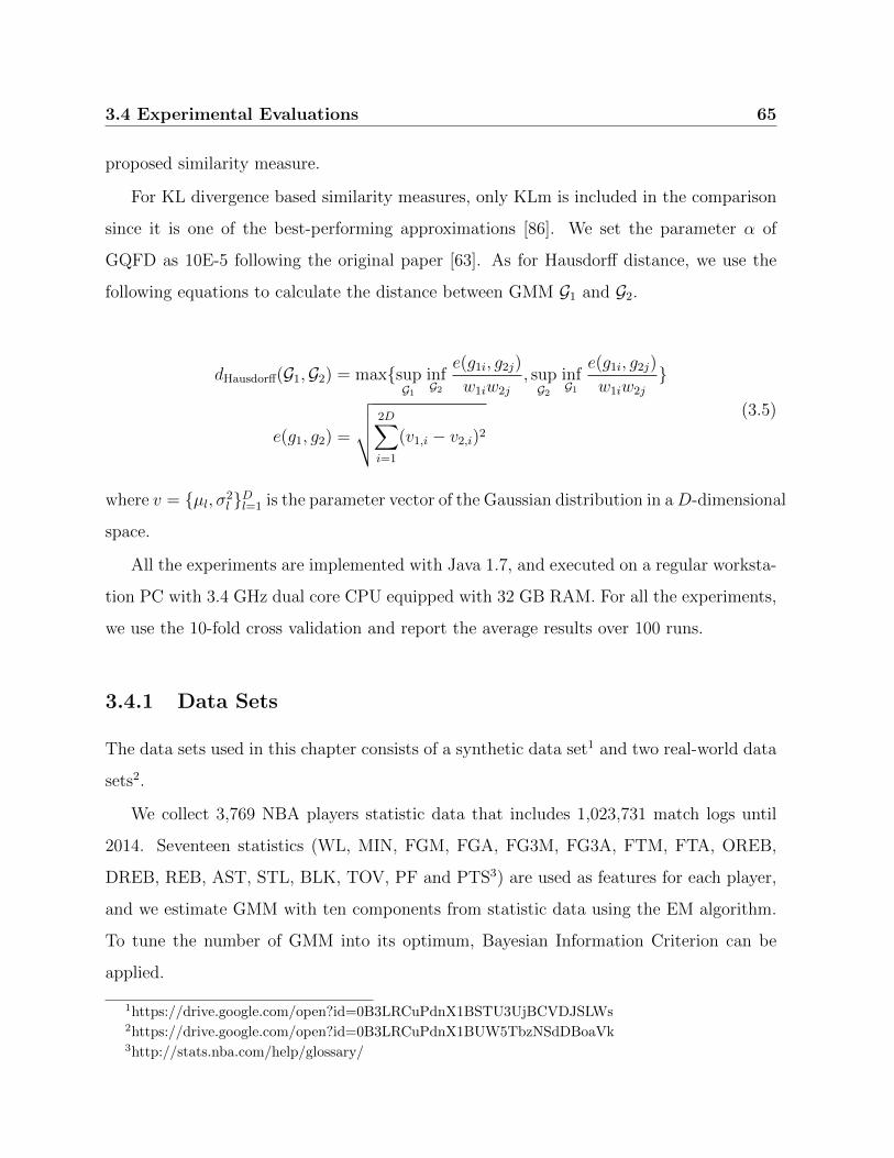
3.4 Experimental Evaluations 65
proposed similarity measure.
For KL divergence based similarity measures, only KLm is included in the comparison
since it is one of the best-performing approximations [86]. We set the parameter α of
GQFD as 10E-5 following the original paper [63]. As for Hausdorff distance, we use the
following equations to calculate the distance between GMM G1 and G2.
dHausdorff(G1,G2) = maxsupG1
infG2
e(g1i, g2j)
w1iw2j
, supG2
infG1
e(g1i, g2j)
w1iw2j
e(g1, g2) =
√√√√2D∑
i=1
(v1,i − v2,i)2
(3.5)
where v = µl, σ2l Dl=1 is the parameter vector of the Gaussian distribution in aD-dimensional
space.
All the experiments are implemented with Java 1.7, and executed on a regular worksta-
tion PC with 3.4 GHz dual core CPU equipped with 32 GB RAM. For all the experiments,
we use the 10-fold cross validation and report the average results over 100 runs.
3.4.1 Data Sets
The data sets used in this chapter consists of a synthetic data set1 and two real-world data
sets2.
We collect 3,769 NBA players statistic data that includes 1,023,731 match logs until
2014. Seventeen statistics (WL, MIN, FGM, FGA, FG3M, FG3A, FTM, FTA, OREB,
DREB, REB, AST, STL, BLK, TOV, PF and PTS3) are used as features for each player,
and we estimate GMM with ten components from statistic data using the EM algorithm.
To tune the number of GMM into its optimum, Bayesian Information Criterion can be
applied.
1https://drive.google.com/open?id=0B3LRCuPdnX1BSTU3UjBCVDJSLWs2https://drive.google.com/open?id=0B3LRCuPdnX1BUW5TbzNSdDBoaVk3http://stats.nba.com/help/glossary/

66 3. Infinite Euclidean Distance
For another real-world data, we use daily weather data of 2,946 airports in the whole
year 2014. Because of missing data, there are 961,308 pieces of records in the data set. The
selected features are temperature and humidity, and only the average values of each day
are used. For each airport, a ten-component GMM is estimated by EM algorithm based
on the whole year weather data.
3.4.2 Query performance
We study the performance of the only two metrics, IED and GQFD4, when using VP-
tree to facilitate efficient queries. The query results on synthetic data are reported in
Figure 3.2. As shown in Figure 3.2(a), the acceleration ratio (comparing with linear scan)
of IED increases with the number of stored objects while that of GQFD almost remains
unchanged. As for the query time (Figure 3.2(b)), IED costs more run-time than GQFD
at the beginning, then achieves a much better results than GQFD with the increase of the
number of objects.
0
5
10
15
20
25
27 28 29 210 211 212
Number of objects
Acc
eler
atio
n R
atio
IED
GQFD
(a) Acceleration ratio
101
102
103
104
105
27 28 29 210 211 212
Number of objects
Que
ry t
ime
(ms)
(b) Query time
Figure 3.2: 1-Nearest Neighbour query results of IED and GQFD on synthetic data using
VP-tree. The capacity of nodes in the VP-tree is set to 32.
4With the given parameter, the query accuracies of GQFD using VP-tree is guaranteed for the synthetic
data.
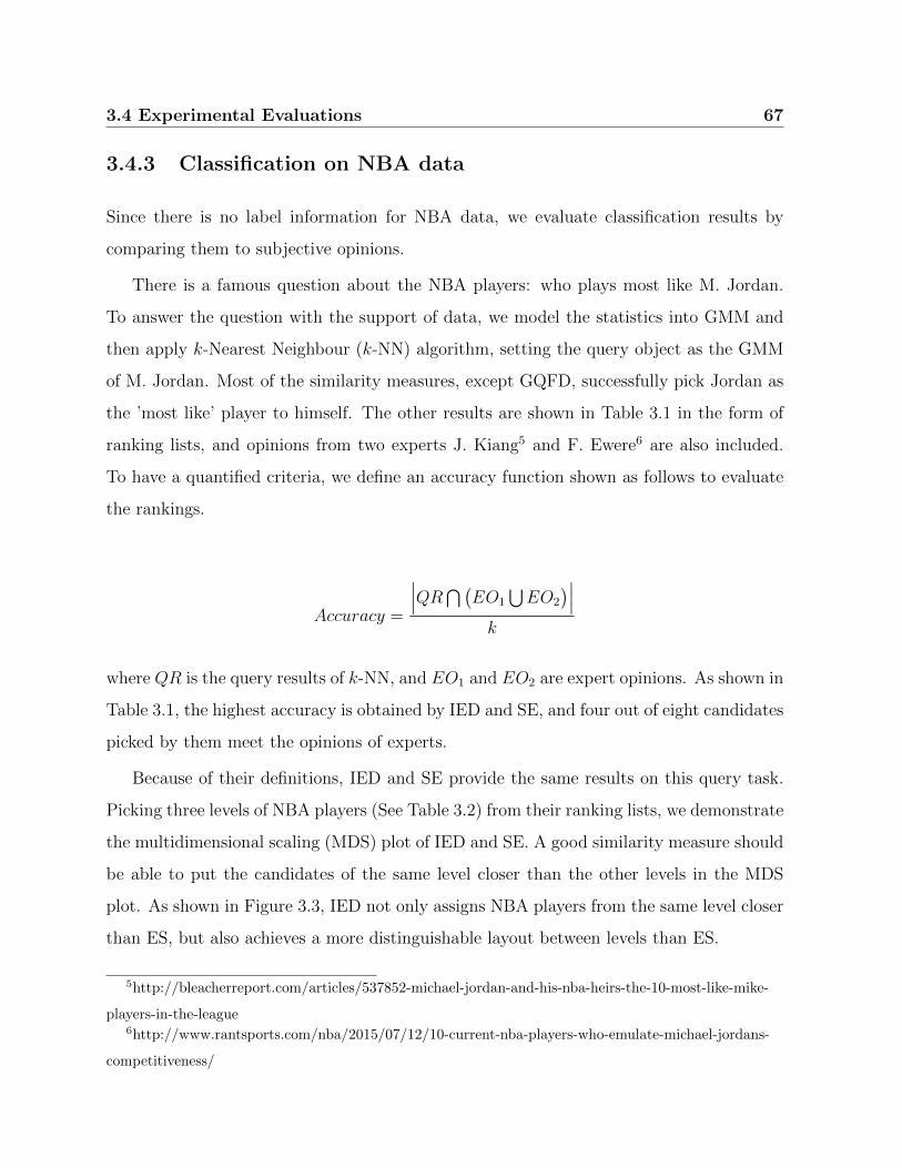
3.4 Experimental Evaluations 67
3.4.3 Classification on NBA data
Since there is no label information for NBA data, we evaluate classification results by
comparing them to subjective opinions.
There is a famous question about the NBA players: who plays most like M. Jordan.
To answer the question with the support of data, we model the statistics into GMM and
then apply k-Nearest Neighbour (k-NN) algorithm, setting the query object as the GMM
of M. Jordan. Most of the similarity measures, except GQFD, successfully pick Jordan as
the ’most like’ player to himself. The other results are shown in Table 3.1 in the form of
ranking lists, and opinions from two experts J. Kiang5 and F. Ewere6 are also included.
To have a quantified criteria, we define an accuracy function shown as follows to evaluate
the rankings.
Accuracy =
∣∣∣QR⋂(
EO1
⋃EO2
)∣∣∣k
where QR is the query results of k-NN, and EO1 and EO2 are expert opinions. As shown in
Table 3.1, the highest accuracy is obtained by IED and SE, and four out of eight candidates
picked by them meet the opinions of experts.
Because of their definitions, IED and SE provide the same results on this query task.
Picking three levels of NBA players (See Table 3.2) from their ranking lists, we demonstrate
the multidimensional scaling (MDS) plot of IED and SE. A good similarity measure should
be able to put the candidates of the same level closer than the other levels in the MDS
plot. As shown in Figure 3.3, IED not only assigns NBA players from the same level closer
than ES, but also achieves a more distinguishable layout between levels than ES.
5http://bleacherreport.com/articles/537852-michael-jordan-and-his-nba-heirs-the-10-most-like-mike-
players-in-the-league6http://www.rantsports.com/nba/2015/07/12/10-current-nba-players-who-emulate-michael-jordans-
competitiveness/
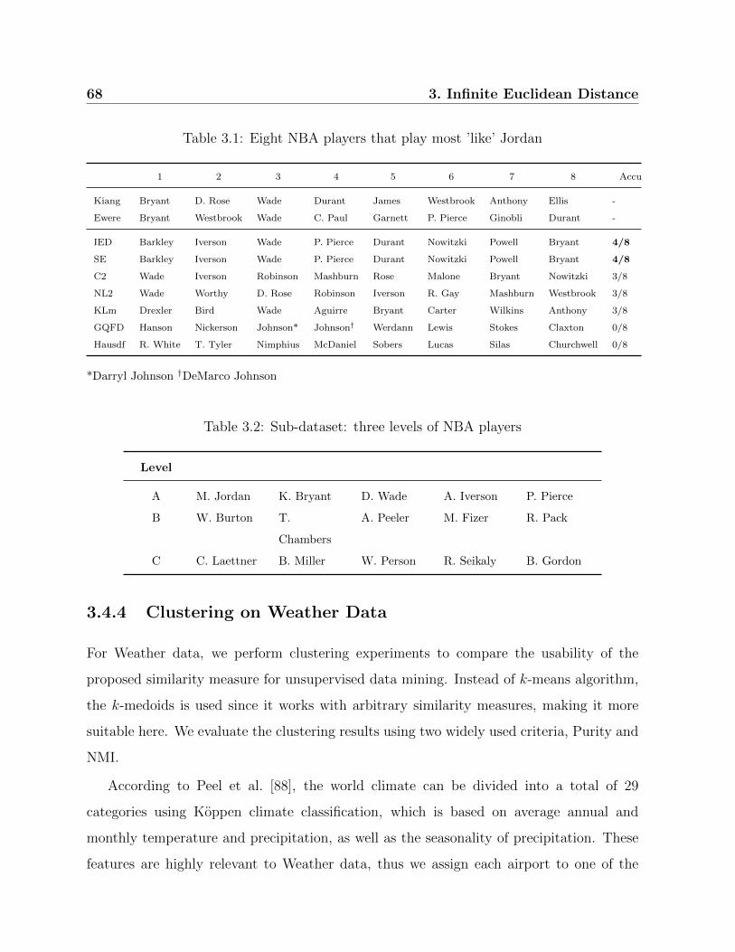
68 3. Infinite Euclidean Distance
Table 3.1: Eight NBA players that play most ’like’ Jordan
1 2 3 4 5 6 7 8 Accu
Kiang Bryant D. Rose Wade Durant James Westbrook Anthony Ellis -
Ewere Bryant Westbrook Wade C. Paul Garnett P. Pierce Ginobli Durant -
IED Barkley Iverson Wade P. Pierce Durant Nowitzki Powell Bryant 4/8
SE Barkley Iverson Wade P. Pierce Durant Nowitzki Powell Bryant 4/8
C2 Wade Iverson Robinson Mashburn Rose Malone Bryant Nowitzki 3/8
NL2 Wade Worthy D. Rose Robinson Iverson R. Gay Mashburn Westbrook 3/8
KLm Drexler Bird Wade Aguirre Bryant Carter Wilkins Anthony 3/8
GQFD Hanson Nickerson Johnson* Johnson† Werdann Lewis Stokes Claxton 0/8
Hausdf R. White T. Tyler Nimphius McDaniel Sobers Lucas Silas Churchwell 0/8
*Darryl Johnson †DeMarco Johnson
Table 3.2: Sub-dataset: three levels of NBA players
Level
A M. Jordan K. Bryant D. Wade A. Iverson P. Pierce
B W. Burton T.
Chambers
A. Peeler M. Fizer R. Pack
C C. Laettner B. Miller W. Person R. Seikaly B. Gordon
3.4.4 Clustering on Weather Data
For Weather data, we perform clustering experiments to compare the usability of the
proposed similarity measure for unsupervised data mining. Instead of k-means algorithm,
the k-medoids is used since it works with arbitrary similarity measures, making it more
suitable here. We evaluate the clustering results using two widely used criteria, Purity and
NMI.
According to Peel et al. [88], the world climate can be divided into a total of 29
categories using Koppen climate classification, which is based on average annual and
monthly temperature and precipitation, as well as the seasonality of precipitation. These
features are highly relevant to Weather data, thus we assign each airport to one of the

3.4 Experimental Evaluations 69
Level ALevel BLevel C
(a) IED (b) ES
Figure 3.3: Multidimensional scaling plot of 15 players using different similarity measures.
Each marker (dot, diamond and square) represents a NBA player.
categories according to its location and get 25 classes of climate types (Cwc, Dsd, Dwd
and EF are not included) in total.
Table 3.3 shows the clustering results of Weather data. We can see that IED achieves
the highest Purity and NMI among all the similarity measures. To get an visualized
impression of the best two results from IED and NL2, we mark the airports of different
clusters as dots with different colors in Figure 3.4.
Figure 3.4(a) shows the ground truth of Koppen climate classification of all the world.
Figure 3.4(b) and (c) demonstrate the clustering results of IED and NL2, respectively. To
compare these two results, we focus on the clusters in areas like Africa, North America
and Southeast Asian Islands. Climate type BWh locates in North Africa and the most
part of Australia. The result of IED indicates the same trend with the ground truth. NL2
clusters airports that locate in North Africa and Australia in the same group, however, it
also includes airports that locate in the south part of Africa. For airports in North America
and Southeast Asian Islands, IED outperforms NL2 with a more clear categories.
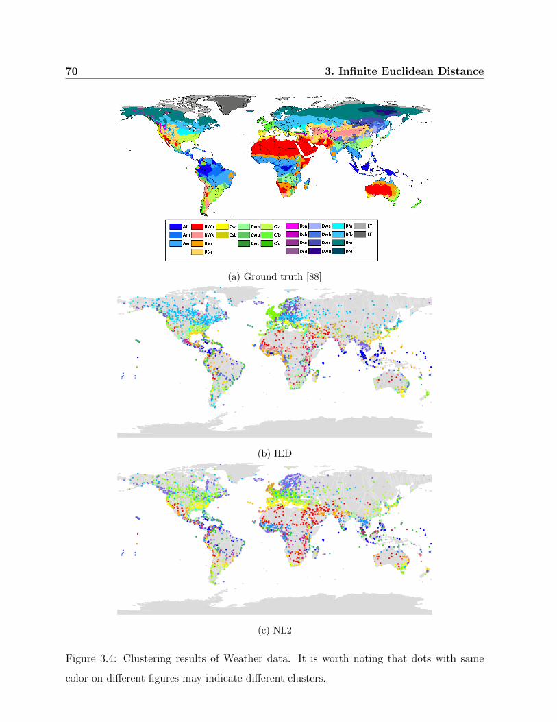
70 3. Infinite Euclidean Distance
(a) Ground truth [88]
(b) IED
(c) NL2
Figure 3.4: Clustering results of Weather data. It is worth noting that dots with same
color on different figures may indicate different clusters.

3.5 Conclusions 71
Table 3.3: Clustering results of Weather data
Purity NMI
IED 0.363±0.010 0.245±0.000SE 0.342±0.014 0.241±0.000
C2 0.347±0.010 0.231±0.010
NL2 0.357±0.010 0.237±0.000
KLm 0.337±0.014 0.224±0.010
GQFD 0.198±0.024 0.143±0.083
Hausdorff 0.219±0.014 0.085±0.010
3.5 Conclusions
In this chapter, we generalize Euclidean distance to IED for probability distribution func-
tions, and derive its closed-form expression for GMM. The metric properties of the proposed
similarity measure enable the usage of metric trees for indexing GMM. Representing
complex data that have inherent structures as GMM, we apply classification and clustering
analysis on real-world data with different similarity measures. Experimental evaluations
demonstrate the efficiency and effectiveness of the proposed similarity measure and better
performances than its comparisons.
For the future work, a GMM-specific index structure that uses IED as the similarity
measure is a perspective to outperform general metric trees.

72 3. Infinite Euclidean Distance

Chapter 4
Novel Indexing Strategy and
Similarity Measures for GMM
“You can use all the quantitative data you can get, but you still have to
distrust it and use your own intelligence and judgment.”
Alvin Toffler
In this chapter, we propose a novel strategy to improve the performance of GCI, and
several novel similarity measures on basis of that. Parts of this chapter have been published
in:
Linfei Zhou, Wei Ye, Bianca Wackersreuther, Claudia Plant, Christian Bohm.
Novel Indexing Strategy and Similarity Measures for Gaussian Mixture Models.
28th International Conference on Database and Expert Systems Applications,
DEXA 2017, August 28-31, 2017, Lyon, France.
where Linfei Zhou was mostly responsible for the development of main concepts, imple-
mented main algorithms and wrote the most parts of the paper. Wei Ye and Bianca
Wackersreuther helped with the discussion and experimental design. Christian Bohm and
Claudia Plant supervised the project. All co-authors contributed to the discussion, paper
writing and revising.

74 4. Novel Indexing Strategy and Similarity Measures for GMM
4.1 Introduction
With the increase of generated and stored data quantity and variety, information extraction
systems face great challenges in the representation and analysis of the data. Take player
statistics for example, far more than field goal made, rebounds and etc., SportVU utilizes
six cameras to track the real-time positions of NBA players and the ball 25 times per
second [70]. Comprehensive and sophisticated data generated by SportVU provides a
possibility to make the best game strategy or to achieve the most effective team building,
but it increases the difficulty of following modeling and analysis as well. Besides, many
modern applications like speaker recognition systems [66, 67], content-based image and
video retrieval [68, 69], biometric identification and stock market analysis not only can
benefit from the retrieval and analysis of complex data, or the distributions of data, but
also are limited by them.
Various statistical models have been proposed in this actively investigated research field.
As a general class of PDF, GMM consist of a weighted sum of univariate or multivariate
Gaussian distributions, allowing a concise but exact representation of data distributions.
Storing complex data as GMM will dramatically reduce the resource consumption and
guarantees the accuracies of retrieval operations.
Besides the data representation, another important aspect is the design of similarity
measures that aims at facilitating indexes and further analysis. Matching probability [45]
sums up the joint probabilities of two PDF, and for GMM it has s closed-form expression
which is essential for efficient calculations. What is more, several similarity measures that
have closed-form expressions can be reformed into the functions of matching probabili-
ty [60, 61, 62]. Since GMM might have different numbers of Gaussian components in
them, traditional indexes designed for fixed-length vectors cannot be applied directly. For
the indexes of distributions, such as U-tree, their performances deteriorate on mixture
models [46]. Storing the components, instead of GMM, into entries, both GCI [48] and
PRQ [65] provide solutions for efficient range queries and nearest-neighbour queries on
GMM using matching probability. However, the efficiency of the two indexes vary with the

4.2 Related Work 75
distributions of components in GMM because of the settings of nodes, which encourages us
to improve the situation. As we will demonstrate, the main contributions of this chapter
are:
• We introduce a generalization technique called Normalize Transformation. After
Normalize Transformation, indexes based on matching probability can achieve the
better performances of queries on GMM.
• Normalize Transformation enables us to derive a set of new similarity measures from
the existing ones. The normalized versions of the similarity measures share the same
time complexity of their origins.
• Our experimental evaluation demonstrates the efficiency of filtering in GCI using
normalized matching probability and the better performances of normalized similarity
measures over their origins.
The rest of this chapter is organized as follows: In Section 4.2, we survey the previous
work. Section 4.3 gives the basic definition of GMM and matching probability. Section 4.4
introduces the motivation of the Normalized Transformation, and demonstrates how it
works. Section 4.5 shows the experimental studies for verifying the efficiency and effective-
ness of the proposed similarity measures. Section 4.6 summarizes the chapter.
4.2 Related Work
This section gives a survey and discussion of similarity measures and indexes for GMM in
previous work.
4.2.1 Similarity Measures
Similarity measures for GMM can be grouped into two categories, having closed-form ex-
pressions for GMM or not. For measures that have no closed-form expression, Monte Carlo

76 4. Novel Indexing Strategy and Similarity Measures for GMM
sampling or other approximation approaches are applied, which may be time consuming
or imprecise.
KL divergence [85] is a common way to measure the distance between two PDF. It
has a closed-form expression for Gaussian distributions, but no such expression for GMM
exists.
To compute the distance between GMM by KL divergence, several approximation
methods have been proposed. For two GMM, a commonly used approximation for KL
divergence between them is Gaussian approximation. It replaces two GMM with two
Gaussian distributions, whose means and covariance matrices depend on those of GMM.
Another popular way is to use the minimum KL divergence of Gaussian components that
are included in two GMM. Moreover, Hershey et al. [59] have proposed the product of
Gaussian approximation and the variation approximation, but the former tends to greatly
underestimate the KL divergence between GMM while the latter does not satisfy the
positivity property. Besides, Goldberger et al. [58] have proposed the matching based KL
divergence (KLm) and the unscented transformation based KL divergence (KLt). KLm
works well when the Gaussian elements are far apart, but it cannot handle the overlapping
situations which are very common in real-world data sets. KLt solves the overlapping
problem based on a non-linear transformation. Cui et al. [86] have compared the six
approximation methods for KL divergence with Monte Carlo sampling, where the variation
approximation achieves the best result quality, while KLm gives a comparable result with
a much faster speed.
Besides the approximation similarity methods for GMM, several methods with closed-
form expression have been proposed. Helen et al. [60] have described a squared Euclidean
distance, which integrates the squared differences over the whole feature space. It has
a closed-form expression for GMM. Sfikas et al. [61] have presented a KL divergence
based distance C2 for GMM. Jensen et al. [62] used a normalized L2 distance to measure
the similarity of GMM in mel-frequency cepstral coefficients from songs. Beecks et al.
have proposed Signature Quadratic form Distance for modeling image similarity in image
databases [63].

4.3 Formal Definitions 77
4.2.2 Indexes
For the indexes of GMM, there are several techniques available, including universal index
structures designed for uncertain data and GMM-specific methods.
U-tree provides a probability threshold retrieval on general multi-dimensional uncertain
data [46]. It pre-computes a finite number of PCR which are possible appearance regions
with fixed probabilities, and uses them to prune unqualified objects. Although U-tree
works well with single-peak PDF, its effectiveness deteriorates for mixture models such as
GMM. The reason behind this is that it is difficult for PCR to represent mixture models,
especially when the component numbers increase.
Rougui et al. [57] have designed a bottom-up hierarchical tree and an iterative grouping
tree for GMM-modeled speaker retrieval systems. Both approaches provide only two index
levels, and are lack of a convenient insertion and deletion strategy. Furthermore, they can
not guarantee reliable query results.
Instead of index curves as spatial objects in feature spaces, PRQ technique [65] and
Gaussian Component based Index [48] search the parameter space of the means and
variances of GMM. However, PRQ can not guarantee the query accuracy since it assumes
that all the Gaussian components of candidates have relatively high matching probabilities
with query objects, which is not common in general cases. For both indexes, their prune
strategies are highly effected by the distributions of Gaussian components.
4.3 Formal Definitions
In this section, we summarize the formal notations for GMM. A GMM is a probabilistic
model that represents the probability distribution of observations. The definition of the
GMM is shown as follows.
Definition 6. (Gaussian Mixture Models) Let x ∈ RD be a variable in a D-dimensional
space, x = (x1, x2, ..., xD). A Gaussian Mixture Model G is the weighted sum of m Gaussian
functions, defined as:

78 4. Novel Indexing Strategy and Similarity Measures for GMM
G(x) =∑
1≤i≤m
wi · Ni(x) (4.1)
where∑
1≤i≤mwi = 1, ∀i ∈ [1,m], wi ≥ 0, and Gaussian component Ni(x) is the density
of a Gaussian distribution with a covariance matrix Σi:
Ni(x) =1√
(2π)D|Σi|exp
(−1
2(x− µi)TΣ−1
i (x− µi))
As we can see in Definition 6, a GMM can be represented by a set of m components,
and each of them is composed of a mean vector µ ∈ RD and a covariance matrix Σ ∈ RD×D.
It is worth noting that only for GMM that have diagonal covariance matrices, matching
probability for GMM has closed-form expressions, so are the other similarity measures1.
The definition of MP is shown as follows.
Definition 7. (Matching Probability [45]) Let G1 and G2 be two GMM with diagonal
covariance matrices, and they have m1 and m2 Gaussian components, respectively. Let
x be a feature vector in RD. Matching probability between G1 and G2 can be derived as:
mp(G1,G2) =
∫
RDG1(x)G2(x)dx
=
m1∑
i=1
m2∑
j=1
w1,iw2,j
D∏
l=1
e−
(µ1,i,l−µ2,j,l)2
2(σ21,i,l
+σ22,j,l
)
√2π(σ2
1,i,l + σ22,j,l)
(4.2)
where σ1,i,l and σ2,j,l are the l-th diagonal elements of Σ1,i and Σ2,j, respectively.
MP between two GMM cannot exceed one, and if the two GMM are very disjoint, it
is close to zero. To obtain a high MP, it is required that two GMM objects have similar
shapes, i.e. similar parameters (µ, σ2, w).
1To the best of our knowledge.

4.4 Normalized Transformation 79
4.4 Normalized Transformation
In this section, we introduce Normalized Transformation. At first the motivation of
Normalized Transformation is given. Secondly the details of this technique and the im-
provement of nodes in GCI are described. Thirdly we derive a set of novel similarity
measures from the previous work using Normalized Transformation.
4.4.1 Motivation
Because of the potential unequal number of components and the complex structures of
mixture models, traditional indexes can not be applied on GMM directly. To tackle
the problem, GCI provides an intuitive solution that stores the Gaussian components
in a parameter space and prunes unqualified GMM candidates in a conservative but tight
way [48].
Given N GMM-modeled objects, of which the maximum Gaussian components is m,
we store the n-lets of their components into GCI with the minimum number of entries
in each node being r. In this case, the time complexity of average queries by GCI is
O(logr
(N(m
n)))
+αO (Nm), where α refers to the percentage of the retrieved GMM over
all the objects. In this expression, the elementary operation of the first part is the minimum
bounding rectangle calculation, and it is cheaper to calculate than that of the second
part, matching probabilities between GMM, especially when GMM have large numbers of
components. α varies in (0, 1], and it is related to data distributions and the settings of
the index. In the worst case, i.e., all the entries in the index have to be refined, the second
part of the time complexity will be equal to that of the linear scan: O (Nm).
In GCI, each entry stores Gaussian components gi = wiN (µi, σ2i ). For efficient queries,
GCI derives the upper bound of matching probability, ˆdmp(Gq, P ), between a query object
Gq and a node of entries P = [w, w, µ, µ, σ2, σ2]. This upper bound is used for filtering
unqualified components safely. Obviously, it is reached when w is taken. Take Figure 4.1
for example, the upper bound of matching probability between a query component and
stored components is determined by the weight of the highest component d and the (µ, σ2)

80 4. Novel Indexing Strategy and Similarity Measures for GMM
of three left-bottom components, a, b and c, which have the similar (µ, σ2) with the query
component. Under this circumstance, GCI gets a very high value of ˆdmp(Gq, P ). However,
having very small wights, components a, b and c play tiny influence in the corresponding
GMM. As for the main components of the corresponding GMM, components d and e are
very disjoint with the query components. Thus the components stored in this node have
no strong proof to be refined. The high value of ˆdmp(Gq, P ), however, will lead to a set of
unnecessary and expensive matching probability calculations between the corresponding
GMM and the query GMM.
σ 2
μ w
σ 2
μ w
Stored components
Query component
a
bc
e
d
f
Figure 4.1: Demonstration of a node P of GCI for univariate GMM. Green crosses indicate
the stored entries of P , and blue dot indicates one of query component of a query GMM.
The conservative strategy guarantees the accuracy of queries, but unnecessary calcula-
tions are always very willing to be excluded when possible, i.e., achieving a lower rate of
refinement, which leads us to a normalized way to simplify the issue and avoid the situation
above.
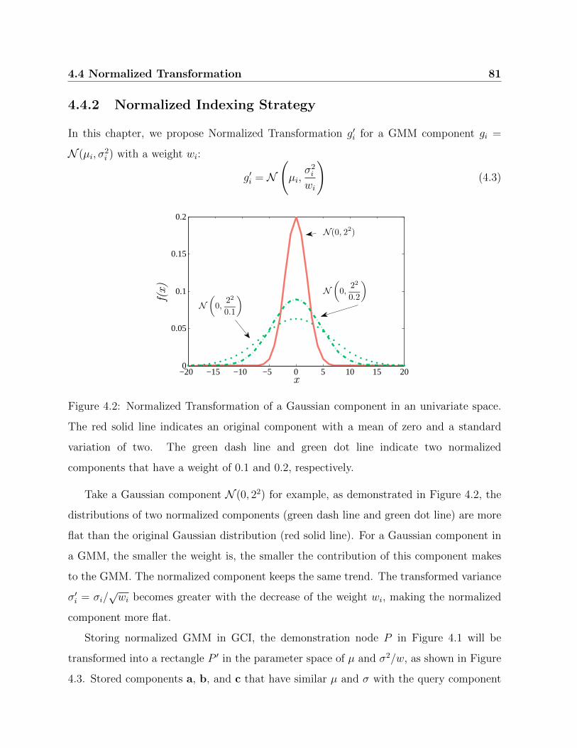
4.4 Normalized Transformation 81
4.4.2 Normalized Indexing Strategy
In this chapter, we propose Normalized Transformation g′i for a GMM component gi =
N (µi, σ2i ) with a weight wi:
g′i = N(µi,
σ2i
wi
)(4.3)
−20 −15 −10 −5 0 5 10 15 200
0.05
0.1
0.15
0.2
x
f(x)
N(0, 22)
N(0,
22
0.2
)
N(0,
22
0.1
)
Figure 4.2: Normalized Transformation of a Gaussian component in an univariate space.
The red solid line indicates an original component with a mean of zero and a standard
variation of two. The green dash line and green dot line indicate two normalized
components that have a weight of 0.1 and 0.2, respectively.
Take a Gaussian component N (0, 22) for example, as demonstrated in Figure 4.2, the
distributions of two normalized components (green dash line and green dot line) are more
flat than the original Gaussian distribution (red solid line). For a Gaussian component in
a GMM, the smaller the weight is, the smaller the contribution of this component makes
to the GMM. The normalized component keeps the same trend. The transformed variance
σ′i = σi/√wi becomes greater with the decrease of the weight wi, making the normalized
component more flat.
Storing normalized GMM in GCI, the demonstration node P in Figure 4.1 will be
transformed into a rectangle P ′ in the parameter space of µ and σ2/w, as shown in Figure
4.3. Stored components a, b, and c that have similar µ and σ with the query component

82 4. Novel Indexing Strategy and Similarity Measures for GMM
σ 2 /w
μ Stored components
Query component
d
e
fa
b
c
Figure 4.3: Demonstration of the normalized node P ′ of GCI for univariate GMM. Green
crosses indicate the stored components, and blue dot indicates one of query component of
a query GMM.
but tiny wights now are separated from the original node. In the present scene, the upper
bound of MP ˆdmp(Gq, P ′) provides a more objective reference than ˆdmp(Gq, P ) to determine
whether the stored components need to be refined or not, thus a more tight prune strategy
can be achieved.
4.4.3 Normalized Similarity Measures
Based on Normalized Transformation, we can derive the normalized matching probability
of two GMM from Equation 4.2. It is shown as follows.
mp′(G1,G2) =
m1∑
i=1
m2∑
j=1
D∏
l=1
e−
(µ1,i,l−µ2,j,l)2
2(σ21,i,l
/wi+σ22,j,l
/wj)
√2π(σ2
1,i,l/wi + σ22,j,l/wj)
(4.4)
Since several similarity measures with closed-form expression for GMM are the functions
of MP, we can easily extend them into a set of novel similarity measures. These normalized
measures share the same time complexities with their origins, and they have closed-form
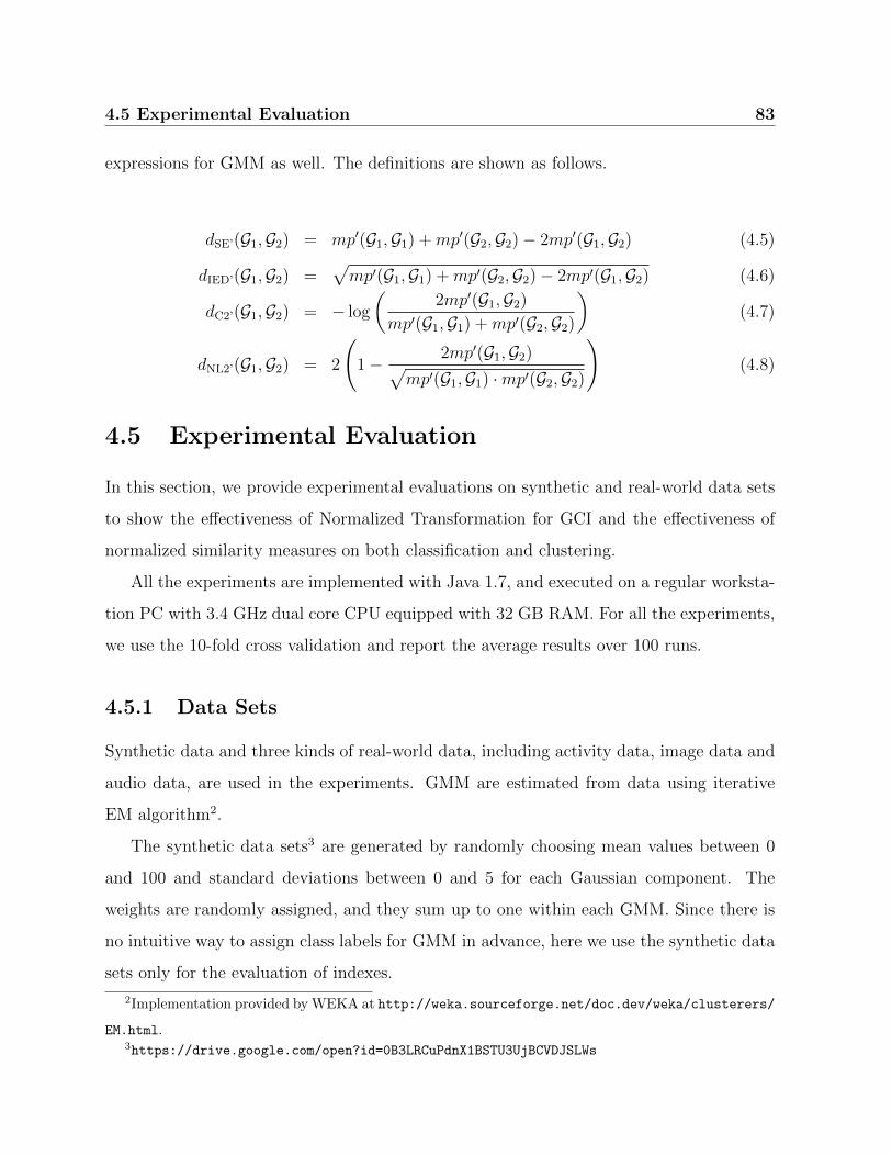
4.5 Experimental Evaluation 83
expressions for GMM as well. The definitions are shown as follows.
dSE’(G1,G2) = mp′(G1,G1) +mp′(G2,G2)− 2mp′(G1,G2) (4.5)
dIED’(G1,G2) =√mp′(G1,G1) +mp′(G2,G2)− 2mp′(G1,G2) (4.6)
dC2’(G1,G2) = − log
(2mp′(G1,G2)
mp′(G1,G1) +mp′(G2,G2)
)(4.7)
dNL2’(G1,G2) = 2
(1− 2mp′(G1,G2)√
mp′(G1,G1) ·mp′(G2,G2)
)(4.8)
4.5 Experimental Evaluation
In this section, we provide experimental evaluations on synthetic and real-world data sets
to show the effectiveness of Normalized Transformation for GCI and the effectiveness of
normalized similarity measures on both classification and clustering.
All the experiments are implemented with Java 1.7, and executed on a regular worksta-
tion PC with 3.4 GHz dual core CPU equipped with 32 GB RAM. For all the experiments,
we use the 10-fold cross validation and report the average results over 100 runs.
4.5.1 Data Sets
Synthetic data and three kinds of real-world data, including activity data, image data and
audio data, are used in the experiments. GMM are estimated from data using iterative
EM algorithm2.
The synthetic data sets3 are generated by randomly choosing mean values between 0
and 100 and standard deviations between 0 and 5 for each Gaussian component. The
weights are randomly assigned, and they sum up to one within each GMM. Since there is
no intuitive way to assign class labels for GMM in advance, here we use the synthetic data
sets only for the evaluation of indexes.
2Implementation provided by WEKA at http://weka.sourceforge.net/doc.dev/weka/clusterers/
EM.html.3https://drive.google.com/open?id=0B3LRCuPdnX1BSTU3UjBCVDJSLWs

84 4. Novel Indexing Strategy and Similarity Measures for GMM
Activity Recognition (AR) data4 is collected from 15 participants performing seven
activities. The sampling frequency of triaxial accelerometer is 52 Hz. Assuming that
participants complete a single activity in three seconds, we regard the 150 continuous
measurements of acceleration on three axes as one data object.
Amsterdam Library of Object Images5 (ALOI) is a collection of images taking under
various light conditions and rotation angles [89]. In this chapter we use the gray images
recording 100 objects from 72 viewpoints. For ALOI data, every image (192×144) is
smoothed by a Gaussian filter with a standard deviation of five.
Speaker Recognition6 (SR) consists of 35 hours of speech from 180 speakers. We
select the speeches from ten speakers to form our audio data set, the Speaker Recognition
(SR) data. The names of the ten speakers are as follows: Aaron, Abdul Moiz, Afshad,
Afzal, Akahansson, Alexander Drachmann, Afred Strauss, Andy, Anna Karpelevich and
Anniepoo. Every wav file is split into ten fragments, transformed into frequency domain
by Fast Fourier Transform. The SR data has ten classes (corresponding to ten speakers),
and each of them has 100 GMM objects.
4.5.2 Effectiveness of queries in GCI
We study the performance of MP and normalized matching probability when using GCI
to facilitate efficient queries. GMM are decomposed into Gaussian components that stored
into the entries of GCI. The minimum and maximum node capacity of GCI are set to
100 and 500, respectively. Original Gaussian components are stored when using MP as
the similarity measure, while normalized Gaussian components are stored for normalized
matching probability.
We apply k-Nearest Neighbors (k-NN) queries using both similarity measures when
varying the number of GMM objects and report the number of refined objects in Figure
4http://archive.ics.uci.edu/ml/machine-learning-databases/00287/5http://aloi.science.uva.nl/6 http://www.repository.voxforge1.org/downloads/SpeechCorpus/Trunk/Audio/Main/16kHz_
16bit/

4.5 Experimental Evaluation 85
0
200
400
600
800
27 28 29 210 211 212
Number of objects
Num
ber
of r
efin
ed o
bjec
ts
Original
Normalized
Figure 4.4: Number of refined GMM in GCI when varying the number of stored GMM on
Synthetic data. Each GMM here has ten Gaussian components in a univariate space.
4.4. With the increasing number of stored GMM objects, both similarity measures need
to refine more and more GMM, but normalized matching probability significantly reduced
the number of expensive calculations between GMM.
4.5.3 Effectiveness of normalized similarity measures
Classification
In the evaluation of classification, only k-NN, rather than the other more complex tech-
niques, is used to compare the effectiveness of the similarity measures, since we are not
interested in tuning the classification accuracy to its optimum.
We start with experiments on SR data sets when varying k in k-NN, and the clas-
sification is applied based on original and normalized similarity measures. Classification
accuracies are shown in Figure 4.5. From this figure we can see that all four normalized
similarity measures outperform their origins, and all the accuracies slightly decrease with
the increase of k.
Fixing k as 1, we report the classification results on AR data when varying the number

86 4. Novel Indexing Strategy and Similarity Measures for GMM
2 4 6 8 100.7
0.75
0.8
0.85
0.9
0.95
1
k in k−NN
Acc
urac
y
Original
Normalized
(a) SE
2 4 6 8 100.7
0.75
0.8
0.85
0.9
0.95
1
k in k−NN
Acc
urac
y
(b) IED
2 4 6 8 100.7
0.75
0.8
0.85
0.9
0.95
1
k in k−NN
Acc
urac
y
(c) C2
2 4 6 8 100.7
0.75
0.8
0.85
0.9
0.95
1
k in k−NN
Acc
urac
y
(d) NL2
Figure 4.5: Classification accuracies on SR data. For each data object, a five-component
GMM is estimated.
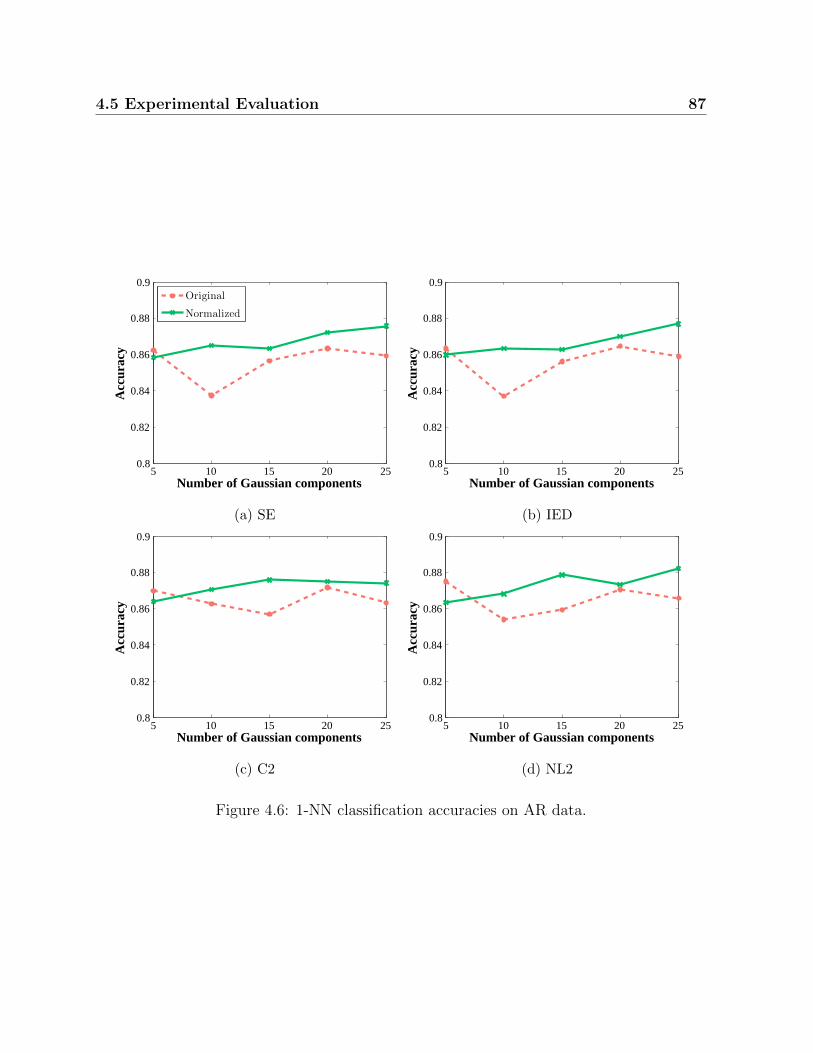
4.5 Experimental Evaluation 87
5 10 15 20 250.8
0.82
0.84
0.86
0.88
0.9
Number of Gaussian components
Acc
urac
y
Original
Normalized
(a) SE
5 10 15 20 250.8
0.82
0.84
0.86
0.88
0.9
Number of Gaussian components
Acc
urac
y
(b) IED
5 10 15 20 250.8
0.82
0.84
0.86
0.88
0.9
Number of Gaussian components
Acc
urac
y
(c) C2
5 10 15 20 250.8
0.82
0.84
0.86
0.88
0.9
Number of Gaussian components
Acc
urac
y
(d) NL2
Figure 4.6: 1-NN classification accuracies on AR data.

88 4. Novel Indexing Strategy and Similarity Measures for GMM
(a) AR (b) ALOI (c) SR
Figure 4.7: 1-NN classification accuracies on three real-world data sets. The numbers
of Gaussian components in each GMM object for (a), (b) and (c) are ten, five and five,
respectively.
of Gaussian components in estimated GMM. As shown in Figure 4.6, the normalized
similarity measures achieve better classification results than the origins in most cases when
the number of Gaussian components is high enough. Only at starting points, normalized
similarity measures, especially for NL2, have lower accuracies than their origins. GMM
have better representations of data objects with the increase of components number,
however, the training time of EM algorithm increases at the same time. To tune the
number of Gaussian components into the optimum for a given similarity measure, Bayesian
Information Criterion can be applied. For the following experiments, we choose the
component numbers by the rule of thumb instead.
Figure 4.7 shows the 1-NN classification results on three read-world data sets. All
similarity measure, SE, IED, C2 and NL2, have similar performances, and their normalized
versions outperform the origins.
Clustering
We perform clustering experiments to compare the usability of the normalized similarity
measures for unsupervised data mining. Instead of k-means algorithm, the k-medoids
is used since it works with arbitrary similarity measures, making it more suitable here.
We evaluate the clustering results using three widely used criteria, Purity, NMI and FM
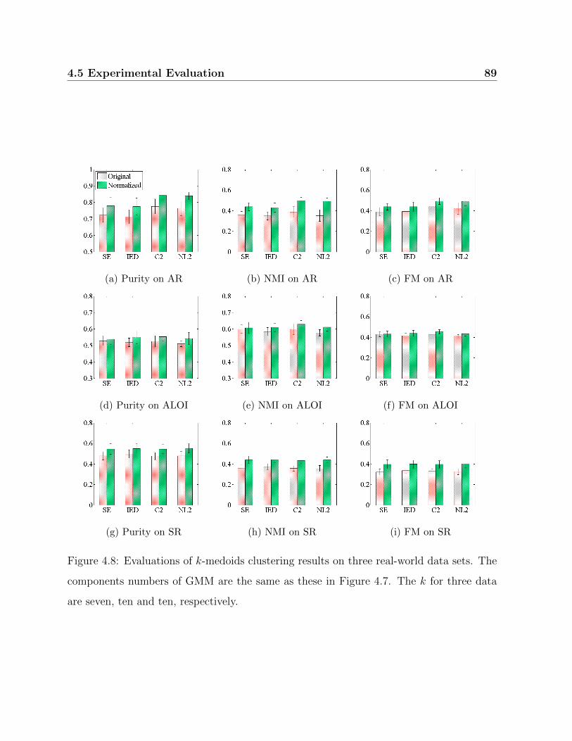
4.5 Experimental Evaluation 89
(a) Purity on AR (b) NMI on AR (c) FM on AR
(d) Purity on ALOI (e) NMI on ALOI (f) FM on ALOI
(g) Purity on SR (h) NMI on SR (i) FM on SR
Figure 4.8: Evaluations of k-medoids clustering results on three real-world data sets. The
components numbers of GMM are the same as these in Figure 4.7. The k for three data
are seven, ten and ten, respectively.

90 4. Novel Indexing Strategy and Similarity Measures for GMM
(β = 1).
Figure 4.8 illustrates the evaluation of clustering results when using different similarity
measures on three real-world data sets. All three criteria have the same pattern for all the
similarity measures on three data sets. The normalized similarity measures have a better
performance than their origins.
4.6 Conclusions
In this chapter, we have introduced Normalized Transformation that aims to improve the
retrieval performance of index for GMM, and it also enable us to derive a set of normalized
similarity measures from proposed ones that have closed-form expressions for GMM. These
normalized similarity measures share the same time complexities with their origins. Queries
on GMM using Gaussian Component based Index have illustrated the effectiveness of
Normalized Transformation, achieving a much lower refinement rate than the original
MP. For the effectiveness of normalized similarity measures, we have demonstrated the
experimental evaluations on the real-world data sets. The normalized similarity measures
outperform their origins on different types of data sets in both classification and clustering.

Chapter 5
Similarity Measures for
Multiple-Instance Learning
“We’ve got to use every piece of data and piece of information, and hopefully
that will help us be accurate with our player evaluation. For us, that’s our
life blood.”
Billy Beane
In this chapter, we propose two similarity measures for MIL. Parts of this chapter have
been published in:
Linfei Zhou, Claudia Plant, Christian Bohm. Joint Gaussian Based Similarity
Measures for Multiple-Instance Learning. IEEE 33th International Conference
on Data Engineering, ICDE 2017, April 19-22, 2017, San Diego, United States.
where Linfei Zhou was mostly responsible for the development of main concepts, im-
plemented main algorithms and wrote the most parts of the paper. Christian Bohm
and Claudia Plant supervised the project and proposed the initial idea. All co-authors
contributed to the discussion, paper writing and revising.

92 5. Similarity Measures for Multiple-Instance Learning
5.1 Introduction
First motivated by the problem of drug activity predictions, MIL deals with MI objects
that are sets (or bags) of instances [77]. For objects with inherent structures, which are
very common in real-world data, MI is a natural way to represent them. Thus various MIL
methods have been proposed in many application domains like image classification [80],
text categorization [90], activity recognition [91], etc..
The major work of MIL concerns with binary classification problems under a set of
assumptions including the standard assumption [77] and the collective assumption [92].
For all these assumptions, each instance is assumed to have an explicit label, known or
unknown, which is the same type as the label of the MI object. A learning model is trained
in an instance space in the same way as the ’single’ instance situation, then the labels of
bags are obtained from that of their instances by OR operators in the standard assumption
or mathematical expectations in the collective assumption. These assumptions work well
for many applications such as drug activity predictions and content based image retrieval.
However, they cannot deal with situations when the instances or bags have no labels, or
there is no clear relation between instance-level labels and over-all labels. For example,
the performance of an athlete is a MI object when the statistics of each match is regarded
as an instance. It is impossible to obtain the learning model from instance spaces because
there is a large number of instances (more than 0.7 million) need to be labeled, and even
for a single instance it is difficult to label it for evaluations.
There are two strategies to solve the problem, mapping each MI object into embedded
spaces and defining similarity measures for MI objects. However, they either are time
consuming or lose the information of MI objects, especially for the first strategy. Suitable
similarity measures for MI objects are yet to be developed and tested. A competitive
candidate for such a similarity measure has competencies to be robust to noise, to be
efficient in its computation, and to facilitate index and further analysis. As we will
demonstrate, our techniques are effective, and also support index for improving data
retrieval operations. The main contributions of this chapter are:
5.2 Related Work 93
• We propose two novel similarity measures for MIL, JGS and JGD. They have clear
physical meanings, are efficient to be calculated and are robust to noise while taking
all the information into account.
• Experimental results show that JGS and JGD work well for traditional MIL tasks and
also have good performances in the situation when there is no need of assumptions
of relations between the labels of instances and bags.
The rest of this chapter is organized as follows. In Section 5.2, we survey the previous
work. Section 5.3 gives the basic definition. Section 5.4 describes the ideas of JGS and
JGD. Section 5.5 shows the experimental studies to verify the effectiveness of proposed
measures. Finally, Section 5.6 summarizes this chapter.
5.2 Related Work
5.2.1 Instance Space Based Paradigm
In this category, Axis-Parallel Rectangles (APR) [77] searches for appropriate axis-rectangles
constructed by the features of positive instances. Similarly, an algorithm maximizing
Diverse Density (DD) measure has been proposed by O. Maron and T. Lozano-Perez [93].
EM-DD [94] combines EM algorithm and DD measure. Several algorithms [90, 95, 96,
97, 98] represent each bag with one of its instance. Algorithm mi-DS uses rules that are
generated from classified instances to construct a similarity matrix [98].
Instance space based MIL has the ability to extend many well developed algorithms
designed for the ’single’ instance situation. However, it can not deal with situations when
the labels of instances are unknown or there is no clear relation between the labels of
instances and bags.
94 5. Similarity Measures for Multiple-Instance Learning
5.2.2 Embedded Space Based Paradigm
The embedded space based paradigm defines mapping functions to project each bag into
a feature vector. Many mapping methods have been proposed, including the vocabulary
based mapping, the instance based mapping and the model based mapping. The first
mapping method clusters all instances from all bags into k clusters (vocabularies), and
then uses the histogram information to obtain a k-dimensional feature vector for each
bag [72, 78, 79]. The instance based mapping defines a feature vector for each bag using
the information of its instances [80, 99, 81]. The model based mapping trains each bag to
a model [75, 74, 82].
Besides the extra time cost of mappings, there needs to be enough instances in each
bag to estimate the parameters, and appropriate similarity measures are also needed.
5.2.3 Bag Space Based Paradigm
In the bag space based paradigm, algorithms treat each bag as a single object and define
similarity measures for bags.
All distance functions that measure the (dis)similarity between point sets can be used
for MI objects, including Hausdorff distance, SMD[100], Chamfer matching [29], Earth
Mover’s Distance (EMD) [101], Netflow distance [102], etc.. What is more, J. Wang and J.
Zucker have proposed modified Hausdorff distances for Bayesian k-NN and Citation k-NN
[103]. Similarly, W. Zhang et al. have applied Quantile based k-NN on MI data, defining
φ-quantile distance [104]. X. He has proposed PIM on the basis of an idea that each MI
object is a manifestation of some templates [31]. L. Sørensen et al. have compared BWmax
and BWmean distance [105]. Metric learning has been extended to MIL [106], however,
they actually learn a metric for instances, replacing Euclidean distances with Mahalanobis
distances.
The existing similarity measures range from simple and efficient ones like Hausdorff
distance to complex ones like Netflow distance and PIM, but only a few of them are
metrics and take account of the information of all instances. Taking Hausdorff distance for

5.3 Formal Definitions 95
example, it is a metric, but it only uses the distance between two single instances of bags,
which makes it sensitive to noise. More information about these similarity measures are
shown in Table 5.1.
5.3 Formal Definitions
In this section, we summarize the formal definitions of MI objects. The definition is shown
as follows.
Definition 8. (Multiple-Instance Object)
A MI object X ∈P(RD) is a finite set of n instances x1, x2, ..., xn and a corresponding
weight vector W = w1, w2, ..., wn, where n = |X | is the cardinality of the object, an
instance xi = (xi1, xi2, ..., xiD) is a feature vector in a D-dimensional space RD, P(RD) is
the power set of RD and∑n
1 wi = 1.
Under the circumstance when there is no weight information attached with instances,
which occurs in most cases, the weight of each instance is assigned as 1/n.
5.4 Joint Gaussian Based Measures
In this section, we present the ideas of JGS and JGD for MI objects. Firstly, we introduce
Multiple-Instance Density and generalize it to Potential Instance Density for MI objects.
Then we define JGS and JGD as the similarity measures.
5.4.1 Density of Instances
Being a finite set of instances, a MI object can be treated as a probability density function
of instances. We define Multiple-Instance Density as follows.
Definition 9. (Multiple-Instance Density)

96 5. Similarity Measures for Multiple-Instance Learning
Table 5.1: Overview of similarity measures for MIL
Distance Formula Ref.
Use the
information
of all
instances
Metric
Hausdorff maxmaxx∈X
miny∈Y‖x− y‖,max
y∈Yminx∈X‖x− y‖ [30] No Yes
SMD‡1
|X |+|Y| (∑
x∈X miny∈Y‖x− y‖+
∑y∈Y min
x∈X‖x− y‖) [100] No No
Chamfer1|X |∑
x∈X miny∈Y‖x− y‖+ 1
|Y|∑
y∈Y minx∈X‖x− y‖ [29] No No
EMD∑
x∈X∑
y∈Y wij‖x−y‖∑x∈X
∑y∈Y wij
[101] Yes Yes
Netflowmin
f∈N(P,dist,M,W,X ,Y)W (f(X ,Y))
See more details in the corresponding reference[102] Yes Yes
minHausdorff minx∈X
miny∈Y‖x− y‖ [103] No No
φ-quantile‖xi − yj‖x∈X ,y∈Y
i, j = arg φ-quantile(wxi · wyj of sorted ‖xi − yj‖)[104] No No
PIM
∫RD∫∞
0p(r)hX ,Y(t, r)drdt
p(r) = drD−1
(2σ2)d/2Γ(D/2+1)e−
r2
2σ2
hX ,Y(t, r) = 1, if cX (t, r) 6= cY(t,r); 0, otherwisecX (t, r) = 1, if minx∈X ‖t− x‖ ≤ r; 0, otherwise
[31] Yes Yes
BWmean
12 (dEMD(HX , HX ,Y) + dEMD(HY , HX ,Y))
HX : Histogram of instance distance within XHX ,Y : Histogram of instance distance between X ,Y
[105] Yes No
‡SMD is also called average Hausdorff distance [107].

5.4 Joint Gaussian Based Measures 97
Given a MI object X = xin1 where xi is a feature vector in a space RD, Multiple-
Instance Density fX (t) of the variable t ∈ RD can be represented by:
fX (t) =∑
1≤i≤n
wiδi(t) (5.1)
where wi is the weight of instance xi,∑n
1 wi = 1 and
δi(t) =
+∞ if t = xi;
0 otherwise;(5.2)
Since Multiple-Instance Density is a piecewise function, some MIL algorithms train
probabilistic models to represent MI objects under the assumption that the instances of
a MI object are independently and identically distributed [73, 74, 83]. To obtain a high
accuracy of representing, there needs to be enough instances in each bag for the training,
which leads to another problem, i.e., the training is time consuming.
Instead of assuming that all the instances of a bag are generated from a known distribu-
tion such as a Gaussian model, we use a Gaussian distribution to represent the suppositional
density around each instance. The definition of Potential Instance Density is shown as
follows.
Definition 10. (Potential Instance Density)
Given the instance x of a MI object X , Potential Instance Density f(t|x, σ2X ) of x in the
feature space RD is defined as:
f(t|x, σ2X ) =
1√2πσ2
Xe− (t−x)2
2σ2X (5.3)
where σ2X is the potential variance of X .
Replacing the δ function in Definition 9 with Potential Instance Density, we derive
Potential Multiple-Instance Density as follows.
Definition 11. (Potential Multiple-Instance Density)
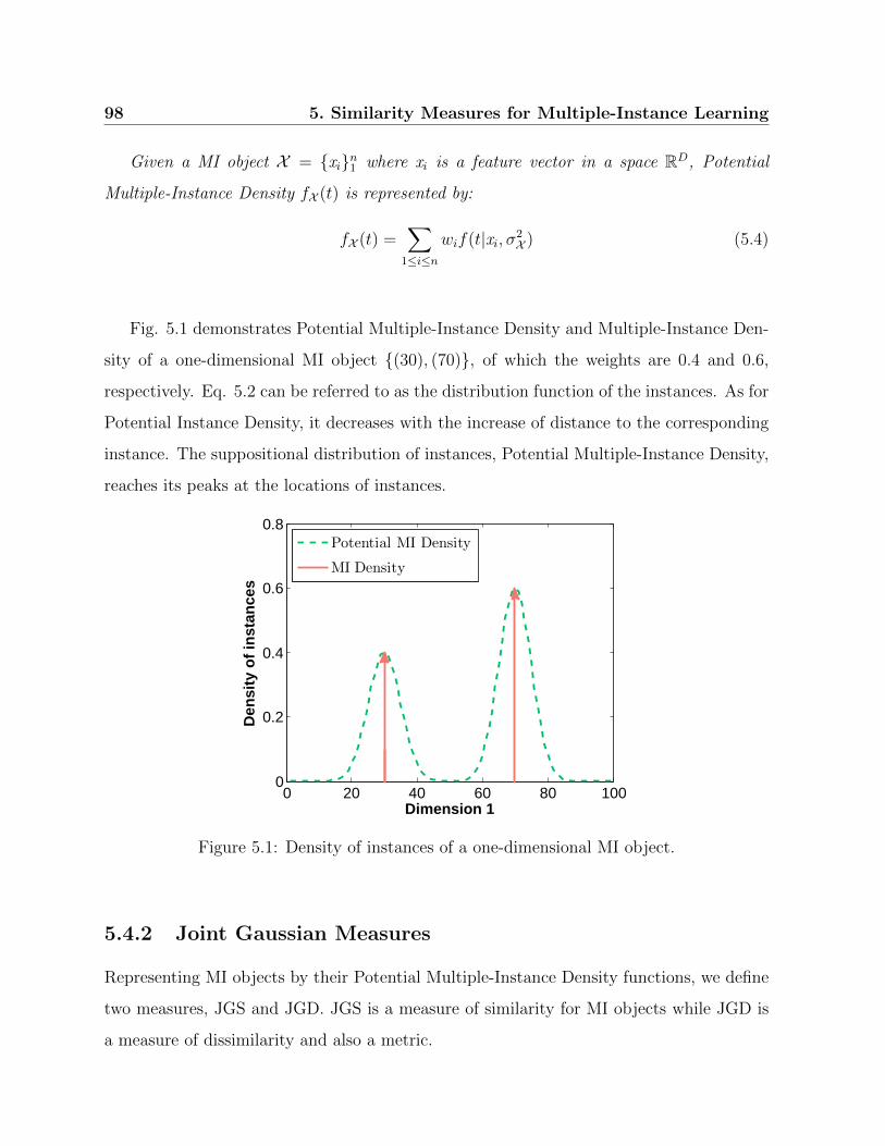
98 5. Similarity Measures for Multiple-Instance Learning
Given a MI object X = xin1 where xi is a feature vector in a space RD, Potential
Multiple-Instance Density fX (t) is represented by:
fX (t) =∑
1≤i≤n
wif(t|xi, σ2X ) (5.4)
Fig. 5.1 demonstrates Potential Multiple-Instance Density and Multiple-Instance Den-
sity of a one-dimensional MI object (30), (70), of which the weights are 0.4 and 0.6,
respectively. Eq. 5.2 can be referred to as the distribution function of the instances. As for
Potential Instance Density, it decreases with the increase of distance to the corresponding
instance. The suppositional distribution of instances, Potential Multiple-Instance Density,
reaches its peaks at the locations of instances.
0 20 40 60 80 1000
0.2
0.4
0.6
0.8
Dimension 1
Den
sity
of
inst
ance
s
Potential MI Density
MI Density
Figure 5.1: Density of instances of a one-dimensional MI object.
5.4.2 Joint Gaussian Measures
Representing MI objects by their Potential Multiple-Instance Density functions, we define
two measures, JGS and JGD. JGS is a measure of similarity for MI objects while JGD is
a measure of dissimilarity and also a metric.
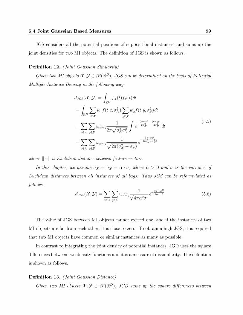
5.4 Joint Gaussian Based Measures 99
JGS considers all the potential positions of suppositional instances, and sums up the
joint densities for two MI objects. The definition of JGS is shown as follows.
Definition 12. (Joint Gaussian Similarity)
Given two MI objects X ,Y ∈P(RD), JGS can be determined on the basis of Potential
Multiple-Instance Density in the following way:
dJGS(X ,Y) =
∫
RDfX (t)fY(t)dt
=
∫
RD
∑
x∈X
wxf(t|x, σ2X )∑
y∈Y
wyf(t|y, σ2Y)dt
=∑
x∈X
∑
y∈Y
wxwy1
2π√σ2Xσ
2Y
∫e− (t−x)2
2σ2X− (t−y)2
2σ2Y dt
=∑
x∈X
∑
y∈Y
wxwy1√
2π(σ2X + σ2
Y)e− ‖x−y‖2
2(σ2X+σ2Y )
(5.5)
where ‖ · ‖ is Euclidean distance between feature vectors.
In this chapter, we assume σX = σY = α · σ, where α > 0 and σ is the variance of
Euclidean distances between all instances of all bags. Thus JGS can be reformulated as
follows.
dJGS(X ,Y) =∑
x∈X
∑
y∈Y
wxwy1√
4πα2σ2e−‖x−y‖2
4α2σ2 (5.6)
The value of JGS between MI objects cannot exceed one, and if the instances of two
MI objects are far from each other, it is close to zero. To obtain a high JGS, it is required
that two MI objects have common or similar instances as many as possible.
In contrast to integrating the joint density of potential instances, JGD uses the square
differences between two density functions and it is a measure of dissimilarity. The definition
is shown as follows.
Definition 13. (Joint Gaussian Distance)
Given two MI objects X ,Y ∈ P(RD), JGD sums up the square differences between
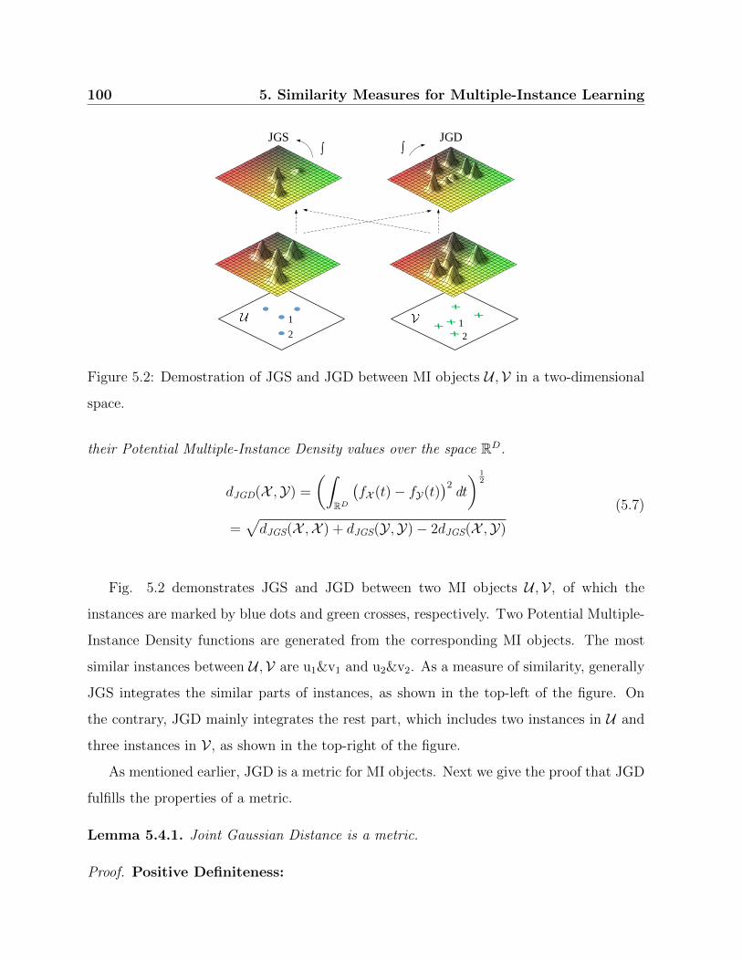
100 5. Similarity Measures for Multiple-Instance Learning
JGS JGD
1
21
2
Figure 5.2: Demostration of JGS and JGD between MI objects U ,V in a two-dimensional
space.
their Potential Multiple-Instance Density values over the space RD.
dJGD(X ,Y) =
(∫
RD
(fX (t)− fY(t)
)2dt
) 12
=√dJGS(X ,X ) + dJGS(Y ,Y)− 2dJGS(X ,Y)
(5.7)
Fig. 5.2 demonstrates JGS and JGD between two MI objects U ,V , of which the
instances are marked by blue dots and green crosses, respectively. Two Potential Multiple-
Instance Density functions are generated from the corresponding MI objects. The most
similar instances between U ,V are u1&v1 and u2&v2. As a measure of similarity, generally
JGS integrates the similar parts of instances, as shown in the top-left of the figure. On
the contrary, JGD mainly integrates the rest part, which includes two instances in U and
three instances in V , as shown in the top-right of the figure.
As mentioned earlier, JGD is a metric for MI objects. Next we give the proof that JGD
fulfills the properties of a metric.
Lemma 5.4.1. Joint Gaussian Distance is a metric.
Proof. Positive Definiteness:

5.4 Joint Gaussian Based Measures 101
The integrated function of JGD in Eq. 5.7 is everywhere greater or equal to zero. If
and only if X and Y are exactly the same, the differences between their Potential Multiple-
instance Density values, fX (t) and fY(t), are zero for all t in the space RD, thus dJGD = 0.
If for some t, fX (t) and fY(t) are not equal, then it will have a positive influence on the
integral. In that case, dJGD > 0.
Symmetry:
Obviously, dJGD(X ,Y) = dJGD(Y ,X ) for any MI object X ,Y ∈P(RD).
Triangle Inequality:
The triangle inequality of JGD states that for any MI object X ,Y ,Z ∈ P(RD), the
following inequality always holds.
dJGD(X ,Y) + dJGD(Y ,Z) ≥ dJGD(X ,Z)
Since for any real value a, b, c ≥ 0, a+ b ≥ c is equivalent to (a+ b)2 ≥ c2. The inequality
can be transformed to:
(dJGD(X ,Y) + dJGD(Y ,Z))2 ≥ (dJGD(X ,Z))2
To prove this inequality, we substitute it by an object function Obj as shown below.
Obj = (dJGD(X ,Y) + dJGD(Y ,Z))2 − (dJGD(X ,Z))2
= 2
∫
RD(fY(t)− fZ(t))(fY(t)− fX (t))dt
+ 2
√∫
RD(fX (t)− fY(t))2dt
∫
RD(fY(t)− fZ(t))2dt
Due to Cauchy−Schwarz inequality, for complex-valued functions u(x) and v(x), one
has:∫
RD|u(x)|2dx ·
∫
RD|v(x)|2dx ≥
∣∣∣∣∫
RDu(x)v(x)dx
∣∣∣∣2

102 5. Similarity Measures for Multiple-Instance Learning
thus we have:
Obj ≥ 2
∫
RD(fY(t)− fZ(t))(fY(t)− fX (t))dt
+ 2
∣∣∣∣∫
RD(fY(t)− fZ(t))(fY(t)− fX (t))dt
∣∣∣∣
≥ 0
Thus we obtain dJGD(X ,Y) + dJGD(Y ,Z) ≥ dJGD(X ,Z).
Having MI objects represented in our way, we can also extend several similarity mea-
sures designed for GMM to MIL [61, 62, 86], but none of them is a metric.
5.5 Experimental Evaluations
In this section, we provide experimental evaluations on real-world data sets to show the
effectiveness of the proposed measures. We employ the simplest and widely used algorithm
k-NN for the classification and k-medoids for the clustering.
All experiments are implemented1 with Java 1.7, and executed on a regular workstation
PC with 3.4 GHz dual core CPU equipped with 32 GB RAM. To keep the consistency of
the codes, we use the reciprocal value of JGS as its dissimilarity value. For all experiments,
we use the 10-fold cross validation and report the average results over 100 runs.
5.5.1 Data Sets
Synthetic data sets2 include demonstration data Syn1 and randomized data Syn2 which
is generated from a normal distribution. Syn1 consists of four MI objects in a two-
dimensional space, while Syn2 varies in the number of MI objects, the number of instances
in each object and the dimensionality of instances.
1https://drive.google.com/open?id=0B3LRCuPdnX1BMFViblpaS1VKZmM2https://drive.google.com/open?id=0B3LRCuPdnX1BQlBOZzlQWmNrMVk

5.5 Experimental Evaluations 103
Table 5.2: Real-world data sets
Objects # Avg. Instances # Dimension Classes #
Musk1 92 5.2 166 2
Musk2 92 64.7 166 2
Fox 200 6.6 230 2
Tiger 200 6.1 230 2
Elephant 200 6.9 230 2
NBA 2477 295.7 18 -
CorelDB 500 49 8 4
Weather 2937 12 6 5
Musk data3 is a benchmark data for MIL. It has two data sets, Musk 1 and Musk
2, the details of which have been described by T. Dietterich et al. [77]. Fox, Tiger and
Elephant data4 is another benchmark data. It is generated from image data sets after
preprocessing and segmentation [90]. Besides these data sets, we also use three other real-
world data sets5, NBA data, CorelDB data and Weather data. NBA data provides the
statistics of NBA players in every match till 2014. CorelDB data consists of extracted
features from images. Each image is smoothed by a Gaussian filter and then it generates
a 9× 9 grid of pixels of which the 7× 7 non-border are chosen as instances. The features
of each instance are color differences between a pixel and its neighbours. Weather data is
the historical weather data of airports around the world. Each instance of airports is the
average statistics in a month. We use the main categories of Koppen climate classification
system to label each airport. More details are shown in Table 5.2.

104 5. Similarity Measures for Multiple-Instance Learning
.1 .2 .3 .4 .5 .6 .7 .8 .9 1 2 3 4 5 6 7 8 90.6
0.65
0.7
0.75
0.8
0.85
0.9
0.95
1
α
Acc
ura
cy
JGS
JGD
(a) Musk1
.1 .2 .3 .4 .5 .6 .7 .8 .9 1 2 3 4 5 6 7 8 90.6
0.65
0.7
0.75
0.8
0.85
0.9
0.95
1
α
Acc
ura
cy
(b) Musk2
Figure 5.3: Classification accuracies on Musk data.
5.5.2 Parameter Setting
To evaluate the influence of parameter α in Eq. 12, we perform 1-NN classifications on
Musk data. The classification accuracies when varying α are shown in Fig. 5.3. The
accuracies of both data sets shoot up before α reaches 1, especially for JGS, and level off
afterward. Therefore, we choose α = 1 for all the following experiments. The variances of
Euclidean distance between all instances in real-world data sets are shown in Table 5.3.
5.5.3 Effectiveness
In this part, we demonstrate the metric properties of JGD and other measures (Table 5.1)
on the synthetic data set, and report the performances of JGS and JGD on the real-world
data sets. Finally for benchmark tasks we compare the optimal classification accuracies
achieved by k-NN using JGD with those of state-of-the-art MIL algorithms.
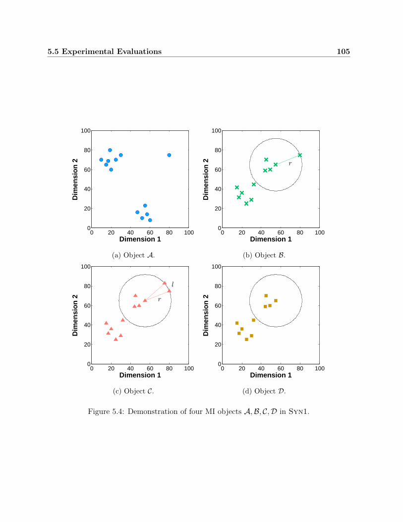
5.5 Experimental Evaluations 105
0 20 40 60 80 1000
20
40
60
80
100
Dimension 1
Dim
ensi
on
2
(a) Object A.
0 20 40 60 80 1000
20
40
60
80
100
r
Dimension 1
Dim
ensi
on
2
(b) Object B.
0 20 40 60 80 1000
20
40
60
80
100
r
l
Dimension 1
Dim
ensi
on
2
(c) Object C.
0 20 40 60 80 1000
20
40
60
80
100
Dimension 1
Dim
ensi
on
2
(d) Object D.
Figure 5.4: Demonstration of four MI objects A,B, C,D in Syn1.

106 5. Similarity Measures for Multiple-Instance Learning
Table 5.3: σ of real-world data sets
σ
Musk1 429
Musk2 400
Fox 9.37
Tiger 11.91
Elephant 8.71
NBA 11.02
CorelDB 0.26
Weather 18.10
Metric Properties on Syn1 Data
Fig. 5.4 shows the four MI objects of Syn1 data, where object A and B have the same
center of instances and one shared instance. Most instances of object B, C,D are the same
except three instances that locate on the circle of radius r.
According to formulas listed in Table 5.1, the minHausdorff distance between AB, AC,BC, etc. are zero, although none of these pairs is exactly the same. It is similar for φ-
quantile distance when φ = 0.05. As for SMD, the distances between object B, C,D are
shown as follows:
dSMD(B, C) =1
11 + 12(0 + l)
dSMD(B,D) =1
11 + 10(r + 0)
dSMD(C,D) =1
12 + 10(2r + 0)
When l < 230/231r, which is true in our case, dSMD(C,D) > dSMD(B, C) + dSMD(B,D),
violating the triangle inequality. Chamfer, φ-quantile and BWmean also violate some
metric properties, and more information are shown in Table 5.4.
3https://archive.ics.uci.edu/ml/machine-learning-databases/musk/4http://www.miproblems.org/datasets/foxtigerelephant/5https://drive.google.com/open?id=0B3LRCuPdnX1BYXpGUzlxYVdsSDA
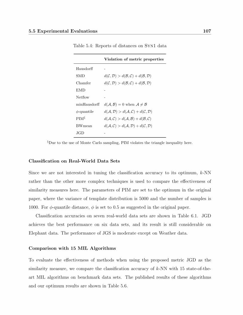
5.5 Experimental Evaluations 107
Table 5.4: Reports of distances on Syn1 data
Violation of metric properties
Hausdorff -
SMD d(C,D) > d(B, C) + d(B,D)
Chamfer d(C,D) > d(B, C) + d(B,D)
EMD -
Netflow -
minHausdorff d(A,B) = 0 when A 6= Bφ-quantile d(A,D) > d(A, C) + d(C,D)
PIM§ d(A, C) > d(A,B) + d(B, C)BWmean d(A, C) > d(A,D) + d(C,D)
JGD -
§Due to the use of Monte Carlo sampling, PIM violates the triangle inequality here.
Classification on Real-World Data Sets
Since we are not interested in tuning the classification accuracy to its optimum, k-NN
rather than the other more complex techniques is used to compare the effectiveness of
similarity measures here. The parameters of PIM are set to the optimum in the original
paper, where the variance of template distribution is 5000 and the number of samples is
1000. For φ-quantile distance, φ is set to 0.5 as suggested in the original paper.
Classification accuracies on seven real-world data sets are shown in Table 6.1. JGD
achieves the best performance on six data sets, and its result is still considerable on
Elephant data. The performance of JGS is moderate except on Weather data.
Comparison with 15 MIL Algorithms
To evaluate the effectiveness of methods when using the proposed metric JGD as the
similarity measure, we compare the classification accuracy of k-NN with 15 state-of-the-
art MIL algorithms on benchmark data sets. The published results of these algorithms
and our optimum results are shown in Table 5.6.
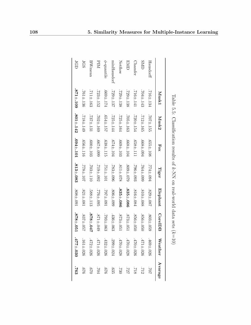
108 5. Similarity Measures for Multiple-Instance Learning
Tab
le5.5:
Classifi
cationresu
ltsofk-N
Non
real-world
data
sets(k
=10)
Musk
1M
usk
2Fox
Tiger
Elephant
Core
lDB
Weath
er
Avara
ge
Hau
sdorff
.716±
.134
.707±.155
.655±
.108
.774±
.094
.829±
.087
.803±.059
.469±.026
.707
SM
D.7
04±.14
3.712±
.165.6
68±
.094
.764±
.099
.810±
.088
.856±.050
.471±.026
.712
Ch
am
fer.7
16±.14
1.720±
.154.6
58±
.111
.796±
.093
.816±
.084
.856±.050
.470±.026
.718
EM
D.7
29±.13
8.705±
.163.6
68±
.104
.809±
.079
.835±
.086
.873±.051
.470±.028
.727
Netfl
ow.7
29±.1
38.725±
.164.6
69±
.103
.811±
.078
.835±
.086
.873±.051
.470±.028
.730
min
Hau
sdorf
.729±
.137
.725±.144
.674±
.104
.783±
.096
.806±
.099
.436±.063
.299±.024
.635
φ-q
uan
tile.66
9±.1
74.654±
.157.6
38±
.115
.751±
.101
.797±
.091
.793±.063
.432±.026
.676
PIM
.723±
.152
.702±.169
.667±
.099
.719±
.092
.776±
.095
.871±.049
.471±.026
.704
BW
mea
n.711±
.163
.737±.131
.600±
.103
.703±
.110
.588±
.113
.878±
.047
.472±.026
.670
JG
S.761±
.136.718±
.149
.656±
.116
.778±
.107
.821±
.081
.837±.057
.161±.026
.676
JG
D.871±
.109
.801±
.142
.694±
.101
.813±
.083
.808±
.091
.878±
.051
.477±
.030
.763

5.6 Conclusions 109
Generally k-NN using JGD is the most competitive method comparing the existing
technologies, even without tuning parameter α (Table 5.6). Since the Musk data fully
fulfilled the standard assumption, JGD does not outperform all the methods duo to its
needless of priori knowledge. However, JGD turns k-NN to be a better performing method
than APR, which has been specifically designed and optimized for the classification on the
Musk data.
5.6 Conclusions
In this chapter, we have proposed JGS and JGD for MIL. JGS and JGD break the limitation
of MIL assumptions and turn MIL into a traditional machine learning problem. They use
all the information of instances in MI objects and they are robust to noise. Evaluations on
real-world data demonstrate the better performances of proposed measures than the other
similarity measures, especially on the data without clear relations between instance-level
labels and over-all labels. In addition to the bag space based paradigms, JGD achieves
considerably higher classification accuracies on the benchmark tasks than the state-of-
the-art MIL algorithms. As a metric, JGD has the ability to employ any metric tree to
accelerate queries.
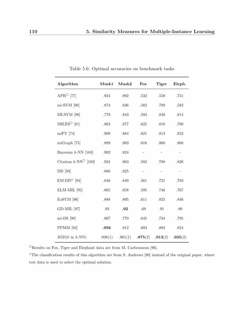
110 5. Similarity Measures for Multiple-Instance Learning
Table 5.6: Optimal accuracies on benchmark tasks
Algorithm Musk1 Musk2 Fox Tiger Eleph.
APR [77] .924 .892 .532 .558 .751
mi-SVM [90] .874 .836 .582 .789 .582
MI-SVM [90] .779 .843 .594 .840 .814
MILES [81] .863 .877 .625 .810 .790
miFV [74] .909 .884 .621 .813 .852
miGraph [75] .889 .903 .616 .860 .868
Bayesian k-NN [103] .902 .824 - - -
Citation k-NN [103] .924 .863 .582 .788 .826
DD [93] .880 .825 - - -
EM-DD♦ [94] .848 .849 .561 .721 .783
ELM-MIL [95] .865 .858 .595 .746 .767
EoSVM [96] .888 .895 .611 .825 .846
GD-MIL [97] .93 .92 .69 .91 .89
mi-DS [98] .867 .770 .645 .734 .795
PPMM [82] .956 .812 .603 .802 .824
JGD(k in k-NN) .938(1) .901(1) .875(2) .913(2) .935(2)
Results on Fox, Tiger and Elephant data are from M. Carbonneau [96].
♦The classification results of this algorithm are from S. Andrews [90] instead of the original paper, where
test data is used to select the optimal solution.

Chapter 6
Indexing Multiple-Instance Objects
“I think you can have a ridiculously enormous and complex data set, but if
have the right tools and methodoloy then it’s not a problem.”
Aaron Koblin
In this chapter, we introduce indexing techniques for MI Objects. Parts of this chapter
have been published in:
Linfei Zhou, Wei Ye, Zhen Wang, Claudia Plant, Christian Bohm. Indexing
Multiple-Instance Objects. 28th International Conference on Database and
Expert Systems Applications, DEXA 2017, August 28-31, 2017, Lyon, France.
where Linfei Zhou was mostly responsible for the development of main concepts, imple-
mented main algorithms and wrote the most parts of the paper. Wei Ye and Zhen Wang
helped with the discussion and experimental design. Christian Bohm and Claudia Plant
supervised the project. All co-authors contributed to the discussion, paper writing and
revising.
6.1 Introduction
First motivated by the problem of drug activity predictions, MIL deals with MI objects
that are sets (or bags) of instances [77]. For objects with inherent structures, which are

112 6. Indexing Multiple-Instance Objects
very common in real-world data, MI is a natural way to represent them. Therefore, various
MIL methods have been proposed in many application domains like image classification
[80], text categorization [90], activity recognition [91], etc.
With the increase of generated and stored data quantity, the efficiency of querying on
MI data becomes a more and more important aspect. However, dynamic index structures
for MI objects are yet to be developed and tested. A competitive candidate for such a
structure has the properties to guarantee the query accuracy and to keep high efficiency in
similarity calculations and pruning steps, which largely depends on the choice of similarity
measures.
For MIL itself, the study of similarity measures is also the future direction. Most of
MIL approaches are under a set of assumptions including the standard assumption [77]
and the collective assumption [92]. For all these assumptions, each instance is assumed
to have an explicit label, known or unknown, which is the same type as the label of the
MI object. These assumptions work well for many applications such as drug activity
predictions and content based image retrieval. However, they cannot deal with situations
when the instances or bags have no labels, or there is no clear relation between instance-
level labels and over-all labels. For example, the performance of an athlete is a MI object
when the statistics of each match is regarded as an instance. It is impossible to obtain the
learning model from instance spaces because there is a large number of instances (more
than 0.7 million) need to be labeled, and even for a single instance it is difficult to label it
for the evaluation of athletes. Figure 6.1(a) shows the Andrews plot (a smoothed version of
parallel coordinate plot) of ten match logs from three NBA players, M. Jordan, K. Bryant
and D. Harris. Each match log includes three statistics, minutes, field goal made and field
goal attempted. As shooting guards, Jordan and Bryant have similar statistics, except that
two match logs of Bryant are more like that of Harris who is a point guard. Nevertheless,
due to the difference of play positions, it is not fair to label those two logs the same as the
logs of Harris while label the other eight the same as the logs of Jordan. With the help
of similarity measures, we can avoid these problems by taking each MI object as a whole,
instead of starting with learning in instance spaces.
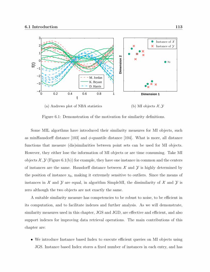
6.1 Introduction 113
0 0.2 0.4 0.6 0.8 1−4
−3
−2
−1
0
1
2
3
t
f(t)
M. JordanK. BryantD. Harris
(a) Andrews plot of NBA statistics
x0
Dimension 1
Dim
ensi
on
2
Instance of XInstance of Y
(b) MI objects X ,Y
Figure 6.1: Demonstration of the motivation for similarity definitions.
Some MIL algorthms have introduced their similarity measures for MI objects, such
as minHausdorff distance [103] and φ-quantile distance [104]. What is more, all distance
functions that measure (dis)similarities between point sets can be used for MI objects.
However, they either lose the information of MI objects or are time consuming. Take MI
objects X ,Y (Figure 6.1(b)) for example, they have one instance in common and the centers
of instances are the same. Hausdorff distance between X and Y is highly determined by
the position of instance x0, making it extremely sensitive to outliers. Since the means of
instances in X and Y are equal, in algorithm SimpleMI, the dissimilarity of X and Y is
zero although the two objects are not exactly the same.
A suitable similarity measure has competencies to be robust to noise, to be efficient in
its computation, and to facilitate indexes and further analysis. As we will demonstrate,
similarity measures used in this chapter, JGS and JGD, are effective and efficient, and also
support indexes for improving data retrieval operations. The main contributions of this
chapter are:
• We introduce Instance based Index to execute efficient queries on MI objects using
JGS. Instance based Index stores a fixed number of instances in each entry, and has

114 6. Indexing Multiple-Instance Objects
an effective strategy to prune non-qualified candidates.
• As a metric, JGD enables any metric tree to index MI objects. We apply VP-tree [76]
on the index of MI objects using JGD.
• Experimental results show the effectiveness of JGS and JGD, and the efficiency of
both indexes for MI objects.
The rest of this chapter is organized as follows. In Section 6.2, we survey the previous
work.Section 6.3 describes the idea of Instance based Index for MI objects. Section 6.4
shows the experimental studies to verify the effectiveness of similarity measures and the
efficiency of the proposed index. Finally, Section 6.5 summarizes this chapter and presents
some ideas for further research.
6.2 Related Work
In this section we give a brief survey and discussion of similarity measures for MI objects
and indexes in previous work.
6.2.1 Similarity Measures for MI objects
MIL algorithms can be grouped into three categories, the instance space based paradigm,
the embedded space based paradigm and the bag space based paradigm [78]. For the last
paradigm, the similarity measure for MI data is the essential part. In the bag space based
paradigm, algorithms treat each bag as a single object and define similarity measures for
bags. In this case, all distance based technologies can be used in MIL, such as k-NN, SVM,
k-mediods, DBSCAN, etc.
All distance functions that measure the (dis)similarity between point sets can be used
for MI objects, including Hausdorff distance [30], SMD [100], Chamfer matching [29], EMD
[101], Netflow distance [102], etc. What is more, some MIL algorithms have introduced
their similarity measures for MI objects. J. Wang and J. Zucker have proposed modified

6.2 Related Work 115
Hausdorff distances for Bayesian k-NN and Citation k-NN, and concluded that the minimal
Hausdorff distance slightly outperformed the maximal one [103]. It is worth noting that
these two algorithms can also handle general classification tasks besides MIL, and it is the
similarity measures that solve the MIL problem. Similarly, W. Zhang et al. have applied
Quantile based k-NN on MI data, defining φ-quantile distance [104]. X. He has proposed
PIM on the basis of an idea that each MI object is a manifestation of some templates
[31]. L. Sørensen et al. have compared BWmax and BWmean distance, and found that
the latter had a better performance [105]. T. Fukui and T. Wada have introduced four
similarity measures based on Diverse Density measure in their clustering algorithm, but
all these measures can only handle the binary situation [108]. Metric learning has been
extended to MIL [109, 106], however, they actually learn a metric for instances, replacing
Euclidean distances with Mahalanobis distances.
The existing similarity measures range from simple and efficient ones like Hausdorff
distance to complex ones like Netflow distance and PIM, but only a few of them are
metrics and take account of the information of all instances. Taking Hausdorff distance for
example, it is a metric, but it only uses the distance between two single instances of bags,
which makes it sensitive to noise.
6.2.2 Index
Index structures, besides linear scan, are essential techniques to make accesses to data
more efficient.
Most of indexes are based on classical binary search algorithms, for instance, k-d
tree [37], R-tree [38], etc. Spatial objects that can be treated as vectors are grouped
by L-norm distance. Gauss-tree [45] and GCI [48] store objects in parameter space instead
of feature spaces, and customized distance measures are used.
For general case where only a collection of objects and a function for measuring simi-
larities are given, metric trees are introduced. However, similarity measures are required
to satisfy the triangle inequality to prune candidates using the result of each similarity

116 6. Indexing Multiple-Instance Objects
comparison. Metric trees includes M-tree [44], VP-tree [76], etc.
6.3 Index MI Objects
In this part we discuss index techniques for querying MI objects with JGS and JGD. Since
JGS is not a metric, we need to design a specialized index structure to ensure the query
efficiency and accuracy. As for JGD, we employ VP-tree, a hierarchical structure, directly
to speed up both k-NN queries and range queries while guaranteeing the accuracy.
Instance Based Index
Due to the potential unequal numbers of instances in MI objects, traditional index tech-
niques like R-tree cannot be used on MI data. To tackle this problem, on basis of GCI [48],
we introduce Instance based Index for MI objects using JGS. Firstly we store all the
instances of MI objects into a Gauss-tree [45] which supports efficient queries for Gaussian
distributions, thus Instance based Index shares the same insertion and deletion strategies
with the Gauss-tree. Then we build an extra structure to locate and store potential
candidates.
MI objects are decomposed into instances and stored in a Gauss-tree. Given a query
object XQ = xjnQj=1, where nQ is the number of instances in XQ, we start the ranking of
instances by JGS between them and XQ, and get the candidates list of MI objects. As for
the query processing, we assume that we always have a pruning threshold τ , below which
the corresponding objects of the instances are not of interest. Only for these instances
that have higher JGS than τ , their corresponding MI objects will be retrieved to execute
the expensive calculation of JGS between MI objects, which we call the refinement. τ can
either be defined by the user in range queries, or be the k-th ranked JGS with the query
object in k-NN queries. In the latter case we start with τ = 0 and update it whenever we
find a greater k-th JGS than τ . For instances that have lower JGS than τ , we can safely
exclude the corresponding MI objects if they have not been retrieved yet.
Given an index node P = [wp, wp; xpi, xpiD1 ; np, np], in the prune stage of instance
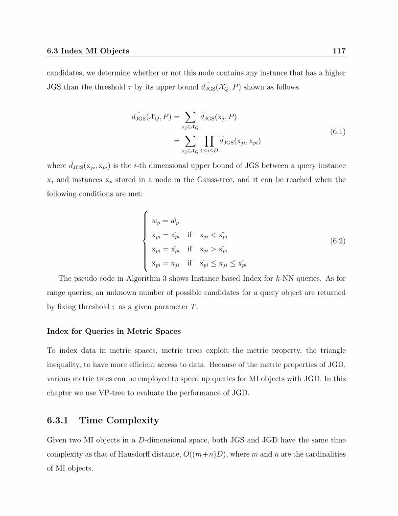
6.3 Index MI Objects 117
candidates, we determine whether or not this node contains any instance that has a higher
JGS than the threshold τ by its upper bound ˆdJGS(XQ, P ) shown as follows.
ˆdJGS(XQ, P ) =∑
xj∈XQ
dJGS(xj, P )
=∑
xj∈XQ
∏
1≤i≤D
dJGS(xji, xpi)(6.1)
where dJGS(xji, xpi) is the i-th dimensional upper bound of JGS between a query instance
xj and instances xp stored in a node in the Gauss-tree, and it can be reached when the
following conditions are met:
wp = wp
xpi = xpi if xji < xpi
xpi = xpi if xji > xpi
xpi = xji if xpi ≤ xji ≤ xpi
(6.2)
The pseudo code in Algorithm 3 shows Instance based Index for k-NN queries. As for
range queries, an unknown number of possible candidates for a query object are returned
by fixing threshold τ as a given parameter T .
Index for Queries in Metric Spaces
To index data in metric spaces, metric trees exploit the metric property, the triangle
inequality, to have more efficient access to data. Because of the metric properties of JGD,
various metric trees can be employed to speed up queries for MI objects with JGD. In this
chapter we use VP-tree to evaluate the performance of JGD.
6.3.1 Time Complexity
Given two MI objects in a D-dimensional space, both JGS and JGD have the same time
complexity as that of Hausdorff distance, O((m+n)D), where m and n are the cardinalities
of MI objects.
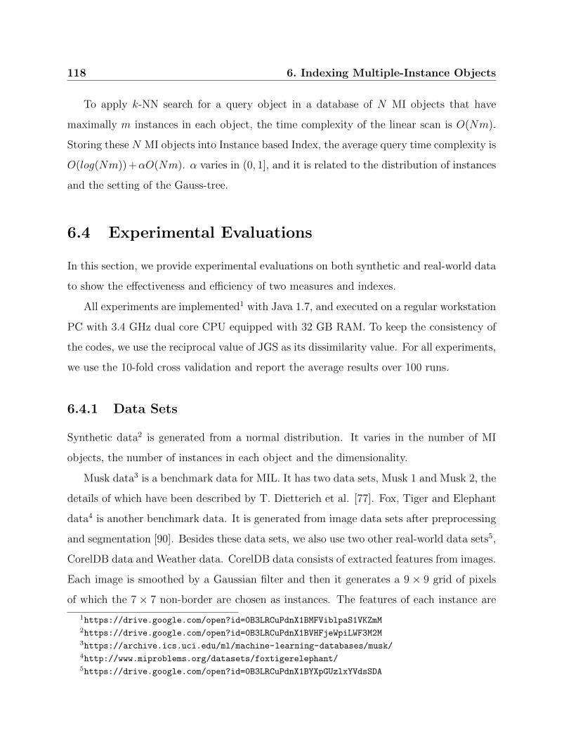
118 6. Indexing Multiple-Instance Objects
To apply k-NN search for a query object in a database of N MI objects that have
maximally m instances in each object, the time complexity of the linear scan is O(Nm).
Storing these N MI objects into Instance based Index, the average query time complexity is
O(log(Nm)) +αO(Nm). α varies in (0, 1], and it is related to the distribution of instances
and the setting of the Gauss-tree.
6.4 Experimental Evaluations
In this section, we provide experimental evaluations on both synthetic and real-world data
to show the effectiveness and efficiency of two measures and indexes.
All experiments are implemented1 with Java 1.7, and executed on a regular workstation
PC with 3.4 GHz dual core CPU equipped with 32 GB RAM. To keep the consistency of
the codes, we use the reciprocal value of JGS as its dissimilarity value. For all experiments,
we use the 10-fold cross validation and report the average results over 100 runs.
6.4.1 Data Sets
Synthetic data2 is generated from a normal distribution. It varies in the number of MI
objects, the number of instances in each object and the dimensionality.
Musk data3 is a benchmark data for MIL. It has two data sets, Musk 1 and Musk 2, the
details of which have been described by T. Dietterich et al. [77]. Fox, Tiger and Elephant
data4 is another benchmark data. It is generated from image data sets after preprocessing
and segmentation [90]. Besides these data sets, we also use two other real-world data sets5,
CorelDB data and Weather data. CorelDB data consists of extracted features from images.
Each image is smoothed by a Gaussian filter and then it generates a 9 × 9 grid of pixels
of which the 7 × 7 non-border are chosen as instances. The features of each instance are
1https://drive.google.com/open?id=0B3LRCuPdnX1BMFViblpaS1VKZmM2https://drive.google.com/open?id=0B3LRCuPdnX1BVHFjeWpiLWF3M2M3https://archive.ics.uci.edu/ml/machine-learning-databases/musk/4http://www.miproblems.org/datasets/foxtigerelephant/5https://drive.google.com/open?id=0B3LRCuPdnX1BYXpGUzlxYVdsSDA

6.4 Experimental Evaluations 119
color differences between a pixel and its neighbours. Weather data is the historical weather
data of airports around the world. Each instance of airports is the average statistics in a
month. We use the main categories of Koppen climate classification system to label each
airport.
6.4.2 Effectiveness
In this part, we evaluate the performances of proposed similarity measures on both su-
pervised and unsupervised learning. The parameters of PIM are set to the optimum in
the original paper, where the variance of template distribution is 5000 and the number of
samples is 1000. For φ-quantile distance, φ is set to 0.5 as suggested in the original paper.
Classification on Real-World Data Sets
Since we are not interested in tuning the classification accuracy to its optimum, k-NN
rather than the other more complex techniques is used to compare the effectiveness of
similarity measures here.
The accuracies of classification on seven real-world data sets are shown in Table 6.1.
JGD achieves the best performance on six data sets, and its result is still considerable on
Elephant data. The performance of JGS is moderate except on Weather data.
Clustering on Real-World Data Sets
We perform clustering experiments to compare the usability of proposed similarity mea-
sures for unsupervised data mining. k-medoids is used in this chapter because unlike
k-means, it works with arbitrary similarity measures. We evaluate clustering results with
two widely used criteria, Purity and NMI).
Evaluation results on CorelDB data and Weather data that have more than two classes
are shown in Table 6.2. We can see that the performance of JGD is the best or comparable
to the best on this task, while JGS achieves a moderate performance.

120 6. Indexing Multiple-Instance Objects
6.4.3 Efficiency
In this part, we compare the efficiency of JGS, JGD and the other similarity measures. We
start with the time cost6 of all the similarity calculations when varying the dimensionality
and the number of instances of each MI object, and then investigate the performances of
five metrics supported by VP-tree, as well as JGS supported by Instance based Index.
Time Complexity
Dimensionality
Tim
e co
st (
ms)
22 23 24 25 26 27 28 29 210
24
26
28
210
212
214
216
218
220
(a)
Number of instances
Tim
e co
st (
ms)
22 23 24 25 26 27 28
2−5
20
25
210
215
220
(b)
Hausdorff
EMD
Netflow
minHaudorff
Quantile
PIM
BWmean
JGS
JGD
(c)
Figure 6.2: Time cost of similarity calculations on synthetic data.
All the similarity measures compared in this chapter have a linear relation with the
dimensionality and the number of instances in each MI object. Since the curves of SMD
and Chamfer almost duplicate that of Hausdorff, their results are not included in Figure
6.2.
Due to the inherent complexity of EMD, Netflow and BWmean distance, the influence
of dimensionality becomes evident after the dimensionality reaches 512, as shown in Figure
6.2(a), where the number of instances is fixed to ten. Hausdorff distance, SMD, Chamfer,
minHausdorff distance and JGS are the most efficient measures. JGD costs slightly more
run-time than these relatively simple measures, but it is much efficient than sophisticated
6The time cost in this chapter refers to the CPU time.

6.4 Experimental Evaluations 121
measures like PIM. Fixing the data dimensionality to two, the run-time of similarity
measures increases linearly with the number of instances in each MI object, and the
performance of JGD is almost comparable with that of the most efficient techniques like
Hausdorff distance (Figure 6.2(b)).
Number of objects
Tim
e co
st (
ms)
27 28 29 210 211 212
2−2
20
22
24
26
28
210
212 Hausdorff
EMD
Netflow
PIM
JGS
JGD
Figure 6.3: Time cost of 1-NN queries using linear scan on synthetic data.
Index
We study the scalability of five metrics with VP-tree and JGS with Instance based Index
here. The capacity of nodes in the VP-tree is set to 32, while the minimum and maximum
node capacity of the Instance based Index are set to 10 and 50, respectively.
Firstly linear scan queries are applied on synthetic data, and there are ten two-dimensional
instances in each MI object. As shown in Figure 6.3, the run-time of all six measures
increase linearly with the number of objects. JGD and JGS have almost the same perfor-
mance as Hausdorff distance which is the most efficient among all the proposed techniques.
To evaluate the performance of five metrics and JGS when using indexes, we report the
ratio of linear scan query time and the index query time on synthetic data. The higher the
ratio is, the more the similarity measure benefits from indexes. As shown in Figure 6.4,
JGD profits the most and its acceleration ratio is much higher than those of the others for
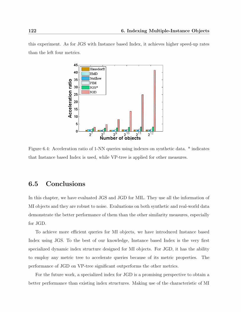
122 6. Indexing Multiple-Instance Objects
this experiment. As for JGS with Instance based Index, it achieves higher speed-up rates
than the left four metrics.
Figure 6.4: Acceleration ratio of 1-NN queries using indexes on synthetic data. * indicates
that Instance based Index is used, while VP-tree is applied for other measures.
6.5 Conclusions
In this chapter, we have evaluated JGS and JGD for MIL. They use all the information of
MI objects and they are robust to noise. Evaluations on both synthetic and real-world data
demonstrate the better performance of them than the other similarity measures, especially
for JGD.
To achieve more efficient queries for MI objects, we have introduced Instance based
Index using JGS. To the best of our knowledge, Instance based Index is the very first
specialized dynamic index structure designed for MI objects. For JGD, it has the ability
to employ any metric tree to accelerate queries because of its metric properties. The
performance of JGD on VP-tree significant outperforms the other metrics.
For the future work, a specialized index for JGD is a promising perspective to obtain a
better performance than existing index structures. Making use of the characteristic of MI

6.5 Conclusions 123
objects, the customized index could exploit the potential of efficient queries for MIL.

124 6. Indexing Multiple-Instance Objects
Algorithm 3: Instance based Index for the k-NN QueryData: int k, Node root, Query Object XQResult: PriorityQueue results
1 PriorityQueue results = new PriorityQueue() ; /* Ascending */
2 PriorityQueue activePages = new PriorityQueue() ; /* Descending */
3 results.put(-1, -MAX REAL);
4 activePages.put(root, MAX REAL);
5 τ = 0;
6 while activePages.isNotEmpty() and results.getMinJGS()<activePages.getMaxJGS() do
7 P = activePages.getFirstPage;
8 activePages.removeFirstPage();
9 if P .isDataPage() then
10 Entry E = P .data;
11 if ˆdJGS(XQ, P ) > τ then
12 Xcandidate = E.getMIobject;
13 results.put(Xcandidate, dJGS(Xcandidate,XQ));
14 if results.size> k then
15 results.removeFirst;
16 τ =results.getMinJGS();
17 else
18 children = P .getChildren();
19 while children.hasMoreElements() do
20 child = children.getNextElement();
21 probability = ˆdJGS(XQ, child);
22 activePages.put(child,probability);
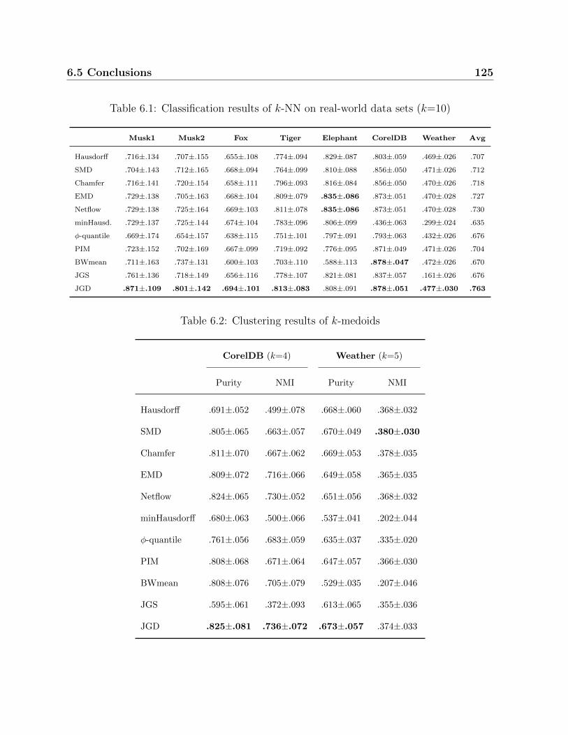
6.5 Conclusions 125
Table 6.1: Classification results of k-NN on real-world data sets (k=10)
Musk1 Musk2 Fox Tiger Elephant CorelDB Weather Avg
Hausdorff .716±.134 .707±.155 .655±.108 .774±.094 .829±.087 .803±.059 .469±.026 .707
SMD .704±.143 .712±.165 .668±.094 .764±.099 .810±.088 .856±.050 .471±.026 .712
Chamfer .716±.141 .720±.154 .658±.111 .796±.093 .816±.084 .856±.050 .470±.026 .718
EMD .729±.138 .705±.163 .668±.104 .809±.079 .835±.086 .873±.051 .470±.028 .727
Netflow .729±.138 .725±.164 .669±.103 .811±.078 .835±.086 .873±.051 .470±.028 .730
minHausd. .729±.137 .725±.144 .674±.104 .783±.096 .806±.099 .436±.063 .299±.024 .635
φ-quantile .669±.174 .654±.157 .638±.115 .751±.101 .797±.091 .793±.063 .432±.026 .676
PIM .723±.152 .702±.169 .667±.099 .719±.092 .776±.095 .871±.049 .471±.026 .704
BWmean .711±.163 .737±.131 .600±.103 .703±.110 .588±.113 .878±.047 .472±.026 .670
JGS .761±.136 .718±.149 .656±.116 .778±.107 .821±.081 .837±.057 .161±.026 .676
JGD .871±.109 .801±.142 .694±.101 .813±.083 .808±.091 .878±.051 .477±.030 .763
Table 6.2: Clustering results of k-medoids
CorelDB (k=4) Weather (k=5)
Purity NMI Purity NMI
Hausdorff .691±.052 .499±.078 .668±.060 .368±.032
SMD .805±.065 .663±.057 .670±.049 .380±.030
Chamfer .811±.070 .667±.062 .669±.053 .378±.035
EMD .809±.072 .716±.066 .649±.058 .365±.035
Netflow .824±.065 .730±.052 .651±.056 .368±.032
minHausdorff .680±.063 .500±.066 .537±.041 .202±.044
φ-quantile .761±.056 .683±.059 .635±.037 .335±.020
PIM .808±.068 .671±.064 .647±.057 .366±.030
BWmean .808±.076 .705±.079 .529±.035 .207±.046
JGS .595±.061 .372±.093 .613±.065 .355±.036
JGD .825±.081 .736±.072 .673±.057 .374±.033

126 6. Indexing Multiple-Instance Objects
Chapter 7
Conclusions and Future Work
The complexity of data analysis increases with the generated and stored data quantity and
variety, especially in the age of “Big Data”. Indexing and efficient similarity search provides
essential supports for data mining algorithms. Representing complex data by GMM and
MI objects, in this thesis we have proposed indexing techniques on basis of component
combinations, and introduced several similarity measures with closed-form expressions.
7.1 Knowledge Discovery Using GMM
As a general class of probability distribution functions, GMM have the ability to ap-
proximate arbitrary distributions in a concise way. Modeling complex data into GMM
will dramatically reduce resource consumptions and computation efforts. Indexing and
similarity search on GMM provide an effective solution for the knowledge discovery of
complex data and enable the following usage of various analysis algorithms.
We stored the Gaussian component combinations instead of GMM into well-studied
indexing trees and proposed an efficient and conservative refinement strategy to locate the
interested objects of given queries. To achieve better efficiency of the indexing technique,
we normalized the stored GMM by their weights of components and improve the ability
of filtering unqualified candidates. Several novel similarity measures with closed-form

128 7. Conclusions and Future Work
expressions for GMM have been introduced and some of them are also metrics, of which
properties are essential for some data mining technologies.
For the index of GMM using the proposed metric, Infinite Euclidean Distance, we have
not reinvented the wheel in this thesis and employed metric trees directly, which saved extra
efforts. The efficiency could be further increased by specific-designed indexing structures
which exploit the properties of the proposed metric. Gaussian Component based Index
uses Matching Probability as the similarity measure, which cannot be extended for the
metric in a similar way. However, the idea of storing GMM by their components is still a
perspective to enable the specific-designed indexing structure using metrics.
7.2 Multiple-Instance Learning
First motivated by the problem of drug activity predictions, MIL discovers the knowledge
of data objects by their instances. The assumptions of traditional algorithms describe the
relations between the label of a data object and the labels of its instances in a given way,
e.g., a drug molecule is active if and only if one or more of its conformers are active. On
basis of that, most of MIL problems are transferred into single-instance spaces and then
solved with the assembled results of instances.
In this thesis, we have solved MIL in the object-level and proposed novel similarity
measures that make use of all the information of Multiple-Instance objects, which are
effective and efficient for computations. Similarity measures enable the usage of clustering
algorithms on MIL problems, and evaluations on synthetic and real-world data demonstrate
the better performance of our measures. What is more, indexing structures have been
introduced to Multiple-Instance objects.
For the future work, various analysis technologies could be extended to MIL on basis
of proposed metric for Multiple-Instance objects, such as Multidimensional Scaling, index-
accelerating clustering algorithms. A general assumption between the labels of instances
and the labels of objects is also a perspective for the further exploration of MIL.

Bibliography
[1] M. Chen, S. Mao, and Y. Liu, “Big data: A survey,” MONET, vol. 19, no. 2, pp.
171–209, 2014.
[2] J. Han and M. Kamber, Data Mining: Concepts and Techniques. Morgan Kaufmann,
2000.
[3] W. J. Frawley, G. Piatetsky-Shapiro, and C. J. Matheus, “Knowledge discovery in
databases: An overview,” in Knowledge Discovery in Databases. AAAI/MIT Press,
1991, pp. 1–30.
[4] H. Chen, R. H. L. Chiang, and V. C. Storey, “Business intelligence and analytics:
From big data to big impact,” MIS Quarterly, vol. 36, no. 4, pp. 1165–1188, 2012.
[5] G. S. Linoff and M. J. Berry, Data mining techniques: for marketing, sales, and
customer relationship management. John Wiley & Sons, 2011.
[6] I. Yeh and C. Lien, “The comparisons of data mining techniques for the predictive
accuracy of probability of default of credit card clients,” Expert Syst. Appl., vol. 36,
no. 2, pp. 2473–2480, 2009.
[7] “Iris dataset,” https://archive.ics.uci.edu/ml/datasets/Iris, accessed: 2017-06-21.
[8] S. P. Lloyd, “Least squares quantization in PCM,” IEEE Trans. Information Theory,
vol. 28, no. 2, pp. 129–136, 1982.
130 BIBLIOGRAPHY
[9] A. P. Dempster, N. M. Laird, and D. B. Rubin, “Maximum likelihood from
incomplete data via the em algorithm,” Journal of the royal statistical society. Series
B (methodological), pp. 1–38, 1977.
[10] M. Ester, H.-P. Kriegel, J. Sander, and X. Xu, “A density-based algorithm for
discovering clusters in large spatial databases with noise,” in SIGKDD, 1996, pp.
226–231.
[11] M. Ankerst, M. M. Breunig, H. Kriegel, and J. Sander, “OPTICS: ordering points
to identify the clustering structure,” in SIGMOD, 1999, pp. 49–60.
[12] N. R. Draper and H. Smith, Applied regression analysis. John Wiley & Sons, 2014.
[13] L. S. Aiken, S. G. West, and R. R. Reno, Multiple regression: Testing and interpreting
interactions. Sage, 1991.
[14] C. Cortes and V. Vapnik, “Support-vector networks,” Machine Learning, vol. 20,
no. 3, pp. 273–297, 1995.
[15] I. Naseem, R. Togneri, and M. Bennamoun, “Linear regression for face recognition,”
IEEE Trans. Pattern Anal. Mach. Intell., vol. 32, no. 11, pp. 2106–2112, 2010.
[16] K. Kim, “A hybrid classification algorithm by subspace partitioning through semi-
supervised decision tree,” Pattern Recognition, vol. 60, pp. 157–163, 2016.
[17] D. BS, K. Subramaniam, and N. HR, “Hep-2 cell classification using artificial neural
network approach,” in ICPR, 2016, pp. 84–89.
[18] R. Sibson, “SLINK: an optimally efficient algorithm for the single-link cluster
method,” Comput. J., vol. 16, no. 1, pp. 30–34, 1973.
[19] D. Defays, “An efficient algorithm for a complete link method,” Comput. J., vol. 20,
no. 4, pp. 364–366, 1977.
BIBLIOGRAPHY 131
[20] H. Park and C. Jun, “A simple and fast algorithm for k-medoids clustering,” Expert
Syst. Appl., vol. 36, no. 2, pp. 3336–3341, 2009.
[21] J. D. Banfield and A. E. Raftery, “Model-based gaussian and non-gaussian
clustering,” Biometrics, pp. 803–821, 1993.
[22] R. Agrawal, T. Imielinski, and A. N. Swami, “Mining association rules between sets
of items in large databases,” in SIGMOD, 1993, pp. 207–216.
[23] M. Beyer, “Gartner says solving ’big data’ challenge involves more than just
managing volumes of data,” Gartner. Archived from the original on, vol. 10, 2011.
[24] M. Hilbert, “Big data for development: A review of promises and challenges,”
Development Policy Review, vol. 34, no. 1, pp. 135–174, 2016.
[25] C. W. Granger, “Some properties of time series data and their use in econometric
model specification,” Journal of econometrics, vol. 16, no. 1, pp. 121–130, 1981.
[26] J. C. Gower, “A general coefficient of similarity and some of its properties,”
Biometrics, pp. 857–871, 1971.
[27] L. Hamers, Y. Hemeryck, G. Herweyers, M. Janssen, H. Keters, R. Rousseau, and
A. Vanhoutte, “Similarity measures in scientometric research: The jaccard index
versus salton’s cosine formula,” Inf. Process. Manage., vol. 25, no. 3, pp. 315–318,
1989.
[28] I. Niiniluoto, Truthlikeness. Springer, 1987, vol. 185.
[29] S. J. Belongie, J. Malik, and J. Puzicha, “Shape matching and object recognition
using shape contexts,” Pattern Anal. Mach. Intell., vol. 24, no. 4, pp. 509–522, 2002.
[30] F. Hausdorff and J. R. Aumann, Grundzuge der mengenlehre. Veit, 1914.
[31] X. He, “Multi-purpose exploratory mining of complex data,” Ph.D. dissertation,
Ludwig-Maximilians-Universitat Munchen, 2014.

132 BIBLIOGRAPHY
[32] A. Bhattacharyya, “On a measure of divergence between two statistical populations
defined by their probability distributions,” Bull. Calcutta Math. Soc., vol. 35, pp.
99–109, 1943.
[33] S. Kullback, Information Theory and Statistics. Courier Corporation, 1968.
[34] C. Carson, M. Thomas, S. J. Belongie, J. M. Hellerstein, and J. Malik, “Blobworld:
A system for region-based image indexing and retrieval,” in VISUAL, 1999, pp. 509–
516.
[35] E. J. Keogh, K. Chakrabarti, S. Mehrotra, and M. J. Pazzani, “Locally adaptive
dimensionality reduction for indexing large time series databases,” in SIGMOD, 2001,
pp. 151–162.
[36] A. K. Jain, S. Prabhakar, L. Hong, and S. Pankanti, “Filterbank-based fingerprint
matching,” IEEE Trans. Image Processing, vol. 9, no. 5, pp. 846–859, 2000.
[37] J. L. Bentley, “Multidimensional binary search trees used for associative searching,”
Commun. ACM, vol. 18, no. 9, pp. 509–517, 1975.
[38] A. Guttman, “R-trees: A dynamic index structure for spatial searching,” in
SIGMOD, 1984, pp. 47–57.
[39] N. Beckmann, H. Kriegel, R. Schneider, and B. Seeger, “The R*-tree: An efficient
and robust access method for points and rectangles,” in SIGMOD, 1990, pp. 322–331.
[40] S. Berchtold, D. A. Keim, and H. Kriegel, “The X-tree: An Index Structure for
High-Dimensional Data,” in VLDB, 1996, pp. 28–39.
[41] D. A. White and R. Jain, “Similarity indexing with the SS-tree,” in ICDE, 1996, pp.
516–523.
[42] R. Kurniawati, J. S. Jin, and J. Shepherd, “SS+-tree: An improved index structure
for similarity searches in a high-dimensional feature space,” in Storage and Retrieval
for Image and Video Databases V, 1997, pp. 110–120.

BIBLIOGRAPHY 133
[43] N. Katayama and S. Satoh, “The SR-tree: An index structure for high-dimensional
nearest neighbor queries,” in SIGMOD, 1997, pp. 369–380.
[44] P. Ciaccia, M. Patella, and P. Zezula, “M-tree: An efficient access method for
similarity search in metric spaces,” in VLDB, 1997, pp. 426–435.
[45] C. Bohm, A. Pryakhin, and M. Schubert, “The Gauss-tree: Efficient object
identification in databases of probabilistic feature vectors,” in ICDE, 2006, p. 9.
[46] Y. Tao, R. Cheng, X. Xiao, W. K. Ngai, B. Kao, and S. Prabhakar, “Indexing multi-
dimensional uncertain data with arbitrary probability density functions,” in VLDB,
2005, pp. 922–933.
[47] A. Strehl and J. Ghosh, “Cluster ensembles — A knowledge reuse framework for
combining multiple partitions,” Journal of Machine Learning Research, vol. 3, pp.
583–617, 2002.
[48] L. Zhou, B. Wackersreuther, F. Fiedler, C. Plant, and C. Bohm, “Gaussian
component based index for GMMs,” in ICDM, 2016, pp. 1365–1370.
[49] L. Zhou, W. Ye, C. Plant, and C. Bohm, “Knowledge discovery of complex data
using Gaussian Mixture Models,” in DaWaK, 2017.
[50] L. Zhou, W. Ye, B. Wackersreuther, C. Plant, and C. Bohm, “Novel indexing strategy
and similarity measures for Gaussian Mixture Models,” in DEXA, 2017.
[51] L. Zhou, C. Plant, and C. Bohm, “Joint gaussian based measures for multiple-
instance learning,” in ICDE, 2017, pp. 203–206.
[52] L. Zhou, W. Ye, Z. Wang, C. Plant, and C. Bohm, “Indexing multiple-instance
objects,” in DEXA, 2017.
[53] M. A. Pathak and B. Raj, “Privacy-preserving speaker verification and identification
using gaussian mixture models,” vol. 21, no. 2, 2013, pp. 397–406.

134 BIBLIOGRAPHY
[54] C. Beecks, M. S. Uysal, and T. Seidl, “Content-based image retrieval with Gaussian
Mixture Models,” in MMM Part I, 2015, pp. 294–305.
[55] Y. Song, M. B. Salem, S. Hershkop, and S. J. Stolfo, “System level user behavior
biometrics using fisher features and Gaussian Mixture Models,” in SSPW, 2013, pp.
52–59.
[56] D. Reynolds, “Gaussian Mixture Models,” Encyclopedia of Biometrics, pp. 827–832,
2015.
[57] J. E. Rougui, M. Gelgon, D. Aboutajdine, N. Mouaddib, and M. Rziza, “Organizing
Gaussian Mixture Models into a tree for scaling up speaker retrieval,” Pattern
Recognition Letters, vol. 28, no. 11, pp. 1314–1319, 2007.
[58] J. Goldberger, S. Gordon, and H. Greenspan, “An efficient image similarity measure
based on approximations of KL-divergence between two gaussian mixtures,” in ICCV,
2003, pp. 487–493.
[59] J. R. Hershey and P. A. Olsen, “Approximating the kullback leibler divergence
between gaussian mixture models,” in ICASSP, 2007, pp. 317–320.
[60] M. L. Helen and T. Virtanen, “Query by example of audio signals using Euclidean
distance between Gaussian Mixture Models,” in ICASSP, 2007, pp. 225–228.
[61] G. Sfikas, C. Constantinopoulos, A. Likas, and N. P. Galatsanos, “An analytic
distance metric for Gaussian Mixture Models with application in image retrieval,” in
ICANN, Part II, 2005, pp. 835–840.
[62] J. H. Jensen, D. P. W. Ellis, M. G. Christensen, and S. H. Jensen, “Evaluation of
distance measures between Gaussian Mixture Models of MFCCs,” in ISMIR, 2007,
pp. 107–108.

BIBLIOGRAPHY 135
[63] C. Beecks, A. M. Ivanescu, S. Kirchhoff, and T. Seidl, “Modeling image similarity
by Gaussian Mixture Models and the signature quadratic form distance,” in ICCV,
2011, pp. 1754–1761.
[64] K. Haegler, F. Fiedler, and C. Bohm, “Searching uncertain data represented by non-
axis parallel Gaussian Mixture Models,” in ICDE, 2012, pp. 246–257.
[65] C. Bohm, P. Kunath, A. Pryakhin, and M. Schubert, “Querying objects modeled by
arbitrary probability distributions,” in SSTD, 2007, pp. 294–311.
[66] W. M. Campbell, D. E. Sturim, and D. A. Reynolds, “Support vector machines using
GMM supervectors for speaker verification,” IEEE Signal Process. Lett., vol. 13,
no. 5, pp. 308–311, 2006.
[67] D. A. Reynolds, T. F. Quatieri, and R. B. Dunn, “Speaker verification using adapted
Gaussian Mixture Models,” Digital Signal Processing, vol. 10, no. 1-3, pp. 19–41,
2000.
[68] P. KaewTraKulPong and R. Bowden, “An improved adaptive background mixture
model for real-time tracking with shadow detection,” in Video-based surveillance
systems. Springer, 2002, pp. 135–144.
[69] Z. Zivkovic, “Improved adaptive Gaussian Mixture Model for background
subtraction,” in ICPR, 2004, pp. 28–31.
[70] “STATS description,” https://www.stats.com/sportvu-basketball-media/, accessed:
2017-02-25.
[71] V. Cheplygina, D. M. J. Tax, and M. Loog, “Dissimilarity-based ensembles for
multiple instance learning,” IEEE Transactions on Neural Networks and Learning
Systems, vol. 27, no. 6, pp. 1379–1391, 2016.
[72] J. Sivic and A. Zisserman, “Video google: A text retrieval approach to object
matching in videos,” in ICCV, 2003, pp. 1470–1477.
136 BIBLIOGRAPHY
[73] H. Kriegel, A. Pryakhin, and M. Schubert, “An EM-approach for clustering multi-
instance objects,” in PAKDD, 2006, pp. 139–148.
[74] X. Wei, J. Wu, and Z. Zhou, “Scalable multi-instance learning,” in ICDM, 2014, pp.
1037–1042.
[75] Z. Zhou, Y. Sun, and Y. Li, “Multi-instance learning by treating instances as non-
i.i.d. samples,” in ICML, 2009, pp. 1249–1256.
[76] P. N. Yianilos, “Data structures and algorithms for nearest neighbor search in general
metric spaces,” in ACM/SIGACT-SIAM SODA, 1993, pp. 311–321.
[77] T. G. Dietterich, R. H. Lathrop, and T. Lozano-Perez, “Solving the multiple instance
problem with axis-parallel rectangles,” Artif. Intell., vol. 89, no. 1-2, pp. 31–71, 1997.
[78] J. Amores, “Multiple instance classification: Review, taxonomy and comparative
study,” Artif. Intell., vol. 201, pp. 81–105, 2013.
[79] N. Weidmann, E. Frank, and B. Pfahringer, “A two-level learning method for
generalized multi-instance problems,” in ECML, 2003, pp. 468–479.
[80] Y. Chen and J. Z. Wang, “Image categorization by learning and reasoning with
regions,” Journal of Machine Learning Research, vol. 5, pp. 913–939, 2004.
[81] Y. Chen, J. Bi, and J. Z. Wang, “MILES: multiple-instance learning via embedded
instance selection,” Pattern Anal. Mach. Intell., vol. 28, no. 12, pp. 1931–1947, 2006.
[82] H. Wang, Q. Yang, and H. Zha, “Adaptive p-posterior mixture-model kernels for
multiple instance learning,” in ICML, 2008, pp. 1136–1143.
[83] R. R. Vatsavai, “Gaussian multiple instance learning approach for mapping the slums
of the world using very high resolution imagery,” in SIGKDD, 2013, pp. 1419–1426.
[84] K. Sikka, R. Giri, and M. S. Bartlett, “Joint clustering and classification for multiple
instance learning,” in BMVC, 2015, pp. 71.1–71.12.

BIBLIOGRAPHY 137
[85] S. Kullback, Information theory and statistics. Courier Dover Publications, 2012.
[86] S. Cui and M. Datcu, “Comparison of Kullback-Leibler divergence approximation
methods between Gaussian Mixture Models for satellite image retrieval,” in IGARSS,
2015, pp. 3719–3722.
[87] M. Ester, H. Kriegel, J. Sander, and X. Xu, “A density-based algorithm for
discovering clusters in large spatial databases with noise,” in SIGKDD, 1996, pp.
226–231.
[88] M. C. Peel, B. L. Finlayson, and T. A. McMahon, “Updated world map of the koppen-
geiger climate classification,” Hydrology and Earth System Sciences Discussions
Discussions, vol. 4, no. 2, pp. 439–473, 2007.
[89] J.-M. Geusebroek, G. J. Burghouts, and A. W. Smeulders, “The amsterdam library
of object images,” International Journal of Computer Vision, vol. 61, no. 1, pp.
103–112, 2005.
[90] S. Andrews, I. Tsochantaridis, and T. Hofmann, “Support vector machines for
multiple-instance learning,” in Advances in Neural Information Processing Systems
15, 2002, pp. 561–568.
[91] X. Guan, R. Raich, and W. Wong, “Efficient multi-instance learning for activity
recognition from time series data using an auto-regressive hidden markov model,” in
ICML, 2016, pp. 2330–2339.
[92] X. Xu, “Statistical learning in multiple-instance problems,” Master’s thesis,
University of Waikato, 2003.
[93] O. Maron and T. Lozano-Perez, “A framework for multiple-instance learning,” in
Advances in Neural Information Processing Systems 10, 1997, pp. 570–576.

138 BIBLIOGRAPHY
[94] Q. Zhang and S. A. Goldman, “EM-DD: an improved multiple-instance learning
technique,” in Advances in Neural Information Processing Systems 14, 2001, pp.
1073–1080.
[95] J. Wang, L. Cai, J. Peng, and Y. Jia, “A novel multiple instance learning method
based on extreme learning machine,” Comp. Int. and Neurosc., vol. 2015, pp.
405 890:1–405 890:6, 2015.
[96] M. Carbonneau, E. Granger, A. J. Raymond, and G. Gagnon, “Robust multiple-
instance learning ensembles using random subspace instance selection,” Pattern
Recognition, vol. 58, pp. 83–99, 2016.
[97] A. Shrivastava, V. M. Patel, J. K. Pillai, and R. Chellappa, “Generalized dictionaries
for multiple-instance learning,” International Journal of Computer Vision, vol. 114,
no. 2-3, pp. 288–305, 2015.
[98] D. T. Nguyen, C. D. Nguyen, R. H. Hargraves, L. A. Kurgan, and K. J. Cios, “mi-
DS: Multiple-instance learning algorithm,” IEEE Trans. Cybernetics, vol. 43, no. 1,
pp. 143–154, 2013.
[99] L. Dong, “A comparison of multi-instance learning algorithms,” Master’s thesis,
University of Waikato, 2006.
[100] I. Niiniluoto, Truthlikeness. Springer Science & Business Media, 2012, vol. 185.
[101] Y. Rubner, C. Tomasi, and L. J. Guibas, “The Earth Mover’s distance as a metric for
image retrieval,” International journal of computer vision, vol. 40, no. 2, pp. 99–121,
2000.
[102] J. Ramon and M. Bruynooghe, “A polynomial time computable metric between point
sets,” Acta Inf., vol. 37, no. 10, pp. 765–780, 2001.
[103] J. Wang and J. Zucker, “Solving the multiple-instance problem: A lazy learning
approach,” in ICML, 2000, pp. 1119–1126.
BIBLIOGRAPHY 139
[104] W. Zhang, X. Lin, M. A. Cheema, Y. Zhang, and W. Wang, “Quantile-based KNN
over multi-valued objects,” in ICDE, 2010, pp. 16–27.
[105] L. Sørensen, M. Loog, D. M. J. Tax, W. Lee, M. de Bruijne, and R. P. W. Duin,
“Dissimilarity-based multiple-instance learning,” in IAPR, 2010, pp. 129–138.
[106] R. Jin, S. Wang, and Z. Zhou, “Learning a distance metric from multi-instance
multi-label data,” in CVPR, 2009, pp. 896–902.
[107] M. Zhang and Z. Zhou, “Multi-instance clustering with applications to multi-instance
prediction,” Appl. Intell., vol. 31, no. 1, pp. 47–68, 2009.
[108] T. Fukui and T. Wada, “Commonality preserving multiple-instance clustering based
on diverse density,” in ACCV, 2014, pp. 322–335.
[109] M. Guillaumin, J. J. Verbeek, and C. Schmid, “Multiple-instance metric learning
from automatically labeled bags of faces,” in ECCV, 2010, pp. 634–647.

140

Acknowledgments
Time flies. So many beautiful memories here in Munich. I would like to take this
opportunity to express my deepest gratitude to numerous people who have helped and
supported me during my four years as a PhD student.
First of all, I would like to thank my supervisor, Professor Christian Bohm, for intro-
ducing me to the fantastic world of data and guiding me in the exploration of that world
with great expertise. Thank you Christian for all the inspiring, fruitful and enjoyable
guidance and discussions. I would also offer my special thanks to Professor Claudia Plant
for her pleasant guidance and friendly encouragement.
Thanks to all collaborators who have contributed during my PhD study, especially Dr.
Elisabeth Georgii, Dr. Bianca Wackersreuther, Wei Ye, Zhen Wang and Frank Fiedler.
This work would not be possible without your great efforts. Thanks to former and current
colleagues at Oettingenstr, Dr. Xiao He, Dr. Jing Feng, Dr. Mai Thai Son, Dr. Xin
Sun, Sebastian Goebl, Dominik Mautz and people from Helmholtz center, Dr. David
Endesfelder, Dr. Samuel Maurus, Alexandra Derntl, Sahar Behzadi Soheil, Annika Tonch,
Nina Hubig, for bringing me so much joy to both work and life. I am deeply grateful for
the time we had together. Special thanks to Dominik and Bo Zhang for translating the
abstract. Furthermore, I would like to acknowledge Franz Krojer, Susanne Grienberger
and Sandra Mayer for their excellent technical and background supports.
I would also like to thank my landlady Maria Herrmann for having me in the house
after my dormitory contract ended. Also thanks my friend Liang Jin for the pleasure of
hiking in Alps, and other friends for being an important part of life.

142
I would like to thank China Scholarship Council and Ludwig–Maximilians–Universitat
Munich (CSC-LMU) programme for providing me the financial support during my PhD
study.
Last but certainly not least, I want to thank my beloved family. Thank you my parents
for being the harbor of my heart, wish my mother all the best in paradise, thank you my
elder brother Linkang Zhou for the selfless support and dedication to the family, thank you
my wife Li Zhang for the warm and sweet companionship.
Linfei Zhou
Munich, Germany
August, 2017

Curriculum Vitae
Linfei Zhou
November 1987 Born in Shandong Juancheng, P. R. China
September 1994 - July 1999 The First Primary School in Juancheng, P. R. China
September 1999 - July 2006 The First High School in Juancheng, P. R. China
September 2006 - July 2010 Bachelor in Electrical Engineering and Automation,
School of Electrical Engineering, Southwest Jiaotong
University, P. R. China
September 2010 - July 2013 Master in Control Engineering, Department of Automa-
tion, Tsinghua University, P. R. China
September 2013 - Now PhD Candidate in Computer Science, Institute of
Mathematics, Informatics and Statistics, Ludwig-
Maximilians-Universitat Munchen, Germany

144


Formular 3.2
Ort, Datum Unterschrift Doktorand/in
Name, Vorname
Zhou Linfei
Eidesstattliche Versicherung(Siehe Promotionsordnung vom 12.07.11, § 8, Abs. 2 Pkt. .5.)
Hiermit erkläre ich an Eidesstatt, dass die Dissertation von mir
selbstständig, ohne unerlaubte Beihilfe angefertigt ist.
2017-08-18, München

![Homology of gaussian groups - Centre Mersenne · 493 1.1. Gaussian and locally Gaussian monoids. Our notations follow those of [42] on the one hand, and those of [25] and [23] on](https://static.fdocuments.fr/doc/165x107/5fd4001a720ab320977220ad/homology-of-gaussian-groups-centre-mersenne-493-11-gaussian-and-locally-gaussian.jpg)