
ImageNet Large Scale Visual Recognition Challenge
43
Noname manuscript No. (will be inserted by the editor) ImageNet Large Scale Visual Recognition Challenge Olga Russakovsky* · Jia Deng* · Hao Su · Jonathan Krause · Sanjeev Satheesh · Sean Ma · Zhiheng Huang · Andrej Karpathy · Aditya Khosla · Michael Bernstein · Alexander C. Berg · Li Fei-Fei Received: date / Accepted: date Abstract The ImageNet Large Scale Visual Recogni- tion Challenge is a benchmark in object category classi- fication and detection on hundreds of object categories and millions of images. The challenge has been run an- nually from 2010 to present, attracting participation from more than fifty institutions. This paper describes the creation of this benchmark dataset and the advances in object recognition that have been possible as a result. We discuss the chal- O. Russakovsky* Stanford University, Stanford, CA, USA E-mail: [email protected] J. Deng* University of Michigan, Ann Arbor, MI, USA (* = authors contributed equally) H. Su Stanford University, Stanford, CA, USA J. Krause Stanford University, Stanford, CA, USA S. Satheesh Stanford University, Stanford, CA, USA S. Ma Stanford University, Stanford, CA, USA Z. Huang Stanford University, Stanford, CA, USA A. Karpathy Stanford University, Stanford, CA, USA A. Khosla Massachusetts Institute of Technology, Cambridge, MA, USA M. Bernstein Stanford University, Stanford, CA, USA A. C. Berg UNC Chapel Hill, Chapel Hill, NC, USA L. Fei-Fei Stanford University, Stanford, CA, USA lenges of collecting large-scale ground truth annotation, highlight key breakthroughs in categorical object recog- nition, provide a detailed analysis of the current state of the field of large-scale image classification and ob- ject detection, and compare the state-of-the-art com- puter vision accuracy with human accuracy. We con- clude with lessons learned in the five years of the chal- lenge, and propose future directions and improvements. Keywords Dataset · Large-scale · Benchmark · Object recognition · Object detection 1 Introduction Overview. The ImageNet Large Scale Visual Recogni- tion Challenge (ILSVRC) has been running annually for five years (since 2010) and has become the standard benchmark for large-scale object recognition. 1 ILSVRC follows in the footsteps of the PASCAL VOC chal- lenge (Everingham et al., 2012), established in 2005, which set the precedent for standardized evaluation of recognition algorithms in the form of yearly competi- tions. As in PASCAL VOC, ILSVRC consists of two components: (1) a publically available dataset, and (2) an annual competition and corresponding workshop. The dataset allows for the development and comparison of categorical object recognition algorithms, and the com- petition and workshop provide a way to track the progress and discuss the lessons learned from the most successful and innovative entries each year. 1 In this paper, we will be using the term object recogni- tion broadly to encompass both image classification (a task requiring an algorithm to determine what object classes are present in the image) as well as object detection (a task requir- ing an algorithm to localize all objects present in the image). arXiv:1409.0575v3 [cs.CV] 30 Jan 2015
Transcript of ImageNet Large Scale Visual Recognition Challenge

Noname manuscript No.(will be inserted by the editor)
ImageNet Large Scale Visual Recognition Challenge
Olga Russakovsky* · Jia Deng* · Hao Su · Jonathan Krause ·Sanjeev Satheesh · Sean Ma · Zhiheng Huang · Andrej Karpathy ·Aditya Khosla · Michael Bernstein · Alexander C. Berg · Li Fei-Fei
Received: date / Accepted: date
Abstract The ImageNet Large Scale Visual Recogni-
tion Challenge is a benchmark in object category classi-
fication and detection on hundreds of object categories
and millions of images. The challenge has been run an-
nually from 2010 to present, attracting participation
from more than fifty institutions.
This paper describes the creation of this benchmark
dataset and the advances in object recognition that
have been possible as a result. We discuss the chal-
O. Russakovsky*Stanford University, Stanford, CA, USAE-mail: [email protected]
J. Deng*University of Michigan, Ann Arbor, MI, USA(* = authors contributed equally)
H. SuStanford University, Stanford, CA, USA
J. KrauseStanford University, Stanford, CA, USA
S. SatheeshStanford University, Stanford, CA, USA
S. MaStanford University, Stanford, CA, USA
Z. HuangStanford University, Stanford, CA, USA
A. KarpathyStanford University, Stanford, CA, USA
A. KhoslaMassachusetts Institute of Technology, Cambridge, MA, USA
M. BernsteinStanford University, Stanford, CA, USA
A. C. BergUNC Chapel Hill, Chapel Hill, NC, USA
L. Fei-FeiStanford University, Stanford, CA, USA
lenges of collecting large-scale ground truth annotation,
highlight key breakthroughs in categorical object recog-
nition, provide a detailed analysis of the current state
of the field of large-scale image classification and ob-
ject detection, and compare the state-of-the-art com-
puter vision accuracy with human accuracy. We con-
clude with lessons learned in the five years of the chal-
lenge, and propose future directions and improvements.
Keywords Dataset · Large-scale · Benchmark ·Object recognition · Object detection
1 Introduction
Overview. The ImageNet Large Scale Visual Recogni-
tion Challenge (ILSVRC) has been running annually
for five years (since 2010) and has become the standard
benchmark for large-scale object recognition.1 ILSVRC
follows in the footsteps of the PASCAL VOC chal-
lenge (Everingham et al., 2012), established in 2005,
which set the precedent for standardized evaluation of
recognition algorithms in the form of yearly competi-
tions. As in PASCAL VOC, ILSVRC consists of two
components: (1) a publically available dataset, and (2)
an annual competition and corresponding workshop. The
dataset allows for the development and comparison of
categorical object recognition algorithms, and the com-
petition and workshop provide a way to track the progress
and discuss the lessons learned from the most successful
and innovative entries each year.
1 In this paper, we will be using the term object recogni-tion broadly to encompass both image classification (a taskrequiring an algorithm to determine what object classes arepresent in the image) as well as object detection (a task requir-ing an algorithm to localize all objects present in the image).
arX
iv:1
409.
0575
v3 [
cs.C
V]
30
Jan
2015

2 Olga Russakovsky* et al.
The publically released dataset contains a set of
manually annotated training images. A set of test im-
ages is also released, with the manual annotations with-
held.2 Participants train their algorithms using the train-
ing images and then automatically annotate the test
images. These predicted annotations are submitted to
the evaluation server. Results of the evaluation are re-
vealed at the end of the competition period and authors
are invited to share insights at the workshop held at the
International Conference on Computer Vision (ICCV)
or European Conference on Computer Vision (ECCV)
in alternate years.
ILSVRC annotations fall into one of two categories:
(1) image-level annotation of a binary label for the pres-
ence or absence of an object class in the image, e.g.,
“there are cars in this image” but “there are no tigers,”
and (2) object-level annotation of a tight bounding box
and class label around an object instance in the image,
e.g., “there is a screwdriver centered at position (20,25)
with width of 50 pixels and height of 30 pixels”.
Large-scale challenges and innovations. In creating the
dataset, several challenges had to be addressed. Scal-
ing up from 19,737 images in PASCAL VOC 2010 to
1,461,406 in ILSVRC 2010 and from 20 object classes to
1000 object classes brings with it several challenges. It
is no longer feasible for a small group of annotators to
annotate the data as is done for other datasets (Fei-Fei
et al., 2004; Criminisi, 2004; Everingham et al., 2012;
Xiao et al., 2010). Instead we turn to designing novel
crowdsourcing approaches for collecting large-scale an-
notations (Su et al., 2012; Deng et al., 2009, 2014).
Some of the 1000 object classes may not be as easy
to annotate as the 20 categories of PASCAL VOC: e.g.,bananas which appear in bunches may not be as easy
to delineate as the basic-level categories of aeroplanes
or cars. Having more than a million images makes it in-
feasible to annotate the locations of all objects (much
less with object segmentations, human body parts, and
other detailed annotations that subsets of PASCAL VOC
contain). New evaluation criteria have to be defined to
take into account the facts that obtaining perfect man-
ual annotations in this setting may be infeasible.
Once the challenge dataset was collected, its scale
allowed for unprecedented opportunities both in evalu-
ation of object recognition algorithms and in developing
new techniques. Novel algorithmic innovations emerge
with the availability of large-scale training data. The
broad spectrum of object categories motivated the need
for algorithms that are even able to distinguish classes
which are visually very similar. We highlight the most
2 In 2010, the test annotations were later released publicly;since then the test annotation have been kept hidden.
successful of these algorithms in this paper, and com-
pare their performance with human-level accuracy.
Finally, the large variety of object classes in ILSVRC
allows us to perform an analysis of statistical properties
of objects and their impact on recognition algorithms.
This type of analysis allows for a deeper understand-
ing of object recognition, and for designing the next
generation of general object recognition algorithms.
Goals. This paper has three key goals:
1. To discuss the challenges of creating this large-scale
object recognition benchmark dataset,
2. To highlight the developments in object classifica-
tion and detection that have resulted from this ef-
fort, and
3. To take a closer look at the current state of the field
of categorical object recognition.
The paper may be of interest to researchers working
on creating large-scale datasets, as well as to anybody
interested in better understanding the history and the
current state of large-scale object recognition.
The collected dataset and additional information
about ILSVRC can be found at:
http://image-net.org/challenges/LSVRC/
1.1 Related work
We briefly discuss some prior work in constructing bench-
mark image datasets.
Image classification datasets. Caltech 101 (Fei-Fei et al.,
2004) was among the first standardized datasets for
multi-category image classification, with 101 object classes
and commonly 15-30 training images per class. Caltech
256 (Griffin et al., 2007) increased the number of object
classes to 256 and added images with greater scale and
background variability. The TinyImages dataset (Tor-
ralba et al., 2008) contains 80 million 32x32 low resolu-
tion images collected from the internet using synsets in
WordNet (Miller, 1995) as queries. However, since this
data has not been manually verified, there are many
errors, making it less suitable for algorithm evaluation.
Datasets such as 15 Scenes (Oliva and Torralba, 2001;
Fei-Fei and Perona, 2005; Lazebnik et al., 2006) or re-
cent Places (Zhou et al., 2014) provide a single scene
category label (as opposed to an object category).
The ImageNet dataset (Deng et al., 2009) is the
backbone of ILSVRC. ImageNet is an image dataset
organized according to the WordNet hierarchy (Miller,
1995). Each concept in WordNet, possibly described by
multiple words or word phrases, is called a “synonym

ImageNet Large Scale Visual Recognition Challenge 3
set” or “synset”. ImageNet populates 21,841 synsets of
WordNet with an average of 650 manually verified and
full resolution images. As a result, ImageNet contains
14,197,122 annotated images organized by the semantic
hierarchy of WordNet (as of August 2014). ImageNet is
larger in scale and diversity than the other image clas-
sification datasets. ILSVRC uses a subset of ImageNet
images for training the algorithms and some of Ima-
geNet’s image collection protocols for annotating addi-
tional images for testing the algorithms.
Image parsing datasets. Many datasets aim to provide
richer image annotations beyond image-category labels.
LabelMe (Russell et al., 2007) contains general pho-
tographs with multiple objects per image. It has bound-
ing polygon annotations around objects, but the ob-
ject names are not standardized: annotators are free
to choose which objects to label and what to name
each object. The SUN2012 (Xiao et al., 2010) dataset
contains 16,873 manually cleaned up and fully anno-
tated images more suitable for standard object detec-
tion training and evaluation. SIFT Flow (Liu et al.,
2011) contains 2,688 images labeled using the LabelMe
system. The LotusHill dataset (Yao et al., 2007) con-
tains very detailed annotations of objects in 636,748
images and video frames, but it is not available for free.
Several datasets provide pixel-level segmentations: for
example, MSRC dataset (Criminisi, 2004) with 591 im-
ages and 23 object classes, Stanford Background Dataset
(Gould et al., 2009) with 715 images and 8 classes,
and the Berkeley Segmentation dataset (Arbelaez et al.,
2011) with 500 images annotated with object bound-
aries. OpenSurfaces segments surfaces from consumer
photographs and annotates them with surface proper-
ties, including material, texture, and contextual infor-
mation (Bell et al., 2013) .
The closest to ILSVRC is the PASCAL VOC dataset
(Everingham et al., 2010, 2014), which provides a stan-
dardized test bed for object detection, image classifi-
cation, object segmentation, person layout, and action
classification. Much of the design choices in ILSVRC
have been inspired by PASCAL VOC and the simi-
larities and differences between the datasets are dis-
cussed at length throughout the paper. ILSVRC scales
up PASCAL VOC’s goal of standardized training and
evaluation of recognition algorithms by more than an
order of magnitude in number of object classes and im-
ages: PASCAL VOC 2012 has 20 object classes and
21,738 images compared to ILSVRC2012 with 1000 ob-
ject classes and 1,431,167 annotated images.
The recently released COCO dataset (Lin et al.,
2014b) contains more than 328,000 images with 2.5 mil-
lion object instances manually segmented. It has fewer
object categories than ILSVRC (91 in COCO versus
200 in ILSVRC object detection) but more instances
per category (27K on average compared to about 1K
in ILSVRC object detection). Further, it contains ob-
ject segmentation annotations which are not currently
available in ILSVRC. COCO is likely to become another
important large-scale benchmark.
Large-scale annotation. ILSVRC makes extensive use
of Amazon Mechanical Turk to obtain accurate annota-
tions (Sorokin and Forsyth, 2008). Works such as (Welin-
der et al., 2010; Sheng et al., 2008; Vittayakorn and
Hays, 2011) describe quality control mechanisms for
this marketplace. (Vondrick et al., 2012) provides a de-
tailed overview of crowdsourcing video annotation. A
related line of work is to obtain annotations through
well-designed games, e.g. (von Ahn and Dabbish, 2005).
Our novel approaches to crowdsourcing accurate image
annotations are in Sections 3.1.3, 3.2.1 and 3.3.3.
Standardized challenges. There are several datasets with
standardized online evaluation similar to ILSVRC: the
aforementioned PASCAL VOC (Everingham et al., 2012),
Labeled Faces in the Wild (Huang et al., 2007) for
unconstrained face recognition, Reconstruction meets
Recognition (Urtasun et al., 2014) for 3D reconstruc-
tion and KITTI (Geiger et al., 2013) for computer vi-
sion in autonomous driving. These datasets along with
ILSVRC help benchmark progress in different areas of
computer vision. Works such as (Torralba and Efros,
2011) emphasize the importance of examining the bias
inherent in any standardized dataset.
1.2 Paper layout
We begin with a brief overview of ILSVRC challenge
tasks in Section 2. Dataset collection and annotation
are described at length in Section 3. Section 4 discusses
the evaluation criteria of algorithms in the large-scale
recognition setting. Section 5 provides an overview of
the methods developed by ILSVRC participants.
Section 6 contains an in-depth analysis of ILSVRC
results: Section 6.1 documents the progress of large-
scale recognition over the years, Section 6.2 concludes
that ILSVRC results are statistically significant, Sec-
tion 6.3 thoroughly analyzes the current state of the
field of object recognition, and Section 6.4 compares
state-of-the-art computer vision accuracy with human
accuracy. We conclude and discuss lessons learned from
ILSVRC in Section 7.

4 Olga Russakovsky* et al.
2 Challenge tasks
The goal of ILSVRC is to estimate the content of pho-
tographs for the purpose of retrieval and automatic
annotation. Test images are presented with no initial
annotation, and algorithms have to produce labelings
specifying what objects are present in the images. New
test images are collected and labeled especially for this
competition and are not part of the previously pub-
lished ImageNet dataset (Deng et al., 2009).
ILSVRC over the years has consisted of one or more
of the following tasks (years in parentheses):3
1. Image classification (2010-2014): Algorithms pro-
duce a list of object categories present in the image.
2. Single-object localization (2011-2014): Algorithms
produce a list of object categories present in the im-
age, along with an axis-aligned bounding box indi-
cating the position and scale of one instance of each
object category.
3. Object detection (2013-2014): Algorithms produce
a list of object categories present in the image along
with an axis-aligned bounding box indicating the
position and scale of every instance of each object
category.
This section provides an overview and history of each
of the three tasks. Table 1 shows summary statistics.
2.1 Image classification task
Data for the image classification task consists of pho-
tographs collected from Flickr4 and other search en-
gines, manually labeled with the presence of one of
1000 object categories. Each image contains one ground
truth label.
For each image, algorithms produce a list of object
categories present in the image. The quality of a label-
ing is evaluated based on the label that best matches
the ground truth label for the image (see Section 4.1).
Constructing ImageNet was an effort to scale up
an image classification dataset to cover most nouns in
English using tens of millions of manually verified pho-
tographs (Deng et al., 2009). The image classification
task of ILSVRC came as a direct extension of this ef-
fort. A subset of categories and images was chosen and
fixed to provide a standardized benchmark while the
rest of ImageNet continued to grow.
3 In addition, ILSVRC in 2012 also included a taster fine-grained classification task, where algorithms would classifydog photographs into one of 120 dog breeds (Khosla et al.,2011). Fine-grained classification has evolved into its ownFine-Grained classification challenge in 2013 (Berg et al.,2013), which is outside the scope of this paper.
4 www.flickr.com
2.2 Single-object localization task
The single-object localization task, introduced in 2011,
built off of the image classification task to evaluate the
ability of algorithms to learn the appearance of the tar-
get object itself rather than its image context.
Data for the single-object localization task consists
of the same photographs collected for the image classi-
fication task, hand labeled with the presence of one of
1000 object categories. Each image contains one ground
truth label. Additionally, every instance of this category
is annotated with an axis-aligned bounding box.
For each image, algorithms produce a list of object
categories present in the image, along with a bounding
box indicating the position and scale of one instance
of each object category. The quality of a labeling is
evaluated based on the object category label that best
matches the ground truth label, with the additional re-
quirement that the location of the predicted instance is
also accurate (see Section 4.2).
2.3 Object detection task
The object detection task went a step beyond single-
object localization and tackled the problem of localizing
multiple object categories in the image. This task has
been a part of the PASCAL VOC for many years on
the scale of 20 object categories and tens of thousands
of images, but scaling it up by an order of magnitude
in object categories and in images proved to be very
challenging from a dataset collection and annotation
point of view (see Section 3.3).
Data for the detection tasks consists of new pho-
tographs collected from Flickr using scene-level queries.
The images are annotated with axis-aligned bounding
boxes indicating the position and scale of every instance
of each target object category. The training set is ad-
ditionally supplemented with (a) data from the single-
object localization task, which contains annotations for
all instances of just one object category, and (b) nega-
tive images known not to contain any instance of some
object categories.
For each image, algorithms produce bounding boxes
indicating the position and scale of all instances of all
target object categories. The quality of labeling is eval-
uated by recall, or number of target object instances
detected, and precision, or the number of spurious de-
tections produced by the algorithm (see Section 4.3).

ImageNet Large Scale Visual Recognition Challenge 5
Task Imageclassification
Single-objectlocalization
Objectdetection
Manual labelingon training set
Number of object classesannotated per image
1 1 1 or more
Locations ofannotated classes
—all instances
on some imagesall instanceson all images
Manual labelingon validationand test sets
Number of object classesannotated per image
1 1 all target classes
Locations ofannotated classes
—all instanceson all images
all instanceson all images
Table 1 Overview of the provided annotations for each of the tasks in ILSVRC.
3 Dataset construction at large scale
Our process of constructing large-scale object recogni-
tion image datasets consists of three key steps.
The first step is defining the set of target object
categories. To do this, we select from among the ex-
isting ImageNet (Deng et al., 2009) categories. By us-
ing WordNet as a backbone (Miller, 1995), ImageNet
already takes care of disambiguating word meanings
and of combining together synonyms into the same ob-
ject category. Since the selection of object categories
needs to be done only once per challenge task, we use a
combination of automatic heuristics and manual post-
processing to create the list of target categories appro-
priate for each task. For example, for image classifica-
tion we may include broader scene categories such as
a type of beach, but for single-object localization and
object detection we want to focus only on object cate-
gories which can be unambiguously localized in images
(Sections 3.1.1 and 3.3.1).
The second step is collecting a diverse set of can-
didate images to represent the selected categories. We
use both automatic and manual strategies on multiple
search engines to do the image collection. The process is
modified for the different ILSVRC tasks. For example,
for object detection we focus our efforts on collecting
scene-like images using generic queries such as “African
safari” to find pictures likely to contain multiple ani-
mals in one scene (Section 3.3.2).
The third (and most challenging) step is annotat-
ing the millions of collected images to obtain a clean
dataset. We carefully design crowdsourcing strategies
targeted to each individual ILSVRC task. For example,
the bounding box annotation system used for localiza-
tion and detection tasks consists of three distinct parts
in order to include automatic crowdsourced quality con-
trol (Section 3.2.1). Annotating images fully with all
target object categories (on a reasonable budget) for
object detection requires an additional hierarchical im-
age labeling system (Section 3.3.3).
We describe the data collection and annotation pro-
cedure for each of the ILSVRC tasks in order: image
classification (Section 3.1), single-object localization (Sec-
tion 3.2), and object detection (Section 3.3), focusing
on the three key steps for each dataset.
3.1 Image classification dataset construction
The image classification task tests the ability of an algo-
rithm to name the objects present in the image, without
necessarily localizing them.
We describe the choices we made in constructing
the ILSVRC image classification dataset: selecting the
target object categories from ImageNet (Section 3.1.1),
collecting a diverse set of candidate images by using
multiple search engines and an expanded set of queries
in multiple languages (Section 3.1.2), and finally filter-
ing the millions of collected images using the carefully
designed crowdsourcing strategy of ImageNet (Deng et al.,
2009) (Section 3.1.3).
3.1.1 Defining object categories for the image
classification dataset
The 1000 categories used for the image classification
task were selected from the ImageNet (Deng et al.,
2009) categories. The 1000 synsets are selected such
that there is no overlap between synsets: for any synsets
i and j, i is not an ancestor of j in the ImageNet hierar-
chy. These synsets are part of the larger hierarchy and
may have children in ImageNet; however, for ILSVRC
we do not consider their child subcategories. The synset
hierarchy of ILSVRC can be thought of as a “trimmed”
version of the complete ImageNet hierarchy. Figure 1
visualizes the diversity of the ILSVRC2012 object cat-
egories.
The exact 1000 synsets used for the image classifica-
tion and single-object localization tasks have changed
over the years. There are 639 synsets which have been
used in all five ILSVRC challenges so far. In the first
year of the challenge synsets were selected randomly
from the available ImageNet synsets at the time, fol-
lowed by manual filtering to make sure the object cat-
egories were not too obscure. With the introduction of

6 Olga Russakovsky* et al.
Fig. 1 The diversity of data in the ILSVRC image classification and single-object localization tasks. For each of the eightdimensions, we show example object categories along the range of that property. Object scale, number of instances and imageclutter for each object category are computed using the metrics defined in Section 3.2.2 and in Appendix B. The other propertieswere computed by asking human subjects to annotate each of the 1000 object categories (Russakovsky et al., 2013).

ImageNet Large Scale Visual Recognition Challenge 7
the object localization challenge in 2011 there were 321
synsets that changed: categories such as “New Zealand
beach” which were inherently difficult to localize were
removed, and some new categories from ImageNet con-
taining object localization annotations were added. In
ILSVRC2012, 90 synsets were replaced with categories
corresponding to dog breeds to allow for evaluation of
more fine-grained object classification, as shown in Fig-
ure 2. The synsets have remained consistent since year
2012. Appendix A provides the complete list of object
categories used in ILSVRC2012-2014.
3.1.2 Collecting candidate images for the image
classification dataset
Image collection for ILSVRC classification task is the
same as the strategy employed for constructing Ima-
geNet (Deng et al., 2009). Training images are taken
directly from ImageNet. Additional images are collected
for the ILSVRC using this strategy and randomly par-
titioned into the validation and test sets.
We briefly summarize the process; (Deng et al., 2009)
contains further details. Candidate images are collected
from the Internet by querying several image search en-
gines. For each synset, the queries are the set of Word-
Net synonyms. Search engines typically limit the num-
ber of retrievable images (on the order of a few hundred
to a thousand). To obtain as many images as possi-
ble, we expand the query set by appending the queries
with the word from parent synsets, if the same word
appears in the glossary of the target synset. For exam-
ple, when querying “whippet”, according to WordNet’s
glossary a “small slender dog of greyhound type de-veloped in England”, we also use “whippet dog” and
“whippet greyhound.” To further enlarge and diversify
the candidate pool, we translate the queries into other
languages, including Chinese, Spanish, Dutch and Ital-
ian. We obtain accurate translations using WordNets in
those languages.
3.1.3 Image classification dataset annotation
Annotating images with corresponding object classes
follows the strategy employed by ImageNet (Deng et al.,
2009). We summarize it briefly here.
To collect a highly accurate dataset, we rely on hu-
mans to verify each candidate image collected in the
previous step for a given synset. This is achieved by us-
ing Amazon Mechanical Turk (AMT), an online plat-
form on which one can put up tasks for users for a
monetary reward. With a global user base, AMT is par-
ticularly suitable for large scale labeling. In each of our
labeling tasks, we present the users with a set of can-
didate images and the definition of the target synset
(including a link to Wikipedia). We then ask the users
to verify whether each image contains objects of the
synset. We encourage users to select images regardless
of occlusions, number of objects and clutter in the scene
to ensure diversity.
While users are instructed to make accurate judg-
ment, we need to set up a quality control system to
ensure this accuracy. There are two issues to consider.
First, human users make mistakes and not all users fol-
low the instructions. Second, users do not always agree
with each other, especially for more subtle or confus-
ing synsets, typically at the deeper levels of the tree.
The solution to these issues is to have multiple users
independently label the same image. An image is con-
sidered positive only if it gets a convincing majority of
the votes. We observe, however, that different categories
require different levels of consensus among users. For
example, while five users might be necessary for obtain-
ing a good consensus on Burmese cat images, a much
smaller number is needed for cat images. We develop a
simple algorithm to dynamically determine the number
of agreements needed for different categories of images.
For each synset, we first randomly sample an initial
subset of images. At least 10 users are asked to vote
on each of these images. We then obtain a confidence
score table, indicating the probability of an image being
a good image given the consensus among user votes. For
each of the remaining candidate images in this synset,
we proceed with the AMT user labeling until a pre-
determined confidence score threshold is reached.
Empirical evaluation. Evaluation of the accuracy of the
large-scale crowdsourced image annotation system was
done on the entire ImageNet (Deng et al., 2009). A to-
tal of 80 synsets were randomly sampled at every tree
depth of the mammal and vehicle subtrees. An inde-
pendent group of subjects verified the correctness of
each of the images. An average of 99.7% precision is
achieved across the synsets. We expect similar accuracy
on ILSVRC image classification dataset since the im-
age annotation pipeline has remained the same. To ver-
ify, we manually checked 1500 ILSVRC2012-2014 image
classification test set images (the test set has remained
unchanged in these three years). We found 5 annotation
errors, corresponding as expected to 99.7% precision.
3.1.4 Image classification dataset statistics
Using the image collection and annotation procedure
described in previous sections, we collected a large-
scale dataset used for ILSVRC classification task. There

8 Olga Russakovsky* et al.
PASCAL ILSVRC
bir
ds
· · ·
cats
· · ·
dogs
· · ·
Fig. 2 The ILSVRC dataset contains many more fine-grained classes compared to the standard PASCAL VOC benchmark;for example, instead of the PASCAL “dog” category there are 120 different breeds of dogs in ILSVRC2012-2014 classificationand single-object localization tasks.
are 1000 object classes and approximately 1.2 million
training images, 50 thousand validation images and 100
thousand test images. Table 2 (top) documents the size
of the dataset over the years of the challenge.
3.2 Single-object localization dataset construction
The single-object localization task evaluates the ability
of an algorithm to localize one instance of an object
category. It was introduced as a taster task in ILSVRC
2011, and became an official part of ILSVRC in 2012.
The key challenge was developing a scalable crowd-
sourcing method for object bounding box annotation.
Our three-step self-verifying pipeline is described in Sec-
tion 3.2.1. Having the dataset collected, we perform
detailed analysis in Section 3.2.2 to ensure that the
dataset is sufficiently varied to be suitable for evalu-
ation of object localization algorithms.
Object classes and candidate images. The object classes
for single-object localization task are the same as the
object classes for image classification task described
above in Section 3.1. The training images for localiza-
tion task are a subset of the training images used for
image classification task, and the validation and test
images are the same between both tasks.
Bounding box annotation. Recall that for the image
classification task every image was annotated with one
object class label, corresponding to one object that is
present in an image. For the single-object localization
task, every validation and test image and a subset of the
training images are annotated with axis-aligned bound-
ing boxes around every instance of this object.
Every bounding box is required to be as small as
possible while including all visible parts of the object
instance. An alternate annotation procedure could be
to annotate the full (estimated) extent of the object:
e.g., if a person’s legs are occluded and only the torso
is visible, the bounding box could be drawn to include
the likely location of the legs. However, this alterna-
tive procedure is inherently ambiguous and ill-defined,
leading to disagreement among annotators and among
researchers (what is the true “most likely” extent of
this object?). We follow the standard protocol of only
annotating visible object parts (Russell et al., 2007; Ev-
eringham et al., 2010).5
3.2.1 Bounding box object annotation system
We summarize the crowdsourced bounding box anno-
tation system described in detail in (Su et al., 2012).
The goal is to build a system that is fully automated,
5 Some datasets such as PASCAL VOC (Everingham et al.,2010) and LabelMe (Russell et al., 2007) are able to providemore detailed annotations: for example, marking individualobject instances as being truncated. We chose not to providethis level of detail in favor of annotating more images andmore object instances.
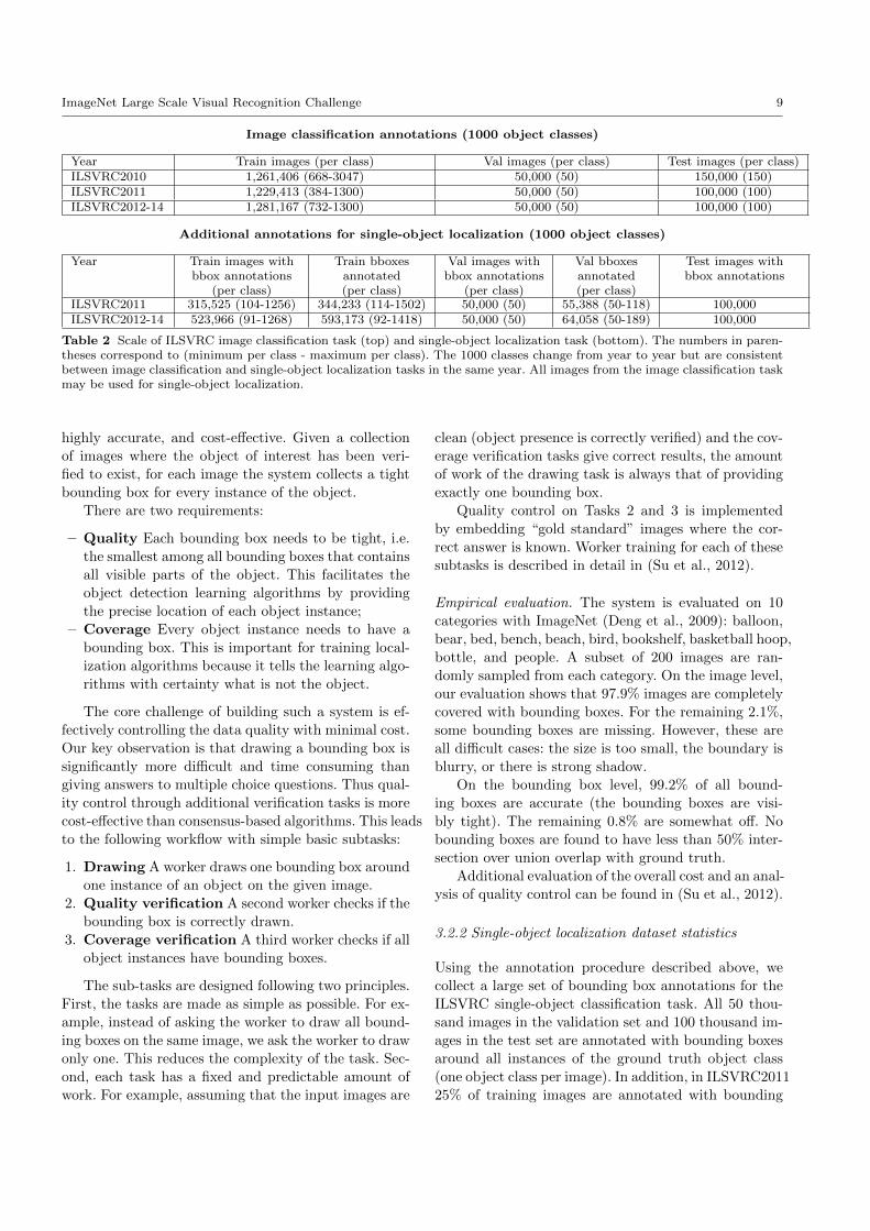
ImageNet Large Scale Visual Recognition Challenge 9
Image classification annotations (1000 object classes)
Year Train images (per class) Val images (per class) Test images (per class)ILSVRC2010 1,261,406 (668-3047) 50,000 (50) 150,000 (150)ILSVRC2011 1,229,413 (384-1300) 50,000 (50) 100,000 (100)ILSVRC2012-14 1,281,167 (732-1300) 50,000 (50) 100,000 (100)
Additional annotations for single-object localization (1000 object classes)
Year Train images withbbox annotations
(per class)
Train bboxesannotated(per class)
Val images withbbox annotations
(per class)
Val bboxesannotated(per class)
Test images withbbox annotations
ILSVRC2011 315,525 (104-1256) 344,233 (114-1502) 50,000 (50) 55,388 (50-118) 100,000ILSVRC2012-14 523,966 (91-1268) 593,173 (92-1418) 50,000 (50) 64,058 (50-189) 100,000
Table 2 Scale of ILSVRC image classification task (top) and single-object localization task (bottom). The numbers in paren-theses correspond to (minimum per class - maximum per class). The 1000 classes change from year to year but are consistentbetween image classification and single-object localization tasks in the same year. All images from the image classification taskmay be used for single-object localization.
highly accurate, and cost-effective. Given a collection
of images where the object of interest has been veri-
fied to exist, for each image the system collects a tight
bounding box for every instance of the object.
There are two requirements:
– Quality Each bounding box needs to be tight, i.e.
the smallest among all bounding boxes that contains
all visible parts of the object. This facilitates the
object detection learning algorithms by providing
the precise location of each object instance;
– Coverage Every object instance needs to have a
bounding box. This is important for training local-
ization algorithms because it tells the learning algo-
rithms with certainty what is not the object.
The core challenge of building such a system is ef-
fectively controlling the data quality with minimal cost.
Our key observation is that drawing a bounding box is
significantly more difficult and time consuming than
giving answers to multiple choice questions. Thus qual-
ity control through additional verification tasks is more
cost-effective than consensus-based algorithms. This leads
to the following workflow with simple basic subtasks:
1. Drawing A worker draws one bounding box around
one instance of an object on the given image.
2. Quality verification A second worker checks if the
bounding box is correctly drawn.
3. Coverage verification A third worker checks if all
object instances have bounding boxes.
The sub-tasks are designed following two principles.
First, the tasks are made as simple as possible. For ex-
ample, instead of asking the worker to draw all bound-
ing boxes on the same image, we ask the worker to draw
only one. This reduces the complexity of the task. Sec-
ond, each task has a fixed and predictable amount of
work. For example, assuming that the input images are
clean (object presence is correctly verified) and the cov-
erage verification tasks give correct results, the amount
of work of the drawing task is always that of providing
exactly one bounding box.
Quality control on Tasks 2 and 3 is implemented
by embedding “gold standard” images where the cor-
rect answer is known. Worker training for each of these
subtasks is described in detail in (Su et al., 2012).
Empirical evaluation. The system is evaluated on 10
categories with ImageNet (Deng et al., 2009): balloon,
bear, bed, bench, beach, bird, bookshelf, basketball hoop,
bottle, and people. A subset of 200 images are ran-
domly sampled from each category. On the image level,
our evaluation shows that 97.9% images are completely
covered with bounding boxes. For the remaining 2.1%,
some bounding boxes are missing. However, these are
all difficult cases: the size is too small, the boundary is
blurry, or there is strong shadow.
On the bounding box level, 99.2% of all bound-
ing boxes are accurate (the bounding boxes are visi-
bly tight). The remaining 0.8% are somewhat off. No
bounding boxes are found to have less than 50% inter-
section over union overlap with ground truth.
Additional evaluation of the overall cost and an anal-
ysis of quality control can be found in (Su et al., 2012).
3.2.2 Single-object localization dataset statistics
Using the annotation procedure described above, we
collect a large set of bounding box annotations for the
ILSVRC single-object classification task. All 50 thou-
sand images in the validation set and 100 thousand im-
ages in the test set are annotated with bounding boxes
around all instances of the ground truth object class
(one object class per image). In addition, in ILSVRC2011
25% of training images are annotated with bounding

10 Olga Russakovsky* et al.
boxes the same way, yielding more than 310 thousand
annotated images with more than 340 thousand anno-
tated object instances. In ILSVRC2012 40% of training
images are annotated, yielding more than 520 thousand
annotated images with more than 590 thousand anno-
tated object instances. Table 2 (bottom) documents the
size of this dataset.
In addition to the size of the dataset, we also ana-
lyze the level of difficulty of object localization in these
images compared to the PASCAL VOC benchmark. We
compute statistics on the ILSVRC2012 single-object lo-
calization validation set images compared to PASCAL
VOC 2012 validation images.
Real-world scenes are likely to contain multiple in-
stances of some objects, and nearby object instances are
particularly difficult to delineate. The average object
category in ILSVRC has 1.61 target object instances
on average per positive image, with each instance hav-
ing on average 0.47 neighbors (adjacent instances of
the same object category). This is comparable to 1.69
instances per positive image and 0.52 neighbors per in-
stance for an average object class in PASCAL.
As described in (Hoiem et al., 2012), smaller ob-
jects tend to be significantly more difficult to local-
ize. In the average object category in PASCAL the ob-
ject occupies 24.1% of the image area, and in ILSVRC
35.8%. However, PASCAL has only 20 object categories
while ILSVRC has 1000. The 537 object categories of
ILSVRC with the smallest objects on average occupy
the same fraction of the image as PASCAL objects:
24.1%. Thus even though on average the object in-
stances tend to be bigger in ILSVRC images, there are
more than 25 times more object categories than in PAS-
CAL VOC with the same average object scale.
Appendix B and (Russakovsky et al., 2013) have
additional comparisons.
3.3 Object detection dataset construction
The ILSVRC task of object detection evaluates the abil-
ity of an algorithm to name and localize all instances of
all target objects present in an image. It is much more
challenging than object localization because some ob-
ject instances may be small/occluded/difficult to accu-
rately localize, and the algorithm is expected to locate
them all, not just the one it finds easiest.
There are three key challenges in collecting the ob-
ject detection dataset. The first challenge is selecting
the set of common objects which tend to appear in clut-
tered photographs and are well-suited for benchmarking
object detection performance. Our approach relies on
statistics of the object localization dataset and the tra-
dition of the PASCAL VOC challenge (Section 3.3.1).
Class name in Closest class in Avg object scale (%)PASCAL VOC ILSVRC-DET PASCAL ILSVRC-(20 classes) (200 classes) VOC DETaeroplane airplane 29.7 22.4bicycle bicycle 29.3 14.3bird bird 15.9 20.1boat watercraft 15.2 16.5bottle wine bottle 7.3 10.4bus bus 29.9 22.1car car 14.0 13.4cat domestic cat 46.8 29.8chair chair 12.8 10.1cow cattle 19.3 13.5dining table table 29.1 30.3dog dog 37.0 28.9horse horse 29.5 18.5motorbike motorcyle 32.0 20.7person person 17.5 19.3potted plant flower pot 12.3 8.1sheep sheep 12.2 17.3sofa sofa 41.7 44.4train train 35.4 35.1tv/monitor tv or monitor 14.6 11.2
Table 3 Correspondences between the object classes in thePASCAL VOC (Everingham et al., 2010) and the ILSVRCdetection task. Object scale is the fraction of image area (re-ported in percent) occupied by an object instance. It is com-puted on the validation sets of PASCAL VOC 2012 and ofILSVRC-DET. The average object scale is 24.1% across the20 PASCAL VOC categories and 20.3% across the 20 corre-sponding ILSVRC-DET categories. Section 3.3.4 reports ad-ditional dataset statistics.
The second challenge is obtaining a much more var-
ied set of scene images than those used for the image
classification and single-object localization datasets. Sec-
tion 3.3.2 describes the procedure for utilizing as much
data from the single-object localization dataset as pos-
sible and supplementing it with Flickr images queried
using hundreds of manually designed high-level queries.
The third, and biggest, challenge is completely an-
notating this dataset with all the objects. This is done
in two parts. Section 3.3.3 describes the first part: our
hierarchical strategy for obtaining the list of all target
objects which occur within every image. This is nec-
essary since annotating in a straight-forward way by
creating a task for every (image, object class) pair is
no longer feasible at this scale. Appendix E describes
the second part: annotating the bounding boxes around
these objects, using the single-object localization bound-
ing box annotation pipeline of Section 3.2.1 along with
extra verification to ensure that every instance of the
object is annotated with exactly one bounding box.

ImageNet Large Scale Visual Recognition Challenge 11
3.3.1 Defining object categories for the object detection
dataset
There are 200 object classes hand-selected for the de-
tection task, eacg corresponding to a synset within Im-
ageNet. These were chosen to be mostly basic-level ob-
ject categories that would be easy for people to identify
and label. The rationale is that the object detection
system developed for this task can later be combined
with a fine-grained classification model to further clas-
sify the objects if a finer subdivision is desired.6 As with
the 1000 classification classes, the synsets are selected
such that there is no overlap: for any synsets i and j, i
is not an ancestor of j in the ImageNet hierarchy.
The selection of the 200 object detection classes in
2013 was guided by the ILSVRC 2012 classification and
localization dataset. Starting with 1000 object classes
and their bounding box annotations we first eliminated
all object classes which tended to be too “big” in the
image (on average the object area was greater than
50% of the image area). These were classes such as
T-shirt, spiderweb, or manhole cover. We then man-
ually eliminated all classes which we did not feel were
well-suited for detection, such as hay, barbershop, or
poncho. This left 494 object classes which were merged
into basic-level categories: for example, different species
of birds were merged into just the “bird” class. The
classes remained the same in ILSVRC2014. Appendix D
contains the complete list of object categories used in
ILSVRC2013-2014 (in the context of the hierarchy de-
scribed in Section 3.3.3).
Staying mindful of the tradition of the PASCAL
VOC dataset we also tried to ensure that the set of
200 classes contains as many of the 20 PASCAL VOC
classes as possible. Table 3 shows the correspondences.
The changes that were done were to ensure more accu-
rate and consistent crowdsourced annotations. The ob-
ject class with the weakest correspondence is “potted
plant” in PASCAL VOC, corresponding to “flower pot”
in ILSVRC. “Potted plant” was one of the most chal-
lenging object classes to annotate consistently among
the PASCAL VOC classes, and in order to obtain accu-
rate annotations using crowdsourcing we had to restrict
the definition to a more concrete object.
3.3.2 Collecting images for the object detection dataset
Many images for the detection task were collected dif-
ferently than the images in ImageNet and the classifica-
6 Some of the training objects are actually annotated withmore detailed classes: for example, one of the 200 objectclasses is the category “dog,” and some training instancesare annotated with the specific dog breed.
Fig. 3 Summary of images collected for the detection task.Images in green (bold) boxes have all instances of all 200 de-tection object classes fully annotated. Table 4 lists the com-plete statistics.
tion and single-object localization tasks. Figure 3 sum-
marizes the types of images that were collected. Ideally
all of these images would be scene images fully anno-
tated with all target categories. However, given budget
constraints our goal was to provide as much suitable de-
tection data as possible, even if the images were drawn
from a few different sources and distributions.
The validation and test detection set images come
from two sources (percent of images from each source
in parentheses). The first source (77%) is images from
ILSVRC2012 single-object localization validation and
test sets corresponding to the 200 detection classes (or
their children in the ImageNet hierarchy). Images where
the target object occupied more than 50% of the image
area were discarded, since they were unlikely to con-
tain other objects of interest. The second source (23%)
is images from Flickr collected specifically for detection
task. We queried Flickr using a large set of manually de-
fined queries, such as “kitchenette” or “Australian zoo”
to retrieve images of scenes likely to contain several ob-
jects of interest. Appendix C contains the full list. We
also added pairwise queries, or queries with two tar-
get object names such as “tiger lion,” which also often
returned cluttered scenes.
Figure 4 shows a random set of both types of val-
idation images. Images were randomly split, with 33%
going into the validation set and 67% into the test set.7
The training set for the detection task comes from
three sources of images (percent of images from each
source in parentheses). The first source (63%) is all
training images from ILSVRC2012 single-object local-
ization task corresponding to the 200 detection classes
(or their children in the ImageNet hierarchy). We did
not filter by object size, allowing teams to take advan-
7 The validation/test split is consistent with ILSVRC2012:validation images of ILSVRC2012 remained in the validationset of ILSVRC2013, and ILSVRC2012 test images remainedin ILSVRC2013 test set.

12 Olga Russakovsky* et al.
Fig. 4 Random selection of images in ILSVRC detection validation set. The images in the top 4 rows were taken fromILSVRC2012 single-object localization validation set, and the images in the bottom 4 rows were collected from Flickr usingscene-level queries.
tage of all the positive examples available. The second
source (24%) is negative images which were part of the
original ImageNet collection process but voted as neg-
ative: for example, some of the images were collected
from Flickr and search engines for the ImageNet synset
“animals” but during the manual verification step did
not collect enough votes to be considered as containing
an “animal.” These images were manually re-verified
for the detection task to ensure that they did not in
fact contain the target objects. The third source (13%)
is images collected from Flickr specifically for the de-
tection task. These images were added for ILSVRC2014
following the same protocol as the second type of images
in the validation and test set. This was done to bring
the training and testing distributions closer together.
ImageNet Large Scale Visual Recognition Challenge 13
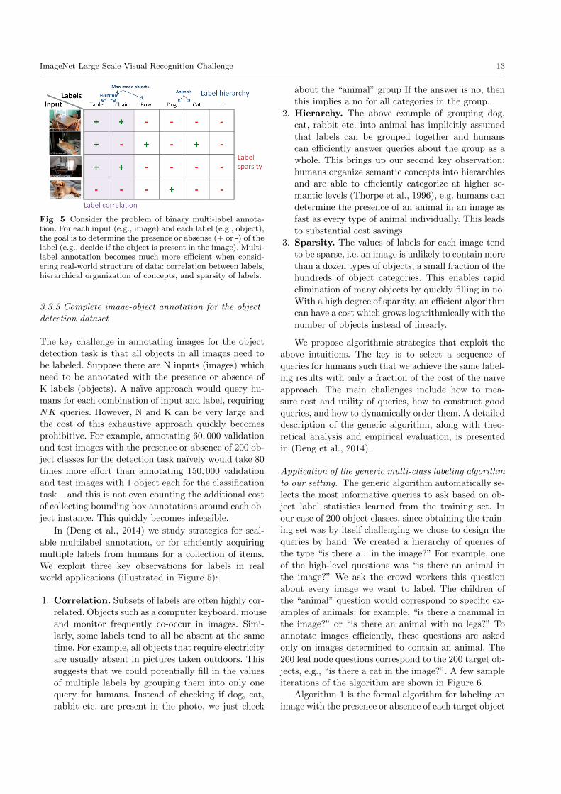
Fig. 5 Consider the problem of binary multi-label annota-tion. For each input (e.g., image) and each label (e.g., object),the goal is to determine the presence or absense (+ or -) of thelabel (e.g., decide if the object is present in the image). Multi-label annotation becomes much more efficient when consid-ering real-world structure of data: correlation between labels,hierarchical organization of concepts, and sparsity of labels.
3.3.3 Complete image-object annotation for the object
detection dataset
The key challenge in annotating images for the object
detection task is that all objects in all images need to
be labeled. Suppose there are N inputs (images) which
need to be annotated with the presence or absence of
K labels (objects). A naıve approach would query hu-
mans for each combination of input and label, requiring
NK queries. However, N and K can be very large and
the cost of this exhaustive approach quickly becomes
prohibitive. For example, annotating 60, 000 validation
and test images with the presence or absence of 200 ob-
ject classes for the detection task naıvely would take 80
times more effort than annotating 150, 000 validation
and test images with 1 object each for the classification
task – and this is not even counting the additional cost
of collecting bounding box annotations around each ob-
ject instance. This quickly becomes infeasible.
In (Deng et al., 2014) we study strategies for scal-
able multilabel annotation, or for efficiently acquiring
multiple labels from humans for a collection of items.
We exploit three key observations for labels in real
world applications (illustrated in Figure 5):
1. Correlation. Subsets of labels are often highly cor-
related. Objects such as a computer keyboard, mouse
and monitor frequently co-occur in images. Simi-
larly, some labels tend to all be absent at the same
time. For example, all objects that require electricity
are usually absent in pictures taken outdoors. This
suggests that we could potentially fill in the values
of multiple labels by grouping them into only one
query for humans. Instead of checking if dog, cat,
rabbit etc. are present in the photo, we just check
about the “animal” group If the answer is no, then
this implies a no for all categories in the group.
2. Hierarchy. The above example of grouping dog,
cat, rabbit etc. into animal has implicitly assumed
that labels can be grouped together and humans
can efficiently answer queries about the group as a
whole. This brings up our second key observation:
humans organize semantic concepts into hierarchies
and are able to efficiently categorize at higher se-
mantic levels (Thorpe et al., 1996), e.g. humans can
determine the presence of an animal in an image as
fast as every type of animal individually. This leads
to substantial cost savings.
3. Sparsity. The values of labels for each image tend
to be sparse, i.e. an image is unlikely to contain more
than a dozen types of objects, a small fraction of the
hundreds of object categories. This enables rapid
elimination of many objects by quickly filling in no.
With a high degree of sparsity, an efficient algorithm
can have a cost which grows logarithmically with the
number of objects instead of linearly.
We propose algorithmic strategies that exploit the
above intuitions. The key is to select a sequence of
queries for humans such that we achieve the same label-
ing results with only a fraction of the cost of the naıve
approach. The main challenges include how to mea-
sure cost and utility of queries, how to construct good
queries, and how to dynamically order them. A detailed
description of the generic algorithm, along with theo-
retical analysis and empirical evaluation, is presented
in (Deng et al., 2014).
Application of the generic multi-class labeling algorithm
to our setting. The generic algorithm automatically se-
lects the most informative queries to ask based on ob-
ject label statistics learned from the training set. In
our case of 200 object classes, since obtaining the train-
ing set was by itself challenging we chose to design the
queries by hand. We created a hierarchy of queries of
the type “is there a... in the image?” For example, one
of the high-level questions was “is there an animal in
the image?” We ask the crowd workers this question
about every image we want to label. The children of
the “animal” question would correspond to specific ex-
amples of animals: for example, “is there a mammal in
the image?” or “is there an animal with no legs?” To
annotate images efficiently, these questions are asked
only on images determined to contain an animal. The
200 leaf node questions correspond to the 200 target ob-
jects, e.g., “is there a cat in the image?”. A few sample
iterations of the algorithm are shown in Figure 6.
Algorithm 1 is the formal algorithm for labeling an
image with the presence or absence of each target object

14 Olga Russakovsky* et al.
Imag
e
Object PresenceIs there
an animal?Is there
a mammal?Is therea cat?
Fig. 6 Our algorithm dynamically selects the next query toefficiently determine the presence or absence of every objectin every image. Green denotes a positive annotation and reddenotes a negative annotation. This toy example illustrates asample progression of the algorithm for one label (cat) on aset of images.
category. With this algorithm in mind, the hierarchy of
questions was constructed following the principle that
false positives only add extra cost whereas false nega-
tives can significantly affect the quality of the labeling.
Thus, it is always better to stick with more general but
less ambiguous questions, such as “is there a mammal
in the image?” as opposed to asking overly specific but
potentially ambiguous questions, such as “is there an
animal that can climb trees?” Constructing this hierar-
chy was a surprisingly time-consuming process, involv-
ing multiple iterations to ensure high accuracy of label-
ing and avoid question ambiguity. Appendix D shows
the constructed hierarchy.
Bounding box annotation. Once all images are labeled
with the presence or absence of all object categories we
use the bounding box system described in Section 3.2.1
along with some additional modifications of Appendix E
to annotate the location of every instance of every present
object category.
3.3.4 Object detection dataset statistics
Using the procedure described above, we collect a large-
scale dataset for ILSVRC object detection task. There
are 200 object classes and approximately 450K training
images, 20K validation images and 40K test images. Ta-
ble 4 documents the size of the dataset over the years of
the challenge. The major change between ILSVRC2013
and ILSVRC2014 was the addition of 60,658 fully an-
notated training images.
Prior to ILSVRC, the object detection benchmark
was the PASCAL VOC challenge (Everingham et al.,
2010). ILSVRC has 10 times more object classes than
PASCAL VOC (200 vs 20), 10.6 times more fully an-
notated training images (60,658 vs 5,717), 35.2 times
more training objects (478,807 vs 13,609), 3.5 times
more validation images (20,121 vs 5823) and 3.5 times
more validation objects (55,501 vs 15,787). ILSVRC has
2.8 annotated objects per image on the validation set,
compared to 2.7 in PASCAL VOC. The average ob-
ject in ILSVRC takes up 17.0% of the image area and
in PASCAL VOC takes up 20.7%; Table 3 contains
Input: Image i, queries Q, directed graph G over QOutput: Labels L : Q → {“yes”, “no”}Initialize labels L(q) = ∅ ∀q ∈ Q;Initialize candidates C = {q: q ∈ Root(G)};while C not empty do
Obtain answer A to query q∗ ∈ C;L(q∗) = A; C = C\{q∗};if A is “yes” then
Chldr = {q ∈ Children(q∗,G): L(q) = ∅};C = C ∪ Chldr;
elseDes = {q ∈ Descendants(q∗,G): L(q) = ∅};L(q) = “no′′ ∀q ∈ Des;C = C\Des;
end
end
Algorithm 1: The algorithm for complete multi-class
annotation. This is a special case of the algorithm de-
scribed in (Deng et al., 2014). A hierarchy of ques-
tions G is manually constructed. All root questions
are asked on every image. If the answer to query q∗on image i is “no” then the answer is assumed to be
“no” for all queries q such that q is a descendant of
q∗ in the hierarchy. We continue asking the queries
until all queries are answered. For images taken from
the single-object localization task we used the known
object label to initialize L.
per-class comparisons. Additionally, ILSVRC contains
a wide variety of objects, including tiny objects such as
sunglasses (1.3% of image area on average), ping-pong
balls (1.5% of image area on average) and basketballs
(2.0% of image area on average).
4 Evaluation at large scale
Once the dataset has been collected, we need to define a
standardized evaluation procedure for algorithms. Some
measures have already been established by datasets such
as the Caltech 101 (Fei-Fei et al., 2004) for image clas-
sification and PASCAL VOC (Everingham et al., 2012)
for both image classification and object detection. To
adapt these procedures to the large-scale setting we had
to address three key challenges. First, for the image
classification and single-object localization tasks only
one object category could be labeled in each image due
to the scale of the dataset. This created potential ambi-
guity during evaluation (addressed in Section 4.1). Sec-
ond, evaluating localization of object instances is inher-
ently difficult in some images which contain a cluster
of objects (addressed in Section 4.2). Third, evaluating
localization of object instances which occupy few pixels
in the image is challenging (addressed in Section 4.3).
In this section we describe the standardized eval-
uation criteria for each of the three ILSVRC tasks.

ImageNet Large Scale Visual Recognition Challenge 15
Object detection annotations (200 object classes)
Year Train images(per class)
Train bboxes annotated(per class)
Val images(per class)
Val bboxes annotated(per class )
Testimages
ILSVRC2013 395909(417-561-66911 pos,185-4130-10073 neg)
345854(438-660-73799)
21121(23-58-5791 pos,
rest neg)
55501(31-111-12824)
40152
ILSVRC2014 456567(461-823-67513 pos,
42945-64614-70626 neg)
478807(502-1008-74517)
21121(23-58-5791 pos,
rest neg)
55501(31-111-12824)
40152
Table 4 Scale of ILSVRC object detection task. Numbers in parentheses correspond to (minimum per class - median perclass - maximum per class).
We elaborate further on these and other more minor
challenges with large-scale evaluation. Appendix F de-
scribes the submission protocol and other details of run-
ning the competition itself.
4.1 Image classification
The scale of ILSVRC classification task (1000 categories
and more than a million of images) makes it very ex-
pensive to label every instance of every object in every
image. Therefore, on this dataset only one object cate-
gory is labeled in each image. This creates ambiguity in
evaluation. For example, an image might be labeled as
a “strawberry” but contain both a strawberry and an
apple. Then an algorithm would not know which one
of the two objects to name. For the image classification
task we allowed an algorithm to identify multiple (up
to 5) objects in an image and not be penalized as long
as one of the objects indeed corresponded to the ground
truth label. Figure 7(top row) shows some examples.
Concretely, each image i has a single class label Ci.
An algorithm is allowed to return 5 labels ci1, . . . ci5,
and is considered correct if cij = Ci for some j.
Let the error of a prediction dij = d(cij , Ci) be 1
if cij 6= Ci and 0 otherwise. The error of an algorithm
is the fraction of test images on which the algorithm
makes a mistake:
error =1
N
N∑i=1
minjdij (1)
We used two additional measures of error. First, we
evaluated top-1 error. In this case algorithms were pe-
nalized if their highest-confidence output label ci1 did
not match ground truth class Ci. Second, we evaluated
hierarchical error. The intuition is that confusing two
nearby classes (such as two different breeds of dogs) is
not as harmful as confusing a dog for a container ship.
For the hierarchical criteria, the cost of one misclassifi-
cation, d(cij , Ci), is defined as the height of the lowest
common ancestor of cij and Ci in the ImageNet hier-
archy. The height of a node is the length of the longest
path to a leaf node (leaf nodes have height zero).
However, in practice we found that all three mea-
sures of error (top-5, top-1, and hierarchical) produced
the same ordering of results. Thus, since ILSVRC2012
we have been exclusively using the top-5 metric which
is the simplest and most suitable to the dataset.
4.2 Single-object localization
The evaluation for single-object localization is similar
to object classification, again using a top-5 criteria to al-
low the algorithm to return unannotated object classes
without penalty. However, now the algorithm is con-
sidered correct only if it both correctly identifies the
target class Ci and accurately localizes one of its in-
stances. Figure 7(middle row) shows some examples.
Concretely, an image is associated with object class
Ci, with all instances of this object class annotated with
bounding boxesBik. An algorithm returns {(cij , bij)}5j=1
of class labels cij and associated locations bij . The error
of a prediction j is:
dij = max(d(cij , Ci),minkd(bij , Bik)) (2)
Here d(bij , Bik) is the error of localization, defined as 0
if the area of intersection of boxes bij and Bik divided
by the areas of their union is greater than 0.5, and 1
otherwise. (Everingham et al., 2010) The error of an
algorithm is computed as in Eq. 1.
Evaluating localization is inherently difficult in some
images. Consider a picture of a bunch of bananas or a
carton of apples. It is easy to classify these images as
containing bananas or apples, and even possible to lo-
calize a few instances of each fruit. However, in order
for evaluation to be accurate every instance of banana
or apple needs to be annotated, and that may be impos-
sible. To handle the images where localizing individual
object instances is inherently ambiguous we manually
discarded 3.5% of images since ILSVRC2012. Some ex-
amples of discarded images are shown in Figure 8.

16 Olga Russakovsky* et al.
Fig. 7 Tasks in ILSVRC. The first column shows the ground truth labeling on an example image, and the next three showthree sample outputs with the corresponding evaluation score.
Fig. 8 Images marked as “difficult” in the ILSVRC2012 single-object localization validation set. Please refer to Section 4.2for details.
4.3 Object detection
The criteria for object detection was adopted from PAS-
CAL VOC (Everingham et al., 2010). It is designed to
penalize the algorithm for missing object instances, for
duplicate detections of one instance, and for false posi-
tive detections. Figure 7(bottom row) shows examples.
For each object class and each image Ii, an algo-
rithm returns predicted detections (bij , sij) of predicted
locations bij with confidence scores sij . These detec-
tions are greedily matched to the ground truth boxes
{Bik} using Algorithm 2. For every detection j on im-
age i the algorithm returns zij = 1 if the detection is
matched to a ground truth box according to the thresh-
old criteria, and 0 otherwise. For a given object class,
let N be the total number of ground truth instances
across all images. Given a threshold t, define recall as
the fraction of the N objects detected by the algorithm,
and precision as the fraction of correct detections out
of the total detections returned by the algorithm. Con-
cretely,
Recall(t) =
∑ij 1[sij ≥ t]zij
N(3)
Precision(t) =
∑ij 1[sij ≥ t]zij∑ij 1[sij ≥ t]
(4)

ImageNet Large Scale Visual Recognition Challenge 17
Input: Bounding box predictions with confidencescores {(bj , sj)}Mj=1 and ground truth boxes Bon image I for a given object class.
Output: Binary results {zj}Mj=1 of whether or notprediction j is a true positive detection
Let U = B be the set of unmatched objects;
Order {(bj , sj)}Mj=1 in descending order of sj ;
for j=1 . . . M doLet C = {Bk ∈ U : IOU(Bk, bj) ≥ thr(Bk)};if C 6= ∅ then
Let k∗ = arg max{k : Bk∈C} IOU(Bk, bj);
Set U = U\Bk∗;Set zj = 1 since true positive detection;
elseSet zj = 0 since false positive detection;
end
end
Algorithm 2: The algorithm for greedily matching
object detection outputs to ground truth labels. The
standard thr(Bk) = 0.5 (Everingham et al., 2010).
ILSVRC computes thr(Bk) using Eq. 5 to better han-
dle low-resolution objects.
The final metric for evaluating an algorithm on a
given object class is average precision over the different
levels of recall achieved by varying the threshold t. The
winner of each object class is then the team with the
highest average precision, and then winner of the chal-
lenge is the team that wins on the most object classes.8
Difference with PASCAL VOC. Evaluating localization
of object instances which occupy very few pixels in the
image is challenging. The PASCAL VOC approach was
to label such instances as “difficult” and ignore them
during evaluation. However, since ILSVRC contains a
more diverse set of object classes including, for exam-
ple, “nail” and “ping pong ball” which have many very
small instances, it is important to include even very
small object instances in evaluation.
In Algorithm 2, a predicted bounding box b is con-
sidered to have properly localized by a ground truth
bounding box B if IOU(b, B) ≥ thr(B). The PASCAL
VOC metric uses the threshold thr(B) = 0.5. However,
for small objects even deviations of a few pixels would
be unacceptable according to this threshold. For exam-
ple, consider an object B of size 10× 10 pixels, with a
detection window of 20× 20 pixels which fully contains
that object. This would be an error of approximately 5
pixels on each dimension, which is average human an-
notation error. However, the IOU in this case would be
100/400 = 0.25, far below the threshold of 0.5. Thus
8 In this paper we focus on the mean average precisionacross all categories as the measure of a team’s performance.This is done for simplicity and is justified since the orderingof teams by mean average precision was always the same asthe ordering by object categories won.
for smaller objects we loosen the threshold in ILSVRC
to allow for the annotation to extend up to 5 pixels on
average in each direction around the object. Concretely,
if the ground truth box B is of dimensions w× h then
thr(B) = min
(0.5,
wh
(w + 10)(h+ 10)
)(5)
In practice, this changes the threshold only on objects
which are smaller than approximately 25 × 25 pixels,
and affects 5.5% of objects in the detection validation
set.
Practical consideration. One additional practical con-
sideration for ILSVRC detection evaluation is subtle
and comes directly as a result of the scale of ILSVRC.
In PASCAL, algorithms would often return many de-
tections per class on the test set, including ones with
low confidence scores. This allowed the algorithms to
reach the level of high recall at least in the realm of
very low precision. On ILSVRC detection test set if
an algorithm returns 10 bounding boxes per object per
image this would result in 10×200×40K = 80M detec-
tions. Each detection contains an image index, a class
index, 4 bounding box coordinates, and the confidence
score, so it takes on the order of 28 bytes. The full set of
detections would then require 2.24Gb to store and sub-
mit to the evaluation server, which is impractical. This
means that algorithms are implicitly required to limit
their predictions to only the most confident locations.
5 Methods
The ILSVRC dataset and the competition has allowed
significant algorithmic advances in large-scale image recog-
nition and retrieval.
5.1 Challenge entries
This section is organized chronologically, highlighting
the particularly innovative and successful methods which
participated in the ILSVRC each year. Tables 5, 6 and 7
list all the participating teams. We see a turning point
in 2012 with the development of large-scale convolu-
tional neural networks.
ILSVRC2010. The first year the challenge consisted
of just the classification task. The winning entry from
NEC team (Lin et al., 2011) used SIFT (Lowe, 2004)
and LBP (Ahonen et al., 2006) features with two non-
linear coding representations (Zhou et al., 2010; Wang

18 Olga Russakovsky* et al.
et al., 2010) and a stochastic SVM. The honorable men-
tion XRCE team (Perronnin et al., 2010) used an im-
proved Fisher vector representation (Perronnin and Dance,
2007) along with PCA dimensionality reduction and
data compression followed by a linear SVM. Fisher vector-
based methods have evolved over five years of the chal-
lenge and continued performing strongly in every ILSVRC
from 2010 to 2014.
ILSVRC2011. The winning classification entry in 2011
was the 2010 runner-up team XRCE, applying high-
dimensional image signatures (Perronnin et al., 2010)
with compression using product quantization (Sanchez
and Perronnin, 2011) and one-vs-all linear SVMs. The
single-object localization competition was held for the
first time, with two brave entries. The winner was the
UvA team using a selective search approach to gener-
ate class-independent object hypothesis regions (van de
Sande et al., 2011b), followed by dense sampling and
vector quantization of several color SIFT features (van de
Sande et al., 2010), pooling with spatial pyramid match-
ing (Lazebnik et al., 2006), and classifying with a his-
togram intersection kernel SVM (Maji and Malik, 2009)
trained on a GPU (van de Sande et al., 2011a).
ILSVRC2012. This was a turning point for large-scale
object recognition, when large-scale deep neural net-
works entered the scene. The undisputed winner of both
the classification and localization tasks in 2012 was the
SuperVision team. They trained a large, deep convolu-
tional neural network on RGB values, with 60 million
parameters using an efficient GPU implementation and
a novel hidden-unit dropout trick (Krizhevsky et al.,2012; Hinton et al., 2012). The second place in image
classification went to the ISI team, which used Fisher
vectors (Sanchez and Perronnin, 2011) and a stream-
lined version of Graphical Gaussian Vectors (Harada
and Kuniyoshi, 2012), along with linear classifiers us-
ing Passive-Aggressive (PA) algorithm (Crammer et al.,
2006). The second place in single-object localization
went to the VGG, with an image classification sys-
tem including dense SIFT features and color statis-
tics (Lowe, 2004), a Fisher vector representation (Sanchez
and Perronnin, 2011), and a linear SVM classifier, plus
additional insights from (Arandjelovic and Zisserman,
2012; Sanchez et al., 2012). Both ISI and VGG used
(Felzenszwalb et al., 2010) for object localization; Su-
perVision used a regression model trained to predict
bounding box locations. Despite the weaker detection
model, SuperVision handily won the object localization
task. A detailed analysis and comparison of the Super-
Vision and VGG submissions on the single-object local-
ization task can be found in (Russakovsky et al., 2013).
The influence of the success of the SuperVision model
can be clearly seen in ILSVRC2013 and ILSVRC2014.
ILSVRC2013. There were 24 teams participating in the
ILSVRC2013 competition, compared to 21 in the pre-
vious three years combined. Following the success of the
deep learning-based method in 2012, the vast majority
of entries in 2013 used deep convolutional neural net-
works in their submission. The winner of the classifica-
tion task was Clarifai, with several large deep convolu-
tional networks averaged together. The network archi-
tectures were chosen using the visualization technique
of (Zeiler and Fergus, 2013), and they were trained
on the GPU following (Zeiler et al., 2011) using the
dropout technique (Krizhevsky et al., 2012).
The winning single-object localization OverFeat sub-
mission was based on an integrated framework for us-
ing convolutional networks for classification, localiza-
tion and detection with a multiscale sliding window
approach (Sermanet et al., 2013). They were the only
team tackling all three tasks.
The winner of object detection task was UvA team,
which utilized a new way of efficient encoding (van de
Sande et al., 2014) densely sampled color descriptors (van de
Sande et al., 2010) pooled using a multi-level spatial
pyramid in a selective search framework (Uijlings et al.,
2013). The detection results were rescored using a full-
image convolutional network classifier.
ILSVRC2014. 2014 attracted the most submissions, with
36 teams submitting 123 entries compared to just 24
teams in 2013 – a 1.5x increase in participation.9 As
in 2013 almost all teams used convolutional neural net-
works as the basis for their submission. Significant progress
has been made in just one year: image classification er-
ror was almost halved since ILSVRC2013 and object
detection mean average precision almost doubled com-
pared to ILSVRC2013. Please refer to Section 6.1 for
details.
In 2014 teams were allowed to use outside data for
training their models in the competition, so there were
six tracks: provided and outside data tracks in each
of image classification, single-object localization, and
object detection tasks.
The winning image classification with provided data
team was GoogLeNet, which explored an improved con-
volutional neural network architecture combining the
multi-scale idea with intuitions gained from the Heb-
bian principle. Additional dimension reduction layers
allowed them to increase both the depth and the width
9 Table 7 omits 4 teams which submitted results but chosenot to officially participate in the challenge.

ImageN
etL
arg
eS
cale
Visu
al
Reco
gn
ition
Ch
allen
ge
19
ILSVRC 2010
Codename CLS LOC Insitutions Contributors and references
Hminmax 54.4 Massachusetts Institute of Technology Jim Mutch, Sharat Chikkerur, Hristo Paskov, Ruslan Salakhutdinov, Stan Bileschi, Hueihan Jhuang
IBM 70.1 IBM research†, Georgia Tech‡ Lexing Xie†, Hua Ouyang‡, Apostol Natsev†
ISIL 44.6 Intelligent Systems and Informatics Lab., The University ofTokyo
Tatsuya Harada, Hideki Nakayama, Yoshitaka Ushiku, Yuya Yamashita, Jun Imura, Yasuo Kuniyoshi
ITNLP 78.7 Harbin Institute of Technology Deyuan Zhang, Wenfeng Xuan, Xiaolong Wang, Bingquan Liu, Chengjie Sun
LIG 60.7 Laboratoire d’Informatique de Grenoble Georges Quenot
NEC 28.2 NEC Labs America†, University of Illinois at Urbana-
Champaign‡, Rutgers∓Yuanqing Lin†, Fengjun Lv†, Shenghuo Zhu†, Ming Yang†, Timothee Cour†, Kai Yu†, LiangLiang Cao‡,Zhen Li‡, Min-Hsuan Tsai‡, Xi Zhou‡, Thomas Huang‡, Tong Zhang∓(Lin et al., 2011)
NII 74.2 National Institute of Informatics, Tokyo,Japan†, Hefei Nor-
mal Univ. Heifei, China‡Cai-Zhi Zhu†, Xiao Zhou‡, Shinıchi Satoh†
NTU 58.3 CeMNet, SCE, NTU, Singapore Zhengxiang Wang, Liang-Tien Chia
Regularities 75.1 SRI International Omid Madani, Brian Burns
UCI 46.6 University of California Irvine Hamed Pirsiavash, Deva Ramanan, Charless Fowlkes
XRCE 33.6 Xerox Research Centre Europe Jorge Sanchez, Florent Perronnin, Thomas Mensink(Perronnin et al., 2010)
ILSVRC 2011
Codename CLS LOC Institutions Contributors and references
ISI 36.0 - Intelligent Systems and Informatics lab, University of Tokyo Tatsuya Harada, Asako Kanezaki, Yoshitaka Ushiku, Yuya Yamashita, Sho Inaba, Hiroshi Muraoka, YasuoKuniyoshi
NII 50.5 - National Institute of Informatics, Japan Duy-Dinh Le, Shinıchi Satoh
UvA 31.0 42.5 University of Amsterdam†, University of Trento‡ Koen E. A. van de Sande†, Jasper R. R. Uijlings‡, Arnold W. M. Smeulders†, Theo Gevers†, Nicu Sebe‡,Cees Snoek†(van de Sande et al., 2011b)
XRCE 25.8 56.5 Xerox Research Centre Europe†, CIII‡ Florent Perronnin†, Jorge Sanchez†‡(Sanchez and Perronnin, 2011)
ILSVRC 2012
Codename CLS LOC Institutions Contributors and references
ISI 26.2 53.6 University of Tokyo†, JST PRESTO‡ Naoyuki Gunji†, Takayuki Higuchi†, Koki Yasumoto†, Hiroshi Muraoka†, Yoshitaka Ushiku†, Tatsuya
Harada†‡, Yasuo Kuniyoshi†(Harada and Kuniyoshi, 2012)
LEAR 34.5 - LEAR INRIA Grenoble†, TVPA Xerox Research Centre
Europe‡Thomas Mensink†‡, Jakob Verbeek†, Florent Perronnin‡, Gabriela Csurka‡(Mensink et al., 2012)
VGG 27.0 50.0 University of Oxford Karen Simonyan, Yusuf Aytar, Andrea Vedaldi, Andrew Zisserman(Arandjelovic and Zisserman, 2012; Sanchez et al., 2012)
SuperVision 16.4 34.2 University of Toronto Alex Krizhevsky, Ilya Sutskever, Geoffrey Hinton(Krizhevsky et al., 2012)
UvA 29.6 - University of Amsterdam Koen E. A. van de Sande, Amir Habibian, Cees G. M. Snoek(Sanchez and Perronnin, 2011; Scheirer et al., 2012)
XRCE 27.1 - Xerox Research Centre Europe†, LEAR INRIA ‡ Florent Perronnin†, Zeynep Akata†‡, Zaid Harchaoui‡, Cordelia Schmid‡(Perronnin et al., 2012)
Table 5 Teams participating in ILSVRC2010-2012, ordered alphabetically. Each method is identified with a codename used in the text. We report flat top-5 classificationand single-object localization error, in percents (lower is better). For teams which submitted multiple entries we report the best score. In 2012, SuperVision also submittedentries trained with the extra data from the ImageNet Fall 2011 release, and obtained 15.3% classification error and 33.5% localization error. Key references are providedwhere available. More details about the winning entries can be found in Section 5.1.

20
Olg
aR
ussa
kovsk
y*
etal.
ILSVRC 2013
Codename CLS LOC DET Insitutions Contributors and references
Adobe 15.2 - - Adobe†, University of Illinois at Urbana-Champaign‡ Hailin Jin†, Zhe Lin†, Jianchao Yang†, Tom Paine‡(Krizhevsky et al., 2012)
AHoward 13.6 - - Andrew Howard Consulting Andrew Howard
BUPT 25.2 - - Beijing University of Posts and Telecommunications†, Orange Labs
International Center Beijing‡Chong Huang†, Yunlong Bian†, Hongliang Bai‡, Bo Liu†, Yanchao Feng†, Yuan Dong†
Clarifai 11.7 - - Clarifai Matthew Zeiler(Zeiler and Fergus, 2013; Zeiler et al., 2011)
CogVision 16.1 - - Microsoft Research†, Harbin Institute of Technology‡ Kuiyuan Yang†, Yalong Bai†, Yong Rui‡
decaf 19.2 - - University of California Berkeley Yangqing Jia, Jeff Donahue, Trevor Darrell(Donahue et al., 2013)
Deep Punx 20.9 - - Saint Petersburg State University Evgeny Smirnov, Denis Timoshenko, Alexey Korolev(Krizhevsky et al., 2012; Wan et al., 2013; Tang, 2013)
Delta - - 6.1 National Tsing Hua University Che-Rung Lee, Hwann-Tzong Chen, Hao-Ping Kang, Tzu-Wei Huang, Ci-Hong Deng, Hao-Che Kao
IBM 20.7 - - University of Illinois at Urbana-Champaign†, IBM Watson Re-
search Center‡, IBM Haifa Research Center∓Zhicheng Yan†, Liangliang Cao‡, John R Smith‡, Noel Codella‡,Michele Merler‡, Sharath
Pankanti‡, Sharon Alpert∓, Yochay Tzur∓,
MIL 24.4 - - University of Tokyo Masatoshi Hidaka, Chie Kamada, Yusuke Mukuta, Naoyuki Gunji, Yoshitaka Ushiku, Tat-suya Harada
Minerva 21.7 Peking University†, Microsoft Research‡, Shanghai Jiao Tong
University∓, XiDian University§, Harbin Institute of TechnologyςTianjun Xiao†‡, Minjie Wang∓‡, Jianpeng Li§‡, Yalong Baiς‡, Jiaxing Zhang‡, Kuiyuan
Yang‡, Chuntao Hong‡, Zheng Zhang‡(Wang et al., 2014)
NEC - - 19.6 NEC Labs America†, University of Missouri ‡ Xiaoyu Wang†, Miao Sun‡, Tianbao Yang†, Yuanqing Lin†, Tony X. Han‡, Shenghuo Zhu†(Wang et al., 2013)
NUS 13.0 National University of Singapore Min Lin*, Qiang Chen*, Jian Dong, Junshi Huang, Wei Xia, Shuicheng Yan (* = equalcontribution)(Krizhevsky et al., 2012)
Orange 25.2 Orange Labs International Center Beijing†, Beijing University of
Posts and Telecommunications‡Hongliang BAI†, Lezi Wang‡, Shusheng Cen‡, YiNan Liu‡, Kun Tao†, Wei Liu†, Peng Li†,Yuan Dong†
OverFeat 14.2 30.0 (19.4) New York University Pierre Sermanet, David Eigen, Michael Mathieu, Xiang Zhang, Rob Fergus, Yann LeCun(Sermanet et al., 2013)
Quantum 82.0 - - Self-employed†, Student in Troy High School, Fullerton, CA‡ Henry Shu†, Jerry Shu‡(Batra et al., 2013)
SYSU - - 10.5 Sun Yat-Sen University, China. Xiaolong Wang(Felzenszwalb et al., 2010)
Toronto - - 11.5 University of Toronto Yichuan Tang*, Nitish Srivastava*, Ruslan Salakhutdinov (* = equal contribution)
Trimps 26.2 - - The Third Research Institute of the Ministry of Public Security,P.R. China
Jie Shao, Xiaoteng Zhang, Yanfeng Shang, Wenfei Wang, Lin Mei, Chuanping Hu
UCLA - - 9.8 University of California Los Angeles Yukun Zhu, Jun Zhu, Alan Yuille
UIUC - - 1.0 University of Illinois at Urbana-Champaign Thomas Paine, Kevin Shih, Thomas Huang(Krizhevsky et al., 2012)
UvA 14.3 - 22.6 University of Amsterdam, Euvision Technologies Koen E. A. van de Sande, Daniel H. F. Fontijne, Cees G. M. Snoek, Harro M. G. Stokman,Arnold W. M. Smeulders(van de Sande et al., 2014)
VGG 15.2 46.4 - Visual Geometry Group, University of Oxford Karen Simonyan, Andrea Vedaldi, Andrew Zisserman(Simonyan et al., 2013)
ZF 13.5 - - New York University Matthew D Zeiler, Rob Fergus(Zeiler and Fergus, 2013; Zeiler et al., 2011)
Table 6 Teams participating in ILSVRC2013, ordered alphabetically. Each method is identified with a codename used in the text. For classificaton and single-objectlocalization we report flat top-5 error, in percents (lower is better). For detection we report mean average precision, in percents (higher is better). Even though the winnerof the challenge was determined by the number of object categories won, this correlated strongly with mAP. Parentheses indicate the team used outside training dataand was not part of the official competition. Some competing teams also submitted entries trained with outside data: Clarifai with 11.2% classification error, NEC with20.9% detection mAP. Key references are provided where available. More details about the winning entries can be found in Section 5.1.

ImageN
etL
arg
eS
cale
Visu
al
Reco
gn
ition
Ch
allen
ge
21
ILSVRC 2014Codename CLS CLSo LOC LOCo DET DETo Insitutions Contributors and references
Adobe - 11.6 - 30.1 - - Adobe†, UIUC‡ Hailin Jin†, Zhaowen Wang‡, Jianchao Yang†, Zhe Lin†
AHoward 8.1 - ◦ - - - Howard Vision Technologies Andrew Howard (Howard, 2014)
BDC 11.3 - ◦ - - - Institute for Infocomm Research†, Uni-
versit Pierre et Marie Curie‡Olivier Morre†‡, Hanlin Goh†, Antoine Veillard‡, Vijay Chandrasekhar†(Krizhevsky et al., 2012)
Berkeley - - - - - 34.5 UC Berkeley Ross Girshick, Jeff Donahue, Sergio Guadarrama, Trevor Darrell, Jitendra Malik (Girshick et al., 2013,2014)
BREIL 16.0 - ◦ - - - KAIST department of EE Jun-Cheol Park, Yunhun Jang, Hyungwon Choi, JaeYoung Jun (Chatfield et al., 2014; Jia, 2013)
Brno 17.6 - 52.0 - - - Brno University of Technology Martin Kolar, Michal Hradis, Pavel Svoboda (Krizhevsky et al., 2012; Mikolov et al., 2013; Jia, 2013)
CASIA-2 - - - - 28.6 - Chinese Academy of Science†, South-
east University‡Peihao Huang†, Yongzhen Huang†, Feng Liu‡, Zifeng Wu†, Fang Zhao†, Liang Wang†, Tieniu
Tan†(Girshick et al., 2014)
CASIAWS - 11.4 - ◦ - - CRIPAC, CASIA Weiqiang Ren, Chong Wang, Yanhua Chen, Kaiqi Huang, Tieniu Tan (Arbelaez et al., 2014)
Cldi 13.9 - 46.9 - - - KAIST†, Cldi Inc.‡ Kyunghyun Paeng†, Donggeun Yoo†, Sunggyun Park†, Jungin Lee‡, Anthony S. Paek‡, In So Kweon†,Seong Dae Kim†(Krizhevsky et al., 2012; Perronnin et al., 2010)
CUHK - - - - - 40.7 The Chinese University of Hong Kong Wanli Ouyang, Ping Luo, Xingyu Zeng, Shi Qiu, Yonglong Tian, Hongsheng Li, Shuo Yang, Zhe Wang,Yuanjun Xiong, Chen Qian, Zhenyao Zhu, Ruohui Wang, Chen-Change Loy, Xiaogang Wang, XiaoouTang (Ouyang et al., 2014; Ouyang and Wang, 2013)
DeepCNet 17.5 - ◦ - - - University of Warwick Ben Graham (Graham, 2013; Schmidhuber, 2012)
DeepInsight - - - - - 40.5 NLPR†, HKUST‡ Junjie Yan†, Naiyan Wang‡, Stan Z. Li†, Dit-Yan Yeung‡(Girshick et al., 2014)
FengjunLv 17.4 - ◦ - - - Fengjun Lv Consulting Fengjun Lv (Krizhevsky et al., 2012; Harel et al., 2007)
GoogLeNet 6.7 - 26.4 - - 43.9 Google Christian Szegedy, Wei Liu, Yangqing Jia, Pierre Sermanet, Scott Reed, Drago Anguelov, Dumitru Erhan,Andrew Rabinovich (Szegedy et al., 2014)
HKUST - - - - 28.9 - Hong Kong U. of Science and Tech.†,Chinese U. of H. K.‡, Stanford U.∓
Cewu Lu†, Hei Law*†, Hao Chen*‡, Qifeng Chen*∓, Yao Xiao*†Chi Keung Tang†(Uijlings et al., 2013;Girshick et al., 2013; Perronnin et al., 2010; Felzenszwalb et al., 2010)
libccv 16.0 - ◦ - - - libccv.org Liu Liu (Zeiler and Fergus, 2013)
MIL 18.3 - 33.7 - - 30.4 The University of Tokyo†, IIT
Guwahati‡Senthil Purushwalkam†‡, Yuichiro Tsuchiya†, Atsushi Kanehira†, Asako Kanezaki†, Tatsuya
Harada†(Kanezaki et al., 2014; Girshick et al., 2013)
MPG UT - - - - - 26.4 The University of Tokyo Riku Togashi, Keita Iwamoto, Tomoaki Iwase, Hideki Nakayama (Girshick et al., 2014)
MSRA 8.1 - 35.5 - 35.1 - Microsoft Research†, Xi’an Jiaotong
U.‡, U. of Science and Tech. of China∓Kaiming He†, Xiangyu Zhang‡, Shaoqing Ren∓, Jian Sun†(He et al., 2014)
NUS - - - - 37.2 - National University of Singapore†,IBM Research Australia‡
Jian Dong†, Yunchao Wei†, Min Lin†, Qiang Chen‡, Wei Xia†, Shuicheng Yan†(Lin et al., 2014a; Chenet al., 2014)
NUS-BST 9.8 - ◦ - - - National Univ. of Singapore†, Beijing
Samsung Telecom R&D Center†Min Lin†, Jian Dong†, Hanjiang Lai†, Junjun Xiong‡, Shuicheng Yan†(Lin et al., 2014a; Howard, 2014;Krizhevsky et al., 2012)
Orange 15.2 14.8 42.8 42.7 - 27.7 Orange Labs Beijing†, BUPT China‡ Hongliang Bai†, Yinan Liu†, Bo Liu‡, Yanchao Feng‡, Kun Tao†, Yuan Dong†(Girshick et al., 2014)
PassBy 16.7 - ◦ - - - LENOVO†, HKUST‡, U. of Macao∓ Lin Sun†‡, Zhanghui Kuang†, Cong Zhao†, Kui Jia∓, Oscar C.Au‡(Jia, 2013; Krizhevsky et al., 2012)
SCUT 18.8 - ◦ - - - South China Univ. of Technology Guo Lihua, Liao Qijun, Ma Qianli, Lin Junbin
Southeast - - - - 30.5 - Southeast U.†, Chinese A. of Sciences‡ Feng Liu†, Zifeng Wu‡, Yongzhen Huang‡
SYSU 14.4 - 31.9 - - - Sun Yat-Sen University Liliang Zhang, Tianshui Chen, Shuye Zhang, Wanglan He, Liang Lin, Dengguang Pang, Lingbo Liu
Trimps - 11.5 - 42.2 - 33.7 The Third Research Institute of theMinistry of Public Security
Jie Shao, Xiaoteng Zhang, JianYing Zhou, Jian Wang, Jian Chen, Yanfeng Shang, Wenfei Wang, LinMei, Chuanping Hu (Girshick et al., 2014; Manen et al., 2013; Howard, 2014)
TTIC 10.2 - 48.3 - - - Toyota Technological Institute at
Chicago†, Ecole Centrale Paris‡George Papandreou†, Iasonas Kokkinos‡(Papandreou, 2014; Papandreou et al., 2014; Jojic et al., 2003;Krizhevsky et al., 2012; Sermanet et al., 2013; Dubout and Fleuret, 2012; Iandola et al., 2014)
UI 99.5 - ◦ - - - University of Isfahan Fatemeh Shafizadegan, Elham Shabaninia (Yang et al., 2009)
UvA 12.1 - ◦ - 32.0 35.4 U. of Amsterdam and Euvision Tech. Koen van de Sande, Daniel Fontijne, Cees Snoek, Harro Stokman, Arnold Smeulders (van de Sande et al.,2014)
VGG 7.3 - 25.3 - - - University of Oxford Karen Simonyan, Andrew Zisserman (Simonyan and Zisserman, 2014)
XYZ 11.2 - ◦ - - - The University of Queensland Zhongwen Xu and Yi Yang (Krizhevsky et al., 2012; Jia, 2013; Zeiler and Fergus, 2013; Lin et al., 2014a)
Table 7 Teams participating in ILSVRC2014, ordered alphabetically. Each method is identified with a codename used in the text. For classificaton and single-objectlocalization we report flat top-5 error, in percents (lower is better). For detection we report mean average precision, in percents (higher is better). CLSo,LOCo,DETocorresponds to entries using outside training data (officially allowed in ILSVRC2014). ◦ means localization error greater than 60% (localization submission was requiredwith every classification submission). Key references are provided where available. More details about the winning entries can be found in Section 5.1.

22 Olga Russakovsky* et al.
of the network significantly without incurring signifi-
cant computational overhead. In the image classifica-
tion with external data track, CASIAWS won by using
weakly supervised object localization from only clas-
sification labels to improve image classification. MCG
region proposals (Arbelaez et al., 2014) pretrained on
PASCAL VOC 2012 data are used to extract region
proposals, regions are represented using convolutional
networks, and a multiple instance learning strategy is
used to learn weakly supervised object detectors to rep-
resent the image.
In the single-object localization with provided data
track, the winning team was VGG, which explored the
effect of convolutional neural network depth on its ac-
curacy by using three different architectures with up to
19 weight layers with rectified linear unit non-linearity,
building off of the implementation of Caffe (Jia, 2013).
For localization they used per-class bounding box re-
gression similar to OverFeat (Sermanet et al., 2013). In
the single-object localization with external data track,
Adobe used 2000 additional ImageNet classes to train
the classifiers in an integrated convolutional neural net-
work framework for both classification and localization,
with bounding box regression. At test time they used
k-means to find bounding box clusters and rank the
clusters according to the classification scores.
In the object detection with provided data track, the
winning team NUS used the RCNN framework (Gir-
shick et al., 2013) with the network-in-network method
(Lin et al., 2014a) and improvements of (Howard, 2014).
Global context information was incorporated follow-
ing (Chen et al., 2014). In the object detection with
external data track, the winning team was GoogLeNet
(which also won image classification with provided data).
It is truly remarkable that the same team was able to
win at both image classification and object detection,
indicating that their methods are able to not only clas-
sify the image based on scene information but also accu-
rately localize multiple object instances. Just like most
teams participating in this track, GoogLeNet used the
image classification dataset as extra training data.
5.2 Large scale algorithmic innovations
ILSVRC over the past five years has paved the way for
several breakthroughs in computer vision.
The field of categorical object recognition has dra-
matically evolved in the large-scale setting. Section 5.1
documents the progress, starting from coded SIFT fea-
tures and evolving to large-scale convolutional neural
networks dominating at all three tasks of image classifi-
cation, single-object localization, and object detection.
With the availability of so much training data (along
with an efficient algorithmic implementation and GPU
computing resources) it became possible to learn neural
networks directly from the image data, without need-
ing to create multi-stage hand-tuned pipelines of ex-
tracted features and discriminative classifiers. The ma-
jor breakthrough came in 2012 with the win of the Su-
perVision team on image classification and single-object
localization tasks (Krizhevsky et al., 2012), and by 2014
all of the top contestants were relying heavily on con-
volutional neural networks.
Further, over the past few years there has been a
lot of focus on large-scale recognition in the computer
vision community . Best paper awards at top vision con-
ferences in 2013 were awarded to large-scale recognition
methods: at CVPR 2013 to ”Fast, Accurate Detection
of 100,000 Object Classes on a Single Machine” (Dean
et al., 2013) and at ICCV 2013 to ”From Large Scale
Image Categorization to Entry-Level Categories” (Or-
donez et al., 2013). Additionally, several influential lines
of research have emerged, such as large-scale weakly
supervised localization work of (Kuettel et al., 2012)
which was awarded the best paper award in ECCV 2012
and large-scale zero-shot learning, e.g., (Frome et al.,
2013).
6 Results and analysis
6.1 Improvements over the years
State-of-the-art accuracy has improved significantly from
ILSVRC2010 to ILSVRC2014, showcasing the massive
progress that has been made in large-scale object recog-
nition over the past five years. The performance of thewinning ILSVRC entries for each task and each year are
shown in Figure 9. The improvement over the years is
clearly visible. In this section we quantify and analyze
this improvement.
6.1.1 Image classification and single-object localization
improvement over the years
There has been a 4.2x reduction in image classification
error (from 28.2% to 6.7%) and a 1.7x reduction in
single-object localization error (from 42.5% to 25.3%)
since the beginning of the challenge. For consistency,
here we consider only teams that use the provided train-
ing data. Even though the exact object categories have
changed (Section 3.1.1), the large scale of the dataset
has remained the same (Table 2), making the results
comparable across the years. The dataset has not changed
since 2012, and there has been a 2.4x reduction in image
classification error (from 16.4% to 6.7%) and a 1.3x in

ImageNet Large Scale Visual Recognition Challenge 23
Fig. 9 Performance of winning entries in the ILSVRC2010-2014 competitions in each of the three tasks (details aboutthe entries and numerical results are in Section 5.1). There isa steady reduction of error every year in object classificationand single-object localization tasks, and a 1.9x improvementin mean average precision in object detection. There are twoconsiderations in making these comparisons. (1) The objectcategories used in ISLVRC changed between years 2010 and2011, and between 2011 and 2012. However, the large scaleof the data (1000 object categories, 1.2 million training im-ages) has remained the same, making it possible to compareresults. Image classification and single-object localization en-tries shown here use only provided training data. (2) Thesize of the object detection training data has increased signif-icantly between years 2013 and 2014 (Section 3.3). Section 6.1discusses the relative effects of training data increase versusalgorithmic improvements.
single-object localization error (from 33.5% to 25.3%)
in the past three years.
6.1.2 Object detection improvement over the years
Object detection accuracy as measured by the mean
average precision (mAP) has increased 1.9x since the in-
troduction of this task, from 22.6% mAP in ILSVRC2013
to 43.9% mAP in ILSVRC2014. However, these results
are not directly comparable for two reasons. First, the
size of the object detection training data has increased
significantly from 2013 to 2014 (Section 3.3). Second,
the 43.9% mAP result was obtained with the addition
of the image classification and single-object localiza-
tion training data. Here we attempt to understand the
relative effects of the training set size increase versus
algorithmic improvements. All models are evaluated on
the same ILSVRC2013-2014 object detection test set.
First, we quantify the effects of increasing detec-
tion training data between the two challenges by com-
paring the same model trained on ILSVRC2013 de-
tection data versus ILSVRC2014 detection data. The
UvA team’s framework from 2013 achieved 22.6% with
ILSVRC2013 data (Table 6) and 26.3% with ILSVRC2014
data and no other modifications.10 The absolute in-
crease in mAP was 3.7%. The RCNN model achieved
31.4% mAP with ILSVRC2013 detection plus image
classification data (Girshick et al., 2013) and 34.5%
mAP with ILSVRC2014 detection plus image classifi-
cation data (Berkeley team in Table 7). The absolute
10 Personal communication with members of the UvA team.
increase in mAP by expanding ILSVRC2013 detection
data to ILSVRC2014 was 3.1%.
Second, we quantify the effects of adding in the ex-
ternal data for training object detection models. The
NEC model in 2013 achieved 19.6% mAP trained on
ILSVRC2013 detection data alone and 20.9% mAP trained
on ILSVRC2013 detection plus classification data (Ta-
ble 6). The absolute increase in mAP was 1.3%. The
UvA team’s best entry in 2014 achieved 32.0% mAP
trained on ILSVRC2014 detection data and 35.4% mAP
trained on ILSVRC2014 detection plus classification
data. The absolute increase in mAP was 3.4%.
Thus, we conclude based on the evidence so far
that expanding the ILSVRC2013 detection set to the
ILSVRC2014 set, as well as adding in additional train-
ing data from the classification task, all account for
approximately 1 − 4% in absolute mAP improvement
for the models. For comparison, we can also attempt
to quantify the effect of algorithmic innovation. The
UvA team’s 2013 framework achieved 26.3% mAP on
ILSVRC2014 data as mentioned above, and their im-
proved method in 2014 obtained 32.0% mAP (Table 7).
This is 5.8% absolute increase in mAP over just one
year from algorithmic innovation alone.
In summary, we conclude that the absolute 21.3%
increase in mAP between winning entries of ILSVRC2013
(22.6% mAP) and of ILSVRC2014 (43.9% mAP) is
the result of impressive algorithmic innovation and not
just a consequence of increased training data. However,
increasing the ISLVRC2014 object detection training
dataset further is likely to produce additional improve-
ments in detection accuracy for current algorithms.
6.2 Statistical significance
One important question to ask is whether results of dif-
ferent submissions to ILSVRC are statistically signifi-
cantly different from each other. Given the large scale,
it is no surprise that even minor differences in accuracy
are statistically significant; we seek to quantify exactly
how much of a difference is enough.
Following the strategy employed by PASCAL VOC
(Everingham et al., 2014), for each method we obtain
a confidence interval of its score using bootstrap sam-
pling. During each bootstrap round, we sample N im-
ages with replacement from all the available N test
images and evaluate the performance of the algorithm
on those sampled images. This can be done very effi-
ciently by precomputing the accuracy on each image.
Given the results of all the bootstrapping rounds we
discard the lower and the upper α fraction. The range
of the remaining results represents the 1 − 2α confi-

24 Olga Russakovsky* et al.
Image classificationYear Codename Error (percent) 99.9% Conf Int2014 GoogLeNet 6.66 6.40 - 6.922014 VGG 7.32 7.05 - 7.602014 MSRA 8.06 7.78 - 8.342014 AHoward 8.11 7.83 - 8.392014 DeeperVision 9.51 9.21 - 9.822013 Clarifai† 11.20 10.87 - 11.532014 CASIAWS† 11.36 11.03 - 11.692014 Trimps† 11.46 11.13 - 11.802014 Adobe† 11.58 11.25 - 11.912013 Clarifai 11.74 11.41 - 12.082013 NUS 12.95 12.60 - 13.302013 ZF 13.51 13.14 - 13.872013 AHoward 13.55 13.20 - 13.912013 OverFeat 14.18 13.83 - 14.542014 Orange† 14.80 14.43 - 15.172012 SuperVision† 15.32 14.94 - 15.692012 SuperVision 16.42 16.04 - 16.802012 ISI 26.17 25.71 - 26.652012 VGG 26.98 26.53 - 27.432012 XRCE 27.06 26.60 - 27.522012 UvA 29.58 29.09 - 30.04
Single-object localizationYear Codename Error (percent) 99.9% Conf Int2014 VGG 25.32 24.87 - 25.782014 GoogLeNet 26.44 25.98 - 26.922013 OverFeat 29.88 29.38 - 30.352014 Adobe† 30.10 29.61 - 30.582014 SYSU 31.90 31.40 - 32.402012 SuperVision† 33.55 33.05 - 34.042014 MIL 33.74 33.24 - 34.252012 SuperVision 34.19 33.67 - 34.692014 MSRA 35.48 34.97 - 35.992014 Trimps† 42.22 41.69 - 42.752014 Orange† 42.70 42.18 - 43.242013 VGG 46.42 45.90 - 46.952012 VGG 50.03 49.50 - 50.572012 ISI 53.65 53.10 - 54.172014 CASIAWS† 61.96 61.44 - 62.48
Object detectionYear Codename AP (percent) 99.9% Conf Int2014 GoogLeNet† 43.93 42.92 - 45.652014 CUHK† 40.67 39.68 - 42.302014 DeepInsight† 40.45 39.49 - 42.062014 NUS 37.21 36.29 - 38.802014 UvA† 35.42 34.63 - 36.922014 MSRA 35.11 34.36 - 36.702014 Berkeley† 34.52 33.67 - 36.122014 UvA 32.03 31.28 - 33.492014 Southeast 30.48 29.70 - 31.932014 HKUST 28.87 28.03 - 30.202013 UvA 22.58 22.00 - 23.822013 NEC† 20.90 20.40 - 22.152013 NEC 19.62 19.14 - 20.852013 OverFeat† 19.40 18.82 - 20.612013 Toronto 11.46 10.98 - 12.342013 SYSU 10.45 10.04 - 11.322013 UCLA 9.83 9.48 - 10.77
Table 8 We use bootstrapping to construct 99.9% confi-dence intervals around the result of up to top 5 submissionsto each ILSVRC task in 2012-2014. †means the entry usedexternal training data. The winners using the provided datafor each track and each year are bolded. The difference be-tween the winning method and the runner-up each year issignificant even at the 99.9% level.
Fig. 10 For each object class, we consider the best perfor-mance of any entry submitted to ILSVRC2012-2014, includ-ing entries using additional training data. The plots showthe distribution of these “optimistic” per-class results. Perfor-mance is measured as accuracy for image classification (left)and for single-object localization (middle), and as averageprecision for object detection (right). While the results arevery promising in image classification, the ILSVRC datasetsare far from saturated: many object classes continue to bechallenging for current algorithms.
dence interval. We run a large number of bootstrap-
ping rounds (from 20,000 until convergence). Table 8
shows the results of the top entries to each task of
ILSVRC2012-2014. The winning methods are statis-
tically significantly different from the other methods,
even at the 99.9% level.
6.3 Current state of categorical object recognition
Besides looking at just the average accuracy across hun-
dreds of object categories and tens of thousands of im-
ages, we can also delve deeper to understand where
mistakes are being made and where researchers’ efforts
should be focused to expedite progress.
To do so, in this section we will be analyzing an
“optimistic” measurement of state-of-the-art recogni-
tion performance instead of focusing on the differences
in individual algorithms. For each task and each object
class, we compute the best performance of any entry
submitted to any ILSVRC2012-2014, including meth-
ods using additional training data. Since the test sets
have remained the same, we can directly compare all
the entries in the past three years to obtain the most
“optimistic” measurement of state-of-the-art accuracy
on each category.
For consistency with the object detection metric
(higher is better), in this section we will be using image
classification and single-object localization accuracy in-
stead of error, where accuracy = 1− error.
6.3.1 Range of accuracy across object classes
Figure 10 shows the distribution of accuracy achieved
by the “optimistic” models across the object categories.
The image classification model achieves 94.6% accu-
racy on average (or 5.4% error), but there remains a
41.0% absolute difference inaccuracy between the most

ImageNet Large Scale Visual Recognition Challenge 25
and least accurate object class. The single-object local-
ization model achieves 81.5% accuracy on average (or
18.5% error), with a 77.0% range in accuracy across
the object classes. The object detection model achieves
44.7% average precision, with an 84.7% range across the
object classes. It is clear that the ILSVRC dataset is far
from saturated: performance on many categories has re-
mained poor despite the strong overall performance of
the models.
6.3.2 Qualitative examples of easy and hard classes
Figures 11 and 12 show the easiest and hardest classes
for each task, i.e., classes with the best and worst results
obtained with the “optimistic” models.
For image classification, 121 out of 1000 object classes
have 100% image classification accuracy according to
the optimistic estimate. Figure 11 (top) shows a ran-
dom set of 10 of them. They contain a variety of classes,
such as mammals like “red fox” and animals with dis-
tinctive structures like “stingray”. The hardest classes
in the image classification task, with accuracy as low as
59.0%, include metallic and see-through man-made ob-
jects, such as “hook” and “water bottle,” the material
“velvet” and the highly varied scene class “restaurant.”
For single-object localization, the 10 easiest classes
with 99.0− 100% accuracy are all mammals and birds.
The hardest classes include metallic man-made objects
such as “letter opener” and “ladle”, plus thin structures
such as “pole” and “spacebar” and highly varied classes
such as “wing”. The most challenging class “spacebar”
has a only 23.0% localization accuracy.
Object detection results are shown in Figure 12. The
easiest classes are living organisms such as “dog” and
“tiger”, plus “basketball” and “volleyball” with distinc-
tive shape and color, and a somewhat surprising “snow-
plow.” The easiest class “butterfly” is not yet perfectly
detected but is very close with 92.7% AP. The hard-
est classes are as expected small thin objects such as
“flute” and “nail”, and the highly varied “lamp” and
“backpack” classes, with as low as 8.0% AP.
6.3.3 Per-class accuracy as a function of image
properties
We now take a closer look at the image properties to
try to understand why current algorithms perform well
on some object classes but not others. One hypothesis
is that variation in accuracy comes from the fact that
instances of some classes tend to be much smaller in
images than instances of other classes, and smaller ob-
jects may be harder for computers to recognize. In this
section we argue that while accuracy is correlated with
object scale in the image, not all variation in accuracy
can be accounted for by scale alone.
For every object class, we compute its average scale,
or the average fraction of image area occupied by an in-
stance of the object class on the ILSVRC2012-2014 val-
idation set. Since the images and object classes in the
image classification and single-object localization tasks
are the same, we use the bounding box annotations of
the single-object localization dataset for both tasks. In
that dataset the object classes range from “swimming
trunks” with scale of 1.5% to “spider web” with scale
of 85.6%. In the object detection validation dataset
the object classes range from “sunglasses” with scale
of 1.3% to “sofa” with scale of 44.4%.
Figure 13 shows the performance of the “optimistic”
method as a function of the average scale of the object
in the image. Each dot corresponds to one object class.
We observe a very weak positive correlation between ob-
ject scale and image classification accuracy: ρ = 0.14.
For single-object localization and object detection the
correlation is stronger, at ρ = 0.40 and ρ = 0.41 re-
spectively. It is clear that not all variation in accuracy
can be accounted for by scale alone. Nevertheless, in
the next section we will normalize for object scale to
ensure that this factor is not affecting our conclusions.
6.3.4 Per-class accuracy as a function of object
properties.
Besides considering image-level properties we can also
observe how accuracy changes as a function of intrin-
sic object properties. We define three properties in-
spired by human vision: the real-world size of the ob-
ject, whether it’s deformable within instance, and how
textured it is. For each property, the object classes are
assigned to one of a few bins (listed below). These prop-
erties are illustrated in Figure 1.
Human subjects annotated each of the 1000 im-
age classification and single-object localization object
classes from ILSVRC2012-2014 with these properties. (Rus-
sakovsky et al., 2013). By construction (see Section 3.3.1),
each of the 200 object detection classes is either also
one of 1000 object classes or is an ancestor of one or
more of the 1000 classes in the ImageNet hierarchy. To
compute the values of the properties for each object de-
tection class, we simply average the annotated values of
the descendant classes.
In this section we draw the following conclusions
about state-of-the-art recognition accuracy as a func-
tion of these object properties:
– Real-world size: XS for extra small (e.g. nail),
small (e.g. fox), medium (e.g. bookcase), large (e.g.
car) or XL for extra large (e.g. church)

26 Olga Russakovsky* et al.
Image classificationEasiest classes
Hardest classes
Single-object localizationEasiest classes
Hardest classes
Fig. 11 For each object category, we take the best performance of any entry submitted to ILSVRC2012-2014 (includingentries using additional training data). Given these “optimistic” results we show the easiest and harder classes for each task.The numbers in parentheses indicate classification and localization accuracy. For image classification the 10 easiest classes arerandomly selected from among 121 object classes with 100% accuracy. Object detection results are shown in Figure 12.

ImageNet Large Scale Visual Recognition Challenge 27
Object detectionEasiest classes
Hardest classes
Fig. 12 For each object category, we take the best performance of any entry submitted to ILSVRC2012-2014 (including entriesusing additional training data). Given these “optimistic” results we show the easiest and harder classes for the object detectiontask, i.e., classes with best and worst results. The numbers in parentheses indicate average precision. Image classification andsingle-object localization results are shown in Figure 11.
Fig. 13 Performance of the “optimistic” method as a function of object scale in the image, on each task. Each dot correspondsto one object class. Average scale (x-axis) is computed as the average fraction of the image area occupied by an instance ofthat object class on the ILSVRC2014 validation set. “Optimistic” performance (y-axis) corresponds to the best performanceon the test set of any entry submitted to ILSVRC2012-2014 (including entries with additional training data). The test sethas remained the same over these three years. We see that accuracy tends to increase as the objects get bigger in the image.However, it is clear that far from all the variation in accuracy on these classes can be accounted for by scale alone.

28 Olga Russakovsky* et al.
The image classification and single-object localiza-
tion “optimistic” models performs better on large
and extra large real-world objects than on smaller
ones. The “optimistic” object detection model sur-
prisingly performs better on extra small objects than
on small or medium ones.
– Deformability within instance: Rigid (e.g., mug)
or deformable (e.g., water snake)
The “optimistic” model on each of the three tasks
performs statistically significantly better on deformable
objects compared to rigid ones. However, this ef-
fect disappears when analyzing natural objects sep-
arately from man-made objects.
– Amount of texture: none (e.g. punching bag), low
(e.g. horse), medium (e.g. sheep) or high (e.g. hon-
eycomb)
The “optimistic” model on each of the three tasks
is significantly better on objects with at least low
level of texture compared to untextured objects.
These and other findings are justified and discussed in
detail below.
Experimental setup. We observed in Section 6.3.3 that
objects that occupy a larger area in the image tend to
be somewhat easier to recognize. To make sure that
differences in object scale are not influencing results in
this section, we normalize each bin by object scale. We
discard object classes with the largest scales from each
bin as needed until the average object scale of object
classes in each bin across one property is the same (or
as close as possible). For real-world size property for
example, the resulting average object scale in each ofthe five bins is 31.6%−31.7% in the image classification
and single-object localization tasks, and 12.9%−13.4%
in the object detection task.11
Figure 14 shows the average performance of the “op-
timistic” model on the object classes that fall into each
bin for each property. We analyze the results in detail
below. Unless otherwise specified, the reported accura-
cies below are after the scale normalization step.
To evaluate statistical significance, we compute the
95% confidence interval for accuracy using bootstrap-
ping: we repeatedly sample the object classes within
the bin with replacement, discard some as needed to
normalize by scale, and compute the average accuracy
of the “optimistic” model on the remaining classes. We
report the 95% confidence intervals (CI) in parentheses.
11 For rigid versus deformable objects, the average scale ineach bin is 34.1%− 34.2% for classification and localization,and 13.5%−13.7% for detection. For texture, the average scalein each of the four bins is 31.1%−31.3% for classification andlocalization, and 12.7%− 12.8% for detection.
Real-world size. In Figure 14(top, left) we observe that
in the image classification task the “optimistic” model
tends to perform significantly better on objects which
are larger in the real-world. The classification accuracy
is 93.6%− 93.9% on XS, S and M objects compared to
97.0% on L and 96.4% on XL objects. Since this is after
normalizing for scale and thus can’t be explained by
the objects’ size in the image, we conclude that either
(1) larger real-world objects are easier for the model to
recognize, or (2) larger real-world objects usually occur
in images with very distinctive backgrounds.
To distinguish between the two cases we look Fig-
ure 14(top, middle). We see that in the single-object
localization task, the L objects are easy to localize at
82.4% localization accuracy. XL objects, however, tend
to be the hardest to localize with only 73.4% localiza-
tion accuracy. We conclude that the appearance of L
objects must be easier for the model to learn, while
XL objects tend to appear in distinctive backgrounds.
The image background make these XL classes easier for
the image-level classifier, but the individual instances
are difficult to accurately localize. Some examples of L
objects are “killer whale,” “schooner,” and “lion,” and
some examples of XL objects are “boathouse,” “mosque,”
“toyshop” and “steel arch bridge.”
In Figure 14(top,right) corresponding to the object
detection task, the influence of real-world object size is
not as apparent. One of the key reasons is that many of
the XL and L object classes of the image classification
and single-object localization datasets were removed in
constructing the detection dataset (Section 3.3.1) since
they were not basic categories well-suited for detection.
There were only 3 XL object classes remaining in the
dataset (“train,” “airplane” and “bus”), and none af-
ter scale normalization.We omit them from the analy-
sis. The average precision of XS, S, M objects (44.5%,
39.0%, and 38.5% mAP respectively) is statistically in-
significant from average precision on L objects: 95%
confidence interval of L objects is 37.5%− 59.5%. This
may be due to the fact that there are only 6 L object
classes remaining after scale normalization; all other
real-world size bins have at least 18 object classes.
Finally, it is interesting that performance on XS ob-
jects of 44.5% mAP (CI 40.5%− 47.6%) is statistically
significantly better than performance on S or M ob-
jects with 39.0% mAP and 38.5% mAP respectively.
Some examples of XS objects are “strawberry,” “bow
tie” and “rugby ball.”
Deformability within instance. In Figure 14(second row)
it is clear that the “optimistic” model performs statis-
tically significantly worse on rigid objects than on de-
formable objects. Image classification accuracy is 93.2%

ImageNet Large Scale Visual Recognition Challenge 29
Real-world size
Deformability within instance
Amount of texture
Fig. 14 Performance of the “optimistic” computer vision model as a function of object properties. The x-axis corresponds toobject properties annotated by human labelers for each object class (Russakovsky et al., 2013) and illustrated in Figure 1. They-axis is the average accuracy of the “optimistic” model. Note that the range of the y-axis is different for each task to makethe trends more visible. The black circle is the average accuracy of the model on all object classes that fall into each bin. Wecontrol for the effects of object scale by normalizing the object scale within each bin (details in Section 6.3.4). The color barsshow the model accuracy averaged across the remaining classes. Error bars show the 95% confidence interval obtained withbootstrapping. Some bins are missing color bars because less than 5 object classes remained in the bin after scale normalization.For example, the bar for XL real-world object detection classes is missing because that bin has only 3 object classes (airplane,bus, train) and after normalizing by scale no classes remain.

30 Olga Russakovsky* et al.
on rigid objects (CI 92.6%−93.8%), much smaller than
95.7% on deformable ones. Single-object localization ac-
curacy is 76.2% on rigid objects (CI 74.9% − 77.4%),
much smaller than 84.7% on deformable ones. Object
detection mAP is 40.1% on rigid objects (CI 37.2% −42.9%), much smaller than 44.8% on deformable ones.
We can further analyze the effects of deformabil-
ity after separating object classes into “natural” and
“man-made” bins based on the ImageNet hierarchy. De-
formability is highly correlated with whether the object
is natural or man-made: 0.72 correlation for image clas-
sification and single-object localization classes, and 0.61
for object detection classes. Figure 14(third row) shows
the effect of deformability on performance of the model
for man-made and natural objects separately.
Man-made classes are significantly harder than nat-
ural classes: classification accuracy 92.8% (CI 92.3%−93.3%) for man-made versus 97.0% for natural, localiza-
tion accuracy 75.5% (CI 74.3%− 76.5%) for man-made
versus 88.5% for natural, and detection mAP 38.7% (CI
35.6 − 41.3%) for man-made versus 50.9% for natural.
However, whether the classes are rigid or deformable
within this subdivision is no longer significant in most
cases. For example, the image classification accuracy is
92.3% (CI 91.4% − 93.1%) on man-made rigid objects
and 91.8% on man-made deformable objects – not sta-
tistically significantly different.
There are two cases where the differences in per-
formance are statistically significant. First, for single-
object localization, natural deformable objects are eas-
ier than natural rigid objects: localization accuracy of
87.9% (CI 85.9% − 90.1%) on natural deformable ob-
jects is higher than 85.8% on natural rigid objects –
falling slightly outside the 95% confidence interval. This
difference in performance is likely because deformable
natural animals tend to be easier to localize than rigid
natural fruit.
Second, for object detection, man-made rigid ob-
jects are easier than man-made deformable objects: 38.5%
mAP (CI 35.2%− 41.7%) on man-made rigid objects is
higher than 33.0% mAP on man-made deformable ob-
jects. This is because man-made rigid objects include
classes like “traffic light” or “car” whereas the man-
made deformable objects contain challenging classes like
“plastic bag,” “swimming trunks” or “stethoscope.”
Amount of texture. Finally, we analyze the effect that
object texture has on the accuracy of the “optimistic”
model. Figure 14(fourth row) demonstrates that the
model performs better as the amount of texture on the
object increases. The most significant difference is be-
tween the performance on untextured objects and the
performance on objects with low texture. Image clas-
sification accuracy is 90.5% on untextured objects (CI
89.3%− 91.6%), lower than 94.6% on low-textured ob-
jects. Single-object localization accuracy is 71.4% on
untextured objects (CI 69.1%−73.3%), lower than 80.2%
on low-textured objects. Object detection mAP is 33.2%
on untextured objects (CI 29.5%− 35.9%), lower than
42.9% on low-textured objects.
Texture is correlated with whether the object is nat-
ural or man-made, at 0.35 correlation for image classi-
fication and single-object localization, and 0.46 corre-
lation for object detection. To determine if this is a
contributing factor, in Figure 14(bottom row) we break
up the object classes into natural and man-made and
show the accuracy on objects with no texture versus
objects with low texture. We observe that the model
is still statistically significantly better on low-textured
object classes than on untextured ones, both on man-
made and natural object classes independently.12
6.4 Human accuracy on large-scale image classification
Recent improvements in state-of-the-art accuracy on
the ILSVRC dataset are easier to put in perspective
when compared to human-level accuracy. In this sec-
tion we compare the performance of the leading large-
scale image classification method with the performance
of humans on this task.
To support this comparison, we developed an inter-
face that allowed a human labeler to annotate images
with up to five ILSVRC target classes. We compare hu-
man errors to those of the winning ILSRC2014 image
classification model, GoogLeNet (Section 5.1). For this
analysis we use a random sample of 1500 ILSVRC2012-
2014 image classification test set images.
Annotation interface. Our web-based annotation inter-
face consists of one test set image and a list of 1000
ILSVRC categories on the side. Each category is de-
scribed by its title, such as “cowboy boot.” The cate-
gories are sorted in the topological order of the Ima-
geNet hierarchy, which places semantically similar con-
cepts nearby in the list. For example, all motor vehicle-
related classes are arranged contiguously in the list. Ev-
ery class category is additionally accompanied by a row
of 13 examples images from the training set to allow for
faster visual scanning. The user of the interface selects 5
categories from the list by clicking on the desired items.
12 Natural object detection classes are removed from thisanalysis because there are only 3 and 13 natural untexturedand low-textured classes respectively, and none remain afterscale normalization. All other bins contain at least 9 objectclasses after scale normalization.
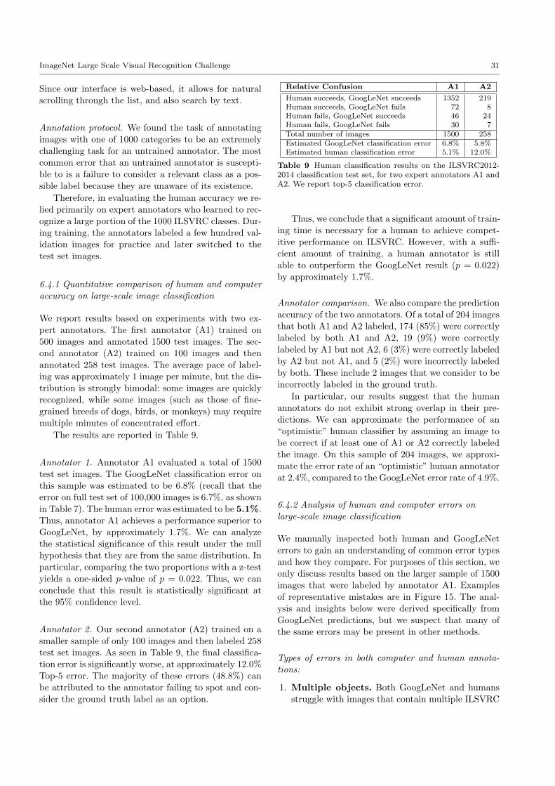
ImageNet Large Scale Visual Recognition Challenge 31
Since our interface is web-based, it allows for natural
scrolling through the list, and also search by text.
Annotation protocol. We found the task of annotating
images with one of 1000 categories to be an extremely
challenging task for an untrained annotator. The most
common error that an untrained annotator is suscepti-
ble to is a failure to consider a relevant class as a pos-
sible label because they are unaware of its existence.
Therefore, in evaluating the human accuracy we re-
lied primarily on expert annotators who learned to rec-
ognize a large portion of the 1000 ILSVRC classes. Dur-
ing training, the annotators labeled a few hundred val-
idation images for practice and later switched to the
test set images.
6.4.1 Quantitative comparison of human and computer
accuracy on large-scale image classification
We report results based on experiments with two ex-
pert annotators. The first annotator (A1) trained on
500 images and annotated 1500 test images. The sec-
ond annotator (A2) trained on 100 images and then
annotated 258 test images. The average pace of label-
ing was approximately 1 image per minute, but the dis-
tribution is strongly bimodal: some images are quickly
recognized, while some images (such as those of fine-
grained breeds of dogs, birds, or monkeys) may require
multiple minutes of concentrated effort.
The results are reported in Table 9.
Annotator 1. Annotator A1 evaluated a total of 1500
test set images. The GoogLeNet classification error on
this sample was estimated to be 6.8% (recall that the
error on full test set of 100,000 images is 6.7%, as shown
in Table 7). The human error was estimated to be 5.1%.
Thus, annotator A1 achieves a performance superior to
GoogLeNet, by approximately 1.7%. We can analyze
the statistical significance of this result under the null
hypothesis that they are from the same distribution. In
particular, comparing the two proportions with a z-test
yields a one-sided p-value of p = 0.022. Thus, we can
conclude that this result is statistically significant at
the 95% confidence level.
Annotator 2. Our second annotator (A2) trained on a
smaller sample of only 100 images and then labeled 258
test set images. As seen in Table 9, the final classifica-
tion error is significantly worse, at approximately 12.0%
Top-5 error. The majority of these errors (48.8%) can
be attributed to the annotator failing to spot and con-
sider the ground truth label as an option.
Relative Confusion A1 A2
Human succeeds, GoogLeNet succeeds 1352 219Human succeeds, GoogLeNet fails 72 8Human fails, GoogLeNet succeeds 46 24Human fails, GoogLeNet fails 30 7Total number of images 1500 258Estimated GoogLeNet classification error 6.8% 5.8%Estimated human classification error 5.1% 12.0%
Table 9 Human classification results on the ILSVRC2012-2014 classification test set, for two expert annotators A1 andA2. We report top-5 classification error.
Thus, we conclude that a significant amount of train-
ing time is necessary for a human to achieve compet-
itive performance on ILSVRC. However, with a suffi-
cient amount of training, a human annotator is still
able to outperform the GoogLeNet result (p = 0.022)
by approximately 1.7%.
Annotator comparison. We also compare the prediction
accuracy of the two annotators. Of a total of 204 images
that both A1 and A2 labeled, 174 (85%) were correctly
labeled by both A1 and A2, 19 (9%) were correctly
labeled by A1 but not A2, 6 (3%) were correctly labeled
by A2 but not A1, and 5 (2%) were incorrectly labeled
by both. These include 2 images that we consider to be
incorrectly labeled in the ground truth.
In particular, our results suggest that the human
annotators do not exhibit strong overlap in their pre-
dictions. We can approximate the performance of an
“optimistic” human classifier by assuming an image to
be correct if at least one of A1 or A2 correctly labeled
the image. On this sample of 204 images, we approxi-
mate the error rate of an “optimistic” human annotator
at 2.4%, compared to the GoogLeNet error rate of 4.9%.
6.4.2 Analysis of human and computer errors on
large-scale image classification
We manually inspected both human and GoogLeNet
errors to gain an understanding of common error types
and how they compare. For purposes of this section, we
only discuss results based on the larger sample of 1500
images that were labeled by annotator A1. Examples
of representative mistakes are in Figure 15. The anal-
ysis and insights below were derived specifically from
GoogLeNet predictions, but we suspect that many of
the same errors may be present in other methods.
Types of errors in both computer and human annota-
tions:
1. Multiple objects. Both GoogLeNet and humans
struggle with images that contain multiple ILSVRC

32 Olga Russakovsky* et al.
Fig. 15 Representative validation images that highlight common sources of error. For each image, we display the ground truthin blue, and top 5 predictions from GoogLeNet follow (red = wrong, green = right). GoogLeNet predictions on the validationset images were graciously provided by members of the GoogLeNet team. From left to right: Images that contain multipleobjects, images of extreme closeups and uncharacteristic views, images with filters, images that significantly benefit from theability to read text, images that contain very small and thin objects, images with abstract representations, and example of afine-grained image that GoogLeNet correctly identifies but a human would have significant difficulty with.
classes (usually many more than five), with little in-
dication of which object is the focus of the image.
This error is only present in the Classification set-
ting, since every image is constrained to have ex-
actly one correct label. In total, we attribute 24
(24%) of GoogLeNet errors and 12 (16%) of human
errors to this category. It is worth noting that hu-
mans can have a slight advantage in this error type,
since it can sometimes be easy to identify the most
salient object in the image.
2. Incorrect annotations. We found that approxi-
mately 5 out of 1500 images (0.3%) were incorrectly
annotated in the ground truth. This introduces an
approximately equal number of errors for both hu-
mans and GoogLeNet.
Types of errors that the computer is more susceptible to
than the human:
1. Object small or thin. GoogLeNet struggles with
recognizing objects that are very small or thin in
the image, even if that object is the only object
present. Examples of this include an image of a
standing person wearing sunglasses, a person hold-
ing a quill in their hand, or a small ant on a stem of a
flower. We estimate that approximately 22 (21%) of
GoogLeNet errors fall into this category, while none
of the human errors do. In other words, in our sam-
ple of images, no image was mislabeled by a human
because they were unable to identify a very small
or thin object. This discrepancy can be attributed
to the fact that a human can very effectively lever-
age context and affordances to accurately infer the
identity of small objects (for example, a few barely
visible feathers near person’s hand as very likely be-
longing to a mostly occluded quill).
2. Image filters. Many people enhance their photos
with filters that distort the contrast and color dis-
tributions of the image. We found that 13 (13%)
of the images that GoogLeNet incorrectly classified
contained a filter. Thus, we posit that GoogLeNet is
not very robust to these distortions. In comparison,
only one image among the human errors contained
a filter, but we do not attribute the source of the
error to the filter.
3. Abstract representations. GoogLeNet struggles
with images that depict objects of interest in an ab-
stract form, such as 3D-rendered images, paintings,
sketches, plush toys, or statues. An example is the
abstract shape of a bow drawn with a light source in
night photography, a 3D-rendered robotic scorpion,
or a shadow on the ground, of a child on a swing.
We attribute approximately 6 (6%) of GoogLeNet
errors to this type of error and believe that humans
are significantly more robust, with no such errors
seen in our sample.
4. Miscellaneous sources. Additional sources of er-
ror that occur relatively infrequently include ex-
treme closeups of parts of an object, unconventional
viewpoints such as a rotated image, images that
can significantly benefit from the ability to read
text (e.g. a featureless container identifying itself as
“face powder”), objects with heavy occlusions, and
images that depict a collage of multiple images. In
general, we found that humans are more robust to
all of these types of error.
Types of errors that the human is more susceptible to
than the computer:
1. Fine-grained recognition. We found that humans
are noticeably worse at fine-grained recognition (e.g.
dogs, monkeys, snakes, birds), even when they are

ImageNet Large Scale Visual Recognition Challenge 33
in clear view. To understand the difficulty, consider
that there are more than 120 species of dogs in the
dataset. We estimate that 28 (37%) of the human
errors fall into this category, while only 7 (7%) of
GoogLeNet errors do.
2. Class unawareness. The annotator may sometimes
be unaware of the ground truth class present as a
label option. When pointed out as an ILSVRC class,
it is usually clear that the label applies to the im-
age. These errors get progressively less frequent as
the annotator becomes more familiar with ILSVRC
classes. Approximately 18 (24%) of the human er-
rors fall into this category.
3. Insufficient training data. Recall that the anno-
tator is only presented with 13 examples of a class
under every category name. However, 13 images are
not always enough to adequately convey the allowed
class variations. For example, a brown dog can be
incorrectly dismissed as a “Kelpie” if all examples of
a “Kelpie” feature a dog with black coat. However,
if more than 13 images were listed it would have
become clear that a “Kelpie” may have brown coat.
Approximately 4 (5%) of human errors fall into this
category.
6.4.3 Conclusions from human image classification
experiments
We investigated the performance of trained human an-
notators on a sample of 1500 ILSVRC test set images.
Our results indicate that a trained human annotator is
capable of outperforming the best model (GoogLeNet)
by approximately 1.7% (p = 0.022).
We expect that some sources of error may be rela-
tively easily eliminated (e.g. robustness to filters, rota-
tions, collages, effectively reasoning over multiple scales),
while others may prove more elusive (e.g. identifying
abstract representations of objects). On the other hand,
a large majority of human errors come from fine-grained
categories and class unawareness. We expect that the
former can be significantly reduced with fine-grained
expert annotators, while the latter could be reduced
with more practice and greater familiarity with ILSVRC
classes. Our results also hint that human errors are not
strongly correlated and that human ensembles may fur-
ther reduce human error rate.
It is clear that humans will soon outperform state-
of-the-art ILSVRC image classification models only by
use of significant effort, expertise, and time. One inter-
esting follow-up question for future investigation is how
computer-level accuracy compares with human-level ac-
curacy on more complex image understanding tasks.
7 Conclusions
In this paper we described the large-scale data collec-
tion process of ILSVRC, provided a summary of the
most successful algorithms on this data, and analyzed
the success and failure modes of these algorithms. In
this section we discuss some of the key lessons we learned
over the years of ILSVRC, strive to address the key
criticisms of the datasets and the challenges we encoun-
tered over the years, and conclude by looking forward
into the future.
7.1 Lessons learned
The key lesson of collecting the datasets and running
the challenges for five years is this: All human in-
telligence tasks need to be exceptionally well-
designed. We learned this lesson both when annotat-
ing the dataset using Amazon Mechanical Turk workers
(Section 3) and even when trying to evaluate human-
level image classification accuracy using expert label-
ers (Section 6.4). The first iteration of the labeling in-
terface was always bad – generally meaning completely
unusable. If there was any inherent ambiguity in the
questions posed (and there almost always was), work-
ers found it and accuracy suffered. If there is one piece
of advice we can offer to future research, it is to very
carefully design, continuously monitor, and extensively
sanity-check all crowdsourcing tasks.
The other lesson, already well-known to large-scale
researchers, is this: Scaling up the dataset always
reveals unexpected challenges. From designing com-
plicated multi-step annotation strategies (Section 3.2.1)
to having to modify the evaluation procedure (Section 4),
we had to continuously adjust to the large-scale setting.
On the plus side, of course, the major breakthroughs in
object recognition accuracy (Section 5) and the analysis
of the strength and weaknesses of current algorithms as
a function of object class properties ( Section 6.3) would
never have been possible on a smaller scale.
7.2 Criticism
In the past five years, we encountered three major crit-
icisms of the ILSVRC dataset and the corresponding
challenge: (1) the ILSVRC dataset is insufficiently chal-
lenging, (2) the ILSVRC dataset contains annotation
errors, and (3) the rules of ILSVRC competition are
too restrictive. We discuss these in order.
The first criticism is that the objects in the dataset
tend to be large and centered in the images, making
the dataset insufficiently challenging. In Sections 3.2.2

34 Olga Russakovsky* et al.
and 3.3.4 we tried to put those concerns to rest by an-
alyzing the statistics of the ILSVRC dataset and con-
cluding that it is comparable with, and in many cases
much more challenging than, the long-standing PAS-
CAL VOC benchmark (Everingham et al., 2010).
The second is regarding the errors in ground truth
labeling. We went through several rounds of in-house
post-processing of the annotations obtained using crowd-
sourcing, and corrected many common sources of errors
(e.g., Appendix E). The major remaining source of an-
notation errors stem from fine-grained object classes,
e.g., labelers failing to distinguish different species of
birds. This is a tradeoff that had to be made: in order
to annotate data at this scale on a reasonable budget,
we had to rely on non-expert crowd labelers. However,
overall the dataset is encouragingly clean. By our esti-
mates, 99.7% precision is achieved in the image classi-
fication dataset (Sections 3.1.3 and 6.4) and 97.9% of
images that went through the bounding box annota-
tion system have all instances of the target object class
labeled with bounding boxes (Section 3.2.1).
The third criticism we encountered is over the rules
of the competition regarding using external training
data. In ILSVRC2010-2013, algorithms had to only use
the provided training and validation set images and an-
notations for training their models. With the growth of
the field of large-scale unsupervised feature learning,
however, questions began to arise about what exactly
constitutes “outside” data: for example, are image fea-
tures trained on a large pool of “outside” images in an
unsupervised fashion allowed in the competition? Af-
ter much discussion, in ILSVRC2014 we took the first
step towards addressing this problem. We followed the
PASCAL VOC strategy and created two tracks in the
competition: entries using only “provided” data and en-
tries using “outside” data, meaning any images or an-
notations not provided as part of ILSVRC training or
validation sets. However, in the future this strategy will
likely need to be further revised as the computer vision
field evolves. For example, competitions can consider
allowing the use of any image features which are pub-
lically available, even if these features were learned on
an external source of data.
7.3 The future
Given the massive algorithmic breakthroughs over the
past five years, we are very eager to see what will hap-
pen in the next five years. There are many potential
directions of improvement and growth for ILSVRC and
other large-scale image datasets.
First, continuing the trend of moving towards richer
image understanding (from image classification to single-
object localization to object detection), the next chal-
lenge would be to tackle pixel-level object segmenta-
tion. The recently released large-scale COCO dataset (Lin
et al., 2014b) is already taking a step in that direction.
Second, as datasets grow even larger in scale, it may
become impossible to fully annotate them manually.
The scale of ILSVRC is already imposing limits on the
manual annotations that are feasible to obtain: for ex-
ample, we had to restrict the number of objects labeled
per image in the image classification and single-object
localization datasets. In the future, with billions of im-
ages, it will become impossible to obtain even one clean
label for every image. Datasets such as Yahoo’s Flickr
Creative Commons 100M,13 released with weak human
tags but no centralized annotation, will become more
common.
The growth of unlabeled or only partially labeled
large-scale datasets implies two things. First, algorithms
will have to rely more on weakly supervised training
data. Second, even evaluation might have to be done
after the algorithms make predictions, not before. This
means that rather than evaluating accuracy (how many
of the test images or objects did the algorithm get right)
or recall (how many of the desired images or objects did
the algorithm manage to find), both of which require
a fully annotated test set, we will be focusing more on
precision: of the predictions that the algorithm made,
how many were deemed correct by humans.
We are eagerly awaiting the future development of
object recognition datasets and algorithms, and are grate-
ful that ILSVRC served as a stepping stone along this
path.
Acknowledgements We thank Stanford University, UNCChapel Hill, Google and Facebook for sponsoring the chal-lenges, and NVIDIA for providing computational resourcesto participants of ILSVRC2014. We thank our advisors overthe years: Lubomir Bourdev, Alexei Efros, Derek Hoiem, Ji-tendra Malik, Chuck Rosenberg and Andrew Zisserman. Wethank the PASCAL VOC organizers for partnering with usin running ILSVRC2010-2012. We thank all members of theStanford vision lab for supporting the challenges and puttingup with us along the way. Finally, and most importantly, wethank all researchers that have made the ILSVRC effort a suc-cess by competing in the challenges and by using the datasetsto advance computer vision.
Appendix A ILSVRC2012-2014 image
classification and single-object localization
object categories
abacus, abaya, academic gown, accordion, acorn, acorn squash, acoustic gui-tar, admiral, affenpinscher, Afghan hound, African chameleon, African crocodile,
13 http://webscope.sandbox.yahoo.com/catalog.php?
datatype=i&did=67

ImageNet Large Scale Visual Recognition Challenge 35
African elephant, African grey, African hunting dog, agama, agaric, aircraft car-rier, Airedale, airliner, airship, albatross, alligator lizard, alp, altar, ambulance,American alligator, American black bear, American chameleon, American coot,American egret, American lobster, American Staffordshire terrier, amphibian,analog clock, anemone fish, Angora, ant, apiary, Appenzeller, apron, Arabiancamel, Arctic fox, armadillo, artichoke, ashcan, assault rifle, Australian terrier,axolotl, baboon, backpack, badger, bagel, bakery, balance beam, bald eagle, bal-loon, ballplayer, ballpoint, banana, Band Aid, banded gecko, banjo, bannister,barbell, barber chair, barbershop, barn, barn spider, barometer, barracouta, bar-rel, barrow, baseball, basenji, basketball, basset, bassinet, bassoon, bath towel,bathing cap, bathtub, beach wagon, beacon, beagle, beaker, bearskin, beaver,Bedlington terrier, bee, bee eater, beer bottle, beer glass, bell cote, bell pepper,Bernese mountain dog, bib, bicycle-built-for-two, bighorn, bikini, binder, binoc-ulars, birdhouse, bison, bittern, black and gold garden spider, black grouse, blackstork, black swan, black widow, black-and-tan coonhound, black-footed ferret,Blenheim spaniel, bloodhound, bluetick, boa constrictor, boathouse, bobsled,bolete, bolo tie, bonnet, book jacket, bookcase, bookshop, Border collie, Borderterrier, borzoi, Boston bull, bottlecap, Bouvier des Flandres, bow, bow tie, boxturtle, boxer, Brabancon griffon, brain coral, brambling, brass, brassiere, break-water, breastplate, briard, Brittany spaniel, broccoli, broom, brown bear, bub-ble, bucket, buckeye, buckle, bulbul, bull mastiff, bullet train, bulletproof vest,bullfrog, burrito, bustard, butcher shop, butternut squash, cab, cabbage butter-fly, cairn, caldron, can opener, candle, cannon, canoe, capuchin, car mirror, carwheel, carbonara, Cardigan, cardigan, cardoon, carousel, carpenter’s kit, car-ton, cash machine, cassette, cassette player, castle, catamaran, cauliflower, CDplayer, cello, cellular telephone, centipede, chain, chain mail, chain saw, chain-link fence, chambered nautilus, cheeseburger, cheetah, Chesapeake Bay retriever,chest, chickadee, chiffonier, Chihuahua, chime, chimpanzee, china cabinet, chi-ton, chocolate sauce, chow, Christmas stocking, church, cicada, cinema, cleaver,cliff, cliff dwelling, cloak, clog, clumber, cock, cocker spaniel, cockroach, cocktailshaker, coffee mug, coffeepot, coho, coil, collie, colobus, combination lock, comicbook, common iguana, common newt, computer keyboard, conch, confectionery,consomme, container ship, convertible, coral fungus, coral reef, corkscrew, corn,cornet, coucal, cougar, cowboy boot, cowboy hat, coyote, cradle, crane, crane,crash helmet, crate, crayfish, crib, cricket, Crock Pot, croquet ball, crosswordpuzzle, crutch, cucumber, cuirass, cup, curly-coated retriever, custard apple,daisy, dalmatian, dam, damselfly, Dandie Dinmont, desk, desktop computer,dhole, dial telephone, diamondback, diaper, digital clock, digital watch, dingo,dining table, dishrag, dishwasher, disk brake, Doberman, dock, dogsled, dome,doormat, dough, dowitcher, dragonfly, drake, drilling platform, drum, drumstick,dugong, dumbbell, dung beetle, Dungeness crab, Dutch oven, ear, earthstar,echidna, eel, eft, eggnog, Egyptian cat, electric fan, electric guitar, electric lo-comotive, electric ray, English foxhound, English setter, English springer, enter-tainment center, EntleBucher, envelope, Eskimo dog, espresso, espresso maker,European fire salamander, European gallinule, face powder, feather boa, fid-dler crab, fig, file, fire engine, fire screen, fireboat, flagpole, flamingo, flat-coated retriever, flatworm, flute, fly, folding chair, football helmet, forklift, foun-tain, fountain pen, four-poster, fox squirrel, freight car, French bulldog, Frenchhorn, French loaf, frilled lizard, frying pan, fur coat, gar, garbage truck, gar-den spider, garter snake, gas pump, gasmask, gazelle, German shepherd, Ger-man short-haired pointer, geyser, giant panda, giant schnauzer, gibbon, Gilamonster, go-kart, goblet, golden retriever, goldfinch, goldfish, golf ball, golfcart,gondola, gong, goose, Gordon setter, gorilla, gown, grand piano, Granny Smith,grasshopper, Great Dane, great grey owl, Great Pyrenees, great white shark,Greater Swiss Mountain dog, green lizard, green mamba, green snake, green-house, grey fox, grey whale, grille, grocery store, groenendael, groom, groundbeetle, guacamole, guenon, guillotine, guinea pig, gyromitra, hair slide, hairspray, half track, hammer, hammerhead, hamper, hamster, hand blower, hand-held computer, handkerchief, hard disc, hare, harmonica, harp, hartebeest, har-vester, harvestman, hatchet, hay, head cabbage, hen, hen-of-the-woods, hermitcrab, hip, hippopotamus, hog, hognose snake, holster, home theater, honeycomb,hook, hoopskirt, horizontal bar, hornbill, horned viper, horse cart, hot pot, hot-dog, hourglass, house finch, howler monkey, hummingbird, hyena, ibex, Ibizanhound, ice bear, ice cream, ice lolly, impala, Indian cobra, Indian elephant, in-digo bunting, indri, iPod, Irish setter, Irish terrier, Irish water spaniel, Irishwolfhound, iron, isopod, Italian greyhound, jacamar, jack-o’-lantern, jackfruit,jaguar, Japanese spaniel, jay, jean, jeep, jellyfish, jersey, jigsaw puzzle, jinrik-isha, joystick, junco, keeshond, kelpie, Kerry blue terrier, killer whale, kimono,king crab, king penguin, king snake, kit fox, kite, knee pad, knot, koala, Ko-modo dragon, komondor, kuvasz, lab coat, Labrador retriever, lacewing, ladle,ladybug, Lakeland terrier, lakeside, lampshade, langur, laptop, lawn mower, leafbeetle, leafhopper, leatherback turtle, lemon, lens cap, Leonberg, leopard, lesserpanda, letter opener, Lhasa, library, lifeboat, lighter, limousine, limpkin, liner,lion, lionfish, lipstick, little blue heron, llama, Loafer, loggerhead, long-hornedbeetle, lorikeet, lotion, loudspeaker, loupe, lumbermill, lycaenid, lynx, macaque,macaw, Madagascar cat, magnetic compass, magpie, mailbag, mailbox, mail-lot, maillot, malamute, malinois, Maltese dog, manhole cover, mantis, maraca,marimba, marmoset, marmot, mashed potato, mask, matchstick, maypole, maze,measuring cup, meat loaf, medicine chest, meerkat, megalith, menu, Mexicanhairless, microphone, microwave, military uniform, milk can, miniature pinscher,miniature poodle, miniature schnauzer, minibus, miniskirt, minivan, mink, mis-sile, mitten, mixing bowl, mobile home, Model T, modem, monarch, monastery,mongoose, monitor, moped, mortar, mortarboard, mosque, mosquito net, mo-tor scooter, mountain bike, mountain tent, mouse, mousetrap, moving van, mudturtle, mushroom, muzzle, nail, neck brace, necklace, nematode, Newfoundland,night snake, nipple, Norfolk terrier, Norwegian elkhound, Norwich terrier, note-book, obelisk, oboe, ocarina, odometer, oil filter, Old English sheepdog, or-ange, orangutan, organ, oscilloscope, ostrich, otter, otterhound, overskirt, ox,oxcart, oxygen mask, oystercatcher, packet, paddle, paddlewheel, padlock, paint-brush, pajama, palace, panpipe, paper towel, papillon, parachute, parallel bars,park bench, parking meter, partridge, passenger car, patas, patio, pay-phone,peacock, pedestal, Pekinese, pelican, Pembroke, pencil box, pencil sharpener,perfume, Persian cat, Petri dish, photocopier, pick, pickelhaube, picket fence,pickup, pier, piggy bank, pill bottle, pillow, pineapple, ping-pong ball, pinwheel,pirate, pitcher, pizza, plane, planetarium, plastic bag, plate, plate rack, platy-pus, plow, plunger, Polaroid camera, pole, polecat, police van, pomegranate,Pomeranian, poncho, pool table, pop bottle, porcupine, pot, potpie, potter’swheel, power drill, prairie chicken, prayer rug, pretzel, printer, prison, proboscismonkey, projectile, projector, promontory, ptarmigan, puck, puffer, pug, punch-ing bag, purse, quail, quill, quilt, racer, racket, radiator, radio, radio telescope,rain barrel, ram, rapeseed, recreational vehicle, red fox, red wine, red wolf, red-backed sandpiper, red-breasted merganser, redbone, redshank, reel, reflex cam-era, refrigerator, remote control, restaurant, revolver, rhinoceros beetle, Rhode-sian ridgeback, rifle, ringlet, ringneck snake, robin, rock beauty, rock crab, rockpython, rocking chair, rotisserie, Rottweiler, rubber eraser, ruddy turnstone,ruffed grouse, rugby ball, rule, running shoe, safe, safety pin, Saint Bernard,saltshaker, Saluki, Samoyed, sandal, sandbar, sarong, sax, scabbard, scale, schip-perke, school bus, schooner, scoreboard, scorpion, Scotch terrier, Scottish deer-hound, screen, screw, screwdriver, scuba diver, sea anemone, sea cucumber, sealion, sea slug, sea snake, sea urchin, Sealyham terrier, seashore, seat belt, sewing
machine, Shetland sheepdog, shield, Shih-Tzu, shoe shop, shoji, shopping bas-ket, shopping cart, shovel, shower cap, shower curtain, siamang, Siamese cat,Siberian husky, sidewinder, silky terrier, ski, ski mask, skunk, sleeping bag,slide rule, sliding door, slot, sloth bear, slug, snail, snorkel, snow leopard, snow-mobile, snowplow, soap dispenser, soccer ball, sock, soft-coated wheaten ter-rier, solar dish, sombrero, sorrel, soup bowl, space bar, space heater, spaceshuttle, spaghetti squash, spatula, speedboat, spider monkey, spider web, spin-dle, spiny lobster, spoonbill, sports car, spotlight, spotted salamander, squirrelmonkey, Staffordshire bullterrier, stage, standard poodle, standard schnauzer,starfish, steam locomotive, steel arch bridge, steel drum, stethoscope, stingray,stinkhorn, stole, stone wall, stopwatch, stove, strainer, strawberry, street sign,streetcar, stretcher, studio couch, stupa, sturgeon, submarine, suit, sulphur but-terfly, sulphur-crested cockatoo, sundial, sunglass, sunglasses, sunscreen, suspen-sion bridge, Sussex spaniel, swab, sweatshirt, swimming trunks, swing, switch,syringe, tabby, table lamp, tailed frog, tank, tape player, tarantula, teapot,teddy, television, tench, tennis ball, terrapin, thatch, theater curtain, thimble,three-toed sloth, thresher, throne, thunder snake, Tibetan mastiff, Tibetan ter-rier, tick, tiger, tiger beetle, tiger cat, tiger shark, tile roof, timber wolf, titi,toaster, tobacco shop, toilet seat, toilet tissue, torch, totem pole, toucan, towtruck, toy poodle, toy terrier, toyshop, tractor, traffic light, trailer truck, tray,tree frog, trench coat, triceratops, tricycle, trifle, trilobite, trimaran, tripod, tri-umphal arch, trolleybus, trombone, tub, turnstile, tusker, typewriter keyboard,umbrella, unicycle, upright, vacuum, valley, vase, vault, velvet, vending machine,vestment, viaduct, vine snake, violin, vizsla, volcano, volleyball, vulture, waffleiron, Walker hound, walking stick, wall clock, wallaby, wallet, wardrobe, war-plane, warthog, washbasin, washer, water bottle, water buffalo, water jug, waterouzel, water snake, water tower, weasel, web site, weevil, Weimaraner, Welshspringer spaniel, West Highland white terrier, whippet, whiptail, whiskey jug,whistle, white stork, white wolf, wig, wild boar, window screen, window shade,Windsor tie, wine bottle, wing, wire-haired fox terrier, wok, wolf spider, wom-bat, wood rabbit, wooden spoon, wool, worm fence, wreck, yawl, yellow lady’sslipper, Yorkshire terrier, yurt, zebra, zucchini
Appendix B Additional single-object
localization dataset statistics
We consider two additional metrics of object localiza-
tion difficulty: chance performance of localization and
the level of clutter. We use these metrics to compare
ILSVRC2012-2014 single-object localization dataset to
the PASCAL VOC 2012 object detection benchmark.
The measures of localization difficulty are computed
on the validation set of both datasets. According to
both of these measures of difficulty there is a subset of
ILSVRC which is as challenging as PASCAL but more
than an order of magnitude greater in size. Figure 16
shows the distributions of different properties (object
scale, chance performance of localization and level of
clutter) across the different classes in the two datasets.
Chance performance of localization (CPL). Chance per-
formance on a dataset is a common metric to con-
sider. We define the CPL measure as the expected ac-
curacy of a detector which first randomly samples an
object instance of that class and then uses its bounding
box directly as the proposed localization window on all
other images (after rescaling the images to the same
size). Concretely, let B1, B2, . . . , BN be all the bound-
ing boxes of the object instances within a class, then
CPL =
∑i
∑j 6=i IOU(Bi, Bj) ≥ 0.5
N(N − 1)(6)
Some of the most difficult ILSVRC categories to lo-
calize according to this metric are basketball, swim-
ming trunks, ping pong ball and rubber eraser, all with
less than 0.2% CPL. This measure correlates strongly
(ρ = 0.9) with the average scale of the object (fraction
of image occupied by object). The average CPL across
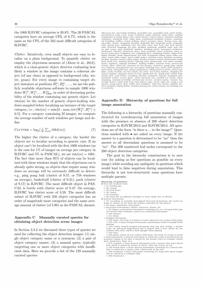
36 Olga Russakovsky* et al.
the 1000 ILSVRC categories is 20.8%. The 20 PASCAL
categories have an average CPL of 8.7%, which is the
same as the CPL of the 562 most difficult categories of
ILSVRC.
Clutter. Intuitively, even small objects are easy to lo-
calize on a plain background. To quantify clutter we
employ the objectness measure of (Alexe et al., 2012),
which is a class-generic object detector evaluating how
likely a window in the image contains a coherent ob-
ject (of any class) as opposed to background (sky, wa-
ter, grass). For every image m containing target ob-
ject instances at positions Bm1 , B
m2 , . . . , we use the pub-
licly available objectness software to sample 1000 win-
dows Wm1 ,W
m2 , . . .W
m1000, in order of decreasing proba-
bility of the window containing any generic object. Let
obj(m) be the number of generic object-looking win-
dows sampled before localizing an instance of the target
category, i.e., obj(m) = min{k : maxi iou(Wmk , B
mi ) ≥
0.5}. For a category containing M images, we compute
the average number of such windows per image and de-
fine
Clutter = log2( 1M
∑mobj(m)) (7)
The higher the clutter of a category, the harder the
objects are to localize according to generic cues. If an
object can’t be localized with the first 1000 windows (as
is the case for 1% of images on average per category in
ILSVRC and 5% in PASCAL), we set obj(m) = 1001.
The fact that more than 95% of objects can be local-
ized with these windows imply that the objectness cue is
already quite strong, so objects that require many win-
dows on average will be extremely difficult to detect:e.g., ping pong ball (clutter of 9.57, or 758 windows
on average), basketball (clutter of 9.21), puck (clutter
of 9.17) in ILSVRC. The most difficult object in PAS-
CAL is bottle with clutter score of 8.47. On average,
ILSVRC has clutter score of 3.59. The most difficult
subset of ILSVRC with 250 object categories has an
order of magnitude more categories and the same aver-
age amount of clutter (of 5.90) as the PASCAL dataset.
Appendix C Manually curated queries for
obtaining object detection scene images
In Section 3.3.2 we discussed three types of queries we
used for collecting the object detection images: (1) sin-
gle object category name or a synonym; (2) a pair of
object category names; (3) a manual query, typically
targetting one or more object categories with insuffi-
cient data. Here we provide a list of the 129 manually
curated queries:
afternoon tea, ant bridge building, armadillo race, armadillo yard, artist studio,auscultation, baby room, banjo orchestra, banjo rehersal, banjo show, califoneheadphones & media player sets, camel dessert, camel tourist, carpenter drilling,carpentry, centipede wild, coffee shop, continental breakfast toaster, continen-tal breakfast waffles, crutch walking, desert scorpion, diner, dining room, din-ing table, dinner, dragonfly friendly, dragonfly kid, dragonfly pond, dragonflywild, drying hair, dumbbell curl, fan blow wind, fast food, fast food restau-rant, firewood chopping, flu shot, goldfish aquarium, goldfish tank, golf carton golf course, gym dumbbell, hamster drinking water, harmonica orchestra,harmonica rehersal, harmonica show, harp ensemble, harp orchestra, harp re-hersal, harp show, hedgehog cute, hedgehog floor, hedgehog hidden, hippo bird,hippo friendly, home improvement diy drill, horseback riding, hotel coffee ma-chine, hotel coffee maker, hotel waffle maker, jellyfish scuba, jellyfish snorkling,kitchen, kitchen counter coffee maker, kitchen counter toaster, kitchenette, koalafeed, koala tree, ladybug flower, ladybug yard, laundromat, lion zebra friendly,lunch, mailman, making breakfast, making waffles, mexican food, motorcycleracing, office, office fan, opossum on tree branch, orchestra, panda play, pandatree, pizzeria, pomegranate tree, porcupine climbing trees, power drill carpenter,purse shop, red panda tree, riding competition, riding motor scooters, school sup-plies, scuba starfish, sea lion beach, sea otter, sea urchin habitat, shopping forschool supplies, sitting in front of a fan, skunk and cat, skunk park, skunk wild,skunk yard, snail flower, snorkling starfish, snowplow cleanup, snowplow pile,snowplow winter, soccer game, south american zoo, starfish sea world, startsshopping, steamed artichoke, stethoscope doctor, strainer pasta, strainer tea,syringe doctor, table with food, tape player, tiger circus, tiger pet, using a canopener, using power drill, waffle iron breakfast, wild lion savana, wildlife pre-serve animals, wiping dishes, wombat petting zoo, zebra savana, zoo feeding, zooin australia
Appendix D Hierarchy of questions for full
image annotation
The following is a hierarchy of questions manually con-
structed for crowdsourcing full annotation of images
with the presence or absence of 200 object detection
categories in ILSVRC2013 and ILSVRC2014. All ques-
tions are of the form “is there a ... in the image?” Ques-
tions marked with • are asked on every image. If the
answer to a question is determined to be “no” then the
answer to all descendant questions is assumed to be
“no”. The 200 numbered leaf nodes correspond to the
200 object detection categories.
The goal in the hierarchy construction is to save
cost (by asking as few questions as possible on every
image) while avoiding any ambiguity in questions which
would lead to false negatives during annotation. This
hierarchy is not tree-structured; some questions have
multiple parents.
Hierarchy of questions:• first aid/ medical items
◦ (1) stethoscope
◦ (2) syringe
◦ (3) neck brace
◦ (4) crutch
◦ (5) stretcher
◦ (6) band aid: an adhesive bandage to cover small cuts or blisters
• musical instruments
◦ (7) accordion (a portable box-shaped free-reed instrument; the reeds aremade to vibrate by air from the bellows controlled by the player)
◦ (8) piano, pianoforte, forte-piano
◦ percussion instruments: chimes, maraccas, drums, etc
◦ (9) chime: a percussion instrument consisting of a set of tuned bells thatare struck with a hammer; used as an orchestral instrument
◦ (10) maraca
◦ (11) drum
◦ stringed instrument
◦ (12) banjo, the body of a banjo is round. please do not confuse with guitar
◦ (13) cello: a large stringed instrument; seated player holds it upright whileplaying
◦ (14) violin: bowed stringed instrument that has four strings, a hollowbody, an unfretted fingerboard and is played with a bow. please do notconfuse with cello, which is held upright while playing
◦ (15) harp
◦ (16) guitar, please do not confuse with banjo. the body of a banjo is round
◦ wind instrument: a musical instrument in which the sound is produced by anenclosed column of air that is moved by the breath (such as trumpet, frenchhorn, harmonica, flute, etc)
◦ (17) trumpet: a brass musical instrument with a narrow tube and a flaredbell, which is played by means of valves. often has 3 keys on top
◦ (18) french horn: a brass musical instrument consisting of a conical tubethat is coiled into a spiral, with a flared bell at the end
◦ (19) trombone: a brass instrument consisting of a long tube whose lengthcan be varied by a u-shaped slide
◦ (20) harmonica

ImageNet Large Scale Visual Recognition Challenge 37
1000 classes of ILSVRC2012-2014 single-object localization (dark green)versus 20 classes of PASCAL 2012 (light blue)
→ more diffiult more diffiult ← more diffiult ← → more diffiult
200 hardest classes of ILSVRC2012-2014 single-object localization (dark green)versus 20 classes of PASCAL 2012 (light blue)
→ more diffiult more diffiult ← more diffiult ← → more diffiult
Fig. 16 Distribution of various measures of localization difficulty on the ILSVRC2012-2014 single-object localization (darkgreen) and PASCAL VOC 2012 (light blue) validation sets. Object scale is fraction of image area occupied by an averageobject instance. Chance performance of localization and level of clutter are defined in Appendix B. The plots on top containthe full ILSVRC validation set with 1000 classes; the plots on the bottom contain 200 ILSVRC classes with the lowest chanceperformance of localization. All plots contain all 20 classes of PASCAL VOC.
◦ (21) flute: a high-pitched musical instrument that looks like a straighttube and is usually played sideways (please do not confuse with oboes, whichhave a distinctive straw-like mouth piece and a slightly flared end)◦ (22) oboe: a slender musical instrument roughly 65cm long with metalkeys, a distinctive straw-like mouthpiece and often a slightly flared end(please do not confuse with flutes)◦ (23) saxophone: a musical instrument consisting of a brass conical tube,often with a u-bend at the end
• food: something you can eat or drink (includes growing fruit, vegetables andmushrooms, but does not include living animals)◦ food with bread or crust: pretzel, bagel, pizza, hotdog, hamburgers, etc◦ (24) pretzel◦ (25) bagel, beigel◦ (26) pizza, pizza pie◦ (27) hotdog, hot dog, red hot◦ (28) hamburger, beefburger, burger
◦ (29) guacamole◦ (30) burrito◦ (31) popsicle (ice cream or water ice on a small wooden stick)◦ fruit◦ (32) fig◦ (33) pineapple, ananas◦ (34) banana◦ (35) pomegranate◦ (36) apple◦ (37) strawberry◦ (38) orange◦ (39) lemon
◦ vegetables◦ (40) cucumber, cuke◦ (41) artichoke, globe artichoke◦ (42) bell pepper◦ (43) head cabbage
◦ (44) mushroom• items that run on electricity (plugged in or using batteries); including clocks,microphones, traffic lights, computers, etc◦ (45) remote control, remote◦ electronics that blow air◦ (46) hair dryer, blow dryer◦ (47) electric fan: a device for creating a current of air by movement of asurface or surfaces (please do not consider hair dryers)
◦ electronics that can play music or amplify sound◦ (48) tape player◦ (49) iPod
◦ (50) microphone, mike◦ computer and computer peripherals: mouse, laptop, printer, keyboard, etc◦ (51) computer mouse
◦ (52) laptop, laptop computer◦ (53) printer (please do not consider typewriters to be printers)◦ (54) computer keyboard
◦ (55) lamp◦ electric cooking appliance (an appliance which generates heat to cook foodor boil water)◦ (56) microwave, microwave oven◦ (57) toaster◦ (58) waffle iron◦ (59) coffee maker: a kitchen appliance used for brewing coffee automati-cally
◦ (60) vacuum, vacuum cleaner◦ (61) dishwasher, dish washer, dishwashing machine◦ (62) washer, washing machine: an electric appliance for washing clothes◦ (63) traffic light, traffic signal, stoplight◦ (64) tv or monitor: an electronic device that represents information in visualform◦ (65) digital clock: a clock that displays the time of day digitally
• kitchen items: tools,utensils and appliances usually found in the kitchen◦ electric cooking appliance (an appliance which generates heat to cook foodor boil water)◦ (56) microwave, microwave oven◦ (57) toaster◦ (58) waffle iron◦ (59) coffee maker: a kitchen appliance used for brewing coffee automati-cally
◦ (61) dishwasher, dish washer, dishwashing machine◦ (66) stove◦ things used to open cans/bottles: can opener or corkscrew◦ (67) can opener (tin opener)◦ (68) corkscrew
◦ (69) cocktail shaker◦ non-electric item commonly found in the kitchen: pot, pan, utensil, bowl,etc◦ (70) strainer◦ (71) frying pan (skillet)◦ (72) bowl: a dish for serving food that is round, open at the top, and hasno handles (please do not confuse with a cup, which usually has a handleand is used for serving drinks)◦ (73) salt or pepper shaker: a shaker with a perforated top for sprinklingsalt or pepper◦ (74) plate rack◦ (75) spatula: a turner with a narrow flexible blade◦ (76) ladle: a spoon-shaped vessel with a long handle; frequently used totransfer liquids from one container to another
◦ (77) refrigerator, icebox• furniture (including benches)

38 Olga Russakovsky* et al.
◦ (78) bookshelf: a shelf on which to keep books◦ (79) baby bed: small bed for babies, enclosed by sides to prevent baby fromfalling◦ (80) filing cabinet: office furniture consisting of a container for keepingpapers in order◦ (81) bench (a long seat for several people, typically made of wood or stone)◦ (82) chair: a raised piece of furniture for one person to sit on; please do notconfuse with benches or sofas, which are made for more people◦ (83) sofa, couch: upholstered seat for more than one person; please do notconfuse with benches (which are made of wood or stone) or with chairs (whichare for just one person)◦ (84) table
• clothing, article of clothing: a covering designed to be worn on a person’s body◦ (85) diaper: Garment consisting of a folded cloth drawn up between the legsand fastened at the waist; worn by infants to catch excrement◦ swimming attire: clothes used for swimming or bathing (swim suits, swimtrunks, bathing caps)◦ (86) swimming trunks: swimsuit worn by men while swimming◦ (87) bathing cap, swimming cap: a cap worn to keep hair dry while swim-ming or showering◦ (88) maillot: a woman’s one-piece bathing suit
◦ necktie: a man’s formal article of clothing worn around the neck (includingbow ties)◦ (89) bow tie: a man’s tie that ties in a bow◦ (90) tie: a long piece of cloth worn for decorative purposes around theneck or shoulders, resting under the shirt collar and knotted at the throat(NOT a bow tie)
◦ headdress, headgear: clothing for the head (hats, helmets, bathing caps, etc)◦ (87) bathing cap, swimming cap: a cap worn to keep hair dry while swim-ming or showering◦ (91) hat with a wide brim◦ (92) helmet: protective headgear made of hard material to resist blows
◦ (93) miniskirt, mini: a very short skirt◦ (94) brassiere, bra: an undergarment worn by women to support their breasts◦ (95) sunglasses
• living organism (other than people): dogs, snakes, fish, insects, sea urchins,starfish, etc.◦ living organism which can fly◦ (96) bee◦ (97) dragonfly◦ (98) ladybug◦ (99) butterfly◦ (100) bird
◦ living organism which cannot fly (please don’t include humans)◦ living organism with 2 or 4 legs (please don’t include humans):◦ mammals (but please do not include humans)◦ feline (cat-like) animal: cat, tiger or lion◦ (101) domestic cat◦ (102) tiger◦ (103) lion
◦ canine (dog-like animal): dog, hyena, fox or wolf◦ (104) dog, domestic dog, canis familiaris◦ (105) fox: wild carnivorous mammal with pointed muzzle and earsand a bushy tail (please do not confuse with dogs)
◦ animals with hooves: camels, elephants, hippos, pigs, sheep, etc◦ (106) elephant◦ (107) hippopotamus, hippo◦ (108) camel◦ (109) swine: pig or boar◦ (110) sheep: woolly animal, males have large spiraling horns (pleasedo not confuse with antelope which have long legs)◦ (111) cattle: cows or oxen (domestic bovine animals)◦ (112) zebra◦ (113) horse◦ (114) antelope: a graceful animal with long legs and horns directedupward and backward
◦ (115) squirrel◦ (116) hamster: short-tailed burrowing rodent with large cheek pouches◦ (117) otter◦ (118) monkey◦ (119) koala bear◦ (120) bear (other than pandas)◦ (121) skunk (mammal known for its ability fo spray a liquid with astrong odor; they may have a single thick stripe across back and tail,two thinner stripes, or a series of white spots and broken stripes◦ (122) rabbit◦ (123) giant panda: an animal characterized by its distinct black andwhite markings◦ (124) red panda: Reddish-brown Old World raccoon-like carnivore
◦ (125) frog, toad◦ (126) lizard: please do not confuse with snake (lizards have legs)◦ (127) turtle◦ (128) armadillo◦ (129) porcupine, hedgehog
◦ living organism with 6 or more legs: lobster, scorpion, insects, etc.◦ (130) lobster: large marine crustaceans with long bodies and musculartails; three of their five pairs of legs have claws◦ (131) scorpion◦ (132) centipede: an arthropod having a flattened body of 15 to 173segments each with a pair of legs, the foremost pair being modified asprehensors◦ (133) tick (a small creature with 4 pairs of legs which lives on the bloodof mammals and birds)◦ (134) isopod: a small crustacean with seven pairs of legs adapted forcrawling◦ (135) ant
◦ living organism without legs: fish, snake, seal, etc. (please don’t includeplants)◦ living organism that lives in water: seal, whale, fish, sea cucumber, etc.◦ (136) jellyfish◦ (137) starfish, sea star◦ (138) seal◦ (139) whale◦ (140) ray: a marine animal with a horizontally flattened body andenlarged winglike pectoral fins with gills on the underside◦ (141) goldfish: small golden or orange-red fishes
◦ living organism that slides on land: worm, snail, snake◦ (142) snail◦ (143) snake: please do not confuse with lizard (snakes do not havelegs)
• vehicle: any object used to move people or objects from place to place
◦ a vehicle with wheels
◦ (144) golfcart, golf cart
◦ (145) snowplow: a vehicle used to push snow from roads
◦ (146) motorcycle (or moped)
◦ (147) car, automobile (not a golf cart or a bus)
◦ (148) bus: a vehicle carrying many passengers; used for public transport
◦ (149) train
◦ (150) cart: a heavy open wagon usually having two wheels and drawn byan animal
◦ (151) bicycle, bike: a two wheeled vehicle moved by foot pedals
◦ (152) unicycle, monocycle
◦ a vehicle without wheels (snowmobile, sleighs)
◦ (153) snowmobile: tracked vehicle for travel on snow
◦ (154) watercraft (such as ship or boat): a craft designed for water trans-portation
◦ (155) airplane: an aircraft powered by propellers or jets
• cosmetics: toiletry designed to beautify the body
◦ (156) face powder
◦ (157) perfume, essence (usually comes in a smaller bottle than hair spray
◦ (158) hair spray
◦ (159) cream, ointment, lotion
◦ (160) lipstick, lip rouge
• carpentry items: items used in carpentry, including nails, hammers, axes,screwdrivers, drills, chain saws, etc
◦ (161) chain saw, chainsaw
◦ (162) nail: pin-shaped with a head on one end and a point on the other
◦ (163) axe: a sharp tool often used to cut trees/ logs
◦ (164) hammer: a blunt hand tool used to drive nails in or break things apart(please do not confuse with axe, which is sharp)
◦ (165) screwdriver
◦ (166) power drill: a power tool for drilling holes into hard materials
• school supplies: rulers, erasers, pencil sharpeners, pencil boxes, binders
◦ (167) ruler,rule: measuring stick consisting of a strip of wood or metal orplastic with a straight edge that is used for drawing straight lines and mea-suring lengths
◦ (168) rubber eraser, rubber, pencil eraser
◦ (169) pencil sharpener
◦ (170) pencil box, pencil case
◦ (171) binder, ring-binder
• sports items: items used to play sports or in the gym (such as skis, raquets,gymnastics bars, bows, punching bags, balls)
◦ (172) bow: weapon for shooting arrows, composed of a curved piece of re-silient wood with a taut cord to propel the arrow
◦ (173) puck, hockey puck: vulcanized rubber disk 3 inches in diameter thatis used instead of a ball in ice hockey
◦ (174) ski
◦ (175) racket, racquet
◦ gymnastic equipment: parallel bars, high beam, etc
◦ (176) balance beam: a horizontal bar used for gymnastics which is raisedfrom the floor and wide enough to walk on
◦ (177) horizontal bar, high bar: used for gymnastics; gymnasts grip it withtheir hands (please do not confuse with balance beam, which is wide enoughto walk on)
◦ ball
◦ (178) golf ball
◦ (179) baseball
◦ (180) basketball
◦ (181) croquet ball
◦ (182) soccer ball
◦ (183) ping-pong ball
◦ (184) rugby ball
◦ (185) volleyball
◦ (186) tennis ball
◦ (187) punching bag, punch bag, punching ball, punchball
◦ (188) dumbbell: An exercising weight; two spheres connected by a short barthat serves as a handle
• liquid container: vessels which commonly contain liquids such as bottles, cans,etc.
◦ (189) pitcher: a vessel with a handle and a spout for pouring
◦ (190) beaker: a flatbottomed jar made of glass or plastic; used for chemistry
◦ (191) milk can
◦ (192) soap dispenser
◦ (193) wine bottle
◦ (194) water bottle
◦ (195) cup or mug (usually with a handle and usually cylindrical)
• bag
◦ (196) backpack: a bag carried by a strap on your back or shoulder
◦ (197) purse: a small bag for carrying money
◦ (198) plastic bag
• (199) person
• (200) flower pot: a container in which plants are cultivated
Appendix E Modification to bounding box
system for object detection
The bounding box annotation system described in Sec-
tion 3.2.1 is used for annotating images for both the
single-object localization dataset and the object de-
tection dataset. However, two additional manual post-
processing are needed to ensure accuracy in the object
detection scenario:

ImageNet Large Scale Visual Recognition Challenge 39
Ambiguous objects. The first common source of error
was that workers were not able to accurately differenti-
ate some object classes during annotation. Some com-
monly confused labels were seal and sea otter, backpack
and purse, banjo and guitar, violin and cello, brass in-
struments (trumpet, trombone, french horn and brass),
flute and oboe, ladle and spatula. Despite our best ef-
forts (providing positive and negative example images
in the annotation task, adding text explanations to alert
the user to the distinction between these categories)
these errors persisted.
In the single-object localization setting, this prob-
lem was not as prominent for two reasons. First, the
way the data was collected imposed a strong prior on
the object class which was present. Second, since only
one object category needed to be annotated per image,
ambiguous images could be discarded: for example, if
workers couldn’t agree on whether or not a trumpet was
in fact present, this image could simply be removed. In
contrast, for the object detection setting consensus had
to be reached for all target categories on all images.
To fix this problem, once bounding box annota-
tions were collected we manually looked through all
cases where the bounding boxes for two different object
classes had significant overlap with each other (about
3% of the collected boxes). About a quarter of these
boxes were found to correspond to incorrect objects
and were removed. Crowdsourcing this post-processing
step (with very stringent accuracy constraints) would
be possible but it occurred in few enough cases that it
was faster (and more accurate) to do this in-house.
Duplicate annotations. The second common source of
error were duplicate bounding boxes drawn on the same
object instance. Despite instructions not to draw more
than one bounding box around the same object instance
and constraints in the annotation UI enforcing at least
a 5 pixel difference between different bounding boxes,
these errors persisted. One reason was that sometimes
the initial bounding box was not perfect and subsequent
labelers drew a slightly improved alternative.
This type of error was also present in the single-
object localization scenario but was not a major cause
for concern. A duplicate bounding box is a slightly per-
turbed but still correct positive example, and single-
object localization is only concerned with correctly lo-
calizing one object instance. For the detection task algo-
rithms are evaluated on the ability to localize every ob-
ject instance, and penalized for duplicate detections, so
it is imperative that these labeling errors are corrected
(even if they only appear in about 0.6% of cases).
Approximately 1% of bounding boxes were found
to have significant overlap of more than 50% with an-
other bounding box of the same object class.We again
manually verified all of these cases in-house. In approx-
imately 40% of the cases the two bounding boxes cor-
rectly corresponded to different people in a crowd, to
stacked plates, or to musical instruments nearby in an
orchestra. In the other 60% of cases one of the boxes
was randomly removed.
These verification steps complete the annotation pro-
cedure of bounding boxes around every instance of ev-
ery object class in validation, test and a subset of train-
ing images for the detection task.
Training set annotation. With the optimized algorithm
of Section 3.3.3 we fully annotated the validation and
test sets. However, annotating all training images with
all target object classes was still a budget challenge.
Positive training images taken from the single-object
localization dataset already had bounding box annota-
tions of all instances of one object class on each im-
age. We extended the existing annotations to the de-
tection dataset by making two modification. First, we
corrected any bounding box omissions resulting from
merging fine-grained categories: i.e., if an image be-
longed to the ”dalmatian” category and all instances of
”dalmatian” were annotated with bounding boxes for
single-object localization, we ensured that all remain-
ing ”dog” instances are also annotated for the object
detection task. Second, we collected significantly more
training data for the person class because the existing
annotation set was not diverse enough to be representa-
tive (the only people categories in the single-object lo-
calization task are scuba diver, groom, and ballplayer).
To compensate, we additionally annotated people in a
large fraction of the existing training set images.
Appendix F Competition protocol
Competition format. At the beginning of the competi-
tion period each year we release the new training/validation/test
images, training/validation annotations, and competi-
tion specification for the year. We then specify a dead-
line for submission, usually approximately 4 months af-
ter the release of data. Teams are asked to upload a
text file of their predicted annotations on test images
by this deadline to a provided server. We then evaluate
all submissions and release the results.
For every task we released code that takes a text file
of automatically generated image annotations and com-
pares it with the ground truth annotations to return a
quantitative measure of algorithm accuracy. Teams can
use this code to evaluate their performance on the val-
idation data.
40 Olga Russakovsky* et al.
As described in (Everingham et al., 2014), there are
three options for measuring performance on test data:
(i) Release test images and annotations, and allow par-
ticipants to assess performance themselves; (ii) Release
test images but not test annotations – participants sub-
mit results and organizers assess performance; (iii) Nei-
ther test images nor annotations are released – partic-
ipants submit software and organizers run it on new
data and assess performance. In line with the PASCAL
VOC choice, we opted for option (ii). Option (i) allows
too much leeway in overfitting to the test data; option
(iii) is infeasible, especially given the scale of our test
set (40K-100K images).
We released ILSVRC2010 test annotations for the
image classification task, but all other test annotations
have remained hidden to discourage fine-tuning results
on the test data.
Evaluation protocol after the challenge. After the chal-
lenge period we set up an automatic evaluation server
that researchers can use throughout the year to con-
tinue evaluating their algorithms against the ground
truth test annotations. We limit teams to 2 submis-
sions per week to discourage parameter tuning on the
test data, and in practice we have never had a problem
with researchers abusing the system.
*Bibliography
Ahonen, T., Hadid, A., and Pietikinen, M. (2006). Face
description with local binary patterns: Application to
face recognition. PAMI, 28.
Alexe, B., Deselares, T., and Ferrari, V. (2012). Mea-
suring the objectness of image windows. In PAMI.
Arandjelovic, R. and Zisserman, A. (2012). Threethings everyone should know to improve object re-
trieval. In CVPR.
Arbelaez, P., Maire, M., Fowlkes, C., and Malik, J.
(2011). Contour detection and hierarchical image seg-
mentation. IEEE TPAMI, 33.
Arbelaez, P., Pont-Tuset, J., Barron, J., Marques,
F., and Malik, J. (2014). Multiscale combinatorial
grouping. In Computer Vision and Pattern Recogni-
tion.
Batra, D., Agrawal, H., Banik, P., Chavali, N., Math-
ialagan, C. S., and Alfadda, A. (2013). Cloudcv:
Large-scale distributed computer vision as a cloud
service.
Bell, S., Upchurch, P., Snavely, N., and Bala, K. (2013).
OpenSurfaces: A richly annotated catalog of sur-
face appearance. In ACM Transactions on Graphics
(SIGGRAPH).
Berg, A., Farrell, R., Khosla, A., Krause, J., Fei-Fei, L.,
Li, J., and Maji, S. (2013). Fine-Grained Competi-
tion. https://sites.google.com/site/fgcomp2013/.
Chatfield, K., Simonyan, K., Vedaldi, A., and Zisser-
man, A. (2014). Return of the devil in the de-
tails: Delving deep into convolutional nets. CoRR,
abs/1405.3531.
Chen, Q., Song, Z., Huang, Z., Hua, Y., and Yan, S.
(2014). Contextualizing object detection and classi-
fication. volume PP.
Crammer, K., Dekel, O., Keshet, J., Shalev-Shwartz,
S., and Singer, Y. (2006). Online passive-aggressive
algorithms. Journal of Machine Learning Research,
7:551–585.
Criminisi, A. (2004). Microsoft Research Cambridge
(MSRC) object recognition image database (version
2.0). http://research.microsoft.com/vision/
cambridge/recognition.
Dean, T., Ruzon, M., Segal, M., Shlens, J., Vijaya-
narasimhan, S., and Yagnik, J. (2013). Fast, accu-
rate detection of 100,000 object classes on a single
machine. In CVPR.
Deng, J., Dong, W., Socher, R., Li, L.-J., Li, K., and
Fei-Fei, L. (2009). ImageNet: a large-scale hierarchi-
cal image database. In CVPR.
Deng, J., Russakovsky, O., Krause, J., Bernstein, M.,
Berg, A. C., and Fei-Fei, L. (2014). Scalable multi-
label annotation. In CHI.
Donahue, J., Jia, Y., Vinyals, O., Hoffman, J., Zhang,
N., Tzeng, E., and Darrell, T. (2013). Decaf: A
deep convolutional activation feature for generic vi-
sual recognition. CoRR, abs/1310.1531.
Dubout, C. and Fleuret, F. (2012). Exact acceleration
of linear object detectors. In Proceedings of the Eu-
ropean Conference on Computer Vision (ECCV).
Everingham, M., , Eslami, S. M. A., Van Gool, L.,
Williams, C. K. I., Winn, J., and Zisserman, A.
(2014). The Pascal Visual Object Classes (VOC)
challenge - a Retrospective. IJCV.
Everingham, M., Gool, L. V., Williams, C., Winn, J.,
and Zisserman, A. (2005-2012). PASCAL Visual Ob-
ject Classes Challenge (VOC). http://www.pascal-
network.org/challenges/VOC/voc2012/workshop/index.html.
Everingham, M., Van Gool, L., Williams, C. K. I.,
Winn, J., and Zisserman, A. (2010). The Pas-
cal Visual Object Classes (VOC) challenge. IJCV,
88(2):303–338.
Fei-Fei, L., Fergus, R., and Perona, P. (2004). Learn-
ing generative visual models from few examples: an
incremental bayesian approach tested on 101 object
categories. In CVPR.
Fei-Fei, L. and Perona, P. (2005). A bayesian hierar-
chical model for learning natural scene categories. In
CVPR.
Felzenszwalb, P., Girshick, R., McAllester, D., and Ra-
manan, D. (2010). Object detection with discrimina-

ImageNet Large Scale Visual Recognition Challenge 41
tively trained part based models. PAMI, 32.
Frome, A., Corrado, G., Shlens, J., Bengio, S., Dean,
J., Ranzato, M., and Mikolov, T. (2013). Devise: A
deep visual-semantic embedding model. In Advances
In Neural Information Processing Systems, NIPS.
Geiger, A., Lenz, P., Stiller, C., and Urtasun, R. (2013).
Vision meets robotics: The kitti dataset. Interna-
tional Journal of Robotics Research (IJRR).
Girshick, R., Donahue, J., Darrell, T., and Malik., J.
(2014). Rich feature hierarchies for accurate object
detection and semantic segmentation. In CVPR.
Girshick, R. B., Donahue, J., Darrell, T., and Malik, J.
(2013). Rich feature hierarchies for accurate object
detection and semantic segmentation (v4). CoRR.
Gould, S., Fulton, R., and Koller, D. (2009). Decom-
posing a scene into geometric and semantically con-
sistent regions. In ICCV.
Graham, B. (2013). Sparse arrays of signatures for on-
line character recognition. CoRR.
Griffin, G., Holub, A., and Perona, P. (2007). Caltech-
256 object category dataset. Technical Report 7694,
Caltech.
Harada, T. and Kuniyoshi, Y. (2012). Graphical gaus-
sian vector for image categorization. In NIPS.
Harel, J., Koch, C., and Perona, P. (2007). Graph-based
visual saliency. In NIPS.
He, K., Zhang, X., Ren, S., , and Su, J. (2014). Spatial
pyramid pooling in deep convolutional networks for
visual recognition. In ECCV.
Hinton, G. E., Srivastava, N., Krizhevsky, A.,
Sutskever, I., and Salakhutdinov, R. (2012). Improv-
ing neural networks by preventing co-adaptation of
feature detectors. CoRR, abs/1207.0580.
Hoiem, D., Chodpathumwan, Y., and Dai, Q. (2012).
Diagnosing error in object detectors. In ECCV.
Howard, A. (2014). Some improvements on deep con-
volutional neural network based image classification.
ICLR.
Huang, G. B., Ramesh, M., Berg, T., and Learned-
Miller, E. (2007). Labeled faces in the wild: A
database for studying face recognition in uncon-
strained environments. Technical Report 07-49, Uni-
versity of Massachusetts, Amherst.
Iandola, F. N., Moskewicz, M. W., Karayev, S., Gir-
shick, R. B., Darrell, T., and Keutzer, K. (2014).
Densenet: Implementing efficient convnet descriptor
pyramids. CoRR.
Jia, Y. (2013). Caffe: An open source convolutional
architecture for fast feature embedding. http://
caffe.berkeleyvision.org/.
Jojic, N., Frey, B. J., and Kannan, A. (2003). Epitomic
analysis of appearance and shape. In ICCV.
Kanezaki, A., Inaba, S., Ushiku, Y., Yamashita, Y.,
Muraoka, H., Kuniyoshi, Y., and Harada, T. (2014).
Hard negative classes for multiple object detection.
In ICRA.
Khosla, A., Jayadevaprakash, N., Yao, B., and Fei-Fei,
L. (2011). Novel dataset for fine-grained image cat-
egorization. In First Workshop on Fine-Grained Vi-
sual Categorization, CVPR.
Krizhevsky, A., Sutskever, I., and Hinton, G. (2012).
ImageNet classification with deep convolutional neu-
ral networks. In NIPS.
Kuettel, D., Guillaumin, M., and Ferrari, V. (2012).
Segmentation Propagation in ImageNet. In eccv.
Lazebnik, S., Schmid, C., and Ponce, J. (2006). Be-
yond bags of features: Spatial Pyramid Matching for
recognizing natural scene categories. In CVPR.
Lin, M., Chen, Q., and Yan, S. (2014a). Network in
network. ICLR.
Lin, T.-Y., Maire, M., Belongie, S., Hays, J., Perona, P.,
Ramanan, D., Dollr, P., and Zitnick, C. L. (2014b).
Microsoft COCO: Common Objects in Context. In
ECCV.
Lin, Y., Lv, F., Cao, L., Zhu, S., Yang, M., Cour, T.,
Yu, K., and Huang, T. (2011). Large-scale image clas-
sification: Fast feature extraction and SVM training.
In CVPR.
Liu, C., Yuen, J., and Torralba, A. (2011). Nonparamet-
ric scene parsing via label transfer. IEEE Transac-
tions on Pattern Analysis and Machine Intelligence,
33(12).
Lowe, D. G. (2004). Distinctive image features from
scale-invariant keypoints. IJCV, 60(2):91–110.
Maji, S. and Malik, J. (2009). Object detection using
a max-margin hough transform. In CVPR.
Manen, S., Guillaumin, M., and Van Gool, L. (2013).
Prime Object Proposals with Randomized Prim’s Al-
gorithm. In ICCV.
Mensink, T., Verbeek, J., Perronnin, F., and Csurka,
G. (2012). Metric Learning for Large Scale Image
Classification: Generalizing to New Classes at Near-
Zero Cost. In ECCV.
Mikolov, T., Chen, K., Corrado, G., and Dean, J.
(2013). Efficient estimation of word representations
in vector space. ICLR.
Miller, G. A. (1995). Wordnet: A lexical database for
english. Commun. ACM, 38(11).
Oliva, A. and Torralba, A. (2001). Modeling the shape
of the scene: A holistic representation of the spatial
envelope. IJCV.
Ordonez, V., Deng, J., Choi, Y., Berg, A. C., and Berg,
T. L. (2013). From large scale image categorization
to entry-level categories. In IEEE International Con-
ference on Computer Vision (ICCV).

42 Olga Russakovsky* et al.
Ouyang, W., Luo, P., Zeng, X., Qiu, S., Tian, Y., Li,
H., Yang, S., Wang, Z., Xiong, Y., Qian, C., Zhu,
Z., Wang, R., Loy, C. C., Wang, X., and Tang, X.
(2014). Deepid-net: multi-stage and deformable deep
convolutional neural networks for object detection.
CoRR, abs/1409.3505.
Ouyang, W. and Wang, X. (2013). Joint deep learning
for pedestrian detection. In ICCV.
Papandreou, G. (2014). Deep epitomic convolutional
neural networks. CoRR.
Papandreou, G., Chen, L.-C., and Yuille, A. L. (2014).
Modeling image patches with a generic dictionary of
mini-epitomes.
Perronnin, F., Akata, Z., Harchaoui, Z., and Schmid, C.
(2012). Towards good practice in large-scale learning
for image classification. In CVPR.
Perronnin, F. and Dance, C. R. (2007). Fisher kernels
on visual vocabularies for image categorization. In
CVPR.
Perronnin, F., Sanchez, J., and Mensink, T. (2010). Im-
proving the fisher kernel for large-scale image classi-
fication. In ECCV (4).
Russakovsky, O., Deng, J., Huang, Z., Berg, A., and Fei-
Fei, L. (2013). Detecting avocados to zucchinis: what
have we done, and where are we going? In ICCV.
Russell, B., Torralba, A., Murphy, K., and Freeman,
W. T. (2007). LabelMe: a database and web-based
tool for image annotation. IJCV.
Sanchez, J. and Perronnin, F. (2011). High-dim. signa-
ture compression for large-scale image classification.
In CVPR.
Sanchez, J., Perronnin, F., and de Campos, T. (2012).
Modeling spatial layout of images beyond spatial
pyramids. In PRL.
Scheirer, W., Kumar, N., Belhumeur, P. N., and Boult,
T. E. (2012). Multi-attribute spaces: Calibration for
attribute fusion and similarity search. In CVPR.
Schmidhuber, J. (2012). Multi-column deep neural net-
works for image classification. In CVPR.
Sermanet, P., Eigen, D., Zhang, X., Mathieu, M., Fer-
gus, R., and LeCun, Y. (2013). Overfeat: Integrated
recognition, localization and detection using convo-
lutional networks. CoRR, abs/1312.6229.
Sheng, V. S., Provost, F., and Ipeirotis, P. G. (2008).
Get another label? Improving data quality and data
mining using multiple, noisy labelers. In SIGKDD.
Simonyan, K., Vedaldi, A., and Zisserman, A. (2013).
Deep fisher networks for large-scale image classifica-
tion. In NIPS.
Simonyan, K. and Zisserman, A. (2014). Very deep con-
volutional networks for large-scale image recognition.
CoRR, abs/1409.1556.
Sorokin, A. and Forsyth, D. (2008). Utility data anno-
tation with Amazon Mechanical Turk. In InterNet08.
Su, H., Deng, J., and Fei-Fei, L. (2012). Crowdsourc-
ing annotations for visual object detection. In AAAI
Human Computation Workshop.
Szegedy, C., Liu, W., Jia, Y., Sermanet, P., Reed, S.,
Anguelov, D., Erhan, D., and Rabinovich, A. (2014).
Going deeper with convolutions. Technical report.
Tang, Y. (2013). Deep learning using support vector
machines. CoRR, abs/1306.0239.
Thorpe, S., Fize, D., Marlot, C., et al. (1996). Speed
of processing in the human visual system. nature,
381(6582):520–522.
Torralba, A. and Efros, A. A. (2011). Unbiased look at
dataset bias. In CVPR’11.
Torralba, A., Fergus, R., and Freeman, W. (2008). 80
million tiny images: A large data set for nonparamet-
ric object and scene recognition. In PAMI.
Uijlings, J., van de Sande, K., Gevers, T., and Smeul-
ders, A. (2013). Selective search for object recogni-
tion. International Journal of Computer Vision.
Urtasun, R., Fergus, R., Hoiem, D., Torralba, A.,
Geiger, A., Lenz, P., Silberman, N., Xiao, J.,
and Fidler, S. (2013-2014). Reconstruction meets
recognition challenge. http://ttic.uchicago.edu/
~rurtasun/rmrc/.
van de Sande, K. E. A., Gevers, T., and Snoek, C.
G. M. (2010). Evaluating color descriptors for object
and scene recognition. IEEE Transactions on Pattern
Analysis and Machine Intelligence, 32(9):1582–1596.
van de Sande, K. E. A., Gevers, T., and Snoek, C. G. M.
(2011a). Empowering visual categorization with the
gpu. IEEE Transactions on Multimedia, 13(1):60–70.
van de Sande, K. E. A., Snoek, C. G. M., and Smeul-
ders, A. W. M. (2014). Fisher and vlad with flair.
In Proceedings of the IEEE Conference on Computer
Vision and Pattern Recognition.
van de Sande, K. E. A., Uijlings, J. R. R., Gevers, T.,
and Smeulders, A. W. M. (2011b). Segmentation as
selective search for object recognition. In ICCV.
Vittayakorn, S. and Hays, J. (2011). Quality assessment
for crowdsourced object annotations. In BMVC.
von Ahn, L. and Dabbish, L. (2005). Esp: Labeling im-
ages with a computer game. In AAAI Spring Sympo-
sium: Knowledge Collection from Volunteer Contrib-
utors.
Vondrick, C., Patterson, D., and Ramanan, D. (2012).
Efficiently scaling up crowdsourced video annotation.
International Journal of Computer Vision.
Wan, L., Zeiler, M., Zhang, S., LeCun, Y., and Fergus,
R. (2013). Regularization of neural networks using
dropconnect. In Proc. International Conference on
Machine learning (ICML’13).
ImageNet Large Scale Visual Recognition Challenge 43
Wang, J., Yang, J., Yu, K., Lv, F., Huang, T., and
Gong, Y. (2010). Locality-constrained Linear Coding
for image classification. In CVPR.
Wang, M., Xiao, T., Li, J., Hong, C., Zhang, J., and
Zhang, Z. (2014). Minerva: A scalable and highly ef-
ficient training platform for deep learning. In APSys.
Wang, X., Yang, M., Zhu, S., and Lin, Y. (2013). Re-
gionlets for generic object detection. In ICCV.
Welinder, P., Branson, S., Belongie, S., and Perona, P.
(2010). The multidimensional wisdom of crowds. In
NIPS.
Xiao, J., Hays, J., Ehinger, K., Oliva, A., and Torralba.,
A. (2010). SUN database: Large-scale scene recogni-
tion from Abbey to Zoo. CVPR.
Yang, J., Yu, K., Gong, Y., and Huang, T. (2009). Lin-
ear spatial pyramid matching using sparse coding for
image classification. In CVPR.
Yao, B., Yang, X., and Zhu, S.-C. (2007). Introduction
to a large scale general purpose ground truth dataset:
methodology, annotation tool, and benchmarks.
Zeiler, M. D. and Fergus, R. (2013). Visualizing
and understanding convolutional networks. CoRR,
abs/1311.2901.
Zeiler, M. D., Taylor, G. W., and Fergus, R. (2011).
Adaptive deconvolutional networks for mid and high
level feature learning. In ICCV.
Zhou, B., Lapedriza, A., Xiao, J., Torralba, A., and
Oliva, A. (2014). Learning deep features for scene
recognition using places database. NIPS.
Zhou, X., Yu, K., Zhang, T., and Huang, T. (2010).
Image classification using super-vector coding of local
image descriptors. In ECCV.