Groupe de Recherche en Économie et Développement...

1

Cahier de Recherche / Working Paper 10-06

SCALING UP INFRASTRUCTURE SPENDING IN THE PHILIPPINES: A CGE TOP-DOWN BOTTOM UP MICROSIMULATION APPROACH

Luc Savard

Groupe de Recherche en Économie et Développement International

1

SCALING UP INFRASTRUCTURE SPENDING IN THE PHILIPPINES:

A CGE TOP-DOWN BOTTOM UP MICROSIMULATION APPROACH

Luc Savard February 2010

Abstract

In this paper we use a top-down bottom up microsimulation CGE model with endogenous labour supply to explore the impact of scaling up infrastructure in the Philippines. As the debate on the importance of scaling up infrastructure to stimulate growth and provide a push to growth, some analyst raise concern on financing these infrastructures after construction and that external funding can create major distortion and have a negative impact on the trade balance of these countries and adverse effect on poverty. This study aims to provide so insight into this debate. It draws from the infrastructure productivity literature to postulate positive productive externalities of new infrastructure and Fay and Yepes (2003) for operating cost associated with new infrastructure. We investigate on types fiscal tools to fund the new infrastructure and operation and maintenance costs. We compare our simulations to non productive investments. JEL codes: C68, D68, E62, F35, H54. Keywords: Investment externalities, foreign aid, fiscal reforms, poverty, CGE, microsimulation.

2

Introduction

Since Aschauer (1989) and Munnell (1990a, 1990b) stressed the important role of the public

sector in funding infrastructure to stimulate economic development, a vast literature has dealt

with this issue. Theoretical models and empirical studies have attempted to shed some light on

this relationship. Some authors believed that a decline of productivity would be induced by slow

expansion of the public infrastructure investment (Bergman and Suan 1996; Hakfoort 1996 and

Binder and Smith 1997). In policy circles, this role was much less popular in the context of

reforms and structural adjustment programs of the mid eighties and nineties. For many

international institutions and developing countries the focus was directed at liberalizing trade,

improving macroeconomic balances and reacting to various external shocks. With improvements

on these grounds but with sluggish results for poverty reduction in many countries, the end of the

nineties saw major changes in development strategies by international financial institutions (IFI),

development partners and governments of developing countries.

According to Estache (2007), infrastructure seems to be returning to the agenda of

development economists. The interest of the economists is the result of a change in focus from

governments of developing country, IFI’s and multi and bilateral donor agencies bringing back

infrastructure at the top of the Agenda. The Asian Development Bank organized a major

conference on Infrastructure Development, Private solutions for the Poor in October 2002 in

Manila. This conference dealt with important issues such as making infrastructure projects pro-

poor, increasing private sector participation to scale up infrastructure and strengthening and

increasing pro-poor public-private infrastructure partnerships. This conference built on the May

2000 conference organized by Department for International Development (DFID-UK) and the

3

World Bank. The World Bank’s world development report published in 2001 is an important

illustration of this change as well as the implementation of the Poverty Reduction Strategy

programs. More recently the Asian Development Bank (2009) published a report on investing in

sustainable infrastructure to improve the lives. Since the turn of the century, poverty has been at

the center of the development strategies. In many countries, growth is constrained by

infrastructure bottlenecks in a large number of developing countries and this is reflected in many

investment climate survey where infrastructure rank as top priority (Estache 2007)1.

Governments from developing countries and various development partners have been

investigating the determinants of poverty and most efficient roads out of poverty. One important

determinant of poverty reduction is improvement of productivity. On one hand, education has

received much attention to improve workers productivity and significant investments have been

made and major reforms have been implemented to improve education of workers in developing

countries. More and more analysts have raised the issue of faltering or obsolete infrastructure in

development countries has a stumbling block for growth. In many countries, infrastructure

growth has not followed the economic and demographic growth and in some instances the

infrastructure wasn’t even maintained. This situation has lead many analysts to return to the

literature linking public expenditure on infrastructure. These stakeholders have argued that

major investments to scale-up to levels of infrastructures would transform their role from a

constraint to a motor for growth and indirectly would contribute in the long run to reducing

poverty.

Some authors such as; Gupta et al (2006), Foster and Killick (2006), Mckinley (2005)),

Rajan and Subramanian (2005) have suggested that scaling up aid could have negative

1 Estache (2007) provide an interesting survey of the state of infrastructure for development and reviewing the main issues at stake for policy makers of developing countries and donor agencies.

4

macroeconomic consequences among which the spreading of the Dutch disease due to the risks

of appreciation of the real exchange rate. It is important to note that scaling-up infrastructure is a

subset of scaling up aid in general. These conclusions have been challenged by others in

empirical studies such as Berg et al. (2007) for five Sub-Saharan African countries, Li and Rowe

(2007) for Tanzania or Mongardini and Rayer (2009) for a panel of 28 Sub-Saharan African

countries. Although this shows that the matter has not been settled, the concern for the risks

associated with large scaling up of aid (for infrastructure or other expenditures) continues to

prevail in many policy circles. A fair amount of authors have investigated the impacts or

challenges of scaling up aid to achieve the Millennium Development Goals (MDG), namely

Bourguignon and Sundberg (2006), Hailu (2007) and Serieux et al (2008). Others argue that

significant infrastructure scaling-up will results in inflation and loss of competiveness. There is

also an important body of literature on public investment dealing with eviction private

investment. Finally, some authors have raised concerns over excessive burden created with

scaling-up of infrastructure on operation and maintenance costs (O&M).

In a recent comprehensive report sponsored jointly by the African Development Bank,

the World Bank and the Agence Française pour le Développement, edited by Foster and Briceño-

Garmendia (2010) found that half of Africa’s improved growth was generated by infrastructure.

In the report, the authors argue that improved infrastructure will accelerate urbanization which

has been the motor of growth in many countries and that will also improve regional integration.

They focus on the potential for contribution to growth of various forms of infrastructure such as

information and communication technologies, electricity, transport (in a broad sense), water,

irrigation and sanitation. They further decompose the contribution of roads, railway, ports and

airports. They also investigate the impact on poverty, the role of institutions and the various

5

function options available. The main contribution of this report is to provide a price tag to

upgrading infrastructure in Africa to what would be needed to achieve optimal growth rates. This

price tag is estimated 93 billion per year of which one third is required for operation and

maintenance.

In this paper we provide a comparative analysis of funding mechanism to finance the new

infrastructure and operation and maintenance cost. As described in Adam and Bevan (2006)

Levy (2007) and Estache et al (2007) the literature shows that infrastructure investment can

contribute to the so-called Dutch disease (i.e., in which a booming sector adversely affects

performance in that country’s other economic sectors—in particular, the non-booming tradable

sector). In their 2006 paper, Adam and Bevan show that the negative economic effect can be

attenuated if non-tradable sectors also benefit from infrastructure investment externalities. They

construct an aggregated model to verify this and apply it to Ugandan data. We extend this idea

by dropping the dichotomous classification of sectors as tradable and non-tradable and we also

introduce an additional element by imposing increases in public expenditure to maintain and

repair the new public infrastructure as in Estache et al (2007). These increases will be included in

the government budget constraints while funding options will be investigated through fiscal

policy and foreign aid. We further extend from these last authors by introducing a distributional

analysis namely poverty analysis. For this purpose, a CGE micro-simulation model is required

and we use a CGE top-down/bottom up micro-simulation approach.

The paper is structured as follow; we present a brief literature review of CGE

microsimulation approaches to situate our methodology, we follow by a presentation of our

model and the resolution strategy, we present our simulations and provide an analysis of macro

6

and sectoral variables and complete the analysis with the poverty impact analysis. We close the

paper with our concluding remarks and possible extensions.

Review of CGE microsimulation

Three main approaches have been used to link macro reforms to changes in income distribution

and poverty. The first one being the most commonly used is the representative household

approach (CGE-RH), the second one is usually referred to as CGE integrated multi-household

(CGE-IMH) approach and the third is generally referred to as the Top-down or micro-simulation

sequential approach (CGE-MMS). The CGE-RH approach consists of using household

subgroups in a CGE model and inferring changes in the income of all household within each

groups based on the change of income of the representative household in the CGE model. With

this approach the within-group redistribution of income is not taken into account and can lead to

misleading conclusions2. The second approach first proposed by Decaluwé, Dumont and Savard

in 1999, is the CGE integrated multi-household approach (CGE-IMH). This method relies on

including a large number of household from household survey or all households of the survey

into a CGE model. This approach has the advantage of being fully coherent between the micro

and macro part of the model albeit data reconciliation can be very problematic [Rutherford et al.

(2005)] and numerical resolution can also be challenging [Chen and Ravallion (2004)]. However,

this approach takes into account the within-group distributional effects. The other drawback of

the approach is that it can become constraining in terms of the types of behaviors that can be

modeled. For example, regime switching behaviors such as employment-unemployment

decisions are extremely difficult to model in this context. As employment type and

unemployment are strong determinants of household welfare, a second micro-simulation

7

approach was proposed by Bourguignon, Robilliard and Robinson (2005) to rigorously integrate

these behaviors. Their approach is referred to as the CGE micro-simulation sequential CGE-MSS

method with rich household behavior. It consists of constructing a CGE module that feeds price

changes into a micro-simulation household model3. As the previous CGE-IMH approach it

allows to capture within-group distributional changes but it offers more flexibility in terms of

household behaviors being modeled. The main drawback of this process is that it does not always

fully take into account the feedback effect of household behavior being modeled in the micro-

simulation module. In fact, when micro-household behavior aggregate perfectly, this approach

implicitly integrates the feedback effect. However, when micro-household behavior does not

aggregate perfectly, the aggregation error is lost in the process. The interesting question is to

know the size of this aggregation error. If the aggregation error is small, not taking into account

the aggregation error is unlikely to bias results but is the error is relatively large, there is a

likelihood biasing the results by not taking into account the feedback effect. This critique of the

CGE-MMS approach has been raised in two literature review of macro-micro modeling for

poverty analysis (Hertel and Reimer (2005) as well as Bourguignon and Spadaro (2006).

To circumvent this problem, we propose a more flexible variant of the CGE-IMH which draws

from the CGE-MMS approach. The basic idea is to push the CGE-MMS approach further by

taking into account the feedback effect of the micro-household module. This allows taking into

account the aggregation error of the micro-household model back into the CGE macro module.

We refer to this approach as the “Top-down/bottom-up” approach (CGE-TD/BU). As we

mentioned, the approach draws from the CGE-MSS approach insofar as its two modules provide

flexibility to model household behavior but introduces a bi-directional link between the two

8

modules (macro CGE module and household micro-simulation module) to obtain a convergent

solution between the two modules. The advantage vis à vis the EGC-MMS approach is that it

takes into account the feedback effect from the micro-module but its main drawback is that

convergence is not guaranteed and must be verified for each simulation. The approach has three

main advantages over the CGE-IMH approach. First, there is no obligation of scaling the

household data to national accounts, and no need to balance income and expenditure for each

household. Consequently, it allows the modeller to use the exact income and expenditure

structure found in the household income and expenditure surveys. The second advantage is that

there is not limit to the level of disaggregation in terms of production sectors and number of

households to be included in the model. This is likely to be a temporary constraint since

computing power increases rapidly for the CGE-IMH approach, but it is presently a real

constraint. These two problems are discussed in Rutherford et al. (2005) and Chen and Ravallion

(2004). Finally, and most importantly, the degree of freedom in choices of functional forms used

to reflect micro-economic heterogeneity of household behaviour is much higher in this

approach2.

The basic idea of the approach is to use the CGE model to generate a price vector (including

wage rates) and a household micro-simulation (HHMS) model, to compute the response of

household behaviours (consumption and labour supply) to these price changes. These micro-

household responses are re-aggregated and these vectors are then fed back into the CGE model

in which they are now exogenous shocks and the iteration process continues until the results,

between two iteration processes for all variables, are equal to zero. In this context it is important

to have the two models and data base as coherent as possible. It is important to note that nothing 2 It draws this advantage from the EGC-MMS approach.

9

guarantees a converging solution to be found; therefore it must be validated and numerically

checked for the introduction of each new hypothesis. Moreover to facilitate convergence, we

introduce aggregate or macro functions mimicking the micro behaviour in the CGE module used

in the first loop of the iterative process. In this application we used an aggregate household

consumption function and a labour supply function.

The model

The basic model used for the analysis and the algorithm used for its resolution is presented in

detail in Bourguignon and Savard (2008). We provide a summary of the model’s hypothesis and

present modification to this model drawn from Estache et al (2007) to capture the productivity of

scaling up infrastructure investment and the operation and maintenance cost of the new

infrastructure. We start with the CGE module for which we present the general model and move

on to the special features to address the infrastructure externalities and the funding of operation

and maintenance costs. We follow the presentation with a description of the microsimulation

module and complete the presentation with a brief presentation of the resolution process.

The CGE module

The CGE model is disaggregated into 20 sectors and comprises 873 equations. The

bottom part of the overall macro/micro model is based on all of the 39,520 households from the

FIES. Production is determined in the first place through a 3-tier system: the total production of

the branch (XS) is made up of a fixed share between value-added (VA) and intermediate

consumptions (CI). VA is a combination of composite labour (LD) and capital (KD) which are

related thanks to a Cobb-Douglas function. Producers minimize their cost of producing VA

10

subject to the Cobb-Douglas function. We introduce an externality parameter in this function

which we describe in more detail below. Optimal labour demand equations are derived from this

process. Labour is then decomposed into formal and informal labour, and the choice of

combinations between these two factors is determined by a constant elasticity of substitution

(CES) function3. This assumption allows for sector-specific elasticity of substitution. We assume

that capital is not mobile between sectors, as it is quite difficult in the short to medium term to

convert capital in order for it to be used in another production sector. Intermediate consumptions

are combined with each other with the Leontief (fixed share) assumption as is commonly

assumed in CGE modelling.

The labour market is quite original with respect to most macro/micro models. The dual

labour market is not perfectly segmented. The nominal wage in the formal market is exogenous

and it is also above the natural market wage: hence we have an excess supply of labour on this

market. Workers choose to offer their labour on those markets or stay unemployed based on their

reservation wage and on the prevailing wages on the two labour markets. The informal nominal

wage is flexible to clear this market4.

In the CGE module, we only have one representative household. Its income is composed

of wage payments (from the two labour categories), capital payments, dividends, and transfers

from other agents (households and remittances from abroad). As opposed to what we would find

in the CGE-IMH approach, labour endowment is endogenous (as stated above) although this is

only factored in the micro module. At an aggregate level (CGE module), workers can move in

and out of unemployment as well as between the formal and informal markets. These movements

will be computed into the micro module and transferred into the CGE module.

3 Workers on the formal market are mostly skilled workers while workers on the informal market are mostly unskilled. 4 Further details concerning the labour market will be given in the micro household module.

11

The key assumptions to capture impact of infrastructure spending rely on their positive

externalities and the government budget constraint. Hence, it is important to look at the series of

equations directly related to these elements. We can first look at the government income sources

(equation 1.1). The government draws its revenues from indirect taxes on output (Ti), direct

taxes on household (Td) and firms (Tde) and import duties (Tim).

1.1 ∑∑ ++++++=m

mim

im TgmTegTrgTiTdeTdTimYg

The others sources of income are transfers from other agents; these transfers can be negative

or positive depending on the observed data of the country. The three other agents provide

transfers from other agents—namely the households (Tgm), the firms (Teg), and the rest of the

world (Trg). The rest of the world transfers mainly comprise foreign aid to the Philippines. This

source of funding will be used to fund infrastructure investments.

This first equation (1.1) does not provide the full picture because the investment will also be

linked to government expenditure on public services. The next equation (1.2) is the budget

constraint for the government, which will spend part of its income (Yg) on public services or

expenditure (G) and the other part on government savings (Sg), which will be used entirely for

public investment.

1.2 Yg - G Sg =

At this point, the closure rule5 used to balance this budget constraint will be central to our

analysis. We introduce an additional assumption that percentage increases in public

infrastructure investment will generate higher operation and maintenance costs for the

government. Hence, the level of government expenditure will be a function of its original 5 The closure rule consists in determining the variable of adjustment to reach an investment objective and hence the government savings will be exogenous.

12

expenditure (Go) plus the operation and maintenance of the new infrastructure. We compute

imposed increases in expenditure by computing the increase in public investment (Itp - Itpo) and

multiplying the increase by a parameter ω, which is the ratio of the maintenance cost over

investment expenditure. The government expenditure (G) will be determined with the following

equation:

1.3 )( ItpoItpGoG −+= ω

An average parameter is used drawn from the Fay and Yepes (2003) figures6. This

assumption for public expenditure is equivalent to having an exogenous variable since the only

element that will change in simulations is the level of investment given the objective. Given this

situation the government savings will also be implicitly exogenous given the identity of equation

1.3.

1.4 SgItp =

Given these assumptions, only one element can be adjusted so as to balance out the

government budget constraint (equation 1.2). The only variable we can use to adjust the budget

constraint is the government income Yg. As this variable is not free in the model (it is determined

by the income generated from all sources of income), one variable of this equation will need to

be rendered endogenous. One option would be to leave the Trg endogenous, which would mean

the objectives for public investment will be met by more foreign aid. The other option would be

to endogenize one of the tax rates (household income tax, firms’ income tax, production tax, or

import duties). An intermediate option that could be simulated is to assume an exogenous rise in

foreign aid (Trg) and let an internal tax rate adjust for the rest of the funds needed to meet the

public investment objectives.

6 We used the average of road, electricity, water, sanitation and telecom infrastructure that provides for a ω value of 1.03.

13

The externality equation (1.4) is the other important element, along with is its role in

increased total productivity of factors of the value added equation (1.5). For this, we draw on the

vast literature linking public infrastructure to private sector factor productivity, such as that

modeled by Dumont and Mesplé-Somps (2000) in a CGE context—although our externality

function does not use the private investment. This function was also used in Estache et al (2008)

The function defining the externality is defined with the following function:

1.5 i

ItpoItp

i

ξ

θ ⎟⎠⎞⎜

⎝⎛=

where θi is the externality or sectoral productivity effect, which is a function of the ratio of

new public investment (Itp) over past public investment (Itpo) with a sector-specific elasticity

(ξi)7. We do not model direct private sector eviction effect tied to increased public investment but

this is captured indirectly since the funding comes from private agents in the economy that are

forced to reduce their level in savings. The externality of public infrastructure investment

produces an increase in total factor productivity. This link to the value added (Va) is taken into

account in the Cobb-Douglas function of the following equation:

1.6 mm

mmmim KdLdAVa ααθ −= 1

where A is the scale parameter, Ld, the labour demand, Kd, the capital demand, and α the

Cobb-Douglas parameter. Hence, an increase in θi represents in Hicks’s neutral productivity

improvement, like the one modeled in Yeaple and Golub (2007).8 With this formulation, the

infrastructure investment can act as a source of comparative advantage because the function is

sector specific. The commodity market is balanced by adjusting the market price of each

commodity. The current account balance is fixed; accordingly, the nominal exchange rate varies 7 The values for this parameter were constructed by using a combination of information from Estache et al (2008) and Harchaoui and Tarkhani (2003). In general, the values of our parameters are conservative with respect to this literature. 8 This formulation is also commonly used in the literature estimating parameters of the externalities of public infrastructure on total factor productivity such as Ashauer (1989), Munnell (1990a), Gramlich (1994), and Dessus and Herrera (1996) among others.

14

to allow the real exchange rate to clear the current account balance. The GDP deflator is used as

the numeraire in the model. We also assume in a standard manner that the Philippines is a small

open economy. Armington’s (1969) assumption for the demand of imported goods (imperfect

substitution with constant elasticity of substitution function (CES)) and constant elasticity of

transformation (CET) functions are used to model for export supply9.

The household micro-simulation module (HHMS)

The construction of the micro household module (HHMS) relies on data from the FIES-

1997 and from three rounds of the LFS between 1997 and 1998. The household module (HHMS)

comprises a representation of the households’ income structure and expenditure behaviour as

well as their labour supply decision. Household consumption is modelled with a linear

expenditure demand system (LES). We use the calibration method proposed by Dervis et al.

(1982). Savings and income tax rates are calibrated according to the observed data in the survey.

All transfers received and paid are exogenous. We consider the capital endowment as fixed

according to the level observed in the FIES-1997.

Households are endowed with formal or informal labour, based on the information found in the

LFS and FIES-1997. Our labour market mechanism is described below. This labour market

hypothesis is drawn from the Roy (1951) model, which was revisited by Heckman and Sedlacek

(1985) and further enriched by Magnac (1991). We selected the non competitive version of the

models presented by Magnac (1991), as it includes a formal and informal market with

unemployment. The formal market in non competitive; it has a rigid nominal wage and requires a

cost of entry into this market. The fixed formal wage is above the market equilibrium wage,

which will create excess supply on this market. The rigid wage can reflect various interventions

9 The complete set of equations and variables can be provided upon request.

15

on the labour market such as labour union contracts, efficiency wages and regulated wages10.

The labour supply model is estimated –more details on the results of the estimation can be found

in Bourguignon and Savard (2008). This labour supply model enables us to establish ranking

criteria for our labour supply function. The supply function for the formal market will be based

on the workers’ qualification and the supply of the informal market will be based on the workers’

estimated reservation wages. On the informal market, the wage is flexible and the endogenous

supply can be cleared with the endogenous demand. As mentioned earlier, we suppose there is a

cost of entry into the formal sector which results in the segmentation of the two labour markets.

The econometric model enables us to estimate the general household specific reservation wage

and cost of entry in the formal sector. It is useful to present the underlying hypothesis concerning

the labour market. We assume that firms recruiting formal sector workers have perfect

information on them: in a recruiting campaign, they will hire out the most qualified workers

available, and will lay off the least productive ones when downsizing. In the informal sector,

workers will only offer their labour if their reservation wage is inferior to the prevalent nominal

wage on the market. The labour market mechanisms described above are found in the CGE

modeling context in Fortin, et al (1997), Savard and Adjovi (1998), Devarajan, et al (1999),

Agénor, et al (2003) among others. All these applications with endogenous labour supply and

unemployment are conducted with the CGE-RA approach. Let us give a graphic representation

of the labour market (it is similar to the model presented in Thomas and Vallée (1996)):

The resolution of the macro loop and passage to the micro loop is the Top-down approach

of the CGE-MMS spirit. The innovation here is the integration on the feedback effect of the

micro to macro loop “bottom-up” segment of the iterative process. This is a cobweb type 10 In the Philippines, formal wages are fixed by regional wage boards.

16

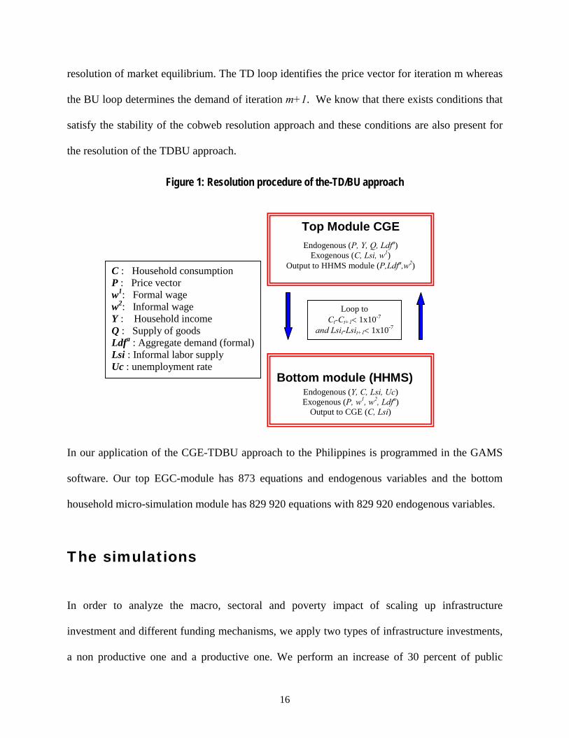
resolution of market equilibrium. The TD loop identifies the price vector for iteration m whereas

the BU loop determines the demand of iteration m+1. We know that there exists conditions that

satisfy the stability of the cobweb resolution approach and these conditions are also present for

the resolution of the TDBU approach.

Figure 1: Resolution procedure of the-TD/BU approach

Top Module CGE Endogenous (P, Y, Q, Ldfa)

Exogenous (C, Lsi, w1) Output to HHMS module (P,Ldfa,w2)

Loop to Ct-Ct+1< 1x10-7

and Lsit-Lsit+1< 1x10-7

Bottom module (HHMS) Endogenous (Y, C, Lsi, Uc) Exogenous (P, w1, w2, Ldfa)

Output to CGE (C, Lsi)

C : Household consumption P : Price vector w1: Formal wage w2: Informal wage Y : Household income Q : Supply of goods Ldfa : Aggregate demand (formal) Lsi : Informal labor supply Uc : unemployment rate

In our application of the CGE-TDBU approach to the Philippines is programmed in the GAMS

software. Our top EGC-module has 873 equations and endogenous variables and the bottom

household micro-simulation module has 829 920 equations with 829 920 endogenous variables.

The simulations

In order to analyze the macro, sectoral and poverty impact of scaling up infrastructure

investment and different funding mechanisms, we apply two types of infrastructure investments,

a non productive one and a productive one. We perform an increase of 30 percent of public

17

investment on infrastructure with respect to the reference period level of investment. To fund the

increase in infrastructure, we use three methods, the first one consists in raising the value added

tax, in the second, income tax are used to fund the increase in investment and finally foreign aid

is used in the final case.

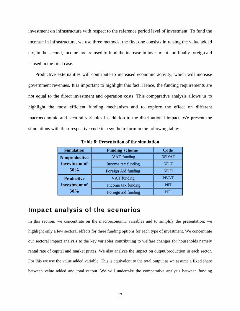
Productive externalities will contribute to increased economic activity, which will increase

government revenues. It is important to highlight this fact. Hence, the funding requirements are

not equal to the direct investment and operation costs. This comparative analysis allows us to

highlight the most efficient funding mechanism and to explore the effect on different

macroeconomic and sectoral variables in addition to the distributional impact. We present the

simulations with their respective code in a synthetic form in the following table:

Table 8: Presentation of the simulation

Simulation Funding scheme Code VAT funding NPIVAT

Income tax funding NPIIT

Foreign Aid funding NPIFI

VAT funding PIVAT

Income tax funding PIIT

Foreign aid funding PIFI

Nonproductive investment of

30%

Productive investment of

30%

Impact analysis of the scenarios In this section, we concentrate on the macroeconomic variables and to simplify the presentation; we

highlight only a few sectoral effects for three funding options for each type of investment. We concentrate

our sectoral impact analysis to the key variables contributing to welfare changes for households namely

rental rate of capital and market prices. We also analyze the impact on output/production in each sector.

For this we use the value added variable. This is equivalent to the total output as we assume a fixed share

between value added and total output. We will undertake the comparative analysis between funding

18

options throughout the section. We begin by presenting the nonproductive investment option as the

baseline scenario. When looking at results, keep in mind a key hypothesis: our current account balance is

fixed. The current account is balanced by adjusting the nominal exchange rate. Finally, in the tables, we

present the nominal exchange rate. But this rate can also be interpreted as the real exchange rate because

our price index is exogenous. So the variation in the nominal exchange rate is equivalent to the variation

in the real exchange rate.

Before moving to the specific simulations, we can extract of few general comments from our

results. First, the impact of our scenarios on GDP and most macro variables are relatively modest. This

comes from the fact that in nominal terms, the 30% increase in public investment is not large compared to

size of the economy. However, this is not an important problem as we are mostly interested by the

comparative analysis between the different scenarios. The second point is that all simulations produce a

positive impact on GDP albeit the non productive simulations produce a very small impact. The positive

effect originates from the imperfect labour market assumption.

Table 1: Macroeconomic results Variations are presented as percentage changes

Variables Definition BaseNon

productive investment

Productive investment

Non productive investment




YhHousehold

income 86476.9 0.15 0.74 0.17 0.75 0.14 0.73

Sh Household savings

9651.8 -2.2 -3.24 -1.98 -2.99 -3.41 -4.21

w2 Informal Wage 0.5 0.43 0.98 0.49 1.05 0.39 0.94

YgGovernment

income 20367 3.94 3.94 3.94 3.94 3.94 3.94Ye Firms' income 26172.9 -0.14 0.52 -0.17 0.49 -0.17 0.51

SgGovernment

savings 13369 30,00 30,00 30,00 30,00 30,00 30,00

GGovernment expenditure 16818.8 2.38 2.38 2.38 2.38 2.38 2.38

ItPrivate

investment 23161.2 -1.23 -0.54 -1.86 -1.07 -1.54 -0.82

Se Firms' savings 7810.5 0,00 0.95 -0.31 0.9 -0.3 0.92

uiUnemployment

rate 16.8 -1.05 -1.95 -1.14 -1.95 -0.9 -1.84

eNominal

exchange rate 1 0.69 0.39 0.06 -0.13 -1.2 -1.18

GDPGross domestic

product 104510.7 0.16 0.79 0.17 0.8 0.15 0.79

Value added tax Income tax Foreign Aid

* Values computed by the author

19

The expansion of the construction sector creates employment directly and indirectly with the increase in

the real informal wage. The impact on the aggregate household is positive for all simulations and we

observe an eviction effect of private investment in all scenarios. The reduction for unemployment rate is

present across the board and the increase in nominal informal wage is also a uniform results. The increase

in government income is the same in all simulations as this is implicitly directly tied to the simulated

increase in public investment and operation and maintenance cost associated with the investment. Other

variables such as nominal exchange rate, firms’ income and savings exhibit qualitative and quantitative

differences.

The investment in nonproductive infrastructure

We use this simulation as the baseline scenario, which can be interpreted as an investment in the

construction of monuments, in the army (if the country is not in conflict), or other types of nonproductive

investments by the government. We look at three funding options to increase the nonproductive public

investment. The first is an increase in the value added tax, and the second is an increase in income tax and

the last is funded by foreign aid.

Investment funded by the value added tax

In this simulation, we increased the nonproductive public investment (investment that does not produce

production externalities for other productive sectors); the increase in spending by the government is

funded by a uniform increase of the effective value added tax. At the reference period, the value added tax

(VAT) is not uniform and the differentiated structure remains after simulation. We apply a uniform tax

increase so the percentage adjustment is the same for all sectors—if the tax rate in the sector is positive at

the reference period. We hold exogenous the other public expenditure made by government but assume as

was explained earlier that the new investment will require some new operational expenditure. Hence the

30 percent increase in government saving and the new public expenditure for operation cost of the new

investment is funded by the increase in value added tax.

20

The first observation is that this option seems to favor households over firms, because wages increase

and than the average rental rate of capital decreases. Since firms’ income originate essentially from

capital income and for households’ it is a mixture of the two sources. The increase in government income

derives mainly from the increased VAT to fund new investment and operation and maintenance cost

(+3.94) and it is identical by definition in all simulations. As the investment in public expenditure does

not produce externalities, the government benefit only slightly from increased income from economic

growth. Therefore, the rise in income can be attributed almost exclusively to the VAT increase to fund the

operation costs of new public investments. For comparative purposes, this will be useful in the following

scenarios to see how growth influences government income. As we have said, the other common feature

is that the simulation produces an increase in the informal wage (+0.43%). This comes from the fact that

public services (+1.86 from table 2) must grow to meet the operational needs created by new investment.

The construction sector also expends (+1.01%) to build the new infrastructure. Given the capital/labour

ratio of these two sectors, their expansion produces more pressure on demand for labour versus capital.

The increase in household income is very slight at the aggregate level (+0.15%) and it is explained

mainly by the reduction in unemployment and increase in nominal informal wage. The total private

investment falls (-1.23%) which is one of the strongest impact at the macro level and this illustrates an

form of eviction of private investment. The nominal exchange rate increases by 0.69% which respresents

a depreciation of the real exchange rate. Given the fixed current account balance, this reflects a response

to counter pressures of an implicit deterioration of current account balance and hence a slight dutch

disease effect.

At the sectoral level, we have already mentioned the growth of public services and construction

sector. The logging and timber sector and finance sectors are the other two sectors benefiting the most

from this scenario. It can be explained by the lower relative use of informal workers in these two sectors

compared to formal labour and capital. The strongest decrease is observed in the food manufacturing and

coconut sector. The market price and rental rate of capital variations exhibit stronger impact compared to

21

macro and production variables. Not surprisingly the strongest positive effect (+2.03%) for the rental rate

of capital is observed in the construction sector. The logging and timber, followed by the transport and

communication sector are also positively affected (+1.3 and +0.55% respectively). For market prices, all

prices increase with the exception of palay and corn sector. This is coherent to inflationary pressures

associated with scaling up of infrastructure when no externalities are present (see Montelpare 2009). The

strongest price increase is observed in the finance sector (+2.2%).

Table 2: Sectoral results: Value added Variations are presented as percentage changes

Variables branches ReferenceNon







Palay & corn 5197.9 -0.17 0.25 -0.14 0.27 -0.08 0.33

Fruit & vegetable 4210.7 -0.26 0.06 -0.26 0.07 -0.11 0.19

Coconut 1789.5 -0.35 0.42 -0.33 0.43 -0.57 0.23

Livestock 4473.5 -0.24 0.27 -0.29 0.22 0.1 0.55

Fishing 3996.8 -0.17 0.23 -0.19 0.2 -0.13 0.27

Other agriculture 1845.8 -0.22 0.09 -0.31 0.01 -0.62 -0.25

Logging & timber 856.5 0.19 0.82 0.07 0.71 0.14 0.77

Mining 1604.3 0.01 0.91 -0.18 0.74 -1.23 -0.14

Manufacturing 13112.5 -0.16 0.9 -0.14 0.91 -0.82 0.34

Rice manufacturing 2022.9 -0.17 0.27 -0.13 0.3 -0.07 0.36

Meat industry 2081.2 -0.12 0.55 -0.19 0.48 0.25 0.87

Food manufacturing 3696.2 -0.54 0.06 -0.49 0.1 -0.36 0.21

Electricity, gas & w ater 2341.3 0.06 0.85 0.1 0.88 0.15 0.93

Construction 6848.2 1.01 1.81 0.93 1.74 1.56 2.27

Commerce 15149.5 -0.18 0.66 -0.17 0.67 -0.54 0.36

Trans. & comm. 5206.4 0.07 0.79 -0.12 0.62 0.22 0.91

Finance 3580.5 0.13 0.7 0.2 0.76 -0.02 0.57

Real estate 7314.2 -0.2 0.48 -0.55 0.16 0.14 0.76

Services 6960 -0.12 0.72 0.11 0.91 -0.09 0.75

Public services 12222.8 1.86 1.87 2.2 2.15 2.33 2.26

Va (value added)



Investment funded by income tax

For the income tax funding option we will analyze both the macro and sectoral results. In this case, we let

the household income tax rate adjust from the reference situation. The macro results are quite similar to

the previous simulation with main differences observed for the nominal exchange rate with a 0.06%

compared to 0.69% in the previous simulation. The total investment decreases more -1.86 compared to -

22

1.23%. The slightly stronger negative impact on firms’ income is at the source of this difference. The

other macro level results largely resemble the VAT-funded scenario.

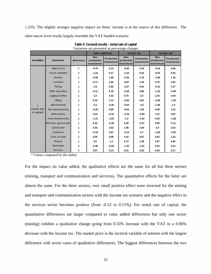
Table 3: Sectoral results : rental rate of capital Variations are presented as percentage changes








Palay & corn 1 -0.76 2.13 -0.49 2.36 -0.16 2.66

Fruit & vegetable 1 -1.24 0.17 -1.16 0.24 -0.34 0.94

Coconut 1 -0.45 1.68 -0.34 1.79 -1.05 1.16

Livestock 1 -0.71 1.66 -0.87 1.49 0.79 2.92

Fishing 1 -0.5 0.92 -0.57 0.84 -0.33 1.07

Other agriculture 1 -0.11 0.79 -0.29 0.65 -1.15 -0.09

Logging & timber 1 1.3 4.33 0.79 3.9 1.03 4.09

Mining 1 0.33 1.14 -0.06 0.81 -2.49 -1.25

Manufacturing 1 -0.1 -0.26 -0.04 -0.2 -1.46 -1.4

Rice manufacturing 1 -0.26 0.86 -0.05 1.03 0.09 1.15

Meat industry 1 -0.01 -0.32 -0.19 -0.49 1.12 0.62

Food manufacturing 1 -1.41 -1.82 -1.2 -1.64 -0.87 -1.38

Electricity, gas & w ater 1 0.32 -0.39 0.49 -0.27 0.65 -0.11

Construction 1 2.03 2.62 1.96 2.56 2.9 3.34

Commerce 1 -0.18 0.67 -0.14 0.7 -1,00 -0.02

Trans. & comm. 1 0.55 0.98 0.16 0.67 0.82 1.22

Finance 1 0.5 1.3 0.72 1.48 0.07 0.94

Real estate 1 -0.48 -0.55 -1.33 -1.31 0.34 0.14Services 1 0.07 0.14 0.51 0.52 0.09 0.17

r (rental rate of capital)



For the impact on value added, the qualitative effects are the same for all but three sectors

(mining, transport and communication and services). The quantitative effects for the latter are

almost the same. For the three sectors, very small positive effect were reversed for the mining

and transport and communication sectors with the income tax scenario and the negative effect in

the services sector becomes positive (from -0.12 to 0.11%). For rental rate of capital, the

quantitative differences are larger compared to value added differences but only one sector

(mining) exhibits a qualitative change going from 0.33% increase with the VAT to a 0.06%

decrease with the income tax. The market price is the sectoral variable of interest with the largest

difference with seven cases of qualitative differences. The biggest differences between the two

23

simulations are observed for services sector, going from 2.1% increase to a 0.2% increase and

the meat industry, going from 0.7% increase to a 0.15% decrease. These stronger differences at

the market price will have an impact household welfare for the poverty analysis.

Investment funded by foreign aid At the macro level, this simulation produces results between the two previous ones presented.

The main difference is observed for the nominal exchange rate which is not surprising insofar as

the current account balance is fixed and an increase in foreign aid requires an appreciation of the

exchange rate to balance out. The GDP and household aggregate income increase less and the

unemployment rate decrease of smaller compared to the previous two simulations.

Table 4: Sectoral results : rental rate of capital Variations are presented as percentage changes








Palay & corn 1.01 -0.09 1.65 -0.24 1.52 -0.21 1.55

Fruit & vegetable 1.02 0.25 0.77 -0.55 0.1 -0.19 0.4

Coconut 1.02 0.62 1.61 0.01 1.11 -0.45 0.71

Livestock 1.01 0.45 1.33 -0.31 0.68 0.17 1.09

Fishing 1.01 0.19 0.81 -0.24 0.43 -0.16 0.51

Other agriculture 1.03 0.57 0.76 0.06 0.33 -0.6 -0.23

Logging & timber 1.01 1.12 2.38 0.46 1.83 0.32 1.71

Mining 1.01 0.69 0.42 0.08 -0.09 -1.07 -1.06

Manufacturing 1.08 0.83 0.4 0.07 -0.23 -0.61 -0.8

Rice manufacturing 1,000 0.16 1.27 -0.11 1.04 -0.2 0.97

Meat industry 1.01 0.7 0.91 -0.15 0.19 0.21 0.5

Food manufacturing 1.03 0.47 0.47 -0.24 -0.12 -0.37 -0.24

Electricity, gas & w ater 1.01 0.97 -0.02 0.25 -0.63 0.05 -0.79

Construction 1.01 1.13 0.82 0.52 0.31 0.33 0.15

Commerce 1.05 1.02 0.8 0.06 -0.01 -0.39 -0.38

Trans. & comm. 1.01 1.08 0.68 0.18 -0.07 -0.03 -0.25

Finance 1.05 2.2 1.92 0.35 0.37 -0.18 -0.08

Real estate 1,000 0.03 -0.68 -0.61 -1.23 0.19 -0.54

Services 1.04 2.1 1.4 0.2 -0.18 0.32 -0.09Public services 1,000 0.51 0.5 0.17 0.23 0.05 0.12

Pq (market price)



24

For value added (implicitly sectoral output), we observe positive effects in 8 sectors compared to

5 and 6 sectors for NPIVAT and the NPIIT simulations respectively. The differences between

sectors are also more pronounced for this scenario. When excluding public services, we have an

increase of 1.56% for the construction sector at one extreme and a 1.23% decrease in the mining

sector at the other extreme. The market price and rental rate of capital are also more sensitive to

this funding scheme and we have many qualitative changes compared to the first two non

productive investment scenarios. These stronger differences should have a distributional impact.

The investment in productive infrastructure

Moving on to the productive investment scenarios, we note a stronger positive effect on GDP,

household income and firms’ revenues. This is not surprising as we built in this growth effect. The

funding schemes do not have a significant impact of these variables. On the other hand, the

unemployment decreases less for the PIFA (-1.84%) compared to the two other simulations (-1.95%). The

impact on the informal wage is greatest with the income tax scenario and weakest with the foreign aid.

The variable producing the largest differences between simulations is the nominal exchange rate. It

depreciates with the VAT (0.39%), appreciates slightly with the income tax ((-0.13) and a stronger

appreciation is observed for the foreign aid. In this last case, we have identified the source of this effect in

the non productive investment. In fact, the appreciation is almost identical to the NPFA scenario. Finally,

the private investment eviction effect observed in the non productive investment scenearios is reduced by

almost half in all three options. The strongest decline between the non productive and productive

scenarios is for the VAT case where cut by more than half going from -1.23% to -0.54%.

For sectoral impact of productive public investment we observe a clear positive effect for value added

(output) in all sectors of the economy for all three scenarios. For price variations (market price and rental

rate of capital) the effects are quite different from one simulation to the other within the productive group

and between the productive and non productive ones. We will first compare productive and non

25

productive simulations before comparing between funding options. For the VAT funding option the rental

rate of capital variations are very different with the productive investment compared to the non productive

one. Nine out of nineteen sectors exhibit a qualitative change. For all agricultural sectors, the

improvement is strong ranging from 0.9% improvement for other agriculture to a 2.89% improvement in

the palay and corn sector. The logging and timber sector is the most improved with an increase of 3.03%

between the two simulations. This will lead to improvement in household income for some households

but for others, the situation will deteriorate as we observe a decrease in positive effect of increase in

negative effect in five sectors. The pattern of differences between the income tax scenarios is similar to

the VAT simulations. This leads us to conclude that the growth effect predominates. The productive

foreign aid simulation produces closer results compared to the non productive one where only five sectors

exhibit qualitative differences. Moreover, the quantitative gap between the productive and non productive

scenarios is weaker. When comparing between productive simulations we note minor differences between

the VAT and income tax and more differences with the foreign aid option. We have five cases of

qualitative differences with this option.

As for market price variations we observe many differences between productive and non productive

option with five (VAT) to eight (foreign aid) qualitative differences. There is not clear trend either with

half of the effects being stronger and half being weaker. When comparing between funding option, in this

case we observe more differences between options compared to output and rental rate of capital. The

differences are observed on the qualitative and quantitative front.

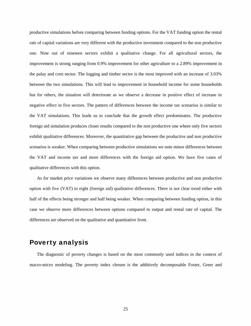
Poverty analysis The diagnostic of poverty changes is based on the most commonly used indices in the context of

macro-micro modeling. The poverty index chosen is the additively decomposable Foster, Greer and

26

Thorbecke (FGT, 1984) Pα 11. We use the change in households’ welfare measured by the equivalent

variation to measure the impact of the policy on each household. This approach has the advantage of

taking into account the price and income effect simultaneously. This approach is quite standard in the

context of macro-micro CGE analysis. The CGE-top-down/bottom up model generates post simulation

changes in welfare at the household level which are used for poverty analysis. Target groups are defined

independently of the CGE modeling exercise and poverty analysis can be performed for the base period

and after simulations.12 For our application we decomposed households based on education level of head

of household.

The first point we can make is that poverty impact are relatively small. As we have highlighted, in the

macro analysis, this comes from the relatively small nominal increase in public investment but we can

still drawn interesting conclusions on relative impact between productive and non productive investments

and between the three funding schemes. Starting at the national level, we observe a decrease in poverty

only for the VAT scenario when considering the non productive investment. This reduction is almost the

same for the three poverty indices ranging from -0.26% for the headcount index (FGT-0) and -0.30% for

poverty severity (FGT-2). The income tax and foreign aid scenarios for non productive investment

produce an increase in poverty. This increase is over up to 1.33% for the poverty severity for the income

tax option and 0.88% for the poverty severity of the foreign aid. This is interesting insofar as the GDP and

aggregate household income increased in both those scenarios. This illustrates the importance of using a

microsimulation approach to conclude on the distributional and welfare impact of such reforms. The

option generating the most negative results for poverty is the income tax option.

The productive investments produce a similar pattern insofar as the best option is the VAT which

produces reductions in poverty ranging from -0.86% for the headcount index to -1.57% for the severity

index. The least positive option is the income tax option with poverty reduction around 0.2% for all three

11 FGT poverty indices are interesting within the framework of this analysis and make it possible to measure the proportion of the poor among the population but also of this poverty depth and severity. For detailed information on the FGT index family, see Ravallion (1994). 12No groups are found in the CGE model but all households of the survey.

27

indices. The foreign aid option provides an intermediary option with reductions of 0.41% for the

headcount index and a drop of 0.60% for the severity index.

Table 5: Poverty indices results Variations are presented as percentage changes

Poverty index

Code-education Base







FGT-0 National 0.311 -0.26 -0.86 0.67 -0.19 0.49 -0.41FGT-1 National 0.096 -0.27 -1.29 1.05 -0.20 0.68 -0.52FGT-2 National 0.04 -0.30 -1.57 1.33 -0.22 0.88 -0.6

0 0.564 -0.36 -1.08 0.51 0.07 0.71 0.2

1 0.501 -0.37 -0.89 0.31 -0.26 0.27 -0.61

2 0.384 -0.29 -0.8 0.70 -0.26 0.3 -0.42

3 0.317 0.35 -0.71 1.52 0.27 1.38 -0.30

4 0.184 -0.34 -0.94 0.85 -0.33 0.2 -0.54

5 0.092 -0.47 -0.83 1.58 -0.35 1.35 0.40

6 0.021 -0.42 -0.42 -0.42 -0.42 3.54 -0.42

0 0.185 -0.19 -0.99 0.96 -0.05 0.92 -0.09

1 0.168 -0.24 -1.19 0.94 -0.20 0.61 -0.50

2 0.116 -0.30 -1.36 1.05 -0.23 0.62 -0.61

3 0.090 -0.32 -1.37 1.15 -0.17 0.79 -0.51

4 0.048 -0.31 -1.56 1.29 -0.22 0.71 -0.71

5 0.022 -0.26 -1.65 1.60 -0.11 1.05 -0.57

6 0.005 -0.49 -1.87 1.43 -0.24 1.51 -0.20

0 0.08 -0.25 -1.32 1.25 -0.09 1.14 -0.18

1 0.075 -0.27 -1.48 1.23 -0.23 0.82 -0.58

2 0.048 -0.32 -1.64 1.34 -0.26 0.82 -0.70

3 0.035 -0.36 -1.66 1.41 -0.20 0.95 -0.64

4 0.018 -0.31 -1.78 1.57 -0.23 0.93 -0.76

5 0.007 -0.28 -2.01 1.92 -0.19 1.22 -0.786 0.002 -0.38 -1.83 1.83 0.00 2.12 0.24

FGT-0

FGT-1

FGT-2

Foreign AidValue added tax Income tax

* Values computed by the author Moving to the decomposition analysis, we observe a relatively uniform qualitative impact

across household types for non productive investment. We only observe two cases of qualitative

differences namely for the VAT simulation, where the poverty headcount increases for group 3

where other households benefit from a reduction in poverty indices. The headcount for the group

6 household also varies in a different direction with a 0.42% reduction when other households

experience an increase in poverty indices. For the VAT simulation, we can identify a weak trend

28

favoring the most educated households. For the income tax option, the most educated groups (4,

5 and 6) have the largest poverty increase when using the poverty depth and severity indices. For

the foreign aid funding scheme the groups suffering the least are groups 1 and 2 for the three

indices with one exception for FGT-0 where the most favored group is group 4. The productive

investment provides more interesting results. For the VAT option, the headcount index indicates

that the least educated would be most advantaged, while the depth and severity indices reveal a

more regressive option where most educated households benefit the most13. In the second

scenario (PIIT), we cannot find a clear trend. Each indicator provides a different picture. The

headcount index seems to favor the most educated and group 3 is faced with an 0.27% increase

in poverty. The poverty depth (FGT-1) group 6 and 2 benefit the most and group 0 the least and

the poverty severity favors group 2, 1 and 4 and group 6 and 1 are the losers. For the foreign aid

simulation, we seem to have a clearer winner with group 4 being top or second in terms of

positive impact and group 0 is last of second to last for all indices. Interestingly, group 5 has the

worst situation for the headcount index and the best when using the severity index.

When comparing each funding option we can clearly conclude that the VAT is the most

favorable option either at the national level and when using household decomposition. Moreover,

all groups benefit for all indices. In addition, the poverty reduction impact is quite large given the

weak changes in macro and sectoral variables. The foreign aid option also dominates the income

tax option for the poverty depth and severity indices. For the headcount index, two groups (group

0 and 4) suffer more with the foreign aid compared to the income tax option. For the other

groups, the foreign aid option is more favorable.

13 The poverty indices at reference period reveal that the more educated the head of household, the lower the poverty indices are.

29

Comparing the micro distributional results with poverty results illustrates the importance of

using a CGE microsimulation approach since the income tax option is the most favorable with

looking at aggregate variables such as GDP, aggregate household income, informal wage and

unemployment whereas it is the least favorable one in terms of poverty impact.

Conclusion

The ambitious modeling exercise has allowed us to analyze the impact of scaling up

infrastructure investment on macroeconomic, sectoral and poverty in the Philippines. To achieve

this we apply a CGE top-down/bottom up approach with endogenous labour supply and

unemployment. The approach allows us to capture numerous issues surrounding infrastructure

expansion among which we have; productivity externalities, relative price changes, investment

eviction issues, Dutch disease, funding issues, fiscal contraints and distributional analysis. We

extend on papers such as Adam and Bevan (2006) and Estache et al (2008) by introducing

rigorous distributional analysis. Our macro results are similar to these authors with the presence

of slight Dutch disease effect that is attenuated with the production externality assumption. We

also present a framework that allows the analyst to conclude on poverty impact of such

programs. As in Estache et al (2008), we do not observe strong differences at the macro level

when comparing funding options to scale-up infrastructure but our poverty analysis has clearly

allowed us to rank the performance of each funding option where the VAT is clearly more

favorable followed by the foreign aid option and completing with the income tax option.

In our analysis, our static modeling framework does not allow us to fully capture the

negative impact of the private investment eviction issue. Another issue is the returns on

investment might come in the medium to long term. To improve the analysis on this front, a

30

sequentially dynamic framework would be a more appropriate tool. In our future research we

will extend this model in this direction. The major challenge for this work program will be to

introduce a capital reallocation mechanism at the micro level. To our knowledge, only one set of

authors (Annabi et al (2005)) applied a dynamic CGE microsimulation model. In their model,

they do not fully resolve the issue of capital reallocation. They assume that the new capital

growth is uniformly redistributed to household endowed with capital at the reference period. This

assumption with grossly underestimate the distributional impact of the growth elements in the

model.

References

Aschauer, D. A. (1989). “Is Public Investment Productive?” Journal of Monetary Economics 23, pp. 177–200. Agénor P.R., Izquierdo A., and H. Fofack. (2003), IMMPA: A quantitative macroeconomic framework for the analysis of poverty reduction strategies. Mimeo World Bank, Washington. Annabi, N., F. Cissé, J. Cockburn, and B. Decaluwé (2005). “Trade Liberalisation, Growth and Poverty in Senegal: a Dynamic Micro-simulation CGE model analysis,” Working Paper No. 0512, CIRPEE. Armington P. (1969), A theory of demand for products distinguished by place of production , IMF Staff Paper n° 16, p. 159-176. Asian Development Bank (2009), Investing in Sustainable Infrastructure: Improving Lives in Asia and in the Pacific, Asian Development Bank, Manilla. Adam, C. and D. Bevan (2006), “Aid and the Supply Side: Public Investment, Export Performance and Dutch Disease in Low Income Countries,” World Bank Economic Review, Vol. 20(2), pp. 261-290. Berg, A., S. Aiyar, M. Hussein, S. Roache, T. Mirzoev and A. Mahone (2007) “The Macroeconomics of Scaling Up Aid: Lessons from Recent Experience” IMF Occasional Paper No. 235.

31

Bergman, E.M. and Suan D. (1996), “Infrastructure and manufacturing productivity: Regional accessibility and development level effects”, in D.F. Batten & C. Karlsson, Infrastructure and the Complexity of Economic development (pp. 17-35), Heidelberg: Springer-Verlag Berlin. Binder, S. A. and Smith, S. S., (1997), Politics or principle?: filibustering in the United States Senate, Brookings Institution, Washington D.C., 248p. Bourguignon F., A.S. Robilliard and S. Robinson, (2005), “Representative Versus Real Households in the Macroeconomic Modelling of Inequality ”, in T. J. Kehoe, T.N. Srinivasan and J. Whalley (eds.) “Frontiers in applied general equilibrium modelling”, Cambridge, Cambridge University Press. Bourguignon, F. and M. Sundberg, (2006). “Absorptive Capacity and Achieving the MDG’s" Working Papers RP2006/47, World Institute for Development Economic Research (UNU-WIDER). Bourguignon, F., and A. Spadaro (2006) “Microsimulation as a Tool for Evaluating Redistribution Policies ”, Journal of Economic Inequality, 4 (1); 77-106. Bourguignon, F. and L. Savard (2008). “A CGE Integrated Multi-Household Model with Segmented Labour Markets and unemployment” in Bourguignon, F., L.A. Pereira Da Silva and M. Bussolo, eds. “The Impact of Macroeconomic Policies on Poverty and Income Distribution: Macro-Micro Evaluation Techniques and Tools” Palgrave-Macmillan Publishers Limited, Houndmills, Angleterre. Chen S. and M. Ravallion. (2004), Welfare impacts of China’s accession to the world trade organization. The World Bank Economic Review, vol 18, n° 1, p. 29-57. Decaluwé B., Dumont J.-C., Savard L. How to measure poverty and inequality in general equilibrium framework. Cahier de recherche, CREFA, Université Laval, 1999, n°99-20, Québec. Decaluwé, B., A. Martens, and L. Savard, (2001), La Politique Economique du Développement et les modèles d’équilibre général calculable. Montreal: Association des Universités Francophones AUF-Presse de l’Université de Montréal. Dervis K., J. de Melo and S. Robinson. (1982), General equilibrium models for development policy. London: Cambridge University Press, 526 p. Dessus, S., and R. Herrera. 1996. “Le rôle du Capital Public dans la Croissance des Pays en Développement au cours des Années 80.” OECD Working Paper 115. Organisation for Economic Co-operation and Development, Paris. Devarajan S., H. Ghanem and K. Thierfelder. (1999), Labour market regulations, trade liberalization and the distribution of income in Bangladesh. Journal of Policy Reform, vol. 3, n° 1, p. 1-28.

32

Dumont, J.C. and S. Mesplé-Somps, (2000), “The Impact of Public Infrastructure on Competitiveness and Growth: A CGE Analysis Applied to Senegal”, Mimeo, CREFA, Université Laval, Québec. Estache, A., (2007), Infrastructure and Development: A Survey of Recent and Upcoming Issues”, in Bourguignon, F., and B. Pleskovic, Rethinking Infrastructure for Development – Annual World Bank Conference on Development Economics, Global, pp. 47-82. Estache, A., J.F. Perrault, and L. Savard, (2008), “Impact of Infrastructure Spending in Sub-Saharan Africa: CGE Modeling Approach”, forthcoming Journal of Policy Modeling. Fay, M., and T. Yepes. (2003), “Investing in Infrastructure: What Is Needed from 2,000 to 2010?” World Bank Policy Research Working Paper 3102, World Bank, Washington, DC. Fortin B., N. Marceau and L. Savard. (1997), Taxation, wage controls and the informal sector. Journal of Public Economics, vol. 66, n° 2, p. 293-312. Foster, M. and T. Killick (2006), “What Would Doubling Aid Do for Macroeconomic Management in Africa?” Working Paper no. 264, Oversees Development Institute, London. Gramlich, E. (1994). “Infrastructure Investment: A Review Essay.” Journal of Economic Literature 32(3), pp.1176–1196. Gupta, S., R. Powell and Y. Yang (2006), The Macroeconomic Challenges of Scaling Up Aid to Africa: a Checklist for Practitioners, Washington DC, International Monetary Fund. Hailu, D. (2007). ‘Scaling-up HIV and AIDS Financing and the Role of Macroeconomic Policies in Kenya’, IPC Conference Paper 4. Paper presented at the Global Conference on Gearing Macroeconomic Policies to Reverse the HIV/AIDS Epidemic, 20–21 November, Brasilia: International Poverty Centre (IPC) (mimeo). Hakfoort, J. (1996). “Public Capital, Private Sector Productivity and Economic Growt: A Macroeconomic Perspective”. pp. 61-72. In Batten, D.F. & C. Kalsson (eds.). Infrastructure and the Complexity of Economic Development. Advances in Spatial Science. Springer. Berlin. Harchaoui, T. M., and Tarkhani, F., (2003), « Le capital public et sa contribution a la productivité du secteur des entreprises du Canada », Statistiques Canada. Heckman J. and G. Sedlacek. (1985), Heterogeneity, aggregation and market wage functions: An empirical model of self-selection in the labour market. Journal of Political Economy, vol. 93, p. 1077-1125. Hertel, T. and Reimer, J. (2005) Predicting the poverty impacts of trade reform, Journal of International Trade & Economic Development, 14(4); 377-405.

33

Li, Y., and Rowe, F. (2007). Aid inflows and the real effective exchange rate in Tanzania. (Policy Research Working Paper Rep. No. 4456). Washington, DC: The World Bank. Magnac T. (1991), Segmented of competitive labour markets. Econometrica, vol. 59, n° 1, p. 165-187. McKinley, T. (2005), “Why is the Dutch Disease Always a Disease? The Macroeconomic Consequences of Scaling Up Overseas Development Assistance”, Working Paper no. 10, International Poverty Centre, Brasilia. Mongardini, J., and B. Rayner, (2009), “Grants, Remittances and the Equilibrium Real Exchange Rate in Sub-Saharan African Countries,” IMF Working Paper (forthcoming; Washington: International Monetary Fund). Montelpare, A. (2009), «Dépenses en infrastructure publiques et externalités positive de production. Une modélisation en équilibre général appliquée au Québec », Master thesis, Université de Sherbrooke, Sherbrooke, Canada. Munnell, A. H., (1990a).“Why has productivity declined? Productivity and public investment”, New England Economic Review, Federal Reserve Bank of Boston. January/February, p. 11-33. Munnell, A. H., (1990b), “How Does Public Infrastructure Affect Regional Economic Performance?,” New England Economic Review, Federal Reserve Bank of Boston., September/October, p. 69-112. Rajan, R., and A. Subramanian. (2005). ‘‘What Undermines Aid’s Impact on Growth?’’ IMF Working Paper 05/126. International Monetary Fund, Washington, D.C. Ravaillon M. (1994), Poverty Comparisons, Fundamentals in Pure and Applied Economics, Vol. 56. Chur, Switzerland: Reading, Harwood Academic Publisher. Roy, A.D, (1951) « Some Thoughts on the Distribution of Earnings » Oxford Economic Papers, Vol 3, no 2 pp 135-146. Rutherford T., D. Tarr, and O. Shepotylo. (2005), Poverty effects of Russia’s WTO accession: modeling “real” household and endogenous productivity effects. World bank policy research working paper n° 3473, World Bank, Washington. Savard, L., and E. Adjovi. (1998), “Externalités de la santé et de l’éducation et bien-être: Un MEGC appliqué au Bénin.” Actualité Économique 74(3), pp. 523–560. Serieux, J. D. Hailu; M. Tumasyan; A. Papoyan; R. White; and M. Njelesani (2008). “Addressing the Macro-Micro Economic Implications of Financing MDG-Levels of HIV/and AIDS Expenditure”, United Nations Development Programme (UNDP), HIV/AIDS Group (mimeo).

34

Thomas, M. and L. Vallée. (1996), Labour market segmentation in Cameroonian manufacturing. Journal of Development Studies, vol.32, n° 6, p. 876-898. Yeaple S.R. and S.S. Golub (2007). “International Productivity Differences, Infrastructure, and Comparative Advantage”, Review of International Economics, 15(2), pp. 223–242.

Appendix Externality parameter Table A.1 Externality elasticities by sector

branches ξ value

Palay & corn 0,01

Fruit & vegetable 0,015

Coconut 0,019

Livestock 0,011

Fishing 0,012

Other agriculture 0,018

Logging & timber 0,003

Mining 0,027

Manufacturing 0,038

Rice manufacturing 0,01

Meat industry 0,025

Food manufacturing 0,025

Electricity, gas & w ater 0,039

Construction 0,021

Commerce 0,022

Trans. & comm. 0,018

Finance 0,013

Real estate 0,027Services 0,01

Table A.2: Educational code definition

Education Code Level of education 1 Elementary undergraduate 2 Elementary graduate 3 1st to 3rd Year High school 4 High School Graduate 5 College Undergraduate 6 At least College graduate 0 Not reported or no grade

Groupe de Recherche en Économie et Développement...

Documents

Transcript of Groupe de Recherche en Économie et Développement...