Gravity of human impacts mediates coral reefconservation gainsJoshua E. Cinnera,1, Eva Mairea,b, Cindy Hucherya, M. Aaron MacNeilc,d, Nicholas A. J. Grahama,e, Camilo Moraf,Tim R. McClanahang, Michele L. Barnesa,h, John N. Kittingeri,j, Christina C. Hicksa,e, Stephanie D’Agatab,g,k, Andrew S. Hoeya,Georgina G. Gurneya, David A. Fearyl, Ivor D. Williamsm, Michel Kulbickin, Laurent Vigliolak, Laurent Wantiezo,Graham J. Edgarp, Rick D. Stuart-Smithp, Stuart A. Sandinq, Alison Greenr, Marah J. Hardts, Maria Begert,u,Alan M. Friedlanderv,w, Shaun K. Wilsonx,y, Eran Brokovichz, Andrew J. Brooksaa, Juan J. Cruz-Mottabb, David J. Boothcc,Pascale Chabanetdd, Charlotte Goughee, Mark Tupperff, Sebastian C. A. Fersegg, U. Rashid Sumailahh, Shinta Pardedeg,and David Mouillota,b

aAustralian Research Council Centre of Excellence for Coral Reef Studies, James Cook University, Townsville, QLD 4811, Australia; bMarine Biodiversity Explorationand Conservation, UMR Institut de Recherche pour le Développement-CNRS-UM-L’Institut Français de Recherche pour l’Exploitation de la Mer 9190, University ofMontpellier, 34095 Montpellier Cedex, France; cAustralian Institute of Marine Science, Townsville, QLD 4810, Australia; dDepartment of Biology, DalhousieUniversity, Halifax, NS B3H 3J5, Canada; eLancaster Environment Centre, Lancaster University, LA1 4YQ Lancaster, United Kingdom; fDepartment of Geography,University of Hawai‘i at Manoa, Honolulu, HI 96822; gGlobal Marine Program, Wildlife Conservation Society, Bronx, NY 10460; hDepartment of Botany, University ofHawai’i at Manoa, Honolulu, HI 96822; iCenter for Oceans, Conservation International, Honolulu, HI 96825; jCenter for Biodiversity Outcomes, Julie Ann WrigleyGlobal Institute of Sustainability, Life Sciences Center, Arizona State University, Tempe, AZ 85281; kLaboratoire d’Excellence LABEX CORAIL, UMR-Institut deRecherche pour le Développement-UR-CNRS ENTROPIE, BP A5, 98848 Nouméa Cedex, New Caledonia; lSchool of Life Sciences, University of Nottingham, NG7 2RDNottingham, United Kingdom; mCoral Reef Ecosystems Program, NOAA Pacific Islands Fisheries Science Center, Honolulu, HI 96818; nUMR Entropie, Labex Corail,Institut de Recherche pour le Développement, Université de Perpignan, 66000 Perpignan, France; oEA4243 LIVE, University of New Caledonia, BPR4 98851Noumea cedex, New Caledonia; pInstitute for Marine and Antarctic Studies, University of Tasmania, Hobart, TAS 7001, Australia; qScripps Institution ofOceanography, University of California, San Diego, La Jolla, CA 92093; rThe Nature Conservancy, Brisbane, QLD 4101, Australia; sFuture of Fish, Bethesda, MD20814; tAustralian Research Council Centre of Excellence for Environmental Decisions, Centre for Biodiversity and Conservation Science, University of Queensland,Brisbane, St Lucia, QLD 4074, Australia; uSchool of Biology, Faculty of Biological Sciences, University of Leeds, LS2 9JT Leeds, United Kingdom; vFisheries EcologyResearch Laboratory, Department of Biology, University of Hawaii, Honolulu, HI 96822; wPristine Seas Program, National Geographic Society, Washington, DC20036-4688; xDepartment of Parks and Wildlife, Kensington, Perth, WA 6151, Australia; yOceans Institute, University of Western Australia, Crawley, WA 6009,Australia; zThe Israel Society of Ecology and Environmental Sciences, 6775323 Tel Aviv, Israel; aaMarine Science Institute, University of California, Santa Barbara, CA93106-6150; bbDepartamento de Ciencias Marinas, Recinto Universitario de Mayaguez, Universidad de Puerto Rico, Mayaguez 00680, Puerto Rico; ccSchool of LifeSciences, University of Technology Sydney, NSW 2007, Australia; ddUMR ENTROPIE, Laboratoire d’Excellence LABEX CORAIL, Institut de Recherche pour leDéveloppement, CS 41095, 97495 Sainte Clotilde, La Réunion (FR); eeOmnibus Business Centre, Blue Ventures Conservation, N7 9DP London, United Kingdom;ffAdvanced Centre for Coastal and Ocean Research and Development, University of Trinidad and Tobago, Chaguaramas, Trinidad and Tobago, W.I.; ggLeibnizCentre for Tropical Marine Research, D-28359 Bremen, Germany; and hhFisheries Economics Research Unit, Institute for the Oceans and Fisheries and Liu Institutefor Global Studies, University of British Columbia, Vancouver, BC V6T 1Z4, Canada

Edited by David M. Karl, University of Hawaii, Honolulu, HI, and approved May 15, 2018 (received for review May 17, 2017)

Coral reefs provide ecosystem goods and services for millions ofpeople in the tropics, but reef conditions are declining worldwide.Effective solutions to the crisis facing coral reefs depend in part onunderstanding the context under which different types of conserva-tion benefits can be maximized. Our global analysis of nearly1,800 tropical reefs reveals how the intensity of human impactsin the surrounding seascape, measured as a function of humanpopulation size and accessibility to reefs (“gravity”), diminishes theeffectiveness of marine reserves at sustaining reef fish biomass andthe presence of top predators, even where compliance with reserverules is high. Critically, fish biomass in high-compliance marine re-serves located where human impacts were intensive tended to beless than a quarter that of reserves where human impacts were low.Similarly, the probability of encountering top predators on reefs withhigh human impacts was close to zero, even in high-compliance ma-rine reserves. However, we find that the relative difference betweenopenly fished sites and reserves (what we refer to as conservationgains) are highest for fish biomass (excluding predators) where hu-man impacts are moderate and for top predators where human im-pacts are low. Our results illustrate critical ecological trade-offs inmeeting key conservation objectives: reserves placed where thereare moderate-to-high human impacts can provide substantial conser-vation gains for fish biomass, yet they are unlikely to support keyecosystem functions like higher-order predation, which is more prev-alent in reserve locations with low human impacts.

marine reserves | fisheries | coral reefs | social-ecological | socioeconomic

The world’s coral reefs are rapidly degrading (1–3), which isdiminishing ecological functioning and potentially affecting

the well-being of the millions of people with reef-dependentlivelihoods (4). Global climate change and local human impacts(such as fishing) are pervasive drivers of reef degradation (1, 5). In

Significance

Marine reserves that prohibit fishing are a critical tool for sus-taining coral reef ecosystems, yet it remains unclear how humanimpacts in surrounding areas affect the capacity of marine re-serves to deliver key conservation benefits. Our global studyfound that only marine reserves in areas of low human impactconsistently sustained top predators. Fish biomass inside marinereserves declined along a gradient of human impacts in sur-rounding areas; however, reserves located where human im-pacts are moderate had the greatest difference in fish biomasscompared with openly fished areas. Reserves in low human-impact areas are required for sustaining ecological functions likehigh-order predation, but reserves in high-impact areas canprovide substantial conservation gains in fish biomass.

Author contributions: J.E.C., E.M., C.H., M.A.M., N.A.J.G., C.M., T.R.M., M.L.B., J.N.K.,C.C.H., S.D., A.S.H., G.G.G., D.A.F., and D.M. designed research; J.E.C., E.M., N.A.J.G.,T.R.M., A.S.H., D.A.F., I.D.W., M.K., L.V., L.W., G.J.E., R.D.S.-S., S.A.S., A.G., M.J.H., M.B.,A.M.F., S.K.W., E.B., A.J.B., J.J.C.-M., D.J.B., P.C., C.G., M.T., S.C.A.F., U.R.S., and S.P. per-formed research; J.E.C., E.M., C.H., and D.M. analyzed data; and J.E.C., E.M., C.H., M.A.M.,N.A.J.G., C.M., T.R.M., M.L.B., J.N.K., C.C.H., S.D., A.S.H., G.G.G., D.A.F., I.D.W., M.K., L.V.,L.W., G.J.E., R.D.S.-S., S.A.S., A.G., M.J.H., M.B., A.M.F., S.K.W., E.B., A.J.B., J.J.C.-M., D.J.B.,P.C., C.G., M.T., S.C.A.F., U.R.S., S.P., and D.M. wrote the paper.

The authors declare no conflict of interest.

This article is a PNAS Direct Submission.

This open access article is distributed under Creative Commons Attribution-NonCommercial-NoDerivatives License 4.0 (CC BY-NC-ND).

Data deposition: A gridded global gravity data layer is freely available at dx.doi.org/10.4225/28/5a0e7b1b3cc0e.1To whom correspondence should be addressed. Email: Joshua.Cinner@jcu.edu.au.

This article contains supporting information online at www.pnas.org/lookup/suppl/doi:10.1073/pnas.1708001115/-/DCSupplemental.

Published online June 18, 2018.

E6116–E6125 | PNAS | vol. 115 | no. 27 www.pnas.org/cgi/doi/10.1073/pnas.1708001115

Dow

nloa

ded

by g

uest

on

Nov

embe

r 12

, 202

1

response to this “coral reef crisis,” governments around the worldhave developed a number of reef conservation initiatives (1, 6, 7).Our focus here is on the efficacy of management tools that limit orprohibit fishing. Management efforts that reduce fishing mortalityshould help to sustain reef ecosystems by increasing the abun-dance, mean body size, and diversity of fishes that perform criticalecological functions (8–10). In practice, however, outcomes fromthese reef-management tools have been mixed (5, 11–13).A number of studies have examined the social, institutional,

and environmental conditions that enable reef management toachieve key ecological outcomes, such as sustaining fish biomass(5, 14, 15), coral cover (16), or the presence of top predators(17). These studies often emphasize the role of: (i) types of keymanagement strategies in use, such as marine reserves wherefishing is prohibited, or areas where fishing gears and/or effortare restricted to reduce fishing mortality (8, 18); (ii) levels ofcompliance with management (12, 19, 20); (iii) the designcharacteristics of these management initiatives, for example thesize and age of reserves, and whether they are placed in remoteversus populated areas (11, 21); and (iv) the role of social drivers,such as markets, socioeconomic development, and human de-mography that shape people’s relationship with nature (14, 22).In addition to examining when key ecological conditions are

sustained, it is also crucial to understand the context under whichconservation gains can be maximized (23, 24). By conservationgains, we are referring to the difference in a conservation outcome(e.g., the amount of fish biomass) when some form of management(i.e., a marine reserve or fishery restriction) is implemented relativeto unmanaged areas. These conservation gains can be beneficial forboth people and ecosystems. For example, increased fish biomassinside marine reserves is not only related to a range of ecosystemstates and processes (18), but can also result in spillover of adultsand larvae to surrounding areas, which can benefit fishers (25–27).The potential to achieve conservation gains may depend on the

intensity of human impacts in the surrounding seascape (23, 24), yetthese effects have never been quantified.Here, we use data from 1,798 tropical coral reef sites in 41

nations, states, or territories (hereafter “nation/states”) in everymajor coral reef region of the world to quantify how expectedconservation gains in two key ecological outcomes are mediated bythe intensity of human impact, namely: (i) targeted reef fish bio-mass (i.e., species generally caught in fisheries) and (ii) the pres-ence of top predators (Materials and Methods and SI Appendix,Table S1). To quantify human impact at each site, we draw from along history of social science theory and practice to develop ametric referred to as “gravity” (Box 1). The concept of gravity(also called interactance) has been used in economics and geog-raphy to measure economic interactions, migration patterns, andtrade flows since the late 1800s (28–30). We adapt this approachto examine potential interactions with reefs as a function of howlarge and far away the surrounding human population is (Box 1).At each site, we also determined the status of reef management,grouped into either: (i) openly fished, where sites are largely un-managed and national or local regulations tend to be poorly

Box 1Drawing on an analogy from Newton’s Law of Gravitation,

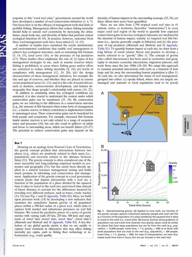
the gravity concept predicts that interactions between twoplaces (e.g., cities) are positively related to their mass (i.e.,population) and inversely related to the distance betweenthem (31). The gravity concept is often considered one of themost successful and long-enduring empirical models in eco-nomics and geography (31), but has rarely been directly ap-plied in a natural resource management setting and holdsmuch promise in informing reef conservation and manage-ment. Application of the gravity concept in a reef governancecontext posits that human interactions with a reef are afunction of the population of a place divided by the squaredtime it takes to travel to the reefs (we used travel time insteadof linear distance to account for the differences incurred bytraveling over different surfaces, such as water, roads, tracks)(14, 32) (see Fig. 1 and SI Appendix, Table S2). Here, we buildupon previous work (14) by developing a new indicator thatexamines the cumulative human gravity of all populatedplaces within a 500-km radius of a given reef, which aims tocapture both market and subsistence pressures on reef fishbiomass. We tested the predictive power of a series of gravitymetrics with varying radii (50 km, 250 km, 500 km) and expo-nents of travel time (travel time, travel time2, travel time3)(Materials and Methods and SI Appendix, Table S3). A key lim-itation of our global gravity metric is that we are unable tocapture local variations in efficiencies that may affect fishingmortality per capita, such as fishing fleet technology or in-frastructure (e.g., road) quality.

5,000

10,000

15,000

20,000

2h 4h 6h 8h 10h 12hTravel time (hours)

Popu

latio

n (p

eopl

e)

0.002

0.05

1

20

400Gravity

Populationy

Travel timex

Populationx

Travel timey

B

A

Fig. 1. Operationalizing gravity. (A) Applied to coral reefs, our heuristic ofthe gravity concept captures interactions between people and coral reef fishas a function of the population of a place divided by the squared time it takesto travel to the reefs (i.e., travel time). (B) Gravity isoclines along gradients ofpopulation size and travel time illustrate how gravity values could be similarfor places that have large populations but are far from the reefs (e.g., pop-ulationx = 15,000 people, travel timex = 7 h, gravityx = 306) as to those withsmall populations that are close to the reef (e.g., populationy = 300 people,travel timey = 1 h, gravityy = 300). For ease of interpretation, we have illus-trated travel time here in hours, but we use minutes in the main text.

Cinner et al. PNAS | vol. 115 | no. 27 | E6117

SUST

AINABILITY

SCIENCE

PNASPL

US

Dow

nloa

ded

by g

uest

on

Nov

embe

r 12

, 202

1

complied with; (ii) restricted fishing, where there are activelyenforced restrictions on the types of gears that can be used (e.g.,bans on spear guns) or on access (e.g., marine tenure systems thatrestrict fishing by “outsiders”); or (iii) high-compliance marinereserves, where fishing is effectively prohibited (Materials andMethods). We hypothesized that our ecological indicators woulddecline with increasing gravity in fished areas, but that marinereserves areas would be less sensitive to gravity. To test our hy-potheses, we used general and generalized linear mixed-effectsmodels to predict target fish biomass and the presence of toppredators, respectively, at each site based on gravity and man-agement status, while accounting for other key environmental andsocial conditions thought to influence our ecological outcomes(14) (Materials and Methods). Based on our models, we calculatedexpected conservation gains along a gravity gradient as the dif-ference between managed sites and openly fished sites.Our analysis reveals that human gravity was the strongest predictor

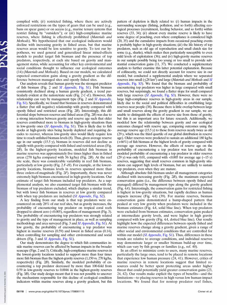
of fish biomass (Fig. 2 and SI Appendix, Fig. S1). Fish biomassconsistently declined along a human gravity gradient, a trend par-ticularly evident at the nation/state scale (Fig. 2 C–E). However, thisrelationship can vary by management type (Fig. 2 and SI Appendix,Fig. S1). Specifically, we found that biomass in reserves demonstrateda flatter (but still negative) relationship with gravity compared withopenly fished and restricted areas (Fig. 2B). Interestingly, this dif-ferential slope between reserves and fished areas (Fig. 2B) was due toa strong interaction between gravity and reserve age such that olderreserves contributed more to biomass in high-gravity situations thanin low-gravity ones (SI Appendix, Fig. S1). This is likely due to fishstocks at high-gravity sites being heavily depleted and requiring de-cades to recover, whereas low-gravity sites would likely require lesstime to reach unfished biomass levels (8). Thus, given average reserveage in our sample (15.5 y), biomass in reserves did not decline asrapidly with gravity compared with fished and restricted areas (Fig.2B). In the highest-gravity locations, modeled fish biomass inmarine reserves was approximately five times higher than in fishedareas (270 kg/ha compared with 56 kg/ha) (Fig. 2B). At the reefsite scale, there was considerable variability in reef fish biomass,particularly at low gravity (Fig. 2 F–H). For example, at the lowest-gravity locations, biomass levels in reserves spanned more thanthree orders-of-magnitude (Fig. 2F). Importantly, there was neverextremely high biomass encountered in high-gravity locations. Ourestimate of target fish biomass included top predators. As a sup-plemental analysis, we also examined target fish biomass with thebiomass of top predators excluded, which displays a similar trend,but with lower fish biomass in reserves at low gravity comparedwith when top predators are included (SI Appendix, Fig. S2).A key finding from our study is that top predators were en-

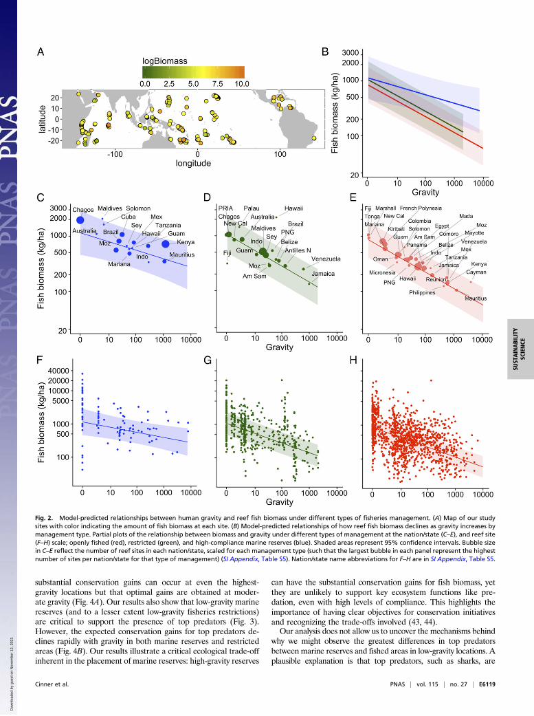
countered on only 28% of our reef sites, but as gravity increases, theprobability of encountering top predator on tropical coral reefsdropped to almost zero (<0.005), regardless of management (Fig. 3).The probability of encountering top predators was strongly relatedto gravity and the type of management in place, as well as samplingmethodology and area surveyed (Fig. 3 and SI Appendix, Fig. S1). Atlow gravity, the probability of encountering a top predator washighest in marine reserves (0.59) and lowest in fished areas (0.14),when controlling for sampling and other environmental and socialdrivers (Fig. 3 and SI Appendix, Fig. S1).Our study demonstrates the degree to which fish communities in-

side marine reserves can be affected by human impacts in the broaderseascape (Figs. 2 and 3). Critically, high-compliance marine reserves inthe lowest-gravity locations tended to support more than four timesmore fish biomass than the highest-gravity reserves (1,150 vs. 270 kg/ha,respectively) (Fig. 2B). Similarly, the modeled probability of en-countering a top predator decreased by more than 100-fold from0.59 in low-gravity reserves to 0.0046 in the highest-gravity reserves(Fig. 3B). Our study design meant that it was not possible to uncoverthe mechanisms responsible for this decline of ecological conditionindicators within marine reserves along a gravity gradient, but this

pattern of depletion is likely related to: (i) human impacts in thesurrounding seascape (fishing, pollution, and so forth) affecting eco-logical processes (recruitment, feeding behavior, and so forth) withinreserves (33, 34); (ii) almost every marine reserve is likely to havesome degree of poaching, even where compliance is considered high(20, 35) and the cumulative impacts from occasional poaching eventsis probably higher in high-gravity situations; (iii) the life history of toppredators, such as old age of reproduction and small clutch size forsome (e.g., sharks), which makes then particularly susceptible to evenmild levels of exploitation (36); and (iv) high-gravity marine reservesin our sample possibly being too young or too small to provide sub-stantial conservation gains (11, 37). We conducted a supplementaryanalysis to further examine this latter potential explanation. Becauseof collinearity, we could not directly account for reserve size in ourmodel, but conducted a supplemental analysis where we separatedreserves into small (≤28 km2) and large (Materials andMethods and SIAppendix, Fig. S3). We found that the biomass and probability ofencountering top predators was higher in large compared with smallreserves, but surprisingly, we found a flatter slope for small comparedwith large reserves (SI Appendix, Fig. S3). However, there were nolarge high-compliance reserves in high-gravity areas in our sample,likely due to the social and political difficulties in establishing largereserves near people (38). Because there is little overlap between largeand small reserves along the gravity gradient in our sample, we areunable to distinguish the effects of reserve size from those of gravity,but this is an important area for future research. Additionally, wemodeled how the relationship between gravity and our ecologicaloutcomes changed with reserve age, comparing outcomes using theaverage reserve age (15.5 y) to those from reserves nearly twice as old(29 y, which was the third quartile of our global distribution in reserveage). Older reserves were predicted to sustain an additional 180 kg/ha(+66%) of fish biomass at the highest levels of gravity compared withaverage age reserves. However, the effects of reserve age on theprobability of encountering a top predator was less marked: themodeled probability of encountering a top predator in older reserves(29 y) was only 0.01, compared with <0.005 for average age (∼15 y)reserves, suggesting that small reserves common in high-gravity situ-ations can support high levels of biomass, but are unlikely to sustaintop predators, even when they are mature.Although absolute fish biomass under all management categories

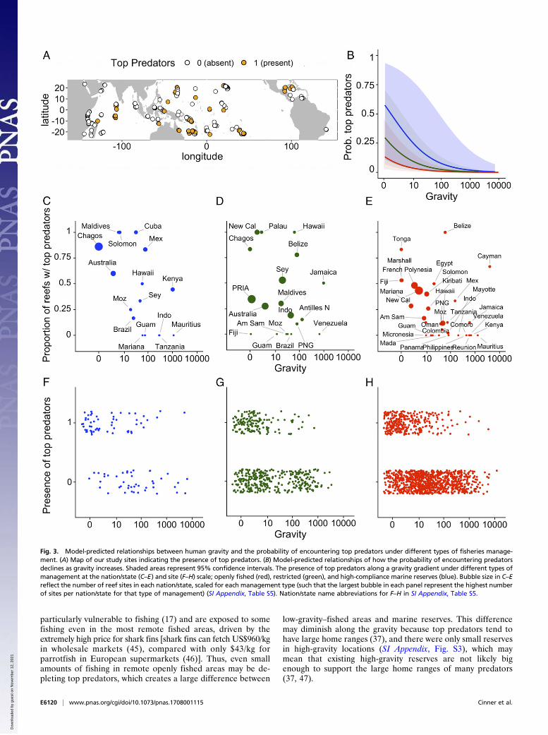
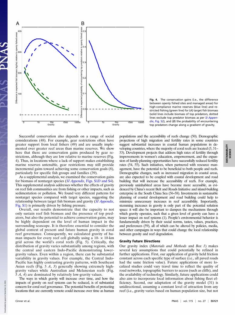
declined with increasing gravity (Fig. 2B), the maximum expectedconservation gains (i.e., the difference between openly fished andmanaged) differed by management type along the gravity gradient(Fig. 4A). Interestingly, the conservation gains for restricted fishingis highest in low-gravity situations, but rapidly declines as humanimpacts increase (Fig. 4A) (39). For marine reserves, biomassconservation gains demonstrated a hump-shaped pattern thatpeaked at very low gravity when predators were included in thebiomass estimates (Fig. 4A, solid blue line). When top predatorswere excluded from biomass estimates, conservation gains peakedat intermediate gravity levels, and were higher in high gravitycompared with low gravity (Fig. 4A, dotted blue line). Our resultshighlight how the expected differences between openly fished andmarine reserves change along a gravity gradient, given a range ofother social and environmental conditions that are controlled forwithin our model (SI Appendix, Fig. S1). Thus, differences in thesetrends are relative to average conditions, and individual reservesmay demonstrate larger or smaller biomass build-up over time,which can vary by fish groups or families (e.g., ref. 40).In an effort to minimize costs to users, many marine reserves,

particularly the large ones, tend to be placed in remote locationsthat experience low human pressure (24, 41). However, critics ofmarine reserves in remote locations suggest that limited re-sources could be better spent protecting areas under higherthreat that could potentially yield greater conservation gains (23,24, 42). Our results make explicit the types of benefits—and thelimitations—to placing reserves in high versus low human-impactlocations. We found that for nontop predator reef fishes,

E6118 | www.pnas.org/cgi/doi/10.1073/pnas.1708001115 Cinner et al.

Dow

nloa

ded

by g

uest

on

Nov

embe

r 12

, 202

1

substantial conservation gains can occur at even the highest-gravity locations but that optimal gains are obtained at moder-ate gravity (Fig. 4A). Our results also show that low-gravity marinereserves (and to a lesser extent low-gravity fisheries restrictions)are critical to support the presence of top predators (Fig. 3).However, the expected conservation gains for top predators de-clines rapidly with gravity in both marine reserves and restrictedareas (Fig. 4B). Our results illustrate a critical ecological trade-offinherent in the placement of marine reserves: high-gravity reserves

can have the substantial conservation gains for fish biomass, yetthey are unlikely to support key ecosystem functions like pre-dation, even with high levels of compliance. This highlights theimportance of having clear objectives for conservation initiativesand recognizing the trade-offs involved (43, 44).Our analysis does not allow us to uncover the mechanisms behind

why we might observe the greatest differences in top predatorsbetween marine reserves and fished areas in low-gravity locations. Aplausible explanation is that top predators, such as sharks, are

Fig. 2. Model-predicted relationships between human gravity and reef fish biomass under different types of fisheries management. (A) Map of our studysites with color indicating the amount of fish biomass at each site. (B) Model-predicted relationships of how reef fish biomass declines as gravity increases bymanagement type. Partial plots of the relationship between biomass and gravity under different types of management at the nation/state (C–E), and reef site(F–H) scale; openly fished (red), restricted (green), and high-compliance marine reserves (blue). Shaded areas represent 95% confidence intervals. Bubble sizein C–E reflect the number of reef sites in each nation/state, scaled for each management type (such that the largest bubble in each panel represent the highestnumber of sites per nation/state for that type of management) (SI Appendix, Table S5). Nation/state name abbreviations for F–H are in SI Appendix, Table S5.

Cinner et al. PNAS | vol. 115 | no. 27 | E6119

SUST

AINABILITY

SCIENCE

PNASPL

US

Dow

nloa

ded

by g

uest

on

Nov

embe

r 12

, 202

1

particularly vulnerable to fishing (17) and are exposed to somefishing even in the most remote fished areas, driven by theextremely high price for shark fins [shark fins can fetch US$960/kgin wholesale markets (45), compared with only $43/kg forparrotfish in European supermarkets (46)]. Thus, even smallamounts of fishing in remote openly fished areas may be de-pleting top predators, which creates a large difference between

low-gravity–fished areas and marine reserves. This differencemay diminish along the gravity because top predators tend tohave large home ranges (37), and there were only small reservesin high-gravity locations (SI Appendix, Fig. S3), which maymean that existing high-gravity reserves are not likely bigenough to support the large home ranges of many predators(37, 47).

Fig. 3. Model-predicted relationships between human gravity and the probability of encountering top predators under different types of fisheries manage-ment. (A) Map of our study sites indicating the presence of top predators. (B) Model-predicted relationships of how the probability of encountering predatorsdeclines as gravity increases. Shaded areas represent 95% confidence intervals. The presence of top predators along a gravity gradient under different types ofmanagement at the nation/state (C–E) and site (F–H) scale; openly fished (red), restricted (green), and high-compliance marine reserves (blue). Bubble size in C–Ereflect the number of reef sites in each nation/state, scaled for each management type (such that the largest bubble in each panel represent the highest numberof sites per nation/state for that type of management) (SI Appendix, Table S5). Nation/state name abbreviations for F–H in SI Appendix, Table S5.

E6120 | www.pnas.org/cgi/doi/10.1073/pnas.1708001115 Cinner et al.

Dow

nloa

ded

by g

uest

on

Nov

embe

r 12

, 202

1

Successful conservation also depends on a range of socialconsiderations (48). For example, gear restrictions often havegreater support from local fishers (49) and are usually imple-mented over greater reef areas than marine reserves. We showhere that there are conservation gains produced by gear re-strictions, although they are low relative to marine reserves (Fig.4). Thus, in locations where a lack of support makes establishingmarine reserves untenable, gear restrictions may still provideincremental gains toward achieving some conservation goals (8),particularly for specific fish groups and families (39).As a supplemental analysis, we examined the conservation gains

for biomass of nontarget species (SI Appendix, Figs. S1D and S4).This supplemental analysis addresses whether the effects of gravityon reef fish communities are from fishing or other impacts, such assedimentation or pollution. We found very different patterns fornontarget species compared with target species, suggesting therelationship between target fish biomass and gravity (SI Appendix,Fig. S1) is primarily driven by fishing pressure.Overall, our results demonstrate that the capacity to not

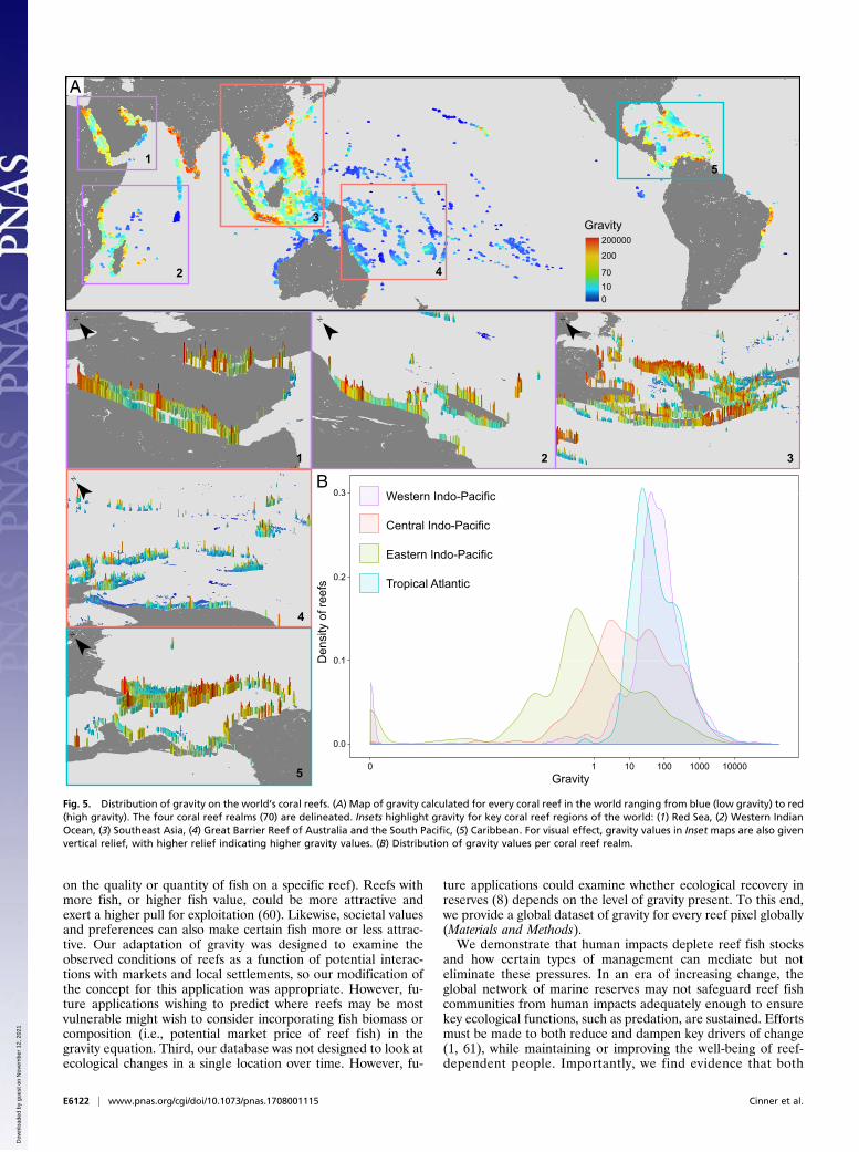
only sustain reef fish biomass and the presence of top pred-ators, but also the potential to achieve conservation gains, maybe highly dependent on the level of human impact in thesurrounding seascape. It is therefore essential to consider theglobal context of present and future human gravity in coralreef governance. Consequently, we calculated gravity of hu-man impacts for every reef cell globally using a 10- × 10-kmgrid across the world’s coral reefs (Fig. 5). Critically, thedistribution of gravity varies substantially among regions, withthe central and eastern Indo-Pacific demonstrating lower-gravity values. Even within a region, there can be substantialvariability in gravity values. For example, the Central Indo-Pacific has highly contrasting gravity patterns, with SoutheastAsian reefs (Fig. 5 A, 3) generally showing extremely high-gravity values while Australian and Melanesian reefs (Fig.5 A, 4) are dominated by relatively low-gravity values.The ways in which gravity will increase over time, and how the

impacts of gravity on reef systems can be reduced, is of substantialconcern for coral reef governance. The potential benefits of protectinglocations that are currently remote could increase over time as human

populations and the accessibility of reefs change (50). Demographicprojections of high migration and fertility rates in some countriessuggest substantial increases in coastal human populations in de-veloping countries, where the majority of coral reefs are located (5, 51–53). Development projects that address high rates of fertility throughimprovements in women’s education, empowerment, and the expan-sion of family-planning opportunities have successfully reduced fertilityrates (54, 55). Such initiatives, when partnered with resource man-agement, have the potential to be beneficial to both people and reefs.Demographic changes, such as increased migration in coastal areas,are also expected to be coupled with coastal development and roadbuilding that will increase the accessibility of reefs. For example,previously uninhabited areas have become more accessible, as evi-denced by China’s recent Belt and Roads Initiative and island-buildingenterprise in the South China Sea (56–58). Investments in sustainableplanning of coastal development and road building could help tominimize unnecessary increases in reef accessibility. Importantly,stemming increases in gravity is only part of the potential solutionspace: it will also be important to dampen the mechanisms throughwhich gravity operates, such that a given level of gravity can have alesser impact on reef systems (1). People’s environmental behavior isfundamentally driven by their social norms, tastes, values, practices,and preferences (59), all of which can be altered by policies, media,and other campaigns in ways that could change the local relationshipbetween gravity and reef degradation.

Gravity Future DirectionsOur gravity index (Materials and Methods and Box 1) makesseveral key assumptions that could potentially be refined infurther applications. First, our application of gravity held frictionconstant across each specific type of surface (i.e., all paved roadshad the same friction value). Future applications of more lo-calized studies could vary travel time to reflect the quality ofroad networks, topographic barriers to access (such as cliffs), andthe availability of technology. Similarly, future applications couldalso aim to incorporate local information about fishing fleet ef-ficiency. Second, our adaptation of the gravity model (31) isunidirectional, assuming a constant level of attraction from anyreef (i.e., gravity varies based on human population size, but not

0

100

200

300

400

0 10 100 1000 10000Gravity

Diff

eren

ce in

exp

ecte

d fis

h bi

omas

s (k

g/ha

) re

lativ

e to

ope

nly

fishe

d ar

eas

0.0

0.1

0.2

0.3

0.4

0.5

0 10 100 1000 10000Gravity

Diff

eren

ce in

exp

ecte

d pr

obab

ility

of e

ncou

nter

ing

top

pred

ator

s re

lativ

e to

ope

nly

fishe

d ar

eas

A B

Fig. 4. The conservation gains (i.e., the differencebetween openly fished sites and managed areas) forhigh-compliance marine reserves (blue line) and re-stricted fishing (green line) for (A) target fish biomass(solid lines include biomass of top predators, dottedlines exclude top predator biomass as per SI Appen-dix, Fig. S2), and (B) the probability of encounteringtop predators change along a gradient of gravity.

Cinner et al. PNAS | vol. 115 | no. 27 | E6121

SUST

AINABILITY

SCIENCE

PNASPL

US

Dow

nloa

ded

by g

uest

on

Nov

embe

r 12

, 202

1

on the quality or quantity of fish on a specific reef). Reefs withmore fish, or higher fish value, could be more attractive andexert a higher pull for exploitation (60). Likewise, societal valuesand preferences can also make certain fish more or less attrac-tive. Our adaptation of gravity was designed to examine theobserved conditions of reefs as a function of potential interac-tions with markets and local settlements, so our modification ofthe concept for this application was appropriate. However, fu-ture applications wishing to predict where reefs may be mostvulnerable might wish to consider incorporating fish biomass orcomposition (i.e., potential market price of reef fish) in thegravity equation. Third, our database was not designed to look atecological changes in a single location over time. However, fu-

ture applications could examine whether ecological recovery inreserves (8) depends on the level of gravity present. To this end,we provide a global dataset of gravity for every reef pixel globally(Materials and Methods).We demonstrate that human impacts deplete reef fish stocks

and how certain types of management can mediate but noteliminate these pressures. In an era of increasing change, theglobal network of marine reserves may not safeguard reef fishcommunities from human impacts adequately enough to ensurekey ecological functions, such as predation, are sustained. Effortsmust be made to both reduce and dampen key drivers of change(1, 61), while maintaining or improving the well-being of reef-dependent people. Importantly, we find evidence that both

Gravity

4

5

3

2

B

1

Den

sity

of r

eefs

A

1 2 3

4

5

Western Indo-Pacific

Central Indo-Pacific

Eastern Indo-Pacific

Tropical Atlantic

0.0

0.1

0.2

0.3

0 1 10 100 1000 10000

Gravity

010

200000

70

200

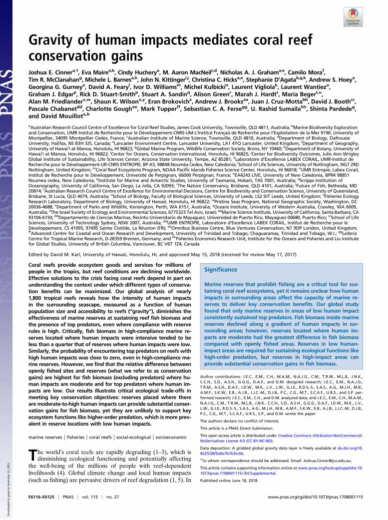
Fig. 5. Distribution of gravity on the world’s coral reefs. (A) Map of gravity calculated for every coral reef in the world ranging from blue (low gravity) to red(high gravity). The four coral reef realms (70) are delineated. Insets highlight gravity for key coral reef regions of the world: (1) Red Sea, (2) Western IndianOcean, (3) Southeast Asia, (4) Great Barrier Reef of Australia and the South Pacific, (5) Caribbean. For visual effect, gravity values in Inset maps are also givenvertical relief, with higher relief indicating higher gravity values. (B) Distribution of gravity values per coral reef realm.

E6122 | www.pnas.org/cgi/doi/10.1073/pnas.1708001115 Cinner et al.

Dow

nloa

ded

by g

uest

on

Nov

embe

r 12

, 202

1

remote and human-surrounded reserves can produce differenttypes of conservation gains. Ultimately, multiple forms of man-agement are needed across the seascape to sustain coral reef fishesand the people who depend upon them.

Materials and MethodsScales of Data. Our data were organized at three spatial scales: reef site (n =1,798), reef cluster (n = 734), and nation/state (n = 41).

Reef site is the smallest scale, which had an average of 2.4 surveys(transects), hereafter referred to as “reef.”

For reef cluster (which had an average of 2.4 ± 2.4 reef sites), weclustered reefs together that were within 4 km of each other, and used thecentroid to estimate reef cluster-level social and environmental covariates.To define reef clusters, we first estimated the linear distance between allreef sites, then used a hierarchical analysis with the complete-linkageclustering technique based on the maximum distance between reefs. Weset the cut-off at 4 km to select mutually exclusive sites where reefs cannotbe more distant than 4 km. The choice of 4 km was informed by a 3-y studyof the spatial movement patterns of artisanal coral reef fishers, corre-sponding to the highest density of fishing activities on reefs based on GPS-derived effort density maps of artisanal coral reef fishing activities (62).This clustering analysis was carried out using the R functions “hclust”and “cutree.”

A larger scale in our analysis was “nation/state” (nation, state, or territory,which had an average of 44 ± 59 reef clusters), which are jurisdictions thatgenerally correspond to individual nations (but could also include states,territories, overseas regions), within which sites were nested for analysis.Targeted fish biomass. Reef fish biomass estimates were based on visual counts in1,798 reef sites. All surveys used standard belt-transects, distance sampling, orpoint-counts, and were conducted between 2004 and 2013. Where data frommultiple years were available from a single reef site, we included only data fromthe year closest to 2010. Within each survey area, reef-associated fishes wereidentified to species level, their abundance counted, and total length (TL) es-timated, with the exception of one data provider whomeasured biomass at thefamily level. To make estimates of targeted biomass from these transect-leveldata comparable among studies, we did the following. (i) We retained fami-lies that were consistently studied, commonly targeted, and were above aminimum size cut-off. Thus, we retained counts of >10 cm diurnally active,noncryptic reef fish that are resident on the reef (14 families), excluding sharksand semipelagic species (SI Appendix, Table S1). We calculated total biomass oftargeted fishes on each reef using standard published species-level length–weight relationship parameters or those available on FishBase (63). Whenlength–weight relationship parameters were not available for a species, weused the parameters for a closely related species or genus. For comparison, wealso calculated nontarget fish biomass (SI Appendix, Table S1). (ii) We directlyaccounted for depth and habitat as covariates in the model (see EnvironmentalDrivers, below). (iii) We accounted for differences among census methods byincluding each census method (standard belt-transects, distance sampling, orpoint-counts) as a covariate in the model. (iv) We accounted for differences insampling area by including total sampling area for each reef (m2) as a covariatein the model.Top predators. We examined the presence/absence of eight families of fishconsidered top predators (SI Appendix, Table S1). We considered presence/absence instead of biomass because biomass was heavily zero inflated.Gravity.We first developed a gravity index for each of our reef sites where wehad in situ ecological data. We gathered data on both population estimatesand a surrogate for distance: travel time.

Population estimates.Wegathered population estimates for each 1- by 1-kmcell within a 500-km radius of each reef site using LandScan 2011 database.We chose a 500-km radius from the reef as a likely maximum distance fishingactivities for reef fish are likely to occur.

Travel time calculation. The following procedure was repeated for eachpopulated cell within the 500-km radius. Travel time was computed using acost–distance algorithm that computes the least “cost” (in minutes) oftraveling between two locations on a regular raster grid. In our case, the twolocations were the centroid of the reef site and the populated cell of in-terest. The cost (i.e., time) of traveling between the two locations was de-termined by using a raster grid of land cover and road networks with thecells containing values that represent the time required to travel across them(32) (SI Appendix, Table S2), we termed this raster grid a “friction-surface”(with the time required to travel across different types of surfaces analogousto different levels of friction). To develop the friction-surface, we usedglobal datasets of road networks, land cover, and shorelines:

Road network data were extracted from the Vector Map Level 0 (VMap0)from the National Imagery and Mapping Agency’s (NIMA) Digital Chart ofthe World (DCW). We converted vector data from VMap0 to 1 kmresolution raster.

Land cover data were extracted from the Global Land Cover 2000 (64).

To define the shorelines, we used the GSHHS (Global Self-consistent, Hi-erarchical, High-resolution Shoreline) database v2.2.2.

These three friction components (road networks, land cover, and shore-lines) were combined into a single friction surface with a Behrmann mapprojection (an equal area projection). We calculated our cost-distance modelsin R using the accCost function of the “gdistance” package. The functionuses Dijkstra’s algorithm to calculate least-cost distance between two cellson the grid taking into account obstacles and the local friction of thelandscape (65). Travel time estimates over a particular surface could be af-fected by the infrastructure (e.g., road quality) and types of technology used(e.g., types of boats). These types of data were not available at a global scalebut could be important modifications in more localized studies.

Gravity computation. To compute gravity, we calculated the population ofthe cell and divided that by the squared travel time between the reef site andthe cell. We summed the gravity values for each cell within 500 km of the reefsite to get the “total gravity” within 500 km. We used the squared distance(or in our case, travel time), which is relatively common in geography andeconomics, although other exponents can be used (31) (Table S3).

We also developed a global gravity index for each 10- × 10-km grid of reefin the world (Box 1), which we provide as an open-access dataset. The pro-cedure to calculate gravity was similar to above with the only differencebeing in the precision of the location; the former was a single data point(reef site), while the latter was a grid cell (reef cell). For the purpose of theanalysis, gravity was log-transformed and standardized.

We also explored various exponents (1–3) and buffer sizes (50, 250, and500 km) to build nine gravity metrics. The metric providing the best model, sowith the lowest Akaike Information Criterion (AIC), was that with a squaredexponent for travel time and a 500-km buffer (SI Appendix, Table S3).Management. For each observation, we determined the prevailing type ofmanagement, including the following. (i) Marine reserve (whether the site fellwithin the borders of a no-take marine reserve): we asked data providers tofurther classify whether the reserve had high or low levels of compliance. For thisanalysis, we removed sites that were categorized as low-compliance reserves (n =233). (ii) Restricted fishing: whether there were active restrictions on gears (e.g.,bans on the use of nets, spearguns, or traps) or fishing effort (which could haveincluded areas inside marine protected areas that were not necessarily no take).Or (iii) openly fished: regularly fished without effective restrictions. To determinethese classifications, we used the expert opinion of the data providers, and tri-angulated this with a global database of marine reserve boundaries (66). We alsocalculated size (median = 113.6 km2, mean= 217,516 km2, SD = 304,417) and age(median = 9, mean = 15.5 y, SD = 14.5) of the no-take portion of each reserve.Reserve size was strongly related to our metric of gravity and could not be di-rectly included in the analysis. We conducted a supplemental analysis where weseparated reserves into small (≤28 km2) and large (>65 km2) based on a naturalbreak in the data to illustrate: (i) how biomass and the presence of top predatorsmight differ between small and large reserves; and (ii) how large reserves areabsent in our sample in high gravity.

Other Social Drivers. To account for the influence of other social drivers thatare thought to be related to the condition of reef fish biomass, we alsoincluded the following covariates in our model.Local population growth.We created a 100-kmbuffer around each site and usedthis to calculate human population within the buffer in 2000 and 2010 basedon the Socioeconomic Data andApplication Centre gridded population of theworld database. Population growthwas the proportional difference betweenthe population in 2000 and 2010. We chose a 100-km buffer as a reasonablerange at which many key human impacts from population (e.g., land-use andnutrients) might affect reefs (67).Human development index. Human development index (HDI) is a summarymeasure of human development encompassing a long and healthy life, beingknowledgeable, and having a decent standard of living. In cases where HDIvalues were not available specific to the state (e.g., Florida and Hawaii), weused the national (e.g., United States) HDI value.Population size. For each nation/state, we determined the size of the humanpopulation. Datawere derivedmainly from the national census reports CIA factbook (https://www.cia.gov/library/publications/the-world-factbook/rankorder/2119rank.html), and Wikipedia (https://en.wikipedia.org/wiki/Main_Page). Forthe purpose of the analysis, population size was log-transformed.

Cinner et al. PNAS | vol. 115 | no. 27 | E6123

SUST

AINABILITY

SCIENCE

PNASPL

US

Dow

nloa

ded

by g

uest

on

Nov

embe

r 12

, 202

1

Environmental Drivers.Depth. The depth of reef surveys was grouped into the following categories:<4 m, 4–10 m, >10 m to account for broad differences in reef fish communitystructure attributable to a number of interlinked depth-related factors. Cat-egories were necessary to standardize methods used by data providers andwere determined by preexisting categories used by several data providers.Habitat. We included the following habitat categories. (i) Slope: the reef slopehabitat is typically on the ocean side of a reef, where the reef slopes down intodeeper water. (ii) Crest: the reef crest habitat is the section that joins a reefslope to the reef flat. The zone is typified by high wave energy (i.e., where thewaves break). It is also typified by a change in the angle of the reef from aninclined slope to a horizontal reef flat. (iii) Flat: the reef flat habitat is typicallyhorizontal and extends back from the reef crest for tens to hundreds of me-ters. (iv) Lagoon/back reef: lagoonal reef habitats are where the continuousreef flat breaks up into more patchy reef environments sheltered from waveenergy. These habitats can be behind barrier/fringing reefs or within atolls.Back reef habitats are similar broken habitats where the wave energy does nottypically reach the reefs and thus forms a less continuous “lagoon style” reefhabitat. Due to minimal representation among our sample, we excluded otherless-prevalent habitat types, such as channels and banks. To verify the sites’habitat information, we used the Millennium Coral Reef Mapping Project hi-erarchical data (68), Google Earth, and site depth information.Productivity.We examined ocean productivity for each of our sites in milligramsof C per square meter per day (mg C m−2 d−1) (www.science.oregonstate.edu/ocean.productivity/). Using the monthly data for years the 2005–2010 (in hdfformat), we imported and converted those data into ArcGIS. We then calcu-lated yearly average and finally an average for all these years. We used a100-km buffer around each of our sites and examined the average productivitywithin that radius. Note that ocean productivity estimates are less accuratefor nearshore environments, but we used the best available data. For thepurpose of the analysis, productivity was log-transformed.Climate stress.We included an index of climate stress for corals, developed byMaina et al. (69), which incorporated 11 different environmental conditions,such as the mean and variability of sea-surface temperature.

Analyses.We first looked for collinearity among our covariates using bivariatecorrelations and variance inflation factor estimates. This led to the exclusionof several covariates (not described above): (i) Biogeographic Realm (TropicalAtlantic, western Indo-Pacific, Central Indo-Pacific, or eastern Indo-Pacific);(ii) Gross Domestic Product (purchasing power parity); (iii) Rule of Law(World Bank governance index); (iv) Control of Corruption (World Bankgovernance index); (v) Voice and Accountability (World Bank governanceindex); (vi) Reef Fish Landings; (vii) Tourism arrivals relative to local pop-ulation; (viii) Sedimentation; and (ix) Marine Reserve Size. Other covariateshad correlation coefficients 0.7 or less and Variance Inflation Factor scoresless than 5 (indicating multicollinearity was not a serious concern). Care mustbe taken in causal attribution of covariates that were significant in ourmodel, but demonstrated collinearity with candidate covariates that wereremoved during the aforementioned process. Importantly, the covariate ofinterest in this study, gravity, was not strongly collinear with candidatecovariates except reserve size (r = −0.8, t = 3.6, df = 104, P = 0.0004).

To quantify the relationships between gravity and target fish biomass, wedeveloped a general linear-mixedmodel in R, using a log-normal distribution forbiomass. To quantify the relationships betweengravity and presence/absence oftop predators, we developed a generalized linear-mixedmodel with a binomialfamily and a logit link function. For both models, we set reef cluster nestedwithin nation/state as a random effect to account for the hierarchical nature ofthe data (i.e., reef sites nested in reef clusters, reef clusters nested in nation/states). We included an interaction between gravity and reserve age, as well asall of the other social and environmental drivers and the sampling method andtotal sampling area as covariates. We also tested interactions between gravityand management and used AIC to select the most parsimonious model. For fishbiomass, the interaction between gravity and reserve age had AIC values >2 lowerthan the interaction between gravity and management (and a combination ofboth interactions). For the top predator models, both interactions were within 2

AIC values, so we chose the interaction with reserve age for consistency. All con-tinuous covariates were standardized for the analysis, and reserve age was thennormalized such that nonreserves were 0 and the oldest reserves were 1. Insummary, our models thus predicted target fish biomass or probability of toppredators being observed at the reef site scale with an interaction between gravityand reserve age, while accounting within the random factors for two bigger scalesat which the data were collected (reef cluster, and nation/state) (SI Appendix), andkey social and environmental characteristics expected to influence the biomass ofreef fish (14). In addition to coefficient plots (SI Appendix, Fig. S1), we conducted asupplemental analysis of relative variable importance (SI Appendix, Table S4).

We ran the residuals from the models against size of the no-take areas ofthe marine reserves and no patterns were evident, suggesting it would ex-plain no additional variance in the model. Trend lines and partial plots(averaged by site and nation/state) are presented in the figures (Figs. 2 B–Hand 3H). We plotted the partial effect of the relationship between gravityand protection on targeted fish biomass and presence of top predators (Figs.2 B–G and 3 B–G) by setting all other continuous covariates to 0 because theywere all standardized and all categorical covariates to their most commoncategory (i.e., 4–10 m for depth, slope for habitat, standard belt transect forcensus method). For age of reserves, we set this to 0 for fished and restrictedareas, and to the average age of reserves (15.5 y) for reserves.

To examine the expected conservation gains of different managementstrategies, we calculated: (i) the difference between the response of openlyfished areas (our counterfactual) and high-compliance marine reserves togravity; and (ii) the difference between the response of openly fished areasand fisheries restricted areas to gravity. For ease of interpretation, weplotted conservation gains in kilograms per hectare (kg/ha; as opposed tolog[kg/ha]) (Fig. 4A). A log-normal (linear) model was used to develop theslopes of the biomass (i) fished, (ii) marine reserve, and (iii) fisheries re-stricted areas, which results in the differences between (i) and (ii) and be-tween (i) and (iii) being nonlinear on an arithmetic scale (Fig. 4A).

Weplotted the diagnostic plots of the general linear-mixedmodel to check thatthemodel assumptionswerenot violated. To check the fit of thegeneralized linear-mixedmodel,weused the confusionmatrix (tabular representationofactual versuspredicted values) to calculate the accuracy of the model, which came to 79.2%.

Toexaminehomoscedasticity, we checked residuals against fitted values.Wechecked our models against a null model, which contained themodel structure(i.e., random effects), but no covariates. We used the null model as a baselineagainst which we could ensure that our full model performed better than amodel with no covariate information. In all cases ourmodels outperformed ournull models by more than 2 AIC values, indicating a more parsimonious model.

All analyses were undertaken using R (3.43) statistical package.

Data Access. A gridded global gravity data layer is freely available at dx.doi.org/10.4225/28/5a0e7b1b3cc0e. The ecological data used in this report areowned by individual data providers. Although much of these data (e.g.,NOAA CRED data, and Reef Life Surveys) are already open access, some ofthese data are governed by intellectual property arrangements and cannot bemade open access. Because the data are individually owned, we have agreedupon and developed a structure and process for those wishing access to thedata. Our process is one of engagement and collaboration with the dataproviders. Anyone interested can send a short (one-half to one page) proposalfor use of the database that details the problem statement, research gap,research question(s), and proposed analyses to the Principle Investigator anddatabase administrator Joshua.cinner@jcu.edu.au, who will send the proposalto the data providers. Individual data providers can agree to make their dataavailable or not. They can also decide whether they would like to be con-sidered as a potential coauthor if their data are used. The administrator willthen send only the data that the providers have agreed to make available.

ACKNOWLEDGMENTS. We thank J. Zamborian Mason and A. Fordyce forassistance with analyses and figures, and to numerous scientists whocollected data used in the research. The Australian Research Council Centreof Excellence for Coral Reef Studies and The Pew Charitable Trusts fundedworking group meetings.

1. Hughes TP, et al. (2017) Coral reefs in the Anthropocene. Nature 546:82–90.2. Pandolfi JM, et al. (2003) Global trajectories of the long-term decline of coral reef

ecosystems. Science 301:955–958.3. Hughes TP, et al. (2003) Climate change, human impacts, and the resilience of coral

reefs. Science 301:929–933.4. Teh LSL, Teh LCL, Sumaila UR (2013) A global estimate of the number of coral reef

fishers. PLoS One 8:e65397.5. Mora C, et al. (2011) Global human footprint on the linkage between biodiversity

and ecosystem functioning in reef fishes. PLoS Biol 9:e1000606.

6. Mora C, Chittaro PM, Sale PF, Kritzer JP, Ludsin SA (2003) Patterns and processes in

reef fish diversity. Nature 421:933–936.7. Bellwood DR, Hughes TP, Folke C, Nyström M (2004) Confronting the coral reef crisis.

Nature 429:827–833.8. MacNeil MA, et al. (2015) Recovery potential of the world’s coral reef fishes. Nature

520:341–344.9. Hopf JK, Jones GP, Williamson DH, Connolly SR (2016) Synergistic effects of marine

reserves and harvest controls on the abundance and catch dynamics of a coral reef

fishery. Curr Biol 26:1543–1548.

E6124 | www.pnas.org/cgi/doi/10.1073/pnas.1708001115 Cinner et al.

Dow

nloa

ded

by g

uest

on

Nov

embe

r 12

, 202

1

10. Krueck NC, et al. (2017) Marine reserve targets to sustain and rebuild unregulatedfisheries. PLoS Biol 15:e2000537.

11. Edgar GJ, et al. (2014) Global conservation outcomes depend on marine protectedareas with five key features. Nature 506:216–220.

12. McClanahan TR, Marnane MJ, Cinner JE, Kiene WE (2006) A comparison of marineprotected areas and alternative approaches to coral-reef management. Curr Biol 16:1408–1413.

13. Gill DA, et al. (2017) Capacity shortfalls hinder the performance of marine protectedareas globally. Nature 543:665–669.

14. Cinner JE, et al. (2016) Bright spots among the world’s coral reefs. Nature 535:416–419.

15. Williams ID, et al.; PLOS ONE Staff (2015) Correction: Human, oceanographic andhabitat drivers of central and western Pacific coral reef fish assemblages. PLoS One 10:e0129407.

16. Bozec YM, O’Farrell S, Bruggemann JH, Luckhurst BE, Mumby PJ (2016) Tradeoffsbetween fisheries harvest and the resilience of coral reefs. Proc Natl Acad Sci USA 113:4536–4541.

17. Dulvy NK, Freckleton RP, Polunin NVC (2004) Coral reef cascades and the indirecteffects of predator removal by exploitation. Ecol Lett 7:410–416.

18. McClanahan TR, et al. (2011) Critical thresholds and tangible targets for ecosystem-based management of coral reef fisheries. Proc Natl Acad Sci USA 108:17230–17233.

19. Pollnac R, et al. (2010) Marine reserves as linked social-ecological systems. Proc NatlAcad Sci USA 107:18262–18265.

20. Bergseth BJ, Russ GR, Cinner JE (2015) Measuring and monitoring compliance in no-take marine reserves. Fish Fish 16:240–258.

21. Graham NAJ, McClanahan TR (2013) The last call for marine wilderness? Bioscience 63:397–402.

22. Cinner JE, et al. (2009) Linking social and ecological systems to sustain coral reeffisheries. Curr Biol 19:206–212.

23. Pressey RL, Visconti P, Ferraro PJ (2015) Making parks make a difference: Pooralignment of policy, planning and management with protected-area impact, andways forward. Philos Trans R Soc Lond B Biol Sci 370:20140280.

24. Devillers R, et al. (2015) Reinventing residual reserves in the sea: Are we favouringease of establishment over need for protection? Aquat Conserv 25:480–504.

25. Andrello M, et al. (2017) Global mismatch between fishing dependency and larvalsupply from marine reserves. Nat Commun 8:16039.

26. Harrison HB, et al. (2012) Larval export from marine reserves and the recruitmentbenefit for fish and fisheries. Curr Biol 22:1023–1028.

27. Januchowski-Hartley FA, Graham NAJ, Cinner JE, Russ GR (2013) Spillover of fishnaïveté from marine reserves. Ecol Lett 16:191–197.

28. Ravenstein EG (1889) The laws of migration. J R Stat Soc 52:241–305.29. Dodd SC (1950) The interactance hypothesis: A gravity model fitting physical masses

and human groups. Am Sociol Rev 15:245–256.30. Bergstrand JH (1985) The gravity equation in international trade: Some microeco-

nomic foundations and empirical evidence. Rev Econ Stat 67:474–481.31. Anderson JE (2011) The gravity model. Annu Rev Econ 3:133–160.32. Maire E, et al. (2016) How accessible are coral reefs to people? A global assessment

based on travel time. Ecol Lett 19:351–360.33. Januchowski-Hartley FA, Graham NAJ, Cinner JE, Russ GR (2015) Local fishing influ-

ences coral reef fish behavior inside protected areas of the Indo-Pacific. Biol Conserv182:8–12.

34. Gil MA, Hein AM (2017) Social interactions among grazing reef fish drive material fluxin a coral reef ecosystem. Proc Natl Acad Sci USA 114:4703–4708.

35. Bergseth BJ, Williamson DH, Russ GR, Sutton SG, Cinner JE (2017) A social-ecologicalapproach to assessing and managing poaching by recreational fishers. Front EcolEnviron 15:67–73.

36. Ward-Paige CA, et al. (2010) Large-scale absence of sharks on reefs in the greater-Caribbean: A footprint of human pressures. PLoS One 5:e11968.

37. Krueck Nils C, et al. (2017) Reserve sizes needed to protect coral reef fishes. ConservLett 0:1–9.

38. Christie P, et al. (2017) Why people matter in ocean governance: Incorporating hu-man dimensions into large-scale marine protected areas. Mar Policy 84:273–284.

39. Campbell SJ, Edgar GJ, Stuart-Smith RD, Soler G, Bates AE (2018) Fishing-gear re-strictions and biomass gains for coral reef fishes in marine protected areas. ConservBiol 32:401–410.

40. McClanahan TR, Graham NAJ, Calnan JM, MacNeil MA (2007) Toward pristine bio-mass: Reef fish recovery in coral reef marine protected areas in Kenya. Ecol Appl 17:1055–1067.

41. O’Leary BC, et al. (2018) Addressing criticisms of large-scale marine protected areas.Bioscience 68:359–370.

42. Ferraro PJ, Pressey RL (2015) Measuring the difference made by conservation initia-tives: Protected areas and their environmental and social impacts Introduction. PhilosTrans R Soc Lond B Biol Sci 370:20140270.

43. Beger M, et al. (2015) Integrating regional conservation priorities for multiple ob-jectives into national policy. Nat Commun 6:8208.

44. Boon PY, Beger M (2016) The effect of contrasting threat mitigation objectives onspatial conservation priorities. Mar Policy 68:23–29.

45. Clark P (August 6, 2014) Shark fin sales in China take a dive. Financial Times. Availableat https://www.ft.com/content/4be44336-1c9f-11e4-98d8-00144feabdc0. Accessed May25, 2018.

46. Thyresson M, Nyström M, Crona B (2011) Trading with resilience: Parrotfish trade andthe exploitation of key-ecosystem processes in coral reefs. Coast Manage 39:396–411.

47. Green AL, et al. (2014) Designing marine reserves for fisheries management, bio-diversity conservation, and climate change adaptation. Coast Manage 42:143–159.

48. Bennett NJ, et al. (2017) Conservation social science: Understanding and integratinghuman dimensions to improve conservation. Biol Conserv 205:93–108.

49. McClanahan TR, Abunge CA (2016) Perceptions of fishing access restrictions and thedisparity of benefits among stakeholder communities and nations of south-easternAfrica. Fish Fish 17:417–437.

50. Watson RA, et al. (2015) Marine foods sourced from farther as their use of globalocean primary production increases. Nat Commun 6:7365.

51. Gerland P, et al. (2014) World population stabilization unlikely this century. Science346:234–237.

52. Mora C (2014) Revisiting the environmental and socioeconomic effects of populationgrowth: A fundamental but fading issue in modern scientific, public, and politicalcircles. Ecol Soc 19:38.

53. Mora C (2015) Perpetual struggle for conservation in a crowded world and theneeded paradigm shift for easing ultimate burdens. Ecology of Fishes on Coral Reefs,ed Mora C (Cambridge Univ Press, Cambridge, UK), pp 289–296.

54. Cottingham J, Germain A, Hunt P (2012) Use of human rights to meet the unmet needfor family planning. Lancet 380:172–180.

55. Sen A (2013) The ends and means of sustainability. J Human Dev Capabil 14:6–20.56. Mora C, Caldwell IR, Birkeland C, McManus JW; PLOS Biology Staff (2016) Dredging in

the Spratly Islands: Gaining land but losing reefs. PLoS Biol 14:e1002497.57. Laurance WF, Arrea IB (2017) Roads to riches or ruin? Science 358:442–444.58. Alamgir M, et al. (2017) Economic, socio-political and environmental risks of road

development in the tropics. Curr Biol 27:R1130–R1140.59. Hicks CC, Crowder LB, Graham NAJ, Kittinger JN, Le Cornu E (2016) Social drivers

forewarn of marine regime shifts. Front Ecol Environ 14:253–261.60. Berkes F, et al. (2006) Ecology. Globalization, roving bandits, and marine resources.

Science 311:1557–1558.61. Cinner JE, Kittinger JN (2015) Linkages between social systems and coral reefs.

Ecology of Fishes on Coral Reefs, ed Mora C (Cambridge Univ Press, Cambridge, UK),pp 215–220.

62. Daw T, et al. (2011) The Spatial Behaviour of Artisanal Fishers: Implications for Fish-eries Management and Development (Fishers in Space). Available at https://www.researchgate.net/profile/Pascal_Thoya2/publication/321796381_The_spatial_behaviour_of_artisanal_fishers_Implications_for_fisheries_management_and_development_Fishers_in_Space_Final_Report/links/5a9ce57d0f7e9be379682636/The-spatial-behaviour-of-artisanal-fishers-Implications-for-fisheries-management-and-development-Fishers-in-Space-Final-Report.pdf?origin=publication_list. Accessed May 25, 2018.

63. Froese R, Pauly D (2012) FishBase: World Wide Web Electronic Publication. Availableat https://www.fishbase.de/home.htm. Accessed May 25, 2018.

64. Bartholomé E, et al. (2002) GLC 2000: Global land cover mapping for the year 2000:Project status November 2002. Available at https://www.researchgate.net/publication/235707577_GLC_2000_Global_Land_Cover_Mapping_for_the_Year_2000_Project_Status_November_2002. Accessed May 25, 2018.

65. Nelson A (2008) Travel Time to Major Cities: A Global Map of Accessibility (GlobalEnvironment Monitoring Unit-Joint Research Centre of the European Commission,Ispra, Italy).

66. IUCN; UNEP-WCMC (2016) The World Database on Protected Areas (WDPA) (UNEP-WCMC, Cambridge, UK). Available at https://www.protectedplanet.net/. AccessedMay 25, 2018.

67. MacNeil MA, Connolly SR (2015) Multi-scale patterns and processes in reef fishabundance. Ecology of Fishes on Coral Reefs, ed Mora C (Cambridge Univ Press,Cambridge, UK), pp 116–126.

68. Andréfouët S, et al. (2006) Global assessment of modern coral reef extent and di-versity for regional science and management applications: A view from space. TenthInternational Coral Reef Symposium, eds Suzuki Y, et al. (Japanese Coral Reef Society,Okinawa, Japan), pp 1732–1745.

69. Maina J, McClanahan TR, Venus V, Ateweberhan M, Madin J (2011) Global gradientsof coral exposure to environmental stresses and implications for local management.PLoS One 6:e23064.

70. Spalding MD, et al. (2007) Marine ecoregions of the world: A bioregionalization ofcoastal and shelf areas. Bioscience 57:573–583.

Cinner et al. PNAS | vol. 115 | no. 27 | E6125

SUST

AINABILITY

SCIENCE

PNASPL

US

Dow

nloa

ded

by g

uest

on

Nov

embe

r 12

, 202

1