ÉTUDE SUR LE TERRAIN ET PAR MODÉLISATION DU BASSIN VERSANT DU RUISSEAU THOMAS (VALLÉE D’ANNAPOLIS,

NOUVELLE-ÉCOSSE) : INFLUENCE DE L’HÉTÉROGÉNÉITÉ ET AUTRES FACTEURS SUR LES INTERACTIONS ENTRE L’EAU DE SURFACE ET

L’EAU SOUTERRAINE ET LA RECHARGE DES AQUIFÈRES

Par Marie-Josée Gauthier

Mémoire présenté pour l’obtention

du grade de Maître ès sciences (M.Sc.) en sciences de la Terre, en hydrogéologie

Jury d’évaluation

Président du jury Yves Michaud et examinateur interne Commission Géologique du Canada

Examinateur externe Kerry MacQuarrie

Génie civil, Département du programme de Génie géologique

Université du Nouveau-Brunswick

Directeur de recherche Claudio Paniconi INRS-Eau,Terre et Environnement

Codirectrices de recherche Christine Rivard

Commission Géologique du Canada

Marie Larocque Université du Québec à Montréal

© droits réservés de Marie-Josée Gauthier, 2009

i

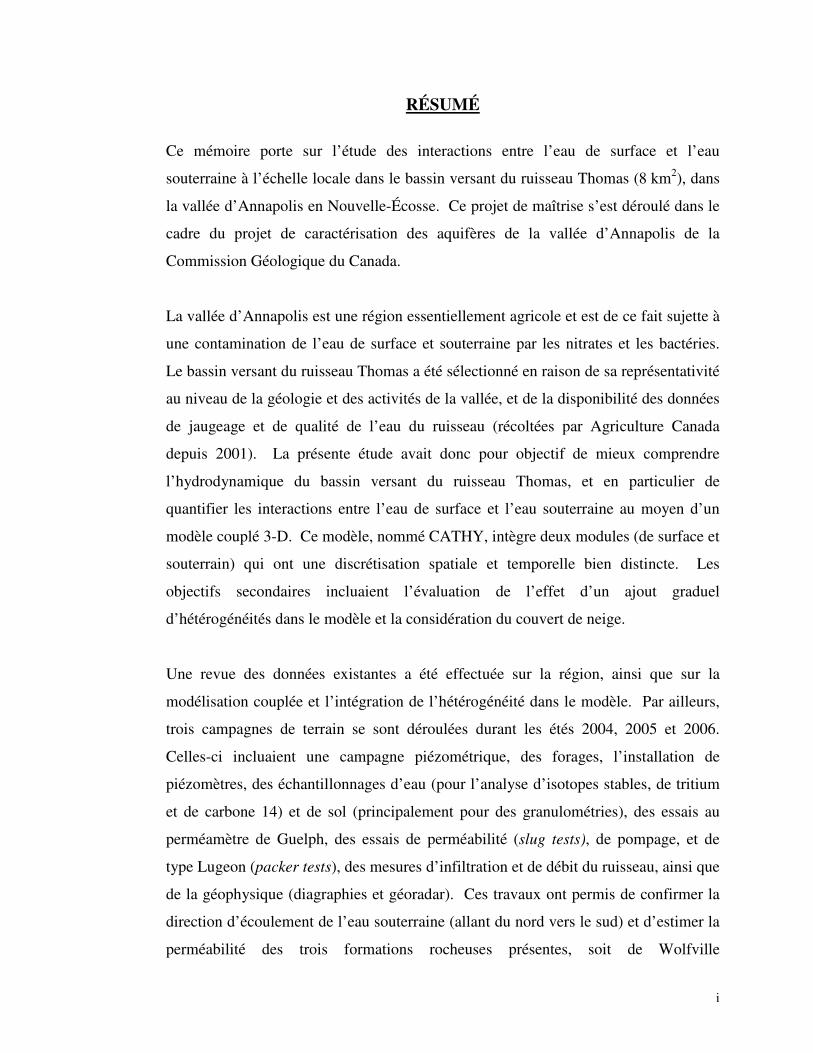
RÉSUMÉ

Ce mémoire porte sur l’étude des interactions entre l’eau de surface et l’eau

souterraine à l’échelle locale dans le bassin versant du ruisseau Thomas (8 km2), dans

la vallée d’Annapolis en Nouvelle-Écosse. Ce projet de maîtrise s’est déroulé dans le

cadre du projet de caractérisation des aquifères de la vallée d’Annapolis de la

Commission Géologique du Canada.

La vallée d’Annapolis est une région essentiellement agricole et est de ce fait sujette à

une contamination de l’eau de surface et souterraine par les nitrates et les bactéries.

Le bassin versant du ruisseau Thomas a été sélectionné en raison de sa représentativité

au niveau de la géologie et des activités de la vallée, et de la disponibilité des données

de jaugeage et de qualité de l’eau du ruisseau (récoltées par Agriculture Canada

depuis 2001). La présente étude avait donc pour objectif de mieux comprendre

l’hydrodynamique du bassin versant du ruisseau Thomas, et en particulier de

quantifier les interactions entre l’eau de surface et l’eau souterraine au moyen d’un

modèle couplé 3-D. Ce modèle, nommé CATHY, intègre deux modules (de surface et

souterrain) qui ont une discrétisation spatiale et temporelle bien distincte. Les

objectifs secondaires incluaient l’évaluation de l’effet d’un ajout graduel

d’hétérogénéités dans le modèle et la considération du couvert de neige.

Une revue des données existantes a été effectuée sur la région, ainsi que sur la

modélisation couplée et l’intégration de l’hétérogénéité dans le modèle. Par ailleurs,

trois campagnes de terrain se sont déroulées durant les étés 2004, 2005 et 2006.

Celles-ci incluaient une campagne piézométrique, des forages, l’installation de

piézomètres, des échantillonnages d’eau (pour l’analyse d’isotopes stables, de tritium

et de carbone 14) et de sol (principalement pour des granulométries), des essais au

perméamètre de Guelph, des essais de perméabilité (slug tests), de pompage, et de

type Lugeon (packer tests), des mesures d’infiltration et de débit du ruisseau, ainsi que

de la géophysique (diagraphies et géoradar). Ces travaux ont permis de confirmer la

direction d’écoulement de l’eau souterraine (allant du nord vers le sud) et d’estimer la

perméabilité des trois formations rocheuses présentes, soit de Wolfville

ii

(3,8 x 10-5 m/s), de Blomidon (2,0 x 10-5 m/s) et des montagnes du Nord

(1,8 x 10-6 m/s). L’hétérogénéité des dépôts de surface a également pu être

représentée avec une perméabilité croissante du nord vers le sud, allant de 10-8 à

10-5 m/s. Finalement, l’alimentation du ruisseau par l’aquifère a pu être quantifiée : il

a été estimé que le débit croissait également du nord au sud, étant de

10-9 m3/s dans les montagnes du Nord et de 10-6 m3/s à l’exutoire du bassin. L’analyse

des données existantes et acquises a permis de développer le modèle conceptuel du

bassin à modéliser. La modélisation couplée a ensuite été effectuée selon

neuf scénarios. Les huit premiers scénarios intègrent graduellement la géologie

« réelle » du bassin alors que le 9e considère le couvert nival sur le modèle le plus

complexe (scénario 8).

La présente étude a ainsi permis de quantifier par modélisation les principaux

processus hydrologiques et hydrogéologiques de ce bassin. La modélisation a

également démontré l’importance de représenter adéquatement la géologie et autres

caractéristiques majeures du bassin étudié afin de se rapprocher des données de

terrain. Le scénario 9 est donc celui dont les valeurs simulées se rapprochent le plus

des valeurs observées tant pour les hydrogrammes du ruisseau et de puits de

surveillance, que pour les niveaux d’eau ponctuels dans des puits résidentiels et la

recharge annuelle. Les valeurs simulées obtenues pour ce dernier scénario sont :

349 mm/an pour la recharge, 0,18 m3/s pour le débit du ruisseau à l’exutoire,

0,21 m3/s pour l’écoulement de surface (overland flow) et 0,097 m3/s pour l’apport

souterrain (return flow). L’estimation de la recharge à partir des données de terrain

avait fourni une valeur de 315 mm/an et le débit moyen annuel du ruisseau pour

l’année 2005 était de 0,17 m3/s. De plus, l’écart entre les niveaux de la nappe simulés

et observés était en moyenne très faible (0,33 m). L’évolution des scénarios simulés,

où l’hétérogénéité représentée devenait de plus en plus complexe, a montré que

l’intégration des différentes conductivités hydrauliques pour chacune des formations

géologiques avait un impact significatif sur les réponses du système. Le pendage des

formations, la porosité et la considération de la neige ont pour leur part eu beaucoup

moins d’influence. Le modèle CATHY a également permis de visualiser quelques

iii

processus dans le temps dont la recharge, la saturation à la surface et la profondeur de

la nappe. Ces distributions spatiotemporelles sont très intéressantes puisqu’elles

permettent de quantifier plusieurs processus difficiles à évaluer in situ. Ces travaux

ont de plus permis de valider l’applicabilité du modèle CATHY à des cas réels.

Ces travaux sur les interactions entre l’eau de surface et l’eau souterraine constituent

un volet important de l’étude hydrogéologique régionale de la vallée d’Annapolis, car

ils ont permis de mieux comprendre l’hydrodynamique de ce système, représentatif de

la vallée, et donc les mécanismes sous-jacents à la contamination par les nitrates. Ces

travaux contribuent ainsi à fournir des informations essentielles à l’élaboration de

plans de gestion et de protection des aquifères pour cette région rurale.

__________________________ __________________________

Étudiante Directeur de recherche

iv

ABSTRACT

This study focuses on the interactions between surface water and groundwater at local

scale, in the Thomas Brook watershed (8 km2), located in the Annapolis Valley, Nova

Scotia. This project has been undertaken within the framework of the Annapolis

Valley project of the Geological Survey of Canada.

The Thomas Brook watershed is subject to nitrate and bacteria contamination, with

agriculture being the main activity in the Valley. This watershed was selected in large

part because it is already the focus of an ongoing study on surface water quality,

undertaken by Agriculture and Agri-Food Canada in 2001, and also because it is

representative of the Valley by its geology and land activities. The objectives of this

project were to better understand the water dynamics in the watershed, particularly

groundwater, and also to quantify the interactions between surface water and

groundwater using a numerical model, CATHY (CATchment HYdrology), that

couples a subsurface module and a surface module with both different runtime and

vertical discretization. Secondary objectives included the evaluation of the effect of

heterogeneity on the watershed dynamics and the snow cover.

A literature review focusing on existing data for this region, on coupled models, and

on the integration of heterogeneity in a model was conducted as a first step. Three

fieldwork campaigns were carried out during the summers of 2004, 2005, and 2006.

These campaigns included: a water level survey, drilling, installation of piezometers,

water sampling (for hydrogen and oxygen isotopes, tritium, and carbon 14 analyses),

soil sampling (mainly for grain size analyses), Guelph permeameter tests, slug,

pumping and packer tests, seepage and flowmeter measurements, ground penetrating

radar and borehole geophysics. This fieldwork allowed the confirmation of the

groundwater flow direction from north to south and the assessment of the permeability

of the three bedrock formations, which are 3.8 x 10-5 m/s for Wolfville, 2.0 x 10-5 m/s

for Blomidon and 1.8 x 10-6 m/s for North Mountain. Heterogeneity of surface

deposits has also been represented with an increasing permeability from north to

south, ranging from 10-8 to 10-5 m/s. Finally, it has been measured that the brook is

v

supplied by the aquifer with an increasing rate ranging from 10-9 m3/s in the North

Mountains to 10-6 m3/s at the outlet of the watershed. The data analysis following

these campaigns allowed the elaboration of a conceptual model of the Thomas Brook

watershed. The coupled model CATHY was subsequently used to develop

increasingly complex models using 9 scenarios. The first 8 scenarios integrated the

watershed geology in a gradual manner and scenario 9 considered snow cover.

This study has thus allowed the assessment of the major hydrological and

hydrogeological processes of this catchment. Modeling also demonstrated the

importance of an accurate representation of the geology and other important

characteristics of the study area, allowing the improvement of the model calibration.

Scenario 9 is thus the one with the simulated values that are closest to observed data

for hydrographs (brook and monitoring wells), groundwater levels in residential wells

and annual recharge. Simulated values for this last scenario are: 349 mm/y for

recharge, 0.18 m3/s for the brook outlet flow, 0.21 m3/s for overland flow, and

0.097 m3/s for return flow. The estimation of recharge from observed data had

provided a value of 315 mm/y and the mean annual flow of the brook for 2005 was

0.17 m3/s. In addition, the mean error between simulated and observed groundwater

levels was generally small (on average 0.33 m). The evolution of the simulated

scenarios, where heterogeneity was becoming more complex, showed that the

integration of individual hydraulic conductivity for each geological formation had a

significant impact on the model’s responses. On the other hand, dip strata formation,

porosity and snow cover showed much less influence. The numerical model CATHY

also allowed the visualization of several processes in time, such as recharge,

saturation and groundwater depth. These spatiotemporal distributions constitute

valuable information, since they allow the quantification of several processes that are

difficult to observe and quantify in situ. This work, in addition, validated the

applicability of the CATHY model to real watershed cases.

These results on groundwater and surface water interactions constituted an important

aspect of the regional hydrogeological study of the Valley. It allowed a better

vi

understanding of the system’s hydrodynamics and thus of the mechanisms related to

nitrate contamination in this representative catchment of the Valley. This study thus

contributes to provide key information for the elaboration of water resources

management and protection plans for this rural area.

__________________________ __________________________

Student Supervisor

vii

��« Ce qui embellit le désert, c’est qu’il cache un puits quelque part …»

Le Petit Prince Antoine de Saint-Exupéry

viii

REMERCIEMENTS

«La maîtrise est un apprentissage continu. Les mentors sont partout sur notre route.

On les croise que pour quelques instants et parfois ils cheminent avec nous un bon bout de temps, sans qu’on s’en rende compte»

M-J Gauthier

Durant ces trois années de maîtrise, j’ai eu la chance de côtoyer des personnes incroyables qui m’ont guidée et aidée tout au long de cet apprentissage. Parmi elles, je tiens à remercier : Claudio Paniconi (directeur de maîtrise), un excellent professeur, d’une grande gentillesse, qui a eu la patience de m’introduire à la modélisation en hydrogéologie, domaine dans lequel je n’avais aucune connaissance. Christine Rivard (co-directrice), la responsable du projet ACVAS qui m’a offert ce projet de maîtrise en Nouvelle-Écosse et en qui j’ai trouvé un mentor ainsi qu’une amie. Marie Larocque (co-directrice), une professeure douée qui m’a fait connaître et aimer l’hydrogéologie. Matteo Camporese et Mauro Sulis, mes deux comparses italiens sans qui la modélisation couplée aurait été impossible! Grazie mille por todo!!! Samuel Trépanier, mon partenaire de terrain, avec qui j’ai partagé de très beaux moments au sein de «notre» sous-bassin du ruisseau Thomas! Daniel Paradis, qui en plus d’être un athlète incomparable, est une personne aux milles talents! Merci encore une fois pour ton aide précieuse, tant sur le terrain qu’au bureau. Christine Deblonde qui, avec mes milles et une question, m’a enseigné l’utilisation de ArcGIS! Merci pour ta patience! Yves Michaud, une personne joviale avec qui j’ai eu beaucoup de plaisir sur le terrain et qui m’a donné de bons conseils. Andrée Bolduc et Serge Paradis, des quaternaristes hors pair, qui m’ont fait comprendre les événements glaciaires complexes de la Nouvelle-Écosse. Harold Vigneault, l’expert en problèmes d’ordinateur!!! Merci également pour ton aide.

ix

René Lefebvre et Richard Martel, deux excellents professeurs de l’INRS qui m’ont fait part de leur savoir en hydrogéologie. Michel Lamothe, un professeur passionné de Quaternaire et de géologie, qui m’a encouragée à poursuivre des études supérieures. Le CRNSG pour m’avoir décerné une bourse de maîtrise et permis d’accomplir ce mémoire. Lise Lamarche, qui en plus de me donner un sacré coup de main, a été là en tant qu’amie et partenaire d’entraînement afin d’évacuer tout notre stress! Valérie Nadeau, une amie («copine») incroyable au sens de l’humour à tomber par terre! Sans toi, ça n’aurait pas été aussi drôle! Mes amis et partenaires de bureau : Thomas Ouellon, Véronique Blais, Cintia Racine, Marc-André Carrier, Anne Croteau, Marc-André Lavigne et Daniel Blanchette avec qui l’ambiance du bureau a été si agréable et amusante! Mes confrères et amis de l’INRS : Marie-Catherine, Geneviève B., Laurie, Stéphanie, Guillaume et Véronique, Bruno, Geneviève P, Guillaume C., Nicolas et tous les autres que j’oublie de mentionner (désolée �). Avec vous j’ai eu beaucoup de plaisir, tant les midis que dans les soirées! Finalement, je tiens à remercier mes parents, Lise et Laval, ma sœur, Cindy, ainsi que le reste de ma famille qui sont fiers de mes accomplissements, où qu’ils soient… Moi aussi je suis fière de vous! Ainsi que Olivier, ma moitié, mon support, mon écoute, sans qui rien de tout cela n’aurait été possible. Tu as toujours été là durant ces sept dernières années, lors des durs et bons moments. Je t’aime.�

x

TABLE DES MATIÈRES RÉSUMÉ .............................................................................................................i ABSTRACT.......................................................................................................iv

REMERCIEMENTS ..................................................................................... viii TABLE DES MATIÈRES.................................................................................x

LISTE DES FIGURES ................................................................................... xii LISTE DES TABLEAUX...............................................................................xiv

LISTE DES ANNEXES..................................................................................xiv

STRUCTURE DU MÉMOIRE.......................................................................xv

CHAPITRE 1 : Introduction ...........................................................................1

1.1 Contexte général ...............................................................................................1 1.2 Problématique ...................................................................................................3 1.3 Région à l’étude ................................................................................................4

1.3.1 Géologie du socle rocheux ...................................................................................6 1.3.2 Géologie des dépôts meubles................................................................................9 1.3.3 Contexte hydrogéologique..................................................................................10 1.3.4 Contexte hydrologique .......................................................................................11

1.4 Revue de literature ..........................................................................................13 1.5 Objectifs du mémoire......................................................................................21 1.6 Méthodologie ..................................................................................................22

1.6.1 Compilation de données .....................................................................................22 1.6.2 Travaux de terrain...............................................................................................22 1.6.3 Analyses des données .........................................................................................24

1.7 Résultats ..........................................................................................................26 1.8 Modélisation ...................................................................................................28 1.9 Lien avec un autre projet de maîtrise ..............................................................29

CHAPITRE 2 : Preliminary study of the interactions between surface water and groundwater at local and regional scales in the Annapolis Valley, Nova Scotia ..........................................................................................31

2.1 Introduction.....................................................................................................33 2.2 Description of the study area ..........................................................................34 2.3 Geology...........................................................................................................36

2.3.1 Bedrock geology.................................................................................................36 2.3.1.1 Wolfville Formation....................................................................................................36 2.3.1.2 Blomidon Formation ...................................................................................................37 2.3.1.3 North Mountain Formation .........................................................................................37

2.3.2 Surficial deposits ................................................................................................38

xi

2.4 Fieldwork ........................................................................................................39 2.4.1 Water level survey ............................................................................................. 40 2.4.2 Drilling and installation of piezometers............................................................. 40 2.4.3 Water and soil sampling..................................................................................... 40 2.4.4 Hydraulic tests.................................................................................................... 41 2.4.5 Seepage and flowmeter measurements .............................................................. 42 2.4.6 Borehole geophysics .......................................................................................... 42 2.4.7 Future work........................................................................................................ 42

2.5 Analyses and interpretation.............................................................................42 2.5.1 Bedrock results................................................................................................... 43 2.5.2 Surficial deposits and soil results....................................................................... 45 2.5.3 Conceptual model .............................................................................................. 46 2.5.4 Surface water results .......................................................................................... 47

2.6 Coupled modeling...........................................................................................48 2.7 Conclusion ......................................................................................................49 2.8 Acknowledgements.........................................................................................50 2.9 References.......................................................................................................50

CHAPITRE 3: A modeling study of heterogeneity and surface water-groundwater interactions in the Thomas Brook subcatchment, Annapolis Valley (Nova Scotia, Canada)......................................................................... 53

3.1 Introduction.....................................................................................................56 3.2 Description of the study area ..........................................................................58 3.3 Geological context ..........................................................................................60

3.3.1 Bedrock geology ................................................................................................ 61 3.3.2 Surficial deposits................................................................................................ 62

3.4 Hydrological model of the Thomas Brook catchment ....................................64 3.4.1 Model description .............................................................................................. 64 3.4.2 Model setup........................................................................................................ 66 3.4.3 Description of scenarios..................................................................................... 70

3.5 Results and discussion ....................................................................................74 3.5.1 Model calibration ............................................................................................... 74 3.5.2 Effects of heterogeneity and other factors.......................................................... 78 3.5.3 Catchment behaviour for different response variables....................................... 82

3.6 Discussion and conclusion..............................................................................85 3.7 Acknowledgements.........................................................................................87 3.8 References.......................................................................................................87

CHAPITRE 4 : Conclusion ........................................................................... 92

BIBLIOGRAPHIE .......................................................................................... 96

xii

LISTE DES FIGURES Figure 1.1. Vallée d'Annapolis en Nouvelle-Écosse (Rivard et al., 2007a). Le bassin

versant du ruisseau Thomas est illustré en bleu pâle...............................................1

Figure 1.2. Modèle numérique de terrain du bassin versant du ruisseau Thomas provenant d’un relevé LIDAR (Webster, 2005). .....................................................5

Figure 1.3. Version simplifiée de la géologie du socle rocheux de la vallée d’Annapolis par Keppie (2000) (Rivard et al., 2007b). Le bassin du ruisseau Thomas est illustré en violet. ...................................................................................7

Figure 1.4. Formations géologiques dans le secteur du bassin versant du ruisseau Thomas. .....................................................................................................8

Figure 1.5. Carte des dépôts de surface de la région du ruisseau Thomas (tirée de Paradis et al., 2006). ..............................................................................................10

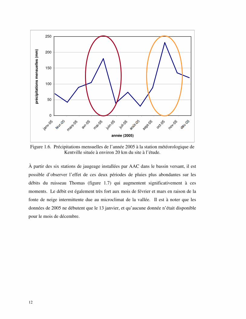
Figure 1.6. Précipitations mensuelles de l’année 2005 à la station météorologique de Kentville située à environ 20 km du site à l’étude. ...............................................12

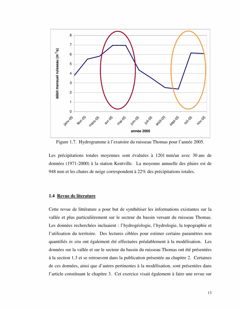
Figure 1.7. Hydrogramme à l’exutoire du ruisseau Thomas pour l’année 2005.........13

Figure 1.8. Bassin versant du ruisseau Thomas représenté par gOcad avec une exagération verticale de trois. ................................................................................28

Figure 2.1. Location of the Annapolis Valley. ............................................................34

Figure 2.2. Thomas Brook watershed land use. ..........................................................35

Figure 2.3. Bedrock geological map of the Valley (Rivard et al., 2005). ...................38

Figure 2.4. Surficial geology in the Thomas Brook watershed region from Paradis et al. (2006). ..............................................................................................39

Figure 2.5. Fieldwork location sites. ...........................................................................41

Figure 2.6. Potentiometric map of the bedrock obtained using water level measurements................................................................................................43

Figure 2.7. Guelph permeameter results. ....................................................................45

Figure 2.8. Stratigraphic information from the Cone Penetrometer Test (CPT).........46

Figure 2.9. Conceptual model of the Thomas Brook wathershed region (not to scale)................................................................................................................................47

Figure 2.10. Conceptual zonation of the study area for the numerical model. ...........49

Figure 3.1: The Annapolis Valley in Nova Scotia, Canada, showing the five watersheds and the location of the Thomas Brook catchment. .............................59

Figure 3.2. Thomas Brook (a) land use and topography and (b) bedrock potentiometric map. ...............................................................................................60

Figure 3.3. Bedrock geology of the Annapolis Valley (modified from Rivard et al., 2007b). ...................................................................................................................62

xiii

Figure 3.4. Surficial geology of the Thomas Brook catchment (modified from Paradis et al., 2006). ...........................................................................................................63

Figure 3.5. The 60 m x 60 m surface mesh representing the topography of the Thomas Brook catchment. .....................................................................................67

Figure 3.6. Geological reconstruction of the Thomas Brook catchment in vertical cross section along a north-south transect (not to scale). ......................................68

Figure 3.7. Zones and layers in the numerical model of the Thomas Brook catchment. The layers define the vertical discretization, and the zones and layers are used to attribute geological heterogeneity, laterally and vertically, respectively. .............69

Figure 3.8: Daily net atmospheric forcing (rainfall – evaporation), measured and simulated (scenario 1) outlet streamflow for 2005 on the Thomas Brook catchment...............................................................................................................70

Figure 3.9. Schematic of the seven scenarios of increasing geological complexity: 1) homogenous conditions; 2) addition of a layer for the surficial sediments; 3) definition of the principal bedrock formations; 4) incorporation of heterogeneity in porosity; 5) variable thickness of the surficial deposits; 6) addition of a sandy unit in the area around the catchment outlet; and 7) most complete geological representation corresponding to the reconstruction from field data.........................................................................................................................73

Figure 3.10. Simulated (scenario 9) and measured groundwater levels for different wells in the Thomas Brook catchment. .................................................................76

Figure 3.11. Simulated (scenario 9) and measured groundwater levels for monitoring wells #1 and #2. .....................................................................................................77

Figure 3.12. Measured and simulated (scenario 9) flow rates at the outlet for 2005. .78

Figure 3.13. Monthly simulated recharge (scenarios 8 and 9) and input atmospheric forcing (rainfall minus evaporation) for the period January 1 - December 31, 2005. ......................................................................................................................80

Figure 3.14. Distribution of simulated recharge (in m/s) on the Thomas Brook catchment on July 29 for scenario 9. The top chart shows the atmospheric input for year 2005, with the red pointer on July 29.......................................................83

Figure 3.15. Distribution of surface saturation state on the Thomas Brook catchment during the drier summer period (August 28) for scenario 9. The top chart shows the atmospheric input for year 2005, with the red pointer on August 28. .............84

Figure 3.16. Distribution of surface saturation state on the Thomas Brook catchment during the wetter autumn period (November 11) for scenario 9. The top chart shows the atmospheric input for year 2005, with the red pointer on November 11................................................................................................................................84

Figure 3.17. Distribution of water table depth along a transect of the Thomas Brook catchment on June 14 for scenario 9. The top chart shows the atmospheric input for year 2005, with the red pointer on June 14. The grid layers are illustrated with dotted lines.............................................................................................................85

xiv

LISTE DES TABLEAUX Table 2.1. Average hydraulic conductivity values for the three formations obtained

from various tests...................................................................................................44

Table 3.1. Model parameters kept fixed for all scenarios. ..........................................74

Table 3.2. Summary of simulated streamflow, two components of surface flow, and recharge for the nine scenarios. .............................................................................79

Table 3.3. Summary of numerical performance for the 9 scenarios. ..........................81

LISTE DES ANNEXES Annexe A : Données de terrain

Annexe B : Résultats de laboratoire

Annexe C : Scénarios de modélisation

* Les annexes sont présentées dans le DVD joint à ce mémoire.

xv

STRUCTURE DU MÉMOIRE

Ce mémoire est divisé en quatre chapitres. Le premier chapitre présente le contexte

général de l’étude, la problématique, la région étudiée, les objectifs, ainsi que la

méthodologie employée. Le lien avec un autre projet de maîtrise y est aussi décrit.

Le deuxième chapitre correspond à un compte-rendu rédigé pour la conférence du

volet canadien de l’AIH (Association Internationale des Hydrogéologues) tenue en

2006 à Vancouver; il décrit principalement les travaux de terrain réalisés et

l’interprétation des données existantes et acquises. Le troisième chapitre représente

l’article scientifique dédié à la modélisation couplée, ainsi qu’aux résultats obtenus se

rattachant aux interactions entre l’eau de surface et l’eau souterraine. Cet article sera

soumis en 2009 à une revue scientifique (Hydrogeology Journal) pour publication. Le

dernier chapitre sert de conclusion pour l’interprétation des interactions et l’utilisation

d’un modèle numérique couplé 3-D (CATHY). Les annexes contiennent des

informations complémentaires, principalement des données brutes de terrain avec leur

analyse, qui supportent les interprétations présentées dans le mémoire et les articles.

1

CHAPITRE 1 : Introduction

1.1 Contexte général

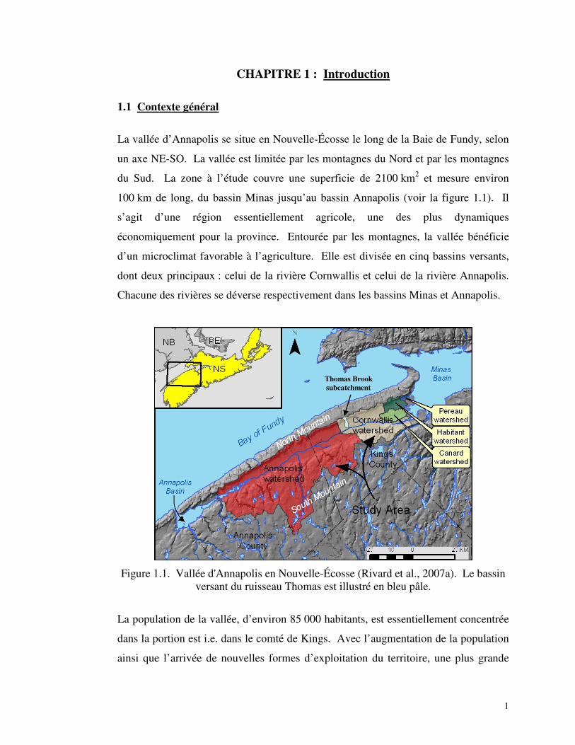
La vallée d’Annapolis se situe en Nouvelle-Écosse le long de la Baie de Fundy, selon

un axe NE-SO. La vallée est limitée par les montagnes du Nord et par les montagnes

du Sud. La zone à l’étude couvre une superficie de 2100 km2 et mesure environ

100 km de long, du bassin Minas jusqu’au bassin Annapolis (voir la figure 1.1). Il

s’agit d’une région essentiellement agricole, une des plus dynamiques

économiquement pour la province. Entourée par les montagnes, la vallée bénéficie

d’un microclimat favorable à l’agriculture. Elle est divisée en cinq bassins versants,

dont deux principaux : celui de la rivière Cornwallis et celui de la rivière Annapolis.

Chacune des rivières se déverse respectivement dans les bassins Minas et Annapolis.

Figure 1.1. Vallée d'Annapolis en Nouvelle-Écosse (Rivard et al., 2007a). Le bassin

versant du ruisseau Thomas est illustré en bleu pâle.

La population de la vallée, d’environ 85 000 habitants, est essentiellement concentrée

dans la portion est i.e. dans le comté de Kings. Avec l’augmentation de la population

ainsi que l’arrivée de nouvelles formes d’exploitation du territoire, une plus grande

Thomas Brook subcatchment

2

pression s’est exercée sur les cours d’eau et les gens délaissent progressivement l’eau

de surface et se tournent vers l’eau souterraine pour leur approvisionnement. En effet,

la population est maintenant alimentée presque uniquement par l’eau souterraine (par

des puits municipaux ou privés). On estime que dans le comté de Kings, près de 80%

de l’eau de surface est utilisée pour des fins agricoles (KCEDA, 2000).

Étant données les activités agricoles importantes de la vallée, les ressources en eau de

cette région sont grandement sollicitées et sujettes à une contamination par les

nitrates, les bactéries et les pesticides. Pourtant, la quantité et la qualité de l’eau

souterraine de la vallée étaient jusqu’à tout récemment relativement peu connues.

Pour cette raison, une étude hydrogéologique régionale a été entreprise par la

Commission géologique du Canada (CGC). Le projet ÉAVAC (Étude des aquifères

de la vallée Annapolis-Cornwallis) (Rivard et al., 2007a; 2007b), d’une durée de

trois ans, avait pour objectif de caractériser les aquifères de la vallée d’Annapolis et

ainsi améliorer la compréhension de l’hydrodynamique de ce système

hydrogéologique.

Ce projet de maîtrise s’insère dans le cadre du projet ÉAVAC et porte sur les

interactions entre l’eau de surface et l’eau souterraine. Une approche locale a été

favorisée pour la quantification des paramètres et le site principal d’étude est le bassin

versant du ruisseau Thomas situé près de la ville de Berwick, dans le comté de Kings

(voir Figure 1.1). Ce secteur d’environ 8 km2 a été sélectionné car il a été jugé

représentatif de la vallée en raison de sa géologie, sa topographie et ses activités

rurales. De plus, ce site faisait l’objet de travaux sur les eaux de surface par d’autres

organismes (Nova Scotia Agricultural College (NSAC) et par Agriculture et

Agroalimentaire Canada (AAC)) depuis 2001. Ainsi, des données de jaugeage et de

concentrations en nitrates étaient disponibles pour le ruisseau.

Les principales cultures du bassin versant du ruisseau Thomas sont le maïs, les fraises,

les pommes de terre, les pommes, et plusieurs aires de pâturage y sont présentes. La

population est d’environ 300 habitants et le secteur résidentiel se situe principalement

3

dans le sud du bassin, le long des chemins principaux. L’agriculture représente

environ 60% de la zone, les terrains boisés 30% et 10% est résidentiel.

Le but du projet de NSAC et d’AAC est de parvenir à une utilisation optimale des

fertilisants sur le territoire en collaboration avec les agriculteurs, et ainsi améliorer la

qualité de l’eau du ruisseau et de l’eau souterraine. Ce projet de maîtrise, s’arrimant

au projet de NSAC et d’AAC, visait à quantifier les échanges entre l’eau de surface et

l’eau souterraine circulant dans les dépôts meubles et le roc. Les résultats de cette

étude pourraient éventuellement être appliqués à l’ensemble de la vallée pour fournir

des ordres de grandeur de certaines composantes du cycle hydrologique

(ex. : recharge, ruissellement). La modélisation de la contamination de l’eau

souterraine par les nitrates sur le bassin du ruisseau Thomas fait l’objet d’un projet de

maîtrise entrepris par un étudiant de l’Université du Québec à Montréal

(Trépanier, 2008, voir plus bas à la section 1.9).

1.2 Problématique

La vallée d’Annapolis fait face à un problème potentiel de contamination de l’eau,

principalement dû aux activités agricoles. En effet, l’agriculture pratiquée de façon

intensive peut être une source importante de contamination des ressources en eau

(KCEDA, 2000). Comme le taux de croissance du comté de Kings est l’un des plus

élevés de la province et que ses activités agricoles sont essentielles, la connaissance de

la ressource en eau y est cruciale, tant au point de vue de sa qualité que de sa quantité.

En conséquence, il est important de bien comprendre les différentes composantes du

cycle hydrologique et les liens entre le lieu de contamination et la propagation du

contaminant dans l’environnement. Il est aussi important de considérer l’eau

souterraine et l’eau de surface comme étant une seule et unique ressource (Winter et

al., 1998; Sophocleous, 2002) puisqu’elles sont interdépendantes.

Dans la vallée d’Annapolis, des concentrations souvent élevées en nitrates et la

présence de bactéries ont été détectées dans l’eau de surface et/ou dans l’eau

4

souterraine (KCEDA, 2000; Trépanier, 2008; Rivard et al., 2007 a et 2007b). Selon

l’agence de développement économique du Comté de Kings, 25% des cours d’eau et

des lacs testés dans le comté de Kings en 1999 dépassaient la limite de 10 mg N-

NO3/L (Santé Canada, 2006) pour l’eau potable (KCEDA, 2000). Pour l’eau

souterraine, la base de données de la province montre qu’environ 15% des puits

dépassent la norme de 10 mg N-NO3/L, et environ 60% avaient des valeurs plus

élevées que 1 mg N-NO3/L (seuil des concentrations « naturelles » établi pour la

vallée), montrant que la ressource est affectée par les activités humaines (voir Rivard

et al., 2007a pour plus de détails). En ce qui concerne les puits des particuliers du

bassin du ruisseau Thomas, les pourcentages sont similaires, confirmant la

représentativité de la zone étudiée (voir Trépanier, 2008). Ces pourcentages ne sont

pas alarmants pour la santé humaine, mais suggèrent que les activités agricoles ont un

impact sur l’eau et que des mesures correctives doivent être entreprises pour protéger

les ressources en eau.

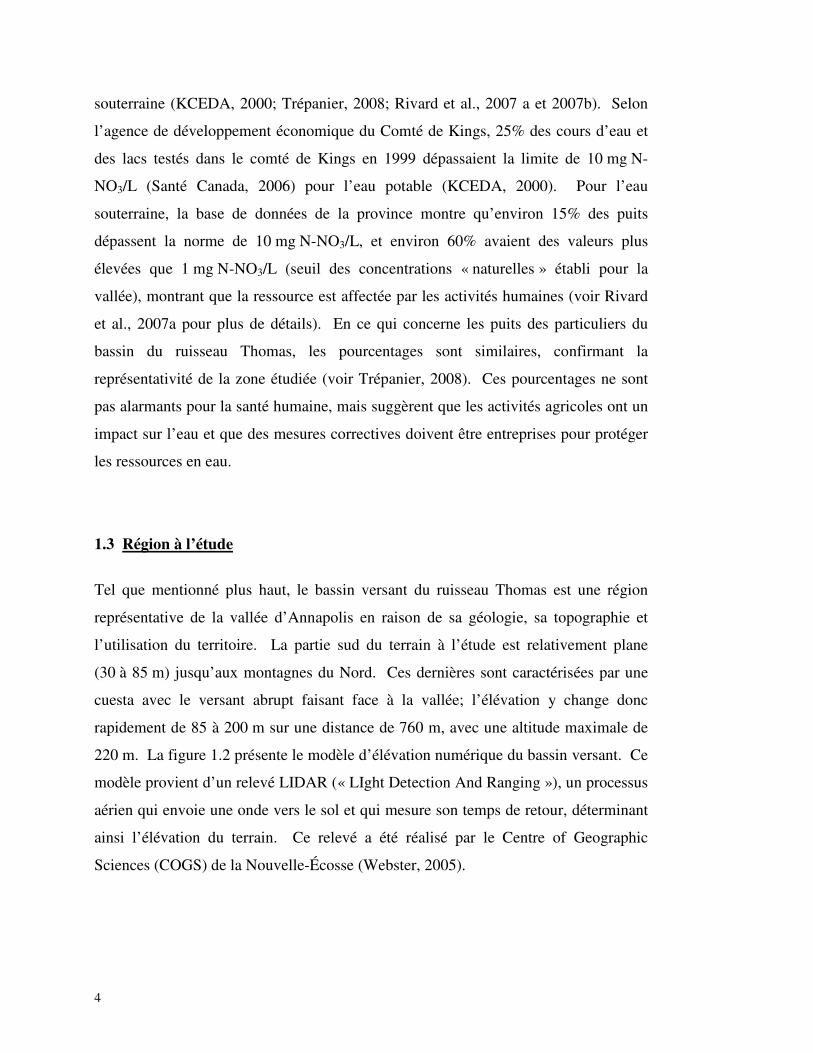
1.3 Région à l’étude

Tel que mentionné plus haut, le bassin versant du ruisseau Thomas est une région

représentative de la vallée d’Annapolis en raison de sa géologie, sa topographie et

l’utilisation du territoire. La partie sud du terrain à l’étude est relativement plane

(30 à 85 m) jusqu’aux montagnes du Nord. Ces dernières sont caractérisées par une

cuesta avec le versant abrupt faisant face à la vallée; l’élévation y change donc

rapidement de 85 à 200 m sur une distance de 760 m, avec une altitude maximale de

220 m. La figure 1.2 présente le modèle d’élévation numérique du bassin versant. Ce

modèle provient d’un relevé LIDAR (« LIght Detection And Ranging »), un processus

aérien qui envoie une onde vers le sol et qui mesure son temps de retour, déterminant

ainsi l’élévation du terrain. Ce relevé a été réalisé par le Centre of Geographic

Sciences (COGS) de la Nouvelle-Écosse (Webster, 2005).

5

�

Figure 1.2. Modèle numérique de terrain du bassin versant du ruisseau Thomas provenant d’un relevé LIDAR (Webster, 2005).

6

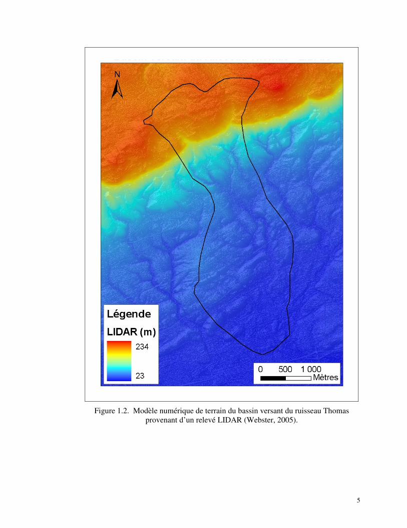
1.3.1 Géologie du socle rocheux

La vallée est caractérisée dans sa partie nord par trois formations géologiques datant

de l’ère Mésozoïque, de la période triassique. Elles appartiennent au groupe de Fundy

et recouvrent les roches du Paléozoïque qui forment la base du socle rocheux. On

retrouve en ordre chronologique : la formation de Wolfville, constituée

essentiellement de grès et de conglomérats avec un peu de shale et de siltstone; la

formation de Blomidon, composée d’une alternance de shale et de grès, mais ayant

une prédominance de strates à grains fins; et finalement la formation de North

Mountain, formée de basaltes tholéitiques (Trescott, 1968). Les formations de

Wolfville et de Blomidon se situent respectivement dans le centre de la vallée et sur le

flanc des montagnes du Nord; leur épaisseur maximale est de 833 et 363 m

respectivement (Crosby, 1962; Taylor, 1969; Smitheringale, 1973). La formation de

Blomidon recouvre celle de Wolfville, mais constituerait peut-être la continuité de la

formation de Wolfville avec un changement progressif de la composition lors de la

sédimentation (Trescott, 1968). En effet, la formation de Blomidon contient les

mêmes types de roches que celle du Wolfville, mais dans des proportions différentes.

La formation de North Mountain, quant à elle, recouvre la formation de Blomidon et

possède une épaisseur maximale de 427 m (Crosby, 1962). Ces trois formations, que

l’on retrouve également dans le secteur du ruisseau Thomas, sont décrites plus en

détails dans le premier article présenté au chapitre 2. Dans la partie sud de la vallée

d’Annapolis, les montagnes du Sud sont composées principalement de roches

granitiques ainsi que d’ardoises datant de l’ère Paléozoïque. La géologie du socle

rocheux de la vallée d’Annapolis, simplifiée par rapport à la version originale de

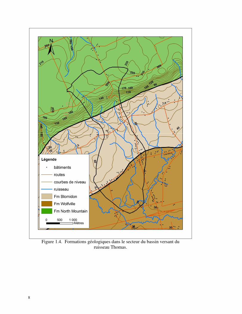
Keppie (2000), est présentée à la figure 1.3. La figure 1.4 présente un zoom de cette

figure sur le secteur du bassin versant du ruisseau Thomas à. La topographie, les

routes et les bâtiments y ont également été ajoutés.

7

�

Figure 1.3. Version simplifiée de la géologie du socle rocheux de la vallée d’Annapolis par Keppie (2000) (Rivard et al., 2007b). Le bassin du ruisseau Thomas est illustré en violet.

Thomas Brook subcatchment

8

Figure 1.4. Formations géologiques dans le secteur du bassin versant du

ruisseau Thomas.

9

1.3.2 Géologie des dépôts meubles

La vallée a été modelée par quatre phases glaciaires importantes : la phase

Calédonienne du Wisconsinien inférieur, la phase Escuminac du maximum glaciaire

au Wisconsinien supérieur, la phase Écossaise et la phase Chignecto (Bolduc et al, en

prép.; Rivard et al., 2007a). Ces épisodes glaciaires ont laissé sur le territoire

beaucoup de till ainsi que de nombreuses formes glaciaires telles que des drumlins,

des moraines et des eskers. Dans le centre de la vallée, on retrouve principalement du

matériel fluvioglaciaire (sables et graviers), orienté selon l’axe de la vallée, laissé par

les eaux de fonte en contact ou à proximité du glacier. Des dépôts marins sont

présents dans l’ouest de la vallée. Ceux-ci se sont déposés lors de l’invasion marine,

suite au retrait des glaces. Sur le versant sud des montagnes du Nord (la pente

abrupte), des lacs proglaciaires alimentés par les eaux de fonte du glacier ont laissé

des dépôts fins glaciolacustres.

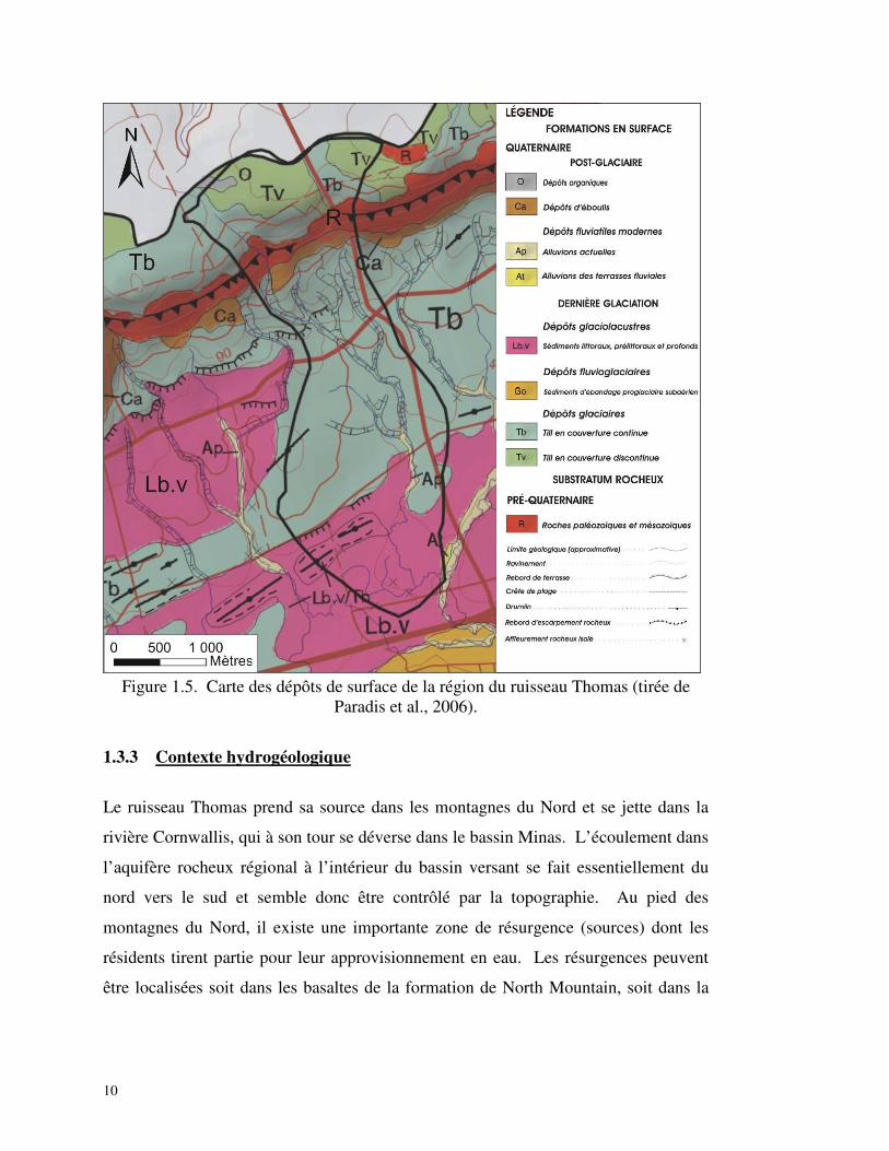
À l’intérieur du bassin versant du ruisseau Thomas (voir Figure 1.5), on retrouve du

till à matrice siltosableuse (Trépanier, 2008; Bolduc et al, en prép.) qui recouvre les

deux tiers de la superficie du bassin à partir des montagnes du Nord. Dans le tiers

inférieur du bassin, ce sont des dépôts glaciolacustres qui affleurent à la surface. Il

s’agit de boues silteuses, parfois sableuses et assez compactes contenant quelques

petits cailloux, qui pourraient facilement parfois se confondre avec le till présent sur le

territoire. Des dépôts fluvioglaciaires (sables) sont également présents, mais se

retrouvent sous les dépôts glaciolacustres. Des drumlins sont également présents dans

les parties centrale et sud des terres.

10

�

Figure 1.5. Carte des dépôts de surface de la région du ruisseau Thomas (tirée de Paradis et al., 2006).

1.3.3 Contexte hydrogéologique

Le ruisseau Thomas prend sa source dans les montagnes du Nord et se jette dans la

rivière Cornwallis, qui à son tour se déverse dans le bassin Minas. L’écoulement dans

l’aquifère rocheux régional à l’intérieur du bassin versant se fait essentiellement du

nord vers le sud et semble donc être contrôlé par la topographie. Au pied des

montagnes du Nord, il existe une importante zone de résurgence (sources) dont les

résidents tirent partie pour leur approvisionnement en eau. Les résurgences peuvent

être localisées soit dans les basaltes de la formation de North Mountain, soit dans la

11

formation de Blomidon, selon l’orientation des fractures, la topographie et la présence

ou non d’une couche imperméable en surface.

La formation rocheuse avec le potentiel aquifère le plus important est la formation de

Wolfville. Cependant, malgré la présence de strates moins perméables (ex : shale), la

formation de Blomidon peut à l’occasion fournir de très bons débits, en fonction de la

fracturation et des unités de grès rencontrées (Rivard et al., 2007a). Les basaltes des

montagnes du Nord peuvent également être localement relativement transmissifs en

fonction de l’interconnexion des fractures. Dans le secteur du ruisseau Thomas, la

quasi-totalité des puits sont au roc et les autres sont alimentés par les sources

localisées au bas des montagnes du Nord. L’aquifère rocheux est souvent confiné en

raison d’une couche imperméable à la surface formée par les shales et le siltstone ou

par les boues glaciolacustres, ou par une absence de fracturation.

1.3.4 Contexte hydrologique

La région est caractérisée par deux périodes de précipitations importantes au

printemps (principalement au mois de mai) et en automne (essentiellement au mois

d’octobre). Les données de la figure 1.6, présentant les précipitations totales

mensuelles à la station de Kentville, proviennent du site d’Environnement Canada

(2004).

12

0

50

100

150

200

250

janv-0

5

mars-0

5

avr-0

5

mai-05

juin-0

5jui

l-05

sept-

05

oct-0

5

nov-0

5

année (2005)

préc

ipita

tions

men

suel

les

(mm

)

�

Figure 1.6. Précipitations mensuelles de l’année 2005 à la station météorologique de Kentville située à environ 20 km du site à l’étude.

À partir des six stations de jaugeage installées par AAC dans le bassin versant, il est

possible d’observer l’effet de ces deux périodes de pluies plus abondantes sur les

débits du ruisseau Thomas (figure 1.7) qui augmentent significativement à ces

moments. Le débit est également très fort aux mois de février et mars en raison de la

fonte de neige intermittente due au microclimat de la vallée. Il est à noter que les

données de 2005 ne débutent que le 13 janvier, et qu’aucune donnée n’était disponible

pour le mois de décembre.

13

0

1

2

3

4

5

6

7

8

janv-0

5

mars-0

5

avr-0

5

mai-05

juin-0

5jui

l-05

sept-

05

oct-0

5

nov-0

5

année 2005

débi

t men

suel

rui

ssea

u (m

3 /s)

�

Figure 1.7. Hydrogramme à l’exutoire du ruisseau Thomas pour l’année 2005.

Les précipitations totales moyennes sont évaluées à 1201 mm/an avec 30 ans de

données (1971-2000) à la station Kentville. La moyenne annuelle des pluies est de

948 mm et les chutes de neige correspondent à 22% des précipitations totales.

1.4 Revue de literature

Cette revue de littérature a pour but de synthétiser les informations existantes sur la

vallée et plus particulièrement sur le secteur du bassin versant du ruisseau Thomas.

Les données recherchées incluaient : l’hydrogéologie, l’hydrologie, la topographie et

l’utilisation du territoire. Des lectures ciblées pour estimer certains paramètres non

quantifiés in situ ont également été effectuées préalablement à la modélisation. Les

données sur la vallée et sur le secteur du bassin du ruisseau Thomas ont été présentées

à la section 1.3 et se retrouvent dans la publication présentée au chapitre 2. Certaines

de ces données, ainsi que d’autres pertinentes à la modélisation, sont présentées dans

l’article constituant le chapitre 3. Cet exercice visait également à faire une revue sur

14

la modélisation couplée, pour voir ses avantages et les différences majeures entre les

modèles existants, et sur l’intégration de l’hétérogénéité dans les modèles.

Modélisation couplée

L’utilisation d’un modèle couplé ou d’un modèle hydrogéologique est possible pour

représenter les écoulements souterrains et valider des combinaisons de paramètres

(conductivités hydrauliques et taux de recharge). La modélisation couplée permet

d’intégrer les écoulements de surface aux écoulements souterrains via un terme

d’interaction représentant le flux traversant la surface du sol. Ce terme permet de

traiter ces deux systèmes interdépendants comme une seule et même ressource

(Winter et al., 1998). Ainsi, les modèles couplés, bien que numériquement plus

complexes, permettent d’étudier de façon détaillée les processus d’échange entre les

écoulements de surface et les écoulements souterrains.

Les facteurs à prendre en considération pour une modélisation couplée incluent le

climat, la topographie, la géologie, la végétation et l’utilisation du territoire, tout

comme pour une évaluation détaillée de la recharge. Toutefois, les difficultés

inhérentes à la quantification des échanges proviennent principalement de

l’hétérogénéité du système représenté (et donc aussi du type de modèle utilisé) et du

problème d’échelle relié au différent maillage de chacun des écoulements

(Sophocleous, 2002). En effet, à cause des différences dans les temps de séjour et les

épaisseurs à considérer pour le milieu de surface et le milieu souterrain, les systèmes

représentés par des modèles couplés doivent être relativement simples pour éviter les

instabilités numériques et les temps de calcul trop longs. De plus, l’utilisation d’un

modèle simple est recommandée au départ dans la plupart des cas afin de bien

comprendre les mécanismes hydrologiques de base (Hill, 2006; Kelson et al., 2002).

Cependant, une représentation trop simplifiée, même avec un modèle robuste

numériquement et représentant les divers paramètres du bilan hydrique, pourrait ne

pas refléter adéquatement la réponse physique du système (Hunt et al., 2007). C’est

pourquoi, une modélisation nécessite généralement plusieurs étapes, afin d’intégrer

15

une hétérogénéité suffisante pour représenter de façon raisonnable le système étudié

en fonction des besoins de l’étude.

Des solutions analytiques ont été proposées par Barlow et Moench (1998) pour

quantifier les interactions entre les écoulements souterrains et de surface en mode

transitoire. Cette approche permet d’étudier les débits d’émergence (« discharge ») au

cours d’eau en réponse à la recharge, et de prédire rapidement les réponses de

l’aquifère suite aux changements de niveau du cours d’eau, tels que des événements

d’inondation. Ces solutions assument un écoulement horizontal en une dimension

pour les aquifères captifs et semi-captifs et un écoulement horizontal et vertical en

deux dimensions pour les nappes libres. Ces solutions analytiques résolues par

convolution (méthode de superposition) sont fondées sur l’équation différentielle

d’écoulement souterrain transitoire pour un aquifère saturé, homogène, légèrement

compressible et anisotrope. Cependant, cette approche ne s’applique qu’au module

souterrain et ne permet pas de représenter un aquifère hétérogène, ni des conditions

limites complexes.

Les modèles numériques sont plus complexes à bâtir et à utiliser, mais ils sont

beaucoup plus souples au niveau des conditions limites, de l’intégration de

l’hétérogénéité des formations géologiques et des directions d’écoulement. Singh et

Bhallamudi (1998) ont été dans les premiers à développer un modèle numérique

couplé bidimensionnel simulant l’écoulement de surface («overland flow») avec

l’équation de Saint-Venant (1-D) et l’écoulement de sous-surface selon l’équation de

Richards (2-D). Le modèle a démontré sa robustesse et son applicabilité à des cas

assez complexes impliquant de la variation spatiale pour les caractéristiques du sol.

VanderKwaak et Loague (2001) ont développé un modèle couplé numérique en 3-D

appelé InHM. Ce modèle utilise une équation 2-D non-linéaire de l’onde de diffusion

(St-Venant) ainsi que l’équation de Manning afin de simuler l’écoulement de surface

et l’équation de Richards en 3-D afin de représenter l’écoulement souterrain. Un des

avantages de ce modèle est qu’il détermine lui-même le réseau de drainage, à savoir

16

où l’eau s’infiltre, s’exfiltre, forme les réseaux hydriques de surface ou les zones

humides en fonction de l’interaction entre les modules de surface et de sous-surface.

Ces auteurs ont démontré l’importance de la représentation des deux mécanismes de

saturation, soit celui de Dunne consistant en un excès de saturation du sol et celui de

Horton correspondant à un excès d’infiltration suite à de fortes précipitations. Dans le

cas étudié par ces auteurs, présentant les réponses d’un bassin versant suite à

différents événements de précipitations, il a été observé que des informations précises

sur l’emmagasinement d’eau dans le sol, telles que la position de la nappe et les zones

de fortes teneur en eau, pouvaient être plus importantes qu’une estimation détaillée de

la perméabilité pour les simulations s’intéressant aux effets des précipitations sur le

ruissellement. Jones et al. (2008) ont appliqué ce modèle à un bassin versant de

75 km2 en Ontario. Cette étude a permis de montrer que le modèle pouvait bien

représenter les processus hydrodynamiques à cette échelle, dont la réponse du bassin

versant aux différents événements de précipitations.

Panday et Huyakorn (2004) ont développé un modèle numérique qui inclut une

solution en trois dimensions pour l’écoulement souterrain saturé – non-saturé

(équation de Richard) couplé avec des solutions en une et deux dimensions pour

l’écoulement de surface (approximation de l’équation de l’onde de diffusion de

St-Venant). Ce modèle intègre des composantes « secondaires » ayant un impact sur

l’écoulement de l’eau telles que les infrastructures, l’irrégularité du fond du cours

d’eau, l’effet d’emmagasinement dans les dépressions et la présence de végétation

dans les cours d’eau (obstruction à l’emmagasinement). De plus, l’évapotranspiration

est modélisée en utilisant des facteurs climatiques et la couverture végétale. De façon

plus détaillée, les conditions limites dans ce modèle peuvent être assignées à l’aide de

charges hydrauliques ou de flux. Le modèle de sous-surface est discrétisé en

différences finies et le maillage (de surface et souterrain) peut être déformé afin de

mieux représenter les limites appliquées. Les cours d’eau sont représentés par des

volumes finis indépendants qui se superposent aux réseaux hydrauliques de surface et

souterrain. Les domaines sont soit couplés entièrement par les équations

gouvernantes selon un terme d’interaction q, soit le couplage s’effectue selon une

17

approche de liaisons/itérations («linking/iterative»). Cette dernière approche peut

s’effectuer selon deux options. La première applique directement les flux de liaison à

chacun des domaines comme conditions limites. Pour la deuxième option, les charges

hydrauliques de surface sont utilisées en tant que limite hydraulique générale pour

résoudre les équations de sous-surface. Les charges hydrauliques souterraines sont

également considérées comme limite hydraulique générale dans la résolution des

équations de surface. La méthode de Newton-Raphson (méthode de Picard modifiée)

est utilisée afin de résoudre les équations non-linéaires avec un pas de temps adaptatif.

Pour l’approche itérative (liaison/itérations), le pas de temps pour le module de

surface est également adaptatif en fonction de celui du module de sous-surface.

L’exemple exposé dans Panday et Huyakorn (2004) présente un aquifère homogène

(loam sableux) en contact hydraulique avec le réseau hydrique de surface (cours

d’eau). L’étude de sensibilité a démontré l’importance de la variation des paramètres

physiques d’écoulement de surface (coefficients de friction de Manning, porosité,

paramètres de van Genuchten, niveau initial de la nappe) sur la réponse du débit du

cours d’eau à l’exutoire. Les désavantages potentiels d’utiliser des solutions de type

« liaison/itération » («linking/iterative») pour des cas complexes avec des flux

d’échange entre les deux modules importants ont également été identifiés. Ces cas

demandent des pas de temps plus grands en raison de leur complexité pour une

convergence plus rapide, alors que cette approche n’est efficace qu’avec des pas de

temps rapprochés.

Le modèle de Panday et Huyakorn (2004) est similaire à CATHY, le modèle utilisé

dans cette étude (Bixio et al., 2000). Les mêmes équations sont employées dans les

deux modèles, mais la représentation du routage de surface, la résolution numérique,

ainsi que le traitement du terme de couplage sont quelques-une des différences

importantes. Les caractéristiques du logiciel CATHY sont présentées au chapitre 3.

Anderson (2005) a présenté un modèle numérique simple d’interactions entre l’eau de

surface et l’eau souterraine basé sur l’équation de Dupuit (développée pour un

18

aquifère homogène à nappe libre dont l’écoulement est horizontal et uniforme). Tel

qu’anticipé, l’approximation engendre des erreurs principalement en cas d’écoulement

vertical. L’auteur propose alors un modèle alternatif avec, comme paramètre

indépendant de l’aquifère, la résistance du lit du cours d’eau , ce qui permet de réduire

considérablement les erreurs observées sur les charges hydrauliques et/ou les débits.

Afin de bien représenter les interactions, les modèles numériques doivent

généralement présenter une discrétisation verticale plus fine pour modéliser

adéquatement les écoulements verticaux, impliquant ici un temps de calcul pour la

convergence plus important. Avec ce modèle, la discrétisation verticale ne s’avère

pas nécessaire puisque la résistance à l’écoulement vertical est intégrée au modèle en

tant que paramètre efficace. En effet, ce paramètre, souvent négligé ou bien considéré

comme paramètre intrinsèque de l’aquifère, engendre souvent des erreurs puisqu’il

n’est pas considéré comme dynamique (ou efficace), i.e. indépendant des conditions

d’écoulement. L’auteur conclut toutefois que cette approche est surtout utile dans les

cas où le détail des interactions entre l’eau de surface et l’eau souterraine n’est pas le

but premier de l’étude, mais bien pour les cas où les cours d’eau sont représentés dans

le modèle en tant que conditions limites.

Hantush (2005) a étudié les interactions eau de surface / eau souterraine en cas

d’inondation et de période sèche (débit de base, soit lorsque les cours d’eau sont

uniquement alimentés par les aquifères) avec des représentations linéaires (en 1-D) de

l’équation de Boussinesq pour un aquifère non confiné avec un écoulement souterrain

horizontal et de la fonction de stockage (utilisation de la méthode de Muskingum

représentant un système linéaire de transfert d'écoulement en rivière). Cette étude,

bien que limitée par ces simplifications, a démontré la robustesse de ses solutions pour

des applications variées tels que les problèmes d’emmagasinement riverain, l’effet des

périodes sèches ainsi que les interactions entre l’eau de surface et l’eau souterraine, en

traitant les systèmes hétérogènes comme une série de systèmes homogènes.

19

Intégration de l’hétérogénéité de la géologie

L’hétérogénéité dans un modèle peut y être intégrée en utilisant des propriétés

équivalentes (moyennes) ou en essayant de décrire la variabilité spatiale des propriétés

des dépôts et du roc à partir d’observations géologiques et de mesures locales

(de Marsily et al., 2005). Toutefois, la représentation d’une géologie complexe dans

un modèle est habituellement limitée par un manque de données sur les réseaux de

fractures et les discontinuités, ainsi que par le nombre disponible des résultats d’essais

de pompage sur les différentes formations géologiques. En effet, les propriétés

hydrogéologiques, et particulièrement la conductivité hydraulique, sont très variables

et ce, à toutes les échelles. La technique de généralisation («upscaling») est souvent

employée en modélisation afin de simplifier les cas complexes (Sánchez-Vila et

al., 1995). Elle consiste à attribuer une valeur équivalente pour une zone donnée en se

servant de diverses approches, généralement des moyennes (par exemple la moyenne

géométrique des valeurs de conductivité hydrauliques disponibles). Selon ces auteurs,

bien que ce type d’approche implique une perte d’information sur l’hétérogénéité

locale, cela permet de traiter un cas complexe de façon plus simple en intégrant les

mesures prises sur le terrain.

La quantité appropriée de données nécessaires pour une étude doit être bien évaluée,

tout comme le temps et l’argent consacrés au développement d’un modèle et aux

travaux de terrain. Ceci est particulièrement important pour les modèles couplés qui

possèdent des dynamiques très différentes dans leurs modules de surface et souterrain,

augmentant ainsi considérablement les coûts de simulation. En complexifiant

graduellement la géologie, cela permet de limiter les temps de calcul durant l’étude

des impacts numériques et physiques de la représentation de l’hétérogénéité. En effet,

il peut souvent s’avérer avantageux de commencer par modéliser un site avec un

système homogène ou ayant une hétérogénéité faible avant de complexifier le modèle

pour mieux représenter son hétérogénéité (Philip, 1980).

20

Cependant, il faut garder en tête que l’écoulement est beaucoup moins sensible à la

connexité des fractures ou des zones perméables et à l’hétérogénéité en général que le

transport, et donc que les études s’intéressant à la quantification des différentes

composantes du cycle hydrologique et aux interactions peuvent souvent être étudiés

en utilisant des résultats d’essais de pompage moyens suivis d’un modèle de

calibration afin d’obtenir de l’information pertinente pour la gestion des aquifères

(de Marsily et al., 2005).

Afin d’explorer le concept d’homogénéité équivalente, Binley et al. (1989) ont utilisé

un modèle numérique 3-D couplé à écoulement saturé variable, appliqué sur un bassin

versant hétérogène. Différents patrons de conductivité hydraulique ont été utilisés

afin de déterminer une seule conductivité hydraulique équivalente capable de

reproduire les hydrogrammes de surface et de sous-surface. Il en ressort que pour les

cas présentant des sols très perméables, les conductivités hydrauliques équivalentes

pour les 16 cas étudiés ont bien reproduit les hydrogrammes de rivière et de sous-

surface, alors que pour des sols de faible perméabilité, caractérisés par un haut taux de

ruissellement de surface, aucune des conductivités hydrauliques pour les cinq cas

étudiés n’a su reproduire les réponses d’écoulement de surface (dominé par le

ruissellement) et de sous-surface observés. Dans chacun des cas, en essayant de faire

correspondre l’écoulement de sous-surface, cela avait pour effet de sous-estimer le

ruissellement, et d’un autre côté, en essayant de faire correspondre l’hydrogramme de

rivière, cela avait pour effet de sous-estimer la réponse de l’écoulement souterrain.

Par ailleurs, Kim and Stricker (1996) ont étudié l’effet de l’hétérogénéité spatiale

horizontale des propriétés du sol ainsi que des précipitations en utilisant des

simulations Monte Carlo. L’une des principales conclusions qui ressortait de l’étude

est que le ruissellement de surface domine sur l’effet de l’hétérogénéité spatiale dans

le calcul des composantes du bilan hydrique, principalement lorsque les sols sont fins

(peu perméables). Ces deux études suggèrent que la caractérisation et la prise en

compte de l’hétérogénéité dans le cas de formations géologiques peu perméables sont

particulièrement importantes pour la reproduction adéquate des réponses du système.

21

Finalement, Kampf et Burges (2007) ont récemment fait une revue des modèles

couplés qui emploient des simulations inverses afin d’identifier les paramètres

hydrauliques du sol. Ces études ont porté sur la zone vadose in situ ainsi que sur des

colonnes de sol expérimentales. Cette revue met en évidence que les cas de géologie

plus complexe posent de grands défis. Elle montre que de nombreuses mesures sont

nécessaires (débit à l’exutoire ainsi que la teneur en eau ou les charges hydrauliques)

afin d’identifier des paramètres uniques lors de simulations inverses sur des colonnes

de sol expérimentales. L’efficacité des simulations inverses à trouver les paramètres

hydrauliques du sol, qui décrivent tant le débit à l’exutoire que les pressions d’eau et

la teneur en eau, dépend de la nature de l’hétérogénéité du sol. Cet article souligne

aussi qu’étant donné qu’il est pratiquement impossible de collecter des mesures

détaillées sur les propriétés hydrauliques du sol à grande échelle, beaucoup d’études

ont recours à des techniques de généralisation («upscaling») à partir des quelques

valeurs obtenues sur le terrain ou même en laboratoire afin de déterminer des

paramètres équivalents.

1.5 Objectifs du mémoire

Les objectifs principaux de ce mémoire sont :

1- Améliorer la compréhension de l’écoulement souterrain et des interactions eau

de surface – eau souterraine au moyen de données existantes et acquises sur le

terrain pour le bassin du ruisseau Thomas.

2- Simuler les écoulements de surface et souterrain ainsi que les échanges

hydrauliques au moyen du modèle numérique couplé 3D CATHY

(CATchment Hydrologic); quantifier l’infiltration, le ruissellement, la recharge

à l’aquifère rocheux, les échanges entre la surface et l’aquifère; et visualiser

les patrons d’écoulement.

22

3- Étudier le rôle de l’hétérogénéité du bassin du ruisseau Thomas sur le calage

du modèle en raffinant la géologie; évaluer l’effet de l’intégration du couvert

de neige.

1.6 Méthodologie

1.6.1 Compilation de données

À partir d’une base de données compilée par la CGC (Rivard et al., 2007a), diverses

informations ont été sélectionnées afin de caractériser le bassin versant du ruisseau

Thomas et d’identifier les données manquantes. Les données compilées proviennent

de divers organismes fédéraux et provinciaux et de collèges:

- Nova Scotia Environment and Labour (NSEL);

- Commission géologique du Canada (CGC);

- Nova Scotia Department of Natural Resources (NSDNR);

- Nova Scotia Agricultural College (NSAC);

- Centre Of Geographic Sciences (COGS);

- et Agriculture et Agroalimentaire Canada (AAC).

Certaines informations issues de la littérature ont également été ajoutées pour

compléter les données manquantes. Grâce à toutes ces données, il a été possible de

réaliser des coupes topo-géologiques ainsi que des cartes géologiques et

piézométrique permettant d’obtenir une connaissance générale du site.

1.6.2 Travaux de terrain

Les campagnes de terrain, réalisées en collaboration avec la CGC durant les étés 2004,

2005 et 2006, représentent une partie importante du projet et ont permis de recueillir

beaucoup d’informations. Ces travaux, décrits dans le premier article au chapitre 2,

incluent : une campagne piézométrique, des sondages, l’installation de piézomètres,

une campagne d’échantillonnage d’eau (isotopes d’hydrogène et d’oxygène, isotopes

23

de nitrates, ions majeurs et mineurs, nitrates, bactéries) et de sol, des essais

hydrauliques, des mesures de débits du ruisseau à l’aide d’un vélocimètre (flowmeter),

et l’utilisation de méthodes géophysiques (diagraphies et géoradar). Les essais

hydrauliques comprennent des essais avec un perméamètre de Guelph pour estimer la

perméabilité du premier mètre de sol, des essais de perméabilité (slug tests), de

pompage et de type Lugeon (packer tests) afin d’évaluer la conductivité hydraulique

des formations rocheuses, et des mesures d’infiltration sous le ruisseau Thomas

(seepage meter) pour connaître la perméabilité des sédiments du ruisseau. De plus, un

suivi de l’évolution des niveaux d’eau durant deux années dans des puits au roc a été

fait au moyen de capteurs de pression avec enregistrement continu aux six heures.

Ces capteurs ont été placés dans des puits résidentiels en juillet 2004. En juin 2006,

sept puits ont été échantillonnés dans la vallée pour dater l’eau souterraine à l’aide

d’analyses de tritium et de carbone 14, dont cinq stations situées à l’intérieur du bassin

et réparties dans les trois formations rocheuses (Wolfville, Blomidon et North

Mountain).

Durant ces travaux de terrain, quelques problèmes sont survenus. L’installation de

piézomètres avait pour objectif d’observer le niveau d’eau dans les dépôts meubles et

de procurer des échantillons d’eau. Cependant, lors des sondages, il s’est avéré que

les sédiments dans le secteur du ruisseau Thomas avaient moins de 5 m d’épaisseur

(contrairement à ce que pouvait suggérer la base de données provinciale) et n’étaient

jamais saturés. En effet, la campagne de terrain de 2005 a révélé que les dépôts de

surface dans la vallée étaient souvent nettement moins épais que ce que laissaient

croire les bases de données, suggérant que le till compact retrouvé un peu partout dans

la vallée ne pouvait pas être différencié du grès friable de la formation de Wolfville

lors de forages conventionnels réalisés par des foreurs. Plusieurs descriptions de la

base de données indiquaient la présence de sable, qui en fait correspondait plutôt au

grès altéré du Wolfville. Aucun niveau d’eau n’a pu être mesuré dans les dépôts de

surface (la nappe étant toujours plus basse) et donc aucune observation n’est

disponible concernant les gradients verticaux dans les sédiments de surface dans le

bassin étudié.

24

Plusieurs participants ont pris part à cette campagne de terrain. Les organismes

impliqués sur le site du ruisseau Thomas sont les suivants :

- la Commission Géologique du Canada (CGC);

- l’Institut National de la Recherche Scientifique, Eau-Terre-

Environnement (INRS-ETE);

- l’Université du Québec à Montréal (UQAM);

- l’Université Acadia;

- le Centre of Geographic Sciences (COGS);

- et le U.S. Geological Survey (USGS).

L’ensemble des résultats de cette étude a été intégré dans la base de données de la

CGC. Ces informations sont disponibles à tous les participants du projet ÉAVAC à

l’adresse électronique suivante : http://www.cgcq.rncan.gc.ca/annapolis/membres/.

De plus, des résultats partiels et certaines cartes de ce projet de maîtrise sont présentés

dans le rapport final et l’atlas du projet ÉAVAC (Rivard et al., 2007a; 2007b).

1.6.3 Analyses des données

L’analyse des données récoltées sur le terrain a permis d’estimer un taux de recharge

pour l’année 2005 et des valeurs de conductivités hydrauliques, de tracer une carte

piézométrique et de concevoir un modèle conceptuel du terrain étudié.

L’interprétation des résultats de laboratoire provenant des échantillons de sol et d’eau

a également permis de raffiner le portrait général de l’hydrogéologie de la région. Ces

résultats incluent des données de signatures d’isotopes stables (δ18O et δ2H), de

datation au tritium et carbone 14, ainsi que des granulométries. Les résultats de ces

analyses sont présentés à la section 2.5.4, dans le premier article au chapitre 2 et en

annexe.

Quatre approches ont été mises en œuvre pour l’évaluation de la recharge du bassin

versant du ruisseau Thomas. Les deux premières utilisent la séparation

d’hydrogramme avec les données de la station de jaugeage à l’exutoire. Les données

25

de jaugeage fournies sont incomplètes (de mai à octobre) aux cinq autres stations,

limitant l’information à la saison agricole. La troisième approche est la méthode

graphique informatisée de Posavec (Posavec et al., 2006) avec les données des deux

hydrogrammes de puits résidentiels, et la quatrième correspond à un bilan hydrique.

Pour la séparation d’hydrogramme, le filtre numérique de Furey et Gupta (2001) et la

méthode graphique Recess/Rora (développée par le USGS, Rutledge, 1998) ont été

utilisés. Pour calculer la recharge à partir des hydrogrammes de puits nous avons fait

l’hypothèse que la nappe dans les puits est à surface libre. Ceci est justifié par la

superposition des fluctuations de la nappe avec la pluviométrie de la région (station de

Kentville) et les informations fournies par les propriétaires du puits (principalement

du grès dans les deux cas). Ainsi, la recharge calculée à partir des niveaux d’eau dans

les puits (Healy et Cook, 2002) identifie la courbe de récession maîtresse du puits

avec une porosité effective de 10% estimée grâce à la littérature (Todd, 1980). Seule

l’année 2005 a été utilisée pour les calculs, les autres années ayant été jugées

incomplètes. Les données de la station de jaugeage située à l’exutoire du bassin

couvrent la période du 13 janvier au 30 novembre 2005 (le reste de l’année, un

couvert de glace empêchait la prise de mesures).

L’analyse des essais de perméabilité aux puits (slug tests et packer test), de pompage

et de perméamètre de Guelph a permis d’obtenir des valeurs de propriétés

hydrauliques pour le roc et les dépôts de surface. L’interprétation des essais de

perméabilité aux puits s’est faite au moyen de la méthode de Bouwer et Rice (1976)

pour les aquifères captifs et libres. Les méthodes de Theis (1935) et de Cooper et

Jacob (1946) ont permis d’interpréter l’essai de pompage effectué. En ce qui a trait

aux données de perméamètre de Guelph, elles ont été analysées selon les méthodes

décrites dans le manuel d’utilisation (Soilmoisture Equipment Corporation, 2005). À

peu près la moitié des essais ont fourni des résultats négatifs avec la méthode

conventionnelle (à double charge hydraulique) et ont donc dû être ré-interprétés avec

la méthode à une seule charge appliquée séparément à chacune des deux charges (une

moyenne a ensuite été calculée, selon la méthode décrite dans Soilmoisture

26

Equipment Corporation, 2005). Les résultats négatifs se produisent généralement en

présence d’hétérogénéité verticale du matériau testé (stratification, racines, cailloux).

1.7 Résultats

Les valeurs de recharge suivantes ont été obtenues pour l’année 2005: 535 mm/an

avec la séparation d’hydrogramme avec le filtre de Furey et Gupta (2001); 585 mm/an

avec la séparation d’hydrogramme selon le modèle numérique de Recess/Rora;

316 mm/an avec la séparation d’hydrogramme de puits selon le modèle numérique de

Posavec, et 318 mm/an avec la méthode du bilan hydrique. Les deux premières

méthodes présentées ici (séparation d’hydrogramme) ainsi que le bilan hydrique

représentent approximativement les quantités d’eau infiltrées, et donc une quantité

maximale pouvant atteindre la nappe. Une partie seulement de cette eau recharge

réellement la nappe régionale tandis qu’une autre partie s’écoule en subsurface

(écoulement hypodermique) jusqu'au ruisseau ou remonte à la surface par résurgence

sans possibilité de retour à la nappe au roc. Pour cette raison, et en comparaison avec

la valeur de 312 mm/an obtenue par Trépanier (2008), ainsi que les valeurs nettement

plus faibles obtenues dans le projet ÉAVAC (115 à 225 mm/an), une valeur de

315 mm/an a été retenue. Basée sur une seule année (2005), cette valeur de recharge

n’est pas nécessairement représentative des conditions moyennes de recharge de

l’aquifère, mais dans le cas de ce projet de maîtrise, le but était de modéliser les

différents processus pour une année donnée. Une valeur d’évapotranspiration

potentielle de 689 mm/an a été estimée selon l’équation de Penman-Monteith

(FAO, 2004).

Les résultats de laboratoire ont montré que les signatures isotopiques de l’eau

souterraine et l’eau de surface sont similaires à celles des précipitations, suggérant que

l’eau dans les différentes formations géologiques du bassin versant a rechargé

l’aquifère dans des conditions climatiques similaires à celles d’aujourd’hui. Les

résultats de datation de tritium et carbone 14 sont en accord avec le patron

d’écoulement indiqué par la carte piézométrique (voir chapitres 2 et 3), à savoir que

27

l’eau dans le roc circule des montagnes du Nord vers le fond de la vallée. L’eau la

plus récente a été identifiée dans les montagnes du Nord, l’eau « mélangée » dans la

formation Blomidon et l’eau datant d’avant 1952 provient de la formation de

Wolfville (un échantillon indiquait un âge approximatif de 5000 ans). Finalement, en

combinaison avec les conductivités hydrauliques obtenues avec le perméamètre de

Guelph, les granulométries ont permis de raffiner les valeurs de conductivités

hydrauliques des sédiments répartis sur le bassin versant.

La représentation des dépôts meubles a été faite dans gOcad 6.1.6 ® par Andrée

Bolduc de la CGC pour la région du ruisseau Thomas, principalement à partir de la

carte quaternaire de la vallée (Paradis et al., 2006) présentée à la figure 1.8. Cette

carte apporte une meilleure compréhension de la zone à l’étude et a contribué à

développer le modèle conceptuel du bassin.

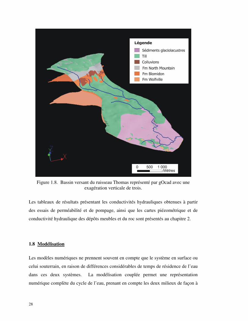
28

Figure 1.8. Bassin versant du ruisseau Thomas représenté par gOcad avec une

exagération verticale de trois.

Les tableaux de résultats présentant les conductivités hydrauliques obtenues à partir

des essais de perméabilité et de pompage, ainsi que les cartes piézométrique et de

conductivité hydraulique des dépôts meubles et du roc sont présentés au chapitre 2.

1.8 Modélisation

Les modèles numériques ne prennent souvent en compte que le système en surface ou

celui souterrain, en raison de différences considérables de temps de résidence de l’eau

dans ces deux systèmes. La modélisation couplée permet une représentation

numérique complète du cycle de l’eau, prenant en compte les deux milieux de façon à

29

pouvoir étudier et quantifier les échanges à l’intérieur d’un bassin. Pour ce projet, le

logiciel 3-D couplé CATHY (CATchment HYdrologic) (Bixio et al., 2000;

Camporese et al., 2008), actuellement en développement à l’INRS-ETE, a été utilisé.

Ce modèle procure des informations spatialement distribuées sur les échanges eau de

surface – eau souterraine, notamment ceux ayant lieu à la limite de la zone saturée et

de la zone non saturée. L’effet de l’hétérogénéité sur le modèle a également été étudié

dans le cadre de ce projet afin d’évaluer le niveau d’information et de représentation

requis pour reproduire adéquatement le système réel. Les résultats du modèle

développé dans CATHY ont permis d’étudier les différentes composantes du cycle

hydrologique et de visualiser les patrons d’écoulement. La modélisation numérique

est davantage détaillée dans le deuxième article présenté au chapitre 3.

1.9 Lien avec un autre projet de maîtrise

Dans le cadre du projet ÉAVAC de la CGC, un autre projet de maîtrise a été réalisé en

parallèle avec celui-ci. Ce dernier concernait la modélisation du transport des nitrates

dans l’eau souterraine dans le même bassin versant (Trépanier, 2008). Les travaux de

terrain ont été effectués conjointement pour les deux projets. Ce second projet de

maîtrise a pour objectif principal de comprendre l’origine des nitrates dans l’eau

souterraine du bassin versant du ruisseau Thomas afin de mieux évaluer l’impact de

l’agriculture sur la qualité de l’eau souterraine et la vulnérabilité de l’aquifère aux

pratiques agricoles. Voir Trépanier (2008) pour plus de détails.

CHAPITRE 2 : Preliminary study of the interactions between surface water and groundwater at local and regional scales in the Annapolis

Valley, Nova Scotia

Reference: Gauthier, M.J., Rivard, C., Paniconi, C., Paradis, D., Larocque, M., Drage, J., Gordon, R., Hebb, D. et Michaud, Y. (2006). Preliminary study of the interactions between surface water and groundwater at local and regional scales in the Annapolis Valley, Nova Scotia, proceedings, in: 59th Canadian Geotechnical Conference – 7th joint CGS/IAH-CNC Conference, Vancouver, British Columbia, pp. 1364-1371.

32

PRELIMINARY STUDY OF THE INTERACTIONS BETWEEN SURFACE WATER AND GROUNDWATER AT LOCAL AND REGIONAL SCALES IN THE ANNAPOLIS VALLEY, NOVA SCOTIA

Marie-Josée Gauthier, Institut National de la Recherche Scientifique – ETE, Québec, Qc, Canada Christine Rivard, Geological Survey of Canada, Québec, Qc, Canada Claudio Paniconi, Institut National de la Recherche Scientifique – ETE, Québec, Qc, Canada Daniel Paradis, Geological Survey of Canada, Québec, Qc, Canada Marie Larocque, Université du Québec à Montréal, Montréal, Qc, Canada John Drage, Nova Scotia Environment and Labour, Halifax, NS, Canada Robert Gordon, Nova Scotia Agricultural College, Truro, NS, Canada Dale Hebb, Agriculture and Agri-Food Canada, Kentville, NS, Canada Yves Michaud, Geological Survey of Canada, Québec, Qc, Canada ABSTRACT

A hydrogeological study focusing on groundwater / surface water (GW/SW)

interactions in the Annapolis Valley, Nova Scotia, has been undertaken within the

framework of the Annapolis Valley project of the Geological Survey of Canada. The

main objective of the current project is to study the hydraulic connection between

surface water and groundwater flowing within unconsolidated sediments and the

regional bedrock aquifer at local (Thomas Brook watershed, 8 km2) and regional

(Annapolis Valley, 2100 km2) scales. Fieldwork for this study was carried out during

the summers of 2004 and 2005. Data will be integrated into a three-dimensional finite

element coupled model to quantify the GW/SW interactions at the local scale in the

Thomas Brook watershed. A better understanding of the processes within the

unsaturated zone will be possible with this 3D modeling.

RÉSUMÉ

Une étude hydrogéologique portant sur les interactions entre l’eau souterraine et l’eau

de surface dans la vallée d’Annapolis, en Nouvelle-Écosse, a été entreprise dans le

cadre d’un projet de la Commission Géologique du Canada. L’objectif principal de

cette maîtrise est d’étudier les liens hydrauliques entre l’eau de surface et l’eau

souterraine circulant dans les sédiments et dans l’aquifère rocheux régional, aux

échelles locale (bassin versant du ruisseau Thomas, 8 km2) et régionale (vallée

d’Annapolis, 2100 km2). Les travaux de terrain pour cette étude ont été effectués

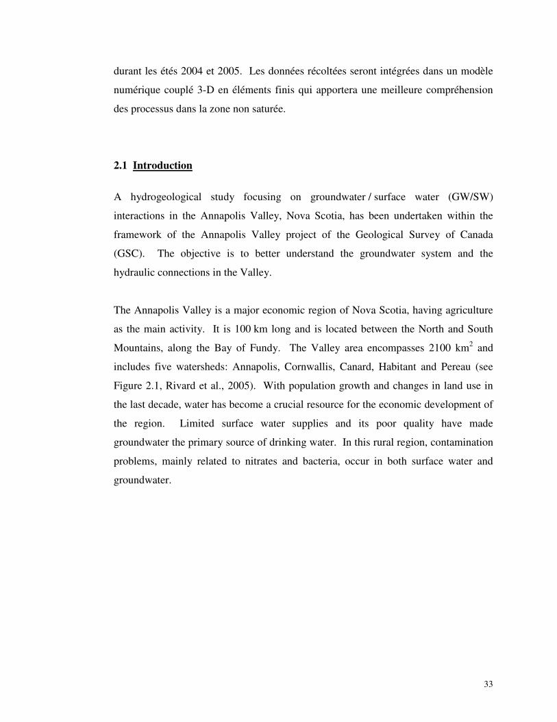
33

durant les étés 2004 et 2005. Les données récoltées seront intégrées dans un modèle

numérique couplé 3-D en éléments finis qui apportera une meilleure compréhension

des processus dans la zone non saturée.

2.1 Introduction

A hydrogeological study focusing on groundwater / surface water (GW/SW)

interactions in the Annapolis Valley, Nova Scotia, has been undertaken within the

framework of the Annapolis Valley project of the Geological Survey of Canada

(GSC). The objective is to better understand the groundwater system and the

hydraulic connections in the Valley.

The Annapolis Valley is a major economic region of Nova Scotia, having agriculture

as the main activity. It is 100 km long and is located between the North and South

Mountains, along the Bay of Fundy. The Valley area encompasses 2100 km2 and

includes five watersheds: Annapolis, Cornwallis, Canard, Habitant and Pereau (see

Figure 2.1, Rivard et al., 2005). With population growth and changes in land use in

the last decade, water has become a crucial resource for the economic development of

the region. Limited surface water supplies and its poor quality have made

groundwater the primary source of drinking water. In this rural region, contamination

problems, mainly related to nitrates and bacteria, occur in both surface water and

groundwater.

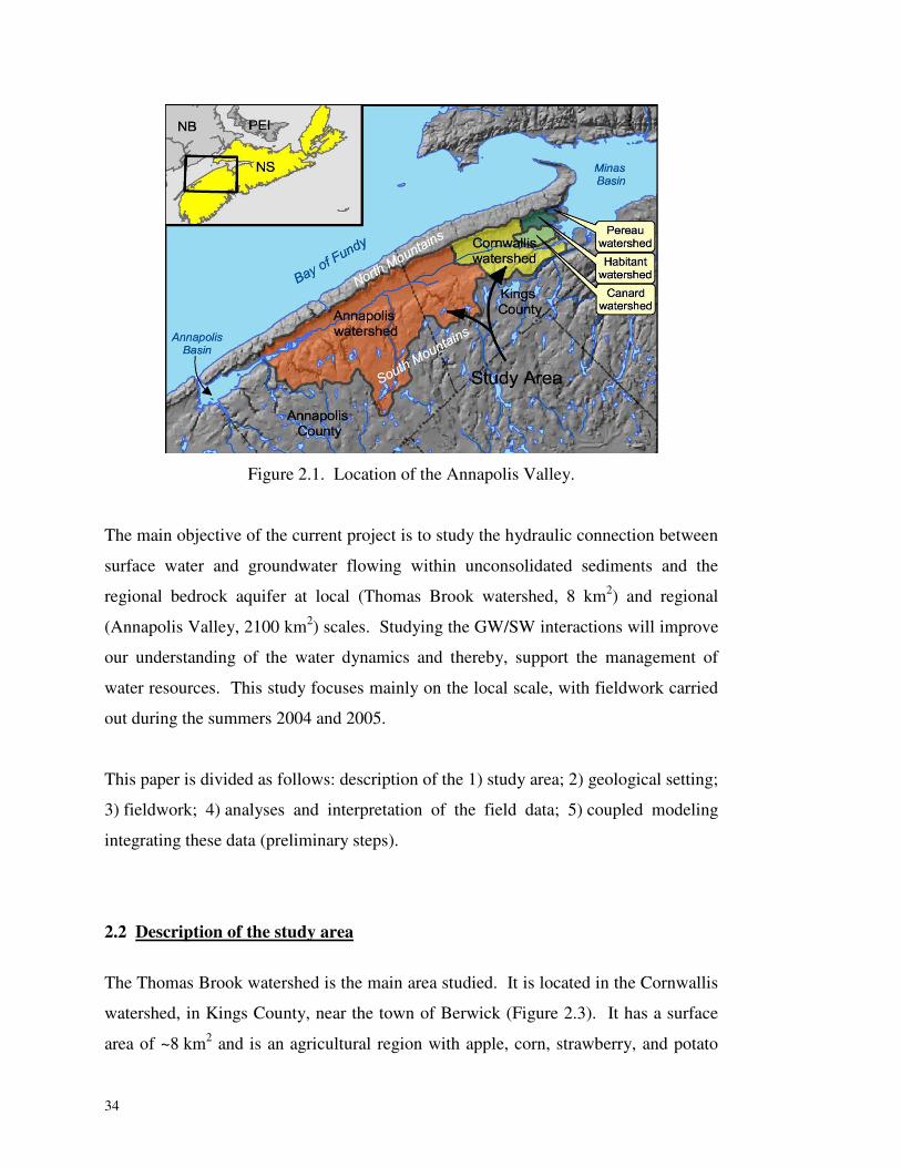
34

Figure 2.1. Location of the Annapolis Valley.

The main objective of the current project is to study the hydraulic connection between

surface water and groundwater flowing within unconsolidated sediments and the

regional bedrock aquifer at local (Thomas Brook watershed, 8 km2) and regional

(Annapolis Valley, 2100 km2) scales. Studying the GW/SW interactions will improve

our understanding of the water dynamics and thereby, support the management of

water resources. This study focuses mainly on the local scale, with fieldwork carried

out during the summers 2004 and 2005.

This paper is divided as follows: description of the 1) study area; 2) geological setting;

3) fieldwork; 4) analyses and interpretation of the field data; 5) coupled modeling

integrating these data (preliminary steps).

2.2 Description of the study area

The Thomas Brook watershed is the main area studied. It is located in the Cornwallis

watershed, in Kings County, near the town of Berwick (Figure 2.3). It has a surface

area of ~8 km2 and is an agricultural region with apple, corn, strawberry, and potato

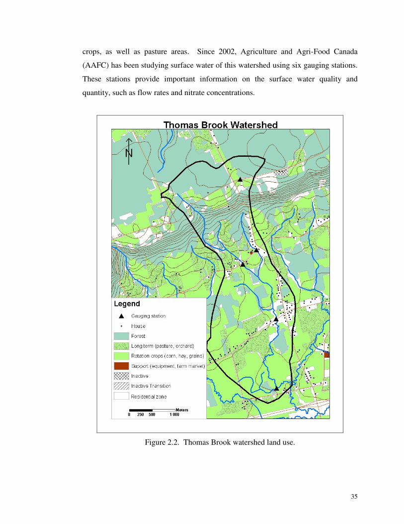
35

crops, as well as pasture areas. Since 2002, Agriculture and Agri-Food Canada

(AAFC) has been studying surface water of this watershed using six gauging stations.

These stations provide important information on the surface water quality and

quantity, such as flow rates and nitrate concentrations.

Figure 2.2. Thomas Brook watershed land use.

36

Figure 2.2 shows the topography and the land use of the Thomas Brook watershed. In

the watershed, the maximum elevation is around 220 m and the minimum is 30 m.

Surface water drainage is mainly north to south, beginning at the top of the North

Mountains and flowing south into the Cornwallis River that discharges ultimately into

the Bay of Fundy.

2.3 Geology

The Thomas Brook watershed is representative of the geological composition of the

Annapolis Valley. Indeed, it is defined by three principal bedrock formations and is

covered by surficial deposits resulting from glacial events.

2.3.1 Bedrock geology

The Triassic Fundy Group from the Mesozoic defines the Annapolis Valley

composition. It overlies the Paleozoic rocks that form the basement of the Valley and

comprises, in ascending order: the Wolfville, Blomidon, North Mountain, Scots Bay,

and McCoy Brook formations. The last two formations are not present in the

Annapolis Valley. The bedrock geological map is presented in Figure 2.3 (Rivard et

al., 2005).

2.3.1.1 Wolfville Formation

The Wolfville Formation, from the Late Triassic age, is composed of reddish thickly-

bedded medium to coarse-grained sandstone, cross-stratified, with subordinate

conglomerate, typically in lenticular beds, and it is sometimes interbedded with

siltstone (Hamblin, 2004; Rivard et al., 2005). It corresponds to a complex of clastic

rocks of continental origin and many facies are present, such as basin margin alluvial

fans, floodplains, aeolian dunes, sand/mud flats and shallow lacustrine environments.

The strata generally dip 5-10°NW and thicknesses up to 833 m are reported. This

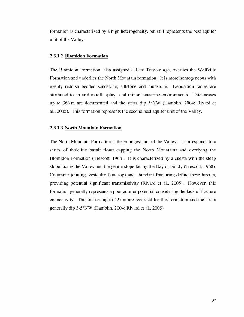
37

formation is characterized by a high heterogeneity, but still represents the best aquifer

unit of the Valley.

2.3.1.2 Blomidon Formation

The Blomidon Formation, also assigned a Late Triassic age, overlies the Wolfville

Formation and underlies the North Mountain formation. It is more homogeneous with

evenly reddish bedded sandstone, siltstone and mudstone. Deposition facies are

attributed to an arid mudflat/playa and minor lacustrine environments. Thicknesses

up to 363 m are documented and the strata dip 5°NW (Hamblin, 2004; Rivard et

al., 2005). This formation represents the second best aquifer unit of the Valley.

2.3.1.3 North Mountain Formation

The North Mountain Formation is the youngest unit of the Valley. It corresponds to a

series of tholeiitic basalt flows capping the North Mountains and overlying the

Blomidon Formation (Trescott, 1968). It is characterized by a cuesta with the steep

slope facing the Valley and the gentle slope facing the Bay of Fundy (Trescott, 1968).

Columnar jointing, vesicular flow tops and abundant fracturing define these basalts,

providing potential significant transmissivity (Rivard et al., 2005). However, this

formation generally represents a poor aquifer potential considering the lack of fracture

connectivity. Thicknesses up to 427 m are recorded for this formation and the strata

generally dip 3-5°NW (Hamblin, 2004; Rivard et al., 2005).

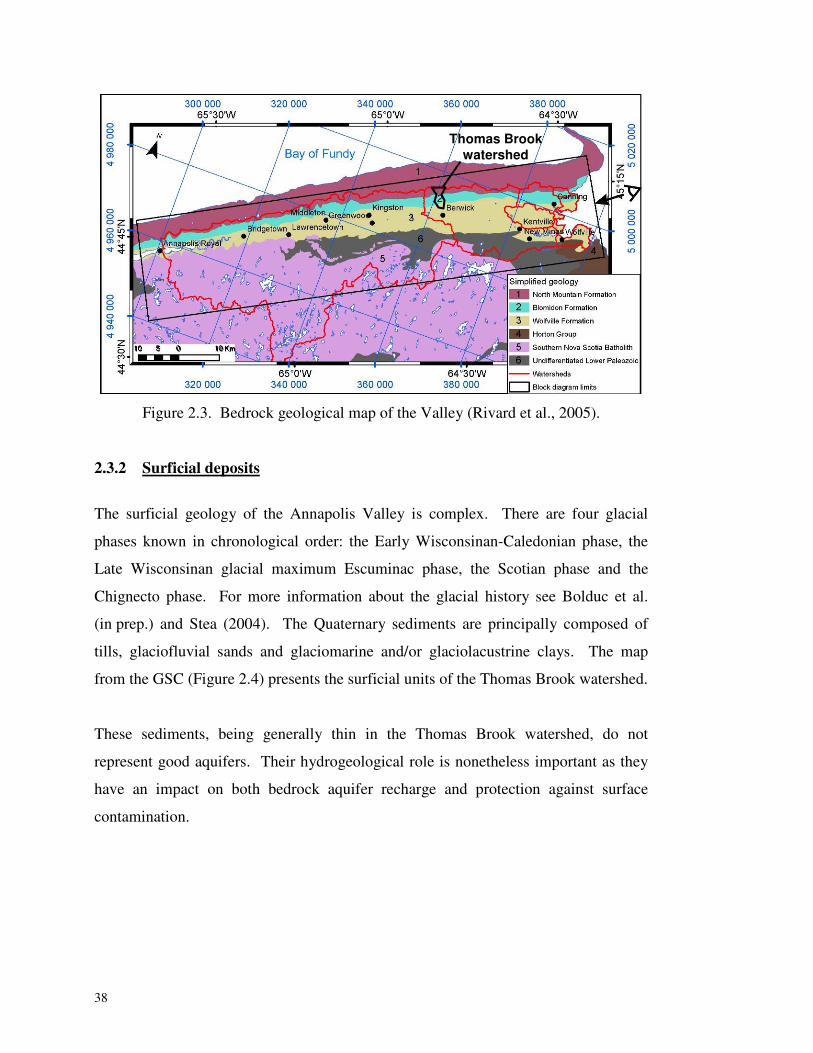
38

Figure 2.3. Bedrock geological map of the Valley (Rivard et al., 2005).

2.3.2 Surficial deposits

The surficial geology of the Annapolis Valley is complex. There are four glacial

phases known in chronological order: the Early Wisconsinan-Caledonian phase, the

Late Wisconsinan glacial maximum Escuminac phase, the Scotian phase and the

Chignecto phase. For more information about the glacial history see Bolduc et al.

(in prep.) and Stea (2004). The Quaternary sediments are principally composed of

tills, glaciofluvial sands and glaciomarine and/or glaciolacustrine clays. The map

from the GSC (Figure 2.4) presents the surficial units of the Thomas Brook watershed.

These sediments, being generally thin in the Thomas Brook watershed, do not

represent good aquifers. Their hydrogeological role is nonetheless important as they

have an impact on both bedrock aquifer recharge and protection against surface

contamination.

Thomas Brook watershed

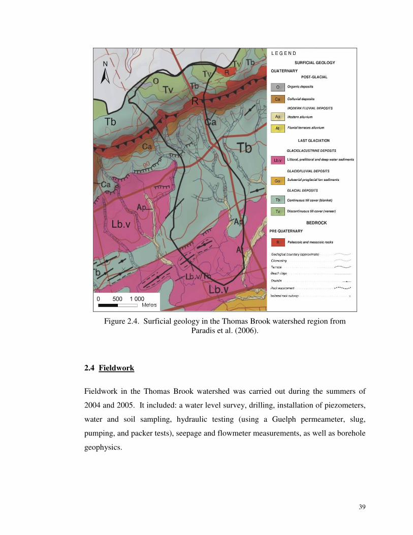
39

Figure 2.4. Surficial geology in the Thomas Brook watershed region from

Paradis et al. (2006).

2.4 Fieldwork

Fieldwork in the Thomas Brook watershed was carried out during the summers of

2004 and 2005. It included: a water level survey, drilling, installation of piezometers,

water and soil sampling, hydraulic testing (using a Guelph permeameter, slug,

pumping, and packer tests), seepage and flowmeter measurements, as well as borehole

geophysics.

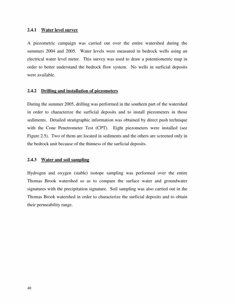
40

2.4.1 Water level survey

A piezometric campaign was carried out over the entire watershed during the

summers 2004 and 2005. Water levels were measured in bedrock wells using an

electrical water level meter. This survey was used to draw a potentiometric map in

order to better understand the bedrock flow system. No wells in surficial deposits

were available.

2.4.2 Drilling and installation of piezometers

During the summer 2005, drilling was performed in the southern part of the watershed

in order to characterize the surficial deposits and to install piezometers in those

sediments. Detailed stratigraphic information was obtained by direct push technique

with the Cone Penetrometer Test (CPT). Eight piezometers were installed (see

Figure 2.5). Two of them are located in sediments and the others are screened only in

the bedrock unit because of the thinness of the surficial deposits.

2.4.3 Water and soil sampling

Hydrogen and oxygen (stable) isotope sampling was performed over the entire

Thomas Brook watershed so as to compare the surface water and groundwater

signatures with the precipitation signature. Soil sampling was also carried out in the

Thomas Brook watershed in order to characterize the surficial deposits and to obtain

their permeability range.

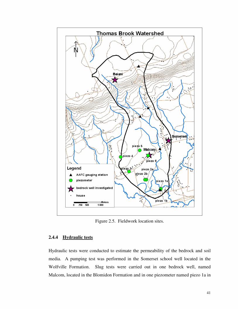
41

Figure 2.5. Fieldwork location sites.

2.4.4 Hydraulic tests

Hydraulic tests were conducted to estimate the permeability of the bedrock and soil

media. A pumping test was performed in the Somerset school well located in the

Wolfville Formation. Slug tests were carried out in one bedrock well, named

Malcom, located in the Blomidon Formation and in one piezometer named piezo 1a in

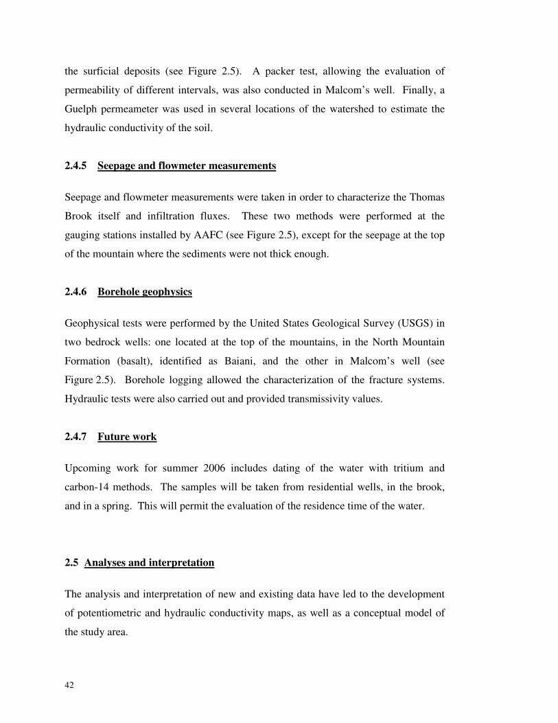
42

the surficial deposits (see Figure 2.5). A packer test, allowing the evaluation of

permeability of different intervals, was also conducted in Malcom’s well. Finally, a

Guelph permeameter was used in several locations of the watershed to estimate the

hydraulic conductivity of the soil.

2.4.5 Seepage and flowmeter measurements

Seepage and flowmeter measurements were taken in order to characterize the Thomas

Brook itself and infiltration fluxes. These two methods were performed at the

gauging stations installed by AAFC (see Figure 2.5), except for the seepage at the top

of the mountain where the sediments were not thick enough.

2.4.6 Borehole geophysics

Geophysical tests were performed by the United States Geological Survey (USGS) in

two bedrock wells: one located at the top of the mountains, in the North Mountain

Formation (basalt), identified as Baiani, and the other in Malcom’s well (see

Figure 2.5). Borehole logging allowed the characterization of the fracture systems.

Hydraulic tests were also carried out and provided transmissivity values.

2.4.7 Future work

Upcoming work for summer 2006 includes dating of the water with tritium and

carbon-14 methods. The samples will be taken from residential wells, in the brook,

and in a spring. This will permit the evaluation of the residence time of the water.

2.5 Analyses and interpretation

The analysis and interpretation of new and existing data have led to the development

of potentiometric and hydraulic conductivity maps, as well as a conceptual model of

the study area.

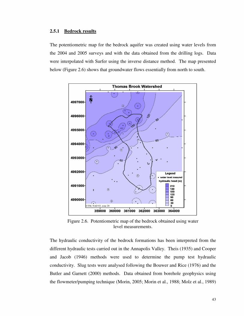
43

2.5.1 Bedrock results

The potentiometric map for the bedrock aquifer was created using water levels from

the 2004 and 2005 surveys and with the data obtained from the drilling logs. Data

were interpolated with Surfer using the inverse distance method. The map presented

below (Figure 2.6) shows that groundwater flows essentially from north to south.

Figure 2.6. Potentiometric map of the bedrock obtained using water

level measurements.

The hydraulic conductivity of the bedrock formations has been interpreted from the

different hydraulic tests carried out in the Annapolis Valley. Theis (1935) and Cooper

and Jacob (1946) methods were used to determine the pump test hydraulic

conductivity. Slug tests were analysed following the Bouwer and Rice (1976) and the

Butler and Garnett (2000) methods. Data obtained from borehole geophysics using

the flowmeter/pumping technique (Morin, 2005; Morin et al., 1988; Molz et al., 1989)

UTM, NAD 83, zone 20

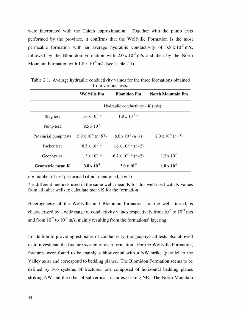
44

were interpreted with the Thiem approximation. Together with the pump tests

performed by the province, it confirms that the Wolfville Formation is the most

permeable formation with an average hydraulic conductivity of 3.8 x 10-5 m/s,

followed by the Blomidon Formation with 2.0 x 10-5 m/s and then by the North

Mountain Formation with 1.8 x 10-6 m/s (see Table 2.1).

Table 2.1. Average hydraulic conductivity values for the three formations obtained from various tests.

Wolfville Fm Blomidon Fm North Mountain Fm

Hydraulic conductivity - K (m/s)

Slug test 1.6 x 10-4 * 1.8 x 10-5 *

Pump test 8.5 x 10-6

Provincial pump tests 5.0 x 10-6 (n=57) 8.6 x 10-6 (n=7) 2.0 x 10-6 (n=7)

Packer test 8.5 x 10-5 * 1.6 x 10-5 * (n=2)

Geophysics 1.3 x 10-4 * 6.7 x 10-5 * (n=2) 1.2 x 10-6

Geometric mean K 3.8 x 10-5 2.0 x 10-5 1.8 x 10-6

n = number of test performed (if not mentioned, n = 1)

* = different methods used in the same well; mean K for this well used with K values from all other wells to calculate mean K for the formation

Heterogeneity of the Wolfville and Blomidon formations, at the wells tested, is

characterized by a wide range of conductivity values respectively from 10-6 to 10-3 m/s

and from 10-7 to 10-4 m/s, mainly resulting from the formations’ layering.

In addition to providing estimates of conductivity, the geophysical tests also allowed

us to investigate the fracture system of each formation. For the Wolfville Formation,

fractures were found to be mainly subhorizontal with a NW strike (parallel to the

Valley axis) and correspond to bedding planes. The Blomidon Formation seems to be

defined by two systems of fractures: one composed of horizontal bedding planes

striking NW and the other of subvertical fractures striking NE. The North Mountain

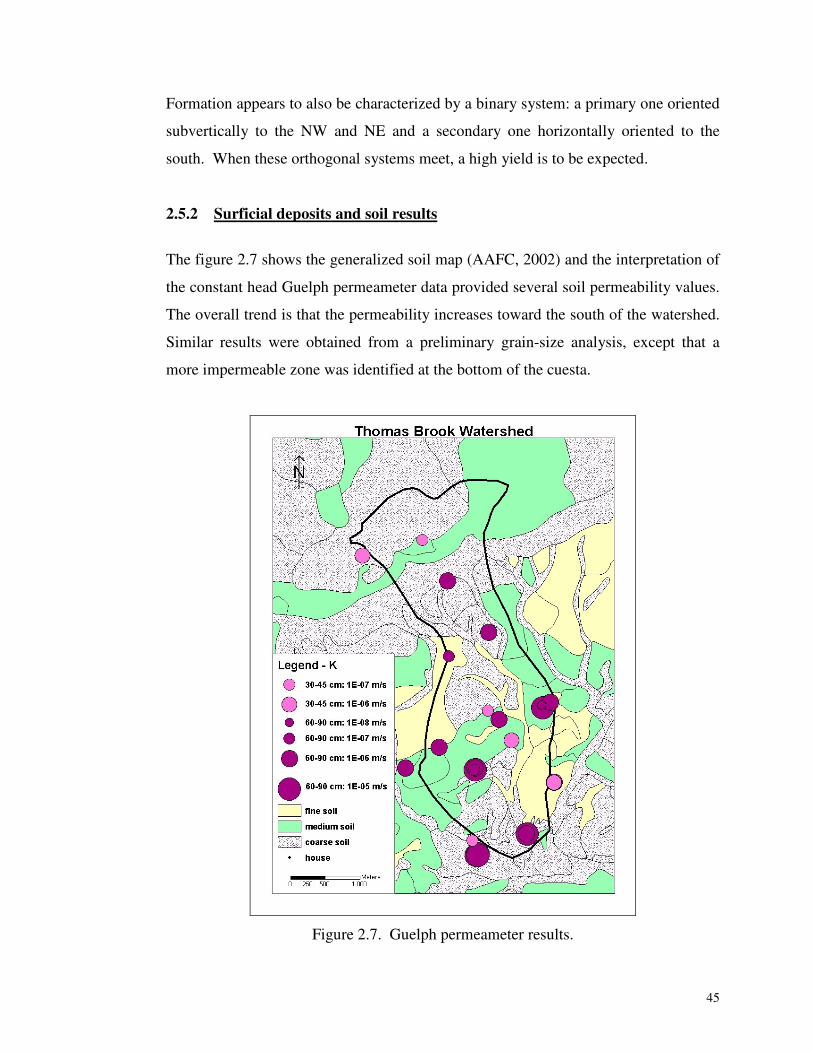
45

Formation appears to also be characterized by a binary system: a primary one oriented

subvertically to the NW and NE and a secondary one horizontally oriented to the

south. When these orthogonal systems meet, a high yield is to be expected.

2.5.2 Surficial deposits and soil results

The figure 2.7 shows the generalized soil map (AAFC, 2002) and the interpretation of

the constant head Guelph permeameter data provided several soil permeability values.

The overall trend is that the permeability increases toward the south of the watershed.

Similar results were obtained from a preliminary grain-size analysis, except that a

more impermeable zone was identified at the bottom of the cuesta.

Figure 2.7. Guelph permeameter results.

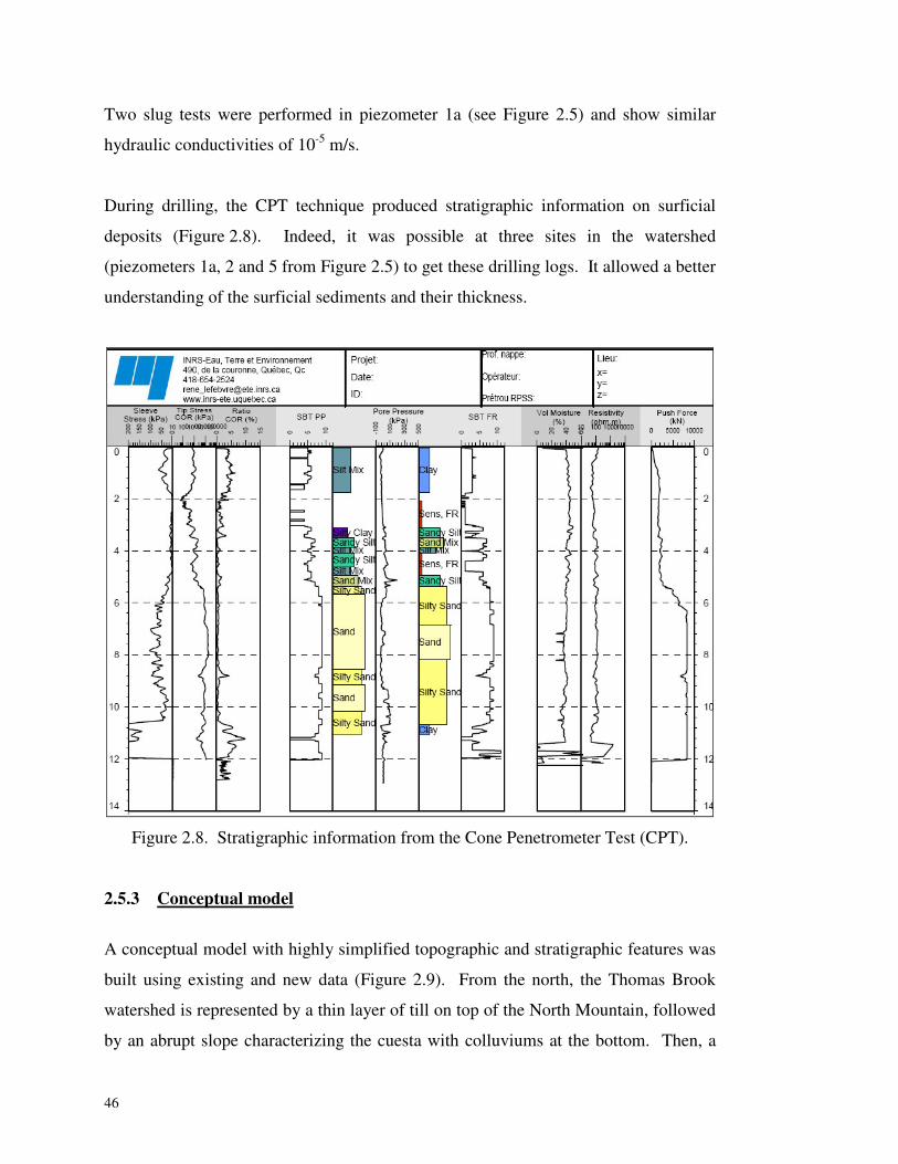
46

Two slug tests were performed in piezometer 1a (see Figure 2.5) and show similar

hydraulic conductivities of 10-5 m/s.

During drilling, the CPT technique produced stratigraphic information on surficial

deposits (Figure 2.8). Indeed, it was possible at three sites in the watershed

(piezometers 1a, 2 and 5 from Figure 2.5) to get these drilling logs. It allowed a better

understanding of the surficial sediments and their thickness.

Figure 2.8. Stratigraphic information from the Cone Penetrometer Test (CPT).

2.5.3 Conceptual model

A conceptual model with highly simplified topographic and stratigraphic features was

built using existing and new data (Figure 2.9). From the north, the Thomas Brook

watershed is represented by a thin layer of till on top of the North Mountain, followed

by an abrupt slope characterizing the cuesta with colluviums at the bottom. Then, a

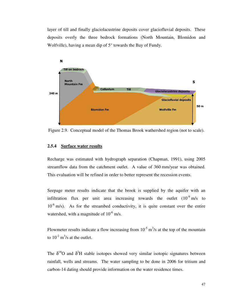
47

layer of till and finally glaciolacustrine deposits cover glaciofluvial deposits. These

deposits overly the three bedrock formations (North Mountain, Blomidon and

Wolfville), having a mean dip of 5° towards the Bay of Fundy.

Figure 2.9. Conceptual model of the Thomas Brook wathershed region (not to scale).

2.5.4 Surface water results

Recharge was estimated with hydrograph separation (Chapman, 1991), using 2005

streamflow data from the catchment outlet. A value of 360 mm/year was obtained.

This evaluation will be refined in order to better represent the recession events.

Seepage meter results indicate that the brook is supplied by the aquifer with an

infiltration flux per unit area increasing towards the outlet (10-9 m/s to

10-6 m/s). As for the streambed conductivity, it is quite constant over the entire

watershed, with a magnitude of 10-6 m/s.

Flowmeter results indicate a flow increasing from 10-5 m3/s at the top of the mountain

to 10-2 m3/s at the outlet.

The δ18O and δ2H stable isotopes showed very similar isotopic signatures between

rainfall, wells and streams. The water sampling to be done in 2006 for tritium and

carbon-14 dating should provide information on the water residence times.

48

All these data described above, together with other information from AAFC, the Nova

Scotia Environment and Labour, and the Nova Scotia Agricultural College, will be

integrated into a 3D finite element coupled model to quantify the GW/SW

interactions.

2.6 Coupled modeling

A 3D coupled model (Bixio et al., 2000; Putti and Paniconi, 2004) will be used to

quantify the GW/SW interactions. It is a finite element model that integrates a surface

routing module and a groundwater module. The main inputs are soil and aquifer

parameters such as hydraulic conductivity and porosity; atmospheric fluxes

corresponding to rainfall and evaporation data; and channel geometry.

Boundary conditions will be no-flow along the catchment boundary and at the base,

and atmospheric forcing on the surface. Heterogeneity from layering constitutes the

main characteristic of the region, and it will be integrated by layers and zones as

shown in Figure 2.10.

The layering will allow the representation of vertical heterogeneity, with at least one

layer (but usually more than one) for each major geologic formation. Finer layering

will be used near the surface of the catchment, to better capture rainfall-runoff-

infiltration partitioning. The zones will represent lateral heterogeneity, as deduced

from the soil and surficial geology data and from the inclined nature of the bedrock

formations (as schematized in Figure 2.9). Because each layer has its own pattern of

lateral heterogeneity, it will be necessary to define a sufficient number of zones to

capture all the desired heterogeneity (at the most, many zones as there are elements in

the 2D, or surface, finite element discretization can be used). Thus, within each layer,

each zone can be assigned its own value of hydraulic conductivity (as well as other

material properties). The model simulations will allow the assessment of the

infiltration and recharge, provide patterns of surface and subsurface flow, and show

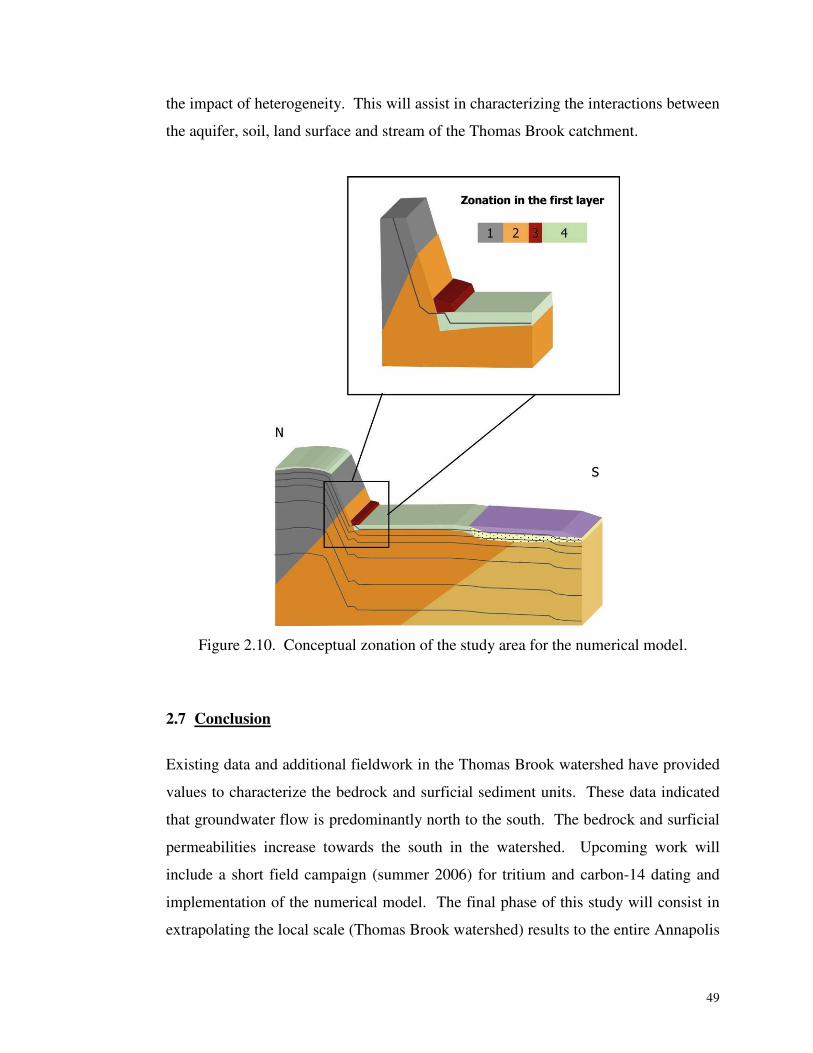
49

the impact of heterogeneity. This will assist in characterizing the interactions between

the aquifer, soil, land surface and stream of the Thomas Brook catchment.

Figure 2.10. Conceptual zonation of the study area for the numerical model.

2.7 Conclusion

Existing data and additional fieldwork in the Thomas Brook watershed have provided

values to characterize the bedrock and surficial sediment units. These data indicated

that groundwater flow is predominantly north to the south. The bedrock and surficial

permeabilities increase towards the south in the watershed. Upcoming work will

include a short field campaign (summer 2006) for tritium and carbon-14 dating and

implementation of the numerical model. The final phase of this study will consist in

extrapolating the local scale (Thomas Brook watershed) results to the entire Annapolis

50

Valley. Indeed, the Thomas Brook watershed is considered in many aspects to be

representative of the Valley, containing the major bedrock and sediment units and

being mainly agricultural.

2.8 Acknowledgements

Special thanks must be addressed to Agriculture and Agri-Food Canada, the Centre of

Geographic Sciences, the Geological Survey of Canada, the Institut National de la

Recherche Scientifique – Eau, Terre et Environnement, the National Science and

Engineering Research Council of Canada, the Nova Scotia Agricultural College, the

Nova Scotia Environment and Labour, the United States Geological Survey, the

Université du Québec à Montréal, and to all residents that made this study possible.

2.9 References

Agriculture and Agri-Food Canada (2002). National soil database, nsd008.20000530, http://www.nsac.ca/bookstore/index.

Bixio, A.C., Orlandini, S., Paniconi, C. and Putti, M. (2000). Physically-based

distributed model for coupled surface runoff and subsurface flow simulation at the catchment scale, in Computational Methods in Water Resources, Surface Water Systems and Hydrology, Balkema, 2: 1115-1122.

Bolduc, A., Paradis, S.J. and Stea R.R. (in prep.). The Annapolis Valley, Nova

Scotia, Surficial geology and groundwater resources, Géographie physique et Quaternaire, in preparation.

Bouwer, H. and Rice, R.C. (1976). A slug test for determining hydraulic conductivity

of unconfined aquifers with completely or partially penetrating wells, Water Resources Research, 12: 423-428.

Butler, J.J.Jr and Garnett, E.J. (2000). Simple procedures for analysis of slug tests in

formations of high hydraulic conductivity using spreadsheet and scientific graphics software, Kansas Geological Survey – Open File 2000-40, 19 p..

51

Chapman, T.G. (1991). Comment on ‘Evaluation of automated techniques for baseflow and recession analyses’ by Nathan, R.J. and McMahon, T.A., Water Resources Research, 27:1783-1784.

Cooper, H.H and Jacob, C.E. (1946). A generalized graphical method for evaluating

formation constants and summarizing well field history, Am. Geophys. Union Trans., 27:526-534.

Hamblin, T. (2004). Regional geology of the Triassic/Jurassic Fundy Group of

Annapolis Valley, Geological Survey of Canada – Open File 4678. Molz, F.J., Morin, R.H., Hess, A.E., Melville, J.G., and Guven, O. (1989). The

impeller meter for measuring aquifer permeability variations: Evaluation and comparison with other tests, Water Resources Research, 25-7: 1677-1683.

Morin, R. (2005). Preliminary analysis of geophysical logs from Annapolis Valley,

United States Geological Survey. Morin, R.H., Hess, A.E. and Paillet, F.L. (1988). Determining the distribution of

hydraulic conductivity in a fractured limestone aquifer by simultaneous injection and geophysical logging, Ground Water, 26-5: 587-595.

Paradis, S.J., Bolduc, A. and Stea R. (2006). Surficial geology, Annapolis Valley,

Nova Scotia, Geological Survey of Canada, Open File 5276, scale 1:100 000. Putti, M. and Paniconi, C. (2004). Time step and stability control for a coupled model

of surface and subsurface flow, in Computational Methods in Water Resources, Elsevier, 2: 1391-1402.

Rivard, C., Michaud, Y., Liao, S., Bolduc, A., Paradis, S., Paradis, D., Castonguay, S.,

Deblonde, C., Hamblin, T., Drage, J., Paniconi, C., Webster, T., and Spooner, I. (2005). Characterization of the Annapolis Valley Aquifers, Nova Scotia – A Work In Progress, Annapolis-Cornwallis Valley Aquifer Study (ACVAS), 6th CGS/IAH-CNC groundwater specialty conference, Saskatoon, Saskatchewan, Canada.

Stea, R.R. (2004). The Appalachian Glacier Complex in Maritime Canada, In Ehlers,

J. and Gibbard, P.L., eds. Quaternary Glaciations - Extent and Chronology Part II: 213-232.

Theis, C.V. (1935). The relation between the lowering of the piezometric surface and

the rate and duration of discharge of a well using groundwater storage, Trans. Amer. Geophys. Union, 16: 519-524.

Trescott, P.C. (1968). Groundwater resources and hydrogeology of the Annapolis-

Cornwallis Valley, Nova Scotia, Province of Nova Scotia - Department of Mines, Memoir 6, Halifax, Nova Scotia, 159 p..

CHAPITRE 3: A modeling study of heterogeneity and surface water-groundwater interactions in the Thomas Brook subcatchment, Annapolis Valley

(Nova Scotia, Canada)

54

A MODELING STUDY OF HETEROGENEITY AND SURFACE WATER–GROUNDWATER INTERACTIONS IN THE THOMAS BROOK SUBCATCHMENT, ANNAPOLIS VALLEY (NOVA SCOTIA, CANADA)* *paper submitted to Hydrogeology Journal in 2009 Gauthier, M.J.1, Camporese, M.1, Paniconi, C.1**, Rivard, C.2 and Larocque, M.3

1 Institut National de la Recherche Scientifique – ETE, Québec, Qc, Canada, (418) 654-4677, (418) 654-2525, 490 rue de la Couronne, Québec, Qc, G1K 9A9, communications @adm.inrs.ca 2 Geological Survey of Canada, Québec, Qc, Canada 3 Université du Québec à Montréal, Montréal, Qc, Canada

** Corresponding author

ABSTRACT

A modeling study of heterogeneity and groundwater–surface water interactions on an

8 km2 catchment was undertaken within the framework of a hydrogeological study of

the Annapolis Valley, Nova Scotia (Canada). The main objectives of the catchment

study were to investigate the hydraulic connection between surface water and

groundwater flowing within unconsolidated sediments and the regional bedrock

aquifer and to assess the effects of heterogeneity and other factors on these

interactions. This was accomplished with a coupled numerical model that integrates a

subsurface module representing three-dimensional unsaturated and saturated zone

flow with a surface module simulating one-dimensional overland and channel flow.

Eight scenarios of increasing geological complexity were simulated, plus a final

scenario incorporating snow cover. From these simulations it was possible to examine

the spatio-temporal patterns of overland flow, return flow, infiltration, recharge,

groundwater levels, surface saturation, and evapotranspiration, and to quantify various

components of the catchment’s water balance.

Calibrated hydraulic conductivity values for the various geological formations are

consistent with field measurements. Simulated groundwater recharge is in line with

estimates obtained from other analyses, and the water table distribution agrees well

with the available groundwater levels. Natural springs located on the catchment are

55

also adequately reproduced by the model. The inclusion of snow accumulation and

snowmelt leads to a slight decrease in groundwater recharge as more overland flow is

generated. For this study area, the hydraulic conductivities of the thin surficial

sediment cover (especially till) and the basalts turned out to be important features of

the basin’s heterogeneity to capture properly the overall catchment response.

RÉSUMÉ

Une étude par modélisation portant sur l’hétérogénéité et les interactions entre l’eau

souterraine et l’eau de surface d’un bassin versant de 8 km2 a été entreprise dans le

cadre d’une étude hydrogéologique de la Vallée d’Annapolis en Nouvelle-Écosse

(Canada). Les objectifs principaux de cette étude locale étaient d’étudier les liens

hydrauliques entre l’eau de surface et l’eau souterraine circulant dans les sédiments et

dans l’aquifère rocheux régional et d’évaluer les effets de l’hétérogénéité et autres

facteurs sur ces interactions. Ceci a été accompli au moyen d’un modèle numérique

couplé, qui permet d’intégrer un module souterrain, représentant en 3D les zones

d’écoulement saturée et non saturée, à un module de surface simulant en 1D les

écoulements de surface. Huit scénarios reflétant une hétérogénéité géologique

croissante ont été simulés. Un neuvième scénario incorporant le couvert de neige est

venu s’ajouter. De ces simulations, il a été possible d’examiner les patrons spatio-

temporels des écoulements de surface (ruissellement de surface et écoulement

restitué), de l’infiltration, de la recharge, des niveaux d’eau, de la saturation du sol et

de l’évaporation, et de quantifier diverses composantes du bilan hydrique du bassin.

Les conductivités hydrauliques calées pour les différentes formations géologiques sont

en accord avec les données de terrain, les valeurs de recharge calculées avec le modèle

sont du même ordre de grandeur que celles estimées avec d’autres approches et la

distribution spatiale des niveaux de la nappe concorde avec les niveaux d’eau mesurés

dans les puits. Les sources situées au pied des abruptes montagnes du Nord sont

également adéquatement reproduites par le modèle. La prise en compte du couvert

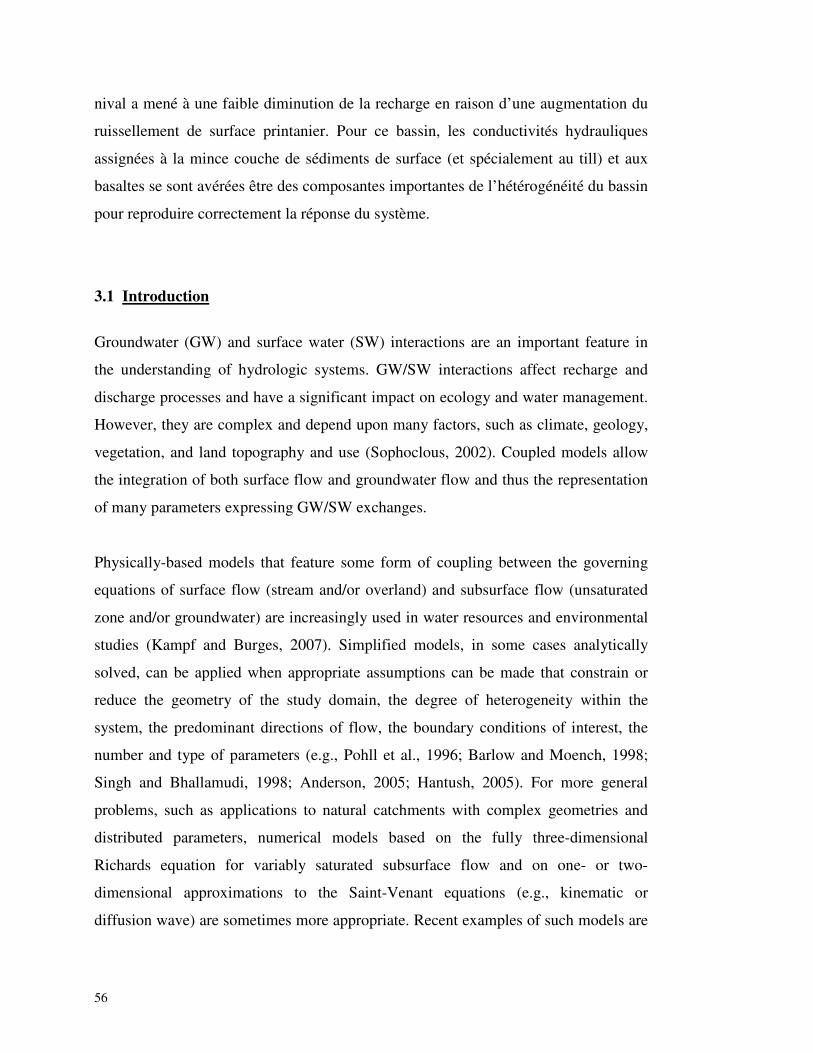
56

nival a mené à une faible diminution de la recharge en raison d’une augmentation du

ruissellement de surface printanier. Pour ce bassin, les conductivités hydrauliques

assignées à la mince couche de sédiments de surface (et spécialement au till) et aux

basaltes se sont avérées être des composantes importantes de l’hétérogénéité du bassin

pour reproduire correctement la réponse du système.

3.1 Introduction

Groundwater (GW) and surface water (SW) interactions are an important feature in

the understanding of hydrologic systems. GW/SW interactions affect recharge and

discharge processes and have a significant impact on ecology and water management.

However, they are complex and depend upon many factors, such as climate, geology,

vegetation, and land topography and use (Sophoclous, 2002). Coupled models allow

the integration of both surface flow and groundwater flow and thus the representation

of many parameters expressing GW/SW exchanges.

Physically-based models that feature some form of coupling between the governing

equations of surface flow (stream and/or overland) and subsurface flow (unsaturated

zone and/or groundwater) are increasingly used in water resources and environmental

studies (Kampf and Burges, 2007). Simplified models, in some cases analytically

solved, can be applied when appropriate assumptions can be made that constrain or

reduce the geometry of the study domain, the degree of heterogeneity within the

system, the predominant directions of flow, the boundary conditions of interest, the

number and type of parameters (e.g., Pohll et al., 1996; Barlow and Moench, 1998;

Singh and Bhallamudi, 1998; Anderson, 2005; Hantush, 2005). For more general

problems, such as applications to natural catchments with complex geometries and

distributed parameters, numerical models based on the fully three-dimensional

Richards equation for variably saturated subsurface flow and on one- or two-

dimensional approximations to the Saint-Venant equations (e.g., kinematic or

diffusion wave) are sometimes more appropriate. Recent examples of such models are

57

reported in VanderKwaak and Loague (2001), Morita and Yen (2002), Panday and

Huyakorn (2004), Kollet and Maxwell (2006), and Jones et al. (2008).

Application of these models at the basin scale is often considered difficult because of

their large data requirements and the usually limited data availability in watershed

studies. Components of the naturally complex system which must be included in the

coupled model to simulate accurately all the relevant hydrological processes have

never been fully investigated.

Heterogeneity in a model can be dealt with using homogeneous equivalent properties

(averaging) or by trying to describe spatial variability of the rock/deposit properties

from geological observations and local measurements (de Marsily et al., 2005). The

representation of geological complexity in a model is, however, usually limited by

lack of data on fracture networks and characteristics of discontinuities, and even by

the number of available pump-test results of the various geological formations. The

appropriate amount of characterization data needed for a given study must be

carefully assessed, as time and money spent on the development of the model and on

fieldwork will depend on them. This is especially important for coupled models with

very different dynamics for the surface and subsurface components that greatly

increases simulation costs. Introducing geological complexity in an incremental way

allows CPU requirements to be contained while investigating the numerical and

physical impacts of different levels of detail in the representation of heterogeneity.

One must keep in mind that flow is much less sensitive to connectivity and

heterogeneity than transport, and thus catchment-scale problems may often be studied

using averaging (or upscaling) of pump-test results followed by a model calibration to

obtain valuable information for aquifer management (de Marsily et al., 2005).

The aim of this study is to investigate the level of heterogeneity required to simulate

surface water – groundwater interactions in a small watershed. The Thomas Brook

catchment, a small basin located in the Annapolis Valley (Nova Scotia, Canada), is

used as a typical case study. This catchment was part of a recent regional

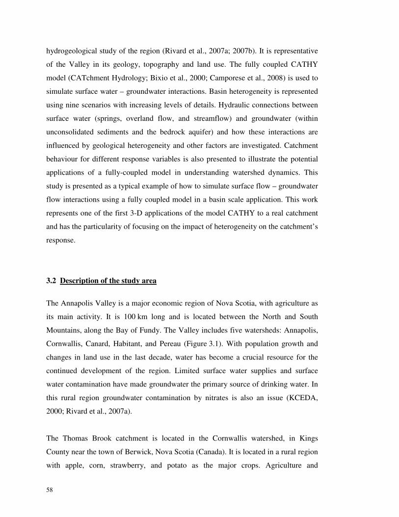
58

hydrogeological study of the region (Rivard et al., 2007a; 2007b). It is representative

of the Valley in its geology, topography and land use. The fully coupled CATHY

model (CATchment Hydrology; Bixio et al., 2000; Camporese et al., 2008) is used to

simulate surface water – groundwater interactions. Basin heterogeneity is represented

using nine scenarios with increasing levels of details. Hydraulic connections between

surface water (springs, overland flow, and streamflow) and groundwater (within

unconsolidated sediments and the bedrock aquifer) and how these interactions are

influenced by geological heterogeneity and other factors are investigated. Catchment

behaviour for different response variables is also presented to illustrate the potential

applications of a fully-coupled model in understanding watershed dynamics. This

study is presented as a typical example of how to simulate surface flow – groundwater

flow interactions using a fully coupled model in a basin scale application. This work

represents one of the first 3-D applications of the model CATHY to a real catchment

and has the particularity of focusing on the impact of heterogeneity on the catchment’s

response.

3.2 Description of the study area

The Annapolis Valley is a major economic region of Nova Scotia, with agriculture as

its main activity. It is 100 km long and is located between the North and South

Mountains, along the Bay of Fundy. The Valley includes five watersheds: Annapolis,

Cornwallis, Canard, Habitant, and Pereau (Figure 3.1). With population growth and

changes in land use in the last decade, water has become a crucial resource for the

continued development of the region. Limited surface water supplies and surface

water contamination have made groundwater the primary source of drinking water. In

this rural region groundwater contamination by nitrates is also an issue (KCEDA,

2000; Rivard et al., 2007a).

The Thomas Brook catchment is located in the Cornwallis watershed, in Kings

County near the town of Berwick, Nova Scotia (Canada). It is located in a rural region

with apple, corn, strawberry, and potato as the major crops. Agriculture and

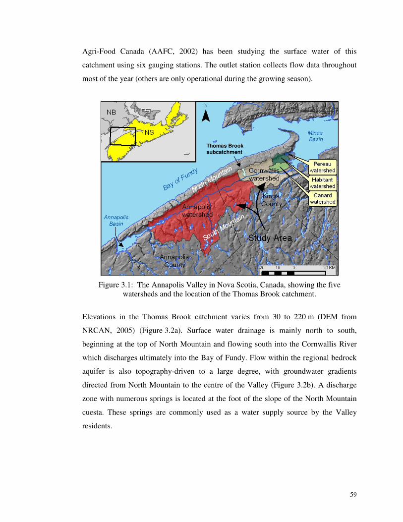
59

Agri-Food Canada (AAFC, 2002) has been studying the surface water of this

catchment using six gauging stations. The outlet station collects flow data throughout

most of the year (others are only operational during the growing season).

Figure 3.1: The Annapolis Valley in Nova Scotia, Canada, showing the five

watersheds and the location of the Thomas Brook catchment.

Elevations in the Thomas Brook catchment varies from 30 to 220 m (DEM from

NRCAN, 2005) (Figure 3.2a). Surface water drainage is mainly north to south,

beginning at the top of North Mountain and flowing south into the Cornwallis River

which discharges ultimately into the Bay of Fundy. Flow within the regional bedrock

aquifer is also topography-driven to a large degree, with groundwater gradients

directed from North Mountain to the centre of the Valley (Figure 3.2b). A discharge

zone with numerous springs is located at the foot of the slope of the North Mountain

cuesta. These springs are commonly used as a water supply source by the Valley

residents.

Thomas Brook subcatchment

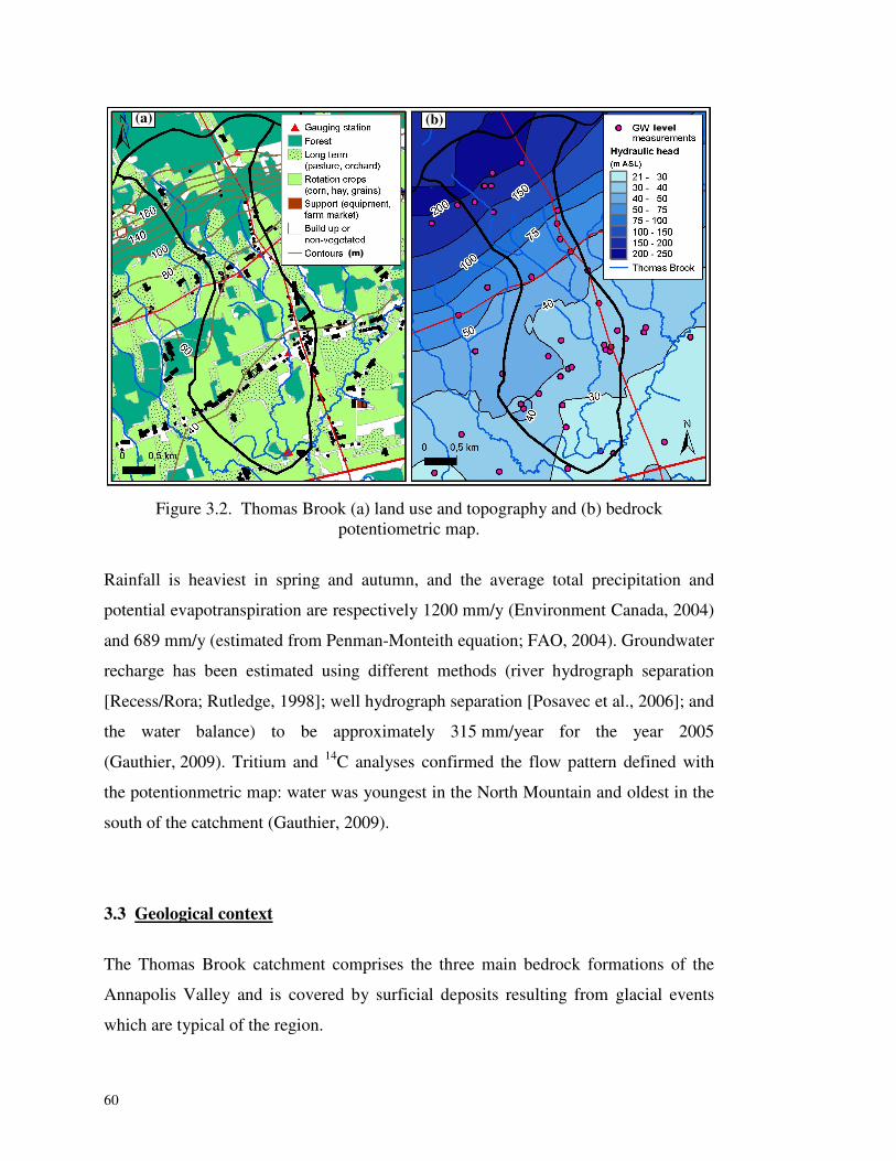
60

Figure 3.2. Thomas Brook (a) land use and topography and (b) bedrock

potentiometric map.

Rainfall is heaviest in spring and autumn, and the average total precipitation and

potential evapotranspiration are respectively 1200 mm/y (Environment Canada, 2004)

and 689 mm/y (estimated from Penman-Monteith equation; FAO, 2004). Groundwater

recharge has been estimated using different methods (river hydrograph separation

[Recess/Rora; Rutledge, 1998]; well hydrograph separation [Posavec et al., 2006]; and

the water balance) to be approximately 315 mm/year for the year 2005

(Gauthier, 2009). Tritium and 14C analyses confirmed the flow pattern defined with

the potentionmetric map: water was youngest in the North Mountain and oldest in the

south of the catchment (Gauthier, 2009).

3.3 Geological context

The Thomas Brook catchment comprises the three main bedrock formations of the

Annapolis Valley and is covered by surficial deposits resulting from glacial events

which are typical of the region.

����

������(a) (b)

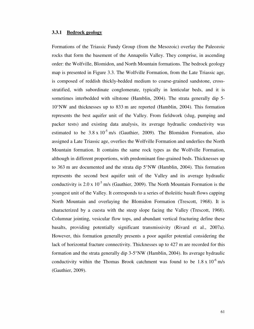
61

3.3.1 Bedrock geology

Formations of the Triassic Fundy Group (from the Mesozoic) overlay the Paleozoic

rocks that form the basement of the Annapolis Valley. They comprise, in ascending

order: the Wolfville, Blomidon, and North Mountain formations. The bedrock geology

map is presented in Figure 3.3. The Wolfville Formation, from the Late Triassic age,

is composed of reddish thickly-bedded medium to coarse-grained sandstone, cross-

stratified, with subordinate conglomerate, typically in lenticular beds, and it is

sometimes interbedded with siltstone (Hamblin, 2004). The strata generally dip 5-

10°NW and thicknesses up to 833 m are reported (Hamblin, 2004). This formation

represents the best aquifer unit of the Valley. From fieldwork (slug, pumping and

packer tests) and existing data analysis, its average hydraulic conductivity was

estimated to be 3.8 x 10-5 m/s (Gauthier, 2009). The Blomidon Formation, also

assigned a Late Triassic age, overlies the Wolfville Formation and underlies the North

Mountain formation. It contains the same rock types as the Wolfville Formation,

although in different proportions, with predominant fine-grained beds. Thicknesses up

to 363 m are documented and the strata dip 5°NW (Hamblin, 2004). This formation

represents the second best aquifer unit of the Valley and its average hydraulic

conductivity is 2.0 x 10-5 m/s (Gauthier, 2009). The North Mountain Formation is the

youngest unit of the Valley. It corresponds to a series of tholeiitic basalt flows capping

North Mountain and overlaying the Blomidon Formation (Trescott, 1968). It is

characterized by a cuesta with the steep slope facing the Valley (Trescott, 1968).

Columnar jointing, vesicular flow tops, and abundant vertical fracturing define these

basalts, providing potentially significant transmissivity (Rivard et al., 2007a).

However, this formation generally presents a poor aquifer potential considering the

lack of horizontal fracture connectivity. Thicknesses up to 427 m are recorded for this

formation and the strata generally dip 3-5°NW (Hamblin, 2004). Its average hydraulic

conductivity within the Thomas Brook catchment was found to be 1.8 x 10-6 m/s

(Gauthier, 2009).

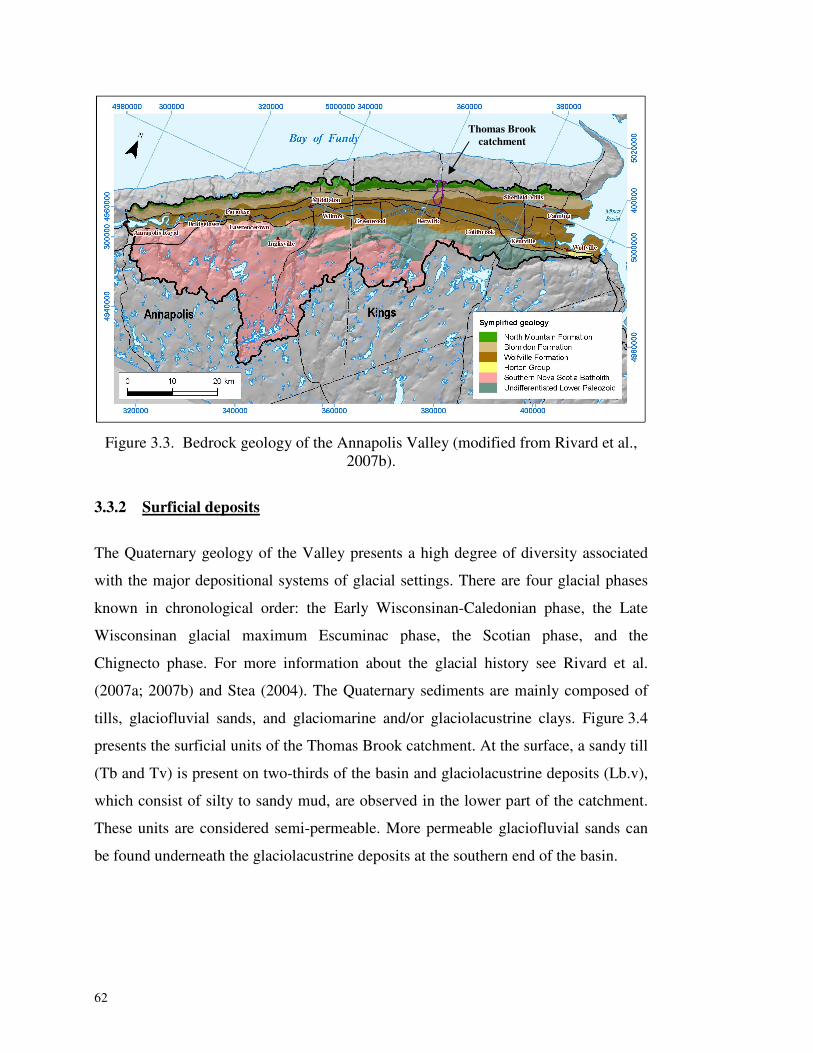
62

Figure 3.3. Bedrock geology of the Annapolis Valley (modified from Rivard et al.,

2007b).

3.3.2 Surficial deposits

The Quaternary geology of the Valley presents a high degree of diversity associated

with the major depositional systems of glacial settings. There are four glacial phases

known in chronological order: the Early Wisconsinan-Caledonian phase, the Late

Wisconsinan glacial maximum Escuminac phase, the Scotian phase, and the

Chignecto phase. For more information about the glacial history see Rivard et al.

(2007a; 2007b) and Stea (2004). The Quaternary sediments are mainly composed of

tills, glaciofluvial sands, and glaciomarine and/or glaciolacustrine clays. Figure 3.4

presents the surficial units of the Thomas Brook catchment. At the surface, a sandy till

(Tb and Tv) is present on two-thirds of the basin and glaciolacustrine deposits (Lb.v),

which consist of silty to sandy mud, are observed in the lower part of the catchment.

These units are considered semi-permeable. More permeable glaciofluvial sands can

be found underneath the glaciolacustrine deposits at the southern end of the basin.

Thomas Brook catchment

63

Figure 3.4. Surficial geology of the Thomas Brook catchment (modified from Paradis

et al., 2006).

These surficial sediments are generally thin on the Thomas Brook catchment (less

than 10 m) and do not represent good aquifers. Their hydrogeological role is

nonetheless important as they have an impact on both bedrock aquifer recharge and

protection against diffuse source contamination. Measured hydraulic conductivities

estimated with a Guelph permeameter range from 10-7 to 10-5 m/s (Gauthier, 2009).

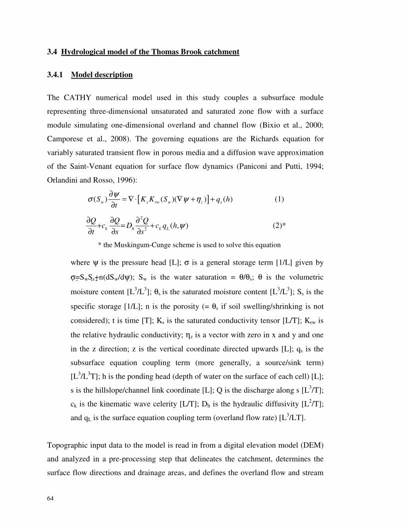
64

3.4 Hydrological model of the Thomas Brook catchment

3.4.1 Model description

The CATHY numerical model used in this study couples a subsurface module

representing three-dimensional unsaturated and saturated zone flow with a surface

module simulating one-dimensional overland and channel flow (Bixio et al., 2000;

Camporese et al., 2008). The governing equations are the Richards equation for

variably saturated transient flow in porous media and a diffusion wave approximation

of the Saint-Venant equation for surface flow dynamics (Paniconi and Putti, 1994;

Orlandini and Rosso, 1996):

[ ]( ) ( )( ) ( )w s rw w z sS K K S q ht

ψσ ψ η∂ = ∇ ⋅ ∇ + +∂

(1)

2

2 ( , )k h k L

Q Q Qc D c q h

t s sψ∂ ∂ ∂+ = +

∂ ∂ ∂ (2)*

* the Muskingum-Cunge scheme is used to solve this equation

where ψ is the pressure head [L]; σ is a general storage term [1/L] given by

σ�=�SwSs�+��n(dSw/dψ); Sw is the water saturation = θ/θs; θ is the volumetric

moisture content [L3/L3]; θs is the saturated moisture content [L3/L3]; Ss is the

specific storage [1/L]; n is the porosity (= θs if soil swelling/shrinking is not

considered); t is time [T]; Ks is the saturated conductivity tensor [L/T]; Krw is

the relative hydraulic conductivity; ηz is a vector with zero in x and y and one

in the z direction; z is the vertical coordinate directed upwards [L]; qs is the

subsurface equation coupling term (more generally, a source/sink term)

[L3/L3T]; h is the ponding head (depth of water on the surface of each cell) [L];

s is the hillslope/channel link coordinate [L]; Q is the discharge along s [L3/T];

ck is the kinematic wave celerity [L/T]; Dh is the hydraulic diffusivity [L2/T];

and qL is the surface equation coupling term (overland flow rate) [L3/LT].

Topographic input data to the model is read in from a digital elevation model (DEM)

and analyzed in a pre-processing step that delineates the catchment, determines the

surface flow directions and drainage areas, and defines the overland flow and stream

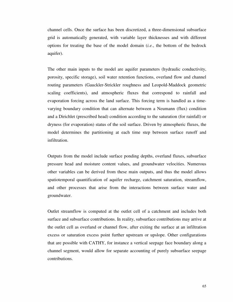
65

channel cells. Once the surface has been discretized, a three-dimensional subsurface

grid is automatically generated, with variable layer thicknesses and with different

options for treating the base of the model domain (i.e., the bottom of the bedrock

aquifer).

The other main inputs to the model are aquifer parameters (hydraulic conductivity,

porosity, specific storage), soil water retention functions, overland flow and channel

routing parameters (Gauckler-Strickler roughness and Leopold-Maddock geometric

scaling coefficients), and atmospheric fluxes that correspond to rainfall and

evaporation forcing across the land surface. This forcing term is handled as a time-

varying boundary condition that can alternate between a Neumann (flux) condition

and a Dirichlet (prescribed head) condition according to the saturation (for rainfall) or

dryness (for evaporation) status of the soil surface. Driven by atmospheric fluxes, the

model determines the partitioning at each time step between surface runoff and

infiltration.

Outputs from the model include surface ponding depths, overland fluxes, subsurface

pressure head and moisture content values, and groundwater velocities. Numerous

other variables can be derived from these main outputs, and thus the model allows

spatiotemporal quantification of aquifer recharge, catchment saturation, streamflow,

and other processes that arise from the interactions between surface water and

groundwater.

Outlet streamflow is computed at the outlet cell of a catchment and includes both

surface and subsurface contributions. In reality, subsurface contributions may arrive at

the outlet cell as overland or channel flow, after exiting the surface at an infiltration

excess or saturation excess point further upstream or upslope. Other configurations

that are possible with CATHY, for instance a vertical seepage face boundary along a

channel segment, would allow for separate accounting of purely subsurface seepage

contributions.

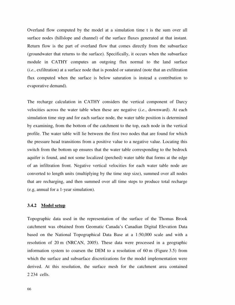
66

Overland flow computed by the model at a simulation time t is the sum over all

surface nodes (hillslope and channel) of the surface fluxes generated at that instant.

Return flow is the part of overland flow that comes directly from the subsurface

(groundwater that returns to the surface). Specifically, it occurs when the subsurface

module in CATHY computes an outgoing flux normal to the land surface

(i.e., exfiltration) at a surface node that is ponded or saturated (note that an exfiltration

flux computed when the surface is below saturation is instead a contribution to

evaporative demand).

The recharge calculation in CATHY considers the vertical component of Darcy

velocities across the water table when these are negative (i.e., downward). At each

simulation time step and for each surface node, the water table position is determined

by examining, from the bottom of the catchment to the top, each node in the vertical

profile. The water table will lie between the first two nodes that are found for which

the pressure head transitions from a positive value to a negative value. Locating this

switch from the bottom up ensures that the water table corresponding to the bedrock

aquifer is found, and not some localized (perched) water table that forms at the edge

of an infiltration front. Negative vertical velocities for each water table node are

converted to length units (multiplying by the time step size), summed over all nodes

that are recharging, and then summed over all time steps to produce total recharge

(e.g, annual for a 1-year simulation).

3.4.2 Model setup

Topographic data used in the representation of the surface of the Thomas Brook

catchment was obtained from Geomatic Canada’s Canadian Digital Elevation Data

based on the National Topographical Data Base at a 1:50,000 scale and with a

resolution of 20 m (NRCAN, 2005). These data were processed in a geographic

information system to coarsen the DEM to a resolution of 60 m (Figure 3.5) from

which the surface and subsurface discretizations for the model implementation were

derived. At this resolution, the surface mesh for the catchment area contained

2 234 cells.

67

Figure 3.5. The 60 m x 60 m surface mesh representing the topography of the

Thomas Brook catchment.

A main focus of this study was on the representation and effects of geological

heterogeneity. Figure 3.6 shows a reconstruction of the geology of the catchment for a

simplified vertical cross section along a north-south transect. The seven principal units

are represented in this conceptual model. In geochronological ascending order these

units are: 1) the Wolfville Formation; 2) the Blomidon Formation; 3) the North

Mountain Formation; 4) the till; 5) the glaciofluvial deposits (sands); 6) the

glaciolacustrine deposits (mud); and 7) the colluviums.

68

Figure 3.6. Geological reconstruction of the Thomas Brook catchment in vertical cross section along a north-south transect (not to scale).

The CATHY model allows the user to represent heterogeneity by layer (vertically)

and by zone (laterally). This process is depicted in Figure 3.7, which shows the seven

units listed above. The zones represent lateral heterogeneity, as deduced from the

bedrock and surficial geology data and from the inclined nature of the bedrock

formations. Each layer has its own pattern of lateral heterogeneity, thus in order to

represent some of the more complex geological scenarios it was necessary to define as

many zones as there are surface cells. This process and the subsequent attribution of

material properties (for instance hydraulic conductivity) to each zone were performed

using the goCad 6.1.6 ® and ArcGIS 9.2 ® software packages.

A flat base was used for the bottom of the study area. At the topographic lower point

(corresponding to the outlet of the catchment), the total thickness (surficial deposits

plus bedrock aquifer) was 50 m. The flat base thus resulted in a maximum thickness

(at the northern limit of the catchment) of 240 m. A total of 17 layers were used for

the vertical discretization, with one or more layers for each major geological

formation. Each layer, except the bottom-most one, is parallel to the surface and has a

constant thickness. The thinnest layers (0.1 m) were those closest to the surface,

needed to accurately resolve rainfall-runoff-infiltration partitioning and in general to

better capture the interactions between surface water and groundwater. The layers

were progressively coarsened with depth (see Figure 3.7), to a maximum thickness of

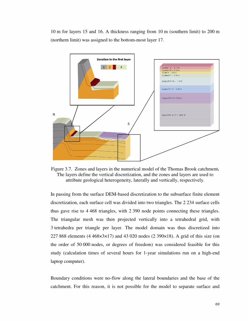
69

10 m for layers 15 and 16. A thickness ranging from 10 m (southern limit) to 200 m

(northern limit) was assigned to the bottom-most layer 17.

Figure 3.7. Zones and layers in the numerical model of the Thomas Brook catchment.

The layers define the vertical discretization, and the zones and layers are used to attribute geological heterogeneity, laterally and vertically, respectively.

In passing from the surface DEM-based discretization to the subsurface finite element

discretization, each surface cell was divided into two triangles. The 2 234 surface cells

thus gave rise to 4 468 triangles, with 2 390 node points connecting these triangles.

The triangular mesh was then projected vertically into a tetrahedral grid, with

3 tetrahedra per triangle per layer. The model domain was thus discretized into

227 868 elements (4 468×3×17) and 43 020 nodes (2 390×18). A grid of this size (on

the order of 50 000 nodes, or degrees of freedom) was considered feasible for this

study (calculation times of several hours for 1-year simulations run on a high-end

laptop computer).

Boundary conditions were no-flow along the lateral boundaries and the base of the

catchment. For this reason, it is not possible for the model to separate surface and

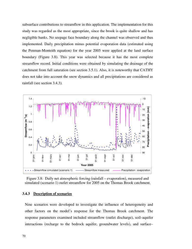
70

subsurface contributions to streamflow in this application. The implementation for this

study was regarded as the most appropriate, since the brook is quite shallow and has

negligible banks. No seepage face boundary along the channel was observed and thus

implemented. Daily precipitation minus potential evaporation data (estimated using

the Penman-Monteith equation) for the year 2005 were applied at the land surface

boundary (Figure 3.8). This year was selected because it has the most complete

streamflow record. Initial conditions were obtained by simulating the drainage of the

catchment from full saturation (see section 3.5.1). Also, it is noteworthy that CATHY

does not take into account the snow dynamics and all precipitations are considered as

rainfall (see section 3.4.3).

0

0.2

0.4

0.6

0.8

1

1.2

1.4

01-ja

nv

01-f

évr

01-m

ars

01-a

vr

01-m

ai

01-ju

in

01-ju

il

01-a

oût

01-s

ept

01-o

ct

01-n

ov

01-d

éc

Year 2005

Str

eam

flow

(m3 /s

)

-10

0

10

20

30

40

50

60

70

80

90

Pre

cipi

tatio

n - e

vapo

ratio

n (m

m)

Streamflow simulated (scenario 1) Streamflow measured Precipitation - evaporation

Figure 3.8: Daily net atmospheric forcing (rainfall – evaporation), measured and simulated (scenario 1) outlet streamflow for 2005 on the Thomas Brook catchment.

3.4.3 Description of scenarios

Nine scenarios were developed to investigate the influence of heterogeneity and

other factors on the model’s response for the Thomas Brook catchment. The

response parameters examined included streamflow (outlet discharge), soil–aquifer

interactions (recharge to the bedrock aquifer, groundwater levels), and surface–

71

subsurface interactions (saturation dynamics at the land surface, return flow).

Scenarios 1 to 8 reflect an increasing geological complexity while scenario 9

includes snow dynamics (see also Figure 3.9):

� Scenario 1: Homogeneous medium. A mean bedrock conductivity of 1 x 10-5 m/s,

a porosity of 15%, and a specific storage of 5 x 10-3 m-1 were used.

� Scenario 2: Addition of a homogeneous surficial sediment layer with mean

hydraulic conductivity of 1 x 10-6 m/s and porosity of 20%. The

specific storage was maintained at 5 x 10-3 m-1 for both the bedrock

and the surficial deposits.

� Scenario 3: Bedrock is divided in three parts in order to represent individual

geological formations. The hydraulic conductivities assigned were

1 x 10-6, 1 x 10-5, and 5 x 10-5 m/s for the North Mountain, Blomidon,

and Wolfville formations, respectively, which represent averages of

the pumping test results for each formation in this catchment. The

bedrock porosity was maintained at 15% for all three formations, and

the specific storage was also unchanged.

� Scenario 4: Incorporation of individual values of porosity (n) for each bedrock

formation. For the North Mountain, Blomidon, and Wolfville

formations, applied n values were 5, 11, and 28%, respectively,

based on Freeze and Cherry (1979) for the North Mountain (basalt)

formation and on estimated values (Rivard et al., 2007a) for the other

two formations.

� Scenario 5: Integration of realistic thicknesses for the surficial sediment units.

� Scenario 6: Addition of a sandy unit beneath the glaciolacustrine deposits, in the

southern portion of the catchment near the outlet. A hydraulic

conductivity of 1 x 10-5 m/s and a porosity of 35% were used. The

specific storage was unchanged.

72

� Scenario 7: Incorporation of the relative thicknesses, shapes, and inclinations of

the bedrock geological units and of additional details in the

unconsolidated sediments. This is the most complete geological

picture and corresponds to the reconstruction obtained using the

gOcad software (Figure 3.6) and from fieldwork carried out on the

Thomas Brook catchment. The permeable colluviums at the foot of

the North Mountain were assigned a hydraulic conductivity of

10-4 m/s, a porosity of 40%, and a specific storage of 0.1 m-1; for the

till deposits, K = 1 x 10-7 m/s, n = 20%, and Ss = 1 x 10-3 m-1 were

used; for the glaciofluvial deposits (sands), K = 1 x 10-5 m/s, n = 35%,

and Ss = 1 x 10-2 m-1; for the glaciolacustrine deposits, K = 5 x 10-

6 m/s, n = 15%, and Ss = 1 x 10-3 m-1. The specific storage for the

North Mountain, Blomidon, and Wolfville formations was reduced

from 5 x 10-3 m-1 to 1 x 10-5, 1 x 10-5, and 1 x 10-4 m-1, respectively.

� Scenario 8: Use of regional values of hydraulic conductivity. Reduction in the

hydraulic conductivity values of the North Mountain basalts

(1 x 10-7 m/s), glaciolacustrine deposits (1 x 10-7 m/s), and colluvium

layer (1 x 10-6 m/s), based on results from the regional study (Rivard

et al., 2007a). The K values for all other formations, as well as the

porosity and specific storage values were unchanged.

� Scenario 9: Consideration of snow dynamics. The impact of snow accumulation

and snowmelt, (where snow was not treated differently from rainfall

in the eight previous scenarios), was investigated. In this scenario, the

accumulated snow was transformed into rain (and thus allowed to

potentially infiltrate) whenever the maximum daily land surface

temperature rose above zero. For the 2005 dataset used, this pre-

treatment of the meteorological data resulted in six infiltration events

over the winter. This is reasonably representative of the mild winter

characteristics of the Annapolis Valley micro-climate. Conductivity,

porosity, and specific storage values for this scenario are as for

scenario 8.

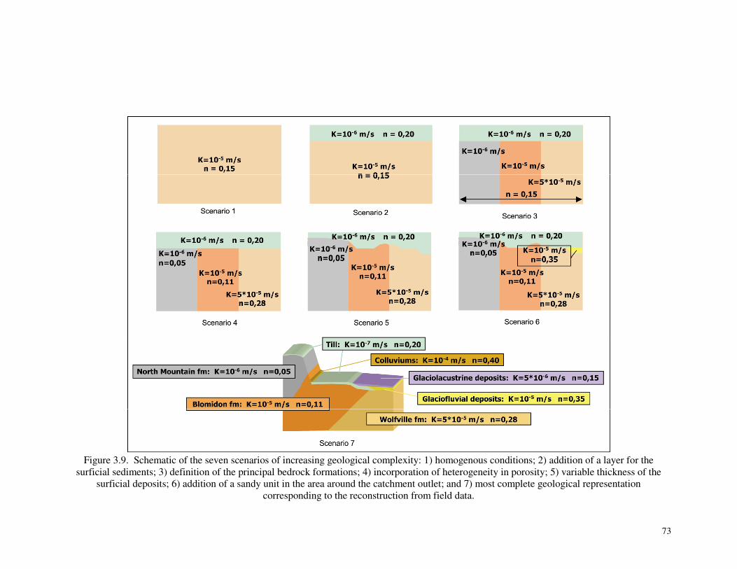
73

Figure 3.9. Schematic of the seven scenarios of increasing geological complexity: 1) homogenous conditions; 2) addition of a layer for the

surficial sediments; 3) definition of the principal bedrock formations; 4) incorporation of heterogeneity in porosity; 5) variable thickness of the surficial deposits; 6) addition of a sandy unit in the area around the catchment outlet; and 7) most complete geological representation

corresponding to the reconstruction from field data.

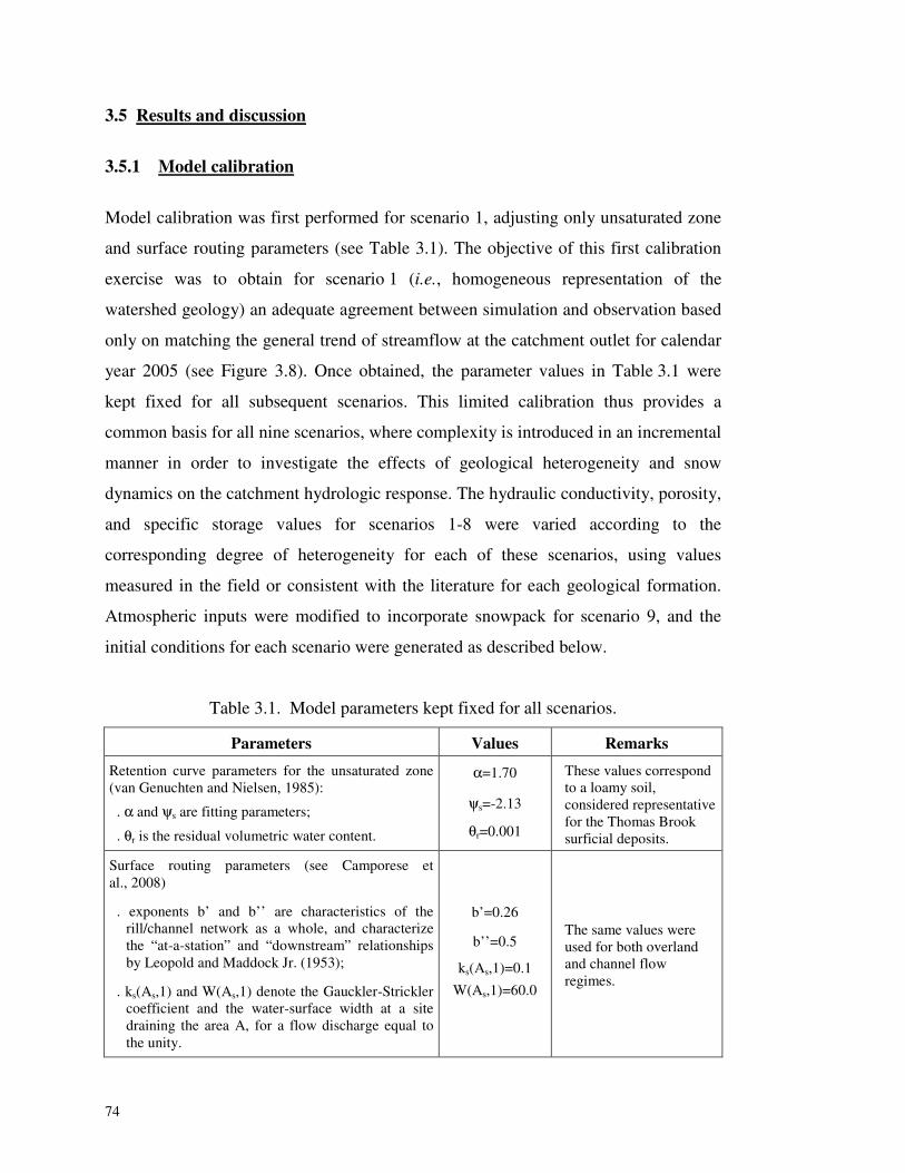
74

3.5 Results and discussion

3.5.1 Model calibration

Model calibration was first performed for scenario 1, adjusting only unsaturated zone

and surface routing parameters (see Table 3.1). The objective of this first calibration

exercise was to obtain for scenario 1 (i.e., homogeneous representation of the

watershed geology) an adequate agreement between simulation and observation based

only on matching the general trend of streamflow at the catchment outlet for calendar

year 2005 (see Figure 3.8). Once obtained, the parameter values in Table 3.1 were

kept fixed for all subsequent scenarios. This limited calibration thus provides a

common basis for all nine scenarios, where complexity is introduced in an incremental

manner in order to investigate the effects of geological heterogeneity and snow

dynamics on the catchment hydrologic response. The hydraulic conductivity, porosity,

and specific storage values for scenarios 1-8 were varied according to the

corresponding degree of heterogeneity for each of these scenarios, using values

measured in the field or consistent with the literature for each geological formation.

Atmospheric inputs were modified to incorporate snowpack for scenario 9, and the

initial conditions for each scenario were generated as described below.

Table 3.1. Model parameters kept fixed for all scenarios.

Parameters Values Remarks

Retention curve parameters for the unsaturated zone (van Genuchten and Nielsen, 1985):

. α and ψs are fitting parameters;

. θr is the residual volumetric water content.

α=1.70

ψs=-2.13

θr=0.001

These values correspond to a loamy soil, considered representative for the Thomas Brook surficial deposits.

Surface routing parameters (see Camporese et al., 2008)

. exponents b’ and b’’ are characteristics of the rill/channel network as a whole, and characterize the “at-a-station” and “downstream” relationships by Leopold and Maddock Jr. (1953);

. ks(As,1) and W(As,1) denote the Gauckler-Strickler coefficient and the water-surface width at a site draining the area A, for a flow discharge equal to the unity.

b’=0.26

b’’=0.5

ks(As,1)=0.1 W(As,1)=60.0

The same values were used for both overland and channel flow regimes.

75

For each scenario, the initial conditions were established by simulating drainage of the

catchment starting from fully saturated conditions and with zero atmospheric forcing.

When the streamflow generated from this pure drainage simulation roughly matched

the Thomas Brook baseflow, the corresponding pressure head values for each grid

node was read in as initial conditions for the subsequent calendar year 2005

simulation of that scenario. Baseflow was taken to be about 0.1 m3/s (see Figure 3.8),

and the match was obtained after 1-2 months of drainage, depending on the scenario.

A repetition of the year 2005 could have also been implemented so as to reduce the

impact of initial conditions that have probably affected the first few weeks of the

simulations (but without impacting significantly annual results). However, in this

case, CPU time for only one year was already long, so the repetition option was not

considered.

Model performance based on streamflow improved slightly from scenario 1 to

scenario 8. When other response variables were considered, model performance

improved significantly for scenarios 8 and 9 (Figure 3.12). In passing from scenario 7

to scenario 8, the hydraulic conductivity values for three formations (North Mountain

basalts, glaciolacustrine deposits, and colluvium layer) were adjusted using regional

values in order to better match available groundwater level data and the recharge

values estimated from other analyses. Scenario 7 produced water levels that were too

low in the North Mountain formation and an annual recharge of 675 mm (Table 3.2).

This is much higher than the recharge estimated for 2005 (315 mm) and also higher

than the bedrock recharge reported by Rivard et al. (2007a) for the entire Annapolis

Valley (120 to 225 mm).

With these adjusted hydraulic conductivities, scenario 8 yielded an annual recharge of

368 mm while scenario 9 produced 349 mm of recharge. The match in groundwater

levels at the end of the year 2005 for scenario 9 is shown in Figure 3.10 (very similar

results were obtained for scenario 8). The wells located in the North Mountain

formation are those in the high range of the graph, while the lower elevation points

correspond to wells in the Blomidon and Wolfville formations in the central and

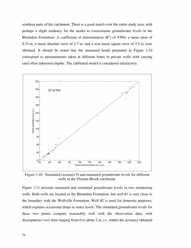
76

southern parts of the catchment. There is a good match over the entire study area, with

perhaps a slight tendency for the model to overestimate groundwater levels in the

Blomidon Formation. A coefficient of determination (R2) of 0.994, a mean error of

0.33 m, a mean absolute error of 3.7 m, and a root mean square error of 5.5 m were

obtained. It should be noted that the measured heads presented in Figure 3.10

correspond to measurements taken at different times in private wells with varying

(and often unknown) depths. The calibrated model is considered satisfactory.

Figure 3.10. Simulated (scenario 9) and measured groundwater levels for different wells in the Thomas Brook catchment.

Figure 3.11 presents measured and simulated groundwater levels in two monitoring

wells. Both wells are located in the Blomidon Formation, but well #1 is very close to

the boundary with the Wolfville Formation. Well #2 is used for domestic purposes,

which explains occasional drops in water levels. The simulated groundwater levels for

these two points compare reasonably well with the observation data, with

discrepancies over time ranging from 0 to about 2 m, i.e. within the accuracy obtained

R2=0.994

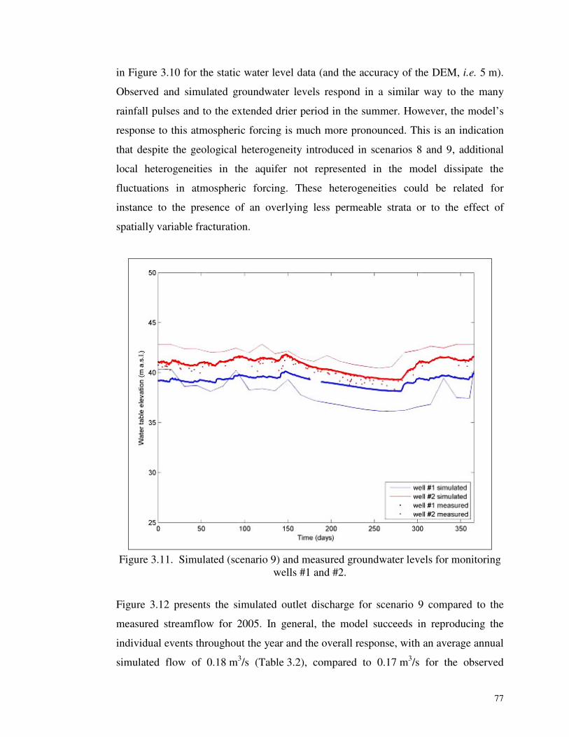
77

in Figure 3.10 for the static water level data (and the accuracy of the DEM, i.e. 5 m).

Observed and simulated groundwater levels respond in a similar way to the many

rainfall pulses and to the extended drier period in the summer. However, the model’s

response to this atmospheric forcing is much more pronounced. This is an indication

that despite the geological heterogeneity introduced in scenarios 8 and 9, additional

local heterogeneities in the aquifer not represented in the model dissipate the

fluctuations in atmospheric forcing. These heterogeneities could be related for

instance to the presence of an overlying less permeable strata or to the effect of

spatially variable fracturation.

�

Figure 3.11. Simulated (scenario 9) and measured groundwater levels for monitoring wells #1 and #2.

Figure 3.12 presents the simulated outlet discharge for scenario 9 compared to the

measured streamflow for 2005. In general, the model succeeds in reproducing the

individual events throughout the year and the overall response, with an average annual

simulated flow of 0.18 m3/s (Table 3.2), compared to 0.17 m3/s for the observed

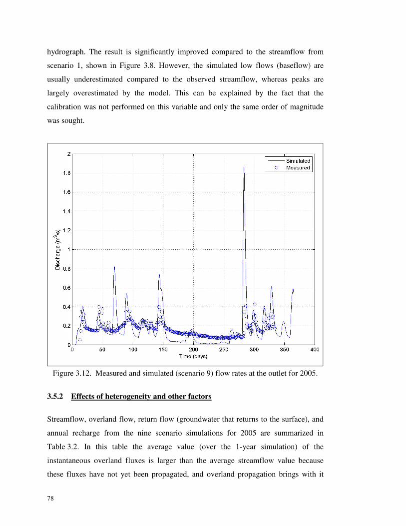
78

hydrograph. The result is significantly improved compared to the streamflow from

scenario 1, shown in Figure 3.8. However, the simulated low flows (baseflow) are

usually underestimated compared to the observed streamflow, whereas peaks are

largely overestimated by the model. This can be explained by the fact that the

calibration was not performed on this variable and only the same order of magnitude

was sought.

�

Figure 3.12. Measured and simulated (scenario 9) flow rates at the outlet for 2005.

3.5.2 Effects of heterogeneity and other factors

Streamflow, overland flow, return flow (groundwater that returns to the surface), and

annual recharge from the nine scenario simulations for 2005 are summarized in

Table 3.2. In this table the average value (over the 1-year simulation) of the

instantaneous overland fluxes is larger than the average streamflow value because

these fluxes have not yet been propagated, and overland propagation brings with it

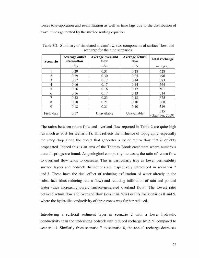
79

losses to evaporation and re-infiltration as well as time lags due to the distribution of

travel times generated by the surface routing equation.

Table 3.2. Summary of simulated streamflow, two components of surface flow, and recharge for the nine scenarios.

Average outlet streamflow

Average overland flow

Average return flow Total recharge

Scenario m3/s m3/s m3/s mm/year

1 0.29 0.31 0.28 628 2 0.29 0.30 0.25 496 3 0.17 0.17 0.14 583 4 0.16 0.17 0.14 564 5 0.16 0.16 0.12 501 6 0.16 0.17 0.13 514 7 0.22 0.23 0.18 675 8 0.18 0.21 0.10 368 9 0.18 0.21 0.10 349

Field data 0.17 Unavailable Unavailable 315 (Gauthier, 2009)

The ratios between return flow and overland flow reported in Table 2 are quite high

(as much as 90% for scenario 1). This reflects the influence of topography, especially

the steep drop along the cuesta that generates a lot of return flow that is quickly

propagated. Indeed this is an area of the Thomas Brook catchment where numerous

natural springs are found. As geological complexity increases, the ratio of return flow

to overland flow tends to decrease. This is particularly true as lower permeability

surface layers and bedrock distinctions are respectively introduced in scenarios 2

and 3. These have the dual effect of reducing exfiltration of water already in the

subsurface (thus reducing return flow) and reducing infiltration of rain and ponded

water (thus increasing purely surface-generated overland flow). The lowest ratio

between return flow and overland flow (less than 50%) occurs for scenarios 8 and 9,

where the hydraulic conductivity of three zones was further reduced.

Introducing a surficial sediment layer in scenario 2 with a lower hydraulic

conductivity than the underlying bedrock unit reduced recharge by 21% compared to

scenario 1. Similarly from scenario 7 to scenario 8, the annual recharge decreases

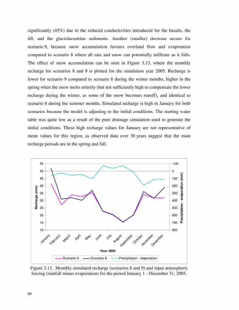
80

significantly (45%) due to the reduced conductivities introduced for the basalts, the

till, and the glaciolacustrine sediments. Another (smaller) decrease occurs for

scenario 9, because snow accumulation favours overland flow and evaporation

compared to scenario 8 where all rain and snow can potentially infiltrate as it falls.

The effect of snow accumulation can be seen in Figure 3.13, where the monthly

recharge for scenarios 8 and 9 is plotted for the simulation year 2005. Recharge is

lower for scenario 9 compared to scenario 8 during the winter months, higher in the

spring when the snow melts entirely (but not sufficiently high to compensate the lower

recharge during the winter, as some of the snow becomes runoff), and identical to

scenario 8 during the summer months. Simulated recharge is high in January for both

scenarios because the model is adjusting to the initial conditions. The starting water

table was quite low as a result of the pure drainage simulation used to generate the

initial conditions. These high recharge values for January are not representative of

mean values for this region, as observed data over 30 years suggest that the main

recharge periods are in the spring and fall.

10

15

20

25

30

35

40

45

50

55

Janu

ary

Febru

ary

March

April

MayJu

ne July

Augus

t

Septem

ber

Octobe

r

Novembe

r

Decembe

r

Year 2005

Rec

harg

e (m

m)

-100

0

100

200

300

400

500

600

700

800

Pre

cipi

tatio

n - e

vapo

ratio

n (m

m)

Scenario 9 Scenario 8 Precipitation - evaporation

�

Figure 3.13. Monthly simulated recharge (scenarios 8 and 9) and input atmospheric forcing (rainfall minus evaporation) for the period January 1 - December 31, 2005.

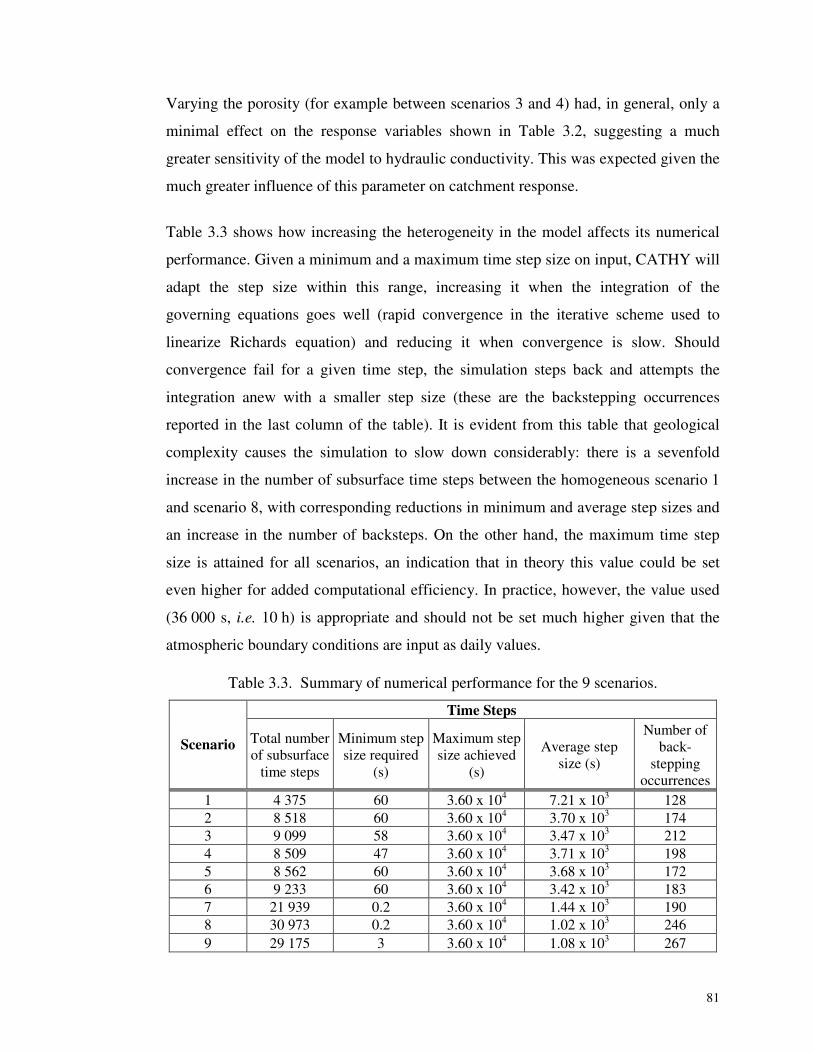
81

Varying the porosity (for example between scenarios 3 and 4) had, in general, only a

minimal effect on the response variables shown in Table 3.2, suggesting a much

greater sensitivity of the model to hydraulic conductivity. This was expected given the

much greater influence of this parameter on catchment response.

Table 3.3 shows how increasing the heterogeneity in the model affects its numerical

performance. Given a minimum and a maximum time step size on input, CATHY will

adapt the step size within this range, increasing it when the integration of the

governing equations goes well (rapid convergence in the iterative scheme used to

linearize Richards equation) and reducing it when convergence is slow. Should

convergence fail for a given time step, the simulation steps back and attempts the

integration anew with a smaller step size (these are the backstepping occurrences

reported in the last column of the table). It is evident from this table that geological

complexity causes the simulation to slow down considerably: there is a sevenfold

increase in the number of subsurface time steps between the homogeneous scenario 1

and scenario 8, with corresponding reductions in minimum and average step sizes and

an increase in the number of backsteps. On the other hand, the maximum time step

size is attained for all scenarios, an indication that in theory this value could be set

even higher for added computational efficiency. In practice, however, the value used

(36 000 s, i.e. 10 h) is appropriate and should not be set much higher given that the

atmospheric boundary conditions are input as daily values.

Table 3.3. Summary of numerical performance for the 9 scenarios.

Time Steps

Scenario Total number of subsurface

time steps

Minimum step size required

(s)

Maximum step size achieved

(s)

Average step size (s)

Number of back-

stepping occurrences

1 4 375 60 3.60 x 104 7.21 x 103 128 2 8 518 60 3.60 x 104 3.70 x 103 174 3 9 099 58 3.60 x 104 3.47 x 103 212 4 8 509 47 3.60 x 104 3.71 x 103 198 5 8 562 60 3.60 x 104 3.68 x 103 172 6 9 233 60 3.60 x 104 3.42 x 103 183 7 21 939 0.2 3.60 x 104 1.44 x 103 190 8 30 973 0.2 3.60 x 104 1.02 x 103 246 9 29 175 3 3.60 x 104 1.08 x 103 267

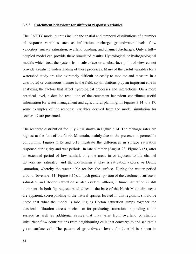
82

3.5.3 Catchment behaviour for different response variables

The CATHY model outputs include the spatial and temporal distributions of a number

of response variables such as infiltration, recharge, groundwater levels, flow

velocities, surface saturation, overland ponding, and channel discharges. Only a fully-

coupled model can provide these simulated results. Hydrological or hydrogeological

models which treat the system from subsurface or a subsurface point of view cannot

provide a realistic understanding of these processes. Many of the useful variables for a

watershed study are also extremely difficult or costly to monitor and measure in a

distributed or continuous manner in the field, so simulations play an important role in

analyzing the factors that affect hydrological processes and interactions. On a more

practical level, a detailed resolution of the catchment behaviour contributes useful

information for water management and agricultural planning. In Figures 3.14 to 3.17,

some examples of the response variables derived from the model simulation for

scenario 9 are presented.

The recharge distribution for July 29 is shown in Figure 3.14. The recharge rates are

highest at the foot of the North Mountain, mainly due to the presence of permeable

colluviums. Figures 3.15 and 3.16 illustrate the differences in surface saturation

response during dry and wet periods. In late summer (August 28; Figure 3.15), after

an extended period of low rainfall, only the areas in or adjacent to the channel

network are saturated, and the mechanism at play is saturation excess, or Dunne

saturation, whereby the water table reaches the surface. During the wetter period

around November 11 (Figure 3.16), a much greater portion of the catchment surface is

saturated, and Horton saturation is also evident, although Dunne saturation is still

dominant. In both figures, saturated zones at the base of the North Mountain cuesta

are apparent, corresponding to the natural springs located in this region. It should be

noted that what the model is labelling as Horton saturation lumps together the

classical infiltration excess mechanism for producing saturation or ponding at the

surface as well as additional causes that may arise from overland or shallow

subsurface flow contributions from neighbouring cells that converge to and saturate a

given surface cell. The pattern of groundwater levels for June 14 is shown in

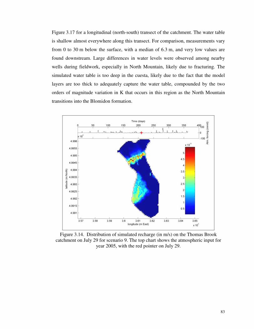
83

Figure 3.17 for a longitudinal (north-south) transect of the catchment. The water table

is shallow almost everywhere along this transect. For comparison, measurements vary

from 0 to 30 m below the surface, with a median of 6.3 m, and very low values are

found downstream. Large differences in water levels were observed among nearby

wells during fieldwork, especially in North Mountain, likely due to fracturing. The

simulated water table is too deep in the cuesta, likely due to the fact that the model

layers are too thick to adequately capture the water table, compounded by the two

orders of magnitude variation in K that occurs in this region as the North Mountain

transitions into the Blomidon formation.

Figure 3.14. Distribution of simulated recharge (in m/s) on the Thomas Brook

catchment on July 29 for scenario 9. The top chart shows the atmospheric input for year 2005, with the red pointer on July 29.

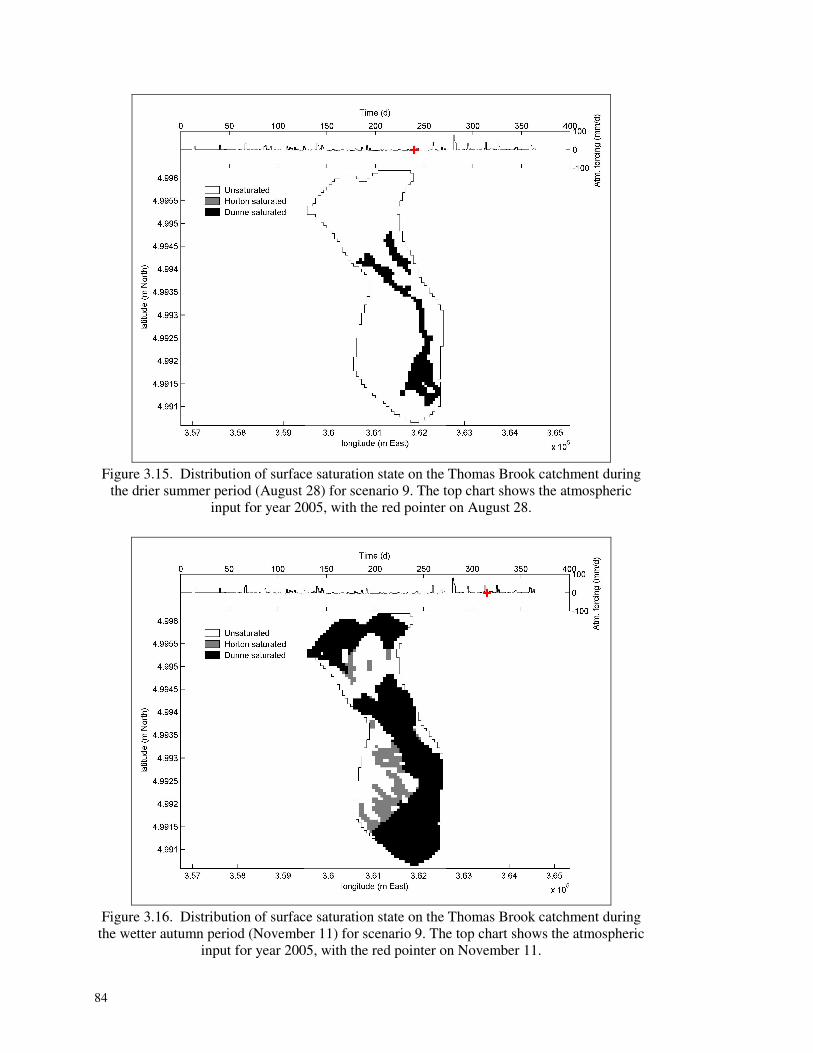
84

�

Figure 3.15. Distribution of surface saturation state on the Thomas Brook catchment during the drier summer period (August 28) for scenario 9. The top chart shows the atmospheric

input for year 2005, with the red pointer on August 28.

Figure 3.16. Distribution of surface saturation state on the Thomas Brook catchment during

the wetter autumn period (November 11) for scenario 9. The top chart shows the atmospheric input for year 2005, with the red pointer on November 11.

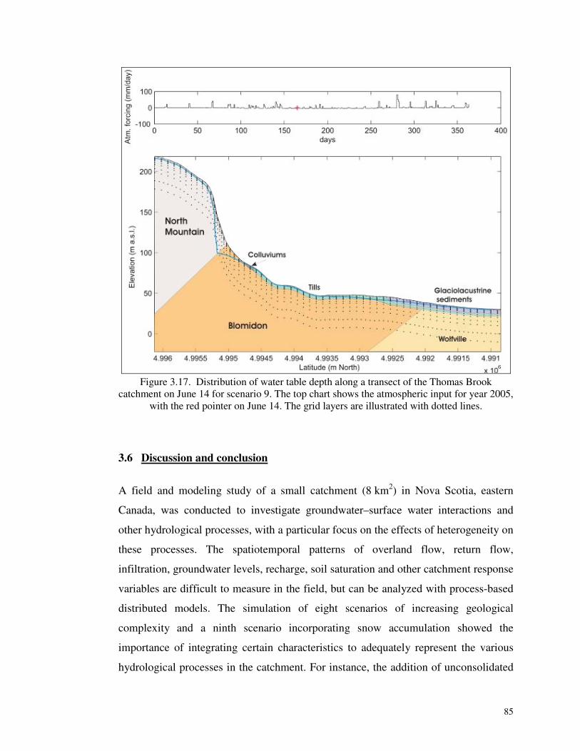
85

Figure 3.17. Distribution of water table depth along a transect of the Thomas Brook

catchment on June 14 for scenario 9. The top chart shows the atmospheric input for year 2005, with the red pointer on June 14. The grid layers are illustrated with dotted lines.

3.6 Discussion and conclusion

A field and modeling study of a small catchment (8 km2) in Nova Scotia, eastern

Canada, was conducted to investigate groundwater–surface water interactions and

other hydrological processes, with a particular focus on the effects of heterogeneity on

these processes. The spatiotemporal patterns of overland flow, return flow,

infiltration, groundwater levels, recharge, soil saturation and other catchment response

variables are difficult to measure in the field, but can be analyzed with process-based

distributed models. The simulation of eight scenarios of increasing geological

complexity and a ninth scenario incorporating snow accumulation showed the

importance of integrating certain characteristics to adequately represent the various

hydrological processes in the catchment. For instance, the addition of unconsolidated

86

sediment units exerted a strong control on infiltration, whereas the assignment of

distinct hydraulic conductivity values to the three bedrock formations influenced the

water table position. The geological formation dip, porosity, and snow accumulation

were shown to have only a relatively minor impact on the catchment results on an

annual basis. The simulated heads, aquifer recharge, and streamflow at the outlet for

scenario 9 were comparable to observed or previously estimated values, and important

features of the Thomas Brook catchment, such as the natural springs at the foot of the

North Mountain cuesta, were also well reproduced. Modeling studies on

groundwater–surface water interactions such as the one reported here should be

helpful for water management and aquifer protection in this rural area, providing,

amongst other things, information on zones of preferential recharge and on the

response of stream discharge to changing inputs.

As in any modeling study of real aquifers and catchments, there are numerous

potential improvements that can be suggested with regards to the representation of

processes, parameters, and boundary conditions used in this study. Even with the most

complex model, simplifications are always necessary, owing to model structure

limitations, lack of data, and other reasons. Limitations of this application include the

size of the basin, which was maybe too small to reflect the general trends of the entire

Valley, the availability of data (only one year) that allowed us to see only a specific

moment in time and not the overall trends of the water dynamics of the watershed

over many years, and the use of equivalent porous media to represent fractured

formations. As an example, additional insight into the role of heterogeneity and

related factors on the Thomas Brook catchment response could probably be obtained

by considering the fractured networks in each geological formation given, if good

information is available. As a first approximation, this could be done using a dual-

porosity representation, allowed by CATHY, of the aquifer in this part of the basin.

More complex representations are of course also possible. Nevertheless, this study

showed that the model CATHY could be successfully used on a real watershed that

was not extensively characterized.

87

3.7 Acknowledgements

This study was supported by the Geological Survey of Canada and the National

Science and Engineering Research Council of Canada (NSERC) and the Institut

National de la Recherche Scientifique – ETE. We wish to thank, for their

contributions and assistance during various stages of this study: John Drage (Nova

Scotia Environment and Labour), Dale Hebb (Agriculture and Agri-Food Canada),

Robert Gordon (Nova Scotia Agricultural College), Roger Morin (United States

Geological Survey), Daniel Paradis, Yves Michaud, Andrée Bolduc, Serge Paradis,

Christine Deblonde (Geological Survey of Canada), and Samuel Trépanier (UQAM),

as well as all the residents of the Thomas Brook catchment.

3.8 References

Agriculture and Agri-Food Canada (2002). National soil database, nsd008.20000530, http://www.nsac.ca/bookstore/index.

Anderson, E.I. (2005). Modeling groundwater–surface water interactions using the

Dupuit approximation, Adv. Water Resour., 28, 315-327. Barlow, P.M. and Moench, A.F. (1998). Analytical solutions and computer programs

for hydraulic interaction of stream-aquifer systems. US Geological Survey - Open File Report 98-415A, 85p.

Bixio, A.C., Orlandini, S., Paniconi, C., and Putti, M. (2000). Physically-based

distributed model for coupled surface runoff and subsurface flow simulation at the catchment scale, in Computational Methods in Water Resources, Vol. 2, Surface Water Systems and Hydrology (L.R. Bentley, J.F. Sykes, C.A. Brebbia, W.G. Gray and G.F. Pinder, eds.), Balkema, Rotterdam, The Netherlands, 1115-1122.

Camporese, M., Paniconi, C., Putti, M., and Orlandini, S. (2008). Surface–subsurface

flow modeling with path-based overland and channel dynamics, boundary condition-based coupling, and assimilation of multisource observation data, submitted to Water Resour. Res.

de Marsily, G., Delay, F., Gonçalvès, J., Renard, P., Teles, V. and Violette, S. (2005).

Dealing with spatial heterogeneity, Hydrogeol. J., 13(1), 161-183. Environment Canada (2004). National climate archive:

http://www.climate.weatheroffice.ec.gc.ca/climateData

88

Food and Agriculture Organization of the United Nations (2004). FAO Penman-Monteith equation: http://www.fao.org/docrep/X0490E/x0490e06.htm#chapter%202%20%20%20fao%20penman%20monteith%20equation

Freeze, R.A. and Cherry, J.A. (1979). Groundwater, Prentice Hall, Inc., United States of America, 604 p..

Gauthier, M.-J. (2009). Étude sur le terrain et par modélisation du bassin versant du

ruisseau Thomas (vallée d’Annapolis, Nouvelle-Écosse) : Influence de l’hétérogénéité et autres facteurs sur les interactions entre l’eau de surface et l’eau souterraine et la recharge des aquifères, Mémoire de maîtrise, Institut National de la Recherche Scientifique, Eau-Terre-Environnement, Québec, 101 p..

Hamblin, T. (2004). Regional geology of the Triassic/Jurassic Fundy Group of

Annapolis Valley, Geological Survey of Canada – Open File 4678. Hantush, M.H. (2005). Modeling stream–aquifer interactions with linear response

functions, J. Hydrol., 311, 59-79. Jones, J.P., Sudicky, E. and McLaren, R. (2008). Application of a fully-integrated

surface–subsurface flow model at the watershed-scale: A case study, Water Resour. Res., doi:10.1029/2006WR005603.

Kampf, S.K. and Burges, S.J. (2007). A framework for classifying and comparing

distributed hillslope and catchment hydrologic models, Water Resour. Res., 43, W05423, doi:10.1029/2006WR005370.

Kings CED Agency’s Environment and Land Use Committee (2000). Quality of the

Environment Report, A Study and Review of Sustainability Indicators, Kings Community Economic Development Agency, Kings County, Nova Scotia, 32 p..

Kollet, S.J. and Maxwell, R.M. (2006). Integrated surface–groundwater flow

modeling: A free-surface overland flow boundary condition in a parallel groundwater flow model, Adv. Water Resour., 29, 945-958.

Leopold, L. B. and Maddock Jr., T. (1953). The hydraulic geometry of stream

channels and some physiographic implications. Prof. Pap. 252, U.S. Geol. Surv., Washington, DC.

Morita, M. and Yen, B.C. (2002). Modeling of conjunctive two-dimensional surface–

three-dimensional subsurface flows, J. Hydraulic Engrg., ASCE, 128(2), 184-200. Natural Resources Canada (2005). Geomatic Canada’s Canadian Digital Elevation

Data based on the National Topographical Data Base at a 1:50,000 scale: http://www.ctis.nrcan.gc.ca/

89

Orlandini, S. and Rosso, R. (1996). Diffusion wave modeling of distributed catchment dynamics, Journal of Hydrologic Engineering, ASCE, 1(3), 103-113.

Panday, S. and Huyakorn, P.S. (2004). A fully coupled physically-based spatially-

distributed model for evaluating surface/subsurface flow, Adv. Water Resour., 27, 361-382.

Paniconi, C. and Putti, M. (1994). A comparison of Picard and Newton iteration in

the numerical solution of multidimensional variably saturated flow problems, Water Resour. Res., 30(12), 3357-3374.

Paradis, S.J., Bolduc, A. and Stea R. (2006). Surficial geology, Annapolis Valley,

Nova Scotia, Geological Survey of Canada, Open File 5276, scale 1:100 000. Posavec, K., Bacani, A. and Nakic, Z. (2006). A visual basic spreadsheet macro for

recession curve analysis, Ground Water, Computer note, 44(5): 764–767. Pohll, G.M., Warwick, J.J. and Tyler, S.W. (1996). Coupled surface–subsurface

hydrologic model of a nuclear subsidence crater at the Nevada test site, J. Hydrol., 186, 43-62.

Rivard, C., Paradis, D., Paradis, S.J., Bolduc, A., Morin, R.H., Liao, S., Pullan, S.,

Gauthier, M.-J., Trépanier, S., Blackmore, A., Spooner, I., Deblonde, C., Fernandes, R., Castonguay, S., Michaud, Y., Drage, J. and Paniconi, C. (2007a). Canadian Groundwater Inventory: Regional Hydrogeological Characterization of the Annapolis-Cornwallis Valley aquifers, GSC internal report (and GSC Bulletin in preparation).

Rivard, C., Deblonde, C., Boivin, R., Bolduc, A., Paradis, S.J., Paradis, D., Liao, S.,

Gauthier, M.-J., Blackmore, A., Trépanier, S., Castonguay, S., Drage, J. and Michaud, Y. (2007b). Canadian Groundwater Inventory: Hydrogeological Atlas of the Annapolis-Cornwallis Valley, Nova Scotia, Geological Survey of Canada, Open File 5541, 128 p..

Rutledge., A.T. (1998) Computer programs for describing the recession of ground-

water discharge and for estimating mean ground-water recharge and discharge from streamflow – Records and update, USGS Water-Resources Investigations, Report 98-4148, 43 p.

Singh, V. and Bhallamudi, S.M. (1998). Conjuctive surface–subsurface modeling of

overland flow, Adv. Water Resour., 21, 567-579. Sophocleous, M. (2002). Interactions between groundwater and surface water: the

state of the science, Hydrogeology Journal, vol. 10, p. 52-67.

90

Stea, R.R. (2004). The Appalachian Glacier Complex in Maritime Canada, In Ehlers, J. and Gibbard, P.L., eds. Quaternary Glaciations - Extent and Chronology Part II: 213-232.

Trescott, P.C. (1968). Groundwater resources and hydrogeology of the Annapolis-

Cornwallis Valley, Nova Scotia, Province of Nova Scotia - Department of Mines, Memoir 6, Halifax, Nova Scotia, 159 p..

VanderKwaak, J.E. and Loague, K. (2001). Hydrologic-response simulations for the

R-5 catchment with a comprehensive physics-based model, Water Resour. Res., 37(4), 999-1013.

van Genuchten, M.Th. and Nielsen, D.R. (1985). On describing and predicting the

hydraulic properties of unsaturated soils, Ann. Geophys., 3(5), 615-628.

92

CHAPITRE 4 : Conclusion

Les principaux objectifs de cette maîtrise consistaient 1) à acquérir une meilleure

compréhension de la dynamique du bassin versant du ruisseau Thomas d’abord à

l’aide de travaux de terrain, 2) à simuler l’écoulement de surface et souterrain au

moyen de la modélisation numérique couplée et 3) à évaluer l’effet de l’hétérogénéité

des formations géologiques sur le modèle (la représentation de la géologie du bassin

versant devenant de plus en plus complexe) et de l’intégration du couvert de neige.

Les travaux de terrain, réalisés en collaboration avec la CGC, se sont échelonnés sur

trois étés (2004, 2005 et 2006). Lors de ces travaux, quelques piézomètres se sont

bouchés et les dépôts de surface se sont avérés être beaucoup plus minces

(généralement moins de 5 m) que ce qu’indiquaient les bases de données provinciales

et, en général, non saturés. Des données in situ de niveaux d’eau à plusieurs

profondeurs et donc de gradients pour l’étude des interactions entre l’eau souterraine

circulant dans les dépôts meubles et le roc n’ont donc pas pu être prises.

De ces travaux, il ressort que l’aquifère rocheux dans ce secteur s’écoule

essentiellement du nord vers le sud. Les trois formations rocheuses présentes sont de

plus en plus perméables vers le sud du bassin, soit respectivement 1,8 x 10-6 m/s pour

les montagnes du Nord, 2,0 x 10-5 m/s pour le Blomidon et 3,8 x 10-5 m/s pour le

Wolfville. Il en est de même pour les sédiments de surface avec une perméabilité

croissante du nord vers le sud allant de 10-8 à 10-5 m/s. Ces travaux ont également

permis de confirmer l’alimentation du ruisseau par l’aquifère à un taux croissant allant

de 10-9 à 10-6 m3/s des montagnes à l’exutoire. La recharge s’effectue principalement

au printemps (mai) et à l’automne (octobre) et se fait préférentiellement au pied des

montagnes du Nord, à travers les colluvions.

L’ensemble des travaux de terrain et la modélisation avec CATHY a permis de mieux

comprendre les échanges d’eau à l’intérieur du bassin du ruisseau Thomas et de

quantifier plusieurs composantes du cycle hydrologique, tels que la recharge,

l’écoulement de surface, l’apport souterrain et la saturation à la surface. L’utilisation

93

du modèle CATHY a permis de quantifier différents processus et paramètres

hydro(géo)logiques dans l’espace et le temps, incluant la profondeur de la nappe, la

saturation de la surface de type Dunne et/ou Horton, la recharge (349 mm/an),

l’écoulement de surface (overland flow; 0,21 m3/s) et l’apport souterrain (return flow;

0,097 m3/s). Plusieurs de ces quantités sont difficiles, voire impossible, à estimer sur

le terrain et permettent donc, une fois la calibration du modèle réalisée avec la

profondeur de la nappe, la recharge et le débit du ruisseau, de fournir des informations

spatio-temporelles sur les interactions autrement inaccessibles.

Les différents scénarios de modélisation ont démontré l’importance d’une bonne

représentation de la géologie du territoire étudié. En effet, avec des scénarios de plus

en plus représentatifs de la réalité, la recharge et la hauteur de la nappe simulées

étaient de plus en plus près des valeurs préalablement estimées ou observées, et le

débit à l’exutoire du ruisseau était similaire à celui mesuré. Par ailleurs, les différents

scénarios ont montré que certaines caractéristiques avaient beaucoup plus d’impact

que d’autres sur les résultats du modèle, comme par exemple l’addition de la couche

de sédiments en surface et l’assignation de valeurs individuelles de conductivités

hydrauliques aux trois formations rocheuses. L’addition du pendage des formations

rocheuses, la différentiation des valeurs de porosité selon les formations et

l’accumulation de la neige n’ont pas montré d’impact majeur sur la réponse du

système.

Cette étude a mis en évidence l’importance de bien définir les objectifs de façon à

trouver le bon équilibre entre les efforts consacrés aux travaux de terrain, à l’étude des

données existantes et au temps investi dans la modélisation. Cette étude suggère par

exemple que le fait d’utiliser des conductivités hydrauliques équivalentes ou des

formations assez peu représentatives de la géologie réelle du système étudié mènent à

des résultats, qui, dans ce cas-ci, semblaient assez proches de la réalité pour les débits

de surface, mais très loin pour les paramètres hydrogéologiques (recharge et niveaux

d’eau souterraine). Une meilleure représentation des réponses du bassin versant aurait

probablement pu être obtenue en utilisant des données climatiques sur une plage de

94

données s’échelonnant sur une période de plus d’un an, ainsi qu’en considérant plus

en détail les caractéristiques du ruisseau, telles que sa rugosité et ses dimensions. Il

pourrait également s’avérer intéressant, dans une version future du modèle CATHY,

de pouvoir intégrer des caractéristiques additionnelles comme par exemple les

systèmes d’irrigation et la végétation étant donnée la vocation agricole du territoire.

Néanmoins, cette étude aura permis de localiser et de quantifier les principaux

processus d’interactions se produisant dans le bassin versant du ruisseau Thomas.

Ceci est d’une grande importance pour les gens de la région, où la nappe présente en

divers endroits des diminutions significatives et des concentrations relativement

élevées en nitrates. En connaissant la distribution de certains processus hydrologiques

et en particulier de la recharge, il est possible d’identifier les endroits à risque pour la

contamination et ainsi gérer plus adéquatement la ressource en eau.

La réalisation de différents scénarios climatiques (avec des données issues du modèle

MRCC4) avec cette application du modèle CATHY pour étudier les réponses du

système et, en particulier, la recharge des aquifères, a été entamée dans le cadre d’un

projet de doctorat (Sulis, en prép.). Malgré les différences observées dans les

réponses du système entre les résultats simulés et les données observées pour

l'année 2005, cette étude permettra de quantifier les débits et la recharge en périodes

de crue et de sécheresse, en fonction du climat futur simulé. Ceci permettra donc

d’obtenir des informations utiles pour une meilleure gestion de la ressource.

96

BIBLIOGRAPHIE

Agriculture and Agri-Food Canada (2002). National soil database, nsd008.20000530, http://www.nsac.ca/bookstore/index

Anderson, E.I. (2005). Modeling groundwater–surface water interactions using the

Dupuit approximation, Adv. Water Resour., 28, 315-327. Barlow, P.M. and Moench, A.F. (1998). Analytical solutions and computer programs

for hydraulic interaction of stream-aquifer systems, US Geological Survey - Open File Report 98-415A, 85p.

Binley, A., Beven, K. and Elgy, J. (1989). A physically based model of

heterogeneous hillslopes – 2. Effective hydraulic conductivities, Water Resour. Res., 25 (6), 1227-1233.

Bixio, A.C., Orlandini, S., Paniconi, C. and Putti, M. (2000). Physically-based

distributed model for coupled surface runoff and subsurface flow simulation at the catchment scale, in Computational Methods in Water Resources, Surface Water Systems and Hydrology, Balkema, 2: 1115-1122.

Bolduc, A., Paradis, S.J. and Stea R.R (in prep.). The Annapolis Valley, Nova Scotia,

Surficial geology and groundwater resources, Géographie physique et Quaternaire, in preparation.

Bouwer, H. and Rice, R.C. (1976). A slug test for determining hydraulic conductivity

of unconfined aquifers with completely or partially penetrating wells, Water Resources Research, 12: 423-428.

Butler, J.J.Jr and Garnett, E.J. (2000). Simple procedures for analysis of slug tests in

formations of high hydraulic conductivity using spreadsheet and scientific graphics software, Kansas Geological Survey – Open File 2000-40, 19 p..

Camporese, M., Paniconi, C., Putti, M., and Orlandini, S. (2008). Surface–subsurface

flow modeling with path-based overland and channel dynamics, boundary condition-based coupling, and assimilation of multisource observation data, submitted to Water Resour. Res..

Chapman, T.G. (1991). Comment on ‘Evaluation of automated techniques for

baseflow and recession analyses’ by Nathan, R.J. and McMahon, T.A., Water Resources Research, 27:1783-1784.

Commission Géologique du Canada (2004). Base de données de la CGC pour le

projet ÉAVAC: http://www.cgcq.rncan.gc.ca/annapolis/membres

97

Cooper, H.H and Jacob, C.E. (1946). A generalized graphical method for evaluating formation constants and summarizing well field history, Am. Geophys. Union Trans., 27:526-534.

Crosby, D.G., (1962). Wolfville map-area, Nova Scotia (21H/1), Geological Survey

of Canada, Memoir 325, 67p.. de Marsily, G., Delay, F., Gonçalvès, J., Renard, P., Teles, V. and Violette, S. (2005).

Dealing with spatial heterogeneity, Hydrogeol. Journal, 13(1), 161-183. Environnement Canada (2004). Archives climatiques nationales:

http://www.climate.weatheroffice.ec.gc.ca/climateData Food and Agriculture Organization of the United Nations (2004). FAO Penman-

Monteith equation: http://www.fao.org/docrep/X0490E/x0490e06.htm#chapter%202%20%20%20fao%20penman%20monteith%20equation

Freeze, R. A. and Cherry, J. A. (1979). Groundwater, Prentice Hall, Inc., United States of America, 604 p..

Furey, P.R. and Gupta, V.K. (2001). A physically based filter for separating base

flow from streamflow time series, Water Resources Research, 37-11: 2709-2722. Gauthier, M.J., Rivard, C., Paniconi, C., Paradis, D., Larocque, M., Drage, J., Gordon,

R., Hebb, D. et Michaud, Y. (2006). Preliminary study of the interactions between surface water and groundwater at local and regional scales in the Annapolis Valley, Nova Scotia, proceedings, in: 59th Canadian Geotechnical Conference – 7th joint CGS/IAH-CNC Conference, Vancouver, British Columbia, pp. 1364-1371.

Hamblin, T. (2004). Regional geology of the Triassic/Jurassic Fundy Group of

Annapolis Valley, Geological Survey of Canada – Open File 4678. Hantush, M.H. (2005). Modeling stream–aquifer interactions with linear response

functions, J. of Hydrol., 311, 59-79. Healy, R.W. and Cook, P.G. (2002). Using groundwater levels to estimate recharge,

Hydrogeology Journal, 10: 91-109. Hill, M.C. (2006). The practical use of simplicity in developing ground water models,

Ground Water, 44 (6), 775-781. Hunt, R.J., Doherty, J. and Tonkin, M.J. (2007). Are models too simple? Arguments

for increased parametrization, Ground Water, 45 (3), 254-262.

98

Jones, J.P., Sudicky, E. and McLaren, R. (2008). Application of a fully-integrated surface–subsurface flow model at the watershed-scale: A case study, Water Resour. Res., doi:10.1029/2006WR005603.

Kampf, S.K. and Burges, S.J. (2007). A framework for classifying and comparing

distributed hillslope and catchment hydrologic models, Water Resour. Res., 43, W05423, doi:10.1029/2006WR005370.

Kelson, V.A., Hunt, R.J. and Haitjema, H.M. (2002). Improving a regional model

using reduced complexity and parameter estimation, Ground Water, 40 (2), 132-143.

Keppie, J.D. (2000). Geological Map of the Province of Nova Scotia, scale

1:500 000, digital version of Nova Scotia Department of Natural Resources, Map ME 2000-1 compiled by Fisher, B.E. and Poole, J.C., Scale 1:500 000.

Kim, C.P. and Stricker, J.N.M. (1996). Influence of spatially variable soil hydraulic

properties and rainfall intensity on the water budget, Water Resour. Res., 32 (6), 1699-1712.

Kings CED Agency’s Environment and Land Use Committee (2000). Quality of the

Environment Report, A Study and Review of Sustainability Indicators, Kings Community Economic Development Agency, Kings County, Nova Scotia, 32 p..

Kollet, S.J. and Maxwell, R.M. (2006). Integrated surface–groundwater flow

modeling: A free-surface overland flow boundary condition in a parallel groundwater flow model, Adv. Water Resour., 29, 945-958.

Leopold, L. B. and Maddock Jr., T. (1953). The hydraulic geometry of stream

channels and some physiographic implications. Prof. Pap. 252, U.S. Geol. Surv., Washington, DC.

Molz, F.J., Morin, R.H., Hess, A.E., Melville, J.G., and Guven, O. (1989). The

impeller meter for measuring aquifer permeability variations: Evaluation and comparison with other tests, Water Resources Research, 25-7: 1677-1683.

Morin, R. (2005). Preliminary analysis of geophysical logs from Annapolis Valley,

United States Geological Survey. Morin, R.H., Hess, A.E. and Paillet, F.L. (1988). Determining the distribution of

hydraulic conductivity in a fractured limestone aquifer by simultaneous injection and geophysical logging, Ground Water, 26-5: 587-595.

Morita, M. and Yen, B.C. (2002). Modeling of conjunctive two-dimensional surface–

three-dimensional subsurface flows, J. Hydraulic Engrg., ASCE, 128(2), 184-200.

99

Natural Resources Canada (2005). Geomatic Canada’s Canadian Digital Elevation Data based on the National Topographical Data Base at a 1:50,000 scale: http://www.ctis.nrcan.gc.ca/

Orlandini, S. and Rosso, R. (1996). Diffusion wave modeling of distributed

catchment dynamics, Journal of Hydrologic Engineering, ASCE, 1 (3), 103-113. Panday, S. and Huyakorn, P.S. (2004). A fully coupled physically-based spatially-

distributed model for evaluating surface/subsurface flow, Advances in Water Resources, 27 (4), 361-382.

Paniconi, C. and Putti, M. (1994). A comparison of Picard and Newton iteration in

the numerical solution of multidimensional variably saturated flow problems, Water Resour. Res., 30 (12), 3357-3374.

Paradis, S.J., Bolduc, A. and Stea R. (2006). Surficial geology, Annapolis Valley,

Nova Scotia, Geological Survey of Canada, Open File 5276, scale 1:100 000. Philip, J.R. (1980). Field heterogeneity: Some Basic Issues, Water Resour. Res.,

16 (2), 443-448. Pohll, G.M., Warwick, J.J. and Tyler, S.W. (1996). Coupled surface–subsurface

hydrologic model of a nuclear subsidence crater at the Nevada test site, J. Hydrol., 186, 43-62.

Posavec, K., Bacani, A. and Nakic, Z. (2006). A visual basic spreadsheet macro for

recession curve analysis, Ground Water, 44: 764–767. Putti, M. and Paniconi, C. (2004). Time step and stability control for a coupled model

of surface and subsurface flow, in Computational Methods in Water Resources, Elsevier, 2: 1391-1402.

Rivard, C., Michaud, Y., Liao, S., Bolduc, A., Paradis, S., Paradis, D., Castonguay, S.,

Deblonde, C., Hamblin, T., Drage, J., Paniconi, C., Webster, T., and Spooner, I. (2005). Characterization of the Annapolis Valley Aquifers, Nova Scotia – A Work In Progress, Annapolis-Cornwallis Valley Aquifer Study (ACVAS), 6th CGS/IAH-CNC groundwater specialty conference, Saskatoon, Saskatchewan, Canada.

Rivard, C., Paradis, D., Paradis, S.J., Bolduc, A., Morin, R.H., Liao, S., Pullan, S.,

Gauthier, M.-J., Trépanier, S., Blackmore, A., Spooner, I., Deblonde, C., Fernandes, R., Castonguay, S., Michaud, Y., Drage, J. and Paniconi, C. (2007a). Canadian Groundwater Inventory: Regional Hydrogeological Characterization of the Annapolis-Cornwallis Valley aquifers, GSC internal report (and GSC Bulletin in preparation).

100

Rivard, C., Deblonde, C., Boivin, R., Bolduc, A., Paradis, S.J., Paradis, D., Liao, S., Gauthier, M.-J., Blackmore, A., Trépanier, S., Castonguay, S., Drage, J. and Michaud, Y. (2007b). Canadian Groundwater Inventory: Hydrogeological Atlas of the Annapolis-Cornwallis Valley, Nova Scotia, Geological Survey of Canada, Open File 5541, 128 p..

Rutledge, A.T., (1998). Computer programs for describing the recession of ground-

water discharge for estimating mean ground-water recharge and discharge from streamflow records — Update: U.S. Geological Survey Water-Resources Investigations Report 98-4148, 43 p..

Sánchez-Vila, X., Girardi, J.P. and Carrera, J. (1995). A synthesis of approaches to

upscaling of hydraulic conductivities, Water Resour. Res., 31 (4), 867-882. Santé Canada (2006). Recommandations pour la qualité de l'eau potable au Canada:

http://www.hc-sc.gc.ca/ewh-semt/pubs/water-eau/doc_sup-appui/index_f.html Singh, V. and Bhallamudi, S.M. (1998). Conjuctive surface–subsurface modeling of

overland flow, Adv. Water Resour., 21, 567-579. Smitheringale, W.G. (1973). Geology of parts of Digby, Bridgetown and Gaspereau

Lake map-areas, Nova Scotia (21A/12, East Half; 21A/14, East Half; 21A/15, West Half), Geological Survey of Canada, Memoir 375, 78 p..

Soilmoisture Equiment Corporation (2005). Operating instructions of a Guelph

Permeameter, 2800KI, Soilmoisture Equipment Corporation, 29p.. Sophocleous, M. (2002). Interactions between groundwater and surface water: the

state of the science, Hydrogeology Journal, vol. 10, p. 52-67. Stea, R.R. (2004). The Appalachian Glacier Complex in Maritime Canada, In Ehlers,

J. and Gibbard, P.L., eds. Quaternary Glaciations - Extent and Chronology Part II: 213-232.

Sulis, Mauro (en prép.). "Improvement, verification, and application of a process-

based numerical model of groundwater / surface water interactions", Thèse de doctorat, Institut National de la Recherche Scientifique, Eau-Terre-Environnement, Québec.

Taylor, F.C. (1969). Geology of the Annapolis – St. Marys Bay map-area, Nova

Scotia (21A, 21B East Half), Geological Survey of Canada, Memoir 358, 65 p.. Theis, C.V. (1935). The relation between the lowering of the piezometric surface and

the rate and duration of discharge of a well using groundwater storage, Trans. Amer. Geophys. Union, 16: 519-524.

101

Todd, D.K. (1980). Groundwater Hydrology, Second edition, John Wesley & Sons, New York. 535 p..

Trépanier, S. (2008). Caractérisation, modélisation et étude de la vulnérabilité de

l’eau souterraine contaminée en nitrates dans un sous-bassin de la vallée d’Annapolis (Nouvelle-Écosse), Mémoire de maîtrise, Université du Québec à Montréal, Montréal, 2008.

Trescott, P.C. (1968). Groundwater resources and hydrogeology of the Annapolis-

Cornwallis Valley, Nova Scotia, Province of Nova Scotia - Department of Mines, Memoir 6, Halifax, Nova Scotia, 159 p..

VanderKwaak, J.E. and Loague, K. (2001). Hydrologic-response simulations for the

R-5 catchment with a comprehensive physics-based model, Water Resour. Res., 37(4), 999-1013.

van Genuchten, M.Th. and Nielsen, D.R. (1985). On describing and predicting the

hydraulic properties of unsaturated soils, Ann. Geophys., 3(5), 615-628. Webster, T. (2005). Groundwater resources and hydrogeology of the Annapolis-

Cornwallis Valley, Nova Scotia, Province of Nova Scotia - Department of Mines, Memoir 6, Halifax, Nova Scotia, 159 p..

Winter, T.C., Harvey, J.W., Franke, O.L. and Alley, W.M. (1998). Ground Water and

Surface Water: A single Resource, U.S. Geological Survey Circular 1139, Denver, Colorado, 79 p..