Estimation of Right Ventricular Volume, Quantitative Assessment of Wall

Motion and Trabeculae Mass in Arrhythmogenic Right Ventricular Dysplasia

Massimo Lemmo¹, Arshid Azarine², Giacomo Tarroni¹, Cristiana Corsi¹, Claudio Lamberti¹

¹ DEIS, University of Bologna, Bologna, Italy

² Department of Radiology, Hôpital Européen Georges Pompidou, Paris, France

Abstract

The aim of this study was to gain a wide perspective of

the arrhythmogenic right ventricular dysplasia (ARVD)

by developing algorithms for Cardiac Magnetic

Resonance Imaging. We developed a semi-automatic

procedure to assess the Right Ventricle (RV) volumes and

to quantify RV wall motion; moreover, with the increased

visible details in a single MR image, a manual method to

evaluate the trabeculae mass was performed. All the

algorithms used were based on the level set theory which

allows detecting both endocardial and wall surfaces, as

well as the black parts characterizing the trabeculae. 6

normal subjects and 6 subjects with ARVD have been

investigated. Our method and the standard manual

method for volume estimation were significantly

correlated (y=0.92x+6.56), (r=0.92 p<0.001). Wall

Motion results showed a significant reduction of RV

segmental function in patients with ARVD, Inferior Wall

was the most involved with more than 80% reduction

(p<0.001) compared with normal subjects, while RV

outflow tract (RVOT) was the least involved with less

than 50% reduction (p<0.001) compared to normal

subjects. A repeatability test was executed on trabeculae

mass assessment, which showed a high intra observer

correlation, in fact the results were significant at 95% of

the cases.

1. Introduction

Cardiac MRI is a non invasive imaging modality

which can be perfectly customized for each patient;

furthermore with the increased time and spatial

resolutions, it provides good images for a complete

overview of the right ventricle (RV) [1]. In facts it allows

an anatomic, functional and morphologic approach, so

that it is possible to detect several disorders despite the

complex crescent shape of the RV. Cardiac MRI is now

becoming the most valid imaging technique to diagnose

arrhythmogenic right ventricular dysplasia (ARVD).

ARVD is a progressive disease leading to right

ventricular failure and several dysfunctions. In early

stages, the dysfunctions may be subtle and the diagnosis

is quite difficult. On the contrary, in advanced stages, RV

enlargement may be evident as well as various clear

clinical signs [2]. It is important to suspect any disorder in

the early stages since sudden death can occur, especially

in the subjects who present premature ventricular

complexes or ventricular tachycardia originating from the

RV, particularly when the 綱 wave is present. Nowadays

Cardiac MRI is the gold standard for assessing RV

volume since the estimation is perfectly carried out by

many tools which require a manual contour tracing, even

if it cannot be standardized. The wall motion analysis,

which is very important in the early stages, is still

assessed visually and as a consequence is performed only

qualitatively so that even experienced operators can miss

subtle abnormalities [3]. Recently with the improved MRI

techniques, more details are visible on a single image;

therefore it is possible to detect both papillary muscles

and trabeculae. Those little parts are suspected to become

hypertrophied in case of ARVD [4]. In this study we

applied level set techniques in order to segment RV in

short axis view utilizing Matlab. We implemented a tool

that performs a semi-automatic RV volume estimation

without geometrical assumptions. We also performed a

quantitative wall motion estimation that could distinguish

normal subjects from ARVD patients by classifying each

wall as Normokinetic, Dyskinetic or Akinetic. Moreover,

a manual method to assess trabeculae mass was

developed with the intention to demonstrate the

feasibility.

2. Method

Our method for assessing RV volumes is based on the

identification of the endocardial border by letting evolve a

closed curve inside the RV cavity visible on MRI image

for each slice corresponding to either End-Diastole (ED)

frame or End-Systole frame (ES). Concerning the

quantitative assessment of wall motion, the method is

based on the superimposition of the ED and ES contours,

both obtained by the evolution in time of a surface

previously laid on the borders of RV walls. The method

ISSN 0276−6574 805 Computing in Cardiology 2010;37:805−808.

used to assess trabeculae mass was based on the manual

tracing of a little surface for each black part present on

the ED images with the intent to calculate the area of a

not connected surface.

2.1. Level set method

The Level Set idea was firstly introduced by Sethian

and Osher in 1988 by modeling the propagating curve as

a specific level set of a higher dimension surface. Since

then, these techniques were applied to many issues, but a

general model to image segmentation was given by

Malladi who described the evolution of a surface ち as the

zero level of a function 剛岫捲┸ 検┸ 建岻, whose relationship can

be written as: d岫建岻 噺 剛貸怠岫建岻岫ど岻 [5]. The motion

equation that describes the evolution of the curve is: 剛痛 髪 惨 ぉ 椛拍剛 噺 ど

Where 惨 is the speed function while 剛痛 噺 穴剛 穴建エ . The

speed function is formulated from the image 荊岫捲岻 to be

segmented as: 惨 噺 訣綱計 伐 紅椛拍訣 椛拍剛】椛拍剛】 In which 綱 weighs the curvature term while 紅 weighs the

advection term. The parameter 訣 is an edge location

function for the image itself, given by the following

formulation: 訣 噺 煩な 髪 峭弁椛盤罫蹄愚荊岫捲岻匪弁糠 嶌態晩貸怠

The parameter 糠 weighs the contrast while 罫蹄represents a

Gaussian kernel which the image is convoluted with. This

convolution sets the level of visible details present in the

image. This approach is well suitable for images that have

a high image gradient defining the edge.

2.2. Volume assessment

Volume estimation was executed by detecting

endocardial contours in previously selected slices of the

dataset. The procedure is semi-automatic; for either ED or

ES images, the user initially places some points inside the

RV cavity defining the initial condition. In fact, the

software joints the points making a polygon that

afterwards starts evolving outwards up to the RV

endocardial borders. All the detected contours are put

together in a matrix so that they can be superimposed and

then displayed as a surface in 3D view. At the same time

as the 3D visualization is shown, the software displays

the volume in [mL] exploiting the data stored in the

DICOM files’ header. In this regard the area of each

segmented region is calculated in pixels, whose

dimensions are known and multiplied by slice thickness.

By adding up the single volumes the ventricular volume

is obtained. A simple linear interpolation can be used in

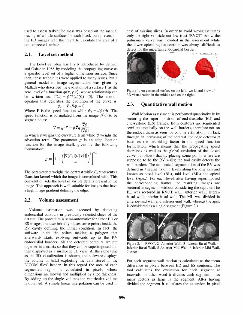
case of missing slices. In order to avoid wrong estimates

only the right ventricle outflow tract (RVOT) below the

pulmonary valve was included in the assessment while

the lower apical region contour was always difficult to

detect for the uncertain endocardial border.

Figure 1. An extracted surface on the left, two lateral view of

3D visualization in the middle and on the right.

2.3. Quantitative wall motion

Wall Motion assessment is performed quantitatively by

sectoring the superimposition of end-diastolic (ED) and

end-systolic (ES) frames. Both contours are segmented

semi-automatically on the wall borders, therefore not on

the endocardium as seen for volume estimation. In fact,

through an increasing of the contrast, the edge detector 訣

becomes the overriding factor in the speed function

formulation, which means that the propagating speed

decreases as well as the global evolution of the closed

curve. It follows that by placing some points where are

supposed to be the RV walls; the tool easily detects the

wall borders. The anatomical segmentation of the RV was

defined in 7 segments on 3 levels along the long axis and

known as basal level (BL), mid level (ML) and apical

level (Apex). For each level, after having superimposed

the corresponding frames, the resulting images are

sectored in segments without considering the septum. The

BL was sectored in RVOT wall, anterior wall; lateral-

basal wall; inferior-basal wall. The ML was divided in

anterior-mid wall and inferior-mid wall; whereas the apex

is considered as a single segment (Figure 2.).

Figure 2. 1- RVOT, 2- Anterior Wall, 3- Lateral-Basal Wall, 4-

Inferior-Basal Wall, 5-Anterior-Mid Wall, 6-Inferior-Mid Wall,

7-Apex.

For each segment wall motion is calculated as the mean

difference in pixels between ED and ES contours. The

tool calculates the excursion for each segment at

intervals, in other word it divides each segment in as

many sectors as large is the segment. After having

divided the segment it calculates the excursion in pixel

1 2

3 4

5

6

7

806

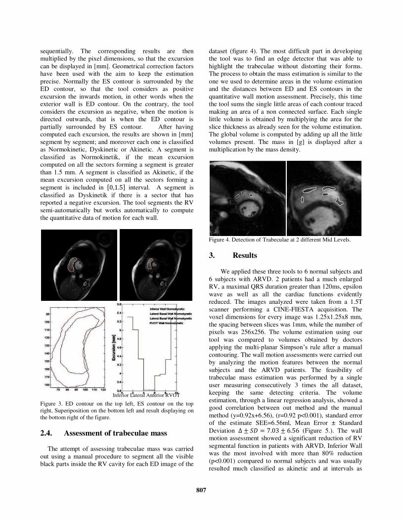
sequentially. The corresponding results are then

multiplied by the pixel dimensions, so that the excursion

can be displayed in [mm]. Geometrical correction factors

have been used with the aim to keep the estimation

precise. Normally the ES contour is surrounded by the

ED contour, so that the tool considers as positive

excursion the inwards motion, in other words when the

exterior wall is ED contour. On the contrary, the tool

considers the excursion as negative, when the motion is

directed outwards, that is when the ED contour is

partially surrounded by ES contour. After having

computed each excursion, the results are shown in [mm]

segment by segment; and moreover each one is classified

as Normokinetic, Dyskinetic or Akinetic. A segment is

classified as Normokinetik, if the mean excursion

computed on all the sectors forming a segment is greater

than 1.5 mm. A segment is classified as Akinetic, if the

mean excursion computed on all the sectors forming a

segment is included in 岷ど┸な┻の峅 interval. A segment is

classified as Dyskinetik if there is a sector that has

reported a negative excursion. The tool segments the RV

semi-automatically but works automatically to compute

the quantitative data of motion for each wall.

Figure 3. ED contour on the top left, ES contour on the top

right, Superiposition on the bottom left and result displaying on

the bottom right of the figure.

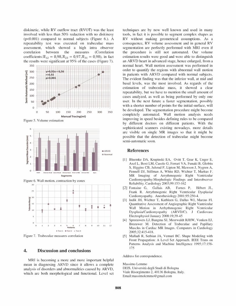
2.4. Assessment of trabeculae mass

The attempt of assessing trabeculae mass was carried

out using a manual procedure to segment all the visible

black parts inside the RV cavity for each ED image of the

dataset (figure 4). The most difficult part in developing

the tool was to find an edge detector that was able to

highlight the trabeculae without distorting their forms.

The process to obtain the mass estimation is similar to the

one we used to determine areas in the volume estimation

and the distances between ED and ES contours in the

quantitative wall motion assessment. Precisely, this time

the tool sums the single little areas of each contour traced

making an area of a non connected surface. Each single

little volume is obtained by multiplying the area for the

slice thickness as already seen for the volume estimation.

The global volume is computed by adding up all the little

volumes present. The mass in [g] is displayed after a

multiplication by the mass density.

Figure 4. Detection of Trabeculae at 2 different Mid Levels.

3. Results

We applied these three tools to 6 normal subjects and

6 subjects with ARVD. 2 patients had a much enlarged

RV, a maximal QRS duration greater than 120ms, epsilon

wave as well as all the cardiac functions evidently

reduced. The images analyzed were taken from a 1.5T

scanner performing a CINE-FIESTA acquisition. The

voxel dimensions for every image was 1.25x1.25x8 mm,

the spacing between slices was 1mm, while the number of

pixels was 256x256. The volume estimation using our

tool was compared to volumes obtained by doctors

applying the multi-planar Simpson’s rule after a manual contouring. The wall motion assessments were carried out

by analyzing the motion features between the normal

subjects and the ARVD patients. The feasibility of

trabeculae mass estimation was performed by a single

user measuring consecutively 3 times the all dataset,

keeping the same detecting criteria. The volume

estimation, through a linear regression analysis, showed a

good correlation between out method and the manual

method (y=0.92x+6.56), (r=0.92 p<0.001), standard error

of the estimate SEE=6.56ml, Mean Error ± Standard

Deviation ッ 罰 鯨経 噺 ば┻どぬ 罰 は┻のは (Figure 5.). The wall

motion assessment showed a significant reduction of RV

segmental function in patients with ARVD, Inferior Wall

was the most involved with more than 80% reduction

(p<0.001) compared to normal subjects and was usually

resulted much classified as akinetic and at intervals as

Inferior Lateral Anterior RVOT

807

808