
Entropy-Regularized Optimal Transport for Machine Learning · Résumé Le Transport Optimal...
136
THÈSE DE DOCTORAT de l’Université de recherche Paris Sciences et Lettres PSL Research University Préparée à l’Université Paris Dauphine et l’École Normale Supérieure Entropy-Regularized Optimal Transport for Machine Learning Spécialité SCIENCES Soutenue par Aude Genevay le 13 mars 2019 Dirigée par Gabriel Peyré RAPPORTEURS : Stefanie JEGELKA Massachusetts Institute of Technology Lorenzo ROSASCO Università di Genova COMPOSITION DU JURY : Francis BACH Ecole Normale Supérieure et INRIA Paris Jean-David BENAMOU INRIA Paris Jérémie BIGOT Université de Bordeaux Olivier BOUSQUET Google Brain Zurich Marco CUTURI ENSAE et Google Brain Paris Rémi FLAMARY Université de Nice Sophia-Antipolis Jean-Michel LOUBES Université Toulouse Paul Sabatier Gabriel PEYRÉ (Directeur de Thèse) Ecole Normale Supérieure
Transcript of Entropy-Regularized Optimal Transport for Machine Learning · Résumé Le Transport Optimal...
THÈSE DE DOCTORAT
de l’Université de recherche Paris Sciences et LettresPSL Research University
Préparée à l’Université Paris Dauphineet l’École Normale Supérieure
Entropy-Regularized Optimal Transport
for Machine Learning
Spécialité SCIENCES
Soutenue par Aude Genevayle 13 mars 2019
Dirigée par Gabriel Peyré
RAPPORTEURS :
Stefanie JEGELKAMassachusetts Institute of Technology
Lorenzo ROSASCOUniversità di Genova
COMPOSITION DU JURY :
Francis BACHEcole Normale Supérieure et INRIA Paris
Jean-David BENAMOUINRIA Paris
Jérémie BIGOTUniversité de Bordeaux
Olivier BOUSQUETGoogle Brain Zurich
Marco CUTURIENSAE et Google Brain Paris
Rémi FLAMARYUniversité de Nice Sophia-Antipolis
Jean-Michel LOUBESUniversité Toulouse Paul Sabatier
Gabriel PEYRÉ (Directeur de Thèse)Ecole Normale Supérieure

i
Abstract
This thesis proposes theoretical and numerical contributions to useEntropy-regularized Optimal Transport (EOT) for machine learning.We introduce Sinkhorn Divergences (SD), a class of discrepancies be-tween probability measures based on EOT which interpolates betweentwo other well-known discrepancies: Optimal Transport (OT) andMaximum Mean Discrepancies (MMD). We develop an efficient nu-merical method to use SD for density fitting tasks, showing that asuitable choice of regularization can improve performance over exist-ing methods. We derive a sample complexity theorem for SD whichproves that choosing a large enough regularization parameter allowsto break the curse of dimensionality from OT, and recover asymptoticrates similar to MMD. We propose and analyze stochastic optimizationsolvers for EOT, which yield online methods that can cope with arbi-trary measures and are well suited to large scale problems, contrarilyto existing discrete batch solvers.
Résumé
Le Transport Optimal régularisé par l’Entropie (TOE) permet dedéfinir les Divergences de Sinkhorn (DS), une nouvelle classe de dis-tance entre mesures de probabilités basées sur le TOE. Celles-ci per-mettent d’interpoler entre deux autres distances connues: le TransportOptimal (TO) et l’Ecart Moyen Maximal (EMM). Les DS peuvent êtreutilisées pour apprendre des modèles probabilistes avec de meilleuresperformances que les algorithmes existants pour une régularisationadéquate. Ceci est justifié par un théorème sur l’approximation desSD par des échantillons, prouvant qu’une régularisation suffisante per-met de se débarrasser de la malédiction de la dimension du TO, etl’on retrouve à l’infini le taux de convergence des EMM. Enfin, nousprésentons de nouveaux algorithmes de résolution pour le TOE baséssur l’optimisation stochastique ‘en-ligne’ qui, contrairement à l’état del’art, ne se restreignent pas aux mesures discrètes et s’adaptent bienaux problèmes de grande dimension.
Contents
Outline of the Thesis 1Notations . . . . . . . . . . . . . . . . . . . . . . . . . . . . . . . . . . . . . . 15
Chapter 1: Entropy-regularized Optimal Transport 171 Introduction . . . . . . . . . . . . . . . . . . . . . . . . . . . . . . . . . . 182 Distances Between Probability Measures . . . . . . . . . . . . . . . . . . 19
2.1 ϕ-divergences . . . . . . . . . . . . . . . . . . . . . . . . . . . . . 192.2 Integral Probability Metrics and Maximum Mean discrepancy . . 212.3 Optimal Transport . . . . . . . . . . . . . . . . . . . . . . . . . . 24
3 Regularized Optimal Transport . . . . . . . . . . . . . . . . . . . . . . . 273.1 Dual Formulation . . . . . . . . . . . . . . . . . . . . . . . . . . . 273.2 The Case of Unbalanced OT . . . . . . . . . . . . . . . . . . . . 293.3 Dual Expectation Formulation . . . . . . . . . . . . . . . . . . . 30
4 Entropy-Regularized Optimal Transport . . . . . . . . . . . . . . . . . . 314.1 Solving the Regularized Dual Problem . . . . . . . . . . . . . . . 33
4.1.1 Hilbert Metric . . . . . . . . . . . . . . . . . . . . . . . 344.1.2 Fixed Point Theorem . . . . . . . . . . . . . . . . . . . 35
4.2 Sinkhorn’s Algorithm . . . . . . . . . . . . . . . . . . . . . . . . 374.3 Semi-Dual Formulation . . . . . . . . . . . . . . . . . . . . . . . 40
4.3.1 Case of a Discrete Measure . . . . . . . . . . . . . . . . 414.3.2 Semi-Dual Expectation Formulation . . . . . . . . . . . 414.3.3 Some Analytic Properties of the Semi-Dual Functional . 42
4.4 Convergence of Entropy-Regularized OT to Standard OT . . . . 43
Chapter 2: Learning with Sinkhorn Divergences 471 Introduction . . . . . . . . . . . . . . . . . . . . . . . . . . . . . . . . . . 482 Density Fitting . . . . . . . . . . . . . . . . . . . . . . . . . . . . . . . . 50
2.1 Learning with ϕ-divergences . . . . . . . . . . . . . . . . . . . . . 512.2 Maximum Mean Discrepancy and Optimal Transport . . . . . . . 522.3 Regularized OT and Variants of the Regularized OT Loss . . . . 532.4 Sinkhorn Divergences : an Interpolation Between OT and MMD 54
3 Sinkhorn AutoDiff Algorithm . . . . . . . . . . . . . . . . . . . . . . . . 58
ii
CONTENTS iii
3.1 Mini-batch Sampling Loss . . . . . . . . . . . . . . . . . . . . . . 593.2 Sinkhorn Iterates . . . . . . . . . . . . . . . . . . . . . . . . . . . 603.3 Learning the Cost Function Adversarially . . . . . . . . . . . . . 613.4 The Optimization Procedure in Practice . . . . . . . . . . . . . . 62
4 Applications . . . . . . . . . . . . . . . . . . . . . . . . . . . . . . . . . . 634.1 Benchmark on Synthetic Problems . . . . . . . . . . . . . . . . . 644.2 Data Clustering with Ellipses . . . . . . . . . . . . . . . . . . . . 674.3 Tuning a Generative Neural Network . . . . . . . . . . . . . . . . 71
4.3.1 With a Fixed Cost c. . . . . . . . . . . . . . . . . . . . 714.3.2 Learning the Cost. . . . . . . . . . . . . . . . . . . . . . 72
Chapter 3: Sample Complexity of Sinkhorn Divergences 751 Introduction . . . . . . . . . . . . . . . . . . . . . . . . . . . . . . . . . . 762 Reminders on Sinkhorn Divergences . . . . . . . . . . . . . . . . . . . . 773 Approximating Optimal Transport with Sinkhorn Divergences . . . . . . 784 Properties of Sinkhorn Potentials . . . . . . . . . . . . . . . . . . . . . . 805 Approximating Sinkhorn Divergence from Samples . . . . . . . . . . . . 846 Experiments . . . . . . . . . . . . . . . . . . . . . . . . . . . . . . . . . . 90
Chapter 4: Stochastic Optimization for Large Scale OT 931 Introduction . . . . . . . . . . . . . . . . . . . . . . . . . . . . . . . . . . 942 Optimal Transport: Primal, Dual and Semi-dual Formulations . . . . . 96
2.1 Primal, Dual and Semi-dual Formulations. . . . . . . . . . . . . . 962.2 Stochastic Optimization Formulations . . . . . . . . . . . . . . . 97
3 Discrete Optimal Transport . . . . . . . . . . . . . . . . . . . . . . . . . 993.1 Discrete Optimization and Sinkhorn . . . . . . . . . . . . . . . . 993.2 Incremental Discrete Optimization with SAG when ε > 0. . . . . 993.3 Numerical Illustrations on Bags of Word-Embeddings. . . . . . . 101
4 Semi-Discrete Optimal Transport . . . . . . . . . . . . . . . . . . . . . . 1034.1 Stochastic Semi-discrete Optimization with SGD . . . . . . . . . 1034.2 Numerical Illustrations on Synthetic Data . . . . . . . . . . . . . 104
5 Continuous Optimal Transport Using RKHS . . . . . . . . . . . . . . . . 1055.1 Kernel SGD . . . . . . . . . . . . . . . . . . . . . . . . . . . . . . 1055.2 Speeding up Iterations with Kernel Approximation . . . . . . . . 108
5.2.1 Incomplete Cholesky Decomposition . . . . . . . . . . . 1085.2.2 Random Fourier Features . . . . . . . . . . . . . . . . . 110
5.3 Comparison of the Three Algorithms on Synthetic Data . . . . . 111
Conclusion 115

iv CONTENTS
Bibliography 119

Remerciements
Je tiens avant tout à remercier mon directeur de thèse, Gabriel Peyré, qui m’a guidéetout au long de ces trois années faites de hauts et de bas, sans jamais se départir de sonenthousiasme. Merci d’avoir cru en moi et de m’avoir poussée à aller de l’avant mêmedans les moments les plus difficiles.
Je tiens aussi à remercier Francis Bach et Marco Cuturi, co-auteurs de luxe, quim’ont beaucoup apporté sur le plan scientifique tout en étant présents pour m’aiderdans mes interrogations plus existentielles; Jean-David Benamou et Guillaume Carlier,qui m’ont accueillie au sein de Mokaplan à ses débuts et m’ont fait découvrir le mondefabuleux du transport régularisé; et enfin Lénaïc Chizat qui me suit de plus ou moinsloin depuis 10 ans et dont l’entrain face aux problèmes mathématiques m’a redonné legoût à la recherche dans une période de doute.
Je remercie également mes rapporteurs, Lorenzo Rosasco et Stefanie Jegelka, ainsique les membres du jury, Jérémie Bigot, Olivier Bousquet, Rémi Flamary et Jean-MichelLoubes, chercheurs dont j’admire le travail et qui m’ont fait l’honneur de s’intéresser aumien.
Ces trois années (et demie) n’auraient bien sûr pas été les mêmes sans les personnesque j’ai pu côtoyer à la fois au CEREMADE (la fantastique équipe de doctorants quia illuminé ma première année...), au DMA, et à MOKAPLAN (merci Luca pour tesfabuleux Mokadiners). J’ai aussi une pensée particulière pour les professeurs que j’aicroisés au long de ma scolarité, et qui m’ont donné goût aux mathématiques – je penseà Jacques Féjoz et Julien Salomon qui ont marqué mon parcours d’étudiante – et mescopains matheux, compagnons de galère: Anna (toujours d’excellent conseil), Daniel,Elsa et Gwendoline (courage, ton tour viendra!).
Enfin, je n’aurais sûrement pas eu le courage d’aller au bout de cette aventure sansmes amis et ma famille qui ont toujours été à mes côtés dans les moments difficiles etn’ont jamais cessé de croire en moi. Merci à Julie, Alice, Rémy, Marie les copains dela Martin; Julien qui n’est jamais bien loin même à l’autre bout du monde; Marion,ma demi-soeur; Sophie et Colo qui comprennent la bizarre aventure de la thèse et qui
v

vi Remerciements
savent me changer les idées à coups de voyages à vélo et/ou au soleil. Merci à Papa,Maman, Alex, Marraine, Papi, Mamie et tout le clan Coquard – je sais bien que vousne comprenez rien à ce que je fais, mais votre soutien me fait chaud au coeur – sansoublier Tristan... merci de m’avoir permis de clore cette aventure de la plus belle desmanières, j’ai hâte de voir ce que la suite nous réserve.
Outline of the Thesis
Comparing probability distributions is a fundamental component of many machinelearning problems, both supercontractvised and unsupervised. The main matter of thisthesis is to study the behavior of a class of discrepancies between probability distri-butions, called Sinkhorn Divergences, which are based on entropy-regularized OptimalTransport. We provide both theoretical contributions, regarding their statistical prop-erties, and numerical ones, including solvers to compute Sinkhorn Divergences and usethem in machine learning tasks.
Supervised Machine Learning. In supervised machine learning, we are providedwith a labeled dataset e.g (xi, yi)i=1...n where xi is the observation in some input spaceX (e.g. pixel intensities of an image) and yi is the associated label (e.g. the fact thatthis image represents an apple). A recurrent issue in supervised learning is to learn aclassification rule from the data, that takes a new observation x as an input and predictsthe associated label y as the output. For instance in nearest-neighbor classification,when provided with a new observation x, one looks for the closest observation xi∗ in thedataset and sets y = yi∗ . This classification rule assumes that if observations are close,they should have the same label. Defining a meaningful notion of distance on the dataspace X is thus crucial. In practice, a lot of data can be represented as histograms onsome other space X ′: a data point x ∈ X is identified to a histogram α
def.=∑ni=1 αiδai ,
where (ai)i ∈ X ′ and∑ni=1 αi = 1. Since normalized histograms are no more than finite
discrete probability distributions, a distance on probability distributions serves as arelevant distance on these data spaces. As a set of representative examples, let us quote:bag-of-visual-words comparison in computer vision (Rubner et al., 2000), color andshape processing in computer graphics (Solomon et al., 2015), bag-of-words for naturallanguage processing (Kusner et al., 2015). Another use of histograms in supervisedlearning is to associate labels to histograms in multi-label classification (Frogner et al.,2015).
Unsupervised Machine Learning. On the other hand, in unsupervised machine-learning, the dataset only consists in observations (xi)i=1...n in the data space X . Oneway to extract information from the data in an unsupervised setting is to perform
1
2 OUTLINE OF THE THESIS
density fitting. The goal is to fit the unknown distribution induced by the dataset witha parametric distribution. This amounts to finding the parameters that minimize somenotion of distance between these two distributions (the unknown one from the dataset,and the one from the parametric model). Choosing the right notion of discrepancybetween measures here is one of the key issues of the problem. A popular research areain unsupervised learning which emerged in recent years is learning generative models(Goodfellow et al., 2014) which can generate new samples resembling the ones in thedataset. The distributions induced by generative models are often assumed to haveintrinsic low dimension, and thus do not have a density with respect to a referencemeasure. The usual Maximum Likelihood Estimation framework can therefore not beused for such models. However, these models are easy to sample from, and thus resortingto a discrepancy on measures which can be robustly computed from samples (from thegenerative model and the dataset) is essential.
Discrepancies on measures. The most popular frameworks that are used to com-pare probability distributions are ϕ−divergences (Csiszár, 1975), Maximum Mean Dis-crepancies (MMD) (Gretton et al., 2006) and Optimal Transport (OT) (Kantorovich,1942). The former are appreciated for their computational simplicity, but they sufferfrom the major shortcoming of not metrizing weak-convergence. Both MMD and OThave the ability to metrize weak-convergence, but they enjoy different characteristics.MMD can be efficiently estimated from samples of the measures, both statistically sincethe estimates are robust with a small number or samples (we say it has a good sam-ple complexity) and also numerically, as they are computed in closed form. OT on theother hand, presents none of these advantages, but has the ability to lift a ground metricfrom the dataspace X to the set of probability measures on this space and thus takeinto account the underlying geometry of the data. Its good geometric properties canbe strengthened by enforcing structure constraints (Alvarez-Melis et al., 2017) whichallows for instance to take into account the class labels in supervised learning. Besides,solving OT also gives a mapping from one measure to the other, which has been suc-cessfully used in domain adaptation (Courty et al., 2014). As a unifying alternative tothese discrepancies, we introduce Sinkhorn Divergences, based on entropy-regularizedOptimal Transport. We prove they interpolate between MMD (with infinitely strongregularization) and OT (with no regularization). In particular, Sinkhorn Divergencespreserve the good geometric properties of OT, and also provide a mapping from onemeasure to the other. However unlike OT – but similarly to MMD – they benefit fromgood statistical properties and efficient computation.
We now get into more details regarding the technical aspects of our work, formalizingkey concepts and outlining the main contributions of this thesis.
3
Chapter 1: Entropy-regularized Optimal Transport
This introductory chapter is both a review of existing tools commonly used in ma-chine learning to compare probability distributions, and a presentation of key propertiesof regularized optimal transport (containing both new results and existing ones from theliterature), which serves as a basis for the work presented in subsequent chapters.
Previous Works. In machine learning, the first discrepancies that were introduced tocompare two probability distributions are ϕ-divergences (Csiszár, 1975), which can beseen as a weighted average (by ϕ) of the odds-ratio between the two measures. Considerϕ a convex, lower semi-continuous function such that ϕ(1) = 0, the ϕ-divergence Dϕ
between two probability measures α and β is defined by:
Dϕ(α|β) def.=∫Xϕ(dα(x)
dβ(x))dβ(x).
up to a corrective (possibly infinite) term if α is not absolutely continuous with respectto β. The computational simplicity of ϕ−divergences made them quite popular – themost widely used being the Kullback-Leibler divergence for ϕ(x) = x log(x). However,they suffer from the major drawback of not metrizing weak-convergence (or conver-gence in law). A measure αn weakly converges to α (denoted αn α) if and onlyif∫f(x)dαn(x) →
∫f(x)dα(x) for all continuous bounded functions f ; and a loss L
metrizes weak-convergence if and only if L(αn, α) → 0 ⇔ αn α. The metrizationof weak-convergence is instrumental for discrepancies on measure, as it ensures thatthe losses remain stable under small perturbations of the support of the measures. Asan example, consider the case on R where α = δ0 a Dirac mass in 0 and αn = δ1/n aDirac mass in 1/n. Then Dϕ(αn|α) is a constant for all n, although it seems naturalto say that when n goes to infinity, αn gets closer to α. This failure case in R becomesvery problematic in higher dimension, when comparing probability distributions thatare supported on low-dimensional manifolds for instance.
The two main classes of discrepancies that satisfy this requirement are MaximumMean Discrepancies (MMD)(Gretton et al., 2006) and Optimal Transport (OT)(Santambrogio, 2015) based losses. MMD are a special instance of Integral ProbabilityMetrics (Müller, 1997). Given a Reproducing Kernel Hilbert Space (RKHS) H withkernel k; MMD between two probability measures α and β are defined as follows:
MMD2k(α, β) def.=
(sup
f |||f ||H61|Eα(f(X))− Eβ(f(Y ))|
)2
= Eα⊗α[k(X,X ′)] + Eβ⊗β[k(Y, Y ′)]− 2Eα⊗β[k(X,Y )]. (0.1)
If the kernel k is universal (i.e. its RKHS is dense in the space of continuous func-tions), they are positive definite, and under some further technical assumptions, they
4 OUTLINE OF THE THESIS
metrize weak-convergence (Sriperumbudur et al., 2010). This family of losses presentsthe advantage of being efficiently computed from samples – both in a computationaland statistical sense (Gretton et al., 2006). OT-based losses on the other hand behaveparticularly well in problems that are intrinsically geometric (e.g. shapes or image pro-cessing). They rely on the choice of a ground cost c which reflects the geometry of theinput space in the following way:
Wc(α, β) def.= minπ∈Π(α,β)
∫X×X
c(x, y)dπ(x, y), (P)
where the feasible set is composed of joint probability distributions with fixed marginalsα, β. A typical choice is c = dp, where d is the natural distance on X , for which Wc
metrizes weak-convergence when p > 1 (Santambrogio, 2015). However, these lossessuffer from a computational burden – solving OT requires solving a linear program inthe discrete case – and a curse of dimensionality, meaning their approximation fromsampled measures degrades quickly in high dimension (Weed and Bach, 2017).
Entropy-regularized OT has recently emerged as a solution to the computationalissue of OT (Cuturi, 2013). The regularized problem reads:
Wc,ε(α, β) def.= minπ∈Π(α,β)
∫X×X
c(x, y)dπ(x, y) + εH(π|α⊗ β), (Pε)
whereH(π|α⊗ β) def.=
∫X×X
log( dπ(x, y)
dα(x)dβ(y)
)dπ(x, y). (0.2)
is the relative entropy of the transport plan π with respect to the product measure α⊗β.It has an equivalent dual formulation, which is unconstrained (contrarily to standardOT):
Wc,ε(α, β) = maxu∈C(X )v∈C(X )
∫Xu(x)dα(x) +
∫Xv(y)dβ(y)
− ε∫X×X
eu(x)+v(y)−c(x,y)
ε dα(x)dβ(y) + ε. (Dε)
In the case of finite discrete measures, iteratively optimizing over each dual variablesyields a fast converging algorithm, called Sinkhorn’s algorithm (Sinkhorn, 1967). Be-sides, the resulting distance happens to perform well in various machine learning tasksas proved in the seminal paper by Cuturi (2013), which opened the way to the use ofentropy-regularized OT in the community.
Contributions. The main objective of this thesis is to prove theoretically and numer-ically that the benefits of entropy-regularized OT extend far beyond this fast algorithm
5
for finite discrete measures, and in this chapter we review the bases that will be requiredfor our main contributions presented in subsequent chapters. However, this collectionof results also includes some original contributions on regularized OT which consist in
(i) Regularization of OT using relative entropy with respect to the productmeasure of the marginals: The seminal paper by Cuturi (2013) deals withthe discrete case and uses entropy H(π) def.=
∑i,j log (πij)πij as a regularizer. We
suggest instead to use the entropy with respect to the product of marginals definedin equation (0.2), as it allows to formulate the dual problem as the maximizationof an expectation :
Wc,ε(α, β) = maxu∈C(X )v∈C(X )
Eα⊗β[fXYε (u, v)
]+ ε,
where fxyε (u, v) def.= u(x)+v(y)−εeu(x)+v(y)−c(x,y)
ε and X,Y are distributed accordingto α and β respectively. This formulation is key to deriving statistical propertiesof entropy-regularized OT in Chapter 3 and new solvers in Chapter 4.
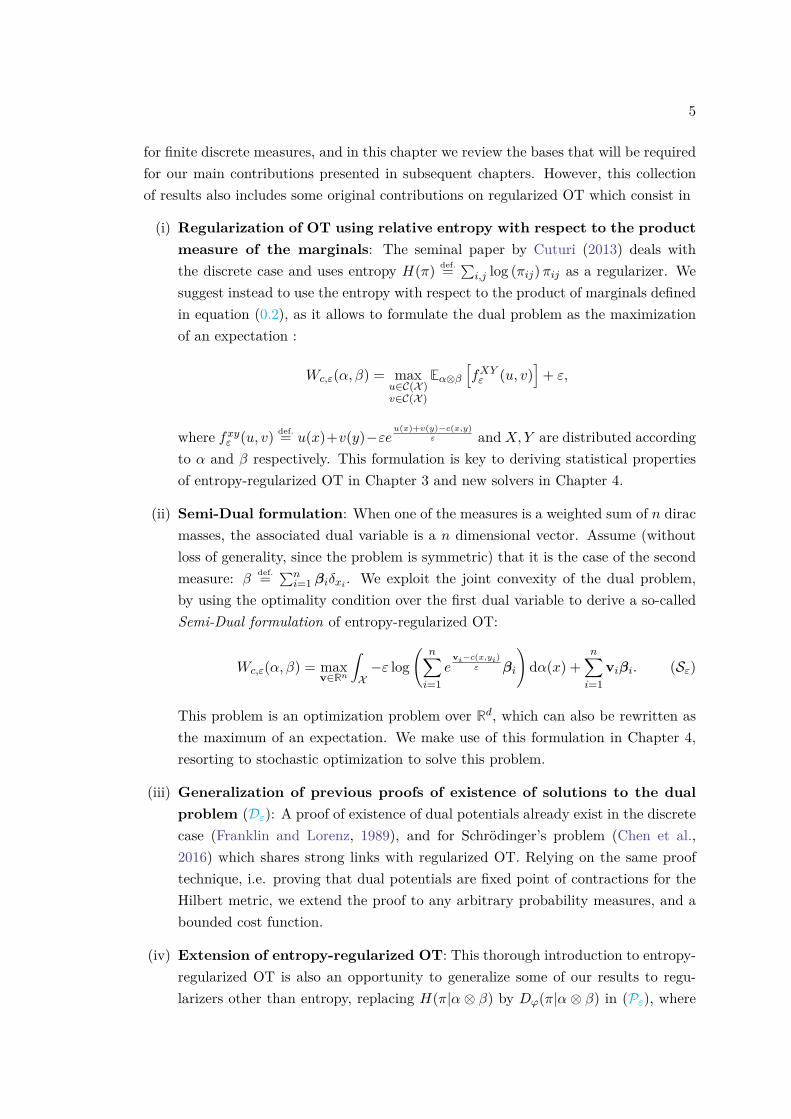
(ii) Semi-Dual formulation: When one of the measures is a weighted sum of n diracmasses, the associated dual variable is a n dimensional vector. Assume (withoutloss of generality, since the problem is symmetric) that it is the case of the secondmeasure: β def.=
∑ni=1 βiδxi . We exploit the joint convexity of the dual problem,
by using the optimality condition over the first dual variable to derive a so-calledSemi-Dual formulation of entropy-regularized OT:
Wc,ε(α, β) = maxv∈Rn
∫X−ε log
(n∑i=1
evi−c(x,yi)
ε βi
)dα(x) +
n∑i=1
viβi. (Sε)
This problem is an optimization problem over Rd, which can also be rewritten asthe maximum of an expectation. We make use of this formulation in Chapter 4,resorting to stochastic optimization to solve this problem.
(iii) Generalization of previous proofs of existence of solutions to the dualproblem (Dε): A proof of existence of dual potentials already exist in the discretecase (Franklin and Lorenz, 1989), and for Schrödinger’s problem (Chen et al.,2016) which shares strong links with regularized OT. Relying on the same prooftechnique, i.e. proving that dual potentials are fixed point of contractions for theHilbert metric, we extend the proof to any arbitrary probability measures, and abounded cost function.
(iv) Extension of entropy-regularized OT: This thorough introduction to entropy-regularized OT is also an opportunity to generalize some of our results to regu-larizers other than entropy, replacing H(π|α ⊗ β) by Dϕ(π|α ⊗ β) in (Pε), where
6 OUTLINE OF THE THESIS
Dϕ is any ϕ−divergence. Besides, we also extend these formulations to unbal-anced transport, which extends the notion of OT to positive Radon measures witharbitrary mass (Liero et al., 2018),(Chizat et al., 2018) whenever possible (e.g.regularization, formulation as an expectation).
Chapter 2: Learning with Sinkhorn Divergences
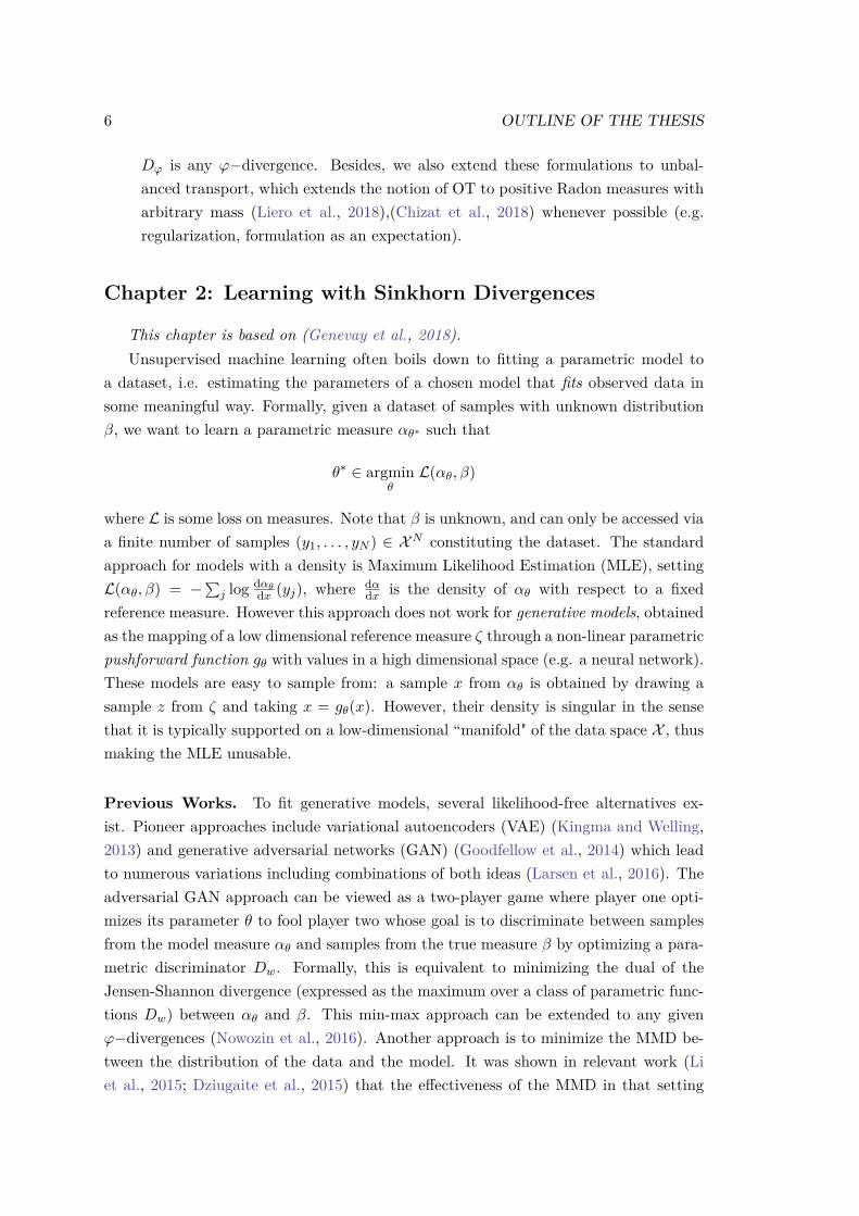
This chapter is based on (Genevay et al., 2018).Unsupervised machine learning often boils down to fitting a parametric model to
a dataset, i.e. estimating the parameters of a chosen model that fits observed data insome meaningful way. Formally, given a dataset of samples with unknown distributionβ, we want to learn a parametric measure αθ∗ such that
θ∗ ∈ argminθ
L(αθ, β)
where L is some loss on measures. Note that β is unknown, and can only be accessed viaa finite number of samples (y1, . . . , yN ) ∈ XN constituting the dataset. The standardapproach for models with a density is Maximum Likelihood Estimation (MLE), settingL(αθ, β) = −
∑j log dαθ
dx (yj), where dαdx is the density of αθ with respect to a fixed
reference measure. However this approach does not work for generative models, obtainedas the mapping of a low dimensional reference measure ζ through a non-linear parametricpushforward function gθ with values in a high dimensional space (e.g. a neural network).These models are easy to sample from: a sample x from αθ is obtained by drawing asample z from ζ and taking x = gθ(x). However, their density is singular in the sensethat it is typically supported on a low-dimensional “manifold" of the data space X , thusmaking the MLE unusable.
Previous Works. To fit generative models, several likelihood-free alternatives ex-ist. Pioneer approaches include variational autoencoders (VAE) (Kingma and Welling,2013) and generative adversarial networks (GAN) (Goodfellow et al., 2014) which leadto numerous variations including combinations of both ideas (Larsen et al., 2016). Theadversarial GAN approach can be viewed as a two-player game where player one opti-mizes its parameter θ to fool player two whose goal is to discriminate between samplesfrom the model measure αθ and samples from the true measure β by optimizing a para-metric discriminator Dw. Formally, this is equivalent to minimizing the dual of theJensen-Shannon divergence (expressed as the maximum over a class of parametric func-tions Dw) between αθ and β. This min-max approach can be extended to any givenϕ−divergences (Nowozin et al., 2016). Another approach is to minimize the MMD be-tween the distribution of the data and the model. It was shown in relevant work (Liet al., 2015; Dziugaite et al., 2015) that the effectiveness of the MMD in that setting
7
hinges on the ability to find a relevant kernel function, which is nontrivial. The Wasser-stein distance, long known to be a powerful tool to compare probability distributionswith non-overlapping supports, a has recently emerged as a serious contender. Althoughthe use of Wasserstein metrics for inference in generative models was considered over tenyears ago in (Bassetti et al., 2006), that development remained exclusively theoreticaluntil a recent wave of papers managed to implement that idea more or less faithfully us-ing several workarounds: entropic regularization over a discrete space (Montavon et al.,2016), approximate Bayesian computations (Bernton et al., 2017) and a neural networkparameterization of the dual potential arising from the dual OT problem when consid-ering the 1-Wasserstein distance (Arjovsky et al., 2017). As opposed to this dual wayto compute gradients of the fitting energy, we advocate for the use of a primal formula-tion, which is numerically stable, because it does not involve differentiating the (dual)solution of an OT sub-problem, as also pointed out in (Bousquet et al., 2017).
Contributions. The main contributions of this chapter include a theoretical contri-bution regarding a new OT-based loss for generative models, and a simple numericalscheme to learn under this loss.
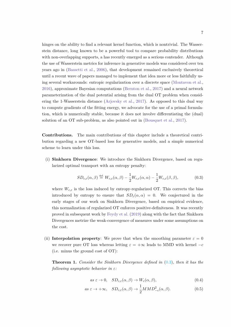
(i) Sinkhorn Divergence: We introduce the Sinkhorn Divergence, based on regu-larized optimal transport with an entropy penalty:
SDc,ε(α, β) def.= Wc,ε(α, β)− 12Wc,ε(α, α)− 1
2Wc,ε(β, β), (0.3)
where Wc,ε is the loss induced by entropy-regularized OT. This corrects the biasintroduced by entropy to ensure that SDε(α, α) = 0. We conjectured in theearly stages of our work on Sinkhorn Divergence, based on empirical evidence,this normalization of regularized OT enforces positive-definiteness. It was recentlyproved in subsequent work by Feydy et al. (2019) along with the fact that SinkhornDivergences metrize the weak-convergence of measures under some assumptions onthe cost.
(ii) Interpolation property: We prove that when the smoothing parameter ε = 0we recover pure OT loss whereas letting ε = +∞ leads to MMD with kernel −c(i.e. minus the ground cost of OT):
Theorem 1. Consider the Sinkhorn Divergence defined in (0.3), then it has thefollowing asymptotic behavior in ε:
as ε→ 0, SDc,ε(α, β)→Wc(α, β), (0.4)
as ε→ +∞, SDc,ε(α, β)→ 12MMD2
−c(α, β). (0.5)
8 OUTLINE OF THE THESIS
Note that to define a proper MMD, −c needs to induce a positive definite kernel.This is the case when c = || · ||p2 for 0 < p < 2, and the associated MMD yields theEnergy Distance (Sejdinovic et al., 2013). This interpolation property is furtherstudied in Chapter 3, where we prove that the sample complexity of SinkhornDivergences also interpolates between that of OT and MMD, alleviating the curseof dimensionality brought by OT when ε is sufficiently large. It is also supportedby empirical evidence in this chapter.
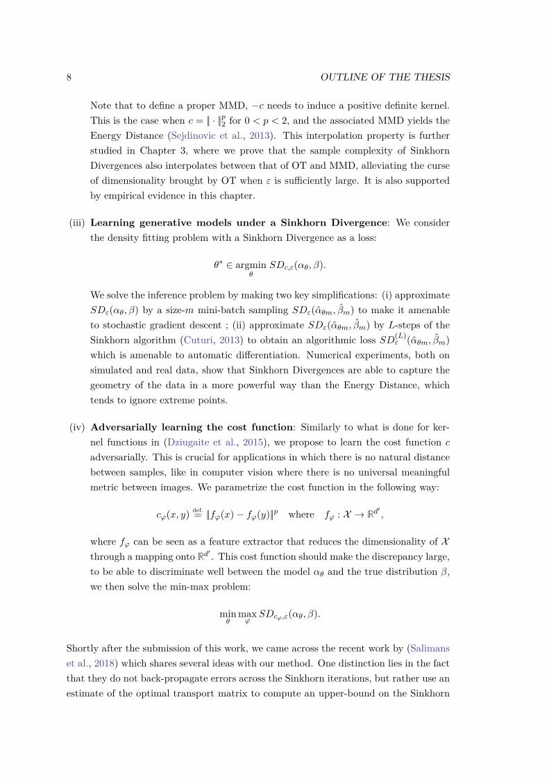
(iii) Learning generative models under a Sinkhorn Divergence: We considerthe density fitting problem with a Sinkhorn Divergence as a loss:
θ∗ ∈ argminθ
SDc,ε(αθ, β).
We solve the inference problem by making two key simplifications: (i) approximateSDε(αθ, β) by a size-m mini-batch sampling SDε(αθm, βm) to make it amenableto stochastic gradient descent ; (ii) approximate SDε(αθm, βm) by L-steps of theSinkhorn algorithm (Cuturi, 2013) to obtain an algorithmic loss SD(L)
ε (αθm, βm)which is amenable to automatic differentiation. Numerical experiments, both onsimulated and real data, show that Sinkhorn Divergences are able to capture thegeometry of the data in a more powerful way than the Energy Distance, whichtends to ignore extreme points.
(iv) Adversarially learning the cost function: Similarly to what is done for ker-nel functions in (Dziugaite et al., 2015), we propose to learn the cost function c
adversarially. This is crucial for applications in which there is no natural distancebetween samples, like in computer vision where there is no universal meaningfulmetric between images. We parametrize the cost function in the following way:
cϕ(x, y) def.= ||fϕ(x)− fϕ(y)||p where fϕ : X → Rd′,
where fϕ can be seen as a feature extractor that reduces the dimensionality of Xthrough a mapping onto Rd
′ . This cost function should make the discrepancy large,to be able to discriminate well between the model αθ and the true distribution β,we then solve the min-max problem:
minθ
maxϕ
SDcϕ,ε(αθ, β).
Shortly after the submission of this work, we came across the recent work by (Salimanset al., 2018) which shares several ideas with our method. One distinction lies in the factthat they do not back-propagate errors across the Sinkhorn iterations, but rather use anestimate of the optimal transport matrix to compute an upper-bound on the Sinkhorn
9
Divergence, as was done for instance in (Cuturi and Doucet, 2014).
Chapter 3: Sample Complexity of Sinkhorn Divergences
This chapter is based on (Genevay et al., 2019).The numerical experiments in Chapter 2 further support what was first observed in
(Cuturi, 2013): entropy-regularized OT breaks the curse-of-dimensionality from whichOT suffers when the regularization parameter is large enough. The goal of this chapteris to make this more formal through a sample complexity theorem. We also provide aconvergence rate of entropy-regularized transport to standard transport, proving thatthere is a tradeoff between a faithful estimation of OT and good sample complexity.
Previous Works. The central theoretical contribution of Chapter 2 (see Theorem 1)states that Sinkhorn Divergences, based on regularized OT, interpolate between OT andMMD. These two metrics, which emerged as popular candidates to compare probabilitymeasures, differ on a fundamental aspect: their sample complexity. The definition ofsample complexity of a loss function that we choose here is the convergence rate of theloss evaluated on empirical measures to the loss evaluated on the “true" measures, asa function of the number of samples. This notion is crucial in machine learning, asbad sample complexity induces overfitting and high gradient variance when using thesedivergences for parameter estimation. In that context, it is well known that the samplecomplexity of MMD is independent of the dimension, scaling as 1√
n(Gretton et al.,
2006) where n is the number of samples. In contrast, it is well known that standardOT suffers from the curse of dimensionality (Dudley, 1969): considering a probabilitymeasure α ∈M(Rd) and its empirical estimation αn, we have E[Wp(α, αn)] = O(n−1/d).Its sample complexity is thus exponential in the dimension of the ambient space d.Although it was recently proved that this result can be refined to d being the intrinsicdimension of data (Weed and Bach, 2017), the sample complexity of OT is now themajor bottleneck for the use of OT in high-dimensional machine learning problems.
A solution to this shortcoming comes, once again, from entropic-regularization.Sinkhorn Divergences (0.3), have been empirically observed to be less prone to over-fitting, as a certain amount of regularization can improve performance in simple learningtasks (Cuturi, 2013). The interpolation property in Theorem 1 also suggests that forlarge regularizations, Sinkhorn Divergences should behave similarly to MMD. However,aside from a recent central limit theorem in the case of measures supported on finitediscrete spaces (Bigot et al., 2017), the convergence of empirical Sinkhorn Divergences,and more generally their sample complexity, remains an open question.
Contributions. This chapter contains the main theoretical contributions of this the-sis, in the form of three theorems exhibiting theoretical properties of Sinkhorn Diver-
10 OUTLINE OF THE THESIS
gences.
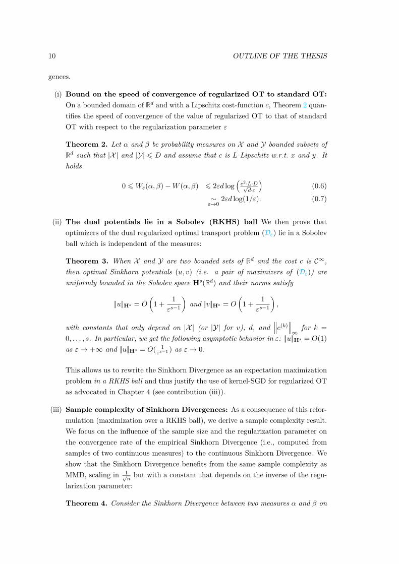
(i) Bound on the speed of convergence of regularized OT to standard OT:On a bounded domain of Rd and with a Lipschitz cost-function c, Theorem 2 quan-tifies the speed of convergence of the value of regularized OT to that of standardOT with respect to the regularization parameter ε
Theorem 2. Let α and β be probability measures on X and Y bounded subsets ofRd such that |X | and |Y| 6 D and assume that c is L-Lipschitz w.r.t. x and y. Itholds
0 6Wε(α, β)−W (α, β) 6 2εd log(e2·L·D√
d·ε
)(0.6)
∼ε→0
2εd log(1/ε). (0.7)
(ii) The dual potentials lie in a Sobolev (RKHS) ball We then prove thatoptimizers of the dual regularized optimal transport problem (Dε) lie in a Sobolevball which is independent of the measures:
Theorem 3. When X and Y are two bounded sets of Rd and the cost c is C∞,then optimal Sinkhorn potentials (u, v) (i.e. a pair of maximizers of (Dε)) areuniformly bounded in the Sobolev space Hs(Rd) and their norms satisfy
||u||Hs = O
(1 + 1
εs−1
)and ||v||Hs = O
(1 + 1
εs−1
),
with constants that only depend on |X | (or |Y| for v), d, and∥∥∥c(k)
∥∥∥∞
for k =0, . . . , s. In particular, we get the following asymptotic behavior in ε: ||u||Hs = O(1)as ε→ +∞ and ||u||Hs = O( 1
εs−1 ) as ε→ 0.
This allows us to rewrite the Sinkhorn Divergence as an expectation maximizationproblem in a RKHS ball and thus justify the use of kernel-SGD for regularized OTas advocated in Chapter 4 (see contribution (iii)).
(iii) Sample complexity of Sinkhorn Divergences: As a consequence of this refor-mulation (maximization over a RKHS ball), we derive a sample complexity result.We focus on the influence of the sample size and the regularization parameter onthe convergence rate of the empirical Sinkhorn Divergence (i.e., computed fromsamples of two continuous measures) to the continuous Sinkhorn Divergence. Weshow that the Sinkhorn Divergence benefits from the same sample complexity asMMD, scaling in 1√
nbut with a constant that depends on the inverse of the regu-
larization parameter:
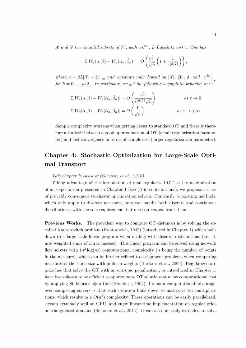
Theorem 4. Consider the Sinkhorn Divergence between two measures α and β on
11
X and Y two bounded subsets of Rd, with a C∞, L-Lipschitz cost c. One has
E|Wε(α, β)−Wε(αn, βn)| = O
(eκε
√n
(1 + 1
εbd/2c
)),
where κ = 2L|X | + ‖c‖∞ and constants only depend on |X |, |Y|, d, and∥∥∥c(k)
∥∥∥∞
for k = 0 . . . bd/2c. In particular, we get the following asymptotic behavior in ε:
E|Wε(α, β)−Wε(αn, βn)| = O
(eκε
εbd/2c√n
)as ε→ 0
E|Wε(α, β)−Wε(αn, βn)| = O
( 1√n
)as ε→ +∞.
Sample complexity worsens when getting closer to standard OT and there is there-fore a tradeoff between a good approximation of OT (small regularization parame-ter) and fast convergence in terms of sample size (larger regularization parameter).
Chapter 4: Stochastic Optimization for Large-Scale Opti-mal Transport
This chapter is based on(Genevay et al., 2016).Taking advantage of the formulation of dual regularized OT as the maximization
of an expectation presented in Chapter 1 (see (i) in contributions), we propose a classof provably convergent stochastic optimization solvers. Contrarily to existing methods,which only apply to discrete measures, ours can handle both discrete and continuousdistributions, with the sole requirement that one can sample from them.
Previous Works. The prevalent way to compute OT distances is by solving the so-called Kantorovitch problem (Kantorovich, 1942) (introduced in Chapter 1) which boilsdown to a large-scale linear program when dealing with discrete distributions (i.e., fi-nite weighted sums of Dirac masses). This linear program can be solved using networkflow solvers with (n3 log(n)) computational complexity (n being the number of pointsin the measure), which can be further refined to assignment problems when comparingmeasures of the same size with uniform weights (Burkard et al., 2009). Regularized ap-proaches that solve the OT with an entropic penalization, as introduced in Chapter 1,have been shown to be efficient to approximate OT solutions at a low computational costby applying Sinkhorn’s algorithm (Sinkhorn, 1964). Its main computational advantageover competing solvers is that each iteration boils down to matrix-vector multiplica-tions, which results in a O(n2) complexity. These operations can be easily parallelized,stream extremely well on GPU, and enjoy linear-time implementation on regular gridsor triangulated domains (Solomon et al., 2015). It can also be easily extended to solve
12 OUTLINE OF THE THESIS
other problems involving optimal-transport, such as the computation of Wassersteinbarycenters or multimarginal optimal transport (Benamou et al., 2015).
This method is however purely discrete and cannot cope with continuous densities.The only known class of methods that overcome this limitation are so-called semi-discretesolvers (Aurenhammer et al., 1998), that can be implemented efficiently using computa-tional geometry primitives (Mérigot, 2011). They compute distance between a discretedistribution and a continuous density, but are restricted to the Euclidean squared cost,and can only be implemented in low dimensions. Lastly, let us point out that there iscurrently no method that can compute OT distances between two continuous densities,which is thus an open problem we tackle in this chapter.
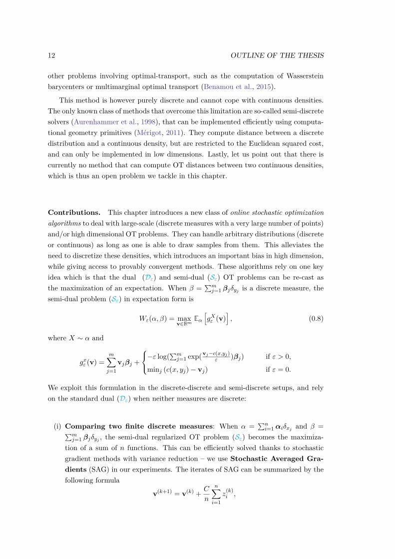
Contributions. This chapter introduces a new class of online stochastic optimizationalgorithms to deal with large-scale (discrete measures with a very large number of points)and/or high dimensional OT problems. They can handle arbitrary distributions (discreteor continuous) as long as one is able to draw samples from them. This alleviates theneed to discretize these densities, which introduces an important bias in high dimension,while giving access to provably convergent methods. These algorithms rely on one keyidea which is that the dual (Dε) and semi-dual (Sε) OT problems can be re-cast asthe maximization of an expectation. When β =
∑mj=1 βjδyj is a discrete measure, the
semi-dual problem (Sε) in expectation form is
Wε(α, β) = maxv∈Rm
Eα[gXε (v)
], (0.8)
where X ∼ α and
gxε (v) =m∑j=1
vjβj +
−ε log(∑mj=1 exp(vj−c(x,yj)
ε )βj) if ε > 0,
minj (c(x, yj)− vj) if ε = 0.
We exploit this formulation in the discrete-discrete and semi-discrete setups, and relyon the standard dual (Dε) when neither measures are discrete:
(i) Comparing two finite discrete measures: When α =∑ni=1 αiδxj and β =∑m
j=1 βjδyj , the semi-dual regularized OT problem (Sε) becomes the maximiza-tion of a sum of n functions. This can be efficiently solved thanks to stochasticgradient methods with variance reduction – we use Stochastic Averaged Gra-dients (SAG) in our experiments. The iterates of SAG can be summarized by thefollowing formula
v(k+1) = v(k) + C
n
n∑i=1
z(k)i ,
13
where an index i(k) is selected at random in 1 . . . n and
z(k)i =
∇gxiε (v(k)) if i = i(k)
z(k−1)i otherwise.
At each iteration an index i(k) is selected at random in 1 . . . n to compute∇g
xi(k)ε (v(k)), the gradient corresponding to the sample xi(k) at the current es-
timate v(k). SAG keeps in memory a copy of that gradient and computes anaverage of all gradients stored so far which provides a better proxy of full gradient∇Eα[gXε ]. Compared to Sinkhorn, which can be viewed as a batch method, SAG isan online algorithm which reduces the complexity of each iteration to O(m), witha O(1/k) convergence rate (since our objective is not strongly convex). There isthus a tradeoff in iteration complexity vs. convergence rate to consider when usingSinkhorn or SAG. The latter is thus more efficient for problems with a very largem – i.e. discrete measures with a very large number of points.
(ii) Comparing a finite discrete measure to an arbitrary probability mea-sure: We solve the semi-dual problem (Sε) in expectation form defined in (0.8)thanks to the Stochastic Gradient Descent (SGD) algorithm. The idea of SGDis fairly intuitive : at each iteration, a sample xk is drawn from α and its gradient∇gxkε is computed at the current iterate v(k) to serve as a proxy for the full gradient∇Gε. The iterations are given by:
v(k+1) = v(k) + C√k∇vgxkε (v(k)) where xk ∼ α.
Since samples from α are drawn online, i.e. without prior discretization, thismethod avoids the discretization bias introduced when using a discrete solvers. Ithas a O(1/
√k) convergence rate along with a O(m) complexity per iteration. This
online semi-discrete algorithm has been successfully applied to texture synthesisin image processing (Galerne et al., 2018), and to the computation of WassersteinBarycenters (Staib et al., 2017).
(iii) Comparing two arbitrary probability measures: When neither measures arefinite discrete ones, we resort to the dual formulation
Wε(α, β) = maxu∈C(X )v∈C(Y)
Eα⊗β[fXYε (u, v)
]+ ε,
where fxyε (u, v) def.= u(x) + v(y)− εeu(x)+v(y)−c(x,y)
ε . We propose a stochastic gradi-ent descent over a Reproducing Kernel Hilbert Space (RKHS), by usingthe fundamental property of a RKHSH with kernel k: u ∈ H ⇔ u(x) = 〈u, k(x, ·)〉.

14 OUTLINE OF THE THESIS
Theorem 3 from Chapter 3, stating that the dual potentials are in a RKHS ball,allows to prove the convergence of this method. We also introduce an approximatefeature approach (via incomplete Cholesky decomposition (Wu et al., 2006) orRandom Fourier features (Rahimi and Recht, 2007)) to significantly reduce com-putational time, going from quadratic to linear in the number of iterations. Thisis currently the only known method to solve entropy-regularized OT between ar-bitrary measures.
15
Notations
Ambient space. For a metric space X , we denote by :
• C(X ) the space of continuous functions on X ,
• Cb(X ) the space of continuous bounded functions on X ,
• C∞(X ) the space of continuous functions, infinitely differentiable with continuousderivatives on X ,
• M+(X ) the set of positive Radon measures on X ,
• M1+(X ) the set of positive Radon probability measures (i.e. of mass 1) on X .
When X is a bounded subset of Rd, we denote by |X | its diameter, defined by |X | def.=maxx,x′∈X ||x− x′||.
Measures. We use upper-cases to denote random variables (e.g. X). We denote byX ∼ α the fact that a random variable X follows a distribution α ∈ M1
+(X ). Wewrite Eα(f(X)) def.=
∫X f(x)dα(x), the expectation of the random variable f(X), for any
measurable function f on X . The Dirac measure at point x is δx. We denote by αn theempirical measure obtained from n i.i.d. samples (x1, . . . xn) of α, i.e. αn
def.= 1n
∑ni=1 δxi .
Let α ∈M1+(X ), β ∈M1
+(Y), we define
Π(α, β) def.= π ∈M1+(X × Y) | ∀(A,B) ⊂ X × Y, π(A× Y) = α(A), π(X ×B) = β(B),
the set of joint probability measures on X × Y with marginals α and β. For somecontinuous map g : Z → X , we denote g] : M1
+(Z) → M1+(X ) the associated push-
forward operator, which is a linear map between distributions. This corresponds todefining, for ζ ∈ M1
+(Z) and B ⊂ X , (g]ζ)(B) = ζ(g−1(B)) ; or equivalently, that∫X ϕd(g]ζ) =
∫Z ϕ gdζ for continuous functions ϕ on X . A random sample x from g]ζ
can be obtained as x = g(z) where z is a random sample from ζ, i.e. g]ζ is the law ofg(Z), where Z ∼ ζ.
Vectors and matrices. We use bold lower-case for vectors (e.g. a) and bold upper-case for matrices (e.g. A). For a matrix A, A> denotes its transpose. Element-wisemultiplication of vectors is denoted by. For two vectors (or matrices) 〈u, v〉 def.=
∑i uivi
is the canonical inner product (the Frobenius dot-product for matrices). We denote1n = (1, . . . , 1)> ∈ Rn and 0n = (0, . . . , 0)> ∈ Rn. The probability simplex of n bins isΣn =
α ∈ Rn+ ;
∑i αi = 1
.
Others. We use the notation ϕ(x) = O(1 + xk) to say that ϕ : R 7→ R is bounded bya polynomial of order k in x with positive coefficients.

16 OUTLINE OF THE THESIS
Chapter 1
Entropy-regularized OptimalTransport
This chapter is a collection of fundamental results on discrepancies between probability mea-sures, with a focus on entropy-regularized optimal transport. Many problems in machine learningboil down to comparing probability measures, thus the question of the right notion of discrepancybetween these measures is itself a crucial matter.
We start by a review of three popular candidates: ϕ-divergences, Maximum Mean Discrepan-cies (MMD) and Optimal Transport (OT). While ϕ-divergences are appreciated for their simplic-ity, they do not metrize weak convergence. This shortcoming is overcome by MMDs, defined asIntegral Probability Metrics on the ball of Reproducing Kernel Hilbert Spaces (RKHS), which canalso be efficiently estimated through samples. As for OT, its ability to capture the geometry of thedata makes it an interesting candidate but the fact that it suffers from a curse of dimensionalityand its computational burden make it impractical.
The recent introduction of Entropy-regularized OT (EOT) has alleviated both shortcomings ofOT (statistical and computational). We detail here the three formulations of EOT: primal, dualand semi-dual along with basic results which are the common base to the remainder of this thesis.Our thorough introduction, both theoretical and algorithmic, includes original contributions:
(i) the regularization of OT using relative entropy with respect to the product measure of themarginals, which allows to have a dual formulation as an expectation useful to derivestatistical properties in Chapter 3 and new solvers in Chapter 4,
(ii) the semi-dual formulation and some key properties, which are exploited in Chapter 4,
(iii) a generalization of the proof of existence of solutions to the dual problem,
(iv) an extension of our results to regularizers other than entropy and unbalanced OT.
17
18 CHAPTER 1. ENTROPY-REGULARIZED OPTIMAL TRANSPORT
1 Introduction
Comparing probability distributions is a fundamental issue arising in many machinelearning problems, both supervised and unsupervised. In unsupervised machine-learning,one of the most popular research areas which emerged in recent years is learning genera-tive models (Goodfellow et al., 2014). The goal is to fit the distribution of a parametricgenerative model to the unknown distribution induced by the dataset, to then be able togenerate new samples which resemble the ones in the dataset. Choosing the right loss tobe minimized between these two distributions is one of the key issues of the problem. Onthe supervised side of things, when one wants to learn a classifier for instance, choosing ameaningful distance on the data space is crucial. Many types of data can be representedas histograms, for instance: bag-of-visual-words comparison in computer vision (Rubneret al., 2000), color and shape processing in computer graphics (Solomon et al., 2015),bag-of-words for natural language processing (Kusner et al., 2015) and multi-label clas-sification (Frogner et al., 2015). Normalized histograms are no more than finite discreteprobability distributions, thus a good distance to compare histograms requires a gooddistance on measures.
Previous Works. In machine learning, the first candidates were ϕ-divergences, whichcan be seen as a weighted average (by ϕ) of the odds-ratio between the two mea-sures (Csiszár, 1975). Their computational simplicity made them very popular, althoughthey suffer from the major drawback of being oblivious to geometry, and they do notmetrize weak-convergence. The latter is solved by Integral Probability Metrics (IPMs)(Müller, 1997), of which Maximum Mean Discrepancies (Gretton et al., 2006) are themost popular instance in machine learning applications as they can be computed ef-ficiently in closed form with samples of the two measures. Another class of losses areOptimal Transport (OT) based losses – of which the Wasserstein Distance is a particularcase. They behave particularly well in problems that are intrinsically geometric (e.g.shapes or image processing). However, they are expensive to compute and suffer from acurse of dimensionality, meaning their approximation from sampled measures degradesquickly in high dimension. A solution to the computational issue was introduced inCuturi (2013), thanks to the regularization of the original OT problem with entropy. Itallows to derive an efficient solver for finite discrete measures, and the resulting distancehappens to perform well in various machine learning tasks as proved in this seminalpaper.
Contributions. The object of this thesis is to showcase that the benefits of entropy-regularized OT extend far beyond fast algorithms for finite discrete measures. Beforegiving both theoretical and empirical evidence that it solves both the computational(Chapters 2 and 4) and statistical (Chapter 3) burdens of OT, we exhibit in this re-
2. DISTANCES BETWEEN PROBABILITY MEASURES 19
view chapter the basics of regularized OT which are exploited in the remainder of thisthesis: primal, dual, semi-dual formulations, existence of solutions, convergence of theregularized problem. We also provide a detailed account on Sinkhorn’s algorithm, thestate-of-the-art solver for discrete entropy-regularized OT. This chapter is different fromthe subsequent ones, as it is a collection of existing results, including some original con-tributions on regularized OT. They consist in (i) the regularization of OT using relativeentropy with respect to the product measure of the marginal (instead of entropy withrespect to the uniform measure in (Cuturi, 2013)), which allows us to formulate thedual problem as the maximization of an expectation – useful to derive statistical prop-erties in Chapter 3 and new solvers in Chapter 4, (ii) the semi-dual formulation and itskey properties, which are exploited in Chapter 4, (iii) and to a lesser extent a proof ofexistence of solutions to the dual problem for arbitrary measures, building on Franklinand Lorenz (1989), which provides a proof in the discrete setting and Chen et al. (2016)which provides a proof in the continuous case for Schrödinger’s problem, which sharesstrong links with OT. These contributions were originally given in (Genevay et al., 2016)and (Genevay et al., 2019) (on which Chapters 4 and 3 are respectively based), but itseems more natural to add them to the collection of the results used in subsequentchapters, to provide a unified and thorough introduction to regularized OT. Eventually,another contribution of this chapter is (iv) the extension of our results for regularizersother than entropy, and links with unbalanced transport (Chizat et al., 2018) wheneverpossible, which was not previously done in published work.
2 Distances Between Probability Measuresand Weak-Convergence
This section introduces three types of discrepancies between measures, which arenot all distances strictly-speaking, but they all define some sort of closeness betweenprobability measures. We review ϕ−divergences, Maximum Mean Discrepancy(MMD)(which comes from the larger class of Integral Probability Metrics) and Optimal Trans-port (OT) distances of which the Wasserstein Distance is a special instance, as theseare all popular losses in machine learning problems.
2.1 ϕ-divergences
The simplest tool to compare two measures are ϕ-divergences. Roughly speaking,they compare dα
dβ (x) to 1 trough the following formulation:
Definition 1. (ϕ-divergence)(Csiszár, 1975) Let ϕ be a convex, lower semi-continuousfunction such that ϕ(1) = 0.
20 CHAPTER 1. ENTROPY-REGULARIZED OPTIMAL TRANSPORT
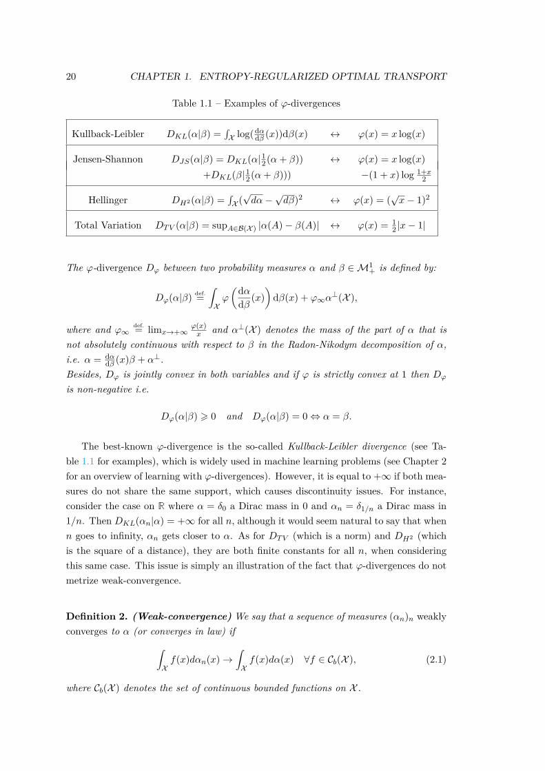
Table 1.1 – Examples of ϕ-divergences
Kullback-Leibler DKL(α|β) =∫X log(dα
dβ (x))dβ(x) ↔ ϕ(x) = x log(x)
Jensen-Shannon DJS(α|β) = DKL(α|12(α+ β)) ↔ ϕ(x) = x log(x)+DKL(β|12(α+ β))) −(1 + x) log 1+x
2
Hellinger DH2(α|β) =∫X (√dα−
√dβ)2 ↔ ϕ(x) = (
√x− 1)2
Total Variation DTV (α|β) = supA∈B(X ) |α(A)− β(A)| ↔ ϕ(x) = 12 |x− 1|
The ϕ-divergence Dϕ between two probability measures α and β ∈M1+ is defined by:
Dϕ(α|β) def.=∫Xϕ
(dαdβ (x)
)dβ(x) + ϕ∞α
⊥(X ),
where and ϕ∞def.= limx→+∞
ϕ(x)x and α⊥(X ) denotes the mass of the part of α that is
not absolutely continuous with respect to β in the Radon-Nikodym decomposition of α,i.e. α = dα
dβ (x)β + α⊥.Besides, Dϕ is jointly convex in both variables and if ϕ is strictly convex at 1 then Dϕ
is non-negative i.e.
Dϕ(α|β) > 0 and Dϕ(α|β) = 0⇔ α = β.
The best-known ϕ-divergence is the so-called Kullback-Leibler divergence (see Ta-ble 1.1 for examples), which is widely used in machine learning problems (see Chapter 2for an overview of learning with ϕ-divergences). However, it is equal to +∞ if both mea-sures do not share the same support, which causes discontinuity issues. For instance,consider the case on R where α = δ0 a Dirac mass in 0 and αn = δ1/n a Dirac mass in1/n. Then DKL(αn|α) = +∞ for all n, although it would seem natural to say that whenn goes to infinity, αn gets closer to α. As for DTV (which is a norm) and DH2 (whichis the square of a distance), they are both finite constants for all n, when consideringthis same case. This issue is simply an illustration of the fact that ϕ-divergences do notmetrize weak-convergence.
Definition 2. (Weak-convergence) We say that a sequence of measures (αn)n weaklyconverges to α (or converges in law) if∫
Xf(x)dαn(x)→
∫Xf(x)dα(x) ∀f ∈ Cb(X ), (2.1)
where Cb(X ) denotes the set of continuous bounded functions on X .
2. DISTANCES BETWEEN PROBABILITY MEASURES 21
We say that a discrepancy d metrizes the weak-convergence of measures if
d(αn, α)→ 0⇔ αn α,
where denotes weak-convergence (or convergence in law, for Xn X where Xn ∼ αnand X ∼ α).
Remark 1. As pointed out in Sec. 5.1 of (Ambrosio et al., 2006), it is sufficient to check(2.1) on any subset Ω of bounded continuous functions whose linear envelope span(Ω)is uniformly dense (i.e. dense in the uniform topology induced by the infinity norm) inCb(X ).
The fact that ϕ−divergences do not metrize weak convergence is a major issue andmakes them poor candidates for learning problems, in spite of their appreciated com-putational simplicity. We discuss this in details in Chapter 2, where focus on finding agood notion of distance between measures to fit a (generative) parametric model to adataset. For now, let us introduce another class of distances between measures whichcan metrize weak convergence under some assumptions.
2.2 Integral Probability Metrics and Maximum Mean discrepancy
The notion of Integral Probability Metrics (IPMs) was introduced by (Müller, 1997)as a class of maximization problems on certain sets of functions, regrouping some wellknown distances:
Definition 3. (Integral probability metrics) (Müller, 1997) Consider two probabilitydistributions α and β on a space X . Given a set of measurable functions F , the integralprobability metric dF is defined as
dF (α, β) def.= supf∈F|Eα(f(X))− Eβ(f(Y ))|. (2.2)
Let us now give a sufficient condition on F so that the associated IPM metrizes weakconvergence:
Proposition 1. If span(F) is uniformly dense in Cb(X ), then dF metrizes weak con-vergence.
Proof. dF metrize weak convergence if and only if dF (αn, α)→ 0⇔ αn α. Using thedefinition of dF (2.2) and the definition of weak convergence (2.1) we can rewrite thisas:
supf∈F
∣∣∣ ∫Xf(x)dαn(x)−
∫Xf(x)dα(x)
∣∣∣→ 0
⇔∣∣∣ ∫Xf(x)dαn(x)−
∫Xf(x)dα(x)
∣∣∣→ 0 ∀f ∈ Cb(X ).
22 CHAPTER 1. ENTROPY-REGULARIZED OPTIMAL TRANSPORT
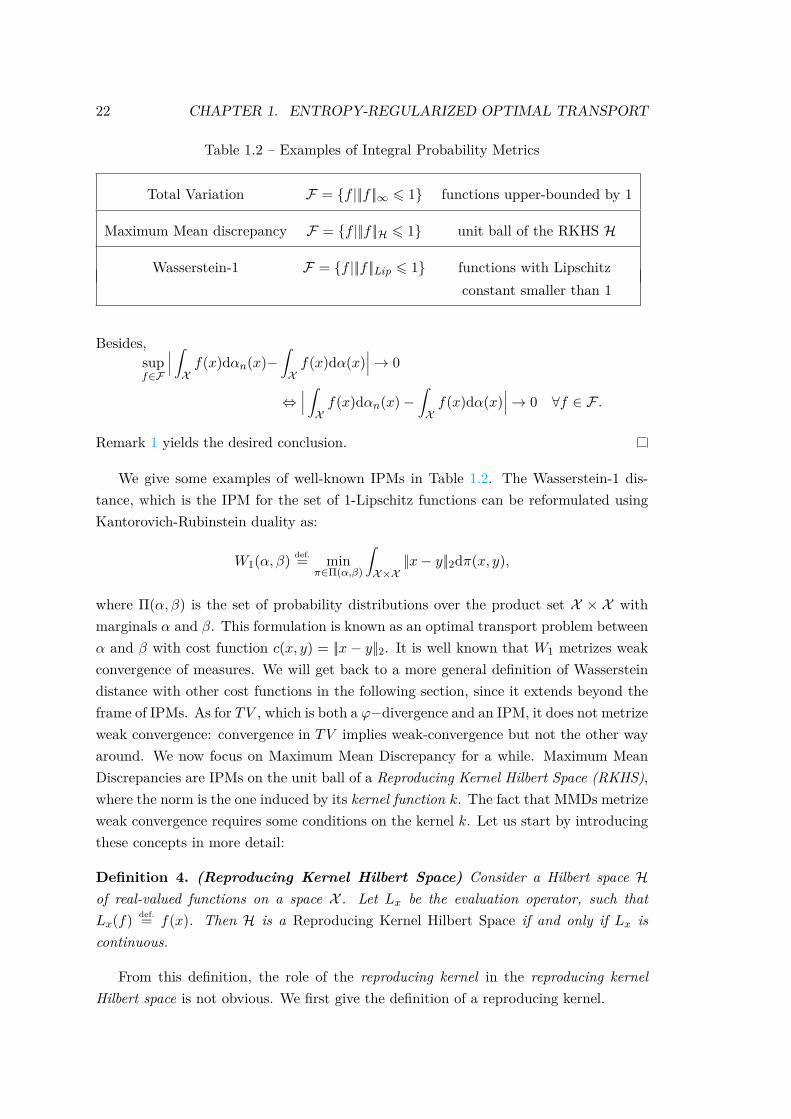
Table 1.2 – Examples of Integral Probability Metrics
Total Variation F = f |||f ||∞ 6 1 functions upper-bounded by 1
Maximum Mean discrepancy F = f |||f ||H 6 1 unit ball of the RKHS H
Wasserstein-1 F = f |||f ||Lip 6 1 functions with Lipschitzconstant smaller than 1
Besides,supf∈F
∣∣∣ ∫Xf(x)dαn(x)−
∫Xf(x)dα(x)
∣∣∣→ 0
⇔∣∣∣ ∫Xf(x)dαn(x)−
∫Xf(x)dα(x)
∣∣∣→ 0 ∀f ∈ F .
Remark 1 yields the desired conclusion.
We give some examples of well-known IPMs in Table 1.2. The Wasserstein-1 dis-tance, which is the IPM for the set of 1-Lipschitz functions can be reformulated usingKantorovich-Rubinstein duality as:
W1(α, β) def.= minπ∈Π(α,β)
∫X×X
||x− y||2dπ(x, y),
where Π(α, β) is the set of probability distributions over the product set X × X withmarginals α and β. This formulation is known as an optimal transport problem betweenα and β with cost function c(x, y) = ||x− y||2. It is well known that W1 metrizes weakconvergence of measures. We will get back to a more general definition of Wassersteindistance with other cost functions in the following section, since it extends beyond theframe of IPMs. As for TV , which is both a ϕ−divergence and an IPM, it does not metrizeweak convergence: convergence in TV implies weak-convergence but not the other wayaround. We now focus on Maximum Mean Discrepancy for a while. Maximum MeanDiscrepancies are IPMs on the unit ball of a Reproducing Kernel Hilbert Space (RKHS),where the norm is the one induced by its kernel function k. The fact that MMDs metrizeweak convergence requires some conditions on the kernel k. Let us start by introducingthese concepts in more detail:
Definition 4. (Reproducing Kernel Hilbert Space) Consider a Hilbert space Hof real-valued functions on a space X . Let Lx be the evaluation operator, such thatLx(f) def.= f(x). Then H is a Reproducing Kernel Hilbert Space if and only if Lx iscontinuous.
From this definition, the role of the reproducing kernel in the reproducing kernelHilbert space is not obvious. We first give the definition of a reproducing kernel.
2. DISTANCES BETWEEN PROBABILITY MEASURES 23
Definition 5. (Reproducing Kernel) Consider a Hilbert space H of real-valued func-tions on a space X . A function k : X × X → R is a reproducing kernel of H if itverifies:
1. ∀x ∈ X , k(x, ·) ∈ H,
2. ∀f ∈ H, f(x) = 〈f, k(x, ·)〉H.
Proposition 2. A function k : X × X → R is a reproducing kernel if and only if it ispositive definite, i.e for all (x1, . . . , xn) ∈ X n, (a1, . . . , an) ∈ Rn,
n∑i=1
n∑j=1
aiajK(xi, xj) > 0.
We can now state a theorem giving an equivalent definition for RKHS.
Theorem 5. A Hilbert space H of real-valued functions on a space X is a ReproducingKernel Hilbert Space if and only if it has a reproducing kernel. Besides, this reproducingkernel is unique.
Thanks to this theorem, it is possible to define the RKHS associated to any positivedefinite kernel k.
Remark 2. The proof of any RKHS having a reproducing kernel is made thanks toRiesz representer theorem. Since the evaluation function is linear and continuous, thereexists a function kx ∈ H such that f(x) = 〈f, kx〉H. Defining the bilinear functionk : X × X → R by k(x, y) = kx(y) we clearly have that k is a reproducing kernel of H.
The reproducing property of RKHS allows to derive a much simpler expression fortheir associated IPM, which becomes a closed form formula.
Proposition 3. (Maximum Mean discrepancy) (Gretton et al., 2006) Considertwo probability measures α and β ∈M1
+(X ). Then, denoting by MMDk the MaximumMean Discrepancy on the Reproducing Kernel Hilbert Space H with kernel k, we havethat
MMD2k(α, β) def.=
(sup
f |||f ||H61|Eα(f(X))− Eβ(f(Y ))|
)2
= Eα⊗α[k(X,X ′)] + Eβ⊗β[k(Y, Y ′)]− 2Eα⊗β[k(X,Y )]. (2.3)
Proof. Using the fact that any function f in the RKHS satisfies f(x) = 〈f, k(x, ·)〉H, wecan rewrite MMD as follows:
supf |||f ||H61
|Eα(f(X))− Eβ(f(Y ))| = supf |||f ||H61
|Eα(〈f, k(X, ·)〉H)− Eβ(〈f, k(Y, ·)〉H)|
= supf |||f ||H61
|〈f,Eαk(X, ·)− Eβk(Y, ·)〉H|
6 ||Eαk(X, ·)− Eβk(Y, ·)||H,
24 CHAPTER 1. ENTROPY-REGULARIZED OPTIMAL TRANSPORT
and this upper bound is reached for f = Eαk(X, ·)− Eβk(Y, ·).
When α and β are finite discrete measures, i.e. α def.=∑ni=1 αiδxi and β
def.=∑ni=1 βiδyi ,
(2.3) becomes
n∑i,j=1
k(xi, xj)αiαj +n∑
i,j=1k(yi, yj)βiβj − 2
n∑i,j=1
k(xi, yj)αiβj .
Thus, MMD can be efficiently estimated with samples from α and β. We discuss thisin Chapter 3 when we compare sample complexity for MMD, Wasserstein distance, andentropy-regularized optimal transport.
We now give some conditions on k to ensure thatMMDk metrizes weak convergence
Theorem 6. (MMD and weak convergence) (Sriperumbudur et al., 2010) ConsiderMaximum Mean Discrepancy with kernel k between two measures α and β on some spaceX , as defined in (2.3).
(i) Let X be a compact space. If the kernel k is universal (i.e. its associated RKHS isdense in the space of continuous functions), then MMDk metrizes weak conver-gence onM1
+(X ).
(ii) Let X = Rd and k(x, y) = κ(x − y) where κ is a bounded strictly positive-definitefunction. If ∃l ∈ N such that:∫
Rd
1κ(ω)(1 + ||ω||2)ldω <∞,
then MMDk metrizes weak convergence onM1+(X ) .
The most widely used kernel is the Gaussian kernel k(x, y) = exp(−||x−y||2
σ2 ), which is auniversal kernel. According to Theorem 6 it metrizes weak convergence on a compact set,but it does not verify the required hypotheses on Rd. They are however characteristic,meaning that MMDk(α, β) = 0 ↔ α = β. An example of kernels that verify thehypotheses of Theorem 6 on Rd are the so-called Matern kernels, whose associatedRKHS are Sobolev spaces. We further discuss the use of various kernels for learningproblems in Chapter 2 and for function estimation in Chapters 3 and 4.
2.3 Optimal Transport
We consider two probability measures α ∈ M1+(X ) and β on M1
+(Y). The Kan-torovich formulation (Kantorovich, 1942) of Optimal Transport (OT) between α and βis defined by:
Wc(α, β) def.= minπ∈Π(α,β)
∫X×Y
c(x, y)dπ(x, y), (P)
2. DISTANCES BETWEEN PROBABILITY MEASURES 25
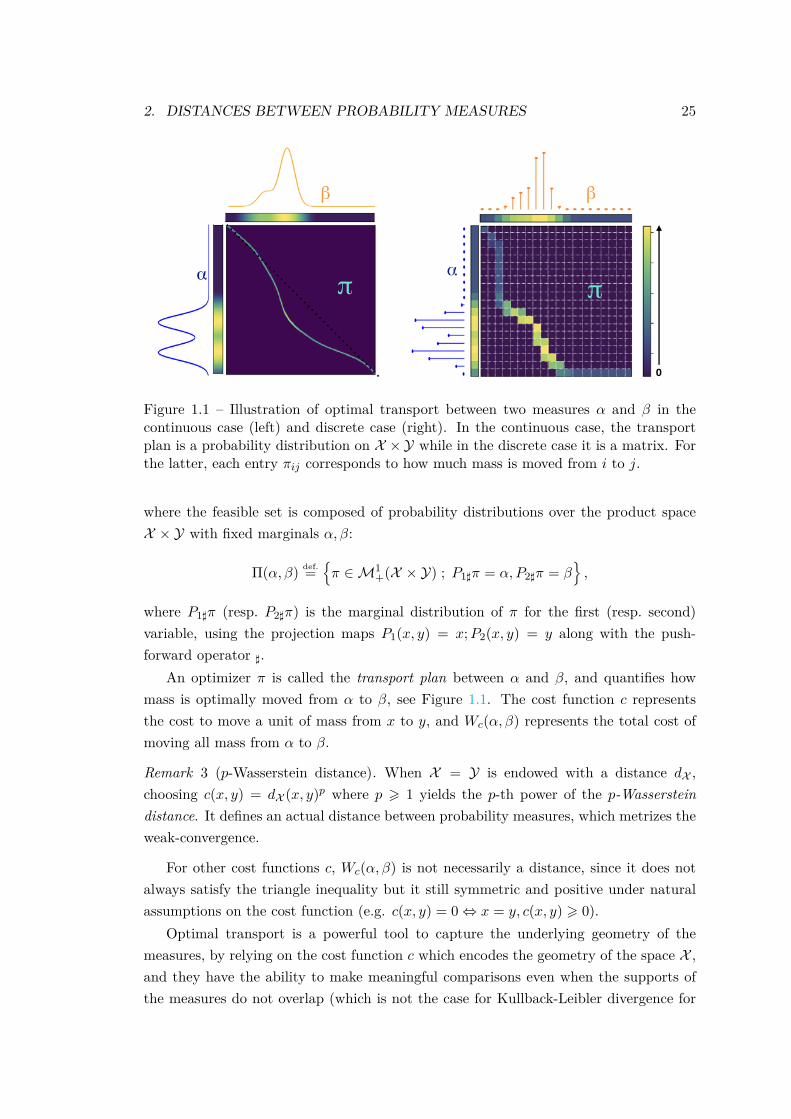
Figure 1.1 – Illustration of optimal transport between two measures α and β in thecontinuous case (left) and discrete case (right). In the continuous case, the transportplan is a probability distribution on X ×Y while in the discrete case it is a matrix. Forthe latter, each entry πij corresponds to how much mass is moved from i to j.
where the feasible set is composed of probability distributions over the product spaceX × Y with fixed marginals α, β:
Π(α, β) def.=π ∈M1
+(X × Y) ; P1]π = α, P2]π = β,
where P1]π (resp. P2]π) is the marginal distribution of π for the first (resp. second)variable, using the projection maps P1(x, y) = x;P2(x, y) = y along with the push-forward operator ].
An optimizer π is called the transport plan between α and β, and quantifies howmass is optimally moved from α to β, see Figure 1.1. The cost function c representsthe cost to move a unit of mass from x to y, and Wc(α, β) represents the total cost ofmoving all mass from α to β.
Remark 3 (p-Wasserstein distance). When X = Y is endowed with a distance dX ,choosing c(x, y) = dX (x, y)p where p > 1 yields the p-th power of the p-Wassersteindistance. It defines an actual distance between probability measures, which metrizes theweak-convergence.
For other cost functions c, Wc(α, β) is not necessarily a distance, since it does notalways satisfy the triangle inequality but it still symmetric and positive under naturalassumptions on the cost function (e.g. c(x, y) = 0⇔ x = y, c(x, y) > 0).
Optimal transport is a powerful tool to capture the underlying geometry of themeasures, by relying on the cost function c which encodes the geometry of the space X ,and they have the ability to make meaningful comparisons even when the supports ofthe measures do not overlap (which is not the case for Kullback-Leibler divergence for
26 CHAPTER 1. ENTROPY-REGULARIZED OPTIMAL TRANSPORT
instance). Besides, the transport plan π gives a mapping between measures which canbe used for instance in domain adaptation (Courty et al., 2014). More structure canbe enforced with extensions of OT (Alvarez-Melis et al., 2017), which can for instancetake into account labels of the data in supervised learning. However, OT suffers from acomputational and statistical burden:
• Computing OT is costly: Solving OT when dealing with discrete distributions(i.e., finite weighted sums of Dirac masses) amounts to solving a large-scale linearprogram. This can be done using network flow solvers, which can be further refinedto assignment problems when comparing measures of the same size with uniformweights (Burkard et al., 2009). The computational complexity is O(n3log(n))where n is the number of points in the discrete measure (see also the monographon Computational OT by Peyré et al. (2017) for a detailed review of OT solvers).
• OT suffers from a curse of dimensionality: considering a probability measureα ∈ M1
+(Rd) and its empirical estimation αn, we have E[Wp(α, αn)] = O(n−1/d)(see (Weed and Bach, 2017) for refined convergence rates depending on the supportof α). Thus the error made when approximating the Wasserstein distance fromsamples grows exponentially fast with the dimension of the ambient space.
These two issues have caused OT to be neglected in machine learning applications for along time in favor of simpler ϕ−divergences or MMD.
Let us conclude this section on OT with a recent extension introduced in (Chizatet al., 2018), (Liero et al., 2018). While OT is restricted to positive measures of mass 1,Unbalanced Optimal Transport can compare any two arbitrary positive measures. Themarginal constraints are relaxed, as they are replaced with ϕ-divergences:
Definition 6. (Unbalanced Optimal Transport) Consider two positive measuresα ∈M+(X ) and β ∈M+(Y). Unbalanced Optimal Transport is defined as the followingminimization problem
minπ∈M+(X×Y)
∫X×Y
c(x, y)dπ(x, y) +Dψ1(P1]π|α) +Dψ2(P2]π|β), (2.4)
where ψ1 and ψ2 are positive, lower-semi-continuous functions such that ψ1(1) = 0 andψ2(1) = 0.
Note that there is no constraint on the transport plan besides positivity: it is notrequired to have marginals equal to α and β nor to have mass 1. For specific choicesof c, ψ1, ψ2, unbalanced OT defines a distance onM+(X ). This extension is popular inseveral applications due to the fact that it can compare any arbitrary positive measures.Whenever possible, we extend our results on regularized OT to the unbalanced case.
3. REGULARIZED OPTIMAL TRANSPORT 27
3 Regularized Optimal Transport
We introduce regularized optimal transport, which consists in regularizing the orig-inal problem by penalizing it with the ϕ-divergence of the transport plan with respectto the product measure:
Wϕc,ε(α, β) def.= min
π∈Π(α,β)
∫X×Y
c(x, y)dπ(x, y) + ε
∫X×Y
ϕ
( dπ(x, y)dα(x)dβ(y)
)dα(x)dβ(y),
(Pε,ϕ)
where ϕ is a convex function with domain R+.Entropic regularization, which is the main focus of this thesis, corresponds to the
case ϕ(w) = w log(w) − w + 1 (or alternatively ϕ(w) = w log(w)) but one may choosethe squared penalty ϕ(w) = w2
2 + ιR+(w), where ι denotes the convex indicator func-tion. However, most of the properties we derive for regularized optimal transport – inparticular fast numerical solvers and improved sample complexity – are specific to theentropic regularization.
3.1 Dual Formulation
An advantage to consider regularized OT is to get an unconstrained dual problem.The dual of standard OT reads:
Wc(α, β) = sup(u,v)∈U(c)
∫Xu(x)dα(x) +
∫Yv(x)dβ(y), (D)
where the constraint set U(c) is defined by
U(c) def.= (u, v) ∈ C(X )× C(Y)|u(x) + v(y) 6 c(x, y), ∀(x, y) ∈ X × Y.
while the dual of regularized OT is given by an unconstrained maximization problem:
Proposition 4. Consider OT between two probability measures α and β with a convexregularizer ϕ with domain R+. Then strong duality holds and (Pε,ϕ) is equivalent to thefollowing dual formulation:
Wϕc,ε(α, β) = sup
u,v∈C(X )×C(Y)
∫Xu(x)dα(x) +
∫Yv(x)dβ(y)
−ε∫X×Y
ϕ∗(u(x) + v(y)− c(x, y)ε
)dα(x)dβ(y), (Dε,ϕ)
where ϕ∗ is the Legendre transform of ϕ defined by ϕ∗(p) def.= supw wp− ϕ(w).
Remark 4. (Strong Duality) Before getting into details on the derivation of the dual prob-lem, note that strong duality holds, thanks to the application of Fenchel-Rockafellar the-orem to the dual problem, which also guarantees existence of a primal solution to (Pε,ϕ)
28 CHAPTER 1. ENTROPY-REGULARIZED OPTIMAL TRANSPORT
(see (Chizat, 2017), Prop. 3.5.6 for technical details). The existence of maximizers forthe dual problem (Dε,ϕ) is not guaranteed in general, and we give a proof of existencein the case of entropic regularization in Sec. 4.1 of this Chapter.
Proof. The primal problem reads
minπ
∫X×Y
c(x, y)dπ(x, y) + ε
∫X×Y
ϕ
( dπ(x, y)dα(x)dβ(y)
)dα(x)dβ(y))
under the constraint that P1]π = α, P2]π = β Introducing the Lagrange multipliers uand v associated to these constraints, the Lagrangian reads
L(π, u, v) =∫X×Y
c(x, y)dπ(x, y) + ε
∫X×Y
ϕ
( dπ(x, y)dα(x)dβ(y)
)dα(x)dβ(y)
+∫Xu(x)
(dα(x)−
∫Y
dπ(x, y))
+∫Yv(y)
(dβ(y)−
∫X
dπ(x, y))
The dual Lagrange function is given by g(u, v) = minπ L(π, u, v) and thus rearrangingterms we get
g(u, v) =∫Xu(x)dα(x) +
∫Yv(x)dβ(y)
+εminπ
(∫X×Y
(ϕ
( dπ(x, y)dα(x)dβ(y)
)− u(x) + v(y)− c(x, y)
ε
dπ(x, y)dα(x)dβ(y)
)dα(x)dβ(y)
)=∫Xu(x)dα(x) +
∫Yv(x)dβ(y)− ε
∫X×Y
ϕ∗(u(x) + v(y)− c(x, y)
ε
)dα(x)dβ(y),
where ϕ∗ the Legendre transform of ϕ is given by
ϕ∗(p) = supwwp− ϕ(w) = − inf
wϕ(w)− wp.
Remark 5. (Primal-Dual Relationship) The primal-dual relationship is given by
π = argminπ ϕ( dπ(x, y)dα(x)dβ(y)
)− u(x) + v(y)− c(x, y)
ε
dπ(x, y)dα(x)dβ(y)
⇔ dπ(x, y) = (ϕ′)−1(u(x) + v(y)− c(x, y)ε
)dα(x)dβ(y),
when (ϕ′) is invertible.
The smoothing effect of regularization is clear when looking at the dual of standardOT , since the constraint on the dual problem is replaced by a smooth penalization. Theterm
∫X×Y ϕ
∗(u(x)+v(y)−c(x,y)ε )dα(x)dβ(y) penalizes large positive values of u(x)+v(y)−
c(x, y). Ideally, to get a regularized problem that stays true to standard OT, we want ϕ∗
to go quickly to large positive values when u(x)+v(y)−c(x, y) grows. A good choice for
3. REGULARIZED OPTIMAL TRANSPORT 29
such a function is ϕ∗(w) = ew, which actually corresponds to the entropic regularization(see section 4 for more details). A weaker penalization can also be considered usingϕ∗(w) = max(w, 0)2/2, which corresponds to the quadratic regularization.
3.2 The Case of Unbalanced OT
Unbalanced OT can also be regularized with a ϕ−divergence, which gives the fol-lowing problem:
minπ∈M+(X×Y)
∫X×Y
c(x, y)dπ(x, y) +Dψ1(P1]π|α) +Dψ2(P2]π|β)
+ ε
∫X×Y
ϕ
( dπ(x, y)dα(x)dβ(y)
)dα(x)dβ(y).
As previously done with balanced OT, we can compute the dual of this problem:
Proposition 5. The dual of regularized unbalanced OT with a convex regularizer ϕ withdomain R+ is given by
supu∈C(X ),v∈C(Y)
−∫Xψ∗1(−u(x))dα(x)−
∫Yψ∗2(−v(y))dβ(y)
− ε∫X×Y
ϕ∗(u(x) + v(y)− c(x, y)
ε
)dα(x)dβ(y).
Proof. The proof is essentially similar to the derivation of the regularized dual in Propo-sition 4 except the problem is unconstrained. The primal problem reads
minπ∈M+(X×Y)
∫X×Y
c(x, y)dπ(x, y) +∫Xψ1
(P1]π(x)dα(x)
)dα(x) +
∫Yψ2
(P2]π(y)dβ(y)
)dβ(y)
+ ε
∫X×Y
ϕ
( dπ(x, y)dα(x)dβ(y)
)dα(x)dβ(y)).
We introduce slack variables a and b such that a = P1]π and b = P2]π. This gives thefollowing constrained problem:
minπ∈M+(X×Y)
(a,b)∈M+(X )×M+(Y)
∫X×Y
c(x, y)dπ(x, y) +∫Xψ1
( da(x)dα(x)
)dα(x) +
∫Yψ2
( db(y)dβ(y)
)dβ(y)
+ ε
∫X×Y
ϕ
( dπ(x, y)dα(x)dβ(y)
)dα(x)dβ(y)),
subject to a = P1]π and b = P2]π. Introducing the Lagrange multipliers u and v
30 CHAPTER 1. ENTROPY-REGULARIZED OPTIMAL TRANSPORT
associated to the constraints, the Lagrangian reads
L(π, a, b, u, v) =∫X×Y
c(x, y)dπ(x, y) +∫Xψ1
( da(x)dα(x)
)dα(x) +
∫Yψ2
( db(y)dβ(y)
)dβ(y)
+∫Xu(x)
(da(x)−
∫Y
dπ(x, y))
+∫Yv(y)
(db(y)−
∫X
dπ(x, y))
+ ε
∫X×Y
ϕ
( dπ(x, y)dα(x)dβ(y)
)dα(x)dβ(y)).
The dual Lagrange function is given by g(u, v) = minπ,a,b L(π, a, b, u, v), and since theproblem is separable we get three distinct minimization problems for each variable:
g(u, v) = mina
[ ∫Xu(x)da(x) + ψ1
( da(x)dα(x)
)dα(x)
]+ min
b
[ ∫Yv(y)db(y) + ψ2
( db(x)dβ(y)
)dβ(x)
]+ min
π
[ ∫X×Y
(c(x, y)− u(x)−v(y))dπ(x, y)
+ ε
∫X×Y
ϕ
( dπ(x, y)dα(x)dβ(y)
)dα(x)dβ(y))
].
The three minimization problems are actually the expression of the Legendre transformfor ψ1,ψ2, and ϕ and so the dual function can be rewritten as:
g(u, v) = −∫Xψ∗1(−u(x))dα(x)−
∫Yψ∗2(−v(y))dβ(y)
− ε∫X×Y
ϕ∗(u(x) + v(y)− c(x, y)
ε
)dα(x)dβ(y),
where f∗ is the Legendre transform of f defined by f∗(p) = supw wp− f(w).
3.3 Dual Expectation Formulation
Another benefit of the regularization introduced above is the fact that is can berewritten as the maximization of an expectation with respect to the product measureα⊗ β
Proposition 6. The dual of regularized OT (Dε,ϕ) has the following equivalent formu-lation:
Wϕc,ε(α, β) = sup
u,v∈C(X )×C(Y)Eα⊗β[fXYε (u, v)],
where fxyεdef.= u(x) + v(y)− ϕ∗(u(x)+v(y)−c(x,y)
ε ).
Since many machine learning problems (e.g. risk minimization) are formulated as themaximization of an expectation, this formulation of the dual of regularized OT allowsus to apply well-known techniques from machine learning to study statistical properties
4. ENTROPY-REGULARIZED OPTIMAL TRANSPORT 31
of regularized OT in Chapter 3 and use stochastic optimization to solve it in Chapter 4.Note that the formulation as an expectation of the dual problem is only available for
ε > 0. Indeed, the dual of standard OT has a constraint (u+ v− c 6 0) whose indicatorfunction cannot be put inside the expectation.
Remark 6. (Generalization to Unbalanced OT) Recall the dual of regularized unbalancedOT with regularizer ϕ:
supu,v−∫Xψ∗1(−u(x))dα(x)−
∫Yψ∗2(−v(y))dβ(y)
−ε∫X×Y
ϕ∗(u(x) + v(y)− c(x, y)ε
)dα(x)dβ(y).
Thus, it can also be cast as the maximization of an expectation with respect to theproduct measure α⊗ β
supu∈C(X ),v∈C(Y)
Eα⊗β
[ψ∗1(−u(X))− ψ∗2(−v(Y )) + ϕ∗(u(X) + v(Y )− c(X,Y )
ε)].
4 Entropy-Regularized Optimal Transport
Entropic regularization is the main focus of this thesis, as it presents several specificproperties:
• closed-form primal-dual relationship, allowing to recover the transport plan π aftersolving the simpler (unconstrained) dual problem,
• a fast numerical solver for finite discrete measures, Sinkhorn’s algorithm (seeSec. 4.2),
• a discrepancy between measures interpolating between standard OT and MMD(see Chapter 2),
• an improved sample complexity compared to OT, breaking the curse of dimen-sionality for a regularization parameter large enough (see Chapter 3),
• reformulation of the dual as the maximization of an expectation in a ReproducingKernel Hilbert Space (RKHS) ball of finite radius, allowing to solve the dualproblem with a kernel version of stochastic gradient descent (see Chapter 3 andChapter 4),
• semi-dual formulation (Sε), allowing to solve semi-discrete OT with online descentalgorithms (see Chapter 4).
Let us rewrite the primal and dual problems (Pε,ϕ) and (Dε,ϕ) derived in Proposi-tion 4 with the entropic regularization:
32 CHAPTER 1. ENTROPY-REGULARIZED OPTIMAL TRANSPORT
Proposition 7. Consider OT between two probability measures α and β with entropicregularization:
Wc,ε(α, β) def.= minπ∈Π(α,β)
∫X×Y
c(x, y)dπ(x, y) + εH(π|α⊗ β), (Pε)
whereH(π|α⊗ β) def.=
∫X×Y
(log
( dπ(x, y)dα(x)dβ(y)
)− 1
)dπ(x, y) + 1 (4.1)
is the relative entropy of the transport plan π with respect to the product measure α⊗β.It is equivalent to this dual formulation:
Wc,ε(α, β) = maxu∈C(X ),v∈C(Y)
∫Xu(x)dα(x) +
∫Yv(y)dβ(y)
− ε∫X×Y
eu(x)+v(y)−c(x,y)
ε dα(x)dβ(y) + ε (Dε)
= maxu∈C(X),v∈C(Y )
Eα⊗β[fXYε (u, v)
]+ ε (4.2)
where fxyε (u, v) = u(x) + v(y)− εeu(x)+v(y)−c(x,y)
ε .
Besides, the primal-dual relationship is given by
dπ(x, y) = exp(u(x) + v(y)− c(x, y)
ε
)dα(x)dβ(y).
Proof. This is a direct application of Proposition 4, using ϕ(w) = w logw − w + 1, inwhich case ϕ∗(p) def.= supw wp− ϕ(w) = ep + 1. Note that the sup is a max is this case,and we prove the existence of optimizers in Sec. 4.1 below.
Remark 7. (Equivalent formulation of (Pε)) The transport plan π is constrained to be aprobability measure which imposes
∫X×Y dπ(x, y) = 1, so the primal problem (Pε) can
be simplified to:
minπ∈Π(α,β)
∫X×Y
c(x, y)dπ(x, y) + ε
∫X×Y
log( dπ(x, y)
dα(x)dβ(y)
). (Pε)
However when computing the dual directly from this formulation, we get a primal-dualrelationship that is less elegant:
dπ(x, y) = eu(x)+v(y)−c(x,y)−1
ε dα(x)dβ(y),
which is why we prefer to formally state Proposition 7 with H defined in (4.1).
Remark 8. (Dual Potentials and Exponential Scalings) As commonly done in the litera-ture on OT, we refer to the variables of the dual problem (u, v) as the dual (Kantorovitch)potentials. We will also often use the so-called exponential scalings of the dual variables(a, b) defined by a def.= e
uε and b def.= e
vε .
4. ENTROPY-REGULARIZED OPTIMAL TRANSPORT 33
Entropic regularization of optimal transport was first introduced with the follow-ing formulation of entropy: H(π) def.=
∫X×Y log
(dπ(x,y)dxdy
)dπ(x, y) (Cuturi, 2013). The
resulting dual problem is slightly different:
maxu∈C(X ),v∈C(Y)
∫Xu(x)dα(x) +
∫Yv(y)dβ(y)− ε
∫X×Y
eu(x)+v(y)−c(x,y)
ε dxdy + ε.
Here, the third term in the dual is an integral with respect to the Lebesgue measure,while with relative entropy, the integral is taken with respect to the product measureα⊗β. The formulation with simple entropy yields an unconstrained dual problem whichcan be solved efficiently (see Proposition. 10 for details) but it can not be formulated asthe maximization of an expectation which, as already mentioned, is crucial for the resultspresented in Chapters 3 and 4. Thus we only use relative-entropy as a regularizer, as itkeeps all the benefits brought by simple entropy with the added benefit of the expectationformulation.
4.1 Solving the Regularized Dual Problem
As most of the methods we develop in this thesis rely on the dual formulation ofentropy-regularized OT, we give a proof of existence of a solution to this problem, fora general setting. We discuss further the regularity of the dual potentials in Chapter 3.This section is dedicated to proving the following existence theorem:
Theorem 7. (Existence of a dual solution) Consider the dual of entropy-regularizedOT, with marginals α, β ∈M1
+(X )×M1+(Y) supported on two subsets of Rd, and with a
cost function c bounded on X × Y. Let L∞(α) def.= f : X → R|∃C > 0 such that f(x) 6C α-a.e.. Then the dual problem has solutions (u∗, v∗) ∈ L∞(α) × L∞(β) which areunique α− and β−a.e. up to an additive constant.
It is straightforward to see that for any solution (u∗, v∗) to the dual problem, thepair (u∗+ k, v∗− k) for k ∈ R is also a solution to the dual problem. Besides, modifyingthe values of u∗ and v∗ outside of the support of the measures does not have any effecton the value of the problem.
The proof of existence of a solution to the dual problem essentially amounts torewriting the optimality condition as a fixed point equation, and proving that a fixedpoint exists. To do so, we show that the operator in the fixed point equation is acontraction for a certain metric, called the Hilbert metric. This proof is based on thesame idea from that of the existence of a solution to Schrodinger’s system (which sharesstrong links with regularized OT) in (Chen et al., 2016), inspired from the original proofof (Franklin and Lorenz, 1989) which deals with discrete regularized OT. We prove theexistence of potentials in a general framework, as we consider arbitrary measures α andβ and any bounded regular cost function c.
34 CHAPTER 1. ENTROPY-REGULARIZED OPTIMAL TRANSPORT
The dual problem is unconstrained, and it is jointly concave in both variables. Thus,we can fix one and optimize over the other, and the first order condition for u gives:
u(x) = −ε log(∫Yev(y)−c(x,y)
ε dβ(y))
for a.e. x ∈ X , (4.3)
and similarly for v:
v(y) = −ε log(∫Xeu(x)−c(x,y)
ε dα(x))
for a.e. y ∈ Y. (4.4)
Remark 9. Although the optimality conditions (4.3) and (4.4) only fix the value ofthe optimal potentials (u∗, v∗) on the supports of α and β respectively, they allow toextrapolate the values of the potentials outside of this support.
4.1.1 Hilbert Metric
We start with a few definitions and properties of the Hilbert metric, which will beuseful later on. Proof of these results can be found in (Bushell, 1973).
Definition 7. (Hilbert metric) Consider K a closed solid cone on a real Banach spaceB i.e. K satisfies the 4 following properties:
1. the interior of K is not empty,
2. K +K ⊆ K,
3. αK ⊆ K∀α > 0,
4. K ∩−K = 0.
We use the partial order induced by the cone, meaning x 6 y ⇔ y − x ∈ K, and definethe following quantities
M(a, b) def.= infλ|a 6 λb and m(a, b) def.= supλ|a 6 λb for a, b ∈ K+ def.= K \ 0.
Then the Hilbert metric dH on K is given by
dH(a, b) def.= log M(a, b)m(a, b) . (4.5)
Note that the Hilbert metric is projective, meaning that it is invariant by multipli-cation by a positive factor: dH(a, b) = dH(αa, b) = dH(a, αb), ∀ α > 0.
The Hilbert metric is a pseudo-metric on the interior of the cone K, and a metric onthe restriction of K to the unit sphere:
Theorem 8. (K, dH) is a pseudo-metric space and (K ∩ S(0, 1), dH) is a metric space,where S(0, 1) is the unit sphere in B

4. ENTROPY-REGULARIZED OPTIMAL TRANSPORT 35
To use Banach’s fixed point theorem on (K ∩B(0, 1), dH), we need to introduce thenotion of contraction ratio:
Definition 8. We say that an operator E is a positive map in the cone if E(K+) ⊂ K+.For a positive map E, we denote its projective diameter by
∆(E) def.= supdH(E(a), E(b)) | a, b ∈ K+,
and its contraction ratio
κ(E) def.= infλ | dH(E(a), E(b)) 6 λdH(x, y)∀x, y ∈ K+.
In the case where the mapping is linear, we have a relation between the contractionratio and the projective diameter.
Proposition 8. Consider a linear positive map E on K, then
κ(E) 6 tanh(1
4∆(E)),
and ∆(E) 6 2 supadH(E(a), 1)) | a ∈ K+.
Since | tanh(x)| < 1 for |x| < +∞, this means that if the projective diameter of apositive mapping is finite, then it is a contraction. The proof of the first inequality isgiven in (Bushell, 1973) while the second is a direct application of the triangle inequality.
4.1.2 Fixed Point Theorem
Now let us rewrite the optimality condition as a fixed point equation. We considerthe exponential scalings (a, b) of the dual variables (u, v). At optimality we have that
a(x) =(∫Yb(y)e
−c(x,y)ε dβ(y)
)−1and b(y) =
(∫Xa(x)e
−c(x,y)ε dα(x)
)−1. (4.6)
We define the operators ϕε,α and ϕε,β such that
ϕε,α(f) def.=∫Xf(x)e
−c(x,y)ε dα(x) and ϕε,β(f) def.=
∫Yf(y)e
−c(x,y)ε dβ(y), (4.7)
and we denote by E the operator such that E(a) def.= 1/a.
Proposition 9. The optimal exponential scalings (a∗, v∗) satisfy the following fixed-point equations:
a∗ = Φ(a∗) where Φ def.= E ϕε,β E ϕε,α, (4.8)
andb∗ = Φ(b∗) where Φ def.= E ϕε,α E ϕε,β. (4.9)
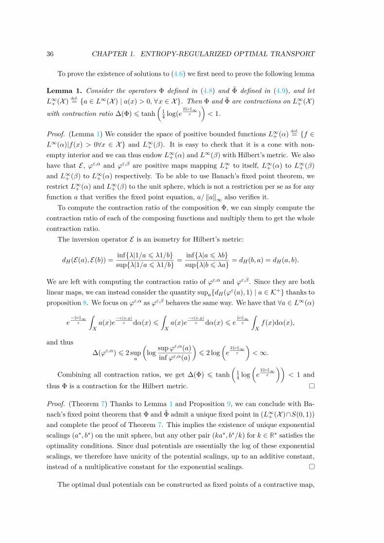
36 CHAPTER 1. ENTROPY-REGULARIZED OPTIMAL TRANSPORT
To prove the existence of solutions to (4.6) we first need to prove the following lemma
Lemma 1. Consider the operators Φ defined in (4.8) and Φ defined in (4.9), and letL∞+ (X ) def.= a ∈ L∞(X ) | a(x) > 0, ∀x ∈ X. Then Φ and Φ are contractions on L∞+ (X )
with contraction ratio ∆(Φ) 6 tanh(
14 log(e
2‖c‖∞ε )
)< 1.
Proof. (Lemma 1) We consider the space of positive bounded functions L∞+ (α) def.= f ∈L∞(α)|f(x) > 0∀x ∈ X and L∞+ (β). It is easy to check that it is a cone with non-empty interior and we can thus endow L∞+ (α) and L∞(β) with Hilbert’s metric. We alsohave that E , ϕε,α and ϕε,β are positive maps mapping L∞+ to itself, L∞+ (α) to L∞+ (β)and L∞+ (β) to L∞+ (α) respectively. To be able to use Banach’s fixed point theorem, werestrict L∞+ (α) and L∞+ (β) to the unit sphere, which is not a restriction per se as for anyfunction a that verifies the fixed point equation, a/ ‖a‖∞ also verifies it.
To compute the contraction ratio of the composition Φ, we can simply compute thecontraction ratio of each of the composing functions and multiply them to get the wholecontraction ratio.
The inversion operator E is an isometry for Hilbert’s metric:
dH(E(a), E(b)) = infλ|1/a 6 λ1/bsupλ|1/a 6 λ1/b = infλ|a 6 λb
supλ|b 6 λa= dH(b, a) = dH(a, b).
We are left with computing the contraction ratio of ϕε,α and ϕε,β. Since they are bothlinear maps, we can instead consider the quantity supadH(ϕε(a), 1) | a ∈ K+ thanks toproposition 8. We focus on ϕε,α as ϕε,β behaves the same way. We have that ∀a ∈ L∞(α)
e−‖c‖∞
ε
∫Xa(x)e
−c(x,y)ε dα(x) 6
∫Xa(x)e
−c(x,y)ε dα(x) 6 e
‖c‖∞ε
∫Xf(x)dα(x),
and thus∆(ϕε,α) 6 2 sup
a
(log supϕε,α(a)
inf ϕε,α(a)
)6 2 log
(e
2‖c‖∞ε
)<∞.
Combining all contraction ratios, we get ∆(Φ) 6 tanh(
14 log
(e
2‖c‖∞ε
))< 1 and
thus Φ is a contraction for the Hilbert metric.
Proof. (Theorem 7) Thanks to Lemma 1 and Proposition 9, we can conclude with Ba-nach’s fixed point theorem that Φ and Φ admit a unique fixed point in (L∞+ (X )∩S(0, 1))and complete the proof of Theorem 7. This implies the existence of unique exponentialscalings (a∗, b∗) on the unit sphere, but any other pair (ka∗, b∗/k) for k ∈ R∗ satisfies theoptimality conditions. Since dual potentials are essentially the log of these exponentialscalings, we therefore have unicity of the potential scalings, up to an additive constant,instead of a multiplicative constant for the exponential scalings.
The optimal dual potentials can be constructed as fixed points of a contractive map,
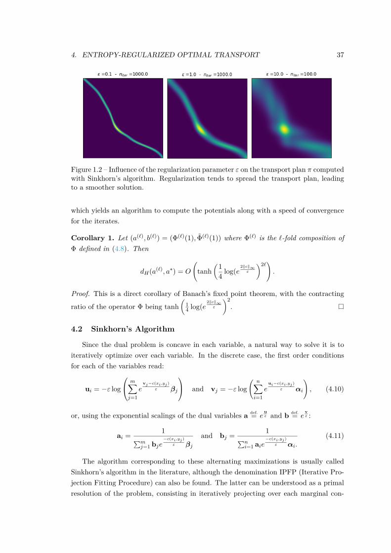
4. ENTROPY-REGULARIZED OPTIMAL TRANSPORT 37
Figure 1.2 – Influence of the regularization parameter ε on the transport plan π computedwith Sinkhorn’s algorithm. Regularization tends to spread the transport plan, leadingto a smoother solution.
which yields an algorithm to compute the potentials along with a speed of convergencefor the iterates.
Corollary 1. Let (a(`), b(`)) = (Φ(`)(1), Φ(`)(1)) where Φ(`) is the `-fold composition ofΦ defined in (4.8). Then
dH(a(`), a∗) = O
(tanh
(14 log(e
2‖c‖∞ε
)2`).
Proof. This is a direct corollary of Banach’s fixed point theorem, with the contracting
ratio of the operator Φ being tanh(
14 log(e
2‖c‖∞ε
)2.
4.2 Sinkhorn’s Algorithm
Since the dual problem is concave in each variable, a natural way to solve it is toiteratively optimize over each variable. In the discrete case, the first order conditionsfor each of the variables read:
ui = −ε log
m∑j=1
evj−c(xi,yj)
ε βj
and vj = −ε log(
n∑i=1
eui−c(xi,yj)
ε αi
), (4.10)
or, using the exponential scalings of the dual variables a def.= euε and b def.= e
vε :
ai = 1∑mj=1 bje
−c(xi,yj)ε βj
and bj = 1∑ni=1 aie
−c(xi,yj)ε αi.
(4.11)
The algorithm corresponding to these alternating maximizations is usually calledSinkhorn’s algorithm in the literature, although the denomination IPFP (Iterative Pro-jection Fitting Procedure) can also be found. The latter can be understood as a primalresolution of the problem, consisting in iteratively projecting over each marginal con-
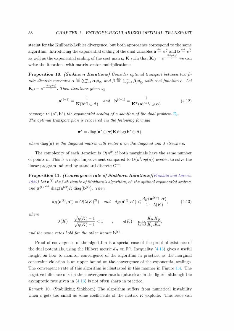
38 CHAPTER 1. ENTROPY-REGULARIZED OPTIMAL TRANSPORT
straint for the Kullback-Leibler divergence, but both approaches correspond to the samealgorithm. Introducing the exponential scaling of the dual variables a def.= e
uε and b def.= e
vε
as well as the exponential scaling of the cost matrix K such that Kij = e−c(xi,yj)
ε we canwrite the iterations with matrix-vector multiplications:
Proposition 10. (Sinkhorn Iterations) Consider optimal transport between two fi-nite discrete measures α def.=
∑ni=1 αiδxi and β
def.=∑mj=1 βjδyj with cost function c. Let
Kij = e−c(xi,yj)
ε . Then iterations given by
a(`+1) = 1K(b(`) β)
and b(`+1) = 1KT (a(`+1) α)
(4.12)
converge to (a∗,b∗) the exponential scaling of a solution of the dual problem Dε.The optimal transport plan is recovered via the following formula
π∗ = diag(a∗ α)K diag(b∗ β),
where diag(a) is the diagonal matrix with vector a on the diagonal and 0 elsewhere.
The complexity of each iteration is O(n2) if both marginals have the same numberof points n. This is a major improvement compared to O(n3log(n)) needed to solve thelinear program induced by standard discrete OT.
Proposition 11. (Convergence rate of Sinkhorn Iterations)(Franklin and Lorenz,1989) Let a(`) the `-th iterate of Sinkhorn’s algorithm, a∗ the optimal exponential scaling,and π(`) def.= diag(a(`))K diag(b(`)). Then
dH(a(`),a∗) = O(λ(K)2`) and dH(a(`),a∗) 6 dH(π(`)1,α)1− λ(K) , (4.13)
whereλ(K) =
√η(K)− 1√η(K)− 1
< 1 ; η(K) = maxi,j,k,l
KikKjl
KjkKil,
and the same rates hold for the other iterate b(`).
Proof of convergence of the algorithm is a special case of the proof of existence ofthe dual potentials, using the Hilbert metric dH on Rn. Inequality (4.13) gives a usefulinsight on how to monitor convergence of the algorithm in practice, as the marginalconstraint violation is an upper bound on the convergence of the exponential scalings.The convergence rate of this algorithm is illustrated in this manner in Figure 1.4. Thenegative influence of ε on the convergence rate is quite clear in the figure, although theasymptotic rate given in (4.13) is not often sharp in practice.
Remark 10. (Stabilizing Sinkhorn) The algorithm suffers from numerical instabilitywhen ε gets too small as some coefficients of the matrix K explode. This issue can
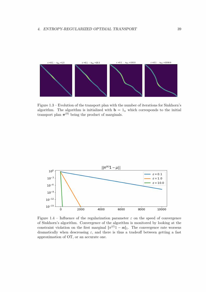
4. ENTROPY-REGULARIZED OPTIMAL TRANSPORT 39
Figure 1.3 – Evolution of the transport plan with the number of iterations for Sinkhorn’salgorithm. The algorithm is initialized with b = 1n which corresponds to the initialtransport plan π(0) being the product of marginals.
Figure 1.4 – Influence of the regularization parameter ε on the speed of convergenceof Sinkhorn’s algorithm. Convergence of the algorithm is monitored by looking at theconstraint violation on the first marginal ||π(`)1 − α||1. The convergence rate worsensdramatically when descreasing ε, and there is thus a tradeoff between getting a fastapproximation of OT, or an accurate one.
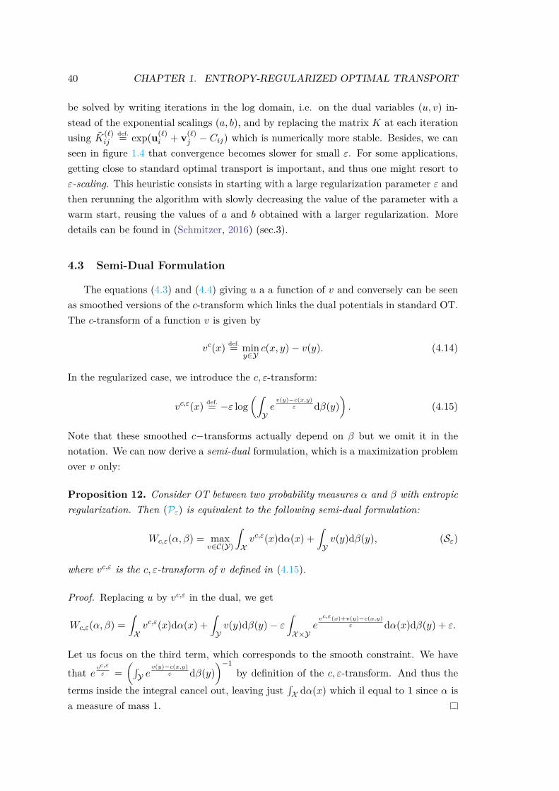
40 CHAPTER 1. ENTROPY-REGULARIZED OPTIMAL TRANSPORT
be solved by writing iterations in the log domain, i.e. on the dual variables (u, v) in-stead of the exponential scalings (a, b), and by replacing the matrix K at each iterationusing K(`)
ijdef.= exp(u(`)
i + v(`)j − Cij) which is numerically more stable. Besides, we can
seen in figure 1.4 that convergence becomes slower for small ε. For some applications,getting close to standard optimal transport is important, and thus one might resort toε-scaling. This heuristic consists in starting with a large regularization parameter ε andthen rerunning the algorithm with slowly decreasing the value of the parameter with awarm start, reusing the values of a and b obtained with a larger regularization. Moredetails can be found in (Schmitzer, 2016) (sec.3).
4.3 Semi-Dual Formulation
The equations (4.3) and (4.4) giving u a a function of v and conversely can be seenas smoothed versions of the c-transform which links the dual potentials in standard OT.The c-transform of a function v is given by
vc(x) def.= miny∈Y
c(x, y)− v(y). (4.14)
In the regularized case, we introduce the c, ε-transform:
vc,ε(x) def.= −ε log(∫Yev(y)−c(x,y)
ε dβ(y)). (4.15)
Note that these smoothed c−transforms actually depend on β but we omit it in thenotation. We can now derive a semi-dual formulation, which is a maximization problemover v only:
Proposition 12. Consider OT between two probability measures α and β with entropicregularization. Then (Pε) is equivalent to the following semi-dual formulation:
Wc,ε(α, β) = maxv∈C(Y)
∫Xvc,ε(x)dα(x) +
∫Yv(y)dβ(y), (Sε)
where vc,ε is the c, ε-transform of v defined in (4.15).
Proof. Replacing u by vc,ε in the dual, we get
Wc,ε(α, β) =∫Xvc,ε(x)dα(x) +
∫Yv(y)dβ(y)− ε
∫X×Y
evc,ε(x)+v(y)−c(x,y)
ε dα(x)dβ(y) + ε.
Let us focus on the third term, which corresponds to the smooth constraint. We have
that evc,ε
ε =(∫Y e
v(y)−c(x,y)ε dβ(y)
)−1by definition of the c, ε-transform. And thus the
terms inside the integral cancel out, leaving just∫X dα(x) which il equal to 1 since α is
a measure of mass 1.
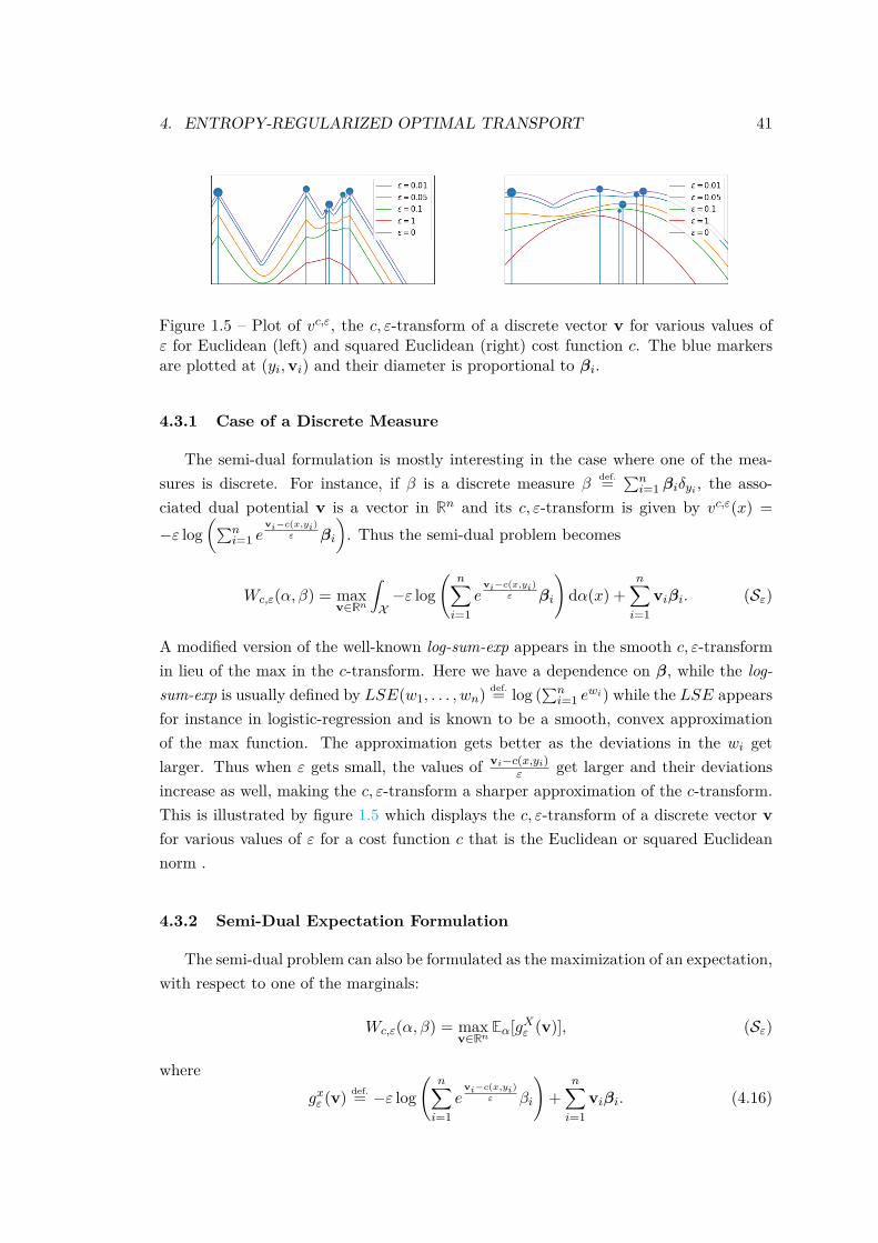
4. ENTROPY-REGULARIZED OPTIMAL TRANSPORT 41
Figure 1.5 – Plot of vc,ε, the c, ε-transform of a discrete vector v for various values ofε for Euclidean (left) and squared Euclidean (right) cost function c. The blue markersare plotted at (yi,vi) and their diameter is proportional to βi.
4.3.1 Case of a Discrete Measure
The semi-dual formulation is mostly interesting in the case where one of the mea-sures is discrete. For instance, if β is a discrete measure β def.=
∑ni=1 βiδyi , the asso-
ciated dual potential v is a vector in Rn and its c, ε-transform is given by vc,ε(x) =−ε log
(∑ni=1 e
vi−c(x,yi)ε βi
). Thus the semi-dual problem becomes
Wc,ε(α, β) = maxv∈Rn
∫X−ε log
(n∑i=1
evi−c(x,yi)
ε βi
)dα(x) +
n∑i=1
viβi. (Sε)
A modified version of the well-known log-sum-exp appears in the smooth c, ε-transformin lieu of the max in the c-transform. Here we have a dependence on β, while the log-sum-exp is usually defined by LSE(w1, . . . , wn) def.= log (
∑ni=1 e
wi) while the LSE appearsfor instance in logistic-regression and is known to be a smooth, convex approximationof the max function. The approximation gets better as the deviations in the wi getlarger. Thus when ε gets small, the values of vi−c(x,yi)
ε get larger and their deviationsincrease as well, making the c, ε-transform a sharper approximation of the c-transform.This is illustrated by figure 1.5 which displays the c, ε-transform of a discrete vector vfor various values of ε for a cost function c that is the Euclidean or squared Euclideannorm .
4.3.2 Semi-Dual Expectation Formulation
The semi-dual problem can also be formulated as the maximization of an expectation,with respect to one of the marginals:
Wc,ε(α, β) = maxv∈Rn
Eα[gXε (v)], (Sε)
wheregxε (v) def.= −ε log
(n∑i=1
evi−c(x,yi)
ε βi
)+
n∑i=1
viβi. (4.16)
42 CHAPTER 1. ENTROPY-REGULARIZED OPTIMAL TRANSPORT
Note that the semi-dual expectation formulation is still valid at the limit when ε = 0,contrarily to the dual expectation formulation (4.2). Indeed, using the c-transform fromstandard OT, we have that
Wc(α, β) = maxv∈Rn
Eα[gX0 (v)],
where gx0 (v) def.= maxj∈1...n vj − c(x, yj) +∑ni=1 viβi.
4.3.3 Some Analytic Properties of the Semi-Dual Functional
Since the potential v is a n-dimensional vector when β is a discrete measure withn diracs, and we can compute the gradient and Hessian of gε, deriving some usefulproperties of the semi-dual function.
Proposition 13. Consider the semi-dual functional gε defined in (4.16). When ε > 0its gradient is defined by
∇vgxε (v) = β − χε(x),
and the hessian is given by
∂2vg
xε (v) = 1
ε
(χε(x)χε(x)T − diag(χε(x))
),
where
χε(x)i =exp(vi−c(x,yi)
ε )∑Jj=1 exp(vj−c(x,yj)
ε ).
Besides,0 ∂2
vgxε (v) 1
ε,
and thus gxε is a convex function with a Lipschitz gradient.When ε = 0 (standard OT) g0 is not smooth and a subgradient is given by
∇vg0(v, x) = β − χ(x),
whereχ(x)i = 1i=j?(x) with j?(x) ∈ argmini∈1...n c(x, yi)− vi.
Note that since the lower bound on the eigenvalues of the Hessian is 0 the semi-dual functional is convex but not strongly convex as strong convexity requires a strictlypositive lower-bound on eigenvalues of the Hessian.Remark 11. (Laguerre Diagrams) Laguerre diagrams are extensions of Voronoi diagramswhere each cell j with center yj has a specific weight vj . They partition the space Xwith n cells (Lj(v))j=1,...,n in the following way:
Lj(v) def.= x ∈ X | ∀i′ 6= i, c(x, yi)− vi 6 c(x, y′i)− v′i.
4. ENTROPY-REGULARIZED OPTIMAL TRANSPORT 43
Figure 1.6 – Illustration taken from (Peyré et al., 2017) of the Laguerre cells and theirsmooth counterpart in 2D, with quadratic cost. The colors indicate the (smoothed)indicator function of the Laguerre cells χε. The red marks are at locations yi and theirsize is proportional to vj . The black lines are the level sets of the c, ε−transform of v.
The function χ appearing in the gradient of the semi-dual is an indicator functioncorresponding to the Laguerre diagram of the space. More specifically, χ(x)i = 1 if andonly if x belongs to cell i of the Laguerre diagram with distance c and weights v. Itsregularized counterpart χε is a smoothed version of the indicator function. Both arerepresented in Figure 1.6 taken from (Peyré et al., 2017). . The connection betweenLaguerre cells and semi-discrete OT is presented in (Mérigot, 2011), and we refer toChapter 4, Sec. 4 for more details.
4.4 Convergence of Entropy-Regularized OT to Standard OT
When using regularized OT as a proxy for OT in various applications, the questionof convergence when ε→ 0 naturally arises. For some applications, we are interested inthe value of OT, and we thus want to understand howWc,ε(α, β) approximatesWc(α, β).For others however, we are interested in the transport plan, and we are thus interestedin the convergence of the optimizer πε (or the optimizers (uε, vε) for the dual problem,to recover πε with the primal-dual relationship.
The convergence of Wc,ε(α, β) to Wc(α, β) is well known, for instance see Chapter 3,Sec. 3 where we derive convergence rates. However convergence of the optimizers is amore delicate issue. For the primal problem (Pε), we have the following theorem from(Carlier et al., 2017) which proves Γ−convergence of the regularized problem to theunregularized one in the case of a euclidean cost in Rd. Γ−convergence is a powerfulproperty implying both convergence of the value of the problem and convergence of theminimizers.
Theorem 9. (Convergence of Entropy-Regularized OT) (Carlier et al., 2017)Consider the primal problem of entropy-regularized optimal transport (Pε) on Rd with
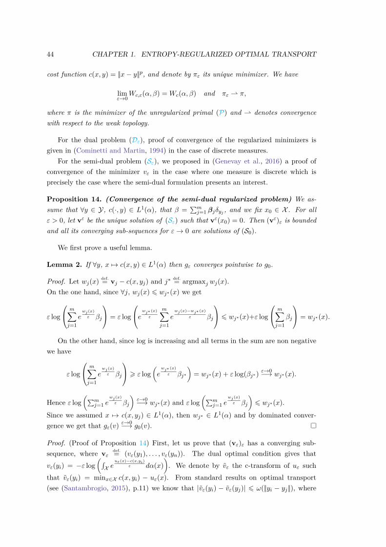
44 CHAPTER 1. ENTROPY-REGULARIZED OPTIMAL TRANSPORT
cost function c(x, y) = ||x− y||p, and denote by πε its unique minimizer. We have
limε→0
Wc,ε(α, β) = Wc(α, β) and πε π,
where π is the minimizer of the unregularized primal (P) and denotes convergencewith respect to the weak topology.
For the dual problem (Dε), proof of convergence of the regularized minimizers isgiven in (Cominetti and Martin, 1994) in the case of discrete measures.
For the semi-dual problem (Sε), we proposed in (Genevay et al., 2016) a proof ofconvergence of the minimizer vε in the case where one measure is discrete which isprecisely the case where the semi-dual formulation presents an interest.
Proposition 14. (Convergence of the semi-dual regularized problem) We as-sume that ∀y ∈ Y, c(·, y) ∈ L1(α), that β =
∑mj=1 βjδyj , and we fix x0 ∈ X . For all
ε > 0, let vε be the unique solution of (Sε) such that vε(x0) = 0. Then (vε)ε is boundedand all its converging sub-sequences for ε→ 0 are solutions of (S0).
We first prove a useful lemma.
Lemma 2. If ∀y, x 7→ c(x, y) ∈ L1(α) then gε converges pointwise to g0.
Proof. Let wj(x) def.= vj − c(x, yj) and j∗ def.= argmaxj wj(x).On the one hand, since ∀j, wj(x) 6 wj∗(x) we get
ε log
m∑j=1
ewj(x)ε βj
= ε log
ewj∗ (x)ε
m∑j=1
ewj(x)−wj∗ (x)
ε βj
6 wj∗(x)+ε log
m∑j=1
βj
= wj∗(x).
On the other hand, since log is increasing and all terms in the sum are non negativewe have
ε log
m∑j=1
ewj(x)ε βj
> ε log(ewj∗ (x)
ε βj∗
)= wj∗(x) + ε log(βj∗)
ε→0−→ wj∗(x).
Hence ε log(∑m
j=1 ewj(x)ε βj
)ε→0−→ wj∗(x) and ε log
(∑mj=1 e
wj(x)ε βj
)6 wj∗(x).
Since we assumed x 7→ c(x, yj) ∈ L1(α), then wj∗ ∈ L1(α) and by dominated conver-gence we get that gε(v) ε→0−→ g0(v).
Proof. (Proof of Proposition 14) First, let us prove that (vε)ε has a converging sub-sequence, where vε
def.= (vε(y1), . . . , vε(yn)). The dual optimal condition gives thatvε(yi) = −ε log
(∫X e
uε(x)−c(x,yi)ε dα(x)
). We denote by vε the c-transform of uε such
that vε(yi) = minx∈X c(x, yi) − uε(x). From standard results on optimal transport(see (Santambrogio, 2015), p.11) we know that |vε(yi) − vε(yj)| 6 ω(||yi − yj ||), where
4. ENTROPY-REGULARIZED OPTIMAL TRANSPORT 45
ω is the modulus of continuity of the cost c. Besides, using once again the soft-maxargument we can bound |vε(y)− vε(y)| by some constant C. Thus we get that:
|vε(yi)− vε(yj)| 6 |vε(yi)− vε(yi)|+ |vε(yi)− vε(yj)|+ |vε(yj)− vε(yj)|
6 C + ω(||yi − yj ||) + C.
Besides, the regularized potentials are unique up to an additive constant. Hence we canset without loss of generality vε(y0) = 0. So from the previous inequality yields:
vε(yi) 6 2C + ω(||yi − y0||).
So vε is bounded on Rm and thus we can extract a subsequence which converges to acertain limit that we denote by v.
Let v∗ ∈ argmaxv g0. To prove that v is optimal, it suffices to prove that g0(v∗) 6
g0(v).By optimality of vε, we have
gε(v∗) 6 gε(vε).
The term on the left-hand side of the inequality converges to g0(v∗) since gε convergespointwise to g0. We still need to prove that the right-hand term converges to g0(v).
By the Mean Value Theorem, there exists vεdef.= (1− tε)vε + tεv for some tε ∈ [0, 1]
such that|gε(vε)− gε(v)| 6 ||∇gε(vε)||||vε − v||
The gradient of gε reads∇vgε(v) = β − π(v),
where πi(v) =∫X e
vi−c(x,yi)ε βidα(x)∫
X
∑m
j=1 evj−c(x,yj)
ε βjdα(x).
It is the difference of two elements in the simplex thus it is bounded by a constantC independently of ε.
Using this bound in (4.4) yields
gε(v)− C||vε − v|| 6 gε(vε) 6 gε(v) + C||vε − v||.
By pointwise convergence of gε we know that gε(v) → g0(v), and since v is a limitpoint of vε we can conclude that the left and right-hand terms of the inequality convergeto g0(v). Thus we get gε(vε)→ g0(v).

46 CHAPTER 1. ENTROPY-REGULARIZED OPTIMAL TRANSPORT
Chapter 2
Learning with SinkhornDivergences
Optimal Transport (OT) metrics and their ability to handle measures with non-overlappingsupports have emerged as a promising tool to learn a parametric distribution – for instance agenerative model – from a dataset. Yet, training generative models using OT raises formidablecomputational and statistical challenges, because of (i) the computational burden of evaluatingOT losses, (ii) their instability and lack of smoothness, (iii) the difficulty to estimate them, aswell as their gradients, in high dimension because of the curse of dimensionality from which theysuffer.
In this chapter we introduce Sinkhorn Divergences, based on entropy-regularized OT, whichgenerates a family of losses interpolating between Wasserstein (OT) (when the regularizationparameter ε = 0) and Maximum Mean Discrepancy (MMD) losses (when ε = ∞). Aside fromthe interpolation in terms of cost, which we demonstrate, we also observe empirically that theyallow to find a sweet spot leveraging the geometry of OT on the one hand, and the favorable high-dimensional sample complexity of MMD on the other hand (this is formally proved in Chapter 3,Theorem 14).
We use this new discrepancy between measures to train large scale generative models, with anOT-based loss which does not suffer from its usual computational and statistical shortcomings.This is achieved thanks to: (a) entropic-regularization, which turns the original OT loss intothe differentiable and more robust Sinkhorn Divergence, that can be computed efficiently usingSinkhorn fixed point iterations; (b) algorithmic (automatic) differentiation, allowing to get stablegradients of these iterations with seamless GPU execution. We further propose an algorithm tolearn a cost function on the data space in an adversarial way, similar to what has been done forkernels with MMD.
This chapter is based on (Genevay et al., 2018), with the addition of some background onthe training of generative models, more details on the adversarial learning of the cost functions,and an extensive comparison of various losses on simple models.
47
48 CHAPTER 2. LEARNING WITH SINKHORN DIVERGENCES
1 Introduction
Several important statistical problems boil down to fitting a parametric model to adataset, i.e. estimating the parameters of a chosen model that fits observed data in somemeaningful way. While the standard approach for models with a density is MaximumLikelihood Estimation (MLE), this approach is often flawed in machine learning taskswhere the sought after distribution is obtained in a generative fashion. These generativemodels are obtained as the mapping of a low dimensional reference measure througha non-linear function with values in a high dimensional space (e.g. a neural network).These models are easy to sample from, but their density is singular in the sense that itonly has positive probability on a low-dimensional “manifold" of the observation spaceand is zero elsewhere, thus making the usual MLE unusable.
Previous works. For purely generative models, several likelihood-free workaroundsexist. Major approaches include variational autoencoders (VAE) (Kingma and Welling,2013), generative adversarial networks (GAN) (Goodfellow et al., 2014) and numerousvariations around these two ideas (Larsen et al., 2016). The adversarial GAN approachcomputes the best achievable classification accuracy (in which the training and gener-ated datapoints have opposite labels) for a given class of classifiers as a proxy for thedistance between two distributions: If accuracy is high distributions are well separated,if accuracy is low they are difficult to tell apart and lie thus at a very close distance. An-other approach consists in minimizing a metric between distributions: the maximal meandiscrepancy (Gretton et al., 2006), parametrized by a positive-definite kernel function.It was shown in ensuing works that the effectiveness of the MMD to learn generativemodels (Li et al., 2015; Dziugaite et al., 2015) hinges on the ability to find a relevantkernel, which is a highly nontrivial choice. The Wasserstein or earth mover’s distance,which also allows to compare distributions with non-overlapping supports, has recentlyemerged as a serious contender to train generative models. While it was long disre-garded because of its computational burden—in its original form solving OT amountsto solving an expensive network flow problem when comparing discrete measures in met-ric spaces—recent works have shown that this cost can be largely mitigated by settlingfor cheaper approximations obtained through strongly convex regularizers, in particularentropy, as detailed in Chapter 1 of this thesis. The benefits of this regularization hasopened the path to many applications of the Wasserstein distance in supervised learn-ing problems (Courty et al., 2014; Frogner et al., 2015; Huang et al., 2016; Rolet et al.,2016). Although the use of Wasserstein metrics for inference in generative models wasconsidered over ten years ago in (Bassetti et al., 2006), that development remained ex-clusively theoretical until a recent wave of papers managed to implement that idea moreor less faithfully: using entropic regularization over a discrete space (Montavon et al.,2016), with approximate Bayesian computations (Bernton et al., 2017), and considering
1. INTRODUCTION 49
a neural network parameterization of the dual potential in the dual OT problem defining1-Wasserstein distance (Arjovsky et al., 2017). As opposed to this dual way to computegradients of the fitting energy, we advocate for the use of a primal formulation, which isnumerically stable, because it does not involve differentiating the (dual) solution of anOT sub-problem, as also pointed out in (Bousquet et al., 2017). Additionally, introduc-ing entropic regularization in the formulation of optimal transport allows to interpolatebetween a pure OT loss and a Maximum Mean Discrepancy loss, thus bridging the gapbetween these two approaches often presented as opposed points of view. Shortly afterthe submission of this work, we came across the recent work by (Salimans et al., 2018)which shares several ideas with our method. One distinction lies in the fact that they donot back-propagate errors across the Sinkhorn iterations, but rather use an estimate ofthe optimal transport matrix to compute an upper-bound on the Sinkhorn divergence,as was done for instance in (Cuturi and Doucet, 2014).
Contributions. The main contributions of this chapter are twofold : (i) a theoreticalcontribution regarding a new OT-based loss on measures, (ii) a simple numerical schemeto learn generative models under this loss. (i) We introduce the Sinkhorn Divergence,based on regularized optimal transport with an entropy penalty, and we prove thatwhen the smoothing parameter ε = 0 we recover pure OT loss whereas letting ε = +∞leads to MMD. The addition of entropy is important to reduce sample complexity andgradient bias, and thus allows us to take advantage of the good geometrical propertiesof OT without its drawbacks in high-dimensions. (ii) We propose a computationallytractable and stable approach to learn with that Sinkhorn Divergence, which enablesinference for any differentiable generative model. It operates by approximating SinkhornDivergences with minibatches and L iterations of Sinkhorn’s algorithm. As routinelydone in standard deep-learning architecture frameworks, the training is then achievedusing stochastic gradient descent and automatic differentiation. This provides accurateand stable approximation of the loss and its gradient, at a reasonable extra computa-tional cost, and streams nicely on GPU hardware. When dealing with complex data,we propose to learn the cost function for OT in an adversarial way, similarly to what isdone for kernels with MMD in (Li et al., 2017).
Subsequent to this work, Sinkhorn Divergences have successfully been used in adeterministic setting for shape registration (Feydy and Trouvé, 2018), which consists infinding a diffeomorphism matching a deformed image to a target. Sinkhorn Divergencesperform better than MMD for this task, as they take the global geometry of the probleminto account where MMD is more local and has trouble dealing with parts of the shapethat are further away.
The GAN rush. This work was carried out in the early stages of what can be calledthe GAN rush. The interest on GANs has kept growing since the seminal work by
50 CHAPTER 2. LEARNING WITH SINKHORN DIVERGENCES
(Goodfellow et al., 2014), and it has clearly exploded in the past couple of years, with alarge part of the machine learning community now studying generative models. Thereare various motivations behind the interest in generative models, but the one that is themost popular is realistic image generation. Thus, although it is a crucial issue, evaluationand comparison of generative models has long been neglected by the community, wheremost papers simply relied on the quality of generated images to assess their performancewith little to no insight on how well they fit the underlying distribution of the data.This resulted in a multitude of papers proposing network architectures, regularizationtechniques, new losses and other heuristics whose superiority over existing methods isdifficult to evaluate. These methods all generate nice images, so their efficiency in termsof computer graphics is clear, but from a statistical point of view, quantifying howwell a model fits the unknown distribution of the data remains an open question.Thechoice of an evaluation metric for GANs is indeed a complex matter, which we quicklydiscuss in Sec. 4, and a recent survey on GANs (Lucic et al., 2018) suggests a fewmetrics which should be used for this purpose, with a focus on image-generation tasks.Conducting a large-scale empirical study to compare several state-of-the art GANmodels(not including regularized OT- and MMD-based GANs) with their metrics, the authorsfound out that “most models can reach similar scores with enough hyperparameteroptimization and random restarts”. Thus in practice, a good network architecture wasenough for their assessed models to perform well in terms of image generation, and theloss function itself did not have much effect on the performance. In the GAN rush, weadopted a different position on the subject, distancing ourselves from image generationand rather trying to answer the following question : what is a robust loss to learn a(possibly high-dimensional) singular distribution from samples? It is this question thatshould be kept in mind through this chapter and the following – which gives statisticalproperties of Sinkhorn Divergences, reinforcing the interpolation theorem presented here.Thus, we consider images generation merely as an application of our density fittingscheme, not a the main goal. For a better overview of the performance of SinkhornDivergences in image generation, the reader should refer to (Salimans et al., 2018).
2 Density Fitting
We consider a data set of n (usually very large) observations (y1, . . . , yn) ∈ X n
generated from an unknown distribution β and we want to learn a generative modelthat produces samples that are similar to that dataset. Samples x = gθ(z) from thegenerative model are defined by taking as input a sample z ∈ Z from some referencemeasure ζ (typically a uniform or a Gaussian measure in a low-dimensional space Z)and mapping it through a differentiable function gθ : Z → X . Formally, this correspondsto defining the generative model measure αθ from which x is drawn as αθ = gθ#ζ. Thegoal is to find θ which minimizes a certain loss L between the model measure αθ and
2. DENSITY FITTING 51
the unknown measure of the data β:
θ ∈ argminθ
L(αθ, β). (2.1)
Maximum likelihood estimation (MLE) is obtained with L(αθ, β) = −∑j log dαθ
dx (yj),where dα
dx is the density of αθ with respect to a fixed reference measure (a typical choice isdx being the Lebesgue measure in X = Rd). This MLE loss can be seen as a discretizedversion of the relative entropy (a.k.a. the Kullback-Leibler divergence) as it converges toDKL(α|β) when N →∞. A major issue with this approach is that in general generativemodels defined this way (when Z has a much smaller dimensionality than X ) havesingular distributions (i.e. supported on a low-dimensional manifold), without densitywith respect to a fixed measure, and therefore MLE cannot be considered.
2.1 Learning with ϕ-divergences
The first idea that emerged in the literature of Generative Adversarial Networks(Goodfellow et al., 2014) was to use the Jensen-Shannon divergence, a special instanceof the class of ϕ−divergences (see Chapter 1, sec. 2.1 for a thorough introduction), tosolve the density fitting problem. Subsequent work by (Nowozin et al., 2016) considersa more general framework to learn a generative model with ϕ−divergences, which wedescribe in this section. The density fitting problem they consider is
minθDϕ(αθ | β) def.=
∫Xϕ
(dαθ(x)dβ(x)
)dβ(x), (2.2)
where αθ and β are absolutely continuous with respect to a reference measure dx anddαθ, dβ are their respective densities (see Chapter 1, sec. 2.1 for a more general definitionin the case of measure that are not absolutely continuous); and is ϕ a convex, lower-semicontinuous function on R+ satisfying ϕ(1) = 0. However, ϕ-divergences are hardto estimate through samples, in particular because of the fact that they do not metrizeweak convergence (again, see Chapter 1, sec. 2.1 for more details).
To alleviate this shortcoming, (Nguyen et al., 2010) suggests using the followinglower bound leveraging the dual definition of ϕ-divergences:
Proposition 15. (Lower bound on ϕ-divergences)
Dϕ(α | β) = supT :X→R
Eα(T (X))− Eβ(ϕ∗T (Y )) > supT∈T
Eα(T (X))− Eβ(ϕ∗T (Y )),
where ϕ∗(t) = supu tu − ϕ(u) is the Legendre transform of ϕ, the set T : X → R isthe set of measurable functions from X to R and T is an arbitrary class of measurablefunctions.
Parametrizing T by a variable w, i.e. setting T def.= Tw | w ∈ W and using the
52 CHAPTER 2. LEARNING WITH SINKHORN DIVERGENCES
previous lower bound (2.2) yields the following saddle point problem:
minθ
maxw
Eβ(Tw(X))− Eαθ(ϕ∗(Tw(X)). (2.3)
The formulation of the original GANs is derived from the above, using f(u) = u log u+(u + 1) log(u + 1) (a slight modification of the Jensen-Shannon divergence given inTable 1.1, Chapter 1) and Tw = logDw, where Dw is a neural network called thediscriminator. Then (2.3) becomes
minθ
maxw
Eβ[logDw(X)]− Eαθ [log(1−Dw(X))]
⇔minθ
maxw
Eβ[logDw(X)]− Eζ [log(1−Dw(gθ(Z)))],
using the definition of αθ as the pushforward of ζ through gθ. From a game-theorypoint of view, the general GAN formulation can be seen as finding the equilibrium ina two-player game where player one optimizes its parameter θ to fool the discriminatorDw, whose parameter w is optimized by the player two whose goal is to distinguishbetween samples from the model measure αθ and samples from the true measure β.
2.2 Maximum Mean Discrepancy and Optimal Transport
A more robust way to compare measures with disjoint support, is to consider losseswhich metrize the weak convergence of measures (see Chapter 1, Sec. 2.1 for a precisedefinition). Intuitively, these losses enables the comparison of singular measures bytaking into account spatial displacement of the measures. For instance, they avoid thetypical failure case of ϕ-divergences by satisfying L(δx, δx′) → 0 as x → x′ where ϕ-divergences would be equal to a constant. A classical framework for such a loss functionL are Integral Probability Metrics (IPMs) which are thoroughly described in Chapter 1,Sec. 2.2. Given a set of measurable functions F , the IPM dF is defined as
dF (α, β) def.= supf∈F|Eα(f(X))− Eβ(f(Y ))|.
Popular IPMs include the 1-Wasserstein distance (with F = f ; ||∇f ||∞ 6 1 the setof 1-Lipschitz functions) and Maximum Mean Discrepancies (with F = f ; ||f ||H 6 1where H is a Reproducing Kernel Hilbert Space). Recall from Chapter 1, Proposition 3that on a RKHS with kernel k, MMD can be rewritten as follows (Gretton et al., 2006):
MMD2k(α, β) = Eα⊗α[k(X,X ′)] + Eβ⊗β[k(Y, Y ′)]− 2Eα⊗β[k(X,Y )]. (2.4)
A different approach, for which we advocate, is to consider Optimal Transport (OT)metrics. The OT metric between two probability distributions (α, β) ∈ M1
+(X ) ×
2. DENSITY FITTING 53
M1+(X ) is defined as the solution of the (possibly infinite dimensional) linear program:
Wc(α, β) def.= minπ∈Π(α,β)
∫X×X
c(x, y)dπ(x, y), (2.5)
where the set of admissible couplings Π(α, β) is composed of joint probability distri-butions over the product space X × X with imposed marginals (α, β). Formula (2.5)corresponds to the celebrated Kantorovitch formulation (Kantorovich, 1942) of OT (seeChapter 1, sec.2.3 for more details). Here c(x, y) is the “ground cost” to move a unit ofmass from x to y, and we shall make no assumptions (except for regularity) on its form.When X is equipped with a distance dX , a typical choice is to set c(x, y) = dX (x, y)p
where p > 0 is some exponent, in which case for p > 1 W1/pc is the so-called p-
Wasserstein distance between probability measures. Two majors obstacles to the useof the Wasserstein-distance for inference, as for many machine learning applications, areits high computational complexity and the curse of dimensionality from which it suffers.
2.3 Regularized OT and Variants of the Regularized OT Loss
As detailed in Chapter 1, Sec. 3 one can resort to regularized optimal transport toalleviate the computational burden of OT. Its primal formulation is given by:
minπ∈Π(α,β)
∫c(x, y)dπ(x, y) + ε
∫log
( dπ(x, y)dα(x)dβ(y)
)dπ(x, y). (Pε)
The primal problem (Pε) has a equivalent dual formulation (see Chapter 1, Proposi-tion 7) which consists in solving
max(u,v)∈C(X )×C(Y)
∫Xu(x)dα(x) +
∫Yv(y)dβ(y)− ε
∫X×Y
eu(x)+v(y)−c(x,y)
ε dα(x)dβ(y) + ε.
(Dε)The optimizer πε of the primal formulation can be recovered from optimizers of the dualproblem (uε, vε) via the following formula: dπε(x, y) = e
uε(x)+vε(y)−c(x,y)ε dα(x)dβ(y). In
practice, state-of-the-art algorithms (including Sinkhorn, the one we use here, alreadydetailed in Chapter 1, Sec. 4.2) solve the dual problem and use the primal-dual rela-tionship to recover the solution of the primal.
Note that introducing this regularization also breaks the curse of dimensionality forε large enough, making the estimation of regularized OT more robust to sampling noise,and this is the main matter of Chapter 3.
These problems yield four different costs, which all converge to the value of unregu-larized OT when ε→ 0 :
• Primal cost with entropy:
L(α, β) def.=∫X×Y
c(x, y)dπε(x, y) + ε
∫log
( dπε(x, y)dα(x)dβ(y)
)dπε(x, y).
54 CHAPTER 2. LEARNING WITH SINKHORN DIVERGENCES
This loss is the value of the primal of the regularized problem. Theoretical resultsare known for this cost, which is extensively studied in Chapter 3. In particular,we have a convergence rate for its approximation from samples, based on theregularization parameter ε.
• Dual cost with entropy:
L(α, β) =∫Xuε(x)dα(x) +
∫Yvε(y)dβ(y)− ε
∫X×Y
euε(x)+vε(y)−c(x,y)
ε dα(x)dβ(y) + ε.
Since strong duality holds for regularized OT, this loss is equal to the primalwith entropy. This is actually this formulation that is used to prove the sample-complexity results from Chapter 3. However in practice, when one uses an algo-rithm to approximate (uε, vε), the primal and dual problems with entropy yielddifferent values.
• Primal cost without entropy:
L(α, β) def.=∫X×Y
c(x, y)dπε(x, y).
This loss is arguably the most widely used in practice. It is this version that is usedin (Cuturi, 2013), which first showed the benefits of regularized OT for machinelearning. It has recently been studied in (Luise et al., 2018) under the name SharpSinkhorn – to avoid confusion with the primal loss with entropy. This paper givesan algorithm to compute the gradient of this loss, which can further be used insupervised learning problems.
• Dual cost without entropy:
L(α, β) =∫Xuε(x)dα(x) +
∫Yvε(y)dβ(y).
The primal-dual relationship is dπε = euε(x)+vε(y)−c(x,y)
ε dα(x)dβ(y). The probabil-ity constraint on πε thus implies
∫X×Y e
uε(x)+vε(y)−c(x,y)ε dα(x)dβ(y) = 1. So the
dual cost without entropy is equal to the dual cost with entropy, which once againmight not be the case when considering approximations of (uε, vε).
2.4 Sinkhorn Divergences : an Interpolation Between OT and MMD
We denote by Wc,ε the primal without entropy variant of the regularized OT loss:
Wc,ε(α, β) def.=∫c(x, y)dπε(x, y), (2.6)
2. DENSITY FITTING 55
where πε is the optimal coupling for the regularized OT problem (Pε), and by Hε theadditional term that comes from the entropic regularization:
Hε(α, β) def.= ε
∫log( dπε(x, y)
dα(x)dβ(y))dπε(x, y), (2.7)
so that the primal loss with entropy is
WHc,ε(α, β) def.= Wc,ε(α, β) +Hε(α, β). (2.8)
To correct for the fact thatWc,ε(α, α) 6= 0 andWHc,ε(α, α) 6= 0, we introduce the following
normalization, which we call Sinkhorn Divergence:
Definition 9. (Sinkhorn Divergence) The Sinkhorn Divergence between two proba-bility measures α, β is defined as:
SDc,ε(α, β) def.= Wc,ε(α, β)− 12Wc,ε(α, α)− 1
2Wc,ε(β, β), (2.9)
where Wc,ε is the primal cost without entropy defined in (2.6). Alternatively, we define:
SDHc,ε(α, β) def.= WH
c,ε(α, β)− 12W
Hc,ε(α, α)− 1
2WHc,ε(β, β), (2.10)
where WHc,ε is the primal cost with entropy defined in (2.8)
Far from simply correcting the bias of Wc,ε(α, α), the Sinkhorn Divergence alsoappears as an interpolating discrepancy between OT and MMD.
Theorem 10. (Asymptotics of Sinkhorn Divergence with Respect to ε) TheSinkhorn Divergence has the following asymptotic behavior in ε:
(i) as ε→ 0, SDc,ε(α, β)→Wc(α, β),
(ii) as ε→ +∞, SDc,ε(α, β)→ 12MMD2
−c(α, β).
When −c is a positive definite kernel, MMD−c is the MMD with the kernel that isminus the cost used in the optimal transport problem.
Besides, if c ∈ C1(X ×Y) and X and Y are bounded domains of Rd, the asymptoticsalso hold for SDH
c,ε.
Remark 12. This theorem is a generalization of (Ramdas et al., 2017, §3.3) for continuousmeasures, and to the cost with entropy.
Proof. Let us start by proving the property for SDc,ε.
(i) The first part of the assumption comes from the fact that πε π (see Chapter 1,Sec. 4.4 or (Carlier et al., 2017)).
56 CHAPTER 2. LEARNING WITH SINKHORN DIVERGENCES
(ii) Letting ε go to infinity in the regularized OT problem amounts to finding thecoupling with minimum entropy in the constraint set. The problem becomes
minπ∈Π(α,β)
∫log
( dπ(x, y)dα(x)dβ(y)
)dπ(x, y),
where Π(α, β) is the set of couplings with marginals α and β. Introducing Lagrangemultipliers u and v for these constraints, the dual problem becomes maxu,v
∫u(x)dα(x)+∫
v(y)dβ(y)−∫
exp(u(x) + v(y))dα(x)dβ(y) and the primal-dual relation is givenby dπ(x, y) = exp(u(x) + v(y))dα(x)dβ(y). Solving the dual gives u = v = 0 andthus the optimal coupling is simply the product of the marginals i.e. π = α ⊗ β.This gives
Wc,+∞(α, β) =∫X×Y
c(x, y)dα(x)dβ(y).
The proof of this assumption for SDHc,ε requires some more assumptions to control
the entropy, and is based on results from Chapter 3.
(i) The asympotics for ε → 0 are a direct consequence of Theorem 12 which provesthat
WHc,ε(α, β)−Wc(α, β) ∼
ε→02εd log(1/ε).
(ii) We want to prove that WHc,ε(α, β) →
ε→+∞
∫X×Y c(x, y)dα(x)dβ(y). Since strong
duality holds for regularized OT, we have
WHc,ε(α, β) =
∫Xuε(x)dα(x)+
∫Yvε(y)dβ(y)−ε
∫X×Yeuε(x)+vε(y)−c(x,y)
ε dα(x)dβ(y)+ε,
where uε and vε are the dual potentials solving (Dε). We know from Chapter 3,Proposition 17 that if the cost function c is C1 and X and Y are bounded, then uεand vε are Lipschitz with the same constant as c, and thus they are bounded in L∞
norm on X and Y independently of ε. This implies that uε(x) + vε(y)− c(x, y) =O(1) when ε→ +∞. Using the Taylor expansion of the exponential when ε→ +∞we get:
WHc,ε(α, β) =
∫Xuε(x)dα(x) +
∫Yvε(y)dβ(y)
− ε∫X×Y
(1 + uε(x) + vε(y)− c(x, y)
ε+O
( 1ε2
))dα(x)dβ(y) + ε,
which simplifies to
WHc,ε(α, β) =
∫X×Y
(c(x, y) +O
(1ε
))dα(x)dβ(y).
Since we have∫X×Y O
(1ε
)dα(x)dβ(y) → 0 when ε → +∞, we get the desired
2. DENSITY FITTING 57
conclusion.
We proved that SDc,ε →MMD−c when ε→ +∞. However, by definition of MMD,−c has to be a positive definite kernel for MMD−c to be well defined. The followingproposition proves that some powers of the Euclidean distance yield a valid cost, anddefine as special instance of MMD also known as Energy Distance.
Proposition 16. (Energy Distance)(Sejdinovic et al., 2013) Consider the Euclideandistance ||.||2 on Rd. Then,
kp(x, y) def.= ||x||p2 + ||y||p2 − ||x− y||p2
is a positive definite kernel for 0 < p < 1. And it induces the following MMD, calledEnergy Distance :
EDp(α, β) def.= MMD2kp(α, β) = 2Eα⊗β[||X − Y ||p2]− Eα⊗α[||X −X ′||p2]− Eβ⊗β[||Y − Y ′||p2].
Recent work by (Feydy et al., 2019) also proves that this normalization of regularizedOT enforces positive-definiteness for SDH
c,ε, which we conjectured in the early stagesof our work on Sinkhorn Divergence, based on empirical evidence, and that Sinkhorndivergences metrize the weak-convergence of measures.
Theorem 11. (Positivity of Sinkhorn Divergence)(Feydy et al., 2019) Let X bea compact metric space with a Lipschitz cost function c, that induces, for ε > 0, apositive universal kernel kε(x, y) def.= exp(−c(x, y)/ε). Then, SDH
c,ε defines a symmetricpositive definite, smooth loss function that is convex in each of its input variables. It alsometrizes the convergence in law (or weak-convergence of measures): for all probabilityRadon measures α and β ∈M+
1 (X ),
0 = SDHc,ε(β, β) 6 SDc,ε(α, β),
α = β ⇔ SDHc,ε(α, β) = 0,
αn α⇔ SDHc,ε(αn, α)→ 0.
Remark 13. In particular, these results hold for measures with bounded support ona Euclidean space X = Rd endowed with ground cost functions c(x, y) = ||x − y||2 orc(x, y) = ||x− y||22 which induce Laplacian and Gaussian kernels respectively. Note thattheir proof only holds for Sinkhorn Divergence based on the primal cost with entropySDH
ε , positive-definiteness of SDε remains an open problem.
58 CHAPTER 2. LEARNING WITH SINKHORN DIVERGENCES
Discussion on OT vs. MMD. As proved in Theorem 1, the Sinkhorn Divergenceinterpolates between a pure OT loss for ε = 0 and MMD losses for ε = +∞. As such,when ε→ +∞, our loss takes advantage of the good properties of MMD losses, and inparticular a favorable sample complexity of O(1/
√n) (decay rate of the approximation
of the true loss with a mini-batch of size n) which is the object of Chapter 3 of thisthesis. In contrast, the unregularized OT loss suffers from a sample complexity ofO(1/n1/d), see (Weed and Bach, 2017) for a recent account on this point. Using MMDto train generative models has been shown to be successful in (Dziugaite et al., 2015;Li et al., 2015). The improved Wasserstein GAN approach (Gulrajani et al., 2017)(which penalizes the squared norm of the gradient of the dual potential) is similar toan MMD in the sense that both are IPMs. By tuning the ε parameter, our method isable to take the best of both worlds, to blend the non-flat geometry of OT with thehigh-dimensional rigidity of MMD losses. Additionally, the Sinkhorn Divergence, as isthe case for the original OT problem, can be defined with any cost c, whereas MMDlosses are only meaningful when used with positive definite kernels k. We discuss thegeometric properties of these losses further in Section 4, where we compare them onvarious fitting tasks.
3 Sinkhorn AutoDiff Algorithm
We now consider density fitting with Sinkhorn Divergence as a loss:
minθ
Eε(θ) where Eε(θ)def.= SDc,ε(αθ, β).
Computing an approximation of ∇θSDc,ε(αθ, β) is itself a difficult problem. Whenε = 0, and when c = ||x − y|| (the case of the 1-Wasserstein distance) a workaround isto use, instead of differentiating the “primal” formula (2.5), the optimum of the “dual”formula, resulting in ∇SD0(αθ, β) =
∫Z ∇[h gθ](z)dζ(z), where h is an optimal dual
continuous potential for α = αθ. This is the problem tackled in (Arjovsky et al., 2017)which uses a deep-network expansion to approximate the continuous dual potential h.While the dual formalism is appealing (in particular because it involves only integrationover Z and not the product space Z × X ), the resulting gradient formula requiresdifferentiating the dual potential, which tends to be difficult to compute and unstable.A very similar conclusion is reached by (Bousquet et al., 2017) (see in particular theirProposition 3).
We propose a different route, by making two key simplifications: (i) approximateSDc,ε(αθ, β) by a size-m mini-batch sampling SDc,ε(αθm, βm) to make it amenableto stochastic gradient descent ; (ii) approximate SDc,ε(αθm, βm) by L-steps of theSinkhorn algorithm (Cuturi, 2013) to obtain an algorithmic loss SD(L)
c,ε (αθm, βm) whichis amenable to automatic differentiation.
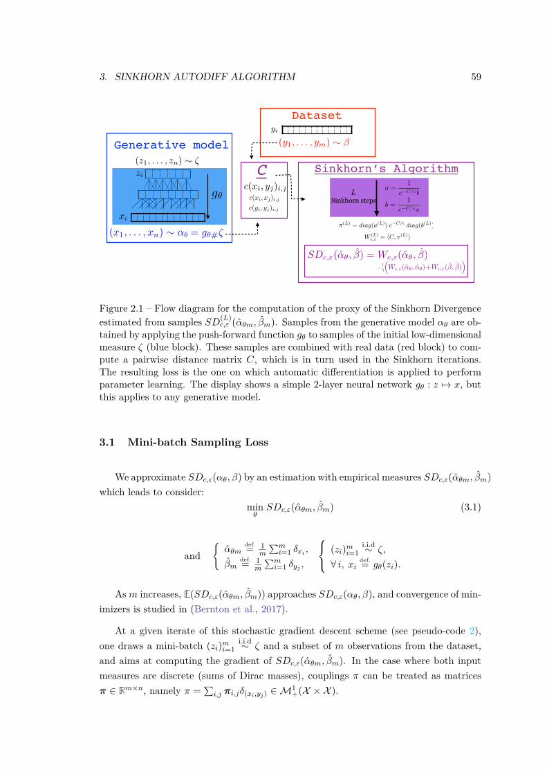
3. SINKHORN AUTODIFF ALGORITHM 59
(z1, . . . , zn)
Generative model
g
C
c(xi, yj)i,j
C
= g#(x1, . . . , xn) ↵
zi
Dataset
(y1, . . . , ym)
Sinkhorn’s Algorithm
L Sinkhorn steps
a =1
eC/"b
b =1
eC/"a
yi
c(xi, xj)i,j
c(yi, yj)i,j
SDc,"(↵, ) = Wc,"(↵, )Wc,"(↵, ↵)+Wc,"(, )
1
2
xi(L) = diag(a(L)) eC/ diag(b(L))
W (L) =hC,(L)iW (L)
c," = hC,(L)i
Figure 2.1 – Flow diagram for the computation of the proxy of the Sinkhorn Divergenceestimated from samples SD(L)
c,ε (αθm, βm). Samples from the generative model αθ are ob-tained by applying the push-forward function gθ to samples of the initial low-dimensionalmeasure ζ (blue block). These samples are combined with real data (red block) to com-pute a pairwise distance matrix C, which is in turn used in the Sinkhorn iterations.The resulting loss is the one on which automatic differentiation is applied to performparameter learning. The display shows a simple 2-layer neural network gθ : z 7→ x, butthis applies to any generative model.
3.1 Mini-batch Sampling Loss
We approximate SDc,ε(αθ, β) by an estimation with empirical measures SDc,ε(αθm, βm)which leads to consider:
minθ
SDc,ε(αθm, βm) (3.1)
andαθm
def.= 1m
∑mi=1 δxi ,
βmdef.= 1
m
∑mi=1 δyj ,
(zi)mi=1i.i.d∼ ζ,
∀ i, xidef.= gθ(zi).
Asm increases, E(SDc,ε(αθm, βm)) approaches SDc,ε(αθ, β), and convergence of min-imizers is studied in (Bernton et al., 2017).
At a given iterate of this stochastic gradient descent scheme (see pseudo-code 2),one draws a mini-batch (zi)mi=1
i.i.d∼ ζ and a subset of m observations from the dataset,and aims at computing the gradient of SDc,ε(αθm, βm). In the case where both inputmeasures are discrete (sums of Dirac masses), couplings π can be treated as matricesπ ∈ Rm×n, namely π =
∑i,j πi,jδ(xi,yj) ∈M1
+(X × X ).
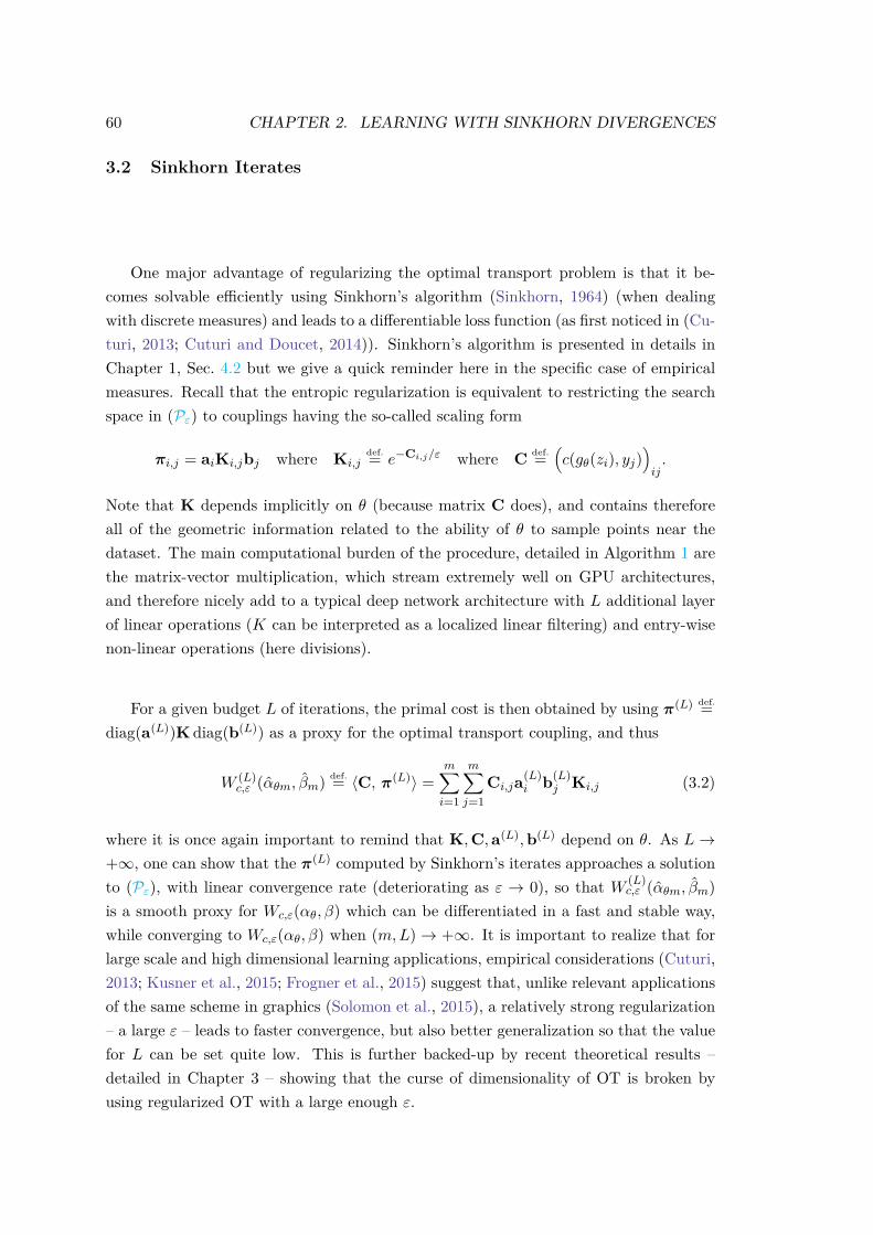
60 CHAPTER 2. LEARNING WITH SINKHORN DIVERGENCES
3.2 Sinkhorn Iterates
One major advantage of regularizing the optimal transport problem is that it be-comes solvable efficiently using Sinkhorn’s algorithm (Sinkhorn, 1964) (when dealingwith discrete measures) and leads to a differentiable loss function (as first noticed in (Cu-turi, 2013; Cuturi and Doucet, 2014)). Sinkhorn’s algorithm is presented in details inChapter 1, Sec. 4.2 but we give a quick reminder here in the specific case of empiricalmeasures. Recall that the entropic regularization is equivalent to restricting the searchspace in (Pε) to couplings having the so-called scaling form
πi,j = aiKi,jbj where Ki,jdef.= e−Ci,j/ε where C def.=
(c(gθ(zi), yj)
)ij.
Note that K depends implicitly on θ (because matrix C does), and contains thereforeall of the geometric information related to the ability of θ to sample points near thedataset. The main computational burden of the procedure, detailed in Algorithm 1 arethe matrix-vector multiplication, which stream extremely well on GPU architectures,and therefore nicely add to a typical deep network architecture with L additional layerof linear operations (K can be interpreted as a localized linear filtering) and entry-wisenon-linear operations (here divisions).
For a given budget L of iterations, the primal cost is then obtained by using π(L) def.=diag(a(L))K diag(b(L)) as a proxy for the optimal transport coupling, and thus
W (L)c,ε (αθm, βm) def.= 〈C, π(L)〉 =
m∑i=1
m∑j=1
Ci,ja(L)i b(L)
j Ki,j (3.2)
where it is once again important to remind that K,C,a(L),b(L) depend on θ. As L→+∞, one can show that the π(L) computed by Sinkhorn’s iterates approaches a solutionto (Pε), with linear convergence rate (deteriorating as ε → 0), so that W (L)
c,ε (αθm, βm)is a smooth proxy for Wc,ε(αθ, β) which can be differentiated in a fast and stable way,while converging to Wc,ε(αθ, β) when (m,L)→ +∞. It is important to realize that forlarge scale and high dimensional learning applications, empirical considerations (Cuturi,2013; Kusner et al., 2015; Frogner et al., 2015) suggest that, unlike relevant applicationsof the same scheme in graphics (Solomon et al., 2015), a relatively strong regularization– a large ε – leads to faster convergence, but also better generalization so that the valuefor L can be set quite low. This is further backed-up by recent theoretical results –detailed in Chapter 3 – showing that the curse of dimensionality of OT is broken byusing regularized OT with a large enough ε.
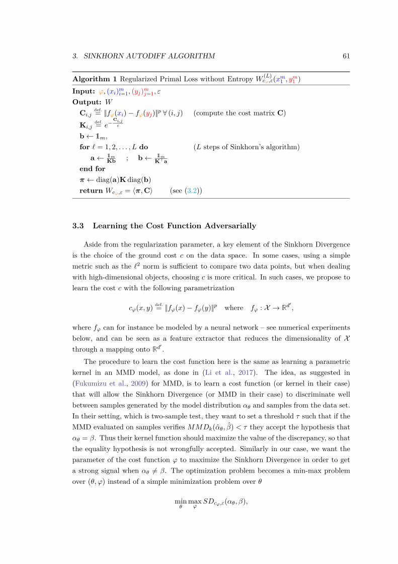
3. SINKHORN AUTODIFF ALGORITHM 61
Algorithm 1 Regularized Primal Loss without Entropy W (L)cϕ,ε(xm1 , ym1 )
Input: ϕ, (xi)mi=1, (yj)mj=1, ε
Output: WCi,j
def.= ||fϕ(xi)− fϕ(yj)||p ∀ (i, j) (compute the cost matrix C)Ki,j
def.= e−Ci,jε
b← 1m,for ` = 1, 2, . . . , L do (L steps of Sinkhorn’s algorithm)
a← 1mKb ; b← 1m
K>aend forπ ← diag(a)K diag(b)return Wcϕ,ε = 〈π,C〉 (see (3.2))
3.3 Learning the Cost Function Adversarially
Aside from the regularization parameter, a key element of the Sinkhorn Divergenceis the choice of the ground cost c on the data space. In some cases, using a simplemetric such as the `2 norm is sufficient to compare two data points, but when dealingwith high-dimensional objects, choosing c is more critical. In such cases, we propose tolearn the cost c with the following parametrization
cϕ(x, y) def.= ||fϕ(x)− fϕ(y)||p where fϕ : X → Rd′,
where fϕ can for instance be modeled by a neural network – see numerical experimentsbelow, and can be seen as a feature extractor that reduces the dimensionality of Xthrough a mapping onto Rd
′ .The procedure to learn the cost function here is the same as learning a parametric
kernel in an MMD model, as done in (Li et al., 2017). The idea, as suggested in(Fukumizu et al., 2009) for MMD, is to learn a cost function (or kernel in their case)that will allow the Sinkhorn Divergence (or MMD in their case) to discriminate wellbetween samples generated by the model distribution αθ and samples from the data set.In their setting, which is two-sample test, they want to set a threshold τ such that if theMMD evaluated on samples verifies MMDk(αθ, β) < τ they accept the hypothesis thatαθ = β. Thus their kernel function should maximize the value of the discrepancy, so thatthe equality hypothesis is not wrongfully accepted. Similarly in our case, we want theparameter of the cost function ϕ to maximize the Sinkhorn Divergence in order to geta strong signal when αθ 6= β. The optimization problem becomes a min-max problemover (θ, ϕ) instead of a simple minimization problem over θ
minθ
maxϕ
SDcϕ,ε(αθ, β),
62 CHAPTER 2. LEARNING WITH SINKHORN DIVERGENCES
where in practice SDcϕ,ε is approximated by minibatches and Sinkhorn, as mentionedabove. We will give details on the optimization algorithm used for this min-max problembelow.
3.4 The Optimization Procedure in Practice
Let us first describe the optimization procedure when the cost function c is fixed.The original problem we want to solve is
minθSDc,ε(αθ, β).
Since αθ and β are only available through finite samples, the idea is to use StochasticGradient Descent (SGD). At each step we draw a minibatch (xi, yi)i=1...m ∼ αθ ⊗ β andapproximate ∇θSDc,ε(αθ, β) by ∇θSDc,ε(αθm, βm). In practice, ∇θSDc,ε(αθm, βm) isfurther approximated by ∇θSD
(L)ε (αθm, βm) where the latter is computed by backprop-
agation through the computational graph of SD(L)ε (αθm, βm).
Our approximation scheme is summarized in Figure 2.1. Samples from the generativemodel αθ are obtained by applying the push-forward function gθ to samples of the initiallow-dimensional measure ζ (blue block). These samples are combined with real data(red block) to compute a pairwise distance matrix C. This matrix, as in MMD-GAN’sapproach (Li et al., 2015) is all we need to compute the loss. In the purple block of thefigure a finite number of Sinkhorn steps (consisting of matrix-vector multiplications) areused to approximate the Sinkhorn Divergence. These Sinkhorn steps are used to evaluate(forward pass) and compute the gradient (backward pass) of our proxy SD(L)
ε (αθm, βm).Note that the procedure AutoDiffθ corresponds to classical reverse mode automatic
differentiation of L steps of the Sinkhorn iteration, and has therefore naturally the samecomplexity as Sinkhorn, i.e. O(Lm2) operations, with an extra storage cost required torun the backward iteration with no additional computational overhead.
When combining this with the adversarial learning of the cost function, the min-max optimization procedure is the same as (Arjovsky et al., 2017),(Li et al., 2017) andconsists in alternating nc optimization steps to train the cost function fϕ (or the dualnetwork in (Arjovsky et al., 2017)) and an optimization step to train the generator gθ.Following advice from these papers, we clip the weights ϕ to ensure a bounded gradientin the maximization and use RMSProp as an optimizer.
A discussion on biased gradients. Convergence of SGD relies on unbiased estimatesof the gradient : when optimizing a function F , SGD approximates ∇F (θ(`)) with aproxy ∇f`(θ(`)) at iteration (`), where E(∇f`(θ)) = ∇F (θ). In the case where thegradient and the expectation can be inverted, a differentiable unbiased estimator of Fyields an unbiased gradient estimate. The question of biased gradient estimates forMMD- and Wasserstein-GAN was first raised in (Bellemare et al., 2017). Subsequently,
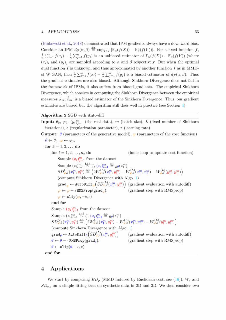
4. APPLICATIONS 63
(Bińkowski et al., 2018) demonstrated that IPM gradients always have a downward bias.Consider an IPM dF (α, β) def.= supf∈F |Eα(f(X)) − Eβ(f(Y ))|. For a fixed function f ,1n
∑ni=1 f(xi) − 1
n
∑nj=1 f(yj) is an unbiased estimator of Eα(f(X)) − Eβ(f(Y )) (where
(xi)i and (yj)j are sampled according to α and β respectively. But when the optimaldual function f is unknown, and thus approximated by another function f as in MMD-of W-GAN, then 1
n
∑ni=1 f(xi) − 1
n
∑nj=1 f(yj) is a biased estimator of dF (α, β). Thus
the gradient estimates are also biased. Although Sinkhorn Divergence does not fall inthe framework of IPMs, it also suffers from biased gradients. The empirical SinkhornDivergence, which consists in computing the Sinkhorn Divergence between the empiricalmeasures αm, βm, is a biased estimator of the Sinkhorn Divergence. Thus, our gradientestimates are biased but the algorithm still does well in practice (see Section 4).
Algorithm 2 SGD with Auto-diffInput: θ0, ϕ0, (yj)nj=1 (the real data), m (batch size), L (fixed number of Sinkhorniterations), ε (regularization parameter), τ (learning rate)
Output: θ (parameters of the generative model), ϕ (parameters of the cost function)θ ← θ0, ϕ← ϕ0,for k = 1, 2, . . . do
for t = 1, 2, . . . , nc do (inner loop to update cost function)Sample (yj)mj=1 from the datasetSample (zi)mi=1
i.i.d∼ ζ, (xi)mi=1def.= gθ(zm1 )
SD(L)ϕ,ε (xm1 , ym1 ) def.=
(2W (L)
ϕ,ε (xm1 , ym1 )−W (L)ϕ,ε (xm1 , xm1 )−W (L)
ϕ,ε (ym1 , ym1 ))
(compute Sinkhorn Divergence with Algo. 1)gradϕ ← AutoDiffϕ
(SD
(L)ϕ,ε (xm1 , ym1 )
)(gradient evaluation with autodiff)
ϕ← ϕ+ τRMSProp(gradϕ). (gradient step with RMSprop)ϕ← clip(ϕ,−c, c)
end forSample (yj)mj=1 from the datasetSample (zi)mi=1
i.i.d∼ ζ, (xi)mi=1def.= gθ(zm1 )
SD(L)ϕ,ε (xm1 , ym1 ) def.=
(2W (L)
ϕ,ε (xm1 , ym1 )−W (L)ϕ,ε (xm1 , xm1 )−W (L)
ϕ,ε (ym1 , ym1 ))
(compute Sinkhorn Divergence with Algo. 1)gradθ ← AutoDiffθ
(SD
(L)ϕ,ε (xm1 , ym1 )
)(gradient evaluation with autodiff)
θ ← θ − τRMSProp(gradθ). (gradient step with RMSprop)θ ← clip(θ,−c, c)
end for
4 Applications
We start by comparing EDp (MMD induced by Euclidean cost, see (16)), Wε andSDc,ε on a simple fitting task on synthetic data in 2D and 3D. We then consider two
64 CHAPTER 2. LEARNING WITH SINKHORN DIVERGENCES
popular problems in machine learning to illustrate the versatility of our method. Thefirst one relies on fitting labeled data with uniform distributions supported on ellipses(note that this could be any parametric shape but ellipses here were a good fit). Thesecond problem consists in tuning a neural network to generate images, first with a fixedcost (on MNIST dataset) and then with a parametric cost (on CIFAR10 dataset). Inboth cases, we used simple initializations (see details below) and the algorithm yieldedsimilar results when rerun, meaning that the results displayed are representative of theperformance of the algorithm and that the procedure is quite stable.
4.1 Benchmark on Synthetic Problems
Since evaluating the performance of generative models is a complicated issue onreal data (see discussion in Sec. 4.3), we construct a synthetic framework to get areliable comparison of different losses. Although our method is meant to be used in highdimensions, we apply it here to two simple problems to be able to visualize the results:
• Deterministic setting : fitting a point cloud in 2D,
• Probabilistic setting: fitting an ellipse in 3D.
In the deterministic setting, we fit a finite discrete measure, to give us a better idea ofthe geometry of the costs without the sampling noise. We then see how our observationscarry out in a probabilistic setting, with sampling and stochastic gradient descent asdescribed in Algorithm 2.
Both problems require the use of losses that are smooth for the weak convergence:for the first one, the model measure is singular, as it is supported on points, while forthe second, the model measure measure has a bounded support which changes duringthe optimization procedure.
Deterministic setting: Fitting a point cloud in 2D. Given a dataset (y1, . . . , yn)of points in 2D, we want to fit the empirical measure β def.= 1
n
∑ni=1 δyi . The parametric
measure that we consider is thus αθdef.= 1
n
∑ni=1 δθi , where the parameters θi are the
positions of the Dirac masses. To get rid of the sampling noise and better observe thegeometry of the losses, we use a full gradient descent to estimate θ (or, in other words,we use minibatches of size m = n, to stick to the scheme of Algorithm 2). The resultsare given in Figure 2.2. We use a cost c = || · ||1.52 to ensure fair comparison with EDp
which is well defined for p < 2 only. We use L = 5 iterations to to Sinkhorn’s algorithm.We can see that Wc,ε successfully captures the extreme points, but yields parametersthat collapse to a mean values in the dense area. The Energy Distance, on the otherhand, fails to capture the extreme points but the points in the dense region are welldistributed. Sinkhorn Divergences get the best of both worlds by successfully capturingboth the extreme points and the dense area for ε = 1, but when ε gets larger, we recoverthe behavior of Energy Distance and the extreme points are not recovered anymore.
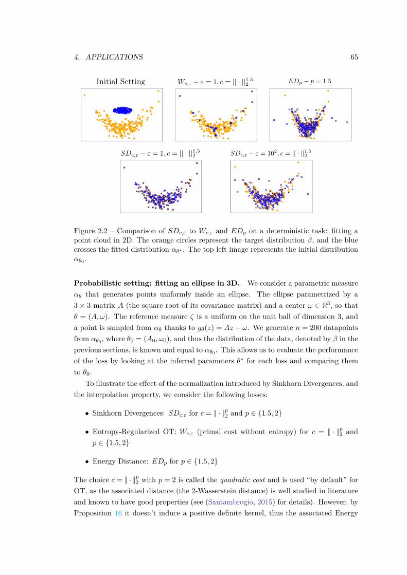
4. APPLICATIONS 65
SDc," " = 102, c = || · ||1.52SDc," " = 1, c = || · ||1.5
2
Wc," " = 1, c = || · ||1.52
EDp p = 1.5Initial Setting
Figure 2.2 – Comparison of SDc,ε to Wc,ε and EDp on a deterministic task: fitting apoint cloud in 2D. The orange circles represent the target distribution β, and the bluecrosses the fitted distribution αθ∗ . The top left image represents the initial distributionαθ0 .
Probabilistic setting: fitting an ellipse in 3D. We consider a parametric measureαθ that generates points uniformly inside an ellipse. The ellipse parametrized by a3 × 3 matrix A (the square root of its covariance matrix) and a center ω ∈ R3, so thatθ = (A,ω). The reference measure ζ is a uniform on the unit ball of dimension 3, anda point is sampled from αθ thanks to gθ(z) = Az + ω. We generate n = 200 datapointsfrom αθ0 , where θ0 = (A0, ω0), and thus the distribution of the data, denoted by β in theprevious sections, is known and equal to αθ0 . This allows us to evaluate the performanceof the loss by looking at the inferred parameters θ∗ for each loss and comparing themto θ0.
To illustrate the effect of the normalization introduced by Sinkhorn Divergences, andthe interpolation property, we consider the following losses:
• Sinkhorn Divergences: SDc,ε for c = || · ||p2 and p ∈ 1.5, 2
• Entropy-Regularized OT: Wc,ε (primal cost without entropy) for c = || · ||p2 andp ∈ 1.5, 2
• Energy Distance: EDp for p ∈ 1.5, 2
The choice c = || · ||p2 with p = 2 is called the quadratic cost and is used “by default” forOT, as the associated distance (the 2-Wasserstein distance) is well studied in literatureand known to have good properties (see (Santambrogio, 2015) for details). However, byProposition 16 it doesn’t induce a positive definite kernel, thus the associated Energy
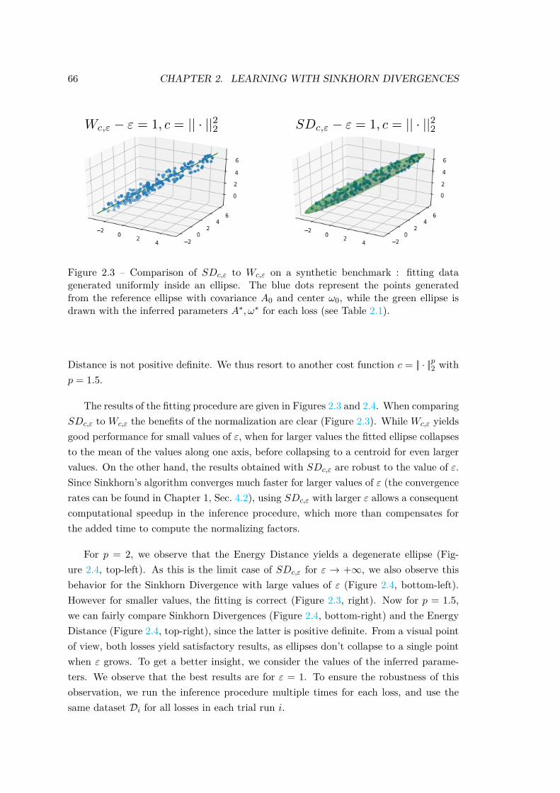
66 CHAPTER 2. LEARNING WITH SINKHORN DIVERGENCES
SDc," " = 1, c = || · ||22Wc," " = 1, c = || · ||22
Figure 2.3 – Comparison of SDc,ε to Wc,ε on a synthetic benchmark : fitting datagenerated uniformly inside an ellipse. The blue dots represent the points generatedfrom the reference ellipse with covariance A0 and center ω0, while the green ellipse isdrawn with the inferred parameters A∗, ω∗ for each loss (see Table 2.1).
Distance is not positive definite. We thus resort to another cost function c = || · ||p2 withp = 1.5.
The results of the fitting procedure are given in Figures 2.3 and 2.4. When comparingSDc,ε to Wc,ε the benefits of the normalization are clear (Figure 2.3). While Wc,ε yieldsgood performance for small values of ε, when for larger values the fitted ellipse collapsesto the mean of the values along one axis, before collapsing to a centroid for even largervalues. On the other hand, the results obtained with SDc,ε are robust to the value of ε.Since Sinkhorn’s algorithm converges much faster for larger values of ε (the convergencerates can be found in Chapter 1, Sec. 4.2), using SDc,ε with larger ε allows a consequentcomputational speedup in the inference procedure, which more than compensates forthe added time to compute the normalizing factors.
For p = 2, we observe that the Energy Distance yields a degenerate ellipse (Fig-ure 2.4, top-left). As this is the limit case of SDc,ε for ε → +∞, we also observe thisbehavior for the Sinkhorn Divergence with large values of ε (Figure 2.4, bottom-left).However for smaller values, the fitting is correct (Figure 2.3, right). Now for p = 1.5,we can fairly compare Sinkhorn Divergences (Figure 2.4, bottom-right) and the EnergyDistance (Figure 2.4, top-right), since the latter is positive definite. From a visual pointof view, both losses yield satisfactory results, as ellipses don’t collapse to a single pointwhen ε grows. To get a better insight, we consider the values of the inferred parame-ters. We observe that the best results are for ε = 1. To ensure the robustness of thisobservation, we run the inference procedure multiple times for each loss, and use thesame dataset Di for all losses in each trial run i.
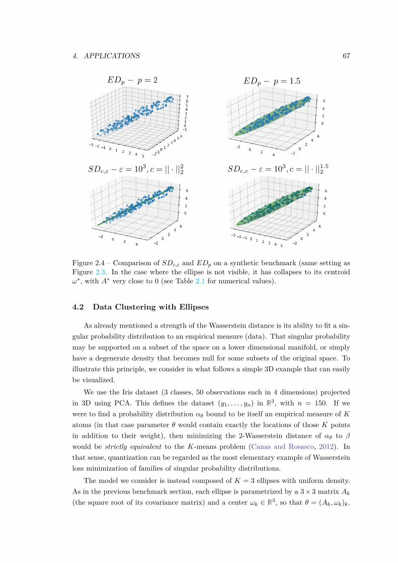
4. APPLICATIONS 67
EDp p = 1.5EDp p = 2
SDc," " = 103, c = || · ||22 SDc," " = 103, c = || · ||1.52
Figure 2.4 – Comparison of SDc,ε and EDp on a synthetic benchmark (same setting asFigure 2.3. In the case where the ellipse is not visible, it has collapses to its centroidω∗, with A∗ very close to 0 (see Table 2.1 for numerical values).
4.2 Data Clustering with Ellipses
As already mentioned a strength of the Wasserstein distance is its ability to fit a sin-gular probability distribution to an empirical measure (data). That singular probabilitymay be supported on a subset of the space on a lower dimensional manifold, or simplyhave a degenerate density that becomes null for some subsets of the original space. Toillustrate this principle, we consider in what follows a simple 3D example that can easilybe visualized.
We use the Iris dataset (3 classes, 50 observations each in 4 dimensions) projectedin 3D using PCA. This defines the dataset (y1, . . . , yn) in R3, with n = 150. If wewere to find a probability distribution αθ bound to be itself an empirical measure of Katoms (in that case parameter θ would contain exactly the locations of those K pointsin addition to their weight), then minimizing the 2-Wasserstein distance of αθ to β
would be strictly equivalent to the K-means problem (Canas and Rosasco, 2012). Inthat sense, quantization can be regarded as the most elementary example of Wassersteinloss minimization of families of singular probability distributions.
The model we consider is instead composed of K = 3 ellipses with uniform density.As in the previous benchmark section, each ellipse is parametrized by a 3× 3 matrix Ak(the square root of its covariance matrix) and a center ωk ∈ R3, so that θ = (Ak, ωk)k.
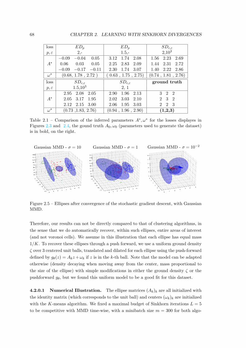
68 CHAPTER 2. LEARNING WITH SINKHORN DIVERGENCES
loss EDp EDp SDc,ε
p, ε 2,- 1.5,- 2,103
A∗−0.09 −0.04 0.050.06 0.03 0.05−0.09 −0.17 −0.11
3.12 1.74 2.082.25 2.83 2.092.30 1.74 3.07
1.56 2.23 2.691.44 2.31 2.721.40 2.22 2.86
ω∗ (0.68, 1.78 , 2.72 ) ( 0.63 , 1.75 , 2.75) (0.74 , 1.81 , 2.76)loss SDc,ε SDc,ε ground truthp, ε 1.5,103 2, 1
A∗2.95 2.08 2.052.05 3.17 1.952.12 2.15 3.00
2.90 1.96 2.132.02 3.03 2.102.06 1.95 3.03
3 2 22 3 22 2 3
ω∗ (0.73 ,1.83, 2.76) (0.94 , 1.96 , 2.90) (1,2,3)
Table 2.1 – Comparison of the inferred parameters A∗, ω∗ for the losses displayes inFigures 2.3 and 2.4, the gound truth A0, ω0 (parameters used to generate the dataset)is in bold, on the right.
Gaussian MMD - = 10 Gaussian MMD - = 1 Gaussian MMD - = 102
Figure 2.5 – Ellipses after convergence of the stochastic gradient descent, with GaussianMMD.
Therefore, our results can not be directly compared to that of clustering algorithms, inthe sense that we do automatically recover, within such ellipses, entire areas of interest(and not voronoi cells). We assume in this illustration that each ellipse has equal mass1/K. To recover these ellipses through a push forward, we use a uniform ground densityζ over 3 centered unit balls, translated and dilated for each ellipse using the push-forwarddefined by gθ(z) = Akz+ωk if z is in the k-th ball. Note that the model can be adaptedotherwise (density decaying when moving away from the center, mass proportional tothe size of the ellipse) with simple modifications in either the ground density ζ or thepushforward gθ, but we found this uniform model to be a good fit for this dataset.
4.2.0.1 Numerical Illustration. The ellipse matrices (Ak)k are all initialized withthe identity matrix (which corresponds to the unit ball) and centers (ωk)k are initializedwith the K-means algorithm. We fixed a maximal budget of Sinkhorn iterations L = 5to be competitive with MMD time-wise, with a minibatch size m = 300 for both algo-
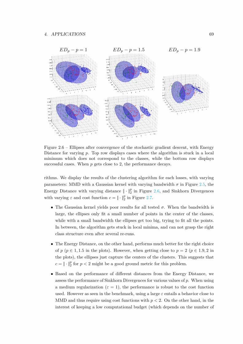
4. APPLICATIONS 69
EDp p = 1 EDp p = 1.5 EDp p = 1.9
Figure 2.6 – Ellipses after convergence of the stochastic gradient descent, with EnergyDistance for varying p. Top row displays cases where the algorithm is stuck in a localminimum which does not correspond to the classes, while the bottom row displayssuccessful cases. When p gets close to 2, the performance decays.
rithms. We display the results of the clustering algorithm for each losses, with varyingparameters: MMD with a Gaussian kernel with varying bandwidth σ in Figure 2.5, theEnergy Distance with varying distance || · ||p2 in Figure 2.6, and Sinkhorn Divergenceswith varying ε and cost function c = || · ||p2 in Figure 2.7.
• The Gaussian kernel yields poor results for all tested σ. When the bandwidth islarge, the ellipses only fit a small number of points in the center of the classes,while with a small bandwidth the ellipses get too big, trying to fit all the points.In between, the algorithm gets stuck in local minima, and can not grasp the rightclass structure even after several re-runs.
• The Energy Distance, on the other hand, performs much better for the right choiceof p (p ∈ 1, 1.5 in the plots). However, when getting close to p = 2 (p ∈ 1.9, 2 inthe plots), the ellipses just capture the centers of the clusters. This suggests thatc = || · ||p2 for p < 2 might be a good ground metric for this problem.
• Based on the performance of different distances from the Energy Distance, weassess the performance of Sinkhorn Divergences for various values of p. When usinga medium regularization (ε = 1), the performance is robust to the cost functionused. However as seen in the benchmark, using a large ε entails a behavior close toMMD and thus require using cost functions with p < 2. On the other hand, in theinterest of keeping a low computational budget (which depends on the number of
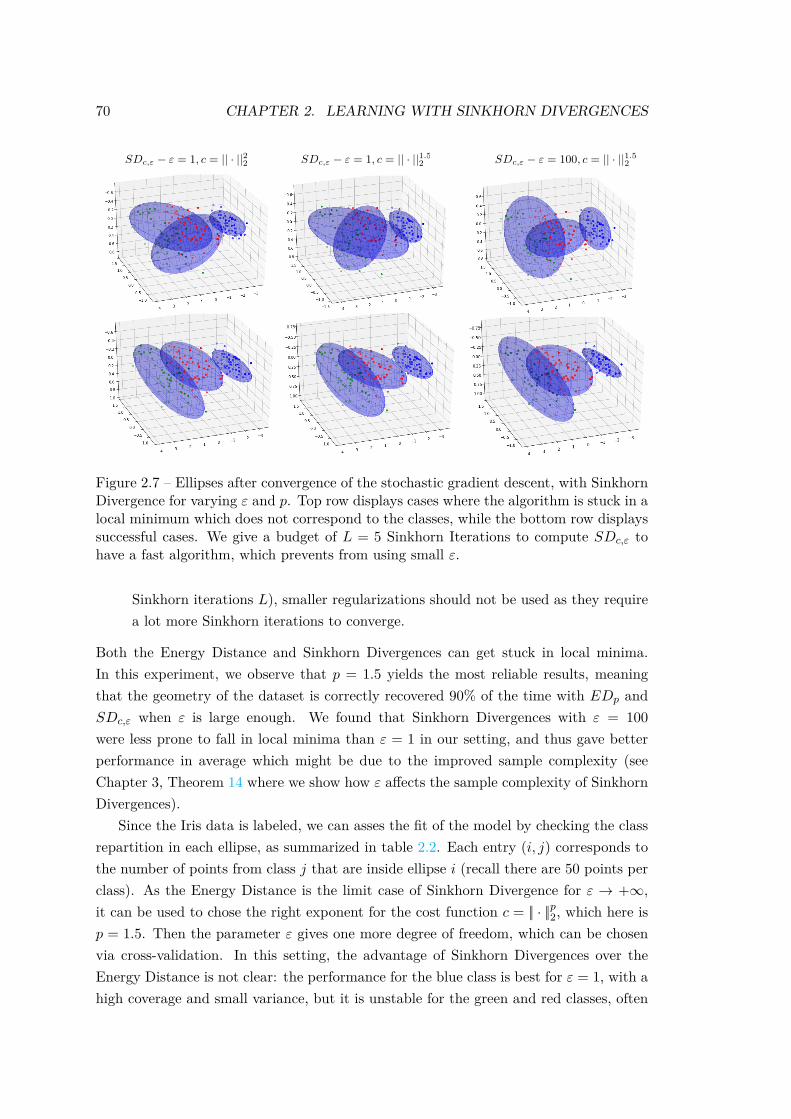
70 CHAPTER 2. LEARNING WITH SINKHORN DIVERGENCES
SDc," " = 1, c = || · ||22 SDc," " = 1, c = || · ||1.52 SDc," " = 100, c = || · ||1.5
2
Figure 2.7 – Ellipses after convergence of the stochastic gradient descent, with SinkhornDivergence for varying ε and p. Top row displays cases where the algorithm is stuck in alocal minimum which does not correspond to the classes, while the bottom row displayssuccessful cases. We give a budget of L = 5 Sinkhorn Iterations to compute SDc,ε tohave a fast algorithm, which prevents from using small ε.
Sinkhorn iterations L), smaller regularizations should not be used as they requirea lot more Sinkhorn iterations to converge.
Both the Energy Distance and Sinkhorn Divergences can get stuck in local minima.In this experiment, we observe that p = 1.5 yields the most reliable results, meaningthat the geometry of the dataset is correctly recovered 90% of the time with EDp andSDc,ε when ε is large enough. We found that Sinkhorn Divergences with ε = 100were less prone to fall in local minima than ε = 1 in our setting, and thus gave betterperformance in average which might be due to the improved sample complexity (seeChapter 3, Theorem 14 where we show how ε affects the sample complexity of SinkhornDivergences).
Since the Iris data is labeled, we can asses the fit of the model by checking the classrepartition in each ellipse, as summarized in table 2.2. Each entry (i, j) corresponds tothe number of points from class j that are inside ellipse i (recall there are 50 points perclass). As the Energy Distance is the limit case of Sinkhorn Divergence for ε → +∞,it can be used to chose the right exponent for the cost function c = || · ||p2, which here isp = 1.5. Then the parameter ε gives one more degree of freedom, which can be chosenvia cross-validation. In this setting, the advantage of Sinkhorn Divergences over theEnergy Distance is not clear: the performance for the blue class is best for ε = 1, with ahigh coverage and small variance, but it is unstable for the green and red classes, often
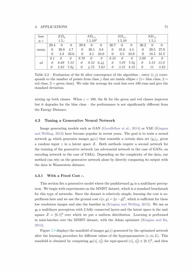
4. APPLICATIONS 71
loss EDp SDc,ε SDc,ε SDc,ε
p, ε 1.5,- 1.5,102 1.5,10 1.5,1
mean29.4 0 0
0 30.8 4.70 4.3 33.6
29.9 0 00 30.1 3.80 3.1 34.0
30.7 0 00 31.6 4.40 3.5 34.9
36.2 0 00 29.5 27.90 18.5 31.5
sd9.1 0 00 8.69 7.330 5.82 7.84
9.79 0 00 8.52 6.440 4.75 7.63
8.55 0 00 7.07 7.940 5.21 8.35
3.09 0 00 5.53 15.80 11 5.65
Table 2.2 – Evaluation of the fit after convergence of the algorithm : entry (i, j) corre-sponds to the number of points from class j that are inside ellipse i (1= blue class, 2 =red class, 3 = green class). We take the average for each loss over 100 runs and give thestandard deviation.
mixing up both classes. When ε = 100, the fit for the green and red classes improvesbut it degrades for the blue class – the performance is not significantly different fromthe Energy Distance.
4.3 Tuning a Generative Neural Network
Image generating models such as GAN (Goodfellow et al., 2014) or VAE (Kingmaand Welling, 2013) have become popular in recent years. The goal is to train a neuralnetwork gθ which generates images gθ(z) that resemble a certain data set (yj)j , givena random input z in a latent space Z. Both methods require a second network forthe training of the generative network (an adversarial network in the case of GANs, anencoding network in the case of VAEs). Depending on the complexity of the data, ourmethod can rely on the generative network alone by directly comparing its output withthe data in Wasserstein distance.
4.3.1 With a Fixed Cost c.
This section fits a generative model where the pushforward gθ is a multilayer percep-tron. We begin with experiments on the MNIST dataset, which is a standard benchmarkfor this type of networks. Since the dataset is relatively simple, learning the cost is su-perfluous here and we use the ground cost c(x, y) = ||x−y||2, which is sufficient for theselow resolution images and also the baseline in (Kingma and Welling, 2013). We use asgθ a multilayer perceptron with 2 fully connected layers and the latent space is the unitsquare Z = [0, 1]2 over which we put a uniform distribution. Learning is performedin mini-batches over the MNIST dataset, with the Adam optimizer (Kingma and Ba,2014).
Figure 2.8 displays the manifold of images gθ(z) generated by the optimized networkafter the learning procedure for different values of the hyperparameters (ε,m,L). Thismanifold is obtained by computing gθ(zi1, z
j2) for equi-spaced (zi1, z
j2) ∈ [0, 1]2, and then
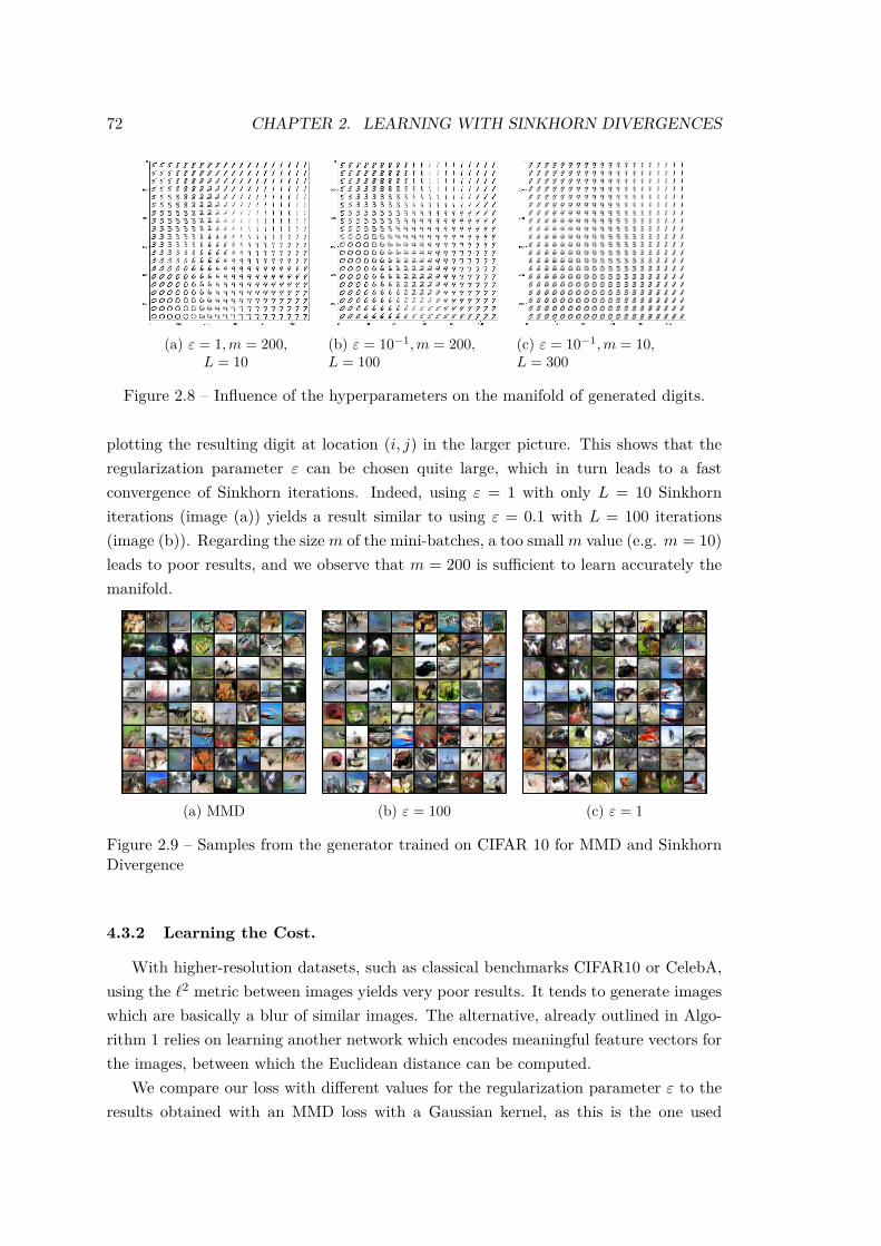
72 CHAPTER 2. LEARNING WITH SINKHORN DIVERGENCES
(a) ε = 1,m = 200,L = 10
(b) ε = 10−1,m = 200,L = 100
(c) ε = 10−1,m = 10,L = 300
Figure 2.8 – Influence of the hyperparameters on the manifold of generated digits.
plotting the resulting digit at location (i, j) in the larger picture. This shows that theregularization parameter ε can be chosen quite large, which in turn leads to a fastconvergence of Sinkhorn iterations. Indeed, using ε = 1 with only L = 10 Sinkhorniterations (image (a)) yields a result similar to using ε = 0.1 with L = 100 iterations(image (b)). Regarding the sizem of the mini-batches, a too smallm value (e.g. m = 10)leads to poor results, and we observe that m = 200 is sufficient to learn accurately themanifold.
(a) MMD (b) ε = 100 (c) ε = 1
Figure 2.9 – Samples from the generator trained on CIFAR 10 for MMD and SinkhornDivergence
4.3.2 Learning the Cost.
With higher-resolution datasets, such as classical benchmarks CIFAR10 or CelebA,using the `2 metric between images yields very poor results. It tends to generate imageswhich are basically a blur of similar images. The alternative, already outlined in Algo-rithm 1 relies on learning another network which encodes meaningful feature vectors forthe images, between which the Euclidean distance can be computed.
We compare our loss with different values for the regularization parameter ε to theresults obtained with an MMD loss with a Gaussian kernel, as this is the one used
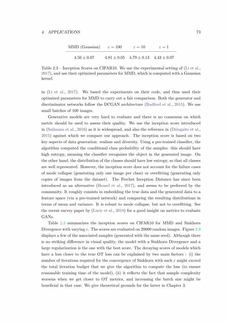
4. APPLICATIONS 73
MMD (Gaussian) ε = 100 ε = 10 ε = 1
4.56± 0.07 4.81± 0.05 4.79± 0.13 4.43± 0.07
Table 2.3 – Inception Scores on CIFAR10. We use the experimental setting of (Li et al.,2017), and use their optimized parameters for MMD, which is computed with a Gaussiankernel.
in (Li et al., 2017). We based the experiments on their code, and thus used theiroptimized parameters for MMD to carry out a fair comparison. Both the generator anddiscriminator networks follow the DCGAN architecture (Radford et al., 2015). We usesmall batches of 100 images.
Generative models are very hard to evaluate and there is no consensus on whichmetric should be used to assess their quality. We use the inception score introducedin (Salimans et al., 2016) as it is widespread, and also the reference in (Dziugaite et al.,2015) against which we compare our approach. The inception score is based on twokey aspects of data generation: realism and diversity. Using a pre-trained classifier, thealgorithm computed the conditional class probability of the samples: this should havehigh entropy, meaning the classifier recognizes the object in the generated image. Onthe other hand, the distribution of the classes should have low entropy, so that all classesare well represented. However, the inception score does not account for the failure casesof mode collapse (generating only one image per class) or overfitting (generating onlycopies of images from the dataset). The Frechet Inception Distance has since beenintroduced as an alternative (Heusel et al., 2017), and seems to be preferred by thecommunity. It roughly consists in embedding the true data and the generated data to afeature space (via a pre-trained network) and comparing the resulting distributions interms of mean and variance. It is robust to mode collapse, but not to overfitting. Seethe recent survey paper by (Lucic et al., 2018) for a good insight on metrics to evaluateGANs.
Table 2.3 summarizes the inception scores on CIFAR10 for MMD and SinkhornDivergence with varying ε. The scores are evaluated on 20000 random images. Figure 2.9displays a few of the associated samples (generated with the same seed). Although thereis no striking difference in visual quality, the model with a Sinkhorn Divergence and alarge regularization is the one with the best score. The decaying scores of models whichhave a loss closer to the true OT loss can be explained by two main factors : (i) thenumber of iterations required for the convergence of Sinkhorn with such ε might exceedthe total iteration budget that we give the algorithm to compute the loss (to ensurereasonable training time of the model), (ii) it reflects the fact that sample complexityworsens when we get closer to OT metrics, and increasing the batch size might bebeneficial in that case. We give theoretical grounds for the latter in Chapter 3.

74 CHAPTER 2. LEARNING WITH SINKHORN DIVERGENCES
Chapter 3
Sample Complexity of SinkhornDivergences
Optimal Transport (OT) and Maximum Mean Discrepancies (MMD) are now routinely usedin machine learning to compare probability measures. We focus in this chapter on SinkhornDivergences (SDs), a regularized variant of OT distances which can interpolate, depending onthe regularization strength ε, between OT (ε = 0) and MMD (ε = ∞). Although the tradeoffinduced by the regularization is now well understood computationally (OT, SDs and MMD requirerespectively O(n3 logn), O(n2) and O(n2) operations given a sample size n), much less is knownin terms of their sample complexity, namely the gap between these quantities, when evaluatedusing finite samples vs. their respective densities. Indeed, while the sample complexity of OTand MMD stand at two extremes, O(1/n1/d) for OT in dimension d and O(1/
√n) for MMD,
that for SDs has only been studied empirically. In this chapter, we
(i) derive a bound on the approximation error made with SDs when approximating OT as afunction of the regularizer ε,
(ii) prove that the optimizers of regularized OT are bounded in a Sobolev (RKHS) ball indepen-dent of the two measures,
(iii) provide the first sample complexity bound for SDs, obtained by reformulating SDs as amaximization problem in a RKHS. We thus obtain a scaling in 1/
√n (as in MMD), with
a constant that depends however on ε, making the bridge between OT and MMD complete.
This chapter is based on (Genevay et al., 2019).
75
76 CHAPTER 3. SAMPLE COMPLEXITY OF SINKHORN DIVERGENCES
1 Introduction
OT has been long neglected in data sciences for two main reasons, which couldbe loosely described as computational and statistical. Following the seminal work by(Cuturi, 2013), we have showed in Chapters 1 and 2 how entropic regularization of OTalleviates this computational burden. In Chapter 2, we further mentioned that entropy-regularized OT seems to break the curse-of-dimensionality from which OT suffers basedon empirical evidence, and the goal of this chapter is to make it more formal through asample complexity result.
Previous Works. The central theoretical contribution of Chapter 2 (see Theorem 10)states that Sinkhorn Divergences, based on regularized OT, interpolate between OT andMMD. These two metrics, which emerged as popular candidates to compare probabilitymeasures, differ on a fundamental aspect: their sample complexity. The definition ofsample complexity of a loss function that we choose here is the convergence rate of theloss evaluated on empirical measures to the loss evaluated on the “true" measures, asa function of the number of samples. This notion is crucial in machine learning, asbad sample complexity implies overfitting and high gradient variance when using thesedivergences for parameter estimation. In that context, it is well known that the samplecomplexity of MMD is independent of the dimension, scaling as 1√
n(Gretton et al.,
2006) where n is the number of samples. In contrast, it is well known that standardOT suffers from the curse of dimensionality (Dudley, 1969): Its sample complexity isexponential in the dimension of the ambient space. Although it was recently proved thatthis result can be refined to consider the implicit dimension of data (Weed and Bach,2017), the sample complexity of OT appears now to be the major bottleneck for the useof OT in high-dimensional machine learning problems.
A remedy to this problem may lie, again, in regularization. The discrepancies definedthrough regularized OT, known as Sinkhorn Divergences, seem to be less prone to over-fitting. Indeed, a certain amount of regularization tends to improve performance insimple learning tasks (Cuturi, 2013). The interpolation theorem from Chapter 2 alsosuggests that for large regularizations, Sinkhorn Divergences behave like MMD.
The asymptotic behavior of empirical estimates of the Wasserstein distance has beenwidely studied, from convergence rates to distributional limits. In particular we referto (Del Barrio and Loubes, 2017), which recently proved a central limit theorem forempirical OT in general dimension, for a thorough historical review of the subject.However, aside from a recent central limit theorem in the case of measures supportedon finite discrete spaces (Bigot et al., 2017), the convergence of empirical SinkhornDivergences, and more generally their sample complexity, remains an open question.
2. REMINDERS ON SINKHORN DIVERGENCES 77
Contributions. This chapter provides three main contributions, which all exhibittheoretical properties of Sinkhorn Divergences. Our first result is a bound on the speedof convergence of regularized OT to standard OT as a function of the regularizationparameter, in the case of continuous measures. The second theorem proves that theoptimizers of the regularized optimal transport problem lie in a Sobolev ball which isindependent of the measures. This allows us to rewrite the Sinkhorn Divergence as themaximization of an expectation over a RKHS ball and thus justify the use of kernel-SGD for regularized OT as advocated in Chapter 4, Sec. 5.1. As a consequence of thisreformulation, we provide as our third contribution a sample complexity result. We focuson how the sample size and the regularization parameter affect the convergence of theempirical Sinkhorn Divergence (i.e., computed from samples of two continuous measures)to the continuous Sinkhorn Divergence. We show that the Sinkhorn Divergence benefitsfrom the same sample complexity as MMD, scaling in 1√
nbut with a constant that
depends on the inverse of the regularization parameter. Thus sample complexity worsenswhen getting closer to standard OT, and there is therefore a tradeoff between a goodapproximation of OT (small regularization parameter) and fast convergence in termsof sample size (larger regularization parameter). We conclude this chapter with a fewnumerical experiments to asses the dependence of the sample complexity on ε and d insimple cases.
2 Reminders on Sinkhorn Divergences
We consider entropy-regularized optimal transport between two probability measuresα ∈ M1
+(X ) and β on M1+(Y), as introduced in Chapter 1, Sec. 4, where X and Y
are two bounded subsets of Rd. The optimal transport problem is regularized withthe relative entropy of the transport plan with respect to the product measure α ⊗ βfollowing (Genevay et al., 2016):
Wε(α, β) def.= minπ∈Π(α,β)
∫X×Y
c(x, y)dπ(x, y) + εH(π | α⊗ β), (Pε)
where H(π | α⊗ β) def.=∫X×Y
log( dπ(x, y)
dα(x)dβ(y)
)dπ(x, y), (2.1)
and the feasible set Π(α, β) is composed of probability distributions over the productspace X × Y with fixed marginals α, β. The cost function c, which represents the costto move a unit of mass from x to y is assumed to be C∞ through this chapter (morespecifically, we need it to be C
d2 +1). Choosing the relative entropy as a regularizer allows
to express the dual formulation of regularized OT as the maximization of an expectation
78 CHAPTER 3. SAMPLE COMPLEXITY OF SINKHORN DIVERGENCES
problem (Proposition 4 in Chapter 1):
Wε(α, β) = maxu∈C(X ),v∈C(Y)
∫Xu(x)dα(x) +
∫Yv(y)dβ(y)
− ε∫X×Y
eu(x)+v(y)−c(x,y)
ε dα(x)dβ(y) + ε
= maxu∈C(X),v∈C(Y )
Eα⊗β[fXYε (u, v)
]+ ε,
where fxyε (u, v) = u(x) + v(y)− εeu(x)+v(y)−c(x,y)
ε .
This reformulation as the maximum of an expectation is crucial to obtain samplecomplexity results. The existence of optimal dual potentials (u, v) is proved in Chapter 1,Sec. 4.1. They are unique α− and β−a.e. up to an additive constant.
To correct for the fact that Wε(α, α) 6= 0, we introduced Sinkhorn Divergences inChapter 2. They are a natural normalization of that quantity defined as
SDε(α, β) = Wε(α, β)− 12(Wε(α, α) +Wε(β, β)). (2.2)
This normalization ensures that SDε(α, α) = 0, but also has a noticeable asymptoticbehavior as proved in Theorem 10 of Chapter 2. Indeed, when ε → 0 one recoversthe original (unregularized) OT problem, while choosing ε → +∞ yields the squaredmaximum mean discrepancy (see Chapter 1, Sec.2.2 for a detailed introduction on thematter) associated to the kernel k = −c/2, where MMD is defined by:
MMD2k(α, β) = Eα⊗α[k(X,X ′)] + Eβ⊗β[k(Y, Y ′)]− 2Eα⊗β[k(X,Y )].
Besides, under some assumptions on the cost function, Sinkhorn Divergences are positivedefinite and metrize weak convergence of measures (Feydy et al., 2019). In the contextof this chapter, we study in detail the sample complexity ofWε(α, β), which immediatelyextends to that of SDε(α, β) by linearity.
Remark 14. Sinkhorn Divergences can be defined with Wε being either the primal costof (Pε) or the primal cost without the entropic term (see Definition 9 in Chapter 2 formore details). While the interpolation theorem in Chapter 2 holds for both definitions,the sample complexity theorem that we prove here is only valid when Wε is the primalcost of (Pε).
3 Approximating Optimal Transport with Sinkhorn Di-vergences
In the present section, we are interested in bounding the error made when approxi-mating W (α, β) with Wε(α, β).
3. APPROXIMATING OPTIMAL TRANSPORT WITH SINKHORN DIVERGENCES79
Theorem 12. Let α and β be probability measures on X and Y subsets of Rd such that|X | and |Y| 6 D and assume that c is L-Lipschitz w.r.t. x and y. It holds
0 6Wε(α, β)−W (α, β) 6 2εd log(e2·L·D√
d·ε
)(3.1)
∼ε→0 2εd log(1/ε). (3.2)
Proof. For a probability measure π on X ×Y, we denote by C(π) =∫cdπ the associated
transport cost and by H(π) its relative entropy with respect to the product measureα ⊗ β as defined in (2.1). Choosing π0 a minimizer of minπ∈Π(α,β)C(π), we will buildour upper bounds using a family of transport plans with finite entropy that approximateπ0. The simplest approach consists in considering block approximation. In contrast tothe work of Carlier et al. (2017), who also considered this technique, our focus here ison quantitative bounds.
Definition 10 (Block approximation). For a resolution ∆ > 0, we consider the blockpartition of Rd in hypercubes of side ∆ defined as
Q∆k = [k1 ·∆, (k1 + 1) ·∆[× . . . [kd ·∆, (kd + 1) ·∆[ ; k = (k1, . . . , kd) ∈ Zd.
To simplify notations, we introduce Q∆ij
def.= Q∆i ×Q∆
j , α∆i
def.= α(Q∆i ), β∆
jdef.= β(Q∆
j ).The block approximation of π0 of resolution ∆ is the measure π∆ ∈ Π(α, β) characterizedby
π∆|Q∆ij
=π0(Q∆
ij)α∆i · β
∆j
(α|Q∆i⊗ β|Q∆
j)
for all (i, j) ∈ (Zd)2, with the convention 0/0 = 0.
π∆ is nonnegative by construction. Observe also that for any Borel set B ⊂ Rd, onehas
π∆(B × Rd) =∑
(i,j)∈(Zd)2
π0(Q∆ij)
α∆i · β
∆j
· α(B ∩Q∆i ) · β∆
j =∑i∈Zd
α(B ∩Q∆i ) = α(B),
which proves, using the symmetric result in β, that π∆ belongs to Π(α, β). As a con-sequence, for any ε > 0 one has Wε(α, β) 6 C(π∆) + εH(π∆). Recalling also thatthe relative entropy H is nonnegative over the set of probability measures, we have thebound
0 6Wε(α, β)−W (α, β) 6 (C(π∆)− C(π0)) + εH(π∆).
We can now bound the terms in the right-hand side, and choose a value for ∆ thatminimizes these bounds.
The bound on C(π∆)−C(π0) relies on the Lipschitz regularity of the cost function.
80 CHAPTER 3. SAMPLE COMPLEXITY OF SINKHORN DIVERGENCES
Using the fact that π∆(Q∆ij) = π0(Q∆
ij) for all i, j, it holds
C(π∆)− C(π0) =∑
(i,j)∈(Zd)2
π0(Q∆ij)(
supx,y∈Q∆
ij
c(x, y)− infx,y∈Q∆
ij
c(x, y))
6 2L∆√d,
where L is the Lipschitz constant of the cost (separately in x and y) and ∆√d is the
diameter of each set Q∆i .
As for the bound on H(π∆), using the fact that π0(Q∆ij) 6 1 we get
H(π∆) =∑
(i,j)∈(Zd)2
log(π0(Q∆
ij)α∆i · β
∆j
)π0(Q∆
ij)
6∑
(i,j)∈(Zd)2
(log(1/α∆
i ) + log(1/β∆j ))π0(Q∆
ij)
= −H∆(α)−H∆(β),
where we have defined H∆(α) =∑i∈Zd α∆
i log(α∆i ) and similarly for β. Note that in
case α is a discrete measure with finite support, H∆(α) is equal to (minus) the discreteentropy of α as long as ∆ is smaller than the minimum separation between atoms ofα. However, if α is not discrete then H∆(α) blows up to −∞ as ∆ goes to 0 andwe need to control how fast it does so. Considering α∆ the block approximation ofα with constant density α∆
i /∆d on each block Q∆i and (minus) its differential entropy
HLd(α∆) =∫
Rd α∆(x) logα∆(x)dx, it holds H∆(α) = HLd(α∆)−d · log(1/∆). Moreover,
using the convexity of HLd , this can be compared with the differential entropy of theuniform probability on a hypercube containing X of size 2D. Thus it holds HLd(α∆) >−d log(2D) and thus H∆(α) > −d · log(2D/∆).
Summing up, we have for all ∆ > 0
Wε(α, β)−W (α, β) 6 2L∆√d+ 2εd · log(2D/∆).
The above bound is convex in ∆, minimized with ∆ = 2√d · ε/L. This yields
Wε(α, β)−W (α, β) 6 4εd+ 2εd log(L ·D√d · ε
).
4 Properties of Sinkhorn Potentials
We prove in this section that Sinkhorn potentials are bounded in the Sobolev spaceHs(Rd) regardless of the marginals α and β. For s > d
2 , Hs(Rd) is a reproducing kernelHilbert space (RKHS): This property will be crucial to establish sample complexityresults later on, using standard tools from RKHS theory.
4. PROPERTIES OF SINKHORN POTENTIALS 81
Definition 11. The Sobolev space Hs(X ), for s ∈ N∗, is the space of functions ϕ : X ⊆Rd → R such that for every multi-index k with |k| 6 s the mixed partial derivative ϕ(k)
exists and belongs to L2(X ). It is endowed with the following inner-product
〈ϕ,ψ〉Hs(X ) =∑|k|6s
∫Xϕ(k)(x)ψ(k)(x)dx. (4.1)
Theorem 13. When X and Y are two bounded sets of Rd and the cost c is C∞, thenthe Sinkhorn potentials (u, v) are uniformly bounded in the Sobolev space Hs(Rd) andtheir norms satisfy
||u||Hs = O
(1 + 1
εs−1
)and ||v||Hs = O
(1 + 1
εs−1
),
with constants that only depend on |X | (or |Y| for v),d, and∥∥∥c(k)
∥∥∥∞
for k = 0, . . . , s.In particular, we get the following asymptotic behavior in ε: ||u||Hs = O(1) as ε→ +∞and ||u||Hs = O( 1
εs−1 ) as ε→ 0.
To prove this theorem, we first need to state some regularity properties of theSinkhorn potentials.
Proposition 17. If X and Y are two bounded sets of Rd and the cost c is C∞, then
• u(x) ∈ [miny v(y)− c(x, y),maxy v(y)− c(x, y)] for all x ∈ X
• u is L-Lipschitz, where L is the Lipschitz constant of c
• u ∈ C∞(X ) and∥∥∥u(k)
∥∥∥∞
= O(1 + 1εk−1 )
and the same results also stand for v (inverting u and v in the first item, and replacingX by Y).
Proof. The proofs of all three claims exploit the optimality condition of the dual prob-lem:
exp(−u(x)
ε
)=∫
exp(v(y)− c(x, y)
ε
)β(y)dy. (4.2)
Since β is a probability measure, e−u(x)ε is a convex combination of ϕ : x 7→ e
v(x)−c(x,y)ε
and thus e−u(x)ε ∈ [miny ϕ(y),maxy ϕ(y)]. We get the desired bounds by taking the
logarithm. The two other points use the following lemmas:
Lemma 3. The derivatives of the potentials are given by the following recurrence
u(n)(x) =∫gn(x, y)γε(x, y)β(y)dy, (4.3)
wheregn+1(x, y) = g′n(x, y) + u′(x)− c′(x, y)
εgn(x, y),
82 CHAPTER 3. SAMPLE COMPLEXITY OF SINKHORN DIVERGENCES
g1(x, y) = c′(x, y) and γε(x, y) = exp(u(x)+v(y)−c(x,y)ε ).
Lemma 4. The sequence of auxiliary functions (gk)k=0... verifies∥∥∥u(k)
∥∥∥∞
6 ‖gk‖∞.
Besides, for all j = 0, . . . , k, for all k = 0, . . . , n−2,∥∥∥g(j)n−k
∥∥∥∞
is bounded by a polynomialin 1
ε of order n− k + j − 1.
From the primal constraint, we have that∫Y γε(x, y)β(y)dy = 1. Thus thanks to
Lemma 3 we immediately get that∥∥∥u(n)
∥∥∥∞
6 ‖gn‖∞. For n = 1, since g1 = c′ we getthat ‖u′‖∞ = ‖c′‖∞ = L and this proves the second point of Proposition 17. The thirdpoint is a direct application of Lemma 4, and we prove both lemmas below.
Proof. (Lemma 3) For better clarity, we carry out the computations in dimension 1but all the arguments are valid in higher dimension and we will clarify delicate pointsthroughout the proof. Differentiating under the integral is justified with the usualdomination theorem, bounding the integrand thanks to the Lipschitz assumption on c,and this bound is integrable thanks to the marginal constraint. Differentiating bothsides of the optimality condition (4.2) and rearranging yields
u′(x) =∫c′(x, y)γε(x, y)β(y)dy. (4.4)
Notice that γ′ε(x, y) = u′(x)−c′(x,y)ε γε(x, y). Thus by immediate recurrence (differentiat-
ing both sides of the equality again) we get that
u(n)(x) =∫gn(x, y)γε(x, y)β(y)dy, (4.5)
where gn+1(x, y) = g′n(x, y) + u′(x)−c′(x,y)ε gn(x, y) and g1(x, y) = c′(x, y)
To extend this first lemma to the d-dimensional case, we need to consider the se-quence of indexes σ = (σ1, σ2, . . . ) ∈ 1, . . . , dN which corresponds to the axis alongwhich we successively differentiate. Using the same reasoning as above, it is straightfor-ward to check that
∂ku
∂xσ1 . . . ∂xσk=∫gσ,kγεβ(y)dy,
where gσ,1 = ∂c∂xσ1
and gσ,k+1 = ∂gσ,k+1∂xσk+1
+ 1ε
(∂u
∂xσk+1− ∂c
∂xσk+1
)gσ,k+1.
Proof. (Lemma 4) The proof is made by recurrence on the following property :Pn : For all j = 0, . . . , k, for all k = 0, . . . , n− 2,
∥∥∥g(j)n−k
∥∥∥∞
is bounded by a polynomialin 1
ε of order n− k + j − 1.
4. PROPERTIES OF SINKHORN POTENTIALS 83
Let us initialize the recurrence with n = 2
g2 = g′1 + u′ − c′
εg1 (4.6)
‖g2‖∞ 6∥∥g′1∥∥∞ + ‖u
′‖∞ + ‖c′‖∞ε
‖g1‖∞ . (4.7)
Recall that ‖u′‖∞ = ‖g1‖∞ = ‖c′‖∞. Let C = maxk∥∥∥c(k)
∥∥∥∞, we get that ‖g2‖∞ 6
C + C+Cε C which is of the required form.
Now assume that Pn is true for some n > 2. This means we have bounds on g(i)n−k, for
k = 0, . . . , n− 2 and i = 0, . . . , k. To prove the property at rank n+ 1 we want boundson g(i)
n+1−k, for k = 0, . . . , n− 1 and i = 0, . . . , k. The only new quantity that we need tobound are g(k)
n+1−k, k = 0, . . . , n− 1. Let us start by bounding g(n−1)2 which corresponds
to k = n− 1 and we will do a backward recurrence on k. By applying Leibniz formulafor the successive derivatives of a product of functions, we get
g2 = g′1 + u′ − c′
εg1, (4.8)
g(n−1)2 = g
(n)1 +
n−1∑p=0
(n− 1p
)u(p+1) − c(p+1)
εg
(n−1−p)1 , (4.9)
∥∥∥g(n−1)2
∥∥∥∞
6∥∥∥g(n)
1
∥∥∥∞
+n−1∑p=0
(n− 1p
)∥∥∥u(p+1)∥∥∥∞
+∥∥∥c(p+1)
∥∥∥∞
ε
∥∥∥g(n−1−p)1
∥∥∥∞(4.10)
6 C +n−1∑p=0
(n− 1p
)‖gp+1‖∞ + C
εC. (4.11)
Thanks to Pn we have that ‖gp‖∞ 6∑pi=0 ai,p
1εi, p = 1, . . . , n so the highest order term
in ε in the above inequality is 1εn . Thus we get
∥∥∥g(n−1)2
∥∥∥∞
6∑n+1i=0 ai,2,n−1
1εi
which is ofthe expected order
Now assume g(j)n+1−j are bounded with the appropriate polynomials for j < k 6 n−1.
Let us bound g(k)n+1−k
∥∥∥g(k)n+1−k
∥∥∥∞
6∥∥∥g(k+1)n−k
∥∥∥∞
+k∑p=0
(k
p
)∥∥∥u(p+1)∥∥∥∞
+∥∥∥c(p+1)
∥∥∥∞
ε
∥∥∥g(k−p)n−k
∥∥∥∞
(4.12)
6∥∥∥g(k+1)n−k
∥∥∥∞
+k∑p=0
(k
p
)‖gp+1‖∞ + C
ε
∥∥∥g(k−p)n−k .
∥∥∥∞
(4.13)
The first term∥∥∥g(k+1)n−k
∥∥∥∞
is bounded with a polynomial of order 1εn+1 by recurrence
assumption. Regarding the terms in the sum, they also have all been bounded and
‖gp+1‖∞∥∥∥g(k−p)n−k
∥∥∥∞
6
( p∑i=0
ai,p+11εi
)(n−p∑i=0
ai,n−k,k−p1εi
)6
n∑i=0
ai1εi,
84 CHAPTER 3. SAMPLE COMPLEXITY OF SINKHORN DIVERGENCES
so∥∥∥g(k)n+1−k
∥∥∥∞
6∑n+1i=0 ai,n+1−k,k
1εi. To extend the result in Rd, the recurrence is made
on the the following property
∥∥∥g(j)σ,n−k
∥∥∥∞
6n−k+|j|−1∑
i=0ai,n−k,j,σ
1εi, (4.14)
∀j | |j| = 0, . . . , k ∀k = 0, . . . , n − 2 ∀σ ∈ 1, . . . , dN, where j is a multi-indexsince we are dealing with multi-variate functions, and gσ,n−k is defined at the end ofthe previous proof. The computations can be carried out in the same way as above,using the multivariate version of Leibniz formula in (4.9) since we are now dealing withmulti-indexes.
Combining the bounds of the derivatives of the potentials with the definition of thenorm in Hs, is enough to complete the proof of Theorem 13.
Proof. (Theorem 13) The norm of u in Hs(X ) is
||u||Hs =
∑|k|6s
∫X
(u(k))2
12
6 |X |
∑|k|6s
∥∥∥u(k)∥∥∥2
∞
12
.
From Proposition 17 we have that ∀k,∥∥∥u(k)
∥∥∥∞
= O(1 + 1εk−1 ) and thus we get that
||u||Hs = O(1 + 1εs−1 ). We just proved the bound in Hs(X ) but we actually want to
have a bound on Hs(Rd). This is immediate thanks to the Sobolev extension theorem(Calderón, 1961) which guarantees that ||u||Hs(Rd) 6 C||u||Hs(X ) under the assumptionthat X is a bounded Lipschitz domain.
This result, aside from proving useful in the next section to obtain sample complexityresults on the Sinkhorn Divergence, also proves that kernel-SGD can be used to solvecontinuous regularized OT. This idea, which we develop in Chapter 4, Sec. 5.1, consistsin assuming the potentials are in the ball of a certain RKHS, to write them as a linearcombination of kernel functions and then perform stochastic gradient descent on thesecoefficients. Knowing the potentials are in a ball of a RKHS is enough to guaranteeconvergence of kernel-SGD (see Theorem 23).
5 Approximating Sinkhorn Divergence from Samples
In practice, measures α and β are only known through a finite number of samples.Thus, what can be actually computed is the Sinkhorn Divergence between the empiricalmeasures αn
def.= 1n
∑ni=1 δXi and βn
def.= 1n
∑ni=1 δYi , where (X1, . . . , Xn) and (Y1, . . . , Yn)
are i.i.d. random variables distributed according to α and β respectively. This yields
5. APPROXIMATING SINKHORN DIVERGENCE FROM SAMPLES 85
the empirical Sinkhorn Divergence:
Wε(αn, βn) = maxu,v
1n
n∑i=1
u(Xi) + 1n
n∑i=1
v(Yi)− ε1n2
n∑i=1
n∑j=1
exp(u(Xi) + v(Yj)− c(Xi, Yj)
ε
)+ ε
where (Xi, Yi)ni=1 are i.i.d random variables distributed according to α ⊗ β. On actualsamples, these quantities can be computed using Sinkhorn’s algorithm (Cuturi, 2013).
Our goal is to quantify the error that is made by approximating α, β by their em-pirical counterparts αn, βn, that is bounding |Wε(α, β)−Wε(αn, βn)|.
Theorem 14. Consider the Sinkhorn Divergence between two measures α and β on Xand Y two bounded subsets of Rd, with a C∞, L-Lipschitz cost c. One has
Eα⊗β∣∣Wε(α, β)−Wε(αn, βn)
∣∣ = O
(eκε
√n
(1 + 1
εbd/2c
)),
where κ = 2L|X | + ‖c‖∞ and constants only depend on |X |,|Y|,d, and∥∥∥c(k)
∥∥∥∞
fork = 0 . . . bd/2c. In particular, we get the following asymptotic behavior in ε:
Eα⊗β∣∣Wε(α, β)−Wε(αn, βn)
∣∣ = O
(eκε
εbd/2c√n
)as ε→ 0,
Eα⊗β∣∣Wε(α, β)−Wε(αn, βn)
∣∣ = O
( 1√n
)as ε→ +∞.
An interesting feature from this theorem is the fact when ε is large enough, theconvergence rate does not depend on ε anymore. This means that at some point, in-creasing ε will not substantially improve convergence. However, for small values of ε thedependence is critical.
We prove this result in the rest of this section. The main idea is to exploit standardresults from PAC-learning in RKHS. Our theorem is an application of the followingresult from Bartlett and Mendelson (2002) ( combining Theorem 12,4) and Lemma 22in their paper):
Proposition 18. (Bartlett-Mendelson ’02) Consider α a probability distribution, ` aB-Lipschitz loss and G a given class of functions. Then
Eα
[supg∈G
Eα`(g,X)− 1n
n∑i=1
`(g,Xi)]6 2BEαR(G(Xn
1 )),
where R(G(Xn1 )) is the Rademacher complexity of class G defined by R(G(Xn
1 )) =supg∈G Eσ 1
n
∑ni=1 σig(Xi) where (σi)i are iid Rademacher random variables. Besides,
when G is a ball of radius λ in a RKHS with kernel k the Rademacher complexity is
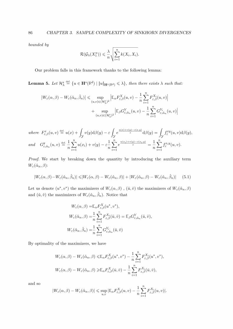
86 CHAPTER 3. SAMPLE COMPLEXITY OF SINKHORN DIVERGENCES
bounded by
R(Gλ(Xn1 )) 6 λ
n
√√√√ n∑i=1
k(Xi, Xi).
Our problem falls in this framework thanks to the following lemma:
Lemma 5. Let Hsλdef.= u ∈ Hs(Rd) | ||u||Hs(Rd) 6 λ, then there exists λ such that:
∣∣Wε(α, β)−Wε(αn, βn)∣∣ 6 sup
(u,v)∈(Hsλ
)2
∣∣∣EαFXε,β(u, v)− 1n
n∑i=1
FXiε,β(u, v)∣∣∣
+ sup(u,v)∈(Hs
λ)2
∣∣∣EβGYε,αn(u, v)− 1n
n∑i=1
GYiε,αn(u, v)∣∣∣
where F xε,β(u, v) def.= u(x) +∫Yv(y)dβ(y)− ε
∫Yeu(x)+v(y)−c(x,y)
ε dβ(y) =∫Yfxyε (u, v)dβ(y),
and Gyε,αn(u, v) def.= 1n
n∑i=1
u(xi) + v(y)− ε 1n
n∑i=1
eu(xi)+v(y)−c(xi,y)
ε = 1n
n∑i=1
fxiyε (u, v).
Proof. We start by breaking down the quantity by introducing the auxiliary termWε(αn, β):
|Wε(α, β)−Wε(αn, βn)| 6|Wε(α, β)−Wε(αn, β)|+ |Wε(αn, β)−Wε(αn, βn)| (5.1)
Let us denote (u∗, v∗) the maximizers of Wε(α, β) , (u, v) the maximizers of Wε(αn, β)and (u, v) the maximizers of Wε(αn, βn). Notice that
Wε(α, β) =EαFXε,β(u∗, v∗),
Wε(αn, β) = 1n
n∑i=1
FXiε,β(u, v) = EβGYε,αn(u, v),
Wε(αn, βn) = 1n
n∑i=1
GYiε,αn(u, v)
By optimality of the maximizers, we have
Wε(α, β)−Wε(αn, β) 6EαFXε,β(u∗, v∗)− 1
n
n∑i=1
FXiε,β(u∗, v∗),
Wε(α, β)−Wε(αn, β) >EαFXε,β(u, v)− 1
n
n∑i=1
FXiε,β(u, v),
and so|Wε(α, β)−Wε(αn, β)| 6 sup
u,v|EαFXε,β(u, v)− 1
n
n∑i=1
FXiε,β(u, v)|.
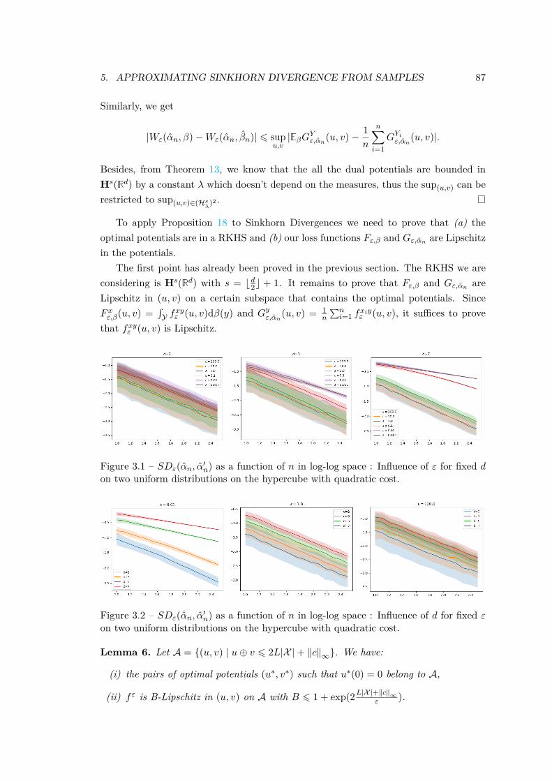
5. APPROXIMATING SINKHORN DIVERGENCE FROM SAMPLES 87
Similarly, we get
|Wε(αn, β)−Wε(αn, βn)| 6 supu,v|EβGYε,αn(u, v)− 1
n
n∑i=1
GYiε,αn(u, v)|.
Besides, from Theorem 13, we know that the all the dual potentials are bounded inHs(Rd) by a constant λ which doesn’t depend on the measures, thus the sup(u,v) can berestricted to sup(u,v)∈(Hs
λ)2 .
To apply Proposition 18 to Sinkhorn Divergences we need to prove that (a) theoptimal potentials are in a RKHS and (b) our loss functions Fε,β and Gε,αn are Lipschitzin the potentials.
The first point has already been proved in the previous section. The RKHS we areconsidering is Hs(Rd) with s = bd2c + 1. It remains to prove that Fε,β and Gε,αn areLipschitz in (u, v) on a certain subspace that contains the optimal potentials. SinceF xε,β(u, v) =
∫Y f
xyε (u, v)dβ(y) and Gyε,αn(u, v) = 1
n
∑ni=1 f
xiyε (u, v), it suffices to prove
that fxyε (u, v) is Lipschitz.
Figure 3.1 – SDε(αn, α′n) as a function of n in log-log space : Influence of ε for fixed don two uniform distributions on the hypercube with quadratic cost.
Figure 3.2 – SDε(αn, α′n) as a function of n in log-log space : Influence of d for fixed εon two uniform distributions on the hypercube with quadratic cost.
Lemma 6. Let A = (u, v) | u⊕ v 6 2L|X |+ ‖c‖∞. We have:
(i) the pairs of optimal potentials (u∗, v∗) such that u∗(0) = 0 belong to A,
(ii) f ε is B-Lipschitz in (u, v) on A with B 6 1 + exp(2L|X |+‖c‖∞ε ).
88 CHAPTER 3. SAMPLE COMPLEXITY OF SINKHORN DIVERGENCES
Proof. Let us prove that we can restrict ourselves to a subspace on which fε is Lipschitzin (u, v),
fε(u, v, x, y) = u(x) + v(y)− ε exp(u(x) + v(y)− c(x, y)
ε
),
∇fε(u, v) = 1− exp(u+ v − c
ε
).
To ensure that f ε is Lipschitz, we simply need to ensure that the quantity inside theexponential is upper bounded at optimality and then restrict the function to all (u, v)that satisfy that bound.
Recall the bounds on the optimal potentials from Proposition 17. We have that∀x ∈ X , y ∈ Y,
u(x) 6 L|x| and v(y) 6 maxx
u(x)− c(x, y).
Since we assumed X to be a bounded set, denoting by |X | the diameter of the space weget that at optimality ∀x ∈ X , y ∈ Y
u(x) + v(y) 6 2L|X |+ ‖c‖∞ .
Let us denote A = (u, v) ∈ (Hs(Rd))2 | u ⊕ v 6 2L|X | + ‖c‖∞, we have that∀(u, v) ∈ A,
|∇fε(u, v)| 6 1 + exp(2L|X |+ ‖c‖∞ε
).
We now have all the required elements to prove our sample complexity result on theSinkhorn loss, by applying Proposition 18.
Proof. (Theorem 14) Since Fε,β and Gε,αn are Lipschitz and we are optimizing overHs(Rd) which is a RKHS, we can apply Proposition 18 to bound the right hand sidein Lemma 5. We start by applying the proposition to the second term, taking theexpectation over β. We get:
Eβ|Wε(α, β)−Wε(αn, βn)| 6 sup(u,v)∈(Hs
λ)2|EαFXε,β(u, v)− 1
n
n∑i=1
FXiε,β(u, v)|
+ 2Bλn
Eβ
√√√√ n∑i=1
k(Yi, Yi),
where B 6 1 + exp(2L|X |+‖c‖∞ε ) (Lemma 6), λ = O(max(1, 1εd/2
)) (Theorem 13).We can further bound
√∑ni=1 k(Yi, Yi) by
√nmaxx∈X k(x, x) where k is the kernel
associated toHs(Rd) (usually called Matern or Sobolev kernel) and thus maxx∈X k(x, x) =k(0, 0) def.= K which does not depend on n or ε.
5. APPROXIMATING SINKHORN DIVERGENCE FROM SAMPLES 89
Applying Proposition 18 to the first term, taking the expectation over α. We get:
Eα⊗β|Wε(α, β)−Wε(αn, βn)| 6 22Bλ√K√
n.
Thus we get the convergence rate in 1√nwith different asymptotic behaviors in ε when
it is large or small.
Using similar arguments, we can also derive a concentration result:
Corollary 2. With probability at least 1− δ,
|Wε(α, β)−Wε(αn, βn)| 6 4BλK√n
+ C
√2 log 1
δ
n,
where B, λ,K are defined in the proof above, and C = κ + ε exp(κε ) with κ = 2L|X | +‖c‖∞.
Proof. We apply the bounded differences inequality (McDiarmid, 1989) to
g : (x1, . . . , xn) 7→ supu,v∈Hs
λ
(EfXYε − 1nfXi,Yiε ).
From Lemma 6 we get that ∀x, y, fxyε (u, v) 6 κ+ εeκ/εdef.= C, and thus, changing one of
the variables in g changes the value of the function by at most 2C/n. Thus the boundeddifferences inequality gives
P (|g(X1, . . . , Xn)− Eg(X1, . . . , Xn)| > t) 6 2 exp(t2n
2C2
).
Choosing t = C
√2 log 1
δn yields that with probability at least 1− δ
g(X1, . . . , Xn) 6 Eg(X1, . . . , Xn) + C
√2 log 1
δ
n,
and from Theorem 14 we already have
Eg(X1, . . . , Xn) = E supu,v∈Hs
λ
(EfXYε − 1nfXi,Yiε ) 6 2BλK√
n.
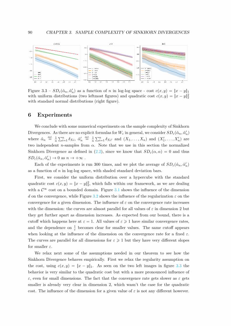
90 CHAPTER 3. SAMPLE COMPLEXITY OF SINKHORN DIVERGENCES
Figure 3.3 – SDε(αn, α′n) as a function of n in log-log space - cost c(x, y) = ||x − y||1with uniform distributions (two leftmost figures) and quadratic cost c(x, y) = ||x − y||22with standard normal distributions (right figure).
6 Experiments
We conclude with some numerical experiments on the sample complexity of SinkhornDivergences. As there are no explicit formulas forWε in general, we consider SDε(αn, α′n)where αn
def.= 1n
∑ni=1 δXi, α′n
def.= 1n
∑ni=1 δXi′ and (X1, . . . , Xn) and (X ′1, . . . , X ′n) are
two independent n-samples from α. Note that we use in this section the normalizedSinkhorn Divergence as defined in (2.2), since we know that SDε(α, α) = 0 and thusSDε(αn, α′n)→ 0 as n→ +∞ .
Each of the experiments is run 300 times, and we plot the average of SDε(αn, α′n)as a function of n in log-log space, with shaded standard deviation bars.
First, we consider the uniform distribution over a hypercube with the standardquadratic cost c(x, y) = ||x − y||22, which falls within our framework, as we are dealingwith a C∞ cost on a bounded domain. Figure 3.1 shows the influence of the dimensiond on the convergence, while Figure 3.2 shows the influence of the regularization ε on theconvergence for a given dimension. The influence of ε on the convergence rate increaseswith the dimension: the curves are almost parallel for all values of ε in dimension 2 butthey get further apart as dimension increases. As expected from our bound, there is acutoff which happens here at ε = 1. All values of ε > 1 have similar convergence rates,and the dependence on 1
ε becomes clear for smaller values. The same cutoff appearswhen looking at the influence of the dimension on the convergence rate for a fixed ε.The curves are parallel for all dimensions for ε > 1 but they have very different slopesfor smaller ε.
We relax next some of the assumptions needed in our theorem to see how theSinkhorn Divergence behaves empirically. First we relax the regularity assumption onthe cost, using c(x, y) = ||x − y||1. As seen on the two left images in figure 3.3 thebehavior is very similar to the quadratic cost but with a more pronounced influence ofε, even for small dimensions. The fact that the convergence rate gets slower as ε getssmaller is already very clear in dimension 2, which wasn’t the case for the quadraticcost. The influence of the dimension for a given value of ε is not any different however.

6. EXPERIMENTS 91
We also relax the bounded domain assumption, considering a standard normal dis-tribution over Rd with a quadratic cost. While the influence of ε on the convergencerate is still obvious, the influence of the dimension is less clear. There is also a highervariance, which can be expected as the concentration bound from Corollary 2 dependson the diameter of the domain.
For all curves, we observe that d and ε impact variance, with much smaller variancefor small values of ε and high dimensions. From the concentration bound, the depen-dency on ε coming from the uniform bound on fε is of the form ε exp(κ/ε), suggestinghigher variance for small values of ε. This could indicate that our uniform bound onfε is not tight, and we should consider other methods to get tighter bounds in furtherwork.

92 CHAPTER 3. SAMPLE COMPLEXITY OF SINKHORN DIVERGENCES
Chapter 4
Stochastic Optimization forLarge-Scale Optimal Transport
Entropy-regularized Optimal Transport (OT) has alleviated the computational burden of OT,for many applications. However, its state of the art solver, Sinkhorn’s algorithm, only copes withdiscrete measures and its iteration complexity scales as O(n2) (where n is the number of points inthe discrete measures). We thus propose a new class of online stochastic optimization algorithmsto cope with large-scale OT problems. They can handle arbitrary distributions (discrete or con-tinuous) as long as one is able to draw samples from them. This alleviates the need to discretizethese densities, while giving access to provably convergent methods without discretization error.These algorithms rely on one key idea which is that the dual OT problem can be re-cast as themaximization of an expectation.
We exploit this formulation in three different setups: (i) when comparing a discrete distribu-tion to another, we show that incremental stochastic optimization schemes can beat Sinkhorn’salgorithm, the current state-of-the-art finite dimensional OT solver; (ii) when comparing a dis-crete distribution to a continuous density, a semi-discrete reformulation of the dual programis amenable to averaged stochastic gradient descent (SGD), leading to better performance thanapproximately solving the problem by discretization ; (iii) when dealing with two continuous den-sities, we propose a stochastic gradient descent over a reproducing kernel Hilbert space (RKHS)and introduce an approximate feature approach (via incomplete Cholesky decomposition or Ran-dom Fourier Features) to significantly alleviate computational time. This is currently the onlyknown method to solve this problem, apart from computing OT on finite samples. We backupthese claims on a set of discrete, semi-discrete and continuous benchmark problems.
Most of the content in this chapter comes from (Genevay et al., 2016), but the section oncontinuous transport is revised in the light of recent results from Genevay et al. (2019). Knowingthat dual potentials are uniformly bounded in a RKHS, we can state a stronger version of theconvergence theorem for kernel-SGD. The numerical experiments are also improved, in particularthanks to the addition of the approximate features approach.
93
94 CHAPTER 4. STOCHASTIC OPTIMIZATION FOR LARGE SCALE OT
1 Introduction
Throughout this thesis, we have already advocated that OT is the natural choice tosolve a large variety of problems which require comparing probability measures or datain the form of histograms, in particular because it takes into account the underlyinggeometry of the problem. However, this comes at the price of an enormous computa-tional overhead, compared to geometrically-oblivious distances such as the Euclideanor χ2 distances or the Kullback-Leibler divergence. This is especially true because cur-rent OT solvers require to sample beforehand the distributions on a pre-defined set ofpoints, or on a grid. This is both inefficient (in term of storage and speed) and counter-intuitive. Indeed, most high-dimensional computational scenarios naturally representdistributions as objects from which one can sample, not as density functions to be dis-cretized. Our goal is to alleviate these shortcomings. We propose a class of provablyconvergent stochastic optimization schemes that can handle both discrete and continu-ous distributions through sampling.
Previous works. The prevalent way to compute OT distances is by solving the so-called Kantorovitch problem (Kantorovich, 1942) (see Chapter 1, Sec. 2.3 for a shortprimer on the basics of OT formulations), which boils down to a large-scale linearprogram when dealing with discrete distributions (i.e., finite weighted sums of Diracmasses). This linear program can be solved using network flow solvers, which can befurther refined to assignment problems when comparing measures of the same size withuniform weights (Burkard et al., 2009). Recently, regularized approaches that solve theOT with an entropic penalization (Cuturi, 2013) have been shown to be extremely effi-cient to approximate OT solutions at a very low computational cost. These regularizedapproaches have supported recent applications of OT to computer graphics (Solomonet al., 2015) and machine learning (Frogner et al., 2015). These methods apply thecelebrated Sinkhorn algorithm (Sinkhorn, 1964), and can be extended to solve a varietyof transportation-related problems such as the computation of barycenters for the opti-mal transport metric or multimarginal optimal transport (Benamou et al., 2015). Theirchief computational advantage over competing solvers is that each iteration boils downto matrix-vector multiplications, which can be easily parallelized, streams extremelywell on GPU, and enjoys linear-time implementation on regular grids or triangulateddomains (Solomon et al., 2015).
These methods are however purely discrete and cannot cope with continuous densi-ties. The only known class of methods that can overcome this limitation are so-calledsemi-discrete solvers (Aurenhammer et al., 1998), that can be implemented efficientlyusing computational geometry primitives (Mérigot, 2011). They can compute distancebetween a discrete distribution and a continuous density. Nonetheless, they are re-stricted to the Euclidean squared cost, and can only be implemented in low dimensions
1. INTRODUCTION 95
(2-D and 3-D). Solving these semi-discrete problems efficiently could have a significantimpact for applications to density fitting with an OT loss (Bassetti et al., 2006) formachine learning applications, see (Montavon et al., 2016). Lastly, let us point out thatthere is currently no method that can compute OT distances between two continuousdensities, which is thus an open problem we tackle in this chapter.
Contributions. This chapter introduces stochastic optimization methods to computelarge-scale optimal transport in all three possible settings: discrete OT, to compare adiscrete vs. another discrete measure; semi-discrete OT, to compare a discrete vs. a con-tinuous measure; and continuous OT, to compare a continuous vs. another continuousmeasure. These methods can be used to solve classical OT problems, but they en-joy faster convergence properties when considering their entropic-regularized versions.We show that the discrete regularized OT problem can be tackled using incremen-tal algorithms, and we consider in particular the stochastic averaged gradient (SAG)method (Schmidt et al., 2016). Each iteration of that algorithm requires n operations(n being the size of the supports of the input distributions), which makes it scale betterin large-scale problems than the state-of-the-art Sinkhorn algorithm, while still enjoy-ing a convergence rate of O(1/k), k being the number of iterations. We show thatthe semi-discrete OT problem can be solved using averaged stochastic gradient descent(SGD), whose convergence rate is O(1/
√k). This approach is numerically advantageous
over the brute force approach consisting in sampling first the continuous density tosolve next a discrete OT problem. Following the publication of this work, this onlinesemi-discrete algorithm has been successfully applied to texture synthesis in image pro-cessing (Galerne et al., 2018), and to the computation of Wasserstein Barycenters (Staibet al., 2017). Lastly, for continuous optimal transport, we propose a novel method whichmakes use of an expansion of the dual variables in a reproducing kernel Hilbert space(RKHS). This allows us for the first time to compute with a converging algorithm OTdistances between two arbitrary densities, thanks to the fact that the dual potentialsare known to be in a RKHS ball(see Chapter 3 for details). We also provide an ap-proach using approximate features (via incomplete Cholesky decomposition (Wu et al.,2006) or Random Fourier features (Rahimi and Recht, 2007)) to significantly alleviatecomputational time (going from quadratic to linear in the number of iterations). Morerecently, (Seguy et al., 2017) exploited our dual formulation as an expectation with aneural network parametrization of the dual variables rather than a RKHS expansion.This gives interesting results on the tasks they consider, although they do not deriveconvergence rates for their approach.

96 CHAPTER 4. STOCHASTIC OPTIMIZATION FOR LARGE SCALE OT
2 Optimal Transport: Primal, Dual and Semi-dual For-mulations
We consider the optimal transport problem between two measures α ∈M1+(X ) and
β ∈ M1+(Y), defined on metric spaces X and Y. No particular assumption is made on
the form of α and β, we only assume that they both can be sampled from to be able toapply our algorithms.
2.1 Primal, Dual and Semi-dual Formulations.
In this section, we recall the different formulations of entropy-regularized optimaltransport which will be exploited in the remainder of the chapter. We refer the readerto Chapter 1 for more details on their derivation and specific properties.
As previously, we consider the Kantorovich formulation (Kantorovich, 1942) of OTwith entropic regularization (Cuturi, 2013) between two probability measures α ∈M1
+(X ) and β ∈M1+(Y) :
Wε(α, β) def.= minπ∈Π(α,β)
∫X×Y
c(x, y)dπ(x, y) + ε
∫X×Y
log( dπ(x, y)
dα(x)dβ(y)
)dπ(x, y), (Pε)
where the constraint set Π(α, β) is the set of couplings on X ×Y with marginals α andβ.
When ε > 0, problem (Pε) is strictly convex, so that the optimal π is unique, andalgebraic properties of the entropy H result in computations that can be tackled usingSinkhorn’s algorithm which is extensively described in Chapter 1, Sec. 4.2.
Recall from Chapter 1, Proposition 7, that entropy-regularized OT between twoprobability measures α and β has an equivalent dual formulation:
Wε(α, β) = maxu∈C(X ),v∈C(Y)
∫Xu(x)dα(x) +
∫Yv(y)dβ(y)
− ε∫X×Y
eu(x)+v(y)−c(x,y)
ε dα(x)dβ(y) + ε, (Dε)
and the primal-dual relationship is given by
dπ(x, y) = exp(u(x) + v(y)− c(x, y)ε
)dα(x)dβ(y).
A nice feature of entropy-regularized OT, which we already highlighted, is the factthat it yields an unconstrained dual problem, contrarily to standard OT. The third termin the dual ε
∫X×Y e
u(x)+v(y)−c(x,y)ε dα(x)dβ(y) is a smooth approximation of the indicator
of the constraint set Uc set that appears in the dual of standard OT:
Ucdef.= (u, v) ∈ C(X )× C(Y) ; ∀(x, y) ∈ X × Y, u(x) + v(y) 6 c(x, y) .
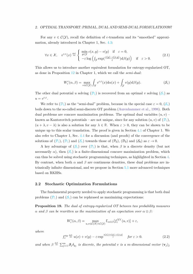
2. OPTIMAL TRANSPORT: PRIMAL, DUAL AND SEMI-DUAL FORMULATIONS97
For any v ∈ C(Y), recall the definition of c-transform and its “smoothed” approxi-mation, already introduced in Chapter 1, Sec. 4.3:
∀x ∈ X , vc,ε(x) def.=
miny∈Y
c(x, y)− v(y) if ε = 0,
−ε log(∫Y exp(v(y)−c(x,y)
ε )dβ(y))
if ε > 0.(2.1)
This allows us to introduce another equivalent formulation for entropy-regularized OT,as done in Proposition 12 in Chapter 1, which we call the semi-dual:
W cε (α, β) = max
v∈C(Y)
∫Xvc,ε(x)dα(x) +
∫Yv(y)dβ(y). (Sε)
The other dual potential u solving (Dε) is recovered from an optimal v solving (Sε) asu = vc,ε.
We refer to (Dε) as the “semi-dual” problem, because in the special case ε = 0, (Sε)boils down to the so-called semi-discrete OT problem (Aurenhammer et al., 1998). Bothdual problems are concave maximization problems. The optimal dual variables (u, v) –known as Kantorovitch potentials – are not unique, since for any solution (u, v) of (Dε),(u + λ, v − λ) is also a solution for any λ ∈ R. When ε > 0, they can be shown to beunique up to this scalar translation. The proof is given in Section 4.1 of Chapter 1. Wealso refer to Chapter 1, Sec. 4.4 for a discussion (and proofs) of the convergence of thesolutions of (Pε), (Dε) and (Sε) towards those of (P0), (D0) and (S0) as ε→ 0.
A key advantage of (Sε) over (Dε) is that, when β is a discrete density (but notnecessarily α), then (Sε) is a finite-dimensional concave maximization problem, whichcan thus be solved using stochastic programming techniques, as highlighted in Section 4.By contrast, when both α and β are continuous densities, these dual problems are in-trinsically infinite dimensional, and we propose in Section 5.1 more advanced techniquesbased on RKHSs.
2.2 Stochastic Optimization Formulations
The fundamental property needed to apply stochastic programming is that both dualproblems (Dε) and (Sε) can be rephrased as maximizing expectations:
Proposition 19. The dual of entropy-regularized OT between two probability measuresα and β can be rewritten as the maximization of an expectation over α⊗ β:
W cε (α, β) = max
u,v∈C(X )×C(Y)Eα⊗β[fXYε (u, v)] + ε,
wherefxyε
def.= u(x) + v(y)− ε expu(x)+v(y)−c(x,y)
ε for ε > 0. (2.2)
and when βdef.=∑mj=1 βjδyj is discrete, the potential v is a m-dimensional vector (vj)j
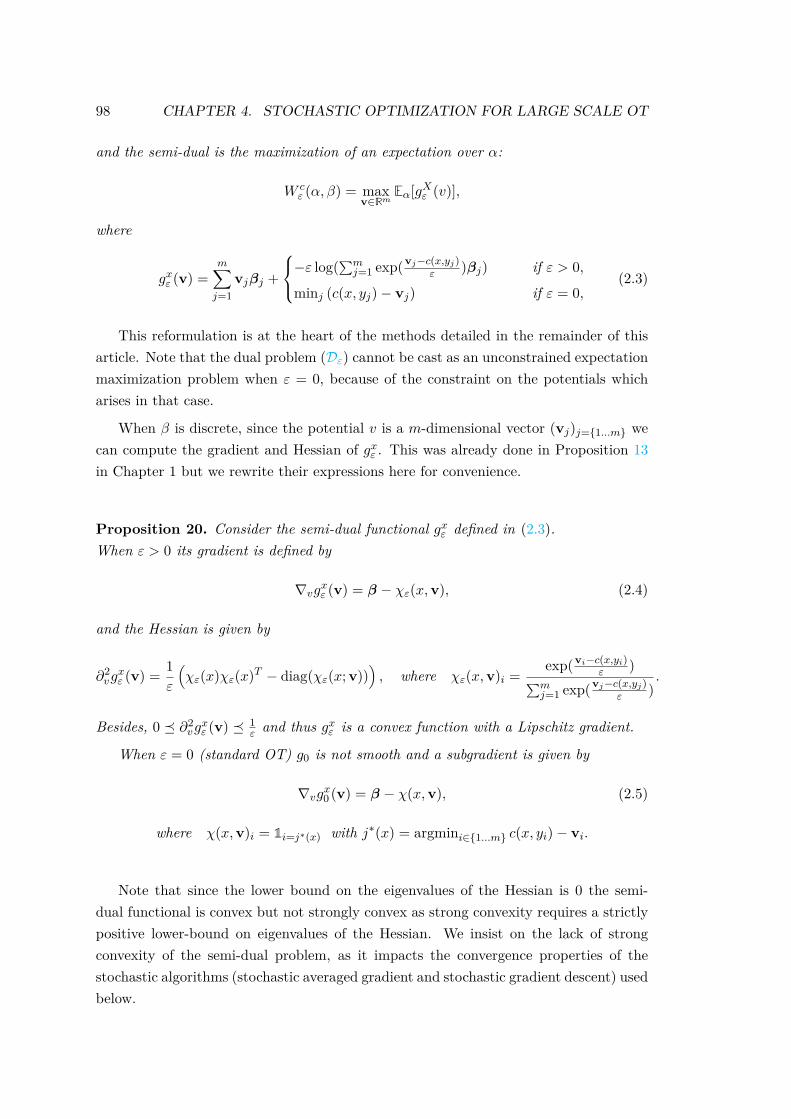
98 CHAPTER 4. STOCHASTIC OPTIMIZATION FOR LARGE SCALE OT
and the semi-dual is the maximization of an expectation over α:
W cε (α, β) = max
v∈RmEα[gXε (v)],
where
gxε (v) =m∑j=1
vjβj +
−ε log(∑mj=1 exp(vj−c(x,yj)
ε )βj) if ε > 0,
minj (c(x, yj)− vj) if ε = 0,(2.3)
This reformulation is at the heart of the methods detailed in the remainder of thisarticle. Note that the dual problem (Dε) cannot be cast as an unconstrained expectationmaximization problem when ε = 0, because of the constraint on the potentials whicharises in that case.
When β is discrete, since the potential v is a m-dimensional vector (vj)j=1...m wecan compute the gradient and Hessian of gxε . This was already done in Proposition 13in Chapter 1 but we rewrite their expressions here for convenience.
Proposition 20. Consider the semi-dual functional gxε defined in (2.3).When ε > 0 its gradient is defined by
∇vgxε (v) = β − χε(x,v), (2.4)
and the Hessian is given by
∂2vgxε (v) = 1
ε
(χε(x)χε(x)T − diag(χε(x; v))
), where χε(x,v)i =
exp(vi−c(x,yi)ε )∑m
j=1 exp(vj−c(x,yj)ε )
.
Besides, 0 ∂2vgxε (v) 1
ε and thus gxε is a convex function with a Lipschitz gradient.
When ε = 0 (standard OT) g0 is not smooth and a subgradient is given by
∇vgx0 (v) = β − χ(x,v), (2.5)
where χ(x,v)i = 1i=j∗(x) with j∗(x) = argmini∈1...m c(x, yi)− vi.
Note that since the lower bound on the eigenvalues of the Hessian is 0 the semi-dual functional is convex but not strongly convex as strong convexity requires a strictlypositive lower-bound on eigenvalues of the Hessian. We insist on the lack of strongconvexity of the semi-dual problem, as it impacts the convergence properties of thestochastic algorithms (stochastic averaged gradient and stochastic gradient descent) usedbelow.
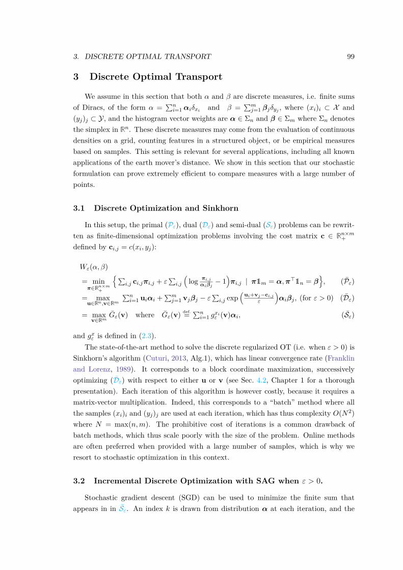
3. DISCRETE OPTIMAL TRANSPORT 99
3 Discrete Optimal Transport
We assume in this section that both α and β are discrete measures, i.e. finite sumsof Diracs, of the form α =
∑ni=1 αiδxi and β =
∑mj=1 βjδyj , where (xi)i ⊂ X and
(yj)j ⊂ Y, and the histogram vector weights are α ∈ Σn and β ∈ Σm where Σn denotesthe simplex in Rn. These discrete measures may come from the evaluation of continuousdensities on a grid, counting features in a structured object, or be empirical measuresbased on samples. This setting is relevant for several applications, including all knownapplications of the earth mover’s distance. We show in this section that our stochasticformulation can prove extremely efficient to compare measures with a large number ofpoints.
3.1 Discrete Optimization and Sinkhorn
In this setup, the primal (Pε), dual (Dε) and semi-dual (Sε) problems can be rewrit-ten as finite-dimensional optimization problems involving the cost matrix c ∈ Rn×m+defined by ci,j = c(xi, yj):
Wε(α, β)
= minπ∈Rn×m+
∑i,j ci,jπi,j + ε
∑i,j
(log πi,j
αiβj− 1
)πi,j | π1m = α,π>1n = β
, (Pε)
= maxu∈Rn,v∈Rm
∑ni=1 uiαi +
∑mj=1 vjβj − ε
∑i,j exp
(ui+vj−ci,j
ε
)αiβj , (for ε > 0) (Dε)
= maxv∈Rm
Gε(v) where Gε(v) def.=∑ni=1 g
xiε (v)αi, (Sε)
and gxε is defined in (2.3).The state-of-the-art method to solve the discrete regularized OT (i.e. when ε > 0) is
Sinkhorn’s algorithm (Cuturi, 2013, Alg.1), which has linear convergence rate (Franklinand Lorenz, 1989). It corresponds to a block coordinate maximization, successivelyoptimizing (Dε) with respect to either u or v (see Sec. 4.2, Chapter 1 for a thoroughpresentation). Each iteration of this algorithm is however costly, because it requires amatrix-vector multiplication. Indeed, this corresponds to a “batch” method where allthe samples (xi)i and (yj)j are used at each iteration, which has thus complexity O(N2)where N = max(n,m). The prohibitive cost of iterations is a common drawback ofbatch methods, which thus scale poorly with the size of the problem. Online methodsare often preferred when provided with a large number of samples, which is why weresort to stochastic optimization in this context.
3.2 Incremental Discrete Optimization with SAG when ε > 0.
Stochastic gradient descent (SGD) can be used to minimize the finite sum thatappears in in Sε. An index k is drawn from distribution α at each iteration, and the

100 CHAPTER 4. STOCHASTIC OPTIMIZATION FOR LARGE SCALE OT
gradient of that term gxkε (·) can be used as a proxy for the full gradient in a standardgradient ascent step to maximize Gε.
Algorithm 3 SAG for Discrete OTInput: step size C ∈ R+
Output: dual potential v ∈ Rm
v← 0m (dual potential)DG← 0m (proxy of the full gradient ∇Gε)∀i, zi ← 0m (vector of partial gradients ∇gxkε )for k = 1, 2, . . . do
Sample i ∈ 1, 2, . . . , n uniform.DG← DG− zi (remove contribution of sample xi from proxy of ∇Gε)zi ← αi∇vgxiε (v) (update gradient of sample xi)DG← d + zi (update proxy of ∇Gε with contribution of sample xi)v← v + Cd (gradient ascent step)
end for
When ε > 0, the finite sum appearing in (Sε) suggests to use incremental gradientmethods – rather than purely stochastic ones – which are known to converge faster thanSGD. We propose to use the stochastic averaged gradient (SAG) (Schmidt et al., 2016).The iterates of SAG can be summarized by the following formula
v(k+1) = v(k) + C
n
n∑i=1
z(k)i ,
where an index i(k) is selected at random in 1 . . . n and
z(k)i =
∇gxiε (v(k)) if i = i(k),
z(k−1)i otherwise.
At each iteration an index ik is selected at random in 1 . . . n to compute ∇gxikε (v(k)),the gradient corresponding to the sample xi(k) at the current estimate v(k). However,SAG doesn’t use this as a proxy for the full gradient ∇Gε, but rather keeps in memorya copy of that gradient and computes an average of all gradients stored so far whichprovides a better proxy of the gradient corresponding to the entire sum. Another dif-ference is that SAG applies a fixed length update, which gives a better convergence ratethan SGD:
Proposition 21. Consider v∗ε a minimizer of Gε, and v(k) that k−th iterate of SAGdefined in (3.2). Then:
|Gε(v∗ε)− Gε(vk)| = O(1/k).
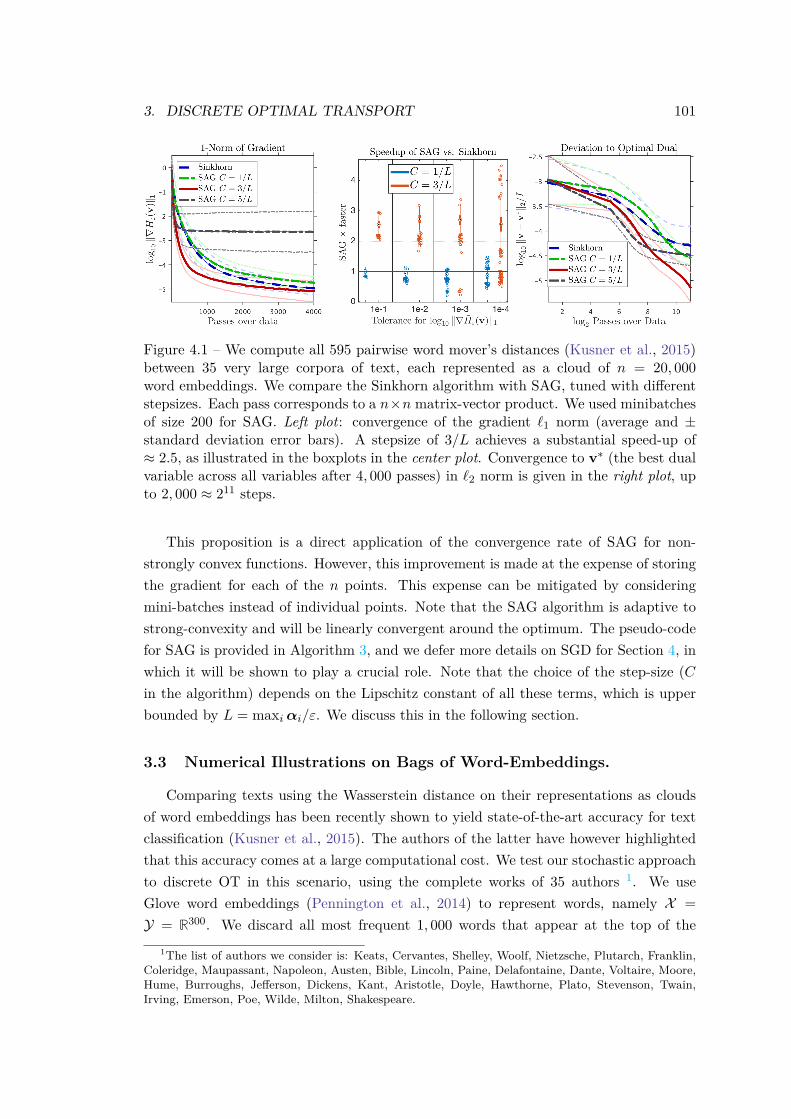
3. DISCRETE OPTIMAL TRANSPORT 101
Figure 4.1 – We compute all 595 pairwise word mover’s distances (Kusner et al., 2015)between 35 very large corpora of text, each represented as a cloud of n = 20, 000word embeddings. We compare the Sinkhorn algorithm with SAG, tuned with differentstepsizes. Each pass corresponds to a n×n matrix-vector product. We used minibatchesof size 200 for SAG. Left plot: convergence of the gradient `1 norm (average and ±standard deviation error bars). A stepsize of 3/L achieves a substantial speed-up of≈ 2.5, as illustrated in the boxplots in the center plot. Convergence to v∗ (the best dualvariable across all variables after 4, 000 passes) in `2 norm is given in the right plot, upto 2, 000 ≈ 211 steps.
This proposition is a direct application of the convergence rate of SAG for non-strongly convex functions. However, this improvement is made at the expense of storingthe gradient for each of the n points. This expense can be mitigated by consideringmini-batches instead of individual points. Note that the SAG algorithm is adaptive tostrong-convexity and will be linearly convergent around the optimum. The pseudo-codefor SAG is provided in Algorithm 3, and we defer more details on SGD for Section 4, inwhich it will be shown to play a crucial role. Note that the choice of the step-size (Cin the algorithm) depends on the Lipschitz constant of all these terms, which is upperbounded by L = maxi αi/ε. We discuss this in the following section.
3.3 Numerical Illustrations on Bags of Word-Embeddings.
Comparing texts using the Wasserstein distance on their representations as cloudsof word embeddings has been recently shown to yield state-of-the-art accuracy for textclassification (Kusner et al., 2015). The authors of the latter have however highlightedthat this accuracy comes at a large computational cost. We test our stochastic approachto discrete OT in this scenario, using the complete works of 35 authors 1. We useGlove word embeddings (Pennington et al., 2014) to represent words, namely X =Y = R300. We discard all most frequent 1, 000 words that appear at the top of the
1The list of authors we consider is: Keats, Cervantes, Shelley, Woolf, Nietzsche, Plutarch, Franklin,Coleridge, Maupassant, Napoleon, Austen, Bible, Lincoln, Paine, Delafontaine, Dante, Voltaire, Moore,Hume, Burroughs, Jefferson, Dickens, Kant, Aristotle, Doyle, Hawthorne, Plato, Stevenson, Twain,Irving, Emerson, Poe, Wilde, Milton, Shakespeare.
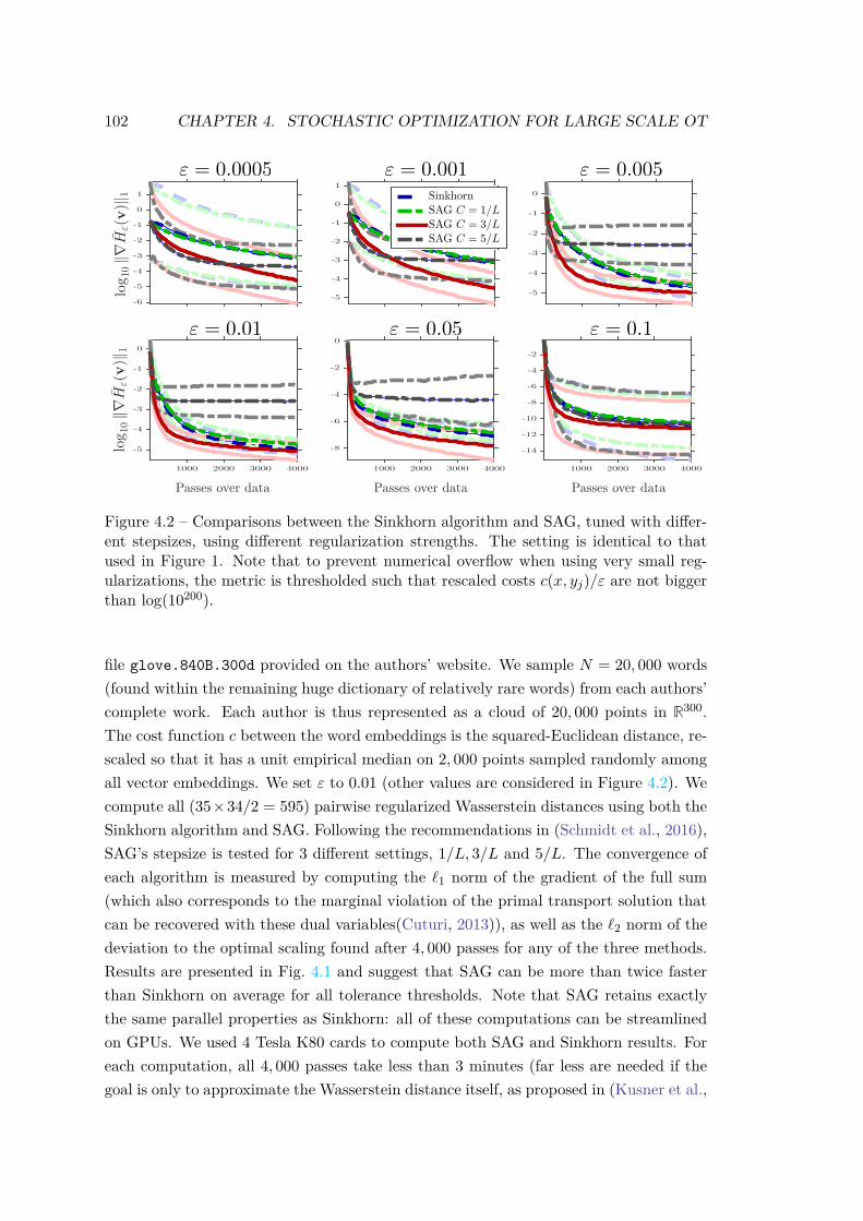
102 CHAPTER 4. STOCHASTIC OPTIMIZATION FOR LARGE SCALE OT
1000 2000 3000 4000
log10∥∇
Hε(v
)∥ 1
-6
-5
-4
-3
-2
-1
0
1
1000 2000 3000 4000
-5
-4
-3
-2
-1
0
1
SinkhornSAG C = 1/LSAG C = 3/LSAG C = 5/L
1000 2000 3000 4000
-5
-4
-3
-2
-1
0
Passes over data1000 2000 3000 4000
log10∥∇
Hε(v
)∥ 1
-5
-4
-3
-2
-1
0
Passes over data1000 2000 3000 4000
-8
-6
-4
-2
0
Passes over data1000 2000 3000 4000
-14
-12
-10
-8
-6
-4
-2
1000 2000 3000 4000
log10∥∇
Hε(v
)∥ 1
-6
-5
-4
-3
-2
-1
0
1
1000 2000 3000 4000
-5
-4
-3
-2
-1
0
1
SinkhornSAG C = 1/LSAG C = 3/LSAG C = 5/L
1000 2000 3000 4000
-5
-4
-3
-2
-1
0
Passes over data1000 2000 3000 4000
log10∥∇
Hε(v
)∥ 1
-5
-4
-3
-2
-1
0
Passes over data1000 2000 3000 4000
-8
-6
-4
-2
0
Passes over data1000 2000 3000 4000
-14
-12
-10
-8
-6
-4
-2
1000 2000 3000 4000
log 1
0∥∇
Hε(v)∥
1
-6
-5
-4
-3
-2
-1
0
1
1000 2000 3000 4000
-5
-4
-3
-2
-1
0
1
SinkhornSAG C = 1/LSAG C = 3/LSAG C = 5/L
1000 2000 3000 4000
-5
-4
-3
-2
-1
0
Passes over data1000 2000 3000 4000
log 1
0∥∇
Hε(v)∥
1
-5
-4
-3
-2
-1
0
Passes over data1000 2000 3000 4000
-8
-6
-4
-2
0
Passes over data1000 2000 3000 4000
-14
-12
-10
-8
-6
-4
-2
1000 2000 3000 4000
log 1
0∥∇
Hε(v
)∥1
-6
-5
-4
-3
-2
-1
0
1
1000 2000 3000 4000
-5
-4
-3
-2
-1
0
1
SinkhornSAG C = 1/LSAG C = 3/LSAG C = 5/L
1000 2000 3000 4000
-5
-4
-3
-2
-1
0
Passes over data1000 2000 3000 4000
log 1
0∥∇
Hε(v
)∥1
-5
-4
-3
-2
-1
0
Passes over data1000 2000 3000 4000
-8
-6
-4
-2
0
Passes over data1000 2000 3000 4000
-14
-12
-10
-8
-6
-4
-2
1000 2000 3000 4000
log10∥∇
Hε(v
)∥1
-6
-5
-4
-3
-2
-1
0
1
1000 2000 3000 4000
-5
-4
-3
-2
-1
0
1
SinkhornSAG C = 1/LSAG C = 3/LSAG C = 5/L
1000 2000 3000 4000
-5
-4
-3
-2
-1
0
Passes over data1000 2000 3000 4000
log10∥∇
Hε(v
)∥1
-5
-4
-3
-2
-1
0
Passes over data1000 2000 3000 4000
-8
-6
-4
-2
0
Passes over data1000 2000 3000 4000
-14
-12
-10
-8
-6
-4
-2
1000 2000 3000 4000
log 1
0∥∇
Hε(v
)∥1
-6
-5
-4
-3
-2
-1
0
1
1000 2000 3000 4000
-5
-4
-3
-2
-1
0
1
SinkhornSAG C = 1/LSAG C = 3/LSAG C = 5/L
1000 2000 3000 4000
-5
-4
-3
-2
-1
0
Passes over data1000 2000 3000 4000
log 1
0∥∇
Hε(v
)∥1
-5
-4
-3
-2
-1
0
Passes over data1000 2000 3000 4000
-8
-6
-4
-2
0
Passes over data1000 2000 3000 4000
-14
-12
-10
-8
-6
-4
-2" = 0.0005 " = 0.001 " = 0.005
" = 0.01 " = 0.05 " = 0.1
Figure 4.2 – Comparisons between the Sinkhorn algorithm and SAG, tuned with differ-ent stepsizes, using different regularization strengths. The setting is identical to thatused in Figure 1. Note that to prevent numerical overflow when using very small reg-ularizations, the metric is thresholded such that rescaled costs c(x, yj)/ε are not biggerthan log(10200).
file glove.840B.300d provided on the authors’ website. We sample N = 20, 000 words(found within the remaining huge dictionary of relatively rare words) from each authors’complete work. Each author is thus represented as a cloud of 20, 000 points in R300.The cost function c between the word embeddings is the squared-Euclidean distance, re-scaled so that it has a unit empirical median on 2, 000 points sampled randomly amongall vector embeddings. We set ε to 0.01 (other values are considered in Figure 4.2). Wecompute all (35×34/2 = 595) pairwise regularized Wasserstein distances using both theSinkhorn algorithm and SAG. Following the recommendations in (Schmidt et al., 2016),SAG’s stepsize is tested for 3 different settings, 1/L, 3/L and 5/L. The convergence ofeach algorithm is measured by computing the `1 norm of the gradient of the full sum(which also corresponds to the marginal violation of the primal transport solution thatcan be recovered with these dual variables(Cuturi, 2013)), as well as the `2 norm of thedeviation to the optimal scaling found after 4, 000 passes for any of the three methods.Results are presented in Fig. 4.1 and suggest that SAG can be more than twice fasterthan Sinkhorn on average for all tolerance thresholds. Note that SAG retains exactlythe same parallel properties as Sinkhorn: all of these computations can be streamlinedon GPUs. We used 4 Tesla K80 cards to compute both SAG and Sinkhorn results. Foreach computation, all 4, 000 passes take less than 3 minutes (far less are needed if thegoal is only to approximate the Wasserstein distance itself, as proposed in (Kusner et al.,
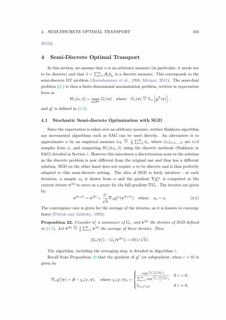
4. SEMI-DISCRETE OPTIMAL TRANSPORT 103
2015)).
4 Semi-Discrete Optimal Transport
In this section, we assume that α is an arbitrary measure (in particular, it needs notto be discrete) and that β =
∑mj=1 βjδyj is a discrete measure. This corresponds to the
semi-discrete OT problem (Aurenhammer et al., 1998; Mérigot, 2011). The semi-dualproblem (Sε) is then a finite-dimensional maximization problem, written in expectationform as
Wε(α, β) = maxv∈Rm
Gε(v) where Gε(v) def.= Eα[gXε (v)
],
and gxε is defined in (2.3).
4.1 Stochastic Semi-discrete Optimization with SGD
Since the expectation is taken over an arbitrary measure, neither Sinkhorn algorithmnor incremental algorithms such as SAG can be used directly. An alternative is toapproximate α by an empirical measure αN
def.= 1N
∑Ni=1 δxi where (xi)i=1,...,N are i.i.d
samples from α, and computing Wε(αN , β) using the discrete methods (Sinkhorn orSAG) detailed in Section 3. However this introduces a discretization noise in the solutionas the discrete problem is now different from the original one and thus has a differentsolution. SGD on the other hand does not require α to be discrete and is thus perfectlyadapted to this semi-discrete setting. The idea of SGD is fairly intuitive : at eachiteration, a sample xk is drawn from α and the gradient ∇gxkε is computed at thecurrent iterate v(k) to serve as a proxy for the full gradient ∇Gε. The iterates are givenby:
v(k+1) = v(k) + C√k∇vgxkε (v(k+1)) where xk ∼ α. (4.1)
The convergence rate is given for the average of the iterates, as it is known to convergefaster (Polyak and Juditsky, 1992):
Proposition 22. Consider v∗ε a minimizer of Gε, and v(k) the iterates of SGD definedin (4.1). Let v(k) def.= 1
k
∑ki=1 v(k) the average of these iterates. Then
|Gε(v∗ε)−Gε(v(k))| = O(1/√k).
The algorithm, including the averaging step, is detailed in Algorithm 4.Recall from Proposition 20 that the gradient of gxε (or subgradient, when ε = 0) is
given by
∇vgxε (v) = β − χε(x,v), where χε(x,v)i =
exp( vi−c(x,yi)
ε)∑m
j=1 exp(vj−c(x,yj)
ε)
if ε > 0,
1i=j∗(x) if ε = 0,
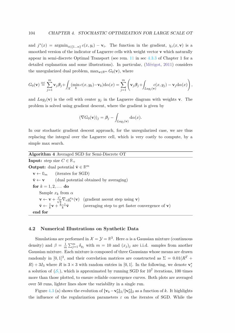
104 CHAPTER 4. STOCHASTIC OPTIMIZATION FOR LARGE SCALE OT
and j∗(x) = argmini∈1...n c(x, yi) − vi. The function in the gradient, χε(x,v) is asmoothed version of the indicator of Laguerre cells with weight vector v which naturallyappear in semi-discrete Optimal Transport (see rem. 11 in sec 4.3.3 of Chapter 1 for adetailed explanation and some illustrations). In particular, (Mérigot, 2011) considersthe unregularized dual problem, maxv∈Rm G0(v), where
G0(v) def.=m∑j=1
vjβj+∫X
(minkc(x, yk)−vk)dα(x) =
m∑j=1
(vjβj+
∫Lagj(v)
c(x, yj)− vjdα(x)),
and Lagj(v) is the cell with center yj in the Laguerre diagram with weights v. Theproblem is solved using gradient descent, where the gradient is given by
(∇G0(v))j = βj −∫Lagj(v)
dα(x).
In our stochastic gradient descent approach, for the unregularized case, we are thusreplacing the integral over the Laguerre cell, which is very costly to compute, by asimple max search.
Algorithm 4 Averaged SGD for Semi-Discrete OTInput: step size C ∈ R+
Output: dual potential v ∈ Rm
v← 0m (iterates for SGD)v← v (dual potential obtained by averaging)for k = 1, 2, . . . do
Sample xk from α
v← v + C√k∇vgxkε (v) (gradient ascent step using v)
v← 1kv + k−1
k v (averaging step to get faster convergence of v)end for
4.2 Numerical Illustrations on Synthetic Data
Simulations are performed in X = Y = R3. Here α is a Gaussian mixture (continuousdensity) and β = 1
m
∑mj=1 δyj with m = 10 and (xj)j are i.i.d. samples from another
Gaussian mixture. Each mixture is composed of three Gaussians whose means are drawnrandomly in [0, 1]3, and their correlation matrices are constructed as Σ = 0.01(RT +R) + 3I3 where R is 3× 3 with random entries in [0, 1]. In the following, we denote v∗εa solution of (Sε), which is approximated by running SGD for 107 iterations, 100 timesmore than those plotted, to ensure reliable convergence curves. Both plots are averagedover 50 runs, lighter lines show the variability in a single run.
Figure 4.3 (a) shows the evolution of ||vk−v∗0||2/||v∗0||2 as a function of k. It highlightsthe influence of the regularization parameters ε on the iterates of SGD. While the
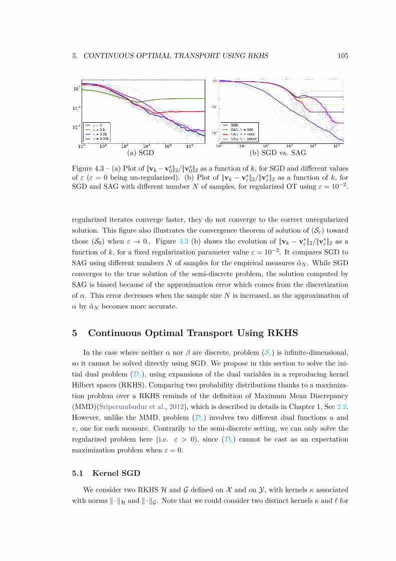
5. CONTINUOUS OPTIMAL TRANSPORT USING RKHS 105
(a) SGD (b) SGD vs. SAG
Figure 4.3 – (a) Plot of ||vk−v∗0||2/||v∗0||2 as a function of k, for SGD and different valuesof ε (ε = 0 being un-regularized). (b) Plot of ||vk − v∗ε||2/||v∗ε||2 as a function of k, forSGD and SAG with different number N of samples, for regularized OT using ε = 10−2.
regularized iterates converge faster, they do not converge to the correct unregularizedsolution. This figure also illustrates the convergence theorem of solution of (Sε) towardthose (S0) when ε → 0.. Figure 4.3 (b) shows the evolution of ||vk − v∗ε||2/||v∗ε||2 as afunction of k, for a fixed regularization parameter value ε = 10−2. It compares SGD toSAG using different numbers N of samples for the empirical measures αN . While SGDconverges to the true solution of the semi-discrete problem, the solution computed bySAG is biased because of the approximation error which comes from the discretizationof α. This error decreases when the sample size N is increased, as the approximation ofα by αN becomes more accurate.
5 Continuous Optimal Transport Using RKHS
In the case where neither α nor β are discrete, problem (Sε) is infinite-dimensional,so it cannot be solved directly using SGD. We propose in this section to solve the ini-tial dual problem (Dε), using expansions of the dual variables in a reproducing kernelHilbert spaces (RKHS). Comparing two probability distributions thanks to a maximiza-tion problem over a RKHS reminds of the definition of Maximum Mean Discrepancy(MMD)(Sriperumbudur et al., 2012), which is described in details in Chapter 1, Sec 2.2.However, unlike the MMD, problem (Dε) involves two different dual functions u andv, one for each measure. Contrarily to the semi-discrete setting, we can only solve theregularized problem here (i.e. ε > 0), since (Dε) cannot be cast as an expectationmaximization problem when ε = 0.
5.1 Kernel SGD
We consider two RKHS H and G defined on X and on Y, with kernels κ associatedwith norms ‖ ·‖H and ‖ ·‖G . Note that we could consider two distinct kernels κ and ` for
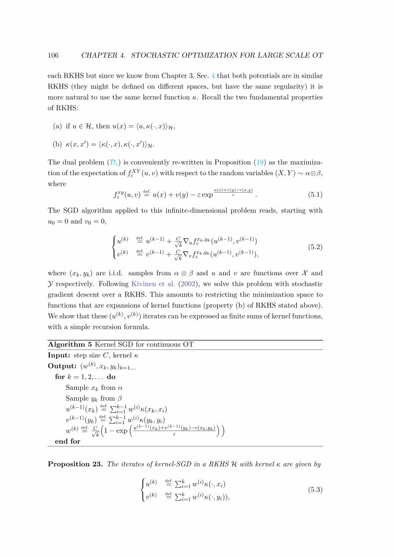
106 CHAPTER 4. STOCHASTIC OPTIMIZATION FOR LARGE SCALE OT
each RKHS but since we know from Chapter 3, Sec. 4 that both potentials are in similarRKHS (they might be defined on different spaces, but have the same regularity) it ismore natural to use the same kernel function κ. Recall the two fundamental propertiesof RKHS:
(a) if u ∈ H, then u(x) = 〈u, κ(·, x)〉H,
(b) κ(x, x′) = 〈κ(·, x), κ(·, x′)〉H.
The dual problem (Dε) is conveniently re-written in Proposition (19) as the maximiza-tion of the expectation of fXYε (u, v) with respect to the random variables (X,Y ) ∼ α⊗β,where
fxyε (u, v) def.= u(x) + v(y)− ε expu(x)+v(y)−c(x,y)
ε . (5.1)
The SGD algorithm applied to this infinite-dimensional problem reads, starting withu0 = 0 and v0 = 0, u
(k) def.= u(k−1) + C√k∇ufxk,ykε (u(k−1), v(k−1))
v(k) def.= v(k−1) + C√k∇vfxk,ykε (u(k−1), v(k−1)),
(5.2)
where (xk, yk) are i.i.d. samples from α ⊗ β and u and v are functions over X andY respectively. Following Kivinen et al. (2002), we solve this problem with stochasticgradient descent over a RKHS. This amounts to restricting the minimization space tofunctions that are expansions of kernel functions (property (b) of RKHS stated above).We show that these (u(k), v(k)) iterates can be expressed as finite sums of kernel functions,with a simple recursion formula.
Algorithm 5 Kernel SGD for continuous OTInput: step size C, kernel κOutput: (w(k), xk, yk)k=1,...
for k = 1, 2, . . . doSample xk from α
Sample yk from β
u(k−1)(xk)def.=∑k−1i=1 w
(i)κ(xk, xi)v(k−1)(yk)
def.=∑k−1i=1 w
(i)κ(yk, yi)w(k) def.= C√
k
(1− exp
(u(k−1)(xk)+v(k−1)(yk)−c(xk,yk)
ε
) )end for
Proposition 23. The iterates of kernel-SGD in a RKHS H with kernel κ are given byu(k) def.=
∑ki=1w
(i)κ(·, xi)
v(k) def.=∑ki=1w
(i)κ(·, yi)),(5.3)
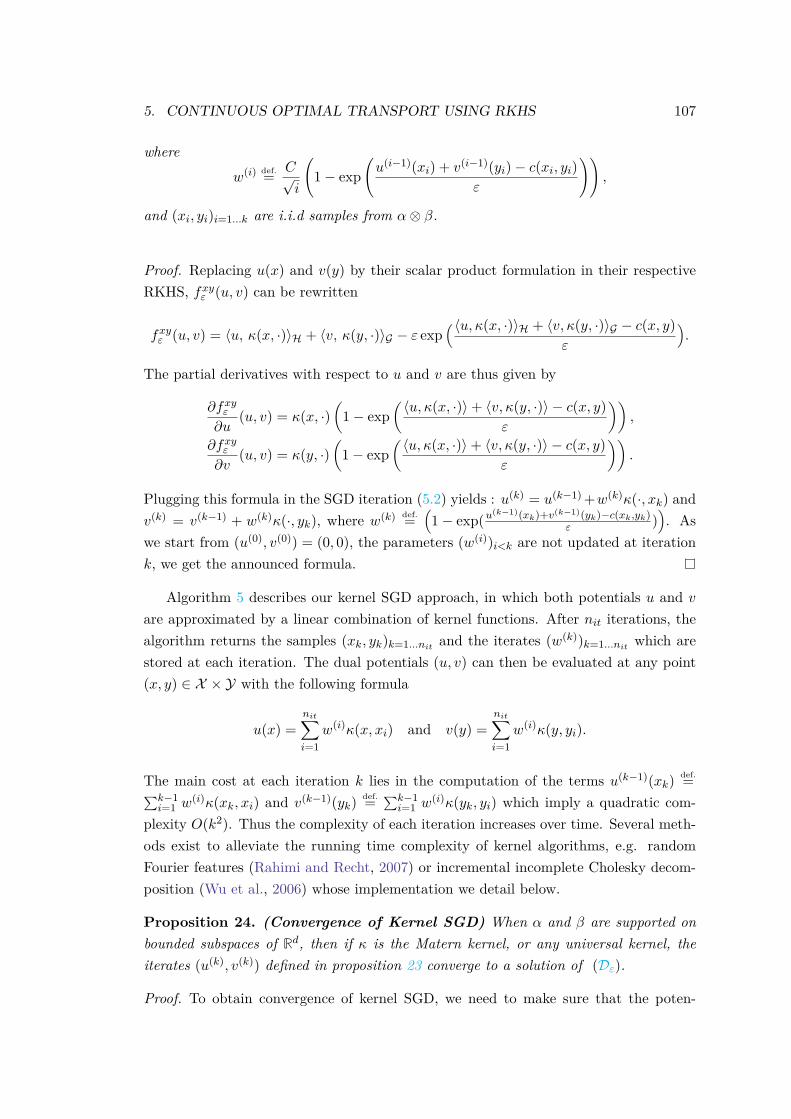
5. CONTINUOUS OPTIMAL TRANSPORT USING RKHS 107
wherew(i) def.= C√
i
(1− exp
(u(i−1)(xi) + v(i−1)(yi)− c(xi, yi)
ε
)),
and (xi, yi)i=1...k are i.i.d samples from α⊗ β.
Proof. Replacing u(x) and v(y) by their scalar product formulation in their respectiveRKHS, fxyε (u, v) can be rewritten
fxyε (u, v) = 〈u, κ(x, ·)〉H + 〈v, κ(y, ·)〉G − ε exp(〈u, κ(x, ·)〉H + 〈v, κ(y, ·)〉G − c(x, y)
ε
).
The partial derivatives with respect to u and v are thus given by
∂fxyε∂u
(u, v) = κ(x, ·)(
1− exp(〈u, κ(x, ·)〉+ 〈v, κ(y, ·)〉 − c(x, y)
ε
)),
∂fxyε∂v
(u, v) = κ(y, ·)(
1− exp(〈u, κ(x, ·)〉+ 〈v, κ(y, ·)〉 − c(x, y)
ε
)).
Plugging this formula in the SGD iteration (5.2) yields : u(k) = u(k−1) +w(k)κ(·, xk) andv(k) = v(k−1) + w(k)κ(·, yk), where w(k) def.=
(1− exp(u
(k−1)(xk)+v(k−1)(yk)−c(xk,yk)ε )
). As
we start from (u(0), v(0)) = (0, 0), the parameters (w(i))i<k are not updated at iterationk, we get the announced formula.
Algorithm 5 describes our kernel SGD approach, in which both potentials u and vare approximated by a linear combination of kernel functions. After nit iterations, thealgorithm returns the samples (xk, yk)k=1...nit and the iterates (w(k))k=1...nit which arestored at each iteration. The dual potentials (u, v) can then be evaluated at any point(x, y) ∈ X × Y with the following formula
u(x) =nit∑i=1
w(i)κ(x, xi) and v(y) =nit∑i=1
w(i)κ(y, yi).
The main cost at each iteration k lies in the computation of the terms u(k−1)(xk)def.=∑k−1
i=1 w(i)κ(xk, xi) and v(k−1)(yk)
def.=∑k−1i=1 w
(i)κ(yk, yi) which imply a quadratic com-plexity O(k2). Thus the complexity of each iteration increases over time. Several meth-ods exist to alleviate the running time complexity of kernel algorithms, e.g. randomFourier features (Rahimi and Recht, 2007) or incremental incomplete Cholesky decom-position (Wu et al., 2006) whose implementation we detail below.
Proposition 24. (Convergence of Kernel SGD) When α and β are supported onbounded subspaces of Rd, then if κ is the Matern kernel, or any universal kernel, theiterates (u(k), v(k)) defined in proposition 23 converge to a solution of (Dε).
Proof. To obtain convergence of kernel SGD, we need to make sure that the poten-
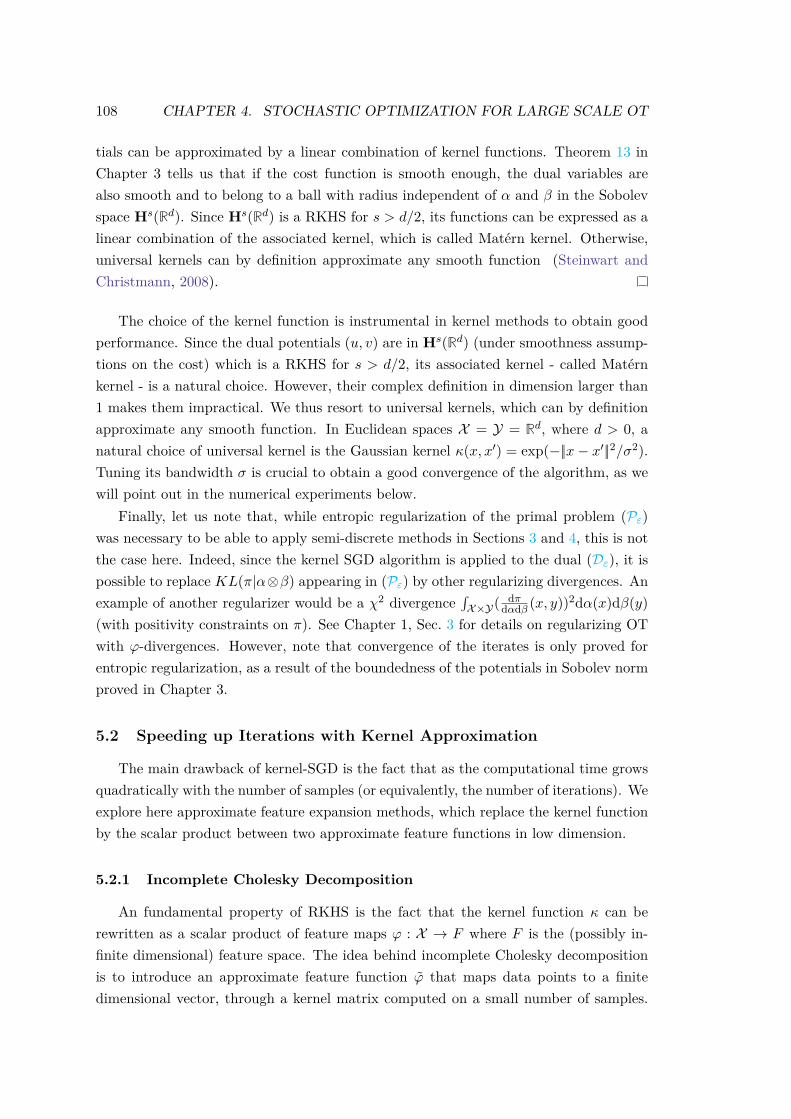
108 CHAPTER 4. STOCHASTIC OPTIMIZATION FOR LARGE SCALE OT
tials can be approximated by a linear combination of kernel functions. Theorem 13 inChapter 3 tells us that if the cost function is smooth enough, the dual variables arealso smooth and to belong to a ball with radius independent of α and β in the Sobolevspace Hs(Rd). Since Hs(Rd) is a RKHS for s > d/2, its functions can be expressed as alinear combination of the associated kernel, which is called Matérn kernel. Otherwise,universal kernels can by definition approximate any smooth function (Steinwart andChristmann, 2008).
The choice of the kernel function is instrumental in kernel methods to obtain goodperformance. Since the dual potentials (u, v) are in Hs(Rd) (under smoothness assump-tions on the cost) which is a RKHS for s > d/2, its associated kernel - called Matérnkernel - is a natural choice. However, their complex definition in dimension larger than1 makes them impractical. We thus resort to universal kernels, which can by definitionapproximate any smooth function. In Euclidean spaces X = Y = Rd, where d > 0, anatural choice of universal kernel is the Gaussian kernel κ(x, x′) = exp(−||x− x′||2/σ2).Tuning its bandwidth σ is crucial to obtain a good convergence of the algorithm, as wewill point out in the numerical experiments below.
Finally, let us note that, while entropic regularization of the primal problem (Pε)was necessary to be able to apply semi-discrete methods in Sections 3 and 4, this is notthe case here. Indeed, since the kernel SGD algorithm is applied to the dual (Dε), it ispossible to replace KL(π|α⊗β) appearing in (Pε) by other regularizing divergences. Anexample of another regularizer would be a χ2 divergence
∫X×Y( dπ
dαdβ (x, y))2dα(x)dβ(y)(with positivity constraints on π). See Chapter 1, Sec. 3 for details on regularizing OTwith ϕ-divergences. However, note that convergence of the iterates is only proved forentropic regularization, as a result of the boundedness of the potentials in Sobolev normproved in Chapter 3.
5.2 Speeding up Iterations with Kernel Approximation
The main drawback of kernel-SGD is the fact that as the computational time growsquadratically with the number of samples (or equivalently, the number of iterations). Weexplore here approximate feature expansion methods, which replace the kernel functionby the scalar product between two approximate feature functions in low dimension.
5.2.1 Incomplete Cholesky Decomposition
An fundamental property of RKHS is the fact that the kernel function κ can berewritten as a scalar product of feature maps ϕ : X → F where F is the (possibly in-finite dimensional) feature space. The idea behind incomplete Cholesky decompositionis to introduce an approximate feature function ϕ that maps data points to a finitedimensional vector, through a kernel matrix computed on a small number of samples.
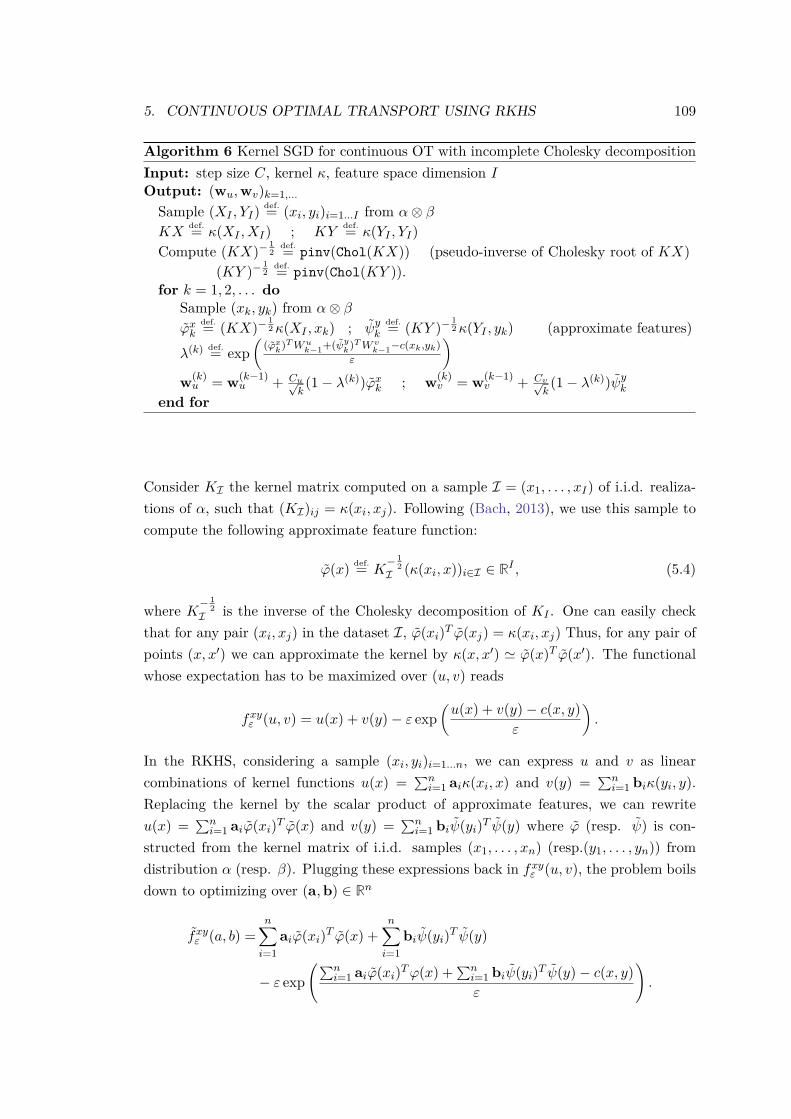
5. CONTINUOUS OPTIMAL TRANSPORT USING RKHS 109
Algorithm 6 Kernel SGD for continuous OT with incomplete Cholesky decompositionInput: step size C, kernel κ, feature space dimension IOutput: (wu,wv)k=1,...
Sample (XI , YI)def.= (xi, yi)i=1...I from α⊗ β
KXdef.= κ(XI , XI) ; KY
def.= κ(YI , YI)Compute (KX)−
12
def.= pinv(Chol(KX)) (pseudo-inverse of Cholesky root of KX)(KY )−
12
def.= pinv(Chol(KY )).for k = 1, 2, . . . do
Sample (xk, yk) from α⊗ βϕxk
def.= (KX)−12κ(XI , xk) ; ψyk
def.= (KY )−12κ(YI , yk) (approximate features)
λ(k) def.= exp(
(ϕxk)TWuk−1+(ψy
k)TW v
k−1−c(xk,yk)ε
)w(k)u = w(k−1)
u + Cu√k(1− λ(k))ϕxk ; w(k)
v = w(k−1)v + Cv√
k(1− λ(k))ψyk
end for
Consider KI the kernel matrix computed on a sample I = (x1, . . . , xI) of i.i.d. realiza-tions of α, such that (KI)ij = κ(xi, xj). Following (Bach, 2013), we use this sample tocompute the following approximate feature function:
ϕ(x) def.= K− 1
2I (κ(xi, x))i∈I ∈ RI , (5.4)
where K−12
I is the inverse of the Cholesky decomposition of KI . One can easily checkthat for any pair (xi, xj) in the dataset I, ϕ(xi)T ϕ(xj) = κ(xi, xj) Thus, for any pair ofpoints (x, x′) we can approximate the kernel by κ(x, x′) ' ϕ(x)T ϕ(x′). The functionalwhose expectation has to be maximized over (u, v) reads
fxyε (u, v) = u(x) + v(y)− ε exp(u(x) + v(y)− c(x, y)
ε
).
In the RKHS, considering a sample (xi, yi)i=1...n, we can express u and v as linearcombinations of kernel functions u(x) =
∑ni=1 aiκ(xi, x) and v(y) =
∑ni=1 biκ(yi, y).
Replacing the kernel by the scalar product of approximate features, we can rewriteu(x) =
∑ni=1 aiϕ(xi)T ϕ(x) and v(y) =
∑ni=1 biψ(yi)T ψ(y) where ϕ (resp. ψ) is con-
structed from the kernel matrix of i.i.d. samples (x1, . . . , xn) (resp.(y1, . . . , yn)) fromdistribution α (resp. β). Plugging these expressions back in fxyε (u, v), the problem boilsdown to optimizing over (a,b) ∈ Rn
fxyε (a, b) =n∑i=1
aiϕ(xi)T ϕ(x) +n∑i=1
biψ(yi)T ψ(y)
− ε exp(∑n
i=1 aiϕ(xi)Tϕ(x) +∑ni=1 biψ(yi)T ψ(y)− c(x, y)ε
).
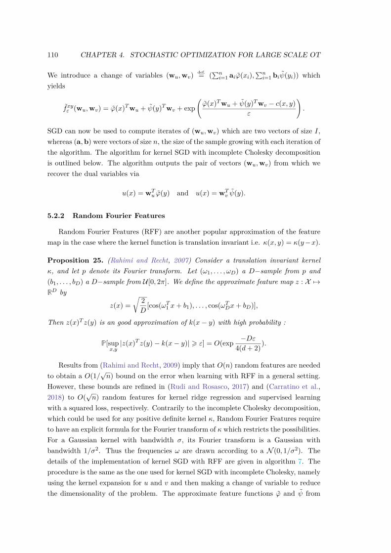
110 CHAPTER 4. STOCHASTIC OPTIMIZATION FOR LARGE SCALE OT
We introduce a change of variables (wu,wv)def.= (
∑ni=1 aiϕ(xi),
∑ni=1 biψ(yi)) which
yields
fxyε (wu,wv) = ϕ(x)Twu + ψ(y)Twv + exp(ϕ(x)Twu + ψ(y)Twv − c(x, y)
ε
).
SGD can now be used to compute iterates of (wu,wv) which are two vectors of size I,whereas (a,b) were vectors of size n, the size of the sample growing with each iteration ofthe algorithm. The algorithm for kernel SGD with incomplete Cholesky decompositionis outlined below. The algorithm outputs the pair of vectors (wu,wv) from which werecover the dual variables via
u(x) = wTu ϕ(y) and u(x) = wT
v ψ(y).
5.2.2 Random Fourier Features
Random Fourier Features (RFF) are another popular approximation of the featuremap in the case where the kernel function is translation invariant i.e. κ(x, y) = κ(y−x).
Proposition 25. (Rahimi and Recht, 2007) Consider a translation invariant kernelκ, and let p denote its Fourier transform. Let (ω1, . . . , ωD) a D−sample from p and(b1, . . . , bD) a D−sample from U [0, 2π]. We define the approximate feature map z : X 7→RD by
z(x) =√
2D
[cos(ωT1 x+ b1), . . . , cos(ωTDx+ bD)],
Then z(x)T z(y) is an good approximation of k(x− y) with high probability :
P[supx,y|z(x)T z(y)− k(x− y)| > ε] = O(exp −Dε
4(d+ 2)).
Results from (Rahimi and Recht, 2009) imply that O(n) random features are neededto obtain a O(1/
√n) bound on the error when learning with RFF in a general setting.
However, these bounds are refined in (Rudi and Rosasco, 2017) and (Carratino et al.,2018) to O(
√n) random features for kernel ridge regression and supervised learning
with a squared loss, respectively. Contrarily to the incomplete Cholesky decomposition,which could be used for any positive definite kernel κ, Random Fourier Features requireto have an explicit formula for the Fourier transform of κ which restricts the possibilities.For a Gaussian kernel with bandwidth σ, its Fourier transform is a Gaussian withbandwidth 1/σ2. Thus the frequencies ω are drawn according to a N (0, 1/σ2). Thedetails of the implementation of kernel SGD with RFF are given in algorithm 7. Theprocedure is the same as the one used for kernel SGD with incomplete Cholesky, namelyusing the kernel expansion for u and v and then making a change of variable to reducethe dimensionality of the problem. The approximate feature functions ϕ and ψ from
5. CONTINUOUS OPTIMAL TRANSPORT USING RKHS 111
Algorithm 7 Kernel SGD for continuous OT with Random Fourier FeaturesInput: C, kernel κ, Fourier transform of the kernel p, dimension of feature space DOutput: (wu,wv)k=1,...Sample (ω1, . . . , ωD) from pSample (b1, . . . , bD) from U [0, 2π]Def z(x) :
return√
2D [cos(ωT1 x+ b1), . . . , cos(ωTDx+ bD)]
for k = 1, 2, . . . doSample (xk, yk) from α⊗ βz
(k)x = z(xk) ; z
(k)y = z(yk)
λ(k) def.= exp(
(z(k)x )Tw(k−1)
u +(z(k)y )Tw(k−1)
v −c(xk,yk)ε
)w(k)u = w(k−1)
u + Cu√k(1− λ(k))z(k)
x ; w(k)v = w(k−1)
v + Cv√k(1− λ(k))z(k)
y
end for
Cholesky decomposition are replaced by z, the feature map obtained with RFF (notethat contrarily to the Cholesky method, we use the same feature map for expansions ofu and v). The algorithm outputs the pair of vectors (wu,wv) from which we recoverthe dual variables via
u(x) = wTu z(x) and v(y) = wT
v z(y).
5.3 Comparison of the Three Algorithms on Synthetic Data
We consider optimal transport in 1D between a Gaussian α and a Gaussian mix-ture β whose densities are represented in Figure 4.4 (a). Since there is no exist-ing benchmark for continuous transport, we use as a proxy for β an empirical distri-bution βN
def.= 1N
∑Ni=1 δyi with N = 103 and we compute the solution of the semi-
discrete problem Wε(α, βN ) with SGD. SGD yields a N−dimensional vector v fromwhich we can compute u at any point of the space thanks to the optimality conditionu(x) = −ε(log 1
N
∑Ni=1 e
vi−c(x,yi)ε ).
We first exhibit the convergence of the classic method (without speedup by approx-imate features) by studying the convergence of the potential u. The iterates u(k) areplotted on a grid for different values of k in Figure 4.4 (c), to emphasize the conver-gence to the proxy u∗. We can see that the iterates computed with the RKHS convergefaster where α has more mass. This makes sense, since convergence estimates are forE[fXYε (u(k), v(k))] and thus the value of u(k) has more influence where α has more mass.Figure 4.4 (b) represents the plot of ||u(k) − u∗||2/||u∗||2 where u(k) (resp. u∗) is theevaluation of u(k) (resp. u∗) on a sample (xi)i=1...N ′ drawn from α. This gives moreemphasis to the norm on points where α has more mass, for the reason given before.
We then compare the classic method to both speedup methods in terms of CPU time.We choose a Gaussian kernel as it is simple to implement in all three cases although it is
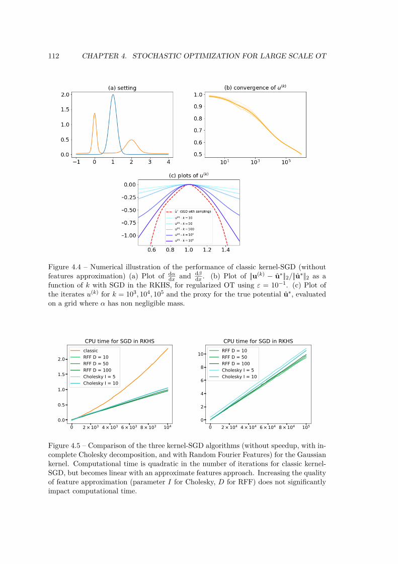
112 CHAPTER 4. STOCHASTIC OPTIMIZATION FOR LARGE SCALE OT
Figure 4.4 – Numerical illustration of the performance of classic kernel-SGD (withoutfeatures approximation) (a) Plot of dα
dx and dβdx . (b) Plot of ||u(k) − u∗||2/||u∗||2 as a
function of k with SGD in the RKHS, for regularized OT using ε = 10−1. (c) Plot ofthe iterates u(k) for k = 103, 104, 105 and the proxy for the true potential u∗, evaluatedon a grid where α has non negligible mass.
0 2×10³ 4×10³ 6×10³ 8×10³ 1040.0
0.5
1.0
1.5
2.0
CPU time for SGD in RKHSclassicRFF D = 10RFF D = 50RFF D = 100Cholesky I = 5Cholesky I = 10
0 2×10⁴ 4×10⁴ 6×10⁴ 8×10⁴ 1050
2
4
6
8
10
CPU time for SGD in RKHSRFF D = 10RFF D = 50RFF D = 100Cholesky I = 5Cholesky I = 10
Figure 4.5 – Comparison of the three kernel-SGD algorithms (without speedup, with in-complete Cholesky decomposition, and with Random Fourier Features) for the Gaussiankernel. Computational time is quadratic in the number of iterations for classic kernel-SGD, but becomes linear with an approximate features approach. Increasing the qualityof feature approximation (parameter I for Cholesky, D for RFF) does not significantlyimpact computational time.
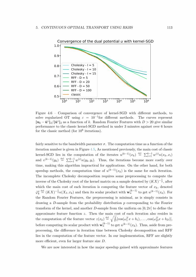
5. CONTINUOUS OPTIMAL TRANSPORT USING RKHS 113
100 101 102 103 104 105 1060.5
0.6
0.7
0.8
0.9
1.0Convergence of the dual potential u with kernel-SGD
Cholesky - I = 5Cholesky - I = 10Cholesky - I = 15RFF - D = 5RFF - D = 20RFF - D = 50RFF - D = 100classic
Figure 4.6 – Comparison of convergence of kernel-SGD with different methods, tosolve regularized OT using ε = 10−1for different methods. The curves represent||uk − u∗||2/||u∗||2 as a function of k. Random Fourier Features with D > 20 give similarperformance to the classic kernel-SGD method in under 3 minutes against over 6 hoursfor the classic method (for 106 iterations).
fairly sensitive to the bandwidth parameter σ. The computation time as a function of theiteration number is given in Figure 4.5, As mentioned previously, the main cost of classickernel-SGD lies in the computation of the iterates u(k−1)(xk)
def.=∑k−1i=1 w
(i)κ(xk, xi)and v(k−1)(yk)
def.=∑k−1i=1 w
(i)κ(yk, yi). Thus, the iterations become more costly overtime, making this algorithm impractical for applications. On the other hand, for bothspeedup methods, the computation time of u(k−1)(xk) is the same for each iteration.The incomplete Cholesky decomposition requires some preprocessing to compute theinverse of the Cholesky root of the kernel matrix on a sample denoted by (KX)−
12 , after
which the main cost of each iteration is computing the feature vector of xk, denotedϕxk
def.= (KX)−12κ(XI , xk) and then its scalar product with w(k−1)
u to get u(k−1)(xk). Forthe Random Fourier Features, the preprocessing is minimal, as is simply consists indrawing a D-sample from the probability distribution p corresponding to the Fouriertransform of the kernel, and another D-sample from the uniform on [0, 2π] to define theapproximate feature function z. Then the main cost of each iteration also resides inthe computation of the feature vector z(xk)
def.=√
2D [cos(ωT1 x+ b1), . . . , cos(ωTDx+ bD)],
before computing its scalar product with w(k−1)u to get u(k−1)(xk). Thus, aside from pre-
processing, the difference in iteration time between Cholesky decomposition and RFFlies in the computation of the feature vector. In our implementation, RFF are slightlymore efficient, even for larger feature size D.
We are now interested in how the major speedup gained with approximate features

114 CHAPTER 4. STOCHASTIC OPTIMIZATION FOR LARGE SCALE OT
impacts the quality of the solution. The curves in Figure 4.6 plot the convergence ofu(k) to u∗ for each of the methods, with the same learning rate C and bandwidth σ. Forthe Cholesky decomposition, the parameter I controls the quality of the approximation.Note that numerically, we are limited to small values of I (no more than 15) because theeigenvalues of the kernel matrix decay exponentially fast with its dimension and thusits Cholesky root quickly become non-invertible. For the Random Fourier Features,the quality of the approximation is controlled by D, for which we have no particularrestriction. From the CPU-time experiment, we see that taking larger values of I and Ddoesn’t impact the computation time very much, but it clearly improves convergence upto a certain point after which there is no more improvement. We can see that RandomFourier Features yield a better approximation than incomplete Cholesky decompositioneven for small D. In terms of performance, RFF with feature vectors of size D =20, 50, 100 give similar results, while D = 5 is too small to get a good approximation. Interms of computational time, RFF with D = 20 takes less than 3 minutes to perform 106
iterations, while D = 100 takes around 5 minutes, without any significant improvement.In comparison, to reach the same level of precision (which requires the same number ofiterations), classic kernel-SGD takes over 6 hours!
Conclusion
Entropy-regularized OT was historically introduced in (Cuturi, 2013) as a computa-tional tool to solve discrete OT efficiently thanks to Sinkhorn’s algorithm, and it openedthe door to a rich line of research which aims at better understanding its computationaland theoretical scope. The contributions of this thesis to this topic can be organizedin two main axes. The first one consists in exploiting the properties of entropic regu-larization to make OT-based losses efficient in machine-learning problems. The secondone concerns the interpolation property of entropy-regularized OT, bridging the gapbetween standard OT and MMD.
Making OT-based Losses Tractable for Machine Learning. Using the entropicregularization with respect to the product measure of the marginals (Genevay et al.,2016) enables us to address both the computational and the statistical issues from whichstandard OT suffers, by reformulating entropy-regularized OT as the maximization ofan expectation (Chapter 1, Sec. 3).
The Statistical Issue: We prove that the dual optimizers of entropy-regularized OTlie in a ball of a Reproducing Kernel Hilbert Space (Chapter 3, Sec. 4). Combinedwith the formulation as an expectation, this enables us to use techniques from errorbounding in learning theory to get a sample complexity result for entropy-regularizedOT. We prove that for a large enough regularization, entropy-regularized OT does notsuffer from a curse of dimensionality (Chapter 3, Sec. 5).
The Computational Issue: Sinkhorn’s algorithm was a major breakthrough for com-putational OT, but it is limited to discrete measures, and does not scale well when thesemeasures have a very large number of points. The formulation as an expectation allowsus to use stochastic optimization solvers, which only require samples from the measuresand operate in an online manner (Chapter 4). These algorithms can tackle cases whereSinkhorn is not a suitable choice to solve entropy-regularized OT: discrete problems witha very large number of points, or problems involving continuous measures. For problemsinvolving two continuous measures, we can exploit the fact that the dual optimizers ofentropy-regularized OT lie in a ball of a Reproducing Kernel Hilbert Space to derive aprovably convergent kernel-SGD solver (Chapter 4, Sec. 5.1).
Minimizing OT-based Losses: We make use of the GPU-friendly structure of Sinkhorn’s
115
116 CONCLUSION
algorithm to propose a minimization scheme for OT based-losses (Chapter 2, Sec. 3). Weuse stochastic gradient over an approximate loss computed with Sinkhorn’s algorithmand compute the gradient with automatic differentiation. We use this method to learn aparametric distribution from samples, and prove that it scales well to high-dimensionalproblems such as generative models of images (Chapter 2, Sec. 4.3) where it can improveon state-of-the-art methods.
Interpolating Between OT and MMD with Sinkhorn Divergences. Whencomparing one measure to itself, the loss induced by entropy-regularized OT is notequal to zero. To solve this issue, we introduced Sinkhorn Divergences, which are basedon entropy-regularized OT with corrective terms. This new family of losses interpolatesbetween OT when the regularization parameter goes to zero and MMD when the regu-larization parameter goes to infinity (Chapter 2, Sec. 2.4). The interpolation propertyis also true in terms of sample complexity, which gives theoretical grounds to empiricalevidence suggesting that using a regularizer that is not too small is better in practice.Indeed, when the regularization parameter is large enough we recover sample complexityrates from MMD, thus breaking the curse of dimensionality from OT. However, whentaking a small regularization, sample complexity degrades quickly in high dimension(Chapter 3, Sec. 5). This theoretical result further advocates for the use of SinkhornDivergences with regularization parameters that are not too small. Aside from yieldingbetter performance for machine learning tasks, a large regularization parameter ensuresa faster convergence of Sinkhorn’s algorithm and is thus also beneficial in terms of com-putational time. In practice, the regularization parameter in Sinkhorn Divergences givesan additional degree of freedom to the loss function which can be cross-validated to getthe best of both OT and MMD in learning tasks (Chapter 2, Sec. 4).
Perspectives for Further Work.
Let us start by mentioning direct extensions of results from this thesis. The first ideato explore is the extension of the sample complexity result from Chapter 3, Theorem 14,to non-smooth cost functions and metric spaces that are not bounded subsets of Rd.Another improvement would consist in tightening the upper-bound on the convergencerate in this theorem to combine it with Theorem 12, which gives a convergence rate onthe approximation of OT with regularized OT. Thus we would get a heuristic on thechoice of the regularization parameter depending on the number of available sampleswhen one wants to approximate standard OT with regularized OT computed on samples.Another issue linked to this chapter, but which extends beyond the techniques that weused, is to derive convergence rates with respect to the number of samples for theregularized transport plan, i.e. the optimizer of the primal problem, as it is a crucialfeature for some machine learning problems (e.g. domain adaptation (Courty et al.,
117
2016)).In Chapter 4, Sec. 5.1 we develop an algorithm to compute regularized OT between
any two arbitrary measures using kernel-SGD on the dual problem. We only applyour algorithm to a simple 1D problem as a proof of concept, as we did not have anybaseline to assess convergence of entropy-regularized OT for continuous measures inhigh dimension. However, following (Seguy et al., 2017) which uses our scheme witha neural-network parametrization of the dual variables instead of a RKHS expansion,we could use the results directly to perform learning tasks that involve OT betweencontinuous measures. The applications they consider are domain adaptation and imagegeneration. Besides, all stochastic algorithms presented in Chapter 4 could be extendedto the case of regularized unbalanced OT (Chizat et al., 2018), as it can also be cast asthe maximization of an expectation (see Chapter 1, Remark 6).
The introduction of Sinkhorn Divergences opens the door to several extensions orgeneralizations. For instance, one might consider unbalanced Sinkhorn Divergencesdefined with regularized unbalanced OT and see if the interpolation property, positivedefiniteness and sample complexity results still hold. Another thing would be to extendthe sample complexity and positive definiteness results to Sinkhorn Divergences definedwithout the added entropy in the cost function (see Definition 9 and Remarks 13 and 14),and more generally to understand the potential benefits and drawbacks of using theentropy or not when considering the cost in Sinkhorn Divergences. Eventually, usingregularizers other than the relative entropy as introduced in Chapter 1, Sec. 3 is a trackworth exploring, although the entropy is central to most of our analysis and only theonline algorithm from Chapter 4, Sec. 4 for continuous measures directly applies.
Wasserstein barycenters, which are used to represent the mean of a set of empiricalprobability measures (Agueh and Carlier, 2011) represent a rich line of research inOT although we did not explore it in this thesis. They can be computed efficientlywith entropic regularization (Cuturi and Doucet, 2014), and the online semi-discretesolver developed in Chapter 4, Sec. 4 is well suited to aggregate streaming data (Staibet al., 2017). Given the good numerical results obtained for the Wasserstein barycenterproblem with entropy, they could also benefit from the corrective terms in SinkhornDivergences.
Taking a step back from entropy-regularized OT, an open issue which is central toChapter 2 is the evaluation of generative models (see Sec. 4.3). Comparing the outcomesof learning procedures with various losses is a burning issue and the lack of good eval-uation metrics makes it impossible to make a definitive ranking of the different lossesappearing in the literature. The recent paper by (Lucic et al., 2018) introduces someevaluation metrics suggesting that losses are all equivalent for high dimensional problemssuch as image generation, making the architecture of the network the most importantfactor. It is then crucial to understand how the architecture influences smoothness,generalization properties or interpolation in the latent space for instance. Besides,

118 CONCLUSION
even though different losses yield similar results for the inference of generative mod-els, entropy-regularized OT can still act as robust metrics to evaluate models after theinference procedure.
Eventually, we conclude this thesis with a final question : are there ways to break thecurse of dimensionality for the Wasserstein distance? Sinkhorn Divergences provide arobust loss for a large enough regularization as seen in Chapter 3, but they do not solvethe curse of dimensionality when one wants to compute standard OT from samples. Theexistence of robust empirical estimators of the Wasserstein distance in high dimensionstill remains an open question.
Bibliography
M. Agueh and G. Carlier. Barycenters in the Wasserstein space. SIAM Journal onMathematical Analysis, 43(2):904–924, 2011.
D. Alvarez-Melis, T. S. Jaakkola, and S. Jegelka. Structured optimal transport. arXivpreprint arXiv:1712.06199, 2017.
L. Ambrosio, N. Gigli, and G. Savaré. Gradient flows in metric spaces and in the spaceof probability measures. Springer, 2006.
M. Arjovsky, S. Chintala, and L. Bottou. Wasserstein generative adversarial networks.In International Conference on Machine Learning, pages 214–223, 2017.
F. Aurenhammer, F. Hoffmann, and B. Aronov. Minkowski-type theorems and least-squares clustering. Algorithmica, 20(1):61–76, 1998.
F. Bach. Sharp analysis of low-rank kernel matrix approximations. In Conference onLearning Theory, pages 185–209, 2013.
P. L. Bartlett and S. Mendelson. Rademacher and gaussian complexities: Risk boundsand structural results. Journal of Machine Learning Research, 3(Nov):463–482, 2002.
F. Bassetti, A. Bodini, and E. Regazzini. On minimum Kantorovich distance estimators.Statistics & probability letters, 76(12):1298–1302, 2006.
M. G. Bellemare, I. Danihelka, W. Dabney, S. Mohamed, B. Lakshminarayanan,S. Hoyer, and R. Munos. The Cramer distance as a solution to biased Wassersteingradients. arXiv preprint arXiv:1705.10743, 2017.
J.-D. Benamou, G. Carlier, M. Cuturi, L. Nenna, and G. Peyré. Iterative bregman pro-jections for regularized transportation problems. SIAM Journal on Scientific Com-puting, 37(2):A1111–A1138, 2015.
E. Bernton, P. E. Jacob, M. Gerber, and C. P. Robert. Inference in generative modelsusing the Wasserstein distance. arXiv preprint arXiv:1701.05146, 2017.
119
120 BIBLIOGRAPHY
J. Bigot, E. Cazelles, and N. Papadakis. Central limit theorems for Sinkhorn divergencebetween probability distributions on finite spaces and statistical applications. arXivpreprint arXiv:1711.08947, 2017.
M. Bińkowski, D. J. Sutherland, M. Arbel, and A. Gretton. Demystifying MMD GANs.arXiv preprint arXiv:1801.01401, 2018.
O. Bousquet, S. Gelly, I. Tolstikhin, C.-J. Simon-Gabriel, and B. Schoelkopf. Fromoptimal transport to generative modeling: the VEGAN cookbook. arXiv preprintarXiv:1705.07642, 2017.
R. Burkard, M. Dell’Amico, and S. Martello. Assignment Problems. SIAM, 2009.
P. J. Bushell. Hilbert’s metric and positive contraction mappings in a Banach space.Archive for Rational Mechanics and Analysis, 52(4):330–338, 1973.
A. Calderón. Lebesgue spaces of differentiable functions. In Proc. Sympos. Pure Math,volume 4, pages 33–49, 1961.
G. Canas and L. Rosasco. Learning probability measures with respect to optimal trans-port metrics. In F. Pereira, C. J. C. Burges, L. Bottou, and K. Q. Weinberger, editors,Advances in Neural Information Processing Systems 25, pages 2492–2500. Curran As-sociates, Inc., 2012.
G. Carlier, V. Duval, G. Peyré, and B. Schmitzer. Convergence of entropic schemes foroptimal transport and gradient flows. SIAM Journal on Mathematical Analysis, 49(2):1385–1418, 2017.
L. Carratino, A. Rudi, and L. Rosasco. Learning with sgd and random features. InAdvances in Neural Information Processing Systems, pages 10213–10224, 2018.
Y. Chen, T. Georgiou, and M. Pavon. Entropic and displacement interpolation: a com-putational approach using the hilbert metric. SIAM Journal on Applied Mathematics,76(6):2375–2396, 2016.
L. Chizat. Unbalanced optimal transport: Models, numerical methods, applications.PhD thesis, PSL Research University, 2017.
L. Chizat, G. Peyré, B. Schmitzer, and F.-X. Vialard. An interpolating distance betweenoptimal transport and Fisher–Rao metrics. Foundations of Computational Mathemat-ics, 18(1):1–44, 2018.
R. Cominetti and J. S. Martin. Asymptotic analysis of the exponential penalty trajectoryin linear programming. Mathematical Programming, 67(1-3):169–187, 1994.
BIBLIOGRAPHY 121
N. Courty, R. Flamary, and D. Tuia. Domain adaptation with regularized optimal trans-port. In Joint European Conference on Machine Learning and Knowledge Discoveryin Databases, pages 274–289. Springer, 2014.
N. Courty, R. Flamary, D. Tuia, and A. Rakotomamonjy. Optimal transport for domainadaptation. IEEE Transactions on Pattern Analysis and Machine Intelligence, PP(99):1–1, 2016.
I. Csiszár. I-divergence geometry of probability distributions and minimization problems.The Annals of Probability, pages 146–158, 1975.
M. Cuturi. Sinkhorn distances: Lightspeed computation of optimal transport. In Adv.in Neural Information Processing Systems, pages 2292–2300, 2013.
M. Cuturi and A. Doucet. Fast computation of Wasserstein barycenters. In InternationalConference on Machine Learning, pages 685–693, 2014.
E. Del Barrio and J.-M. Loubes. Central limit theorem for empirical transportation costin general dimension. arXiv preprint arXiv:1705.01299, 2017.
R. Dudley. The speed of mean Glivenko-Cantelli convergence. The Annals of Mathe-matical Statistics, 40(1):40–50, 1969.
G. Dziugaite, D. Roy, and Z. Ghahramani. Training generative neural networks viamaximum mean discrepancy optimization. In Uncertainty in Artificial Intelligence-Proceedings of the 31st Conference, UAI 2015, pages 258–267, 2015.
J. Feydy and A. Trouvé. Global divergences between measures: from Hausdorff distanceto Optimal Transport. In International Workshop on Shape in Medical Imaging, pages102–115. Springer, 2018.
J. Feydy, T. Séjourné, F.-X. Vialard, S.-I. Amari, A. Trouvé, and G. Peyré. Interpolatingbetween optimal transport and MMD using Sinkhorn divergences. In InternationalConference on Artificial Intelligence and Statistics, 2019.
J. Franklin and J. Lorenz. On the scaling of multidimensional matrices. Linear Algebraand its applications, 114:717–735, 1989.
C. Frogner, C. Zhang, H. Mobahi, M. Araya, and T. Poggio. Learning with a Wassersteinloss. In Adv. in Neural Information Processing Systems, pages 2044–2052, 2015.
K. Fukumizu, A. Gretton, G. R. Lanckriet, B. Schölkopf, and B. K. Sriperumbudur.Kernel choice and classifiability for RKHS embeddings of probability distributions. InAdvances in neural information processing systems, pages 1750–1758, 2009.
122 BIBLIOGRAPHY
B. Galerne, A. Leclaire, and J. Rabin. A texture synthesis model based on semi-discreteoptimal transport in patch space. SIAM Journal on Imaging Sciences, 11(4):2456–2493, 2018.
A. Genevay, M. Cuturi, G. Peyré, and F. Bach. Stochastic optimization for large-scaleoptimal transport. In D. D. Lee, U. V. Luxburg, I. Guyon, and R. Garnett, editors,Proc. NIPS’16, pages 3432–3440. Curran Associates, Inc., 2016.
A. Genevay, G. Peyre, and M. Cuturi. Learning generative models with Sinkhorn di-vergences. In International Conference on Artificial Intelligence and Statistics, pages1608–1617, 2018.
A. Genevay, L. Chizat, F. Bach, M. Cuturi, and G. Peyré. Sample complexity of Sinkhorndivergences. In International Conference on Artificial Intelligence and Statistics, 2019.
I. Goodfellow, J. Pouget-Abadie, M. Mirza, B. Xu, D. Warde-Farley, S. Ozair,A. Courville, and Y. Bengio. Generative adversarial nets. In Advances in neuralinformation processing systems, pages 2672–2680, 2014.
A. Gretton, K. Borgwardt, M. Rasch, B. Schölkopf, and A. Smola. A kernel method forthe two-sample-problem. In Adv. in Neural Information Processing Systems, pages513–520, 2006.
I. Gulrajani, F. Ahmed, M. Arjovsky, V. Dumoulin, and A. Courville. Improved trainingof Wasserstein GANs. arXiv preprint arXiv:1704.00028, 2017.
M. Heusel, H. Ramsauer, T. Unterthiner, B. Nessler, and S. Hochreiter. Gans trainedby a two time-scale update rule converge to a local nash equilibrium. In Advances inNeural Information Processing Systems, pages 6626–6637, 2017.
G. Huang, C. Guo, M. J. Kusner, Y. Sun, F. Sha, and K. Q. Weinberger. Supervisedword mover’s distance. In D. D. Lee, M. Sugiyama, U. V. Luxburg, I. Guyon, andR. Garnett, editors, Advances in Neural Information Processing Systems 29, pages4862–4870. Curran Associates, Inc., 2016.
L. Kantorovich. On the transfer of masses (in Russian). Doklady Akademii Nauk, 37(2):227–229, 1942.
D. Kingma and J. Ba. Adam: A method for stochastic optimization. arXiv preprintarXiv:1412.6980, 2014.
D. P. Kingma and M. Welling. Auto-encoding variational bayes. arXiv preprintarXiv:1312.6114, 2013.
J. Kivinen, A. J. Smola, and R. C. Williamson. Online learning with kernels. In Advancesin neural information processing systems, pages 785–792, 2002.
BIBLIOGRAPHY 123
M. Kusner, Y. Sun, N. Kolkin, and K. Q. Weinberger. From word embeddings todocument distances. In Proc. of the 32nd Intern. Conf. on Machine Learning, pages957–966, 2015.
A. B. L. Larsen, S. K. Sonderby, H. Larochelle, and O. Winther. Autoencoding beyondpixels using a learned similarity metric. In M. F. Balcan and K. Q. Weinberger, editors,Proceedings of The 33rd International Conference on Machine Learning, volume 48 ofProceedings of Machine Learning Research, pages 1558–1566, New York, New York,USA, 20–22 Jun 2016. PMLR.
C.-L. Li, W.-C. Chang, Y. Cheng, Y. Yang, and B. Póczos. MMD GAN: Towards deeperunderstanding of moment matching network. arXiv preprint arXiv:1705.08584, 2017.
Y. Li, K. Swersky, and R. Zemel. Generative moment matching networks. In Interna-tional Conference on Machine Learning, pages 1718–1727, 2015.
M. Liero, A. Mielke, and G. Savaré. Optimal entropy-transport problems and a newHellinger–Kantorovich distance between positive measures. Inventiones mathemati-cae, 211(3):969–1117, 2018.
M. Lucic, K. Kurach, M. Michalski, S. Gelly, and O. Bousquet. Are GANs createdequal? a large-scale study. In Advances in neural information processing systems,pages 697–706, 2018.
G. Luise, A. Rudi, M. Pontil, and C. Ciliberto. Differential properties of Sinkhorn ap-proximation for learning with Wasserstein distance. arXiv preprint arXiv:1805.11897,2018.
C. McDiarmid. On the method of bounded differences, page 148–188. London Mathe-matical Society Lecture Note Series. Cambridge University Press, 1989.
Q. Mérigot. A multiscale approach to optimal transport. Comput. Graph. Forum, 30(5):1583–1592, 2011.
G. Montavon, K.-R. Müller, and M. Cuturi. Wasserstein training of restricted Boltzmannmachines. In Adv. in Neural Information Processing Systems, 2016.
A. Müller. Integral probability metrics and their generating classes of functions. Ad-vances in Applied Probability, 29(2):429–443, 1997.
X. Nguyen, M. J. Wainwright, and M. I. Jordan. Estimating divergence functionals andthe likelihood ratio by convex risk minimization. IEEE Transactions on InformationTheory, 56(11):5847–5861, 2010.
124 BIBLIOGRAPHY
S. Nowozin, B. Cseke, and R. Tomioka. f-GAN: Training generative neural samplersusing variational divergence minimization. In Advances in Neural Information Pro-cessing Systems, pages 271–279, 2016.
J. Pennington, R. Socher, and C. Manning. Glove: Global vectors for word representa-tion. Proc. of the Empirical Methods in Natural Language Processing (EMNLP 2014),12:1532–1543, 2014.
G. Peyré, M. Cuturi, et al. Computational optimal transport. Technical report, 2017.
B. T. Polyak and A. B. Juditsky. Acceleration of stochastic approximation by averaging.SIAM Journal on Control and Optimization, 30(4):838–855, 1992.
A. Radford, L. Metz, and S. Chintala. Unsupervised representation learning with deepconvolutional generative adversarial networks. arXiv preprint arXiv:1511.06434, 2015.
A. Rahimi and B. Recht. Random features for large-scale kernel machines. In Adv. inNeural Information Processing Systems, pages 1177–1184, 2007.
A. Rahimi and B. Recht. Weighted sums of random kitchen sinks: Replacing minimiza-tion with randomization in learning. In Advances in neural information processingsystems, pages 1313–1320, 2009.
A. Ramdas, N. G. Trillos, and M. Cuturi. On Wasserstein two-sample testing andrelated families of nonparametric tests. Entropy, 19(2), 2017.
A. Rolet, M. Cuturi, and G. Peyré. Fast dictionary learning with a smoothedWassersteinloss. In A. Gretton and C. C. Robert, editors, Proceedings of the 19th InternationalConference on Artificial Intelligence and Statistics, volume 51 of Proceedings of Ma-chine Learning Research, pages 630–638, Cadiz, Spain, 09–11 May 2016. PMLR.
Y. Rubner, C. Tomasi, and L. J. Guibas. The earth mover’s distance as a metric forimage retrieval. IJCV, 40(2):99–121, Nov. 2000.
A. Rudi and L. Rosasco. Generalization properties of learning with random features. InAdvances in Neural Information Processing Systems, pages 3215–3225, 2017.
T. Salimans, I. Goodfellow, W. Zaremba, V. Cheung, A. Radford, and X. Chen. Im-proved techniques for training GANs. In Advances in Neural Information ProcessingSystems, pages 2234–2242, 2016.
T. Salimans, H. Zhang, A. Radford, and D. Metaxas. Improving GANs using optimaltransport. In International Conference on Learning Representations, 2018.
F. Santambrogio. Optimal Transport for applied mathematicians, volume 87 of Progressin Nonlinear Differential Equations and their applications. Springer, 2015.
BIBLIOGRAPHY 125
M. Schmidt, N. Le Roux, and F. Bach. Minimizing finite sums with the stochasticaverage gradient. Mathematical Programming, 2016.
B. Schmitzer. Stabilized sparse scaling algorithms for entropy regularized transportproblems. arXiv preprint arXiv:1610.06519, 2016.
V. Seguy, B. B. Damodaran, R. Flamary, N. Courty, A. Rolet, and M. Blondel. Large-scale optimal transport and mapping estimation. arXiv preprint arXiv:1711.02283,2017.
D. Sejdinovic, B. Sriperumbudur, A. Gretton, and K. Fukumizu. Equivalence ofdistance-based and RKHS-based statistics in hypothesis testing. The Annals of Statis-tics, pages 2263–2291, 2013.
R. Sinkhorn. A relationship between arbitrary positive matrices and doubly stochasticmatrices. Ann. Math. Statist., 35:876–879, 1964.
R. Sinkhorn. Diagonal equivalence to matrices with prescribed row and column sums.The American Mathematical Monthly, 74(4):402–405, 1967.
J. Solomon, F. de Goes, G. Peyré, M. Cuturi, A. Butscher, A. Nguyen, T. Du, andL. Guibas. Convolutional Wasserstein distances: Efficient optimal transportation ongeometric domains. ACM Transactions on Graphics (Proc. SIGGRAPH 2015), 2015.
B. K. Sriperumbudur, A. Gretton, K. Fukumizu, B. Schölkopf, and G. R. Lanckriet.Hilbert space embeddings and metrics on probability measures. Journal of MachineLearning Research, 11(Apr):1517–1561, 2010.
B. K. Sriperumbudur, K. Fukumizu, A. Gretton, B. Schölkopf, G. R. Lanckriet, et al.On the empirical estimation of integral probability metrics. Electronic Journal ofStatistics, 6:1550–1599, 2012.
M. Staib, S. Claici, J. M. Solomon, and S. Jegelka. Parallel streaming Wassersteinbarycenters. In Advances in Neural Information Processing Systems, pages 2647–2658, 2017.
I. Steinwart and A. Christmann. Support vector machines. Springer Science & BusinessMedia, 2008.
J. Weed and F. Bach. Sharp asymptotic and finite-sample rates of convergence ofempirical measures in Wasserstein distance. arXiv preprint arXiv:1707.00087, 2017.
G. Wu, E. Chang, Y. K. Chen, and C. Hughes. Incremental approximate matrix factor-ization for speeding up support vector machines. In Proc. of the 12th ACM SIGKDDIntern. Conf. on Knowledge Discovery and Data Mining, pages 760–766, 2006.


Résumé
Le Transport Optimal régularisé parl’Entropie (TOE) permet de définirles Divergences de Sinkhorn (DS),une nouvelle classe de distance en-tre mesures de probabilités baséessur le TOE. Celles-ci permettentd’interpoler entre deux autres dis-tances connues: le Transport Op-timal (TO) et l’Ecart Moyen Maxi-mal (EMM). Les DS peuvent êtreutilisées pour apprendre des mod-èles probabilistes avec de meilleuresperformances que les algorithmesexistants pour une régularisationadéquate. Ceci est justifié parun théorème sur l’approximation desSD par des échantillons, prouvantqu’une régularisation suffisante per-met de se débarrasser de la malé-diction de la dimension du TO, et l’onretrouve à l’infini le taux de conver-gence des EMM. Enfin, nous présen-tons de nouveaux algorithmes derésolution pour le TOE basés surl’optimisation stochastique ‘en-ligne’qui, contrairement à l’état de l’art, nese restreignent pas aux mesures dis-crètes et s’adaptent bien aux prob-lèmes de grande dimension.
Mots Clés
Apprentissage Statistique, TransportOptimal
Abstract
This thesis proposes theoreticaland numerical contributions to useEntropy-regularized Optimal Trans-port (EOT) for machine learning.We introduce Sinkhorn Divergences(SD), a class of discrepancies be-tween probability measures basedon EOT which interpolates betweentwo other well-known discrepancies:Optimal Transport (OT) and Maxi-mum Mean Discrepancies (MMD).We develop an efficient numericalmethod to use SD for density fittingtasks, showing that a suitable choiceof regularization can improve perfor-mance over existing methods. Wederive a sample complexity theoremfor SD which proves that choosinga large enough regularization pa-rameter allows to break the curse ofdimensionality from OT, and recoverasymptotic rates similar to MMD.We propose and analyze stochasticoptimization solvers for EOT, whichyield online methods that can copewith arbitrary measures and arewell suited to large scale problems,contrarily to existing discrete batchsolvers.
Keywords
Machine Learning, Optimal Transport