http://www.cepar.edu.au/

Economic Rationality, Risk Presentation, and

Retirement Portfolio Choice�

Hazel Batemany, Christine Eblingz, John Gewekex,

Jordan Louviere{, Stephen Satchellkand Susan Thorp��

May 18, 2011

Keywords: discrete choice; retirement savings; investment risk;

household �nance; �nancial literacy

JEL Classi�cation: G23; G28; D14

�The authors acknowledge �nancial support under ARC DP1093842, generous assistance withthe development and implementation of the internet survey from PurePro�le and the sta¤ of theCentre for the Study of Choice, University of Technology Sydney; and excellent research assistancefrom Frances Terlich and Edward Wei. Part of this work was completed while Bateman visited theSchool of Finance and Economics at the University of Technology Sydney. Some previous versionsof this paper bore the title �Investment Risk Presentation and Individual Preference Consistency.�

yCentre for Pensions and Superannuation, University of New South Wales,h.bateman@unsw.edu.au

zCentre for the Study of Choice, University of Technology Sydney, Christine.Ebling@uts.edu.auxCentre for the Study of Choice, University of Technology Sydney, John.Geweke@uts.edu.au.{Centre for the Study of Choice, University of Technology Sydney, Jordan.Louviere@uts.edu.aukTrinity College, University of Cambridge, University of Sydney, ses11@cam.ac.uk��Centre for the Study of Choice, University of Technology Sydney, Susan.Thorp@uts.edu.au

1

Abstract

This research studies the propensity of individuals to violate implications of ex-

pected utility maximization in allocating retirement savings within a compulsory de-

�ned contribution retirement plan. The paper develops the implications and describes

the construction and administration of a discrete choice experiment to almost 1200

members of Australia�s mandatory retirement savings scheme. The experiment �nds

overall rates of violation of roughly 25%, and substantial variation in rates, depend-

ing on the presentation of investment risk and the characteristics of the participants.

Presentations based on frequency of returns below or above a threshold generate

more violations than do presentations based on the probability of returns below or

above thresholds. Individuals with low numeracy skills, assessed as part of the ex-

periment, are several times more likely to violate implications of the conventional

expected utility model than those with high numeracy skills. Older individuals are

substantially less likely to violate these restrictions, when risk is presented in terms of

event frequency, than are younger individuals. The results pose signi�cant questions

for public policy, in particular compulsory de�ned contribution retirement schemes,

where the future welfare of participants in these schemes depends on quantitative

decision-making skills that a signi�cant number of them do not possess.

2

1 Introduction

De�ned contribution schemes are now the dominant model for retirement income pro-

vision in many countries. As a result, investment decisions that were once the province

of wealthy households and their advisers are now the norm for most adults in these

countries. One of the most di¢ cult of these decisions, particularly for unsophisti-

cated investors, is choosing a portfolio for retirement savings, where an appreciation

of investment risk is crucial. This brings to the fore interesting positive questions:

for example, how is investment risk assessed by individuals in allocating retirement

wealth, and by retirees in consuming out of this wealth? The fact that public policy

increasingly compels these private decisions leads to attendant normative questions:

what kinds of information and guidance e¤ectively inform retirement portfolio allo-

cation decisions, and how should options for these allocations be structured?

This study elicits decisions about the allocation of retirement wealth from a panel

of 1199 participants in the compulsory retirement savings scheme in Australia (Su-

perannuation Guarantee). We examine these decisions in the context of the core

expected utility model of portfolio allocation, and �nd signi�cant violations of this

model. The propensity for these violations to occur varies systematically with the

way in which risk is presented, as well as with the age and quantitative skills of work-

ers. Our �ndings are relevant for the presentation of risk to participants in de�ned

contribution retirement plans, for education in support of more informed decision-

making by these participants, and for public policy decisions involving compulsory

retirement schemes.

Allocation of retirement wealth is the most signi�cant and sophisticated �nancial

decision that many individuals ever make. In economics, the core model for this de-

cision begins with a regular (i.e., monotone increasing and concave) utility function

3

for consumption and stipulates that portfolio allocations are made so as to maxi-

mize expected utility. Section 2 explains how we used this model in designing the

discrete choice experiment that elicited the retirement savings allocation decisions

from our panel. It develops two restrictions on the decisions panel respondents made.

The strong restriction (Proposition 1) is solely a consequence of the expected utility

model, and implies that certain allocation decisions should never be observed. The

weak restriction (Proposition 2) follows under the further condition that from the

information about risk presented, respondents infer an ordering with respect to sec-

ond order stochastic dominance, and implies that certain pairs of allocation decisions

should never be observed.

Our approach builds on previous studies that have employed an array of methods

to elicit risk preferences. These studies vary widely with respect to the magnitude

of risk under consideration and the method of elicitation. Academic experimental

studies have asked lottery questions (e.g., Holt and Laury 2002; Kimball et al. 2008).

Empirical investigations have inferred risk parameters from observed portfolio allo-

cations or insurance choices (e.g., Friend and Blume 1975, Barseghyan et al. 2009).

More recent methods include interactive interfaces such as distribution builders (Gold-

stein et al. 2008) or experience sampling, which gives feedback about risky choices

through web-based platforms (Haisley et al. 2010).

The discrete choice experiment that is detailed in Section 3 recognizes that retire-

ment portfolio decisions involve a substantial fraction of lifetime wealth, where risk

aversion should be signi�cant, as opposed to decisions about lotteries where the pro-

portion of wealth involved is often small, and the impact of risk aversion is therefore

negligible. The form of our survey resembles instruments used in the �nancial services

sector to obtain relevant information about clients, and is similar to recent academic

studies (e.g. Gerardi et al. 2010) that have measured quantitative aptitude. The

4

form of the discrete choice experiment contained in our survey instrument is similar

to choices that confront workers deciding on retirement savings portfolios.

The experiment varies both the level and presentation of risk. There are four

levels of risk, common to all respondents and presentations, driven by an underlying

lognormal distribution of risky asset returns. There are nine risk presentations, each

respondent being exposed to three. Each respondent makes retirement portfolio al-

locations in twelve environments, the Cartesian product of the four risk levels and

three risk presentations. In each of these allocations the respondent selects the best

and the worst from a portfolio consisting entirely of risky growth assets, a portfolio

consisting entirely of an in�ation-protected guaranteed bank deposit, and a portfolio

in which contributions are divided equally between purchases of the growth asset and

the bank deposit. Thus each respondent reveals a preference ordering over the three

alternatives in a dozen di¤erent settings.

Section 4 studies the rates of violation of the strong and weak restrictions in

the context of three statistical models. The rate at which respondents violate the

strong restriction at some risk level varies by the presentation of risk, the lowest rate

being 14% and the highest rate being 31%. For the weak restriction the rates of

violation are between 25% and 37%. Presentations of risk stating the frequency with

which returns will exceed or fail a benchmark have higher rates of violation than do

presentations stating the probability of returns above or below a specifed level. In

all risk presentations the propensity to violate either restriction is substantially lower

for respondents with high numeracy scores than it is for those with low numeracy

scores, and it is substantially lower for older than for younger respondents. For older

respondents with high numeracy scores the probability of violating the restrictions is

about 5%; for younger respondents with low numeracy scores it is over 60%.

The �nal section reviews these and other �ndings. It outlines tentative conclusions

5

about the presentation of risk in retirement portfolio decisions, the implications for

public policy of requiring these decisions of most adults, and productive directions

for future research.

2 Analytical framework

The discrete choice experiment described in the next section asks respondents to rank

three alternative portfolios of retirement wealth. In the �rst portfolio S (�safe�) all

retirement contributions purchase a guaranteed bank deposit that provides an annual

real return of 2%. In the second portfolio R (�risky,�consisting of growth assets like

equities and property) these contributions purchase shares in a growth fund that

yields an uncertain return. In the third portfolio M (�mixed�) half of each period�s

contributions purchase the bank deposit and half purchase shares in the growth fund.

The outcome of each experiment for each respondent can be written as an ordered

triple: for example, MRS indicates an outcome in which M was ranked �rst and S

was ranked last.

For each respondent the experiment varies the information provided about the un-

certain return of R. The information varies in two dimensions. The �rst dimension is

the presentation of risk to the respondent. For example, respondents were presented

with the frequency of negative annual returns, the �fth and ninety-�fth percentiles

of returns, or one of several alternatives detailed in the next section. In the discrete

choice experiment each set of information presented corresponds to one of four di¤er-

ent log-normal distributions of the gross real return yi to R, indexed by i = 1; 2; 3; 4.

At risk level i, log (yi)iids N (�i; �

2i ) and the corresponding net return is yi � 1. The

gross return on S is x = 1:02 and the gross return on M is zi = (x+ yi) =2. The

experiment is designed so that each respondent is exposed to three di¤erent risk pre-

6

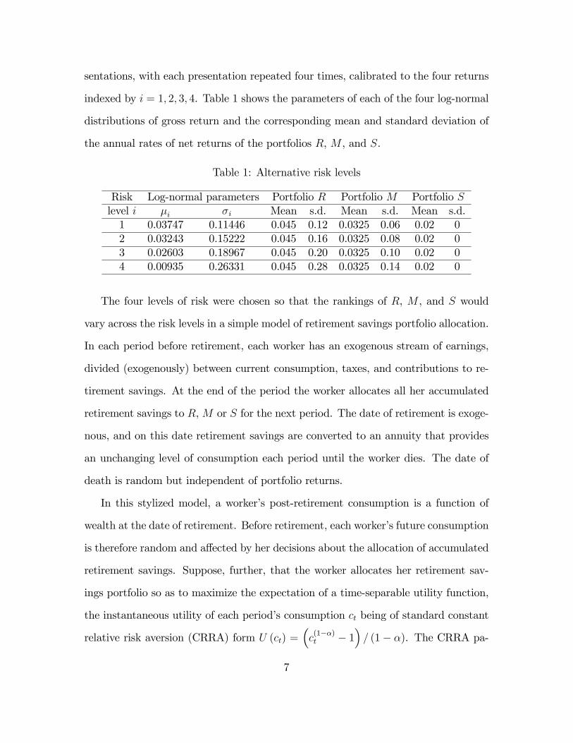
sentations, with each presentation repeated four times, calibrated to the four returns

indexed by i = 1; 2; 3; 4. Table 1 shows the parameters of each of the four log-normal

distributions of gross return and the corresponding mean and standard deviation of

the annual rates of net returns of the portfolios R, M , and S.

Table 1: Alternative risk levels

Risk Log-normal parameters Portfolio R Portfolio M Portfolio Slevel i �i �i Mean s.d. Mean s.d. Mean s.d.1 0.03747 0.11446 0.045 0.12 0.0325 0.06 0.02 02 0.03243 0.15222 0.045 0.16 0.0325 0.08 0.02 03 0.02603 0.18967 0.045 0.20 0.0325 0.10 0.02 04 0.00935 0.26331 0.045 0.28 0.0325 0.14 0.02 0

The four levels of risk were chosen so that the rankings of R, M , and S would

vary across the risk levels in a simple model of retirement savings portfolio allocation.

In each period before retirement, each worker has an exogenous stream of earnings,

divided (exogenously) between current consumption, taxes, and contributions to re-

tirement savings. At the end of the period the worker allocates all her accumulated

retirement savings to R,M or S for the next period. The date of retirement is exoge-

nous, and on this date retirement savings are converted to an annuity that provides

an unchanging level of consumption each period until the worker dies. The date of

death is random but independent of portfolio returns.

In this stylized model, a worker�s post-retirement consumption is a function of

wealth at the date of retirement. Before retirement, each worker�s future consumption

is therefore random and a¤ected by her decisions about the allocation of accumulated

retirement savings. Suppose, further, that the worker allocates her retirement sav-

ings portfolio so as to maximize the expectation of a time-separable utility function,

the instantaneous utility of each period�s consumption ct being of standard constant

relative risk aversion (CRRA) form U (ct) =�c(1��)t � 1

�= (1� �). The CRRA pa-

7

rameter � is worker-speci�c, with � 2 [0;1) and U (ct) = log (ct) when � = 1. Since

returns to the retirement savings portfolio are independent and identically distributed

each period, it follows (Ingersoll, 1997 Chapter 11) that workers maintain the same

allocation of their portfolio to S, M or R each period, even though they are free to

re-allocate. Thus, in this model, retirement portfolio allocations do not depend on

time to retirement or on the level of accumulated wealth. Workers with low values of

� allocate to R, workers with high values of � to S, and workers with intermediate

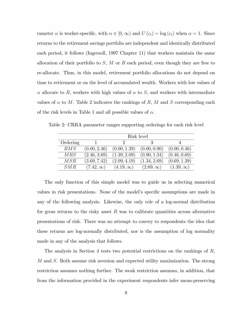
values of � to M . Table 2 indicates the rankings of R, M and S corresponding each

of the risk levels in Table 1 and all possible values of �.

Table 2: CRRA parameter ranges supporting orderings for each risk level

Risk levelOrdering 1 2 3 4RMS (0:00; 2:46) (0:00; 1:39) (0:00; 0:90) (0:00; 0:46)MRS (2:46; 3:69) (1:39; 2:09) (0:90; 1:34) (0:46; 0:69)MSR (3:69; 7:42) (2:09; 4:19) (1:34; 2:69) (0:69; 1:39)SMR (7:42;1) (4:19;1) (2:69;1) (1:39;1)

The only function of this simple model was to guide us in selecting numerical

values in risk presentations. None of the model�s speci�c assumptions are made in

any of the following analysis. Likewise, the only role of a log-normal distribution

for gross returns to the risky asset R was to calibrate quantities across alternative

presentations of risk. There was no attempt to convey to respondents the idea that

these returns are log-normally distributed, nor is the assumption of log normality

made in any of the analysis that follows.

The analysis in Section 4 tests two potential restrictions on the rankings of R,

M and S. Both assume risk aversion and expected utility maximization. The strong

restriction assumes nothing further. The weak restriction assumes, in addition, that

from the information provided in the experiment respondents infer mean-preserving

8

spread relationships among the gross returns to R at di¤erent risk levels.

Proposition 1 (Strong restriction on retirement portfolio choice) The orderings SRM

and RSM are inconsistent with expected utility maximization and risk aversion.

Proof. Recall that the gross returns to R, S andM are yi, x, and zi = (x+ yi) =2

respectively. Risk aversion is equivalent to concavity of utility so that

U (zi) = U

�x+ yi2

�>U (x) + U (yi)

2

and hence

E [U (zi)] >U (x) + E [U (yi)]

2.

Therefore E [U (zi)] > min fU (x) ; E [U (yi)]g and soM cannot be the least preferred

allocation of retirement wealth.

For the log-normal distributions indicated in the second and third columns of

Table 1, �i=�i < �j=�j for all pairs (i; j) with i < j. It follows (Levy 1991) that

(a) the distribution of gross returns yi to R at risk level i second-order stochastically

dominates that of gross returns yj at risk level j, (b) the distribution of yj is a mean-

preserving spread of the distribution of yi, and (c) E [U (yi)] > E [U (yj)] for any U

that is monotone increasing and concave. Directly from the de�nition of second-order

stochastic dominance, relationships (a), (b) and (c) are true of the gross returns zi

and zj to M as well.

Respondents are always told the means of net returns, and each time they are

asked to provide an ordering among R, M and S they are reminded of these means.

As detailed in the next section, each respondent is exposed to three di¤erent pre-

sentations of risk associated with R and M , and there is always a natural ordering

within each of the presentations: for example, if a respondent is told that negative

9

returns occur on average a years out of every 20, it is natural to associate larger a

with greater risk. It is therefore reasonable to entertain the prospect that from the

information provided respondents infer changes in spread with a common mean.

Proposition 2 (Weak restriction on retirement portfolio choice) Suppose

(1) Orderings are consistent with expected utility maximization and risk aversion;

(2) The distribution of R at risk level j is a mean-preserving spread of the distri-

bution of R at risk level i for all pairs (i; j) with i < j.

Then the pairs of orderings with an entry A, Bi or C in Table 3 are all possible,

whereas those with entries D or E are all impossible.

Table 3: Pairs of orderings for lower (i) and higher (j) risk levels

Ordering at Ordering at risk level jrisk level i SMR MSR MRS RMSSMR A E D;E D;EMSR B1 A D DMRS B2 B4 A CRMS B3 B5 B6 A

Proof. Pairs of orderings for cells with entry A can all be generated by su¢ ciently

small di¤erences in mean-preserving spread between risk levels i and j.

Pairs of orderings for cells marked Bi can be found in Table 3: � = 4; i = 1; j = 3

for B1, � = 3; i = 1; j = 3 for B2, � = 2; i = 1; j = 4 for B3, � = 3; i = 1; j = 2 for

B4, � = 2; i = 1; j = 3 for B5 and � = 1; i = 1; j = 3 for B6.

Appendix A provides an example that satis�es conditions (1) and (2) and gener-

ates the pair of orderings for the cell marked C.

Conditions 1 and 2 imply E [U (yi)] > E [U (yj)] (Rothschild and Stiglitz 1970)

and therefore E [U (x)] � E [U (yj)] > E [U (x)] � E [U (yi)]. This eliminates pairs of

10

orderings in which S is preferred to R at the lower risk level i but R is preferred to

S at the higher risk level j, the cells of Table 3 with an entry D.

Condition 2 is equivalent to the existence of a random variable " with E (" j yi) = 0

for all yi such that yj = yi + " (Rothschild and Stiglitz 1970). Therefore zj =

(x+ yj) =2 = (x+ yi + ") =2 = zi+("=2), which is equivalent to the distribution ofM

at risk level j being a mean-preserving spread of the distribution of M at risk level i.

It follows that E [U (zi)] > E [U (zj)] and E [U (x)]�E [U (zj)] > E [U (x)]�E [U (zi)],

thus eliminating pairs of orderings in which S is preferred toM at the lower risk level

i but M is preferred to S at the higher risk level j, the cells of Table 3 with entry E.

3 The discrete choice experiment

The experiment is the third part of an on-line, four-part survey instrument that

collects substantial information about the characteristics of each respondent. The

instructions for the experiment, reproduced in Appendix B, present a simpli�ed

retirement savings (superannuation) program in which the only options for the savings

portfolio are S,M and R. The instructions indicate that the respondent will be asked

to indicate which option he or she would be most likely to choose, and which option he

or she would be least likely to choose, in a series of settings in which average returns

remain the same but levels of risk vary. There are 36 settings in total, of which each

respondent sees 12. Each setting presents the annual returns net of in�ation (2% for

S, 3.25% for M , and 4.5% for R) together with a presentation of risk for M and R.

The 12 settings are the Cartesian product of the four risk levels indicated in Table 1

(common to all respondents) and three of the nine risk presentations.

Many presentations of risk to retirement savers are possible. We utilize nine

11

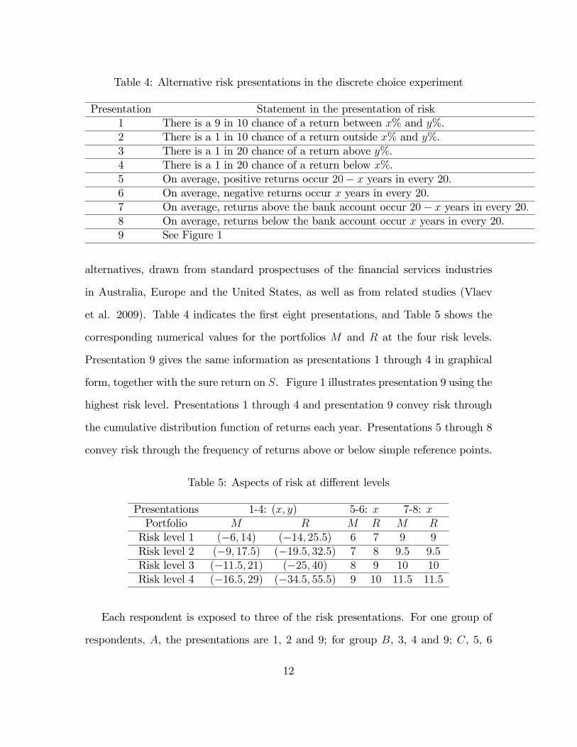
Table 4: Alternative risk presentations in the discrete choice experiment

Presentation Statement in the presentation of risk1 There is a 9 in 10 chance of a return between x% and y%.2 There is a 1 in 10 chance of a return outside x% and y%.3 There is a 1 in 20 chance of a return above y%.4 There is a 1 in 20 chance of a return below x%.5 On average, positive returns occur 20� x years in every 20.6 On average, negative returns occur x years in every 20.7 On average, returns above the bank account occur 20� x years in every 20:8 On average, returns below the bank account occur x years in every 20.9 See Figure 1

alternatives, drawn from standard prospectuses of the �nancial services industries

in Australia, Europe and the United States, as well as from related studies (Vlaev

et al. 2009). Table 4 indicates the �rst eight presentations, and Table 5 shows the

corresponding numerical values for the portfolios M and R at the four risk levels.

Presentation 9 gives the same information as presentations 1 through 4 in graphical

form, together with the sure return on S. Figure 1 illustrates presentation 9 using the

highest risk level. Presentations 1 through 4 and presentation 9 convey risk through

the cumulative distribution function of returns each year. Presentations 5 through 8

convey risk through the frequency of returns above or below simple reference points.

Table 5: Aspects of risk at di¤erent levels

Presentations 1-4: (x; y) 5-6: x 7-8: xPortfolio M R M R M RRisk level 1 (�6; 14) (�14; 25:5) 6 7 9 9Risk level 2 (�9; 17:5) (�19:5; 32:5) 7 8 9:5 9:5Risk level 3 (�11:5; 21) (�25; 40) 8 9 10 10Risk level 4 (�16:5; 29) (�34:5; 55:5) 9 10 11:5 11:5

Each respondent is exposed to three of the risk presentations. For one group of

respondents, A, the presentations are 1, 2 and 9; for group B, 3, 4 and 9; C, 5, 6

12

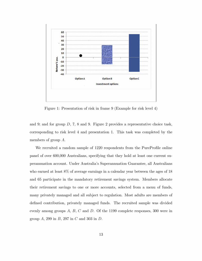
Figure 1: Presentation of risk in frame 9 (Example for risk level 4)

and 9; and for group D, 7, 8 and 9. Figure 2 provides a representative choice task,

corresponding to risk level 4 and presentation 1. This task was completed by the

members of group A.

We recruited a random sample of 1220 respondents from the PurePro�le online

panel of over 600,000 Australians, specifying that they hold at least one current su-

perannuation account. Under Australia�s Superannuation Guarantee, all Australians

who earned at least 8% of average earnings in a calendar year between the ages of 18

and 65 participate in the mandatory retirement savings system. Members allocate

their retirement savings to one or more accounts, selected from a menu of funds,

many privately managed and all subject to regulation. Most adults are members of

de�ned contribution, privately managed funds. The recruited sample was divided

evenly among groups A, B, C and D. Of the 1199 complete responses, 300 were in

group A, 299 in B, 297 in C and 303 in D.

13

Figure 2: A representative choice task in the discrete choice experiment

The other parts of the survey instrument provide respondent characteristics, and

our �ndings utilize some of that information. The �rst part consists of questions

about subjects�retirement savings, including the aggregate amount in their super-

annuation accounts. From this amount we constructed a polychotomous covariate,

�superannuation,�coded as 1 for accounts of less than $20,000, 2 for accounts in the

range $20,000 to $80,000, 3 for accounts in the range $80,000 to $500,000, and 4 for

accounts above $500,000. (Individuals�average accumulation in Australia�s superan-

nuation program is about $70,000.)

The second part of the survey consists of 21 questions measuring numeracy and

�nancial literacy skills, as well as self-assessed knowledge of �nance, access to �nancial

education, use of �nancial advice and con�dence in stock market recovery. The

�ve numeracy questions are drawn from Gerardi et al. (2010) and are designed to

test basic concepts such as fractions, percentages, division, multiplication and simple

probability. They are provided here in Appendix C. We �tted a factor model to the

14

responses to these questions, and used the �tted factor loadings to create the covariate

�numeracy,�a numeracy score for each respondent. This covariate has mean 0 and

standard deviation 1.

The third part of the survey instrument is the experiment just described. The

�nal part of the survey instrument consists of demographic questions relating to age,

marital status, work status, occupation, industry/business, education, income, assets,

household make-up and number in household. From the responses to these questions

we created a polychotomous covariate, �age,�coded as -1 for 18-34 years, 0 for 35-54

years, and 1 for 55 years or older. Bateman et al. (2010) provides a more detailed pre-

sentation of the survey instrument, which may be found at http://survey.con�rmit.com/

wix/p1250911674.aspx.

From this information we selected superannuation account balance, numeracy, and

age as covariates for the propensity to violate Propositions 1 and 2. The selection was

based on our prior belief that wealth, cognition and/or �nancial literacy, and time to

retirement are likely drivers in choosing a retirement portfolio. (See, for example, on

wealth, Mankiw and Zeldes 1991 and Carroll 2001; on cognition and literacy, Dohmen

et al. 2010 and Lusardi et al. 2009; on age, Agnew, Balduzzi and Sunden 2003 and

Ameriks and Zeldes 1997.) Preliminary work with logit models con�rmed that these

choices did not exclude other important covariates.

4 Findings

We investigate the propensity of respondents to violate Propositions 1 and 2, respec-

tively, as a function of the three covariates just described. Since there were 1199

complete responses, each providing 12 orderings of S, M and R, there are 14; 388

orderings all together. Table 6 indicates the frequency of each ordering in each of the

15

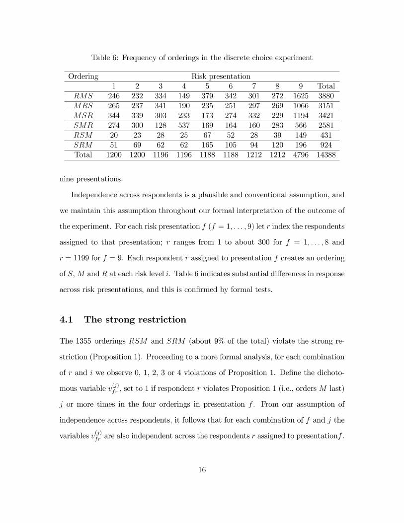
Table 6: Frequency of orderings in the discrete choice experiment

Ordering Risk presentation1 2 3 4 5 6 7 8 9 Total

RMS 246 232 334 149 379 342 301 272 1625 3880MRS 265 237 341 190 235 251 297 269 1066 3151MSR 344 339 303 233 173 274 332 229 1194 3421SMR 274 300 128 537 169 164 160 283 566 2581RSM 20 23 28 25 67 52 28 39 149 431SRM 51 69 62 62 165 105 94 120 196 924Total 1200 1200 1196 1196 1188 1188 1212 1212 4796 14388

nine presentations.

Independence across respondents is a plausible and conventional assumption, and

we maintain this assumption throughout our formal interpretation of the outcome of

the experiment. For each risk presentation f (f = 1; : : : ; 9) let r index the respondents

assigned to that presentation; r ranges from 1 to about 300 for f = 1; : : : ; 8 and

r = 1199 for f = 9. Each respondent r assigned to presentation f creates an ordering

of S,M and R at each risk level i. Table 6 indicates substantial di¤erences in response

across risk presentations, and this is con�rmed by formal tests.

4.1 The strong restriction

The 1355 orderings RSM and SRM (about 9% of the total) violate the strong re-

striction (Proposition 1). Proceeding to a more formal analysis, for each combination

of r and i we observe 0, 1, 2, 3 or 4 violations of Proposition 1. De�ne the dichoto-

mous variable v(j)fr , set to 1 if respondent r violates Proposition 1 (i.e., ordersM last)

j or more times in the four orderings in presentation f . From our assumption of

independence across respondents, it follows that for each combination of f and j the

variables v(j)fr are also independent across the respondents r assigned to presentationf .

16

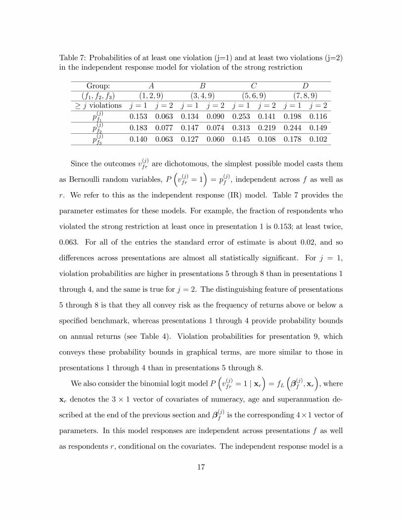
Table 7: Probabilities of at least one violation (j=1) and at least two violations (j=2)in the independent response model for violation of the strong restriction

Group: A B C D(f1; f2; f3) (1; 2; 9) (3; 4; 9) (5; 6; 9) (7; 8; 9)

� j violations j = 1 j = 2 j = 1 j = 2 j = 1 j = 2 j = 1 j = 2

p(j)f1

0.153 0.063 0.134 0.090 0.253 0.141 0.198 0.116

p(j)f2

0.183 0.077 0.147 0.074 0.313 0.219 0.244 0.149

p(j)f3

0.140 0.063 0.127 0.060 0.145 0.108 0.178 0.102

Since the outcomes v(j)fr are dichotomous, the simplest possible model casts them

as Bernoulli random variables, P�v(j)fr = 1

�= p

(j)f , independent across f as well as

r. We refer to this as the independent response (IR) model. Table 7 provides the

parameter estimates for these models. For example, the fraction of respondents who

violated the strong restriction at least once in presentation 1 is 0.153; at least twice,

0.063. For all of the entries the standard error of estimate is about 0.02, and so

di¤erences across presentations are almost all statistically signi�cant. For j = 1,

violation probabilities are higher in presentations 5 through 8 than in presentations 1

through 4, and the same is true for j = 2. The distinguishing feature of presentations

5 through 8 is that they all convey risk as the frequency of returns above or below a

speci�ed benchmark, whereas presentations 1 through 4 provide probability bounds

on annual returns (see Table 4). Violation probabilities for presentation 9, which

conveys these probability bounds in graphical terms, are more similar to those in

presentations 1 through 4 than in presentations 5 through 8.

We also consider the binomial logit model P�v(j)fr = 1 j xr

�= fL

��(j)f ;xr

�, where

xr denotes the 3 � 1 vector of covariates of numeracy, age and superannuation de-

scribed at the end of the previous section and �(j)f is the corresponding 4�1 vector of

parameters. In this model responses are independent across presentations f as well

as respondents r, conditional on the covariates. The independent response model is a

17

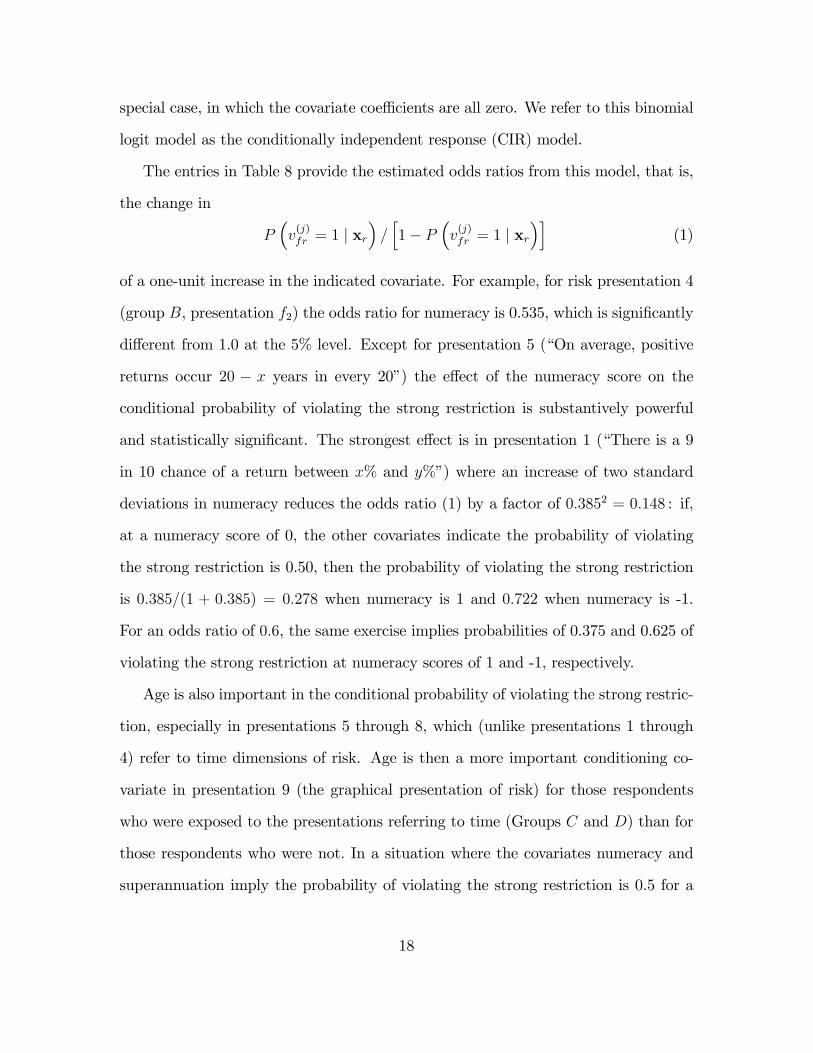
special case, in which the covariate coe¢ cients are all zero. We refer to this binomial

logit model as the conditionally independent response (CIR) model.

The entries in Table 8 provide the estimated odds ratios from this model, that is,

the change in

P�v(j)fr = 1 j xr

�=h1� P

�v(j)fr = 1 j xr

�i(1)

of a one-unit increase in the indicated covariate. For example, for risk presentation 4

(group B, presentation f2) the odds ratio for numeracy is 0.535, which is signi�cantly

di¤erent from 1.0 at the 5% level. Except for presentation 5 (�On average, positive

returns occur 20 � x years in every 20�) the e¤ect of the numeracy score on the

conditional probability of violating the strong restriction is substantively powerful

and statistically signi�cant. The strongest e¤ect is in presentation 1 (�There is a 9

in 10 chance of a return between x% and y%�) where an increase of two standard

deviations in numeracy reduces the odds ratio (1) by a factor of 0:3852 = 0:148 : if,

at a numeracy score of 0, the other covariates indicate the probability of violating

the strong restriction is 0.50, then the probability of violating the strong restriction

is 0:385=(1 + 0:385) = 0:278 when numeracy is 1 and 0:722 when numeracy is -1.

For an odds ratio of 0:6, the same exercise implies probabilities of 0.375 and 0.625 of

violating the strong restriction at numeracy scores of 1 and -1, respectively.

Age is also important in the conditional probability of violating the strong restric-

tion, especially in presentations 5 through 8, which (unlike presentations 1 through

4) refer to time dimensions of risk. Age is then a more important conditioning co-

variate in presentation 9 (the graphical presentation of risk) for those respondents

who were exposed to the presentations referring to time (Groups C and D) than for

those respondents who were not. In a situation where the covariates numeracy and

superannuation imply the probability of violating the strong restriction is 0.5 for a

18

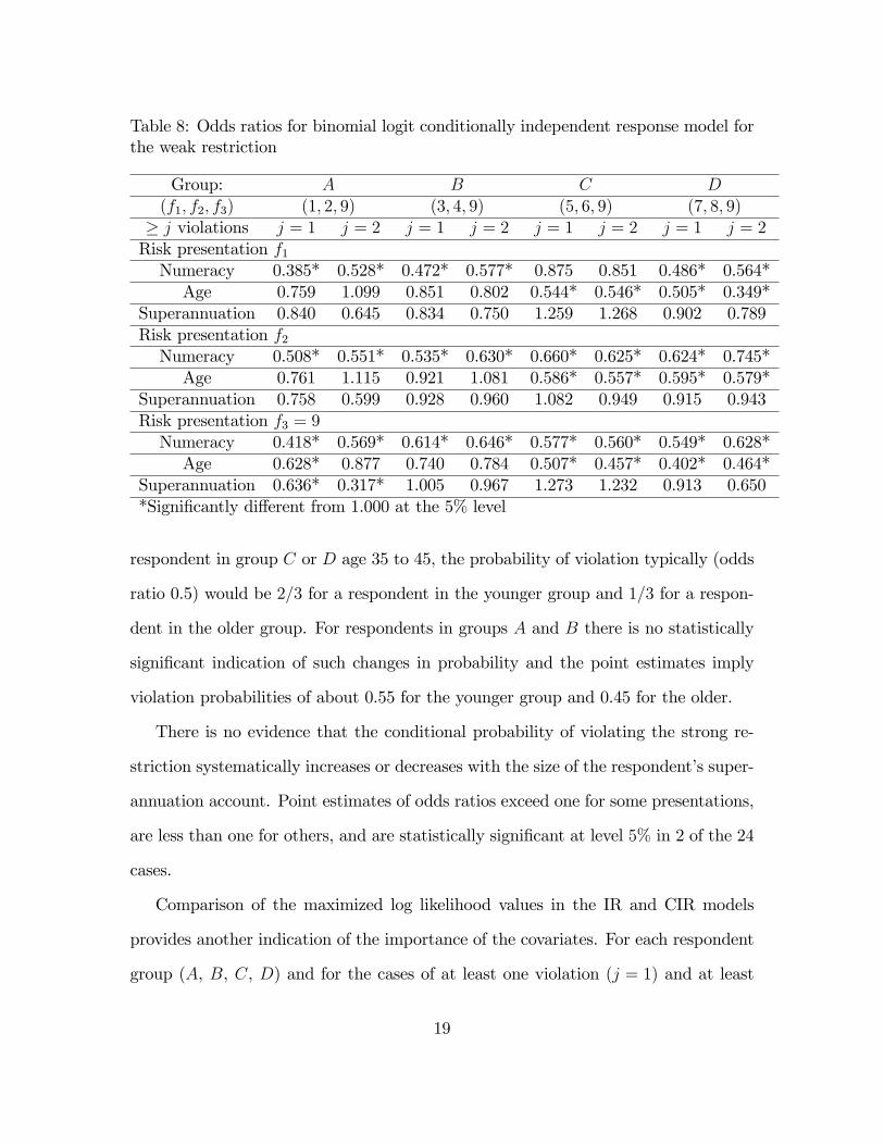
Table 8: Odds ratios for binomial logit conditionally independent response model forthe weak restriction

Group: A B C D(f1; f2; f3) (1; 2; 9) (3; 4; 9) (5; 6; 9) (7; 8; 9)

� j violations j = 1 j = 2 j = 1 j = 2 j = 1 j = 2 j = 1 j = 2Risk presentation f1Numeracy 0.385* 0.528* 0.472* 0.577* 0.875 0.851 0.486* 0.564*Age 0.759 1.099 0.851 0.802 0.544* 0.546* 0.505* 0.349*

Superannuation 0.840 0.645 0.834 0.750 1.259 1.268 0.902 0.789Risk presentation f2Numeracy 0.508* 0.551* 0.535* 0.630* 0.660* 0.625* 0.624* 0.745*Age 0.761 1.115 0.921 1.081 0.586* 0.557* 0.595* 0.579*

Superannuation 0.758 0.599 0.928 0.960 1.082 0.949 0.915 0.943Risk presentation f3 = 9Numeracy 0.418* 0.569* 0.614* 0.646* 0.577* 0.560* 0.549* 0.628*Age 0.628* 0.877 0.740 0.784 0.507* 0.457* 0.402* 0.464*

Superannuation 0.636* 0.317* 1.005 0.967 1.273 1.232 0.913 0.650*Signi�cantly di¤erent from 1.000 at the 5% level

respondent in group C or D age 35 to 45, the probability of violation typically (odds

ratio 0.5) would be 2=3 for a respondent in the younger group and 1=3 for a respon-

dent in the older group. For respondents in groups A and B there is no statistically

signi�cant indication of such changes in probability and the point estimates imply

violation probabilities of about 0.55 for the younger group and 0.45 for the older.

There is no evidence that the conditional probability of violating the strong re-

striction systematically increases or decreases with the size of the respondent�s super-

annuation account. Point estimates of odds ratios exceed one for some presentations,

are less than one for others, and are statistically signi�cant at level 5% in 2 of the 24

cases.

Comparison of the maximized log likelihood values in the IR and CIR models

provides another indication of the importance of the covariates. For each respondent

group (A, B, C, D) and for the cases of at least one violation (j = 1) and at least

19

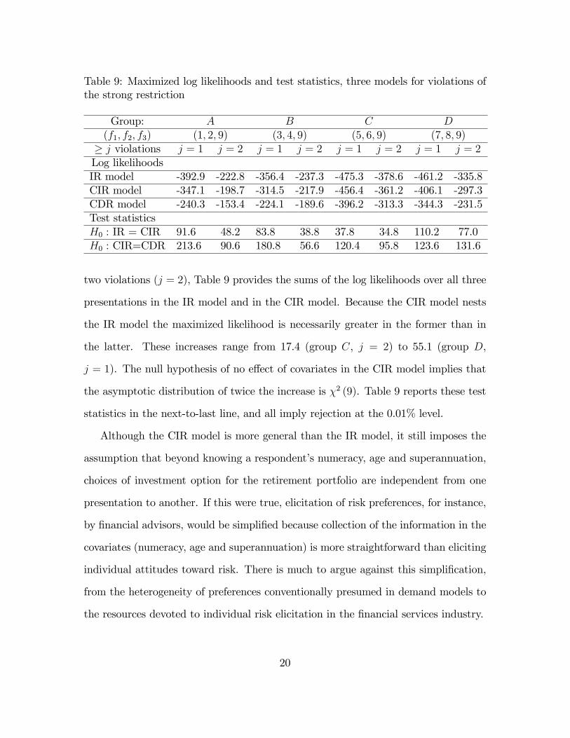
Table 9: Maximized log likelihoods and test statistics, three models for violations ofthe strong restriction

Group: A B C D(f1; f2; f3) (1; 2; 9) (3; 4; 9) (5; 6; 9) (7; 8; 9)

� j violations j = 1 j = 2 j = 1 j = 2 j = 1 j = 2 j = 1 j = 2Log likelihoodsIR model -392.9 -222.8 -356.4 -237.3 -475.3 -378.6 -461.2 -335.8CIR model -347.1 -198.7 -314.5 -217.9 -456.4 -361.2 -406.1 -297.3CDR model -240.3 -153.4 -224.1 -189.6 -396.2 -313.3 -344.3 -231.5Test statisticsH0 : IR = CIR 91.6 48.2 83.8 38.8 37.8 34.8 110.2 77.0H0 : CIR=CDR 213.6 90.6 180.8 56.6 120.4 95.8 123.6 131.6

two violations (j = 2), Table 9 provides the sums of the log likelihoods over all three

presentations in the IR model and in the CIR model. Because the CIR model nests

the IR model the maximized likelihood is necessarily greater in the former than in

the latter. These increases range from 17.4 (group C, j = 2) to 55.1 (group D,

j = 1). The null hypothesis of no e¤ect of covariates in the CIR model implies that

the asymptotic distribution of twice the increase is �2 (9). Table 9 reports these test

statistics in the next-to-last line, and all imply rejection at the 0.01% level.

Although the CIR model is more general than the IR model, it still imposes the

assumption that beyond knowing a respondent�s numeracy, age and superannuation,

choices of investment option for the retirement portfolio are independent from one

presentation to another. If this were true, elicitation of risk preferences, for instance,

by �nancial advisors, would be simpli�ed because collection of the information in the

covariates (numeracy, age and superannuation) is more straightforward than eliciting

individual attitudes toward risk. There is much to argue against this simpli�cation,

from the heterogeneity of preferences conventionally presumed in demand models to

the resources devoted to individual risk elicitation in the �nancial services industry.

20

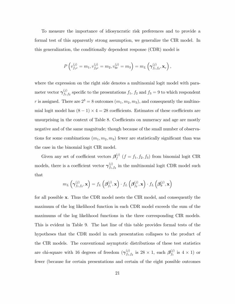
To measure the importance of idiosyncratic risk preferences and to provide a

formal test of this apparently strong assumption, we generalize the CIR model. In

this generalization, the conditionally dependent response (CDR) model is

P�v(j)f1r= m1; v

(j)f2r= m2; v

(j)9r = m3

�= mL

� (j)f1;f2

;xr

�,

where the expression on the right side denotes a multinomial logit model with para-

meter vector (j)f1;f2 speci�c to the presentations f1, f2 and f3 = 9 to which respondent

r is assigned. There are 23 = 8 outcomes (m1;m2;m3), and consequently the multino-

mial logit model has (8� 1)� 4 = 28 coe¢ cients. Estimates of these coe¢ cients are

unsurprising in the context of Table 8. Coe¢ cients on numeracy and age are mostly

negative and of the same magnitude; though because of the small number of observa-

tions for some combinations (m1;m2;m3) fewer are statistically signi�cant than was

the case in the binomial logit CIR model.

Given any set of coe¢ cient vectors �(j)f (f = f1; f2; f3) from binomial logit CIR

models, there is a coe¢ cient vector (j)f1;f2 in the multinomial logit CDR model such

that

mL

� (j)f1;f2

;x�= fL

��(j)f1;x�� fL

��(j)f2;x�� fL

��(j)9 ;x

�for all possible x. Thus the CDR model nests the CIR model, and consequently the

maximum of the log likelihood function in each CDR model exceeds the sum of the

maximums of the log likelihood functions in the three corresponding CIR models.

This is evident in Table 9. The last line of this table provides formal tests of the

hypotheses that the CDR model in each presentation collapses to the product of

the CIR models. The conventional asymptotic distributions of these test statistics

are chi-square with 16 degrees of freedom ( (j)f1;f2 is 28 � 1, each �(j)f1is 4 � 1) or

fewer (because for certain presentations and certain of the eight possible outcomes

21

there are four or fewer observations in the CDR model). While the adequacy of the

conventional asymptotic distribution theory is open to question in this setting there

can be no real doubt that the CIR hypothesis should be rejected. The results in Table

9 indicate substantial dependence of respondent orderings across presentations. Some

of this dependence is explained by the covariates numeracy, age and superannuation,

but even more must be ascribed to idiosyncratic variation. The �nancial services

industry has long devoted substantial resources to eliciting individual tastes for risk,

consistent with these results. (See Yooks and Everett (2003) for discussion.)

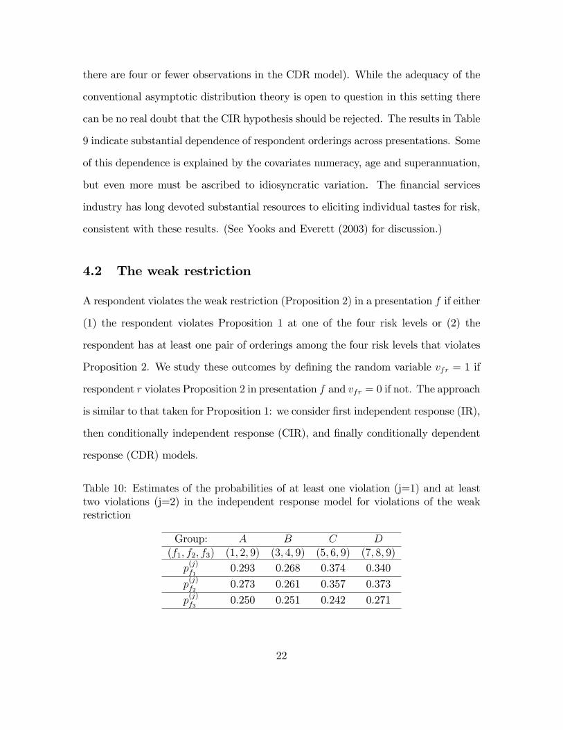
4.2 The weak restriction

A respondent violates the weak restriction (Proposition 2) in a presentation f if either

(1) the respondent violates Proposition 1 at one of the four risk levels or (2) the

respondent has at least one pair of orderings among the four risk levels that violates

Proposition 2. We study these outcomes by de�ning the random variable vfr = 1 if

respondent r violates Proposition 2 in presentation f and vfr = 0 if not. The approach

is similar to that taken for Proposition 1: we consider �rst independent response (IR),

then conditionally independent response (CIR), and �nally conditionally dependent

response (CDR) models.

Table 10: Estimates of the probabilities of at least one violation (j=1) and at leasttwo violations (j=2) in the independent response model for violations of the weakrestriction

Group: A B C D(f1; f2; f3) (1; 2; 9) (3; 4; 9) (5; 6; 9) (7; 8; 9)

p(j)f1

0.293 0.268 0.374 0.340

p(j)f2

0.273 0.261 0.357 0.373

p(j)f3

0.250 0.251 0.242 0.271

22

Table 10 provides the parameter estimates in the IR model, each parameter having

a standard error of estimate of about 0.025. As was the case for the strong restriction,

the probability of violations of the weak restriction is higher in presentations 5 through

8, which couch risk in terms of the frequency of returns above or below benchmark

values, than it is in the other presentations, which express risk in terms of points on

the cumulative distribution function for annual returns.

Table 11: Odds ratios for conditionally independent response binomial logit modelfor the weak restriction

(f1; f2; f3) (1; 2; 9) (3; 4; 9) (5; 6; 9) (7; 8; 9)Risk presentation f1Numeracy 0.407* 0.642* 0.792 0.407*Age 0.673* 0.810 0.719* 0.713*

Superannuation 0.980 0.762 1.101 0.763Risk presentation f2Numeracy 0.419* 0.519* 0.602* 0.606*Age 0.744 0.887 0.696* 0.606*

Superannuation 0.781 0.824 1.067 0.999Risk presentation f3 = 9Numeracy 0.484* 0.761* 0.702* 0.546*Age 0.541* 0.915 0.729 0.478*

Superannuation 0.788 0.969 0.913 0.977

The conditional probabilities of violation of the weak restriction in the CIR model

are similar to those of violation of the strong restriction, as detailed in Table 11. These

probabilities decline rapidly with increasing numeracy and age. The e¤ect of numer-

acy on the conditional probability is about the same as for the strong restriction.

The e¤ect of age is somewhat reduced, and the greater importance of age in presen-

tations 5 through 8 than in the other presentations is somewhat muted. Combined,

the impacts of numeracy and age are substantial: if a respondent aged 35 to 54 with

a numeracy score 0 (the average) violates the strong restriction with probability 0.5,

then (assuming a numeracy odds ratio of 0.6 and an age odds ratio of 0.7) the prob-

23

Table 12: Maximized log likelihoods and test statistics, three models for violations ofthe weak restriction

Group: A B C D(f1; f2; f3) (1; 2; 9) (3; 4; 9) (5; 6; 9) (7; 8; 9)Log-likelihoodsIR model -526.2 -513.7 -554.3 -571.3CIR model -477.8 -484.4 -541.3 -511.4CDR model -402.2 -442.9 -488.4 -455.3Test statisticsH0 : IR = CIR 96.8 58.6 26.0 119.8H0 : CIR=CDR 151.2 83.0 105.8 112.2

ability of violation of the weak restriction is about 0.7 for a younger respondent with

a numeracy score of -1 and 0.3 for an older respondent with a numeracy score of 1.

As was the case with the strong restriction, there is no indication of a systematic

impact of the size of the respondent�s superannuation account on violation of the

weak restriction.

Table 12 details the increase in maximized log likelihood moving from the IR to

the CIR to the CDR model. The comparisons are similar to those for the strong

restriction, and indicate formal rejection of smaller models in favor of larger ones.

The three covariates again account for a substantial proportion of the dependence

of respondent violations of the restriction, moving across presentations, but there

is even more dependence that is not accounted for by the covariates. These results

reinforce the conclusion that there is value in assessing individuals�attitudes toward

risk in retirement planning.

24

5 Conclusion

Our analysis of the results of the discrete choice experiment can be summarized in

�ve main points, as follows.

1. In a setting that is experimental but similar to that in which real decisions are

made, respondents routinely violate the two implications of the expected utility

theory of decision-making under risk, detailed in Section 2. These rates range

from 14% to 37%.

2. When risk is presented with respect to frequency, for example �On average,

negative returns occur 7 years in every 20,� the probability of violating the

restrictions is greater: about 25% for the strong restriction and 35% for the

weak restriction. When risk is presented with respect to the probability of high

or low returns each year, for example �There is a 9 in 10 chance of a return

between -6% and 14%,�the probability of violation is less: about 15% for the

strong restriction and 25% for the weak restriction.

3. A respondent�s quantitative aptitude, as measured by a short conventional test

of numeracy, substantially a¤ects the probability that either restriction will be

violated. For example, in the case of the strong restriction with risk presented

as frequency, for an otherwise randomly selected respondent with numeracy in

the top decile, the probability of violation is about 5%, whereas for one in the

bottom decile, it is about 35%.

4. A respondent�s age substantially a¤ects the probability that either restriction

will be violated when the risk presentation invokes the frequency of events. For

example, in the case of the strong restriction, for an otherwise randomly selected

25

respondent, the probability of violation is about 15% for a respondent age 55

or older, and about 38% for a respondent age 18 to 34 .

5. In the discrete choice experiment the alternative presentations of risk were all

calibrated to the same log-normal distribution of returns at each level of risk.

From the information provided respondents need not have inferred that the dis-

tributions of returns were the same across the alternative presentations. Never-

theless, there is strong dependence in the propensity to violate the strong and

weak restriction across risk presentations: if a respondent violates a restriction

in one presentation this increases the probability that the respondent will vio-

late that restriction in another presentation. Much of this dependence across

risk presentations can be attributed to a respondent�s numeracy score and age,

but it is also the case that much dependence remains after conditioning on these

attributes.

From these results we venture several more tentative conclusions about the di-

rection of future research and lessons for the public policy of compulsory de�ned

contribution retirement schemes.

1. The strong association between poor numeracy skills and the propensity to

violate the expected utility paradigm is strong and consistent with the few

studies that have explored this issue (Peters and Levin, 2008; Gerardi et al.,

2010). This relationship is fundamental to the evaluation of public policy that

delegates sophisticated �nancial decisions to individuals who are compelled to

contribute to de�ned contribution retirement plans. Further research should be

undertaken to understand the relationship between quantitative aptitude and

quantitative decision making, eventually addressing the question of whether

26

there are policy interventions that might increase quantitative decision-making

skills.

2. In the interim, this work would support serious reservations about public policy

linking the future welfare of current workers to quantitative decision-making

skills that a signi�cant number of them do not possess.

3. The presentation of risk is important in the elicitation of decisions for retirement

planning, a conclusion that has emerged in related work. (See, among others,

Saez 2009 on contributions, Benartzi and Thaler 1999, Rubaltelli et al. 2005,

Anagol and Gamble 2008 on asset allocation decisions, and Agnew et al. 2008

and Brown et al. 2008 on annuitization decisions.) Our �ndings suggest, in

particular, that consistency with the core economic model of expected utility is

speci�c to the presentation of risk. Further research is warranted to understand

those attributes of risk presentation that are most important in determining

whether revealed preferences are consistent with the core model.

27

References

Agnew, J., Anderson, L., Gerlach, J., and L. Szykman, �Who Chooses Annuities? An

Experimental Investigation of the Role of Gender, Framing and Defaults,�American

Economic Review 98(2) (2008), 418-22.

Agnew, J., Balduzzi, P., and A. Sunden, �Portfolio Choice and Trading in a Large

401(k) Plan,�American Economic Review 93 (2003), 193-205.

Ameriks, J., and S.P. Zeldes, �How do Household Portfolio Shares Vary with Age?�

Working Paper, Columbia University (2004).

Anagol, S., and K.J. Gamble, �Presenting Investment Results Asset by Asset Lowers

Risk Taking,�Yale University, working paper (2008).

Bateman H., Ebling C., Geweke J., Louviere J., Satchell S., and S. Thorp �Risk

presentation, risk preference and �nancial literacy.�University of Technology Sydney

and University of New South Wales Working paper (2010), Sydney.

Barseghyan, L., Prince, J., and J.C. Teitelbaum, �Are Risk Preference Stable Across

Contexts? Evidence from Insurance Data,�Mimeo, Cornell University (2009).

Benartzi, S., and R.H. Thaler, �Risk Aversion or Myopia? Choices in Repeated

Gambles and Retirement Investments,�Management Science 45(3) (1999), 364-81.

Brown, J., Kling, J., Mullainathan, S., and M. Wrobel, �Why Don�t People Insure

Late Life Consumption? A Framing Explanation of the Under-annuitization Puzzle,�

American Economic Review 98(2).(2008), 304-309.

Carroll, C.D., �Portfolios of the Rich,� in Guiso, L., Haliassos, M., and T. Japelli,

(eds.) Household Portfolios, MIT Press, Cambridge (2001).

28

Dohmen T., Falk A., Hu¤man D., and U. Sunde, �Are Risk Aversion and Impatience

Related to Cognitive Ability?�American Economic Review 100 (3) (2010), 1238�

1260.

Friend, I. and M.E. Blume, �The Demand for Risky Assets,�American Economic

Review 65(5) (1975), 900-922.

Gerardi, K., Goette, L., and S. Meier, �Financial Literacy and Subprime Mortgage

Delinquency: Evidence from a Survey Matched to Administrative Data,� Federal

Reserve Bank of Atlanta Working Paper Series No 2010-10, (2010) Atlanta, GA.

Goldstein, D.G., Johnson, E.J., and W.F. Sharpe, �Choosing Outcomes Versus

Choosing Products: Consumer-Focused Retirement Investment Advice,�Journal of

Consumer Research 35 (2008), 440-456.

Haisley, E., Kaufmann, C., and M. Weber, �How Much Risk can I Handle? The

Role of Experience Sampling and Graphical Displays on One�s Risk Appetite,�Paper

presented at the First Boulder Conference on Consumer Financial Decision Making,

Boulder, Colorado, June (2010).

Holt, C.A., and S.K. Laury, �Risk Aversion and Incentive E¤ects,�American Eco-

nomic Review 92(5) (2002),1644-1655.

Ingersoll, J., Theory of Financial Decision Making, (Lanham: Rowman and Little-

�eld, 1997).

Kimball, M.S., Sahm, C. R., and M.D. Shapiro, �Imputing risk aversion from survey

responses,� Journal of the American Statistical Association 103(483) (2008), 1028-

1038.

29

Levy, H. �The Mean-coe¢ cient-of-variation rule: the Lognormal Case,�Management

Science 37(6) (1991), 745-747.

Lusardi, A., Mitchell, O., and V. Curto, �Financial Literacy and Financial Sophisti-

cation Among Older Americans,�IRM WP2009-25 Insurance and Risk Management

Working Paper, The Wharton School, University of Pennsylvania (2009), Philadel-

phia PA.

Mankiw, N.G., and S.P. Zeldes, �The Consumption of Stockholders and Non-

stockholders,�Journal of Financial Economics 29 (1991), 97-112.

Peters, E., and I.P. Levin, �Dissection the risky-choice framing e¤ect: Numeracy as

an Individual-Di¤erence Factor in Weighting Risky and Riskless Options,�Judgement

and Decision Making 3(6) (2008), 435-448.

Rothschild M., and J. Stiglitz, �Increasing Risk I: A De�nition,�Journal of Economic

Theory 2 (1970), 315-329.

Rubaltelli, E., Rubichi, S., Savadori, L., Tadeschi, M., and R. Ferretti, �Numerical

Information Format and Investment Decisions: Implications for the Disposition E¤ect

and Status Quo Bias,�Journal of Behavioral Finance 6(1) (2005), 19-26.

Saez, E., �Details Matter: The Impact of Presentation and Information on the Take-

up of Financial Incentives for Retirement Savings,� American Economic Journal:

Economic Policy 1(1) (2009), 204-228.

Vlaev, I., Chater, N., and N. Stewart, �Dimensionality of Risk Perception: Factors

A¤ecting Consumer Understanding and Evaluation of Financial Risk,� Journal of

Behavioral Finance 10(3) (2009), 158-181.

30

Yooks, K.C., and R.E. Everett, �Assessing risk tolerance: Questioning the question-

naire method,�Journal of Financial Planning 16(8) (2003), 48-55.

31

Appendix A: Proposition 2, MRS/RMS ordering case

The following example shows that entry C in Table 3 is possible. The example

was produced by an algorithm that randomly generates discrete random variables on

[0; 1] and weakly convex piecewise linear utility functions normalized with u (0) = 0,

u (1) = 1. Through linear transformation all of these examples can be made to match

the values S = 1:02 and E (R) = 1:045 of the experiments without changing the

preference orderings for S, M and R.

The utility function in the example is

U (w) = s1 � I[0;b] (w) � w +�s1b+ s2 � I[b;1] (w) � (w � b)

�with breakpoint b = 0:2383 and slopes s1 = 0:9067 and s2 = 0:0580. The upper

panels of Figure 3 indicate U (w).

The sure return to S is x = 0:1653. The distribution of y (the gross return

to R) has the same 10 points of support in [0; 1] at both risk levels i and j, with

E (y) = 0:4562. Therefore the distribution of z (the gross return to M) also has

common points of support at both risk levels i and j, with E (z) = 0:3107. The

probability distributions are indicated in the upper panels of Figure 3. The lower left

panel shows the cumulative distribution functions F (y) for R at both risk levels, and

the lower right panel shows the values of G (y) :=R y0F (x) dx for both risk levels.

Note that G (y) for the higher risk level either exceeds or is coincident with G (y)

for the lower risk level, and therefore y at the higher risk level is a mean preserving

spread of y at the lower risk level.

Tables 13 and 14 provide complete details for the example. Comparing the two

tables note in particular that at the lower risk level i, E [U (y)] = 0:6926 < 0:7030 =

32

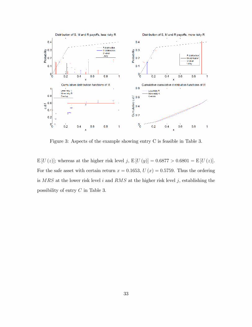
Figure 3: Aspects of the example showing entry C is feasible in Table 3.

E [U (z)]; whereas at the higher risk level j, E [U (y)] = 0:6877 > 0:6801 = E [U (z)].

For the safe asset with certain return x = 0:1653, U (x) = 0:5759. Thus the ordering

is MRS at the lower risk level i and RMS at the higher risk level j, establishing the

possibility of entry C in Table 3.

33

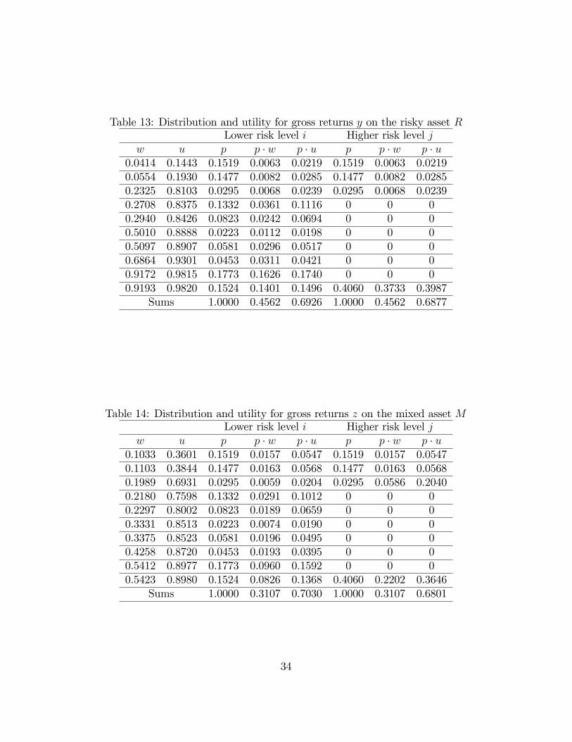
Table 13: Distribution and utility for gross returns y on the risky asset RLower risk level i Higher risk level j

w u p p � w p � u p p � w p � u0.0414 0.1443 0.1519 0.0063 0.0219 0.1519 0.0063 0.02190.0554 0.1930 0.1477 0.0082 0.0285 0.1477 0.0082 0.02850.2325 0.8103 0.0295 0.0068 0.0239 0.0295 0.0068 0.02390.2708 0.8375 0.1332 0.0361 0.1116 0 0 00.2940 0.8426 0.0823 0.0242 0.0694 0 0 00.5010 0.8888 0.0223 0.0112 0.0198 0 0 00.5097 0.8907 0.0581 0.0296 0.0517 0 0 00.6864 0.9301 0.0453 0.0311 0.0421 0 0 00.9172 0.9815 0.1773 0.1626 0.1740 0 0 00.9193 0.9820 0.1524 0.1401 0.1496 0.4060 0.3733 0.3987

Sums 1.0000 0.4562 0.6926 1.0000 0.4562 0.6877

Table 14: Distribution and utility for gross returns z on the mixed asset MLower risk level i Higher risk level j

w u p p � w p � u p p � w p � u0.1033 0.3601 0.1519 0.0157 0.0547 0.1519 0.0157 0.05470.1103 0.3844 0.1477 0.0163 0.0568 0.1477 0.0163 0.05680.1989 0.6931 0.0295 0.0059 0.0204 0.0295 0.0586 0.20400.2180 0.7598 0.1332 0.0291 0.1012 0 0 00.2297 0.8002 0.0823 0.0189 0.0659 0 0 00.3331 0.8513 0.0223 0.0074 0.0190 0 0 00.3375 0.8523 0.0581 0.0196 0.0495 0 0 00.4258 0.8720 0.0453 0.0193 0.0395 0 0 00.5412 0.8977 0.1773 0.0960 0.1592 0 0 00.5423 0.8980 0.1524 0.0826 0.1368 0.4060 0.2202 0.3646

Sums 1.0000 0.3107 0.7030 1.0000 0.3107 0.6801

34

Appendix B: Instructions to survey subjects.

The Australian Government is concerned about the complexity of superannua-

tion arrangements and is looking for ways of simplifying superannuation investment

choices. One possibility is to o¤er only three investment options for all superannu-

ation accounts. Each investment option has a di¤erent expected rate of return (the

average rate at which your investment will grow each year), and a di¤erent amount

of investment risk (year to year UPSIDE and DOWNSIDE variation in the return to

your investment).

The options are

Option A: All (100%) of your superannuation account is invested in a guaranteed

bank deposit with a �xed rate of interest paid each year.

Option B: Your superannuation account will be divided half and half (50%/50%)

between the bank account and growth assets. You can anticipate that savings in this

option will grow faster than the bank deposit (Option A), but will grow more slowly

and be less risky than only choosing growth assets (Option C).

Option C: All (100%) of your superannuation account is invested in assets like

shares and property. On average, you can anticipate that savings in this option will

grow at a faster rate than in the bank deposit (Option A) but without a guarantee.

There is some risk that your account will grow faster or slower than average if you

choose this option.

We are going to show you 12 sets of these options for investing your superannu-

ation. Each set includes 3 investment options like the ones described above. Each

investment option has a average rate of return and investment risk. The average

rates of return stay the same in each of the twelve sets; only the risk will change.

Remember that more risk of high returns also means more risk of low returns.

35

What we want you to do is simple. There are two questions to ask about each set

of options::

1. If these superannuation options were available for you to invest your money

today, which one of the three would you be most likely to choose?

2. If these superannuation options were available for you to invest your money

today, which of the three would you be least likely to choose?

Your choices will inform government and industry about better ways to simplify

superannuation arrangements.

36

Appendix C: Numeracy instrument

The instrument was administered as part of the online survey. There was no limit

on response time.

Q1: In a sale, a shop is selling all items at half price. Before the sale, a sofa costs

$300. How much will it cost in the sale? (Answers: $150; $300; $600; Do not know;

Refuse to answer.)

Q2: If the chance of getting a disease is 10 per cent, how many people out of 1,000

would be expected to get the disease? (Answers: 10; 100; 1000; Do not know; Refuse

to answer.)

Q3: A second hand car dealer is selling a car for $6,000. This is two-thirds of

what it cost new. How much did the car cost new? (Answers: $4,000; $6,600; $9,000;

Do not know; Refuse to answer.)

Q4: If 5 independent, unrelated people all have the winning numbers in the lottery

and the prize is $2 million, how much will each of them get? (Answers: $40,000;

$400,000; $500,000; Do not know; Refuse to answer.)

Q5: If there is a 1 in 10 chance of getting a disease, how many people out of 1,000

would be expected to get the disease? (Answers: 10; 100; 1000; Do not know; Refuse

to answer.)

37