ÉCOLE DE TECHNOLOGIE SUPÉRIEURE UNIVERSITÉ DU QUÉBEC

THÈSE PAR ARTICLES PRÉSENTÉE À L’ÉCOLE DE TECHNOLOGIE SUPÉRIEURE

COMME EXIGENCE PARTIELLE À L’OBTENTION DU

DOCTORAT EN GÉNIE Ph. D.

PAR Ali AIDIBE

INSPECTION DES PIÈCES FLEXIBLES SANS GABARIT DE CONFORMATION

MONTRÉAL, LE 22 MARS 2014

©Tous droits réservés, Ali Aidibe, 2014

©Tous droits réservés

Cette licence signifie qu’il est interdit de reproduire, d’enregistrer ou de diffuser en tout ou en partie, le

présent document. Le lecteur qui désire imprimer ou conserver sur un autre media une partie importante de

ce document, doit obligatoirement en demander l’autorisation à l’auteur.

PRÉSENTATION DU JURY

CETTE THÈSE A ÉTÉ ÉVALUÉE

PAR UN JURY COMPOSÉ DE : M. Souheil-Antoine TAHAN, directeur de thèse Département de génie mécanique à l’École de technologie supérieure M. Roland MARANZANA, président du jury Département de génie de la production automatisée à l’École de technologie supérieure M. Victor SONGMENE, membre du jury Département de génie mécanique à l’École de technologie supérieure M. Vincent FRANÇOIS, membre externe Département de génie mécanique à l’Université du Québec à Trois-Rivières M. Jean BIGEON, membre externe indépendant Laboratoire des sciences pour la conception, l’optimisation et la production à l’Université de Grenoble

IL A FAIT L’OBJET D’UNE SOUTENANCE DEVANT JURY ET PUBLIC

LE 25 FÉVRIER 2014

À L’ÉCOLE DE TECHNOLOGIE SUPÉRIEURE

REMERCIEMENTS

Le présent travail n’aurait pas été possible sans le bienveillant soutien de mon directeur de

thèse, le professeur Souheil-Antoine TAHAN. Je tiens à lui adresser mes chaleureux

remerciements pour son aide, son professionnalisme et ses précieux conseils au cours de ces

années. J’aimerais également lui exprimer à quel point j’ai apprécié sa grande disponibilité

malgré ses nombreuses charges, sa sympathie, ainsi que la confiance qu’il m’a accordée. J’ai

beaucoup appris à ses côtés et je profite pour lui adresser ici ma plus profonde gratitude pour

tout cela.

À la session d’hiver de l’année 2013, j’ai eu la chance et le plaisir de passer un stage de

quatre mois au sein du centre d’industrialisation de la compagnie Bombardier Aéronautique.

Je tiens à adresser mes vifs remerciements à M. Jean-François LALONDE, M. André P.

LEDUC, M. Dominic MOREAU et M. Brent JACKLE pour leur accueil et leur disponibilité

durant ce stage. J’y ai énormément appris. Ce stage représente sans aucun doute une grande

étape dans ma future vie professionnelle. J’ai pu consolider mes connaissances en métrologie

et acquérir une expérience industrielle très pertinente. De plus, j’aimerais remercier le

Conseil de recherches en sciences naturelles et en génie du Canada (CRSNG) et l'École de

technologie supérieure (ÉTS) pour leur soutien et leur contribution financière, ce qui m’a

permis de concentrer la majorité de mon temps à mes activités de recherches.

J’adresse également mes très sincères remerciements au président et à tous les membres du

jury d’avoir accepté d’assister à la présentation de ce travail. Je remercie également tous les

ami(e)s de l’ÉTS, les membres du Laboratoire d'Ingénierie des Produits, Procédés et

Systèmes (LIPPS) et les membres d’AÉROÉTS pour les bons moments partagés.

Ces remerciements seraient incomplets si je n'en adressais pas à ma magnifique famille. Je

souhaite remercier de tout mon cœur ma chère mère Ghada BALHAS et mon cher père

Hussein AIDIBE pour leur soutien constant et leur encouragement ainsi que mon frère et

toutes mes sœurs pour leur soutien moral.

VI

Enfin, je voulais ajouter quelques mots pour la femme de ma vie : « Tu es la plus belle,

JE T’AIME ».

Si vous ne pouvez expliquer un concept à un enfant de six ans, c'est que vous ne le comprenez pas complètement.

Albert Einstein

INSPECTION DES PIÈCES FLEXIBLES SANS GABARIT DE CONFORMATION

Ali AIDIBE

RÉSUMÉ

Le travail présenté dans le cadre de cette thèse porte sur l’automatisation de l’inspection dimensionnelle et géométrique d’une catégorie spécifique de pièces dites flexibles (ou souples). L’objectif principal est de manipuler ce type de composantes et leur nuage de points, qui représentent un scan pris à l’état libre, de manière virtuelle dans le but d’éliminer l’utilisation couteuse des gabarits de conformité et qui posent des problèmes de productivité pour les entreprises manufacturières. La thèse est organisée par articles. Le travail est reparti sur quatre phases. Les premières trois phases sont présentées par trois articles de revue et la quatrième phase est présentée dans une annexe. La première phase de ce travail est une amélioration substantielle du module d’identification d’un outil d’inspection mathématique existant « IDI : The Iterative Displacement Inspection » et qui a été développé par l’équipe de recherche qui travaille sous la direction du professeur Tahan à l’ÉTS. Le module d’identification vise à distinguer les défauts qui sont dus au processus de fabrication des déformations qui sont dues à la flexibilité de la pièce (effets de gravité et effets des contraintes résiduelles). Nous proposons de remplacer le module original par un nouveau qui est basé sur les statistiques extrêmes. Nous démontrons que le nouveau module réduit considérablement les erreurs de type I et II. En plus, contrairement à la méthode d’identification de l’IDI, la méthode proposée n’exige aucun seuil spécifié par l’utilisateur. Dans la deuxième phase de ce travail, nous proposons une approche originale pour quantifier la flexibilité/rigidité des composantes mécaniques. Nous introduisons un facteur qui représente le rapport entre le déplacement maximal résultant de la déformation de la pièce et sa tolérance de profil et nous présentons le tout sur une échelle logarithmique. Trois différentes zones ont été définies donnant une idée claire à l’industrie manufacturière de la situation des pièces sur l’échelle de la flexibilité. Par la suite, nous proposons une nouvelle méthode pour l’inspection des pièces flexibles sans gabarit de conformation : la méthode « IDB-CTB: Inspection of Deformable Bodies by Curvature and Thompson-Biweight ». Cette approche combine l’estimation de la courbure gaussienne, une des propriétés intrinsèques de la surface et qui est invariante sous les transformations isométriques, avec une méthode d’identification basée sur les statistiques extrêmes (Thompson-Biweight test). Le faible pourcentage d’erreur obtenue au niveau de l’estimation du défaut de profil ainsi que de l’aire de la zone de défaut reflète l’efficacité de l’approche. Dans la troisième phase de cette thèse, nous proposons une autre approche, originale et complémentaire à celle de la deuxième phase. En plus de la détection des défauts de profil, nous visons à détecter les défauts de localisation. Nous introduisons deux critères qui correspondent aux spécificités des pièces mécaniques souples : la conservation de la distance curviligne et la minimisation entre deux objets (distance de Hausdorff). Nous adaptons et

VIII

nous automatisons l’algorithme Coherent Point Drift, un puissant algorithme de recalage non rigide très employé dans l’imagerie médicale et d’animation, pour qu’il satisfasse ces deux critères. Nous obtenons de résultats satisfaisants en appliquant cette troisième approche sur une pièce flexible typique du secteur aérospatial. La conclusion de cette thèse résume les contributions scientifiques générées par nos travaux sur l’inspection des pièces flexibles ainsi que les perspectives en relation avec ce sujet. En annexe, nous présentons une interface graphique (GUI) qui a été créée pour manipuler les approches proposées ainsi que la banque des études de cas développée dans le cadre du stage industriel effectué chez Bombardier Aéronautique. Mots-clés : Recalage, tolérancement, inspection, métrologie, gabarit de conformation.

INSPECTION DES PIÈCES FLEXIBLES SANS GABARIT DE CONFORMATION

Ali AIDIBE

ABSTRACT

In this thesis, we focus on the automation of the fixtureless geometric inspection of non-rigid (or compliant) parts. The primary objective of this project is to handle virtually this type of component and their point cloud, which represents a scan taken in a Free State condition, by eliminating the use of very expensive and complicated specialized fixtures posing productivity problems for manufacturing companies. This topic is a very high interest in the transport sector and, more specifically, in the aerospace one in order to significantly improve its productivity and its degree of competitiveness. The thesis is organized by articles. The study is divided over four phases. The first three phases will be represented by three journal papers and the fourth phase is presented as an appendix. The first phase of this work is intended to improve the identification module of an existing inspection mathematical tool « IDI: The Iterative Displacement Inspection » which has been developed by the research team working under the supervision of professor Tahan at ÉTS. The identification module aims to distinguish between defects that are due to the manufacturing process and deformations that are due to the flexibility of the part (gravity and residual stress effects). We propose to replace the original module with a new one which is based on the extreme value statistical analysis. We demonstrate that the new module remarkably reduces the type I and type II errors. In addition, unlike the identification method of the IDI, the proposed one does not require a user-specified threshold based on a trial and error process. In the second phase of this study, we propose an original approach to measure the flexibility/rigidity of the mechanical components. We introduce a factor that represents the ratio between the maximum displacement resulting from the deformation of the part and its profile tolerance and we present the results in a logarithmic scale. Three different regions were defined as giving a clear idea to the manufacturing industry about the situation of the parts on the flexibility scale. Subsequently, we propose a new fixtureless inspection method for compliant parts: the IDB-CTB « Inspection of Deformable Bodies by Curvature and Thompson-Biweight » method. This approach combines the Gaussian curvature estimation, one of the intrinsic properties of the surface which is invariant under isometric transformations, with an identification method based on the extreme value statistics (Thompson-Biweight Test). The low percentage of error in defect areas and in profile deviations estimated reflects the effectiveness of our approach. In the third phase of this thesis, we propose a novel method that can be considered as complementary to the IDB-CTB approach. In addition to the profile deviations, we aim to detect the localization defects. We introduce two criteria that correspond to the specification of compliant parts: the conservation of the curvilinear distance and the minimization between two objects (Hausdorff Distance). We adapt and automate the Coherent Point Drift; a

X

powerful non-rigid registration algorithm widely used in medical imagery and animation, for satisfying these two criteria. We obtain satisfying results by applying the third approach on a typical aerospace sheet metal. The conclusion of this thesis summarizes the scientific contributions through our work on the fixtureless inspection of compliant parts and the perspective related with it. In the appendix, we introduce a graphical user interface (GUI) created to handle the proposed approaches as well as the case studies bank developed in the training at Bombardier Aerospace Inc. Keywords: Registration, geometric dimensional and tolerancing, inspection, metrology,

fixtures.

TABLE DES MATIÈRES

Page

INTRODUCTION .....................................................................................................................1

REVUE DE LA LITTÉRATURE ET STRUCTURE DE LA THÈSE ...................................11

CHAPITRE 1 DISTINGUISHING PROFILE DEVIATIONS FROM A PART’S DEFORMATION USING THE MAXIMUM NORMED RESIDUAL TEST ..................................................................19

1.1 Abstract ........................................................................................................................19 1.2 Introduction ..................................................................................................................20 1.3 Background ..................................................................................................................21 1.4 Methodology ................................................................................................................27 1.5 Results ..........................................................................................................................30 1.6 Conclusion ...................................................................................................................41 1.7 Acknowledgments........................................................................................................42

CHAPITRE 2 THE INSPECTION OF DEFORMABLE BODIES USING CURVATURE ESTIMATION AND THOMPSON-BIWEIGHT TEST .............................................................43

2.1 Abstract ........................................................................................................................43 2.2 Introduction ..................................................................................................................44 2.3 Rigidity/Flexibility definition ......................................................................................46 2.4 Background ..................................................................................................................53 2.5 Inspection of Deformable Bodies by Curvature estimation and the Thompson-

Biweight test (IDB-CTB) approach .............................................................................56 2.5.1 Registration and matching (Step 1, Step 2) .............................................. 56 2.5.2 Curvature estimation method (Step 3) ...................................................... 56 2.5.3 Identification method – The Thompson-Biweight test (Step 4) ............... 58 2.5.4 IDB-CTB approach ................................................................................... 63

2.6 Case Studies and validation .........................................................................................65 2.6.1 Fist set: Simulated case studies ................................................................. 65 2.6.2 Second set: Experimental case study ........................................................ 67 2.6.3 Results ....................................................................................................... 68

2.7 Conclusion ...................................................................................................................73 2.8 Acknowledgments........................................................................................................74

CHAPITRE 3 THE COHERENT POINT DRIFT ALGORITHM ADAPTED FOR FIXTURELESS DIMENSIONAL INSPECTION OF DEFORMABLE BODIES ..................................................................75

3.1 Abstract ........................................................................................................................75 3.2 Introduction ..................................................................................................................76 3.3 Background ..................................................................................................................78

XII

3.4 Methodology ................................................................................................................82 3.4.1 Prealignment ............................................................................................. 82 3.4.2 Initialization of parameters that will be optimized ................................... 82 3.4.3 Optimization of the parameters λ and β: ................................................... 83 3.4.4 The Thompson-Biweight test identification module: ............................... 85 3.4.5 Summary of the proposed method ............................................................ 87

3.5 Case studies and validation ..........................................................................................88 3.5.1 Description of the case studies .................................................................. 88 3.5.2 Results and discussion .............................................................................. 91

3.6 Conclusion ...................................................................................................................93 3.7 Acknowledgments........................................................................................................94

CONCLUSION ........................................................................................................................95

RECOMMANDATIONS ........................................................................................................99

ANNEXE I STAGE BOMBARDIER AÉRONAUTIQUE : DÉVELOPPEMENT DE LA BANQUE DES ÉTUDES DE CAS ET DE DEUX INTERFACES DYNAMIQUES (GUI) .................103

BIBLIOGRAPHIE .................................................................................................................107

LISTE DES TABLEAUX

Page Tableau 0.1 Résumé des méthodes d’inspection de composante

flexible « suite » ..........................................................................................6

Tableau 1.1 Parameters for the algorithm used in the case studies (Abenhaim et al., 2011) ............................................................................32

Tableau 1.2 Type I and II errors – Case a .....................................................................40

Tableau 1.3 Type I and II errors – Case b .....................................................................40

Tableau 1.4 Type I and II errors – Case c .....................................................................41

Tableau 2.1 Results of the flexibility ratio ................................................................51

Tableau 2.2 Researchers working on automated 3D shape inspection .........................53

Tableau 2.3 Steps to create the scanned part ................................................................65

Tableau 2.4 Table of the simulated case studies for the IDB-CTB method .................66

Tableau 2.5 Results of the IDB-CTB method ...............................................................72

Tableau 3.1 Description of the case studies ..................................................................91

Tableau 3.2 Table of results of the proposed method ...................................................93

LISTE DES FIGURES

Page

Figure 0.1 Classification de la rigidité. .........................................................................4

Figure 0.2 Bibliographie sur les phases typiques du processus d’inspection automatisée. .........................................................................12

Figure 0.3 Le problème de recalage des pièces souples. ............................................14

Figure 0.4 Structure de la thèse. .................................................................................18

Figure 1.1 Inspection of non-rigid part using a jig – Source: Volvo, PREVOST Car. ................................................................21

Figure 1.2 Examples of non-rigid parts in the aerospace industry. ............................22

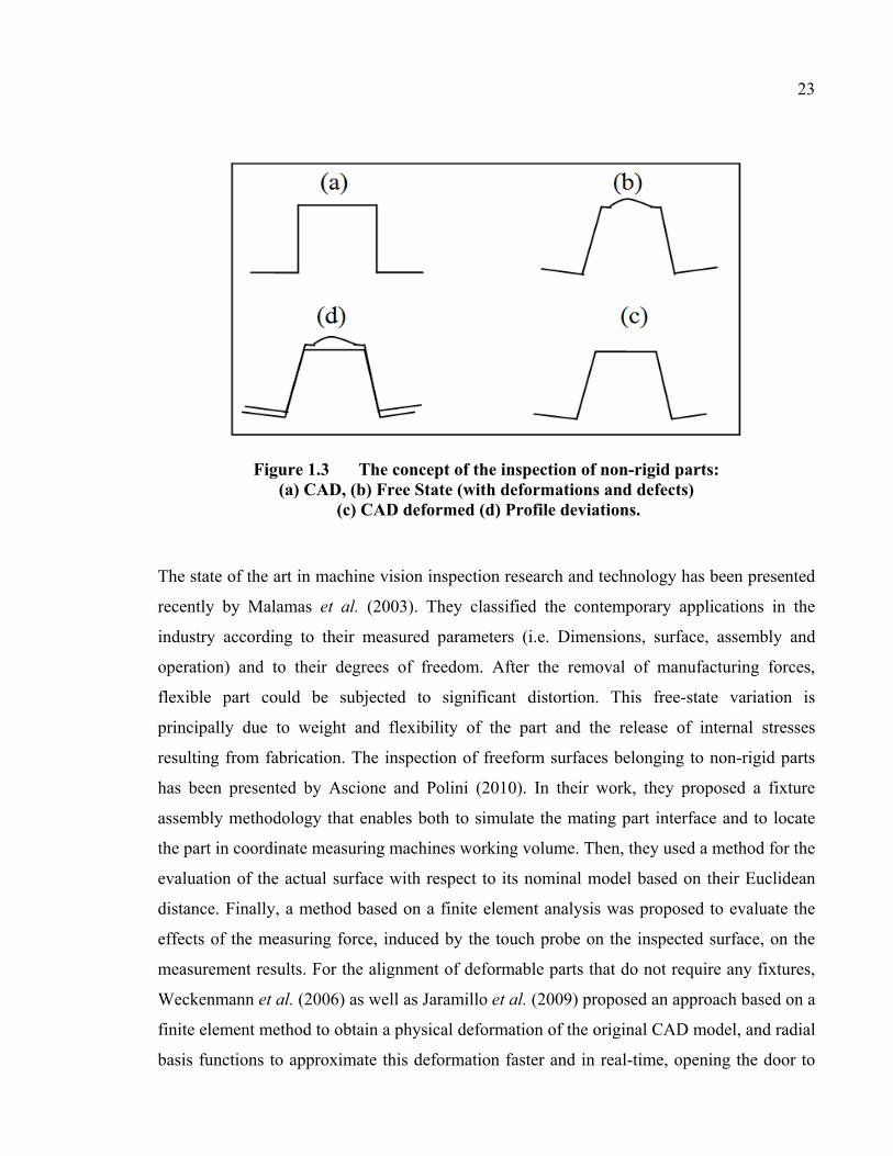
Figure 1.3 The concept of the inspection of non-rigid parts: (a) CAD, (b) Free State (with deformations and defects) (c) CAD deformed (d) Profile deviations. .................................................23

Figure 1.4 Automated 3D shape inspection (Background). ......................................25

Figure 1.5 Outlier detection - : Projection of the distance − on the normal . .....................................................................................28

Figure 1.6 Grubbs implemented in IDI, is the maximum iteration. ....................................................................................................29

Figure 1.7 Descriptions of the case studies (a) quasi-constant surface (b) omega shape Ω (c) freeform surface (Abenhaim et al., 2011) ..........................................31

Figure 1.8 Case a–F1 / V1. .........................................................................................32

Figure 1.9 Case a–F1 / V2. .........................................................................................33

Figure 1.10 Case a–F1 / V3. .........................................................................................33

Figure 1.11 Case a–F1 / V4. .........................................................................................34

Figure 1.12 Case a–F1 / V5. .........................................................................................34

Figure 1.13 Case a–F2 / V1. .........................................................................................35

Figure 1.14 Case a–F2 / V2. .........................................................................................35

XVI

Figure 1.15 Case a–F2 / V3. .........................................................................................36

Figure 1.16 Case a–F2 / V4. .........................................................................................36

Figure 1.17 Case a–F2 / V5. .........................................................................................37

Figure 1.18 Case b–F1 Default detection: (a) V1– IDI (b) V1– Grubbs. .....................37

Figure 1.19 Case b–F1 Default detection: (a) V2 – IDI (b) V2 – Grubbs. ...................38

Figure 1.20 Case b–F1 Default detection: (a) V3 – IDI (b) V3 – Grubbs. ...................38

Figure 1.21 Case c–F1 (a) IDI – V5 (b) Grubbs – V5. .................................................39

Figure 2.1 Inspection of aerospace compliant parts using a jig – Bombardier Aerospace. ..........................................................................45

Figure 2.2 Defects: (a) Waviness profile deviations (b) Dent shapes. .......................46

Figure 2.3 The flexibility definition from an industrial point of view. .....................47

Figure 2.4 Legend for the case studies. ......................................................................48

Figure 2.5 Layout drawing of the compliant case A part. ..........................................48

Figure 2.6 Layout drawing of the compliant case B part. ..........................................49

Figure 2.7 Layout drawing of the compliant case C part. ..........................................49

Figure 2.8 Layout drawing of the compliant case D part. ..........................................50

Figure 2.9 Layout drawing of the compliant case E part. ...........................................50

Figure 2.10 Logarithmic scale representation of the flexibility. ..................................52

Figure 2.11 The curvature at a given point. ..................................................................58

Figure 2.12 Curvature estimation and the identification method of the IDB-CTB algorithm. ...........................................................................62

Figure 2.13 The IDB-CTB approach. ...........................................................................64

Figure 2.14 Descriptions of the simulated case studies for the IDB-CTB method. ...............................................................................66

Figure 2.15 The experimental case study- (a) The specialized inspection fixture designed to conform the part (b) The part restrained on the fixture (c) GD&T description of the test panel. ............................67

XVII

Figure 2.16 Measurement at Free State aligned with its nominal model and located on the proposed flexibility logarithmic scale. ......................................................................................68

Figure 2.17 Results - Case A. .......................................................................................69

Figure 2.18 Results - Case B. .......................................................................................69

Figure 2.19 Results - Case C. .......................................................................................70

Figure 2.20 Results - Experimental case study. ............................................................71

Figure 3.1 Specialized fixtures for the inspection of aerospace compliant parts – Source: Bombardier Aerospace Inc. ............................77

Figure 3.2 Point set registration partial overview. ......................................................79

Figure 3.3 Problematic of relatively flexible parts registration problematic. ...............................................................................................81

Figure 3.4 Description of the criteria that belong to relatively compliant parts. .........................................................................................84

Figure 3.5 Description of the case study (1) ...............................................................89

Figure 3.6 Description of the case studies (2) ............................................................90

Figure 3.7 Results of the identification module .........................................................92

Figure-A I-1 Les études de cas expérimentales - Bombardier Aéronautique ..............104

Figure-A I-2 Interface graphique (GUI) – La banque des études de cas expérimentales .........................................................................................105

Figure-A I-3 Interface graphique (GUI) – Les approches développées dans le cadre du projet CRIAQ MANU-501 ...................................................105

LISTE DES ABRÉVIATIONS, SIGLES ET ACRONYMES

2D/3D Two/Three Dimensional Space

AIAG Automatic Action Group

ASME American Society of Mechanical Engineers

CAD Computer Aided Design

CAT Computer Aided Tolerancing

CIRP The International Academy for Production Engineering

CMM Coordinate Measuring Machine

CPD Coherent Point Drift

CRIAQ Consortium de Recherche et d’Innovation en Aérospatiale au Québec

DB Distance Based

DDL Degré De Liberté

FE Finite Element

GD&T Geometric Dimensioning and Tolerancing

GMM Gaussian Mixture Module

GNIF Generalized Numerical Inspection Fixture

ICP Iterative Closest Point

ICMST International Conference on Manufacturing Science and Technology

IDB-CTB Inspection of Deformable Bodies using the Curvature and Thompson Biweight test

IDI Iterative Displacement Inspection

IGES Initial Graphics Exchange Specification

XX

ISO International Organization for Standardization

LOF Local Outlier Factor

MANU Manufacturing

NSERC National Sciences and Engineering Research Council

ODMAD Outlier Detection for Mixed Attribute Datasets

P²SEL Products, Processes and Systems Engineering Laboratory

RDD Relative Deviation Degree

RMS Root Mean Square

RPM Robust Point Matching

SPOT Stream Projected Outlier Technique

STEP Standard for the Exchange of Product model data

TPS Thin Plate Spline

WHS Wavelet-based Hoteling Statistics

WPCA Wavelet-based Principal Component Analysis

WSEAS World Scientific and Engineering Academy and Society

LISTE DES SYMBOLES ET UNITÉS DE MESURE

1 − Niveau de confiance (ex. 95%)

Paramètre qui contrôle la distance du centre d’une distribution d’un échantillon de données

Ensemble de points de correspondant aux points les plus proches de la surface nominale

Point de l’ensemble correspondant au point le plus proche du point de la surface nominale, ∈

Le déplacement maximal résultant de l’application d’une force [ ] Le module de Young [ ] Force [ ] Gravité [ / ] Nombre de points d’un nuage représentant la pièce physique numérisée, ≫

La médiane d’une distribution [ ] La médiane de la valeur absolue des écarts des valeurs de l’échantillon par

rapport à la médiane [ ] Nombre de points du nuage représentant le modèle nominal maillé

Nuage de points représentant la pièce physique numérisée

Un point de P, ∈

Écart type estimé d’un échantillon de données [ ] Nuage de points représentant le modèle nominal maillé

Le ratio entre le déplacement maximal et la tolérance de profil

XXII

′ Transformation de dans un nouveau système de coordonnées après alignement en utilisant l’algorithme Coherent Point Drift (CPD) , Rayons de courbures principales

Estimation de l’écart type d’un échantillon de données par la méthode biweight [ ]

Un point de S, ∈ ′ Transformation de dans un nouveau système de coordonnées après alignement avec le CPD

Matrice de transformation telle que calculée par l’algorithme CPD

Poids correspondant à chaque observation d’un échantillon de données

Valeur de la tolérance de profile [ ] L'écart type du bruit de mesure gaussien [ ]

, La valeur critique de la loi de Student avec degré de liberté

Poids affecté (valeur 0 ou 1)

Échantillon de données La moyenne d’un échantillon de données [ ] SPÉCIFIQUE POUR LE CHAPITRE 1 (ARTICLE 1)

Erreur de type I

Erreur de type II

Distance euclidienne corrigée représentant la projection de la distance point-point sur la normale du point [mm]

Indicateur de Grubbs

La valeur critique du test de Grubbs

XXIII

Hypothèse nulle – Il n'y a pas de données aberrantes dans l’échantillon

Hypothèse alternative – Il y a au moins une donnée aberrante dans l’échantillon

Nombre d’itérations maximal de l’algorithme Iterative Displacement Inspection (IDI)

Nombre de points pour un échantillon de données

SPÉCIFIQUE POUR LE CHAPITRE 2 (ARTICLE 2)

La valeur imposée de l’aire du défaut de profil [ ] La valeur estimée de l’aire du défaut [ ] ∆ Matrice × 2 contenant la valeur absolue de la différence entre de et ∆ La valeur absolue de la différence entre les courbures estimées de gauss de

et ∆ La différence entre les courbures de gauss de et ∆ Vecteur × 1 de la la différence entre les courbures estimées de gauss de et ∆ La valeur moyenne correspondant au vecteur ∆

La valeur imposée du défaut de profil [ ] ∆ La valeur absolue de la différence entre les courbures gauss estimé de et

La valeur estimée du défaut de profil [ ] La valeur absolue de la déviation de ∆ par rapport à ∆ Pourcentage d’erreur de l’aire du défaut estimé par rapport à la valeur

imposée [%] Pourcentage d’erreur du défaut de profil estimé par rapport aux la valeur

imposée [%]

XXIV

Matrice × 2 contenant la courbure moyenne et la courbure de gauss

La courbure gaussienne , Les valeurs minimales et maximales respectivement de la courbure et qui portent le nom de courbures principales

SPÉCIFIQUE POUR LE CHAPITRE 3 (ARTICLE 3)

Poids associé au critère de ℎ (distance curviligne)

Parameter that represents the amount of smoothness regularization. It defines the model of the smoothness regularizer. , Valeur initiale des paramètres et , Valeur optimisée des paramètres et

Vecteur × 1 contenant les distances

La valeur moyenne estimée de par la méthode biweight

Distance euclidienne entre et ′ [ ] Distance entre et ses voisinages de premier niveau [ ] ′ Distance entre ′ et ses voisinages de premier niveau [ ] ∆ Vecteur × 1 contenant la valeur absolue de la différence entre la distance

de et ′ [ ] La valeur absolue de la déviation de par rapport à ∆ La valeur absolue de la différence entre la valeur du ℎ de et ′ [ ]

ε Termination tolerance on the objective function

La fonction objective a optimisé

The maximum number of iteration

XXV

Nombre d’éléments au voisinage immédiat du point

Erreur moyenne quadratique ℎ Valeur du critère de la somme des par rapport à [ ] Paramètre qui représente le compromis entre la qualité de l'ajustement du

maximum de vraisemblance et la régularisation

INTRODUCTION

Depuis environ deux décennies, le processus de développement des nouveaux produits a

connu des bouleversements majeurs. À ce sujet, nous pouvons invoquer la réduction du

temps de développement, l’intégration massive des modeleurs numériques et l’avènement

d’une économie mondiale. Le contexte canadien se distingue par une forte maturité

technologique, une accélération des changements et des coûts de développement qui

subissent de fortes concurrences de la part des pays en émergence. La majorité des

spécialistes s’entendent pour prédire que l’avenir passe par une économie du savoir, une

spécialisation accrue et un haut niveau d’efficacité (concevoir « bon » du premier coup et

fabriquer « bon » du premier coup). Dans le cadre de ces contraintes grandissantes, la

recherche d’un processus optimal pour le développement des nouveaux produits (conception-

fabrication-inspection) devient un enjeu majeur. L’allocation des tolérances et le choix d’une

méthode de construction se traduisent immédiatement par des coûts. Par conséquent, les

équipes d’ingénierie doivent employer des outils de prédiction pour s’assurer de la maîtrise

des variations et de leurs influences sur l’assemblabilité, la fonctionnalité et le coût global

d’un produit.

L’inspection des composants mécaniques est une tâche indispensable qui doit être prise en

considération dans l'industrie moderne. À la sortie d’un processus de fabrication, nous

devons vérifier si la pièce produite respecte les exigences fonctionnelles AVANT de

l’employer dans une chaîne d’assemblage. En d'autres termes, nous avons besoin de savoir si

une pièce fabriquée correspond bien à son modèle nominal dans le but de localiser et

quantifier les erreurs de forme, d’orientation et de localisation. Dans le cas de pièces rigides,

le problème de la gestion des variations dimensionnelles et géométriques (GD&T) des

composantes mécaniques a été étudié, et résolu, par de nombreux chercheurs. Par contre, la

majorité de ces méthodes souffrent encore de faiblesses qui se traduisent par des prédictions

limitées à un scénario bien spécifique. Les méthodologies utilisées pour résoudre le problème

nous ramènent toujours à des cas souvent trop spécifiques pour être employées dans une

2

panoplie d’applications industrielles. À titre d’exemple, il n’y a toujours pas de solutions

viables dans le cas de composantes non rigides (souples ou flexibles).

Aujourd’hui, le contrôle de la qualité des pièces non rigides nécessite une approche

particulière puisque leurs géométries peuvent prendre des formes significativement

différentes à l’état libre par rapport à leurs géométries nominales telles que définies dans un

modeleur (ex. CAD). Ceci peut être attribué aux déformations engendrées par les contraintes

induites par le procède de fabrication ou par les forces induites lors de l’assemblage, à l’effet

de la gravité et aux variations inhérentes aux procèdes de fabrication. Jusqu’à présent, des

gabarits de conformation très couteux pour l’industrie sont nécessaires pour contraindre la

pièce souple durant l'inspection1.

Qu’est-ce qu’une pièce souple ?

Le terme « souple » est un terme relatif. D’une manière équivalente, on utilise dans la

littérature spécialisée les termes « non rigides », « déformables » ou encore « flexibles » pour

désigner des composants dont la géométrie est facilement modifiable. Nous parlons ici de

déformations strictement dans le domaine élastique et dont l’amplitude est supérieure aux

tolérances des pièces. Beaucoup de pièces dans l’industrie du transport (automobile et

aéronautique) peuvent être considérées et classées comme telles. À titre d’exemple, nous

pouvons citer les panneaux de carrosserie, les pièces à paroi mince, les revêtements

d’aéronefs, etc.

Pour les composants mécaniques, il y a un consensus de considérer qu’une pièce est « non

rigide » si nous pouvons la déformer avec une force raisonnable sans induire des

déformations plastiques et d’une manière à modifier significativement sa géométrie.

Pratiquement, nous parlons généralement pour l'application de la force de

1 Typiquement, dans l’industrie aérospatiale, la préparation d’un gabarit (ou d’un montage) spécialisé pour conformer une pièce flexible nécessite environ 60 heures-homme.

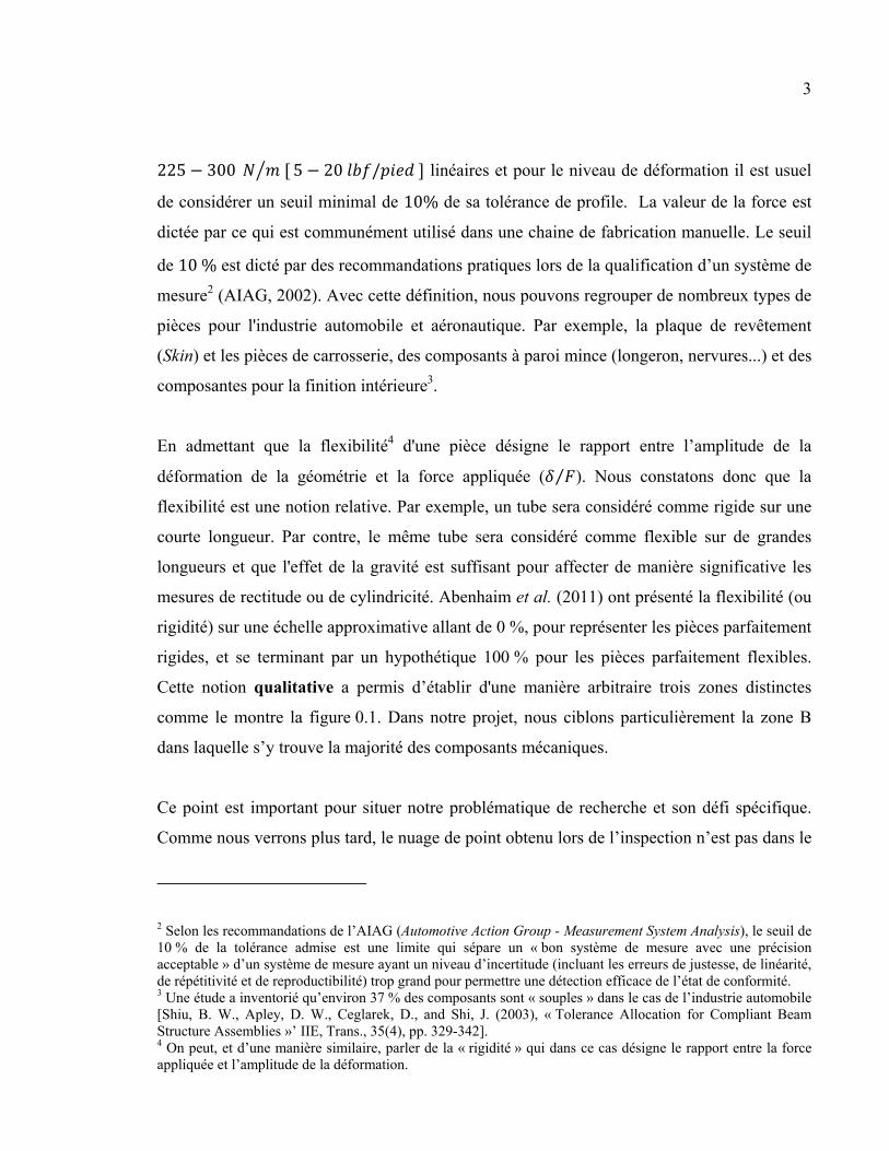
3

225 − 300 [ 5 − 20 / ] linéaires et pour le niveau de déformation il est usuel

de considérer un seuil minimal de 10% de sa tolérance de profile. La valeur de la force est

dictée par ce qui est communément utilisé dans une chaine de fabrication manuelle. Le seuil

de 10 % est dicté par des recommandations pratiques lors de la qualification d’un système de

mesure2 (AIAG, 2002). Avec cette définition, nous pouvons regrouper de nombreux types de

pièces pour l'industrie automobile et aéronautique. Par exemple, la plaque de revêtement

(Skin) et les pièces de carrosserie, des composants à paroi mince (longeron, nervures...) et des

composantes pour la finition intérieure3.

En admettant que la flexibilité4 d'une pièce désigne le rapport entre l’amplitude de la

déformation de la géométrie et la force appliquée ( ⁄ ). Nous constatons donc que la

flexibilité est une notion relative. Par exemple, un tube sera considéré comme rigide sur une

courte longueur. Par contre, le même tube sera considéré comme flexible sur de grandes

longueurs et que l'effet de la gravité est suffisant pour affecter de manière significative les

mesures de rectitude ou de cylindricité. Abenhaim et al. (2011) ont présenté la flexibilité (ou

rigidité) sur une échelle approximative allant de 0 %, pour représenter les pièces parfaitement

rigides, et se terminant par un hypothétique 100 % pour les pièces parfaitement flexibles.

Cette notion qualitative a permis d’établir d'une manière arbitraire trois zones distinctes

comme le montre la figure 0.1. Dans notre projet, nous ciblons particulièrement la zone B

dans laquelle s’y trouve la majorité des composants mécaniques.

Ce point est important pour situer notre problématique de recherche et son défi spécifique.

Comme nous verrons plus tard, le nuage de point obtenu lors de l’inspection n’est pas dans le

2 Selon les recommandations de l’AIAG (Automotive Action Group - Measurement System Analysis), le seuil de 10 % de la tolérance admise est une limite qui sépare un « bon système de mesure avec une précision acceptable » d’un système de mesure ayant un niveau d’incertitude (incluant les erreurs de justesse, de linéarité, de répétitivité et de reproductibilité) trop grand pour permettre une détection efficace de l’état de conformité. 3 Une étude a inventorié qu’environ 37 % des composants sont « souples » dans le cas de l’industrie automobile [Shiu, B. W., Apley, D. W., Ceglarek, D., and Shi, J. (2003), « Tolerance Allocation for Compliant Beam Structure Assemblies »’ IIE, Trans., 35(4), pp. 329-342]. 4 On peut, et d’une manière similaire, parler de la « rigidité » qui dans ce cas désigne le rapport entre la force appliquée et l’amplitude de la déformation.

4

même repère que le modèle nominal (CAD) d’où la nécessité d’une opération de calage (ou

de registration). Or, les algorithmes de calage sont nombreux et ils peuvent proposer des

solutions robustes et rapides. Par contre, ils sont adaptés pour des cas spécifiques qui ne

correspondent pas à notre problématique de la Zone B.

À titre d’exemple, l’algorithme ICP (Iterative Closest Point, Besl et Mackay, 1992) qui très

performant pour le calage rigide (Zone A) ne peut produire de bons résultats dans le cas des

composants souples. À l’opposé, l’algorithme CPD (Coherent Point Drift, Myronenko et

Song, 2009) est efficace pour le calage non rigide (très employé dans l’imagerie) des

composants de la Zone C. Dans ce cas, un étirement (stretching) des surfaces est permis, ce

qui ne correspond nullement à la spécificité des composants mécaniques souples. Bref, nous

devons obtenir une sorte de « calage flexible » qui conserve les distances curvilignes

(géodésiques) tout en admettant sur la pièce inspectée la présence de zones de défauts de

fabrication.

Figure 0.1 Classification de la rigidité.

Notre projet s’insère dans le cadre d’un projet plus global et d’une plus grande envergure

(réf. CRIAQ MANU501). Une fois la problématique de l’inspection des pièces souples sera

résolue, il faut s’attarder à la problématique du tolérancement des pièces souples. Or,

comme mentionnée précédemment, l’échelle précédente (A, B et C) est surtout qualitative et

ne peut qu’être employée pour catégoriser grossièrement les composants à inspecter. Ce

Zone A Zone B Zone C Pièces rigides Pièces très flexibles

Déformations négligeables par rapport aux tolérances données

La flexibilité dépend de la taille de la pièce, la direction et le montage de l’assemblage sur lequel l'inspection est effectuée (nécessite une force)

Très grande déformation uniquement avec l’effet de la

gravité, ex. tissu

5

constat nous a guidés pour développer et proposer une nouvelle approche pour présenter la

flexibilité/rigidité sur une échelle quantitative. Cette approche sera présentée dans le

Chapitre 2 de cette thèse. Nous conjecturons que cette approche permettra aux industriels de

bien classifier leurs composantes mécaniques et sera forte utile lors des opérations de

tolérancement.

Est-ce que la norme ASME Y14.5 contrôle les pièces souples ?

Il existe des standards nationaux et internationaux comme la norme ASME Y14.5 (2009) et

la norme ISO 10579 (2010) pour définir et établir les règles d’interprétation du tolérancement

dimensionnel et géométrique sur les dessins et devis techniques (2D ou 3D). La norme

ASME Y14.5 (2009) considère que, par défaut et sauf indication contraire, l'inspection des

pièces doit être effectuée à l’état libre sans une force appliquée lors de l'inspection (Réf.

ASME Y14.5 (2009), paragraphe 1.4 Fundamental Rules (m), page 8) et que, sauf indication

contraire, la forme doit être parfaite à la condition maximale de matière (principe de

l’enveloppe, principe de Taylor). En plus, la norme établit des règles pour déterminer le

système d'axes (XYZ) lors de l'inspection en utilisant les référentiels (datum). Cette condition

« par défaut » est parfaitement adaptée pour les composants de la Zone A. En d’autres

termes, les modalités d'application sont parfaitement adaptées et applicables pour les

composantes quasi rigides.

La norme ASME Y14.5 indique que la règle de l’enveloppe est exclue dans le cas de pièces

standard et des pièces flexibles telles que les tubes, les tôles, les coques minces, les profils

extrudés, les poutres structurelles et les pièces soumises à des variations géométriques à l'état

libre. Et que ces composantes devraient être traitées différemment.

Avec toutes les possibilités que les normes du tolérancement offrent, malheureusement, il n’y

a pas une méthode adaptable et applicable pour toute la panoplie des pièces de la Zone B.

Nous avons recensé plusieurs parmi les plus employées dans l’industrie. (Voir tableau 0.1)

6

Tableau 0.1 Résumé des méthodes d’inspection de composante flexible « suite »

Méthode Figure/Schéma Exemples d’application Désavantage

Conformation par un gabarit

Pièces produites à moyens et grands volumes (automobile)

Nécessite un gabarit de conformation fidèle à la géométrie nominale/Étalonnage du gabarit/Répétitivité du gabarit

Violation des principes

d’isostatisme

Pièces à paroi mince

Nécessite un montage spécifique et un dispositif pour produire la force nécessaire à la conformation/sensible aux choix du concepteur

Utilisation d’une force

Une note typique est ajoutée sur le dessin de définition ‘Il est permis d'utiliser / pour atteindre la tolérance’ est

ajoutée sur le devis

Pièces avec de faibles déformations élastiques, pièces à paroi mince

L’ajout d’une tolérance à l’état libre est souvent nécessaire pour limiter le niveau de déformation/problématique sur la reproductibilité des mesures

Conformation à une dimension

Métal en feuille, pièces à paroi mince

L’ajout d’une tolérance à l’état libre est souvent nécessaire pour limiter le niveau de déformations

Tolérance relative

Pièces primaires (poutre, tube, plaque, panneau, profilé, etc.)

Limitée pour les défauts de forme seulement. Difficile à contrôler dans le cas des profils

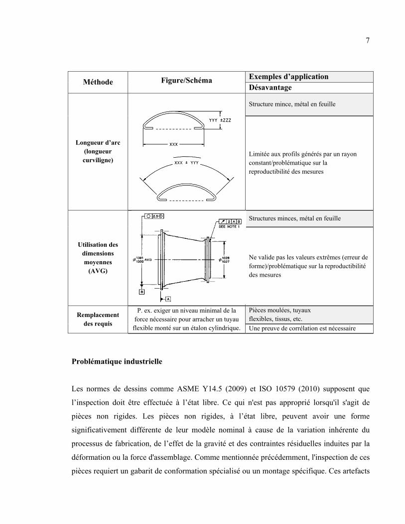
7

Méthode Figure/Schéma Exemples d’application

Désavantage

Longueur d’arc (longueur curviligne)

Structure mince, métal en feuille

Limitée aux profils générés par un rayon constant/problématique sur la reproductibilité des mesures

Utilisation des dimensions moyennes

(AVG)

Structures minces, métal en feuille

Ne valide pas les valeurs extrêmes (erreur de forme)/problématique sur la reproductibilité des mesures

Remplacement des requis

P. ex. exiger un niveau minimal de la force nécessaire pour arracher un tuyau

flexible monté sur un étalon cylindrique.

Pièces moulées, tuyaux flexibles, tissus, etc.

Une preuve de corrélation est nécessaire

Problématique industrielle

Les normes de dessins comme ASME Y14.5 (2009) et ISO 10579 (2010) supposent que

l’inspection doit être effectuée à l’état libre. Ce qui n'est pas approprié lorsqu'il s'agit de

pièces non rigides. Les pièces non rigides, à l’état libre, peuvent avoir une forme

significativement différente de leur modèle nominal à cause de la variation inhérente du

processus de fabrication, de l’effet de la gravité et des contraintes résiduelles induites par la

déformation ou la force d'assemblage. Comme mentionnée précédemment, l'inspection de ces

pièces requiert un gabarit de conformation spécialisé ou un montage spécifique. Ces artefacts

8

posent toujours des difficultés et des coûts non négligeables pour l’industrie. À titre

d'exemple, le temps requis actuellement pour préparer l'inspection d'une pièce flexible

(gabarit, montage, etc.) chez la compagnie Bombardier Aéronautique est d'environ 50-60

heures-hommes.

La question fondamentale de notre projet est donc la suivante : « comment peut-on s’assurer

de la qualité géométrique des pièces non rigides sans le recourt à un gabarit (ou un

montage) pour les conformer ? ». En corolaire à cette première question, nous pouvons

ajouter, une deuxième question : « à partir d’un nuage de points capté dans une condition

arbitraire et connue, comme peut-on identifier les défauts de fabrication sur une pièce

souple ? ». Pour résumer, il s’agit de développer un moyen répétable et précis qui permet

de séparer défauts et déformations. Ces dernières sont attribuables essentiellement à l’effet

de la gravité et à l’effet des contraintes résiduelles.

Ces questions trouvent un intérêt immédiat dans l’industrie manufacturière en général et, plus

spécifiquement, dans le secteur aérospatial. Le problème du tolérancement et de l’inspection

des pièces mécaniques flexibles est décisif pour cette industrie; l’automatisation de

l’inspection contribue grandement à son niveau de compétitivité.

Objectifs de la recherche

Cette recherche a pour but le développement, la validation et l’application des outils

mathématiques permettant à partir d'un nuage de points collectés dans un état sans gabarit

spécialisé de déterminer l'amplitude et la localisation des défauts induits par les variations

des inhérents dues aux procédés de fabrication.

Cette thèse propose plusieurs approches qui proposent des techniques d’identification des

défauts géométriques de profil à partir d’une maquette numérique captée sur un composant

déformé.

9

La recherche proposée contribuera à améliorer nos connaissances fondamentales et par

conséquent, à faire évoluer la capacité de prédiction des modèles. L’amélioration escomptée

découle du fait que nous tenterons de prendre en compte des phénomènes liés à la flexibilité,

au choix des méthodes d’assemblage et aux corrélations qui y en découlent. Le projet se

traduira ultérieurement par des gains transférables à l’industrie canadienne. Nous anticipons

des économies découlant d’une rapidité accrue des opérations d’inspection, d’une utilisation

plus efficiente des tolérances, de l’élimination des gabarits de conformation et d’une

amélioration de la productivité due à la réduction du temps de cycle.

Hypothèses de travail

Après avoir exposé la problématique ainsi que l’objectif de notre thèse, nous allons émettre

les hypothèses générales et communes à toutes les étapes de notre recherche.

Hypothèse 1 : La pièce à inspecter est à parois minces. Elle est donc une pièce mécanique de

faible épaisseur par rapport aux dimensions globales. Sa géométrie est parfaitement définie et

disponible par un fichier mathématique MATH DATA (STEP, IGES, ou tout autre format

compatible). Ces pièces sont largement utilisées dans une variété d'applications d'ingénierie

(structures d’aéronefs, industrie automobile, etc.).

Hypothèse 2 : Le montage, lors de la numérisation, permet des déformations élastiques

semblables ou plus grandes que les tolérances de profil requises.

Hypothèse 3 : La pièce fabriquée est numérisée sur une position arbitraire mais connue. Une

représentation de la pièce sous forme d’un nuage de points ( , , ) est donc disponible.

Hypothèse 4 : L'inspection est limitée aux défauts de profil de surface et de localisation tels

que définis par l'ASME Y14.5 (2009).

10

D’autres hypothèses sont spécifiques pour chaque chapitre-article. Chaque article est

présenté comme un chapitre dans cette thèse.

Suite à l’introduction, une brève revue de la littérature et la structure détaillée de la thèse sont

présentées.

11

REVUE DE LA LITTÉRATURE ET STRUCTURE DE LA THÈSE

La revue de la littérature situe notre travail par rapport à d'autres recherches effectuées dans

le même domaine. Notre bibliographie comportera les phases typiques du processus

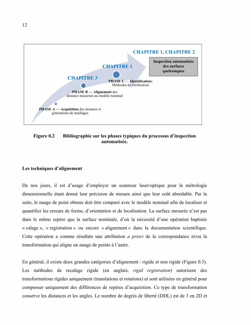
d’inspection automatisée tridimensionnelle (Figure 0.2).

En général, le processus d’inspection automatisée comporte trois phases. La première phase

représente l’acquisition des données et, si nécessaire, un post traitement de ce nuage de

points (ex. la génération d’un maillage, filtrage, etc.). Dans cette phase, un nuage de points

est obtenu à partir des services de numérisation 3D des profils externes des diverses pièces

industrielles. La deuxième phase porte sur l’alignement du nuage de points. Dans cette phase,

les données mesurées seront alignées au système référentiel du modèle conçu par

l’identification des zones de concordance. La troisième phase représente le module

d’identification. Le but de cette phase est de déterminer le degré de conformité entre la pièce

fabriquée et le modèle nominal (amplitude des défauts, localisation, etc.).

Une revue de littérature des travaux de recherche sur l’inspection tridimensionnelle

automatisée des surfaces quelconques (Free-Form surface) sera présentée dans le premier et

le deuxième chapitre de notre thèse. Notre bibliographie comportera également les phases B

et C du processus d’inspection automatisée (Figure 0.2). Dans le Chapitre 1 de la thèse

(article 1), nous présentons une revue générale sur les techniques d'identification (méthodes

de vérification) pour distinguer les défauts qui sont dus à des procédés de fabrication aux

déformations qui sont dues à la flexibilité de la pièce. Dans le Chapitre 3 de la thèse

(article 3), nous exposons une revue générale sur les différentes techniques d'alignement.

12

Figure 0.2 Bibliographie sur les phases typiques du processus d’inspection automatisée.

Les techniques d’alignement

De nos jours, il est d’usage d’employer un scanneur laser/optique pour la métrologie

dimensionnelle étant donné leur précision de mesure ainsi que leur coût abordable. Par la

suite, le nuage de point obtenu doit être comparé avec le modèle nominal afin de localiser et

quantifier les erreurs de forme, d’orientation et de localisation. La surface mesurée n’est pas

dans le même repère que la surface nominale, d’où la nécessité d’une opération baptisée

« calage », « registration » ou encore « alignement » dans la documentation scientifique.

Cette opération a comme résultats une attribution a priori de la correspondance et/ou la

transformation qui aligne un nuage de points à l’autre.

En général, il existe deux grandes catégories d’alignement : rigide et non rigide (Figure 0.3).

Les méthodes de recalage rigide (en anglais, rigid registration) autorisent des

transformations rigides uniquement (translations et rotations) et sont utilisées en général pour

compenser uniquement des différences de repères d’acquisition. Ce type de transformation

conserve les distances et les angles. Le nombre de degrés de liberté (DDL) est de 3 en 2D et

PHASE A — Acquisition des données et générations de maillages

PHASE B — Alignement des données mesurées au modèle nominal

PHASE C — Identification: Méthodes de vérification

Inspection automatisée des surfaces quelconques

CHAPITRE 3

CHAPITRE 1

CHAPITRE 1, CHAPITRE 2

13

de 6 en 3D. L’algorithme ICP (Iterative Closest Point) introduit par Besl et McKay (1992),

est la méthode de recalage rigide la plus populaire en raison de sa simplicité et de sa faible

consommation en calcul. Par contre, si le but consiste à modifier la forme globale des objets,

on fait appel à des algorithmes de recalage non rigide (en anglais, non-rigid registration).

Ces algorithmes sont caractérisés par un grand nombre de DDL et sont employés dans des

applications d’imagerie (ex. imagerie médicale, animation, etc.). On peut citer dans ce cas

l’algorithme CPD (Coherent Point Drift) introduit par Myronenko et al. (2010) et qui

considère l’alignement entre deux nuages de points comme un problème d’estimation de la

densité de la probabilité. Les différents algorithmes les plus utilisés pour les recalages rigides

et non rigides ont été présentés dans le troisième chapitre de la thèse (article 3).

À noter qu’il existe également les méthodes de transformation affine (en anglais, affine

registration). Ces méthodes autorisent, en plus des rotations et des translations, de prendre en

compte un facteur d'échelle anisotrope et de modéliser des cisaillements. Ce type de

transformation conserve le parallélisme. Le nombre de DDL est de 6 en 2D et de 12 en 3D.

Dans notre projet, nous ciblons la Zone B (relativement flexible) dans laquelle se trouve la

majorité des pièces mécaniques. Les trois catégories de recalage ne correspondent pas à la

spécificité des pièces souples situées dans cette zone. Nous devons obtenir une sorte de

« calage flexible » qui conserve les distances curvilignes (géodésiques) tout en admettant sur

la pièce souple inspectée la présence de zones de défauts de fabrication. Pour résoudre ce

problème, une nouvelle approche pour l’inspection des pièces souples sans gabarits de

conformation par optimisation du Coherent Point Drift (CPD) a été proposée dans le

Chapitre 3 de cette thèse. Cette approche vise à adapter l’algorithme de transformation non

rigide du CPD d’une façon à correspondre aux spécificités des pièces souples (Figure 0.3).

14

Figure 0.3 Le problème de recalage des pièces souples.

Les techniques d’identification

Après avoir aligné et cherché les correspondances entre les nuages de points de la pièce

fabriquée et du modèle nominal, il est temps de déterminer le degré de conformité entre eux.

D’où l’importance du choix de la technique d’identification.

Dans notre cas, les défauts dus au processus de fabrication sont considérés comme des

données aberrantes qui doivent être éliminées d’une façon dynamique et itérative tout en

respectant un seuil d’identification à déterminer. Ces défauts doivent être distingués des

déformations qui sont dues à la flexibilité de la pièce et sont de même ordre de grandeur que

Recalage

Non Rigide

(CPD)

Rigide

(ICP) Recalage ‘flexible’ adapté pour

les pièces souples situées dans

la Zone B

Transformation CAD SCAN Recalage

(Hu et al., 2010)

Medical

applications

∗

∗ = ∗

∗

représente la distance curviligne entre and

15

les tolérances de profil assigné. Une revue de littérature portant sur les différentes techniques

d’identification est présentée dans le paragraphe 1.3 du Chapitre 1.

Dans notre projet, nous proposons l’utilisation des statiques extrêmes comme module

d’identification. Dans le premier chapitre, nous utilisons le Maximum Normed Residual Test

développé par Grubbs (1969). Dans le deuxième et troisième chapitre, nous proposons

l’utilisation de la méthode Thompson Test qui sera combinée avec l’estimateur Biweight qui

permet l’estimation de la moyenne et de la variance des données (Thompson, 1985; Hoaglin,

1983).

Structure de la thèse

La suite de cette thèse (figure 0.4) comporte trois (3) chapitres et une conclusion suivit des

recommandations. En Annexe, nous présentons le développement d’une interface graphique

(GUI) et les résultats du stage qui a été effectué chez Bombardier Aéronautique (Usine St-

Laurent, Montréal, QC).

Les contributions de cette thèse sont obtenues à travers de la rédaction de trois (3) articles de

revues, la participation à six (6) conférences et le développement d’une interface graphique

(GUI) et d’une banque d’étude de cas expérimentale. Le tableau 0.2 récapitule les références

bibliographiques des conférences et les articles de revues sont présentés dans les trois (3)

prochains chapitres.

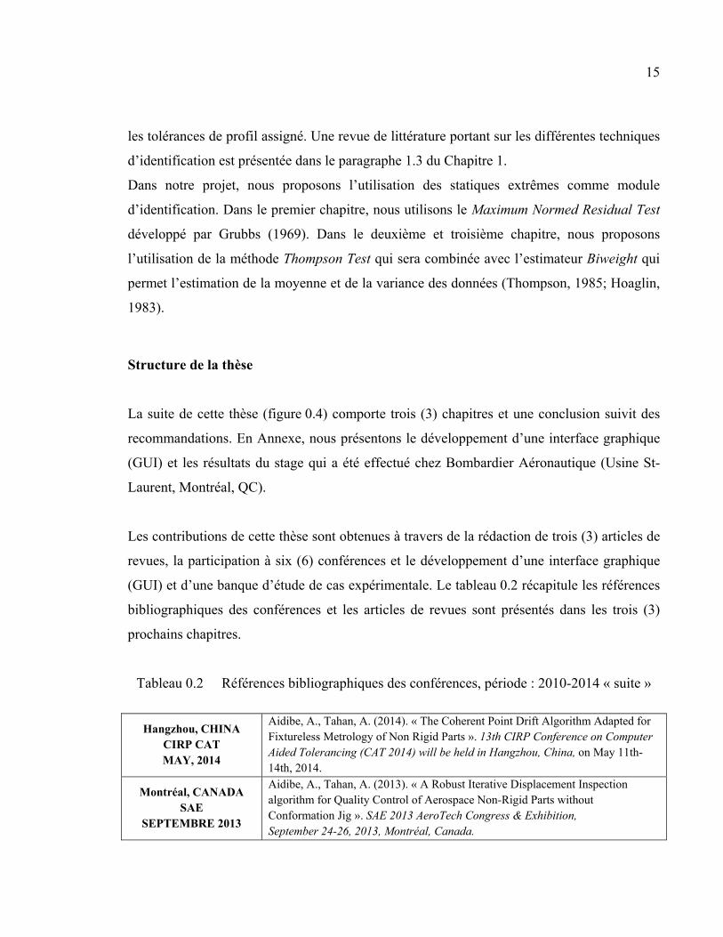
Tableau 0.2 Références bibliographiques des conférences, période : 2010-2014 « suite »

Hangzhou, CHINA CIRP CAT MAY, 2014

Aidibe, A., Tahan, A. (2014). « The Coherent Point Drift Algorithm Adapted for Fixtureless Metrology of Non Rigid Parts ». 13th CIRP Conference on Computer Aided Tolerancing (CAT 2014) will be held in Hangzhou, China, on May 11th-14th, 2014.

Montréal, CANADA SAE

SEPTEMBRE 2013

Aidibe, A., Tahan, A. (2013). « A Robust Iterative Displacement Inspection algorithm for Quality Control of Aerospace Non-Rigid Parts without Conformation Jig ». SAE 2013 AeroTech Congress & Exhibition, September 24-26, 2013, Montréal, Canada.

16

Dubai, UAE ICMST

AUGUST 2013

Aidibe, A., Tahan, A. (2013). « An Inspection Approach for Nonrigid Mechanical Parts ». International Conference on Manufacturing Science and Technology ICMST 2013, Advanced Materials Research Trans Tech Publications, vols. 816-817, pp 806-811.

Wisconsin, USA ASME

JUNE 2013

Aidibe, A., Tahan, A. (2013). « Curvature estimation for metrology of nonrigid parts ». Proceedings of the ASME2013 International Manufacturing Science and Engineering Conference MSEC2013, June 10-14, 2013, Madison, Wisconsin, USA.

Corfu Island, Greece WSEAS

JULY 2011

Aidibe, A., Tahan, A., Abenhaim, G.N. (2011). « Dimensioning control of non-rigid parts using the Iterative Displacement Inspection with the maximum normed residual test ». Proceeding of the 2nd International Conference on Theoretical and Applied Mechanics 2011, TAM'11, July 15, 2011 – July 17, 2011, Corfu Island, Greece, World Scientific and Engineering Academy and Society.

Montréal, CANADA CASI

APRIL 2011

Aidibe, A., Tahan, A., Abenhaim, G.N. (2011). « Improving the Iterative Displacement Inspection (IDI) for Aeronautics Flexible Part ». 58th CASI Aeronautics Conference - AERO 2011 - at the Delta-Centre Ville in Montreal, Quebec, Canada, April 26, 27 and 28.

Deux approches ont été développées par l’équipe de recherche qui travaille sous la

supervision du professeur Tahan dans le cadre du projet de l’inspection des pièces flexibles

sans un gabarit de conformation. La première approche a été proposée par G.-N. Abenhaim

dans le cadre de sa maitrise en génie mécanique à l’École de technologie supérieure (ÉTS).

Abenhaim et Tahan (2011) ont publié l’algorithme Iterative Displacement Inspection (IDI)

qui consiste à appliquer une déformation au modèle nominal afin que celle-ci se rapproche de

la géométrie de la pièce numérisée. La deuxième approche a été proposée par Hassan-Radvar

Esfahlan, dans le cadre de son doctorat en génie mécanique à l’ÉTS. En fusionnant les

technologies existantes de la géométrie métrique et informatique avec les méthodes des

éléments finis, Esfahlan et Tahan (2012) ont développé l’algorithme Generative Numerical

Inspection Fixture (GNIF). Dans le cadre de notre thèse de doctorat, une amélioration du

module d’identification de l’IDI a été proposée dans le Chapitre 1 et une nouvelle méthode

pour la quantification de la flexibilité/rigidité a été développée dans le Chapitre 2. En plus,

deux nouvelles approches pour l’inspection des pièces flexibles sans gabarit de conformation

ont été développées dans les Chapitres 2 et 3 de cette thèse.

17

Comme mentionné précédemment, l’article du Chapitre 1 propose une amélioration du

module d’identification de l’algorithme Iterative Displacement Inspection (IDI). Cet article a

été publié dans la revue WSEAS Transactions on Applied and Theoretical Mechanics sous la

référence: Aidibe, A., Tahan, A., Abenhaim, G.N. (2012). « Distinguishing profile deviations

from a part's deformation using the maximum normed residual test ». WSEAS Transactions

on Applied and Theoretical Mechanics, vol. 7, °1, p. 18-28.

L’article du Chapitre 2 présente une nouvelle méthode pour la quantification de la

flexibilité/rigidité à l’aide d’un ratio ( ) et représente les résultats sur une échelle

logarithmique. Également, on présente une nouvelle approche pour l’inspection des pièces

souples sans gabarit de conformation basée sur l’estimation de la courbure gaussienne, une

des propriétés intrinsèques de la géométrie qui est invariante sous les transformations

isométriques. Cette approche considère les défauts dus aux processus de fabrication comme

des données aberrantes qui doivent être détectées d’une façon dynamique et itérative. Pour

cet effet, on propose une technique d’identification basée sur les statistiques extrêmes

(Thompson-Biweight) pour séparer les défauts dus au processus de fabrication, des

déformations dues à la flexibilité de la pièce. Cette méthode fonctionne bien dans le cas des

défauts de profil d’ordre 1 (ex. bosses) et d’ordre 2 (ex. défaut d’ondulation). Cet article

intitulé « Inspection of Deformable Bodies using Curvature Estimation and Thompson-

Biweight Test » a été publié dans la revue International Journal of Advanced Manufacturing

Technology, vol. 71, ° 9-12, p. 1733-1747 – Springer London.

L’article du Chapitre 3 présente également une nouvelle approche complémentaire à celle du

deuxième article. En plus des défauts de profil, cette approche permet l’identification et la

quantification du défaut de localisation (par exemple, un trou qui n’est pas à sa bonne place).

Cette approche consiste à adapter le puissant algorithme de recalage non rigide Coherent

Point Drift à ce dont il satisfait les spécifications des pièces mécaniques souples. Cet article

intitulé « The Coherent Point Drift Algorithm Adapted for Fixtureless Dimensional

Inspection of Deformable Bodies » a été soumis pour publication.

18

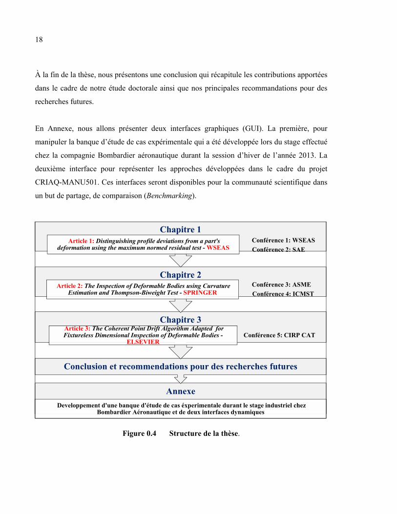
À la fin de la thèse, nous présentons une conclusion qui récapitule les contributions apportées

dans le cadre de notre étude doctorale ainsi que nos principales recommandations pour des

recherches futures.

En Annexe, nous allons présenter deux interfaces graphiques (GUI). La première, pour

manipuler la banque d’étude de cas expérimentale qui a été développée lors du stage effectué

chez la compagnie Bombardier aéronautique durant la session d’hiver de l’année 2013. La

deuxième interface pour représenter les approches développées dans le cadre du projet

CRIAQ-MANU501. Ces interfaces seront disponibles pour la communauté scientifique dans

un but de partage, de comparaison (Benchmarking).

Figure 0.4 Structure de la thèse.

Annexe

Developpement d'une banque d'étude de cas éxperimentale durant le stage industriel chez Bombardier Aéronautique et de deux interfaces dynamiques

Conclusion et recommendations pour des recherches futures

Chapitre 3Article 3: The Coherent Point Drift Algorithm Adapted for Fixtureless Dimensional Inspection of Deformable Bodies -

ELSEVIERConférence 5: CIRP CAT

Chapitre 2Article 2: The Inspection of Deformable Bodies using Curvature

Estimation and Thompson-Biweight Test - SPRINGERConférence 3: ASME

Conférence 4: ICMST

Chapitre 1Article 1: Distinguishing profile deviations from a part's

deformation using the maximum normed residual test - WSEASConférence 1: WSEAS

Conférence 2: SAE

CHAPITRE 1

DISTINGUISHING PROFILE DEVIATIONS FROM A PART’S DEFORMATION USING THE MAXIMUM NORMED RESIDUAL TEST

Ali AIDIBE, Antoine S. TAHAN, Gad N. ABENHAIM,

Mechanical Engineering Department, École de technologie supérieure (ÉTS)

1100 Notre-Dame Ouest, Montréal, Québec, Canada H3C1K3

This chapter has been published in the “WSEAS TRANSACTIONS on APPLIED and

THEORETICAL MECHANICS”, Volume 7, January 2012, Pages 18-28.

1.1 Abstract

Nonrigid parts, in free-state, may have a considerable different shape than their nominal

model due to dimensional and geometric variations of the manufacturing process, gravity

loads and residual stress induced distortion. Therefore, sorting profile deviation from a part's

deformation by comparing the part's nominal shape to its scanned free-state shape is a

challenging task. This task is a key step in the Iterative Displacement Inspection (IDI)

algorithm used for the inspection of non-rigid parts without the use of costly specialized

fixtures. This paper proposes the use of the statistical maximum normed residual test to

improve the aforementioned identification task. Thirty two simulated manufactured parts are

studied to show that the proposed method reduces the type I and II identification errors of the

IDI method.

Key-Words:

Rigid registration, non-rigid registration, quality control, tolerancing, inspection, metrology,

non-rigid parts, deformation, Geometric dimensioning and tolerancing (GD&T).

20

1.2 Introduction

One of the important tasks that have to be taken into consideration in the industry is the

inspection of manufactured parts. At the end of the manufacturing process we must verify if

the produced part respects the functional requirements under a given tolerance. The problem

of the dimensional and geometric variations (GD&T) on mechanical components has been

studied by many researchers in the case of rigid parts. Despite those researches there still no

viable solutions in the case of non-rigid parts. Non-rigid parts, in free- state, may have a

different form than their CAD model due to inherent variations of the manufacturing process,

gravity loads, residual stress induced distortion, and/or assembly force. Specifically, the

inspection of such parts poses difficulties and has significant costs industries because they

need specialized fixtures. Therefore Automatic inspection becomes essential.

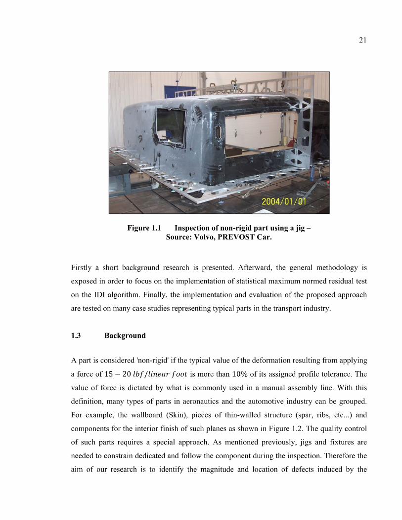
This paper proposes a method enabling the distinction between the geometrical defects due to

an error in the manufacturing process and the deformations due to the flexibility of the parts

in the case of thin shells during the inspection process. The distinction allows for the

detection of profile variations without the need of conformation jig. Figure 1.1 illustrates an

example of a conformation jig used in the inspection of an automotive body part. Extending

the work of Abenhaim and Tahan (2011) on the inspection of non-rigid part, this paper

focuses on the identification module of the iterative displacement inspection (IDI) method

proposed by the latter with the following assumptions:

• The part to inspect is a quasi-constant thin shell.

• In a free-state, the manufactured parts elastic deformation is greater than the tolerances

required profile.

• The defects are not distributed all over the part. In other words, they are localized.

• Inspection is limited to the defects in the surface profile as defined by ASME Y14.5-

2009.

21

Figure 1.1 Inspection of non-rigid part using a jig – Source: Volvo, PREVOST Car.

Firstly a short background research is presented. Afterward, the general methodology is

exposed in order to focus on the implementation of statistical maximum normed residual test

on the IDI algorithm. Finally, the implementation and evaluation of the proposed approach

are tested on many case studies representing typical parts in the transport industry.

1.3 Background

A part is considered 'non-rigid' if the typical value of the deformation resulting from applying

a force of 15 − 20 / is more than 10% of its assigned profile tolerance. The

value of force is dictated by what is commonly used in a manual assembly line. With this

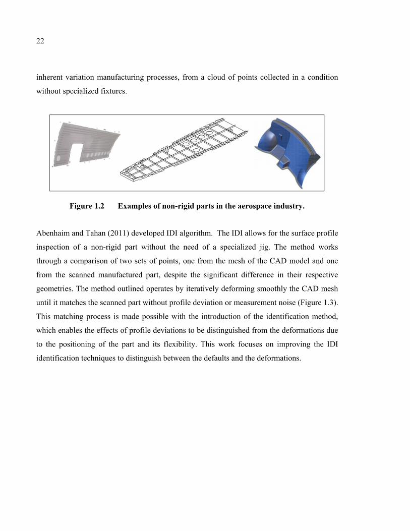
definition, many types of parts in aeronautics and the automotive industry can be grouped.

For example, the wallboard (Skin), pieces of thin-walled structure (spar, ribs, etc...) and

components for the interior finish of such planes as shown in Figure 1.2. The quality control

of such parts requires a special approach. As mentioned previously, jigs and fixtures are

needed to constrain dedicated and follow the component during the inspection. Therefore the

aim of our research is to identify the magnitude and location of defects induced by the

22

inherent variation manufacturing processes, from a cloud of points collected in a condition

without specialized fixtures.

Figure 1.2 Examples of non-rigid parts in the aerospace industry.

Abenhaim and Tahan (2011) developed IDI algorithm. The IDI allows for the surface profile

inspection of a non-rigid part without the need of a specialized jig. The method works

through a comparison of two sets of points, one from the mesh of the CAD model and one

from the scanned manufactured part, despite the significant difference in their respective

geometries. The method outlined operates by iteratively deforming smoothly the CAD mesh

until it matches the scanned part without profile deviation or measurement noise (Figure 1.3).

This matching process is made possible with the introduction of the identification method,

which enables the effects of profile deviations to be distinguished from the deformations due

to the positioning of the part and its flexibility. This work focuses on improving the IDI

identification techniques to distinguish between the defaults and the deformations.

23

Figure 1.3 The concept of the inspection of non-rigid parts: (a) CAD, (b) Free State (with deformations and defects)

(c) CAD deformed (d) Profile deviations.

The state of the art in machine vision inspection research and technology has been presented

recently by Malamas et al. (2003). They classified the contemporary applications in the

industry according to their measured parameters (i.e. Dimensions, surface, assembly and

operation) and to their degrees of freedom. After the removal of manufacturing forces,

flexible part could be subjected to significant distortion. This free-state variation is

principally due to weight and flexibility of the part and the release of internal stresses

resulting from fabrication. The inspection of freeform surfaces belonging to non-rigid parts

has been presented by Ascione and Polini (2010). In their work, they proposed a fixture

assembly methodology that enables both to simulate the mating part interface and to locate

the part in coordinate measuring machines working volume. Then, they used a method for the

evaluation of the actual surface with respect to its nominal model based on their Euclidean

distance. Finally, a method based on a finite element analysis was proposed to evaluate the

effects of the measuring force, induced by the touch probe on the inspected surface, on the

measurement results. For the alignment of deformable parts that do not require any fixtures,

Weckenmann et al. (2006) as well as Jaramillo et al. (2009) proposed an approach based on a

finite element method to obtain a physical deformation of the original CAD model, and radial

basis functions to approximate this deformation faster and in real-time, opening the door to

24

on-line inspection of deformable parts. Yadong and Peihua (2004) provided a comprehensive

literature review of methodologies, techniques and various processes of inspections of parts

with free-form surfaces. They discussed the profile verification techniques for free-form

surface inspection by and without datums. The inspection of free-form surfaces includes two

major processes: (1) the localization of measurement data to design coordinate system based

on the datum reference information or a number of extracted surface features; and (2) the

further localization based on the surface characteristics so that the deviation of the measured

surface from the design model is minimized. Caulier (2010) proposed a general free-form

stripe image interpretation approach on the basis of a four step procedure: (i) comparison of

different feature-based image content description techniques, (ii) determination of optimal

feature sub-groups, (iii) fusion of the most appropriate ones, and (iv) selection of the optimal

features. She applies this technique to a broader range of surface geometries and types, i.e. to

free-form rough and free-form specular shapes. Caulier and Bourennane (2008) proposed a

general free-form surface inspection approach relying on the projection of a structured light

pattern and the interpretation of the generated stripe structures by means of Fourier-based

features. Lin et al. (2008) explored automated visual inspection of surface defects in a light-

emitting diode (LED) chip by applying wavelet-based principal component analysis (WPCA)

and Hotelling statistic (WHS) approaches to integrate the multiple wavelet characteristics.

The principal component analysis of the WPCA and the Hotelling control limit of WHS

individually judge the existence of defects. Cristea (2008) presents aspects of the design of

an intelligent modular inspection system. This system consists of grouping the parts based on

the relation between dimensional inspection process characteristics and modular design of all

inspection equipments with a high universality and flexibility degree. Figure 1.4 summarizes

the principal researchers who have worked on this subject.

25

Figure 1.4 Automated 3D shape inspection (Background).

In our proposed method, the defects are identified as outliers of the Euclidian distance by an

iterative method. A literature review about outliers’ identification methods is presented in

this section. Hawkins (1980) define an outlier as an observation that deviates so much from

other observations as to arouse suspicions that it was generated by a different mechanism.

Fagarasan (2008) provides a comparison between different methods of fault detection and

some examples of the fault detection and identification procedure for industrial processes.

Aggarwal and Yu (2005) developed a method for outlier detection especially suited to very

high dimensional data sets by using the evolutionary search technique. Angiulli and Fassetti

(2010) proposed a method for detecting distance-based outliers in data streams under the

sliding window model. The novel notion of one-time outlier query is introduced in order to

detect anomalies in the current window at arbitrary points-in-time. Breunig et al. (2000)

assigned to each object a degree of being an outlier. This degree is called the local outlier

factor (LOF) of an object (Identifying density-based local outliers). It is a local in that the

degree depends on how isolated the object is with respect to the surrounding neighborhood.

Hsiao et al. (2009) developed an efficient algorithm which converts outlier problem to

pattern and relative deviation degree (RDD) problem. They present a new mechanism to

distinguish outliers from the remainder in univariate dataset. Knorr et al. (1999) proposed

finding strongest and weak outliers and their corresponding structural intensional knowledge.

In 2001, they proposed a robust space transformation called the Donoho-Stahel estimator to

support operations such as nearest neighbor search, distance-based clustering and outlier

26

detection. Koufakou and Georgiopoulos (2010) presented a fast distributed outlier detection

algorithm for mixed attribute datasets that deals with sparse high-dimensional data. The

algorithm called outlier detection for mixed attribute datasets (ODMAD) identifies outliers

based on the categorical attributes first, and then focuses on subsets of data in the continuous

space by utilizing information about these subsets from the categorical attribute space. Lateki

et al. [2007] presented an outlier detection framework that is closely related to statistical non

parametric density estimation methods with a variable kernel to yield a robust local density

estimation. Outliers are then detected by comparing the local density of each point to the

local density of its neighbors. Li and Kitagawa (2008) took an Example-Based approach

based on the notion of the distance based (DB) Outliers and examine behaviors of projections

of the outlier examples in high dimensional datasets. To address the problem with the curse

of dimensionality, they employed a Subspace-Based method to bring down the

dimensionality of detected spaces. Thus, they proposed a method whose central ideas are

making the best of users’ examples to omit boring predefined parameters. They did so by

detecting an optimal subspace where these examples perform more abnormal behaviors than

in others, and picking out outliers having similar characteristics to examples. Limas et al.

(2004) proposed a method of outlier detection and data cleaning for both normal and non-

normal multivariate data sets. This method named the PAELLA algorithm is based on an

iterated local fit without a priori metric assumptions. They proposed a new approach

supported by a finite mixture clustering which provides good results with large data sets.

Because the relationship between the samples and the extreme values in a data set is so

dependent upon the distributional properties of the data set in question. Mingxi and Jermaine

(2009) considered the problem of estimating the extreme values in a data set by looking at a

small number of samples from it by devising a Bayesian framework that uses previously

observed queries to make a statistically rigorous guess as to the type of query that is currently

under consideration. Sarker and Kitagawa (2005) used the definition of the distance-based

outlier detection proposed by Knorr (1999) and proposed a distributed algorithm for

detecting outliers for shared nothing distributed systems. The algorithm finds top n outliers in

its rank based on the distance of a point to its kth nearest neighbor. Rehm et al. (2007)

presented a method to estimate the noise distance in noise clustering based on the

27

preservation of the hyper volume of the feature space. The main purpose of noise clustering

is to reduce the influence of outliers on the regular clusters. Zhang et al. (2009) proposed a

technique named stream projected outlier detector (SPOT), equipped with incrementally

updatable data synapses, to deal with the problem of projected outlier detection in high-

dimensional data streams.

1.4 Methodology

Let = , , , … , ∈ ℝ be a set of nodes representing the meshed CAD model

and = , , , … , ∈ ℝ be a set of | ≫ nodes representing the scanned

part. After the pre-alignment, a dsearchn function in Matlab® based on Quickhull (Barber et

al., 1996) is used to find the closest point = , , , … , ∈ ℝ in to .

As mentioned previously, in our proposed method, the defects are identified as outliers of the

Euclidian distance by an iterative method. To illustrate this idea, Figure 1.5 presents an

example of the outliers identified as defects by the IDI algorithm after 150 iterations. This

identification has been performed by using a threshold defined by the user. In order to

eliminate the user interaction, this research proposes the use of the statistical maximum

normed residual test.

By the definition, the maximum normed residual test (also known as the Grubbs test, 1969)

consists of:

• Detecting outliers in univariate data.

• Assuming data come from a normal distribution.

• Detecting one outlier at a time, removing the outlier, and repeating.

• : There is no outlier in data, : There is at least one outlier.

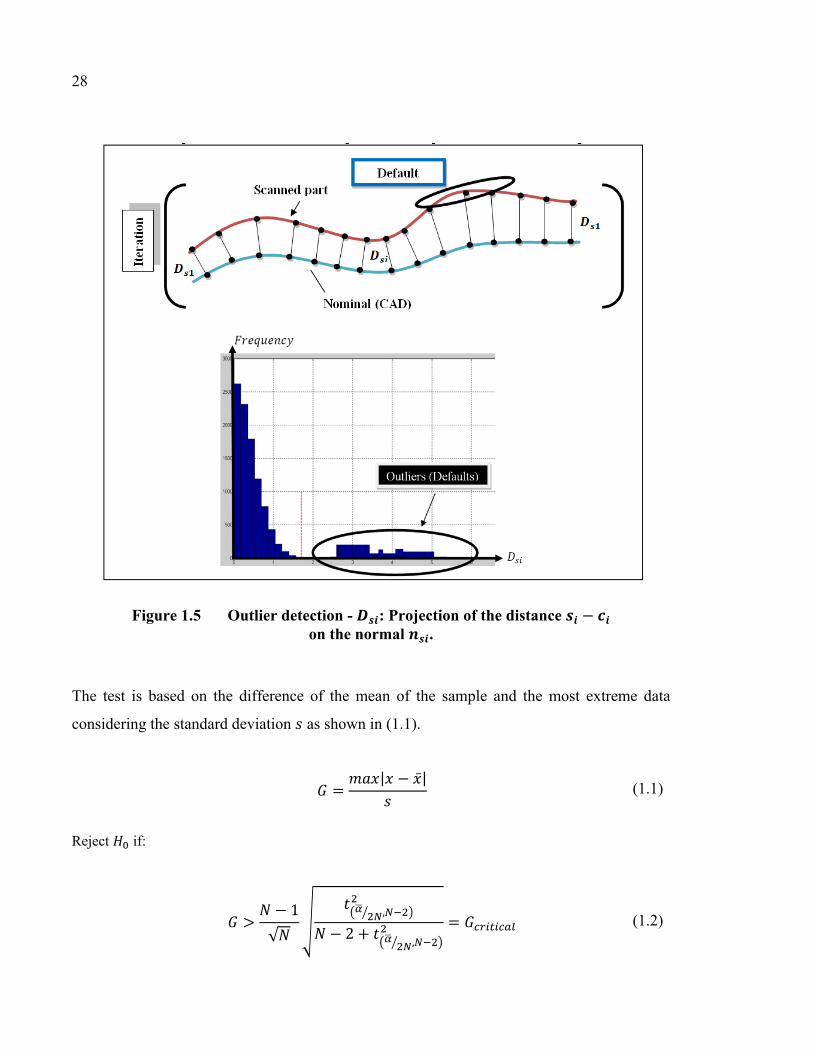
28

Figure 1.5 Outlier detection - : Projection of the distance − on the normal .

The test is based on the difference of the mean of the sample and the most extreme data

considering the standard deviation as shown in (1.1).

= | − | (1.1)

Reject if:

> − 1√ ,− 2 + , = (1.2)

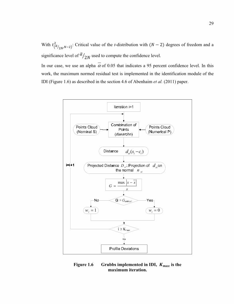
29

With , : Critical value of the t-distribution with ( − 2) degrees of freedom and a

significance level of 2 used to compute the confidence level.

In our case, we use an alpha α of 0.05 that indicates a 95 percent confidence level. In this

work, the maximum normed residual test is implemented in the identification module of the

IDI (Figure 1.6) as described in the section 4.6 of Abenhaim et al. (2011) paper.

s

xxG

−=

max

1=iw

)( iisi csd −

siD sidsin

0=iw

Figure 1.6 Grubbs implemented in IDI, is the maximum iteration.

30

1.5 Results

In order to evaluate the performance of the new implementation, three case studies shapes

representing typical non-rigid parts of transport industry are studied (Figure 1.7). All the

parts are in aluminum gauge 14 (1.63 ) with a Young modulus of 7 × 10 / and a

density of 2700 / . Table 1.1 represents the parameters for the algorithm used in the

case studies. In order to make the comparison between the original IDI identification method

and the proposed herein, type I error ( ) and the type II error ( ) are used thereafter. Type I

error ( ) is the error of rejecting a "correct" null hypothesis( ), and type II error ( ) is the

error of not rejecting a "false" null hypothesis( ). In other words, is rejecting a default

when it should not have been rejected and is failing to reject a default when it should have

been rejected ( is a false detection). Assuming that the density is uniform throughout the

part, the performance of the proposed method and of the IDI’s identification method can be

compared using a point-base metric instead of surface-base metric. In the ideal case the 2

types of errors must be equal to zero.

Analyzing Figure 1.8 to Figure 1.21 and Table 1.2 to Table 1.4, one can notice that the

implementation of the maximum normed residual test has remarkably reduced the number of

points with type I errors ( ) and with type II errors ( ) in the case of quasi constant surface

(case a) compared to their original IDI identification method.

In the case of omega shape (case b) and freeform surface (case c), this implementation has

slightly reduced the number of points with type I errors ( ) and has remarkably reduced

(only in case b) the number of points with type II errors ( ) compared to their original IDI

identification method.

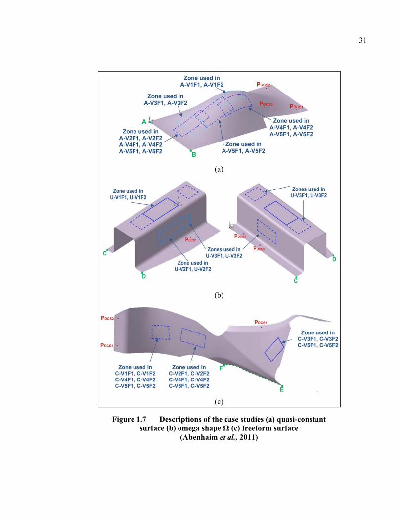
31

(a)

(b)

(c)

Figure 1.7 Descriptions of the case studies (a) quasi-constant surface (b) omega shape Ω (c) freeform surface

(Abenhaim et al., 2011)

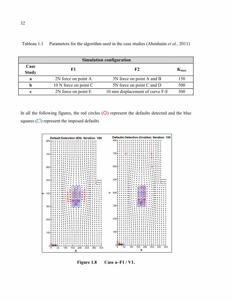
32

Tableau 1.1 Parameters for the algorithm used in the case studies (Abenhaim et al., 2011)

Simulation configuration

Case Study

F1 F2 Kmax

a 2N force on point A 3N force on point A and B 150

b 10 N force on point C 5N force on point C and D 500

c 2N force on point E 10 mm displacement of curve F-E 300

In all the following figures, the red circles () represent the defaults detected and the blue

squares () represent the imposed defaults

Figure 1.8 Case a–F1 / V1.

33

Figure 1.9 Case a–F1 / V2.

Figure 1.10 Case a–F1 / V3.

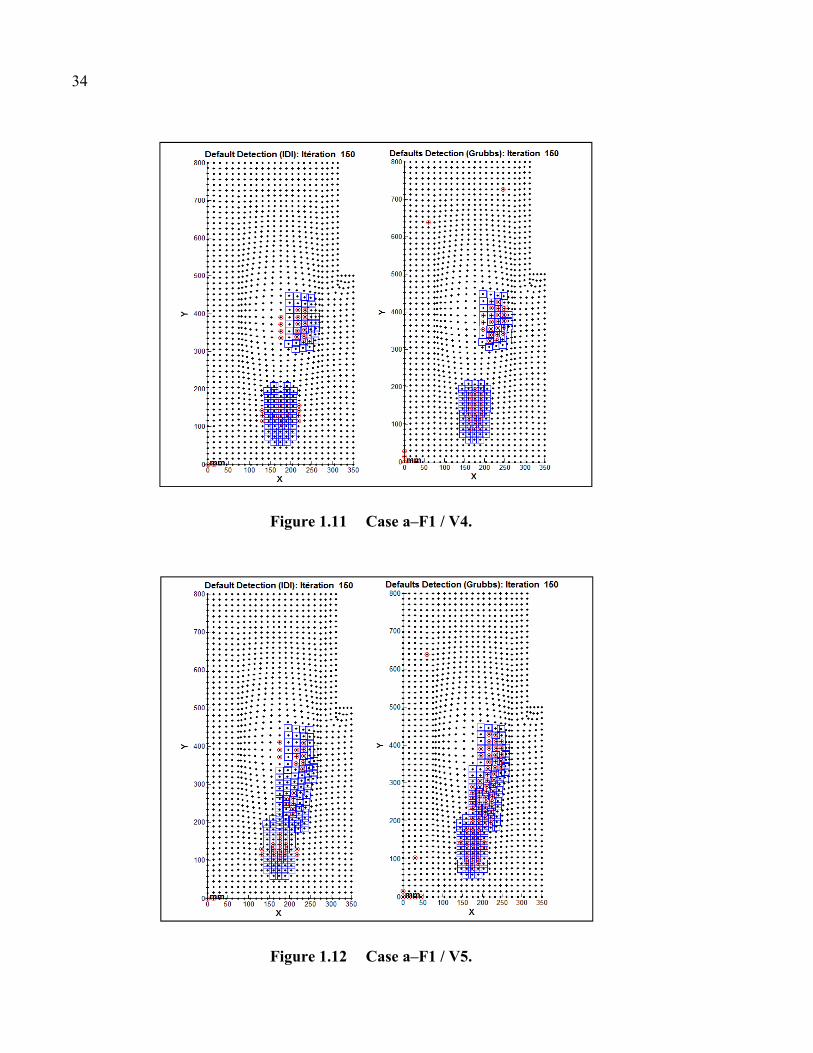
34

Figure 1.11 Case a–F1 / V4.

Figure 1.12 Case a–F1 / V5.

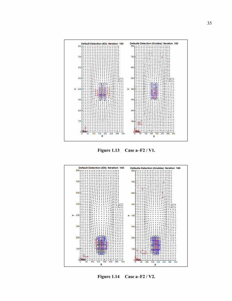
35

Figure 1.13 Case a–F2 / V1.

Figure 1.14 Case a–F2 / V2.

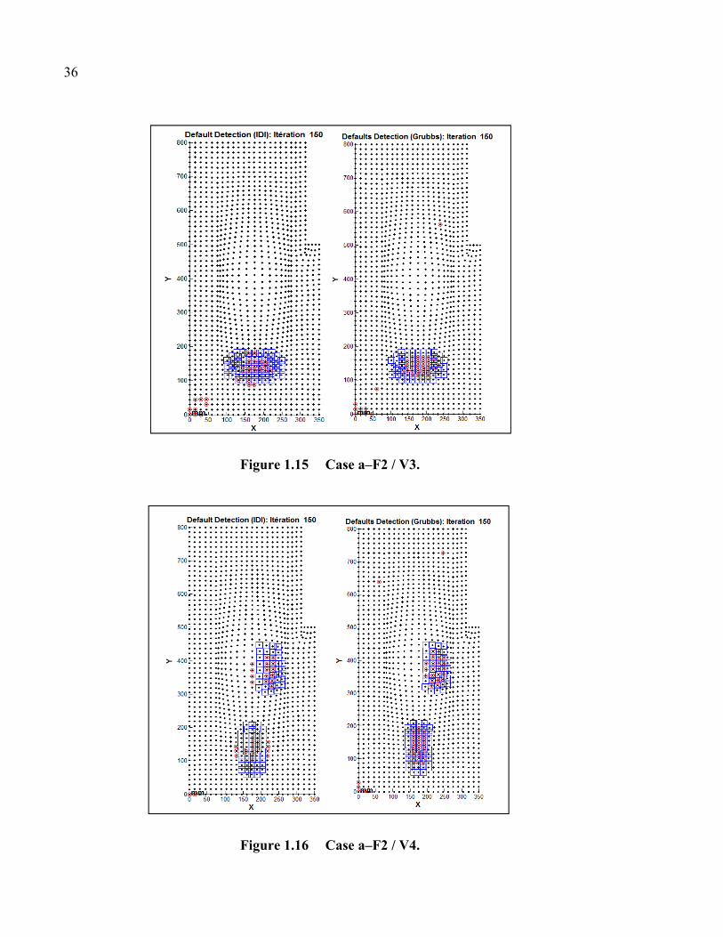
36

Figure 1.15 Case a–F2 / V3.

Figure 1.16 Case a–F2 / V4.

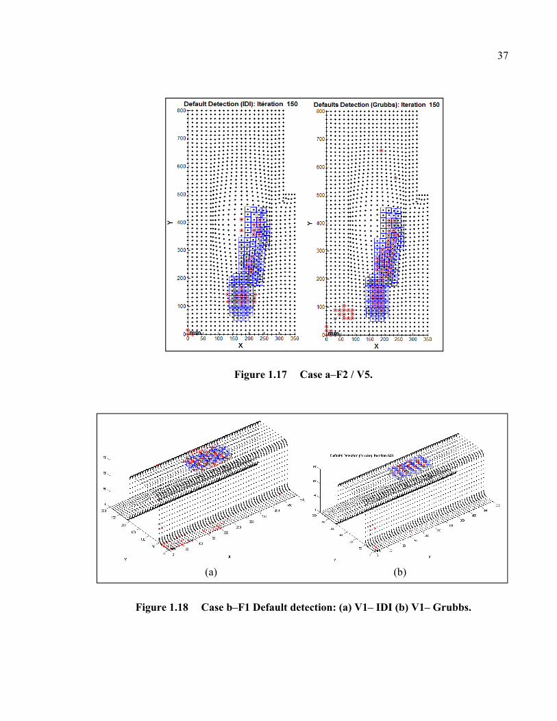
37

Figure 1.17 Case a–F2 / V5.

(a) (b)

Figure 1.18 Case b–F1 Default detection: (a) V1– IDI (b) V1– Grubbs.

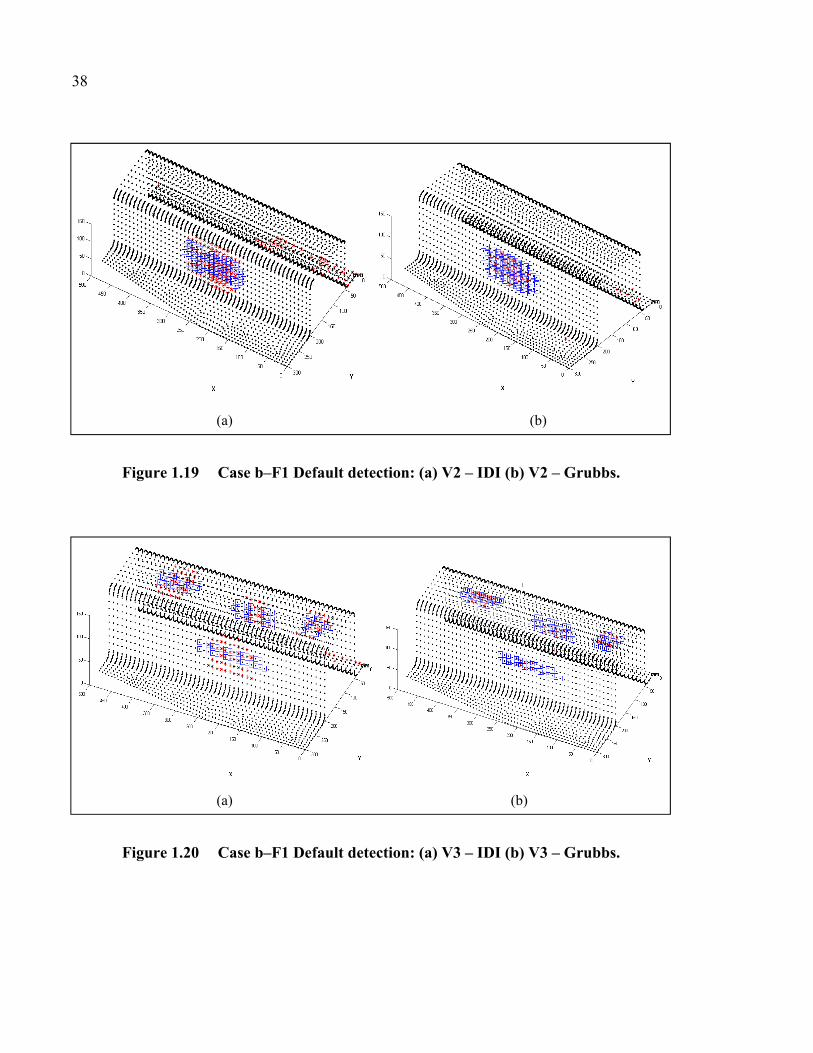
38

(a) (b)

Figure 1.19 Case b–F1 Default detection: (a) V2 – IDI (b) V2 – Grubbs.

(a) (b)

Figure 1.20 Case b–F1 Default detection: (a) V3 – IDI (b) V3 – Grubbs.

39

(a)

(b)

Figure 1.21 Case c–F1 (a) IDI – V5 (b) Grubbs – V5.

Another improvement compared to the original IDI identification module is that the

identification threshold is not estimated by a trial and error process. Herein, the maximum

normed residual test uses a constant parameter = 0.05 that corresponds to ± ≈ 95% of

the set.

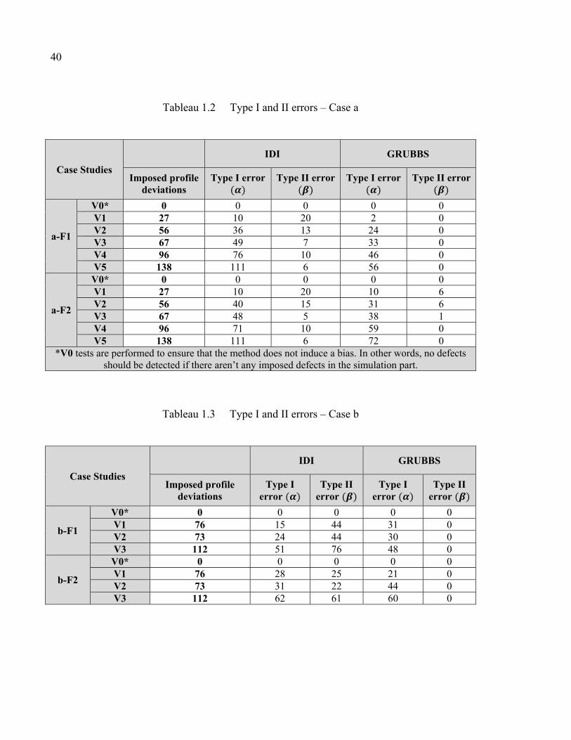
40

Tableau 1.2 Type I and II errors – Case a

Case Studies

IDI GRUBBS

Imposed profile deviations

Type I error ( ) Type II error ( )

Type I error ( ) Type II error ( )

a-F1

V0* 0 0 0 0 0 V1 27 10 20 2 0 V2 56 36 13 24 0 V3 67 49 7 33 0 V4 96 76 10 46 0 V5 138 111 6 56 0

a-F2

V0* 0 0 0 0 0 V1 27 10 20 10 6 V2 56 40 15 31 6 V3 67 48 5 38 1 V4 96 71 10 59 0 V5 138 111 6 72 0

*V0 tests are performed to ensure that the method does not induce a bias. In other words, no defects should be detected if there aren’t any imposed defects in the simulation part.

Tableau 1.3 Type I and II errors – Case b

Case Studies

IDI GRUBBS

Imposed profile deviations

Type I error ( )

Type II error ( )

Type I error ( )

Type II error ( )

b-F1

V0* 0 0 0 0 0 V1 76 15 44 31 0 V2 73 24 44 30 0 V3 112 51 76 48 0

b-F2

V0* 0 0 0 0 0 V1 76 28 25 21 0 V2 73 31 22 44 0 V3 112 62 61 60 0

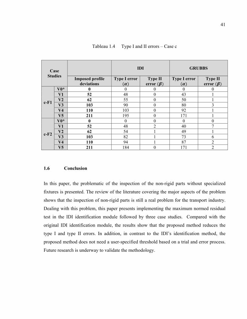
41

Tableau 1.4 Type I and II errors – Case c

Case Studies

IDI GRUBBS

Imposed profile deviations

Type I error ( ) Type II

error ( ) Type I error ( )

Type II error ( )

c-F1

V0* 0 0 0 0 0 V1 52 48 0 43 1 V2 62 55 0 50 1 V3 103 90 0 80 3 V4 110 103 0 92 1 V5 211 195 0 171 1

c-F2

V0* 0 0 0 0 0 V1 52 48 2 40 7 V2 62 54 1 49 1 V3 103 82 1 73 6 V4 110 94 1 87 2 V5 211 184 0 171 2

1.6 Conclusion

In this paper, the problematic of the inspection of the non-rigid parts without specialized

fixtures is presented. The review of the literature covering the major aspects of the problem

shows that the inspection of non-rigid parts is still a real problem for the transport industry.

Dealing with this problem, this paper presents implementing the maximum normed residual

test in the IDI identification module followed by three case studies. Compared with the

original IDI identification module, the results show that the proposed method reduces the

type I and type II errors. In addition, in contrast to the IDI’s identification method, the

proposed method does not need a user-specified threshold based on a trial and error process.

Future research is underway to validate the methodology.

42

1.7 Acknowledgments

The authors would like to thank the National Sciences and Engineering Research Council

(NSERC) and École de Technologie Supérieure (ÉTS) for their support and financial

contribution.

CHAPITRE 2

THE INSPECTION OF DEFORMABLE BODIES USING CURVATURE ESTIMATION AND THOMPSON-BIWEIGHT TEST

Ali AIDIBE, Antoine S. TAHAN,

Mechanical Engineering Department, École de technologie supérieure (ÉTS)

1100 Notre-Dame Ouest, Montréal, Québec, Canada H3C1K3

This chapter has been published in the “International Journal of Advanced Manufacturing

Technology”, Volume 71, April 2014, Pages 1733-1747 – Springer London

2.1 Abstract

Dimensioning and tolerancing standards assume inspection operation, unless otherwise

specified, must be done in Free State. This can be problematic when dealing with compliant

parts. The inspection of compliant parts needs specialized fixtures, because in Free State they

may induce a significantly different form than their nominal model (CAD) due to inherent

variations in the manufacturing process, gravity loads and residual strains. These specialized

fixtures pose difficulties, bear significant costs to industry and the process is very time-

consuming. To address these challenges, this paper proposes a novel method for quantifying

flexibility/rigidity of the mechanical components. Subsequently, a novel approach named

IDB-CTB is proposed to fixtureless Inspection of Deformable Bodies by Curvature

estimation and Thompson-Biweight test. This approach combines the Gaussian curvature

properties of manufactured compliant parts, one of the intrinsic properties of the geometry,

with the Thompson-Biweight statistical test based on the extreme value notion as an

identification method. The aim is to distinguish profile deviation due to the manufacturing

process from a part’s deformation due to its flexibility in order to determine whether the

tolerance fits the CAD model or not. The IDB-CTB approach is tested on two sets of case

studies. Three simulated, typical industrial sheet metal case studies were performed in the

first set, and an experimental case study in the second one. The low percentage of errors in

44

defect areas and in the profile deviations estimated compared with their reference ones in

most cases reflects the effectiveness of the proposed approach.

Keywords – curvature, registration, inspection, metrology, compliant, non-rigid,

deformation, GD&T, fixtureless, intrinsic geometry.

2.2 Introduction

The metrology of compliant parts without specialized fixtures is a challenging task in the

transportation industry especially in the aerospace and automotive fields. At the end of the

manufacturing process, engineers must verify if the produced part satisfies the functional

requirements under a given tolerance. Geometric dimensioning and tolerancing (GD&T)

standards like ASME Y14.5 (2009) and ISO 10579 (2010) consider that, by default and

unless otherwise specified, the inspection of components must be made at Free State without

applied force during the inspection. Many fixtureless inspection methods belonging to rigid

parts have been published (Yadong and Peihua, 2004). In the case of compliant parts there

are still no viable solutions. Due to dimensional variations, gravity loads, residual stress

induced distortion and/or assembly force, compliant parts in a Free State condition may have

a different form than their CAD models. Typically, the metrology of such parts requires a

special approach where expensive and specialized fixtures are needed to constrain dedicated

and follow the component during the inspection. These specialized jigs pose difficulties and

significant costs to industry. For example, currently at Bombardier Aerospace Inc. the

required preparation time for the inspection of compliant parts is about 50-60 man-hours

(Figure 2.1). Therefore, the need for Automatic inspection that is faster and free of human

error becomes essential in order to keep the global manufacturing market competitive.

45

(a)

(b)

Figure 2.1 Inspection of aerospace compliant parts using a jig – Bombardier Aerospace.

The goal of this paper is to distinguish between geometrical defects due to an error in the

manufacturing process, and deformations due to the flexibility of parts in the case of thin

shells in order to ascertain whether the tolerance of the manufactured part fits the CAD

model or not. To deal with this issue, the IDB-CTB method is developed. This new method

takes advantage of the compliant parts’ Gaussian curvature properties (one of the intrinsic

properties of the geometry), and combines it with a statistical test based on the extreme value

analysis techniques as an identification module which respects the following assumptions:

• The assembly, when scanning, allows elastic deformations greater than the required

tolerance profile.

• Inspection is limited to the defects in the surface profile as defined by ASME Y14.5

(2009).

• Defects are dent shapes and/or waviness profile deviations as shown in Figure 2.2.

• Parts materials are considered isotropic with well-known characteristics.

• The manufactured part is a sheet metal completely scanned and represented as a point

cloud ( , , ). • The point cloud represents a significant coverage of the original surface. No curvature

is calculated at areas of the object surface not covered by the point cloud.

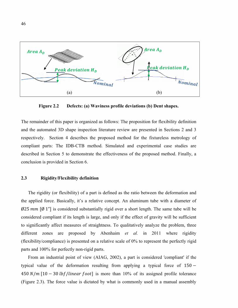
46

(a) (b)

Figure 2.2 Defects: (a) Waviness profile deviations (b) Dent shapes.

The remainder of this paper is organized as follows: The proposition for flexibility definition

and the automated 3D shape inspection literature review are presented in Sections 2 and 3

respectively. Section 4 describes the proposed method for the fixtureless metrology of

compliant parts: The IDB-CTB method. Simulated and experimental case studies are

described in Section 5 to demonstrate the effectiveness of the proposed method. Finally, a

conclusion is provided in Section 6.

2.3 Rigidity/Flexibility definition

The rigidity (or flexibility) of a part is defined as the ratio between the deformation and

the applied force. Basically, it’s a relative concept. An aluminum tube with a diameter of Ø25 [Ø 1”] is considered substantially rigid over a short length. The same tube will be

considered compliant if its length is large, and only if the effect of gravity will be sufficient

to significantly affect measures of straightness. To qualitatively analyze the problem, three

different zones are proposed by Abenhaim et al. in 2011 where rigidity

(flexibility/compliance) is presented on a relative scale of 0% to represent the perfectly rigid

parts and 100% for perfectly non-rigid parts.

From an industrial point of view (AIAG, 2002), a part is considered 'compliant' if the

typical value of the deformation resulting from applying a typical force of 150 −450 / [10 − 30 / ] is more than 10% of its assigned profile tolerance

(Figure 2.3). The force value is dictated by what is commonly used in a manual assembly

47

line. With this definition, many types of parts in the aeronautic and the automotive industry

can be grouped such as a wallboard (skin), pieces of thin-walled structure (spar, ribs, etc...)

and components for the interior finish of such planes. This definition isn’t absolute. In

certain mechanical parts, it’s possible to have rigid, as well and non-rigid, areas. To

quantitatively analyze the problem, a new method to represent flexibility using a logarithmic

graph and a ratio is proposed in this study (equation 2.1).

≜ δ12 (2.1)

Where δ is the maximum displacement induced by a certain force and is the profile

tolerance of the compliant part.

Figure 2.3 The flexibility definition from an industrial point of view.

48

For example, five (5) shapes, representing a sample of common parts in the industry, are

examined. All parts are made of E = 7 × 10 N. m aluminum. Figure 2.5 to Figure 2.9

illustrate the five parts used, their dimensions and their corresponding thickness (aluminium

gauges), as well as the external constraints and the simulation configuration forces imposed

in each case. The maximum induced deformation δ in each case, as well as its relation to

the profile tolerance expressed by the ratio R, is presented in Table 2.1. Lastly, Figure 2.10

represents the proposed quantitative representation of the flexibility in a logarithmic scale.

Figure 2.4 Legend for the case studies.

CASE A Diagonal: 18613 Thickness: 7.3482 (gauge 1)

Figure 2.5 Layout drawing of the compliant case A part.

All dimensions are in

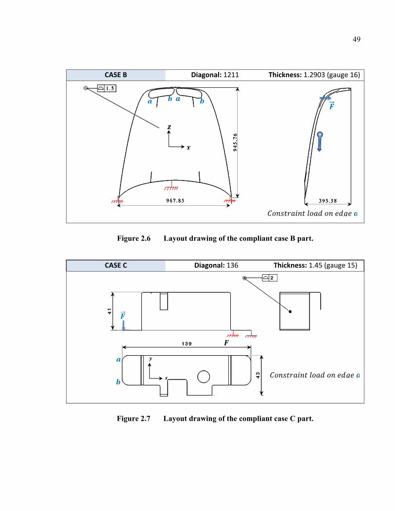
49

CASE B Diagonal: 1211 Thickness: 1.2903 (gauge 16)

Figure 2.6 Layout drawing of the compliant case B part.

CASE C Diagonal: 136 Thickness: 1.45 (gauge 15)

Figure 2.7 Layout drawing of the compliant case C part.

50

CASE D Diagonal: 585 Thickness: 2.3 (gauge 11)

Figure 2.8 Layout drawing of the compliant case D part.

CASE E Diagonal: 43733 Thickness: 7.3482 (gauge 1)

Figure 2.9 Layout drawing of the compliant case E part.

51

Tableau 2.1 Results of the flexibility ratio

Case

Diagonal Force Typical profile

tolerance

Maximum displacement

Flexibility

ratio

[ ] . [ . ] . [ . ] [ ] [ ]

A 18613 [732.8]

9.81 [32.2]

0 5 [0.196] 1140 [45] 456

B 1

1211 [47.7] 0

1.5 [0.06] 10 [0.4] 13.33

2 450 [30] 19.5 [0.77] 26

C 1

136 [5.35] 0

2 [0.078] 0.45 [0.018] 0.45

2 150 [10] 5.53 [0.218] 5.53

D 1

585 [23] 0

1 [0.04] 4 [0.157] 8

2 200 [14] 30 [2.2] 111.2

E 43733

[1721.77] 0 5 [0.196] 1230 [48.42] 492

Three different zones are proposed in the logarithmic graph (Figure 2.10):

• Zone A for the relatively rigid parts ( < 0.1). The displacement caused by a

reasonable force during inspection is less than 10% of the parts’ assigned tolerance.

• Zone B for the relatively compliant parts (0.1 < < 100). Parts classified in this zone

are the most problematic to manage with regards to the specification, tolerance, and

inspection of their geometric and dimensional requirements. By applying a certain

amount of force, these parts get closer to the third zone.

• Zone C for the very flexible parts ( > 100). In this zone, very large deformations are

produced only by the effect of the gravity.

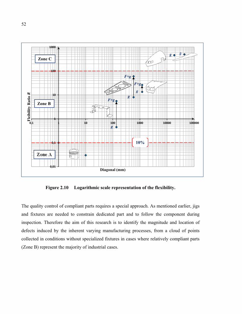
52

Figure 2.10 Logarithmic scale representation of the flexibility.

The quality control of compliant parts requires a special approach. As mentioned earlier, jigs

and fixtures are needed to constrain dedicated part and to follow the component during

inspection. Therefore the aim of this research is to identify the magnitude and location of

defects induced by the inherent varying manufacturing processes, from a cloud of points

collected in conditions without specialized fixtures in cases where relatively compliant parts

(Zone B) represent the majority of industrial cases.

0,01

0,1

1

10

100

1000

0,1 1 10 100 1000 10000 100000

Fle

ibil

ity

Rat

io R

Diagonal (mm)

Zone A

Zone B

Zone C

F+g

F+g

F+g

gg

g

g g

10%

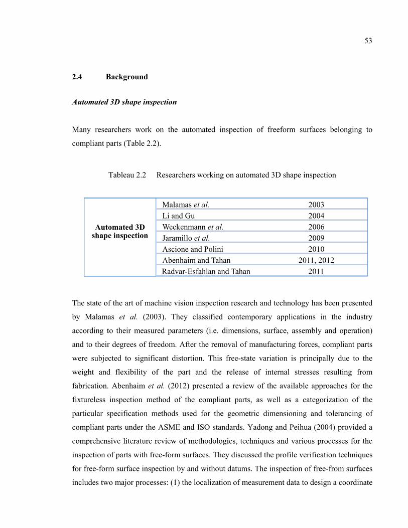
53

2.4 Background

Automated 3D shape inspection

Many researchers work on the automated inspection of freeform surfaces belonging to

compliant parts (Table 2.2).

Tableau 2.2 Researchers working on automated 3D shape inspection

The state of the art of machine vision inspection research and technology has been presented

by Malamas et al. (2003). They classified contemporary applications in the industry

according to their measured parameters (i.e. dimensions, surface, assembly and operation)

and to their degrees of freedom. After the removal of manufacturing forces, compliant parts

were subjected to significant distortion. This free-state variation is principally due to the

weight and flexibility of the part and the release of internal stresses resulting from

fabrication. Abenhaim et al. (2012) presented a review of the available approaches for the

fixtureless inspection method of the compliant parts, as well as a categorization of the

particular specification methods used for the geometric dimensioning and tolerancing of

compliant parts under the ASME and ISO standards. Yadong and Peihua (2004) provided a

comprehensive literature review of methodologies, techniques and various processes for the

inspection of parts with free-form surfaces. They discussed the profile verification techniques

for free-form surface inspection by and without datums. The inspection of free-from surfaces

includes two major processes: (1) the localization of measurement data to design a coordinate

Automated 3D shape inspection

Malamas et al. 2003

Li and Gu 2004

Weckenmann et al. 2006

Jaramillo et al. 2009

Ascione and Polini 2010

Abenhaim and Tahan 2011, 2012

Radvar-Esfahlan and Tahan 2011

54

system based on the datum reference information or a number of extracted surface features;

and (2) the further localization based on the surface characteristics so that the deviation of the

measured surface from the design model is minimized.

In 2010, Ascione and Polini proposed a fixture assembly methodology that enables both to

simulate the mating part interface and to locate the part in a coordinate measuring machine’s

working volume. Then, they used a method for the evaluation of the actual surface with

regard to its nominal model based on their Euclidean distance. Finally, a method based on a

finite element analysis was proposed to evaluate the effects of the measuring force (induced

by the touch probe on the inspected surface) on the measurement results. For the alignment

of deformable parts that do not require any fixtures, Weckenmann et al. (2006), as well as

Jaramillo et al. (2009), proposed an approach based on a finite element method to obtain a

physical deformation of the original CAD model, and radial basis functions to approximate

this deformation faster and in real time, opening the door to the on-line inspection of

deformable parts. Caulier (2010) proposed a general free-form stripe image interpretation

approach on the basis of a four-step procedure: (i) comparison of different feature-based

image content description techniques, (ii) determination of optimal feature sub-groups, (iii)

fusion of the most appropriate ones, and (iv) selection of the optimal features. She applies

this technique to a broader range of surface geometries and types, i.e. to free-form rough and

free-form specular shapes. Caulier and Bourennane (2008) proposed a general free-form

surface inspection approach relying on the projection of a structured light pattern and the

interpretation of the generated stripe structures by means of Fourier-based features. Lin et al.

(2008) explored automated visual inspection of surface defects in a light-emitting diode

(LED) chip by applying wavelet-based principal component analysis (WPCA) and Hotelling

statistic (WHS) approaches to integrate the multiple wavelet characteristics. The principal

component analysis of the WPCA, and the Hotelling control limit of WHS, is individually

judging the existence of defects. Cristea (2008) presents aspects of the design of an

intelligent modular inspection system. This system consists of grouping the parts based on

the relation between dimensional inspection process characteristics and modular design of all

inspection equipment’s with a high universality and flexibility degree. Kase et al. (1999)

55

presented a local and a global evaluation method for the shape error of free form surfaces.

The local evaluation method is based on the modification of principal curvatures between the

CAD and the manufactured surfaces. The global evaluation method is based on the average

normal vectors for the characterization of the representative direction of the surface portions.

In 2011, Abenhaim and Tahan developed the Iterative Displacement Inspection (IDI)

algorithm. The IDI allows for the surface profile inspection of a compliant part without the

need of a specialized jig. The method works through a comparison of two sets of points, one

from the mesh of the CAD model, and one from the scanned manufactured part, despite the

significant difference in their respective geometries. The method outlined operates by

iteratively deforming the smooth CAD mesh until it matches the scanned part without profile

deviation or measurement noise. This matching process is made possible with the

introduction of the identification method, which enables the effects of profile deviations to be

distinguished from the deformations due to the positioning of the part and its flexibility.

Aidibe and Tahan (2012) proposed the use of the statistical maximum normed residual test to

improve the aforementioned identification task and automatically set the identification

threshold. Compared with the original IDI identification module, the results indicate that the

proposed method reduces type I and type II errors. In addition, in contrast to the IDI’s

identification method, the proposed method does not require a user-specified threshold based

on a trial and error process. Radvar-Esfahlan and Tahan (2012) proposed the Generalized

Numerical Inspection Fixture (GNIF) algorithm. By taking advantage of the geodesic

distance metric properties, GNIF uses the imposition of boundary conditions into a finite

element (FE) model of the nominal CAD model to conform it to the scanned part and

automatically determine the corresponding points between them.

Following the IDB-CTB approach which is a new method for fixtureless inspection of

compliant parts will be presented.

56

2.5 Inspection of Deformable Bodies by Curvature estimation and the Thompson-Biweight test (IDB-CTB) approach

In order to compare deformable bodies, one should take advantage of their intrinsic

geometries because they remain unchanged during isometric deformations. The IDB-CTB

proposed method (Figure 2.13) is based on the Gaussian curvature estimation, which is

invariant under isometric deformations, combined with a statistical identification module to

distinguish the defects due to manufacturing process from the deformation due to the

flexibility of a given part. The proposed identification module considered the defects as

‘outliers’ and combines the Thompson extreme value statistical test (Thompson, 1985) with

the biweight mean and standard deviation estimator technique (Hoaglin et al., 1983) in order

to detect them. In this section the main steps of the proposed method will be presented.

2.5.1 Registration and matching (Step 1, Step 2)

Let = , , , … , ∈ ℝ be a set of nodes representing the meshed CAD model

and = , , , … , ∈ ℝ be a set of | ≫ nodes representing the scanned

part. The Iterative Closest Point (ICP) algorithm developed by Besl and McKay (1992) is

used in order to register the two given point sets in a common coordinate system. The ICP

algorithm is one of the most popular 3D matching algorithms which works for nearly any

type of surface representation and aims to determine the transformation between two given

point cloud sets by minimizing the square errors between corresponding entities. After the

pre-alignment, a dsearchn function in Matlab® based on Quickhull (Barber et al., 1996) is

used to find the closest point = , , , … , ∈ ℝ in to .

2.5.2 Curvature estimation method (Step 3)

Knowledge of the curvature of surfaces is important in a number of applications, especially

those dealing with evolving surface geometry. Curvature, defined in 3-space, is the measure

57

of how much the curve “bends” at a single point. It is a measure of how fast the unit tangent

bends in the direction of the normal.

The Gaussian and the mean curvature of a regular surface in ℝ at a point are formally

defined as:

( ) = ( ∗( )) (2.2)

( ) = 12 ( ∗( )) (2.3)

Where ∗ is the shape operator and , denotes the determinant and the matrix trace

respectively.

The Gaussian and mean curvature are also given by:

( ) = = 1 (2.4)

( ) = +2 = 12 1 + 1

(2.5)

Where and are the principal curvatures that measure the maximum and minimum

bending of a regular surface at each point. and are the maximum and minimum of the

normal curvature. and are the principal radii of curvature. (See Figure 2.11)

The Gaussian and mean curvatures are chosen because they are invariant under rotation and

translation.

In our case, the curvature is estimated from discrete surface information (nodes of

triangulation). For this, initial estimation of the surface normal is done using the triangular

mesh. Then a smooth quadratic polynomial surface is fitted to a local set of points around the

point of interest and the surface curvature at that point is used as the curvature estimate (Peng

et al., 2003)

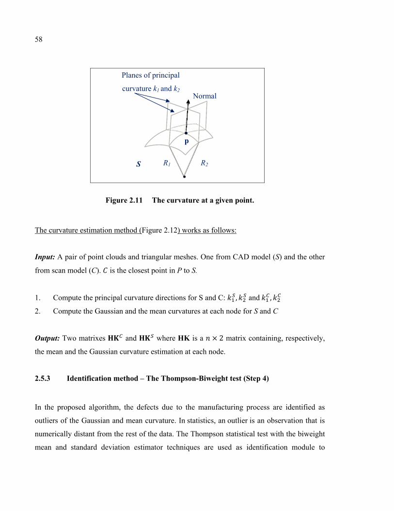
58

Figure 2.11 The curvature at a given point.

The curvature estimation method (Figure 2.12) works as follows:

Input: A pair of point clouds and triangular meshes. One from CAD model (S) and the other

from scan model (C). is the closest point in P to S.

1. Compute the principal curvature directions for S and C: , and ,

2. Compute the Gaussian and the mean curvatures at each node for S and C

Output: Two matrixes and where HK is a × 2 matrix containing, respectively,

the mean and the Gaussian curvature estimation at each node.

2.5.3 Identification method – The Thompson-Biweight test (Step 4)

In the proposed algorithm, the defects due to the manufacturing process are identified as

outliers of the Gaussian and mean curvature. In statistics, an outlier is an observation that is

numerically distant from the rest of the data. The Thompson statistical test with the biweight

mean and standard deviation estimator techniques are used as identification module to

p

Planes of principal

curvature k1 and k2

S R1 R2

Normal

59

distinguish between the defects and the deformations. Defects, in our assumption, are dent

shapes and/or waviness profile deviations.

The Thompson tau technique is a statistical method for deciding whether to keep or discard

suspected outliers in a sample of single and multiple variables. The biweight is a more

sophisticated estimator belonging to a category known as redescending estimators. The

biweight estimate is a weighted average where weighting decreases from the center of the

distribution. Thereafter, the term Thompson-Biweight will be used to designate our proposed

statistical identification method.

The identification module (Figure 2.12) works as follows:

Input: Two matrixes and

1. Compute the difference delta between the two matrixes and

∆ = | − | (2.6)∆ = [∆ ∆ ]

where ∆ is a × 2 matrix containing, respectively, the difference in mean and the

difference in Gaussian curvatures estimations at each node.

2. Arrange the ∆ values in increasing order, so that the suspected outliers are easily

spotted.

3. For each ∆ , we compute the absolute value of the deviation:

= |∆ − ∆ | (2.7)

Where ∆ is estimated using the biweight mean estimator technique.

60

∆ = + ∑ (∆ − )(1 − )∑ (1 − ) (2.8)

• The median ( ) is the “middle” value of a distribution and is estimated (from a sample

of values) by:

= ∆ ( )/(∆ / + ∆ ( / ) ) 2⁄ (2.9)

• The is the median of the absolute values of the deviations of the sample values

from the median.

= (|∆ − |)

(2.10)

• is a weight corresponding to each of the n observations ∆ .

= ∆ −× (2.11)

• The biweight influence function returns to zero at some distance away from the center

of the distribution. This distance is controlled by a parameter . All values beyond a

certain critical distance from the center are given zero weight. A value between 6 and

9 is recommended (Hoaglin et al., 1983). = 9 is proposed in the method (the sensor

values more than 6 standard deviations away).

4. Compute the value of the Thompson technique (Greek letter tau). is calculated from

the critical value of the student’s density function.

= , . ( − 1)√ − 2 + , (2.12)

61

Where , is the critical student’s t value with ( − 2) degrees of freedom and a

significance level of /2.

5. Determine whether to reject or keep this suspected defect, using the following rules:

> Reject the data point. It’s a defect. = 0 ≤ Keep the data point. It’s not a defect. = 1

Where is the estimation of the biweight standard deviation of ∆ .

= ∑ (∆K − ) (1 − )∑ (1 − )(1 − 6 ) (2.13)

The same procedure is applied for ∆ .

Output: The weights = 01 for the points identified as outliers in ∆ (defects)

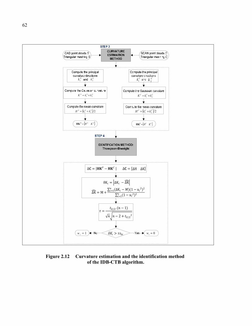
62

Sk 2Sk1

SSS kkK 21 ×=

( ) 221SSS kkH +=

[ ]SS KH=SHK

0=iw1=iw

= /2. ( − 1)√ − 2 + /22

∆ = | − | δK = ∆K − ∆K ∆K = M + ∑ (∆K − )(1 − 2)2=1 ∑ (1 − 2)2=1

∆ = [∆H ∆K]

Ck1Ck 2

CCC kkK 21 ×=

( ) 221CCC kkH +=

[ ]CC KH=CHK

>

Figure 2.12 Curvature estimation and the identification method of the IDB-CTB algorithm.

63

2.5.4 IDB-CTB approach

Having explained the curvature estimation method, as well as the identification method, the

IDB-CTB algorithm will now be presented. Starting with the set of nodes of the CAD

model and the point cloud of the manufactured part, the IDB-CTB method schematized in

Figure 2.13 works as follows:

1. Make a geometric alignment between and using the Iterative Closest Point (ICP)

algorithm.

2. Find point corresponding to each node using the dsearchn function based on

Quickhull algorithm.

3. Create the triangular mesh for .

4. Compute the Gaussian and the mean curvature as described in section 3.1.

5. Applying the proposed Thompson-Biweight test in order to identify deformation from

deviations.

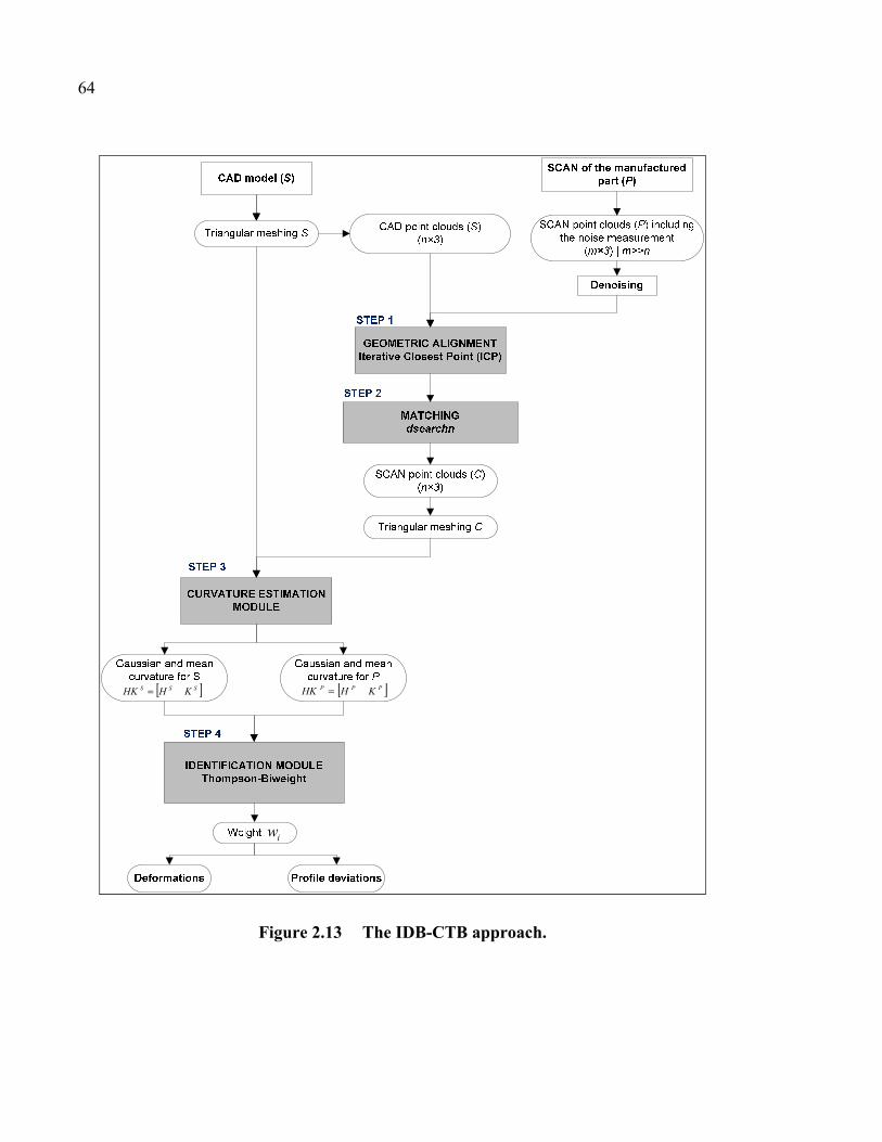
64

[ ]SSS KHHK = [ ]PPP KHHK =

iw

Figure 2.13 The IDB-CTB approach.

65

2.6 Case Studies and validation

This section presents two sets of case studies to test and validate the IDB-CTB approach

developed in this paper: Three simulated case studies and an experimental one.

2.6.1 Fist set: Simulated case studies

In the first set, three shapes are chosen from section 2.3, representing a sample of common

parts in the transport industry. The compliant parts are simulated by CATIA® V5 as well as

the finite element analysis. Starting with the CAD model, the scanned manufactured part is

simulated in accordance with the steps described in Table 2.3. Predefined profile deviation is

added to all case studies. The defect is a dent shape and/or waviness profile deviation

characterized by its peak deviation and its area as already presented in section 1.

Specific external force is applied to model and to simulate the free-state condition. The finite

element analysis takes into account both the mounting fixture configuration during a

presumed digitalization and the force of gravity. The spatial sampling frequency of scanned

data is different from the mesh used in the CAD data. A new point cloud representing the

mesh of the part with a profile deviation zone and also with a deformed shape is then created.

Tableau 2.3 Steps to create the scanned part

Step Action

1 A local modification of the CAD surface, representing a zone with a waviness profile

deviation and/or dent shape, is created using the generative shape design module in

CATIA® V5.

2 A finite element analysis of the model created in the step 1 is generated using the

generative structural analysis module in CATIA® V5.

3 A Gaussian measurement noise N (0, ) is introduced on the newly created

point cloud. = . .

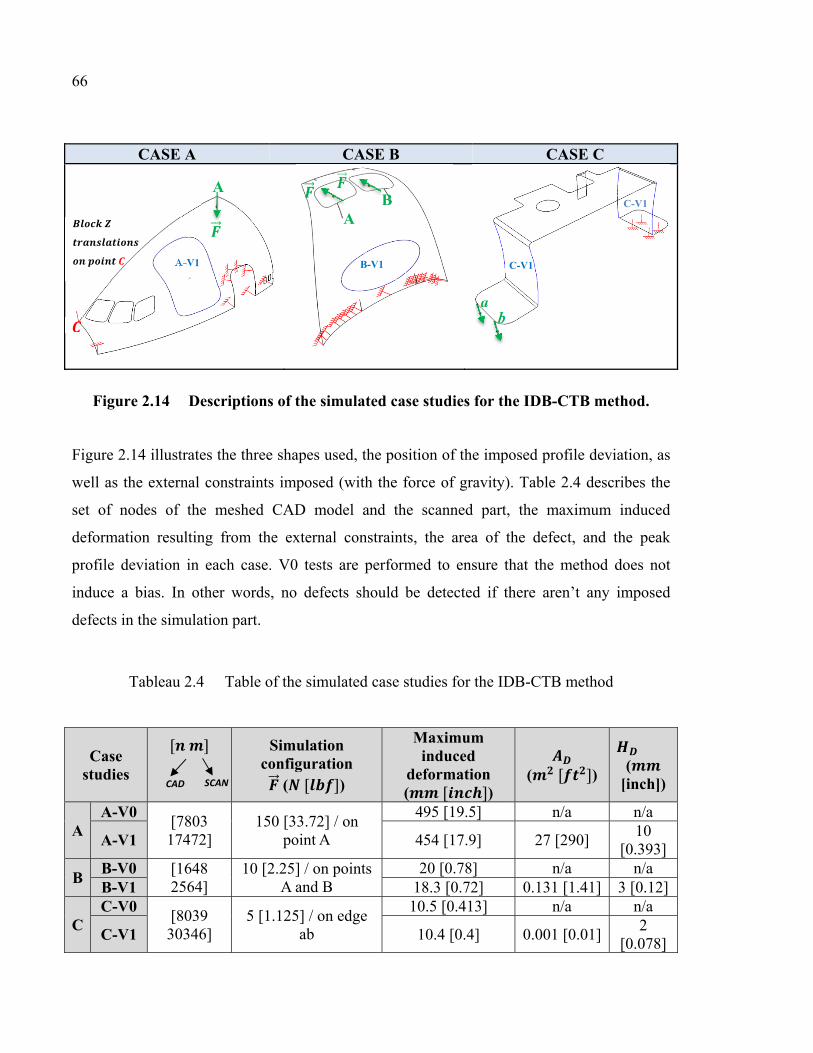
66

CASE A CASE B CASE C

Figure 2.14 Descriptions of the simulated case studies for the IDB-CTB method.

Figure 2.14 illustrates the three shapes used, the position of the imposed profile deviation, as

well as the external constraints imposed (with the force of gravity). Table 2.4 describes the

set of nodes of the meshed CAD model and the scanned part, the maximum induced

deformation resulting from the external constraints, the area of the defect, and the peak

profile deviation in each case. V0 tests are performed to ensure that the method does not

induce a bias. In other words, no defects should be detected if there aren’t any imposed

defects in the simulation part.

Tableau 2.4 Table of the simulated case studies for the IDB-CTB method

Case studies

[ ]

Simulation configuration

( [ ]) Maximum

induced deformation ( [ ])

( [ ]) (

[inch])

A A-V0

[7803 17472]

150 [33.72] / on point A

495 [19.5] n/a n/a

A-V1 454 [17.9] 27 [290] 10

[0.393]

B B-V0 [1648

2564] 10 [2.25] / on points

A and B 20 [0.78] n/a n/a

B-V1 18.3 [0.72] 0.131 [1.41] 3 [0.12]

C C-V0

[8039 30346]

5 [1.125] / on edge ab

10.5 [0.413] n/a n/a

C-V1 10.4 [0.4] 0.001 [0.01] 2

[0.078]

C-V1

C-V1

ab

A-V1

A

B-V1

AB

CAD SCAN

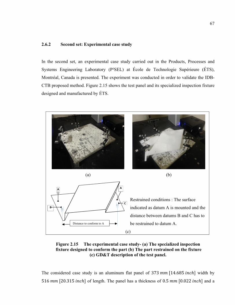
67

2.6.2 Second set: Experimental case study

In the second set, an experimental case study carried out in the Products, Processes and

Systems Engineering Laboratory (P²SEL) at École de Technologie Supérieure (ÉTS),

Montréal, Canada is presented. The experiment was conducted in order to validate the IDB-

CTB proposed method. Figure 2.15 shows the test panel and its specialized inspection fixture

designed and manufactured by ÉTS.

(a) (b)

Restrained conditions : The surface

indicated as datum A is mounted and the

distance between datums B and C has to

be restrained to datum A.

(c)

Figure 2.15 The experimental case study- (a) The specialized inspection fixture designed to conform the part (b) The part restrained on the fixture

(c) GD&T description of the test panel.

The considered case study is an aluminum flat panel of 373 [14.685 ℎ] width by 516 [20.315 ℎ] of length. The panel has a thickness of 0.5 [0.022 ℎ] and a

AA

Distance to conform to A

B C

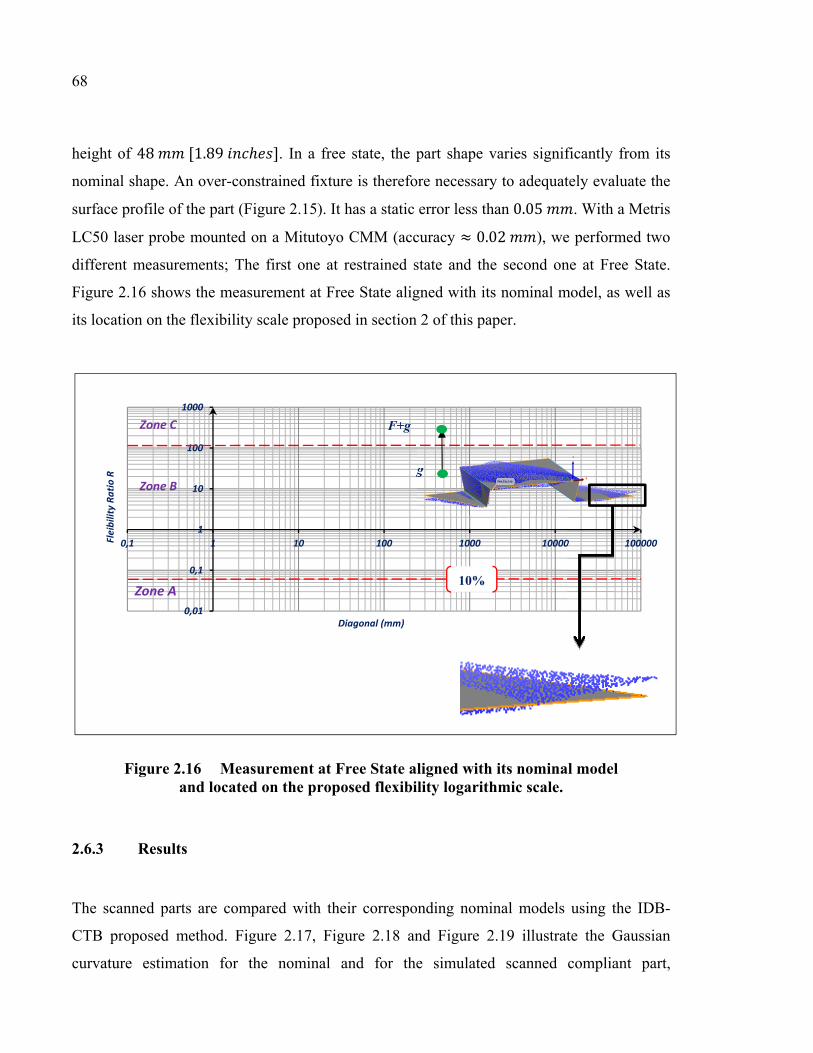
68

height of 48 [1.89 ℎ ]. In a free state, the part shape varies significantly from its

nominal shape. An over-constrained fixture is therefore necessary to adequately evaluate the

surface profile of the part (Figure 2.15). It has a static error less than 0.05 . With a Metris

LC50 laser probe mounted on a Mitutoyo CMM (accuracy ≈ 0.02 ), we performed two

different measurements; The first one at restrained state and the second one at Free State.

Figure 2.16 shows the measurement at Free State aligned with its nominal model, as well as

its location on the flexibility scale proposed in section 2 of this paper.

Figure 2.16 Measurement at Free State aligned with its nominal model and located on the proposed flexibility logarithmic scale.

2.6.3 Results

The scanned parts are compared with their corresponding nominal models using the IDB-

CTB proposed method. Figure 2.17, Figure 2.18 and Figure 2.19 illustrate the Gaussian

curvature estimation for the nominal and for the simulated scanned compliant part,

0,01

0,1

1

10

100

1000

0,1 1 10 100 1000 10000 100000Flei

bilit

y Ra

tio R

Diagonal (mm)

g

10%

F+g

Zone A

Zone B

Zone C

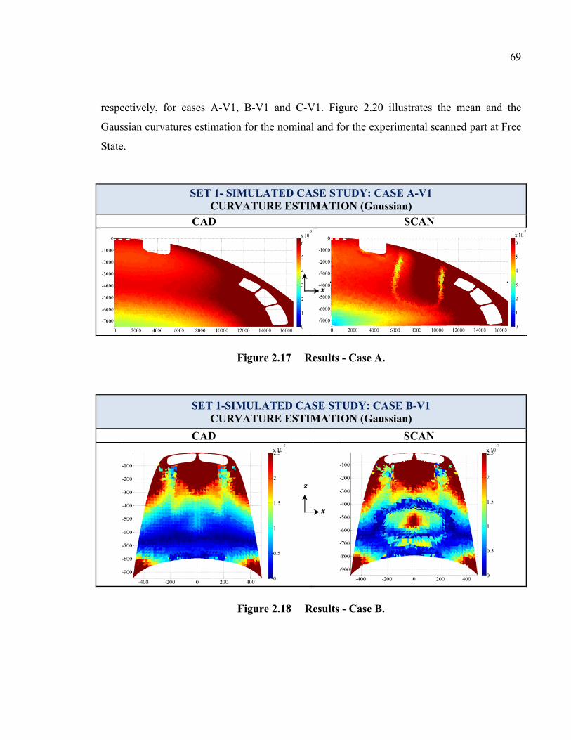
69

respectively, for cases A-V1, B-V1 and C-V1. Figure 2.20 illustrates the mean and the

Gaussian curvatures estimation for the nominal and for the experimental scanned part at Free

State.

SET 1- SIMULATED CASE STUDY: CASE A-V1 CURVATURE ESTIMATION (Gaussian)

CAD SCAN

Figure 2.17 Results - Case A.

SET 1-SIMULATED CASE STUDY: CASE B-V1 CURVATURE ESTIMATION (Gaussian)

CAD SCAN

Figure 2.18 Results - Case B.

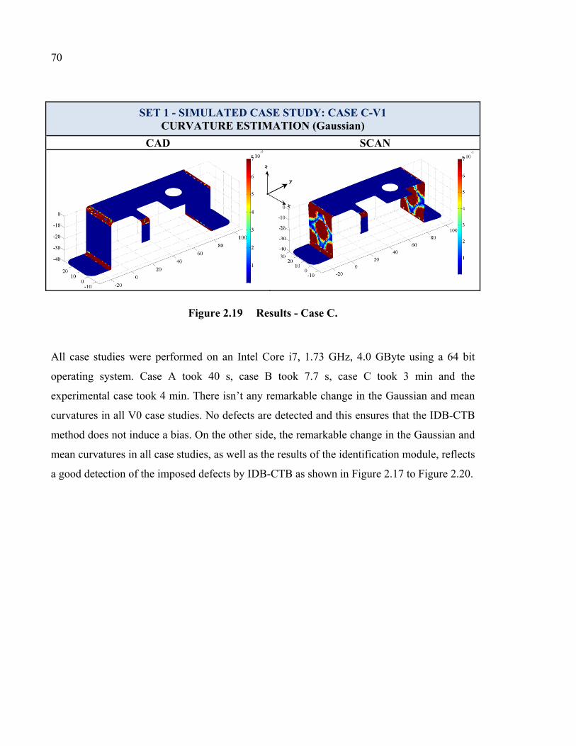
70

SET 1 - SIMULATED CASE STUDY: CASE C-V1 CURVATURE ESTIMATION (Gaussian)

CAD SCAN

Figure 2.19 Results - Case C.

All case studies were performed on an Intel Core i7, 1.73 GHz, 4.0 GByte using a 64 bit

operating system. Case A took 40 s, case B took 7.7 s, case C took 3 min and the

experimental case took 4 min. There isn’t any remarkable change in the Gaussian and mean

curvatures in all V0 case studies. No defects are detected and this ensures that the IDB-CTB

method does not induce a bias. On the other side, the remarkable change in the Gaussian and

mean curvatures in all case studies, as well as the results of the identification module, reflects

a good detection of the imposed defects by IDB-CTB as shown in Figure 2.17 to Figure 2.20.

71

SET 2 - EXPERIMENTAL CASE STUDY CURVATURE ESTIMATION (Mean and Gaussian)

CAD SCAN at free state

Figure 2.20 Results - Experimental case study.

In order to numerically evaluate the detection, the percentage of error in a defect area and the

percentage of error in peak profile deviation is calculated. They are given by equations 2.9

and 2.10, respectively.

= − × 100

(2.9)

= − × 100

(2.10)

Zone1

Zone 2

Zone 3

72

Where represents the estimated area value of the defect, its percentage of area error

compared to the imposed one , the estimated peak profile deviation and its

percentage of peak profile deviation error compared to the imposed one .

For the simulated case studies, the peak profile deviation value is calculated by projecting the

peak point estimated in the SCAN model onto the closest triangle located on the nominal

model. The numerical results of the evaluation are represented in Table 2.5.

For the experimental case study, the peak profile deviation is estimated using

Polyworks V12 ®. The reference values in this case will be those of the restrained parts.

Tableau 2.5 Results of the IDB-CTB method

Case studies

Reference value Estimated value Error

( [ ])

( [inch])

( [ ])

( [inch])

(%) (%)

A A-V0 0 0 0 0 0 0

A-V1 27

[290] 10

[0.393] 26.424 [284.42]

9.667 [0.38]

(-)a 2%

(-) 3%

B B-V0 0 0 0 0 0 0

B-V1 0.131 [1.41]

3 [0.12]

0.1415 [1.52]

2.813 [0.11]

(+) 8%

(-) 6%

C C-V0 0 0 0 0 0 0

C-V1 0.001 [0.01]

2 [0.078]

0.000932 [0.009]

1.655 [0.065]

(-) 6% (-)

17%

Experimental

Reference value ≈ The scanned part on fixture

Estimated values from the scanned part at

freestate

Zone 1

0.043 [0.46]

7.556 [0.297]

0.0445 [0.478]

7.115 [0.28]

(-) 3%

(-) 5%

Zone 2

0.041 [0.44]

6.434 [0.253]

0.0423 [0.455]

6.818 [0.268]

(+) 3%

(+) 6%

Zone 3

0.023 [0.25]

2.319 [0.09]

0.0246 [0.264]

2.715 [0.1]

(+) 6%

(+) 17%

a (+) overestimated the value and (-) underestimated value compared with the reference one.

The percentage of error in a defect area is less than 8% in all the cases (Table 2.5) as well as

the percentage of error in peak profile deviation except in case C and Zone 3 of the

73

experimental case where the percentage is higher than 10% (17.25%). This shows that by

using the IDB-CTB approach good results in the detection of the defect area, position, and

peak deviation have been achieved.

The high percentage error of case C and of experimental - Zone 3 (Table 2.5) is due to the

alignment process. In this work the ICP method is used in order to pre-align the SCAN

model to its nominal one. Working on the alignment stage can improve the peak profile

deviation error percentage in this case.

2.7 Conclusion

In this paper a quantification of the flexibility/rigidity behavior of mechanical parts is

proposed. The maximum deformation induced by a certain force is compared to the profile

tolerance of five typical compliant parts and the results are represented in a logarithmic scale.

Three zones were then defined and reflected where our compliant parts were located in the

flexibility scale. This quantification approach will allow industries to properly classify their

mechanical components and will be strongly useful during tolerancing operations. After that,

the technologies in metric and computational geometry are merged along with extreme

statistics to develop a novel approach to the geometrical inspection of compliant parts located

in the relatively flexible zone (Zone B) which represents the majority of industrial cases. The

IDB-CTB method combines the Gaussian curvature estimation with the Thompson statistical

test, and the biweight mean and standard deviation estimator in order to compare two sets of

points, one from the CAD model, and the other from the scanned manufactured part in a free-

state condition, in order to distinguish deformations due to the flexibility and the positioning

of parts from deviations due to the manufacturing process. The estimated values of the defect

areas and the profile deviations, as well as their positions, are much closer to their reference

ones in most cases, thus reflecting the accuracy of the proposed method. This method is

useful and efficient to verify a diverse range of deformable bodies without using special

inspection fixtures. The IDB-CTB method can be of immediate interest for the

manufacturing industry in general and, more specifically, for the aerospace and automotive

sector. It contributes greatly to its productivity and competitiveness.

74

2.8 Acknowledgments

The authors would like to thank the National Sciences and Engineering Research Council

(NSERC) and the École de Technologie Supérieure (ÉTS) for their support and financial

contribution.

CHAPITRE 3

THE COHERENT POINT DRIFT ALGORITHM ADAPTED FOR FIXTURELESS DIMENSIONAL INSPECTION OF DEFORMABLE BODIES

Ali AIDIBE, Antoine S. TAHAN,

Mechanical Engineering Department, École de technologie supérieure (ÉTS)

1100 Notre-Dame Ouest, Montréal, Québec, Canada H3C1K3

This chapter has been submitted for publication

3.1 Abstract

In a free-state condition, deformable bodies (or compliant parts) may have a significantly

different shape than their nominal geometry (CAD model) due to gravity loads and residual

stress. Typically, the dimensional metrology of such parts requires a particular approach

where expensive and specialized jigs are needed to constrain and follow the component

during inspection. Inspecting these parts without specialized fixtures will have significant

economic impacts on industry, reducing the delays and costs associated with product quality

inspection. This paper proposes a new method to fixtureless inspect compliant parts. This

new approach combines the optimization of the Coherent Point Drift powerful non rigid

registration method with the Thompson-Biweight statistical test as an identification method

to distinguish profile and localization process manufacturing defects of a part’s deformation.

In other words, a ‘flexible’ registration that meets the specifications of compliant parts is

proposed. The CAD model is smoothly modified to fit the scanned part by minimizing two

criteria that belong to deformable bodies. The first criterion is the conservation of the

curvilinear distance. That is to say, it is the condition that the stretch difference between the

original CAD model and the modified one should be very small. The second criterion is the

Euclidian distance between the modified CAD model and its corresponding scanned part.

The goal of this study is to deliver an inspection report which determines whether the

tolerance fits the CAD model or not. Many case studies were performed on an industrial

76

sheet metal which presented profiles and localization defects. The estimated values of the

defects, as well as their positions, are much closer to their reference ones in most cases, thus

reflecting the effectiveness of the proposed method.

Keywords – registration, inspection, metrology, compliant, non-rigid, deformation,

fixtureless, outliers.

3.2 Introduction

The process of new product development has been subject to major changes over the last two

decades. Accordingly, we can cite the reduction of development time, the massive integration

of virtual modelers, as well as the development of the global economy. For instance, the

industrial context is characterized by a technological maturity and development costs which

are subject to strong competition. Competitiveness involves metrology, which concerns the

application of measurement science to manufacturing parts ensuring that they are in a state of

compliance with engineering requirements. The problem with the dimensional and geometric

variations of mechanical components has been studied by many researchers in the case of

rigid parts. In spite of all the research, no viable and industrial solutions in the case of

compliant parts are available. Compliant parts, in a free-state condition, may have a

significantly different form than their nominal model (CAD) due to gravity load and residual

stress. Specialized fixtures are needed for the inspection of such parts which lead to

difficulties and significant costs to the transport industry. Figure 3.1 shows experimental case

studies from Bombardier Aerospace Inc. The required preparation time for the inspection of

these compliant parts is about 50-60 man-hours. Therefore, automatic fixtureless inspection

becomes a crucial issue in order to keep the global manufacturing market competitive. This

work proposes a methodology to improve inspection and validation operations. The expected

improvement derives from taking into account the phenomena which are related to the

flexibility in the choice of assembly and registration methods as well as their arising

correlations.

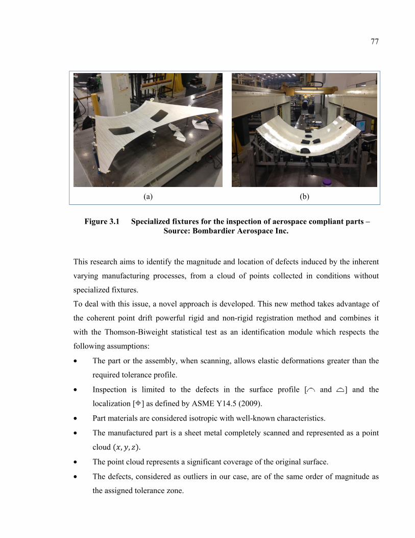
77

(a)

(b)

Figure 3.1 Specialized fixtures for the inspection of aerospace compliant parts – Source: Bombardier Aerospace Inc.

This research aims to identify the magnitude and location of defects induced by the inherent

varying manufacturing processes, from a cloud of points collected in conditions without

specialized fixtures.

To deal with this issue, a novel approach is developed. This new method takes advantage of

the coherent point drift powerful rigid and non-rigid registration method and combines it

with the Thomson-Biweight statistical test as an identification module which respects the

following assumptions:

• The part or the assembly, when scanning, allows elastic deformations greater than the

required tolerance profile.

• Inspection is limited to the defects in the surface profile [ and ] and the

localization [ ] as defined by ASME Y14.5 (2009).

• Part materials are considered isotropic with well-known characteristics.

• The manufactured part is a sheet metal completely scanned and represented as a point

cloud ( , , ). • The point cloud represents a significant coverage of the original surface.

• The defects, considered as outliers in our case, are of the same order of magnitude as

the assigned tolerance zone.

78

The remainder of this paper is organized as follows: the automated 3D shape inspection and a

literature review of registration techniques are presented in Sections 2. Section 3 describes

the proposed approach for the metrology of fixtureless compliant parts. This method is tested

and validated on twenty six case studies described in Section 4 followed by an analysis and a

discussion of the results. Finally, a summary is provided in Section 5.

3.3 Background

From an industrial requirement perspective, a part is considered 'compliant' if the typical

value of the deformation resulting from applying a typical force of 150 − 450 N/m [10 − 30 lbf/linear foot] is more than 10% of its assigned profile tolerance (AIAG, 2002).

The force value is dictated by what is commonly used in a manual assembly line. This

definition isn’t absolute. In certain mechanical parts, it’s possible to have rigid, as well as

non-rigid, areas. To facilitate analysis, three different zones categorized the compliant parts:

• Zone A for the relatively rigid parts. The displacement induced by a reasonable force

during inspection is less than 10% of the parts’ assigned tolerance.

• Zone B for the relatively compliant parts. Parts classified in this zone are the most

problematic to manage with regards to the specification, tolerance, and inspection of

their geometric and dimensional requirements. By applying a certain amount of force,

these parts get closer to the third zone.

• Zone C for the very flexible parts. In this zone very large deformations are produced

just by the effect of the gravity (such as textile, human tissue, vessels, etc.).

As mentioned earlier, jigs and specialized mounting fixtures are needed by the industry to

constrain dedicated and to follow the component during inspection. Therefore the aim of the

research is to identify the magnitude and location of defects induced by the inherent varying

manufacturing processes, from a cloud of points collected in conditions without specialized

fixtures in cases where relatively compliant parts (Zone B) represent the majority of

industrial cases.

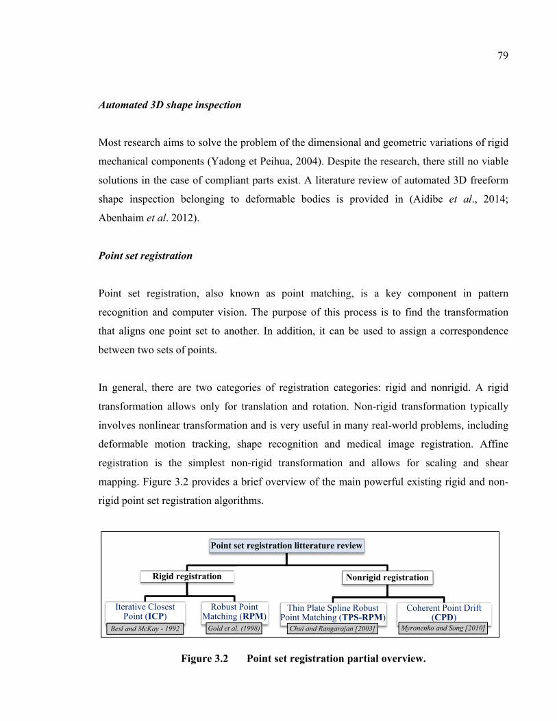
79

Automated 3D shape inspection

Most research aims to solve the problem of the dimensional and geometric variations of rigid

mechanical components (Yadong et Peihua, 2004). Despite the research, there still no viable

solutions in the case of compliant parts exist. A literature review of automated 3D freeform

shape inspection belonging to deformable bodies is provided in (Aidibe et al., 2014;

Abenhaim et al. 2012).

Point set registration

Point set registration, also known as point matching, is a key component in pattern

recognition and computer vision. The purpose of this process is to find the transformation

that aligns one point set to another. In addition, it can be used to assign a correspondence

between two sets of points.

In general, there are two categories of registration categories: rigid and nonrigid. A rigid

transformation allows only for translation and rotation. Non-rigid transformation typically

involves nonlinear transformation and is very useful in many real-world problems, including

deformable motion tracking, shape recognition and medical image registration. Affine

registration is the simplest non-rigid transformation and allows for scaling and shear

mapping. Figure 3.2 provides a brief overview of the main powerful existing rigid and non-

rigid point set registration algorithms.

Figure 3.2 Point set registration partial overview.

Point set registration litterature review

Rigid registration

Iterative Closest Point (ICP)

Besl and McKay - 1992

Robust Point Matching (RPM)

Gold et al. (1998)

Nonrigid registration

Thin Plate Spline Robust Point Matching (TPS-RPM)

Chui and Rangarajan [2003]

Coherent Point Drift (CPD)

Myronenko and Song [2010]

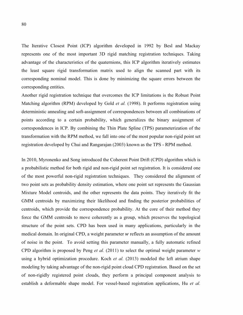
80

The Iterative Closest Point (ICP) algorithm developed in 1992 by Besl and Mackay

represents one of the most important 3D rigid matching registration techniques. Taking

advantage of the characteristics of the quaternions, this ICP algorithm iteratively estimates

the least square rigid transformation matrix used to align the scanned part with its

corresponding nominal model. This is done by minimizing the square errors between the

corresponding entities.

Another rigid registration technique that overcomes the ICP limitations is the Robust Point

Matching algorithm (RPM) developed by Gold et al. (1998). It performs registration using

deterministic annealing and soft-assignment of correspondences between all combinations of

points according to a certain probability, which generalizes the binary assignment of

correspondences in ICP. By combining the Thin Plate Spline (TPS) parameterization of the

transformation with the RPM method, we fall into one of the most popular non-rigid point set

registration developed by Chui and Rangarajan (2003) known as the TPS - RPM method.

In 2010, Myronenko and Song introduced the Coherent Point Drift (CPD) algorithm which is

a probabilistic method for both rigid and non-rigid point set registration. It is considered one

of the most powerful non-rigid registration techniques. They considered the alignment of

two point sets as probability density estimation, where one point set represents the Gaussian

Mixture Model centroids, and the other represents the data points. They iteratively fit the

GMM centroids by maximizing their likelihood and finding the posterior probabilities of

centroids, which provide the correspondence probability. At the core of their method they

force the GMM centroids to move coherently as a group, which preserves the topological

structure of the point sets. CPD has been used in many applications, particularly in the

medical domain. In original CPD, a weight parameter reflects an assumption of the amount

of noise in the point. To avoid setting this parameter manually, a fully automatic refined

CPD algorithm is proposed by Peng et al. (2011) to select the optimal weight parameter w

using a hybrid optimization procedure. Koch et al. (2013) modeled the left atrium shape

modeling by taking advantage of the non-rigid point cloud CPD registration. Based on the set

of non-rigidly registered point clouds, they perform a principal component analysis to

establish a deformable shape model. For vessel-based registration applications, Hu et al.

81

(2010) developed an extension of the CPD algorithm to enable landmarks guides, such as

vessel bifurcations, in order to improve the registration accuracy and speed of execution.

Although there are numerous registration algorithms that offer robust and fast solutions but

they are adapted to specific cases that do not match with our alignment problems of relatively

compliant parts located in Zone B. For example, the ICP algorithm which is perfectly

adapted for rigid parts located in Zone A isn’t able to produce good results for relatively non-

rigid parts. As well, the CPD algorithm is very effective for very flexible parts located in

Zone C (widely used in medical imaging). In this case, a stretching of the surface is permitted

which doesn’t correspond to the characteristics of the relatively flexible parts (Figure 3.3). In

short, a ‘flexible registration’ that retains the curvilinear distances (geodesic) while taking

into account the presence of manufacturing defects areas on the inspected part is needed.

Following the proposed methodology to solve this problem is described.

Figure 3.3 Problematic of relatively flexible parts registration problematic.

Registration

Non Rigid

(CPD)

Rigid

(ICP) ‘Flexible’ registration adapted for

compliant parts located in Zone B

Transformation CAD SCAN Registration

(Hu et al., 2010)

Medical

applications

∗

∗ = ∗

∗

is the curvilinear distance between and

82

3.4 Methodology

As mentioned in Section 3.3, the aim is to develop a ‘flexible’ registration technique adapted

to relatively compliant parts located in Zone B. The proposed method is based on the

optimization of the Coherent Point Drift algorithm parameters combined with a statistical

identification module based on the extreme value analysis to distinguish the defects due to

the manufacturing process from the deformation due to the flexibility of a given compliant

part located in Zone B. The proposed identification module combines the Thompson extreme

value statistical test (Thompson, 1985) with the biweight mean and standard deviation

estimator technique (Hoaglin et al., 1983) in order to detect the defects. The defects are

considered as ‘outliers’ that have the same order of magnitude than the part’s assigned

tolerance and must be detected dynamically and iteratively. In this section the main steps of

the proposed method summarized in Algorithme 3.2 will be detailed.

3.4.1 Prealignment

Let = , , , … , ∈ ℝ be the set of nodes representing the meshed CAD model

and = , , , … , ∈ ℝ be the set of | ≫ nodes representing the scanned

part. The Iterative Closest Point (ICP) algorithm developed by Besl and McKay in 1992 is

used in order to register the two given point sets in a common coordinate system.

3.4.2 Initialization of parameters that will be optimized

Originally, the CPD algorithm includes three free parameters , and which are set

manually:

1. Parameter (0 ≤ ≤ 1) reflects the assumption about the amount of noise in the

point sets and number of outliers in the Gaussian mixture model, and its value has an

influence on the point set registration performance.

2. Parameters and both reflect the amount of smoothness regularization. Parameter

defines the model of the smoothness regularizer. Parameter represents the trade-off

83

between the goodness of maximum likelihood fit and regularization (Myronenko et

Song, 2010). In other words, controls the rigidity and the locality of spatial

smoothing while reflects its strengths. CPD algorithm is more sensitive to parameter

because it defines the model of the nonrigid transformation. A detailed explanation

about the difference between these two parameters is given by Yuille et al. (1989).

One of the main contributions of this paper is a proposition to automatically estimate

parameters and by a process that decides how much smoothing is necessary and how

wide the range of interaction should be with respect to certain specific criteria. These criteria

belong to relatively compliant parts (Zone B) and they are described in the next paragraph.

The proposed method is started by initializing and . Typically ∈ [1 100] and ∈ [1 20], where and are the initial parameters of and .

3.4.3 Optimization of the parameters and :

With an each combination of and (iteration ), the CAD model is aligned to the

scanned part by the non-rigid transformation method of the CPD algorithm. ′ = ′ , ′ , ′ , … , ′ ′ ∈ ℝ is the set of nodes resulting from this alignment and = , , , … , ∈ ℝ is the set of nodes representing the closest point in to ′. A

dsearchn function in Matlab® based on Quickhull (Barber et al., 1996) is used to find .

In this section, two criteria that belong to the problematic of relatively compliant parts (Zone

B) are introduced: the conservation of the curvilinear distance (stretch criterion) and the

minimization between two objects (Euclidian Distance criterion).

• The STRETCH criterion between and ’ (equation 3.1, Figure 3.4). In other words,

the isometric transformation difference between them that should be small.

∆ = | ℎ − ℎ | = ∑ ′′ − ∑

(3.1)

84

Where is the number of neighborhoods around point and the distance between

and its neighborhood.

• The EUCLIDIAN DISTANCE criterion between and ’ (equation 3.2, Figure 3.4).

∆ = , −

(3.2)

Where is the Euclidian distance between ′ and its corresponding point .

represents the ideal value between and ′ that must be equal to zero.

Figure 3.4 Description of the criteria that belong to relatively compliant parts.

For each criterion, its root mean square error is computed as presented in equations 3.3 and

3.4.

= ∑‖∆ ‖− 1 (3.3)

= ∑‖∆ ‖− 1 (3.4)

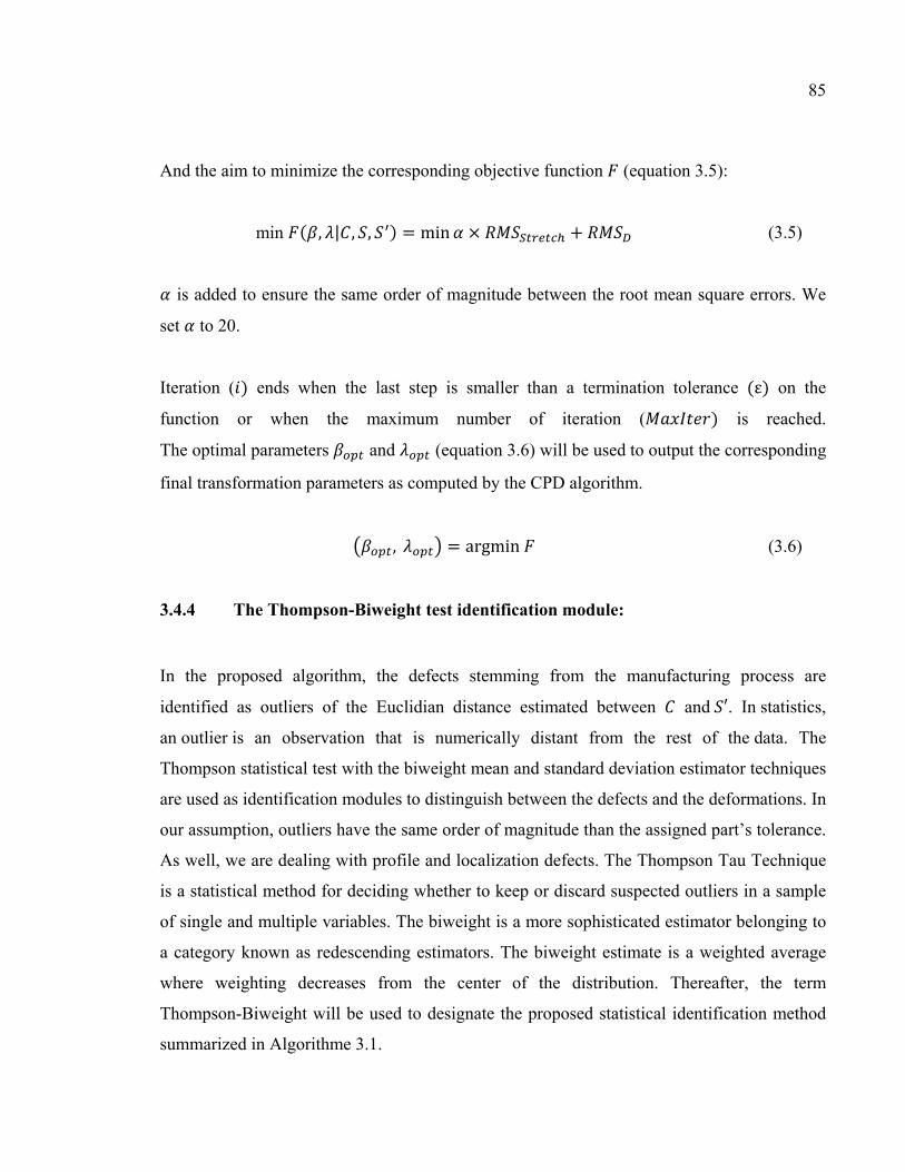
85

And the aim to minimize the corresponding objective function (equation 3.5):

min ( , | , , ) = min × + (3.5)

is added to ensure the same order of magnitude between the root mean square errors. We

set to 20.

Iteration ( ) ends when the last step is smaller than a termination tolerance (ε) on the

function or when the maximum number of iteration ( ) is reached.

The optimal parameters and (equation 3.6) will be used to output the corresponding

final transformation parameters as computed by the CPD algorithm.

, = argmin (3.6)

3.4.4 The Thompson-Biweight test identification module:

In the proposed algorithm, the defects stemming from the manufacturing process are

identified as outliers of the Euclidian distance estimated between and ′. In statistics,

an outlier is an observation that is numerically distant from the rest of the data. The

Thompson statistical test with the biweight mean and standard deviation estimator techniques

are used as identification modules to distinguish between the defects and the deformations. In

our assumption, outliers have the same order of magnitude than the assigned part’s tolerance.

As well, we are dealing with profile and localization defects. The Thompson Tau Technique

is a statistical method for deciding whether to keep or discard suspected outliers in a sample

of single and multiple variables. The biweight is a more sophisticated estimator belonging to

a category known as redescending estimators. The biweight estimate is a weighted average

where weighting decreases from the center of the distribution. Thereafter, the term

Thompson-Biweight will be used to designate the proposed statistical identification method

summarized in Algorithme 3.1.

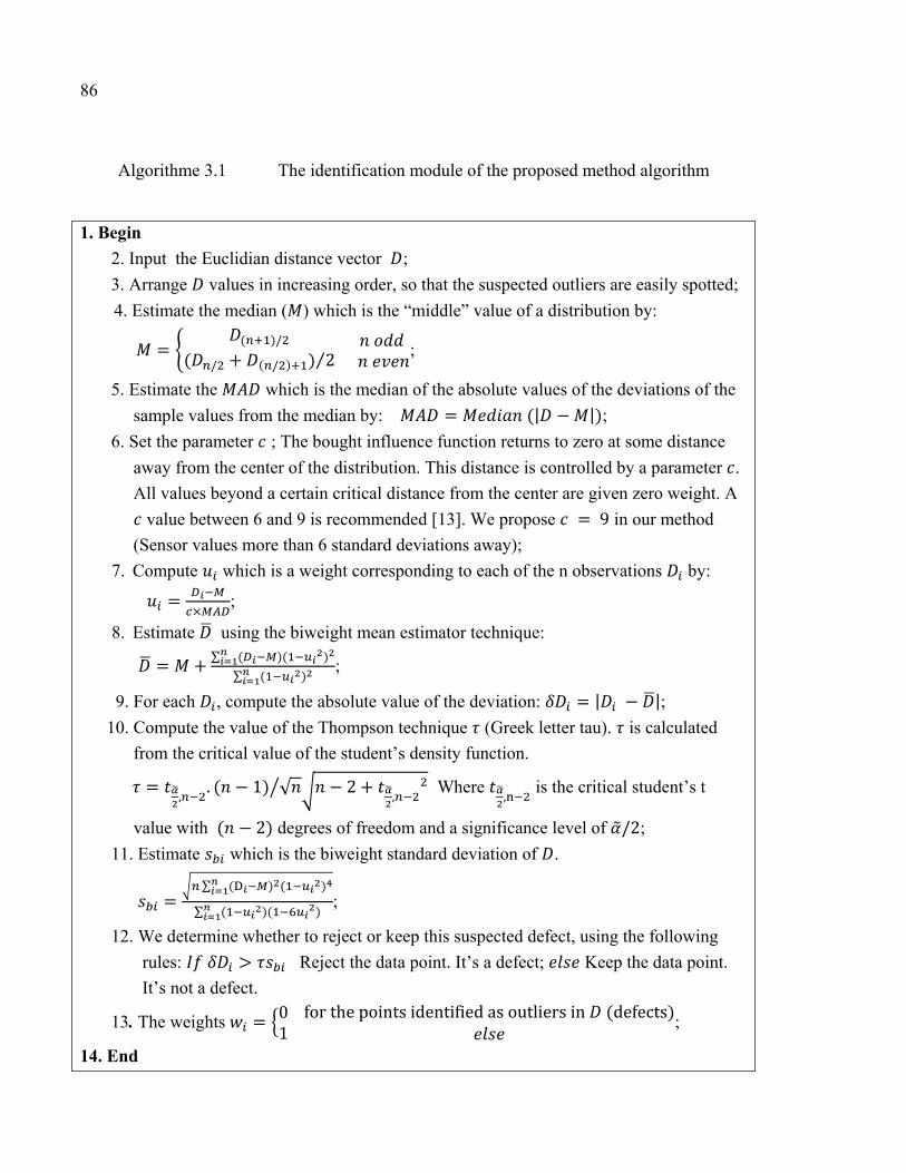
86

Algorithme 3.1 The identification module of the proposed method algorithm

1. Begin

2. Input the Euclidian distance vector ;

3. Arrange values in increasing order, so that the suspected outliers are easily spotted;

4. Estimate the median ( ) which is the “middle” value of a distribution by: = ( )/( / + ( / ) ) 2⁄ ;

5. Estimate the which is the median of the absolute values of the deviations of the

sample values from the median by: = (| − |);

6. Set the parameter ; The bought influence function returns to zero at some distance

away from the center of the distribution. This distance is controlled by a parameter .

All values beyond a certain critical distance from the center are given zero weight. A

value between 6 and 9 is recommended [13]. We propose = 9 in our method

(Sensor values more than 6 standard deviations away);

7. Compute which is a weight corresponding to each of the n observations by:

= × ;

8. Estimate using the biweight mean estimator technique: = + ∑ ( )( )∑ ( ) ;

9. For each , compute the absolute value of the deviation: = | − |; 10. Compute the value of the Thompson technique (Greek letter tau). is calculated

from the critical value of the student’s density function.

= , . ( − 1) √ − 2 + , Where , is the critical student’s t

value with ( − 2) degrees of freedom and a significance level of /2;

11. Estimate which is the biweight standard deviation of .

= ∑ ( ) ( )∑ ( )( ) ;

12. We determine whether to reject or keep this suspected defect, using the following

rules: > Reject the data point. It’s a defect; Keep the data point.

It’s not a defect.

13. The weights = 01 for the points identified as outliers in (defects);

14. End

87

3.4.5 Summary of the proposed method

Having explained the optimization CPD method, as well as the identification method, a

summary of the proposed fixtureless inspection algorithm belonging to compliant parts will

now be presented. Starting with the set of nodes of the CAD model and the point cloud

of the manufactured part, the proposed method is summarized in the Algorithme 3.2.

Algorithme 3.2 Main steps of the proposed method

1. Begin

2. Prealignment using the ICP algorithm;

3. Initialization , ;

4. Repeat

5. CPD non-rigid registration to align the CAD model ( ) into the scanned part. As

a result we’ll have a modified CAD named ′; 6. Compute the Stretch criteria between and ′; 7. Find the corresponding points in to ′; 8. Compute the Euclidean distance criteria between and ;

9. Compute the objective function ;

10. Optimize the objective function using the optimization technique, making ,

the unknown parameters;

11. Update the parameters , ;

12. Until the last step is smaller than a termination tolerance (ε) on the function or when the

maximum number of iteration ( ) is reached; then output the optimal parameters , and its corresponding final transformation parameters as computed by the CPD

algorithm.

13. Thompson-Biweight statistical identification module;

14. CPD using , ;

15. End

88

3.5 Case studies and validation

In order to test and validate the approach developed in this paper; this section will feature

twenty six industrial case studies.

3.5.1 Description of the case studies

A sheet metal representing a sample of common parts in the transport industry will be

considered for our case study. The part is made with an aluminum gauge 14 (1.63 ) with

a Young modulus of 7 × 10 and a density of 2700 . . Figure 3.5 shows the test

panel designed and manufactured at École de Technologie Supérieure (ÉTS), Montréal,

Canada. In a free-state, the part shape varies significantly from its nominal shape. Twenty six

case studies were carried out in order to test and validate our approach.

It is our assumption that we are dealing with profile and localization defects (sheet metal

bend failure, erroneous hole location…). The finite element analysis takes into account both

the mounting fixture configuration during a presumed digitalization and the force of gravity.

The spatial sampling frequency of scanned data is different from the mesh used in the CAD

data. Twenty six point clouds, representing the part’s mesh with different defect zones and

deformed shapes, are then created.

89

CAD (All dimensions are in [ ])

Figure 3.5 Description of the case study (1)

[ . ] [ . ] [ . ] [ . ]

× ∅ [ . ]

[ . ]

[.]

[ . ]

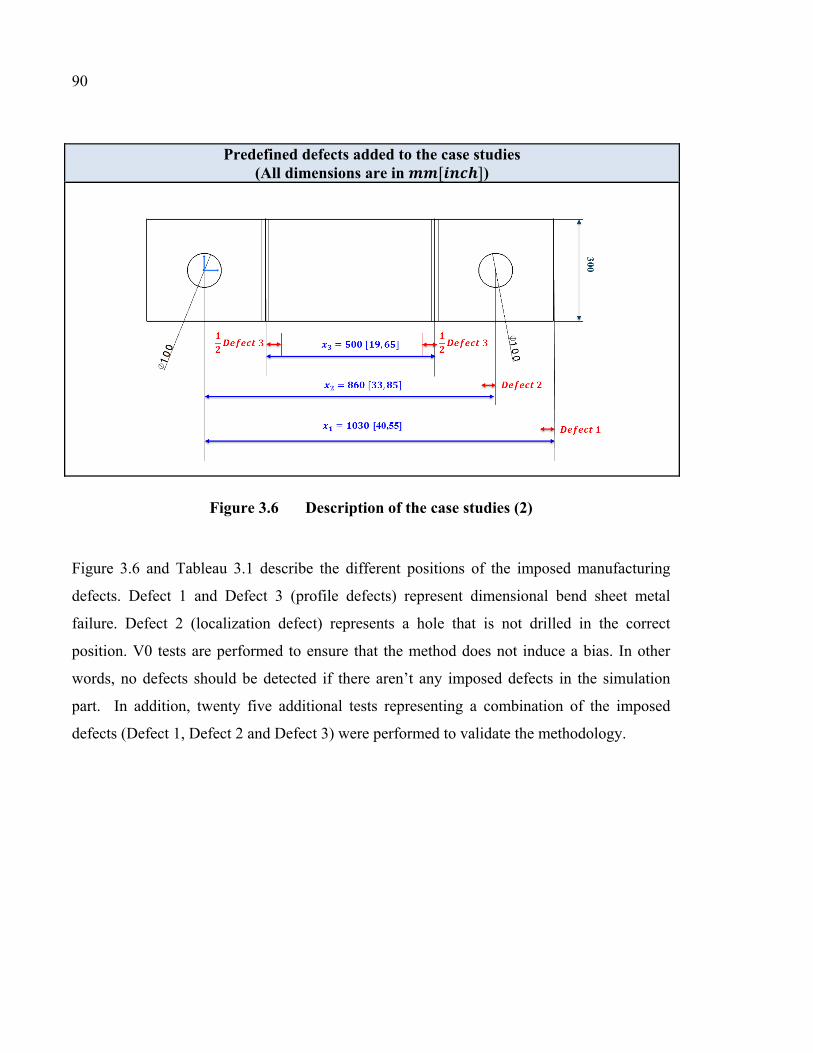
90

Predefined defects added to the case studies (All dimensions are in [ ])

Figure 3.6 Description of the case studies (2)

Figure 3.6 and Tableau 3.1 describe the different positions of the imposed manufacturing

defects. Defect 1 and Defect 3 (profile defects) represent dimensional bend sheet metal

failure. Defect 2 (localization defect) represents a hole that is not drilled in the correct

position. V0 tests are performed to ensure that the method does not induce a bias. In other

words, no defects should be detected if there aren’t any imposed defects in the simulation

part. In addition, twenty five additional tests representing a combination of the imposed

defects (Defect 1, Defect 2 and Defect 3) were performed to validate the methodology.

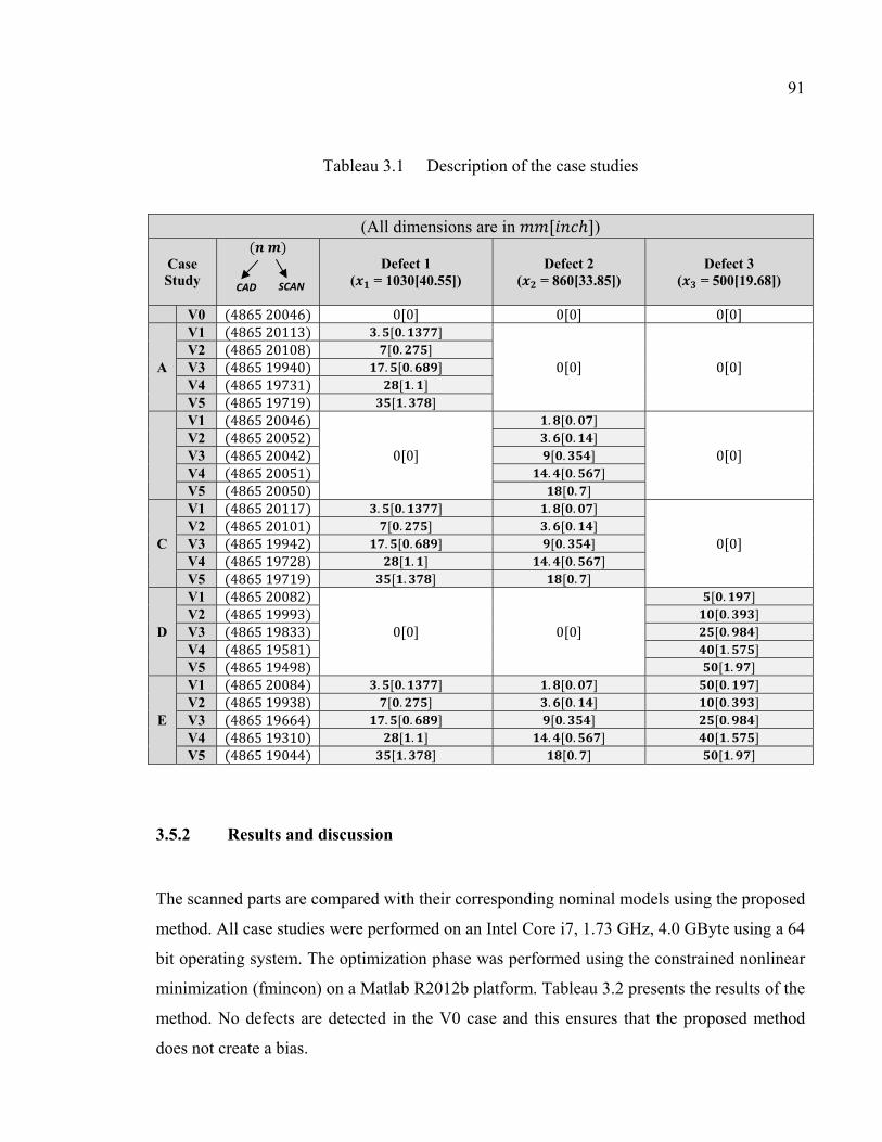
91

Tableau 3.1 Description of the case studies

(All dimensions are in [ ℎ])

Case Study

( )

Defect 1 ( = 1030[40.55])

Defect 2 ( = 860[33.85])

Defect 3 ( = 500[19.68])

V0 (4865 20046) 0[0] 0[0] 0[0]A

V1 (4865 20113) . [ . ] 0[0] 0[0] V2 (4865 20108) [ . ] V3 (4865 19940) . [ . ] V4 (4865 19731) [ . ] V5 (4865 19719) [ . ] V1 (4865 20046) 0[0] . [ . ] 0[0] V2 (4865 20052) . [ . ] V3 (4865 20042) [ . ] V4 (4865 20051) . [ . ] V5 (4865 20050) [ . ]

C

V1 (4865 20117) . [ . ] . [ . ] 0[0] V2 (4865 20101) [ . ] . [ . ] V3 (4865 19942) . [ . ] [ . ] V4 (4865 19728) [ . ] . [ . ] V5 (4865 19719) [ . ] [ . ]

D

V1 (4865 20082) 0[0] 0[0] [ . ] V2 (4865 19993) [ . ] V3 (4865 19833) [ . ] V4 (4865 19581) [ . ] V5 (4865 19498) [ . ]

E

V1 (4865 20084) . [ . ] . [ . ] [ . ] V2 (4865 19938) [ . ] . [ . ] [ . ] V3 (4865 19664) . [ . ] [ . ] [ . ] V4 (4865 19310) [ . ] . [ . ] [ . ] V5 (4865 19044) [ . ] [ . ] [ . ]

3.5.2 Results and discussion

The scanned parts are compared with their corresponding nominal models using the proposed

method. All case studies were performed on an Intel Core i7, 1.73 GHz, 4.0 GByte using a 64

bit operating system. The optimization phase was performed using the constrained nonlinear

minimization (fmincon) on a Matlab R2012b platform. Tableau 3.2 presents the results of the

method. No defects are detected in the V0 case and this ensures that the proposed method

does not create a bias.

CAD SCAN

92

The nominal model is aligned to the scanned one in all cases using the optimized coherent

point drift section of the proposed algorithm. The results of this alignment as well as those of

the Thompson-Biweight identification module reflect an excellent detection of the imposed

profile and localization defects.

Figure 3.7 shows the results of the identification module for case A-V5. The Thompson test

identification threshold corresponds to ±3σ ≈ 99.7% of the set. Profile defects (encircled) are

detected and removed after being considered as outliers. This proves that the proposed

algorithm is able to correctly identify and select the zones that represent the profile and/or

the localization manufacturing defects. This is to say, the position of the defect.

Identification module – The Thompson-Biweight test (A-V5 case study) Before After

(All dimensions are in [ ])

Figure 3.7 Results of the identification module

Threshold @ . %

Outliers

Index of the Euclidian distance between C and S’

Val

ues

. [ 1.396’’]

Profile defects

identified

Profile defects

removed

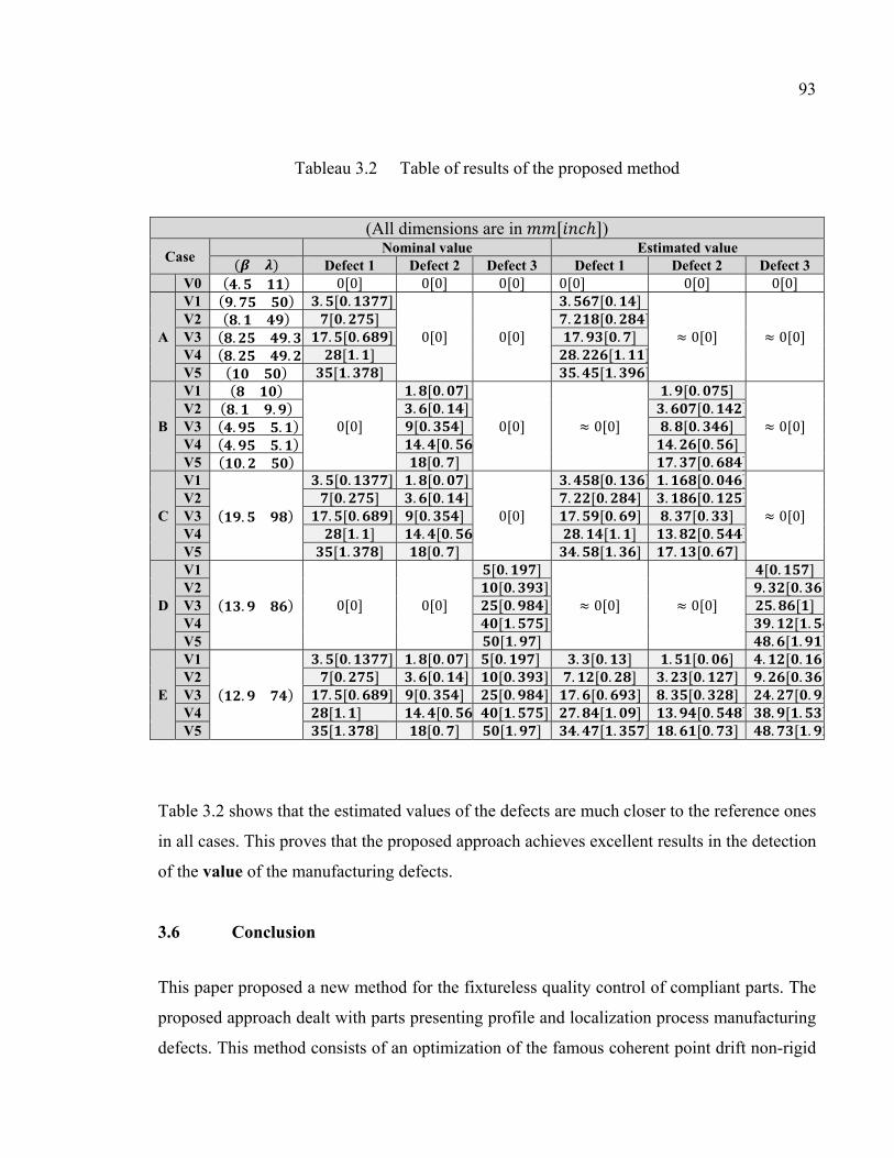
93

Tableau 3.2 Table of results of the proposed method

(All dimensions are in [ ℎ])

Case Nominal value Estimated value ( ) Defect 1 Defect 2 Defect 3 Defect 1 Defect 2 Defect 3

V0 ( . ) 0[0] 0[0] 0[0] 0[0] 0[0] 0[0] A

V1 ( . ) . [ . ] 0[0] 0[0] . [ . ] ≈ 0[0] ≈ 0[0] V2 ( . ) [ . ] . [ . ]V3 ( . . ) . [ . ] . [ . ] V4 ( . . ) [ . ] . [ . ]V5 ( ) [ . ] . [ . ]

B

V1 ( ) 0[0] . [ . ] 0[0] ≈ 0[0] . [ . ] ≈ 0[0] V2 ( . . ) . [ . ] . [ . ]V3 ( . . ) [ . ] . [ . ] V4 ( . . ) . [ . . [ . ]V5 ( . ) [ . ] . [ . ]

C

V1 ( . )

. [ . ] . [ . ] 0[0] . [ . ] . [ . ] ≈ 0[0] V2 [ . ] . [ . ] . [ . ] . [ . ]V3 . [ . ] [ . ] . [ . ] . [ . ] V4 [ . ] . [ . . [ . ] . [ . ]V5 [ . ] [ . ] . [ . ] . [ . ]

D

V1 ( . ) 0[0] 0[0] [ . ] ≈ 0[0] ≈ 0[0] [ . ] V2 [ . ] . [ . ]V3 [ . ] . [ ] V4 [ . ] . [ .V5 [ . ] . [ . ]

E

V1 ( . )

. [ . ] . [ . ] [ . ] . [ . ] . [ . ] . [ . ]V2 [ . ] . [ . ] [ . ] . [ . ] . [ . ] . [ . ]V3 . [ . ] [ . ] [ . ] . [ . ] . [ . ] . [ .V4 [ . ] . [ . [ . ] . [ . ] . [ . ] . [ . ]V5 [ . ] [ . ] [ . ] . [ . ] . [ . ] . [ .

Table 3.2 shows that the estimated values of the defects are much closer to the reference ones

in all cases. This proves that the proposed approach achieves excellent results in the detection

of the value of the manufacturing defects.

3.6 Conclusion

This paper proposed a new method for the fixtureless quality control of compliant parts. The

proposed approach dealt with parts presenting profile and localization process manufacturing

defects. This method consists of an optimization of the famous coherent point drift non-rigid

94

alignment in order to adapt it to the problem of relatively compliant parts. A CAD model is

smoothly aligned to the scanned part by the CPD algorithm. Two criteria belonging to

relatively compliant parts are introduced: the Stretch criterion between the original CAD

model and the aligned one and the Euclidian distance criterion between the aligned CAD

model and its corresponding scanned part. The method proposed to automatically estimate

the regularization parameters and of the CPD algorithm in order to minimize the

proposed objective function that combines these two criteria. This process is followed by the

Thompson statistical test, and the biweight mean and standard deviation estimator in order to

distinguish deformations due to the flexibility and the positioning of parts from deviations

due to the manufacturing process. The identification module considers the ‘outliers’ as

defects having the same order of magnitude than the assigned part’s tolerance. The profile

and localization defects estimated results in twenty six different industrial case studies

present closer values to the reference ones, thus reflecting the effectiveness of the proposed

approach. This work will result in future gains for the industry by anticipating economic

savings and productivity improvement due to the elimination of the conformation jigs and the

reduction of inspection cycle time. This method would efficiently manage deformable bodies

at a lower cost thus providing a manufacturing competitive advantage to the global economy.

3.7 Acknowledgments

The authors would like to thank the National Sciences and Engineering Research Council

(NSERC), Bombardier Aerospace Inc. and the École de Technologie Superieure (ÉTS) for

their support and financial contribution.

CONCLUSION

Dans le cadre de cette thèse, la problématique industrielle de l’inspection des pièces

mécaniques souples (non rigides) sans recours à des gabarits de conformation a été exposée.

Plusieurs approches ont été développées et présentées pour répondre aux deux questions

fondamentales :

• Comment peut-on s’assurer de la conformité géométrique des pièces souples (non

rigides) sans le recourt à un gabarit spécialisé pour les conformer ?

• À partir d’un nuage de points capté à l’état libre dans une condition arbitraire mais

connue, comment peut-on identifier les défauts de fabrication sur une pièce souple ? En

d’autres termes, comment peut-on distinguer, avec un niveau de confiance acceptable,

les défauts qui sont dus au processus de fabrication et les déformations qui sont dues à

la flexibilité de la pièce ?

Ces deux questions trouvent un intérêt très élevé dans le secteur du transport en général et,

plus spécifiquement, dans le secteur aérospatial. En effets, les gabarits de conformation (ou

encore les montages dédiés à l’inspection d’une seule pièce) sont très couteux à fabriquer et à

maintenir (étalonnage). Une réponse robuste et fiable aux deux questions précédentes aura

comme implication directe une amélioration de la compétitivité de l’industrie.

Dans un premier temps, nous avons présenté dans le Chapitre 1 une amélioration

substantielle du module d’identification d’un algorithme existant, le « IDI : Iterative

Displacement Inspection », qui a été développée par Abenhaim et al. (2011). Les résultats

obtenus au niveau des erreurs de Type I et de Type II prouvent le degré d’amélioration que

nous avons apportée à l'algorithme IDI. Également, avec l’automatisation du seuil

d’identification, nous croyons que l’algorithme IDI est plus robuste et surtout, plus apte à un

usage industriel. Cette partie de notre recherche a fait l’objet d’une publication dans une

revue ainsi que deux exposés dans des conférences.

96

Dans le Chapitre 2 de cette thèse, une approche analytique qui vise à quantifier la

flexibilité/rigidité a été présentée et adoptée pour le reste notre recherche. En effet, la

flexibilité peut être subjective, nous avons proposé une « échelle » afin de comparer les

composants entre eux. Suite à cette méthode, trois zones ont été bien établies permettant à

l'industrie manufacturière de bien classifier leurs composantes mécaniques sur l'échelle de la

flexibilité. Nous nous sommes concentrés dans cette thèse à l’inspection des pièces

mécaniques relativement flexibles qui sont situées dans la zone B et qui représentent la vaste

majorité des applications industrielles dans le domaine du transport.

Par la suite, deux méthodes originales et complémentaires ont été développées dans le

deuxième et le troisième chapitre de cette thèse.

La première approche, développée dans le Chapitre 2, vise à détecter les défauts localisés de

profil géométriques de surface. En tirant avantage de l’estimation de la courbure gaussienne

qui représente l’une des propriétés intrinsèques de la géométrie, et en la combinant avec la

méthode statistique Thompson-Biweight, nous avons réussi à développer un module

d’identification qui détecte les défauts localisés de profils et de les séparer des déformations

dues à la flexibilité de la pièce (effets de gravité et contraintes résiduelles). Les performances

métrologiques de cette méthode sont limitées à la détection des défauts de profils d’ordre 1 à

condition qu’ils soient spatialement localisés (comme les bosses) et d’ordre 2 (comme les

ondulations, collines et vallées successives, inscrites dans le profil). Cette méthode ne peut

pas détecter les autres types de défauts de profil tels que le mauvais pliage, ni les défauts de

localisation (un trou qui n’est pas à sa bonne position). Cette partie de notre recherche a fait

l’objet d’une publication dans une revue ainsi que deux exposés dans des conférences.

La deuxième méthode, présentée dans le Chapitre 3 de la thèse, se veut une nouvelle

approche pour remédier aux limites de l’approche basée sur les courbures gaussiennes. Notre

objectif consiste à détecter les autres types de défauts de fabrication comme les défauts sur

les périphéries, les défauts de localisation ou du pliage. Le point de départ de cette approche

a été les caractéristiques intrinsèques à un calage « flexible ». En effet, le calage non rigide

97

ne peut être adapté dans notre cas, car il ne conserve pas la transformation isométrique. Par

conséquent, nous avons introduit dans cette approche deux critères qui correspondent aux

spécificités des composantes mécaniques souples ; la conservation de la distance curviligne

(géodésique) et la minimisation de la distance de Hausdorff propre à n’importe quel calage.

Nous avons adapté l’algorithme CPD (Coherent Point Drift), algorithme de recalage non

rigide basée sur une approche probabiliste, afin qu’il satisfasse ces deux critères à travers

l’optimisation des paramètres de régularisation λ et β. On réussit avec cette méthode à

atteindre notre objectif. Par contre, la limitation se présente au niveau de la section

d’optimisation qui exige un temps de calcul assez long. Cette partie de notre recherche a fait

l’objet d’une soumission dans une revue ainsi d’une participation à une conférence prévue en

2014.

Pour terminer, le défi scientifique et technique de la problématique soulevée nous ont permis

de publier deux articles de revues (et de soumettre un troisième qui est en cours de révision).

Chaque article constitue un des trois chapitres de cette thèse. En plus, cinq publications ont

été achevées à travers la participation à plusieurs conférences internationales. Un récapitulatif

des références des cinq articles a été présenté dans le tableau 0.2. Les propositions pour de

futures recherches reliées à ce domaine sont présentées dans la partie suivante

« Recommandations ».

RECOMMANDATIONS

Aujourd’hui, il est admis que, dès les premières phases de développement d’un nouveau

produit, l’optimisation des opérations de fabrication et d’assemblage requiert la prise en

compte des variations inhérentes aux procédés. Cette question pertinente trouve un intérêt

immédiat dans l’industrie manufacturière en général et, plus spécifiquement, dans le secteur

aérospatial. Le problème du tolérancement et du contrôle de la qualité des pièces mécaniques

est décisif pour cette industrie. Chaque amélioration dans ce processus se traduit par une

amélioration du niveau de compétitivité. Ces incidences économiques sont importantes pour

un secteur qui subit des transformations profondes imposées par la globalisation et la

pression des marchés et par l’évolution technologique.

Le présent projet a pour objectif de faciliter l'inspection dimensionnelle et géométrique des

composantes souples. Actuellement, l'analyse de conformité de telles pièces est réalisée avec

des gabarits spécialisés et dédiés à cette tâche. Cela se traduit par des coûts supplémentaires

et des carences de reproductibilité. Dans le cadre de cette thèse, on a proposé d’une manière

spécifique, le développement d'une méthodologie pour manipuler un nuage de points, capté

dans une condition arbitraire et sans recours à un gabarit, dans le but d'analyser la conformité

géométrique d’une pièce souple. Comme résultats de nos travaux, nous avons amélioré une

approche existante et nous avons proposé deux nouvelles approches complémentaires. Nous

avons obtenu des résultats satisfaisants au niveau de la détection des défauts de fabrication

(profil et localisation).

Nous espérons que les travaux présentés dans cette thèse permettront dans un proche avenir

de stimuler la recherche dans ce domaine d’application. Nous proposons dans cette section

quelques recommandations pour de futures pistes de recherche que nous jugeons comme

utiles aux personnes qui travaillent sur la même problématique et surtout fertiles d’idées et

d’innovation.

100

1. Nous suggérons de développer une approche globale et généralisée basée sur les deux

méthodes complémentaires qui ont été développées dans le cadre de cette thèse. Dans

ce cas, nous devons développer une méthodologie qui permet de regrouper les pièces

mécaniques souples selon le type de défauts géométriques présent. En plus, cette

approche doit être capable d’identifier et de classifier les défauts géométriques sur les

limites de la pièce (les défauts de contour).

2. Les approches développées au cours de cette thèse ne tiennent pas en compte du

comportement réel des composantes mécaniques souples lors de l’assemblage. En

d’autres termes, nos méthodes ont surtout servi à vérifier l’état de conformité et

d’estimer la position et l’amplitude du défaut. Par contre, lors de l’assemblage, les

souplesses (ou la flexibilité) d’un composant peut « corriger » ou « tolérer » plus de

défauts qu’un composant rigide. Notre première recommandation vise le

développement d’une procédure pour évaluer les niveaux des forces nécessaires à

l’assemblage ainsi que les contraintes induites/résiduelles afin d’assurer le respect de

tous les requis de la pièce à l’assemblage après que celle-ci a été qualifiée comme non

conforme à l’inspection. Ainsi, cette piste ouvre la possibilité du « tolérancement pour

pièces souples ».

3. Une autre recommandation se traduit par la généralisation des approches développées

pour qu’elles tiennent en compte des pièces souples plus complexes avec un matériau

non isotrope comme les composites. Dans ce cas, nous parlons de l’introduction d’un

facteur qui contrôle la rigidité locale. En effet, nos méthodes sont basées sur des hyper

paramètres qui représentent en quelque sorte le degré de flexibilité globale d’un

composant. Par contre, on peut avoir des pièces dont la rigidité locale varie grandement

(ex. la pièce étude de cas no 1). Nous jugeons qu’il sera opportun de tenir en compte

non pas d’un seul paramètre, mais peut-être d’une pondération locale qui traduit le

comportement de la rigidité en fonction de la localisation de la pièce.

101

4. Dans le travail du Chapitre 1, nous avons proposé de remplacer le module

d’identification initial de l’algorithme IDI par un nouveau qui est basé sur les

statistiques extrêmes (Grubbs test). Pour faciliter la comparaison, nous avons utilisé les

mêmes études de cas simulés développés par Abenahim et al. et nous avons obtenu de

résultats très satisfaisants au niveau de la réduction des erreurs de types I et II. Par

contre, aucune validation sur des cas industriels réels n’a été effectuée. Nous suggérons

de valider l’amélioration de l’IDI sur les études de cas expérimentales qui ont été

développées lors du stage effectué chez Bombardier Aéronautique (voir Annexe I).

Dans la même perspective, nous proposons une validation expérimentale des

performances métrologiques des deux nouvelles approches développées (IDB-CTB et

Optimisation du CPD).

5. La méthode IDB-CTB a été présentée et vérifiée dans le Chapitre 2 de cette thèse en

utilisant des études de cas tirées des applications d'ingénierie réelles. Les travaux futurs

devraient développer une estimation plus précise de la courbure gaussienne en

améliorant la qualité de génération de maillages 3D des composantes mécaniques

souples (par exemple, appliquer un raffinement local). Une autre amélioration de la

méthode IDB-CTB se situe au niveau de la correspondance. Trouver la meilleure

correspondance garantira une meilleure comparaison entre les courbures gaussiennes

estimées du modèle nominal et de la pièce numérisée. Enfin, nous proposons d’évaluer

les indices de performance de l’approche IDB-CTB.

6. Par la suite, nous allons présenter des recommandations qui sont spécifiques pour le

travail présenté dans le Chapitre 3 de cette thèse :

a. Deux critères ont été proposés pour répondre aux spécificités des pièces mécaniques

souples. Un facteur alpha ( ) a été affecté au critère de « la conservation de la distance

curviligne » dans la formulation de la fonction objective pour rapporter la comparaison

avec le critère de « la minimisation de la distance de Hausdorff » à la même échelle

(voir équation 3.5). Ce paramètre, présentement déterminé par essai-erreur, a été estimé

après avoir examiné les ordres de grandeur de ces deux critères. L’amélioration de

102

l’estimation de ce paramètre pourra augmenter significativement la performance de la

section d’optimisation de l’algorithme proposé. On propose de calculer ce paramètre

alpha en considérant le calcul de résistance de matériaux à travers l’estimation des

contraintes et déformations relatives au cas des composantes souples avec différents

types de matériaux (pas seulement les matériaux isotropes). Ce calcul peut nous donner

une reformulation plus précise de la fonction objective et par la suite une meilleure

optimisation des paramètres de régularisation et ainsi qu’une réduction du temps de

calcul.

b. Proposer une méthode plus performante pour trouver la correspondance entre le CAD

modifié et la pièce numérisée. Réussir à chercher la vraie correspondance et non le plus

proche point correspondant réduira l’erreur moyenne quadratique au niveau de la

distance de Hausdorff.

c. Évaluer les performances métrologiques de la méthode proposée.

ANNEXE I

STAGE BOMBARDIER AÉRONAUTIQUE : DÉVELOPPEMENT DE LA BANQUE DES ÉTUDES DE CAS ET DE DEUX INTERFACES DYNAMIQUES (GUI)

La préparation de la base d'études de cas industriels est cruciale pour l'avancement du projet

CRIAQ MANU501. Elle permet des validations exhaustives des méthodologies et

algorithmes proposés par l'équipe (ex. IDI, GNIF, IDB-CTB, Optimisation du CPD, etc.). Le

but ultime du projet est de développer une méthode de synthèse qui permettrait, dans un

environnement d'ingénierie simultanée, de gérer efficacement les tolérances et les opérations

d'inspection des pièces souples au coût minimum, connaissant les exigences fonctionnelles et

les moyens de production. Dans le cas de l'organisme partenaire (Bombardier Aéro.), ceci se

traduira par des économies tangibles améliorant sa productivité. Typiquement, on parle

d'environ 30 % des composants d'un avion, et à titre d'exemple, le temps requis actuellement

pour préparer l'inspection d'une pièce flexible (gabarit, montage, etc.) est d'environ 50-60

heures-personnes.

La session d’hiver de l’année 2013, un stage industriel a été effectué au sein de la compagnie

Bombardier Aéronautique (Plan-1, St-Laurent, QC). Ce stage a été divisé en deux principales

parties, l'une consacrée à la conception de la base de données sur les pièces flexibles, la

seconde axée sur le développement d'une interface graphique et d'une méthodologie pour

manipuler les bases de données. Le développement de la banque d'études de cas inclut des

cas tirés d'applications industrielles concrètes chez Bombardier Aéronautique. Ces données

seront disponibles pour la communauté scientifique dans un but de partage et de comparaison

(Benchmarking). En plus, ces données servent à valider les différentes méthodes développées

dans le cadre du projet CRIAQ-MANU501 sur l'inspection des pièces flexibles sans gabarits

de conformation. Tous les objectifs du stage ont été atteints.

Dans l'ensemble, le stage a été une expérience très enrichissante du point de vue technique et

humain. En effet, outre l'avantage d'avoir pu me permettre d'approfondir mes connaissances

dans le domaine de métrologie dimensionnelle et géométrique (conception et fabrication

104

mécanique), il m'a également permis de prendre pleinement conscience de la difficulté et des

critères importants à prendre en compte quand on travaille au sein d'un groupe de projet

(travail d'équipe multidisciplinaire). Ce stage m'a donc permis d'acquérir une expérience

professionnelle très importante sur le marché de l'emploi.

Les résultats du stage:

1. Une banque des études de cas expérimentales sur les pièces flexibles a été développée.

La Figure-A I-1 montre les 9 études de cas développées.

2. Deux interfaces graphiques dynamiques ont été développées en utilisant le Platform

GUI de Matlab R2012b. La première pour manipuler les études de cas expérimentales

(Figure-A I-2) et la deuxième pour représenter les approches développées dans le cadre

du projet CRIAQ MANU-501 (Figure-A I-3).

Figure-A I-1 Les études de cas expérimentales - Bombardier Aéronautique

105

Figure-A I-2 Interface graphique (GUI) – La banque des études de cas expérimentales

Figure-A I-3 Interface graphique (GUI) – Les approches développées dans le cadre du projet CRIAQ MANU-501

BIBLIOGRAPHIE

Abenahim, G., S.-A. Tahan, A. Desrochers, et R. Maranzana. 2011. « A Novel Approach for the Inspection of Flexible Parts Without the Use of Special Fixtures ». Journal of Manufacturing Science and Engineering ASME, Vol.133, n° 1, p. 1-11.

Abenhaim, G., A. Desrochers, and A. Tahan. 2012. « Nonrigid parts’ Specification and Inspection Methods: Notions, Challenges, and Recent Advancements ». The International Journal of Advanced Manufacturing Technology, p. 1-12.

Aggarwal, C. C.et S. Y. Philip. 2005. « An effective and efficient algorithm for high- dimensional outlier detection ». The International Journal on Very Large Data Bases, vol. 14, n° 2, p. 211-21.

AIAG. 2002. Measurement Systems Analysis. Reference Manual. 3rd Edition. Automotive Industry Action Group.

Aidibe, A., S-.A. Tahan, et G. N. Abenhaim. 2012. « Distinguishing Profile Deviations from a Part's Deformation using the Maximum Normed Residual Test ». WSEAS Transactions on Applied and Theoretical Mechanics, vol. 7, p. 18-28.

Aidibe, A., S-.A. Tahan, 2014. « The Inspection of Deformable Bodies using Curvature Estimation and Thompson-Biweight Test ». The International Journal of Advanced Manufacturing Technology, vol. 71, n° 9-12, p. 1733-1747.

Angiulli, F. et F. Fasseti. 2010. « Distance-based outlier queries in data streams: the novel task and algorithms ». Data Mining and Knowledge Discovery, vol. 20, n° 2, p. 290-324.

Ascione, R. et W. Polini. 2010. « Measurement of nonrigid freeform surfaces by coordinate measuring machine ». International Journal of Advanced Manufacturing Technology, vol. 51, n° 9-12, p. 1055-1067.

ASME Y14.5-2009. 2009. Dimensioning and Tolerancing. The American Society of Mechanical Engineers National Standard. The American Society of Mechanical Engineers,

Barber, C. B., D. P. Dobkin, et H. Huhdanpaa. 1996. « The Quickhull Algorithm for Convex Hulls ». ACM Trans. Math. Softw., vol. 22, p. 469-483.

108

Besl, P. J. et H. D. McKay. 1992. « A Method for Registration of 3-D Shapes ». IEEE Transactions on Pattern Analysis and Machine Intelligence, vol. 14, p. 239-256.

Breunig, M., H-.P. Kriegel, R. T. Ng, et J. Sander. 2000. « LOF: Identifying Density-Based Local Outliers ». Proc. ACM SIGMOD 2000 Int. Conf. On Management of Data, vol. 29, n° 2, p. 93-104.

Caulier, Y. et S. Bourennane. 2008. « Fourier-based inspection of freeform reflective surfaces ». Advanced Concept for Intelligent Vision Systems Proceedings, vol. 5259, p. 125-136.

Caulier, Y., 2010. « Inspection of Complex Surfaces by Means of Structured Light Patterns ». Optics Express, vol. 18, n° 7, p. 6642-6660.

Chui, H. et A. Rangarajan. 2003. « A New Point Matching Algorithm for Non-Rigid Registration ». Computer Vision and Image Understanding, vol. 89, p. 114–141.

Cristea, L. et M. Manescu. 2008. « Intelligent Modular Design of Automatic Dimensional Inspection Systems ». WSEAS Transactions on Applied and Theoretical Mechanics, vol. 3, n° 7, p. 739-748.

Fagarasan, I. et S. S. Iliescu. 2008. « Applications of Fault Detection Methods to Industrial Processes ». WSEAS Transactions on Systems, vol. 7, n° 6, p. 812-821.

Gold, S., A. Rangarajan, C. P. Lu, P. Suguna, et E. Mjolsness. 1998. « New Algorithms for 2d and 3d Point Matching: Pose Estimation and Correspondence ». Pattern Recognition, vol. 38, p. 1019–1031.

Grubbs, F. E., 1969. « Procedures for Detecting Outlying Observations in Samples ». Technometrics, vol. 11, n° 1, p. 1-21.

Hawkins, D., 1980. Identification of Outliers, Chapman and Hall: London.

Hoaglin D. C., F. Mosteller, et J. W. Tukey. 1983. Understanding Robust and Exploratory Data Analysis. The Wiley Classic Library.

Hsiao, C-.A., H. Chen, K. Furuse, et N. Ohbo. 2009. « Figure and Ground: A Complete Approach to Outlier Detection ». IAENG Transactions on Engineering Technologies Volume I: Special Edition of the International MultiConference of Engineers and Computer Scientists, vol. 1089, p. 70-81.

109

Hu, Y., E. J. Rijkhorst, R. Manber, D. Hawkes, et D. Barratt. 2010. « Deformable Vessel-Based Registration Using Landmark-Guided Coherent Point Drift ». Medical Imaging and Augmented Reality, vol. 6326, p. 60-69.

ISO 10579. 2010. Geometrical product specifications (GPS) — dimensioning and tolerancing — non rigid parts. International Organization for Standardization (ISO), Geneva.

Jaramillo, A. E., P. Boulanger, et F. Prieto. 2009. « On- line 3- D Inspection of Deformable Parts Using FEM Trained Radial Basis Functions ». IEEE 12th International Conference on Computer Vision Workshops, ICCV Workshops, p. 1733-1739.

Kase, K., A. Makinouchi, T. Nakagawa, H. Suzuki, et. F. Kimura. 1999. « Shape Error Evaluation Method of Free-Form Surfaces ». Computer-Aided Design, vol. 31, p. 495-505.

Knorr, E. M. et R. T. Ng. 1999. « Finding Intensional Knowledge of Distance- Based Outliers », Proceedings of the Twenty-Fifth International Conference on Very Large Data Bases, p. 211-222.

Knorr, E. M., R. T. Ng, and R. H. Zamar. 2001. « Robust Space Transformations for Distance-based Operations ». Proceedings of the Seventh ACM SIGKDD International Conference on Knowledge Discovery and Data Mining, p. 126-135.

Koch, M., S. Bauer, J. Hornegger, et N. Strobel. 2013. « Towards Deformable Shape Modeling of the Left Atrium Using Non-Rigid Coherent Point Drift Registration ». Bildverarbeitung für die Medizin, p. 332-337.

Koufakou, A. et M. Georgiopoulos. 2010. « A Fast Outlier Detection Strategy for Distributed High-dimensional Data Sets with Mixed Attributes ». Data mining and Knowledge Discovery, vol. 20, n° 2, p. 259- 289.

Latecki, L. J., A. Lazarevic, et D. Pokrajac. 2007. « Outlier Detection with Kernel Density Functions ». Machine Learning and Data Mining in Pattern Recognition, vol. 4571, p. 61-75.

Li, Y. et H. Kitagawa. 2008. « Example-Based Robust DB- Outlier Detection for High Dimensional Data ». Database Systems for Advanced Applications Lecture Notes in Computer Science, vol. 4947, p. 330-347.

110

Limas, M. C., J. Ordieres Meré, F. J. M. de Pisón Ascacibar, et E. P. V. González. 2004. « Outlier Detection and Data Cleaning in Multivariate Non-Normal Samples: The PAELLA Algorithm ». Data Mining and Knowledge Discovery, vol. 9, n° 2, p. 171-87.

Lin, H.-D., C.-Y. Chung, et W.-T. Lin. 2008. « Principal Component Analysis Based on Wavelet Characteristics Applied to Automated Surface Defect Inspection ». WSEAS Transactions on Computers Research, vol. 3, n° 4, p. 193-202.

Malamas, E. N., E. G. M. Petrakis, M. Zervakis, L. Petit et J-.D. Legat. 2003. « A Survey on Industrial Vision Systems, Applications and Tools ». Image and Vision Computing, vol. 21, n° 2, p. 171-188.

Mingxi, W. et J. Chris. 2009. « Guessing the Extreme Values in a Data Set: a Bayesian Method and its Applications ». The International Journal on Very Large Data Bases, vol. 18, n° 2, p. 571-597.

Myronenko, A. et X. Song. 2010. « Point Set Registration: Coherent Point drift ». IEEE Transactions on Pattern Analysis and Machine Intelligence, vol. 32, p. 2262–2275.

Peng, J., Q. Li, C.-C. Jay Kuo, et M. Zhou. 2003. « Estimating Gaussian Curvatures From 3D Meshes ». Proc. SPIE 5007, Human Vision and Electronic Imaging VIII, vol. 5007, p. 270-280.

Peng, W., W. Ping, Q. ZhiGuo, G. YingHui, et S. ZhenKang. 2011. « A Refined Coherent Point Drift (CPD) Algorithm for Point Set Registration » Science China Information Sciences, vol. 54, p. 2639-2646.

Radvar-Esfahlan, H. et S.-A. Tahan. 2012. « Nonrigid Geometric Metrology Using Generalized Numerical Inspection Fixtures ». Precision Engineering, vol. 36, p. 1-9.

Rehm, F., F. Klawonn, et R. Kruse. 2007. « A Novel Approach to Noise Clustering for Outlier Detection ». Soft Computing, vol. 11, n° 5, p. 489-494.

Sarker, B. K. et H. Kitagawa. 2005. « A Distributed Algorithm for Outlier Detection in a Large Database ». Lecture Notes in Computer Science, vol. 3433, p. 300-309.

Thompson, R. 1985. « A Note on Restricted Maximum Likelihood Estimation with an Alternative Outlier Model ». Journal of the Royal Statistical Society. Series B. Methodological, vol. 47, p. 53-55.

111

Weckenmann, A. et J. Weickmann. 2006. « Optical Inspection of Formed Sheet Metal Parts Applying Fringe Projection Systems and Virtual Fixation ». Metrology and Measurement Systems, vol. 13, n° 4 p. 321-334.

Yuille, A. L. et N. M. Grzywacz. 1989. « A Mathematical Analysis of the Motion Coherence Theory ». International Journal of Computer Vision, vol. 3, p. 155-175.

Zhang, J., Q. Gao, H. Wang, Q. Liu, et K. Xu. 2009. « Detecting Projected Outliers in High-Dimensional Data Streams ». Database and Expert Systems Applications, vol. 5690, p. 629-644.