DOCTORAT DE L’UNIVERSITE DE TOULOUSE´thesesups.ups-tlse.fr/3292/1/2016TOU30145.pdf · act of an...
158
TH ` ESE TH ` ESE En vue de l’obtention du DOCTORAT DE L’UNIVERSIT ´ E DE TOULOUSE D´ elivr´ e par : l’Universit´ e Toulouse 3 Paul Sabatier (UT3 Paul Sabatier) Pr´ esent´ ee et soutenue le 15 septembre 2016 par : Joseph Boudou Proc´ edures de d´ ecision pour des logiques modales d’actions, de ressources et de concurrence JURY Philippe Balbiani Directeur de Recherche St´ ephane Demri Directeur de Recherche Aur´ elie Hurault Maˆ ıtre de Conf´ erences Martin Lange Professeur Nicola Olivetti Professeur Tinko Tinchev Professeur ´ Ecole doctorale et sp´ ecialit´ e: MITT : Domaine STIC : Intelligence Artificielle Unit´ e de Recherche : Institut de Recherche en Informatique de Toulouse (UMR 5505) Directeur de Th` ese : Philippe Balbiani Rapporteurs : St´ ephane Demri , Martin Lange et Nicola Olivetti
Transcript of DOCTORAT DE L’UNIVERSITE DE TOULOUSE´thesesups.ups-tlse.fr/3292/1/2016TOU30145.pdf · act of an...

THESETHESEEn vue de l’obtention du
DOCTORAT DE L’UNIVERSITE DE TOULOUSEDelivre par : l’Universite Toulouse 3 Paul Sabatier (UT3 Paul Sabatier)
Presentee et soutenue le 15 septembre 2016 par :Joseph Boudou
Procedures de decision pour des logiques modalesd’actions, de ressources et de concurrence
JURYPhilippe Balbiani Directeur de RechercheStephane Demri Directeur de RechercheAurelie Hurault Maıtre de ConferencesMartin Lange ProfesseurNicola Olivetti ProfesseurTinko Tinchev Professeur
Ecole doctorale et specialite :MITT : Domaine STIC : Intelligence Artificielle
Unite de Recherche :Institut de Recherche en Informatique de Toulouse (UMR 5505)
Directeur de These :Philippe Balbiani
Rapporteurs :Stephane Demri, Martin Lange et Nicola Olivetti

Decision Procedures for Modal Logics ofActions, Resources and Concurrency
Joseph Boudou
PhD thesis
1

Aknowledgments
Firstly I wish to sincerely thank my supervisor Philippe Balbiani, for his constant sup-port during these three years. His numerous advices were always helpful and oftencontained hidden gems I was able to discover only after some long considerations. Sec-ondly, I am very grateful to the reviewers, Stephane Demri, Martin Lange and NicolaOlivetti who read very carefully this admittedly dry work and wrote many deep anduseful comments about it. I also thank the other members of the jury, Aurelie Huraultand Tinko Tinchev, for the questions they asked during the defense, making it interest-ing and lively. Thirdly, I wish to thank the members of the LILaC team and more gen-erally of IRIT, in particular Florence Bannay, Yannick Chevalier, Martin Dieguez, LuisFarinas, Olivier Gasquet, Andreas Herzig, Dominique Longin, Emiliano Lorini, MathiasPaulin and Laurent Perussel. A first special thanks goes to Tinko Tinchev who kindlyinvited me in Sofia and spend many hours training my understanding of some hard log-ical problems. A second special thanks goes to Sergei Soloviev and Bruno WoltzenlogelPaleo who made me discover both research and logic. Finally, I am very grateful to myfamily whose unconditional support made this work possible.
3

Contents
1 Introduction1.1 Actions, resources and concurrency . . . . . . . . . . . . . . . . . . . . . 71.2 Contribution of the thesis . . . . . . . . . . . . . . . . . . . . . . . . . . 81.3 Conventions and notations . . . . . . . . . . . . . . . . . . . . . . . . . . 9
I Actions
2 Propositional Dynamic Logic2.1 Syntax and semantics . . . . . . . . . . . . . . . . . . . . . . . . . . . . . 132.2 Fischer-Ladner closure . . . . . . . . . . . . . . . . . . . . . . . . . . . . 152.3 Strong finite model property by filtration . . . . . . . . . . . . . . . . . . 182.4 Tree-like model property by unraveling . . . . . . . . . . . . . . . . . . 192.5 Elimination of Hintikka sets . . . . . . . . . . . . . . . . . . . . . . . . . 212.6 Tableaux methods . . . . . . . . . . . . . . . . . . . . . . . . . . . . . . . 222.7 Comparison with LTL . . . . . . . . . . . . . . . . . . . . . . . . . . . . . 24
3 Ockhamist Propositional Dynamic Logics3.1 Syntax and Semantics . . . . . . . . . . . . . . . . . . . . . . . . . . . . . 273.2 Syntactic structures . . . . . . . . . . . . . . . . . . . . . . . . . . . . . . 313.3 Optimal decision procedure for OPDL . . . . . . . . . . . . . . . . . . . . 363.4 Tree syntactic structure property of OPDLlc . . . . . . . . . . . . . . . . 373.5 Optimal decision procedure for OPDLlc . . . . . . . . . . . . . . . . . . . 40
II Resources
4 Resources, Separation and Binary Modalities4.1 Substructural and Linear Logics . . . . . . . . . . . . . . . . . . . . . . . 494.2 Boolean logic of Bunched Implications . . . . . . . . . . . . . . . . . . . 504.3 Normal binary modal logics . . . . . . . . . . . . . . . . . . . . . . . . . 52
5 Decidability of Associative Binary Modal Logics5.1 Minimal associative binary modal logic . . . . . . . . . . . . . . . . . . . 575.2 Propositional Separation Logics kSL0 . . . . . . . . . . . . . . . . . . . . 585.3 Trump semantics and the Propositional Dependence logic . . . . . . . . 605.4 Syntax and semantics of counting logics . . . . . . . . . . . . . . . . . . 615.5 Expressivity of counting logics . . . . . . . . . . . . . . . . . . . . . . . . 645.6 Decidable counting logics . . . . . . . . . . . . . . . . . . . . . . . . . . 66
5
CONTENTS
III Concurrency
6 PDL with Concurrency6.1 Situations of Cooperation . . . . . . . . . . . . . . . . . . . . . . . . . . . 756.2 PDL with Interleaving . . . . . . . . . . . . . . . . . . . . . . . . . . . . . 786.3 Concurrent Dynamic Logic . . . . . . . . . . . . . . . . . . . . . . . . . . 806.4 PDL with Intersection . . . . . . . . . . . . . . . . . . . . . . . . . . . . . 816.5 PDL with Parallel composition, Recover and Store . . . . . . . . . . . . . 836.6 Iteration-free PDL with fork and separation . . . . . . . . . . . . . . . . 90
7 PDL with Deterministic Separating Parallel Composition7.1 Syntax and Semantics . . . . . . . . . . . . . . . . . . . . . . . . . . . . . 977.2 Expressivity . . . . . . . . . . . . . . . . . . . . . . . . . . . . . . . . . . 987.3 Fischer-Ladner closure . . . . . . . . . . . . . . . . . . . . . . . . . . . . 1007.4 Neat model property . . . . . . . . . . . . . . . . . . . . . . . . . . . . . 1037.5 Strong finite model property . . . . . . . . . . . . . . . . . . . . . . . . . 1107.6 Optimal decision procedure for the satisfiability problem . . . . . . . . 116
8 Tableaux Methods for PDL with Separating Parallel Composition8.1 Preliminary . . . . . . . . . . . . . . . . . . . . . . . . . . . . . . . . . . . 1238.2 Tableaux Method . . . . . . . . . . . . . . . . . . . . . . . . . . . . . . . 1258.3 Soundness . . . . . . . . . . . . . . . . . . . . . . . . . . . . . . . . . . . 1298.4 Completeness . . . . . . . . . . . . . . . . . . . . . . . . . . . . . . . . . 1318.5 Optimal Decision Procedure for an iteration-free fragment . . . . . . . 136
9 Conclusion 143
Bibliography 147
Index 153
6

Chapter 1
Introduction
1.1 Actions, resources and concurrency
An action can be defined as the possibility to change the state of the system underconsideration. The concept of actions is ubiquitous in computer science. An action maybe the execution of an instruction in a program, the learning of a new fact, a concreteact of an autonomous agent, a spoken word or a planned task. Modal logics have beensuccessful in modeling actions. The relational semantics of a unary modality is1 anaccessibility binary relation over states. Hence a unary modality allows to change thecurrent state, just as an action. More precisely, an action can be modeled by a unarymodality ^, formula of the form ^ϕ being read “the action can be executed such thatafter its execution, the resulting state satisfies ϕ”.
Similarly, the concept of resources is ubiquitous in computer science. Resources maybe memory cells in a computer, performing agents, different meanings of a phrase, timeintervals or access rights. An important characterization of the notion of resources isthat resources can be divided, for instance to be shared. In modal logics, the ability ofresources to be shared can be captured by binary modalities. The relational semanticsof a binary modality is a ternary relation over states. This ternary relation can be inter-preted as the separation of the initial state into two substates. Hence a binarymodality T
can be used to model resources, formulas of the form ϕTψ being read “the current stateof resources can be divided into two parts, the first part satisfying ϕ and the other onesatisfying ψ”. Additionally, the residual −T of the modality T can model the necessityof additional resources, formulas of the form ϕ −T ψ being read “whenever resourcessatisfying ϕ are added to the current state of resources, the formula ψ is satisfied”.
Concurrency can be defined as the ability to perform more than one task at thesame moment. This is a main concern in computer science. The combination of thenotions of actions and resources gives an interesting notion of concurrency: concurrentactions are actions executed at different parts of the available resources. For instance,the concurrency of a multi-processors system can be modeled as instructions (the ac-tions) operating on different memory cells (the resources). The concurrency of a groupof agents can be interpreted similarly: actions are collective and the resources are theagents. Some modal logics exploit this idea to model concurrency. A first example is theinterpretation of Separation Logics by O’Hearn and Brookes [O’Hearn.04, Brookes.04]which combines a logic to reason about pointers (with a binary modality and its resid-ual) and a Hoare logic of programs. Another example is the Propositional DynamicLogic with Parallel composition, Recover and Store proposed by Benevides, de Freitasand Viana [BFV.11] which features a constructor for parallel actions whose semantics isbased on a ternary relation.
The thesis is divided in three parts, corresponding to each of the three aforemen-tioned notions. The first part deals with modal logics to reason about actions, namelythe propositional dynamic logic (PDL) and some of its variants. The second part deals
1The word “semantics” is a plural noun, in particular when its meaning is “the field of linguistics orlogic concerned with meaning”. But in logic, this word is mostly used to mean “the way to give meanings toformulas” and different semantics are often defined for the same language. Therefore, for the sake of clarity,we abusively use “semantics” as an ordinary (singular) noun when it has the latter meaning.
7

1. Introduction
with logics to reason about resources, namely some substructural logics and modal log-ics with a binary modality. The last part deals with logics to reason about concurrency,namely some extensions of PDL with a construct for parallel compositions of programs.Each part starts with a chapter describing the state of the art. Then the next chapters ofeach part present new results.
There is another transversal reading of the thesis corresponding to the goal of de-signing a modal logic to reason explicitly about concurrent actions with a relatively lowcomputational complexity. In Chapter 7, the extension PPDLdet of the Propositional Dy-namic Logic recalled in Chapter 2 is proved to be a good candidate for that goal. In thislogic, a binary normal modality can be defined which corresponds to the separation ofresources. Concurrency in PPDLdet is closely related to this modality. Although the re-sults in Chapter 7 are promising, we believe that PPDLdet could be improved by forcingthe binary modality to be associative. Since such a modification usually makes a logicundecidable, the associativity of binary modalities is studied in Chapter 5 where newdecidable and expressive logics with an associative binary modality are proposed.
1.2 Contribution of the thesis
In this thesis, I study the expressivity, decidability and complexity of modal logicswhich can be used to reason about actions, resources or concurrency. In particular,I propose decision procedures for the satisfiability problem of some logics. The sat-isfiability problem consists in deciding for any given formula whether there exists asituation (a model) in which the formula holds (is satisfied). The following list detailsall the contributions, in the order they appear in the thesis.
• In Section 2.1, I define the property for a logic to be conservative. Intuitively a logicis conservative if the addition of new syntactic atoms (like propositional variables)does not change the validity of formulas. This property is used in Section 3.1to explain why I discard a particular semantics for the language of Ockhamistpropositional dynamic logics.
• In Section 2.2, I define what is a comprehensive decomposition of a formula. Thisdefinition tries to capture the essential property of decompositions like subfor-mula for the minimal unary normal modal logic (K) or the Fischer-Ladner decom-position for the propositional dynamic logic (PDL), which allows to apply well-known methods like filtration.
• In Chapter 3, I propose sound and complete decision procedures for the satis-fiability problems of the two main variants of Ockhamist propositional dynamiclogics. These logics extend the expressivity of PDLwith features of branching timelogics. I also proved that the given decision procedures are optimal and that bothvariants are 2EXPTIME-complete. The results of this chapter have been publishedin [BouLor.16].
• In Chapter 5, I propose a new family of logics with an associative binary modality.These logics, called counting logics, have a nonstandard semantics for the propo-sitional variables. I first prove that counting logics are more general than thepropositional dependence logic and some separation logics. Then I prove the de-cidability of two logics in the family.
• In Chapter 6 and Section 7.2, I study the expressivity of five variants of PDL to rea-son about concurrency. I define three kinds of situations of cooperation, in whichsome actions can be executed concurrently whereas some other actions cannot beexecuted independently. Then I check whether the variants of PDL allow thesesituations as models.
• In Section 6.5, I further study the expressivity of the propositional dynamic logicwith parallel composition, recover and store (PRSPDL). I prove that some pro-
8

Conventions and notations 1.3
gram operators cannot be removed from the language without changing the ex-pressive power of the logic. This work is an improved version of results publishedin [BalBou.15a].
• In Section 6.6, I propose a decision procedure for a variant of PDL to reason aboutconcurrency. This decision procedure is based on the selection method publishedin [BalBou.14] for another variant of PDL.
• In Section 7.5, I prove that the propositional dynamic logic with deterministicseparating parallel composition (PPDLdet) has a strong finite model property. Thislogic is an interesting variant of PDL to reason about concurrency, in which allsituations of cooperation defined in Section 6.1 can be modeled. This result andsome other parts of Chapter 7 have been published in [Boudou.15].
• In Section 7.6, I propose a sound and complete decision procedure for PPDLdet.This decision procedure is based on the method of eliminating Hintikka sets.Since the procedure can be executed in deterministic exponential time, it is opti-mal and PPDLdet is EXPTIME-complete. This is the main result of the thesis as itstates that the addition of a separating parallel composition of programs to PDLdoes not increase its complexity. This result has been published in [Boudou.16].
• In Chapter 8, I propose tableaux methods for PPDLdet and one of its fragment. Incontrast with the decision procedure proposed in Section 7.6, tableaux methodsare implementable in practice. These decision procedures have been publishedin [BalBou.15b].
1.3 Conventions and notations
Sets, relations and functions
We use the standard mathematical notations for sets. In particular, given a set S, wewrite |S | to denote the cardinality of S and P (S) to denote the set of all subsets of S.We sometimes use the power notation for Cartesian products: S1 = S and for all k > 1,Sk = Sk−1 × S.
We write N for the set of all natural numbers, ω for the cardinality of N and Z
for the set of integers. For all natural numbers a,b ∈ N, we write a . .b for the setx ∈N | a ≤ x ≤ b and a . .ω for the set x ∈N | a ≤ x.
A relation is a subset of the Cartesian product of some sets. In particular, for n ∈N,an n-ary relation is a subset of Sn. A partial function is a binary relation f ⊆ A × Bwhich is deterministic: for all (a,b), (c,d) ∈ f , if a = c then b = d. A function is a partialfunction which is also serial: for all a ∈ A there is b ∈ B such that (a,b) ∈ f . Therefore,all the set operations (like union or inclusion) are properly defined for functions (evenif the result is generally not a function). We write f : A −−− B to denote that f is apartial function from A to B and f : A −→ B to denote that f is a function from A to B.Given any partial function f : A −−− B, for any subset S ⊆ A, we write f [S] for theimage y ∈ B
∣∣∣ there is x ∈ S such that y = f (x) of S by f . Moreover, the domain dom(f )is defined as x ∈ A
∣∣∣ there is y ∈ B such that y = f (x) and the range ran(f ) as f [dom(f )].
Sequences
In the thesis, we deal with different finite and infinite words (or sequences or lists) overdifferent alphabets. Given an alphabet Σ, Σ∗ denotes the set of finite words over Σ, Σω
the set of infinite words and Σ∞ the union of Σ∗ and Σω. The empty word is denotedby ε. Let σ = w1w2 . . . be a finite or infinite word. The length of σ is denoted by |σ |. If σ isinfinite then |σ | =ω. For any i ∈ 1 . . |σ |, we use σ i , σ≤i and σ≥i to denote respectively theith element wi in σ , the prefix w1 . . .wi of σ up to its ith element and the suffix wiwi+1 . . .
9
1. Introduction
of σ from its ith element2 The notations σ<i , σ>i and σ i..j are shorthands for σ≤i−1, σ≥i+1
and (σ≤j )≥i , respectively.
Modal logics
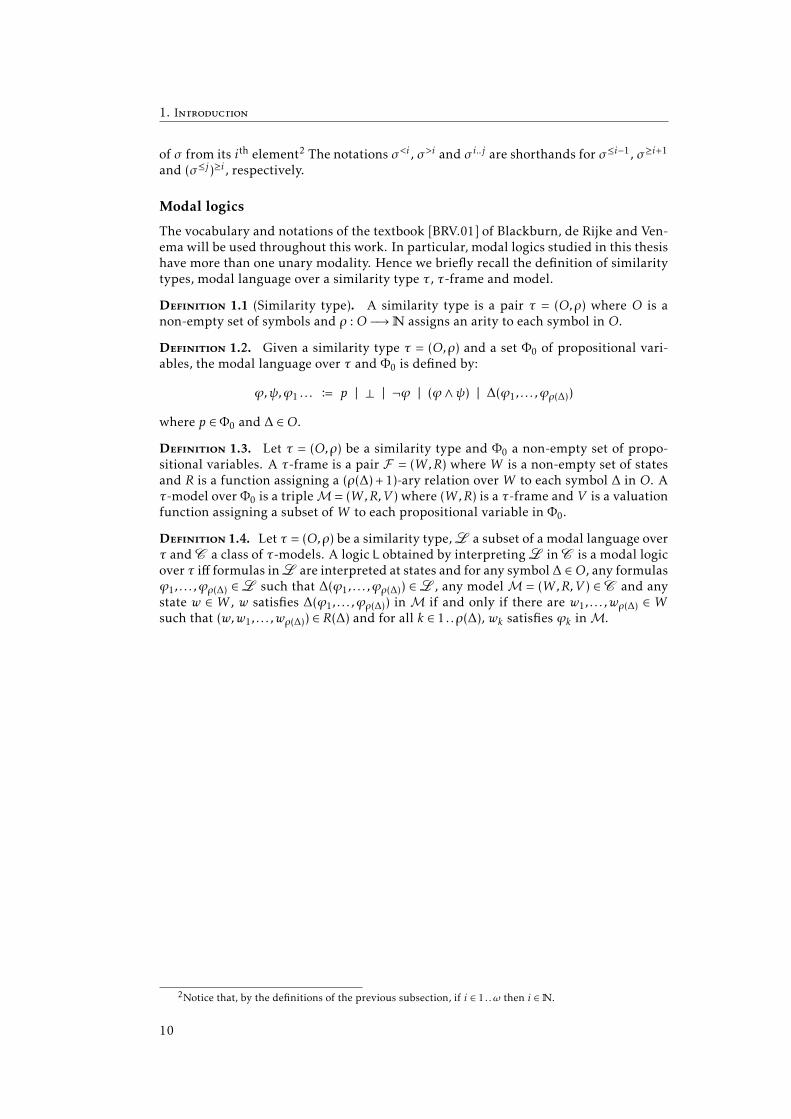
The vocabulary and notations of the textbook [BRV.01] of Blackburn, de Rijke and Ven-ema will be used throughout this work. In particular, modal logics studied in this thesishave more than one unary modality. Hence we briefly recall the definition of similaritytypes, modal language over a similarity type τ , τ-frame and model.
Definition 1.1 (Similarity type). A similarity type is a pair τ = (O,ρ) where O is anon-empty set of symbols and ρ :O −→N assigns an arity to each symbol in O.
Definition 1.2. Given a similarity type τ = (O,ρ) and a set Φ0 of propositional vari-ables, the modal language over τ and Φ0 is defined by:
ϕ,ψ,ϕ1 . . . B p | ⊥ | ¬ϕ | (ϕ ∧ψ) | ∆(ϕ1, . . . ,ϕρ(∆))
where p ∈ Φ0 and ∆ ∈O.
Definition 1.3. Let τ = (O,ρ) be a similarity type and Φ0 a non-empty set of propo-sitional variables. A τ-frame is a pair F = (W,R) where W is a non-empty set of statesand R is a function assigning a (ρ(∆) + 1)-ary relation overW to each symbol ∆ in O. Aτ-model over Φ0 is a tripleM = (W,R,V ) where (W,R) is a τ-frame and V is a valuationfunction assigning a subset ofW to each propositional variable in Φ0.
Definition 1.4. Let τ = (O,ρ) be a similarity type,L a subset of a modal language overτ and C a class of τ-models. A logic L obtained by interpretingL in C is a modal logicover τ iff formulas inL are interpreted at states and for any symbol∆ ∈O, any formulasϕ1, . . . ,ϕρ(∆) ∈L such that ∆(ϕ1, . . . ,ϕρ(∆)) ∈L , any modelM = (W,R,V ) ∈ C and anystate w ∈ W , w satisfies ∆(ϕ1, . . . ,ϕρ(∆)) inM if and only if there are w1, . . . ,wρ(∆) ∈ Wsuch that (w,w1, . . . ,wρ(∆)) ∈ R(∆) and for all k ∈ 1 . .ρ(∆), wk satisfies ϕk inM.
2Notice that, by the definitions of the previous subsection, if i ∈ 1 . .ω then i ∈N.
10
Part I
Actions
11


Chapter 2
Propositional Dynamic Logic
The propositional dynamic logic (PDL) [FisLad.77] is a multimodal logic designed toreason about behaviors of programs. A modal operator 〈α〉 is associated to each pro-gram α, formulas 〈α〉ϕ being read “the program α can be executed from the currentstate to reach a state where the formula ϕ holds”. The set of programs is structured bythe following operators: sequential composition (α ; β) of programs α and β executes βafter α; nondeterministic choice (α ∪ β) of programs α and β executes α or β; test ϕ?on formula ϕ checks whether the current state satisfies ϕ; iteration α∗ of program αexecutes α a nondeterministic number of times.
In contradistinction with other logics of programs, atomic programs are abstract inPDL. Therefore, programs can easily be replaced by some other kinds of actions. Indeed,PDL has been adapted to many different domains like knowledge representation or lin-guistics (see for instance [DHK.07, EijSto.06, Schild.91]). Hence PDL can be regarded asa prominent logic of actions.
PDL has been intensively studied in the last decades and a lot is known about it(see for instance [HKT.00] for a starting point). We do not recall all these results in thepresent chapter. Instead, we present the methods and techniques which we adapt toother logics in the remainder in the thesis, along with some results we use to compareother logics to PDL. Moreover, we use this chapter to introduce notations, conventionsand vocabulary used throughout the thesis.
2.1 Syntax and semantics
LetΠ0 be a countable set of atomic programs (denoted by a,b . . .) and Φ0 a countable setof propositional variables (denoted by p,q . . .). The sets ΠPDL(Π0,Φ0) and ΦPDL(Π0,Φ0)of programs (denoted by α,β . . .) and formulas (denoted by ϕ,ψ . . .) are defined simulta-neously by the following grammar:
α,β B a | (α ; β) | (α ∪ β) | ϕ? | α∗
ϕ B p | ⊥ | ¬ϕ | 〈α〉ϕ
As usual for modalities, we define the dual modality [α] of 〈α〉 by: [α]ϕ ¬〈α〉¬ϕ. Asit will become clear from the semantics, all the Boolean connectives can be defined inPDL, starting for instance with ϕ→ ψ [ϕ?]ψ. Parentheses may be omitted for clarity,but they are taken into account when counting occurrences of symbols. We write |α|and |ϕ| for the number of occurrences of symbols in the program α and the formula ϕ,respectively.
The negation deserves some comments. Since negation is classical, it would be con-venient if it was involutive1. Since it is not the case, we define the syntactic function ∼over formulas such that ∼ϕ = ψ if ϕ = ¬ψ for some formula ψ and ∼ϕ = ¬ψ other-wise. Obviously, ∼ is involutive. Hence, in most situations we would prefer to use ∼instead of ¬. Therefore, we abusively consider that ¬ is in fact ∼. For instance, we willabusively assume that [α]ϕ is defined as ¬〈α〉∼ϕ and that ¬¬ϕ? and ϕ? are the same
1An involutive function is a function which is its own inverse.
13
2. Propositional Dynamic Logic
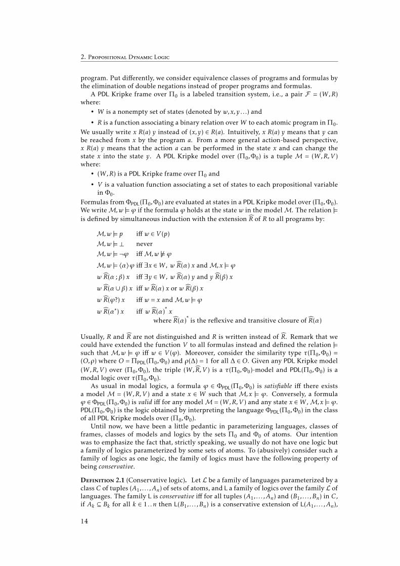
program. Put differently, we consider equivalence classes of programs and formulas bythe elimination of double negations instead of proper programs and formulas.
A PDL Kripke frame over Π0 is a labeled transition system, i.e., a pair F = (W,R)where:
• W is a nonempty set of states (denoted by w,x,y . . .) and
• R is a function associating a binary relation overW to each atomic program inΠ0.We usually write x R(a) y instead of (x,y) ∈ R(a). Intuitively, x R(a) y means that y canbe reached from x by the program a. From a more general action-based perspective,x R(a) y means that the action a can be performed in the state x and can change thestate x into the state y. A PDL Kripke model over (Π0,Φ0) is a tuple M = (W,R,V )where:
• (W,R) is a PDL Kripke frame over Π0 and
• V is a valuation function associating a set of states to each propositional variablein Φ0.
Formulas fromΦPDL(Π0,Φ0) are evaluated at states in a PDL Kripke model over (Π0,Φ0).We writeM,w |= ϕ if the formula ϕ holds at the state w in the modelM. The relation |=is defined by simultaneous induction with the extension R of R to all programs by:
M,w |= p iff w ∈ V (p)
M,w |=⊥ never
M,w |= ¬ϕ iffM,w 6|= ϕ
M,w |= 〈α〉ϕ iff ∃x ∈W, w R(α) x andM,x |= ϕ
w R(α ; β) x iff ∃y ∈W, w R(α) y and y R(β) x
w R(α ∪ β) x iff w R(α) x or w R(β) x
w R(ϕ?) x iff w = x andM,w |= ϕ
w R(α∗) x iff w R(α)∗x
where R(α)∗is the reflexive and transitive closure of R(α)
Usually, R and R are not distinguished and R is written instead of R. Remark that wecould have extended the function V to all formulas instead and defined the relation |=such that M,w |= ϕ iff w ∈ V (ϕ). Moreover, consider the similarity type τ(Π0,Φ0) =(O,ρ) where O =ΠPDL(Π0,Φ0) and ρ(∆) = 1 for all ∆ ∈ O. Given any PDL Kripke model(W,R,V ) over (Π0,Φ0), the triple (W,R,V ) is a τ(Π0,Φ0)-model and PDL(Π0,Φ0) is amodal logic over τ(Π0,Φ0).
As usual in modal logics, a formula ϕ ∈ ΦPDL(Π0,Φ0) is satisfiable iff there existsa model M = (W,R,V ) and a state x ∈ W such that M,x |= ϕ. Conversely, a formulaϕ ∈ ΦPDL(Π0,Φ0) is valid iff for any modelM = (W,R,V ) and any state x ∈W ,M,x |= ϕ.PDL(Π0,Φ0) is the logic obtained by interpreting the language ΦPDL(Π0,Φ0) in the classof all PDL Kripke models over (Π0,Φ0).
Until now, we have been a little pedantic in parameterizing languages, classes offrames, classes of models and logics by the sets Π0 and Φ0 of atoms. Our intentionwas to emphasize the fact that, strictly speaking, we usually do not have one logic buta family of logics parameterized by some sets of atoms. To (abusively) consider such afamily of logics as one logic, the family of logics must have the following property ofbeing conservative.
Definition 2.1 (Conservative logic). Let L be a family of languages parameterized by aclass C of tuples (A1, . . . ,An) of sets of atoms, and L a family of logics over the family L oflanguages. The family L is conservative iff for all tuples (A1, . . . ,An) and (B1, . . . ,Bn) in C,if Ak ⊆ Bk for all k ∈ 1 . .n then L(B1, . . . ,Bn) is a conservative extension of L(A1, . . . ,An),
14

Fischer-Ladner closure 2.2
i.e., the set of valid formulas of L(B1, . . . ,Bn) which are in the language L(A1, . . . ,An) isexactly the set of valid formulas of L(A1, . . . ,An).
If a family of logics is conservative, then the validity of any formula depends only onthe atoms occurring in the formula. In that case only, the set of tuples parameterizinglogics and languages is not relevant and can be omitted. Hopefully, most logic familieshave this property. In particular, as stated by the following proposition, PDL has thisproperty. Hence we will (abusively) consider PDL as a logic. In the remainder of thethesis, we will parameterize languages, classes of frames, classes of models and logicsby sets of atoms only when some considered families of logics are not conservative (likein Section 3.1).
Proposition 2.2. PDL is conservative.
Proof. Let us consider a set Π0 of atomic programs, a set Φ0 of propositional variables,and two PDL Kripke modelsM1 = (W1,R1,V1) over (Π1,Φ1) andM2 = (W2,R2,V2) over(Π2,Φ2) such that Π0 ⊆ Π1 ∩Π2 and Φ0 ⊆ Φ1 ∩Π2. A function f from W1 to W2 is anisomorphism fromM1 toM2 limited to (Π0,Φ0) iff f is a bijection such that:
w ∈ V1(p) iff f (w) ∈ V1(p)w R1(a) x iff f (w) R2(a) f (x)
for all w,x ∈ W1, all p ∈ Φ0 and all a ∈ Π0. If there is such a function, it can easily beproved by induction on n that for all n ∈N, all w,x ∈ W1, all ϕ ∈ ΦPDL(Π0,Φ0) and allα ∈ΠPDL(Π0,Φ0):IH.1 if |ϕ| = n thenM1,w |= ϕ iffM2, f (w) |= ϕ;IH.2 if |α| = n then w R1(α) x iff f (w) R2(α) f (x).Suppose now that Π1 ⊆ Π2 and Φ1 ⊆ Φ2. Since the negation is classical, a formula isvalid if and only if its negation if satisfiable, hence we can reason about satisfiabilityinstead of validity. Suppose a formula ϕ ∈ ΦPDL(Π1,Φ1) is satisfiable in PDL(Π1,Φ1).There is a modelM1 = (W1,R1,V1) over (Π1,Φ1) satisfying ϕ. We construct the modelM2 = (W2,R2,V2) over (Π2,Φ2) such that W2 = W1, R2(a) = R1(a) for all a ∈ Π1 andV2(p) = V1(p) for all p ∈ Φ1. The identity overW1 is an isomorphism limited to (Π1,Φ1)fromM1 toM2. Therefore, ϕ is satisfiable in PDL(Π2,Φ2). The other direction is similarand we do not detail it.
2.2 Fischer-Ladner closure
For many usual techniques and methods in modal logics, the set of subformulas of theconsidered formula is used. For basic modal logics like K, this set has some interestingproperties. First it is finite and usually its cardinality is even linear in the number ofoccurrences of symbols in the formula. Second, for any formula ψ and any state w in aKripke model, checking whether w and its successors satisfy some subformulas of ψ issufficient to decide whether w satisfy ψ. These properties are necessary for instance forthe filtration technique or for the tableauxmethod, both adapted to PDL in the followingsections. We define the second property more formally.
Definition 2.3. Let τ = (O,ρ) be a similarity type, L a modal logic over τ , 4 a well-founded order over the formulas of L and ϕ a formula in L’s language. A set C ofL’s formulas is comprehensive for ϕ with respect to 4 iff there are two finite subsets Land S of C and a terminating deterministic procedure Check such that for any modelM = (W,R,V ) for L and any state w ∈W :
• Check succeeds if and only if w satisfies ϕ inM;
15

2. Propositional Dynamic Logic
〈a〉ϕϕ
⟨ϕ?
⟩ψ
ϕ ψ⟨α ; β
⟩ϕ
〈α〉⟨β⟩ϕ
〈α∗〉ϕ〈α〉〈α∗〉ϕ ϕ⟨
α ∪ β⟩ϕ
〈α〉ϕ⟨β⟩ϕ
ϕ∼ϕ
Figure 2.1: Fischer-Ladner closure rules
• Check has access toM and w only through the following queries:
– Given some formula ψ ∈ L, does w satisfies ψ inM ?– Given a symbol ∆ ∈ O, a tuple (Q0, . . . ,Qρ(∆)) of subsets of S and an indexi ∈ 0 . .ρ(∆), is there a tuple w0, . . . ,wn ∈ R(∆) such that wi = w and for allk ∈ 0 . .ρ(∆) if k , i then wk satisfies inM all formulas in Qk ?
– Given a symbol ∆ ∈ O, a tuple (Q0, . . . ,Qρ(∆)) of subsets of S and an indexi ∈ 0 . .ρ(∆), is it the case that for any tuple (w0, . . . ,wρ(∆)) ∈ R(∆) if wi = wthen there is k ∈ 0 . .ρ(∆) such that k , i and wk satisfies in M all formulasin Qk ?
• Either ϕ is minimal for 4 or for all formula ψ ∈ L, ψ ≺ ϕ where ≺ is the strict ordercorresponding to 4.
The set C is globally comprehensive iff C is comprehensive for all ϕ ∈ C. If there is aterminating deterministic procedure which computes for any formula ϕ in L’s languagea set C(ϕ) such that ϕ ∈ C and C is globally comprehensive then L has comprehensivedecompositions.
When formulas are defined inductively from some symbols, the well-founded or-der 4 is usually defined such that ψ 4 ϕ iff the number of occurrences of symbols in ψis less or equal than the number of occurrences of symbols in ϕ. In such cases, 4 maybe omitted. Besides, it must be outlined that to have comprehensive decomposition isjust a necessary condition to apply some usual method like the filtration and does notimply any other properties.
For PDL, the set of subformulas of any formula is not comprehensive. The culpritsare the program operators. Consider for instance the simple formula ϕ = 〈a ; b〉p. Theonly strict subformula of ϕ is p and it is clearly not sufficient to decide whether a statesatisfies ϕ.
Fischer and Ladner [FisLad.79] devised sets which have these two properties. Givena PDL formula ϕ0, the Fischer-Ladner closure FL(ϕ0) of ϕ0, is the least set (by inclusion)containing ϕ0 and closed by the rules of Figure 2.1. These rules are read as follows:if the premise belongs to the set then all the conclusion must belong to the set too. Itcan easily be proved by induction that for any formulas ϕ0 ∈ ΦPDL and 〈α〉ψ ∈ FL(ϕ0),ψ ∈ FL(ϕ0). The following propositions prove that the Fischer-Ladner closure has thetwo aforementioned properties.
Proposition 2.4 from [FisLad.79]. There is a natural number K such that for any PDLformula ϕ0, the cardinality of FL(ϕ0) is less than K · |ϕ0|.
Proof sketch. The method used in the proof of Fischer and Ladner is very convenientand we use it for different proofs in the remainder of the thesis (for instance in thecompleteness of our tableaux method in Chapter 8). Hence we give here a sketch of theoriginal proof.
The restricted Fischer-Ladner closure rFL(ϕ0) of any formula ϕ0 is defined similarlyto the Fischer-Ladner closure except that the rules for the non-deterministic choice, the
16

Fischer-Ladner closure 2.2
⟨α ∪ β
⟩ϕ
〈α〉Qϕ⟨β⟩Qϕ ϕ
〈α∗〉ϕ〈α〉Q〈α∗〉ϕ ϕ
¬ϕϕ
Figure 2.2: Restricted Fischer-Ladner closure rules
iteration and the negation are replaced with the ones in Figure 2.2. In this figure, thenegation operator ¬ is not the function ∼. New propositional variables of the formQϕ are introduced by these rules. The Fischer-Ladner closure can be obtained fromthe restricted Fischer-Ladner closure by recursively replacing each occurrence of anynew propositional variable Qϕ with ϕ and by adding ∼ϕ for each ϕ in the restrictedFischer-Ladner closure.
Let ∆+ϕ0 be the set of new propositional variables needed for the restricted Fischer-Ladner closure ofϕ0 and defineΦ+ϕ0
0 asΦ0∪∆+ϕ0 . The restricted Fischer-Ladner closureof ϕ0 is a subset of ΦPDL(Π0,Φ
+ϕ00 ).
In some situation though, it is more convenient to use the new propositional vari-ables Qϕ , hence to consider the restricted Fischer-Ladner closure instead of the Fischer-Ladner closure. Since PDL is conservative, this has no impact on the satisfiability offormulas. Any modelM = (W,R,V ) over (Π0,Φ0) can be transformed into the modelM′ = (W,R,V ′) over (Π0,Φ
+ϕ00 ) by extending V to V ′ such that w ∈ V (Qϕ) iffM,w |= ϕ
for any new propositional variable Qϕ ∈ ∆+ϕ0 .To prove that the cardinality of rFL(ϕ0) is linear in |ϕ0|, Fischer and Ladner defined
the following measure on programs and formulas.
γ(p) = 1, for all p ∈ Φ0 γ(a) = 1, for all a ∈Π0
γ(Qϕ) = 0, for all Qϕ ∈ ∆+ϕ0 γ(α ; β) = γ(α) +γ(β) + 1
γ(⊥) = 1 γ(α ∪ β) = γ(α) +γ(β) + 1
γ(¬ϕ) = γ(ϕ) + 1 γ(ϕ?) = γ(ϕ) + 1
γ(〈α〉ϕ) = γ(α) +γ(ϕ) γ(α∗) = γ(α) + 1
Then the following facts can easily be checked:
• For any rule of the restricted Fischer-Ladner closure, let ϕ be the formula inthe premises and ψ1, . . . ,ψn the formulas in the conclusions. We have γ(ϕ) =1+
∑i∈1..nγ (ψi).
• For any formula ϕ, there is at most one rule of the restricted Fischer-Ladner clo-sure applicable to ϕ.
• For any Qϕ ∈ ∆+ϕ0 , ϕ ∈ rFL(ϕ0).
Therefore the cardinality of the restricted Fischer-Ladner closure is linear and so is theFischer-Ladner closure.
Proposition 2.5. For any formula ϕ ∈ ΦPDL, FL(ϕ) is comprehensive for ϕ.
Proof. A procedure can easily be devised for all the program constructs but the itera-tion because |〈α〉〈α∗〉ϕ| > |〈α∗〉ϕ|. Hence, sequences of programs are considered. Thefunctions form^ and form assign the formulas
⟨σ1
⟩. . .
⟨σ |σ |
⟩ϕ and
[σ1
]. . .
[σ |σ |
]ϕ re-
spectively to every pair (σ,ϕ) ∈Π∗PDL×ΦPDL. The function next assigns to each sequenceσ ∈ Π∗PDL a set of pairs (L,σ ′) where the first component L is a set of formulas and the
17

2. Propositional Dynamic Logic
second component σ ′ is a sequence of programs. It is defined inductively as follows:
next(ε) = (∅,ε)next(aσ ) = (∅, aσ )
next((α ; β)σ ) = next(αβσ )
next((α ∪ β)σ ) = next(ασ )∪next(βσ )next((ϕ?)σ ) = (L∪ ϕ,σ1) | (L,σ1) ∈ next(σ )next(α∗σ ) = next(σ )∪ (L,σ1α∗σ ) | (L,σ1) ∈ next(α)
The following hypothesis can easily be proved for all sequences σ ∈Π∗PDL, by inductionon
∑k∈1..|σ |
∣∣∣σ k ∣∣∣.IH.1 for any formula ϕ ∈ ΦPDL, any modelM = (W,R,V ) and any state w ∈W ,M,w |=
form^(σ,ϕ) if and only if there is (L,σ1) ∈ next(σ ) such thatM,w |= form^(σ1,ϕ)∧∧ψ∈Lψ.
IH.2 for all ϕ ∈ ΦPDL and all (L,σ1) ∈ next(σ ), L∪ form^(σ1,ϕ) ⊆ FL(form^(σ,ϕ));
IH.3 for all (L,σ1) ∈ next(σ ), σ1 = ε or σ11 ∈Π0;
IH.4 for all (L,σ1) ∈ next(σ ) and all ψ ∈ L,∣∣∣ψ∣∣∣ <∑
k∈1..|σ |∣∣∣σ k ∣∣∣.
Then for any formula of the form 〈α〉ϕ, the procedure check if there is a pair (L,σ ) ∈next(α) such that
• M,w |= ψ for all ψ ∈ L and
• if σ = aσ1 for some a ∈ Π0 then there is a successor x ∈W of w by R(a) such thatM,x |= form^(σ1,ϕ).
The procedure is similar for formulas of the form [α]ϕ.
2.3 Strong finite model property by filtration
A logic has the finite model property iff any satisfiable formula is satisfiable in a finitemodel, i.e., a model with a finite number of states. A logic has the strong finite modelproperty iff there exists a computable function f on natural numbers such that any sat-isfiable formula ϕ0 is satisfiable in a model with at most f (|ϕ0|) states. Filtration is theusual technique in modal logic to prove strong finite model properties. We illustrate ithere for PDL.
Proposition 2.6 from [FisLad.79]. There is a natural numbers K such that any PDLsatisfiable formula ϕ0 is satisfiable in a model with at most 2K ·|ϕ0 | states.
Let K be defined by Proposition 2.4. To prove Proposition 2.6 above, suppose thatϕ0 is satisfiable. Then there exists a PDL Kripke model M0 = (W0,R0,V0) and a statex0 ∈ W0 such thatM0,x0 |= ϕ0. Let ≡ be the binary relation on W0 such that w ≡ x ifffor all ψ ∈ FL(ϕ0),M0,w |= ψ if and only ifM0,x |= ψ. The relation ≡ is obviously anequivalence relation. For all x ∈ W0, we write [x] for the equivalence class of x by ≡.Each of these equivalence classes corresponds to a distinct subset of FL(ϕ0). Therefore,there are at most 2K ·|ϕ0 | equivalence classes.
Then, we define the modelMf = (Wf ,Rf ,Vf ) where• Wf is the quotientW0/≡ ofW0 by ≡,• for all a ∈Π0, [w] Rf (a) [x] iff there is w′ ∈ [w] and x′ ∈ [x] such that w′ R0(a) x′ ,
• [x] ∈ Vf (p) iff x ∈ V0(p).Mf has at most 2K ·|ϕ0 | states. It remains to prove the following truth lemma.
Lemma 2.7 from [FisLad.79]. For all ψ ∈ FL(ϕ0) and all x ∈W0,M0,x |= ψ if and onlyifMf , [x] |= ψ.
18

Tree-like model property by unraveling 2.4
Proof sketch. Fischer and Ladner used the restricted Fischer-Ladner closure. Let us de-fine the extensionsM+
0 andM+f ofM0 andMf over (Π0,Φ
+ϕ00 ) as described in the proof
of Lemma 2.4. It can easily be checked that whenever w ≡ x for some w,x ∈W0 then forany formula ψ ∈ rFL(ϕ0),M+
0 ,w |= ψ if and only ifM+0 ,x |= ψ.
Fischer and Ladner proved that for all ψ ∈ rFL(ϕ0):IH.1 for all w ∈W0,M+
0 ,x |= ψ if and only ifM+f , [x] |= ψ;
IH.2 if ψ = 〈α〉ϕ for some α and ϕ then for all w,x ∈W0, if w R+0 (α) x then [w] R+
f (α) [x].
The proof is by induction on γ(ψ) as defined in the proof of Proposition 2.4. The re-stricted Fischer-Ladner closure is useful for the proof of IH.1 when ψ = [α∗]ϕ. Sup-pose that M+
0 ,w |= [α∗]ϕ and [w] R+f (α∗) [x]. There is a finite sequence w0 . . .wn such
that w0 ≡ w, wn ≡ x and for all k < n, [wk] R+f (α) [wk+1]. We prove that for all k ≤ n,
M+0 ,wk |= [α∗]ϕ. Suppose M+
0 ,wk |= [α∗]ϕ. Then M+0 ,wk |= [α]Q[α∗]ϕ . By induction
M+f , [wk] |= [α]Q[α∗]ϕ , hence M+
f , [wk+1] |= Q[α∗]ϕ . By definition, M+0 ,wk+1 |= Q[α∗]ϕ ,
therefore M+0 ,wk+1 |= [α∗]ϕ. Finally, we have proved that M+
0 ,x |= [α∗]ϕ. Therefore,M+
0 ,x |= ϕ and by inductionM+f , [x] |= ϕ.
2.4 Tree-like model property by unraveling
The tree-like model is an interesting property of logics with relational semantics. Sincethis property (and its absence) is important for the remainder of this thesis, we defineit in full generality.2
Definition 2.8 (Tree-like frame). Given a similarity type τ = (O,ρ), a τ-frame F =(W,R) is tree-like iff there exists a symmetric binary relation E overW such that (W,E)is an acyclic graph and for any symbol ∆ ∈ O, any tuple (w0, . . . ,wρ(∆)) ∈ R (∆) and anyindex i, j ∈ 0 . .ρ(∆), there is a path in (w0, . . . ,wρ(∆),E) between wi and wj .
Definition 2.9 (Tree-like model property). A logic has the tree-like model property iffany satisfiable formula is satisfiable in a model with a tree-like frame.
We prove that PDL has the tree-like model property.
Proposition 2.10. PDL has the tree-like model property.
Since the method used to prove this proposition has been adapted to other logicsin the remainder of the thesis, we recall the sketch of the proof. Suppose that ϕ0 issatisfiable. There must exists a Kripke PDL modelM0 = (W0,R0,V0) and a state x0 ∈W0such that M0,x0 |= ϕ0. By Proposition 2.6, we can assume that W0 is countable. Wenow use the unraveling technique. Intuitively, it consists in constructing a model wherestates are all the paths from x0 inM0. It is a special case of the more general methodof fixing defects in which we start with a model which does not meet all the neededrequirements, we list all the possible defects of this model and then we iteratively fixall these defects one by one.
For the unraveling of M0, a defect is a triple (n,a,w) ∈ N ×Π0 ×W0. Since PDL isconservative, we can assume that Π0 is finite but not empty. Therefore, there is anω-sequence δ of defects in which each defect appears infinitely often.
We inductively construct the pairs (M′k ,hk) for all k ∈N whereM′k = (W ′k ,R′k ,V
′k ) is
a PDL Kripke model withW ′k ⊆N and hk is a PDL homomorphism fromM′k toM0.
Definition 2.11 (PDL homomorphism). A PDL homomorphism fromM′ toM is a func-tion h fromW ′ toW such that
2The definition of the tree-like model property given here is slightly different from the definition givenin [BRV.01]. In particular, for modalities of arity greater than one, we consider any spanning of the tuples inthe relation.
19
2. Propositional Dynamic Logic
1. for all w′ ∈W ′ and all p ∈ Φ0, w′ ∈ V ′(p) if and only if h(w′) ∈ V (p).3
2. for all w′ ,x′ ∈W ′ and all a ∈Π0, if w′ R′(a) x′ then h(w′) R(a) h(x′);
The construction proceeds as follows.
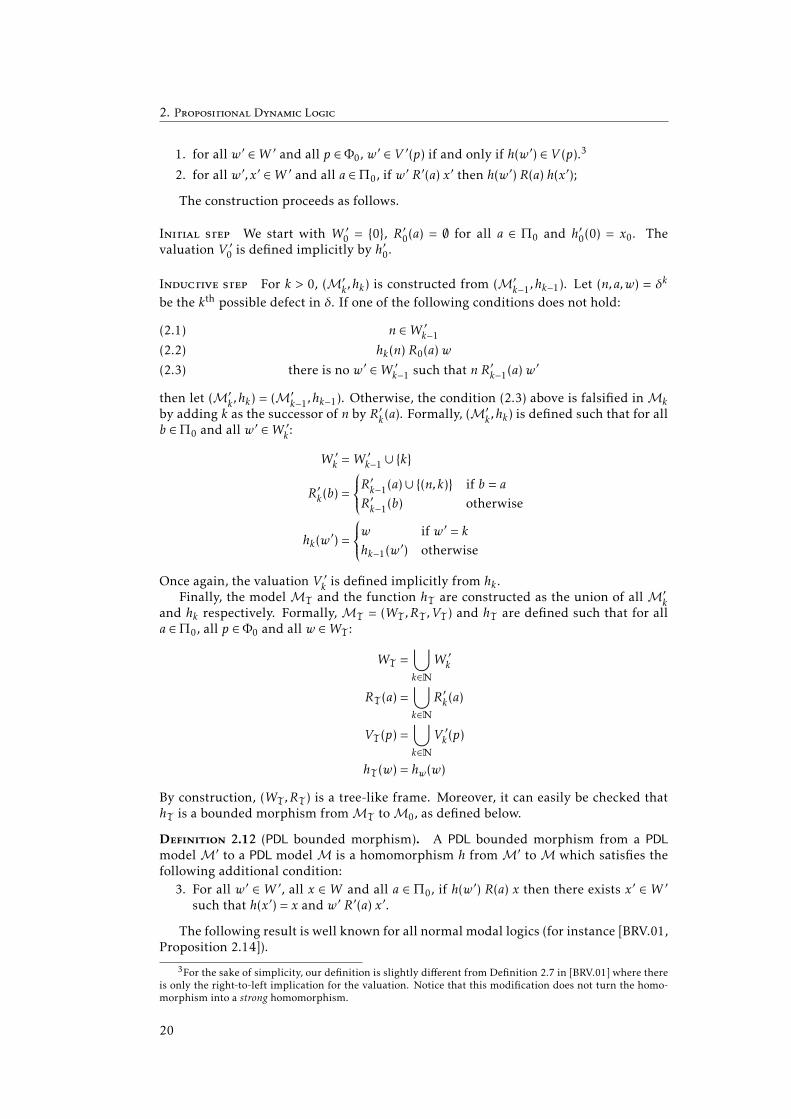
Initial step We start with W ′0 = 0, R′0(a) = ∅ for all a ∈ Π0 and h′0(0) = x0. Thevaluation V ′0 is defined implicitly by h′0.
Inductive step For k > 0, (M′k ,hk) is constructed from (M′k−1,hk−1). Let (n,a,w) = δk
be the kth possible defect in δ. If one of the following conditions does not hold:
n ∈W ′k−1(2.1)
hk(n) R0(a) w(2.2)
there is no w′ ∈W ′k−1 such that n R′k−1(a) w′(2.3)
then let (M′k ,hk) = (M′k−1,hk−1). Otherwise, the condition (2.3) above is falsified inMkby adding k as the successor of n by R′k(a). Formally, (M′k ,hk) is defined such that for allb ∈Π0 and all w′ ∈W ′k :
W ′k =W′k−1 ∪ k
R′k(b) =
R′k−1(a)∪ (n,k) if b = aR′k−1(b) otherwise
hk(w′) =
w if w′ = khk−1(w′) otherwise
Once again, the valuation V ′k is defined implicitly from hk .Finally, the modelMT and the function hT are constructed as the union of allM′k
and hk respectively. Formally,MT = (WT ,RT ,VT) and hT are defined such that for alla ∈Π0, all p ∈ Φ0 and all w ∈WT :
WT =⋃k∈N
W ′k
RT(a) =⋃k∈N
R′k(a)
VT(p) =⋃k∈N
V ′k (p)
hT(w) = hw(w)
By construction, (WT ,RT) is a tree-like frame. Moreover, it can easily be checked thathT is a bounded morphism fromMT toM0, as defined below.
Definition 2.12 (PDL bounded morphism). A PDL bounded morphism from a PDLmodelM′ to a PDL modelM is a homomorphism h fromM′ toM which satisfies thefollowing additional condition:
3. For all w′ ∈W ′ , all x ∈W and all a ∈ Π0, if h(w′) R(a) x then there exists x′ ∈W ′such that h(x′) = x and w′ R′(a) x′ .
The following result is well known for all normal modal logics (for instance [BRV.01,Proposition 2.14]).
3For the sake of simplicity, our definition is slightly different from Definition 2.7 in [BRV.01] where thereis only the right-to-left implication for the valuation. Notice that this modification does not turn the homo-morphism into a strong homomorphism.
20
Elimination of Hintikka sets 2.5
Proposition 2.13. Bounded morphisms preserve satisfiability.
Therefore, ϕ0 is satisfiable inMT . We have proved Proposition 2.10.
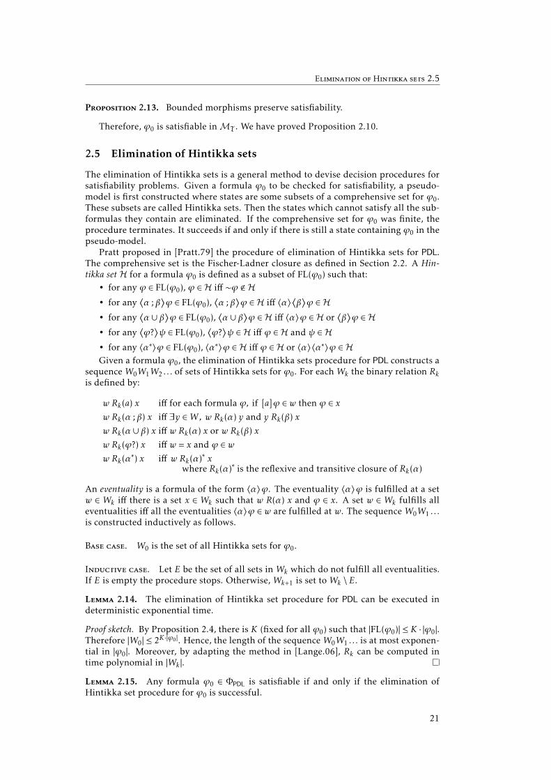
2.5 Elimination of Hintikka sets
The elimination of Hintikka sets is a general method to devise decision procedures forsatisfiability problems. Given a formula ϕ0 to be checked for satisfiability, a pseudo-model is first constructed where states are some subsets of a comprehensive set for ϕ0.These subsets are called Hintikka sets. Then the states which cannot satisfy all the sub-formulas they contain are eliminated. If the comprehensive set for ϕ0 was finite, theprocedure terminates. It succeeds if and only if there is still a state containing ϕ0 in thepseudo-model.
Pratt proposed in [Pratt.79] the procedure of elimination of Hintikka sets for PDL.The comprehensive set is the Fischer-Ladner closure as defined in Section 2.2. A Hin-tikka set H for a formula ϕ0 is defined as a subset of FL(ϕ0) such that:
• for any ϕ ∈ FL(ϕ0), ϕ ∈ H iff ∼ϕ <H• for any
⟨α ; β
⟩ϕ ∈ FL(ϕ0),
⟨α ; β
⟩ϕ ∈ H iff 〈α〉
⟨β⟩ϕ ∈ H
• for any⟨α ∪ β
⟩ϕ ∈ FL(ϕ0),
⟨α ∪ β
⟩ϕ ∈ H iff 〈α〉ϕ ∈ H or
⟨β⟩ϕ ∈ H
• for any⟨ϕ?
⟩ψ ∈ FL(ϕ0),
⟨ϕ?
⟩ψ ∈ H iff ϕ ∈ H and ψ ∈ H
• for any 〈α∗〉ϕ ∈ FL(ϕ0), 〈α∗〉ϕ ∈ H iff ϕ ∈ H or 〈α〉〈α∗〉ϕ ∈ HGiven a formula ϕ0, the elimination of Hintikka sets procedure for PDL constructs a
sequenceW0W1W2 . . . of sets of Hintikka sets for ϕ0. For eachWk the binary relation Rkis defined by:
w Rk(a) x iff for each formula ϕ, if [a]ϕ ∈ w then ϕ ∈ xw Rk(α ; β) x iff ∃y ∈W, w Rk(α) y and y Rk(β) x
w Rk(α ∪ β) x iff w Rk(α) x or w Rk(β) xw Rk(ϕ?) x iff w = x and ϕ ∈ ww Rk(α
∗) x iff w Rk(α)∗ x
where Rk(α)∗ is the reflexive and transitive closure of Rk(α)
An eventuality is a formula of the form 〈α〉ϕ. The eventuality 〈α〉ϕ is fulfilled at a setw ∈ Wk iff there is a set x ∈ Wk such that w R(α) x and ϕ ∈ x. A set w ∈ Wk fulfills alleventualities iff all the eventualities 〈α〉ϕ ∈ w are fulfilled at w. The sequenceW0W1 . . .is constructed inductively as follows.
Base case. W0 is the set of all Hintikka sets for ϕ0.
Inductive case. Let E be the set of all sets inWk which do not fulfill all eventualities.If E is empty the procedure stops. Otherwise,Wk+1 is set toWk \E.
Lemma 2.14. The elimination of Hintikka set procedure for PDL can be executed indeterministic exponential time.
Proof sketch. By Proposition 2.4, there is K (fixed for all ϕ0) such that |FL(ϕ0)| ≤ K · |ϕ0|.Therefore |W0| ≤ 2K ·|ϕ0 |. Hence, the length of the sequenceW0W1 . . . is at most exponen-tial in |ϕ0|. Moreover, by adapting the method in [Lange.06], Rk can be computed intime polynomial in |Wk |.
Lemma 2.15. Any formula ϕ0 ∈ ΦPDL is satisfiable if and only if the elimination ofHintikka set procedure for ϕ0 is successful.
21

2. Propositional Dynamic Logic
Proof sketch. We use the vocabulary of the dual problem of validity. The proof of sound-ness is closely related to the filtration. Suppose ϕ0 is satisfiable. There is a modelM0satisfying ϕ0. Let M = (W,R,V ) be the filtration of M0 by FL(ϕ0). We construct forall k an injective function fk from W to Wk such that for any states w,x ∈ W , any for-mula ϕ ∈ FL(ϕ0) and any program α such that 〈α〉ψ ∈ FL(ϕ0) for some ψ, the followingtwo conditions hold:
M,w |= ϕ iff ϕ ∈ fk(w)if w R(α) x then fk(w) Rk(α) fk(x)
Since there is w0 ∈W such thatM,w0 |= ϕ0, the elimination of Hintikka set procedureis successful.
For the completeness proof, we suppose that the elimination of Hintikka sets pro-cedure for the formula ϕ0 is successful and constructs the sequence W0 . . .Wn. Weconstruct from Wn the model M = (Wn,R,V ) such that w R(a) x iff w Rn(a) x andV (p) = w ∈Wn | p ∈ w. We prove by induction that for any states w,x ∈ Wn, any for-mula ϕ ∈ FL(ϕ0) and any program α such that 〈α〉ψ ∈ FL(ϕ0) for some ψ, the followingtwo conditions hold:
M,w |= ϕ iff ϕ ∈ ww R(α) x iff w Rk(α) x
Since there is a state w0 ∈Wn such that ϕ0 ∈ w,M satisfies ϕ0.
We have proved the following proposition.
Proposition 2.16 from [Pratt.78]. The satisfiability problem of PDL is in EXPTIME.
2.6 Tableaux methods
Fischer and Ladner proved in [FisLad.77] that the satisfiability problem of PDL is EXP-TIME-hard. Therefore, the elimination of Hintikka sets procedure for PDL presentedin the previous section is optimal. But this procedure is not useful in practice becauseit always requires exponential time to construct the initial pseudo-model. In contrast,tableaux methods construct a model state by state. Hence they are more interestingin practice. Tableaux methods for PDL are quite complicated though. Hence, we willnot detail a comprehensive formal definition of any tableaux method for PDL in thissection. Instead, we give a general framework for such decision procedures, we out-line the difficult points and we mention solutions proposed in the literature. The firsttableaux method for PDL has been devised by Pratt in [Pratt.78] and interesting vari-ants have been proposed by Gore and Widmann in [GorWid.09] and by De Giacomoand Massacci in [De Mas.96].
Consider the saturation rules in Figure 2.3. Each rule has one premise and at leastone conclusion. A premise is a single formula whereas a conclusion is a set of formulaswith a conjunctive meaning. Conversely the set of conclusions of any rule has a disjunc-tive meaning. Besides, these rules are similar to the rules of the Fischer-Ladner closureand it can easily be checked that any conclusion of any saturation rule is included in theFischer-Ladner closure of the premise. A saturation rule applies to a set S of formulas:if a formula in S is an instantiation of the premise of the rule and there is no conclusionof the rule whose instantiation is already included in S then the rule can be applied byadding the instantiation of one of the conclusion to S. Hence, the rule for
⟨ϕ?
⟩ψ adds
both ϕ and ψ to the current set of formulas whereas the rule for [ϕ?]ψ adds either ∼ϕor ψ. A set of formulas is saturated iff no rule can be applied to it.
Given a formula ϕ0, the tableaux method procedure constructs a directed graphwhere nodes are subsets of FL(ϕ0) and edges are labeled with either a program in Π0
22

Tableaux methods 2.6
⟨α ; β
⟩ϕ
〈α〉⟨β⟩ϕ
[α ; β]ϕ[α] [β]ϕ⟨
α ∪ β⟩ϕ
〈α〉ϕ⟨β⟩ϕ
[α ∪ β]ϕ[α]ϕ [β]ϕ⟨
ϕ?⟩ψ
ϕ ψ
[ϕ?]ψ∼ϕ ψ
〈α∗〉ϕϕ 〈α〉〈α∗〉ϕ
[α∗]ϕϕ [α] [α∗]ϕ
Figure 2.3: Saturation rules for PDL tableaux methods
or the symbol ∨ (we assume ∨ <Π0). Initially there is only one node ϕ0 and no edge.Then the procedure recursively performs one of the following steps:
• if an instantiation π of a rule is applicable to a node w which has no successor,then for each conclusion C of π, add the node xC = w ∪ C if it does not alreadyexist and add an edge from w to xC labeled with ∨;
• for any saturated node w with no successor, and each formula 〈a〉ϕ ∈ w, add thenode x〈a〉ϕ = ϕ∪ψ
∣∣∣ [a]ψ ∈ w if it does not already exist and add an edge from wto x〈a〉ϕ labeled with a.
Saturated nodes are called states and unsaturated nodes pre-states. If an instantiationof a rule has been applied to a pre-state, the premise is called the main formula of thepre-state. The procedure terminates when no more step can be applied. Since eachnode of the graph is a subset of FL(ϕ0), the graph can be constructed in deterministicexponential time in |ϕ0|. Now, good graphs corresponding to a satisfiable formula mustbe distinguished from bad graphs corresponding to an unsatisfiable formula. A generalsolution is to mark unsatisfiable nodes as closed and to define that the tableaux methodis successful if and only if the initial node of the graph is open (i.e., not closed). Inparticular we want the following rules:
1. a node w is closed if ⊥ ∈ w or both ϕ ∈ w and ¬ϕ ∈ w for some ϕ;
2. a saturated node is closed if one of its successor is closed;
3. an unsaturated node is closed if all its successors are closed;But the difficulties come from cycles in the graph. Consider for instance the graphs forthe satisfiable formula [a∗]〈a〉> and the unsatisfiable formula 〈a∗〉⊥ in Figure 2.4 on thefollowing page. The first one has a “good” cycle whereas the second one has a “bad”cycle. But the previous rules for closed node are not sufficient to distinguish these twographs.
To address this issue, Pratt [Pratt.78] and Gore and Widmann [GorWid.09] intro-duce an accessibility relation from eventualities to formulas. An eventuality is a for-mula of the form 〈α〉ϕ. For instance, if an instantiation of a saturation rule with premise⟨ϕ?
⟩ψ is applied to the node w then the successor of
⟨ϕ?
⟩ψ in w is the formula ψ in
the successor of w. Similarly, if an instantiation of a saturation rule with premise 〈α∗〉ϕis applied to the node w then the successors of 〈α∗〉ϕ in w are the formula ϕ in thefirst successor of w and the formula 〈α〉 〈α∗〉ϕ in the second successor of w. Then, thefollowing condition is added for the propagation of the “closed” mark:
4. a node w is closed if for some eventuality 〈α〉 ϕ ∈ w there is no finite acyclicpath from 〈α〉ϕ in w by the accessibility relation over eventualities passing onlythrough open nodes.
An interesting variation of this method has been proposed by De Giacomo and Mas-sacci in [De Mas.96]. In this variant, whenever an eventuality of the form 〈α∗〉ϕ arises
23

2. Propositional Dynamic Logic
[a∗]〈a〉>
[a∗]〈a〉>〈a〉>[a] [a∗]〈a〉>
>[a∗]〈a〉>
>[a∗]〈a〉>〈a〉>[a] [a∗]〈a〉>
∨
a
∨ a
(a) Graph for [a∗]〈a〉>
〈a∗〉⊥
〈a∗〉⊥⊥
〈a∗〉⊥〈a〉〈a∗〉⊥
∨ ∨ a
(b) Graph for 〈a∗〉⊥
Figure 2.4: Examples of tableaux graphs for PDL
in a node, it is replaced by a fresh special propositional variable. These special propo-sitional variables are considered as the eventualities they replace but since they aresomehow unique, they make the additional condition for cycles easier to check.
2.7 Comparison with LTL
We end this chapter by comparing PDL with Pnueli’s linear temporal logic [Pnueli.77].Not only this comparison prepares the next chapter which proposes a variant of PDLrelated to branching temporal logics, but it also introduces the important notions ofembedding and of a logic being more general than another one.
Pnueli’s linear temporal logic (LTL) is a temporal logic where the flow of time isdiscrete and deterministic: each moment has exactly one successor. This logic featuresa unary modality X and a binary modality U . Intuitively, the formula Xϕ means that ϕwill hold at the next moment and the formula ϕU ψ means that ψ will eventually holdand that ϕ will hold until ψ holds.
Formally, the language of LTL is defined from a set Φ0 of propositional variables by:
ϕ,ψ B p | ⊥ | ¬ϕ | (ϕ ∧ψ) | Xϕ | (ϕU ψ)
A linear model is a tupleM = (W,S,V ) whereW is a nonempty set of states, S is the suc-cessor function fromW toW and V is the valuation function assigning a subset ofW toeach propositional variable in Φ0. LTL formulas are interpreted at states in linear mod-els. We writeM,w |=LTL ϕ if the formula ϕ holds at the state w inM. The relation |=LTLis defined as usual for the boolean connectives and as follows for the modalities:
M,w |=LTL Xϕ iffM,S(w) |=LTL ϕ
M,w |=LTL ϕU ψ iff there is n ∈N such thatM,Sn(w) |=LTL ψ and for all k < n, M,Sk(w) |=LTL ϕ
where S0 is the identity function and for all k > 0, Sk = S Sk−1.We prove that we can see LTL as the logic obtained by interpreting a fragment of the
language of PDL into a subclass of PDLmodels. We say that PDL ismore general than LTL,according to the following definition.
24

Comparison with LTL 2.7
Definition 2.17. A modal logic L1 is more general than a logic L2 if there is a func-tion τ from the language of L2 to the language of L1, called the translation function,and a function f from pointed models4 of L2 to pointed models of L1, called the for-ward function, such that for any pointed model (M,x) of L2 and any formula ϕ of L2’slanguage,M,x |=L2 ϕ iff f (M,x) |=L1 τ(ϕ).
Intuitively, we can model the discrete flow of time in PDL by choosing an action a torepresent the passing of time. We use these ideas to prove that PDL is more general thanLTL.
Proposition 2.18. PDL is more general than LTL.
Proof sketch. We define the translation function τ from the language of LTL to ΦPDL suchthat:
τ(p) = p for all p ∈ Φ0
τ(⊥) =⊥τ(¬ϕ) = ¬τ(ϕ)
τ(ϕ ∧ψ) = τ(ϕ)∧ τ(ψ)τ(Xϕ) = 〈a〉τ(ϕ)
τ(ϕU ψ) =⟨(τ(ϕ)? ; a)∗
⟩τ(ψ)
Similarly, we define the forward function f such that for any linear modelM = (W,S,V )and any state x ∈W , we define (M′ ,x′) = f (M,x) such thatM′ = (W,R,V ) with R(a) = Sand R(b) = ∅ for all b , a, and x′ = x. It can easily be proved that for any formula ϕ of L2,M,x |=LTL ϕ iffM′ ,x |= τ(ϕ).
The property for a logic L1 to be more general than a logic L2 gives some hints aboutthe relative expressive power of L1 and L2. But this notion has some limitations. First,the computational complexity of the translation function matters. Second, formulasof L2 are interpreted through the translation function in a subclass of L1’s models, andit may be the case that L1 is not expressive enough to characterize this subclass. Thissecond limitation is fixed by the following definition of a logic being embeddable intoanother one.
Definition 2.19. A logic L2 is embeddable into another logic L1 if L1 is more generalthan L2 with translation function τ and for any L2 formula ϕ, if τ(ϕ) is L1 satisfiablethen ϕ is L2 satisfiable. In such a case, τ is called an embedding of L2 into L1.
For the comparison of PDL and LTL, it can be easily checked that the images of theforward function as defined in the proof of Proposition 2.18 have the following proper-ties of being serial and deterministic for a:
for all x ∈W, there is y ∈W such that x R(a) y(seriality)
for all x,y,z ∈W, if x R(a) y and x R(a) z then y = z(determinism)
Whereas the seriality for a (from x) can easily be expressed in PDL by the formula[a∗]〈a〉>, this is not the case for the determinism of a. Indeed, using the van BenthemCharacterization Theorem, it can easily be proved that the determinism of a (from x)cannot be defined modally, since this property is not preserved by bisimulation. Thisfact does not prove that LTL is not embeddable in PDL but it indicates that finding suchan embedding is hard.
Therefore, we prove instead that LTL is embeddable in deterministic PDL. Determin-istic PDL [Harel.84] is the logic obtained by interpreting ΦPDL in the class of PDLmodelswhich are deterministic for all programs.
4A pointed model is a pair (M,w) consisting of a model and a state. More generally, we can consider thata pointed model is any structure at which formulas are evaluated.
25

2. Propositional Dynamic Logic
Proposition 2.20. LTL is embeddable in deterministic PDL.
Proof sketch. Let τ and f be defined as in the proof of Proposition 2.18. The translationfunction θ from the language of LTL to ΦPDL is defined by θ(ϕ) = τ(ϕ) ∧ [a∗]〈a〉> forall formula ϕ. It can easily be checked that LTL is more general than deterministicPDL with translation function θ and forward function f . Suppose that M,w |= θ(ϕ)for some modelM = (W,R,V ) deterministic for all programs and some LTL formula ϕ.LetM′ = (W ′ ,R′ ,V ′) be the PDL model such thatW ′ = x ∈W | w R(a∗) x, R′(a) = R(a)∩(W ×W ), R′(b) = ∅ for all b , a and V ′(p) = V (p) ∩W for all p ∈ Φ0. It can easily beproved thatM′ ,w |= θ(ϕ) and that there is a pointed linear model (M′′ ,w′′) such thatf (M′′ ,w′′) = (M′ ,w).
26

Chapter 3
Ockhamist Propositional DynamicLogics
The Propositional Dynamic Logic (PDL) presented in the previous chapter has interest-ing connections with temporal logics. For instance, we proved that the Linear Tempo-ral Logic (LTL) of Pnueli [Pnueli.77], can be embedded in deterministic PDL. The fullComputation Tree Logic (CTL*) proposed by Emerson and Halpern in [EmeHal.83], is abranching time temporal logic: the evolution of the system is supposed to be nondeter-ministic and different futures are considered. There is no known embedding betweenCTL* and PDL. Some logics like Kozen’s µ-calculus [Kozen.83] or Vardi and Wolper’sYAPL [VarWol.83] embed both PDL and CTL*. But the embedding of CTL* in these logicsuse automata and is not polynomial.
In [BalLor.13], Balbiani and Lorini proposed a new variant of PDL, the OckhamistPropositional Dynamic Logic (OPDL), which embeds both PDL and CTL* in polynomialtime. In this chapter, we propose sound, complete and optimal decision procedures forthe satisfiability problems of this logic and one of its variant. This solves the question,left open in [BalLor.13], of the exact complexity of these problems.
3.1 Syntax and Semantics
The language of Ockhamist propositional dynamic logics is the language of PDL withone special additional program ≡ called the branching program. Formally, assume acountable set Φ0 = p,q, . . . of atomic propositions and a countable set Π0 = a,b, . . .of atomic programs (or actions). The language LOPDL (Π0,Φ0) of OPDL consists of a setΠOPDL (Π0,Φ0) of programs and a set ΦOPDL (Π0,Φ0) of formulas, defined as follows:
α,β B a | ≡ | (α ; β) | (α ∪ β) | ϕ? | α∗
ϕ B p | ⊥ | ¬ϕ | 〈α〉ϕ
where ≡ is a syntactic symbol distinct from atomic programs. We adopt the standarddefinitions for the remaining Boolean operators. The dual [α] of the modality 〈α〉 isdefined in the expected way: [α]ϕ ¬〈α〉∼ϕ. We write |α| and |ϕ| to denote the num-bers of occurrences of symbols in the program α and the formula ϕ. Like for PDL, theformula [α]ϕ has to be read as “ϕ holds after all possible executions of α”.
Ockhamist semantics
Ockhamist models are structures with two dimensions: a vertical dimension corre-sponding to the concept of history and a horizontal dimension corresponding to theconcept of moment. Formally, an Ockhamist model is a tuple M = (W,Q,L,R (≡) ,V )where:
• W is a nonempty set of states (or worlds),
• Q is a partial function Q :W −→W assigning a successor to each state,
• L is a mapping L : W ×W −→ P (Π0) from pairs of states to sets of atomic pro-grams such that L(w,x) , ∅ iff x is the successor of w, i.e., x =Q(w),
27

3. Ockhamist Propositional Dynamic Logics
• R (≡) ⊆W ×W is an equivalence relation between states inW ,
• V :W −→P (Φ0) is a valuation function for atomic propositions,and such that for all w,x,y ∈W :(3.1) if Q(w) = x and x R(≡) y then there is z ∈ W such that w R(≡) z, Q(z) = y and
L(z,y) = L(w,x).(3.2) if w R(≡) x then V (w) = V (x).R (≡)-equivalence classes are called moments. A history starting in w is a maximal
sequence σ of states such that σ1 = w and σ k =Q(σ k−1
)for all k ∈ 2 . . |σ |.
The truth of anOPDL formula is evaluated with respect to a worldw in an Ockhamistmodel M. LetM = (W,Q,L,R (≡) ,V ) be an Ockhamist model. Given a program α, wedefine a binary relation R (α) on W with w R(α) v meaning that v is accessible from wby performing α. We also define a binary relation |= between worlds inM and formulaswithM,w |= ϕmeaning that formula ϕ is true at w inM. The rules inductively definingR (α) and |= are:
M,w |= p iff w ∈ V (p)
M,w |=⊥ never
M,w |= ¬ϕ iffM,w 6|= ϕM,w |= 〈α〉ϕ iff there is x ∈W such that w R(α) x andM,x |= ϕw R(a) x iff Q(w) = x and a ∈ L(w,x)w R(α ; β) x iff there is y ∈W such that w R(α) y and y R(β) x
w R(α ∪ β) x iff w R(α) x or w R(β) xw R(ϕ?) x iff w = x andM,w |= ϕw R(α∗) x iff w R(α)∗ x
where R(α)∗ is the reflexive and transitive closure of R(α)
OPDL is the logic obtained by interpreting the language LOPDL (Π0,Φ0) in the class ofall Ockhamist models. An OPDL formula ϕ is OPDL valid, denoted by |=OPDL ϕ, iff forevery Ockhamist modelM and for every world w inM, we haveM,w |= ϕ. An OPDLformula ϕ is OPDL satisfiable iff ¬ϕ is not OPDL valid.
It can be observed that if we consider instead that ≡ belongs to Π0 then OPDL is thelogic obtained by interpreting the language of PDL in the class of modelsM = (W,R,V )such that all the following conditions hold:
• for all a,b ∈Π0 \ ≡ and all w,x,y ∈W , if w R(a) x and w R(b) y then x = y ;
• R(≡) is an equivalence relation ;
• for all a ∈Π0 \ ≡ and all w,x,y ∈W , if w R(a) x and x R(≡) y then there is z ∈Wsuch that w R(≡) z and z R(a) y ;
• for all p ∈ Φ0 and all w,x ∈W , if w R(≡) x and w ∈ V (p) then x ∈ V (p).This proves that PDL is more general then OPDL in the sense of Definition 2.17.
Path semantics
We now describe some alternative semantics for LOPDL (Π0,Φ0), called path semanticsand inspired by the path semantics for branching time logics [Reynolds.01]. In thesesemantics, histories are not implicit as in the Ockhamist semantics. Instead, the set ofall histories is explicit in the model and formulas are interpreted at histories. We showthat one of these semantics is equivalent to the Ockhamist semantics of the previoussection, while another defines the OPDLlc logic studied in Sections 3.4 and 3.5.
A path model is a tupleM = (W,L,B,V ) where:• W is a nonempty set of states,
28

Syntax and Semantics 3.1
• L :W ×W −→P (Π0) is a function assigning a set of atomic programs to each pairof states,
• B ⊆W∞ is a bundle, i.e., a nonempty set of sequences of states (histories) such thatfor each sequence σ ∈ B and all k ∈ 1 . . (|σ | − 1), L(σ k ,σ k+1) , ∅ and
• V :W −→P (Φ0) is a valuation for the propositional variables.In path semantics, the states in W are the moments and the sequences in the bundle Bare histories. The binary relations R (α) over B for all programs α and the forcing rela-tion |= betweenM, sequences in B and formulas are defined by simultaneous inductionsuch that:
M,σ1 |= p iff σ11 ∈ V (p)
M,σ1 |=⊥ never
M,σ1 |= ¬ϕ iffM,σ1 6|= ϕM,σ1 |= 〈α〉ϕ iff there is σ2 ∈ B such that σ1 R(α) σ2 andM,σ2 |= ϕσ1 R(a) σ2 iff σ2 = σ
≥21 and a ∈ L(σ1
1 ,σ12 )
σ1 R(≡) σ2 iff σ11 = σ1
2
σ1 R(α ; β) σ2 iff there is y ∈W such that σ1 R(α) y and y R(β) σ2σ1 R(α ∪ β) σ2 iff σ1 R(α) σ2 or σ1 R(β) σ2σ1 R(ϕ?) σ2 iff σ1 = σ2 andM,σ1 |= ϕσ1 R(α
∗) σ2 iff σ1 R(α)∗ σ2
where R(α)∗ is the reflexive and transitive closure of R(α)
The main interest in path semantics is that, by adding additional conditions restrict-ing the possible bundles, they provide a convenient framework to analyze and distin-guish different logics on the same language. We list some such conditions and discusstheir impact on logics. We abusively write that a model has one of these conditionswhenever its bundle has it.
Suffix closure. B is suffix closed iff for any sequence σ ∈ B and any k ∈ 1 . . |σ |, σ≥k ∈ B.In contrast with CTL*, as long as seriality is not imposed, this condition does not changethe logic, as the next lemma proves. But since this condition makes the definition ofR (a) more natural, we will usually consider suffix closed models.
Lemma 3.1. If ϕ0 is satisfiable in a path model then ϕ0 is satisfiable in a suffix closedpath model.
Proof. LetM = (W,L,B,V ) be a path model, and f a function from B to W∞ such thatf (σ ) = σ if for all k ∈ 1 . . |σ |, σ≥k ∈ B and f (σ ) = σ≤k if σ≥k+1 < B and for all k′ ∈ 1 . . k,σ≥k
′ ∈ B. We define M′ = (W,L,B′ ,V ) where B′ = f [B]. Clearly, B′ is suffix closed byconstruction. Moreover, it can easily be proved by induction on n that for all σ1 ∈ B andall n ∈N:
• for any formula ϕ, if |ϕ| = n andM,σ1 |= ϕ thenM, f (σ1) |= ϕ;• for any sequence σ2 ∈ B and any program α ∈ Π0, if |α| = n and σ1 R(α) σ2 thenf (σ1) R′(α) f (σ2);
• for any sequence σ2 ∈ B′ and any program α, if |α| = n− 1 and f (σ1) R′(α) σ2 thenthere is σ3 ∈ B such that f (σ3) = σ2 and σ1 R(α) σ3.
Fusion closure. B is fusion closed iff for any two sequences σ1,σ2 ∈ B, if σ k1 = σ k′
2for some k and k′ then the sequence σ<k1 σ≥k
′
2 is in B. This condition corresponds tocondition (3.1). Indeed, we have the following proposition.
29
3. Ockhamist Propositional Dynamic Logics
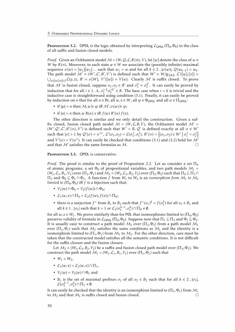
Proposition 3.2. OPDL is the logic obtained by interpreting LOPDL (Π0,Φ0) in the classof all suffix and fusion closed models.
Proof. Given an Ockhamist modelM = (W,Q,L,R (≡) ,V ), let [w] denote the class of w ∈W by R (≡). Moreover, to each state w ∈W we associate the (possibly infinite) maximalsequence σ (w) = [w1][w2] . . . such that w1 = w and for all k ∈ 2 . . |σ (w)|, Q (wk−1) = wk .The path model M′ = (W ′ ,L′ ,B′ ,V ′) is defined such that W ′ = W/R (≡), L′([w], [x]) =⋃y∈[w],z∈[x]L(y,z), B′ = σ [W ], V ′([w]) = V (w). Clearly M′ is suffix closed. To prove
that M′ is fusion closed, suppose σ1,σ2 ∈ B′ and σ k1 = σ k′
2 . It can easily be proved byinduction that for all i ∈ 1 . . k, σ i..k1 σ>k
′2 ∈ B. The base case when i = k is trivial and the
inductive case is straightforward using condition (3.1). Finally, it can easily be provedby induction on n that for all n ∈N, all w,x ∈W , all ϕ ∈ ΦOPDL and all α ∈ΠOPDL:
• if |ϕ| = n thenM,w |= ϕ iffM′ ,σ (w) |= ϕ;
• if |α| = n then w R(α) x iff f (w) R′(α) f (x).The other direction is similar and we only detail the construction. Given a suf-
fix closed, fusion closed path model M = (W,L,B,V ), the Ockhamist model M′ =(W ′ ,Q′ ,L′ ,R′ (≡) ,V ′) is defined such that W ′ = B, Q′ is defined exactly at all σ ∈ W ′
such that |σ | > 1 by Q′(σ ) = σ>1, L′(σ1,σ2) = L(σ11 ,σ
21 ), R
′ (≡) =(σ1,σ2) ∈W ′
∣∣∣ σ11 = σ1
2
and V ′(σ ) = V (σ1). It can easily be checked that conditions (3.1) and (3.2) hold forM′and thatM′ satisfies the same formulas asM.
Proposition 3.3. OPDL is conservative.
Proof. The proof is similar to the proof of Proposition 2.2. Let us consider a set Π0of atomic programs, a set Φ0 of propositional variables, and two path models M1 =(W1,L1,B1,V1) over (Π1,Φ1) andM2 = (W2,L2,B2,V2) over (Π2,Φ2) such thatΠ0 ⊆Π1∩Π2 and Φ0 ⊆ Φ1 ∩Φ2. A function f from W1 to W2 is an isomorphism fromM1 toM2limited to (Π0,Φ0) iff f is a bijection such that:
• V1(w)∩Φ0 = V2(f (w))∩Φ0;
• L1(w,x)∩Π0 = L2(f (w), f (x))∩Π0;
• there is a surjection f + from B1 to B2 such that f +(σ1)k = f (σk1 ) for all σ1 ∈ B1 and
all k ∈ 1 . . |σ1| such that k = 1 or L1(σ k−11 ,σ k1 )∩Π0 , ∅.for all w,x ∈W1. We prove similarly than for PDL that isomorphisms limited to (Π0,Φ0)preserve validity of formula in LOPDL (Π0,Φ0). Suppose now that Π1 ⊆Π2 and Φ1 ⊆ Φ2.It is usually easy to construct a path model M2 over (Π2,Φ2) from a path model M1over (Π1,Φ1) such that M2 satisfies the same conditions as M1 and the identity is aisomorphism limited to (Π1,Φ1) fromM1 toM2. For the other direction, care must betaken that the constructed model satisfies all the semantic conditions. It is not difficultfor the suffix closure and the fusion closure.
LetM2 = (W2,L2,B2,V2) be a suffix and fusion closed path model over (Π2,Φ2). Weconstruct the path modelM1 = (W1,L1,B1,V1) over (Π1,Φ1) such that
• W1 =W2,
• L1(w,x) = L2(w,x)∩Π1,
• V1(w) = V2(w)∩Φ1 and
• B1 is the set of maximal prefixes σ1 of all σ2 ∈ B2 such that for all k ∈ 2 . . |σ1|,L(σ k−12 ,σ k2 )∩Π1 , ∅.
It can easily be checked that the identity is an isomorphism limited to (Π1,Φ1) fromM1toM2 and thatM1 is suffix closed and fusion closed.
30

Syntactic structures 3.2
Limit closure. B is limit closed iff whenever an infinite sequence σ ∈Wω is such thatfor all k ≥ 1, there is a sequence σk ∈ B such that σ≤kk = σ≤k then σ ∈ B. A similar con-dition makes the difference between BCTL* and CTL* [Reynolds.01]. The logic obtainedby interpreting LOPDL (Π0,Φ0) in the class of suffix, fusion and limit closed models iscalled OPDLlc.
Proposition 3.4. OPDLlc is conservative.
Proof. We use exactly the same constructions as in the proof of Proposition 3.3. We onlyhave to prove that the path modelM1 constructed fromM2 is limit closed. Let σ ∈Wω
1be an infinite sequence such that for all k ∈N there is σ1,k ∈ B1 such that σ≤k1,k is a prefixof σ . By definition, for all k ∈N there is σ2,k ∈ B2 such that σ1,k is a prefix of σ2,k . SinceM2 is limit closed by hypothesis, σ ∈ B2. If σ < B1 it means that for some ` ∈ 2 . .ω,L(σ `−1,σ `)∩Π1 = ∅ which is not possible because
∣∣∣σ1,`∣∣∣ ≥ ` and σ≤`1,` is a prefix of σ .
Total maximality. B is totally maximal iff B is the set of all maximal paths. Thelogic obtained by interpreting LOPDL (Π0,Φ0) in the class of totally maximal models isOPDLlts(Φ0,Π0), studied in [BalLor.13]. Unlike OPDL and OPDLlc, OPDLlts(Φ0,Π0) is notconservative. As a counter-example, consider the formula [a]⊥∧ 〈≡ ; a〉>. This formulais not OPDLlts(Φ0, a) satisfiable but is OPDLlts(Φ0, a,b) satisfiable. It can be provedthat OPDLlc and OPDLlts(Φ0,Π0) are the same if and only ifΠ0 is infinite. Moreover, theproof from [BalLor.13] that CTL* can be embedded into OPDLlts can easily be adaptedto prove that CTL* can be embedded into OPDLlc.
Seriality. B is serial iff all paths in B are infinite (B ⊆Wω). Combining this conditionwith suffix closure corresponds, in the Ockhamist semantics, to enforcingQ to be a totalfunction. The logic obtained by interpreting the language LOPDL (Π0,Φ0) in the class ofall serial path models is not conservative: consider for instance the formula [a]⊥ whichis not satisfiable if Π0 = a. But if Π0 is infinite, then any path model satisfying aformula ϕ0 can be turned into a serial path model satisfying ϕ0 by choosing an atomicprogram e not occurring in ϕ0 and by adding for each finite sequence σ ∈ B a state wσsuch that wσ is a successor by e of itself and of the last state in σ . This transformationpreserves satisfiability and the suffix closed, fusion closed and limit closed conditions.Therefore, since OPDL and OPDLlc are conservative, we can assume that these logics areinterpreted in serial path models.
Total seriality. B is totally serial iff B is the set of all infinite paths. By the con-structions used in the proofs of Corollary 3.12, we can prove that the logic obtainedby interpreting LOPDL (Π0,Φ0) in the class of all suffix closed, fusion closed and totallyserial models is OPDLlc.
3.2 Syntactic structures
In the next section, we describe a decision procedure for the satisfiability problem ofOPDL, based on the elimination of Hintikka sets procedure for PDL presented in Sec-tion 2.5 and its adaptation to BCTL* by Reynolds [Reynolds.07]. Since OPDL embedsboth PDL and BCTL* [BalLor.13], the decision procedure for OPDL combines features ofboth the aforementioned decision procedures. As presented in Section 2.5, the generalidea of elimination of Hintikka sets procedures is, given a formula ϕ0, to construct asyntactic structure which contains all the possible states then to eliminate the statespreventing the structure to be a proper satisfying model for ϕ0. For PDL the possiblestates are Hintikka sets (hues in [Reynolds.07]). For BCTL*, states are sets of Hintikkasets, called clusters in this chapter (colors in [Reynolds.07]). For OPDL, states must be
31

3. Ockhamist Propositional Dynamic Logics
〈≡〉ϕϕ
Figure 3.1: Additional rule for the Fischer-Ladner closure in OPDL
clusters too. But because of formulas like 〈a〉p∧ [b]¬p∧ 〈≡〉〈b〉p, the atomic programslabeling edges have to be considered. Hence the syntactic structures are more involvedthan for PDL or BCTL*. In the present section, we study these syntactic structures.There are two main results. First, Proposition 3.6 gives a syntactic characterizationof the satisfiability of a formula using syntactic structures. Second, the Witness Lemma(Lemma 3.8) provides a decomposition of any formula of the form 〈α〉ϕ into a set offormulas for the current state on one hand and a formula for a successor state on theother hand. We first define the basic concepts of Hintikka sets and clusters, then thesyntactic structures and the paths in such structure, before proving the aforementionedresults.
Hintikka sets and clusters
We extend the definition of the Fischer-Ladner closure from Section 2.2 to the lan-guage LOPDL (Π0,Φ0). From a purely syntactic point of view, ≡ is indistinguishable fromatomic programs. Hence, it suffices to add the rule in Figure 3.1 to extend the Fischer-Ladner closure to OPDL. As usual, we write FL(ϕ0) for the Fischer-Ladner closure ofthe OPDL formula ϕ0. It is straightforward to adapt the proof of Proposition 2.4 toprove that the cardinal of FL(ϕ0) is linear in |ϕ0|. We write SP (ϕ0) to denote the setα | ∃ϕ, 〈α〉ϕ ∈ FL(ϕ0).
A set H⊂ FL(ϕ0) is a Hintikka set for ϕ0 iff all the following conditions are satisfied:• for any ϕ ∈ FL(ϕ0), ϕ ∈ H iff ∼ϕ <H• for any
⟨α ; β
⟩ϕ ∈ FL(ϕ0),
⟨α ; β
⟩ϕ ∈ H iff 〈α〉
⟨β⟩ϕ ∈ H
• for any⟨α ∪ β
⟩ϕ ∈ FL(ϕ0),
⟨α ∪ β
⟩ϕ ∈ H iff 〈α〉ϕ ∈ H or
⟨β⟩ϕ ∈ H
• for any⟨ϕ?
⟩ψ ∈ FL(ϕ0),
⟨ϕ?
⟩ψ ∈ H iff ϕ ∈ H and ψ ∈ H
• for any 〈α∗〉ϕ ∈ FL(ϕ0), 〈α∗〉ϕ ∈ H iff ϕ ∈ H or 〈α〉〈α∗〉ϕ ∈ H• if [≡]ϕ ∈ H then ϕ ∈ HA set C of Hintikka sets for ϕ0 is a cluster for ϕ0 iff C , ∅ and for any H1,H2 ∈ C the
following conditions are satisfied:• for any propositional variable p ∈ FL(ϕ0), p ∈ H1 iff p ∈ H2
• for any formula 〈≡〉ϕ ∈ FL(ϕ0), 〈≡〉ϕ ∈ H1 iff 〈≡〉ϕ ∈ H2
Given a set P ⊆Π0 of atomic programs, the successor relation SP over Hintikka setsis defined such that H1 SP H2 iff
• for any formula 〈a〉ϕ ∈ H1, a ∈ P and
• for any formula 〈a〉ϕ ∈ FL(ϕ0) such that a ∈ P , 〈a〉ϕ ∈ H1 iff ϕ ∈ H2.These relations are extended to clusters: given a set P ⊆Π0, C1 SP C2 iff for all H2 ∈ C2there exists H1 ∈ C1 such that H1 SP H2.
Syntactic structures and paths
A syntactic structure is a pseudo-model where the valuation has been replaced with afunction assigning clusters and where the bundle is implicit. Intuitively, each Hintikkaset in the cluster associated to a state w corresponds to the set of formulas satisfiedby a history starting at w. Formally, a syntactic structure for a formula ϕ0 is a tupleS = (W,L,C) where:
32

Syntactic structures 3.2
• W is a nonempty set of states,
• L assigns a set of atomic programs to each pair of states,
• C assigns a cluster for ϕ0 to each state such that for all w,x ∈W , if L(w,x) , ∅ thenC(w) SL(w,x) C(x).
A syntactic structure is standard iff:• ϕ0 ∈ H for some H ∈C(w) and some w ∈W and
• for all w ∈W , there exists x ∈W such that L(w,x) , ∅.A path in a syntactic structure S is a (possibly infinite) nonempty sequence π over
the alphabet composed by the special branching symbol • and all pairs (H,w) such thatw ∈ W and H ∈ C(w). Any path π must satisfy all the following conditions, for allk ∈ 1 . . |π|:
• π1 , • and if |π| < ω, π|π| , •;• if πk = • then we have that πk−1 = (H,w) and πk+1 = (H′ ,w) for some w ∈W andsome H,H′ ∈C(w);
• if πk = (Hk ,wk) and πk+1 = (Hk+1,wk+1) then we have that L(wk ,wk+1) , ∅ andHk SL(wk ,wk+1) Hk+1.
The relation carries between a finite path and a program is defined as the least relationsatisfying the following conditions:
• (H1,w1)(H2,w2) carries a iff a ∈ L(w1,w2).
• (H1,w) • (H2,w) carries ≡.• (H1,w1) carries ϕ? iff ϕ ∈ H1.
• π carries (α ∪ β) iff π carries α or β.
• π carries (α ; β) iff for some m ∈ 1 . . |π|, π≤m carries α and π≥m carries β.
• π carries α∗ iff there is a nonempty list k0, . . . , km such that k0 = 1, km = |π| and forall i < m, ki < ki+1 and πki ...ki+1 carries α.
An unbranching path is a path which contains no occurrences of the branching symbol •.The trunk of a path is its longest unbranching prefix. The support of an unbranchingpath (H1,w1)(H2,w2) . . . is the sequence w1w2 . . ..
An eventuality chain is a nonempty sequence η = α1 . . .αnϕ where the last element isa formula and the other elements are programs. To an eventuality chain η = α1 . . .αnϕcorresponds the formula form(η) = 〈α1〉 . . .〈αn〉ϕ. This correspondence is not injective,for instance the eventuality chains aap, a〈a〉p and 〈a〉 〈a〉p all correspond to the sameformula 〈a〉〈a〉p. Themaximal eventuality chain for a formulaϕ is the longest eventualitychain η such that form(η) = ϕ. Fulfillment of an eventuality chain η by a path π isdefined inductively as follows:
• The path π fulfills a one-element eventuality chain η = ϕ iff π = (H1,w1) andϕ ∈ H1 for some state w1 and some Hintikka set H1 ∈C(w1);
• The path π fulfills an eventuality chain η = αη′ iff there is k ∈ 1 . . |π| such thatπ≤k carries α and π≥k fulfills η′ .
For any eventuality chain η = αϕ of length two, the corresponding formula 〈α〉ϕ iscalled an eventuality and any path fulfilling η is said to fulfill the eventuality 〈α〉ϕ. A statew ∈W is fulfilling if for any Hintikka setH ∈C(w) and any eventuality 〈α〉ϕ ∈ H, thereis a path π from (H,w) fulfilling 〈α〉ϕ. A syntactic structure S fulfills all eventualities iffall its states are fulfilling. A justifying path is an infinite unbranching path π such thatfor all k, if πk = (Hk ,wk) for some Hk and wk then for any eventuality 〈α〉ϕ ∈ Hk , thereis a fulfilling path π′ for 〈α〉ϕ starting at (Hk ,wk) such that the trunk of π′ is a prefixof π≥k .
33
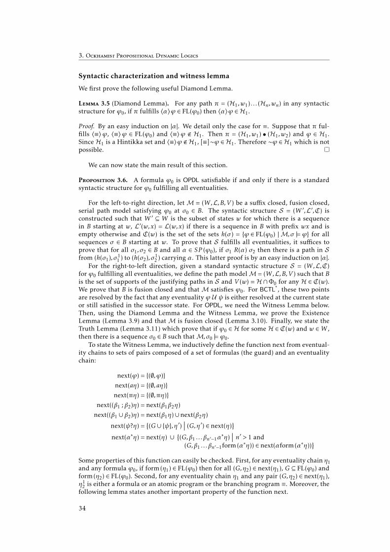
3. Ockhamist Propositional Dynamic Logics
Syntactic characterization and witness lemma
We first prove the following useful Diamond Lemma.
Lemma 3.5 (Diamond Lemma). For any path π = (H1,w1) . . . (Hn,wn) in any syntacticstructure for ϕ0, if π fulfills 〈α〉ϕ ∈ FL(ϕ0) then 〈α〉ϕ ∈ H1.
Proof. By an easy induction on |α|. We detail only the case for ≡. Suppose that π ful-fills 〈≡〉ϕ, 〈≡〉ϕ ∈ FL(ϕ0) and 〈≡〉ϕ < H1. Then π = (H1,w1) • (H1,w2) and ϕ ∈ H1.Since H1 is a Hintikka set and 〈≡〉ϕ <H1, [≡]∼ϕ ∈ H1. Therefore ∼ϕ ∈ H1 which is notpossible.
We can now state the main result of this section.
Proposition 3.6. A formula ϕ0 is OPDL satisfiable if and only if there is a standardsyntactic structure for ϕ0 fulfilling all eventualities.
For the left-to-right direction, letM = (W,L,B,V ) be a suffix closed, fusion closed,serial path model satisfying ϕ0 at σ0 ∈ B. The syntactic structure S = (W ′ ,L′ ,C) isconstructed such that W ′ ⊆ W is the subset of states w for which there is a sequencein B starting at w, L′(w,x) = L(w,x) if there is a sequence in B with prefix wx and isempty otherwise and C(w) is the set of the sets h(σ ) = ϕ ∈ FL(ϕ0) | M,σ |= ϕ for allsequences σ ∈ B starting at w. To prove that S fulfills all eventualities, it suffices toprove that for all σ1,σ2 ∈ B and all α ∈ SP (ϕ0), if σ1 R(α) σ2 then there is a path in Sfrom (h(σ1),σ
11 ) to (h(σ2),σ
12 ) carrying α. This latter proof is by an easy induction on |α|.
For the right-to-left direction, given a standard syntactic structure S = (W,L,C)for ϕ0 fulfilling all eventualities, we define the path modelM = (W,L,B,V ) such that Bis the set of supports of the justifying paths in S and V (w) = H∩Φ0 for any H ∈ C(w).We prove that B is fusion closed and thatM satisfies ϕ0. For BCTL*, these two pointsare resolved by the fact that any eventuality ϕ U ψ is either resolved at the current stateor still satisfied in the successor state. For OPDL, we need the Witness Lemma below.Then, using the Diamond Lemma and the Witness Lemma, we prove the ExistenceLemma (Lemma 3.9) and thatM is fusion closed (Lemma 3.10). Finally, we state theTruth Lemma (Lemma 3.11) which prove that if ϕ0 ∈ H for some H ∈ C(w) and w ∈W ,then there is a sequence σ0 ∈ B such thatM,σ0 |= ϕ0.
To state the Witness Lemma, we inductively define the function next from eventual-ity chains to sets of pairs composed of a set of formulas (the guard) and an eventualitychain:
next(ϕ) = (∅,ϕ)next(aη) = (∅, aη)next(≡η) = (∅,≡η)
next((β1 ; β2)η) = next(β1β2η)
next((β1 ∪ β2)η) = next(β1η)∪next(β2η)next(ψ?η) =
(G∪ ψ,η′)
∣∣∣ (G,η′) ∈ next(η)next(α∗η) = next(η) ∪
(G,β1 . . .βn′−1α
∗η)∣∣∣ n′ > 1 and
(G,β1 . . .βn′−1form(α∗η)) ∈ next(αform(α∗η))
Some properties of this function can easily be checked. First, for any eventuality chain η1and any formula ϕ0, if form(η1) ∈ FL(ϕ0) then for all (G,η2) ∈ next(η1), G ⊆ FL(ϕ0) andform(η2) ∈ FL(ϕ0). Second, for any eventuality chain η1 and any pair (G,η2) ∈ next(η1),η12 is either a formula or an atomic program or the branching program ≡. Moreover, thefollowing lemma states another important property of the function next.
34

Syntactic structures 3.2
Lemma 3.7. For any eventuality chain η1 and any Hintikka set H, if form(η1) ∈ H thenthere is (G,η2) ∈ next(η1) such that G∪ form(η2) ⊆ H.
Proof. The proof is by a straightforward induction on the sum∑∣∣∣η1∣∣∣−1k=1
∣∣∣ηk1 ∣∣∣ of the lengthof the programs in η1.
We now prove the Witness Lemma.
Lemma 3.8 (Witness Lemma). For any syntactic structure S = (W,L,C), any state w ∈W , any Hintikka setH ∈C(w), any eventuality chain η1 such that form(η1) ∈ H and anypath π in S from (H,w), π fulfills η1 if and only if there is (G,η2) ∈ next(η1) such thatG∪ form(η2) ⊆ H and π fulfills η2.
Proof. The proof is by induction on the sum∑∣∣∣η1∣∣∣−1k=1
∣∣∣ηk1 ∣∣∣ of the length of the programsin η1. We only detail the case when η11 is an iteration, the other cases being straightfor-ward.
For the left-to-right direction, suppose that π fulfills α∗η. By definition, there isa nonempty list k0 . . . km such that k0 = 1, π≥km fulfills η and for all i < m, ki < ki+1and πki ..ki+1 carries α. If m = 0 then π fulfills η and the property holds by inductionhypothesis. Suppose m > 0. By Lemma 3.5, form(α∗η) ∈ Hk1 for (Hk1 ,Ck1 ) = π
k1 andform(αα∗η) ∈ H. By induction hypothesis, there is (G,η2) ∈ next(αform(α∗η)) such thatG∪form(η2) ⊆ H and π≤k1 fulfills η2. It is the case that
∣∣∣η2∣∣∣ > 1 because otherwise k1 =
k0 which is not possible. Therefore π fulfills η<∣∣∣η2∣∣∣
2 α∗η and (G,η<∣∣∣η2∣∣∣
2 α∗η) ∈ next(α∗η).For the right-to-left direction, suppose there is (G,η2) ∈ next(α∗η) such that G ∪
form(η2) ⊆ H and π fulfills η2. If (G,η2) ∈ next(η) then by induction hypothesis, π ful-fills η. Therefore, π fulfills α∗η. Suppose now that (G,η2) < next(η). For some eventu-
ality chain η3 we have (G,η3) ∈ next(αform(α∗η)) and η2 = η<∣∣∣η3∣∣∣
3 α∗η. There must existsa nonempty list k0 . . . km such that k0 = 1, π≥km fulfills α∗η and for all i ∈ 1 . .m, ki−1 ≤ kiand πki−1..ki carries ηi3. Moreover, by Lemma 3.5, form(α∗η) ∈ Hkm for (Hkm ,Ckm ) = π
km .Therefore, by induction hypothesis, π≤km carries α. Hence, by definitions, π fulfillsα∗η.
We can now prove the other lemmas mentioned in the proof of Proposition 3.6.
Lemma 3.9 (Existence Lemma). For any finite unbranching path π in a standard syn-tactic structure S fulfilling all eventualities, there is a justifying path π′ in S such thatπ is a prefix of π′ .
Proof. Suppose S = (W,L,C) is a standard syntactic structure for ϕ0 fulfilling all even-tualities. Given a finite unbranching path π0 = (H1,w1) . . . (Hn,wn), we collect the set Eof pairs (k,〈α〉ϕ) such that k ∈ 1 . .n, 〈α〉ϕ ∈ Hk and there is no path π1 from (Hk ,wk) inS such that π1 fulfills 〈α〉ϕ and the trunk of π1 is a prefix of π
≥k0 . If E is empty, since S is
standard, there exists (Hn+1,wn+1) such that π0(Hn+1,wn+1) is a path. If E is not empty,we choose (k,〈α〉ϕ) ∈ E such that for all (k′ ,〈α′〉ϕ′) ∈ E, k′ ≥ k. Then we extend π0 toπ0π+ such that there is a path π1 from (Hk ,wk) fulfilling 〈α〉ϕ and such that the trunkof π1 is π≥k0 π+. By repeating this procedure infinitely, a justifying path with prefix πis clearly obtained. The only point to prove is that there always exists such a path π+.If k = n, since S fulfills all eventuality, π+ exists. Otherwise, by the Witness Lemma, iffor some eventuality chain ηk , (k, form(ηk)) ∈ E, then there is another eventuality chainηk+1 such that (k + 1, form(ηk+1)) ∈ E and for any path π1 from (Hk+1,wk+1) fulfillingηk+1, the path (Hk ,wk)π1 fulfills ηk . Therefore, π+ always exists.
35

3. Ockhamist Propositional Dynamic Logics
Lemma 3.10. The set of the supports of the justifying paths in any syntactic structureis fusion closed.
Proof. Let S = (W,L,C) be a syntactic structure and B the set of the supports of thejustifying paths in S . Suppose σ1,σ2 ∈ B are two sequences such that σ `1 = σm2 for some`,m ∈N. Since B is suffix closed, there is a justifying path π2 in S from (H` ,σ `1 ) whosesupport is σ≥m2 . We prove by induction on ` that there is a justifying path π1 such thatπ≥`1 = π2 and the support of π≤`1 is σ≤`1 . The case when ` = 1 is trivial. For ` > 1, byinduction hypothesis, there is a justifying path π1 such that π≥`−11 = π2 and the supportof π≤`−11 is σ2..`
1 . Let (H2,w2) = π11 and w1 = σ
11 . By definition, there is H1 ∈ C(w1) such
thatH1 SL(w1,w2) H2. By Lemma 3.8, for any eventuality 〈α〉ϕ ∈ H1, either (H1,w1) is thetrunk of a path fulfilling 〈α〉ϕ, or there is an eventuality chain η such that form(η) ∈H2 and for any path π3 from (H2,w2) fulfilling η, the path (H1,w1)π3 fulfills 〈α〉ϕ.Therefore, (H1,w1)π1 is justifying.
Lemma 3.11 (Truth Lemma). For any justifying path (H1,w1) . . . with support σ , andany formula ϕ ∈ H1,M,σ |= ϕ.
Proof. We prove, by induction on N ∈ N, that the following conditions hold for anyjustifying path π from (H1,w1) with support σ and any N ∈N:
IH.1 For any formula ϕ ∈ H1, if |ϕ| =N thenM,σ |= ϕ.IH.2 For any program α, any finite path π1 = (H′1,w
′1) . . . (H′n,w′n) and any integer ` ∈
1 . .n, if |α| = N , π≤`1 carries α and the trunk of π1 is a prefix of π then there existsa justifying path π2 with support σ2 such that σ R(α) σ2 and the trunk of π≥`1 is aprefix of π2.
IH.3 For any program α ∈ SP (ϕ0) and any infinite sequence σ1 ∈ B, if |α| = N − 1 andσ R(α) σ1 then there is an infinite path π1 from (H′1,w
′1) justifying σ1 and a finite
path from (H1,w1) to (H′1,w′1) carrying α.
All the cases are straightforward. We detail only the proof of hypothesis IH.2 for se-quential compositions. Suppose π≤`1 carries α ; β. By definition, there is `′ ∈ 1 . . ` suchthat π≤`
′
1 carries α and π`′ ..`
1 carries β. Since |α| < N , by induction hypothesis, there is ajustifying path π2 with support σ2 such that σ R(α) σ2 and the trunk of π≥`
′
1 is a prefixof π2. Similarly, since
∣∣∣β∣∣∣ < N , by induction hypothesis, there is a justifying path π3
with support σ3 such that σ2 R(β) σ3 and the trunk of π≥`1 is a prefix of π3. Moreover,σ R(α ; β) σ3.
In the proof of Proposition 3.6, given a standard syntactic structure S = (W,L,C)fulfilling all eventualities, we construct the path modelM = (W,L,B,V ) in which B isthe set of the supports of the justifying paths in S . Therefore if the set of the supportsof the justifying paths in S is limit closed then B is limit closed too. Hence the followingcorollary can be deduced from Proposition 3.6.
Corollary 3.12. A formula ϕ0 is OPDLlc satisfiable if and only if there is a standardsyntactic structure S for ϕ0 which fulfills all eventualities and such that the set of thesupports of the justifying paths in S is limit closed.
3.3 Optimal decision procedure for OPDL
We describe a procedure which, given a formula ϕ0, either fails or exhibits a standardsyntactic structure for ϕ0 fulfilling all eventualities. The procedure inductively con-structs a finite sequence S0 . . .Sn of syntactic structures for ϕ0.
36

Tree syntactic structure property of OPDLlc 3.4
The initial syntactic structure S0 = (W0,L0,C0) is defined such that:• W0 is the set of all pairs (P ,C) where P is a nonempty subset of SP + (ϕ0) and C is acluster for ϕ0,
• L((P1,C1), (P2,C2)) = P2 if C1 SP2 C2 and is empty otherwise,
• C(P ,C) = C.where SP + (ϕ0) SP (ϕ0)∪ e for some fixed e < SP (ϕ0). Then for all k, the syntacticstructure Sk+1 is constructed from Sk = (Wk ,Lk ,Ck) by removing from Wk the states(P ,C) which are not fulfilling or such that for some H ∈ C, there is no (P ′ ,C′) ∈Wk andH′ ∈ C′ such that C SP ′ C′ and H SP ′ H′ .
There exists a constant K such that the number of states inW0 for any ϕ0 is boundedby 22
K ·`where ` = |ϕ0|. Therefore, for some n ≤ 22
K ·`no state can be eliminated from Sn.
The procedure terminates successfully iff there is a state (P ,C) ∈Wn and a Hintikka setH ∈ C such that ϕ0 ∈ H.
Lemma 3.13. The procedure for ϕ0 is successful if and only if ϕ0 is OPDL satisfiable.
Proof. The completeness proof is direct by Proposition 3.6. For the soundness proof, byProposition 3.6 there is a standard syntactic structure S = (W,L,C) for ϕ0 fulfilling alleventualities. We first define the function g fromΠ0 to SP + (ϕ0) by g(a) = a if a ∈ SP (ϕ0)else g(a) = e. Then, for all k ∈ 0 . .n, the function fk is defined inductively by
f (P , (H,w)) = (H, (p,C(w)))
f (P , (H1,w1)π) = (H1, (P ,C(w1)))f (g [L(w1,w2)] ,π) where (H2,w2) = π1
f (P , (H1,w1) •π) = (H1, (P ,C(w1))) • f (P ,π)
for all subsets P ⊆ SP + (ϕ0) and all finite paths π in S . It can easily be proved byinduction on k that for all k ∈ 0 . .n, all w ∈W , all P ⊆ SP + (ϕ0), all paths π in S and alleventuality chains η:IH.1 (P ,C(w)) ∈Wk
IH.2 if π fulfills η in S and form(η) ∈ FL(ϕ0) then f (P ,π) fulfills η in Sk .
Proposition 3.14. The satisfiability problem of OPDL is 2EXPTIME-complete.
Proof. We have already proved that the number of steps in our decision procedure isbounded by a double exponential in |ϕ0|. The method used in [Lange.06] can easily beadapted to prove that the eventuality condition can be checked in deterministic poly-nomial time in the number of pairs (H, (P ,C)) such that H ∈ C and (P ,C) in Wk . There-fore, the decision procedure can be executed in deterministic double exponential timein |ϕ0|. By a polynomial faithful translation of BCTL* into OPDL, it has been shownin [BalLor.13] that the satisfiability problem for OPDL is 2EXPTIME-hard. Thereforethe satisfiability problem for OPDL is 2EXPTIME-complete.
3.4 Tree syntactic structure property of OPDLlc
The procedure of Section 3.3 is difficult to adapt to OPDLlc because no simple conditioncan be checked during the construction of the syntactic structure to guarantee that theset of the supports of all justifying paths is limit closed. Therefore, we prove in thissection that OPDLlc has a particular tree model property. This property is used in thenext section to reduce the satisfiability problem of OPDLlc to the (dual of) the emptinessproblem of an automaton on infinite trees. Because syntactic structures are more conve-nient than models for decision procedures, we prove a tree syntactic structure property,from which the usual tree model property can be deduced using the construction ofSection 3.2.
37
3. Ockhamist Propositional Dynamic Logics
An N -ary ω-tree over an alphabet Σ is a function T : [1 . .N ]∗ −→ Σ. In such a tree,nodes are labeled with elements of Σ. A branch in T is an infinite sequence σ1 = λ1λ2 . . .for which there exists σ2 ∈ [1 . .N ]ω and i ∈N such that for all k > 0, λk = σ
≤i+k2 . Like in
the previous section, we need nodes to be labeled with pairs (P ,C) where P is the set ofatomic programs labeling the incoming edge and C is a cluster. To simulate incompletetrees, we allow P to be empty, in which case the branch is said to be pruned.
Definition 3.15. An N -ary syntactic tree for a formula ϕ0 is an N -ary ω-tree T overΣ =P (Π0)×Clusters(ϕ0) where Clusters(ϕ0) is the set of clusters on ϕ0 and such that:
(3.3) TP (ε) = ∅ and there is σ ∈ [1 . .N ]ω such that for all i > 0, TP (σ≤i) , ∅;(3.4) for all λ ∈ [1 . .N ]∗ and k ∈ 1 . .N , TP (λk) = ∅ or TC(λ) STP (λk) TC(λk);where TP and TC are the projections of T on P (Π0) and Clusters(ϕ0), respectively. Abranch σ in T is valid if for all k > 1, TP (σ k) , ∅ and pruned otherwise.
To any N -ary syntactic tree T = (TP ,TC) naturally corresponds the syntactic struc-ture S(T ) = ([1 . .N ]∗,L,TC) where L(λ1,λ2) = TP (λ2) if λ2 = λ1k for some k ∈ 1 . .Nand is the empty set otherwise. Therefore, an N -ary syntactic tree can be seen as atree syntactic structure. Indeed, we will abusively write about paths in syntactic trees.For the following definition of a good syntactic tree, since we do not assume that thecorresponding syntactic structure fulfills all eventualities, we adapt the definition of ajustifying path. A pseudo-justifying path is an infinite unbranching path π such that forall k > 0, if πk = (Hk ,wk) then for any eventuality 〈α〉ϕ ∈ Hk there is ` ≥ k such thatπ` = (H` ,w`) and either πk..` fulfills 〈α〉ϕ or there is an eventuality chain η such thatη1 = ≡, form(η) ∈ H` and for any path π2 from π` fulfilling η, πk..(`−1)π2 fulfills 〈α〉ϕ.By the Witness Lemma, any justifying path is a pseudo-justifying path.
Definition 3.16. An N -ary syntactic tree T = (TP ,TC) for a formula ϕ0 is good iff all thefollowing conditions hold:(3.5) any valid branch σ is the support of a pseudo-justifying path;
(3.6) for any node λ in a valid branch of T , if there is H ∈ TC(λ) such that 〈≡〉ψ ∈ Hfor some formula ψ, then there is a Hintikka set H′ ∈ TC(λ) and a finite path πin T from (H′ ,λ) such that
• π fulfilling the maximal eventuality chain for ψ and• for all k ∈ 2 . . |π|, if πk = (H′′ ,λ′′) then there is a pseudo-justifying path in Tfrom (H′′ ,λ′′);
(3.7) there is a pseudo-justifying path in T from (H,ε) such that ϕ0 ∈ H.
Lemma 3.17. In a good N -ary syntactic tree, any pseudo-justifying path whose supportis on a valid branch is a justifying path.
Proof. Let π be a pseudo-justifying path in a good N -ary syntactic tree such that π1 =(H,λ) for some λ in a valid branch. We prove that π is a justifying path. Suppose thatπk = (Hk ,λk) and 〈α〉ϕ ∈ Hk . Since π is a pseudo-justifying path, there is ` ≥ k such thatπ` = (H` ,λ`) and either πk..` fulfills 〈α〉ϕ or there is an eventuality chain η such thatη1 = ≡, form(η) ∈ H` and for any path π2 from π` fulfilling η, πk..(`−1)π2 fulfills 〈α〉ϕ.In the latter case, since λ` is in a valid branch, by condition (3.6) there is a path from(Hk ,λk) fulfilling 〈α〉ϕ.
Let N≡ϕ0be the number of eventualities of the form 〈≡〉ψ in FL(ϕ0) plus one. The
tree property of OPDLlc is stated as follows.
Proposition 3.18. A formula ϕ0 is OPDLlc satisfiable if and only if there is a goodN≡ϕ0
-ary syntactic tree for ϕ0.
38

Tree syntactic structure property of OPDLlc 3.4
Proof. For the left-to-right direction, suppose T is a good syntactic tree for ϕ0. Considerthe tuple S ′(T ) = ([1 . .N≡ϕ0
]∗,L,C) where L is define as for S(T ) and C(λ) is the set ofHintikka set H such that there is a pseudo-justifying path in T starting with (H,λ). Itcan easily be checked that S ′(T ) is a syntactic structure and fulfills all eventualities.Moreover, to each pseudo-justifying path in T corresponds a justifying path in S ′(T )and since the set of valid branches is limit closed, the set of the supports of the justifyingpaths in S ′(T ) is limit closed. By Corollary 3.12, ϕ0 is OPDLlc satisfiable.
For the left-to-right direction, suppose ϕ0 is satisfiable. By Corollary 3.12, thereis a standard syntactic structure S = (W,L,C) for ϕ0 which fulfills all eventualitiesand such that the set of the supports of the justifying paths in S is limit closed. Weconstruct from S a good N≡ϕ0
-ary syntactic tree for ϕ0. The construction is inspiredby a similar construction for CTL* [EmeSis.84]. Let 〈≡〉ψ2, . . . ,〈≡〉ψN≡ϕ0 be an orderingof the eventualities of the form 〈≡〉ψ in FL(ϕ0). We first define the N≡ϕ0
-ary ω-treeTpath over the alphabet of all the paths in S plus the empty word ε. By Lemma 3.9,there is a justifying path π0 from (H0,w0). We label the root of Tpath with this path:Tpath(ε) = π0. For each node λ ∈ [1 . .N≡ϕ0
]∗, if Tpath(λ) , ε, the labeling path continues atthe first successor: Tpath(λ1) = Tpath(λ)≥2. For the other successors k ∈ 2 . .N≡ϕ0
of λ, let(Hλ,wλ) = Tpath(λ)1. If 〈≡〉 ψk ∈ Hλ then let π1 be the shortest path in S fulfillingthe maximal eventuality chain for ψk and such that π1
1 = (H′ ,wλ) for some H′ . ByLemma 3.9, there is a justifying path πλk which has the trunk of π1 as prefix. Welabel the kth successor of λ with it: Tpath(λk) = π
≥2λk . Otherwise, if 〈≡〉ψk−1 < Hλ then
Tpath(λk) = ε. All successors of a node labeled with ε are labeled with ε.The good N≡ϕ0
-ary syntactic tree T for ϕ0 is constructed from Tpath as follows. Forthe root node, T (ε) = (∅,C(w0)). For λ ∈ [1 . .N≡ϕ0
]∗ and k ∈ 1 . .N≡ϕ0, if Tpath(λ)1 = (Hλ,wλ)
and Tpath(λk)1 = (Hλk ,wλk) then T (λk) = (L(wλ,wλk),C(wλk)). Otherwise, T (λk) = (∅,C)for some arbitrary cluster C. T is a syntactic tree because, by construction, for allλ ∈ [1 . .N≡ϕ0
]∗ and k ∈ 1 . .N≡ϕ0, if Tpath(λ)1 = (Hλ,wλ) and Tpath(λk)1 = (Hλk ,wλk), then
TP (λk) , ∅ and C(wλ) STP (λk) C(wλk). It remains to be proved that T is good. Letus define the N≡ϕ0
-ary ω-tree TW over W ∪ ⊥ (we assume ⊥ < W ) such that for allλ ∈ [1 . .N≡ϕ0
]∗, TW (λ) = wλ if (Hλ,wλ) = Tpath(λ)1 and TW (λ) = ⊥ otherwise. A validpath in T is a path π whose support is a valid branch, i.e., for all (H,λ) occurring in π,TW (λ) , ⊥. To each valid path π = (H1,λ1)(H2,λ2) . . . in T we associate the sequencef (π) = (H1,TW (λ1))(H2,TW (λ2)) . . .. We prove the following two claims:
Claim 1. If π is a valid path in T then f (π) is a path in S . Moreover, if π is finitethen π and f (π) carry the same programs.
Proof. For the first part of the claim, the proof is by transfinite induction on thelength of π. The base case when the length of π is 1 is trivial. Consider nowa path π of length n ∈ N and let πn = (Hn,λn) and T (λn) = (Pn,Cn). If πn−1 =(Hn−1,λn−1), then λn = λn−1k for some k ∈ 1 . .N≡ϕ0
. Moreover, Pn , ∅, Hn−1 SPn HnandL(TW (λn−1),TW (λn)) = Pn. Hence, since by induction hypothesis, f (π<n) is a pathin S , f (π) is a path in S . If πn−1 = • then πn−2 = (Hn−2,λn) for some Hn−2 ∈ TC(λn)and since by induction hypothesis, f (π≤n−2) is a path in S , f (π) is a path in S . Fi-nally, if π is infinite, by transfinite induction hypothesis, for all k > 0, f (π≤k) is apath in S . Since the set of all the paths in any syntactic structure is limit closed,f (π) is a path in S . The second part of the claim can easily be proved by inductionon the length of the program.
Claim 2. For any valid branch σ = λ1λ2 . . . in T , there is a justifying path in S withsupport TW (λ1)TW (λ2) . . ..
Proof. Since the set of the supports of the justifying paths in S is limit closed, itsuffices to prove that for any valid branch σ = λ1λ2 . . . in T and for all n > 0 there is
39

3. Ockhamist Propositional Dynamic Logics
a justifying path π in S such that the support of π≤n is a prefix of TW (λ1)TW (λ2) . . ..The proof is by induction on n. For the base case when n = 1, the property holdsby Lemma 3.9. For n > 1, by induction hypothesis, there is a justifying path πn−1in S such that the support of π≤n−1n−1 is a prefix of TW (λ1)TW (λ2) . . .. Moreover, bydefinition, λn = λn−1k for some k ∈ 1 . .N≡ϕ0
. Since T is a syntactic tree, for someHintikka sets Hn−1 and Hn, (Hn−1,λn−1)(Hn,λn) is a path in T . By the previousclaim, (Hn−1,TW (λn−1))(Hn,TW (λn)) is a path in S and by Lemma 3.9 this path canbe extended to a justifying path π+. Finally, since by Lemma 3.10 the set of thesupports of the justifying paths in S is fusion closed, there is a justifying path πnin S such that the support of π≤nn is a prefix of TW (λ1)TW (λ2) . . ..
Now we prove that T satisfies condition (3.5) of Definition 3.16. Let σ = λ1λ2 . . . be avalid branch in T . By Claim 2, there is a justifying path π1 = (H1,TW (λ1))(H2,TW (λ2)) . . .in S . Obviously, π2 = (H1,λ1)(H2,λ2) . . . is a valid path in T . For any eventuality 〈α〉ϕ ∈Hk , for any k > 1, there is a finite path π3 of length ` in S fulfilling 〈α〉ϕ and such
that the trunk of π3 is a prefix of π≥k1 . If π3 is unbranching then πk..(k+`)2 fulfills 〈α〉ϕin T . Otherwise, there is m < ` such that π≤m3 is unbranching and πm+1
3 = •. By theWitness Lemma, there is an eventuality chain η such that η1 = ≡, form(η) ∈ Hk+m andfor all path π4 from (Hk+m,TW (λk+m)) in S fulfilling η, the path π<m3 π4 fulfills 〈α〉ϕ.Therefore, if π5 is a path from (Hk+m,λk+m) in T fulfilling η, by the first claim f (π5)
fulfills η too. Hence, by the first claim again, πk..(k+m−1)2 π5 fulfills 〈α〉ϕ. Therefore, π2is pseudo-justifying. Condition (3.7) can be proved similarly.
To prove that T satisfies condition (3.6), suppose 〈≡〉ψ ∈ H for some H ∈ TC(λ) andsome λ ∈ [1 . .N≡ϕ0
]∗ such that TP (λ) , ∅. By construction, 〈≡〉ψ ∈ Hλ where (Hλ,wλ) =Tpath(λ)1. Hence a minimal path π from (H′λ,wλ) in S fulfilling the maximal eventualitychain η for ψ has been selected during the construction of Tpath. We construct induc-tively a sequence of triple (πT ,i ,ηi ,πS,i) where the length of πS,i is strictly decreasingand such that for all i:(3.8) πT ,i is a finite path from (H′λ,λ) in T ;(3.9) πS,i is a minimal path in S fulfilling ηi ;
(3.10) π1S,i = (Hi ,TW (λi)) where (Hi ,λi) = π
∣∣∣πT ,i ∣∣∣T ,i ;
(3.11) for any path π+ from (Hi ,λi) in T , if π+ fulfills ηi then πT ,iπ≥2+ fulfills η;
(3.12) if π2S,i = (Hi+1,wi+1) for some wi+1 ∈ W and Hi+1 ∈ C(wi+1) then for some k,
Tpath(λik) starts with π2S,i and Hi STP (λik) Hi+1.
The initial triple is defined as ((H1,λ1),η,π) where (H1,TW (λ1)) = π1. It can easilybe checked that all the invariants hold. Suppose all the invariants hold for the triple(πT ,i ,ηi ,πS,i). If πS,i is of length 1 then πT ,i fulfills η and condition (3.6) is provedfor T . If π2
S,i = (Hi+1,wi+1) by the invariant (3.12), πT ,i+1 = πT ,i(Hi+1,λik) is a path
in T . It can easily be checked that (πT ,i+1,η≥2i ,π≥2S,i ) satisfies all the invariants. Finally,
if π2S,i = • then η
1i = ≡ and by construction, form(ηi) ∈ Hλi where (Hλi ,wi) = Tpath(λi)
1,hence a minimal path πS,i+1 from (Hi+1,wi) in S fulfilling ηi has been selected duringthe construction of Tpath. By minimality, the length of πS,i+1 is strictly less than thelength of πS,i . Hence, it can easily be checked that (πT ,i • (Hi+1,λi),η≥2i ,πS,i+1) satisfiesall the invariants.
3.5 Optimal decision procedure for OPDLlc
The decision procedure for OPDLlc presented in this section is by reduction to the dualof the emptiness problem of Streett tree automata. By Proposition 3.18, whenever a for-mula ϕ0 is satisfiable, there is a good N≡ϕ0
-ary syntactic tree for ϕ0. Therefore, we con-
40

Optimal decision procedure for OPDLlc 3.5
struct an automaton which recognizes exactly the good N≡ϕ0-ary syntactic trees for ϕ0.
We first recall the definitions of the automata used in the procedure before describingthe construction of our automaton.
Automata
A word automaton is a tuple A = (Σ,S,ρ,S0,F) where• Σ is the input alphabet,
• S is the set of states of the automaton,
• ρ : S ×Σ −→P (S) is a non-deterministic transition function,
• S0 ⊆ S is the set of initial states and
• F is the termination condition.The word automaton A is deterministic iff for any state s ∈ S and any symbol a ∈ Σ,∣∣∣ρ(s,a)∣∣∣ ≤ 1. Given an infinite word µ over Σ, a run of A on µ is a word r over S suchthat r1 ∈ S0 and for all k ≥ 1, rk+1 ∈ ρ(rk ,µk). The set of states occurring infinitely oftenin a run r is denoted by inf(r). For Buchi word automata, the termination condition is asubset F ⊆ S of accepting states. A word µ is accepted by a Buchi word automaton A iffthere is a run r of A on µ in which accepting states occur infinitely often: inf(r)∩F , ∅.
An N -ary tree automaton is a tuple A = (Σ,S,ρ,S0,F) similar to a word automatonexcept that ρ : S ×Σ −→ P
(SN
)assigns a set of N -ary tuples of states. Given an N -ary
ω-tree T over Σ, a run of A on T is a tree Tr over S such that Tr (ε) ∈ S0 and for allλ ∈ [1 . .N ]∗, (Tr (λ1), . . . ,Tr (λN )) ∈ ρ(Tr (λ),T (λ)). For all branches σ in Tr , the set ofstates occurring infinitely often in σ is denoted by inf(σ ). For Buchi tree automata, thetermination condition is a subset F ⊆ S of accepting states, as for Buchi word automata.A tree T is accepted by a Buchi tree automaton A iff there is a run Tr of A on T suchthat for any branch σ in Tr , inf(σ )∩ F , ∅. For Streett tree automata, the terminationcondition F ⊆ P (S) ×P (S) is a set of pairs of set of states. A tree T is accepted by aStreett tree automaton A iff there is a run Tr of A on T such that for any branch σ in Trand any pair (A,B) ∈ F, if inf(σ )∩A , ∅ then inf(σ )∩B , ∅.
There is a natural translation from any word automaton to a tree automaton suchthat a tree is accepted by the tree automaton iff all its branches, considered as infinitewords, are accepted by the word automaton. However, to directly translate a word au-tomaton to a tree automaton, the word automaton must be deterministic, because other-wise different branches may have to perform different choices at the same node. Hence,to any deterministic Buchi word automaton (Σ,S,ρ,S0,F), corresponds the Buchi treeautomaton (Σ,S,ρ′ ,S0,F) where ρ′(s,a) = (ρ(s,a), . . . ,ρ(s,a)). Moreover, a Buchi tree au-tomaton (Σ,S,ρ,S0,F) is equivalent to the Streett tree automaton (Σ,S,ρ,S0, (S\S0,S0)).
Decision procedure
Given a formula ϕ0 we construct a Streett tree automaton A which recognizes exactlythe goodN≡ϕ0
-ary syntactic trees forϕ0. We first describe three automata,AS ,AJ andAEover the same alphabet Σ = P (Π0)×Clusters(ϕ0). Each of these automata checks con-ditions from Definitions 3.15 and 3.16. Then we combine them into A.
Condition (3.4) is checked by the “safety” Buchi word automaton AS = (Σ,SS ,ρS ,SS,0,F) where:
• SS is the set of clusters on ϕ0 plus the special state I ,
• SS,0 = I, FS = SS and
• s1 ∈ ρS (s0, (P ,C)) iff– either s1 = I and P = ∅– or s1 = C, P , ∅, s0 is a cluster and s0 SP s1.
41
3. Ockhamist Propositional Dynamic Logics
Condition (3.5) is checked by the “justifying” Buchi word automaton AJ = (Σ,SJ ,ρJ ,SJ,0,FJ ) where:
• SJ is the set of pairs (H,E) where E is a set of eventuality chains to be fulfilled andH is a subset of FL(ϕ0) which is either a Hintikka set of the parent cluster or theempty set if the current node is the root or FL(ϕ0) if the current branch is pruned;
• SJ,0 = (∅,∅) and FJ =(H,E) ∈ SJ
∣∣∣ H , ∅ and E = ∅;
• (H1,E1) ∈ ρJ ((H0,E0), (P ,C)) if one of the following conditions holds:
– H0 is a Hintikka set, E0 , ∅, H1 ∈ C, P , ∅, H0 SP H1 and for all η0 ∈ E0,form(η0) ∈ H1 and there is (G1,η1) ∈ next(η0) such that G1 ∪ form(η1) ⊆ H1and if η11 ∈Π0 then η
≥21 ∈ E1.
– H0 , FL(ϕ0), E0 = ∅, H1 ∈ C, if H0 , ∅ then H0 SP H1 and for any eventuality〈α〉ϕ ∈ H1, there is (G1,η1) ∈ next(αϕ) such that G1 ∪ form(η1) ⊆ H1 and ifη11 ∈Π0 then η
≥21 ∈ E1.
– H1 = FL(ϕ0) and E1 , ∅.– H1 = FL(ϕ0), E1 = ∅ and P = ∅.– H1 = FL(ϕ0), E1 = ∅, H0 = FL(ϕ0) and E0 = ∅.
Finally, the “existential” Streett tree automatonAE = (Σ,SE ,ρE ,SE,0,FE) ensures thatthere is a pseudo-justifying path π from (H1,ε) where ϕ0 ∈ H1 and such that the sup-port of π is the branch obtained by always choosing the first successor (conditions (3.3)and (3.7)). Moreover, AE checks conditions (3.6). It is defined such that:
• SE is the set of triples (H,E, t) where H and E play the same role as in AJ and t isa Boolean value (> or ⊥) indicating whether the state is final;
• SE,0 = (∅,∅,⊥) and FE = (SE ,F) where F = (H,E, t) ∈ SE | t =>.The transition function ρE is defined such that if ((H1,E1, t1), . . . , (HN≡ϕ0 ,EN≡ϕ0 , tN≡ϕ0 )) ∈ρE((H0,E0, t0), (P ,C)) then all the following conditions hold:
• for all k ∈ 1 . .N≡ϕ0, either Hk ∈ C or Hk = FL(ϕ0);
• if H0 = ∅ then H1 is a Hintikka set and ϕ0 ∈ H1;
• if H0 is a Hintikka set then P , ∅, H1 is a Hintikka set and H0 SP H1;
• if H1 is a Hintikka set and E0 = ∅ then for all eventuality 〈α〉ϕ ∈ H1 there is(G2,η2) ∈ next(αϕ) such that G2 ∪ form(η2) ⊆ H1, if η
12 ∈Π0 then η
≥22 ∈ E1;
• if H1 is a Hintikka set then for all η1 ∈ E0, form(η1) ∈ H1 and there is (G2,η2) ∈next(η1) such that G2 ∪ form(η2) ⊆ H1, if η
12 ∈ Π0 then η≥22 ∈ E1 and if η12 = ≡
then tk =⊥ for k such that form(η2) = 〈≡〉ψk−1;• for all k ∈ 2 . .N≡ϕ0
, if H1 is a Hintikka set and 〈≡〉ψk−1 ∈ H1 then Hk is a Hintikkaset, ψk−1 ∈ Hk and there is (G2,η2) ∈ next(η1) where η1 is the maximal eventualitychain for ψk−1 such that G2 ∪ form(η2) ⊆ Hk , if η12 ∈ Π0 then η≥22 ∈ Ek and if
η12 = ≡ then∣∣∣∣form(
η≥22)∣∣∣∣ < ∣∣∣ψk−1∣∣∣;
• if E1 , ∅ then t1 =⊥.AS is deterministic and the number of its states is double exponential in |ϕ0|. It can
be directly translated into a Streett tree automaton with no termination pair. AJ has anexponential number of states but it must be determinized before being transformed intoa tree automaton because the choice of the Hintikka sets depends on the successor ofthe node. Piterman [Piterman.06] proved that a nondeterministic Buchi word automa-ton with n states can be translated into a deterministic Street word automaton withn2n+2 states and n termination pairs. Hence, the resulting Streett tree automaton corre-sponding to AJ has a double exponential number of states and an exponential numberof termination pairs. AE has an exponential number of states and a single termination
42

Optimal decision procedure for OPDLlc 3.5
pair. The product of these three tree automata gives a Streett tree automaton A with adouble exponential number of states and an exponential number of pairs. Emerson andJutla [EmeJut.99] proved that the emptiness of a Streett tree automaton with s statesand p termination pairs can be decided in deterministic time (s · p)O(p). We have provedthe following result.
Lemma 3.19. The emptiness problem for A can be decided in double exponential timein |ϕ0|.
Soundness
In this section we prove that if there is a good N≡ϕ0-ary syntactic tree T for ϕ0 then there
is a N≡ϕ0-ary ω-tree over Σ =P (Π0)×Clusters(ϕ0) that is accepted by A as defined pre-
viously for ϕ0. For that matter, we prove Lemmas 3.20, 3.21 and 3.22. Notice that sinceAE imposes an ordering of the branches, the tree accepted by A is not necessarily T .
Lemma 3.20. Any branch of any N≡ϕ0-ary syntactic tree for ϕ0 is accepted by AS .
Proof. Let σ = λ1λ2 . . . be a branch in an N≡ϕ0-ary syntactic tree T for ϕ0. The infinite
sequence r = s1s2 . . . of AS ’s states is defined such that s1 = I and for all i > 1, si =TC (λi−1) if TP (λi−1) , ∅ and si = I otherwise. By condition (3.4) of Definition 3.15, r isan accepting run of AS .
Lemma 3.21. Any branch of any good N≡ϕ0-ary syntactic tree for ϕ0 is accepted by AJ .
Proof. Let σ = λ1λ2 . . . be a branch in a good N≡ϕ0-ary syntactic tree T for ϕ0. We con-
struct the infinite sequence r = s1s2 . . . of AS ’s states and we prove that r is an acceptingrun of AJ on σ . If σ is pruned then there is ` > 0 such that TP (λ`) = ∅. Let us define rsuch that s1 = (∅,∅), sk = (FL(ϕ0) , ⊥) for all k ∈ 2 . . ` and sk = (FL(ϕ0) ,∅) for all k > `. Itcan easily be checked that r is an accepting run of AJ on σ .
If σ is valid, by Lemma 3.17, σ is the support of a justifying path (H1,λ1)(H2,λ2) . . ..We define inductively the infinite sequence (E1, f1)(E2, f2) . . . such that for all k > 0:
• Ek is is a set of eventuality chains such that for all η ∈ Ek , form(η) ∈ Hk and
• fk is a function assigning to each η ∈ Ek a path from (Hk ,λk) fulfilling η.Initially, let (E1, f1) = (∅,∅). Then, for all k > 0, two cases are distinguished. First supposethat Ek = ∅. For all eventualities 〈α〉ϕ ∈ Hk there is a path παϕ fulfilling αϕ and whosetrunk is a prefix of (Hk ,λk)(Hk+1,λk+1) . . .. Moreover, by the witness Lemma 3.8, thereis (ηαϕ ,Gαϕ) ∈ next(αϕ) such that Gαϕ ∪
form
(ηαϕ
)⊆ Hk and παϕ fulfills ηαϕ . Let
Ek+1 be the set of all eventuality chains η′ such that ηαϕ = aη′ for some eventuality〈α〉ϕ ∈ Hk and some atomic program a ∈ Π0. Similarly, define fk+1(η′) = π
≥2αϕ for some
eventuality 〈α〉ϕ ∈ Hk such that ηαϕ = aη′ for some a ∈ Π0. Now suppose that Ek , ∅.For all η ∈ Ek , form(η) ∈ Hk and fk(η) is a path fulfilling η and whose trunk is a prefixof (Hk ,λk)(Hk+1,λk+1) . . .. By the witness Lemma, for each η ∈ Ek , there is (ηη ,Gη) ∈next(η) such that Gη ∪
form
(ηη
)⊆ Hk and fk(η) fulfills ηη . Let Ek+1 be the set of all
eventuality chains η′ such that ηη = aη′ for some eventuality chain η ∈ Ek and someatomic program a ∈ Π0. Similarly, define fk+1(η′) = fk(η)≥2 for some eventuality chainη ∈ Ek such that ηη = aη′ for some a ∈ Π0. It can easily be checked that the sequencer = (∅,E1)(H1,E2)(H2,E3) . . . is a run of AJ on σ . Moreover, since fulfilling paths arefinite, r is accepting.
Lemma 3.22. If there is a goodN≡ϕ0-ary syntactic tree for ϕ0 then there is a goodN≡ϕ0
-arysyntactic tree that is accepted by AE .
43

3. Ockhamist Propositional Dynamic Logics
Proof. Given a good N≡ϕ0-ary syntactic tree T for ϕ0, we construct simultaneously both
the N≡ϕ0-ary ω-tree T ′ and the run T ′r of AE on T ′ . For any word λ ∈ [1 . .N≡ϕ0
]∗, the tuple(Cλ, Pλ,Hλ,Eλ, tλ,πλ,σλ) is constructed inductively as defined below. In each of thesetuples:
• the pair (Cλ, Pλ) is the label of λ in T ′ , i.e., T ′(λ) = (Cλ, Pλ), hence Cλ is a clusterand Pλ a set of atomic programs;
• the triple (Hλ,Eλ, tλ) is the state of AE at λ, i.e., T ′r (λ) = (Hλ,Eλ, tλ), hence Hλ is aset of formulas, Eλ is a set of eventuality chains and tλ ∈ >,⊥;
• πλ is a path in T and σλ is a justifying path in T such that the trunk of πλ is a prefixof σλ and for any eventuality chain η ∈ Eλ, there is a path πη in T fulfilling η andwhose trunk is a prefix of πλ.
Base case. Let (Cε, Pε) = T (ε), (Hε,Eε, tε) = (∅,∅,⊥), πε = ε and σε be a pseudo-justifyingpath in T such that σ1
ε = (H0,ε) for some H0 such that ϕ0 ∈ H0. By condition (3.7), σεexists and by Lemma 3.17, σε is a justifying path in T .
Pruned branch. IfHλ = FL(ϕ0) or Pλ = ∅ then for all k ∈ 1 . .N≡ϕ0, Pλk = ∅,Hλk = FL(ϕ0),
Eλk = ∅ and tλk =>, the other components being non-significant.
First child. The tuple for λ1 is constructed from the tuple for λ. Let (H,µ) = σ1λ
and (H′ ,µ′) = σ2λ . We set Cλ1 = TC(µ′), Pλ1 = TP (µ′), Hλ1 = H and σλ1 = σ≥2λ . For the
remaining components, two cases are distinguished.
• If Eλ = ∅ then, since σλ is a justifying path, for any eventuality 〈α〉ϕ ∈ H thereis a minimal path π〈α〉ϕ fulfilling 〈α〉ϕ and such that the trunk π′〈α〉ϕ is a prefixof σλ. Moreover, by the Witness Lemma (Lemma 3.8), there is (G〈α〉ϕ ,η〈α〉ϕ) ∈next(αϕ) such that G〈α〉ϕ ∪
form
(η〈α〉ϕ
)⊆ H and π〈α〉ϕ fulfills η〈α〉ϕ . We set
Eλ1 =η′
∣∣∣∣ there is 〈α〉ϕ ∈ H s.t. η1〈α〉ϕ ∈Π0 and η≥2〈α〉ϕ = η′
, tλ1 = > and πλ1 is the
shortest prefix of σλ1 such that for all 〈α〉ϕ ∈ H, π′〈α〉ϕ is a prefix of σ1λπλ1.
• If Eλ , ∅ then for any eventuality η ∈ Eλ, there is a path πη fulfilling η and suchthat the trunk of πη is a prefix of πλ. Moreover, by the Witness Lemma, there
is (Gη ,ηη) ∈ next(η) such that Gη ∪form
(ηη
)⊆ H and πη fulfills ηη . We set
Eλ1 =η′
∣∣∣ there is η ∈ Eλ s.t. η1η ∈Π0 and η≥2η = η′, tλ1 =⊥ and πλ1 = π
≥2λ .
Other children. For any k ∈ 2 . .N≡ϕ0, the tuple for λk is constructed from the tuple
for λ. Let (H,µ) = σ1λ . If 〈≡〉ψk−1 < H then set Pλk = ∅, Hλk = FL(ϕ0) and tλk = >, the
remaining components being non-significant. Otherwise, by condition (3.6), there isH′ ∈ Cλ and a path πk from (H′ ,µ) in T that fulfills the maximal eventuality chain ηkfor ψk−1. If the trunk of πk has length one then again set Pλk = ∅, Hλk = FL(ϕ0) andtλk = >, the remaining components being non-significant. Otherwise, let (H′′ ,µ′′) =π2k . By condition (3.6) and Lemma 3.17, there is a justifying path θk from (H′′ ,µ′′)
in T . Moreover, by the Witness Lemma, there is(Gηk ,ηηk
)∈ next(ηk) such that Gηk ∪
form(ηηk
)⊆H′ and πk fulfills ηηk . Set Cλk = TC(µ
′′), Pλk = TP (µ′′),Hλk =H′ , Eλk = η≥2ηk ,πλk = π≥2k and σλk = θ. Finally, if there is η ∈ Eλ such that form(η) = 〈≡〉ψk−1 thentλk =⊥, otherwise tλk =>.
It can easily be proved that T ′ is a good N≡ϕ0-ary syntactic tree for ϕ0 and that T ′r is
an accepting run of AE on T ′ .
44

Optimal decision procedure for OPDLlc 3.5
Completeness
In this section, we prove that if a N≡ϕ0-ary ω-tree T over Σ = P (Π0) ×Clusters(ϕ0) is
accepted byA then T is a goodN≡ϕ0-ary syntactic tree for ϕ0. It can easily be proved that
for any N≡ϕ0-ary ω-tree T over Σ = P (Π0) ×Clusters(ϕ0), if T is accepted by AE then
T satisfies condition (3.3) and if T is accepted by AS then T satisfies condition (3.4).Each of the following lemmas proves that T satisfies one of the remaining conditions inDefinitions 3.15 and 3.16.
First, we define that a finite path π1 pseudo-fulfills an eventuality chain η1 iff π1fulfills η1 or there is an eventuality chain η2 such that
• η12 = ≡,
• form(η2) ∈ H|π1 | where π|π1 |1 = (H|π1 |,w|π1 |) and
• for any path π2 from π|π1 |1 fulfilling η2, π1π
≥22 fulfills η1.
These definition extends naturally to pseudo-fulfillment of eventualities. It can easilybe checked that an infinite unbranching path π is pseudo-justifying if and only if forall i > 0 and any eventuality 〈α〉ϕ ∈ Hi where πi = (Hi ,wi), there is j ≥ i such that πi..j
pseudo-fulfills 〈α〉ϕ. The first lemma can now be stated.
Lemma 3.23. Any N≡ϕ0-ary syntactic tree T accepted by AJ satisfies condition (3.5).
Proof. Suppose that a valid branch σ of a N≡ϕ0-ary syntactic tree is accepted by AJ with
the run r = (H0,E0) . . . (Hk ,Ek) . . .. We construct the path π = (H1,σ≤1) . . . (Hk ,σ≤k) . . .. We
have that for all k ∈ N and all η ∈ Ek , form(η) ∈ Hk+1. We first prove the followingclaim.
Claim. For all k ∈N and all η ∈ Ek , there is j > k such that πk+1..j pseudo-fulfills η.
Proof. By construction, for all k ∈N there is a least d(k) such that Ek+d(k) = 0. Theproof is by induction on d(k). The base case is trivial. For the inductive case, letη0 ∈ Ek . By construction, there is (G,η1) ∈ next(η0) such that G∪ form(η1) ⊆ Hk+1and if η11 ∈ Π0 then η≥21 ∈ Ek+1. If η
11 ∈ Π0, by induction there is j > k + 1 such that
πk+2..j pseudo-fulfills η≥21 . Otherwise, it suffices to set j = k +1.
The proof that π is pseudo-justifying is similar (by induction on d(k)) and uses theprevious claim along with Lemma 3.7.
Lemma 3.24. Any N≡ϕ0-ary syntactic tree T accepted by AE satisfies condition (3.7).
Proof. The proof is similar to the proof of the previous lemma.
Lemma 3.25. Any N≡ϕ0-ary syntactic tree T accepted by AE satisfies condition (3.6).
Proof. Let Tr be a successful run of AE on a N≡ϕ0-ary syntactic tree T . Using the same
method as for the previous lemma, it can be proved that for any node λ in T and any k ∈1 . .N≡ϕ0
, if for all i ∈ 2 . . |λ|, TP(λ≤i
), ∅ and TP (λk) , ∅, then there is a pseudo-justifying
path in T from (Hλk ,λ) where Hλk is the first component of Tr (λk).A guided path is defined as a pair (π,θ) such that:• π is a finite path in T such that for all i ∈ 1 . . |π|, if πi = (H,λ) for some node λ in Tand some Hintikka set H then H is the projection of Tr (λk) on its first componentfor k such that if i < |π| and πi+1 = (H′ ,λ′) then λk = λ′ , otherwise k = 1;
• θ is a finite sequence of eventuality chains such that |θ| = |π| and for all i ∈ 1 . . |θ|,if πi = (Hi ,λi) then form
(θi)∈ Hi and there is (G,η) ∈ next(θi) such that G ∪
form(η) ⊆ Hi and– i = |π| iff η1 ∈ Φ ;
45

3. Ockhamist Propositional Dynamic Logics
– if η1 ∈Π0 then θi+1 = η≥2 and πi+1 , •;– if η1 = ≡ then i +1 < |π|, θi+2 = η≥2 and πi+1 = •.
The following properties can easily be proved for any guided path (π,θ):1. for all i ∈ 2 . . |π|, if πi , • then (π≥i ,θ≥i) is a guided path;
2. π fulfills θ1;
3. for all i ∈ 2 . . |π|, if πi = (H,λ) then there is a pseudo-justifying path from (H,λ)in T .
Suppose that 〈≡〉ψk−1 ∈ H for some node λ on a valid branch in T , some Hintikka setH ∈ TC(λ) for ϕ0 and some k ∈ 2 . .N≡ϕ0
. Then 〈≡〉ψk−1 ∈ Hλ1 where Hλ1 is the firstcomponent of Tr (λ1). Let (Hλk ,Eλk) = Tr (λk) and η1 be the maximal eventuality chainfor ψk−1. Following the construction of Tr , a guided path (π,θ) can easily be constructedsuch that π1 = (H,λ) and θ1 = η1.
We can now state the final results on the complexity of OPDLlc.
Lemma 3.26. The formula ϕ0 is satisfiable in OPDLlc if and only if there is an N≡ϕ0-ary
ω-tree over Σ =P (Π0)×Clusters(ϕ0) which is accepted by A.
Proof. By Proposition 3.18 and Lemmas 3.20, 3.21, 3.22, 3.23, 3.24 and 3.25.
Proposition 3.27. The satisfiability problem of OPDLlc is 2EXPTIME-complete.
Proof. The upper bound is given by Lemmas 3.19 and 3.26. For the lower bound, theproof from [BalLor.13] that OPDLlts is 2EXPTIME-hard can easily be adapted to OPDLlc.
46

Part II
Resources
47


Chapter 4
Resources, Separation and BinaryModalities
This chapter gives an overview of propositional logics to reason about resources. Thefirst ones of them, like Girard’s Linear Logic [Girard.87] and Pym’s logic of Bunched Im-plication [Pym.02] are substructural logics (Section 4.1) and arose from proof-theoreticconsiderations. The notion of resources is handled in these logics by means of a mul-tiplicative conjunction and its residuals. Simple, convenient and natural semantics forthese multiplicative conjunction is given by the notion of separation (Section 4.2). Sincethis separation can be represented as a ternary relation, it turns out that the multiplica-tive conjunction can be considered as a binary modality (Section 4.3).
4.1 Substructural and Linear Logics
In Gentzen’s sequent calculi of both classical and intuitionistic logics, there are twopossible equivalent rules for the right introduction of the conjunction:
Γ ` ϕ Γ ` ψΓ ` ϕ ∧ψ
∧r1Γ ` ϕ ∆ ` ψΓ ,∆ ` ϕ ∧ψ
∧r2
These two rules are equivalent because of the structural rules of weakening and con-traction:
Γ ` ϕΓ ,∆ ` ϕ
Weakening`Γ ,Γ ` ϕΓ ` ϕ
Contraction`
In substructural logics, some structural rules may be missing (hence the name). Ifboth weakening and contraction are missing, logics with two conjunctions are obtainedwith the following right introduction rules.
Γ ` ϕ Γ ` ψΓ ` ϕ ∧ψ
∧rΓ ` ϕ ∆ ` ψΓ ,∆ ` ϕ ⊗ψ
⊗r
The operator ∧ is called the additive conjunction whereas ⊗ is the multiplicative con-junction (or tensor product).
The conditional of such a logic, denoted by(, is defined as the right adjunct of themultiplicative conjunction. Two binary operators M and O are logical adjuncts iff thefollowing rules1 are admissible:
ϕ M χ ` ψϕ ` χ O ψ
Here, M is called the left adjunct of O and reciprocally O is the right adjunct of M. Theoperator O is also called the residual of M. In substructural logics without weakeningand contraction the following rules are admissible:
1A double line in an inference rule means that the rule can be read both top-down and bottom-up. Hencethere are in fact two rules.
49

4. Resources, Separation and Binary Modalities
ϕ ⊗χ ` ψϕ ` χ( ψ
In substructural logics, it may be the case that the following structural rule of commu-tativity does not hold.
Γ ,∆ ` ϕ∆,Γ ` ϕ
Commutativity
In this case there are two residuals of the multiplicative conjunction ⊗, namely the leftresidual( and the right residual, defined by the following rules:
ϕ ⊗χ ` ψϕ ` χ( ψ
ϕ ⊗χ ` ψχ ` ϕ ψ
We will not enter into details of substructural logics here (see [Restall.00] for anintroduction). What is interesting for this thesis is the resources-based reading of theselogics, which has been first introduced for Linear Logic [Girard.87]. In this reading,a formula represents a resource as the possibility to perform an action2. For instance,let s be the possibility to spend one euro, p the possibility to buy one item and q thepossibility to buy one other item. The multiplicative conjunction ⊗3 represents thepossibility to perform both actions. For instance, p ⊗ q is the possibility to buy bothitems (at once) and s⊗ s is the possibility to spend two euros. Hence there is clearly noequivalence between s and s ⊗ s. The additive conjunction ∧ represents the possibilityto choose one action between two. For instance, p∧q is the possibility to buy one or theother item but not both. There is some disjunctiveness in the additive conjunction, butit is clearly distinct from the (additive) disjunction ∨ which does not give any choice.For instance, p∨ q is either the possibility to buy one item or the possibility to buy theother item. The conditional ( represents the possibility to transform a resource intoanother one. For instance, s( p represents the possibility to spend one euro to be ableto buy one item. Clearly, it cannot be deduced from s( p and s( q that s( p⊗ q buts( p∧ q or s⊗ s( p⊗ q can be. Even more interesting is the fact that the antecedentsof a conditional have to be “used” exactly once. For instance, neither s ⊗ s ( p nors∧ q( p can be deduced from s( p. Finally, in Linear Logic, the modality !, called theexponential, provides unlimited use of a resource. Intuitively, !ϕ can be understood as∧n∈N
⊗k∈1..nϕ. For instance, !s represents the possibility to spend an arbitrary amount
of euros. This exponential modality is used in Linear Logic to express the intuitionisticimplication: ϕ → ψ in intuitionistic logic is translated in Linear Logic into !ϕ0 ( ψ0,where ϕ0 and ψ0 are the translation of ϕ and ψ respectively.
4.2 Boolean logic of Bunched Implications
The logic of Bunched Implication (BI) [O’HPym.99, Pym.02] and its Boolean variant(BBI) [Pym.02, GalLar.06] have been devised to reason about resources, which was notthe case of Linear Logic. The main difference is that in Linear Logic, formulas are theresources whereas in BI and BBI, formulas describe the resources. Let us adapt the pre-vious example to this new reading. Now, s represents any situation in which I haveenough resources to be able to spend one euro, p represents any situation in which Ican buy an item and q represents any situation in which I can buy another item. Themultiplicative conjunction, denoted by T, represents any situation in which there areenough resources for both situations to hold simultaneously. For instance, p T q means
2It is interesting to note that in this reading, Linear Logic is simultaneously a logic of resources and alogic of actions.
3To not add unnecessary new notations, we use the notation of substructural logic and not the symbolsof Linear Logic. Therefore ∧, ∨ and ⊕ correspond respectively to N, ⊕ and O.
50

Boolean logic of Bunched Implications 4.2
that I can buy both items. In other words, ϕTψ means that the current resources can besplit into two parts, one part being enough for ϕ to hold and the other part enough forψ to hold. As we will see in the next sections, the separation of the current state into twosubstates as done by the multiplicative conjunction of BI and BBI, is a very interestingfeature which can be used to express many different properties. The other main contri-bution of BI and BBI is the presence of a multiplicative implication −T called the magicwand. This implication is the adjunct of the multiplicative conjunction. Intuitively, theformula ϕ−Tψ represents any situation such that if enough resources for ϕ to hold wereadded to the current resources then there would be enough resources for ψ to hold. Forinstance s −T p means that if I had one more euro then I could buy an item. BI and BBIalso have additive operators, which are equivalent to the intuitionistic operators for BIand to the classical operators for BBI. For instance, p∧ q means that I can buy one item,I can buy the other item, but maybe I cannot buy them both. Similarly, p → q meansthat if I can buy one item then I can buy the other one. To outline the differences be-tween the logics of Bunched Implication and the Linear Logic, here are some examplefrom [Pym.02]. In Linear Logic, !ϕ ( ψ can be deduced from ϕ ( ψ. This is not thecase in BI. Suppose for instance that I have one euro and the first item costs two euros.Then s −T p holds but not s→ p. Another example is the formula (s∧ (s→ p))−T p whichis valid in BI whereas (s∧ (!s( p))( p is not valid in Linear Logic because only one ofs and !s( p can be used by the multiplicative implication.
In this thesis we are not interested in intuitionism, therefore we will only describethe Boolean variant BBI. The language of this logic is defined from a set Φ0 of proposi-tional variables (denoted p,q . . .) by the following grammar:
ϕ,ψ B p | ¬ϕ | > | (ϕ ∧ψ) | (ϕ→ ψ) | I | (ϕ Tψ) | (ϕ −Tψ)
As usual parentheses may be omitted for clarity, the conjunctions having precedenceover the implications. Themissing Boolean operators are defined by⊥ ¬> andϕ∨ψ ¬(¬ϕ ∧¬ψ). The constant I is the neutral element of the multiplicative conjunction T.The septraction operator −T¬ from [BDL.08] is defined by ϕ −T¬ψ ¬(ϕ −T¬ψ).
There are many different semantics for BBI, hence different logics. The terminologyof all these logics is not fixed yet. In this thesis, we will consider that BBI is the logic ob-tained by interpreting the previous language in non-deterministic monoids as definedbelow (this logic is sometimes called BBIND). This semantics has been introduced byGalmiche and Larchey-Wendling in [GalLar.06] and the other semantics can be definedas special cases of it.
Let us consider a set M and a binary function :M ×M −→ P (M). The function can be extended to a binary operator on P (M) by X Y
⋃x y
∣∣∣ x ∈ X and y ∈ Y forall X,Y ⊆ M. Therefore, by identifying any element a ∈ M with the singleton a, weabusively write expression like a X instead of a X.
Definition 4.1. A non-deterministic monoid4 is a triple (M,, e) where• M is a set of elements,
• :M ×M −→P (M) is the composition and
• e ∈M the neutral elementfor which the following properties hold for all a,b,c ∈M:
e a = a(identity)
a b = b a(commutativity)
a (b c) = (a b) c(associativity)
4Strictly speaking, such a tuple should be called a non-deterministic commutative monoid. We use theoriginal terminology from [GalLar.06] though, for the sake of succinctness and also to emphasize the fact thatsuch a tuple is not a monoid.
51

4. Resources, Separation and Binary Modalities
A BBI model is a tupleM = (M,, e,V ) where (M,, e) is a non-deterministic monoidand V is a valuation assigning a subset of M to each propositional variable in Φ0. BBIformulas are evaluated at element of a BBI model. We writeM, a |= ϕ when ϕ holds atthe element a ofM and the relation |= is defined inductively by:
M, a |= p iff a ∈ V (p)
M, a |= ¬ϕ iffM, a 6|= ϕM, a |=> always
M, a |= ϕ ∧ψ iffM, a |= ϕ andM, a |= ψM, a |= ϕ→ ψ iffM, a 6|= ϕ orM, a |= ψM, a |= I iff a = eM, a |= ϕ Tψ iff there exist b,c ∈M s.t. a ∈ b c,M,b |= ϕ andM, c |= ψM, a |= ϕ −Tψ iff for all b,c ∈M, if c ∈ b a andM,b |= ϕ thenM, c |= ψ
BBI has been axiomatized in [GalLar.06] by extending any Hilbert axiomatization forthe classical propositional logic containing the modus ponens and the uniform substi-tution with the following three axioms
` p↔ I T p
` p T q→ q T p
` p T (q T r)→ (p T q) T r
and the following three inference rules
` ϕ Tψ→ χ
` ϕ→ (ψ −Tχ)−T1
` ϕ→ (ψ −Tχ)` ϕ Tψ→ χ
−T2` ϕ1→ ψ1 ` ϕ2→ ψ2
` ϕ1 Tϕ2→ ψ1 Tψ2T
The added axioms correspond to the properties of non-deterministic monoids listed inDefinition 4.1 and that the first two inference rules make −T and T adjuncts. The lastinference rule is the monotonicity rule of T (see Section 4.3).
The two other main semantics for the language of BBI add a condition on non-deterministic monoids:Partial deterministic monoids are non-deterministic monoids (M,, e) with the addi-
tional condition that for all a,b ∈M, the cardinality of ab is at most one. The logicobtained by interpreting the language of BBI in the class of partial deterministicmonoids is denoted by BBIPD.
Total deterministic monoids are non-deterministic monoids (M,, e) with the addi-tional condition that for all a,b ∈ M, the cardinality of a b is exactly one. Thelogic obtained by interpreting the language of BBI in the class of total determinis-tic monoids is denoted by BBITD.
Remark that total deterministic monoids are equivalent with commutative monoids bythe bijection between elements and singletons.
The logics BBI, BBIPD and BBITD have all been proved to be undecidable [LarGal.10,BroKan.10, LarGal.13]. In Section 5.1, we give a different argument for the undecid-ability of this logics which outline the role of the associativity of T.
4.3 Normal binary modal logics
The most studied modal logics (like K, S4, S5 or PDL) have unary modalities. But as itis done in [BRV.01], modal logics can be generalized to languages with any number ofmodalities of any arity. In this thesis, we are particularly interested in binarymodalities,
52

Normal binary modal logics 4.3
because such modalities can express the key notion of separation which leads to bothresources and concurrency.
Given a setΦ0 of propositional variables (denoted as usual by p,q . . .), the basic binarymodal language ΦK2 is defined inductively by the following grammar:
ϕ,ψ B p | ⊥ | ¬ϕ | (ϕ ∧ψ) | (ϕ · ψ)
Themissing Boolean operators are defined as usual. The dual binarymodality is definedby ϕ · ψ ¬(¬ϕ · ¬ψ). Parentheses may be omitted for clarity, the modalities havingprecedence over the other operators.
A logic L over the language ΦK2 is a normal binary modal logic iff all the axioms ofthe classical propositional logic plus the axioms (K2`) and (K2r) below are valid in Land the inference rules of modus ponens, uniform substitution and the two rules ofnecessitation (gen2`) and (gen2r) below are admissible in L.
` (p→ q) · r→ (p · r→ q · r)(K2`)
` p · (q→ r)→ (p · q→ p · r)(K2r)
` ϕ` ψ · ϕ
gen2`` ϕ` ϕ · ψ
gen2r
The minimal normal binary modal logic is named K2. Similarly, given a logic L in whichall the axioms of the classical propositional logic are valid and the rules of modus po-nens and uniform substitution are admissible, and a binary modality · of L, · is normaliff (K2`) and (K2r) are valid in L and (gen2`) and (gen2`) are admissible.
The previous definition of normal binary modal logic is the traditional one (see forinstance [BRV.01]). But it is often useful to have a characterization of normal binarymodal logics in terms of the existential modality · instead of the universal · . Thefollowing proposition is a well-known result in modal logic.
Proposition 4.2. A logic L over the language ΦK2 is a normal binary modal logic iffall the axioms of the classical propositional logic plus the axioms (⊥2`), (⊥2r), (K2`)and (K2r) below are valid in L and the inference rules of modus ponens, uniform sub-stitution and monotonicity below are admissible in L.
` ⊥ · p→⊥(⊥2`)
` p · ⊥ → ⊥(⊥2r)
` (p∨ q) · r↔ (p · r)∨ (q · r)(K2`)
` p · (q∨ r)↔ (p · q)∨ (p · r)(K2r)
` ϕ1→ ψ1 ` ϕ2→ ψ2
` ϕ1 · ϕ2→ ψ1 · ψ2monotonicity
We now prove that normal binary modal logics are more general than BBI, i.e., thatboth T and −T¬ are normal binary modalities in BBI. We will shortly see a semanticalargument for this claim, but we first prove it syntactically.
Proposition 4.3. The multiplicative conjunction T is a normal binary modality in BBI.
Proof. We use Proposition 4.2 and the axiomatization of BBI from [GalLar.06] presentedin Section 4.2. The monotonicity is the rule (T), the axioms (⊥2`) and (K2`) have beenproved in [GalLar.06, Proposition 1] and the two remaining axioms can be easily de-rived by commutativity of T.
53
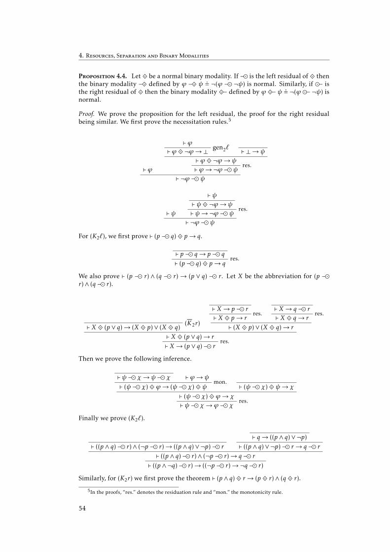
4. Resources, Separation and Binary Modalities
Proposition 4.4. Let · be a normal binary modality. If − is the left residual of · thenthe binary modality − · defined by ϕ − · ψ ¬(ϕ − ¬ψ) is normal. Similarly, if − isthe right residual of · then the binary modality · − defined by ϕ · − ψ ¬(ϕ − ¬ψ) isnormal.
Proof. We prove the proposition for the left residual, the proof for the right residualbeing similar. We first prove the necessitation rules.5
` ϕ
` ϕgen2`` ϕ · ¬ϕ→⊥ ` ⊥→ ψ
` ϕ · ¬ϕ→ ψres.
` ϕ→¬ϕ − ψ` ¬ϕ − ψ
` ψ
` ψ` ψ · ¬ϕ→ ψ
res.` ψ→¬ϕ − ψ` ¬ϕ − ψ
For (K2`), we first prove ` (p − q) · p→ q.
` p − q→ p − qres.
` (p − q) · p→ q
We also prove ` (p − r)∧ (q − r)→ (p ∨ q) − r. Let X be the abbreviation for (p −r)∧ (q − r).
(K2r)` X · (p∨ q)→ (X · p)∨ (X · q)
` X→ p − rres.
` X · p→ r
` X→ q − rres.
` X · q→ r
` (X · p)∨ (X · q)→ r
` X · (p∨ q)→ rres.
` X→ (p∨ q) − r
Then we prove the following inference.
` ψ − χ→ ψ − χ ` ϕ→ ψmon.
` (ψ − χ) · ϕ→ (ψ − χ) · ψ ` (ψ − χ) · ψ→ χ
` (ψ − χ) · ϕ→ χres.
` ψ − χ→ ϕ − χ
Finally we prove (K2`).
` ((p∧ q) − r)∧ (¬p − r)→ ((p∧ q)∨¬p) − r` q→ ((p∧ q)∨¬p)
` ((p∧ q)∨¬p) − r→ q − r` ((p∧ q) − r)∧ (¬p − r)→ q − r
` ((p∧¬q) − r)→ ((¬p − r)→¬q − r)
Similarly, for (K2r) we first prove the theorem ` (p∧ q) · r→ (p · r)∧ (q · r).
5In the proofs, “res.” denotes the residuation rule and “mon.” the monotonicity rule.
54
Normal binary modal logics 4.3
` p∧ q→ p ` r→ rmon.
` (p∧ q) · r→ p · r` p∧ q→ q ` r→ r
mon.` (p∧ q) · r→ q · r
` (p∧ q) · r→ (p · r)∧ (q · r)
We also prove the theorem ` (p − q)∧ (p − r)→ p − (q ∧ r). We write Q and R forp − q and p − r respectively.
` (Q∧R) · p→ (Q · p)∧ (R · p)`Q · p→ q ` R · p→ r
` (Q · p)∧ (R · p)→ q∧ r` (Q∧R) · p→ q∧ r
res.` (p − q)∧ (p − r)→ p − (q∧ r)
Then we prove the following inference.
` (ϕ − ψ) · ϕ→ ψ ` ψ→ χ
` (ϕ − ψ) · ϕ→ χres.
` ϕ − ψ→ ϕ − χ
Finally, we prove (K2r).
` (p − (q→ r))∧ (p − q)→ (p − ((q→ r)∧ q))` (q→ r)∧ q→ r
` (p − ((q→ r)∧ q))→ (p − r)` (p − (q→ r))∧ (p − q)→ (p − r)
Corollary 4.5. The septraction operator −T¬ is a normal binary modality in BBI.
Kripke semantics for normal binary modal logics
A Kripke binary frame is a pair F = (W,C) where W is a non-empty set of states (de-noted by w,x . . .) and C is a ternary relation over W . We write w C (x,y) for (w,x,y) ∈C.Intuitively, w C (x,y) means that the state w can be decomposed into two states x and y.We say that x and y are substates of w by the decomposition (w,x,y) ∈C. Equivalently,w C (x,y) means that the substates x and y can be merged together to obtain the state w.
A Kripke binary frame F = (W,C) may have the following properties.
Separation The frame F is separated iff for all w,x1,x2, y1, y2 ∈ W , if w C (x1, y1) andw C (x2, y2) then x1 = x2 and y1 = y2.
Determinism The frame F is deterministic iff for all w1,w2,x,y ∈W , if w1 C (x,y) andw2 C (x,y) then w1 = w2.
Seriality The frame F is serial iff for all x,y ∈W there exists w ∈W such that w C (x,y).
Commutativity The frame F is commutative iff for all w,x,y ∈ W , if w C (x,y) thenw C (y,x).
Left associativity The frame F is left associative iff for all w,w′ ,x,y,z ∈W , if w C (w′ , z)and w′ C (x,y) then there exists w′′ ∈W such that w C (x,w′′) and w′′ C (y,z).
Right associativity The frame F is right associative iff for all w,w′ ,x,y,z ∈ W , if w C(x,w′) and w′ C (y,z) then there exists w′′ ∈W such that w C (w′′ , z) and w′′ C (x,y).
Associativity The frame F is associative iff F is both left and right associative.
55

4. Resources, Separation and Binary Modalities
Given any set W , there is a trivial bijection between the set of functions W ×W −→P (W ) and the set of ternary relations over W . Therefore, non-deterministic monoids(as defined page 51) are isomorphic with commutative associative Kripke binary frames.Similarly, partial deterministic monoids add the determinism condition and total deter-ministic monoids further add the seriality condition.
A Kripke binary model is a triple M = (W,C,V ) where (W,C) is a Kripke binaryframe and V is a valuation function assigning a subset ofW to each propositional vari-able in Φ0. If (W,C) has some of the previously listed properties thenM is said to havethese properties too. For instance, a deterministic Kripke binary model is a model overa deterministic Kripke binary frame.
A formula in ΦK2 can be interpreted at a state of a Kripke binary model. We writeM,w |= ϕ when the formula ϕ ∈ ΦK2 holds at the state w ∈W of the modelM = (W,C,V ). The relation |= is defined inductively by:
M,w |= p iff w ∈ V (p)
M,w |=⊥ never
M,w |= ¬ϕ iffM,w 6|= ϕM,w |= ϕ ∧ψ iffM,w |= ϕ andM,w |= ψM,w |= ϕ · ψ iff there exist x,y ∈W s.t. w C (x,y) , M,x |= ϕ andM, y |= ψ
It is well-known that the logic obtained by interpreting the language ΦK2 in theclass of all Kripke binary frames is the minimal binary normal logic K2 (see for in-stance [BRV.01, Section 4.2]).
56

Chapter 5
Decidability of Associative BinaryModal Logics
The Boolean logic of Bunched Implications (BBI) presented in the previous chapter hasbeen proved to be undecidable [LarGal.10, BroKan.10]. Actually, most logics with anassociative binary modality are undecidable, as it has been proved by Kurucz, Nemeti,Sain and Simon [KNSS.95]. Some are decidable though, like the separation logics kSL0and the Propositional Dependance logic (PD). We conjecture that these logics are decid-able because of their non-standard semantics for propositional variables.
After succinctly reproving the undecidability of BBI in Section 5.1 and introducingthe aforementioned decidable logics with a binary modality in Sections 5.2 and 5.3,we propose in Section 5.4 a new family of logics with an associative binary modality,called counting logics. The semantics of the propositional variables in counting logicsis inspired by the semantics of kSL0 and PD. Indeed, we draw in Section 5.5 somelinks between counting logics and both kSL0 and PD. In Section 5.6, we prove that thesatisfiability problems of some counting logics are decidable.
5.1 Minimal associative binary modal logic
Let us consider the following axioms in the basic binary modal language ΦK2 (see Sec-tion 4.3):
p · (q · r)↔ (p · q) · r(A)
p · q→ q · p(C)
From an algebraic point of view, these axioms correspond respectively to the associativ-ity and the commutativity of the binary modality. An associative modal logic is a logicover the language ΦK2 in which all the propositional tautologies plus the axioms (K2`),(K2r) and (A) are valid and the inference rules of modus ponens and uniform substitu-tion are admissible (see on page 53). The minimal associative normal modal logic (K2A)is the minimal associative modal logic which further admits the rules of necessitation(see on page 53), i.e., K2A is the minimal normal binary modal logic in which the ax-iom (A) is valid. Similarly, the minimal associative and commutative modal logic is theminimal logic in which all the propositional tautologies plus the axioms (K2`), (K2r),(A) and (C) are valid and the inference rules of modus ponens and uniform substitutionare admissible. The minimal associative and commutative normal modal logic (K2AC)further admits the rules of necessitation, i.e., K2AC is the minimal normal binary modallogic in which the axioms (A) and (C) are valid.
The axiom (A) can be decomposed into two implications which are Sahlqvist formu-las. By the Sahlqvist completeness theorem (see for instance [BRV.01]), K2A is soundand complete with respect to the class of associative Kripke frames. Similarly, the ax-iom (C) is a Sahlqvist formula and K2AC is sound and complete with respect to the classof associative and commutative Kripke frames. We say that a logic is valid in a frame Fiff all the theorems of this logic are valid in F .
Kurucz, Nemeti, Sain and Simon proved that all the aforementioned associativemodal logics are undecidable.
57

5. Decidability of Associative Binary Modal Logics
Proposition 5.1 from [KNSS.95]. The minimal associative modal logic, the minimalassociative normal modal logic and the minimal associative and commutative modallogic are all undecidable.
The undecidability of the minimal associative and commutative normal modal logicis not proved explicitly in [KNSS.95]. Since this result is important to prove that BBI isundecidable, we show that the proof of the undecidability of the minimal associativeand commutative modal logic given in [AKNSS.96] applies to the minimal associativeand commutative normal modal logic. We first recall some definitions about groups:
• A group is non-trivial iff its carrier set is not a singleton.
• Let Gk = (Ak ,+k ,0k) be a group for all k ∈ 1 . .n for some n ≥ 2. The direct product G =G1×. . .×Gn of G1, . . . ,Gn is the group G = (A,+,0) such thatA is the Cartesian productof all the Ak , + is defined component wise, i.e., for all (x1, . . . ,xn), (y1, . . . , yn) ∈ A,(x1, . . . ,xn) + (y1, . . . , yn) = (x1 +1 y1, . . . ,xn +n yn) and 0 = (01, . . . ,0n).
Moreover, given any group G = (A,+,0), the group frame of G is the Kripke frame FG =(A,C) where x C (y,z) iff x = y + z. The proof uses the following result.
Proposition 5.2 from [AKNSS.96]. An associative modal logic L is undecidable if toeach n ≥ 2 there are n nontrivial finite groups G1, . . . ,Gn such that L is valid in the groupframe of the direct product G1 × . . .×Gn.
Corollary 5.3. Theminimal associative and commutative normal logic is undecidable.
Proof. Let (Z/2Z,+) be the commutative group of integers modulo 2 with addition. Itcan be easily checked that for all n ≥ 2, the frame group of the direct product of noccurrences of (Z/2Z,+) is a commutative and associative Kripke frame. Since K2AC issound with respect to the class of all commutative and associative Kripke frames, byProposition 5.2, K2AC is undecidable.
We can now prove that BBI is undecidable. The possibility to prove the undecidabil-ity of BBI in this way is mentioned in [BroKan.10].
Lemma 5.4. BBI is a conservative extension of K2AC.
Proof. We identify the symbols T and · . By Proposition 4.3, (K2`) and (K2r) are the-orems of BBI and the inference rules of modus ponens, uniform substitution and ne-cessitation are admissible. Therefore, any theorem of K2AC is a theorem of BBI. Con-versely, we prove that any theorem of the fragment of BBI without −T and I is validin the class of all associative and commutative Kripke frames. Let ϕ be a theoremof BBI and M = (W,C,V ) an associative and commutative Kripke model. We defineM′ = (W ′ ,, e,V ′) such that e < W , W ′ = W ∪ e, a b = c ∈W | c C (a,b) if a,b ∈ W ,a e = e a = a for all a ∈ W ′ and V ′(p) = V (p) for all p ∈ Φ0. It can easily be checkedthat (W ′ ,, e) is a nondeterministic monoid. Therefore, ϕ is valid inM′ . Furthermore,it can easily be proved by induction on the number of occurrences of symbols in ψ thatfor all a ∈W ′ and all ψ ∈ ΦK2 , ifM
′ , a |=BBI ψ thenM, a |=K2AC ψ. Therefore, ϕ is valid inM.
Corollary 5.5. BBI is undecidable.
5.2 Propositional Separation Logics kSL0
Separation logics have been devised to reason about programs with pointers to memorycells [Reynolds.02]. They are instantiations of the first-order variant of BBI with atomicpropositions of the form x0 → x1 . . .xk meaning intuitively that the address x0 pointsto the vector x1 . . .xk of values (see [DemDet.15] for an overview). Separation logics arenamed kSLn where k is the length of the vectors of values addresses point to and n is
58

Propositional Separation Logics kSL0 5.2
the number of first-order variables. In the present work, we are only interested in thefamily kSL0 of propositional separation logics.
Formally, let V be a countable set of program variables (denoted by x,y . . .) and k > 0a strictly positive natural number. The language ΦkSL0 of kSL0 is defined by:
ϕ,ψ B x0 → x1 . . .xk | x0 = x1 | ⊥ | ¬ϕ | ϕ ∧ψ | ε | ϕ Tψ | ϕ −Tψ
where x0, . . . ,xk ∈ V and ε < V . Intuitively, ε corresponds to an empty memory and T
and −T have the same meaning as in BBI, but with memory states in place of the moreabstract states of BBI.
Formulas of kSL0 are evaluated atmemory stateswhich are pairs (s,h) where s : V −→N is the stack assigning a value1 to any program variable and h :N −−−N
k is a partialfunction called the heap assigning vectors of values to values. For any fixed k > 0, twoheaps h1 and h2 are disjoint iff dom(h1)∩dom(h2) = ∅. The partial binary operator] overheaps is defined for all disjoint heaps h1,h2 such that dom(h1 ] h2) = dom(h1)∪dom(h2),(h1 ] h2) (x) = h1(x) if x ∈ dom(h1) and (h1 ] h2) (x) = h2(x) if x ∈ dom(h2). The expressions,h |= ϕ denotes the fact that the formula ϕ ∈ ΦkSL0 is satisfied at the memory state(s,h). The relation |= is defined inductively by:
s,h |= x0 → x1 . . .xk iff s(x0) ∈ dom(h) and h (s(x0)) = (s(x1), . . . ,s(xk))
s,h |= x0 = x1 iff s(x0) = s(x1)
s,h |=⊥ never
s,h |= ¬ϕ iff s,h 6|= ϕs,h |= ϕ ∧ψ iff s,h |= ϕ and s,h |= ψs,h |= ε iff dom(h) = ∅s,h |= ϕ Tψ iff there is h1 and h2 such that h = h1 ] h2,s,h1 |= ϕ and s,h2 |= ψs,h |= ϕ −Tψ iff for all h1 and h2 if h2 = h] h1 and s,h1 |= ϕ then s,h2 |= ψ
A formula ϕ ∈ ΦkSL0 is satisfiable if ϕ is satisfiable at some memory state. The expres-sion |= ϕ denotes the fact that the formula ϕ ∈ ΦkSL0 is valid, i.e., ϕ is satisfied at anymemory state.
Atomic formulas of the form x0 7→ x1 . . .xk can be defined by x0 7→ x1 . . .xk x0 →x1 . . .xk∧¬ (¬ε T¬ε). Moreover, since |= x0 → x1 . . .xk ↔ (> T x0 7→ x1 . . .xk), it is possibleto define kSL0 such that 7→ is the primitive and → is defined from 7→. We chose to use→ as primitive because of its “existential” nature which will be useful for comparisonpurposes.
Calcagno, Yang and O’Hearn [CYO.01] proved that the validity problem of kSL0 isdecidable for all k > 0.
Proposition 5.6 from [CYO.01]. For all k > 0, the validity problem of kSL0 is decid-able.
Proof sketch. We consider 7→ as primitive. The proof proceeds in four steps.First, the model checking problem of kSL0 is proved to be decidable, i.e., given any
memory state (s,h) and any formula ϕ ∈ ΦkSL0, it can be decided whether s,h |= ϕ. Thedifficult point is to prove that formulas of the form ϕ −T ψ can be checked by consid-ering only a finite number of heaps. A measure on formulas is given which intuitivelyindicates the number of cells in the heap to consider for deciding whether the formulaholds. For instance, the measure of both x0 7→ x1 . . .xk and ε is one. Then for any mem-ory state (s,h) and any formulas ϕ,ψ ∈ ΦkSL0 the finite sets D,R ⊆N are defined usingfor D the previous measure and for R the image by s of the program variables occurring
1We useN as the set of values for simplicity and because this is the set of values which is used in practice.But any other infinite set can be used instead.
59

5. Decidability of Associative Binary Modal Logics
in ϕ and ψ. It is proved that if for all heaps h1,h2 such that dom(h1) ⊆ D, ran(h1) ⊆ R,h2 = h1 ] h and s,h1 |= ϕ it is the case that s,h2 |= ψ then s,h |= ϕ −Tψ. This proves thatthe model checking problem of kSL0 is decidable.
Second, consider the following decision problem of stack validity: given a stack s anda formula ϕ ∈ ΦkSL0, is it the case that s,h |= ϕ for any heap h. It can easily be provedthat this problem is equivalent to deciding whether s,h∅ |= >−Tϕ where h∅ is the heapwith empty domain. Therefore the stack validity problem is decidable.
Third, for any subset V ⊆ V of program variables, the equivalence relation ≡V overmemory states is defined such that (s1,h1) ≡V (s2,h2) iff there is a bijection b from N toN such that for all x ∈ V , s2(x) = b (s1(x)), dom(h2) = b [dom(h1)] and for all v ∈ dom(h1),h2(b(v)) = (b(v1), . . . ,b(vk)) where (v1, . . . ,vk) = h1(v). It is proved that for any formulaϕ ∈ ΦkSL0 and any memory states (s1,h1) and (s2,h2), if (s1,h1) ≡V (s2,h2) where V isthe set of program variables occurring in ϕ then s1,h1 |= ϕ iff s2,h2 |= ϕ.
Finally, given a formula ϕ ∈ ΦkSL0, let V ⊆ V be the set of program variables oc-curring in ϕ and ` ∈N the cardinality of V . The finite set Sϕ0
of stacks is defined suchthat s ∈ Sϕ0
iff s(x) ∈ 1 . . ` for all x ∈ V and s(x) = 0 for all x ∈ V \ V . It can be provedthat for any memory state (s1,h1) there is a memory state (s2,h2) such that s2 ∈ Sϕ0
and(s1,h1) ≡V (s2,h2). Therefore, to decide the validity of ϕ it suffices to check the stack va-lidity of ϕ0 in all stacks in Sϕ0
. Since Sϕ0is finite and computable and the stack validity
problem is decidable, the validity problem of kSL0 is decidable.
5.3 Trump semantics and the Propositional Dependence logic
Dependence Logics arose from considerations about existential quantifications in first-order logic. Such existentially quantified variables can be skolemized, i.e., replaced bya call to a function. But which universally quantified variables should be set as argu-ments of a Skolem function ? Whereas in traditional first-order logic, all previouslyuniversally bound variables are used as arguments of Skolem functions, in DependenceLogics, any subset of these variables can be specified as the arguments of a Skolemfunction. Consider for instance the formula ∀x1.∃y1.∀x2.∃y2.ϕ(x1, y1,x2, y2). In tradi-tional first-order logic, the choice of y2 depends on both x1 and x2. Hintikka and Sanduproposed in [HinSan.89] to allow to specify after any existential quantification a set ofvariables the quantification does not depend on. For instance, the previous formulacan be changed into ∀x1.∃y1.∀x2.∃y2/x1.ϕ(x1, y1,x2, y2) in which the choice of y2 de-pends only on x2. Hodges gave in [Hodges.97] a compositional semantics of the logicof Hintikka and Sandu, called the trump semantics. The very interesting point in thesesemantics is that assignments are replaced with sets of assignments. In the proposi-tional fragment, the corresponding shift is to replace valuations with sets of valuations.We illustrate the interest of such a semantics by presenting the Propositional Depen-dence logic (PD) [Yang.14] which is the propositional variant of Vaananen’s dependencelogic [Vaananen.07].
Let Φ0 be a non-empty set of propositional variables. The language ΦPD of PD isdefined by:
ϕ,ψ B p | ¬p | ϕ ∧ψ | ϕ ∨ψ | =(q1, . . . ,qn,p)
where n ≥ 1 and p,q1, . . . ,qn ∈ Φ0. Notice that, in contradistinction with the separa-tion logics kSL0, n is not fixed here and ΦPD contains atomic formulas of the form=(q1, . . . ,qn,p) for all n ≥ 1. A formula of the form =(q1, . . . ,qn,p) is called a dependenceatom and means intuitively that the truth value of p can be deduced deterministicallyfrom the truth values of q1, . . . ,qn.
PD formulas are evaluated at trumps. A trump is a set of valuations and a valuation isa function assigning a truth value in 0,1 to each propositional variable. The expressionT |= ϕ denotes the fact that the formula ϕ ∈ ΦPD is satisfied by the trump T . The relation
60

Syntax and semantics of counting logics 5.4
|= is defined inductively as follows:
T |= p iff for all V ∈ T , V (p) = 1
T |= ¬p iff for all V ∈ T , V (p) = 0
T |= ϕ ∧ψ iff T |= ϕ and T |= ψT |= ϕ ∨ψ iff there are T1 and T2 such that T = T1 ∪ T2, T1 |= ϕ and T2 |= ψT |= =(q1, . . . ,qn,p) iff for all V ,V ′ ∈ T ,
if V (qk) = V′(qk) for all k ∈ 1 . .n then V (p) = V ′(p)
Some points are worth being mentioned about this semantics. First, as noticed for in-stance in [AbrVaa.09], the semantics of the “disjunction” is very similar to the one of abinary modality and hence ∨ is more like a multiplicative conjunction. Second, it caneasily be proved that for any trump T and any formula ϕ ∈ ΦPD not containing anydependence atom, T |= ϕ if and only if ϕ is classically satisfied by all valuations in T .Third, since negations can only appear in front of propositional variables, the inferencerule of substitution is not admissible in PD. Forth, the logic has the downward closureproperty: if T |= ϕ then for any subset T ′ ⊆ T , T ′ |= ϕ. Finally, since the empty trump isallowed, formulas like p∧¬p are satisfiable. Indeed, it can easily be proved by inductionon the size of the formula ϕ that for all ϕ, ∅ |= ϕ. Hence, the satisfiability problem of PDis trivial. This is not the case for the validity problem of PD which has been proved byVirtema [Virtema.14] to be NEXPTIME-complete
5.4 Syntax and semantics of counting logics
In [AbrVaa.09], Abramsky and Vaananen noticed the similarity between the “disjunc-tion” in PD and the multiplicative conjunction in BI. They proposed a variant of BI witha trump semantics, called BID2. In the present section, we propose slight variations ofBID, making the following modifications:
1. We use classical additive connectives instead of intuitionistic ones. Hence ourlogics are variants of BBI.
2. We reintroduce the neutral element I of the multiplicative conjunction.
3. We use the disjoint union instead of the union as partial operator for the separa-tion.
These modifications provide some interesting properties. First, the cardinality of thetrump can be expressed. For this reason, we call these logics counting logics. More-over, dependence atoms can be defined. Therefore we remove them from the language.Finally, at least some of these logics are decidable.
The language of counting logics is the language of BBI. Only the semantics distin-guishes these logics. We recall that the language ΦBBI of BBI is defined inductively froma set Φ0 of propositional variables by:
ϕ,ψ B p | > | ¬ϕ | (ϕ ∧ψ) | I | (ϕ Tψ) | (ϕ −Tψ)
We introduce the following abbreviations:• The dual i of T is defined by ϕ iψ ¬ (¬ϕ T¬ψ).• The minimal cardinality predicate ≥n is defined inductively by ≥0 >, ≥1 ¬Iand for all n > 1, ≥n ¬I T≥(n− 1).
• The cardinality predicate =n is defined for all n ∈N by =n ≥n∧¬≥(n+1).
• The universal modality is defined by ϕ ⊥i (I ∨ϕ).2Whereas BID is defined as a first-order logic in [AbrVaa.09], we consider only propositional logics in the
present work.
61
5. Decidability of Associative Binary Modal Logics
Models for counting logics are subset models as proposed by Moss and Parikh fora modal logic with two unary modalities in [MosPar.92]. Formally, a subset model is atupleM = (X,O,V ) where:
• X is an arbitrary set called the universe,
• O is a non-empty set of subsets of X and
• V is valuation function assigning a subset of X to each propositional variablein Φ0. Notice that these subsets do not need to belong to O.
Our subset semantics for the language of BBI interprets formulas at subsets S ∈ O in asubset modelM = (X,O,V ) as follows:
M,S |=S p iff S ∩V (p) , ∅M,S |=S > always
M,S |=S ¬ϕ iffM,S 6|= ϕM,S |=S ϕ ∧ψ iffM,S |=S ϕ andM,S |=S ψM,S |=S I iff S = ∅M,S |=S ϕ Tψ iff there is S1,S2 ∈ O such that
S = S1 ] S2,M,S1 |=S ϕ andM,S2 |=S ψM,S |=S ϕ −Tψ iff for all S1,S2 ∈ O,
if S2 = S1 ] S andM,S1 |=S ϕ thenM,S2 |=S ψ
where ] is the disjoint union of sets, i.e. the partial binary operator over sets such thatA = B ] C iff B ∩ C = ∅ and A = B ∪ C. A formula ϕ ∈ ΦBBI is valid in a subset modelM = (X,O,V ), denoted byM |= ϕ, iffM,S |= ϕ for all S ∈ O.
Since ] is commutative, the separating conjunction T is commutative in these se-mantics. We define the following additional properties:Associativity A subset model M = (X,O,V ) is associative iff for all S,S1,S2,S3 ∈ O, if
S1,S2,S3 is a partition of S and S2∪S3 ∈ O then S1∪S2 and S1∪S3 belong to O.Decomposability A subset modelM = (X,O,V ) is decomposable iff for all S ∈ O if |S | > 1
then there is S1,S2 ⊆ O which is a partition of S.
Closure under inclusion A subset modelM = (X,O,V ) is closed under inclusion iff forall S ∈ O and S1 ⊆ S, S1 ∈ O.
Closure under union A subset model M = (X,O,V ) is closed under union iff for allS1,S2 ∈ O, S1 ∪ S2 ∈ O.
Subset-finiteness A subset modelM = (X,O,V ) is subset-finite iff all subsets in O arefinite.
Subset-infiniteness A subset modelM = (X,O,V ) is subset-infinite iff all subsets in Oare infinite.
Atomicity A subset modelM = (X,O,V ) is atomic iff for all x ∈ X and all p,q ∈ Φ0, ifx ∈ V (p) and p , q then x < V (q).
A counting logic is a logic obtained by interpreting the language ΦBBI of BBI in a class ofclosed-under-inclusion subset models. The name is justified by the following proposi-tion.
Proposition 5.7. For any closed-under-inclusion subset modelM = (X,O,V ), any S ∈ Oand any n ∈N,M,S |= ≥n iff |S | ≥ n.
Proof. The proof is by induction on n. The base case and the left-to-right direction ofthe inductive case are trivial and do not use the closure under inclusion property ofM.For the right-to-left direction, suppose |S | ≥ n > 0. There is x ∈ S and sinceM is closedunder inclusion, x and S \ x belong to O. The conclusion is straightforward.
62

Syntax and semantics of counting logics 5.4
Closed under inclusion models are obviously associative and decomposable. But theconverse is not true. To prove it, consider any modelM = (X,O,V ) where X is infiniteand O is the set of all infinite subsets of X. Since any infinite set can be partitionedinto two infinite subsets,M is decomposable and since the union of two infinite sets isinfinite, M is closed under union hence associative. But since ∅ < O, M is not closedunder inclusion.
The following proposition proves that the class of all subset-infinite decomposablemodels is modally definable.
Proposition 5.8. For any subset modelM,M is subset-infinite and decomposable ifand only ifM |= ¬I T¬I .
Proof. For the left-to-right direction, letM = (X,O,V ) be a subset-infinite decomposablesubset model. First suppose that M 6|= ¬I T ¬I . There must exists S1 ∈ O such thatM,S1 |= I i I . SinceM is decomposable and S1 is infinite, there must be a subset S2 ∈ Osuch thatM,S2 |= I , which is not possible.
For the right-to-left direction, let M = (X,O,V ) be a subset model such that M |=¬I T¬I . Clearly,M is decomposable and there is no subset S ∈ O with a cardinality lessthan 2. We prove by induction on n that for all n ∈ N, there is no subset S ∈ O suchthat |S | ≤ n. We already proved the cases when n < 2. For n ≥ 2, suppose that S ∈ O and|S | = n. SinceM is decomposable, there is a partition S1,S2 of S such that S1,S2 ∈ O.But since |S1| ≤ n− 1, S1 < O.
It is easy to prove that counting logics are conservative.
Proposition 5.9. The logics obtained by interpreting the language ΦBBI in a class ofmodels corresponding to any combination of the properties defined on the precedingpage are all conservative.
Proof. Suppose Φ1 ⊆ Φ2. From a subset modelM1 = (X1,O1,V1) over Φ1, we constructthe modelM2 = (X1,O1,V2) such that:
V2(p) =
V1(p) if p ∈ Φ1
∅ otherwise
It can easily be proved by induction that
• ifM1 has any property defined on the facing page thenM2 has it too;
• for any formula ϕ ∈ Φ(Φ1) and any S ∈ O1,M1,S |= ϕ iffM2,S |= ϕ.
To conclude this section, we would like to outline that what makes counting logicsdifferent from most undecidable logics with an associative modality is the constrainedvaluation of propositional variables: the valuation of any subset is determined by thevaluation of the singletons it contains. We observe that valuations are constrained toofor many decidable logics with an associative modality. This is the case for the proposi-tional separation logics and the propositional dependence logic presented in this chap-ter, but for some other logics too, like Pandya’s variant of interval logic [Pandya.95]. Weconjecture that, because of this constrained valuation, most counting logics are decid-able. In Section 5.6, we prove that two of them are. Constrained valuation has somedrawbacks though, as the one stated by following proposition.
Proposition 5.10. Let L be a counting logic obtained by interpreting the languageΦBBI in a class CL of closed-under-intersection subset models such that there is a modelM = (X,O,V ) in CL with |O| > 1. Then the inference rule of uniform substitution is notadmissible in L.
63

5. Decidability of Associative Binary Modal Logics
Proof. We prove that the formula (p T¬I )→ p is valid in L while (I T¬I )∧¬I is satisfi-able in L. SupposeM,S |= p T¬I for some modelM = (X,O,V ) in CL and some S ∈ O.There is a subset S1 ∈ S such that S1 ∩V (p) , ∅. Therefore, S ∩V (p) , ∅ andM,S |= p.Now, letM = (X,O,V ) be a model in CL such that |O| > 1. There is a subset S ∈ O suchthat S , ∅, henceM,S |= ¬I . Moreover, sinceM is closed under inclusion, ∅ ∈ O. SinceS = ∅] S,M,S |= I T¬I .
5.5 Expressivity of counting logics
In this section, we study the expressivity of counting logics by proving that the count-ing logic obtained by interpreting the language ΦBBI in the class of all closed-under-inclusion subset models, called the basic counting logic, is more general, in the senseof Definition 2.17, than both the propositional separation logics kSL0 and the proposi-tional dependence logic PD.
Comparison with the propositional separation logics kSL0
We prove the following proposition
Proposition 5.11. For any natural number k, the basic counting logic is more generalthan the propositional separation logic kSL0.
Fix a natural number k. First, the atomic formulas of the form x0 → x1 . . .xk andx0 = x1 must be mapped to propositional variables in Φ0. Since V is countable andthe basic counting logic is conservative, there is an injective function from the set ofthese atomic formulas to Φ0 and we write [x0 → x1 . . .xk] and [x0 = x1] for the image ofx0 → x1 . . .xk and x0 = x1 by this function.
The forward function f from memory states to pairs (M,S) whereM = (X,O,V ) is asubset model closed by inclusion and S ∈ O is defined such that f (s,h) = ((X,O,V ),S) if
X =Nk+1
O =S ′ ⊆ X
∣∣∣ S ′ is finite and for all (n0 . . .nk), (m0 . . .mk) ∈ S ′ ,if n0 =m0 then (n0 . . .nk) = (m0 . . .mk)
V ([x0 → x1 . . .xk]) = (n0 . . .nk) ∈ X | for all i ∈ 0 . . k, ni = s(xi)
V ([x0 = x1]) =
X if s(x0) = s(x1)∅ otherwise
S = h
It can easily be checked that M = (X,O,V ) is a subset model closed by inclusion andthat S ∈ O.
The translation function τ from the language of kSL0 toΦBBI is defined in the naturalstraightforward way for the constructs which are common to both languages and asfollows for atomic formulas:
τ (ε) = I
τ (x0 → x1 . . .xn) = [x0 → x1 . . .xk]
τ (x0 = x1) = (¬I )−T [x0 = x1]
Notice that the translation of atoms of the form x0 = x1 is not straightforward becauseobviously ∅∩V ([x0 = x1]) = ∅. Hence, it is needed to checkwhether V ([x0 = x1]) containssome element that can be added to the empty set.
Now, it suffices to prove the following lemma to prove Proposition 5.11.
64

Expressivity of counting logics 5.5
Lemma 5.12. For any formula ϕ ∈ ΦkSL0 and any memory state (s,h), s,h |= ϕ if andonly if f (s,h) |= τ(ϕ).
Proof. The proof is by a straightforward induction on the number of occurrences ofsymbols in ϕ. We detail only the case for atomic formulas of the form x0 = x1 to justifytheir translation. Suppose that s,h |= x0 = x1 and let f (s,h) = (M,S) withM = (X,O,V ).We have s(x0) = s(x1) and V ([x0 = x1]) = X. Therefore, for any S ′ ∈ O such that S ′ ⊃S, M,S ′ |= [x0 = x1]. Conversely, suppose that M,S |= (¬I ) −T [x0 = x1] for some M =(X,O,V ), some S ∈ O and some memory state (s,h) such that f (h,h) = (M,S). Since byconstruction, S is finite, there is some S ′ ∈ O such that S ′ ⊃ S. Hence, V ([x0 = x1]) cannot be empty and it must be the case that s(x0) = s(x1).
Comparison with the propositional dependence logic PD
We prove the following proposition.
Proposition 5.13. The basic counting logic is more general than the propositional de-pendence logic.
Since both the basic counting logic and the propositional dependence logic are con-servative, we assume that they have the same set Φ0 of propositional variables.
The forward function f from trumps to pairs (M,S) whereM = (X,O,V ) is a subsetmodel closed by inclusion and S ∈ O is defined such that f (T ) = ((X,O,V ),S) if
X =P (Φ0)
O =P (X)
V (p) = x ∈ X | p ∈ xS = x ∈ X | there is v ∈ T , x = p ∈ Φ0 | v(p) = 1
Notice that the modelM = (X,O,V ) does not depend on T and that T is just the char-acteristic function of S.
To define the translation function τ from the language ΦPD to the language ΦBBI, letus first define the following syntactic function for all formulas ϕ ∈ ΦBBI:
same(ϕ) (ϕ Tϕ)∨ ((¬I ∧¬ϕ) T (¬I ∧¬ϕ))
Intuitively, for any propositional variable p ∈ Φ0, same(p) means that the current sub-set can be partitioned into two non-empty subsets which agree on p. The translationfunction τ is defined as follows:
τ(p) = p
τ(¬p) = ¬pτ(ϕ ∧ψ) = τ(ϕ)∧ τ(ψ)τ(ϕ ∨ψ) = τ(ϕ) T τ(ψ)
τ(=(q1, . . . ,qn,p)) =
=2→ ∧i∈1..n
same(qi)
→ same(p)
Now, to prove Proposition 5.13, it suffices to prove the following lemma.
Lemma 5.14. For any formula ϕ ∈ Φ and any trump T , T |= ϕ iff f (T ) |= τ(ϕ).
Proof. The proof is by induction on the number of occurrences of symbols in ϕ. We de-tail only some cases, the other cases being straightforward. For propositional variables,it can be easily proved that for any subset modelM = (X,O,V ) closed by inclusion, anysubset S ∈ O and any formula ψ ∈ ΦBBI,M,S |= ψ iffM,S1 |= ψ for all S1 ⊆ S. For the
65

5. Decidability of Associative Binary Modal Logics
left-to-right direction of the case for disjunctions, suppose T |= ϕ1 ∨ϕ2. There are twotrumps T1,T2 such that TS = T1 ∪ T2, T1 |= ϕ1 and T2 |= ϕ2. But since PD is downwardclosed, T2 \ T1 |= ϕ2. By induction, there are S,S1,S2 ∈ O such that S1,S2 is a partitionof S, M,S1 |= ϕ1, M,S2 |= ϕ2 and f (T ) = (M,S). For dependence atoms, consider anysubset x,y ∈ O such that x , y. For all p ∈ Φ0, since M,∅ 6|= p, M, x,y |= (p T p) iffx,y ⊆ V (p). Similarly, M, x,y |= (¬I ∧ ¬p) T (¬I ∧ ¬p) iff x,y ∩ V (p) = ∅. There-fore, f (T ) |= τ(=(q1, . . . ,qn,p)) if and only if for all v1,v2 ∈ T such that v1 , v2, ifv1(pi) = v2(pi) for all i ∈ 1 . .n then v1(q) = v2(q).
5.6 Decidable counting logics
The complete finite counting logic (CBLcomp) is the logic obtained by interpreting thelanguage ΦBBI in the class Ccomp of all subset models which are closed under inclu-sion, closed under union and subset-finite. Similarly, the complete atomic finite count-ing logic (CBLatom) is the logic obtained by interpreting the language ΦBBI in the classCatom of all subset models which are closed under inclusion and union, subset-finiteand atomic.
LetM1 = (X1,O1,V1) be a subset model which is closed under inclusion and union.Define M2 = (X2,O2,V2) such that X2 =
⋃O1, O2 = O1 and V2(p) = V1(p) ∩X2 for all
p ∈ Φ0. Clearly,M2 is a closed under inclusion and union. Moreover, it can easily beproved that for any formula ϕ ∈ ΦBBI and any subset S ∈ O1,M1,S |= ϕ iffM2,S |= ϕ.Therefore, since wheneverM1 is subset-finite,M2 is subset-finite too, we will assumethat any modelM = (X,O,V ) in Ccomp is such that O is the set of all finite subsets ofX. Similarly, since wheneverM1 is atomic,M2 is atomic too, we will assume that anymodelM = (X,O,V ) in Catom is such that O is the set of all finite subsets of X.
We prove that the satisfiability problems of CBLcomp and CBLatom are decidable andwe give a complexity upper bound.
Decidability of the satisfiability problem of CBLatom
We prove the following proposition.
Proposition 5.15. The satisfiability problem of CBLatom is in 3EXPTIME.
The proof proceeds as follows. First we propose a new semantics for the language ofBBI. We temporarily call B the logic obtained by interpreting ΦBBI in the new semantics.Then, we give a polynomial reduction from the satisfiability problem of B to the satis-fiability problem of Presburger arithmetic. Finally we prove that B and CBLatom are thesame logic. Since CBLatom is conservative, we will assume that Φ0 is infinite.
A B-model is a partial functionM from Φ0 toN. LetM (M) be the set of functionsmfromΦ0 toN such that for all p ∈ dom(M),m(p) ≤M(p). Formulas inΦBBI are evaluatedat functions m ∈M (M) as follows:
M,m |=B p iff m(p) > 0
M,m |=B > always
M,m |=B ¬ϕ iffM,m 6|= ϕM,m |=B ϕ ∧ψ iffM,m |=B ϕ andM,m |=B ψ
M,m |=B I iff m(p) = 0 for all p ∈ Φ0
M,m |=B ϕ Tψ iff ∃m1,m2 ∈M (M) . m =m1 +m2,M,m1 |=B ϕ andM,m2 |=B ψ
M,m |=B ϕ −Tψ iff ∀m1,m2 ∈M (M) . if m2 =m1 +m andM,m1 |=B ϕ thenM,m2 |=B ψ
where the binary operator + over M (M) is defined such that for all p,
(m1 +m2)(p) =m1(p) +m2(p)
66

Decidable counting logics 5.6
The logic B is obtained by interpreting the language ΦBBI in B-models.Presburger arithmetic is the first-order theory of the natural numbers N with ad-
dition +. The set of quantified variables of Presburger arithmetic is denoted by V .Formulas of this theory are called constraints. A Presburger assignment is a functionA from V to N. We write A |=PA C to denote that the constraint C is satisfied by theassignment A.
To establish the reduction from the satisfiability problem of B to the satisfiabilityproblem of Presburger arithmetics, we use vectors which are ordered finite sets, i.e., fi-nite sequences without repetitions (each component of a vector occurs exactly once). Inaddition to the notations for sequences introduced in Section 1.3, we use the followingones. Vectors are distinguished by an arrow accent, for instance −→p is a vector of propo-sitional variables. We write pi instead of −→p i . We may abusively consider a vector to bethe set of its components and write for instance q ∈ −→p .
A B-correspondence is a tuple(−→p , −→x , −→r , −→s ) where −→p is a vector of propositional
variables in Φ0,−→x , −→r and −→s are vectors of Presburger arithmetic variables of same
length as −→p and such that the sets of components of −→x , −→r and −→s are disjoint (−→x ∩−→r = −→r ∩ −→s = −→s ∩ −→x = ∅). A B-correspondence allows to link a pair (M,m) whereM is a B-model and m ∈ M (M) with a Presburger assignment A. Intuitively, for alli ∈ 1 . .
(∣∣∣−→p ∣∣∣− 1), xi encodes m (pi), ri encodes whether pi belongs to dom(M) and si en-codesM (pi). But the last component p∣∣∣−→p ∣∣∣ is special as it represents all the propositionalvariables not in −→p <
∣∣∣−→p ∣∣∣. Formally, a pair (M,m) composed of a B-modelM and a functionm ∈M (M) corresponds to a Presburger arithmetic assignment A by a B-correspondence(−→p , −→x , −→r , −→s ), denoted byM,m
−→p ,−→x ,−→r ,−→s A, iff the following conditions hold:
• for all i <∣∣∣−→p ∣∣∣, A(xi) =m(pi),
• dom(M)∩ −→p <∣∣∣−→p ∣∣∣ =
pi∣∣∣ i < ∣∣∣−→p ∣∣∣ and A(ri) = 0
,
• for all i <∣∣∣−→p ∣∣∣, if A(ri) = 0 then A(si) =M(pi),
• A(x∣∣∣−→p ∣∣∣) =∑p<−→p <
∣∣∣ −−−→p ∣∣∣m(p)
• A(r∣∣∣−→p ∣∣∣
)= 0 iff Φ0 \ −→p <
∣∣∣−→p ∣∣∣ ⊆ dom(M),
• if A(r∣∣∣−→p ∣∣∣) = 0 then A(s∣∣∣−→p ∣∣∣) =∑p<−→p <
∣∣∣ −−−→p ∣∣∣M(p)
Similarly, a B-correspondence establishes a syntactic link between B-logic and Pres-burger arithmetic, by means of a translation θ
(−→p , −→x , −→r , −→s ). First the Presburger arith-metic formula Ψ
(−→p , −→x , −→r , −→s ) is defined by:
Ψ(−→p , −→x , −→r , −→s ) ∧
i∈1..∣∣∣−→p ∣∣∣ (ri > 0∨ xi ≤ si)
As stated by the following lemma, this formula ensures that there is a pair (M,m) cor-responding to any assignment satisfying it.
Lemma 5.16. Let(−→p , −→x , −→r , −→s ) be a B-correspondence.
• For any B-modelM, any function m ∈M (M) and any Presburger arithmetic as-
signment A, ifM,m−→p ,−→x ,−→r ,−→s A then A |= Ψ
(−→p , −→x , −→r , −→s ).• For any B-modelM and any function m ∈M (M), there is a Presburger arithmetic
assignment A such thatM,m−→p ,−→x ,−→r ,−→s A.
• For any Presburger arithmetic assignment A, if A |= Ψ(−→p , −→x , −→r , −→s ) then there is
a B-modelM and a function m ∈M (M) such thatM,m−→p ,−→x ,−→r ,−→s A.
67

5. Decidability of Associative Binary Modal Logics
Proof. Straightforward.
For any formula ϕ ∈ ΦBBI such that all propositional variables occurring in ϕ occur
in −→p <∣∣∣−→p ∣∣∣, the translation function θ
(−→p , −→x , −→r , −→s ) is defined inductively as follows:
θ(−→p , −→x , −→r , −→s ) (pi) = xi > 0
θ(−→p , −→x , −→r , −→s ) (>) =>
θ(−→p , −→x , −→r , −→s ) (¬ϕ) = ¬θ (−→p , −→x , −→r , −→s ) (ϕ)
θ(−→p , −→x , −→r , −→s ) (ϕ ∧ψ) = θ (−→p , −→x , −→r , −→s ) (ϕ)∧θ (−→p , −→x , −→r , −→s ) (ψ)θ(−→p , −→x , −→r , −→s ) (I ) = ∧
i∈1..∣∣∣−→p ∣∣∣xi = 0
θ(−→p , −→x , −→r , −→s ) (ϕ Tψ) = ∃−→y , −→z .
∧i∈1..
∣∣∣−→p ∣∣∣xi = yi + zi ∧Ψ
(−→p , −→y , −→r , −→s )∧θ (−→p , −→y , −→r , −→s ) (ϕ) ∧Ψ
(−→p , −→z , −→r , −→s )∧θ (−→p , −→z , −→r , −→s ) (ψ)θ(−→p , −→x , −→r , −→s ) (ϕ −Tψ) = ∀−→y , −→z . ∧
i∈1..∣∣∣−→p ∣∣∣zi = xi + yi →
Ψ(−→p , −→y , −→r , −→s )→ θ
(−→p , −→y , −→r , −→s ) (ϕ) →
Ψ(−→p , −→z , −→r , −→s )→ θ
(−→p , −→z , −→r , −→s ) (ψ)where the sets of variables in −→x , −→y , −→z , −→r and −→s are pairwise disjoint. The followinglemma proves that this translation is faithful.
Lemma 5.17. For any B-correspondence(−→p , −→x , −→r , −→s ), any B-model M, any function
m ∈ M (M), any Presburger arithmetic assignment A and any formula ϕ ∈ ΦBBI, if
M,m−→p ,−→x ,−→r ,−→s A and all propositional variables occurring in ϕ occur in −→p <
∣∣∣−→p ∣∣∣ thenM,m |= ϕ iff A |= θ
(−→p , −→x , −→r , −→s ) (ϕ)Proof. By induction on the number of occurrences of symbols in ϕ. All the cases arestraightforward, hence we detail only the case for the magic wand. For the left-to-rightdirection, supposeM,m |= ϕ and for some assignment A,
A |=∧
i∈1..∣∣∣−→p ∣∣∣zi = xi + yi ∧Ψ
(−→p , −→y , −→r , −→s )∧θ (−→p , −→y , −→r , −→s ) (ϕ)∧Ψ (−→p , −→z , −→r , −→s )We define m1 and m2 such that, for all i ∈ 1 . .
∣∣∣−→p ∣∣∣, m1(pi) = A(yi) and m2(p2) = A(zi).
It can easily be checked that M,m1−→p ,−→y ,−→r ,−→s A, M,m2
−→p ,−→z ,−→r ,−→s A, m1,m2 ∈ M (M) andm2 = m +m1, By induction,M,m1 |= ϕ henceM,m2 |= ψ and by induction again, A |=θ(−→p , −→z , −→r , −→s ) (ψ).For the right-to-left direction suppose A |= θ
(−→p , −→x , −→r , −→s ) (ϕ −Tψ), m2 =m+m1 andM,m1 |= ϕ. It can be easily checked that for any assignment A′ such that for all v ∈−→x ∪ −→r ∪ −→s , A′(v) =A(v):
A′ |=∧
i∈1..∣∣∣−→p ∣∣∣zi = xi + yi → Ψ
(−→p , −→y , −→r , −→s )→ θ(−→p , −→y , −→r , −→s ) (ϕ)
→ Ψ(−→p , −→z , −→r , −→s )→ θ
(−→p , −→z , −→r , −→s ) (ψ)68

Decidable counting logics 5.6
By Lemma 5.16, there is A1 and A2 such that M,m1−→p ,−→y ,−→r ,−→s A1, M,m2
−→p ,−→z ,−→r ,−→s A2,A1 |= Ψ
(−→p , −→y , −→r , −→s ) and A2 |= Ψ(−→p , −→z , −→r , −→s ). Moreover, by induction we have A1 |=
θ(−→p , −→y , −→r , −→s ) (ϕ). We define A0 such that:
A0(v) =
A(v) if v ∈ −→x ∪ −→r ∪ −→sA1(v) if v ∈ −→yA2(v) if v ∈ −→z
Since for all v ∈ −→r ∪ −→s , A0(v) =A(v) =A1(v) =A2(v), we have:
A0 |=∧
i∈1..∣∣∣−→p ∣∣∣zi = xi + yi ∧Ψ
(−→p , −→y , −→r , −→s )∧θ (−→p , −→y , −→r , −→s ) (ϕ)∧Ψ (−→p , −→z , −→r , −→s )Therefore A0 |= θ
(−→p , −→z , −→r , −→s ) (ψ) and A2 |= θ(−→p , −→z , −→r , −→s ) (ψ). By induction,M,m2 |=
ψ.
We have proved that the satisfiability problem of B is decidable.
Lemma 5.18. The satisfiability problem of B is in 3EXPTIME.
Proof. Let ϕ ∈ ΦBBI. Since Φ0 is infinite, there is q ∈ Φ0 which does not occur inϕ. Therefore there is a B-correspondence −→p , −→x , −→r , −→s such that −→p <
−→p are the propo-
sitional variables occurring in ϕ and −→p∣∣∣−→p ∣∣∣ = q. The Presburger arithmetic formula
Ψ(−→p , −→x , −→r , −→s )∧θ (−→p , −→x , −→r , −→s ) (ϕ) can be computed in time polynomial in the number
of occurrences of symbols in ϕ. By Lemmas 5.16 and 5.17, this formula is satisfiable inPresburger arithmetic if and only if ϕ is satisfiable in B. Since the satisfiability problemof Presburger arithmetic is in 3EXPTIME [Oppen.78], the satisfiability problem of B isin 3EXPTIME too.
We prove now that B is indeed the same logic as CBLatom. We first prove the follow-ing lemma. We say that a B-modelMM is flat on a subset Q ⊆ Φ0 iff Q ⊆ dom(MM ) andfor all p ∈Q,MM (p) = 0.
Lemma 5.19. Let ϕ ∈ ΦBBI and P the set of propositional variables occurring in ϕ. IfM1,m1 |= ϕ and the subsetsQ, P and q are pairwise disjoint then there exists a B-modelM2 and a function m2 ∈M (M2) such thatM2 is flat on Q andM2,m2 |= ϕ.
Proof. DefineM2 and m2 fromM1, m1, Q, P and q such that
m2(p) =
0 if p ∈Q∑p∈Q∪qm1(p) if p = q
m1(p) otherwise
and if Q∪ q ⊆ dom(M1):
dom(M2) = dom(M1)
M2(p) =
0 if p ∈Q∑p∈Q∪qM1(p) if p = qM1(p) otherwise
otherwise:
dom(M2) =Q∪dom(M1) \ q
M2(p) =
0 if p ∈QM1(p) otherwise
69

5. Decidability of Associative Binary Modal Logics
Let −→p be a vector of length |P |+1 such that pi ∈ P for all i ∈ 1 . . |P | and p|P |+1 = q. For anyvectors −→x , −→r and −→s such that
(−→p , −→x , −→r , −→s ) is a B-correspondence and any assignment
A, it can be easily checked thatM1,m1−→p ,−→x ,−→r ,−→s A iffM2,m2
−→p ,−→x ,−→r ,−→s A.
We can now prove the main lemma.
Lemma 5.20. For any formula ϕ ∈ ΦBBI, ϕ is satisfiable in a B-model if and only if ϕ isCBLatom satisfiable.
Proof. For the left-to-right direction, supposeM0,m0 |= ϕ0. DefineM = (X,O,V ) suchthat
• X = (p,n) ∈ Φ0 ×N | if p ∈ dom(M0) then n <M0(p),• O is the set of all finite subsets of X and
• V (p) = (q,n) ∈ X | q = p for all p ∈ Φ0.Clearly, M is in Catom. Further define the function h from O to M (M0) such that forall S ∈ O and all p ∈ Φ0, h(S)(p) is the cardinality of (q,n) ∈ S | q = p. This function is“homomorphic” in the sense that h (S1 ] S2) = h(S1) + h(S2). Let P be the set of proposi-tional variables occurring in ϕ0, q ∈ Φ0\P andQ = Φ0\(P ∪ q). By Lemma 5.19, we canassume thatM0 is flat onQ. Therefore, for allm ∈M (M0), there is only a finite numberof propositional variables p such that m(p) > 0. Hence, h is surjective. Moreover, westate the following claim.
Claim. For any subset S ⊆ X and any m1 ∈M (M0), if for all p ∈ Φ0, the cardinalityof (q,n) ∈ S | q = p is greater than or equal to m1(p) then there is S1 ∈ O such thatS1 ⊆ S and h(S1) =m1.
Proof. It suffices to choosem1(p) elements of the form (p,n) in S for all p. Since thereis only a finite number of propositional variables p such that m1(p) > 0, this subsetis finite.
Now we prove that for all S ∈ O and all ψ ∈ ΦBBI such that the set of propositionalvariables occurring in ψ is a subset of P :IH.1 M,S |= ψ iffM0,h(S) |= ψThe proof is by induction on the number of occurrences of symbols in ψ. We only detailthe two following cases, the other ones being easy. For the right-to-left direction ofseparating conjunction’s case, suppose M0,h(S) |= ψ1 T ψ2. There is m1,m2 ∈ M (M0)such that h(S) =m1 +m2,M0,m1 |= ψ1 andM0,m2 |= ψ2. By the previous claim, there isS1 ⊆ S such that h(S1) = m1. Moreover, it can be easily checked that h(S \ S1) = m2. Byinduction,M,S1 |= ψ1 andM,S \S1 |= ψ2. Therefore,M,S |= ψ1Tψ2. For the left-to-rightdirection of magic wand’s case, supposeM0,h(S) 6|= ψ1 −Tψ2. There is m1,m2 ∈M (M0)such that m2 = h(S) +m1,M0,m1 |= ψ1 andM0,m2 6|= ψ2. For all p ∈ Φ0, the cardinalityof (q,n) ∈ X \ S | q = p is greater or equal than m1(p) because otherwise we would havethat p ∈ dom(M0) and m2(p) > M0(p). Therefore, by the previous lemma, there isS1 ∈ O such that S1 ∩ S = ∅ and h(S1) = m1. SinceM is closed under union, S ] S1 ∈ O.By induction,M,S1 |= ψ1 andM,S2 6|= ψ2. Therefore,M,S 6|= ψ1 −Tψ2.
The proof of the right-to-left direction of the lemma is similar to the left-to-rightdirection. SupposeM0,S0 |= ϕ0 for some subset modelM0 = (X0,O0,V0) in Catom. Let Pbe the set of propositional variables occurring in ϕ0 and q ∈ Φ0 \P . Define the valuationV1 such that for all p ∈ Φ0:
V1(p) =
V0(p) if p ∈ P⋃p′<P V0(p
′) if p = q∅ otherwise
70

Decidable counting logics 5.6
The subset modelM1 = (X0,O0,V1) is clearly inCatom. Moreover, it can be easily provedby induction that for any formula ϕ ∈ ΦBBI such that the set of propositional variablesoccurring in ϕ is included in P and any subset S ∈ O0,M0,S |= ϕ iffM1,S |= ϕ. Definethe B-model M such that dom(M) = p ∈ Φ0 | V1(p) is finite and for all p ∈ dom(M),M(p) = |V (p)|. Moreover, define the function h from O0 to M (M) such that for allS ∈ O0 and all p ∈ Φ0, h(S)(p) = |V (p)∩ S |. It can be easily checked that this functionh is surjective and “homomorphic” in the sense that h (S1 ] S2) = h(S1) + h(S2). Theremainder of the proof is identical to the proof of the left-to-right direction.
We have proved Proposition 5.15.
Decidability of the satisfiability problem of CBLcomp
We prove the following proposition.
Proposition 5.21. The satisfiability problem of CBLcomp is in 4EXPTIME.
The proof is by an exponential reduction to the satisfiability problem of CBLatom. Wefirst define a power correspondence as a triple (Q1,b,Q2) such that Q1 and Q2 are subsetsof Φ0 and b is a bijection assigning an element of Q2 to every subset of Q1. Then,given a power correspondence (Q1,b,Q2) and a formula ϕ ∈ ΦBBI such that the set ofpropositional variables occurring in ϕ is included in Q1, the translation τ (Q1,b,Q2)(ϕ)of ϕ is obtained by replacing each occurrence of p in ϕ with∨
p∈P⊆Q1
b(P )
for all p ∈ Q1. The resulting formula has size exponential in the size of the originalformula.
Moreover, given any universe X and any power correspondence (Q1,b,Q2), the rela-tion Q1,b,Q2
X over valuations on X is defined such that V1Q1,b,Q2
X V2 iff for all x ∈ X andall Q ⊆Q1
x ∈ V2 (b (Q)) iff Q = p ∈Q1 | x ∈ V1(p)We first state the following lemmas.
Lemma 5.22. For any subset modelM = (X,O,V1) in Ccomp and any power correspon-
dence (Q1,b,Q2), there is a valuation V2 on X such that V1Q1,b,Q2
X V2 and (X,O,V2) is asubset model in Catom.
Proof. Define V2 by
V2(p)
x ∈ X
∣∣∣ b−1(p) = q ∈Q1 | x ∈ V1(p)
if p ∈Q2
∅ otherwise
for all p ∈ Φ0. It can easily be checked that V1Q1,b,Q2
X V2 and (X,O,V2) is a subset modelin Catom.
Lemma 5.23. For all subset modelM = (X,O,V2) inCatom and all power correspondence(Q1,b,Q2), there is a valuation V1 on X such that V1
Q1,b,Q2X V2 and (X,O,V1) is a subset
model in Ccomp.
Proof. Define V1 byV1(p)
⋃p∈P⊆Q1
V2 (b (P ))
for all p ∈ Φ0. It can easily be checked that V1Q1,b,Q2
X V2 and (X,O,V1) is a subset modelin Ccomp.
71
5. Decidability of Associative Binary Modal Logics
Lemma 5.24. For any subset models M1 = (X,O,V1) and M2 = (X,O,V2), any powercorrespondence (Q1,b,Q2), any subset S ∈ O and any formula ϕ ∈ ΦBBI such that the setof propositional variables occurring in ϕ is included in Q1:
M1,S |= ϕ iffM2,S |= τ (Q1,b,Q2)(ϕ)
Proof. The proof is by induction on the number of occurrences of symbols in ϕ. Thecases for propositional variables and their negations are straightforward by definitionof τ (Q1,b,Q2). All the other cases are trivial.
Suppose now that we want to check whether a formula ϕ0 ∈ ΦBBI is satisfiable inCBLcomp. Since CBLcomp is conservative, we can assume that Φ0 is infinite. Hence wecan construct a power correspondence (Q1,b,Q2) such thatQ1 is the set of all the propo-sitional variables occurring in ϕ0. Then we check whether τ (Q1,b,Q2)(ϕ) is satisfiablein CBLatom. If it is the case, then there is a modelM2 in Catom satisfying τ (Q1,b,Q2)(ϕ).By Lemmas 5.23 and 5.24, there is a modelM1 in Catom satisfying ϕ. Therefore, ourprocedure is complete. Conversely, if there is a modelM1 inCcomp satisfying ϕ then, byLemmas 5.22 and 5.24, there is a modelM2 in Ccomp satisfying τ (Q1,b,Q2)(ϕ). There-fore, our procedure is sound. Finally, computing (Q1,b,Q2) and τ (Q1,b,Q2)(ϕ) takesdeterministic exponential time and the satisfiability problem of CBLatom can be decidedin triple exponential time in the size of the input formula. Therefore, the satisfiabilityproblem of CBLcomp is in 4EXPTIME. We have proved Proposition 5.21.
72

Part III
Concurrency
73


Chapter 6
PDL with Concurrency
The Propositional Dynamic Logic (PDL), presented in Chapter 2, has not been devisedto reason about concurrent actions. There is no construct in the language of PDL for par-allel composition of programs. Different variations of PDL have been proposed to over-come this limitation. Some of the most interesting ones are presented in this chapter.These logics can be divided into three categories. In PDLwith Interleaving (Section 6.2),two programs can be executed concurrently only if an interleaving of their atoms can beexecuted. Hence, two atomic programs are never executed at the samemoment. In Con-current PDL and PDLwith Intersection (Sections 6.3 and 6.4), concurrency is consideredas a dual of PDL’s nondeterministic choice. Finally, in PDL with Parallel composition,Recover and Store and in PDL with fork and separation (Section 6.5 and 6.6), concur-rency is expressed by means of separation: to execute two programs concurrently, theinitial state must be separated in two substates or the final state must be the composi-tion of two substates. Hence, these two latter logics are logics of resources as well aslogic of actions and concurrency.
We recall the complexity of all these logics and study the notions of concurrencythey can express. Although concurrency can be seen just as the possibility to do differ-ent things at the same time or as a mean to speed up some task, in the present work, weare interested in the possibilty to perform with concurrent actions things that could nothave been done without concurrency. In such a notion of concurrency, some situationsof cooperation are possible. For instance, we can have a situation where a set of agentscan move a heavy item only if they cooperate. Formal definitions of three situationsof cooperation are given in the first section. These definitions are used to analyse thenotion of concurrency expressible in the variants of PDL to reason about concurrency.It turns out that none of the logics presented in this chapter can express all these kindsof cooperation. This fact justifies the interest in the logic studied in the next chapterwhich allows all the situations of cooperation defined here.
6.1 Situations of Cooperation
To precisely characterize the level of cooperation allowed in each logic, three categoriesof situations of cooperation are defined.
• A situation of simple cooperation is a situation where two actions α and β can beexecuted concurrently but neither α nor β can be executed independently.
• A situation of atomic cooperation is a situation where two actions α and β can beexecuted concurrently but no subaction of neither α nor β can be executed.
• A situation of forced cooperation is a situation where the only way to change thestate of the system is to perform some concurrent actions.
Clearly, a situation of atomic cooperation is a situation of simple cooperation. Whethera situation of forced cooperation is a situation of atomic cooperation is not so obvious. Itis generally the case though when actions are defined inductively from non-concurrentatomic actions. We first give some illustrations of situations of cooperation then weformally define what it means for a logic to allow situations of cooperation.
75
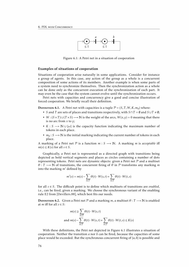
6. PDL with Concurrency
≤ 1
a
≤ 1
b
Figure 6.1: A Petri net in a situation of cooperation
Examples of situations of cooperation
Situations of cooperation arise naturally in some applications. Consider for instancea group of agents. In this case, any action of the group as a whole is a concurrentcomposition of some actions of its members. Another example is when some parts ofa system need to synchronize themselves. Then the synchronization action as a wholecan be done only as the concurrent execution of the synchronization of each part. Itmay even be the case that the system cannot evolve until the synchronization occurs.
Petri nets with capacities and concurrency give a good and concise illustration offorced cooperation. We briefly recall their definition.
Definition 6.1. A Petri net with capacities is a tuple P = (S,T ,W ,K,m0) where:• S and T are sets of places and transitions respectively, with S∩T = ∅ and S∪T , ∅;• W : (S ×T )∪ (T ×S) −→N is the weight of the arcs,W (x,y) = 0 meaning that thereis no arc from x to y;
• K : S −→ N ∪ ω is the capacity function indicating the maximum number oftokens in each place.
• m0 : S −→N is the initial marking indicating the current number of tokens in eachplace.
A marking of a Petri net P is a function m : S −→ N. A marking m is acceptable iffm(s) ≤ K(s) for all s ∈ S.
Graphically, a Petri net is represented as a directed graph with transitions beingdepicted as bold vertical segments and places as circles containing a number of dotsrepresenting tokens. Petri nets are dynamic objects: given a Petri net P and a multisetθ : T −→ N of transitions, the concurrent firing of θ in P transforms any marking minto the marking m′ defined by
m′(s) =m(s)−∑t∈T
θ(t) ·W (s, t) +∑t∈T
θ(t) ·W (t, s)
for all s ∈ S. The difficult point is to define which multisets of transitions are enabled,i.e., can be fired, given a marking. We choose the synchronous variant of the enablingrule E2 from [Devillers.88], which best fits our needs.
Definition 6.2. Given a Petri net P and a markingm, a multiset θ : T −→N is enabledat m iff for all s ∈ S:
m(s) ≥∑t∈T
θ(t) ·W (s, t)
and m(s)−∑t∈T
θ(t) ·W (s, t) +∑t∈T
θ(t) ·W (t, s) ≤ K(s)
With these definitions, the Petri net depicted in Figure 6.1 illustrates a situation ofcooperation. Neither the transition a nor b can be fired, because the capacities of someplace would be exceeded. But the synchronous concurrent firing of a,b is possible and
76

Situations of Cooperation 6.1
leads to the samemarking. This is clearly a situation a simple cooperation and, since theactions a and b are atomic, also a situation of atomic cooperation. Strictly speaking, thisPetri net is not in a situation of forced cooperation because the concurrent executionof a and b does not change the state of the system. But the Petri net could easily bemodified to be in a situation of forced cooperation, for instance by adding an emptyoutgoing place for the transition b.
Formal definitions of cooperations
In this section, we formally define how a PDL-like logic allows cooperations. This prop-erty is not necessary for a logic to be able to express some useful notions of concur-rency, but since cooperation is common in some application, this property is desirable.It turns out that none of PDL’s extensions for concurrency presented in this chapter al-lows atomic cooperation. These facts justify the existence of the logic studied in thenext chapter.
First, a formal definition of PDL-like logics is needed. Basically, a PDL-like logic isjust a multimodal logic whose unary modalities are called programs. Since cooperationconcerns concurrency, a definition of PDL-like logics with concurrency is provided. Fi-nally, forced cooperation induces that actions allow to change the current state. HencePDL-like logics with accessibility function are defined too.
Definition 6.3. A PDL-like logic is a logic L having all the following properties:
• L embeds the classical propositional logic;
• L features a set ΠL of syntactic elements called programs, representing actions;
• to each program α ∈ΠL corresponds a unary modality 〈α〉;
• formulas of L are evaluated at states in a model for L.
Definition 6.4. A PDL-like logic with concurrency is a PDL-like logic featuring a binaryoperator m on programs designated as the concurrency operator. In such a logic, allprograms where the operator m (syntactically) occurs are called concurrent programs.
Definition 6.5. A PDL-like logic with accessibility function is a PDL-like logic L suchthat, given any modelM for L, an accessibility function R assigning a binary relationover states to each program can be defined such that any state w in M satisfies anyformula 〈α〉ϕ iff there is a state x inM such that w R(α) x and x satisfies ϕ. A model fora PDL-like logic with accessibility function is called a PDL-like model with accessibilityfunction.
It has to be outlined that the previous definitions are just ad-hoc definitions for thesole purpose of having convenient definitions for situations of cooperation. In a moregeneral context, these definitions would be either too strong or too weak. This is par-ticularly the case for Definition 6.4 which formally only enforces that the logic of thelanguage features a binary operator. In fact, the important point in this definition isthat this binary operator has been designated to express concurrency of actions.
We now give definitions for situations of cooperation. We say that a logic allowsa particular kind of situations of cooperation if and only if a model of this logic canrepresent such a situation of cooperation. We give a formal definition of this notion forthe three kinds of situations proposed previously.
Definition 6.6. A PDL-like logic L with concurrency operator m allows simple cooper-ation iff for some programs α and β, some modelM for L and some state w inM, theformula
⟨α m β
⟩> is satisfied at w inM but neither 〈α〉> nor
⟨β⟩> is satisfied at w inM.
77

6. PDL with Concurrency
Definition 6.7. A PDL-like logic L with concurrency operator m allows atomic coop-eration iff for some programs α and β, some model M for L and some state w in M,the formula
⟨α m β
⟩> is satisfied at w inM but for all subprograms γ of α and β, the
formula⟨γ⟩> is not satisfied at w inM.
Definition 6.8. A PDL-like logic L with accessibility function and concurrency opera-tor m allows forced cooperation iff there is a modelM for L and a state w inM such thatboth the following conditions hold:(6.1) there are two programs α and β and a state x , w such that w R(α m β) x;
(6.2) there is no non-concurrent program γ and no state x , w such that w R(γ) x.
The notion of subprograms in Definition 6.7 is not defined formally. When programsare defined inductively, they can be identified with their syntactic tree and the subpro-grams of a program α are usually defined as the subtrees of α which are programs. Weassume though that any program is a subprogram of itself, hence the following lemmais trivial.
Lemma 6.9. If a logic L allows atomic cooperation then L allows simple cooperation.
6.2 PDL with Interleaving
To reason about concurrency, Abrahamson [Abrahamson.79, Abrahamson.80] proposedthe Propositional Dynamic Logic with Interleaving (IlPDL) which extends PDL with theinterleaving operator | corresponding to the shuffle operator for languages. Theshuffle product L1 L2 of the languages L1 and L2 is the language of all the wordsx1y1 . . .xnyn such that x1 . . .xn ∈ L1 and y1 . . . yn ∈ L2 where the xk and the yk are possiblyempty words. Obviously, the shuffle operator does not increase the expressive powerof regular expressions. But Gruber and Holzer [GruHol.08] proved that, for any alpha-bet with at least two symbols, there is a regular expression with one shuffle operatorwhich is at least exponentially more succinct than any equivalent regular expressionwithout the shuffle operator. For finite automata, the shuffle operator corresponds tothe asynchronous product.
The interleaving operator of IlPDL is the inverse image of the shuffle operator by thetrivial function L from programs to languages over the alphabet consisting of all theatomic programs and all the tests. Hence, the program α | β is the non-deterministicchoice over all the possible interleavings of α and β. The kind of concurrency expressedby this operator can be compared to a multiprocessus system on a monoprocessor com-puter.
Formally, given a set Π0 of atomic programs (denoted a,b . . .) and a set Φ0 of propo-sitional variables (denoted p,q . . .), the languages ΠIlPDL and ΦIlPDL of programs and for-mulas are defined simultaneously by:
α,β B a | (α ; β) | (α ∪ β) | ϕ? | α∗ | (α | β)ϕ B p | ⊥ | ¬ϕ | 〈α〉ϕ
As usual: parentheses may be omitted; the dual modalities are defined by [α]ϕ ¬〈α〉¬ϕ and the missing Boolean operators can be defined using modalities and tests,starting with ϕ→ ψ [ϕ?]ψ.
An IlPDL model is a tripleM = (W,ρ,V ) where• W is a nonempty set of states (denoted by w,x . . .),
• ρ is a function assigning to each atomic program a set of words of length one1
over the alphabet (W ×W ) and
1This rather complicated definition of a binary relation is justified by the extension of ρ to all programs.
78
PDL with Interleaving 6.2
• V is a valuation function assigning a subset ofW to each propositional variable.In this context, finite words over the alphabet W ×W are called computation sequences.A computation sequence σ ∈ (W ×W )∗ is legal iff for all k < |σ |, the second componentof σ k = (wk ,xk) is equal to the first component of σ k+1 = (wk+1,xk+1), i.e., xk = wk+1. Acomputation sequence σ ∈ (W ×W )∗ is from w to x, where w and x are states in W ,iff either σ = ε and w = x or the first component of σ1 = (w1,x1) is w and the secondcomponent of σ |σ | = (w|σ |,x|σ |) is x, i.e., w1 = w and x|σ | = x.
IlPDL formulas are evaluated at states of an IlPDLmodel. WewriteM,w |= ϕ to denotethat the formulaϕ ∈ ΦIlPDL is satisfied at the statew ∈W of themodelM = (W,ρ,V ). Therelation |= is defined by simultaneous induction with the extension of ρ to all programsas follows:
M,w |= p iff w ∈ V (p)
M,w |= ¬ϕ iffM,w 6|= ϕM,w |= 〈α〉ϕ iff there is σ ∈ ρ(α) and x ∈W s.t.
σ is a legal computation sequence from w to x andM,x |= ϕρ(α ; β) = ρ(α).ρ(β)
ρ(α ∪ β) = ρ(α) + ρ(β)
ρ(ϕ?) = (w,w) | M,w |= ϕρ(α∗) = (ρ(α))∗
ρ(α | β) = ρ(α) ρ(β)
The extension of ρ to all programs assigns languages over the alphabetW ×W . Hence,., +, ∗ and are operations on languages, respectively the concatenation, union, Kleenestar and shuffle. As usual, a formula ϕ ∈ ΦIlPDL is satisfiable iff there is a modelM =(W,ρ,V ) and a state w ∈ W such that M,w |= ϕ. Mayer and Stockmeyer [MaySto.96]proved that the satisfiability problem of IlPDL is 2EXPTIME-complete.
The accessibility function R can be defined in IlPDL such that for any program α ∈ΠIlPDL, R(α) is the set of all the pairs (w,x) such that there is a legal computation se-quence from w to x in ρ(α). Hence, IlPDL is a PDL-like logic with accessibility functionas stated in Definition 6.5. We prove that IlPDL allows only simple cooperation. Intu-itively, this is the case because for all programs α and β which are either atomic pro-grams or tests, the formula
⟨α | β
⟩> → 〈α〉> ∨
⟨β⟩> is valid. Formally, we first prove
the following lemma.
Lemma 6.10. For any program α ∈ ΠIlPDL, any modelM = (W,ρ,V ), any computationsequence σ ∈ ρ(α) and any pair (w,x) occurring in σ , there is a subprogram γ of αsuch that (w,x) ∈ ρ(γ). Moreover, if w , x then there is an atomic program a such that(w,x) ∈ ρ(a).
Proof. By a straightforward induction on the number of occurrences of symbols in α.
Proposition 6.11. IlPDL allows simple cooperation.
Proof. Let Π0 = N andM = (N, (n, (n,n+1)) | n ∈N ,V ) for some V . Then the com-putation sequence (0,1)(1,2)(2,3) ∈ ρ((0 ;2) |1) is legal but there is no legal computationsequences from 0 in neither ρ(0 ; 2) = (0,1)(2,3) nor ρ(1) = (1,2).
Proposition 6.12. IlPDL does not allow atomic cooperation.
Proof. Suppose that the formula⟨α | β
⟩> is satisfied at a state w ∈ W of a modelM =
(W,ρ,V ). There is a legal computation sequence σ ∈ ρ(α | β) from w. If σ = ε thenε ∈ ρ(α) andM,w |= 〈α〉>. If σ , ε then let (w,x) = σ1. There is a computation sequence
79
6. PDL with Concurrency
σ1 such that (w,x) = σ11 and either σ1 ∈ ρ(α) or σ1 ∈ ρ(β). In both cases, by Lemma 6.10,
there is a subprogram γ of α or β such thatM,w |=⟨γ⟩>.
Proposition 6.13. IlPDL does not allow forced cooperation.
Proof. Suppose condition (6.1) of Definition 6.8 holds: for some programs α and β inΠIlPDL, some model M = (W,ρ,V ) and some distinct states w,x ∈ W , w R(α | β) x. Bydefinition, there is a legal computation sequence σ ∈ ρ(α | β) from w to x. Since w , x,|σ | > 0 and there is a positive integer k such that σ k = (w,y) with w , y. By Lemma 6.10,there exists a ∈Π0 such that w R(a) y. Therefore, condition (6.2) of Definition 6.8 doesnot hold.
6.3 Concurrent Dynamic Logic
Peleg [Peleg.85, Peleg.87] proposed an interpretation of concurrency as the dual of non-determinism. This interpretation is inspired by alternating Turing machine [CKS.81]where computation is viewed as a tree with existential and universal nodes. At exis-tential nodes, only one computation path has to be considered whereas at universalnodes all computation paths have to be considered. Hence existential nodes representnon-determinism whereas universal nodes represent concurrency.
The Concurrent Propositional Dynamic Logic (CPDL) extends PDLwith the dual ∩ ofthe non-deterministic choice ∪. Whereas the non-deterministic choice has a disjunctivemeaning illustrated by validities of the form
⟨α ∪ β
⟩ϕ↔ 〈α〉ϕ∨
⟨β⟩ϕ, the concurrency
operator ∩ has a conjunctive meaning and all formulas of the form⟨α ∩ β
⟩ϕ↔ 〈α〉ϕ ∧⟨
β⟩ϕ are valid in CPDL. Formally, given a set Π0 of atomic programs (denoted a,b . . .)
and a set Φ0 of propositional variables (denoted p,q . . .), the languagesΠCPDL and ΦCPDLof programs and formulas are defined simultaneously by:
α,β B a | (α ; β) | (α ∪ β) | ϕ? | α∗ | (α ∩ β)ϕ B p | ⊥ | ¬ϕ | 〈α〉ϕ
Once again, parentheses may be omitted for clarity; the dual modalities are defined by[α]ϕ ¬〈α〉¬ϕ and the missing Boolean operators can be defined using modalities andtests, starting with ϕ→ ψ [ϕ?]ψ.
Like in IlPDL, the semantics of CPDL deviates from PDL’s semantics, the accessibil-ity function being modified to cope with concurrency. Following the interpretation ofcomputation in alternating Turing machines, more than one successor may have to beconsidered when running concurrent programs. Hence accessibility relations link statesto sets of states.
Formally, a CPDL model is a tripleM = (W,ρ,V ) where• W is a nonempty set of states,
• ρ is the accessibility function2 assigning a subset of W ×P (W ) to each atomicprogram a ∈Π0 such that for all (w,S) ∈ ρ(a), S is a singleton and
• V is the valuation function assigning a subset ofW to each propositional variablein Φ0.
CPDL formulas are evaluated at states in a CPDL model. The expressionM,w |= ϕ de-notes the fact that the formula ϕ ∈ ΦCPDL is satisfied at the state w ∈ W of the modelM = (W,ρ,V ). The relation |= is defined by simultaneous induction with the extensionof ρ to all programs in ΠCPDL by:
M,w |= p iff w ∈ V (p)
M,w |= ¬ϕ iffM,w 6|= ϕM,w |= 〈α〉ϕ iff there is S ⊆W s.t. (w,S) ∈ ρ(α) and for all x ∈ S, M,x |= ϕ
2Although ρ is called an accessibility function, it does not satisfy the conditions of Definition 6.5.
80
PDL with Intersection 6.4
ρ(α ; β) = ρ(α) · ρ(β)ρ(α ∪ β) = ρ(α)∪ ρ(β)ρ(ϕ?) = (w, w) | M,w |= ϕρ(α∗) = Iter(ρ(α))
ρ(α ∩ β) =(w,S)
∣∣∣ ∃T ,U s.t. S = T ∪U, (w,T ) ∈ ρ(α) and (w,U ) ∈ ρ(β)
where for any subsets P and Q ofW ×P (W ):
P ·Q = (w,S) | ∃x1,S1,x2,S2 . . . s.t. S = ∪iSi , (w, x1,x2 . . .) ∈ P and ∀i, (xi ,Si) ∈Q
and Iter(P ) is the least fixed point of the function FP defined by FP (Q) = ρ(>?)∪ (P ·Q).As usual, a formula ϕ ∈ ΦCPDL is satisfiable iff there is a model M = (W,ρ,V ) and astate w ∈ W such thatM,w |= ϕ. The satisfiability problem of CPDL has been provedin [Peleg.87] to be EXPTIME-complete.
It can easily be checked that for any programs α,β ∈ ΠCPDL and any formula ϕ ∈ΦCPDL, the formula
⟨α ∩ β
⟩ϕ↔ 〈α〉ϕ ∧
⟨β⟩ϕ is valid. Indeed, this is an axiom schema
of the axiomatization of CPDL proposed in [Peleg.87]. Hence, the following propositionis trivial.
Proposition 6.14. CPDL does not allow neither simple cooperation nor atomic cooper-ation.
Strictly speaking, it cannot be stated whether CPDL allows forced cooperation be-cause CPDL is not a PDL-like logic with accessibility function. In fact, CPDL is not anormal modal logic: it can easily be observed from the proof of the following proposi-tion that [α]ϕ ∧ [α]ψ→ [α] (ϕ ∧ψ) is not a valid schema in CPDL.
Proposition 6.15. CPDL is not a PDL-like logic with accessibility function.
Proof. The proof relies on the satisfaction condition for box modalities which reads:
M,w |= [α]ϕ iff for all S ⊆W, if (w,S) ∈ ρ(α) then there is x ∈ X such thatM,x |= ϕ
LetM = (1,2,ρ,V ) where ρ(a) = (1, 1), ρ(b) = (1, 2) and V (p) = 2. We haveρ (a∩ b) = (1, 1,2). Suppose R is defined such that it satisfies the conditions of Defini-tion 6.5. BecauseM,1 |= 〈a∩ b〉>, there exists w ∈ 1,2 such that 1 R(a∩ b) w. But sinceM,1 |= [a∩ b]p, w , 1 and sinceM,1 |= [a∩ b]¬p, w , 2.
6.4 PDL with Intersection
A very natural extension of PDL consists in adding a semantic dual ∩ of the non-deter-ministic choice ∪ such that R(α ∩ β) = R(α)∩R(β). The resulting logic is the Proposi-tional Dynamic Logic with Intersection (IPDL) which has been first mentioned by Harelin [Harel.83]. Although IPDL and CPDL both have a dual of the non-deterministic choiceand use the same symbol for it, the two logics are different. For instance, as it will beclear shortly, the schema 〈α〉ϕ∧
⟨β⟩ϕ→
⟨α ∩ β
⟩ϕ is not valid in IPDL, which means that
being able to perform two actions in a given situation does not imply that these actionscan be executed concurrently. Another noteworthy difference between IPDL and CPDLis that IPDL is a normal modal logic.
Formally, the language of IPDL is the same as the language of CPDL: the setΠIPDL andΦIPDL of programs and formulas are defined inductively from Π0 and Φ0 by:
α,β B a | (α ; β) | (α ∪ β) | ϕ? | α∗ | (α ∩ β)ϕ B p | ⊥ | ¬ϕ | 〈α〉ϕ
81
6. PDL with Concurrency
For any program α and any formula ϕ, |α| and |ϕ| denote the number of occurrencesof symbols in α and ϕ respectively. An IPDL model is a PDL model, i.e., a tripleM =(W,R,V ) where W is a nonempty set of states, R is the accessibility function assigninga binary relation over W to each atomic program and V is the valuation function as-signing a subset of W to each propositional variable. As expected, IPDL formulas areevaluated at states in IPDL models. The expressionM,w |= ϕ denotes that the formulaϕ ∈ ΦIPDL is satisfied at the state w ∈ W of the modelM = (W,R,V ). The relation |= isdefined by simultaneous induction with the extension of R to all programs by:
M,w |= p iff w ∈ V (p)
M,w |=⊥ never
M,w |= ¬ϕ iffM,w 6|= ϕM,w |= 〈α〉ϕ iff ∃x ∈W, w R(α) x andM,x |= ϕw R(α ; β) x iff ∃y ∈W, w R(α) y and y R(β) x
w R(α ∪ β) x iff w R(α) x or w R(β) xw R(α ∩ β) x iff w R(α) x and w R(β) xw R(ϕ?) x iff w = x andM,w |= ϕw R(α∗) x iff w R(α)∗ x
where R(α)∗ is the reflexive and transitive closure of R(α)
A formula ϕ ∈ ΦIPDL is satisfiable iff there is a modelM = (W,R,V ) and a state w ∈ Wsuch that M,w |= ϕ. The satisfiability problem of IPDL is 2EXPTIME-complete. Theupper bound has been proved byDanecki [Danecki.84] and the lower boundwas provedmore than twenty years later by Lange and Lutz [LanLut.05]. It has to be noted too thatthe satisfiability of IPDL interpreted in the class of models where at least two atomicprograms are deterministic has been proved to be undecidable in [Harel.83]. A programα is deterministic in a modelM = (W,R,V ) iff for all states w,x,y ∈W , if w R(α) x andw R(α) y then x = y.
Two other important (negative) properties of IPDL must be mentioned. First, IPDLdoes not have the tree-like model property. For instance, it can easily be checked thatfor any modelM = (W,R,V ) satisfying the formula 〈(a ; a)∩ a〉>, the graph (W,R(a)) hascycles. Second, IPDL does not have comprehensive decompositions (see Definition 2.3).This property comes from the fact that bounded-morphisms do not preserve intersec-tion (see [BRV.01, pages 59-60] for a definition). Hence by the Goldblatt-Thomason the-orem [GolTho.75] the intersection is not modally definable. The following propositiongives another, more direct, proof.
Proposition 6.16. IPDL does not have comprehensive decompositions.
Proof. Consider the formula ϕ0 = 〈a∩ b〉> and the modelsM1 = (0,1,R1,V ) andM2 =(2,3,4,R2,V ) such that R1(a) = R1(b) = (0,1), R2(a) = (2,3), R2(b) = (2,4), R1(c) =R2(c) = ∅ for all c ∈Π0\a,b and V (p) = ∅ for all p ∈ Φ0. ClearlyM1,0 |= ϕ0,M2,2 |= ¬ϕ0and for any formula ψ ∈ ΦIPDL, if ∩ occurs in ψ then
∣∣∣ψ∣∣∣ ≥ |ϕ0|. Hence, it suffices to provethe following hypotheses for all ψ ∈ ΦIPDL.IH.1 M1,1 |= ψ iffM2,3 |= ψ iffM2,4 |= ψ;IH.2 if ∩ does not occur in ψ thenM1,0 |= ψ iffM2,2 |= ψ.The proofs are by induction on
∣∣∣ψ∣∣∣. We only detail the cases when ψ = 〈α∗〉ψ′ for someα and ψ′ , the other cases being either similar or straightforward. For IH.1, let P =(1,1), (2,3), (2,4) and first observe that for any program β ∈ΠIPDL and any state x ∈ 0 . .4,if w Ri(β) x for some (i,w) ∈ P then x = w. Since w Ri(α∗) w for all (i,w) ∈ P thenMi ,w |= ψ iffMi ,w |= ψ′ . Since,
∣∣∣ψ′∣∣∣ < ∣∣∣ψ∣∣∣, IH.1 holds by induction. For IH.2, the proofis similar: it suffices to observe that Mi ,w |= ψ iff Mi ,w |= ψ′ or Mi ,w |= 〈α〉ψ′ for(i,w) ∈ (1,0), (2,2).
82

PDL with Parallel composition, Recover and Store 6.5
w2
w
w1 w3
x
w4
α
β
Figure 6.2: Semantics of the parallel program α ‖ β in PRSPDL
An interesting variant of IPDL is the Propositional Dynamic Logic with Intersectionand Converse (ICPDL) which extends IPDL with the converse unary operator − on pro-grams. After executing the program α− it is always possible to execute the program αto return to the original state. Semantically, w R(α−) x iff x R(α) w. Goller, Lohrey andLutz [GLL.07] proved that the satisfiability problem of ICPDL is 2EXPTIME-complete.
The notion of concurrency expressed by means of the intersection in IPDL is ratherweak. By definition, whenever a a state can be reached by the execution of the programα ∩ β, the same state can be reached by both α and β alone. Hence, the followingproposition can easily be proved.
Proposition 6.17. IPDL does not allow neither simple, nor atomic, nor forced coopera-tion.
6.5 PDL with Parallel composition, Recover and Store
Benevides, Freitas and Viana proposed in [BFV.11] an extension of PDL inspired by forkalgebras (see [Frias.02] for an overview) and called the Propositional Dynamic Logicwith Parallel composition, Recover and Store (PRSPDL). This logic features an opera-tor ‖ for parallel composition of programs based on the cross product of fork algebras.Intuitively, for the parallel program (α ‖ β) to be executed at some statew,wmust be de-composed into two states w1 and w2 by a ternary relation called the separation relation,then α is executed at w1 reaching w3, β is executed at w2 reaching w4 and the final statex is obtained by composing w3 and w4 by the separation relation (see Figure 6.2). Thisternary relation is identical to the ternary relation in normal binary modal logics. In-deed, the corresponding binary modalities (often called the multiplicative conjunction)can be defined in PRSPDL. Hence, PRSPDL embeds both PDL and K2. Moreover, the in-terpretation of concurrency by means of separation is very natural: for two actions to beperformed simultaneously, the agent or current state must somehow be separated. Thisis the case for instance in multiprocessus systems on multiprocessor computers. Thiskind of separation contrasts with the temporal separation of logics with interleaving.To outline this difference, PRSPDL’s separation is sometimes called a spacial separation.
Formally, given a set Π0 of atomic programs (denoted a,b . . .) and a set Φ0 of propo-sitional variables (denoted p,q . . .), the languages ΠPRSPDL and ΦPRSPDL of programs andformulas are defined simultaneously by:
α,β B a | (α ; β) | (α ∪ β) | ϕ? | α∗ | r1 | r2 | s1 | s2 | (α ‖ β)ϕ B p | ⊥ | ¬ϕ | 〈α〉ϕ
The special programs r1, r2, s1 and s2 are respectively the left recover program, the rightrecover program, the left store program and the right store program. These specialprograms allow to access a state from its substate and conversely from a state to one ofits substates. Their names come from the fact that by going from a substate to a state,the substate is stored in the state. Conversely, by going from a state to one of its substate,a previously stored substate can be recovered.
83

6. PDL with Concurrency
A PRSPDL frame is a triple F = (W,R,C) where• W is a nonempty set of states,
• R is the accessibility function assigning a binary relation over W to each atomicprogram and
• C is a ternary relation overW called the separation relation.Both R and C are used infix, i.e., we write w R(a) x and w C (x,y) instead of (w,x) ∈ R(a)and (w,x,y) ∈C. Intuitively, w C (x,y) means that w can be split into the states x and y(in that order). We say that x and y are substates of w by the decomposition (w,x,y) ∈C.Equivalently, w C (x,y) means that the substates x and y can be merged to obtain w. Thesame frame properties as for Kripke binary frames can be defined for PRSPDL frames.We recall the ones which are used in the remainder of the thesis.C-separation The frame F = (W,R,C) is C-separated iff for all w,x1,x2, y1, y2 ∈ W , if
w C (x1, y1) and w C (x2, y2) then x1 = x2 and y1 = y2.
C-determinism The frame F = (W,R,C) is C-deterministic iff for all w1,w2,x,y ∈W , ifw1 C (x,y) and w2 C (x,y) then w1 = w2.
C-associativity The frame F = (W,R,C) is C-associative iff for all w,x,y,z ∈W , there isx′ ∈ W such that w C (x,x′) and x′ C (y,z) if and only if there is z′ ∈ W such thatw C (z′ , z) and z′ C (x,y).
A PRSPDLmodel is a tupleM = (W,R,C,V ) where (W,R,C) is a PRSPDL frame and Vis a valuation function assigning a subset ofW to each atomic program. Given a frameproperty, a model is said to have this property iff its frame has it. PRSPDL formulasare evaluated at states in PRSPDL models. The expression M,w |= ϕ denotes that theformula ϕ ∈ ΦPRSPDL is satisfied at the state w ∈W of the modelM = (W,R,C,V ). Therelation |= is defined by simultaneous induction with the extension of R to all programsas follows:
M,w |= p iff w ∈ V (p)
M,w |=⊥ never
M,w |= ¬ϕ iffM,w 6|= ϕM,w |= 〈α〉ϕ iff there is x ∈W such that w R(α) x andM,x |= ϕw R(α ; β) x iff there is y ∈W such that w R(α) y and y R(β) x
w R(α ∪ β) x iff w R(α) x or w R(β) xw R(ϕ?) x iff w = x andM,w |= ϕw R(α∗) x iff w R(α)∗ x
where R(α)∗ is the reflexive and transitive closure of R(α)
w R(r1) x iff there is y ∈W such that w C (x,y)
w R(r2) x iff there is y ∈W such that w C (y,x)
w R(s1) x iff there is y ∈W such that x C (w,y)
w R(s2) x iff there is y ∈W such that x C (y,w)
w R(α ‖ β) x iff there are w1,w2,w3,w4 ∈W such thatw C (w1,w2) , w1 R(α) w3, w2 R(β) w4 and x C (w3,w4)
Given a class C of models, a PRSPDL formula ϕ is satisfiable in C iff there is a modelM = (W,R,C,V ) in C and a state w ∈ W such thatM,w |= ϕ. The satisfiability prob-lem of PRSPDL in the class of all models has been proved in [BalBou.15b] to be in2EXPTIME. The proof is by a polynomial faithful translation to ICPDL. Balbiani andTinchev [BalTin.14] proved that the satisfiability of PRSPDL in the class of C-separ-ated models is undecidable. The proof is by the encoding of a tiling problem and canbe compared to the proof of the undecidability of IPDL with two deterministic pro-grams [Harel.83]. Note that in the class of C-separated PRSPDL models, r1 and r2 are
84
PDL with Parallel composition, Recover and Store 6.5
deterministic. Finally, since K2 can be embedded in PRSPDL (see below), by Proposi-tion 5.1, PRSPDL interpreted in the class of C-associative models is undecidable.
Expressivity of PRSPDL
A normal binary modality interpreted by a ternary relation can be defined in PRSPDL.Let ϕ Tψ
⟨ϕ? ‖ ψ?
⟩>. It can easily be checked that, for any modelM = (W,R,C,V ),
any state w ∈W and any formulas ϕ,ψ ∈ ΦPRSPDL,M,w |= ϕ Tψ if and only if there arex,y ∈W such that w C (x,y),M,x |= ϕ andM, y |= ψ. In the class of C-separated models,the left and right residuals of T can be defined by ϕ −Tψ [r1 ;¬ψ? ; s2]¬ϕ and ϕ T−ψ [r2 ;¬ψ? ; s1]¬ϕ. We give a semantical proof for the left residual in Proposition 6.18, theproof for the right one being symmetrical. Proposition 6.19 shows that the residuals ofT cannot be defined in PRSPDL interpreted in the class of all PRSPDL models.
Proposition 6.18. For any C-separated modelM = (W,R,C,V ), any state w ∈ W andany formulas ϕ,ψ ∈ ΦPRSPDL,M,w |= ϕ−Tψ if and only if for all x,y ∈W , if x C (w,y) andM, y |= ϕ thenM,x |= ψ.
Proof. For the left-to-right direction, suppose M,w |= ϕ −T ψ, x C (w,y) and M, y |= ϕ.Then w R(r1) x and x R(s2) y. IfM,x 6|= ψ thenM, y |= ¬ϕ which is impossible. ThereforeM,x |= ψ.
For the right-to-left direction, suppose that w R(r1 ;¬ψ? ; s2) y0 and for all x,y ∈W ,if x C (w,y) and M, y |= ϕ then M,x |= ψ. Then there is x0 ∈ W such that w R(r1) x0,M,x0 |= ¬ψ and x0 R(s2) y0. Moreover, there are w1, y1 ∈ W such that x0 C (w,y1) andx0 C (w1, y0). SinceM is C-separated, w1 = w and y1 = y0. IfM, y0 |= ϕ thenM,x0 |= ψwhich is impossible. Therefore,M, y0 |= ¬ϕ.
Proposition 6.19. Given two propositional variables p,q ∈ Φ0, there is no formulaϕ ∈ ΦPRSPDL such that for any PRSPDL model M = (W,R,C,V ) and any states w ∈ W ,M,w |= ϕ if and only if for all x,y ∈W , x C (w,y) andM, y |= p impliesM,x |= q.
Proof. Suppose that there is such a formula ϕ ∈ ΦPRSPDL and consider the modelM =(W,R,C,V ) where
• W = 0 . .4,
• R(a) = ∅ for all a ∈Π0,
• C= (0,1,2), (0,3,4),• V (p) = 4 and V (r) = ∅ for all r ∈ Φ0 \ p.
By hypothesis, it must be the case thatM,1 |= ϕ andM,3 6|= ϕ. We prove that for alln > 0, all ψ ∈ ΦPRSPDL, all α ∈ΠPRSPDL and all w ∈W :IH.1 if
∣∣∣ψ∣∣∣ = n andM,1 |= ψ thenM,3 |= ψ;IH.2 if |α| = n, w , 1 and 1 R(α) w then 3 R(α) w.
IH.3 if |α| = n, w , 1 and w R(α) 1 then w R(α) 3.
IH.4 if |α| = n and 1 R(α) 1 then 3 R(α) 3.The proof is by induction on n.
For IH.1, the cases for ⊥, >, propositional variables and their negations are trivial.For eventualities, suppose thatM,1 |= 〈α〉ψ. There must existsw ∈W such that 1 R(α) wand M,w |= ψ. Remark that |α| <
∣∣∣〈α〉ψ∣∣∣. Then if w , 1, by IH.2, 3 R(α) w. If w = 1,by IH.4, 3 R(α) 3 and since
∣∣∣ψ∣∣∣ < ∣∣∣〈α〉ψ∣∣∣, by IH.1,M,3 |= ψ. The case for necessities issimilar.
For IH.2, we only detail the cases for sequential compositions and iterations, theother cases being straightforward. For sequential compositions, suppose that 1 R(β ;γ)w and w , 1. There must exist x ∈W such that 1 R(β) x and x R(γ). Clearly,
∣∣∣β∣∣∣ < ∣∣∣β ;γ ∣∣∣85

6. PDL with Concurrency
2 3
4 8 9
5 6 10 11
1
7 12
b
(a)M
2′ 3′
4′ 8′ 9′
5′ 6′ 10′ 11′
1′
7′ 12′
b
(b)M′
Figure 6.3: Models used in the proof of Proposition 6.20.
and∣∣∣γ ∣∣∣ < ∣∣∣β ;γ ∣∣∣. If x , 1, by IH.2, 3 R(β) x hence 3 R(β ;γ) w. If x = 1, by IH.4, 3 R(β) 3
and by IH.2, 3 R(γ) w hence 3 R(β ;γ) w. For iterations, suppose that 1 R(β∗) w andw , 1. There must exist a number m > 0 and a sequence x0 . . .xm of states such thatx0 = 1, xm = w and for all k < m, xk R(β) xk+1. Moreover, there is a number ` < m suchthat x` = 1 and x`+1 , 1. Since
∣∣∣β∣∣∣ < |α∗|, by IH.2, 3 R(β) x`+1 hence 3 R(β∗) w.The proofs for IH.3 and IH.4 are similar to the proofs for IH.2.
We prove now that the test (Proposition 6.20), r1 (Proposition 6.21) and parallelcomposition (Proposition 6.22) constructs are not modally definable in PRSPDL. Thefirst proposition extends a well-known result of Berman and Paterson [BerPat.81] toPRSPDL. The second proposition can easily be modified to prove that r2 is not modallydefinable in PRSPDL.
Proposition 6.20. There is no test-free formula ϕ ∈ PRSPDL such that for any modelM = (W,R,C,V ) and any state w ∈W ,M,w |= ϕ iffM,w |= 〈a ‖ (a ; 〈b〉>? ; a)〉>.
Proof. Suppose that such a formula ϕ exists and consider the modelsM = (W,R,C,V )andM′ = (W ′ ,R′ ,C′ ,V ′) defined by
• W = 1 . .12,
• R(a) = (2,5), (3,4), (4,6), (3,9), (9,11), R(b) = (4,8) and R(c) = ∅ for all c ∈ Π0 \a,b,
• C= (1,2,3), (7,5,6), (12,10,11),• V (p) = ∅ for all pΦ0,
• W ′ = 1′ . .12′ ,
• R′(a) = (2′ ,5′), (3′ ,4′), (4′ ,11′), (3′ ,9′), (9′ ,6′), R′(b) = (4′ ,8′) and R′(c) = ∅ for allc ∈Π0 \ a,b,
• C′= (1′ ,2′ ,3′), (7′ ,5′ ,6′), (12′ ,10′ ,11′),• V ′(p) = ∅ for all pΦ0.
These two models are represented in Figure 6.3, where the unlabeled edges are implic-itly labeled with a. Intuitively these two models are similar except that the edges (4,6)and (9,11) have been replaced inM′ with (4′ ,11′) and (9′ ,6′). It can easily be checkedthatM,1 |= 〈a ‖ (a ; 〈b〉>? ; a)〉> butM′ ,1′ 6|= 〈a ‖ (a ; 〈b〉>? ; a)〉>. Therefore, by hypoth-esis, it must be the case that M,1 |= ϕ and M′ ,1′ |= ¬ϕ. We will prove though thatM,1 |= ϕ if and only ifM′ ,1 |= ϕ.
Let f and f ′ be functions onW andW ′ respectively such that• f (9) = 4, f (10) = 5, f (11) = 6, f (12) = 7 and for all w ∈W \ 9,10,11,12, f (w) = w;
86

PDL with Parallel composition, Recover and Store 6.5
• f ′(4′) = 9′ , f ′(10′) = 5′ , f ′(11′) = 6′ , f ′(12′) = 7′ and for allw′ ∈W ′\4′ ,10′ ,11′ ,12′f ′(w′) = w′ .
Let Z ⊆W ×W ′ be the binary relation defined by Z = (1,1′), (2,2′), (3,3′), (4,4′), (5,5′),(6,6′), (7,7′), (8,8′), (9,9′), (10,10′), (11,11′), (12,12′), (5,10′), (6,11′), (7,12′), (10,5′),(11,6′), (12,7′). We first prove the following claims.
Claim 1. For any test-free program α, any states w,x ∈W and w′ ,x′ ∈W ′ :• if w ∈ 10,11,12 and w R(α) x then x ∈ 10,11,12;• if w′ ∈ 10′ ,11′ ,12′ and w′ R′(α) x′ then x′ ∈ 10′ ,11′ ,12′;• if 8′ R′(α) x′ then x′ = 8′ .
Proof. By straightforward induction on |α|.
Claim 2. For any test-free program α, any states w,x ∈W , w′ ∈W ′ and x′ ∈W ′ \ 8′:1. if w R(α) x then f (w) R(α) f (x);2. if w′ R′(α) x′ then f ′(w′) R′(β) f ′(x′).
Proof. By induction on |α|. We detail only the proof of 2 for iterations, the othercases being either similar or straightforward. Suppose w′ R′(α∗) x′ and x′ , 8′ . Thereis a sequence y′0 . . . y
′n such that y′0 = w′ , y′n = x′ and for all k < n, y′k R
′(α) y′k+1. ByClaim 1, for all k ≤ n, y′k , 8
′ . Hence by induction, for all k < n, f ′(y′k) R′(α) f ′(y′k+1)
and w′ R′(α∗) x′ .
Now we prove that for all n > 0, all test-free program α ∈ ΠPRSPDL, all test-free for-mula ψ ∈ ΦPRSPDL and all states w ∈W and w′ ∈W ′ such that w Z w′ :IH.1 if |α| = n and for some x ∈W , w R(α) x then there is x′ ∈W ′ such that x Z x′ and
w′ R′(α) x′ ;
IH.2 if |α| = n and for some x′ ∈W ′ , w′ R′(α) x′ then there is x ∈W such that x Z x′ andw R(α) x;
IH.3 if∣∣∣ψ∣∣∣ = n andM,w |= ψ thenM′ ,w′ |= ψ.
The proof is by induction on n. We detail only the proof of IH.1 for parallel composi-tions, the other cases being either similar or straightforward. Suppose that w R(β ‖ γ) xand w Z w′ . There is w1,w2,w3,w4 ∈W such that w C (w1,w2), w1 R(β) w3, w2 R(γ) w4and x C (w3,w4). Clearly, there are w′1,w
′2 ∈ W ′ such that w1 Z w′1, w2 Z w′2 and
w′ C′(w′1,w
′2
). Since
∣∣∣β∣∣∣ < ∣∣∣β ‖ γ ∣∣∣ and ∣∣∣γ ∣∣∣ < ∣∣∣β ‖ γ ∣∣∣, by IH.1, there are w′3,w′4 ∈ W
′ suchthat w3 Z w
′3, w4 Z w
′4, w
′1 R′(β) w′3 and w′2 R
′(γ) w′4. It remains to prove that there isx′ ∈W ′ such that x Z x′ and x′ C′
(w′3,w
′4
). The only non-straightforward cases are when
(w′3,w′4) = (5′ ,11′) or (w′3,w
′4) = (10′ ,6′). If w′3 = 5′ and w′4 = 11′ , by Claim 2, f ′(w′2) R(γ)
6′ . By Claim 1, w′1 < 10′ ,11′ ,12′ and since w′ C′(w′1,w
′2
), w′2 < 4′ ,10′ ,11′ ,12′ and
f ′(w′2) = w′2. Clearly, w4 Z 6′ , x Z 7′ and w′ R(β ‖ γ) 7′ . The proof when w′3 = 10′ and
w′4 = 6′ is symmetrical.
Proposition 6.21. There is no r1-free formula ϕ ∈ PRSPDL such that for any modelM = (W,R,C,V ) and any state w ∈W ,M,w |= ϕ iffM,w |= 〈r1 ‖ >?〉>.
Proof. Suppose such a formula ϕ does exist and consider the model M = (W,R,C,V )where
• W = 1 . .13,
• R(a) = ∅ for all a ∈Π0,
• C= (1,4,5), (2,6,5), (3,6,7), (4,8,9), (6,10,11), (12,8,5), (13,10,7),• V (p) = ∅ for all p ∈ Φ0.
87

6. PDL with Concurrency
1 2 3
4 5 6 7
8 9 10 11
12 13
Figure 6.4: Model used in the proof of Proposition 6.21.
The modelM is depicted in Figure 6.4. Clearly,M,1 |= 〈r1 ‖ >?〉> butM,2 6|= 〈r1 ‖ >?〉>.Therefore, by hypothesis, it must be the case that M,1 |= ϕ and M,2 |= ¬ϕ. We willprove though that for all r1-free formula ψ,M,1 |= ψ ifM,2 |= ψ.
First, W is partitioned into WL = 1,2,4,5,8,9,12 and WR = 3,6,7,10,11,13 andthe function f and g fromWL toWR and reciprocally are defined by:
• f (1) = f (2) = 3, f (4) = 6, f (5) = 7, f (8) = 10, f (9) = 11 and f (12) = 13;
• g(3) = 1, g(6) = 4, g(7) = 5, g(10) = 8, g(11) = 9 and g(13) = 12.The following claims are proved.
Claim 1. For any r1-free program α and any states w,x ∈W , if w R(α) x and w ∈WLthen x ∈WL.
Proof. By straightforward induction on |α|. For instance suppose that w R(β ‖ γ) x.There is w1,w2,w3,w4 ∈ W such that w C (w1,w2), w1 R(β) w3, w2 R(γ) w4 and x C(w3,w4). Clearly, w2 ∈WL, hence by induction, w4 ∈WL and x ∈WL.
Claim 2. For any integer n > 0, any r1-free program α such that |α| = n, any r1-freeformula ψ such that
∣∣∣ψ∣∣∣ = n, and any states w,x ∈W such that w R(α) x:1. if w,x ∈WL then f (w) R(α) f (x);2. if w,x ∈WR then g(w) R(α) g(x);3. if w ∈WR and x ∈WL then w R(α) f (x);4. if w ∈WL andM,w |= ψ thenM, f (w) |= ψ;5. if w ∈WR andM,w |= ψ thenM, g(w) |= ψ.
Proof. The proof is by induction on n. We only detail the proof of 1. for parallel com-positions, the other cases being either similar or straightforward. Supposew R(β ‖ γ)x and w,x ∈ WL. There is w1,w2,w3,w4 ∈ W such that w C (w1,w2), w1 R(β) w3,w2 R(γ) w4 and x C (w3,w4). If w , 2 then w1,w2 ∈WL and by Claim 1, w3,w4 ∈WLhence x , 2. In that case, by induction, f (w1) R(β) f (w3) and f (w2) R(γ) f (w4) hencef (w) R(β ‖ γ) f (x). If w = 2 and x , 2 then w1 = 6, w2 = 5 and w3,w4 ∈ WL. By in-duction, w1 R(β) f (w3) and f (w2) R(γ) f (w4) hence 3 R(β ‖ γ) f (x). If w = x = 2 thenw1 = w3 = 6 and w2 = w4 = 5. By induction, 7 R(γ) 7 hence 6 R(β ‖ γ) 6.
Now, since M,2 |= ¬ϕ, by Claim 2, M,3 |= ¬ϕ and by Claim 2 again, M,1 |= ¬ϕ,which is not possible.
Proposition 6.22. There is no ‖-free formula ϕ ∈ PRSPDL such that for any modelM = (W,R,C,V ) and any state w ∈W ,M,w |= ϕ iffM,w |= 〈a ‖ a〉>.
Proof. Suppose that such a formula ϕ exists and consider the modelsM = (W,R,C,V )andM′ = (W ′ ,R′ ,C′ ,V ′) defined by
• W = 1 . .5,
88

PDL with Parallel composition, Recover and Store 6.5
0
1 3
5
2 4(a)M
0′1′ 3′
5′6′
2′ 4′
7′
8′
(b)M′
Figure 6.5: Models used in the proof of Proposition 6.22.
• R(a) = (1,3), (2,4) and for all b ∈Π0 \ a, R(b) = ∅,• C= (0,1,2), (5,3,4),• V (p) = ∅, for all p ∈ Φ0,
• W ′ = 1′ . .8′ ,
• R′(a) = (1′ ,3′), (2′ ,4′) and for all b ∈Π0 \ a, R′(b) = ∅,• C′= (0′ ,1′ ,2′), (5′ ,3′ ,6′), (7′ ,8′ ,4′),• V ′(p) = ∅, for all p ∈ Φ0.
These two models are depicted in Figure 6.5, where edges are implicitly labeled with a.It can easily be checked thatM,0 |= 〈a ‖ a〉> butM′ ,0′ 6|= 〈a ‖ a〉>. Hence, by hypothesis,it must be the case thatM,0 |= ϕ andM′ ,0′ |= ¬ϕ. We prove though thatM,0 |= ϕ ifand only ifM′ ,0′ |= ϕ.
The binary relation Z between W and W ′ is defined by Z = (0,0′), (1,1′), (2,2′),(3,3′), (4,4′), (5,5′), (4,6′), (5,7′), (3,8′). The following hypothesis are proved for allintegers n > 0, all ‖-free programs α, all ‖-free formulas ψ and all pairs of states (w,w′) ∈Z:IH.1 if |α| = n and w R(α) x for some x ∈W then there is x′ ∈W ′ such that x Z x′ and
w′ R′(α) x′ ;
IH.2 if |α| = n and w′ R′(α) x′ for some x′ ∈W ′ then there is x ∈W such that x Z x′ andw R(α) x;
IH.3 if∣∣∣ψ∣∣∣ = n thenM,w |= ψ iffM′ ,w′ |= ψ.
The proof is by a straightforward induction on n.
Interestingly, PRSPDL allows atomic cooperation (Proposition 6.23), hence simplecooperation, but not forced cooperation (Proposition 6.24). This latter property is dueto the presence of the special programs of recover and store, as it will become clear inthe next chapter.
Proposition 6.23. PRSPDL allows atomic cooperation.
Proof. Consider the model M = (W,R,C,V ) where W = 0 . .5, R(a) = (1,3), (2,4) andR(b) = ∅ for all b ∈ Π0 \ a, C= (0,1,2), (5,3,4) and V (p) = ∅ for all p ∈ Φ0. ThenM,0 |= 〈a ‖ a〉>. Moreover, the only subprogram of a is a andM,0 6|= 〈a〉>.
Proposition 6.24. PRSPDL does not allow forced cooperation.
Proof. Sequential programs are defined inductively by:• r1, r2, s1, s2 and all atomic programs in Π0 are sequential;
• if α and β are sequential then α ; β is sequential.
89
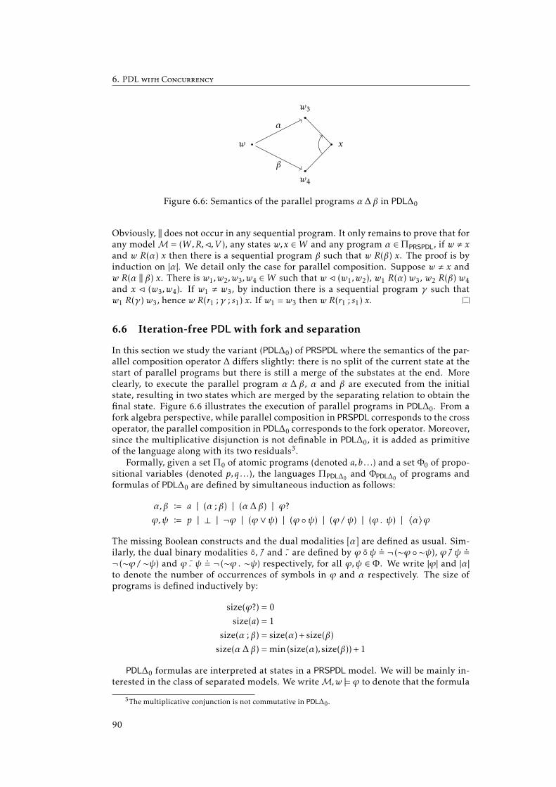
6. PDL with Concurrency
w
w4
w3
x
α
β
Figure 6.6: Semantics of the parallel programs α∆ β in PDL∆0
Obviously, ‖ does not occur in any sequential program. It only remains to prove that forany modelM = (W,R,C,V ), any states w,x ∈W and any program α ∈ΠPRSPDL, if w , xand w R(α) x then there is a sequential program β such that w R(β) x. The proof is byinduction on |α|. We detail only the case for parallel composition. Suppose w , x andw R(α ‖ β) x. There is w1,w2,w3,w4 ∈W such that w C (w1,w2), w1 R(α) w3, w2 R(β) w4and x C (w3,w4). If w1 , w3, by induction there is a sequential program γ such thatw1 R(γ) w3, hence w R(r1 ;γ ; s1) x. If w1 = w3 then w R(r1 ; s1) x.
6.6 Iteration-free PDL with fork and separation
In this section we study the variant (PDL∆0) of PRSPDL where the semantics of the par-allel composition operator ∆ differs slightly: there is no split of the current state at thestart of parallel programs but there is still a merge of the substates at the end. Moreclearly, to execute the parallel program α ∆ β, α and β are executed from the initialstate, resulting in two states which are merged by the separating relation to obtain thefinal state. Figure 6.6 illustrates the execution of parallel programs in PDL∆0. From afork algebra perspective, while parallel composition in PRSPDL corresponds to the crossoperator, the parallel composition in PDL∆0 corresponds to the fork operator. Moreover,since the multiplicative disjunction is not definable in PDL∆0, it is added as primitiveof the language along with its two residuals3.
Formally, given a set Π0 of atomic programs (denoted a,b . . .) and a set Φ0 of propo-sitional variables (denoted p,q . . .), the languages ΠPDL∆0
and ΦPDL∆0of programs and
formulas of PDL∆0 are defined by simultaneous induction as follows:
α,β B a | (α ; β) | (α∆ β) | ϕ?ϕ,ψ B p | ⊥ | ¬ϕ | (ϕ ∨ψ) | (ϕ ψ) | (ϕ /ψ) | (ϕ .ψ) | 〈α〉ϕ
The missing Boolean constructs and the dual modalities [α] are defined as usual. Sim-ilarly, the dual binary modalities , / and . are defined by ϕ ψ ¬ (∼ϕ ∼ψ), ϕ / ψ ¬ (∼ϕ /∼ψ) and ϕ . ψ ¬ (∼ϕ .∼ψ) respectively, for all ϕ,ψ ∈ Φ . We write |ϕ| and |α|to denote the number of occurrences of symbols in ϕ and α respectively. The size ofprograms is defined inductively by:
size(ϕ?) = 0
size(a) = 1
size(α ; β) = size(α) + size(β)
size(α∆ β) = min(size(α),size(β)) + 1
PDL∆0 formulas are interpreted at states in a PRSPDL model. We will be mainly in-terested in the class of separated models. We writeM,w |= ϕ to denote that the formula
3The multiplicative conjunction is not commutative in PDL∆0.
90
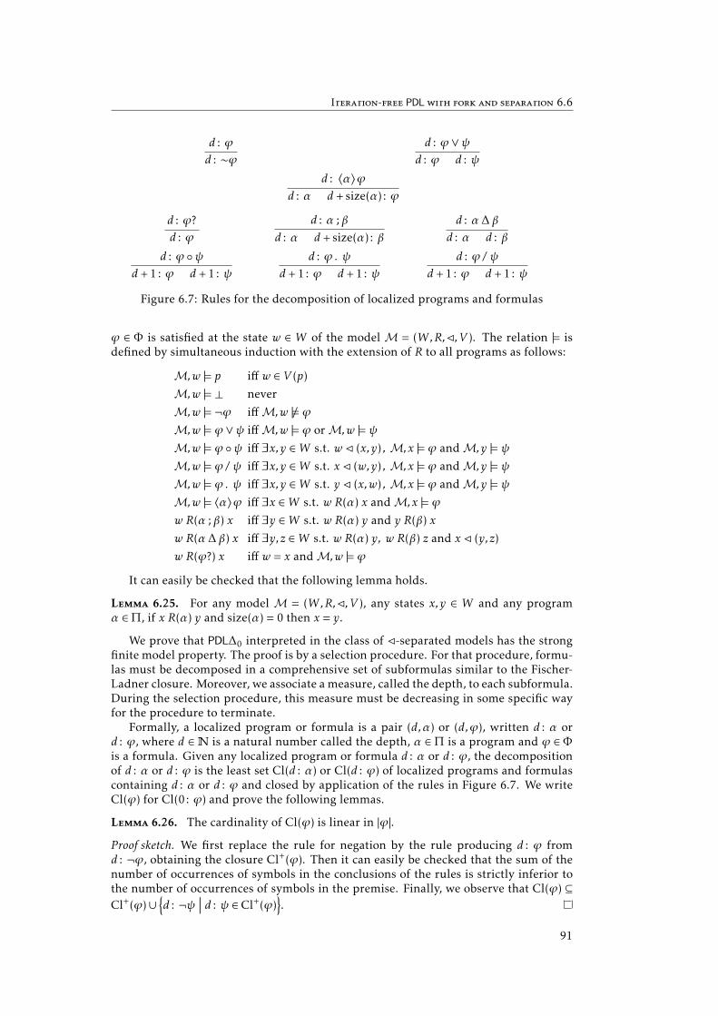
Iteration-free PDL with fork and separation 6.6
d : ϕd : ∼ϕ
d : ϕ ∨ψd : ϕ d : ψ
d : 〈α〉ϕd : α d + size(α) : ϕ
d : ϕ?d : ϕ
d : α ; βd : α d + size(α) : β
d : α∆ β
d : α d : β
d : ϕ ψd +1: ϕ d +1: ψ
d : ϕ .ψd +1: ϕ d +1: ψ
d : ϕ /ψd +1: ϕ d +1: ψ
Figure 6.7: Rules for the decomposition of localized programs and formulas
ϕ ∈ Φ is satisfied at the state w ∈ W of the modelM = (W,R,C,V ). The relation |= isdefined by simultaneous induction with the extension of R to all programs as follows:
M,w |= p iff w ∈ V (p)
M,w |=⊥ never
M,w |= ¬ϕ iffM,w 6|= ϕM,w |= ϕ ∨ψ iffM,w |= ϕ orM,w |= ψM,w |= ϕ ψ iff ∃x,y ∈W s.t. w C (x,y) , M,x |= ϕ andM, y |= ψM,w |= ϕ /ψ iff ∃x,y ∈W s.t. x C (w,y) , M,x |= ϕ andM, y |= ψM,w |= ϕ .ψ iff ∃x,y ∈W s.t. y C (x,w) , M,x |= ϕ andM, y |= ψM,w |= 〈α〉ϕ iff ∃x ∈W s.t. w R(α) x andM,x |= ϕw R(α ; β) x iff ∃y ∈W s.t. w R(α) y and y R(β) x
w R(α∆ β) x iff ∃y,z ∈W s.t. w R(α) y, w R(β) z and x C (y,z)
w R(ϕ?) x iff w = x andM,w |= ϕ
It can easily be checked that the following lemma holds.
Lemma 6.25. For any model M = (W,R,C,V ), any states x,y ∈ W and any programα ∈Π, if x R(α) y and size(α) = 0 then x = y.
We prove that PDL∆0 interpreted in the class of C-separated models has the strongfinite model property. The proof is by a selection procedure. For that procedure, formu-las must be decomposed in a comprehensive set of subformulas similar to the Fischer-Ladner closure. Moreover, we associate ameasure, called the depth, to each subformula.During the selection procedure, this measure must be decreasing in some specific wayfor the procedure to terminate.
Formally, a localized program or formula is a pair (d,α) or (d,ϕ), written d : α ord : ϕ, where d ∈N is a natural number called the depth, α ∈Π is a program and ϕ ∈ Φis a formula. Given any localized program or formula d : α or d : ϕ, the decompositionof d : α or d : ϕ is the least set Cl(d : α) or Cl(d : ϕ) of localized programs and formulascontaining d : α or d : ϕ and closed by application of the rules in Figure 6.7. We writeCl(ϕ) for Cl(0 : ϕ) and prove the following lemmas.
Lemma 6.26. The cardinality of Cl(ϕ) is linear in |ϕ|.
Proof sketch. We first replace the rule for negation by the rule producing d : ϕ fromd : ¬ϕ, obtaining the closure Cl+(ϕ). Then it can easily be checked that the sum of thenumber of occurrences of symbols in the conclusions of the rules is strictly inferior tothe number of occurrences of symbols in the premise. Finally, we observe that Cl(ϕ) ⊆Cl+(ϕ)∪
d : ¬ψ
∣∣∣ d : ψ ∈ Cl+(ϕ).91

6. PDL with Concurrency
Lemma 6.27. The function assigningmax d | either ∃ϕ,d : ϕ ∈ Cl(ϕ) or ∃α,d : α ∈ Cl(ϕ)to every formula ϕ ∈ ΦPDL∆0
is linear in |ϕ|.
Proof sketch. Let us write ν for both a program or a formula. We first prove by inductionon n that for all n > 0, if for some d ∈N and program α, d : α ∈ Cl(ϕ) and size(α) = n,then there exists ν such that d + n − 1: ν ∈ Cl(ϕ). Then it can easily be proved that ifd : ν ∈ Cl(ϕ) for some d > 0 and ν, then there exists ν′ such that d − 1: ν′ ∈ Cl(ϕ).
Selection Procedure
Given a formula ϕ0, a modelMo and a state w0 such thatMo,w0 |= ϕ0, a modelMs isconstructed such thatMs satisfies ϕ0 and the number of states inMo is bounded by anexponential in |ϕ0|. The construction ofMs is performed by the procedure Selection
on the facing page. Selection uses the recursive procedure Link described on page 94.Whereas Selection ensures that the satisfiability of all subformulas is preserved, Linkensures that subprograms can be executed between states inMs. The following lemmasare used to prove the strong finite model property.
Lemma 6.28. The procedure Selection terminates and the cardinality of Ws is expo-nential in |ϕ0|.
Proof. We consider the tree (V ,E) such that V =Ws and there is an edge from (kx,dx,x)to (ky ,dy , y) iff (ky ,dy , y) has been added toWs while (kx,dx,x) was chosen in Selection.It can easily be proved by induction on |α| that during any call to Link with programargument α, the number of states added to Ws is inferior or equal to 2 · |α|. Hence,by Lemma 6.26, the branching factor of (V ,E) is bounded by a quadratic function in|ϕ0|. To prove that the depth of (V ,E) is bounded by a linear function in |ϕ0|, we useLemma 6.27 and prove that d is strictly increasing along the branches of (V ,E). Forthat matter, it suffices to verify that whenever Link(Ms,n, (kx,dx,x), (ky ,dy , y),α) is calledwhile (kw,dw,w) is chosen in Selection, then dx ≥ dw and dy > dw.
Lemma 6.29. Whenever Link is called, dy ≤ dx + size(α).
Proof. For the call at line 16 of Selection, the property holds by the assignment atline 13. For the recursive calls of Link, we suppose that dy ≤ dx + size(α). Supposefirst that α = β ; γ . Then dy ≤ dx + size(β) + size(γ). Therefore, if size(β) = 0 then dy ≤dx + size(γ) and the property holds for the call at line 5. The proof is identical for thecall at line 7. For the calls at lines 13 and 14, the assignment line 11 set dz = dx+size(β),therefore these two calls satisfies the property. Suppose now that α = β∆γ . For the callsat lines 31 and 39, by the assignments at lines 28 and 35, we have that dw ≤ dx +size(β).The proof is identical for the calls at lines 24 and 40.
The following lemma is essential for the forthcoming truth lemma (Lemma 6.33) asit makes the proof for the dual modalities , / and . trivial.
Lemma 6.30. For all((ky ,dy , y), (kw,dw,w), (kz,dz, z)
)∈Cs:
y Co (w,z)
|dy − dw | ≤ 1
|dy − dz | ≤ 1
|dw − dz | ≤ 1
Proof. We prove that at line 38 of Link, |dy − dw | ≤ 1 and |dw − dz | ≤ 1, the others casesand properties being either similar or straightforward.
Suppose first that dw = dy + 1. Then obviously |dy − dw | ≤ 1. If dz = dy + 1, then|dw − dz | ≤ 1 is trivial too. If dz = dx + size(β) + 1, by minimality, dz ≤ dy +1 and size(β) <
92

Iteration-free PDL with fork and separation 6.6
Procedure 1: SelectionResult: A finite modelMs = (Ws,Rs,Cs,Vs).Data: A subset K ⊆Ws of marked nodes and an integer n ∈N.
1 initialization2 n = 03 Ws = (0,0,w0)4 Rs(a) = ∅ for all a ∈Π05 Cs= ∅6 K = ∅
7 while K ,Ws do8 choose an unmarked state (k,d,w) ∈Ws \K9 while (k,d,w) < K do
10 let Vs(p) = (kx,dx,x) ∈Ws | x ∈ Vo(p) for all p ∈ Φ0
11 if there exists d′ : 〈α〉ϕ ∈ Cl(ϕ0) such that size(α) > 0, d′ ≥ d,Mo,w |= 〈α〉ϕandMs, (k,d,w) 6|= 〈α〉ϕ then
12 choose y s.t. w Ro(α) y andMo, y |= ϕ13 let dy = d + size(α)14 let n = n+115 add (n,dy , y) toWs
16 call Link(Ms,n, (k,d,w), (n,dy , y),α
)17 else if there exists d′ : ϕ ψ ∈ Cl(ϕ0) such that d′ ≥ d,Mo,w |= ϕ ψ and there
is no (kx,dx,x), (ky ,dy , y) ∈Ws such that (k,d,w) Cs((kx,dx,x), (ky ,dy , y)
)then
18 choose x and y s.t. w Cs (x,y),Mo,x |= ϕ andMo, y |= ψ19 add (n+1,d +1,x) and (n+2,d +1, y) toWs20 add ((k,d,w), (n+1,d +1,x), (n+2,d +1, y)) to Cs21 let n = n+2
22 else if there exists d′ : ϕ .ψ ∈ Cl(ϕ0) such that d′ ≥ d,Mo,w |= ϕ .ψ andMs, (k,d,w) 6|= ϕ .ψ then
23 choose x and y s.t. y Cs (x,w),Mo,x |= ϕ andMo, y |= ψ24 add (n+1,d +1,x) and (n+2,d +1, y) toWs25 add ((n+2,d +1, y), (n+1,d +1,x), (k,d,w)) to Cs26 let n = n+2
27 else if there exists d′ : ϕ /ψ ∈ Cl(ϕ0) such that d′ ≥ d,Mo,w |= ϕ /ψ andMs, (d,w) 6|= ϕ /ψ then
28 choose x and y s.t. x Cs (w,y),Mo,x |= ϕ andMo, y |= ψ29 add (n+1,d +1,x) and (n+2,d +1, y) toWs30 add ((n+1,d +1,x), (k,d,w), (n+2,d +1, y)) to Cs31 let n = n+2
32 else33 add (k,d,w) to K
93

6. PDL with Concurrency
Procedure 2: LinkInput: A finite modelMs = (Ws,Rs,Cs,Vs), an integer n, two states
(kx,dx,x), (ky ,dy , y) ∈Ws and a program α such that x Ro(α) y.Result:Ms and nmodified.
1 if α is of the form a ∈Π0 then2 add
((kx,dx,x), (ky ,dy , y)
)to Rs(a)
3 else if α is of the form (β ;γ) then4 if size(β) = 0 then5 call Link
(Ms,n, (kx,dx,x), (ky ,dy , y),γ
)6 else if size(γ) = 0 then7 call Link
(Ms,n, (kx,dx,x), (ky ,dy , y),β
)8 else9 choose z s.t. x Ro(β) z and z Ro(γ) y
10 let n = n+111 let dz = dx + size(β)12 add (n,dz, z) toWs13 call Link (Ms,n, (kx,dx,x), (n,dz, z),β)
14 call Link(Ms,n, (n,dz, z), (ky ,dy , y),γ
)15 else if α is of the form (β ∆γ) then16 if size(β) = 0 and size(γ) = 0 then17 add ((ky ,dy , y), (kx,dx,x), (kx,dx,x)) to Cs18 else if size(β) = 0 then19 choose z s.t. x Ro(γ) z and y Co (x,z)20 let n = n+121 let dz =min
(dy +1,dx + size(γ)
)22 add (n,dz, z) toWs23 add ((ky ,dy , y), (kx,dx,x), (n,dz, z)) to Cs24 call Link (Ms,n, (kx,dx,x), (n,dz, z),γ)25 else if size(γ) = 0 then26 choose w s.t. x Ro(β) w and y Co (w,x)27 let n = n+128 let dw =min
(dy +1,dx + size(β)
)29 add (n,dw,w) toWs30 add ((ky ,dy , y), (n,dw,w), (kx,dx,x)) to Cs31 call Link (Ms,n, (kx,dx,x), (n,dw,w),β)32 else33 choose w and z s.t. x Ro(β) w, x Ro(γ) z and y Co (w,z)34 let n = n+235 let dw =min
(dy +1,dx + size(β),dx + size(γ) + 1
)36 let dz =min
(dy +1,dx + size(γ),dx + size(β) + 1
)37 add (n− 1,dw,w) and (n,dz, z) toWs38 add ((ky ,dy , y), (n− 1,dw,w), (n,dz, z)) to Cs39 call Link (Ms,n, (kx,dx,x), (n− 1,dw,w),β)40 call Link (Ms,n, (kx,dx,x), (n,dz, z),γ)
94

Iteration-free PDL with fork and separation 6.6
size(γ). By Lemma 6.29, dy ≤ dz. Therefore, dw − 1 ≤ dz ≤ dw. If dz = dx + size(γ),by minimality, dz ≤ dy + 1 and size(γ) ≤ size(β). By Lemma 6.29, dy < dz. Therefore,dw − 1 < dz ≤ dw.
Suppose now that dw = dx +size(γ)+1. By minimality, dy > dx +size(γ) and size(β) >size(γ). By Lemma 6.29, dy ≤ dx + size(γ) + 1. Therefore, dy = dw. If dz = dy + 1 ordz = dx+size(γ), then obviously dw−1 ≤ dz ≤ dw+1. If dz = dx+size(β)+1, by minimalitysize(β) < size(γ), which is impossible.
Suppose finally that dw = dx + size(β). By minimality, dy ≥ dx + size(β) and size(γ) ≥size(β). By Lemma 6.29, dy ≤ dx + size(β) + 1. Therefore, dw ≤ dy ≤ dw + 1. If dz =dx+size(β)+1, then obviously dz = dw+1. If dz = dx+size(γ)+1, by minimality, size(γ) ≤size(β). Hence size(γ) = size(β) and dz = dw. If dz = dy+1, byminimality, dy < dx+size(β),which is impossible.
Lemma 6.31. If (kx,dx,x) Rs(α) (ky ,dy , y) then dy ≤ dx + size(α).
sketch. From Lemmas 6.29 and 6.30 by an easy induction on |α|.
Lemma 6.32. IfMo is C-separated, thenMs is C-separated too.
Proof. Let us suppose that the tuple t =((kw,dw,w), (kw1
,dw1,w1), (kw2
,dw2,w2)
)has been
added to Cs while (kw,dw,w) Cs((k′w1
,d′w1,w1
′), (k′w2,d′w2
,w2′)). Then t cannot have been
added toCs in Selection because at lines 25 and 30, (kw,dw,w) is fresh and at line 20, thecondition ensures that
((kw,dw,w), (k′w1
,d′w1,w1
′), (k′w2,d′w2
,w2′))<Cs. The tuple t cannot
have been added to Cs in Link neither, because whenever Link is called there is no(ky1 ,dy1 , y1) and (ky2 ,dy2 , y2) inWs such that (ky ,dy , y) Cs
((ky1 ,dy1 , y1), (ky2 ,dy2 , y2)
).
Lemma 6.33. IfMo is C-separated thenMs, (0,0,w0) |= ϕ0
Proof. The following properties are proved for all n ∈N:IH.1 for all d : ϕ ∈ Cl(ϕ0) and all (kw,dw,w) ∈Ws, if |ϕ| = n, d ≥ dw andMo,w |= ϕ then
Ms, (kw,dw,w) |= ϕIH.2 if Link has been called with last arguments (kx,dx,x), (ky ,dy , y) and α with |α| = n,
then (kx,dx,x) Rs(α) (ky ,dy , y)
IH.3 for all α and (kx,dx,x), (ky ,dy , y) ∈Ws, if (kx,dx,x) Rs(α) (ky ,dy , y) and |α| = n thenx Ro(α) y
The proof is by induction on n. We give details of the following cases only, the otherones being either similar or straightforward.
Hypothesis IH.1 when ϕ = 〈α〉ψ. There is y ∈Wo such that w Ro(α) y andMo, y |= ψ.Moreover, d + size(α) : ψ ∈ Cl(ϕ0). If Ms, (kw,dw,w) 6|= 〈α〉ψ, conditions at line 11 aresatisfied. Therefore, a state (ky ,dw + size(α), y) is added to Ws and Link is called witharguments (kw,dw,w), (ky ,dw + size(α), y) and α. Since |α| < |ϕ|, by induction hypoth-esis IH.2, (kw,dw,w) Rs(α) (ky ,dw + size(α), y). And since dw + size(α) ≤ d + size(α) and∣∣∣ψ∣∣∣ < |ϕ|, by induction hypothesis IH.1,Ms, (ky ,dw + size(α), y) |= ψ.
Hypothesis IH.1 when ϕ = [α]ψ. Suppose (kw,dw,w) Rs(α) (ky ,dy , y). Since |α| < |ϕ|,by induction hypothesis IH.3,w Ro(α) y. ThereforeMo, y |= ψ. By Lemma 6.31, dy ≤ dw+size(α). Since d + size(α) : ψ ∈ Cl(ϕ0), by induction hypothesis IH.1,Ms, (ky ,dy , y) |= ψ.
Hypothesis IH.1 when ϕ = ψ χ. By the condition at line 17, there exists (kx,dx,x)and (ky ,dy , y) such that (kw,dw,w) Cs
((kx,dx,x), (ky ,dy , y)
). By Lemma 6.30, w Co (x,y),
dx ≤ dw + 1 and dy ≤ dw + 1. SinceMo is C-separated,Mo,x |= ψ andMo, y |= χ. Sinced +1: ψ ∈ Cl(ϕ0) and d +1: χ ∈ Cl(ϕ0), by induction hypothesis IH.1,Ms, (kx,dx,x) |= ψandMs, (ky ,dy , y) |= χ.
Hypothesis IH.2 when α = β ; γ and size(β) = 0. First, it has to be verified thatwhenever Link is called, there exists d ∈N such that d ≥ dx and d : α ∈ Cl(ϕ0), which is
95

6. PDL with Concurrency
straightforward. Let dα be such that dα ≥ dx and dα : α ∈ Cl(ϕ0). Since size(α) = 0, thereis a list ϕ1, . . . ,ϕm such that β = ϕ1? ; . . . ;ϕm?. Moreover, for all ` ∈ 1 . .m, |ϕ` | < |α| anddα : ϕ` ∈ Cl(ϕ0). Hence, by induction hypothesis IH.1, (kx,dx,x) Rs(β) (kx,dx,x). Andsince
∣∣∣γ ∣∣∣ < |α|, by induction hypothesis IH.2, (kx,dx,x) Rs(γ) (ky ,dy , y).Hypothesis IH.3 when α = a. First, it has to be verified that whenever Link is called,
x Ro(α) y, which is straightforward whenMo is C-separated. Finally, it suffices to re-mark that since (kx,dx,x) Rs(a) (ky ,dy , y), line 2 of Link have been called.
We have proved the following proposition:
Proposition 6.34. Any PDL∆0 formula ϕ satisfiable in a C-separated model is satisfi-able in a C-separated finite model with a number of states bounded by an exponentialin |ϕ|.
And since the model-checking problem for PDL∆0 is obviously polynomial in thesize of the model (see [Lange.06] for a generic method), we have the following corollary.
Corollary 6.35. The satisfiability problem of PDL∆0 in the class of C-separated framesis decidable in non-deterministic exponential time.
96
Chapter 7
PDL with Deterministic SeparatingParallel Composition
The separating parallel composition of programs as found in PDL with Parallel com-position, Recover and Store (PRSPDL) or PDL with fork and separation, both presentedin the previous chapter, adds an interesting and natural notion of concurrency to dy-namic logics. The separation allows a fine-grain control over concurrency. In this chap-ter, a variant of PRSPDL is studied. This logic, called the Propositional Dynamic Logicwith Deterministic separating Parallel composition (PPDLdet) is the fragment of PRSPDLwithout the four store and recover programs, interpreted in the class of C-deterministicframes. With this syntactic restriction, PPDLdet allows all situations of cooperations de-fined in Section 6.1. The semantic restriction to deterministic separation is very natural:whereas there often are different ways to split a state into substates, there is only oneway (if any) to merge two substates. Hence this restriction, which turns the ternaryseparation relation into a partial binary operator, is common in binary modal logics.
However, PPDLdet, like PRSPDL and PDL with intersection, lacks the two importantproperties of having comprehensive decompositions and the tree-like model property.After the presentation of the syntax and semantics of PPDLdet in Section 7.1 and of someexpressivity results in Section 7.2, the absence of these two properties is overcome inthe next two sections. For the lack of comprehensive decompositions, the language isextended in Section 7.3 such that an adaptation of the Fischer-Ladner closure is possi-ble. For the lack of the tree-like model property, the alternative neat model property isdefined then proved for PPDLdet in Section 7.4. These two constructions are then usedin the remaining sections to prove decidability and complexity results for PPDLdet andits iteration-free variant.
7.1 Syntax and Semantics
The Propositional Dynamic Logic with Deterministic separating Parallel composition(PPDLdet) is the fragment of PRSPDL without the store and recover special programs,interpreted in the class of C-deterministic frames. Formally, letΠ0 be a countable set ofatomic programs (denoted by a,b . . .) and Φ0 a countable set of propositional variables(denoted by p,q . . .). The setsΠPPDL and ΦPPDL of programs and formulas are defined by:
α,β B a | (α ; β) | (α ∪ β) | ϕ? | α∗ | (α ‖ β)ϕ B p | ⊥ | ¬ϕ | 〈α〉ϕ
As usual: parentheses may be omitted for clarity; the dual modalities are defined by[α]ϕ ¬〈α〉¬ϕ; the missing Boolean operators are defined from ϕ→ ψ [ϕ?]ψ and |α|and |ϕ| denote the number of occurrences of symbols in the program α and the formulaϕ. Moreover, we will sometimes explicitly use the syntactic operator ∼ of involutivenegation defined such that ∼ϕ = ψ if ϕ = ¬ψ for some ψ and ∼ϕ = ¬ϕ otherwise (seeSection 2.1 for a discussion about negations).
A PPDLdet frame is a C-deterministic PRSPDL frame, i.e., a triple F = (W,R,C) whereW is a nonempty set of states (denoted by w,x,y . . .), R is the accessibility function as-signing a binary relation overW to each atomic program and C is a ternary relation over
97

7. PDL with Deterministic Separating Parallel Composition
W called the separation relation and such that for all x,y,w1,w2 ∈W :
(C-determinism) if x C (w1,w2) and y C (w1,w2) then x = y
Intuitively, x R(a) y means that the program a can be executed in state x, reaching statey. Similarly, x C (y,z) means that x can be split into the states y and z. We say that y andz are substates of x by the decomposition (x,y,z) ∈C. Equivalently, x C (y,z) means thatthe substates y and z can be merged to obtain x. PPDLdet frames being C-deterministic,the merging of substates is functional. Hence C is equivalent to a partial binary operatoronW .
A PPDLdet model is a C-deterministic model, i.e., a tuple M = (W,R,C,V ) where(W,R,C) is a C-deterministic frame and V is a valuation function associating a subsetofW to each propositional variable. PPDLdet formulas are evaluated at states in PPDLdet
models. The expressionM,w |= ϕ denote the fact that the formula ϕ ∈ΠPPDL is satisfiedat the state w ∈W of the modelM = (W,R,C,V ). The relation |= is defined by parallelinduction along with the extension of R to all programs as follows:
M,w |= p iff w ∈ V (p)
M,w |=⊥ never
M,w |= ¬ϕ iffM,w 6|= ϕM,w |= 〈α〉ϕ iff there is x ∈W such that w R(α) x andM,x |= ϕw R(α ; β) x iff there is y ∈W such that w R(α) y and y R(β) x
w R(α ∪ β) x iff w R(α) x or w R(β) xw R(ϕ?) x iff w = x andM,w |= ϕw R(α∗) x iff w R(α)∗ x
where R(α)∗ is the reflexive and transitive closure of R(α)
w R(α ‖ β) x iff there are w1,w2,w3,w4 ∈W such thatw C (w1,w2) , w1 R(α) w3, w2 R(β) w4 and x C (w3,w4)
PPDLdet is the logic with language ΦPPDL interpreted in C-deterministic frames. Aformula ϕ ∈ ΦPPDL is PPDLdet satisfiable iff there exists a C-deterministic model M =(W,R,C,V ) and a state w ∈W such thatM,w |= ϕ. The satisfiability problem of PPDLdet
is the decision problem answering whether a formula in ΦPPDL is PPDLdet satisfiable.This problem is proved to be in EXPTIME in Section 7.6. Finally, the following proposi-tion can easily be proved by a straightforward adaptation of the proof of Proposition 2.2.
Proposition 7.1. PPDLdet is conservative.
7.2 Expressivity
Most of the expressivity results of PRSPDL proved in Section 6.5 hold for PPDLdet.Specifically, the binary modality T defined by ϕ T ψ
⟨ϕ? ‖ ψ?
⟩> for any formulas
ϕ,ψ ∈ ΦPPDL, is such that for any C-deterministic model M = (W,R,C,V ), any statew ∈ W and any formulas ϕ,ψ ∈ ΦPPDL, M,w |= ϕ T ψ iff there are x,y ∈ W such thatw C (x,y),M,x |= ϕ andM, y |= ψ. Moreover, the models used in the proofs of Proposi-tions 6.19, 6.20, 6.21 and 6.23 are all C-deterministic, hence all these propositions holdfor PPDLdet too. Namely: no residual of T can be defined in PPDLdet, neither test nor therecover programs are modally definable in PPDLdet and PPDLdet allows both simple andatomic cooperations. The following proposition proves that unlike PRSPDL, PPDLdet
allows forced cooperation.
Proposition 7.2. PPDLdet allows forced cooperation.
98

Expressivity 7.2
Proof. Consider the model M = (W,R,C,V ) where W = 0 . .5, R(a) = (1,3)(2,4) andR(b) = ∅ for all b ∈Π0 \ a, C= (0,1,2), (5,3,4) and V (p) = ∅ for all p ∈ Φ0. ThenM,0 |=〈a ‖ a〉>. Moreover, it can easily be proved by induction on |α| that for all α ∈ΠPPDL andall w ∈W if ‖ does not occur in α and 0 R(α) w then w = 0.
Like for PDL with intersection, it is not possible to adapt the Fischer-Ladner clo-sure directly to PPDLdet, as the following proposition shows. The adaptation proposedin Section 7.3 extends the language of PPDLdet with some non-standard propositionalvariables.
Proposition 7.3. PPDLdet does not have comprehensive decomposition.
Proof. Consider the formula ϕ = 〈a ‖ a〉> and the same twomodelsM = (W,R,C,V ) andM′ = (W ′ ,R′ ,C′ ,V ′) as in the proof of Proposition 6.22, defined by:
• W = 1 . .5,
• R(a) = (1,3), (2,4) and for all b ∈Π0 \ a, R(b) = ∅,• C= (0,1,2), (5,3,4),• V (p) = ∅, for all p ∈ Φ0,
• W ′ = 1′ . .8′ ,
• R′(a) = (1′ ,3′), (2′ ,4′) and for all b ∈Π0 \ a, R′(b) = ∅,• C′= (0′ ,1′ ,2′), (5′ ,3′ ,6′), (7′ ,8′ ,4′),• V ′(p) = ∅, for all p ∈ Φ0.
These two models are depicted in Figure 6.5 on page 89 where edges are implicitlylabeled with a. It can easily be checked thatM,0 |= 〈a ‖ a〉> butM′ ,0′ 6|= 〈a ‖ a〉>.
Since ‖ does not occur in any formulaψ ∈ ΦPPDL such that∣∣∣ψ∣∣∣ < |ϕ|, we already proved
for Proposition 6.22 that 0 and 0′ cannot be distinguished by any formula ψ ∈ ΦPPDLsuch that
∣∣∣ψ∣∣∣ < |ϕ|. It remains to prove that 1 and 2 cannot be distinguished from 1′ and2′ by any formula in ΦPPDL. The binary relation Z between W and W ′ is first definedby Z = (1,1′), (2,2′), (3,3′), (4,4′), (5,5′), (4,6′), (5,7′), (3,8′). We prove the followinghypotheses for all n ∈N, all α ∈ΠPPDL, all ψ ∈ ΦPPDL and all (w,w′) ∈ Z:IH.1 for any x ∈ W , if |α| = n and w R(α) x then x , 0 and there is x′ ∈ W ′ such that
x Z x′ and w′ R′(α) x′ ;
IH.2 for any x′ ∈W ′ , if |α| = n and w′ R′(α) x′ then x′ , 0′ and there is x ∈W such thatx Z x′ and w R(α) x;
IH.3 if∣∣∣ψ∣∣∣ = n thenM,w |= ψ iffM′ ,w′ |= ψ.
The proof is by a straightforward induction on n.
Interpretation of PPDLdet for Petri nets with capacities and concurrency
We briefly illustrate Proposition 7.2 by giving an interpretation of PPDLdet for Petrinets with capacities and concurrency as defined in Section 6.1. Given a Petri net P =(S,T ,W ,K,m0) (see Definition 6.1 on page 76), a corresponding C-deterministic modelMP = (WP ,RP ,CP ,VP ) over the set Π0 = T of atomic programs is defined such that:
• WP is the set of all acceptable markings of P ;• m RP (a)m′ iff for all s ∈ S m(s) ≥W (s,a) and m′(s) =m(s)−W (s,a) +W (a,s);
• m1 CP (m2,m3) iff m1(s) =m2(s) +m3(s) for all s ∈ S.Remark thatMP is C-associative.
Considering again the Petri net P from Figure 6.1, Figure 7.1 illustrates how theexecution of the program a ‖ b in MP corresponds to the firing of the multiset a,b.This result is generalized by the following proposition.
99

7. PDL with Deterministic Separating Parallel Composition
≤ 1 a ≤ 1 b
a b
Figure 7.1: Concurrent firing of transitions a and b with PPDLdet semantics.
Proposition 7.4. Let P = (S,T ,W ,K,m0) be a Petri net with capacities and concurrency,MP its corresponding model and θ = a1, . . . , an a finite multiset of transitions. Then θis enabled in P if and only ifMP ,m0 |= 〈a1 ‖ . . . ‖ an〉>.
Proof. For the left-to-right direction, suppose that θ is enabled, i.e., m0(s) ≥∑t∈T θ(t) ·
W (s, t) and m0(s)−∑t∈T θ(t) ·W (s, t) +
∑t∈T θ(t) ·W (t, s) ≤ K(s). For all s ∈ S, let m1(s) =
m0(s)−∑k∈2..nW (s,ak) and for all k ∈ 2 . .n, let mk(s) =W (s,ak). Clearly, for all k ∈ 1 . .n,
mk ∈WP . For all s ∈ S, let m′1(s) =m1(s)−W (s,a1) +W (a1, s) and for all k ∈ 2 . .n, m′k(s) =W (ak , s). Clearly, for all k ∈ 1 . .n, m′k ∈ WP and mk RP (ak) m′k . Therefore, MP ,m0 |=〈a1 ‖ . . . ‖ an〉>.
For the right-to-left direction, suppose that MP ,m0 |= 〈a1 ‖ . . . ‖ an〉 >. Then thereare m1, . . . ,mn,m
′ ,m′1, . . . ,m′n ∈ WP such that for all s ∈ S, m0(s) =
∑k∈1..nmk(s), m
′(s) =∑k∈1..nm
′k(s) and for all k ∈ 1 . .n, mk(s) ≥W (s,ak) and m′k(s) =mk(s)−W (s,ak) +W (ak , s).
Therefore, θ is enabled.
7.3 Fischer-Ladner closure
As proved by Proposition 7.3, PPDLdet does not have comprehensive decompositions.Hence there is no hope to have a comprehensive set of subformulas for every formula.To workaround this difficulty, a more expressive logic is devised by extending PPDLdet
as follows. Firstly, symbols ‖ of parallel composition are annotated with unique identi-fiers called indices. Secondly, to each such index i are associated two specials formulasLi and Ri called placeholders. Placeholders are reminiscent of nominals as found in hy-brid logics [Prior.67, PasTin.85]. Intuitively, we want formulas of the form
⟨α ‖i β
⟩ϕ
to be satisfied at some state w if and only if there are states w1,w2,w3,w4,x and an in-terpretation of Li and Ri such thatM,x |= ϕ, x C (w3,w4), w C (w1,w2),M,w1 |= 〈α〉Li ,M,w2 |=
⟨β⟩Ri and Li and Ri are satisfied only at w3 and w4 respectively.
Formally, using the same setsΠ0 and Φ0 of atomic programs and propositional vari-ables as for PPDLdet, the setsΠPH and ΦPH of annotated programs and annotated formulas
100
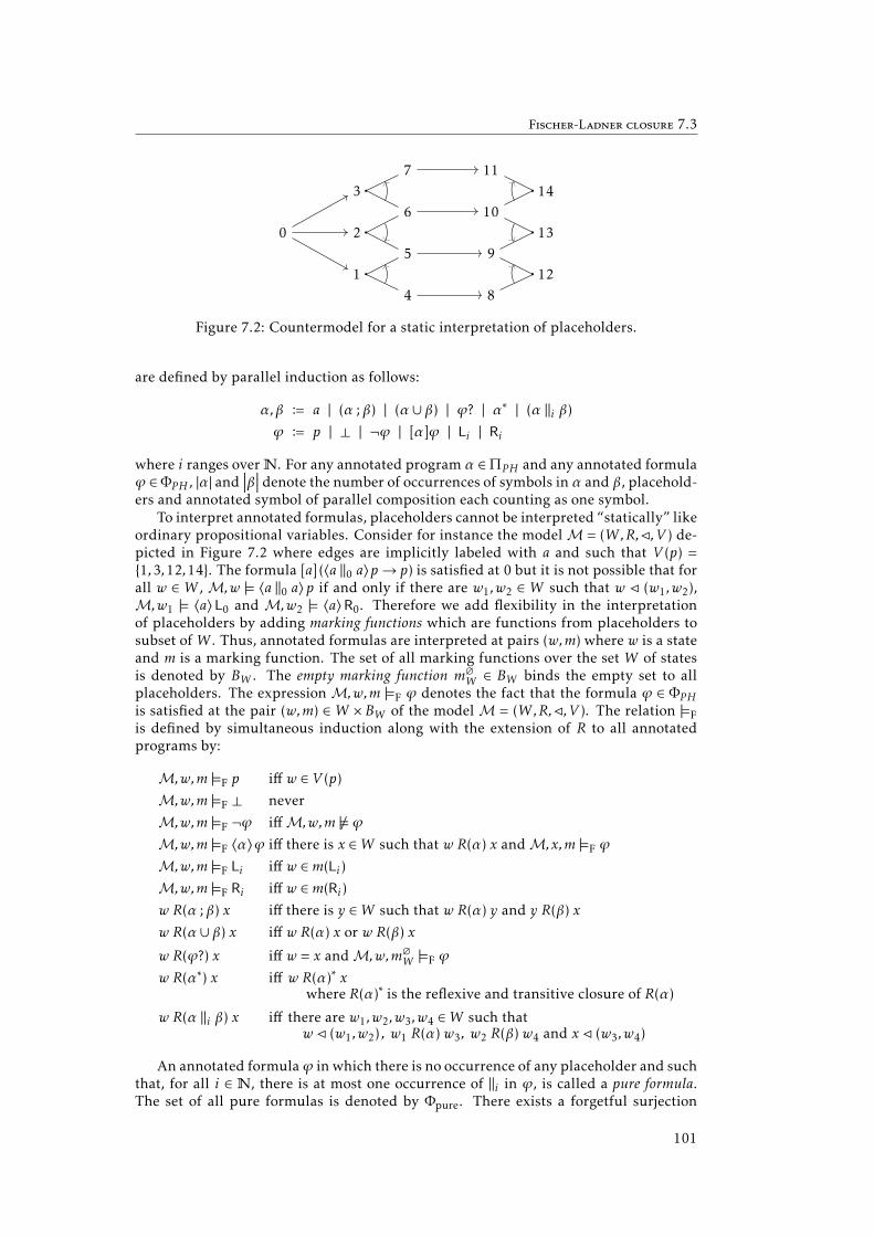
Fischer-Ladner closure 7.3
0
4
5
6
7
8
9
10
11
1
2
3
12
13
14
Figure 7.2: Countermodel for a static interpretation of placeholders.
are defined by parallel induction as follows:
α,β B a | (α ; β) | (α ∪ β) | ϕ? | α∗ | (α ‖i β)ϕ B p | ⊥ | ¬ϕ | [α]ϕ | Li | Ri
where i ranges overN. For any annotated program α ∈ΠPH and any annotated formulaϕ ∈ ΦPH , |α| and
∣∣∣β∣∣∣ denote the number of occurrences of symbols in α and β, placehold-ers and annotated symbol of parallel composition each counting as one symbol.
To interpret annotated formulas, placeholders cannot be interpreted “statically” likeordinary propositional variables. Consider for instance the modelM = (W,R,C,V ) de-picted in Figure 7.2 where edges are implicitly labeled with a and such that V (p) =1,3,12,14. The formula [a] (〈a ‖0 a〉p→ p) is satisfied at 0 but it is not possible that forall w ∈ W ,M,w |= 〈a ‖0 a〉p if and only if there are w1,w2 ∈ W such that w C (w1,w2),M,w1 |= 〈a〉 L0 and M,w2 |= 〈a〉 R0. Therefore we add flexibility in the interpretationof placeholders by adding marking functions which are functions from placeholders tosubset ofW . Thus, annotated formulas are interpreted at pairs (w,m) where w is a stateand m is a marking function. The set of all marking functions over the set W of statesis denoted by BW . The empty marking function m∅
W ∈ BW binds the empty set to allplaceholders. The expressionM,w,m |=F ϕ denotes the fact that the formula ϕ ∈ ΦPHis satisfied at the pair (w,m) ∈ W × BW of the modelM = (W,R,C,V ). The relation |=Fis defined by simultaneous induction along with the extension of R to all annotatedprograms by:
M,w,m |=F p iff w ∈ V (p)
M,w,m |=F ⊥ never
M,w,m |=F ¬ϕ iffM,w,m 6|= ϕM,w,m |=F 〈α〉ϕ iff there is x ∈W such that w R(α) x andM,x,m |=F ϕ
M,w,m |=F Li iff w ∈m(Li)
M,w,m |=F Ri iff w ∈m(Ri)
w R(α ; β) x iff there is y ∈W such that w R(α) y and y R(β) x
w R(α ∪ β) x iff w R(α) x or w R(β) x
w R(ϕ?) x iff w = x andM,w,m∅
W |=F ϕ
w R(α∗) x iff w R(α)∗ xwhere R(α)∗ is the reflexive and transitive closure of R(α)
w R(α ‖i β) x iff there are w1,w2,w3,w4 ∈W such thatw C (w1,w2) , w1 R(α) w3, w2 R(β) w4 and x C (w3,w4)
An annotated formulaϕ in which there is no occurrence of any placeholder and suchthat, for all i ∈ N, there is at most one occurrence of ‖i in ϕ, is called a pure formula.The set of all pure formulas is denoted by Φpure. There exists a forgetful surjection
101

7. PDL with Deterministic Separating Parallel Composition
(µ, ϕ)(µ, ∼ϕ)
(µ, 〈a〉ϕ)(µ, ϕ)
(µ,⟨α ; β
⟩ϕ)
(µ, 〈α〉⟨β⟩ϕ)
(µ,⟨α ∪ β
⟩ϕ)
(µ, 〈α〉ϕ) (µ,⟨β⟩ϕ)
(µ,⟨ϕ?
⟩ψ)
(µ, ϕ) (µ, ψ)(µ, 〈α∗〉ϕ)
(µ, 〈α〉〈α∗〉ϕ) (µ, ϕ)
(µ,⟨α ‖i β
⟩ϕ)
(µ.`, 〈α〉Li) (µ.r,⟨β⟩Ri) (µ, ϕ)
Figure 7.3: Fischer-Ladner closure rules for localized annotated formulas.
(µ,⟨α ∪ β
⟩ϕ)
(µ, 〈α〉Qϕ) (µ,⟨β⟩Qϕ) (µ, ϕ)
(µ, 〈α∗〉ϕ)(µ, 〈α〉Q〈α∗〉ϕ) (µ, ϕ)
(µ, ¬ϕ)(µ, ϕ)
Figure 7.4: Restricted Fischer-Ladner closure rules for PPDLdet.
· : Φpure −→ Φ associating to each pure formula ϕ the formula ϕ obtained by removingall indices in ϕ. Thanks to the following proposition, the satisfiability of pure formulascan be considered instead of the satisfiability of PPDLdet formulas.
Proposition 7.5. For any modelM = (W,R,C,V ), any formula ϕ ∈ Φpure and any statew ∈W ,M,w,m∅
W |=F ϕ iffM,w |= ϕ.
Proof. By a straightforward induction on |ϕ|.
Now, the Fischer-Ladner closure (see Section 2.2) is adapted to annotated formulas.For some constructions done in the next sections, we need to keep track of the level ofseparation (called depth) of each subformula. Hence we consider localized formulas. Alocation is a word on the alphabet `, r, the empty word being denoted by ε. A localizedformula is a pair (µ, ϕ) composed of a location µ and a formula ϕ.
Given a localized annotated formula (µ, ϕ), the closure FL(µ, ϕ) of (µ, ϕ) is the leastset of localized annotated formulas which contains (µ, ϕ) and is closed by the appli-cation of the rules in Figure 7.3. In the remainder of this chapter, we will be mainlyinterested in closure of localized pure formulas of the form (ε, ϕ0). For all pure formu-las ϕ0 ∈ Φpure, the following abbreviations are defined:
FL(ϕ0) = FL(ε, ϕ0)
SP(ϕ0) =α∣∣∣ ∃µ,∃ϕ, (µ, 〈α〉ϕ) ∈ FL(ϕ0)
Loc(ϕ0) =
µ∣∣∣ ∃ϕ, (µ, ϕ) ∈ FL(ϕ0)
where SP stands for “subprograms”. The cardinality of FL(ϕ0) is denoted by Nϕ0
. Westate the following proposition.
Proposition 7.6. Nϕ0is linear in |ϕ0|.
Proof. The proof is similar to the proof of Proposition 2.4. We define for any localizedannotated formula (µ, ϕ) the restricted closure rFL(µ, ϕ) by replacing the rules for non-deterministic choices, iterations and negations of Figure 7.3 by the rules of Figure 7.4where new propositional variables of the form Qψ are added to the language.
102

Neat model property 7.4
The function γ on annotated programs and annotated formulas is inductively de-fined by:
γ(p) = 1 for all p ∈ Φ0
γ(⊥) = 1
γ(Li) = γ(Ri) = 1 for all i ∈Nγ(Qϕ) = 1
γ(¬ϕ) = γ(ϕ) + 1
γ(〈α〉ϕ) = γ(α) +γ(ϕ)
γ(a) = 1 for all a ∈Π0
γ(α ; β) = γ(α) +γ(β) + 1
γ(α ∪ β) = γ(α) +γ(β) + 3
γ(ϕ?) = γ(ϕ) + 1
γ(α∗) = γ(α) + 2
γ(α ‖i β) = γ(α) +γ(β) + 3
The following properties can easily be proved by induction on n > 0:• For any annotated program α, if n = |α| then γ(α) ≤ 3n.
• For any annotated formula ϕ, if n = |ϕ| then γ(ϕ) ≤ 3n.
• For any localized annotated formula (µ, ϕ), if γ(ϕ) = n then∣∣∣rFL(µ, ϕ)∣∣∣ ≤ n.
Finally, FL(ϕ) can be recovered from rFL(ε, ϕ) by adding the negations of all formulasand by recursively replacing all occurrences of formulas of the form Qψ with ψ.
Moreover, the following two lemmas can easily be proved.
Lemma 7.7. For any location µ, any program α, any pure formula ϕ0 ∈ Φpure and anyannotated formulas ψ ∈ ΦPH , if (µ, 〈α〉ψ) ∈ FL(ϕ0) then (µ, ψ) ∈ FL(ϕ0).
Lemma 7.8. For any location µ, any pure formula ϕ0 ∈ Φpure and any annotated formu-las ψ ∈ ΦPH , if (µ, ψ) ∈ FL(ϕ0) and ψ? ∈ SP(ϕ0) then ψ is a pure formula.
Since annotated formulas are evaluated at pairs consisting of a state and a markingfunction, Definition 2.3 does not apply and PPDLdet extended with indices and place-holders does not have comprehensive decompositions. Nevertheless, the adaptationof the Fischer-Ladner closure presented above is sufficient for some adaptations of theusual method like the filtration (see Section 7.5) or the elimination of Hintikka sets (seeSection 7.6). The difficulty of these adaptations can be understood by the necessity tochoose suitable current marking functions at some steps and to remember these choicesat some other steps.
7.4 Neat model property
As stated by the following proposition, PPDLdet does not have the tree-like model prop-erty as defined by Definition 2.9 on page 19.
Proposition 7.9. PPDLdet does not have the tree-like model property.
Proof. Consider the formulaϕ =⟨(¬p∧¬q? ; a ; p∧¬q?) ‖ (¬p∧ q? ; a ; p∧ q?)
⟩> and sup-
pose there is a model M = (W,R,C,V ) over a tree-like frame, satisfying ϕ at w ∈ W .There is w1,w2,w3,w4,x ∈W such that w C (w1,w2), w1 R(a) w3, w2 R(a) w4, x C (w3,w4)and the states w1,w2,w3,w4 are pairwise distinct. Since (W,R,C) is tree-like, there isa symmetric binary relation E over W such that w1 E w3, w2 E w4, there is a path in(w,w1,w2,E) between w1 and w2 and there is a path in (x,w3,w4,E) between w3 andw4. Hence (W,E) is cyclic.
As a replacement for the tree-like model property, we prove that PPDLdet as the neatmodel property, i.e., that any PPDLdet satisfiable formula is satisfiable in the class of neatmodels. This property is very useful to prove decidability results about PPDLdet and is atthe core of all the main results in the remainder of the thesis. Unfortunately, the notionof neat model is involved and Definition 7.12 uses many auxiliary concepts. Intuitively,
103

7. PDL with Deterministic Separating Parallel Composition
a neat model is a model which can be partitioned into a hierarchy of tree-like models(for the union of all the accessibility relations), where the hierarchic order correspondsto the depth of formulas.
For a formal definition, we first introduce the notion of hierarchical models, whichhave a depth corresponding directly to the locations of subformulas in the Fischer-Ladner closure of Section 7.3.
Definition 7.10. Given a modelM = (W,R,C,V ), a function λ :W −→ `, r∗ is a hier-archy function forM iff
∀x,y,z ∈W, x C (y,z)⇒ λ(y) = λ(x).` and λ(z) = λ(x).r(7.1)
∀x,y ∈W,∀α ∈ΠPH , x R(α) y⇒ λ(x) = λ(y)(7.2)
λ(x) is called the depth of x. A model for which there exists a hierarchy function is ahierarchical model.
Secondly, we introduce the notions of threads and twines. Given a model M =(W,R,C,V ), consider the reachability relation R∃ = ∪α∈ΠPH
R(α). This relation is ob-
viously reflexive. Hence its symmetric and transitive closure, denoted by Mcd, is an
equivalence relation. The equivalence classes of W by Mcd are called threads and M
cdthe thread relation. Thus threads are maximal sets of states which can be reached fromeach other by some programs. Notice that ifM is hierarchical, all states in any threadT have the same depth, noted λ(T ). To strengthen the link between threads and depth,threads are grouped into pairs, each thread in a pair corresponding to one side of theseparations. These pairs of threads are called twines. A twine is either a thread whichcontains no substates of another state or a pair of threads such that whenever a state inone thread is a substate by a decomposition then the other substate by this decomposi-tion belongs to the other thread in the twine.
Definition 7.11. A twine is an ordered pair (TL,TR) of threads such that for all x,y,z ∈W if x C (y,z) then y < TR, z < TL and y ∈ TL⇔ z ∈ TR.
A twine (T1,T2) is often identified with the set T1∪T2. Obviously, if a thread T is suchthat for all (x,y,z) ∈C, y < T and z < T , then for any thread T ′ having the same property,(T ,T ′) is a twine. Such a thread is called an isolated thread. It can easily be proved that if(T1,T2) and (T1,T3) are twines, then T2 = T3 or T1, T2 and T3 are all isolated. The notionof neat models can now be defined formally.
Definition 7.12. AmodelM = (W,R,C,V ) is neat if it satisfies all the following condi-tions:
1. for any thread T1 inM, there exists a thread T2 such that (T1,T2) or (T2,T1) is atwine;
2. there is exactly one isolated thread T0;
3. there exists a hierarchy function λ forM such that λ(T0) = ε.
We now prove Proposition 7.29 on page 110 which states that whenever a PPDLdet
formula is satisfiable in a C-deterministic model, it is satisfiable in a C-deterministicneat model. Supposing that the formula ϕ0 ∈ ΦPPDL is PPDLdet satisfiable, the proofproceeds in the three following steps:
1. by Proposition 7.13 below, there exists a countable modelMC satisfying ϕ0;
2. MC is unraveled intoMU.
3. unreachable states fromMU are pruned to obtainMN andMN is proved to be aC-deterministic neat model satisfying ϕ0.
104

Neat model property 7.4
Proposition 7.13. For any satisfiable pure formula ϕ0, there exists a countable modelsatisfying ϕ0.
Proof. The proof is identical to the proof of Corollary 6.3 in [BalTin.14]. By the Stan-dard Translation (see for instance [BRV.01, pages 83–90]), any PPDLdet formula (henceany pure formula) can be faithfully translated in Lω1ω, the infinitary logic that allowscountably infinite conjunctions and disjunctions in addition to the usual first-order con-structs. By the Lowenheim-Skolem theorem for Lω1ω, any satisfiable formula is satisfi-able in a countable model.
Unraveling
LetMC =(WC,RC,CC,V C
)be a countable C-deterministic model satisfying a formula
ϕ0 at x′0. We will construct the unraveling of MC at x′0. The following method is anadaptation of the well-known unraveling method (see Section 2.4). The key differenceis that the resulting model is not a tree-like model.
Let W∞ be a countably infinite set. For all k ∈ N we will construct the tuple Uk =(Mk ,hk) such that Mk = (Wk ,Rk ,Ck ,Vk) is a model with Wk ⊆ W∞ and hk is a homo-morphism from Wk to WC, thus preserving valuation. The initial tuple U0 is such thatW0 = x0 for some x0 ∈ W∞, R0(a) = ∅ for all a ∈ Π0, C0= ∅ and h0(x0) = x′0. Then forall k ∈N, Uk+1 is constructed from Uk by fixing one of the following defects for somev,w1,w2 ∈Wk , a ∈Π0 and w′ ,w′1,w
′2 ∈WC:
Successor defect (v,a,w′). If hk(v) RC(a) w′ but there is no w ∈Wk such that hk(w) = w′
and v Rk(a) w, then Uk+1 is obtained from Uk by adding a new state w ∈W∞ \Wksuch that hk+1(w) = w′ and v Rk+1(a) w,
Split defect (v,w′1,w′2). If hk(v) CC
(w′1,w
′2
)but there are no w1,w2 ∈ Wk such that
hk(w1) = w′1, hk(w2) = w′2 and v Ck (w1,w2), then Uk+1 is obtained from Uk byadding two new states w1,w2 ∈ W∞ \Wk such that hk+1(w1) = w′1, hk+1(w2) = w′2and v Ck+1 (w1,w2).
Merge defect (w′ ,w1,w2). If w′ CC (hk(w1),hk(w2)) but there is no w ∈ Wk such thathk(w) = w′ and w Ck (w1,w2), then Uk+1 is obtained from Uk by adding a new statew ∈W∞ \Wk such that hk+1(w) = w′ and w Ck+1 (w1,w2).
Since PPDLdet is conservative, it can be assumed that Π0 is finite, and since W∞ andWC are countable sets, there is a sequence δ0,δ1, . . . of possible defects such that eachpossible defect appears infinitely often. We enforce that for all k ∈ N, either δk is adefect for Uk fixed in Uk+1 or δk is not a defect for Uk and Uk+1 = Uk . The unravelingMU =
(WU,RU,CU,VU
)ofMC at x′0 is the union ofMk for all k ∈N:
WU =⋃k∈N
Wk
for all a ∈Π0, RU(a) =
⋃k∈N
Rk(a)
CU =⋃k∈NCk
for all p ∈ Φ0, VU(p) =
⋃k∈N
Vk(p)
To prove thatMU is a C-deterministic model satisfying ϕ0 (Lemma 7.18), we first provethe following lemma.
Lemma 7.14. The modelMU is C-deterministic.
105

7. PDL with Deterministic Separating Parallel Composition
Proof. Suppose v CU (x,y) and w CU (x,y). Let kv and kw be the greatest integers suchthat (v,x,y) <Ckv and (w,x,y) <Ckw , respectively. If kv = kw then v = w. Suppose v < w,
the other case being identical. We have hkw (v) CC(hkw (x),hkw (y)
). Since x ∈ Wkw , δkw
is a merge defect. Hence, there exists z′ ∈ WC such that z′ CC(hkw (x),hkw (y)
)and for
all z ∈Wkw , if z Ckw (x,y) then hkw (z) , z′ . Therefore, hw(v) , z′ which is impossible by
C-determinism ofMC.
To prove thatMU satisfiesϕ0, we adapt the boundedmorphism definition to PPDLdet
and prove Proposition 7.16. Then, considering the functions (hk)k∈N as subsets ofWU×WC, we define h as their union and prove that h is a bounded morphism (Lemma 7.17).
Definition 7.15. Given two PPDLdet modelsM = (W,R,C,V ) andM′ = (W ′ ,R′ ,C′ ,V ′),a mapping h :M −→M′ is a bounded morphism iff it satisfies the following conditionsfor all v,w,w1,w2 ∈W , w′ ,w′1,w
′2 ∈W ′ and a ∈Π0:
w and h(w) satisfy the same propositional variables(7.3)
v R(a) w⇒ h(v) R′(a) h(w)(7.4)
h(v) R′(a) w′⇒∃w, h(w) = w′ and v R(a) w(7.5)
w C (w1,w2)⇒ h(w) C′ (h(w1),h(w2))(7.6)
h(w) C′ (w′1,w′2)⇒∃w1,w2, h(w1) = w
′1,h(w2) = w
′2 and w C (w1,w2)(7.7)
w′ C′ (h(w1),h(w2))⇒∃w, h(w) = w′ and w C (w1,w2)(7.8)
Proposition 7.16. If h is a bounded morphism fromM toM′ , then for all w ∈W andϕ ∈ Φ ,M,w |= ϕ iffM′ ,h(w) |= ϕ.
Proof. We prove that for any states w,x ∈ W and x ∈ W ′ , any program α ∈ ΠPPDL, anyformula ϕ ∈ ΦPPDL and any integer n > 0, the following hypotheses hold:IH.1 if |ϕ| = n thenM,w |= ϕ iffM′ ,h(w) |= ϕ;IH.2 if |α| = n and w R(α) x then h(w) R′(α) h(x);
IH.3 if |α| = n and h(w) R′(α) x′ then there is x ∈W such that h(x) = x′ and w R(α) x.The proof is by a straightforward induction on n.
Lemma 7.17. The homomorphism h is a bounded morphism fromMU toMC.
Proof. Conditions (7.3), (7.4) and (7.6) trivially hold. Conditions (7.5), (7.7) and (7.8)are ensured by exhaustivity of the successor, split and merge defects, respectively.
Lemma 7.18. MU is a C-deterministic model satisfying ϕ0 at x0.
Proof. By Lemmas 7.14 and 7.17 and Proposition 7.16.
DespiteMU not being tree-like, it has some form of acyclicity, as defined below.
Definition 7.19. A modelM = (W,R,C,V ) is acyclic iff for any programs α,β and anystates w,w1,w2,w3,w4,x, all the following conditions hold:(7.9) if α ∈Π0 then (w,w) < R(α);
(7.10) if w R(α) x and x R(β) w then w = x;
(7.11) if w C (w1,w2), w C (w3,w4) and (w1,w2) , (w3,w4) then (w1,w3) < R(α) and(w2,w4) < R(α).
Lemma 7.20. MU is acyclic.
Proof. First notice that condition (7.9) and the following claim hold by construction ofMU.
106

Neat model property 7.4
Claim. For all x,w1,w2,w3,w4 ∈WU such that x CU (w1,w2) and x CU (w3,w4), w1 =w3 if and only if w2 = w4.
Then we prove the following two properties by induction on k:
IH.1 for all x,y ∈Wk and α,β ∈ΠPPDL, if x Rk(α) y and y Rk(β) x then x = y;
IH.2 for all x,w1,w2,w3,w4 ∈Wk , if x Ck (w1,w2), x Ck (w3,w4) and w1 , w3, then for allα ∈ΠPPDL, (w1,w3) < Rk(α) and (w2,w4) < Rk(α).
Both properties trivially hold for k = 0. Let us suppose they hold for k and prove themfor k +1.
When fixing a successor defect (w,a,v) by adding the world w′ , we first notice thatfor all α ∈ΠPPDL and all y ∈Wk+1, if w′ Rk+1(α) y, then y = w′ . Moreover, for all x,y,z ∈Wk+1, if x Ck+1 (y,z) then x Ck (y,z). Then it can be proved by induction on α that for allα ∈ΠPPDL and all x,y ∈Wk , if x Rk+1(α) y, then there exists β ∈ΠPPDL such that x Rk(β) y.
Similarly, when fixing a split defect (w,v1,v2) by adding the worlds w1 and w2, wefirst notice that for all α ∈ ΠPPDL, all x ∈ Wk+1 and all n ∈ 1,2, if wn Rk+1(α) x orx Rk+1(α) wn, then x = wn. Then it can be proved by induction on α that for all α ∈ΠPPDLand all x,y ∈Wk , if x Rk+1(α) y, then there exists β ∈ΠPPDL such that x Rk(β) y.
When fixing amerge defect (v,w1,w2) by adding the worldw, we prove the followingthree properties for all α ∈ΠPPDL and all x,y ∈Wk :
IH.3 if x Rk+1(α) w then there are z,w3,w4 ∈Wk and β1,β2,β3 ∈ΠPPDL such that x Rk(β1)z, z C k (w3,w4), w3 Rk(β2) w1 and w4 Rk(β3) w2;
IH.4 if w Rk+1(α) y then there exist z,w3,w4 ∈ Wk and β1,β2,β3 ∈ ΠPPDL such thatw1 Rk(β2) w3, w2 Rk(β3) w4, z C k (w3,w4) and z Rk(β1) y;
IH.5 if x Rk+1(α) y then there is β ∈ΠPPDL such that x Rk(β) y.
The proofs are by simultaneous sub-inductions on |α|. We detail only the proof of IH.3for iterations and the proof of IH.5 for sequential compositions, the other cases beingeither obvious or similar. To prove IH.3 for iterations, suppose x Rk+1(α∗) w. Theremust exist a chain z0, . . . , zn such that z0 = x, zn = w and for all m < n, zm Rk+1(α) zm+1.Let ` be the lowest integer such that z` = w. Obviously, ` , 0 hence z`−1 Rk+1(α) w. Bythe induction hypothesis IH.3, there exist z,w3,w4 ∈Wk and β1,β2,β3 ∈ΠPPDL such thatz C k (w3,w4), z`−1 Rk(β1) z, w3 Rk(β2) w1 and w4 Rk(β3) w2. By the induction hypoth-esis IH.5, for all m < ` − 1, zm Rk(α) zm+1. Therefore, x Rk
(α`−1 ; β1
)z. To prove IH.5
for sequential compositions, suppose x Rk+1(α ; β) y. There must exist z ∈ Wk+1 suchthat x Rk+1(α) z Rk+1(β) y. If z , w, the proof terminates by two applications of theinduction hypothesis IH.5. If z = w, by induction hypotheses IH.3 and IH.4, there existβ1,β2,β3,β4,β5,β6 ∈ΠPPDL and i ∈N, such that x Rk(β1 ; ((β2 ; β4) ‖i (β3 ; β5)) ; β6) y.
To prove IH.2, suppose x Ck+1 (w3,w4) and x Ck+1 (w5,w6). Since w3,w4,w5,w6 ⊆Wk , by IH.5 and by induction the property holds. To prove IH.1, suppose x Rk+1(α) yand y Rk+1(β) x. If x , w and y , w, by IH.5 and by induction the property holds.Hence suppose y = w (the case when x = w being similar). By IH.3 and IH.4, thereexist z1, z2,w3,w4,w5,w6 ∈ Wk and β1,β2,β3,β4,β5,β6 ∈ ΠPPDL such that x Rk(β1) z1,z1 Ck (w3,w4), w3 Rk(β2) w1, w4 Rk(β3) w2, w1 Rk(β4) w5, w2 Rk(β5) w6, z2 Ck (w5,w6)and z2 Rk(β6) x. By the induction hypothesis IH.1, x = z1 = z2. By the induction hy-pothesis IH.2, w3 = w5 and w2 = w6. Hence w3 Rk(β2) w1 and w1 Rk(β4) w3 and by IH.1,w1 = w3. Similarly, w2 = w4. Finally, by C-determinism, x = w.
Therefore we have the following proposition.
Proposition 7.21. Whenever a formula ϕ0 ∈ ΦPPDL is satisfiable, it is satisfiable in anacyclic model.
107

7. PDL with Deterministic Separating Parallel Composition
Pruning
In this section, we remove unreachable states from MU and prove that the resultingmodel is neat. The method consists in identifying reachable threads and relies on thefact that new reachable threads are added only by split defects. We use a functionρ associating to each state x ∈ WU either the first state of x’s thread if this thread isreachable or the special value Out otherwise. The function ρ : WU −→ WU ∪ Out isdefined by induction on the construction ofMU as follows:
0. initially, ρ(x0) = x0 ;
1. when fixing a successor defect (w,a,v) by adding w′ , ρ(w′) = ρ(w) ;
2. when fixing a split defect (w,v1,v2) by adding w1 and w2, if ρ(w) , Out thenρ(w1) = w1 and ρ(w2) = w2, otherwise ρ(w1) = ρ(w2) =Out ;
3. when fixing a merge defect δk = (v,w1,w2) by adding w, if there exists w′ ∈ Wksuch that w′ Ck (ρ(w1),ρ(w2)) then ρ(w) = ρ(w′), otherwise ρ(w) =Out.
The function ρ is well-defined becauseMU is C-deterministic. Then, the modelMN =(WN,RN,CN,VN
)is defined as the reduction ofMU to the worlds x for which ρ(x) ,Out.
Let MN
cd be the thread relation ofMN. The following lemmas prove thatMN is a neatC-deterministic model satisfying ϕ0.
Lemma 7.22. For all α ∈ΠPPDL, all ϕ ∈ ΦPPDL, all w,x ∈WN and all y ∈QU:(7.12) if w RU(α) y then y ∈WN and w RN(α) y;
(7.13) if w RN(α) x then w RU(α) x;
(7.14) MN,w |= ϕ iffMU,w |= ϕ.
Proof. The proof is by simultaneous induction on |α| and |ϕ|. To prove (7.12) for parallelcompositions, it has to be noted that for all x,y,z ∈WU, if x CU (y,z) and ρ(x) ,Out thenρ(y) ,Out and ρ(z) ,Out. All other cases are straightforward.
Lemma 7.23. For all x,y ∈WN, ρ(x) = ρ(y) iff x MN
cd y.
Proof. We first state the following claim.
Claim. For all k ∈N and all x ∈ Wk , if ρ(x) , Out then there exists α ∈ ΠPPDL suchthat ρ(x) Rk(α) x.
Proof. By a straightforward induction on k.
The left-to-right direction follows directly from the previous claim and (7.12).For the right-to-left direction, since the relation
(x,y) ∈WN ×WN
∣∣∣ ρ(x) = ρ(y) issymmetric and transitive, it suffices to prove that for all α ∈ ΠPPDL and all x,y ∈ WU,x RU(α) y implies ρ(x) = ρ(y). The proof is by induction on |α|. We detail only thecase for parallel composition, the other cases being straightforward. Suppose thatx RU(α ‖i β) y. There exists w1,w2,w3,w4 ∈ WU such that x CU (w1,w2), w1 R
U(α) w3,w2 R
U(β) w4 and y CU (w3,w4). Let δx and δy be the defects such that (x,w1,w2) and(y,w3,w4) have been added to CU when fixing δx and δy , respectively. If δy is a splitdefect, then ρ(w3) = w3 and ρ(w4) = w4. By the previous claim, there exist α′ ,β′ ∈ΠPPDLsuch that w3 R
U(α′) w1 and w3 RU(β′) w2. By (7.13),MN inherits the acyclicity prop-
erty of MU (Lemma 7.20). Hence w1 = w3, w2 = w4 and by C-determinism, x = y.If δx is a split defect and δy a merge defect, then by induction ρ(w3) = ρ(w1) = w1and ρ(w4) = ρ(w2) = w2 and by construction ρ(y) = ρ(x). Suppose now that both δxand δy are merge defects. By C-determinism, there is at most one w ∈ WU such thatw CU (ρ(w1),ρ(w2)). If there is no such w, then ρ(x) = ρ(y) = Out. If there is one, let δwbe the defect such that (w,ρ(w1),ρ(w2)) has been added to CU when fixing δw. If δw is a
108
Neat model property 7.4
split defect, then δw has been fixed before δx and δy get fixed and ρ(x) = ρ(y) = ρ(w). Ifδw is a merge defect, then ρ(w) =Out and ρ(x) = ρ(y) =Out.
Lemma 7.24. If z CN (x,y) then there exists z′ ∈ WN such that z′ CN (ρ(x),ρ(y)) and(z′ ,ρ(x),ρ(y)) has been added to CU by a split defect.
Proof. If (z,x,y) has been added to CN by a split defect, the property trivially holds. Sup-pose (z,x,y) has been added to CN by a merge defect. Since ρ(z) ,Out, by construction,there must exist z′ ∈WN such that z′ CN (ρ(x),ρ(y)). Now, let k′ be the greatest integersuch that (z′ ,ρ(x),ρ(y)) <Ck′ and suppose δk′ is a merge defect. Since MU is C-deter-ministic, there is no z′′ ∈ Wk such that z′′ Ck′ (ρ(x),ρ(y)). Therefore, by construction,ρ(z′) =Out which is impossible since ρ(z) = ρ(z′).
Lemma 7.25. For all x1,x2, y1, y2, z1, z2 ∈ WN, if z1 CN (x1, y1) and z2 CN (x2, y2) thenρ(x1) = ρ(x2) iff ρ(y1) = ρ(y2).
Proof. Suppose that z1 CN (x1, y1) and z2 CN (x2, y2). By Lemma 7.24, there exist z′1, z′2 ∈
WN such that both (z′1,ρ(x1),ρ(y1)) and (z′2,ρ(x1),ρ(x2)) have been added to CN by splitdefects. Then, by construction, ρ(x1) = ρ(x2) iff ρ(y1) = ρ(y2).
Lemma 7.26. The state x0 is the only x ∈WN such that ρ(x) = x and for all (w,y,z) ∈CN,ρ(y) , x and ρ(z) , x.
Proof. We first prove that x0 satisfies these properties. Obviously, ρ(x0) = x0. Supposew CN (y,z) and ρ(y) = x0, the case when ρ(z) = x0 being similar. By Lemma 7.24, thereexists w′ ∈ WN such that (w′ ,ρ(y),ρ(z)) has been added to CU by a split defect, whichis impossible by construction. We now prove the uniqueness. By construction, for allx ∈WN, either ρ(x) = x0 or ρ(x) has been added to WU by a split defect. In the formercase, ρ(x) = x implies that x = x0. In the latter case, there exist w,y′ ∈ WU such thatw CU (ρ(x), y′) or w CU (y′ ,ρ(x)). By construction, since ρ(ρ(x)) = ρ(x) ,Out, w,y′ ∈WN.Hence, if ρ(x) = x then there exist y,z ∈WN such that w CN (y,z) and either ρ(y) = x orρ(z) = x.
Lemma 7.27. There is a hierarchical function λ forMN such that λ(x0) = ε.
Proof. Let us define the function λ which assigns a word over the alphabet `, r to eachstate in WN. The function is constructed by induction on the unraveling. Initially,λ(x0) = ε. Then, when fixing a split defect (w,v1,v2) by adding w1 and w2, with ρ(w) ,Out, we set λ(w1) = λ(ρ(w)).` and λ(w2) = λ(ρ(w)).r. Thereafter, λ is extended toWN bystating λ(x) = λ(ρ(x)) for all x ∈WN.
Now, it suffices to show that if (x,y,z) has been added to CU when fixing a mergedefect and x,y,z ⊆ WN then λ(y) = λ(x).` and λ(z) = λ(x).r. By Lemma 7.24, thereexists x′ ∈ WN such that (x′ ,ρ(y),ρ(z)) has been added to WU by a split defect. Byconstruction λ(ρ(y)) = λ(x′).` and λ(ρ(z)) = λ(x′).r. Since ρ(x′) = ρ(x), λ(y) = λ(x).` andλ(z) = λ(x).r.
Lemma 7.28. MN is a neat C-deterministic model satisfying ϕ0 at x0.
Proof. The C-determinism ofMN directly comes from the C-determinism ofMU andthe satisfaction of ϕ0 at x0 is proved by Lemma 7.22. For the neat property, Lem-mas 7.26 and 7.27 prove conditions 2 and 3 of Definition 7.12. For condition 1, supposeT1 be a non-isolated thread ofMN and x ∈ T such that ρ(x) = x. By Lemma 7.26, thereis (w,y,z) ∈CN such that x = y or x = z. Suppose x = y, the other case being symmetri-cal. Let T2 be the thread of z. We prove that (T1,T2) is a twine. Suppose w′ CN (x′ , z′)for some w′ ,x′ , z′ ∈ WN and let λ be the hierarchical function for MN as defined inLemma 7.27. Obviously, λ(x) and λ(x′) end with ` whereas λ(z) and λ(z′) end with r.Therefore x′ < T2 and z′ < T1. Finally, by Lemma 7.25, x′ ∈ T1 iff z′ ∈ T2.
109

7. PDL with Deterministic Separating Parallel Composition
We have proved the following proposition.
Proposition 7.29. Any PPDLdet satisfiable formula ϕ ∈ ΦPPDL is satisfiable in a neatC-deterministic model.
7.5 Strong finite model property
We now prove the first decidability result for the full logic PPDLdet, namely that PPDLdet
has the exponential-model property. Hence the satisfiability of PPDLdet formulas can bedecided in nondeterministic exponential time.
Proposition 7.30. Whenever a formula ϕ ∈ ΦPPDL is satisfiable in a C-deterministicmodel, it is satisfiable in a C-deterministic finite modelM = (W,R,C,V ) in which thecardinality ofW is bounded by an exponential in |ϕ|.
Corollary 7.31. The satisfiability problem of PPDLdet is in NEXPTIME.
Proof. The method used in [Lange.06] can easily be adapted to give a polynomial de-cision procedure for the model checking of PPDLdet. Hence, the corollary holds by theprevious proposition.
The method used to prove these results is the traditional filtration method. Anno-tated formulas and the Fischer-Ladner closure adaptation of Section 7.3 are used. Butsince the Fischer-Ladner closure is not (really) comprehensive, the filtration methodmust be further altered. Using Proposition 7.29, the initial model is supposed to beneat and the filtration is applied on each twine independently. We call this method apiecewise filtration.
Suppose the formula ψ0 ∈ ΦPPDL is PPDLdet satisfiable. By Propositions 7.5 and 7.29,there is a neat C-deterministic modelMN =
(WN,RN,CN,VN
)with hierarchy function
λ, a state x0 ∈WN and a pure formula ϕ0 ∈ Φpure such that ϕ0 = ψ0,MN,x0,m∅
W |=F ϕ0
and λ(x0) = ε. The modelMF with a number of states bounded by a fixed exponentialfunction in |ϕ0| is inductively constructed fromMN. At the initial step, the filtration byFL(ϕ0) of the thread containing x0 is added toMF . At the inductive steps, for each pairof states (w,x) ∈ MF which must be connected by a parallel program, the filtration byFL(ϕ0) of a twine ofMN corresponding to an execution of this parallel program fromw to x is added toMF .
In order to preserve the C-determinism of MN during the filtration, we need todistinguish for any filtered twine, the forward (split) decomposition from the backward(merge) one. For that purpose, placeholders are duplicated and the special pair L0,R0of placeholders is used to mark the forward decomposition. Formally, for any formulaϕ ∈ ΦPH and any k ∈N, let fdup(k,ϕ) be the formula obtained from ϕ by replacing eachoccurrence of Li and Ri in ϕ with L2i+k and R2i+k respectively, for all i ∈N. We definethe sets
FL+(ϕ0) =(µ, fdup(k,ϕ))
∣∣∣ k ∈ 1,2, (µ, ϕ) ∈ FL(ϕ0)∪
((µ, L0), (µ, ¬L0), (µ, R0), (µ, ¬R0)∣∣∣ µ ∈ Loc(ϕ0)
SF+(ϕ0) =
ϕ∣∣∣ ∃µ, (µ, ϕ) ∈ FL+(ϕ0)
The filtrations are done using the ≡m equivalence relations over WN, defined for
any marking function m ∈ BWN by x ≡m y iff λ(x) = λ(y) and for all (µ,ϕ) ∈ FL+(ϕ0) ifµ = λ(x) thenMN,x,m |=F ϕ iffMN, y,m |=F ϕ. The functions Ω and Ψ are defined forall X ⊆WN and m ∈ BWN by:
Ω(X,m) =Y ∩X
∣∣∣ Y ∈WN/≡m
Ψ (X,m) =ϕ∣∣∣ ∃x ∈ X, (λ(x),ϕ) ∈ FL+(ϕ0) andMN,x,m |=F ϕ
110

Strong finite model property 7.5
Finally, the set PC compiles all the parallel program links for which we may haveto add the filtration of a twine. Formally, PC is the greatest subset of N × `, r∗ ×P (SF+(ϕ0))× SP(ϕ0)×P (SF+(ϕ0)) such that for all (k,µ,F,α,G) ∈ PC:
• α is of the form (α1 ‖i α2),
• for all ψ ∈ F ∪G, (µ, ψ) ∈ FL+(ϕ0) and
• there exists ϕ ∈ ΦPH such that (µ, 〈α〉ϕ) ∈ FL+(ϕ0).
Since P (SF+(ϕ0)) and SP(ϕ0) are finite, there exists a total order over PC with a leastelement and such that (k,µ,F,α,G) < (k′ ,µ′ ,F′ ,α′ ,G′) implies k ≤ k′ . This order deter-mines a bijective function fromN to PC. Moreover, if (k,µ,F,α,G) is the nth tuple in PCthen k ≤ n.
Now we inductively construct the models Mn = (Wn,Rn,Cn,Vn) for n ∈ N, whereWn ⊆N×P
(WN
)×BWN . The following invariants hold for all n ∈N:
(7.15) for all (k,X,m) ∈Wn, all ϕ ∈ Ψ (X,m) and all x ∈ X,MN,x,m |=F ϕ;
(7.16) for all (k,X,m), (k′ ,Y ,m′) ∈ Wn, if k = k′ then m = m′ and for all x ∈ X and ally ∈ Y , x and y belong to the same twine and x ≡m y iff X = Y .
Therefore, for all (k,X,m) ∈Wk , the location λ(X) can be defined such that λ(x) = λ(X)for all x ∈ X.
Initial step. Let T0 be the thread inMN containing x0. We set:
W0 =(0,X,m∅
WN )∣∣∣ X ∈Ω(T0,m
∅
WN )
R0(a) =((k,X,m), (k′ ,X ′ ,m′)) ∈W0 ×W0
∣∣∣k = k′ and ∃x ∈ X,∃x′ ∈ X ′ , x RN(a) x′
C0 = ∅
V0(p) = (k,X,m) ∈W0 | p ∈ Ψ (X,m)
If PC = ∅ then Mn =M0 for all n ∈ N. Otherwise the following inductive step isapplied.
Inductive step. SupposeMn has already been defined and let (k,µ,F,α1 ‖i α2,G) bethe nth tuple in PC. If for allX,Y ⊆WN and allm ∈ BWN , one of the following conditionsis not satisfied
(k,X,m) ∈Wn and (k,Y ,m) ∈Wn(7.17)
Ψ (X,m) = F and Ψ (Y ,m) = G(7.18)
λ(X) = λ(Y ) = µ(7.19)
∃x ∈ X,∃y ∈ Y , x RN(α1 ‖i α2) y(7.20)
then Mn+1 =Mn. Otherwise, by the invariants (7.15) and (7.16), there is exactly onetuple (X,Y ,m) satisfying (7.18) and (7.17). By condition (7.20), there exist x ∈ X, y ∈ Yand w1,w2,w3,w4 ∈WN such that x CN (w1,w2), w1 R
N(α1) w3, w2 RN(α2) w4 and y CN
(w3,w4). The marking function mn+1 is defined such that
mn+1(L0) = w1
mn+1(Li) =w
∣∣∣∣ ∃β1,β2 s.t. (β1 ‖ i−12β2) ∈ SP(ϕ0) and w1 R
N(β1) w, if i is odd
mn+1(Li) =w
∣∣∣∣ ∃β1,β2 s.t. (β1 ‖ i−22β2) ∈ SP(ϕ0) and w3 R
N(β1) w, if i is even and i > 0
111

7. PDL with Deterministic Separating Parallel Composition
mn+1(R0) = w2
mn+1(Ri) =w
∣∣∣∣ ∃β1,β2 s.t. (β1 ‖ i−12β2) ∈ SP(ϕ0) and w2 R
N(β2) w, if i is odd
mn+1(Ri) =w
∣∣∣∣ ∃β1,β2 s.t. (β1 ‖ i−22β2) ∈ SP(ϕ0) and w4 R
N(β2) w, if i is even and i > 0
SinceMN is neat, w1, w2, w3 and w4 belong to the same twine θ. For all t ∈ 1 . .4, thereexists Xt ∈Ω(θ,mn+1) such that xt ∈ Xt .Mn+1 is defined by:
Wn+1 =Wn ∪ (n+1,X,mn+1) | X ∈Ω(θ,mn+1)Rn+1(a) =
((k,X,m), (k′ ,X ′ ,m′)) ∈Wn+1 ×Wn+1
∣∣∣k = k′ and ∃x ∈ X,∃x′ ∈ X ′ , x RN(a) x′
Cn+1 =Cn ∪((k,X,m), (n+1,X1,mn+1), (n+1,X2,mn+1)),
((k,Y ,m), (n+1,X3,mn+1), (n+1,X4,mn+1))Vn+1(p) = (k,X,m) ∈Wn+1 | p ∈ Ψ (X,m)
Finally,MF =(W F ,RF ,CF ,V F
)is defined as the union ofMn for all n ∈N. Similarly,
the marking function mF is defined by:
mF (Li) =(k,X,m) ∈W F
∣∣∣ Li ∈ Ψ (X,m)
mF (Ri) =(k,X,m) ∈W F
∣∣∣ Ri ∈ Ψ (X,m)
The following lemmas prove thatMF is a C-deterministic model which satisfies ϕ0 andhas a number of states bounded by an exponential in |ϕ0|.
Lemma 7.32. The cardinality of W F is bounded by an exponential in the number ofsymbols in ϕ0.
Proof. Let G(n) =(k,X,m) ∈W F
∣∣∣ k = n for all n ∈ N and G = n ∈N | G(n) , ∅. Thegraph T whose nodes are elements from G is constructed such that there is an edge fromn to m iff m > 0 and the (m − 1)th tuple (k,F,α,G) in PC is such that k = n. Obviously,T is connected and a directed tree. Since the cardinalities of SF+(ϕ0) and SP(ϕ0) arebounded by 2Nϕ0
+ 2 and Nϕ0respectively, the branching factor of T is bounded by
Nϕ024Nϕ0+4. SinceMN is hierarchical, for all n ∈N the length `(n) of λ(x) is the same
for all x ∈ X and all (k,X,m) ∈ G(n). Moreover, `(n) is strictly increasing along the edgesof T and for some d ≤ Nϕ0
there is no program of the form (α ‖i β) such that for someµ with length d and some ϕ ∈ ΠPH , (µ,
⟨α ‖i β
⟩ϕ) ∈ FL+(ϕ0). Therefore, the depth of
T is bounded by Nϕ0. Hence the cardinality of G is bounded by 24N
2ϕ0+4Nϕ0+Nϕ0 log(Nϕ0 ).
By construction, for all n ∈N, the cardinality of G(n) is bounded by 22Nϕ0+2. Therefore,
the cardinality ofW F is bounded by 24N2ϕ0+6Nϕ0+Nϕ0 log(Nϕ0 )+2.
Lemma 7.33. MF is C-deterministic.
Proof. Suppose that
(k0,X0,m0) CF ((k2,X2,m2), (k3,X3,m3))
(k1,X1,m1) CF ((k2,X2,m2), (k3,X3,m3))
(k0,X0,m0) , (k1,X1,m1)
By construction, k2 = k3 and k0 = k1, hence by the invariant (7.16), m2 = m3, m0 = m1and X0 ∩X1 = ∅. Moreover, there exist x0 ∈ X0, x1 ∈ X1, w0 ∈ X2, w1 ∈ X3, w2 ∈ X2 andw3 ∈ X3 such that m2(L0) = w0, m3(R0) = w1, xt CN (w0,w1) and x1−t CN (w2,w3), forsome t ∈ 0,1. But since L0 ∈ Ψ (X2,m2) and R0 ∈ Ψ (X3,m3), w0 = w2 and w1 = w3. SinceMN is C-deterministic, x0 = x1, which is a contradiction.
112

Strong finite model property 7.5
Lemma 7.34. For all (k,X,m), (k′ ,Y ,m′) ∈W F and all α ∈ΠPH , if (k,X,m) RF (α) (k′ ,Y ,m′)then k = k′ and λ(X) = λ(Y ).
Proof. By a straightforward induction on |α|.
Lemma 7.35. For all (k,X,m) ∈ W F and all formulas ϕ such that (λ(X), ϕ) ∈ FL+(ϕ0),ϕ ∈ Ψ (X,m) iff ¬ϕ < Ψ (X,m).
Proof. By the invariant (7.15).
Lemma 7.36. MF satisfies ϕ0.
Proof. The following properties are proved for all states (k,X,m) ∈ W F , all formulasϕ ∈ ΦPH , all programs α ∈ΠPH and all integers n > 0:IH.1 If |ϕ| = n and (λ(X), ϕ) ∈ FL+(ϕ0) then ϕ ∈ Ψ (X,m) iffMF , (k,X,m),mF |=F ϕ.
IH.2 If |α| = n and for some x ∈ X, Y ∈ Ω(θx,m) where θx is the twine of x, y ∈ Y andψ ∈ ΦPH , it is the case that (λ(x), 〈α〉ψ) ∈ FL(ϕ0) and x RN(α) y, then (k,X,m) RF (α)(k,Y ,m).
IH.3 If |α| = n and for some Y ⊆ WN and ψ ∈ ΦPH , it is the case that (k,Y ,m) ∈ W F ,(k,X,m) RF (α) (k,Y ,m) and [α]ψ ∈ Ψ (X,m), then ψ ∈ Ψ (Y ,m).
The proof is by induction on n.
Left-to-right direction of the induction hypothesis IH.1. When the formula is apropositional variable, a placeholder or the false constant, the property trivially holds.When the formula is a negation, suppose ¬ψ ∈ Ψ (X,m). By Lemma 7.35, ψ < Ψ (X,m)and by the right-to-left direction of the induction hypothesis IH.1,MF , (k,X,m),mF 6|=F ψhence MF , (k,X,m),mF |=F ¬ψ. When the formula ϕ is of the form 〈α〉ψ, by invari-ant (7.15), for any x ∈ X, MN,x,m |=F 〈α〉 ψ. Hence there exists y ∈ WN such thatx RN(α) y and MN, y,m |=F ψ. Since MN is neat, y ∈ θx where θx is the twine of x.Therefore, there exists Y ∈ Ω(θx,m) such that y ∈ Y and by the induction hypothe-sis IH.2, (k,X,m) RF (α) (k,Y ,m). Since (λ(y), ψ) ∈ FL+(ϕ0), ψ ∈ Ψ (Y ,m) and by theinduction hypothesis IH.1,MF , (k,X,m),mF |=F 〈α〉ψ.
Right-to-left direction of the induction hypothesis IH.1. When the formula is apropositional variable, a placeholder or the false constant, the property trivially holds.When the formula is a negation, suppose (λ(X), ¬ψ) ∈ FL+(ϕ0) and ¬ψ < Ψ (X,m). ByLemma 7.35, ψ ∈ Ψ (X,m) and by the left-to-right direction of the induction hypothe-sis IH.1,MF , (k,X,m),mF |=F ψ henceMF , (k,X,m),mF 6|=F ¬ψ. When the formula ϕ is ofthe form 〈α〉ψ, suppose (λ(X), 〈α〉ψ) ∈ FL+(ϕ0) and 〈α〉ψ < Ψ (X,m). By Lemma 7.35,[α]¬ψ ∈ Ψ (X,m). Since |α| < |ϕ| and
∣∣∣¬ψ∣∣∣ < |ϕ|, the property holds by induction hypoth-esis IH.3 and IH.1.
Induction hypothesis IH.2. First notice that if (k,X,m) ∈ W F , x ∈ X, θx is the twineof x and Y ∈ Ω(θx,m), then (k,Y ,m) ∈ W F . Then, when the program α is atomic,the induction hypothesis IH.2 trivially holds. When the program α is a test, supposethe left side of the implication holds for α = ϕ?. Then x = y and MN,x,m |=F ϕ.Since Ω(θx,m) is a partition of θx, X = Y . Since (λ(x), ϕ) ∈ FL(ϕ0), ϕ ∈ Ψ (X,m).Hence by the induction hypothesis IH.1, MF , (k,X,m),mF |=F ϕ. When the programα is a nondeterministic choice, suppose the left side of the implication holds for α =(β1 ∪ β2). Then both (λ(x),
⟨β1
⟩ϕ) ∈ FL(ϕ0) and (λ(x),
⟨β2
⟩ϕ) ∈ FL(ϕ0). Moreover,
either x RN(β1) y or x RN(β2) y. By induction hypothesis IH.2, either (k,X,m) RF (β1)(k,Y ,m) or (k,X,m) RF (β2) (k,Y ,m). In both cases, (k,X,m) RF (β1 ∪ β2) (k,Y ,m). Whenthe program α is a sequential composition, suppose the left side of the implicationholds for α = (β1 ; β2). There exists z ∈ WN such that x RN(β1) z and z RN(β2) y.
113

7. PDL with Deterministic Separating Parallel Composition
Since MN is neat, z ∈ θx and there exists Z ∈ Ω(θx,m) such that z ∈ Z. Moreover,(λ(x),
⟨β1
⟩ ⟨β2
⟩ϕ) ∈ FL(ϕ0) and (λ(x),
⟨β2
⟩ϕ) ∈ FL(ϕ0). Thus by the induction hypoth-
esis IH.2, (k,X,m) RF (β1) (k,Z,m) and (k,Z,m) RF (β2) (k,X,m). The proof for the casewhen the program is an iteration is similar to the proof for sequential compositions.When the program α is a parallel composition, suppose the left side of the implicationholds for α = (β1 ‖i β2). Let F = Ψ (X,m) and G = Ψ (Y ,m). Since MN is hierarchical,there exists n such that (k,F,α,G) is the nth tuple in PC. Therefore, either (k,X,m) Rn(α)(k,Y ,m) and the property holds or there existX1,X2,X3,X4 ⊆WN,mn+1 ∈ BWN ,w1 ∈ X1,w2 ∈ X2, w3 ∈ X3 and w4 ∈ X4 such that (k,X,m) Cn+1 ((n+1,X1,mn+1), (n+1,X2,mn+1)),(k,Y ,m) Cn+1 ((n+1,X3,mn+1), (n+1,X4,mn+1)), w1 R
N(β1) w3 and w2 RN(β2) w4. More-
over, λ(w1) = λ(w3) = λ(x).` and λ(w2) = λ(w4) = λ(x).r. Obviously, (λ(x).L,⟨β1
⟩L2i+1)
and (λ(x).RN,⟨β2
⟩R2i+1) belong to FL+(ϕ0). Thus, by the induction hypothesis IH.2,
(n+1,X1,mn+1) RF (β1) (n+1,X3,mn+1) and (n+1,X2,mn+1) RF (β2) (n+1,X4,mn+1).
Induction hypothesis IH.3. The case when the program is an atomic program is triv-ial. When the program is a test, suppose (k,X,m) RF (ϕ?) (k,Y ,m) and [ϕ?]ψ ∈ Ψ (X,m).Obviously, X = Y andMF , (k,X,m),mF |=F ϕ. Since (λ(X), ϕ) ∈ FL(ϕ0), by induction hy-pothesis IH.1, ϕ ∈ Ψ (X,m). For all x ∈ X,MN,x,m |=F [ϕ?]ψ andMN,x,m |=F ϕ, henceMN,x,m |=F ψ. Since (λ(X), ψ) ∈ FL+(ϕ0), ψ ∈ Ψ (X,m). When the program is a nondeter-ministic choice, suppose that (k,X,m) RF (α ∪ β) (k,Y ,m) and [α ∪ β]ϕ ∈ Ψ (X,m). Then[α]ϕ, [β]ϕ ⊆ Ψ (X,m) and either (k,X,m) RF (α) (k,Y ,m) or (k,X,m) RF (β) (k,Y ,m). Inboth cases, by induction hypothesis IH.3, ϕ ∈ Ψ (Y ,m). When the program is a se-quential composition, suppose that (k,X,m) RF (α ; β) (k,Y ,m) and [α ; β]ϕ ∈ Ψ (X,m).There exists Z ⊆ WN such that (k,X,m) RF (α) (k,Z,m) and (k,Z,M) RF (β) (k,Y ,m).Since [α] [β]ϕ ∈ Ψ (X,m), by the induction hypothesis IH.3, [β]ϕ ∈ Ψ (Z,m) and by thesame induction hypothesis, ϕ ∈ Ψ (Y ,m). When the program is an iteration, suppose(k,X,m) RF (α∗) (k,Y ,m) and [α∗]ϕ ∈ Ψ (X,m). There exists a chain Z0, . . . ,Zn such thatX = Z0, Y = Zn and for all j < n, (k,Zj ,m) RF (α) (k,Zj+1,m). It can be proved by subin-duction on j that for all j ≤ n, [α∗]ϕ,ϕ, [α] [α∗]ϕ ⊆ Ψ (Zj ,m). When the program is aparallel composition, suppose (k,X,m) RF (β1 ‖i β2) (k,Y ,m) and [β1 ‖i β2]ϕ ∈ Ψ (X,m).For all ` ∈ 1 . .4, there is (k` ,X` ,m`) ∈W F such that (k,X,m) CF ((k1,X1,m1), (k2,X2,m2)),(k,Y ,m) CF ((k3,X3,m3), (k4,X4,m4)) and (k` ,X` ,m`) RF (β`) (k`+1,X`+1,m`+1) for all ` ∈1,2. By construction, k1 = k2, m1 = m2, k3 = k4, m3 = m4 and there exist x ∈ X, y ∈ Y ,w1 ∈ X1, w2 ∈ X2, w3 ∈ X3 and w4 ∈ X4 such that x CN (w1,w2) and y CN (w3,w4). More-over, there exists t ∈ 1,2 such that for all w ∈WN:
w1 RN(β1) w iff w ∈m1(L2i+t)(7.21)
w2 RN(β2) w iff w ∈m2(R2i+t)(7.22)
Hence,MN,w1,m1 |=F [β1]L2i+t andMN,w2,m2 |=F [β2]R2i+t . SinceMN is hierarchical,(λ(X1), [β1]L2i+t) ∈ FL(ϕ0) and (λ(X2), [β2]R2i+t) ∈ FL(ϕ0). By the induction hypothe-sis IH.3, L2i+t ∈ Ψ (X3,m3) and R2i+t ∈ Ψ (X4,m4). By (7.21) and (7.22), w1 R
N(β1) w3 andw2 R
N(β2) w4. Hence, x RN(β1 ‖i β2) y and since [β1 ‖i β2]ϕ ∈ Ψ (X,m), ϕ ∈ Ψ (Y ,m).
We have proved Proposition 7.30. Beside having a number of states bounded by anexponential, the model MF has some interesting properties. We prove that by elim-inating the unreachable states of MF , a neat model MR is obtained which has the ad-ditional property that for each thread T inMR there are at most two decompositions(w,x,y) ∈CR such that x,y ∩ T , ∅. This latter property is used implicitly in the nextsection. We first define the reachM function and state general results about it.
Definition 7.37. Given a modelM = (W,R,C,V ) and a state w ∈W , the set reachM(w)of reachable states from w is the least set by inclusion such that:(7.23) w ∈ reachM(w),
114
Strong finite model property 7.5
(7.24) if x ∈ reachM(w) and x R(α) y for some α ∈ΠPPDL then y ∈ reachM(w),
(7.25) if x ∈ reachM(w) and x C (y,z) then y,z ⊆ reachM(w).The restriction ofM to reachM(w), called the generated submodel ofM from w, is themodel M′ = (W ′ ,R′ ,C′ ,V ′) such that W ′ = reachM(w), R′(a) = R(a) ∩W ′ ×W ′ , C′=C∩W ′ ×W ′ ×W ′ and V ′(p) = V (p)∩W ′ .
Proposition 7.38. IfM′ = (W ′ ,R′ ,C′ ,V ′) is a generated submodel ofM = (W,R,C,V )then for any formula ϕ ∈ ΦPPDL and any state w ∈W ′ ,M′ ,w |= ϕ iffM,w |= ϕ.
Proof. The canonical injection from W ′ to W is not a bounded morphism, because itdoes not satisfy condition (7.8) of Definition 7.15. Therefore, we prove that for allformulas ϕ ∈ ΦPPDL, all programs α ∈ΠPPDL, all n > 0 and all states w ∈W ′ and x ∈W :IH.1 M′ ,w |= ϕ iffM,w |= ϕ;IH.2 (x ∈W ′ and w R′(α) x) iff w R(α) x.The proof is by induction on n and most of the cases are straightforward. We detail theright-to-left direction of IH.2 for parallel compositions though. Suppose w R(β ‖ γ) xandw ∈W ′ . By condition 7.24 of Definition 7.37, x ∈W ′ . There existsw1,w2,w3,w4 ∈Wsuch that w C (w1,w2), w1 R(β) w3, w2 R(γ) w4 and x C (w3,w4). By condition 7.25 ofDefinition 7.37, w1,w2,w3,w4 ∈ W ′ . Finally, by induction, w1 R
′(β) w3 and w2 R′(γ)
w4.
Lemma 7.39. LetM = (W,R,C,V ) be a model with hierarchic function λ, w ∈W a statein M, Tw the thread of w in M and Mw = Tw ∪
x ∈W
∣∣∣ λ(x) = λ(w).µ for some µ , ε,
then reachM(w) ⊆Mw.
Proof. It suffices to check thatMw satisfies the three conditions of Definition 7.37.
Lemma 7.40. LetM = (W,R,C,V ) be a model with hierarchic function λ. For all w ∈Wand x ∈ reachM(w), if λ(x) , λ(w) then there exist x′ , y,z ∈ W and α ∈ ΠPPDL such thaty ∈ reachM(w), x′ R(α) x and either y C (x′ , z) or y C (z,x′).
Proof. Suppose the lemma does not hold for some x and define S by
S y ∈W∣∣∣ y R(α) x for some α ∈ΠPPDL
It can easily be checked that reachM(w) \ S satisfies the three conditions of Defini-tion 7.37, which is impossible by minimality of reachM(w).
We recall that x0 is the state in WN satisfying ϕ0 and T0 is the thread of x0 inMN.Let X0 ∈Ω(T0,m
∅
WN ) be the equivalence class of x0 in T0 by m∅
WN andMR the generatedsubmodel ofMF from (0,X0,m
∅
WN ). It can easily be checked, using Lemma 7.34, thatthe function λ on WR defined such that λ(k,X,m) = λ(X) is a hierarchical function forMR. We define the equivalence relation over WR such that (k,X,m) (k′ ,Y ,m′) iffk = k′ and λ(X) = λ(Y ). The following lemmas prove thatMR is neat.
Lemma 7.41. Each C ∈WR/ is a thread.
Proof. By Lemma 7.34, for all C ∈WR/ and all (k,X1,m) ∈ C, the thread T1 of (k,X1,m)is included in C. If λ(X1) = λ(X0), by Lemma 7.39, T1 = C. If λ(X1) , λ(X0), supposethere is a state (k,X2,m) ∈ C \ T1 and let T2 be the thread of (k,X2,m). Further supposethat λ(X1) = λ(X2) ends with `, the other case being symmetrical. By Lemma 7.40, thereare (k3,X3,m3), (k,X4,m), (k,X5,m), (k6,X6,m6), (k,X7,m), (k,X8,m) ∈ WR and β1,β2 ∈ΠPPDL such that (k,X4,m) RF (β1) (k,X0,m), (k,X7,m) RF (β2) (k,X8,m), (k3,X3,m3) CF
((k,X4,m), (k,X5,m)) and (k6,X6,m6) CF ((k,X7,m), (k,X8,m)). By construction of MF ,there are x4 ∈ X4, x7 ∈ X7, α ∈ ΠPH and i > 0 such that (λ(X1), 〈α〉 Li) ∈ FL+(ϕ0) andeither x4 = x7 or x4 RN(α) x7 or x7 RN(α) x4. In both latter cases, by hypothesis IH.2 inthe proof of Lemma 7.36, T1 = T2.
115
7. PDL with Deterministic Separating Parallel Composition
Lemma 7.42. MR is neat.
Proof. By construction, the thread inMR of each state (k,X,m) ∈WR is uniquely identi-fied by the pair (k,λ(X)). Hence, we write Tk,λ(X) to denote this thread. The uniquenessof the isolated thread T0,λ(x0) is proved by Lemma 7.40. By Lemma 7.39, for all (k,X,m) ∈WR, λ(x0) is a prefix of λ(k,X,m). Hence the function obtained from λ by removing thisprefix satisfies condition 3 of Definition 7.12. Finally, we prove that for all k > 0 and allµ such that for some (k2,X2,m2) ∈ WR, k = k2 and µ.` = λ(X2), (Tk,µ.` ,Tk,µ.r ) is a twine.Suppose (k1,X1,m1) CR ((k2,X2,m2), (k3,X3,m3)) for some (k1,X1,m1), (k3,X3,m3) ∈WR.By construction, k3 = k and λ(X3) = µ.r. Finally, since k > 0, by Lemma 7.40, thereare such (k1,X1,m1) and (k3,X3,m3). Therefore Tk,µ.r is a thread and (Tk,µ.` ,Tk,µ.r ) is atwine.
We have proved the following proposition which will be useful in the remainingsections of this chapter.
Proposition 7.43. Whenever a PPDLdet formula ϕ0 is satisfiable, there is a neat C-deter-ministic modelM = (W,R,C,V ) with hierarchy function λ such that
• for some state x0 ∈W , λ(x0) = ε andM,x0 |= ϕ0;
• for any twine θ inM, there are at most two decompositions (w,x,y) ∈C such thatx,y ⊆ θ.
7.6 Optimal decision procedure for the satisfiability problem
We describe a decision procedure for the satisfiability problem of PPDLdet which runsin deterministic exponential time. Since PDL is trivially embedded in PPDLdet, the com-plexity of this decision procedure is optimal and the following proposition is proved.
Proposition 7.44. The satisfiability problem of PPDLdet is EXPTIME-complete.
In short, the addition of deterministic separating parallel composition of programsto PDL extends its expressive power (see Proposition 6.22) without increasing the com-plexity of the satisfiability problem. This result contrasts with the 2EXPTIME-hardnessof the satisfiability problems of concurrent PDL and PDL with intersection, presented inthe previous chapter.
The decision procedure presented in this section is based on the procedure of elim-inating Hintikka sets devised for PDL by Pratt [Pratt.79] and recalled in Section 2.5.There are two main difficulties in adapting this decision procedure to PPDLdet. Firstly,Hintikka sets are not sufficient to characterize states of PPDLdet models. The decom-position path leading to each state is an essential information. Therefore, we intro-duce plugs, which correspond to decompositions by the separation relation, and sockets,which are sets of plugs and correspond to twines. A state of the initial model is a pair(H,S) where H is a Hintikka set and S a socket. Secondly, the resulting model is notC-deterministic. Hence to prove that whenever the procedure succeeds the formula issatisfiable, a C-deterministic model must be constructed from the final model.
Before introducing the procedure formally, we adapt the general Fischer-Ladner clo-sure introduced in Section 7.3 to the particular needs of the procedure. Indeed, for thesake of simplicity, only four placeholders are used in the procedure: by Proposition 7.43it is possible to have at most two decompositions per twine and we need only one place-holder for each substate in these decompositions. Since only the set ∆+ = L1,L2,R1,R2of placeholders is used, indices are useless and will be omitted. Formally, for any for-mula ϕ ∈ ΦPH and any integer k ∈N, let fred(k,ϕ) be the formula obtained from ϕ by
116

Optimal decision procedure for the satisfiability problem 7.6
replacing all occurrences in ϕ of Li and Ri , for any i ∈N, with Lk and Rk respectively.For any pure formula ϕ0 ∈ Φpure, we define the set
FL−(ϕ0) =(µ, fred(k,ϕ))
∣∣∣ k ∈ 1,2 and (µ, ϕ) ∈ FL(ϕ0)
Clearly, the cardinality of FL−(ϕ0) is bounded by 2 ·Nϕ0.
Now, the procedure of eliminating Hintikka sets for PPDLdet is described formally.
Definition 7.45. Let ϕ0 ∈ Φ be a pure formula and µ a location in Loc(ϕ0). A Hin-tikka set H over ϕ0 at µ is any maximal subset of FL−(ϕ0) verifying all the followingconditions:
1. If (µ′ , ϕ) ∈H , then µ′ = µ.
2. If (µ, ¬ϕ) ∈ FL−(ϕ0), then (µ, ¬ϕ) ∈H iff (µ, ϕ) <H .
3. If (µ,⟨α ; β
⟩ϕ) ∈ FL−(ϕ0), then (µ,
⟨α ; β
⟩ϕ) ∈H iff (µ, 〈α〉
⟨β⟩ϕ) ∈H .
4. If (µ,⟨α ∪ β
⟩ϕ) ∈ FL−(ϕ0), then (µ,
⟨α ∪ β
⟩ϕ) ∈H iff (µ, 〈α〉ϕ) ∈H or (µ,
⟨β⟩ϕ) ∈H .
5. If (µ,⟨ϕ?
⟩ψ) ∈ FL−(ϕ0), then (µ,
⟨ϕ?
⟩ψ) ∈H iff (µ, ϕ) ∈H and (µ, ψ) ∈H .
6. If (µ, 〈α∗〉ϕ) ∈ FL−(ϕ0), then (µ, 〈α∗〉ϕ) ∈H iff (µ, 〈α〉〈α∗〉ϕ) ∈H or (µ, ϕ) ∈H .µ is called the location of H , denoted by λ(H). The set of all Hintikka sets over ϕ0 at allµ ∈ Loc(ϕ0) is denoted by Hin (ϕ0).
Definition 7.46. A plug for ϕ0 is a triple P = (H,H1,H2) of Hintikka sets fromHin (ϕ0)such that:
1. λ(H1) = λ(H).` and λ(H2) = λ(H).r;
2. P has a type, which is an index t ∈ 1,2 such that (λ(H1), Lt) ∈H1 and (λ(H2), Rt) ∈H2.
Notice that a plug may have more than one type. Two plugs have different typesif there is no t ∈ 1,2 such that t is a type of both plugs. The location of the plugP = (H,H1,H2), denoted by λ(P ), is the location of H .
Definition 7.47. A socket for ϕ0 is a set S of plugs for ϕ0 such that :1. S is either the empty set, a singleton or an unordered pair P ,P ′ such that P andP ′ have the same location but different types;
2. for any (H,H1,H2), (H ′ ,H3,H4) ∈ S, any type t′ of (H ′ ,H3,H4) and any α,β,ϕ suchthat (λ(H),
⟨α ‖ β
⟩ϕ) ∈ FL−(ϕ0),
if (λ(H ′), ϕ) ∈H ′ and
(λ(H1), 〈α〉Lt′ ) ∈H1 and
(λ(H2),⟨β⟩Rt′ ) ∈H2
then (λ(H),⟨α ‖ β
⟩ϕ) ∈H .
The set of all sockets for ϕ0 is denoted by S(ϕ0). The location set of a socket S, denotedby Λ(S), is defined such that Λ(∅) = ε and for all S , ∅, Λ(S) = λ(P ).`,λ(P ).r | P ∈ S.
Given a pure formula ϕ0 ∈ Φ we inductively construct for each k ∈ N the tupleMH
k =(W H
k ,RH
k ,CH
k ,VH
k
)whereW H
k ⊆Hin (ϕ0)×S(ϕ0). Each of these tuples is a model iff
W H
k , ∅. The restricted accessibility relation Rk(α) over WH
k is inductively defined for allk ∈N and all α ∈Π by:
• (H,S) Rk(a) (H ′ ,S ′) iff (H,S) RH
k (a) (H′ ,S ′),
• (H,S) Rk(ϕ?) (H ′ ,S ′) iff (H,S) = (H ′ ,S ′) and (λ(H), ϕ) ∈H ,
117
7. PDL with Deterministic Separating Parallel Composition
• (H,S) Rk(α ; β) (H ′ ,S ′) iff there is (H ′′ ,S ′′) ∈ W H
k such that (H,S) Rk(α) (H ′′ ,S ′′)and (H ′′ ,S ′′) Rk(β) (H ′ ,S ′),
• (H,S) Rk(α ∪ β) (H ′ ,S ′) iff (H,S) Rk(α) (H ′ ,S ′) or (H,S) Rk(β) (H ′ ,S ′),
• (H,S) Rk(α∗) (H ′ ,S ′) iff (H,S) Rk(α)∗(H ′ ,S ′) where Rk(α)
∗is the reflexive and tran-
sitive closure of Rk(α),
• (H,S) Rk(α ‖ β) (H ′ ,S ′) iff S = S ′ and there are H1,H2,H3,H4 ∈ Hin (ϕ0) such thatS ′′ = (H,H1,H2), (H ′ ,H3,H4) ∈ S(ϕ0), (H1,S
′′) Rk(α) (H3,S′′) and (H2,S
′′) Rk(β)(H4,S
′′).
Initial step. The initial tupleMH0 =
(W H
0 ,RH0 ,C
H0 ,V
H0
)is constructed as follows:
• W H0 is the set of pairs (H,S) ∈ Hin (ϕ0)×S(ϕ0) such that λ(H) ∈Λ(S),
• for all a ∈ Π0, (H,S) RH0 (a) (H
′ ,S ′) iff S = S ′ and for all (µ, ϕ) ∈ H ′ , if (µ, 〈a〉ϕ) ∈FL−(ϕ0) then (µ, 〈a〉ϕ) ∈H ,
• (H,S) CH0 ((H1,S1) , (H2,S2)) iff S1 = S2 and (H,H1,H2) ∈ S1,
• for all p ∈ Φ0, VH0 (p) =
(H,S) ∈W H
0
∣∣∣∣ (λ(H), p) ∈H.
Inductive (k +1)th step. SupposeMH
k =(W H
k ,RH
k ,CH
k ,VH
k
)has already been defined. A
state (H,S) ∈ W H
k is demand-satisfied inMH
k iff for any program α and any formula ϕ,
if (λ(H), 〈α〉ϕ) ∈ H then there exists (H ′ ,S ′) ∈ W H
k such that (H,S) Rk(α) (H ′ ,S ′) and
(λ(H ′), ϕ) ∈ H ′ . Define MH
k+1 =(W H
k+1,RH
k+1,CH
k+1,VH
k+1
)as the reduction of MH
k to thedemand-satisfied states, i.e.:
W H
k+1 =(H,S) ∈W H
k
∣∣∣∣ (H,S) is demand-satisfied inMH
k
RH
k+1(a) = RH
k (a)∩ (WH
k+1 ×WH
k+1), for all a ∈Π0
CH
k+1 = CH
k ∩ (WH
k+1 ×WH
k+1 ×WH
k+1)
V H
k+1(p) = VH
k (p)∩WH
k+1, for all p ∈ Φ0
It can easily be proved that there are less than 214·Nϕ0+1 states in W H0 . Hence, there
exists n ≤ 214·Nϕ0+1 such thatMHn =MH
n+k for all k ∈ N. LetMH =(W H,RH,CH,V H
)=
MHn and R = Rn. Our procedure succeeds iff there is a state (H0,S0) ∈ W H such that
(ε, ϕ0) ∈H0.
Lemma 7.48. Given a pure formula ϕ0 ∈ Φpure, to construct the corresponding modelMH and to check whether there is a state (H0,S0) ∈ W H such that (ε, ϕ0) ∈ H0 can bedone in deterministic exponential time.
Proof. We have already stated that the procedure constructs at most an exponentialnumber of models. The method from [Lange.06] can easily be adapted to prove thatRk(α) can be computed in time polynomial in the cardinality of W H
k . Therefore, thewhole procedure can be executed in deterministic exponential time.
The next subsections are devoted to prove that this procedure is a decision procedurefor the satisfiability problem of PPDLdet. We use the traditional vocabulary used for thedual problem of validity.
118

Optimal decision procedure for the satisfiability problem 7.6
Completeness
We prove that if the procedure of eliminating Hintikka sets succeeds for a pure formulaϕ0 then ϕ0 is PPDLdet satisfiable. Suppose that MH =
(W H,RH,CH,V H
)has been con-
structed, for a given formula ϕ0 ∈ Φ , by the procedure of eliminating Hintikka sets forPPDLdet and that there exists (H0,S0) ∈ W H such that (ε, ϕ0) ∈ H0. Obviously,MH is amodel. But in the general case,MH is not C-deterministic. Therefore we will constructfrom MH a C-deterministic model MD =
(WD,RD,CD,VD
)satisfying ϕ0. The main
idea is to consider the equivalence classes by the relation over W H defined such that(H,S) (H ′ ,S ′) iff S = S ′ . These equivalence classes are called pseudo-twines becauseeach copy of such a twine inMD will be a twine (modulo unreachable states). Remarkthat each such pseudo-twine corresponds exactly to a socket. The initial pseudo-twineθ0 corresponds to the empty socket ∅. The modelMD is constructed inductively as fol-lows. Initially, the model contains only a copy of the initial twine θ0. Then, whenevertwo states in MD are copies of states reachable in MH by a parallel program, a copyof the pseudo-twine linking these two states inMH is added toMD. Since there are nodecompositions within pseudo-twines, we can ensure thatMD is C-deterministic, whilepreserving the satisfiability of ϕ0. Formally, to be able to copy pseudo-twines, hencestates, the states of MD are pairs (i, (H,S)) where i is a positive natural number and(H,S) is a state fromMH. We define the set P L ⊆N×W H×SP(ϕ0)×W H of parallel linkssuch that (n, (H,S) ,α, (H ′ ,S ′)) ∈ P L iff (H,S) R(α) (H ′ ,S ′) and there exist β,γ ∈ Π suchthat α = β ‖ γ . As both W H and SP(ϕ0) are finite, P L can be totally ordered such thatif (n1, (H1,S1) ,α1,
(H ′1,S
′1
)) < (n2, (H2,S2) ,α2,
(H ′2,S
′2
)) then n1 ≤ n2.If P L is not empty,
such an order has a least element, hence the kth element of P L is well defined for allk ∈N. Moreover, if (n, (H,S) ,α, (H ′ ,S ′)) is the kth element of P L, then n ≤ k. Now, weinductively construct the models
(MD
k
)k∈N
as follows.
Initial step. MD0 =
(WD
0 ,RD0 ,C
D0 ,V
D0
)is defined such that:
WD0 = (0, (H,S)) | (H,S) ∈ θ0
RD0 (a) =
((iF , (HF ,SF)), (iT , (HT ,ST ))) ∈WD
0 ×WD0
∣∣∣ iF = iT and (HF ,SF) RH(a) (HT ,ST )
CD0 = ∅
VD0 (p) =
(i, (H,S)) ∈WD
0
∣∣∣ (λ(H), p) ∈H
If P L is empty, let us defineMDk =MD
0 for all k > 0. Otherwise, the following step isapplied recursively.
Inductive (k+1)th step. Suppose thatMDk has already been constructed and (n, (H,S) ,
α ‖ β, (H ′ ,S ′)) is the kth tuple in P L. If (n, (H,S)) < WDk or (n, (H ′ ,S ′)) < WD
k thenMD
k+1 =MDk . Otherwise, since (H,S) R(α ‖ β) (H ′ ,S ′), there are H1,H2,H3,H4 ∈ Hin (ϕ0)
such that S ′′ = (H,H1,H2), (H ′ ,H3,H4) ∈ S(ϕ0), (H1,S′′) R(α) (H3,S
′′) and (H2,S′′) R(β)
(H4,S′′). Let θ be the pseudo-twine corresponding to S ′′ . The modelMD
k+1 is definedby:
WDk+1 =W
Dk ∪
(i, (H ′′′ ,S ′′′))
∣∣∣ i = k +1 and (H ′′′ ,S ′′′) ∈ θ
RDk+1(a) =
((iF , (HF ,SF)), (iT , (HT ,ST ))) ∈WD
k+1 ×WDk+1
∣∣∣ iF = iT and (HF ,SF) RH(a) (HT ,ST )
CDk+1 =C
Dk ∪((n, (H,S)), (k +1, (H1,S
′′)), (k +1, (H2,S′′))),
((n, (H ′ ,S ′)), (k +1, (H3,S′′)), (k +1, (H4,S
′′)))
vDk+1(p) =(i, (H ′′′ ,S ′′′)) ∈WD
k+1
∣∣∣ (λ(H ′′′), p) ∈H ′′′119
7. PDL with Deterministic Separating Parallel Composition
Finally, the modelMD is defined as the union of all the modelsMDk for k ∈N. We
now prove thatMD is a C-deterministic model satisfying ϕ0.
Lemma 7.49. MD is C-deterministic.
Proof. Let us suppose that (k, (H,S)) CD ((k1, (H1,S1)), (k2, (H2,S2))) and (k′ , (H ′ ,S ′)) CD
((k1, (H1,S1)), (k2, (H2,S2))). By construction, k1 = k2 and S1 = S2. Moreover, those twotuples have been added to CD at the k1th inductive step. Therefore, k = k′ , S = S ′ and(H,H1,H2), (H ′ ,H1,H2) ∈ S(ϕ0). Since the types of (H,H1,H2) and (H ′ ,H1,H2) onlydepend on H1 and H2, these two plugs have the same types. Hence, by Definition 7.47,H =H ′ .
To prove thatMD satisfies ϕ0 (Lemma 7.52), we need the following two lemmas.
Lemma 7.50. For all k ∈N, all (H,S) , (H ′ ,S ′) ∈W H
k and all programs α, if (H,S) Rk(α)(H ′ ,S ′), then S = S ′ , λ(H) = λ(H ′) and for all i ≤ k, (H,S) Ri(α) (H ′ ,S ′).
Proof. The proof is by induction on |α|. We detail only the case for parallel compo-sitions. Suppose that (H,S) Rk(α ‖ β) (H ′ ,S ′). By definition, S = S ′ and there existH1,H2,H3,H4 such that S ′′ = (H,H1,H2), (H ′ ,H3,H4) is a socket, (H1,S
′′) Rk(α) (H3,S′′)
and (H2,S′′) Rk(β) (H4,S
′′). Since S ′′ is a socket, λ(H) = λ(H ′). By induction, for all i ≤ k,(H1,S
′′) Ri(α) (H3,S′′) and (H2,S
′′) Ri(β) (H4,S′′), hence (H,S) Ri(α ‖ β) (H ′ ,S ′).
Lemma 7.51. For all (H,S) , (H ′ ,S ′) ∈W H, all α ∈ Π and all ϕ ∈ Φ , if (λ(H), [α]ϕ) ∈ Hand (H,S) R(α) (H ′ ,S ′) then (λ(H ′), ϕ) ∈H ′ .
Proof. The proof is by induction on |α|. We only prove the case when α is a par-allel composition. The other cases are straightforward and left to the reader. Sup-pose that (λ(H), [α ‖ β]ϕ) ∈ H and (H,S) R(α ‖ β) (H ′ ,S ′). By definition, there existH1,H2,H3,H4 ∈ Hin (ϕ0) such that, S ′′ = (H,H1,H2), (H ′ ,H3,H4) ∈ S(ϕ0), (H1,S
′′) R(α)(H3,S
′′) and (H2,S′′) R(β) (H4,S
′′). As H is a Hintikka set, (λ(H),⟨α ‖ β
⟩¬ϕ) <H . Since
(H ′ ,H3,H4) is a plug, there exists t′ ∈ 1,2 such that (λ(H3), Lt′ ) ∈H3 and (λ(H4), Rt′ ) ∈H4. Since S ′′ is a socket, by Condition 2 of Definition 7.47, one of the following state-ments holds:
(λ(H1), 〈α〉Lt′ ) <H1(7.26)
(λ(H2),⟨β⟩Rt′ ) <H2(7.27)
(λ(H ′), ¬ϕ) <H ′(7.28)
If (7.26) holds, then (λ(H1), [α]¬Lt′ ) ∈ H1. By induction hypothesis, (λ(H3), ¬Lt′ ) ∈ H3,which is a contradiction. The case when (7.27) holds is similar. Finally, if (7.28) holdsthen (λ(H ′), ϕ) ∈H ′ .
We can now state the following truth lemma.
Lemma 7.52 (Truth lemma). For all (k, (H,S)) ∈WD and all (µ, ϕ) ∈ FL−(ϕ0),
(µ, ϕ) ∈H iffMD, (k, (H,S)) |= ϕ and λ(H) = µ
Proof. The following two properties are proved by induction on n for all n ∈N and all(k, (H,S)) ∈WD:IH.1 for all α ∈ Π and all (k′ , (H ′ ,S ′)) ∈ WD, if n = |α| and there is ϕ ∈ ΦPH such that
(λ(H), 〈α〉ϕ) ∈ FL−(ϕ0) then:
(k, (H,S)) RD(α) (k′ , (H ′ ,S ′)) iff (H,S) R(α) (H ′ ,S ′) and k = k′
120

Optimal decision procedure for the satisfiability problem 7.6
IH.2 for all (µ, ϕ) ∈ FL−(ϕ0), if n = |ϕ| and λ(H) = µ then:
(µ, ϕ) ∈H iffMD, (k, (H,S)) |= ϕ
First note that by Lemma 7.50 and by the construction of MD, if (k, (H,S)) ∈ WD
and (H,S) R(α) (H ′ ,S ′) then (k, (H ′ ,S ′)) ∈ WD. Then for IH.1, we detail only the casefor parallel compositions, the other cases being straightforward. Suppose α = β ‖ γ .For the right-to-left direction, (k, (H,S) ,α, (H ′ ,S ′)) ∈ P L, hence by construction andby IH.1, (k, (H,S)) RD(α) (k′ , (H ′ ,S ′). For the left-to-right direction, for each i ∈ 1 . .4there is wi = (ki , (Hi ,Si)) ∈ WD such that (k, (H,S)) CD (w1,w2), w1 R
D(β) w3, w2 RD(γ)
w4 and (k′ , (H ′ ,S ′)) CD (w3,w4). By IH.1, k1 = k3, k2 = k4, (H1,S1) R(β) (H3,S3) and(H2,S2) R(γ) (H4,S4). By the construction of MD, we have that k = k′ , S1 = S2 =S3 = S4 and (H,H1,H2), (H ′ ,H3,H4) ⊆ S1. Since any subset of a socket is a socket,(H,S) R(α) (H ′ ,S ′). For IH.2, the cases for propositional variables and their negationare trivial. For diamond modalities, suppose ϕ = 〈α〉ψ. By construction ofMH, thereis (H ′ ,S ′) ∈ W H such that (H,S) R(α) (H ′ ,S ′) and (λ(H ′), ψ) ∈ H ′ . By IH.1 and IH.2,MD, (k, (H,S)) |= 〈α〉ψ. The case for box modalities is handled by Lemma 7.51.
By hypothesis, there exists (H,S) ∈ W H such that (ε, ϕ0) ∈ H . By construction, forany state (H,S) ∈W H, if λ(H) = ε then (0, (H,S)) ∈WD. Therefore, Lemma 7.52 provesMD satisfy ϕ0.
Soundness
We now prove that, for any a pure formula ϕ0, if ϕ0 is PPDLdet satisfiable, then theprocedure of eliminating Hintikka sets succeeds for ϕ0. Suppose the pure formulaϕ0 ∈ Φpure is satisfiable in a C-deterministic model and let MH =
(W H,RH,CH,V H
)be
the model obtained by the procedure of eliminating Hintikka sets for ϕ0. The proofproceeds as follows. First, considering a C-deterministic modelM satisfying ϕ0, a cor-respondence between the states ofM and some states of W H
0 is constructed. Then, it
is proved that the states of W H0 corresponding to states inM cannot be deleted by the
procedure and that one of these states (H0,S0) ∈WH0 is such that (ε, ϕ0) ∈ H0. The dif-
ficulties come from the involved structure ofMH0 with locations, Hintikka sets, plugs,
sockets and placeholders. To overcome these difficulties, we use Proposition 7.43 andassume there is a modelM = (W,R,C,V ) with hierarchy function λ and a state x0 ∈Wsuch thatM,x0,m∅
W |= ϕ0 and λ(x0) = ε.
To define the correspondence between W and W H0 , the functions hhin, hplug, hsocket
and hstate are defined such that for all x,y,z ∈W , T ⊆C and m,m′ ∈ BW :
hhin(x,m) =(µ, ϕ) ∈ FL−(ϕ0)
∣∣∣ µ = λ(x) andM,x,m |= ϕ
hplug((x,y,z),m,m′) = (hhin(x,m
′),hhin(y,m),hhin(z,m))
hsocket(T ,m,m′) =hplug(D,m,m
′)∣∣∣ D ∈ T
hstate(x,T ,m,m′) = (hhin(x,m),hsocket(T ,m,m′))
A state (H,S) ∈W H0 has a correspondence if there exist x ∈W , T ⊆C and m,m′ ∈ BW such
that hstate(x,T ,m,m′) = (H,S). Obviously, for all x ∈ W and all m ∈ BW , hhin(x,m) isa Hintikka set. The following lemmas prove that this correspondence has the desiredproperties.
Lemma 7.53. There is x ∈ W , T ⊆C and m,m′ ∈ BW such that (ε, ϕ0) ∈ hhin(x,m) andhstate(x,T ,m,m′) ∈W
H0 .
121

7. PDL with Deterministic Separating Parallel Composition
Proof. Define m∅ such that m∅(P ) = ∅ for all P ∈ ∆+. SinceM,x0,m∅
W |= ϕ0 and λ(x0) =ε, (ε, ϕ0) ∈ hhin(x0,m∅). Moreover, hsocket(∅,m∅,m∅) = ∅ is trivially a socket and sinceΛ(∅) = ε, hstate(x0,∅,m∅,m∅) ∈W
H0 .
Lemma 7.54. For all x ∈W , all T ⊆C and all m,m′ ∈ BW ,
if hstate(x,T ,m,m′) ∈WH0 then for all k ∈N, hstate(x,T ,m,m′) ∈W
H
k .
Proof. We prove by induction on k that for all k ∈N, x ∈W , T ⊆C and m,m′ ∈ BW :
IH.1 if hstate(x,T ,m,m′) ∈WH0 then hstate(x,T ,m,m′) ∈W
H
k ;
IH.2 for all y ∈ W and all α ∈ ΠPH such that ∃ϕ, (λ(x), 〈α〉ϕ) ∈ FL−(ϕ0), if x R(α) yand hstate(x,T ,m,m′) ∈W
H
k then hstate(y,T ,m,m′) ∈WH
k and hstate(x,T ,m,m′) Rk(α)hstate(y,T ,m,m′).
Base case. IH.1 is trivial. For IH.2, we first prove that hstate(y,T ,m,m′) ∈ WH0 . By
hypothesis, hsocket(T ,m,m′) is a socket. Hence it only remains to prove that λ(y) ∈Λ (hsocket(T ,m,m′)) which is the case by (7.2) since λ is a hierarchy function and λ(x) ∈Λ (hsocket(T ,m,m′)). The proof that hstate(x,T ,m,m′) R0(α) hstate(y,T ,m,m′) is by subin-duction on |α|. We detail only the case for parallel compositions, the other cases beingstraightforward. Suppose x R(β ‖ γ) y. There exists w1, w2, w3, w4 ∈ W such that x C(w1,w2), w1 R(β) w3, w2 R(γ) w4 and y C (w3,w4). Let m′′ be defined such that m′′(L1) =w1, m′′(R1) = w2, m′′(L2) = w3 and m′′(R2) = w4. Since, by hypothesis, there ex-ists ϕ such that (λ(x),
⟨β ‖ γ
⟩ϕ) ∈ FL−(ϕ0), by Lemma 7.7, (λ(x).`, L1) ∈ FL−(ϕ0) and
(λ(x).r, R1) ∈ FL−(ϕ0). Therefore, since λ is a hierarchy function, hplug((x,w1,w2),m′′ ,m)is a plug of type 1. By a similar reasoning, hplug((y,w3,w4),m′′ ,m) is a plug of type 2. LetT ′ = (x,w1,w2), (y,w3,w4), S ′ = hsocket(T ′ ,m′′ ,m) and Hi = hhin(wi ,m′′) for all i ∈ 1 . .4.By definition, (Hi ,S ′) = hstate(wi ,T ′ ,m′′ ,m) for all i ∈ 1 . .4. We prove that S ′ is a socket.For Condition 1 of Def. 7.47, suppose first that hplug((x,w1,w2),m′′ ,m) has both types.Then (λ(w1), L2) ∈H1 and (λ(w2), R2) ∈H2, hencew1 = w3,w2 = w4 and T ′ is a singleton.The case is similar if hplug((y,w3,w4),m′′ ,m) has both types. If the plugs have differenttypes, sinceM is hierarchical, they have the same location. For Condition 2 of Def. 7.47,suppose that (λ(x),
⟨α′ ‖ β′
⟩ϕ′) ∈ FL−(ϕ0), (λ(y), ϕ′) ∈ hhin(y,m), (λ(w1), 〈α′〉L2) ∈H1 and
(λ(w2),⟨β′⟩R2) ∈ H2, the other case being symmetrical. By definition of m′′ , w1 R(α′)
w3 and w2 R(β′) w4, hence M,x,m |=⟨α′ ‖ β′
⟩ϕ′ and (λ(x),
⟨α′ ‖ β′
⟩ϕ′) ∈ hhin(x,m).
Therefore, S ′ is a socket. Moreover, since Λ(S ′) = λ(x).`,λ(x).r and M is hierarchi-cal, (H1,S
′), (H2,S′), (H3,S
′), (H4,S′) ⊆ W H
0 . By the subinduction hypothesis, we have(H1,S
′) R0(β) (H3,S′) and (H2,S
′) R0(γ) (H4,S′). Therefore, by definition of the re-
stricted accessibility relation, hstate(x,T ′ ,m,m′′) R0(β ‖ γ) hstate(y,T ′ ,m,m′′).
Inductive step. Suppose now that IH.1 and IH.2 hold for a given k. Here the orderof the proofs matters since we use IH.1 for k + 1 to prove IH.2 for k + 1. To prove IH.1for k + 1, suppose that hstate(x,T ,m,m′) ∈ W
H
k . Then for any formula 〈α〉ϕ such that(λ(x), 〈α〉ϕ) ∈ hhin(x,m), there exists y ∈W such that x R(α) y andM, y,m |= ϕ. By IH.2and Lemma 7.7, hstate(y,T ,m,m′) ∈ W
H
k , hstate(x,T ,m,m′) Rk(α) hstate(y,T ,m,m′) and
(λ(y), ϕ) ∈ hhin(y,m). Therefore hstate(x,T ,m,m′) is demand-satisfied and belongs toW H
k+1. The proof of IH.2 for k + 1 is similar to the corresponding proof in the base caseexcept that the hypothesis IH.1 for k + 1 is used. For instance, in the case for parallelcompositions, once it has been proved that hstate(wi ,T ′ ,m′′ ,m) ∈W H
0 for all i ∈ 1 . .4, we
use IH.1 to state that hstate(wi ,T ′ ,m′′ ,m) ∈W H
k+1 for all i ∈ 1 . .4. Thus the subinductionhypothesis can be used to conclude.
122

Chapter 8
Tableaux Methods for PDL withSeparating Parallel Composition
In this chapter, we propose tableaux methods for PPDLdet and one of its fragments.Such tableaux methods are not trivial because of the lack of the tree model propertyin PPDLdet. To deal with the merging of states at the end of parallel compositions, weborrowMassacci’s idea [Massacci.01] to allow non-atomic programs as labels of edges inthe built structure. We also use the fact that whenever a PPDLdet formula is satisfiable, itis satisfiable in an acyclic model (Proposition 7.21). Moreover, we use the placeholders,indices and marking functions defined in Section 7.3.
8.1 Preliminary
In this section, we define and describe some functions used by the tableaux methods.We first prove the following lemma.
Lemma 8.1. For any pure formula ϕ0 and any i ∈N, there is at most one formula of theform [α ‖i β]ϕ in SF(ϕ0).
Proof. First notice that because of the Fischer-Ladner rule for iteration, there may be,for some i ∈ N, an annotated formula in FL(ϕ0) with more than one occurrence of ‖i .Therefore, we use the restricted closure rFL(ε, ϕ0) as defined in the proof of Proposi-tion 7.6. We prove that for all ϕ0 ∈ Φpure and all i ∈N, there is at most one formula ofthe form [α ‖i β]ϕ in rFL(ε, ϕ0). First, it can easily be proved by induction that for allϕ ∈ rFL(ε, ϕ0) and all i ∈ N, there is at most one occurrence of ‖i in ϕ. Then, for anyannotated formula ϕ, let I(ϕ) = i ∈N | ‖i occurs in ϕ. It suffices to check that for anyrules of the restricted Fischer-Ladner closure calculus with premise ϕ and conclusionsψ1, . . . ,ψn, I(ψk) and I(ψl) are disjoint for all k , l and ∪k∈1..nI(ψk) ⊆ I(ϕ).
Therefore, the function Gϕ0can be defined such that, for all i ∈ N, if there exist
α,β ∈ ΠPH verifying [α ‖i β]ϕ ∈ SF(ϕ0) then Gϕ0(i) = ϕ, otherwise Gϕ0
(i) = >. Whenthe index ϕ0 is obvious from the context, we write G instead of Gϕ0
.We also define the size function which assigns a value in 0,1,∗ to each annotated
program. This function gives a hint during the tableaux construction about whether astate reachable by a program α must be the same state as the current state. If size(α) = 0then it must be the same state. If size(α) = 1 then it should be a different state. Ifsize(α) = ∗ then both possibilities must be considered. The size function is definedinductively as follows:
size(ϕ?) = 0
size(a) = 1
123

8. Tableaux Methods for PDL with Separating Parallel Composition
size(α ; β) =
0 if size(α) = size(β) = 01 if size(α) = 1 or size(β) = 1∗ otherwise
size(α ∪ β) =
s if size(α) = size(β) = s∗ otherwise
size(α∗) =
0 if size(α) = 0∗ otherwise
size(α ‖i β) =
0 if size(α) = size(β) = 01 if size(α) = 1 or size(β) = 1∗ otherwise
We state the following lemmas to strengthen intuitions about the meaning of the sizefunction. The first one is quite important as it explains why C-determinism simplifiesreasoning about PDL with separating parallel composition.
Lemma 8.2. For any C-deterministic modelM = (W,R,C,V ) any states x,y ∈W and anyprogram α, if x R(α) y and size(α) = 0 then x = y.
Proof. By induction on |α|.
Lemma 8.3. For any PPDLdet modelM = (W,R,C,V ), any states w,x ∈W and any pro-gram α ∈ ΠPH , if w R(α) x, size(α) = ∗ and w , x then there is β ∈ ΠPH such thatsize(β) = 1 and w R(β) x.
Proof. The proof is by an easy induction on |α|. We detail only the case for parallelcompositions. Suppose w R(γ1 ‖i γ2) x, w , x and size(γ1) = ∗. There is w1,w2,w3,w4such that w C (w1,w2), w1 R(γ)1 w3, w2 R(γ)2 w4 and x C (w3,w4). Moreover, size(γ1) = ∗or size(γ2) = ∗. Let us suppose the former, the latter case being symmetric. If w1 =w3 since w , x and M is C-deterministic, w2 , w4 and by Lemma 8.2, size(γ2) = ∗.Therefore, by symmetry, we assume that size(γ1) = ∗ and w1 , w3. By induction, there isβ1 such that size(β1) = 1 and w1 R(β1) w3. Therefore w R(β1 ‖i γ2) x and size(β1 ‖i γ2) =1.
Lemma 8.4. A PPDLdet modelM = (W,R,C,V ) is acyclic iff the two following conditionshold:(8.1) for all w ∈W and all α ∈ΠPH , if w R(α) w then size(α) , 1;
(8.2) for all w,w1,w2,w3,w4 ∈W such that w C (w1,w2) and w C (w3,w4), there is anannotated program α such that w1 R(α) w3 if and only if there is an annotatedprogram β such that w2 R(α) w4.
Proof. For the left-to-right direction, condition (8.2) follows from condition (7.11) ofDefinition 7.19 and condition (8.1) is proved by induction on |α|. We detail only thecases for sequential and parallel compositions. For sequential compositions, supposew R(β ;γ) w. There is x ∈ W such that w R(β) x and x R(γ) w. By condition (7.10),x = w and by induction size(β) , 1 and size(γ) , 1. Therefore size(α ;β) , 1. For parallelcompositions, suppose w R(β ‖i γ) w. There is w1,w2,w3,w4 such that w C (w1,w2),w1 R(γ1) w3, w2 R(γ2) w4 and w C (w3,w4). By condition (7.11), (w1,w2) = (w3,w4) andby induction size(β) , 1 and size(γ) , 1. Therefore size(α ‖i β) , 1.
For the right-to-left direction, condition (7.9) follows from condition (8.1). For con-dition (7.10), suppose w R(α1) x and x R(β1) w. By condition (8.1), there are no pro-grams α2,β2 ∈ ΠPH such that w R(α2) x, x R(β2) w and size(α2) = 1 or size(β2) = 1.Therefore, by Lemma 8.3, size(α1) = 0 and by Lemma 8.2, w = x. For condition (7.11),
124

Tableaux Method 8.2
suppose w C (w1,w2), w C (w3,w4) and for some α, w1 R(α) w3 or w2 R(α) w4. Bycondition (8.2), there are β,γ ∈ ΠPH such that w1 R(β) w3 and w2 R(γ) w4. By a simi-lar reasoning than for sequential composition, we prove that size(β) = size(γ) = 0. ByLemma 8.2, (w1,w2) = (w3,w4).
Since programs of size ∗ have to be considered as programs of both size 0 and 1, weuse the function uniter to transform a program of size ∗ to a program of size 0. Thefunction is defined inductively by:
uniter(a) = a
uniter(α ; β) = uniter(α) ; uniter(β)
uniter(α ∪ β) =
uniter(α) if size(α) , 1 and size(β) = 1uniter(β) if size(α) = 1 and size(β) , 1uniter(α)∪uniter(β) otherwise
uniter(ϕ?) = ϕ?
uniter(α∗) =>?uniter(α ‖i β) = uniter(α) ‖i uniter(β)
The following lemma lists some interesting properties of the function uniter.
Lemma 8.5. For all annotated program α ∈ΠPH , we have the following properties:
size(uniter(α)) =
0 if size(α) = ∗size(α) otherwise
|uniter(α)| ≤ |α|
Moreover, for any modelM = (W,R,C,V ) and any states w,x ∈ W , if w R(uniter(α)) xthen w R(α) x.
Proof. By a straightforward induction on |α|.
Additionally, we state the following lemma which characterizes the use of uniter inthe tableaux method.
Lemma 8.6. For any modelM = (W,R,C,V ), any state w ∈W and any annotated pro-gram α ∈ΠPH , ifM is acyclic and w R(α) w then w R(uniter(α)) w.
Proof. The proof is by induction on |α|. We detail only the following cases, the missingones being straightforward. For sequential compositions, suppose w R(β ;γ) w. Thereis x ∈W such that w R(β) x and x R(γ) w. By condition (7.10) of Definition 7.19, x = w.Hence by induction w R(uniter(β) ; uniter(γ)) w. For nondeterministic choices, supposew R(β ∪γ) w. By condition (8.1) of Lemma 8.4, it is not possible that uniter(β ∪ γ) =uniter(β) and w R(γ) w neither that uniter(β ∪ γ) = uniter(γ) and w R(β) w. There-fore, by induction, w R(uniter(β ∪γ)) w. For parallel compositions, suppose w R(β ‖i γ)w. There is w1,w2,w3,w4 such that w C (w1,w2), w1 R(β) w3, w2 R(γ) w4 and w C(w3,w4). By condition (7.11), (w1,w2) = (w3,w4). Therefore, by induction we have thatw R(uniter(β) ‖i uniter(γ)) w.
8.2 Tableaux Method
The rules of the proposed tableaux method act on judgments about a given set W ofstates. A judgment aboutW is either:
• a judgment x : ϕ stating that x must satisfy ϕ;
125

8. Tableaux Methods for PDL with Separating Parallel Composition
x : [a]ϕ (x,y) : a
y : ϕ
^1x : 〈α〉ϕ
(x,n) : α n : ϕsize(α) = 1 ^0
x : 〈α〉ϕ(x,x) : α x : ϕ
size(α) = 0
^∗x : 〈α〉ϕ
(x,n) : α n : ϕ (x,x) : α x : ϕsize(α) = ∗
Figure 8.1: Basic rules of the tableaux calculus
• a judgment (x,y) : α stating that y can be reached from x by α;
• a judgment (x,y,z) : ∆ with ∆ ∈ F,B, stating that x can be decomposed forwardly(if ∆ = F) or backwardly (if ∆ = B) into y and z.
where w,x,y ∈ W , ϕ ∈ ΦPH and α ∈ ΠPH . A judgment j involves a state x iff x appearson the left side of j. A structure is a tuple S = (W,J,K) where W is the set of states, Jthe set of judgments about W and K ⊆ J the subset of inactive judgments. An inactivejudgment is a judgment which already triggered the application of one of the rule andwhich must not trigger another one.
A tableau T for a pure formula ϕ0 ∈ Φpure is a finitely branching, ordered, possiblyinfinite tree whose nodes are labeled with structures. The root of a tableau for ϕ0 mustbe labeled with an initial structure (w0, w0 : ϕ0,∅) for some arbitrary w0. Successornodes are constructed in accordance with the rules in Figures 8.1, 8.2, 8.3, 8.4, 8.5and 8.6. Rules have the general form:
X0X1 . . . X`
C
where X0 is the set of premises, (Xk)k∈1..` are the sets of conclusions, C is the set ofside conditions and ` > 0. The rules (), (‖1F), (‖1B), (‖0>) and (‖0⊥) are calleduniversal. States denoted by n, n1, n2, n3 and n4 in the conclusions must be fresh. A ruleinstantiation is applicable to a node η0 labeled with S0 = (W0, J0,K0) if all the followingconditions are met:
• the instantiation X0 of the set of premises is a subset of J0 \K0,
• all side conditions’ instantiations are satisfied,
• if the rule is universal then for all k ∈ 1 . . `, there is a judgment jk in Xk ’s instanti-ation such that jk < J0.
When applying a rule instantiation, the ` child nodes η1, . . . ,η` of η0, labeled withS1, . . . ,S`, are created such that for all k ∈ 1 . . `, Sk = (W0 ∪ Fk , J0 ∪ Xk ,K0 ∪Q) whereFk is the set of fresh states corresponding to n, n1, n2, n3 or n4 in Xk , Xk is the instanti-ation of Xk and Q = X0 except for the universal rules for which Q = ∅.
The rules ensure that for any judgment (x,y) : α ∈ J , if size(α) = 0 then x = y and ifsize(α) = 1 then x , y. When size(α) = ∗, both cases must be considered. For instancerule (^∗) may be seen as the disjunction of the rules (^1) and (^0). When a programα of size ∗ is considered as having size 0, it is implicitly replaced by uniter(α). Thereplacement is made explicit in the right-hand side conclusion of rule (‖0>) in orderto enable the application of rule (‖0⊥) afterward.
For judgments of the form (x,y,z) : ∆, we distinguish forward (∆ = F) and backward(∆ = B) decompositions. The rules ensure that if (x,y,z) : ∆ ∈ J , (x′ , y′ , z′) : ∆′ ∈ J andy′ and z′ are reachable from y and z respectively, then either (y,z) = (y′ , z′) or ∆ = Fand ∆′ = B. This property is used in rules (‖1F) and (‖1B) to ensure that no newjudgments about a state is added after all successors of that state have been added (see
126

Tableaux Method 8.2
;x : [α ; β]ϕx : [α][β]ϕ
^;00(x,x) : α ; β
(x,x) : α (x,x) : β
^;0(x,y) : α ; β
Y0size(α) = 0,x , y ^;0
(x,y) : α ; βY0
size(β) = 0,x , y
^;11(x,y) : α ; β
Y11size(α) = size(β) = 1
^;1∗(x,y) : α ; βY0 Y11
size(α) = 1,size(β) = ∗
^;∗1(x,y) : α ; βY0 Y11
size(α) = ∗,size(β) = 1
^;∗∗(x,y) : α ; β
Y0 Y0 Y11size(α) = size(β) = ∗,x , y
Y0 = (x,x) : α, (x,y) : βY0 = (x,y) : α, (y,y) : βY11 = (x,n) : α, (n,y) : β
Figure 8.2: Sequence rules of the tableaux calculus
∪x : [α ∪ β]ϕ
x : [α]ϕ x : [β]ϕ
^∪=00(x,x) : α ∪ β
(x,x) : α (x,x) : βsize(α) , 1,size(β) , 1
^∪=01(x,x) : α ∪ β(x,x) : α
size(α) , 1,size(β) = 1
^∪=10(x,x) : α ∪ β(x,x) : β
size(α) = 1,size(β) , 1
^∪,11(x,y) : α ∪ β
(x,y) : α (x,y) : βx , y,size(α) , 0,size(β) , 0
^∪,10(x,y) : α ∪ β(x,y) : α
x , y,size(α) , 0,size(β) = 0
^∪,01(x,y) : α ∪ β(x,y) : β
x , y,size(α) = 0,size(β) , 0
Figure 8.3: Nondeterministic choice rules of the tableaux calculus
?x : [ϕ?]ψ
x : ¬ϕ x : ψ ^?(x,x) : ϕ?x : ϕ
Figure 8.4: Test rules of the tableaux calculus
127

8. Tableaux Methods for PDL with Separating Parallel Composition
∗x : [α∗]ϕ
x : ϕ x : [α][α∗]ϕ
^∗,(x,y) : α∗
(x,y) : α (x,n) : α (n,y) : α∗x , y
Figure 8.5: Iteration rules of the tableaux calculus
‖1Fx : [α ‖i β]ϕ (x,y,z) : Fy : [α]Li z : [β]Ri
size(α ‖i β) , 0
‖1By : Li z : Ri (x,y,z) : B
x : G(i)
‖0>x : [α ‖i β]ϕ
x : ϕ x : [uniter(α ‖i β)]⊥size(α ‖i β) , 1
‖0⊥x : [α ‖i β]⊥ (x,y,z) : ∆y : [α]⊥ z : [β]⊥
size(α ‖i β) = 0
^‖00(x,x) : α ‖i β
(x,n1,n2) : F (n1,n1) : α (n2,n2) : β
^‖0(x,y) : α ‖i β
Z0size(α) = 0,x , y ^‖0
(x,y) : α ‖i βZ0
size(β) = 0,x , y
^‖11(x,y) : α ‖i β
Z11size(α) = 1,size(β) = 1
^‖1∗(x,y) : α ‖i βZ0 Z11
size(α) = 1,size(β) = ∗
^‖∗1(x,y) : α ‖i βZ0 Z11
size(α) = ∗,size(β) = 1
^‖∗∗(x,y) : α ‖i β
Z0 Z0 Z11size(α) = size(β) = ∗,x , y
Z0 = (x,n1,n2) : F, (y,n1,n4) : B, (n1,n1) : α, (n2,n4) : βZ0 = (x,n1,n2) : F, (y,n3,n2) : B, (n1,n3) : α, (n2,n2) : βZ11 = (x,n1,n2) : F, (y,n3,n4) : B, (n1,n3) : α, (n2,n4) : β
Figure 8.6: Parallel composition rules of the tableaux calculus
128

Soundness 8.3
Lemma 8.22 on page 137). Rules (‖1F) and (‖1B) ensure that if x : [α ‖i β]ϕ ∈ Jthen for any state y , x reachable from x by α ‖i β, y : ϕ ∈ J . Similarly, rules (‖0>)and (‖0⊥) ensure that if x : [α ‖i β]ϕ ∈ J then either x : ϕ ∈ J or x is not reachable fromx by α ‖i β. When size(α ‖i β) = ∗, since the rules (‖1F) and (‖0>) are both universal,they could be both applied on the same judgment x : [α ‖i β]ϕ.
In a tableau, a maximal path from the root is called a branch. For any branch B,we write WB (resp. JB) for the union of the W (resp. J) such that there exists a nodein B labeled with (W,J,K) for some J (resp. W ) and K . A structure S = (W,J,K) isinconsistent if there exists x ∈ W such that x : ⊥ ∈ J or both x : ϕ ∈ J and x : ¬ϕ ∈ J forsome ϕ ∈ ΦPH . A branch is open if its nodes are all labeled with a consistent structure.A branch B is saturated iff for any node η ∈ B labeled with S = (W,J,K) and any rule’sinstantiation π applicable on S , there exists a node η′ in B labeled with S ′ = (W ′ , J ′ ,K ′)and such that one of π’s conclusions sets is a subset of J ′ . A branch B is demand-satisfiediff for any node η ∈ B labeled with S = (W,J,K) and any judgment in J of the form(x,y) : α∗ there is a node η′ ∈ B labeled with S ′ = (W ′ , J ′ ,K ′) and a list x0, . . . ,xm ∈ W ′such that x0 = x, xm = y and for all i < m, (xi ,xi+1) : α ∈ J ′ . A tableau is satisfying if it hasan open saturated demand-satisfied branch. We will prove that for any pure formulaϕ0, there exists a satisfying tableau for ϕ0 if and only if ϕ0 is satisfiable.
8.3 Soundness
We prove the soundness of the tableaux method by interpreting branches into a satis-fying model. The use of placeholders necessitates the selection of marking functions tointerpret judgments. We assign the same marking function to states in the same twine.We first identify twines using the twine function. Given a branch B in a tableau for ϕ0,the twine function tB assigns to each state inWB an element inW 2
B∪θ0where θ0 <W2B .
The function tB is constructed from the root of B as follows:• If x is the unique state in the label of the root, then t(x) = θ0.• If x has been added by an application of a rule which did not add a judgmentof the form (z,w1,w2) : F (rules (^1), (^∗), (^;11), (^;1∗), (^;∗1), (^;∗∗) and (^∗,))then t(x) = t(y), y being any state involved in the premises of the rule instantiation.A careful analysis of the rules shows that the choice of y does not matter, becausewhenever (y1, y2) : α ∈ JB then t(y1) = t(y2).
• If x has been added by an application of a rule which did add a judgment of theform (z,w1,w2) : F (rules (^‖00), (^‖0), (^‖0), (^‖11), (^‖1∗), (^‖∗1) and (^‖∗∗)),then t(x) = (w1,w2).
Let ΘB be the image of the twine function. For any pair (w1,w2) ∈ ΘB \ θ0, there is aunique x ∈WB such that (x,w1,w2) : F ∈ JB . In that case, we write Cθ for t(x).
Given a branch B with twine function tB , a structure S = (W,J,K) labeling a nodein B and a modelM′ = (W ′ ,R′ ,C′ ,V ′), a pair (f ,g) is an interpretation of S intoM′ withrespect to B if f is a function from W to W ′ and g a function from ΘB to BW ′ such thatfor all x,y,z ∈W , x′ , y′ , z′ ∈W ′ , ϕ ∈ ΦPH , α ∈ΠPH , ∆ ∈ F,B, θ ∈ΘB \ θ0 and i ∈N:
x : ϕ ∈ J ⇒M′ , f (x), g (tB(x)) |=F ϕ(8.3)
(x,y) : α ∈ J ⇒ f (x) R′(α) f (y)(8.4)
(x,x) : α ∈ J ⇒ f (x) R′(uniter(α)) f (x)(8.5)
(x,y) : α ∈ J,x , y and size(α) = ∗ ⇒ (f (x), f (y)) < R′(uniter(α))(8.6)
(x,y,z) : ∆ ∈ J ⇒ f (x) C′ (f (y), f (z))(8.7)
x′ C′ (y′ , z′) , y′ ∈ g(θ)(Li) and z′ ∈ g(θ)(Ri)⇒M′ ,x′ , g(Cθ) |=F G(i)(8.8)
If there is such an interpretation, S is said to be interpretable inM′ with respect to B.If the label of each node in B is interpretable inM′ with respect to B, then B is inter-pretable inM′ .
129

8. Tableaux Methods for PDL with Separating Parallel Composition
Obviously, interpretable branches are open and the rules preserve the interpretabil-ity. We establish the soundness of the tableaux method by proving the following lem-mas.
Lemma 8.7. If a pure formula ϕ0 ∈ Φpure is satisfiable then the initial structure S0 =(w0, w0 : ϕ0,∅) is interpretable with respect to any branch of any tableau for ϕ0.
Proof. Let B be a branch in a tableau for ϕ0 andM′ a model satisfying ϕ0 at x0. Thefunction f and g are defined by f (w0) = x0 and g(θ) = m∅
W ′ for all θ ∈ ΘB . It can easilybe checked that (f ,g) is an interpretation of (w0, w0 : ϕ0,∅) intoM′ with respect toB.
Lemma 8.8. Let ϕ0 ∈ Φpure be a pure formula satisfiable in a model M′ , B a branchin a tableaux T for ϕ0 and η ∈ B a non-leaf node labeled with the structure S . If S isinterpretable inM′ with respect to B, then there are a child η′ of η and a branch B′ in Tsuch that η′ ∈ B′ and the label of η′ is interpretable inM′ with respect to B′ .
Proof. Suppose the label S = (W,J,K) of a non-leaf node η is interpretable inM′ withrespect to B by (f ,g) and π is the rule applied to η in T . We will prove there exist η′ ,f ′ and g ′ such that η′ is a child of η in T and (f ′ , g ′) is an interpretation of the labelS ′ = (W ′ , J ′ ,K ′) of η′ into M′ with respect to any branch containing η′ . The proof isby a case by case analysis of all the rules. We detail the cases for rules (^∗), (^;00),(^∗,), (‖1F), (‖0>) and (^‖11) only, the other cases being either similar or routine.We use the same notations as in Figure 8.1 to 8.6, identifying rules variables with thecorresponding states of the structures.
Rule (^∗). If f (x) R′(α) f (x) and f (x) R′(uniter(α)) f (x) then the leftmost child is cho-sen with (f ′ , g ′) = (f ,g). Otherwise, by condition (8.3), there exists w′ ∈ W ′ such thatf (x) R′(α) w′ andM′ ,w′ , g(t(x)) |=F ϕ. The rightmost child of η is chosen with g ′ = g andf ′ defined such that f ′(n) = w′ and for all w ∈W , f ′(w) = f (w).
Rule (^;00). Let (f ′ , g ′) = (f ,g). By construction, size(α ; β) , 1, hence size(α) , 1and size(β) , 1. By condition (8.5), f (x) R′(uniter(α ; β)) f (x). Thus there exists w′ ∈W ′ such that f (x) R′(uniter(α)) w′ and w′ R′(uniter(β)) f (x). Since size(uniter(α)) =size(uniter(β)) = 0, by Lemma 8.2, w′ = f (x).
Rule (^∗,). First notice that by condition (8.6), f (x) , f (y). If f (x) R′(α) f (y) then theleftmost child is chosen with (f ′ , g ′) = (f ,g). Otherwise, by condition (8.4), let ` be theleast integer such that there exist x′0, . . . ,x
′` ∈W
′ such that x′0 = f (x), x′` = f (y) and for all
k < `, x′k R′(α) x′k+1. Obviously, ` > 1, x′1 , f (x) and x
′1 , f (y). The rightmost child of η is
chosen with g ′ = g and f ′ defined such that f ′(n) = x′1 and for all w ∈W , f ′(w) = f (w).
Rule (‖1F). Let f ′ = f . By construction of the twine function, tB(y) = tB(z) = (y,z). ByLemma 8.1 and by construction of the tableau, there is no judgment w : ψ in J such thatLi or Ri occurs in ψ and t(w) = (y,z). Let m be the marking function defined such thatm(Li) = w′ ∈W ′
∣∣∣ f (y) R′(α) w′, m(Ri) = w′ ∈W ′∣∣∣ f (z) R′(β) w′ and m(P ) = g(tB(y))(P )
for P < Li ,Ri. We define g ′ such that g ′(tB(y)) =m and g ′(θ) = g(θ) for all θ , tB(y).
Rule (‖0>). IfM′ , f (x), g(t(x)) |=F ϕ then the leftmost child is chosen with (f ′ , g ′) =(f ,g). Otherwise, (f (x), f (x)) < R′(α ‖i β). By Lemma 8.5, (f (x), f (x)) < R′ (uniter(α ‖i β)).Since size(uniter(α ‖i β)) = 0, by Lemma 8.2,M′ , f (x), g(t(x)) |=F [uniter(α ‖i β)]⊥. Therightmost child of η is chosen with (f ′ , g ′) = (f ,g).
130

Completeness 8.4
Rule (^‖11). Let f ′ = f and g ′ defined such that g ′((w1,w2)) = m∅
W ′ and g′(θ) = g(θ)
for all θ ∈ dom(g).
Lemma 8.9. For any pure formula ϕ0 ∈ Φpure, there is a tableau for ϕ0 in which everybranch is saturated.
Proof. For all nodes of any tableau for ϕ0, let us order the rule instantiations applicableto this node with a strict total order defined inductively as follows. By construction,for the root node there is only one rule instantiation applicable. For any edge from aparent node η′ to a child node η, let P ′ be the set of all rule instantiations applicable toη′ and <′ the strict total order on P ′ . The strict total order < over the rule instantiationsapplicable to η is defined such that:
π1 < π2 if (π1 ∈ P ′ and π2 < P′) or π1 <
′ π2
Since the number of rule instantiations applicable to a node in a tableau is finite, anystrict total order as defined above has a least element. Hence, a tableau such that onlyleast rule instantiations are applied can easily be constructed. It can easily be checkedthat such a tableau would have all its branches saturated.
Lemma 8.10. If ϕ0 is satisfiable and T is a tableau for ϕ0 in which all open branchesare saturated, then T has an open saturated demand-satisfied branch.
Proof. Suppose thatM′ ,x′ ,m∅
W ′ |= ϕ0 for some modelM′ = (W ′ ,R′ ,C′ ,V ′), some state x′
and some pure formula ϕ0 and that T is a tableau for ϕ0 in which all open branchesare saturated. We identify the branch B of T using the procedure from the proof ofLemmas 8.7 and 8.8. By construction, B is interpretable, hence open. By hypothesis,B is saturated. Suppose B is not demand-satisfied. By saturation, B is infinite. Forall k ∈ N, let ηk be the kth node in B (η0 being the root). By construction, we have aninfinite sequence (f0, g0), (f1, g1), . . . such that for all k ∈ N, (fk , gk) is an interpretationof ηk inM and for all x ∈ dom(fk), fk+1(x) = fk(x). By saturation again, there exists aprogram α ∈ ΠPH , a state y ∈ WB , an infinite sequence of states x0,x1, . . . ∈ WB and astrictly increasing function σ :N −→N such that for all k ∈N, the rule (^∗,) is appliedto ησ (k) with premise instantiation (xk , y) : α∗ and the child of ησ (k) in B correspondsto the conclusion instantiation (xk ,xk+1) : α, (xk+1, y) : α∗. For all k ∈ N, let mk be theleast integer such that there exists a list x′k,0, . . . ,x
′k,mk∈ W ′ such that x′k,0 = fσ (k)(xk),
x′k,mk = fσ (k)(y) and for all i < mk , x′k,i R(α) x′k,i+1. Since, fσ (k+1)(xk+1) = fσ (k)+1(xk+1),
mk+1 < mk . Therefore, there must exists ` ∈N such thatm` < 0, which is impossible.
We have proved the following proposition.
Proposition 8.11. If ϕ0 ∈ Φpure is satisfiable, there exists a tableaux for ϕ0 with anopen saturated demand-satisfied branch.
8.4 Completeness
We now consider a satisfying tableau T for ϕ0. We construct a model satisfying ϕ0.Since T is satisfying, it has an open saturated demand-satisfied branch B. The modelM = (W,R,C,V ) and the marking function m are defined by:
W =WB
R(a) =(x,y) ∈W 2
∣∣∣ (x,y) : a ∈ JBC =
(x,y,z) ∈W 3
∣∣∣ ∃∆ ∈ F,B, (x,y,z) : ∆ ∈ JBV (p) = x ∈W | x : p ∈ JBm(P ) = x ∈W | x : P ∈ JB
131

8. Tableaux Methods for PDL with Separating Parallel Composition
∗′x : [α∗]ϕ
x : ϕ x : [α]Q[α∗]ϕQ
x : Q[α∗]ϕ
x : [α∗]ϕ
Figure 8.7: Modified iteration rules
for all atomic programs a, all propositional variables p and all placeholders P .By construction of T ,M is C-deterministic. It remains to prove thatM satisfies ϕ0.
There are two difficult points. The first is to prove that whenever w : [α∗]ϕ ∈ JB ,M,w,m |=F [α∗]ϕ. For that purpose, we use a slightly modified version of the tableauxcalculus where the applications of rule (∗) are replaced by applications of rules (∗′)and (Q) in Figure 8.7. In these rules, new propositional variable of form Q[α∗]ϕ areadded like in the restricted Fischer-Ladner closure for PPDLdet (see the proof of Proposi-tion 7.6 on page 102). The second difficulty is to prove that whenever w : [α ‖i β]ϕ ∈ JB ,M,w,m |=F [α ‖i β]ϕ. For that matter, we prove thatM is acyclic by studying the binaryrelation 999
JBK defined below.
Definition 8.12. Given a set J of judgments about a set W of states and two statesx,y ∈ W , a judgment path from x to y in J is a chain w0, . . . ,wn of length n such thatw0 = x, wn = y and for all k < n there exists αk ∈ ΠPH such that (wn,wn+1) : αk ∈ J . Thebinary relation 99
JK over W is defined such that x 99
JK y iff there exists a judgment path
from x to y in J .
Lemma 8.13. 999JBK is antisymmetric.
Proof. It suffices to prove that for any node η ∈ B, labeled with S = (W,J,K), 99JK is
antisymmetric. The proof is by induction on the length of the path from the root to η.The initial case is obvious and the inductive case is by a straightforward case by caseanalysis of each tableaux rule.
Lemma 8.14. If w 999JBK x and y 999
JBK x then either w 999
JBK y or y 999
JBK w.
Proof. First notice that if w = x, w = y or y = x, then the property trivially holds. Thenwe prove the following claims.
Claim 1. For any node η ∈ B, labeled with Sη = (Wη , Jη ,Kη), and any y ∈Wη , there isat most one pair (x,α) ∈Wη ×ΠPH such that x , y and (x,y) : α ∈ Jη \Kη .
Proof. By induction on the length of the path from the root node to η.
Claim 2. For any node η ∈ B, labeled with Sη = (Wη , Jη ,Kη), any x,y,z ∈Wη and anyα ∈ΠPH , if (x,y) : α ∈ Jη \Kη , x 999Jη
K z and z 999JηK y, then either z = x or z = y.
Proof. By induction on the length of the path from the root node to η. The prop-erty trivially holds for the root of the tableaux. Suppose now the property holdsfor the parent node η ∈ B labeled with Sη = (Wη , Jη ,Kη). We will prove the prop-erty holds for the child η′ of η in B, labeled with Sη′ = (Wη′ , Jη′ ,Kη′ ). The onlynon-straightforward cases are when η′ has been obtained by applying one of therules (^;11), (^;1∗), (^;∗1), (^;∗∗) or (^∗,), with premise instantiation (x,y) : α1, andconclusions instantiation (x,n) : α2 and (n,y) : α3, with n < Wη . In that cases, sup-pose (x′ , y′) : α ∈ Jη′ \Kη′ , x′ 9999Jη′
K z and z 9999Jη′K y′ for some x′ , y′ , z ∈Wη′ and α ∈ΠPH .
If x′ = n, then y′ = y and y 9999Jη′K z. Hence by antisymmetry z = y. Similarly, if
y′ = n, then x′ = x, z 9999Jη′K x and by antisymmetry z = x. If n , x′ and n , y′ , then
132

Completeness 8.4
(x′ , y′) : α ∈ Jη \Kη . Moreover, if n , z then x′ 999JηK z, z 999
JηK y′ and by the induction
hypothesis either z = x′ or z = y′ . If n , x, n , y′ and n = z, then x′ 999JηK y, y 999
JηK y′ and
by the induction hypothesis either y = x′ or y = y′ . As n , y and n 9999Jη′K y, the former
case is impossible by antisymmetry since it would imply that y 9999Jη′K n. In the latter
case, (x′ , y) : α ∈ Jη \Kη and since (x,y) : α1 ∈ Jη \Kη , by the previous claim x′ = x andα = α1. But (x,y) : α1 ∈ Kη′ and (x′ , y′) : α ∈ Jη′ \Kη′ , which is a contradiction.
Now, we will prove that for any node η ∈ B, with label Sη = (Wη , Jη ,Kη), and anyw,x,y ∈ Wη , if w , x, w , y, y , x, w 999Jη
K x and y 999JηK x then w 999
JηK y or y 999
JηK w.
The proof is by induction on the length l of the path from the root to η. When l =0, the property trivially holds since there is no judgment of the form (x,y) : α in theinitial structure. When l > 0, suppose the property holds for the parent node η ∈ Blabeled with Sη = (Wη , Jη ,Kη). We will prove the property holds for the child η′ of η inB, labeled with Sη′ = (Wη′ , Jη′ ,Kη′ ). The only non-straightforward case is when η′ hasbeen obtained by applying one of the rules (^;11), (^;1∗), (^;∗1), (^;∗∗) or (^∗,), withpremise instantiation (x,y) : α1, and conclusions instantiation (x,n) : α2 and (n,y) : α3,with n < Wη . In that case, suppose w′ 9999
Jη′K x′ and y′ 9999
Jη′K x′ for some pairwise distinct
w′ ,x′ , y′ ∈ Wη′ . If n < w′ ,x′ , y′, then w′ 999JηK x′ and y′ 999
JηK x′ and the property holds
by induction hypothesis. If n = x′ , then w′ 999JηK x and y′ 999
JηK x and again the property
holds by induction hypothesis. If n = w′ , then y 999JηK x′ and y′ 999
JηK x′ and by induction
hypothesis y 999JηK y′ or y′ 999
JηK y. In the former case, it can be concluded that n 9999
Jη′K y′ . In
the latter case, since x 999JηK y, by induction hypothesis y′ 999
JηK x or x 999
JηK y′ . In the former
case, it can be concluded that y′ 9999Jη′K n. In the latter case, by Claim 2, y′ = x or y′ = y.
Hence y′ 9999Jη′K n or n 9999
Jη′K y′ . The case when n = y′ is identical to the previous one.
Lemma 8.15. If (x,y,z) : F ∈ JB , for all w ∈W ,
w 999JBK y⇒ w = y
w 999JBK z⇒ w = z
Proof. We give the proof for the first implication only, the proof for the second one beingsimilar. We first prove the following claim.
Claim. If (x,y) : α ∈ JB and x , y then there exist z ∈ W and β ∈ ΠPH such thatz , y and the judgment (z,y) : β has been introduced by the rule application whichintroduced y.
Proof. The property is proved for all structures labeling a node η in B and the proofis by induction on the length of the path from the root node to η. The initial casefor the root node is trivial. Suppose η′ ∈ B is a child of η, Sη = (Wη , Jη ,Kη) andSη′ = (Wη′ , Jη′ ,Kη′ ) being their respective labels, and (x,y) : α ∈ Jη′ for some x , y.If y < Wη or there exists β ∈ ΠPH such that (x,y) : β ∈ Jη then the property triviallyholds. Suppose y ∈ Wη and for all β ∈ ΠPH , (x,y) : β < Jη . It can easily be checkedthat the rule applied to η is one of (^;11), (^;1∗), (^;∗1), (^;∗∗) and (^∗,). Moreover,there exist z′ ∈Wη and α′ ,β′ ∈ ΠPH such that (z′ ,x) : α′ ∈ Jη′ \ Jη , (z′ , y) : β′ ∈ Jη andz , y. By induction hypothesis, there exist z ∈Wη and β ∈ ΠPH such that z , y andthe judgment (z,y) : β has been introduced by the rule application which introducedy.
133

8. Tableaux Methods for PDL with Separating Parallel Composition
The proof of the lemma is by induction on the length n of the shortest judgment pathfromw to y. Suppose that (x,y,z) : F ∈ JB andw 999JB
K y. When n = 0, the property trivially
holds. When n = 1, there exists α ∈ΠPH such that (w,y) : α ∈ JB . If w , y, by the previ-ous claim there exist w′ ∈W and β ∈ΠPH such that w′ , y and the judgment (w′ , y) : βhas been introduced by the rule application which introduced y. But since the rule ap-plication which introduced y is the one which introduced the judgment (x,y,z) : F, thenw′ = y which is a contradiction. Hence w = y. When n > 1, let w0, . . . ,wn be a judgmentpath from w to y. By induction w1 = y and by induction again w0 = y.
Lemma 8.16. If x R(α) y then x 999JBK y.
Lemma 8.17. If x R(α ‖i β) y and x , y, then there exist w1,w2,w3,w4 ∈ W such that(x,w1,w2) : F ∈ JB , (y,w3,w4) : B ∈ JB , w1 R(α) w3 and w2 R(β) w4.
Proof of both Lemmas 8.16 and 8.17. We prove that for all n ∈N and all x,y ∈W :IH.1 For all α,β ∈ΠPH and all i ∈N, if |α|+
∣∣∣β∣∣∣ = n, x R(α ‖i β) y and x , y, then thereexist w1,w2,w3,w4 ∈W such that (x,w1,w2) : F ∈ JB , (y,w3,w4) : B ∈ JB , w1 R(α) w3and w2 R(β) w4.
IH.2 For all α ∈ΠPH , if |α| = n and x R(α) y, then x 999JBK y.
The proof of this property is by induction on n. The cases for n < 2 are trivial.
Hypothesis IH.1. Suppose that x R(α ‖i β) y and x , y. There must exist w1, w2, w3,w4 ∈W and ∆1,∆2 ∈ F,B such that (x,w1,w2) : ∆1 ∈ JB , (y,w3,w4) : ∆2 ∈ JB , w1 R(α) w3and w2 R(β) w4. We will prove that ∆1 = F and ∆2 = B. If both w1 = w3 and w2 = w4,since the model is C-deterministic, then x = y. Therefore we will assume, that w1 , w3,the other case when w2 , w4 being symmetrical. Since w1 R(α) w3, by IH.2, w1 999JB
K w3.
Hence by Lemma 8.15, ∆2 = B. Suppose that ∆1 = B. There exists x′ ,w′1,w′2 ∈ W
and α1,α2 ∈ ΠPH such that the judgments (x′ ,w′1,w′2) : F, (w
′1,w1) : α1 and (w′2,w2) : α2
have been introduced by the rule application which introduced (x,w1,w2) : B. Simi-larly, there exist y′ ,w′3,w
′4 ∈W and α3,α4 ∈ΠPH such that the judgments (y′ ,w′3,w
′4) : F,
(w′3,w3) : α3 and (w′4,w4) : α4 have been introduced by the rule application which intro-duced (y,w3,w4) : B. Since w1 999JB
K w3 and w′3 999JBK w3, by Lemma 8.14, either w1 999JB
K w′3
or w′3 999JBK w1. In the former case, by Lemma 8.15, w1 = w′3, which is impossible since
w1 and w3 cannot have been introduced by the same rule application. In the latter case,since w′1 999JB
K w1, by Lemma 8.14, w′1 999JBK w′3 or w
′3 999JBK w′1. In both cases, by Lemma 8.15,
w′1 = w′3. Therefore, w1 and w3 must have been introduced by the same rule application,
which is impossible. We have proved that ∆1 = F.
Hypothesis IH.2. When x = y the property trivially holds. Only the case for paral-lel compositions will be detailed, the other cases being straightforward. Suppose thatx R(α ‖i β) y and x , y. By IH.1, there exist w1,w2,w3,w4 ∈W such that (x,w1,w2) : F ∈JB , (y,w3,w4) : B ∈ JB , w1 R(α) w3 and w2 R(β) w4. Moreover, there exist y′ ,w′3,w
′4 ∈W ,
α′ ,β′ ∈ΠPH and i′ ∈N such that (y′ , y) : α′ ‖i′ β′ ∈ JB and the judgments (y′ ,w′3,w′4) : F,
(w′3,w3) : α′ and (w′4,w4) : β′ have been introduced by the rule application which in-troduced (y,w3,w4) : B. Since w1 R(α) w3, by IH.2 w1 999JB
K w3. Since w′3 999JBK w3, by
Lemma 8.14, w1 999JBK w′3 or w
′3 999JBK w1. In both cases, by Lemma 8.15, w1 = w′3. Therefore
x = y′ , (x,y) : α′ ‖i′ β′ ∈ JB and x 999JBK y.
Lemma 8.18. M is acyclic.
Proof. We first prove the following claims.
134

Completeness 8.4
Claim 1. For any node η, any state x ∈W and any program α ∈ΠPH , if (x,x) : α ∈ Jηthen size(α) , 1, where Sη = (Wη , Jη ,Kη) is the label of η.
Proof. The proof is by induction on the length of the path from the root to η. Theinitial case is obvious and the inductive case is by a straightforward case by caseanalysis of each tableaux rule.
Claim 2. For any states w,w1,w2,w3,w4 ∈W such that w C (w1,w2) and w C (w3,w4),w1 = w3 iff w2 = w4.
Proof. Suppose w C (w1,w2), w C (w3,w4) and w1 = w3, the other direction beingsymmetrical. There is ∆1,∆2 ∈ F,B such that (w,w1,w2) : ∆1 and (w,w1,w4) : ∆2. If(∆1,∆2) = (B,B) then w2 = w4 because whenever a judgment of the form (x,y,z) : Bis introduced, y and z are fresh. The case is similar if (∆1,∆2) = (F,F). Suppose(∆1,∆2) = (F,B). For the same freshness reason, the judgments (w,w1,w2) : F and(w,w1,w4) : B must have been introduced by the same rule application π which canonly be an instance of (^‖0), (^‖∗1) or (^‖∗∗). The premise of π must be (w,w) : α ‖iβ for some α, β and i. But π cannot be an instance of (^‖0) or (^‖∗∗), because theirside conditions state x , y. Finally, π can neither be an instance of (^‖∗1), becausethe side condition states that size(α) = ∗ and size(β) = 1, hence size(α ‖i β) = 1 whichis not possible by Claim 1.
Now condition (7.9) directly follows from Claim 1.For condition (7.10), suppose w R(α) x and x R(β) w. By Lemma 8.16, w 999
JBK x and
x 999JBK w. Since 999
JBK is antisymmetric, w = x.
For condition (7.11), suppose w C (w1,w2), w C (w3,w4), (w1,w2) , (w3,w4) andw1 R(α) w3, the case when w2 R(α) w4 being identical. By Claim 2, w1 , w3 and w2 , w4.By Lemma 8.16, w1 999JB
K w3. By Lemma 8.15, (w,w3,w4) : B ∈ JB . By construction, there
are x,x1,x2 ∈ W and αx ∈ ΠPH such that x , w, (x,x1,x2) : F ∈ JB and (x1,w3) : αx ∈ JB .Suppose that (w,w1,w2) : B ∈ JB . By construction, there are y,y1, y2 ∈W and αy ∈ ΠPHsuch that y , w, (y,y1, y2) : F ∈ JB and (y1,w1) : αy ∈ JB . By Lemma 8.16, x1 999JB
K w3 and
y1 999JBK w1. Therefore, by Lemmas 8.14 and 8.15, x1 999JB
K w1. Since we already have
y1 999JBK w1, (y,y1, y2) : F ∈ JB and (x,x1,x2) : F ∈ JB , by Lemmas 8.14 and 8.15 again, we
have reached a contradiction. Suppose now that (w,w1,w2) : F ∈ JB . Since x1 999JBK w3
and w1 999JBK w3, by Lemmas 8.14 and 8.15, x = w which is not possible since x , w by
construction.
Lemma 8.19. For all x,y ∈W , ϕ ∈ ΦPH and α ∈ΠPH ,
x : ϕ ∈ JB ⇒M,x,m |=F ϕ(8.9)
(x,y) : α ∈ JB ⇒ x R(α) y(8.10)
Proof. Supposing that the number n of occurrences of symbols are the same in both ϕand α, we will prove by induction on n that the hypothesis (8.9) and (8.10) hold forall n ∈N. The proof for hypothesis (8.10) is straightforward, hence we detail only theproof of hypothesis (8.9).
The cases for propositional variables and placeholders are trivial. For formulas ofthe form 〈α〉ϕ, suppose x : 〈α〉ϕ ∈ JB . By saturation, there exists y ∈ W such that(x,y) : α ∈ JB and y : ϕ ∈ JB . And by the induction hypothesis, M,x,m |=F 〈α〉ϕ. Forformulas of the form [a]ϕ with a ∈ ΠPH , suppose x : [a]ϕ ∈ JB and x R(a) y. By defi-nition, (x,y) : a ∈ JB . By saturation, y : ϕ ∈ JB . And by induction,M,x,m |=F [a]ϕ. Forformulas of the form [ϕ?]ψ, suppose x : [ϕ?]ψ ∈ JB . By saturation, either x : ¬ϕ ∈ JB or
135
8. Tableaux Methods for PDL with Separating Parallel Composition
x : ψ ∈ JB . Hence, by the induction hypothesis, M,x,m |=F [ϕ?]ψ. For formulas of theform [(α ; β)]ϕ, suppose x : [(α ; β)]ϕ ∈ JB . By saturation, x : [α][β]ϕ ∈ JB . By induc-tion,M,x,m |=F [α][β]ϕ henceM,x,m |=F [(α ; β)]ϕ. For formulas of the form [α ∪ β]ϕ,suppose x : [α ∪ β]ϕ and x R(α ∪ β) y. By definition, x R(α) y or x R(β) y. By satu-ration, x : [α]ϕ ∈ JB and x : [β]ϕ ∈ JB . Therefore, by induction, M, y,m |=F ϕ. Thus,M,x,m |=F [α ∪ β]ϕ.
For formulas of the form [α∗]ϕ, suppose x : [α∗]ϕ ∈ JB and x R(α∗) y. There is n ∈Nand a sequence w0 . . .wn such that w0 = x, wn = y and for all k < n, wk R(α) wk+1. Weprove that for all k ≤ n,M,wk ,m |=F ϕ andM,wk ,m |=F [α]Q[α∗]ϕ . For the base case, bysaturation, w0 : ϕ ∈ JB and w0 : [α]Q[α∗]ϕ ∈ JB . Therefore, by induction hypothesis (8.9),M,w0,m |=F ϕ andM,w0,m |=F [α]Q[α∗]ϕ . For the inductive case, supposeM,wk−1,m |=F[α]Q[α∗]ϕ for k > 0. By definition ofM, wk : Q[α∗]ϕ ∈ JB . By saturation wk : [α∗]ϕ and weare in the same situation as for the base case.
For formulas of the form [α ‖i β]ϕ, suppose x : [α ‖i β]ϕ ∈ JB and x R(α ‖i β) y. Thereis w1,w2,w3,w4 ∈ W such that x C (w1,w2), w1 R(α) w3, w2 R(β) w4 and y C (w3,w4).We first consider the case when x = y. Since M is acyclic, by Lemma 8.4 we havethat size(α ‖i β) , 1. Therefore, by saturation, x : ϕ ∈ JB or x : [uniter(α ‖i β)]⊥ ∈ JB .In the former case we conclude by induction hypothesis. In the latter case, supposethat x : [uniter(α ‖i β)]⊥ ∈ JB . Since (x,w1,w2) : ∆ ∈ JB for some ∆ ∈ F,B, by satura-tion, w1 : [uniter(α)]⊥ ∈ JB and w2 : [uniter(β)]⊥ ∈ JB . By Lemma 8.5 we have that|[uniter(α)]⊥| <
∣∣∣[α ‖i β]ϕ∣∣∣ and ∣∣∣[uniter(β)]⊥∣∣∣ < ∣∣∣[α ‖i β]ϕ∣∣∣. By induction hypothesis,M,w1,m |=F [uniter(α)]⊥ and M,w2,m |=F [uniter(β)]⊥. By condition (7.11), w1 = w3and w2 = w4. Therefore, by Lemma 8.6, w1 R(uniter(α)) w1 and w2 R(uniter(β)) w2.Hence, M,w1,m |=F ⊥ and M,w2,m |=F ⊥ which is impossible. We now consider thecase when x , y. By Lemma 8.2, size(α ‖i β) , 0. By Lemma 8.17, we can assumethat (x,w1,w2) : F ∈ JB and (y,w3,w4) : B ∈ JB . By saturation, w1 : [α](i,1) ∈ JB andw2 : [β](i,2) ∈ JB . By induction,M,w1,m |=F [α](i,1) andM,w2,m |=F [β](i,2). Therefore,M,w3,m |=F (i,1) andM,w4,m |=F (i,2). By definition, w3 : (i,1) ∈ JB and w4 : (i,2) ∈ JB .By saturation, y : ϕ ∈ JB . And by induction,M, y,m |=F ϕ.
The completeness of the tableaux method follows directly from Lemma 8.19.
Proposition 8.20. For any pure formula ϕ0, if there exists a satisfying tableau for ϕ0then ϕ0 is satisfiable.
8.5 Optimal Decision Procedure for an iteration-free fragment
In this section, we consider the logic PPDLdet0 obtained by interpreting the fragment ofΦPPDL without iterations and nondeterministic choices. We prove that the satisfiabilityproblem of this logic is in PSPACE. We write Π0,PH for the set of annotated programswithout iterations and nondeterministic choices,Φ0,PH for the set of annotated formulaswithout iterations and nondeterministic choices and Φ0,pure for the set of pure formulaswithout iterations and nondeterministic choices. Obviously, for any program α ∈Π0,PH,size(α) , ∗. Moreover, it can easily be checked that for all ϕ0 ∈ Φ0,pure, SF(ϕ0) ⊆ Φ0,PH.
Tableaux Method
The rules for the tableaux calculus of PPDLdet0 are the rules (), (^1), (^0), (;), (^;00),(^;11), (^;0), (^;0), (?), (^?), (‖1F), (‖1B), (‖0>), (‖0⊥), (^‖00), (^‖0), (^‖0)and (^‖11) in Figure 8.1, 8.2, 8.4 and 8.6 along with the rule (^;D) in Figure 8.8. Therule (^;D) is needed to ensure local saturation in the strategy (see Lemma 8.22 on thenext page). Using the same techniques as in Sections 8.3 and 8.4, we can prove thatfor any pure formula ϕ0 ∈ Φ0,pure, there exists a tableau for ϕ0 with an open saturatedbranch if and only if ϕ0 is satisfiable. Let SF+(ϕ0) = SF(ϕ0)∪ [α]⊥ | α ∈ SP(ϕ0). The
136

Optimal Decision Procedure for an iteration-free fragment 8.5
^;Dx :
⟨α ; β
⟩ϕ
x : 〈α〉⟨β⟩ϕ
Figure 8.8: Additional rule for PPDLdet0 tableaux calculus
Procedure 3: Decision
Input: A pure iteration-free formula ϕ0 ∈ Φ0,pure.Output: SAT or UNKNOWN.Data: A structure S = (W,J,K).
1 S ← (w0, w0 : ϕ0,∅)2 while there is a local rule’s instantiation π applicable to S do3 S ← a nondeterministically chosen successor of S by π4 S ← Extend(S ,w0)5 ifW , ∅ then return SAT6 else return UNKNOWN
following lemma can be proved by induction on the length of the path from the root ofthe tableau to the node η.
Lemma 8.21. Let S = (W,J,K) be a structure labeling a node in a tableau for ϕ0. Forany judgment x : ϕ ∈ J , ϕ ∈ SF+(ϕ0) and for any judgment (x,y) : α ∈ J , α ∈ SP(ϕ0).
Optimal Decision Procedure
We will prove that the nondeterministic procedure Decision defined above solves thesatisfiability problem of PPDLdet0 in polynomial space. Called with a pure formula ϕ0,this procedure constructs a branch of a tableau for ϕ0 and returns SAT if this branch isopen and saturated. In order to reduce memory usage, the procedure ensures that afterany application of an instantiation π of the rules (^1) and (^‖00), no new judgmentscan be added which involve only the states in π’s premises (see Lemma 8.22). A localrule is a rule which is neither (^1) nor (^‖00). A structure is locally saturated iff no localrule instantiations can be applied to it. A rule’s instantiation π is appropriate to S and xiff π is applicable to S and either π is an instantiation of a local rule or the instantiationsof the premises involve only x.
Lemma 8.22. Let S = (W,J,K) be a locally saturated structure labeling a node η in abranch of a tableau. For any descendant node η′ of η with label S ′ = (W ′ , J ′ ,K ′) and anyjudgment j ∈ J ′ involving only one state x ∈W ′ , if x ∈W then j ∈ J .
Proof. First notice that the judgments in the conclusion of each of the rules involve onlyfresh states or states involved by one of the premises. Now, we suppose Rule (^1) isapplied to S on premise x : 〈α〉ϕ. Since S is locally saturated, either α = a for somea ∈Π0 or α = β ‖i γ for some β,γ ∈ΠPH and i ∈N. In the former case, the only rule forwhich (x,n) : amay be a premise is Rule (), whose conclusion does not involve x. In thelatter case, one of the rules (^‖0), (^‖0) and (^‖11) can be applied on the new premise(x,n) : β ‖i γ . For all of these rules, the only conclusion involving x is (x,n1,n2) : F. Thejudgment (x,n1,n2) : F can only be used to apply rules (‖1F) and (‖0⊥), whose con-clusions do not involve x. Similarly, supposing Rule (^‖00) is applied to S on premise(x,x) : α ‖i β, the only conclusion involving x is (x,n1,n2) : F which can be used onlywith rules (‖1F) and (‖0⊥).
The procedure Decision proceeds as follows. First, the structure for the root node(line 1) is created. Then the structure is locally saturated without adding any new state
137

8. Tableaux Methods for PDL with Separating Parallel Composition
Procedure 4: ExtendInput: A locally saturated structure S = (W,J,K) and a state x ∈W .Output: A (possibly empty) structure Sf = (Wf , Jf ,Kf ).Data: A set J0 of judgments and a structure S ′ = (W ′ , J ′ ,K ′).
7 J0← j ∈ J | j involves only x8 S ′← (W,J0,K ∩ J0)9 while there is a rule’s instantiation π appropriate to S ′ and x do
10 S ′← a nondeterministically chosen successor of S ′ by π11 if S ′ is inconsistent then12 Sf ← (∅,∅,∅)13 else14 Sf ← (W ′ , J ∪ J ′ ,K ∪K ′)15 foreach y ∈W ′ \W do16 Sf ← Extend
(Sf , y
)17 return Sf
(line 2 to 3). Finally the recursive procedure Extend is called and it is checked whetherit returns the empty structure. Extend uses the empty structure as a marker for a closedbranch. The procedure Extend operates in two steps. First, in the existential loop (lines 9to 10), successors of x are added and the structure is locally saturated. Second, in theuniversal loop (lines 15 to 16), Extend is recursively called for each state created by theexistential loop. We prove the following lemmas.
Lemma 8.23. At each run of Extend, the existential loop adds a number of new statesbounded by a polynomial in |ϕ0|.
Proof. We define the fertility measures on formulas and programs by:
|p|F = |⊥|F = |¬ϕ|F = 0 |a|F = |ϕ?|F = 0
|〈α〉ϕ|F = |α|F +1∣∣∣α ; β
∣∣∣F= |α|F +
∣∣∣β∣∣∣F+1∣∣∣α ‖i β∣∣∣F = |α|F + ∣∣∣β∣∣∣
F+4
Given a set W of states and a state x ∈W , the fertility measure of any judgment aboutW with respect to x is defined by:
∣∣∣y : ϕ∣∣∣x=
|ϕ|F if y = x0 otherwise
∣∣∣(y,z) : α∣∣∣x=
|α|F if y = x|α|F if y , z0 otherwise∣∣∣(w,y,z) : ∆∣∣∣
x= 0
Finally, the fertility of any structure S = (W,J,K) with respect to x ∈W is defined as thesum of the fertility of all active judgments in S with respect to x:
|S|x =∑j∈J\K|j|x
It can easily be proved that for all α ∈ Π0,PH, |α|F < 2 |α| and for all ϕ ∈ Φ0,PH, |ϕ|F <2 |ϕ|. We now consider a run of the Extend procedure with arguments S and x. Let
138

Optimal Decision Procedure for an iteration-free fragment 8.5
S1,S2, . . . be the successive values of S ′ across the iterations of the existential loop. Itcan easily be proved that for all ψ ∈ SF+(ϕ0),
∣∣∣ψ∣∣∣ < |ϕ0|. Therefore, since the number ofjudgments involving only x is O(|ϕ0|) and for any judgment j ∈ J0, |j|x is O(|ϕ0|) too, |S1|xis O
(|ϕ0|2
). Then, for all k, the rule’s instantiation π applied to Sk is appropriate for Sk
and x. Moreover, by Lemma 8.22 no judgment in any conclusion of π involves x only.Therefore, a case by case analysis of all rules shows that if Sk+1 is a successor of Sk byπ, |Sk+1|x + |Wk+1 \Wk | ≤ |Sk |x.
Lemma 8.24. During a call to Decision(ϕ0), the recursion depth of the calls to Extend
is bounded by a polynomial in |ϕ0|.
Proof. New measures |·|R for formulas, programs and judgments are defined by:
|p|R = |⊥|R = 1 |a|R = 1
|¬ϕ|R = |ϕ|R∣∣∣α ; β
∣∣∣R= |α|R +
∣∣∣β∣∣∣R+1
|[α]ϕ|R = |α|R + |ϕ|R |ϕ?|R = |ϕ|R +1
|(i, j)|R = |G(i)|R +1∣∣∣α ‖i β∣∣∣R = |α|R +
∣∣∣β∣∣∣R+1
|x : ϕ|R = |ϕ|R∣∣∣(x,y) : α∣∣∣
R= |α|R
∣∣∣(x,y,z) : ∆∣∣∣R= 0
For any pure formula ϕ ∈ Φ0,pure and any program α ∈ Π0,PH, |ϕ|R ≤ |ϕ| and |α|R ≤|α|. Moreover, if a structure S = (W,J,K) has been obtained from the initial structure(w0, w0 : ϕ0,∅) by applying only local rules, then for all j ∈ J , |j|R ≤ |ϕ0|R. Now, fora given execution of the Extend procedure, let us use the same notation as in the pro-cedure Extend. It suffices to prove that for any y ∈ W ′ \W , and any judgment j′ ∈ J ′involving y, there exists a judgment j ∈ J0 such that |j′ |R < |j|R. The proof is by induc-tion on the number of iteration of the existential loop. The only non obvious case iswhen the existential loop’s iteration applies rule (‖0>). But in this case, since S ′ islocally saturated, the x in the premise of the rule is different from the currently se-lected state, and by induction there exists j ∈ J0 such that
∣∣∣x : [α ‖i β]ϕ∣∣∣R < |j|R, hence∣∣∣x : [α ‖i β]⊥∣∣∣R < |j|R.Lemma 8.25. Decision(ϕ0) returns SAT only if a saturated branch for ϕ0 has been con-structed.
Proof. Let B be the branch constructed by an execution of Decision(ϕ0) returning SAT.First notice that for each rule in the tableaux calculus there is at most one premiseinvolving more than one state and there is exactly one premise involving all the statesinvolved in all the premises. We suppose a rule’s instantiation π′ is applicable to a nodeη in B.
Suppose first that the premises of π′ involve exactly one state w′ . If π′ is local andw′ = w0, at the end of the loop lines 2 to 3 of theDecision procedure, by local saturation,all premises of π′ must belong to J and π′ cannot be applicable to S . Similarly, if π′ islocal and w′ , w0, at the end of the existential loop of the call to Extend introducing w′ ,all premises of π′ must belong to J ′ and π′ cannot be applicable to S ′ . If π′ is not local,there exists S = (W,J,K) such that Extend(S ,w′) is called at some step. Since S is locallysaturated, all premises of π′ belong to J and π′ is either not applicable or appropriateto S and w.
Suppose now there is one premise j of π′ involving more than one state. Thenπ′ is local and any other premises of π′ involve only one state. Let η, labeled withSη = (Wη , Jη ,Kη), be the first node in B such that j ∈ Jη . Obviously, this node has beenobtained by an iteration of the existential loop of a call of Extend(S ,w) for some S andw. Since the structure the existential loop operates on, initially has judgments involving
139

8. Tableaux Methods for PDL with Separating Parallel Composition
only the selected state w, all the states involved in j and different from w have been in-troduced by the existential loop of the call of Extend(S ,w). Hence, by local saturation,before the end of this existential loop, all the premises of π′ belong to J ′ . Therefore atthe end of the existential loop, π′ cannot be applicable to S ′ .
By Proposition 7.6 and Lemma 8.21, the number of judgments added by the loopat lines 2 to 3 is polynomial in |ϕ0|. Hence this loop terminates. By Lemma 8.23, thenumber of new states added by the existential loop (lines 9 to 10) is polynomial in |ϕ0|.Therefore, by Proposition 7.6 and 8.21, the cardinality of J ′ is always bounded by apolynomial in |ϕ0|. Hence the existential loop terminates. By Lemmas 8.24 and Konig’slemma, the execution tree of Extend is finite, hence the whole procedure terminates.Moreover, each call to Extend(S ,x) needs to keep track of the judgments involving onlystates in x∪(W ′ \W ) and the number of these judgments is polynomial in |ϕ0|. Finally,by Lemma 8.23, only a polynomial number of such configurations have to be stored. Wehave proved the following proposition.
Proposition 8.26. All executions of Decision(ϕ0) terminate and Decision can be im-plemented using polynomial space.
Given a pure formula ϕ0 ∈ Φ0,pure, the set of executions ofDecision(ϕ0) correspondsto a collection Γ of tableaux for ϕ0 where each execution corresponds to a branch of atree. If ϕ0 is satisfiable, by soundness of the tableaux method (Lemmas 8.7 and 8.8),there is an open branch in each tree of Γ . Since Decision returns UNKOWN only whenthe corresponding branch is close, there is an execution of Decision(ϕ0) returning SAT.Conversely, by Lemma 8.25, if an execution of Decision(ϕ0) returns SAT, the corre-sponding branch B is saturated. Since B is open too, by completeness of the tableauxmethod (Proposition 8.20), ϕ0 is satisfiable. As a result:
Proposition 8.27. The nondeterministic procedure Decision is a decision procedurefor the satisfiability problem of PPDLdet0 .
By Propositions 8.27 and 8.26 and Savitch’s Theorem [Savitch.70], the satisfiabilityproblem of PPDLdet0 is in PSPACE. PSPACE-hardness is given by the obvious embeddingof the modal logic K. Hence:
Proposition 8.28. The satisfiability problem of PPDLdet0 is PSPACE-complete.
140


Chapter 9
Conclusion
In this thesis, different decision procedures for the satisfiability problem of differentmodal logics of actions, resources and concurrency have been proposed. Whereas themethods used to devise these decision procedures are standart (elimination of Hintikkasets, reduction to the emptiness problems of ω-tree automata, reduction to Presburgerarithmetic, selection of a finite model, filtration and tableaux), the adaptation of thesemethods to the considered logics was difficult, because each of the studied logics lackssome properties usualy satisfied by modal logics like for instance the existence of acomprehensive decomposition, the tree-like model property or the admissibility of theinference rule of uniform substitution.
The complexity of a decision procedures gives a complexity upper bound for theproblem solved by the procedure. The complexity of almost all the decision proceduresin the thesis is equal to the best known upper bound for the corresponding satisfiabilityproblem. Moreover, the complexity of many decision procedures in the thesis matchesthe best known complexity lower bound, hence these procedures are optimal. The detailof these results is sumed up in Figure 9.1.
Propositional Dynamic Logics with separating parallel composition
The main part of the thesis is dedicated to the study of variants of PDL featuring aconstruct for parallel composition of programs whose semantics is based on a ternaryrelation called the separation relation. PRSPDL is such a logic (recalled in Section 6.5)and PPDLdet, presented in Chapter 7, is one of its variants. These logics have some strongconnections with resources logics like BBI. Moreover, we showed in the thesis that thenotion of concurrency expressible in these logics is new and somehow more powerfulthan previous notions of concurrency expressible in other variants of PDL. Therefore,the decidability and the complexity of these logics are of great interest and have beenstudied in the current thesis and in some related works.
Logic Sect. Method Complexity Lower bound
OPDL 3.3 elimination of Hintikka sets 2EXPTIME 2EXPTIMEOPDLlc 3.5 ω-tree automata 2EXPTIME 2EXPTIME
CBLatom 5.6 Presburger arithmetic 3EXPTIME unknownCBLcomp 5.6 Presburger arithmetic 4EXPTIME unknown
PDL∆0 6.6 selection NEXPTIME PSPACE
PPDLdet 7.5 filtration NEXPTIME EXPTIME7.6 elimination of Hintikka sets EXPTIME8.2 tableaux not terminating
PPDLdet0 8.5 tableaux PSPACE PSPACE
Figure 9.1: Decision procedures proposed in the thesis
143

9. Conclusion
Class of models
Language all C-deterministic C-separated both
full 2EXPTIME Σ11-complete Σ1
1-complete∗-free 2EXPTIME NEXPTIME NEXPTIMEri , si-free 2EXPTIME EXPTIME-completeri , si ,∗-free 2EXPTIME PSPACE-complete NEXPTIME
Figure 9.2: Complexity of the satisfiability problem of some PRSPDL’s variants
Figure 9.2 sums up the current knowledge on the complexity of the satisfiabilityproblem of fragments of PRSPDL’s language interpreted in different classes of models.In this table, the last column corresponds to the class of C-deterministic C-separatedmodels. The full language interpreted in the class of all frame is the logic PRSPDLwhose satisfiability problem has been proved in [BalBou.15b] to be in 2EXPTIME. Bal-biani and Tinchev proved in [BalTin.14] that PRSPDL interpreted in the class of C-separ-ated models and many subclasses is highly undecidable. The satisfiability problem ofthe iteration-free fragment of PRSPDL interpreted in the class of C-deterministic mod-els and many subclasses has been proved in [BalBou.14] to be in NEXPTIME, using amethod similar to the one presented in Section 6.6. Finally, the fragment of PRSPDLwithout the four special programs, interpreted in the class of C-deterministic frame, isthe logic PPDLdet. We proved in this thesis that the satisfiability problem for PPDLdet isEXPTIME-complete and that the satisfiability problem for the iteration-free fragmentof PPDLdet is PSPACE-complete. Despite all these results, the table is not complete yet,leaving room for future works.
Toward a decidable dynamic logic of cooperative concurrency
An important aim of the present work was to devise an extension of PDL in which itwould be possible to reason about cooperative concurrent actions. Intuitively, the con-current execution of some actions is said to be cooperative if its outcome can not beobtained by non-concurrent executions of actions. We discussed this notion in Chap-ter 6 and showed in Chapter 7 that PPDLdet is a good candidate. Moreover, the mainresult of the thesis states that the complexity of PPDLdet is the same as the complexity ofPDL. While these results are quite promising, we believe that PPDLdet could be furtherimproved. The main drawback of PPDLdet is that the separation relation is not associa-tive. This means that it is not really possible to execute concurrently three actions (ormore), because (α ‖ (β ‖ γ)) is not equivalent with ((α ‖ β) ‖ γ). Furthermore, by theresult of Kurucz, Nemeti, Sain and Simon recalled in Section 5.1, PPDLdet interpretedin the class of C-deterministic C-associative models is undecidable. For that reason, wedevised and investigated Counting Logics in Chapter 5. We believe that in most prac-tical situations of cooperative concurrency, Counting Logics’ constraints on valuationsare natural, as it is the case for instance in separation logics. Therefore, we think thatthe natural continuation of the current work would be to first investigate further thecomplexity and the expressivity of different variants of Counting Logics, then to com-bine some of these logics with PPDLdet to obtain a decidable expressive variant of PDLwith an associative separating parallel composition of programs.
144


Bibliography
[Abrahamson.79] Karl R. Abrahamson. Modal Logic of Concurrent Nondeterministic Pro-grams. In: Semantics of Concurrent Computation, volume 70 of Lec-ture Notes in Computer Science, pages 21–33. Springer, 1979.
[Abrahamson.80] Karl R. Abrahamson. Decidability and Expressiveness of Logics of Pro-cesses. PhD thesis, University of Washington, 1980.
[AbrVaa.09] Samson Abramsky & Jouko A. Vaananen. From IF to BI. Synthese,vol. 167, no. 2, pages 207–230, 2009.
[AKNSS.96] Hajnal Andreka, Agnes Kurucz, Istvan Nemeti, Ildiko Sain & AndrasSimon. Causes and remedies for undecidability in arrow logics and inmulti-modal logics. In: Arrow logic and multi-modal logic, pages63–99. Center for the Study of Language and Information, 1996.
[BalBou.14] Philippe Balbiani & Joseph Boudou. Decidability of Iteration-free PDLwith Parallel Composition. In: Automated Deduction: Decidability,Complexity, Tractability – ADDCT, 2014.
[BalBou.15a] Philippe Balbiani & Joseph Boudou. Iteration-free PDL with storing,recovering and parallel composition: a complete axiomatization. Journalof Logic and Computation, 2015.
[BalBou.15b] Philippe Balbiani & Joseph Boudou. Tableaux Methods for Proposi-tional Dynamic Logics with Separating Parallel Composition. In: Auto-matic Deduction - CADE, volume 9195 of Lecture Notes in ComputerScience, pages 539–554. Springer, 2015.
[BalLor.13] Philippe Balbiani & Emiliano Lorini. Ockhamist Propositional Dy-namic Logic: A Natural Link between PDL and CTL. In: Workshop onLogic, Language, Information and Computation – WoLLIC, volume8071 of Lecture Notes in Computer Science, pages 251–265. Springer,2013.
[BalTin.14] Philippe Balbiani & Tinko Tinchev. Definability and computability forPRSPDL. In: Advances in Modal Logic - AiML, pages 16–33. CollegePublications, 2014.
[BDL.08] Remi Brochenin, Stephane Demri & Etienne Lozes. On the AlmightyWand. In: Computer Science Logic – CSL, volume 5213 of LectureNotes in Computer Science, pages 323–338. Springer, 2008.
[BerPat.81] Francine Berman & Mike Paterson. Propositional Dynamic Logic isWeaker without Tests. Theoretical Computer Science, vol. 16, pages321–328, 1981.
[BFV.11] Mario R. F. Benevides, Renata P. de Freitas & Jorge Petrucio Viana.Propositional Dynamic Logic with Storing, Recovering and Parallel Com-position. In: Logical and Semantic Frameworks, with Applications -LSFA, volume 269 of ENTCS, pages 95–107, 2011.
147

[Boudou.15] Joseph Boudou. Exponential-Size Model Property for PDL with Separat-ing Parallel Composition. In: Mathematical Foundations of ComputerScience - MFCS, volume 9234 of Lecture Notes in Computer Science,pages 129–140. Springer, 2015.
[Boudou.16] Joseph Boudou. Complexity Optimal Decision Procedure for a Proposi-tional Dynamic Logic with Parallel Composition. In: International JointConference on Automated Reasoning – IJCAR, volume 9706 of Lec-ture Notes in Computer Science, pages 373–388. Springer, 2016.
[BouLor.16] Joseph Boudou & Emiliano Lorini. Decidability and Expressivity ofOckhamist Propositional Dynamic Logics. In: Logics in Artificial Intel-ligence – JELIA, volume 10021 of Lecture Notes in Computer Science,pages 144–158. Springer, 2016.
[BroKan.10] James Brotherston & Max I. Kanovich. Undecidability of PropositionalSeparation Logic and Its Neighbours. In: Logic in Computer Science –LICS, pages 130–139. IEEE Computer Society, 2010.
[Brookes.04] Stephen D. Brookes. A Semantics for Concurrent Separation Logic. In:Concurrency Theory - CONCUR, volume 3170 of Lecture Notes inComputer Science, pages 16–34. Springer, 2004.
[BRV.01] Patrick Blackburn, Maarten de Rijke & Yde Venema. Modal logic,volume 53 of Cambridge Tracts in Theoretical Computer Science. Cam-bridge University Press, 2001.
[CKS.81] Ashok K. Chandra, Dexter Kozen & Larry J. Stockmeyer. Alternation.Journal of the ACM, vol. 28, no. 1, pages 114–133, 1981.
[CYO.01] Cristiano Calcagno, Hongseok Yang & PeterW. O’Hearn. Computabil-ity and Complexity Results for a Spatial Assertion Language for DataStructures. In: Foundations of Software Technology and TheoreticalComputer Science - FSTTCS, volume 2245 of Lecture Notes in Com-puter Science, pages 108–119. Springer, 2001.
[Danecki.84] Ryszard Danecki. Nondeterministic Propositional Dynamic Logic withintersection is decidable. In: Computation Theory, volume 208 of Lec-ture Notes in Computer Science, pages 34–53. Springer, 1984.
[De Mas.96] Giuseppe De Giacomo & Fabio Massacci. Tableaux and Algorithms forPropositional Dynamic Logic with Converse. In: International Confer-ence on Automated Deduction – CADE, volume 1104 of Lecture Notesin Computer Science, pages 613–627. Springer, 1996.
[DemDet.15] Stephane Demri & Morgan Deters. Separation Logics and Modalities:A Survey. Journal of Applied Non-Classical Logics, vol. 25, no. 1,pages 50–99, 2015.
[Devillers.88] Raymond R. Devillers. The semantics of capacities in P/T nets. In: Eu-ropean Workshop on Applications and Theory in Petri Nets, volume424 of Lecture Notes in Computer Science, pages 128–150. Springer,1988.
[DHK.07] Hans van Ditmarsch, Wiebe van der Hoek & Barteld Pieter Kooi.Dynamic epistemic logic, volume 337 of Synthese Library. Springer,2007.
[EijSto.06] Jan van Eijck &Martin Stokhof. The gamut of dynamic logics. In: Logicand the Modalities in the Twentieth Century, volume 7 of Handbookof the History of Logic, pages 499–600. Elsevier, 2006.
148

[EmeHal.83] E. Allen Emerson & Joseph Y. Halpern. “Sometimes” and “Not Never”Revisited: On Branching Versus Linear Time. In: ACM Symposium onPrinciples of Programming Languages, pages 127–140. ACM Press,1983.
[EmeJut.99] E. Allen Emerson & Charanjit S. Jutla. The Complexity of Tree Au-tomata and Logics of Programs. SIAM Journal on Computing, vol. 29,no. 1, pages 132–158, 1999.
[EmeSis.84] E. Allen Emerson & A. Prasad Sistla. Deciding Full Branching TimeLogic. Information and Control, vol. 61, no. 3, pages 175–201, 1984.
[FisLad.77] Michael J. Fischer & Richard E. Ladner. Propositional Modal Logicof Programs (Extended Abstract). In: ACM Symposium on Theory ofComputing, pages 286–294, 1977.
[FisLad.79] Michael J. Fischer & Richard E. Ladner. Propositional Dynamic Logic ofRegular Programs. Journal of Computer and System Sciences, vol. 18,no. 2, pages 194–211, 1979.
[Frias.02] Marcelo F. Frias. Fork algebras in algebra, logic and computer sci-ence, volume 2 of Advances in Logic. World Scientific, 2002.
[GalLar.06] Didier Galmiche & Dominique Larchey-Wendling. Expressivity Prop-erties of Boolean BI Through Relational Models. In: Foundations ofSoftware Technology and Theoretical Computer Science – FSTTCS,volume 4337 of Lecture Notes in Computer Science, pages 357–368.Springer, 2006.
[Girard.87] Jean-Yves Girard. Linear Logic. Theoretical Computer Science,vol. 50, pages 1–102, 1987.
[GLL.07] Stefan Goller, Markus Lohrey & Carsten Lutz. PDL with Intersectionand Converse Is 2 EXP-Complete. In: Foundations of Software Scienceand Computational Structures – FOSSACS, volume 4423 of LectureNotes in Computer Science, pages 198–212. Springer, 2007.
[GolTho.75] Robert I Goldblatt & Steve K Thomason. Axiomatic classes in propo-sitional modal logic. In: Algebra and logic, pages 163–173. Springer,1975.
[GorWid.09] Rajeev Gore & Florian Widmann. An Optimal On-the-Fly Tableau-Based Decision Procedure for PDL-Satisfiability. In: International Con-ference on Automated Deduction – CADE, volume 5663 of LectureNotes in Computer Science, pages 437–452. Springer, 2009.
[GruHol.08] Hermann Gruber & Markus Holzer. Finite Automata, Digraph Con-nectivity, and Regular Expression Size. In: International Colloquiumon Automata, Languages and Programming – ICALP, volume 5126of Lecture Notes in Computer Science, pages 39–50. Springer, 2008.
[Harel.83] David Harel. Recurring Dominoes: Making the Highly UndecidableHighly Understandable (Preliminary Report). In: Fundamentals ofComputation Theory, volume 158 of Lecture Notes in Computer Sci-ence, pages 177–194, 1983.
[Harel.84] David Harel. Dynamic Logic. In: Handbook of PhilosophicalLogic, volume II: Extensions of Classical Logic, chapitre II.10, pages497–604. Kluwer Academic, 1984.
149

[HinSan.89] Jakko Hintikka & Gabriel Sandu. Informational independence as a se-mantical phenomenon. In: Logic, Methodology and Philosophy of Sci-ence, volume 126 of Studies in Logic and the Foundations of Mathemat-ics, pages 571–589. Elsevier, 1989.
[HKT.00] David Harel, Dexter Kozen & Jerzy Tiuryn. Dynamic logic. MITpress, 2000.
[Hodges.97] Wilfrid Hodges. Compositional Semantics for a Language of ImperfectInformation. Logic Journal of the IGPL, vol. 5, no. 4, pages 539–563,1997.
[KNSS.95] Agnes Kurucz, Istvan Nemeti, Ildiko Sain & Andras Simon. Decid-able and Undecidable Logics with a Binary Modality. Journal of Logic,Language and Information, vol. 4, no. 3, pages 191–206, 1995.
[Kozen.83] Dexter Kozen. Results on the Propositional µ-Calculus. TheoreticalComputer Science, vol. 27, pages 333–354, 1983.
[Lange.06] Martin Lange. Model checking propositional dynamic logic with all ex-tras. Journal of Applied Logic, vol. 4, no. 1, pages 39–49, 2006.
[LanLut.05] Martin Lange & Carsten Lutz. 2-ExpTime lower bounds for propo-sitional dynamic logics with intersection. Journal of Symbolic Logic,vol. 70, no. 4, pages 1072–1086, 2005.
[LarGal.10] Dominique Larchey-Wendling &Didier Galmiche. The Undecidabilityof Boolean BI through Phase Semantics. In: Logic in Computer Science– LICS, pages 140–149. IEEE Computer Society, 2010.
[LarGal.13] Dominique Larchey-Wendling & Didier Galmiche. NondeterministicPhase Semantics and the Undecidability of Boolean BI. ACM Transac-tions on Computational Logic, vol. 14, no. 1, 2013.
[Massacci.01] Fabio Massacci. Decision Procedures for Expressive Description Log-ics with Intersection, Composition, Converse of Roles and Role Identity.In: International Joint Conference on Artificial Intelligence – IJCAI,pages 193–198. Morgan Kaufmann, 2001.
[MaySto.96] Alain J. Mayer & Larry J. Stockmeyer. The Complexity of PDL withInterleaving. Theoretical Computer Science, vol. 161, no. 1&2, pages109–122, 1996.
[MosPar.92] Lawrence S. Moss & Rohit Parikh. Topological Reasoning and The Logicof Knowledge. In: Theoretical Aspects of Reasoning about Knowledge– TARK, pages 95–105. Morgan Kaufmann, 1992.
[O’Hearn.04] Peter W. O’Hearn. Resources, Concurrency and Local Reasoning. In:Concurrency Theory - CONCUR, volume 3170 of Lecture Notes inComputer Science, pages 49–67. Springer, 2004.
[O’HPym.99] Peter W. O’Hearn & David J. Pym. The logic of bunched implications.Bulletin of Symbolic Logic, vol. 5, no. 2, pages 215–244, 1999.
[Oppen.78] Derek C. Oppen. A 222pn
Upper Bound on the Complexity of PresburgerArithmetic. Journal of Computer and System Sciences, vol. 16, no. 3,pages 323–332, 1978.
[Pandya.95] Paritosh K. Pandya. Some Extensions to Propositional Mean-Value Cac-ulus: Expressiveness and Decidability. In: Computer Science Logic– CSL, volume 1092 of Lecture Notes in Computer Science, pages434–451. Springer, 1995.
150

[PasTin.85] Solomon Passy & Tinko Tinchev. Quantifiers in combinatory PDL:completeness, definability, incompleteness. In: Fundamentals of Com-putation Theory – FCT, volume 199 of Lecture Notes in Computer Sci-ence, pages 512–519. Springer, 1985.
[Peleg.85] David Peleg. Concurrent Dynamic Logic (Extended Abstract). In: Sym-posium on Theory of Computing – STOC, pages 232–239. ACM,1985.
[Peleg.87] David Peleg. Concurrent dynamic logic. Journal of the ACM, vol. 34,no. 2, pages 450–479, 1987.
[Piterman.06] Nir Piterman. From Nondeterministic Buchi and Streett Automata toDeterministic Parity Automata. In: Logic in Computer Science – LICS,pages 255–264. IEEE Computer Society, 2006.
[Pnueli.77] Amir Pnueli. The Temporal Logic of Programs. In: Annual Sympo-sium on Foundations of Computer Science – FOCS, pages 46–57.IEEE Computer Society, 1977.
[Pratt.78] Vaughan R. Pratt. A Practical Decision Method for Propositional Dy-namic Logic: Preliminary Report. In: Symposium on Theory of Com-puting – STOC, pages 326–337. ACM, 1978.
[Pratt.79] Vaughan R. Pratt. Models of Program Logics. In: Annual Symposiumon Foundations of Computer Science – FOCS, pages 115–122. IEEEComputer Society, 1979.
[Prior.67] Arthur N Prior. Past, present and future, volume 154. ClarendonPress, 1967.
[Pym.02] David J Pym. The semantics and proof theory of the logic of bunchedimplications, volume 26 of Applied Logic Series. Kluwer AcademicPublishers, 2002.
[Restall.00] Greg Restall. An introduction to substructural logics. Routledge,2000.
[Reynolds.01] Mark Reynolds. An Axiomatization of Full Computation Tree Logic.Journal of Symbolic Logic, vol. 66, no. 3, pages 1011–1057, 2001.
[Reynolds.02] John C. Reynolds. Separation Logic: A Logic for Shared Mutable DataStructures. In: Logic in Computer Science – LICS, pages 55–74. IEEEComputer Society, 2002.
[Reynolds.07] Mark Reynolds. A Tableau for Bundled CTL. Journal of Logic andComputation, vol. 17, no. 1, pages 117–132, 2007.
[Savitch.70] Walter J. Savitch. Relationships Between Nondeterministic and Deter-ministic Tape Complexities. Journal of Computer and System Sciences,vol. 4, no. 2, pages 177–192, 1970.
[Schild.91] Klaus Schild. A Correspondence Theory for Terminological Logics: Pre-liminary Report. In: International Joint Conference on Artificial In-telligence – IJCAI, pages 466–471. Morgan Kaufmann, 1991.
[Vaananen.07] Jouko A. Vaananen. Dependence logic - A new approach to inde-pendence friendly logic, volume 70 of London Mathematical Societystudent texts. Cambridge University Press, 2007.
[VarWol.83] Moshe Y. Vardi & Pierre Wolper. Yet Another Process Logic (Prelimi-nary Version). In: Logics of Programs, volume 164 of Lecture Notes inComputer Science, pages 501–512. Springer, 1983.
151

[Virtema.14] Jonni Virtema. Complexity of validity for propositional dependence log-ics. In: Games, Automata, Logics and Formal Verification – GandALF,volume 161 of EPTCS, pages 18–31, 2014.
[Yang.14] Fan Yang. On extensions and variants of dependence logic. PhD thesis,University of Helsinki, 2014.
152

Index
ω-tree, 37C-associativity, 84C-determinism, 84C-separation, 84
acceptable marking, 76acyclic, 106acyclicity, 106adjunct, 49annotated formulas, 100annotated programs, 100associative, 62
basic counting logic, 64branch, 38bundle, 29
carries, 33closure
fusion, 29limit, 31suffix, 29under inclusion, 62under union, 62
cluster, 32comprehensive decomposition, 15–17computation sequence, 79conservative, 14–15cooperation
atomic, 75, 78forced, 75, 78simple, 75, 77
counting logic, 62
decomposable, 62defect, 19dependence atom, 60depth, 104downward closure, 61
eventuality, 21, 33chain, 33
filtration
piecewise, 110Fischer-Ladner closure, 16, 32
restricted, 16–17function, 9
partial, 9
generated submodel, 115
heap, 59disjoint, 59
hierarchical model, 104hierarchy function, 104Hintikka set, 21, 32, 117history, 27–29homomorphism, 19
index, 100isomorphism
limited, 15, 30
judgments, 125
magic wand, 51marking function, 101memory states, 59moment, 27–29more general, 24
neat, 104negation, 13non-deterministic monoid, 51normal binary modal logic, 53
path, 33fulfilling, 33justifying, 33pseudo-justifying, 38support, 33trunk, 33unbranching, 33
path model, 28placeholder, 100plug, 117power correspondence, 71
153

program variables, 59pure formula, 101
residual, 49
saturation, 22sequence, 9–10seriality
path semantics, 31similarity type, 10socket, 117stack, 59subset model, 62subset-finite, 62subset-infinite, 62substate, 55substates, 84syntactic structure, 32
ternary relationassociative, 55commutative, 55deterministic, 55left associative, 55right associative, 55separated, 55serial, 55
thread, 104total maximality, 31trump, 60twine, 104
pseudo-, 119twine function, 129
unraveling, 19unreachable states, 114
vector, 67
154


Abstract
The concepts of action and resource are ubiquitous in com-puter science. The main characteristic of an action is to changethe current state of the modeled system. An action may bethe execution of an instruction in a program, the learning ofa new fact, a concrete act of an autonomous agent, a spokenword or a planned task. The main characteristic of resourcesis to be divisible, for instance in order to be shared. Resourcesmay be memory cells in a computer, performing agents, dif-ferent meanings of a phrase, time intervals or access rights.Together, actions and resources often constitute the temporaland spatial dimensions of a modeled system. Consider for in-stance the instructions of a computer executed at memory cellsor a set of cooperating agents. We observe that in these cases,an interesting modeling of concurrency arises from the combi-nation of actions and resources: concurrent actions are actionsperformed simultaneously on disjoint parts of the available re-sources.Modal logics have been successful in modeling both conceptsof actions and resources. The relational semantics of a unarymodality is a binary relation which allows to access anotherstate from the current state. Hence, unary modalities are con-venient to model actions. Similarly, the relational semanticsof a binary modality is a ternary relation which allows to ac-cess two states from the current state. By interpreting thesetwo states as substates of the current state, binary modalitiesallow to divide states. Hence, binary modalities are conve-nient to model resources.In this thesis, we study modal logics used to reason aboutactions, resources and concurrency. Specifically, we analyzethe decidability and complexity of the satisfiability problemof these logics. These problems consist in deciding whether agiven formula can be true in any model. We provide decisionprocedures to prove the decidability and state the complexityof these problems.Namely, we study modal logics with a binary modality used toreason about resources. We are particularly interested in theassociativity property of the binary modality. This property isdesirable since the separation of resources is usually associa-tive too. But the associativity of a binary modality generallymakes the logic undecidable. We propose in this thesis to con-strain the valuation of propositional variables to make modallogics with an associative binary modality decidable.The main part of the thesis is devoted to the study of variants ofthe Propositional Dynamic Logic (PDL). These logics featuresan infinite set of unary modalities representing actions, struc-tured by some operators like sequential composition, iterationand non-deterministic choice. We first study branching timevariants of PDL and prove that the satisfiability problems ofthese logics have the same complexity as the correspondingbranching-time temporal logics. Then we thoroughly studyextensions of PDL with an operator for parallel compositionof actions called separating parallel composition and based onthe semantics of binary modalities. This operator allows toreason about resources, in addition to actions. Moreover, thecombination of actions and resources provides a convenientexpression of concurrency. In particular, these logics can ex-press situations of cooperation where some actions can be ex-ecuted only in parallel with some other actions. Finally, ourmain contribution is to prove that the complexity of the sat-isfiability problem of a practically useful variant of PDL withseparating parallel composition is the same as the satisfiabilityproblem of plain PDL.
Résumé
Les concepts d’action et de ressource sont omniprésents en in-formatique. La caractéristique principale d’une action est dechanger l’état actuel du système modélisé. Une action peutainsi être l’exécution d’une instruction dans un programme,l’apprentissage d’un fait nouveau, l’acte concret d’un agent au-tonome, l’énoncé d’un mot ou encore une tâche planifiée. Lacaractéristique principale d’une ressource est de pouvoir êtredivisée, par exemple pour être partagée. Il peut s’agir des casesde la mémoire d’un ordinateur, d’un ensemble d’agents, desdifférent sens d’une expression, d’intervalles de temps ou dedroits d’accès. Actions et ressources correspondent souventaux dimensions temporelles et spatiales du système modéli-sé. C’est le cas par exemple de l’exécution d’une instructionsur une case de la mémoire ou d’un groupe d’agents qui co-opèrent. Dans ces cas, il est possible de modéliser les actionsparallèles comme étant des actions opérant sur des parties dis-jointes des ressources disponibles.Les logiques modales permettent de modéliser les conceptsd’action et de ressource. La sémantique relationnelle d’unemodalité unaire est une relation binaire permettant d’accé-der à un nouvel état depuis l’état courant. Ainsi une modali-té unaire correspond à une action. De même, la sémantiqued’une modalité binaire est une relation ternaire permettantd’accéder à deux états. En considérant ces deux états commedes sous-états de l’état courant, une modalité binaire modélisela séparation de ressources.Dans cette thèse, nous étudions des logiques modales utiliséespour raisonner sur les actions, les ressources et la concurrence.Précisément, nous analysons la décidabilité et la complexitédu problème de satisfaisabilité de ces logiques. Ces problèmesconsistent à savoir si une formule donnée peut être vraie. Pourobtenir ces résultats de décidabilité et de complexité, nousproposons des procédures de décision.Ainsi, nous étudions les logiques modales avec des modali-tés binaires, utilisées notamment pour raisonner sur les res-sources. Nous nous intéressons particulièrement à l’associa-tivité. Alors qu’il est généralement souhaitable que la mo-dalité binaire soit associative, puisque la séparation de res-sources l’est, cette propriété rend la plupart des logiques in-décidables. Nous proposons de contraindre la valuation desvariables propositionnelles afin d’obtenir des logiques déci-dables ayant une modalité binaire associative.Mais la majeure partie de cette thèse est consacrée à desvariantes de la logique dynamique propositionnelle (PDL).Cette logiques possède une infinité de modalités unaires struc-turée par des opérateurs comme la composition séquentielle,l’itération et le choix non déterministe. Nous étudions toutd’abord des variantes de PDL comparables aux logiques tem-porelle avec branchement. Nous montrons que les problèmesde satisfaisabilité de ces variantes ont la même complexité queceux des logiques temporelles correspondantes. Nous étu-dions ensuite en détails des variantes de PDL ayant un opé-rateur de composition parallèle de programmes inspiré des lo-giques de ressources. Cet opérateur permet d’exprimer la sé-paration de ressources et une notion intéressante d’actions pa-rallèle est obtenue par la combinaison des notions d’actions etde séparation. En particulier, il est possible de décrire dans ceslogiques des situations de coopération dans lesquelles une ac-tion ne peut être exécutée que simultanément avec une autre.Enfin, la contribution principale de cette thèse est de montrerque, dans certains cas intéressants en pratique, le problème desatisfaisabilité de ces logiques a la même complexité que PDL.