
DOCTORAT DE L'UNIVERSITÉ DE TOULOUSE · 2018-09-07 · En vue de l'obtention du DOCTORAT DE...
218
En vue de l'obtention du DOCTORAT DE L'UNIVERSITÉ DE TOULOUSE Délivré par : Institut National Polytechnique de Toulouse (INP Toulouse) Discipline ou spécialité : Systèmes Embarqués Présentée et soutenue par : M. MATHIEU BRUNOT le jeudi 30 novembre 2017 Titre : Unité de recherche : Ecole doctorale : Identification of rigid industrial robots A system identification perspective Systèmes (Systèmes) Laboratoire de Génie de Productions de l'ENIT (E.N.I.T-L.G.P.) Directeur(s) de Thèse : M. FRANCISCO CARRILLO M. ALEXANDRE JANOT Rapporteurs : M. JOONO CHEONG, KOREA UNIVERSITY M. YANNICK AOUSTIN, UNIVERSITE DE NANTES Membre(s) du jury : M. PHILIPPE BIDAUD, ONERA - CENTRE DE PALAISEAU, Président M. ALEXANDRE JANOT, ONERA, Membre M. FRANCISCO CARRILLO, ECOLE NATIONALE D'INGENIEUR DE TARBES, Membre M. HUGUES GARNIER, UNIVERSITÉ LORRAINE, Membre M. JEAN-PHILIPPE NOEL, UNIVERSITE DE LIEGE, Membre
Transcript of DOCTORAT DE L'UNIVERSITÉ DE TOULOUSE · 2018-09-07 · En vue de l'obtention du DOCTORAT DE...
En vue de l'obtention du
DOCTORAT DE L'UNIVERSITÉ DE TOULOUSEDélivré par :
Institut National Polytechnique de Toulouse (INP Toulouse)Discipline ou spécialité :
Systèmes Embarqués
Présentée et soutenue par :M. MATHIEU BRUNOT
le jeudi 30 novembre 2017
Titre :
Unité de recherche :
Ecole doctorale :
Identification of rigid industrial robots A system identification perspective
Systèmes (Systèmes)
Laboratoire de Génie de Productions de l'ENIT (E.N.I.T-L.G.P.)Directeur(s) de Thèse :
M. FRANCISCO CARRILLOM. ALEXANDRE JANOT
Rapporteurs :M. JOONO CHEONG, KOREA UNIVERSITY
M. YANNICK AOUSTIN, UNIVERSITE DE NANTES
Membre(s) du jury :M. PHILIPPE BIDAUD, ONERA - CENTRE DE PALAISEAU, Président
M. ALEXANDRE JANOT, ONERA, MembreM. FRANCISCO CARRILLO, ECOLE NATIONALE D'INGENIEUR DE TARBES, Membre
M. HUGUES GARNIER, UNIVERSITÉ LORRAINE, MembreM. JEAN-PHILIPPE NOEL, UNIVERSITE DE LIEGE, Membre

Acknowledgements
Finally, it is time to write my acknowledgements and it is maybe the most difficultpart to do. I may forget someone in these lines and I would like to apologise inadvance for that.
First of all, I wish to thank you, Alexandre and Francisco, for your support,involvement and availability. Obviously, this work is also the result of your knowl-edge and experiences. I would also like to thank Pr. Yannick Aoustin and Pr.Joono Cheong for accepting to review this thesis manuscript. Their interestingand kind comments were appreciated. Many thanks also go to Pr. Bidaud whoaccepted to preside the defence committee as well as to the remaining members ofthis committee, Pr. Garnier and Dr. Noël, for the interesting questions session.
There was a great atmosphere amongst PhD students that has been crucial formy motivation. Manu, it was my pleasure to "share breaks and cycle". Guillaume,after Champo, N6K and Onera, I hope our paths will cross again. Adèle, goodluck for the Lot and meanwhile keep ruling the office. Pauline, Gustav and Alexan-dre, good luck with Adèle! A special thank to our Italian connection of Post-doc:Matteo and Mario. Hélène, Thomas, Jorrit, Mehdi, Vincent, thanks for the joy-ful coffee breaks and after-works. I forget those who are already doctors: Alvaro,Igor, Martin, Victor, Jérémy, Adrien, Patrick, Nicolas... Good luck to the newcandidates!
I wish also to thank the whole staff of the former "Département de Commandedes Systèmes et de Dynamique du Vol". That was a pleasure to work amongst you.I am therefore grateful to have had the opportunity to stay. Not the least, I wishto thank Jean and all the Eole team for the trust they placed in me. My thanks arealso directed to Onera for the financial support, as well as Region Midi-Pyrénées. Ialso have a thought for the DIDS team in Tarbes. I unfortunately ran out of timeto spend more time with them. A special thank to Johann and his colleagues inthe UAV team of DLR, Braunschweig. Those three months were a breath of freshair and an instructive break.
Last but not least, I wish to thank my family for their unconditional support,at all times. I feel extremely fortunate to have had this opportunity to study forthe last nine years. Finally, I thank Amandine without whom nothing would bepossible.
Mathieu

iii
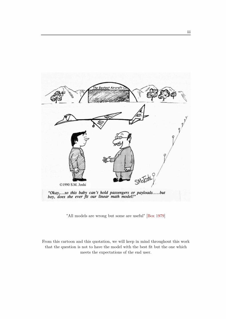
"All models are wrong but some are useful" [Box 1979]
From this cartoon and this quotation, we will keep in mind throughout this workthat the question is not to have the model with the best fit but the one which
meets the expectations of the end user.

Contents
Acknowledgements i
Table of Contents v
Notations ix
Acronyms xi
List of Publications xiii
I Introduction 1
1 Background and scope 31.1 Research motivation . . . . . . . . . . . . . . . . . . . . . . . . . . . 41.2 State of the art . . . . . . . . . . . . . . . . . . . . . . . . . . . . . . 61.3 Goal . . . . . . . . . . . . . . . . . . . . . . . . . . . . . . . . . . . . 91.4 Thesis outline . . . . . . . . . . . . . . . . . . . . . . . . . . . . . . . 9
II Preliminaries 11
2 Robots modelling and identification 132.1 Modelling of robot arms . . . . . . . . . . . . . . . . . . . . . . . . . 14
2.1.1 Geometric model of serial robots . . . . . . . . . . . . . . . . 142.1.2 Inverse dynamic model . . . . . . . . . . . . . . . . . . . . . . 152.1.3 Robot dynamic parameters . . . . . . . . . . . . . . . . . . . 172.1.4 Direct dynamic model . . . . . . . . . . . . . . . . . . . . . . 18
2.2 Robot systems architecture . . . . . . . . . . . . . . . . . . . . . . . 192.2.1 Robot control laws . . . . . . . . . . . . . . . . . . . . . . . . 192.2.2 Robot actuators . . . . . . . . . . . . . . . . . . . . . . . . . 212.2.3 Position sensors . . . . . . . . . . . . . . . . . . . . . . . . . . 212.2.4 Inverse dynamic identification model . . . . . . . . . . . . . . 23
2.3 Robot arms identification methods . . . . . . . . . . . . . . . . . . . 232.3.1 Filtering methodology . . . . . . . . . . . . . . . . . . . . . . 242.3.2 The least-squares method . . . . . . . . . . . . . . . . . . . . 242.3.3 The instrumental variable method . . . . . . . . . . . . . . . 262.3.4 The DIDIM method . . . . . . . . . . . . . . . . . . . . . . . 282.3.5 Exciting trajectories . . . . . . . . . . . . . . . . . . . . . . . 30
2.4 Concluding remarks . . . . . . . . . . . . . . . . . . . . . . . . . . . 31
vi Contents
3 System identification for continuous time systems 333.1 Closed-loop identification challenges . . . . . . . . . . . . . . . . . . 343.2 The refined instrumental variable method . . . . . . . . . . . . . . . 34
3.2.1 The hybrid Box-Jenkins model . . . . . . . . . . . . . . . . . 343.2.2 The hybrid RIVC algorithm . . . . . . . . . . . . . . . . . . . 363.2.3 Statistical elements of the method . . . . . . . . . . . . . . . 38
3.3 Prediction error methods . . . . . . . . . . . . . . . . . . . . . . . . 393.3.1 Prediction error principle . . . . . . . . . . . . . . . . . . . . 393.3.2 DT prediction error method . . . . . . . . . . . . . . . . . . . 403.3.3 Hybrid output error method . . . . . . . . . . . . . . . . . . . 423.3.4 Computational aspects . . . . . . . . . . . . . . . . . . . . . . 43
3.4 Concluding remarks . . . . . . . . . . . . . . . . . . . . . . . . . . . 44
III Contributions to robot system identification 45
4 Evaluation of the robustness of identification methods based onthe auxiliary model simulation 474.1 Choice of the identification signal . . . . . . . . . . . . . . . . . . . . 48
4.1.1 Output error methods for robot identification . . . . . . . . . 484.1.2 Sensitivity analysis . . . . . . . . . . . . . . . . . . . . . . . . 494.1.3 Contribution of the linearity . . . . . . . . . . . . . . . . . . 554.1.4 Experimental validation . . . . . . . . . . . . . . . . . . . . . 55
4.2 Robustness to modeling errors of the DIDIM and IDIM-IV methods 614.2.1 Similarity between the methods . . . . . . . . . . . . . . . . . 614.2.2 Disparity between the methods . . . . . . . . . . . . . . . . . 634.2.3 Experimental validations . . . . . . . . . . . . . . . . . . . . 65
4.3 Miscellaneous remarks . . . . . . . . . . . . . . . . . . . . . . . . . . 664.3.1 Closed-loop aspects of the robot identifications methods . . . 664.3.2 Considerations on the robot identification with OEM . . . . . 664.3.3 Remarks on the linearity . . . . . . . . . . . . . . . . . . . . . 68
4.4 Conclusions . . . . . . . . . . . . . . . . . . . . . . . . . . . . . . . . 70
5 Robot system identification without the knowledge of the con-troller and the bandwidths 715.1 Joint derivatives estimation . . . . . . . . . . . . . . . . . . . . . . . 72
5.1.1 Derivatives estimation from noisy signals . . . . . . . . . . . 725.1.2 Integrative random walk smoother . . . . . . . . . . . . . . . 735.1.3 Application to robot identification . . . . . . . . . . . . . . . 765.1.4 Numerical differentiation tests . . . . . . . . . . . . . . . . . 80
5.2 Controller identification . . . . . . . . . . . . . . . . . . . . . . . . . 815.2.1 Closed-loop system identification with an unknown controller 815.2.2 Controller parametric identification . . . . . . . . . . . . . . . 835.2.3 Controller non-parametric identification . . . . . . . . . . . . 83
Contents vii
5.3 Experimental validation . . . . . . . . . . . . . . . . . . . . . . . . . 855.3.1 The IDIM-LS method with the IRWSM technique . . . . . . 855.3.2 The IDIM-IV method with the IRWSM technique . . . . . . 875.3.3 The IDIM-IV method with an unknown controller . . . . . . 90
5.4 Conclusions . . . . . . . . . . . . . . . . . . . . . . . . . . . . . . . . 94
6 Noise modelling for robot system identification 976.1 Noise modelling and identification . . . . . . . . . . . . . . . . . . . 98
6.1.1 Closed-loop relations . . . . . . . . . . . . . . . . . . . . . . . 986.1.2 Filters models . . . . . . . . . . . . . . . . . . . . . . . . . . . 996.1.3 Auto-regressive filters identification . . . . . . . . . . . . . . . 103
6.2 Refined identification methods . . . . . . . . . . . . . . . . . . . . . 1056.2.1 The separable PEM method . . . . . . . . . . . . . . . . . . . 1056.2.2 The IDIM-PIV method . . . . . . . . . . . . . . . . . . . . . 1066.2.3 Comments on the extensions . . . . . . . . . . . . . . . . . . 107
6.3 Experimental validations . . . . . . . . . . . . . . . . . . . . . . . . . 1086.3.1 Study of the black-box noise model . . . . . . . . . . . . . . . 1086.3.2 Study of the grey-box noise model . . . . . . . . . . . . . . . 1126.3.3 Study with noisy data . . . . . . . . . . . . . . . . . . . . . . 113
6.4 Conclusions . . . . . . . . . . . . . . . . . . . . . . . . . . . . . . . . 116
IV Conclusion 121
7 Discussions and Future Work 1237.1 Contributions summary . . . . . . . . . . . . . . . . . . . . . . . . . 124
7.1.1 Analysis of the OEM for robot identification . . . . . . . . . 1247.1.2 Robustness analysis of the IDIM-IV and DIDIM methods . . 1247.1.3 Identification with an unknown controller . . . . . . . . . . . 1247.1.4 Automated estimation of the joint derivatives . . . . . . . . . 1257.1.5 Noise filter identification . . . . . . . . . . . . . . . . . . . . . 125
7.2 A practitioner guide . . . . . . . . . . . . . . . . . . . . . . . . . . . 1267.3 Further developments . . . . . . . . . . . . . . . . . . . . . . . . . . 126
7.3.1 Actuator modelling . . . . . . . . . . . . . . . . . . . . . . . . 1267.3.2 Friction modelling . . . . . . . . . . . . . . . . . . . . . . . . 1267.3.3 Broader perspectives . . . . . . . . . . . . . . . . . . . . . . . 128
V Appendices 129
A Industrial robot modelling 131A.1 Computation of the energies . . . . . . . . . . . . . . . . . . . . . . . 131A.2 Newton-Euler formulation . . . . . . . . . . . . . . . . . . . . . . . . 135A.3 Parameter reduction . . . . . . . . . . . . . . . . . . . . . . . . . . . 136
viii Contents
B Stäubli TX40 143B.1 Model of the TX40 . . . . . . . . . . . . . . . . . . . . . . . . . . . . 143B.2 Reference values of the dynamic parameters . . . . . . . . . . . . . . 143B.3 Control law . . . . . . . . . . . . . . . . . . . . . . . . . . . . . . . . 145B.4 Illustration of experimental signals . . . . . . . . . . . . . . . . . . . 146
C Mathematical background 149C.1 Random Variables . . . . . . . . . . . . . . . . . . . . . . . . . . . . 149C.2 Properties of Estimators . . . . . . . . . . . . . . . . . . . . . . . . . 150C.3 Random Process . . . . . . . . . . . . . . . . . . . . . . . . . . . . . 151
VI Résumé de thèse en français 153
D Identification de robots industriels rigides – Apport des méthodesde l’identification de systèmes 155D.1 Introduction . . . . . . . . . . . . . . . . . . . . . . . . . . . . . . . . 157
D.1.1 Contexte . . . . . . . . . . . . . . . . . . . . . . . . . . . . . 157D.1.2 État de l’art . . . . . . . . . . . . . . . . . . . . . . . . . . . 158D.1.3 Problématique . . . . . . . . . . . . . . . . . . . . . . . . . . 159
D.2 Evaluation de la robustesse des méthodes d’identification basées surla simulation du modèle auxiliaire . . . . . . . . . . . . . . . . . . . 160D.2.1 Choix du signal d’identification . . . . . . . . . . . . . . . . . 160D.2.2 Comparaison des méthodes IDIM-IV et DIDIM . . . . . . . . 163D.2.3 Remarques et conclusion . . . . . . . . . . . . . . . . . . . . . 165
D.3 Identification de systèmes robotiques sans connaissance du contrôleuret des bande-passsantes . . . . . . . . . . . . . . . . . . . . . . . . . 165D.3.1 Estimation des dérivées articulaires . . . . . . . . . . . . . . . 166D.3.2 Identification du contrôleur . . . . . . . . . . . . . . . . . . . 170D.3.3 Conlusions . . . . . . . . . . . . . . . . . . . . . . . . . . . . 173
D.4 Modélisation du bruit pour l’identification de systèmes robotiques . 174D.4.1 Modélisation et identification du bruit . . . . . . . . . . . . . 174D.4.2 Extension des méthodes d’identification . . . . . . . . . . . . 177D.4.3 Conlusions . . . . . . . . . . . . . . . . . . . . . . . . . . . . 181
D.5 Conclusions et perspectives . . . . . . . . . . . . . . . . . . . . . . . 181D.5.1 Résumé des contributions . . . . . . . . . . . . . . . . . . . . 181D.5.2 Un guide pour l’utilisateur . . . . . . . . . . . . . . . . . . . 183D.5.3 Développements futurs . . . . . . . . . . . . . . . . . . . . . . 184
References 187
Index 201
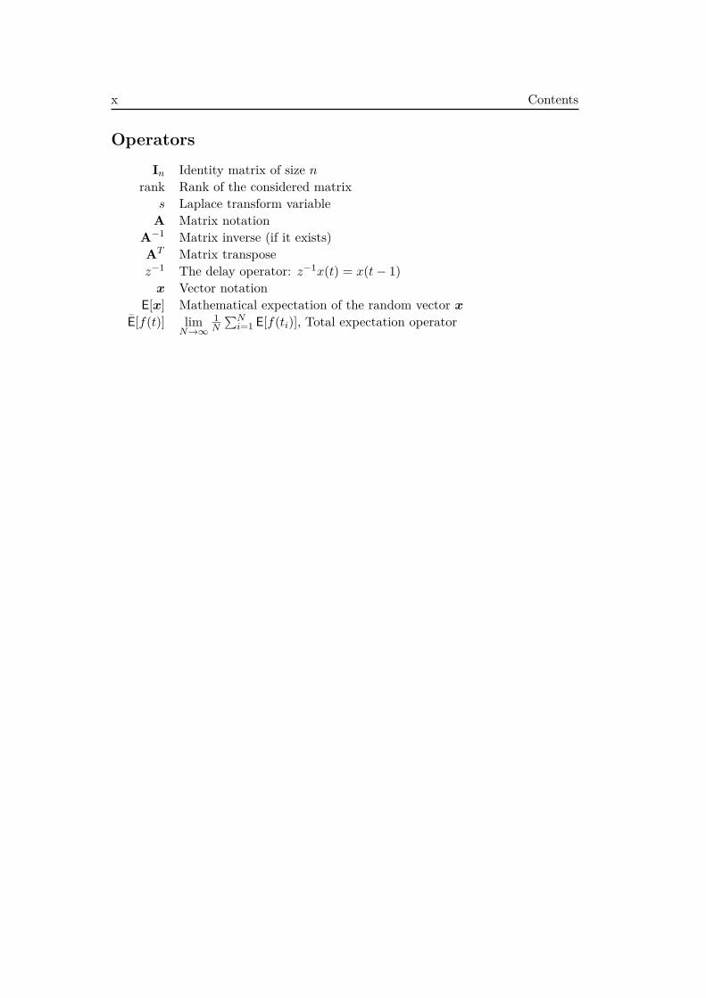
Notations
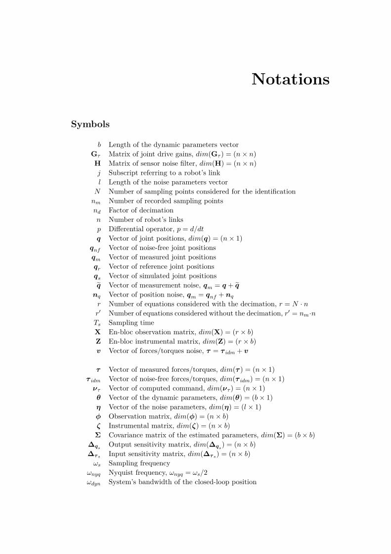
Symbols
b Length of the dynamic parameters vectorGτ Matrix of joint drive gains, dim(Gτ ) = (n× n)H Matrix of sensor noise filter, dim(H) = (n× n)j Subscript referring to a robot’s linkl Length of the noise parameters vectorN Number of sampling points considered for the identificationnm Number of recorded sampling pointsnd Factor of decimationn Number of robot’s linksp Differential operator, p = d/dt
q Vector of joint positions, dim(q) = (n× 1)qnf Vector of noise-free joint positionsqm Vector of measured joint positionsqr Vector of reference joint positionsqs Vector of simulated joint positionsq Vector of measurement noise, qm = q + qnq Vector of position noise, qm = qnf + nqr Number of equations considered with the decimation, r = N · nr′ Number of equations considered without the decimation, r′ = nm·nTs Sampling timeX En-bloc observation matrix, dim(X) = (r × b)Z En-bloc instrumental matrix, dim(Z) = (r × b)v Vector of forces/torques noise, τ = τ idm + v
τ Vector of measured forces/torques, dim(τ ) = (n× 1)τ idm Vector of noise-free forces/torques, dim(τ idm) = (n× 1)ντ Vector of computed command, dim(ντ ) = (n× 1)θ Vector of the dynamic parameters, dim(θ) = (b× 1)η Vector of the noise parameters, dim(η) = (l × 1)φ Observation matrix, dim(φ) = (n× b)ζ Instrumental matrix, dim(ζ) = (n× b)Σ Covariance matrix of the estimated parameters, dim(Σ) = (b× b)
∆qs Output sensitivity matrix, dim(∆qs) = (n× b)∆τ s Input sensitivity matrix, dim(∆τ s) = (n× b)ωs Sampling frequency
ωnyq Nyquist frequency, ωnyq = ωs/2ωdyn System’s bandwidth of the closed-loop position
x Contents
Operators
In Identity matrix of size nrank Rank of the considered matrix
s Laplace transform variableA Matrix notation
A−1 Matrix inverse (if it exists)AT Matrix transposez−1 The delay operator: z−1x(t) = x(t− 1)x Vector notation
E[x] Mathematical expectation of the random vector xE[f(t)] lim
N→∞1N
∑Ni=1 E[f(ti)], Total expectation operator
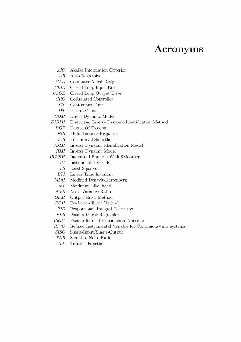
Acronyms
AIC Akaike Information CriterionAR Auto-Regressive
CAD Computer-Aided DesignCLIE Closed-Loop Input ErrorCLOE Closed-Loop Output ErrorCRC CoRrelated ControllerCT Continuous-TimeDT Discrete-Time
DDM Direct Dynamic ModelDIDIM Direct and Inverse Dynamic Identification Method
DOF Degree Of FreedomFIR Finite Impulse ResponseFIS Fix Interval Smoother
IDIM Inverse Dynamic Identification ModelIDM Inverse Dynamic Model
IRWSM Integrated Random Walk SMootherIV Instrumental VariableLS Least-SquaresLTI Linear Time Invariant
MDH Modified Denavit-HartenbergML Maximum Likelihood
NVR Noise Variance RatioOEM Output Error MethodPEM Prediction Error MethodPID Proportional–Integral–DerivativePLR Pseudo-Linear Regression
PRIV Pseudo-Refined Instrumental VariableRIVC Refined Instrumental Variable for Continuous-time systemsSISO Single-Input/Single-OutputSNR Signal to Noise RatioTF Transfer Function

List of Publications
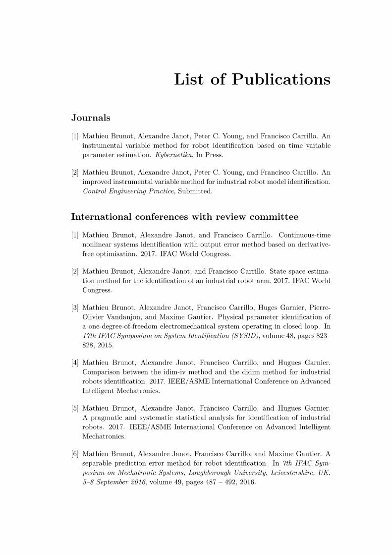
Journals
[1] Mathieu Brunot, Alexandre Janot, Peter C. Young, and Francisco Carrillo. Aninstrumental variable method for robot identification based on time variableparameter estimation. Kybernetika, In Press.
[2] Mathieu Brunot, Alexandre Janot, Peter C. Young, and Francisco Carrillo. Animproved instrumental variable method for industrial robot model identification.Control Engineering Practice, Submitted.
International conferences with review committee
[1] Mathieu Brunot, Alexandre Janot, and Francisco Carrillo. Continuous-timenonlinear systems identification with output error method based on derivative-free optimisation. 2017. IFAC World Congress.
[2] Mathieu Brunot, Alexandre Janot, and Francisco Carrillo. State space estima-tion method for the identification of an industrial robot arm. 2017. IFAC WorldCongress.
[3] Mathieu Brunot, Alexandre Janot, Francisco Carrillo, Huges Garnier, Pierre-Olivier Vandanjon, and Maxime Gautier. Physical parameter identification ofa one-degree-of-freedom electromechanical system operating in closed loop. In17th IFAC Symposium on System Identification (SYSID), volume 48, pages 823–828, 2015.
[4] Mathieu Brunot, Alexandre Janot, Francisco Carrillo, and Hugues Garnier.Comparison between the idim-iv method and the didim method for industrialrobots identification. 2017. IEEE/ASME International Conference on AdvancedIntelligent Mechatronics.
[5] Mathieu Brunot, Alexandre Janot, Francisco Carrillo, and Hugues Garnier.A pragmatic and systematic statistical analysis for identification of industrialrobots. 2017. IEEE/ASME International Conference on Advanced IntelligentMechatronics.
[6] Mathieu Brunot, Alexandre Janot, Francisco Carrillo, and Maxime Gautier. Aseparable prediction error method for robot identification. In 7th IFAC Sym-posium on Mechatronic Systems, Loughborough University, Leicestershire, UK,5–8 September 2016, volume 49, pages 487 – 492, 2016.

xiv Contents
[7] Mathieu Brunot, Alexandre Janot, Francisco Carrillo, and Maxime Gautier.State space estimation method for robot identification. In 7th IFAC Sympo-sium on Mechatronic Systems, Loughborough University, Leicestershire, UK,5–8 September 2016, volume 49, pages 228 – 233, 2016.

Part I
Introduction

Chapter 1
Background and scope
This chapter is the introduction of this thesis work where the main problems con-sidered are introduced. They concern industrial rigid robots and their parametricidentification. Having high quality models is of the highest importance in order todesign effective control laws. Furthermore, for stability and safety reasons, robotsmust be identified in closed-loop which induces a correlation in the experimentaldata. In order to tackle those challenges, the robotic community has developedspecific identification techniques based on rules of thumb and the skills of the prac-titioner. That motivates the development of generic methods able to deal with asystem in an automatic way without a priori knowledge. A state of the art of thedifferent fields of research involved is proposed and the major contributions of thisthesis are introduced.
This chapter is organized as follows. Firstly, a general introduction to theconsidered domain is proposed in section 1.1. Secondly, a state of the art of themodels and methodologies involved is provided in section 1.2. The goal of this thesisis stated in section 1.3. Finally, the manuscript outline is detailed in section 1.4.
1.1 Research motivation . . . . . . . . . . . . . . . . . . . . . . . . 41.2 State of the art . . . . . . . . . . . . . . . . . . . . . . . . . . . 61.3 Goal . . . . . . . . . . . . . . . . . . . . . . . . . . . . . . . . . 91.4 Thesis outline . . . . . . . . . . . . . . . . . . . . . . . . . . . . 9
4 Chapter 1. Background and scope
1.1 Research motivation
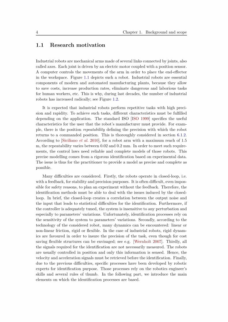
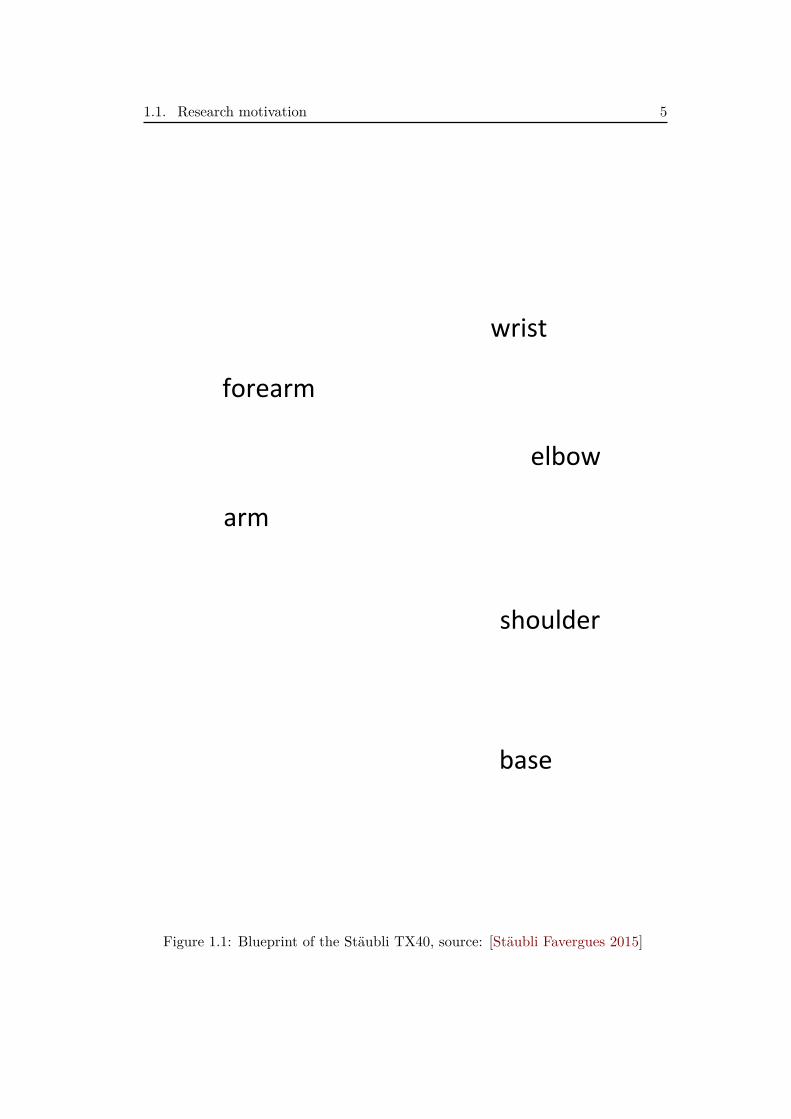
Industrial robots are mechanical arms made of several links connected by joints, alsocalled axes. Each joint is driven by an electric motor coupled with a position sensor.A computer controls the movements of the arm in order to place the end-effectorin the workspace. Figure 1.1 depicts such a robot. Industrial robots are essentialcomponents of modern and automated manufacturing plants, because they allowto save costs, increase production rates, eliminate dangerous and laborious tasksfor human workers, etc. This is why, during last decades, the number of industrialrobots has increased radically; see Figure 1.2.
It is expected that industrial robots perform repetitive tasks with high preci-sion and rapidity. To achieve such tasks, different characteristics must be fulfilleddepending on the application. The standard ISO [ISO 1999] specifies the usefulcharacteristics for the user that the robot’s manufacturer must provide. For exam-ple, there is the position repeatability defining the precision with which the robotreturns to a commanded position. This is thoroughly considered in section 6.1.2.According to [Siciliano et al. 2010], for a robot arm with a maximum reach of 1.5m, the repeatability varies between 0.02 and 0.2 mm. In order to meet such require-ments, the control laws need reliable and complete models of those robots. Thisprecise modelling comes from a rigorous identification based on experimental data.The issue is thus for the practitioner to provide a model as precise and complete aspossible.
Many difficulties are considered. Firstly, the robots operate in closed-loop, i.e.with a feedback, for stability and precision purposes. It is often difficult, even impos-sible for safety reasons, to plan an experiment without the feedback. Therefore, theidentification methods must be able to deal with the issues induced by the closed-loop. In brief, the closed-loop creates a correlation between the output noise andthe input that leads to statistical difficulties for the identification. Furthermore, ifthe controller is adequately tuned, the system is insensitive to any perturbation andespecially to parameters’ variations. Unfortunately, identification processes rely onthe sensitivity of the system to parameters’ variations. Secondly, according to thetechnology of the considered robot, many dynamics can be encountered: linear ornon-linear friction, rigid or flexible. In the case of industrial robots, rigid dynam-ics are favoured in order to insure the precision of the task, even though for costsaving flexible structures can be envisaged; see e.g. [Wernholt 2007]. Thirdly, allthe signals required for the identification are not necessarily measured. The robotsare usually controlled in position and only this information is sensed. Hence, thevelocity and acceleration signals must be retrieved before the identification. Finally,due to the previous difficulties, specific processes have been developed by roboticexperts for identification purpose. Those processes rely on the robotics engineer’sskills and several rules of thumb. In the following part, we introduce the mainelements on which the identification processes are based.
1.1. Research motivation 5
base
shoulder
arm
elbow
forearm
wrist
Figure 1.1: Blueprint of the Stäubli TX40, source: [Stäubli Favergues 2015]
6 Chapter 1. Background and scope
1973 1983 1990 1995 2000 2005 2010 2014 2015 2016*2019*0
1,000
2,000
3 66
454605
750923
1,059
1,4721,632
1,824
2,589
1,824
2,58910
3of
units
Figure 1.2: Worldwide estimated operational stock of industrial robots, source: IFRWorld Robotics 2016*: forecast
1.2 State of the art
The robot arms models come from the laws of classical mechanics: Newton-Euler orLagrange formulations. In order to derive the equations of motion, a specific nota-tion must be defined to characterise the problem. In [Denavit & Hartenberg 1955],the authors have introduced such a notation for industrial robots that has beenimproved by Khalil and Kleinfinger in [Khalil & Kleinfinger 1986]. This notationdefines the geometric relations between the components of the robot by introducingthe minimal amount of parameters. That allows expressing the dynamic models in asystematic and standardized way. If those works consider the inertial forces/torques,they do not deal with the friction phenomena. Other works have studied frictionand different models have proposed; see e.g. [Canudas de Wit et al. 1989, Bona& Indri 2005]. With the combination of the standardized notations for inertiaforces and the friction modelling, a comprehensive model of robot arms’ dynamicsis available.
From those modelling techniques, two model reduction methods have been pro-posed in [Gautier & Khalil 1990] and [Gautier 1991]. The first one is based on thealgebraic relations whereas the second one uses numerical evaluation of the model.Firstly, this reduction gives the set of base parameters that can be structurallyidentified. Secondly, it keeps unspoiled the torque linearity with respect to the pa-rameters. Therefore, the base parameters can be estimated with the Least-Squares(LS) technique, provided that the issue of the noise correlation is correctly handled.For this purpose, a specific procedure of experimental data prefiltering has beendesigned. The first step of this procedure, described in [Gautier 1997], consists infiltering the measured position to estimate the velocity and the acceleration. Forthe second step, a decimate filter is applied to the torque in order to reject high fre-

1.2. State of the art 7
quency perturbations. That process makes the LS feasible from a statistical pointof view. This whole process (prefiltering and LS estimation) is referred to as theIDIM-LS method. The drawbacks of this method are that the estimation result issensitive to the tuning of the filters and this tuning is based on a priori knowledgeof the system’s bandwidth.
Other robot identification approaches have been developed over the years, with-out really improving the IDIM-LS method coupled with an appropriate settingof the filters. One can cite: the Total Least-Squares (TLS) method [Gautieret al. 1994, Xi 1995], a method based on Linear Matrix Inequality (LMI) tools[Calafiore & Indri 2000], the Extended Kalman Filter (EKF) [Kostic et al. 2004] oran approach based on the Maximum Likelihood (ML) [Olsen & Petersen 2001, Olsenet al. 2002].
In [Janot et al. 2014c], the authors have introduced an Instrumental Variable(IV) approach, coming from the econometrics and for the robot identification. Theidea is to simulate the closed-loop model to obtain signals non-correlated withthe measurement noise. This method, named IDIM-IV, uses the same prefilteringprocess as the IDIM-LS method although the final estimates are less sensitive tothe setting of the filters. In addition to the system’s bandwidths, the controllermodel for the simulation is also required. To simplify the prefiltering process, in[Gautier et al. 2013a], the authors have developed the Direct and Inverse DynamicIdentification Method (DIDIM) that is also based on the simulation of the closed-loop model. This method has the advantage of not requiring the first step of theprefiltering process because it based only on the torque measurement. However,the second step (the decimate filter) is still necessary as well as a priori knowledge(controller and bandwidths).
The robot identification methods introduced above share the common propertyof not identifying the noise model. In the system identification community, Ljunghas introduced the Prediction Error Method (PEM) that is able to identify mainlyLinear Time Invariant (LTI) models in open- or closed-loop; see [Ljung 1976]. Theconsidered models are discrete-time and include the noise model. Unfortunately,this method cannot be applied on robots since their models are nonlinear andcontinuous-time. Almost simultaneously, Young and Jakeman have introduced theRefined IV for Continuous time systems (RIVC) in [Young & Jakeman 1980]. Witha different approach, this method is able to identify LTI models in open- or closed-loop, but in a continuous time framework. Due to the nonlinearities, the RIVCmethod can neither be applied to industrial robots in a straightforward manner.For both methods, identifying the noise allows an automatic filtering of the dataand provides optimal estimated parameters. It should be noticed that a specific kindof PEM, called Output Error Method (OEM), is able to deal with the identificationof continuous-time and nonlinear systems; see e.g. [Richalet et al. 1971] for thegeneric framework or [Landau et al. 1999] for closed-loop systems applications.Nonetheless, OEM do not take into account the noise model.
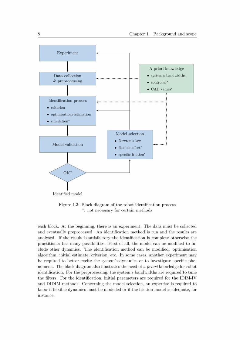
Figure 1.3 depicts the usual robot identification process. The general frame iscommon to all systems. The specificities of each application lie in the content of
8 Chapter 1. Background and scope
Experiment
Data collection& preprocessing
Identification process• criterion
• optimisation/estimation
• simulation∗
Model validation
Model selection• Newton’s law
• flexible effect∗
• specific friction∗
OK?
Identified model
A priori knowledge• system’s bandwidths
• controller∗
• CAD values∗
Figure 1.3: Block diagram of the robot identification process∗: not necessary for certain methods
each block. At the beginning, there is an experiment. The data must be collectedand eventually preprocessed. An identification method is run and the results areanalysed. If the result is satisfactory the identification is complete otherwise thepractitioner has many possibilities. First of all, the model can be modified to in-clude other dynamics. The identification method can be modified: optimisationalgorithm, initial estimate, criterion, etc. In some cases, another experiment maybe required to better excite the system’s dynamics or to investigate specific phe-nomena. The black diagram also illustrates the need of a priori knowledge for robotidentification. For the preprocessing, the system’s bandwidths are required to tunethe filters. For the identification, initial parameters are required for the IDIM-IVand DIDIM methods. Concerning the model selection, an expertise is required toknow if flexible dynamics must be modelled or if the friction model is adequate, forinstance.
1.3. Goal 9
1.3 Goal
It appears that the robotic community has at its disposal methods able of identifyingindustrial robots operating in closed-loop. The challenges of the closed-loop arehandled differently depending on the considered method. In parallel, the systemidentification community has developed methods to identify closed-loop systems inan automatic and accurate way. That is to say that they identify the noise modelwithout a priori knowledge on the system. Nonetheless, those methods deal withLTI systems, which make them impractical for industrial robots. On their side,the robotic engineers do not have dealt with the noise modelling thoroughly. Theirmethods are based on an "home-made" prefiltering relying on a physical knowledgeof the system. If they wonder about the level of the noise and its location in thefrequency range, they do not try to model it.
That is in this context that this work take place. This thesis consists in de-veloping identification methods for industrial robot systems in an automatic andaccurate way, while minimising the required a priori knowledge, in order to bridgethe gap between the robotic and system identification communities.
1.4 Thesis outline
This manuscript is divided into four parts. Part I is devoted to the introduction.Materials on the existing theories required to understand the contributions of thiswork are provided in Part II. Part III contains the main contributions of this thesiswith regard to robot system identification. Conclusions are provided in Part IVbefore some appendices in Part V.
Part II: Preliminaries
The preliminaries are divided in two chapters. Chapter 2 aims at describing therobot system modelling as well as the usual methods for the estimation of thedynamic parameters. The elements of modelling are mainly based on the referencematerials [Khalil & Dombre 2004] and [Siciliano et al. 2010]. In accordance withthe preview given in the state of the art, the identification methods introduced arethe IDIM-LS, IDIM-IV and DIDIM ones.
Chapter 3 introduced other methods coming from the system identification com-munity. If those methods cannot be applied straightforwardly to robot applications,they have interesting properties that may improve the robot identification process.The chapter mainly focuses on the RIVC and PEM methods introduced in thestate of the art. The core material of this chapter can be found in [Söderström &Stoica 1988], [Ljung 1999] and [Young 2011].
Part III: Contributions to robot system identification
In chapter 4, the approach consists in evaluating the sensitivity and the robustness ofthe robot identification methods based on the auxiliary model simulation. Firstly,
10 Chapter 1. Background and scope
the best observation signal must be selected for the identification purpose: theinput torque or the output position. To this end, a sensitivity analysis with respectto the dynamic parameters is performed. In addition, the benefit of the torque’slinearity with respect to the parameters is highlighted. This element has resulted ina publication [Brunot et al. 2015]. Afterwards, we show a better robustness of theIDIM-IV method compared with the DIDIM one in order to establish their limits.This comparison is undertaken by considering an error-free model to illustrate anominal case. Then, an error is introduced in auxiliary model to put the methodsin default. This analysis has been presented in [Brunot et al. 2017c].
The following step is to revisit those methods in chapter 5 to reduce the a prioriknowledge required to their execution. The idea is to deal with a robot system whosebandwidths and controller are unknown. In a first part, we look for an automaticmethod to estimate the joint velocities and accelerations to avoid the prefilteringprocess. To do so, a method is selected from literature and adapted to industrialrobots. This work has resulted in several publications [Brunot et al. 2016b], [Brunotet al. 2017b] and a submission to [Brunot et al. In Press 2017]. The second partfocuses on the identification of the controller. It is indeed necessary to the aux-iliary model simulation, which is itself necessary to the dynamic model identifica-tion. The controller identification is tackled in parametric and in a non-parametricway. The principles of the controller identification has been submitted to [Brunotet al. Submitted 2017]. The third part is dedicated to experimental validations ofthe suggested methods.
The last step consists in continuing the effort of a priori knowledge reductionby taking into account the noise model instead of using the decimate filter. Theaim is to provide estimated parameters as accurate as possible without relying onthe practitioner’s skills. A first part is devoted to the noise modelling through theclosed-loop system. From the closed-loop relations, the model of the noise affectingthe input torque is derived. The second part uses this noise model to replacethe usual decimate filter used prior to the identification. A first method, basedon the DIDIM approach, is called separable PEM in connection with the methoddeveloped within the system identification community. A second method, referredto as IDIM-PIV, is directly inspired from the RIVC method. Those methods havebeen published in [Brunot et al. 2016a] and submitted to [Brunot et al. Submitted2017], following a preliminary work presented in [Brunot et al. 2017d]. The thirdpart deals with the experimental validation of the two suggested methods.

Part II
Preliminaries

Chapter 2
Robots modelling andidentification
Robot modelling has been extensively studied during the last decades. To stan-dardize the coordinate frames, several conventions have been proposed. One ofthe most popular is the Denavit-Hartenberg convention developed in [Denavit &Hartenberg 1955] and modified in [Khalil & Kleinfinger 1986]. In this thesis, wefocus on the modelling of rigid robots with single open chain structure thanks tothe Modified Denavit-Hartenberg (MDH) convention. Based on this geometric con-vention, the Newton’s laws give the equations of motion. From these equations andtaking into account the robot systems architecture, techniques have been developedto identify the dynamic models. The material of this chapter mainly come from thebook [Khalil & Dombre 2004] and summarizes the main results in robots modellingand identification.
An introduction to the MDH convention and the different dynamic models con-sidered for robot identification is proposed in section 2.1. In section 2.2, the wholestructure of a robot arm system is described taking into account the controller,the sensors and the actuators. Section 2.3 outlines the common methods for robotidentification. Conclusions are provided in section 2.4.
2.1 Modelling of robot arms . . . . . . . . . . . . . . . . . . . . . 142.1.1 Geometric model of serial robots . . . . . . . . . . . . . . . . 142.1.2 Inverse dynamic model . . . . . . . . . . . . . . . . . . . . . . 152.1.3 Robot dynamic parameters . . . . . . . . . . . . . . . . . . . 172.1.4 Direct dynamic model . . . . . . . . . . . . . . . . . . . . . . 18
2.2 Robot systems architecture . . . . . . . . . . . . . . . . . . . 192.2.1 Robot control laws . . . . . . . . . . . . . . . . . . . . . . . . 192.2.2 Robot actuators . . . . . . . . . . . . . . . . . . . . . . . . . 212.2.3 Position sensors . . . . . . . . . . . . . . . . . . . . . . . . . . 212.2.4 Inverse dynamic identification model . . . . . . . . . . . . . . 23
2.3 Robot arms identification methods . . . . . . . . . . . . . . . 232.3.1 Filtering methodology . . . . . . . . . . . . . . . . . . . . . . 242.3.2 The least-squares method . . . . . . . . . . . . . . . . . . . . 242.3.3 The instrumental variable method . . . . . . . . . . . . . . . 262.3.4 The DIDIM method . . . . . . . . . . . . . . . . . . . . . . . 282.3.5 Exciting trajectories . . . . . . . . . . . . . . . . . . . . . . . 30
2.4 Concluding remarks . . . . . . . . . . . . . . . . . . . . . . . . 31
14 Chapter 2. Robots modelling and identification
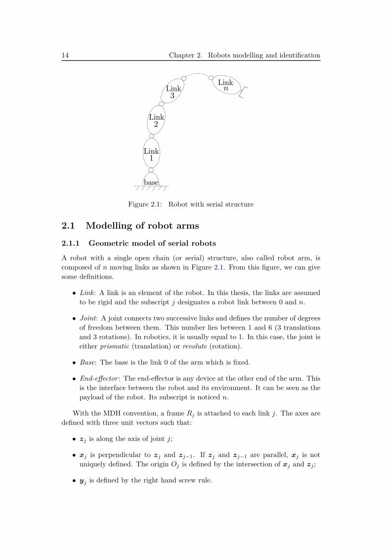
Figure 2.1: Robot with serial structure
2.1 Modelling of robot arms
2.1.1 Geometric model of serial robots
A robot with a single open chain (or serial) structure, also called robot arm, iscomposed of n moving links as shown in Figure 2.1. From this figure, we can givesome definitions.
• Link: A link is an element of the robot. In this thesis, the links are assumedto be rigid and the subscript j designates a robot link between 0 and n.
• Joint: A joint connects two successive links and defines the number of degreesof freedom between them. This number lies between 1 and 6 (3 translationsand 3 rotations). In robotics, it is usually equal to 1. In this case, the joint iseither prismatic (translation) or revolute (rotation).
• Base: The base is the link 0 of the arm which is fixed.
• End-effector : The end-effector is any device at the other end of the arm. Thisis the interface between the robot and its environment. It can be seen as thepayload of the robot. Its subscript is noticed n.
With the MDH convention, a frame Rj is attached to each link j. The axes aredefined with three unit vectors such that:
• zj is along the axis of joint j;
• xj is perpendicular to zj and zj−1. If zj and zj−1 are parallel, xj is notuniquely defined. The origin Oj is defined by the intersection of xj and zj ;
• yj is defined by the right hand screw rule.
2.1. Modelling of robot arms 15
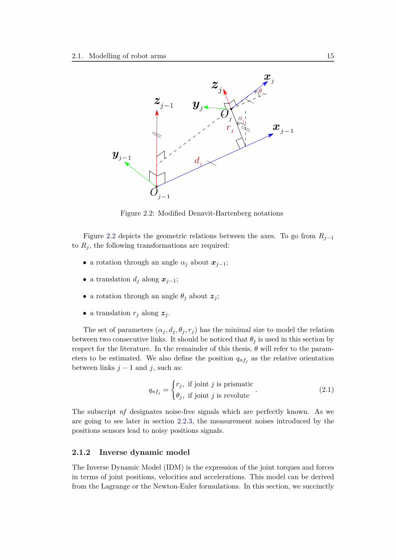
Figure 2.2: Modified Denavit-Hartenberg notations
Figure 2.2 depicts the geometric relations between the axes. To go from Rj−1to Rj , the following transformations are required:
• a rotation through an angle αj about xj−1;
• a translation dj along xj−1;
• a rotation through an angle θj about zj ;
• a translation rj along zj .
The set of parameters (αj , dj , θj , rj) has the minimal size to model the relationbetween two consecutive links. It should be noticed that θj is used in this section byrespect for the literature. In the remainder of this thesis, θ will refer to the param-eters to be estimated. We also define the position qnfj as the relative orientationbetween links j − 1 and j, such as:
qnfj =rj , if joint j is prismaticθj , if joint j is revolute
. (2.1)
The subscript nf designates noise-free signals which are perfectly known. As weare going to see later in section 2.2.3, the measurement noises introduced by thepositions sensors lead to noisy positions signals.
2.1.2 Inverse dynamic model
The Inverse Dynamic Model (IDM) is the expression of the joint torques and forcesin terms of joint positions, velocities and accelerations. This model can be derivedfrom the Lagrange or the Newton-Euler formulations. In this section, we succinctly
16 Chapter 2. Robots modelling and identification
develop the Lagrange formulation to illustrate the robots dynamics. The Newton-Euler formulation is developed in appendix A.2.
For a robot with n moving links, the Lagrange equations can be written in theform:
τ idm = d
dt
(∂L
∂qnf
)− ∂L
∂qnf+ τ f , (2.2)
with
• τ idm is the (n × 1) vector of joint torques or forces, depending on the jointtechnology (revolute or prismatic);
• qnf , qnf , qnf are respectively the (n× 1) noise-free vectors of joint positions,velocities and accelerations;
• τ f is the (n× 1) vector of friction;
• L = E − U , where L, E and U are respectively the Lagrangian, the kineticenergy and the potential energy of the system.
The expressions of the energies are developed in appendix A.1. The developmentof the equations leads to :
τ idm = M(qnf
)qnf +N
(qnf , qnf
), (2.3)
where M is the (n × n) inertia matrix of the robot (see appendix A.1) and N isthe (n× 1) vector of centrifugal, Coriolis, gravitational, and friction torques. As ithas been said, the dynamics is modelled in rigid framework. The reader interestedin a flexible representation could refer to [Cheong et al. 2004] for instance. N canbe broken down such as:
N(qnf , qnf
)= C
(qnf , qnf
)qnf +Q
(qnf
)+ τ f (2.4)
where:
• C(qnf , qnf
)qnf = dM
dt qnf −∂E∂qnf
is the (n × 1) vector of centrifugal andCoriolis torques;
• Q(qnf
)= ∂U
∂qnfis the (n× 1) vector of gravity torques.
The coefficients of the matrix M, as well as those of the vectors C and Q, arefunctions of the geometric and inertial parameters of the considered robot. Thisis emphasized in appendix A.1. The IDM is thus a system of n second orderdifferential equations, coupled and nonlinear with respect to the states (positionsand velocities).
2.1. Modelling of robot arms 17
2.1.3 Robot dynamic parameters
According to [Khalil & Dombre 2004] and the references given therein like [Gautier& Khalil 1990], a joint j of an industrial robot has 14 standard parameters :
χj = [XXj XYj XZj Y Yj Y Zj ZZj (2.5)MXj MYj MZj Mj Iaj Fvj Fcj τoffj ]T
where
• XXj , XYj , XZj , Y Yj , Y Zj and ZZj are the six components of the inertiatensor jJOj defined at the origin of frame Oj , in the axes of the frame Rj ,such as:
jJOj =
XXj XYj XZjXYj Y Yj Y ZjXZj Y Zj ZZj
(2.6)
=
∫
(y2 + z2)dm −∫xydm −
∫xzdm
−∫xydm
∫(x2 + z2)dm −
∫yzdm
−∫xzdm −
∫yzdm
∫(x2 + y2)dm
• MXj , MYj , MZj are the three components of the first moments jMSj =Mj ·j Sj = [MXj MYj MZj ]T , where jSj = [Xj Yj Zj ]T is vector from theorigin Oj to the center of gravity Gj , expressed in the axes of the frame Rj ;
• Mj is the mass of link j;
• Iaj is the total inertia moment for rotor and gears of the actuator;
• Fvj and Fcj are respectively the viscous and Coulomb friction coefficients;
• τoffj is an offset parameter containing the asymmetry of the Coulomb frictionwith respect to the sign of the velocity and the current amplifier offset whichsupplies the motor.
The friction is an important phenomenon which can represent 10 to 20 % ofthe nominal actuator torque, even 30% in some cases [Lischinsky et al. 1999]. Inaccordance with [Canudas de Wit et al. 1989, Daemi & Heimann 1997, Bona &Indri 2005], for a given link j, a simple and common friction model used in roboticsis:
τfj = Fcjsign(qnfj ) + Fvj qnfj + τoffj , (2.7)
with
sign(qnfj ) =
1, if qnfj > 00, if qnfj = 0−1, if qnfj < 0
.
18 Chapter 2. Robots modelling and identification
This model is usually satisfactory for the range of velocity used for robot trajectories.However, in some specific cases like low velocity, the friction model may be moreinvolved [Hamon et al. 2011, Janot et al. 2017]. For simulation purpose, the signfunction can be replaced by the arctangent function which has the advantage tobe continuous. In fact, the function 2
πatan(γqj) tends to sign(qj) when γ tends toinfinity. The value of γ depends on the practical case and especially on the velocityrange of the trajectory. The user must keep in mind that, with a too large value, thenumerical integration of the differential equations would become stiff. A stiff modelcan be described as a system with very fast components compare with others; seee.g. [Murray-Smith 1995, Hairer & Wanner 1996] for further information on stiffsystems simulation.
All the standard parameters are not identifiable. As shown in [Gautier 1991]for instance, some dynamic parameters have indeed no influence on the IDM whilesome others are regrouped together thanks to linear relations. The set of identifiabledynamic parameters has to be determined to obtain a (b×1) vector: θ. This vectoris called as the set of base parameters . They are in fact the minimum number ofdynamic parameters from which the IDM can be calculated. Appendix A.3 detailsthe two methods available to determine the base parameters. The IDM can bewritten as a linear function of those base parameters:
τ idm = φ(qnf , qnf , qnf
)θ, (2.8)
where φ is the (n×b) matrix of basis functions (also called observation matrix) andθ is the (b × 1) vector of parameters. Each element of φ is a basis function of thebody dynamics, which is also called regressor or independant variable . Those basisfunctions can be nonlinear relations of the positions, velocities and accelerations.
2.1.4 Direct dynamic model
The Direct Dynamic Model (DDM) provides the joint accelerations in terms of thejoint positions, velocities and torques as well as the parameters. It is described by:
qnf = M−1(qnf
) (τ idm −N
(qnf , qnf
)). (2.9)
The DDM can also be written as a state-space form given by:
x =[
qnf−M−1
(qnf
)N(qnf , qnf
)]+
0M(qnf
)−1
u, (2.10)
with
• x = [qTnf qTnf ]T is the (2n× 1) state vector;
• u = τ idm is the (n× 1) input vector.
According to (2.10), the DDM is a nonlinear relation of the states and the dynamicparameters included in M and N .
2.2. Robot systems architecture 19
The prime purpose of the DDM is to simulate the robot. With known inputtorques and base parameters, the dynamic equations are solved for the joint accel-erations and the current state of the robot. We detail here the method developedin [Walker & Orin 1982] that is used in practice. This method has the advantage touse the IDM. Therefore, an explicit calculation of the DDM is not required. Withthe subscript s designating the simulated signals, the method is divided in threesteps:
• Calculation of N (qs, qs).The simulated acceleration is temporally set to zero, qs = 0n×1. such thatN (qs, qs) = τ s = φ (qs, qs,0n×1)θ, according to (2.8) and (2.9).
• Calculation of M(qnf
).
In order to set N (qs, qs) to zero, we fix:
– the simulated velocity: qs = 0n×1;– the gravity: g = 0;– the Coulomb friction coefficients and the offsets, for each j = 1, · · · , n:Fcj = 0 and τoffj = 0.
The position vector qs cannot be set to zero since it appears in the inertiamatrix. We define aj that is a (n× 1) vector with the jth element equal to 1and 0 everywhere else. Each column j of the matrix M is calculated separatelyby setting qs = aj and evaluating M(:, j) = M
(qnf
)aj = φ
(qs,0n×1,a
j)θ.
• Solution of the linear equation (2.9) by taking τ idm equal to the input of thesimulated system.
Section 3.3.3 provide more details on the simulation process and especially on inte-gration solver.
2.2 Robot systems architecture
In this thesis, we study the identification of the robots dynamical models. However,since they operate in closed-loop, the robots can be viewed as a global systemregrouping: a controller, actuators, sensors and the robot arm. The robot armmodels have been described in section 2.1, the remaining elements of the roboticsystems are described here. Figure 2.3 provides an illustration of the architectureand defines the signals involved.
2.2.1 Robot control laws
Robots operate in closed-loop due to their double integrator behaviour. This isthe reason why are controlled in position with two nested loops: the inner-loopfor the current control and the outer-loop for the position control. The control
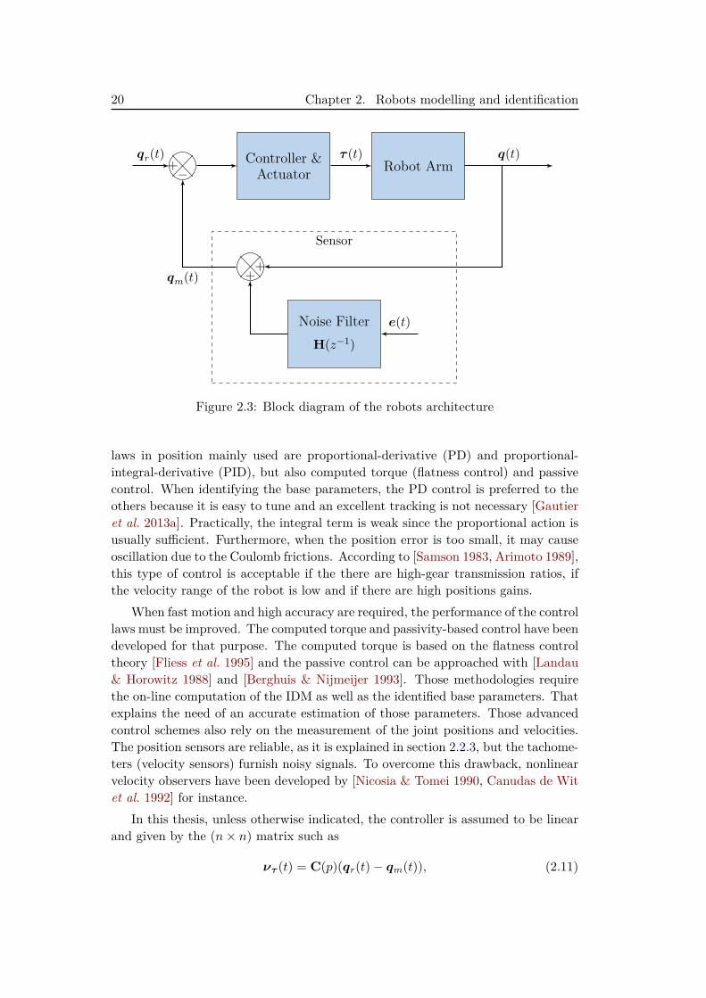
20 Chapter 2. Robots modelling and identification
−+ Controller &
Actuator Robot Arm
++
Noise FilterH(z−1)
qr(t) τ (t) q(t)
qm(t)
e(t)
Sensor
Figure 2.3: Block diagram of the robots architecture
laws in position mainly used are proportional-derivative (PD) and proportional-integral-derivative (PID), but also computed torque (flatness control) and passivecontrol. When identifying the base parameters, the PD control is preferred to theothers because it is easy to tune and an excellent tracking is not necessary [Gautieret al. 2013a]. Practically, the integral term is weak since the proportional action isusually sufficient. Furthermore, when the position error is too small, it may causeoscillation due to the Coulomb frictions. According to [Samson 1983, Arimoto 1989],this type of control is acceptable if the there are high-gear transmission ratios, ifthe velocity range of the robot is low and if there are high positions gains.
When fast motion and high accuracy are required, the performance of the controllaws must be improved. The computed torque and passivity-based control have beendeveloped for that purpose. The computed torque is based on the flatness controltheory [Fliess et al. 1995] and the passive control can be approached with [Landau& Horowitz 1988] and [Berghuis & Nijmeijer 1993]. Those methodologies requirethe on-line computation of the IDM as well as the identified base parameters. Thatexplains the need of an accurate estimation of those parameters. Those advancedcontrol schemes also rely on the measurement of the joint positions and velocities.The position sensors are reliable, as it is explained in section 2.2.3, but the tachome-ters (velocity sensors) furnish noisy signals. To overcome this drawback, nonlinearvelocity observers have been developed by [Nicosia & Tomei 1990, Canudas de Witet al. 1992] for instance.
In this thesis, unless otherwise indicated, the controller is assumed to be linearand given by the (n× n) matrix such as
ντ (t) = C(p)(qr(t)− qm(t)), (2.11)
2.2. Robot systems architecture 21
where p = d/dt is the differential operator, ντ is the (n×1) vector of control signals,qr is the (n × 1) vector of reference trajectories and qm is the (n × 1) vector ofmeasured positions. In the remainder of this thesis, C designates the controller andnot the Coriolis matrix. For convenience, the controller is modelled as a Continuous-Time (CT) system, although in practice it is implemented in Discrete Time (DT) onthe micro-controllers that are used to perform the controls. Since each axis of therobot arm is controlled separately, the matrix C can be assumed diagonal. Hence,for each link j, there is
ντ j (t) = Cj(p)(qrj (t)− qmj (t)). (2.12)
As explained in [Arimoto 1989] for instance, the controller at each joint can bedesigned independently because the nonlinear cross-coupling effects are smaller thanthe dynamics of each individual axis. That is due to the mechanical design of therobot arms.
2.2.2 Robot actuators
Rigid industrial robots are steered by current driven electrical actuators, also calleddrive trains. Those actuators encompass a current-controlled voltage source am-plifier, a motor (permanent magnet DC or brushless) and a gear train. There isone drive train per link. For further information about the design of drive trains,see for instance [Pasch & Seering 1984]. The voltage source amplifiers are current-controlled with a proportional-integral (PI) law. The current-loop usually has abandwidth greater than 500Hz. Then, within the frequency range of body dynam-ics (usually less than 10Hz), its transfer function is modelled as a static gain kajfor link j [Gautier & Briot 2012b]. Considering link j, the motor has a torqueconstant ktj and the gear ratio is Nj . At last, the joint torques are connected withthe control signals by the following relation
τ (t) = Gτντ (t), (2.13)
where Gτ is the (n× n) diagonal matrix of joint drive gains and ντ is the (n× 1)vector of the currents serving as a references for the current amplifiers. The matrixGτ is diagonal, since there is one actuator per link, and the diagonal componentsare given by
Gτ j = kajktjNj . (2.14)
Those actuators parameters have a priori values given by the manufacturers whichcan be checked with special tests; see e.g. [Gautier & Briot 2012b]. In this thesis,we consider that those static gains are already available.
2.2.3 Position sensors
Many technologies exist to sense robot position. For industrial robot arms, thereare two main possibilities: a resolver or an encoder [Warnecke et al. Y Nof 1999].
22 Chapter 2. Robots modelling and identification
A resolver is a rotary transformer which provides an analog output signal. It istypically composed of a rotor carrying the primary winding and a stator carryingtwo secondary windings. When an AC voltage is applied to the primary winding,it induces current in the stator windings. The amplitudes of the voltages in thestator windings vary as the sine and cosine of the angular position. By comparingthe two signals, the angular position is retrieved. In practice, for a better accuracy,many pairs of stator windings can be considered.
An encoder can measure linear or angular displacements. It can be either in-cremental or absolute. An incremental encoder records just changes in positionwhereas an absolute encoder records an absolute position. In other words, it doesnot need a reference run after switching on. The technology can be either magnetic,conductive or optical. According to [Warnecke et al. Y Nof 1999], only optical en-coders are considered in industrial robotics (incremental or absolute). In opticalencoders, light from LEDs passes through a code disk fixed to the robot link j.The code disk is composed of parallel tracks of binary patterns made of opaque andtransparent segments. On the other side, fixed on link j − 1, photovoltaic diodesread the optical pattern which results of the disc’s position.
During this thesis, we mainly study the Stäubli TX40 robot arm that usesencoders for position control [Stäubli Favergues 2015]. Therefore, we will focus onencoder technology for the noise analysis. Introducing the measurement noise, wedefine the (n× 1) vector of measured joint positions as
qm(t) = q(t) + q(t) = q(t) + H(z−1)e(t), (2.15)
where q is the measurement noise, H is the (n × n) output noise matrix with z−1
the delay operator, q is the (n×1) vector of joint positions and e is a (n×1) vectorof white noises, with zero means and (n × n) covariance matrix Λ. For the samereasons as [Gilson et al. 2008], in this thesis, the noise filters are considered as DTsystems. Those reasons are:
• The discrete modelling is more practical than purely stochastic CT noisemodels;
• The main function of the noise modelling is to improve the statistical efficiencyof the estimated parameters, which can be adequately achieved with suchfilters.
Since there is one independent sensor per link, H is diagonal and composed of filtersHj(z−1) with j from 1 to n. Furthermore, the noises contained in the (n×1) vectore are uncorrelated and the covariance matrix Λ is also diagonal, with a covariancenoted λj for the link j. It comes out for each link j
qmj = qj + qj = qj +Hj(z−1)ej . (2.16)
According to [Bélanger et al. 1998], a shaft encoder has a white, zero meanand uniformly distributed noise with a variance equal to 1
3∆2e, where ∆e is the
2.3. Robot arms identification methods 23
encoder resolution. In [Swevers et al. 2007], the authors have pointed out that, ina factory environment, the position sensors can be influenced by other machineslike welding apparatus and other electromagnetic disturbances. For this reason, weconsider a more general case where the noise is not necessary white especially athigh frequency. The limit between low and high frequencies can be defined by thecut-off frequency of the closed-loop position: ωdyn. A covariance proportional to ∆2
e
seems reasonable in the operating range of system, i.e. below ωdyn. With respect to[Marcassus et al. 2007], the angular resolution of the Stäubli TX40 robot is 2 10−4
degree per count. That order of magnitude shows that the spectral density of thenoise is really low below ωdyn. Concerning the high frequencies, beyond ωdyn, weassume that the spectral density can vary without any specific assumption.
2.2.4 Inverse dynamic identification model
Because of perturbations coming from measurement noise and modelling errors, theactual torque τ differs from τ idm by an error v. This usual definition of the InverseDynamic Identification Model (IDIM) is given by
τ (t) = τ idm(t) + v(t) = φ(qnf (t), qnf (t), qnf (t)
)θ + v(t). (2.17)
Sections 2.3.3 and 6.1.2 provide further information on the model of this error.
2.3 Robot arms identification methods
As shown by (2.17), the IDIM is linear with respect to the parameters. Therefore,methods relying on this linearity have been considered in the first place for robotidentification. The aim of this section is to present the usual methods for robotidentification:
• the Least-Squares (LS) method, based on the IDIM, referred to as IDIM-LS;
• the Instrumental Variable (IV) method, based on the IDIM, referred to asIDIM-IV;
• the method based on the Direct and Inverse Dynamic Identification Model(DIDIM).
The IDIM-LS method has a long history in robot identification and is still consideredas the reference method [Khalil & Dombre 2004]. The DIDIM and IDIM-IV meth-ods have been introduced recently in [Gautier et al. 2013a] and [Janot et al. 2014b]respectively. As explained in section 1.2, there exist many other identification meth-ods; see e.g. [Urrea & Pascal 2016] for a recent comparison of some of them. In thisthesis, we focus on the three methods listed above. Before presenting the methods,we detail the filtering process required to deal with robots data in order to obtainall the signals included in the mathematical relations.
24 Chapter 2. Robots modelling and identification
2.3.1 Filtering methodology
In most applications, the available information is the (n×1) measurement vector ofthe joint positions, qm defined by (2.15). The joint velocities and accelerations haveto be retrieved from this information in order to build the observation matrix φ asdescribed in [Gautier 1997]. qm is firstly filtered to obtain q. From this filteredposition, the derivatives can be calculated with finite differences while avoidingnoise amplification. The filter type and the cut-off frequency, ωfq , are selected suchas(q, q, q) ≈ (
qnf , qnf , qnf
)in the range [0, ωfq ]. The filter, which is usually
a Butterworth one, is applied in both forward and reverse directions to avoid lagintroduction. The signals are indeed used thereafter to construct the nonlinear basisfunctions and those nonlinearities do not tolerate any phase shift. The rule of thumbfor the cut-off frequency is ωfq ≥ 5 ·ωdyn. The combination of the Butterworth filterand the central differentiation is referred to as the bandpass filtering process.
In practice, the torque is perturbed by high-frequency ripples: unmodelled fric-tion and flexibility effects, which are rejected by the controller. Those ripples areremoved prior to the identification with a low-pass filtering of each basis functionand the torque, at the cut-off frequency ωFp ≥ 2 · ωdyn. Since there is no moreuseful information beyond the cut-off frequency, the data are also re-sampled bykeeping one sample over nd. This combination of parallel filtering and re-samplingis referred to as the decimate process. After data acquisition and parallel filtering,we obtain:
τFp(t) = Fp(z−1)τ (t) = φFp
(q(t), q(t), q(t)
)θ + vFp(t), (2.18)
with Fp the parallel1 filter applied to each element of the observation matrix andthe error vector such as:
φFp
(q(t), q(t), q(t)
)= Fp(z−1)φ
(q(t), q(t), q(t)
)vFp(t) = Fp(z−1)v(t).
Those rules are thoroughly studied and developed in [Pham et al. 2001, Pham 2002].
2.3.2 The least-squares method
If nm measurements are recorded during the experiment, after the re-sampling wehave N = nm/nd available sets of data. From (2.18), there is an overdeterminedlinear system which can be solved thanks to Ordinary LS (OLS):
θOLS(N) =[
1N
N∑i=1φTFp(t(i))φFp(t(i))
]−1 [1N
N∑i=1φTFp(t(i))τFp(t(i))
], (2.19)
1The term parallel is used here with respect to the literature, but it does not mean it is appliedin an on-line manner.
2.3. Robot arms identification methods 25
with t(i) = ti·nd = t0+i·nd/fm, where t0 and fm are respectively the initial time andthe recording frequency. In the following of this thesis, that will be simplified bynoting just ti instead of t(i). The reader has to be aware of this feature if a decimatefilter is involved. Without modelling errors, the LS estimator is consistent underthe two conditions:
• E[φTFp(t)φFp(t)
]is full column rank;
• E[φTFp(t)vFp(t)
]= 0.
The notation E[f(t)] = limN→∞
1N
∑Ni=1 E[f(ti)], with E the mathematical expectation,
comes from the Prediction Error Framework (PEM), see [Ljung 1999]. For closed-loop systems, the assumption that the observation matrix is not correlated withthe error is not valid due to the feedback [Van den Hof 1998]. In practice, thanksto the appropriate filtering, the IDIM-LS predictor is still consistent provided thatωfq and ωFp are tuned accordingly to ωdyn.
In practice, the LS estimation can be computed thanks to a regrouped matrixformulation, which we may also called en-bloc formulation. The IDIM is re-written
y(τ ) = X(q, q, q)θ + ε (2.20)
where
• y(τ ) is the (r × 1) measurements vector built from the filtered torques τFp ;
• X(q, q, q) is the (r × b) regrouped observation matrix;
• ε is the (r × 1) vector of errors terms;
• r = n ·N is the number of rows in (2.20).
In y and X, the equations of each joint j are regrouped together. Thus, y and Xare partitioned so that
y(τ ) =
y1
...yn
, X(q, q, q) =
X1
...Xn
, (2.21)
with
• yj =
τ jFp(t1)
...τ jFp(tN )
;
• Xj =
φjFp
(q(t1), q(t1), q(t1)
)...
φjFp
(q(tN ), q(tN ), q(tN )
);
26 Chapter 2. Robots modelling and identification
• φjFp(q(tk), q(tk), q(tk)
)is the jth row of the (n×b) filtered observation matrix
at time tk (k between 1 and N).
With the en-bloc matrix formulation, the Ordinary LS (OLS) estimates are com-puted with (2.22). The solution exists if
(XTX
)is invertible. That is to say that
X is full column rank.
θOLS(N) =(XTX
)−1XTy(τ ) (2.22)
Alternatively, the parameters can be estimated with the Weighted LS (WLS) so-lution:
θWLS(N) =(XT Ω−1
τ X)−1
XT Ω−1τ y(τ ), (2.23)
with Ωτ defined such as:
Ωτ = diag(σ2
1IN , . . . , σ2j IN , . . . , σ2
nIN)
(2.24)
where IN is the (N ×N) identity matrix and σ2j is the noise variance of link j. This
matrix is constructed from the covariance matrix of the vFp defined by:
Λτ = diag(σ2
1, . . . , σ2j , . . . , σ
2n
). (2.25)
In other words, the noise vFp is assumed to have zero mean, to be serially uncor-related and to be homoskedastic; i.e. a white noise. In practice, the covariance isestimated with
Λτ = 1N
N∑i=1
(τFp(ti)− φTFp(ti)θOLS
) (τFp(ti)− φTFp(ti)θOLS
)T. (2.26)
Finally, the covariance matrix of the LS estimates is
Σ(θLS) =(XT Ω−1
τ X)−1
. (2.27)
2.3.3 The instrumental variable method
Another well-known technique for linear estimation is the IV method which is suit-able for system identification in closed-loop. We give here some elements of theextended IV theory in a general framework, based on [Söderström & Stoica 1983],before explaining how it is employed for robot identification.
2.3. Robot arms identification methods 27
The Extended IV theory
The extended-IV estimator is given by
θIV (N) = argminθ
∥∥∥∥∥[
1N
N∑i=1ζT (ti)L(z−1)φ(ti)
]θ −
[1N
N∑i=1ζT (ti)L(z−1)τ (ti)
]∥∥∥∥∥2
W(2.28)
where ζ is the (n × b) instrument matrix, L is a (n × n) matrix of prefilters andW is a (n × n) positive-definite weighting matrix. For the rest of this thesis, theweighting matrix will be the identity. If there is no modelling errors, the extended-IV is consistent under the two conditions:
• E[ζT (t)φL(t)
]is full column rank;
• E[ζT (t)vL(t)
]= 0.
The first condition means that the instrumental matrix must be well correlatedwith the observation one. This condition can be called the instrument relevance[Wooldridge 2008] . The second condition expresses the fact that the instrumentalmatrix must be uncorrelated with the error, which is known as the instrumentexogeneity. Assuming no modelling error, the vector v defined in (2.17) containsonly measurement noises, such as
v(t) = Hτ (z−1)e(t), (2.29)
where e is a (n× 1) vector of white noises, with zero means and (n× n) covariancematrix Λ. Hτ is the (n × n) matrix filter modelling the input noise, assumed tobe asymptotically stable and invertible. In [Söderström & Stoica 1988], Chapter 8,the authors showed that the optimal variance is reached with
L(z−1) = Λ−1H−1τ (z−1) ζ(t) = L(z−1)φnf (t). (2.30)
The optimal covariance matrix (i.e. the lower bound) is given by
Σopt =E
[[H−1τ (z−1)φnf (t)
]TΛ−1
[H−1τ (z−1)φnf (t)
]]−1. (2.31)
The main question with this methodology is the choice of the instruments to esti-mate φnf . That topic was widely studied in automatic control, see e.g. [Söderström& Stoica 1983] and the references given therein. We are going to see now how theproblem is tackled in robot identification.
The IDIM-IV method
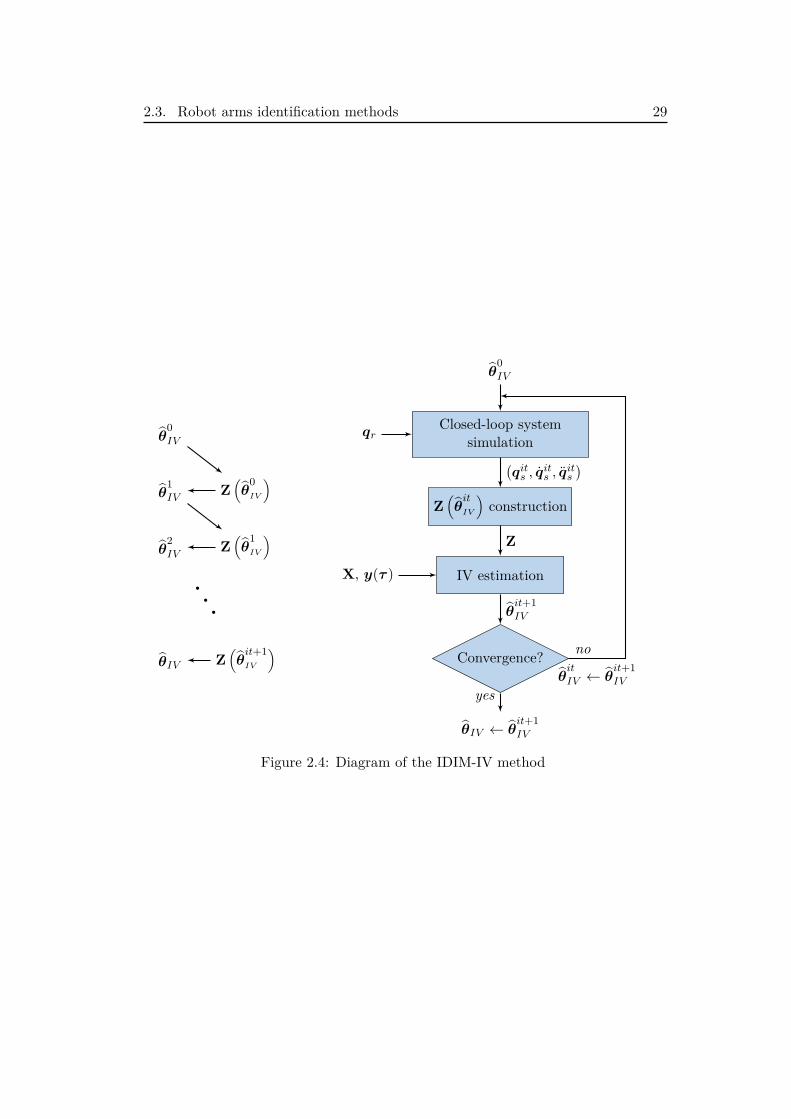
Based on [Young 2011], in [Janot et al. 2014c], the authors have shown that thesimulation of the DDM provides a very convenient way to obtain the instrumentsfor robot identification. This simulation model contains the whole closed-loop and
28 Chapter 2. Robots modelling and identification
is referred to as the auxiliary model. From the simulation of this auxiliary model,noise-free simulated signals are retrieved and used to construct the instrument ma-trix. The signals are noise-free since the only input is the reference trajectorywhich is perfectly known. The process is iterative because the simulation is basedon the parameters previously identified. By noting the simulated signals with asubscript s, the instrumental matrix is ζ(t) = Fp(z−1)φ (qs(t), qs(t), qs(t)). Theinstrumental matrix can be viewed as an estimation of the noise-free part of theobservation matrix. This IDIM-IV method also includes the decimate filter, i.e.L(z−1) ← Fp(z−1)In, with In the (n × n) identity matrix. The fact is that theIDIM-IV method does not take into account the noise model to provide optimalestimates.
The (r × b) instrumental matrix is constructed such as
Z(θit
IV
)=
Zit,1IV
...Zit,nIV
, (2.32)
where Zit,jIV =
ζj(t1, θ
it
IV
)...
ζj(tN , θ
it
IV
). At iteration it, the new estimated parameters are
computed withθit+1IV =
[Z(θitIV )TX
]−1Z(θitIV )Ty(τ), (2.33)
with X given by (2.21). Alternatively, a weighted IV can be performed similarlyto the WLS method. As explained in [Janot et al. 2014c] and described in Figure2.4, the process is iterated until its convergence. The convergence criterion is basedon the relative variation of the estimated parameters and the one of the estimationerror: εit = y(τ) − Xθ
it
IV . Concerning the initialisation, the inertia parametersare usually initialised with Computer-Aided Design (CAD) values, whereas theothers parameters are set to zero. After convergence (superscript cv), the covariancematrix of the IV estimates is given by:
Σ(θcvIV ) =(ZT (θcvIV )Ω−1
τ Z(θcvIV ))−1
. (2.34)
2.3.4 The DIDIM method
Recently [Gautier et al. 2013a] has introduced a method based on the simulation ofthe DDM. This method, called DIDIM for Direct and Inverse Identification Model,minimizes the squared difference between the actual torques and the simulated ones.In other words, there is no observation matrix, the predicted signal comes only fromthe simulation. The considered signal is the input torque and, at time ti, the error
2.3. Robot arms identification methods 29
θ0IV
Z(θ
0IV
)θ
1IV
Z(θ
1IV
)θ
2IV
Z(θit+1IV
)θIV
. . .
θ0IV
Closed-loop systemsimulation
Z(θit
IV
)construction
IV estimation
Convergence?
θIV ← θit+1IV
X, y(τ )
qr
(qits , q
its , q
its
)
Z
θit+1IV
yes
no
θit
IV ← θit+1IV
Figure 2.4: Diagram of the IDIM-IV method
30 Chapter 2. Robots modelling and identification
is given by:
εdidim(ti,θ) = τFp(ti)− τ s(ti,θ) (2.35)= τFp(ti)− φFp (qs(ti), qs(ti), qs(ti))θ,
where τ s(ti,θ) is the (n × 1) simulated torques vector. The vectors qs, qs andqs contain respectively the angular positions, velocities and accelerations of robotjoints, coming from the simulation of the auxiliary model. Hence, the knowledge ofthe controller is required for the simulation. Since the input of the simulation, qr,is perfectly known (i.e. noise free), τ s is not correlated with the measurement noiseq. That insures the consistency of the estimation, assuming no modelling error.
Furthermore, if the dependence of φ in θ is neglected, the optimisation is greatlyenhanced. In fact, the gradient of the simulated torque with respect to the estimatedparameters is just φ (qs(ti), qs(ti), qs(ti)). In the field of system identification, thistechnique is called Pseudo-Linear Regression (PLR), see Eq. (7.112) in [Ljung 1999].According to the same reference, PLR is derived from [Solo 1979]. Since the DIDIMrelies on this assumption, the parameters are iteratively estimated thanks to thelinear Least-Squares:
θit+1DIDIM =
[Z(θitDIDIM)TZ(θitDIDIM)
]−1Z(θitDIDIM)Ty(τ), (2.36)
with Z and y constructed accordingly to (2.21) and (2.32). Like the IDIM-IVmethod, the DIDIM one is iterative. In practice, they can share the same initiali-sation and the same convergence criterion. A complete description of the methodis available in [Janot 2007]. In addition, [Gautier et al. 2011, Robet et al. 2012]provide some applications examples. After convergence, the covariance matrix ofthe DIDIM estimates is given by:
Σ(θcvDIDIM) =(ZT (θcvDIDIM)Ω−1
τ Z(θcvDIDIM))−1
. (2.37)
2.3.5 Exciting trajectories
To finish this section about robots identification, we shortly address the issue ofexciting trajectories. The idea is to insure that X, or Z, is full column rank andhas a good condition number. Section 4.1.2 provide further information on theconditioning number and its influence on the estimation solution. First of all, asexplained in [Walter & Pronzato 1994] for instance, (2.22) should not be appliedas it stands. The singular values decomposition is a better alternative from a com-putation point of view, especially if the conditioning is not perfect. However, aneffective algorithm is not enough to insure a good estimation. The experimentaldata must contain enough information. With the vocabulary of the system identifi-cation community, the robot trajectory must be persistently exciting . [Söderström& Stoica 1988, Ljung 1999] give a mathematical definition of a persistent excitationand [Gautier & Khalil 1992] presents a method dedicated to the optimal trajectory
2.4. Concluding remarks 31
design for robot identification.The principle of the method develop by [Gautier & Khalil 1992] is to find a
sequence of optimal points with respect to a given criterion, the conditioning numberof X for example. Thereafter, a continuous and smooth trajectory is calculated byinterpolating a function at the optimal points. This interpolating function can be atime polynomial. Alternatively, special test motions can be designed to excite someparameters specifically and/or sequentially; see e.g. [Vandanjon et al. 1995, Janotet al. 2007].
To illustrate physically a counterexample of an exciting trajectories, we canthink about a basic trajectory where the arm j moves always in the same direction,i.e. its velocity has a constant sign. In this case, the regressor of the Coulombfriction is constantly +1, or −1 depending on the direction, and the regressor ofthe offset is always 1. Therefore, both regressors are linearly dependent and conse-quently X is column rank deficient.
2.4 Concluding remarks
In this chapter, the notations for robot modelling have been introduced. The ge-ometry of rigid serial robots is parametrised with the MDH notation. From theNewton’s law, the DDM expresses the joint accelerations as a function of the inputtorques and the dynamic parameters. Nonetheless, the input torques can be ex-pressed as a linear function of those dynamic parameters with the IDM. The IDIMdiffers from the IDM in that it takes into account the noise inherent in experimentaldata. Based on this linear IDIM, three identification methods have been introduced.The reference technique is the IDIM-LS method that relies on a careful prefilteringof the measured data. In addition, the recently introduced IDIM-IV and DIDIMtechniques are able to deal with closed-loop data and proved their relevance forrobot identification.

Chapter 3
System identification forcontinuous time systems
In this chapter, some techniques from the system identification community arepresented. If a lot of research has been done on Discrete Time (DT) system identi-fication, see e.g. chapters 6-7 of [Eykhoff 1974] or [Ljung 1999] and the referencesgiven therein, the identification of Continuous Time (CT) systems has also been de-veloped over the years [Young 1966, Young 1981, Unbehauen & Rao 1998, Garnieret al. 2008]. The major part of the identification research (DT or CT) has focusedon Linear Time Invariant (LTI) systems. As explained in the previous chapter, theindustrial robot are not linear with respect to the states. Thus, if all the techniquesdeveloped by the identification community cannot be applied directly to industrialrobots, they still represent a valuable background that we summarize in this chap-ter.
An introduction to the issues raised by the closed-loop configuration is proposedin section 3.1. The following section introduces the Refined Instrumental Variablemethod dedicated to CT- and DT-LTI systems. Section 3.3 outlines the PredictionError Method for hybrid systems (CT and DT). Concluding remarks are providedin section 3.4.
3.1 Closed-loop identification challenges . . . . . . . . . . . . . . 343.2 The refined instrumental variable method . . . . . . . . . . 34
3.2.1 The hybrid Box-Jenkins model . . . . . . . . . . . . . . . . . 343.2.2 The hybrid RIVC algorithm . . . . . . . . . . . . . . . . . . . 363.2.3 Statistical elements of the method . . . . . . . . . . . . . . . 38
3.3 Prediction error methods . . . . . . . . . . . . . . . . . . . . . 393.3.1 Prediction error principle . . . . . . . . . . . . . . . . . . . . 393.3.2 DT prediction error method . . . . . . . . . . . . . . . . . . . 403.3.3 Hybrid output error method . . . . . . . . . . . . . . . . . . . 423.3.4 Computational aspects . . . . . . . . . . . . . . . . . . . . . . 43
3.4 Concluding remarks . . . . . . . . . . . . . . . . . . . . . . . . 44
34 Chapter 3. System identification for continuous time systems
3.1 Closed-loop identification challenges
The identification experiments can be performed in closed-loop for miscellaneousreasons. Firstly, the system may be unstable in open-loop. Therefore, it is impossi-ble to operate it safely without a control law. Secondly, it can be impossible to dowithout the regulator because the system has been bought "off the self" with an inte-grated controller. One can also think about the case where, although the system isstable in open-loop, the practitioner has to process closed-loop data because he hasno influence on the experimental work. At last, in a control design purpose, it canbe more relevant to identify the system directly in closed-loop [De Callafon 1998].
An issue with closed-loop identification is that the usual methods for open-loopdata fail if they are applied directly without precaution. The reason of this failure isthe correlation between the input and the unmeasurable output noise as illustratedin Figure 2.3, see e.g. [Van den Hof 1998]. That issue of the non zero correlationbetween the noise and the input has already been stressed with the IDIM-LS methodin section 2.3.2. The other main issue with closed-loop data is that identifiabilitymay be lost. In this sense, it is impossible to estimate an unique set of parametersfrom measured input-output data. This is due to lack of sensitivity of the systemoutput with respect to the parameters due to the controller action, as shown forinstance in [Janot et al. 2014a] for robots.
It is common in the literature to divide closed-loop identification methods inthree different types [Gustavsson et al. 1977, Söderström & Stoica 1988, Forssell &Ljung 1999]: direct, indirect and joint input-output methods. Each type correspondsto different assumptions concerning the nature of the feedback. According to [Fors-sell 1999], in the direct approach, no assumption is made on the data generation andthe method is applied directly on the measured data. With the indirect approach,the practitioner is perfectly aware of the feedback used during the experiment. Fromthe closed-loop system identified, the open-loop parameters are retrieved using theknowledge of the controller. The joint input-output approach considers the inputand the output signals jointly as a global output of an augmented system, drivenby the reference signal and the unmeasurable noise. From the identification of thisaugmented system, the open-loop and the controller models are retrieved.
3.2 The refined instrumental variable method
In this section, we give a brief overview of the Refined Instrumental Variable methodfor Continuous-time (RIVC) systems introduced in [Young & Jakeman 1979]. Thismethod has been developed for LTI systems and is extensively presented in chapters8-9 of [Young 2011] and in [Young 2015] for instance.
3.2.1 The hybrid Box-Jenkins model
To illustrate the RIVC method, we need to introduce the hybrid Box-Jenkins (BJ)model for SISO systems. This BJ model is called hybrid because it consists of a
3.2. The refined instrumental variable method 35
CT state model coupled with DT observations. The CT state model is driven bythe differential equation
dnax(t)dtna
+ a1dna−1x(t)dtna−1 + · · ·+ anax(t) = b0
dnbu(t)dtnb
+ · · ·+ bnbu(t), (3.1)
where x is the state and u is the input signal. In the transfer function form, theCT can be written:
x(t) = B(p)A(p)u(t), (3.2)
with B(p) = b0pnb + b1p
nb−1 + · · · + bnb , A(p) = pna + a1pna−1 + · · · + ana and
p = ddt , the differential operator. The polynomials coefficients are regrouped in the
(na + nb + 1× 1) vector:
θ =[a1 · · · ana b0 · · · bnb
]T. (3.3)
The signals are assumed to be uniformly sampled, with a sampling interval Ts.The measured output y(ti) is expressed as
y(ti) = x(ti) + ξ(ti), (3.4)
where ξ(ti) is an additive measurement noise coloured such as
ξ(ti) = Dn(z−1)Cn(z−1) e(ti), (3.5)
with e(ti) a Gaussian white noise, i.e. e(ti) ∼ N (0, σ2). Such a noise filter definesan AutoRegressive Moving Average (ARMA) model. It thus assumes that the noisehas a rational spectral density.
Based on the normality of the Gaussian noise e(ti), it can be defined the pre-diction error:
ε(ti) = Cn(z−1)Dn(z−1)
(y(ti)−
B(p)A(p)u(ti)
)(3.6)
= Cn(z−1)Dn(z−1)
1A(p) (A(p)y(ti)−B(p)u(ti)) .
By defining, the hybrid filter
f = Cn(z−1)Dn(z−1)
1A(p) = fd(z−1,η)fc(p,θ), (3.7)
with the (l × 1) vector η regrouping the coefficients of Cn and Dn. Since thepolynomial operators commute:
ε(ti) = A(p)yf (ti)−B(p)uf (ti). (3.8)
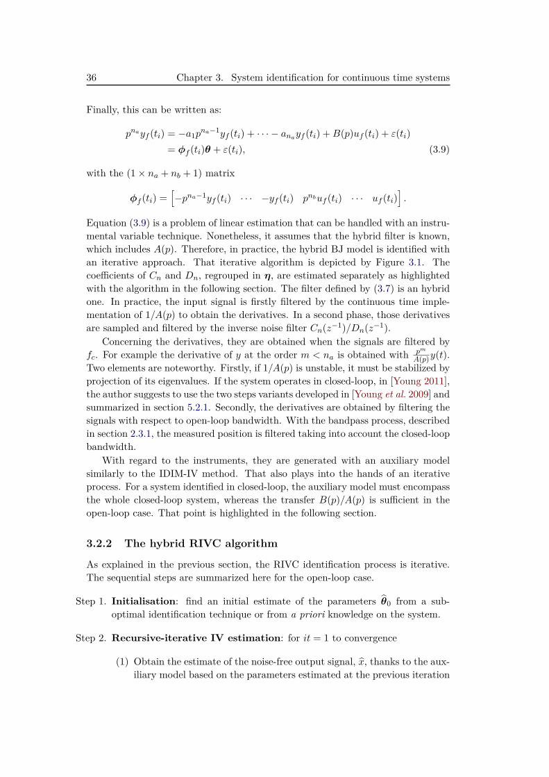
36 Chapter 3. System identification for continuous time systems
Finally, this can be written as:
pnayf (ti) = −a1pna−1yf (ti) + · · · − anayf (ti) +B(p)uf (ti) + ε(ti)
= φf (ti)θ + ε(ti), (3.9)
with the (1× na + nb + 1) matrix
φf (ti) =[−pna−1yf (ti) · · · −yf (ti) pnbuf (ti) · · · uf (ti)
].
Equation (3.9) is a problem of linear estimation that can be handled with an instru-mental variable technique. Nonetheless, it assumes that the hybrid filter is known,which includes A(p). Therefore, in practice, the hybrid BJ model is identified withan iterative approach. That iterative algorithm is depicted by Figure 3.1. Thecoefficients of Cn and Dn, regrouped in η, are estimated separately as highlightedwith the algorithm in the following section. The filter defined by (3.7) is an hybridone. In practice, the input signal is firstly filtered by the continuous time imple-mentation of 1/A(p) to obtain the derivatives. In a second phase, those derivativesare sampled and filtered by the inverse noise filter Cn(z−1)/Dn(z−1).
Concerning the derivatives, they are obtained when the signals are filtered byfc. For example the derivative of y at the order m < na is obtained with pm
A(p)y(t).Two elements are noteworthy. Firstly, if 1/A(p) is unstable, it must be stabilized byprojection of its eigenvalues. If the system operates in closed-loop, in [Young 2011],the author suggests to use the two steps variants developed in [Young et al. 2009] andsummarized in section 5.2.1. Secondly, the derivatives are obtained by filtering thesignals with respect to open-loop bandwidth. With the bandpass process, describedin section 2.3.1, the measured position is filtered taking into account the closed-loopbandwidth.
With regard to the instruments, they are generated with an auxiliary modelsimilarly to the IDIM-IV method. That also plays into the hands of an iterativeprocess. For a system identified in closed-loop, the auxiliary model must encompassthe whole closed-loop system, whereas the transfer B(p)/A(p) is sufficient in theopen-loop case. That point is highlighted in the following section.
3.2.2 The hybrid RIVC algorithm
As explained in the previous section, the RIVC identification process is iterative.The sequential steps are summarized here for the open-loop case.
Step 1. Initialisation: find an initial estimate of the parameters θ0 from a sub-optimal identification technique or from a priori knowledge on the system.
Step 2. Recursive-iterative IV estimation: for it = 1 to convergence
(1) Obtain the estimate of the noise-free output signal, x, thanks to the aux-iliary model based on the parameters estimated at the previous iteration
3.2. The refined instrumental variable method 37
u(t)
++
D(z−1)C(z−1)
B(p)A(p)
B(p,θ)A(p,θ)
Optimalhybrid statevariable filters
C(z−1,η)D(z−1,η)A(p,θ)
Refinedinstrumental
variableestimator(RIVC)
e(tk) ξ(tk)
x(t) y(t)
u(t)
x(t)
Optimallyfiltered
derivatives θ
Figure 3.1: Block diagram of the RIVC algorithm for the hybrid BJ model, source[Young 2011]
θit−1:
x(t) = B(p, θit−1)A(p, θit−1)
u(t).
If the estimated model is unstable, the unstable eigenvalues of the de-nominator polynomial are reflected into the stable region.
(2) From the sampled signals and the estimated noise ξ(ti) = y(ti) − x(ti),obtain the estimate of the noise model parameters ηit. [Young 2006]provides further information about the identification of ARMA noisemodels.
(3) Prefilter the input, u(t), the output, y(t) and the estimated output, x(t)by the continuous time filter:
fc(p, θit−1) = 1
A(p, θit−1).
(4) After signals sampling, prefilter the input and output derivatives by thediscrete filter:
fd(z−1, ηit) = Cn(z−1, ηit)Dn(z−1, ηit)
.
(5) Compute the IV estimate
θit =
[1N
N∑i=1ζTfit(ti)φfit(ti)
]−1 [1N
N∑i=1ζTfit(ti)(p
nayfit(ti))]
(3.10)
38 Chapter 3. System identification for continuous time systems
with
φfit(ti) =[−pna−1yfit(ti) · · · −yfit(ti) pnbufit(ti) · · · ufit(ti)
],
ζfit(ti) =[−pna−1xfit(ti) · · · −xfit(ti) pnbufit(ti) · · · ufit(ti)
],
fit = fd(z−1, ηit)fc(s, θit−1).
Step 3. Computation of the estimated parametric error covariances matrices:
Σθ = σ2[N∑i=1ζ(ti)T ζ(ti)
]−1
, Ση = σ2[N∑i=1φn(ti)Tφn(ti)
]−1
, (3.11)
where φn is the (1× nc + nd + 1) observation matrix of the noise model.
The algorithm presented here is the open-loop version of the RIVC method. In theclosed-loop case, the signal u and by construction x are correlated with the mea-surement noise. Consequently, the instrument exogeneity is not validated anymore.The solution is then to estimate the input, u, and the output, x, thanks to theclosed-loop relations like with the IDIM-IV method. That changes part (1) of thestep 2 in the previous algorithm. The reader can refer to [Gilson et al. 2008] for acomprehensive study about the RIVC method for closed-loop systems.
3.2.3 Statistical elements of the method
With the algorithm previously described, it appears that the RIVC method relieson the decomposition into two separate identification problems. The theoreticaljustification comes from the theorem of [Pierce 1972] that is based on the followingassumptions:
• the noises of the sequence e(ti)Ni=1 are independent and identically dis-tributed with zero mean and variance σ2;
• the parameters values are admissible, i.e. the model is stable and identifiable;
• the input sequence u(ti)Ni=1 is persistently existing.
As outlined in [Young 2011], the result of [Pierce 1972] validates the RIVC algo-rithm.
The RIVC method has been developed rather separately from the automaticcontrol literature. However, that can be seen as an application of the extended IVtheory summarized in section 2.3.3. Instead of τ , the observation variable is theoutput y and the prefilter matrix L is replaced by f . In the opposite of (2.30), thenoise covariance matrix Λ does not appear in the filter because it is a SISO caseand this weighting can be removed from the equations.
3.3. Prediction error methods 39
3.3 Prediction error methods
The prediction error is a wide-spread family of identification methods. Severalbooks deal with those methods: Chapter 7 in [Söderström & Stoica 1988] and alsoChapter 7 in [Ljung 1999]. We give here a brief overview of the techniques, stayingquite close to the material presented in [Åström 1980, Ljung 1999].
3.3.1 Prediction error principle
The purpose of the Prediction Error Methods (PEM) is to find the best parametricmodel with respect to a specific criterion. The criterion is a function of the error be-tween the noisy measured output and the predicted model output. Sometimes, themodel structure comes from the knowledge of the concerned scientific community,like in robot identification with the Newton’s law, and the problem becomes thedetermination or the estimation of the model’s parameters. The generic criterionof PEM is given by:
VN (θ) = 1N
N∑i=1
l(L(z−1)ε(ti,θ))
)(3.12)
where l(·) is a scalar function like the euclidean norm, L is a (n × n) matrix ofstable linear filters and ε is the (n× 1) vector of prediction error, which is functionof the measured data. At time ti, the prediction vector is given by
ε(ti|tm,θ) = y(ti)− y(ti|tm,θ), i ≥ m (3.13)
where y and y are the (n × 1) vectors of the measured and predicted outputsrespectively. A prediction error method solves the minimization problem:
θ(N) = arg minθ
VN (θ). (3.14)
It thus appears that the PEM family is large depending on the choice of l(·), thechoice of the prefilters L, the choice of the model structure, the choice of the consid-ered output signals and even the choice of the minimization algorithm. To evaluatethe difference between the two outputs many scalar functions may be used, as ex-plained in [Walter & Pronzato 1994]. The general principle of the PEM is illustratedin Figure 3.2, where u and y are respectively the inputs and the outputs of a thesystem.
The prediction error formulation is usually presented with the Maximum Like-lihood (ML) that requires normality assumption for the observations. It has beenshown that the ML estimator is asymptotically efficient. That is to say that thereis no other unbiased estimator giving a smaller covariance. However, as pointed outby [Åström 1980], in many practical cases the normality assumption is not validatedand it is not necessary to postulate (3.12).
To illustrate the wide spectrum of methods encompassed by the definition, we
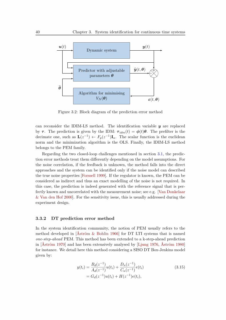
40 Chapter 3. System identification for continuous time systems
Dynamic system
Predictor with adjustableparameters θ
+−
Algorithm for minimisingVN (θ)
u(t)
y(t,θ)
y(t)
ε(t,θ)
θ
Figure 3.2: Block diagram of the prediction error method
can reconsider the IDIM-LS method. The identification variable y are replacedby τ . The prediction is given by the IDM: τ idm(t) = φ(t)θ. The prefilter is thedecimate one, such as L(z−1) ← Fp(z−1)In. The scalar function is the euclideannorm and the minimization algorithm is the OLS. Finally, the IDIM-LS methodbelongs to the PEM family.
Regarding the two closed-loop challenges mentioned in section 3.1, the predic-tion error methods treat them differently depending on the model assumptions. Forthe noise correlation, if the feedback is unknown, the method falls into the directapproaches and the system can be identified only if the noise model can describedthe true noise properties [Forssell 1999]. If the regulator is known, the PEM can beconsidered as indirect and thus an exact modelling of the noise is not required. Inthis case, the prediction is indeed generated with the reference signal that is per-fectly known and uncorrelated with the measurement noise; see e.g. [Van Donkelaar& Van den Hof 2000]. For the sensitivity issue, this is usually addressed during theexperiment design.
3.3.2 DT prediction error method
In the system identification community, the notion of PEM usually refers to themethod developed in [Åström & Bohlin 1966] for DT LTI systems that is namedone-step-ahead PEM. This method has been extended to a k-step-ahead predictionin [Åström 1970] and has been extensively analysed by [Ljung 1976, Åström 1980]for instance. We detail here this method considering a SISO DT Box-Jenkins modelgiven by:
y(ti) = Bd(z−1)Ad(z−1)u(ti) + Dn(z−1)
Cn(z−1) e(ti) (3.15)
= Gd(z−1)u(ti) +H(z−1)e(ti),
3.3. Prediction error methods 41
where Bd and Ad are respectively the numerator and denominator of the DT transferfunction Gd. Given a data set DN = y(ti), u(ti)Ni=1, the idea of the one step aheadPEM is to predict the output, such as:
y(ti|ti−1) = Gd(z−1, θ)u(ti) + ξ(ti|ti−1) (3.16)
= Gd(z−1, θ)u(ti) +(1−H−1(z−1, η)
)ξ(ti)
= Gd(z−1, θ)u(ti) +(1−H−1(z−1, η)
) (y(ti)−Gd(z−1, θ)u(ti)
)=(1−H−1(z−1, η)
)y(ti) +H−1(z−1, η)Gd(z−1, θ)u(ti).
The details of the one-step-ahead prediction of ξ are available in Chapter 3 of[Ljung 1999]. In the final relation of (3.16), the first term on the right-hand-sideis only function of y(tm), with m < i. Thee predicted output is thus independentof the current one. That expression requires that the filters H−1Gd and H−1 arestable. From the output prediction (3.16), the error can be written:
εpem(ti, ρ) = y(ti)− y(ti|ti−1) (3.17)
= H−1(z−1, η)(y(ti)−Gd(z−1, θ)u(ti)
),
with ρ = [θT ηT ]T .
The one-step-ahead PEM takes into account the past measured output. Nev-ertheless, the estimated output could be simulated only with the past measuredinput, such as:
y(ti|ti−1) = Gd(z−1, θ)u(ti) +H(z−1, η)e∗(ti), (3.18)
where e∗ is a random number that would be generated by the computer. However,with such a mathematical framework, the simulation is not appropriate to identifythe noise model due to the randomness of e∗. There is one exception when H = 1.In this case, the additive noise is white and can be neglected in the simulation. Forthis case, we talk about an output error model and the prediction error is definedby:
εoem(ti, θ) = y(ti)−Gd(z−1, θ)u(ti). (3.19)
As outlined with Exercise 61 in [Schoukens et al. 2012], the error converge to zeromore rapidly with the PEM than with the simulation. That is due to the initialstates effects which vanishes faster.
Regarding the closed-loop aspects, this one-step-ahead method perfectly suitsfor a direct identification approach. As outlined in [Forssell & Ljung 1999], theidentification of the system and noise models are linked. An error in one partcauses fallacies in the other.
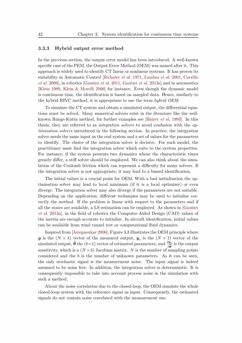
42 Chapter 3. System identification for continuous time systems
3.3.3 Hybrid output error method
In the previous section, the output error model has been introduced. A well-knownspecific case of the PEM, the Output Error Method (OEM) was named after it. Thisapproach is widely used to identify CT linear or nonlinear systems. It has proven itssuitability in Automatic Control [Richalet et al. 1971, Landau et al. 2001, Carrilloet al. 2009], in robotics [Gautier et al. 2011, Gautier et al. 2013a] and in aeronautics[Klein 1989, Klein & Morelli 2006] for instance. Even though the dynamic modelis continuous time, the identification is based on sampled data. Hence, similarly tothe hybrid RIVC method, it is appropriate to use the term hybrid OEM.
To simulate the CT system and obtain a simulated output, the differential equa-tions must be solved. Many numerical solvers exist in the literature like the well-known Runge-Kutta method, for further examples see [Hairer et al. 1993]. In thisthesis, they are referred to as integration solvers to avoid confusion with the op-timisation solvers introduced in the following section. In practice, the integrationsolver needs the same input as the real system and a set of values for the parametersto identify. The choice of the integration solver is decisive. For each model, thepractitioner must find the integration solver which suits to the system properties.For instance, if the system presents two dynamics whose the characteristic timesgreatly differ, a stiff solver should be employed. We can also think about the simu-lation of the Coulomb friction which can represent a difficulty for many solvers. Ifthe integration solver is not appropriate, it may lead to a biased identification.
The initial values is a crucial point for OEM. With a bad initialisation the op-timisation solver may lead to local minimum (if it is a local optimizer) or evendiverge. The integration solver may also diverge if the parameters are not suitable.Depending on the application, different techniques may be used to initialize cor-rectly the method. If the problem is linear with respect to the parameters and ifall the states are available, a LS estimation can be employed. As shown in [Gautieret al. 2013a], in the field of robotics the Computer-Aided Design (CAD) values ofthe inertia are enough accurate to initialize. In aircraft identification, initial valuescan be available from wind tunnel test or computational fluid dynamics.
Inspired from [Jategaonkar 2006], Figure 3.3 illustrates the OEM principle wherey is the (N × 1) vector of the measured output, ys is the (N × 1) vector of thesimulated output, θ the (b×1) vector of estimated parameters, and ∂ys
∂θis the output
sensitivity, which is a (N × b) Jacobian matrix. N is the number of sampling pointsconsidered and the b is the number of unknown parameters. As it can be seen,the only stochastic signal is the measurement noise. The input signal is indeedassumed to be noise free. In addition, the integration solver is deterministic. It isconsequently impossible to take into account process noise in the simulation withsuch a method.
About the noise correlation due to the closed-loop, the OEM simulate the wholeclosed-loop system with the reference signal as input. Consequently, the estimatedsignals do not contain noise correlated with the measurement one.
3.3. Prediction error methods 43
Dynamic system+
+
Measurement noise
Mathematical model simulation−
+
Nonlinear optimisation algorithm
Input
ys
y
∂ys∂θ
Output error
θ
Figure 3.3: Block diagram of the output error method
3.3.4 Computational aspects
With the PEM, the unknown system parameters are tuned iteratively, so that thepredicted model output fits the measured system output, with
θit+1 = θ
it + ∆θit (3.20)
where ∆θit is the innovation vector. This innovation is calculated differently de-pending on the applied nonlinear optimisation algorithm. The criterion minimisa-tion is usually solved thanks to nonlinear optimisation algorithms based on a first- orsecond-order Taylor series expansion like the gradient, the Gauss-Newton and theLevenberg-Marquardt methods. With these methods, the parameter innovationsare respectively given by
∆θit = −µ∂VN∂θ
∣∣∣∣θ=θ
it= −µV ′N (θit), (3.21)
∆θit = −[V ′′N (θit)
]−1V ′N (θit), (3.22)
∆θit = −[V ′′N (θit) + µ · diag
(V ′′N (θit
)]−1V ′N (θit), (3.23)
where V ′N (θit) and V ′′N (θit) are the gradient vector and the hessian matrix of thecriterion VN , µ is a parameter which permits the tuning of the iterative algorithms.Those innovations require the computation of the criterion derivatives with respectto the parameters. In some cases those derivatives can be exactly known. Forexample, in [Carrillo et al. 2009], the authors have developed an exact formulationof the first derivative for CT-LTI systems. In [Landau et al. 2001], the authors havedone the same for nonlinear systems. Those derivatives of the criterion are function
44 Chapter 3. System identification for continuous time systems
of the derivatives of the system’s outputs with respect to the parameters, which arecalled sensitivities.
However, those sensitivities can be difficult to calculate exactly for complexnonlinear systems, like the robots. In such cases, they are usually approximatedwith finite differences. Furthermore, they can even be undefined due to the selectedscalar function (e.g. absolute value at zero) or the model’s properties (e.g. signfunction at zero). The user should then select a solver that is not based on thecalculation of the derivatives. Those solvers are referred to as derivative-free op-timisation solvers; see e.g. the Nelder-Mead method [Nelder & Mead 1965]. Theuser can also consider stochastic and/or global optimisation solvers. It appearsthat many solutions are available for the optimisation, depending on the consideredidentification problem. For example, several optimisation solutions available for anidentification purpose are summarized in [Walter & Pronzato 1994].
3.4 Concluding remarks
The Refined Instrumental Variable for Continuous-time systems has been presentedin this chapter. Although this approach has its roots in the areas of time seriesanalysis and environmental modelling, it has been used successfully in many appli-cations; see [Young 2011] and the references given therein. In parallel, the systemidentification community has established the Prediction Error Methods. This frame-work encompasses a lot of methods including the Output Error Method that is ableto identify CT models with white measurement noise. All those methods are ableto identify systems operating in closed-loop by considering different approaches:direct, indirect or joint input-output.
This chapter concludes the preliminary part of this thesis. The contributionsare now presented starting with the study of the identification methods based onthe model simulation.
Part III
Contributions to robot systemidentification

Chapter 4
Evaluation of the robustness ofidentification methods based onthe auxiliary model simulation
As shown in chapter 2, the usual robot identification methods use the input torquebecause of its linearity with respect to the parameters. However, it has been seenin chapter 3 that the OEM are able to identify models nonlinear with respectto the parameters. The resultant question is: would it be possible to consideranother identification signal like the output position to improve the robustness ofthe estimation? Furthermore, since those methods rely on the simulation of theclosed-loop system, an underlying issue is the robustness of those simulations. Inother words, the question is to what extent those methods can reject modellingerrors or a too large noise.
In section 4.1, we investigate the choice of the identification signal for OEMapplied to robot identification. Then, the robustness of the simulation used for theDIDIM and IDIM-IV methods is investigated in section 4.2. Then, some miscella-neous remarks are made in section 4.3 before concluding in section 4.4.
4.1 Choice of the identification signal . . . . . . . . . . . . . . . . 484.1.1 Output error methods for robot identification . . . . . . . . . 484.1.2 Sensitivity analysis . . . . . . . . . . . . . . . . . . . . . . . . 494.1.3 Contribution of the linearity . . . . . . . . . . . . . . . . . . 554.1.4 Experimental validation . . . . . . . . . . . . . . . . . . . . . 55
4.2 Robustness to modeling errors of the DIDIM and IDIM-IVmethods . . . . . . . . . . . . . . . . . . . . . . . . . . . . . . . 61
4.2.1 Similarity between the methods . . . . . . . . . . . . . . . . . 614.2.2 Disparity between the methods . . . . . . . . . . . . . . . . . 634.2.3 Experimental validations . . . . . . . . . . . . . . . . . . . . 65
4.3 Miscellaneous remarks . . . . . . . . . . . . . . . . . . . . . . 664.3.1 Closed-loop aspects of the robot identifications methods . . . 664.3.2 Considerations on the robot identification with OEM . . . . . 664.3.3 Remarks on the linearity . . . . . . . . . . . . . . . . . . . . . 68
4.4 Conclusions . . . . . . . . . . . . . . . . . . . . . . . . . . . . . 70
48 Chapter 4. Robustness of the identification methods
4.1 Choice of the identification signal
4.1.1 Output error methods for robot identification
By applying directly the OEM to a robot model, it seems natural to take the jointposition vector as the identification signal. The output error vector is defined by:
εCLOE(t,θ) = qm(t)− qs(t,θ), (4.1)
where qs is the (n × 1) vector of simulated joint positions. Since the robots areunstable in open-loop, they are identified in closed-loop and the dedicated iden-tification method is called the Closed-Loop Output Error (CLOE) method. Asexplained in section 3.3.3, the simulated output qs is generated with the noise-freereference signal qr. Therefore, there is not bias induced by a noise correlation andthe estimation is consistent, assuming that there is no modelling error and that theoptimisation solver has converged to the global minimum.
As explained in section 3.3.4, the OEM problem is usually solved thanks tononlinear optimisation algorithms such as the gradient or Newton methods. In thispart, we focus on the Gauss-Newton method (GN method), which is based on asecond order Taylor series expansion of qs, at current estimates θCLOE; see (3.22).After data sampling, the following over-determined system is obtained at iterationit:
∆y(q) = ΨitCLOE∆θitCLOE + eCLOE (4.2)
where
• ∆y(q) is the (r′ × 1) vector built from the sampling of εCLOE(t,θ), similarlyto (2.20);
• ΨitCLOE is the (r′×b) matrix built from the nmatrices Ψit
CLOEj =
∆jqs
(t1)...
∆jqs
(tnm)
,where ∆j
qs(·) is the jth row of the (n×b) jacobian matrix ∆qs = ∂qs
∂θ
∣∣∣θ=θ
it
CLOE
;
• eCLOE is the (r′×1) vector built from the sampling of εCLOE and the residualsof the Taylor series expansion
• r′ = n · nm is the number of equation considered, without any decimation.
∆θitCLOE is the (b× 1) vector of estimated parameters increments and is the LSsolution of (4.2). Each element of the jacobian ∆qs is an output sensitivity functionwhich defines the variation of the output position with respect to the parameters.Usually, those sensitivities functions are not exactly known and approximated withfinite differences.
The construction of the en-bloc formulation is really similar to the one of theIDIM-LS method (2.20). The difference is the use of r′ instead of r. This is due
4.1. Choice of the identification signal 49
to the fact that we are in an output error framework. Hence, the additive noise isassumed white and does not need any prefiltering such as the decimate filter. Itbegins to emerge here a limitation of OEM for robot identification. In addition,as we shall see later the decimation process presents also an advantage for theconditioning number. The number of sampling points to treat is indeed reduced forthe optimisation solver.
As we have seen in section 2.3, it is common to use the input torque/force forrobot identification. Therefore, a variant of the CLOE method based on the inputsignal can be considered. This technique called the Closed-Loop Input Error (CLIE)method relies on the input error vector
εCLIE(t,θ) = τ (t)− τ s(t,θ). (4.3)
If the problem is solved with the GN algorithm, ∆θitCLIE is the LS solution of
∆y(τ ) = ΨitCLIE∆θitCLIE + eCLIE (4.4)
where
• ∆y(τ ) is the (r′ × 1) vector built from the sampling of εCLIE(t,θ), similarlyto (2.20);
• ΨitCLIE is the (r′×b) matrix built from the n matrices Ψit
CLIEj =
∆jτ s(t1)...
∆jτ s(tnm)
,where ∆j
τ s(·) is the jth row of the (n×b) jacobian matrix ∆τ s = ∂τ s
∂θ
∣∣∣θ=θ
it
CLIE
;
• eCLIE is the (r′× 1) vector built from the sampling of εCLIE and the residualsof the Taylor series expansion.
The general principle of the CLOE and CLIE methods is illustrated by Figure4.1. Both methods are iterative and can share the initialisation and the conver-gence criterion of the IDIM-IV and DIDIM methods. In the following section, weinvestigate their properties.
4.1.2 Sensitivity analysis
Sensitivities relation
For the CLIE method, at iteration it, the input sensitivity is defined such as
∆τ s(t) = ∂τ s(t)∂θ
∣∣∣∣θ=θ
it
CLIE
. (4.5)
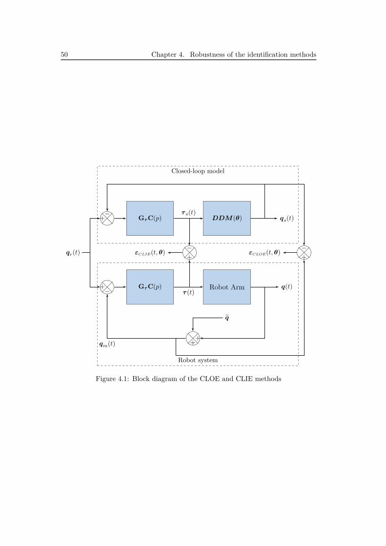
50 Chapter 4. Robustness of the identification methods
qr(t)
−+ GτC(p) Robot Arm q(t)
++
q
τ (t)
qm(t)
−+ GτC(p) DDM(θ)
−+
−+
εCLIE(t,θ) εCLOE(t,θ)
qs(t)τ s(t)
Closed-loop model
Robot system
Figure 4.1: Block diagram of the CLOE and CLIE methods
4.1. Choice of the identification signal 51
By using the controller definition (2.11), it comes:
∆τ s(t) =∂GτC(p)
(qr(t)− qs(t, θ
it
CLIE))
∂θ
∣∣∣∣∣∣∣θ=θ
it
CLIE
, (4.6)
and assuming that the controller is known, or at least not identified at the sametime:
∆τ s(t) = −GτC(p)∂(qs(t, θ
it
CLIE))
∂θ
∣∣∣∣∣∣∣θ=θ
it
CLIE
(4.7)
= −GτC(p)∆qs(t).
Eq. (4.7) is the key relation to compare the CLOE and CLIE methods. Looselyspeaking, the CLIE method is a frequency weighting of the CLOE method by thecontroller. In practice, the input sensitivity functions can be obtained from thefiltering of the output ones, if they are available.
Because the robots are controlled in position, the following relation is expected:
qm(t) ≈ qr(t). (4.8)
Assuming that the optimisation solver is adequately initialized, it implies:
qs(t) ≈ qr(t), (4.9)
at each iteration it of the algorithm. Because of (4.8) and (4.9), the controller maybe assumed to operate in low frequencies range and, then, to be a (n× n) constantmatrix C0. If the controller is a PD control law then this result is straightforward. Ifthe controller contains an integral part, this result can be still considered as valid. Infact, as explained in section 2.2.1, to avoid oscillations due to the Coulomb friction,the integral action is deactivated when the position error is too small. Thus, (4.7)may be re-written
∆τ s(t) = −GτC0∆qs(t). (4.10)
52 Chapter 4. Robustness of the identification methods
Equivalence of the CLOE and CLIE estimations
Considering relation (4.10), the CLIE method can be seen as a weighted CLOEmethod (WCLOE). That can be seen with the LS solution of (4.4):
∆θitCLIE =[(
ΨitCLIE
)TΨitCLIE
]−1 (ΨitCLIE
)T∆y(τ ) (4.11)
=[(
ΨitCLOE
)TCT
0 C0ΨitCLOE
]−1 (ΨitCLOE
)TCT
0 C0∆y(q)
=[(
ΨitCLOE
)TWΨit
CLOE
]−1 (ΨitCLOE
)TW∆y(q),
where
• C0 is (r′ × r′) matrix built from the constant controller matrix GτC0;
• ∆y(τ ) is equal to −C0∆y(q) because it is built from
τ (t)− τ s(t) = GτC(p) (qr(t)− qm(t))−GτC(p) (qr(t)− qs(t))= −GτC(p) (qm(t)− qs(t))≈ −GτC0 (qm(t)− qs(t)) .
Relation (4.11) is clearly a weighted least-squares solution. If nm is sufficientlylarge, according to the theory of statistics [Davidson & MacKinnon 1993], one has
E[θitCLIE]→ E[θitCLOE].
It comes out that the CLIE and CLOE methods asymptotically provide the sameestimates. The resulting question is: is there a dominant estimator?
Because we are in an output error framework, the output position can be written:
qm(t) = qnf (t) + nq(t), (4.12)
where nq is a (n× 1) vector of independent white noises with a (n× n) covariancematrix Λq. With the closed-loop, the input is given by:
τ (t) = GτC(p)(qr(t)− qm(t)) (4.13)= GτC(p)(qr(t)− qnf (t))−GτC(p)nq(t).
The reference trajectory is noise-free. Consequently, the noise seen by the inputtorque is v(t) = −GτC(p)nq(t); see (2.17). With no further assumption, it appearsthat if the output error assumption is made on the output position, it is not validatedfor the input torque. Nonetheless, we assume that the closed-loop system operatesin its bandwidth and consequently C(p) ≈ C0. The noises relation is given by:
v(t) = −GτC0nq(t). (4.14)
4.1. Choice of the identification signal 53
Consequently, E[v] = −GτC0E[nq] = 0 and, using covariance matrix definition(C.8), the covariances are linked such as:
Λv = E[(v − E[v]) (v − E[v])T
](4.15)
= E[GτC0nqn
Tq CT
0 GTτ
]= GτC0ΛnqCT
0 GTτ .
In practice, the matrices Gτ and C0 can be assumed diagonal, which is justifiedby the technology of the actuators, the controller and the sensors presented insection 2.2. Attention is drawn to the fact that the covariance Λv is the one ofv(t) whereas Λτ is the one of vFp(t); see (2.25). Assuming no modelling error andthat the optimisation solver has converged to true parameters values, the estimatedparameters covariances are then given by:
Σ(θit
CLIE
)=[(
ΨitCLIE
)TΩ−1v Ψit
CLIE
]−1(4.16)
=[(
ΨitCLOE
)TCT
0
(C0ΩqC
T0
)−1C0Ψit
CLOE
]−1
=[(
ΨitCLOE
)TΩ−1q Ψit
CLOE
]−1
= Σ(θit
CLOE
),
where Ωv and Ωq are the (r′× r′) covariances matrices built respectively built fromΛv and Λq like in (2.24). It comes out that the CLIE and the CLOE methodsprovide the same estimates with the same variances.
To summarize, the users have the choice between qm and τ , but the CLIEand the CLOE methods asymptotically provide the same results. The questionis: what is the best choice to identify continuous-time systems operating in closedloop? The following subsection presents the main difference between the CLOEand CLIE methods.
Robustness of the CLIE method to errors
With the good tracking assumption (4.9), qs has a little dependence to parameters’variations and the output sensitivity matrix ∆qs contains little information. Thisimplies that the singular values of ∆qs are small whereas the its conditioning num-ber denoted as condCLOE2 may be very good i.e. condCLOE2 ≈ 1; see e.g. [Lawson &Hanson 1974]. To show that, from (4.2), the OLS solution can be written
∆θitCLOE =[(
ΨitCLOE
)TΨitCLOE
]−1 (ΨitCLOE
)T∆y(q) (4.17)
54 Chapter 4. Robustness of the identification methods
Then, the relative variation of the solution ∆θitCLOE denoted as d∆θitCLOE is ex-pressed by two upper bounds given by∥∥∥d∆θitCLOE∥∥∥2∥∥∥∆θitCLOE∥∥∥2
≤ condCLOE2‖d∆y(q)‖2‖∆y(q)‖2
, (4.18)
∥∥∥d∆θitCLOE∥∥∥2∥∥∥∆θitCLOE + d∆θitCLOE∥∥∥
2
≤ condCLOE2
∥∥∥dΨitCLOE
∥∥∥2∥∥∥Ψit
CLOE
∥∥∥2
, (4.19)
where d∆θitCLOE, d∆y(q) and dΨitCLOE are small variations of ∆θitCLOE, ∆y(q) and
ΨitCLOE respectively. ‖·‖2 is the 2-norm of a vector or a matrix.Let µCLOEmin and µCLOEmax be the smallest and the greatest singular values of Ψit
CLOE
respectively. With, condCLOE2 = µCLOEmax /µCLOEmin and∥∥∥Ψit
CLOE
∥∥∥2
= µCLOEmax , one obtains
∥∥∥d∆θitCLOE∥∥∥2∥∥∥∆θitCLOE∥∥∥2
≤ µCLOEmax
µCLOEmin
‖d∆y(q)‖2‖∆y(q)‖2
, (4.20)
∥∥∥d∆θitCLOE∥∥∥2∥∥∥∆θitCLOE + d∆θitCLOE∥∥∥
2
≤
∥∥∥dΨitCLOE
∥∥∥2
µCLOEmin
. (4.21)
Assuming that µCLOEmin and µCLOEmax are very small with µCLOEmin ≈ µCLOEmax , one hascondCLOE2 ≈ 1 and 1/µCLOEmin very large.
With (4.20), it appears the interest of having a conditioning number as smallas possible to minimize the relative norm error on the solution vector. That prop-erty was pointed out in [Pressé & Gautier 1993] where a new criterion of excitingtrajectory was developed based on this relation. Equation (4.21) pinpoints the roleof µCLOEmin as we shall see below. In practice, two cases must be considered for theCLOE method.
• The first case is when (4.8) and (4.9) are fulfilled. That is to say that thecontroller has been designed to provide an excellent tracking, while rejectingperturbations and model mismatches. In this case, there is εCLOE(t,θ) ≈ 0,for each t, or equivalently ∆y(q) ≈ 0. Then, from (4.17), the innovationis approximately zero. It comes out that the CLOE method may be totallyinsensitive to modelling errors and/or to measurement noise, if the controllaw is effective enough. In practice, the optimisation solver would not movefrom the initialisation point.
• The second case to be considered is when (4.8) and (4.9) are not totallyfulfilled. In other words, the controller presents relatively poor trackingperformances. Regarding the upper bound (4.21), ∆θitCLOE may not be ro-bust against a small variation dΨit
CLOE. In fact,∥∥∥dΨit
CLOE
∥∥∥2is amplified by
4.1. Choice of the identification signal 55
1/µCLOEmin . It can be thought that dΨitCLOE is mainly due to modelling errors
and a poor initialisation, since the simulated output is not affected by themeasurement noise. This leads to unpredictable results because those errorscan be interpreted as an information by the optimisation solver. It comesout that the CLOE method may be sensitive to small modelling errors, if thecontrol law is not effective enough.
As a result, the objective is to obtain a conditioning number as small as possiblewhile having the smallest singular value as large as possible. Contrary to the CLOEmethod, the CLIE one will not suffer from small singular values because it is theCLOE method weighted by the control. As regards the industrial robots, the gainsof the controller are usually high and this implies C0 In. Then, it follows thatµCLIEmin and µCLIEmax the smallest and the greatest singular values of Ψit
CLIE are fargreater than µCLOEmin and µCLOEmax . It comes out that the CLIE method is more robustagainst a small modelling error and is more sensitive to parameters’ variations thanthe CLOE method.
4.1.3 Contribution of the linearity
A careful reader might notice that the CLIE method is really similar to the DIDIMmethod introduced in section 2.3.4. The error considered by the DIDIM method(2.35) is the CLIE error (4.3) filtered by the parallel filter. The introduction of thisfilter implies that it is technically not an output error model anymore. However,the DIDIM method is not a PEM because the noise model is not identified in theprocess. The second specificity of the DIDIM method is the PLR assumption. Withsuch an assumption the GN algorithm becomes equivalent to the linear LS, as shownin section 4.3.3.3 of [Walter & Pronzato 1994]. The input sensitivity is written:
∆τ s(t) = ∂τ s(t)∂θ
∣∣∣∣θ=θ
it
DIDIM
(4.22)
= φ(qs(t, θ
it
DIDIM), qs(t, θit
DIDIM), qs(t, θit
DIDIM)).
Thanks to this relation, the input sensitivity can be calculated with only one sim-ulation of the closed-loop system. In the opposite, with finite differences, b + 1simulations are needed to evaluate the sensitivity; considering a forward or a back-ward first order and one-sided difference scheme. The gain in computing time istherefore not negligible.
4.1.4 Experimental validation
In this part, we illustrate the performances of the CLIE, CLOE and DIDIM methodswith the Stäubli TX40 presented in Appendix B. In a first time, the CLIE andCLOE methods are studied in a strict output error framework. In a second time,the three methods are compared in more general framework by taking into accountthe decimate filter.
56 Chapter 4. Robustness of the identification methods
The DDM is simulated thanks to a Simulink c© model integrated with the ode3integration solver: Bogacki-Shampine. The gains of the simulated controller arenot updated to keep the bandwidth constant as it could be done with the DIDIMmethod, see e.g. [Gautier et al. 2013a]. For the CLIE and CLOE methods, theoptimisation is done with the Levenberg-Marquardt (LM) algorithm implementedin the lsqnonlin function of the MatLab c© Optimization Toolbox. The three methodsare initialized with acceptable CAD values: all base parameters equal to 0 exceptiaj = 1 for j 6= 5 and ia5 = 2 because of the coupling effect. The essential estimatedparameters and relative standard deviation are summarized in Table 4.4.
Strict output error framework
First of all, the CLIE estimated parameters are close to those provided in AppendixB and lie in the 3σ confidence intervals of the LS estimates. The CLOE estimates arenot so far except for few parameters like mx4 or fc6. This can be explained by thelack of sensitivity of this method. As explained in section 4.1.2, the CLIE methodis in fact a CLOE method weighted by the controller. Due to large controller gains,the sensitivity with respect to the parameters is more important at the input thanat the output. That is confirmed by the singular values of the jacobian matrices inTable 4.2. The interest of considering the input torque for the identification is alsovisible in Table 4.3. The CLOE method indeed provides larger simulation errorson the torques than the CLIE method, whereas both have equivalent errors on thepositions. The relative standard deviations of the estimated parameters may seempromising, however there is an issue with the computation of the variances. Theadditive noises are indeed assumed to be serially uncorrelated which is not verifiedwith the residuals autocorrelations; see Figures 4.2 and 4.3 for the CLOE andCLIE methods respectively. Consequently, the CLOE and CLIE methods cannotbe applied in a strict output error framework to industrial robots, although theCLIE method provides consistent estimates. In fact, the CLIE estimator appearsto be consistent but inefficient; see Appendix C.2.
OEM with the decimate filter
In this part, we consider the CLIE and CLOE methods with the decimate filter aswell as the DIDIM method. According to Appendix B, the cut-off frequency is setat 20 Hz. The estimated parameters provided in Table 4.4 are close to the previousestimations. There is still a lack of sensitivity for the CLOE method. Concerningthe relative standard deviations of the CLIE, CLOE and DIDIM methods, theyproved to be equivalent. Since the CLIE and DIDIM results are really close, onlythe correlation of the DIDIM residuals is presented. Thus, Figure 4.4 and Figure 4.5depict the autocorrelations of the identification residuals of the CLOE and DIDIMmethods respectively. For both methods, the effect of the parallel filter is clear sincethe estimated autocorrelations coefficients are included in the confidence intervalsindicated by the blue lines. These estimated autocorrelations prove that the CLOE
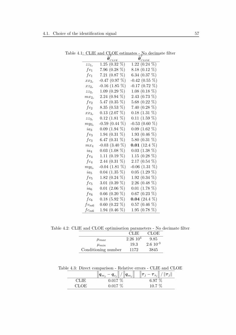
4.1. Choice of the identification signal 57
Table 4.1: CLIE and CLOE estimates - No decimate filterθ
7CLIE θ
7CLOE
zz1r 1.25 (0.32 %) 1.22 (0.24 %)fv1 7.96 (0.28 %) 8.18 (0.12 %)fc1 7.21 (0.87 %) 6.34 (0.37 %)xx2r -0.47 (0.97 %) -0.42 (0.55 %)xz2r -0.16 (1.85 %) -0.17 (0.72 %)zz2r 1.09 (0.29 %) 1.08 (0.18 %)mx2r 2.24 (0.94 %) 2.43 (0.73 %)fv2 5.47 (0.35 %) 5.68 (0.22 %)fc2 8.35 (0.53 %) 7.40 (0.28 %)xx3r 0.13 (2.07 %) 0.18 (1.31 %)zz3r 0.12 (1.81 %) 0.11 (1.59 %)my3r -0.59 (0.44 %) -0.53 (0.60 %)ia3 0.09 (1.94 %) 0.09 (1.62 %)fv3 1.94 (0.31 %) 1.93 (0.46 %)fc3 6.47 (0.31 %) 5.80 (0.31 %)mx4 -0.03 (3.40 %) 0.01 (12.4 %)ia4 0.03 (1.08 %) 0.03 (1.38 %)fv4 1.11 (0.19 %) 1.15 (0.28 %)fc4 2.44 (0.31 %) 2.17 (0.54 %)my5r -0.04 (1.81 %) -0.06 (1.31 %)ia5 0.04 (1.35 %) 0.05 (1.29 %)fv5 1.82 (0.24 %) 1.92 (0.34 %)fc5 3.01 (0.39 %) 2.26 (0.48 %)ia6 0.01 (2.06 %) 0.01 (1.78 %)fv6 0.66 (0.20 %) 0.67 (0.23 %)fc6 0.18 (5.92 %) 0.04 (24.4 %)fvm6 0.60 (0.22 %) 0.57 (0.46 %)fcm6 1.94 (0.46 %) 1.95 (0.78 %)
Table 4.2: CLIE and CLOE optimisation parameters - No decimate filterCLIE CLOE
µmax 2.26 104 9.85µmin 19.3 2.6 10-3
Conditioning number 1172 3845
Table 4.3: Direct comparison - Relative errors - CLIE and CLOE∥∥∥qmj − qsj∥∥∥ / ∥∥∥qmj∥∥∥ ∥∥∥τ j − τ sj∥∥∥ / ‖τ j‖CLIE 0.017 % 6.97 %CLOE 0.017 % 10.7 %
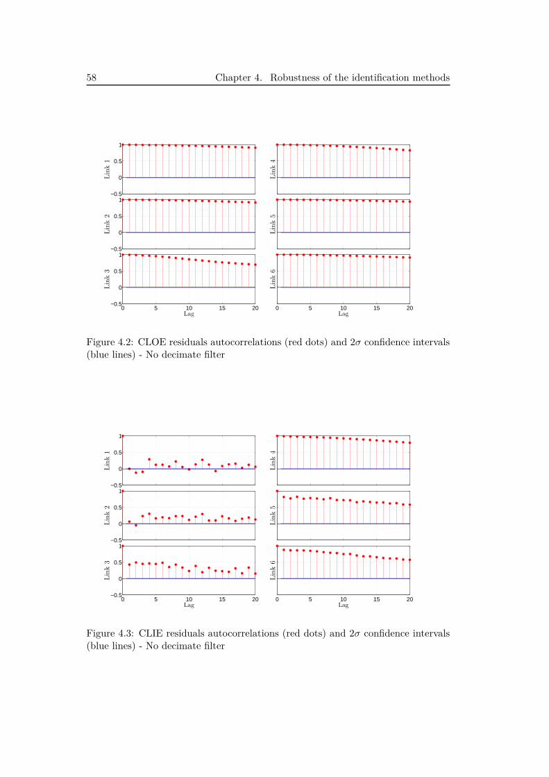
58 Chapter 4. Robustness of the identification methods
−0.5
0
0.5
1
Link1
Link4
−0.5
0
0.5
1
Link2
Link5
0 5 10 15 20−0.5
0
0.5
1
Link3
Lag0 5 10 15 20
Link6
Lag
Figure 4.2: CLOE residuals autocorrelations (red dots) and 2σ confidence intervals(blue lines) - No decimate filter
−0.5
0
0.5
1
Link1
Link4
−0.5
0
0.5
1
Link2
Link5
0 5 10 15 20−0.5
0
0.5
1
Link3
Lag0 5 10 15 20
Link6
Lag
Figure 4.3: CLIE residuals autocorrelations (red dots) and 2σ confidence intervals(blue lines) - No decimate filter
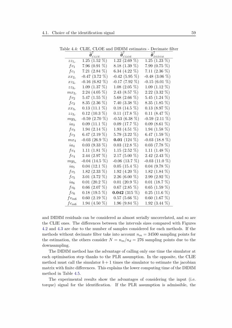
4.1. Choice of the identification signal 59
Table 4.4: CLIE, CLOE and DIDIM estimates - Decimate filterθ
7CLIE θ
7CLOE θ
7DIDIM
zz1r 1.25 (1.52 %) 1.22 (2.69 %) 1.25 (1.23 %)fv1 7.96 (0.91 %) 8.18 (1.39 %) 7.99 (0.75 %)fc1 7.21 (2.84 %) 6.34 (4.22 %) 7.11 (2.36 %)xx2r -0.47 (3.72 %) -0.42 (5.95 %) -0.48 (3.06 %)xz2r -0.16 (6.82 %) -0.17 (7.92 %) -0.15 (6.01 %)zz2r 1.09 (1.37 %) 1.08 (2.05 %) 1.09 (1.12 %)mx2r 2.24 (4.05 %) 2.43 (8.57 %) 2.22 (3.32 %)fv2 5.47 (1.55 %) 5.68 (2.66 %) 5.45 (1.24 %)fc2 8.35 (2.36 %) 7.40 (3.38 %) 8.35 (1.85 %)xx3r 0.13 (11.1 %) 0.18 (14.5 %) 0.13 (8.97 %)zz3r 0.12 (10.3 %) 0.11 (17.8 %) 0.11 (8.47 %)my3r -0.59 (2.70 %) -0.53 (6.38 %) -0.59 (2.11 %)ia3 0.09 (11.1 %) 0.09 (17.7 %) 0.09 (8.61 %)fv3 1.94 (2.14 %) 1.93 (4.51 %) 1.94 (1.58 %)fc3 6.47 (2.19 %) 5.79 (3.22 %) 6.47 (1.59 %)mx4 -0.03 (26.9 %) 0.01 (124 %) -0.03 (18.8 %)ia4 0.03 (9.33 %) 0.03 (12.8 %) 0.03 (7.78 %)fv4 1.11 (1.81 %) 1.15 (2.52 %) 1.11 (1.48 %)fc4 2.44 (2.97 %) 2.17 (5.00 %) 2.42 (2.43 %)my5r -0.04 (14.5 %) -0.06 (13.7 %) -0.03 (11.0 %)ia5 0.04 (12.1 %) 0.05 (15.4 %) 0.04 (9.78 %)fv5 1.82 (2.33 %) 1.92 (4.20 %) 1.82 (1.84 %)fc5 3.01 (3.72 %) 2.26 (6.00 %) 2.99 (2.92 %)ia6 0.01 (20.2 %) 0.01 (20.9 %) 0.01 (18.7 %)fv6 0.66 (2.07 %) 0.67 (2.85 %) 0.65 (1.59 %)fc6 0.18 (19.5 %) 0.042 (315 %) 0.25 (11.6 %)fvm6 0.60 (2.19 %) 0.57 (5.66 %) 0.60 (1.67 %)fcm6 1.94 (4.50 %) 1.96 (9.84 %) 1.92 (3.44 %)
and DIDIM residuals can be considered as almost serially uncorrelated, and so arethe CLIE ones. The differences between the intervals sizes compared with Figures4.2 and 4.3 are due to the number of samples considered for each methods. If themethods without decimate filter take into account nm = 34500 sampling points forthe estimation, the others consider N = nm/nd = 276 sampling points due to thedownsampling.
The DIDIM method has the advantage of calling only one time the simulator ateach optimisation step thanks to the PLR assumption. In the opposite, the CLIEmethod must call the simulator b+ 1 times the simulator to estimate the jacobianmatrix with finite differences. This explains the lower computing time of the DIDIMmethod in Table 4.5.
The experimental results show the advantages of considering the input (i.e.torque) signal for the identification. If the PLR assumption is admissible, the
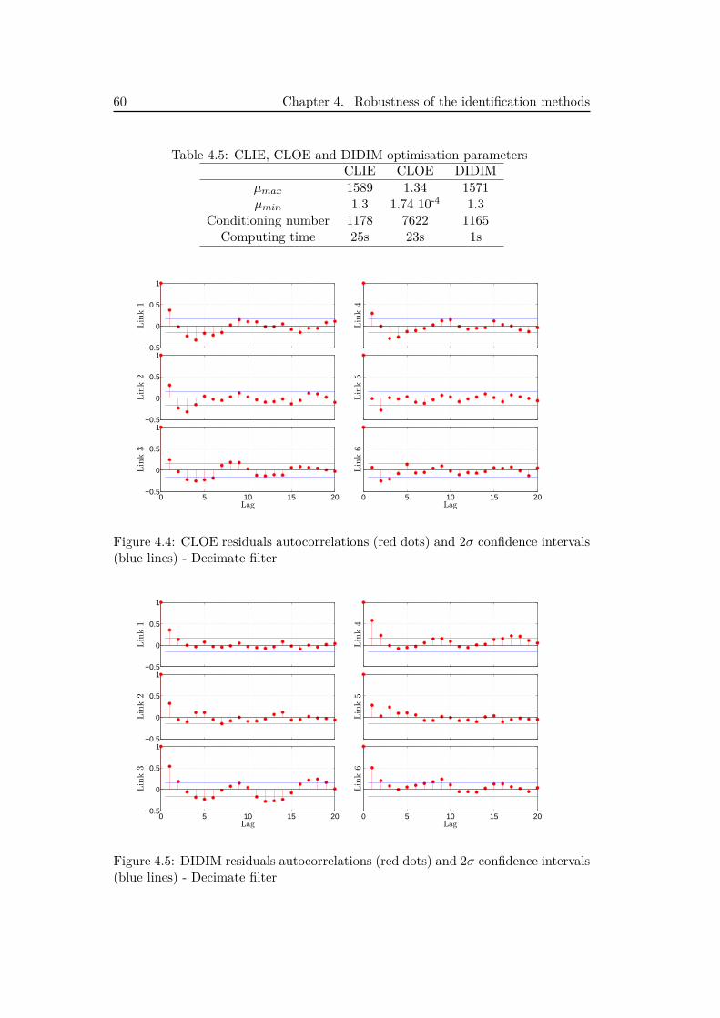
60 Chapter 4. Robustness of the identification methods
Table 4.5: CLIE, CLOE and DIDIM optimisation parametersCLIE CLOE DIDIM
µmax 1589 1.34 1571µmin 1.3 1.74 10-4 1.3
Conditioning number 1178 7622 1165Computing time 25s 23s 1s
−0.5
0
0.5
1
Link1
Link4
−0.5
0
0.5
1
Link2
Link5
0 5 10 15 20−0.5
0
0.5
1
Link3
Lag0 5 10 15 20
Link6
Lag
Figure 4.4: CLOE residuals autocorrelations (red dots) and 2σ confidence intervals(blue lines) - Decimate filter
−0.5
0
0.5
1
Link1
Link4
−0.5
0
0.5
1
Link2
Link5
0 5 10 15 20−0.5
0
0.5
1
Link3
Lag0 5 10 15 20
Link6
Lag
Figure 4.5: DIDIM residuals autocorrelations (red dots) and 2σ confidence intervals(blue lines) - Decimate filter
4.2. Robustness to modeling errors of the DIDIM and IDIM-IV methods 61
DIDIM method should be preferred to save computation time.
4.2 Robustness to modeling errors of the DIDIM andIDIM-IV methods
In the previous section, the interest of considering the input torque for the identifi-cation was demonstrated. Furthermore, it appeared that the DIDIM method is themost effective way of applying OEM to robot systems. This method, presented insection 2.3.4, is based on the simulation of the DDM and relies on the input torquelike the IDIM-IV method presented in section 2.3.3. In this section, we investigatethe relations between those methods.
4.2.1 Similarity between the methods
At first glance, by looking at the estimation formula (2.33) and (2.36), the IDIM-IV and the DIDIM methods are very similar. They indeed rely on the simulationof the DDM and their estimations are iterative. In practice, they use the sameconvergence criterion and the same initialisation, which is based on CAD values.
Assuming that there is no modelling error and that the IDM is well specified,we obtain
Z(θitDIDIM) = Z(θitIV ) = Xnf , (4.23)
where Xnf is the noise free component of the observation matrix X defined by(2.21). Equivalently, we have at each sampling time:
ζFp(t, θit
IV ) = ζFp(t, θit
DIDIM) = φnfFp (t),
where φnfFp is the noise free component of φFp . It is indeed assumed that thefiltered observation matrix can be divided such as φFp = φnfFp + φFp . The noise
free and noisy parts are uncorrelated, i.e. E[(φnfFp
)TφFp
]= 0, with E
[φFp
]= 0.
This assumption deserves some explanations that are provided in [Janot 2017] andrecalled here. The separation between a noise-free and a noisy component comesfrom the fact that the noise is mostly contained in the joint accelerations. As itis highlighted in section 6.1.2, due to the ISO standard, the output joint positionsand their measurements can be considered as noise-free
qm ≈ qnf . (4.24)
With nq, the position noise defined in (4.12), and Ts, the sampling time, the noisesintroduced with finite differences to joint velocities and accelerations are respec-tively nq/Ts and nq/T 2
s . In practice, the sampling frequency is greater than 100Hz. Therefore, the following relation can be expected:
nq/T2s nq/Ts nq.
62 Chapter 4. Robustness of the identification methods
This relation explains that the noises contained in the regressors linear with respectto the joint accelerations are dominant over those contained in the basis functionslinear with respect to the joint positions and velocities. For the basis functions thatare nonlinear combinations of joint positions and velocities, this requires furtherinvestigations. With respect to (2.3) and (2.4), it appears that the matrix M andthe vector Q contain sine and cosine basis functions of the position. Regarding(4.24), we obtain
cos (qm) ≈ cos(qnf
)and sin (qm) ≈ sin
(qnf
). (4.25)
Consequently, one has M (qm) ≈M(qnf
)and Q (qm) ≈ Q
(qnf
). The last non-
linearities to consider are included in the vector of centrifugal and Coriolis torques.According to Appendix A, only the joint velocities can be squared. For each jointj, we then have
q2mj =
(qnfj + nqj/Ts
)2= q2
nfj + nqj/Ts(nqj/Ts + 2qnfj
). (4.26)
Because the trajectories are sufficiently exciting, it can be stated qnfj nqj/Ts,which yields
q2mj ≈ q
2nfj + 2qnfjnqj/Ts ≈ qnfj
(qnfj + 2nqj/Ts
)≈ q2
nfj . (4.27)
That leads to the relation C(qm, qm) ≈ C(qnf , qnf )1. This reasoning proves thatthe division of the observation matrix in two parts is admissible.
Coming back to our comparison and assuming there are enough sampling points,i.e. N large enough, it comes out
E[(φnfFp
)TφFp
]≈ 1N
N∑i=1
(φnfFp (ti)
)TφFp(ti) (4.28)
and
θit+1IV =
[Z(θitIV )TX
]−1Z(θitIV )Ty(τ) (4.29)
= P−1φFp
[1N
N∑i=1ζTFp(ti, θ
it
IV )τFp(ti)]
≈ P−1φnfFp
[1N
N∑i=1
(φnfFp (ti)
)TτFp(ti)
]
=[XTnfXnf
]−1XTnfy(τ)
= θit+1DIDIM ,
1Exceptionally, the matrix C designates the centrifugal and Coriolis effects instead of the con-troller
4.2. Robustness to modeling errors of the DIDIM and IDIM-IV methods 63
with
PφFp= 1N
N∑i=1ζTFp(ti, θ
it
IV )φFp(ti)
= 1N
N∑i=1
(φnfFp (ti)
)T [φnfFp (ti) + φFp(ti)
]
≈ 1N
N∑i=1
(φnfFp (ti)
)TφnfFp (ti) = P
φnfFp.
Therefore, if there is no modelling error, the DIDIM and IDIM-IV methods areperfectly equivalent and unbiased. The unbiased property of the DIDIM estimatorwas originally shown in [Gautier et al. 2013a]. It is worth noting that the DIDIMestimation given by (2.36) is the IV solution raised in [Söderström & Stoica 1983]equation (3.43b) page 38. If we follow the authors’ point of view, the DIDIMapproach can be considered as a sort of bootstrap IV variant.
If there is a modelling error in the dynamic model of the robot arm, like a frictionmismatch, this error is present in the observation matrix and by construction inthe instrumental matrix. In this case, the DIDIM and IDIM-IV methods are alsoequivalent and biased.
4.2.2 Disparity between the methods
The difference between those methods lies in the use of the observation matrix, X,for the IDIM-IV method. That may be seen as a drawback since it requires themeasurement of the position signals, qm, and the careful bandpass filtering, detailedin section 2.3.1, in order to obtain the joint velocities and accelerations. As stressedin [Gautier et al. 2013a], the DIDIM method has the advantage of requiring onlythe measured torques.
However, the use of X can make the IDIM-IV method less sensitive to modellingerrors, in the simulation model, than the DIDIM method. We do not considermodelling errors in the dynamic model but in the rest of the closed-loop system;e.g. drive gains, bandwidth of the controller, etc. In fact, if we made an error in Z,that error would also be present in X due to the construction of the instrumentsand, consequently, both the IDIM-IV and DIDIM estimates would be biased. Inother words, we consider here that the simulator is biased but not X. The simulatorerror can be located in the controller used for the simulation for instance. If thereis such an error, the auxiliary model is biased and, therefore, also the simulatedsignals. Hence the assumption (4.23) does not hold and the simulation errors canbe introduced such as
ζFp(t, θit
IV ) = φnfFp (t) + ∆φitIV (t), (4.30)
ζFp(t, θit
DIDIM) = φnfFp (t) + ∆φitDIDIM(t).
64 Chapter 4. Robustness of the identification methods
Whatever the method used, one assumption can be made concerning the (n × n)simulation error matrix ∆φ: it is uncorrelated with the measurement noise, i.e.
E[(
∆φit)TφFp
]= 0 and E
[(∆φit
)TvFp
]= 0, (4.31)
with vFp the noisy component of τFp ; see (2.18). This assumption makes sensebecause the simulator is noise-free, as explained in section 2.3.3. From those defi-nitions, two cases can be considered according to ∆φ.
The first case is when expectation of the error is null:
E[∆φitIV
]= E
[∆φitDIDIM
]= 0.
Hence, it appears for IDIM-IV solution:
θit+1IV = P−1
φFp
[1N
N∑i=1
(φnfFp (ti) + ∆φitIV (ti)
)TτFp(ti)
](4.32)
≈ P−1φnfFp
[1N
N∑i=1
(φnfFp (ti)
)TτFp(ti)
]
=[XTnfXnf
]−1XTnfy(τ),
with
P φFp= 1N
N∑i=1
[φnfFp (ti) + ∆φitIV (ti)
]T [φnfFp (ti) + φFp(ti)
]
≈ 1N
N∑i=1
(φnfFp (ti)
)TφnfFp (ti) = P
φnfFp.
Concerning the DIDIM method, there is a persistent term
θit+1DIDIM ≈
(PnfφFp
+ ∆P)−1
[1N
N∑i=1
(φnfFp (ti)
)TτFp(ti)
](4.33)
=[XTnfXnf +N ·∆P
]−1XTnfy(τ),
with
∆P = 1N
N∑i=1
(∆φitDIDIM(ti)
)T∆φitDIDIM(ti).
Equation (4.32) shows that the IDIM-IV method is robust against a modelling errorlocated in the simulator with a null expected value. In the opposite, (4.33) showsthat the DIDIM method is sensitive to such an error and its estimates are biased.
The second case is when the simulation error has a non zero expectation, i.e.E[∆φitIV
]6= 0 and E
[∆φitDIDIM
]6= 0. In this case, both methods are biased and so
are the estimated parameters.
4.2. Robustness to modeling errors of the DIDIM and IDIM-IV methods 65
4.2.3 Experimental validations
In a first time, we illustrate the behaviour of the methods in the nominal case. Thatis to say that the auxiliary model is error-free. This auxiliary model is composed ofthe robot dynamic model, the actual controller, the gains of the actuators and thegear ratios. The DDM is simulated thanks to a SimulinkR© model integrated with theode3 solver. The methods are initialized with acceptable CAD values; see Table 4.4.The essential estimated parameters and relative standard deviation are summarizedin Table 4.6. The IDIM-IV and the DIDIM methods respectively converged in 3and 7 iterations. As expected, both methods estimate equivalent parameters withcomparable standard deviations. That is confirmed by the satisfactory relativeerrors provided in Table 4.7. Furthermore, the estimated values are consistent withprevious work on this robot arm; see Table 4.4. Those observations are consistentwith the work of [Gautier et al. 2013a] and [Janot et al. 2014c]: the IDIM-IV andthe DIDIM methods are appropriate to identify industrial robots.
In a second time, we highlight the difference between the IDIM-IV and DIDIMmethods. Thus, an error is introduced in the auxiliary model: the gear ratios aretaken equal to 80% of their actual values. Table 4.6 summarizes the estimatedparameters and the relative standard deviations. The IDIM-IV and the DIDIMmethods respectively converged in 3 and 7 iterations. At a first glance, looking atTable 4.7, the difference is not so significant. With a closer scrutiny, it appearsthat the inertia parameters are poorly estimated with the DIDIM method, likezz1r , zz2r or ia3 for instance. Compared with the parameters previously estimated,there is a gap of almost 20 %. On the other hand, the IDIM-IV estimates are stillconsistent. However, the relative standard deviations seem a little optimistic, seethe same parameters as previously. This can be explained by the calculation of theestimated parameters covariance matrix, which relies on the assumption that theinstrumental matrix is an estimation of the noise free observation matrix; see e.g.[Young 2011] equation (7.31) page 211. In fact, the exact covariance matrix for theIV estimate is obtained as:
Σ(θIV
)= 1NP−1φFp
[1N
N∑i=1ζTFp(ti, θIV )Λ−1
τ (ti)ζFp(ti, θIV )]P−1φFp
, (4.34)
with
P φFp= 1N
N∑i=1ζTFp(ti, θIV )φFp(ti)
and Λτ is the error covariance matrix defined in (2.25). Usually, assumption (4.23)
66 Chapter 4. Robustness of the identification methods
holds and it comes out:
Σ(θIV
)= 1N
[1N
N∑i=1
(φnfFp (ti)
)TΛ−1τ (ti)φnfFp (ti)
]−1
(4.35)
= 1N
[1N
N∑i=1ζTFp(ti, θIV )Λ−1
τ (ti)ζFp(ti, θIV )]−1
.
Equation (4.35) significantly simplifies the computation of the covariance. Inpractice, this approximate formula is used for the IDIM-IV method; see (2.34).Nonetheless, by using the approximate relation and although E
[∆φitIV
]= 0, we
introduced a persistent error:
1N
[1N
N∑i=1
(ζFp(ti, θIV ) + ∆φIV (ti)
)TΛ−1τ (ti)
(ζFp(ti, θIV ) + ∆φIV (ti)
)]−1
6= 1N
[1N
N∑i=1
(φnfFp (ti)
)TΛ−1τ (ti)φnfFp (ti)
]−1
= Σ(θIV
)(4.36)
Therefore, the approximate covariance should not be used if there is a risk of mod-elling error in the simulator. This practical example illustrates the impact of abiased simulator on the estimation when the simulation error has a zero expecta-tion. In this case, we have illustrated a better robustness of the IDIM-IV methodcompared with the DIDIM one.
4.3 Miscellaneous remarks
4.3.1 Closed-loop aspects of the robot identifications methods
In the previous sections, we considered different methods for robot identification:the CLOE, CLIE, DIDIM and IDIM-IV methods. Like the usual IDIM-LS methoddescribed in section 2.3.2, those methods do not fall within the definitions of theclosed-loop approaches given in section 3.1. The open-loop parameters are in-deed identified directly from the measured data. There is no identification of thewhole closed-loop model (indirect approach) or of an augmented system (joint input-output approach). Nevertheless, they do not belong to direct approach neither sincethe controller is taken into account for the simulation of the DDM, in the case ofthe OEM and the IDIM-IV method, and to tune the filters, for all the methods in-cluding the IDIM-LS one. This may explain why the robot identification methodsand especially the IDIM-LS one are not well perceived by the automatic controlcommunity.
4.3.2 Considerations on the robot identification with OEM
In section 4.1, we considered three pseudo-OEM for robot identification: the CLOE,CLIE and DIDIM methods. They are qualified as pseudo-OEM because they need
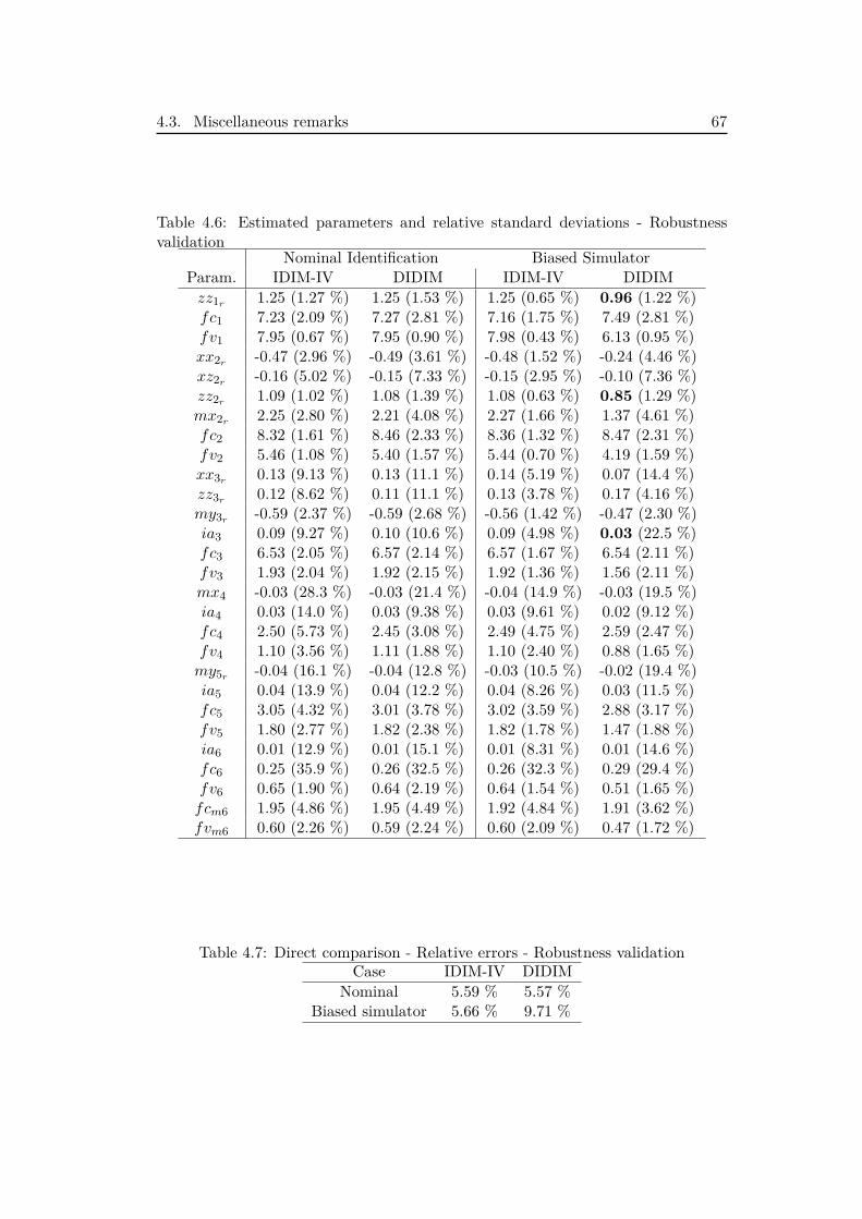
4.3. Miscellaneous remarks 67
Table 4.6: Estimated parameters and relative standard deviations - Robustnessvalidation
Nominal Identification Biased SimulatorParam. IDIM-IV DIDIM IDIM-IV DIDIMzz1r 1.25 (1.27 %) 1.25 (1.53 %) 1.25 (0.65 %) 0.96 (1.22 %)fc1 7.23 (2.09 %) 7.27 (2.81 %) 7.16 (1.75 %) 7.49 (2.81 %)fv1 7.95 (0.67 %) 7.95 (0.90 %) 7.98 (0.43 %) 6.13 (0.95 %)xx2r -0.47 (2.96 %) -0.49 (3.61 %) -0.48 (1.52 %) -0.24 (4.46 %)xz2r -0.16 (5.02 %) -0.15 (7.33 %) -0.15 (2.95 %) -0.10 (7.36 %)zz2r 1.09 (1.02 %) 1.08 (1.39 %) 1.08 (0.63 %) 0.85 (1.29 %)mx2r 2.25 (2.80 %) 2.21 (4.08 %) 2.27 (1.66 %) 1.37 (4.61 %)fc2 8.32 (1.61 %) 8.46 (2.33 %) 8.36 (1.32 %) 8.47 (2.31 %)fv2 5.46 (1.08 %) 5.40 (1.57 %) 5.44 (0.70 %) 4.19 (1.59 %)xx3r 0.13 (9.13 %) 0.13 (11.1 %) 0.14 (5.19 %) 0.07 (14.4 %)zz3r 0.12 (8.62 %) 0.11 (11.1 %) 0.13 (3.78 %) 0.17 (4.16 %)my3r -0.59 (2.37 %) -0.59 (2.68 %) -0.56 (1.42 %) -0.47 (2.30 %)ia3 0.09 (9.27 %) 0.10 (10.6 %) 0.09 (4.98 %) 0.03 (22.5 %)fc3 6.53 (2.05 %) 6.57 (2.14 %) 6.57 (1.67 %) 6.54 (2.11 %)fv3 1.93 (2.04 %) 1.92 (2.15 %) 1.92 (1.36 %) 1.56 (2.11 %)mx4 -0.03 (28.3 %) -0.03 (21.4 %) -0.04 (14.9 %) -0.03 (19.5 %)ia4 0.03 (14.0 %) 0.03 (9.38 %) 0.03 (9.61 %) 0.02 (9.12 %)fc4 2.50 (5.73 %) 2.45 (3.08 %) 2.49 (4.75 %) 2.59 (2.47 %)fv4 1.10 (3.56 %) 1.11 (1.88 %) 1.10 (2.40 %) 0.88 (1.65 %)my5r -0.04 (16.1 %) -0.04 (12.8 %) -0.03 (10.5 %) -0.02 (19.4 %)ia5 0.04 (13.9 %) 0.04 (12.2 %) 0.04 (8.26 %) 0.03 (11.5 %)fc5 3.05 (4.32 %) 3.01 (3.78 %) 3.02 (3.59 %) 2.88 (3.17 %)fv5 1.80 (2.77 %) 1.82 (2.38 %) 1.82 (1.78 %) 1.47 (1.88 %)ia6 0.01 (12.9 %) 0.01 (15.1 %) 0.01 (8.31 %) 0.01 (14.6 %)fc6 0.25 (35.9 %) 0.26 (32.5 %) 0.26 (32.3 %) 0.29 (29.4 %)fv6 0.65 (1.90 %) 0.64 (2.19 %) 0.64 (1.54 %) 0.51 (1.65 %)fcm6 1.95 (4.86 %) 1.95 (4.49 %) 1.92 (4.84 %) 1.91 (3.62 %)fvm6 0.60 (2.26 %) 0.59 (2.24 %) 0.60 (2.09 %) 0.47 (1.72 %)
Table 4.7: Direct comparison - Relative errors - Robustness validationCase IDIM-IV DIDIM
Nominal 5.59 % 5.57 %Biased simulator 5.66 % 9.71 %
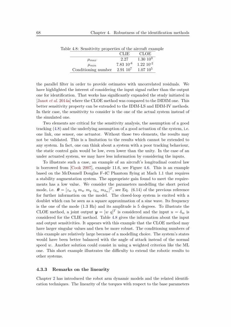
68 Chapter 4. Robustness of the identification methods
Table 4.8: Sensitivity properties of the aircraft exampleCLIE CLOE
µmax 2.27 1.30 103
µmin 7.83 10-8 1.22 10-2
Conditioning number 2.91 107 1.07 105
the parallel filter in order to provide estimates with uncorrelated residuals. Wehave highlighted the interest of considering the input signal rather than the outputone for identification. That works has significantly expanded the study initiated in[Janot et al. 2014a] where the CLOE method was compared to the DIDIM one. Thisbetter sensitivity property can be extended to the IDIM-LS and IDIM-IV methods.In their case, the sensitivity to consider is the one of the actual system instead ofthe simulated one.
Two elements are critical for the sensitivity analysis, the assumption of a goodtracking (4.8) and the underlying assumption of a good actuation of the system, i.e.one link, one sensor, one actuator. Without those two elements, the results maynot be validated. This is a limitation to the results which cannot be extended toany system. In fact, one can think about a system with a poor tracking behaviour,the static control gain would be low, even lower than the unity. In the case of anunder actuated system, we may have less information by considering the inputs.
To illustrate such a case, an example of an aircraft’s longitudinal control lawis borrowed from [Cook 2007], example 11.6, see Figure 4.6. This is an examplebased on the McDonnell Douglas F-4C Phantom flying at Mach 1.1 that requiresa stability augmentation system. The appropriate gain found to meet the require-ments has a low value. We consider the parameters modelling the short periodmode, i.e. θ = [zw zq mw mq zδm mδm ]T , see Eq. (6.14) of the previous referencefor further information on the model. The closed-loop system is excited with adoublet which can be seen as a square approximation of a sine wave. Its frequencyis the one of the mode (1.3 Hz) and its amplitude is 5 degrees. To illustrate theCLOE method, a joint output y = [w q]T is considered and the input u = δm isconsidered for the CLIE method. Table 4.8 gives the information about the inputand output sensitivities. It appears with this example that the CLOE method mayhave larger singular values and then be more robust. The conditioning numbers ofthis example are relatively large because of a modelling choice. The system’s stateswould have been better balanced with the angle of attack instead of the normalspeed w. Another solution could consist in using a weighted criterion like the MLone. This short example illustrates the difficulty to extend the robotic results toother systems.
4.3.3 Remarks on the linearity
Chapter 2 has introduced the robot arm dynamic models and the related identifi-cation techniques. The linearity of the torques with respect to the base parameters
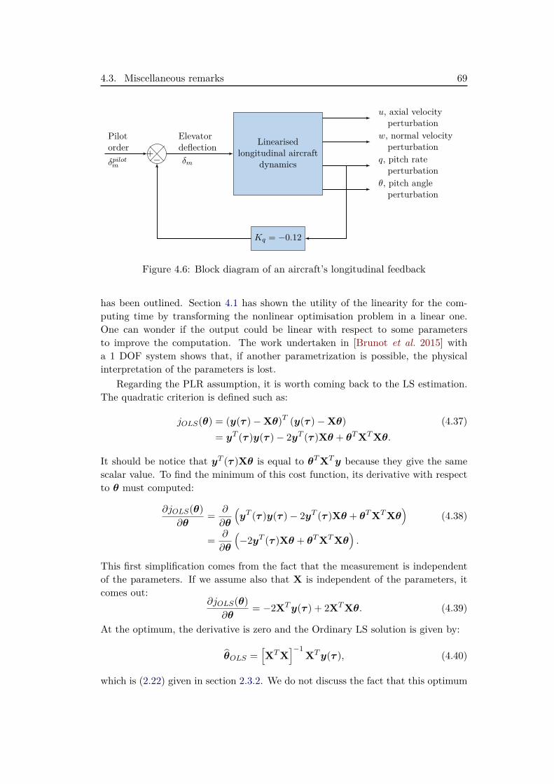
4.3. Miscellaneous remarks 69
−+
Linearisedlongitudinal aircraft
dynamics
Kq = −0.12
u, axial velocityperturbation
w, normal velocityperturbation
q, pitch rateperturbation
θ, pitch angleperturbation
Pilotorderδpilotm
Elevatordeflectionδm
Figure 4.6: Block diagram of an aircraft’s longitudinal feedback
has been outlined. Section 4.1 has shown the utility of the linearity for the com-puting time by transforming the nonlinear optimisation problem in a linear one.One can wonder if the output could be linear with respect to some parametersto improve the computation. The work undertaken in [Brunot et al. 2015] witha 1 DOF system shows that, if another parametrization is possible, the physicalinterpretation of the parameters is lost.
Regarding the PLR assumption, it is worth coming back to the LS estimation.The quadratic criterion is defined such as:
jOLS(θ) = (y(τ )−Xθ)T (y(τ )−Xθ) (4.37)= yT (τ )y(τ )− 2yT (τ )Xθ + θTXTXθ.
It should be notice that yT (τ )Xθ is equal to θTXTy because they give the samescalar value. To find the minimum of this cost function, its derivative with respectto θ must computed:
∂jOLS(θ)∂θ
= ∂
∂θ
(yT (τ )y(τ )− 2yT (τ )Xθ + θTXTXθ
)(4.38)
= ∂
∂θ
(−2yT (τ )Xθ + θTXTXθ
).
This first simplification comes from the fact that the measurement is independentof the parameters. If we assume also that X is independent of the parameters, itcomes out:
∂jOLS(θ)∂θ
= −2XTy(τ ) + 2XTXθ. (4.39)
At the optimum, the derivative is zero and the Ordinary LS solution is given by:
θOLS =[XTX
]−1XTy(τ ), (4.40)
which is (2.22) given in section 2.3.2. We do not discuss the fact that this optimum
70 Chapter 4. Robustness of the identification methods
is a minimum and not a maximum. It thus appears that the IDIM-LS methodimplicitly relies on the PLR assumption. Otherwise the derivative of X with respectto θ would not be zero and the estimate would be different.
4.4 Conclusions
This chapter has been dedicated to evaluate the robustness of the methods intro-duced in Chapter 2 and, more specifically, the robustness of the methods relyingon the simulation of the auxiliary model. In a first time, it has been shown thatit is more appropriate to consider the input torque for robot identification, even inan OEM framework. The CLIE method is indeed more robust to modelling errorsthanks to its better sensitivity. Even though, in the ideal case where there is nomodelling error, it produces as accurate estimates as the CLOE method. If the PLRassumption is met, the DIDIM method should be employed to save computationtime. The experimental results have highlighted that, if it is possible to obtainconsistent estimates in a strict OEM framework, the decimate filter is required toprovide a consistent estimate of the covariances.
In second time, we have shown that the IDIM-IV method can be more robustthan the DIDIM method, although they are really similar. The IDIM-IV methodcan indeed tolerate some error in the auxiliary model as long as the expected valueof the resulting error in the IDM is null. If the error is located directly in the IDM,both methods are identically biased.
All the identification methods need a priori knowledge concerning the system.For instance, the IDIM-IV requires the system’s bandwidth to tune the bandpassfilter. That knowledge is also needed by the DIDIM and the IDIM-IV methods inorder to set the cut-off frequency of the decimate filter. Furthermore, the actualcontroller is needed to simulate the auxiliary model. In the next chapter, effortsare ongoing to reduce the dependency to a priori knowledge.
Chapter 5
Robot system identificationwithout the knowledge of thecontroller and the bandwidths
In the previous chapter, the robustness of the IDIM-IV and DIDIM methods hasbeen investigated. It appeared that those methods rely on a careful prefilteringmethodology which requires the knowledge of the bandwidths. Furthermore, theyneed the knowledge of the controller for the simulation of their auxiliary model.That may be an issue if the robot system has a proprietary controller. It emergeshere an usual dilemma of system identification: to identify a system correctly,we need a good knowledge of this system. In this chapter, the robot identificationmethodologies are revisited in order to avoid a priori knowledge as much as possible.This work is a new way of dealing with robot identification that has been presentedin [Brunot et al. 2017b] as well as in [Brunot et al. In Press 2017].
The chapter is organised as follows. The derivatives estimation is studied insection 5.1. Then, the issue of an unknown controller is stated in section 5.2. Theselected approaches are then applied on the TX40 example in section 5.3 beforeconcluding in section 5.4 on future perspectives for the developed methodologies.
5.1 Joint derivatives estimation . . . . . . . . . . . . . . . . . . . 725.1.1 Derivatives estimation from noisy signals . . . . . . . . . . . 725.1.2 Integrative random walk smoother . . . . . . . . . . . . . . . 735.1.3 Application to robot identification . . . . . . . . . . . . . . . 765.1.4 Numerical differentiation tests . . . . . . . . . . . . . . . . . 80
5.2 Controller identification . . . . . . . . . . . . . . . . . . . . . 815.2.1 Closed-loop system identification with an unknown controller 815.2.2 Controller parametric identification . . . . . . . . . . . . . . . 835.2.3 Controller non-parametric identification . . . . . . . . . . . . 83
5.3 Experimental validation . . . . . . . . . . . . . . . . . . . . . 855.3.1 The IDIM-LS method with the IRWSM technique . . . . . . 855.3.2 The IDIM-IV method with the IRWSM technique . . . . . . 875.3.3 The IDIM-IV method with an unknown controller . . . . . . 90
5.4 Conclusions . . . . . . . . . . . . . . . . . . . . . . . . . . . . . 94
72 Chapter 5. Identification with unknown controller and bandwidths
5.1 Joint derivatives estimation
5.1.1 Derivatives estimation from noisy signals
Many researches are ongoing concerning the numerical differentiation issue, see e.g.[Diop et al. 1994, Vasiljevic & Khalil 2006, Dridi 2011, Sidhom 2011] and the refer-ences given therein. Some of them are summarized here to have an overview of thepossibilities. Nonetheless, the goal is here to suggest a practical and straightforwardtechnique. The idea is to find a solution that requires neither a priori knowledgeof the system nor a complex computational process.
The issue of estimating unknown system states is not recent for the automaticcontrol community. It has been indeed the subject of a long-established literatureabout observers. The goal is to provide the signals derivatives to the controller inorder to reduce the number of required sensors. The problem has been introducedby Luenberger [Luenberger 1971]. In the case of a noisy signal, a stochastic observerlike the Kalman one may be more appropriate; see e.g. [Singer 1970]. There is alsoa large and active research on nonlinear observers; see e.g. [Dabroom & Khalil 1997,Besançon 2007]. For example, the Extended Kalman Filter (EKF) can be consideredto estimate the states of a nonlinear stochastic system, like in [Ljung 1979]. Whetherthe observer is deterministic or stochastic, it relies on the model of the consideredsystem. In other words, the observer needs the system’s model and its parametersto provide unbiased estimations of the derivatives. Therefore, an observer doesnot appear as a solution to estimate the joint derivatives in order to estimate thedynamic parameters. Although a solution could consist in estimating the states andthe parameters at the same time in a similar manner to [Gautier & Poignet 2001],a less complex solution is sought. In fact, we do not want such a solution in orderto avoid coupling effects.
Another approach consists in relying on the signals only and not on the model.It is then more appropriate to talk about differentiator. The usual bandpass filterbelongs to this approach; see section 2.3.1. Another method is based on the poly-nomial interpolation of the signal over a sliding window; see e.g. section 11.2.2 of[Klein & Morelli 2006]. The signal derivative is approximated by the derivative ofthe polynomial.
It exists also the algebraic differentiators which have been recently revisited; seee.g. [Fliess & Sira-Ramírez 2003]. The idea is to estimate the signal derivativesthanks to successive integrations of the measured signal. It is based on a truncatedTaylor expansion of the signal. Thus, the practitioner has to provide the order ofthe truncation. Since the excitation trajectories used for robot identification arenot really smooth, the required order of the truncation can be large.
Another family of techniques is based on the sliding mode theory introducedduring the 1960s [Filippov 1960]. Among the developed techniques, we can mentionthe Super Twisting algorithm introduced in [Levant 1998]. Without going through
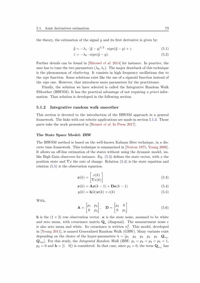
5.1. Joint derivatives estimation 73
the theory, the estimation of the signal y and its first derivative is given by:
˙y = −λ1 · |y − y|1/2 · sign(y − y) + z (5.1)z = −λ0 · sign(y − y). (5.2)
Further details can be found in [Shtessel et al. 2014] for instance. In practice, theuser has to tune the two parameters (λ0, λ1). The major drawback of this techniqueis the phenomenon of chattering. It consists in high frequency oscillations due tothe sign function. Some solutions exist like the use of a sigmoid function instead ofthe sign one. However, that introduces more parameters for the practitioner.
Finally, the solution we have selected is called the Integrative Random WalkSMoother (IRWSM). It has the practical advantage of not requiring a priori infor-mation. That solution is developed in the following section.
5.1.2 Integrative random walk smoother
This section is devoted to the introduction of the IRWSM approach in a generalframework. The links with our robotic applications are made in section 5.1.3. Thoseparts take the work presented in [Brunot et al. In Press 2017].
The State Space Model: IRW
The IRWSM method is based on the well-known Kalman filter technique, in a dis-crete time framework. This technique is summarized in [Norton 1975, Young 2000].It allows an off-line estimation of the states without using the dynamic model, un-like High Gain observers for instance. Eq. (5.3) defines the state vector, with x theposition state and ∇x the rate of change. Relation (5.4) is the state equation andrelation (5.5) is the observation equation.
x(k) =[x(k)∇x(k)
](5.3)
x(k) = Ax(k − 1) + Dκ(k − 1) (5.4)y(k) = h(k)x(k) + e(k) (5.5)
With,
A =[p1 p20 p3
], D =
[p4 00 p5
](5.6)
h is the (1 × 2) row observation vector. κ is the state noise, assumed to be whiteand zero mean, with covariance matrix Qκ (diagonal). The measurement noise eis also zero mean and white. Its covariance is written σ2
e . This model, developedin [Young 2011], is named Generalized Random Walk (GRW). Many variants existdepending on the choice of the hyper-parameters γ = [p1 p2 p3 p4 p5 Qκ11
Qκ22 ]. For this study, the Integrated Random Walk (IRW: p1 = p2 = p3 = p5 = 1,p4 = 0 and h = [1 0]) is considered. In that case, since p4 = 0, the term Qκ11 has
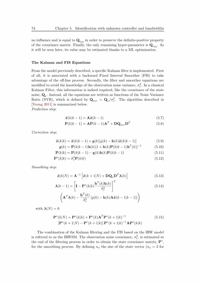
74 Chapter 5. Identification with unknown controller and bandwidths
no influence and is equal to Qκ22 in order to preserve the definite-positive propertyof the covariance matrix. Finally, the only remaining hyper-parameter is Qκ22 . Asit will be seen later, its value may be estimated thanks to a ML optimization.
The Kalman and FIS Equations
From the model previously described, a specific Kalman filter is implemented. Firstof all, it is associated with a backward Fixed Interval Smoother (FIS) to takeadvantage of the off-line process. Secondly, the filter and smoother equations aremodified to avoid the knowledge of the observation noise variance, σ2
e . In a classicalKalman Filter, this information is indeed required, like the covariance of the statenoise, Qκ. Instead, all the equations are written as functions of the Noise VarianceRatio (NVR), which is defined by Qnvr = Qκ/σ
2e . The algorithm described in
[Young 2011] is summarized below.Prediction step:
x(k|k − 1) = Ax(k − 1) (5.7)P(k|k − 1) = AP(k − 1)AT + DQnvrDT (5.8)
Correction step:
x(k|k) = x(k|k − 1) + g(k)[y(k)− h(k)x(k|k − 1)] (5.9)g(k) = P(k|k − 1)h(k)[1 + h(k)P(k|k − 1)hT (k)]−1 (5.10)
P(k|k) = P(k|k − 1)− g(k)h(k)P(k|k − 1) (5.11)P∗(k|k) = σ2
eP(k|k) (5.12)
Smoothing step:
x(k|N) = A−1[x(k + 1|N) + DQκDTλ(k)
](5.13)
λ(k − 1) =[I−P∗(k|k)hT (k)h(k)
σ2e
]T(5.14)(
ATλ(k)− hT (k)σ2e
[y(k)− h(k)Ax(k − 1|k − 1)])
with λ(N) = 0
P∗(k|N) = P∗(k|k) + P∗(k)ATP∗(k + 1|k)−1 (5.15)[P∗(k + 1|N)−P∗(k + 1|k)] P∗(k + 1|k)−1AP∗(k|k)
The combination of the Kalman filtering and the FIS based on the IRW modelis referred to as the IRWSM. The observation noise covariance, σ2
e , is estimated atthe end of the filtering process in order to obtain the state covariance matrix, P∗,for the smoothing process. By defining nx the size of the state vector (nx = 2 for
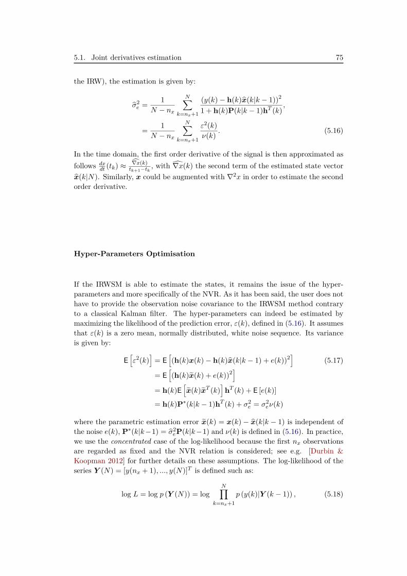
5.1. Joint derivatives estimation 75
the IRW), the estimation is given by:
σ2e = 1
N − nx
N∑k=nx+1
(y(k)− h(k)x(k|k − 1))2
1 + h(k)P(k|k − 1)hT (k),
= 1N − nx
N∑k=nx+1
ε2(k)ν(k) . (5.16)
In the time domain, the first order derivative of the signal is then approximated asfollows dx
dt (tk) ≈∇x(k)tk+1−tk , with ∇x(k) the second term of the estimated state vector
x(k|N). Similarly, x could be augmented with ∇2x in order to estimate the secondorder derivative.
Hyper-Parameters Optimisation
If the IRWSM is able to estimate the states, it remains the issue of the hyper-parameters and more specifically of the NVR. As it has been said, the user does nothave to provide the observation noise covariance to the IRWSM method contraryto a classical Kalman filter. The hyper-parameters can indeed be estimated bymaximizing the likelihood of the prediction error, ε(k), defined in (5.16). It assumesthat ε(k) is a zero mean, normally distributed, white noise sequence. Its varianceis given by:
E[ε2(k)
]= E
[(h(k)x(k)− h(k)x(k|k − 1) + e(k))2
](5.17)
= E[(h(k)x(k) + e(k))2
]= h(k)E
[x(k)xT (k)
]hT (k) + E [e(k)]
= h(k)P∗(k|k − 1)hT (k) + σ2e = σ2
eν(k)
where the parametric estimation error x(k) = x(k)− x(k|k − 1) is independent ofthe noise e(k), P∗(k|k−1) = σ2
eP(k|k−1) and ν(k) is defined in (5.16). In practice,we use the concentrated case of the log-likelihood because the first nx observationsare regarded as fixed and the NVR relation is considered; see e.g. [Durbin &Koopman 2012] for further details on these assumptions. The log-likelihood of theseries Y (N) = [y(nx + 1), ..., y(N)]T is defined such as:
log L = log p (Y (N)) = logN∏
k=nx+1p (y(k)|Y (k − 1)) , (5.18)
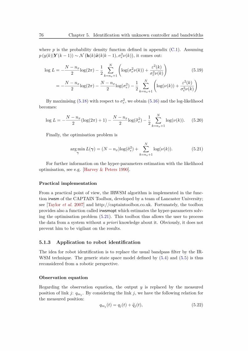
76 Chapter 5. Identification with unknown controller and bandwidths
where p is the probability density function defined in appendix (C.1). Assumingp (y(k)|Y (k − 1)) ∼ N
(h(k)x(k|k − 1), σ2
eν(k)), it comes out:
log L = −N − nx2 log(2π)− 12
N∑k=nx+1
(log(σ2
eν(k)) + ε2(k)σ2eν(k)
)(5.19)
= −N − nx2 log(2π)− N − nx2 log(σ2
e)−12
N∑k=nx+1
(log(ν(k)) + ε2(k)
σ2eν(k)
)
By maximising (5.18) with respect to σ2e , we obtain (5.16) and the log-likelihood
becomes:
log L = −N − nx2 (log(2π) + 1)− N − nx2 log(σ2
e)−12
N∑k=nx+1
log(ν(k)). (5.20)
Finally, the optimisation problem is
arg minγ
L(γ) = (N − nx)log(σ2e) +
N∑k=nx+1
log(ν(k)). (5.21)
For further information on the hyper-parameters estimation with the likelihoodoptimisation, see e.g. [Harvey & Peters 1990].
Practical implementation
From a practical point of view, the IRWSM algorithm is implemented in the func-tion irwsm of the CAPTAIN Toolbox, developed by a team of Lancaster University;see [Taylor et al. 2007] and http://captaintoolbox.co.uk. Fortunately, the toolboxprovides also a function called irwsmopt which estimates the hyper-parameters solv-ing the optimisation problem (5.21). This toolbox thus allows the user to processthe data from a system without a priori knowledge about it. Obviously, it does notprevent him to be vigilant on the results.
5.1.3 Application to robot identification
The idea for robot identification is to replace the usual bandpass filter by the IR-WSM technique. The generic state space model defined by (5.4) and (5.5) is thusreconsidered from a robotic perspective.
Observation equation
Regarding the observation equation, the output y is replaced by the measuredposition of link j: qmj . By considering the link j, we have the following relation forthe measured position:
qmj (t) = qj(t) + qj(t), (5.22)
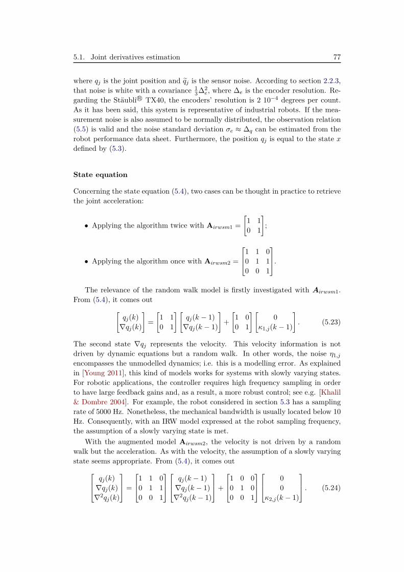
5.1. Joint derivatives estimation 77
where qj is the joint position and qj is the sensor noise. According to section 2.2.3,that noise is white with a covariance 1
3∆2e, where ∆e is the encoder resolution. Re-
garding the StäubliR© TX40, the encoders’ resolution is 2 10−4 degrees per count.As it has been said, this system is representative of industrial robots. If the mea-surement noise is also assumed to be normally distributed, the observation relation(5.5) is valid and the noise standard deviation σe ≈ ∆q can be estimated from therobot performance data sheet. Furthermore, the position qj is equal to the state xdefined by (5.3).
State equation
Concerning the state equation (5.4), two cases can be thought in practice to retrievethe joint acceleration:
• Applying the algorithm twice with Airwsm1 =[1 10 1
];
• Applying the algorithm once with Airwsm2 =
1 1 00 1 10 0 1
.The relevance of the random walk model is firstly investigated with Airwsm1.
From (5.4), it comes out[qj(k)∇qj(k)
]=[1 10 1
] [qj(k − 1)∇qj(k − 1)
]+[1 00 1
] [0
κ1,j(k − 1)
]. (5.23)
The second state ∇qj represents the velocity. This velocity information is notdriven by dynamic equations but a random walk. In other words, the noise η1,jencompasses the unmodelled dynamics; i.e. this is a modelling error. As explainedin [Young 2011], this kind of models works for systems with slowly varying states.For robotic applications, the controller requires high frequency sampling in orderto have large feedback gains and, as a result, a more robust control; see e.g. [Khalil& Dombre 2004]. For example, the robot considered in section 5.3 has a samplingrate of 5000 Hz. Nonetheless, the mechanical bandwidth is usually located below 10Hz. Consequently, with an IRW model expressed at the robot sampling frequency,the assumption of a slowly varying state is met.
With the augmented model Airwsm2, the velocity is not driven by a randomwalk but the acceleration. As with the velocity, the assumption of a slowly varyingstate seems appropriate. From (5.4), it comes out qj(k)
∇qj(k)∇2qj(k)
=
1 1 00 1 10 0 1
qj(k − 1)∇qj(k − 1)∇2qj(k − 1)
+
1 0 00 1 00 0 1
0
0κ2,j(k − 1)
. (5.24)
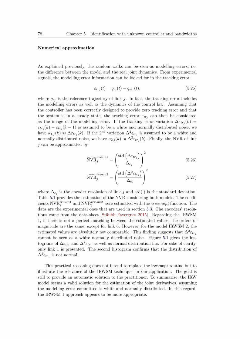
78 Chapter 5. Identification with unknown controller and bandwidths
Numerical approximation
As explained previously, the random walks can be seen as modelling errors; i.e.the difference between the model and the real joint dynamics. From experimentalsignals, the modelling error information can be looked for in the tracking error:
εtrj (t) = qrj (t)− qmj (t), (5.25)
where qrj is the reference trajectory of link j. In fact, the tracking error includesthe modelling errors as well as the dynamics of the control law. Assuming thatthe controller has been correctly designed to provide zero tracking error and thatthe system is in a steady state, the tracking error εtrj can then be consideredas the image of the modelling error. If the tracking error variation ∆εtrj (k) =εtrj (k) − εtrj (k − 1) is assumed to be a white and normally distributed noise, wehave κ1,j(k) ≈ ∆εtrj (k). If the 2nd variation ∆2εtrj is assumed to be a white andnormally distributed noise, we have κ2,j(k) ≈ ∆2εtrj (k). Finally, the NVR of linkj can be approximated by
NVRirwsm1j =
std(∆εtrj
)∆ej
2
(5.26)
NVRirwsm2j =
std(∆2εtrj
)∆ej
2
(5.27)
where ∆ej is the encoder resolution of link j and std(·) is the standard deviation.Table 5.1 provides the estimation of the NVR considering both models. The coeffi-cients NVRirwsm1
j and NVRirwsm2j were estimated with the irwsmopt function. The
data are the experimental ones that are used in section 5.3. The encoders’ resolu-tions come from the data-sheet [Stäubli Favergues 2015]. Regarding the IRWSM1, if there is not a perfect matching between the estimated values, the orders ofmagnitude are the same; except for link 6. However, for the model IRWSM 2, theestimated values are absolutely not comparable. This finding suggests that ∆2εtrjcannot be seen as a white normally distributed noise. Figure 5.1 gives the his-tograms of ∆εtr1 and ∆2εtr1 as well as normal distribution fits. For sake of clarity,only link 1 is presented. The second histogram confirms that the distribution of∆2εtr1 is not normal.
This practical reasoning does not intend to replace the irwsmopt routine but toillustrate the relevance of the IRWSM technique for our application. The goal isstill to provide an automatic solution to the practitioner. To summarize, the IRWmodel seems a valid solution for the estimation of the joint derivatives, assumingthe modelling error committed is white and normally distributed. In this regard,the IRWSM 1 approach appears to be more appropriate.
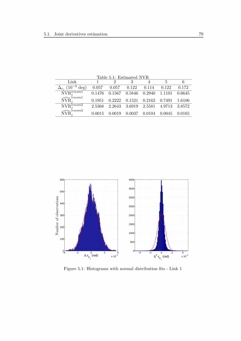
5.1. Joint derivatives estimation 79
Table 5.1: Estimated NVRLink 1 2 3 4 5 6
∆ej (10−3 deg) 0.057 0.057 0.122 0.114 0.122 0.172NVRirwsm1
j 0.1476 0.1567 0.5846 0.2940 1.1101 0.6645NVR
irwsm1j 0.1951 0.2222 0.1521 0.2162 0.7491 1.6106
NVRirwsm2j 2.5368 2.2643 3.6919 2.5581 4.9713 3.8572
NVRirwsm2j 0.0015 0.0019 0.0037 0.0104 0.0045 0.0165
−4 −2 0 2 4
x 10−5
0
100
200
300
400
500
600
∆ εtr
1
(rad)
Number
ofob
servations
−4 −2 0 2 4
x 10−6
0
500
1000
1500
2000
2500
3000
3500
4000
∆2 εtr
1
(rad)
Figure 5.1: Histograms with normal distribution fits - Link 1
80 Chapter 5. Identification with unknown controller and bandwidths
5.1.4 Numerical differentiation tests
In [Brunot et al. 2016b], the use of the IRWSM to differentiate the position signal ofthe rigid 1 DOF Electro-Mechanical Positioning System (EMPS) is studied. Thatis a robotic system simpler than the TX40. We recall here briefly its model toevaluate the differentiation with the IRWSM technique. The EMPS is modelled by
τ(t) = Mq(t) + Fv q(t) + Fcsign(q(t)), (5.28)
where M is the inertia of the arm; Fv and Fc are respectively the viscous andCoulomb friction coefficients; q, q and q are respectively the position, velocity andacceleration; τ is the motor force. The system is driven by a nested PD controllersuch as
τ(t) = gfkv (kp (qr(t)− q(t))− q(t)) , (5.29)
where qr is the reference trajectory and gf is the electronic gain of the actuator.In practice, the controller gains have been chosen kp = 160.2 1/s and kv = 242.5V.s/m. The actuator gain has previously been identified to 35.2 N/V.
The study is done thanks to simulated data. The values of parameters are chosenclose to those which have previously been estimated for other works: M = 96.0kg, Fv = 205.0 N/(m/s) and Fc = 20.0 N. A measurement noise is added to thesimulated output. To be realistic, the Signal to Noise Ratio (SNR) is taken equal to100 dB; see section 6.1.2 for further justification. Monte Carlo Simulations (MCS)are run to evaluate the effect of this noise over the estimates.
From the noisy position signal generated by the simulator, three methods arecompared. The first one is the standard bandpass filter introduced in section 2.3.1and will be named by "Bandpass". The second method is the IRWSM implementedin the CAPTAIN Toolbox with the model Airwsm1 and will be referred as "IRWSM1". The last one is a variant of the IRWSM with Airwsm2, which allows estimatingdirectly the second derivative without calling the algorithm twice. This approachwill be named "IRWSM 2". Concerning the bandpass method, from previous works,it is known that the highest mode frequency is about 20 Hz. It should be noticedthat this relation requires knowing the controller parameters and structure. TheButterworth filter is designed with a cut-off frequency equal to 40 Hz (i.e. twicethe highest natural mode). To get the acceleration, its order is fixed at 2+2=4.
Table 5.2 summarizes the results by providing the mean of the 100 relativeerrors for each estimate. The relative error of the signal s(t) is given by 100 ·‖snf − s‖ / ‖snf‖, where snf (t) is the noise free component of s(t) generated bythe simulator. IRWSM 1 and 2 give very good results for the velocity and theacceleration, since the relative errors are very small and less than those of thebandpass approach. The methods seem to be equivalently effective in order toestimate the position.
This simple example tends to show the IRWSM technique is appropriate todifferentiate signals from a robotic system. To go further, in section 5.3, we con-sider the TX40 and investigate the identification with the IDIM-LS and IDIM-IV
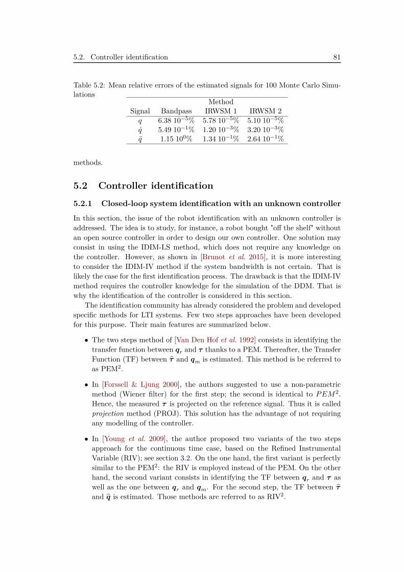
5.2. Controller identification 81
Table 5.2: Mean relative errors of the estimated signals for 100 Monte Carlo Simu-lations
MethodSignal Bandpass IRWSM 1 IRWSM 2q 6.38 10−5% 5.78 10−5% 5.10 10−5%q 5.49 10−1% 1.20 10−3% 3.20 10−3%q 1.15 100% 1.34 10−1% 2.64 10−1%
methods.
5.2 Controller identification
5.2.1 Closed-loop system identification with an unknown controller
In this section, the issue of the robot identification with an unknown controller isaddressed. The idea is to study, for instance, a robot bought "off the shelf" withoutan open source controller in order to design our own controller. One solution mayconsist in using the IDIM-LS method, which does not require any knowledge onthe controller. However, as shown in [Brunot et al. 2015], it is more interestingto consider the IDIM-IV method if the system bandwidth is not certain. That islikely the case for the first identification process. The drawback is that the IDIM-IVmethod requires the controller knowledge for the simulation of the DDM. That iswhy the identification of the controller is considered in this section.
The identification community has already considered the problem and developedspecific methods for LTI systems. Few two steps approaches have been developedfor this purpose. Their main features are summarized below.
• The two steps method of [Van Den Hof et al. 1992] consists in identifying thetransfer function between qr and τ thanks to a PEM. Thereafter, the TransferFunction (TF) between τ and qm is estimated. This method is be referred toas PEM2.
• In [Forssell & Ljung 2000], the authors suggested to use a non-parametricmethod (Wiener filter) for the first step; the second is identical to PEM2.Hence, the measured τ is projected on the reference signal. Thus it is calledprojection method (PROJ). This solution has the advantage of not requiringany modelling of the controller.
• In [Young et al. 2009], the author proposed two variants of the two stepsapproach for the continuous time case, based on the Refined InstrumentalVariable (RIV); see section 3.2. On the one hand, the first variant is perfectlysimilar to the PEM2: the RIV is employed instead of the PEM. On the otherhand, the second variant consists in identifying the TF between qr and τ aswell as the one between qr and qm. For the second step, the TF between τand q is estimated. Those methods are referred to as RIV2.
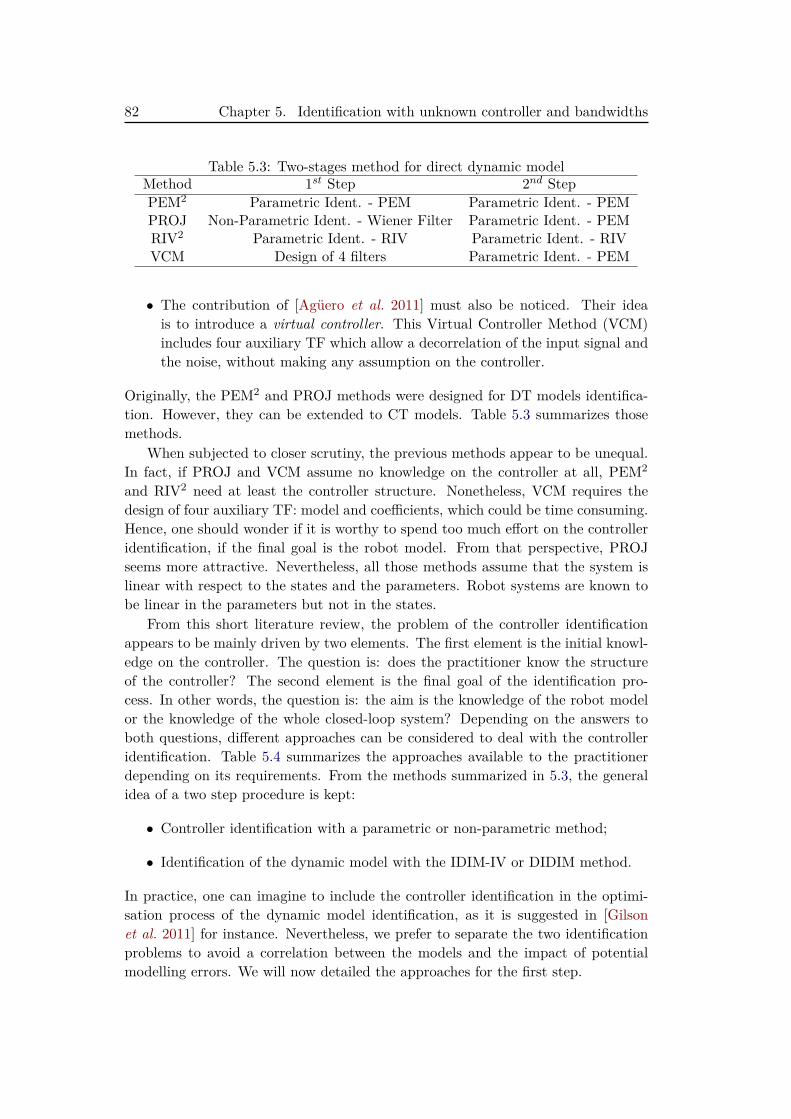
82 Chapter 5. Identification with unknown controller and bandwidths
Table 5.3: Two-stages method for direct dynamic modelMethod 1st Step 2nd StepPEM2 Parametric Ident. - PEM Parametric Ident. - PEMPROJ Non-Parametric Ident. - Wiener Filter Parametric Ident. - PEMRIV2 Parametric Ident. - RIV Parametric Ident. - RIVVCM Design of 4 filters Parametric Ident. - PEM
• The contribution of [Agüero et al. 2011] must also be noticed. Their ideais to introduce a virtual controller. This Virtual Controller Method (VCM)includes four auxiliary TF which allow a decorrelation of the input signal andthe noise, without making any assumption on the controller.
Originally, the PEM2 and PROJ methods were designed for DT models identifica-tion. However, they can be extended to CT models. Table 5.3 summarizes thosemethods.
When subjected to closer scrutiny, the previous methods appear to be unequal.In fact, if PROJ and VCM assume no knowledge on the controller at all, PEM2
and RIV2 need at least the controller structure. Nonetheless, VCM requires thedesign of four auxiliary TF: model and coefficients, which could be time consuming.Hence, one should wonder if it is worthy to spend too much effort on the controlleridentification, if the final goal is the robot model. From that perspective, PROJseems more attractive. Nevertheless, all those methods assume that the system islinear with respect to the states and the parameters. Robot systems are known tobe linear in the parameters but not in the states.
From this short literature review, the problem of the controller identificationappears to be mainly driven by two elements. The first element is the initial knowl-edge on the controller. The question is: does the practitioner know the structureof the controller? The second element is the final goal of the identification pro-cess. In other words, the question is: the aim is the knowledge of the robot modelor the knowledge of the whole closed-loop system? Depending on the answers toboth questions, different approaches can be considered to deal with the controlleridentification. Table 5.4 summarizes the approaches available to the practitionerdepending on its requirements. From the methods summarized in 5.3, the generalidea of a two step procedure is kept:
• Controller identification with a parametric or non-parametric method;
• Identification of the dynamic model with the IDIM-IV or DIDIM method.
In practice, one can imagine to include the controller identification in the optimi-sation process of the dynamic model identification, as it is suggested in [Gilsonet al. 2011] for instance. Nevertheless, we prefer to separate the two identificationproblems to avoid a correlation between the models and the impact of potentialmodelling errors. We will now detailed the approaches for the first step.
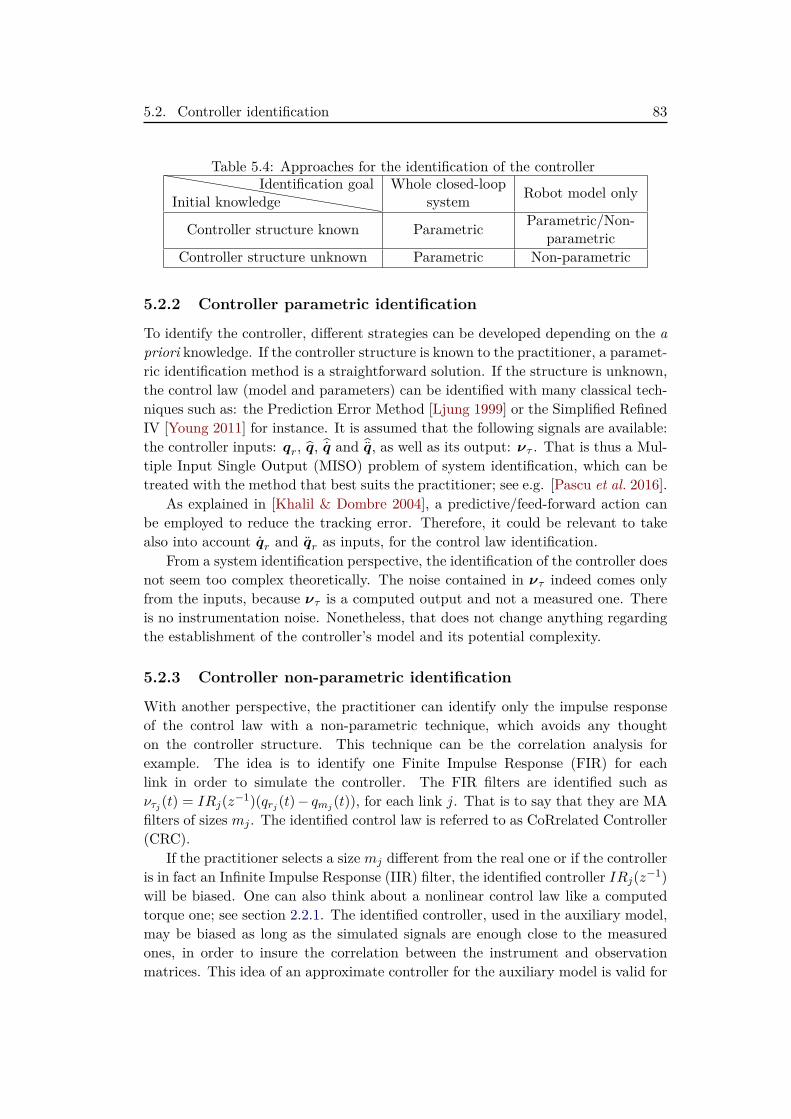
5.2. Controller identification 83
Table 5.4: Approaches for the identification of the controller
Initial knowledgeIdentification goal Whole closed-loop
system Robot model only
Controller structure known Parametric Parametric/Non-parametric
Controller structure unknown Parametric Non-parametric
5.2.2 Controller parametric identification
To identify the controller, different strategies can be developed depending on the apriori knowledge. If the controller structure is known to the practitioner, a paramet-ric identification method is a straightforward solution. If the structure is unknown,the control law (model and parameters) can be identified with many classical tech-niques such as: the Prediction Error Method [Ljung 1999] or the Simplified RefinedIV [Young 2011] for instance. It is assumed that the following signals are available:the controller inputs: qr, q, q and q, as well as its output: ντ . That is thus a Mul-tiple Input Single Output (MISO) problem of system identification, which can betreated with the method that best suits the practitioner; see e.g. [Pascu et al. 2016].
As explained in [Khalil & Dombre 2004], a predictive/feed-forward action canbe employed to reduce the tracking error. Therefore, it could be relevant to takealso into account qr and qr as inputs, for the control law identification.
From a system identification perspective, the identification of the controller doesnot seem too complex theoretically. The noise contained in ντ indeed comes onlyfrom the inputs, because ντ is a computed output and not a measured one. Thereis no instrumentation noise. Nonetheless, that does not change anything regardingthe establishment of the controller’s model and its potential complexity.
5.2.3 Controller non-parametric identification
With another perspective, the practitioner can identify only the impulse responseof the control law with a non-parametric technique, which avoids any thoughton the controller structure. This technique can be the correlation analysis forexample. The idea is to identify one Finite Impulse Response (FIR) for eachlink in order to simulate the controller. The FIR filters are identified such asντj (t) = IRj(z−1)(qrj (t)− qmj (t)), for each link j. That is to say that they are MAfilters of sizes mj . The identified control law is referred to as CoRrelated Controller(CRC).
If the practitioner selects a size mj different from the real one or if the controlleris in fact an Infinite Impulse Response (IIR) filter, the identified controller IRj(z−1)will be biased. One can also think about a nonlinear control law like a computedtorque one; see section 2.2.1. The identified controller, used in the auxiliary model,may be biased as long as the simulated signals are enough close to the measuredones, in order to insure the correlation between the instrument and observationmatrices. This idea of an approximate controller for the auxiliary model is valid for
84 Chapter 5. Identification with unknown controller and bandwidths
the IDIM-IV method but not for the DIDIM one. In fact, as it has been explainedin section 4.2.2, the IDIM-IV method can provide efficient estimates while havingan error in the auxiliary model.
If the correlation analysis is thoroughly developed in Chapter 3 of [Söderström& Stoica 1988] for instance, we summarize here the main features of this method.The form of the DT model used is:
ντj (ti) =∞∑k=0
hj(k)εtrj (ti − k ·∆t) + εd(ti) (5.30)
where εtrj (t) = qrj (t)− qmj (t),hj(k)
is a weighting sequence and εd is a distur-
bance not correlated with the input εtrj . Hence, it comes out:
Rjντ εtr(τd) = E[ντj (t+ τd)εtrj (t)] (5.31)
=∞∑k=0
hj(k)E[εtrj (t+ τd − k · Ts)εtrj (t)]
=∞∑k=0
hj(k)Rjεtrεtr(τd − k · Ts),
with τd the discrete time lag. With the estimated correlations and a truncated filterresponse at order mj , we have the following relation:
Rjντ εtr(τd) =mj−1∑k=0
hj(k)Rjεtrεtr(τd − k · Ts). (5.32)
Writing the previous equation for τd = 0, ..., (mj−1) ·Ts, we obtain a linear systemof mj equations with mj unknowns IRj =
hj(k)
mj−1k=0 . In practice, the algorithm
can be implemented as follows:
(1) Identify an AR filter based on the input signal εtrj , see section 6.1.3;
(2) Filter the input and the output by the inverse of the identified AR filter tohave εftrj and ν
fτj ;
(3) Estimate the correlation Rjντ εtr and Rjεtrεtr from the filtered signals: εftrj andνfτj ;
(4) Solve the linear system defined by (5.32).
This algorithm includes in addition an AR filter to prewhiten the data in accordancewith the corresponding Matlab R© function named cra which come from the techniquedeveloped in section 11.2 of [Box & Jenkins 1976].
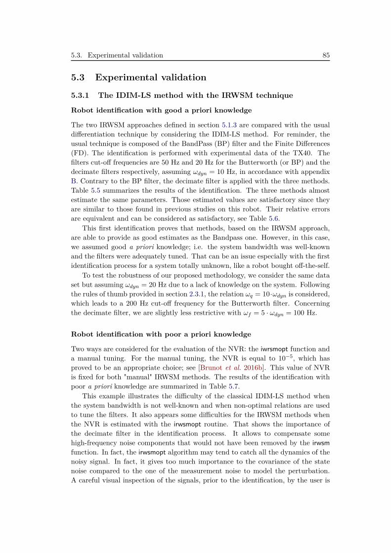
5.3. Experimental validation 85
5.3 Experimental validation
5.3.1 The IDIM-LS method with the IRWSM technique
Robot identification with good a priori knowledge
The two IRWSM approaches defined in section 5.1.3 are compared with the usualdifferentiation technique by considering the IDIM-LS method. For reminder, theusual technique is composed of the BandPass (BP) filter and the Finite Differences(FD). The identification is performed with experimental data of the TX40. Thefilters cut-off frequencies are 50 Hz and 20 Hz for the Butterworth (or BP) and thedecimate filters respectively, assuming ωdyn = 10 Hz, in accordance with appendixB. Contrary to the BP filter, the decimate filter is applied with the three methods.Table 5.5 summarizes the results of the identification. The three methods almostestimate the same parameters. Those estimated values are satisfactory since theyare similar to those found in previous studies on this robot. Their relative errorsare equivalent and can be considered as satisfactory, see Table 5.6.
This first identification proves that methods, based on the IRWSM approach,are able to provide as good estimates as the Bandpass one. However, in this case,we assumed good a priori knowledge; i.e. the system bandwidth was well-knownand the filters were adequately tuned. That can be an issue especially with the firstidentification process for a system totally unknown, like a robot bought off-the-self.
To test the robustness of our proposed methodology, we consider the same dataset but assuming ωdyn = 20 Hz due to a lack of knowledge on the system. Followingthe rules of thumb provided in section 2.3.1, the relation ωq = 10·ωdyn is considered,which leads to a 200 Hz cut-off frequency for the Butterworth filter. Concerningthe decimate filter, we are slightly less restrictive with ωf = 5 · ωdyn = 100 Hz.
Robot identification with poor a priori knowledge
Two ways are considered for the evaluation of the NVR: the iwrsmopt function anda manual tuning. For the manual tuning, the NVR is equal to 10−5, which hasproved to be an appropriate choice; see [Brunot et al. 2016b]. This value of NVRis fixed for both "manual" IRWSM methods. The results of the identification withpoor a priori knowledge are summarized in Table 5.7.
This example illustrates the difficulty of the classical IDIM-LS method whenthe system bandwidth is not well-known and when non-optimal relations are usedto tune the filters. It also appears some difficulties for the IRWSM methods whenthe NVR is estimated with the irwsmopt routine. That shows the importance ofthe decimate filter in the identification process. It allows to compensate somehigh-frequency noise components that would not have been removed by the irwsmfunction. In fact, the irwsmopt algorithm may tend to catch all the dynamics of thenoisy signal. In fact, it gives too much importance to the covariance of the statenoise compared to the one of the measurement noise to model the perturbation.A careful visual inspection of the signals, prior to the identification, by the user is
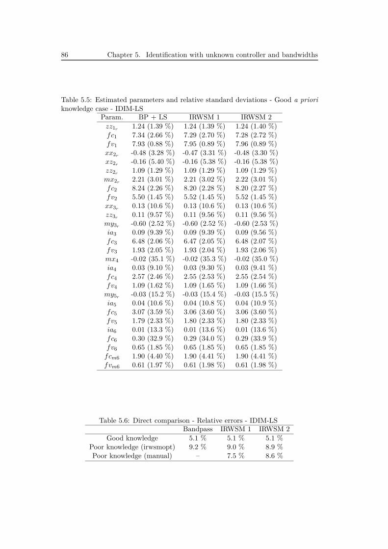
86 Chapter 5. Identification with unknown controller and bandwidths
Table 5.5: Estimated parameters and relative standard deviations - Good a prioriknowledge case - IDIM-LS
Param. BP + LS IRWSM 1 IRWSM 2zz1r 1.24 (1.39 %) 1.24 (1.39 %) 1.24 (1.40 %)fc1 7.34 (2.66 %) 7.29 (2.70 %) 7.28 (2.72 %)fv1 7.93 (0.88 %) 7.95 (0.89 %) 7.96 (0.89 %)xx2r -0.48 (3.28 %) -0.47 (3.31 %) -0.48 (3.30 %)xz2r -0.16 (5.40 %) -0.16 (5.38 %) -0.16 (5.38 %)zz2r 1.09 (1.29 %) 1.09 (1.29 %) 1.09 (1.29 %)mx2r 2.21 (3.01 %) 2.21 (3.02 %) 2.22 (3.01 %)fc2 8.24 (2.26 %) 8.20 (2.28 %) 8.20 (2.27 %)fv2 5.50 (1.45 %) 5.52 (1.45 %) 5.52 (1.45 %)xx3r 0.13 (10.6 %) 0.13 (10.6 %) 0.13 (10.6 %)zz3r 0.11 (9.57 %) 0.11 (9.56 %) 0.11 (9.56 %)my3r -0.60 (2.52 %) -0.60 (2.52 %) -0.60 (2.53 %)ia3 0.09 (9.39 %) 0.09 (9.39 %) 0.09 (9.56 %)fc3 6.48 (2.06 %) 6.47 (2.05 %) 6.48 (2.07 %)fv3 1.93 (2.05 %) 1.93 (2.04 %) 1.93 (2.06 %)mx4 -0.02 (35.1 %) -0.02 (35.3 %) -0.02 (35.0 %)ia4 0.03 (9.10 %) 0.03 (9.30 %) 0.03 (9.41 %)fc4 2.57 (2.46 %) 2.55 (2.53 %) 2.55 (2.54 %)fv4 1.09 (1.62 %) 1.09 (1.65 %) 1.09 (1.66 %)my5r -0.03 (15.2 %) -0.03 (15.4 %) -0.03 (15.5 %)ia5 0.04 (10.6 %) 0.04 (10.8 %) 0.04 (10.9 %)fc5 3.07 (3.59 %) 3.06 (3.60 %) 3.06 (3.60 %)fv5 1.79 (2.33 %) 1.80 (2.33 %) 1.80 (2.33 %)ia6 0.01 (13.3 %) 0.01 (13.6 %) 0.01 (13.6 %)fc6 0.30 (32.9 %) 0.29 (34.0 %) 0.29 (33.9 %)fv6 0.65 (1.85 %) 0.65 (1.85 %) 0.65 (1.85 %)fcm6 1.90 (4.40 %) 1.90 (4.41 %) 1.90 (4.41 %)fvm6 0.61 (1.97 %) 0.61 (1.98 %) 0.61 (1.98 %)
Table 5.6: Direct comparison - Relative errors - IDIM-LSBandpass IRWSM 1 IRWSM 2
Good knowledge 5.1 % 5.1 % 5.1 %Poor knowledge (irwsmopt) 9.2 % 9.0 % 8.9 %Poor knowledge (manual) – 7.5 % 8.6 %
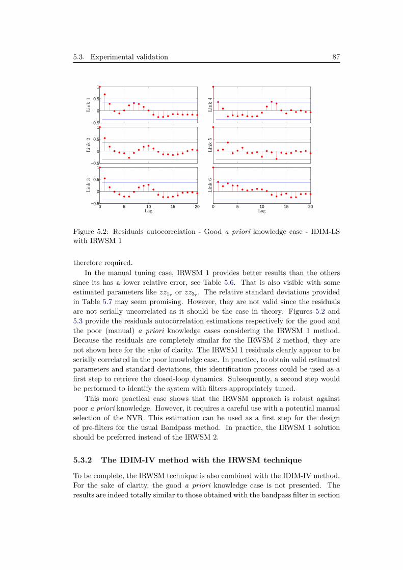
5.3. Experimental validation 87
−0.5
0
0.5
1Link1
Link4
−0.5
0
0.5
1
Link2
Link5
0 5 10 15 20−0.5
0
0.5
1
Link3
Lag0 5 10 15 20
Link6
Lag
Figure 5.2: Residuals autocorrelation - Good a priori knowledge case - IDIM-LSwith IRWSM 1
therefore required.In the manual tuning case, IRWSM 1 provides better results than the others
since its has a lower relative error, see Table 5.6. That is also visible with someestimated parameters like zz1r or zz3r . The relative standard deviations providedin Table 5.7 may seem promising. However, they are not valid since the residualsare not serially uncorrelated as it should be the case in theory. Figures 5.2 and5.3 provide the residuals autocorrelation estimations respectively for the good andthe poor (manual) a priori knowledge cases considering the IRWSM 1 method.Because the residuals are completely similar for the IRWSM 2 method, they arenot shown here for the sake of clarity. The IRWSM 1 residuals clearly appear to beserially correlated in the poor knowledge case. In practice, to obtain valid estimatedparameters and standard deviations, this identification process could be used as afirst step to retrieve the closed-loop dynamics. Subsequently, a second step wouldbe performed to identify the system with filters appropriately tuned.
This more practical case shows that the IRWSM approach is robust againstpoor a priori knowledge. However, it requires a careful use with a potential manualselection of the NVR. This estimation can be used as a first step for the designof pre-filters for the usual Bandpass method. In practice, the IRWSM 1 solutionshould be preferred instead of the IRWSM 2.
5.3.2 The IDIM-IV method with the IRWSM technique
To be complete, the IRWSM technique is also combined with the IDIM-IV method.For the sake of clarity, the good a priori knowledge case is not presented. Theresults are indeed totally similar to those obtained with the bandpass filter in section
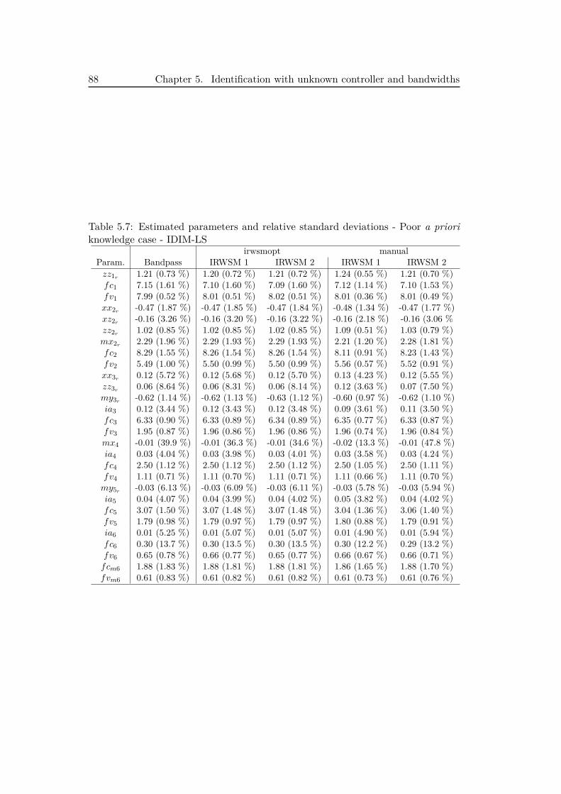
88 Chapter 5. Identification with unknown controller and bandwidths
Table 5.7: Estimated parameters and relative standard deviations - Poor a prioriknowledge case - IDIM-LS
irwsmopt manualParam. Bandpass IRWSM 1 IRWSM 2 IRWSM 1 IRWSM 2zz1r 1.21 (0.73 %) 1.20 (0.72 %) 1.21 (0.72 %) 1.24 (0.55 %) 1.21 (0.70 %)fc1 7.15 (1.61 %) 7.10 (1.60 %) 7.09 (1.60 %) 7.12 (1.14 %) 7.10 (1.53 %)fv1 7.99 (0.52 %) 8.01 (0.51 %) 8.02 (0.51 %) 8.01 (0.36 %) 8.01 (0.49 %)xx2r -0.47 (1.87 %) -0.47 (1.85 %) -0.47 (1.84 %) -0.48 (1.34 %) -0.47 (1.77 %)xz2r -0.16 (3.26 %) -0.16 (3.20 %) -0.16 (3.22 %) -0.16 (2.18 %) -0.16 (3.06 %zz2r 1.02 (0.85 %) 1.02 (0.85 %) 1.02 (0.85 %) 1.09 (0.51 %) 1.03 (0.79 %)mx2r 2.29 (1.96 %) 2.29 (1.93 %) 2.29 (1.93 %) 2.21 (1.20 %) 2.28 (1.81 %)fc2 8.29 (1.55 %) 8.26 (1.54 %) 8.26 (1.54 %) 8.11 (0.91 %) 8.23 (1.43 %)fv2 5.49 (1.00 %) 5.50 (0.99 %) 5.50 (0.99 %) 5.56 (0.57 %) 5.52 (0.91 %)xx3r 0.12 (5.72 %) 0.12 (5.68 %) 0.12 (5.70 %) 0.13 (4.23 %) 0.12 (5.55 %)zz3r 0.06 (8.64 %) 0.06 (8.31 %) 0.06 (8.14 %) 0.12 (3.63 %) 0.07 (7.50 %)my3r -0.62 (1.14 %) -0.62 (1.13 %) -0.63 (1.12 %) -0.60 (0.97 %) -0.62 (1.10 %)ia3 0.12 (3.44 %) 0.12 (3.43 %) 0.12 (3.48 %) 0.09 (3.61 %) 0.11 (3.50 %)fc3 6.33 (0.90 %) 6.33 (0.89 %) 6.34 (0.89 %) 6.35 (0.77 %) 6.33 (0.87 %)fv3 1.95 (0.87 %) 1.96 (0.86 %) 1.96 (0.86 %) 1.96 (0.74 %) 1.96 (0.84 %)mx4 -0.01 (39.9 %) -0.01 (36.3 %) -0.01 (34.6 %) -0.02 (13.3 %) -0.01 (47.8 %)ia4 0.03 (4.04 %) 0.03 (3.98 %) 0.03 (4.01 %) 0.03 (3.58 %) 0.03 (4.24 %)fc4 2.50 (1.12 %) 2.50 (1.12 %) 2.50 (1.12 %) 2.50 (1.05 %) 2.50 (1.11 %)fv4 1.11 (0.71 %) 1.11 (0.70 %) 1.11 (0.71 %) 1.11 (0.66 %) 1.11 (0.70 %)my5r -0.03 (6.13 %) -0.03 (6.09 %) -0.03 (6.11 %) -0.03 (5.78 %) -0.03 (5.94 %)ia5 0.04 (4.07 %) 0.04 (3.99 %) 0.04 (4.02 %) 0.05 (3.82 %) 0.04 (4.02 %)fc5 3.07 (1.50 %) 3.07 (1.48 %) 3.07 (1.48 %) 3.04 (1.36 %) 3.06 (1.40 %)fv5 1.79 (0.98 %) 1.79 (0.97 %) 1.79 (0.97 %) 1.80 (0.88 %) 1.79 (0.91 %)ia6 0.01 (5.25 %) 0.01 (5.07 %) 0.01 (5.07 %) 0.01 (4.90 %) 0.01 (5.94 %)fc6 0.30 (13.7 %) 0.30 (13.5 %) 0.30 (13.5 %) 0.30 (12.2 %) 0.29 (13.2 %)fv6 0.65 (0.78 %) 0.66 (0.77 %) 0.65 (0.77 %) 0.66 (0.67 %) 0.66 (0.71 %)fcm6 1.88 (1.83 %) 1.88 (1.81 %) 1.88 (1.81 %) 1.86 (1.65 %) 1.88 (1.70 %)fvm6 0.61 (0.83 %) 0.61 (0.82 %) 0.61 (0.82 %) 0.61 (0.73 %) 0.61 (0.76 %)
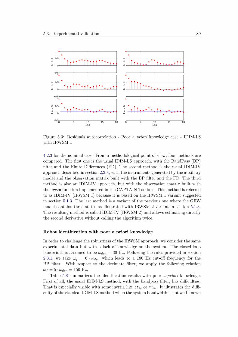
5.3. Experimental validation 89
−0.5
0
0.5
1Link1
Link4
−0.5
0
0.5
1
Link2
Link5
0 5 10 15 20−0.5
0
0.5
1
Link3
Lag0 5 10 15 20
Link6
Lag
Figure 5.3: Residuals autocorrelation - Poor a priori knowledge case - IDIM-LSwith IRWSM 1
4.2.3 for the nominal case. From a methodological point of view, four methods arecompared. The first one is the usual IDIM-LS approach, with the BandPass (BP)filter and the Finite Differences (FD). The second method is the usual IDIM-IVapproach described in section 2.3.3, with the instruments generated by the auxiliarymodel and the observation matrix built with the BP filter and the FD. The thirdmethod is also an IDIM-IV approach, but with the observation matrix built withthe irwsm function implemented in the CAPTAIN Toolbox. This method is referredto as IDIM-IV (IRWSM 1) because it is based on the IRWSM 1 variant suggestedin section 5.1.3. The last method is a variant of the previous one where the GRWmodel contains three states as illustrated with IRWSM 2 variant in section 5.1.3.The resulting method is called IDIM-IV (IRWSM 2) and allows estimating directlythe second derivative without calling the algorithm twice.
Robot identification with poor a priori knowledge
In order to challenge the robustness of the IRWSM approach, we consider the sameexperimental data but with a lack of knowledge on the system. The closed-loopbandwidth is assumed to be ωdyn = 30 Hz. Following the rules provided in section2.3.1, we take ωq = 6 · ωdyn which leads to a 180 Hz cut-off frequency for theBP filter. With respect to the decimate filter, we apply the following relationωf = 5 · ωdyn = 150 Hz.
Table 5.8 summarizes the identification results with poor a priori knowledge.First of all, the usual IDIM-LS method, with the bandpass filter, has difficulties.That is especially visible with some inertia like zz1r or zz3r . It illustrates the diffi-culty of the classical IDIM-LS method when the system bandwidth is not well-known
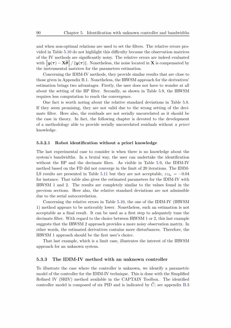
90 Chapter 5. Identification with unknown controller and bandwidths
and when non-optimal relations are used to set the filters. The relative errors pro-vided in Table 5.10 do not highlight this difficulty because the observation matricesof the IV methods are significantly noisy. The relative errors are indeed evaluatedwith
∥∥∥y(τ )−Xθ∥∥∥ / ‖y(τ )‖. Nonetheless, the noise located in X is compensated by
the instrumental matrices for the parameters estimation.Concerning the IDIM-IV methods, they provide similar results that are close to
those given in Appendix B.1. Nonetheless, the IRWSM approach for the derivatives’estimation brings two advantages. Firstly, the user does not have to wonder at allabout the setting of the BP filter. Secondly, as shown in Table 5.9, the IRWSMrequires less computation to reach the convergence.
One fact is worth noting about the relative standard deviations in Table 5.8.If they seem promising, they are not valid due to the wrong setting of the deci-mate filter. Here also, the residuals are not serially uncorrelated as it should bethe case in theory. In fact, the following chapter is devoted to the developmentof a methodology able to provide serially uncorrelated residuals without a prioriknowledge.
5.3.2.1 Robot identification without a priori knowledge
The last experimental case to consider is when there is no knowledge about thesystem’s bandwidths. In a brutal way, the user can undertake the identificationwithout the BP and the decimate filers. As visible in Table 5.9, the IDIM-IVmethod based on the FD did not converge in the limit of 20 iterations. The IDIM-LS results are presented in Table 5.11 but they are not acceptable, zz3r = −0.04for instance. That table also gives the estimated parameters for the IDIM-IV withIRWSM 1 and 2. The results are completely similar to the values found in theprevious sections. Here also, the relative standard deviations are not admissibledue to the serial autocorrelation.
Concerning the relative errors in Table 5.10, the one of the IDIM-IV (IRWSM1) method appears to be noticeably lower. Nonetheless, such an estimation is notacceptable as a final result. It can be used as a first step to adequately tune thedecimate filter. With regard to the choice between IRWSM 1 or 2, this last examplesuggests that the IRWSM 2 approach provides a more noisy observation matrix. Inother words, the estimated derivatives contains more disturbances. Therefore, theIRWSM 1 approach should be the first user’s choice.
That last example, which is a limit case, illustrates the interest of the IRWSMapproach for an unknown system.
5.3.3 The IDIM-IV method with an unknown controller
To illustrate the case where the controller is unknown, we identify a parametricmodel of the controller for the IDIM-IV technique. This is done with the SimplifiedRefined IV (SRIV) method available in the CAPTAIN Toolbox. The identifiedcontroller model is composed of six PID and is indicated by C; see appendix B.3
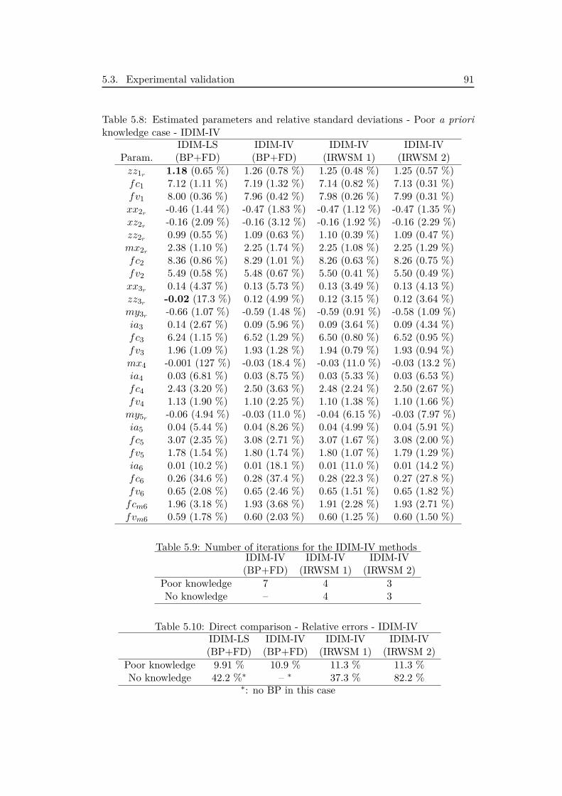
5.3. Experimental validation 91
Table 5.8: Estimated parameters and relative standard deviations - Poor a prioriknowledge case - IDIM-IV
IDIM-LS IDIM-IV IDIM-IV IDIM-IVParam. (BP+FD) (BP+FD) (IRWSM 1) (IRWSM 2)zz1r 1.18 (0.65 %) 1.26 (0.78 %) 1.25 (0.48 %) 1.25 (0.57 %)fc1 7.12 (1.11 %) 7.19 (1.32 %) 7.14 (0.82 %) 7.13 (0.31 %)fv1 8.00 (0.36 %) 7.96 (0.42 %) 7.98 (0.26 %) 7.99 (0.31 %)xx2r -0.46 (1.44 %) -0.47 (1.83 %) -0.47 (1.12 %) -0.47 (1.35 %)xz2r -0.16 (2.09 %) -0.16 (3.12 %) -0.16 (1.92 %) -0.16 (2.29 %)zz2r 0.99 (0.55 %) 1.09 (0.63 %) 1.10 (0.39 %) 1.09 (0.47 %)mx2r 2.38 (1.10 %) 2.25 (1.74 %) 2.25 (1.08 %) 2.25 (1.29 %)fc2 8.36 (0.86 %) 8.29 (1.01 %) 8.26 (0.63 %) 8.26 (0.75 %)fv2 5.49 (0.58 %) 5.48 (0.67 %) 5.50 (0.41 %) 5.50 (0.49 %)xx3r 0.14 (4.37 %) 0.13 (5.73 %) 0.13 (3.49 %) 0.13 (4.13 %)zz3r -0.02 (17.3 %) 0.12 (4.99 %) 0.12 (3.15 %) 0.12 (3.64 %)my3r -0.66 (1.07 %) -0.59 (1.48 %) -0.59 (0.91 %) -0.58 (1.09 %)ia3 0.14 (2.67 %) 0.09 (5.96 %) 0.09 (3.64 %) 0.09 (4.34 %)fc3 6.24 (1.15 %) 6.52 (1.29 %) 6.50 (0.80 %) 6.52 (0.95 %)fv3 1.96 (1.09 %) 1.93 (1.28 %) 1.94 (0.79 %) 1.93 (0.94 %)mx4 -0.001 (127 %) -0.03 (18.4 %) -0.03 (11.0 %) -0.03 (13.2 %)ia4 0.03 (6.81 %) 0.03 (8.75 %) 0.03 (5.33 %) 0.03 (6.53 %)fc4 2.43 (3.20 %) 2.50 (3.63 %) 2.48 (2.24 %) 2.50 (2.67 %)fv4 1.13 (1.90 %) 1.10 (2.25 %) 1.10 (1.38 %) 1.10 (1.66 %)my5r -0.06 (4.94 %) -0.03 (11.0 %) -0.04 (6.15 %) -0.03 (7.97 %)ia5 0.04 (5.44 %) 0.04 (8.26 %) 0.04 (4.99 %) 0.04 (5.91 %)fc5 3.07 (2.35 %) 3.08 (2.71 %) 3.07 (1.67 %) 3.08 (2.00 %)fv5 1.78 (1.54 %) 1.80 (1.74 %) 1.80 (1.07 %) 1.79 (1.29 %)ia6 0.01 (10.2 %) 0.01 (18.1 %) 0.01 (11.0 %) 0.01 (14.2 %)fc6 0.26 (34.6 %) 0.28 (37.4 %) 0.28 (22.3 %) 0.27 (27.8 %)fv6 0.65 (2.08 %) 0.65 (2.46 %) 0.65 (1.51 %) 0.65 (1.82 %)fcm6 1.96 (3.18 %) 1.93 (3.68 %) 1.91 (2.28 %) 1.93 (2.71 %)fvm6 0.59 (1.78 %) 0.60 (2.03 %) 0.60 (1.25 %) 0.60 (1.50 %)
Table 5.9: Number of iterations for the IDIM-IV methodsIDIM-IV IDIM-IV IDIM-IV(BP+FD) (IRWSM 1) (IRWSM 2)
Poor knowledge 7 4 3No knowledge – 4 3
Table 5.10: Direct comparison - Relative errors - IDIM-IVIDIM-LS IDIM-IV IDIM-IV IDIM-IV(BP+FD) (BP+FD) (IRWSM 1) (IRWSM 2)
Poor knowledge 9.91 % 10.9 % 11.3 % 11.3 %No knowledge 42.2 %∗ – ∗ 37.3 % 82.2 %
∗: no BP in this case
92 Chapter 5. Identification with unknown controller and bandwidths
Table 5.11: Estimated parameters and relative standard deviations - Without apriori knowledge case - IDIM-IV
IDIM-LS IDIM-IV IDIM-IVParam. (FD) (IRWSM 1) (IRWSM 2)zz1r 0.07 (4.46 %) 1.25 (0.76 %) 1.25 (2.73 %)fc1 6.47 (1.39 %) 7.14 (1.31 %) 7.14 (4.72 %)fv1 8.14 (0.40 %) 7.99 (0.41 %) 7.98 (1.49 %)xx2r -0.07 (4.33 %) -0.47 (1.79 %) -0.47 (6.45 %)xz2r -0.02 (6.74 %) -0.16 (3.06 %) -0.16 (11.1 %)zz2r 0.05 (3.12 %) 1.09 (0.62 %) 1.09 (2.23 %)mx2r 4.02 (0.68 %) 2.25 (1.73 %) 2.25 (6.23 %)fc2 9.88 (0.83 %) 8.26 (1.00 %) 8.27 (3.62 %)fv2 4.34 (0.80 %) 5.50 (0.66 %) 5.50 (2.38 %)xx3r -0.03 (9.43 %) 0.13 (5.47 %) 0.13 (20.0 %)zz3r -0.04 (3.83 %) 0.12 (4.68 %) 0.12 (17.2 %)my3r -0.20 (1.96 %) -0.59 (1.44 %) -0.59 (5.16 %)ia3 0.06 (2.53 %) 0.09 (5.73 %) 0.09 (20.5 %)fc3 6.20 (1.33 %) 6.53 (1.28 %) 6.52 (4.62 %)fv3 2.10 (1.17 %) 1.93 (1.27 %) 1.93 (4.56 %)mx4 0.05 (2.98 %) -0.03 (17.1 %) -0.03 (60.6 %)ia4 0.01 (10.2 %) 0.03 (8.34 %) 0.03 (29.3 %)fc4 2.60 (3.45 %) 2.50 (3.59 %) 2.50 (12.9 %)fv4 1.13 (2.18 %) 1.10 (2.22 %) 1.10 (8.01 %)my5r -0.02 (8.15 %) -0.03 (10.2 %) -0.03 (36.4 %)ia5 0.01 (7.19 %) 0.04 (6.45 %) 0.04 (24.9 %)fc5 3.09 (2.70 %) 3.08 (2.66 %) 3.08 (9.58 %)fv5 1.77 (1.77 %) 1.79 (1.72 %) 1.80 (6.19 %)ia6 0.001 (21.3 %) 0.01 (14.5 %) 0.01 (56.8 %)fc6 0.25 (41.9 %) 0.27 (36.5 %) 0.28 (132 %)fv6 0.66 (2.38 %) 0.65 (2.42 %) 0.65 (8.71 %)fcm6 1.89 (3.81 %) 1.93 (3.60 %) 1.93 (13.0 %)fvm6 0.61 (1.99 %) 0.60 (2.00 %) 0.60 (7.21 %)
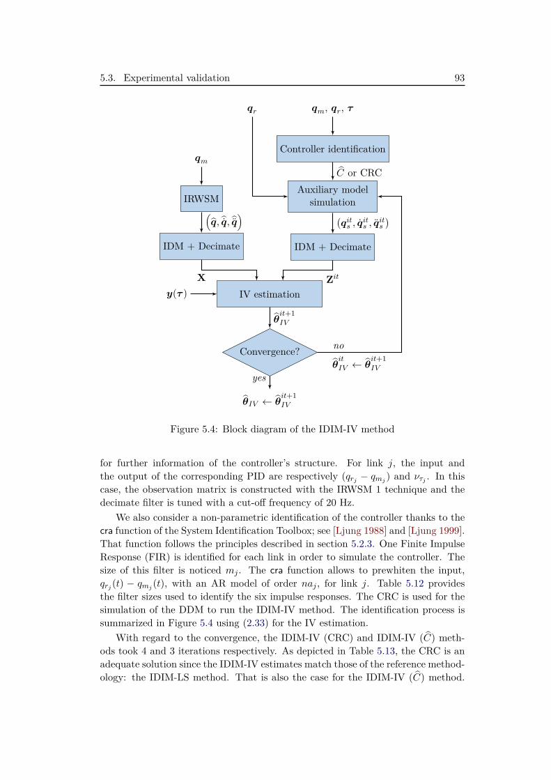
5.3. Experimental validation 93
qm
IRWSM
IDM + Decimate
qm, qr, τ
Controller identification
Auxiliary modelsimulation
IDM + Decimate
qr
IV estimation
Convergence?
θIV ← θit+1IV
y(τ )
(q, q, q)
X
C or CRC
(qits , q
its , q
its
)
Zit
θit+1IV
yes
no
θit
IV ← θit+1IV
Figure 5.4: Block diagram of the IDIM-IV method
for further information of the controller’s structure. For link j, the input andthe output of the corresponding PID are respectively (qrj − qmj ) and ντj . In thiscase, the observation matrix is constructed with the IRWSM 1 technique and thedecimate filter is tuned with a cut-off frequency of 20 Hz.
We also consider a non-parametric identification of the controller thanks to thecra function of the System Identification Toolbox; see [Ljung 1988] and [Ljung 1999].That function follows the principles described in section 5.2.3. One Finite ImpulseResponse (FIR) is identified for each link in order to simulate the controller. Thesize of this filter is noticed mj . The cra function allows to prewhiten the input,qrj (t) − qmj (t), with an AR model of order naj , for link j. Table 5.12 providesthe filter sizes used to identify the six impulse responses. The CRC is used for thesimulation of the DDM to run the IDIM-IV method. The identification process issummarized in Figure 5.4 using (2.33) for the IV estimation.
With regard to the convergence, the IDIM-IV (CRC) and IDIM-IV (C) meth-ods took 4 and 3 iterations respectively. As depicted in Table 5.13, the CRC is anadequate solution since the IDIM-IV estimates match those of the reference method-ology: the IDIM-LS method. That is also the case for the IDIM-IV (C) method.
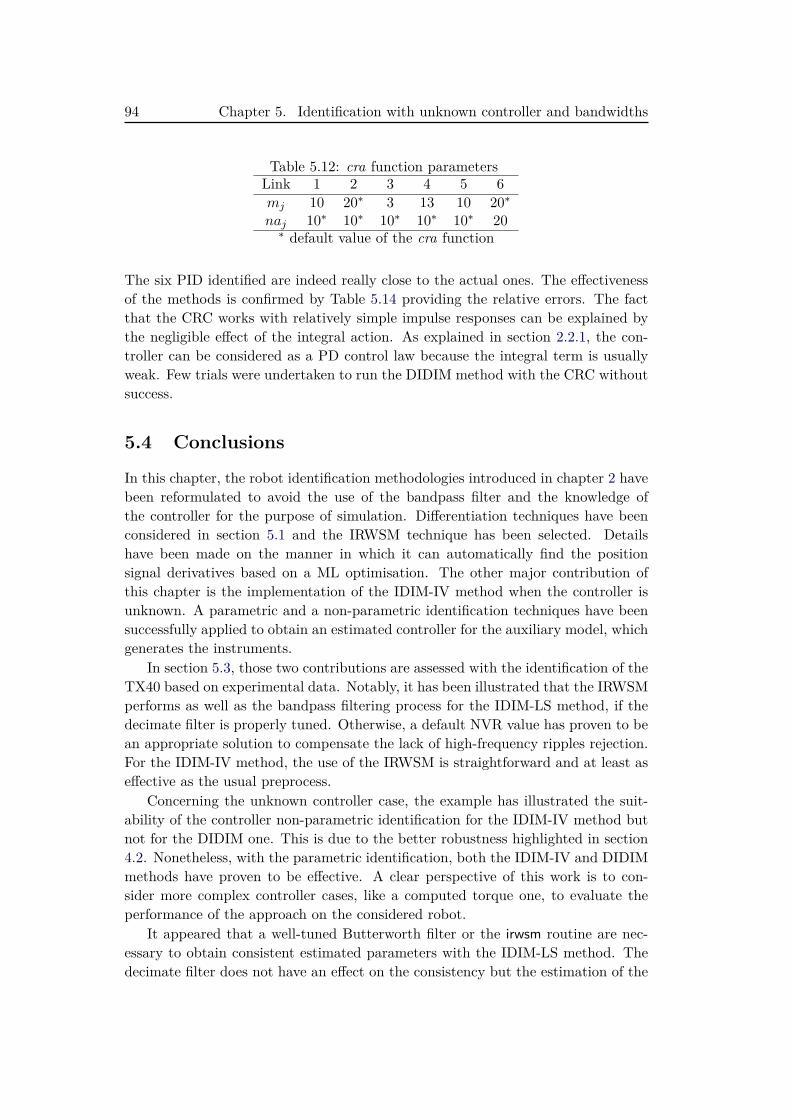
94 Chapter 5. Identification with unknown controller and bandwidths
Table 5.12: cra function parametersLink 1 2 3 4 5 6mj 10 20∗ 3 13 10 20∗naj 10∗ 10∗ 10∗ 10∗ 10∗ 20∗ default value of the cra function
The six PID identified are indeed really close to the actual ones. The effectivenessof the methods is confirmed by Table 5.14 providing the relative errors. The factthat the CRC works with relatively simple impulse responses can be explained bythe negligible effect of the integral action. As explained in section 2.2.1, the con-troller can be considered as a PD control law because the integral term is usuallyweak. Few trials were undertaken to run the DIDIM method with the CRC withoutsuccess.
5.4 Conclusions
In this chapter, the robot identification methodologies introduced in chapter 2 havebeen reformulated to avoid the use of the bandpass filter and the knowledge ofthe controller for the purpose of simulation. Differentiation techniques have beenconsidered in section 5.1 and the IRWSM technique has been selected. Detailshave been made on the manner in which it can automatically find the positionsignal derivatives based on a ML optimisation. The other major contribution ofthis chapter is the implementation of the IDIM-IV method when the controller isunknown. A parametric and a non-parametric identification techniques have beensuccessfully applied to obtain an estimated controller for the auxiliary model, whichgenerates the instruments.
In section 5.3, those two contributions are assessed with the identification of theTX40 based on experimental data. Notably, it has been illustrated that the IRWSMperforms as well as the bandpass filtering process for the IDIM-LS method, if thedecimate filter is properly tuned. Otherwise, a default NVR value has proven to bean appropriate solution to compensate the lack of high-frequency ripples rejection.For the IDIM-IV method, the use of the IRWSM is straightforward and at least aseffective as the usual preprocess.
Concerning the unknown controller case, the example has illustrated the suit-ability of the controller non-parametric identification for the IDIM-IV method butnot for the DIDIM one. This is due to the better robustness highlighted in section4.2. Nonetheless, with the parametric identification, both the IDIM-IV and DIDIMmethods have proven to be effective. A clear perspective of this work is to con-sider more complex controller cases, like a computed torque one, to evaluate theperformance of the approach on the considered robot.
It appeared that a well-tuned Butterworth filter or the irwsm routine are nec-essary to obtain consistent estimated parameters with the IDIM-LS method. Thedecimate filter does not have an effect on the consistency but the estimation of the
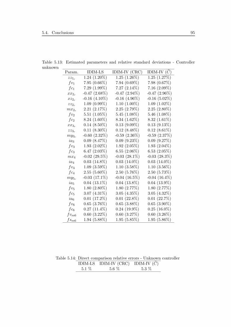
5.4. Conclusions 95
Table 5.13: Estimated parameters and relative standard deviations - Controllerunknown
Param. IDIM-LS IDIM-IV (CRC) IDIM-IV (C)zz1r 1.24 (1.20%) 1.25 (1.26%) 1.25 (1.27%)fv1 7.95 (0.66%) 7.94 (0.69%) 7.98 (0.67%)fc1 7.29 (1.99%) 7.27 (2.14%) 7.16 (2.09%)xx2r -0.47 (2.68%) -0.47 (2.94%) -0.47 (2.96%)xz2r -0.16 (4.10%) -0.16 (4.96%) -0.16 (5.02%)zz2r 1.09 (0.99%) 1.10 (1.00%) 1.09 (1.02%)mx2r 2.21 (2.17%) 2.25 (2.79%) 2.25 (2.80%)fv2 5.51 (1.05%) 5.45 (1.08%) 5.46 (1.08%)fc2 8.24 (1.60%) 8.34 (1.62%) 8.32 (1.61%)xx3r 0.14 (8.50%) 0.13 (9.09%) 0.13 (9.13%)zz3r 0.11 (8.30%) 0.12 (8.48%) 0.12 (8.61%)my3r -0.60 (2.32%) -0.59 (2.36%) -0.59 (2.37%)ia3 0.09 (8.47%) 0.09 (9.23%) 0.09 (9.27%)fv3 1.93 (2.02%) 1.92 (2.05%) 1.93 (2.04%)fc3 6.47 (2.03%) 6.55 (2.06%) 6.53 (2.05%)mx4 -0.02 (29.5%) -0.03 (28.1%) -0.03 (28.3%)ia4 0.03 (14.8%) 0.03 (14.0%) 0.03 (14.0%)fv4 1.09 (3.59%) 1.10 (3.58%) 1.10 (3.56%)fc4 2.55 (5.60%) 2.50 (5.76%) 2.50 (5.73%)my5r -0.03 (17.1%) -0.04 (16.5%) -0.04 (16.4%)ia5 0.04 (13.1%) 0.04 (13.8%) 0.04 (13.9%)fv5 1.80 (2.80%) 1.80 (2.77%) 1.80 (2.77%)fc5 3.07 (4.31%) 3.05 (4.35%) 3.05 (4.32%)ia6 0.01 (17.2%) 0.01 (22.8%) 0.01 (22.7%)fv6 0.65 (3.76%) 0.65 (3.88%) 0.65 (3.90%)fc6 0.27 (11.4%) 0.24 (19.9%) 0.25 (16.0%)fvm6 0.60 (3.22%) 0.60 (3.27%) 0.60 (3.26%)fsm6 1.94 (5.88%) 1.95 (5.85%) 1.95 (5.86%)
Table 5.14: Direct comparison relative errors - Unknown controllerIDIM-LS IDIM-IV (CRC) IDIM-IV (C)5.1 % 5.6 % 5.3 %

96 Chapter 5. Identification with unknown controller and bandwidths
covariance. As far as the decimate process is concerned, an automated selectionof the cut-off frequency could be of interest. The current method requires to befamiliar with the system, which hinders its applicability quite a bit. In the nextchapter, the noise circulation through the system is analysed in order to provide analternative to the usual decimate process.
Chapter 6
Noise modelling for robotsystem identification
In the previous chapter, the bandpass filter and the knowledge of the controllerhave been bypassed to reduce the knowledge required prior to the identification. Ifthe results were satisfactory from this perspective, they have underlined the roleof the decimate filter to whiten the noise and provide efficient estimates of thecovariances. In order to tune adequately this filter, a solution could consist inestimating the dynamical parameters with incorrect covariances in a first time toretrieve the dynamics, before estimating correct covariances in a second time with acorrectly tuned filter. In this chapter, an automatic and one-step solution is ratherinvestigated. The idea is to take into account the noise model similarly to theRIVC method, introduced in section 3.2, to provide estimates with low covariancesand white residuals. This work has been presented in [Brunot et al. 2016a] andsubmitted in [Brunot et al. Submitted 2017].
The chapter is organised as follows. The noise modelling is investigated insection 6.1. From the selected noise model, the robot identification methods arerevised to provide estimates automatically in section 6.2. The methods are thenapplied on the TX40 example in section 6.3 before concluding in section 6.4 onfuture perspectives for those extensions.
6.1 Noise modelling and identification . . . . . . . . . . . . . . . 986.1.1 Closed-loop relations . . . . . . . . . . . . . . . . . . . . . . . 986.1.2 Filters models . . . . . . . . . . . . . . . . . . . . . . . . . . . 996.1.3 Auto-regressive filters identification . . . . . . . . . . . . . . . 103
6.2 Refined identification methods . . . . . . . . . . . . . . . . . 1056.2.1 The separable PEM method . . . . . . . . . . . . . . . . . . . 1056.2.2 The IDIM-PIV method . . . . . . . . . . . . . . . . . . . . . 1066.2.3 Comments on the extensions . . . . . . . . . . . . . . . . . . 107
6.3 Experimental validations . . . . . . . . . . . . . . . . . . . . . 1086.3.1 Study of the black-box noise model . . . . . . . . . . . . . . . 1086.3.2 Study of the grey-box noise model . . . . . . . . . . . . . . . 1126.3.3 Study with noisy data . . . . . . . . . . . . . . . . . . . . . . 113
6.4 Conclusions . . . . . . . . . . . . . . . . . . . . . . . . . . . . . 116
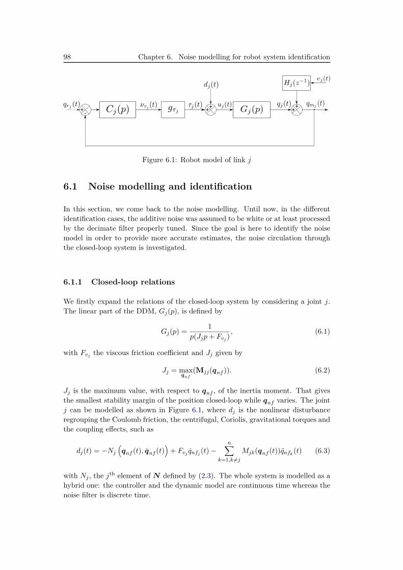
98 Chapter 6. Noise modelling for robot system identification
Figure 6.1: Robot model of link j
6.1 Noise modelling and identification
In this section, we come back to the noise modelling. Until now, in the differentidentification cases, the additive noise was assumed to be white or at least processedby the decimate filter properly tuned. Since the goal is here to identify the noisemodel in order to provide more accurate estimates, the noise circulation throughthe closed-loop system is investigated.
6.1.1 Closed-loop relations
We firstly expand the relations of the closed-loop system by considering a joint j.The linear part of the DDM, Gj(p), is defined by
Gj(p) = 1p(Jjp+ Fvj )
, (6.1)
with Fvj the viscous friction coefficient and Jj given by
Jj = maxqnf
(Mjj(qnf )). (6.2)
Jj is the maximum value, with respect to qnf , of the inertia moment. That givesthe smallest stability margin of the position closed-loop while qnf varies. The jointj can be modelled as shown in Figure 6.1, where dj is the nonlinear disturbanceregrouping the Coulomb friction, the centrifugal, Coriolis, gravitational torques andthe coupling effects, such as
dj(t) = −Nj
(qnf (t), qnf (t)
)+ Fvj qnfj (t)−
n∑k=1,k 6=j
Mjk(qnf (t))qnfk(t) (6.3)
with Nj , the jth element of N defined by (2.3). The whole system is modelled as ahybrid one: the controller and the dynamic model are continuous time whereas thenoise filter is discrete time.
6.1. Noise modelling and identification 99
From Figure 6.1, it comes out the hybrid closed-loop relation
qmj (t) = Tj(p)qrj (t) + Sj(p)Hj(z−1)ej(t) + Sj(p)Gj(p)dj(t) (6.4)
Tj(p) =gτjCj(p)Gj(p)
1 + gτjCj(p)Gj(p), Sj(p) = 1
1 + gτjCj(p)Gj(p)
where Sj is the sensitivity function and Tj is the complementary sensitivity function;see e.g. [Aström & Murray 2010]. Since for each p: Tj(p)+Sj(p) = 1, both functionscannot be made small simultaneously. As explained in [Janot et al. 2014a] andreminded in section 2.2.1, in order to have a good tracking at low frequencies, thecontroller is tuned to insure Tj(p) ≈ 1 and consequently Sj(p) ≈ 0. Since Tj is alow-pass filter, at high frequencies, we have the opposite configuration. Noting thatthe relevant information comes from the reference signal, the closed-loop transferfunction Tj provides an ideal frequency range for the filtering process. In this range,we have Tj(p) ≈ 1, Sj(p) ≈ 0 and the component from the noise becomes negligible.Therefore, it is consistent to filter the measured position close to the closed-loopdynamics to retrieve a noise-free position signal.
The closed-loop transfer function of the position, qj , is given by
qj(t) = Tj(p)qrj (t)− Tj(p)Hj(z−1)ej(t) + Sj(p)Gj(p)dj(t). (6.5)
The torque closed-loop transfer function is defined by
τj(t) = gτjCj(p)Sj(p)[qrj (t)−Hj(z−1)ej(t)
]− Tj(p)dj(t) (6.6)
= Fτj (p)[qrj (t)−Hj(z−1)ej(t)
]− Tj(p)dj(t).
The reference signal and the noise have the same transfer function: Fτj (p) =gτjCj(p)Sj(p).
6.1.2 Filters models
The IDIM and the measured position respectively defined in (2.17) and (4.12) arerecalled here
τ (t) = τ idm(t) + v(t) (6.7)qm(t) = qnf (t) + nq(t),
where τ idm and qnf are the noise-free components, v and nq are respectively thetorque and position noises we want to model. Furthermore, based on the noise-freeassumption of the reference trajectory, it comes out the key relation between theinput and output noises established in section 4.1.1:
v(t) = −GτC(p)nq(t). (6.8)
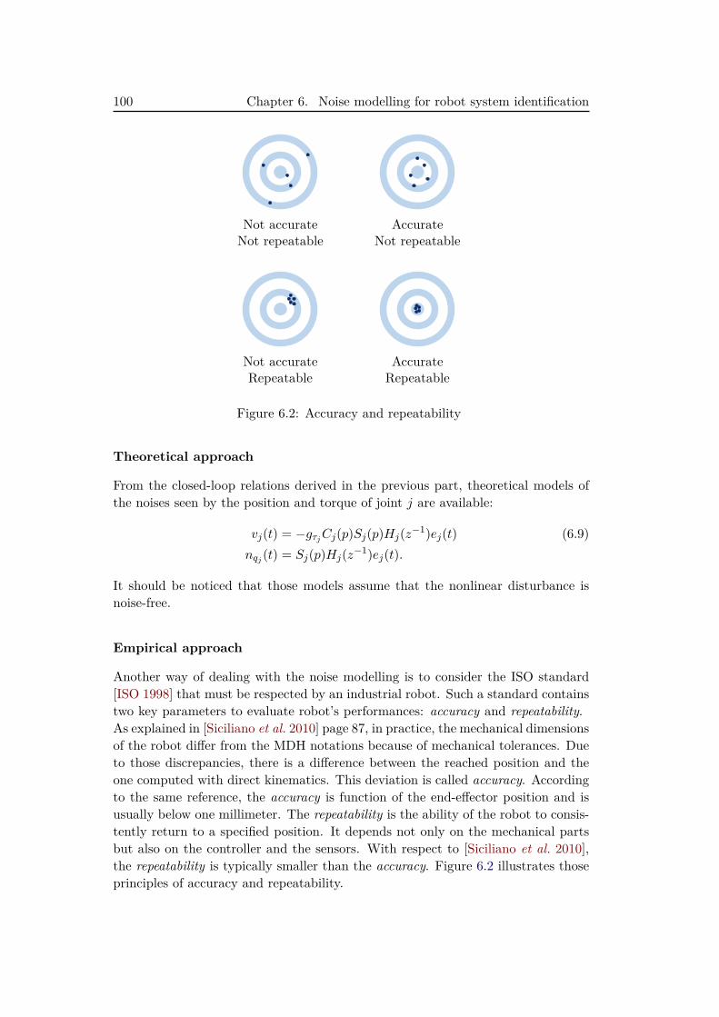
100 Chapter 6. Noise modelling for robot system identification
Not accurateNot repeatable
AccurateNot repeatable
Not accurateRepeatable
AccurateRepeatable
Figure 6.2: Accuracy and repeatability
Theoretical approach
From the closed-loop relations derived in the previous part, theoretical models ofthe noises seen by the position and torque of joint j are available:
vj(t) = −gτjCj(p)Sj(p)Hj(z−1)ej(t) (6.9)nqj (t) = Sj(p)Hj(z−1)ej(t).
It should be noticed that those models assume that the nonlinear disturbance isnoise-free.
Empirical approach
Another way of dealing with the noise modelling is to consider the ISO standard[ISO 1998] that must be respected by an industrial robot. Such a standard containstwo key parameters to evaluate robot’s performances: accuracy and repeatability.As explained in [Siciliano et al. 2010] page 87, in practice, the mechanical dimensionsof the robot differ from the MDH notations because of mechanical tolerances. Dueto those discrepancies, there is a difference between the reached position and theone computed with direct kinematics. This deviation is called accuracy. Accordingto the same reference, the accuracy is function of the end-effector position and isusually below one millimeter. The repeatability is the ability of the robot to consis-tently return to a specified position. It depends not only on the mechanical partsbut also on the controller and the sensors. With respect to [Siciliano et al. 2010],the repeatability is typically smaller than the accuracy. Figure 6.2 illustrates thoseprinciples of accuracy and repeatability.
6.1. Noise modelling and identification 101
From those definitions, we define the following relation:
q(t) = qr(t)− εqtr(t) = qr(t)− (acc(t) + rep(t)) (6.10)
where εqtr is the closed-loop tracking error divided in a deterministic accuracy vectoracc and a stochastic repeatability vector rep. Although the accuracy and repeata-bility are defined in static framework, we consider them here within a dynamicmodel. The transient effects of the tracking law can be seen as a part of the ac-curacy vector acc. At first approximation, the repeatability may be modelled by awhite noise with a covariance matrix R2
r . Since qr is noise-free, the noise seen bythe measurement position of link j is given by:
nqj (t) = −repj (t) + qj(t), (6.11)
with the sensor noise qj(t) = Hj(z−1)ej(t). The goal of the control law is to makethe tracking error εqtrj negligible to set the tool at the right position in the workspace.Therefore, from a design perspective, the noise introduced by the sensor should havea mean and a covariance lower than those of the tracking error. Continuing thisline of reasoning, it may even be written
nqj (t) ≈ −repj (t). (6.12)
According to [Stäubli Favergues 2015], the repeatability is ±0.02 mm with a maxi-mum reach of 450 mm between joint 1 and 5. Using the Pythagoras’s theorem, itcomes out the angular repeatability of joint 1: Rr1 = 2.5 10−3 degree, assuming thatthe joints are perfectly rigid and that all the error comes from link 1. That is con-sistent with the sensor’s angular resolution of 2 10−4 degree per count provided insection 2.2.3. On the other hand, the order of magnitude of the reference trajectoryis 102 degree. Therefore, the output Signal to Noise Ratio (SNR) is approximately
SNRqdB = 10 · log10
((AsignalAnoise
)2)
= 92 dB, (6.13)
where Asignal = 102 and Anoise = 2.5 10−3 are the amplitudes of the signal andthe noise respectively. In the light of this low SNR, the ultimate assumption is toneglect the noise on the joint positions and to consider them as noise-free. Theconsequence of such an assumption is that the circulation of the noise, on which isbased the noise model (6.9), is neglected.
By considering (6.8) and (6.12), it comes out v(t) = GτC(p)rep(t). The de-terministic component of the torque is then τ det(t) = GτC(p)acc(t). Around anoperating point, there is C(p) ≈ C0. Therefore, the input SNR is approximately
SNRτdB = 10 · log10
(accrep
)2 . (6.14)
102 Chapter 6. Noise modelling for robot system identification
In the case of the TX40, the accuracy is not given by the manufacturer. Accordingto [Siciliano et al. 2010], we know that the repeatability should be lower than theaccuracy. If we assume that the ratio is acc = 10 ·rep, there is SNRτdB = 20 dB. Forexample, with the accuracy and repeatability of the PUMA 560 provided in [Conradet al. 2000], we have SNRτdB = 32 dB. Those simple numerical applications showthat there is much more noise in the input torque signals than in the output ones.
The orders of magnitude of the SNR found, for the input and output signals,are similar to what is observed in practice; see e.g. [Calanca et al. 2011]1. If it doesnot theoretically validate this empirical noise model, that illustrates its credibility.
Amplified noise
The reader has to keep in mind that we study here the noise proper to the physicalsystem and more specifically the noise seen by the input torques. As explainedin section 4.2.1, the practitioner may also introduce another noisy component intothe IDIM with the amplification of the measurement noise through the numericaldifferentiation of the joint positions. In fact, from the development of the section4.2.1, we would have:
τ (t) = τ idm(t) + v(t) + M(t)nq(t)/T 2s (6.15)
where M is the inertia matrix. With a high sampling frequency, this amplifiednoise may become predominant. That shows why a specific attention must be paidto this issue. As illustrated in section 5.3.1, even with the IRWSM method, thepractitioner must be careful.
Retained noise model
As it has been seen, the question of the noise model is complex and our practicalreasonings do not intend to perfectly model the circulation of this noise throughthe system. For our identification purpose, we will consider two cases:
vj(t) = Hτj (z−1)ej(t), (6.16)vj(t) = −gτjCj(p)nqj (t) = −gτjCj(p)Hc
j (z−1)ej(t). (6.17)
The idea of the first model (6.16) is to evaluate the noise filter with a black-box point of view. For reminder, the noise of the sensor is qj(t) = Hj(z−1)ej(t).Assuming that the noise filter Hj just "shapes" the white noise but does not amplifyit, it comes out var(qj) ≈ var(ej). With such an assumption, it is expected thatthe residual ej has a variance approximately equal to the one of the encoder; i.e.var (ej) ≈ ∆2
e.The second model (6.17) takes into account the controller relation and can thus
be considered as a grey-box approach. Based on the theoretical development, wewould have Hc
j = SjHj ; i.e. the sensor noise filter weighted by the closed-loop1It should be noticed that the SNR definition is slightly different in this reference.
6.1. Noise modelling and identification 103
sensitivity function. In the opposite, based on the empirical approach, Hcj would
be a filter shaping the noisy part of the tracking error; i.e. nqj (t) = Hcj (z−1)ej(t) =
−repj (t). The idea of this second noise model, with two variants, is to see thecontroller influence and, especially, if that knowledge of the controller allows abetter estimation. To distinguish between the two variants, the variance of theestimated position error nqj can be examined.
• With the empirical model, the estimated position error nqj should have astandard deviation nearly equal to the the repeatability, following (6.12).
• With the theoretical noise model, nqj (t) = Sj(p)qj(t) should have a varianceslightly lower than the one of the measurement noise. The transfer Sj isassumed to be a perfect high-pass filter such as
Sj (ω) =
0, if ω ∈ [−ωdyn, ωdyn]1, otherwise
. (6.18)
It comes out:
σ2nqj
= 12π
∫ ∞−∞
Pqj qj (ω) |Sj (ω) |2dω
= 12π
(∫ −ωdyn−ωnyq
Pqj qjdω +∫ ωnyq
ωdyn
Pqj qjdω
)
= 1πPqj qj (ωnyq − ωdyn) = σ2
qj− ωdynPqj qj/π
= σ2qj
(1− ωdyn
ωnyq
),
where Pqj qj is the power spectral density of qj assumed to be white with acovariance σ2
qj= 1
πPqj qj · ωnyq, using the material from Appendix C.3. Theprevious estimation of the variance σ2
nqjmakes rough assumptions. However,
it illustrates the order of magnitude which should be expected.
In any case, the noise is assumed to be modelled with a rational spectral densityand to be independent between the links.
6.1.3 Auto-regressive filters identification
The noise model may be identified thanks to the instrumental variable approachfor AutoRegressive - Moving - Average (ARMA) models described in [Young 2006].This method is implemented in the ivarma function of the CAPTAIN Toolbox. Fora given link, the function requires the sizes of the numerator and the denominatorof the ARMA model. One solution consists in identifying just the AutoRegressive(AR) model which gives the best Akaike Information Criterion (AIC) without tak-ing into account the Moving - Average (MA) filter [Akaike 1974]. That approachis implemented in the aic function of the CAPTAIN. Another solution consists in
104 Chapter 6. Noise modelling for robot system identification
estimating the sizes of MA and AR filters by a visual inspection of the autocorre-lation and partial autocorrelation functions of the signals, as explained in Chapter6 of [Box & Jenkins 1976].
Because our goal is to find an automatic solution which does not require thepractitioner’s skills, we focus on the aic technique. The user has to specify themaximum expected order of the AR filter and the function performs a line searchto find the order corresponding to the best AIC. The AR filter is defined such as:
ξ(ti) = 1Cl(z−1)e(ti) (6.19)
= −c1ξ(ti−1)− ...− clξ(ti−l) + e(ti),
where l is the number of estimated parameters and e is the generating zero mean,normally distributed, white noise sequence with variance λ2. With the autocovari-ance function:
Rk = 1N
N∑i=1
ξ(ti−k)ξ(ti), k ≥ 0 (6.20)
it comes the Yule-Walker equation
Rm = −l∑
k=1ckRm−k + λ2δm,0 (6.21)
withm = 0, · · · , l and δm,0 the Kronecker delta function. From those l+1 equations,the linear system of l equations (6.22) provides the estimation of the coefficientswith OLS. The last equation (6.23) provides an estimation of the covariance.
R0 R1 · · · Rl−1...
... Rl−2Rl−1 Rl−2 · · · R0
c1...cl
=
c−R1
...−Rl
(6.22)
R0 = −l∑
k=1ckR−k + λ2 (6.23)
In practice, the en-bloc estimation should be avoided due to potential conditioningissues. Several recursive and robust methods have been developed like the Burgmethod or the Levinson-Durbin algorithm; see e.g. [Burg 1975] and the section10.1 of [Ljung 1999]. The AIC is defined by:
AIC = 2l − 2log(L), (6.24)
where L is the likelihood function. According to [Shibata 1976] for the AR processconsidered, it comes out:
AIC = 2l +N log(λ2), (6.25)
where λ2 is the estimated covariance of the generating noise estimated with (6.23).
6.2. Refined identification methods 105
6.2 Refined identification methods
6.2.1 The separable PEM method
If the PEM is an attractive methodology, it means identifying the dynamic modeland the noise model at the same time, as it is visible with (3.17). This raises twoproblems for a robotic application. Firstly, we have no prior information about theorder of the filter. Secondly, the identification of both models at the same time maylead to a complex nonlinear optimisation problem, whereas it has been simplifiedwith the PLR assumption. Therefore, inspired by the RIVC method, we propose aseparable approach by considering the following error:
εseppem(tk, ρ) = H−1τ (z−1, η)εdidim(tk, θ), (6.26)
where ρ is the (b + l × 1) vector of unknown parameters, regrouped such as ρT =[θT ηT ], and η is the (l× 1) vector regrouping all the noise parameters. The pro-posed methodology, a SEParable PEM (SEP-PEM), is composed of three sequentialsteps.
1. Identification of the dynamic model. The physical parameters are estimatedwith the DIDIM method without using the decimate filter.
2. Identification of the noise model. For each link j, obtain an estimate of thenoise parameters, ηj , and an estimate of the noise covariance, λj . The inputnoise filter Hτj can be identified based on
εdidimj (t) = Hτj (z−1,ηj)ej(t), (6.27)
for the black-box model or based on
− C−1j (p)εdidimj (t) = Hc
j (z−1,ηj)ej(t), (6.28)
for the grey-box model.
3. Estimated covariance. The estimated parametric error covariance matrixof the physical parameters is computed with the following relation
Σ(θ) =
E n∑j=1
[H−1τj (z−1, ηj)φsj
(t, θ)]T
λ−1j
[H−1τj (z−1, ηj)φsj
(t, θ)]
−1
(6.29)
where φsj is jth row of the simulated observation matrix φ (qs, qs, qs)2.
The separation of the identification of the physical parameters and the one of thenoise model implies that both models are statistically independent. To go through
2The simulated observation matrix is noted φs and not ζ because there is no filter involved.
106 Chapter 6. Noise modelling for robot system identification
the second step, we must be sure that the first one has converged and that there isno significant modelling error. However, as shown in section 4.1.4, the CLIE andDIDIM methods can converge to consistent parameters even without the decimateor the noise filter. Therefore, the first step of the method is admissible. This wouldnot be the case with a direct approach since the noise and the dynamic modelswould be linked, as explained in section 3.1.
It should be noticed that in the algorithm above that we assume the matrix Hτ
is diagonal. Following the development of the section 6.1.1, this assumption seemsreasonable. Furthermore, it simplifies radically the process.
6.2.2 The IDIM-PIV method
Still inspired by the RIVC method, we reconsider the IDIM-IV method by takinginto account the noise filter instead of the decimate one. The introduced techniqueis called Prefiltered IV (PIV). The term "refined" is not used because the RIVCtheory has been developed for LTI systems. We do not develop here a theory fornonlinear systems, like the robots, but we modify the algorithm so that it canbe applied on the IDIM. With the same notations as the SEP-PEM method, theIDIM-PIV algorithm is implemented as follows:
1. Initialisation. For the initial physical parameters, θ0, we use the CAD val-ues for the inertia. The other physical parameters are set to zero. For eachlink, the initial noise filter is set as follows: Hj(z−1, ηj
0) = 1 with λ0j = 1.
If the controller is unknown, it must be identified with an approach describedin section 5.2 in order to simulate the auxiliary model generating the instru-ments. Once the controller available, step 2 can be performed.The observation matrix should be constructed with the IRWSM technique inorder to have a systematic process.
2. Iteration: repeat until convergence the following steps (k stands for the kthiteration)
(a) Simulate the auxiliary model (i.e. the DDM) to retrieve the noise-freesignals for the instruments by using θk−1.
(b) Determine the IV estimate of the physical parameters using
θk =
nm∑i=1
n∑j=1ζTj (ti, ρk−1)φLj (ti, ρ
k−1)
−1 nm∑i=1
n∑j=1ζTj (ti, ρk−1)τLj (ti, ρk−1)
(6.30)
6.2. Refined identification methods 107
with
φLj(t, ρk−1) = Lj(z−1, ηk−1j )φj
(q(t), q(t), q(t)
),
ζj(t, ρk−1) = Lj(z−1, ηk−1j )φj
(qs(t, θ
k−1), qs(t, θk−1), qs(t, θ
k−1)),
τLj(t, ρk−1) = Lj(z−1, ηk−1j )τj(t),
Lj(z−1, ηk−1j ) =
(λk−1j
)−1H−1τj (z−1, ηk−1
j ).
(c) For each link j, obtain an estimate of the noise parameters, ηkj , andan estimate of the noise covariance, λkj . The input noise filter Hτj canbe identified based either on (6.27) for the black-box noise model or on(6.28) for the grey-box noise model.
3. Estimated covariance. After convergence, based on (2.31), the estimatedparametric error covariance matrix of the physical parameters is computedwith the following relation
Σ(θ) =
E n∑j=1
[H−1τj (z−1, ηj)φ
nfj
(t, θ)]T
λ−1j
[H−1τj (z−1, ηj)φ
nfj
(t, θ)]
−1
.
(6.31)
In practice, the noise-free observation matrix φnf is approximated by thesimulated one φ (qs, qs, qs).
If the method is really similar to the SEP-PEM method introduced in section6.2.1, there are few discrepancies. Firstly, the IDIM-PIV method iteratively iden-tifies the dynamic model then the noise filters. An error in the noise filters couldthus contaminate the dynamic model and vice versa. The practitioner should becautious. Secondly, since it is an IV method, it requires the observation matrix φand consequently the measurement of the joint positions. However, in the end, theyshare the same third step to estimate the covariance matrix.
6.2.3 Comments on the extensions
This section is devoted to three comments concerning the two extended methodsproposed in previous sections. We first want to underline the philosophical differ-ence between the decimate filter and the noise filter identification. In both cases,the goal is to provide white residuals to have consistent and minimal estimates ofthe variances. Both methods accept that the measurement noise cannot be whiteover all the frequency range. With the decimate filter, the noise is assumed tobe white only over the two times the system’s bandwidth. That explains the rulegiven in section 2.3.1. Consequently, the practitioner focuses only on this rangeand removes anything else. With the identification of the noise filter, the idea is to
108 Chapter 6. Noise modelling for robot system identification
whiten the residuals over the whole frequency range of the system. That may leadto two issues of which we must be aware. Firstly, the noise filters are most likelylowpass filter. Thus, their inverses amplify high frequency components like unmod-elled flexibilities, electromagnetic disturbances in the motor or numerical artefactscoming from the integration solver. Secondly, the process is more time consumingthan the decimate filter. As highlighted in section 4.1.4, with the decimate filter theoptimisation solver has to consider N = 276 sampling points against nm = 34500with the filter identification.
The second element we want to discuss in this section is the optimality. ThePEM and RIVC methods have been indeed developed in order to provide optimalestimates; i.e. the Cramér-Rao lower bound is reached. With the two extensionsintroduced here, we do not strictly speak about optimality. In fact, the PEM andRIVC theories were developed for LTI systems. Consequently, the optimality hasnot been demonstrated for nonlinear systems like robots. Our goal is not here todevelop a theory of optimality in a nonlinear framework but only to refine/extendthe usual methods.
Finally, the aic function described in section 6.1.3 is reconsidered. If this methodis able to identify AR filters, it can be viewed as an auto-correlation information.The function indeed finds the order of the AR filter which gives the best Akaike’sinformation criterion. That information indicates the range on which the signalis serially correlated. Therefore, the size of the AR filter can be used to tune thedecimate filter such as nd = size(AR). This solution makes the decimate processautomated while avoiding the potential issues of the filtering by the inverses of thenoise models described previously.
6.3 Experimental validations
6.3.1 Study of the black-box noise model
For the beginning, the black-blox noise model is tested with our SEParable PEM(SEP-PEM) method as well as the standard DIDIM method for comparison. Forthe DIDIM and SEP-PEM methods, the controller used for the simulation is theactual controller of the robot, also used in Chapter 4. It has been shown in theprevious chapter that the identification of the controller is possible. Therefore, weconsider it as known to separate the problem.
The DIDIM and SEP-PEM methods converged in 7 steps. Two elements arenoteworthy concerning the values of the estimated parameters in Table 6.1. Firstly,the two iterative methods estimate dynamical parameters close to those estimatedby the IDIM-LS method when the bandwidths are perfectly known; see AppendixB. The discrepancies are not critical since they fell in 3σ confidence intervals. Sec-ondly, it can be remarked that the SEP-PEM estimates converged to the samevalues than those of the DIDIM method. Those satisfactory results concerning theestimated parameters are confirmed by the low and equivalent relative estimationerrors provided in Table 6.2.
6.3. Experimental validations 109
Regarding the relative standard deviations of the DIDIM and SEP-PEM meth-ods, they proved to be equivalent to the IDIM-LS results; see e.g. Table 5.13.Figure 6.3 depicts the autocorrelations of the identification residuals. For the SEP-PEM method, the effect of the identified noise filter is clear since the estimatedautocorrelations coefficients are included in the confidence intervals indicated bythe blue lines. If the estimated coefficients are larger for the DIDIM method, theycan still be considered as negligible because they are also included in their confi-dence intervals. The differences between the intervals sizes are due to the number ofsamples considered for each method. These estimated autocorrelations prove thatthe DIDIM and SEP-PEM residuals can be considered as serially uncorrelated andconsequently as white. With those results, it appears that the decimate filter thathas the same effect as the inverse of the noise filter, H−1
τ .
With regard to the input noise filters identified, the average order found is 141.The function thus needs in average 141 successive samples to whiten the noise.In other words, the signals are serially correlated over a range of 141 samples.With the Nyquist frequency ωnyq, the usual decimate filter keeps one sample overnd = ωnyq/ωFp = ωnyq/2/ωdyn = 125 to insure a white noise. Those close numbersshow that the decimate and the refined filters behave similarly. Therefore, thatstrengthens the idea suggested in section 6.2.3 of setting the decimate filter’s cut-off frequency thanks to the aic function.
Beyond those encouraging results from an estimation perspective, we investigatethe estimated noise
ej(t) = H−1τj (z−1, ηj)εdidimj (t, θ). (6.32)
Table 6.3 gives the estimated covariances of εdidimj and ej along with the squaredencoders’ resolutions. The DIDIM residuals are considered with and without thedecimate filter, given by εdidimj and εNDdidimj respectively. The decimation processindeed modifies the noise characteristics. To illustrate this property, we considerthe relation y(k) = Fp(z−1)x(k) = x(k · nd) where Fp is the decimate filter witha ratio nd and x is the input noise assumed to be white. With an ideal decimatefilter, the transfer is given by
Fp (ω) =
1, if ω ∈ [−ωFp , ωFp ]0, otherwise
. (6.33)
In accordance with Appendix C.3, x is a white noise with a constant power spectraldensity Pxx (ω) = Pe and a covariance σ2
x = ωnyqπ Pe. Therefore, the output noise
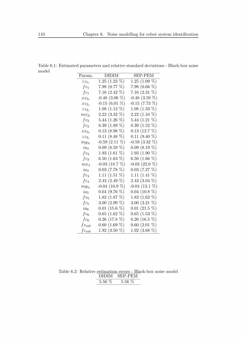
110 Chapter 6. Noise modelling for robot system identification
Table 6.1: Estimated parameters and relative standard deviations - Black-box noisemodel
Param. DIDIM SEP-PEMzz1r 1.25 (1.23 %) 1.25 (1.09 %)fv1 7.98 (0.77 %) 7.98 (0.66 %)fc1 7.16 (2.42 %) 7.16 (2.31 %)xx2r -0.48 (3.06 %) -0.48 (3.59 %)xz2r -0.15 (6.01 %) -0.15 (7.73 %)zz2r 1.08 (1.12 %) 1.08 (1.33 %)mx2r 2.22 (3.32 %) 2.22 (1.34 %)fv2 5.44 (1.26 %) 5.44 (1.21 %)fc2 8.39 (1.89 %) 8.39 (1.52 %)xx3r 0.13 (8.98 %) 0.13 (12.7 %)zz3r 0.11 (8.48 %) 0.11 (9.40 %)my3r -0.59 (2.11 %) -0.59 (3.32 %)ia3 0.09 (8.59 %) 0.09 (8.19 %)fv3 1.93 (1.61 %) 1.93 (1.90 %)fc3 6.50 (1.63 %) 6.50 (1.66 %)mx4 -0.03 (18.7 %) -0.03 (22.0 %)ia4 0.03 (7.78 %) 0.03 (7.27 %)fv4 1.11 (1.51 %) 1.11 (1.41 %)fc4 2.43 (2.49 %) 2.43 (3.04 %)my5r -0.04 (10.9 %) -0.04 (13.1 %)ia5 0.04 (9.76 %) 0.04 (10.8 %)fv5 1.82 (1.87 %) 1.82 (1.62 %)fc5 3.00 (2.99 %) 3.00 (3.21 %)ia6 0.01 (15.6 %) 0.01 (21.5 %)fv6 0.65 (1.62 %) 0.65 (1.53 %)fc6 0.26 (17.8 %) 0.26 (16.5 %)fvm6 0.60 (1.69 %) 0.60 (2.01 %)fcm6 1.92 (3.50 %) 1.92 (3.68 %)
Table 6.2: Relative estimation errors - Black-box noise modelDIDIM SEP-PEM5.56 % 5.56 %
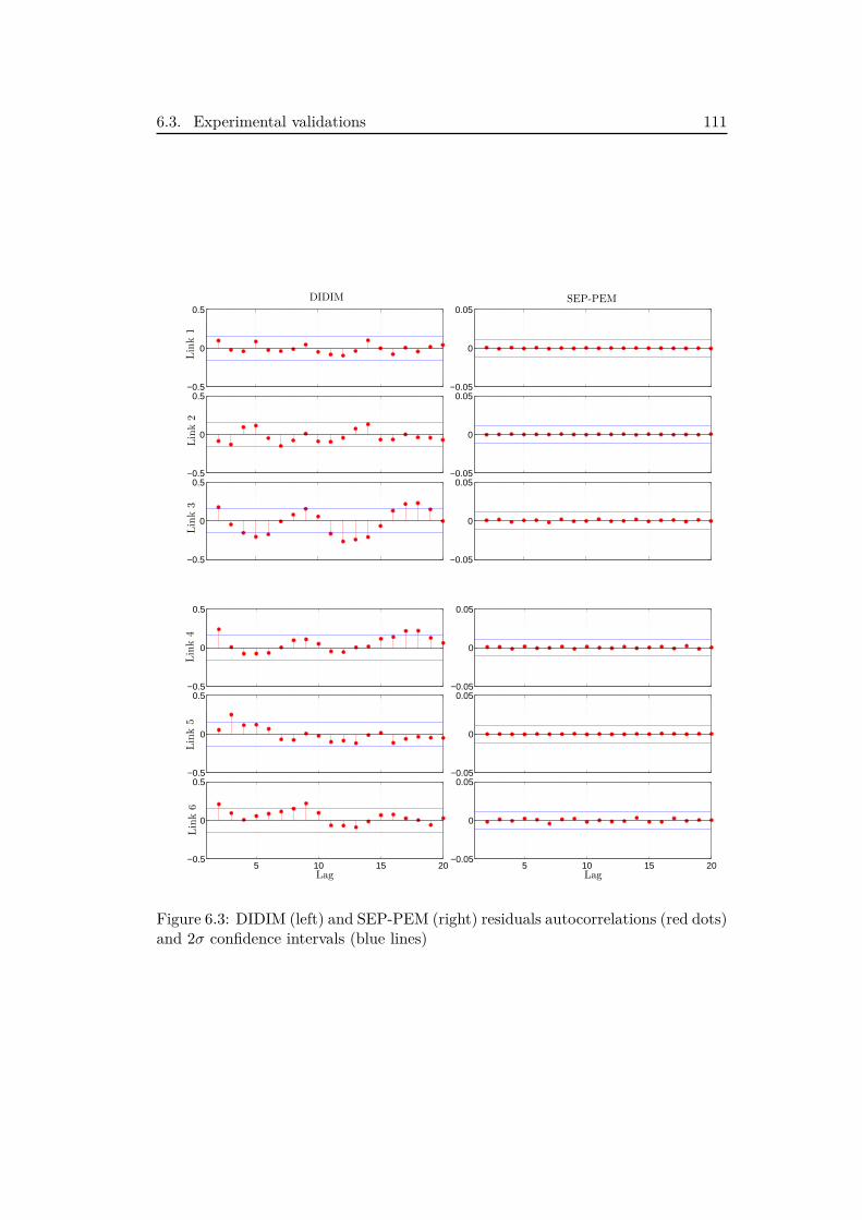
6.3. Experimental validations 111
−0.5
0
0.5
Link1
DIDIM
−0.05
0
0.05
−0.5
0
0.5
Link2
−0.05
0
0.05
−0.5
0
0.5
Link3
−0.05
0
0.05
SEP-PEM
−0.5
0
0.5
Link4
−0.05
0
0.05
−0.5
0
0.5
Link5
−0.05
0
0.05
5 10 15 20−0.5
0
0.5
Link6
Lag5 10 15 20
−0.05
0
0.05
Lag
Figure 6.3: DIDIM (left) and SEP-PEM (right) residuals autocorrelations (red dots)and 2σ confidence intervals (blue lines)
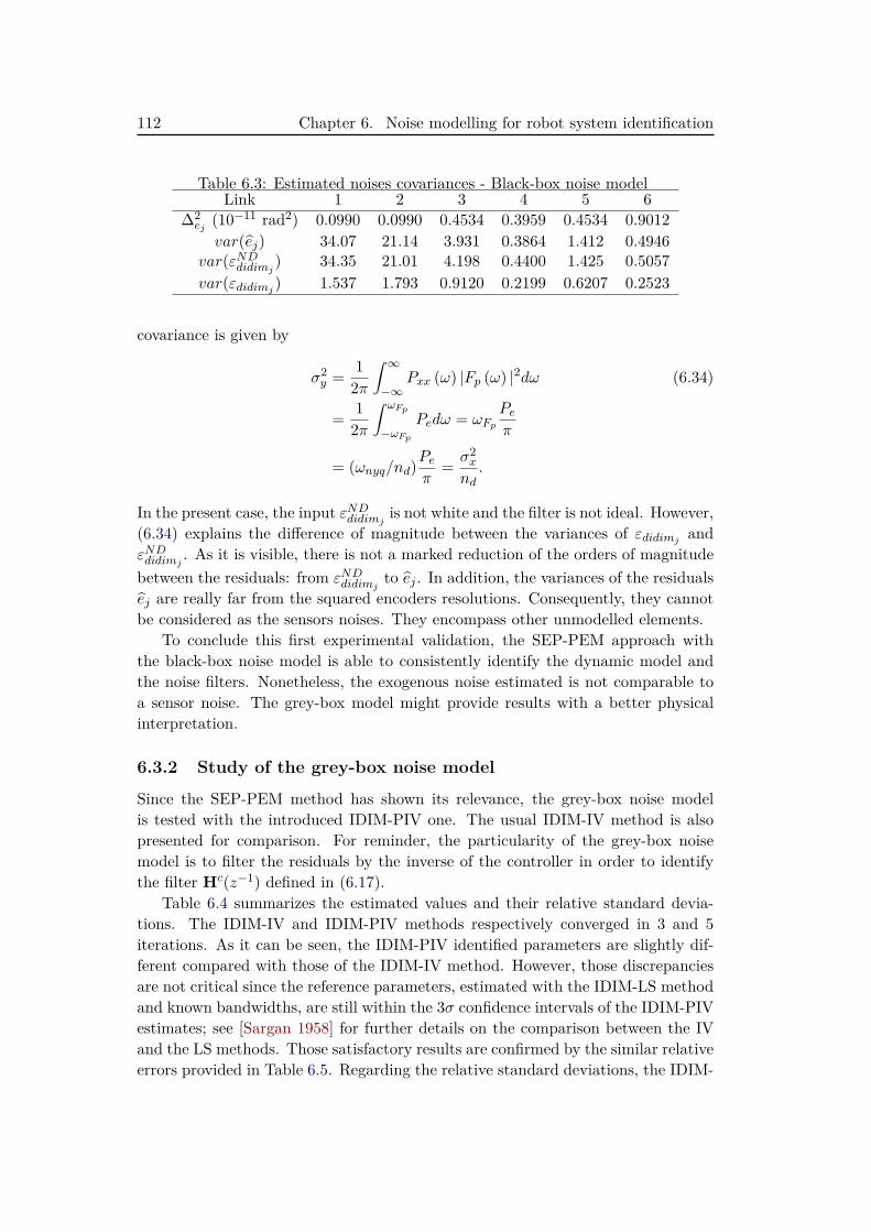
112 Chapter 6. Noise modelling for robot system identification
Table 6.3: Estimated noises covariances - Black-box noise modelLink 1 2 3 4 5 6
∆2ej (10−11 rad2) 0.0990 0.0990 0.4534 0.3959 0.4534 0.9012var(ej) 34.07 21.14 3.931 0.3864 1.412 0.4946
var(εNDdidimj ) 34.35 21.01 4.198 0.4400 1.425 0.5057var(εdidimj ) 1.537 1.793 0.9120 0.2199 0.6207 0.2523
covariance is given by
σ2y = 1
2π
∫ ∞−∞
Pxx (ω) |Fp (ω) |2dω (6.34)
= 12π
∫ ωFp
−ωFpPedω = ωFp
Peπ
= (ωnyq/nd)Peπ
= σ2x
nd.
In the present case, the input εNDdidimj is not white and the filter is not ideal. However,(6.34) explains the difference of magnitude between the variances of εdidimj andεNDdidimj . As it is visible, there is not a marked reduction of the orders of magnitudebetween the residuals: from εNDdidimj to ej . In addition, the variances of the residualsej are really far from the squared encoders resolutions. Consequently, they cannotbe considered as the sensors noises. They encompass other unmodelled elements.
To conclude this first experimental validation, the SEP-PEM approach withthe black-box noise model is able to consistently identify the dynamic model andthe noise filters. Nonetheless, the exogenous noise estimated is not comparable toa sensor noise. The grey-box model might provide results with a better physicalinterpretation.
6.3.2 Study of the grey-box noise model
Since the SEP-PEM method has shown its relevance, the grey-box noise modelis tested with the introduced IDIM-PIV one. The usual IDIM-IV method is alsopresented for comparison. For reminder, the particularity of the grey-box noisemodel is to filter the residuals by the inverse of the controller in order to identifythe filter Hc(z−1) defined in (6.17).
Table 6.4 summarizes the estimated values and their relative standard devia-tions. The IDIM-IV and IDIM-PIV methods respectively converged in 3 and 5iterations. As it can be seen, the IDIM-PIV identified parameters are slightly dif-ferent compared with those of the IDIM-IV method. However, those discrepanciesare not critical since the reference parameters, estimated with the IDIM-LS methodand known bandwidths, are still within the 3σ confidence intervals of the IDIM-PIVestimates; see [Sargan 1958] for further details on the comparison between the IVand the LS methods. Those satisfactory results are confirmed by the similar relativeerrors provided in Table 6.5. Regarding the relative standard deviations, the IDIM-
6.3. Experimental validations 113
PIV method performs as well as the IDIM-IV one providing that the decimate filteris properly tuned. The effect of the prefilter on the residuals is illustrated by theautocorrelation coefficients in Figure 6.4.
The critical point is the variances of the estimated position noises, nq. Followingthe discussion of section 6.1.2, the order of magnitude of the standard deviation ofnq should be 10−3 and 10−4 degree (or 1.7 · 10−5 and 1.7 · 10−6 radian) respectivelyfor the empirical variant (repeatability) and the theoretical variant (measurementnoise). Table 6.6 provides the estimated values with a mean value of 1.47 · 10−2
rad2 for var(nqj ), or ¯std(nqj ) = 0.121 rad. This result does not fit our modelsand suggests that the controller knowledge does not bring enough information forthe noise modelling. Looking at var(nqj ), there is still a clear reduction comparedwith the variance of εNDdidimj in Table 6.3 thanks to the filtering by the inverse of thecontroller.
Further investigations are hence necessary to find a physical interpretation ofthe observed noise. An idea could be to take into account more complete modelsof the actuators. That is strengthened by [Wernholt 2007] and the reference giventherein where it is stressed that the torque ripples are "caused by distortion of thestator flux linkage distribution, variable magnetic reluctance at the stator slots, andsecondary phenomena". Such an electronic phenomenon has not been taken intoaccount in the current grey-box model.
6.3.3 Study with noisy data
In order to test the limit of the IDIM-PIV method, another identification is con-ducted using rather noisy data. The black-box noise model is considered for sim-plicity’s sake. For this purpose, the resolution of the encoders is downgraded in anequivalent manner to [Marcassus et al. 2007]. The resolution is chosen equal to 3600points per revolution. Three identification methods are considered: the IDIM-LS,IDIM-IV and IDIM-PIV methods. The observation matrix is constructed with theIRWSM for the IDIM-PIV method in order to have an automatic process.
Table 6.7 summarizes the estimated values and their relative standard devia-tions. The estimated parameters of the IDIM-LS method are not satisfactory due tolarge mismatches like the inertia zz1r and zz3r . This is explained by the noise corre-lation from the closed-loop that biases the estimation. The IDIM-IV and IDIM-PIVmethods respectively converged in 3 and 5 iterations. The estimated values of theIDIM-IV and IDIM-PIV methods are similar to those found in previous works. Theresults of the IDIM-PIV method corroborate the relevance of the IRWSM to con-struct the observation matrix. Nonetheless, due to the noise introduced, the relativeerrors are larger in this case; see Table 6.8.
Concerning the relative standard deviations of the IDIM-PIV method, the valuesgive a good indication on the order of magnitude of the optimal solution. They areslightly lower than those of the IDIM-IV method whereas the filters of the latter arecorrectly tuned. Furthermore, the estimated covariances of the IDIM-PIV methodseem more reliable by looking at Figure 6.5 which depicts the autocorrelations of
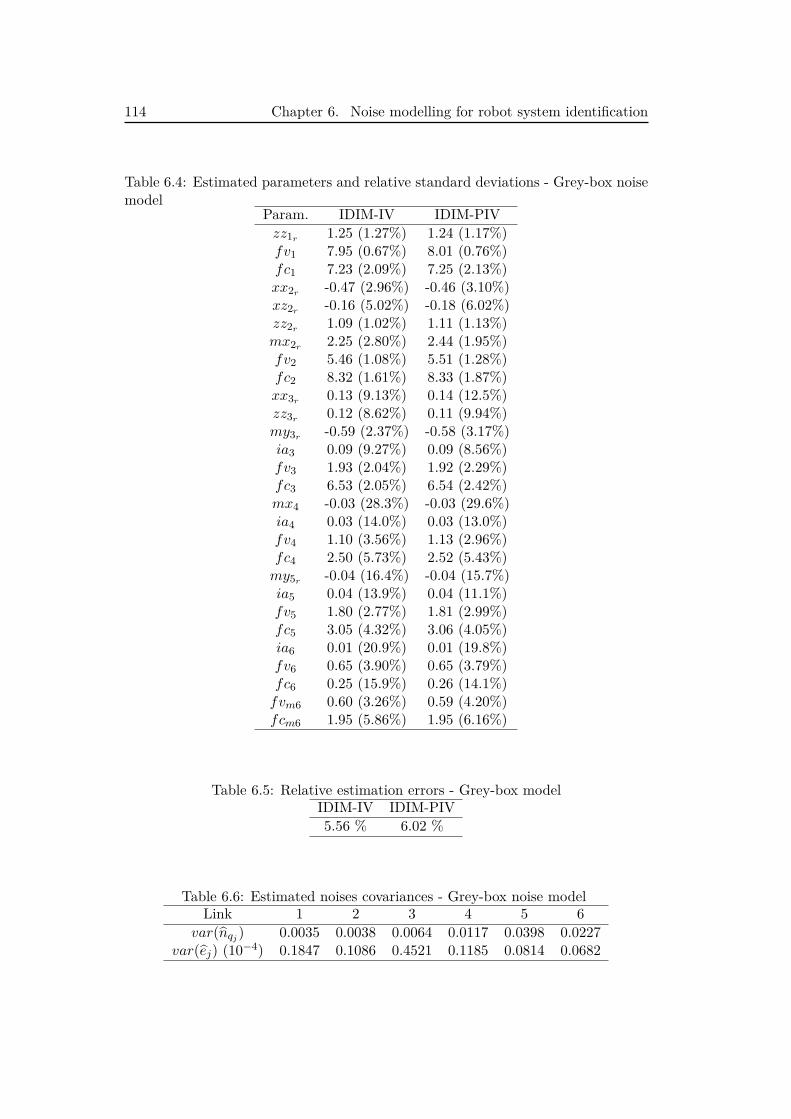
114 Chapter 6. Noise modelling for robot system identification
Table 6.4: Estimated parameters and relative standard deviations - Grey-box noisemodel
Param. IDIM-IV IDIM-PIVzz1r 1.25 (1.27%) 1.24 (1.17%)fv1 7.95 (0.67%) 8.01 (0.76%)fc1 7.23 (2.09%) 7.25 (2.13%)xx2r -0.47 (2.96%) -0.46 (3.10%)xz2r -0.16 (5.02%) -0.18 (6.02%)zz2r 1.09 (1.02%) 1.11 (1.13%)mx2r 2.25 (2.80%) 2.44 (1.95%)fv2 5.46 (1.08%) 5.51 (1.28%)fc2 8.32 (1.61%) 8.33 (1.87%)xx3r 0.13 (9.13%) 0.14 (12.5%)zz3r 0.12 (8.62%) 0.11 (9.94%)my3r -0.59 (2.37%) -0.58 (3.17%)ia3 0.09 (9.27%) 0.09 (8.56%)fv3 1.93 (2.04%) 1.92 (2.29%)fc3 6.53 (2.05%) 6.54 (2.42%)mx4 -0.03 (28.3%) -0.03 (29.6%)ia4 0.03 (14.0%) 0.03 (13.0%)fv4 1.10 (3.56%) 1.13 (2.96%)fc4 2.50 (5.73%) 2.52 (5.43%)my5r -0.04 (16.4%) -0.04 (15.7%)ia5 0.04 (13.9%) 0.04 (11.1%)fv5 1.80 (2.77%) 1.81 (2.99%)fc5 3.05 (4.32%) 3.06 (4.05%)ia6 0.01 (20.9%) 0.01 (19.8%)fv6 0.65 (3.90%) 0.65 (3.79%)fc6 0.25 (15.9%) 0.26 (14.1%)fvm6 0.60 (3.26%) 0.59 (4.20%)fcm6 1.95 (5.86%) 1.95 (6.16%)
Table 6.5: Relative estimation errors - Grey-box modelIDIM-IV IDIM-PIV5.56 % 6.02 %
Table 6.6: Estimated noises covariances - Grey-box noise modelLink 1 2 3 4 5 6
var(nqj ) 0.0035 0.0038 0.0064 0.0117 0.0398 0.0227var(ej) (10−4) 0.1847 0.1086 0.4521 0.1185 0.0814 0.0682
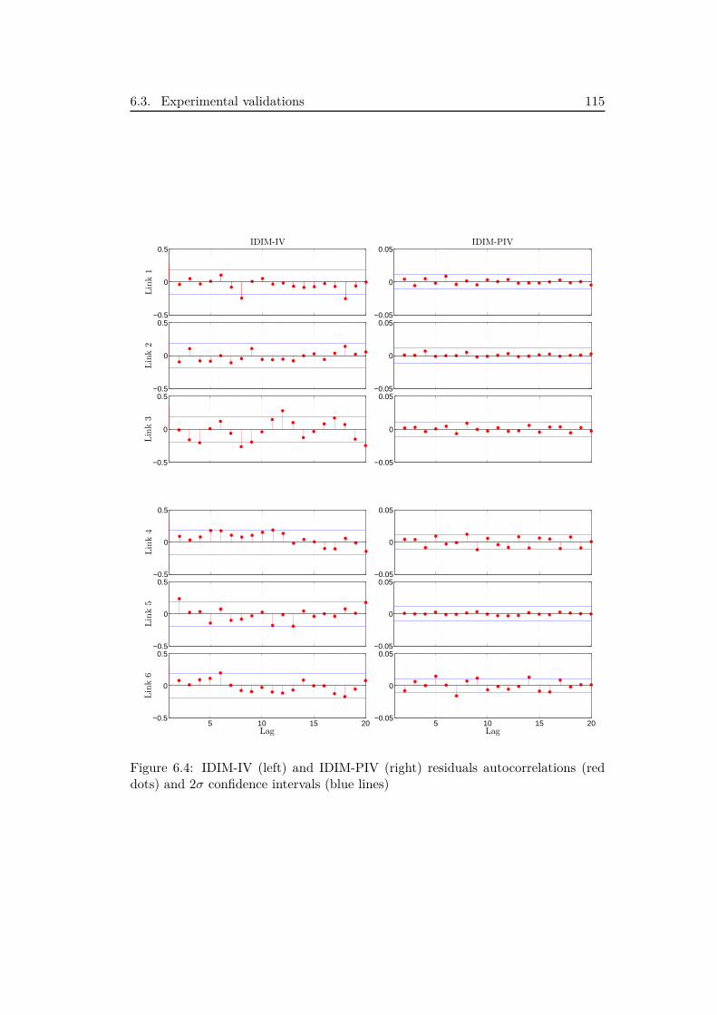
6.3. Experimental validations 115
−0.5
0
0.5
Link1
IDIM-IV
−0.05
0
0.05IDIM-PIV
−0.5
0
0.5
Link2
−0.05
0
0.05
−0.5
0
0.5
Link3
−0.05
0
0.05
−0.5
0
0.5
Link4
−0.05
0
0.05
−0.5
0
0.5
Link5
−0.05
0
0.05
5 10 15 20−0.5
0
0.5
Link6
Lag5 10 15 20
−0.05
0
0.05
Lag
Figure 6.4: IDIM-IV (left) and IDIM-PIV (right) residuals autocorrelations (reddots) and 2σ confidence intervals (blue lines)
116 Chapter 6. Noise modelling for robot system identification
the identification residuals. For the IDIM-PIV method, the effect of the refinedinput filter is clear since the estimated autocorrelations coefficients are includedin the confidence intervals indicated by the blue lines. The estimated coefficientsare larger for the IDIM-IV method and they cannot all be considered as negligiblebecause some are not included in the confidence intervals. Therefore, the serialdecorrelation is not insured.
A visual inspection of the residuals time series brings a limitation of those re-sults. In fact, as illustrated with Figure 6.6, the residuals are not perfectly ho-moskedastic: the variance changes over time. Only Link 1 is presented for thesake of clarity. A correlation can be found with the acceleration signal. The ideawould be that during acceleration phases the input noise is amplified. Here again,it appears the issue of the noise amplification during the estimation of the jointderivatives, as reminded in section 6.1.2.
6.4 Conclusions
In this chapter, the question of the noise circulation through the closed-loop systemhas been investigated. The underlying goal is to find an automated filtering of theexperimental data and have consistent estimates with covariances as low as possible.Two noise models have been drawn in section 6.1. From those models, the DIDIMand IDIM-IV methods have been revised to achieve our goal. The methods alongwith the two noise models have been assessed with the identification of the TX40based on experimental data in section 6.3. In practice, the methods have providedas accurate estimates as the usual ones. In the large noise case, the IDIM-PIVmethod has even provided estimates with lower covariances. Regarding the noisemodelling, the black-box model should be preferred for now since the suggestedgrey-box model showed some limitations.
As far as a physical interpretation of the noise is concerned, further investiga-tions should be conducted. The noise introduced by the position measurement doesnot seem indeed sufficient to explain everything. A finer model of the actuators andespecially the motors could be of some interest for this purpose.
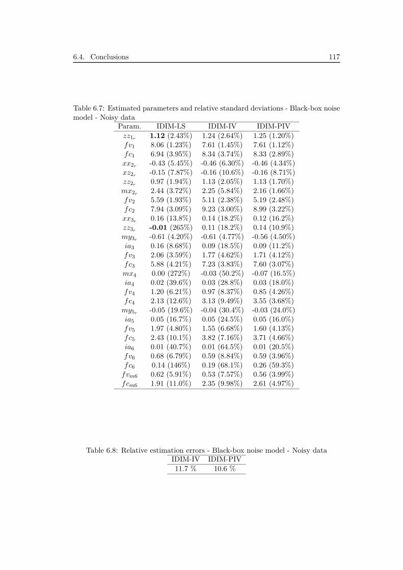
6.4. Conclusions 117
Table 6.7: Estimated parameters and relative standard deviations - Black-box noisemodel - Noisy data
Param. IDIM-LS IDIM-IV IDIM-PIVzz1r 1.12 (2.43%) 1.24 (2.64%) 1.25 (1.20%)fv1 8.06 (1.23%) 7.61 (1.45%) 7.61 (1.12%)fc1 6.94 (3.95%) 8.34 (3.74%) 8.33 (2.89%)xx2r -0.43 (5.45%) -0.46 (6.30%) -0.46 (4.34%)xz2r -0.15 (7.87%) -0.16 (10.6%) -0.16 (8.71%)zz2r 0.97 (1.94%) 1.13 (2.05%) 1.13 (1.70%)mx2r 2.44 (3.72%) 2.25 (5.84%) 2.16 (1.66%)fv2 5.59 (1.93%) 5.11 (2.38%) 5.19 (2.48%)fc2 7.94 (3.09%) 9.23 (3.00%) 8.99 (3.22%)xx3r 0.16 (13.8%) 0.14 (18.2%) 0.12 (16.2%)zz3r -0.01 (265%) 0.11 (18.2%) 0.14 (10.9%)my3r -0.61 (4.20%) -0.61 (4.77%) -0.56 (4.50%)ia3 0.16 (8.68%) 0.09 (18.5%) 0.09 (11.2%)fv3 2.06 (3.59%) 1.77 (4.62%) 1.71 (4.12%)fc3 5.88 (4.21%) 7.23 (3.83%) 7.60 (3.07%)mx4 0.00 (272%) -0.03 (50.2%) -0.07 (16.5%)ia4 0.02 (39.6%) 0.03 (28.8%) 0.03 (18.0%)fv4 1.20 (6.21%) 0.97 (8.37%) 0.85 (4.26%)fc4 2.13 (12.6%) 3.13 (9.49%) 3.55 (3.68%)my5r -0.05 (19.6%) -0.04 (30.4%) -0.03 (24.0%)ia5 0.05 (16.7%) 0.05 (24.5%) 0.05 (16.0%)fv5 1.97 (4.80%) 1.55 (6.68%) 1.60 (4.13%)fc5 2.43 (10.1%) 3.82 (7.16%) 3.71 (4.66%)ia6 0.01 (40.7%) 0.01 (64.5%) 0.01 (20.5%)fv6 0.68 (6.79%) 0.59 (8.84%) 0.59 (3.96%)fc6 0.14 (146%) 0.19 (68.1%) 0.26 (59.3%)fvm6 0.62 (5.91%) 0.53 (7.57%) 0.56 (3.99%)fcm6 1.91 (11.0%) 2.35 (9.98%) 2.61 (4.97%)
Table 6.8: Relative estimation errors - Black-box noise model - Noisy dataIDIM-IV IDIM-PIV11.7 % 10.6 %
118 Chapter 6. Noise modelling for robot system identification
−0.5
0
0.5
Link1
IDIM-IV
−0.05
0
0.05IDIM-PIV
−0.5
0
0.5
Link2
−0.05
0
0.05
5 10 15 20−0.5
0
0.5
Link3
5 10 15 20−0.05
0
0.05
−0.5
0
0.5
Link4
−0.05
0
0.05
−0.5
0
0.5
Link5
−0.05
0
0.05
5 10 15 20−0.5
0
0.5
Link6
Lag5 10 15 20
−0.05
0
0.05
Lag
Figure 6.5: IDIM-IV (left) and IDIM-PIV (right) residuals autocorrelations (reddots) and 2σ confidence intervals (blue lines) - Noisy data
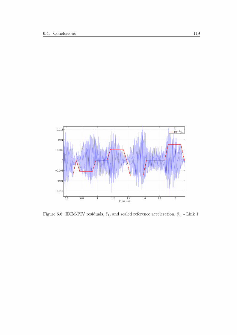
6.4. Conclusions 119
0.6 0.8 1 1.2 1.4 1.6 1.8 2
−0.015
−0.01
−0.005
0
0.005
0.01
0.015
Time (s)
e110−5qr1
Figure 6.6: IDIM-PIV residuals, e1, and scaled reference acceleration, qr1 - Link 1


Part IV
Conclusion

Chapter 7
Discussions and Future Work
In this final chapter, an overview of the contributions presented in Part III is pro-vided. The goal is to give a clear picture of how the problem of robotic systemsidentification has been tackled. The different methods that were presented haveobviously their limitations. Those are recalled in this chapter along with hints forfuture works.
7.1 Contributions summary . . . . . . . . . . . . . . . . . . . . . . 1247.1.1 Analysis of the OEM for robot identification . . . . . . . . . 1247.1.2 Robustness analysis of the IDIM-IV and DIDIM methods . . 1247.1.3 Identification with an unknown controller . . . . . . . . . . . 1247.1.4 Automated estimation of the joint derivatives . . . . . . . . . 1257.1.5 Noise filter identification . . . . . . . . . . . . . . . . . . . . . 125
7.2 A practitioner guide . . . . . . . . . . . . . . . . . . . . . . . . 1267.3 Further developments . . . . . . . . . . . . . . . . . . . . . . . 126
7.3.1 Actuator modelling . . . . . . . . . . . . . . . . . . . . . . . . 1267.3.2 Friction modelling . . . . . . . . . . . . . . . . . . . . . . . . 1267.3.3 Broader perspectives . . . . . . . . . . . . . . . . . . . . . . . 128
124 Chapter 7. Discussions and Future Work
7.1 Contributions summary
7.1.1 Analysis of the OEM for robot identification
The preliminary comparison of the DIDIM and CLOE methods introduced in [Janotet al. 2014a] has been enlarged in Chapter 4 to consider the CLIE method. It hasbeen highlighted the relation between the methods CLIE and DIDIM. The interestof considering those methods instead of the CLOE one has been shown. The inputtorque appears indeed to have a better sensitivity to the parameters. The difficultyof extending this result to non-robotic systems has been discussed in the samechapter. Furthermore, the role of the decimate filter for robot identification hasbeen emphasized. It thus appeared the dual nature of the DIDIM method which isneither an output error method nor a prediction error one, because the measurementnoise is neither white nor modelled.
7.1.2 Robustness analysis of the IDIM-IV and DIDIM methods
One of the major contributions of this thesis is the comparison of the IDIM-IVand DIDIM methods. Both methods proved to be effective solutions for robotidentification. It is known that both methods are iterative and can share the sameconvergence criterion and initial values. By contrast, the DIDIM method doesnot require the same careful bandpass filtering as the IDIM-IV one to build theobservation matrix [Gautier et al. 2013a]. The novelty lies in the demonstrationof the better robustness of the IDIM-IV method to a modelling error located inthe auxiliary model. That has been experimentally validated with the TX40 robotin Chapter 4. Furthermore, it has been also highlighted that a special attentionmust be paid to the evaluation of the estimates’ covariance if any errors exist. Thiscontribution was presented in [Brunot et al. 2017c].
7.1.3 Identification with an unknown controller
In this thesis work, considering our necessity to process data coming from closed-loop experiments, it has been decided to consider the case where the control lawis not available. If some works have already dealt with this problem, they consid-ered LTI systems only. To overcome the nonlinear feature of robotic models, theperspective has been changed in order to treat the identification of the controllerseparately from the rest of the system. Two scenarios have been envisaged depend-ing on the practitioner’s goal. Firstly, if the objective is to know the actual controllaw or if there is enough time available, the controller can be parametrically iden-tified. That could be a complex task especially if nonlinearities are included in thelaw. Secondly, the practitioner can choose a non-parametric identification to sparetime and focus on the dynamic model, at the cost of a less complete knowledgeon the system. Those two approaches are quite novel and have been successfullytested with the TX40 robot in Chapter 5, by considering the IDIM-IV and DIDIMmethods. This work has been submitted in [Brunot et al. Submitted 2017].
7.1. Contributions summary 125
Perspectives include considering unknown models of the actuators as well asmore complex control laws. An assessment of the control laws identifiability couldalso be of interest from an industrial perspective. For a robot manufacturer, thedual goal would be indeed to discover the competitor’s control law and keep its ownsecret.
7.1.4 Automated estimation of the joint derivatives
As mentioned previously, the usual identification methods, IDIM-LS and IDIM-IV,need a numerical differentiation of the measured position signal that comes witha bandpass filter to avoid noise amplification. In order to reduce the informationnecessary to deal with the setting of the filter, we wanted to find another automaticmethod for the differentiation of the measured signal. We have tested a solution,called IRWSM, based on a random walk model, a Kalman filter and a FIS that wasoriginally developed for time varying parameters estimation. It has been shownthat the random walk model does not exactly represent the dynamics of the roboticsystem. Nonetheless, it has been observed that the use of the IRWSM improvesthe performances, especially when the system’s bandwidths are unavailable to thepractitioner. However, some limitations to this contribution can be mentioned:
• A modified version of the model taking into account the reference trajectory asan input could be of some interest in a similar manner to [Kostic et al. 2004];
• The automated IRWSM approach allows a consistent estimation of the dy-namic parameters but their standard deviations. Another procedure is re-quired to automatically set the cut-off frequency of the decimate filter.
7.1.5 Noise filter identification
To deal with the setting of the decimate filter, the usual approach of the systemidentification community has been investigated. The idea is to filter the data by theinverse of the estimated noise model. That technique has the advantage of insuringoptimal estimates for LTI systems. If the optimality is not our target with thenonlinear robot models, a refinement of estimates is of some interest along with theautomation of the process. To achieve such a goal, a discussion has been initiatedon the noise seen by the identification algorithm coming from the whole closed-loopsystem. The identification of the noise model has been thought to be automaticwithout a priori knowledge on the system. The IDIM-IV and DIDIM methods havebeen reconsidered to integrate the noise filter identification as well as the resultingprefiltering. Furthermore, it appeared an alternative way to automatically estimatethe order of the decimate filter thanks to the Akaike information criterion.
The experimental results have shown that the approach is suitable to identifyan industrial robot systematically and can even improve the precision, based on ablack-box noise model. Nonetheless, it appeared that our understanding of the noisecirculation through the closed-loop system is still limited. A perspective would beto develop a more comprehensive grey-box noise model.
126 Chapter 7. Discussions and Future Work
7.2 A practitioner guide
We reconsider the identification process depicted in Figure 1.3. Based on the con-tributions, Figure 7.1 describes our vision of the process including the developedmethodologies. The a priori information block is replaced by three preliminaryquestions put to the user. Those three questions are the following:
• Does the practitioner know the system’s bandwidth? If the answer is posi-tive, the usual methods based on the bandpass and decimate filters can beused. Otherwise, the joint derivatives should be estimated with the IRWSMapproach. Concerning the noise whitening, the practitioner can either iden-tify a black-box noise model or tune the decimate filter thanks to the AIC.A third solution, which we would recommend, consists in coupling a roughlytuned decimate filter and the identification of a filter modelling the remainingnoise. The cost of this solution is the lost of the physical interpretation of theidentified noise model.
• Does the practitioner know the system’s controller? If the answer is negative,the identification of the controller must be performed. If the objective is touse the DIDIM method or if there is an interest in the controller knowledge,a parametric identification must be conducted. Otherwise, a non-parametricidentification coupled with the IDIM-IV method can achieve the goal.
• Is there an interest in a statistical analysis? If the answer is positive, thenoise identification should be performed with a black-box or even a grey-boxmodel. Otherwise, the usual decimate filtering can provide reliable estimatedparameters in potentially less computation time.
7.3 Further developments
7.3.1 Actuator modelling
Regarding the modelling, the characterisation of the actuators would be an inter-esting development. Along this thesis, they have indeed been considered as knownsubsystems and more specifically as static gains. Their knowledge could improvethe understanding of the noise model. In this regard, further efforts are needed tobetter understand the noise faced by the identification methods. A more compre-hensive statistical analysis could be of interest.
7.3.2 Friction modelling
As shown in Chapter 2, the dynamic models are formulated from the Newton’s lawsor Lagrange’s equations. The practitioner thus needs a complete knowledge of thephysical phenomena. One major difficulty lies in the model of the friction which isusually nonlinear at low velocities and may depend on many exogenous parameters
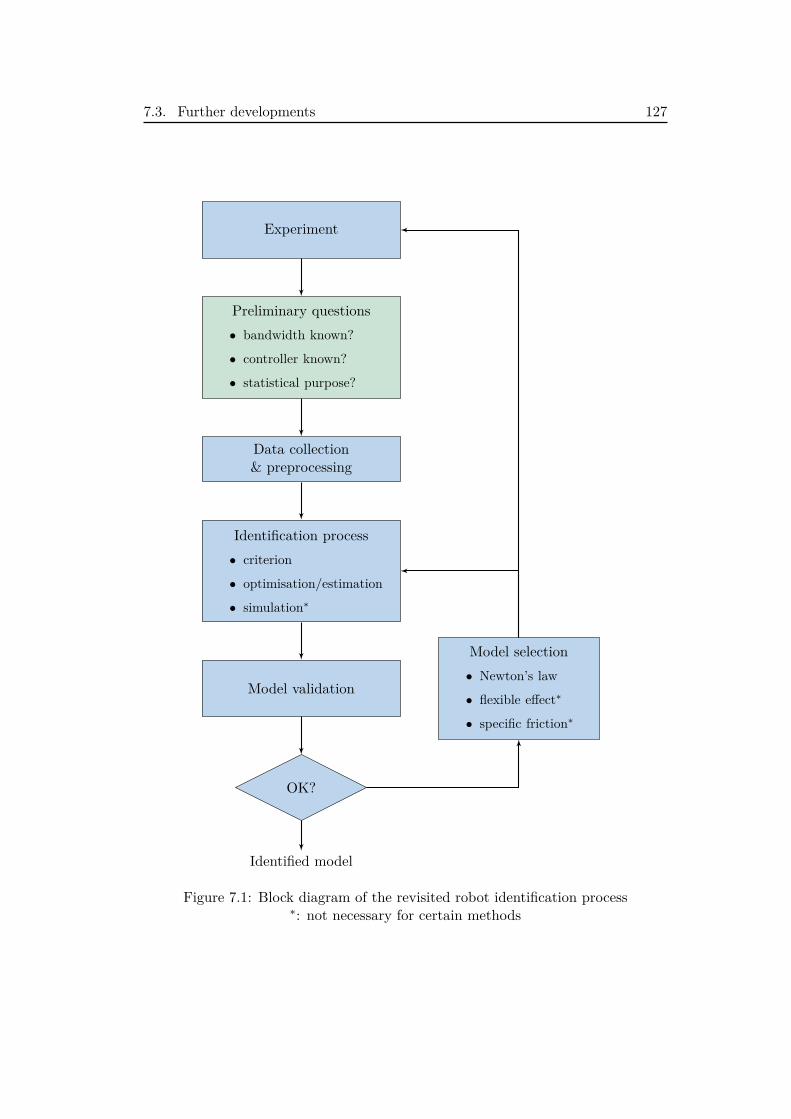
7.3. Further developments 127
Experiment
Preliminary questions• bandwidth known?
• controller known?
• statistical purpose?
Data collection& preprocessing
Identification process• criterion
• optimisation/estimation
• simulation∗
Model validation
Model selection• Newton’s law
• flexible effect∗
• specific friction∗
OK?
Identified model
Figure 7.1: Block diagram of the revisited robot identification process∗: not necessary for certain methods
128 Chapter 7. Discussions and Future Work
like the temperature; see e.g. [Bittencourt & Axelsson 2014]. Therefore, the frictionremains a major challenge for robot identification.
Recently, in [Janot et al. 2017], a new way of dealing with this challenge hasbeen introduced. The idea is to separate the problem in two: a "grey-box" part re-grouping the inertial forces and a "black-box" part to capture the nonlinear effectsof the friction. The grey-box part is identified with an usual method described insection 2.3 like the IDIM-IV one. The black-box part is non-parametrically identi-fied with the State-Dependent Parameter (SDP) method. In a second time, fromthe non-parametric model provided by the SDP method, a parametric model of thefriction can be identified. This method is a statistical procedure able to identifythe presence of nonlinearities in dynamic system models by giving their graphicalshape. The procedure is based on experimental sampled data, with a minimum ofassumptions about the nature of the nonlinearities. The SDP estimation algorithmis an extension of the stochastic approach to Time-Varying Parameter (TVP) esti-mation; see e.g. [Young 1999] and the prior references therein. The SDP methodrepresents thus a valuable tool which should be further investigated in order to dealwith more complex nonlinear friction phenomena. In addition, it could be of someinterest to consider techniques like the one developed in [Noël & Schoukens 2017]where the model is divided in a linear part and a nonlinear one. The nonlinearityis then seen as an additional input applied to the underlying linear system.
7.3.3 Broader perspectives
As far as the robot identification is concerned, the amount of knowledge required forthe process has been reduced in Chapter 5 and Chapter 6. Further developmentsshould focus on considering the element in the process that has not been studied:the design of excitation signals. In fact, to a certain extent, the design of inputsignals for identification can require a priori knowledge.
Regarding the identification methods themselves, they could be adapted to workin a recursive framework. The goal would be ultimately to perform online identi-fication for monitoring or adaptive control. Furthermore, the application of thosemethods to other closed-loop or nonlinear systems could be explored. This hasbeen started with the study of the output error methods for nonlinear systems withundefined sensitivity functions [Brunot et al. 2017a].

Part V
Appendices

Appendix A
Industrial robot modelling
This appendix summarizes the main results for robot modelling in order to have acomprehensive overview. All the elements presented here can be found in [Khalil &Dombre 2004] or [Siciliano et al. 2010] for instance.
A.1 Computation of the energies
This section is devoted to the development of the kinetic and potential energiesrequired to compute the Lagrangian of an industrial robot. As explained in section2.1, those energies are linear with respect to the standard dynamic parameters. Letus consider a link j where
• Gj and Oj are respectively the center of mass and the origin of link j;
• Lj is the (3× 1) vector from the Oj−1 to Oj ;
• Sj is the (3× 1) vector from the origin point to the center of gravity, definedin section 2.1.3.
Kinetic energy
For a robot with n links, the kinematic energy is given by:
E =n∑j=1
Ej , (A.1)
with Ej the kinematic energy of link j. By introducing the (3 × 1) vectors ωjand V Gj , which are respectively the angular velocity and the linear velocity (atthe center of gravity Gj) of link j, defined in the inertial frame R0 (fixed base), itcomes out:
Ej = 12(ωTj JGjωj +MjV
TGjV Gj
)(A.2)
where JGj is the inertia tensor at the center of gravity Gj and Mj is the mass ofthe link. By composition of the velocities, we have:
V Gj = V Oj + ωj ∧ Sj , (A.3)
with the cross-product ∧. With respect to the Huygens-Steiner theorem, the inertiatensor at the origin is
JOj = JGj −MjSSj , (A.4)
132 Appendix A. Industrial robot modelling
where Sj is the (3 × 3) skew-symmetric matrix defined by the components of thevector Sj in order to calculate the vector product Sj ∧ Sj . Hence (A.2) can bedeveloped:
Ej = 12[ωTj JOjωj −Mjω
Tj SSjωj +Mj
(V Oj + ωj ∧ Sj
)T (V Oj + ωj ∧ Sj
)]= 1
2[ωTj JOjωj +MjV
TOjV Oj + 2MjV
TOj (ωj ∧ Sj) (A.5)
−MjωTj SSjωj +Mj (ωj ∧ Sj)T (ωj ∧ Sj)
].
Using the scalar triple product, it comes out: V TOj (ωj ∧ Sj) = STj
(V Oj ∧ ωj
).
Furthermore, it appears (ωj ∧ Sj)T (ωj ∧ Sj) =(Sjωj
)T (Sjωj
)= ωTj SSjωj .
Therefore, the kinematic energy of link j can be written as a function of the inertiaand velocities defined in Oj such as:
Ej = 12[ωTj JOjωj +MjV
TOjV Oj + 2MjS
Tj
(V Oj ∧ ωj
)](A.6)
If (A.2) is linear in the elements of JGj , it is not linear with respect to the distancesof the vector Sj . On the contrary, (A.6) has the advantage to be linear in the massMj and the elements of JOj and MSj ; i.e. the standard inertial parameters.
Until this point, the velocities were expressed with respect to the inertial frame,R0. To be consistent with the standard parameters introduced in section 2.1.3,the kinematic energy should be expressed as a function of the velocities and theparameters in the frame Rj . We introduce the rotation matrix Rj
0(qnf ), from R0to Rj , such as:
ωj = Rj0(qnf )jωj , V Oj = Rj
0(qnf )jV Oj ,
jJOj =(Rj
0(qnf ))T
JOjRj0(qnf ), MSj = Rj
0(qnf )jMSj ,
with the superscript j, before the vectors, which indicates that it is expressed inframe Rj . Consequently, it appears a dependence on the relative positions, qnf ,due to the rotations. To make the notation less cluttered, the dependence on therelative positions will not be expressed thereafter. Since it is a rotation matrix, wehave (Rj
0)−1 = (Rj0)T = R0
j . Eq. (A.6) can be rewritten:
Ej = 12[(ωj)T (Rj
0)T jJOjRj0ωj +Mj(V Oj )TV Oj + 2(jMSj)TR0
j
(V Oj ∧ ωj
)].
Relations between velocities
In the previous part, the energy was expressed as a function of the translationaland rotational velocity vectors. We need to express those velocities as functions ofthe joint derivatives. For that purpose, we define the prismatic boolean prj whichis equal to 0 or 1 if the joint is revolute or prismatic respectively. In practice, the
A.1. Computation of the energies 133
velocities of each link are recursively calculated such as:
ωj = ωj−1 + prj qnfjzj , (A.7)V Oj = V Oj−1 + ωj−1 ∧Lj + prj qnfjzj , (A.8)
with zj the unit vector defined in section 2.1.1. Considering that the base is fixed,we have V O0 = 03 and ω0 = 03. It should be noticed that the vector Lj containsqnfj if the link is prismatic. From those recursive relations, it comes the linearexpressions:
ωj = Tjωqnf , (A.9)
V Oj = TjV qnf , (A.10)
with Tjω and Tj
ω two (3× n) jacobian matrices defined by:
Tjω =
[tjω1 . . . tjωj 03 . . . 03
], (A.11)
TjV =
[tjV 1 . . . tjV j 03 . . . 03
]. (A.12)
As explained in [Siciliano et al. 2010], the (6 × n) matrix Tn is the manipulatorgeometric Jacobian
Tn =[Tnω
TnV
]. (A.13)
According to the recursive relations (A.7) and (A.8), the columns can be computedsuch as
tjωk = prkzk (A.14)
tjV k = prkzk + prkzk ∧Lj , (A.15)
with 1 ≤ k ≤ j.
With the scalar triple product, it comes out:
(jMSj)TR0j
(V Oj ∧ ωj
)= (ωj)T
((Rj
0)T (jMSj) ∧ V Oj
)= (Tj
ωqnf )T(Rj
0 (jMSj) ∧TjV qnf
)= qTnf (Tj
ω)T MSjTjV qnf ,
where MSj =
0 −c b
c 0 −a−b a 0
and Rj0 (jMSj) =
abc
.At last, we have shown that the kinetic energy can also be written:
E = 12 q
TnfM(qnf )qnf , (A.16)
134 Appendix A. Industrial robot modelling
with M the (n × n) inertia matrix. The diagonal element Mjj are the coefficientsof q2
nfj/2 and, for i 6= j, Mij = Mji is equal to the coefficient of qnfi qnfj .
Potential energy
The potential energy of the robot arm is defined as
U =n∑j=1
Uj =n∑j=1−Mjg
T (L0,j + Sj) =n∑j=1−gT (MjL0,j +MSj) (A.17)
with L0,j the (3× 1) vectors from the origin of the base O0 to Oj and g the (3× 1)vector of gravity. The potential energy is thus linear with respect to Mj and theelements of MSj . Here also the vectors must be projected in the same frame It isvisible in (A.17) that the potential energy is not function of the velocities: ∂U
∂qnf= 0.
Lagrangian
As a reminder, the Lagrangian is defined such as L = E − U and the input torqueis calculated with (2.2). Therefore, it comes out:
τ idm = d
dt
(∂L
∂qnf
)− ∂L
∂qnf+ τ f (A.18)
= d
dt
(∂E
∂qnf
)− ∂E
∂qnf− ∂U
∂qnf+ τ f
= d
dt
(M(qnf )qnf
)− ∂E
∂qnf− ∂U
∂qnf+ τ f
= M(qnf )qnf + M(qnf )qnf −∂E
∂qnf− ∂U
∂qnf+ τ f
= M(qnf )qnf +(
M(qnf )qnf −∂E
∂qnf
)+ τ f −
∂U
∂qnf.
This proves the IDM relation (2.3) with C(qnf , qnf )qnf = M(qnf )qnf − ∂E∂qnf
.Noting that for any i and j:
Mij(qnf ) =n∑k=1
∂qnfk∂t
∂Mij(qnf )∂qk
=n∑k=1
∂Mij(qnf )∂qk
qnfk , (A.19)
and by using (A.16), it comes out:
Cij(qnf , qnf ) =n∑k=1
cijkqnfk , (A.20)
withcijk =
∂Mij(qnf )∂qk
− 12∂Mjk(qnf )
∂qi. (A.21)
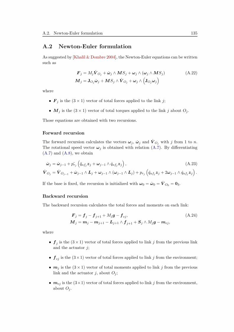
A.2. Newton-Euler formulation 135
A.2 Newton-Euler formulation
As suggested by [Khalil & Dombre 2004], the Newton-Euler equations can be writtensuch as
F j = MjV Oj + ωj ∧MSj + ωj ∧ (ωj ∧MSj) (A.22)
M j = JOj ωj +MSj ∧ V Oj + ωj ∧(JOjωj
)where
• F j is the (3× 1) vector of total forces applied to the link j;
• M j is the (3× 1) vector of total torques applied to the link j about Oj .
Those equations are obtained with two recursions.
Forward recursion
The forward recursion calculates the vectors ωj , ωj and V Oj with j from 1 to n.The rotational speed vector ωj is obtained with relation (A.7). By differentiating(A.7) and (A.8), we obtain
ωj = ωj−1 + prj
(qnfjzj + ωj−1 ∧ qnfjzj
), (A.23)
V Oj = V Oj−1 + ωj−1 ∧Lj + ωj−1 ∧ (ωj−1 ∧Lj) + prj
(qnfjzj + 2ωj−1 ∧ qnfjzj
).
If the base is fixed, the recursion is initialized with ω0 = ω0 = V O0 = 03.
Backward recursion
The backward recursion calculates the total forces and moments on each link:
F j = f j − f j+1 +Mjg − f ej , (A.24)M j = mj −mj+1 −Lj+1 ∧ f j+1 + Sj ∧Mjg −mej ,
where
• f j is the (3× 1) vector of total forces applied to link j from the previous linkand the actuator j;
• f ej is the (3×1) vector of total forces applied to link j from the environment;
• mj is the (3× 1) vector of total moments applied to link j from the previouslink and the actuator j, about Oj ;
• mej is the (3×1) vector of total forces applied to link j from the environment,about Oj .
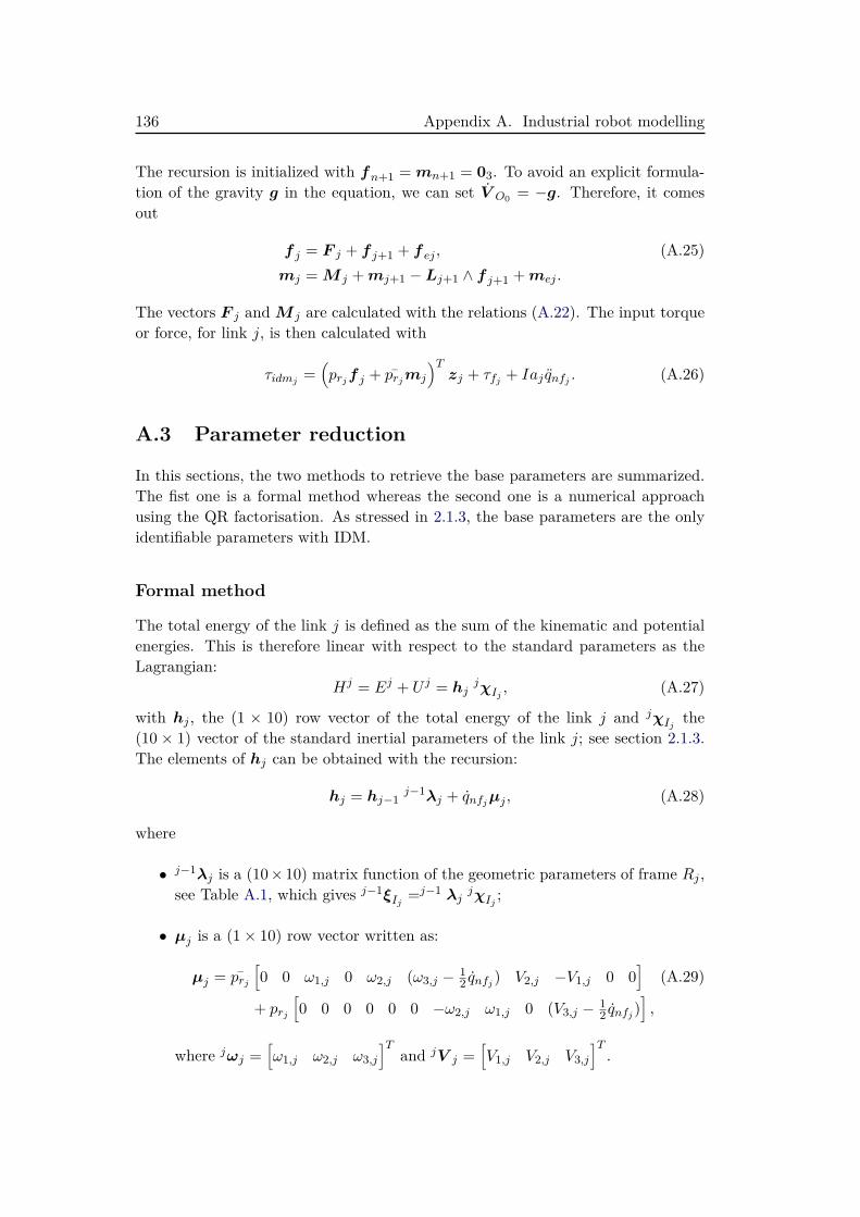
136 Appendix A. Industrial robot modelling
The recursion is initialized with fn+1 = mn+1 = 03. To avoid an explicit formula-tion of the gravity g in the equation, we can set V O0 = −g. Therefore, it comesout
f j = F j + f j+1 + f ej , (A.25)mj = M j +mj+1 −Lj+1 ∧ f j+1 +mej .
The vectors F j andM j are calculated with the relations (A.22). The input torqueor force, for link j, is then calculated with
τidmj =(prjf j + prjmj
)Tzj + τfj + Iaj qnfj . (A.26)
A.3 Parameter reduction
In this sections, the two methods to retrieve the base parameters are summarized.The fist one is a formal method whereas the second one is a numerical approachusing the QR factorisation. As stressed in 2.1.3, the base parameters are the onlyidentifiable parameters with IDM.
Formal method
The total energy of the link j is defined as the sum of the kinematic and potentialenergies. This is therefore linear with respect to the standard parameters as theLagrangian:
Hj = Ej + U j = hjjχIj , (A.27)
with hj , the (1 × 10) row vector of the total energy of the link j and jχIj the(10 × 1) vector of the standard inertial parameters of the link j; see section 2.1.3.The elements of hj can be obtained with the recursion:
hj = hj−1j−1λj + qnfjµj , (A.28)
where
• j−1λj is a (10× 10) matrix function of the geometric parameters of frame Rj ,see Table A.1, which gives j−1ξIj =j−1 λj
jχIj ;
• µj is a (1× 10) row vector written as:
µj = prj
[0 0 ω1,j 0 ω2,j (ω3,j − 1
2 qnfj ) V2,j −V1,j 0 0]
(A.29)
+ prj
[0 0 0 0 0 0 −ω2,j ω1,j 0 (V3,j − 1
2 qnfj )],
where jωj =[ω1,j ω2,j ω3,j
]Tand jV j =
[V1,j V2,j V3,j
]T.
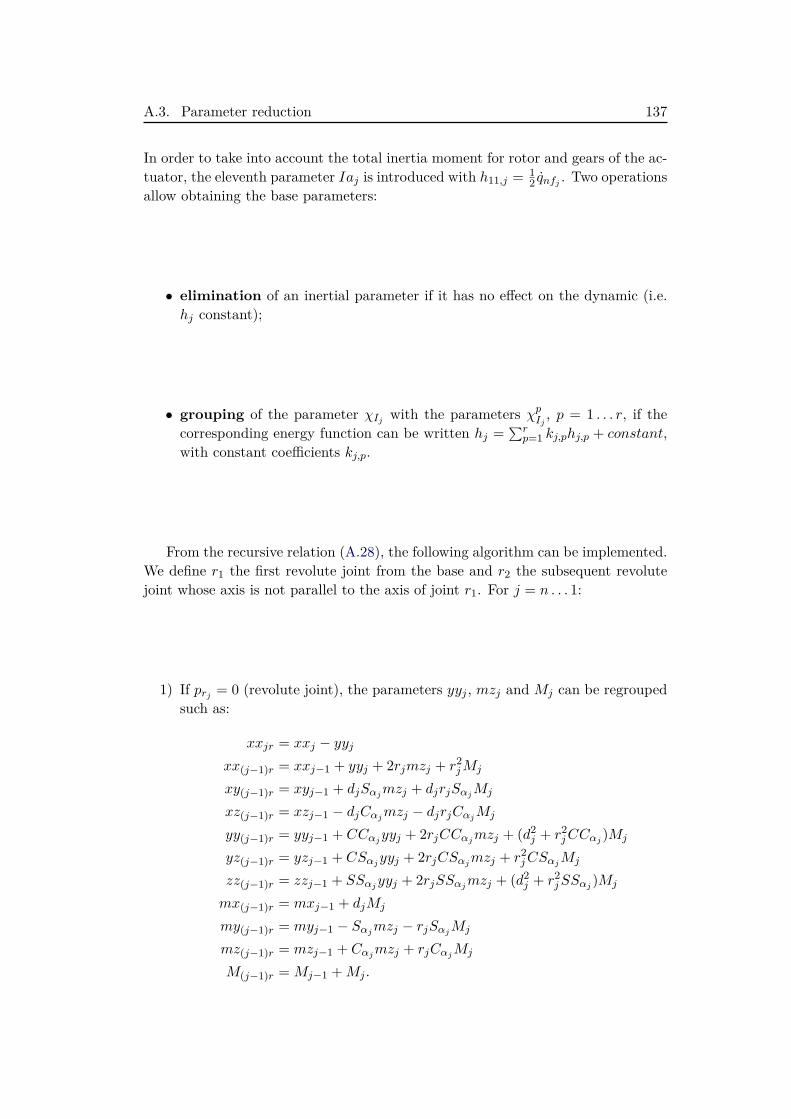
A.3. Parameter reduction 137
In order to take into account the total inertia moment for rotor and gears of the ac-tuator, the eleventh parameter Iaj is introduced with h11,j = 1
2 qnfj . Two operationsallow obtaining the base parameters:
• elimination of an inertial parameter if it has no effect on the dynamic (i.e.hj constant);
• grouping of the parameter χIj with the parameters χpIj , p = 1 . . . r, if thecorresponding energy function can be written hj =
∑rp=1 kj,phj,p + constant,
with constant coefficients kj,p.
From the recursive relation (A.28), the following algorithm can be implemented.We define r1 the first revolute joint from the base and r2 the subsequent revolutejoint whose axis is not parallel to the axis of joint r1. For j = n . . . 1:
1) If prj = 0 (revolute joint), the parameters yyj , mzj and Mj can be regroupedsuch as:
xxjr = xxj − yyjxx(j−1)r = xxj−1 + yyj + 2rjmzj + r2
jMj
xy(j−1)r = xyj−1 + djSαjmzj + djrjSαjMj
xz(j−1)r = xzj−1 − djCαjmzj − djrjCαjMj
yy(j−1)r = yyj−1 + CCαjyyj + 2rjCCαjmzj + (d2j + r2
jCCαj )Mj
yz(j−1)r = yzj−1 + CSαjyyj + 2rjCSαjmzj + r2jCSαjMj
zz(j−1)r = zzj−1 + SSαjyyj + 2rjSSαjmzj + (d2j + r2
jSSαj )Mj
mx(j−1)r = mxj−1 + djMj
my(j−1)r = myj−1 − Sαjmzj − rjSαjMj
mz(j−1)r = mzj−1 + Cαjmzj + rjCαjMj
M(j−1)r = Mj−1 +Mj .
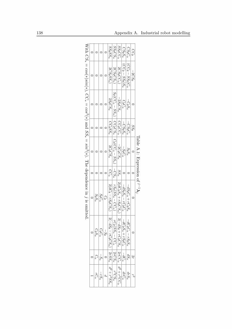
138 Appendix A. Industrial robot modelling
TableA.1:
Expressionof
j−1λ
j
CCθ
−2CSθ
0SSθ
00
00
2rr 2
CSθ C
α(CCθ −
SSθ )C
α−Cθ S
α−CSθ C
αSθ S
α0
−dSθ C
α+rC
θ Sα
−dCθ C
α−rS
θ Sα
dSα
drS
α
CSθ S
α(CCθ −
SSθ )S
αCθ C
α−CSθ S
α−Sθ C
α0
−dSθ S
α−r C
θ Cα
−dCθ S
α+r S
θ Cα
−dCα
dr C
α
SSθ CCα
2CSθ CCα )
−2S
θ CSα
CCθ CCα
−2C
θ CSα
SSα
2(dCθ S
α+rS
θ CSα )
2(−dSθ +
rCθ CSα
2rCCα
d2+
r 2CCα
SSθ CSα
2CSθ CSα )
Sθ (C
Cα−SSα )
CCθ CSα
Cθ (C
Cα−SSα )
−CSα
rSθ (S
Sα−CCα )
rCθ (S
Sα−CCα
2rCSα
r 2CSα
SSθ SSα
2CSθ SSα )
2Sθ CSα
CCθ SSα
2Cθ CSα
CCα
2(dCθ −
r Sθ CSα )
2(−dSθ −
r Cθ CSα )
2r SSα
d2+
r 2SSα
00
00
00
Cθ
−Sθ
0d
00
00
00
Sθ C
αCθ C
α−Sα
−rS
α
00
00
00
Sθ S
αCθ S
αCα
r Cα
00
00
00
00
01
With
CS∗
=cos(∗)sin(∗),
CC∗
=cos 2(∗)
andSS∗
=sin
2(∗).The
dependenceinjis
omitted.
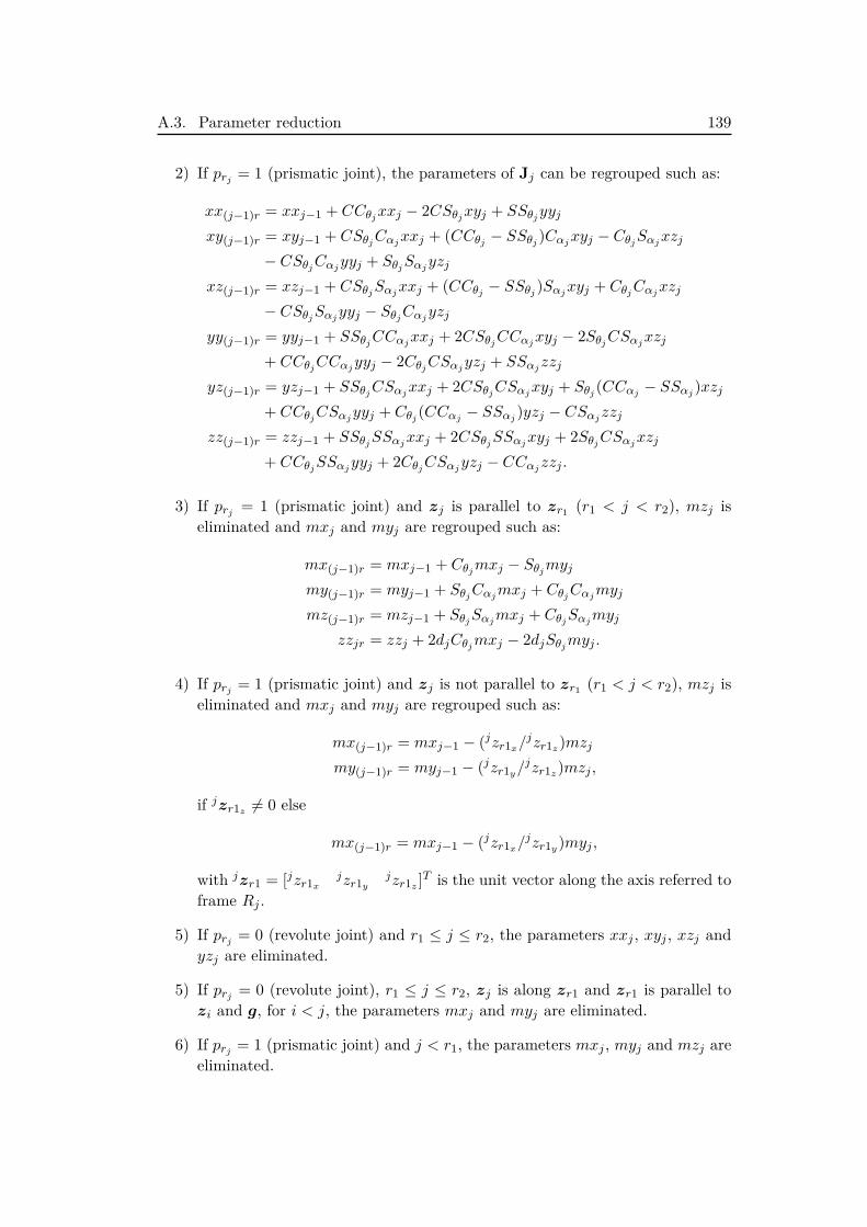
A.3. Parameter reduction 139
2) If prj = 1 (prismatic joint), the parameters of Jj can be regrouped such as:
xx(j−1)r = xxj−1 + CCθjxxj − 2CSθjxyj + SSθjyyj
xy(j−1)r = xyj−1 + CSθjCαjxxj + (CCθj − SSθj )Cαjxyj − CθjSαjxzj− CSθjCαjyyj + SθjSαjyzj
xz(j−1)r = xzj−1 + CSθjSαjxxj + (CCθj − SSθj )Sαjxyj + CθjCαjxzj
− CSθjSαjyyj − SθjCαjyzjyy(j−1)r = yyj−1 + SSθjCCαjxxj + 2CSθjCCαjxyj − 2SθjCSαjxzj
+ CCθjCCαjyyj − 2CθjCSαjyzj + SSαjzzj
yz(j−1)r = yzj−1 + SSθjCSαjxxj + 2CSθjCSαjxyj + Sθj (CCαj − SSαj )xzj+ CCθjCSαjyyj + Cθj (CCαj − SSαj )yzj − CSαjzzj
zz(j−1)r = zzj−1 + SSθjSSαjxxj + 2CSθjSSαjxyj + 2SθjCSαjxzj+ CCθjSSαjyyj + 2CθjCSαjyzj − CCαjzzj .
3) If prj = 1 (prismatic joint) and zj is parallel to zr1 (r1 < j < r2), mzj iseliminated and mxj and myj are regrouped such as:
mx(j−1)r = mxj−1 + Cθjmxj − Sθjmyjmy(j−1)r = myj−1 + SθjCαjmxj + CθjCαjmyj
mz(j−1)r = mzj−1 + SθjSαjmxj + CθjSαjmyj
zzjr = zzj + 2djCθjmxj − 2djSθjmyj .
4) If prj = 1 (prismatic joint) and zj is not parallel to zr1 (r1 < j < r2), mzj iseliminated and mxj and myj are regrouped such as:
mx(j−1)r = mxj−1 − (jzr1x/jzr1z)mzjmy(j−1)r = myj−1 − (jzr1y/jzr1z)mzj ,
if jzr1z 6= 0 else
mx(j−1)r = mxj−1 − (jzr1x/jzr1y)myj ,
with jzr1 = [jzr1x jzr1yjzr1z ]T is the unit vector along the axis referred to
frame Rj .
5) If prj = 0 (revolute joint) and r1 ≤ j ≤ r2, the parameters xxj , xyj , xzj andyzj are eliminated.
5) If prj = 0 (revolute joint), r1 ≤ j ≤ r2, zj is along zr1 and zr1 is parallel tozi and g, for i < j, the parameters mxj and myj are eliminated.
6) If prj = 1 (prismatic joint) and j < r1, the parameters mxj , myj and mzj areeliminated.
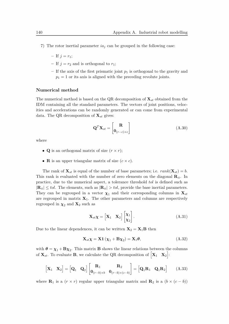
140 Appendix A. Industrial robot modelling
7) The rotor inertial parameter iaj can be grouped in the following case:
– If j = r1;
– If j = r2 and is orthogonal to r1;
– If the axis of the first prismatic joint p1 is orthogonal to the gravity andp1 = 1 or its axis is aligned with the preceding revolute joints.
Numerical method
The numerical method is based on the QR decomposition of Xst obtained from theIDM containing all the standard parameters. The vectors of joint positions, veloc-ities and accelerations can be randomly generated or can come from experimentaldata. The QR decomposition of Xst gives:
QTXst =[
R0(r−c)×c
](A.30)
where
• Q is an orthogonal matrix of size (r × r);
• R is an upper triangular matrix of size (c× c).
The rank of Xst is equal of the number of base parameters; i.e. rank(Xst) = b.This rank is evaluated with the number of zero elements on the diagonal Rii. Inpractice, due to the numerical aspect, a tolerance threshold tol is defined such as|Rii| ≤ tol. The elements, such as |Rii| > tol, provide the base inertial parameters.They can be regrouped in a vector χ1 and their corresponding columns in Xst
are regrouped in matrix X1. The other parameters and columns are respectivelyregrouped in χ2 and X2 such as
Xstχ =[X1 X2
] [χ1χ2
]. (A.31)
Due to the linear dependences, it can be written X2 = X1B then
Xstχ = X1 (χ1 + Bχ2) = X1θ, (A.32)
with θ = χ1 + Bχ2. This matrix B shows the linear relations between the columnsof Xst. To evaluate B, we calculate the QR decomposition of
[X1 X2
]:
[X1 X2
]=[Q1 Q2
] [ R1 R20(r−b)×b 0(r−b)×(c−b)
]=[Q1R1 Q1R2
](A.33)
where R1 is a (r × r) regular upper triangular matrix and R2 is a (b × (c − b))

A.3. Parameter reduction 141
matrix. We get
X1 = Q1R1 (A.34)X2 = Q1R2 = X1R−1
1 R2
and finallyθ = χ1 + R−1
1 R2χ2. (A.35)

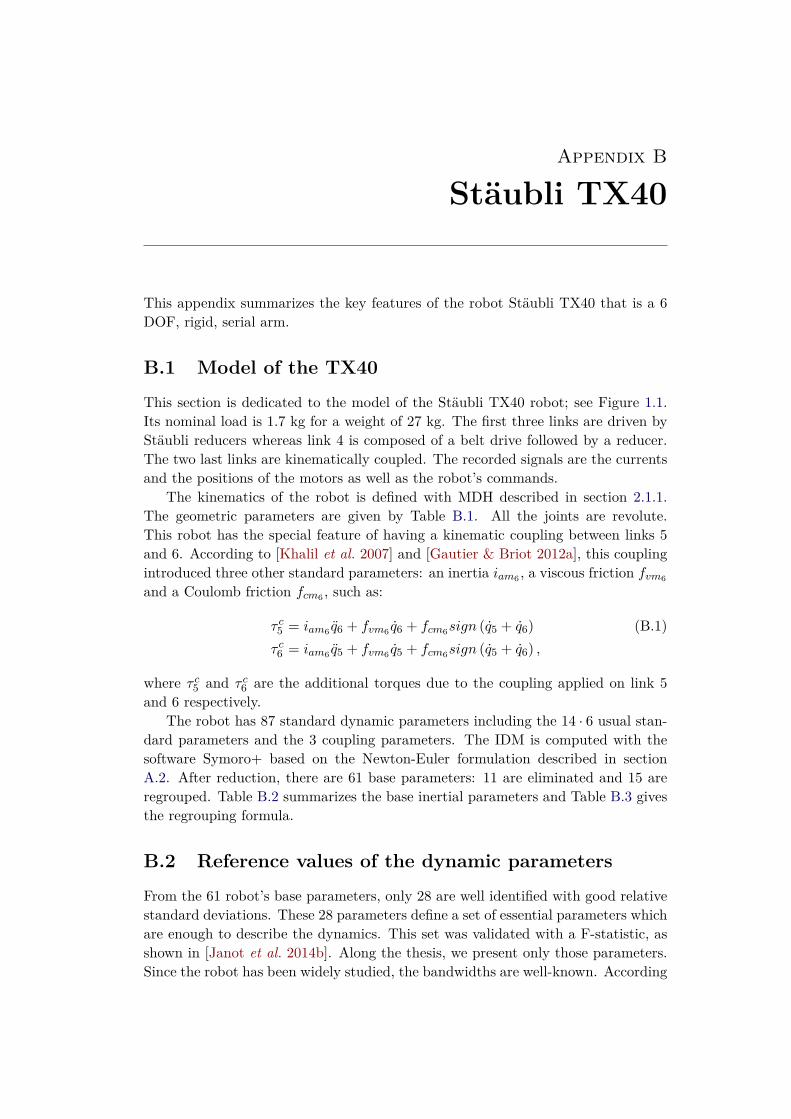
Appendix B
Stäubli TX40
This appendix summarizes the key features of the robot Stäubli TX40 that is a 6DOF, rigid, serial arm.
B.1 Model of the TX40
This section is dedicated to the model of the Stäubli TX40 robot; see Figure 1.1.Its nominal load is 1.7 kg for a weight of 27 kg. The first three links are driven byStäubli reducers whereas link 4 is composed of a belt drive followed by a reducer.The two last links are kinematically coupled. The recorded signals are the currentsand the positions of the motors as well as the robot’s commands.
The kinematics of the robot is defined with MDH described in section 2.1.1.The geometric parameters are given by Table B.1. All the joints are revolute.This robot has the special feature of having a kinematic coupling between links 5and 6. According to [Khalil et al. 2007] and [Gautier & Briot 2012a], this couplingintroduced three other standard parameters: an inertia iam6 , a viscous friction fvm6
and a Coulomb friction fcm6 , such as:
τ c5 = iam6 q6 + fvm6 q6 + fcm6sign (q5 + q6) (B.1)τ c6 = iam6 q5 + fvm6 q5 + fcm6sign (q5 + q6) ,
where τ c5 and τ c6 are the additional torques due to the coupling applied on link 5and 6 respectively.
The robot has 87 standard dynamic parameters including the 14 · 6 usual stan-dard parameters and the 3 coupling parameters. The IDM is computed with thesoftware Symoro+ based on the Newton-Euler formulation described in sectionA.2. After reduction, there are 61 base parameters: 11 are eliminated and 15 areregrouped. Table B.2 summarizes the base inertial parameters and Table B.3 givesthe regrouping formula.
B.2 Reference values of the dynamic parameters
From the 61 robot’s base parameters, only 28 are well identified with good relativestandard deviations. These 28 parameters define a set of essential parameters whichare enough to describe the dynamics. This set was validated with a F-statistic, asshown in [Janot et al. 2014b]. Along the thesis, we present only those parameters.Since the robot has been widely studied, the bandwidths are well-known. According
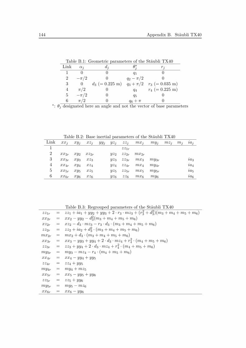
144 Appendix B. Stäubli TX40
Table B.1: Geometric parameters of the Stäubli TX40Link αj dj θ∗j rj1 0 0 q1 02 −π/2 0 q2 − π/2 03 0 d3 (= 0.225 m) q3 + π/2 r3 (= 0.035 m)4 π/2 0 q4 r4 (= 0.225 m)5 −π/2 0 q5 06 π/2 0 q6 + π 0
∗: θj designated here an angle and not the vector of base parameters
Table B.2: Base inertial parameters of the Stäubli TX40Link xxj xyj xzj yyj yzj zzj mxj myj mzj mj iaj1 zz1r2 xx2r xy2 xz2r yz2 zz2r mx2r3 xx3r xy3 xz3 yz3 zz3r mx3 my3r ia34 xx4r xy4 xz4 yz4 zz4r mx4 my4r ia45 xx5r xy5 xz5 yz5 zz5r mx5 my5r ia56 xx6r xy6 xz6 yz6 zz6 mx6 my6 ia6
Table B.3: Regrouped parameters of the Stäubli TX40zz1r = zz1 + ia1 + yy2 + yy3 + 2 · r3 ·mz3 + (r2
3 + d23)(m3 +m4 +m5 +m6)
xx2r = xx2 − yy2 − d23(m3 +m4 +m5 +m6)
xz2r = xz2 − d3 ·mz3 − r3 · d3 · (m3 +m4 +m5 +m6)zz2r = zz2 + ia2 + d2
3 · (m3 +m4 +m5 +m6)mx2r = mx2 + d3 · (m3 +m4 +m5 +m6)xx3r = xx3 − yy3 + yy4 + 2 · d3 ·mz4 + r2
4 · (m4 +m5 +m6)zz3r = zz3 + yy4 + 2 · d3 ·mz4 + r2
4 · (m4 +m5 +m6)my3r = my3 −mz4 − r4 · (m4 +m5 +m6)xx4r = xx4 − yy4 + yy5zz4r = zz4 + yy5my4r = my4 +mz5xx5r = xx5 − yy5 + yy6zz5r = zz5 + yy6my5r = my5 −mz6xx6r = xx6 − yy6
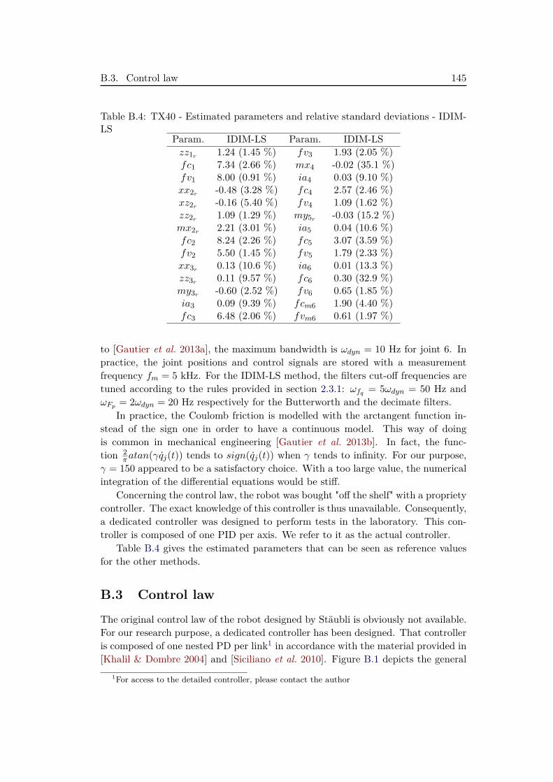
B.3. Control law 145
Table B.4: TX40 - Estimated parameters and relative standard deviations - IDIM-LS
Param. IDIM-LS Param. IDIM-LSzz1r 1.24 (1.45 %) fv3 1.93 (2.05 %)fc1 7.34 (2.66 %) mx4 -0.02 (35.1 %)fv1 8.00 (0.91 %) ia4 0.03 (9.10 %)xx2r -0.48 (3.28 %) fc4 2.57 (2.46 %)xz2r -0.16 (5.40 %) fv4 1.09 (1.62 %)zz2r 1.09 (1.29 %) my5r -0.03 (15.2 %)mx2r 2.21 (3.01 %) ia5 0.04 (10.6 %)fc2 8.24 (2.26 %) fc5 3.07 (3.59 %)fv2 5.50 (1.45 %) fv5 1.79 (2.33 %)xx3r 0.13 (10.6 %) ia6 0.01 (13.3 %)zz3r 0.11 (9.57 %) fc6 0.30 (32.9 %)my3r -0.60 (2.52 %) fv6 0.65 (1.85 %)ia3 0.09 (9.39 %) fcm6 1.90 (4.40 %)fc3 6.48 (2.06 %) fvm6 0.61 (1.97 %)
to [Gautier et al. 2013a], the maximum bandwidth is ωdyn = 10 Hz for joint 6. Inpractice, the joint positions and control signals are stored with a measurementfrequency fm = 5 kHz. For the IDIM-LS method, the filters cut-off frequencies aretuned according to the rules provided in section 2.3.1: ωfq = 5ωdyn = 50 Hz andωFp = 2ωdyn = 20 Hz respectively for the Butterworth and the decimate filters.
In practice, the Coulomb friction is modelled with the arctangent function in-stead of the sign one in order to have a continuous model. This way of doingis common in mechanical engineering [Gautier et al. 2013b]. In fact, the func-tion 2
πatan(γqj(t)) tends to sign(qj(t)) when γ tends to infinity. For our purpose,γ = 150 appeared to be a satisfactory choice. With a too large value, the numericalintegration of the differential equations would be stiff.
Concerning the control law, the robot was bought "off the shelf" with a proprietycontroller. The exact knowledge of this controller is thus unavailable. Consequently,a dedicated controller was designed to perform tests in the laboratory. This con-troller is composed of one PID per axis. We refer to it as the actual controller.
Table B.4 gives the estimated parameters that can be seen as reference valuesfor the other methods.
B.3 Control law
The original control law of the robot designed by Stäubli is obviously not available.For our research purpose, a dedicated controller has been designed. That controlleris composed of one nested PD per link1 in accordance with the material provided in[Khalil & Dombre 2004] and [Siciliano et al. 2010]. Figure B.1 depicts the general
1For access to the detailed controller, please contact the author
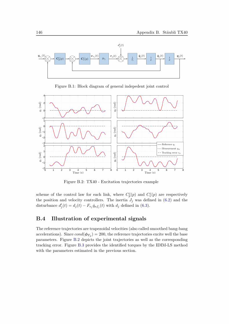
146 Appendix B. Stäubli TX40
−+ Cj
p(p) −+ Cj
v(p) gτj+
+ 1Jj
1p
1p
d′j(t)
qrj (t) ντj (t) τ j(t) qj(t) qj(t) qj(t)
Figure B.1: Block diagram of general indepedent joint control
−2
0
2
4
q 1(rad
)
q 2(rad
)
−3
−2
−1
0
1
q 3(rad
)
q 4(rad
)
0 1 2 3 4 5 6 7 8−2
−1
0
1
2
q 5(rad
)
Time (s)0 1 2 3 4 5 6 7 8
q 6(rad
)
Time (s)
Reference qr
Measurement qm
Tracking error ǫtr
Figure B.2: TX40 - Excitation trajectories example
scheme of the control law for each link, where Cjp(p) and Cjv(p) are respectivelythe position and velocity controllers. The inertia Jj was defined in (6.2) and thedisturbance d′j(t) = dj(t)− Fvj qnfj (t) with dj defined in (6.3).
B.4 Illustration of experimental signals
The reference trajectories are trapezoidal velocities (also called smoothed bang-bangaccelerations). Since cond(φFp) = 200, the reference trajectories excite well the baseparameters. Figure B.2 depicts the joint trajectories as well as the correspondingtracking error. Figure B.3 provides the identified torques by the IDIM-LS methodwith the parameters estimated in the previous section.
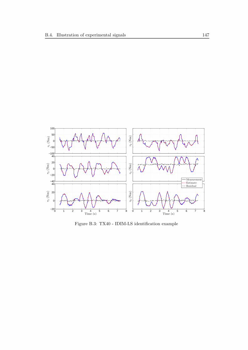
B.4. Illustration of experimental signals 147
−100
−50
0
50
100
τ 1(N
m)
τ 2(N
m)
−40
−20
0
20
40
τ 3(N
m)
τ 4(N
m)
0 1 2 3 4 5 6 7 8−20
0
20
40
τ 5(N
m)
Time (s)0 1 2 3 4 5 6 7 8
τ 6(N
m)
Time (s)
MeasurementEstimateResidual
Figure B.3: TX40 - IDIM-LS identification example

Appendix C
Mathematical background
This appendix gives some mathematical elements useful for the reading of thisthesis. The first three sections are devoted to the fields of probability and statisticswhereas the fourth one concerns few optimisation schemes.
C.1 Random Variables
In this section, several definitions of probabilistic concepts used in the thesis arerecalled. Let us tart with a random variable X that can take values randomly aprobability Pr(X ≤ x) = Pr(x), with x a selected value. That probability Pr(x)gives a scalar values on the interval [0, 1] expressing the probability that X takes avalue less than or equal to x. In the following development, the random variable isassumed to be continuous although there exists a discrete counterpart.
The probability density function of the random variable X is defined as
p(x) = dPr(x)dx
. (C.1)
The expected value, or mean, is defined as
E(X) =∫ ∞−∞
xp(x)dx. (C.2)
If an the same experiment is conducted N times, the expected value can be approx-imated by
E(X) ≈ 1N
N∑i=1
xi, (C.3)
where the xi are the sample values of the random variable X.Considering a random variable X with expected value E(X) = mX , its variance
is defined by
σ2X = E
[(X −mX)2
]=∫ ∞−∞
(x−mX)2p(x)dx (C.4)
= E(X2)−m2
X = E(X2)−[E(X2)]2
.
Two random variables, X and Y , are uncorrelated if
E(XY ) = E(X)E(Y ) (C.5)
150 Appendix C. Mathematical background
and they are orthogonal ifE(XY ) = 0 (C.6)
A random vector is a collection of n random variables X1, X2, ... Xn such asX = [X1, X2, ...Xn]T . Similarly to the scalar case, the mean value and covariancematrix of X are defined by
E(X) = mX (C.7)
cov(X) = E[(X −mX) (X −mX)T
]= ΣX (C.8)
C.2 Properties of Estimators
With a model defined by a vector of parameters θ, we obtain an estimate θ basedon N observations y1,..., yN . The algorithm processing the observations is calledthe estimator. An estimator is said to be unbiased if B(θ) = E[θ]−θ = 0, for all θ.
An estimate can be said to asymptotically unbiased if θ(N) based on N samplesis unbiased for N →∞.
The mean square error (MSE) of θ is given by
MSE(θ) = E[(θ − θ
)2]. (C.9)
The variance of θ is defined by
var(θ) = E[(θ − E(θ)
)2]. (C.10)
The standard deviation is the square root of the variance. The MSE, bias andvariance are linked by MSE(θ) = var(θ) +B(θ)2.
An estimator is said to be consistent if
p limk→∞
θ(k) = θ, (C.11)
where p lim is the probability in the limit defined such as limk→∞
Pr(∣∣∣θ(k)− θ
∣∣∣ ≥ ε) =0 for any ε > 0.
The weak law of large numbers states that that the sample average converges inprobability towards the expected value; i.e. p lim
k→∞θ(k) = µ with θ(k) = 1
k
∑ki=1 θi
and µ = E[θ1] = ... = E[θk].Two features are interesting for an estimator: to be unbiased and to have a
minimal MSE. These dual objectives cannot be necessary satisfied at the sametime. In some cases, it can be defined an unbiased efficient estimator which hasthe lowest variance among the unbiased estimators and satisfies the Cramér-Raobound. That bound is the lower bound on the variance of any unbiased estimator.All the material provided in this section can be found in [Kay 1993] for instance.
C.3. Random Process 151
C.3 Random Process
A random process, also called stochastic process, is a set random variables X(t)indexed by a parameter t from a set T . In our study, the index parameter is thetime. If the set T is continuous, respectively discrete, we talk about CT randomprocess, respectively DT. A random process X(t) is said to be strictly stationary iffor each (t1, t2, ..., tN ) and any τ :
Pr [X(t1 + τ), ..., X(tN + τ)] = Pr [X(t1), ..., X(tN )] . (C.12)
A random process is said to be wide-sense stationary if mx and σ2X are not
function of the time. Using the definition of the expected value and the covariance,it can be shown that the strict stationary condition implies the wide-sense stationarycondition.
A stationary random process X(t) has an autocorrelation function defined suchas
RXX(τ) = E [X(t)X(t+ τ)] (C.13)
where τ is a time shift. Then, we can define the Power Spectral Density (PSD)function as the Fourier transform of this autocorrelation
PXX(ω) =∫ ∞−∞
RXX(τ)e−jωτdτ, (C.14)
where j2 = −1 and ω is a frequency in rad/s over the range (−∞,∞). Reciprocally
RXX(τ) = 12π
∫ ∞−∞
PXX(τ)ejωτdω. (C.15)
A white noise is wide-sense stationary process with
mX(t) = 0 ∀t
cov [X(t1), X(t2)] =σ2X
0t1 = t2
t1 6= t2.
With a constant PSD, Pe, a white noise has a covariance given by
σ2X = RXX(0) = 1
2π
∫ ∞−∞
Pedω (C.16)
= 12πPe
∫ ωnyq
−ωnyqdω = 1
2πPe · 2 · ωnyq = PeTs
where ωnyq = ωs/2 = πTs
is the Nyquist frequency. Finally, for a SISO model withthe input X and the output Y defined such as
Y (t) =∫ ∞
0h(τ)X(t− τ)dτ, (C.17)

152 Appendix C. Mathematical background
the spectral relation is given by
PY Y (ω) = |H(ω)|2PXX(ω). (C.18)
The interested reader can refer to [Bendat & Piersol 2010] for further informationon this topic.

Part VI
Résumé de thèse en français

Annexe D
Identification de robotsindustriels rigides – Apport desméthodes de l’identification de
systèmes
L’identification paramétrique de robots industriels est problème complexe maisnéanmoins nécessaire pour la synthèse de lois de commandes. Cela permet à termede mettre au point des lois commandes rapides et précises satisfaisant les besoinsdes divers utilisateurs industriels. Dans cette thèse, nous explorons et enrichissonsles différentes méthodes d’identification dédiées aux robots industriels.
Ce chapitre reprend de manière fidèle l’organisation du manuscrit écrit en an-glais à l’exception des chapitres de prérequis contenus dans la partie II. La problé-matique de la thèse est introduite dans la section D.1, accompagnée d’un état del’art sommaire. L’étude de la robustesse des méthodes d’identification est présentéedans la section D.2. La section D.3 est dédiée à l’identification de robots sans laconnaissance du contrôleur ni des bandes-passantes. La modélisation du bruit estconsidérée dans la section D.4. Les conclusions de l’étude sont exposées dans lasection D.5.
D.1 Introduction . . . . . . . . . . . . . . . . . . . . . . . . . . . . 157D.1.1 Contexte . . . . . . . . . . . . . . . . . . . . . . . . . . . . . 157D.1.2 État de l’art . . . . . . . . . . . . . . . . . . . . . . . . . . . 158D.1.3 Problématique . . . . . . . . . . . . . . . . . . . . . . . . . . 159
D.2 Evaluation de la robustesse des méthodes d’identificationbasées sur la simulation du modèle auxiliaire . . . . . . . . . 160
D.2.1 Choix du signal d’identification . . . . . . . . . . . . . . . . . 160D.2.2 Comparaison des méthodes IDIM-IV et DIDIM . . . . . . . . 163D.2.3 Remarques et conclusion . . . . . . . . . . . . . . . . . . . . . 165
D.3 Identification de systèmes robotiques sans connaissance ducontrôleur et des bande-passsantes . . . . . . . . . . . . . . . 165
D.3.1 Estimation des dérivées articulaires . . . . . . . . . . . . . . . 166D.3.2 Identification du contrôleur . . . . . . . . . . . . . . . . . . . 170D.3.3 Conlusions . . . . . . . . . . . . . . . . . . . . . . . . . . . . 173

156 Annexe D. Résumé de thèse en français
D.4 Modélisation du bruit pour l’identification de systèmes ro-botiques . . . . . . . . . . . . . . . . . . . . . . . . . . . . . . . 174
D.4.1 Modélisation et identification du bruit . . . . . . . . . . . . . 174D.4.2 Extension des méthodes d’identification . . . . . . . . . . . . 177D.4.3 Conlusions . . . . . . . . . . . . . . . . . . . . . . . . . . . . 181
D.5 Conclusions et perspectives . . . . . . . . . . . . . . . . . . . 181D.5.1 Résumé des contributions . . . . . . . . . . . . . . . . . . . . 181D.5.2 Un guide pour l’utilisateur . . . . . . . . . . . . . . . . . . . 183D.5.3 Développements futurs . . . . . . . . . . . . . . . . . . . . . . 184
D.1. Introduction 157
D.1 Introduction
D.1.1 Contexte
Les robots industriels sont des bras mécaniques composés de plusieurs corps reliéspar des articulations, également appelés axes. Chaque articulation est actionnée parun moteur électrique couplé à un capteur de position. Un ordinateur contrôle lesmouvements du bras afin de placer la charge utile dans l’espace de travail. La figure1.1 illustre un tel robot. Les robots industriels sont des composants essentiels del’industrie moderne car ils permettent une réduction des coûts, l’augmentation descadences, l’élimination des tâches dangereuses pour les travailleurs humains, etc.C’est pourquoi, pendant les dernières décennies, le nombre de robots industriels afortement augmenté ; voir la figure 1.2.
Les robots industriels doivent effectuer des tâches répétitives rapidement etde manière précise. Afin d’accomplir de telles tâches, différentes caractéristiquesdoivent être satisfaites suivant l’application. La norme ISO [ISO 1999] spécifie lescaractéristiques utiles pour l’utilisateur que doit fournir le constructeur du robot.Par exemple, il y a la répétabilité définissant la précision avec laquelle le robotretourne à une position commandée. D’après [Siciliano et al. 2010], pour un brasrobotique avec un élancement maximum de 1.5 m, la répétabilité varie entre 0.02and 0.2 mm. Afin de satisfaire de tels spécifications, les lois de commande ont besoinde modèles fiables et complets de ces robots. Cette modélisation précise vient d’uneidentification rigoureuse basée sur des données expérimentales. Ainsi, le problèmeest pour le praticien de fournir un modèle aussi précis et complet que possible.
Plusieurs difficultés sont envisagées. Tout d’abord, les robots opèrent en bouclefermée, i.e. avec une rétroaction, pour des raisons de stabilité et de précision. Il estsouvent difficile, voire impossible pour des raisons de sécurité, de mettre en œuvreune expérience sans cette rétroaction. La méthode d’identification doit donc pouvoirtraiter cette problématique de la boucle fermée. En quelques mots, la rétroactioncréée une corrélation entre le bruit de sortie et l’entrée qui mène à des difficultésstatistiques pour l’identification. De plus, si le contrôleur est réglé correctement, lesystème sera insensible à n’importe quelle perturbation et spécialement aux varia-tions des paramètres. Or, les méthodes d’identification sont basées sur la sensibilitédu système aux variations des paramètres. Ensuite, suivant la technologie du robotconsidéré, différentes dynamiques peuvent être rencontrées : frottement linéaire ounon-linéaire, modes rigides ou flexibles. Dans le cas de robots à usages industriels,une dynamique rigide est privilégiée dès la conception afin d’assurer la précision dela tâche, bien que des structures flexibles peuvent être envisagées afin de réduireles coûts ; voir par exemple [Wernholt 2007]. Enfin, suite aux difficultés énoncéesprécédemment, des processus spécifiques ont été développés par les roboticiens pourl’identification. Ces processus sont basés sur les compétences et le savoir-faire duroboticien ainsi que sur quelques règles empiriques. Dans la partie suivante, nousintroduisons les éléments principaux de ces méthodes.
158 Annexe D. Résumé de thèse en français
D.1.2 État de l’art
Les modèles dynamiques de bras industriels sont issus des lois de la mécanique géné-rale : formalisme de Newton ou de Lagrange. Afin d’exprimer les équations du mou-vement, une notation doit tout d’abord être définie afin de paramétrer le problème.Dans [Denavit & Hartenberg 1955], les auteurs ont introduit une notation pour lesrobots industriels, qui a été améliorée ensuite dans [Khalil & Kleinfinger 1986]. Cettenotation définit les relations géométriques entre les éléments constitutifs du robot,en introduisant un nombre minimal de paramètres. Cela a permis d’exprimer lesmodèles dynamiques de manière générique et normalisée. Si ces travaux permettentde modéliser fidèlement les forces inertielles, ils n’ont pas abordé spécifiquementla question des forces de frottements. D’autres travaux ont ainsi proposé différentsmodèles de frottement, comme [Canudas de Wit et al. 1989, Bona & Indri 2005]par exemple. En combinant la notation standard pour les forces inertielles et lamodélisation des frottements, un modèle complet des bras robotiques est ainsi ànotre disposition.
À partir de ces modélisations, deux techniques de réduction de modèle ont étéproposées dans [Gautier & Khalil 1990] et [Gautier 1991]. L’une est basée sur l’ana-lyse des relations algébriques alors que la deuxième repose sur une évaluation nu-mérique du modèle. Cette réduction permet d’une part d’extraire l’ensemble desparamètres de base, dont les effets peuvent être identifiés de manière distincte.D’autre part, cette réduction conserve la linéarité du couple par rapport aux pa-ramètres issue de la modélisation de Denavit-Hartenberg. Ainsi les paramètres debase peuvent être estimés à l’aide de la technique des moindres carrés, à conditionde traiter la question des bruits de mesure corrélés à cause de la rétroaction. Àcette fin, dans [Gautier 1997], l’auteur a mis en place une procédure de pré-filtragedes données expérimentales en deux étapes. La première étape consiste à filtrerla position articulaire mesurée pour en déduire la vitesse et l’accélération via unfiltre passe-bande. La deuxième étape consiste à filtrer le couple mesuré afin derejeter les perturbations haute-fréquences via un filtre decimate, encore appelé fil-trage parallèle. Ce processus de pré-filtrage rend les moindres carrés (LS) viablesstatistiquement. L’ensemble pré-filtrage et estimation compose la méthode IDIM-LS. L’inconvénient de cette méthode est qu’elle est sensible au réglage des filtresqui reposent sur une connaissance a priori des bandes passantes du système.
D’autres approches d’identification ont été développées au cours des années,sans réellement améliorer la méthode IDIM-LS si elle est couplée avec des filtrescorrectement réglés. Il peut être cité par exemple : la méthode des moindres carréstotaux (TLS) [Gautier et al. 1994, Xi 1995], la méthode basée sur les outils d’inéga-lité matricielle linéraire (LMI) [Calafiore & Indri 2000], le filtre de Kalman étendu(EKF) [Kostic et al. 2004] ou une approche basée sur le maximum de vraisemblance(ML) [Olsen & Petersen 2001, Olsen et al. 2002].
Dans [Janot et al. 2014c], les auteurs ont introduit une approche de la variableinstrumentale (IV), provenant de l’économétrie et adaptée à l’identification de ro-bots. L’idée est de simuler le modèle en boucle-fermée afin d’obtenir des signaux
D.1. Introduction 159
non-corrélés avec le bruit de mesure. Cette méthode, nommée IDIM-IV, utilise lemême processus de pré-filtrage que la méthode IDIM-LS bien que les estimées fi-nales soient moins sensibles au réglage des filtres. En plus des bandes passantes dusystème, le modèle du contrôleur est aussi requis pour la simulation. Pour simplifierle processus de pré-filtrage, dans [Gautier et al. 2013a], les auteurs ont développéune méthode d’identification basée sur les modèles dynamiques direct et indirect(DIDIM) qui repose aussi sur la simulation du modèle en boucle-fermée. Cette mé-thode a l’avantage de ne pas avoir besoin de la première étape du processus depré-filtrage car elle est basée uniquement sur la mesure du couple. Cependant, ladeuxième étape (filtre decimate) reste nécessaire tout comme la connaissance apriori (contrôleur et bandes passantes).
Les méthodes d’identification introduites ci-avant partagent le fait de ne pasidentifier le modèle du bruit. Au sein de la communauté d’identification des sys-tèmes, Ljung a introduit la méthode d’erreur de prédiction (PEM) qui s’appliqueprincipalement à des modèles linéaire temps invariant (LTI) en boucle ouverte oufermée ; cf [Ljung 1976]. Les modèles considérés sont à temps discret et incluent lemodèle de bruit. Malheureusement, cette méthode ne peut pas être appliquée auxrobots car leurs modèles sont non-linéaires et à temps continu. Quasi simultanément,Young and Jakeman ont mis au point la variable instrumentale raffinée pour les sys-tèmes à temps continu (RIVC) dans [Young & Jakeman 1980]. Avec une approchedifférente, cette méthode s’applique à l’identification de modèles LTI en boucle ou-verte ou fermée, mais dans un cadre temps continu. À cause des non-linéarités, laméthode RIVC ne peut pas être appliqué non plus aux robots industriels d’unemanière directe. Pour les deux méthodes, identifier le bruit permet un filtrage au-tomatique des données et fournit des paramètres estimés optimaux. Il doit êtrenoté qu’un cas particulier de la PEM, appelé méthode d’erreur de sortie (OEM),peut traiter l’identification de systèmes non-linéaires et à temps continu ; voir parexemple [Richalet et al. 1971] pour un contexte général ou [Landau et al. 1999] pourles systèmes en boucle-fermée. Néanmoins, la méthode à erreur de sortie ne prendpas en compte le modèle de bruit.
D.1.3 Problématique
Il apparaît ainsi que la communauté robotique dispose de méthodes capables d’iden-tifier des robots industriels opérant en boucle fermée. Cette problématique de bouclefermée a été traitée de différentes manières suivant la méthode d’identification consi-dérée. En parallèle, la communauté d’automatique a mis au point des méthodespermettant d’identifier des systèmes fonctionnant en boucle fermée, de manièreprécise et systématique. C’est-à-dire qu’elles prennent en compte le modèle de bruitsans connaissance a priori. Cependant, ces méthodes ne s’appliquent que sur dessystèmes LTI, ce que ne sont pas les robots industriels. De leur côté, les roboti-ciens n’ont pas traité la question de la modélisation du bruit de manière approfon-die. Leurs méthodes reposent en effet sur un pré-filtrage empirique basée sur uneconnaissance physique du système a priori. Si le niveau de bruit et sa localisation
160 Annexe D. Résumé de thèse en français
fréquentielle sont une préoccupation majeure, les roboticiens n’ont pas essayé de lemodéliser.
C’est dans ce contexte que cette thèse a été réalisée. Elle consiste à mettre enplace des méthodes d’identification de systèmes robotiques industriels de manièreprécise et automatique, tout en minimisant la connaissance a priori nécessaire,afin de faire un lien entre la communauté d’identification de systèmes et celle derobotique.
D.2 Evaluation de la robustesse des méthodes d’iden-tification basées sur la simulation du modèle auxi-liaire
D.2.1 Choix du signal d’identification
Méthodes à erreur de sortie
En considérant la méthode d’erreur de sortie pour un robot, il semble naturel deprendre la position articulaire comme signal pour l’identification. Ainsi, le vecteurd’erreur de sortie est définit par :
εCLOE(t,θ) = qm(t)− qs(t,θ), (D.1)
où qm et qs sont les vecteurs (n × 1) de position articulaires mesurées et simuléesrespectivement. Puisque les robots sont instables en boucle-ouverte, ils sont iden-tifiés en boucle-fermée. La méthode est ainsi nommée Closed-Loop Output Error(CLOE) pour erreur de sortie en boucle-fermée.
En identification de robot, il est cependant plus usuel de considérer le signald’entrée (couple ou force) pour l’identification car il a l’avantage d’être linéairevis-à-vis des paramètres. Une variante peut de la méthode CLOE peut donc êtreenvisagée avec le signal d’entrée. Cette technique est ainsi nommée Closed-LoopInput Error (CLIE) pour erreur d’entrée en boucle-fermée. Le vecteur d’erreurd’entrée est définit par :
εCLIE(t,θ) = τ (t)− τ s(t,θ), (D.2)
où τ et τ s sont les vecteurs (n× 1) de couples/forces mesurées et simulées respec-tivement.
Les deux méthodes se basent sur une optimisation non-linéaire afin de régleritérativement les paramètres. Cette optimisation est généralement réalisée à l’aided’un algorithme de Gauss-Newton comme il est indiqué avec (4.2). L’information clépour l’optimiseur est la sensibilité, qui est la dérivée relative de la sortie considéréepar rapport aux paramètres. Généralement ces sensibilités ne sont pas connuesexactement mais approximées par des différences finies.
Un élément théorique de la méthode de l’erreur de sortie est à noter. Le bruit
D.2. Robustesse des méthodes d’identification 161
additif sur le signal considéré doit être blanc, sinon les hypothèses statistiques pourl’estimation des variances des paramètres ne sont pas vérifiées. Comme nous le ver-rons par la suite, cela représente une limitation à l’application d’une telle méthodeaux robots industriels. Le principe général des méthodes CLOE et CLIE est illustrépar la Figure 4.1.
Analyse de la sensibilité
Pour la méthode CLIE, à l’itération it, la sensibilité en entrée est donnée par
∆τ s(t) = ∂τ s(t)∂θ
∣∣∣∣θ=θ
it
CLIE
. (D.3)
En utilisant la définition de contrôleur (2.11), il vient :
∆τ s(t) =∂GτC(p)
(qr(t)− qs(t, θ
it
CLIE))
∂θ
∣∣∣∣∣∣∣θ=θ
it
CLIE
, (D.4)
avec Gτ , la matrice (n × n) de gain des actionneurs ; C(p), la matrice (n × n) detransfert du contrôleur ; et qr est le vecteur (n× 1) de position de référence. Et ensupposant le contrôleur connu :
∆τ s(t) = −GτC(p)∆qs(t). (D.5)
Puisque les robots sont contrôlés en position, la relation suivante est attendue :
qm(t) ≈ qr(t). (D.6)
En supposant que l’optimiseur est bien initialisé, on obtient :
qs(t) ≈ qr(t). (D.7)
À partir de (D.6) et (D.7), il peut être supposé que le contrôleur opère dans lesbases fréquences et qu’il peut être approximé par une (n× n) matrice C0. Dans lecas d’une loi Proportionnelle-Dérivée, ce résultat est direct. Si une action intégraleest présente, comme expliqué dans la section 2.2.1, le terme intégral est désactivélorsque l’erreur de position est faible, afin d’éviter des oscillations dues aux frotte-ment de Coulomb. Ainsi, nous avons :
∆τ s(t) = −GτC0∆qs(t). (D.8)
En considérant (D.8), il peut être montré que la méthode CLIE est une versionpondérée de la méthode CLOE ; voir (4.11). Par conséquent, d’après la théorie desstatistiques [Davidson & MacKinnon 1993], nous avons
E[θitCLIE]→ E[θitCLOE].
162 Annexe D. Résumé de thèse en français
Il apparaît ainsi que les méthodes CLIE et CLOE fournissent asymptotiquement lesmêmes paramètres estimés. La question qui en suit est : existe-t-il un estimateurplus efficace que l’autre ?
Dans le cadre de l’erreur de sortie, le bruit additif sur la position est supposéblanc. Le signal peut ainsi être écrit :
qm(t) = qnf (t) + nq(t), (D.9)
où nq est un vecteur (n × 1) de bruits blancs indépendants. En se basant surl’équation du contrôleur, il peut être montré que le bruit vu par le couple d’entréeest donné par :
v(t) = −GτC0nq(t). (D.10)
De cette relation, un lien entre les covariances des bruits d’entrée et de sortie peutêtre établi. Par la suite, les covariances des paramètres estimés apparaissent égalespour les deux méthodes ; voir le développement (4.16). Les méthodes CLIE et CLOEfournissent donc les mêmes estimations avec les mêmes variances. La question ensuspens est donc de savoir quelle méthode est la plus intéressante pour le praticien.
Pour répondre à cette interrogation, deux cas doivent être considérés pour laméthode CLOE.
• Le premier cas est lorsque les relations (D.6) et (D.7) sont statisfaites. laloi de commande assure alors un excellent tracking. Dans ce cas, nous avonsεCLOE(t,θ) ≈ 0, pour tout t, et l’innovation est nulle d’après (4.17). Ainsi, laméthode CLOE peut être totalement insensible aux erreurs de modèle et/oubruit de mesure si la loi de commande est assez performante. En practique,l’optimiseur ne varierait pas du point d’initialisation.
• Le deuxième cas est lorsque (D.6) et (D.7) ne sont pas totalement satisfaites,suite à une loi de commande pas assez performante. D’après (4.21), il se peutalors que l’estimation ne soit pas assez robuste face à une erreur de modéli-sation à cause des faibles valeurs propres de la matrice jacobienne regroupantles sensibilités.
A contrario, la méthode CLIE présente des valeurs propres plus grandes que laméthode CLOE grâce à la pondération du contrôleur (D.8). Par conséquent, laméthode CLIE est plus robuste face à de faibles erreurs de modèle et elle est plussensible aux variations des paramètres.
Résultats expérimentaux
Pour illustrer l’intérêt de considérer le signal d’entrée, trois méthodes d’identifica-tion sont considérées : les méthodes CLOE, CLIE et DIDIM. Il peut être montréque la méthode DIDIM est une méthode CLIE avec deux particularités. Premiè-rement, le couple est supposé linéaire par rapport aux paramètres, ce qui simplifiegrandement le calcul des sensibilités. Cette hypothèse est appelée Pseudo-Linear
D.2. Robustesse des méthodes d’identification 163
Regression (PLR), pour régression pseudo-linéaire. Deuxièmement, le filtrage deci-mate est inclus dans la méthode.
Dans un premier temps, seules les méthodes CLOE et CLIE sont testées dans uncadre d’erreur de sortie strict. Autrement dit, le bruit additif est blanc et aucuneopération de filtrage n’est effectuée. Les résultats, récapitulés dans les Tableaux4.2 et 4.3, montrent une meilleure robustesse de la méthode CLIE. Néanmoins,il apparait que les résidus de l’estimation sont auto-corrélés. Par conséquent, lesvariances des paramètres estimés sont biaisées.
Dans un deuxième temps, un filtre decimate est inclus dans le processus d’iden-tification afin d’obtenir des résidus dé-corrélés. Les paramètres estimés par les mé-thodes CLOE et CLIE sont alors totalement comparables à ceux estimés sans lefiltre decimate. Il y a toujours une meilleure robustesse pour la méthode CLIE. Laméthode DIDIM, quant à elle, fournit des résultats parfaitement équivalents à ceuxde la méthode CLIE, mais avec un temps de calcul beaucoup plus court commeindiqué dans le tableau 4.5. Pour les trois méthodes, le filtre decimate permet bienune dé-corrélation des résidus et une bonne estimation des variances.
Les résultats expérimentaux ont donc montré qu’il est plus intéressant de consi-dérer l’entrée (couple ou force) pour l’identification, mais que le filtre decimate estnécessaire à une bonne estimation des variances. Si l’hypothèse PLR est valide alorsla méthode DIDIM doit être préférée afin de gagner en temps de calcul.
D.2.2 Comparaison des méthodes IDIM-IV et DIDIM
Dans la partie précédente, il a été montré l’intérêt de considérer le couple d’entréepour l’identification de robot. De plus, la méthode DIDIM est apparue comme laméthode la plus efficace pour appliquer le principe de l’erreur de sortie à un robotindustriel. Tout comme la méthode IDIM-IV, la méthode DIDIM repose sur lasimulation d’un modèle auxiliaire. Cette partie est dédiée à la comparaison de cesdeux méthodes.
Similarité entre les méthodes
À première vue, les deux méthodes sont très similaires. En effet, à l’itération it, lesparamètres regroupé dans le vecteur θ sont estimés via :
θit+1IV =
[Z(θitIV )TX
]−1Z(θitIV )Ty(τ), (D.11)
θit+1DIDIM =
[Z(θitDIDIM)TZ(θitDIDIM)
]−1Z(θitDIDIM)Ty(τ), (D.12)
où X et Z sont les matrices (r× b) d’observations et d’instruments respectivement.X est construite à partir des positions, vitesses et accélérations articulaires me-surées alors que Z est construite à partir des positions, vitesses et accélérationsarticulaires simulées. Les deux matrices utilisent les équations issues des lois deNewton qui expriment l’entrée (couple ou force) en fonction des paramètres ainsique les positions, vitesses et accélérations articulaires. Cet ensemble d’équations est
164 Annexe D. Résumé de thèse en français
nommé modèle dynamique inverse, Inverse Dynamic Model (IDM). Les méthodessont itératives, basées sur la simulation du modèle auxiliaire pour la constructionde Z et elles peuvent utiliser la même initialisation.
Le développement de la section 4.2.1 montre que si le IDM ne contient pasd’erreur de modélisation alors la matrice d’instruments est égale à partie non-bruitéede la matrice d’observation. Il peut être montré que les deux méthodes estimentalors des paramètres égaux et sans biais. Le caractère sans biais de la méthodeDIDIM a été montré dans [Gautier et al. 2013a].
Si l’IDM contient une erreur de modèle, comme un frottement mal modélisé,cette erreur est présente dans les matrices d’observations et d’instruments parconstruction. Dans ce cas, les deux méthodes fournissent des résultats équivalentset biaisés.
Différence entre les méthodes
La différence entre les deux méthodes se situe dans l’utilisation de la matrice d’obser-vations pour la méthode IDIM-IV (D.11). Cela peut être vu comme un inconvénientparce que la mesure des positions articulaires est alors requise. De plus, un filtrageprécis des signaux est nécessaire afin de retrouver les dérivées via différences finies.Comme cela a été mis en évidence dans [Gautier et al. 2013a], la méthode DIDIMprésente l’avantage de n’avoir besoin que de la mesure du couple (ou force).
Cependant, il a été montré dans la section 4.2.2 que la méthode IDIM-IV peutêtre plus robuste que la méthode DIDIM, dans le cas où une erreur est présente dansle modèle mais pas dans l’IDM. L’erreur peut se trouver par exemple dans le modèledes actionneurs ou encore le contrôleur. Entre d’autres termes, nous considérons uneerreur dans le simulateur mais pas dans la matrice X. En pratique deux cas doiventconsidérés :
• Si l’espérance de l’erreur introduite est nulle alors l’estimation via la méthodeIDIM-IV est non-biaisée contrairement à celle via la méthode DIDIM ;
• Si l’espérance de l’erreur introduite n’est pas nulle alors les deux méthodesfournissent une estimation biaisée.
Résultats expérimentaux
Dans un premier temps, les deux méthodes ont été appliquées dans un cas nominaloù le modèle auxiliaire ne contient pas d’erreur. Les résultats, fournis dans le tableau4.6, sont équivalents et similaires à ceux de précédents travaux comme [Gautieret al. 2013a].
Dans un second temps, une erreur a été introduite dans le modèle auxiliaire. Ils’agit d’une erreur sur les rapports de transmission qui sont pris égaux à 80% deleurs valeurs réelles. À la vue des résultats du tableau 4.6, les paramètres estiméspar la méthode DIDIM sont biaisés et en particulier les inerties comme zz1r , zz2r onencore ia3. A contrario, les paramètres estimés par la méthode IDIM-IV sont sans
D.3. Identification sans connaissance du contrôleur et des bande-passsantes 165
biais, ce qui démontre la meilleure robustesse de cette méthode face à une erreurdans le simulateur.
Un point mérite une attention particulière : l’estimation des covariances pour laméthode IDIM-IV. En effet, la formule usuelle suppose que la matrice d’instrumentsest une approximation de la partie non-bruitée de la matrice d’observation. Or,avec une erreur persistante dans le simulateur, ce n’est pas le cas. C’est pourquoi laformule non approchée (4.34) doit être employée en cas de doute sur le simulateur.
D.2.3 Remarques et conclusion
Dans la partie D.2.1, nous avons considéré trois méthodes d’erreur de sortie pourl’identification de robot : les méthodes CLOE, CLIE et DIDIM. En fait, elles nesont pas des méthodes à erreur de sortie stricto sensu car elles ont besoin d’unfiltrage parallèle afin de fournir des estimées avec des résidus non-corrélés. S’il aété mis en évidence l’intérêt de considérer le signal d’entrée plutôt que celui desortie, ce résultat peut être étendu aux méthodes IDIM-LS et IDIM-IV. Dans leurcas, la sensibilité à prendre en compte est celle du système réel au lieu du systèmesimulé. Pour en revenir aux méthodes à erreur de sortie dans le cadre robotique, ilest plus intéressant d’employer la méthode DIDIM si l’hypothèse PLR est vérifiée.Cela permet en effet de réduire significativement le temps de calcul.
Deux éléments sont fondamentaux dans l’analyse de la sensibilité effectuée. Lepremier est l’hypothèse de bon tracking ou, autrement dit, que la loi de commandeest performante. Le deuxième est l’hypothèse sous-jacente que le système est bienactionné. C’est-à-dire qu’il y a un capteur et un actionneur par axe. Sans ces deuxéléments, les résultats observés ne seraient plus valides. En d’autres termes, pourun système ayant une loi de contrôle avec une faible capacité de tracking et étantsous-actionné, il pourrait être plus intéressant de considérer le signal de sortie pourl’identification. La partie 4.3.2 donne un tel exemple basé sur l’identification avion.
Toutes les méthodes d’identification présentées dans cette section requièrentune certaine connaissance a priori. Par exemple, la méthode IDIM-IV a besoin desbandes-passantes du systèmes afin de régler le filtre passe-bande. Cette informationest également nécessaire aux méthodes DIDIM et IDIM-IV pour régler le filtredecimate. De plus, la connaissance des actionneurs et du contrôleur est incluse dansle simulateur. Dans la section suivante, nos efforts portent sur la réduction de cetteconnaissance a a priori nécessaire.
D.3 Identification de systèmes robotiques sans connais-sance du contrôleur et des bande-passsantes
Dans la section précédente nous avons étudié la robustesse des méthodes IDIM-IVet DIDIM. Ces méthodes reposent sur un préfiltrage minutieux qui nécessite uneconnaissance des bandes-passantes. De plus, elles ont besoin de la connaissance ducontrôleur pour la simulation du modèle auxiliaire. Il apparaît ainsi un dilemme
166 Annexe D. Résumé de thèse en français
classique de l’identification de systèmes : pour identifier correctement un système,nous avons besoin d’une bonne connaissance a priori.
D.3.1 Estimation des dérivées articulaires
Estimation de dérivées à partir de signaux bruités
De nombreuses recherches portent sur la différentiation numérique ; voir par exemple[Diop et al. 1994, Vasiljevic & Khalil 2006, Dridi 2011, Sidhom 2011] et les réfé-rences données par les auteurs. Nous récapitulons ici certaines de ces méthodes afind’avoir une vue d’ensemble. Néanmoins, l’objectif est pour nous de sélectionner uneméthode simple qui ne requière pas de connaissance a priori sur le système.
La problématique d’estimation des états d’un système inconnu n’est pas récentepour la communauté d’automatique. Cela a fait l’objet d’une longue littératuresur les observateurs. L’objectif est de fournir les dérivées des signaux au contrô-leur afin de réduire le nombre de capteurs nécessaires. Le problème a été introduitpar Luenberger [Luenberger 1971]. Dans le cas d’un signal bruité, un observateurstochastique, comme celui de Kalman, peut être plus approprié ; voir par exemple[Singer 1970]. Il existe également une recherche abondante sur les observateurs non-linéaires ; voir entre autres [Dabroom & Khalil 1997, Besançon 2007]. Par exemple,le filtre de Kalman étendu peut être considéré pour l’estimation des états d’un sys-tème nonlinéaire stochastique, comme dans [Ljung 1979]. Qu’il soit déterministeou stochastique, un observateur est basé sur le modèle dynamique du système.Ainsi, un observateur n’est pas la solution pour l’estimation des dérivées articu-laires dans le but d’identifier le modèle dynamique. Bien qu’une solution pourraitconsister à estimer les paramètres et les états en même temps comme dans [Gau-tier & Poignet 2001], nous cherchons une solution moins complexe, ne couplant pasl’estimation des paramètres et des états.
Une autre approche consiste à ne considérer que les signaux et non les modèles.Il est alors plus approprié de parler de différentiateur. La technique usuelle de filtrepasse-bande, décrite dans la section 2.3.1, appartient à ce type d’approche. Il existeune autre méthode basée sur l’interpolation polynomiale sur une fenêtre glissante ;voir par exemple [Klein & Morelli 2006]. La dérivée du signal est alors approximéela dérivée du polynôme.
Il existe également les différentiateurs algébriques qui ont été récemment revisi-tés ; voir entre autres [Fliess & Sira-Ramírez 2003]. L’idée est d’estimer les dérivéesdu signal grâce à des intégrations successives. Cela est basé sur une troncatured’une série de Taylor du signal considéré. Ainsi l’utilisateur doit fournir l’ordre dela troncature. Puisque les trajectoires utilisées pour l’excitation de robots ne sontpas très lisses, l’ordre requis peut être élevé.
Une autre famille de techniques est basée sur la théorie des modes glissantsintroduite dans les années 1960 [Filippov 1960]. Parmi les techniques développées,nous pouvons citer celle de l’algorithme Super Twisting introduite par [Levant 1998].L’Eq. (5.1) donne le principe de fonctionnement de la méthode qui repose sur deux
D.3. Identification sans connaissance du contrôleur et des bande-passsantes 167
hyper-paramètres que l’utilisateur doit régler.Finalement, la solution que nous avons retenue est intitulée l’Integrative Random
Walk SMoother (IRWSM). Elle a l’avantage pratique de ne pas avoir besoin deconnaissance a priori. Cette solution est développée dans le paragraphe suivant.
Integrative random walk smoother
La méthode IRWSM est basée sur le filtre de Kalman dans un cadre temps-discret.Cette méthode est récapitulée dans [Norton 1975, Young 2000]. Elle permet uneestimation hors-ligne des états sans utiliser le modèle dynamique, à la différencedes observateurs grands gains par exemple. L’Eq. (D.13) définit le vecteur d’état,avec x le signal de position et ∇x son taux de variation. la relation (D.14) estl’équation d’état et (D.15) est l’équation d’observation.
x(k) =[x(k)∇x(k)
](D.13)
x(k) = Ax(k − 1) + Dκ(k − 1) (D.14)y(k) = h(k)x(k) + e(k) (D.15)
Avec,
A =[p1 p20 p3
], D =
[p4 00 p5
](D.16)
h est le vecteur (1 × 2) d’observation. κ est le bruit d’état, supposé blanc avecune matrice de covariance Qκ (diagonale). Le bruit de mesure e est égalementblanc avec une variance σ2
e . Ce modèle, développé dans [Young 2011], est intituléGeneralized Random Walk (GRW). Plusieurs variantes existent suivant le choixdes hyper-paramètres γ = [p1 p2 p3 p4 p5 Qκ11 Qκ22 ]. Pour cette étude,l’Integrated Random Walk (IRW : p1 = p2 = p3 = p5 = 1, p4 = 0 et h = [1 0])est considéré. Dans ce cas, puisque p4 = 0, le terme Qκ11 n’a pas d’influence etest pris égal à Qκ22 afin de s’assurer que la matrice de covariance reste définiepositive. Au final, le seul hyper-paramètre restant est Qκ22 . Comme il a été montrédans la section 5.1.2, cet hyper-paramètre peut être estimé via une optimisation dumaximum de vraisemblance.
En pratique ce modèle IRW est utilisé par un filtre de Kalman qui est couplé àun processus de lissage, Fixed Interval Smoother (FIS), afin de profiter de l’aspecthors-ligne. De plus, le filtre et le lisseur son modifiés afin d’éviter la connaissancede la variance du bruit d’observation, σ2
e . Dans un filtre de Kalman traditionnel,cette information est en effet requise, tout comme la covariance du bruit d’état, Qκ.À la place, toutes les équations sont écrites en fonction du Noise Variance Ratio(NVR) qui est définit par Qnvr = Qκ/σ
2e . L’algorithme décrit dans [Young 2011]
est récapitulé avec les équations (5.7) à (5.15). La méthode IRWSM désigne lacombinaison du filtre de Kalman, du FIS et du modèle IRW. Une fois cette méthodeappliquée, la dérivée première du signal est approximée par dx
dt (tk) ≈∇x(k)tk+1−tk , avec
168 Annexe D. Résumé de thèse en français
∇x(k) le second élément du vecteur d’état estimé x(k|N). De manière similaire, xpourrait être augmenté avec ∇2x pour estimer la dérivée seconde.
D’un point de vue pratique, l’algorithme IRWSM est implémenté dans la fonc-tion irwsm de la Toolbox CAPTAIN, développée par une équipe de la LancasterUniversity ; voir [Taylor et al. 2007] et http ://captaintoolbox.co.uk. Heureuse-ment, la Toolbox fournit aussi une fonction intitulée irwsmopt qui estime les hyper-paramètres. Cette Toolbox permet ainsi à l’utilisateur de traiter les données sansconnaître les bande-passantes. Cela n’empêche en rien d’être vigilant quant auxrésultats.
Application à l’identification de robots
Pour l’identification de robot, l’idée est de remplacer le filtre passe-bande habituelpar l’IRWSM. Dans l’équation d’observation (D.15), la sortie y est remplacée parla mesure de l’axe j : qmj , tel que :
qmj (t) = qj(t) + qj(t), (D.17)
où qj est la position articulaire et qj est le bruit de capteur ; voir la Figure 2.3 pourune présentation des signaux du système. D’après la section 2.2.3, ce bruit est blancavec une variance 1
3∆2e, où ∆e est la résolution de l’encodeur. Si on suppose aussi
que le bruit de mesure est normalement distribué, l’équation d’observation (D.15)est valide et l’écart type du bruit σe ≈ ∆q peut être estimé avec les données fourniespar le constructeur. De plus, la position qj est égale à l’état x définit par (D.13).
Concernant l’équation d’état (D.14), deux cas peuvent être envisagés pour re-trouver l’accélération articulaire :
• Appliquer l’algorithme deux fois avec Airwsm1 =[1 10 1
];
• Appliquer l’algorithme une fois avec Airwsm2 =
1 1 00 1 10 0 1
.La pertinence du modèle IRW est d’abord étudiée pourAirwsm1. De (D.14), il vient :[
qj(k)∇qj(k)
]=[1 10 1
] [qj(k − 1)∇qj(k − 1)
]+[1 00 1
] [0
κ1,j(k − 1)
]. (D.18)
Le deuxième état∇qj représente la vitesse. Cette information de vitesse n’est pas ca-ractérisée par les équations dynamiques mais par une marche aléatoire. En d’autrestermes, le bruit η1,j regroupe la dynamique non-modélisée ; c’est-à-dire que c’estune erreur de modèle. D’après [Young 2011], ce type de modélisation fonctionnepour des systèmes dont les états varient lentement. Pour les systèmes robotiques, lecontrôleur nécessite une grande fréquence d’échantillonnage pour assurer une com-mande robuste à l’aide de grands gains ; voir [Khalil & Dombre 2004]. Néanmoins,
D.3. Identification sans connaissance du contrôleur et des bande-passsantes 169
la bande-passante mécanique est bien plus basse. Par conséquent, avec un IRW ex-primé à la fréquence d’échantillonnage du contrôleur, l’hypothèse d’états lentementvariable est validée.
Avec le système augmenté Airwsm2, ce n’est pas la vitesse mais l’accélérationqui est caractérisée par une marche aléatoire. Comme pour la vitesse, l’hypothèsed’état lentement variable semble appropriée. L’Eq. (D.14) donne : qj(k)
∇qj(k)∇2qj(k)
=
1 1 00 1 10 0 1
qj(k − 1)∇qj(k − 1)∇2qj(k − 1)
+
1 0 00 1 00 0 1
0
0κ2,j(k − 1)
. (D.19)
Résultats expérimentaux
Dans la section 5.1.4, quelques tests exécutés sur le robot EMPS ont montré quel’IRWSM est une solution appropriée pour la différentiation de signaux d’un systèmerobotique. De fait, la technique IRWSM a été testée pour l’identification du robotindustriel TX40. D’abord, dans la section 5.3.1, la méthode d’identification IDIM-LS est considérée via un premier test comparatif avec des filtres Butrerworth etdecimate bien réglés. Le Tableau 5.5 montre que les paramètres ainsi obtenus sonttout à fait similaires à ceux de référence. Ce résultat est confirmé par les erreursrelatives fournies dans le Tableau 5.6.
Afin de pousser la méthode IDIM-LS dans ses retranchements, l’identificationest ensuite considérée avec des filtres mal réglés afin de prendre en compte unmanque de connaissance a priori sur le robot. Le Tableau 5.7 donne les résultatsobtenus avec deux méthodes de réglages des NVR : la méthode automatique avec lafonction iwrsmopt et une version manuelle. Pour cette dernière, une valeur de 10−5
a prouvé être un choix judicieux dans [Brunot et al. 2016b]. Les résultats montrentles difficultés de la méthode IDIM-LS classique (Butterworth et decimate) quandles bandes-passantes sont mal connues. De plus, la technique IRWSM apparaît endifficulté avec la sélection automatique du NVR. Par comparaison avec les résultatsprécédents, cela souligne le rôle du filtre decimate. Cela permet en effet de compenserles composantes du bruit haute-fréquence qui n’auraient pas été rejetées par lafonction irwsm. En effet, la fonction irwsmopt peut donner trop d’importance aubruit d’état par rapport à celui de mesure. L’utilisateur doit donc rester prudent avecune telle technique. Dans le cas manuel, les paramètres estimés sont satisfaisant maispas leurs écarts-types. Comme le montre la Figure 5.3, les résidus sont en effet auto-corrélés, ce qui va à l’encontre des hypothèse de calcul des écarts-types. Néanmoins,la bonne estimation des paramètres dynamiques, dans un premier temps, pourraitpermettre d’estimer les bandes-passantes afin de régler correctement les filtres pourune identification complète, dans un second temps.
Afin d’être complet, la technique IRWSM est également étudiée avec la méthodeIDIM-IV dans la section 5.3.2. Avec le mauvais réglage des filtres Butterworth et de-cimate, les méthodes donnent les résultats du Tableau 5.8. Que ce soit avec l’IRWSMou la méthode de différentiation classique, la méthode IDIM-IV fournit les mêmes
170 Annexe D. Résumé de thèse en français
résultats. Ici aussi, les écarts-types estimés ne sont pas recevables à cause de l’au-tocorrélation résidus résultant du mauvais réglage du filtre decimate. La techniqueIRWSM présente tout de même deux avantages. Elle permet de ne pas se poserde questions quant aux bandes-passantes et, dans ce cas, elle requière moins detemps de calcul ; voir le Tableau 5.9. Un dernier test critique est réalisé en omet-tant totalement les filtres. Le Tableau 5.9 montre que la méthode usuelle basée surla différentiation finie ne converge pas dans la limite de 20 itérations. Au contraire,avec la technique IRWSM, le méthode IDIM-IV converge vers des résultats satis-faisants comme le montrent les paramètres exposés dans le Tableau 5.11. À noterque la mauvaise estimation des écarts-types n’est pas résolue.
D.3.2 Identification du contrôleur
Identification avec un contrôleur inconnu
Dans cette partie, nous traitons de l’identification de robot dans le cas où le contrô-leur est inconnu. L’idée est d’étudier, par exemple, un robot acheté "sur étagère"avec un contrôleur sans code source ouvert. Une solution pourrait consister à em-ployer la méthode IDIM-LS qui n’a pas besoin de la connaissance du contrôleur pourla simulation. Cependant, comme il a été montré dans [Brunot et al. 2015], il estplus intéressant de considérer la méthode IDIM-IV si les bandes-passantes ne sontpas certaines. C’est vraisemblablement le cas pour le premier processus d’identifica-tion. L’incovénient est que la méthode IDIM-IV nécessite le contrôleur pour simulerle modèle auxiliaire. C’est pourquoi nous considérons ce problème dans cette partie.
La communauté d’identification a d’ores et déjà envisagé ce problème et dé-veloppé des méthodes dédiées pour les systèmes LTI. Quelques méthodes à deuxétapes sont récapitulées ci-après.
• La méthode à deux étapes de [Van Den Hof et al. 1992] consiste à identifierle transfert entre qr et τ grâce à la méthode PEM. Ensuite, la fonction detransfert (TF) entre τ et qm est identifiée à son tour. Cette méthode estdésignée par l’acronyme PEM2.
• Dans [Forssell & Ljung 2000], les auteurs proposent d’utiliser une méthodenon-paramétrique pour la première étape ; la deuxième est identique à cellede PEM2. La mesure τ est projetée sur le signal de référence. Ainsi cetteméthode est nommée projection method (PROJ). Cette solution a l’avantagede ne pas requérir une modélisation du contrôleur.
• Dans [Young et al. 2009], l’auteur propose deux variantes de l’approche àdeux étapes pour les modèles à temps continu, à partir de la méthode RefinedInstrumental Variable (RIV) ; voir la section 3.2. D’un part, la première va-riante est parfaitement similaire à l’approche PEM2 puisque la méthode RIVest utilisée à la place de la PEM. D’autre part, la seconde variante consiste àidentifier la TF entre qr et τ ainsi que celle entre qr et qm. Pour la deuxième
D.3. Identification sans connaissance du contrôleur et des bande-passsantes 171
étape, la TF entre τ et q est identifiée. Ces méthodes sont désignées parl’acronyme RIV2.
• L’article [Agüero et al. 2011] doit également être cité. L’idée de cette contri-bution est d’introduire un "contrôleur virtuel". Cette méthode du contrôleurvirtuel (VCM) fait intervenir quatre TF auxiliaires qui permettent une décor-rélation entre le signal d’entrée et le bruit, sans faire aucune hypothèse sur laloi de commande.
À l’origine, les méthodes PEM2 et PROJ ont été créées pour l’identification demodèles à temps discret. Néanmoins, elles peuvent être étendues à des modèlestemps continu. Le Tableau 5.3 récapitule ces différentes méthodes.
À y regarder de plus près, les méthodes citées précédemment ne sont pas touteségales. En effet, si PROJ et VCM ne suppose rien quant à la loi de commande,PEM2 et RIV2 ont besoin au moins de sa structure. Cependant, VCM requière lasynthèse de quatre TF auxiliaires, ce qui peut s’avérer chronophage. Nous pouvonsdonc s’interroger sur la pertinence de dépenser trop de temps et d’efforts à l’identi-fication du contrôleur si l’objectif final est l’identification du modèle mécanique. Dece point de vue, la méthode PROJ semble plus attrayante. Mais toutes ces méthodessupposent que le système est linéaire vis-à-vis des états et des paramètres. Or cen’est pas le cas des systèmes robotiques qui sont linéaires vis-à-vis des paramètresmais pas des états.
De cet état de l’art rapide, le problème de l’identification du contrôleur apparaîtêtre gouverné par deux éléments. Le premier élément est la connaissance initiale ducontrôleur. La question est : est-ce que l’utilisateur connaît la structure de la loide commande ? Le second élément est l’objectif final de l’identification. En d’autrestermes, la question est : l’objectif est l’identification du modèle du bras ou celledu système bouclé complet ? Suivant la réponse à ces deux questions, différentesapproches peuvent être considérées pour traiter de l’identification du contrôleur. LeTableau 5.4 récapitule les approches disponibles pour l’utilisateur. De ces méthodes,l’idée générale d’une approche à deux étapes est gardée :
• Identification du contrôleur avec une méthode paramétrique ou non ;
• Identification du modèle dynamique avec la méthode IDIM-IV ou DIDIM.
En pratique, nous pouvons envisager d’inclure l’identification du contrôleur danscelle du modèle dynamique via un modèle augmenté, comme cela a été proposédans [Gilson et al. 2011] par exemple. Néanmoins, nous préférons séparer les deuxproblèmes d’identification afin d’éviter toute corrélation entre les deux modèles etl’impact d’une potentielle erreur de modélisation. Par la suite, les approches pourla première étape (identification du contrôleur) sont détaillées.
Identification paramétrique du contrôleur
Pour identifier le contrôleur, différentes stratégies peuvent être développées suivantla connaissance a priori. Si la structure du contrôleur est connue par l’utilisateur,
172 Annexe D. Résumé de thèse en français
une méthode d’identification paramétrique est une solution immédiate. Si la struc-ture est inconnue alors la loi de commande (modèle et paramètres) peut être iden-tifiée avec de nombreuses méthodes classiques comme la PEM [Ljung 1999] ou laSimplified Refined IV (SRIV) [Young 2011] par exemple. Il est supposé que les si-gnaux suivants sont accessibles : les entrées du contrôleur qr, q, q et q, ainsi quesa sortie ντ . Il s’agit ainsi d’un problème d’identification multi-entrée mono-sortie(MISO) qui peut être traité par la méthode qui convient le mieux à l’utilisateur ;voir par exemple [Pascu et al. 2016].
Comme expliqué dans [Khalil & Dombre 2004], un terme de pré-compensation(feedforward) peut être utilisé afin de réduire l’erreur de tracking. Par conséquent,il peut être pertinent de prendre aussi en compte qr et qr comme entrées, pourl’identification de la loi de commande.
D’un point de vue de l’identification de système, l’identification du contrôleurn’apparaît pas comme un problème trop complexe en théorie. En effet, le bruitcontenu dans ντ provient seulement des entrées car ντ est une sortie calculée etnon pas mesurée. Il n’y a ainsi pas de bruit de mesure. Néanmoins, cela ne préjugeen rien de la potentielle complexité à identifier le modèle du contrôleur.
Identification non-paramétrique du contrôleur
Avec une autre perspective, l’utilisateur peut identifier seulement la réponse impul-sionnelle de loi de commande avec une technique non-paramétrique, afin d’évitertoute réflexion sur la structure de la loi. Cette technique peut être celle de l’ana-lyse de corrélation (correlation analysis) décrite dans la section 5.2.3. Elle permetd’identifier un filtre à réponse impulsionnelle finie (FIR) par axe. Les filtres peuventensuite être utilisés pour la simulation du modèle auxiliaire. Ils sont identifiés tel queντj (t) = IRj(z−1)(qrj (t)− qmj (t)), pour chaque axe j. Le contrôleur ainsi identifiéest nommé contrôleur corrélé (CRC).
Le contrôleur identifié peut être biaisé s’il s’agit en réalité d’un filtre à réponseimpulsionnelle infinie, ou encore si le contrôleur est non-linéaire. Néanmoins, uncontrôleur biaisé peut être utilisé pour la simulation tant que les signaux simuléssont assez proches de ceux mesurés afin d’assurer la corrélation entre les matricesd’observation et instrumentale. Ce concept de contrôleur biaisé pour le modèleauxiliaire est valide pour la méthode IDIM-IV mais pas DIDIM. Cela provient dela meilleure robustesse de la méthode IDIM-IV démontrée dans la partie D.2.2.
Résultats expérimentaux
Pour illustrer le cas où le contrôleur est inconnu, nous avons tout d’abord identifié unmodèle paramétrique avec la méthode SRIV disponible dans la Toolbox CAPTAIN.La loi de commande ainsi identifiée est composée de six PID notés C ; voir l’annexeB.3 pour plus d’information sur la loi de commande. Pour un axe j, l’entrée etla sortie du PID sont respectivement (qrj − qmj ) et ντj . Dans ce cas, la matriced’observation est construite avec la technique IRWSM 1 et le filtre decimate estréglé avec une fréquence de coupure à 20 Hz.
D.3. Identification sans connaissance du contrôleur et des bande-passsantes 173
Nous considérons également une identification non-paramétrique via la fonctioncra de la Toolbox System Identification ; voir [Ljung 1988, Ljung 1999]. Cette fonc-tion suit le principe décrit dans la section 5.2.3. Un filtre FIR est identifié par axepour simuler le contrôleur. La taille du filtre est notée mj . La fonction cra permetde blanchir l’entrée au préalable avec un filtre AR de taille naj , pour l’axe j. LeTableau 5.12 fournit les tailles des filtres utilisés pour identifier les six réponses im-pulsionnelles. Que ce soit pour l’identification paramétrique ou non, la Figure 5.4décrit le processus d’identification avec la méthode IDIM-IV.
En ce qui concerne la convergence, les méthodes IDIM-IV (CRC) et IDIM-IV(C) ont eu besoin de 3 et 4 itérations respectivement. Comme le montre le Tableau5.12, le CRC est une solution adéquate puisque les estimées de la méthode IDIM-IV correspondent à ceux de la méthode IDIM-LS qui peut être considérée commela référence. C’est également le cas pour la méthode IDIM-IV (C). L’efficacité desméthodes est confirmée par le Tableau 5.14 qui donne les erreurs relative. Le faitque le CRC fonctionne avec des réponses impulsionnelles simples (ordres faibles)peut être expliqué par l’action intégrale négligeable du contrôleur. Comme expliquédans la section 2.2.1, les lois de commande pour les robots industriels ont souventdes actions intégrales faibles voire nulles. Quelques essais ont été entrepris pourutiliser la méthode DIDIM avec le CRC mais ils sont restés infructueux.
D.3.3 Conlusions
Dans cette section, les méthodes d’identification de robots ont été revisitées afind’éviter la connaissance des bandes-passantes et celle du contrôleur. Des techniquesde différentiation numérique ont été considérées et la technique IRWSM a été re-tenue. Les résultats expérimentaux ont montré que cette technique est aussi per-formante que le filtrage usuel pour la méthode IDIM-LS dans le cas où les bandes-passantes sont connues. Si elles ne le sont pas, la technique IRWSM avec une valeurpar défaut du NVR a prouvé être une solution acceptable. Pour la méthode IDIM-IV, l’utilisation de l’IRWSM est au moins aussi efficace que le processus habituel.
L’autre contribution de cette section est la mise en œuvre de la méthode IDIM-IV lorsque le contrôleur est inconnu. L’idée consiste à identifier le contrôleur avant del’utiliser pour la simulation du modèle auxiliaire. Deux techniques d’identification,une paramétrique et l’autre non, ont été testées avec succès sur le robot TX40. Ànoter que l’identification paramétrique du contrôleur peut également s’appliquer àla méthode DIDIM.
Il est apparu qu’un filtre de Butterworth bien réglé ou la technique IRWSM sontnécessaires à l’obtention de paramètres estimés asymptotiquement sans biais. Lefiltre decimate, lui, n’affecte que l’estimation des écarts-types (ou covariances). Ainsiun réglage automatique de sa fréquence de coupure, ou même une alternative, semblenécessaire afin d’en faciliter l’emploi par un utilisateur non-expert. La prochainesection est donc dédiée à l’étude du bruit circulant dans le système afin de réglercorrectement ce filtre decimate.
174 Annexe D. Résumé de thèse en français
D.4 Modélisation du bruit pour l’identification de sys-tèmes robotiques
Dans la section précédente, le filtre passe-bande et la connaissance du contrôleur ontété contournés afin de réduire la connaissance a priori nécessaire à l’identification.Si les résultats ont été satisfaisants, ils ont souligné le rôle du filtre decimate pourblanchir le bruit et apporter une estimation non biaisée des covariances. Afin derégler correctement ce filtre, une solution pourrait consister à d’abord identifiercorrectement les paramètres, avec des covariances incorrectes, pour retrouver ladynamique du système et identifier dans un second temps les covariances avec unfiltre réglé correctement. Dans cette section, nous cherchons plutôt une solution enune étape et automatisée. L’idée est de prendre en compte le modèle du bruit commela méthode RIVC, introduite dans la partie 3.2, pour fournir des paramètres estimésavec des faibles covariances et des résidus blancs. Ces travaux ont été présentés à[Brunot et al. 2016a] et soumis dans [Brunot et al. Submitted 2017].
D.4.1 Modélisation et identification du bruit
Dans cette partie, nous revenons sur la modélisation du bruit. Jusqu’à présent, dansles différentes situations, le bruit a été supposé blanc ou correctement traité par lefiltre decimate. Parce que notre objectif est ici d’identifier le modèle du bruit vupar l’algorithme d’identification, la circulation du bruit à travers le système boucléeest étudiée.
D.4.1.1 Relations en boucle-fermée
Tout d’abord, nous développons les relations en boucle fermée pour l’axe j. Lapartie linéaire du modèle dynamique direct, Gj(p), est définie par
Gj(p) = 1p(Jjp+ Fvj )
, (D.20)
avec Fvj le coefficient de frottement visqueux et Jj donné par
Jj = maxqnf
(Mjj(qnf )). (D.21)
Jj est la valeur maximale du moment d’inertie par rapport aux variations de qnf .Cela donne la marge de stabilité de la boucle-fermée la plus petite possible lorsqueqnf varie. L’axe j peut être modélisé comme indiqué par la Figure 6.1, où dj estla perturbation non-linéaire regroupant le frottement de Coulomb, les frottementscentrifuges, de Coriolis, gravitationnelles et les effets de couplages conformémentà (6.3). Le système présente une modélisation hybride : le contrôleur et le modèledynamique sont à temps-continu alors que le filtre de bruit est à temps-discret.
D.4. Modélisation du bruit pour l’identification de systèmes robotiques 175
À partir de la Figure 6.1, il vient la relation boucle-fermée hybride
qmj (t) = Tj(p)qrj (t) + Sj(p)Hj(z−1)ej(t) + Sj(p)Gj(p)dj(t) (D.22)
Tj(p) =gτjCj(p)Gj(p)
1 + gτjCj(p)Gj(p), Sj(p) = 1
1 + gτjCj(p)Gj(p)
où Sj est la fonction de sensibilité et Tj est la fonction de sensibilité complé-mentaire ; voir par exemple [Aström & Murray 2010]. Puisque pour chaque p :Tj(p) + Sj(p) = 1, les deux fonctions ne peuvent pas être rendues petites simulta-nément. Comme il est expliqué dans [Janot et al. 2014a] et rappelé dans la section2.2.1, afin d’avoir un bon tracking à basses fréquences, la loi de commande estélaborée tel que Tj(p) ≈ 1 et par conséquent Sj(p) ≈ 0. Puisque Tj est un filtrepasse-bas, à hautes fréquences, nous avons la configuration opposée. Sachant quel’information importante provient du signal de référence, la fonction de transfert enTj fournit un intervalle de fréquence idéal pour le filtrage. Dans cet intervalle, nousavons Tj(p) ≈ 1, Sj(p) ≈ 0 et la composante du bruit devient négligeable. Ainsi, ilest cohérent de filtrer la position mesurée par une fréquence proche de la dynamiqueen boucle fermée afin d’obtenir un signal de position presque sans bruit.
D.4.1.2 Modèles de filtres
L’IDIM et la position mesurée, respectivement définis par (2.17) et (4.12), sontrappelés ici
τ (t) = τ idm(t) + v(t) (D.23)qm(t) = qnf (t) + nq(t),
où τ idm et qnf sont des composantes non-bruitées, v et nq sont respectivementles bruits du couple et de la position que nous voulons modéliser. De plus, grâce àl’hypothèse de trajectoire de référence non-bruitée, il vient la relation clé entre lesbruits d’entrée et de sortie :
v(t) = −GτC(p)nq(t). (D.24)
Approche théorique À partir des relations en boucle-fermée de la partie pré-cédente, nous avons des modèles théoriques des bruits vus par la position et lecouple de l’axe j :
vj(t) = −gτjCj(p)Sj(p)Hj(z−1)ej(t) (D.25)nqj (t) = Sj(p)Hj(z−1)ej(t).
Il doit être noté que ces modèles supposent que la perturbation non-linéaire estnon-bruitée.
Approche empirique Une autre manière de traiter la modélisation du bruitest de considérer la norme ISO [ISO 1998] qui doit être respectée par un robot
176 Annexe D. Résumé de thèse en français
industriel. Une telle norme contient deux éléments clés pour évaluer les performancesd’un robot : la précision et la répétabilité. Comme expliqué à la page 87 de [Sicilianoet al. 2010], en pratique, les dimensions du robot différent des notations de Denavit-Hartenberg à cause des tolérances mécaniques. Cela entraîne une différence entre laposition atteinte et la position calculée par la cinématique directe. Cette écart estappelé précision. D’après la même référence, la précision est fonction de la positionde la charge utile et elle est généralement inférieure au millimètre. La répétabilitéest la capacité du robot à retourner à une position spécifique. Cela ne dépend passeulement des composants mécaniques mais également du contrôleur et des capteurs.La Figure 6.2 illustre ces principe de précision et répétabilité.
De ces définitions, nous posons la relation suivante :
q(t) = qr(t)− εqtr(t) = qr(t)− (acc(t) + rep(t)) (D.26)
où εqtr est l’erreur de tracking en boucle-fermée divisée en une précision déterministeacc et une répétabilité stochastique rep. Bien que la précision et la répétabilité aientété définies dans un cadre statique, nous les considérons ici dans un cadre dyna-mique. Les effets transitoires de la commande peuvent être vus comme appartenantà la précision acc. Puisque la référence est non-bruitée, le bruit vu par la positionmesurée est donnée par :
nqj (t) = −repj (t) + qj(t), (D.27)
avec le bruit du capteur qj(t) = Hj(z−1)ej(t). L’objectif de loi de commande est derendre l’erreur de tracking εqtrj négligeable pour positionner l’outils à l’emplacementvoulu dans l’espace de travail. D’un point de vue la conception, le bruit introduitpar le capteur ne doit donc pas excéder l’erreur de tracking. Ainsi, il peut mêmeêtre écrit :
nqj (t) ≈ −repj (t). (D.28)
La section 6.1.2 fournit quelques ordres de grandeur basés sur des robots existantsafin d’évaluer la pertinence d’une telle modélisation. Si les résultats ne confirmentpas théoriquement la modélisation, ils lui donnent néanmoins une certaine crédibi-lité.
Bruit amplifié Le lecteur doit garder à l’esprit que nous étudions ici le bruitdu système physique et plus spécifiquement le bruit vu par le couple d’entrée. Ce-pendant, l’utilisateur peut également introduire une autre composante stochastiquedans l’IDIM en amplifiant le bruit de mesure via le processus de différentiation despositions articulaires. Il a été illustré dans la section 5.3.1 que même avec l’IRWSMl’utilisateur doit précautionneux.
Modèle de bruit retenu Comme il été vu, la question du bruit est complexeet nos raisonnements pratiques n’ont pas la prétention de modéliser parfaitementla circulation du bruit à travers le système non-linéaire. Pour notre objectif d’iden-
D.4. Modélisation du bruit pour l’identification de systèmes robotiques 177
tification, nous considérerons deux cas :
vj(t) = Hτj (z−1)ej(t), (D.29)vj(t) = −gτjCj(p)nqj (t) = −gτjCj(p)Hc
j (z−1)ej(t). (D.30)
L’idée du premier modèle (6.16) est d’évaluer le filtre de bruit avec un perspectiveblack-box (boîte noire). Le second modèle (6.17) prend en compte la relation ducontrôleur et peut ainsi être considérée comme une approche grey-box (boîte grise).À partir du développement théorique, on aurait Hc
j = SjHj ; c’est-à-dire que le filtredu bruit est pondéré par la fonction de sensibilité en boucle fermée. A contrario, àpartir du raisonnement empirique, Hc
j serait un filtre façonnant la partie bruitée del’erreur de tracking : nqj (t) = Hc
j (z−1)ej(t) = −repj (t). L’idée de ce second modèlede bruit, avec deux variantes, est de voir l’influence du contrôleur et particulièrementsi cette connaissance du contrôleur permet une meilleure estimation. La section 6.1.2donne des éléments afin de distinguer entre les deux variantes. Dans tous les cas, lebruit est supposé être modélisé avec une densité spectrale rationnelle et indépendantentre les axes.
D.4.1.3 Identification des filtres auto-regressifs
Le modèle du bruit peut être identifié grâce à l’approche de la variable instrumentalepour les modèles autorégressifs à moyennes glissantes, AutoRegressive - Moving -Average (ARMA), décrits dans [Young 2006]. Cette méthode est implémentée dansla fonction ivarma de la Toolbox Captain. Pour un axe donné, la fonction a besoin destailles du numérateur et du dénominateur du modèle ARMA. Une solution consisteà identifier seulement le modèle autorégressif, AutoRegressive (AR), qui donne lemeilleur critère d’information d’Akaike, Akaike Information Criterion (AIC), sansprendre en compte le filtre à moyenne glissante [Akaike 1974]. Cette approche estimplémentée dans la fonction aic de la Toolbox Captain. Une autre solution consisteà estimer les tailles des filtres MA et AR par une inspection visuelle des leursfonctions d’autocorrélation et d’autocorrélation partielle, comme expliqué dans lechapitre 6 de [Box & Jenkins 1976]. Puisque notre objectif est de mettre en place uneméthode automatisée qui ne requière pas de compétences particulières de la part del’utilisateur, nous nous sommes concentrés sur la technique aic. Son fonctionnementest détaillé dans la section 6.1.3.
D.4.2 Extension des méthodes d’identification
D.4.2.1 La méthode PEM séparable
Si la PEM est une méthode attractive, elle demande d’identifier le modèle dyna-mique et le bruit de modèle en même temps, comme cela est visible avec (3.17).Cela soulève deux problèmes pour une application robotique. Premièrement, nousn’avons pas d’idée a priori de l’ordre du filtre. Deuxièmement, l’identification desdeux modèles en même temps peut mener à un problème d’optimisation non-linéaire
178 Annexe D. Résumé de thèse en français
complexe, alors qu’il a été simplifié avec l’hypothèse de régression pseudo-linéaire.Inspirés par la méthode RIVC, nous proposons donc une approche séparable enconsidérant l’erreur de prédiction (6.26) où les paramètres inconnus sont regroupésdans le vecteur ρT = [θT ηT ], avec η le vecteur contenant les paramètres de bruit.La méthode proposée, la PEM séparable (SEP-PEM), est composée de trois étapessuccessives.
1. Identification du modèle dynamique. Les paramètres physique sont estimésavec la méthode DIDIM sans le filtre decimate.
2. Identification dumodèle de bruit. Pour chaque axe j, obtenir une estimationdes paramètres de bruit, ηj , et une estimation de la variance du brut, λj . Lefiltre du bruit d’entrée peut être identifié à partir de (6.27) pour le modèleblack-box ou de (6.28) pour le modèle grey-box.
3. Estimation de la covariance. L’estimée de la matrice de covariance deserreurs paramétriques est calculée avec (6.29) pour les paramètres physiques.
La séparation de l’identification des paramètres physiques et de ceux du bruit im-plique que les deux modèles sont statistiquement indépendants. Avant de mettreen œuvre la deuxième étape, nous devons être sûrs que la première ait convergé etqu’il n’y ait pas de d’erreurs de modèle significatives. Cependant, comme il a étémontré dans la section 4.1.4, les méthodes CLIE et DIDIM peuvent converger versdes paramètres consistent sans filtrage decimate. La première étape de la méthodeest donc admissible.
D.4.2.2 La méthode IDIM-PIV
Toujours inspirés par la méthode RIVC, nous reconsidérons la méthode IDIM-IVpour prendre en compte le filtre de bruit à la place du filtre decimate. La techniqueainsi introduite est nommée variable instrumentale préfiltrée, Prefiltered IV (PIV).Le terme "refined" n’est pas employé car la méthode RIVC a été développée pourdes systèmes LTI. Nous ne développons pas ici une nouvelle théorie pour les sys-tèmes non-linéaires, tels que les robots, mais nous modifions l’algorithme pour qu’ilsoit applicable aux robots. Avec les mêmes notations que la méthode SEP-PEM,l’algorithme IDIM-PIV est implémenté ainsi :
1. Initialisation. Pour les paramètres physiques initiaux, θ0, nous utilisons lesvaleurs CAO pour les inerties. Les autres paramètres physiques sont mis àzéro. Pour chaque axe, le filtre de bruit initial est réglé tel que :Hj(z−1, ηj
0) =1 avec λ0
j = 1.Si le contrôleur est inconnu alors il doit être identifié avec une approche dé-crite dans la section 5.2 afin de simuler le modèle auxiliaire et générer lesinstruments. Une fois le contrôleur disponible, l’étape 2 peut être entreprise.La matrice d’observation devrait être construite avec la technique IRWSMafin d’avoir un processus automatisé.
D.4. Modélisation du bruit pour l’identification de systèmes robotiques 179
2. Itération : répéter jusqu’à convergence les étapes suivantes (k représente lakeme itération)
(a) Simuler le modèle auxiliaire pour obtenir les signaux non-bruités pourles instruments en utilisant θk−1.
(b) Obtenir l’estimation des paramètres physiques avec la relation (6.30).
(c) Pour chaque axe j, obtenir une estimation des paramètres de bruit, ηkj ,et une estimation de la covariance du bruit, λkj . Le filtre du bruit d’entréeHτj peut être identifié soit avec (6.27) pour le modèle black-box, soit avec(6.28) pour le modèle grey-box.
3. Estimation de la covariance. Après convergence, l’estimée de la matricede covariance des erreurs paramétriques est calculée avec (6.31) pour les pa-ramètres physiques.
Si la méthode est très similaire à la PEM séparable introduite dans la partie pré-cédente, il y a quelques différences. Premièrement, la méthode IDIM-PIV identi-fie itérativement le modèle dynamique puis les filtres de bruit. Une erreur dansles filtres de bruit pourrait ainsi contaminer le modèle dynamique et inversement.L’utilisateur doit donc être précautionneux. Deuxièmement, puisqu’il s’agit d’uneméthode IV, la matrice d’observation est requise et par conséquent la mesure despositions articulaires aussi. Néanmoins, au final, les deux méthodes partagent lamême troisième étape pour estimer les covariances.
D.4.2.3 Commentaires sur les extensions
Cette partie est dédiée à trois commentaires relatifs aux méthodes étendues propo-sées ci-avant. Nous voulons d’abord souligner la différence de philosophie entre lefiltre decimate et l’identification du filtre de bruit. Dans les deux cas, l’objectif estde fournir des résidus blancs pour avoir des variances asymptotiquement non-biaiséeet minimales. Avec le filtre decimate, l’utilisateur se focalise sur la bande-passantedu système mécanique, où le bruit est supposé blanc, et rejette tout le reste. Avecl’identification du filtre de bruit, l’idée est de blanchir les résidus sur l’ensembledes fréquences du système. Cela peut mener à deux problèmes pratiques. Premiè-rement, les filtres de bruit sont vraisemblablement des filtres passe-bas. Leurs in-verses amplifient donc les hautes fréquences comme des flexibilités non-modéliséespar exemple. Deuxièmement, le processus est plus couteux en temps de calcul quele filtre decimate. Comme souligné dans la section 4.1.4, avec le filtre decimate l’op-timiseur doit considérer N = 276 points d’échantillonnage contre nm = 34500 pourl’identification des filtres de bruit.
Le deuxième élément à aborder est l’optimalité. Les méthodes PEM et RIVCont en effet été développées afin d’assurer l’optimalité des paramètres estimés. Maispuisqu’elles ont été développées pour des systèmes LTI, l’optimalité n’est pas assuréepour les systèmes robotiques considérés ici. Notre objectif n’est pas de mettre en
180 Annexe D. Résumé de thèse en français
place une théorie pour l’optimalité dans le cadre non-linéaire mais d’affiner/étendreles méthodes usuelles.
Finalement, la fonction aic décrite dans la section 6.1.3 est reconsidérée. Sicette méthode est capable d’identifier des filtres AR, elle peut être vue comme uneinformation d’autocorrélation. La fonction trouve en effet l’ordre du filtre qui donnele meilleur critère d’information d’Akaike. Cela indique la plage sur laquelle le signalest auto-corrélé. Par conséquent, la taille du filtre AR peut être utiliser pour réglerle filtre decimate tel que nd = size(AR). Cette solution rend le processus decimateautomatisé tout en évitant les risques potentiels du filtrage par l’inverse du modèlede bruit.
D.4.2.4 Résultats expérimentaux
Study of the black-box noise model
Le modèle black-box a d’abord été étudié avec la méthode SEP-PEM. La comparai-son avec la méthode DIDIM montre que les résultats sont satisfaisants : paramètreset variances ; voir Tableau 6.1. La Figure 6.3 montre l’efficacité du filtrage afind’éliminer l’autocorrélation des résidus. L’ordre moyen des filtres est 141. Cet ordreest relativement élevé mais cela renforce l’idée d’utiliser la fonction aic pour réglerle filtre decimate. Celui-ci garde en effet 1 échantillon sur 125 lorsqu’il est bienréglé. Malgré ces résultats encourageants, l’analyse des variances des bruits généra-teurs montre que ces derniers ne peuvent pas être expliqués qu’avec les erreurs descapteurs de position ; voir le Tableau 6.3.
La méthode SEP-PEM est donc capable d’identifier le modèle dynamique avecdes paramètres et des variances sans biais. Néanmoins, le bruit exogène estimé necorrespond pas aux capteurs. Nous considérons donc maintenant le modèle grey-boxavec la méthode IDIM-PIV, afin d’obtenir une interprétation physique. Le Tableau6.4 récapitule des les résultats qui apparaissent être satisfaisants puisque compa-rables aux travaux de références. La Figure montre 6.4 que les résidus sont correcte-ment blanchis. Concernant la pertinence du modèle de bruit, l’analyse des variancesmontre que le modèle n’explique pas les niveaux de bruit observés, quelque soit lavariante du modèle grey-box utilisée. Ainsi, d’autres recherches seraient nécessairesafin d’expliquer la dynamique du bruit observé.
Pour finir nos tests expérimentaux, nous considérons la méthode IDIM-PIV avecle modèle black-box, mais dans un cas dégradé où les données sont plus bruitées.Comme il est visible dans le Tableau 6.7, les résultats de la méthode IDIM-PIVsont comparables à ceux de la méthode IDIM-IV, sauf que la première donne desécarts-types plus faibles. La Figure 6.5 démontre que les résidus sont bien décorrélés.Néanmoins, il apparaît un souci avec l’hypothèse d’homoscédasticité avec la Figure6.6 vraisemblablement dû à l’amplification du bruit lors de la différentiation.
D.5. Conclusions et perspectives 181
D.4.3 Conlusions
Dans cette section, la question de la circulation du bruit à travers le système boucléa été étudiée. L’objectif est de trouver un filtrage automatisé et d’avoir des estiméesavec covariances aussi faibles que possible. Deux modèles de bruit ont été établisdans la section 6.1. À partir de ces deux modèles, les méthodes DIDIM et IDIM-IV ont été revisitées et testées avec des données expérimentales. Les résultats ontmontré que ces méthodes fournissent des résultats aussi précis que les méthodesusuelles et même avec des variances plus faibles dans le cas où le système est trèsbruité. En pratique le modèle de bruit black-box devrait être préféré pour l’instant.
Tant qu’une interprétation physique du bruit est nécessaire, d’autres recherchesdevraient être menées. Le bruit introduit par la mesure de la position ne semble eneffet pas suffisant pour tout expliquer. Un modèle plus fin des actionneurs pourraitêtre intéressant dans cette perspective.
D.5 Conclusions et perspectives
Cette dernière section donne une vue d’ensemble des contributions présentées dansla Partie III. L’objectif est de fournir une vision claire de la manière dont l’identifica-tion de robots a été abordée. Les différentes méthodes considérées ont évidemmentleurs limitations qui sont rappelées ici. De plus, des pistes pour des travaux futurssont esquissées.
D.5.1 Résumé des contributions
Analyse des méthodes à erreur de sortie
La comparaison préliminaire des méthodes DIDIM et CLOE introduite dans [Janotet al. 2014a] a été élargie dans le Chapitre 4 afin de prendre en compte la méthodeCLIE. Il a été ainsi mis en exergue la relation entre les méthodes CLIE et DIDIM.L’intérêt de considérer ces méthodes à la place de la méthode CLOE a été démon-tré. Le couple en entrée présente en effet une meilleure sensibilité aux paramètres.La difficulté d’étendre ce résultat à des systèmes non-robotiques a également étéabordée dans ce chapitre. De plus, le rôle du filtre decimate pour l’identificationde robot a été mis en évidence. Il est ainsi apparu la nature duale de la méthodeDIDIM qui n’est ni une méthode à erreur de sortie au sens strict ni une méthoded’erreur de prédiction, car le bruit de mesure n’est pas modélisé.
Analyse de la robustesse des méthodes IDIM-IV et DIDIM
Une des contributions majeures de cette thèse est la comparaison des méthodesIDIM-IV et DIDIM. Les deux méthodes ont prouvé leur efficacité pour l’identifica-tion de robots. Il est connu que ces deux méthodes sont itératives et partagent lemême critère de convergence ainsi que les valeurs initiales. Par contre, la méthode
182 Annexe D. Résumé de thèse en français
DIDIM n’a pas besoin du même préfiltrage minutieux que celui utilisé par la mé-thode IDIM-IV pour construire la matrice d’observation [Gautier et al. 2013a]. Lanouveauté se situe dans la démonstration de la meilleure robustesse de la méthodeIDIM-IV par rapport aux erreurs de modèle localisées dans le modèle auxiliaire.Cela a été validé expérimentalement avec le robot TX40. De plus, il a été mis enévidence la nécessaire attention à porter à l’estimation des covariances, si une erreurexiste. Cette contribution a été présentée dans [Brunot et al. 2017c].
Identification avec un contrôleur inconnu
Dans le cadre de cette thèse, dû à la nécessité de traiter des données provenantd’expériences en boucle-fermée, nous avons décidé d’aborder le cas où la loi de com-mande n’est pas accessible. Si certains travaux ont déjà abordé le problème, ils n’ontconsidéré que des systèmes LTI. Pour surmonter l’aspect non-linéaire des modèlesrobotiques, nous avons décidé de traiter l’identification du contrôleur séparémentde celle du modèle dynamique. Deux scenarii ont été envisagés suivant l’objectif del’utilisateur. Premièrement, si l’objectif est de connaître la loi de commande réelle,le contrôleur peut être identifié de manière paramétrique. Cela peut se révéler unetâche complexe, en particulier si des non-linéarités sont présentes. Deuxièmement,l’utilisateur peut choisir une méthode d’identification non-paramétrique afin d’éco-nomiser du temps et se concentrer sur l’identification du modèle dynamique, auprix d’une connaissance moins complète du système. Ces deux approches ont ététestées avec succès sur le robot TX40 dans le Chapitre 5, en considérant les mé-thodes IDIM-IV et DIDIM. Ce travail a été soumis dans [Brunot et al. Submitted2017].
Les perspectives de ces travaux peuvent porter sur des lois de commande pluscomplexes ainsi que des modèles d’actionneurs inconnus. Une évaluation de l’iden-tifiabilité des lois de commande peut également être intéressante pour un acteurindustriel. Pour le fabricant, le double objectif serait de découvrir les contrôleursde ses concurrents tout en gardant les siens secrets.
Estimation automatisée des dérivées articulaires
Comme il a été mentionné précédemment, les méthodes usuelles (IDIM-LS et IDIM-IV) ont besoin d’une différentiation du signal de la position mesurée, accompagnéed’un filtrage passe-bande pour éviter l’amplification du bruit. Afin de réduire l’in-formation nécessaire à la mise en œuvre du filtrage, nous avons cherché une autreméthode automatisée pour la différentiation du signal mesuré. Nous avons sélec-tionné et testé la technique IRWSM, basée sur une marche aléatoire, un filtre deKalman et un lisseur, qui fut développée à l’origine pour l’estimation de paramètresvariant dans le temps. Si la marche aléatoire ne modélise pas la dynamique exactedu système, il a été vérifié qu’elle améliore les performances des méthodes d’iden-tification, particulièrement si les bandes-passantes sont inconnues de l’utilisateur.Cependant quelques limitations ont été entrevues :
D.5. Conclusions et perspectives 183
• Une version modifiée de l’algorithme prenant en compte le signal de référencecomme entrée pourrait apporter en précision, d’une manière similaire à [Kosticet al. 2004] ;
• L’approche automatisée IRWSM permet d’estimer correctement les paramètresdynamiques mais pas leurs écarts-types. Une autre procédure est donc requisepour automatiser le réglage de la fréquence de coupure du filtre decimate.
Identification du filtre de bruit
Pour traiter du réglage du filtre decimate, l’approche usuelle de la communautéde l’identification de systèmes a été étudiée. L’idée est de filtrer les données parl’inverse du filtre colorant le bruit. Cette technique a l’avantage d’assurer l’optima-lité des paramètres estimés pour les systèmes LTI. Si l’optimalité n’est pas notreobjectif avec les modèles non-linéaires de robots, une amélioration des estimationsprésente un intérêt non négligeable en même temps que l’automatisation du proces-sus. Pour atteindre un tel objectif, une discussion a été initiée sur le bruit vu parl’algorithme d’identification provenant de l’ensemble du système bouclé. L’identifi-cation du modèle de bruit a été pensée pour être automatisée et sans connaissancea priori sur le système. Les méthodes IDIM-IV et DIDIM ont été reconsidérées afind’intégrer l’identification du modèle de bruit ainsi que le filtrage résultant. En plus,il est apparu une manière alternative de régler automatiquement l’ordre du filtredecimate grâce au critère d’information d’Akaike.
Les résultats expérimentaux ont montré qu’une telle approche convient pouridentifier un robot industriel d’une manière systématique et qu’elle peut mêmeaméliorer la précision des paramètres estimés. Néanmoins, il est également apparuque notre compréhension de la circulation du bruit à travers le système est encorelimitée. Une perspective réside dans le développement d’un modèle plus complet dubruit.
D.5.2 Un guide pour l’utilisateur
Nous reconsidérons ici le processus d’identification décrit par la Figure 1.3. À partirdes contributions, la Figure 7.1 décrit notre vision du processus en incluant les mé-thodes développées. Le bloc d’information a priori est remplacé par trois questionspréliminaires pour l’utilisateur. Ces trois questions sont les suivantes :
• Est-ce que l’utilisateur connaît les bandes-passantes du système ? Si la réponseest positive, les méthodes usuelles basées sur les filtres passe-bande et deci-mate peuvent être employées. Sinon, les dérivées articulaires devraient êtreestimées avec la technique IRWSM. En ce qui concerne le blanchissement dubruit, l’utilisateur peut soit identifier un modèle black-box, soit régler le filtredecimate avec AIC. Une troisième solution, que nous préconiserions, consisteà coupler un filtre decimate mal réglé et une estimation du filtre du bruitrestant, au prix d’une perte de l’interprétation physique de ce bruit.
184 Annexe D. Résumé de thèse en français
• Est-ce que l’utilisateur connaît le contrôleur du système ? Si la réponse estnégative, l’identification du contrôleur doit être réalisée. Si l’objectif est d’uti-liser la méthode DIDIM ou s’il y a un intérêt dans la connaissance précisedu contrôleur, une identification paramétrique doit être conduite. Sinon, uneidentification non-paramétrique couplée avec la méthode IDIM-IV permettrad’atteindre l’objectif : l’identification du modèle dynamique.
• Y a-t-il un intérêt dans l’analyse statistique ? Si la réponse est positive, lamodélisation du bruit devrait être réalisée. Sinon, le filtre decimate habituelpeut fournir des paramètres estimés avec un temps de calcul potentiellementréduit.
D.5.3 Développements futurs
Modélisation des actionneurs
En ce qui concerne la modélisation, la caractérisation des actionneurs serait undéveloppement intéressant. Tout au long de cette thèse, ils ont en effet considéréscomme des sous-systèmes connus et, plus particulièrement, comme des gains sta-tiques. Leur connaissance pourrait améliorer la connaissance du modèle de bruit. Àcet égard, des efforts supplémentaires sont nécessaires à la meilleure compréhensiondu bruit vu par les méthodes d’identification. Ainsi, une analyse statistique pluscomplète pourrait être intéressante.
Modélisation du frottement
Comme il a été montré dans le chapitre 2, les modèles dynamiques sont formulés àpartir des lois de Newton ou du principe de Lagrange. L’utilisateur doit donc avoirune connaissance complète des phénomènes physiques en présence. Une difficultémajeure est le modèle de frottement qui est généralement non-linéaire à bassesvitesses et qui peut dépendre de plusieurs variables exogènes comme la température ;voir par exemple [Bittencourt & Axelsson 2014]. Par conséquent, le frottement resteun défi majeur pour l’identification de robots.
Récemment, dans [Janot et al. 2017], une nouvelle approche pour relever cedéfi a été proposée. L’idée est de séparer le problème en deux : une partie "grey-box" regroupant les forces inertielles et une partie "black-box" pour capturer leseffets non-linéaires du frottement. La partie grey-box est identifiée avec une mé-thode usuelle décrite dans la section 2.3 comme la méthode IDIM-IV. La partieblack-box est identifiée non-paramétriquement avec la méthode State-DependentParameter (SDP). Dans un second temps, à partir du modèle non-paramétriquefournit par la méthode SDP, un modèle paramétrique du frottement peut être iden-tifié. Cette méthode est une procédure statistique capable d’identifier la présence denon-linéarités dans le modèle dynamique en donnant leur représentation graphique.Cette procédure est basée sur les données expérimentales, avec un minimum d’hy-pothèses concernant la nature des non-linéarités. L’algorithme d’estimation SDP est
D.5. Conclusions et perspectives 185
une extension de l’approche stochastique pour l’estimation de paramètres variantdans le temps, Time Varying Parameter (TVP) ; voir par exemple [Young 1999] etles références précédentes qui y sont indiquées. La méthode SDP représente ainsiun outil précieux qui devrait être étudié d’avantage afin d’aborder des phénomènesde frottement non-linéaires plus complexes. En plus, il pourrait être intéressant deconsidérer des techniques comme celle développée dans [Noël & Schoukens 2017] oùle modèle est divisé en un partie linéaire et une autre non-linéaire. Les non-linéaritéssont alors vues comme une entrée additionnelle appliquée au système sous-jacent.
Perspectives générales
En ce qui concerne l’identification des robots, la quantité de connaissances requisespour le processus a été réduite dans les chapitres 5 et 6. Des développements futursdevraient porter sur l’élément du processus qui n’a pas été étudié : la conception designaux d’excitation optimaux. En effet, dans un certaine limite, la conception designaux d’excitation pour l’identification peut nécessiter une certaine connaissancea priori.
Vis-à-vis des méthodes d’identification à proprement parler, elles pourraientêtre adaptées afin de fonctionner dans un cadre récursif. L’objectif final serait deréaliser une identification en ligne pour la surveillance et le contrôle adaptatif. Deplus, l’application de ces méthodes à d’autres systèmes en boucle fermée et/ounon-linéaires pourrait être explorée. Cela a été initié avec l’étude des méthodes àerreur de sortie pour les systèmes non-linéaires avec des fonctions de sensibilitésnon-définies [Brunot et al. 2017a].

References
[Agüero et al. 2011] Juan C. Agüero, Graham C. Goodwin and Paul M.J. Van denHof. A virtual closed loop method for closed loop identification. Automatica,vol. 47, no. 8, pages 1626–1637, 2011. (Cited on pages 82 and 171.)
[Akaike 1974] Hirotugu Akaike. A new look at the statistical model identification.IEEE Transactions on Automatic Control, vol. 19, no. 6, pages 716–723, Dec1974. (Cited on pages 103 and 177.)
[Arimoto 1989] Suguru Arimoto. Design of robot control systems. AdvancedRobotics, vol. 4, no. 1, pages 79–97, 1989. (Cited on pages 20 and 21.)
[Åström & Bohlin 1966] Karl Johan Åström and Torsten Bohlin. Numerical iden-tification of linear dynamic systems from normal operating records. In PHHammond: Theory of Self-Adaptive Control Systems, pages 96–111. PlenumPress, 1966. (Cited on page 40.)
[Aström & Murray 2010] Karl Johan Aström and Richard M Murray. Feedbacksystems: an introduction for scientists and engineers. Princeton universitypress, 2010. (Cited on pages 99 and 175.)
[Åström 1970] Karl Johan Åström. Introduction to stochastic control theory. Aca-demic Press, 1970. (Cited on page 40.)
[Åström 1980] Karl Johan Åström. Maximum likelihood and prediction error meth-ods. Automatica, vol. 16, no. 5, pages 551–574, 1980. (Cited on pages 39and 40.)
[Bélanger et al. 1998] P.R. Bélanger, P. Dobrovolny, A. Helmy and X. Zhang. Es-timation of angular velocity and acceleration from shaft-encoder measure-ments. The International Journal of Robotics Research, vol. 17, no. 11,pages 1225–1233, 1998. (Cited on page 22.)
[Bendat & Piersol 2010] Julius S Bendat and Allan G Piersol. Random data: anal-ysis and measurement procedures. Wiley series in probability and statistics.Wiley, 4th Edition, 2010. (Cited on page 152.)
[Berghuis & Nijmeijer 1993] Harry Berghuis and Henk Nijmeijer. A passivity ap-proach to controller-observer design for robots. IEEE Transactions onrobotics and automation, vol. 9, no. 6, pages 740–754, 1993. (Cited onpage 20.)
[Besançon 2007] Gildas Besançon. Nonlinear observers and applications, volume363. Springer, 2007. (Cited on pages 72 and 166.)
188 References
[Bittencourt & Axelsson 2014] Andre Carvalho Bittencourt and Patrik Axelsson.Modeling and experiment design for identification of wear in a robot joint un-der load and temperature uncertainties based on friction data. IEEE/ASMETransactions on Mechatronics, vol. 19, no. 5, pages 1694–1706, 2014. (Citedon pages 128 and 184.)
[Bona & Indri 2005] Basilio Bona and Marina Indri. Friction compensation inrobotics: an overview. In Decision and Control, 2005 and 2005 EuropeanControl Conference. CDC-ECC’05. 44th IEEE Conference on, pages 4360–4367. IEEE, 2005. (Cited on pages 6, 17 and 158.)
[Box & Jenkins 1976] George E.P. Box and Gwilym M. Jenkins. Time series analy-sis: forecasting and control. Holden-Day Inc., revised Edition, 1976. (Citedon pages 84, 104 and 177.)
[Box 1979] George EP Box. Robustness in the strategy of scientific model building.In Robustness in statistics, pages 201–236. Academic Press, 1979. (Cited onpage iii.)
[Brunot et al. 2015] Mathieu Brunot, Alexandre Janot, Francisco Carrillo, HugesGarnier, Pierre-Olivier Vandanjon and Maxime Gautier. Physical parameteridentification of a one-degree-of-freedom electromechanical system operatingin closed loop. In 17th IFAC Symposium on System Identification (SYSID),volume 48, pages 823–828, 2015. (Cited on pages 10, 69, 81 and 170.)
[Brunot et al. 2016a] Mathieu Brunot, Alexandre Janot, Francisco Carrillo andMaxime Gautier. A Separable Prediction Error Method for Robot Identi-fication. In 7th IFAC Symposium on Mechatronic Systems, LoughboroughUniversity, Leicestershire, UK, 5–8 September 2016, volume 49, pages 487 –492, 2016. (Cited on pages 10, 97 and 174.)
[Brunot et al. 2016b] Mathieu Brunot, Alexandre Janot, Francisco Carrillo andMaxime Gautier. State Space Estimation Method for Robot Identification. In7th IFAC Symposium on Mechatronic Systems, Loughborough University,Leicestershire, UK, 5–8 September 2016, volume 49, pages 228 – 233, 2016.(Cited on pages 10, 80, 85 and 169.)
[Brunot et al. 2017a] Mathieu Brunot, Alexandre Janot and Francisco Carrillo.Continuous-Time Nonlinear Systems Identification with Output ErrorMethod Based on Derivative-Free Optimisation. 2017. IFACWorld Congress.(Cited on pages 128 and 185.)
[Brunot et al. 2017b] Mathieu Brunot, Alexandre Janot and Francisco Carrillo.State Space Estimation Method for the Identification of an Industrial RobotArm. 2017. IFAC World Congress. (Cited on pages 10 and 71.)
[Brunot et al. 2017c] Mathieu Brunot, Alexandre Janot, Francisco Carrillo andHugues Garnier. Comparison Between the IDIM-IV Method and the DIDIM
References 189
Method for Industrial Robots Identification. 2017. IEEE/ASME Interna-tional Conference on Advanced Intelligent Mechatronics. (Cited on pages 10,124 and 182.)
[Brunot et al. 2017d] Mathieu Brunot, Alexandre Janot, Francisco Carrillo andHugues Garnier. A Pragmatic and Systematic Statistical Analysis for Iden-tification of Industrial Robots. 2017. IEEE/ASME International Conferenceon Advanced Intelligent Mechatronics. (Cited on page 10.)
[Brunot et al. In Press 2017] Mathieu Brunot, Alexandre Janot, Peter C. Youngand Francisco Carrillo. An instrumental variable method for robot identifi-cation based on time variable parameter estimation. Kybernetika, In Press2017. (Cited on pages 10, 71 and 73.)
[Brunot et al. Submitted 2017] Mathieu Brunot, Alexandre Janot, Peter C. Youngand Francisco Carrillo. An improved instrumental variable method for in-dustrial robot model identification. Control Engineering Practice, Submitted2017. (Cited on pages 10, 97, 124, 174 and 182.)
[Burg 1975] John Parker Burg. Maximum entropy spectral analysis. PhD thesis,Stanford University, 1975. (Cited on page 104.)
[Calafiore & Indri 2000] Giuseppe Calafiore and Marina Indri. Robust calibrationand control of robotic manipulators. In American Control Conference, 2000.Proceedings of the 2000, volume 3, pages 2003–2007. IEEE, 2000. (Cited onpages 7 and 158.)
[Calanca et al. 2011] A. Calanca, L. M. Capisani, A. Ferrara and L. Magnani.MIMO Closed Loop Identification of an Industrial Robot. IEEE Transactionson Control Systems Technology, vol. 19, no. 5, pages 1214–1224, September2011. (Cited on page 102.)
[Canudas de Wit et al. 1989] Carlos Canudas de Wit, P. Noel, A. Aubin,B. Brogliato and P. Drevet. Adaptive friction compensation in robot manip-ulators: low-velocities. In IEEE International Conference on Robotics andAutomation, pages 1352–1357. IEEE, 1989. (Cited on pages 6, 17 and 158.)
[Canudas de Wit et al. 1992] Carlos Canudas de Wit, N. Fixot and Karl JohanÅström. Trajectory tracking in robot manipulators via nonlinear estimatedstate feedback. IEEE Transactions on Robotics and Automation, vol. 8, no. 1,pages 138–144, 1992. (Cited on page 20.)
[Carrillo et al. 2009] Francisco Carrillo, Arnaud Baysse and Abdallah Habbadi.Output error identification algorithms for continuous-time systems operatingin closed-loop. IFAC Proceedings Volumes, vol. 42, no. 10, pages 408–413,2009. (Cited on pages 42 and 43.)
190 References
[Cheong et al. 2004] Joono Cheong, Wan Kyun Chung and Youngil Youm. Inversekinematics of multilink flexible robots for high-speed applications. IEEETransactions on Robotics and Automation, vol. 20, no. 2, pages 269–282,2004. (Cited on page 16.)
[Conrad et al. 2000] Kevin L Conrad, Panayiotis S Shiakolas and T.C. Yih. Roboticcalibration issues: Accuracy, repeatability and calibration. In Proceedings ofthe 8th Mediterranean Conference on Control and Automation (MED2000),Rio, Patras, Greece, page 6, 2000. (Cited on page 102.)
[Cook 2007] Michael V Cook. Flight dynamics principles: a linear systems approachto aircraft stability and control. Butterworth-Heinemann, 2nd Edition, 2007.(Cited on page 68.)
[Dabroom & Khalil 1997] Ahmed Dabroom and Hassan K Khalil. Numerical dif-ferentiation using high-gain observers. In Decision and Control, 1997., Pro-ceedings of the 36th IEEE Conference on, volume 5, pages 4790–4795. IEEE,1997. (Cited on pages 72 and 166.)
[Daemi & Heimann 1997] M Daemi and B Heimann. Identification and compensa-tion of gear friction for modeling of robots. In ROMANSY 11, pages 89–96.Springer, 1997. (Cited on page 17.)
[Davidson & MacKinnon 1993] Russell Davidson and James MacKinnon. Estima-tion and inference in econometrics. Oxford University Press, 1993. (Citedon pages 52 and 161.)
[De Callafon 1998] Raymond A. De Callafon. Feedback oriented identification forenhanced and robust control. PhD thesis, Delft University of Technology,Delft, the Netherlands, 1998. (Cited on page 34.)
[Denavit & Hartenberg 1955] Jacques Denavit and Richard Hartenberg. A kine-matic notation for lower-pair mechanisms based on matrices. Trans. of theASME. Journal of Applied Mechanics, vol. 22, pages 215–221, 1955. (Citedon pages 6, 13 and 158.)
[Diop et al. 1994] SSD Diop, JW Grizzle, PE Moraal and A Stefanopoulou. Inter-polation and numerical differentiation for observer design. In Proceedings ofthe American Control Conference, volume 2, pages 1329–1329. AMERICANAUTOMATIC CONTROL COUNCIL, 1994. (Cited on pages 72 and 166.)
[Dridi 2011] Mehdi Dridi. Dérivation numérique: synthèse, application et intégra-tion. PhD thesis, Ecole Centrale de Lyon, 2011. (Cited on pages 72 and 166.)
[Durbin & Koopman 2012] James Durbin and Siem Jan Koopman. Time seriesanalysis by state space methods. Number 38. Oxford University Press, 2012.(Cited on page 75.)
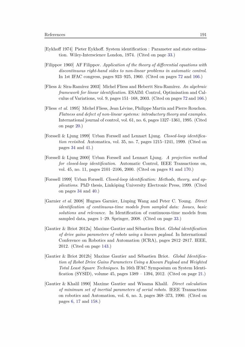
References 191
[Eykhoff 1974] Pieter Eykhoff. System identification : Parameter and state estima-tion. Wiley-Interscience London, 1974. (Cited on page 33.)
[Filippov 1960] AF Filippov. Application of the theory of differential equations withdiscontinuous right-hand sides to non-linear problems in automatic control.In 1st IFAC congress, pages 923–925, 1960. (Cited on pages 72 and 166.)
[Fliess & Sira-Ramírez 2003] Michel Fliess and Hebertt Sira-Ramírez. An algebraicframework for linear identification. ESAIM: Control, Optimisation and Cal-culus of Variations, vol. 9, pages 151–168, 2003. (Cited on pages 72 and 166.)
[Fliess et al. 1995] Michel Fliess, Jean Lévine, Philippe Martin and Pierre Rouchon.Flatness and defect of non-linear systems: introductory theory and examples.International journal of control, vol. 61, no. 6, pages 1327–1361, 1995. (Citedon page 20.)
[Forssell & Ljung 1999] Urban Forssell and Lennart Ljung. Closed-loop identifica-tion revisited. Automatica, vol. 35, no. 7, pages 1215–1241, 1999. (Cited onpages 34 and 41.)
[Forssell & Ljung 2000] Urban Forssell and Lennart Ljung. A projection methodfor closed-loop identification. Automatic Control, IEEE Transactions on,vol. 45, no. 11, pages 2101–2106, 2000. (Cited on pages 81 and 170.)
[Forssell 1999] Urban Forssell. Closed-loop identification: Methods, theory, and ap-plications. PhD thesis, Linköping University Electronic Press, 1999. (Citedon pages 34 and 40.)
[Garnier et al. 2008] Hugues Garnier, Liuping Wang and Peter C. Young. Directidentification of continuous-time models from sampled data: Issues, basicsolutions and relevance. In Identification of continuous-time models fromsampled data, pages 1–29. Springer, 2008. (Cited on page 33.)
[Gautier & Briot 2012a] Maxime Gautier and Sébastien Briot. Global identificationof drive gains parameters of robots using a known payload. In InternationalConference on Robotics and Automation (ICRA), pages 2812–2817. IEEE,2012. (Cited on page 143.)
[Gautier & Briot 2012b] Maxime Gautier and Sébastien Briot. Global Identifica-tion of Robot Drive Gains Parameters Using a Known Payload and WeightedTotal Least Square Techniques. In 16th IFAC Symposium on System Identi-fication (SYSID), volume 45, pages 1389 – 1394, 2012. (Cited on page 21.)
[Gautier & Khalil 1990] Maxime Gautier and Wisama Khalil. Direct calculationof minimum set of inertial parameters of serial robots. IEEE Transactionson robotics and Automation, vol. 6, no. 3, pages 368–373, 1990. (Cited onpages 6, 17 and 158.)
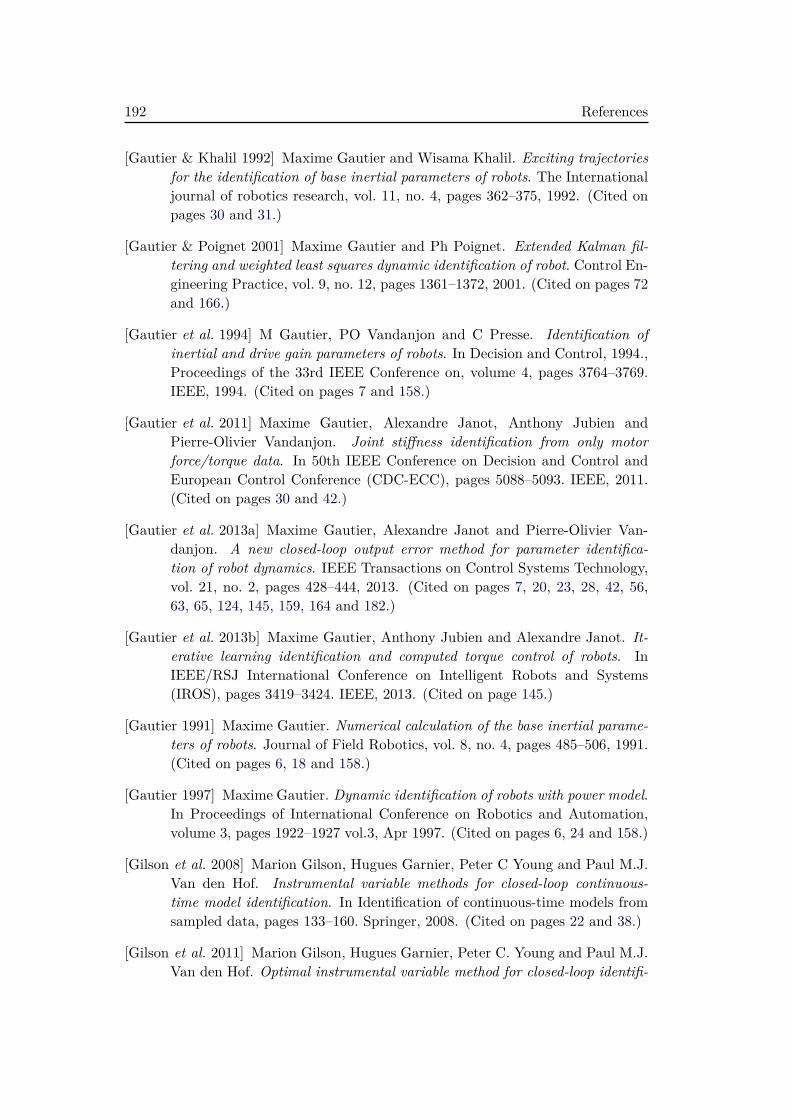
192 References
[Gautier & Khalil 1992] Maxime Gautier and Wisama Khalil. Exciting trajectoriesfor the identification of base inertial parameters of robots. The Internationaljournal of robotics research, vol. 11, no. 4, pages 362–375, 1992. (Cited onpages 30 and 31.)
[Gautier & Poignet 2001] Maxime Gautier and Ph Poignet. Extended Kalman fil-tering and weighted least squares dynamic identification of robot. Control En-gineering Practice, vol. 9, no. 12, pages 1361–1372, 2001. (Cited on pages 72and 166.)
[Gautier et al. 1994] M Gautier, PO Vandanjon and C Presse. Identification ofinertial and drive gain parameters of robots. In Decision and Control, 1994.,Proceedings of the 33rd IEEE Conference on, volume 4, pages 3764–3769.IEEE, 1994. (Cited on pages 7 and 158.)
[Gautier et al. 2011] Maxime Gautier, Alexandre Janot, Anthony Jubien andPierre-Olivier Vandanjon. Joint stiffness identification from only motorforce/torque data. In 50th IEEE Conference on Decision and Control andEuropean Control Conference (CDC-ECC), pages 5088–5093. IEEE, 2011.(Cited on pages 30 and 42.)
[Gautier et al. 2013a] Maxime Gautier, Alexandre Janot and Pierre-Olivier Van-danjon. A new closed-loop output error method for parameter identifica-tion of robot dynamics. IEEE Transactions on Control Systems Technology,vol. 21, no. 2, pages 428–444, 2013. (Cited on pages 7, 20, 23, 28, 42, 56,63, 65, 124, 145, 159, 164 and 182.)
[Gautier et al. 2013b] Maxime Gautier, Anthony Jubien and Alexandre Janot. It-erative learning identification and computed torque control of robots. InIEEE/RSJ International Conference on Intelligent Robots and Systems(IROS), pages 3419–3424. IEEE, 2013. (Cited on page 145.)
[Gautier 1991] Maxime Gautier. Numerical calculation of the base inertial parame-ters of robots. Journal of Field Robotics, vol. 8, no. 4, pages 485–506, 1991.(Cited on pages 6, 18 and 158.)
[Gautier 1997] Maxime Gautier. Dynamic identification of robots with power model.In Proceedings of International Conference on Robotics and Automation,volume 3, pages 1922–1927 vol.3, Apr 1997. (Cited on pages 6, 24 and 158.)
[Gilson et al. 2008] Marion Gilson, Hugues Garnier, Peter C Young and Paul M.J.Van den Hof. Instrumental variable methods for closed-loop continuous-time model identification. In Identification of continuous-time models fromsampled data, pages 133–160. Springer, 2008. (Cited on pages 22 and 38.)
[Gilson et al. 2011] Marion Gilson, Hugues Garnier, Peter C. Young and Paul M.J.Van den Hof. Optimal instrumental variable method for closed-loop identifi-
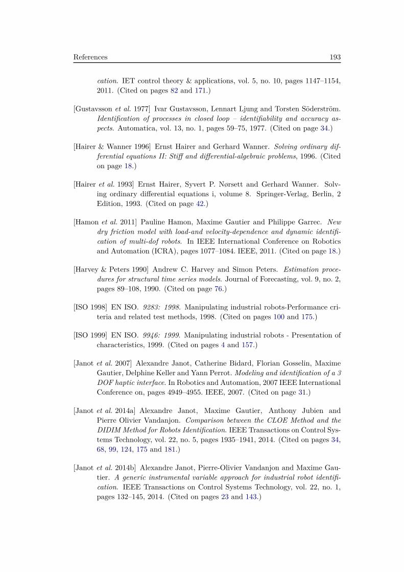
References 193
cation. IET control theory & applications, vol. 5, no. 10, pages 1147–1154,2011. (Cited on pages 82 and 171.)
[Gustavsson et al. 1977] Ivar Gustavsson, Lennart Ljung and Torsten Söderström.Identification of processes in closed loop – identifiability and accuracy as-pects. Automatica, vol. 13, no. 1, pages 59–75, 1977. (Cited on page 34.)
[Hairer & Wanner 1996] Ernst Hairer and Gerhard Wanner. Solving ordinary dif-ferential equations II: Stiff and differential-algebraic problems, 1996. (Citedon page 18.)
[Hairer et al. 1993] Ernst Hairer, Syvert P. Nørsett and Gerhard Wanner. Solv-ing ordinary differential equations i, volume 8. Springer-Verlag, Berlin, 2Edition, 1993. (Cited on page 42.)
[Hamon et al. 2011] Pauline Hamon, Maxime Gautier and Philippe Garrec. Newdry friction model with load-and velocity-dependence and dynamic identifi-cation of multi-dof robots. In IEEE International Conference on Roboticsand Automation (ICRA), pages 1077–1084. IEEE, 2011. (Cited on page 18.)
[Harvey & Peters 1990] Andrew C. Harvey and Simon Peters. Estimation proce-dures for structural time series models. Journal of Forecasting, vol. 9, no. 2,pages 89–108, 1990. (Cited on page 76.)
[ISO 1998] EN ISO. 9283: 1998. Manipulating industrial robots-Performance cri-teria and related test methods, 1998. (Cited on pages 100 and 175.)
[ISO 1999] EN ISO. 9946: 1999. Manipulating industrial robots - Presentation ofcharacteristics, 1999. (Cited on pages 4 and 157.)
[Janot et al. 2007] Alexandre Janot, Catherine Bidard, Florian Gosselin, MaximeGautier, Delphine Keller and Yann Perrot. Modeling and identification of a 3DOF haptic interface. In Robotics and Automation, 2007 IEEE InternationalConference on, pages 4949–4955. IEEE, 2007. (Cited on page 31.)
[Janot et al. 2014a] Alexandre Janot, Maxime Gautier, Anthony Jubien andPierre Olivier Vandanjon. Comparison between the CLOE Method and theDIDIM Method for Robots Identification. IEEE Transactions on Control Sys-tems Technology, vol. 22, no. 5, pages 1935–1941, 2014. (Cited on pages 34,68, 99, 124, 175 and 181.)
[Janot et al. 2014b] Alexandre Janot, Pierre-Olivier Vandanjon and Maxime Gau-tier. A generic instrumental variable approach for industrial robot identifi-cation. IEEE Transactions on Control Systems Technology, vol. 22, no. 1,pages 132–145, 2014. (Cited on pages 23 and 143.)
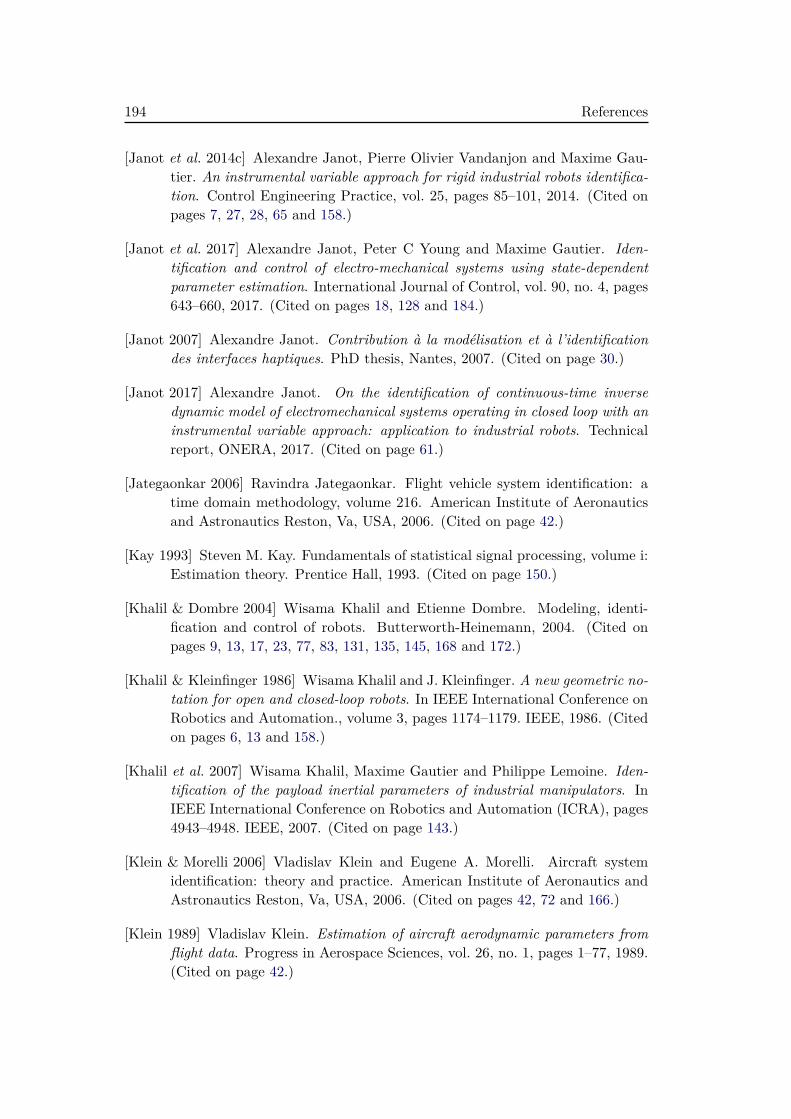
194 References
[Janot et al. 2014c] Alexandre Janot, Pierre Olivier Vandanjon and Maxime Gau-tier. An instrumental variable approach for rigid industrial robots identifica-tion. Control Engineering Practice, vol. 25, pages 85–101, 2014. (Cited onpages 7, 27, 28, 65 and 158.)
[Janot et al. 2017] Alexandre Janot, Peter C Young and Maxime Gautier. Iden-tification and control of electro-mechanical systems using state-dependentparameter estimation. International Journal of Control, vol. 90, no. 4, pages643–660, 2017. (Cited on pages 18, 128 and 184.)
[Janot 2007] Alexandre Janot. Contribution à la modélisation et à l’identificationdes interfaces haptiques. PhD thesis, Nantes, 2007. (Cited on page 30.)
[Janot 2017] Alexandre Janot. On the identification of continuous-time inversedynamic model of electromechanical systems operating in closed loop with aninstrumental variable approach: application to industrial robots. Technicalreport, ONERA, 2017. (Cited on page 61.)
[Jategaonkar 2006] Ravindra Jategaonkar. Flight vehicle system identification: atime domain methodology, volume 216. American Institute of Aeronauticsand Astronautics Reston, Va, USA, 2006. (Cited on page 42.)
[Kay 1993] Steven M. Kay. Fundamentals of statistical signal processing, volume i:Estimation theory. Prentice Hall, 1993. (Cited on page 150.)
[Khalil & Dombre 2004] Wisama Khalil and Etienne Dombre. Modeling, identi-fication and control of robots. Butterworth-Heinemann, 2004. (Cited onpages 9, 13, 17, 23, 77, 83, 131, 135, 145, 168 and 172.)
[Khalil & Kleinfinger 1986] Wisama Khalil and J. Kleinfinger. A new geometric no-tation for open and closed-loop robots. In IEEE International Conference onRobotics and Automation., volume 3, pages 1174–1179. IEEE, 1986. (Citedon pages 6, 13 and 158.)
[Khalil et al. 2007] Wisama Khalil, Maxime Gautier and Philippe Lemoine. Iden-tification of the payload inertial parameters of industrial manipulators. InIEEE International Conference on Robotics and Automation (ICRA), pages4943–4948. IEEE, 2007. (Cited on page 143.)
[Klein & Morelli 2006] Vladislav Klein and Eugene A. Morelli. Aircraft systemidentification: theory and practice. American Institute of Aeronautics andAstronautics Reston, Va, USA, 2006. (Cited on pages 42, 72 and 166.)
[Klein 1989] Vladislav Klein. Estimation of aircraft aerodynamic parameters fromflight data. Progress in Aerospace Sciences, vol. 26, no. 1, pages 1–77, 1989.(Cited on page 42.)
References 195
[Kostic et al. 2004] Dragan Kostic, Bram De Jager, Maarten Steinbuch and RonHensen. Modeling and identification for high-performance robot control: AnRRR-robotic arm case study. IEEE Transactions on Control Systems Tech-nology, vol. 12, no. 6, pages 904–919, 2004. (Cited on pages 7, 125, 158and 183.)
[Landau & Horowitz 1988] Ioan-Doré Landau and Roberto Horowitz. Synthesis ofadaptive controllers for robot manipulators using a passive feedback systemsapproach. In IEEE International Conference on Robotics and Automation,pages 1028–1033. IEEE, 1988. (Cited on page 20.)
[Landau et al. 1999] ID Landau, BDO Anderson and F De Bruyne. Closed-loopoutput error identification algorithms for nonlinear plants. In Decision andControl, 1999. Proceedings of the 38th IEEE Conference on, volume 1, pages606–611. IEEE, 1999. (Cited on pages 7 and 159.)
[Landau et al. 2001] ID Landau, Brian DO Anderson and Franky De Bruyne. Re-cursive identification algorithms for continuous-time nonlinear plants oper-ating in closed loop. Automatica, vol. 37, no. 3, pages 469–475, 2001. (Citedon pages 42 and 43.)
[Lawson & Hanson 1974] C.L. Lawson and R.J. Hanson. Solving least squares prob-lems. Englewood Cliffs: Prentice-Hall, 1974. (Cited on page 53.)
[Levant 1998] Arie Levant. Robust exact differentiation via sliding mode technique.automatica, vol. 34, no. 3, pages 379–384, 1998. (Cited on pages 72 and 166.)
[Lischinsky et al. 1999] P Lischinsky, C Canudas-de Wit and G Morel. Frictioncompensation for an industrial hydraulic robot. IEEE Control Systems Mag-azine, vol. 19, no. 1, pages 25–32, 1999. (Cited on page 17.)
[Ljung 1976] Lennart Ljung. On the consistency of prediction error identificationmethods. Mathematics in Science and Engineering, vol. 126, pages 121–164,1976. (Cited on pages 7, 40 and 159.)
[Ljung 1979] Lennart Ljung. Asymptotic behavior of the extended Kalman filter asa parameter estimator for linear systems. IEEE Transactions on AutomaticControl, vol. 24, no. 1, pages 36–50, 1979. (Cited on pages 72 and 166.)
[Ljung 1988] Lennart Ljung. System identification toolbox. The Matlab user’s guide,1988. (Cited on pages 93 and 173.)
[Ljung 1999] Lennart Ljung. System identification: theory for the user. PTR Pren-tice Hall, Upper Saddle River, NJ, 1999. (Cited on pages 9, 25, 30, 33, 39,41, 83, 93, 104, 172 and 173.)
[Luenberger 1971] David Luenberger. An introduction to observers. IEEE Trans-actions on automatic control, vol. 16, no. 6, pages 596–602, 1971. (Cited onpages 72 and 166.)
196 References
[Marcassus et al. 2007] Nicolas Marcassus, Pierre-Olivier Vandanjon, AlexandreJanot and Maxime Gautier. Minimal resolution needed for an accurateparametric identification-application to an industrial robot arm. In 2007IEEE/RSJ International Conference on Intelligent Robots and Systems,pages 2455–2460. IEEE, 2007. (Cited on pages 23 and 113.)
[Murray-Smith 1995] David Murray-Smith. Continuous system simulation.Springer Science & Business Media, 1995. (Cited on page 18.)
[Nelder & Mead 1965] John A Nelder and Roger Mead. A simplex method for func-tion minimization. The computer journal, vol. 7, no. 4, pages 308–313, 1965.(Cited on page 44.)
[Nicosia & Tomei 1990] S. Nicosia and P. Tomei. Robot control by using only jointposition measurements. IEEE Transactions on Automatic Control, vol. 35,no. 9, pages 1058–1061, 1990. (Cited on page 20.)
[Noël & Schoukens 2017] J.P. Noël and J. Schoukens. Grey-box state-space identifi-cation of nonlinear mechanical vibrations. International Journal of Control,pages 1–22, 2017. (Cited on pages 128 and 185.)
[Norton 1975] J.P. Norton. Optimal smoothing in the identification of linear time-varying systems. In Proceedings of the Institution of Electrical Engineers,volume 122, pages 663–668. IET, 1975. (Cited on pages 73 and 167.)
[Olsen & Petersen 2001] Martin M Olsen and Henrik Gordon Petersen. A newmethod for estimating parameters of a dynamic robot model. IEEE Trans-actions on Robotics and Automation, vol. 17, no. 1, pages 95–100, 2001.(Cited on pages 7 and 158.)
[Olsen et al. 2002] Martin M Olsen, Jan Swevers and Walter Verdonck. Maximumlikelihood identification of a dynamic robot model: Implementation issues.The international Journal of robotics research, vol. 21, no. 2, pages 89–96,2002. (Cited on pages 7 and 158.)
[Pasch & Seering 1984] K. A. Pasch and W. P. Seering. On the Drive Systemsfor High-Performance Machines. Journal of Mechanisms Transmissions andAutomation in Design, vol. 106, 1984. (Cited on page 21.)
[Pascu et al. 2016] Valentin Pascu, Hugues Garnier, Lennart Ljung and AlexandreJanot. Developments towards formalizing a benchmark for continuous-timemodel identification. In 55th IEEE Conference on Decision and Control(CDC), pages 7171–7176. IEEE, 2016. (Cited on pages 83 and 172.)
[Pham et al. 2001] Minh Tu Pham, Maxime Gautier and Philippe Poignet. Identifi-cation of joint stiffness with bandpass filtering. In Robotics and Automation,2001. Proceedings 2001 ICRA. IEEE International Conference on, volume 3,pages 2867–2872. IEEE, 2001. (Cited on page 24.)
References 197
[Pham 2002] Minh Tu Pham. Contribution à la modélisation, l’identification etla commande de systèmes mécaniques à flexibilités localisées: application àdes axes de machines-outils rapides. PhD thesis, Nantes, 2002. (Cited onpage 24.)
[Pierce 1972] David A. Pierce. Least squares estimation in dynamic-disturbancetime series models. Biometrika, pages 73–78, 1972. (Cited on page 38.)
[Pressé & Gautier 1993] C Pressé and Maxime Gautier. New criteria of excitingtrajectories for robot identification. In Robotics and Automation, 1993. Pro-ceedings., 1993 IEEE International Conference on, pages 907–912. IEEE,1993. (Cited on page 54.)
[Richalet et al. 1971] Jacques Richalet, André Rault and R Pouliquen. Identifica-tion des processus par la méthode du modèle. Gordon & Breach, 1971.(Cited on pages 7, 42 and 159.)
[Robet et al. 2012] P. Ph. Robet, Maxime Gautier, Anthony Jubien and AlexandreJanot. A new output error method for a decoupled identification of electri-cal and mechanical dynamic parameters of DC motor-driven robots. IFACProceedings Volumes, vol. 45, no. 22, pages 25–30, 2012. (Cited on page 30.)
[Samson 1983] Claude Samson. Problèmes en identification et commande desystlèmes dynamiques. PhD thesis, Université de Rennes I, 1983. Thèsed’Etat. (Cited on page 20.)
[Sargan 1958] John D. Sargan. The estimation of economic relationships usinginstrumental variables. Econometrica: Journal of the Econometric Society,pages 393–415, 1958. (Cited on page 112.)
[Schoukens et al. 2012] Johan Schoukens, Rik Pintelon and Yves Rolain. Masteringsystem identification in 100 exercises. John Wiley & Sons, 2012. (Cited onpage 41.)
[Shibata 1976] Ritei Shibata. Selection of the order of an autoregressive model byAkaike’s information criterion. Biometrika, vol. 63, no. 1, pages 117–126,1976. (Cited on page 104.)
[Shtessel et al. 2014] Yuri Shtessel, Christopher Edwards, Leonid Fridman and ArieLevant. Sliding mode control and observation. Springer, 2014. (Cited onpage 73.)
[Siciliano et al. 2010] Bruno Siciliano, Lorenzo Sciavicco, Luigi Villani andGiuseppe Oriolo. Robotics: modelling, planning and control. Springer Sci-ence & Business Media, 2010. (Cited on pages 4, 9, 100, 102, 131, 133, 145,157 and 176.)
[Sidhom 2011] Lilia Sidhom. Sur les différentiateurs en temps réel: Algorithmes etApplications. PhD thesis, INSA de Lyon, 2011. (Cited on pages 72 and 166.)
198 References
[Singer 1970] Robert A Singer. Estimating optimal tracking filter performance formanned maneuvering targets. IEEE Transactions on Aerospace and Elec-tronic Systems, no. 4, pages 473–483, 1970. (Cited on pages 72 and 166.)
[Söderström & Stoica 1983] Torsten Söderström and Petre Stoica. Instrumentalvariable methods for system identification, volume 57. Springer, 1983. (Citedon pages 26, 27 and 63.)
[Söderström & Stoica 1988] Torsten Söderström and Petre Stoica. System identifi-cation. Prentice-Hall, Inc., 1988. (Cited on pages 9, 27, 30, 34, 39 and 84.)
[Solo 1979] Victor Solo. Time series recursions and stochastic approximation. Bul-letin of the Australian Mathematical Society, vol. 20, no. 01, pages 159–160,1979. (Cited on page 30.)
[Stäubli Favergues 2015] Stäubli Favergues. Arm - TX series 40 family. Stäubli,02 2015. (Cited on pages 5, 22, 78 and 101.)
[Swevers et al. 2007] Jan Swevers, Walter Verdonck and Joris De Schutter. Dy-namic model identification for industrial robots. IEEE Control Systems,vol. 27, no. 5, pages 58–71, 2007. (Cited on page 23.)
[Taylor et al. 2007] C. James Taylor, Diego J. Pedregal, Peter C. Young andWlodek Tych. Environmental time series analysis and forecasting with theCaptain toolbox. Environmental Modelling & Software, vol. 22, no. 6, pages797–814, 2007. (Cited on pages 76 and 168.)
[Unbehauen & Rao 1998] H. Unbehauen and G.P. Rao. A review of identificationin continuous-time systems. Annual reviews in Control, vol. 22, pages 145–171, 1998. (Cited on page 33.)
[Urrea & Pascal 2016] Claudio Urrea and José Pascal. Design, simulation, com-parison and evaluation of parameter identification methods for an industrialrobot. Computers & Electrical Engineering, 2016. (Cited on page 23.)
[Van Den Hof et al. 1992] Paul M.J. Van Den Hof, Ruud J.P. Schrama and Okko H.Bosgra. An indirect method for transfer function estimation from closed loopdata. In Proceedings of the 31st IEEE Conference on Decision and Control„pages 1702–1706. IEEE, 1992. (Cited on pages 81 and 170.)
[Van den Hof 1998] Paul M.J. Van den Hof. Closed-loop issues in system identifi-cation. Annual reviews in control, vol. 22, pages 173–186, 1998. (Cited onpages 25 and 34.)
[Van Donkelaar & Van den Hof 2000] Edwin T. Van Donkelaar and Paul M.J.Van den Hof. Analysis of closed-loop identification with a tailor-made pa-rameterization. European Journal of Control, vol. 6, no. 1, pages 54–62,2000. (Cited on page 40.)
References 199
[Vandanjon et al. 1995] Pierre-Olivier Vandanjon, Maxime Gautier and P. Desbats.Identification of robots inertial parameters by means of spectrum analysis.In IEEE International Conference on Robotics and Automation (ICRA),volume 3, pages 3033–3038. IEEE, 1995. (Cited on page 31.)
[Vasiljevic & Khalil 2006] Luma K Vasiljevic and Hassan K Khalil. Differentiationwith high-gain observers the presence of measurement noise. In Decisionand Control, 2006 45th IEEE Conference on, pages 4717–4722. IEEE, 2006.(Cited on pages 72 and 166.)
[Walker & Orin 1982] M. W. Walker and D. E. Orin. Efficient Dynamic ComputerSimulation of Robotic Mechanisms. Journal of Dynamic Systems Measure-ment and Control, vol. 104, 1982. (Cited on page 19.)
[Walter & Pronzato 1994] Éric Walter and Luc Pronzato. Identification de modèlesparamétriques à partir de données expérimentales. Masson, 1994. (Cited onpages 30, 39, 44 and 55.)
[Warnecke et al. Y Nof 1999] H.-J. Warnecke, R.D. Schraft, M. Hagele, O. Barthand G. Schmierer. Manipulator design, in handbook of industrial robotics.John Wiley & Sons, Inc., Second Edition, (ed S. Y. Nof) 1999. (Cited onpages 21 and 22.)
[Wernholt 2007] Erik Wernholt. Multivariable frequency-domain identification ofindustrial robots. PhD thesis, Institutionen för systemteknik, 2007. (Citedon pages 4, 113 and 157.)
[Wooldridge 2008] JM Wooldridge. Introductory econometrics: A modern ap-proach. South-Western, fourth Edition, 2008. (Cited on page 27.)
[Xi 1995] Fengfeng Xi. Effect of non-geometric errors on manipulator inertial cali-bration. In Robotics and Automation, 1995. Proceedings., 1995 IEEE Inter-national Conference on, volume 2, pages 1808–1813. IEEE, 1995. (Cited onpages 7 and 158.)
[Young & Jakeman 1979] Peter C. Young and Anthony Jakeman. Refined instru-mental variable methods of recursive time-series analysis Part I. Single in-put, single output systems. International Journal of Control, vol. 29, no. 1,pages 1–30, 1979. (Cited on page 34.)
[Young & Jakeman 1980] Peter C. Young and Anthony Jakeman. Refined instru-mental variable methods of recursive time-series analysis Part III. Exten-sions. International Journal of Control, vol. 31, no. 4, pages 741–764, 1980.(Cited on pages 7 and 159.)
[Young et al. 2009] Peter C. Young, Hugues Garnier and Marion Gilson. Simplerefined IV methods of closed-loop system identification. In 15th IFAC Sym-posium on System Identification (SYSID), 2009. (Cited on pages 36, 81and 170.)
200 References
[Young 1966] Peter C Young. Process parameter estimation and self adaptive con-trol. In Theory of Self-Adaptive Control Systems, pages 118–140. Springer,1966. (Cited on page 33.)
[Young 1981] Peter C. Young. Parameter estimation for continuous-time models –a survey. Automatica, vol. 17, no. 1, pages 23–39, 1981. (Cited on page 33.)
[Young 1999] Peter C Young. Nonstationary time series analysis and forecasting.Progress in Environmental Science, vol. 1, pages 3–48, 1999. (Cited onpages 128 and 185.)
[Young 2000] Peter C. Young. Stochastic, dynamic modelling and signal process-ing: time variable and state dependent parameter estimation. Nonlinear andnonstationary signal processing, pages 74–114, 2000. (Cited on pages 73and 167.)
[Young 2006] Peter C. Young. An instrumental variable approach to arma modelidentification and estimation. In 14th IFAC Symposium on System Identi-fication (SYSID), pages 410 – 415, Newcastle, Australia, 2006. (Cited onpages 37, 103 and 177.)
[Young 2011] Peter C. Young. Recursive estimation and time-series analysis: anintroduction for the student and practitioner. Springer Berlin Heidelberg,2nd Edition, 2011. (Cited on pages 9, 27, 34, 36, 37, 38, 44, 65, 73, 74, 77,83, 167, 168 and 172.)
[Young 2015] Peter C. Young. Refined instrumental variable estimation: maximumlikelihood optimization of a unified Box–Jenkins model. Automatica, vol. 52,pages 35–46, 2015. (Cited on page 34.)
Index
AAccuracy . . . . . . . . . . . . . . . . . . . . . . . . . . . . 98Auxiliary model. . . . . . . . . . . . . . . . . .27, 59
BBasis function . . . . . . . . . . . . see Regressor
CController . . . . . . . . . . . . . . . . . . . . 20, 49, 79
DDIDIM . . . . . . . . . . . . . . . . . . . . . . . . . . 29, 59Drive gains . . . . . . . . . . . . . . . . . . . . . . . . . . 21
EEncoder resolution. . . . . . . . . . . . . . . . . . .23
FFilter
bandpass . . . . . . . . . . . . . . . . . . . . . . . . 24decimate . . . . . . . . . . . . . 24, 46, 53, 66
Frame . . . . . . . . . . . . . . . . . . . . . . . . . . . . . . . 14Friction model . . . . . . . . . . . . . . . . . . . . . . . 17
IIndependant variable . . . . . see RegressorInertia
matrix. . . . . . . . . . . . . . . . . . . . . .16, 132tensor . . . . . . . . . . . . . . . . . . . . . . 17, 129
Instrumentexogeneity . . . . . . . . . . . . . . . . . . . 27, 36relevance . . . . . . . . . . . . . . . . . . . . . . . . 27
Instrumental variableestimate . . . . . . . . . . . . . . . . . . . . . 28, 59extended . . . . . . . . . . . . . . . . . . . . . . . . 26
JJoint . . . . . . . . . . . . . . . . . . . . . . . . . . . . . . . . 14
LLeast-Squares
ordinary . . . . . . . . . . . . . . . . . . . . . 26, 67weighted . . . . . . . . . . . . . . . . . . . . . . . . 26
Link . . . . . . . . . . . . . . . . . . . . . . . . . . . . . . . . . 14Center of gravity . . . . . . . . . . . 17, 129Origin . . . . . . . . . . . . . . . . . . . . . . 17, 129
MMass . . . . . . . . . . . . . . . . . . . . . . . . . . . . . . . . 17Maximum Likelihood. . . . . . . .37, 73, 102Modified Denavit-Hartenberg . . . . 14, 98
NNoise
measurement . . . . . . . . . . . . . . . 22, 100position . . . . . . . . . . . . . . . . . . . . . 50, 97torque. . . . . . . . . . . . . . .23, 50, 97, 100
Noise variance ratio . . . . . . . . . . . . . . . . . 72
PParallel filter . . . . . . . .see Filter decimateParameters
base . . . . . . . . . . . . . . . . . . . . . . . . . . . . . 18standard. . . . . . . . . . . . . . . . . . . .17, 130
Persistent excitation . . . . . . . . . . . . 30, 126Prediction error method
one-step-ahead . . . . . . . . . . . . . . . . . . 38
RRegressor . . . . . . . . . . . . . . . . . . . . . . . . 18, 60Repeatability . . . . . . . . . . . . . . . . . . . . . 4, 98
SSensitivity . . . . . . . . . . . . . . . . 41, 46, 47, 54Solver
integration . . . . . . . . . . . . . . . . . . . . . . 40optimisation . . . . . . . . . . . . . . . . . . . . . 40
Stiff system . . . . . . . . . . . . . . . . . . . . . . 18, 40
TTorque error . . . . . . . . . . .see Noise torque
Identification of rigid industrial robots – A system identification perspective
Abstract In modern manufacturing, industrial robots are essential components that allow saving cost, increasequality and productivity for instance. To achieve such goals, high accuracy and speed are simultaneouslyrequired. The design of control laws compliant with such requirements demands high-fidelity mathematicalmodels of those robots. For this purpose, dynamic models are built from experimental data. The main objectiveof this thesis is thus to provide robotic engineers with automatic tools for identifying dynamic models of industrialrobot arms. To achieve this aim, a comparative analysis of the existing methods dealing with robot identificationis made. That allows discerning the advantages and the limitations of each method. From those observations,contributions are presented on three axes. First, the study focuses on the estimation of the joint velocitiesand accelerations from the measured position, which is required for the model construction. The usual methodis based on a home-made prefiltering process that needs a reliable knowledge of the system’s bandwidths,whereas the system is still unknown. To overcome this dilemma, we propose a method able to estimate the jointderivatives automatically, without any setting from the user. The second axis is dedicated to the identificationof the controller. For the vast majority of the method its knowledge is indeed required. Unfortunately, forcopyright reasons, that is not always available to the user. To deal with this issue, two methods are suggested.Their basic philosophy is to identify the control law in a first step before identifying the dynamic model of therobot in a second one. The first method consists in identifying the control law in a parametric way, whereasthe second one relies on a non-parametric identification. Finally, the third axis deals with the home-madesetting of the decimate filter. The identification of the noise filter is introduced similarly to methods developedin the system identification community. This allows estimating automatically the dynamic parameters withlow covariance and it brings some information about the noise circulation through the closed-loop system. Allthe proposed methodologies are validated on an industrial robot with 6 degrees of freedom. Perspectives areoutlined for future developments on robotic systems identification and other complex problems.
Keywords: system identification, robot identification, prediction error methods, instrumental variable, outputerror methods
Identification de robots industriels rigides – Apport des méthodes de l’identification de systèmes
Résumé L’industrie moderne fait largement appel à des robots industriels afin de réduire les coûts, ou encoreaméliorer la productivité et la qualité par exemple. Pour ce faire, une haute précision et une grande vitessesont simultanément nécessaires. La conception de lois de commande conformes à de telles exigences demandeune modélisation mathématique précise de ces robots. A cette fin, des modèles dynamiques sont construits àpartir de données expérimentales. L’objectif de cette thèse est ainsi de fournir aux ingénieurs roboticiens desoutils automatiques pour l’identification de bras robotiques. Dans cette perspective, une analyse comparativedes méthodes existantes pour l’identification de robot est réalisée. Les avantages et inconvénients de chaqueméthode sont ainsi mis en exergue. À partir de ces observations, les contributions sont articulées selon troisaxes. Premièrement, l’étude porte sur l’estimation des vitesses et accélérations des corps du robot à partirde la position mesurée. Ces informations sont en effet nécessaires à la construction du modèle. La méth-ode usuelle est basée sur prétraitement "sur mesure" qui requière une connaissance fiable des bande-passantesdu système, alors que celui-ci est encore inconnu. Pour surmonter ce dilemme, nous proposons une méthodecapable d’estimer les dérivées automatiquement sans réglage préalable par l’utilisateur. Le deuxième axe con-cerne l’identification du contrôleur. Sa connaissance est en effet requise par la grande majorité des méthodesd’identification. Malheureusement, pour des raisons de propriété industrielle, il n’est pas toujours accessible.Pour traiter ce problème, deux méthodes sont introduites. Leur principe de base est d’identifier la loi de com-mande dans un premier temps avant d’identifier le modèle dynamique du bras robotique dans un second temps.La première méthode consiste à identifier la loi de commande de manière paramétrique, alors que la secondefait appel à une identification non-paramétrique. Finalement, le troisième axe porte sur le réglage "sur mesure"du filtre decimate. L’identification du filtre de bruit est introduite en s’inspirant des méthodes développées parla communauté d’identification de systèmes. Ceci permet l’estimation automatique des paramètres dynamiquesavec de faibles covariances tout en apportant une connaissance concernant la circulation du bruit à travers lesystème en boucle-fermée. Toutes les méthodes proposées sont validées sur un robot industriel à six degrésde liberté. Des perspectives sont esquissées pour de futurs travaux portant sur l’identification de systèmesrobotiques, voire d’autres applications.
Mots-clés: identification de systèmes, identification de robots, méthodes d’erreur de prédiction, variableinstrumentale, méthodes d’erreur de sortie